NUMERICAL
C MPUTATION
o
INTERNAL
an
EXTERNAL FLOWS
Volume 2
o •utational ethods
for In viscid and
Viscous Flo s
CHIRSCH

Numerical Computation
of
INTERNAL AND EXTERNAL
FLOWS
Volume 2: Computational Methods for Inviscid and
Viscous Flows

WILEY SERIES IN
NUMERICAL METHODS IN ENGINEERING
Consulting Editors
R. H. Gallagher, Worcester Polytechnic Institute,
Worcester, Massachusetts, USA
and
O. C. Zienkiewicz, Department of Civil Engineering,
University College of Swansea
Rock Mechanics in Engineering Practice
Edited by K. G. Stagg and 0. C. Zienkiewicz
Optimum Structural Design: Theory and Applications
Edited by R. H. Gallagher and 0. C. Zienkiewicz
Finite Elements in Fluids
Vol. 1 Viscous Flow and Hydrodynamics
Vol. 2 Mathematical Foundations, Aerodynamics and Lubrication
Edited by R. H. Gallagher, J. T Oden, C. Taylor, and 0. C. Zienkiewicz
Finite Elements in Geomechanics
Edited by G. Gudehus
Numerical Methods in Offshore Engineering
Edited by 0. C. Zienkiewicz, R. W. Lewis, and K. G. Stagg
Finite Elements in Fluids
Vol.3
Edited by R. H. Gallagher, 0. C. Zienkiewicz, J. T. Oden, M. Morandi Cecchi,
and C. Taylor
Energy Methods in Finite Element Analysis
Edited by R. Glowinksi, E. Rodin, and O. C. Zienkiewicz
Finite Elements in Electrical and Magnetic Field Problems
Edited by M.V. K. Chari and P. Silvester
Numerical Methods in Heat Transfer
Vol.1
Edited by R. W. Lewis, K. Morgan, and 0. C. Zienkiewicz
Finite Elements in Biomechanics
Edited by R. H. Gallagher, B. R. Simon, P. C. Johnson, and J. F. Gross
Soil Mechanics—Transient and Cyclic Loads
Edited by G. N. Pande and 0. C. Zienkiewicz
Finite Elements in Fluids
Vol.4
Edited by R. H. Gallagher, D. Norrie, J. T Oden, a, d 0. C. Zienkiewicz
Foundations of Structural Optimization: A Unified Approach
Edited by A. J. Morris
Numerical Methods in Heat Transfer
Vol. II
Edited by R. W. Lewis, K. Morgan, and B. A. Schrefler

Numerical Methods in Coupled Systems
Edited by R. W. Lewis, E. Hinton, and P. Bettess
New Directions in Optimum Structural Design
Edited by E. Atrek, R. H. Gallagher, K. M. Ragsdell, and 0. C. Zienkiewicz
Mechanics of Engineering Materials
Edited by C. 5. Desai and R. H. Gallagher
Numerical Analysis of Forming Processes
Edited by J, F. T. Pittman, 0. C. Zienkiewicz, R. D. Wood, and J. M. Alexander
Finite Elements in Fluids
Vol. 5
Edited by R. H. Gallagher, J. T, Oden, 0. C. Zienkiewicz,
T. Kawai, and M. Kawahara
Mechanics of Geomaterials: Rocks, Concretes, Soils
Edited by Z. P. Bazant
Finite Elements in Fluids
Vol.6
Edited by R. H. Gallagher, G. F. Carey, J. T. Oden, and O. C. Zienkiewicz
Numerical Methods in Heat Transfer
Vol. Ill
Edited by R. W. Lewis and K. Morgan
Accuracy Estimates and Adaptive Refinements in Finite Element Computations
Edited by I. Babuska, J. Gago, E. R. de Arantes e Oliveira, and 0. C. Zienkiewicz
The Finite Element Method in the Deformation and Consolidation
of Porous Media
R. W. Lewis and B. A. Schrefler
Numerical Methods for Transient and Coupled Problems
Edited by R. W. Lewis, E. Hinton, P. Bettess, and B. A. Schrefler
Microcomputers in Engineering Applications
Edited by B. A. Schrefler and R. W. Lewis
Numerical Computation of Internal and External Flows
Vol. 1: Fundamentals of Numerical Discretization
C. Hirsch
Finite Elements in Fluids
Vol.7
Edited by R. H. Gallagher, R. Glowinski, P. M. Gresho,
J. T. Oden, and O. C. Zienkiewicz
Mathematical Modeling of Creep and Shrinkage of Concrete
Edited by Z. P. Bazant
Numerical Computation of Internal and External Flows
Vol. 2: Computational Methods for Inviscid and Viscous Flows
C. Hirsch

Numerical Computation
of
INTERNAL AND EXTERNAL
FLOWS
Volume 2: Computational Methods for
Inviscid and Viscous Flows
Charles Hirsch
Department of Fluid Mechanics,
Vrije Universiteit Brussel,
Brussels, Belgium
A Wiley-Inter science Publication
JOHN WILEY & SONS
Chichester • New York • Brisbane • Toronto • Singapore

Copyright O 1990 by John Wiley & Sons Ltd.
Baffins Lane, Chichester, West Sussex P019 1UD. England
Reprinted November 1991
Reprinted August 1992
Reprinted August 1994
All rights reserved.
No part of this book may be reproduced by any means,
or transmitted, or translated into a machine language
without the written permission of the publisher.
Other Wiley Editorial Offices
John Wiley & Sons, Inc., 605 Third Avenue,
New York, NY 10158-0012, USA
Jacaranda Wiley Ltd, G.P.O. Box 859, Brisbane,
Queensland 4001, Australia
John Wiley & Sons (Canada) Ltd, 22 Worcester Road,
Rexdale, Ontario M9W ILL Canada
John Wiley & Sons (SEA) Pte Ltd, 37 Jalan Pemimpin #05-04,
Block B, Union Industrial Building, Singapore 2057
Library of Congress Cataloging-in-Publication Data:
Hirsch, Ch.
Numerical computation of internal and external flows.
(Wiley series in numerical methods in engineering)
"A Wiley-lnterscience publication."
Contents: v. 1. Fundamentals of numerical
discretization—v. 2. Computational methods for inviscid and
viscous flows.
1. Fluid dynamics—Mathematical models. 1. Title.
II. Title: Numerical computation of internal and external
flows. III. Series.
TA357.H574 1988 620.1064 87-23116
ISBN 0471 917621 (v. 1)
ISBN 0471 92351 6 (v. 2)
ISBN 0471 924520 (pbk..v. 2)
British Library Cataloguing in Publication Data:
Hirsch, Ch. (Charles)
Numerical computation of internal and external flows.
Vol. 2. Computational methods for inviscid and viscous flows
I. Fluids. Flow. Simulations. Numerical methods
I. Title
532'.051'0724
ISBN 0471 92351 6 (Pbk: 0471 924520)
Typeset by Thomson Press (India) Ltd
Printed and bound in Great Britain by
Redwood Books, Trowbridge, Wiltshire

To A. F.

CONTENTS
PREFACE xv
NOMENCLATURE xix
PART V: THE NUMERICAL COMPUTATION OF POTENTIAL
FLOWS 1
Chapter 13 The Mathematical Formulations of the Potential Flow Model 4
13.1 Conservative Form of the Potential Equation 4
13.2 The Non-conservative Form of the Isentropic Potential Flow Model 6
13.2.1 Small-perturbation potential equation 7
13.3 The Mathematical Properties of the Potential Equation 9
13.3.1 Unsteady potential flow 9
13.3.2 Steady potential flow 9
13.4 Boundary Conditions 14
13.4.1 Solid wall boundary condition 14
13.4.2 Far field conditions 15
13.4.3 Cascade and channel flows 17
13.4.4 Circulation and Kutta condition 18
13.5 Integral or Weak Formulation of the Potential Model 18
13.5.1 Bateman variational principle 19
13.5.2 Analysis of some properties of the variational integral 20
Chapter 14 The Discretization of the Subsonic Potential Equation 26
14.1 Finite Difference Formulation 27
14.1.1 Numerical estimation of the density 29
14.1.2 Curvilinear mesh 31
14.1.3 Consistency of the discretization of metric coefficients 34
14.1.4 Boundary conditions—curved solid wall 36
14.2 Finite Volume Formulation 38
14.2.1 Jameson and Caughey's finite volume method 39
14.3 Finite Element Formulation 42
14.3.1 The finite element-Galerkin method 43
14.3.2 Least squares or optimal control approach 47
14.4 Iteration Scheme for the Density 47
IX

X
Chapter 15 The Computation of Stationary Transonic Potential Flows 57
15.1 The Treatment of the Supersonic Region: Artificial Viscosity—Density
and Flux Upwinding 61
15.1.1 Artificial viscosity—non-conservative potential equation 62
15.1.2 Artificial viscosity—conservative potential equation 66
15.1.3 Artificial compressibility 67
15.1.4 Artificial flux or flux upwinding 70
15.2 Iteration Schemes for Potential Flow Computations 77
15.2.1 Line relaxation schemes 77
15.2.2 Guidelines for resolution of the discretized potential equation 81
15.2.3 The alternating direction implicit method—approximate
factorization schemes 88
15.2.4 Other techniques—multigrid methods 98
15.3 Non-uniqueness and Non-isentropic Potential Models 104
15.3.1 Isentropic shocks 105
15.3.2 Non-uniqueness and breakdown of the transonic potential flow
model 105
15.3.3 Non-isentropic potential models 112
15.4 Conclusions 117
PART VI: THE NUMERICAL SOLUTION OF THE SYSTEM OF EULER
EQUATIONS 125
Chapter 16 The Mathematical Formulation of the System of Euler
Equations 132
16.1 The Conservative Formulation of the Euler Equations 132
16.1.1 Integral conservative formulation of the Euler equations 133
16.1.2 Differential conservative formulation 134
16.1.3 Cartesian system of coordinates 134
16.1.4 Discontinuities and Rankine-Hugoniot relations—entropy
condition 135
16.2 The Quasi-linear Formulation of the Euler Equations 138
16.2.1 The Jacobian matrices for conservative variables 138
16.2.2 The Jacobian matrices for primitive variables 145
16.2.3 Transformation matrices between conservative and non-conservative
variables 147
16.3 The Characteristic Formulation of the Euler Equations—Eigenvalues and
Compatibility Relations 150
16.3.1 General properties of characteristics 151
16.3.2 Diagonalization of the Jacobian matrices 153
16.3.3 Compatibility equations 154
16.4 Characteristic Variables and Eigenvalues for One-dimensional Flows 157
16.4.1 Eigenvalues and eigenvectors of Jacobian matrix 158
16.4.2 Characteristic variables 162
16.4.3 Characteristics in the xt-plane—shocks and contact discontinuities 168
16.4.4 Physical boundary conditions 171
16.4.5 Characteristics and simple wave solutions 173
16.5 Eigenvalues and Compatibility Relations in Multidimensional Flows 176

XI
16.5.1 Jacobian eigenvalues and eigenvectors in primitive variables 177
16.5.2 Diagonalization of the conservative Jacobians 180
16.5.3 Mach cone and compatibility relations 184
16.5.4 Boundary conditions 191
16.6 Some Simple Exact Reference Solutions for One-dimensional Inviscid Flows 196
16.6.1 The linear wave equation 196
16.6.2 The inviscid Burgers equation 196
16.6.3 The shock tube problem or Riemann problem 204
16.6.4 The quasi-one-dimensional nozzle flow 211
Chapter 17 The Lax-Wendroff Family of Space-centred Schemes 224
17.1 The Space-centred Explicit Schemes of First Order 226
17.1.1 The one-dimensional Lax-Friedrichs scheme 226
17.1.2 The two-dimensional Lax-Friedrichs scheme 229
17.1.3 Corrected viscosity scheme 233
17.2 The Space-centred Explicit Schemes of Second Order 234
17.2.1 The basic one-dimensional Lax-Wendroff scheme 234
17.2.2 The two-step Lax-Wendroff schemes in one dimension 238
17.2.3 Lerat and Peyret's Sf family of non-linear two-step Lax-Wendroff
schemes 246
17.2.4 One-step Lax-Wendroff schemes in two dimensions 251
17.2.5 Two-step Lax-Wendroff schemes in two dimensions 258
17.3 The Concept of Artificial Dissipation or Artificial Viscosity 272
17.3.1 General form of artificial dissipation terms 273
17.3.2 Von Neumann-Richtmyer artificial viscosity 274
17.3.3 Higher-order artificial viscosities 279
17.4 Lerat's Implicit Schemes of Lax-Wendroff Type 283
17.4.1 Analysis for linear systems in one dimension 285
17.4.2 Construction of the family of schemes 288
17.4.3 Extension to non-linear systems in conservation form 292
17.4.4 Extension to multi-dimensional flows 296
17.5 Summary 296
Chapter 18 The Central Schemes with Independent Time Integration 307
18.1 The Central Second-order Implicit Schemes of Beam and
Warming in One Dimension 309
18.1.1 The basic Beam and Warming schemes 310
18.1.2 Addition of artificial viscosity 315
18.2 The Multidimensional Implicit Beam and Warming Schemes 326
18.2.1 The diagonal variant of Pulliam and Chaussee 328
18.3 Jameson's Multistage Method 334
18.3.1 Time integration 334
18.3.2 Convergence acceleration to steady state 335
Chapter 19 The Treatment of Boundary Conditions 344
19.1 One-dimensional Boundary Treatment for Euler Equations 345
19.1.1 Characteristic boundary conditions 346
19.1.2 Compatibility relations 347

Xll
19.1.3 Characteristic boundary conditions as a function of
conservative and primitive variables 349
19.1.4 Extrapolation methods 353
19.1.5 Practical implementation methods for numerical boundary
conditions 357
19.1.6 Nonreflecting boundary conditions 369
19.2 Multidimensional Boundary Treatment 372
19.2.1 Physical and numerical boundary conditions 372
19.2.2 Multidimensional compatibility relations 376
19.2.3 Farfield treatment for steadystate flows 377
19.2.4 Solid wall boundary 379
19.2.5 Nonreflective boundary conditions 384
19.3 The Far-field Boundary Corrections 385
19.4 The Kutta Condition 395
19.5 Summary 401
Chapter 20 Upwind Schemes for the Euler Equations 408
20.1 The Basic Principles of Upwind Schemes 409
20.2 One-dimensional Flux Vector Splitting 415
20.2.1 Steger and Warming flux vector splitting 415
20.2.2 Properties of split flux vectors 417
20.2.3 Van Leer's flux splitting 420
20.2.4 Non-reflective boundary conditions and split fluxes 425
20.3 One-dimensional Upwind Discretizations Based on Flux Vector Splitting 426
20.3.1 First-order explicit upwind schemes 426
20.3.2 Stability conditions for first-order flux vector splitting schemes 428
20.3.3 Non-conservative firstorder upwind schemes 438
20.4 Multi-dimensional Flux Vector Splitting 438
20.4.1 Steger and Warming flux splitting 440
20.4.2 Van Leer flux splitting 440
20.4.3 Arbitrary meshes 441
20.5 The Godunov-type Schemes 443
20.5.1 The basic Godunov scheme 444
20.5.2 Osher*s approximate Riemann solver 453
20.5.3 Roe's approximate Riemann solver 460
20.5.4 Other Godunov-type methods 469
20.5.5 Summary 472
20.6 First-order Implicit Upwind Schemes 473
20.7 Multi-dimensional First-order Upwind Schemes 475
Chapter 21 Second-order Upwind and High-resolution Schemes 493
21.1 General Formulation of Higher-order Upwind Schemes 494
21.1.1 Higher-order projection stages—variable extrapolation or
MUSCL approach 495
21.1.2 Numerical flux for higher-order upwind schemes 498
21.1.3 Second-order space- and time-accurate upwind schemes
based on variable extrapolation 499
21.1.4 Linearized analysis of second-order upwind schemes 502

Xlll
21.1.5 Numerical flux for higher-order upwind schemes—flux
extrapolation 504
21.1.6 Implicit second-order upwind schemes 512
21.1.7 Implicit second-order upwind schemes in two dimensions 514
21.1.8 Summary 516
21.2 The Definition of High-resolution Schemes 517
21.2.1 The generalized entropy condition for in viscid equations 519
21.2.2 Monotonicity condition 525
21.2.3 Total variation diminishing (TVD) schemes 528
21.3 Second-order TVD Semi-discretized Schemes with Limiters 536
21.3.1 Definition of limiters for the linear convection equation 537
21.3.2 General definition of flux limiters 550
21.3.3 Limiters for variable extrapolation—MUSCL—method 552
21.4 Timeintegration Methods for TVD Schemes 556
21.4.1 Explicit TVD schemes of first-order accuracy in time 557
21.4.2 Implicit TVD schemes 558
21.4.3 Explicit second-order TVD schemes 560
21.4.4 TVD schemes and artificial dissipation 564
21.4.5 TVD limiters and the entropy condition 568
21.5 Extension to Non-linear Systems and to Multi-dimensions 570
21.6 Conclusions to Part VI 583
PART VII: THE NUMERICAL SOLUTION OF THE NAVIER-STOKES
EQUATIONS 595
Chapter 22 The Properties of the System of Navier-Stokes Equations 597
22.1 Mathematical Formulation of the Navier-Stokes Equations 597
22.1.1 Conservative form of the Navier-Stokes equations 597
22.1.2 Integral form of the Navier-Stokes equations 599
22.1.3 Shock waves and contact layers 600
22.1.4 Mathematical properties and boundary conditions 601
22.2 Reynolds-averaged Navier-Stokes Equations 603
22.2.1 Turbulent-averaged energy equation 604
22.3 Turbulence Models 606
22.3.1 Algebraic models 608
22.3.2 One- and two-equation models—k-e models 613
22.3.3 Algebraic Reynolds stress models 615
22.4 Some Exact One-dimensional Solutions 618
22.4.1 Solutions to the linear convection-diffusion equation 618
22.4.2 Solutions to Burgers equation 620
22.4.3 Other simple test cases 621
Chapter 23 Discretization Methods for the Navier-Stokes Equations 624
23.1 Discretization of Viscous and Heat Conduction Terms 625
23.2 Time-dependent Methods for Compressible Navier-Stokes Equations 627
23.2.1 First-order explicit central schemes 628
23.2.2 One-step Lax-Wendroff schemes 629
23.2.3 Two-step Lax-Wendroff schemes 630

XIV
23.2.4 Central schemes with separate space and time discretization 636
23.2.5 Upwind schemes 648
23.3 Discretization of the Incompressible Navier-Stokes Equations 654
23.3.1 Incompressible Navier-Stokes equations 654
23.3.2 Pseudo-compressibility method 656
23.3.3 Pressure correction methods 661
23.3.4 Selection of the space discretization , 666
23.4 Conclusions to Part VII 674
INDEX
685

Preface
This volume, divided into Parts V to VII, is a continuation of the first one
which was devoted to fundamentals of numerical discretizations. It contains a
presentation of computational methods for inviscid and viscous flow models as
they have evolved over the last decade.
Over the last twenty to thirty years considerable progress has been achieved
and the field of Computational Fluid Dynamics (CFD) is reaching a mature
stage, where most of the basic methodology is, and will remain, well established.
Basically, the 1970s can be considered as the development period for the
foundations of the discretization methods for transonic potential models and
for the foundations of the central discretization methods for the Euler and
Navier-Stokes equations, following on the landmark introduction of the
Lax-Wendroff scheme.
Although prepared by earlier fundamental developments in the line of
Godunov's method for physically based discretizations of the Euler equations,
the upwind, high resolution methods have reached their maturity and been
established on solid theoretical grounds in the 1980s. They are by now as firmly
established as the central methods. Hence a large variety of techniques are
available and a considerable experience has already been accumulated with
various discretizations of the Euler equations.
The concomitant tremendous development of computer performance over
the same period has resulted in the present capacity of solving two-dimensional
Euler equations in seconds of computer time, and simple three-dimensional
problems in minutes of CPU times, with the best available codes on the powerful
supercomputers. Hence more attention can be given to the validation, accuracy
and reliability of numerical flow simulations and to their extensions to complex
industrial design and analysis applications.
Another consequence is the current possibility of obtaining Navier-Stokes
solutions, within the Reynolds-averaged approximation, in rather short
computer times (at least for two-dimensional problems and simple three-
dimensional configurations). Although the accumulated experience with
Navier-Stokes solutions is not yet as large as with the inviscid models, it is
rapidly building up. Due to the strong connection between Euler and Navier-
Stokes equations at high Reynolds numbers, most of the inviscid methods are
of application to the viscous flows. The major topic of uncertainty remains
xv

XVI
essentially connected to the fundamental problems of turbulence and its model-
lization within the Reynolds-averaged approximation.
The content of this volume reflects in a certain way the situation just described.
Part V deals with the simplest inviscid approximation which is, in certain
flow regimes, equivalent to the full system of Euler equations, namely the full
potential model. It contains three chapters, 13 to 15, covering the mathematical
formulations (Chapter 13), the discretization of subsonic potential flows
(Chapter 14) and the treatment of transonic situations (Chapter 15).
Part VI is devoted to a detailed presentation of the Euler equations and of
the basic numerical techniques developed in order to discretize the complex
system of inviscid, compressible conservation laws. It covers Chapters 16 to 21,
dealing with the algebra of the Euler equations (Chapter 16), the central schemes
(Chapter 17 and 18), the treatment of boundary conditions (Chapter 19) and
the upwind methods (Chapters 20 and 21).
Part VII finally introduces the discretization methods for the Navier-Stokes
equations and contains two chapters, 22 and 23. Chapter 22 covers the basic
mathematical formulation of Reynolds-averaged Navier-Stokes equations with
an introduction to turbulence models and the last chapter summarizes the
approaches for compressible and incompressible viscous conservation laws.
The present text is directed at students at the graduate level as well as at
scientists and engineers already engaged, or starting to be engaged, in
Computational Fluid Dynamics. Although Computational Fluid Dynamics
requires a good theoretical base, it remains for the large part an experimental
science since many properties depend on the non-linear character of the flow
equations and cannot be fully analysed. Therefore, a fraction of the problems
added to each chapter request the writing of a program, mainly for the
one-dimensional flow equations.
Since the development of a code covers many aspects: selection of a scheme,
implementation of boundary conditions, selection of a time integration method,
definition of control mechanisms of non-linear instabilities,..., it is
recommended to experiment intensively with as many variants as possible, either
individually or by sharing the number of selected options and different test
cases within a group or a class of students. A single modular code with many
options is a remarkably effective and instructive 'numerical laboratory'.
Initial versions of some chapters have been written while holding the NAVAIR
Research Chair at the Naval Postgraduate School in Monterey. I am particularly
grateful to Ray Shreeve for this opportunity and for his friendship.
Some sections on Euler equations have been written during a summer stay
at ICASE, NASA Langley, and I would like to acknowledge particularly
Dr Milton Rose, former Director of ICASE, for his hospitality and the
stimulating atmosphere.
I have also had the privilege to benefit from results of computations performed,
at my request, on different test cases by several groups and I would like to
thank D. Caughey at Cornell University, T. Hoist at NASA Ames, A. Jameson

XV11
at Princeton University, M. Salas at NASA Langley, and J. South and
C. Gumbert also at NASA Langley, for their willingness and effort.
During the redaction of this book, I have had some stimulating discussions
on the subject of the Kutta condition with T. Pulliam and A. Rizzi for which
I am grateful.
I have also the pleasure to thank my coworkers C. Lacor and G. Van Dijck
for their comments and support, as well as my secretary J. D'haes for her
considerable help with figures and text.
Ch. HlRSCH
Brussels, July 1988

Nomenclature
a convection velocity or wave speed
A jacobian of flux vector with respect to conservative variables, with
components A, By C
c speed of sound
cp specific heat at constant pressure
cv specific heat at constant volume
D artificial dissipation function
e internal energy per unit mass
£ total energy per unit mass
/ scalar flux function
P numerical flux function
/e external force vector
F flux vector woth components /, gy h
9**> dap contra variant and co variant metric tensor
G amplification factor/matrix; convergence operator of iterative schemes
h enthalpy per unit mass
H stagnation enthalpy per unit mass
/ rothalpy
J Jacobian of coordinate transformation
k coefficient of thermal conductivity
k wave number
K stiffness matrix
K = Ak projection of jacobian matrix on propagation direction k
KT jacobian matrix of differential operator L
/<j) left eigenvector of jacobian matrix
L differential operator
M Mach number
n normal distance
n normal vector
N{ finite element interpolation function for node I
p pressure
P convergence or conditioning operator
Pt Prandtl number
q modulus of velocity; source term
Q source term column-vector
r gas constant per unit mass
r(j) right eigenvector of jacobian matrix
R residual of iterative scheme
xix

XX
Re Reynolds number
s entropy per unit mass
S characteristic surface, area of nozzle cross-section
5 surface vector
t time
T temperature
u scalar dependent variable
U column-vector of conservative variables
IT velocity vector cartesian components u, y, w
V column-vector of primitive variables
w characteristic variable
W column-vector of characteristic variables
x position vector
x, y, i cartesian coordinates
a diffusivity coefficient
y specific heat ratio
r circulation; boundary of domain ft
S central-difference operator: £u, = ui+1/2 — ut_ 1/2
S central-difference operator: Sut = (ui+1 — u^ j)/2
S+ forward difference operator S+ui = u.+ l — ui
S ~ backward difference operator S ~ u( = ut — u. _ t
A Laplace operator
At time step
Ax, Ay spatial mesh size in x and y directions
e turbulence dissipation rate
eD dissipation or diffusion error
6^ dispersion error
C vorticity vector
~k wave-number vector; wave propagation direction
X(A) eigenvalue of matrix A
\i coefficient of dynamic viscosity
\k averaging difference operator: \iu{ = (u. + lJ2 + ut _ 1/2)/2
fi switching function for transonic potential flow
f, rj, C curvilinear coordinates
p density
p(A) spectral radius of matrix A
a Courant number
a internal stress tensor
t ratio At I Ax
f viscous shear stress tensor
v kinematic viscosity
4> velocity potential function
<t> phase angle in Von Neumann analysis
<D phase angle of amplification factor
co time frequency of plane wave
o) overrelaxation parameter
Q volume
1 „ 1 y, 1 r unit vectors along the x, y, z directions

xxi
Subscripts
e
U
U
J
L,R
min
max
n
0
V
x,y,z
x,y,z
00
uc
external variable
mesh point locations in x, y directions
nodal point index
eigenvalue number
left and right states
minimum
maximum
normal or normal component
stagnation values
viscous term
components in x, y, z directions
partial differentiation with respect to x, y, z
freestream value
components in {, rj, f directions
Superscripts
AV artificial viscosity
n iteration level
n time level
exact solution of discretized equation
exact solution of differential equation
Symbols
x vector product of two vectors
® tensor product of two vectors
V gradient or divergence operator

PART V: THE NUMERICAL
COMPUTA TION OF
POTENTIAL FLOWS
The potential flow model is the simplest inviscid description that takes full
account of compressibility effects. The lower levels of approximation, such as
the small disturbance equation and the linearized potential flows, will not be
discussed here since they do not contain all the geometrical or compressibility
properties of the full potential equation. Moreover, the computational speed
of modern computers allows the computation of full non-linear potential flows
at only a marginal increase in computer cost, compared to the cost of
applications of small disturbance equations or Panel methods (Kutler, 1983).
Therefore there does not seem to be a strong justification to develop operational
codes based on approximation levels lower than the full potential model.
The development of numerical methods for the solution of the full potential
equation, in particular for transonic and supersonic flow configurations with
the presence of shock and sonic surfaces, has been an essential topic of research
in the 1970s. Presently, this problem can be considered as solved, and
three-dimensional potential codes are operational tools in industry and applied
systematically in preliminary design stages. Due to the advancement in computer
technology and in algorithms, computational times have evolved from several
hours to a few seconds for a three-dimensional computation—typically of the
order of five seconds on a CRAY-X-MP supercomputer for 50 000 mesh points.
(Hoist and Thomas, 1983; Shankar, 1985.) The reader will find in this last
reference a synthesis of the level of achievement reached in the numerical
solution of potential flows, while the review of Hoist et al. (1982) gives an
overview of the state of the art typical of the end of the 1970s.
Chapter 13 will describe the various mathematical formulations of the
potential model as they can be used for space discretizations.
A first distinction is to be made between stationary and unsteady flow
situations. Many, if not all, of the computational methods for unsteady potential
flows do rely on, or are close to, the approaches developed for steady flows.
Therefore steady-state computational methods form the basis of nearly all the
potential flow applications and we will restrict our presentation of potential
flow discretizations to steady flows.
1

Mj= 0.50
a - 3.5#
o TEST DATA
— EULER SOLUTION (QAZ1D)
-- FULL POTENTIAL SOLUTION (TAIR)
PRESSURE CONTOURS
Figure V.l Comparison of Euler and potential flow computations for a NACA 0012 profile
under incidence at subsonic flow conditions. (Courtesy A. VerhofF, McDonnell Aircraft Co., USA)
Another basic distinction is to be made between subcritical and supercritical
flows. As discussed in Section 2.9.2 in Volume 1, the subsonic potential flow
model is fully equivalent to the full system of Euler equations if the initial flow
is irrotational. In this case, the potential model is an exact description of the
inviscid flow. An example is shown in Figure V.l for a two-dimensional NACA
0012 airfoil under 3.5 degrees of incidence. The Euler and potential flow
computations are nearly identical and the discrepancy with experimental data
on the suction surface is most probably tied to viscous effects generated at the
leading edge.
Chapter 14 will deal with the rather simple and by now classical computation
of subsonic potential flows. The steady-state potential equation is of the elliptic
type and a very large variety of techniques can be used to discretize and solve
the non-linear algebraic system of equations. Most of the methods described
in Chapter 12 to Volume 1 can be, or have been, applied together with various
approaches to treat the non-linearity due to compressibility.
We would like to mention at this point that the methods presented in
Chapter 14 can be applied to other elliptic or parabolic problems having the
same mathemetical structure, such as the heat conduction equation defining
the temperature distribution in a stationary medium, electrostatic potentials, etc.
The much more complex problem of transonic potential flows will be treated
in Chapter 15.
The hyperbolic character of the potential equation in supersonic flow regions,
as well as the possible occurrence of shocks, require a particular treatment,

3
since the straightforward extrapolation of the subsonic algorithms into the
supersonic zones leads to unstable codes.
It will be seen that the final outcome of the analysis of the transonic behaviour
will lead to the possibility of maintaining the subsonic discretization methods
in all flow regions, but with the addition of some form of upwind estimation
of the density or mass flux, or alternatively by the addition of artificial viscosity
terms.
Since the transonic, isentropic potential model is at a lower level of
approximation of inviscid flows, compared to the Euler equations, as seen in
Chapter 2 in Volume 1, large differences in shock position and strength,
compared to Euler solutions, can be observed.
Section 15.3 will discuss the consequences of this fact, in particular the
observed non-uniqueness of transonic isentropic potential flows, resulting from
a progressive breakdown of this model with increasing shock strength. Some
of the techniques which could be applied in order to overcome these isentropic
limitations connected to a potential shock will then be presented. This requires
the introduction of non-isentropic corrections.
As an illustration of the achievement of different methods, several results of
computations performed with high accuracy or (and) on very fine meshes for
two- and three-dimensional flow configurations will be presented. Many of
them could be considered as reference potential solutions and we would like
to thank particularly at this point D. Caughey, C. Gumbert, A. Jameson, M.
Salas and J. South for their willingness to perform these computations.
References
Hoist, T., and Thomas S. (1933). 'Numerical solution of transonic wing flowfields.' AIAA
Journal, 21, 863-70.
Hoist, T. L, Slooff, J. W., Yoshihara, H., and Ballhaus, W. F. (1982). 'Applied
computational transonic aerodynamics.' AGARD AG-266.
Kutler, P. (1983). 'A perspective of theoretical and applied computational fluid dynamics/
AIAA Paper 83-0037, AIAA 21st Aerospace Sciences Meeting.
Shankar, V. (1985). 'A unified full potential scheme for subsonic, transonic and supersonic
flows.* AIAA Paper 85-1643, AIAA 18th Fluid Dynamics, Plasmadynamics and Lasers
Conference.

Chapter 13
^
The Mathematical Formulations of
the Potential Flow Model
The potential flow model can be expressed in several ways, through differential
as well as integral, weak, formulations. The differential form is certainly the
most common and, if the conservative form is the only one appropriate for
numerical discretizations, the quasi-linear form is best adapted to the analysis
of the characteristic properties of the potential flow model. Finite difference
methods will be based on the conservative differential equation, while the finite
volume method will take as starting point the integral form. This will also be
the case for the finite element applications, which require a weak, integral
formulation.
These various formulations will be defined in the following sections.
13.1 CONSERVATIVE FORM OF THE POTENTIAL EQUATION
The basic assumption for the existence of a potential, inviscid flow is the
condition of irrotationality, that is the condition of vanishing vorticity vector.
If the initial flow field is irrotational it will remain so according to Kelvin's
theorem and the flow will be isentropic.
For inviscid irrotational flows, one can define a potential function <f> by
!T=Vtf> (13.1.1)
The conservative form of the potential model is obtained from the continuity
equation (1.2.2):
^ + V(pV0) = O (13.1.2)
dt
Remember that the term under the gradient is the mass flux F = pv with
Cartesian components f = pu, g = pv, h = pxv.
The momentum and energy equation reduce to the following relation for the
stagnation enthalpy:
ft+H = H0 (13.1.3)
where H0 is constant over the whole flow field. The density is a unique function
4

5
of V<t> and dt<f> and can be written for a perfect gas, with stagnation density p0
and stagnation enthalpy H0, following equation (2.9.6):
p0 L 2H0 H0]
since the potential flow is considered as isentropic.
The steady-state form of the potential equation reduces to
V-(pVtf>) = 0 (13.1.5)
with the isentropic density law
JL = \ i-\l^L (13.1.6)
and the energy equation
v2
H = h + — = H0 (13.1.7)
In the following, the partial derivatives of 0 and other scalar quantities with
respect to an independent variable will be indicated by a subscript when no
ambiguity can arise; that is we will write <j>t for 3r0, pt for 3rp, and so on.
Subscripts on vector quantities such as velocities will represent the
corresponding projections.
In many practical computations, the explicit form of equation (13.1.2) is
required in general curvilinear coordinate systems.
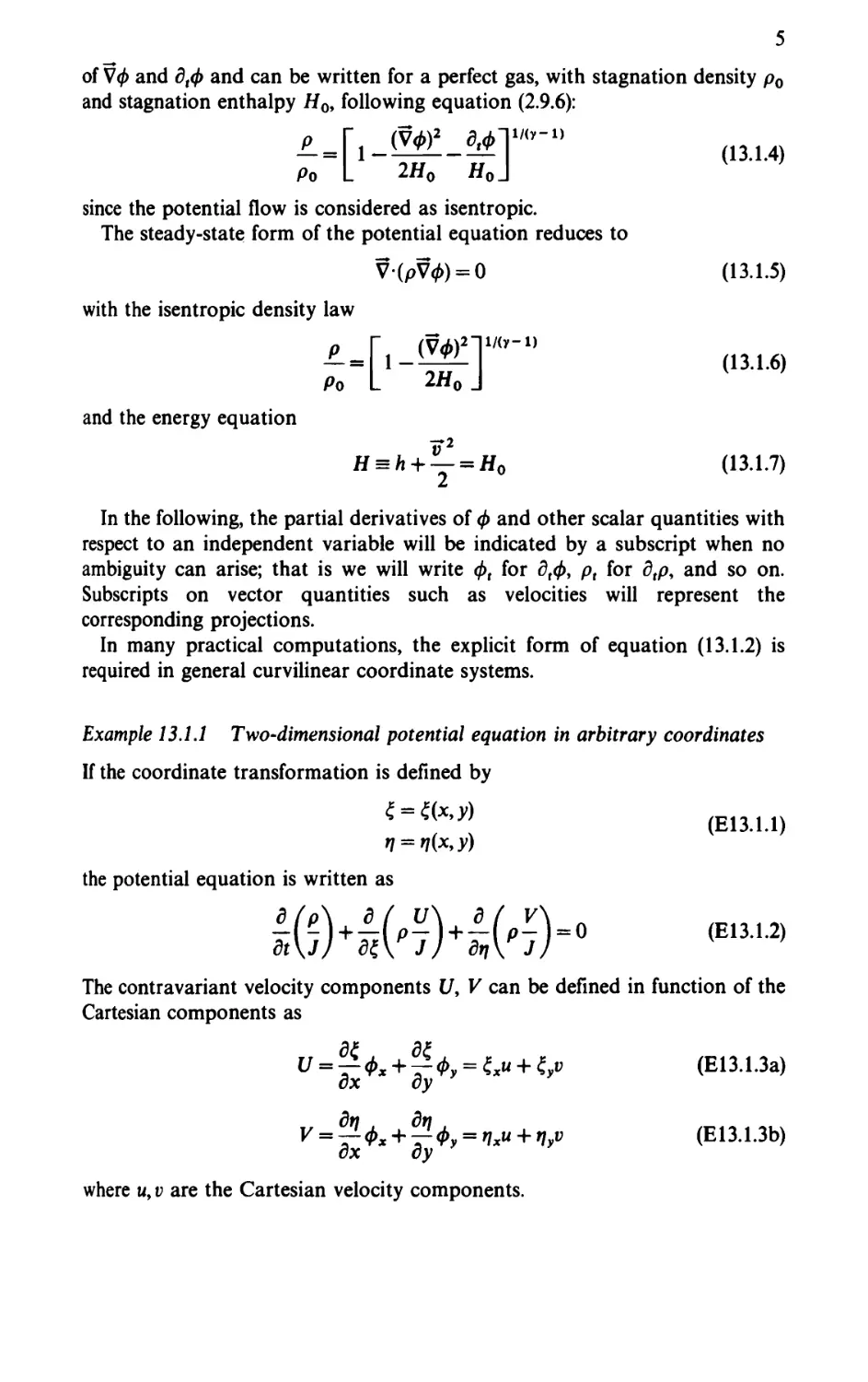
Example 13.1.1 Two-dimensional potential equation in arbitrary coordinates
If the coordinate transformation is defined by
(E13.1.1)
l = l(x,y)
the potential equation is written as
&>U$+H3-
The contravariant velocity components U9 V can be defined in function of the
Cartesian components as
dx x dy
ox dy
where u, v are the Cartesian velocity components.
U—rh + ^^te + Z* (E13.1.3a)
V = ^<t>x + ^y = t,xu + t,yv (E13.1.3b)

6
The stationary potential equation is also to be obtained as
V-(p7) = ^Ln^ + 5lV,)jl + fr521^ + 522^)jl = 0 (E13.1.4)
(E13.1.5)
since one has also
U = gll4>t + gll<l>,
V = g21<l>i + g22<t>,
The matrix tensor g has the following components:
0n = £2 + £2
gl2 = g2i = ^x + ^t}y
g22 = rt2x + t,2 (E13.1.6)
In practical computations, one will often have to determine the metric
coefficients through the inverse relations
X = X(Z,TJ)
This is obtained by the relations
L = Jy, Zy=-Jxv
*ix=- Jy< ny = Jxt
with the Jacobian J:
(El 3.1.7)
(E13.1.8)
J = (E13.1.9)
Example 13.1.2 Potential equation in cylindrical coordinates
In cylindrical coordinates (r,6,z), one has an orthogonal coordinate system,
with metric coefficients ht = l,h2 = r,h3 = l and J= 1/r. The components a*"
are diagonal with g11 = 1, g22 = 1/r2, g33 = 1.
The potential equation becomes, in steady-state conditions,
13.2 THE NON-CONSERVATIVE FORM OF THE ISENTROPIC
POTENTIAL FLOW MODEL
The isentropic potential model can be written in non-conservative form by
working out the derivatives of the density (see Problem 13.1):
i 14>„ + 3,( V>)2] = (1 - M2x)<f>xx + (1 - Mfy„ + (1 - M 1)4>ZZ - 2MXM A,
- 2MxMz<pxz - 2M yMz4>zy (13.2.1)

7
As mentioned above, the subscript on <f> indicates a partial derivative with
respect to the corresponding coordinate, but the same subscript on the Mach
number M indicates the corresponding velocity component.
The second term in the left-hand side of this equation can be explicitly
calculted by
dt(V<f>)2 = 2((t>x4>xt + 4>y<t>yt + <M«) (13.2.2)
and the Mach numbers are defined in the coordinate direction x,y,z by
c c c
(13.2.3)
The speed of sound c is given by
= (V-l)/z = (v-l)rH0-^-^l (13.2.4)
for perfect gases.
For steady flows, the left-hand side of equation (13.2.1) vanishes, and one
obtains the non-conservative equivalent to equation (13.1.5) in Cartesian
coordinates. It can be written in condensed notation, with a summation
convention on /, j = x, y, z:
(Sij-MiM^j-O (13.2.5)
13.2.1 Small-perturbation potential equation
The small-perturbation potential equation has been for a long time the basis
for potential flow theories, particularly for transonic flows where it is known as
the transonic small-perturbation (TSP) equation, as it is a simplified form valid
for flow fields along slender bodies aligned with the x axis (Figure 13.2.1).
It can be written in various ways from a small-perturbation expansion of the
full potential equations (13.1.5) or (13.2.5). Defining the perturbation potential
<D by
^[Ux + O) (13.2.6)
the velocity components are defined by
U=t/»(1+^ (13.2.7)
v = U^v
where V ^ is the free-stream velocity. With the assumption of a dominating

8
u
► —
► —
(a) Physical plane
▲
u
=►
►
►
airfoil
(b) Computational plane
Figure 13.2.1 Small-perturbation potential flow along slender foody
x component of the velocity field, that is v « u, the two-dimensional form of
equation (13.2.5) reduces to
(l-M2x)<l>xx + %y = 0 (13.2.8)
neglecting second-order terms in Q>y and assuming M* « 1.
The factor of the first term can be worked out by introducing the free-stream
Mach number M^ and the relation
C2(l+^M2) = ci(l+^Mi) (13.2.9)
derived from the energy equation (13.1.7) for a perfect gas.
This leads to the following form of the small-perturbation potential equation
see Problem 13.10):
[1 - Mi - (y + l)Mi<t>x^xx + [1 - (y - l)A#i*J*w = 0 (13.2.10)
neglecting terms proportional to O* and O*.
This equation is generally further simplified to the more classical form
[1 - Af i - (y + lJM^OJO^ + *yy = 0 (13.2.11)
The sonic condition corresponds to w = Ox = (l — M^)/[(y + l)Af^]. The
first-order TSP equation is the Prandtl-Glauert equation
(l-M2JOxx + <I>yy = 0 (13.2.12)
If y = f(x) is the equation of the thin airfoil surface, it is customary with the
^>rr///s7T^
airfoil

9
small-disturbance hypothesis to set the surface boundary condition on the x
axis, that is at y = 0. Hence, the flow is calculated in the half-plane where the
airfoil occupies a portion of the x axis. The presence of the airfoil will appear
in the computation only through the boundary condition (Figure 13.2.1)
v = (Um + u)f{x)*Umf{x) (13.2.13)
where f'(x) is the derivative of /.
Other formulations of the small-perturbation equations as well as references
to earlier work can be found in J. Slooff (1982).
13.3 THE MATHEMATICAL PROPERTIES OF THE
POTENTIAL EQUATION
The mathematical properties of the potential flow equation can best be obtained
from an analysis of the non-conservative form (13.2.1).
133.1 Unsteady potential flow
The time-dependent potential equation is a quasi-linear, second-order partial
differential equation and it is of importance to determine its type: hyperbolic,
parabolic or elliptic (see Chapter 3 in Volume 1).
Since this equation contains a second derivative with respect to time, and
since a coordinate system can always be chosen such that one of the velocity
components is locally zero, at least one of the second-order space derivatives
will have a positive coefficient, indicating that the equation is hyperbolic with
respect to time, independently of Mach number.
In many unsteady potential flow computations, the additional
approximation of low-frequency unsteady motion is introduced, allowing the second-order
time derivative in the potential equation to be neglected. However, this does
not change the type of the equation.
133.2 Steady potential flow
For steady potential flows, the situation with respect to the type of the equation
is more complex.
In two dimensions, x,y, it was shown in Chapter 3 that the potential equation
is hyperbolic in (x, y) for supersonic velocities, parabolic along sonic lines, M = 1
and elliptic in the subsonic flow regime.
In three-dimensional flows, the situation is somewhat more complicated, since
at each point one has an infinity of possible characteristic directions and the
properties of the system in supersonic flows also depend on the coordinate
selected to act as a time-like direction.
Following the guidelines of Chapter 3, the stationary form of the
three-dimensional potential equation (13.2.5) is first cast into a system of

10
first-order equations by addition of the irrotationality condition
VxTT = 0
Defining the column vector U as
U =
u
V
w
=
**l
^
<t>z\
(13.3.1)
(13.3.2)
representing the velocity field and adding the y and z projections of the
irrotationality equation (13.3.1), under the form
dv du _
dx dy
dw du _
dx dz
(13.3.3)
to the potential equation (13.2.1) written as
(1 - M2x)ux + (1 - M*)vy + (1 - M22)w2 - MxMy(uy + t;x) - MyMz(wy + v2)
~MxMz(tiz + wx) = 0
one obtains the following equivalent first-order system:
(Aldx + A2dy + A3d2)V = 0
The three matrices Ax are defined by
A,=
A2 =
A3 =
I-Ml
0
0
-MxMy
-1
0
-MXMZ
0
-1
-MxMy
1
0
1-MJ
0
0
-MyMz
0
0
-MXMZ
0
1
-Af„M2
0
0
I-M22
0
0
(13.3.4)
(13.3.5)
(13.3.6a)
(13.3.6b)
(13.3.6c)
The system (13.3.5) will be hyperbolic, if normals n{nxynyynz) can be found,
satisfying the condition (3.2.22) for the vanishing of the determinant
det \Axnx + A2ny + A3nz\ = 0
(13.3.7)
Since ~n is defined up to an arbitrary scale factor, each solution of (13.3.7)
represents a one-parameter family of characteristic surfaces, defined by a relation
of the form nx/n2 = f(ny/nz).
A straightforward calculation, which is left to the reader as an exercise (see

11
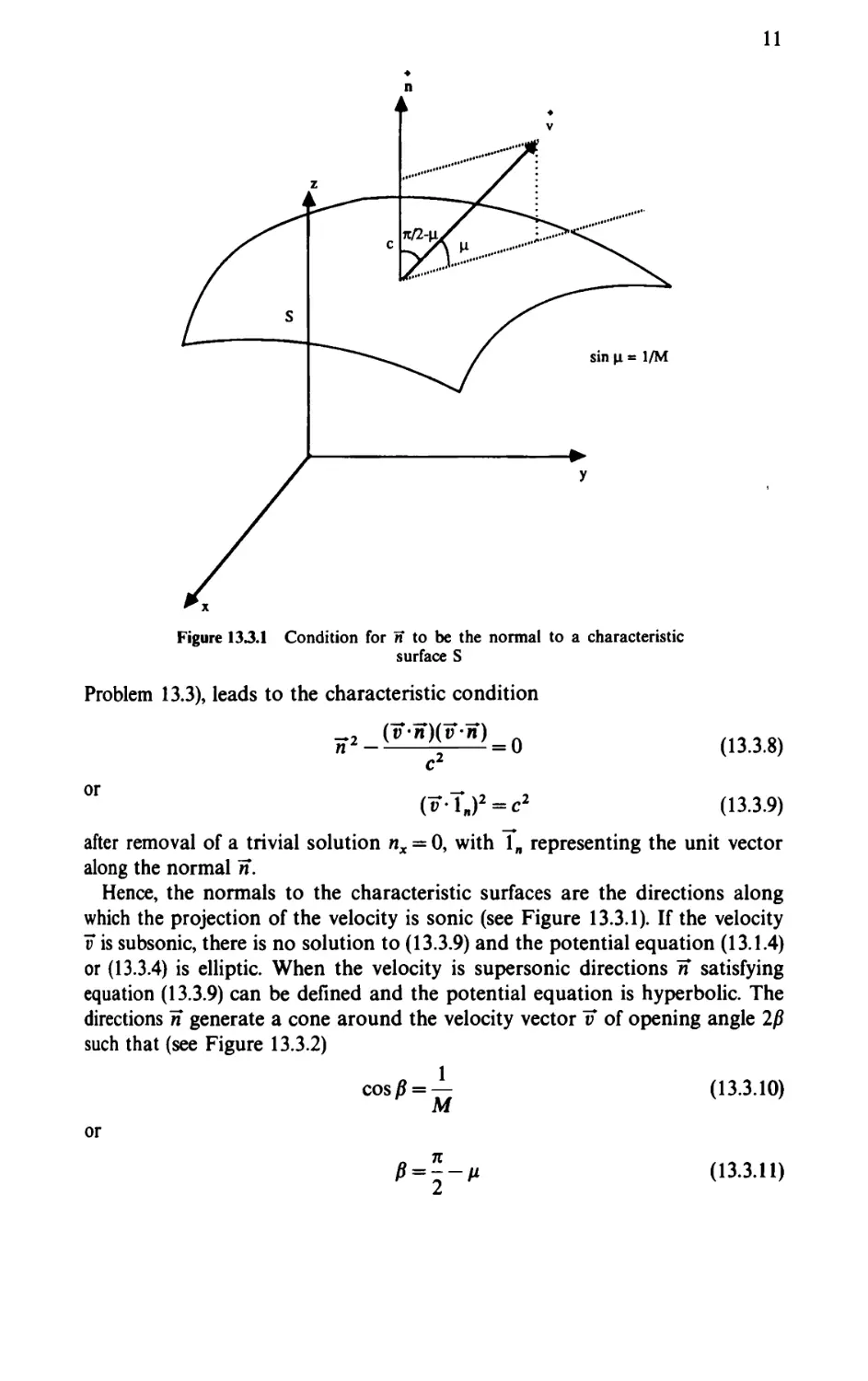
Figure 133.1 Condition for n to be the normal to a characteristic
surface S
Problem 13.3), leads to the characteristic condition
C2
(t?'U2 = C2 (13.3.9)
after removal of a trivial solution wx = 0, with 1„ representing the unit vector
along the normal 7T.
Hence, the normals to the characteristic surfaces are the directions along
which the projection of the velocity is sonic (see Figure 13.3.1). If the velocity
? is subsonic, there is no solution to (13.3.9) and the potential equation (13.1.4)
or (13.3.4) is elliptic. When the velocity is supersonic directions It satisfying
equation (13.3.9) can be defined and the potential equation is hyperbolic. The
directions ~n generate a cone around the velocity vector ~v of opening angle 2)3
such that (see Figure 13.3.2)
cosjff = — (13.3.10)
M
or
» = \-v (13-311)

12
Cone of normals
characteristic surface normal to n
y
Figure 13.3.2 Mach cone and cone of the normals n to the characteristic surfaces S
where \l is the Mach angle defined by
sin/* = — (13.3.12)
M
Each normal Ji lying on the cone of opening angle (n — 2n) centered on the
velocity defines a characteristic surface. The envelope of the characteristic surfaces
when ~n sweeps its cone forms a second cone, of opening angle 2/j centered on
the velocity, the Mach cone. The Mach cone limits the zone of influence of point
P and the downstream prolongation of the cone defines the domain of dependence
of P.
However, if for supersonic absolute velocities the potential equation is
hyperbolic, it is yet not clear which coordinate direction can be taken as a
time-like variable. This is of importance since, following the developments of
Chapter 3, Section 3.4, a time-like direction z implies that an arbitrary
perturbation in the direction 7c(wx, ny) of the x, y plane will propagate in the z
direction with a 'frequency* w equal to — nz. The component n2 is the solution
of equation (13.3.8), written as follows after multiplication by c2 and development
of the scalar products:
n\(c2 - w2) - 2wnx(v-lc) + c2k2 - (IT-7c)2 = 0 (13.3.13)
where
F-7c = unx + vny (13.3.14)
A real solution n2 to the quadratic equation (13.3.13) will exist for all k:, if the

13
discriminant is positive, that is if
w2(vk)2 - (c2 - w2)[c27c2 - (fie)2] > 0
or
w2k2 + (vk)2 > c2k2 (13.3.15)
Since one can always choose ~k2 = 1, this equation will be satisfied for all k: if
w2>c2 (13.3.16)
that is if the velocity projection in the considered direction is supersonic. For
subsonic flows, equation (13.3.13) has no real solutions.
Referring to Figure 13.3.2, the condition (13.3.16) implies that all time-like
directions are located inside the cone of normals. In a curvilinear system of
coordinates, a particular coordinate direction, say £x = £, will be time-like if
the associated co variant component of the normal direction, nu is real for all
values of n2, w3. Applying the above procedure, one obtains the condition on
the contravariant velocity component U:
U
>c
(13.3.17)
CLl
S: characteristic line 4 4
CLl, CL2 : limit directions for which v.l n = c
intersections with cone of normals
n, : normal to ^ = ct line
♦
n : normal to r\ = ct line
Figure 13.33 Conditions for the directions { to be a time-like coordinate

14
that is the 'physical* value of the velocity projection in the direction normal to
the ^-constant lines has to be supersonic (Figure 13.3.3); see also Problem 13.5.
A direction outside the cone of normals will correspond to an elliptic
behaviour and will be called a space-like direction.
In Figure 13.3.3 the line S is the intersection of the surface £3 = £ with the
characteristic surface and the lines CL1 and CL2 are the intersections with the
cone of normals. Hence, CL2 is perpendicular to S and makes an angle (n/2 - /z)
with the direction of the local velocity. All the normals between the limit lines
CL1 and CL2 correspond to time-like directions since the projection of the
velocity on this direction is larger than the sonic velocity. This is the case for
the normal 7f4 to the ^-coordinate line (a line { = ct). Note that the projection
of the velocity along this direction is equal to the left-hand side of equation
(13.3.17). On the other hand, the normal ~nn to the ^-coordinate line (a line
tj = ct) is outside the lines CL1 and CL2 and therefore the associated
^-coordinate line is space-like.
The application of these considerations to the computation of three-
dimensional supersonic potential flows with embedded subsonic regions has
been developed by Shankar and Osher (1983) and Shankar et al. (1983).
In practical computations, the separation surface between subsonic and
supersonic regions is not known and is part of the solution. Next to the
occurrence of shock discontinuities, this makes up for the difficulties of transonic
potential flows.
13.4 BOUNDARY CONDITIONS
A computational domain has to be selected, limited by a boundary T and the
boundary conditions for the potential flow computations have to be defined.
13.4.1 Solid wall boundary condition
At solid boundaries, the normal velocity is
on
where
4 = 0
if the solid wall is at rest, while
q = pvytTn (13.4.2b)
if the solid wall has a velocity 7W, where 1„ is the unit vector along the normal
to the boundary. If a local mass flux mw per area unit is injected through the
wall surface (Figure 13.4.1), then
(13.4.1)
(13.4.2a)
<j = mw
(13.4.2c)

15
Figure 13.4.1 Boundary conditions along a wall with real or simulated mass
flow injection
For instance, in viscid-inviscid interaction computations where the potential
flow is corrected for the boundary layer thickness, the displaced boundary of
the inviscid region is the edge of the boundary layer. For small boundary layer
thicknesses the displaced boundary of the computational region can be modelled
by the introduction of the displacement thickness <5*. In this case a mass balance
over the domain ABCD gives
*w-^(P*.**) (13A3)
Ql
where ve is the velocity at the edge of the boundary layer and d/ the elementary
distance along the wall.
13.4.2 Far field conditions
At the external boundaries of the computational domain, the flow field is
assumed to be known. In external flow problems, such as the flow around a
body under uniform inflow K^, the potential flow is known by
0=Koox-h0o (13.4.4)
where 0O is an arbitrary constant and x* the distance to a point on the boundary
with respect to a chosen reference.
Single airfoil
For lifting bodies with circulation TB the contribution of the circulation to the
potential flow at large distance has to be taken into account (Figure 13.4.2).
This is best represented, for a two-dimensional airfoil, by a vortex singularity,
cqrrected for compressibility effects (Ludford, 1951):
0farneid = *V* + ^ tan"1 i^l^Mi tan(0 - a,)] + 0o (13.4.5)
where 6 is the angular position of a far field point, TB the circulation and Mw
the Mach number corresponding to the free-stream velocity V^ under an
incidence angle of a^.

16
Figure 13.4.2 Computational domain and boundary conditions for isolated airfoils
^
Figure 13.4.3 Computational domain for cascade configurations

17
13.4.3 Cascade and channel flows
(Figure 13.4.3) The upstream velocity field is assumed to be known and the
potential field along AB can be determined. Hence, a Dirichlet condition
<t> = 0abCv) can be applied along the inlet section AB. At the outlet, the flow is
generally not completely known and the potential at point H is unknown.
Therefore the most appropriate boundary condition is a Neumann condition
expressing conservation of mass flow through the cascade channel, assuming
uniform flow conditions along the outlet section of the computational domain
GH:
(p<t>n)GH = (PiVin)^ (13.4.6)
where pt is the inlet specific mass, ~v the inlet velocity with normal component
i?ln and Au A2 the inlet and outlet areas.
For transonic cascade and channel flows, additional problems arise when
shock waves are present under choked conditions due to the non-uniqueness
of the potential solutions for given physical inlet and outlet conditions (see
Section 2.9 in volume 1). In addition, for choking conditions occurring when
the flow is accelerated through sonic conditions at a minimum area section of
the channel, the mass flow is fixed by the critical, sonic conditions and is therefore
unknown. Consequently, a Neumann boundary condition cannot be applied
and the condition (13.4.6) has to be replaced by a more appropriate condition.
A detailed analysis has been given by Deconinck and Hirsch (1983) and the
following boundary treatment can be applied.
Choked flow with subsonic inlet and outlet flow conditions
This will occur, for instance, in a convergent-divergent channel when the
pressure difference between inlet and exit is sufficiently large. The flow is
accelerated through sonic velocity in the throat and further accelerated to
supersonic velocities. The supersonic region is terminated by a strong shock
which brings the flow back to subsonic conditions. As discussed in Section 2.9.2,
the shock position cannot be defined by the physical variables, since the outlet
isentropic variables such as velocity, pressure and density are uniquely
determined by the subsonic isentropic flow conditions. In addition the mass
flow is unknown and only Dirichlet conditions can be applied. The following
approach will lead to a unique isentropic potential flow with shocks:
Dirichlet condition at inlet: <t> = <t>l
Dirichlet condition at outlet: <t>z=<t>2 based on a uniformity assumption
The potential difference (<f>2 — <t>\) fixes the shock position and the mass flow
results from the computation. The same situation occurs for a divergent channel
with sonic inlet and subsonic outlet.

18
Divergent channel with shock
If the inlet is supersonic with a subsonic outlet the flow is not necessarily choked
but a shock is present. Therefore one has to impose:
(1) A Neumann condition at inlet (or outlet) to fix the mass flow;
(2) A potential difference by imposing the value of the potential at one point
on the Neumann boundary.
13.4.4 Circulation and Kutta condition
Single airfoil
As discussed in Section 2.9, lifting airfoils require a circulation whose intensity
is defined by the Kutta condition. In practical computations a branch cut is to
be defined along which the potential will have a discontinuity given by equation
(2.9.11). (Figure 13.4.2):
<t>?' - <t>? = TB = 0b - <I>a (! 3.4.7)
The value of the circulation is updated during the iterative process by imposing
equal velocities or pressures at both sides of the trailing edge.
Cascades
For cascades, along the boundaries BC and AD all physical flow variables are
identical. The circulation around the closed contour of Figure 13.4.3, ABGHA,
is equal to
TB = s(v2y-vly) (13.4.8)
where s is the spacing between consecutive blades. Therefore, the periodicity
condition can be satisfied by imposing
0b ~ 0a = 4>r - 0p = svly (13.4.9a)
<t>G-<t>H = <t>Q' - <t>Q = sv2y (13.4.9b)
The value of v2y = v2x cos /?2 is obtained either by imposing f}2 as an outlet
variable or by applying a Kutta condition at the trailing edge, under the form
of requiring equal velocities at E and F.
13.5 INTEGRAL OR WEAK FORMULATION OF THE
POTENTIAL MODEL
The weak formulation forms the common basis for finite element and finite
volume discretizations. For any smooth function Wy the weak form of the
potential equation in conservation form (13.1.2) is obtained after multiplica-

19
tion by W and integration over the computational domain Q. A partial
integration is performed, leading to
I ptwdti- I pV<t>'Vwdn + &> p<t>nwdr = o (13.5.1)
In general, W is chosen to be zero on the part S0 of the boundary where the
function <t> is known and the boundary integral reduces to a contribution on
the part of the boundary where a Neumann boundary condition is imposed.
If a discontinuity surface £ propagating with speed C exists in the flow
domain H, the application of the approach followed in Section 2.7 leads to the
jump condition valid locally along Z and expressing mass conservation over
the discontinuity),
[p0J-C-T.[p] = O (13.5.2)
where 1„ is the unit vector normal to the discontinuity surface I and the square
brackets indicate the discontinuous variation over the surface, [p] = p2 — Pi-
Comparing with the Rankine-Hugoniot relations derived in Section 2.7, it
is seen that the potential discontinuities do not satisfy the jump relations for
the momentum components. Instead they satisfy the isentropic condition [5] = 0,
which is not valid for the Rankine-Hugoniot discontinuities. Since the latter
represent the correct, inviscid conservation laws over discontinuities, the
potential shocks will represent an isentropic approximation to the Euler shocks.
These shocks are connected to an entropy increase proportional to (M2 — l)3
and hence the potential shocks might be valid for Mach numbers close enough
to 1, say M < 1.25; see Section 2.9.2 for a more detailed discussion and
comparison.
The finite volume discretization for a given mesh point will be obtained
with W = 1 in the control volume associated to the mesh point and zero
outside.
For finite element formulations, with a Galerkin method, W is equal to the
element interpolation functions.
13.5.1 Bateman variational principle
The weak formulation (13.5.1) can also be obtained from Bateman's variational
principal (Bateman, 1929), stating that the pressure integral
/= I pdQdr (13.5.3)
isextremum, where dCldt is a space-time domain element and where the initial
and boundary conditions are supposed to be satisfied for all variations 5<j>.
If not, their contribution has to be added to the functional (13.5.3). For
instance, the boundary condition p<t>n = g on T1 will give a contribution
|n#drdt.

20
The pressure p is considered as a unique function of the potential derivatives
defined by the isentropic relations for a perfect gas:
P_
Po
-UJ =U=(^^-^J (115-4)
The first variation SI is obtained by
51 = f 5pdQdt = f (^5<t>x^^Sct>y^^S(t>2 + ^S(t>t)dQdt (13.5.5)
From equation^ 13.5.4) one has, with a straightforward calculation (see Problem
13.7),
and
5p = -p[7Sl>+d<l>J = (-^\dp = c2dp (13.5.6)
~v-5~v Sd>t
SP--P—T—P-T (13-57)
c2 c2
Hence, with the potential definition ~v = V<f>, one obtains
SI= - J (PV0 dV<t> + pd<l)t)dndt= - (pV<l)V6<l) + pdtd<l))dndt (13.5.8)
Jn Jo
which gives, after integration by part, with 8<t> = 0 on the boundaries,
61= J [V(pV0) + arp)^dQdr = O (13.5.9)
Jn
Hence, the vanishing of the first variation is equivalent to the mass conservation
equation (13.1.2), written for the potential function. Note also that equation
(13.5.8) put to zero is equivalent to the weak formulation (13.5.1) with W = 6(j)
and a partial integration of the time derivative term.
13.5.2 Analysis of some properties of the variational integral
It is interesting to estimate the second variation of the pressure functional, since
its sign will indicate if the functional extremum is a maximum or a minimum.
Since this is of particular importance for steady-state potential flows, we will
develop this analysis for the stationary formulation (13.1.5), (13.1.6).
The variational Bateman integral can be written without the time variable,
and the first variation 51 becomes
= —I p~v'8~v
SI=-\ pltdlfdn (13.5.10)

subsonic flow
61
sonic conditions
supersonic flow
space like
Figure 13.5.1 Representation of the dependence of the variational pressure integral with Mach number
time like

22
The second variation is obtained by the following steps:
= - J dp(v-S7)da- I p(S?dl>)dn- I p(~v S2"v)dQ (13.5.11)
Jn Jn Jn
In the last term d2~v is taken to be zero, since 8~v is the independent variable.
With dp defined by equation (13.5.7), one obtains for the second variation
*/«-J ,[(«*)»-<*^]dQ (13.5.12)
The two terms under the integral can be written out explicitly, in Cartesian
coordinates,
2uw 2vw
rSuSw -SvSw (13.5.13)
c2 c2
This expression parallels completely the right-hand side of the potential equation
(13.2.5). This is of course not by accident, since the same type of information
is contained in both equations. The sign of the second variation S2I can best
be analysed by comparing the expression under the integral in equation (13.5.12)
with the characteristic relation (13.3.8).
Both expressions are identical, if S~v is replaced by n. Therefore, one has
immediately the following results:
(1) The quantity [(S~v)2 — ((v S~v)2/c2)] is always positive for arbitrary
variations d~v if the flow is subsonic. In this case, S2I < 0 and the extremum
of the variational pressure integral is a maximum.
(2) Along sonic surfaces, 52I = 0 for certain variations and the curve
representing the relation between / and the velocity variation goes through
an inflection point.
(3) If the flow is supersonic, one has to distinguish, following the relations
(13.3.13) to (13.3.15), between space-like and time-like variations 8~v. US~v
is a space-like variation, that is if 5~v lies outside the cone of normals of
Figure 13.3.2, the second variation 52I remains negative. When S~v is
time-like, within the cone of normals, d2I is positive and I has a minimum.
This is summarized in Figure 13.5.1 by a one-dimensional representation of the
functional / in the function of v.
An essential guideline in the supersonic case will be to avoid velocity variations
during the computations which cause a change of sign of the second variation

23
S2I. This would have in consequence a loss in unicity of the computed solutions
associated with a loss of positive definiteness of the iteration matrix, which
could become singular.
This will become clearer in the next chapter, where it will be seen that the
Jacobian iteration matrix applied on 6<f> for a Newton iteration on the density
is identical to the quadratic form defining the second variation S2L This should
not be surprising to the reader, since the first variation 51 is precisely the
potential flow equation applied to S<f>.
References
Bateman, H. (1929). "Notes on a differential equation which occurs in the two-dimensional
motion of a compressible fluid and the associated variational problem/ Proc. Roy.
Soc. Series A, 125, 598-618.
Deconinck, H., and Hirsch, Ch. (1983). 'Boundary conditions for the potential equation
in transonic internal flow calculations.' ASME Paper 83-GT-135, 26th International
ASME Gas Turbine Conference.
Ludford, G. S. (1951). The behavior at infinity of the potential function of a
two-dimensional compressible flow.' Journal of Mathematical Physics, 30, 117-30.
Shankar, V., and Osher, S. (1983). 'An efficient, full potential implicit method based on
characteristics for supersonic flows.' AIAA Journal, 21, 1262-70.
Shankar, V., Szema, K. Y., and Osher, S. (1983). 'A conservative type dependent full
potential method for the treatment of supersonic flows with embedded subsonic
regions.' Proc. AIAA 6th Computational Fluid Dynamics Conf., AIAA Paper 83-1887,
pp. 36-47.
Slooff, J. (1982). 'General theory.' In Applied Computational Transonic Aerodynamics,
Chap. 2, AGARDograph AGARD-AG-206.
PROBLEMS
Problem 13.1
Derive the quasi-linear potential equation (13.2.1) by applying the relation (13.5.7) to
the conservative form (13.1.2).
Hint: Work out the spatial gradients and replace the derivative of the density by
derivatives of the potential function based on equation (13.5.7).
Problem 13.2
Obtain the matrices (13.3.6).
Problem 133
Obtain, by working out the determinant (13.3.7), the relation (13.3.8) for the characteristic
normals.
Hint: Introduce the scalar product
-(v- ~n) = Mxnx + Myny + Mznz

24
Problem 13.4
Derive the relations for the characteristic lines for a two-dimensional potential flow.
Show by an explicit calculation that they form an angle \i = sin \jM with the velocity
vector.
Hint: Solve for the directions (n^ny) of the normals. The characteristic lines are
orthogonal to 7f.
(1) Define k = ny/nx and obtain the characteristic normal directions as
MxMy±(M2-l)1/2
A.+ —
± 1-M2
(2) Obtain the characteristic directions as s±:
_MXM>
MXM,T(M2-1)1/2
s+ — -
I-Ml
and consider a local coordinate system with the x axis aligned with the velocity
vector.
Problem 13.5
Obtain the condition (13.3.17) for the coordinate line f1 = <J to be time-like, taking into
account that the scaled contravariant component U/y/g^ is the projection of the velocity
in the direction normal to the line £ = constant.
Hint: Take k = n{e2 + n3T3 and develop ~v~n— ~v-jc + vlnt and 7T2 =~k2 + (n1)2011 +
2k1h1. Follow the reasoning which led to equation (13.3.15) and choose jc1 =0.
Apply also to the two-dimensional case of Figure 13.3.3.
Problem 13.6
Obtain equation (13.5.2).
Problem 13.7
Obtain the relation (13.5.6) for the pressure variations from the isentropic relation (13.5.4).
Hint: Apply the density relation (13.1.4) and the perfect gas law for the stagnation
quantities.
Problem 13.8
Define the critical speed of sound cm by the condition |7fJ=c^ and obtain the
steady-density relation as a function of a non-dimensional velocity ratio:
--5
Define the critical density and show that one can distinguish the supersonic from the
subsonic points by comparing the expression
('-•&)
with or p with p*
7+1

25
Hint: Apply the constancy of energy to relate c0 and i/0. Obtain
po V *y + ij
The last observation is often used in programs where the density is evaluated in order
to detect supersonic points.
Problem 13.9
Repeat the calculations of Example 13.1.1 for the three-dimensional potential equation,
with the coordinate transformations <J = £(x, y, z), n = n(x, y, z), £ = C(x, y, z).
Note that the gradients of f define the transformation between the Cartesian and
contravariant components of velocity; for instance U = ~v-V£. The metric tensor gafi
defines the transformation between the gradients of the potential in the curvilinear system
and the contravariant velocity components; for instance U* = g**<t>p, where <j>p = d<f>/d^
Problem 13.10
Obtain the small perturbation potential equations (13.2.10) and (13.2.11). Derive first
equation (13.2.9) using equation (13.2.4).
Hint: Write M2x as follows:
M^Af^l+flg2^
and work out using equation (13.2.9), neglecting quadratic terms in <D^.
Problem 13.11
Write the small perturbation potential equation in conservation form and derive the
corresponding shock relations. Compare with the Rankine-Hugoniot relations derived
from the Euler equations.
Hint: Obtain
and the jump relations
[a - m>, - ^±-Uf]^+r>,]=o
where the square brackets now represent the jump over the discontinuity: [A] = A2 — At
and dy/dx is the slope of the discontinuity in the xy plane.

Chapter 14
The Discretization of the Subsonic
Potential Equation
Since the stationary subsonic potential flows are governed by an elliptic equation
they can be computed in a straightforward way, the numerical resolution of
smooth elliptic problems being nowadays an easy task.
The main steps to be defined are the following:
(1) The selection of a discretization scheme. One has the choice between finite
difference, finite volume and finite element representations. All of them
have been applied and are in use at different places with equal success. The
choice is therefore more a matter of personal taste than of efficiency.
(2) The iteration method to deal with the non-linearity introduced by the
density.
(3) The algorithm for the resolution of the obtained algebraic system.
In addition the interaction between the last two steps and the implementation
of the boundary conditions will completely define the numerical scheme.
With subsonic flows, which have a smooth behaviour, we will be able to
operate with rather coarse meshes, with the exception of certain localized regions
such as corners, leading or trailing edges of airfoils, and other regions where
strong flow gradients can be expected. Hence, the total number of mesh points
will be restricted and nearly any of the methods described in Chapter 12 in
volume 1 for the resolution of algebraic systems, will be sufficiently effective.
Therefore, readers only interested in subsonic potential flows will be able to
limit themselves to this chapter. It could be mentioned at this point that the
algorithms for subsonic potential flows are equally applicable to all problems
governed by a similar equation, such as heat conduction in solid bodies, electrical
potential distributions, groundwater flows, etc.
The particular problems attached to transonic flows will be dealt with in the
following chapter. They concern essentially steps 2 and 3 since the density
variations contain all the non-linearities, in particular the transition from
subsonic to supersonic regions and the eventual presence of shock discontinuity
surfaces.
We will deal essentially with the conservative form (13.1.5) of the potential
equation. As discussed in Chapter 6, a non-conservative formulation of a
26

27
conservation law, in the present case mass conservation, generates internal
sources, although for smooth flows these contributions will be of the same order
as the truncation errors. However, in regions with strong gradients or with
discontinuities, unacceptable errors are introduced in this way and the
conservative form has to be used.
Also, for the sake of simplicity, we will present the various discretizations for
two-dimensional flow problems. In most cases the generalization to a higher
dimension will be straightforward and we refer readers to the appropriate
literature for more details concerning three-dimensional applications.
14.1 FINITE DIFFERENCE FORMULATION
In Cartesian coordinates, the most straightforward discretization, of
second-order accuracy, is the central symmetrical form following equation (4.4.7)
in volume 1.
0 potential evaluation
X density evaluation
j=l
j+1/2
j-1/2
3/2
1/2
(
i-
f
K
~ 3
)—i—(
;— $
Di
■ i
— ■*■---
1 v.
— u*^ ■-
i !
\
j
\~
y-
B
"*1
; a
j «
%
j
i
! i"
)
fl
i-1/2 i+1/2
Figure 14.1.1 Cartesian two-dimensional finite difference computational mesh

28
Referring to Figure 14.1.1, the following two-dimensional scheme can be
defined:
where 5+ and <5~ are defined in Chapter 4 as the forward and backward
difference operators, acting on all the terms to their right. The subscripts indicate
the variable on which the difference operators act. For memory, we recall the
definitions
<5+0i = 0<+i-0i <5 4>t = 4>t — 4>t-\ <50< = <k+i/2-<k
1/2
H<t>i =
_<fo+1/2 + 01-
1/2
fr,,*'"-*'-!,^
(14.1.2)
2 ' 2
Worked out explicitly, equation (14.1.1) becomes, for Ax = Ay,
-Pij-1/2(^0-^u-i) = °
(14.1.3)
As seen from Figure 14.1.1, the discretized equation will involve the five points
marked on this figure. Note that the densities have to be evaluated at the
mid-point locations, while the potential values are evaluated at the corners of
the mesh. This standard five-point molecule is shown in Figure 14.1.2 and
reduces to the five-point Laplace operator for incompressible flows.
j+i
i-l/2j
j-i
1
PiJ+l/2
i-l/2j
i+l/2j
-P.
iJ-1/2
nj+1/2
pJ-1/2
i+l/2j
i+1
Figure 14.1.2 Computational molecule for the Finite
difference scheme (14.1.3)

29
+ M M
2 * y
1-M
-±
M M
x y
,-M.
-2(2-
i-M2)
-M
-4-M M
2 x y
1-M^
+ M M
x y
Figure £14.1.1 Computational molecule for the non-
conservative potential equation and second-order central
differences
Example 14.1.1 Non-conservative potential equation in two dimensions
In a Cartesian mesh, the following equation has to be discretized:
(1 - M2x)<t>xx + (1 - M2y)4>yy - 2MxMy<j>xy = 0 (E14.1.1)
With central differences, one obtains in point (i, j) for Ax = Ay, with second-order
accuracy,
(1 " Af 5y(^+ x J - 2&J + fa^j) + (1 - My%(tf>iJ+ % - 2<fc; + </>,;_ ,)
- l(*'*A'AM+u+1 - *i +u-1 - *i-u+i + *i-ij-iJ^O (E14.1.2)
The computational molecule can be visualized as in Figure El4.1.1.
Observe that the matrix of the system (El4.1.2) is diagonal dominant for
subsonic flows. In supersonic flows, for instance for a flow in the x direction,
the matrix does not remain diagonal dominant. This is easily seen and left as
an exercise for the reader.
14.1.1 Numerical estimation of the density
The numerical estimation of pn at the mid-point locations is obtained from the
velocity field, since p is a unique function of the velocity squared.
In order to obtain the mid-point velocities, for instance at point (/+ 1/2, j),
one can apply the following operations:
"» +1/2 j = 7~ 5* <l>ij = 7Z^'+ U - <l>ij)
(14.1.4)

30
= ^(0i+u+i + ^u+i~^+ij~^v) (14.1.5)
Another alternative for the estimation of vi+l/2J is to consider the central
derivative with respect to j since equation (14.1.5) is only a first-order estimate
of ui+1/2j (it is actually a second-order estimation of v.+ 1/2j+lj2). To second
order, one has
tfi+i/2j = ^A*A^+i/2j = ^(^i+ij+i + *£j+i-^+ij-i-0u-i) 04-1.6)
Various alternatives can be applied to evaluate the densities needed in
equation (14.1.3):
(1) Evaluate the densities at the mid-points of Figure 14.1.1 by
Each mesh point requires the evaluation of two densities, pl + 1/2,; and
Pij+i/2> anc'' tf needed, the density at a mesh point can be obtained by
averaging the four surrounding mid-cell values. For instance,
Pu = i(Pi+1/2 j + Pi-1/2 j + P..;+1/2 + Pij-112) (14.1.8)
(2) Estimate the density at the centres ABCD of the finite difference mesh of
Figure 14.1.1. For instance,
Pt+1/2 j+1/2 = P(vf+ 1/2J+1/2) 04.1.9)
where the corresponding velocity component could be evaluated by
Mi + 1/2J + 1/2 = 2~(Mi + 1/2J + 1 + M» + l/2,j) /j4 j jqj
y/+l/2J+l/2 = 2(^+1,7+1/2 + yU+l/2)
and
^2+l/2J+l/2=(w2 + ^)i+l/2J+l/2 (14.1.11)
The velocity components at mid-point are evaluated with the help of
equations (14.1.4) and (14.1.6) to second-order accuracy (see also Problem
14.1).
Another variant could be to use equations (14.1.10) and (14.1.11) directly
for the squares of the velocity components.
The densities at the mid-points in Figure 14.1.1, needed for equation
(14.1.3), can then be obtained by averaging the corresponding centre-point
values. For instance,
Pu-1/2 j = i(Pi+ 1/2.J+1/2 + Pi+1/2,;-1/2) (14.1.12)
This variant is more economical since the number of density evaluations

31
per mesh point is one instead of two (or three in a three-dimensional
problem). This is a welcome gain, since the fractional power in the
expression of the density is a costly numerical operation.
(3) Evaluate the density at the mesh points, via
Pt+ll2J = l(PiJ + Pi+lj)
Pi J+1/2 =?(Pij + PiJ+l)
with
Pii = P&2ij)
and
w.7 = l(Mi + i/2.; + Mi-i/2j)
^ = 1(^+1/2 + ^-1/2)
Clearly many other variants can be defined and the precise method adopted
has been found to have little influence on the results (Jameson, 1976) if the
order of accuracy is maintained.
14.1.2 Curvilinear mesh
In practice, one seldom has Cartesian meshes, but instead one attempts to adapt
the mesh to the geometry of the flow configuration via various mesh generation
techniques.
Figure 13.4.3 is an example of a numerically generated mesh for a cascade
and Figure 14.1.3 provides some typical topologies for isolated airfoil
geometries.
In order to apply a finite difference discretization on a general mesh, the lines
are considered as forming a set of curvilinear coordinates {"({, rj). The coordinate
transformation laws £ = £(*,)>)> t] = rj(x,y) generate a mapping of the physical
space (x9y) to a computational domain (£,rj) where a Cartesian mesh is set up
(Figure 14.1.4).
By writing the potential equation in the curvilinear coordinate system (<!;, rj),
equation (El3.1.2), it can be discretized directly in the Cartesian computational
space (£,>/).
The following two-dimensional scheme is a direct generalization of the
Cartesian finite difference scheme (14.1.1), with A£ = Arj = 1:
^"(p7)i*i/2j + «;(p7)W+i/2-0 (14.1-16)
The contravariant velocities are defined by the relations of Example 13.1.1 and
can be discretized as follows.
UH-1I2J = ffll U2J5( <t>i} + 01* l/2jM,~ 0I+1/2J
+ i0"i/2.M+ij+i + *»j+i -*»+u-i -*u-i) (,4117)
(14.1.13)
(14.1.14)
(14.1.15)

to
MESHSIZE : 97* 17
fCSHSIZE : 33* 9
MESHSIZE : 65* 13
(a) C - mesh
(b) H - mesh
Figure 14.13 Some typical mesh configurations
(c)O-mesh

33
Physical space
Computational space
4"
ffl
Figure 14.1.4 Mapping from the physical space (x,y) to a computational domain ({,»/)
and
nj+i/a-«a+i/2^«-*w+i/2+^i/2*;*« (1411g)
Similar formulas are easily derived for the other components (see Problem 14.2).
Example 14.1.2 Discretization of metric coefficients
An interesting way of discretizing the metric coefficients is based on a
representation of the mapping x(£9rj\ y(£,rj) on a cell-by-cell basis and considering locally
a bilinear isoparametric transformation compatible with second-order accuracy.
This particular transformation is used to compute the coordinate derivatives
appearing in the metric coefficients.
In Scheme (14.1.16) the metric is required at the mid-points (i± 1/2,;) and
(ij + 1/2). If A, B,C, D are the centres of the four cells surrounding mesh point
(ij) (Figure 14.1.4), the metric coefficient at (i+l/2J) can be defined by
averaging the values computed first at points A and B.
Considering point B within the quadrilateral 1234, the isoparametric
transformation with bilinear shape functions JVf({, rj) is written as
7=1
(E14.1.3)
with
Nf(T)-J(l+«i)(l+Wi) (E14.1.4)
where /= 1,2,3,4 and <!;,*/ range from - 1 to + 1 following the standard finite
element representation of Table 5.1 in Chapter 5, Volume 1, with £7= ± 1,

34
*//= ±1. This representation corresponds to a local £yrj coordinate system
centred in point B with an overall variation A£ = Arj = 2.
Derivatives such as x5, xn are computed from
' i 5{ 4 '
*< - I *j ^ = -£ *id + ^/)^7/ (E14.1.6)
/ orj 4/
where the sum ranges from 1 to 4 over the four nodes of the considered element.
At the centre B(£ = 0, rj = 0) of element 1234 the following discretization formulas
are obtained:
s<|„ = X2 + X> ~*4~Xl (E14.1.7a)
x,|,-*» +**-*»-*' (E14.1.7b)
which can be written as a finite difference formula for point B
*«lu = /*,*«*<+1/2J+1/2 (E14.1.8a)
*„lB = Mi*i+i/2.j+i/2 (E14.1.8b)
Similar relations are derived for the other derivatives. With the relations of
Example 13.1.1, one has
gn = J(x* + yl) = Xi+yn (E14.1.9a)
g" = - J(xtx, + y<yJ = X<X' + W" (E14.1.9b)
and
^+i/2.; = ^4^ (E14.1.10a)
,12+ .12
T
9\lm,i = 9K t*' (E14.1.10b)
14.1.3 Consistency of the discretization of metric coefficients
Generally, the metric coefficients will be evaluated in the computational plane
(£yrj) through the relations of Example 13.1.1, and particular care has to be
exercised in the discretization of these relations in order to avoid the introduction
of systematic errors, which would appear as numerical mass sources. In
particular, the consistency of free-stream or uniform flow conditions must be

35
ensured numerically, that is equation (14.1.16) with (14.1.17) and (14.1.18) must
be satisfied identically by the numerical discretization for a uniform flow field 7^.
Written out explicitly, this implies, in two dimensions with l/^, V^ being the
contravariant components of 7^,
or
d (Zxuw + ZyVjp* , 3 jtixum + fij>Jp
+ —'x °° ,y co/rap«0 (14.1.19b)
where u^ and i?^ are the Cartesian components of TT^.
If A4 and A^ represent the selected finite difference discretization operator of
the mass flux derivatives, this equation is discretized in the scheme as
A (£x"oo + t,vjp» A to^oo + frOPoo = Q n4 j 2Qv
* J n J \ • • )
Since Ma and t;^ are to be considered as independent constants, the following
equations, which are algebraic identities, have to be satisfied by the
discretization. With £x and rjx computed via relations (El3.1.8), one has
A<(y,) - A„(^) = 0 or analytically y^ = y^ (14.1.21)
and
A<( - x,) + A„(x<) = 0 or analytically x<„ = x* (14.1.22)
The metric coefficients are not necessarily estimated via the same difference
operators as applied to the flux components. If one denotes by A™ and A™ the
difference operators applied for the metric coefficients, the above conditions
imply that the two sets of difference operators have to commute. More precisely,
one should select A^, A^, A™, A™ such that
A^yij-ArlA^yij = 0 (14.1.23)
and similarly on x.
If both operators are obtained from second-order central differences, this
condition is satisfied since
and
-iCyj+u+i-yi-ij+i-yi+u-i+yi-w-i) (Ri.24)
However, this is not true in general. For instance, if one-sided, backward
formulas are applied for the fluxes and central differences for the metric, one

36
obtains
(Atf - Atf)yu = (Sft - S;S,)yu
=i(yij+i-^.i-i-yi-ij+i+yi-ij-i) (14.1.25)
which is clearly different from zero (see Problems 14.3 and 14.4).
The situation is still more complex in three dimensions, where one would
have, instead of (14.1.21) and (14.1.22), with coordinates &>/,C (refer to
Problem 13.9),
Ac(y,zc - ycz„) - An(y& - yft) + Ac(^z„ - y^ = 0 (14.1.26)
with two other similar relations.
Contrary to the two-dimensional case (14.1.24), this relation is not satisfied
for central differences (see also Problem 14.5).
In general, the error introduced by the non-consistency of the metric
discretization is small for smoothly varying meshes, remaining of the order of
the truncation error of the difference operators used. However, when the mesh
cells are highly distorted or in regions with large mesh spacings, this error can
have a significant effect on the accuracy of the computation.
A detailed investigation and analysis of the consistency of metric
discretizations with regard to potential flows, including additional requirements
with regard to the consistent estimation of free-stream density and velocities,
is to be found in Flores et al. (1983).
A simple and effective way to cancel any remaining consistency errors due
to metric discretizations consists in substracting the free-stream equation
(14.1.19) from the basic equation, when both are of course discretized in the
same way (Pulliam and Steger, 1980). Hence one discretizes instead the equation
This procedure is recommended for all finite difference codes operating on
non-Cartesian grids.
14.1.4 Boundary conditions—curved solid wall
The implementation of the boundary conditions is straightforward for the
Dirichlet conditions as well as for the Kutta condition. The Neuman boundary
condition p(d<f>/dn) = 0 is most generally implemented by a one-sided difference
along the corresponding boundary. Various forms can be given to this
implementation and one of the most accurate methods, with second-order
schemes such as equation (14.1.3), is obtained by the reflecting boundary
condition. Along the boundary corresponding to the plane coordinate surface
j= 1 (Figure 14.1.1), this condition is expressed by
(M,l/2=-(M,3/2
(14.1.28)

37
This leads to a contribution to equation (14.1.3) along; = 1 of
_2_
Ay2
2^1.3/2(^.2-^1.1)
(14.1.29)
instead of the complete expression for the second y derivative applied in equation
(14.1.3).
If the solid wall is curved, the condition of vanishing normal velocity is
expressed by the corresponding contravariant velocity component being zero.
Referring to Figure 14.1.4, for a boundary defined asa^/ = constant line, the
contravariant velocity V is normal to the solid wall and hence is set to zero:
V = 0 along the solid wall boundary
(14.1.30)
A more precise formulation is to express the corresponding mass flux as zero,
that is
J
(14.1.31)
which can be discretized by a reflecting boundary condition leading to
(14.1.32)
\ J /i,l/2 V J / »\3/2
The velocity has to be estimated in order to obtain the density and one might
use the wall velocity for the density at point (i, 1/2). A more accurate boundary
condition formulation can be obtained from the condition of vanishing vorticity,
i-i i i+i
Figure 14.2.1 Finite volume discretization in physical space

38
which relates the normal velocity gradient to the wall curvature Kw.
(14.1.33)
dvi v{
dn Rw
where vx is the local velocity component tangent to the wall boundary and d/dn
denotes the derivative in the direction normal to the wall.
For a boundary formed by a j'-line on Figure 14.1.4, for instance the line
(j= 1), the direction of positive values of n is towards the inside of the flow
domain, and the radius of curvature is defined as positive.
This relation can be used to estimate a velocity magnitude at (i, 1/2) by an
appropriate extrapolation of (t?i)j?l to (vx)itl/2-
14.2 FINITE VOLUME FORMULATION
Finite volume methods have the advantage of allowing a direct discretization
in the physical space, for arbitrary mesh configurations, without the necessity
of an explicit computation of metric coefficients.
Since one discretizes directly the integral conservation laws over a control
volume cell, errors connected to the free-stream consistency requirements
discussed in the previous section should also be strongly reduced if not
eliminated.
Referring to Figure 14.2.1, we consider the element ABCD as attached to the
mesh point (ij). The mass conservation law is integrated as follows:
J A
F dS = 0 with F =pv= pV<f> (14.2.1)
/ABCD
or
(F S)AB + (F-S)BC + (FS)CD + (F S)DA = 0 (14.2.2)
where the surface vectors all point outwards.
The four fluxes can be evaluated directly in physical space, referring to
Chapter 6 in Volume 1,
(F'S)AB = (pvS)AB = lP(uAy - *Ax)]AB (14.2.3)
If the control volume ABCD is referred to a local £, r\ coordinate system, then
the equivalence of the discretizations (14.2.3) with (14.1.16) can easily be seen
from the direct application of the relations of Example 13.1.1.
Considering transformation laws ^ = ^(x, y\ rj = rj(x, y) with the side AB of
unit length in the rj direction, that is ArjAB = 1, one has
^ab = (£*" + <^)ab = [VOy - *„»)]ab
= [J(uAy-vAx)] (14.2.4)
Hence, comparing with (14.2.3),
-WD.
(FS)AB = (p7S)AB = [p-) (14.2.5)

39
Actually \/J is a measure of the area of the element ABCD, when AB is
considered of unit length along the rj axis.
This shows that the integral conservation law (14.2.2) can be written as
/ab -/cd + 0cb - 0da = 0 (14.2.6)
where/and g are the £,rj components of the flux vector F, that is
U V
f = P~ 9 = Pj 04.2.7)
It appears, therefore, that the finite volume method can be considered as a
finite difference method applied directly in the computational space if the flux
components are evaluated in a similar way. It is easily seen that the finite
difference_discretization (14.1.16) is identical to the finite volume approach if
/AB = (F-S)AB is defined as the mid-point value fi+i/2j (see Problem 14.6).
A large number of possible finite volume methods can be generated, according
to the choice of the control volume ABCD and, for a given control cell ABCD,
according to the way the flux components are evaluated on the cell faces; see
Chapter 6 for a presentation of various options.
It is recommended to the reader to investigate a large number of formulations
in order to become familiar with the definition of finite volume discretizations
(see Problems 14.7 to 14.14).
14.2.1 Jameson and Caughey's finite volume method
In the approach developed by Jameson and Caughey (1977) for two- and
three-dimensional flows, and applied to various configurations by Caughey and
l
'
H
T
V
i
a
°<
""(
t
3
)
a
*
:>
i
\
j
i
u
Figure 14.2.2 Computational molecule for the scheme
(14.2.11)

40
Jameson (1979, 1980), the flux at the faces is obtained from the average of the
corner values. For face AB,
jab —
/a+/b
(14.2.8)
and similarly for the other faces.
-6F
-Sf
-3^
-1
*♦+♦♦.
♦+♦*.
*♦**
******
XXXXXXXXXXXXXXXXXX)
d
(«)

41
Figure 14.2.3 (a) Pressure distribution and (b) iso-Mach lines for the potential
flow on an NACA 0012 airfoil at 10° incidence and upstream Mach number of
0.3. (From Salas et al.y 1983)
When applied to the form (14.2.6), the sum of the / components (/AB —fCD)
becomes
r r — /a +/b /c+/d
Jab -Jcd - ~ r—
~l\fi+U2J+l/2 "K/i+l/2,j-l/2 ~Ji-l/2J+l/2 ~fi- 1/2 J- 1/2/
This leads to the scheme, written in the two-dimensional computational space,
for A£ = Ai; = 1:
W + ^)u-o (1421°)
or
M«"/«+l/2J + ^,"fflJ+l/2 =° (14.2.11)
showing the difference with the finite difference formula (14.1.16).
The velocities, densities and metric coefficients at the points A,B,C,D are
computed by equations (14.1.9) to (14.1.11).
This scheme is more compact than (14.1.16) and requires only one density
evaluation per computational cell (point B for cell 1234 of Figure 14.2.1).
However, a consequence of this compactness is that the even and odd numbered
points are decoupled from each other and a tendency towards oscillatory
behaviour of the solutions has been noticed; refer to the discussion in Section 4.4

42
in Volume 1. This can be seen from the application of scheme (14.2.11) to the
incompressible form of the potential equation, which would lead to the molecule
shown in Figure 14.2.2 for the Laplace operator. The set of points E,F,G,H is
not connected to corner points and two different error levels could subsist (see
Problem 14.7). This can be corrected by the explicit addition of recoupling terms
and we refer the reader to the original references and to Caughey and Jameson
(1982) for the details of this procedure.
Other finite volume schemes can be defined following various options
described in Chapter 6 in Volume 1.
An interesting finite volume approach, worth mentioning because of its
simplicity, has been developed by Wedan and South (1983), defining a Cartesian
mesh, with a particular treatment of the boundary cells which are cut by the
solid walls.
Practical example
Figure 14.2.3 shows the pressure distribution and the iso-Mach lines obtained
with the Jameson and Caughey method for the subsonic flow on an NACA
0012 airfoil at 10° incidence and M*, = 0.3 (Salas et al., 1983).
14J FINITE ELEMENT FORMULATION
The first application of finite element methods to potential flows were developed
by Argyris et al. (1969) and De Vries and Norrie (1971) for incompressible flows
and Thompson (1974), Periaux (1975) and Shen and Habashi (1976) for
compressible, subsonic flows. These authors apply various elements, linear or
quadratic triangles, bilinear and biquadratic quadrilaterals with either the
potential function or stream function formulations for two-dimensional
problems. Other earlier applications have been developed by Hirsch and Warzee
(1977) and Prince (1978) for subsonic cascade flows in two dimensions and by
Laskaris (1978) for three-dimensional potential flows in the subsonic range. For
transonic flow computations, finite elements were used initially by Glowinsky
et al. (1976), Ecer and Akay (1976), Eberle (1977), Deconinck and Hirsch (1979a,
1979b) and Habashi and Hafez (1982). An account of the evolution of transonic
finite element computation methods can be found in Hirsch and Deconinck
(1982).
As discussed in Chapter 5 in Volume 1, the application of the finite element
method requires the definition of an integral formulation to initiate the
discretization. For subsonic applications, and for many transonic methods, the
weak Galerkin formulation, equivalent to Bateman's variational principle, is
the best appropriate choice. However, in order to treat the problems of the
supersonic regions, other variational formulations can be defined. One
alternative, which has been strongly developed, is the least squares or optimal
control approach (Glowinski et a/., 1976; Glowinski and Periaux, 1983). Various

43
other variational formulations have been attempted and the interested reader
will find a review of these attempts in Hafez et al. (1978).
The simplest method is still the weighted residual or weak formulation coupled
to a Galerkin method, and we will follow this approach in this section.
14.3.1 The finite element—Galerkin method
With interpolation functions Nj(x) attached to a mesh point J, the weak
formulation (13.5.1) becomes, with W = Nj(x),
1
- Pv<i>vNjdn +
qNjdT = 0 (14.3.1)
where T is the part of the boundary where the Neumann condition
P4>n = q (14.3.2)
is imposed.
With the finite element representation
0 = 10/^/(7) (14.3.3)
/
one obtains
-10/ I pVNrVNjdQ+ I qNjdT^O (14.3.4)
/ Jft Jr
The stiffness matrix
Ku= J pVNjVNjdQ (14.3.5)
is non
where
-linear and the system
<?j
<Ij
KiAi = <?j
=i
qNj(x)dr
(14.3.6)
(14.3.7)
Jr
has to be solved iteratively.
Note that the subscripts /, J correspond to mesh point or node numbers in
a general triangulation of the space domain Q. If a mesh is generated by families
of lines as in finite difference discretizations, where each mesh point lies on one
line of each family, then each node number / corresponds to a set (ij) in a finite
difference notation.
One of the most commonly used elements next to the linear triangles (or
tetrahedra) is the bilinear (or trilinear) element with four node quadrilaterals
(or eight node bricks) because of its good compromise between simplicity and

44
i-1 * i+1 i-1
(a) linear (b) bilinear
(c) biquadratic
Figure 14.3.1 Elements contributing to the equation for node J(iJ)
are in shaded area
accuracy. This element gives a second-order accuracy for the potential function
and is therefore equivalent to the use of second-order difference formulas.
However, second-order elements, such as quadratic triangles or quadrilaterals,
are also applied, when third-order accuracy is required (Deconinck and Hirsch,
1980; Chen, 1982). In this last reference, third-order isoparametric elements are
actually used to improve a finite difference discretization.
The integration domain ilj attached to node J is defined by the region around
J in which the interpolation functions Nj are different from zero. Since these
functions have local support only, this implies that only the elements which
contain the node J will contribute to the integral over Qj, An example is shown
in figure 14.3.1, where the shaded areas represent the domain Qj. For bilinear
elements, eight surrounding points will contribute to the discretized equation
at node 7, while 25 nodes will contribute for biquadratic elements and six for
linear triangles.

45
The integrations in equation (14.3.4) are performed numerically by Gauss
point integrations (see Chapter 5 in Volume 1). Note that with the exception
of the density, the other factors of the stiffness matrix are only dependent on
the geometry and the chosen elements. Therefore an important simplification
and reduction in the computational work is obtained if the density is assumed
constant over an element, equal for instance to its value at the centre of the
element. This leads to
*0 = IPie) f ™7-VNjdO = £p^Kfj (14.3.8)
where the summation extends to all the elements QJ contained in Qj. Hence,
for each element (e), the elemental stiffness matrix K{t) has to be computed only
once and can be stored for its use during the iterative process. For linear triangles,
this procedure is an exact one since the velocity is constant over each triangular
element and so is the density. In general, the density at the centre of the element
will be evaluated through the central value of the velocity. For instance, for
quadrilateral elements,
72 = |fy||-
1<f>,VN ,(0,0)
I
(14.3.9)
since the origin of the local coordinate system is the centre of the quadrilateral
and where the summation extends over all the nodes of the element. For instance,
in element 1234 of Figure 14.3.1(b), the summation extends over the four nodes
1,2,3 and 4.
It is instructive to compare the computational molecules obtained on an
orthogonal mesh with these assumptions, using finite elements with linear
triangles and bilinear quadrilaterals, and the corresponding molecules obtained
with second-order finite difference discretizations. Figure 14.3.2 illustrates the
configurations obtained where the notation px indicates the constant value of
p in element i. It is seen that with bilinear elements the residual at the central
node depends on all the surrounding nodes, including the corner nodes. This
is not the case for the finite difference formulation, which is closer to a
discretization as obtained from linear triangles and actually identical to it for
the Laplace equation corresponding to incompressible flow (see Problems 14.12
to 14.14).
The computational molecules in Figure 14.3.2 are obtained from equation
(14.3.8) either by an exact integration or by a Gauss quadrature formula, with
two or more points. If an approximate, one-point Gauss formula is applied
with bilinear elements, an explicit calculation would lead to
^ = Zp(e)(«/ + ^;)(e) (14.3.10)
(e)
with £/, £./, *//, f/j being equal to ± 1. For the potential equation, this leads to
the scheme given by Figure 14.3.3, with the corresponding scheme for the

46
Potential equation
Laplace equation
2
4
-2P.
-2P,
3
1
-JP,
-2P,
2
P.
P.+P.
2
P,
-8 1
Linear triangles
Potential equation
Laplace equation
p + p
2
y' 6
s 4
2
i y^
-P, /
3 v'
P +P
2
Figure 14.3.2 Comparison of computational molecules from bilinear and triangular elements,
for compressible and incompressible potential flows

47
p4
(
P3
2
pi
1
■?! 1
3 4
7
r
Figure 14.3*3 Computational molecule obtained with equation (14.3.10)
Laplace equation. This scheme is actually identical to the finite volume scheme
of Jameson and Caughey introduced in Section 14.2.
Practical example
An example of a finite element subsonic computation performed for a turbine
cascade is shown in Figure 14.3.4. A finite element Galerkin method was used,
with biquadratic interpolation functions as developed by Hirsch and Warzee
(1977). The mesh is shown in Figure 14.3.4(a) and Mach number distributions
are displayed in Figure 14.3.4(b).
14.3.2 Least squares or optimal control approach
This approach has been developed by Glowinski et al (1976) for transonic flow
computations and is extensively applied in the French aeronautical industry
(Bristeau et aly 1980; Glowinski and Periaux, 1983) as an alternative to the
Galerkin formulation. We refer the reader to these references for more details.
14.4 ITERATION SCHEME FOR THE DENSITY
The evaluation of the density is an essential aspect in potential flow
computations since it contains the full non-linearity effects of the flow. The
simplest approach is a linearization method whereby the density is calculated
from the known values of the velocities obtained at the previous iteration.
Symbolically this would lead, if n indicates the iteration number in an iterative
procedure, to the formulation
where
V(p"Vtf>n+1) = 0
p" = p(|Vtf>»|2)
(14.4.1)
(14.4.2)
Some authors call this method Taylor linearization (Shen, 1978; Caspar, 1980)

48
(a)
Finite Clement geometry for a
turbine blade row
Typical blade-to-blade
TURBINE BLADE
VKI-LS59-BL.2 -15
INLET ANGLE = 30 .00 DEG OUTLET ANGLE = -65 .95 DEG
INLET HACH NUMBER = .2675 OUTLET MACH NUMBER = .7500
(b) Iso - Mach lines
Figure 14.3.4 Subsonic potential flow through a turbine cascade

49
and in the finite element literature it is called the secant stiffness method
(Section 12.4 in Volume 1). This approach is the most widely used, in subsonic
as well as supercritical flow situations.
A Newton method to handle the non-linearity can also be considered,
following equation (12.4.3). The Jacobian matrix can be computed analytically
in this case, and one obtains the following iteration scheme with <5</> = </>n+* — <j)n.
Writing formally
KT8<j> = - V(pnVtf>") = - Rn (14.4.3)
the Jacobian operator KT is computed as follows. Newton's method is written as
V-(p"+1 Vtf>"+*) = V[(p" + Sp)V((f>tt + <ty)]
= V-(pnVtf>n) + VidpV<t>n) + V:{pnV5<j>) = 0 (14.4.4)
where the higher-order term containing products of dp and 5<f> has been
neglected.
Introducing equation (13.5.7), with </>t = 0 for a steady formulation, the dp
term becomes, with ~v = V</>,
V-(6pV4>) = Viv6p)= -fj^^YL -VJV("JW] (14.4.5)
and
KT6<I> = V(pnVS(t>) + V(SpV(t>n)
The Newton operator can be written in Cartesian coordinates:
KT-dtWfiv-MtMjWj] (14.4.7)
which, written out explicitly in two dimensions, becomes
(14.4.8)
This method is rarely used, however, due to the increased computational cost
involved in the evaluation of the Jacobian matrix KT. It has been applied by
Prince (1978) and Laskaris (1978) to two- and three-dimensional subsonic
potential flows. It has exceptionally been applied to transonic potential flow
computations, but an analysis of the properties of equations (14.4.3) and (14.4.6)
is most instructive. It reveals the source and the nature of the problems connected
to the transition from subsonic to supersonic flow regimes. Indeed, one can
consider that for sufficiently small variations <50, any iterative method, even a
linearization (14.4.1), will actually be an approximation to equation (14.4.3),
which contains all the effects of the density variations.

50
Therefore, the properties of equation (14.4.3) are representative of the
properties of the non-linear potential equation. The structure of the Jacobian
operator is closely related to the structure of the non-conservative form of the
potential equations (13.2.5), as can be seen from a direct comparison with
equation (14.4.7). However, it is also related to the expression appearing in the
second variation of the pressure functional, equation (13.5.12), and both provide
indeed the same information.
In order to analyse the Jacobian operator, let us consider its eigenvalues for
a wave-like solution of the form of a Fourier mode
5<t> = 5<t>0e** (14.4.9)
where k is a wave-number vector in space of components (Kx9Ky,K2) and d(j>0
a constant dependent on the boundary values.
Introducing (14.4.9) into equation (14.4.6), one obtains, for the left-hand side
operator, at fixed p\ the eigenvalue equation
KTS<t>= -pn|ic2-^-^l<50 (14.4.10)
Hence, the eigenvalues XK of the Jacobian operator of the potential equation
are given by
AK=-p-^2-^-p] (14.4.11)
For incompressible flows, c2-► oo and one recognizes the eigenvalue — k2 of
the Laplace operator for Fourier eigenmodes.
The expression between brackets in (14.4.11) is identical to the left-hand side
of the characteristic condition (13.3.8), and also to the expression defining the
second variation of the pressure functional (13.5.12). All three approaches do
express the same information with regard to the influence of compressibility.
One has therefore the following properties:
(1) For subsonic flows, XK is always negative and the operator (— KT) is positive
definite.
(2) Zero eigenvalues will appear for supersonic flows, making the operator
KT singular, for directions k lying on the cone of normals defined by
equation (13.3.8).
(3) For supersonic flows, the eigenvalues kK change sign and become positive
for directions k inside the cone of normals, that if for time-like vectors k .
It is seen that the second term dominates the first in this case as a
consequence of the dominating contribution from the density variations
(14.4.5). This is another expression of the fact that in supersonic flows the
variations of density have a stronger influence on the flow properties than
the velocity variations,
(4) When the k directions are outside the cone of normal, that is for space-like
directions, the eigenvalues remain negative and (— KT) will remain positive

51
definite. In this case, since k is normal to the wave-front surface 5<t>, the
potential variations remain inside the domain of dependence (see Figures
13.3.2 and 13.3.3).
These properties reveal that the Jacobian ( — KT), which is positive definite
in the subsonic flow regions, can become singular and non-positive definite in
the supersonic domains. This makes equation (14.4.3) ill-defined, and unless a
resolution algorithm can be devised to handle non-positive definite operators,
one has to define a numerical formulation based on positive definite operators
able to handle the above properties.
The alternatives are indicated by equation (14.4.10):
(1) Attempt to avoid the singularities of KT, that is discretize the potential
equation in a way that prevents the eigenvalues of KT from becoming zero
or changing sign.
(2) Define an iterative scheme P such that P~1KT does not generate negative
eigenvalues when XK is positive. Remember that P should have negative
eigenvalues in order to be considered as conditioning operator (see Section 12.4
in Volume 1).
The replacement of equation (14.4.3) by a preconditioned system Pd<f> = — Rn,
where P is an elliptic operator, is currently applied for subsonic problems (see
also equation (14.4.1)). With pn fixed, P is equal or very close to a Laplace
operator, and this is a very effective method for subsonic problems. However,
the same method will tend to diverge in the presence of supersonic regions,
since the eigenvalues of KT can become positive. As a consequence, the
corresponding eigenvalues of the amplification matrix
G=\-P1KT (14.4.12)
will become larger than one.
References
Argyris, J. H., Mareczek, G., Sharpf, D. W. (1969). Two and three dimensional flow
using finite elements.' Aeronautical Journal of the Royal Aero. Society, 73, 961-964.
Bristeau, M. O., Glowinski, R., Periaux, J., Perrier, P., Pironneau, P., Poirier, G. (1980).
Transonic flow simulation by finite element and least squares/ Finite Elements in
Fluids, Vol. 4, Chichester, J. Wiley/& Sons.
Caspar, J. R. (1980). 'A model problem study of transonic potential flow procedures.'
AIAA 18th Aerospace Sciences Meeting—AIAA Paper 80-0337.
Caughey, D. A., Jameson, A. (1979). 'Numerical calculation of transonic potential flow
about wing-body combinations.' AIAA Journal, 17, 175-181.
Caughey, D. A., and Jameson, A. (1980). 'Progress in finite volume calculations for
wing-fuselage combinations.' AIAA Journal, 18, 1281-1288.
Caughey, D. A., Jameson, A. (1982). 'Basic Advances in the finite volume method for
transonic potential flow calculations.' In Cebeci, T. (eds.), Numerical and Physical
Aspects of Aerodynamic Flows, Berlin: Springer Verlag.

52
Chen, L. T. (1982). 'Improved finite difference scheme for transonic airfoil flowfield
calculations.' AIAA Journal, 20, 218-226.
Deconinck, H., Hirsch, Ch. (1979a). 'A finite element method solving the full potential
equation with boundary layer interaction in transonic cascade flow/ AIAA 17th
Aerospace Sciences Meeting—AIAA Paper 79-0132.
Deconinck, H., Hirsch, Ch. (1979b). Transonic flow calculations with finite elements.'
In Rizzi, A. & Viviand, H. (eds.), Notes on Numerical Fluid Dynamics, Vol. 3, Proc.
GAMM Workshop on Numerical Methods for the Computation of Inviscid Transonic
Flows with Shock Waves, Vieweg.
Deconinck, H., Hirsch, Ch. (1980). Transonic flow calculations with higher order finite
elements.' Proc. Seventh Int. Conf. on Numerical Methods in Fluid Dynamics, Reynolds,
W. C. (Ed.) Lecture Notes in Physics, Vol. 141, Berlin: Springer Verlag.
De Vries, G., Norrie, D. H. (1971). The application of the finite element technique to
potential flow problems.' Trans. ASME—Journal of Applied Mechanics, 798-802.
Doria, M. L., South, J. C. (1982). Transonic potential flow and coordinate generation
for bodies in a wind tunnel.' AIAA Paper 82-0223—AIAA 20th Aerospace Sciences
Meeting.
Eberle, A. (1977). 'Eine Methode Finiter Elemente zur Berechnung der Transsonischen
Potential-Stromung um Profile.' MBB Rapport MBB-UFE 1352. (English
Translation—NASA TM-75324).
Ecer, A., Akay, H. U. (1976). 'Application of finite element method for the solution of
transonic flow.' Finite Elements in Fluids, Vol. 3, pp. 191-201, Chichester, J. Wiley &
Sons.
Flores, J., Hoist, T. L., Kwak, D., Batiste, D. (1983). 'A new consistent spatial differencing
scheme for the transonic full potential equation.' AIAA 21st Aerospace Sciences
Meeting, Reno—AIAA Paper 83-0373.
Glowinski, R., Periaux, J., Pironneau, O. (1976). Transonic flow simulation by the finite
element method via optimal control' Finite Elements in Fluids. Vol. 3, pp. 249-259,
Chichester, J. Wiley & Sons.
Glowinski, R., Periaux, J. (1983). 'Least squares and domain decomposition methods
applied to the numerical solution of non-linear problems in fluid dynamics.' Von
Karman Institute Lecture Series, 1983-04, Belgium, Rhode St. Genese.
Habashi, W. G., Hafez, M. M. (1982). 'Finite element solutions of transonic flow
problems.' AIAA Journal, 20, 1368-1376.
Hafez, M. M., Wellford, L. C, Murman, E. M. (1978). 'Finite elements and finite
differences for transonic flow calculations.' Finite Elements in Fluids, Vol. 3, Chichester,
J. Wiley & Sons.
Hirsch, Ch., Warzee, G. (1977). 'Finite element computation of subsonic cascade flows'.
Proc. 6th Canadian Congress on Applied Mechanics, Vancouver.
Hir>ch, Ch., Warzee, G. (1980). 'Quasi 3D finite element computation of flows in
centrifugal compressors.' In Performance Prediction of Centrifugal Pumps and
Compressors, pp. 69-75, ASME Publications.
Hirsch, Ch., Deconinck, H. (1982). 'A survey of finite element methods for transonic
flows.' In Roe, P. J. (ed.), Numerical Methods in Aeronautical Fluid Mechanics, London:
Academic Press.
Jameson, A. (1976). Transonic flow calculations.' Von Karman Institute Lecture Series
on Computational Fluid Dynamics LS-87, Belgium: Rhode-St-Genese.
Jameson, A., Caughey, D. E. (1977). 'A finite volume method for transonic potential
flow calculations.' Proc. AIAA Third Computational Fluid Dynamics Conference,
Albuquerque, pp. 35-54.
Laskaris, T. E. (1978). 'Finite element analysis of three-dimensional potential flow in
turbomachines.' AIAA Journal, 16.
Periaux, J. (1979). 'Resolution de quelques problemes non-lineaires en Aerodynamique
par des methodes d'elements finis et de moindres carres fonctionnels.' Ph.D. Thesis,
Universite Paris VI, France.

53
Prince, T. C. (1978). 'Prediction of steady inviscid compressible flow on a blade-to-blade
surface by finite element method.' AIAA 16th Aerospace Sciences Meeting—AIA A
Paper 78-244.
Pulliam, T. H., Steger, J. L. (1980). 'Implicit finite difference simulations of three
dimensional compressible flows.' AIAA Journal, 18, 159-167.
Salas, M. D., Jameson, A., Melnik, R. E. (1983). 'A comparative study of the non-
uniqueness problem of the potential equation.' Proc. AIAA 6th Computational Fluid
Dynamics Conference—AIAA Paper 83-1888y pp. 48-60.
Shen, S. F., Habashi, W. (1976). 'Local linearization of the finite element method and
its applications to compressible flows/ Int. Journal for Num. Meth. in Engineering, 10,
565-577.
Shen, S. F. (1978). 'Transonic aerodynamic computation with finite element method.'
Finite Elements in Fluids, Vol. 3, Chichester, J. Wiley & Sons.
Schulz, H. D., Neuhoff, F., Hirsch, Ch., Shreeve, R. P. (1984). 'Application of finite
element code Q3DFLO-81 to turbomachinery flow fields.' Naval Postgraduate School
Report, NPS67-84-005-PR, NPS, Dept. Aeronautics, Montesery, U.S.A.
Thompson, D. S. (1974). 'Flow through a cascade of airfoils.' In Oden, J. T. (Ed.), Finite
Elements in Flow Problems, URH Press.
Wedan, B., South, J. (1983). 'A method for solving the transonic full potential equation
for general configurations.' Proc. AIAA 6th Computational Fluid Dynamics
Conference—AIAA Paper 83-1889, pp. 515-526.
PROBLEMS
Problem 14.1
Express the velocity components at the corners A BCD of the computational cell of
Figure 14.1.1 as a function of the potential values at the mesh points, following equations
(14.1.10), by applying (14.1.4) and (14.1.5). Draw the corresponding computational
molecules for the two velocity components. Repeat the calculation by applying (14.1.4)
with (14.1.6).
Problem 14.2
Write the equations (14.1.17) and (14.1.18) for the velocity components at the points
(i - 1/2,7) and (i,j - 1/2) and write out explicitly the scheme (14.1.16) for <p{J. Determine
the coefficients of the computational molecule.
Problem 143
Show that a central differencing of the Jacobian matrix coefficients at the mesh points,
followed by an averaging to obtain the values at mid-side points (i ± 1/2J) and (i,j ± 1/2),
does not satisfy the consistency relations (14.1.23) when the flux difference operators are
defined by equations (14.1.16) to (14.1.18).
Hint: Coefficients such as x^, xn are discretized by
and
(*«)*+1/2 j = Mx«)j+ i/2, j= I [(*«)*+i.j + (*«)v3

54
Problem 14.4
Show that the metric discretization defined in a way similar to the difference expressions
of (14.1.18), namely a different discretization dependent on the mid-cell point location,
for instance:
A"*j+ 1/2J = P&Xi+ 1/2,./
Ar^j+i/2 = ^A^+i/2
satisfies the consistency condition for the scheme (14.1.16) to (14.1.18).
Problem 14.5
Verify by an explicit calculation that the three-dimensional consistency condition (14.1.26)
is not verified for central difference operators on the flux components and on the metric
coefficients evaluated at mesh point ijk. Show also that if the central operators on the
metric are replaced by central differences averaged in the associated direction the
condition will be satisfied.
Hint: For instance, for the first term in equation (14.1.26), associated with £x, one replaces
the central difference
by the averaged form, with fiut = \ (ut+1 + ut _ l) = ^(S + + S ~ )uh
The other terms are obtained by cyclic permutation.
Problem 14.6
Show that the finite volume formulation (14.2.2) is identical to the finite difference
discretization (14.1.16) with the choice
fAB = (F'S)AB = fi+l/2J
Problem 14.7
Obtain the computational molecule for the scheme (14.2.11) and prove Figure 14.2.2 for
an incompressible flow on a Cartesian mesh.
Problem 14.8
Apply the scheme (14.1.16) to the flow around a cylinder in polar coordinates (r,0) and
solve for an incompressible flow as well as for an incident Mach number of M^ = 0.2.
Hint: Define a mesh formed by circles and radial lines, taking £ = r, rj = 6. Solve the
algebraic system with a relaxation method or a direct method. Compare with the exact
incompressible solution <f>(r,0) = U^r + a2/r)cos0 for a cylinder of radius a.
Problem 14.9
Repeat Problem 14.8 for the scheme (14.2.11).

55
Problem 14.10
Apply a finite volume formulation to the cell 1234 of Figure 14.2.1 and develop the
scheme for a Cartesian mesh.
Define u,y,p at the corners of the cell, that is at (ij\ (i + 1J), etc., but define the
potential function at the cell centres, that is at (i + 1/2, j + 1/2) for cell 1234 (Doria and
South, 1982).
Hint: Define the fluxes at the cell face centres, that is at (iyj + 1/2) and (i + 1J + 1/2) for
the / component and at (i + 1/2,7) and (i + 1/2J + 1) for the g component. Define also
the velocities by second-order central differences, such as
u _ = 4t+U2J+U2~4i-112.1+112
"ij+1/2'
Ax
Show that, in the incompressible case, one obtains the five-point Laplace operator centred
at point B, and compare with the finite difference scheme (14.1.1).
Problem 14.11
Apply the scheme of the preceding problem to the flow around a cylinder, with various
formulas for the evaluation of the density. Solve, by direct methods, for an incident flow
at Mach number M^ *= 0.2 and for an incompressible flow.
Problem 14.12
Compute the stiffness matrix elements on a rectangular mesh for bilinear elements for
the potential equation. Do the explicit exact integrations for each element and obtain
the molecule of Figure 14.3.2(a).
Hint: Take
and apply
N/ = £(l + «/)(l+W/)
Problem 14.13
Perform the same calculations for linear triangles on a rectangular mesh. Prove the
molecule of Figure 14.3.2(b).
Problem 14.14
Apply the finite element-Galerkin formulation to the flux form of the potential equation
on linear triangles, and show that one obtains a finite volume formulation for the control
volume ABCDEF of Figure 14.3.1.
Define the formulas to be applied to the potential derivatives in order to obtain the
molecule of Figure 14.3.2(b).

56
Hint: Calculate, with f = pu = p<f>xt g = pv = p<f>y as components of the flux vector F,
J (V-F)N7dQ=- j (F-V)JV, dfl + cj) F^Njdr
and show that one obtains the expression
£ (fAy-g*x) = 0
sides
using the relations to be found in Chapter 5 in Volume 1.
Problem 14.15
Derive the complete expressions, as a function of the mesh point coordinates, of all the
metric coefficients in Example 14.1.2.
Show that these metric derivatives based on a local isoparametric finite element
representation with bilinear interpolation functions do not satisfy the metric compatibility
conditions (14.1.23) when applied with scheme (14.1.16).
Show that they do satisfy the metric compatibility conditions (14.1.23) when applied
to scheme (14.2.11).
Problem 14.16
Solve the small disturbance potential equation (13.2.11) for a 4% circular arc airfoil and
a cartesian mesh for incident Mach numbers of 0.2 and 0.4.

Chapter 15
The Computation of Stationary
Transonic Potential Flows
As pointed out in the previous chapter, the standard solution methods for
subsonic potential flows break down when the flow becomes supersonic. This
results from the transition of the potential equation from elliptic to
hyperbolic type, indicating that the flow changes from a diffusive character to a
propagation-dominated behaviour. Consequently the typical elliptic numerical
operators will not be able to simulate correctly the propagation properties of
the supersonic flow regions. This shows up in the properties of the Jacobian
matrix KT for a Newton iteration on the density, which ceases to be positive
definite, or in the fact that the matrix of the coefficients of the algebraic system
of the central difference potential equation ceases to be diagonally dominant
for supersonic flows. These are various illustrations of the same difficulties and
the supersonic region will require an appropriate treatment. Moreover, the
specific field of transonic flows, with mixed supersonic and subsonic regions,
has the additional complication that the sonic transition line between the two
regions is unknown and is part of the solution and that the transition from
supersonic to subsonic flow can occur through a shock discontinuity which has
also to be computed. Figures 15.1.1 and 15.1.2 show typical transonic flow
configurations for an isolated airfoil and a more complex channel flow with
supersonic inlet and subsonic outlet flow.
Therefore, the following steps have to be considered for transonic potential
flow computations:
(1) Define an appropriate discretization in the supersonic regions which takes
into account the existence of domains of dependence of the flow properties
limited by the characteristics of the hyperbolic equation.
(2) Define an appropriate iteration scheme for the non-linear system of
algebraic equations which ensures that during the evolution towards the
converged steady state the computed solution remains within the proper
regions of dependence.
(3) Avoid the appearance of non-physical expansion shocks, which are also
solution of the isentropic potential equation.
Actually the introduction of the first step automatically ensures condition 3
57

58
Figure 15.1.1 Typical transonic flow configurations for an isolated airfoil. (From Shankar et al,
1985)
so there are no particular measures to take for this step, once step 1 is ensured.
The reason behind this situation is that the introduction of typical supersonic
distretization methods leads to schemes which, when compared to the elliptic
central-type discretizations, appear as equivalent to the addition of an artificial
viscosity term added to the subsonic elliptic schemes. This explains also why
the resolution of step 1 is often referred to in the literature as the introduction
of artificial viscosity.
The first successful computation of a steady transonic potential flow was
obtained by Murman and Cole (1971) for the small disturbance equation in
two dimensions. This basic work marked a breakthrough that initiated
considerable activity in this field, giving rise to an extremely rapid development
which led, in about ten years time, to the situation where the computation of
transonic potential flows can be considered as a practically solved problem. A
large number of operational codes exist by now, which compute three-
dimensional transonic potential flows in a few seconds of CPU time on the
most advanced computers (Thomas and Hoist, 1983).

Figure 15.1.2 Typical transonic channel flow with multiple shock configuration; isentropic potential computation. (From Deconinck, 1983)
LA
SO

60
The original idea of Murman and Cole consisted of using different finite
difference formulas in the supersonic, sonic and subsonic regions. As with many
ideas which appear simple afterwards, the original development required deep
understanding of the underlying problems both numerical and physical. It is
fascinating and instructive to read the historical account of the genesis of these
ideas, as reported by Hall (1981), and which we cannot resist quoting here for
our and, we hope, for the reader's pleasure.
Earll Murman had been working for a year or so at Boeing on finite difference methods
for integrating the compressible Navier-Stokes equations when, in 1968, Julian Cole
arrived on a one-year visit. Cole writes: 'it was Goldberg who suggested that transonic
flow was a timely subject. I decided on a joint analytical and numerical approach and
he said that Earll and I could work together (since my programming was feeble)'. Our
approach was founded on several bits of previous experience.
i) The fact that Lax-Wendroff could give the correct shock jumps (had) made a deep
impression and I (had) learned about artificial viscosity, diffusion and dispersion of
difference schemes. Yosh (Yoshihara) was convinced that steady flows could not be
calculated directly but I decided while at Boeing to try using a conservative scheme
(d la Lax) in order to catch shocks.
ii) I was aware of Howard Emmon's very early 'successful' relaxation calculations of
mixed flows in nozzles and decided to try a relaxation method.
iii) I had studied the fundamentals of small disturbance theory... rather extensively
earlier. I knew it had all the essential difficulties and could even be a good
approximation. It was clear that it would make the numerical work easier.
Murman writes that Cole
...spent several months systematically deriving a small disturbance theory from the
complete Euler equations.
It laid the theoretical groundwork for our later developments.
In January 1969 we started some computations solving Laplace equations and
then the TSP using centered finite differences. By April we found that we could not
get the calculations to converge for supercritical flow. It was in the following several
months that we hit upon the idea of switching and type dependent schemes. I believe
that the idea grew out of an afternoon brainstorming session when we were
discussing finite difference methods for elliptic and hyperbolic problems and how the two
were basically different. Julian, I believe, threw out a comment that maybe we could
combine them somehow.
I have often reflected back on that event to realise how important it is in research
to be open-minded, imaginative, and receptive to unconventional suggestions.
Cole adds:
I knew enough numerical analysis to know that hyperbolic schemes were unstable
if the domain of dependence was incorrect. Even though the time-like direction was
unclear I thought that perhaps we should have only downstream influence. So we
decided to switch schemes: explicit hyperbolic was ruled out by the CFL condition
near the sonic line.

61
Murman continues:
My experience the previous year on the Navier-Stokes computations allowed us to
make rapid progress. It was clear that we should maintain conservation form to calculate
shock waves. Unfortunately we missed the essential point of the shock point operator.
For stability reasons, the hyperbolic operator had to be implicit. This naturally led to
a line relaxation algorithm so that the method would work in the limits of both purely
supersonic and purely subsonic flow. In July we programmed up the first code and it
worked almost immediately.
After this initial work, Murman and Cole's procedure was extended to three-
dimensions by Ballhaus and Bailey (1972), to the non-conservative full potential
equation for two-dimensions by Steger and Lomax (1972) and Garabedian and
Korn (1972), and for three-dimensions by Jameson (1974). The conservative full
potential equation was solved initially by Jameson (1975) for two-dimensional
flows and extended to three-dimensional configurations by Jameson and
Caughey (1977). Subsequently, improvements were introduced with regard to
the treatment of the artificial viscosity terms, leading to the concept of artificial
compressibility (Eberle, 1977; Hoist and Ballhaus, 1979; Hafez et al.y 1978). Also
an important effort was made towards the improvement of the convergence
rate of the iterative techniques.
The above-mentioned initial developments were based on line relaxation
iterative methods but Ballhaus and Steger (1975) and Ballhaus et al (1978)
introduced variants of the implicit alternative direction ADI techniques, called
approximate factorization (AF) methods. These have been extended to the full
potential equation by Hoist and Ballhaus (1979) and Hoist (1979) and by Hoist
(1980) for three-dimensional computations. Multi-grid acceleration techniques
were introduced by Jameson (1979) for finite difference methods and by
Deconinck and Hirsch (1981) for finite element potential flow discretizations.
15.1 THE TREATMENT OF THE SUPERSONIC REGION:
ARTIFICIAL VISCOSITY—DENSITY AND FLUX UPWINDING
The original scheme of Murman and Cole was based on the observation that
in the supersonic region, with the flow oriented in the x-direction, the central
difference operator does not respect the proper region of dependence. Indeed,
a central difference operator for the second-order derivative <f>xx at point P
(Figure 15.1.3)
«, = *'+"-y'-W = J-^j (15.1.1)
would suggest that the solution in P(iJ) is dependent on a downstream point
(i + ij). This is in opposition to the physical properties of supersonic flows since
only the points located within the region of dependence of P can have an effect
on the flow properties at this point. Therefore, if a backward or upwind difference

62
sin \i = 1/M
domain of dependence of P
Figure 15.13 Region of dependence of P in supersonic flow
operator is used instead, at supersonic points, such as
*2l«j
_ <t>j-2J ~ Wj- l,] + <f>ij_ *
Ax2
Ax2
s;1^,
(15.1.2)
this would be in agreement with the physical reality of supersonic flow.
Hence, a type-dependent differencing is introduced whereby the derivatives in
the flow direction are upwind differenced. It is to be noted that the difference
formula (15.1.2) is a first-order approximation to the second derivative at point
(ij) and hence, while the subsonic regions have second-order accuracy, the
supersonic regions have only first-order accuracy. This will be the case for most
of the transonic potential flow methods, although attempts to work with second-
order accurate upwind differencing have been developed.
15.1.1 Artificial viscosity—non-conservative potential equation
When the two formulas (15.1.2) and (15.1.1) are compared one obtains
*2-*
= 6 (O _ ^+i.j-30g.j + tyg-u-0i-a..
Ax2
-*2-Ax*,
(15.1.3)
where the difference expression is seen to be a formula for the third-order
derivative <f>xxx.
Hence, the upwind differencing of Murman and Cole can be interpreted as
the addition of an artificial viscosity term proportional to ^x<t>xxx = Axuxx to
the central differenced second-order derivative. Two equivalent points of view
can therefore be taken: either the stream wise derivatives are upwind differenced
in the supersonic regions or all derivatives are centrally differenced everywhere
but an artificial viscosity term is added to the equations.

63
The form of the artificial viscosity terms are obviously not arbitrary, but, as
shown by Lax (1954) (see Section 21.2), any form of non-vanishing dissipation
will be sufficient to implement the entropy condition and exclude expansion
shocks. Therefore, the upwind differencing automatically adds an entropy
condition under the form of artificial dissipation terms proportional to the mesh
size. However, some care is required in order to prevent these terms vanishing
over a shock transition, where the flow changes from supersonic to subsonic
regime, or over a sonic point, where the inverse transition takes place.
When applied to the small disturbance equation, under the two-dimensional
form
(1-M2)*„ + *W = 0 (15.1.4)
an artificial viscosity term (1 — M2)Ax0xxx for M > 1 is obtained and either we
write the scheme
(l-A#2)*2 + *g>-0 (15.1.5)
or we introduce first the artificial viscosity term and discretize subsequently the
left-hand side centrally:
(1 - M2)<t>™ + 4>™ = - Ax(M2 - \)<t>x
= 0
forM>l
forM <1
(15.1.6)
In order to apply these concepts to the full potential equation, we have to take
into account the local flow direction and define an upwind differencing with
respect to the local velocity direction. Such a procedure has been introduced
*-x
Figure 15.1.4 Transformation between local streamline and
Cartesian coordinate systems (/, n), (x, y)

64
by Jameson (1974) for the non-conservative form of the potential equations and
was termed the 'rotated difference scheme'.
The potential equation can be written locally in streamline coordinates (/, n)
under the form
(l-M2)0// + 0nn = O (15.1.7)
where the local streamline coordinate system (l9n) is related to the Cartesian
coordinates by a rotation of angle a, with cos a = u/q, where q is the modulus
of the velocity vector TT = q 11 = u\x + vly (see Figure 15.1.4).
Hence, one has
ul — vn
x — I cos a — n sin a =
q
i . ri + tin ,,*, m
y = Jsina + wcosa = . (15.1.8)
and applying standard transformation rules
^ = ,yxx-2^y^,^yy (1519)
The rotated difference scheme consists in differencing all the derivatives
contributing to <t>nn centrally while the derivatives contributing to <f>tl are upwind
differenced at supersonic points. For instance, equation (15.1.1) is applied for
<t>xx when used for the estimation of <f>nn while equation (15.1.2) will be applied
in the computation of <f>n for the same second derivative <f>xx. Similarly, the
other derivatives such as <j)xy are discretized centrally in <j)nn as
= 4AxA (0t+u»i-0<+i.,;-i~^-i.,/+i+^i-ij-i) (15.1.10)
and in the upwind manner in <j>u as
Ax Ay
= <«-—*,,,--^A„ (15.1-H)
These expressions are written for u > 0 and t? > 0. If the sign of these components
is negative the upwinding direction has to be reversed. The corresponding
artificial viscosity terms can be obtained by comparing the upwinded expressions

65
with the central differenced ones, and one obtains, with equations (15.1.3) and
(15.1.11), for w>0,t;>0,
<C = K) - -Ax <t>xxx - -Ay <t>yyy - -(Ax 4>xxy + Ay <i>xyy) (15.1.12)
q q q
When all the terms are grouped, an artificial viscosity term (AVT) appears of
the form
AVT = i(A#2 - l)[Ax(u20xxx + ut,tf>xxy) + Ay(v24>yyy + w^)] (15.1.13)
and the centrally differenced equation becomes
(1-M2)0<f>+ </><? = AVT (15.1.14)
It is to be noted from equation (15.1.3) that the artificial viscosity terms must
be discretized in an appropriate way corresponding to their original derivation.
For instance, </>xxx in equation (15.1.3) has to be upwind differenced as &~&l<i>ij
and not otherwise. Similar conclusions appear when equation (15.1.11) is worked
out in detail. It is a general rule that the artificial viscosity terms have to be
differenced with formulas containing upwind contributions (see Problem 15.2).
Example 15.1.1 Murman and Cole method on the small disturbance equation
Consider the small disturbance equation for the perturbation potential O, in
the form (13.2.11):
[1 - Ml - (y + l)Mj> ,]•„ + <t>yy = 0 (E15.1.1)
The discretization is performed on a Cartesian mesh for thin airfoils. Designating
by A the coefficient of the <DXX term, Atj is obtained from a second-order central
difference of Ox:
**,o-*'^~ *'-''' (E15-1.2)
where the central discretization in the subsonic region would be, with Ax = Ay,
M*i+uj - 2*o + %-1 j) + (*u+1 - 2<bu + *..,-1) = ° (E1513)
In the supersonic region, the first term is backward differenced:
Vij(*«" 2*,- Uj + *i-ij + (*u+1 -2*,.,. + <!>,,-!) = 0 (E15.1.4)
The two equations can be combined with the introduction of a switch factor
H, such that \i = 0 for subsonic flows or A > 0 and // = 1 in the supersonic
regions where A < 0:
HA-i./*u- 2*i- w + *»-aj) + (*«♦ i ~ 2*0 + *,j-1)
+ (1 - HJiA,^ UJ - 2%j + d>._,,_,) = 0 (E15.1.5)

66
This scheme is not in conservative form, since the switch coefficient is taken
at point (ij) for the subsonic as well as the supersonic term. A conservative
form is obtained when /j is taken at (i — I J) with the first term. In this case the
scheme can be written as, see Problem 15.9,
The boundary condition (13.2.13) is introduced in the discretization via the
second y derivative of 0 at points i,j=\ of the airfoil surface on the x axis (see
Figure 13.2.1). Considering Figure 14.1.1 and a Active point j = 0, symmetric of
^i.i=*i.2-2*u+*lt0 (E15.1.7)
The value at./ = 0 is obtained by expressing the boundary condition as a central
difference
"u = *''2A*''0 = /: (E151'8)
and the second y derivative becomes
*,2Ou = 2(<D(>2 - <DU - Ay/j) (E15.1.9)
15.1.2 Artificial viscosity—conservative potential equation
The expression (15.1.13) is not in conservative form and cannot be used for the
conservative potential equation, which requires that all the terms appear in
divergence form. Hence, one should be able to write the artificial viscosity terms
under the form of the divergence of a vector quantity,
AVT = V- A = Ax + By (15.1.15)
in such a way that the potential equation becomes
V-(pVtf> + J) = 0 (15.1.16)
This equation would subsequently be centrally discretized everywhere in the
flow field, with A going to zero as the mesh size is reduced.
The method followed by Jameson (1975) was to adopt a form for A that
contained, to the highest-order derivatives of </>, the corresponding terms of
equation (15.1.13), multiplied by the density p.
If one considers the first term of equation (15.1.13), the x-component of
equation (15.1.15) should contain the expression
Axf-(M2-l)(u2<t>xxx + uv(t>xxy)
and an obvious generalization is
Ax = |~4(M2 - \)(u2<t>xx + uv<t>xy{\ Ax (15.1.17)

67
The artificial viscosity terms are Switched off for subsonic flows by the switching
function
p = max\oJl-±-]] (15.1.18)
and the artificial viscosity terms of Jameson can be written, for u > 0, v > 0, as
A = ^p(u2ux + uvvx)Ax (15.1.19)
B = ^fi(uvuy + v2vy)Ay (15.1.20)
Applying equation (13.5.7) with </>r = 0, these expressions can be written in a
very convenient way as derivatives of the density p, since
Px = - ^'yx = - £(™x + vvx) (15.1.21)
P>= -^'T-= --2(uuy + vvy) (15.1.22)
c2 oy c2
and the artificial viscosity terms become
A = -p(upxAxlx + vpyAy~Ty) (15.1.23)
where the derivatives of the density are upwind differenced.
These terms are of first order and reduce the overall second-order accuracy
of the subsonic regions to first-order accuracy in the supersonic zones.
Second-order variants of the conservative artificial viscosity can be found in
Jameson (1976a) and Caughey and Jameson (1982).
15.1.3 Artificial compressibility
The form of equation (15.1.23) leads to the concept of artificial compressibility.
Indeed, with equation (15.1.23) the potential equation (15.1.16) can be written
as follows:
ox ay
with
?-'-"'«** (15.1.25)
9 = 9- Wyb-y
This form was introduced by Hoist and Ballhaus (1979).
In curvilinear coordinates, one would have, instead of equation (15.1.24),
('"7K('tH (15L26a)

68
with
'I-'-"*** (15.1.26b)
p = p-ppn&r\
The implications of equations (15.1.24) and (15.1.26a) are extremely important.
These equations show indeed that the correct discretization of the supersonic
regions, which has to be consistent with the physical upstream regions of
dependence, can be fully described and obtained by an upwind estimation of
the density, according to equations (15.1.25) and (15.1.26b). This upwinding is
introduced prior to discretization and the resulting equation is then treated
centrally as in the subsonic case.
Example 15.1.2 Discretization on a Cartesian mesh
With a finite difference scheme on a Cartesian mesh and a discretization of the
form (14.1.1), the artificial densities are needed at the mid-points (i ± 1/2 J) and
(U ± 1/2). Hence, if w.+ l/2j > 0,
Pi+i/2j = Pi+itij- HiM+mj- Pi-i/ij) (E15.1.10)
andifw.+ 1/2J<0,
Pi+1/2J = Pi+1/2J + Vi+1,M+1/2J- Pi + 3/2j) (E15.1.11)
and similar relations for p. If viJ+1/2 > 0,
Pij+1/2 = Pij+1/2 - PijiPij* 1/2 - Pij- 1/2) (E15.1.12)
and if t>u+1/2<0,
Pij+i/2 = Pij+i/2 + Vij+i(Pij+i/2- Pij+3/2) (E15.1.13)
Another form of the artificial density was introduced independently by Eberle
(1977). If the supersonic influence is taken into account by an upwind effect on
the mass flux, one can estimate these fluxes in a point H situated in the streamwise
direction at a distance A/ upstream of the discretization point P (Figure 15.1.4).
Hence,
(pu)H = (pu)r-M^ (15.1.27)
The second term can be approximated by
8iipu)=ji\%r-q-ir (15128)
neglecting the local effect of the streamline curvature. With equation (13.5.7),
one obtains
d±=-qdl- (15.1.29)
dl c2 dl

69
and
M2) dl
A/|(p«) = A/«l l-^l)T7 (15.1.30)
Similar expressions are obtained for the other mass flux components and hence
the potential equation can be discretized as
V(pV0) = O (15.1.31)
where p is the artificial density defined by
p = p-p*lu = p-p6l(-px + -p,) (15.1.32)
dl \q q J
Hafez et al. (1978) obtained a very similar expression where, instead of equation
(15.1.32), one computes p by the relations
Note that the derivations in the artificial density are upwind differenced,
according to the sign of u,v or of (U9 V). Equation (15.1.31) with either (15.1.32)
or (15.1.33) is an extremely convenient form, particularly with finite element
formulations, since third-order derivatives are explicitly avoided, and is widely
used in many transonic potential flow computations. This concept of artificial,
upwinded density has actually some analogy to an upwinding method
introduced by Hughes and Brooks (1982) for the treatment of advective-diffusive
transport equations and further generalized to the Euler equations by Hughes
and Mallet (1986).
In practical computations, it appeared that some empirical corrections had
to be introduced on the switching function /i, in order to ensure better stability
in shock regions as a consequence of the ambiguity of \i at the sonic transition.
Various expressions have been attempted, such as
K-£)}
/z=maxL0'l1-^JJCM2
where M\ is a cut-off Mach number of the order of M % 0.95 and C a coefficient
between one and two. The cut-off Mach number Mc activates the switching
function in the small subsonic region Mc ^ M ^ 1, close to the sonic lines. This
appears to improve the stability in some cases. The constant C and the additional
factor M2 increase the amount of artificial viscosity and have also a stabilizing
effect.
Other variants can be found in the literature; see, for instance, Habashi and
Hafez (1981). Figure 15.1.5 compares various options for the switching function
as applied to the transonic flow over a NACA 0012 profile at zero angle of
incidence and free-stream Mach number of 0.85. The calculations are
performed with a finite element discretization and artificial compressibility. The

70
1.6 r
14
12
1 NUMBER
b
5
.6
.4
.2 1
/ LEGEND:
-/ a)
b|
1 C|
dl
e|
i
Mi - max 10,1 — J_ 1
L M<2J
Mi - Cmax [b,1- J_l , C-3
Mi - CM,2 max [o,1- jj ; d
Mj ■ max
|jj * max
0,1-1 , 1-_L "
~0,1 - J_ . 1- 1
Mj Mj^
-
, ,
; C-1
; C-2
; nodal
; elemental
i
—^i
20
40 60
PER CENT CHORD
80
100
Figure 15.1.5 Comparison of various options for the switching function as
applied to a finite element computation with artificial compressibility by
Habashi and Hafez (1981). (Courtesy M. Hafez, University of California,
Davis, USA)
considerable influence of a proper choice of the switching function on the shock
position and the shock resolution can clearly be seen.
The concept of artificial density is, however, superseded by the flux upwinding
approach, which completely removes the sonic transition uncertainty of the
switching function.
15.1.4 Artificial flux or flux upwinding
The upwinding techniques leading to artificial viscosity or artificial
compressibility concepts have been widely used, but a more precise formulation can be

71
defined, inspired by the developments of controlled, monotone schemes for
Euler equations (see Chapter 20).
These developments attempt to control the generation of non-linear pre- or
postshock oscillations (over- or undershoots) in the vicinity of strong
discontinuities such as shocks or contact discontinuities. Conditions are imposed in
order to prevent the appearance of unwanted peaks in the numerical solution
instead of having them occur and damped afterwards by the addition of artificial
dissipation terms.
These concepts have some application in transonic potential flow problems
as a consequence of the unsatisfactory treatment of the sonic transition region
by the artificial viscosity or density methods. Indeed, the switching function
defined by equation (15.1.18) goes through zero at sonic points and hence the
dissipation vanishes around the sonic transition region. This can lead to the
appearance of expansion shocks or to instabilities when the sonic point is passed
with steep gradients, for instance in leading edge regions of certain profiles. It
is known that the one-dimensional time-dependent small-disturbance equation
with the Murman-Cole switching will not damp an initial expansion shock
(Jameson, 1976b; Goorjian and Van Buskirk, 1981).
In order to avoid these effects the switching at sonic points should be better
controlled in such a way as to avoid the possibilities of unwanted expansion
peaks.
These concepts have been introduced initially by Engquist and Osher (1980),
and applied by Goorjian and Van Buskirk (1981) for the small disturbance
equations and by Boerstoel (1981) and Osher (1982) for the full potential
equation. Further applications are discussed in Hafez (1983), Boerstoel and
Kassies (1983), Goorjian et al. (1983), Hafez et al. (1984), Osher et al. (1985)
and Shankar et al. (1985).
A first observation can be made with regard to the concept of flux upwinding.
The artificial density form of equation (15.1.32) can be written as an artificial
flux, since one has, using equation (15.1.29),
-^ = (M=-^^^ + p^ = p(l-M2)^
dl ar ol dl ol
9\ M2)di
(15.1.34)
where / is the streamwise direction and the subscript / indicates derivatives with
respect to the streamwise direction /. Hence, the corrected upwinded flux pq
can be written in supersonic regions as
pq = pq-q(l—^flAl (15.1.35a)
or
pq = pq-^Al (15.1.35b)
Ol

72
In order to obtain a better treatment of the sonic region and to avoid expansion
shocks, the upwinded flux correction is referred to the sonic mass flux value
p*q*. The artificial mass flux is defined by
P9 - W -1 Mpq - p*q*)W (15.1.36)
where
v = 0 for subsonic flow and at the sonic line, that is for M ^ 1 or q ^ q* or p ^ p*
v = 1 for supersonic flows, that is M > 1 or q > q* or p < p*
This allows a clear distinction between subsonic, supersonic, sonic and shock
points while the artificial density methods allow only a distinction between
subsonic and supersonic points (see Figure 15.1.6).
The discretized form of equation (15.1.36) will be written as follows, for
instance at a face centre of a two-dimensional cell:
(M+1/2 j = (M+1/2 j - vi+ in j(M ~ P*4*)i+1/2 j
+ Vi/2>9-PV)i-i/2.i (15.1.37)
and similar expressions at other points.
At subsonic points the artificial or upwinded mass flux (15.1.36) gives the
same result as the artificial density, since p*q* is constant for steady flows,
depending only on the flow conditions at infinity (see Problem 15.5).
At a subsonic point, M < 1 both at (i — 1/2,j) and (i + 1/2, j) and
(M+i/2.j = (M+ i/2j for a subsonic P°int (15.1.38)
At a supersonic point, M > 1 both at (i — 1/2J) and (i + 1/2, j) and
(P4)j+i/2,j = (P4)i-i/2j f°r a supersonic point (15.1.39)
At a sonic point transition, from subsonic to supersonic velocities, q > q* (M > 1)
at (i + l/2,j) but q < q* or M < 1 at (i - 1/2J) (Figure 15.1.6), equation (15.1.37)
reduces to
(pq)i+ 1/2j = (p*q*) at a sonic point transition (15.1.40)
Note that this guarantees that expansion shocks will not occur, since in this
case one would have (pq)i+ lf2j < p*q*.
At a shock transition, q < q* (M < 1) at (i + 1/2J) and q > q* (M > 1) at
(i— 1/2, j)y equation (15.1.37) becomes (see also Problem 15.6)
(M+1/2 j = (P<?)»+i/2fy + (M ~ P*<I*)i-i/2j (15.1.41)
At shock points, the switching ensures that there is only one mesh point in
the shock region since the corresponding cell is treated either as fully supersonic
or fully subsonic as soon as the shock cell is left. This generates very sharp
shocks, as demonstrated by Figure 15.1.7, from Hafez et a\. (1984), for the flow

(a)
M < 1
i-1/2
M >1
i-1/2
1-1/2
M >1
i-1/2
1+1/2
M >1
i+1/2
M- i« <J
1+1/2
1+1/2
i-1/2
subsonic cell
supersonic cell
sonic cell
shock cell
i+1
i+1/2
(C)
Figure 15.1.6 Flux upwinding at sonic and shock point transitions, (a) Sonic cell, (b) Shock cell, (c) Computational cell attached to point i

74
over a NACA 0012 airfoil at incident Mach number of 0.8 and zero angle of
incidence, to be compared with Figure 15.1.5, and at M^ = 0.75 and 2° incidence.
When the potential equation is written in curvilinear coordinates, the flux
terms are written as
p- = (pq)—
J qJ
(15.1.42)
and the first mass flux factor (pq) is upwinded as described above in the
coordinate direction corresponding to the index a of the considered flux
component. Hence, the conservative potential equation will be discretized in
-*.or
-i.tfr
-i .tt
.♦•-•
■■••••
••••
•
•
9
.•"•••••^
I'll
KflCM
.600
*.*« 0-000
(a)

75
-#••
•ii
-M
-J
Cp -«
y
•*
,♦--*
.♦♦♦♦♦♦*♦♦♦
^L. •
««CM .750 # RLfHR *.000
(b)
Figure 15.1.7 Pressure distribution on a NACA 0012 airfoil at (a) M = 0.8
and zero angle of attack, (b) M = 0.75,2° incidence, calculated with flux
upwinding. (From Hafez et a/., 1984)
finite difference form, with the artificial mass flux approach, as
^AtXJ^^tXJ-0 (,51'43)
In supersonic flows, the upwinding directions have to correspond to time-like
directions, as defined in Chapter 13. Hence the £ term, for instance, of equation
(15.1.41) will be upwinded only if the associated contravariant velocity

76
component is supersonic, that is if
~^=>c (15.1.44)
When this condition is not satisfied, the £ derivative is centrally discretized
without upwinding. The reason behind this rule can be understood from an
explicit calculation of the Murman and Cole procedure applied to the
^-derivative term of the potential equation written in curvilinear coordinates
(see Problem 15.8).
All the transonic potential calculations performed with the upwinded mass
flux instead of the upwinded density indicate improved shock and sonic point
treatment, improved stability with strong gradients and better convergence
properties. In particular, Goorjian et a/., (1983) present some interesting
comparisons between the two approaches (see also Volpe, 1986). In addition,
the flux upwinding does not require any user—specified constants. Therefore
this approach to the transonic treatment of the potential equation is to be
recommended.
In conclusion, it is seen that the original type of differencing method of
Murman and Cole has evolved into the artificial density and flux upwinding
concepts, which, when introduced before discretization, allow a full subsonic
type of discretization to be performed on the potential equation while correctly
taking into account the supersonic properties of the flow.
In addition, the entropy condition is thereby automatically fulfilled ensuring
that no expansion shocks will occur and that the shocks captured by the
computation will be physical compression shocks.
It has to be remembered, however (see Section 2.9.2 in Volume 1), that the
shock produced by the isentropic potential model is an isentropic shock, in
contrast with the exact Rankine-Hugoniot shocks which are connected to
discontinuous positive entropy variations. As a consequence, the shock intensity
will differ from the intensity obtained from solution of the Euler equations, but
also the position of the shock might be different from the one obtained from
an Euler solution. We will come back to this in a later section, 15.3, where
some approximate methods will be discussed that allow the potential flow
solutions to be corrected for non-isentropic effects.
Similar differences with respect to the captured shocks are obtained between
the non-conservative and conservative computations. It is a general observation
that non-conservative computations produce shocks that are closer to the
experimental data than the conservative ones. This comes about because the
mass deficit due to non-conservation of mass flux at the shock, in the non-
conservative calculations, simulates in some sense the effects of shock-boundary
layer interactions occurring in practice. However, the correct way is to respect
the conservation laws during computations and add the physical interactions,
such as a boundary layer viscid-inviscid interaction, in order to have good
control of the various effects contributing to a given flow configuration.

77
15.2 ITERATION SCHEMES FOR POTENTIAL
FLOW COMPUTATIONS
Once a proper discretization and a linearization procedure for the density have
been set up, the algebraic system of mesh point values has to be solved by an
appropriate method.
For subsonic problems, direct methods would leave only iterations on the
density non-linearity and are most appropriate when the number of mesh points
is not too high.
For very fine meshes and for three-dimensional flow problems with a large
number of unknowns, direct methods will generally lead to prohibitive
computational times and computer storage requirements. In these cases, iterative
methods for the solution of the algebraic system of equations will be more
appropriate. In addition, preconditioning, multi-grid and conjugate gradient
methods have led to the development of very efficient iterative schemes.
As described in the introduction, this step in the solution of potential flow
equations is an essential part of the whole computation. It has to ensure that
the iterative process towards the final solution is convergent and, secondly, that
this convergent process is as fast as possible.
An additional problem arises in the computation of transonic and supersonic
flows. In order to ensure the convergence of the iterative method, the problems
referred to earlier, and connected to the fact that the passage to supersonic
regions makes the Jacobian matrix KT non-positive definite, have to be solved.
The iterative technique will have to be chosen in such a way as to maintain
the sign of the quadratic form in equation (14.4.10) which is equivalent to the
requirement that the successive computed values of the potential all satisfy the
conditions imposed by the supersonic region of dependence.
15.2.1 Line relaxation schemes
The initial success of Murman and Cole's approach for transonic flows was not
only due to the introduction of the type differencing but essentially to the result
of the application of a line relaxation method to solve the system of algebraic
equations by a series of tridiagonal systems along the vertical lines perpendicular
to the flow directions, sweeping with the flow. Furthermore, it can be shown
by a Von Neumann analysis of the iterative scheme, following Section 12.1.5
in Volume 1, that an explicit method is unstable (see Problem 15.12).
A standard line overrelaxation (SLOR) iteration method, following equation
(12.2.43) in Volume 1, can be applied to equation (15.1.5) on a Cartesian mesh,
with Ax = Ay. In the supersonic region the scheme becomes
(1 - M\W±lj - tyllj + 4ft1) + (^ - 24ft1 + <tftl1) = 0 (15.2.1a)
0»+1 = <f>» + ^(^ - <f>») (15.2.1b)
This equation can be written in correction form PA0 = — Rn (see Chapter 12),

78
where A<j> = (t)n+1 — <j)n and Rn is the residual equal to the left-hand side of
equation (15.2.1) taken at the level n:
(M2 - l),,(co A<t>i_2tj- 2co Atf>._UJ + Atfg - (A0.J+ x - 2A^y + Atf>.,_ t) = o>^.
(15.2.2)
This relaxation scheme can be analysed by representing the conditioning
operator P as a differential operator, following the presentation of Section 12.5.
This leads to the representation (see Problem 15.13)
(M 2 - l)[co£;'<52 + (1 - co)]A0O. - <52Atf>.. = toR*, (15.2.3)
where the standard finite difference operators are used (equation (14.1.2)); E is
the shift operator £*</>,-; = </>i+ lf; and <52 is the central second difference operator.
The equivalent artificial time-dependent formulation is
(M2 - l)[cotf>XJrt + (1 - a>)*,] - ^ = ™R (15.2.4)
where A0 has been represented by the pseudo-time derivative </>r ca Ac/>/t, with
t being a Active time step, and where </>xxt is backward differenced. R in the
right-hand side has now to be interpreted as the differential potential equation.
This iterative scheme has to be evaluated in function of the compatibility
of the iterative process with the condition that Ac/> should not leave the proper
region of dependence (see Section 14.4).
The <f>yy term is represented in equation (15.2.3) by £2</>n+1 + (co — 1)^0", but
the appropriate procedure in the supersonic region is to march in the flow
direction, such that <j>**l can be determined only in function of the new values
4>1-2j and 0"-i,j determined on the previous columns. This implies that <j>yy
should be represented by <520n+1 in the supersonic region. Note that the scheme
(15.2.1) satisfies this requirement for co = 1. For a general relaxation procedure,
this condition can be satisfied by taking the y-derivative terms at the new level
n + 1, instead of the intermediate level, introducing hereby a factor a in front
of the y second difference operator of equation (15.2.3).
An additional modification to the standard SLOR method has been
introduced by Jameson (1974) for the treatment of the x-derivative terms. In
the first term of equation (15.2.1), the second </> derivative is replaced by the
expression
and the iterative scheme (15.2.1) is now replaced by
(l-M\#^2,J-2^^ + 2^+1-^ + (C+1i-W1+<I-1.) = °
(15.2.5)
The conditioning operator becomes
2(M2 - 1)5; A0(J - S2y A*u = R1, (15.2.6)

79
and the equivalent artificial time-dependent equation is
This treatment leads to the appearance of a <j)xt term in the convergence operator
P, where t is the artificial time, reflecting the convergence history.
The reason behind the introduction of this term comes from a more general
analysis, performed by Jameson (1974), investigating the requirements on the
operator P in order to maintain, during the iterative process, the appropriate
regions of dependence in the supersonic zones.
A general iterative relaxation procedure applied to equation (15.1.4), or more
generally to equation (15.1.7) in the local streamline coordinates, will lead to
a time-dependent equation of the following form, as seen in Section 12.5 in
Volume 1:
2a<t>lt + 2p<t>nt + y<t>t = (1 - M2)<j>n + <t>nn (15.2.8)
where <f>t represents A0/t and where the residual in the right-hand side is taken
at iteration level n.
For instance, applying a decomposition of the form (15.2.5) to the derivatives
in the rotated difference scheme (15.1.14) leads to
\_Axq Ayq_\
P = \~ (15.2.9)
V = 0
where <j)lt is differenced upwind in space, with respect to the local velocity
direction, in order to provide the correct sign for increasing the magnitude of
the matrix diagonal. The left-hand side of equation (15.2.8) can be diagonalized
by the following transformation:
T = r ^— + jSn (15.2.10)
M2-l
leading to the equation
(l-M2)0„ + 0nrt + (^ (15.2.11)
which is of the form
K<t>TT + y<t>T = (1 - M2)<t>n + <t>nn (15.2.12)
For subsonic flows, K = a2/(l — M2) + /?2 is always positive and equation
(15.2.12) is hyperbolic in T; hence a stationary solution <f>T = 0 will be obtained

80
if the coefficient y provides a positive damping. This requires
y > 0 for subsonic flows M < 1
On the other hand, for supersonic flows, the coefficients of <j)n and </>„„ have
opposite signs and the steady-state equation is hyperbolic in /, where / is a
time-like direction. The iterative evolution has to respect this property and
therefore equation (15.2.12) must remain hyperbolic in /. This requires that K<j>TT
should have the opposite sign to <j>m and hence K < 0, or
a>Py/(M2 - 1) forM>l (15.2.13)
In addition, in order to maintain the hyperbolic character, no damping term
is allowed and, therefore, y should be zero. This is also confirmed by a Von
Neumann analysis (Jameson, 1974). Hence
y = 0 for M > 1
These are necessary conditions to ensure the compatibility between the
convergence process and the physical properties of the supersonic flow, but it
does not guarantee the unconditional convergence to the steady-state solution.
It shows, nevertheless, that the presence of a <f>lt term, with positive coefficient,
increasing with Mach number, is necessary in the equivalent artificial
time-dependent equations (15.2.8).
The modification in equation (15.2.5) introduces such a <f)lt term when
marching with the flow direction, but this may not the case with other iterative
schemes. Even with relaxation schemes the intensity of the naturally introduced
<t>lt term might not be sufficient to satisfy equation (15.2.13)—for instance in
the vicinity of the sonic line where a as given by equation (15.2.9) approaches
zero. In both cases, additional <j)lt terms can be introduced explicitly, for instance
under the form
a^ir = «(T--0* + T--M (15.2.14)
\Axq Ayq )
where <j>xt and <f>yt are upwind differenced.
The parameter e is a user-specified constant which should be proportional
to Mach number in order to maintain stability of the scheme. However, a too
large value of e could slow down the convergence rate.
The SLOR technique is a simple and effective method for transonic flows
although its convergence rate is not always very efficient. Nevertheless, it is one
of the most widely used methods and can be very effectively coupled with
multi-grid acceleration techniques.
A simple way of improving the convergence properties of line relaxation
methods is to use a sequence of grids ranging from coarse to fine. The solution
is computed initially on the coarser mesh and after a certain number of relaxation
sweeps transferred to the next finer mesh. Since the line relaxation method is
very effective in reducing the high-frequency components of the error, the

81
solution transferred to the next mesh will be closer to the exact solution than
the first guess. If this is performed on a series of grids, the starting solution on
the fine grid will already be a good guess and allow a substantial gain compared
to a calculation with the initial solution used from the start on the fine mesh.
This procedure is also of benefit because the line relaxation computation on
the coarser meshes is relatively inexpensive compared to a relaxation sweep on
the fine mesh.
For most of the schemes described in the previous sections, the line relaxation
method will involve the solution of tridiagonal systems along each line. This
can be done in a very effective way be applying the Thomas algorithm. Since
relaxation along the n lines perpendicular to the streamlines gives the highest
coefficients for the <f>u terms, the 'natural' relaxation sweeping direction is in
the streamwise direction solving along n lines.
15.2.2 Guidelines for resolution of the discretized potential equation
Once the proper region of dependence of supersonic flows has been introduced
in the discretization, through one or the other form of artificial viscosity, density
of flux upwinding, one could ask if direct methods can be applied, or any other
method for the resolution of algebraic systems, next to relaxation techniques.
To gain more insight into the convergence process of transonic potential flow
computations, Caspar (1980) studied a simple model problem, which allows a
very enlightening analysis of the convergence properties and conditions of
transonic numerical procedures. This analysis, which we will summarize in the
following, explains the role of the artificial viscosity or upwinding in removing
multiple solutions, as well as the effect of <j)lt terms in ensuring better convergence
behaviour. Also, this simple model leads to certain guidelines for ensuring
unconditional stability of the iterative process and explains, for instance, why
subsonic potential codes can still converge in the presence of small, shock-free,
supersonic pockets.
A uniform flow l/^ina rectangular domain is considered with an inflow
section at x = 0 and an outlet section at x = a (Figure 15.2.1). The boundary
conditions are taken to be periodic in the x direction and Dirichlet conditions
are imposed:
<^(x,O) = 0(x,f>)=l/oox (15.2.15)
<t>(x + a,y) = <t>(x,y)+U„a (15.2.16)
The solution is given by the uniform flow
<l>(x,y) = U<X)x (15.2.17)
and the density
P. 1 2 -l + [(y-l)/2]MiJ
(15.2.18)

82
-A—
0 M i i+1 *
Figure 15.2.1 Model problem analysis with uniform flow
has the solution
r* = (1 - K)1/(y"1} = \ - r } (15.2.19)
since |V0|2 = (/^. An orthogonal Cartesian finite difference mesh is defined
with (N + l) points in the x direction and (L + 2) points in the y direction
(Figure 15.2.1), and the potential equation is differenced centrally, following
equation (14.1.1):
Utoj = V-(r V*)fi = -^{6: ri+lf2JS; 4>i}) + ^L(«; rIJ+1/2<5; *„) = 0
(15.2.20)
with
r»+l/2.j = ^xr»,j
riJ+1/2 = PyriJ
Since the exact solution is known, the various iterative procedures can be
analysed. Following the general framework developed in Chapter 12,
Section 12.4, the iterative solution of equation (15.2.20), PA<t>= -Rn9A<t> =
<t>n+1 - </>", will converge for the non-singular conditioning operator P, if the
convergence operator
G = l-P~1KT (15.2.22)

83
where KT is the Jacobian matrix 5L/50, has all its eigenvalues lower than one;
that is the spectral radius of the matrix G should be lower than one. Note that
when some eigenvalues reach the value of one, KT is singular and hence multiple
solutions of R(<t>) = 0 are possible (Ortega and Rheinboldt, 1970).
The eigenvalues of KT = dL/d<f> can easily be obtained for the present model
problem, applying equation (14.4.8) at the point corresponding to the exact
solution:
Kr~[£?{1-*M + I?*i\ (15123)
The operator P, on the other hand, is dependent on the selected iterative process.
The standard, subsonic, linearized iteration technique is defined by
equation (14.4.1), with central difference operators, and the convergence
operator P being the Laplace operator. This is actually a good approximation
to the Jacobian matrix KT and should therefore lead to rapid convergence. On
the small-disturbance equation, equation (15.1.4), this choice corresponds to the
iterative scheme
KV + ry;l = M2Pxx (15.2.24)
On the full potential equation, one obtains the following scheme (also called
the constant stiffness scheme in the finite element literature):
p*(A0xx + A<j>yy) = - (Vp V<t>)n (15.2.25)
where p* is the density taken at a previous iteration.
These methods are very effective in subsonic flows, but are not valid in
supersonic flows without appropriate modification, as discussed next. The
convergence operator, obtained for the present model problem, is given by PD/C,
with a = Ax/Ay:
and hence the amplification matrix G becomes
D/c "dl + aW
GDIC = Ml«*\.r (15.2.27)
y
The eigenvalues of this amplification operator can best be analysed by a Fourier
representation for periodic boundary conditions in x. Denoting by X the
eigenvalues of the operator G, one obtains
sin2^
sin2 <t>J2 + a1 sin2 4>,/2
AD/C = Ml . ^T i.. ,-~ (15-2-28)

84
where
_ In 2;tAx
<P, = —m = m, m=l,...,N
N a
«D, = -^- = ^/, /=1,...,L+1 (15.2.29)
L+ 1 D
These eigenvalues are always lower than one for subsonic Mach numbers, which
explains the rapid convergence of the method for subsonic flows (Gelder, 1971;
Hirsch and Warzee, 1977; Shen, 1978).
For supersonic flows, there is a maximum value of Mach number, say Ms,
above which the method will diverge since max XD/C ^ 1. The maximum value
of XD/C at a given Mach number is obtained for the high frequencies Ox = n
and for the low frequency in y, <by = n/(L + 1), and hence one has approximately
n2Ax2
max AD/C « Ml -TT-i (15.2.30)
1+-
(4b2)
The limiting Mach number Ms is given by
M?*l+(^J>1 (15.2.31)
and the stability condition for supersonic flows is M^ < Af s.
Thus, the scheme can remain stable for slightly supersonic flows, but the limit
decreases with the mesh size. This explains the observation of various authors
that the subsonic codes still converge in the presence of shock-free, small,
supersonic regions (Prince, 1978; Caspar et a/., 1979; Shen, 1978; Deconinck
and Hirsch, 1980a).
When eigenvalues of G pass through one, eigenvalues of the Jacobian
matrix KT become zero, independently of the iterative operator P. This leads
to multiple solutions of equation (15.2.20) as an explicit calculation shows
(Caspar, 1980).
Artificial compressibility
If artificial compressibility is introduced (equation (15.1.25)) to account for the
supersonic flow regions,
r = r-fi5;r (15.2.32)
the Jacobian matrix becomes, replacing (15.2.23),
Kr\Ac = £^M + °2s2y-Ml(l-»K)S2xl (15.2.33)

85
The eigenvalues of KT\AC are, with / = y/— 1,
A(Xr|AC) = ^4{sin2 Ox/2 + a2sin20>,/2 - M^l - tfl - e-'*-)]sin20)^2}
(15.2.34)
Due to the complex factor (1 — e_/*x), these eigenvalues can never be zero and
hence the matrix KT\AC is never singular (and positive definite). An explicit
calculation confirms that multiple solutions do not appear (Caspar, 1980).
With the same Laplace iterative operator the amplification matrix GD/AC
becomes
GD/AC = GD/c(l-^;) (15.2.35)
and the eigenvalues of GD/AC are given by
-W^D/ct1-^-6"'**)]
= AD/C[1 + (M% - l)e-'°*]-i- when M„ > 1 (15.2.36)
Hence, with artificial viscosity the linear Laplace direct method will be only
conditionally stable with a limit proportional to Mach number. The limit is,
however, larger than the limit value Afs obtained from equation (15.2.31), but
still proportional to the mesh size. Therefore the stability limit is reduced when
the mesh is refined. For instance, at the highest frequencies in x, Q>x = tt, the
modulus of the eigenvalue becomes, for M^ > 1,
l>Vc = 1^-21, , _2_^ „ (15.2.37)
'l+(72sin2<V2
which is to be compared to equation (15.2.30) when <by = tt/(L + 1); that is one
should have M^ < (2 + M82).
Jameson (1976a) has used the rapid convergence properties of the direct
Laplace operator, applying fast Poisson solvers, to accelerate the overall iterative
transonic convergence process by combining it with another method which
would remove the high-frequency errors introduced in the supersonic regions
by the non-convergent Laplace operator. Since the line relaxation method is
effective for this purpose, one could apply several relaxation sweeps after each
Poisson solver solution. This combined scheme converges for transonic flows
with shocks at a much faster rate than relaxation alone (Jameson, 1976a), when
five to eight relaxation sweeps are performed after each direct solution. The
direct, Poisson solution leads to rapid convergence in the subsonic zones while
the relaxation sweeps dominate the convergence behaviour in the supersonic
regions.
Another approach has been followed by Ecer and Akay (1981) using a direct
method for the solution of the algebraic system and a finite element
discretization. Their analysis of the error propagation and amplification confirms the

86
results of the present model problem. These authors also deduce a sequence of
increased artificial viscosity coefficients a in p = p — a/i(3p/3/)A/ in order to
maintain convergence.
However, increasing the artificial viscosity to stabilize a conditionally
convergent scheme can lead to inaccuracy in the shock position and intensity
since the effect of the viscosity persists in the converged solution on a finite
mesh. Therefore the artificial viscosity should be kept at a minimum value,
while convergence should be enhanced by appropriate iteration techniques and
additional terms, such as the <f>xt terms mentioned above.
The addition of <f)xt terms to the iteration scheme can be performed in various
ways, when coupled to direct methods for the algebraic system.
Introduction of <j)xt terms
This leads to an operator PD/LT (see equation (15.2.14)):
^d/lt^ = " wMl^r** + TV-(pV0r) = - Rn (15.2.38)
where the <j)xt term can be handled in two ways:
(1) Explicitly by <j>xt = A<^w/t, leading to an operator PDfLTE
(2) Implicitly by <j)xt = A</>"+1/x, leading to an operator PD/vn
In this last case a linearization procedure is necessary.
When added implicitly, the convergence operator PD/LT, has an additional
term proportional to eM^, while the explicitly added </>xt term will give an
additional eM^ term in the expression of KT. Therefore, the M^ dependence
of the maximum eigenvalue will remain in this latter case, but with the implicit
operator PD/LTI the limiting value will be independent of Mach number since
the amplification matrix G = 1 — P~i • KT will have a Mach number dependence
in the denominator which will compensate the corresponding factor in the
numerator of equations (15.2.28) and (15.2.36). Therefore, the presence of the
<t>xt term will enhance the stability when added explicitly, but will not allow
unconditional stability with a direct method when the mesh size is reduced or
the Mach number increased. However, an implicitly added <j)xt term, with a
coefficient proportional to M^, will allow unconditional stability for reduced
mesh sizes or increased Mach number. Note that the M^ dependence of the
<t>xt term is essential to obtain unconditional stability in this case.
Introduction of (f>xt terms in the density
Hafez et al. (1978) suggested another alternative for the introduction of artificial

87
time-dependent terms, namely the addition of a 0r term in the expression of
the density, following the time-dependent exact expression (equation
(13.1.4)):
p0 V 2if0 ^x)
(15.2.39)
In this case, too, the added <j)t term can be treated explicitly or implicitly. Similar
conclusions as above are obtained for a direct method resolution, namely the
implicit artificial time term in the density will lead to unconditional stability,
while the explicit treatment will improve the convergence properties but will
not lead to unconditional stability. Figure 15.2.2, taken from Caspar (1980),
illustrates these properties for the model problem of Figure 15.2.1. The figure
displays the evolution of the spectral radius of the amplification operator with
increasing Mach number for the different options discussed. The 'Taylor'
denomination stands for a linearized direct method. The improvement brought
by the artificial time-dependent terms—either <j)t in the density or <t>xt—is clearly
seen, but remains conditional while the implicit treatment of these terms allows
an unconditional stability.
Similar results are obtained when the spectral radius is computed for
decreasing mesh size. Only the implicit artificial time dependence will lead to
unconditional stability.
1.0
Q
3
■o
'35
0)
DC
E
E
x
n
5
<r*
0.6
T/AC/ATE/
T/AC/ATI
J
T = Taylor
C = Centered
AC = Artificial compressibility
ATE = Explicit artificial </>j
ATI = Implicit artificial </>t
_l I i I
1.00 1.25 1.50 1.75 2.00 2.25
CD
Figure 15.2.2 Spectral radius of amplification operators for the
model problem. (Courtesy J. Caspar, United Technology
Research Center, USA)

88
Linearized line relaxation method
If the same linearization procedure is coupled to a line relaxation
iteration and artificial compressibility, one obtains from the vertical SLOR on
equation (15.2.20) the convergence operator
'--fzKi-')-^*'-"] il52M)
and the amplification operator GSLOR is given by
Gslor^-JYlorKt (15.2.41)
where KT is given by equation (15.2.33).
Here, again, the M^ term in KT will limit the stability region of the scheme
and hence only conditional stability will be achieved. The method will not
converge if the space discretization is continuously refined or the Mach number
is increased.
This can be improved, and unconditional stability achieved, if an additional
<t>xt term proportional to M^ is added to the SLOR operator, that is in an
implicit way. Note that introducing the density terms as part of the SLOR
iteration will produce these implicit <t>xt terms.
Linearized approximate factorization method
The approximate factorization techniques, derived from ADI methods, will be
discussed in the next section and are widely used in transonic potential flow
computations.
The model problem analysis shows that standard ADI is stabilized
unconditionally by the addition of implicit <j>t in the density or <f>xt terms in close
analogy with SLOR behaviour, but are only conditionally stable otherwise.
15.2.3 The alternating direction implicit method—approximate
factorization schemes
The alternating direction implicit scheme—ADI—has already been discussed
in Chapter 12, Section 12.3.2. It provides a locally one-dimensional space
splitting, together with an implicit treatment in each direction, generally leading
to tridiagonal systems for three-point discretization formulas as developed in
the previous sections. Hence convergence rates higher than obtainable by line
relaxation methods can be achieved, since the influence of one mesh point on
the others is transmitted in a faster way.
It was therefore tempting to consider the application of these schemes to the
transonic full potential equation. This was introduced by Ballhaus and Steger
(1975) for the unsteady transonic small disturbance equation and for steady
flows by Ballhaus et al. (1978). It was then extended to the full potential equation
by Hoist and Ballhaus (1979). The original ADI formulation is adapted to

89
elliptic problems and, as mentioned above, is not expected to provide
unconditional stability for higher Mach numbers or finer meshes in the transonic
regime. Some adaptations will therefore be necessary, introducing <t>xt terms in
the convergence operator, leading to the so-called AF2 schemes.
The basic ADI scheme—AF1 scheme
In a general curvilinear coordinate system, the ADI scheme will take the
following form, referring to a discretization of equations (14.1.16) to (14.1.18):
CADIA0O. = (1 -cd + AfiYil -*5;Aj5;)A4> = e<DR*j (15.2.42)
In the above formulation the right-hand side is the residual, as would be obtained
by any of the discretization methods discussed in the previous sections. The
coordinates £,rj represent curvilinear coordinates and the coefficients A are
defined as follows:
' \J^2J,-U2.J
Aj =
922P
JAri2
(15.2.43a)
(15.2.43b)
liJ-l/2
Note that only the diagonal elements of the metric tensor g appear in the above
coefficients. In the case of a discretization in a Cartesian mesh, the variables
£,y\ become identical to the x,y coordinates and the coefficients A reduce to
the density divided by the mesh spacing squared, in the corresponding direction.
In practical calculations the density will be replaced by some form of artificial
density in the supersonic regions.
As usual the ADI method is solved by a local one-dimensional splitting in
the following steps:
(1 - (T(5{+ Afi; )fij = coRlj (15.2.44a)
(\-cd;AjS;)Act>ij = fij (15.2.44b)
An alternative form, requiring less computational effort, but which might be
less efficient in iteration counts, consists in setting the A coefficients outside the
difference operator.
In the formulation of equations (15.2.43) corresponding to second-order
discretizations, each of these equations represents a set of tridiagonal matrix
equations along the corresponding lines. Hence, the whole mesh is swept through
twice for each iteration step, once along the different coordinate directions.
The parameters o and a> have to be optimized and can be selected according
to the guidelines mentioned in Section 12.3.2 in Volume 1. This scheme gives
excellent convergence rates in subsonic flows.
Since this iteration scheme, unlike the line relaxation method, does not
generate the equivalent of the <j>lt terms, it is not expected to have good

90
convergence properties for transonic flow regimes, unless some form of <t>lt
upwind term is artificially added. In order to generate these upwind terms within
the iteration scheme, the variant called AF2 has been introduced by Hoist and
Ballhaus (1979) and Hoist (1980).
The AF2 scheme for transonic potential flows
In order to provide a natural build-in <f)lt term in the convergence operator, the
derivative in the mainstream direction, taken here as the £ direction, is split
over two factors as follows, written for a two-dimensional flow:
{l-ei + AMiJ-attAfi^h^aaR^ (15.2.45)
This is implemented in a two-step procedure:
(l-aS + AM^aaRij (15.2.46a)
(5~ - etjAjS;)^ =ftj (15.2.46b)
The first step, along the £ lines, is a bidiagonal matrix system which is solved
by sweeping in the negative £ direction. The second step solves a tridiagonal
system in the rj direction for each constant £ line, sweeping in the positive £
direction.
As for the ADI-AF1 scheme, the parameters a and a> have to be optimized.
The latter is generally taken close to the theoretical optimum of two. Large
values of a are effective in reducing the low-frequency errors, while small values
will be effective at the high-frequency end of the error frequency bandwidth.
Therefore it is suggested, following Ballhaus et ai (1978), that a sequence of
values of a be used, ranging from low to high in order to cover the largest
possible range of error frequencies (see also Section 12.3.2 in Volume 1).
One of the problems of ADI factorization methods is the definition of
boundary conditions for the intermediate solution/in equations (15.2.44) and
(15.2.46). In many cases a Dirichlet condition on / is imposed, setting the
function value to zero at the boundary, or a Von Neumann condition can be
chosen. Restrictions on the stability conditions can follow from the boundary
conditions, and limitations on a and o might have to be imposed. This is
discussed in South and Hafez (1983). In particular, the a coefficients in the AF2
scheme have to be restricted at the boundaries in order to ensure convergence.
As mentioned earlier, the density is to be replaced by an upwinded form in
the residual and in the convergence operator on the left-hand side of the factored
equation. However, tests performed by Hoist (1980) with the AF2 scheme show
that introducing the upwinded density in the residual only and not in the
factored convergence operators does not reduce the convergence rate. Moreover,
replacing the density by a constant in the left-hand side also produced stable
results, but with a convergence rate slowed down by a factor of two to three.
Figure 15.2.3, from Hoist and Ballhaus (1979), shows a comparison of
convergence rates between the AF1, AF2 and SLOR schemes as applied to a

,-5 I I 1 I I I I I I 1 1 1
0 100 200 300 400 500 600 700 800 900 1000 1100
NUMBER OF ITERATIONS ~ n
Figure 15.2.3 Maximum residual convergence history for SLOR, AF1 and AF2
iterative schemes applied to the transonic potential flow over a circular arc airfoil of
10 per cent thickness, at a free-stream Mach number of 0.84. (From Hoist and
Ballhaus, 1979)
Figure 15.2.4 Mach number distribution on the upper surface of the ONER A M6 wing
at a free-stream Mach number of 0.84 and 3.0° incidence, with a 225 x 30 x 30 mesh.
(Courtesy T. Hoist, NASA Ames Research Center, USA)

92
10 per cent thick, circular arc airfoil at a free-stream Mach number of 0.84.
The convergence rate is expressed by the maximum residual. The marked
improvement in convergence rate over SLOR is clearly seen as well as the
superiority of the AF2 formulation compared with the standard AF1-ADI
method. However, the AF1 scheme behaves better with subsonic flows. The
excellent behaviour of these schemes is tied to an optimization procedure of
the o parameter as described in Section 12.3.2, and some trial and error is
required to find the optimal range.
Most of the stability and convergence properties of ADI schemes and their
approximate factorization versions are based on uniform grid assumptions and
do not take into account the effects of strongly stretched or distorted grids.
Computations show, however, a significant decrease in convergence rates in
these cases, when compared to the same flow problem calculated on a uniform
grid. A detailed investigation of the influence of the grid distortion on the
convergence properties of approximate factorization schemes has been presented
by Catherall (1982), following the introduction of a very successful variant called
AF3 by Baker (1981). The AF3 variant is similar to the AF2 or backward
difference operator, but the coefficients A are also factorized and distributed
between the various factors. In particular, the metric coefficients can be explicitly
factorized in order to take into account the effects of grid stretching, and an
analysis of the optimal choices for the factorization of the A coefficients can be
found in Catherall (1982).
The ADI approximation factorization techniques can be applied to finite
element discretizations if the mesh is generated by intersections of families of
lines, as obtained from curvilinear coordinate systems. Applications to
(transonic) potential flow computations on arbitrary, body-fitted meshes were
developed by Deconinck and Hirsch (1979, 1980a, 1980b) for various bilinear
and biquadratic elements.
The ADI approximate factorization method has been extended by Hoist and
Thomas (1983) to the computation of three-dimensional potential flows over
swept wings. The following figures show the results of a computation on the
ONERA M6 wing at a free-stream Mach number of 0.84 and 3.0° incidence,
for which experimental data are available (AGARD Report AR-138, 1979),
performed by T. Holts (private communication) with a very fine mesh of
225 x 30 x 30 points using the TAIR code, Dougherty et al (1981).
Figure 15.2.4 shows the Mach number distribution on the upper surface, while
Figure 15.2.5 persents the Mach number cross-sectional plots at five stations
and a typical cross-sectional O-grid used for the computation with a nearly
constant chordwise spacing. The computed pressure coefficients are compared
to the experimental data on Figure 15.2.6 at five different stations. Note that
the spanwise locations of the experimental data and the computed results are
not identical. As expected, the potential shock is downstream of the
experimentally observed position, but the high resolution gives an excellent
prediction. In particular, at 80 per cent span the double-shock structure is still
well captured.

93
MflCH CONTOURS
STATION 1
ONERA M6
2y/b - 0.0 (ROOT)
-0.8 -0.6 -0.4
(a) Root section
o.o
X
MflCH CONTOURS
STATION 5
ONERA M6
2y/b - 0.205
-0.6 -0.4 -0.2
(b) 20.5 percent span

94
MflCH CONTOURS
STATION 9
ONERA M6
2y/b= 0.410
-0.-! -0.2
(c) 41 per cent span
vMRCH CONTOURS
STATION 13
ONERA M6
2y/b = 0.615
-0.4 -0.2
(d) 61.5 per cent span

MflCH CONTOURS
STRTION 17
95
-0.4 -0.2 0.0
(e)82.1 per cent span
0.4
X
<D
0.6 C
0.4
d"
o
o"
OJ
d"
i
(D
d"
CD
d_
GRID
STATION 1
j^^i
^sSsS™
s=sss
1
0.0
X
0.8
-0.8 -0.6 -0.4 -0.
(f) Cross - sectional 0-grid
Figure 15.2.5 Mach number cross-sectional plots at five spanwise
stations of the ONERA M6 wing at a free-stream Mach number of
0.84 and 3.0° incidence with a 225 x 30 x 30 grid. (Courtesy T. Hoist,
NASA Ames Research Center, USA)

A V
0.8395
0.8400
3.0600
3.0000
2y/b
0.2000
0.2051
EXP
TWING
Coefficient of Pressure
x/c
A v
hi oo
0.8395
0.8400
3.0600
3.0000
2y/o
0.4400
0.4615
EXP
TWING
v©
ON
Coefficient of Pressure

£• V 0.8395 3.0600 0.6500 EXP
— 0.8400 3.0000 0.6154 TWING
Coefficient of Pressure
X / C
Figure 15.2.6 (c) 61.5 per cent span - exp. 65 per cent span
"^^Wv^ ^7- ■'
A V
£wm CO
0 8395
0.8400
"u;
3.06uu
3 0000
"US v
0.8000
0.7602
hAP
TWING
i 1 i 1 i i » ■ ■ ' i 1 1
A
r
r
7
i
K*
,yi
Coefficient of Pressure
\
/\ls
■ •<:•• ' • •
^
....
J
\n
-1 1 1 1 1 1 r 1 1 1 1 1
-0.1 00 0.1 0.2 0.3 0.4 0.5 0.6 0.7 0.8 0.9 1.0 ]0
X / C
Figure 15.2.6 (d) 76.9 per cent span - exp. 80 per cent span

98
A v 0.8395 3.0600 0.9000 EXP
0.8400 3.0000 0.9231 TWING
Coefficient of Pressure
*•
""
CM
O
•
d"
<p
b J
*
d-
M
1 °
o^
'*•
1
*
1
•
*
J
O
1
i H
'
<
^
0.1 0
p
^
ta
r
•
7
i
^£l
V
7
■ *■. ■•..
*\
V
. _. :.
V
A A
" A
A^^
£^
.0 G
.1 0
.2 0
.3 0
.4
V
• \--
*■
K-
G
.5 0
.8
. i
0
.7
1
..
*V
T-*n
0
.8 G
.■::
S
^
ss
r
.0
--
1
%
.*
•i
.J
*
■*
.0
jr/c
(e) 92.3 per cent span - exp. 90 per cent span
Figure 15.2.6 Computed pressure coefficients at five spanwise stations of the
ONERA M6 wing at a free-stream Mach number of 0.84 and 3.0° incidence
compared to experimental data. (Courtesy T. Hoist, NASA Ames Research
Center, USA)
15.2.4 Other techniques—multi-grid methods
Although line relaxation and approximate factorization methods are most
widely used in potential flow computations and are applied in many of the
available potential codes, many other methods have been investigated which
have shown prospects for equal or better convergence properties than SLOR
or approximate factorization.

10
10
10
max
10
10
10
■7h
T
NACA 0012
Nl = 0.85
oo
TAIR (AF2)
ZEBRA
ZEBRA (TWO LINES)
ZEBRA (THREE LINES
IN THE FAR FIELD
99
50
100
150
ITERATIONS
200
250
300
Figure 15.2.7 Comparison of convergence rates of the AF2 scheme and Zebra line
relaxation—three variants—for the flow on a NACA 0012 airfoil at a free-stream Mach
number of 0.85 and 0° incidence. (From Hafez and Lovell, 1983a)
Among successful variants,. Zebra line relaxation, easily vectorizable, can be
mentioned (Hafez and South, 1981; Hafez and Lovell, 1983a), as well as several
conjugate gradient preconditioning techniques (Habashi and Hafez, 1982; Wong
and Hafez, 1982; Wong, 1983; Hafez, 1983). Figure 15.2.7, from Hafez and Lovell
(1983a), compares the convergence rates of the AF2 scheme with several variants
of Zebra relaxation for an NACA 0012 calculation at 0.85 Mach number.
For practical computations on coarse meshes, simple SLOR, eventually under
Zebra form, or approximate factorization can be recommended as a good
compromise between simplicity and performance.
For more advanced codes, and if minimization of computer time is of concern,
then the multi-grid method should be strongly recommended. It has been applied
initially by Jameson (1979) to the conservative full potential equation with
considerable success, producing converged results in a few multi-grid cycles.

Q.o.
o
O '
^
........^
NACA
MACH
CL
GRJO
15.2.8
64A410
0.720
0.6465
48X 8
ALPHA 0.0
CO 0.0010
NCTC 3
CM -0.1433
RES0.334D-04
<b)
NACA 64A410
MflCH 0.720
CL 0.6613
GRID 96X16
ALPHA 0.0
CO D.0027
NCTC 3
CM -0.1469
RESO.3490-05
(C)
NACA 64A410
MACH 0.720
CL 0.6640
GRID 192X32
ALPHA 0.0
CD 0.0031
NCTC 3
CM -0.1476
RES0.S80D-0C
Pressure coefficients on three successive meshes of 48 x 8, 96 x 16 and 192 x 32, obtained with the multi-grid method, for an NACA 64A410 airfoil at a free-strean
Mach number of 0.72 and 0° incidence. (Courtesy A. Jameson, University of Princeton, USA)

UPPER SURFfiCE PRESSURE
L0WER SURFfiCE PRESSURE
0NERR HINC 0N CYUNORICfiL FUSELfiGE
MRCH 0.840 fiLPHfi 3.000
CL 0.3960 CD 0.0131 CM -0.2032
GRID 160X24 NCYC 14 RESO.2740-06
UPPER SURFfiCE PRESSURE L0WER SURFACE PRESSURE
0NERfi WING 0N WALL
HfiCH 0.840 fiLPHfi 3.000
CL 0.2853 CO 0.0104 CM -0.2157
GRID 160X24 NCYC 14 RESO.5880-07
(a) Pressure coefficients for cylindrical fuselage (1) and plane wall (2)

102
UPPER SURFACE (1)
UPPER SURFACE (2)
(b) Upper surface isobars for cylindrical fuselage (1) and plane wall (2)

103
LOWER SUR
LOWER SURFACE (2)
(c) Lower surface isobars for cylindrical fuselage (1) and plane wall (2)
Figure 15.2.9 Comparison of the influence of two wing-body combinations on the
ONERA M6 wing at a free-stream Mach number of 0.84 and 3° incidence. (Courtesy
D. Caughey, Cornell University, USA)

104
An enhanced approximate factorization approach with increased
sensitivity to the high-frequency errors is used as a smoothing operator. Compared
to the ADI scheme (15.2.42), Jameson applies the scheme
(S - a5^Aid-)(S - vSfAfi^Afaj = (to>SK0 (15.2.47)
where
S=l+a<5-+0<5; (15.2.48)
The coefficients a and /? depend on the flow type and are user input and a single
ADI iteration sweep is performed on each mesh before passing to the other
mesh.
Figure 15.2.8 shows results of a transonic flow on an NACA 64A410 airfoil
at M „ = 0.72 and 0° incidence obtained with this multi-grid technique. Pressure
coefficients on three successive meshes of 48 x 8,96 x 16 and 192 x 32 are shown
after only three multi-grid cycles (A. Jameson, private communication). The
residual reduction rate has a remarkably low value of 0.4637 on the fine mesh
and after ten cycles the residual has dropped to 10"8 with no change in the
lift coefficient of 0.6640 obtained after three cycles.
Other variants have been developed with finite element discretizations by
Deconinck and Hirsch (1981) and subsequently improved by Bredif (1983). A
detailed investigation of multi-grid strategies and smoothing operators applied
to the potential equation is to be found in Van der Wees et al (1983).
Three-dimensional applications of the multi-grid method have also been
developed by McCarthy and Reyhner (1982), Caughey (1983) and others.
Although convergence rates are generally not as impressive as in two-
dimensions, excellent results can be achieved.
Figure 15.2.9 compares the influence of two different wing-body combinations
on the ONERA M6 wing at a free-stream Mach number of 0.84 and 3.0°
incidence, namely a cylindrical fuselage and a plane wall. The importance of
the three-dimensional interference effects can be seen on the upper as well as
lower surface pressure and distributions. In particular, the shock intensity in
the root area is markedly reduced by a circular fuselage, while the leading edge
expansion is enhanced. These calculations were obtained after fourteen multi-
grid cycles, with SLOR relaxation, on a 160 x 24 x 25 grid by D. Caughey
(private communication).
15.3 NON-UNIQUENESS AND NON-ISENTROPIC
POTENTIAL MODELS
As discussed in Section 2.9.2 in Volume 1, the isentropic assumption leads to
a restricted validity range of the potential flow model for transonic flows with
shocks, as compared to the exact inviscid flow description provided by the
system of Euler equations. As soon as shocks appear in the flow, consequences
of the isentropicity are twofold.

105
15.3.1 Isentropic shocks
The shock intensity as resulting from the constancy of entropy cannot be equal
to the correct non-isentropic shock jumps as defined by the Rankine-Hugoniot
relations. The Rankine-Hugoniot shock relations are obtained through the
satisfaction of all the conservation laws, mass, momentum, energy, and lead to
an entropy increase through the shock discontinuity, while the potential model
imposes constancy of entropy and can only satisfy mass and energy conservation.
Compared to the correct shock intensity and position, the potential shocks
are stronger and located further downstream on airfoils and in channel flows.
The difference between potential and Euler shocks increases with increasing
Mach number levels but remains relatively limited for non-lifting airfoils. For
lifting airfoils, however, these differences can become very strong and lead to
very different flow configurations at the same incident conditions.
Figure 15.3.1 to 15.3.3 show comparisons between potential and Euler
solutions. The potential solution is obtained with Jameson's finite volume code
(Jameson and Caughey, 1977), using artificial viscosity and the multi-grid
acceleration scheme (Jameson, 1979). This code allows the residual to converge
up to machine accuracy due to the effective multi-grid scheme. The second
solution is obtained by solving the Euler equations with a modified version of
a code developed by Jameson and described in Chapter 18. Figure 15.3.1
compares the two solutions for a non-lifting NACA 0012 airfoil at 0° incidence
and an incident Mach number of 0.82.
Figure 15.3.2 and 15.3.3 show a similar comparison of pressure coefficients
and iso-Mach lines at a free-stream Mach number of 0.75 and an incidence
angle of 2°. The potential calculation has been performed on a very fine O-mesh
of 384 x 64 points, while the Euler calculation was obtained on a more standard
mesh of 192 x 33 shown in Figure 15.3.3(c). The consistently stronger potential
shock is clearly seen; the potential model predicts a lift coefficient of 0.615 while
the Euler model leads to a value of 0.439. Additional examples at higher Mach
numbers are presented in Figures 2.9.5 to 2.9.7 in Volume 1.
153.2 Non-uniqueness and breakdown of the transonic potential flow model
It has been found numerically that the isentropic potential flow model has
non-unique solutions in the transonic range. This is well known for internal
flows but has also been found in external flows, as discussed in Section 2.9.3
(Steinhoffand Jameson, 1982; Salas et a/., 1983); see Figures 2.9.15 and 2.9.16 in
Volume 1. Non-physical solutions are found with negative lift coefficients at
positive angles of incidence or non-symmetrical solutions at zero incidence.
The extremely careful investigation of Salas et a\. (1983) and Salas and
Gumbert (1985) shows, without any doubt, that this is a feature of the
mathematical model of the conservative differential equation for the isentropic
potential function. These non-unique, non-physical solutions do not seem to
appear with the Euler equations and nor are they found when the same flow

-1.6r
-1.6r
-l-2r
O
ON
-1.2h
-.8—
a
o
a
O
.81—
0—
•H|—
<
2|
a
NPCP 0012
MRCH .820
CL -.0000
GRID 192X32
flLPHfl 0.000
CD .0186
NCYC 71
CM .0000
RES .660E-12
(a) Potential flow model
NflCfi C012
MflCH .820
CL .0000
GRID 120X34
(b) Euler model
flLPHfl 0.000
CO .0190
NCYC 2000
CM -.CCOO
RES .165E-06
Figure 153.1 Comparison of pressure coefficients on a NACA 0012 aircoil at Af = 0.82 and 0° incidence. (Courtesy M. Salas, NASA Langley Research
Center, USA)

-2.0
-1.6
-1.2
-0.8
Cp-0.4
0.4
0.8
.1.2 L
c:
-2.0
-1.6
-1.2
-0.8
Cp -0.4
0.4
0.8 h
1.2 Li
_L
J_
0.2
0.4 0.6
x/c
0.8 1.0
(a)
NflCA 0012
MUCH .750 BLPHB 2-000
CL .6151 CO .0219 CH^ -.0333 NACA oo12
192 X 33 GRID
C
GRID 384X64 NCYC 150 RES .404E-11
M = .750
(b)
ALPHA =« 2.000
CD. CL = .01282
.4386
Figure 153.2 Comparison of pressure coefficients on a NACA 0012 airfoil at M = 0.75 and 2° incidence, computed with: (a) Potential flow model.
(Courtesy C. R. Gumbert and J. South, NASA Langley Research Center, USA.) (b) Euler model. (Courtesy M. Salas, NASA Langley Research Center, USA)

108
LOCAL MACH NUMBER
(a)
Figure 1533 Comparison of iso-Mach lines on a NACA 0012
airfoil at M = 0.75 and 2° incidence, computed with: (a) Potential
flow model. (Courtesy C. R. Gumbert and J. South, NASA Langley
Research Center, USA.) (b) Euler model. (Courtesy M. Salas, NASA
Langley Research Center, USA.) (c) O-Mesh of 192 x 33 points
around an NACA 0012 airfoil
is computed with a non-conservative potential code, which leads to shock jumps
of lower strength than the isentropic conservative ones. Figure 15.3.4 shows a
comparison for the NACA 0012 airfoil between the lift-incidence angle curves
as computed by these three flow models. The potential results show a lift-
incidence relation which is unphysical, since the slope at the origin has to be
positive. For certain incidence angles there can be three different solutions, none
of them having physical significance.
It seems, therefore, that the non-uniqueness is strongly connected with the
isentropic condition of the conservative potential model which is not satisfied,
at the shock, by the other two computations. Actually a more detailed
investigation, by Salas and Gumbert (1985), of the transonic potential flow over

109
Q.rr
MRCH CONTOURS MIN VALUE= .0387 MRX= 1.3498
NflCfl 0012
192X33 GRID tt= .750 PLPHfl = 2-000 CD. CL = .01282 .4386
NRCR 0012
193X33 GRID

110
NACA 0012 M_ = 0.83
O Conservative potential model
Q Euler model
A Non-conservative potential
model
0.7
0.6
0.5
0.4
0.3
0.2
0.1
0
-0.1
-0.2
-0.3
-0.4
-0.5
-0.6
-0.7
■1.0-0.8-0.6-0.4-0.2 0 0.2 0.40.6 0.81.0
a, deg
Figure 153.4 Calculated variation of lift coefficient with incidence angle for a
NACA 0012 airfoil at an incident Mach number of 0.83 obtained with Euler,
conservative and non-conservative potential model. (Courtesy M. Salas, NASA
Langley Research Center, USA)
several airfoil sections, covering a wide range of Mach numbers, has shown
that the observed non-uniqueness of the potential equation is the continuation
of a progressive breakdown of the isentropic potential model. This breakdown is
illustrated by the increasing deviation between the potential model behaviour
and the physically correct behaviour, in the inviscid approximation, predicted
by the Euler equations. Figure 15.3.5 shows a computed diagram of lift
coefficient versus incidence angle, at various Mach numbers, for the NACA
0012 and the NLR 7301 supercritical airfoils. The remarkable fact is the increase
in lift above the well-known linear behaviour at small incidences where one
expects physically the lift to decrease. This is shown in Figure 15.3.6 to be
correctly predicted by the Euler computations.
The upper part of the S-shaped curves stops rather abruptly. This is due to
the upper surface shock wave reaching the airfoil trailing edge and the difficulty
of the O-mesh used in the code to resolve shocks downstream of the trailing edge.
Normally the curves should start turning down beyond this point because of
the increasing size of the supersonic bubble on the pressure surface, reducing
the lift on the airfoil.
The slope of the lift-incidence curve as obtained from the Euler computations
is essentially negative since the vorticity generated behind the shock is of
opposite sign to the circulation. Hence this tends to reduce the lift for increasing
angles of attack. Since the potential model is irrotational, the vorticity created
downstream of a shock is not taken into account and the lift will increase with

Ill
3. Or
ZOh
1.0
0.0
-1.01
-ZO1!
11.
0.670
0 690
0.710
0730
0.750
0.770
0.7IK)
0.810
0.820
•jmbol
a
b
c
d
e
f
C
h
i
(a) NACA 0012 airfoil
3.0
-2.01!
(b) NLR 7301 supercritical airfoil
ure 15.3.5 Calculated variations of lift coefficient with incidence angle at diflerent
ident Mach numbers, obtained with the conservative potential model. (From Salas and
Gumbert, 1985)

112
Potential
(a) Lift coefficient versus incidence angle at
incident Mach number of 0.75
(b) Slope of lift - incidence curve in function of
lift coefficient at two incident Mach numbers
Figure 15.3.6 Comparative variation of lift-incidence curves for a NACA 0012 airfoil, as obtained
from potential and Euler models. (From Salas and Gumbert, 1985)
shock strength. Figure 15.3.6(b) shows the behaviour of the slope lift-incidence
at two values of incident Mach number, demonstrating these effects. The same
behaviour of the potential model is found for all airfoils tested (Salas and
Gumbert, 1985). From these curves a diagram can be generated, displaying the
Mach number-incidence range above which the potential model breaks down,
as indicated by the values where the slope of the curve lift-incidence deviates
from the linear behaviour. This is shown in Figure 15.3.7 for five airfoil sections.
The regions above the curves can be considered as the region of non-validity
of the potential flow model. Note the design points of the two shock-free
supercritical airfoils (b) and (c), which are isolated shockless solutions appearing
as singular points surrounded by solutions with shocks.
These severe limitations of the standard potential flow models could be
reduced if the isentropic assumptions at the shocks are removed and replaced
by some approximations of the correct Ranking-Hugoniot jump relations. This
would maintain the advantage of potential flow models with regard to their
economy and reduced computer cost, and extend their applicability range.
15.3.3 Non-isentropic potential models
An illuminating analysis has been presented by Klopfer and Nixon (1983) of
the various assumptions at the basis of potential theories. Klopfer and Nixon
investigated the different options available within the isentropic assumptions
with regard to the conservation laws over a shock discontinuity. The standard
potential model conserves mass and energy but not momentum. Other
alternatives consist in conserving mass and momentum or energy and
momentum. A one-dimensional analysis shows that conserving mass and
momentum leads to shock intensities which are the closest to the Rankine-
Hugoniot relations, followed by the standard potential model assumptions. The
last option, which does not conserve mass, leads to large deviations and is not

-O NACA 0012
o KORN 75-06-12
-O NLR 7301
A A RAE 2822
b- k NACA 65-213
DESIGN POINT
(e) NACA 66-213
Figure 15.3.7 Mach number-incidence range above which the potential model breaks down for five different airfoils.
Design points of the two shock-free supercritical airfoils are indicated. (From Salas and Gumbert, 1985)

114
to be recommended. Discussions of these various options can be found also in
Viviand (1980) and Hafez and Lovell (1983b).
If, instead of satisfying all the conservation equations, errors are introduced
by the model assumptions, for instance by the non-conservation of momentum
in the isentropic potential model, one has the following steady-state equations:
V-[ptT(l+6„)] = 0 (15.3.1)
V|>Tr®tr + p(l+eJ] = 0 (15.3.2)
V-[pTTH(l+£c)] = 0 (15.3.3)
where ep, em, ee are the errors in the conservation of mass, momentum and energy
respectively. For the standard potential model £p = ec = 0,em/0 at shock
discontinuities. Introducing Crocco's form of the momentum equation,
equation (2.7.4) of Volume 1, leads to
-tTxT=TV5- Vh(^) - -[V(p£m) - 7- V(pTT£p)] (15.3.4)
\l+c,/ P
This shows that the conservation errors appear as vorticity sources unless their
gradient is zero, which is highly unlikely in a general flow configuration. For
the isentropic potential model, equation (15.3.4) reduces to
-v*X=--V(pem) (15.3.5)
P
showing that the non-conservation of momentum through a shock produces
vorticity and hence the potential function does not exist any more downstream
of a shock. This is a basic inconsistency of the potential model for flows with
shocks. Actually, a non-uniform shock will generate an entropy gradient
downstream of the shock and hence the correct inviscid flow with ep = em = ee = 0
satisfies
-tTxT = (TVs)8hock (15.3.6a)
or
<K = T^ (15.3.6b)
and is also not irrotational. However, a small-perturbation analysis shows
(Klopfer and Nixon, 1983) that the vorticity produced at an isentropic potential
shock, with Mach number M x upstream of the shock, due to non-conservation
of momentum is of the order of (M\ — 1), while it is of the order of (M\ — l)3
for the non-isentropic shock satisfying all the conservation equations, that is
for the Rankine-Hugoniot shocks. Hence, a non-isentropic correction to the
potential shocks can be expected to have better accuracy than the isentropic
potential shock.
The approach followed by Klopfer and Nixon consists in modifying the
relation between density and velocity in such a way as to introduce the entropy

115
variation over the shock, writing instead of equation (13.1.6)
iii'-W" ,,537)
where (see equation (2.1.27) in Volume 1)
K = e"As/Cv (15.3.8)
and As is the entropy increase over the shock. Actually, this is equivalent to a
modification of the stagnation density p0, since one has ahead of the shock
p0 = p0l=p0l/rT0 and downstream of the shock p02 = Po2/r^o^Poi where
P02/P01 ^ the total pressure loss over the shock given by equation (2.9.21) in
Volume 1. Hence equation (15.3.7) can be rewritten as
772 \l/(y-l)
(15.3.9)
(x »2Y
where p02 is given by
Po2 = PoA — } (15.3.10)
\P01J
This approach has been considered independently by Deconinck and Hirsch
(1983) in order to resolve the non-uniqueness of the potential flow with shocks
in internal flows and to be able to establish a relation between the physical
downstream pressure and the potential difference boundary condition
necessary to locate the shock position according to the procedure developed in
Section 13.4. The same approach has been applied to transonic nozzles and
transonic cascades by Habashi et al. (1983).
Of course this requires that the computational procedure be adapted in order
to find the shock position and subsequently to assume that the one-dimensional
shock relations for a normal shock are valid. This is justified for simple shock
structures but is undoubtly more difficult to apply for complex shock
configurations such as the ones illustrated in Figure 15.1.2.
Figure 15.3.8, from Whitlow (1988), shows a comparison between a potential
flow and a Euler solution for an NLR 7301 airfoil at M^ = 0.70 and 2° incidence.
As can be seen from this figure, the isentropic potential model gives a strong
shock close to the trailing edge and no shock on the pressure surface, while
the Euler solution has a weaker shock close to the 60 per cent chord. With the
isentropic corrections closer agreement with the Euler solution is obtained.
For external flow problems an additional adaptation has to be introduced
with regard to the Kutta condition, since a relation exists between the shock
position, which fixes the circulation, and the jump in potential at the trailing
edge cut. A detailed investigation of the relation between the shock position
and trailing edge flow, in particular the flow angle of the stagnation streamline
for lifting airfoils, has been applied by Lucchi (1983) in order to introduce
non-isentropic shock corrections to a potential flow computation.

116
-*ik_-V1
0.4
0.8
1.2
— lipotropic FP Upper
--- leentropic FP Lower
o Euler Upper
a Euler Lower
_J I I L
0 0.2 0.4 0.6 0.8
x/c
(a)
1.0
0.4
fill
0.8 fr
1.2
— Nonisentropic FP Upper
--- Nonisentropic FP Lower
o Euler Upper
a Euler Lower
_!_
_L
-L
0.2 0.4 0.6 0.8 1.0
X/C
(b)
Figure 15.3.8 Pressure distribution on an NLR 7301 airfoil at M^ = 0.7 and 2° incidence, obtained
from the potential model, Euler model and non-isentropic corrections to the potential model, (a)
Isentropic potential and Euler solutions, (b) Non-isentropic potential and Euler solutions. (From
Whitlow, 1988)
The Kutta condition satisfied by the potential calculation corresponds to
equal static pressures on both sides of the trailing edge, since the stagnation
pressures are equal in the isentropic assumption. Hence, the dividing streamline
leaves the trailing edge along the bisector direction. However, with a
nonisentropic shock the stagnation pressures are different on pressure and suction
surfaces and the bisector direction is not a force-free streamline. The stagnation
streamline will in this case leave the trailing edge under an angle atc with the
bisector directed towards the suction surface. This angle is a measure of the
stagnation pressure difference between both sides of the airfoil, and therefore
allows the position of the isentropic shocks to be fixed. Although the shock
positions are extremely sensitive to small variations in the angle of the stagnation
streamline (Lucchi, 1983), good results are obtained by correcting the potential
pressure distribution by a constant shift defined by the Rankine-Hugoniot
relation and iterating over the streamline angle at the trailing edge in order to
satisfy the condition of equal static pressures.
All the methods based on corrections to a potential function do require some
form of shock detection and some simplifying assumption with regard to the
normal shock relations. This is also the case for the non-isentropic
calculation of Ecer and Akay (1983). In this approach the Clebsch representation
(equations (2.8.12) and (2.8.14) in Volume 1) is used and the rotational function

117
ij/ is obtained through equation (2.8.14) and the generated entropy over the
shock.
Clearly the introduction of non-isentropic corrections into conservative
potential is to be recommended as a simple way to increase the validity range
of potential flow models. Examples of applications can be found in Siclari and
Rubel (1984) and Chen et al (1985).
15.4 CONCLUSIONS
The potential model is actually a correct inviscid representation for subsonic
flows as well as for shock-free supersonic flows and can be used in this range
with excellent results as long as no strong shocks are present. A large number
of applications exist currently in industry.
The problems connected with the hyperbolic properties of the potential
equation in the supersonic regions can be treated by the introduction of artificial
viscosity, density upwinding or flux upwinding, while maintaining the subsonic,
central differencing of the potential equation. This has to be coupled to an
appropriate iterative scheme of the algebraic system of equations.
For weak normal shocks, the inconsistencies with regard to the full Euler
model can be circumvented in various ways, through non-isentropic corrections,
as long as the maximum Mach number remains below values of the order of
M ^ 1.3. Also, within this range, the interactive computation with the boundary
layer development provides a valid approximation to the viscous eflects, as
illustrated by the examples of Figure 2.5.3 in Volume 1.
The computational methods for potential flows have reached a strongly
developed stage and three-dimensional flows can be computed today in a few
seconds of computer time on the present available computers. Although the
isentropic potential flow model has a limited range of validity and problems of
non-uniqueness for the conservative formulation, its usefulness in the subsonic,
low transonic and fully supersonic flow regimes is well established.
Outside this range, the full system of Euler equations should be advocated
for the computation of inviscid flows.
REFERENCES
Baker, J. T. (1981). 'Potential flow calculations by the approximate factorization method.'
Journal Computational Physics, 42, 1-19.
Ballhaus, W. F., and Bailey, F. R. (1972). 'Numerical calculation of transonic flow about
swept wings.' AIAA Paper 72-677.
Ballhaus, W. F., and Steger, J. L. (1975). 'Implicit approximate factorization schemes for
the low-frequency transonic equations.' NASA TM X-73082.
Ballhaus, W. F., Jameson, A., Albert, J. (1978). Implicit approximate factorization
schemes for steady transonic flow problems.' AIAA Journal, 16, 573-9.
Boerstoel, J. W. (1981). 'A multi-grid algorithm for steady transonic potential flows
around airfoils using Newton iteration.' NASA CP 2022, pp. 151-72; also Journal
Computational Physics, 48, 314-43 (1982).

118
Boerstoel, J. W„ and Kassies, A. (1983). 'Integrating multigrid relaxation into a robust
fast-solver for transonic potential flows around lifting airfoils.' AIAA Paper 83-1885,
AIAA 6th Computational Fluid Dynamics Conference, Danvers.
Bredif, M. (1983). 'A fast finite element method for transonic flow calculations.' AIAA
Paper 83-0507, AIAA 21st Aerospace Sciences Meeting, Reno.
Caspar, J. R. (1980). 'A model problem study of transonic potential flow procedures.'
AIAA Paper 80-0337, AIAA 18th Aerospace Sciences Meeting.
Caspar, J. R., Hobbs, D. E., Davis, R. L. (1979). The calculation of potential flow in
cascades using finite area techniques.' AIAA Paper 79-0077, AIAA 17th Aerospace
Sciences Meeting. See also AIAA Journal, 18, 103-109, 1980.
Catherall, D. (1982). 'Optimum approximate factorization schemes for two-dimensional
steady potential flows.' AIAA Journal, 20, 1057-63.
Caughey, D. A. (1983). 'Multigrid calculation of three dimensional transonic potential
flows.' AIAA Paper 83-0374, AIAA 21st Aerospace Sciences Meeting.
Caughey, D. A., and Jameson, A. (1982). 'Basic advances in the finite volume method
for transonic potential flow calculations.' In T. Cebeci (ed.), Numerical and Physical
Aspects of Aerodynamic Flows, Berlin: Springer Verlag.
Chen, L. T., Clark, R. W., and Vassberg, J. C. (1985). 'Improvements in transonic airfoil
potential flow calculations.' AIAA Paper 85-1642, AIAA 18th Fluid Dynamics and
Plasmadynamics and Lasers Conference.
Deconinck, H. (1983). 'The numerical computation of transonic potential flows.' Ph.D.
Thesis, Department of Fluid Mechanics, Vrije universiteit Brussel, Brussels, Belgium.
Deconinck, H., and Hirsch, Ch. (1979). Transonic flow calculations with finite elements.'
In A. Rizzi, and H. Viviand (eds), Notes on Numerical Fluid Dynamics, Vol. 3, Proc.
GAMM Workshop on Numerical Methods for the Computation of Inviscid Transonic
Flows with Sliock Waves, Braunschweig: Vieweg.
Deconinck, H.? Hirsch, Ch. (1980a). 'Subsonic and transonic computations of cascade
flows.' In Glbwinski, R. and Lions, J. (eds), Computing Methods in Applied Sciences
and Engineering, North Holland.
Deconinck, H., and Hirsch, Ch. (1980b). 'Transonic flow calculations with higher order
finite elements.' In W. C. Reynolds, (ed.), Proc. Seventh International Conference
on Numerical Method in Fluid Dynamics, Lecture Notes in Physics, Vol. 141, Springer
Verlag. ,
Deconinck, H., and Hirsch, Ch. (1981). 'A multigrid method for the transonic full potential
equation iiiscretized with finite elements on an arbitrary body fitted mesh.' NASA CP
2022, pp. 61-81; also Journal Computational Physics, 48, 344-65 (1982).
Deconinck, H., Hirsch, Ch. (1983). 'Boundary conditions for the potential equation in
transonic internal flow calculations.' 26th International ASME Gas Turbine
Conference—ASME Paper 83-GT-135.
Dougherty, F. C, Hoist, T. L., Gundy, K. L., and Thomas, S. D. (1981). 'TAIR—a
transonic airfoil analysis computer code.' NASA TM-81296.
Eberle, A. (1977). 'Eine methode finiter Elemente zur Berechnung der Transsonischen
Potential-Stromung urn Profile.' MBB Rapport MBB-UFE 1352; English Translation,
NASA TM-75324.
Ecer, A., and Akay, H. U. (1981). 'Investigation of transonic flow in a cascade using
finite element method.' AIAA Journal, 19, 1174-82.
Ecer, A., and Akay, H. U. (1983). 'A finite element formulation for steady transonic Euler
equations.' AIAA Journal, 21, 343-50.
Engquist, B., and Osher, S. (1980). 'Stable and entropy satisfying approximations for
transonic flow calculations.' Mathematics of Computation, 34, 45-75.
Garabedian, P. R., and Korn, D. (1972). 'Analysis of transonic airfoils.' Comm. Pure and
Applied Mathematics, 24, 841-51.
Gelder, D. (1971). 'Solution of the compressible flow equations.' Int. Journal for Numerical
Methods in Engineering, 3, 35-43.

119
Goorjian, P. M., Van Buskirk, R. (1981). 'Implicit calculation of transonic flows using
monotone methods.' AIAA Paper 81-0331, AIAA 19th Aerospace Sciences Meeting,
St. Louis.
Goorjian, P. M., Meagher, M. E., Van Buskirk, R. (1983). 'Monotone implicit algorithms
for the small disturbance and full potential equations applied to transonic flows.'
AIAA Paper 83-0371, AIAA 21st Aerospace Sciences Meeting, Reno.1
Habashi, W. G., and Hafez, M. M. (1981). 'Finite element method for transonic cascade
flows.' AIAA Paper 81-1472, AIAA/SAE/ASME 17th Joint PropulsWri Conference,
Colorado Springs. M
Habashi, W. G., and Hafez, M. M. (1982). 'Finite element solutions of transonic flow
problems/ AIAA Journal, 20, 1368-76. ' J
Habashi, W. G., Hafez, M., and Kotiuga, P. I. (1983). 'Finite element methods for internal
flow calculations; AIAA Paper 83-1404, AIAA/SAE/ASME 19th Joint Propulsion
Conference.
Hafez, M. M. (1983). 'Progress in finite element techniques for transonic flows.' AIAA
Paper 83-1919, Proc. AIAA 6th Computational Fluid Dynamics Conference, Danvers,
pp. 243-50.
Hafez, M. M., and Lovell, D. R. (1983a). 'Improved relaxation schemes for transonic
potential calculations.' AIAA Paper 83-0372, AIAA 21st Aerospace Sciences Meeting,
Reno. S;
Hafez, M. M., and Lovell, D. (1983b). 'Entropy and vorticity corrections for transonic
flows.' AIAA Paper 83-1926, Proc. AIAA 6th Computational Fluid Dynamics
Conference, pp. 630-44.
Hafez, M. M., and South, J. C. (1981). 'Vectorization of relaxation methods for solving
transonic full potential equation.' In A. Rizzi, and H. Viviand (eds), GAMM Workshop
on Numerical Methods for the Computation of Inviscid Transonic Flows with Shock
Waves, Vieweg Verlag (1981).
Hafez, M. M., South, J. C, and Murman, E. M. (1978). 'Artificial compressibility methods
for the numerical solution of the full potential equation.' AIAA Paper 78-1148; see
also AIAA Journal, 17, 838-44.
Hafez, M. M., Osher, S., and Whitlow, W. (1984). 'Improved finite difference schemes
for transonic potential calculations.' AIAA Paper 84-0092, AIAA 22nd Aerospace
Sciences Meeting.
Hall, M. G. (1981). 'Computational fluid dynamics—a revolutionary force in
aerodynamics.' AIAA Paper 81-1014, Proc. Fifth AIAA Computational Fluid Dynamics
Conference, pp. 176-88.
Hirsch, Ch., and Warzee, G. (1977). 'Finite element computation of subsonic cascade
flows.' Proc. 6th Canadian Congress on Applied Mechanics, Vancouver.
Hoist, T. L. (1979). 'An implicit algorithm for the conservative transonic full potential
equation using an arbitrary mesh.' AIAA Journal, 17, 1038-45.
Hoist, T. L. (1980). 'A fast, conservative algorithm for solving the transonic full potential
equation; AIAA Journal, 18, 1431-9.
Hoist, T. L., and Ballhaus, W. F. (1979). 'Fast, conservative schemes for the full potential
equation applied to transonic flows.' AIAA Journal, 17, 145-52.
Hoist, T., and Thomas, S. (1983). 'Numerical solution of transonic wing flowfields.' AIAA
Journal, 21, 863-70.
Hughes, T. J. R., and Brooks, A. N. (1982). *A theoretical framework for Petrov-Galerkin
methods with discontinuous weighting functions: application to the streamline upwind
procedure.' In R. H. Gallagher et al. (eds), Finite Elements in Fluids, London: John
Wiley and Sons.
Hughes, T. J. R., and Mallet, M. (1986). *A new finite element formulation for
computational fluid dynamics: III. The generalized streamline operator for
multidimensional advective-difFusive systems.' Computer Methods for Applied Mechanical
Engineering, 58, 305-28.

120
Jameson, A. (1974). 'Iterative solutions of transonic flows over airfoils and wings,
including flows at Mach 1.' Comm. Pure and Applied Mathematics, 27, 283-309.
Jameson, A. (1975). 'Transonic potential flow calculations using conservative form.' Proc.
AIAA Second Computational Fluid Dynamics Conference, Hartford, pp. 148-61.
Jameson, A. (1976a). 'Numerical computation of transonic flows with shock waves.' In
Symposium Transonicum, Vol. II, Springer Verlag.
Jameson, A. (1976b). 'Numerical solutions of nonlinear partial differential equations of
mixed type.' In Numerical Solutions of Partial Differential Equations, Vol. Ill, Academic
Press, New York, pp. 275-320.
Jameson, A. (1979). 'Acceleration of transonic potential flow calculations on arbitrary
meshes by the multi-grid method.' AIAA Paper 79-1458, AIAA 4th Computational
Fluid Dynamics Conference.
Jameson, A., and Caughey, D. E. (1977). 'A finite volume method for transonic potential
flow calculations.* Proc. AIAA 3rd Computational Fluid Dynamics Conference,
Albuquerque, pp. 35-54.
Klopfer, G. H., and Nixon, D. (1983). 'Non isentropic potential formulation for transonic
flows.' AIAA Paper 83-0375, AIAA 21st Aerospace Sciences Meeting, Reno.
Lax, P. D. (1954). 'Weak solutions of non linear hyperbolic equations and their numerical
computation.' Comm. Pure and Applied Mathematics, 7, 159-93.
Lucchi, C. W. (1983). 'Shock connection and trailing edge pressure jump in two
dimensional transonic potential flows at subsonic uniform mach numbers.' Pro. AIAA
6th Computational Fluid Dynamics Conf. AIAA Paper 83-1884, pp. 23-29.
Murman, E. M, and Cole, J. D. (1971). 'Calculation of plane steady transonic flows.'
AIAA Journal, 9, 114-21.
McCarthy, D. R., and Reyhner, T. A. (1982). 'Multigrid code for three dimensional
transonic potential flow about inlets. AIAA Journal, 20, 45-50.
Ortega, J. M., and Rhinboldt, W. C. (1970). Iterative Solutions of Non-Linear Equations
in Several Variables, London: John Wiley and Sons.
Prince, T. C. (1978). 'Prediction of steady inviscid compressible flow on a blade-to blade
surface by finite element method.' AIAA 16th Aerospace Sciences Meeting—AIAA
Paper 78-244.
Osher, S. (1982). 'Shock modelling in aeronautics.' In K. W. Morton and M. J. Baines
(eds), Numerical Methods for Fluid Dynamics, pp. 179-218, London: Academic Press.
Osher, S., Hafez, M., and Whitlow, W. Jr. (1985). 'Entropy condition satisfying
approximations for the full potential equation of transonic flow.' Mathematics of
Computation, 44, 1-29.
Salas, M. D., Gumbert, C. R. (1985). 'Breakdown of the conservative potential equation.'
AIAA Paper 85-0367, AIAA 23rd Aerospace Sciences Meeting.
Salas, M. D., Jameson, A., and Melnik, R. E. (1983). 'A comparative study of the non
uniqueness problem of the potential equation.' AIAA Paper 83-1888, Proc. AIAA 6th
Computational Fluid Dynamics Conference, pp. 48-60.
Shankar, V., Hiroshi, I., Gorski, J., and Osher, S. (1985). 'A fast, time accurate unsteady
full potential scheme.' AIAA Paper 85-1512, Proc. AIAA 7th Computational Fluid
Dynamics Conference, pp. 214-27.
Shen, S. F. (1978). 'Transonic aerodynamic computation with finite element method.' In
Finite Elements in Fluids, Vol. 3, London: John Wiley and Sons.
Siclari, M. J., and Rubel, A. (1984). 'Entropy corrections to supersonic conical nonlinear
potential flows.' AIAA-Paper 84-1683, AIAA 17th Fluid Dynamics, Plasma Dynamics
and Lasers Conference.
South, J. C, and Hafez, M. M. (1983). 'Stability analysis of intermediate boundary
conditions in approximate factorization schemes.' AIAA Paper 83-1896, Proc. AIAA
6th Computational Fluid Dynamics Conference, Danvers, pp. 527-34.
Steger, J. L., and Lomax, H. (1972). 'Transonic flow about two-dimensional airfoils by
relaxation procedures.' AIAA Journal, 10, 49-54.

121
Steinhoff, J., and Jameson, A. (1982). 'Multiple solutions of the transonic potential flow
equation.' AIAA Journal, 20, 1521-5.
Thomas, S. D., and Hoist, T. L. (1983). 'Numerical computation of transonic flows about
wing-fuselage configurations on a vector computer/ AIAA Paper 83-0499, AIAA 26th
Aerospace Sciences Meeting.
Van der Wees, A. J., Van der Vooren, J., and Meelker, J. H. (1983). 'Robust calculation
of 3D transonic potential flow based on the non-linear FAS multi-grid method and
incomplete LU decomposition.' AIAA Paper 83-1950, Proc. AIAA 6th Computational
Fluid Dynamics Conference, pp. 584-601.
Viviand, H. (1980). 'Pseudo-unsteady methods for transonic flow computations.' Proc.
7th Int. Conference on Numerical Methods in Fluid Dynamics, Springer Verlag (1981).
Volpe, G. (1986). 'Transonic potential flow calculations by two artificial density methods.'
AIAA Paper 86-1084, AIAA/ASME 4th Fluid Mechanics, Plasma Dynamics and
Lasers Conference.
Whitlow, W. Jr (1988). 'Application of a nonisentropic full potential method to AGARD
standard airfoils.' AIAA Paper 88-0710, AIAA 26th Aerospace Sciences Meeting.
Wong, Y. S. (1983). 'Calculation of Transonic Potential Flows by a Parameter Free
Procedure.' AIAA Paper 83-1886, Proc. AIAA 6th Computational Fluid Dynamics
Conference, pp. 30-5.
Wong, Y. S., and Hafez, M. M. (1982). 'Conjugate gradient methods applied to transonic
finite difference and finite element calculations.' AIAA Journal, 20, 1526-33.
PROBLEMS
Problem 15.1
Obtain the relations (15.1.9) analytically.
Problem 15.2
Work out explicitly the difference form of equation (15.1.9) applying equations (15.1.10)
and (15.1.11) and derive the rotated difference scheme in the Cartesian system of
coordinates.
Show the validity of equation (15.1.12).
)
Problem 15.3
Apply the artificial density formulation to the finite difference discretization of
Problem 14.8 for the flow along a cylinder. Try various expressions and coefficients of
the artificial density.
Problem 15.4
Repeat Problem 15.3 with a finite volume scheme (Problem 14.10) and artificial viscosity
(15.1.19). Compare with the formulations of Problem 15.3.
Problem 15.5
Show that the sonic conditions are related to the reference conditions of the flow at

122
infinity, by the following relations:
,2 r2_fi + [(r-i)/2]M2J
*.( 2 )-» or M£-"T_1'
Poo \y+l/ Poo Woo /
Hint: Apply the perfect gas relations and the conservation of energy H0 = h + F2/2 to
obtain the relations for the critical, sonic conditions q+ = cm. The velocity at infinity is U^.
Problem 15.6
Compare the upwinded fluxes (15.1.37) at sonic and shock points with the fluxes obtained
from the corresponding upwinded densities, according to the following equations:
P,+ l/2J = [(1 - ^)P],+ 1/2J + A*i+ l/2JPi+1/2+JJ
f""[*(i-^)]a<i
t*l+l/2,j \
t+U2J>0
<+l/2J<0
The subscript / is equal to minus the sign of Ui+ ..
Analyse the differences and observe the effects of the constant M\ on the spreading
of the shock.
Problem 15.7
Apply the artificial flux formulation, equation (15.1.37) to Problem 15.3. Compare both
cases.
Problem 15.8
Consider the conservative potential equation in two dimensions, in curvilinear
coordinates, Example 13.1.1, and apply the Murman-Cole upwinding in the f direction,
following equation (15.1.3). Develop the diflerence equations by applying the formulas
(14.1.17) and (14.1.18).
Show that the additional term from the upwinding is proportional to
W?-^
Observe that for subsonic contravariant £ velocities this artificial viscosity coefficient
has the wrong sign and hence the scheme will not converge.
Hint: Apply equation (15.1.21) in curvilinear coordinates, as
d£ c2 dt c2 d£
and
«'-?(vh+v£)*<

123
Introduce in (d/d£)(p(U/J)) and show that this leads to a term
5(''-?M(''-£K
Problem 15.9
Show that the Murman-Cole equation (15.1.6) can be written as follows, with the
introduction of a switch coefficient //, such that p = 0 for M < 1 and \i = 1 for M > 1:
O-MV^ + ^^ft/l-ni^y-^j^j)
Write out the discretized equation at a shock point, namely for M > 1 at (i — 1 J) and
M < 1 at (i J).
Compare the shock point treatment with a conservative formulation
(1 - A#V»*U + *,2*U = Ml " MV>U " fit-1./I " ^2),-1,/**,-1j
Hint: Observe that equation (15.1.2) can be written as
*2i«j=*£i,-u
Problem 15.10
Apply the flux upwinding technique to the small-disturbance potential equation (13.2.12)
and compare with the Murman-Cole approach of the previous problem.
Problem 15.11
Apply the flux upwinding method to the steady Burgers equation (<f>l)x = 0 and compare
with the original Murman-Cole switch.
Problem 15.12
Show that an explicit scheme applied to the Murman-Cole differencing (15.1.5) is
unstable by a Von Neumann analysis.
Apply also a Von Neumann analysis to the scheme (15.2.1) and show that it is
unconditionally stable.
Hint: Consider the scheme, valid for M > 1,
(i - m2)(#_ ,,, - 2*;_ M+#;>)+«J+, - 2#;' + ^.,)=o
and analyse the extreme cases <f>y — ± n with <f>x = 0, n.
Problem 15.13
Derive equations (15.2.2) to (15.2.4), (15.2.6) and (15.2.7).
Problem 15.14
Verify the SLOR equation (15.2.5), and write explicitly the tridiagonal system of equations
to solve along the y lines.

124
Problem 15.15
Apply the SLOR technique to solve the flow around a cylinder following Problem 15.3.
Solve for free-stream Mach numbers of 0.2, 0.4 and for the supercritical values of 0.51.
Consider only half a circle on a symmetry plane.
Problem 15.16
Repeat Problem 15.15 for the scheme of Problem 15.4.
Problem 15.17
Write the discretized equations for the AF2 scheme in full, following equations (15.2.46).
Problem 15.18
Repeat Problem 15.15 with the ADI and AF2 methods and compare with the SLOR
iterations. Investigate the influence of the parameters <r, co.
Problem 15.19
Apply the line relaxation to the matrix system obtained by the finite element discretization
with bilinear quadrilateral elements on a rectangular mesh. Notice the similarity and
differences with the equations obtained in Problem 15.14.
Hint: In the limiting case of an incompressible flow, the finite element tridiagonal matrix
structure is (1 -8 1) instead of (1 —4 1) for the finite difference schemes.
Problem 15.20
Applying the results of Problem 15.2, obtain equation (15.1.14).
Problem 15.21
Obtain the eigenvalues (15.2.34) from a Von Neumann analysis of the operator (15.2.33).
Problem 15.22
Apply the SLOR technique to solve the flow over a thin circular arc airfoil of 4 per cent
thickness applying the small-disturbance approximation.
Consider a uniform Cartesian mesh with the airfoil replaced by a segment 0 < x < 1.
The airfoil is introduced via the boundary condition u/v = d//dx, where y = f(x) is the
airfoil's surface. Solve for a free-stream Mach number of 0.6 and 0.85 with the artificial
viscosity concept.
Problem 15.23
Solve the same problem (15.22) and apply an artificial density method for the transonic
cases.
Solve the algebraic system of equations by line relaxations along the radii.
Problem 15.24
Introduce the non-isentropic corrections (15.3.10) into Problem 15.22 for the incident
Mach number of 0.85 and comment on the observed differences with regard to shock
position and intensity.

PART VI: THE NUMERICAL
SOLUTION OF THE SYSTEM OF
EULER EQUATIONS
The system of Euler equations constitutes the most complete description of
inviscid, non-heat-conducting flows and hence, is the highest level of
approximation for non-viscous fluids (see Section 2.7 in Volume 1). In this sense,
it should simulate physical flows in the limit of vanishing viscosities.
Although the inviscid flow models are obviously not of universal validity, the
importance of their accurate numerical simulation resides in the dominating
convective character of the Navier-Stockes equations at high Reynolds
numbers.
Therefore most, if not all, of the methods developed for the Euler equations
are also valid for the Navier-Stokes equations, with the addition of centrally
discretized shear stress terms. Actually, many of them were originally developed
for the Navier-Stokes equations. It is only at very low Reynolds numbers, when
the flow is diffusion dominated, that specific methods for the Navier-Stokes
equations have to be defined. However, since the overwhelming majority of
flow situations encountered in industry and nature have high Reynolds numbers,
they are essentially dominated by convective effects and hence close to the Euler
equations, to which they reduce outside the viscous regions.
A large number of methods and approaches have been developed in order
to handle the complex, non-linear system of convection-dominated conservation
laws.
The history of numerical techniques for the resolution of the inviscid Euler
equations goes back to the early 1950s, with the first-order methods of Courant
et ai (1952) and Lax and Friedrichs (Lax, 1954). Since these early days, a very
large number of schemes have been developed, some of them having already
been introduced in Volume 1 as applied to the one-dimensional linear
convection equation.
The milestone for the modern development of numerical schemes for
time-dependent Euler (and also compressible Navier-Stokes) equations is
undoubtly to be found in the pioneering work of Lax and Wendroff (Lax, 1957;
Lax and Wendroff, 1960, 1964). An account of the earlier work in the field of
numerical developments for Euler equations can be found in Richtmyer and
Morton (1967).
125

126
The second-order accurate Lax-Wendroff method has led to a whole family
of variants when applied to non-linear systems, characterized by their common
property of being space centred, reducing to three-point central schemes in
one-dimension, explicit in time and derived from a combined space and time
discretization. The most popular of these variants is due to MacCormack (1969)
and a more general family, with two parameters, has been developed by Lerat
and Peyret (1974).
When time accuracy is not required, as for steady-state calculations or when
the time-step restriction imposed by the conditional stability of explicit schemes
is much smaller than the typical time constant of unsteady phenomena, implicit
methods can be considered. Implicit generalizations of the Lax-Wendroff
schemes have been developed by Lerat (1979, 1983).
Many other variants can be developed in this framework and the bidiagonal,
compact schemes presented by MacCormack (1981), Casier et al. (1983) have
some attractive properties.
Another approach to space-centred schemes is based on a separate space and
time discretization, unlike the Lax-Wendroff family which is basically derived
from a combined space and time discretization. As a consequence, the steady-
state limit of the numerical solution depends on the time-step used in the
computation. Although the error attached to the time-step terms is of the same
order as the truncation error, because of the CFL condition, it nevertheless
represents a conceptual drawback, since it introduces a numerical parameter
in the predicted steady-state flow.
This drawback is avoided when the time integration is separated from the
space discretization. By performing first the space discretization, a system of
ordinary differential equations in time is obtained and the steady-state solution
is reached when the sum of the space terms vanishes.
Space-centred schemes (three-point schemes in one dimension) of
second-order accuracy in space belonging to this approach were initially
introduced with implicit, linear multi-step time-integration methods by Briley
and McDonald (1975), Beam and Warming (1976) and Warming and Beam
(1978).
An explicit scheme, applying a fourth-order Runge-Kutta time-integration
method has been introduced by Jameson et al (1981), based on essentially
similar second-order space discretization methods.
The basic concept behind space-centred schemes is the application of Taylor
expansions and analytic continuation to equations that are essentially of a
convective nature and hence directionally biased.
Alternative discretization methods can be developed which relate to the
physical propagation properties of the solutions of the Euler equations. These
'non-space-centred' schemes are classified as upwind schemes in a global sense,
since many variants can be defined. Their common point is the relation
established between the characteristic propagation properties and the differencing such
as to apply directional space discretizations in accordance with the physical
behaviour of the inviscid flows.

127
The first explicit upwind scheme was introduced by Courant et al (1952),
and several extensions to second-order accuracy and implicit time integrations
have been developed. The flux vector splitting methods of Steger and Warming
(1981) and Van Leer (1982) can be considered as members of the same subgroup,
based on a directional discretization of the flux derivatives. A second subgroup
of schemes is in the line of Godunov's (1959) method which solves, over each
mesh interval, the locally one-dimensional Euler equations for discontinuous
neighbouring states (the Riemann problem). This most original approach, which
introduces in the numerical discretization information from the exact, local,
non-linear solutions of the Euler equations, has generated a series of schemes
that introduce different approximate Riemann solvers (Engquist and Osher,
1980; Osher, 1982; Roe, 1981a, 1981b). They are also known as flux difference
splitting methods.
The extension of this approach has generated some remarkable mathematical
analysis, leading to a deep understanding of basic properties of the discretization
of non-linear systems of hyperbolic equations and to the introduction of
non-linear components in the discretizations. Essential contributions in these
directions are due to Van Leer (1974, 1979), Harten (1983, 1984), Osher (1984),
Osher and Chakravarthy (1984) and others.
The outcome of these investigations is the ability to generate numerical
algorithms which allow a high resolution of discontinuities, such as shock waves
and contact discontinuities, without oscillations. This last aspect is of
considerable importance since the appearance of shocks, and other discontinuities, is a
frequent and essential phenomenon of high-speed inviscid flows.
Practically all the schemes for Euler equations behave in a satisfactory way
for stationary, smooth flows without strong gradients, but they can have very
different behaviours in the presence of shock waves, for instance. Therefore,
particular attention will be given to the numerical simulation of discontinuities
and to the behaviour of different schemes in dealing with these situations. Most
of the originally developed schemes, such as the Lax-Wendroff type of central
schemes, generate oscillations around shock discontinuities. Various methods
have been attempted to control or limit these oscillations through the
introduction of artificial viscosity, which is required, on the other hand, by the entropy
condition to exclude non-physical shocks.
Another approach aims at preventing the generation of numerical oscillations,
instead of damping them after they have been allowed. This approach is based
on the concepts of non-linear limiters introduced initially by Boris and Book
(1973) and Van Leer (1974) and later generalized via the important concept of
total variation diminishing (TVD) schemes, introduced by Harten (1983), whereby
the variation of the numerical solution is controlled in a non-linear way, such
as to forbid the appearance of any new extremum. This concept, when applied
to central schemes, leads to particular forms of artificial viscosity without
empirical constants.
A simplified classification of some of the most important and widely applied
schemes is given in Table VI. 1. This classification is by far not exhaustive and

Table VI.l. Schemes for Euler and Navier-Stokes equations
Combined space-time discretization Separate space discretization and time integration
Explicit schemes Implicit schemes of
Lax-Friedrichs scheme (1954)—first order Briley and McDonald (1975)
Lax-Wendroff schemes (I960)—second order Beam and Warming (1976)
Two-step schemes Multi-stage Runge-Kutta explicit schemes of
. . Richtmyer and Morton (1967) Jameson, Schmidt and Turkel (1981)
Space-centred schemes MacCormack (1969)
Lerat and Peyret (1974)
Implicit schemes
MacCormack (1981); Casier, Deconinck and Hirsch (1983)
Lerat (1979, 1983)
. ' ' "it, i , -. _'■■—^ ■■■■ . , , „ i &. ;
Flux vector splitting
Courant, Isaacson and Reeves (1952)—First-order upwind
Moretti (1979)—non-conservative schemes plus shock fitting
Steger and Warming (1981)
Van Leer (1982)
Godunov-type methods—Riemann solvers
Upwind schemes Exact Riemann problem solution -3
Godunov (1959)—first order
Van Leer (1979)—second order
Woodward and Colella (1984); Ben-Artzi and Falcovitz (1984)
Approximate Riemann solvers
Roe (1981a, 1981b)
Engquist and Osher (1980); Osher (1982)
Harten, Lax and Van Leer (1983)
,'■'. T'" "T ' ■'■' ■"■ ■ ' ' '' ' •' '" " " '" , '*-■,'"" — '■' '- ■,-"
Explicit TVD upwind schemes
Boris and Book (1973); Van Leer (1974, 1979)
Harten (1983, 1984)
... . . . ™,~ . Osher (1984); Osher and Chakravarthy (1984)
High-resolution TVD schemes
(non-linear schemes) Implicit TVD upwind schemes
Yee and Harten (1985)
Central TVD schemes (implicit or explicit)
3~Z*n**m m Davis (1984); Roe (1985); Yee (1985, 1987)

129
it is hardly possible to list all the existing schemes. A more complete list, of
essentially space-centred schemes, can be found in Yanenko et al. (1983, 1984)
and in Shokin (1983). This classification is to be viewed as a presentation of
general boxes where most existing schemes can be placed, with the aim of
providing some guideline to the reader.
Like all classifications, loopholes can be found. For instance, one can extract
concepts from the techniques applied to generate high-resolution upwind
schemes, following the total variation controlled (TVD) approach, and introduce
them in the space-centred schemes, generating in this way improved shock
resolutions in the Lax-WendrofT schemes (Davis, 1984; Roe, 1985; Yee, 1985,
1987).
It is our goal, in this part composed of Chapters 16 to 21, to present an
overview of some of the most important methods and their properties.
Chapter 16 will deal essentially with the algebra of the coupled non-linear
system formed by the Euler equations. Due to the strong coupling between the
five equations (in three dimensions) a large variety of options are open for the
selection of the set of basic variables. Each choice results in a different
formulation, with different Jacobian matrices of the fluxes with respect to the
basic dependent variables. Transformations from one set of variables to another
have to be defined, since one often has to deal with two or more sets
simultaneously, particularly when treating the boundary conditions.
Chapter 17 will introduce the second-order Lax-WendrofT family of schemes,
characterized by the combined space-time discretization. The original explicit
versions and the two-step variants of MacCormack, Lerat and Peyret, as well
as the implicit variants of Lerat, will be discussed.
Chapter 18 is devoted to the explicit as well as implicit space-centred methods
based on separate space (second-order) and time discretizations. This covers
essentially the schemes of Beam and Warming and of Jameson. An essential
element with this approach is the introduction of artificial dissipation terms
required to maintain stability.
Chapter 19 discusses the important problem of boundary conditions for the
Euler equations.
Chapter 20 is devoted to a presentation of the first-order upwind schemes.
This covers the flux vector splitting methods and the Godunov-type schemes,
also known as flux difference splitting methods, based on either exact or
approximate solutions to the Riemann problem.
Chapter 21 introduces the reader to the techniques for the generation of
second-order upwind schemes. Since these schemes still generate numerical
oscillations in the vicinity of discontinuities a deeper analysis of the properties
of numerical discretizations is required. Some recent developments are presented,
leading to the introduction of non-linear components in second- or higher-order
schemes, in order to satisfy general requirements such as monotonicity, total
variation diminishing schemes, entropy conditions, which guarantee unique,
oscillation-free solutions of scalar conservation laws.

130
References
Beam, R. M., and Warming, R. F. (1976). 'An implicit finite-difference algorithm for
hyperbolic system in conservation law form/ Journal Computational Physics, 22,
87-109.
Ben-Artzi, M., and Falcovitz, J. (1984). 'A second order Godunov-type scheme for
compressible fluid dynamics.' Journal Computational Physics, 55, 1-32.
Boris, J. P., Book, D. L. (1973). 'Flux corrected transport I. SHASTA, a fluid transport
algorithm that works/ Journal Computational Physics, 11, pp. 38-69.
Briley, W. R., McDonald, H. (1975). 'Solution of the three-dimensional Navier-Stokes
equations by an implicit technique.' Proc. Fourth International Conference on Numerical
Methods in Fluid Dynamics, Lecture Notes in Physics, Vol. 35, Berlin: Springer.
Casier, F., Deconinck, H., and Hirsch, Ch. (1983). 'A class of central bidiagonal schemes
with implicit boundary conditions for the solution of Euler's equations/ AIAA Paper
83-0126, AIAA 21st Aerospace Sciences Meeting; see also AIAA Journal, 22,
1556-1563.
Courant, R., Isaacson, E., and Reeves, M. (1952). 'On the solution of nonlinear hyperbolic
differential equations by finite differences/ Comm. Pure and Applied Mathematics, 5,
243-55.
Davis, S. F. (1984). TVD finite difference schemes and artificial viscosity/ I CASE Report
84-20, NASA CR-172373, NASA Langley Research Center.
Engquist, B., and Osher, S. (1980). 'Stable and entropy satisfying approximations for
transonic flow calculations/ Mathematics of Computation, 34, 45-75.
Godunov, S. K. (1959). 'A difference scheme for numerical computation of discontinuous
solution of hydrodynamic equations/ Math. Sbornik, 47, 271-306 (in Russian).
Translated US Joint Publ. Res. Service, JPRS 7226 (1969).
Harten, A. (1983). 'High resolution schemes for hyperbolic conservation laws/ Journal
Computational Physics, 49, 357-93.
Harten, A., Lax, P. D., and Van Leer B. (1983). 'On upstream differencing and
Godunov-type schemes for hyperbolic conservation laws/ SI AM Review, 25, 35-61.
Harten, A. (1984). 'On a class of high resolution total variation stable finite difference
schemes/ SI AM Journal of Numerical Analysis, 21, 1-23.
Jameson, A., Schmidt, W., and Turkel, E. (1981). 'Numerical simulation of the Euler
equations by finite volume methods using Runge-Kutta time stepping schemes/ AIAA
Paper 81-1259, AIAA 5th Computational Fluid Dynamics Conference.
Lax, P. D. (1954). 'Weak solutions of non linear hyperbolic equations and their numerical
computation/ Comm Pure and Applied Mathematics, 7, 159-93.
Lax, P. D. (1957). 'Hyperbolic systems of conservation laws 11/ Comm. Pure and Applied
Mathematics, 10, 537-66.
Lax, P. D., and Wendroff, B. (1960). 'Systems of conservation laws/ Comm. Pure and
Applied Mathematics, 13, 217-37.
Lax, P. D., and Wendroff, B. (1964). 'Difference schemes for hyperbolic equations with
high order of accuracy/ Comm. Pure and Applied Mathematics, 17, 381-98.
Lerat, A. (1979). Une Classe de Schemas aux Differences Implicites pour les Systemes
Hyperboliques de Lois de Conservation, Vol. A288, pp. 1033-6, Paris: Comptes Rendus
Academic des Sciences.
Lerat, A. (1983). 'Implicit methods of second order accuracy for the Euler equations/
AIAA Paper 83-1925, AIAA 6th Computational Fluid Dynamics Conference; also
AIAA Journal, 23, 33-40.
Lerat, A., and Peyret, R. (1974). 'Non centered schemes and shock propagation problems/
Computers and Fluids, 2, 35-52.
MacCormack, R. W. (1969). 'The effect of viscosity in hypervelocity impact cratering/
AIAA Paper 69-354.
MacCormack, R. W. (1981). 'A numerical method for solving the equations of

131
compressible viscous flow.' AIAA Paper 81-0110, AIAA 19th Aerospace Sciences
Meeting.
Moretti, G. (1979). The A-scheme.' Computers and Fluids, 7, 191-205.
Osher, S. (1982). 'Shock modelling in aeronautics.' In, K. W. Morton and M. J. Baines
(eds), Numerical Methods for Fluid Dynamics, pp. 179-218, London: Academic Press.
Osher, S. (1984). 'Riemann solvers, the entropy condition and difference approximations.'
SI AM Journal Numerical Analysis, 21, 217-35.
Osher, S., and Chakravarthy, S. R. (1984). 'High resolution schemes and the entropy
condition.' SI AM Journal Numerical Analysis, 21, 955-84.
Richtmyer, R. D., and Morton, K. W. (1967). Difference Methods for Initial Value
Problems, 2nd edn, New York: John Wiley and Sons.
Roe, P. L. (1981a). The use of the Riemann problem in finite difference schemes.' Lecture
Notes in Physics, Vol. 141, 354-9, Berlin: Springer Verlag.
Roe, P. L. (1981b). 'Approximate Riemann solvers, parameter vectors and difference
schemes.' Journal Computational Physics, 43, 357-72.
Roe, P. L. (1985). 'Some contributions to the modelling of discontinuous flows.' Proc.
1983 AMS-SIAM Summer Seminar on Large Scale Computing in Fluid Mechanics,
Lecture in Applied Mathematics, 22, 163-93.
Shokin, Yu. I. (1983). The Method of Differential Approximation, New York, Springer
Verlag.
Steger, J. L., and Warming, R. F. (1981). 'Flux vector splitting of the inviscid gas-dynamic
equations with application to finite difference methods.' Journal Computational Physics,
40, 263-93.
Van Leer, B. (1974). Towards the ultimate conservative difference scheme. II.
Monotinicity and conservation combined in a second order scheme.' Journal
Computational Physics, 14, 361-70.
Van Leer, B. (1979). Towards the ultimate conservative difference scheme. V. A second
order sequel to Godunov's method.' Journal Computational Physics, 32, 101-36.
Van Leer, B. (1982). 'Flux vector splitting for the Euler equations.' In Proc. 8th
International Conference on Numerical Methods in Fluid Dynamics, Springer Verlag.
Warming, R. F., and Beam, R. M. (1978). 'On the construction and application of implicit
factored schemes for computational fluid dynamics.' SI AM-AM S Proc, 11, 85-129.
Woodward, P. R., and Colella, P. (1984). The piecewise parabolic method (PPM) for
gas dynamical calculations.' Journal Computational Physics, 54, 174-201.
Yanenko, N. K, Fedotova, Z. I., Tusheva, L. A., Shokin, Yu. I. (1983). 'Classification of
difference schemes of gas dynamics by the method of differential approximation—one
dimensional case.' Computers and Fluids, 11, 187-99.
Yanenko, N. N., Fedotova, Z. I., Kompaniets, L. A., Shokin, Yu. I. (1984). 'Classification
of difference schemes of gas dynamics by the method of differential approximation—
two-dimensional case.' Computers and Fluids, 12, 93-119.
Yee, H. C. (1985). 'On symmetric and upwind TVD schemes.' Proc. 6th GAMM
Conference on Numerical Methods in Fluid Mechanics, pp. 399-407, Braunschweig:
Vieweg.
Yee, H. C. (1987). 'Construction of explicit and implicit symmetric TVD schemes and
their applications.' Journal Computational Physics, 68, 151-79.
Yee, H. C., and Harten, A. (1985). 'Implicit TVD schemes for hyperbolic conservation
laws in curvilinear coordinates.' AIAA Paper 85-1513, Proc. AIMM 7th Computational
Fluid Dynamics Conference, 228-41.

Chapter 16
The Mathematical Formulation
of the System of Euler Equations
The system of inviscid conservation laws, called the Euler equations, forms a
first-order system of non-linear coupled equations, which can be written in
various equivalent forms.
Since the physical basis of the Euler equations is the expression of the
conservation laws for mass, momentum and energy, the basic formulation will
be derived from the integral form of these conservation laws. As shown earlier
in Chapter 6 in Volume 1, the conservation form of the equations is essential
in order to compute correctly the propagation speed and the intensity of
discontinuities, such as contact discontinuities or shocks that can occur in
inviscid flows. However, when discontinuities are not expected, non-conservative
formulations can be used.
Various algebraical formulations can be defined depending on the choice of
the dependent flow variables. The vector^ of variables formed by density,
momentum and total energy, obeying the conservation form of the equations,
and called the conservative variables. The more 'direct* variables, however, are
those that can be directly controlled experimentally and are defined as density,
velocity and pressure. These variables will generally be imposed by the physical
boundary conditions and are called the primitive variables. In addition, as the
system of Euler equations is hyperbolic in time, quantities that propagate along
characteristics can be defined and the system of equations can be transformed
to the characteristic form.
From the mathematical point of view, one can write equivalently the
equations in either form and transformation matrices between the three sets
can be defined.
16.1 THE CONSERVATIVE FORMULATION OF
THE EULER EQUATIONS
The natural form of the flow equations is connected to the quantities satisfying
conservation laws, as discussed in Chapter 1 in Volume 1. These quantities are
mass, momentum and total energy per unit volume, and the expression of the
Euler equations in terms of these basic variables constitutes the framework of
the conservative form of the inviscid flow equations.
132

133
16.1.1 Integral conservative formulation of the Euler equations
This formulation has been derived in Chapter 1 (see Table 1.1 for a summary)
and was discussed in Section 2.7 in Volume 1.
For a three-dimensional flow through a volume Q, enclosed by the surface
S, the conservation laws are expressed by
— pdQ-h(j) pv-dS = 0
St J a Js
— pFdQ + (|) (pF®TT + p)dS =
- pEdCl + &> pfTvdS = p/^TTdQ
Un Js Jn
p/cdO
dt.
(16.1.1)
(16.1.2)
(16.1.3)
where fc are the external forces.
These equations can be written in a rotating frame of reference, when a steady
rotation co is imposed on the references system, with an entrainment velocity
equal to c5 x T,T being the local position vector. In this case the velocity ~v has
to be replaced everywhere by the relative velocity w = ~v — 3 x F, and the
Coriolis and centrifugal forces [ — 2pc5 x vv — pco x (c5 x F)] have to be added
to pft in the right-hand side of equation (16.1.2). In the energy equation (16.1.3),
the total energy E is to be replaced by
w2 (co x r )2 _, ._ _ _
£* = ^ + = E - (c5 x F)F
2 2
(16.1.4)
and the stagnation enthalpy H is to be replaced by the rothalpy /, h denoting
the static enthalpy:
w2
/ = H - (5 x F)F = h +
(w x F)2
(16.1.5)
while fe remains unchanged in the right-hand side.
The system of equations (16.1.1) to (16.1.3) can be written in a compact form,
introducing the column hypervectors and tensors U and F, and / representing
the 3 x 3 unit matrix:
U =
F =
p
pv
pE
=
P
pu
pv
pw
pE
pF
pF®F + p/
pvl
i
= ~vU +
0
I
~v
(16.1.6)
(16.1.7)

134
as well as the source column Q:
I ° I
The integral compact form of the Euler equations becomes
- I t/dn + (( FdS = I QdQ (16.1.9)
dtJn Js Jn
The column vector U contains the conservative variables, while F contains the
conserved fluxes.
The system of equations (16.1.9) has to be completed by an equation of state
defining the thermodynamical properties of the considered fluid. In general, an
equation of the form p = p(p, T) with the definitions of the internal energy, for
instance e = e(p, T) or e = e(p, S), are required. For a perfect gas, one has p/p = rT
and e = cv 7.
Various equivalent thermodynamic relations, valid for perfect gases, are given
in Section 2.1.1 in Volume 1.
16.1.2 Differential conservative formulation
In the vector form, the system of five Euler equations has been derived previously,
and can be summarized as follows, following Section 2.1:
-^ + V(pTT) = 0 (16.1.10)
dt
d(pl)) - -
KH --hV(pTr®TT-hp/) = p/e (16.1.11)
dt
dipE) -
-^r; + V(ptTH) = p/ctT (16.1.12)
or in condensed notation:
dV
_ + VF=G (16.1.13)
dt
The Cartesian formulation of the above equations has been given in Section 2.7,
equations (2.7.1) to (2.7.2), and is repeated here for convenience.
16.1.3 Cartesian system of coordinates
We write equation (16.1.13) in Cartesian coordinates x,y,z, with the velocity
vector IT having components w, v, w and magnitude
q = (v'-v)112 = (u2 + v2 + w2)1/2 (16.1.14)

135
as
dU df dg dh n
—+—+—+—=6
dt dx dy dz
(16.1.15)
The components /, g, h of the flux vector-tensor F are defined by equations
(2.7.2)
pu
\pu2 + p
puv
puw
puH
9 =
pv
puv
pv2 + p
pvw
pvH
h =
pw
puw
pvw
pw2 + p
pwH
/-
The Cartesian components of U are
P
pu
(/= | pv
pw
pE
and the equation (16.1.15) becomes explicitly
d
dt
P
pu
pv
pw
pE
d
pu
pu2+p
puv
puw
puH
8
+ Ty
pv
pvu
pv2 + p
pvw
pvH
d
+e~z
pw
pwu
pwv
pw2 + p
pwH
=
o 1
/ex
U
/ez|
w,\
(16.1.16)
(16.1.17)
(16.1.18)
In many applications, the Euler equations are discretized on arbitary curvilinear
meshes and the conservative formulation in general coordinates is therefore
required.
16.1.4 Discontinuities and Rankine-Hugoniot relations—entropy condition
Inviscid flows can undergo a discontinuous behaviour, namely shocks or contact
discontinuities can appear in the flow. These situations are described by solutions
of the integral conservation equations or by weak generalized solutions, in the
sense of distribution theories, of the Euler equations. The relations between
flow variables on both sides of a discontinuity surface moving with a velocity
C have been derived in Section 2.7.1. They are known as the Rankine-Hugoniot
relations and are given by equation (2.7.11) if it is assumed that the external
forces fc are continuous:
[F]TB-C[U]TB = 0 (16.1.19)
In this equation, 1 „ is the unit vector normal to the discontinuity surface and

136
Figure 16.1.1 Discontinuity surface
[A] represents the jump in the quantity A over the discontinuity surface when
following a streamline; that is
[A] = A2-Al (16.1.20)
where the subscripts 1 and 2 designate respectively upstream and downstream
states with respect to the discontinuity surface (Figure 16.1.1).
If the discontinuity surface is defined by an equation of the form
(16.1.21)
unit vector along the normal
I(5c
is
T.=
,I) = 0
VI
= ~=5
(16.1.22)
|VL|
By definition of the discontinuity propagation speed C, the following relation
must hold, expressing that the surface £ = constant moves with velocity C:
^ + C-VZ = 0 (16.1.23)
ot
and equation (16.1.19) can be written as
[F]VI + ^[t/] = 0 (16.1.24)
ot
Worked out explicitly, the Rankine-Hugoniot relations become
[PirTB]-cT11[p] = o (16.1.25)
Kpvljv + p-Tj - C T„|>ir| = 0 (16.1.26)
[HplTTB] - C l„lpE] = 0 (16.1.27)
For a stationary discontinuity surface, these equations simplify to
[p7T11] = 0 (16.1.28)

137
[7]p?-ln + [>]ln = 0 (16.1.29)
[H] = 0 (16.1.30)
Various forms of discontinuities are physically possible: shocks, where all flow
variables undergo a discontinuous variation, contact discontinuities and vortex
sheets, also called slip lines, across which no mass transfer takes place but where
density, as well as the tangential velocity, may be discontinuous, although
pressure and normal velocity remain continuous.
Seen from a reference system moving with the discontinuity, the following
properties result from the Rankine-Hugoniot relations.
Contact discontinuities/slip lines
They are defined by the condition of no mass flow through the discontinuity
vmi = vm2 = 0 (16.1.31)
and of continuous pressure
[p] = 0 (16.1.32)
allowing non-zero values for the jump in specific mass and tangential velocity:
[P]*0 Mfii™
M#0 (16U3)
Shock surfaces
Shocks are solutions of the Rankine-Hugoniot relations with non-zero mass
flow through the discontinuity. Consequently, pressure and normal velocity
undergo discontinuous variations, while the tangential velocity remains
continuous. Hence shocks satisfy the following properties:
r['ilIo <«»■*»
M = o
Note that since the stagnation pressure p0 is not constant across the shock, the
inviscid shock relations nevertheless imply a discontinuous entropy variation
through the shock. This variation has to be positive, corresponding to
compression shocks and excluding thereby expansion shocks, for physical
reasons connected to the second principle of thermodynamics.
It has to be added that expansion shocks, whereby the entropy jump is
negative, are valid solutions of the invispd equations since, in the absence of
heat transfer, they describe reversible flow variations. Hence, there is no
mechanism that allows a distinction to be made between discontinuities with
entropy increase (positive entropy jump) or entropy decrease (negative entropy
variation).

138
A condition has to be imposed on the entropy in order to ensure that the
obtained solutions of the inviscid equations are indeed limits, for vanishing
viscosity, of the real fluid behaviour.
This condition is expressed as
d
-(ps) + V(pTTs)^0 (16.1.35)
ot
This form of the entropy condition, in the absence of heat conduction effects,
ensures that unphysical solutions, such as expansion shocks, will not appear.
' One has also
(!♦„.*)
^0 (16.1.36)
The introduction of this property into numerical schemes will be presented in
Chapter 21.
16.2 THE QUASI-LINEAR FORMULATION OF
THE EULER EQUATIONS
In order to investigate the mathematical properties of the system of Euler
equations, it is necessary, following Chapter 3 in Volume 1, to write these
equations in a quasi-linear form. The Euler system of equations contains only
first-order derivatives and if the external forces fe are independent of the flow
gradients, the system of Euler equations is of first order in the variables U.
16.2.1 The Jacobian matrices for conservative variables
The quasi-linear form of equations (16.1.13) or (16.1.15) is written as
dU fdF\ -
7T+U/W-8 ,16'21a)
or
?E + AVU=Q (16.2.1b)
or explicitly
dU AdU dU dU „ /ir_
— + A — + B — + C— = 6 (16.2.2)
ot ox oy oz
where A9B9C are the three Jacobian matrices of the flux vector F. They can
be condensed into a vector form A (A, B, C):
- dF
A=— (16.2.3)

139
having the components A, B, C defined by
dU
dU
C-*
dU
(16.2.4)
The flux components f,g,h have the very remarkable property of being
homogeneous functions of degree 1 of the conservative variable vector U in the
case of a perfect gas or, more generally, for fluids satisfying the relation
P = pf(e) (16.2.5)
where e is the internal energy (Beam and Warming, 1976; Steger and Warming,
1981). This implies that
F(W) = XF(U) for any A
(16.2.6)
and by differencing with respect to k and setting X = 1, one obtains the relation
F(U) = — U = AU (16.2.7)
dU
or in component form
f=AU g=BU h=CU
(16.2.8)
Inserting these relations in the conservative form of equations (16.1.13) or
(16.1.15) shows that one can write the Euler equations in the form
dU ^d(AU) t d(BU) | flCIQ
dt dx dy dz
(16.2.9)
Compared with equation (16.2.2), it appears that it makes no difference whether
the Jacobian matrices A, By C are inside or outside the derivatives as long as
the functions are continuous. However, from the numerical point of view, the
two formulations do not lead to identical discretizations. One must have the
following identities, using condensed notation:
{AU)X = AUX
Then
(16.2.10)
(16.2.11)
AxU = 0
and similarly for B and C, namely
ByU = CzU = 0 (16.2.12)
The homogeneous property is demonstrated by writing the vector U and the
fluxes F as a function of the conservative variables p, m = pv, e = pE. Hence, with
U =
1 p
m
1 £
rn =
m\
n
I
(16.2.13)

140
the flux vector components can be written as
f-
m
m2
— + P
P
mn
P
nd
P
P
(16.2.14a)
and similar relations for g and h:
h =
n
mn
P
n2
— + P
P
«/
P
-(e + P)
P
I
nd
P
nl
P
I2
- + P
-(e + p)
P
(16.2.14b)
(16.2.14c)
Since
e = pe + —
2p
(16.2.15)

141
the internal energy e is a function of degree zero in U and therefore the above
fluxes will be homogeneous of degree one in the variables p, m, e if the pressure
p is of degree one. This implies that p can be expressed as the density times a
function of degree zero. This is expressed by the relation (16.2.5).
Some methods do explicitly use this homogeneity property in the
discretization scheme (Steger and Warming, 1981), and it should be kept in
mind that the relation (16.2.5) might not be true for real fluids, such as air at
very high temperatures, combustion gases or steam, for instance.
The Jacobian matrices can be determined explicitly if the fluid constitutive
relations are specified. For a perfect gas assumption, one has (see Section 2.1.1)
p = (y-l)pe
-*-i-l
(16.2.16)
dU
df df df df df
dp dm dn 81' ds
III
df df df\
dp9dm ds\
The rather abstract compact notation dF/dU is to be interpreted as
representing the three Jacobian matrices A,B,C formed by assembling the
column vectors obtained by differencing the corresponding flux components
with respect to the dependent conservative variables p,m,e. For instance,
(16.2.17)
where each derivative is a 5 x 1 column. The compact notation df/dm represents
a 5 x 3 matrix, which is introduced in order to obtain a formulation valid for
any number of space variables, from one to three.
A detailed computation gives, for /,
m2 dp
~7+s~p
nm
^2
dp'
9
Im
„2
(16.2.18)
m . . m dp
—l(c + P) + -/
9 9 dp
The derivatives of p with respect to the conservative variables are obtained
from the above relation (16.2.16). Hence,
^=(y-i)^=^F2
dp 2p2 2
— =-(y-l) — =_(y_i)„T
cm p
(16.2.19)
(16.2.20)

142
dp .
(16.2.21)
The notation dp/dm represents a 1 x 3 line vector and since the vectors are
considered as columns, fnT or ~vT are line vectors, T indicating the transpose.
first column of the Jacobian A becomes
dp
0
m2 y — 1 m2
mn
~7
ml
One obtains for the 5 x 3 matrix df/dfn the following form:
dm
0
1
2™-(y-l)*
P P
n
P
i 0
P
y--y-^(m2 + 2m2) -(y-l)-y
p 2p2 ~2
which can be written out explicitly as
0
-(y-i)- -(y-i)-
p p
™ o
p
o 5
p
mn , ^lm
P' P2
dm
1
(3-y)«
c
w
0 0
-(y-l)» -(y-l)w
u 0
0 u
y£-
y—^-(v2 + 2u2) -(y- l)uv -(y- l)uw
(16.2.22)
(16.2.23)
(16.2.24)

143
Finally,
0
y— 11
o
o
yu
(16.2.25)
and the Jacobian matrix A can be written in the general form
0 1 0 0 0
v- 1
-u2 + ^— V2 (3-y)u -(y-l)v -(y-l)w y-1
A =
— uv
— uw
V
w
0
0
y — 1
-«[y£-(y-l)lT2] y£-- (v2 + 2w2) -(y-\)uv -(y-l)ww yu
(16.2.26)
The other Jacobians B and C are obtained by cyclic permutation of w, vy w:
0 0 1 0 0
v u 0 0
-(y-l)u (3-y)t> -(y-l)w y-l|
— tw 0 w i7 0
£ =
— uv
2
v — 1
-t>[y£-(y-l)If2] -(y-l)wi; y£-- (lT2 + 2t;2) -(y-l)uw yv
(16.2.27)
C =
0
— uw
— vw
0
w
0
0
0
w
-wz +
r-Ui
-(y-l)u -(y-l)r
(3-y)w
0
0
0
7-1
y — 1
-w[y£-(y-l)lf2] -(y-l)uw -(y-\)vw yE-- (IT2 + 2w2) yw
(16.2.28)
Note that E can also be expressed as E = c2/y(y — 1) 4- TT2/2.
The structure of the conservative Jacobian matrices A9B,C is quite
complicated, so much so that in order to assert the hyperbolicity of the Euler
equations it is necessary to find the eigenvalues of linear combinations of A> B, C.
Indeed, referring to Chapter 3 in Volume 1, the Euler equations will be

144
2n
hyperbolic with respect to time if the matrix K defined by
K = Ak = Akx + B-k, + Ck2 (16.2.29)
has real eigenvalues for any set of values of k .
Example 162A One-dimensional Jacobians in conservative variables
For the one-dimensional Euler equations, the system contains three equations
for the vector
U =
9
pu
\pE
=
P\
m
£
(E16.2.1)
and the flux vector F reduces to its x component /:
/ =
pu
pu2 + p
puH
m
m2/p + p
rg(e + p)
(E16.2.2)
The Jacobian matrix A = df/dU is obtained from equation (16.2.26) by removing
the third and fourth lines and the third and fourth columns (associated with
df/dn and df/dl). Hence, one has
A =
0
-<3-7)T
1
(3-y)«
(y - l)u3 - yuE yE-3
y-1
0
y-1
yu
(E16.2.3)
Example 16.2.2 Two-dimensional Jacobians in conservative variables
lorm
In the two-dimensional case, the conservative variables from the vector
t/ =
p
\pu
pv
\pE
P\
m\
n
e
(E16.2.4)
The Jacobians A and B are obtained from equations (16.2.26) and (16.2.27) by
removing the fourth column and line in both matrices. This leads to
A =
0
u2 + L v2
2 2
— uv
1
(3-y)«
V
o o
-(y-l)r y-1
u 0
- yuE + (y - \)uv2 yE-- (v2 + 3u2) -(y-l)up
(E16.2.5)

145
B =
0 0 10
— uv v u 0
^t;2+^V -(7-1)ii <3-y)t> 7-1
v— 1
-yvE + (y-l)vv2 -(y-l)uv yE-- (u2 + 3v2) yv
(E16.2.6)
16.2.2 The Jacobian matrices for primitive variables
It is easier to obtain the eigenvalues of the system of Euler equations when
these are written in non-conservative form as a function of the primitive variables
p,Tf,p. Referring to Table 1.1, Chapter 1, one can write the inviscid flow
equations in the absence of heat conduction and heat sources as
-^ + (vVp) + pVV = 0
ot
8v - — — Vp —
— + (IT-V)Tf + — = /c (16.2.30)
ot p
dE - 1- -
— + (7-V)£ + -V-(Fp) = /.-7
ot p
The last equation has to be transformed to an equation for the pressure p. In
order to obtain this equation, the isentropic assumption will be introduced,
through the relations
e = e(p9s) (16.2.31)
and
dpi
dp
= c2 (16.2.32)
defining the speed of sound c. If the flow is isentropic, one can write for any
variation be:
be- —
dp
■5p (16.2.33)
and the isentropic derivative de/dp\, can be deduced from the thermodynamic
relations
rds = d>j-^ = de + pd(-) (16.2.34)
Introducing the isentropic condition, the isentropic derivatives satisfy
dh- — = de + pd(-) = 0 at constants (16.2.35)
P \PJ

146
Hence
and
m, P
(16.2.36)
de
dp
dh
"dp
-1 + 4(?)-fl <«*">
P P \dp/, P2c2
The energy equation becomes, after subtracting the momentum equation
scalarly multiplied by ~v and introducing the definition of E = e + if2/2,
^ + (^V)p + pc2(ViT) = 0
dt
(16.2.38)
Actually this equation, compared to the continuity equation, is an alternative
form of the isentropic law, namely
dp = c2dp
(16.2.39)
where the differentials in dp and dp designate the total convective derivatives
(d/dt + l?'V). The system (16.2.30) becomes
^ + (Tr-V)p + p(V-tT) = 0
dt
dv ,_ =* _ 1 =; -r
— + (t?-V)t;+-Vp = /c
dt p
^+(irv)p + pc2(v-rr) = o
dt
(16.2.40)
With the primitive variables vector K,
K =
P
m
P
M-S)
(16.2.41)
one obtains the system of Euler equations in the form
dV =•-
ct
(16.2.42)
or
dV ~dV ~dV ~dV ~
—+x—+b—+c—=e
at ox oy oz
(16.2.43)
where A, B, C are the components of the Jacobian vector matrix A. Compare

147
with the expression for the Jacobian A, it is obvious that A has a much simpler
structure. Explicitly, one obtains for the components (A, B> C),
A =
up
• ii • • 1/p
u
u
B =
pc*
and similar relations for B and C:
u
v • p • •
. v
■ ■ v ■ 1/p
v
• pc2 v
(16.2.44)
(16.2.45)
C =
w
w
w 1/p
pc2 w
(16.2.46)
16.2.3 Transformation matrices between conservative and
non-conservative variables
The Jacobian matrix of the transformation from the conservative to the
non-conservative variables is defined by
dU
M = —
dV
(16.2.47)
and its evaluation requires the explicit formulation of the fluid constitutive
relations. It is important to notice that the definition of the non-conservative
Jacobians does not require an explicit definition of the fluid constitutive relations,
and therefore has a larger validity range; that is they are not necessarily
connected to a perfect gas assumption as is the case with the conservative
Jacobians A. For a perfect gas, using relation (16.2.16), one obtains the
condensed form (see Problem 16.7):
M =
dU dU dU
dp , Sv dp
1 0
v
pi
o
0
1
72 -T
— pv'
2 * y-1
(16.2.48)

148
and its inverse
M-
dV dV_ dV
dp dm de
1
7
P
(v-i)
0
P
0
0
■v2
-(y-l)tTT y-1
(16.2.49)
The determinant of M l is (y — l)/p; hence
detM = "
V-1
(16.2.50)
The relations between the conservative and the non-conservative jacobians A
and A can be expressed through a similarity transformation with matrix M.
Indeed, introducing the Jacobian matrix M in equation (16.2.1) leads to
dV - -
M — + AMVV = Q
dt
or, after multiplication by M 1
dV
dt
+ (M-1AM)VV = M-lQ
(16.2.51)
Identifying with the non-conservative form, equation (16.2.42), gives the relation
A=M~lAM or A=MAM~l (16.2.52)
and for the source terms
Q = MlQ (16.2.53)
With regard to the analysis of the eigenvalues of the Euler system of equations,
it is easier to work with the non-conservative Jacobians A, wWch are of a simple
structure. From the above transformations, the matrix K = A Tc and the matrix
K = A -ic have the same eigenvalues, since they are connected by the similarity
transformation
K = MlKM (16.2.54)
Therefore, the characteristic properties of the system of Euler equations will be
analysed on the non-conservative, primitive variable formulation.
Example 16.2.3 Non-conservative Jacobians in one and two dimensions
For one-dimensional flows, the transformation matrix M reduces to
1
m p
u2
— pu
M =
1
y-1
(E16.2.7)

149
and its inverse M i is obtained from equation (16.2.49):
M~l =
The Jacobian A becomes
1
u
P
p
Z_Jv -(7-i)« v-i
A =
u p 0
0 u i
0 pc2 u
In two dimensions, one has
1
M =
Ml =
u p
v ■ p ■
V2 1
y pu pv v^i
u
p
p
i_
p
p
(E16.2.8)
(El 6.2.9)
(E16.2.10)
(u2 + v2) -(y-l)u -(y-l)r y-\
(E16.2.11)
and for the two Jacobians A and B:
u p
A =
B =
u
■ pc*
v ■ p
V
V
(E16.2.12)
pc2 v
(El 6.2.13)

150
163 THE CHARACTERISTIC FORMULATION OF THE EULER
EQUATIONS—EIGENVALUES AND COMPATIBILITY
RELATIONS
The eigenvalues of the matrix K = A jc, associated to an arbitrary direction of
propagation *c, define for a large part the behaviour of the solutions to the
Euler equations. It is therefore essential to have a clear understanding of the
characteristic properties, since they represent essential aspects of inviscid flows,
namely the propagation of disturbances. We refer the reader to Chapter 3 of
Volume 1 for a general introduction to hyperbolic properties and
characteristics.
For the first-order system of equation, written in non-conservative form with
the primitive variable K, equations (16.2.42) and (16.2.43),
^ + (I-V)K = 6 (16.3.1)
ot
or
dv ~dv ~dv ~dv ~ (A^^
— + A — + * — + C— = Q (16.3.2)
ot ox oy oz
the condition for hyperbolicity is expressed by the existence of simple wave-like
solutions of the form
V = Vtmlj) = Ke/(**-a*) / = N/^T (16.3.3)
The function
S{x,t) = Kx-o)t (16.3.4)
represents the phase of the wave propagating in the direction ic, with a pulsation
a) (for an observef moving with the group velocity of the wave packet).
Wave-like Ablutions will exist if the eigenvalues of the matrix K = A ic, for
arbitary )c, jire real with linear independence of the corresponding left
eigenvectors /.
If X{J) denotes an eigenvalue of the matrix Ky obtained from
det\XT- Ak\ = 0 (16.3.5)
the left eigenvectors /°\ defined as line vectors in the five-dimensional space of
the vectors K, are solutions of
TU)K = A0)f0) no summation onj (16.3.6a)
or explicitly
7?(A'K)ik = Xjjp Uh fe = 1, • • •, 5 (16.3.6b)
with summation only on i.

151
Figure 163.1 Characteristic surface in space at a given time t
16.3.1 General properties of characteristics
To each eigenvalue X{ j}(7c) and vector 7c one can associate a characteristic surface
S(x, t) = constant (Figure 16.3.1), normal to the vector 7c at instant t and defined
by the relations
d,S=-A0,(7c) (16.3.7)
VS^Tc (16.3.8)
To each eigenvalue A0) one can associate an infinity of characteristic surfaces
by varying the vector 7c up to a normalization constant.
From the definition of the eigenvalue A0) one has
o>=+Aa) (16.3.9)
Hence the eigenvalues of K represent the frequency, up to a factor 2tt, of the
propagating wave. This wave propagates with a phase velocity Zf, defined by
the usual wave relations
a = - (16.3.10)
K
a=aTK=+X(j)^ (16.3.11)
K
in the direction of 7c, that is normal to the constant wave phase surface
S(x91) = constant.
Characteristic speed of propagation
If one defines a direction, locally tangent to the phase velocity,
f-^J (16.3.12)

152
the characteristic surface will follow this direction, since
— = 0 along —= a (16.3.13)
dr dr
Indeed, along this curve,
dS
= d,S + aVS = -A^ + Jk =0 (16.3.14)
At
by definition of 3\ This expresses also that the four-dimensional space-time
vector (<f, 1) lies in the surface S(x91) = constant since —A.(j) = St is _the time
component of the normal n to S(x9t) with components (7f, nt) = (VS, nt) =
(ic, — A0)). Hence, the characteristic surface attached to a normal k propagates
in this direction with a velocity a, the characteristic velocity.
The relation (16.3.12) above can be considered as defining the characteristic
surfaces.
For each eigenvalue (j)9 one has an infinity of characteristic surfaces,
propagating in the arbitrary direction k. The envelope of all these wave surfaces
obtained by varying /c constitutes the Mach conoid and the curves of tangency
between a wave surface and the Mach conoid are called the bicharacteristics.
The Mach conoid, the bicharacteristics and the wave surface S(x9 t) are all to
be considered in the four-dimensional space-time (x9 t).
Since the bicharacteristics lie in the wave surface S(x9 t) = constant, they must
obey the following condition:
- — A(/) + "6k=0 (16.3.15)
dt J
where b and bt are the space-time components of the bicharacteristic. Since
one can always choose dtb = 1, one has the condition
T>'K=kin (16.3.16)
One solution is b = <f, which was just shown to be on the wave surface, but
this is not the bicharacteristic since ~a is the direction of k . If the eigenvalue
can be written as
Xm = Tk (16.3.17)
with 7 not in the direction of ic, then the intersection of the characteristic
surface and its envelope (the Mach conoid) is given by the particular value
E = 7 (16.3.18)
The bicharacteristic direction is therefore defined by
b:(e9l) (16.3.19)
On the other hand, the characteristic surface is also defined by the property
that an appropriate linear combination of the equations will result in a form

153
that contains only derivatives in directions lying in this surface. As shown in
Chapter 3 in Volume 1, when this is the case, the coefficients of the linear
combination are the left eigenvectors T0). The transformed equation, given by
equation (3.3.6), becomes here, for the eigenvalue A0),
dt
(16.3.20)
and is the compatibility equation for the eigenvalue XU). Since the eigenvalue AU)
is a function of the normal vector /c, there is an infinity of compatibility relations
that can be associated with a given eigenvalue. As will be discussed later, certain
compatibility relations can be more significant than others. In particular, for
points lying on a given surface, for instance an inlet or an outlet boundary of
a computational domain or a solid wall boundary embedded in a flow, the
direction of propagation normal to these surfaces is of particular significance.
16.3.2 Diagonalization of the Jacobian matrices
It is seen from equation (16.3.6) that a matrix L"1 can be defined that will
diagonalize the matrix K. Indeed, constructing a matrix LT1 with the left
eigenvectors 70), that is the jth line of LTx is the left eigenvector 7ij), equation
(16.3.6) for all the eigenvalues grouped together can be written as
L-1K = AL~1 (16.3.21)
where A is the diagonal matrix of all the eigenvalues; that is
A2
A =
where all A0) are functions of ~k . Hence with A = A(k ) one has
(16.3.22)
or
K = LALTl
A = L-1(Ak)L
(16.3.23)
(16.3.24)
It is of particular importance to notice here that one can diagonalize any linear
combination Akx + B-Ky + Ckz = A k by the appropriate matrix UJc\ but it
is not possible to diagonalize simultaneously the three jacobians A, B9 C. By
selecting kx = 1, Ky = kz = 0, a matrix Lx will be defined which will diagonalize
A, and similarly a matrix L2 defined by kx = 0, Ky = 1, kz = 0 will diagonalize
5, but it will be shown in the following that Lx ^ L2 and hence A and B cannot
be diagonalized by the same matrix. This follows from the fact that the Jacobian
matrices A, B, C actually do not commute and have, therefore, not the same
set of eigenvalues.

154
->
Right eigenvectors
Since the matrix K = A • jc is not symmetric, there exists a set of right eigenvectors
r01 associated with the same eigenvalues A0). These column vectors r0) are
defined by
KfU) = k^^ no summation on j (16.3.25a)
or explicitly
**?? = VT U. fe = 1, • • •, 5 (16.3.25b)
with a summation only on k.
Comparing with the equations for the left eigenvectors 7U\ it is seen that,
grouping all the vectors r0) in a matrix R, where the jth column is the vector
r0*, the above equations can be written as
KR = RA
or
K = RAR~X
Hence, the matrix of the right eigenvectors is
the left eigenvectors; that is
R = L (16.3.27)
From equations (16.3.25) one has the orthogonality property between the left
and right eigenvectors
p).r(k) = 5jk (16.3.28)
which is another expression for the identity LI71 = 1.
The right eigenvectors have the important property to be proportional to
the intensity of the propagating disturbance, as seen from equation (3.3.13).
16.3;3 Compatibility equations
With the introduction of the matrices Land 17 *, one can write the compatibility
equations in a compact form, since equations (16.3.20) can be grouped as
(171dt +17 lA • V)V = 17 lQ (16.3.29)
It is easy to see that the compatibility relations can be expressed as a function
of the conservative variables by application of the matrix I71M~1. Indeed, the
above equation can be written as
L-1Af-1(3f-l-AV)Lr = L-1M"1e (16.3.30)
The matrix P defined by
P-1 = L^1M~1 and P = ML (16.3.31)
plays the same role, with respect to the conservative variables, as the matrix L
with the primitive variables.
(16.3.26a)
(16.3.26b)
the inverse of the matrix 17 * of

155
In particular, the matrix P will diagonalize the matrix K = A k in the same
way as Ldiagonalizesjhe matrix K = AJc. Indeed, from equation (16.3.24) and
the relation between A and A,
A = M~lAM (16.3.32)
one has
A = 17 XM ~ \Ak)ML = P~1KP (16.3.33)
The lines of P~ x are therefore the left eigenvectors of X, while the columns of
P are the right eigenvectors of the same matrix, associated with the conservative
variables.
The compatibility relations (16.3.29) lead to the introduction of a new set of
characteristic variables.
They are defined as a 5 x 1 column vector by the relation valid for arbitrary
variations S (either dt or V):
6W = I7l5V (16.3.34a)
or explicitly
<5wk = X'ik)<5t>< (16.3.34b)
i
Hence, the component Swk of d W is obtained from the linear combination of
the primitive variables with coefficients equal to the components of the Jcth left
eigenvector. Inversely, one has
5V = L5W (16.3.35)
the compatibility relations can be written as follows:
8V =* —
IT1 — + (L-1AL)L-1VV = L~1Q (16.3.36)
dt
or
dW s- —
.+ (17 1AL)VW = L-1Q (16.3.37)
dt
Note that the characteristic variables are now associated with a given direction
of propagation k , and therefore these variables are a function of /c.
The definition (16.3.35) expresses the increments 8W as a linear combination
of the increments of the primitive variables, <5 V, with coefficients equal to the
components of the left eigenvectors. Since the left eigenvectors are generally
functions of the flow variables, the coefficients are not constant. Therefore, the
variables W will exist if the Pfaff conditions of integrability of a differential
form are satisfied; see, for instance, Narasimhan (1973). This is the case when *«i««ft.«
the coefficients of the Lmatrix are constant, that is for linear equations, whereby (r-111"
W is defined by
W = L~1V if IT1 constant (16.3.38)
*,;.

156
The characteristic variable Wean also be defined for non-constant coefficients
if no more than two differentials appear in the linear combination (16.3.34).
This is the case for the one-dimensional time-dependent Euler equations, or for
supersonic stationary two-dimensional flows. For more general flows, the
integrability conditions cannot be satisfied and the variables W cannot be
defined. However, 5W always exists and we will maintain the above
characteristic formulation (16.3.37) as a shorthand notation for the compatibility
equations, keeping in mind that in general only the variations 5W are
meaningful.
The characteristic variables can also be related to the conservative variables
l/by
SW = P-1SU (16.3.39a)
or
5U = P5W (16.3.39b)
Hence, the relation between the three sets of variables can be summarized as
shown in Figure 16.3.2.
One can also observe the particular situation of one-dimensional flows, where
the matrix LTXAL is diagonal, so that the characteristic equations(16.3.37)
become decoupled and appear as a set of scalar equations. This is a unique
feature of one-dimensional flows.
Equations (16.3.39) can also be read differently, if one remembers that the
columns of L (or P) are the right eigenvectors of K (or K). Hence,
equation (16.3.39) reads
SU = £ Swkr{k) (16.3.40)
where 8wk are the components of the column vector 5W. This expresses the
decomposition of 5 U in simple waves described by the right eigenvectors of the
matrix K, with amplitudes equal to the characteristic 8wk component. The above
Figure 16.3.2 Relation between the
conservative variables 17, the primitive
variables V and the characteristic variables W

157
relation is at the basis of a most original method developed by Roe (1981), to
be discussed in Chapter 20.
The numerical schemes and their properties, as well as the mathematical
formulation of the equations, are dominated by the hyperbolic character (in
time) of the system of Euler equations. Since the basic phenomena are of
propagation or convective nature, the characteristics of the system and their
properties will play an essential role in the mathematical description and in
many numerical discretization techniques.
The situation is actually more complex with respect to the space variables,
where the stationary form of the Euler equations is of mixed or hybrid type,
depending on Mach number and the considered spatial direction. This explains
why nearly all the schemes developed for the numerical solution of the Euler
equations take as a starting point the time-dependent formulation, even when
only the steady state is of interest. In this case, the time evolution of the system
is of no importance and the goal of an efficient numerical scheme will be to
reach the steady-state conditions in a minimum of time steps.
16.4 CHARACTERISTIC VARIABLES AND EIGENVALUES
FOR ONE-DIMENSIONAL FLOWS
One-dimensional flows play an important role in the computation and analysis
of solutions to the Euler equations. They are altogether simple enough to
warrant a detailed analysis of the non-linear propagation effects and
representative of higher-dimensional flows, allowing in many cases local
applications of one-dimensional properties. In particular, the application
of local one-dimensional concepts for the definition of boundary conditions
is an extremely important outcome of the properties of one-dimensional
characteristics.
The most general case is described by the quasi one-dimensional flow in a
channel of varying cross-section S (Figure 16.4.1). The conservative form of the
©
"01
■oi
S(x>
Figure 16.4.1 Quasi one-dimensional flow in channel of varying cross-section
S(x)

158
Euler equations can be written as follows (see, for instance, Shapiro, 1953):
d(pS) d(puS)
dt
dx
= 0
d(puS) d(pu2 + p)S_ dS
dt + dx ~Pdi
d(pES) ^d(puHS) = Q
(16.4.1)
dt
dx
This system can be transformed into primitive variables p, u, p, leading to the
system (see Problem 16.8)
dp dp du pudS
— + u — + p — = --
dt dx dx S dx
du du I dp ^
— + w — +—- = 0
dt dx p dx
dp dp ~du puc2dS
— + u — + pc2 — =
dt dx dx S dx
(16.4.2)
Defining the source vector Q,
Q =
-pu
0
]_dS
Sdx
(16.4.3)
—pc*u\
the equations can be written for the primitive variable vector V — (p, w, p)T:
dV ~dV ~
— + A — = 6
dt dx
where the Jacobian matrix A is given by equation (El6.2.9).
(16.4.4)
16.4.1 Eigenvalues and eigenvectors of Jacobian matrix
The vector k is one dimensional, k = k\ x, and since its magnitude is arbitary,
one can take k = 1. The eigenvalue equation (16.3.5) becomes
det|A/-^|=0 (16.4.5)
or
u-X
0
0
P
u-X
PC2
0
1
p
u-X
= 0
(16.4.6)

A direct calculation gives the eigenvalues
X2 = u + c
A3 = M - C
159
(16.4.7)
and the three left eigenvectors of A, defined up to an arbitrary normalizations,
are
]ti>
f(2)
-(•' i)
■(• ' -a
(16.4.8)
where a, /J, S are three normalization coefficients.
Example 16.4.1 Determination of the left eigenvector of Jacobian matrix A
The left eigenvectors /0) are defined by
P>A = lU)Tij) (E16.4.1)
Writing this equation explicitly for a given eigenvalue A, the components ll912,1$
of the left eigenvector / are solutions of
u p 0
1
0 u -
P
= A(/1,/2,/3)
]0. PC2 M
For the first eigenvalue A = w, we obtain
w^ = ulx
plx +ul2 + pc2l3 = ul2
-l2 + ul3 =u/3
P
(E16.4.2)
(E16.4.3)
The last equation gives l2 = 0 and the first one is satisfied for arbitrary values
of lv Taking lx = a as an arbitrary normalization factor, the second equation
gives /3 = — a/c2.

160
For the second and third eigenvalues A = u ± c, we obtain the system
uh =(u±c)h
ph + ul2 +pc2l3 = (u±c)l2
(E16.4.4)
-/2 + u/3 =(w±c)/3
P
The first equation shows that lx = 0, and the two others are satisfied for
'2 = ±pc/3. This leads to equations (16.4.8).
Taking a = /? = 6 = 1, the following diagonalization matrix is obtained:
1
L~l =
and
L =
1
0
0
1
0
0
0
1
1
p
2c
1
2'
pc
2
"c1
1
pc
1
pc
p
2c
1
2
_pc
2
(16.4.9)
(16.4.10)
Note that the columns of L are the right eigenvectors of A, corresponding to
the normalization of L~i.
The conservative Jacobian matrix A can also be diagonalized by application
of the transformation matrix P, following equation (16.3.33). With the above
normalization one obtains, with A/-1 defined by equation (E. 16.2.8),
P-1 = L-1M~1 =
1-
r-in2
2 c2
(y-i)4
(y-J.U2-UC\l. l[c_(y_l)M]
V 2 /pc pc
-(y-^ru2 + uc)- -Cc+(y-iM
\ 2 /pc pc
y-i
c2
y-i
pc
y-l
pc
(16.4.11)

161
The matrices L" * and P~* corresponding to other normalizations are obtained
by multiplying the first row by a, the second by p and the third by S.
Similarly, one obtains the inverse of the above matrix by direct multiplication
of M and L, with M defined by equation (El6.2.7):
P = ML =
1
2c
P_
2c
(u + c)
2c
-f(«-c)
2c
u2 p(u2 c2 \ p(u2 c2 \
— — — + WC + -— WC +
2 2c\2 y-1/ 2c\2 y-1/
(16.4.12)
The matrices L and P for other normalizations are obtained by dividing the
first column by a, the second by P and the third by S. A normalization that is
often found in the literature isa = l,/?=— 6= l/>/2 (Warming et a/., 1975).
Note also that the terms u2/2 + c2/(y — 1) = //, the stagnation enthalpy.
The lines of P~ * are the left eigenvectors of the Jacobian A in the conservative
variables, while the columns of P are the right eigenvectors of the same matrix,
associated with the same eigenvalues.
The compatibility relations are obtained after multiplication from the left by
the matrix ZT1, following equation (16.3.29). With
L"M =
0
0 u + c
u
72
pc
-(M + C)
(16.4.13)
0 u —c (m — c)
pc
we obtain the compatibility relations from equations (16.3.36):
dV dV
L-1^--h(L"UL)L-1^ = L-1C
dt dx
- \
dt dx
introducing the diagonal matrix of the eigenvalues A
]u
A=| u+c
u — c
(16.4.14)
(16.4.15)
(16.4.16)

162
Explicitly, these equations are written as
dp I dp dp u dp
— —+ w— — =0
dt c2dt dx c2dx
du 1 dp /
dt pc dt
(du 1 3p\ ucdS
\dx pcdxj S dx
du_l dp /du_ 1 3p\ ucdS
dt pcdt \dx pcdxj S dx
(16.4.17)
16.4.2 Characteristic variables
Applying the definition (16.3.34), the following definitions of the characteristic
variables SW = (dwli5w2,dw3)T, with SW representing an arbitrary variation,
either dt or dx, are obtained from 8W — LTl&V\ ]U^A9)/
; *@
Swx = <5p—-5p
5w2 = Su + — 5p (16.4.18)
pc
Sw3 = Su Sp
pc
The characteristic form of the one-dimensional Euler equations can be decoupled
in the W variables and written as
dt dx
(16.4.19a)
or
d
dt
Wl
w2
w3
+
u + c
u/a
d
dx
Wi
w2
w3
=
0
— uc
uc
IdS
Sdx
-— (16.4.19b)
Riemann variables
The decoupling of the equations shows that the quantities w, propagate along
the corresponding characteristics with the speed A0). Hence,
Swl^Sp-—5p
propagates with velocity u along the characteristic C0 defined by dx/dt = u.

163
This characteristic is the path line of the fluid. On the other hand,
Sw2 = 8u-\—dp
pc
P
propagates with velocity w + c along the characteristic C+ defined by
dx/dt = u + c and
8w3 — Su dp
pc
x 5f>
= ou — c—
propagates with velocity u — c along the characteristic CL defined by
dx/dt = u-c. The C+ and C_ characteristics are also called Mach lines
(Figure 16.4.2).
When the right-hand side of the equations is zero, the corresponding
characteristic variables are strictly conserved during their propagation along
the characteristic; that is the quantity w, satisfying
dw „dw ^
— + A— = 0
dt dx
remains consant along the characteristic C, defined by
dt
(16.4.20)
(16.4.21)
Figure 16.4.2 Characteristic lines for a one-dimensional flow

164
since along C,
d»mdw + te.dwm0 (16422)
dt dt dt dx
The variables w are also called Riemann variables and Riemann invariants when
they remain constant. The system of equations in characteristic form can also
be written as follows:
d<o)p_J_d<o>p =0 d(0) =dt + udx
c2
di+)u + Ld^p=--— d^ = dt + (u + c)dx (16.4.23)
pc S dx
d<->M-±d<->p = + ^*s d<-> = dt + (u-c)dx
pc S dx
with the definitions of the three characteristics
onC0:
onC+:
onC:
dx
— = u
dt
dx
— = u + c
dt
dx
— = u — c
dt
(16.4.24)
It is of interest also to notice that the first characteristic equation expresses
the constant transport of entropy along the path line dx/dt = u. From
equation (2.1.17) in Volume 1, one has, for the variations of entropy s,
ds=-^(dp-^) (16.4.25)
and the first equation is equivalent to the condition
di0)s = 0 along — = u (16.4.26)
or
^ + «^ = 0 (16.4.27)
dt ox
Hence, the entropy propagates along the path line and is conserved along this
characteristic, as long as discontinuities do not appear.
For isentropic flows, the Riemann or characteristic variables can be integrated

165
as follows, for either C+ or CL,. For instance, on C+,
w2 = u + I — * u + K(P) — (16.4.28)
Jpc J p
where the isentropic relations
p = kpy and c2 = kypy~l (16.4.29)
can be introduced, k being a constant. This gives
2
w2 = w + c (16.4.30)
and similarly
w3 = u — c (16.4.31)
y-1
for the two Riemann variables on the characteristics C+ and C_. The system
of one-dimensional Euler equations is then equivalent to the following
characteristic form:
ds ds ^
— + w_ = o
dt dx
d ( 2c \ t v d ( 2c \ IdS
dt\ y-1/ 3x\ y~l/ Sdx
This formulation expresses the propagation or the convection of entropy along
the streamlines and the propagation of pressure waves as described by the
Riemann variables w2 and w3 along the characteristics C+ and C_.
Other formulations in characteristic variables can be found in Liepmann and
Roshko (1957).
Example 16.4.2 Steady two-dimensional supersonic flow
We consider a stationary, two-dimensional supersonic isentropic flow written
in non-conservative form with the variables w, v, p as basic dependent variables.
By transforming the continuity equation, via the isentropic relation, into an
equation for the pressure, as done in Section 16.2.2, equation (16.2.40), the system
of stationary Euler equations becomes
du du I dp .
dx dy p ox
dv dv I dp ^
u — + v— + -~- = 0 (E16.4.5)
ox dy p dy
dp dp ydu ~dv ^
"Z + ^ + ^V + ^V"0
dx dy dx dy

166
This can be written as a system for the variable
u
7='
under the form
. SV A dV „
Ax — + /42— = 0
dx dy
(E16.4.6)
(E16.4.7)
Taking the x direction as time like, the system can be transformed to
dV dV
— + A — = 0 (E16A8)
dx dy
where the Jacobian matrix A is obtained from A = A j"1 -A2:
A =
uv
— c
(u2-c>)
— pvc"
PUC*
V
9
u2-c2
pu
uv
u2-c2
(E16.4.9)
It is seen that (w2 — c2) may not vanish for the matrix A to exist, that is the
flow should be supersonic in the x direction. This is the condition for the
selection of x as a time-like direction, as seen in Chapter 13, Section 13.3.
The properties of the stationary system are defined by the eigenvalue structure,
solutions of det \A — U\ = 0.
A straightforward calculation gives the three eigenvalues
where
'M*
Ai
X2
^3
-1
V
u
UV + C2tt
~ u2-c2
uv-
u2-
ar
-c2«
-c2
\<\
wa — v
_ VOL — U
UOL + V
M2^
+ v2
=sl
(E16A10)
= \ (E16A11)
They are real and the system is hyperbolic in x if a > 0, that is for supersonic
flows. Otherwise there is one real and two complex eigenvalues and the system
is hybrid.

167
The first eigenvalue defines the characteristic C0, identical to the streamline,
while the two other eigenvalues define the characteristics C+ and C_ and are
the Mach lines (see also Chapter 13 and Problem 13.4).
The diagonalization matrix LTl, such that LTlAL = A, where A is the diagonal
matrix of the eigenvalues, is obtained from the left eigenvectors of the matrix
A. Applying the method of Example 16.4.1, with the third component /3
normalized to 1, one obtains
L~l =
pu
pv
a
pv
a
pv
pu
a
_P"
a
1
1
1
(E16.4.12)
The inverse matrix, containing the right eigenvectors as columns, is
L =
U + VOL VCt — U
V
p72
0
2pq2
ua — v
~2pV
1
2
2pq2
v + ua
2Pq2
1
2
(E16.4.13)
(E16.4.14)
The characteristic variables are defined by 5W = L 15V, or
Sw1 = pudu + pvSv + Sp
a \m/ a a
5W3 = Sp + p-^s(V-) = Sp + ^Su-^Sv
a \«/ a a
The compatibility relations can be written as follows by defining the directional
derivatives <Pk) along the characteristic k:
pud(l)u + pvdil)v + d(up = 0
(E16.4.15)
pv
pu
a. a
^d<3)H_^d(3>t, + d(3)p = 0

168
These relations can also be written in characteristic form for the variables W\
dwt vdw* ^
—- + - = 0
dt u dx
hVUZ-S:
dw2 Mt> + c2adw2
dt
■c2 dx
(E16.4.16)
dt u2-c2 dx
where wx is constant along the streamline, the quantity w2 is constant along
the Mach line C+ and w3 is constant along CL.
16.4.3 Characteristics in the xt plane—shocks and contact discontinuities
One can interpret the physical state at a given point in a one-dimensional
isentropic inviscid flow as resulting from the quantities transported along the
characteristics.
At a given point P(x,t) (Figure 16.4.3), the physical flow condition will be
determined by the entropy transported along C0 at speed u, that is along the
streamline. The velocity u and the pressure or the density are determined from
the quantities [u ± 2c/(y — 1)] transported at velocity (u ± c) along C±. Hence,
V y-i/p V v-i/r
SP — sPo
(16.4.33b)
(16.4.33c)
supersonic flow
subsonic flow
jjg>g Physical region of
dependence
Figure 16.4.3 Propagation of flow quantities in a one-dimensional inviscid flow

169
1+ lo
Figure 16.4.4 Intersecting characteristics for dj^u + c) < 0
The left side of Figure 16.4.3 is drawn for the case of a supersonic flow, while
for a subsonic flow, the C_ characteristic has a negative slope and one has the
situation shown on the right side of the figure.
Each point P in the (x, t) plane is reached by one characteristic of each type
and therefore the flow situation at a given position x, at the time f, is solely
dependent on the domain between P+ and P.. This is the domain of dependence
of P. Inversely, referring to Figure 16.4.2, the region included between the
characteristics issuing from P forms the domain of influence of P.
Due to the non-linearity of the flow equations, the streamline slopes may
decrease, in particular if dx(u + c) < 0, that is when (u + c) decreases with
increasing x, and one can have the situation illustrated in Figure 16.4.4, where
theC+ characteristic emanating from Pj + intersects the C+ characteristic from
P+, and hence multi-valued quantities would occur in Px; that is one would have
(u + ^-) =(w + _ii-) (16.4.34a)
and
(u + -^-) =(" + -^7) (16.4.34b)
(u + -^-r) Au + —)\ (16.4.34c)
This impossible situation leads to a discontinuous flow behaviour called a shock
wave.
It is shown (see, for instance, Shapiro, 1953 and Whitham, 1974 for a more
where

170
detailed discussion of shock properties) that the shock velocity C satisfies
(u + c)p1+<C<(u + c)P+ (16.4.35)
This implies also that all the variables satisfy the relation
(P, u, P)P+ > (p,", P)Pl + (16.4.36)
and also
(c)P+>(c)Pl +
(16.4.37)
in order for a shock to occur.
The fact that (dxp) should be negative implies that a fixed observer sees a
wave of increasing pressure, that is a compression wave, in order to generate a
shock. On the other hand, an expansion wave will not give rise to discontinuities
in physical situations, but will lead to an expansion fan.
Hence, with respect to a fixed observer, a shock situation will be characterized
by the following properties shown in Figure 16.4.5(a), while for a stationary
shock, one has the situation of Figure 16.4.5(b), with the conditions that the
velocity towards the shock is supersonic and subsonic when going away from
the shock.
Another discontinuity that can arise is the contact discontinuity representing
an interface between two fluid regions of different densities but equal pressure.
However, since the contact interface moves with the fluid particles, the velocity
has to be continuous over a contact discontinuity.
These various aspects of one-dimensional inviscid flows will be illustrated by
the solution of the so-called shock-tube problem described in Section 16.6. This
problem forms a non-trivial solution of unsteady Euler flows.
(u + c)
p+
(u + c)r
(u + c>
rl+
0>-c)B
rl+
(u + c) >C>(u + c)
r+ rl+
(u + c) >0 (u-c) <0
P+ Pl+
(a) Moving shock (b) Stationary shock
Figure 16.4.5 Shock condition for fixed observer and for an observer moving with the shock

171
At
hypothetical
expansion shock
x
Figure 16.4.6 Situation with an hypothetical expansion shock
Note that the condition for the occurrence of a compression shock can be
expressed by the fact that the characteristics on both sides intersect the shock.
This means that the information carried by the characteristics is propagated
towards the discontinuity. A hypothetical expansion shock would lead to a
situation where (u + c)P+ < C < (u + c)Pl+ instead of equation (16.4.35) and to
characteristics carrying information away from the discontinuity. This is
illustrated in Figure 16.4.6. The conceptualization of these conditions to the
definition of an entropy condition, which would exclude the above expansion
shock, is discussed in Chapter 21.
16.4.4 Physical boundary conditions
The above considerations have a direct bearing on the number of boundary
conditions to be imposed in a one-dimensional inviscid flow problem. Consider
an inlet plane x = x0, an outlet plane x = xt and points P0 and Px at a given
time on these boundaries. The number of boundary conditions to be imposed
will depend on the way the information transported along the characteristics
interacts with the boundaries (Figure 16.4.7). ds uvc A»A ^
A^f an inlet point P0, the characteristics C+ and C0 have slopes u and c + m,
which are always positive, for a flow in the positive x direction. Therefore, they
will always carry information from the boundaries towards the inside of the
domain. This requires the values of the transported quantities to be known at
Po
The third characteristic C_ has a slope whose sign depends on the inlet Mach
number. For supersonic inlet flow conditions, C_ will have a positive slope,
but a negative slope at subsonic inlet conditions.
In the first case, the information from the inlet surface enters the domain and
a corresponding boundary condition has to be imposed. On the other hand, at

172
Figure 16.4.7 Boundary conditions for one-dimensional in viscid flows
subsonic inlet conditions, information from inside the domain-reaches the
boundary along C_ and no boundary condition associated with C_ is allowed
to be fixed arbitrarily.
Similar considerations can be made at the outlet. Two characteristics, C0 and
C + , always reach the outlet from inside the domain and therefore they determine
two of the three independent characteristic variables in the outlet plane from
the behaviour of the interior flow.
The third condition is dependent on the outlet flow Mach number. For
supersonic outlet velocities no boundary condition is to be imposed, while at
subsonic outlet velocities one boundary condition is to be fixed at the outlet
section.
This is summarized in Table 16.1. Table 16.1 shows the number and the
nature of the boundary conditions required by the physical properties of the
flow. However, this raises several problems with regard to the numerical
formulations.

173
Table 16.1. Physical boundary conditions for one-dimensional
inviscid flows
Inlet
Outlet
Subsonic
Two conditions
wx and w2 given
One condition
H>3 given
Supersonic
Three conditions
Wi,w2,w3 given
Zero conditions
(1) The physical conditions to be imposed are the entropy and the values of
the characteristic or Riemann variables. This is not a very practical
requirement, since these variables are generally not known. Instead, the
conditions that are fixed in practical situations in experimental set-ups are
velocities and pressures, and therefore the characteristic information might
have to be defined in an iterative or approximate way, particularly at
subsonic boundaries.
(2) On the other hand, the numerical schemes generally require the values of
all the variables at the boundaries. Hence, additional conditions of numerical
origin will have to be added to the physical conditions in order to define
completely the numerical problem. These conditions, called the numerical
boundary conditions, correspond to the boundary variables defined by the
inner flow. They should reflect in some way this information, which is
dependent on the yet-unknown internal flow conditions. Therefore, these
numerical conditions should be compatible with the physical flow behaviour
and should not influence the physical boundary conditions.
The importance of the numerical boundary conditions is considerable and
can not be emphasized enough. In addition, it can be shown from the theoretical
point of view, as well as through numerical experiments, that the choice of the
numerical boundary conditions can have a dominating effect on the accuracy,
stability and convergence rate of many schemes. For instance, many implicit
schemes which are linearly, unconditionally stable, appear to be only
conditionally stable in practice if an unadapted boundary treatment is
introduced.
A large number of methods have been and still are being investigated in order
to find the most appropriate boundary formulation for a given discretization
scheme, and this will be discussed in more detail in Chapter 19.
16.4.5 Characteristics and simple wave solutions
The characteristic attached to an eigenvalue kU) is a curve in the space-time
domain (x,t), defined by equation (16.4.20), which expresses that its direction
is equal to Xur Under certain circumstances, such as one-dimensional isentropic
flows, the characteristic variables are constant along the associated

174
characteristics in the (x,t) space. However, as mentioned at the end of
Section 16.3, the W variables cannot always be integrated.
Following Lax (1957), more general solutions to systems of hyperbolic
equations can be defined by considering characteristics or simple wave solutions
in phase space, that is in the space of the variables U.
We consider a scalar variable v9 constant along the characteristic (j), that
satisfies
dt dx
(16.4.38)
and we look for solutions defined by Uij) = UU)(v\ everywhere tangent to the
right eigenvector rU)(v) associated to the eigenvalue A0)(r). This solution defines
a wave path in phase space, as illustrated in Figure 16.4.8, and is such that
dUU\
dv
(16.4.39)
Hence UiJ) satisfies the conservation equation dU/dt + AdU/dx = 0, because of
(i)
x
characteristic (j)
Space • time domain
™ Phase space U
k*j
U%)
1
Figure 16.4.8 Characteristics and simple wave solutions in
space-time and phase space domains

175
equation (16.4.38), since
d^^dU^dv^ (J)dv
dt ~ dv dt dt
(16.4.40)
AdU{» dU^dv , (hdv
dx dv dx ij) dx
Along this wave path quantities can be defined that remain invariant.
The functional RU)(v) is invariant along the wave path U(i) if
dRU)
= 0 (16.4.41a)
dv
or
dRij) dR(J) dUiJ) dR(J) ,,
-7- = UT^- = ^77r =0 (16.4.41b)
dt? dU dv dU
This equation indicates that the gradient of RU) with respect to the U variables
is orthogonal to the corresponding ./-right eigenvector. Since the (n — 1) left
eigenvectors lik\ k ^j, are also orthogonal to r0), there are (n — 1) independent
RU) invariants whose U gradients can be expressed as linear combinations of
these (n — 1) left eigenvectors.
Note that dR/dU is a line vector with the following elements in conservative
variables dR/dU s (dR/dp, dR/dm, dR/de).
For each eigenvalue (j), one can write
dRU)
^r =!*/«*> (16.4.42)
dv k*j
with (n— 1) arbitrary constants ak. Hence (n—1) independent invariants
R^, m=l,...,n— 1, can be defined for each j eigenvalue.
It is easily shown (see Lax, 1957) that the boundaries of a region of constant
state U in the xt space are characteristics that are necessarily straight lines.
The compatibility relation (16.4.15) can be written separately for each
eigenvalue, considered for the conservative variables:
^(dJL + ^dJL) = 0 (16.4.43)
\ dt dx J
For j # fc, the feth left eigenvector can be expressed as a linear combination of
the (n— 1) invariants R^ by inverting the relations (16.4.42):
n-i arU)
lik)=l Py-TTT k*j (16.4.44)
m=l dU
Inserting this relation in equation (16.4.43), we obtain
£ W ^l + ^)^l ) = o k±j (16.4.45)
m \ dt dx J
and if the j characteristic is the boundary of a constant-state region, each term
should vanish separately; hence, for all k ^j,

176
dRiJ) dR{j)
^L + ^)^m_ = 0 k^j (16.4.46)
dt dx
indicating that the) invariants are constant along the (n — 1) other characteristics
in the x-t space.
Consequently, a solution in a region of the x-t space for which ally invariants
are constant is called a j simple wave. Simple wave solutions separate regions
of constant state.
Referring to Figure 16.4.8 for the purpose of a simple illustration, the
invariants R^ are constant along the wave path r0) in phase space. However,
since this wave path is generated by varying the parameter v, that is by crossing
the associated characteristic in the physical space-time domain, it is also seen
from equation (16.4.46) that the j invariants are constant across the j
characteristic in the x-t space.
Multiplying equation (16.4.39), which defines they invariants, by the fcth left
eigenvector for k^j and introducing the characteristic variables defined by
equation (16.3.35) leads to the following relation:
|«^-**-0 h+1 (16.4.47)
dv dv
Hence, the (n — 1) characteristic variables wk, for k #;', defined for the simple
wave solution, satisfy equation (16.4.41) and are therefore; invariants. They are
called Riemann invariants, following the definition given in Section 16.4.2. When
a j characteristic is followed in physical space-time, the variable vv, remains
constant, but when the simple wave path defined by the jth right eigenvector
is followed in phase space, then the (n — 1) other characteristic variables wk, k #y,
are constant. Both points of view are actually consistent since in following the
wave path in phase space one crosses the j characteristics in x-t space and
thereby follows the various other k characteristics in the x-t'domain.
For the one-dimensional Euler equation, three characteristics exist. For the
wave of speed u-c, the quantity [u — 2c/(y — 1)] is constant along the associated
characteristic in the x-t space, while the two^j&ther variables 5 and
[u + 2c/(y — 1)] are constant when this simple wave is crossed. Similarly,
[u — 2c/(y — 1)] and s are constant when the u + c characteristic is crossed. For
the third wave of speed u, it is seen from equation (16.4.18) that w2 and w3 can
be combined for the simple wave solutions to u and p as invariants.
Finally we mention here a general property shown by Lax (1957); namely
when crossing a shock of intensity e, the j invariants all undergo a change of
third order in e.
16.5 EIGENVALUES AND COMPATIBILITY RELATIONS IN
MULTI-DIMENSIONAL FLOWS
The eigenvalues of the system of multi-dimensional Euler equations are
surprisingly simple, in view of the complexity of the Jacobian matrices. The
associated eigenvectors are easily derived for the Jacobians in primitive variables.

177
16.5.1 Jacobian eigenvalues and eigenvectors in primitive variables
The eigenvalues are obtained as solutions of equation (16.3.5):
det|A/-J-7c| = 0
or explicitly with A defined by equations (16.2.44) to (16.2.46):
(16.5.1)
det
(If-lc — X) pKx
0 (VK-X)
0 0
0 0
0 PC2KX
pKy
0
(VK-X)
0
pc\
PK2
0
0
(VK-X)
PC2K2
0
kJp
Ky/P
kJp
(VK-X)
= 0 (16.5.2)
(16.5.3)
(16.5.4)
The above eigenvalue equation becomes
(TT-Tc - A)3[(TT-7c - A)2 - cV] = 0
leading to the following eigenvalues:
Ax = A2 = A3 = Tf-7c
A4 = TT-7c-h ck
A5 =TT-7c — ck
where k is the modulus of the vector 7c.
The first eigenvalue has a multiplicity corresponding to the space dimension,
that is three for a general three-dimensional flow or two in a two-dimensional
flow system. The other two eigenvalues are the obvious generalizations of the
one-dimensional case with a very similar physical interpretation. The
corresponding speeds of propagation of the waves are respectively
ff4 = [(^-Xc) + c]Tlc (16.5.5)
The first three propagation velocities are the projection of IT along the direction
of the wave vector 7c, while the two remaining velocities are identical to the
one-dimensional propagation velocities when viewed along the direction of 7c.
According to equation (16.3.19), the bicharacteristic directions are given by
(TT,1), &nd(v±c7K,l).^
The left eigenvectors lU) can readily be found by solving the homogeneous
problem (16.3.6). For the triple eigenvalue A = lT-7c, one obtains the following
equations for the components of Tij):
lx arbitrary
/1+c2/5 = 0
/1+c2/5 = 0 (16.5.6)
lx+c2l5 = 0
Kxl2 + Kyl3 + Kz/4 = 0
where kx, /cy, k2 are the Cartesian projections of 7c.

178
This system, which occurs three times, has nevertheless three linearly
independent solutions, which are defined, up to two arbitrary normalization
factors, by
r<2> = {tf\ - K,fi\ 0, Kztf\ - n^lc2) (16.5.7)
For the two remaining eigenvalues, one obtains
/1=0
/2 = + ckxPl5
h=±ckypl5 (16.5.8)
U = ± CKzpl5
l5 arbitrary
and
f<*> = (0, kx^\ ky^\ k2^\ fi^/pc)
f<5> = (o, - kJ5\ - ky^5\ - /ez/x(5),/x(5Vpc)
(16.5.9)
where k„krk2 are the Cartesian components of the unit vector 1K along
the direction of ~k.
The p. coefficients are arbitrary normalization coefficients which can be freely
chosen.
Since the norm of ^c is of no physical significance, it is customary to select
the coefficients \i of the three first eigenvectors to be proportional to 1/k. For
instance, one can take
1
u<l) = z.(2) (3) = _
A*2 A*2 /*2
,(4)= (5)=1
and
n\l)=*x
n?-
M3) = *z
(16.5.10)
(16.5.11)
This leads to a diagonalization matrix L ',of K = -4*^Tformed by lines equal
to the left eigenvectors 1^ of the following form:
0 ic,
L~l =
ty ~K 0
Kg Ky Kx
0 kx kv
0 -kx -kv
*y
*,
0
c2
c2
-*.
,2
pc
pc
pc
(16.5.12)

179
The inverse of L Ms composed of columns equal to the right eigenvectors of
K = A1< and is equal to (see Problem 16.10)
L
flic 2c
_£ "" x
vy 2 2
L =
0 -tf,
o _,ex Is _s
2 2
-K»
0
Kx 0
0
i 2
pc pc
T T
Q PC P£
(16.5.13)
Note that the two-dimensional matrices, for flows in the xy plane, are obtained
by removing the fourth column and the second line of L~l and setting kz = 0
in the remaining elements. Similarly, the second column and fourth line have
to be removed for the two-dimensional form of L (see Problem 16.11). It is
interesting to observe that the determinant of L is equal to
det(L) = ^ = —-
2 det(L_1)
(16.5.14)
Many other choices can be made for the normalization coefficients p.. For
instance, a curent choice is piA) = /i<5) = 1/^/2 (Wanning et al., 1975); see also
Problem 16.12.
_As noted earlier, the matrix L diagonalizes the linear combination
(^ic, + Bky + Cicz) but does not diagonalize the individual matrices A, B, C. Of
course, the matrix Lt corresponding to &x = 1, fty = ft2 = 0 will diagonalize the
Jacobian A, but not B and C. Since these three Jacobians do not commute they
cannot be diagonalized simultaneously. For instance, if L is written as a function
of LO^tf^tfJ then the matrix Lx is equal to L(1,0,0), while the
matrix L2 = L(0,1,0) will diagonalize B and the matrix L3 = L(0,0, l) will
diagonalize C.
Explicitly, we have
v-
0
0
0
0 0
0
-1
-1
c2
0
0
0 0 1
pc
0 0 1
pc
(16.5.15a)

180
L1 =
(16.5.15b)
10 0 — —
2c 2c
0 0 0 i Zl
2 2
0 0-10 0
0 1 0 0 0
oo o £ .£
2 2
and the eigenvalues oM are obained from A0)(lc) for the values Kx=l,Ky = Kz = 0
if 1c is normalized to a unit length. Hence,
and similarly
L^AL^
LI lBL2 =
v •
u + c
u — c
v + c
v — c
(16.5.16)
(16.5.17)
l; 1cl3 =
W
w + c
w — c
(16.5.18)
3
Note that Lx l contains the left eigenvectors of A and similarly L2 l and L
contain the left eigenvectors of B and C respectively. /
16.5.2 Diagonalization of the conservative Jacobians
The conservative Jacobians will be diagonalized by applying the transformation
matrix M: _^
A = L-1(Ak)L = L-1M-1(Ak)ML (16.5.19)
and the matrix P = ML will diagonalize the conservative Jacobians in the form
P-1{Ak)P = A (16.5.20)
where A is the diagonal matrix of the eigenvalues AU):
A =
(16.5.21)
V • K + CK
VK —CK

181
From a direct multiplication of M and L, which is left as an exercise to the
reader (Problem 16.13), one obtains the following form for P, with the variables
-(?>T-
\K + p(v x 1J ^
V2 C2
V2
2 y-1 2
(16.5.22)
P =
UKV
p_
2c
UKy - p£2 uk2 + pky — (u + tfxc)
2c
2c
2c
(« - * *c)
t>tfx-l-ptfr vky vAx-pkx —(v + AyC) —(v-ityC)
I
witx - pity wky + pkx
WK-
2c
2c
2c
(w + ^c) ;Hw-*rc)
2c
^.T, P
bl, ^(H + cFlJ r.(H-cv-lK)
1c 1c
(16.5.23)
For other choices of the normalization coefficients /i<4) and /i<5), the fourth
column has to be divided by nw and the fifth by /i(5). As with the corresponding
matrix L, the two-dimensional version of P is obtained by removing the second
column and fourth line and by setting kz = w = 0 in the remaining terms.
Similarly, from LTl and M"' one obtains for P" \ with the auxiliary variables
Bo= 1-
V-l
M2)T,-V
xlj
(16.5.24)
(16.5
/»' =
BoT,
(y-D^*, (r-D-i*«+- (r-«-;<«-- -L-r«.
c2 c* p c* p p'
(y-D-V,-- <7-i)4*, (7-i>4*,+- -^*,
c2 p c2 c2 p p2
(r-i)4*.+- (7-«4*.-- (7-d4*. -L^*.
c2 p c2 p c2 p2
c* i,
c.T,
c.T,
y-
PC
y-
(16.5.26)
25)

182
The two-dimensional form for P"1 is obtained by removing the fourth column
and second line^Note also that the columns of P are the right eigenvectors of
the marix K = Ale. Similarly, the left eigenvectors of A lc are obtained from
the lines of p-'^L^M"1.
The matrix Px = MLX will diagonalize the Jacobian A and can be constructed
from Af and Ly. One obtains by direct multiplication or by taking kx= 1,
^ = ^ = 0in the general expression (16.5.23) of P:
Pi =
1
u
V
w
0
0
0
P
0
0
-P
0
p
2c
p{u + c)
2c
pv
2c
pw
2c
P
2c
p(u-c)
2c
pv
2c
pw
2c
and one has
v2
— pw
P^AP^
.pv £-(H + uc) Uh-uc)
2c 2c
u + c
u — c
(16.5.27)
(16.5.28)
Similar properties are obtained for the other two components B and C.
Example 16.5 J Two-dimensional matrices of eigenvectors
For a two-dimensional flow, one obtains, with the orthogonality condition
L~ lL = 1, the following forms:
L^ =
1
0
0
0
0
Ky
**
-K
0
-<x
*y
-a,
-l
c2
0
1
pc
1
pc
(El 6.5.1)

183
and
L =
I 0 L L
2c 2c
0 * 2* —5*
y 2 2
x 2 2
0 0
pc pc
(El 6.5.2)
The associated P matrices are obtained from equations (16.5.23) by removing
the second column and fourth line, with >cz = w = 0 in the remaining
terms:
P =
0
P_
2c
f (U + CKX)
2c '
2c
2c
2c
^(i;-ctfy)
2c
?2
T v P
(E16.5.3)
p(u*,-»*j ^(fJ + ctMj ^(H-cir-ij
2 2c 2c !
and the two-dimensional form for P l is obtained by removing the fourth
column and second line from the three-dimensional form, with kz = w = 0,
P~l =
l-t-ijtf2 (r -1)4
-(v*x - ufiy)
P
(y-1)-
c
p
y-1
£(Iz1m»-^) ik-(r-D^l ik-(7-i)=l ^
P\ 2 c J pi cj p|_ cj pc
i(y^M*+HL) -l-U+t,-it] -ik+(y-i)H] z=l
p\ 2 c / pL cj p\_ cj pc
(E16.5.4)
i4n alternative expression for the L i matrix
Other choices for the left eigenvector normalization coefficients lead to different

184
combinations for the compatibility relations. For instance, the choice
^1») = /iw = /i<5)=l
1
nf = n^ =
leads to the following form:
IT1 =
1
0
o -*r
0 Ky
o *x
0 -Ar
0
0
■*„
-1
~c*~
0
0
_1_
J_
pc
with the following matrix of the right eigenvectors:
0 0
L =
£_
2c
-a,
2
*y2 + *l
o
*x
Ky*2
*x
o
p^
2c
•*A -(*,2 + *x)*> A
2 2
2 2
pc pc
t y
(16.5.29)
(16.5.30)
(16.5.31)
The other matrices P l and P can be derived by direct calculations (see Problem
16.13).
16.5.3 Mach cone and compatibility relations
The characteristic surfaces in a three-dimensional flow are easily obtained from
the knowledge of the eigenvalues of the Jacobian matrices. For the multiple
eigenvalue A = ~v-k, all characteristic surfaces contain not only the vector
((IT- 1K)TK, 1) in the space-time domain but also the vector (v, 1), as shown in
Section 16.3.1. The characteristic surfaces are therefore the stream surfaces and
this vector is called the pseudo-path line. This projection on the space-like

185
(a) Supersonic flows
xv-projection
(b) The xy projection of ^characteristics
Figure 16.5.1 Characteristic surface and Mach conoid for a supersonic flow
configuration
domain t = constant is the velocity vector. Hence, the envelope of all he
corresponding characteristic surfaces are the pseudo-path line (if, 1), since this
vector is independent of the normal "k and the Mach conoid attached to this
multiple eigenvalue reduces to the pseudo-path line.
The two remaining eigenvalues generate the same Mach conoid, whose

186
intersection with a t = constant surface is the sphere, or the circle in a
two-dimensional flow, obtained by the rotation of the vector (c\K) around the
extremity of the vector F. Indeed, since the characteristic surface contains^ the
^characteristics, defined by^equations (16.3.18) and (16.3.19), b = (~v ±c\K,\)
and the vector (<f, 1) = {(v- \K ± c) 1K, 1), the projection of the envelope of the
wave phase surfaces may be obtained by varying 1K on all the space components
of the bicharacteristics b. For a two-dimensional flow, Figures 16.5.1 and 16.5.2
represent the two possible situations for supersonic and subsonic flows
respectively.
It is seen that the axis of the Mach conoid is the pseudo-path line (If, 1) and
that the point P lies within the circle of radius c around ~v in the t = constant
projection for a subsonic flow, while it lies outside this circle for supersonic flows.
\
The compatibility relations in multi-dimensional flow
The compatibility equations can be obtained by multiplying the system of
non-conservative equations in primitive variables by each of the left eigenvectors
following equation (16.3.20). ^
A practical way to proceed is to calculate first a vector Z 0) defined as three-line
vectors by
Z{j) = W A Zij) ee (Zx, Zr ZZ)U) (16.5.32a)
Z? ^ (Zxlf Zx2, Zx3, Zx4, Zx5Y» (16.5.32b)
such that equation (16.3.20) becomes ; /
/o> VJL + (Z u>. V)K = PQ (16.5.33)
dt "*'
If one defines the following directional derivatives as a 1x5 line vector of
operators
Jo) = (^| + ZU)-V) (16.5.34)
the compatibility equation (16.3.20) can be written as
Jo)y = (JU)gj for a given eigenvalue kU) (16.5.35a)
Denoting by a subscript k the fcth component of dU) associated with a vector
Z0), it can be observed that the feth directional derivative acts only on the
corresponding component of V; that is the derivative in the direction of Z x
will act on the density p, the derivative d2 associated with Z2 will act on the
velocity component u, and so on. Hence, this equation reads
dfp + dfu + dfv + d^w + dfp = JU)-Q (16.5.35b)
for a given eigenvalue A0).
Since the eigenvalues are a function of the normal 7c, one can define an infinity
of sets of vectors Z0) associated to the same eigenvalue by orienting the

187
characteristic surface
(a) Subsonic flows
boundary
(b)Thexy projection
Figure 16.5.2 Characteristic surface and Mach conoid for
a subsonic flow configuration

188
wave-number vector 7c in various directions. Note that the magnitude of k plays
no physical role since it can always be set to one by an appropriate
normalization.
Since the set of Euler equations can be replaced by an equivalent set of
compatibility equations for each of the eigenvalues (five in a three-dimensional
flow), it is seen that there is an infinite manifold of equivalent formulations of
the form dkvk = IQ, which can replace the original form of the Euler equations.
It must be ensured, of course, that the selected characteristic compatibility
equations form an independent set. One guideline is to define one compatibility
equation for each eigenvalue number (;). Since the five space-time vectors
(/ 0), Z0)) all lie in the four-dimensional characteristic surface Stf, t) = constant
(see Chapter 3 in Volume 1), they are not independent from each other. Hence,
one can always recombine the compatibility equation SjA^^/Q into
derivatives along four independent directions. For instance, one can always
select the bicharacteristic direction in order to define a directional derivative
and three orthogonal directions within the characteristic surface. Another
alternative is to select different values of ~k and then combine the equations. In
particular, selecting ~k along the coordinate directions will allow the connection
with one-dimensional propagation properties to be expressed; see, for instance,
Zannetti and Colasurdo (1981) for an application of these properties.
Example 16.5.2 Determination ofZ direction
/
Consider the form (16.5.12) for the matrix of the left eigenvectors. The
components of Zil)(Z„ Zy, Zz)(1) are obtained from the products 1{1)A, /(1)5, /(1)C.
With
/(1> =
— it
it 0 it — it —
one obtains, by direct multiplication of A from the left by /(1),
Z<*> =
utf x, 0, uitzy — u£.
r c2
(E16.5.5)
(E16.5.6)
The y-component of Z(1) is obtained by a similar operation on the jacobian B:
Le„ 0, »<„ - »*„ - |<^+2c2*'1 (E16.5.7)
7(1)-.
and with Z^ = /(1)C,
Zl1) =
w*x,0, w*z9 - w*y, - rW**Py2*yl| (E16.5.8)
Similar forms are derived for the second and third eigenvectors, by permutation
of the x, y9 z components of 7c.

The fourth eigenvector
/<4) =
ft £ £ £
My *VX, »Vy, »VZ,
pc
generates the following components of Z(4) = li4)A:
Z<4> =
Z<4> =
Z(4) =
0, i;kx, v£y + c, i;tfz,
/i/ + M
£yC+P
0, wtfx, wtfy, w&2 + c,
tfzc +w
pc
189
(E16.5.9)
(E16.5.10)
(E16.5.11)
(E16.5.12)
These components now allow a straightforward determination of the
compatibility relations.
For any of the three first eigenvectors, for instance f(1), the following
compatibility relation is obtained, applying directly equation (16.5.33) in the
absence of source terms:
**| (d, + ^V)p-^(d, + 7V)p UtfJ (d, + ?V)t; + -dyp
-*J (d, + lTV)i; + -dzp =0
(16.5.36)
The last two terms are the projections of the momentum equation along the y
and z directions and the compatibility equation reduces to
dvP -^dvp = 0 dv = dt + TT-V
(16.5.37)
where the derivative dv indicates the convective derivative along the pseudo-path
line. As shown for the one-dimensional case, this is equivalent to the conservation
of entropy along the path line for continuous flow variations.
The eigenvectors f(4) and I(5) corresponding to the eigenvalues (vie ± ck) lead
to the following compatibility equations:
&x(dt + 7- V)w + Ay(dt + TW)v + *z(dt + 7-V)w ± c VTT
±-[d, + (7±cTK)-V]p = 0
pc
(16.5.38)
The pressure term represents a contribution from the derivatives along the
bicharacteristic (v ±clK) and will be written as d£:
d±=dt + (v±clK)f (16.5.39)

190
The first terms can also be transformed into variations along the bicharacteristic,
leading to the following expression:
T.-rf** ± -rf*p ± clWv - TK(TK- V)TT] = 0 (16.5.40)
pc
This compatibility equation has a close resemblance to the one-dimensional
form, at least for the first two terms. These two terms correspond exactly to
the one-dimensional Riemann variables, but written for the velocity component
in the direction of 7c. Hence, for isentropic flows, one can define one-dimensional
Riemann variables associated with an arbitrary direction 7c, butj these will not
be invariants because of the two last terms, with the exception of
one-dimensional flows. Defining j-
*%-*-\±—. (16.5.41)
y— 1
the above compatibility equation can be written as
W*)= ±c[TK(TpcV)t;- Vvl + vd±K (16.5.42)
The last term on the right-hand side vanishes when the selected propagation
direction 7c is constant along the bicharacteristic. The term between brackets
on the right-hand side^represents the components of the divergence of ~v in the
subspace normal to 1*. Denoting this subspace by ~nK v/e. have, referring to
Figure 16.5.3, /
v? = Tl((Tl(v)Tr-h7rpc(7rl(v)ir (16.5.43)
In a two-dimensional space, ~nK represents the unit vector lj in the direction
normal to 1K, while in a three-dimensional space, ~nK represents the unit vectors
'1 *\
Surface normal to 1^
Three -dimensional space
Two-dimensional space
Figure 16.53 Subspaces normal to the k direction

191
1, and lm normal to 1K. Hence
^VCrtic'V)7 = l,-( 1,-VyiT in a two-dimensional space (16.5.44)
with 1,1^ = 0 and
~nK'(nK''V)'v^ 1 j( 1/V)TT + lm-( lm*V)iT in a three-dimensional space
(16.5.45)
with lz, lm, \K forming an orthogonal set. Equation (16.5.45) represents the
contribution of the divergence originating from the surface normal to 1c, that
is from the characteristic surface.
The compatibility condition (16.5.42) can then be written, in the absence of
source terms and for constant 7c, as follows:
dtR?K}=?cnK-(nK-V)v (16.5.46)
This has been used by different authors (Moretti, 1979, 1983; Zanetti and
Colasurdo, 1981; Pandolfi, 1983, 1984) to develop numerical schemes with the
aim of following the physical propagation phenomena as closely as possible.
The compatibility equation is applied in various directions, for instance the
coordinate directions, and combined in order to obtain a set of equations for
the time derivatives Ff and pt (pt being connected to pf by the other compatibility
conditions).
Another important and widespread application of the compatibility relations
is their use as additional, 'numerical' conditions at the boundaries of the
computational domain in order to provide the necessary information for the
variables that are not imposed by the physical boundary conditions. In this
case the direction /c is mostly chosen along the noral to the boundaries. However,
it can also be used, in a modified form, in order to express the physical boundary
conditions such as to avoid parasitic wave reflections at the boundaries. This
is known as 'non-reflecting boundary conditions' and will be discussed in
Chapter 19.
Relations (16.5.40) or (16.5.42) are often used in the far field in external
aerodynamics or at inlet and outlet surfaces with internal flows in a local
one-dimensional form by setting the right-hand side to zero. Some caution is
in order here, since this will be valid only if the velocity is uniform in the
boundary surfaces.
16.5.4 Boundary conditions
The number of boundary conditions to be imposed at a given boundary is
connected to the amount of information, that is the number of ^characteristics,
entering or leaving the domain.
Considering the Mach conoid on the boundary surface, say the surface
x = constant, one can decompose the bicharacteristic propagation into the

192
direction parallel to the boundary and a component normal to the boundary.
The former will describe information that remains within this boundary surface
and neither enters nor leaves the domain. The latter, on the other hand, will
represent information that effectively enters or leaves the domain. Hence, the
number of conditions to be imposed at a boundary will correspond to the number
of bicharacteristics associated with ^c = 7f, the normal to the boundary surfaces,
that enter the computational domain. *
For a supersonic flow entering the domain, there will be four (or five) for
two- (or three-) dimensional flow conditions, all of whiqh have to be imposed.
If the inlet is subsonic, certain bicharacteristics will leave the domain, those
associated with (~v- 7f — c) < 0, and only three (or four) conditions have to be
imposed. Similarly, at the outlet no conditions are to be given if the velocity
is supersonic and one condition is to be imposed for a subsonic outlet
speed.
The remaining variables will have to be determined by appropriate numerical
procedures, which have to be compatible with the physical flow conditions and
the numerical scheme. As discussed in the previous section for one-dimensional
configurations, this is an important and difficult problem to which careful
attention has to be given in the development of a computational method.
This is best illustrated by Figures 16.5.1 and 16.5.2, considering the dashed
line through P as an inlet or an outlet boundary of tljp<fomputational domain.
In the supersonic flow case (Figure 16.5.1), the projection of all bicharacteristics
will be on one side of the boundary. On the other hand, the same boundary
for a subsonic inlet velocity will always have bicharacteristics on both sides of
the projected boundary (Figure 16.5.2).
Examle 16.5.3 Two-dimensional compatibility relations
We apply the same procedure as described above to the two-dimensional case,
with the matrix of the left eigenvectors defined by equation (E16.5.1)
a. First compatibility relation With
/(1) =
1,0,0,
-1
(E16.5.13)
one obtains
Z(1) =
",0,0,—
c2
yd) _
(E16.5.14)
and the compatibility equation for the first eigenvalue is identical to the
0,0,0,-^-
c2

193
three-dimensional form (16.5.37):
1
dvp--dvp = 0 dy = 5r+tT-V
c2
(E16.5.15)
b. Second compatibility relation With the second left eigenvector equal to
/<2) = |0,tfy,-tfx,0| (E16.5.16)
one has
Z(2) =
Z(2) =
0, uky, - u£x
0, vity, — v&v
P
(E16.5.17)
and the compatibility relation becomes
dr(utfy - v&x) + (v-V)(uity - v*x) + -(*ydx - ftxdy)p = 0 (E16.5.18)
P
c. Third and fourth compatibility relations They can both be treated
simultaneously, since they correspond to opposite propagation directions, as
seen from the structure of the eigenvectors. Hence, with
/(3) =
U, Kjp Ky, "
l
pc
(E16.5.19)
one has, in full similarity with the three-dimensional case,
K^C + ul
z(3) =
7(3) _
0,utfx + c,utfy,
0, v£x, vAy + c,
pc
KyC + V
pc
(E16.5.20)
and the compatibility relations become
Hx(dt + ?• V)w + fiy(dt + ?• V)i>±cVTT± — [5, + (v ±cl>V]p = 0 (E16.5.21)
pc
Characteristic variables
In treating boundary conditions through the compatibility relations it is most
appropriate to work with characteristic variables defined in the same way as
in the one-dimensional case. They are defined by multiplication of the primitive
variable vector V by the left eigenvectors; that is thejth component of SW is
obtained by
Swj = f»SV (16.5.47)

194
In the three-dimensional case, it is simpler to operate with the alternate form
(16.5.30) for the matrix of the left eigenvectors. Hence one obtains
1
Swx = 8p—~8p
c2
Sw2 = kxSw — kzSu = (1K x ly)<5TT = — (\K x 8~vyly
Sw3 = *y8u - &x8v = (Tr x Tj-aiT = (lK x <5TT)-TZ (16.5.48)
<5w4= 1K<5IT +—8p
pc
8w5 = — \K-87 + —Sp
pc
The first characteristic variables describe entropy perturbations, as analysed
in the one-dimensional case. The second and the third characteristic variables
correspond to shear layer or vorticity waves in the characteristic surface normal
to the direction of propagation 7c. The last two variablps-are associated with
acoustic pressure waves. Note the change of sign of w4 and w5 with respect to
their one-dimensional counterpart.
As noticed in Secction 16.3.3, the characteristic variables W cannot be
integrated in the general case, although the variations 8W can always be defined.
However, the variables W can always be defined locally if a linearization around
a constant state is performed, such that equation (16.3.38) is valid locally. In
all cases the characteristic equations can always be considered as a convenient
representation of the compatibility relations for the variations 8W.
The characteristic equations_can_Jbe obtained by writing the space gradient
terms of equation (16.3.37) as ZLVW, leading to the system
0
0
0 (16.5.49)
0
0
Observe that the first term of each equation is purely convective and that the
characteristic equations would be totally decoupled, as in the one-dimensional
case, if the other terms would vanish. This is, however, not the case, unless
directions ~k could be chosen to make the other, non-diagonal, terms vanish.
(^+tTVJw2-^(TyxTI()V(w4 + w5) =
(dt+F' / 3 + 2^z x Tk)'^(W4 + W5) =
- + (v + clK)V w4 + cnK(nK-V)F =
- + (v - cTj-V]w5 + en An K- V)7 =

195
These properties have been used by Deconinck et al. (1986) and Hirsch et al
(1987) in order to define multi-dimensional upwind algorithms independently
of the mesh orientation.
The non-diagonal terms in the second and third equations are equal to the y
and z projections of the term
^(TKxV)(w4 + w5)
•M)
(16.5.50)
and depend only on the pressure gradient. The non-diagonal terms in the fourth
and fifth equations, on the other hand, do not contain the pressure term, since
this term is identical to the right-hand side of the compatibility relation (16.5.46).
This system of equations is fully equivalent to the^Euler equations in primitive
variables. It indicates that the variations of wl3w2,w3 along the pseudo-path
line is due to the variations of the pressure gradient in the direction normal to
the wave-number vector 7c. The variations of the characteristic variables w4
and w5 along the bicharacteristic, which represents the transport of pressure
waves, are due, for their part, to the variations of the velocity field in the
wave-front surface perpendicular to 7c.
These relations can be used to solve the Euler equations or can be applied
to generate numerical boundary conditions.
Two-dimensional characteristic relations
In the two-dimensional case, the characteristic variables reduce to
SW =
The characteristic system becomes
SWt
Sw2
<5w3
<5w4
—
*-?
&y5u — Az8v
pc
pc
(16.5.51)
( jt + v- V jw2 - C-(&xdy - *ydx)(w3 + w4) = 0
I k+(F+cTk) '^r3 ~ c{*xdy ~ *ydx)Wl=°
I jt + (v - cTj-VJwj - c(Zxdy -1
(16.5.52)
<tydx)w2 = 0
This is easily obtained from the relations of Example 16.5.3 (see Problem 16.15).

196
16.6 SOME SIMPLE EXACT REFERENCE SOLUTIONS FOR
ONE-DIMENSIONAL INVISCID FLOWS
We will present in this section some exact solutions, which can be used as test
cases for the validation of one-dimensional schemes.
16.6.1 The linear wave equation
This equation represents a wave propagating at a velocity a in the positive x
direction or the convective transport of a scalar quantity u in a flow of velocity
equal to a. This equation has been used extensively in Volume 1 and we mention
it here again for completeness:
du du ^ ,«, , ,x
—-ha —= 0 (16.6.1)
dt dx
Its general solution is
u = f(x-at) (16.6.2)
and allows a variety of test cases, from smooth solutions, like a sinusoidal wave,
to discontinuities. For instance, an initial distribution
u(x,0) = sinfcx t = 0 (16.6.3)
will lead to the solution
u(x, t) = sin k(x - at) t > 0 (16.6.4)
This test case allows us to test the diffusion and dispersion properties of
schemes and to define the accuracy of the scheme on smooth functions as a
function of the wave-number k. On the other hand, the following discontinuous
variation
u(x,0) = 1 x<0 . , , « /«,,*.
v ' with b<\ (16.6.5)
w(x,0)=+fc x>0
leads to a discontinuity of amplitude (1 — b\ moving with the velocity a in the
positive x direction.
This extremely simple test case is by far not trivial, as shown in Volume 1,
indicating that its numerical treatment can be very instructive with regard to
the properties of the scheme at handling propagating discontinuities.
When b > 1, the discontinuity is typical of an expansion shock and the scheme
should not propagate this discontinuity (although it is an exact solution of the
wave equation (16.6.1)) but instead damp this expansion through an introduced
entropy condition or any form of dissipative mechanism.
16.6.2 The inviscid Burgers equation
This equation has a non-linear flux term, proportional to the square of the
basic variable w, identical to the convection term of the Euler equations. It is

197
therefore representative for the non-linearities occurring in the flow equations.
It is written in standard form as
(16.6.6)
(16.6.7)
or in quasi-linear form
The Jacobian is equal i
The general solution is
du
dt
as
du
dt
d u2 _
+ dx2~
du
= 0
0
to u and the characteristics a
given by
du = 0
dx
— = u
dt
along
dx
— = u
dt
(16.6.8)
(16.6.9)
expressing that u remains constant on the characteristic (16.6.8).
For an initial distribution
u(x,0) = g(x) -oo<x<oo, t = 0 (16.6.10)
the characteristics in the xt plane are straight lines given by the parametric
equations as a function of the initial position x0:
x = xo + 0(xo)-t (16.6.11)
and the general solution is
u(x, t) = u(x0,0) = g(x0) = g(x - g(x0)t) (16.6.12)
Note that the gradients of u are given by
du—0x*o)_ (16613)
dx l+g'(x0)-t
and
*.-#**-&£& (16.6.4)
dt dx l+g(x0)-t
where g' denotes the derivative of g with respect to its argument.
The characteristics have a slope proportional to \/g(x0) in the xt plane
(Figure 16.6.1), and if g'(x0) is positive, which is typical for an expansion profile,
they will never intersect. However, for a decreasing initial distribution of u, that
is 0'(*o) < 0» typical for a compression profile, the characteristics will intersect.
The time evolution of the 'compression' branch of the initial distribution
u = g(x) is shown in Figure 16.6.1(c). Since point A propagates with a speed
ua = 9(x03) greater than the speed of point B, uB = g(x04), point A will

d
198
(a)
4
i
Ul
U2
i l
iix/dt = g(x()) •
1 // i
/ // yfl
// y^Y
1 / s) ton l ^^ds'/ / I
kgC*o>
initial
distribution
*o
att=0 ■/
/ 'expansion' profile
X
~^u=g(x0)
\
'compression' profile >v
X
01
/
02
characteristics
corresponding to
initial profile u = g(x^
X
X
evolution of 'compression' profile with time
(0
isQ
dx/dt=g(x0^
X01 *03 x04 x02 Wl
X +U t *„ +U t
02 2 1 01 1 2
xQ2+u2t2
Figure 16.6.1 Behaviour of solutions to Burgers equation, (a) Characteristics corresponding to
initial profile shown in (b) and (c) time evolution of compression profile with shock formation

199
progressively take over point B, resulting in a multi-valued profile as shown at
time t = t2. The solution at time t = t2 has clearly no physical significance, since
the function u cannot take on different values at the same time t2 and in the
same location x. Therefore an initial profile with decreasing intensities will lead
to a breakdown of the continuous solution and to the appearance of a shock
discontinuity.
The shock will appear only when g'(x0) < 0 or ux < 0 and at the time ts given
by the condition that the tangent to the u(x) profiles becomes vertical. This
happens at first for
l> = T^TTi (16615)
max 1g'(x0) I
The shock will move at a velocity C satisfying the Rankine-Hugoniot relation,
which becomes here
[y]-C[u]=0
(16.6.16)
leading to the shock speed
C = i(u2 + Wl) (16.6.17)
where ul and u2 are the values upstream and downstream of the shock, with
u2<uv Note that
u2<C<ux (16.6.18)
that is the upstream waves propagate faster than the shock, feeding waves into
the shock, while the downstream waves propagate at a slower velocity.
If the initial profile covers values between u2 and ul9 these limits will define
the shock intensity. Let x02 and x01 denote the respective initial positions
corresponding to these values (Figure 16.6.1). It is easily shown (Whitham, 1974)
that the conservation property of the area under the curve u = g(x) implies that
the shaded areas in Figure 16.6.1(c) are equal and that
r
g{x)dx = \tg(x01) + g(x0Mx02-xol) (16.6.19)
The conditions for the shock position xs = x,(t) can be expressed as
*iM = *oi+**01)f (16.6.20)
*.(O = *O2+0(*O2)'
These three conditions define the quantities x01, x02 and xs, and also allow
the development of the shock in time to be followed. A more detailed discussion
can be found in Whitham (1974).
Sinusoidal wave profile
An interesting test case for unsteady flows with shock formation and propagation
is provided by the time evolution of a single sinusoidal wave profile:

200
/ '
0(*) =
fu(x,0) = A sin \-u0 0<x<L
x < 0 and x > L
(16.6.21)
The relations (16.6.19) and (16.6.20) allow the time evolution and the shock
formation to be followed, but a simple asymptotic situation results, which is
given by the following relations.
For t»rs, the shock moves at a speed
and has an intensity
C = UQt + y/Wt
i
(16.6.22)
(16.6.23)
where B/2 is the area under the sinusoidal curve, which remains constant
following (16.6.19); that is
B=2r
[#(*)-"o]d* =
AAL
The expansion part takes on a linear shape asymptotically:
u « - u0t < x < u0t 4- y/Bt
(16.6.24)
(16.6.25)
Note that the amplitude decreases as t -► oo, while the shock velocity increases,
both at a rate oc J~t if w0 = 0. This solution is ilustrated in Figure 16.6.2.
U(T
k
A
^g(x)
A
0
L
O^^i
V
£""$'■
X
1 ' '" W
u t+v"5l
Figure 16.6.2 Solution of Burgers equation for an initial sinusoidal distribution

201
iu
"l
t = 0
©=o
<UL+UR)t/2
Figure 16.63 Burgers solution for a propagating discontinuity
Initial shock discontinuity
A rather simple test case, which can be used both for steady and unsteady
computations, is provided by an initial discontinuous distribution (Figure 16.6.3):
u(x,O) = 0(x)={"L
x < 0, t = 0
x > 0, t = 0
(16.6.26)
The solution is given by (16.6.17), namely a shock propagating at speed
C — (uL + mr)/2 with unmodified intensity [w] = uL — wR. If uR = — wL, the shock
is stationary and this forms a simple, although non-linear, test case for
steady-state methods.
Initial linear distribution
Actually, any initial distribution with g'(x)<0 between ux and u2 will lead to
the same shock structure. For instance, a linear distribution (Figure 16.6.4)
K
u(x90) = g(x) = {
x<0,
t = 0
Ml\ Z/ "2Z °^*<L' ' = ° (16.6.27)
"2
x>L,
f = 0
will lead to the solution shown in Figure 16.6.4, where the characteristics are
also indicated. The shock is formed at a time given by equation (16.6.15), which
becomes here
',=
«1 -«7
(16.6.28)

202
/
Figure 16.6.4 Shock formation for an initial linear distribution
and at the position
The solution is therefore, for t > ts,
"(M)=<
Ui for x<— -t
2
u2 for x > — 1
(16.6.29)
(16.6.30)
Expansion fan
If the initial distribution corresponds to 0'(*)>O> there will be no shock
formation as described above. For an initial discontinuity
u(xf0) = g(x) =
u2
x < 0, t = 0
x > 0, t = 0
(16.6.31)
with ux < u2y the characteristics behave as shown in Figure 16.6.5. Between the
points uxt < x < u2ty there is no information available and the solution is not

203
Figure 16.6.5 Initial expansion discontinuity for BurgerVequations
E^rgers'
determined by the intersection of characteristics. Hence a continuous solution
is possible and is given by
ux x/t < ux
u(x, t) ={ x/t ux < x/t < u2
u2 x/t > u2
(16.6.32)
This continuous solution, which corresponds to a series of characteristics
emanating from the origin with continuous slopes between ux and u2> is called
an expansion fan.
However, a discontinuous solution can also be defined for the same initial

204
conditions. The solution
«2
|
"l
xt<— -
2
xt>—
2
u(xyt)=( (16.6.33)
satisfies the jump conditions and is clearly a solution to Burgers equation.
This solution, which corresponds to an expansion shock, has to be rejected
on physical grounds since it would violate the entropy condition. It can be
shown, by the analysis of the complete Burgers equation ut + uux = vwxx, that
the continuous solution, equation (16.6.32), is the limit for v->0 of solutions of
the dissipative Burgers equation, while this is not the case for the discontinuous
solutions (see Whitham, 1974). Therefore an additional entropy condition is
necessary to restore the unicity of the inviscid solutions. Any scheme that would
maintain, or create, an expansion discontinuity on the test case of the type
defined by equation (16.6.31) would have to be modified by the addition of
some dissipative mechanism.
16.6.3 The shock tube problem or Riemann problem
The shock tube problem constitutes a particularly interesting and difficult test
case, since it presents an exact solution to the full system of one-dimensional
Euler equations containing simultaneously a shock wave, a contact discontinuity
and an expansion fan.
This particular problem, also called the Riemann problem, is altogether of
practical and theoretical interest. It can be realized experimentally by the sudden
breakdown of a diaphragm in a long one-dimensional tube separating two
initial gas states at different pressures and densities. The initial conditions are
the following:
" = «l. P = Pl P = Pl *<*o ' = 0 (16634)
« = "r, P = Pk P = Pk x>x0 t = 0
with pK < pL and the diaphragm is located at x = x0. We will assume that the
two regions contain the same gas.
If viscous effects can be neglected along the tube walls and if an infinitely
long tube is considered, avoiding reflections at the tube ends, the exact solution
to the Euler equations can easily be obtained on the basis of simple waves
separating regions of uniform conditions.
At the bursting of the diaphragm, at time t = 0, the pressure discontinuity
propagates to the right in the low-pressure gas and simultaneously an expansion
fan propagates to the left in the high-pressure gas. In addition, a contact
discontinuity separating the two gas regions propagates to the right in the tube.
This is illustrated in Figures 16.6.6 and 16.6.7, which show also the characteristics
and the discontinuities.

diaphragm
Initial state at t=0
Initial position
of diaphragm
dtaphn
©
©
©
Expansion
wave
Contact
discontinuity
Shock wave
Flow state at t>0 ^
Figure 16.6.6 Schematic presentation of the shock tube flow
u+c) characteristics
Figure 16.6.7 Characteristics and discontinuities originating at the interface between two
gas states—the Riemann problem
X3 c U. - C

206
Since the shock and the contact discontinuity move in regions of uniform
conditions, they will have a constant velocity and the expansion is centred at
the diaphragm position x0, t = 0.
We will distinguish the following regions: region R contains the undisturbed
gas at the low pressure pR. It is separated by a shock wave from region 2 which
represents the disturbed low-pressure gas. The contact discontinuity separates
region 2 from the disturbed high-pressure gas region 3, which in turn has been
influenced by the expansion fan propagating to the left into the undisturbed
high-pressure region L. The expansion fan region, through which the flow
quantities vary continuously, is defined as region 5.
Shock wave
The shock is generated between region R and 2, and for values of fluid velocities
u2 and pressure p2, the normal shock relations, equation (16.1.28) to (16.1.30),
hold. As a function of Mach numbers or pressure ratio, the normal shock
relations are applied in Section 2.9 in Volume 1. One has, as a function of the
pressure ratio p2/Pr = ^
p, 1+aP v + lON
^2 - with a = 7-—^ (16.6.35)
pR a + P y-1
w2-"r '-1
0+^)1/2v^6-TV2
(16.6.36)
m = c^=(jp-^ (1663?)
cR y("2 - wr)
2 a + P
= J> —— (16.6.38)
1+aP
—
The quantity C is the propagation speed of the shock in the undisturbed region R.
Contact surface
The contact surface sustains a discontinuity in density but the pressures and
velocities normal to the surfaces are continuous. Therefore the contact
discontinuity propagates at a velocity V equal to u2.
Along this surface, the following conditions have to be satisfied:
p3 = P2 (16.6.39)
u3 = u2 = V (16.6.40)
Expansion fan
The expansion fan is formed by the left running characteristics of slopes (u — c),
and the information between regions L and 3 is transmitted along the C0 and

or
and along the C+
—
s3:
Pi
Pi
= sL
_Pl
~Pl
characteristic, the Riemann variable is constant:
7-1
2
or, when uL = 0 and u3 = V,
"l + cl =
7-1
2
207
C+ characteristics. Hence, along the C0 characteristics, the path line, the entropy
is constant:
(16.6.41a)
(16.6.41b)
(16.6.42)
cL = c3 + 7-^-V (16.6.43)
From (16.6.41) and (16.6.42) one obtains the relation between V and p3:
"-*- ^-A'-(vJ""l ,,66•44,
The above relations allow the determination of all the constant states in the
regions 2, 3 and L. In particular, expressing equation (16.6.40) in equation
(16.6.36) leads to a relation between u2 = V and the pressure ratio i\ while
another relation between V and P is obtained by introducing the condition of
pressure continuity across the contact surface, equation (16.6.39). in equation
(16.6.44). Eliminating V between these two relations leads to an implicit equation
for P.
One obtains
n~ f-'„,=-*-iiY&r""-1»-h+5==* ,,6.6.45)
which can be solved for known pressure ratios pL/pR by an iterative method,
for instance a Newton iteration. With the knowledge of P, all other variables
are determined, using the above relations.
Variations through expansion fan—region 5
Finally, the continuous evolution of the flow variables through region 5
separating the regions 3 and L has to be determined. The gas state in region
5 is determined by conditions (16.6.41) and (16.6.42), which express the constancy
of the information carried by the characteristics C0 and C + . Hence
^ = ^ (16.6.46)
Pi Pi

208
and
y-1 y-1
^"5 + ^ = ^-^ + ^ (16.6.47)
In addition, the expansion fan is formed by the C _ characteristics along which
y — 1 dx
u5 — c5 = constant along— = u5 — c5 (16.6.48)
2 dt
Each characteristic of the expansion fan is defined by
using equation (16.6.47). The combination of equations (16.6.48) and (16.6.47)
also shows that u5 and c5 are separately constant along this characteristic,
implying that they can be defined by x/t = u5 — c5.
Hence, since u5 varies between zero and V, one has, within the expansion
fan, considering the diaphragm to be initially located at x = 0 (otherwise x is
to be replaced by (x — x0) for an initial position x0),
2 (x y-1 \
ci = cL-y-^(u5-uL) = ui--t (16.6.50)
2y/(y-l)
This completes the solution of the shock tube problem.
An important observation is that the complete solution of the shock tube
problem is only a function of the ratio x/t and the initial conditions (p, w,p)L,
(P»m»p)r- Also, it can be seen from the second of the above equations that the
flow acceleration through the expansion fan will reach sonic conditions, u5 = c5,
at the original diaphragm position x = 0.
Typical solutions are shown in Figures 16.6.8 and 16.6.9 for the following data,
in SI units for a perfect gas with y = 1.4 (see Problem 16.25):
Figure 16.6.8: pL = 105; pL=l; pR=104; pR = 0.125; uL = uR = 0
corresponding to an initial pressure ratio of 10.
Figure 16.6.9: pL = 105; pL =1; pR = 103; pR = 0.010; uL = uR = 0
corresponding to an initial pressure ratio of 106
These test data correspond to those applied by Sod (1978).

Shock Tube Flow
Solution at t = 6.1 usee.
.00x1.0D
J 0.50
3.00
3.00
2.50 5.00 7.50 10.00
X-Coordinate (n)
Shock Tube Floy
Solution at t = 6.1 usee.
00
I
&
1 1 I
I
1 • • ■ — i- ■- - - - 1 - - -
1
j
■ 1 , ■ ■ ,
1.00
0.0G
9.00 2.50 5.00 7.50 10.80
X-Coordinate (*)
Shock Tube Floy
Solution at t = 6.1 usee.
0.00
J 3.00x1.0^
J 2.80
J 1.00
0.00
2.50 5.00 7.50 10.00
X-Coordinate (*)
Shock Tube Floy
Solution at t = 6.1 usee.
mber
=3
C
f.
Mac
■ ■ ■ ■ i ■ ■ ■ ■ i ■ ■ ■ ■ i ■ ■ ' ■
/
/
/
_J
■ ■ '
J
1.00
J 0.50
0.00
0.QG 2.50 5.00 7.50 10.00
X-Coordinate (a)
Shock Tuoe Flow
Solution at t : 6.1 usee.
N
0.00
1.00
0.50
J 0.00
2.50 5.00 7.50 10.00
X-Coordinate (*)
Shock Tube Floy
Solution at t = 6.1 usee.
h
0.00
1.00x10'
J 0.50
0.00
2.50 5.00 7.50 10.00
X-Coordinate (*)
Figure 16.6.8 Variation of flow quantities in the shock tube—Riemann—problem for pL = 105; pL = 1; pR = 104; pR = 0.125; uL = uR = 0

Shock Tube Floy
Solution at t = 3.9 msec.
Shock Tube Flow
Solution at t = 3.9 usee.
Shock Tube Floy
Solution at t = 3.9 usee.
A l.OOxl.O3
6.5G
O.OQ
6.00 2.5Q 5.09 7.58 10.00
X-Coondinate («)
bo
§
0.00 2.50 5.0G 7.50 10,
X-Coordinate (*)
6.00
4.09
2.00
0.00
00
5.00x1.02
2.50
0.00
8.00 2.50 5.08 7.50 10.00
X-Coordinate (a)
Shock Tube Flow
Solution at t = 3.9 usee.
J 2.00
J 1.00
6.00
0.80
2.50 5.00 7.50 10.00
X-Coordinate (*)
Shock Tube Flow
Solution at t = 3.9 usee.
1.90
J 0.50
0.00
0.08 2.59 5.00 7.59 19.89
X-Coordinate («)
Shock Tube Floy
Solution at t = 3.9 usee.
l.OOxlO2
9.59
9.99
9.99 2.50 5.90 7.50 10.00
X-Coordinate (a)
Figure 16.6.9 Variation of flow quantities in the shock tube—Riemann—problem for pL = 105; pL = 1; pR = 103; pR = O.OIO; uL = uR = O

211
In the first case the shock pressure ratio is moderate, P = 3.031, while the
second case in Figure 16.6.9 corresponds to a strong shock with a pressure ratio
P = 7.155 and supersonic Mach numbers after the expansion. The variations
of pressure, density, Mach number, entropy, velocity and mass flux pu are shown
as a function of distance.
Looking at the Mach number evolution from right to left, the first
discontinuity is due to the shock wave propagating downstream, followed by
the contact discontinuity. By analysing the other curves it is seen that the shock
wave corresponds to discontinuous variations of all the variables including
entropy, while velocity and pressure are continuous over the contact
discontinuity. Upstream of the contact discontinuity, the smooth variation
represents the expansion waves. Observe the linear variation of the velocity in
the expansion region and its isentropic nature.
16.6.4 The quasi-one-dimensional nozzle flow
This flow forms an excellent family of test cases for steady-state computations,
allowing a variety of conditions to be tested: in particular, subsonic flows,
supersonic flows without shocks, subsonic-supersonic transition without
shocks, subsonic-supersonic-subsonic flow with shocks. Also the impact of
boundary conditions on convergence and accuracy can be investigated.
The exact one-dimensional flow in a nozzle of varying cross-section S(x) is
solved in many textbooks (see, for instance, Shapiro, 1953, or Zucrow and
Hoffman, 1976).
For isentropic continuous flow one has, with subscript 1 indicating inlet
conditions and referring to Figure 16.4.1, K is?
Po = Poi
- _ M) = M)l
The critical conditions are defined by
and the critical mass flow rate by
m* = p*c*S* (16.6.54)
The critical section S* is the minimal area where sonic conditions are reached
when the mass flow is at the critical value m*.
(16.6.51)
(16.6.52)
(16.6.53)

212
The relations defining the mass flow rate at a section S can be written as
l)/[2(y-l)]
m = p0c0MSll + y—-M2\
PoS \ 2 J
)/I2(y-l)] (16.6.55)
Expressing constancy of mss flow, one obtains the ratio of the current section
area to the critical area S*:
S* M\y+1 T/ "MLy + lV + 2 /J
)/(2(y-l)l
(16.6.56a)
M = - = —= (16.6.56b)
c
y/yp/p
Choked flow conditions, that is m = p*S*c* = m*, are obtained if the throat
area St equals the critical area 5*. For instance, in a Laval nozzle with throat
area St = 5*, the mass flow rate will be equal to the maximum value allowed
and the throat Mach number will be equal to 1.
If, on the other hand, S* is selected such that S* < 5t, the flow is unchoked
and Mt, the throat Mach number, will never reach the sonic value of 1. Its
value will depend on whether the inlet flow is subsonic or supersonic. In the
subsonic case (Mx < \)Mi will also be subsonic and in the supersonic case
(Af! > l)Aft will also remain supersonic. Hence, by selecting the stagnation
conditions at the inlet, p01, 701, as well as the critical area S*, a variety of
shock-free test cases can be defined.
Since, for a given mass flow m > m*, two solutions are always possible, a
subsonic and a supersonic one, the inlet value of the Mach number has also to
be selected; refer to Figure 2.9.6 in Volume 1.
If shocks are to be considered, the Rankine-Hugoniot relations have to be
satisfied, that is over the shock
M>=2+irl)Ml
R 2yMl-(y-l)
PjL = 2yMl-(y-l) (1665?)
pl ? + i
Po» = ([(V + 1)/2]M*/{1 + [(y - 1)/2]M *})"<'- »>
Pol {[2y/(? + 1)]ML - (y - l)/(y + 1)} ^~ »
where the subscripts R and L denote respectively the conditions at the right
(downstream) and the left (upstream) sides of the shock.

213
The definition of a test case is then as follows:
(1) Define S(x), S*> p01, T0l, Mu xshock. The Mach number variation M(x) is
obtained from the iterative solution of above equations, where the initial
value Mx will allow selection of the subsonic or supersonic branch.
(2) When a sonic point is reached, at the throat of a converging-diverging
nozzle for instance, a choice has to be made again between the subsonic
or supersonic evolution.
(3) If a shock point is reached, the shock relations (16.6.57) are applied to find
the conditions downstream of the shock, fixing the shock intensity and the
stagnation pressure downstream of the shock.
(4) Downstream of the shock, the isentropic relations (16.6.51) to (16.6.56) are
applied again with the new value of the stagnation pressure.
References
Deconinck, H., Hirsch, Ch., and Peuteman, J. (1986) 'Characteristic decomposition
methods for the multidimensional Euler equations.' Proc. Tenth International
Conference on Numerical Methods in Fluid Dynamics, Lecture Notes in Physics, Vol.
264, 216-21.
Hirsch, Ch., Lacor, C, and Deconinck, H. (1987). 'Convection algorithms based on a
diagonalization procedure for the multidimensional Euler equations.' ^4/^4^4 Paper
87-1163, Proc. AIAA 8th Computational Fluid Dynamics Conference, 667-76.
Liepmann, H. W., and Roshko, A. (1957). Elements of Gas Dynamics, New York, John
Wiley and Sons. <=j
Moretti, G. (1983). 'A fast Euler solver for steady flows.' AIAA Paper 83-1940, Proc. N \ ^
AIAA 6th Computational Fluid Dynamics Conference, 357-362. (is^S)"
Pandolfi, M. (1983). 'A contribution to the numerical prediction of unsteady flows.' AIAA
Paper 83-0121, AIAA 21st Aerospace Sciences Meeting.
Pandolfi, M. (1984). 'On the flux difference splitting method in multidimensional unsteady
flows.' AIAA Paper 84-0166, AIAA 22nd Aerospace Sciences Meeting.
Shapiro, A. H. (1953). The Dynamics and Thermodynamics of Compressible Fluid Flow,
New York: Ronald Press.
Sod, G. A. (1978). 'A survey of several finite difference methods for systems of nonlinear
hyperbolic conservation laws.' Journal Computational Physics, 27, 1-31.
Warming, R. F., Beam, R. M., and Hyett, B. J. (1975). 'Diagonalization and simultaneous
symmetrization of gas-dynamic matrices.' Mathematics of Computation, 29, 1037.
Whitham, G. B. (1974). Linear and Nonlinear Waves, New York: John Wiley and Sons.
Zanetti, L., and Colasurdo, G. (1981). 'Unsteady compressible flow: a computational
method consistent with the physical phenomena.' AIAA Journal, 19, 852-56.
Zucrow, M. J., and Hoffman, J. D. (1976). Gas Dynamics, Vols I and II, New York: John
Wiley and Sons.
PROBLEMS
Problem 16.1
Show that a vortex sheet discontinuity is always associated with a discontinuous density
variation, implying a discontinuous entropy, if constancy of total enthalpy is assumed.
InviactinqtA iU* s*qco Tel — ft ti/itVi fl/l -J. ft
Investigate the case [s] = 0 with [H] # 0.

214
Hint: Consider the possibility [p] = 0 and show that this implies [s] = 0 and [pvf] = 0
from the relation between entropy and stagnation pressure and the definition of
stagnation pressure as a function of Mach number.
Problem 16.2
Show that the flux hypervector F can be written in a condensed form as
m
F =
m®— + pl
P
•G-5)
where
/ =
1
0
0
0
1
0
01
0
1
= (IXJyJ2)
defines the three column vectors Ix, Iyy lz as the matrix representation of the unit vectors
* x> * y> *z'
11
0
0
',=
0
1
0
/*=
01
0
11
/.=
Obtain also the condensed form of the flux vector components
m
f =
- m
m— + plx
P
-(s + P)
and similar relations for g and h:
9 =
h =
- n
m- + ply
p
-(«+p)
/
m- + p7r
P
I
L(e + f>)

215
Problem 16.3
Derive equations (16.2.22) to (16.2.25) for the components of the flux Jacobians in
conservative variables.
Problem 16.4
Derive by a direct calculation the Jacobians B and C of the flux components g and h
given in equations (16.2.27) and (16.2.28).
Problem 16.5
tiVC,
Derive the pressure equation in primifc£variables (16.2.38).
Problem 16.6
Show that the set of three Jacobian matrices in primitive variables (16.2.44) to (16.2.46)
can be written as
A =
~v
0
0
pTt
m
pc27J
0
l-r
p
?r
where the unit matrices are defined by
with
/; = U,0,0) /J = (0,1,0) /J = (0,0,1)
Problem 16.7
Derive the explicit form of the transformation matrix between conservative and primitive
variables (16.2.48) and its inverse (16.2.49).
Problem 16.8
Derive the quasi-one-dimensional Euler equations for the flow in a nozzle of varying
cross-section S(x) for the conservative variable I/, taking as the starting point the
conservative form (16.4.1).
Hint: Obtain the form
dp d(pu) 1 dS
— + -^—-= pu
dt dx Sdx
d(pu) d(pu2 + p) \dS 2
-^—^ + — = pu1
Sdx
dt
dx
d(pE) 3{puH) IdS __
f- = pun
dt dx SdxH

216
Problem 16.9
Obtain the diagonalization matrix P~l and its inverse P for the one-dimensional Euler
equation, given by equations (16.4.11) and (16.4.12) by a direct calculation of the left
eigenvectors of the Jacobian matrix A in conservative variables.
Problem 16.10
Obtain the matrix (16.5.13) of the right eivenvectors L in primitive variables by a direct
determination of the right eigenvectors of the matrix K, following the procedure applied
to obtain the left eigenvectors. Determine the normalization coefficients by the condition
LL~l = 1, using the form (16.3.29).
Problem 16.11
Obtain the matrices L~' and L of the left and right eigenvectors of the matrix K in two
dimensions by a direct determination of the eigenvectors. Fix the normalization constants
such as to obtain equation (El6.4.5) and (El6.4.6).
Problem 16.12
Obtain the matrices Vl and L of the left and right eigenvectors of the matrix K in two
and three dimensions for the normalization /i(4) = /x(5) = l/>/2.
Problem 16.13
Calculate the matrix P of the right eigenvectors of the conservative Jacobians Ky equation
(16.5.23), by direct multiplication P = ML.
Obtain the same matrix by a direct computation of the eigenvectors of K.
Problem 16.14
Derive the matrices L, P"J and P associated with the choice defined by equations
(16.5.29) and (16.5.30) for L"1 by finding the right eigenvectors corresponding to the
normalization (16.5.29).
Problem 16.15
Obtain the characteristic variables (16.5.48) and the characteristic form (16.5.49). Show
that it reduces to equations (16.5.51) and (16.5.52) in the two-dimensional case.
Problem 16.16
Consider the quasi-one-dimensional system in the variables
I pS I
U = \puS\
\pES\
and calculate the Jacobian of the source term with respect to U.

217
Hint: The Jacobian of the source term is given by
/ uldS
0
u2
2
0
0
— u
0
01
1
0
Problem 16.17
Consider the quasi-one-dimensional system in the variables
X =
pS
uS
pS
and derive the Jacobian of the flux and of the source term.
Problem 16.18
Consider the stationary, two-dimensional supersonic isentropic flow analysed in
Example 16.4.2. Work out all the equations and in particular the matrices of left and
right eigenvectors.
Repeat the analysis when the continuity equation is added, leading to a system of
four equations for the variables (p, u, u, p). Show that the same eigenvalues are obtained
with the first one appearing twice and derive the associated eigenvectors.
Show also that the additional characteristic equation expresses the constancy of
entropy along the streamline.
Problem 16.19
Define the Jacobians, their eigenvalues and left and right eigenvectors for the
quasi-one-dimensional Euler equations, written in the variables
where c is the speed of sound and the entropy s has been non-dimensionalized by the
specific heat coefficient cv.
Obtain the compatibility relations and the source term as well as the characteristic
variables and equations.
Derive the transformation matrix Y = dU/dX between the X variables and the
conservative variable U of Problem 16.16.
Hint: The entropy is defined as a function of p and p by the relation ds/cv = dp/p - y dp/p
and in non-dimensional form by ds = dp/p — y dp/p.

218
The Jacobian matrix is
— c*
2c
7(7-1) y-1
The characteristic variables are
Swt = Ss
Sw2 =
0
7-1
£w3 =
7-1
-2
7-i
Sc + Su — -
-dc + du + -
7(7-D
c
7(7^0
Ss
Ss
.>2*l d>U 'Mur^
Problem 16.20
Define the Jacobians, their eigenvalues and left and right eigenvectors for the
quasi-one-dimensional Euler equations, written in the variables
X =
where c is the speed of sound and the entropy 5 has been non-dimensionalized by the
specific heat coefficient cv.
Obtain the compatibility relations and source term as well as the characteristic
variables and equations.
Derive the transformation matrix Y = dU/dX between the X variables and the
conservative variable V of Problem 16.16.
Hint: The Jacobian matrix is
and the matrix of the left eigenvectors
L"! =
u p 0
c2 c2
— u —
P 7
0 0 u
0 0
c p
C£
7
cp
■c p
7

219
Problem 16.21
Define the Jacobians, their eigenvalues and left and right eigenvectors for the quasi-one-
dimensional Euler equations, written in the variables
X =
Obtain the compatibility relations and the source term as well as the characteristic
variables and equations.
Derive the transformation matrix Y — dU/dX between the X variables and the
conservative variable U of Problem 16.16.
Hint: Obtain
/4 =
■uc
1
2u
c2
0
1
u
A-
U + C
L~lAL = \
L =
1 1
U U—C tt+C
L~l =
1
u
2c
u
~2c
0
1
2c
1
2c
-1/c2
f
2?
1
2?
Problem 16.22
Define the Jacobians, their eigenvalues and left and right eigenvectors for the quasi-one-
dimensional Euler equations, written in the variables
X =
where c is the speed of sound and P the logarithm of the pressure P = In p.
Obtain the compatibility relations and the source term as well as the characteristic
variables and equations.
Derive the transformation matrix Y = dU/dX between the X variables and the
conservative variable U of Problem 16.16.
Problem 16.23
Consider the one-dimensional Euler equation for isoenthalpic flows H = H0.
By extracting the pressure from f/ = f/0, write the system of equations for the

220
variables
\p\
Calculate the eigenvalues and eigenvectors of the Jacobian matrix.
Obtain the compatibility relations as well as the characteristic variables and equations.
Hint: The Jacobian matrix is
H u2 u
7 2y y
and has the eigenvalues
22J—u + b(u) bHu) = — (H- — u2)
The matrix of the left eigenvectors is
-A2 1
-A, l|
and the inverse matrix L, containing the right eigenvectors as columns, is
L =
1 -1
1
2^
Problem 16.24
Define a transformation matrix P with columns, equal to the right eigenvectors of A,
such that one can write
U= £rM
;=i
//mr: Choose the normalization coefficients a, 0,6 in order to satisfy this property. Obtain
l/a = p(y-l)/y;0=-c5 = y/c.
Problem 16.25
Write a program to solve the Riemann problem (shock tube problem) for the following
initial data (all data in SI units) for air taken as a perfect gas with y = 1.4:
Case 1
Case 2:
Case 3
pL=105; pL=l
Pl=105; Pl=\
PL=105; pL=l
pR=104; pR = 0.125; «L = «R = 0
pR = 5 x 103; pR = 0.050; uL = uR = 0
Pr=103; pR = 0.010; «L = «R = 0
Generate plots of the x variation of pressure, density, entropy, Mach number, velocity
and mass flux at fixed times. Take the initial position of the diaphragm at x = 5.
Hint: Solve the equation (16.6.45) for P with a Newton-Raphson method. Obtain the

221
following values:
Casel: P = 3.031
Case 2: P = 3.729;
Case 3: P = 7.155
p2 = 30313; u2 = 293; C = 544
p2 = 18643; u2 = 399; C = 684
p2 = 7155; u2 = 587; C = 838
Problem 16.26
Write a program to calculate the exact solutions of the stationary flow in a diverging
nozzle of cross-section
S(x) = 1.398 + 0.347 tanh [0.8(x - 4)] 0<x<10
Consider the following cases, with T0 = 300K and p0l = 1 bar and air considered as a
perfect gas y = 1.4.:
Subsonic flow: 5* = 0.8 with a subsonic inlet Mach number
Supersonic flow: 5* = 0.8 with a supersonic inlet Mach number
Transonic flow with a shock at x = 4 and S* = 0.8 and supersonic inlet Mach number
Hint: Solve equation (16.6.56) by a Newton-Raphson method and select an intial guess
to be subsonic or supersonic according to the chosen solution. Note that all these cases
are unchoked.
Problem 16.27
Write a program to calculate the exact solutions of the stationary flow in a converging-
diverging nozzle of cross-section
1 + 1.51 1-- \ 0<x<5
S(x) =
1 +
4-0"
•4-0"
5<x<10
Consider the following cases, with T0 = 300 K and p01 = 1 bar and air considered as a
perfect gas y = 1.4:
Subsonic flow in the whole domain: 5* = 0.8
Subsonic flow in the whole nozzle with sonic velocity at the throat: 5* = 1 (select the
subsonic branches at all points)
Subsonic-supersonic flow without shock: 5* = 1 (select the subsonic solution upstream
of the throat and the supersonic solution downstream of the throat)
Supersonic flow in the whole domain: S* = 0.8
Transonic flow with a shock at x = 7 with a subsonic inlet Mach number and 5* = 1
Transonic flow with a shock at x = 7 with a supersonic inlet Mach number and S* — 0.8
Hint: Solve equation (16.6.56) by a Newton-Raphson method and select an initial guess
to be subsonic or supersonic according to the chosen solution.
The cases with S* = 0.8 are unchoked since the throat area corresponds to S = 1.
Problem 16.28
Define the Jacobians, their eigenvalues and left and right eigenvectors for the quasi-one-

222
dimensional Euler equations, written in the variables
\P\
X = \u
I s
where c is the speed of sound and the entropy s has been non-dimensionalized by the
specific heat coefficient cv.
Obtain the compatibility relations and the source term as well as the characteristic
variables and equations.
Derive the transformation matrix Y = dU/dX between the X variables and the
conservative variable U of Problem 16.16.
Hint: The Jacobian matrix is
and the matrix of the left eigenvectors is
u
1
p
0
pc2
u
0
0
0
u
L~l =
c
2yp
c
2yp
— — 0
and the inverse matrix L is defined as
L =
yp yp
c c
0 — —
-1
0
Problem 16.29
Define the Jacobians, their eigenvalues and left and right eigenvectors for the quasi-one-
dimensional Euler equations, written in the variables
X =
where c is the speed of sound and M is the Mach number.
Obtain the compatibility relations and the source term as well as the characteristic
variables and equations.

223
Derive the transformation matrix Y = dU/dX between the X variables and the
conservative variable U of Problem 16.16.
Hint: The transformation matrix Y is defined by
1 0 0
Y =
\cM pM
E
where the total energy is written as E = c2[l/y(y — 1) + M2/2].
pc
2pE
— pc2M
c
Problem 16.30
Write the Rankine-Hugoniot relations in one dimension. Show that the Rankine-
Hugoniot relations for a moving shock of velocity C are identical to the stationary
shock relations (16.1.28) to (16.1.30) for the velocities ux — C and u2 - C.
Show that the pressure increase over the stationary shock is given by
y +1
.M{(^)W+,;}"
where the subscripts 1 and 2 correspond to the regions upstream and downstream of
the shock.
Problem 16.31
Derive the exact solution of Burgers equation for a block wave defined as
u = u0 for x < 0
u = Mj forCXx^Xj
u = u0 forx^Xj
with u0 <ut.
Show that the exact solution is composed of an expansion (linear variation) followed
by a shock. Show also that the initial square wave takes a triangular shape for all times
after the expansion wave reaches the shock.
Hint: The top of the expansion moves at a speed ux and the shock at speed («0 + u^/2,
while the foot of the expansion has a speed equal to u0.

Chapter 17
The Lax-Wendroff Family of
Space-Centred Schemes
The space-centred algorithms for the Euler equations were historically the first
to be derived and still form the basis and the reference for all the other schemes
derived since then.
The second-order accurate scheme of Lax and Wendroffis the most important
of them, due to its uniqueness for linear equations (it is the unique second-order
central explicit scheme for the linear convection equation on a three-point
support) and its essential role as the guideline for all schemes attempting to
improve certain of its deficiencies. Since all centred second-order accurate
schemes refer to the Lax-Wendroff algorithm, its weaknesses, such as the
generation of oscillations at discontinuities, play an essential role in the
understanding of the behaviour of centrally discretized schemes.
The essential property of the Lax-Wendroff schemes lies in the combination
of time and space-centred discretizations. This is required in order to achieve
second-order accuracy with an explicit time integration on a three-point support,
and the Lax-Wendroff schemes are therefore the simplest explicit schemes of
second-order accuracy.
Although this scheme is unique for the one-dimensional linear convection
equation, many variants can be defined for non-linear fluxes, even in one
dimension. They all reduce to the same linear form and are generally structured
as predictor-corrector algorithms with an explicit time integration. However,
implicit extensions have been developed and will be presented in Section 17.4.
We will consider in the following all centred explicit or implicit schemes oj
second-order accuracy with combined space-time discretization as belonging to
the Lax-Wendroff family.
We will generally present the various schemes in their one-dimensional form
and after a one-dimensional analysis we will introduce their multi-dimensional
formulations and illustrate some properties by examples of applications.
The one-dimensional scalar, non-linear conservative form will be considered
as
or in quasi-linear form as
du d/ =
dt*dx~q
— + a(u) — = q with a(u) = —
at ox du
224

225
When written as a system we will use U as the basic set of variables and A(U)
as the Jacobian matrix. Similar conventions apply to the multi-dimensional case.
The field of one-dimensional flows offers a wide test space for methods and
algorithms for the numerical computation of inviscid, steady or unsteady flows.
This is due to a combination of complexity of the one dimensional Euler
equations, making them representative of the full non-linearity of real flows
and of sufficient simplicity, allowing the existence of exact solutions for both
stationary and time-dependent situations.
In addition, the idealized one-dimensional Burgers equation, ut + uux = 0>
and the even simpler case of the linearized, first-order wave equation,
ut + aux = 0, offer non-trivial test cases for accuracy and convergence properties
of numerical schemes for hyperbolic equations, particularly with regard to the
extremely difficult problem of representing accurately propagating
discontinuities such as shock waves or contact discontinuities; several examples were
presented in Volume 1.
Nearly all existing schemes have initially been analysed and developed on a
one-dimensional basis and a considerable literature on the properties of
one-dimensional algorithms, including topics such as stability and dissipation
properties, influence of boundary conditions on convergence and accuracy,
treatment of discontinuities, etc., is available.
An existing scheme that behaves statisfactory on a one-dimensional basis
might lead to difficulties in its extension to two- or three-dimensional flows.
However, there is no example of a scheme that failed in the one-dimensional
version and still worked well in its multi-dimensional extensions. It is therefore
safe to say and to recommend that any scheme should first be tested on a
one-dimensional basis before extending it to multi-dimensional problems.
An essential property of discretized schemes, already discussed in Section 6.1
in Volume 1, is the conservative property. Essentially, this property requires that
the time derivative of the integral of U over a given space domain only depends
on the boundary fluxes and not on the fluxes within this domain. This ensures
that the discretization technique actually represents a discrete approximation
to the integral form of the conservation laws.
The conservative property of a discretization leads to a unified formulation
of a scheme by the introduction of a numerical flux F*, where F* is a function
of mesh point values Uj with components/*, g* see Lax (1957). All conservative
explicit schemes have to be expressed in the following form, written here in two
dimensions:
Uu ~ u"j= ~a^~^*+ W2j "" /*-1/2j) - ^7toJ/+1/2 - 9*j- m)
with the consistency condition
f{Uj,..., t/,+t) =f(U) when all Uj = U
g*(Uj9...,Uj+k) = g(U) when all Uj = U

226
In Section 17.1. we will introduce the first-order Lax-Friedrichs scheme which,
although not belonging to the Lax-Wendroff family, has in common the
combined space-time and space-centred discretization. Historically, it is the
unsatisfactory behaviour of this scheme that has led Lax and WendrofTto search
for a second-order discretization.
The other sections will be devoted to the analysis of the basic explicit
Lax-Wendroff scheme in one and two dimensions, including the non-linear
variant of MacCormack and their generalization by Lerat and Peyret.
Several properties of these schemes have already been introduced in Chapters 8
and 9 of Volume 1 for the linear scalar case and eventually for the Burgers
equation, and we refer the reader to the appropriate sections for an introduction
and stability analysis.
Section 17.3 will introduce the important concept of artificial viscosity or
dissipation which plays an essential role in space-centred discretizations,
particularly in the vicinity of strong gradients and discontinuities.
Section 17.4 will present the very interesting family of implicit variants of the
Lax-WendrofT schemes developed by Lerat.
17.1 THE SPACE-CENTRED EXPLICIT SCHEMES OF
FIRST ORDER
The family of schemes considered in this section are perhaps the first
representatives of the modern developments in the field of numerical discretizations of the
Euler equations. They are known as the schemes of Lax or Lax-Friedrichs
(Lax, 1954).
They are not applied in their original form any longer, due to their poor
first-order accuracy, but several variants with improved accuracy are still in
use (see Section 17.1.3). They form, however, an interesting base for comparisons
with other schemes, and can be used as intermediate step in higher-order
schemes, as in the Richtmyer two-step variant of the second-order
Lax-Wendroff method, to be discussed in Section 17.2.
17.1.1 The one-dimensional Lax-Friedrichs scheme
The basic idea behind this scheme is to stabilize the explicit, unstable central
scheme obtained from a central differencing of the first derivative of the flux term.
When applied to the linearized convection equation ut + aux = 0, it has been
shown in Chapter 7 in Volume 1 that the explicit scheme
«ri-«?=-^(«?+i-«?-i) (i7.i.i)
is unstable. The variable a is the Courant number, also called the CFL number:

227
The stabilizing procedure consists of replacing u" by (w"+1 + u*_ x)l% leading to
the scheme
<+1=^(«?*i+ «?-.)-§(«?♦.-«?-i) (17-1.3)
When applied to the conservative form Ut + fx = 0, the Lax-Friedrichs scheme
is
where
At
r = — (17.1.5)
Ax
Comparing equation (17.1.3) with equation (17.1.1) it is seen that the
stabilization procedure of Lax corresponds to the addition of a dissipative term
proportional to the second derivative of m. Equation (17.1.4) can also be
written as
[/»+, = C7?-^(/;+1-/r_1) + ^(l/;+1-2t/- + U?_1) (17.1.6)
Since the last term between parentheses can be considered as the discretization
of (Ax2/2At- UIX), the Lax-Friedrichs scheme can be viewed as being obtained
from an explicit Euler time integration of an equation of the form
^+i=^ (m-7)
which is a dissipative equation with the numerical viscosity a.
This scheme has been analysed in Chapter 8 in Volume 1 for the linear
convection equation and from the truncation error analysis, in the linearized
case f = aU, with constant a:
a = f Ax(l - <x2) = ^(1 - a1) (17.1.8)
2a 2Ar
For a non-linear equation, one can deduce, from equations (9.4.21) and (9.4.24),
Ax2 Ax2
a = —(1 - rV) + —-(3tV - l)<v Ux (17.1.9)
2 At 2
This shows that the system is first-order accurate at constant a, that is for a
fixed ratio At/Ax. For independent variations of Ax and At, one could consider
the scheme to be second-order accurate in space and first-order accurate in
time. In practice, however, one operates at a fixed Courant number, so that the
Lax-Friedrichs scheme is to be considered as a first-order scheme in space and
time. Equation (17.1.9) contains a non-linear contribution to the numerical

228
dissipation, under the form of a term proportional to ax = av-Ux (the subscripts
indicate partial derivatives).
Linearized stability analysis
It has been shown in Chapter 8 that the linearized, one-dimensional Lax-
Friedrichs scheme is conditionally stable by a Von Neumann analysis, satisfying
the Courant-Friedrichs-Lewy condition, in brief the CFL condition.
Applying the analysis to the linearized system Ut + AUx = 0, for a finite
Fourier mode /c, with <\> = k Ax with / = <J — l, one obtains
G = cos<t> - It A sin <f> (17.1.10)
The eigenvalues A(G) of G are determined from '
A(G) = costf> -I—X(A)sin<f> = |A(G)|e'* (17.1.11)
Ax
We define
<r = — X(A) (17.1.12)
Ax
where k(A) is an eigenvalue of the Jacobian matrix A and the Courant number
of the system is
* = ~^)max^PM) (17.1.13)
Ax
The stability condition p(G) ^ 1 is satisfied for the CFL condition, since A has
real eigenvalues:
<7 = ^p(/t) = ^|u + c|<l (17.1.14)
Ax Ax
where p(A) is the spectral radius of the matrix A equal to \u + c\ for the system
of one-dimensional Euler equations. This is a necessary and sufficient stability
condition.
The dispersion and diffusion errors are obtained from the amplification matrix
by separating the phase and the amplitude.
The error analysis can be performed on G, through the eigenvectors A(G), as
shown in Chapter 8, where a is defined by equation (17.1.13).
The phase <& of G is given by
tan<D= +<7tan0 (17.1.15)
and the error in phase is obtained by the ratio of <D and of the phase of the
exact solution a<t>. The relative phase error is
tan "V tan 0)
e* = (17.1.16)

229
Since 8«, is mostly greater than 1, in particular for <f> = rc/2, e«, = 1/<t, the phase
error is a leading error, namely the numerical computed waves propagate at a
higher velocity than the physical waves, since the numerical phase speed
anum = C>/(KAr) = aO/<T0 and the ratio of propagation speeds is equal to
The dissipation error is defined by
eD = |G\ »(cos2 <t> + a1 sin2 <f>)l/2 (17.1.17)
The highest damping occurs for <f> = rc/2, that is in the mid-range frequencies
with |G|min = <r, and any discontinuity will be strongly smoothed out for low
CFL numbers a and therefore this scheme is not very accurate.
Observe that <r=l reproduces the exact solution l/J + 1 = l/"_1, since it
corresponds to G = 1. Note also that, since G(n) = 1, the scheme is not dissipative
in the sense of Kreiss.
Non-linear formulations
The general form of a conservative discretization is based on the introduction
of numerical fluxes /*, such that the scheme can be written under the form
When compared to the formulation (17.1.4), one obtains
2tx
= /i+i/a-5l(^i-^) (17.1.19)
as the numerical flux defining the Lax-Friedrichs scheme. Here ft+1/2 is defined
as /i + i/2 = (/» + /f+i)/2' which is distinct from /[(£/* + Ui + l)/2] in the
non-linear case.
In the steady-state limit, the numerical scheme solves for the balance of the
numerical fluxes ff+1/2 = ff_ 1/2 as an approximation to the balance of the
physical fluxes /i^1/2 = /i-i/2- The resulting stationary solution satisfies
fi+1/2 ~ Si-1/2 = (^*+1 ~ 21/,. + U._ J/2T instead, and is dependent on the ratio
t = At/Ax.
17.1.2 The two-dimensional Lax-Friedrichs scheme
Applied to the two-dimensional system of Euler equations, written as
^ + f£+|*-0 (17.1.20)
dt dx dy

230
the generalization of the one-dimensional scheme (17.1.4) is
^;l=Jw+ij+^ij+^
-^(0";+i-0";-i)
where
T* = -
Ar
Ax
Tv = "
A*
Ay
(17.1.21)
(17.1.22)
This scheme can be represented by the stencil in Figure 17.1.1.
The linearized stability condition is obtained from the constant coefficient
quasi-linear form
dU JU dU A
dt dx dy
(17.1.23)
Applying a standard Von Neumann analysis, with <f>x = kx Ax and <f>y = KyAy,
one obtains the amplification matrix
G = ±(cos <f>x + cos 4>) - IAxx sin <j>x - IBxy sin 4>y (17.1.24)
=nAt
Figure 17.1.1 Computational stencil for the standard two-dimensional Lax-
Friedrichs scheme applied to the linearized Euler equations

231
If the matrices A and B would commute (which is not the case for the Euler
equations), they would have the same eigenvectors and one would obtain A(G)
for the eigenvalues of G:
A(G) = ^(cos 4>x + cos <t>y) - 1^-X(A) sin 0X - J^A(B)sin </>y (17.1.25)
2 Ax Ay
Defining
** = £^)max^TP04)
^ = ^(B)max^zp(B) (17.1.26)
Ay
A(^)max and A(B)max being the maximum eigenvalues of the Jacobians A and B,
the necessary and sufficient stability condition, obtained in Chapter 8,
Section 8.6.2, is
or
x ' y ^ 2
A'2, ^2 Af2/ x2 1
_ - -, - ,,- . -, ^ (17.1.27)
Ax2 Ay2 2
This is illustrated in Figure 17.1.2 in a diagram of ax and ayy where the stability
region is inside a circle of radius >/2/2.
When the matrices A and B do not commute, there are no general conditions
known that are necessary and sufficient for the Von Neumann stability.
However, some sufficient conditions can be obtained for A,B being real
symmetric matrices. As seen in the previous chapter for the full system of Euler
equations, the Jacobians A and B are not symmetric but a similarity trans-
Domain of instability
Figure 17.1.2 Two-dimensional Lax-Friedrichs scheme.
Necessary and sufficient Von Neumann stability
condition for commuting Jacobian matrices

232
formation S can be found, which simultaneously symmetrizes A and B (Turkel,
1973; Harten, 1983a); that is there exist non-singular matrices S such that
SAS"1 = A0 and SBS~1 = B0 (17.1.28)
where A0 and B0 are symmetric matrices. In this case, the following conjecture
has been made by Turkel (1977), which provides a guideline for obtaining
sufficient conditions for stability in the non-commuting case:
Turkel's conjecture: If the amplification matrix G of a symmetric hyperbolic difference
scheme is power bounded (that is the scheme is stable) for commuting matrices
A,B,...,when their real eigenvalues are restricted to some subset Rs, then G is also
power bounded for all real symmetric matrices having their eigenvalues restricted to the
same subset Rs.
The scheme is said to be symmetric hyperbolic if G is symmetric, that is its real
and imaginary parts are both real symmetric matrices. Within this conjecture,
the above condition (17.1.27) can be considered as sufficient for stability of the
Lax-Friedrichs scheme (17.1.21). Other sufficient conditions are summarized
for a variety of explicit central schemes in Yanenko et al (1984). For instance,
<rx^ and <7y<£ (17.1.29)
which is represented by the region inside the square of Figure 17.1.1.
A variant of the scheme (17.1.21) can be defined where the corner points of
the mesh cell are used for the averaging term as in Figure 17.1.3 (Yanenko et al.,
1984):
"■"TW+w+i +0J-1J+1 ~ 07+ij-i ~0i-i.j(-i)
or introducing the difference operators
/^ = lU'«+i.,+ t/,-i.,) ^ = }(l/Wll + Uu.t)
Ulfi = fixfiyUij - ixii,Pxfij - iyfixSy9ij
From Figure 17.1.3, it is seen that the modified scheme decouples the even- and
odd-numbered mesh points. This could generate some oscillations; see Chapter 4
in Volume 1 for a discussion on this problem.
The linearized amplification matrix is (see Problem 17.2)
G = COS <f>x cos 4>y — l0x Sm 4>x cos <l>y — Iffy cos <t>x sm 4>y (17.1.33)
(17.1.30)
(17.1.31)
(17.1.32)

233
Figure 17.13 Computational stencil for the two-dimensional Lax-Friedrichs scheme
(17.1.30)
and sufficient stability conditions are given by
<rx^l and ay^l (17.1.34)
increasing the stability range with respect to the original scheme (17.1.21).
17.1.3 Corrected viscosity scheme
An attempt to improve the accuracy of the Lax-Friedrichs scheme by
achieving asymptotically second-order accuracy for steady-state problems has
been introduced by McDonald (1971) and further analysed by Couston et al.
(1975).
In the one-dimensional case, the quantity (fiAx2/At)uxx is substracted from
the right-hand side of equation (17.1.7), leading to a scheme
■<!+1-«*-^</;*i-^
(17.1.35)
where the last term is updated every N iterations; that is / is kept constant
between two updatings and set equal to I = N mod(n, N), where mod(n,N) is
the integer part of n/N.

234
When this term is not updated, the scheme has the properties of the original
Lax scheme, but the solution is regularly corrected every N iterations for the
accumulated truncation error.
The solution of the difference equation converges to the solution of the
corrected equation
ut + fx-(l-fi-a*)%£-u„ (17.1.36)
and if the coefficient /? is chosen as P = 1 — a2 — O(Ax), the final accuracy will
approach second order. An improvement in accuracy is obtained, however
calibrations of N and P are required. In particular, the corrected scheme is
linearly stable only if N is larger than the maximum number of mesh points
on the x axis. The interested reader will find more details in Van Hove and
Arts (1979). Note that the Lax-Friedrichs version of McDonald (1971) is
probably the first application of a finite volume method to the Euler equations
(see Problem 17.3).
Another scheme based on a first-order discretization with corrected viscosity
in order to approach second-order accuracy has been developed by Denton
(1975, 1982) and is widely used in the field of internal turbomachinery flows.
17.2 THE SPACE-CENTRED EXPLICIT
SCHEMES OF SECOND ORDER
The second-order space-centred explicit schemes are all derived from the
basic Lax-Wendroff scheme (1960). It has already been shown in Chapter 9 in
Volume 1 that this scheme is the unique second-order space-centred
discretization on the three-point support (i— l,i, i+1) for the linear
one-dimensional convection equation. Therefore, the numerous variants of the
Lax-Wendroff scheme differ in the treatment of the non-linearities and in their
multi-dimensional aspects, but reduce to the same linearized, one-dimensional
form.
The popularity of these schemes, and in particular the two-step version of
MacCormack (1969), is due to their second-order accuracy and simplicity,
although their behaviour around discontinuities is not fully satisfactory.
We will review first the one-dimensional, linear and non-linear versions of
the Lax-Wendroff schemes (Sections 17.2.1, 17.2.2 and 17.2.3) and then discuss
in Sections 17.2.4 and 17.2.5 the two-dimensional extensions.
17.2.1 The basic one-dimensional Lax-Wendroff scheme
The idea behind the Lax-Wendroff scheme is to stabilize the unstable central
scheme (17.1.1), while obtaining second-order accuracy in space and time. A
close look at the origin of the instability of this scheme shows that it is due to
the combination of a first-order time difference with a second-order space
discretization of the flux term.

235
Indeed, developing equation (17.1.1) in a Taylor series, gives a truncation
error of the form
ut + aux = - y utt + 0(Ax2, Ar2) (17.2.1)
leading to a negative numerical viscosity.
Hence, if the term At utt/2 is added to the left-hand side, the truncation error
would be of second order in Ax and At.
The basic approach is therefore as follows: in the time series development
l/-+l = Un + At Ut + ^- Utt + ^- Um (17.2.2)
2 6
the At2 term is maintained and replaced by the space derivative term
« £L__±r,*2)_±(„v\ (17.2.3)
ft2 dxdt dx\ dtj dx\ dxj
where the Jacobian A = df/dU = /^ is introduced.
Equation (17.2.2) becomes
I/-+i = l/.-At^ + ——f^^V^Ar3) (17.2.4)
3x 2 3x\ 3x/
and is discretized at point i with second-order central differences, leading to
the one-step non-linear version of the Lax-Wendroff scheme:
vr^ui-wUi-fi-j+ww+uiifUL-fv-Ai-mW-fi-in
(17.2.5a)
with
4+1/2-^l+lfl) (1725b)
or
4*i/2~iMi + 4+i> (17-2-5c)
The linearized form can be written as
ii"+ ' = «- -|<t("?+t - iij_t) + i<x2«+1 - 2u? + II?.t) (17.2.6)
Equation (17.2.5a) can also be written in conservative form as the difference in
numerical fluxes/*:
U-+I-U-- -t(/*+1/2-/*_1/2) (17.2.7)
with
, _fi±f1±1 (17.2.8)
Ji+1/2— Z

236
Introducing the compact difference notations defined in Chapter 4,
/it/,-
_ ^1+1/2 + "<-l/2
2 (17.2.9)
<5+l/,= l/j+1-l/(
<5-[/i=l/1.-t/i_1
the Lax-Wendroff scheme can be rewritten as follows:
Uni + l-Uni = -T6fni+±T25+(Ai_l/2S-fni) (17.2.10)
t/-+l-l/-= -TV- + |T25(i4lV") (17.2.11)
or
The stability conditions for the Lax-WendrofT scheme are obtained from a
linearized Von Neumann analysis, leading to the amplification matrix
G = 1 - It A sin <f> - r2A2(l - cos <f>) (17.2.12)
The stability condition on the spectral radius of G requires the computation of
its eigenvalues X(G):
p(G) = A(G)max = 1 - la sin 4> - <x2(l - cos </>) (17.2.13)
defining <r by
a = fxKA)m" (17'214)
In the complex A(G) plane, this represents an ellipse centred on the real axis at
the abscissa (1 — a2) with a semi-axis of a2 along the real axis and a along the
vertical axis, leading to the CFL condition (see Chapter 8). We recall here that
for the Euler equations, the CFL condition is to be applied to the highest
eigenvalue (u + c). The modulus of the amplification factor is given by
|p(G)|2 = 1 -4<t2(1 -<r2)sin- (17.2.15)
(17.2.16)
(17.2.17)
is mostly lower than one, indicating a dominating lagging phase error. The
highest frequencies, corresponding to 0 = 7r, are damped by a factor \G\% =
1 - 2<r2, while the phase angle <t> goes to zero if a2 < \ and tends to n Ha2 > \.
and the phase <t>
is defined by
The relative phase error
tan<D =
~1-
V
<rsin</>
- 2<r2 sin 0/2
<T(f)

(
237
At low CFL values, for a2 < \, the phase error is the largest at the high
frequencies, since fi^ = 0 for <f> = n. Hence, this will tend to accumulate the
high-frequency errors generated at a discontinuity and oscillations will appear,
for instance for a propagating discontinuity, since the phase error indicates a
lagging computed phase.
The truncation error of the Lax-Wendroff scheme is, in the linear case,
a2 Ax3 a Ax3 ,,
6 6 At 6
-—^(l-a2)uxxx (17.2.18)
o
The equivalent equation has now a dispersive term in the right-hand side. The
dissipation of the scheme is of fourth order, since for small <f> = k Ax, one has,
from equation (17.2.15),
|p(G)|2^ 1-^(1- <r2)04 (17.2.19)
4
showing that the Lax-Wendroff scheme is dissipative to the fourth order, in
the sense of Kreiss, for 0 < a < 1.
Non-linear variant
The non-linear formulation of the Lax-Wendroff scheme requires the evaluation
of the Jacobian At^l/2, defined by equation (17.2.5b) or (17.2.5c). However,
other definitions are possible, leading to alternative, non-linear variants of the
basic scheme (17.2.5a). Instead of evaluating analytically the Jacobian A and
calculating its values at Ui+l/2 = (Ui + Ui+l)/2, one can perform a direct
numerical evaluation of At+l/2 by the following formula (Roe, 1981; Harten,
1983b):
——- if ui+x - ut #o A tUlWUc) z <> . i,
'+1 ' (17.2.20)
^»+l/2 "" \
^A(Ut) ifl/i+1 = l/,
With this definition, the Lax-Wendroff scheme takes the form
l/»^ = l/»-I(/-+1-/-_1) + I^[i4f+1/2(l/-+1-t/-)-i4f_1/2(l/?-l/?_1)]
(17.2.21)
and the associated numerical flux becomes, instead of (17.2.8),
fUm = /<+i/2-^,2+1/2(^-1" Ut) (17.2.22)

238
In order to generalize the above definition of Ai+1/2 to non-linear systems of
equations, one can apply a decomposition in simple waves of the form (16.3.40):
«W = U,+ i - ui- !**?♦ !«»■?♦ 1/2 (172-23)
k
where r* are the right eigenvectors of the Jacobian matrix A and Swk are the
characteristic variables.
The operator Af^l/2(Ui^l — I/,) is decomposed as
^iW^i * ^) = Z(«i+i/2)2*<i/2^i,2 (17-2-24)
This can be realized in a most natural way by the linearization introduced by
Roe (1981) (see Section 20.5.3), where a Jacobian matrix Ai+1/2 is defined which
satisfies exactly the numerical relation
/.♦l-/« = 4 + l/2(t>l+I-tf|> <17-2-25)
with
^i+ 1/2 = ^i+ l/2^» ^i+ 1)
such that
Ai+i,2(Ui9Ui) = AiUt) (17.2.26)
17.2.2 The two-step Lax-Wendroff schemes in one dimension
The scheme represented by equation (17.2.5a) requires the evaluation of the
Jacobian matrices /4, which can be a costly operation in practical computations.
Hence a two-step procedure has been introduced by Richtmyer and Morton
(1967) that avoids the estimation of the Jacobians. This scheme, known as the
Richtmyer scheme, is at the basis of many modern two-step predictor-corrector
methods which are able to handle non-linearities in a straightforward way.
An intermediate state is introduced which can be considered as the solution
at a time t = (n + ^)At, followed by a second step which brings the solution to
the final time step t = (n + l)At. Richtmyer's scheme is then defined as
u",:lili=MvBt + ui+l)-r-(f!+l -ft)
uri-ui- <fi:Vii - /?-♦$> (17-2'27)
The first step is identical to the Lax-Friedrichs scheme (LF) applied to the
mid-point (i -I- \) between times n and (n + \\ while the second step is a leapfrog
scheme, applied at (n + |) (see Figure 17.2.1).
This second step is of second-order accuracy at the points (i, n + \\ while the
first step has first-order accuracy at the points (i + \, n + \) at fixed Courant
number. Globally, the two-step scheme is second order in space and time at
(Un+ 1). It is easily seen that in the linear case / = a-u, the two-step scheme
becomes identical to the single-step Lax-Wendroff scheme equation (17.2.6).

239
(n ♦ 1)A t
(n + 1/2)A t
nAt
i-1/2
Figure 17.2.1 Computational stencil for the two-step Richtmyer variant of
the Lax-Wendroff scheme
MacCormack's scheme
The two-step predictor-corrector scheme of MacCormack (1969) is another
version of the Lax-Wendroff discretization to which it becomes identical in the
linear case. This scheme is probably the most widely applied version of the Lax-
Wendroff schemes. Predictor values are defined at (n + 1) and point i, followed
by a corrector step, where fi = f(Ui):
tf,=i/?-T(/;+1-/D
i/r+1=iw+t/i)-^(/i-/i-i)
(17.2.28)
This scheme has been introduced in a linearized version in Chapter 11 in
Volume 1.
The first step is a first-order forward discretization in space, which is actually'
unstable for positive eigenvalues of A, that is for supersonic velocities.
The second, corrector, step is a backward first-order scheme, which will be
unstable for negative characteristic speeds of propagation, that is for subsonic
flows. However, the overall combined scheme is stable and of second order due
to the cancellations of the truncation errors of each step.
MacCormack's scheme can be written more explicitly in a predictor-corrector
sequence where the symmetry between the two steps is more apparent:
t/<=t/?-T(/?+1-/n
Ui=Ul-T(Ji-Jl_l)
(17.2.29a)
(17.2.29b)

240
Updating gives
t/ri=i(^i+^i) (17.2.29c)
An alternative is to reverse the order of the predictor and the corrector:
Predictor: Ut = U* - t(/? - /?_ x) (17.2.30a)
Corrector: U^U1!- z(f{+ x - f{) (17.2.30b)
Updating: U»+l = ^{U, + Gt) (17.2.30c)
Note that, for non-linear problems, the three versions (17.2.27), (17.2.29) and
(17.2.30) will lead to different results, although they are identical on linear
problems.
Since the predictor of the version (17.2.30) only transmits downwind
influences, an error generated at a shock discontinuity, for instance, will tend
to propagate downstream. Hence, this version will be better adapted for
discontinuities moving from right to left, while the version (17.2.29) might be
more suitable in the opposite situation. This is confirmed by Lerat and Peyret
(1975), where it is shown that this choice gives the best non-linear dissipation
properties. However, this can be strongly dependent on the way the boundary
conditions are treated and on the presence of artificial viscosity.
When the boundary conditions are applied at the downstream end of the x
domain the predictor of (17.2.30) will treat the last point in the same way as
all the others, while a numerical boundary condition will be imposed in this
point at the corrector sequence. Similar situations occur at the other end of the
interval with the predictor and corrector roles inversed.
The MacCormack schemes can also be written for the variations At/, as
follows for the version (17.2.29):
Al7,= -T<5V7 (17.2.31a)
AU^-r^/i (17.2.31b)
AUi^url-U^ = ^Wi + Wi)^^T-lfUl-fl^-fi-fi^l (17.2.31c)
wjiere AU is the predictor variation (U - Un\ AU is the corrector variation
(U - Un) and AU the global variation of the solution over one full step.
A similar form is obtained for scheme (17.2.30) by interchanging the forward
and backward differences. Equation (17.2.31c) shows that the MacCormack
schemes are in the conservation form with the numerical fluxes/^ 1/2 equal to
/f+i/2-i(/i+/?+i)
= \UWU 1) + f"iul- t(/j+!-/?)]
- ft* 1/2 -\*i+ i/»(/i+ i-/i) + °(to2) (172-32)

241
It is of importance to notice here that the steady-state solution satisfies the
balance of the numerical flux /*:
f* = f*
-M+l/2 J i-l/2
or from (17.2.32), for scheme (17.2.29),
/l+l+/Ct/|-T(/l+1-/l)D=/i + /[t/f-1-TC/,-/<-1)]
The steady-state solution will therefore depend on the time step At, t = At/Ax.
This is considered as a drawback, since it introduces a dependence on a
non-physical parameter unless the predictor and the corrector converge
separately to the steady state. This is, however, not the case generally._
Indeed, if the predictor step would converge to zero residual, that is to Ut = £/",
implying f{ = /f +y, the residual of the corrector step would be proportional to
(/i+1 ~~ fi-1) anc* °f the order of the truncation error. Hence, the final residual
after the two steps is
au( = url - ut = - ami; = - t(/*+ 1/2 - /•_ 1/2)
where Rn is the difference of the numerical fluxes and will not necessarily
converge to machine zero but may remain at the level of the truncation error
of the discretization.
Predictor-corrector sequences using the same operator for each step will not
be subject to this problem and the residual will be able to converge to machine
zero. This in turn will lead to the same steady-state solution, independent of
the time step size At.
Example 17.2.1 MacCormack scheme for the Euler equations
with source term
The quasi-one-dimensional Euler equations for the flow in a nozzle of varying
cross-section S(x) are given by equation (16.4.1). The adaptation of the scheme
(17.2.29) to a system with a source term can be done in a straightforward way.
Denoting by Q the source term vector for the system
^ + ^ = G (E17.2.1)
ot ox
the scheme (17.2.29) is extended as follows:
Uj = U?" *(/7+1 - /?) + At Q1 (E17.2.2a)
^i-l/?-T(7i-/,-!) +At ft (E17.2.2b)
Updating gives
L/»*1=i(C7f+^.) (E17.2.2c)
In the corrector step the source term is evaluated as Q = Q(U). With the
numerical flux (17.2.32) the scheme can be written as

Divergent Nozzle Flow
Study Stati
Divergent Nozzle Flow
Steady State
f 1
LA
It -1
2.66 4.66 6.66
X-Coordlnate (a)
Divergent Nozzle Flo*
Steady State
4.98 6.66
X-Coordlnate (a)
Divergent Nozzle Flow
Steedy State
1.75
1.56
1.25
2.00x10"1
4.66 6.96
X-Coordlnate (a)
Divergent Nozzle Flow
Steady State
4.66 6.66
X-Coordlnate (a)
Divergent Nozzle Flow
Convergence History
if
1.00X10"1
4.66 6.66
x-Coordlnete (a)
6.66 16.66
256 566 756 1666 1256 1566 1756 2666 2256 2566
Nuaber of Iterations
Figure 17.2.2 Results of MacCormack's scheme applied to the stationary flow in a diverging nozzle
with 81 mesh points at CFL =0.9. Calculated results OOO Exact solution

243
AC/, = Ur' - U1 = - t(/f+1/2 -/*. 1/2) + ~{Ql + ft) (E17.2.3)
a
See also Problem 17.11 for a formulation of the one-step Lax-Wendroff scheme
in the presence of source terms.
Figure 17.2.2 shows a computation of the stationary transonic flow in the
diverging nozzle of Problem 16.26 with MacCormack's scheme (17.2.29) at a
Courant number of 0.9 with 81 mesh points. Results for Mach number, density,
entropy and stagnation temperature variations are plotted as a function of
distance, next to the exact solution shown by a continuous line. Figure 17.2.2
also displays the streamwise evolution of the error in mass flux, expressed as
a percentage of the exact value (pu)cx. The plotted quantity is [(pu)/(pu)cx — 1]
as a percentage. The convergence history is also shown via the L2 and max
norms of the density residuals.
As can be observed, excellent accuracy is obtained in the smooth regions,
but strong oscillations appear around the shock. The plots of entropy and
stagnation temperature are very instructive with regard to the hidden deficiencies
or qualities of a scheme, since both are derived quantities. Entropy should
remain constant everywhere with the exception of the discontinuity, while
stagnation temperature has to remain constant for stationary flows, even over
discontinuities. The errors occurring in the shock region are an indication of
the way the scheme treats discontinuous variations, and in the present case the
behaviour of the mass flux error is an additional indication of the generated
high-frequency oscillations.
This is typical of all the central second-order algorithms and requires the
introduction of some mechanism to damp the high-frequency errors generated
at discontinuities.
Figure 17.2.3 presents a computation of the unsteady shock tube flow with
the same version of MacCormack's scheme (17.2.29) at CFL = 0.95 after 35
time steps.
This test case corresponds to the data of Figure 16.6.8 and shows an expansion
shock at the original position (x = 5) of the diaphragm, where sonic conditions
would occur if the expansion fan would reach this location. The acceleration
phase through the expansion fan comes close enough to sonic velocities, as can
be seen from the Mach number distribution, to generate the expansion shock.
This is due to the lack of dissipation of the scheme at the points where the
Courant number goes to zero (see equation (17.2.13)). This equation shows
indeed that the eigenvalues of the amplification matrix are equal to one when
the eigenvalues of the Jacobian matrix vanish, that is for sonic conditions. Hence
there is no mechanism to ensure the increase in entropy required by the second
law of thermodynamics. This is confirmed by the entropy diagram in
Figure 17.2.3, showing no entropy variation over the expansion shock at x — 5.
Similar results are obtained in Figure 17.2.4 which displays the computations
for the test case of Figure 16.6.9, corresponding to an expansion fan acceleration

Shock Tubi Flow
Solution at t = 5.8 aaac.
Shock Tub* Flow
Solution at t = 5.8 aaac.
4.68 6.66
X-Coordlnate (a>
6.66 16.88
Shock Tuba Flow
Solution at t = 5.8 atac.
2.66 4.66 6.68
X-Coordtnate (*)
Shock Tube Flow
Solution at t = 5.8 usee.
J1.00x105
6.48 2
2.66 4.66 6.66
X-Coordinata (a)
Shock Tuba Flow
Solution at t = 5.8 asac
X-Coordlnata (a)
Shock Tuba Flow
Solution at t r 5.8 asac.
H5.00X102
4.66 6.98 6.86 16.66 6.68 2.66 4.68 6.68 6.66
X-Coordlnate (a) X-Coordinate (a)
Figure 17.2J Results of MacCormack's scheme applied to the shock tube problem of Figure
with 81 mesh points at CFL = 0.95 after 35 time steps. Calculated results OOO
solution
16.6.8,
Exact

Shock Tubi Flow
Solution at t 3 4.9 aaac.
Shock Tubi Flow
Solution it t : 4.9 asac.
8 4.BB 6.99
X-Coordinate Ca)
Shock Tubi Flow
Solution at t = 4.9 asac
1.98105
IB 4.BB 6.96
X-Coordinata (a)
Shock Tuba Flow
Solution at t = 4.9 asac
Shock Tuba Flow
Solution at t = 4.9 aacc
1.5Q182
X-Coordinata (a)
Shock Tuba Flow
Solution at t = 4.9 asec
6.98 IB2
4.BB 6.96
x-Coordinata (a)
Figure 17.2.4 Results of MacCormack's scheme applied to the shock tube problem of
16.6.9, with 81 mesh points at CFL = 0.95 after 35 time steps. Calculated results OOO
solution
Figure
Exact

246
to supersonic velocities. The expansion shock at x = 5 is clearly seen. On the
other hand, the shock is sharply resolved but the contact discontinuity is
smeared. This is a feature common to many schemes.
The cure to the stationary shock oscillations as well as to the expansion
shock lies in the introduction of additional dissipative terms proportional to
the mesh size and of the same order or higher than the truncation error. This
will be discussed in Section 17.3.
The semi-explicit variant of Casier, Deconinck and Hirsch (1983)
From a bidiagonal implicit family of schemes developed by Casier et al. (1983),
a subclass can be extracted that can be considered as a generalization of
MacCormack's schemes. The following represents a quasi-explicit extension of
the explicit scheme (17.2.31):
K + i)At/,= -T-5+/? + K-i)Al7,-i (17.2.33a)
(£ + ±)At/,.= -t-«-/i + K-i)At/i+i (17.2.33b)
At/? = i(Al7, + Al/,) (17.2.33c)
This scheme is conditionally stable for the CFL condition
k|^2{ (17.2.34)
and reduces to (17.2.31) for f = |.
Each ^tep involves only two mesh points and is a bidiagonal system, which
is solved by a single sweep through the mesh. Details concerning the properties
of the sweeps and the related boundary conditions are given in the original
reference.
For steady calculations in particular, computations at high Courant numbers
can be performed by appropriate choices of £. Hence the number of iterations
to reach steady state can be considerably reduced, as shown in Figure 17.2.5
at similar computational cost per iteration. In addition the parameter f
introduces a dissipation at each step level. Figure 17.2.5 shows the results
obtained with scheme (17.2.33) at f = 20, CFL = 39 for a supersonic flow in a
converging-diverging nozzle. Observe the excellent shock resolution, typical of
compact box-type schemes, to be compared with Figure 17.2.2. The comparison
of the convergence histories with MacCormack's scheme shows the considerable
improvement obtained with the above scheme.
17.2.3 Lerat and Peyret's Sj family of non-linear, two-step
Lax-Wendroff schemes
Lerat and Peyret (1974, 1975) made a systematic investigation of all the explicit
second-order accurate schemes in space and time, which are centrally differenced

247
LAVAL NOZZLE FLOW
SOLUTION PLOT
■*■ 1-50
100
0.500
(a)
2.50 5.00 7 50 10.0
DISTANCE
LAVAL N02ZLE FLOW
SOLUTION PLOT
1.00"105
0.80
0.60
0.40
(b)
2.50 500 750 10.0
DISTANCE
o
z
(C)
LAVAL NOZZLE FLOW
SOLUTION PLOT
I <mmmam^mmm
DATE- 86/08/27. TIME- 16.43.20.
LAVAL NOZZLE FLOW
CONVERGENCE HISTORY
_ 0.00
-1.00
2.50 5-00 7.50
DISTANCE
10.0
100 200 300 400 500
NUMBER OF TIME STEPS
(d)
Figure 17.23 Results of scheme (17.2.33) with CFL = 39 and f = 20 applied to a stationary,
transonic nozzle flow
with respect to (i — 1), i, (i -h 1) and have a predictor-corrector two-step structure
between the time levels n and n + 1.
These schemes correspond to an explicit discretization of the predictor
variables in (i + ft) at time level (n + a) (Figure 17.2.6). The predictor step leads
to the following equations, for a forward differencing choice, by performing a

248
(n + l)At
(n+a)At
nAt
i-1 i+^1 i "~ i+1
Figure 17.2.6 Computational molecule in Lerat and Peyret's Sj schemes
Taylor expansion of 11"*%:
2 A*2
a2 At
UK; = Ui+0 + *At(Ut)t+fi + —-(Utt)t+fi +
2 Av2
J?2 AX
2 A*2
= Uf + PAx{UJl + a Af(l/r)J -I- a0 At Ax l/te + £—— l/XJC +
a2 At
l/«
(17.2.35)
The last three terms are the truncation error of the predictor step at (n, i).
Applying forward difference formulas for the space derivatives after replacing
Ut by — fx leads to
uil; = i/, = i/- + p(uul-uai)- «(/?+, - /;) (17.2.36)
The corrector step is defined as to obtain overall second-order accuracy and
can be written as
c^*i-c/--^c/i-7i-i)-^c(«-«/7+i+(2^-i)/r+(i-«-«/r-j
2a 2a
(17.2.37)
This family of schemes for arbitrary (a, P) are designated as the Sf schemes by
Lerat and Peyret. They can be written in the alternative way by introducing
the predictor and corrector variations AC/, AU with the same definitions as for

249
MacCormack's scheme (17.2.29), namely
AJ7«--<Ti+i-/i) (17.2.38a)
aFi=-t(7,-/,-,) (17.2.38b)
where
f^fW^mH) (17.2.38c)
The Sf schemes take the following form:
tj. = U» + 0(1/^ x - U1) + a AU, (17.2.39a)
Al/, s l/"+* - U1 = — [(a - P)Kui + (« + /?- l)Al/,_ t + At/J (17.2.39b)
2a
The interpretation of the predictor variation (tJi — U") is clear from the Taylor
expansion (17.2.35). It represents the flux contribution to the solution at the
predictor level at point (i + /?), (n + a). The corrector variation A U is also to be
considered as a flux contribution at level (n + a) to the final correction
AU=Un+l -Un, which can be written as
AUi = $[Wi + Wi-1)~[fiWiHl-fiWi-l + Wi'} (17.2.40)
2a
With regard to the conservative form of the equations, the numerical flux of
the Sf scheme is
1
2a1
/fn/a-^aa-ft/fi+^ + ^-lJ/i + Zi]
= i(/i+i+/i)-^-W/i+i+d-ft/i] + f/i 07.2.41)
2a 2a
For a = P = \ one obtains exactly the Richtmyer two-step version of the Lax-
Wendroff scheme, while a = 1, ft = 0 gives MacCormack's scheme (17.2.29) and
a = l, p = l gives the variant (17.2.30). The family of schemes a,0 = \, SlJ2, has
been considered by McGuire and Morris (1973), while the particular case a = 1,
P = j has been proposed by Rubin and Burstein (1967). Another family a, /? = 0,
S°, or P= 1, Sl9 has also been investigated independently by Warming et al
(1973).
All the Sf schemes reduce to the Lax-Wendroff scheme in the linear case
f — au and have therefore identical linear properties. Hence, they represent a
family of non-linear splittings of the Lax-Wendroff scheme into two steps. Lerat
and Peyret (1975) made an investigation of the optimal properties for non-linear
problems, in particular for Burgers equation, which allows a detailed analysis
of the truncation errors, with the aim of reducing the oscillations around shock
waves generated by the insufficient dissipation of three-point, explicit, central,
second-order schemes.

250
Computing the truncation error of the Sf schemes in the general non-linear
case up to the highest order (see Section 9.4, equations (9.4.21) to (9.4.24) in
Volume 1) leads to the equivalent differential equation of the scheme
l/. + /* = *r (17.2.42)
where eT is the truncation error.
From the definition of the numerical flux /*+1/2» the contribution to the
truncation error arising from the non-linearity contains a term proportional to
the mixed derivative of/* with respect to Ut and l/l + 1. This is the term gl2
in equations (9.4.21) to (9.4.25), where
*» = Lfln12 =^-Av(l-P + nAM - *xA\ (17.2.43)
oUldUi+l 2<x
Hence, the truncation error becomes, with o = t/4,
^Ax2 d
Sj~ 6 dx
r(tr2-l)/xx + ^^(j?-a<r)(l-i?-ha(T)^ + 2a2^l/2l (17.2.44)
By applying the relation AUX = fx, an alternative expression for the truncation
error is
*r-^£|(t2i42-l)^
(17.2.45)
where the subscripts indicate derivatives, in particular Av is the derivative of
the Jacobian with respect to I/, Au = fuu.
The first term is the only one in the linear case Av — 0, and is of a dispersive
nature as discussed earlier. The second term is proportional to the second
derivative fuu and, hence, if the coefficient is appropriately chosen, could allow
a non-linear dissipation to be introduced in order to damp the oscillations
created at shock or contact discontinuities. However, since the coefficient of
this term is proportional to fx, the scheme can be made dissipative for
compression shocks but would then be antidissipative for expansion waves. A
detailed analysis, based on Burgers equation, shows that the choice
r!+V1 (17.2.46)
P = 2
gives a maximum dissipation with compression shocks and keeps the
antidissipation to a minimum with rarefaction waves (Lerat and Peyret, 1975).
It is to be noted that the effect of the antidissipative term is partly
counterbalanced by a higher-order term proportional to Ax4(34//<5x4) with a negative
coefficient. The optimum values above are confirmed by numerical experiments
on Euler equations, to minimize the non-linear oscillations at discontinuities.

251
17.2.4 One-step Lax-Wendroff schemes in two dimensions
The one-step Lax-Wendroff scheme for the multi-dimensional Euler equations
is obtained from equation (17.2.2), following the same procedure as in one
dimension. In two dimensions, the equation U, + fx + gy = 0 leads to the
following estimation of U„:
o
ft
U»--{-fx-g,)
dx\ dtj dy\ ct)
flA(fx + g,)l + £
ox dy
- - IML + g,)l + r [«(/, + g,)l
^AdA + UBdA + UAdA + UBdA (17.2.47)
dx\ dxj dy\ dy) dx\ dy) dy\ dx)
The mixed derivatives that appear in the last two terms are somewhat
cumbersome, so much so that A and B do not commute.
The direct generalization of equation (17.2.11), with central symmetric
difference formulas for the mixed derivatives, leads to the following scheme,
written in difference operators notation:
+ ^WxMiAfti) + WBijSJtj)] (17.2.48)
where
At At /«^„™
tx = — t, = — (17.2.49)
Ax Ay
and the central difference operators 5X and Sy are defined by equation
(17.1.31), while Sx,Sy are the operators in the x and y directions defined as in
equation (17.2.9).
This scheme uses all of the nine points surrounding ((/), and various other
variants can be defined by treating the mixed derivative terms differently (see
Problem 17.4).
The stability of the two-dimensional Lax-Wendroff scheme (17.2.48) is
analysed by the Von Neumann method. The following amplification matrix is
obtained for constant Jacobians A, B and linearized fluxes f = Au,g = Bu:
G=\- I(rxA sin <f>x + zyB sin </>y) -x2xA2(\- cos <f>x) - t2P2(\ - cos <f>y)
- ^(AB + BA) sin <f>x sin <t>y (17.2.50)

252
For real, symmetric and commuting matrices A,B, Turkel (1977) has shown
that the following condition is necessary and sufficient for the Von Neumann
stability:
\rxp(A)\2'3 + \hp(B)\2'3^l (17.2.51)
Since the matrices A and B do not commute, this condition is only sufficient
(Turkel, 1977). Weaker conditions had been given originally by Lax and
Wendroff(1964)as
t,p(X)<-|=
and
T,p(B)< —
V8
(17.2.52)
and an improvement found by Tadmor is reported by Turkel (1977) as
[TxpM)]2 + [Txp(B)]2^i (17.2.53)
All of the above sufficient relations are valid for real, symmetric matrices A
and B are compared in Figure 17.2.7, in a diagram (<rx,<ry)
ax = rxp(A) oy = zyp(B) (17.2.54)
It is worth mentioning that for a scalar equation with Ax = Ay, a numerical
study of the amplification factor (17.2.50) performed by Burstein (1967) has led
a-condition (17.2.51)
b - condition (17.2.52)
c-condition (17.2.53)
Figure 17.2.7 Comparison of different sufficient stability conditions for the
one-step Lax-Wendroff scheme in two dimensions

253
to the stability condition
t(|7| + c)< 0.5406
which is close to the condition (17.2.53).
Although interesting conceptually, the one-step Lax-Wendroff schemes are
rarely applied since they require many Jacobian matrices evaluations; therefore
one favours, in practice, extensions of the two-step methods.
Reinterpretation of the one-step Lax-Wendroff scheme
The one-step Lax-Wendroff schemes have recently gained a renewed interest
for practical computations in the framework of multi-grid schemes (Ni, 1982;
Hall, 1985; see also Koeck, 1985). Ni (1982) reformulated the Taylor expansion
in time (17.2.2) as a 'distribution' formula for the finite variation
MJ = c/n + 1 - Utt at a mesh point.
The guiding idea is obtained from rewriting the Lax-Wendroff algorithm in
the form (17.2.7), (17.2.8) as a two-step procedure:
A^i +1/2 =-^(/i+i-/i) (17.2.55)
/f+i/2-/i + i/2 + Hr+i/aAl7| + i,2 (17-2-56)
A^=-r(/f+1/2-/*_1/2) (17.2.57)
The variation AC/? = U^1 - U1 from time n to time level n + 1 is considered
to result from contributions of the flux imbalance over the cells (i + 1,0 and
(Ui— 1) (Figure 17.2.8). The flux imbalance over cell (i+ 1/2) is (/.+1 -/,) and
contributes to the overall variation A I/" by an amount
1/2 AL
^
i-l " *
i-1/2
(i-l
i
l/257M/2
i. *
i
i
t
1/2^i+l/2
1/2 AU
i+l/2
fc~ r
^ i.
1+
w
i-l ■ i+1
Figure 17.2.8 Distribution of flux imbalances in the distribution interpretation
of the one-step Lax-Wendroff scheme

254
Similarly, the cell (i - 1/2) contributes with
AU.-i/2= -</7-/:-.)- -rf/7-i/a (17.2.59)
If no other contributions to A t/j are taken into account, the formula
At/- = i(M7j+1/2 + Ai7(_1/2)=-^/?+1-/?_,) (17.2.60)
is the unstable central difference scheme.
The contributions from the second time derivative Utt stabilizes the central
scheme while maintaining second-order accuracy. As seen from equation (17.2.5),
the stabilizing terms can be viewed as arising from a contribution
A?«-i/2->l|-i,2'Al7|-i/2 = (|0 -Wt_ll2 (17.2.61)
from cell (i - 1/2) and
A/,+1/2 "^i/a-^i/2-(^) -A^i+i/i (17.2.62)
from cell (i + 1/2).
The total contribution from cell (i— 1/2) to C/"+1 is defined in the Lax-
Wendroff scheme as
At/,+-1/2ai(Al/|-i,2 + tA7,-i,2) (17-2-63)
and the contribution from the downstream cell (i + 1/2) is
At/-+1/2 = i(Al/(+1/2-TA7(+1/2) (17.2.64)
The Lax-Wendroff scheme can then be written as
AUtmU'+i-Ul-tAUr+w + AU^) (17.2.65)
Within each cell, for instance cell (i + 1/2), the first variation Al/J + 1/2 is equally
distributed to the points i and i+ 1, while the second contribution A/.+1/2 is
added to the downstream point and subtracted from the upstream point; that
is one has
Al/,++1/2 = £(Al7j+1/2 + TA?j+1/2) (17.2.66)
such that
A[/r+1/2-hAL/.++1/2 = Al//+1/2 (17.2.67)
Although the resultant scheme is central, each separate contribution has an
upwind character. This can best be seen for a scalar (characteristic) equation
where A or its eigenvalue a is taken as positive.
In this case, with a = xa > 0,
AI/,-1/2 = t(1+^)A17|.i,2 (17-2-68)

255
and
showing that the upstream cell provides a larger correction to AC/, than the
downstream cell. This is in agreement with the physical properties of wave
propagations. The central properties of the Lax-Wendroff scheme result from
the equal distribution of A/ contained in equation (17.2.65).
The interpretation of Lax-Wendroff scheme as distribution formulas of
corrections is used by Ni (1982) and Hall (1985) in order to define multi-grid
strategies, whereby the above formulas are applied on a succession of coarser
meshes.
It is interesting to observe at this point that MacCormack's scheme (17.2.29)
can be interpreted as a distribution scheme whereby
and
A1/
(17.2.70)
(17.2.71)
where the tilde indicates that the variation in the upstream cell (i —1/2) is
considered to have been already affected by the downstream cell variation; that is
1/2 2Iit/<-l/2
At/r1/2 = ^AC/<_1/2(l/? + Al/.++1/2,C/-_1 + AC/,+_1/2)SiAl7JTl/2 (17.2.72)
with
A^^A^^l/",^)
(17.2.73)
The alternative version (17.2.30) is obtained by considering the downstream cell
variations to be affected by the prior, upstream corrections.
Various ways can be defined for the computation of the flux corrections
A/.±1/2. A straightforward way, avoiding the calculation of the Jacobian
matrices, consists in the following equations:
(17.2.74)
A/ = A
pu
pu2 + p
pu+ 1
=
A(pu)
u A(pu) -1- pu Aw + Ap
HA(pu) + puAH
A represents the appropriate finite difference and
Al/ =
1 Ap
A(pu)
A(pE)
(17.2.75)
is used to derive the values of Ap, Aw and AH from their relations to the
conservative variables seen in Chapter 16.
Two-dimensional distribution formulas
The extension of the above interpretation to two dimensions has the additional
advantage that the mixed derivative terms of equation (17.2.48) do not appear

256
i-l/2J+l/2
1+1/2 j+1/2
7*
-&
i-l/2j-l/2
i+l/2J-l/2
CONTRIBUTIONS TO POINT A FROM SURROUNDING CELLS
D
A B
DISTRIBUTION WITHIN A CELL
Figure 17.2.9 Two-dimensional distribution interpretation of the Lax-
Wendroff one-step schemes
explicitly in the calculation. Indeed, referring to Figure 17.2.9, four cells will
contribute to the variation Al/^.= C/"/1 - Uniy
Considering cell (i + 1/2J + 1/2), the variations associated to the first
derivative terms of equation (17.2.48) lead to a contribution
A ^»+ 1/2 J+ 1/2 = "" Tx(/j+ 1,./+ 1/2 ~~ fij+ 1/2) ~~ Xy\Qi+ 1/2J+ 1 ~~ 0i+ l/2j) U'2.76)
where
and similar formulas for the other flux components at mid-side points.
For an arbitrary mesh, the contribution Al/.+1/2J+1/2 will be defined by a
finite volume discretization with a control volume ABCD having the mesh

257
points at its corners:
ACWi*i/2=-^-^ I (/Ay-jfAx) (17.2.78)
»\+l/2,./+l/2 ABCD
where Si+1/2 j+1/2 is the area of ABCD and the summation extends to the four
sides of the cell.
This variation is distributed equally to the four corners of the cell with a
weight coefficient of £ and when these contributions from the four cells common
to point (ij) are added to form AUnip one obtains again the central unstable
scheme.
The stabilizing terms arising from the Utt contributions are evaluated from
the second line of equation (17.2.47). With
A/<+1/2,;+1/2 = Ai +1/2,;+1/2 A U( +1/2 J+1/2 (17.2.79)
A#f+ 1/2,i+ 1/2 ~ ^i+ 1/2J+ 1/2At/j+ 1/2J+ 1/2
the following distributions occur within the cell (i + 1/2,; + 1/2) towards the
four corners:
Al/l±+t/2j+1/2 = i( At/ ± txA/ ± TyA^)i+1/2>,+1/2 (17.2.80)
with obvious definitions of the four combinations of signs. For instance
A^C+)i/2j+i/2 = At/iVi/2j+i/2 (17.2.81)
^ui+l/2J+l/2 ^uf+1/2,7+1/2
Finally, the distribution form of the Lax-Wendroff scheme can be written as
*uiJ=u»;i- uij=ai/(-+-;/2,,+1/2+ai/,-+1/2J_1/2
+ AC/i+^/2,,_1/2 + Al/i+.l/2,,+ 1/2 (17.2.82)
For unequal mesh sizes, the above formula can be replaced by volume-weighted
averages.
For more details on the multi-grid application we refer the reader to the
above-mentioned references for two-dimensional applications and to the
extension to three dimensions developed by Koeck (1985).
Figure 17.2.10, from Ni (1982), is an example of a transonic flow in a channel
with a circular arc obstacle on the lower wall. The height of the channel is
equal to the chord of the circular arc, and its thickness to chord ratio is
10 per cent.
For an incident Mach number of M^ = 0.675, a supersonic region terminated
by a normal shock is obtained. Behind the non-uniform shock, the flow is
known to become rotational, and this can be seen from the way the iso-mach
lines intersect the flat surfaces. Upstream of the circular arc, the flow is
irrotational and the iso-mach lines are perpendicular to the surface, which is
not the case any-longer in the downstream part (see Problem 17.12).
The stagnation pressure contours (Figure 17.2.10(c)) show the generated

258
M
15 r
10h
0.5h
(b) lso-mach lines
AP = 10 - PT/PT_„.
1 " 1 ' \^^ f
^--^ ft 01
(c) Total pressure loss contours
Transonic solution for flow in the channel at Af .m =* 0.675.
Figure 17.2.10 Transonic flow in a channel with a circular arc obstacle
on the lower wall. (From Ni, 1982)
entropy at the shock being convected further downstream. The convergence
history in Figure 17.2.11 shows the improvement achieved by the multi-grid
strategy using four successive grids.
17.2.5 Two-step Lax-Wendroff schemes in two dimensions
As with one-dimensional problems, the one-step Lax-WendrofT schemes also
suffer from the difficulty of requiring calculations of Jacobian matrices.
This can be avoided by the two-step versions, such as the Richtmyer and
MacCormack schemes, which are generalized by the two-dimensional versions
of the Sf schemes of Lerat and Peyret.
The two-step Richtmyer scheme
Equation (17.2.27) can be generalized to two (or three) dimensions in a
straightforward way by applying a first-step Lax-Friedrichs scheme (17.1.21), followed

259
3
9
SYMBOL GRIDS
H
CPU (SEC)
120
240 480 720 960
NUMBER OF STEPS
Convergence history for transonic flow In the channel.
Figure 17.2.11 Convergence history for the transonic
channel flow of Figure 17.2.10. (From Ni, 1982)
by a leapfrog step. One obtains, in two dimensions,
f/«+1/2 _ _(Jjn . Tjn tJjn , jjn \
/
"~ ~z{fni+ uj ~ f*- up ~~ T«u+1 ~~ 9i*i-\)
I7"+l _ Tin _T //"» +1/2 __ fn+l/2\ T /^rt+ 1/2 _ « +l/2\
Uij ~Uij TxUi+iJ Ji-ljf M»i,7+1 ViJ-l'
(17.2.83)
This scheme involves the points (i ±1,7) and (1,7 ± 1) at two different time levels,
since the first step is written at integer mesh points.
The more direct generalization of equation (17.2.27) has also been considered
as follows (Zwas, 1973):
"7+1/2,7+1/2 = t(^"+1,7+1 + ^7+i,y + ^"7+1 + '^"y)""'r(/"+i,i/+i/2""/"ij+i/2)
2^*+1/2,7+1 #i+1/2.7)
Tjn+ 1 = Tin _ (fn+ 111 _ /•»+1/2 \ _ T /-n+1/2 —/jii+1/2\
uij uij Tx\J i+1/2,7 Ji-lflj) M»i,7+l/2 yiJ-l/2J
(17.2.84)

260
These two versions are equivalent but not identical. In the version (17.2.84),
the half-integer mesh point values can be estimated as
./i+l,y+i/2 J\ 2 J
/Tjn+1/2 ,1711+1/2 \
Ji+l/2.j-J\ 2 J
(17.2.85)
The alternative option
fn+l/2 _ fn+1/2 _l/fn+l/2 , fn+1/2 \
J 1+U2J J i-l/2,j— 2\J i+l/2J+l/2 ^ J i+l/2J-l/2>
is a third-order estimation.
The stability conditions of these two versions are also different. Applying a
Von Neumann analysis, scheme (17.2.83) gives, in the linearized case,
G = 1 — I(rxA sin <f>x + zyB sin </>y)(cos <f>x + cos 0y) — 2(txA sin <f>x + zyB sin </>y)2
(17.2.87)
When the scheme (17.2.83) is reduced to a single equation, it involves points
(i ± 2,;) and (ij + 2) shown in Figure 17.2.12.
The necessary and sufficient stability property can be found in this case
(Richtmyer and Morton, 1967), and for Ax = Ay can be written as
—(M + c)< —
A* ^2
which is a CFL condition with the limit 1/^/2.
(17.2.88)
J+2
j+l
J
j-l
J-2
i-2 i-1 i i+1 i+2
j+l
J
j-l
i-1
j+1/2
j
Tl/2
i+1
i-1/2
i+1/2
(a) Computational stencil
for scheme (17.2.83)
(b) Computational stencil
for scheme (17.2.84)
Figure 17.2.12 Computational molecules for schemes (17.2.83) and (17.2.84)

261
The variant (17.2.84) is more compact and involves the nine points indicated
in Figure 17.2.12(b), leading to the amplification matrix
*
G = 1 --[^,4 sin 0,(1 +cos</>y) + TyBsin</>y(l +cos<£J]
- (xxA sin ^ cos ^ + xyB cos ^ sin ^ Y (17.2.89)
V 2 2 y 2 2/
Here, also, a necessary and sufficient condition for stability can be found (Zwas,
1973; Turkel, 1977), for Ax = Ay:
^(|1T|+cK1 (17.2.90)
Ax
which is a CFL condition limited by one. Hence this version of the Richtmyer
scheme allows a maximum time step larger by a factor y/2 compared to the
scheme (17.2.83).
The two-step MacCormack scheme
This scheme is the most popular two-step variant of the explicit Lax-WendrofT
family as it involves only seven points instead of nine.
Since MacCormack's scheme combines forward and backward differences in
separate predictor and corrector steps, four different schemes can be defined in
two dimensions, through various combinations of the one-sided diflerences on
the flux components / and g. For instance, in the line of scheme (17.2.29), one
would write the following version of MacCormack's scheme:
y Vjj =uij-zx(fuXJ-flj)-i,(rfJ+1 -(fij)
U(J = U*iL- TjLfiS - /,_ XJ) - zy(gi} - gUJ^) (17.2.91)
Figure 17.2.13 shows the computational molecule associated to scheme (17.2.91)
where the points marked P indicate the values used at the predictor level.
The amplification matrix of the two-dimensional MacCormaqK scheme _£an
be derivedjbr Jhe version (17.2.91) by defining Gas U = GUn,G as U = GUn
and G = (G + G)/2, leading to
G = 1 - rxA(t^x - l)TyB(e'*y - 1)
G « 1 - GlrxA(l - e"'**) + ryB(l - e"^)]
G = 1 -I(xxA sin <t>x + ryB sin <f>y) (17.2.92)
- \(r2xA2(l - cos <f>x) + tv2B2(1 - cos <f>y)
<f>x . <f>y 4>x - 4>.
+ 4txtvAB sin — • sin — cos
vxvy
2 2
>]
written for commuting matrices A, B.

262
Forward-forward version
Forward-backward version
j+i
j-l
c
X-ti.
P
%■
P
'c
c
\:
-:.- •■ \A
P
i-l
i+1
j+l
j-l
i-l
:H|t#
i+1
P : Predictor points
C : Corrector points
Figure 17.2.13 Computational molecule for MacCormack's scheme
This expression is quite complicated and no analytically derived stability
condition is known. An experimentally derived necessary condition for stability
is obtained by MacCormack and Paullay (1972) as a CFL condition, indicating
that the physical domain of dependence should be contained in the numerical
one:
W^)L + t,Wfi)U<i
(17.2.93)
or
At^\*wu+\m\n
l Ax
Ay
■r
This condition is obtained from the stability condition p{G) ^ 1 for <f>x = <f>y = n.
See also Tong (1987) for an independent confirmation through a numerical
evaluation of the amplification factor G. In Cartesian coordinates,
|A(y4)|max = |u|-he and U(B)|max = \v\ -he, where u and v are the x and y
components of the velocity vector ~v. Hence, one obtains for the Euler equations
At<
1
Ax Ay
'(|ii| + c)/Ax + (M + c)/Ay |M|Ay + |t;|Ax + cVAx2 + Ay2
(17.2.94)
where the right-hand side is the current form, as generally found in the literature.
A backward-backward predictor version is described by the scheme
U(J = Ulj - rx(fjj - fUJ - xM, ~ ti.j-i)
Vij = u"ii_- T*(/f+ uj ~ fij) ~ xAhi+1 - 0<P
(17.2.95)

263
A comparative study of the four variants has led Lerat and Sides (1977) to the
conclusion that the best results are obtained in steady flows when the corrector
step is upwind with regard to the flow direction, in concordance with the one-
dimensional observations. A dynamic switch between the four variants as a
function of the flow direction is applied by Lerat and Sides (1977), but most of
the applications use a fixed version. In this case, it is recommended to cycle
between the four possibilities during a computation, in order to avoid a bias
provided by an eventual accumulation of errors.
Finite volume formulation of MacCormack's scheme
Due to its importance, we present here a finite volume formulation of
MacCormack's scheme on an arbitrary mesh, which was actually one of the
first applications of the finite volume method (see Chapter 6 in Volume 1).
The current approach consists of a discretization of both predictor and
corrector steps on the same control volume ABCD with mesh points (ij) at its
centre (Figure 17.2.14). The two steps are distinguished by the way the fluxes
are estimated. In the predictor forward-forward version, for instance, the flux
along the downstream side BC is defined as being equal to the flux value at
point Q (i + 1,7) and along the side CD to the value at point R(iyj + S). In the
corrector step, the upstream flux values are selected.
Designating the cell side normals by Si±lf2 and S j±1/2, the predictor step is
defined by
Uij=ljnij~7Z-(F i+ufS 1+1/2 + Fi.;+rs;+1/2 + Fij'Si-1/2 + FifSj-1/2)
(17.2.96)
where Qi;- is the area of the cell.
Figure 17.2.14 Control volume ABCD for finite
volume discretization of MacCormack's scheme

264
The corrector step is
Uij = U*ij ~ 7T^FWS * + 1/2 + *VSi +1/2 +Fi-rSi- 1/2 + Fj-l'Sj- 1/2)
and
The flux contributions are evaluated, for instance, as follows:
^i+l/2 = (.V/+l/2J+l/2 ""^+l/2J-l/2) ^*
^Xi+l/2,y+l/2 ~'X<+l/2.j-l/2) *y
(17.2.97)
(17.2.98)
(17.2.99)
sAJ,i+l/21x-^l+l/21
1/2 ly
*f+U^i + l/2 ""/i+l.j^i+1/2 0J + l.;Ax| +
1/2
Computational note With the definitions of the flux components / and g in
conservative variables, the above contributions can be calculated as follows,
where U is the vector of the conservative variables:
F S =
p(uAy — vAx)
pu(u Ay — v Ax) + p Ay
pv(u Ay — v Ax) — p Ax
pH(uAy — vAx)
= U(uAy — vAx) + p
0
Ax
-Ax
0
(17.2.100)
The scalar quantity
q = uAy — vAx = ~v-S
(17.2.101)
is the volume flow rate through the cell side S. Hence, it is computationally
advantageous and recommended to follow this approach, defining
^f+lJ^«+l/2 "~ "i+ljfli+l.j + Pi+l,./
0
Ay
-Ax
0
(17.2.102)
Other variants can be defined by selecting different control volumes for
predictor and corrector steps and defining the points at which the fluxes are
estimated in an appropriate way; see, for instance, Thompkins et al (1983) and
Problem 17.24.
A three-dimensional finite volume formulation can be found in Rizzi and
Inouye (1973).
A necessary CFL condition for stability is expressed by the condition that
the numerical domain of dependence should contain all of the physical one.

265
This can be expressed by the general form
Ar^minf ^— _ ) (17.2.103)
™ WtjSt-i,i\ + \Vijsj-ii2\ + WlSl+1/2|2 + |Sf+1/2|2/
77te operator splitting approach to multi-dimensional explicit schemes
An alternative to the multi-dimensional schemes of the previous section consists
in splitting the discretized space operators into products of one-dimensional
operators. This is also known as the fractional step method, advocated by
Yanenko (1971).
A similar, but not identical, concept has been introduced for the resolution
of multi-dimensional implicit schemes in Chapter 11 in Volume 1, known as
ADI factorization. In the present context, the operator splitting has to be handled
with more care than the ADI factorization, since the splitting acts directly on
the order of accuracy of the scheme.
As a result it is expected that the split formulation will lead to improved
stability properties or to reduced computational work. For instance, the two-
dimensional Lax-Wendroff scheme could be replaced by a product of one-
dimensional schemes as follows. Defining the Lax-Wendroff discretization
operator for a one-dimensional equation, following equation (17.2.10),
= [ 1 - xxAtJSx + y*M2A>] u"j (17.2.104)
one can define a two-dimensional Lax-Wendroff scheme as
Ui;1 = L^L^UI. (17.2.105)
The Von Neumann stability analysis for linear equations is readily obtained as
the product of the one-dimensional amplification matrices (17.2.12):
G = GxGy (17.2.106)
where Gx and Gy are the expressions (17.2.12) for the x and y variables
respectively. Hence, the stability conditions will be
|ffx|^l and |ff,|<l (17.2.107)
These conditions are more favourable than those represented in Figure 17.2.7.
Working out the product L^LW)L^LW), it is seen that third- and fourth-order
terms in t3 and t4 appear in the development that are not present in the original
two-dimensional form (17.2.48) (see Problem 17.15). If the matrices A9B do not
commute, all the terms of (17.2.48) cannot be obtained by the product LxLy
and the second-order accuracy might be lost. Therefore, the symmetric splitting
Ui;1 = %LxL, + L,Lx)U*j (17.2.108)

266
will reproduce all the xxry terms, plus additional terms, but the resulting scheme
will remain second order in At and Ax.
Split MacCormack scheme
The two-dimensional MacCormack scheme can be formulated in split form by
products of one-dimensional operators. The operator LjcM)(Ar/2) is defined by
the scheme (17.2.29) as
UmJl/2 = L™(—)uHtJ (17.2.109)
where L^M) results from the predictor corrector sequence
U^Ulj-rAfUuj-flj) (17.2.110)
Ui;m = l-(U1J+UlJ)-^(/i-fi_l) (17.2.111)
The operator L^M)(At) is defined in a similar way by interchanging the roles of
i and ; as well as / and g. Hence, the scheme
^+1=4M,(f)^M,(f)^ <17-2-112)
is an alternative to MacCormack's scheme (17.2.91). The linear stability analysis
is identical to the one just described, since each factor L^Lj1 has the
amplification matrix of the corresponding one-dimensional Lax-Wendroff
scheme. Hence, one also obtains the conditions (17.2.107).
Here, again, it is seen by developing the operator product Lj^-Lj* that an
order of accuracy is lost when the Jacobian matrices A, B do not commute.
In order to maintain the second order of accuracy, it is necessary to define
symmetric sequences of split operators (see Strang, 1976). The following
alternatives are valid:
(1) Alternate the sequences L^M) L™ and Lj,M) L^M); a 2Af cycle is defined whereby
^+2 = Lr(f)LiM,(f)^+1 (17-2.113)
=^(f>r(f)Lr(f)Lr(f)c/«
(2) Distribute the time interval in fractions through the scheme
Utf2 = ^M)(f)LtM,(At)^M,(f) U"j (17.2.114)

267
or
^+2 = 4M)(f)^M,(At)4M)(f)^y (17.2.115)
advancing the solution by two time steps 2Af.
(3) A still more general splitting sequence is
^+2 = [c(^)j4M{nM,(U)J^ (17-2.116)
In these sequences the one-dimensional operators have different time steps.
For unequal mesh sizes Ax # Ay, larger time steps can be chosen for the direction
with the larger mesh size. If Ay > Ax, one can allow Ly(Aty) with the CFL
limitation Aty ^ Ay/p(B) and combine in a symmetric set with Lx(Atx) operators,
such that the sum of all At equals the interval AT over which the solution is
advanced in time.
The two-dimensional version of the Sf schemes
The extension of the Sf schemes to two-dimensional problems has been
investigated by Lerat (1981) in a systematic analysis of predictor-corrector
schemes, which reduce in the linear case to the two-dimensional Lax-Wendroff
schemes (see also Lerat and Sides, 1982).
A first extension with one predictor in unsplit form did not appear to be
satisfactory. Consequently, Lerat considered schemes with two predictors and
a single corrector, in an approach which resembles the operator splitting concept.
However, the predictors are not pure one-dimensional operators.
Requiring the schemes to be restricted to nine points around (ij) to be second-
order accurate in space and time leads to a family with four parameters <xly a2,
/?!, /?2, which can be extracted from the original 67 parameters and defined as
follows:
-«i5<tf*iJ+i+rfj*.-«;*ij-i-0u-i> (171117>
0U = Ulj + &(l/-J+1 - Ulj) - cc2zy(gTiJ+1 - #,)
1
""a2~(/?+lJ+l + fl+lj~~fl-lj+l ~~ fi-l,j>
Kl = Uli - t,(/f+1/2 - ft 1/2 J - hWj+1/2 " 9tj-1/2) (17-2.119)
/f+i/2,, = ^[(«. -Pi)fUuj + («i +Pi~ D/y + 7</]
1 . (17.2.120)
9tj+ ,/2 - 2^ C(«2 " 02)<;+1 + («2 + 02 - Mi + 0y]
(17.2.118)

268
The numerical flux /*+1/2,; is defined as in equation (17.2.41) with a = a1 and
P = P1 while gf.+1/2 is obtained from a similar expression^vith j taking the role
of i, with a = <x2, p = p2 and / replaced by g. In addition, fi} is defined by /(l/y)
'm ft* ui j and by 9ij = 9(Vij)in ^*/+i/2-
It can be observed that the predictor steps are close to the one-dimensional
predictors (17.2.38), except for the last terms, which represent a two-dimensional
contribution. Hence these schemes are a straightforward extension of the
one-dimensional Sf schemes.
This family of predictor-corrector schemes contains several known schemes
a£lT particular case. For olx — ol2 = Px = P2 = \ one obtains a scheme proposed
earlier by Thommen (1966) for the Navier-Stokes equations and applied by
Singleton (1968) and Magnus and Yoshihara (1975) to the Euler equations.
The choice ax = a2 = 1, P\=Pi = \ corresponds to a scheme proposed by
Palumbo and Rubin (1972).
It is to be noticed, however, that the two-dimensional MacCormack schemes
are not included in the above four-parameter family, in contrast to the
one-dimensional case where the choice a = l, 0 = 0 or a = 1, /?=! reduce to
(a) MacCormack scheme
(b) Optimal 5(a,/3) scheme
y o w» n »
Figure 17.2.15 Pressure distribution on an RAE 2822 airfoil at M*> = 0.75 and 3° incidence.
(From Lerat and Sides, 1982)

269
the MacCormack schemes. Observe also that for px = p2 — 5, the schemes are
symmetric around i + j and j + j.
All the schemes reduce to the Lax-Wendroff form (17.2.48) for constant
matrices A and B9 independently of the <*i, a2> 0iȣ2 coefficients. They represent
therefore a family of non-linear multi-step variants of the Lax- Wendroff scheme.
In calculating the equivalent differential equations, the coefficients of Ax2
and Ay2 are identical to the corresponding one-dimensional terms (17.2.45) and
hence an optimal scheme selection can be made, which would, as in the
one-dimensional Sf schemes, have an optimal dissipation for the compression
waves due to the non-linear contributions in the truncation error, while keeping
to a minimum the antidissipation of the expansion waves. This can then be
obtained for the same set of values; that is
a1 = a2 = l+v/|
/*i = /W
Figure 17.2.15 shows a comparison between MacCormack's scheme and the
above optimal scheme for a transonic airfoil computation, from Lerat and Sides
(1982). Both calculations have been performed on the same mesh of 224 x 29
T Ei(£.)/(£?-'
0.08+
0.0$+
0JH+
0.02+
0+
-0.021
(a) MacCormack scheme
0.08
0.06+
Q0i+
002
Hattf-'
f^^^*
II
x/c
-0.02-1-
(b) Optimal 5(a, P) scheme
Figure 17.2.16 Entropy distribution on an RAE 2822 airfoil at M«, = 0.75 and 3° incidence.
(From Lerat and Sides, 1982)

270
cells, with the same boundary conditions and additional artificial viscosity (see
Section l/tf.3 for more details on this last aspect).
The calculations performed on an RAE 2822 airfoil at Mao = 0.75 and 3°
incidence show the postshock oscillations with MacCormack's method on the
pressure distributions (Figure 17.2.15(a)), compared to the results of the optimal
scheme (Figure 17.2.15(b)). The horizontal bars indicate the Rankine-Hugoniot
jump, which appears somewhat inaccurate with the MacCormack computation.
The plot of the surface entropy distribution on Figure 17.2.16 gives a better
view of the difference in behaviour of the two schemes.
It can be seen that the strong expansion at the leading edge produces a large
entropy rise with the MacCormack scheme—about four times as large as with
the optimal scheme.
The plotted quantity I = (p/py)(Po/py0) - 1 is a measure of the entropy errors,
since the entropy should remain zero in this isentropic flow, except at the shock,
Figure 17.2.17 Geometry and mesh for the stator-rotor
interaction in the two-dimensional section of a turbine
stage. (From Fourmaux and Le Meur, 1987)

271
where the Rankine-Hugoniot conservation laws impose an entropy
discontinuity. Hence any deviation from this behaviour indicates a generation
of numerical (unwanted) viscosity.
Observe also that the entropy has a maximum inside the numerical shock
structure. A similar property is actually obtained when physical shock structures
are analysed on the basis of the Navier-Stokes equations; see, for example,
Zeldovich a^d Rainer (1967).
Figure 17.2.18 Instantaneous pressure field for the stator-rotor
interaction in the two-dimensional section of a turbine stage. (From
Fourmaux and Le Meur, 1987)

272 /
Example 17.2.2 Unsteady flow in a two-dimensional section of
a turbine stage
The interaction between the rotor and stator in turbomachines creates an
unsteady flow component which can have a non-negligible effect on performance.
Calculations of this interaction on a domain composed of three stator and five
rotor blades have been performed at ONERA with MacCormack's scheme
(Fourmaux and Le Meur, 1987). Figure 17.2.17 displays the mesh between two
consecutive blades and several of the full-stage arrangements considered. The
total mesh contains 40000 points and characteristic relations are applied as
boundary conditions. A typical instantaneous pressure field is shown in
Figure 17.2.18 for steady inflow conditions in front of the stator demonstrating
the unsteady flow pattern.
17.3 THE CONCEPT OF ARTIFICIAL DISSIPATION OR
ARTIFICIAL VISCOSITY
All the second-order, three-point central schemes of the Lax-Wendroff family
generate oscillations around sharp discontinuities, as shown in Figures 17.2.2
to 17.2.4. Similar effects were also observed with the linear convection equation
in Chapters 8 and 9 in Volume 1.
First-order schemes, on the other hand, have truncation errors proportional
to a second derivative which acts as an added numerical viscosity (see equation
(17.1.7)). Therefore, these schemes will damp the high-frequency components
and smooth out strong gradients.
An alternative explanation for the oscillatory behaviour of the shock
transition with Lax-Wendroff schemes is given by Lax and Wendroff(1960) in
their original paper. This remarkable paper contains many basic ideas and
considerations which are still highly up to date and we strongly recommend a
careful reading of this work.
A stationary solution, in particular a stationary discontinuity, will satisfy the
asymptotic part of the scheme (17.2.6), that is the steady state ut will satisfy in
the linearized case
i
--fo+i-w.-i) + M"i+i-2*i + "i-i) = 0 (17-3.1)
When this solution is approached, for w" + 1 =w", the spatial error ef=u" — t^
satisfies the same equation
■i<
--(«i+i-«i-i) + iff2(«i+i-26| + ci-1) = 0 (17.3.2)
Following the normal mode analysis of Section 10.5 in Volume 1, an exact
solution of the form ef = k1 can be found, leading to
k = ^- (17.3.3)
a— 1

273
Since the stability limit is |<r| < 1, k will always be negative. Hence at consecutive
points i, i + 1, the error ef = k1 will change sign, leading to an oscillatory
behaviour of the numerical solution. This behaviour represents an 'odd-even'
point error of wavelength 2Ax, that is of high frequency. Since G(n) = 1 — 2cx2,
these oscillations will not be damped when a ~ 0, that is when a sonic point is
encountered.
For the Lax-Friedrichs first-order scheme, k is always positive, since
K = (1 + <x)/(l — a) in this case.
In order to remove the anavoidable high-frequency oscillations around
discontinuities in second-order central schemes, Von Neumann and Richtmyer
(1950) introduced the concept of artificial viscosity of artificial dissipation. These
additional terms should simulate the effects of the physical viscosity, on the
scale of the mesh, locally around the discontinuities and be negligible, that is
of an order equal or higher than the truncation error, in smooth regions.
Additional dissipation is also required to avoid the appearance of expansion
shocks, as seen in Figures 17.2.3 and 17.2.4, by providing enough dissipation
when the intrinsic dissipation of the scheme vanishes at sonic transitions.
173.1 General form of artificial dissipation terms
Lax and Wendroff (1960) made a general analysis on the conditions to be fulfilled
by an additional dissipative term added to a difference scheme of second-order
accuracy.
The numerical fluxes/*+1/2 given by equations (17.2.8), (17.2.32) or (17.2.41)
for the different versions of the non-linear Lax-Wendroff schemes do all have
the same structure and are members of a general family, which can be written
according to Lax and Wendroff (1960) as
^1/2=^^-1^^^ (17.3.4)
where D is any positive function of (Ul+1 — Ui) which goes to zero at least
linearly with (Ui + 1 - Ut).
All the numerical fluxes of the form (17.3.4) satisfy the requirement derived
in Section 9.4 for second-order accuracy (equation (9.4.22)), written here as
(JC-2C) .-,A; (n.3.5,
The freedom in the choice of the function D can be used to generate additional
dissipation in the scheme in order to control the high-frequency oscillations
generated around discontinuities.
The function D must have the dimensions of A, that is the dimension of a
velocity, and therefore D Ax has the dimensions of a viscosity if u represents a
velocity component; Lax and Wendroff call D the artificial viscosity. Introducing
(17.3.4) into the general form of the conservative scheme (17.2.7) leads to the

274
Lax-Wendroff scheme (17.2.5) with an additional contribution from D:
t/ri-t/?=-T(/r+1/2-/r_1/2)LW
+ *[JW(^+i-^)-JV 1/2(^-^-1)] 07.3.6)
where the artificial viscosity term can be considered as a discretization of
&x(d/dx)((D(dU/dx)). Hence, the addition of an artificial viscosity (AV) term
can be considered as a modification of the numerical flux/* which is replaced by
/<AV>* = /*-AxD —
dx
and in discretized form
(17.3.7a)
(17.3.7b)
•M+l/2 J i+1/2 ui+l/2yui+l ui>
where D is at least proportional to Ax in order to maintain the second-order
accuracy. Note the similarity of equation (17.3.7a) with the viscous flux terms
of the Navier-Stokes equations, where D Ax plays the role of the viscosity.
The additional terms will have a non-negligible influence at points where the
solution undergoes strong variations, but will be negligible in smooth regions
where they are at least of the order of the truncation error.
In order for Di+1/2 to have a stabilizing influence, it has to be positive.
However, one can also define D as a polynomial function of (l/£+1 — U^
which is often done in practical implementations of artificial viscosity terms.
17.3.2 Von Neumann-Richtmyer artificial viscosity
The original method applied by Von Neumann and Richtmyer (1950) can be
written for a one-dimensional flow in the above form, when the conservative
variable U is replaced by the velocity u for the momentum and energy equations
and is not considered with the continuity equation. The origin of the method
is based on the consideration of an additional pressure term, which is added
only to the momentum and energy equations, under the following form, for a
one-dimensional case:
du
— = a Ax p
dx
01
1 1
u 1
M
\dx\
du
dx
The discretized form of the associated dissipation terms is
(0
Di+i/2("i+i-«i) = a/>i+i/2
(17.3.8)
or as alternative
^i+i/jK+i-^^api
l«i+i-«il(«,+ i-«i) (17.3.9a)
i+l/2
l«l+l-".!(«,+1-M.)
(17.3.9b)

275
The coefficient a is of the order of unity and has to be adjusted empirically.
In multi-dimensional problems, similar terms are added to each flux
component separately.
The Von Neumann and Richtmyer artificial viscosity can be generalized to
the following form:
/<AV)«=/*_fi.AxV
dU
dx
— (17.3.10)
dx
where \j/ are positive coefficients, which could depend on the mesh point i, such
that i/jU has the dimension of a velocity. Equation (17.3.10) is not to be
interpreted as matrix products, but is to be read componentwise.
The artificial dissipation of Von Neumann and Richtmyer is non-linear and
proportional to Ax2. Lower-order expressions have been attempted, for instance
of the form
D = aAx(|u| + c) (17.3.11)
but this gives generally too much dissipation in smooth flow regions and is not
sufficiently selective in regions of sharp discontinuities.
Example 17.3.1 MacCormack scheme with artificial dissipation
In MacCormack's scheme the dissipation terms are generally added both at
the predictor and corrector levels. In this case the scheme can be written as
follows:
At7« = - *(/«+1 - fif + AtQ? + tZ>?+ 1/2(t/(+, - U,r - tD?_ ll2[Ut - U^J
(El 7.3.1)
AUi -- x(J{ -/,_,) + AtQ( + rDl+ l/2(U(+,- 0t) - zDt_ l/2(0t -(/,_,)
(El 7.3.2)
The modified numerical flux of the explicit MacCormack scheme with the
addition of artificial viscosity becomes
f&\% = *(/;♦, + fi) - KJ><+i,2<t>i+1 - ui) + 5t+1/»(^+.JVM (E17-3-3)
Figure 17.3.1 shows the result of the application of MacCormack's scheme
to the stationary nozzle flow of Figure 17.2.2 under the same conditions but
with the addition of the Von Neumann-Richtmyer artificial viscosity. As can
be seen, the oscillations at the shock have been damped and the mass flux error
is reduced in amplitude from a maximum of 10 per cent to 0.4 per cent, but
remains still spread over a large part of the flow region.
Figures 17.3.2 and 17.3.3 show the effects of the same dissipation terms on
the shock tube flows of Figures 17.2.3 and 17.2.4. The artificial dissipation has
prevented the appearance of the expansion shocks at the sonic transition.
Observe also the smearing of the contact discontinuity and the good resolution
of the shock. However, the results are not totally satisfactory, since some
oscillations can still be observed.

276
Divergent Howie How
Study State
Divergent Nozzle Flow
Steady State
e.oo 2.00 <.bq 6.00
X-Coordinate (»)
Divergent Nozzle Flow
Steady State
4.00 6.06
X-Coordinate (■)
Divergent Nozzle Flow
Steady State
f
r
N
f I
T I
t 1 i
LmmmJ J
12.00X10-1
1.3*
—Tin
L- ... 1 ..., i .... 1 ■■■■.■... J
4.00x10-3
4.90 6.00
X-Coordlnate <■)
J 0.70
0.50
4.00 6.00 6.00 10.1
x-Coordinate (a)
Divergent Nozzle Flow
Steady State
6.00X10-2
0.00 2.00
4.00 6.00
x-Coordinete (a)
-4.00
00
Figure 173.1 Results of MacCormack's
scheme applied to the stationary flow in a
diverging nozzle with 81 mesh points at
CFL = 0.9, with Von Neumann-Richtmyer
artificial dissipation. Calculated results OOO
Exact solution

2-VT
Shock Tubs Flow
Solution at t = 6.1 aaac.
Shock Tubi Flow
Solution it t : 6.1 asac.
Shock Tubs Flow
Solution at t = 6.1 mic.
4.ee 6.ee
X-Coordinati (a)
Shock Tuba Flow
Solution at t r 6.1 Mtc.
e.ee ie.ee
4.60 6.90
x-Coordmate (a)
Shock Tuba Flow
Solution at t = 6.1 asac.
4.66 6.66
X-CoordinaU (a)
Shock Tuba Flow
Solution at t = 6.1 asac.
1.25x10*
4.66 6.66
X-Coordinata (a)
3.66182
e.ee 2.ee
4.ee 6.ee
X-Coordinate (a)
Figure 173.2 Results of MacCormack's scheme applied to the shock tube problem of Figure 16.6.8,
with 81 mesh points at CFL = 0.95, after 35 time steps, with Von Neumann-Richtmyer artificial
dissipation. Calculated results OOO Exact solution

278
Shock Tubi Floy
Solution at t = 5.B atec.
Shock Tubi Flow
Solution at t = 5.0 asec.
n
It
!
c
LU
© \mmm
s>
T '
G
©
©
—BBftiiwwMy^y *' y
<*>
e.ee 2.oe
4.00 6.BB
X-Coordinate (a)
Shock Tuba Flow
Solution at t = 5.B asec.
1.00x105
e.6B ^
<* §
Shock Tuba Flow
Solution at t = 5.B aaac.
<? ©
7 ©
I <i G
J i
J
j
> j
W
J ©
©/ (
.....>—. . . . 1 - . . . 1 ^ . . . 1
►
1.25x102
B.BB 2.66
4.BB 6.BB
X-Coordlnata (a)
B.BB 2.BB
6.BO IB.BO
X-Coordlnata (a)
Shock Tuba Flow
Solution at t = 5.0 asec.
Shock Tuba Flow
Solution at t = 5.0 asac.
kOOxK
4.BB 6.BB B.OB
X-Coordlnata (a)
Figure 1733 Results of MacCormack's scheme applied to the shock tube problem of Figure 16.6.9,
with 81 mesh points at CFL = 0.95, after 35 time steps, with Von Neumann-Richtmyer artificial
dissipation. Calculated results 000 Exact solution

279
17.3.3 Higher-order artificial viscosities
A third-order artificial viscosity has been applied by MacCormack and Baldwin
(1975), whereby D is made proportional to a second derivative of the pressure
field in order to enhance the effect of the dissipation in the presence of strong
pressure gradients and to reduce it in the smooth flow regions.
The D factor is defined as follows:
D-«Ax*M±£
P
and the modified numerical flux becomes
d2P
dx:
(17.3.12)
\u\ + c
d2P
8x2
dx
(17.3.13)
f(W* = f*-eAx3
It is generally computed as follows:
« = « "<(M + c)j+1/2 '^'"f'^'-'Wi " Ut) (17.3.14)
Another form of artificial viscosity is based on the addition of higher-order
derivatives. It cannot be written as (17.3.7) but takes the form, with a = \u\ + c
as the scaling velocity,
/<av)* = /* + e Ax3(|m| + c)d-^r (17.3.15)
ex*
and represents a dissipation proportional to a fourth difference, linear in U.
This last expression has been introduced by Steger (1978) in the Beam and
Warming schemes to be discussed in the following chapter.
Jameson's artificial dissipation
Jameson and others (Jameson et al.9 1981; Jameson, 1982) apply a blend of the
expressions (17.3.14) and (17.3.15) with excellent shock-capturing properties. In
this approach the third derivative term is switched off when the quantity (17.3.12)
dominates. The same formulation has also been applied by Pulliam (1984) and
Pulliam and Steger (1985) into the Beam and Warming codes with excellent
results.
The corrected numerical flux is defined by
/<(A+V1)/Wf+1/2-<W (17-3.16)
where d combines the MacCormack-Baldwin artificial dissipation with the
linear fourth-order dissipation (17.3.15) in the following way:
(17.3.17)

280
where e(2) is defined According to equation (17.3.14) and e<4) according to
equation (17.3.15).
The non-linear coefficient e(2) is evaluated by
•ffi/a-i^ + 'R't) (17318>
or
e<2+>1/2 = max(£<2>,e<2+»1) (17.3.19)
where
e<2> = a<2>(|M| + c)<lft^-^ + ft-il (17.3.20)
P*+i +2p, + Pi-i
The pressure term in e(2) is generally of second order, except in regions of strong
pressure gradients, where it reduces to first order or becomes of the order of
one. Hence, around shocks, the e(2) term is dominating.
This did not appear to be sufficient to avoid completely some small
oscillations, of the order of 1 per cent in density variation, preventing the complete
convergence to the steady state. They are noticeable mostly near regions with
sharp gradients, such as airfoil trailing edges.
These oscillations were removed by the introduction of the third derivative
term (17.3.15), providing some background dissipation through the domain, but
led to the reappearance of overshoots around the Shockwaves. Hence, the
background dissipation is turned off when e(2) is large and one defines
e|?l/2 - max[0,(oe<4> - e<2>1/2/(M + c)l+1/2)] (17.3.21)
where a(4) is an adjustable constant.
Typical values of a(2) and a(4) are
<x(2)*i «(4)*2I6 (17-3-22)
The dissipation terms are added to the four equations, but in the energy
equation the fourth component of U9 namely pE, is replaced by pH in equation
(17.3.17). This ensures that the steady state satisfies H = H^ = constant. Details
of implementation and considerations of boundary treatment of these dissipation
terms can be found in Pulliam (1985) and Swanson and Turkel (1987).
Many other forms of artificial viscosity can be found in the literature, and
although the introduction of artificial viscosity may appear somewhat arbitrary
it is by far not as 'artificial' as a first impression might lead us to think.
It will be shown indeed in Chapter 20 that any upwind scheme can be written
as a central scheme plus dissipation terms. This fact has already been introduced
in Chapter 15 when dealing with the calculation of transonic potential flows.
It shows that the dissipation terms introduce an upwind correction to the
central schemes, such as to remove non-physical effects arising from the central
discretization of wave propagation phenomena. These effects arise mainly
around discontinuities, where a sudden change in the propagation direction of
certain waves occurs. Due to its nature, the central discretization is not able to

281
handle this discontinuous change and generates oscillations. On the other hand,
the upwind schemes are on the contrary defined as a function of the signs of
the propagation velocities. Some form of equivalence is obtained in this way
between upwind schemes, on one hand, and central schemes with artificial
viscosity, on the other hand. It will even be shown in Chapter 21 that the
introduction of upwind, second-order non-linear algorithms, controlling and
preventing the appearance of unwanted oscillations, called TVD (total variation
diminishing) schemes, allow the definition of artificial viscosity terms for Lax-
WendrofT schemes, rendering them equivalent to upwind TVD schemes. This
approach leads to artificial viscosity forms, without adjustable and empirical
constants.
In the following we will refer to various forms of artificial viscosity and we
encourage the reader to experiment with various forms on simple test cases.
Figure 17.3.4 shows the same test case as Figure 17.3.1 with the MacCormack-
Baldwin dissipation (17.3.12) and e = 0.625. Comparing to Figure 17.3.1 one
notices the sharper shock, which is resolved over two mesh cells. The mass flux
error is also extremely narrow and concentrated over the shock only. This
indicates that the filter provided by the pressure derivatives in the dissipation
terms is indeed very effective. Note, however, that the maximum mass flux error
remains here at the level reached without artificial dissipation.
When applied to the shock tube problems of Figures 17.3.2 and 17.3.3, similar
observations can be made with regard to the shock definition, namely that the
shock is sharper with the MacCormack-Baldwin dissipation.
Remark
Some ambiguity is found in the literature with regard to the definition of
numerical and artificial viscosities.
Lax and Wendroffcall the function D in equation (17.3.4) the artificial viscosity
defined as the contribution in the numerical flux above the Lax-Wendroff term
i*4+i/2(/fi -/i) or> according to (17.2.22), (t/2M^1/2(L/.^ - I/,).
More recent trends write the numerical flux as
fU^-^^-^i.^U^^U,) (17.3.23)
and call the function D-+l/2 = D{A^l/2) the coefficient of numerical viscosity.
The significance of these denominations should be related to the numerical
dissipation as obtained from the truncation errors. A first observation should
be kept in mind, namely that the truncation error will have the structure of an
effective viscosity or dissipation only if the scheme is first order. In this case,
the truncation error has a term proportional to Uxx.
For instance, in the Lax-Friedrichs scheme, equation (17.1.19) shows that
D(j4i + 1/2)= 1/t, but from the truncation error one has an expression of the
form of equation (17.1.7), where a = (Ax2/2Af)(l —t2A2) plays the role of an
effective numerical dissipation coefficient.

282
Divergent Nozzle Flo
Steady State
Divergent Nozzle Floi
Steady State
<.ee 6.BB
X-Coordlnete (■)
Divergent Nozzle Flow
Steady state
4.60 6.68
X-Coordinate (■)
Divergent Nozzle Flow
Steedy State
i.ee
J 8.75
LOOxICT1
€.00
X-Coordinate (■)
8.00 18.60
J.OOxlO"1
1.56
1.88 J
9.58 J_
8.66
Divergent Nozzle Flo**
Steady State
/
■j
\
■ . ..*,. .■■!.■■
\
L^ \
^ ^^ .. i ..—.—- .. _i—.—^^ .^_i—.—^ .. ^—i—_^ ^ ^1
43.00x10
2.56
I 2.66
1.58
i.ee
6.56
6.80
4.80 6.08
X-Coordlnete (■)
4.66 6.86
x-Coordlnete (■)
Figure 173.4 Results of MacCormack's
scheme applied to the stationary flow in a
diverging nozzle with 81 mesh points at
CFL = 0.9, with MacCormack-Baldwin
artificial dissipation, e = 0.625 Calculated
results ooo Exact solution

283
More generally, the first-order truncation term of a scheme in conservative
form with a numerical flux /* is given by equation (9.4.21), Chapter 9 in
Volume 1. Applied to the above equation (17.3.16), the coefficient of the Uxx
term can be written as
8f* 8f
*
+ TA2 = -D + tA2 (17.3.24)
and the effective numerical dissipation coefficient, to be compared to the physical
viscosity, is
<x = Ax(D-tA2) (17.3.25)
2
The Lax-Wendroff scheme corresponds to D = xA2 and equation (17.3.4)
corresponds to 5 = xA2 + 2D, where D goes to zero with (l/.+, — I/,). Hence
D is proportional to Ax and does not contribute to the Uxx truncation error.
For second-order schemes, the lowest-order truncation error is a dispersive
error of the form pAx2Uxxx. Hence, the dominating effect is not of a dissipative
nature and care has to be exercised in the interpretation of terms like D and
D as 'viscosity' coefficients in a strict sense.
17.4 LERATS IMPLICIT SCHEMES OF LAX-WENDROFF TYPE
The schemes of the Lax-Wendroff family presented in the previous sections are
explicit as an outcome of the initial derivation by a Taylor expansion in time,
followed by a central space discretization. When compared to the
straightforward central space discretization of the flux terms, fx = {fi+l — fi-x)/2Ax,
which is unstable with an explicit forward difference in time, the Lax-Wendroff
approach can be considered as a means to introduce some dissipation in the
scheme through the time derivative terms. This dissipation is proportional to
the time step and is sufficient to stabilize the central flux difference, although
additional dissipation has to be introduced in order to resolve the shock
oscillations.
A similar line of development can be adopted to generate implicit schemes,
in the line of the Lax-Wendroff 'methodology', by combining time and space
discretizations in order to achieve certain desirable properties. This approach
has been applied by Lerat (1979,1985) to generate a family of implicit, central,
second-order schemes depending on three parameters that are unconditionally
stable and have dissipative properties, resulting in an implicit extension of the
Lax-Wendroff schemes.
The reason behind the development of implicit schemes is to be found in the
severe limitation on the permissible time step of explicit schemes as a
consequence of the CFL-condition. If am„ is the maximum speed of propagation
of a one-dimensional problem amix = (| u| + c)m„, the time step At is limited by
Ar < CFL ^^ = AXmin CFL
0m« (M+C)m«

284
where CFL is the maximum Courant number. The maximum allowable time
step At can become very small, particularly with fine meshes.
With steady-state problems, where the stationary solution is sought and
convergence is reached when the variations AU = l/"*1 — Un come below an
imposed limit, explicit schemes will require a large number of time steps, of the
order of several thousands. Although this concern becomes less severe with the
development of new generations of vector and parallel processors and with the
introduction of multi-grid techniques, it is still important to be able to reach
the computed steady-state flow in a minimum of time steps.
When time accuracy is not required for stationary flows solved, with a
time-dependent method, one can apply a simple convergence acceleration
technique by using local time steps which differ from one point to the other as
a function of the local propagation speeds and corresponding local CFL
condition. Hence, one will allow the solution to progress in time towards the
steady-state conditions, at a different pace in each point.
The local time step at point i will be defined by
CFL AXmin < At, < AXmin CFL
The time evolution of the solution loses its physical significance since the
time-dependent problem which is solved in this way corresponds to the pseudo
time-dependent equation t/,* + /x = 0, where t* = t-(|w| + c)max/(|u| -he). An
alternative for strongly varying mesh sizes is to select
r^t(l"K4«, Ax
(|ii| + c) Axmin
leading to a local permissible time step
At, = CFL AXi (17.4.1)
(M + c),.
This leads to significant improvements of convergence rates but remains limited
since the overall convergence rate will still depend on the slowest progressing
zones.
Implicit schemes can also be important for time-dependent problems when
the time scale of the unsteady phenomena is much larger than the time step
allowed by the CFL condition. Although time-accurate solutions are required
in this case, the possibility of allowing larger time steps than the CFL limit leads
to a welcome gain in computational efficiency.
Therefore an alternative to the explicit schemes lies in the development of
implicit methods that allow, as a consequence of their unconditional stability,
higher time steps, limited only by accuracy requirements and eventual non-linear
stability problems or boundary condition treatment.
We will present the developments of Lerat in some detail in this section, not
only because of the interest and importance of the resulting schemes but also

285
because of the considerable didactic value of the rigorous and systematic analysis
at the basis of these developments. As we will see from the following, all the
properties of numerical schemes will be called upon in order to specify conditions
on the parameters of the scheme. The truncation error analysis will lead to
conditions on the order of accuracy and the development of the equivalent
differential equation will provide guidelines for optimization of the dispersion
and diffusion errors. The Von Neumann analysis will lead to conditions for the
stability of the scheme and also to conditions for the solvability of the implicit
operators (non-vanishing of the implicit operator). Furthermore, the error
analysis will allow conditions to be set for maximal dissipation of high-frequency
errors; in particular it can be requested that the Kreiss dissipative condition be
satisfied for the parameters of the schemes. The available degrees of freedom
also allow the imposition of an additional condition on the implicit
operator, namely strict diagonal dominance.
Finally, the resulting three-parameter family of schemes can be tuned to
optimize certain desirable properties: for instance, maximize convergence rates
for stationary problems, or minimize dissipation and dispersion errors for
unsteady flows, or fix the order of accuracy of the first, explicit, step, opening
a wide range of Lax-Wendroff variants for this step.
17.4.1 Analysis for linear systems in one dimension
The starting point is the following, most general, implicit scheme with two time
levels and three-point support for the linear system Ut + AUx = Qt which
generalizes the explicit form (9.2.10) in Volume 1:
The coefficients bj and Cj are general functions of t = At/Ax and A, The following
considerations are an extension of the procedures developed in Section 9.2 in
Volume 1, to which the reader is referred for the details of the calculations
concerning the truncation errors and the consistency conditions.
A first consistency condition, expressing that a constant U should be a possible
solution, is
I bJ= Z c>=1 <17A3)
Performing a Taylor expansion in the same way as in Section 9.2.1, the (p + 1)
conditions for the scheme (17.4.2) to be accurate of order p in space and time
for fixed ratios t = At/Ax are obtained as
Dm*j = I<jO'-<rr for ^ = 0,1,2,...,p (17.4.4)
J J
where a is defined by
a = zA (17.4.5)

286 \
For a scalar equation, A = a and a is the Courant number. For a system of
equations, a is a matrix whose maximum eigenvalue will represent the Courant
number of the scheme, following equation (17.2.14).
It can be seen that equation (17.4.4) is a direct generalization of
equation (9.2.23) and that the coefficients b} and c, are only dependent on a.
Eliminating b0 and c0 via equation (17.4.3), four coefficients are left, and
defining
b+=b1 + b^1 fe_=b1 —b_!
c+ =c1+c-l C- =cl — C-l (17.4.6)
the schemes (17.4.2) can be written as follows (see problem 17.31):
l/^1 + c_^(;p1+|c+52^+1 = ^ + t_^ + ^ + <52C;J, (17.4.7)
The difference operators have been defined earlier (equation (14.1.2)) and S2 is
the central second difference 52Ui = l/i+x — 2l/f + l/£_ x. In A form,
equation (17.4.7) can be written as
l\+C-S + ±c+S2]AUni=(b--C-)SU» + ±(b+-c+)d2Uni (17.4.8)
Note that it is assumed for the moment that A is a constant matrix and therefore
the coefficients b and c are also independent of the mesh point index i.
Obviously we require that the schemes be at least first-order accurate and
the first consistency condition (17.4.4) for m = 1,
b_-c_ = -<7 (17.4.9)
imposes the condition that the coefficient of the first difference in the right-hand
side of equation (17.4.8) be equal to —a. This merely shows that this term
should be an approximation to the space derivative AdU/dx.
Equation (17.4.8) becomes
ll+c-8 + $c+82]AU"i = -a5ui + %b+-c+)82U'l (17.4.10)
The choice b+=c+=0 and c_=0<x reproduces the Beam and Warming
schemes (18.1.10) with ^ = 0 to be introduced in the following chapter (see also
Problem 17.30).
In addition, if the coefficient of the second difference term in the right-hand
side is set equal to y, the explicit scheme obtained by c± =0 reproduces the
family of first-order schemes (9.3.3).
If we look for, at least, second-order schemes in space and time, the relations
(17.4.4) for for m = 2, expressed as a function of the b ± and c ± coefficients, become
b+-c+ = -2ac_+<72 (17.4.11)
and equation (17.4.10) can be expressed as a function of the parameters c±
defining the implicit part of the algorithm as
[l-hc_3"-h|c + 52]ALri=-a^-h|((T-2c_)(T(52^ (17.4.12)

287
The explicit scheme, obtained by setting the c± coefficients to zero, is the unique
second-order space-centred scheme on the three-point support, namely the
Lax-Wendroff scheme (17.2.6). For any other choice of the c± coefficients, an
implicit scheme is obtained, which maintains the second-order accuracy on the
same three-point support.
The Beam and Warming schemes to be discussed in the following chapter are
defined by the central discretization of the flux terms in the right-hand side of
the A formulation. This implies the absence of any second difference term in
the right-hand side residuals, hence, c_ = <r/2, leading to the trapezoidal scheme
0 = j, when c+ =0.
For third-order accuracy, the additional condition
l-<72
i c+=<7C_+ (17.4.13)
has to be satisfied, while the unique fourth-order accurate scheme will satisfy,
in addition, the condition
c_=^ (17.4.14)
Von Neumann analysis: stability and solvability
A classical Von Neumann stability analysis is applied to the general scheme
(17.4.7), leading to the amplification matrix G defined by
[1 + /c_ sin <t> - c + (l - cos 0)]G = 1 + Ib_ sin <f> - fc + (l - cos </>) (17.4.15)
A first condition to be imposed on the implicit operator is that the factor
multiplying G (which is equal to one for an explicit scheme) should not vanish
in the range </>[-7t,7t]. This ensures that the scheme will always be solvable.
Hence this will be the case if
c+<± (17.4.16)
The stability of the scheme can be analysed following Section 8.6.1 in Volume 1,
where the conditions (8.6.7) can be directly applied. The following necessary
and sufficient conditions are obtained in this linear case:
b2_-c2_<b+-c+ (17.4.17a)
b\-c\^b+-c+ (17.4.17b)
For an explicit scheme, where c+ = c_ = 0, the stability conditions reduce to
b2_^b+^l (17.4.18)
For the Lax-Wendroff scheme, with b_ = a and b+ = <r2, one obtains the CFL
condition |<r| ^ 1.
Dissipative properties
The schemes (17.4.7) will be dissipative in the sense of Kreiss (see

288
equation (8.5.13)) if the spectral radius of G satisfies the condition
p(G)^\-K<f>2r for K>0 and </>[-*, tt] (17.4.19)
From an analysis of the amplification matrix in the limit as 0->O and in the
region <t> = n, it can be shown (Lerat, 1981) that the schemes consiidered are
dissipative in the sense of Kreiss if the stability conditions (17.4.17) are satisfied
with a strict inequality in (17.4.17b). This implies, next to stability, that
b+#c + and b+#l-c+ (17.4.20)
for all eigenvalues of A.
For an explicit scheme, these conditions reduce to
fc+#0 and fc+#l (17A21)
When the schemes are dissipative, the order of dissipation is four, with the
exception of the first-order schemes which are dissipative of order two only.
For the Lax-Wendroff schemes, b+ = a1 and the scheme is dissipative when
the Jacobian matrix A does not have zero eigenvalues.
Diagonal dominance
A property on the implicit operator that guarantees the convenient resolution
of the algebraic system of the unknowns U"*1 either by direct or by iterative
methods, is the condition of strict diagonal dominance. For the system (17.4.2)
applied to a scalar equation, this is expressed by
kol>kil + |c-il (17.4.22)
or in function of the c± coefficients as
|l-c+|>|c++c_| + |c+-c-| (17.4.23)
By simple inspection it is seen that the condition of strict diagonal dominance
is satisfied if
c+<± and c+ + |c_|<l (17.4.24)
Observe that the conditions (17.4.24) are more severe than the solvability
condition (17.4.16).
17.4.2 Construction of the family of schemes
The above-derived properties have to be satisfied by the coefficients b± and
c±, considered as arbitrary functions of a = A At/Ax.
Realistic algorithms will be obtained if the schemes are restricted to coefficients
that are polynomials of a. Although one could define more complex schemes,
they do not appear to be of general interest.
In addition, at least second-order accuracy in space and time is requested
and the schemes with the lowest number of free parameters are obtained for

289
polynomials with degree lower or equal to two, as can be seen from
equations (17.4.9) and (17.4.11).
Equation (17.4.11) shows that c_ may not be of degree higher than one and
the most general form is then
C-=aff + " (17.4.25)
c+ = (}<t2 + v<7 + y
where a,/?,y,//,v are real numbers.
If the condition (17.4.13) for third-order accuracy is introduced the coefficients
have to be restricted to /? = a -1, 7 = 3, \i = v, with a # \. For a < £, the
third-order schemes are solvable and stable for a < 1, and if the CFL number
a is restricted to a < 1, the scheme is also dissipative and strictly diagonal
dominant. A simple choice is a = 0, /? = \ and y = ^. The unique fourth-order
scheme, a = j, /? = £, y = i> // = v = 0 is solvable only if a2 < 1 but in this case
the scheme is not dissipative. It has been analysed in some detail by Harten
and Tal-Ezer (1981).
Family of schemes are now constructed which are implicit and space centred,
second-order accurate in space and time, unconditionally stable, dissipative,
solvable and satisfying the scalar condition for strict diagonal dominance.
The requirement of space-centred schemes implies that the scheme remains
invariant when (i — 1) is changed into (i + 1) while A changes into — A. Hence,
from the formulation (17.4.7), it is seen that one should have
c_(— <t)= — c_(a) and c+(— <j) = cAo)
(17.4.26)
M-<t)=-M<t) and M-<r) = M<7)
With the choice (17.4.25) these conditions will be satisfied when // = v = 0
and one obtains
c+=0<x2 + y b+=(l-2a + j?)<72 + y
The schemes (17.4.12) then take the following form:
[1 + zed + \(fo2 + y)<52]Al/? = - adV" + ±(1 - 2a)<r2<52l/? (17.4.28)
Some of the schemes to be discussed in the next chapter belong to the family
(17.4.28). The choice a = y, /? = y = 0 is the trapezoidal Beam and Warming
scheme corresponding to 0 = ± £ = 0. The choice a = ^0 = O, y = ± reproduces
the scheme (18.1.14) for 0 = ^, <^ = 0, which has fourth-order spatial accuracy
but is only second order in time.
More insight is obtained when the algorithm (17.4.28) is written as a two-step
scheme, whereby the explicit part is separated from the implicit operations.
Defining an intermediate variation AU by
AlT; = - al U1 + (£ - a)<x2 S2 Un. (17.4.29a)
[1 + aad + i(j?<72 + y)S2]AUl = AU, (17.4.29b)

290
The first step, (17.4.29a), is an explicit operation that defines AL^-lby a
Lax-Wendroff-type scheme. For a = 0, this step is identical to the Lax-Wendroff
scheme and has the same CFL limitations on the maximum time step for
stability. However, the second step introduces an implicit correction on AC/,,
which extends the admissible maximum Courant number and provides
additional dissipation through the parameters a, P and y.
When a = P = y = 0, the scheme is identical to the explicit Lax-Wendroff
scheme. However, for a # 0, the explicit step is only first-order accurate and
the implicit step provides a correction on the truncation error of the first step,
such that the overall solution l/" + 1 = Un + AUn is second-order accurate.
The above general requirements can now be translated into conditions on
the coefficients a,/?,y. The solvability condition (17.4.16) has to be valid for all
values of <r, and from
jff<72 + y<£ (17.4.30)
we deduce
P^0 and y<\ (17.4.31)
Adding the conditions for unconditional linear stability requires
P«*-h y<lv *<i (17-4-32)
In order to ensure a dissipative scheme, the conditions (17.4.20) have to be
satisfied, that is
(l-2a)<72#0 (17.4.33)
When the eigenvalues of A are different from zero, the parameter a may not
take the value \. Hence the last condition in (17.4.32) is to be replaced by
a<± (17.4.34)
It is to be observed at this point that the schemes will not be dissipative
when the eigenvalues of the Jacobian matrix go through zero, that is at sonic
and stagnation points. Therefore, these schemes might still need some artificial
dissipation to damp oscillations that would occur at shock discontinuities (Sides,
1985). However, further extensions by Lerat and Sides (1986) indicate that with
an appropriate treatment of the explicit step and the addition of implicit
boundary conditions, excellent shock-capturing properties are obtained without
any artificial viscosity.
Finally, the conditions (17.4.24) for diagonal dominance are satisfied for all
values of a if
£<-—?— or a = 0 = 0 (17.4.35)
4(1-y)
and
y<i

291
Hence all the properties will be satisfied for all values of the CFL number a if
j8<a-i 7<h *<x2 and p<---^— (17.4.36)
This still leaves a large number of possible schemes, and additional conditions
can be imposed in order to satisfy certain properties, such as the maximum
convergence rate or minimal error generation.
Selection of parameters
The parameter y does not seem to play an important role in the definition of
the properties of the second-order schemes (17.4.29). This can be seen, for
instance, on the expression of the amplification matrix G (equation (17.4.15)),
which takes on the following form when the definitions (17.4.27) are introduced:
c t^ -/gsin0-(l-2tt)<72(l-cos0) (17437)
1 + Iota sin <f> — (Pa2 + y)(\ - cos </>)
As in the implicit step (17.4.29b), the parameter y appears always in the
combination (Pa2 + y) and its influence can be overtaken by the parameter /?.
Hence, setting y = 0 will not affect the generality of the schemes, nor limit the
influence of the remaining parameters a and /?.
Analysing further the amplification matrix, it is seen that for a = ^, the scheme
does not damp the high-frequency errors, since in this case G = 1 for (f> = n.
Hence the scheme is not dissipative in the sense of Kreiss when a = y. For other
values of a, the parameter (1 — 2a) controls the dissipation of the high-frequency
errors, since
W-,-1-i^M ("A38)
On the other hand, the parameter P controls the behaviour of the scheme at
high Courant numbers, that is for very large time steps. This is particularly
interesting for steady-state computations, where it is expected to reach the
stationary conditions as fast as possible.
Steady-state computations
For increasing a, the amplification matrix tends to the limits
G * 1+^-^ (17.4.39)
<r-co P
and the maximum convergence rate is achieved for
P = 2<x-\ (17.4.40)
since G -► 0 in this case.
The behaviour at the low-frequency end of the error spectrum is obtained

292
from an expansion of the amplification matrix in powers of <f> or, alternatively,
from the first terms of the truncation error.
Applying the Taylor expansion technique to the scheme (17.4.29), following
the approach outlined in Section 9.2 in Volume 1 leads to the following
equivalent differential equation of scheme (17.4.29) (see Problem 17.33):
Ut + AUX = -^/1[(1 - 3y) + *2(3a - 3)8 - l)]l/„
- ^<M(1 - 2a)[(l - 2y) + <x2(2a - 2)8- l)]l/XJCJCJC (17.4.41)
From the conditions (17.4.36) it is seen that the coefficient of the Uxxx term
describing the dispersion error never vanishes, which is to be expected from a
second-order scheme. Observe that the conditions y = ^, )8 = a — 5, which make
the dispersion error vanish, are precisely the conditions for third-order accuracy
of the scheme.
Unsteady flow computations
Many unsteady flows have time scales much larger than the time scale of the
propagation of the acoustic waves. In this case, the Courant number limitation
of an explicit Lax- Wendroff-type method will lead to allowable time steps that
are much smaller than the time steps requested by an accurate simulation of
the physical phenomena. In these circumstances, occurring for instance for the
flow along an oscillating airfoil, there is much to be gained by the use of implicit
methods, where one can adapt the time steps to the desired accuracy without
being limited by CFL conditions of explicit methods.
One would like, in such a situation, to minimize the dispersion and diffusion
errors during computation. This can be achieved by looking at the dominant
contributions to these errors from the right-hand side of equation (17.4.41) for
large values of the Courant number a, namely the coefficients of the a2 terms.
From the conditions (17.4.36), it is seen that the coefficient of a1 in the
dispersion error never vanishes and reaches its lowest value for the choice
)8 = a-± (17.4.42)
which is also the value for which the a1 term vanishes in the dissipation error
term. Observe also that the coefficient of the Uxxxx term is always negative, as
it should be for stability, as seen in Section 9.2 in Volume 1.
17.4.3 Extension to non-linear systems in conservation form
The derived family of implicit schemes (17.4.29) can be extended in a
straightforward way to the non-linear system in conservation form
%S/-0 (17.4.43,
ot ox

293
as follows:
AUt = _ rSf! + (± - a)T2<5(/4^/^) (17.4.44a)
|l +OLT8Ani+^x18(A:t8) + y-d1 \AV{ = AlJ, (17.4.44b)
The scheme (17.4.44) can be considered as constituted of an explicit step of the
Lax-Wendroff type, to which it reduces exactly for a = 0 (see equation (17.2.5)),
followed by an implicit operator defined by equation (17.4.44b).
Introducing the numerical flux of the scheme
/r+i/2=-^y±1-(l-2a)^i+1/2(/i+1-/i) (17.4.45)
equation (17.4.44) becomes
R . v -ln
AUi^-Tdf* (17.4.46)
P -2£( A2Z\ . 1 £2
l+aT(M1 + -T2<5M2<5) + ^<5
L 2 2
The choice a = 0 is of particular interest since the explicit step becomes of
second-order accuracy and is then identical to the Lax-Wendroff scheme. In
addition the jS term in the implicit operator,
Pr28(A2SAU) ~ PAt3A2Utxx ~ /?Af3l/m (17.4.47)
is of the same order as the truncation error of the Lax-Wendroff scheme.
The implicit step can therefore be considered as an implementation of a
correction to the explicit truncation error without affecting the overall accuracy
of the scheme.
Note that in the non-linear case, the maximum order of accuracy cannot
exceed two, since the non-linear fluxes introduce truncation terms proportional
to Ax2, as seen in Section 9.4 in Volume 1.
A similar idea of increasing the accuracy of a scheme by solving a modified
equation, obtained after subtracting a fraction of the leading non-linear
truncation error, has also been analysed and exploited by Klopfer and McRae
(1983).
With the choice y = 0, the simplified schemes with a = 0 become
AUt = - xSfl + it2«(y|Jtf/J) (17.4.48a)
\+^r2S(A2S) \AUi~AUi (17.4.48b)
The choice a = 0 allows the substitution of the explicit step by any other scheme
which is linearly equivalent to the Lax-Wendroff schemes. Therefore, any of
the methods discussed in Section 17.2 can be used. Lerat (1981) and Lerat etal,
(1982, 1985) have applied various versions of the Sf scheme, in particular the
optimal choice (1 + y/I/2,0) for the explicit step.
For steady-state calculations, optimal convergence rates will be obtained with

294
the choice (17.4.40), that is P = — 1, while unsteady calculations will be optimized
by selecting /?= — ^, following (17.4.42).
Since the first, explicit, step has the full second-order accuracy of the scheme,
the intermediate value AU can be considered as equal to AtRn, where Rn is
the residual of the space balance of the fluxes.
The implicit step can therefore be viewed as a way of redistributing the
residuals, producing a new value AU from the explicit initial approximation
AU. In particular, considering A2 as a constant in the implicit step is identical
to the residual smoothing step applied by Jameson, as will be seen in next
chapter, equation (18.3.10).
For steady-state computations, the physical solution correponds to AU = 0,
that is to the right-hand side of the first, explicit, step equal to zero. The second,
implicit, step improves the convergence rate by allowing large time steps through
the unconditional stability and provides additional dissipation to damp
undesirable high-frequency errors. However, it has no effect on the final
converged solution which is completely defined by the first, explicit, step. Hence,
the second step can be viewed, for steady-state problems, as a mathematical or
numerical step.
Simplification of the schemes
The block tridiagonal system in (17.4.48b) can be replaced by scalar tridiagonal
inversions if At is approximated by its maximum eigenvalue amax = |u| + cmax.
The system (17.4.48b) becomes, with p(A) representing the spectral radius of
the matrix A,
|l + ?-x1S(p2(Ai)8) \AUt = AL7f (17.4.49)
The implicit operator is simplified to scalar tridiagonal operations instead of
the block tridiagonal. This reduces the computational cost of the scheme but
slows down the convergence rate, as can be seen from the amplification matrix,
which becomes, instead of (17.4.37),
In the large time step limit
a2
1--5- (17.4.51)
'max
Hence, the asymptotic value G-^^O cannot be reached and slower
convergence rates are to be expected. This is confirmed by computations in a
diverging nozzle by Lerat et al. (1985), as shown in Figure 17.4.1. The results
shown in Figure 17.4.1 have been obtained with the simplified schemes (17.4.48)
and (17.4.49).

295
0.0
-5.0
-lo.o H
-15.0
Q
o **
b
HHHH
ITERATIONS
10*0
(a)
(b)
mplicit
Figure 17.4.1 (a) Convergence history for a one-dimensional nozzle flow with Lerat's
(Lax-Wendroff) schemes.
E Explicit Lax-Wendroff scheme, (CFL = 1
I Implicit diagonalized version (17.4.49), fi = - 1, CFL = 20
Ib Implicit block tridiagonal version (17.4.48), P = - 1, CFL = 20
(b) Computed density variation with run /b- (From Lerat et a/., 1985)
Figure 17.4.1(a) shows a comparison at a CFL number of 20 of the
convergence rates for the implicit steps with block tridiagonal inversions
(17.4.48b) and with the scalar inversion (17.4.49).
The rate of convergence of the Lax-Wendroff explicit step (E) is also shown
at CFL = 1. The converged density distribution is shown in Figure 17.4.1(b),
illustrating the good shock-capturing properties of the scheme. The
simplification introduction by equation (17.4.49) will therefore only be interesting at
low CFL numbers.
Boundary conditions
A detailed analysis of the impact of the boundary conditions on stability of the
implicit schemes (17.4.48) and (17.4.49) has been performed by Daru (1983) and
Daru and Lerat (1985) for the one-dimensional nozzle flows. The results of the
analysis can be summarized as follows, referring to Chapter 19 for more details
on the various options and to the original references for the detailed derivations:
(1) At supersonic inlet AU = 0 may be taken at the boundaries.
(2) At a supersonic outlet section, the unknowns can be obtained by zero-order
extrapolation in a stable way.
(3) At a subsonic outlet, zero-order extrapolation is always stable. Linear
extrapolation is also always stable with the exception of the case /? = — 1
for the scheme (17.4.48) for which the stability is conditional and restricted
to CFL < 5. Quadratic extrapolation is always unstable.

296
17.4.4 Extension to multi-dimensional flows
The family of schemes with a = y = 0 has an explicit step which is identical to
the Lax-Wendroff scheme and therefore the extension to two-dimensional flows
can be obtained by taking any of the two-dimensional versions of Section 17.2
as the first, explicit, step.
If Al/y is the explicit variation at mesh point (ij\ the generalization of the
implicit step can be defined as
[l + £vl84A*J6x) + £x;6,(B2v8,)JAUu = AUtJ (17.4.52)
In order to avoid block pentadiagonal systems, an ADI factorization is applied,
reducing the implicit part of the algorithm to a two-step procedure
|^l+^Tx2c5xM^x)]AC;* = Al/y
[l +|tJ(«5^)]ac/v-AC/*
(17.4.53)
For steady-state problems, the value /? = — 1 is recommended.
A further simplification can be considered, losing, however, the optimal
convergence rates for high CFL numbers, by replacing the Jacobians A and B
by their spectral radius. This leads to implicit systems that are scalar tridiagonal,
as in equation (17.4.49), and the implicit steps (17.4.53) reduce to
(17.4.54)
Applications of this approach to steady and unsteady two-dimensional inviscid
flows can be found in Sides (1985), Lerat et al. (1982, 1985) and Lerat and Sides
(1986), where the explicit step is based on the two-dimensional version of the
Sf schemes presented in Section 17.2.
17.5 SUMMARY
The Lax-Wendroff family of schemes has been presented at some length in this
chapter, since they play a major role in the development of discretization
methods for compressible Euler and Navier-Stokes equations. They are still
widely used, in particular under the form of the MacCormack predictor-
corrector formulation.
An important feature is the requirement of the addition of artificial dissipation
terms in order to remove the oscillations around discontinuities. This requires

297
good judgement and empiricism and several possible forms have been described,
although many others can be defined. A rational method for the determination
of artificial dissipation terms will also be presented in Chapter 21, in connection
with TVD upwind schemes, leading to a bridge between the central and the
upwind methods.
If the one-dimensional form of the Lax-Wendroff schemes is straightforward
to apply, a larger variety exists in multidimensions. In this connection, the
two-step formulation of Ni can be recommended as an interesting alternative,
in particular when coupled to a multigrid approach. This can actually be
generalized to any two-step formulation: the explicit Lax-Wendroff schemes
should best be applied with multigrid schemes for stationary problems in order
to compensate for the unfavourable CFL limitations on the allowable time step.
Another interesting approach for steady state problems is the implicit version
of Lerat, which can be tuned to optimal convergence for high CFL and shows
also excellent shock resolution without artificial dissipation, Lerat and Sides
(1986, 1988).
References
Burstein, S. Z. (1967). 'High order accurate difference methods in hydrodynamics.' In F.
Ames (ed.), Nonlinear Partial Difference Equations, pp. 279-90, New York: Academic
Press.
Casier, F., Deconinck, H., and Hirsch Ch. (1983). 'A class of central bidiagonal schemes
with implicit boundary conditions for the solution of Euler's equations.' AIAA Paper
83-0126, AIAA 21st Aerospace Sciences Meeting. See also AIAA Journal, Vol. 22,
1556-1563.
Couston, M. McDonald, P. W., and Smolderen, J. (1975). The Damping surface technique
for time dependent solutions to fluid dynamics problems.' Von Karman Institute Report
VKI-TN 109, Brussels, Belgium.
Daru, V. (1983). 'Contribution a l'etude d'une methode numerique implicite pour resoudre
les equations d'Euler.' These de 3eme cycle, Universite de Paris VI.
Dam, V., and Lerat, A. (1985). 'Analysis of an implicit Euler solver.1 In Angrand et al
(eds), Numerical Methods for the Euler Equations of Fluid Dynamics. Philadelphia:
SIAM Publications.
Denton, J. (1975). 'A time marching method for two and three dimensional blade to
blade flows.' R & M 3795, Aeronautical Research Council.
Denton, J. (1982). 'An improved time marching method for turbomachinery flow
calculations/ In P. L. Roe (ed.), Numerical Methods in Aeronautical Fluid Dynamics,
London: Academic Press.
Fourmaux, A., and Le Meur, A. (1987). 'Computation of unsteady phenomena in
transonic turbines and compression/ Onera Report TP 131, Onera, France.
Hall, M. G. (1985). 'Cell-vertex multigrid schemes for solutions of the Euler equations/
In Proc. IMA Conference on Numerical Methods in Fluids, Oxford: Oxford University
Press.
Harten, A. (1983a). 'On the symmetric form of systems of conservation laws with entropy/
Journal Computational Physics, 49, 151-64.
Harten, A. (1983b). 'High resolution schemes for hyperbolic conservation laws/ Journal
Computational Physics, 49, 357-93.
Harten, A., and Tal-Ezer, H. (1981). 'On a fourth order accurate implicit scheme for
hyperbolic conservation laws/ Mathematics of Computation, 36, 353.

298
Jameson, A. (1982). Transonic aerofoil calculations using the Euler equations/ In P. L.
Roe (ed.), Numerical Methods in Aeronautical Fluid Dynamics, New York: Academic
Press.
Jameson, A., Schmidt, W., and Turkel, E. (1981). 'Numerical simulation of the Euler
equations by finite volume methods using Runge-Kutta time stepping schemes.' AIAA
Paper 81-1259, AIAA 5th Computational Fluid Dynamics Conference.
Klopfer, G. H., and McRae, D. S. (1983). 'Nonlinear truncation error analysis of finite
difference schemes for the Euler equations/ AIAA Journal, 21, 487-94.
Koeck, C. (1985). 'Computation of three-dimensional flow using the Euler equations
and a multiple-grid scheme/ Int. Journal for Numerical Methods in Fluids, 5,483-500.
Lax, P. D. (1954). 'Weak solutions of non linear hyperbolic equations and their numerical
computation/ Comm. Pure and Applied Mathematics, 1, 159-93.
Lax, P. D. (1957). 'Hyperbolic systems of conservation laws 11/ Comm. Pure and Applied
Mathematics, 10, 537-66.
Lax, P. D., and Wendroff, B. (1960). 'Systems of conservation laws/ Comm. Pure and
Applied Mathematics, 13, 217-37.
Lax, P. D., and Wendroff, B. (1964). 'Difference schemes for hyperbolic equations with
high order of accuracy/ Comm. Pure and Applied Mathematics, 17, 381-98.
Lerat, A. (1979). Une Classe de Schemas aux Differences Implicites pour les Systemes
Hyperboliques de Lois de Conservation, Vol. 288A, pp. 1033-6, Paris: Comptes Rendus
Academie des Sciences.
Lerat, A. (1981). 'Sur le calcul des solutions falbles des systemes hyperboliques de lois
de conservations a l'aide de schemas aux differences/ Publication ON ERA 1981-1.
Lerat, A. (1985). 'Implicit methods of second order accuracy for the Euler equations/
AIAA Journal, 23, 33-40.
Lerat, A., and Peyret, R. (1974). 'Non centered schemes and shock propagation problems/
Computers and Fluids, 2, 35-52.
Lerat, A., and Peyret, R. (1975). 'The problem of spurious oscillations in the numerical
solution of the equations of gas dynamics/ Lecture Notes in Physics, Vol. 35,
pp. 251-256, New York: Springer Verlag.
Lerat, A., and Sides, J. (1977). 'Calcul numerique d'ecoulements transsoniques
instationnaires/ AGARD Conference Proc. CP-226, pp. 15.1-15.10.
Lerat, A., and Sides, J. (1982). 'A new finite volume method for the Euler equations with
applications to transonic flows/ In P. L. Roe (ed.), Numerical Methods in Aeronautical
Fluid Dynamics, New York: Academic Press.
Lerat, A., and Sides, J. (1986). 'Implicit transonic calculations without artificial viscosity
or upwinding/ GAMM Workshop on Numerical Simulation of Compressible Euler
Flows, Vieweg and Sols, Branhschei. Also, ONERA TP, 87-195.
Lerat, A., Sides, J., and Daru, V. (1982). 'An implicit finite volume method for solving
the Euler equations/ Lecture Notes In Physics, Vol. 170, pp. 343-9.
Lerat, A., Sides, J., and Daru, V. (1985). 'Efficient computation of steady and unsteady
transonic flows by an implicit solver/ In W. G. Habashi (ed.), Advances in
Computational Transonics, London: Pineridge Press.
Lerat, A., and Sides, J. (1988). 'Efficient solution of the steady Euler equations with a
centered implicit method/ In Morton and Baines (eds), Numerical Methods for Fluid
Dynamics III, 65-86, Clarendon Press, Oxford.
MacCormack, R. W. (1969). 'The effect of viscosity in hypervelocity impact cratering/
AIAA Paper 69-354.
MacCormack, R. W., and Baldwin, B. S. (1975). 'A numerical method for solving the
Navier-Stokes equations with application to shock-boundary layer interaction/ AIAA
Paper 75-1.
MacCormack, R. W., and Paullay, A. J. (1972). 'Computational efficiency achieved by
time splitting of finite difference operators/ AIAA Paper 72-154.
MaDonald, P. W. (1971). 'The computation of transonic flow through two-dimensional
gas turbine cascades/ ASME Paper 71-GT-89.

299
Magnus, R., and Yoshihara, H. (1975). 'Unsteady transonic flows over an airfoil.' AIAA
Journal, 13, 1622-8.
McGuire, G. R., Morris, J. L. (1973). 'A class of second order accurate methods for the
solution of systems of conservation laws: Journal Computational Physics, 11,
pp. 531-549.
Ni, R. N. (1982). 'A multiple grid scheme for solving the Euler equations.' AIAA Journal,
20, 1565-71.
Palumbo, D. J., and Rubin, D. L. (1972). 'Solution of the two-dimensional unsteady
compressible Navier-Stokes equations using a second order accurate numerical
scheme.' Journal Computational Physics, 9, 466-95.
Pulliam, T. H. (1984). 'Euler and thin layer Navier-Stokes codes: ARC2D, ARC3D.'
Proc. Computational Fluid Dynamics User's Workshop, The University of Tennessee
Space Institute, Tullahoma, Tennessee.
Pulliam, T. H. (1985). 'Artificial dissipation models for the Euler equations.' AIAA Paper
85-0438, AIAA 23th Aerospaces Sciences Meeting.
Pulliam, T. H., and Steger, J. L. (1985). 'Recent improvements in efficiency, accuracy and
convergence for implicit approximate factorization algorithms.' ,47,4,4 Pager 85-0360,
AIAA 23rd Aerospace Sciences Meeting.
Richtmyer, R. D., and Morton, K. W. (1967). Difference Methods for Initial Value
Problems, 2nd eds, New York: John Wiley and Sons.
Rizzi, A. W., and Inouye, M. (1973). 'Time split finite volume method for
three-dimensional blunt-body flows.' AIAA Journal, 11, 1478-85.
Roe, P. L. (1981). 'The use of the Riemann Problem in finite difference schemes.' Lecture
Notes in Physics, Vol. 141, pp. 354-9, Berlin: Springer Verlag.
Rubin, E. L., Burstein, S. Z. (1967). 'Difference methods for the inviscid and viscous
equations of a compressible gas' Journal Computational Physics, 2, pp. 178-196.
Sides, J. (1985). 'Computation of unsteady transonic flows with an implicit numerical
method for solving the Euler equations.' La Recherche Aerospatiale, 1985-2, 17-39.
Singleton, R. E. (1968). 'Lax-Wendroff difference scheme applied to the transonic airfoil
problem.' AGARD Conference Proc, CP-35, 2.1-2.9.
Steger, J. L. (1978). 'Implicit finite difference simulation of flow about two-dimensional
geometries.' AIAA Journal, 16, 679-86.
Strang, G. (1976). Linear Algebra and Its Applications, New York: Academic Press.
Swanson, R. C, and Turkel, E. (1987). 'Artificial dissipation and central difference schemes
for the Euler and Navier-Stokes equations.' AIAA Paper 87-1107, Proc. AIAA 8th
Computational Fluid Dynamics Conference, pp. 55-69.
Tadmon, E. (1984). 'The large time behaviour of the scalar, genuinely nonlinear Lax-
Friedrichs Scheme: Mathematics of Computation, 43, pp. 353-368.
Thompkins, W. T., Tong, S. S., Bush, R. H., Usab, W. J., and Norton, R. J. G. (1983).
'Solution procedures for accurate numerical simulations of flow in turbomachinery
cascades.' AIAA Paper 83-0257, AIAA 21st Aerospace Sciences Meeting.
Thommen, H. U. (1966). 'Numerical integration of the Navier-Stokes equations.' ZAMP,
17, 369-84.
Tong, S. S. (1987). 'The impact of smoothing formulations on the stability and accuracy
of various time marching schemes.' AIAA Paper 87-1106, Proc. AIAA 8th
Computational Fluid Dynamics Conference, pp. 47-54.
Turkel, E. (1973). 'Symmetrization of the fluid dynamic matrices with applications.'
Mathematics of Computation, 27, 729-36.
Turkel, E. (1977). 'Symmetric hyperbolic difference schemes and matrix problems.' Linear
Algebra and Applications, 16, 109-29.
Van Hove, W., and Arts, A. (1979). 'Comparison of several finite difference schemes for
time marching methods as applied to one dimensional nozzle flow.' Von Karman
Institute Report VKI-TN132, Brussels, Belgium.
Von Neumann, J., and Richtmyer, R. D. (1950). 'A method for the numerical calculations
of hydrodynamical shocks.' Journal Mathematical Physics, 21.

300
Warming, R. F., Kutler, P., Lomax, H. (1973). 'Second and third order non centered
difference schemes for non linear hyperbolic equations/ AIAA Journal, 11,
pp. 189-195.
Yanenko, N. N. (1971). The Method of Fractional Steps, New York: Springer Verlag.
Yanenko, N. N., Fedotova, Z. I., Kompaniets, L. A., and Shokin, Yu. I. (1984).
'Classification of difference schemes of gas dynamics by the method of differential
approximation—two dimensional case.' Computers and Fluids, 12, 93-119.
Zeldovich, Y. B., Ranzer, Y. P. (1967). Physics of Shock Waves and High Temperature
Hydrodynamic Phenomena. Academic Press, New York.
Zwas, G. (1973). 'On two step Lax-Wendroff methods in several dimensions.' Numerische
Mathematik, 20, 350-5.
PROBLEMS
Problem 17.1
Consider a modified one-dimensional Lax-Friedrichs scheme, applied to the scalar
hyperbolic equation ut + fx = 0, instead of (17.1.4) (Tadmor, 1984):
»rl=i(»i+i+2»i + »i-i)-l(fi+i-fi-i)
Analyse the stability, error spectrum and truncation error for this scheme. Show that
the stability condition is now restricted to |a| < l/>/2.
Derive the expression of the numerical flux /* and observe that the above scheme
corresponds to the addition of half of the stabilizing dissipation by comparing with
equation (17.1.6).
Problem 17.2
Derive the amplification matrix for the modified Lax-Friendrichs scheme (17.1.30) and
show that the conditions (17.1.34) are sufficient for stability in the linear case.
Problem 17 J
Apply the Lax-Friedrichs scheme in finite volume form to the hexagonal control volume
ABCDEF of Figure 6.2.4 in Volume 1 on a Cartesian mesh, and a Lax-Friedrichs
averaging over the six nodes. Derive the Von Neumann amplification matrix.
Hint: Write
-(l/Q) + <b (fdy-gdx) = 0
dt
ABCDEF
and take average values for the fluxes. For instance, /AB = (//+1 tJ + fUj_x)l2.
Obtain the following scheme, with O = 3Ax Ay:
Kl =^u^uj + vi+lJ+l + uiJ+l + ut_ltJ+1/,.,,,., + iv,)
~"7r""(0i+ij+i + fi,j-i + 2/f+1j —2/f_1J — fi_lj_l — fij+i)

301
Problem 17.4
Solve Burger's equation ut + uux = 0 for a stationary discontinuity with the Lax-
Friedrichs scheme.
Hint: Take uL = 1 and uR = — 1 where uL and uR are the value of the solution left and
right of the discontinuity. The shock velocity is equal to (uL + uR)/2; therefore this choice
gives a stationary shock.
Consider two cases:
(1) Shock placed in a mesh point;
(2) Shock located between two mesh points.
Start with an initial solution, linear over 20 mesh points, and take different CFL
numbers, such as 0.2, 0.5, 0.8, 1. Plot and compare the results of these two cases every
five time steps.
Problem 17.5
Repeat Problem 17.4 for a moving discontinuity by taking wL = 1, wR = — 0.8. Compare
with the case uL = 1, uR = 0.8.
Problem 17.6
Apply the Lax-Friedrichs scheme to the shock tube problem of Figure 16.5.8. Take
CFL = 0.95 and generate plots of the flow variables as a function of x after 15, 25 and
35 time steps. Compare with the exact solution.
Problem 17.7
Apply the Lax-Friedrichs scheme to the diverging nozzle with a shock at x = 4, shown
in Figure 17.2.2. Take the same data and refer to Chapter 19 for the treatment of the
boundary conditions. Apply a simple zero-order extrapolation technique for the
numerical boundary conditions.
For the physical condition of downstream pressure, take the value of the exact solution.
Generate plots of the flow variables as a function of x and compare with the exact
solution.
Problem 17.8
Find the amplification matrix for the two-step Richtmyer schemes (17.2.83) and (17.2.84).
Reduce the scheme to a one-step form for the linearized case and compare with the Lax-
WendrofT scheme.
Hint: Define an intermediate amplification matrix G for the intermediate step by
Un+il2 = GUn
and
Un+l =GUn
Calculate G from the first step and the relation between G and G from the second step.
Problem 17.9
Show that the form (17.2.21) can be obtained also from an analytical derivation of
equation (17.2.4) where the flux derivative in the last term is replaced by AUX, leading
to a term (A2UX)X.

302
Calculate directly the matrix A2 for the conservative variables and compare the
discretized form of A2UX with the expression (17.2.24) taking the right eigenvectors as
defined in Chapter 16 and Sw as wl + 1 — w;.
Hint: Obtain
A2 =
(y-3)«2
[*&■-*}
(5y-9)-
ir 3 + y
4 2(y-l)
(3-y)u
y-1
3(2-y)u2 + c2 3(y-l)u
7-5y , 2uc2 5y-3 _
u3 + j u2 + (
2 y-1 2
Problem 17.10
Obtain the amplification matrices (17.2.50) and (17.2.92) for the one-step, two-dimensional
Law-Wendroff scheme and the two-step MacCormack version.
Compare the two expressions, in particular the high-frequency behaviour, and observe
that MacCormack's scheme has a stronger damping of the high frequency for the same
values of Courant numbers, and obtain the condition (17.2.93).
Write a programme to plot the lines of constant amplification in a diagram (<f>x, <j>y)
for a range of values of the x and y Courant numbers.
Problem 17.11
Extend the Lax-Wendroff derivation to the quasi-one-dimensional Euler equations for
a nozzle flow (equation (16.4.1)).
Refer to Example 17.2.1 and obtain the following scheme generalizing equation (17.2.10):
W +l -</?=-xSfl + ±t2<5+(At.lf2S'f1)
■ Atfe, - UiA.Q,) + Xt(AtQt - rf/i)l
where X = dQ/dU is the Jacobian matrix of the source term (see Problem 16.16).
Work out completely the matrix products of the terms containing the source vector
and write out the three components of the additional corrections to AtQ arising from
the Taylor expansion in time.
Compare with the MacCormack formulation of Example 17.2.1 and derive the above
result from the two-step version.
Problem 17.12
Show that constant velocity lines should intersect a flat s, rface at right angles for an
irrotational flow.
Hint: Calculate the direction of the constant velocity line q = const, as
dy dq/dy
tan a = — = —
dx dq/cx
with the x direction along the surface.
Introduce the irrotational condition at the wall with v = 0 to show that a = 90°.

303
Problem 17.13
Write the forward-backward and backward-forward versions of the MacCormack
scheme on a Cartesian mesh.
Calculate the amplification factors.
Problem 17.14
Write the forward-backward and backward-forward versions of the MacCormack
scheme in a finite volume form on an arbitrary mesh, on the control volume ABCD of
Figure 17.2.14.
Write out all the terms explicitly and recover the versions of problem 17.13 on a
regular mesh.
Problem 17.15
Develop the products £<LW)£,<LW> jn the split operator version (17.2.105) of the Lax-
Wendroff scheme, assuming that the matrices A and B do not commute. Show that one
does not recover all the terms of the unsplit version (17.2.48). Show by a Taylor expansion
that the split scheme is no longer of second-order accuracy.
Problem 17.16
Show, by an explicit calculation, that Lerat's two-dimensional family of schemes reduces
to the single-step Lax-Wendroff scheme (17.2.48) for constant matrices A,B and for all
values oioLlyoL2ypiyp2 coefficients.
Problem 17.17
Write out in full the Thommen scheme by introducing ax =a2 = fi{ = P2 =j in the
general family of Lerat's predictor-corrector schemes. Calculate the amplification matrix
and show that it is identical to the Lax-Wendroff amplification matrix (17.2.50).
Problem 17.18
Solve Burger's equation for the stationary discontinuity of Problem 17.4 with the
distributive formulation of Lax and Wendroff. Compare the results with those obtained
from the original Lax-Wendroff scheme and with MacCormack's scheme. Test with
different Courant numbers.
Problem 17.19
Repeat the previous problem for the moving discontinuities of Problem 17.5.
Problem 17.20
Obtain the results of Figure 17.2.2 with MacCormack's scheme
Take the same data and refer to Chapter 19 for the treatment of the boundary
conditions. Apply a simple zero-order extrapolation technique for the numerical
boundary conditions.
For the physical condition of downstream pressure, take the value of the exact solution.
Generate plots of the flow variables as a function of x and compare with the exact
solution. Plot in particular entropy, stagnation temperature and mass flux error in
addition to the other variables.

304
Problem 17.21
Solve Problem 17.20 with the Sj scheme of Lerat and Peyret. Compare different values
of (a,p) and observe that the choice a = 1 4- y/SJl,P = \i$ indeed optimal.
Problem 17.22
Obtain the results of Figure 17.2.3 with MacCormack's scheme.
Take the same data and generate plots of the flow variables as a function of x and
compare with the exact solution after 15, 25 and 35 time steps.
Experiment with other CFL numbers.
Test the alternative scheme (17.2.30).
Note that the expansion shock appears only when the end of the expansion fan is
close enough to the sonic value.
Problem 17.23
Repeat Problem 17.22 with the Sj scheme and compare the results for different values
of the parameters a, p.
Problem 17.24
Derive a finite volume formulation for the forward-forward version of MacCormack's
scheme by considering the triangle PQR for the predictor step and PST for the corrector
step, referring to Figure 17.2.14.
Apply the integration formulas (6.2.26) and (6.2.27) in Volume 1 to define average
values of the flux derivatives over the triangles.
Show that one recovers the scheme (17.2.91) on a Cartesian mesh.
Obtain the other three versions of the two-dimensional MacCormack scheme by
permutation of the triangles. For instance, the forward-backward version is obtained
by selecting the triangle PRS for the predictor and PTQ for the corrector.
Hint: The integral ofdf/dx over the triangle PQR leads to a discretization of the average
value of this derivative as
Tf 1
1£ - ^— c/i+ijyu - yu-i) - fu(yi+ij - >v i >+fu-1(*+u - *«)]
and similar relations for the other derivatives.
Problem 17.25
Show the result (17.3.3) for the normal mode analysis of the stationary part of the
Lax-Wendroff scheme.
Repeat the same normal mode analysis for the Lax-Friedrichs scheme.
Problem 17.26
Add the artificial viscosity of fourth order (17.3.15) to the Lax-Wendroff scheme applied
to Burger's equation for the stationary discontinuity case of Problems 17.4 and 17.18.
Compare with the results obtained without artificial dissipation.
Problem 17.27
Compare the effects of the artificial viscosity of fourth order with (a) Von Neumann-
Richtmyer artificial viscosity and (b) MacCormack-Baldwin artificial viscosity applied
to the test case of Problem 17.26.

305
Problem 17.28
Repeat Problem 17.20 by applying (a) Von Neumann-Richtmyer artificial viscosity and
(b) MacCormack-Baldwin artificial viscosity, and obtain Figures 17.2.1 and 17.2.4.
Experiment with different values of the adjustable coefficient and observe the influence
of increasing this parameter.
Problem 17.29
Repeat Problem 17.22 by applying (a) Von Neumann-Richtmyer artificial viscosity and
(b) MacCormack-Baldwin artificial viscosity, and obtain Figures 17.2.2 and 17.2.3.
Compare with the outcome of the MacCormack-Baldwin artificial viscosity.
Experiment with different values of the adjustable coefficient and observe the influence
of increasing this parameter.
Problem 17.30
Derive the conditions (17.4.4) by following the developments of Section 9.2.1 in Volume 1.
Write out explicitly the conditions for the schemes (17.4.2) to be first-, second- and
third-order accurate. Compare with the Beam and Warming schemes (18.1.10) and show
that one can reproduce only the schemes 0, £ = 0. Explain the reason for this fact.
Problem 1731
Obtain equations (17.4.7) and (17.4.8) and write the schemes explicitly by working out
the difference operators.
Problem 1732
Derive the stability conditions (17.4.17) by applying the method presented in Section 8.6.1
in Volume 1.
Obtain also the conditions for dissipation in the sense of Kreiss, by deriving the limit
of the amplification matrix G for <j> -> 0 and for <f> = n.
Problem 1733
Obtain the equivalent differential equation (17.4.41) of Lerat's implicit schemes, by a
Taylor series development of the scheme (17.4.29) following the method described in
Chapter 9 in Volume 1.
Problem 1734
Write the scheme (17.4.48) with /?= — 1 as a one-step algorithm for Un + l.
Observe that in this case the second difference disappears from the right-hand side
explicit operator.
Compare and comment on the differences with the Beam and Warming scheme (18.1.10)
for £ = 0 and 0=1.
Hint: The Scheme (17.4.48) with fi= - 1 reads
U*+l -\ttb(A*nbU*+l)=Uni-TSfni
or explicitly

306
while the Beam and Warming scheme reduces to
Problem 17.35
Solve the inviscid Burger equation for a stationary shock with the implicit Lerat
scheme (17.4.48) with f$ = — 1 at increasing CFL number a.
Consider a linear initial distribution and solve for the cases where the shock is on a
mesh point and between mesh points.
Observe the shock resolution and the convergence rate with increasing values of
Courant number a.
Problem 17.36
Repeat Problem 17.35 by replacing the explicit step by the MacCormack two-step
scheme.
Problem 17.37
To the programme developed in Problem 17.28 add an implicit step (17.4.48) using the
block tridiagonal solver.
Compare the convergence rate at different CFL values, with 0= - 1. Observe the
effects of increasing the CFL number towards very high values.
Compare with the diagonalized version of equation (17.4.49).
Test different values of f$ and its influence on the convergence rate.

Chapter 18
The Central Schemes with
Independent Time Integration
The schemes presented in this chapter share the common property of being
based on a central, second-order discretization of the flux gradients and a
separate time-integration method. If the first property can also be found in the
Lax-Wendroff family the second is not, as seen in the previous chapter.
Schemes with these properties have been applied by Briley and McDonald
(1975), and extensively developed by Beam and Warming (1976, 1978) in
conjunction with implicit linear multi-step time-integration methods and by
Jameson et al (1981) with explicit fourth-order multistage Runge-Kutta
time-integration schemes.
Both Beam and Warming's as well as Jameson's schemes have essentially the
same central space discretization of the flux terms, although they can differ in
their practical application, mainly for historical reasons: the former having been
developed in a finite difference formulation of the flow equations (Euler or
Navier-Stokes) in curvilinear coordinates, the latter having been formulated
with a finite volume approach.
When applied on a Cartesian uniform mesh the space discretization of these
schemes is the simplest one can consider with second-order accuracy, namely
df { dtf^fUij-f'-u { 0u+i-9u-i
dx dy 2Ax 2Ay
The time-dependent Euler equations are transformed, after the space
discretization, into a system of ordinary differential equations (ODE) in time, of the form
duij= l[7i+ij-/i-w ■ gij+i-gij-il (18 j n
dr 2|_ Ax Ay J
Referring to Chapter 11 in Volume 1, various integration methods can be
adopted for this system of ODEs under the condition that the stability region
of the time-integration operators contains the spectrum of the matrix
representing the space discretization. The analysis is performed on the linearized equations
and as shown in Chapter 10 the spectrum of the central difference operator lies
on the imaginary axis. Hence the time-integration methods to be considered
must contain at least part of the imaginary axis in their stability domain. This
307

308
is the case for the multistage Runge-Kutta methods, while the linear
multi-step methods have the whole left-hand side of the complex OAf plane as
the stability region, implying unconditional stability.
It has also been seen that the straightforward Euler explicit method (forward
difference in time) is unstable, while the central difference in time, the leapfrog
method, is marginally stable. However, even with a stable time integration the
central schemes suffer from certain tendencies to instability. It has to be observed
that the central difference generates odd-even point decoupling of the type
already described in Chapter 4 and also in Section 17.3. Reducing
equation (18.1.1) to the one-dimensional scalar case leads to
at 2Ax
and a steady solution where u takes the value b at even points and c at the
odd-numbered points satisfies the steady-state limit of equation (18.1.2). This
decoupling corresponds to a wavelengths of 2Ax and is therefore a
high-frequency error.
Although this can be removed in linear problems by an appropriate treatment
of the boundary conditions, in non-linear problems the convection terms
produce a non-linear interaction of modes, the aliasing effect mentioned in
Section 8.5.3 of Volume 1. Thereby the high-frequency modes generate
low-frequency errors that can affect the smoothly varying solution. It is therefore
essential to damp the high-frequency error modes, and the addition of dissipation
terms forms an undissociable part of the central schemes.
In addition, dissipation terms are required to damp the oscillations around
shock discontinuities and to prevent the appearance of expansion shocks.
The origin of the application of the linear multi-step methods considered by
Beam and Warming is to be found in the search for implicit time-integration
methods.
An important requirement for implicit methods, particularly when they are
to be used with large time steps, is that the achieved steady state should be
independent of the values of the time steps applied to reach the stationary
solution. This property is not satisfied by the explicit methods of the Lax-
Wendroff type, as already discussed in Section 17.2. This problem is not too
severe with explicit methods since the CFL stability condition guarantees that
the associated error remains of the order of the truncation error. However, with
the larger time steps allowed by the implicit methods, the time-step dependence
of the steady-state solution can lead to large errors and should be avoided.
Earlier attempts to introduce implicit schemes were based on local iterative
techniques which made them too costly per time step compared to equivalent
explicit methods. With the introduction of an adapted linearization of the
implicit operators. (Briley and McDonald, 1975; Beam and Warming, 1976,
1978), the implicit operators are reduced to tridiagonal or block tridiagonal
inversions which can be performed in an efficient way through the Thomas
algorithm.

309
These developments for the Euler equations were systematically investigated
by Beam and Warming and a recent account of their approach and related
concepts is to be found in Beam and Warming (1982). These methods have
been largely developed to two- and three-dimensional flows, including
Navier-Stokes solutions, and a large body of research has been devoted to the
analysis and the treatment of associated implicit boundary conditions and to
the control of non-linear high-frequency oscillations.
18.1 THE CENTRAL SECOND-ORDER IMPLICIT SCHEMES
OF BEAM AND WARMING IN ONE DIMENSION
The time discretization and linearization are defined by applying linear
multi-step integration schemes to the space-discretized Euler equations,
considered as a system of ordinary differential equations in time, following the
developments of Chapter 11 in Volume 1.
The general, two-level time-integration formula (11.1.23) applied to the one-
dimensional equation Ut + fx = 0 leads to the semi-discretized scheme
(\ + £)AUn-ZAU"-1 = - At\ O^^ + il -0)^ 1
L dx dx J
+ (0 - \ - Z)0(At2) + 0(At2) (18.1.3)
An essential aspect of the implicit schemes is connected to the linearization
process of the flux derivative terms dfn + 1/dx.
The following linearization technique was introduced by Briley and
McDonald (1975) and Beam and Warming (1976). The fluxes at time level (n + 1)
are obtained by
/"♦W + Atl^J + 0(A*2)
GO"-
■K*S)
= /- + ArIi4-—J +0(Ar2)
= /" + A\U*+l - Utt) + 0(At2) (18.1.4)
Equation (18.1.3) becomes, applying the procedure of (18.1.4) to the flux
derivative fx,
|(l + £) + Af0^->t"\un=-At^^^AUn-l^(e---Ao(At2) (18.1.5)
Obviously, this scheme can be of second order in time only for 8 = f + \ and
is a three-level scheme, containing C/""1, Un and U"*1 for <J #0. This general
scheme has been introduced by Beam and Warming (1978) and is part of the
family of linear multi-step methods of order two. For particular values of 9 and
<J one obtains some well-known schemes, summarized in Table 18.1.

310
Table 18.1. Currently applied linear multi-step methods
6
0
0
i
2
1
1
(
0
1
2
0
0
1
2
Name
Euler explicit scheme
Explicit leapfrog scheme
Implicit trapezoidal
scheme
Euler implicit scheme
Three-point backward
implicit scheme
Scheme
AC/"=-A<^
dx dr
t/"+i_t/"-i=£_2Af—
/ At a \ dx dr
(1+ A Al/*=-At—
\ 2 ax / dx
fl+At-^W=-^
\ dx ) dx
(_ + At—A]AU*=-M— + -AU*-1
\2 dx J dx 2
Accuracy in
time
O(Ar)
0(At2)
0(M2)
0(At)
0(At2)
Linear stability properties
The linear stability properties of the above scheme have been investigated within
the framework of the theory of ordinary differential equations as a function of
the eigenvalue range of the space-discretized matrix of /".
It can be shown, (see Beam Warming, 1982, for a detailed discussion and
original references and also see Chapter 11, Section 11.1 in Volume 1) that the
scheme (18.1.5) is A stable for the following range of parameters (0,f):
From Table 18.1, it is seen that next to the first-order explicit Euler method
only the leapfrog method is not A stable or unconditionally stable for the Euler
equations. There is also an interesting theorem by Dahlquist (1963) showing that
an ^-stable method cannot have an order of accuracy higher than two and
must be implicit.
Note that the trapezoidal scheme lies on the boundary of the A -stability region
and hence will be only marginally stable for hyperbolic problems, since some
errrors could not be sufficiently damped. The stability region of equation (18.1.5)
is not necessarily identical to the ^-stability region of equation (18.1.3) because
of the way the implicit terms are treated, in particular in multi-dimensional
problems where a separate analysis is necessary. Warming and Beam (1978)
and Beam and Warming (1980) have analysed these schemes for linear parabolic
and hyperbolic model equations in several dimensions.
18.1.1 The basic Beam and Warming schemes
The schemes discussed in this chapter refer to central discretized flux terms,

311
that is
fxi = fi+i~fi-l + 0(Ax2) (18.1.7)
2Ax
(AAU)xi = 4± Al/.+ .-d.-.AI/,., + 0{Ax2)
2Ax
A large number of other space discretizations could be selected for the scheme
(18.1.5). In particular, various upwind formulas can be applied to the flux terms
as well as to the implicit terms on the left-hand side, and examples of implicit
schemes of this type will be presented in Chapter 20.
When second-order central differences are applied on the implicit operators,
the implicit matrix transforms into block tridiagonal systems which can be
solved in an economical way with a minimum of arithmetic operations. Applying
the central discretizations, the following schemes of second-order spatial
accuracy are obtained, known as the Beam and Warming schemes:
[(1 + £) + rOSA^AUl = ~ **/? + i^uni~l (18.1.9a)
or explicitly
(l + i)AU»t + r-d(Ai+1AVU1-Al_l-AUUi)=-l(f:+l-fUi) + &Url
(18.1.9b)
In the linearized case A = a, the tridiagonal system has the following form:
(i + «Ai/; + ^eff-Ai/;+1-iflffAi7;.1--^(i/j+1-i/;) + €Ai/;-1
(18.1.10)
The Beam and Warming schemes can also be written under the standard form
(17.2.7) with a numerical flux /*:
A^+^(Ai/?-Ai/ri)= -t(/r+1/2-/r_1/2) (I8.1.11)
where the numerical flux /* is defined by
/r+1/2=^t^ + ^W+iAl/?+1 + »?AC/?) (18.1.12)
which reduces to (/i+1+/i)/2 in the steady-state limit. Note also that the
steady-state limit, attained when all AL^ = 0, is /.+! = /)_ x and is independent
of the time step At.
Higher-order spatial accuracy can be obtained by taking advantage of the
implicit character of the equations while maintaining the tridiagonal structure
of the matrix. This is achieved through implicit difference formulas, as presented
in Section 4.3 in Volume 1, which define implicity the first derivative up to

312
fourth-order accuracy:
(^)rhr^aUt*°^ (181l3)
If this approximation is introduced into equation (18.1.9), the following variant
of the Beam and Warming schemes, with fourth-order spatial accuracy, is
obtained after formal multiplication by (1 +62/6):
\(l+Z) + T-6$A'l + -{l + Z)6i |ai/?=-tJ/i + ^1+-Wp1 (18.1.14a)
Written out in full:
2
3
(i + 0At/; + ^M<+1+^At/?+1-^H-.-4^)At/r-i
= -^(/r+i-/?-i) + !(AC/;.-11 + 4AUr1 + AC7?+-11) (18.1.14b)
2 o
This scheme is basically no more expensive to run than the second-order version
(18.1.9); see Harten and Tal-Ezer (1981) for an analysis of similar implicit
fourth-order schemes.
Von Neumann analysis and overall accuracy
The stability and accuracy of the above schemes can be investigated through
a Von Neumann analysis of the linearized forms of the schemes.
For schemes (18.1.10), the amplification factor G is obtained from
(l + f + Ja0sin</>)(G-l)=-J<7sin0 + -(G-^ (18.1.15)
G
For <J ^ 0, G is defined by a quadratic expression which can be analysed by the
method of Section 8.6.3. This analysis confirms the conditions (18.1.6); see also
Problem 18.1.
For the particular case £ = 0, which is mostly used in practice, the
amplification factor is
la sin d> r^
G=1~i r a *=\G\e-'* (18-1-16)
1 +7(70 sin 0
The amplitude \G\ and the relative phase error e+ = <D/<r</> are given by
l+<r2(0-l)2sin2<4
|G12= * * . * (18.1.17)
1 + a202sin20
and
^-Ltan-T /sin* 2 1 (18.1.18)

313
From equation (18.1.17) it is seen that the stability condition |G| ^ 1 for any
value of <j> is satisfied for 0 ^ \.
The polar plots of \G\ and e^ as a function of the parameter <f>, from 0 to the
highest frequency <f> = n for the schemes (0 = |, £ = 0), (0=l,f = O) and
(0=l,f = ±), have already been shown in Figure 11.1.3 in Chapter 11 in
Volume 1. It is seen, from equation (18.1.17) that the trapezoidal scheme
(<J = 0,0 = £) is only marginally stable since \G\ = 1.
The phase errors become increasingly large with increasing frequency for all
three schemes indicated in Figure 11.1.3 and correspond to a lagging error since
e^ < 1. Indeed, the high-frequency waves tend to a zero phase speed, compared
to 7rcr for the exact phase speed of a linear wave. Hence, since G = 1 for <f> = 7t,
these high-frequency waves are, in addition, undamped and the schemes are
not dissipative in the sense of Kreiss. As a consequence large oscillations can
be expected in the vicinity of rapid variations of the solution.
Note also that for increasing Courant numbers <x, the amplification factor \G\
tends to (0 - l)/0, and the tangent of the phase <D tends to zero, like l/<70(0 - 1)
when 0 #1, and to infinity, like a for the Euler implicit scheme (0 = 1, f = 0).
For low frequencies, <f> = fcAx->0, the schemes have a second-order dissipation
since
|G|2:*l-<72(20-l)02 (18.1.19)
with the exception of the trapezoidal scheme, corresponding to 0 = |.
Performing a Taylor series expansion on the linearized equation (18.1.10)
leads to the following truncation error terms in the equivalent equation (see also
Problems 18.2 and 18.3):
ut + aux = aAtl 9 - f - - Jutt - - Ax2uxxx
- Ax2<r2a\- + (2£ - 0)(1 + £ - 9Uuxxx + 0(Ax3) (18.1.20)
The first-order schemes in time, 0 # <J + j> lead to a viscosity-like contribution
from the time discretization which, however, disappears as the steady state is
approached. The remaining terms have a dominant dispersive error proportional
to uxxxy and this contributes to the lack of build-in dissipation.
Some of these properties are illustrated in Figure 18.1.1 showing results of a
computation of solutions to the in viscid Burgers equation with the Euler implicit
scheme.
Three cases are shown corresponding to a stationary shock located in a mesh
point (case 1), to the shock located between two mesh points (case 2) and a
third case with slowly moving shock with a velocity = 0.05. The shock
discontinuity is from uL = 0.8 to uR = - 0.8 for cases 1 and 2, and between 0.8
and — 0.7 for the propagating shock.
Figure 18.1.1 shows a series of diagrams containing the exact solution and
the computed profiles after respectively 5, 10, 15, 20, 25 and 30 time steps. All
cases are computed at a Courant number of 0.8.

314
Beam and Warming scheme
1.5-1 5 it. 10 it. 15 it 20 it. 25 it. 30 it.
~1
Test case 1 : steady - state problem with shock placed in a point
1.0-
0.5-
o.o-
0.5"
in-
tl
5 iL 10 i
t. 15 it.
LL
20 it.
25 it.
30 it.
Test case 2 : steady - state problem with shock between two points
5 At lOAt 15AI 20Ai 25 At 30At
Test case 3 : non stationary problem with moving shock
Figure 18.1.1 Application of the schemes (18.1.9) to Burgers equation.
Results are given for CFL = 0.8, after respectively 5,10,15,20,25 and 30
iterations

315
The differences between case 1 and case 2 illustrate in a spectacular way the
generation of high-frequency oscillations when the amplification factor is equal
to 1. This occurs for all wavelengths when the eigenvalues of the Jacobian A
go through zero, leading to a zero value of the Courant number a. These errors
are then undamped since G = 1 for a = 0. When the shock is located at a mesh
point, the propagation velocity is sonic at this point and the oscillations are
undamped, while this is not the case when the shock is located between mesh
points. In this latter case there is no mesh point where the sonic velocity is
attained. In test cases 2 and 3, one can observe the relative displacement of the
high-frequency error waves, which form a wave-packet that should be travelling
at the numerical group velocity, as seen in Section 8.3.5 in Volume 1. The
numerical group velocity can readily be calculated by writing the amplification
factor (18.1.16) under the form G = exp( — IcoAt) and taking the derivative of
both sides. This leads to the expression, valid for linearized equations with
phase speed a:
V° ~ Re\-dk) ~ "(1 + oW sin2 *)[1 + a\e - 1)> sin2 ft (1U2l)
At the highest frequencies <j> ^ 7t, the group velocity equals - a, indicating that
the numerical waves travel in the opposite direction to the convection of the
flow properties. Hence, in front of the shock, where uL > 0, vG will be negative
and the wave-packet will travel to the left. The opposite situation occurs
downstream of the shock, where the convection velocity is negative. Hence the
error waves will travel to the right. This is the case in Figure 18.1.1, and
considering test case 2, for instance, with uL = — wR = 0.8, at a CFL number of
0.8 the ratio Ax/At = 1 and after five time steps the wave has covered a distance
equal to 0.8 x 5Af = 4Ax. This is confirmed by the figures, where it can be seen
that the error waves have moved by four mesh points from one plot to the other.
Case 1 in Figure 18.1.1 shows the generation of the oscillations at the
discontinuity and their propagation throughtout the flow field, destroying the
accuracy of the complete solution. A similar behaviour is to be observed for
the non-stationary shock. Clearly these results indicate the need for additional
damping or dissipation in the implicit schemes.
18.1.2 Addition of artificial viscosity
As seen from the previous examples, artificial viscosity is required to damp the
high-frequency waves and a fourth-order dissipation term of the form (17.3.15)
has been added (Beam and Warming, 1976; Steger, 1978).
This leads to an additional term in the right-hand side of scheme (18.1.9),
equal to
M(0L-(£O,J
-e-Ax3a,| \-TT) -(t-t) I wherea = |u| + c (18.1.22)

316
Since t has the dimensions of the inverse of a velocity, the product era can be
absorbed into a constant eE, producing a linear dissipation term
-eeAx40S -e*CFLAx4^ (18.1.23)
wher eE and eg are artificial viscosity coefficients. Observe that this linear
disipation is obtained also if a( = (\u\ + c)£ and a local time step such as (17.4.1) is
selected.
At steady-state conditions, all AU tend to zero and the stationary solution
corresponds to
2Ax
/i+i=/i-i--^^4^ + 0(Ax3)
At
If eE is fixed the steady state would depend on the time step, which is not
desirable. Hence this coefficient has to remain proportional to the time step,
and since eE is a non-dimensional coefficient, one can take eE proportional to
a Courant number, for instance the reference Courant number of the
computation. This is applied in equation (18.1.23) where the dissipation
coefficient is taken as 6E = e£ CFL.
The corrected scheme can be written as
[(1 + {) + T0-I4J]Al/J = - rSfl + {At/y * - eE<54t/? (18.1.24)
where <54 is a central approximation for the fourth-order derivative:
*4l/i-l/,+2-^i+i + W|-W|-i + ^i-2 (18.1.25)
Of course, this fourth-order term does not modify the overall accuracy of the
scheme.
For f = 0, the Von Neumann analysis applied to the linearized equation leads
to the following amplification factor (see Problem 18.4):
G_1__J»rin» + 4Ml-ooi»)» (18U6)
1 + loO sin <f>
For the highest frequencies, we now have a dissipative contribution, since
G=l-16eE for</> = 7r (18.1.27)
with a stability limit determined by |G|< 1, that is
0<eE<£ (18.1.28)
The value eE = -^ is linearly the optimal choice since G = 0 for <f> = n and the
high frequencies are completely damped.
When <J # 0, the stability limit for the artificial viscosity coefficients is extended
to (see Problem 18.5)
0<6E<^-^ (18.1.29)
o

317
Beam and Warming Scheme - Euler implicit
0=1 5=0
i ■ r~
45 90 135
Phase angle
180
phase error
e=i, 5=0
270
Beam and Warming Scheme — Trapezoidal
9=0.5 5=0
45 90 135
Phase angle
180
e =0.125 90
0=0.5, 5=0
phase error
Beam and Warming Scheme - Backward differentiation
9=1 5=0.5
e =0.25
45 90 135
Phase angle
180
phase error
0=1, 5=0.5
Figure 18.1.2 Amplification modulus and phase error for scheme (18.1.24) with explicit, linear
fourth-order dissipation

318
Figure 18.1.2 shows the influence of eE on the amplitude (diffusion error) and
the phase ratio <t>/<f>e (dispersion error) for the schemes (18.1.24) for different
values of the dissipation coefficient at a Courant number of 0.95. Three different
schemes are represented, the Euler implicit (0=l,f = O), the trapezoidal
(0 = i, f = 0) and the backward differenced (0 = 1, £ = 0.5) schemes. Compared
to the situation without dissipation terms, represented by the curves labelled
eE = 0.00, the reduction in the modulus of the amplification factor is
representative of the increased dissipation of the scheme.
1.0
0.5 |
0.01
-0.5-
-1.0
eE» 0.025 0.05 0.075 0.1 0.125
vvi vfA ^4 ~4 ~4
\,
p\& |iw* |/^ y*~ '
Test case 1
1.0 ■
0.5 ■
0.0 -
0.5-
1.0 -
\"
. \
e£- 0.025 0.05
WW
\
t\
<wvtf
»«.*.«.«-
0.075
<w/^
^M
0.1
G-W\fl
yw--
0.125
~^A
w**-~ i
Test case 2
CE"U
1.0 -
0.5
u.u ■
■0.5
1.0
'5-it
... ^Jtil
■
10-it
| PWV^
yL-JUI1
15-it.
"4
^w
20-it
MM* ^
U«y*9*»«v«
25-it.
-1
^A*~-
30-it
^•4
f<~ '
^SM
Test case 3 : fixed artifical viscosity coefficient eE = 0.1
Figure 18.1.3 Application of explicit artificial viscosity (18.1.22).
Comparison of converged shock structures as a function of eE for Burgers
equation and the test cases of Figure 18.1.1 at CFL = 3.2

319
Figure 18.1.3 presents the effect of increasing the artificial viscosity coefficient
eE on the same test case of Burgers equation as shown in Figure 18.1.1, at
higher values of the Courant number, namely a = 3.2. At these high CFL
numbers, the steady-state solution is obtained in a few iterations.
The values of eE cover the whole range from eE = ^ to the stability limit eE = £.
The results of test cases 1 and 2 correspond to the converged profiles with
different values of the dissipation parameter, while test case 3 shows the
evolution of the non-stationary shock at eE = ^, where the different profiles are
obtained after 5,10,15,20,25 and 30 time steps. This last calculation is unstable
at the same CFL number of 3.2 in the absence of the dissipation term.
Clearly this higher-order dissipation term is insufficient to damp completely
the oscillations at larger CFL values, although it allows computations at values
of the Courant number that otherwise would be unstable in the absence of this
term.
Implicit dissipation terms
When performing computations at higher Courant numbers, which is the goal
of implicit methods, it appears that increasing values of the dissipation coefficient
eE are required in order to obtain sufficient dissipation. However, the stability
limit (18.1.29) precludes the increase of eE. In order to extend the stability range
of the dissipation terms an implicit dissipation Dx of second order has been
introduced by Pulliam and Steger (1978), in addition to the explicit term. This
term, which operates on the left-hand side in the implicit operator of
equation (18.1.24), has the form
D^-^Ax2^-^ (18.1.30)
dx2
Discretized centrally, the corrected equation (18.1.24) becomes
[(l + {) + TflJA"-^2]At/"=-TV; + {Al/;-1--6B54l/^ (18.1.31)
A Von Neumann analysis on the linearized equation gives the amplification
function G, for ^ = 0, as
G-1 = - /"M + 4M1-OQ10'- (18U2)
1 + IaO sin 4> + 26,(1 - cos <f>)
In the high-frequency limit, <j> = tc, the amplification factor becomes equual to
l + 4«,
and the stability limit requires
0s$8eE<l+4e, (18.1.34)
instead of equation (18.1.28).

MODULUS OF
AMPLIFICATION FACTOR C
cc#| so.ooo
e ,0.125
€2
e =0.250
c*m 0.500
£4
0.0 50.0 100.0 150.0
PHASE ANGLE
MODULUS OF
AMPLIFICATION FACTOR C
r— —r- «r i ' ' I
CFL-3.0 >
L e ■ o.ooo
e s0.125
Et2«0.250
1 ^»0.500
y2
\3 \y i
i.i
1.00
0.750
0.500
0.250
0.0
1.00
J 0.750
0.500
\ 0.250
0.0
PHASE ERROR
0.0 50.0 100.0 150.0
PHASE ANGLE
MODULUS OF
AMPLIFICATION FACTOR G
1.00
0.750
0.500
0.250
0.0
0.0
50.0 100.0 150.0
PHASE ANGLE
1.00
0.500
50.0 100.0 150.0
PHASE ANGLE
PHASE ERROR
1.00
0.500
50.0 100.0
PHASE ANCLE
PHASE ERROR
150.0
1.00
J 0.500
0.0 50.0 100.0 150.0
PHASE ANGLE
Figure 18.1.4 Amplification amplitude and phase error for scheme (18.1.31) with explicit, linear,
fourth-order dissipation and second-order implicit dissipation

321
With f #0, the stability limit is easily seen to be (see Problem 18.6)
(K8eE< (l + 2{ + 4e,) (18.1.35)
Hence, a choice of the form (Pulliam and Steger, 1978)
ei = 2eE (18.1.36)
guarantees linear stability for all values of eE.
Figure 18.1.4 presents the effects of the implicit dissipation terms on the
amplification factor and on the dispersion error for different values of eE, while
e, is selected according to equation (18.1.36), at a CFL = 3. This is to be compared
with Figure 18.1.2.
Figure 18.1.5 shows, the effect of the implicit dissipation term on the solutions
of Burgers equation of Figure 18.1.3 for different values of eE and for e, = 2eE.
Due to the presence of the implicit term, higher values of eE could be used,
leading to an improved accuracy.
These examples show that the shock structure is essentially dependent on
the explicit coefficient eE, while e, only allows the range of eE to be extended.
The following figures show results obtained for a quasi-one-dimensional
nozzle flow, solving the full system of one-dimensional Euler equations, with
1.0
0.5
0.0
-0.5
-1.0
Test
«E-o.
48 0.40
—-A
0.32
"1
0.24
pun-A
yw
0.16
0.12
w*—
case 1 : CFL = 5.2
1.0 -
0.5
0.0
-0.5-
-1.0-
eE=0.48 0.40
~-4
-
Immmm
0.32
i
V-
0.24
"■"■■VT
INmmn
0.16
o Yt
\Kmmmm
0.12
»^/A
yu~ I
fy
Test case 2 : CFL = 3.2
Figure 18.13 Application of the scheme (18.1.31) to Burgers equation,
with explicit and implicit viscosity (ei = 2eE) for CFL = 3.2 and several
values of £e to the test cases 1 and 2 of Figure 18.1.3

322
the three-point backward scheme (0 = 1, £ = \) and the implicit, first order in
time Euler scheme (0 = 1, f = 0).
The basic scheme (18.1.31) is adapted as follows for the quasi-one-dimensional
nozzle, where a non-zero source term Q appears in the right-hand side (see
equations (16.4.1)):
|(1 + £) + 0At — An - 6AtBn\AUn = - At—/" + &Qn + {Al/"~l
L dx J dx
(18.1.37)
Adding the central space discretization leads to, instead of equation (18.1.9),
[(1 + i) + 6x8 A? - 0 AtB^AUl = - rdf? + Atfif + f At/?"* (18.1.38)
where 4f is the standard Jacobian matrix 4 = 3//3I/ at point i and B is the
Jacobian of the source terms, B = dQ/dU. B is given for a perfect gas by
0 0 0
(y-l)u2
S\dxJ
-(y-l)w y-l
0 0 0
(18.1.39)
Note that the source term can also be treated explicitly, leading to a slightly
simpler scheme, with, however, a penalty on the convergence rate for stationary
problems. This alternative is obtained from scheme (18.1.38) by setting B = 0:
[(1 + {) + OrSAflAUl = - rSf" + AtQnt + {At/JTl (18.1.40)
The considered test case is obtained for the converging-diverging nozzle of
Problem 16.27 with inlet stagnation conditions of p0 = 1 bar and T0 = 300 K
and the shock positioned at x = 7.
The figures display the convergence history, the density and Mach number
distributions and also two diagrams showing the spatial variation of the errors
generated by the scheme, namely the absolute value (on a logarithmic scale) of
the mass flux error as defined earlier in relation to Figure 17.2.2, and the entropy
distribution. All cases correspond to e£ =5 and e, = 2eE.
The three-point backward scheme (Figure 18.1.6) converges to machine
accuracy in approximately 100 iterations for a CFL number of 40 using local
time stepping. This is roughly 30 per cent faster than the Euler implicit scheme
(Figure 18.1.7) under the same conditions, although the former scheme requires
an additional storage level. Both schemes give identical converged results, which
is to be expected since the steady state is independent on the implicit iterative
algorithm.
An example of a non-stationary computation run at CFL = 0.95 with the
Euler implicit scheme is shown in Figure 18.1.8 for the shock tube problem and
artificial dissipation coefficients of e, = 2eE with eg = 0.500. As seen in
Figure 18.1.8, the accuracy in the discontinuity regions is not very good, since
the contact discontinuity is completely smeared out and the shock is distributed

HACH NUMBER VERSUS AXIAL DISTANCE
DENSITY VERSUS AXIAL DISTANCE
J 1.50
1.00
.500
....■■■■■..■■■.■■.. In
0.0 2.50 5.00 7.50 10.0
AXIAL DISTANCE
0.800
0.600
2.50 5.00 7.50 10.0
AXIAL DISTANCE
0.0
0.0
(NIA
_i
UJ
UJ
H
o
—}
^
ft
oc
£
UJ
ENTROPY VERSUS AXIAL DISTANCE
•-.. J
...... .....
^^^^m 1# -
\
\
J
■
- \
' 1 ■ ■ ■ i 1
DENSITY FLUX ERROR VERSUS AXIAL DISTANCE
10.0 ^
2 .50 5 .00 7 .50
AXIAL DISTANCE
-10.0
J -20.0
10.0
2 .50 5 .00 7 .50
AXIAL DISTANCE
10.0
CONVERGENCE HISTORY
O.o 50.0 100.0
NUMBER OF ITERATIONS
150.0
Figure 18.1.6 One-dimensional Euler flow in
a nozzle, computed with the Beam and
Warming scheme (18.1.38), with implicit and
explicit linear dissipation terms. Three-point
backward scheme 6 = 1, £ = ^

MACH NUMBER VERSUS AXIAL DISTANCE
i '' '—' ' i
1.50
J 1 .00
0.500
O
*
u>
3£
"—
5
BUT
£
to
a
>-
i-
co
z
£
DENSITY VERSUS AXIAL DISTANCE
1 '« 1 ■ ,--..,...., w . T^—,
X ^^
\ /l
\ r '
^^
j
■j
• j
. . . ■ i . . . . i_i_* . . i . . . . -1
J 1 .20
.00
0.800
0.60C
2.50 5.00 7.50 10.0
AXIAL DISTANCE
0.0 2.50 5.00 7.50 10.0
AXIAL DISTANCE
ENTROPY VERSUS AXIAL DISTANCE
r ° H
| ° I
L i) J
J o.o
-10.0
-20.0
0.0 2.50 5.00 7.50 10.0
AXIAL DISTANCE
DENSITY FLUX ERROR VERSUS AXIAL DISTANCE
-r-
10.0 -=-
2.50 5.00 7.50 10.0
AXIAL DISTANCE
CONVERGENCE HISTORY
0.0 25.0 50.0 75.0 100.0
NUHBFR IF ITERATIONS
Figure 18.1.7 One-dimensional Euler flow in
a nozzle, computed with the Beam and
Warming scheme (18.1.38), with implicit and
explicit linear dissipation terms. Euler implicit
scheme 6= 1, { =0

SHOCK TUBE FLOW T-STEP -35 CFL -0.95
WARMING AND BEAM SCHEME
SHOCK TUBE FLOW T-STEP -35 CFL -095
WARMING AND BEAM SCHEME
1.00
0.750
J 0.500
0.250
J 0.0
.0 2.50 5.00 7.50 10.0
AXIAL DISTANCE (M)
SHOCK TUBE FLOW T-STEP -35 CFL -0.95
WARMING AND BEAM SCHEME
J 1.00x10 =
2.50 5.00 7.50
AXIAL DISTANCE (M)
SHOCK TUBE FLOW T-STEP -35 CFL -0.95
WARMING AND BEAM SCHEME
J 1.00
0.500
2.50 5.00 7.50
AXIAL DISTANCE (M)
10.0
^
tn
\
3
fc
O
o
-J
*>
' ' ' ' l ■—• ■ ■ J—■ ■ ■ —™r •" ■*—'—'—
i ^
P °
D 1
0 (P
/)
.... i . . i.^.^—.—.—i—.—
5>
O
kj
J 300
J 200
100
0.0 2 50 5.00 7.50
AXIAL DISTANCE (M)
.0.0
SHOCK TUBE FLOW T-STEP -35 CFL -0.95
WARMING AND BEAM SCHEME
OJ
3
•
(A
o
o
i
1
MAS
—^—i—.,.,,. 7 ■-.,. t ■,■■ .
& o
E Q
.1
P **%i 1
JP 0
$ c
Q C
M '
1
"j
)
3
....!.. . . 1 . . . . 1 . . . ..J
100
J 50
2.50 5.00 7.50
AXIAL DISTANCE (U)
• 0.0
SHOCK TUBE FLOW T-STEP -35 CFL -0.95
WARMING AND BEAM SCHEME
a:
fc
o
DC
Z
lii
'
(
Q
©
o
0
o j
) 1
i 1
J
--- L —■ ■ 1—..« J ■ ■ ■ 1
0.0
2.50 5.00 7.50
AXIAL DISTANCE (M)
1.50
J 1.00
0.500
J 0.0
10.0
Figure 18.1.8 Shock tube problem (pressure ratio 10) computed with the Beam and Warming
scheme (18.1.38), with implicit and explicit linear dissipation terms. Euler implicit scheme 6 = 1, £ = 0

326
over roughly ten points. Reducing the dissipation coefficients does not alter this
situation but increases the oscillations at the limits of the expansion fan.
Compared to the results obtained with McCormack's scheme on similar test
cases, it can be seen that McCormack's scheme captures the discontinuities in
a sharper way, the shock being distributed over three mesh points. This is one
of the properties that made McCormack's scheme very popular for aeronautical
applications, as a consequence of its excellent shock-capturing properties.
However, the two computations have not been performed with the same artificial
viscosity.
The linear artificial dissipation as described above appears generally
sufficiently effective, although other forms of artificial dissipation can be
introduced such as the MacCormack-Baldwin form or the Jameson
combination presented in Section 17.3. The latter has been introduced in the
Beam and Warming schemes by Pulliam (1986), with improved results, as shown
in next section.
18.2 THE MULTI-DIMENSIONAL IMPLICIT BEAM AND
WARMING SCHEMES
Since the time integration is distinct from the space discretization the multi-step
method (11.1.23) applied to the one-dimensional form in (18.1.3) is readily
generalized to two and three dimensions.
Let us consider the two-dimensional system of Euler equations:
^ + V + *.0 (18.2.1)
dt dx dy
Applying the two level time-integration formulas (11.1.23) leads to
(1 + £)AUn + At 61— + — Y = - Atl — + — Y + { AUn~x (18.2.2)
\dx dy/ \dx dy/
The linearization (18.1.4) is applied to / and g separately and the above equation
becomes
(18.2.3)
Applying a central space discretization in Cartesian coordinates leads to the
following two-dimensional form of the Beam and Warming schemes:
(1 + £)AU'U + 6(zxdxA + x,5yBTAU^ = - M,/y + *Atf,) + « W«~»
(18.2.4)

327
or explicitly
+ ^(«u+lAi/IJ+1-flIJ.1Ai/lii.1r
= - At(f"+ ^~/?- W + *"■/+ i ~ g?J-^ + * AI/?r * (18.2.5)
V 2Ax 2Ay J lJ
The implicit operator on the left-hand side is a block pentadiagonal matrix and
is quite costly to invert. Therefore an ADI factorization is applied, following
the methodology described in Section 11.4 in Volume 1.
For £ = 0, the ADI factorization results in
(1 +0xx6xA)(l +0t,*,!»■)Al/J- -(rJJlj + TySyglj) (18.2.6)
and is solved by the two-step procedure
(1 + 0txM») Atfl7 = - (tJJIj + xy8ygl) (18.2.7a)
(1 + 0xy SyB^AUlj = Wu (18.2.7b)
Each step is a tridiagonal system along the x lines for AU and along the y lines
for AC/.
On arbitrary curvilinear meshes the above schemes have generally been
applied after transforming equation (18.2.1) to curvilinear coordinates. However,
one could as well start from an equivalent finite volume discretization as
described in Section 6.2 in Volume 1; see Jameson and Yoon (1986) for
example.
When discretized with finite differences in curvilinear coordinates, care should
be taken to satisfy numerically the geometrical consistency relations. This has
already been discussed in Chapter 14, Section 14.1, dealing with the numerical
solutions of potential flows. A useful guideline is to discretize the metric
coefficients similarly to the formulas derived from finite volume methods.
Another way, valid for external flow problems, is to subtract the equation written
for the far field from the general equation; that is one discretizes the following
equation:
-( ^) + — (- =-*) = 0 (18.2.8)
This guarantees that the conservation equations are numerically identically
satisfied for uniform flow conditions; see also Hindman (1981) and Pulliam and
Steger (1978,1980) for a detailed discussion.
The linear dissipation terms are added for each coordinate direction separately,
as described above. However, an improved damping of the oscillations has been
obtained with Jameson's combination of artificial viscosity, as described in

328
J / '•""*
1
1
<
/ / W...,
^— —
c*
"~0.2 0 0.2 0.4 0.6 0.8 1.0 1.2 -0.2 0 0.2 0.4 0.6 0.6 1.0 1.2
X X
(a) (b)
Figure i8.2.1 Comparison of shock resolution for the flow over an NACA 0012 between (a) the
linear fourth difference and (b) Jameson's dissipation terms. (From Pulliam, 1986)
Section 17.3 (Pulliam, 1986). Figure 18.2.1 from this last reference shows the
improvement in the shock resolution obtained by replacing the above linear
terms by the combined dissipation terms of Jameson.
The extension to three dimensions is obvious from the equations (18.2.6),
where a third factor is to be introduced. However, it has been shown in
Section 11.4 in Volume 1 that the three-dimensional factorization is linearly
unconditionally unstable for the centrally discretized convection equations. This
instability is nevertheless weak and can be removed by the presence of dissipation
terms, so that in practice instability problems do not seem to occur (Pulliam,
1986).
18.2.1 The diagonal variant of Pulliam and Chaussee
The tridiagonal system in the left-hand side of equations (18.1.9) defining the
standard Beam and Warming scheme is in fact a block tridiagonal system where
each element is a 3 x 3 matrix for the one-dimensional Euler equations and a
5x5 matrix when considered as a factor of a three-dimensional computation.
The solution of this system is the most costly operation at each time step
because of the necessity to invert the Jacobian matrices. Hence, a worthwhile
gain in computational work could be obtained if the implicit operations were
to contain only scalar tridiagonal inversions. This has been suggested by Pulliam
and Chaussee (1981).
We will discuss this approach in one dimension, since it applies without
transformation to the factorized multi-dimensional case when each factor is
treated separately. The method is based on the introduction of the
transformation matrix P which diagonalizes A (see Section 16.3):
,4 = PAP"1 (18.2.9)
where A is the diagonal matrix of the eigenvalues.

329
With this relation the Beam and Warming implicit scheme (18.1.9) becomes
1(1 +Z) + er6(PAp-l)]iAUi= -rSfi + ZAU?-1 (18.2A0)
Scalar tridiagonal systems are obtained by displacing the matrix P outside of
the differencing operator, leading to
P[(l + £) + 9rSAlP- l-AUl = - rSf? + ^AUnrl (18.2.11)
Since the Jacobian A is a diagonal matrix, the block tridiagonal system reduces
to three independent tridiagonal scalar equations.
An error is introduced by the above manipulation since the matrix P is not
a constant matrix. Comparing the two equations (18.2.10) and (18.2.11), the
additional error introduced in equation (18.2.11) is
9x(AP'1)5{P'AUi) (18.2.12)
which is proportional to At2 since AC/ is first order in time.
Hence the error is of the same order as the (9 — \ — £) truncation error in
equation (18.1.5). This procedure reduces the accuracy to first order in time and
would destroy the highest-order time accuracy for the family of schemes
satisfying 9 = f +1. However, the spatial accuracy remains unchanged by this
modification to the basic scheme. Note that the variables P~lAUi are the
characteristic variables AWi = P~1AUi.
Actually, a further simplification can be introduced for steady-state
computations, considering that the convergence operator on the left-hand side
is a numerical procedure for driving the solution to the converged conditions.
If the diagonal matrix A of the eigenvalues is replaced by its spectral radius,
that is by its maximum eigenvalue (| w| + c)max = amax, equation (18.2.10) becomes
[(1 + 0 + Ota^AUi = - xSfl + ZAU1;-1 (18.2.13)
where C7 = tamax.
This simplification of the Beam and Warming scheme has been also applied
by Lerat (1985), as seen in Section 17.4. It has the advantage, over the full
tridiagonal system, of ensuring diagonal dominance of the left-hand side
operator since a is never zero or negative, while not affecting the accuracy of
the scheme. Of course, it reduces the time accuracy to first order as does
equation (18.2.11).
Since the left-hand side operator is not exactly equal to the Jacobian of the
right-hand side flux terms, it is to be expected that the convergence rate to
steady state will be reduced, compared to the full system (18.1.7). This is indeed
confirmed by Pulliam and Chaussee (1981), as well as by the calculations of
Lerat et al. (1984). Therefore, the reduced computational cost of the simplified
schemes (18.2.11) or (18.2.13) has to be balanced against the loss in convergence
rate.
The schemes presented in this section have been developed into an effective
operational code for two- and three-dimensional Euler (and also Navier-Stokes)
equations at NASA Ames Research Center (USA) under the code name ARC2D

330
and ARC3D. A description of the components of these codes can be found in
Pulliam and Steger (1985).
Practical example Three-dimensional inviscid flow in a 90° elbow passage
The considered internal flow in a 90° elbow duct has been investigated
experimentally by Stanitz et al. (1953) with different shear flow profiles at inlet,
generated by spoilers placed upstream of the duct. The original experiments
have been repeated recently by Kreatsoulas et al (1988) on a half-scale replica
Velocity profile at entrance plane centre line
(a)
(b)
•t% tMilfl.UUjMhi I UI4I I-IH-I. I
(c)
Figure 18.2.2 Original geometry, inlet profile and partial mesh for Stanitz duct, (a) Original
geometry, (b) Inlet velocity profiles. (From Kreatsoulas et a/., 1988.) (c) Inlet turbulence profiles.
(From Kreatsoulas et al, 1988.) (d) Partial mesh. (Courtesy C. Lacor, Vrije Universiteit Brussel)

331
of Stanitz's duct, adding, however, detailed turbulence profiles at the inlet in
order to allow more reliable validations of turbulence models.
The present results correspond to a spoiler size of 2.5 inch and a nominal
outlet Mach number of 0.4 The inlet axial velocity distribution produced by
the spoiler and taken as the inlet boundary condition is shown in Figure 18.2.2
together with the duct geometry, the inlet turbulence profiles and the discretized
duct domain. The grid has 55 cross-sectional planes and 25 x 25 mesh points
per cross-section, and only part of the mesh is shown for reasons of clarity.
Since the flow is symmetric about the mid-span section, only half of the duct
is discretized. The calculations have been performed with the ARC3D code in
the diagonalized version by C. Lacor with the support of W. Chan and T.
Pulliam at NASA Ames.
CROSS-SECTION NUMBER 54 CROSS-SECTION NUM8ER 54 CROSS-SECTION NUMBER 54
VELOCITIES : 82.8H/S = 8.67 CH absolute total pressure absolute iso-kach lines
experiment siteit Brussel.) (b) Experimental
•y STANrrz et ai_ stagnation pressure distributions
at exit. (From Stanitz (1953) and
(b) Kreatsoulas et a/., 1988)

332
Due to the combination of the non-uniform inlet velocity with the turning
of the streamlines, streamwise vorticity is generated, creating a rotating flow
pattern in the cross-sectional planes, designated as secondary flow.
This is seen in Figure 18.2.3 where the calculated secondary flow in the exit
section of the duct is displayed, together with the calculated total pressure
distributions and the experimental data from Stanitz et al (1953) and
Kreatsoulas et al (1988). The development of the secondary flow can be observed
CROSS-SECTION NUMBER 7
ABSOLUTE ISO-MACH LINES
CROSS-SECTION NUMBER 19
ABSOLUTE ISO-MACH LINES
CROSS-SECTION NUMBER 31
ABSOLUTE ISO-MACH LINES
CROSS-SECTION NUMBER 43
ABSOLUTE ISO-tlACH LINES
f//rV..3i 8.ul
p.32Va.4o )8.3j! A.A 18.28
jt.iL e.3i die
.32 %.32-JB.32" fi.*/fl.28
[\J /*n.a-jg*>Vt.
CROSS-SECTION NUMBER 94
ABSOLUTE ISO-NACH LINES
.39 0
^/o/afe 0.49
^-3^/0.40 0.41
r.^9^<3.39 0.40
*9
38
Figure 18.2.4 Calculated Mach number distributions in
various cross-sections from section 7 to exit section 54.
(Courtesy C. Lacor, Vrije Universiteit Brussel)

333
in more detail by following the iso-Mach and isostagnation pressure lines in
the sections numbered 7, 19, 31, 43 and 54 (exit section) (Figures 18.2.4 and
18.2.5). The progressive rolling up of the stagnation pressure lines is a measure
of the secondary flow, since in this subsonic inviscid flow the stagnation pressure
remains constant along streamlines.
CROSS-SECTION NUMBER 7
ABSOLUTE TOTAL PRESSURE
CROSS-SECTION NUMBER 19
ABSOLUTE TOTAL PRESSURE
0.91 -0.81
[0.91 -0.91 -O.Ol -0.91 -0.91
^ lQ.91 iQ.Gl -O.Gil
Me
1 -0.01 IV/ -0.91 -0.91 -0.92 id.80
-0.91 -O.04 -0.92 -0.92 -0.92 0.92
CROSS-SECTION NUMBER 31
ABSOLUTE T9TAL PRESSURE
CROSS-SECTION NUMBER 43
ABSOLUTE TOTAL PRESSURE
CROSS-SECTION NUMBER 54
ABSOLUTE TOTAL PRESSURE
Figure 18.2.5 Calculated stagnation pressure distributions
in various cross-sections from section 7 to exit section 54.
(Courtesy C. Lacor, Vrije Universiteit Brussel)

334
Compared to the experimental total pressure distribution at the exit, it is
seen that an excellent agreement is obtained from the inviscid calculation,
confirming that the main contributions to the secondary flow in this geometry
are of inviscid origin.
18.3 JAMESON'S MULTI-STAGE METHOD
The method developed by Jameson et al (1981), Jameson (1982,1987) and listed
references applies a Runge-Kutta multi-stage time integration to the central
discretization of the flux balance. This time-integration scheme contains part
of the imaginary axis in its stability domain, as seen in Chapter 11, Section 11.5.
It is therefore well adapted to centrally discretized hyperbolic convection
operators that have pure imaginary eigenvalues. Additional dissipation terms
are, however, still required to control the high-frequency waves, which are not
damped by the scheme.
The method developed by Jameson and coworkers is a remarkable
combination of components such as efficient dissipation terms, convergence
acceleration ingredients and multi-grid techniques, leading to most efficient and
accurate prediction codes. In addition, the properties of the Runge-Kutta
multi-stage method are fully exploited to provide optimized smoothing
properties as required by the multi-grid method.
The space discretization is identical to equation (18.1.1), namely a central
differencing of the fluxes, although in practice a finite volume method is applied
as outlined in Chapter 6 of Volume 1.
The dissipation terms are defined by equations (17.3.16) to (17.3.21) and added
to the numerical flux 2.
18.3.1 Time integration
A four-step Runge-Kutta integration is applied, following Section 11.5 in
Volume 1. For instance, in version (11.5.1), writing — K(AV) for the right-hand-
side residual of equation (18.1.1) when /(AV) and #(AV) are introduced instead
of/and 0,
U™ = U'j - *2AtRiAy\U™) (18.3.1)
Uff=Ul-*3AtRiAV\Uff)
Urj+'^Ulj-AtR^KU™)
A fourth-order accurate scheme (in time) can be obtained for
a2=i «3 = i a2 = i (18.3.2)

335
This integration scheme is explicit with a CFL condition of
CFL^^ (18.3.3)
To reduce the computational cost of the evaluation of the dissipation term at
each stage of the Runge-Kutta time integration, the di+l/2j terms are frozen
at the time level n. Hence, if one writes
K<AV> = *,., + />,-,• (18.3.4)
where D contains all the dissipation terms and R^ is the right-hand side of
equation (18.1.1), at each stage K(AV) is calculated as
K(AV)(C/I.f) = R(U$) + D(U\y) (18.3.5)
The implications of this decomposition on stability properties are analysed in
Jameson and Baker (1984).
18.3.2 Convergence acceleration to steady state
Several ingredients have been introduced by Jameson in order to accelerate the
convergence towards the steady-state solution.
Local time step
Within each cell the solution is allowed to advance in time at the maximum
rate compatible with a fixed Courant number and the size of the cell following
equation (17.4.1).
Enthalpy damping
It has been seen in the treatment of the transonic potential equation that a
d<f>/dt term has a damping effect when the problem is hyperbolic in the variable
t (see Chapter 15, Section 15.2).
Since the general form of the energy equation (13.1.3) is
</>, + // = //„ = constant (18.3.6)
adding a term of the form (H — H^) could have a similar effect.
Since the discretization described in this section guarantees that // = //„ will
be satisfied by the discrete equations at convergence, one is ensured that
(tf - tf J will tend to zero.
It is interesting to observe at this point that McCormack's scheme, with
different flux balance estimations for the predictor and the corrector, will not
converge exactly to a constant stagnation enthalpy at steady state. Hence, the

336
following terms are added to the residuals:
K<AV> =>£ = K<AV> + <xU(H - HJ (18.3.7)
For reasons of homogeneity the fourth variable of the last term should be pE
or pH. However, as pointed out by Jameson et a\. (1981), this would give a
quadratic term in the energy equation for //, making it close to a Riccati
equation, which could have destabilizing effects. The replacement of pH by 1
in the damping term for the energy equation appeared to be effective (see also
Volpe et aU 1987).
Residual smoothing
This step has been introduced to give an additional implicit character and
increase thereby the maximum allowable Courant number. In addition this has
the effect of smoothing the high-frequency variations of the residual and is
essential Jo multi-grid convergence accelerations.
After R has been calculated, an additional explicit step can be added in order
to average the residual variations, for instance defining an averaged residual R(T):
Ry = Rij_+e(S2x+J2y)Rij
= s(Rt- x j + Ri+lJ + Ru_ x + RiJ+ x) + (1 - 4s)Rij (18.3.8)
which also increases the support of the scheme.
However, performing a Fourier analysis on this averaging operator when K0
is developed in a finite Fourier series leads to
K<J> = [2e(cos <j>x + cos <j>y) + (1 - 4e)]Kl7 (18.3.9)
for an individual mode defined by </>x, <f>y.
It is seen that for values of e such that e > £, the amplification factor of the
averaging operator could have zero eigenvalues, since the factor between
brackets could vanish in the range — 2 ^ cos <^x + cos <f>y ^ 2. This would have
as a consequence that R(J> could be zero when Ru is not, which is an undesirable
property.
Therefore, the step (18.3.8) is replaced by an implicit averaging of the form
[l-e((5x2 + (5y2)]/?!.p = ^ (18.3.10)
This leads to a pentadiagonal system and a more efficient formulation is obtained
from an ADI factorization:
(l-sSDd-sS^^R.j (18.3.11)
Observe that each tridiagonal step has an explicit solution on an infinite support.
For instance the solution of
(l-6(5x)/?iJ> = R* (18.3.12)
or
- eR^j + (1 - 28)K<? - «*£ = R* (jg.3.13)

337
is
K(J> = L_±lR?. + K{RKi. + R* uj) + K2{R?+2 . + Rf_2j) + ...-, (18.114)
where k is a solution of
e»c2 + (l-2fi)K-e = 0 (18.3.15)
or
£ = —?—r (18.3.16)
(1-k)2
This indicates that after the residual smoothing, RT is made dependent on all the
Rip with terms proportional to Kk for Ri+kJ.
Hence, e should be chosen such as to allow a solution of (18.3.15) such that
k < 1. This is always possible for e > 0, since the product of the two solutions
to (18.3.15) is equal to one.
Applying a Fourier analysis, one obtains, instead of equation (18.3.9),
R™ = ^ (18.3.17)
J (1 + 2fi - 2e cos <k)(l + 2e - 2ecos <j>y)
The denominator attains a maximum for the high frequencies cos</>x~7i,
cos</>y~7i, showing that the implicit operator provides maximum residual
smoothing at these frequencies.
With regard to amplification factors, it is to be noticed from equation (18.3.1)
that the Fourier transform of the residual is (G — 1), where G is the amplification
factor of the explicit scheme. Hence, equation (18.3.11) leads to the amplification
factor
G(T) - 1 = (18.3.18)
(1 + 2e - 2e cos <j>x)(l + 2e - 2e cos <f>y)
and any Courant number can now be selected provided e is made large enough.
It is sufficient to apply the smoothing at alternate stages, provided the
smoothing parameter e is sufficiently increased, for instance at the second and
fourth stage in the four-stage Runge-Kutta time integration.
This additional step of residual smoothing is similar to the implicit step in
the general family of implicit schemes developed by Lerat and analysis in
Section 17.4.
Multi-grid acceleration
By transferring to coarser meshes, the convergence to steady state is accelerated
since larger time steps can be used on the coarser mesh. The corrections are
then interpolated back to the fine grid, where a smoothing operator removes
the high-frequency errors.

338
(a) Views of the aesh
(b) Surface pressure contours
Figure 18.3.1 Transonic flow over a complete Boeing 747-200 aircraft at incident
Mach number of 0.84 and 2.73° incidence. (From Jameson, 1987)

339
The details of the multi-grid technique can be found in the mentioned
references, in particular in Jameson (1983a, 1987).
This method has been developed into very efficient two- and three-
dimensional codes (Jameson, 1987) and Figure 18.3.1 is an example of the flow
over a complete Boeing 747-200 aircraft calculated with a version of the method
applied with a non-structured mesh. The mesh contained 35370 points and
181952 tetrahedra. Although this mesh is rather coarse, the significant flow
features are predicted, such as the supersonic region on the wings and the
interference effects between the components.
It is to be observed that the treatment of the dissipation terms, in particular
at the solid boundaries, can have strong effects on accuracy and the convergence
rate of the inviscid flow computations. Detailed discussions of the influence of
these damping terms can be found in Rizzi (1984), Pulliam (1986), Swanson and
Turkel (1987) and Caughey and Turkel (1988). One of the important conclusions
is the necessity to reduce the second-order dissipation terms at the solid
boundaries.
References
Beam, R. M., and Warming, R. F. (1976). 'An implicit finite-difference algorithm for
hyperbolic systems in conservation law form.' Journal Computational Physics, 22,
87-109.
Beam, R. M., and Warming, R. F. (1978). 'An implicit factored scheme for the
compressible Navier-Stokes equations.' AIAA Journal, 16, 393-402.
Beam, R. M., and Warming, R. F. (1980). 'Alternating direction implicit methods for
parabolic equations with a mixed derivative.' SI AM Journal of Sci. Stat. Comp., 1,
131-59.
Beam, R. M., and Warming, R. F. (1982). 'Implicit numerical methods for the
compressible Navier-Stokes and Euler equations.' Von Karman Institute Lecture
Series 1982-04, Rhode Saint Genese, Belgium.
Briley, W. R., and McDonald, H. (1975). 'Solution of the three-dimensional
Navier-Stokes equations by an implicit technique.' Proc. Fourth International
Conference on Numerical Methods in Fluid Dynamics, Lecture Notes in Physics, Vol. 35,
Berlin: Springer.
Caughey, D. A., and Turkel, E. (1988). 'Effects of numerical dissipation of finite volume
solutions of compressible flow problems.' AIAA Paper 88-0621, AIAA 26th Aerospace
Sciences Meeting.
Dahlquist, G. (1963). 'A special stability problem for linear multistep methods.' BIT, 3,
27-43.
Harten, A., and Tal-Ezer, H. (1981). 'On a fourth order accurate implicit scheme for
hyperbolic conservation laws.' Mathematics of Computation, 36, 353.
Hindman, R. G. (1981). 'Geometrically induced errors and their relationship to the form
of the governing equations and the treatment of generalized mappings.' AIAA Paper
81-1008, Proc. Fifth AIAA Computational Fluid Dynamics Conference, pp. 113-25.
Jameson, A. (1982). 'Transonic aerofoil calculations using the Euler equations. In P. L.
Roe (ed.), Numerical Methods in Aeronautical Fluid Dynamics, New York: Academic
Press.
Jameson, A. (1983a). 'Solution of the Euler equations for two dimensional transonic
flow by a multigrid method.* Applied Math, and Computation, 13, 327-55.
Jameson, A. (1983b). 'The evolution of computational methods in aerodynamics.' Journal
of Applied Mechanics, 50, 1052-70.

340
Jameson, A. (1987). 'Successes and challenges in computational aerodynamics.* AIAA
Paper 87-1184, Proc. AIAA 8th Computational Fluid Dynamics Conference.
Jameson, A., and Baker, T. J. (1984). 'Multigrid solution of the Euler equations for
aircraft configurations.* AIAA Paper 84-0093, AIAA 22nd Aerospace Sciences Meeting.
Jameson, A., and Yoon S. (1986). 'Multigrid solution of the Euler equations using implicit
schemes.* AIAA Journal, 24, 1734-43.
Jameson, A., Schmidt, W., and Turkel, E. (1981). 'Numerical simulation of the Euler
equations by finite volume methods using Runge-Kutta time stepping schemes.' AIAA
Paper 81-1259, AIAA 5th Computational Fluid Dynamics Conference.
Kreatsoulas, J. C, Lee, D., Ballantyne, A., and Knight, C.J. (1988). 'Experimental/
computational study of viscous flow in an accelerating, 90 degree rectangular duct.'
AIAA Paper 88-0186, AIAA 26th Aerospace Sciences Meeting.
Lerat, A. (1983). 'Implicit methods of second order accuracy for the Euler equations.'
AIAA Paper 83-1925, AIAA 6th Computational Fluid Dynamics Conference.
Lerat, A. (1985). 'Implicit methods of second order accuracy for the Euler equations.'
AIAA Journal, 23, 33-40.
Lerat, A., Sides, J., and Daru, V. (1984). 'Efficient computation of steady and unsteady
transonic flows by an implicit solver.' In W. G. Habashi (ed.), Advances in
Computational Transonics, Pineridge Press.
Pulliam, T. H. (1984). 'Euler and thin layer Navier-Stokes codes: ARC2D, ARC3D.'
Proc. Computational Fluid Dynamics User's Workshop, The University of Tennessee
Space Institute, Tullahoma, Tennessee.
Pulliam, T. H. (1986). 'Artificial dissipation models for the Euler equations.' AIAA
Journal, 24, 1931-40.
Pulliam, T. H., and Chaussee, D. S. (1981). 'A diagonal form of an implicit approximate
factorization algorithm.' Journal Computational Physics, 39, 347-63.
Pulliam, T. H., and Steger, J. L. (1978). 'On implicit finite difference simulations of three
dimensional flows/ AIAA Paper 78-10, AIAA 16th Aerospace Sciences Meeting.
Pulliam, T. H., and Steger, J. L. (1980). 'Implicit finite difference simulations of three
dimensional compressible flows.' 4/44 Journal, 18, 159-67.
Pulliam, T. H., and Steger, J. L. (1985). 'Recent improvements in efficiency, accuracy and
convergence for implicit approximate factorization algorithms.' AIAA Paper 85-0360,
AIAA 23rd Aerospace Sciences Meeting.
Rizzi, A. (1984). 'Spurious entropy production and very accurate solutions to the Euler
equations.' AIAA Paper 84-1644, AIAA 17th Fluid Dynamics, Plasma Dynamics and
Lasers Conference.
Stanitz, J. D., Osborn, W. M., and Misizin, J. (1953). 'An experimental investigation of
secondary flow in an accelerating rectangular elbow with 90° of turning.' NACA
TN-3015 Report.
Steger, J. L. (1978). 'Implicit finite difference simulation of flow about two-dimensional
geometries.' AIAA Journal, 16, 697-86.
Swanson, R. C, and Turkel, E. (1987). 'Artificial dissipation and central difference schemes
for the Euler and Navier-Stokes equations.' AIAA Paper 87-1107, Proc. AIAA 8th
Computational Fluid Dynamics Conference, pp. 55-69.
Volpe, G., Siclari, M. J., and Jameson, A. (1987). 'A new Euler method for fighter type
configurations.' AIAA Paper 87-1160, Proc. AIAA 8th Computational Fluid Dynamics
Conference.
Warming, R. F., and Beam, R. M. (1978). 'On the construction and application of implicit
factored schemes for computational fluid dynamics.' SI AM - AM S Proc, 11, 85-129.
PROBLEMS
Problem 18.1
Obtain equation (18.1.15) and deduce the stability conditions by applying the method
described in Chapter 8, Section 8.6.3 of Volume 1.

341
Show that conditions (18.1.6) are necessary and sufficient for the Von Neumann
stability.
Hint: Since (18.1.15) is a scalar equation, G is equal to its eigenvalue X.
Write (18.1.15) as a polynomial P{X).
Define the associated polynomial P{X):
P(X) = a2 - [1 + 2£ - Ia(6 - l)sin 0]A + (1 + <J - /aflsin <t>)
Obtain
P^A) = (1 + 2£ + <r202 sin2 <t>)X + /<r(l + 2£)sin<t>-(1 + 2£) -<r20(0 - l)sin20
The solution to Pt(X) = 0 should satisfy \X\ < 1.
Problem 18.2
Obtain equation (18.1.20) for the equivalent differential equation of scheme (18.1.10) up
to the terms in uxxxx included.
Problem 18.3
Derive the expression (18.1.21) for the numerical group velocity of the Beam and Warming
schemes (18.1.10), with £ = 0.
Problem 18.4
Obtain the amplification factor (18.1.26) for the linearized form of equation (18.1.24).
Problem 18.5
Apply the method of Problem 18.1 to equation (18.1.24) containing the explicit
fourth-derivative dissipation terms. Show that one obtains the condition (18.1.29) after
having defined the stability condition from the solution of Pt(X) = 0.
Hint: The solution of Pt (X) = 0 can be written as
X(eE, <t>) + 0<r2 sin2 0 + la sin <ft[l + 2j - X{eE, 0)0]
l+2<J + 02<r2sin20
where
X(eE, <f>) = 4eE(l — cos <f>)2
Problem 18.6
Apply the method of Problem 18.1 to scheme (18.1.31) containing the explicit and the
implicit dissipation terms. Show that one obtains the condition (18.1.35) after having
defined the stability condition from the solution of Pi(X) = 0.
Hint: The solution of Pt (X) = 0 can be written as
{l + Y)X + ea2sm2<l> + I<T6sin<f>[\+2Z + Y-0X]
(1 + y)(l + 2<J + Y) + O202sm2<t>
where
X = X(eE, <t>) = 4eE(l - cos <t>)2
Y =Y(elt<f>) = 26^1-cos <f>)

342
Problem 18.7
Solve Burgers equation for the cases shown in Figure 18.1.1 with the Euler implicit
scheme and reproduce the results shown in this figure. Experiment with different CFL
numbers.
Problem 18.8
Repeat Problem 18.7 with the backward difference scheme 0 = 1, £ = |.
Problem 18.9
Repeat Problem 18.7 with the trapezoidal scheme 0 = £, { = 0. Comment and explain
the increased convergence difficulties.
Problem 18.10
Reproduce the results shown in Figure 18.1.5 by solving Burgers equation with the
Beam and Warming scheme and explicit artificial viscosity of fourth order.
Problem 18.11
Repeat Problem 18.10 with the MacCormack-Baldwin artificial dissipation.
Problem 18.12
Solve the shock tube problem of Figure 18.1.8 with Beam and Warming's scheme
(18.1.24).
Problem 18.13
Work out explicitly the discrete form of the two tridiagonal systems (18.2.7).
Problem 18.14
Write the explicit form of the diagonalized implicit schemes (18.2.11) and compare with
(18.2.13). Comment on the difference in computational work between these two
possibilities.
Problem 18.15
Apply the diagonal form (18.2.11) and (18.2.13) to the shock tube problem of Figure 18.1.8
and compare with the results of the non-diagonal algorithm.
Apply different dissipation models and compare their performance.
Problem 18.16
Consider a two-stage Runge-Kutta method, written as
Um = Un
U(i) = Un - ax AtR{Un) =Un + Al/(1)
U»+l = Un-AtR(U(i))
where, in a two-dimensional case, R is a centrally discretized form of (dxf + dyg), for
instance, following equation (18.1.1) in a Cartesian mesh.

343
If R(Uil)) is approximated by a Taylor expansion, with
R(Uil)) = R(UH) + At( — J Al/(1)
show that for at = \ one obtains the Lax-Wendroff scheme in the linear case.
In the non-linear case, compare the present formulation with the distributive formulas
applied to a Cartesian mesh, and show that they lead to the same non-linear variant of
Lax-WendrofT.
Hint: Calculate (dR/dU)AUil):
dR
= - ai At(dxA + dyB)(dxf + dyg)n
= -<xlAt(dxA + dyB)R{H)
Obtain the discretized form of
Un+i = Um-Attl-alAt(dxA + dfB)']RM
Problem 18.17
Solve the nozzle problem of Figure 18.1.6 with the Jameson scheme and fourth-order
Runge-Kutta time integration. Compare the convergence rates with and without residual
averaging.
—Al/(1) - (M + dyB)MJ{l)

Chapter 19
The Treatment of Boundary
Conditions
In the preceding chapters, no particular reference was made to the associated
boundary conditions, although this is an essential aspect of the practical
application of a scheme into a working code.
The reader who has attempted to apply any of the methods described in the
previous sections to a flow in a finite domain, for instance a. stationary,
one-dimensional nozzle flow, is immediately faced with the problem of how to
discretize the equations at the boundary points.
Since we deal with hyperbolic propagation-dominated systems, the following
essential questions have to be answered:
(1) How many conditions of physical origin are to be imposed at a given
boundary?
(2) How are the remaining variables to be defined at the boundaries?
(3) How are these conditions to be formulated and discretized in order to be
compatible with the order of accuracy and the stability conditions of the
internal scheme?
We will first present an analysis of these questions, and of their answers, for
one-dimensional Euler flows.
The outcome of the one-dimensional analysis is actually of direct application
to multi-dimensional flows. Indeed, as seen in Section 16.5, the number and
type of conditions at a boundary of a multi-dimensional domain are defined
by the eigenvalue spectrum of the Jacobians associated with the normal to the
boundary. This defines locally quasi-one-dimensional propagation properties.
Therefore, we will give a detailed discussion of the one-dimensional boundary
treatments for the Euler equations in Section 19.1, while the multi-dimensional
aspects will be dealt with in Section 19.2.
Section 19.3 gives a brief mention of far-field boundary conditions, while
Section 19.4 discusses the question of the Kutta condition with Euler
calculations.
344

345
inflow boundary outflow boundary
(supersonic) (subsonic)
Figure 19.1.1 Boundary conditions for a supersonic inlet and subsonic outlet in a
one-dimensional flow
19.1 ONE-DIMENSIONAL BOUNDARY TREATMENT
FOR EULER EQUATIONS
If a one-dimensional flow problem has to be solved in a range 0 ^ x ^ L, where
x = 0 is the inflow boundary and* = L the outflow boundary, the application
of any scheme requires the knowledge of the flow variables at the points x = 0
and x = L. We will consider that the space interval (0, L) is divided into (M - 1)
cells of length Ax, ranging from i = 1 at x = 0 to i = M at x = L (Figure 19.1.1).
For instance, writing the explicit Lax-Wendroff scheme at the point next to
the inflow boundary, i = 2, leads to cfSoA * l" M-(*-*-*s>
^ri-^2=-^/3-/ir + y[^3/2(/3-/2)-v41/2(/2-/l)r (19.1.1)
where the right-hand side is taken at time level n. The values of the dependent
variable vectc>r U^ at point x = 0 have to be determined in some way, since
one cannot write equation (19.1.1) at i= 1 as this would require values of the
flow variables at i = — 1, which lies outside the computational domain.
If an explicit scheme is applied, the influence of the boundary values propagate
numerically one space step at a time, that is a change in U x at time n will
influence U2 at time (n + 1), U3 at time (n + 2) and so on.
On the other hand, an implicit scheme couples all the points at the same
time level and a change in Ux at time nAt influences all the l^ at the next time
step, through the solution of the implicit (tridiagonal) system, if the boundary
conditions are treated in an implicit way. This can best be seen on the following
example of a Euler backward integration of the Beam and Warming scheme

346
(0=1, £ = 0):
(1 + xSA'DAUi = - x5f* (19.1.2)
Explicitly the system to solve at each time step is
T^+1A^+1+2At/^T^_1At/i_1 = -T(/?+1 -/?_,) (19.1.3)
At point i = M — 1, the equation becomes
xA»MAUM + 2Al/M_l - tA»m_2AUm_2 = - t(/J, - rM_2) (19.1.4)
and the way the information on AUM is introduced will influence the solution
alorithm and all the AC/,. Therefore, the influence of the implementation of the
boundary conditions on the behaviour of the scheme may be considered as
stronger with implicit methods as compared to explicit schemes.
If all the variables were known at a boundary from the knowledge of the
physical input, there would be no difficulty in solving equation (19.1.1). However,
this is generally not the case with hyperbolic equations.
The number of physical variables that can be imposed freely at a boundary
is dependent on the propagation properties of the system and in particular on
the information propagated from the boundary towards the inside of the flow
region. See Section 16.4.4 for a discussion of these properties.
Since each characteristic direction can be considered as transporting a given
information, expressed as a combination of conservative or primitive flow
variables, the quantities transported from the inside of the domain towards the
boundary will influence and modify the situation along this boundary.
Hence, only variables transported from the boundaries towards the interior
can be freely imposed at the boundaries as physical boundary conditions. The
remaining variables will depend on the computed flow situations and are
therefore part of the solution. However, from a numerical point of view, in
order to solve for U^1 in equation (19.1.1), that is to compute the solution at
the following time step, information about all the components of U\ is required
in addition to the allowed physical conditions. This additional information,
called numerical boundary conditions, has to be consistent with the physical
properties of the flow, as well as compatible with the discretized equations.
The number of physical conditions has been defined in Section 16.4.4 as a
function of the flow situation at the boundary (see Table 16.1). Since the total
number of dependent variables is three in a one-dimensional flow (N in general),
the number Nn of numerical boundary conditions to be added to the discretized
system of equations is equal to
Nn = N-Np (19.1.5)
where Np is the number of physical conditions.
19.1.1 Characteristic boundary conditions
The propagation properties in a one-dimesional flow are expressed in a
straightforward way by the characteristic variables, or equivalently by the

Inlet
347
Table 19.1. Physical and numerical boundary conditions for one-dimensional flows
Subsonic Supersonic
— ■ • • • ~r-*y *-
Physical conditions: wt, w2 ■ - - * v Physical conditions: wly w2> w3 -^ ****'*
■■*.
Numerical conditions: w3 Numerical conditions: none
Outlet
Physical conditions: vv3 Physical conditions: none
Numerical conditions: wlfw2 Numerical conditions: wl9w29w2
Riemann invariants. The form of the missing information is therefore defined
by the variables associated with the outgoing characteristics (Figures 16.4.7 and
19.1.1).
Table 16.1 can now be completed with the requirements on the numerical
boundary conditions, and this is presented in Table 19.1, referring to the
notations of Section 16.4 for the characteristic variables W with components
wuw29w3.
Hence, the number as well as the form of the missing information is
theoretically known. For instance, at a subsonic outlet, one should impose the
characteristic variable w3 as the physical boundary condition and add, as
numerical conditions, the characteristic equations for wl and w2 discretized in
a suitable way.
This forms the basis of the characteristic boundary method, which adds the
Riemann invariants or the compatibility equations for the outgoing
characteristics to the imposed physical boundary conditions, in order to obtain
the missing equations for points i = 1 and i = M; see also Moretti (1981) for a
general discussion and earlier references.
For instance, using the Riemann invariants one can apply the following
relations at point P1 of Figure 19.1.1, referring to equations (16.4.33):
ivvf (19.1.8)
( 2C \
where the variables at points Q+ and Q0 are known, as can be seen from
Figure 19.1.1. The quantity w(3P) is the imposed physical boundary condition.
The system of these three equations determines all the quantities in point Px
and define the vector C/" +1 at i = M.
19.1.2 Compatibility relations
An alternative to the characteristic method is to apply the compatibility relations
in differential form, discretizing them in an appropriate manner.

348
For a quasi-one-dimensional nozzle flow of area S, this would lead to the
following equations (see equations (16.4.17)) at the subsonic outlet point P1 of
Figure 19.1.1, assuming u > 0:
(5-S)~(S-&)"
(du \dp\ . Jdu 1 dp\ ucdS „n<<n
li; + —^) + (tt + clr + _/)*"TT- (19-1.10)
\dt pcdtj \dx pcdxj S dx
B(u,p,p) = 0 (19.1.11)
where B{u9p9p) = 0 is the imposed physical boundary condition.
These equations have to be discretized at point Pl9 i = M, by using only
interior information, that is one has to apply one-sided differencing only. An
example of this approach can be found in Steger et al. (1980).
This is fully compatible with the mathematical analysis of boundary
conditions and of the well-posedness of an initial boundary value problem, as
analysed by Kreiss (1968, 1970). Indeed, the scalar hyperbolic equation
ut + aux = 0 is well posed in the sense of Kreiss, that is the boundary conditions
are not over- or underspecified and the solution depends continuously on the
initial and boundary data if a boundary condition is imposed at x = 0 when
a > 0 and at x = L when a < 0.
In addition, the same condition corresponds also to the stability requirements
of the upwind differencing. Indeed, as seen in Chapter 10 in Volume 1, the
upwind scheme applied at i = M:
«"m+1-«3,-'(«S,-«"m-i) (19-1.12)
is stable for a > 0 and a < 1 but unstable for a < 0, as is easily seen from the
Von Neumann amplification factor G = 1 — a -1- <re~**.
Since the numerical conditions (19.1.9) and (19.1.10) correspond precisely to
the characteristics with positive speeds of propagation, they will be stable under
an upwind differencing. On the other hand, the physical boundary condition
replaces the negative characteristic which would have been unstable under a
backward discretization.
This consistency and harmony between the physical, mathematical and
numerical properties is, of course, to be expected but is nevertheless worth
mentioning.
The above considerations do not resolve, by far, all the problems connected
with the implementation of the boundary conditions. If the characteristic
boundary method is the most rigorous one from a physical point of view, various
other ways of expressing the information corresponding to the outgoing
characteristics can be defined. These are known as extrapolation techniques and
will be discussed in the following sections. Other forms for the physical boundary
conditions can also be defined, such as the non-reflecting boundary conditions,
which are a particular formulation of the characteristic equations (Engquist
and Majda, 1977, 1979; Hedstrom, 1979).

349
In addition, the Euler equations are generally solved in conservative form,
and the physical boundary conditions on the characteristics have to be expressed
as a function of the conservative variables. On the other hand, the physical
boundary conditions are derived in many cases from experimental set-ups and
are given in terms of measurable quantities such as the primitive variables p,
u, p. For instance, the flow conditions in a nozzle are dominated for fixed inlet
conditions by the downstream value of the pressure.
Various combinations of primitive or conservative variables have therefore
to be selected as physical boundary conditions, raising several questions:
(1) Which combinations of primitive (or conservative) variables may be applied
as physical boundary conditions, in order to reconstruct the information
contained in the incoming and outgoing characteristics? If this is not
possible, the selected combination leads to an ill-posed problem. This will
be investigated in Section 19.1.3.
(2) What is the interrelation between physical boundary conditions at inlet
and at outlet? Is any combination of non-characteristic variables equally
valid in defining a well-posed problem with a unique solution? Wornom
and Hafez (1984) have pointed out that certain combinations are to be
excluded and this will also be discussed in Section 19.1.3.
(3) What is the influence of the boundary treatment on the stability and
accuracy of the basic scheme, also called the interior scheme! This is a
crucial topic, since stable interior schemes can be strongly affected by
unadapted boundary treatments, leading to possible instability of the
complete scheme or to the reduction of unconditional to conditional
stability. The theoretical analysis of the influence of boundary schemes on
stability and accuracy is a difficult task and some results are available for
simple problems which will be mentioned in Section 19.1.4.
Most of the research work in the field of the analysis of boundary schemes
for initial boundary value problems is of a mathematical and theoretical
nature. We refer the interested reader to the important contributions of
Kreiss (1968, 1970, 1974); Osher (1969a, 1969b); Gustafsson et al (1972);
Gustafsson and Kreiss (1979); Trefethen (1983, 1984, 1985); and to the more
complete references listed in these publications and in the review of Higdon
(1986).
The non-mathematical-oriented reader will find much benefit in consulting
the publications by Yee (1981), Yee et al (1982), Beam et al (1981) and Warming
et al (1983), which summarize the state of the art oriented towards the applied
numerical scientists and focusing on the applications to the system of Euler
equations.
19.1.3 Characteristic boundary conditions as a function of conservative
and primitive variables
The problem will be well posed if the full information on the ingoing and
outgoing characteristics can be recovered from the imposed combinations of

350
conservative or primitive variables. Since the transformation matrices
between the characteristic Wy primitive V and conservative variables U
are known, it is not difficult to investigate the conditions under which an
imposed combination of variables leads to a well-posed problem.
The following transformation matrices between the variables Wy V and U
have been defined in Section 16.4, for arbitrary variations A:
AW = L~1AV
AW = LT1M-1AU = P~1 AU
(19.1.13)
(19.1.14)
=
Awx
Aw2
Aw3
U =
P
pu
pE
V =
P\
u
P\
The matrices L * and P * are given in their one-dimensional form by equations
(16.4.9) and (16.4.11). The three set of variables are
Ap—-Ap
AW= |Aw + — Apl = |Aw2| U=\pu\ V=\u\ (19.1.15)
pc
Am Ap
pc
The well-posedness analysis has to be performed on the linearized equations
whereby the coefficients of the matrices L" * and P~ * are considered as constants,
equal to their value on the boundaries. Consequently, the variations A are small
perturbations around the local boundary values, which will be indicated by a
subscript 0.
The analysis procedure can be systematized as follows (Yee, 1981). If the
transformation matrix, say between W and K, is reordered such that the imposed
set of physical boundary conditions is separated from the remaining variables,
the information along the characteristics corresponding to the numerical
boundary condition must allow these remaining variables to be defined.
Referring to Figure 19.1.1 and the subsonic outlet point Px, one physical
boundary condition is allowed, say pressure p. The transformation relation
(19.1.13) is written with the 'physical' characteristic w3 on top (see Table 19.1):
AW =
Aw3
Awx
Aw2
-1
pc
-1
c2
1 o .
pc
0 1
1 0
Ap
Ap
Au
(19.1.16)
The numerical conditions, obtained from (19.1.16),
-Ap
Aw, = —r- + Ap
(19.1.17)

Ap
Aw 2 =5 1- Au
Poco
351
(19.1.18)
can clearly be solved for the remaining variables p and u at the boundary, since
p is known.
Formally writing AWP for the characteristics corresponding to the physical
boundary conditions and AW™ for the remaining characteristics defining the
numerical information from the interior towards the boundaries, equation
(19.1.16) is formalized as follows:
AW =
AW?
AW"
AVl
AVn
(19.1.19)
|(L^)f (L-^l
The group of variables V1 represents the imposed physical conditions while the
group Vn represents the free variables to be defined by the numerical or internal
information. The transformation matrix L"* is subdivided into the appropriate
submatrices. In the case of equation (19.1.16) one has Wp = w3:
W" =
and
wt
w2
K' = p K" =
pc
-1
(^^ = (0,1)
(L-l)? =
1
pc
(^l)S-
(19.1.20)
(19.1.21)
(19.1.22)
The condition for well-posedness is that Vu can be recovered from the
information carried by the characteristics W™ which intersect the boundary
from the interior of the flow domain. Writing
A^N = (L-1)f,AKI + (L-1)^AK11 (19.1.23)
the free variables Vn are defined by
1
AKlI=7r^[AH'N-(L"1^AKl]
\L hi
(19.1.24)
Hence, the condition for well-posedness is that the matrix (L ^JJ is non-singular,
that is the condition of non-zero determinant
detKir^MO
(19.1.25)
has to be satisfied. This can be applied for the various combinations of primitive
variables at inlet and at outlet.
At a subsonic outlet, equation (19.1.16) shows that any of three variables p,
u9 p can be chosen as a physical boundary condition, since none of the
submatrices defining W™ is zero.

352
Subsonic inlet
At a subsonic inlet, WF is formed by wx and w2, while WN = w3 and one has
-1
J_
pc
-1
w*
^N
1 0
0 1
0 1
(19.1.26)
Since one of the elements of the submatrix defining WN(0 1 — \jpc) is zero,
namely the element corresponding to the density p, the choice (w,p) as a physical
boundary condition is not well posed. Indeed, since
AWN = Aw-
1
(pc)(
Ap
(19.1.27)
one cannot define Ap at the boundary from the information on AWN. For any
other combination involving p as a physical condition, equation (19.1.27) will
allow the determination of the remaining free variable.
The same considerations can be applied to the conservative variables U and
the matrix P"1 instead of L"1. Examining matrix F"1 (equation (16.4.11)), it
is seen that there are no zero elements and hence any possible combination of
variables as physical boundary conditions will be well-posed.
This analysis can also be extended to other combination of variables, say X>
by setting up the transformation matrix AW = KAX and investigating the
submatrices of K (see Problems 19.1 and 19.2).
At supersonic boundaries, either all or none of the variables have to be
imposed and the problem is always well posed.
The above-described procedure defines the allowable combinations of
variables at a given boundary without relation to the selection of variables at
the other boundary. This question applies only to flow situations that are
subsonic at both boundaries and is actually not a trivial question, since it has
been observed (Wornom and Hafez, 1984) that certain combinations can give
rise to non-unique steady-state solutions.
Wornom and Hafez show that the steady-state subsonic nozzle flow with
equal inlet and outlet areas leads to non-unique solutions if the same variable
is specified at outlet and at inlet.
This is easily shown from the stationary conservation laws, the subscripts 0
and 1 referring to the two end-points x = 0 and x = L:
(pmS)0 = (pmS)1
h=(^^t)0-(^Tp+t)1
(19.1.28)
(19.1.29)

353
Wo \PVi
(19.1.30)
If p and p are imposed at inlet and p at outlet, that is p0, p0 and p, are fixed,
the other variables have to be defined from
p\=Pl~ (19.1.31)
Po
\poSo / y-i\Pi Po/
If the imposed boundary conditions are such that Pi=p0, corresponding to a
subsonic inviscid flow without shocks, then px = p0 and the right-hand side of
equation (19.1.32) vanishes. Hence, the coefficient of u\ has also to be zero in
order for a flow to exist. This leaves ux undetermined and so the problem is
not well posed. Hence, the computed distribution of flow variables will depend
on the initial conditions. Therefore, when the flow conditions are identical at
the two boundaries, one should not apply the same variable twice as the
boundary condition.
Summarizing, all combinations of conservative and primitive variables can be
selected as physical boundary conditions, with the exception of the pair (u,p)
at a subsonic inlet, if one has to determine the missing information from the
characteristic variables. In this case, the imposed conditions should contain the
density; for instance, (p, p) or (p, u) are well-posed boundary conditions.
Note, however, that this restriction does not apply with other boundary
treatments where the characteristic variables are explicitly determined at the
boundaries.
In the particular case of identical subsonic inflow and outflow situations, the
outlet boundary condition should contain the third variable, that is ux has to
be associated with (p0»Po) or Pi has to be coupled to (u0,p0). This restriction
is, however, not necessary when the inlet and outlet flow conditions are different.
19.1.4 Extrapolation methods
Next to the direct application of the characteristic and compatibility relations,
many other methods can be applied in order to implement numerical boundary
conditions.
Various forms are listed below as a sample of the most popular methods,
although many other approaches can be defined. They are based on
extrapolations of the internal variables towards the boundary.
The listed formulas are at most of first order, which is generally sufficient for
second-order schemes, but quadratic extrapolation formulas can be used as well.
The following methods can be applied to any set of variables—conservative,
primitive or characteristic—at an inlet or an outlet boundary. In order to stress
this fact, we will use the variable X to represent either Uy V9 W or any other

354
i—h
i= 1 2 3
Zero-order
Figure 19.1.2 Illustration of various forms of variable extrapolation. Space
extrapolation of variable X at fixed time
combination, and write the conditions for an outlet boundary i = M. The
transposition to inlet conditions is straightforward, replacing i = M by i= 1,
i = (M - 1) by i = 2 and so on (Figures 19.1.2 to 19.1.4).
A. Space extrapolation
Zero-order extrapolation
or
where
First-order extrapolation
or
AM — AM-1
AAr = Arn+1-Arn = AA'n
yn +1 *) Yn + 1 Yn + *
AX-M = 2AX"M_1-AX-M.
(19.1.33)
(19.1.34)
(19.1.35)
(19.1.36)
(19.1.37)
B. Space-time extrapolation
Zero order
Yn + 1 Yn
AM — AAf-l
or
AjrM = A*"M-_\
First order space/zero order in time
yn + 1 <■> yn
AAf —ZAM-1~
- Yn
AM-2
or
AX"M = 2AX-M-_»1-AX"M-_»2
(19.1.38)
(19.1.39)
(19.1.40)
(19.1.41)

355
First order in space/zero
order in time
i= 1 2 3
First order in space / first order in time
Figure 19.1.3 Illustration of various forms of variable extrapolation. Space-time extrapolation
First order in space and time
y» +1 "} Yn Yn ~ *
AX»M = 2AX»„-_\-AX»M-}2
or
C. Time extrapolation
Zero order
x*+l
lM
or
AXnM = 0
(19.1.42)
(19.1.43)
(19.1.44)
(19.1.45)

1
n+1 '
n i
il
i
1
f
i
\
■w
n-1
Zero order
First order
Figure 19.1.4 Illustration of various forms of variable extrapolation. Time extrapolation of variable
X at fixed position
First order
n+,=2^-n" (19.1-46)
or
AXnh( = AXnM-1 (19.1.47)
Note that Figure 19.1.3 is a representation in the space-time plane x-t, while
Figures 19.1.2 and 19.1.4 are representations of the variable X as a function of
space or time.
The space-extrapolation techniques can be considered either as an explicit
or as an implicit treatment of the numerical boundary conditions and are
adapted to explicit and implicit schemes. On the other hand, the space-time
extrapolations are explicit in nature, while the pure time extrapolations are well
adapted to implicit (tridiagonal) schemes in A form.
The extrapolation techniques are discussed in some detail by Griffin and
Anderson (1977) and by Gottlieb and Turkel (1978) for applications to the
two-step Lax-Wendroff type of schemes, such as the Richtmyer or MacCormack
schemes. They show, for instance, that the space-extrapolation methods do not
destabilize these schemes nor reduce the stability limits.
With regard to accuracy, an important theorem by Gustafsson (1975) proves
that, for linear equations, the boundary scheme can be one order lower than
the interior scheme without reducing the global order of accuracy of the complete
scheme. Hence, the zero-order space-accurate boundary schemes will reduce
the overall accuracy of second-order schemes, while this will not be the case
for the first-order boundary scheme.

357
With regard to implicit methods, the available results can be summarized,
following Yee et al (1982), as follows:
(1) All 4-stable interior schemes remain unconditionally stable with the
implicit space extrapolation.
(2) Coupled to space-time extrapolations, the implicit schemes will tend to
lose their unconditional stability. An interesting example is given in the
above-mentioned reference of the implicit Euler scheme (0=1, £ = 0),
which is unconditionally stable for an odd number of mesh points but
becomes conditionally stable for an even number of mesh points.
(3) Generally, when coupled to other implicit boundary schemes, the interior
implicit 4-stable schemes remain unconditionally stable, while they reduce
to conditional stability when coupled with explicit boundary schemes.
These results are based on linearized theory, but have been generally
confirmed by numerical tests on non-linear equations such as Burgers equation
and the Euler equations. We note also here that the unconditional stability
referred to is to be interpreted as allowing very large CFL values to be applied
for steady-state computations. We refer the reader to the cited references for
more precise mathematical definitions of the stability criteria.
Another approach
Another family of numerical boundary conditions consists in discretizing the
equations at the boundary points in a one-sided manner and adding this
equation to the interior scheme. For instance, considering equation (19.1.1) for
the Lax-Wendroff scheme, one could add a first-order appropriate upwind
equation for U^ (see the next chapter for more details on the upwind formulation
with mixed sign eigenvalues) and provide in this way the missing information.
19.1.5 Practical implementation methods for numerical
boundary conditions
Since the various forms for the numerical boundary conditions can be applied
to any of the variables, a large number of non-equivalent formulations can be
defined. For instance, a space-extrapolation method can be applied to the
conservative variables, as, for instance, Lerat et al (1984), or to the characteristic
variables, following Yee et al (1982), or to the primitive variables, or to any
other combination of variables. In addition, various forms of extrapolation can
be used for any of the above choice of variables. Due to the non-linearity of
the flow equations, these choices are not equivalent and lead to different
boundary treatments.
As another alternative, one can discretize directly the comptability equations
associated with the outgoing characteristics, or add to the internal scheme a
one-sided discretization of the conservation equations or of the non-conservative
form of the equations, coupled at the boundary with the physical conditions.

358
We will describe in this section a few of the methods that can be applied,
since it is not possible to cover all the possibilities. We encourage the reader
to experiment with as many methods as possible, since the numerical treatment
of the boundary conditions is an essential aspect of a numerical simulation.
Characteristic extrapolation method
The transformation between the different set of variables follows the framework
described in Section 19.1.2, and we will illustrate it on the example of a space
extrapolation on the characteristic variables with a scheme based on the
conservative variables and boundary conditions imposed on the primitive
variables. This is the method adapted by Yee et al. (1982) and is an alternative
to the one-sided discretization of the compatibility equations corresponding to
the outgoing characteristics.
Referring to equation (19.1.24), the numerical characteristic variables AWN
are defined by an extrapolation, say equation (19.1.37), where A represents a
time increment:
AW"\M = 2A*nM_1 - A*nM_2 (19.1.48)
The values at i = (M—1) and i = (M — 2) are obtained from the primitive
variables by an explicit evaluation following equation (19.1.23):
AW? = (Lfl)?-AV\ + {LrX'AK fori = M-l, Af-2 (19.1.49)
where the matrix elements are evaluated at time level n. Equation (19.1.24) then
gives
,AWl (19.1.50)
1
AVn =■
where AVXM = 0 has been introduced since this indicates that the variables VlM
are fixed by the physical boundary conditions. In a time-dependent problem
AVlM will not be zero and determined by the imposed time variation.
Finally, the free variables KjJ, are transformed to the conservative variables
by application of the matrix M, evaluated at time level n:
AUM = MA
AV1 I
= M
M
0
(19.1.51)
Subsonic outflow boundary, outflow pressure imposed
Referring to Figure 19.1.1 and equations (19.1.16) to (19.1.22), which define the
different submatrices, we have for A WN at points i = M — 1 and M — 2, following
equation (19.1.49),
AW? = A
\w2
i
-l
c2
1
pc
1 0
0 1
A
i
(19.1.52)

359
and
A»*=2
-Ap A
c2
AP A
—+ Au
pc
M-\
-Ap A
c2
AP A
— + Aw
pc
Awi
Aw?
(19.1.53)
M
M-2
The primitive free variables AFJJ, are obtained from equation (19.1.50) with
1
-1\M
(Vfl
AFl-
1
0
0 1
Ap
Au
M
1 0
0 1
|Aw,
|Aw2
(19.1.54)
(19.1.55)
M
and the corresponding conservative variables are obtained from equation
(19.1.51):
Al/M = M
|Ap
Au
0
=
M
1
0
p
— pu
0
0
1
y-1
M
Awx
Aw2
0
=
M
Ap 1
A(pu)
A(pE)|
(19.1.56)
where the coefficients of the matrix M are evaluated at time level n. One finally
obtains the equation, for instance for Ap,
APm + (^t)w -2-ApM-i-(jj) +ApM_2 = 0 (19.1.57)
which has to be added to the interior scheme equations written up to the point
Af-1.
Equation (19.1.56) can be considered as an explicit or an implicit boundary
scheme. For an implicit interior scheme with a tridiagonal matrix structure such
as equations (19.1.3) and (19.1.4), the above equation (19.1.57) and the two others
for A(pw)M and A(p£)M provide the additional equations needed for AUM.
An alternative consists in the elimination of AUM in equation (19.1.4) by
introducing equation (19.1.56) without adding additional equations. One should
take care to maintain the block tridiagonal structure of the systems. Indeed,
this structure might be lost for some combinations when equations of the form
(19.1.57) are added as additional equations.
Example 19.1.1 MacCormack scheme with time extrapolation of
characteristic variables
Consider the original explicit MacCormack scheme under the form (17.2.31)

360
with the source term Q:
g,= -*(/^ i-/7) +Ar^
At/, = rift - fi-jH MQi (E19.1.1)
A^ = i(A^ + AC/;)
Boundary conditions are required for each step separately which have to be
compatible with the conditions on the global scheme.
The first equation of (E19.1.1) defines the predictor boundary values at the
inlet AL^ and the second equation can be used to obtain a corrector boundary
value at the outlet Al/M, since the forward predictor step defines AU1 from the
variables in point i = 2 and similarly for the backward corrector at outlet.
In order to obtain global boundary values a predictor boundary correction
at the outlet A(7M and a corrector boundary correction at the inlet AL^ are
required. Characteristic information at the boundaries together with the
physically imposed boundary conditions are applied to calculate AC/xand At/M.
(a) Inlet boundary correction AL^
(i) Subsonic inlet
At a subsonic inlet, we select density and pressure as the physical boundary
conditions and the velocity u is to be defined numerically. With
p = p* physical boundary condition
p = p* physical boundary condition
u = Mnum numerical boundary condition
the characteristic variables at the inlet at the corrector step are defined as follows:
A^A^-^rA^ (E19.1.2a)
c2
Aw2 = Aunum + — Ap (E19.1.2b)
pc
Aw3 = A wn3um = Aunum Ap (E19.1.2c)
pc
The boundary corrections A V for the corresponding primitive variables V will
be consistent if the updating step
Vn+1 = Vn + \(AV + AV) (E19.1.3)
maintains the constancy of the imposed variables p* and p*; that is at a subsonic
inlet, the corrector boundary values are related to the imposed variables and

361
to the calculated predictors at inlet by
Ap = 2(p* - pB) - Ap (E19.1.4a)
Ap = 2(p* - f) - Ap (E19.1.4b)
The velocity Au"um is calculated from (El9.1.2c) by the time extrapolation
Aw5um = Aw^ or AwSum = 0 (E19.1.5)
leading to
Aii = Aunum =—Ap + Aw™"1 (E19.1.6)
pc
These corrections are easily transformed into conservative corrections AU1.
Note that generally the initial solution will satisfy the physical boundary
conditions and in this case the first terms in equations (El9.1.4) will be zero,
that is p" = p* and p" = p* leading to Ap = — Ap and Ap = — Ap.
(ii) Supersonic inlet
All three variables are imposed and the boundary corrections can be written
directly in terms of conservative variables U:
Tux = 2(1/* - Uy-Wt (E19.1.7)
where £/* is obtained by transforming the physical imposed primitive variables
to conservative variables.
(b) Outlet boundary correction AUM
(i) Subsonic outlet
At a subsonic exit, where the pressure is imposed the characteristic predictor
values are defined by
A^ = Apnum-^Ap (E19.1.8a)
Aw^ = Awnum + — Ap (E19.1.8b)
pc
Aw^ = Aunum Ap (E19.1.8c)
pc
with
A^ = p*-p" (E19.1.9)
The variables Apnum and Aunum are calculated from (El9.1.8a) and (El9.1.8b)
respectively using a zero-order or first-order extrapolation in time for the
corrections Awx and Aw2; that is
AwJ = 0 k = 1,2 zero-order extrapolation (E19.1.10)

362
Avvjj = Awnk~x k = 1,2 first-order extrapolation (E19.1.11)
The primitive corrections are then finally given by
A^ = Apnum = AH^ + 4Ap (E19.1.12)
c2
AM = Awnum = Aw^-— Ap (E19.1.13)
pc
which are easily transformed to conservative corrections A(7M.
(ii) Supersonic outlet
Three numerical boundary conditions have to be imposed. One can directly
work with conservative corrections using the following possibilities: a first-order
extrapolation in time
AUnN = AUnN-1 (E19.1.14)
or a zero-order extrapolation, which gives excellent results,
AUnN = 0 (E19.1.15)
Compatibility relations with time-differenced physical boundary conditions
This approach, introduced by Chakravarthy (1983), is based on a
systematization of the characteristic method, as illustrated by equations (19.1.9)
to (19.1.11), whereby the physical boundary conditions are discretized in a time
differential form.
The idea behind this formulation relies on the fact that the compatibility
relations are obtained by multiplying the conservative Euler equations by the
left eigenvectors of the Jacobian matrix A, as seen in Chapter 16.
At a boundary only the characteristics with negative (outgoing) eigenvalues
may be considered, since they provide information from inside the domain,
while the characteristics with positive eigenvalues have to be replaced by the
physical boundary conditions. Hence at a boundary the matrix P_1, grouping
the left eigenvectors as lines, will have the lines associated with the incoming
characteristics zeroed out, in order to maintain only valid information. The
remaining equations can be derived from the physical boundary conditions by
differentiation in order to define a system of three by three equations at a
boundary, which is to be added to the system applied at the internal
points.
With the notation of equation (19.1.19), the characteristic compatibility
equations (16.4.19) can be written as
= L"1C = P-1Q (19.1.58)
d
dt
Wv
Ws
+ A-1
dx
wr
WN

363
or with (16.3.39), as a function of the conservative variables, as
3_
dt
Wv
i\p
(p-r
dx
Ul
U"
= P~1Q
(19.1.59)
where A is the Jacobian of the conservative variables. Note that the factor
AdU/dx can be replaced by the conservative flux derivative df/dx.
Following the procedure described by equations (19.1.9) to (19.1.11), the
variables W?, which correspond to incoming characteristics, have to be replaced
by the physical boundary conditions B(C/) = 0, where U stands for the
conservative variables, for instance.
A fully combined treatment is obtained by taking the time derivative of the
boundary conditions
dB dB
- = 0 = —Ut (19.1.60)
dt
dU
where dB/dU is the Jacobian matrix of the B functions with respect to U.
Introducing this equation for the physical boundary terms, the full system at
the boundaries then becomes
d
dt
B
W"
+ aA
dx
0
W"
0
(P-'H
(19.1.61)
or with AW = P~1AU,
dB
dU
(p-T
dU
h
dt
0
(p-r
A™ =
dx
0
(p-r\
(19.1.62)
Explicitly, the equations (19.1.62) are discretized after isolating dU/dt in the
following way. Defining the two matrices Pl,P2,
dU
(p-1)N|
0 I
\(p-ir\
the equations (19.1.62) are discretized after multiplication by PJ1, which is
non-singular by construction as a consequence of the well-posedness of the
selected boundary treatment:
Pi'
P2 =
(19.1.63)
(19.1.64)
or
dU , dU
— + (P;ip2A) — = (P;1P2)Q
ot ox
T + '.-'.^-W.-'JO
(19.1.65)
(19.1.66)

364
The system (19.1.66) can be discretized in relation to the considered scheme,
that is explicitly or implicitly. In both cases, the flux term df/dx will have to
be differenced in a one-sided way, forward at an inlet boundary and backward
at an outlet section.
When an implicit scheme is selected, these equations can be discretized as
follows, with P* = P~1P2, in the line of the Beam and Warming schemes:
(i + tp*5-a*)mawm = p; 1(P2QTM - *P*s-fnM
(19.1.67)
for an outflow boundary and a similar equation at the inflow boundary with
a forward differencing operator <5+ instead of 5~.
The examples shown in Figure 18.1.6 to 18.1.8 have been obtained with this
treatment of the boundary conditions and a first-order upwind discretization
of (19.1.67). Note that equation (19.1.67) can also be applied with a second-order
backward difference, leading to a second-order accurate boundary scheme.
It is to be noted that the boundary equations (19.1.65) and (19.1.66) are not
in conservation form and, furthermore, the upwind discretization at the
boundaries is not consistent with the interior scheme from the point of view of
global conservation. FoHnstance, if the interior scheme is based on a central
differencing of the fluxes 8f{ and if at the boundary one would apply a first-order
upwind formula <5~/i = /i_/i-i> this would leave a conservation error of
(/M-i+/AfV2 + (/M-/M-i) = (3/M-/M-i)A For strict conservation the
sum £fi j * 5ft + {5 fM) should depend only onf^ and/M and not on the fluxes
at interior points.
For the implicit schemes of Lerat (Section 17.4) with a = 0, the explicit step
is the physical one, and will require a correct boundary treatment of an explicit
nature. The implicit step, being of a mathematical nature, can allow a simplified
treatment, such as A U = 0 at the boundaries.
Example 19.1.2 Subsonic outlet boundary, imposed exit pressure
The method just described is applied to a subsonic exit section, with imposed
pressure, directly in the conservative variables. The matrix P~l (equation
(16.4.11)) is split as follows, keeping the usual order of the equations, that is
writing first (P"1)":
v — 1m2 u v — 1
y (y-D-i y
j»-» =
(P-»)N|
(P->f\
1--
2 c2
/y-i 2 \i
I ur — uc |—
[c-(y-l)«]-
pc pc
c
7-1
pc
-(y—^u2 + uc)- (c + (?-l)a]- -V—
\ 2 /pc pc pc
(E19.1.16)

365
The condition B{U) = 0 is given by
(E19.1.17)
where px is a constant. The Jacobian dB/dU is actually formed by the last line
of the matrix M'1:
3B
du'
y-i..2
u2 — (y —l)u y —1
(E19.1.18)
The matrices Pl and P2 are defined here as
1 -
(p~r
dB
dU
1-
y-l»2
2 c2
(y-i)4
c2
y-1
\ 2 /pc pc pc
P.-
(p-,)N
0
1-
^«2
2
y-lM2
2 c2
-(y-l)u
(y-i)4
cr
y-i
y-i
c2
(E19.1.19)
P^«2-«cU [c-(y-l)«]l I=i
\ 2 / pc pc pc
(E19.1.20)
0 0 0
The matrix P* = P~1P2 is derived by direct algebraic manipulations:
P* =
1-
y-lu2
2 c2
(?-l£
i-y
(E19.1.21)
Example 19.13 Subsonic inlet—pressure and density fixed
There is only one numerical boundary condition corresponding to the third
characteristic. In this case, (P_1)N and (P-1)p are reversed in comparison to the
previous example and we have
B(U) = \P~P\ = 0 (E19.1.22)
\P-P*\
where p* and p* are the imposed values.

366
The Jacobian 8B/dU is formed by the second and last rows of M l:
dB _
dU~
1
2
The matrices Px and P2 become
Pi =
p2=
1
^
-(^-^
0
0
-(^«
Jpc
0 0
-(y-l)« (y-1)
0
-(y-l)u
[c + (y-l)„]l
0
0
[(c + (y-l)u]-
pc
0 1
y-1
y-i
pc
0
0
y-i
pc
(E19.1.23)
(E19.1.24)
(E19.1.25)
The matrix P* = Pt 1P2 is derived by direct algebraic manipulations:
0 0 0
P* =
(E19.1.26)
Example 19.1 A Application to MacCormack and Beam and Warming schemes
Equation (19.1.66) is written with P* = P~1P2:
M + r'-L-rQ
dt dx *
(E19.1.27)
This equation, valid at the boundaries, will be discretized in a one-sided way.
A first-order explicit scheme seems to be a good choice, since it has to be
combined with the explicit MacCormack scheme.
For an inlet boundary i = 1 one would write
AU\ = -%P*6+f\ + MP*Q\
and for an outlet boundary i = M,
(E19.1.28)
(E19.1.29)

367
For the Beam and Warming scheme, equation (El9.1.27) is discretized in an
implicit way with one-sided differences.
For an inlet boundary i = 1 we have, with an implicit treatment of the source
term where C = dQ/dU is here the Jacobian of the source term.
(1 +tP*5+A\- AtPfCJJAt/J = -tP*<$+/i + btP*Q\ (E19.1.30)
For an outlet boundary i = M,
(1 +xPfl5-A'll- AtP*M CM)AVM= -TP*«Vi + AtPtCL (E19.1.31)
Equations (E19.1.30) and (E19.1.31) represent the extra boundary equations
completing the blocktridiagonal system of Beam and Wanning. More explicitly
they can be written as follows:
YAU\ + ZAUn2 = RHS, inlet boundary (E19.1.32)
with
Y=\-xP*A\-AtP*C\
Z-xP*A\ (E19.1.33)
RHSt = - xP*(fl -f\) + AtP*Q\
At the outlet boundary
XAUnM_! + YAUnM = RHSU outlet boundary (E19.1.34)
with
Y=l+xP*fAnM-AtP*fCnM
X=-xP*MAlf_1 (E19.1.35)
RHSM = - tP£(/"m -f"M_,) + AtP*u Q"M
In general, since the physical boundary conditions are imposed as time
derivatives dtB = 0 and linearized as equation (19.1.60), the non-linearity of the
boundary conditions will lead to small errors on the exact condition B(U) = 0.
Hence, it is recommended to update the imposed variables, for instance pressure
in Example 19.1.1, after each time step in order to satisfy exactly the imposed
values. An alternative to the updating, which is actually more consistent with
an implicit approach, is to replace equation (19.1.60) by a Newton iteration
B(Un+1) = B(Un) + — (Un + 1-Un) (19.1.68)
dU
which is a discretized form of equation (19.1.60). Under the condition that the
solution at time step n + 1 satisfies exactly the boundary condition B{Un* *) = 0,
equation (19.1.68) can be written with the boundary residual in the right-hand
side as
( — J AUn = - B(Un) (19.1.69)

368
This can easily be introduced in equations (19.1.61) to (19.1.67) by adding to
\-B\
the right-hand side the matrix
I 0|
of (19.1.62):
, leading to the following equation, instead
| dB
dU
\(p-ir
3U
0
(P-Y
dx
-B
(P-'fQl
and equation (19,1.66) becomes
dU
dt
^ + P;>P281 = P;>
(19.1.70)
(19.1.71)
In the discretized form of equation (19.1.67), this modification leads to the
boundary scheme
(\+tP*6-A")mAU"m= -Tp*5-fnM + P;
(19.1.72)
The first group of equations are in fact B(U) = 0 at time level n.
A comparison between this last method and the implicit characteristic
extrapolation method is shown in Figures 19.1.5 and 19.1.6. They correspond to the
same case and the same conditions as Figure 18.1.7, in particular the same
physical boundary conditions, identical CFL numbers of 40 and the same
artificial dissipation coefficients. The convergence rates of the three cases are
practically identical, reaching a residual reduction of eight orders of magnitude
in 100 time steps.
o.o
ONF DIMENSIONAL NOZZLE FLOW
ENTROPY VERSUS AXIAL DISTANCE
ONE DIMENSIONAL NOZZLE FLOW
OENSITY FLUX ERROR VERSUS AXIAL DISTANCE
2 .50 5 .00 7 .50
AXIAL DISTANCE
2 .50 5 .00 7 .50
AXIAL DISTANCE
Figure 19.1.5 Mass flux error and entropy distribution obtained with the Beam and Warming
scheme and first-order characteristic extrapolation as boundary treatment

369
ONE DIMENSIONAL NOZZLE FLOW
ENTROPY VERSUS AXIAL DISTANCE
ONE DIMENSIONAL NOZZLE FLOW
DENSITY FLUX ERROR VERSUS AXIAL DISTANCE
0.0
f ' ' ' ' 1 ' ' I-r"~' •
[ B
-I • - ' ■ 1
(Himttiiuwiwq
_ 1
1 0 J
L rP •' J
1- . . . . i . ._^ ... _i ■ ... i .... 1
2.50 5.00 7.50 10.0
AXIAL DISTANCE
2.50 5.00 7,50 1&.0
AXIAL DISTANCE
Figure 19.1.6 Mass flux error and entropy distribution obtained with the Beam and Warming
scheme and zero-order characteristic extrapolation as boundary treatment
Figure 18.1.7 is obtained with the implicit characteristic treatment, while
Figure 19.1.5 and 19.1.6 show the error evolution and entropy plots for the
first- order extrapolation on the characteristic variables and the zero-order
extrapolation respectively.
The results of Mach and density distributions can not be distinguished from
those shown in Figure 181.7, but the error curves show an increase in the error
level of the density flux which remains limited for the first-order extrapolation
but reaches one order of magnitude for the zero-order extrapolation. This is to
be expected since Gustafsson's theorem predicts that the coupling of a
second-order accurate interior scheme with a zero-order boundary treatment
reduces the overall order of accuracy of the complete scheme. This can also be
seen on the entropy variation which shows an increased error in the region
downstream of the shock.
19.1.6 Non-reflecting boundary conditions
This approach is an alternative for the expression of physical boundary
conditions.
When imposing a constant pressure at a subsonic exit section under the
form pn+1=p* or Ap = 0, where Ap = p"+1 -p" = p* -pn as considered in
Examples 19.1.1 and 19.1.2, one actually allows perturbation waves to be
reflected at the boundaries. Indeed, since the amplitude of the local perturbation
wave carried by the incoming characteristic is Aw3 = Am — Ap/pc, imposing
Ap = 0 amounts to the generation of an incoming wave of intensity Aw3 = Am
reflected from the exit boundary.

370
The non-reflecting boundary condition (Engquist and Majda, 1977;
Hedstrom, 1979) expresses the physical boundary conditions as the requirement
that the local perturbations propagated along incoming characteristics be made
to vanish: that is
dwk
—-» 0 for all k such that kk enters the domain (19.1.73)
dt
In discretized form this condition is expressed as
Awk = 0 for all k such that Xk enters the domain (19.1.74)
This condition is automatically satisfied with the characteristic approach (19.1.6)
to (19.1.8), but it can be applied with other treatments of the numerical boundary
conditions (see Problems 19.6 and 19.7). For a subsonic outlet, equation (19.1.74)
becomes
Aw3 = Am V- = 0 (19.1.75)
pV
For a subsonic inlet, the non-reflecting boundary conditions would be
Ap
Aw1=Ap—£ = 0
c2n
Aw2 = Aw + —= 0 (19.1.76)
pV
It is to be noted that this reasoning remains valid as long a shocks do not cross
the boundary, since the characteristic variables are not constant across a shock.
Hence the above conditions will generate a reflection when a shock passes
through a boundary. However, if the shock is of strength ^, the Riemann variables
change by an amount 0(e2) through the shock and produce a reflection of this
order of magnitude (Hedstrom, 1979).
In the presence of source terms, the characteristic equations are defined by
equation (16.4.19) or
^ + ^-^Q (19.1.77)
dt dx
where l{k) is the left eigenvector of the Jacobian associated with Xk. At a fixed
poisition of the inlet or outlet boundaries, equation (19.1.73) is generalized as
— = l{k)Q for all k such that kk enters the domain (19.1.78)
dt
For a nozzle of cross-section S(x), equation (19.1.75) for a subsonic exit becomes
*"Mll> Ap IdS
Aw3 = Aw- —*- = mV (19.1.79)
pV Sdx

371
Computations show, in particular with unsteady flows but also for stationary
conditions, that this procedure provides an improved accuracy at the boundaries
and we refer to the listed references for specific examples; see also Thompson
(1987) for additional examples.
In steady-state computations and an imposed pressure at a subsonic exit, the
non-reflecting condition (19.1.75) does not ensure that p = p*, and a strict
application of this equation might lead to a steady state depending on the initial
data. An ad hoc cure to this situation has been proposed by Rudy and
Strickwerda (1980). It consists in replacing equation (19.1.73) for the incoming
characteristic by the condition a > 0:
^- — ^- — (p-p*) = 0 at i = M (19.1.80)
dt pc ot pc
For any finite value of a the steady-state solution will satisfy the condition
p = p*.
The parameter a has to be optimized and some guidelines are provided by
Rudy and Strickwerda (1980). For the two-dimensional test cases analysed by
these authors with the MacCormack scheme, the convergence rate to steady
state was strongly dependent on the parameter a. The optimum value of a
decreases with increasing Mach number, from roughly 0.1 to 0.2 at Mach
number 0.8 to a value close to 1 for Mach numbers of 0.4. However, these
values are strongly problem dependent. In any case, the convergence rate was
considerably better compared to the case where the condition p = p* at exit
was used.
Equation (19.1.80) can be discretized in an implicit way, leading to
ApM = (pVAt* + aA*Ap*)M —1— (19.1.81)
1 +aAr
where Ap = pn +1 — pn and Ap* = p* — p", or in an explicit way
APm = (pVAu + a At Ap*)M (19.1.82)
Better results are obtained with the implicit form (19.1.81).
An interesting combination for the expression of boundary conditions, in
particular for unsteady problems, is to combine the compatibility equations for
the outgoing waves with the non-reflective condition for the incoming
characteristics. This corresponds to an application of the procedure developed
in Section 19.1.5 with the replacement of the equation dB/dt = 0 by equation
(19.1.78). This replacement maintains equation (19.1.65) with Pl = P~1, the
complete diagonalization matrix of the Jacobian (E19.1.16). A straightforward
interpretation of the equation obtained in this way can be given in terms of
flux splitting concepts and will be discussed in Section 20.2.4.
Note that, for stationary problems, equation (19.1.80) might be used in this
approach, instead of (19.1.78).

372
19.2 MULTI-DIMENSIONAL BOUNDARY TREATMENT
Multi-dimensional flows contain a variety of boundaries, which can be grouped
into:
(1) Free surfaces, either far-field boundaries in external flows or inlet and outlet
sections of internal flow systems (Figures 19.2.1 and 19.2.2).
These are the boundaries through which the flow enters or leaves the
computational domain. In external flow problems, free boundaries
are generally located far enough from the body such that free-stream
conditions can be considered although, as will be seen next, higher accuracy
is obtained when some far-field corrections, taking into account the finite
distance between the body and the outer boundaries of the computational
domain, are introduced.
In internal flow systems, ducts or cascades, these boundaries refer to the
inlet and outlet surfaces. For cascades, one has in addition periodic surfaces,
resulting from the periodicity of the cascade geometry. These surfaces are
not to be considered as external boundaries, since the periodicity condition
of equality of all physical flow quantities at corresponding points E, F
results in treating these points as internal points, without other boundary
treatment.
(2) Solid body surfaces, either bodies immersed in a flow or bounding walls
in ducts and cascades.
19.2.1 Physical and numerical boundary conditions
In all cases, the number of physical boundary conditions to be imposed at the
boundary surfaces is determined by the characteristic properties.
Referring to the presentation in Section 16.5, the number of physical
conditions to be imposed at a boundary with the normal vector n pointing
towards the flow domain is defined by the signs of the eigenvalues of the matrix
K = A-ln = AAx + Bny (19.2.1)
where 1 „ is the unit vector normal to the surface, with components {fix, ny) in
a two-dimensional Cartesian coordinate system.
Remember that A and B are the Jacobians of the conservative x and y
components of the flux vector, with respect to the conservative variables. The
matrix
K = A~\n = Afix + My (19.2.2)
formed by the Jacobians of the flux components with respect to the primitive
variables has the same eigenvalues.
The eigenvalues of the matrix K are ~vlm ~v-1„, iM„ + c, TM„ — c in a
two-dimensional flow.
The first two eigenvalues are equal to the normal component of the velocity
vector, vn. The two remaining eigenvalues are associated with the acoustic waves

373
<^22£^
flow domain
Figure 19.2.1 External flow boundary configuration
(a) Duct flow
Outlet boundary
surface
Outlet boundary
surface
(b) Cascade flow
Figure 19.2.2 Internal flow boundary configuration

374
and are equal to v„ ± c. Hence the sign of these eigenvalues will be determined
by the velocity components normal to the boundary surfaces.
Note that in a three-dimensional flow, the eigenvalue vn appears three times.
The associated wave propagation speeds in the direction 1„ are k 1„ where
k represents any of the above eigenvalues, according to equation (16.3.11). Hence,
when k is positive, the information carried by the associated characteristics
propagates from the boundary towards the interior of the flow domain and a
physical boundary condition has to be imposed.
On the other hand, when the eigenvalue k is negative, information is
propagated from the flow domain towards the boundary, influencing thereby
the boundary surface conditions. These effects have therefore to be expressed
numerically, through numerical boundary conditions.
If the inlet flow is subsonic in the direction normal to the entry surface, three
eigenvalues are positive (four in a three-dimensional situation) and one is
negative. Therefore, three (or four) quantities will have to be fixed by the physical
flow conditions at the inlet of the flow domain, while the remaining one will
be determined by the interior conditions, through a numerical boundary
condition (Figure 19.2.3).
Two thermodynamic variables will generally be determined by the upstream
stagnation conditions. Most currently, stagnation pressure and temperature can
be imposed, or, equivalently, entropy and stagnation enthalpy. The third (and
fourth) physical variable(s) will be defined by one (or two) velocity component(s).
The remaining velocity component will result from the numerical boundary
treatment.
An equivalent option often applied in internal flows, such as channels or
cascade computations, is to specify inlet Mach number or velocity magnitude,
and have the inlet flow angle defined by the computed flow, or, inversely, fix
the incident flow angle, determining inlet Mach number from the computed flow.
In addition, when the flow is choked, that is when the sonic velocity is reached
in a minimum area section which is lower than, or equal to, the critical section
the mass flow rate cannot be imposed, but has to be calculated from the flow
properties through a numerical procedure.
v » V
<Ve>'. 1
<£ n
v !«
n n
-^r7c)l
n n
dn/dt = v
dn/dt = v - c
dn/dt = v + c
interior domain
Figure 19.23 Subsonic inlet boundary in two-dimensional flows

375
Figure 19.2.4 Subsonic outlet boundary in two-dimensional flows
At an outlet boundary, with subsonic normal velocity, three (four) eigenvalues
are negative, since the normals are defined as pointing towards the interior flow
domain. Three (four) numerical boundary conditions have therefore to be set,
while the fourth (fifth) condition, associated with the positive eigenvalue
(— \vn\ + c)> propagates information from the boundary towards the flow region.
It is consequently associated with a physical boundary condition (Figure 19.2.4).
The most appropriate physical condition, particularly for internal flows and
corresponding to most experimental situations, consists in fixing the downstream
static pressure. This can also be applied for external flow problems. However,
in this latter case, free-stream velocity is generally imposed.
If the flow is supersonic normal to the inlet surface, all boundary conditions
are physical.
With the same circumstances at the outlet, all eigenvalues are of negative
sign and no physical conditions have to be given. All the boundary variables
are defined by the interior flow, for instance via extrapolation formulas.
At a solid wall boundary, the normal velocity is zero, since no mass or other
convective flux can penetrate the solid body. Hence, only one eigenvalue is
positive and only one physical condition can be imposed, namely vn = 0. The
other variables at the wall, in particular velocity and pressure, have to be
determined by extrapolation from the interior to the boundary (Figure 19.2.5).
An important effect of the numerical boundary procedure is to ensure that
unwanted perturbations, generated in the computational domain, for instance
the transients in a steady-state flow, leave the domain without being reflected
at the boundaries. This implies that the propagation of these perturbations is
compatible with the characteristic propagation properties of the Euler equations,
as expresed by the compatibility relations or the equations for the characteristic
variables.
When this is not the case, the accuracy of the computation can be greatly
affected by the reflection occurring at the boundaries. It is therefore
recommended to apply, as in the one-dimensional case, characteristic or compatibility
relations as boundary procedures.

376
Direction of acoustic wave
speeds at the wall
Propagation of characteristics
at the wall
dn/dt - -c
0>. //<
Solid body
Figure 19.2.5 Solid wall boundary in two-dimensional flows
dn/dt = c
m,.
Solid body
19.2.2 Multi-dimensional compatibility relations
The compatibility or characteristic relations can be written, for an arbitrary
propagation direction, under the various formulations presented in Section
16.5.
They differ from their one-dimensional counterpart by the presence of
contributions to the convective transport of characteristic quantities, arising
from variations of velocity and pressure in the surface normal to the considered
propagation direction. This is best seen in equation (16.5.46), which is the
compatibility relation associated with the acoustic waves of celerity vn ± c.
This equation is reproduced here for the direction ~n normal to the surface as
where
dt=jt + {v±cln)V
(19.2.3)
(19.2.4)
and with 1 representing unit directions in the surface, that is normal to n,
namely
Tn=0 (19.2.5)
The Riemann variables R* associated with the direction n are defined by
n.± = ir-T.±-2c
y-1
(19.2.6)
as in the one-dimensional case.
It is seen here that these variables are generally not invariants, in the sense
of being transported along an associated bicharacteristic, as a consequence of
the presence of the right-hand side in equation (19.2.3).
The other characteristic relations are contained in the equations (16.5.51) to

377
(16.5.52) and are reproduced here for a two-dimensional flow and the direction 7f:
SW =
5w2
<Jw3
<5w4
5P--,
Ay5u - fix8v
pc
-T,» + *
pc
(19.2.7)
P
(19.2.8)
The characteristic system becomes
(s+*•*)"■-0
[I+ (7 + cTn) ^1W3 = °(My ~ AyS>2 = " CT(T '^
\jt+ (?~cTn) "*]"4 = C(My" *yd>1 = " CT(T '^
The first equation of (19.2.8) describes the constancy of entropy along a
streamline, while the second characteristic equation has no equivalent in
one-dimensional flows and represents the propagation of vorticity waves. The
last two characteristic equations are identical to equation (19.2.3).
We recall here that these equations are to be considered as a shorthand form
for the combination of primitive variable variations defined by (19.2.7) since,
as pointed out in Chapter 16, the variables w cannot always be determined.
However, if the flow is close to uniform, as in a far-field region of an immerged
body, then the characteristic variables can be linearized around the uniform
flow variables and W can always be defined, as seen in Chapter 16, Section 16.5.
If the pressure and the velocity are uniform in the boundary surface, that is
/•Vp = 0 and (/V)TT = 0
(19.2.9)
then the right-hand sides of all the equations (19.2.8) vanish and one recovers
locally a one-dimensional situation.
19.2.3 Par-field treatment for steady-state flows
A simple treatment of the inlet and outlet boundaries for stationary flows
can be defined when (19.2.9) is valid (Thomas and Salas, 1986), where the

378
compatibility relations associated with the acoustic waves reduce to
2c
R+ =vn + = constant along the path 7 + cln (19.2.10)
2c
Rn = vH = constant along the path 7 —cl„ (19.2.11)
y-1
Subsonic inlet boundary
The first relation corresponds to the positive, incoming, characteristic and is
associated with the physical boundary condition. Hence, the values at the
boundary, indicated by a subscript B, are obtained from
^ = ^ + ^7=^00 + ^7 (19.2.12)
y-1 y-1
where V^ is the free-stream velocity and c^ the free stream speed of sound.
The second relation (19.2.11) is associated with a numerical boundary
condition and has to be estimated from inside the domain by an appropriate
extrapolation from the mesh points close to the boundary surface. Hence,
Ki=»nB—^7 = 0.1—^7 (19.2.13)
y-1 y-1
where the subscript i refers to a value at an internal mesh point along the
direction ~v — c 1„ or alternatively along the normal direction, since the boundary
variations along the tangent to the surface have been assumed to vanish.
The boundary values of the normal velocity and sound speed are obtained
by adding and subtracting equations (19.2.12) and (19.2.13), leading to
»»B = ^y^ (19214)
cB = (R;B-R-)y-^± (19.2.15)
4
The second characteristic relation can be simplified if the local coordinate
system is oriented such that the x direction is along the normal. In this case,
the variable w2 reduces to the tangential velocity vt and the compatibility relation
becomes
v, = constant along the directions ~v or Tf , ^
_ _ (19.2.16)
s = constant along the direction v or n
both variables being associated to the physical free-stream values; that is
»/b = »/oo (19.2.17)
sB = saD (19.2.18)

379
The above treatment does not indicate that the stagnation enthalpy is constant
and equal to its imposed value, since H is not associated with a characteristic
variable. This is an extremely important aspect for steady calculations and
should be enforced. This can be achieved in several ways, for instance by defining
the speed of sound along the boundary by
c2 = (^f^)(V-l) (19.2.19)
instead of equation (19.2.15).
Alternatively, one could replace equation (19.2.12) or (19.2.18) by the condition
HB = H00 (19.2.20)
Subsonic outlet boundary
The same relations apply at the outlet, with the difference that the quantities
R~B, vlB and sB are determined from the internal values. Remember that we
define the direction of the normal towards the inside of the computational
domain, that is vn > 0 at the inlet and v„ < 0 at the outlet.
The fourth relation for R+B is defined by the physical condition of fixed
pressure:
**=-\v*\+^-R:«--\vnJ+-*±- (19.2.21)
If the flow is not uniform in the boundary surfaces the complete form (19.2.3)
of the characteristic equations have to be used.
An equivalent formulation to the one just described can be defined by a direct
extension of the treatment of Section 19.1.3 where the variables R* are replaced
by the characteristic variables Aw3 and Aw4, while vt and s are replaced by Aw2
and Awx respectively.
Also, the treatment of Chakravarthy, combining the time-differenced physical
boundary conditions with the characteristic equations associated with the
negative eigenvalues into one system of equations at the boundaries, can be
extended in a straightforward way to two and three dimensions (Chakravarthy,
1983; Rai and Chaussee, 1983).
It is to be observed that other directions than the normal to the boundary
surface may be selected in applying the characteristic relations. One interesting
choice results from an analysis of Bayliss and Turkel (1982) which has been
shown by Roe (1986) to correspond to a direction making an angle 6 with the
incident velocity directions, supposed to be aligned with the x axis, such that
tan0 = P2y/(x - PRMJ with p2 = \-M2a0 and R2 = y2 + x2/p2.
19.2.4 Solid wall boundary
At a solid wall one characteristic enters the flow domain and a single physical
boundary condition is to be imposed. This condition is expressed by the

380
Fln =
0
pAx
Pfiy
0
vanishing of the normal velocity
vn = 0 (19.2.22)
As a consequence, all convective flux components through the solid wall
will vanish in the computation of the flux terms and the normal component
of the flux vector reduces to the following expression in a two-dimensional
flow:
(19.2.23)
Hence, only the pressure contribution remains at the walls.
The variables other than the normal velocity, in particular the tangential
velocity, the pressure and another thermodynamic variables, for instance total
enthalpy or entropy, have to be obtained from the interior flow. Here again
these variables can be extrapolated directly from their values at points adjacent
to the wall surface, or the conservation equations can be solved for mesh points
on the boundary from a one-sided discretization.
A third alternative consists in applying the characteristic relations discretized
in a one-sided way from the wall towards the inside of the flow field. It is
essential to observe here that the simplified form of the compatibility relations,
namely equations (19.2.10), (19.2.11) and (19.2.16), are not valid here, since the
assumption of uniform velocity and pressure in the boundary surface is certainly
not satisfied at a solid wall boundary. Hence the full form (19.2.7) and (19.2.8)
has to be applied at the walls.
These relations are applied in differential form in the combined treatment of
Chakravarthy, where the equation for w3, asociated with a positive
characteristic, is replaced by the time-differenced form of the physical boundary condition
(19.2.22) (Chakravarthy, 1983; Rai and Chaussee, 1983).
Determination of the wall pressure
The numerical determination of the wall pressure is an essential element in any
computation with solid boundaries and various methods can be applied in
order to obtain the wall pressures.
Extrapolation from adjacent points This is the simplest approach, whereby
an extrapolation, generally linear or quadratic, is applied from neighbouring
points to the wall along a mesh point line.
When mesh points are located on the wall, as in Figure 19.2.6, one can also
solve the Euler equations with one-sided discretizations to find all the variables
in addition to the vanishing normal velocity.

381
" •■'««*)
Figure 19.2.6 Streamwise curvilinear coordinates at solid boundary
Compatibility relations at the wall The wall pressure can be obtained from
a one-sided discretization of the compatibility relations (19.2.8), considered as
a system where the equation for w3 is replaced by the physical boundary
condition.
These equations couple streamwise and normal derivatives of the pressure,
for instance the equation for w4 becomes at the solid wall
1 dp 1 - v, dp 1 dp ■=! _
pc dt Rw pc dl p dn
(19.2.24)
where Rw is the wall radius of curvature and dl is the elementary arc length
along the wall. If the continuity equation is subtracted from equation (19.2.24),
after having replaced the density variations by the isentropic pressure variations,
that is under the form
1 dp P5 — *> ^
- + CV-TT + —-Vp = 0
pc dt pc
(19.2.25)
one is left with the following equation, which is nothing else than the normal
projection of the momentum equation at the wall:
1
\dp
O P3n
(19.2.26)
Hence a third way, recommended initially by Rizzi (1978), consists in discretizing
directly the normal momentum equation at the wall.
Normal momentum equation Equation (19.2.26) is discretized in a one-sided
way along the normal to the solid wall boundary.

382
In practical computations, however, one has seldom a mesh system formed
by normals to the wall, that is mesh points aligned along the wall normals.
Consequently, equation (19.2.26) is difficult to discretize as its stands and a
more appropriate form is based on the projection of the momentum equation
in arbitrary curvilinear coordinates, (<!;, rj) in two dimensions, with the coordinate
line rj = constant being the wall surface (Figure 19.2.6).
Projecting the momentum equation along the normal to the wall corresponds
to taking the second contravariant component, if one defines £, = fx and ^ = £2.
From the vanishing normal velocity at the wall,
one has
-(vn) = 0
dr
— nvp + pv— = 0
dt
(19.2.27a)
(19.2.27b)
For stationary walls, the second term reduces to the streamwise derivative
-n-Vp + p7(7-V)n = 0 (19.2.28)
With 7F equal to the unit vector 1 „ along the normal, this equation leads directly
to equation (19.2.26)^
Taking ~n = F2 = Wrj leads to
= g2"d.p = K,n, + iyny)jz + (til + nV>T
= pir(7-V)7T= — p7i'(v'V)~v
du
pv^ + v,
(19.2.29)
flow domain
Figure 19.2.7 Reflected boundary cell at a solid boundary

383
The contra variant £ component U of the velocity vector is defined by
f? = kii + ^i> (19.2.30)
where the subscripts on £ and r\ indicate partial derivatives. This formula can
be applied to estimate dp/dn by calculating the metric coefficients from the mesh
point coordinates. Note that alternative expressions can also be obtained from
these equations (see Problem 19.20).
A current implementation technique is based on the definition of reflected
cells as shown in Figure 19.2.7, where the flow variables are defined as to ensure
vanishing normal velocities at the wall; that is one defines the conditions at the
reflected point R by
Pr = Pp
VlR = Vlp (19.2.31)
= P*-(-)
RP
The derivative in the direction of the curvilinear coordinate n is related to the
normal pressure gradient by relations (19.2.29). The derivative dp/dn is estimated
at the wall and the wall values of all the variables are obtained from the
arithmetic average between P and R. Hence,
Pw = Pp + PR = Pp_i/3p\ Af/Rp (19.2.32a)
If the radius of curvature is known, dp/dn is given by equation (19.2.26) and
dp/drj is estimated directly from
dp dpfdn\ dp(d£\ dp 1 dp ,^„L,
/* \T +57 \T =/ + ^tana (19.2.32b)
dn drj\dnj di\dnj drj cosa df,
where the angle a is obtained from cos a = (area of cell)/(ABAC) and dp/dl; can
be approximated with a central finite difference of p along the solid wall.
A further improvement is obtained by the replacement of the second reflection
condition on the tangential velocity at the wall by the condition of vanishing
wall vorticity if the flow conditions are irrotational. In this case, the discretization
of the following equation leads to an alternative to the third equation (19.2.31)
^ + -^ = 0 (19.2.33)
dn R„
The normal derivative of the tangential velocity is estimated from the chain
rule as in equation (19.2.32b). If the r\ direction is normal to ^, equation (19.2.33)
can be approximated as follows:
vJ^^ + vJl±l!* = 0 (19.2.34)
A*/RP 2RW

384
from which the tangential velocity in the reflected cell vlR can be estimated,
leading to
w« = Vl*~*—i 7^~ (19.2.35)
1 - Af/RP/Kw
19.2.5 Non-reflective boundary conditions
As in one dimension, non-reflective boundary conditions can be imposed as
physical boundary conditions in order to prevent the outgoing waves from
producing unwanted reflections at the boundaries.
Referring to the characteristic equations (19.2.7) and (19.2.8), written in the
condensed form
^ + (akV)wk = bk fc=l,...,4 (19.2.36)
dt
where bk represents the right-hand side of equations (19.2.8) and ~ak = Xk \n.
For all characteristics corresponding to incoming waves in the direction
normal to the boundary, that is with positive eigenvalues A, the non-reflective
boundary condition becomes
— = fc* for all ^>0 (19.2.37)
dt
For instance, at a subsonic outlet section where A4 > 0, this condition is written
as
— dv 1 dv dvt
dt pc dt dl
where the right-hand side represents the tangential variations of the velocity
components in the boundary surface. When these variations are zero, either for
uniform conditions in the exit surface or for normal exit velocities, then condition
(19.2.38) is identical locally to the one-dimensional form.
The adaptation of Rudy and Strickwerda (1980) can be applied in the following
form, instead of (19.2.38) for an imposed exit pressure p*:
dt pc dt pc dl
where a > 0 has to be calibrated empirically.

385
19.3 THE FAR-FIELD BOUNDARY CORRECTIONS
In external as well as internal flow problems the inlet and outlet boundaries
are assumed to be located far enough from the main flow region so that the
influence of the flow disturbances does not affect the free-stream values.
Since these disturbances generally require long distances to damp out, the
boundaries will have to be situated, in practice, at an appreciable distance from
the source of the disturbances, for instance an airfoil in an external flow problem.
In this latter case, a distance of the order of or larger than 50 chords between
the airfoil and the far-field boundary is not uncommon.
These large distances have to be filled either with a very large number of
mesh points in the far-field region, where on the other hand the flow variations
are often unimportant, or with very large mesh cells having reduced accuracy.
Both situations are undesirable and could be overcome if an approximate
behaviour of the far-field flow would be known and matched to the interior
flow field by an adaptation of the boundary conditions. As a consequence, the
external boundaries could be taken closer to the disturbed flow region with a
reduction in the total number of mesh points, reducing the total computational
cost while improving the accuracy.
An approximate description of the far field can easily be obtained by
introducing a perturbation field to the uniform flow and expressing it as an
asymptotic series in a perturbation parameter. In the inviscid far field, the
perturbation satisfies the small disturbance potential equation
o-A#i)^ + *;y=o (19.3.1)
where x' and y' are directions along and normal to the free-stream velocity and
Mw the associated Mach number. The potential <f>' is the isentropic disturbance
field defining the perturbation velocities as
F = V</>' (19.3.2)
A solution can be obtained as a series expansion in function of x' and /, or
of corresponding polar coordinates. For external flow problems, a solution can
be found of the form (see, for instance, Thomas and Salas, 1986)
w'= £ ^[^cos(fc0)-hc;sin(fc0)]
• i (19.3.3)
t/= £ -[h;sin(fc0) + c;cos(fc0)]
* = 1 r
where r is the radius measured from the quarter chord of the airfoil and 9 the
polar angle. The coefficients can be obtained numerically by matching this
expansion to the numerical solution along a boundary at a certain distance
form the airfoil, such as the surface Sx on Figure 19.3.1.
In the case of an isolated airfoil, however, theoretical far-field expansions can

386
in direction is orthogonal to r
V«V
Figure 19.3.1 Far-field boundaries for flow along airfoil
be derived for thin airfoils, where the V coefficients are related to the thickness
distribution and the d coefficients to the circulation.
To the lowest order one obtains the corrections uf and v{ to the far-field
velocities, expressed as fractions of the free-stream velocity K^, under an
incidence angle of a^:
^=J^ = cosaao + Fsin0
-=^— = sin a a, — F cos 0
where F is defined as a function of the circulation r by
1
*--£ *
with
Kj2Krl-M>,sin(0~aJ
The circulation T is obtained from the lift coefficient
(19.3.4)
(19.3.5)
(19.3.6)
(19.3.7)
WJe
for an airfoil with chord c, where the lift coefficient is calculated from a
momentum flux balance over an arbitrary closed contour S around the airfoil.
The axial and normal forces Lx and Ly expressed as coefficients, normalized
by the free-stream dynamic pressure and the chord c, are calculated from the

387
following momentum balance (see, for instance, Yu et al., 1983, for an overview
of drag and lift calculations):
Cx = ,2Ll , = ~2 , <t lpu(vdS) + p7zdS] (19.3.8)
Cy = ,2Ly , = ,~2 , <t |>GfdS) + pTydS] (19.3.9)
The corrected far-field velocities are to be introduced in the boundary
conditions, replacing the velocities with the subscript B in the relations of
Section 19.2.2.
The application of this correction leads to an improvement in the accuracy
and allows the far-field boundary to be placed at distances of the order of five
chords without penalty on the accuracy. An example, from Pulliam and Steger
(1985), shows the variation of lift coefficient with the outer distance of the
boundaries for an NACA 0012 airfoil at subsonic incidence conditions.
Figure 19.3.2 compares the variation of the lift coefficient with and without
the far-field corrections, (19.3.4) to (19.3.6), demonstrating the spectacular
improvement.
A more general formulation, valid for external and internal flows, has been
developed by Gustafsson (1982), Ferm and Gustafsson (1982), Gustafsson and
Ferm (1986), VerhofT (1985), Hirsch and Verhoff (1989). In this approach the
Euler equations are linearized in the far field and analytical solutions are
obtained for the perturbations from the uniform conditions at infinity, as a
Fourier series expansion in the direction along the boundary, allowing also far
field perturbations for the entropy waves. The coefficients of the expansion are
written in the form of exponentials in the incoming direction, normal to the
boundary. The linearized form of the compatibility equations (19.2.8) can be
written as follows
dx dx
dx dx 2 dy
ox ox dy
^ + (M.-l)^ + ^ = 0
ox ox dy
where the dash indicates perturbations from the free stream values.
Considering the internal nozzle flow of Figure 19.3.3, an expansion of the form
w'2= t *„Msin^ (19.3.11a)
m=l P
(19.3.10a)
(19.3.10b)
(19.3.10c)
(19.3.10d)

388
"3 = I /mMC0S—'-
m=l 0
(19.3.11b)
w
4= Z 9m(x)C0S
mny
(19.3.11c)
is considered.
Since the first characteristic variable, which is proportional to the entropy,
is purely convected and decoupled from the other equations, we can solve
separately for the entropy perturbation and remove the corresponding equation
from the system (19.3.10).
The choice of the Fourier terms results from the flow tangency boundary
condition at the solid walls y = + b/2. Introducing these solutions in the
stationary form of equations (19.3.10) leads to the following system, for an
arbitrary Fourier mode m, writing M instead of M^, the free stream Mach
number and removing the subscript m on the amplitudes /, g and h.
(M + l)^- + — h = 0
dx b
(M-1)^* = 0
dx b
_ _ dh mn, _ ^
(19.3.12)
For each Fourier mode, solutions of the form
1/
9
\ h
=
f\
0\
h\
(19.3.13)
can be applied in the inflow region, with x measured from the boundary on.
The coefficients \i are eigenvalues of the system (19.3.12) and the amplitudes
are proportional to the eigenvectors of this system. The general solution is of
the form
1/
g
'*
= cx
l
-l
0
+c2
p 1
M+l
-P
1-M
1
e-(m«/b0)x_|_ Q
-P
M + l
P
1-M
1
,(mit/fc/»)x
(19.3.14)

389
From the properties of the characteristic variables it is known that w'2 and
w'3 are characteristics propagating from left to right (for positve u\ while WA is
propagating right to left for a subsonic flow, since they correspond respectively
to wave speeds w, u + c and u — c. Hence, in order to determine the far field
disturbances we express the amplitudes of the incoming characteristic
perturbations as zero at infinity, leading to a correction on the physical boundary
conditions for finite distances, and the amplitudes of the outgoing characteristics
are defined by the numerical solution at the boundary.
Hence, for the variables associated with the outgoing waves, a relation is
obtained for the coefficients C by developing the numerically obtained internal
solution at the boundary AA (x = 0), for instance, as a Fourier series in y.
Figure 19.3.4 shows an example, from Verhoff (1985), of a two dimensional
nozzle flow comparing the computed solutions on the boundaries and in the
constant area regions, with and without the far-field matching procedure.
The figures compare the Mach number distributions for the nozzle mesh
shown in Figure 19.3.4 (a), when boundary conditions are applied at the sections
AA and BB (solid line) or at the limits of the computational domain (dashed line).
Figure 19.3.4 (b) is obtained with characteristic-type boundary conditions,
while Figure 19.3.4 (c) applies the perturbation expansion. As can be seen, the
error introduced by applying these boundary conditions in sections AA and
BB is very small, demonstrating the effectiveness of adapted far field corrections.
Another example is shown in the following figures for the transonic flow
through a similar nozzle, demonstrating the validity of this boundary treatment
for non-isentropic flows. Figure 19.3.5 shows the isoMach number distributions
in the central part of the long channel, with the presence of a curved shock,
resulting in a non uniform entropy downstream of the shock, comparing the
results obtained for the extended and restricted domains, the latter with
uncorrected (b) and corrected (c) boundary treatment.
The Mach number distributions on the lower and upper walls are shown on
Figure 19.3.6, for the three cases of Figure 19.3.5. There is a shift in the shock
position by one mesh cell, which is not very significant even on this relatively
coarse mesh. The improvement due to the boundary corrections is clearly seen.
Another measure of the corrections concerns the inlet angles; the corrected inlet
angle for the short channel is 2.6 degrees, to be compared with the value of 2.7
degrees calculated along the same section of the long channel, while in the
uncorrected case the inlet angle is fixed at zero degrees. Another display of the
effects of the boundary treatment is shown on Figure 19.3.7 where the Mach
number profiles are compared at inlet and outlet of the short channel. The
differences between the dashed lines and the plus-symbols indicate the amplitude
of the corrections on the short channel, while the solid line is the reference
value from the long channel. The small difference between the latter and the
corrected values of the short channel computation (+ symbols) is probably due
to the fact that the boundaries of the long channel have not been taken far
enough. This confirms again the efficiency of this boundary treatment.

390
0.37
0.36
0.35
0.34
V FAR FtELD VORTEX CORRECTION
r O NO VORTEX CORRECTION
A VORTEX CORRECTION
0L 0.33 I- °^
0.32
0.31
0.30
0.29
) u= 1.25°
I a- 1.25°
0.1
MR
0.2
96 41 21 10.5
R: RADIUS TO OUTER BOUNDARY
4.5
Figure 19.3.2 Effect on lift of varying outer boundary
distances with and without vortex correction. (From Pulliam
and Steger, 1985)
Figure 19.3.3 Far-field regions for nozzle flow. The regions left of A A and right of BB
are considered as far field

391
(a) Nozzle geometry and grid
10
0.8
0.6
0.4
- 20 Cells
- 0 CeNs
h CONSTANT
AREA'
«cr-^-
(b) Mach numbers distribution obtained with characteristic - type boundary conditions. Solid
line : boundaries in AA, BB
(c) Mach number distribution obtained with perturbation boundary
conditions. Solid line : boundaries in AA, BB
Figure 19.3.4 Comparison of characteristic and perturbation boundary conditions. (Courtesy A.
Verhoff, McDonnell Aircraft Co., USA)
Therefore we suggest applying and deriving perturbative far field corrections
whenever possible. It always reduces considerably the extension of the
computational domain, while maintaining the required accuracy.
Applications of the Fourier series development of the flow disturbances along

Mach Number
a) Long channel
Mach Number
b) Short channel and uncorrected boundary conditions
Mach Number
c) Short channel with corrected boundary conditions
Figure 19J.5 Comparison of iso-Mach lines in the central part of the sinusoidal channel at
transonic conditions

Y/H - 0.000 line
1.40
-0.50 -0.40 -0.30 -0.20 -0.10 0.00 010 0.20 030 0.40 0.50
.s X-coordinate
Y/H-1.000 line
1.10
-10.90
0.70
0.50
-0.50 -0.40 -0.30 -0.20 -0.10 0.00 0.10 0.20 0.30 0.40 0.50
X-coordinate
b)
Figure 193.6 Comparison of Mach number
distributions in the central part of the sinusoidal channel at
transonic conditions on lower (a) and upper (b) walls
Solid line: long channel
Dashed line: short channel and uncorrected boundary
conditions
+ + symbols: short channel with corrected boundary
conditions

Inlet Section
0.40 0.42 0.44 0.46 0.48 0.50 0.52 0.54 0.56
a) Mach Number Profile
Outlet Section
030
•.39 o.40 0.45 0.50 0.55 0.60 0.65
Mach Number Profile
Figure 193.7 Comparison of Mach number
distributions along the inlet (a) and exit (b) stations
of the short sinusoidal channel at transonic conditions
Solid line: long channel
Dashed line: short channel and uncorrected boundary
conditions
+ + symbols: short channel with corrected boundary
conditions

395
the boundaries have also been applied by Giles (1988), (1989) within the context
of non-reflective boundary conditions.
It is of interest to notice the differences between the non-reflective boundary
conditions and the far field corrections obtained by the above approach.
Although the basic idea remains the same, namely to avoid incoming
disturbances, the former approach expresses this condition at the finite distance
location of the computational boundary, while the latter approach expresses
this condition at infinity. From this requirement, an exact linearized solution
is obtained in the far field. Hence the far field corrections give rise to incoming
disturbances at finite distances which tend to zero at infinity. This is the correct
physical assumption while the non-reflective conditions are approximations
when expressed at finite distances.
However, linearized exact solutions cannot always be easily obtained and in
these cases the application of non-reflective conditions at finite distances is the
next best approximation.
19.4 THE KUTTA CONDITION
It is well known that inviscid flows over lifting bodies, such as airfoils, have an
infinity of solutions depending on a free parameter, namely the circulation
around the airfoil.
The Kutta condition states that the closest approximation to the physical,
viscous reality is obtained for the value of the circulation which locates the
downstream stagnation point at the sharp trailing edge of the airfoil.
This condition, which can be implemented in a variety of ways, is essential
in potential flows in order to compute lifting airfoils. As seen in Chapter 13, a
jump in potential equal to the circulation has to be introduced along a cut in
the computational domain, simulating a singularity-vortex sheet. The intensity
of the potential discontinuity is determined, for instance, by imposing equal
pressures or velocities at the trailing edge points on the pressure and suction
surfaces.
At a Workshop on inviscid transonic flow computations (Rizzi and Viviand,
1981), it appeared that computations based on the Euler equations, and which
did not implement any form of Kutta condition, still produced accurate results,
with the correct value of the circulation.
This has been confirmed since then by many computations on
two-dimensional as well as three-dimensional airfoils and wings; see, for instance, Rizzi
(1982, 1985).
It seems, therefore, that it is not necessary to impose a Kutta condition on
calculations with time-dependent Euler flow models in order to obtain the
correct lift on airfoils with sharp trailing edges. This remarkable result implies

396
the existence of some mechanism in the pseudo-time evolution of the computed
Euler solutions, which reproduces and simulates the essential physical
phenomena leading to the generation of circulation and lift.
It is well known (see, for instance, Prandtl, 1952, pp. 50-52,69-70; Batchelor,
1970) that this mechanism is of a transient nature and is induced by the presence
of an eddy at the trailing edge, generating a surface of discontinuity in the
inviscid flow. In a viscous flow this surface of discontinuity will diffuse into a
thin shear layer and form the wake of the airfoil.
Indeed, at the initial instants the flow behaves in an irrotational manner with
a stagnation point S on the suction surface inducing a turning of the flow
around the sharp trailing edge (Figure 19.4.1(a)).
Around the trailing edge, very strong velocity gradients exist since the inviscid,
incompressible velocity tends to infinity at P and the compressible flow will
expand up to zero vacuum pressure. By some mechanism, an eddy is formed
at P, preventing the infinite velocities or the vacuum conditions, and a surface
of discontinuity appears, also called a vortex sheet, along which the two flows
from the pressure and suction sides merge with a discontinuity in the tangential
velocity (Figure 19.4.1(b)).
Note that the generation of this surface of discontinuity is not in contradiction
with Kelvin's theorems on the impossibility of vorticity creation in inviscid
flows, since there are no streamlines that join points on the two sides of the
surface of discontinuity. Therefore this surface is a possible weak solution of
the Euler equations, in the same way as shocks.
The counterclockwise velocity induced by the eddy on the suction surface
moves the stagnation point S towards the trailing edge P. As long as the
stagnation point remains on the upper airfoil side, the discontinuity surface
rolls up and feeds the eddy intensity, increasing the induced velocity which
tends to move S towards P. After some short time, the stagnation point has
indeed reached the trailing edge and the eddy is transported by convection
downstream of the airfoil (Figure 19.4.1(c)).
Finally, a circulation appears around the airfoil, equal and opposite to the
circulation around the downstream convected eddy (Figure 19.4.1(d)) such that
the total circulation around any contour enclosing the airfoil and the rolling-up
eddy is zero according to Kelvin's theorem.
This sequence of events can not be simulated with potential flows, since this
isentropic, irrotational flow model does not allow for vortex sheets with a
discontinuity in tangential velocities.
With the Euler flow model, on the other hand, vortex sheets can be captured
by the computations and this transient sequence of events can be simulated
numerically and inviscidly as soon as some mechanism exists that would trigger
the generation of the trailing edge eddy of Figure 19.4.1(b).
Prandtl (1952) does not specify by which mechanism a trailing edge eddy can
be produced, but it is clear from his remarks (pp. 51 and 58) that viscosity plays

397
(b)
(c)
(d)
Figure 19.4.1 Mechanism behind the generation of lift on an airfoil

398
an essential, if not dominating, role in the vorticity generation at the trailing
edge that feeds the eddy. Once this eddy is created the sequence of events
described above proceeds in an inviscid way.
It is clear, therefore, that in the Euler computations that do not require the
imposition of the Kutta condition, some mechanism has to exist that generates
vorticity around the trailing edge in order to initiate the production of
circulation. Remember, also, that in a real flow the physical circulation around
airfoils is equal to the total amount of vorticity generated in the wall regions
by viscosity (and eventually by non-uniform shocks). This vorticity feeds the
downstream convected eddy.
One possible mechanism can therefore be connected to the numerical
dissipation present in every sheme, either from additional artificial viscosity or
from the internal dissipation of the scheme needed for stability, both of which
are proportional to the gradients of the flow variables and in particular of the
(c) Crossflow velocity vectors:
conical Navier - Stokes
Figure 19.4.2 Effects of numerical dissipation on the vorticity generation in Euler flow solutions.
(From Newsome, 1985)

399
velocity. This provides a mechanism for the numerical generation of vorticity
(and entropy) at the scale of the mesh. With the very strong velocity gradients
at the sharp edge, even very small amounts of viscosity or dissipative effects
will generate local entropy layers and hence induce vorticity.
This is confirmed by various computations on coarse and fine grids (Barton
and Pulliam, 1984; Newsome, 1985), which clearly show the numerical
generation of vorticity or entropy layers by numerical dissipative effects. In this
second reference (Newsome, 1985) an interesting test is run for a conical delta
wing at supersonic Mach numbers and 10° incidence. This flow shows
experimentally a large leading edge separation vortex and a smaller secondary
viscous vortex, both of which are obtained with a Navier-Stokes computation
(Figure 19.4.2c). The large separation vortex is also obtained with the Euler flow
model on a coarse grid, although the smaller vortex (of viscous origin) does
not appear. The coarse grid calculations are run without the imposition of a
Kutta condition.
When the Euler flow is computed on a fine grid and the dissipation gradually
switched off, the leading edge separation disappears from the computed solution,
which is, however, a valid, converged solution of the Euler equations. When
the Kutta condition is explicitly introduced in the fine grid calculations, the
large local leading edge separation zone is recovered (Figure 19.4.2a, b).
These interesting computations seem to confirm that numerical dissipation
plays an essential role in the local generation of vorticity, and in addition also
shows that some caution has to be exercised when interpreting numerical Euler
solutions with large separated regions. Results can be obtained that are valid
numerical solutions to the inviscid flow models, but that can not be considered
as acceptable approximations to the limit of viscous flows for very high Reynolds
numbers.
This is also shown by Barton and Pulliam (1984) for the flow along airfoils
at subsonic free-stream velocities and high angles of attack. Figure 19.4.3 shows
a computation of the flow along a NACA 0012 airfoil at an incident Mach
number of 0.301 and 15° incidence, comparing a Navier-Stokes with a Euler
computation on a fine mesh. The viscous, this shear layer computation gives a
steady flow, fully confirmed by experimental data (Figure 19.4.3(a)), while the
Euler solution is an unsteady flow with large separated vortex regions. This
unsteady Euler flow is induced by the generation of vorticity due to a small
normal recompression shock in the leading edge region, resulting from the
strong leading edge expansion caused by the high incidence (Figure 19.4.3(b)).
Although not a good approximation of the corresponding Navier-Stockes flow,
it is nevertheless to be considered as a correct solution of the inviscid Euler
equations.
The viscous solution exhibits also a strong leading edge acceleration which
remains, however, fully subsonic, so that the generated vorticity, due only to
the boundary layer vorticity, is not sufficient to induce the unsteady flow pattern
generally produced by large amounts of concentrated vorticity, exemplified by
the Von Karman vortex street periodic flow structure.

c.
-7.3
-s.o
-2.S
0.0
i
<
<
'
>
0 Experiment
- Computation
/■» 7v-°--fr fl 1
i*^-*— i
,
_Z^=»-
i . |
-0.23 0.00 0.23 0.30 0.75 1.00 1.23
Pressure coefficient
Comparison of thin layer Navier-Stokes
with experimental data of McCroskey
forM* = 0.301, a = 15°, Ke = 3.91 x 10*
Mach contours
for M* =0.301, a = 15°, Re = 3.91 x 10*
Thin layer Navier-Stokes
/0.00
0.93 0.91 0.97 0.98 9.99 1.00 101
Mach contours at leading edge
for M% =0.301, a = 15°, Re = 3.91 x 10*
Thin layer Navier-Stokes
Velocity vectors at trailing edge
showing limited extent of separation
for M* =0.301, a =15°, to « 3.91 x 10*
Thin layer Navier-Stokes
(a) Thin shear layer Navier-Stokes calculation
0.023 I ' 1 '
* i \ \ \ \ K \>T~\\\\VyxAZ •
i
y 0.000
0.900 0.923 0.930 0.973 1.000
-0.CJ0 -0.023
0.029 0.030
Velocity vectors at trailing edge
showing greater extent of separation
for M» =0.301, a =15°
Euler solution, fine grid
Mach contours at leading edge
showing strength of shock
for M»= 0.301, a =15°
Euler solution, fine grid
(b) Euler solution
Figure 19.4J Comparison between Euler and Navier-Stokes solutions for flow over a NACA
0012 airfoil at 15° incidence and 0.3 Mach number. (From Barton and Pulliam, 1984)

401
This suggests another mechanism that could contribute to the initial creation
of an eddy at sharp edges as put forward by Rizzi (1982). In this mechanism,
the large acceleration at the sharp edge leads to local supersonic flows with the
subsequent creation of expansion fans, shocks and contact discontinuities, much
like in the shock tube problem. The transient appearance of the shock wave
creates vorticity and induces the vortex sheet surface to roll up into the eddy.
Once the stagnation point is at the sharp edge, the local supersonic expansion
disappears.
Note that the whole procedure described here is strongly dependent on the
presence of a sharp edge. If the trailing or leading edges are rounded, then the
above mechanisms do not operate and a Kutta condition is necessary to obtain
lift on the smooth body. However, the position of the stagnation point at which
the Kutta condition is to be imposed can only be determined by viscous
considerations.
19.5 SUMMARY
Various methods can be adopted for the implementation of boundary conditions
and any of these methods can be discretized in a variety of ways, applying
various extrapolation formulas or different discretizations of the differential
form of the characteristic relations.
A particular choice or combination of boundary conditions can have a
considerable influence on the accuracy and even on the stability properties of
the computational scheme; see, for instance, Trefethen (1983) and Foreman
(1986) for examples and discussions of boundary condition influences.
It is strongly recommended to test, with any scheme, many options and
combinations of implementations, by monitoring carefully the behaviour of
variables at the boundaries, displaying local errors and following the
conservation of variables such as total enthalpy for stationary flow problems
or entropy. For instance, in test problems where exact or reference solutions
are available, one should plot the detailed error evolution at the boundaries.
This reveals the detailed boundary behaviour of the solution and allows the
wave reflections and influence on accuracy, stability and convergence rate
of the boundary treatment to be controlled.
References
Barton, J. T, and Pulliam, T. H. (1984). 'Airfoil computation at high angles of attack,
in viscid and viscous phenomena.* AIAA Paper 84-0524, AIAA 22nd Aerospace Sciences
Meeting.
Batchelor, G. K. (1970). An Introduction to Fluid Dynamics, Cambridge: Cambridge
University Press.
Bayliss, A., and Turkel E. (1982). Tar field boundary conditions for compressible flows.'
Journal Computational Physics, 48, 182-99.
Beam, R. M., Warming, R. F., and Yee, H. C. (1981). 'Stability analysis for numerical
boundary conditions and implicit difference approximations of hyperbolic equations.*

402
In Numerical Boundary Condition Procedures, NASA CP 2201, pp. 257-82, NASA
AMES Research Center.
Chakravarthy, S. R. (1983). 'Euler equations—implicit schemes and boundary
conditions.' AIAA Journal 21, 699-706.
Engquist, B., and Majda, A. (1977). * Absorbing boundary conditions for the numerical
simulation of waves.' Mathematics of Computation, 31, 629-51.
Engquist, B., and Majda, A. (1979). 'Radiation boundary conditions for acoustic and
elastic wave calculations.' Comm. Pure and Applied Mathematics, 32, 312-58.
Ferm, L., Gustafsson, B. (1982). 'A downstream boundary procedure for the Euler
equations.' Computers and Fluids, 10, 261-276.
Foreman, M. G. G. (1986). 'An accuracy analysis of boundary conditions for the forced
shallow water equations.' Journal Computational Physics, 64, 334-67.
Giles, M. B. (1988). 'Non-reflecting boundary conditions for the Euler equations.'
Technical Report TR-88-1, MIT Computational Fluid Dynamics Laboratory,
Massachusetts Institute of Technology, USA.
Giles, M. B. (1989). 'Non-reflecting boundary conditions for Euler equation calculations.*
AIAA Paper-89-1942, Proc. AIAA 9th Computational Fluid Dynamics Conference,
143-152.
Gottlieb, D., and Turkel, E. (1978). 'Boundary conditions for multistep finite difference
methods for time-dependent equations.* Journal Computational Physics, 26, 181-96.
Griffin, M. D., and Anderson, J. D. (1977). 'On the application of boundary conditions
to time dependent computations for quasi one dimensional fluid flows.' Computers
and Fluids, 5, 127-37.
Gustafsson, B. (1975). 'The convergence rate for difference approximations to mixed
initial boundary value problems.* Mathematics of Computation, 29, 396-406.
Gustafsson, B. (1982). 'The choice of numerical boundary conditions for hyperbolic
systems.* Journal of Computational Physics, 48, 270-283.
Gustafsson, B., Ferm, L. (1986). 'Far field boundary conditions for steady state solutions
to hyperbolic systems.* In Nonlinear Hyperbolic Problems. (Eds. C. Carasso, P.
Raviart, D. Serre), Lecture Notes in Mathematics, Vol. 1270, Springer Verlag, Berlin.
Gustafsson, B., and Kreiss, H. O. (1979). 'Boundary conditions for time dependent
problems with an artificial boundary.' Journal Computational Physics, 30, 333-51.
Gustafsson, B., Kreiss, H. O., and Sundstrom, A. (1972). 'Stability theory of difference
approximations for mixed initial boundary value problems, II.' Mathematics of
Computation, 26, 649-86.
Hedstrom, G. W. (1979). 'Non reflecting boundary conditions for non linear hyperbolic
systems.' Journal Computational Physics, 30, 222-37.
Higdon, R. L. (1986). 'Initial boundary value problems for linear hyperbolic systems.'
SIAM Review, 28, 177-217.
Hirsch, Ch., Verhoff, A. (1989). 'Far field numerical boundary conditions for internal
and cascade flow computations.' AIAA Paper-89-1943, Proc. AIAA 9th Computational
Fluid Dynamics Conference, pp. 154-168.
Kreiss, H. O. (1968). 'Stability theory for difference approximations of mixed initial
boundary value problems, I.' Mathematics of Computation, 22, 703-14.
Kreiss, H. O. (1970). 'Initial boundary value problem for hyperbolic systems.' Comm.
Pure and Applied Mathematics, 23, 273-98.
Kreiss, H. O. (1974). 'Boundary conditions for hyperbolic differential equations.' Proc.
Dundee Conference on Numerical Solution of Differential Equations, Lecture Notes in
Mathematics, 363, Berlin: Springer Verlag.
Lerat, A., Sides, J., and Daru, V. (1984). 'Efficient computation of steady and unsteady
transonic flows by an implicit solver.' In W. G. Habashi, (ed.), Advances in
Computational Transonics, Pineridge Press.
Moretti, G. (1981). 'A physical approach to the numerical treatment of boundaries in
gas dynamics.' In Numerical Boundary Condition Procedures, NASA CP 2201, pp.
73-96, NASA AMES Research Center.

403
Osher, S. (1969a). 'Systems of difference equations with general homogeneous boundary
conditions.' Trans. Am. Math. Soc, 137, 177-201.
Osher, S. (1969a). 'Stability of difference approximations of dissipative type for mixed
initial-boundary value problems I.' Mathematics of Computation, 23, 335-40.
Newsome, R. W. (1985). 'A comparison of Euler and Navier-Stokes solutions for
supersonic flow over a concal delta wing/ AIAA Paper 856-0111, AIAA 23rd Aerospace
Sciences Meeting.
Prandtl L. (1952). Essentials of Fluid Dynamics, London: Blackie and Sons Ltd.
Pulliam, T. H., and Steger, J. L. (1985). 'Recent improvements in efficiency, accuracy and
convergence for implicit approximate factorization algorithms.' AIAA Paper-85-0360,
AIAA 23rd Aerospace Sciences Meeting.
Rai, M. M., and Chaussee, D. S. (1983). 'New implicit boundary procedures: theory and
applications.' AIAA Paper 83-0123, AIAA 21st Aerospace Sciences Meeting.
Rizzi, A. W. (1978). 'Numerical implementation of solid-body boundary conditions for
the Euler equations.' ZAMM, 58, 301-4.
Rizzi, A. (1982). 'Damped Euler equation method to compute transonic flow around
wing-body combinations.' AIAA Journal, 20, 1321-8.
Rizzi, A. (1985). 'Test cases for inviscid flow field methods.' AGARD Report AR-211.
Rizzi, A., and Viviand, H. (eds) (1981). Proc. GAMM Workshop on Numerical Methods
for the Computation of Inviscid Transonic Flows with Shock Waves. Notes on
Numerical Fluid Dynamics, Vol. 3, Braunschweig/Wiesbaden: Vieweg.
Roe, P. L. (1986). 'Remote boundary conditions for unsteady multidimensional
aerodynamic computations.' ICASE Report 86-75, NASA Langley Research Center.
Rudy, D. H., and Strickwerda, J. C. (1980). 'A non-reflecting outflow boundary condition
for subsonic Navier-Stokes calculations.' Journal Computation Physics, 36, 55-70.
Steger, J. L., Pulliam, T. H., and Chima, R. V. (1980). 'An implicit finite difference code
for inviscid and viscous cascade flows.' AIAA Paper 80-1427, AIAA 13th Fluid and
Plasma Dynamics Conference, July 1980.
Thomas, J. L., and Salas, M. D. (1986). 'Far field boundary conditions for transonic
lifting solutions to the Euler equations.' AIAA Journal, 24, 1074-80.
Thompson, K. W. (1987). 'Time dependent boundary conditions for hyperbolic systems.'
Journal Computational Physics, 68, 1-24.
Trefethen, L.N. (1983). 'Group velocity interpretation of the stability theory of
Gustafsson, Kreiss and Sundstrom.' Journal Computational Physics, 49, 199-217.
Trefethen, L. N. (1984). 'Instability of difference models for hyperbolic initial boundary
value problems.' Comm. Pure and Applied Mathematics, 37, 329-67.
Trefethen, L. N. (1985). 'Stability of finite difference models containing two boundaries
or interfaces.' Mathematics of Computation, 45, 279-300.
Verhoff, A. (1985). 'Modeling of computational and solid surface boundary conditions
for fluid dynamics calculations.' AIAA Paper 85-1496, Proc. AIAA 7th Computational
Fluid Dynamics Conference.
Warming, R. F., Beam, R. M., and Yee, H. C. (1983). 'Lecture notes on the stability of
difference approximations for initial boundary value problems.' NASA Report
TM-84318.
Wornom, S. F., and Hafez, M. M. (1984). 'A rule for selecting analytical boundary
conditions for the conservative quasi-one-dimensional nozzle flow equations.' AIAA
Paper 84-0431, AIAA 22nd Aerospace Sciences Meeting.
Yee, H. C. (1981). 'Numerical approximations of boundary conditions with applications
to inviscid gas dynamics.' NASA Report TM-81265.
Yee, H. C, Beam, R. M., and Warming, R. F. (1982). 'Boundary approximation for
implicit schemes for one-dimensional inviscid equations of gas dynamics.' AIAA
Journal, 20, 1203-11.
Yu, N. J., Chen, H. C, Samant, A. A., and Rubbert, P. E. (1983). inviscid drag calculations
for transonic flows.' AIAA Paper 83-1928, Proc. AIAA 6th Computational Fluid
Dynamics Conference, pp. 283-92.

404
PROBLEMS
Problem 19.1
Investigate the well-posedness of the system of variables (s,c,u) with regard to the
acceptable combinations of boundary variables for a subsonic inlet and outlet section,
following the method of Section 19.1.3. Refer also to Problem 16.19.
Problem 19.2
Repeat Problem 19.1 for the variables (p,u,s) and (p,pu,p). Refer to Problems 16.20 and
16.21.
Problem 193
Apply the boundary treatment by characteristic extrapolation of Section 19.1.5 to a
subsonic inlet section in a one-dimensional flow, considering that p and u are given as
physical boundary conditions. Determine the boundary relations for p and for the
conservative variables.
Problem 19.4
Work out the boundary procedure for MacCormack's scheme applying first-order space
extrapolation on the conservative variables.
Consider the four possibilities for sub/supersonic inlet/outlet sections with p and u
fixed at a subsonic inlet and p fixed at a subsonic outlet.
Apply the relation pE = p/(y — 1) + pu2/2 to obtain p at the inlet and pE at the outlet.
Work out this procedure for the variables U and for the variations AU.
Hint: In the second case write at the inlet Ap/(y — 1) = A(p£) — uA(pu) — u2Ap/2 where
A(p£) is extrapolated. At the outlet Ap and A(pu) are extrapolated and Ap is known
and generally equal to zero.
Problem 19.5
Reproduce the boundary treatment of Example 19.1.3, based on compatibility relations
and time-differenced physical boundary conditions, for imposed values of u and p at the
subsonic inlet.
Find the matrices Pu P2 and P*.
Problem 19.6
Redefine the boundary procedure based on characteristic extrapolation with
MacCormack's scheme, as developed in Example 19.1.1, with the non-reflecting
conditions for the physical boundary values.
Problem 19.7
Repeat Problem 19.6 with a first-order extrapolation of the conservative variables as
numerical boundary conditions.
Problem 19.8
Solve the one-dimensional stationary nozzle flow with the MacCormack scheme and
first-order extrapolated boundary conditions on the conservative variables.

405
Consider the different cases of Problem 16.26 for the diverging nozzle and of Problem
16.27 for the converging-diverging nozzle.
Plot the errors in mass flux and the entropy and compare the results with the exact
solution.
Compare with the zero-order extrapolated boundary conditions.
Problem 19.9
Solve the one-dimensional stationary nozzle flow with the MacCormack scheme and
characteristic first-order extrapolated boundary conditions, following Example 19.1.1.
Consider the different cases of Problem 16.26 for the diverging nozzle and of
Problem 16.27 for the converging-diverging nozzle.
Plot the errors in mass flux and the entropy and compare the results with the exact
solution.
Compare with the zero-order extrapolated boundary conditions.
Problem 19.10
Repeat the previous problem by introducing the non-reflecting boundary conditions.
Compare also with the form (19.1.81) for the non-reflecting condition at exit.
Problem 19.11
Develop Chakravarthy's boundary treatment for a subsonic inlet, with enthalpy h and
entropy s as physical imposed variables. Work out all the matrices and equations and
write them out explicitly.
Problem 19.12
Solve the one-dimensional stationary nozzle flow with the MacCormack scheme and
the boundary treatment of Example 19.1.4, with p, p and u as boundary variables.
Consider the different cases of Problem 16.26 for the diverging nozzle and of
Problem 16.27 for the converging-diverging nozzle.
Plot the errors in mass flux and the entropy and compare the results with the exact
solution.
Compare with the zero-order extrapolated boundary conditions.
Problem 19.13
Solve the one-dimensional stationary nozzle flow with the Beam and Warming scheme
and various boundary extrapolation formulas on the conservative variables, with p, u
and p as boundary variables.
Consider the different cases of Problem 16.26 for the diverging nozzle and of Problem
16.27 for the converging-diverging nozzle.
Plot the errors in mass flux and the entropy and compare the results with the exact
solution.
Compare with the zero-order extrapolated boundary conditions.
Problem 19.14
Solve the one-dimensional stationary nozzle flow with the Beam and Warming scheme
0=1, { = 0 and the characteristic boundary treatment, with p,u and p as boundary
variables. Test different discretizations, comparing first- and second-order one-sided
difference formulas.

406
Consider the dhTerent cases of Problem 16.26 for the diverging nozzle and of
Problem 16.27 for the converging-diverging nozzle.
Plot the errors in mass flux and the entropy and compare the results with the exact
solution.
Compare with the zero-order extrapolated boundary conditions.
Problem 19.15
Solve the one-dimensional stationary nozzle flow with the Beam and Warming scheme
0 = 1, £ = 0 and the boundary treatment of Example 19.1.4.
Consider the different cases obtained in Problems 16.26 and 16.27.
Plot the errors in mass flux and the entropy and compare the results with the exact
solution.
Problem 19.16
Solve the shock tube problem for the first case of Problem 16.25 with MacCormack's
scheme, applying the compatibility relations for the numerical conditions and the
non-reflective relations for the physical boundary conditions. Perform the calculations
for a sufficient number of time steps until the waves reach the exit boundary.
Observe the effects of the non-reflective condition by a comparison with a one-sided
discretization of the compatibility relation for the incoming characteristic.
Problem 19.17
Define the matrix transformations for a two-dimensional flow between the characteristic
variables and various appropriate combinations of primitive variables p, u, t>, p, following
the methodology of Section 19.1.3, for
(a) a subsonic inlet,
(b) a subsonic outlet,
(c) a solid wall boundary.
Determine which combinations lead to an ill-posed boundary formulation.
Problem 19.18
Define the two-dimensional matrix transformations between the characteristic variables
and various appropriate combinations of the variables s, u, v> H> following the methodology
of Section 19.1.3, for
(a) a subsonic inlet,
(b) a subsonic outlet
(c) a solid wall boundary.
Determine which combinations lead to an ill-posed boundary formulation.
Problem 19.19
Work out the boundary formulation of Section 19.1.5 for a two-dimensional flow, for
(a) a subsonic inlet with s, H, u fixed,
(b) a subsonic outlet with p fixed,
(c) a solid wall boundary with vanishing normal velocity.
Write out the different matrices and the final boundary system of equations.

407
Problem 19.20
Show from equations«( 19.2.28) and (19.2.29) that the normal pressure gradient can be
written as
or as
dp pU _d!T__ pU / du dv\
Problem 19.21
Consider the two-dimensional oblique shock reflection on a flat plate and discretize on
a rectangular mesh defined as a cell-centred finite volume mesh, whereby no mesh points
are located on the plate; refer to Figure 19.2.7.
Apply the Jameson scheme to this problem with determination of the pressure from
the reflected cell method of equations (19.2.31) and (19.2.32).
Compare the convergence rates with and without residual smoothing.
Problem 19.22
Solve the reflected shock problem on a flat plate with the Beam and Warming scheme
from a discretization with a cell vertex finite volume or, equivalently, a finite difference
discretization, whereby the mesh points are on the flat plate.
Obtains the wall variables from the resolution of the difference equations at the wall
by applying the interior central discretization scheme after introduction of reflected wall
cells.
Compare with a discretization based on the compatibility relations at the wall for the
determination of the wall variables.
Problem 19.23
Repeat Problem 19.22 by replacing the time integration by a fourth-order Runge-Kutta
method, following Jameson's approach but keeping the same space discretization.
Compare the details of the boundary treatment with the procedure of Problem 19.21.
Problem 19.24
Work out in detail the discretized form for the wall pressure in the case of a curved
wall as in Figure 19.2.7, following the relations (19.2.31) and (19.2.32) for a reflected wall
cell.
Problem 19.25
Work out equation (19.2.34) when the r\ direction is not perpendicular to the wall surface,
following the development of equation (19.2.32).

Chapter 20
Upwind Schemes for the Eulev
Equations
The schemes discussed in Chapters 17 and 18 are based on central space
discretizations and have a symmetry with respect to a change in sign of the
Jacobian eigenvalues which does not distinguish upstream from downstream
influences. Hence the physical propagation of perturbations along character*
istics, typical of hyperbolic equations, is not considered in the definition of the
numerical model.
The family of upwind schemes, whose origin may be taken back to Courant,
Isaacson and Reeves (1952), is directed towards an introduction of the physical
properties of the flow equations into the discretized formulation and has led
to the family of techniques known as upwinding, covering a variety of approaches,
such as flux vector splitting, flux difference splitting and various 'flux controlling'
methods.
Other schemes based on characteristic formulations, such as the X scheme of
Moretti (1979), also rely on the physical propagation information contained
in the equations. They are, however, non-conservative and require some shock
fitting in the presence of discontinuities.
As seen earlier, all second-order central schemes generate oscillations in the
vicinity of discontinuities, which have to be damped by the addition of artificial
dissipation terms. Constructing schemes which take into account the essential
physical properties of the equations aim at preventing the creation of unwanted
oscillations.
In smooth regions of the flow, where the flow variables can be considered
as continuous, the central schemes based on Taylor series expansions can be
applied with any order of accuracy. This will be the case even for supersonic
flows, the apparent contradiction between the physical one-way propagation
of waves and the symmetrical central differenced schemes which are direction
independent, being resolved by considering the analytic continuation properties
of smooth functions. The validity of Taylor series expansions expresses, indeed,
a most remarkable property of continuous functions, namely that it suffices to
know the value of a continuous function in a single point, together with a
sufficiently high number of derivatives in that same point, to be able to
reconstruct the function in an increasingly large domain around that point. In
408

409
the limit, the complete local knowledge of a function, that is the knowledge of
its value and all its derivatives in a single point, is equivalent to the knowledge
of the function everywhere. However, as soon as discontinuities appear this
information is destroyed and more physical input is required in order to resolve
the non-linear behaviour.
The introduction of physical properties in the discretization process of the
Euler equations can be done at different levels.
The first level introduces only information on the sign of the eigenvalues,
whereby the flux terms are split and discretized directionally according to the
sign of the associated propagation speeds. This leads to the flux vector splitting
methods and will be described in Sections 20.2 to 20.4.
A higher level of introduction of physical properties into the definition of
the scheme can, however, be defined, following the very remarkable scheme of
Godunov (1959). In Godunov's method, the conservative variables are
considered as piecewise constant over the mesh cells at each time step and the
time evolution is determined by the exact solution of the Riemann (shock tube)
problem at the inter-cell boundaries. Hence, properties derived from the exact
local solution of the Euler equations are introduced in the discretization. This
approach has been extended to higher orders, as well as to variants, whereby
the local Riemann problem is only approximately solved through approximate
Riemann solvers. They are referred to sometimes as flux difference splitting
methods and we will refer to the family of methods which call on exact or
approximate local properties of basic solutions to the Euler equations as
Godunov-type methods.
Section 20.1 introduces the principles of the upwind schemes, while the basic
concepts and properties of flux vector splitting are discussed in Section 20.2.
The first-order discretization techniques applied to one-dimensional flux vector
splitting are presented in Section 20.3 and extended to multi-dimensions in
Section 20.4. Section 20.5 presents the basic first-order Godunov scheme and
the approximate Riemann solvers of Roe and Osher.
The schemes presented in this chapter are restricted to first-order accuracy,
while higher-order upwind schemes will be discussed in Chapter 21.
20.1 THE BASIC PRINCIPLES OF UPWIND SCHEMES
The original scheme of Courant et al. (1952) was based on the characteristic
form of the equations ut + aux = 0 and a discretization depending on the sign
of the eigenvalue a.
With a first-order forward difference in time, namely the explicit Euler method,
it has been noted that the central difference of ux leads to an unstable scheme.
However, with a one-sided differencing the following scheme can be considered
for a > 0:
uni^1-uni-a{uni -<_!> (20.1.1)

410
Its amplification function is
.2*
G = 1 — 2<t sin2 la sin 6
2
(20.1.2)
which is represented by a circle in the complex G plane, with centre at (1 — a)
on the real axis and radius a, as seen in Chapter 8 in Volume 1. Hence
scheme (20.1.1) will be stable for values of the Courant number o between zero
and one:
0^(7<1 (20.1.3)
but unstable for negative characteristic speeds. The truncation error eT is
a Ax,
£j — ■
-(\-<T)ux
(20.1.4)
showing that the scheme is only first-order accurate in space and time and that
the equivalent equation has a dissipative term with a numerical viscosity
coefficient equal to a Ax(l — <r)/2.
It is to be observed that this viscosity term vanishes for a = 0, that is when
the characteristic eigenvalues pass through zero, as will be the case in stagnation
regions and at sonic transitions. Comparing with the numerical viscosity
introduced by the Lax-Friedrichs scheme, which is also first-order accurate, it
is seen from equation (17.1.8) that in this latter scheme the numerical dissipation
never vanishes and is higher than (20.1.4) by a factor equal to (<r + l)/a.
Hence, the upwind scheme may be expected to lead to a better representation
of discontinuities. This is clearly seen on Figure 20.1.1, displaying the solutions
to Burgers equation for a moving discontinuity at o = 0.5 after 80 time steps.
This property of vanishing dissipation at sonic transitions is needed in order
to be able to resolve sharp discontinuities, but can also lead to non-physical
shocks.
Notice the odd-even oscillations of the Lax-Friedrichs scheme.
1.2
1.0
0.8
0.6
0.4
0.2
0.C
"*T
-o- U exact
• U calculated
CFL=0.5
80 time steps
1.2-t
1.0-1
0 8-1
0.6 J
0.4 A
0.2 J
0.0-1
•o- U exact
• U calculated
CFU0.5
80 time steps
(a) First-order upwind scheme
0 1 2
(b) Lax-Friedrichs scheme
Figure 20.1.1 Solution to Burgers equation for a moving discontinuity

411
For negative propagation speeds, a < 0, the following one-sided scheme is
stable:
u»+1 - ul = - <j(u»+ 1 - ul) (20.1.5)
The amplification matrix is
G = 1 + 2<rsin2 - - /(xsin </> (20.1.6)
and is lower than one in modulus for
-1^<7^0 (20.1.7)
This shows that an upwind scheme cannot be simultaneously stable for both
positive and negative eigenvalues. Steger and Warming (1981) give arguments
to support this property for any non-symmetrical upwind sided scheme.
Schemes (20.1.1) and (20.1.5) are called upwind schemes. They apply a
discretization that depends on the propagation direction of the wave or on the
sign of the convection velocity a.
This also affects the boundary conditions. Scheme (20.1.1), valid for a>0,
will be solved by prescribing a physical boundary condition at the left side, for
i = 1, and no numerical condition is required at the downstream end of the
domain. The reverse applies to the scheme (20.1.5) which will be solved by
sweeping the mesh from the downstream end, where a physical boundary
condition will be applied, and no condition is necessary at i= 1. This is of
course in full agreement with physical propagation phenomena.
A visual representation is given in Figure 20.1.2. The points involved in the
discretization are always on the side of the intersection of the characteristic
with the x axis; P+ for a > 0 and P_ for a < 0.
The solution in point i at r = (n+l)Ar will only be influenced by the
information at t = n At which can be transported by the characteristic. The CFL
condition expresses that all of the information physically influencing point P,
which is contained in the physical domain of dependence (P_,P,P+), should
be allowed to influence numerically the solution in P. This has already been
discussed in Chapter 8 in Volume 1.
When u represents a Riemann variable, we obtain the first-order k scheme
of Moretti (1979), which is then equivalent to the Courant el al. scheme.
The Euler equations have generally mixed sign eigenvalues and both
schemes (20.1.1) and (20.1.5) can be combined in the following way. Defining
positive and negative projections of the eigenvalues
a+ =max(fl,O) = |(0 + |a|) (20.1.8)
a~ =min(fl,0) = ^(fl-|fl|) (20.1.9)
we obtain the general form for the first-order accurate upwind scheme written
for the linearized scalar form of the Euler equations:
M^i_M?==_T[fl + (M^M?i) + fl-(M?+i_M?)] (20.1.10)

412
(n+ l)At
nAt
(n + 1)a t
dx/dt = - a
nAt
i P. i + 1
Figure 20.1.2 Characteristic properties and upwind discretization
The stability limit is now
|<T| = T|<I|<1
(20.1.11)
Observe that a+ is always positive (or zero), a" is always negative (or zero)
and that a problem of undeterminacy exits when a = 0, which has to be treated
carefully.
Equation (20.1.1) can be interpreted as an integration of du/dt = 0 along the
characteristic dx/dt = aby finding u(P+) through a linear interpolation between
i and i - 1 at level n, and writing mJ+ 1 = mJ+ = u" - (t(m" - w"_ x).
It is interesting to observe at this point that the Lax-Wendroff scheme can
also be interpreted in the same way be performing a quadratic symmetric

413
interpolation between the three points i— l,i,i"+ 1 in order to estimate w(P+).
Indeed, with the second-order interpolation formula
"W - u, + »"»-"'-»(» - xf) + "'^"^"'-'(x - x,.)2 (20.1.12)
2Ax 2Ax2
the Lax-Wendroff scheme is obtained from this relation at x — x, = — a At
<* = «"Pt - «- - fa 1-ii?_1) + y(u?+ x - 2n? + «?_,) (20.1.13)
This shows one way of defining second-order upwind schemes, for instance by
a quadratic interpolation between i, i — 1 and i — 2. A general presentation of
this approach can be found in Yang (1986).
It is interesting to compare again this first-order scheme with the Lax-
Friedrichs method. Equation (20.1.10) can be recast into a form which brings
up the stabilization process of the unstable central scheme introduced by the
upwinding process. Equation (20.1.10) is written as
showing the presence of a numerical viscosity of the form Ax2|<7|wXJC/2 added
to an otherwise centrally discretized scheme. Hence, two options can be taken
in order to take properly into account the propagation properties of an
hyperbolic equation. Either one applies an upwind, directionally biased space
discretization, or one uses central discretization without paying attention to the
direction of propagation, but introduces an adapted artificial viscosity term. As
described in Chapter 15, this technique has been largely applied for steady
transonic potential flow computations. As an additional comparison, the Lax-
Wendroff scheme has the same form as (20.1.14) but with a2/2 as the coefficient
of the centrally discretized uxx term. Rewriting equation (20.1.10) in still another
form, namely
M?+1=Tfl + M?_1-h(l-T|fl|K + (-Tfl-)M?+1 (20.1.15)
it is seen that all weight coefficients of the right-hand side contributions to the
solution at level n + 1 are positive when the CFL condition (20.1.11) is satisfied.
This is illustrated in Figure 20.1.3.
This property is necessary and sufficient for a scheme to be monotone as
defined by Godunov (1959). This will be discussed more in detail in Chapter 21.
Let us, however, mention here that a monotone scheme has the property of
not allowing the creation of new extrema and does not allow unphysical
discontinuities. However, they cannot have an order of accuracy higher than one.
When applied to linear systems of equations, the scalar form of the first-order
upwind scheme can be applied to each of the decoupled characteristic equations
separately. With the diagonal matrix of the eigenvalues A, defined by equation
(16.4.16), the schemes (20.1.14) written for the three characteristics can be

414
(n + 1)A t
nAt
i-1
i+1
Figure 20.1.3 Weight coefficients in the distributive interpretation of the first-order
upwind scheme
grouped as
^+1-^=-^A(^+1-^.1) + ^W^.-IW^W^,) (20.1.16)
where W is the vector of the characteristic variables (16.4.18) and |A| is the
diagonal matrix of the absolute value of the eigenvalues. Reverting back to the
conservative variables through the transformation (16.3.39) and defining the
absolute value of the Jacobian by
\A\ = P\\\P'1 (20.1.17)
leads to the conservative form of the first-order upwind scheme
Note that scheme (20.1.18) has the numerical flux
r* _/f+l+ fi \A\Ui+l~Vi
Ji+112 — 2 ' ' 2
The stability condition is
£"-'«■
(20.1.19)
(20.1.20)
This scheme is uniquely defined by equation (20.1.18) when the system is
linear. When applied to non-linear systems, it is not clear at which point the
Jacobian matrix A has to be evaluated. In addition, one requires the schemes
to be in conservative form. The flux splitting method of the following section
is one way of combining upwind discretization with conservation.

415
20.2 ONE-DIMENSIONAL FLUX VECTOR SPLITTING
Since the Euler equations form a coupled system in the conservative variables
and since the correct capture of discontinuities requires a conservative
formulation, a more general definition of upwind schemes is necessary in order
to define a splitting of the fluxes according to the signs of the eigenvalues. This
can be achieved in the following way, introduced by Steger and Warming (1981).
20.2.1 Steger and Warming flux vector splitting
If the homogeneous Euler equations are put in characteristic form, equatioif
(16.4.19),
dW kdW „
—+ A—= 0
dt dx
(20.2.1)
the upwind scheme (20.1.10) can be applied to each of the three characteristic
variables separately, with the definitions
v =
2
K =
(20.2.2a)
(20.2.2b)
for each of the eigenvalues of A:
A= "
u + c
u — c
(20.2.3)
This defines two diagonal matrices A*:
A± =
*?
$
tf
«±l«l
{u + c)±\u + c\
(k-c)^|m-c|
2
(20.2.4)
where A + has only positive eigenvalues, A only negative eigenvalues, and such
that
or
A = A++A~ |A| = A+-A"
*-k = \ +AJ 1^1 = /.^ — Ak
(20.2.5)
(20.2.6)

416
The quasi-linear coupled equations are obtained from the characteristic form
by the transformation matrix P, with the Jacobian A satisfying
A = PAP~1
Hence an upwind formulation can be obtained with the Jacobians
A+=PA+Pl A'^PA-P-1
with
A = A* +A-
\A\ = A*-A-
(20.2.7)
(20.2.8)
(20.2.9a)
(20.2.9b)
The fluxes associated with these split Jacobians are obtained from the
remarkable property of homogeneity of the flux vector f{U). As noted earlier
(Section 16.2), f{U) is an homogeneous function of degree one of U. Hence,
one has
f = A-U
and the following flux splitting can be defined:
f+=A+U f~=A-
U
with
f=r+f
(20.2.10)
(20.2.11)
(20.2.12)
This flux vector splitting, based on (20.2.2), has been introduced by Steger and
Warming (1981). The split fluxes /+ and /" are also homogeneous functions
of degree one in U.
It is important to notice that the splitting (20.2.2) is not unique, even under
the restriction (20.2.5). For instance, the following splitting has been applied by
Steger (1978):
K =
« + M
*r-
u-\u\
(20.2.13)
which verifies equation (20.2.5), Af + Xk = Xk.
Subsonic flow
For a subsonic flow, the third eigenvalue X3 = u — c is negative and the two
others are positive. Hence
A+ =
u + c
0
A" =
0
u — c
(20.2.14)
The Jacobians A + and A are obtained from (20.2.8) with the matrices P and

417
P * given by equations (16.4.11) and (16.4.12). Starting with A , which has
more zero elements, one obtains (see Problem 20.1)
/■ =
p(«-c)
2y
l
(u-e)
(u-cf ,/3-rV2
2 \y-lJ2
(20.2.15)
and /+ is obtained from f+ =f — f~, where the energy has been expressed
as a function of the sonic velocity by
(20.2.16)
e = pE
/♦--£■
2y
pc2 pu2
~y(y-l) + T
(2y - l)u + c
2(y-l)u2 + (u + c)2
.. , (m + c)3 3 — y .. . J
(y - 1)«3 +l——i- + -—ij-(u + c)c2
2 2(y -1)
(20.2.17)
A general calculation for an arbitrary splitting:
A =
As
(20.2.18)
performed by Steger and Warming, gives the corresponding flux as (see also
Problem 20.2)
J 2y
2(y-l)X,+X2 + X3
2(y - 1)7, k +12(« + c) + Xj(u - c)
(y- l)XlM2 + -(u+c)2 + -^(u-c)2 + ^^(Xj +X3)c2
2(7-1)
(20.2.19)
Before presenting some schemes based on the flux vector splitting, it is
important to notice a certain number of properties of the split fluxes.
20.2.2 Properties of split flux vectors
A first important remark to be made here is that the whole concept of flux
splitting as defined by equations (20.2.9) to (20.2.11) is totally dependent on the
fact that the fluxes are homogeneous functions of degree one in U. One cannot
therefore directly apply this approach to a general scalar flux function /(«),
since the only homogeneous scalar flux function of degree one is the linear case
/ = au. For instance, the flux of Burgers equation / = «2/2 is homogeneous of

418
degree two and has the Jacobian a(u) = df/du = w, leading to the relation
f = au/2 instead of the scalar version of equation (20.2.10). Upwind methods
that are not dependent on the homogeneity property of the fluxes will be
discussed in Section 20.5 in relation to Godunov-type methods.
The splittings (20.2.9) and (20.2.11) give
A=A* + A~ (20.2.20)
/ =AU = f++f-=A+U + A-JJ
and
but one has not generally the equality of the split Jacobians, that is
§^#^ + and §P#^~ (20.2.22)
This can be verified by a direct calculation for the Steger-Warming flux splitting
(see Problem 20.4).
More importantly, these matrices have not the same set of eigenvalues. By
construction, the eigenvalues of A4" and A~ are the positive and negative
eigenvalues of A, that is Afc+ and k^, but this is not true for df*/dU and df ~ jd U.
However, Steger and Warming (1981) report that / + = df*/dU has only
positive eigenvalues and f~=df~/dU has only negative eigenvalues. Lerat
(1983) has given an analytical proof of this property for the one-dimensional
Euler equations for a perfect gas, under the condition that the specific heat
ratio y satisfies the condition 1 < y < f (see also Problem 20.5).
The non-equality of / + and A + on the one hand and of / ~ and A ~ on the
other hand has very important consequences with regard to the definition of
upwind schemes based on the concept of flux vector splitting. Indeed, we can
write the conservation equations in split form as
™ + Ul + *Jl = 0 (20.2.23)
dt dx d$
which becomes, in quasi-linear form,
% + f:f + r.f=« (20.2.24,
dt dx ox
Alternatively, we can first write the quasi-linear form and split the Jacobians
afterwards, that is
dU AdU dU A.dU A_dU „ ,™^x
— + A— = — + /4 + — + A — = 0 (20.2.25)
dt dx dt dx dx
These two formulations are not identical, as a consequence of equations (20.2.22),
showing that the two operations of splitting the fluxes and introducing the

419
quasi-linearization do not commute. Only (20.2.25) corresponds to the direct
generalization of the uncoupled equations (20.1.10) and therefore keeps the
same physical characteristics which are separated according to thek sign.
Equation (20.2.24) does not represent a decomposition of the physical
characteristics, but is the only linearization consistent with the conservative form (20.2.23).
Connection with the eigenvectors of the Jacobian matrix A
The split fluxes can be related to the eigenvectors of the Jacobian matrix A, in
particular to the right eigenvectors, that constitute the columns of the matrix
P (see Section 16.4). This leads to a simple way of computing the Jacobian A±
and the associated fluxes /* (Lerat, 1983).
The set of left (or right) eigenvectors lij) (or r{j)) associated with the eigenvalue
Xj of A are linearly independent by definition of the hyperbolic character of the
Euler equations. Hence, any function of the conservative variables can be
expressed as linear combinations of the left (or the right) eigenvectors considered
as basic vectors spanning the U space. In particular, we have
i/- I *j(uy*(u)
(20.2.26)
j=i
where «j are the coefficients of the expansion and can be considered as the
projection of U in the base ru\
Since the r0) vectors are defined up to a normalization constant (see equation
(16.4.8)), we can always normalize each r0) such that o,= 1. The appropriate
normalization factors can be derived by inspection of equation (16.4.12) which
defines the matrix P and which is repeated here for convenience. The matrix P
(20.2.27)
contains the right eigenvectors rU) as columns with the normalization defined
by a = P = 5 = 1 in equation (16.4.8).
If a, = 1, equation (20.2.26) shows that the sum of the elements along the
same line of P must be equal to the elements of U. This leads to the following
renormalized eigenvectors r(J) (see Problem 16.24):
i L
2c
P(« + c)
2c
u2 p(H + uc)
2 2c
2c
p(u-c)
2c
p(H-uc)
2c
r" = py-^±
1 1
u
\u2
1 2
rw-£-
2?
1
u + c
H + uc
r<3>__?
2y
1 1
u — c
H-uc\
(20.2.28)

420
where the perfect gas relations
p = (y - \)pe
u2 p
E=e + — = H-- (20.2.29)
2 p
have been introduced. Equation (20.2.26) now becomes
U = X rU> (20.2.30)
The flux vector / can also be projected in the space ru\ applying the homogenity
property of the fluxes in the Euler equations,
f = AU= £ Ar<*> (20.2.31)
Since rj is an eigenvector of A associated with the eigenvalue Xj9
/= I V(J) (20.2.32)
showing that the projections of the flux vector on the basis r0) are precisely
the corresponding eigenvalues. This can be verified by a direct calculation (see
Problem 20.7).
The split fluxes can now be defined with equations (20.2.11) and (20.2.2) to
(20.2.9) as follows:
/= I (V +*7>r<J) = /+ +/" (20-2-33)
i-i
with
/+= t^r^ /"= t A;^ (20.2.34)
This applies also to the arbitrary splitting of equation (20.2.18), where the flux
/, associated with a set of partial eigenvalues X,, becomes
/ = I */* (20-2-35)
which should be identical to equation (20.2.19).
20.2.3 Van Leer's flux splitting
The Jacobian of the split fluxes /M+ and / ~ as defined above are not continuously
differentiable, since they have a discontinuous slope at sonic velocities. This can
best be seen from the mass flux components, expressed as a function of the
variables p,c,M = u/cy introducing the Mach number M. Since f1 = pu = pcM
is linear in M, a plot of f/pc as a function of Mach number illustrates the
properties we wish to put forward. Since / + = / for supersonic flows u > c, and

421
considering negative as well as positive velocities, we have (see also Problem 20.7)
fo
forM*£-l
for - 1 ^ M < 0
'*-<
^(Af+1)
—[(2y-l)M+l] forO<M<l
2y
(20.2.36)
Similarly,
u
ffl
pc
forM>l
forM<-l
A-=<
—[(2y-l)M-l] for-l«SM<0
2y
£(M-1)
2y
(20.2.37)
forO<M*Sl
forM>l
The variations of /* are shown in Figure 20.2.1(a). The discontinuity in the
(a) Mass flux
3.0
2.5
2.0
Momentum
flux L5
1.0
-0.5
0
— >,K
1+lJL
k f2/pC
\—iV
_ \
\
\
>s^
*^>
j——^-i- ■:::
^;;S
tC-'''*
t
/
■ ■
4
3
2
1
flux q
-1
-2
•3
r /arJ
f3/pc
- rr -J/*'
'. /'
:-'-■
^..'-
•1.50 -1.00 -0.50 0 O.50 1.00 1.50
Mach number
(b) Momentum flux
-1.50 -1.00 -0.50 0 0.50 1.00
Mach number
(c) Energy flux
Figure 20.2.1 Mach number dependence of the Steger-Warming split fluxes. (From Anderson
et a/., 1986a)

422
slope of/* when the eigenvalues go to zero (at sonic and stagnation points)
is clearly seen. Figures 20.2.1(b) and 20.2.1(c) show similarly the momentum
fluxes /* divided by pc2 and the energy fluxes divided by pc3, both as a function
of Mach number.
This will cause certain difficulties since a discontinuity in slope at the sonic
transition might occur on the computed solution (Steger and Warming, 1981).
This is illustrated later in Figure 20.3.7, which shows the results of a shock tube
flow computation with a first-order upwind scheme based on the Steger-
Warming flux splitting. The 'glitch' at the sonic transition is clearly seen.
Van Leer (1982) has introduced a flux splitting different from (20.2.15), (20.2.17)
by imposing a certain number of conditions on /+ and /" satisfying (20.2.12).
In particular, / ± and the associated Jacobians / * are requested to be continuous
functions of Mach number and expressed as polynomials of the lowest possible
order. In addition, the eigenvalues of / * must be positive or zero and those of
f~ negative or zero, with one eigenvalue equal to zero in the subsonic range
| M | < 1. This last condition is fulfilled by the Jacobians A + and A ~ but generally
not by/ + and/tt".
Since for M ^ 1,/+ =/ and for M < — 1,/" =/, the symmetry properties
of each flux component ff must be the same as those of the total flux, that is
//(Af) = ±/r(-Af) if/;(Af)= ±fj(-M) (20.2.38)
The above conditions require the flux components to be proportional to
(Af + 1)", with n ^ 2 for vanishing slopes at Af = + 1. The lowest possible order
is n = 2. The simplest expression for the mass flux component is then
/*(Af) = pc(M + l)2/4. The momentum flux component can be defined as
/* =/*P(Af), where P(M) is the lowest possible polynomial in Af, namely
first order. The energy flux component is selected under the condition that one
of the eigenvalues of the split flux Jacobians /* should vanish in the range
0 < M < 1. Hence /* is taken to be proportional to /* 2//f. This leads to the
following form (Van Leer, 1982):
1 I
(y - \)u + 2c
y
[(y.-l)M + 2c32
2(V2-D |
4c
4

423
The negative part of the flux is given by
/vl — / /vl —
pc
"s*-*
(M - l)2
1
1
f(-,+tl„)
(y-l)u-2c
[2c-(r-l)n]2
2(y2-D
(20.2.40)
One has clearly f£VL(M) = - / ~VL( - Af) for the first (j = 1) and third (; = 3)
components, which are uneven in M (fx = pu = pcAf and /3 = pw// =
pc3M[l/(y - 1) + M2/2]) and flVL(M) = /J,Vl(-Af) for the momentum flux
component /2 = pu2 + p = pc2{\ + yAf 2)/y, which is an even function of Af. The
continuity of the slopes df+/dM at Af = 1 is readily checked, while at Af = - 1
it is guaranteed by the presence of the factor (Af + l)2, which has a vanishing
derivative at Af = — 1 (see also Problem 20.9).
The Van Leer split flux components are represented in Figure 20.2.2 as a
function of Af, and the continuity of slopes at sonic and stagnation points is
clearly seen.
A direct but lengthy calculation, identifying the obtained splitting with the
general form (20.2.19), leads to the following eigenvalue decomposition:
ii+.VL = 4(M+1)
(20.2.41a)
(20.2.41b)
(20.2.41c)
Note that A£VL is negative in the range 0 < M < 1, although the eigenvalues of
the Jacobian of the corresponding split flux are positive or zero.
The negative parts are obtained from
WA*)=-<tf.vL(-M)
^".vlM = - A3+.vl( - AO (20.2.42)
>WM)=-A2+,VL(-M)
A direct calculation shows that the relations (20.2.6) are satisfied.

424
•,/*
1.5
1.0
0.5
Mass _
flux °
-0.5
-10
-L5
-
•1.50
(a)
;-_.
»
-1.00
Mass
rl/»
-r\fr
i
,..'.■■>*
r~"
i
-0.50 0 0.50
Mach numbar
flux
i
1.00
S*-
1
1.51
0.60 0 0.50
Mach number
(b) Momentum flux (c) Energy flux
Figure 20.2.2 Mach number dependence of the Van Leer split fluxes. (From Anderson et a/., 1986a)
This eigenvalue splitting is obviously strongly distinct from the Steger-
Warming choice. The vanishing of one of the eigenvalues of/*VL for |M|< 1
forces a steady shock transition over two mesh cells (Van Leer, 1982).
A variant of the splitting (20.2.39), (20.2.40) has been applied by Hanel et al.
(1987), with the aim of ensuring the constancy of the stagnation enthalpy H for
stationary flows. Referring to Figure 20.3.1, the steady-state solution of a
first-order upwind discretization is obtained from the balance of fluxes
/*_ l + /." = /.+ + /r+1 and when applied to the energy component the above
splittings do not lead to the constancy of H over the cell i(i — 1/2, i + 1/2) (see
Problem 20.14). This is a weakness of the flux splitting approach, which is not
shared by the central schemes which solve /._ t = /l + x, leading to Hi_l= Hi+l
when mass conservation is satisfied. The error is, however, of the order of the
truncation error.
Since the energy flux /3 = puH = pcMH, a valid splitting of the third
component is
ff=ffH (20.2.43)
The third component of (20.2.39) can be written as /* = /* [H - (Af + l)2c2/
(y+l)]» indicating that the choice (20.2.43) satisfies the conditions of slope

425
continuity at sonic and stagnation points. However, there is no longer any
vanishing eigenvalue of the split flux Jacobians in the range \M\ ^ 1; refer also
to Problem 20.10.
The energy flux in the Van Leer splitting can be generalized to the form
ft = ft I" ~ c2P(M ± 1)] (20.2.44)
where P(M + 1) is a polynomial in M+ 1. If it is requested that the slopes
df+/dM are continuous at M = 1, then P should be a polynomial in (M - 1),
for /+ of second degree or higher. The lowest degree is two, leading to the
original choice of (20.2.39). Other properties could be put forward (see, for
instance, Problem 20.15), and use can be made of this degree of freedom for
extending the flux splittings to non-perfect gases (Vinokur and Liu, 1988; Liou
et a/., 1988).
20.2.4 Non-reflective boundary conditions and split fluxes
The non-equality of A ± and/* has also an impact on the treatment of boundary
conditions by methods connected to the characteristic approach. The
compatibility relations for the outgoing characteristics are written as follows,
referring to Section 19.1,
dWN d\VN
^_ + A£^_ = P-iq (20.2.45)
dt dx
where the superscript N stands for numerical boundary condition and where
WN represents the number of outgoing characteristics.
At a subsonic inlet, Ws stands for the third characteristic w3 and (20.2.45)
represents one equation, while at a subsonic exit Ws stands for the characteristics
wx and w2 so that (20.2.45) represents two equations. To fix our ideas, let us
suppose that the outgoing characteristics correspond to positive eigenvalues.
The above equation can then be written as
dW" , d\VN
+ A+ = P~ lQ (20.2.46)
dt dx
The non-reflecting condition (19.1.78) for the incoming characteristics is then
associated with the negative eigenvalues and corresponds to the condition
d\Vp/dt = P~lQ. Hence, when combined with the above compatibility equation
as described at the end of Section 19.1.5, the three equations obtained in this
way can be written as
•^ + A^-P-fl (20.2.47)
dt dx
Reverting back to conservative variables, one obtains, in the presence of a
source term Q, where A* is defined from the Steger-Warming flux splitting

426
(20.2.2), the non-conservative formulation
dJL + A+dJL = Q (20.2.48)
dt dx
These boundary conditions have to be discretizcd in an upwind way, for instance
at an exit boundary point i = M,
U'm l - l/Jf = - *K(UM -C/M.1) + AJ-Qm (20.2.49)
On the other hand, the alternative conservative formulation of the numerical
conditions
^ + ^P = C (20.2.50)
dt dx
discretized as
U");i-UnM=-T(n-fM-1) + toQ^ (20.2.51)
has not the same physical significance, since the eigenvalues of/* are not equal
to the eigenvalues A+ of A*. Hence along the path of the /u+ eigenvalues, the
Riemann invariants are not constant as is the case when applying equation
(20.2.48). Therefore, this formulation is not physically consistent and should not
be applied with the split flux vectors/+ and/".
When the incorrect boundary treatment (20.2.51) is applied, for instance to
the one-dimensional shock tube problem, reflected waves are produced at the
exit boundary. This will not be the case with the formulation (20.2.49). Therefore,
equation (20.2.48) represents a consistent formulation for the compatibility
relations in combination with the non-reflective condition.
20.3 ONE-DIMENSIONAL UPWIND DISCRETIZATIONS
BASED ON FLUX VECTOR SPLITTING
The definition of fluxes with Jacobian eigenvalues always having a positive or
negative sign, like /+ and /", allows a general definition of upwind schemes
in conservation form, although these eigenvalues are not equal to those of A.
Writing the system of Euler equations in the form of equation (20.2.23)
™ + Sll + d-r=0 (20.3.1)
dt dx dx
the basic idea of the upwind scheme will be realized if f* is discretized with a
backward difference and / ~ with a forward difference.
20.3.1 First-order explicit upwind schemes
The following explicit first-order scheme is the obvious conservative
generalization of the upwind scheme (20.1.10) (Steger and Warming, 1981):

427
u»+1 _ u- = _ t(/;+ _f+_j- T(/(- x _/rr.
= -*ut+/•,-+1 - iff- i+/ r)]" (20.3.2)
This scheme is first-order accurate in space and time. It can also be written,
after isolating the central difference terms, like in (20.1.18) by introducing the
absolute value flux
\f\ = f+-f-=\A\U (20.3.3)
where
\A\ = P\A\P~1 (20.3.4)
[7?+i_[/?=_l(/j+i_/j_i)- + l(|/,t+i_2|/|J + |/|<_ir (20.3.5)
showing an artificial viscosity term proportional to the second derivative of the
absolute flux value |/|.
Comparing with the Lax-Wendroff scheme, we can transform equation
(20.3.2) in a form that explicits the absolute value Jacobian \A\. Up to second-
order accuracy, one can write, after a Taylor expansion valid for smooth
variations,
l/Ui -|/li=-l^li+1/a«/l+1 - C/i) + 0(Ax)(C/|.+ 1 - Ut) (20.3.6)
Hence, equation (20.3.2) becomes, to the same first-order accuracy,
- \*\i- mWi - tfi-.)]" + °(AU2) (20-3-7)
while the Lax-Wendroff scheme, which is second-order accurate, can be written
(20.3.8)
The differences between the two schemes can be viewed as the replacement of
the first-order coefficients x\A\/2 by a second-order coefficients x2A2/2 in the
pseudo-viscosity terms, which stabilize the unstable central difference scheme
(see also Problem 20.10). *
Equations (20.3.2) and (20.3.7) are equivalent formulations of the first-order
conservative upwind scheme for smooth variations of U. In terms of a numerical
flux /*, one can write the conservative upwind scheme (20.3.2) as
[7-+i_[7-=_T<5/r+i/2 (20.3.9)
with
/f+1/2 = /<++/r+1 (20.3.10a)
or, up to second-order accuracy,

428
i-l
i-1
f. ,„=f. +f. .
1+1/2 i i+l
i-1/2
i+1/2
Figure 20.3.1 Interpretation of numerical fluxes associated with the
first-order upwind scheme
This has an interesting physical interpretation, as seen from Figure 20.3.1. The
flux contribution to the time variation of the solution at point i is described
by the balance between the fluxes /*+1/2 and /fL1/2- If the fluxes /+ and f~
are attached to the characteristics of positive and negative signs, it is seen that
/*+1/2 ^ the sum of the fluxes entering the cell (i,i + 1), namely /* and /,~+1,
and similarly for/fL 1/2 > which is formed by the fluxes entering the cell (i, i — 1).
203.2 Stability conditions for first-order flux vector splitting schemes
The stability conditions of scheme (20.3.2) have to be considered carefully. In
the strict linear case,/ = au, the stability condition reduces to the CFL condition
of equation (20.1.11), \a\ < 1. However, in the non-linear case of equation (20.3.2),
the Jacobians of /* are not equal to 4*, as seen in the previous section, and,
even more significant, their eigenvalues are different. Hence, if a local
linearization is performed, around a given state Un, equation (20.3.2) becomes
[/-+i_ i/- = -tCw,- r/^^-t/;-(i/l+1 - utr (20.3.H)
where f*n and/u"" are the linearized values taken by the Jacobians of/+ and
/" for U = Un. The amplification matrix G becomes, from a Von Neumann
analysis,
G-l = -2r(/;-/;)sin2^/T(/;+/;)sin0
(20.3.12)
Introducing the matrix
I/J-/;-/.-
(20.3.13)

429
which is different from \A\ because of equation (20.2.22), one has
G = l-2T|/Jsin2--/T>4sin</> (20.3.14)
The stability condition is given by the requirement of the spectral radius of G
being lower or equal to one.
A difficulty arises here since |/J and A have, generally, not the same set of
eigenvalues. However, an estimation of the eigenvalues of the matrix G can be
obtained by first transforming G with the similarity transformation matrix P
which diagonalizes A. Since G and
G = P~1GP (20.3.15)
have the same eigenvalues, one can as well analyse the eigenvalues of
G = l-2T|£|sin2--/TAsin</> (20.3.16)
where |£| is the transformed matrix of \fu\ and A the diagonal matrix of the
eigenvalues of A:
\E\ = P~l\fu\P = P-lf;P-P-lf;P (20.3.17)
A numerical estimation of the eigenvalues of G shows that they reach their
maximum value for the high-frequency_ limit <f> = n. Hence, the maximum
eigenvalue of G, or its spectral radius p(G), is given by
p(G)=l-2Tp(|£|) (20.3.18)
where p(\E\) is the spectral radius of |£|. The stability condition of the flux
split scheme (20.3.2) is therefore given by p(G) ^ 1, that is by
tkU.^1 (20.3.19)
where Mmax is the maximum eigenvalue of |£|, instead of the linear CFL
condition, written for u > 0:
CFL = t|u + c|max = t|A|max < 1 (20.3.20)
where mroax represents the maximum eigenvalue of the Jacobian A. Hence, the
stability limits of the scheme (20.3.2) are defined by the eigenvalues of |/J and
not by the Jacobian eigenvalues of \A\.
An explicit calculation performed by Lerat (1983) for a shock tube problem
with an initial pressure ratio of 2.8 and equal temperatures on both sides of
the diaphragm shows that the condition (20.3.19) corresponds to a CFL number
limit t|m 4- c|max below one; in particular, for this case the stability limit (20.3.19)
corresponds to CFL < 0.858 instead of one according to equation (20.3.20).
Figure 20.3.2 presents computed results for this shock tube problem at
CFL = 0.9 and 0.85. The instability of the computed solutions at CFL = 0.90
clearly demonstrates the validity of the stability limit (20.3.19).

O
I o
1.90
o
b
00*6
CM
I '°
r
I ,
.
\ '\ J -I-
V
"J
•-'
*
~
:l
I
. 1.
•
1
1.
f\
(a) CFL = 0.85 (b) CFL = 0.9 (c)CFL«1
Figure 20.3.2 Shock tube problem with first-order Steger-Warming flux splitting. (From Lerat, 1983)

BS hW Atc+s
Shock Tube Flow
Solution at t r 6.2 nsec.
Shock Tube Flow
Solution at t = 6.2 a«ec.
2.60 4.96 6.66
X-Coordinate (a)
Shock Tuba Floy
Solution at t = 6.2 asac.
4.ee 6.Be
X-Coordlnate (a)
Shock Tuba Flow
Solution at t = 6.2 asac.
4.ee G.ee
X-Coordlnate (a)
Shock Tuba Flow
Solution at t = 6.2 asac.
4.66 6.66
X-Coordinata (a)
Shock Tuba Flow
Solution at t = 6.2 asac.
1 ' ■ ■ ' 1 - ■ • ■ 1 ' ■ • ' 1 ' ■
p ft ♦ G
to (
0/
O I
J* 1
r . . .—-_i—.—. . .. i—.—.—^ . i ^
■ ■ ■ l » « » ' I
J1
s i
0
\
D ]
J1.25x10*
j 1.66
6.75 J
i
r /<* i
/°
/°
/°
if T
L £ r J
4.66 6.86
X-Coordlnate (a)
4.90 6.66
x>Coordinata (a)
J 3.66IS2
J 1.58
Figure 20.3.3 Computation of the shock tube problem with a first-order scheme and the flux
vector splitting of Steger and Warming
f. restate raVio fw/p s \0

Shock Tube Flow
Solution et t = 6.2 Mec.
S
o»
tr
ff
c
Hi
Shock Tube Flow
Solution at t = 6.2 wee.
Q
0 j
0 1
Q |
0
r^
0
Q
Q
. . . ■ i » * -
J
■ . . i . . . . i
4.88 G.ee
x-Coordlnete (■>
Shock Tube Flow
Solution at t r 8.2 irec.
x-Coordlnete (■)
Shock Tube Flow
Solution et t = 6.2 Mec.
1 ' ■ ' ' 1 ' ■ ' ■ 1 ' ■ ■ ■ 1 ' '
L P «
L qI
© /
1 .... i ....!.... 1 . .
-
■
<
>
9
2.68 4.99 6.96
X-Coordlnete (■)
h.25x102
4.66 6.66
x>Coordlnete (■)
2.66 4.66 6.66
x-Coordlnete (»)
Shock Tube Flow
Solution et t = 6.2 Mec.
1.75
>1.58
1.25
i.ee
6.75
6.56
6.25
.00x1
6.66
6.66
8.46
6.28
O5
■
Density
Shock Tube Flow
Solution et t = 6.2 Mec.
'■■■^K"! J
_—.__ .__»—. . .—^_»—^^^—. i . .—^^j—. . . . J
-13.00x1 (
4.68 6.86
X-Coordlnete (■)
9.9G 16.86
Figure 20.3.4 Computation of the shock tube problem with a first-order scheme and the flux
vector splitting of Van Leer

Divergent Nozzle Flow
Steady State
Divergent Nozzle Flo*
Steady State
It
Q
1 <
P 1
V
i i
8.ee le.oe
X-Coordlnete (a)
. Divergent Nozzle Flow
Steadg-State
ft 3
1 I
J 2.00x1a1
e.ee 2.ee a.bb e.ee s.ee le.e
X-Coordlnate (a)
Divergent Nozzle Flow
Steady State
8.00X10-2
Divergent Nozzle Flow
Steady State
2.69 4.ee G.ee
X-Coordlnate (a)
2.69 4.66 6.66
X-Coordlnate (a)
6.66 16.66
Figure 20.3.5 Computation of the shock
transition in a divergent nozzle with a
first-order flux vector splitting scheme of
Steger and Warming

434
For the Van Leer splitting, a practical stability condition is given by Van Leer
(1982), for m>0:
2v + Af(3 - y)
*(" + <0max < y \ V for M < 1 (20.3.21)
y + 3
Figures 20.3.3 and 20.3.4 show a comparison, on the shock tube problem
with a pressure ratio of 10 after 35 time steps, between the Steger and Warming
flux vector splitting and the flux splitting defined by Van Leer, both at
CFL = 0.95 with the first-order upwind scheme (20.3.2). Van Leer's fluxes give
a marked improvement of the expansion region, although in both cases the
contact discontinuity is poorly represented.
This is a general property of flux splitting schemes, since sharp transitions
require a vanishing dissipation when crossing discontinuities. Since this does
not happen at contact discontinuities, they will tend to diffuse continuously
with time. To circumvent this difficulty non-linear devices will have to be
introduced (see Chapter 21). Note also that Roe's and Osher's approximate
Riemann solvers, to be presented in Section 20.5, detect stationary contact
discontinuities and hence better preserve their sharpness.
With regard to shocks, the Van Leer splitting has, by construction, a vanishing
eigenvalue of the split flux Jacobians in the range 0 < M < 1 and leads to sharp
stationary shock transitions, over two cells. Since the Steger-Warming splitting
does not have this property, shocks will be more smeared out. These properties
are clearly illustrated in Figures 20.3.5 and 20.3.6, comparing the two methods
on a shock transition in a divergent nozzle. Observe that in both cases there
is no mass flux, nor total temperature error upstream of the shock. This results
from the adaptation of the upwind procedure with the supersonic flow in this
region, preventing errors to propagate upstream.
Figure 20.3.7 shows the results of a computation with the Steger-Warming
flux splitting for a shock tube problem with an initial pressure discontinuity of
100, corresponding to the test case of Figure 16.6.9. The expansion fan reaches
supersonic velocities and a sonic transition occurs at the initial position of the
diaphragm x = 5.
Observe the small discontinuity at the sonic point transition as a consequence
of the slope discontinuity of the components/+ and/". This can be corrected
by a modification proposed by Buning and Steger (1982), whereby the
eigenvalues are redefined as
X±=X±Jk2 + t (20.3.22)
2
where £ is a small number. This leads to a smooth transition through the sonic
points, as can be seen from Figure 20.3.8, at the expense of introducing some
small error.
First-order schemes are not sufficiently accurate for practical purposes and
the passage to second-order schemes is essential. This will be discussed in the
following Chapter 21.

Divergent Nozzle Ft on
Steady State
4.88 6.86
X-Coordtnate (•)
Divergent Nozzle Flow
Steady State
2.60 4.88 6.66
X-Coordlnete (a)
Divergent Nozzle Flou «
Steady State
1.75
1.59
1.25
1.80
8.75
6.56
u
Density
Divergent Nozzle Flow
Steady State
....,...,..,-.. , .
w \
T
^\
\
\
>j
- . . . . i—. . . . i—.—^—. i .—. . . i—. . . . i
2.00x101
o
6.00X10-2
4.66 6.66
X-Coordlnete (a)
Divergent Nozzle Flow
Steady State
e.ee ie.ee
4.ee 6.66
X-Coordmate (a)
4.86 6.66
X-Coordlnete (a)
Figure 203.6 Computation of the shock
transition in a divergent nozzle with a
first-order flux vector splitting scheme of Van
Leer

Shock Tube Flow
Solution at t = 3.9 asec.
2.56
2.68
1.56
1.86
6.56
6.66
i
DC
1
c
LU
Shock Tube Floy
Solution at t = 3.9 asec.
O 1%—pjJ
© ™ |
© 1
r J
T
2.66 4.66 6.66 6.66 16.66 6.1
X-Coordlnate (a)
Shock Tube Floy
Solution et t = 3.9 asec.
1.60
e.ee
16.66
X-Coordlnate (a)
Shock Tube Flow
Solution at t = 3.9 aseo.
4.66 6.66
x-Coordlnete (a)
Shock Tuba Floy
Solution et t = 3.9 nsec.
e.ee ie.ee
A.60 6.ee e.ee ie.es
x-Coordlnete (a)
Shock Tuba Floy
Solution at t = 3.9 asec.
1.25162
4.66 6.66
X-Coordlnete (a)
4.66 G.66
X-Coordlnete (•>
Figure 20.3.7 Computation of the shock tube problem of Figure 16.6.9 with a first-order scheme
and the flux vector splitting of Steger and Warming, with e = 0

Shock Tube Flow
Solution it t = 3.9 atac
gas
<r
fr
o
c
LU
Shock Tube Flot*
Solution at t = 3.9 a«c.
© I
©
* ]
T 1
Q
J?
■J
........ . . . 1
4.99 8.96
X-Coord inati (a)
e.ee 2.ee
4.99 G.ee
X-Coordlnata (a)
Shock Tube Floy
Solution at t = 3.9 asac.
Shock Tube Flow
Solution at t = 3.9 rsoc.
4.99 G.99
X-Coordlnata (a)
4.ee 6.66 e.ee
X-Coordlnata (a)
Shock Tuba Floy
Solution at t = 3.9 asac
♦
1 /£^ T
d ©
r °i c
J (
L °l
I © I
©
1 ...... i . ■ ■ *. J,,. .—. . > . . «
4 J
J
Shock Tuba Floy
Solution at t = 3.9 asac.
4l.25x102
9.75 ^
e.ee 2.99
JB.OOxlO2
4.66 6.90
X-Coordlnata (a)
4.66 6.66
X-Coordlnata (a)
e.ee ie.ee
Figure 20.3.8 Computation of the shock tube problem of Figure 16.6.9 with a first-order scheme
and the flux vector splitting of Steger and Warming, with e * 0

438
20.3.3 Non-conservative first-order upwind schemes
Several non-conservative schemes can be derived from the split form of the
Euler equations, based on the splitting of the Jacobian following equations
(20.2.8) and (20.2.9).
Considering the quasi-linear equation (20.2.25), a first-order accurate upwind
discretization can be defined as
1/-+1 - i/. = _ xAl lf2(Ut - Ut_ 1 r - Ti4,-+ u2{Ui+1 - [/.r (20.3.23)
This method has been applied by Chakravarthy et al. (1980) under the name
of split coefficient matrix method and is a direct generalization of the Courant,
Isaacson and Reeves characteristic upwind scheme. A less accurate variant of
this scheme consists in taking A+ and A ~ at a mesh point, leading to
[/» +1 _ i/- = _ Ty4 + (Ui - l/,_ ^ -1^-{Ui+1 - l/fr (20.3.24)
Since these schemes are not in conservative form, they will require some form
of shock fitting in order to obtain the correct shock intensities. Otherwise the
discontinuities are not correctly captured.
Another family of non-conservative upwind schemes has been extensively
developed by Moretti under the name of X schemes (Moretti, 1979, 1986; see
also Dadone and Napolitano, 1983; Moretti and Zannetti, 1984; Favini and
Zannetti, 1986).
These schemes are based on the compatibility relations, using the Riemann
variables as unknowns and discretizing the equations in an upwind way
according to the sign of the associated characteristic speeds. Since the
characteristic relations explicitly express the conservation of entropy along a
streamline, the inclusion of shock fitting is an essential part of the formulation.
20.4 MULTI-DIMENSIONAL FLUX VECTOR SPLITTING
The flux splitting upwind methods can readily be extended to multi-dimensional
flows by applying the one-dimensional splitting to each flux component
separately according to the sign of the associated eigenvalues.
Considering a two-dimensional flow in a Cartesian coordinate system
dU df da
— + / + /-0 (20.4.1)
dt dx dy
the Jacobians A and B of the flux components / and g can be diagonalized by
the matrices Pt and P2 derived from the general matrix P of Example 16.5.1
which diagonalizes the combination
K = Ak (20.4.2)
by setting respectively 7c = 1 x and 7c = Tr
The two-dimensional Jacobian A has the eigenvalues m, m, u + c, u — c, and the

439
transformation by the matrix Px leads to the diagonal matrix Ax:
u
p;1api =
u + c
u — c
= At
(20.4.3)
where Pt is defined by setting &x = 1 and &y = 0 in equation (E 16.5.3). Similarly,
the matrix B is diagonalized to
PpBP2 =
V + C
v — c
= A,
(20.4.4)
where P2 is defined by setting &x = 0 and &y = 1 in equation (E16.5.3).
Separating the positive rrom the negative eigenvalues in A leads to the
definition of the split Jacooians A± and B± as well as to the split fluxes /*
and g±, following the steps of Section 20.2.
For a supersonic flow in the x direction,
/-=o
and for a subsonic flow, one would have
(20.4.5)
A*-
U + C
(20.4.6)
and
A,""
u — c
with
?1+=P,A1+P1-1
and similar definitions for B.
The split fluxes are defined by
f± = A±-U
g±=B±U
(20.4.7)
(20.4.8)
(20.4.9)

440
20.4.1 Steger and Warming flux splitting
Following equations (20.2.18) and (20.2.19), a flux splitting of the Steger-
Warming type can be defined for a general eigenvalue matrix
A,«
*i
*i
leading to a split flux
H
u2 + v2
0LU + C(k2 — X3)
(XV
-hMC(I2 —I3) + C:
2X2 + A3
where
a = 2(y - 1)^ + A2 + A3
For the same splitting, the flux component g would be given by
a
<XU
(XV + c(X2 — X3)
u2 + i;2
+ uc(A2-A3) + c:
y-l
(20.4.10)
(20.4.11)
(20.4.12)
(20.4.13)
The corresponding three-dimensional expressions can be found in the original
reference (Steger and Warming, 1981).
20.4.2 Van Leer flux splitting
The Van Leer splitting is extended to two dimensions by the following
expression:
1
f± = /**
•/ VL J \ ,VL
(y-l)u±2c
r
V
v2 [(r-i)«±2c]2
2 2(y2 -1)
(20.4.14)
where the split mass flux component /fVL is defined as in the one-dimensional

case by
/1±,VL=±^(u±c)2
441
(20.4.15)
Similarly, the split flux component associated to the y direction is given by
1
u
(y-l)p±2c
0VL~ 01.VL
with
u2 [(y-l)i;±2c]2
2 2(y2-l)
gt^=±^(v±c)2
4c
(20.4.16)
(20.4.17)
The three-dimensional split fluxes are to be found in the original reference (Van
Leer, 1982) or in Anderson et al (1986b).
20.4.3 Arbitrary meshes
In practical computations one deals mostly with arbitrary meshes, considered
either in a finite volume approach or in a curvilinear coordinate system £,>/.
In both cases, the upwind characterization is based on the signs of the
eigenvalues of the matrix
K{n) = A-ln = AAX + Bfiy (20.4.18)
where the unit vector along the considered cell face is introduced.
The fluxes will be decomposed by their components
F(n) = f.^ = fAx + gfiy (20.4.19)
and separated into positive and negative parts according to the sign of the
eigenvalues of K{n) as described above, considering the normal direction as a
local coordinate direction.
For a general eigenvalue splitting (20.2.2), the normal flux projection (20.4.19)
is decomposed by a Steger-Warming flux splitting as
±_2r
au + c(X*-XZ)Ax
<xv + c(A$-Af)A,
i —^— + cv„(X± -Xf) + c2 2_t3
(20.4.20)

442
where the eigenvalues of the matrix K are defined as
and the ± sign indicates the positive or negative parts respectively.
The parameter a is defined as in (20.4.12) by
?
(20.4.21)
o^y-lMf+^+A
(20.4.22)
In the curvilinear coordinate system £9ti, selecting the normal components
amounts to work with the contravariant components of the dependent variable
and flux vectors.
In three dimensions, a similar form is readily obtained, defining the velocity
squared as q2 = u2 + v2 + w2:
a
txu + c(A* - Af)fix
ctv + c{Xf - Af)Ay
aw + ctf*-**)*,
L y l
(20.4.23)
For the Van Leer splitting a general form for curvilinear coordinates, whereby
the splitting is defined according to the Mach number components in a
coordinate direction, has been given in Thomas et al. (1985). For finite volume
schemes, this is best expressed under the form of the splitting of the normal
projection of the flux, according to the normal Mach number Mn = vjc. The
following expression can be applied
1
r(n) fm
^±,VL- J ±
g2-v2n L(y-i)vn±2cV
2 2(y2 -1)
where /+ is the split mass flux component defined by
u +
*X(-»n±2c)
p|<M-g.±2c)
y
A,(-vn±2c)
w +
(20.4.24)
/? = ±
pc(M„±l)2
(20.4.25)

443
In multi-dimensional flows, the flux splitting approach is based on a locally
one-dimensional eigenvalue decomposition, implying the assumption of
propagation of information in the directions normal to the cell faces. This leads
to a mesh dependence of the multi-dimensional flux splitting, see Section 20.7.
20.5 THE GODUNOV-TYPE SCHEMES
As mentioned in the introduction to this chapter, we can go a step further in
the interaction between discretization method and physical properties by
introducing information from the local exact solutions to the Euler equations.
This most original idea has been introduced by Godunov (1959).
In Godunov's method, the solution is considered as piecewise constant over
each mesh cell at a fixed time and the evolution of the flow to the next time
step results from the wave interactions originating at the boundaries between
adjacent cells. The cell interfaces separate two different fluid states UL at the
left side and UR at the right side, and the resulting local interaction can be
exactly resolved since the initial conditions at time t = n At correspond to the
Riemann or shock tube problem.
As seen in Section 16.6.3, this problem has an exact solution generally
composed of a shock wave, a contact discontinuity and an expansion fan
separating regions of uniform flow conditions. The solutions to the Riemann
problem at each cell interface produces a perturbation of the piecewise constant
fluid state, resulting from the propagating waves over the time interval At.
Each wave carries information in an upwind manner and hence the resulting
state will only depend on the local physical properties. In order to define
completely the interaction between adjacent cells, the time interval over which
the waves are allowed to propagate should be limited by the condition that the
adjacent Riemann problems do not interfere. This leads to a form of CFL
condition.
The new piecewise constant approximation at time f = (n+l)At is then
obtained by averaging, over each cell, the fluid states resulting from the
perturbation waves. This produces an explicit conservative scheme, which is,
however, of first-order accuracy as will be shown next. Actually Godunov's
scheme was the first successful conservative upwind scheme. A detailed
description of thVmethod and applications to numerous flow problems, as it
has been experienced by Godunov and his coworkers over a time span of nearly
twenty years, is given in Godunov et al. (1979).
As a consequence of the averaging procedure, much of the details of the
Riemann solutions are lost. Since the exact solution of the Riemann problem
requires the resolution of a non-linear algebraic equation which can be quite
time consuming, approximate Riemann solutions could be considered, reducing
the computational work at each interface. The most interesting approximate
Riemann solvers have been developed by Roe (1981a) and Osher (Osher,
1981; Osher and Solomon, 1982). They will be summarized in the following
sections.

444
20.5.1 The basic Godunov scheme
Three steps are involved in Godunov's method in order to define the solution
at time t = (n + l)Af from the known solution at t = nAt:
Step 1 Define a piecewise constant approximation of the solution at t = nAt.
This is illustrated in Figure 20.5.1(a). Since the piecewise constant approximation
is an average of the solution over the cell of size Ax, the spatial error is of the
order Ax and hence the resulting scheme will be first-order accurate in space.
Note that this approximation corresponds to a finite volume representation
whereby the discrete values represent averages of the state variables over the
cells. This is to be compared with the alternate representation whereby the discrete
variables are considered as nodal values of smoothly varying functions.
Exact relations for the averaged cell values can be obtained from the integral
conservation laws. Integrating the conservation equation dU/dt + 3//3x = 0
▲ u
n
i-l
' i-l
t-nAt
n
u.
i
i
n
ui+l
i+1
X
M/2 i+1/2
/XC1. .. .. . . (b) Step 2 : exact resolution of Ricmann problem at
(a) Step 1 : piecewise constant distribution at t=n At interfaces
l = (n + 1)A t
141
(c) Step 3 : averaging of perturbed state after time
interval At
Figure 20.5.1 The three basic steps of Godunov's method

445
over x in the domain (a, b) gives the general relation
d
| U(x,t
j , , .t)dx = f(a,t)-f(b,t) (20.5.1)
dt.
and if further integrated in time, from t = nAt to t = (n + 1) At, we obtain the
exact relation
J t/B+,(x)dx- | t/"(x)dx=-At[/(t/(b))-/(t/(a))] (20.5.2)
J a J a
where / is the time average of the physical flux between n At and (n + l)Ar.
Defining the average state variable over the cell (i — j, i + ^) as
i fi+1/2
£/, = — t7(x,r)dx (20.5.3)
AxJ;-1/2
the integral conservation relation (20.5.3) becomes
V^-V*= -^[/(l/,+1/2)-M-1/2)] (20.5.4)
Ax
This is again an exact relation in conservation form. It expresses the variation,
over the time interval At, of the cell-averaged state variables as resulting from
the balance of the time-averaged fluxes at the boundaries of the cell. Observe
that the conservation equation (20.5.4) is of the same form as the general
expression of a numerical scheme in conservation form (20.3.9). Hence the
numerical flux of a scheme is to be considered as an approximation to the time
average of the physical flux at the cell interfaces and the mesh point variables
U" as a representation of the cell averages.
Step 2 Obtain the solution for the local Riemann problem at the cell
interfaces.
This is the physical step of the whole procedure. The discontinuities at the
interfaces are resolved in a superposition of waves satisfying locally the
conservation equations. This is illustrated in Figure 20.5.1(b), where the basic
components of tne one-dimensional Riemann problem solution are shown.
The original Godunov method is based on the exact solution of the Riemann
problems. However, approximate solutions can be applied as an alternative
and two of them will be described in the following subsection.
If we denote by l/(R)(x/t, ULi UR) the exact solution of the Riemann problem
with initial conditions
U '^ X<° (20.5.5)
U = t/R x > 0
we know from Section 16.6.3 that the exact solution is a unique function of
initial conditions and of the ratio x/t. Hence in each interval (i,i+ 1), the local

446
exact solution is given by
U™(x, t) = U™(* ~f('_^2t)AX. U», U% t) «Ax<x<0 + l)Ax (20.5.6)
Step 3 Average the state variables after a time interval At.
The state variables obtained after step 2 are averaged over each cell defining
a new piecewise constant approximation resulting from the wave propagation
during the time interval At (Figure 20.5.1(c)). In order to be consistent, the time
interval At should be limited such that the waves issued at an interface do not
interact with the waves created at the adjacent interfaces. Otherwise the situation
inside a cell would be influenced by interacting Riemann problems. This leads
to the CFL condition |amax| At < Ax/2, where amax is the maximum wave speed
in the cell eigenvalue of the local Jacobian matrix.
The piecewise constant approximation at time level n + 1 is therefore defined
by
1 ff+l/2
t/-+i«_ t/(R)(x,(n+ l)Ar)dx (20.5.7)
A*J,_1/2
Since the integration covers two half-cells influenced by different Riemann
problems, the solution at n + 1 can be split into two contributions:
sJTi-Er,°"(='D!-B:)d{+=r«B"(ffo;,of")d<
(20.5.8)
where ^ = 0 corresponds to the cell interfaces, origins of the Riemann problems.
The first and third steps are actually of a numerical nature and can be
considered as a 'projection stage', independent of the second, physical, step, the
'evolution stage', following the terminology of Van Leer (1977a, 1977b).
Therefore, they can be modified without influencing the physical input, for
instance by replacing the piecewise constant approximation by a piecewise linear
variation inside each cell, leading to the definition of second-order
space-accurate schemes (Van Leer, 1979). This will be discussed in more detail
in Section 21.2.
In the following we will remove the overbars from the discrete state variables
but it has to be kept in mind that they represent average states.
The basic steps of the Godunov approach can best be made clear when
applied first to the simple linear scalar convection equation ut + aux = 0, with
a > 0. The first step is shown in Figure 20.5.2(a) and is independent of the
equation to be solved. The second, physical, step is obtained from the exact
solution of the equation at the interface. For the linear convection equation,
the discontinuity at the interface is translated over the distance a At without
modification, resulting in the situation shown in Figure 20.5.2(b) for a > 0. The
new approximation at time level n + 1 results from the averaging of this new

♦ u
i i i+1
i-1/2 i+1/2
447
Au
n
1 '~1
' i-1
n
u.
aAt
■n
O
i
n
u •
-*-►
aAt
{j •••
i+1
X
(a) Step 1 : piecewise constant distribution at t=n At <b) i*1'2 : exact convec,ion of discontinuity at
interfaces
fu
1 r\
1 V*J
' i-l
t = d
un+1
1
n
u.
l
i
l + 1)A t
A 1
1
i+1 '
(c) Step 3 : averaging of new state after time
interval At
Figure 20.5.2 Godunov's method for the linear wave equation with a > 0
state. Since the exact linear solution is
uin)(x,t) = un[x-a{t-nAt)]
the new average value in cell i is obtained as
(20.5.9)
1 f'+1/2 1
t£ + 1 =— wn(x-aAf)dx =— [aAru?.! +(Ax-aA0w"]
Ar
Ax
(20.5.10)
We recognize here the first-order upwind scheme and the condition that the
discontinuity at (i — j) does not leave cell i is the CFL condition
At
a—<1
Ax
(20.5.11)
When a is negative, the discontinuities propagate to the left and the above

448
procedure leads to (see Problem 20.18)
u»+i=u»_fl^i(H«+i_M?) (20.5.12)
Ax
Hence, for an arbitrary sign we obtain the general upwind scheme (20.1.10).
t
Godunovs numerical flux
The discrete form of Godunov's scheme is obtained from equation (20.5.8) by
application of the conservation formula (20.5.2), since U{R) is an exact solution
of the conservation equations and therefore satisfies equation (20.5.2). The first
of the integrals in the right-hand side of equation (20.5.8) is calculated as follows:
))]
1 fAx/2 / I \ 1 At
—J u™\±9u%l9u:\de=^
(20.5.13)
The first term results from the fact that the solution at time t = nAt is the
piecewise constant state C7".
The flux terms are both constant in time, since the flux at f = Ax/2 is equal
to /(£/") as long as the waves generated at (i —£) do not reach point i. This
will be the case if the time step At is chosen to satisfy the condition
AtK„l<y (20-5.14)
as a consequence of the following property of the Riemann solution, as seen in
Section 16.6.3:
U^(-,VL,uX\Ul- ««*"<**. ' (20.5.15)
where amln and amax are the smallest and largest wave speeds. Note that generally
one would have a . = aL and <z = aR.
mm *- max **■
The second flux term is associated with the Riemann solution at the interface
f = 0 and is therefore independent of time since the Riemann solution depends
only on the ratio f/r. Hence the time-averaged fluxes of equation (20.5.13) are
equal to the corresponding flux values. Similarly the second integral in
equation (20.5.8) is obtained as
h f ^R)(^ ^uui)d<^ ^+Xx"um "/(c/(R)(a ^ ui+i))]
(20.5.16)
and Godunov's scheme can be written as
u"*'= u"-^wu™&ui>u"+i»-fiu™&u"-i*uw (20517)

449
or, introducing the following notation for the Riemann solutions at the
interfaces,
t/«»1/2 = 1/<R>(0,U't, U^i) (20.5.18a)
U1*1 = U"~lfiU$i,2)-f(UPm)1 (20.5.18b)
The scheme is clearly in conservation form with the numerical flux
ftl% = fmm) (20.5.19)
equal to the value taken by the physical flux for the Riemann solution at the
interface.
Since the derivation takes place on a cell by cell basis, the Godunov scheme
is easily extended to arbitrary meshes (see Problem 20.19). A generalization to
time-varying and adaptive grids is developed in Harten and Hyman (1983).
The CFL condition (20.5.14) is established here under the requirement of non-
interacting Riemann problems in order to obtain the simplest numerical flux
and does not result from a stability limit on an amplification factor of the
numerical scheme. Therefore the Godunov scheme could be extended to larger
values of the CFL number if interactions between neighbouring Riemann
problems are taken into account. Attempts in that direction have been developed
by Leveque (1983, 1984, 1985) with an approximate treatment of the wave
interactions, demonstrating the feasibility of Godunov schemes with larger time
steps. However, when applied to the Euler equations the wave interactions can
become quite complicated.
Godunov's scheme contains all the physics of the Euler equations, including
■proper representations of shocks and contact discontinuities. In addition,
Godunov (1959) showed that the scheme does not accept expansion shocks,
that is it satisfies an entropy condition (to be introduced in the following chapter),
and that it is monotone.
Godunov s scheme for a scalar conservation law
More insight into the structure and properties of the Godunov scheme for
non-linear conservation laws can be obtained in the case of a single conservation
law, with arbitrary flux function /(«).
The initial value problem for a scalar conservation equation
du df „
— + — = 0
dt dx
u(x,0) = uo(x) (20.5.20)
has generally discontinuous solutions, satisfying the Rankine-Hugoniot
relations for a discontinuity propagating at speed C (see equation (16.1.19))
which becomes here
/("*) - f(uL) = C(uR - uL) (20.5.21a)

450
or
fM - CuR = f(uL) -CuL (20.5.21b)
where mr and uL are the states right and left of the discontinuity. The function
f{u) - Cu is therefore continuous.
The Riemann problem for the scalar equation (20.5.20) is defined by the initial
conditions
"(x,0) = {"
, for x < 0
L (20.5.22)
R for x ^ 0
The solution of equation (20.5.20) with these initial conditions exists for arbitrary
values of uL and mr and is a unique function of x'/t for t >0. It can be shown
(Lax, 1971) that its values lie between uL and mr.
Denoting the Riemann solution by M(R)(x,f) = w(R)(x/*,ml,wr), a remarkable
closed-form formula for this solution has been found by Osher (1984), valid for
arbitrary flux functions /(«). We refer the reader to this reference for a proof.
Defining £ = x/t, Osher's formulas are as follows:
IfwL<wR:
and
/(W<R>(C))-C"(R)(C)= min [/(u)-Cu] (20.5.23a)
ue[ui_,uR]
«(R)(0=-^j min [/(«)-{«]} (20.5.23b)
QC IiwIiil.kr] % J
If uL > uR:
and
/(«<R)(C))-C«(R,(C)= max [J(u)- Cu] (20.5.24a)
ue[uL,uR]
«(R)(0=-^j max [/(«)-C«]j (20.5.24b)
<K UetuL.UR] J
From these expressions a simple formula can be derived for the numerical flux
(20.5.19) of Godunov's scheme, which is defined by the flux values at ( = ()•
Hence, from equations (20.5.23a) and (20.5.24a),
min f(u) ifuf<Mi+1
max f(u) if Ui>ui+l
When the flux is a convex function of m, that is d2f/du2 > 0, as it is the case
for the Euler equations or Burger's equation, the above relation states that
when / is monotone between ut and m.+ 1 the appropriate end point value has
to be taken. When a critical sonic point u = u* exists in this interval, defined

451
by the vanishing first derivative /'(m*) = 0, then either this point or an end
value is selected.
Example 20.5.1 Godunov's scheme for Burgers equation
Consider the flux function / = u2/2 of Burgers equation. For arbitrary values
of m. and ui+1 the exact solution of the Riemann problem with initial conditions
u = \Ui f°r*<0 (E20.5.1)
has been derived in Section 16.6.2.
If u( >ui+l the solution is a shock propagating at speed C,+1/2 = (t^ + «i+J/2
and
«™(->«^)=\Ui *"t/t<ct.ll2
\t ' 7 l«,+ i for{/t>C(+1/2
If M; < «i+1 the solution is an expansion fan and the Riemann solution is
/ «f for £/t < u(
«(R,P,M(,M1 + 1J= J " foril,<{/t<ll|+1
(E20.5.3)
for{/t>ii,+ 1
It is seen from equation (20.5.25X!Eat for the quadratic flux function / = u2/2
the numerical flux for Godunov's scheme is
j*<g) =J2»i+i ifwt and wi+1 are both negative (E20.5.4)
r*(G) _j2Mi+i
1+1/2 "IK
. 2**t if w, and wi+1 are both positive
When ut and wi+1 have opposite signs, one has
10 if u{< 0 < ut + j (expansion fan)
K ifWi>0>Wi+1 and Cl+1/2>0 (E20.5.5)
i«f+i if«i>0>iil+1 and C.+ 1/2<0
The various cases are illustrated in Figure 20.5.3 where the characteristics with
slopes \/Ui and l/wi+1 are shown. When they meet a shock is created, while an
expansion fan appears when the characteristics diverge. The wave speed
a(u) = df/du = u vanishes at the 'sonic' value u* = 0 and, in analogy with the
Euler equations, positive values of u are considered as 'supersonic' and negative
values as 'subsonic'. The flux function is minimum at the critical sonic value
u = u* and separating the supersonic and subsonic values through the definitions
U+=max(«,«* = 0) (E2Q56)
u = min (w, u* = 0)

expansion fan
0 < u. < u. ,
i i+l
'Supersonic' expansion
ui " " ^ ui+i
'Transonic' expansion
u. < u. < 0 Jl*Vx.
i >+
Subsonic' expansion
©
&• ^
'Supersonic' Shock
1 *;.*.'
'Transonic' Shock
Figure 20.5.3 Representation of different Riemann solutions for Burgers equation

453
with the properties
u+ -I- u~ = u
+ _ . , (E20.5.7)
u — u =\u\
the numerical flux of Godunov's scheme can be written as (Van Leer, 1984)
ffl% = max [i(«f+ 1 )2, i« )2] (E20.5.8)
For the Euler equations we have to solve exactly the Riemann problem
following the procedure of Section 16.6.3. This requires the solution of a
non-linear equation at each cell interface and is quite time consuming. Since
the exact solution is averaged over the cell, we can also consider approximate
Riemann solutions which would require less computational work. A variety of
possibilities can be defined and the most interesting approximate Riemann solvers
derived by Osher and Roe will be discussed next.
20.5.2 Osher's approximate Riemann solver
This approximate Riemann solution originated from the upwind method
developed by Engquist and Osher (1980, 1981) for scalar conservation laws.
The generalization of the linear upwind scheme (20.1.1) for the scalar
conservation law (20.5.20) is straightforward when the Jacobian function
a{u) = d//dw is of constant sign, say a(u) > 0:
u!+l = uj - T(f* -/?.!> if a(u) > 0 (20.5.26)
Similarly, a forward difference scheme can be written if the propagation speed
a(u) < 0.
For a convex flux function, for which the second derivative has a constant
sign, for instance /"(w) > 0, a unique critical or 'sonic' value u* is obtained from
a(u*) = 0 (20.5.27)
The difficulty in defining an upwind scheme appears when a(u) changes sign,
that is at sonic and shock points. It is not at all obvious how to handle this
transition from upstream to downstream differencing without creating local
non-linear instabilities or non-physical expansion shocks while maintaining a
sharp transition for physical acceptable shocks.
Examples of these difficulties have been discussed in the framework of the
stationary potential equation in Chapter 15. The switching process of Murman
and Cole can be written here as follows. Defining the switching function fi(u):
OF a(M)>° (20.5.28)
or a(u) < 0
_fl ifu^u*
^"jo if « < u*
and the positive and negative flux parts:
/-(«) = [l-Ai(«)]/(«)

454
with
/ = /++/" (20.5.30)
the scheme
„»+i
-«?--t[/ + («l)-/ + («l.1)]-T[/-(«l+1)-/-(«l)] (20.5.31)
is completely defined when the numerical value of the switching is chosen. When
the switch function \i is evaluated at the cell interface, the numerical flux of this
Murman-Cole scheme can be written as
ft?& = AW/< + (* - /*i+i/2)/i+ , (20-5.32)
Other choices can be considered (see also Problem 20.24).
With the definition (20.5.27), this numerical flux can also be written as
/,*•?$ = i(/,+1 + ft) - *sgn(«<+1/a)(/l+, - /,) (20.5.33)
and if ai+1/2 is calculated via
^W^1^ (20-5.34)
it is seen from the Rankine-Hugoniot relations (20.5.21) that a1+1/2 is equal to
the shock speed CJ+1/2 where the cells i and (i+ 1) are connected through a
shock discontinuity. Hence, in all cases one has
*(MC)_]/i+l tf C|+1/2.^0
/?■?!« = 1 1/2* (20.5.35)
1+1/2 U tfcJ+1/2>o
Therefore, when compared with the exact Riemann solution at the interface
(i + £), the Murman-Cole scheme (20.5.32) considers only shock transitions,
without distinguishing between compressions wf>wi + 1 and expansions
In particular, for Burgers equation treated in Example 20.5.1, Cj+1/2 =
(Mi + Mi+i)/2 and equation (20.5.35) is to be compared with (E20.5.5) which
distinguishes the expansion from the shock transition. Consequently, this scheme
will allow expansion shocks (see Chapter 15 and Problem 20.23).
Engquist and Osher's scheme for a scalar conservation law
Engquist and Osher's approach provides a method to perform this transition
or 'switch', leading to a monotone conservative scheme which excludes
expansion shocks and resolves discontinuities with at most two interior points.
In addition Engquist and Osher prove that the resulting scheme is stable under
a CFL condition At\amax\ < Ax.
The essential component of the scheme is tied to the way the positive and
negative parts of the flux function are defined. They are given in the Engquist
and Osher scheme, for convex flux functions, by
/ + (w) = /[max(u,M*)] (20 5 36)
f-(u) = flmin(u,u*n

455
Wlth f = f++f (20.5.37)
and discretized with equation (20.5.31). The associated numerical flux is
fffi?i = /Tmaxfo, u*)] + /[min(uj+v «•)] (20.5.38)
This is extended as follows for arbitrary non-convex fluxes:
(20.5.39)
(20.5.41)
/"(«)= f [1-A«(«]/'(0<1{
Jo
where the switching function /x(u) is, with f'(u) = a(w),
**-{! ?**»• (20.5.40,
[0 ifa(w)<0
An alternative expression for the definitions (20.5.39) is
/»= pmax[/m0]d^ fVtfJctf
Jo Jo
/»= fmin[/m0Jd^ fV(£)d<J
Jo Jo
and equation (20.5.37) holds if the flux function is normalized to /(0) = 0.
The first-order upwind scheme (20.5.31) becomes
M»+i_M?=-^jr max[/,(M),0]dM+ r + 1min[/'(M),0]dMJ (20.5.42a)
or
M»+i_M?=_Mp ^(M)/'(M)d«+ r+,[l-M«)]/'(«)di«l (20.5.42b)
AxU«,-, Ju< J
The generalized numerical flux for arbitrary scalar flux functions is
r*(Eo>.
£+ 1/2 '
f*(EO) _ f+ i f~
Ji+l/2'~Ji ^Ji+1
= f%(u)/'(t<)dt< + \\l-l*(u)lf'(u)du (20.5.43)
Jo Jo
2S
and can also be written alternatively as (see Problem 20.25)
?JE$ = /.+ P+,[l-A*M]/#Mdtt = /i+ [M,+1^(u)dw
Jut Jin
= /m- f"'*'/*(«)/'(«)d« = /i+1- P"+V(«)du
Ju< Ju<
= it/l + /*+i)-i f'+,|fl(«)|d« (20.5.44)
Ju<

456
A unique property of the Engquist-Osher numerical flux is its differentiability
with respect to its arguments u( and ui+l as a consequence of the presence of
the integrals in the above equation. This property is not shared by the Godunov
numerical flux, nor by the Murman-Cole numerical flux, at the sonic transition
over a stationary shock, that is at the points where wi+1<w* <ut with
f(ui) = f(ui+1).
Example 20.5,2 Engquist-Osher's scheme for Burgers equation
For / = u2/2 equation (20.5.44) becomes
Z?J$«i<«? + «?+i)-ir*,|«l<i« (E20-5-9)
J Ui
Applying this expression to the various situations of Example 20.5.1, it is seen
that
/•ceo) =Ii<i if ui and M. + i are both negative (E20.5.10)
l+1/2 liM? tf ui and wi+1 are both positive
When ut and ui+l have opposite signs, one has
i-*(EO) = { ° if ui < ° < ui+1 (expansion fan) 5 {
2 U(«? + «?+i) ifu,>0>u,+ 1 (transonic shock)
Compared to the Godunov scheme, this scheme differs only by the
representation of the shock transition. As shown by Van Leer (1984), the
Engquist-Osher scheme replaces the shock in the exact Riemann solution by
an 'overturned' centred compression wave. This is a consequence of the smooth
transitions involved in the phase space integral defining the numerical flux.
Consequently, discontinuous transitions are excluded in the approximate
Riemann solution. This will appear even more clearly in the extension of this
scheme to systems of conservation laws. However, after averaging to obtain the
new piecewise approximation at time (n + l)Af, shocks are represented as sharp
transitions over no more than two cells. The above relations can be summarized
by the formula
ftiZ = K(«i'+. )2 + K+ )2] (E20.5.12)
Osher's scheme for systems of conservation laws
The extension to systems of hyperbolic equations has been developed on the
basis of the generalization of the third form (20.5.44) for the numerical flux of
the scalar case (Osher, 1981; Osher and Solomon, 1982).
The integral in the last expression of equation (20.5.44) is replaced by an
integral in the phase space of the variable U (having n components, with n = 3
for the one-dimensional Euler equations), and the function \a(u)\ is replaced by
the absolute value of the Jacobian matrix 14(17)1, defined according to equation

457
(20.2.9b). Hence the numerical flux of Osher's scheme for a system of
conservation laws becomes
fri% = i(fi + fi+i)-i r*l\A{U)\W (20.5.45)
JUi
The integration path in phase space from L^ to l/i+1 is split over all simple
wave solutions defined in Section 16.4.5.
Each of the n simple wave solutions,
dw
- = rU)
j=l,...,n
(20.5.46)
associated with the eigenvalue ^0)(w) and the right eigenvector rij)(w\ defines
a wave path in phase space. As seen in Section 16.4.5, (n — 1) Riemann invariants
can be defined along each of these wave paths. Hence if a certain order is
selected, there is a unique decomposition of the integration path from Ui to
[/,-+! into simple wave paths. The order selected by Osher for theoretical reasons,
which allow certain properties to be proved, is the order of decreasing
eigenvalues. Starting from point i, one follows the right eigenvector associated
with the eigenvalue k = u + c and then the path associated with X = w, and point
(i +1) is attained along the path connected to the eigenvalue (u — c). This is
illustrated in Figure 20.5.4. Note that in practice the reverse order can also be
selected (Hemker and Spekreise, 1986), and corresponds actually to a more
physical interpretation, since the waves are taken in increasing order of
propagation speed.
The unique position, in the U space, of the intermediate points (i + \) and
(i + §) between i and {i + 1) is obtained from the constancy of the two Riemann
invariants along each of the three simple wave paths. This provides six relations
for the six unknowns Ui+1/3 and t/.+2/3. Considering the invariants 5 (entropy)
Phase space U
Figure 20.5.4 Integration paths in phase space for Osher's scheme and
the one-dimensional Euler equations

458
and u — 2c/{y — 1) along the path (Uh Ui+1/3), we can write
Si+l/3 = Si
*i±m-u *« (2a5-47)
Along the wave path associated with X — u, the quantities u and p remain
invariant and hence
"<+i/3 = wi+2/3 (20.5.48)
Pj+1/3 =Pi + 2/3
while along the third path, 5 and u + 2c/(y — 1) are constant. Hence,
Sf + 2/3 = S1+1
u + ^ = M + *m (20.5.49)
The solutions to this system are easily found and are left as an exercise to the
reader, so that the integration path is completely determined.
Since the integration paths follows only the simple wave solutions of the
Euler equations, the approximate Riemann solution involved in this
decomposition depends only on characteristics and hence does not contain
discontinuous transitions. This generalizes Van Leer's (1984) analysis on the
basis of Burgers equation.
Along each subpath T(j\ the integration of \A\ in equation (20.5.45) takes on
a simple expresion, since
I |4|dL/=| |v4|r^dw=| l^lr^dw (20.5.50)
Jr<j) Jru) Jru)
the numerical flux (20.5.45) can be written as
/R?/2-K/l + /i+i)-ilf Uwl^dw (20.5.51)
Alternative expressions generalizing the formulas (20.5.44) are
fti%2 = /i + Z f ^ (20.5.52a)
f?l%2 = fi +1 " I f ^r^dw (20.5.52b)
J Jro)
where X± are the positive, respectively negative, eigenvalues. These expressions
clearly show the upwind nature of the scheme: the flux at the interface {i + \)
is obtained by correcting the flux of the adjacent cell, i or (i-hi), by the
contributions from all the simple waves that connect the boundary to the interior
of the considered cell (Figure 20.5.5).

459
i+l/2
Figure 20.5.5 Illustration of the upwind character of Osher's
numerical flux
For practical calculations the integrals are evaluated in terms of the flux
values at the end-points of the wave paths or at the sonic points. Indeed, we
have to distinguish (following Lax, 1957) between genuinely non-linear waves
for which the eigenvalues XU) are not constant along the simple wave associated
with the 7*th right eigenvector, that is for which
<Uq) = (Ua)
dw dU
.0)
*0
and the linearly degenerate waves that satisfy
dw dU
(20.5.53)
(20.5.54)
The second case applies to the contact waves associated with the eigenvalue
X = u9 while the eigenvalues X = u±c correspond to genuinely non-linear
acoustic waves.
Along the paths associated with X = m, the eigenvalue remains constant and
hence
11
|i4|dl/ = sgn(ii)[/(l/l+a/3)-/(i;l+1/3)]
(20.5.55)
In the genuinely non-linear case, the non-zero gradient of X can always be
normalized to 1 by an appropriate normalization of the right eigenvectors.
Hence equation (20.5.53) can be set to
dw dU
(20.5.56)
equating the U gradient of X to its associated left eigenvector.
With this choice, X is a monotone function of the wave path parameter w
(refer to Figure 16.4.8), and a unique sonic point U* exists defined by X{U*) = 0
at which X changes sign. The integral of | A | will therefore depend on the existence

460
of eventual sonic points along the wave path. For instance, from i to (i + y), one
has
X(Ui)>0andX(Ui+l/3)>0
X{Ut)>02indX{Ui+lf3)<0
A(C/1.)<0andA(C/f+1/3)>0
X{Ut)<02indX(Ui+lf3)<0
(20.5.57)
The integrals for A ~ are similarly constructed and we refer the reader to the
mentioned references for details of demonstration of the scheme properties. The
scheme is shown to converge to the physically correct weak solutions, excluding
expansion shocks and resulting in sharp, monotone shock profiles, with at most
two interior cells.
Extensions to multi-dimensional flows can be developed along the same lines
by considering local one-dimensional Riemann problems in the direction normal
to the cell boundaries. Practical applications of the method can be found in
Chakravarthy and Osher (1983a, 1983b), Osher and Chakravarthy (1983) and
Hemker and Spekreijse (1986).
20.5.3 Roe's approximate Riemann solver
The approximate Riemann solver developed by Roe (1980, 1981; see also Roe,
1985, 1986d) is based on a characteristic decomposition of the flux differences
while ensuring the conservation properties of the scheme.
Referring to the first-order linear numerical flux (20.1.19), the schemes
presented in this chapter can be regarded as defining different representations
of the \A\ term for non-linear systems of conservation equations. This can also
be seen by comparing with equations (20.3.10) and (20.5.45).
In the light of Godunov-type methods this reflects different ways of resolving
the Riemann problem at the cell interfaces and Roe's approach is an ingenious
way of extending the linear wave decomposition, which is the exact linear
solution to Riemann's problem, to non-linear equations. Therefore, before
presenting this approach, we will reinterpret the linear first-order upwind
schemes as a sum of simple wave contributions, generalizing the scalar scheme
(20.1.10) to systems of equations.
Reinterpretation of upwind schemes for linear systems
The first-order upwind scheme for a linear system can be written as
l/; + l-l/f = -xA+d-JJi-xA-d + Ui
or (20.5.58)
and the associated numerical flux takes different forms, & representing here the
ft/*+1/3
JUi
A+dU=(
/«W)-/(l/|) if
/(U|%3)-/(tf|) if
/(IWWTOi/s) if
0 if

461
central difference operator
/i\i,2-/r+/r+i-K/i+/i+i)-ii^i(^+i-^)
= /f + Vf+l/2
= /l+l-V|++l,2 (20-559)
The variations SU can be expressed as a sum of simple wave contributions as
seen in Section 16.3, referring in particular to equation (16.3.40).
Considering the transformation from conservative to characteristic variables
(16.3.39), SU = PSW9 written as
(20.5.60)
this relation expresses the variations SU of the conservative variables as a sum
of simple waves r0) with amplitudes dwj. Each fraction SUU) represents the
contribution from the ;th wave to the total variation SU. For the one-
dimensional Euler equations (see Section 16.4), the right eigenvectors are the
columns of the matrix P (equation (16.4.12)) and the dW variables are given by
equation (16.4.18). Hence,
5U = dwl
1 1
u
\u2/2
+£**
1
M + C
H + uc
♦z**
1
u — c
H-uc\
(20.5.61)
where each term represents one of the SU^, with frw^fe. 4»)-*»<•*■*)'•
dw, = 5u +
Sp
pc
dw3 — Su
pc
(20.5.62)
In these notations dw represents the particular combinations in the above
equation, where S is, for instance, the central difference operator acting on the
variables defined at (i + %). We choose to maintain this notation in order to
express the link with the characteristic variables and to point out that the dw
quantities are combinations of differences. In the linearized case, the SU
appearing in the first form of equation (20.5.59) is expressed by the sum on the
SUU\ with, for instance, JO*^-^)* ^fi] J*-)
L PC J
In a linear system, with constant values of the variables, this decomposition is
unambiguously defined, while the difficulty with the non-linear equations is to
Ufc
•1/2

462
determine the proper way for the evaluation of the coefficients in front of the
S terms. We consider for the time being that the equations are linearized and
that all the coefficients are constants. In this case, we can write the flux variations
as
Sf = A5U = A X dwjr<» = X X^dwjr^ (20.5.63)
j J
with A(1) = w, A(2) = w + c and A(3) = w — c. The positive and negative
contributions can be simply sorted out by
Sf+^A+SU^Kj)8™/"
(20.5.64)
j
where A+ are the positive, respectively negative, eigenvalues. The numerical flux
of the scheme can be obtained by estimating the \A\ term in equation (20.5.59) as
S\f\ = \A\SU = Xl^ldvv/* (20.5.65)
j
The different forms of the first-order upwind numerical flux become, with an
evaluation of the wave components at point (i + \) and S the central first
difference,
/?+1/2=i(/i+/i+1)-iEU0)i^/0'
j
j
j
The parallelism with equations (20.5.51), (20.5.52) is obvious, as is the upwind
nature of the scheme (see Figure 20.5.5).
Roe's generalization of the above relations to nonlinear equations is based on
a linearization which maintains the above forms while ensuring the conservative
property of the resulting scheme.
Roes scheme for the one-dimensional Euler equations
The conservative property of the wave decomposition requires that the sum
(20.5.63), where the variables A,r,dw are functions of Ut and Ui+l9 still reduces
to a flux difference as in the linear case. This is certainly not a trivial problem.
A simple idea which comes up for equation (20.5.63) would be to define the

463
Jacobian matrix A at the mid-points (i + j), for instance
/ih-/."^^^^!- Ut) = Al+ll2(Ul+l - Ut) (20.5.67)
However, if the eigenvalues and right eigenvectors of this Jacobian matrix are
taken as the basis for the simple wave decomposition, the sum of all the
contributions would not produce an expresion of an exact difference of flux
terms. This would be the case for a quadratic function such as Burgers equation
for which one has
fi+1 - /, = U'*l2U* " ft1' + «i+ i>fo+1 - «i> (20-5-68)
but since A(Uh l/f+ x) is not a quadratic function of the U variables, this choice
is not a valid candidate. Hence a matrix A(Uh Ui+l)is sought with the following
properties:
(1) For any pair Ui91/,+ 1 one should have exactly
/i+1 " Si = MUi, l/,+ i)(l/,+1 - l/,) (20.5.69)
(2) For l/£ = l/l+! = U the matrix A(l/, I/) = A(U) = 3//31/.
(3) A has real eigenvalues with linearly independent eigenvectors.
Once such a matrix is defined the above wave decompositions can be written
without any change. The eigenvalues of this matrix can be considered as the
wave speeds of the approximate Riemann problem and the right eigenvectors
as the associated waves.
Independently of the particular form of the A matrix, its definition indicates
the nature of the Riemann problem approximation it provides. Its eigenvalues
C satisfy the relations
/i+i-/i = C(l/l+1-l/,) (20.5.70)
which are identical to the Rankine-Hugoniot relations for a discontinuity of
speed C between the states Ut and Ui+l. The projection on the corresponding
eigenvector is the intensity of the jump over this discontinuity. Hence the
approximate Riemann solver contained in the definition (20.5.69) recognizes
only, and exactly, discontinuities. This is to be compared with Osher's
approximation which recognizes only continuous transitions.
A consequence of this fact is that the method will not be able to identify
properly an expansion fan containing a sonic point and in particular a stationary
expansion for which f{ = fi + i and (7, ^Ui+l will appear as an expansion shock.
Construction of the Roe matrix
Roe (1981b) observes that the column vectors U and / can be expressed as

464
quadratic functions of the variable Z defined by
, 1
(20.5.71
This is easily verified and one obtains for a perfect gas, using the relations
,2
y —1 2
U =
and
/-
ztz2
y 2y
(r-ito ,(y-i)^
(20.5.72;
(20.5.73;
2y
Z2Z3
(20.5.74
Hence one can apply the following identity for quadratic functions, valid foi
arbitrary variations Sa,^.ll2 = ai+1 — ah where the overbar indicates ar
arithmetic average d = (ai+1+ a,)/2 = a,+1/2:
^(4+i/2 = fl*i+ia + Wfli+i/2 (20.5.75
When applied to U as given by equation (20.5.73), we have identically
l/i+1-l/1. = 5(Zj+1-Zi) (20.5.76
with
B =
2zl
Z~2
h.
y
0
*1
^1,
y
0
0
y
(20.5.77
An analogous elementary calculation gives for the flux difference the identity
/f+i-/i*^(Z,+1-Z,) (20.5.78;
with
C =
z2 f, 0
y-1_ y + l. y —l _
Z3 *2 *1
(20.5.79;
Observe that the vectors U and / are homogeneous functions of degree two in
Z, while the matrices B and C are homogeneous of degree one in Z. Remembei

465
also that the flux / is homogeneous of order one in U. However, the above
properties are not dependent on the homogeneous relations between / and U.
Combining equations (20.5.77) and (20.5.79) produces the desired linearization
represented by equation (20.5.69):
A = CB-
(20.5.80)
u
i+l/2 '
(20.5.81)
A straightforward calculation (see Problem 20.27) shows a very remarkable
result: the matrix A is identical to the local Jacobian given by equation (El6.2.3), * v**
when expressed as a function of the variables u and //, if these variables are
replaced by an average weighted by the square root of the densities.
These particular averages are defined by setting Ki+1/2 = \/Pi+ilPv
Pi+ 1/2 = V Pi+ iPi = Ri + l/2Pi
= Z2=(Us/p)i+i+(Us/p)j_Rl+il2Ui+l+Ul
\f(>^l+\fpi *l+l/2+1
R _ h = Wyfp)i+1 + (Hy/p), = *,+ 1/2gf+ x + Hf
*l y/PU~i + y/pi R.'+i/2+1
The eigenvectors and eigenvalues of the linearized matrix A can now be
obtained without further calculations. It suffices to replace the local variables
in all the wave decomposition terms, developed in Section 20.5.3 for the linear
case, by the above averages. Roe and Pike (1984) have shown that these averages
are the unique choice satisfying the definition (20.5.69). It is also easily seen
that this result remains unchanged for multi-dimensional flows.
Roe's scheme is therefore completely defined and can be summarized as
follows:
(1)
For each cell (i,i+ 1), calculate the above averaged values as well as the
associated averaged speed of sound by
;-(r-.)(S-|)
(20.5.82)
«)
Note that the formulas containing the variable R are computationally more
efficient, since only one square root has to be evaluated per cell.
Calculate the eigenvalues and eigenvectors of the linearized matrix
A{Ui9 t/i + 1). They are obtained by
A
(D = w X
(2) = « + C
ith the eigenvectors
r(1) =
1
u
.2
u2
2
s(2)_
2 —
1
u + c
H + uc
P^
2c
%3s = U^C
^_ r<3> -
(20.5.83)
W*-'
1
u — c
H-uc
2c
(20.5.84)

466
All these variables are considered at (i + %).
(3) Calculate the wave amplitudes, all quantities evaluated at {i + \)\
dw( = op —-
c2
dw2 = <5u + ^ (20.5.85)
pc
dw3 — ou
pc
*Pt+1,2 = Pun-Pt (20.5.86)
sPi+ui = Pi + i-Pi
(4) Evaluate the numerical flux of Roe's scheme by any of the following formula:
j
»/i + I*JW> (20-5.87)
J
«/«+1-£*<W">
J
where the + sign on the eigenvalues represents positive and negative values
respectively.
For scalar non-linear equations the matrix A reduces to a scalar function
and the averaged propagation speed is defined, from equation (20.5.69), by
*i+i/2-< ui+i ui (20.5.88)
[aiUi) ifw.+ 1=M(
It is seen that (20.5.88) is the Rankine-Hugoniot relation: hence the averaged
propagation speed considered in Roe's scheme is equal to the speed of the
discontinuities.
The numerical flux for the first-order scheme becomes
/*+i/2 = i(/< + /i+i)-ilai+i/2l(«i+i-«<)
= /■ if«i+i/a>0 (20.5.89a)
= /*+i iffl;+i/2<°
and is actually identical to the Murman and Cole scheme (20.5.33) for the scalar
case. Roe's scheme can also be written as
/r!Ri)/2=i(/i + /i+i)-isgn(5i+1/2)(/i + 1-/£) (20.5.89b)

467
Example 20.5.3 Roe's scheme for Burgers equation
For Burgers equation the averaging defined by equation (20.5.69) is
straightforward since the flux function is quadratic. Hence
5i+1/2=^^ (E20.5.13)
and
/l +! - /, = al+ 1/2(ul+ x - u() (E20.5.14)
Observe that ai+1/2 is the propagation speed of the discontinuity (ui + l,ui).
The numerical flux is defined by
U«f lffli+l/2>0
and is identical to the Murman-Cole flux (20.5.35).
Summarizing the above results, it is seen that equations (20.5.87) and (20.5.89)
are formally identical to their linear counterpart on a local basis; that is within
each cell (/, i+1), Roe's scheme solves the piecewise linear problem
dU -dU - -
—+ v4 — = 0 mthA~A(Ui9Ui+l) (20.5.90a)
dt dx
and the numerical flux
ft?l,i -K/£ + /i+,)-iMi+,/al(^+i - Ui) (20.5.90b)
where the second term is expanded in eigenvectors of A, representing
propagating discontinuities satisfying the Rankine-Hugoniot relations.
Removing the expansion shock
The numerical flux of Roe's method differs from the exact Godunov flux for
Burgers equation in the case of an expansion with a sonic transition. For an
initial stationary expansion shock located in mesh point j9
f°li<j (20.5.91)
fori>j
equation (E20.5.15) shows that the balance of numerical fluxes is zero, since
fWxn = /f-Ri/2 = uf/2 for (<; and /*«/a = /*«/a = uf+1/2 for i >j. Hence the
initial expansion shock remains a stationary solution at all times. This is
confirmed in Figure 20.5.6 where the solution to Burgers equation for an initial
stationary expansion shock is shown. It can be compared to the result of the
Lax-Friedrichs scheme which follows the correct solution, represented by a
continuous expansion.
The reason behind this undesirable situation it to be found in the fact that
-ft

468
J u
Li^^i—^J
I ■ i
0 1
(a) Roc's scheme
Burgers equation
— U initial
• U calculated
X
i • i
2 3
2n
Burgers equation
ii—-5ul
r .ii
initial
■ U calculated
U exact
(b) Lax- Friedrichs scheme
Figure 20.5.6 Solution to Burgers equation for an initial stationary expansion
shock
the approximate Riemann solver of Roe's scheme does not see the sonic point.
In Osher's scheme the detection of the sonic point is essential and therefore the
above expansion shock will not remain a solution. Indeed, in this case f*^*X = 0
and /*iE°> = uf/2 for i =j while /*?»> = 0 and /*f°> = uf^/2 for i -j + 1,
and we obtain
U;
-+i=II? + !^
r2
for i = i
Mi+1 Mf+1
TM
i+1
for i =jf + 1
(20.5.92)
showing that the expansion shock resolves in an expansion fan. The difference
between Roe's and Osher's approximate Riemann solvers is illustrated in
Figure 20.5.7 for the case of a sonic point within the interval (wL,uR). The former
connects the two states by a direct, discontinuous jump, while the latter includes
the sonic point as an intermediate step. This effect is also seen on the shock
tube computation of Figure 20.5.9.
Hence, in order to cure the problem, an additional flux contribution can be
introduced in Roe's scheme when an expansion through a sonic point is detected,
and added to the upstream point while being subtracted from the downstream
point in order to ensure conservation (Roe and Pike, 1984).
For Burgers equation, the additional flux can be set equal to UjUj+l/2 and
added to point i =;, while subtracted from point i =j + 1. Note that this flux
is negative.
An alternative technique to avoid the expansion shock is advocated by Harten
and Hyman (1983). It consists in introducing a local expansion fan in the
approximate Riemann solution when an expansion is detected through a sonic
point. This can be realized by modifying the modulus of the eigenvalue |/l| in

469
.F(u)
\
t
L
V
J
J
—►"
UL u R
(a) Roc's approximate Riemann solver
(b) Osher's approximate Riemann solver
Figure 20.5.7 Transition from state L to state R according to (a) Roe's approximate
Riemann solver and (b) Osher's approximate Riemann solver
equation (20.5.87) for the corresponding wave as follows:
l*Lo<i = Pli+1/2 !!!i!l+l/a*8 (20.5.93)
The quantity e is derived on the basis of
e = max [0,(II+1/2 - *,),(*,+i - X,+1/2)] (20.5.94)
The zero in the maximum function automatically eliminates this correction for
compression shocks.
A fully equivalent choice (Harten and Hyman, 1983) is given by
ui„
J|X|,+ 1/a
ti\M(+l,2>e
(20.5.95)
if|*l,+
1+ 1/2
<e
with the advantage of a continuously differentiable correction.
Figure 20.5.8 shows results obtained for the stationary nozzle flow with Roe's
scheme and Figure 20.5.9 displays similar results for the shock tube problem
with a sonic transition in the expansion fan. A small expansion shock appears
as discussed above. The shock is sharply captured, as is to be expected, but the
contact discontinuity is strongly smeared.
20.5.4 Other Godunov-type methods
Other approximate Riemann solvers could be defined and we refer the reader
to Harten et al. (1983), where general conditions for the definition of approximate
Riemann solvers are given and several alternatives are analysed, although little
practical use has been made of them.

Divergent Nozzle FIom
Steady State
Divergent Nozzle Flo
Steady State
2.86 4.00 6.66
X-Coordlnate (■)
2.66 4.66 6.66
X-Coordlnate (■)
Oivergent Nozzle FIom
Steady State
Divergent Nozzle FIom
Steady State
4.66 6.66
X-Coordinate (a)
2.00x10-2
Divergent Nozzfe Flow
Steady state
8.00x10-2
Figure 20.5.8 Computation of a stationary
nozzle flow with a first-order scheme and Roe's
Riemann solver

Shock Tuba Flow
Solution at t = 3.9 Mac.
3
5
iS
Shock Tuba Rou
Solution at t = 3.9 aaac.
© ^^^
© 1
r J
T
O
O
o
- . '—• . '—^^^... 1 - . . . 1 . .—-
\
J
9 4.96 6.66
x-Coordlnata (a)
Shock Tuba Flou
Solution at t = 3.9 aaac.
6.66 16.66
2.6G 4.G9 6.G8 6.86 19.9
X-coordlnate (a)
Shock Tuba FIom
Solution at t = 3.9 aaac.
Shock Tuba Flow
Solution at t = 3.9 aaec
t X ©
r ? &
i ©
T ©
( 4 °
\ J G
i <
©
r ©I
©i
\.... i ^.^^—^—.—.—. ^_i—_^—_
41
> |
M
^_i—.—.—.—._!
Shock Tuba FIom
Solution at t = 3.9 aaac.
Jl .25x10*
2.9i
6.66 16.Gl
-3.88
9.9G
2.66 4.86 6.68
X-Coordinata (a)
X-Coordlnata (a)
Figure 20.5.9 Computation of the shock tube problem with a first-order scheme and Roe's Riemann
solver
*rv OBynt«h.*n
«*\**» '

472
Variants of Roe's flux difference splitting have been applied by Lombard
et a\. (1983) and Dick (1988), the latter in solving the stationary Euler equations
with relaxation methods for the primitive variables.
Glimm s random choice method
A most original approach, based like Godunov's method on the solution of
local Riemann problems, is the random choice method proposed by Glimm
(1965) and further analysed and applied by Chorin (1976,1977); see also Chorin
and Marsden (1982).
As in Godunov's method, the solution is represented as piecewise constant
at a given time step and advanced in time by solving Riemann problems at the
cell interfaces. However, instead of averaging the wave distribution at time
(n +1)At as in Godunov's method, Glimm's method takes as the new
approximation inside each cell the value of the exact solution at a randomly
chosen point inside the cell. Convergence of this process has been proven by
Glimm and it is shown that it resolves discontinuities with unlimited sharpness
without under- or overshoots. In addition, Harten and Lax (1981) showed that
these essential properties are maintained if the exact Riemann solution is
replaced by appropriate approximate Riemann solutions.
Additional applications of Glimm's method can be found in Colella (1982)
and Sod (1985).
20.5.5 Summary
The various options for first-order conservative upwind schemes can be
expressed in a unified way through the numerical flux formulation. Referring
to equation (20.5.4) we write all the first-order explicit upwind schemes as
where
ft+w-fWt'Ut+i) (20.5.96b)
with the following options:
Flux vector splitting: /■*«* = f-(Ui+l) + f+(U,)
Godunov scheme: ffi% = f(V™l/2(0, U„ I/i+,))
Osher scheme: /,*♦%-Kf« + /,+i)-*I f Uu>k0,dw
Roe scheme: ff™2 = ±(/f + fi+,)- §E |XU)|dw/W
J
With the addition of the expansion fan corrections to Roe's scheme, all these

473
first-order schemes satisfy the properties of monotonicity and of convergence
to the physical acceptable weak solutions of the Euler equations.
The difficult problem of extending the upwind schemes to second-order
accuracy, while maintaining these properties and avoiding the production of
oscillations around discontinuities, is the subject of the following chapter.
20.6 FIRST-ORDER IMPLICIT UPWIND SCHEMES
The numerical fluxes summarized in equation (20.5.96) represent
approximations to the physical fluxes at the cell interfaces, in the line of equation (20.5.4).
Hence the numerical flux balance over a cell represents a discretization of the
spatial terms of the Euler equations and can be combined with appropriate
time-integration schemes, such as implicit schemes, in the line of the approach
developed in Chapter 18.
For any first-order upwind flux (20.5.96), a semi-discretized system of ordinary
differential equations in time can be defined as
Implicit upwind schemes can now be developed by applying the
time-linearization procedure and linear multi-step time-integration methods, as
introduced in Chapter 18 for the central discretized schemes.
Equation (18.1.5) applied to equation (20.6.1), that is after an upwind space
discretization selecting f = 0, leads to
At/, = - rlOSff" + (1 - e)Sf*n+1] (20.6.2)
The linearization of the flux term at time level n + 1 is defined in general terms
for a first-order upwind scheme as follows, taking into account that the numerical
flux only depends on two consecutive mesh point values:
/f+1/2 = /*(!/„ I/i+i) (20.6.3)
/r±r/2=/r±%/2+|^A^+^Ai/f±1+o(ac/2) (20.6.4)
dUi dUl±l
Following Section 9.4 in Volume 1, the derivatives of the numerical flux with
respect to the first or second variable are represented respectively by gx and
02, defined by
df* df*
With the above linearization the general form of an implicit first-order upwind
scheme can be written as
AUi + r(l-e)l(g1,i-g2,i)AUi + g2,,+1AUl+l-gu_1AUi_ir=-x5fr
(20.6.6)

474
For a flux vector splitting scheme, one has, with the notations of Section 20.3,
0i-/: 92 = K (20-6.7)
and a first-order implicit flux vector splitting scheme can be defined by
[i+10(5-/:+<5+/ui)]M/;,=-t(*-/,++&+/nn (20.6.8)
where /* are the Jacobians of the split fluxes, generally not equal to A±9 the
split Jacobians.
The solution of the implicit scheme requires the inversion of block tridiagonal
systems, since gx and g2 are 3 x 3 matrices. An important property can be
observed from equation (20.6.6), as a consequence of the upwind wave
decomposition, namely that the tridiagonal system is always diagonal dominant.
Indeed, writing equation (20.6.6) for a linear system as
aAl/^/JAl/^+yAl/,^ = -*/*" (20.6.9)
with
0 = (l-%2
a = !-0_y (20.6.10)
T
For the flux splitting scheme (20.6.7), /? and y are both negative and a is positive,
satisfying the diagonal dominance condition
«>|0| + M (20.6.11)
This property remains valid for all the Riemann solvers of Section 20.5, as can
be seen from equations (20.5.52) for the Osher scheme or equation (20.5.87) for
Roe's scheme. By selecting the appropriate formula for the numerical fluxes it
is readily seen that gx contains only contibutions from positive eigenvalues (see,
for instance, equation (20.5.52b) for Osher's scheme) while g2 has only negative
contributions (equation (20.5.52a)).
An important consequence of the diagonal dominance property is the
guarantee it provides that iterative relaxation schemes, applied to the implicit
operators, will converge. This is not so essential for one-dimensional problems,
where the system is only tridiagonal, but it becomes of larger interest for
multi-dimensional cases where the implicit operators are block pentadiagonal
in two-dimensional first-order upwind schemes and block heptadiagonal
in similar three-dimensional problems (Dadone and Napolitano, 1983;
Chakravarthy, 1984).
It will be seen in Chapter 21 that this property can remain valid for
higher-order upwind schemes if non-linear flux limiters are introduced in order
to avoid the appearance of numerical oscillations in the computed solutions.

475
20.7 MULTI-DIMENSIONAL FIRST-ORDER UPWIND SCHEMES
The extension of the first-order upwind schemes to multi-dimensional problems
can be done formally in a simple way, treating each flux component in an
upwind manner in its own direction on a local one-dimensional basis.
On a Cartesian mesh and in two dimensions, the flow equations are written as
dt dx by
(20.7.1)
where / and g are the x and y projections of the flux vector.
For a selected scheme, numerical fluxes can be defined separately for the two
components and attributed to the faces of the cell centred on point (i9j)
(Figure 20.7.1). Considering a flux vector splitting, one would write
At
At
UU+ ~U"j~ ~^lf*+ll2J-f*-lllj)-T7tl0*J+ll2-0tj-ll2)
Ax
*y
(20.7.2)
with
(20.7.3)
fi+l/2J ~ fi+lj + flj
9iJ+ 1/2 = &ij+ 1 + 9ij
where the splitting criteria are based on the eigenvalues of A for / and on the
eigenvalues of B for the g component.
For Godunov-type methods the numerical fluxes are obtained from the
solution (exact or approximate) of the Riemann problem in the directions normal
to the cell interfaces. For each cell two Riemann problems have to be solved,
one in the x direction based on the Jacobian A of the flux component / and
one in the y direction associated with the flux component g and Jacobian B.
Hence the variations SU between adjacent cells are split into different
contributions according to the considered direction. Taking Roe's approximate
ii-l/ZJ|
ij+l/2
A—0 $
i+l/2h
ij-1/2
. curvilinear mesh
cartesian mesh
Figure 20.7.1 Two-dimensional cells in arbitrary and Cartesian coordinates

476
Riemann solver we can write the numerical fluxes in the following condensed
way:
f?i%,j = Wu + W - *I*U 1,2j<t>i+1j - Vu) (20-7.4)
where the second term is decomposed into simple waves, eigenvectors of the
matrix A with eigenvalues lA = u,uyu + c,u — c> and dw variations in the x
direction:
\A\l+m.j(Ui+1J- UlJ) = Y.\"K)\dw^k)A (20-7.5)
k
while the numerical flux in the y direction is
9t??m = fatj + 9u+1) - il5|(J+ 1/2(t/M+, - l/y) (20.7.6)
where the second term is decomposed into simple waves, eigenvectors of the
matrix B with eigenvalues 1B = v,v,v + c,v — c, and dw variations in the y
direction:
|5|iJ+1/a(tf,J+i - tfy>- 11%!^!** (20.7.7)
k
Hence two distinct set of waves are considered in the discretization in order to
simulate the same physical behaviour.
This decomposition into one-dimensional wave patterns introduces a
dependence on the mesh orientation and creates a strong numerical diffusion
transverse to the direction of the wave speed vector. This can best be seen on
the linear scalar convection equation
du du du
— + a— + b — = 0 (20.7.8)
dt dx dy
expressing that the quantity u is constant in the direction of the convection
velocity.
For a > 0 and b > 0, the first-order upwind scheme (20.7.3) reduces to
a At bAt
<x-"o = —jte{uv"M<-*J" 47(M«"Mw-1> (2a79)
Defining <jx = aAt/Ax and ay — bAt/Ayy the computational molecule is shown
in Figure 20.7.2. The consequence of the one-dimensional decomposition
appears in the dependence of the scheme on the points Q and S, while point
R does not contribute. This is to compared to the exact solution uP = uT while
scheme (20.7.9) has a stationary solution
„p = g,uQ + g,us (20710)
The error introduced is highest for a convection at 45° to the mesh, where the
exact solution is uP = wR. Figure 20.7.3 compares the computational molecule
corresponding to the exact solution with scheme (20.7.9), whose stationary

477
Exact solution
Figure 20.7.2 Computational molecule for two-
dimensional first-order upwind scheme
(a) Exact solution
(b) First-order upwind
Figure 20.7.3 First-order upwind scheme and exact solution for a convection velocity
at 45° to the mesh
solution is in this case wP = (wQ + ws)/2. If the initial state is formed by a
propagating discontinuity separating two constant states, this numerical
solution generates considerable cross-diffusion. Hence this upwind scheme has
poor directional properties since it is dependent on the mesh orientation.
It should also be mentioned that the necessary and sufficient conditioner
Von Neumann stability of scheme (20.7.9) is |<rx| + \ay\^ 1 (see Problem 20.3*).
The weakness of the above scheme finds its origin in the independence of the
x and y discretizations, defined respectively by the A and B matrices, while the
two-dimensionality of the physical flow interconnects the variations in both
directions. For instance, if the flow is assumed to have a local linear variation
in the direction transverse to the propagation speed, then the exact solution
(2**rt

478
would satisfy the relation, for a and b positive, uij — ui-lj = uT — UQ =
- ("q - u*)bla = - (n£_ u - u._ uj_ Jb/a.
This gives a guideline towards the definition of schemes with reduced
cross-diffusion.
Fractional step methods
Fractional step methods (Yanenko, 1979; see also Chapter 11 in Volume 1) form
another general framework for the generation of two-dimensional algorithms,
with some interaction between the two directions, although the approach is
based on one-dimensional decompositions. A fractional step formulation of
equation (20.7.1) would be
— + — = 0 (20.7.11a)
dt dx
followed by the discretization of
^ + ^ = 0 (20.7.11b)
dt dy
With upwind numerical fluxes, an explicit fractional step discretization of
first-order accuracy would replace scheme (20.7.2) by
U,j- Wtj= —(fT+xnj-fT-inJ (20.7.12a)
followed by
UKl - UtJ = - fyiK}, w -»w+ m) (20.7.12b)
Applied to the linear convection equation (20.7.8) the fractional step convection
algorithm becomes
or
""/l ~ <} = ~ **K - ui-i,j) - °y(uij - «ij-1)
+ **<Mw.v - "«- uj - uu-1 + ut- i.j+i) (20.7.13b)
Compared to scheme (20.7.9), an additional contribution appears corresponding
to the discretization of a mixed xy derivative, representing some form of
two-dimensional interaction. The associated computational molecule is
illustrated in Figure 20.7.4.

479
o (1-a )
l~(a +o -a a )
> x y x y
a o
x y
a (1-a )
y x
Figure 20.7.4 Computational molecule for a two-
dimensional first-order upwind scheme obtained
from the fractional step method
Other convection algorithms with two-dimensional properties have been
suggested by Raithby (1976) and Rice and Schnipke (1985), drawing the
first-order schemes closer to a streamline tracking procedure.
In Raithby's scheme the variable at a cell interface (i + ± J) is interpolated to
the centerline i between the points {ij) and (ij - 1), according to the ratio
a = <Ty/2<jx (Figure 20.7.5).
If a < 1 the convection velocity from Q intersects the segment PS and the
value of u at point T is linearly interpolated between P and S. If a > 1
(Figure 20.7.5(b)), the value at T is approximated by point S. This combines to
tt.+1/2. = {(1-a)M- + a"'-1 ifK<1 (20.7.14)
,+1/2j U,j_, ifa>l
or
«i+i/2j = (l -0H/ + 0«w-i with /3 = min(l,a)
In a similar fashion, the values at (ij + 5) are determined by
with
/? = min(l,a)
a = -
2a»
(20.7.15)
(20.7.16)
(20.7.17)

480
The resulting scheme, obtained from the flux balance of the contour around P,
becomes
""/ 1~U"ij~ ax(Ut + 1/2J _ "i- 1/2,./) — ffy(Ui,]+ 1/2 - ui,j- 1/2)
= U"u - O,[0Utj_ , + (1 - «Hy - #1,_ , j_ , - (1 - «U,_ , j]
- <x,[/fo,_, j + (1 - PH - /V,,.,-x -(1 - «uw_ J (20.7.18)
The schemes corresponding to non-positive values of a and b are derived in a
similar way.
J"i
y
1
PT
r
= bA
i
1
x/2a
J
P
bAx/2a^-
S
i
/
i*
k
^
? /
1 /
/
I
w
Ax/2
/
/
/
a
^rr ,
"q
w
(a) °y < °x
j
^^^^^_
1
^
1
p
fc—n ^
P '
_
i
/
k* ..
/a
/
f
/f
/
1 /T
/
f
X
^
(b) oy > 2ax
Figure 20.7,5 First-order upwind scheme in two dimensions,
following Raithby (1976)

481
a (a > b)
a (a<b)
a -a
x y_
i-<*.
a>b
0
1
r
g
^
•
a -a
y x
a<b
Figure 20*7.6 First-order upwind scheme in two dimensions, following Rice and
Schnipke (1985)
This scheme reproduces the exact solution for a convection velocity at 45°
to a Cartesian mesh.
In Rice and Schnipke's (1985) method (Figure 20.7.6) the values of the
convected quantities at P are approximated by the upstream values at Tl or
T2 according to the direction of the convection speed. For a > 0 and b > 0 with
a<b,
,n+ 1 _ f.n
uu - **Kj-i " ui-1j-i) " <MM« ~ Mu-1)
(20.7.19)
and for a > b,
<"' - wu-^K-«,_w)"<Ty(Wi.XJ-M|.u. J (20.7.20)
An exact solution is again recovered for a convection at 45° to the mesh. An
extension to systems of hyperbolic equations the conservative form can be
defined after a wave decomposition, applying the convection algorithms to each
wave separately.

482
(a) Initial distribution
bAt
aAt
"1 (b) Convected initial distribution
Figure 20.7.7 Two-dimensional Godunov method for a scalar convection equation: (a) initial
piecewise distribution and (b) convected distribution over time step A*
Godunov-type approach for two-dimensional convection
In the line of the Godunov-type approach an algorithm can be derived from
the convection over a time interval At of an initial, piecewise constant
distribution of the state variable over each cell (Figure 20.7.7), followed by an
averaging of the newly obtained distribution. Point P undergoes a displacement
of components a At, b At and cell (i,j) receives contributions from the convected
cells as shown in Figure 20.7.7(b). A straightforward averaging of this new
distribution leads to
1
- {abAt2u^ j§i_ l + (Ay - b At)a Atui_lJ + (Ax - a At)b Atui}_ 1
AxAy
+ (Ax - a At)(Ay - b Ar)My} (20.7.21)
This scheme is identical to the fractional step scheme (20.7.13). It can also be
written in a conservative form as follows:
<' = «y-**(«?+ xi2.j-«,*-i/aj)"<M<;+m ~<i-1/2) (20-722)
with
«?+ m j = «"« " W«"« " Kj- 1) (20-7-23a)
<j+1,2 -«"/- w«y -«:- x j) (207-23b)
Equation (20.7.23a) can be considered as an approximation for the flux value
at the interface (i + jj), resulting from a propagation over a time interval At/2
in the y direction. Similar interpretations are obtained for the other cell faces.

483
Additional considerations concerning multi-dimensional convection schemes
can be found in Van Leer (1983) and Colella (1984).
Attempts to define two-dimensional upwind schemes which do not reduce
to products of one-dimensional upwind operators can be found in Roe and
Baines (1982, 1984). Further developments, based on a wave decomposition
essentially determined by the flow properties and free from mesh dependence
effects, are considered by Roe (1986a, 1986b), Deconinck et a\. (1986), Hirsch
et al (1987), (1989), Powell and Van Leer (1989).
References
Anderson, W. K., Thomas, J. L., and Van Leer, B. (1986a). 'Comparison of finite volume
flux vector splittings for the Euler equations/ AIAA Journal 24, 1453-60.
Anderson, W. K., Thomas, J. L., and Whitfield, D. L. (1986b). 'Multigrid acceleration of
the flux split Euler equations.' AIAA Paper 86-0274, AIAA 24th Aerospace Sciences
Meeting.
Buning, P. G., and Steger, J. L. (1982). 'Solution of the two-dimensional Euler equations
with generalized coordinate transformations using flux vector splitting.' AIAA Paper
82-0971, AIAA/ASME 3rd Joint Thermophysics Conference.
Chakravarthy, S. R. (1984). 'Relaxation methods for unfactored implicit upwind schemes.'
AIAA Paper 84-0165, AIAA 22nd Aerospace Sciences Meeting.
Chakravarthy, S. R., and Osher, S. (1983a). 'Numerical experiments with the Osher
upwind scheme for the Euler equations.' AIAA Journal, 21, 1241-68.
Chakravarthy, S. R., and Osher, S. (1983b). 'High resolution applications of the Osher
upwind scheme for the Euler equations.' AIAA Paper 86-1943, Proc. AIAA 6th
Computational Fluid Dynamics Conference, pp. 363-73.
Chakravarthy, S. R., Anderson, D. A., and Salas, M. D. (1980). 'The split coefficient
matrix method for hyperbolic systems of gas dynamic equations.' AIAA Paper 80-0268,
AIAA 19th Aerospace Sciences Meeting.
Chorin, A. J. (1976). 'Random choice solution of hyperbolic systems.' Journal
Computational Physics, 22, 517-33.
Chorin, A. J. (1977). 'Random choice methods with application to reacting gas flows.'
Journal Computational Physics, 25, 253-71.
Chorin, A. J., and Marsden, J. E. (1982). A Mathematical Introduction to Fluid Mechanics,
New York: Springer Verlag.
Cojfella, P. (1982). 'Glimm's method for gas dynamics.' SI AM Journal for Sci. Stat
Comp., 3, 76.
Colella, P. (1984). 'Multidimensional upwind methods for hyperbolic conservation laws.'
Report LBL-17023, Lawrence Berkeley Laboratory, University of California, Berkeley,
California.
Courant, R., Isaacson, E., and Reeves, M. (1952). 'On the solution of nonlinear hyperbolic
differential equations by finite differences.' Comm. Pure and Applied Mathematics, 5,
243-55.
Dadone, A., and Napolitano, M. (1983). 'An implicit lambda scheme.' AIAA Journal,
21, 1391-9.
Deconinck, H., Hirsch, C, and Peuteman, J. (1986). 'Characteristic decomposition
methods for the multidimensional Euler equations.' Proc. Tenth International
Conference on Numerical Methods in Fluid Dynamics, Lecture Notes in Physics,
Vol. 264, pp. 216-21. Springer Varlag, Berlin.
Dick, E. (1988). 'A flux difference splitting method for steady Euler equations.' Journal
Computational Physics, 76, 19-32.

484
Engquist, B., and Osher, S. (1980). 'Stable and entropy satisfying approximations for
transonic flow calculations/ Mathematics of Computation, 34, 45-75.
Engquist, B., and Osher, S. (1981). 'One-sided difference approximations for. nonlinear
conservation laws/ Mathematics of Computation, 36, 321-52.
Favini, B., and Zannetti, L. (1986). 'On conservative properties and non-conservative
forms of Euler solvers.' Proc. Tenth International Conference on Numerical Methods
in Fluid Dynamics, Lecture Notes in Physics, Vol. 264, pp. 270-5. Springer Verlag,
Berlin.
Glimm, J. (1965). 'Solutions in the large for nonlinear hyperbolic systems of equations.*
Comm. Pure and Applied Mathematics, 18, 697-715.
Godnov, S. K. (1959). 'A difference scheme for numerical computation of discontinuous
solution of hydrodynamic equations/ Math. Sbornik, 47, 271-306 (in Russian).
Translated US Joint Publ. Res. Service, JPRS 7226 (1969).
Godunov, S., Zabrodine, A., Ivanov, M., Kraiko, A., and Prokopov, G. (1979). Resolution
Numerique des Problems Multidimensionnels de la Dynamique des Gaz. Moscow, USSR:
Editions MIR.
Hanel, D., Schwane, R., and Seider, G. (1987). 'On the accuracy of upwind schemes for
the solution of the Navier-Stokes equations/ AIAA Paper 87-1105, Proc. AIAA 8th
Computational Fluid Dynamics Conference, pp. 42-6.
Harten, A., and Hyman, J. M. (1983). 'Self adjusting grid methods for one-dimensional
hyperbolic conservation laws/ Journal Computational Physics, 50, 235-69.
Harten, A., and Lax, P. D. (1981). 'A random choice finite difference scheme for hyperbolic
conservation laws/ SI AM Journal Numerical Analysis, 18, 289-315.
Harten, A., Lax, P. D., and Van Leer, B. (1983). 'On upstream differencing and
Godunov-type schemes for hyperbolic conservation laws/ SI AM Review, 25, 35-61.
Hemker, P. W., and Spekreijse, S. P. (1986). 'Multiple grid and Osher's scheme for the
efficient solution of the steady Euler equations/ Applied Numerical Mathematics, 2,
475-93.
Hirsch, Ch., Lacor, C, and Deconinck, H. (1987). 'ConvStion algorithms based on a
diagonalization procedure for the multidimensional Euler equations/ AIAA Paper
87-1163, Proc. AIAA 8th Computational Fluid Dynamics Conference, pp. 667-76.
Hirsch, Ch., Lacor, C. (1989). 'Upwind algorithms based on a Diagonalizafion of the
multidimensional Euler equations/ AIAA-Paper 89-1958, AIAA 9th Computational
Fluid Dynamics Conference.
Lax, P. D. (1957). 'Hyperbolic systems of conservation laws 11/ Comm. Pure and Applied
Mathematics, 11, 537-66. fc
Lax, P. D. (1971). 'Shock waves and entropy. In E. H. Zar^ntonello (ed.), Contributions
to Nonlinear Functional Analysis, pp. 603-34, New York: Academic Press.
Lerat, A. (1983). 'Proprietes d'homogeneite et decomposition des flux en dynamique des
gaz/ Journal de Mecanique Theorique et Appliquee, 2, 185-213.
Leveque, R.J. (1983). 'Some preliminary results using a large time step generalization
of Godunov's method/ In F. Angrand et al. (eds), Numerical Methods for the Euler
Equations of Fluid Dynamics, Philadelphia: SIAM Publications. a
LcVe<j** Leveque, R. J. (1984). 'Convergence of a large time step generalization of Godon^v's
method for conservation laws/ Comm. Pure and Applied Mathematics, 37, 463-77.
Leveque, R. J. (1985). 'A large time step generalization of Godunov's method for systems
of conservation laws/ SIAM Journal Numerical Analysis, 22, 1051-73.
Liou, M. S., Van Leer, B., and Shuen, J. S. (1988). 'Splitting of inviscid fluxes for real
gases/ NASA Report TM 100856, ICOMP-88-7, NASA Lewis Research Center.
Lombard, C. K., Bardina, J., Venkatapathy, E., and Oliger, J. (1983). 'Multidimensional
formulation of CSCM—an upwind flux difference, eigenvector split method for the
compressible Navier-Stokes equations/ AIAA Paper 83-1895, Proc. AIAA 6th
Computational Fluid Dynamics Conference, pp. 649-64.
Moretti, G. (1979). 'The A-scheme/ Computers and Fluids, 7, 191-205.

485
Moretti, G. (1987). 'A technique for integrating two-dimensional Euler equations.*
Computer and Fluids, 15, 59-75.
Moretti, G., and Zannetti, L. (1984). 'A new and improved computational technique for
two-dimensional, unsteady, compressible flows.' AIAA Journal, 22, 758-65.
Napolitano, M., and Dadone, A. (1985). implicit lambda methods for three-dimensional
compressible flows.* AIAA Journal, 23, 1343-7.
Osher, S. (1981). 'Numerical solution of singular perturbation problems and hyperbolic
systems of conservation laws.' In O. Axelsson etal. (eds), Mathematical Studies, No. 47,
Amsterdam: North Holland.
Osher, S. (1984). 'Riemann solvers, the entropy condition and difference approximations.'
SI AM Journal Numerical Analysis, 21, 217-35.
Osher, S., and Chakravarthy, S. R. (1983). 'Upwind schemes and boundary conditions
with applications to Euler equations in general coordinates.' Journal Computational
Physics, 50, 447-81.
Osher, S., and Solomon, F. (1982). 'Upwind difference schemes for hyperbolic systems
of conservation laws.' Mathematics of Computation, 38, 339-74.
Powell, K. G., Van Leer, B. (1989). 'A genuinely multidimensional upwind cell-vertex
scheme for the Euler equations.' AIAA Paper 89-0095, AIAA 27th Aerospace Sciences
Meeting.
Raithby, G. D. (1976). 'Skew upstream differencing schemes for problems involving
fluid flows.' Computer Methods in Applied Mechanics and Engineering, 9, 153-
64.
Rice, J. G., and Schnipke, R. J. (1985). 'A monotone streamline upwind finite element
method for convection dominated flows.' Computer Methods in Applied Mechanics
and Engineering, 48, 313-27.
Roe, P. L. (1981a). 'The use of the Riemann problem in finite difference schemes.' Lecture
Notes in Physics, Vol. 141, pp. 354-9, Berlin: Springer Verlag.
Roe, P. L. (1981b). 'Approximate Riemann solvers, parameter vectors and difference
schemes.' Journal Computational Physics, 43, 357-72.
Roe, P. L. (1985). 'Upwind schemes using various formulations of the Euler equations.'
In F. Angrand et al. (eds), Numerical Methods for the Euler Equations of Fluid Dynamics,
Philadelphia: SIAM Publications.
Roe, P. L. (1986a). 'Characteristic based schemes for the Euler equations.' Annual Review
of Fluid Mechanics, 18, 337-65.
Roe, P. L. (1986b). 'Discrete models for the numerical analysis of time-dependent
multidimensional gas dynamics.' Journal Computational Physics, 63, 458-76.
Roe, P. L., and Baines, M. J. (1982). 'Algorithms for advection and shock problems.'
Proc. 4th GAMM Conference on Numerical Methods in Fluid Mechanics, Braunschweig,
Vieweg.
Roe, P. L., and Baines, M. J. (1984). 'Asymptotic behaviour of some non-linear schemes
for linear advection.' Proc. 5th GAMM Conference on Numerical Methods in Fluid
Mechanics, Braunschweig, Vieweg.
Roe, P. L., and Pike, J. (1984). 'Efficient construction and utilisation of approximate
Riemann solutions.' In R. Glowinski and J. L. Lions (eds), Computing Methods in
Applied Sciences and Engineering, Amsterdam: North Holland.
Sod, G. A. (1985). 'A ramdom choice method with application to reaction-diffusion
systems in combuston.' Comp. and Maths. Appi, II.
Steger, J. L. (1978). 'Coefficient matrices for implicit finite difference solution of the
inviscid fluid conservation law equations.' Computer Methods in Applied Mechanics
and Engineering, 13, 175-88.
Steger, J. L., and Warming, R. F. (1981). 'Flux vector splitting of the inviscid gas-dynamic
equations with applications to finite difference methods.' Journal Computational
Physics, 40, 263-93.
Thomas, J. L., Van Leer, B., and Walters, R. W. (1985). implicit flux-split schemes for

486
the Euler equations/ AIAA Paper 85-1680, AIAA 18th Fluid Dynamics, Plasma
Dynamics and Lasers Conference.
Van Leer, B. (1977a). Towards the ultimate conservative difference scheme. Ill:
Upstream-centered finite difference schemes for ideal compressible flow., Journal of
Computational Physics, 23, 263-275.
Van Leer, B. (1977b). Towards the ultimate conservative difference scheme. IV: A new
approach to numerical convection/ Journal of Computational Physics, 23, pp. 276-299.
Van Leer, B. (1979). Towards the ultimate conservative difference scheme. V: A second
order sequel to Godunov's method/ Journal of Computational Physics, 32, 101-136.
Van Leer, B. (1982). 'Flux vector splitting for the Euler equations/ Proc. 8th International
Conference on Numerical Methods in Fluid Dynamics, Berlin: Springer Verlag.
Van Leer, B. (1983). 'Multidimensional explicit difference schemes for hyperbolic
conservation laws/ I CASE Report 172254, NASA Langley Research Center.
Van Leer, B. (1984). 'On the relation between the upwind differencing schemes of
Godunov, Engquist-Osher and Roe/ SI AM Journal Sci. Stat. Computing, 5, 1-20.
Whitfield, D. L., and Janus, J. M. (1984). Three dimensional unsteady Euler equations
solution using flux vector splitting/ AIAA Paper 84-1552, AIAA 17th Fluid Dynamics,
Plasma Dynamics and Lasers^onference.
Yanenko, N. N. (1979). The Method of Fractional Steps, New York: Springer Verlag.
Yang, J. Y. (1986). 'Higher order flux difference splitting schemes for the Euler equations
using upstream interpolations/ Proc. 6th GAMM Conference ojx Numerical Methods
in Fluid Mechanics, Notes on Numerical Fluid Mechanics, Vol. 13, pp. 391-98,
Braunschweig/Wiesbaden,: Vieweg.
PROBLEMS
Problem 20.1
Obtain the conservative Steger and Warming split fluxes /+ and /"" for a subsonic flow,
with the splitting (20.2.14). Verify the homogeneity property of/+ and /" and derive
the Jacobians A + and A ~ as a function of the conservative variables.
Problem 20.2
Obtain the general transformed flux / given by equation (20.2.19) for the eigenvalue
splitting (20.2.18).
Problem 20.3
Derive the split fluxes for the decomposition (20.2.13) and compare with the expressions
(20.2.15) and (20.2.17).
Problem 20.4
Show by an explicit calculation that the Jacobians of the split fluxes df+/d(J and df~/dU
are not equal to A + and A ~ respectively.
Show also that the orthogonality property A*(A~U) = 0 is always satisfied.
Problem 20.5
Find the eigenvalue equation of the matrices / + and f~ for the splitting of Steger and
Warming (20.2.15), (20.2.17). Show that there is no zero eigenvalue in the range | M \ < 1.
Hint: Consider the set of variables (p, c, M).
Calculate the Jacobian of the split fluxes as a function of these variables
J = df*/d(p,c, M). Show that the independent term in the third-order polynomial in X,
obtained from det(J - X) = 0, is equal to det(J).

487
Problem 20.6
Show that the isentropic system of the Euler equations for the variables U(p9pu) with
the isentropic condition p/py — constant does not have a homogeneous flux of order one
in U.
Hint: Show that the corresponding flux does not satisfy condition (20.2.10).
Problem 20.7
Verify by an explicit calculation that the flux / can be written as equation (20.2.32) for
the normalization (20.2.28).
Prove also equations (20.2.36) and (20.2.37) by applying the relations (20.2.34).
Write out the corresponding decompositions for the two other flux components of
the Steger-Warming splitting.
Hint: Obtain, for 0 ^ M < 1,
2 2
ft - 94rC2(7 - DM2 + (M + l)2] fl = ^-(M - l)2
2y 2y
and apply the symmetry relation f+(M) = f~( — M) for the domain — 1< M < 0.
Similarly, the third component is given in the region 0 < M < 1 by the relations
A+=stH 2(y-DM3 + (M + l)3 + ^(M+l)|
4y L 7 -1 J
/-^(M-IjLm-I)2*^]
4y L y-lj
and apply the symmetry relation /^"(Af) = — /" (— M) for the domain — 1 < M <0.
Problem 20.8
Obtain the eigenvalues (20.2.41) associated with the Van Leer flux splitting and show
that they satisfy equations (20.2.6).
Problem 20.9
Show that the Van Leer split fluxes (20.2.39) have the same slopes in function of M, at
M = ± 1, as the corresponding unsplit flux components.
Show that these properties remain valid for the alternative definition of the split energy
flux (20.2.43).
Show also that this property is not satisfied by the Steger-Warming flux splitting.
Problem 20.10
Calculate the eigenvalues X of the Jacobian of Van Leer's split flux f*L defined by
equation (20.2.39). Show that one of the eigenvalues is zero and that the non-zero
eigenvalues are positive for 1 < y < 3 in the range 0 < M < 1.
Show also that there is no zero eigenvalue for the alternative choice (20.2.43).
Hint: Consider the set of variables (p, c, M).
Calculate the Jacobian of the split fluxes as a function of these variables
J = df+/d(p,ctM). Show that the first eigenvalue is zero by observing tha,t the

488
independent term in the third-order polynomial in A, obtained from det (J — k) = 0, is
equal to det (7), which is zero for the Van Leer splitting (20.2.39).
The two remaining eigenvalues are solutions of the quadratic equation in A:
A..A1+JI0{1.^(M.l,rM».3^1}
2 { 12(y + l) L V J J
4 { 8y(y + l) J
Problem 20.11
Consider the general form of a first-order explicit scheme for the linear convection
equation, where the centrally discretized convection term has been stabilized by a term
of the form (Ax2/2At)(aux)x.
Show that the obtained scheme is
Analyse the linear stability of this scheme, applying the procedure of Section 8.6.2,
Chapter 8 in Volume 1, and show that the artificial viscosity coefficient a has to satisfy
the condition a2 < a < 1.
Observe that the upper limit corresponds to the Lax-Friedrichs scheme and the lower
limit to the Lax-Wendroff scheme, while the first-order upwind scheme is associated
with the choice a = |<y|.
Problem 20.12
Derive the two-dimensional Steger-Warming split flux components associated with the
contravariant components of the flux vector in a curvilinear coordinate system <!;, n.
Show that the Cartesian form remains valid if the Cartesian velocity components are
replaced by the contravariant velocity components.
Problem 20.13
Derive the Van Leer flux splitting for the isenthalpic one-dimensional Euler equations,
written for the variables p and pu with H = constant, by applying the definition conditions
of Section 20.2.3.
Hint: Define the Mach number with respect to the critical velocity c*, for which the
lowest eigenvalue vanishes. Obtain c*2 = 2(y — l)H/(y + 1) and, with M = u/c*, the
following positive parts of the mass and momentum fluxes /+ =pc*(M + l)2/4 and
Problem 20.14
Show that the balance of fluxes over cell i(i — \, i + \\ defined by ff_ t+f~= f+ + f~+v
does not ensure the constancy of stagnation enthalpy, neither with the Steger-Warming
nor the Van Leer splittings, for stationary flow conditions.
Assume mass conservation over the cell and apply the above discretization to the
split energy fluxes, considering subsonic flow conditions. Calculate the error with respect
to the condition Hi-l= Hi+lby performing a Taylor expansion of the remaining terms.

489
Problem 20.15
Derive the eigenvalue decomposition for the modified Van Leer splitting (20.2.39) with
the third component replaced by (20.2.44) and compare with the splitting given by
equations (20.2.41).
Define a splitting such that ^=0 for subsonic flows Af<l and show that it
corresponds to the choice P(M - l) = (Af- l)[l/()>- 1) + (M- l)]/y and to
/+ = / + [H-c2(M - \)/y(y - 1) - c2(M - Xf/y], Show that this flux component has a
slope discontinuity at M = 1.
Hint: Obtain
^i+vl = "(M + V?\M{2 - hi) + yP(M - 1)]
4
K vl = -SM + l?V -M + (V- 1)(M - l)1 - y(y - 1)P(M - 1)]
4
Problem 20.16
Apply the first-order upwind scheme with the Steger and Warming flux splitting to the
stationary nozzle problem of Problem 16.26 selecting a transonic case with and without
a shock.
Compare the results after the eigenvalue modification of equation (20.3.22) and observe
the effects of increasing the parameter e.
Repeat with the Van Leer splitting (20.2.39), (20.2.40) and compare with the alternative
variant (20.2.43).
Problem 20.17
Apply the first-order upwind scheme with the flux splitting of Steger and Warming to
the shock tube problem of Problem 16.25, case 1. Repeat the same computations for
higher shock intensities applying the initial conditions of case 2.
Compare the results after the eigenvalue modification of equation (20.3.22) and observe
the effects of increasing the parameter e.
Repeat with the Van Leer splitting (20.2.39), (20.2.40) and compare with the alternative
variant (20.2.43).
Problem 20.18
Apply the flux vector splitting scheme (20.3.10) to the Burgers equation following the
analysis of Example 20.5.1.
Write f±=a±u/2 with a = u and show that the scheme is identical to the
Engquist-Osher scheme applied to the same equation.
Problem 20.19
Apply the Godunov method to the linear convection equation with a < 0.
Draw the corresponding figure to Figure 20.5.2 and show that the upwind scheme
(20.5.12) is obtained.

490
Problem 20.20
Derive the general expression of the Godunov scheme on an arbitrary mesh, where the
points x, are randomly distributed. Consider the cell interfaces located at points
xi+ 1/2 = (xi + xi+ l)/2«
Show that the relations (20.5.8) and (20.5.16) remain valid with the substitution of Ax
by (Ax,-_! -I- Axf)/2 where Ax,- = x, + x — x,.
Show that the first-order upwind scheme (20.5.10) remains valid with the same
replacement.
Problem 20.21
Consider an arbitrary mesh point distribution in the domain (a,b) with
Axi = xJ+1/2 — *i-i/2 = (**+i — *i-i)/2 and such that the flux is periodic, that is
f(a) = f(b). Apply the general form of the conservation law (20.5.4) for the cell-averaged
state variables and show the following discrete form of the conservative condition on
an arbitrary mesh:
i i 2
Consider the first-order upwind scheme on an arbitrary mesh under the form
uHi + 1=uni-aAt^ ^
xi~ xi-l
and show that this generalization of the upwind scheme on an arbitrary mesh is not
conservative, since it does not satisfy the above relation.
Compare also with the result of the previous problem.
Problem 20.22
By applying the integral conservation law (20.5.2) on the interval [iAx, (i + l)Ax] to the
Riemann solution (20.5.6), show the following property, valid for all times
nAt <t<(n + l)Ar, with At restricted by the condition At|amM| < Ax/2:
Problem 20.23
Consider the Godunov method for Burgers equation following Example 20.5.1.
Derive the numerical flux for all the configurations of Figure 20.5.3 and show that
the expression (E20.5.8) is valid in all cases.
Problem 20.24
Solve Burgers equation with Godunov's method for the initial conditions of a stationary
shock, u = 1 for x < 0 and u = — 1 for x > 0.
Repeat for an initial expansion shock, u = — 1 for x < 0 and u = 1 for x > 0, and note
that the numerical solution correctly produces an expansion fan between the values — 1
and +1.
Solve the same problems with Murman and Cole's first-order upwind method (20.5.32)
and oberve that the expansion shock remains as a valid solution of this scheme.

491
Problem 20.25
Show on the example of Burgers equation that the Murman-Cole scheme with the
numerical flux
instead of (20.5.32), is identical to the Engquist and Osher scheme.
Analyse all the cases of Figure 20.5.3.
Problem 20.26
Obtain the relations (20.5.44) for the Engquist-Osher numerical flux and derive the
relations of Example 20.5.2 for Burgers equation by analysing all the cases.
Solve the Burgers equation for the initial data of Problem 20.24 and distinguish between
moving and stationary shocks.
Problem 20.27
Work out the equations (20.5.47) to (20.5.49) defining the intermediate states in the Osher
scheme.
Develop completely the algorithm by applying the relations (20.5.57) and their analogue
for the negative part of the Jacobian.
Problem 20.28
Apply the first-order upwind Osher scheme to the stationary nozzle of Problem 16.26
selecting a transonic case with and without a shock.
Adapt the boundary conditions to the wave decomposition of the scheme.
Problem 20.29
Obtain the matrices 5 and C of equations (20^5.77) and (20.5.79) and by a direct
application of equation (20.5.80) the Roe matrix A.
Show that the matrix A is identical to the local Jacobian given by equation (El6.2.3),
when expressed as a function of the variables u and H, if these variables are replaced
by the weighted averages (20.5.81).
Problem 2030
Apply the first-order Roe scheme to the shock tube problem of Problem 16.25, case 1.
Repeat the same computations for higher shock intensities applying the initial
conditions of case 2.
Problem 20.31
Develop the Roe-averaged matrix for the stationary two-dimensional supersonic flow
treated in Example 16.4.2. Show the validity of the averaging of the variables defined in
the one-dimensional case.
Problem 20.32
Perform a Von Neumann stability analysis of the two-dimensional first-order upwind
scheme (20.7.9).

492
Write the scheme by extracting central difference terms, in the line of equation (20.1.14),
and apply the results of Section 8.6.2 in Volume 1.
Show that the necessary and sufficient condition for Von Neumann stability of
scheme (20.7.9) is |<7X| + |<7y| < 1.
Problem 2033
Apply a flux splitting decomposition on the Lax-Wendroff scheme (17.2.5).
Show that the numerical flux (17.2.8) can be written as
nili=ft+/,♦,+*o - **u mwu t/2 - id+^r+ i/2Wf+ m
where A can be defined as a Roe Matrix
Him: Introduce / = /++/~ and A = A++A~ and take into account that
A+A-=A--A+=0.

Chapter 21
Second-order Upwind and
High-resolution Schemes
The straightforward replacement of the first-order upwind space differences by
appropriate second-order accurate formulas leads to deficiencies similar to those
encountered with central schemes, namely the generation of oscillations around
discontinuities.
This is somehow disappointing since one of the motivations behind upwind
schemes is the hope that the introduction of physical propagation properties
in the discretization will prevent the generation of oscillations in the numerical
solutions. This is only partly fulfilled in the sense that for non-linear equations,
such as the Euler equations, oscillation-free results can be obtained for weak
stationary discontinuities. However, this is not a general property, since it can
be shown theoretically that linear second-order upwind schemes always generate
oscillations (Engquist and Osher, 1981).
A deeper analysis is therefore necessary to achieve the goals of oscillation-free,
second-order schemes able to represent accurately shock as well as contact
discontinuities. A systematic analysis of the conditions required by a scheme
to satisfy these properties has been developed, initiated by Godunov (1959)
who introduced the important concept of monotonicity. For non-linear
equations the concept of bounded total variation of the solution is more general
and has been introduced by Harten (1983) as a criterion to ensure that unwanted
oscillations are not generated by a numerical scheme.
The converged solution should also be physically acceptable and the
formalization of this requirement under the form of an entropy condition has
been developed by Lax (1973) through the concept of entropy function.
General families of schemes satisfying these conditions can be defined (Harten,
1983, 1984; Osher, 1984), but it is shown that these schemes can only be
first-order accurate. The only way to overcome this limitation, while satisfying
the required conditions, is to introduce non-linear components. Non-linear
discretizations imply that the schemes will be non-linear even when applied to
linear equations. This important concept was introduced initially by Van Leer
(1973,1974) and Boris and Book (1973,1976) under the form of 'limiters', which
control the gradients of the computed solution such as to prevent the appearance
of over- or undershoots.
We will review these concepts and their consequences in this chapter after a
493

494
presentation of a general framework for the generation of second-order upwind
schemes.
Various approaches can be followed in this direction and a general framework
has been set by Van Leer (1977b, 1979) in a series of papers leading to a
second-order Godunov method satisfying all of the above- mentioned conditions
and where many of the ideas at the basis of modern high-resolution schemes
have been developed. This will form the content of Section 21.1, where the
upwind fluxes with second-order accuracy in space are derived first. The
adaptations necessary to generate an explicit scheme with second-order accuracy
in time are presented separately.
Section 21.2 introduces the concept of high-resolution schemes and the
requirements for preventing unwanted oscillations with higher-order schemes
This covers the concepts of entropy condition and monotonicity expressed
through the total variation diminishing (TVD) conditions.
Section 21.3 introduces the non-linear limiters for upwind TVD schemes witl
second-order accuracy in space, basically for semi-discretized formulations
while Section 21.4 discusses the time-integration methods and their implication
for the TVD properties. Examples for one- and multi-dimensional Eulei
equations are presented in Section 21.5.
21.1 GENERAL FORMULATION OF HIGHER-ORDER
UPWIND SCHEMES
Second-order spatial accuracy can be achieved by introducing more upwind
points in the schemes. The procedure to be followed here is based on an extension
of the Godunov approach, as described in Section 20.5.1, following Van Leei
(1977b, 1979). It has been noted that the projection stage, whereby the solutior
is projected in each cell (i — \, i + j) on piecewise constant states, is the cause
of the first-order space accuracy of the Godunov schemes. This stage i*
completely decoupled from the physical stage where the Riemann problems an
solved at the interfaces of the cells.
Hence, it is sufficient to modify the first projection stage without modifying
the Riemann solver, in order to generate higher spatial approximations. Th<
state variables at the interfaces are thereby obtained from an extrapolatioi
between the neighbouring cell averages. This method for the generation o
second-order upwind schemes via variable extrapolation is often referred to ii
the literature as the MUSCL approach, this acronym standing for Monoton(
Upstream-centred Scheme^ for Conservation Laws, i "ter the name of the firs
code applying this method as developed by Van Leer (1979).
Time-integration methods based on a separate time and space discretization
following the approach of Chapter 18, such as linear multi-step methods (implici
schemes) or multi-stage Runge-Kutta techniques, can then directly be applie<
to the modified numerical flux.
For explicit schemes the time discretization should also be raised to seconc
or higher order, giving rise to combined space-time discretizations in the lin<

495
of the Lax-Wendroff approach. This will require an additional step between
the projection stage and the physical stage.
21.1.1 Higher-order projection stages—variable extrapolation or
MUSCL approach
Representing the numerical approximation of the solution as a piecewise
constant is equivalent to a first-order spatial discretization. Hence a linear
approximation of the solution on each cell is a second-order space discretization,
while a quadratic representation on each cell leads to a third-order spatial
discretization. This is easily understood since a linear solution is exactly resolved
in the first case and a quadratic solution is exactly represented in the second
case. The generated truncation errors are respectively of the order Ax2 and Ax3.
In the representation of the conservation laws based on equation (20.5.4), the
discrete state variables are representative of the average state within the cells
and the piecewise linear or quadratic distributions have to average out to these
values. Let us consider the general local representation, valid within cell i, at
a given instant, Figure 21.1.1:
U(x) = Ui + ±(x-xi)SiU
Ax
3k T Ax2~|
+ 2A^L(X^Xl)2^l2"jl?C/ x*-i/2<x<x.*+i/2 <21-u>
where Ut is the average value, defined by
-1/2
1 fi +
AxJ,-:
U(x)dx (21.1.2)
1/2
and 5iU95fU are estimations of the first and second derivatives within cell i.
The form of the Ax2 term in this representation results from the definition
(21.1.2).
For 3k = 1, equation (21.1.1) is a correct Taylor development up to third
order and this parabolic representation then generates a third-order accurate
space discretization. For other values of the parameter k the above
representation is considered as linear with various truncation terms. Observe
that the nodal value within the cell, U{xt\ is equal to the average value Ut only
for k = 0, since
Uix^Ui-^SfU (21.1.3)
Hence, this approach differs from a finite element representation which is based
on nodal values (Figure 21.1.1).
In order to define completely the representation, the derivatives 5f[7 and 5fU
have to be estimated. If we require these gradients to depend only on quantities

496
i-l/2 i+1/2
Figure 21.1.1 Piecewise linear representation within cells
of adjacent cells, the only choice is to use central differences of averaged values;
that is
(21.1.4a)
(21.1.4b)
Actually, the resolution of the Riemann problem or the numerical flux
estimation requires only the values at the cell boundaries. Setting x = x,, ± Ax/2
within cell i gives the interface values
« C/, + i(l -k)(U(- C/f.1) + i(l +*)(Ui+l - U() (21.1.5a)
- I/i-iCl +«)(!/*— t/^t)-^! —■c)(C/1+1 — C/f) (21.1.5b)
where the superscripts L and R refer to the left and right sides at the considered
boundary.
The first term on the right-hand side corresponds to the first-order schemes
discussed in the previous chapter, and it is the additional dependence on adjacent
points that gives the schemes a higher-order accuracy in space. Both options
can be combined via the introduction of a parameter e, such that e = 0 for a
first-order scheme and e = 1 for a higher-order scheme, defining
l/|Vi/2 = yi + 7[(»-*)(^-^.i) + a + K)(^+i-^)] (2L1.«)
4

497
i-l/2 i+1/2 i+3/2
Figure 21.1.2 Linear one-sided extrapolation of interface values for k = — 1
and similarly for the extrapolated values at the right of (i + £) within cell (i + 1):
^f+i/a - ^i+i —|C(1 + «)(C/I+1 - C/,) + (l - ic)(C/f+a - l/J+1)3 (21.1.7)
The interface values can be considered as resulting from a combination of
backward and forward extrapolations. In particular k = — 1 corresponds to a
linear one-sided extrapolation at the interface between the averaged values at
the two upstream cells i and (i— 1) (Figure 21.1.2):
2l
Ul1/2 = Ui + "-(Ui-Ul.l)
K=-l
U*+lli = Ut+l--(Ui+2-Ul+l) k=-1
(21.1.8)
(21.1.9)
leading to a second-order fully one-sided scheme, as will be seen next.
For k = 0 the interface value is approximated by a linear interpolation between
one upstream and one downstream cell:
tW-tf. + ldJ.+i-tfi-i)
K = 0
(21.1.10)
Ulw-Ui+i-jiUM-Ud k = 0
(21.1.11)
Observe that with k = 1 the interface values are the arithmetic mean of the
adjacent cell values and the upwind character is totally lost. This corresponds
to a central scheme since there is no discontinuity at the cell interfaces.
Indeed, the discontinuity at the interface is defined by
^+l/2-^+l/2--i(»-*)(^ + 2-3^+l+3I/»-l/,-1)
= -i(l-K)^Ax3 + 0(Ax4) (21.1.12)
4 dx3

498
where the difference formula (4.2.56) in Volume 1 has been applied at (i + j).
This difference is seen to be of third order except for k = 1, where it is at least
of fourth order. The value k = \ corresponds to the QUICK scheme of Leonard
(1979). Note also that for any value of k, the following relation holds within
each cell i:
*>}•-1/2-^-1/2=4(^1-^-1) (21113)
but
^1,2 + ^f-i/2 = 2t/, + ^(^+1 -2t/( + l7,_1) (21.1.14)
21.1.2 Numerical flux for higher-order upwind schemes
Once the discontinuities at the cell interfaces have been defined, the second step
of the Godunov approach can be applied, namely the resolution of the Riemann
problem or, more generally, the definition of the numerical fluxes representing
the selected approximation to the physical fluxes at the cell interfaces.
Any of the upwind numerical fluxes summarized in equation (20.5.96) can be
applied with the above interfaces values. If the first-order scheme is defined by
the numerical flux
/f+i/2 = /*(^>^+i) (21.1.15a)
the second-order space-accurate numerical flux is obtained from
/ri2l,/2=/*(^+,/2.^+l/2) (21.1.15b)
and the semi-discretized upwind scheme of second-order accuracy in space is
This generalizes the first-order schemes to which the above equation reduces
when the variable e = 0. For example, a higher-order flux splitting method is
obtained from
/?!2l)/2 = / + (^+,/2) + /"(^f+1/2) (21-116)
Another example is the first-order Roe scheme, whose numerical flux is given
by equation (20.5.89):
/i^-Kri + /i+i)-il^Ui/2(^i+i-^) (21.1.17a)
with A defined as the Roe matrix, such that
^+i/2(t/i+i-^) = /i+i-/r (21.1.17b)
Its extension to second-order spatial accuracy is written as follows:
ftfU = KfWli/2) + f(Ulm)-\A\%u2(Ul l/2 - U\+1/2)] (21.1.18a)

499
with
A?Si,i(Ul1/2 ~ "I m) = f(Ul 1/2) - f(Uf+1/2) (21.1.18b)
All the second-order upwind schemes necessarily involve at least five mesh
points.
The higher-order space discretization of the physical flux balance is thereby,
in principle, completely defined. The mention 'in principle' points to the
additional modifications to be introduced in order to avoid oscillations around
discontinuities. This will be achieved via the introduction of non-linear limiters,
to be discussed in the following sections.
21.1.3 Second-order space- and time-accurate upwind schemes based on
variable extrapolation
For schemes based on separate time and space discretizations, such as linear
multi-step methods leading to implicit schemes or Runge-Kutta methods, the
higher-order extension of the space discretization is hereby completed. However,
this is not the case for explicit schemes based on combined space-time
discretizations, in the line of the Lax-Wendroff approach.
A simple explicit Euler time integration applied to equation (21.1.15c) would
lead to the scheme of first-order accuracy in time:
Ur' = U"t - t(/*<2>/2 - ff%) (21.1.19)
This scheme is, however, linearly unconditionally unstable, although the
instability may be considered as weak (see Problem 21.1).
Since the instability arises from the first-order time differencing whose
second-order truncation error, — AtuJ2 = — a2Atuxx/2, is not compensated by
a similar term from the second-order space difference (the first term of the
truncation error is proportional to a third-order derivative), second-order time
differencing has to be considered.
This can be obtained if the physical step of the Riemann solution is introduced
after a propagation, over a time step At/2, of the waves produced at the interfaces.
In order to make the procedure clear, let us consider the linear convection
equation and a local linear representation of the solution, with k = 0
(Figure 21.1.3). At t = nAt the solution is represented within cell i by
u"(x) = U? + (*-X')(^ —?-»> xj.1/2<x<xf+1/2 (21.1.20)
The exact solution of the Riemann problem is a pure convection:
u(R\xyt) = un{x-at) (21.1.21)
and the approximation at time level n + 1 is defined by the cell averages of the
exact solution after a time interval At:
i r~i/2
Mpi=_ un(x-aAt)dx (21.1.22a)
A* Jj+l/2

500
i-l
(a) Intial distribution
i-l
i+1
i+1
(b) Propagation over time At
X
(c) New piecewise line distribution of time (n + 1) Af
Figure 21.1.3 Second-order Godunov-type scheme for the linear convection equation
which becomes after exact integration
< l = \ K- 1/2 + ""(*■- 1/2 - flA0] + 1(1 - *)!>?- 1/2 + ""(*■+ 1/2 - *A')]
(21.1.22b)
With equations (21.1.10) and (21.1.11) the scheme becomes
uni + 1-^=-(r(ui-ui_ir--(l^<j)(ui+l-ui^ui^+ui_2r (21.1.23)
4
where one recognizes the scheme presented by Fromm (1968).
Introducing the cell boundary values through equations (21.1.5) and selecting
the symmetric choice k — 0 for the gradient of the linear distribution of the
state variable, Fromm's scheme is rewritten as
uri_u?=_(T^uL+i/2_^(U^_^Li/2_^i_iM^J (2i.i.24)
The terms in brackets can be considered as resulting from a propagation of the

501
intercell values over a time step Af/2, before the wave decomposition at the cell
interfaces, since the contribution — abujl is obtained from the application of
the first-order scheme over At/2. With
A^=-^un (21.1.25a)
equation (21.1.24) is written as
M^i_M»=_a[(ML+i/2 + Ati|.)-(^_1/2 + ^.1)] (21.1.25b)
An extension of Fromm's scheme to general upwind discretizations has been
applied along these lines by Van Leer (1979) and Van Albada et a\. (1982).
A general formulation of second-order space- and time-accurate upwind
schemes can be obtained as follows, based on equation (11.5.7) (Chapter 11 in
Volume 1).
The first step defines intermediate values after a propagation over a time
interval Af/2:
Ut = U?- A(/f+1/2 _ /*_ i/2) (21.1.26a)
where /* is any of the first-order numerical fluxes (20.5.96). p\?i
The second step defines the interface variables as second-order extrapolations
to the intermediate values U:
UXlf2 = Ui + il(l-K)(Ui-Ui-l) + (l+K)(Ui+l-Ui)l
(21.1.26b)
The forward and backward gradients of U will be modified subsequently to
ensure monotonicity.
The last step defines the second-order numerical flux as
fWhi =/W+*,/2- lT.?i,2> (21126c)
and the final scheme is
l/J+,-l/?--t(/*w/a-/^/2) (21.1.26d)
If the first step (21.1.26a) is suppressed, the resulting flux is second-order accurate
in space and (21.1.26d) is first order in time and hence unstable.
It is important to observe here that the propagation step (21.1.26a) and the
approximation on the interface values (21.1.26b) do not have to be conservative.
They could be performed on the characteristic variables for instance. The
conservative property of the scheme is ensured by the third step which defines
the numerical flux.
Applied to the linear convection equation and a first-order numerical flux,
the above scheme is stable for 0<a<(\ —tc). It becomes identical to the
second-order upwind scheme of Warming and Beam (1976) for k= — 1 (see
&m;Wr»

502
Problem 21.5) and represents a non-linear generalization of the unique
second-order upwind scheme (9.3.12) (Chapter 9 in Volume 1) on the support
fti-U-2).
21.1.4 Linearized analysis of second-order upwind schemes
The linearized form of the second-order upwind scheme is obtained for / = au,
with a > 0, a = a At /Ax and all the right-hand side terms taken at level n, for
k = — 1 (Warming and Beam, 1976):
2
<+1-<=-^(3Mi-4W/_1 + Wl._2r + y(Mi-2Wl._1 + Wi_2r (21.1.27)
This scheme appears as a Lax-Wendroff-type scheme (17.2.4) where the space
derivatives are discretized with upwind formulas. The scheme can also be written
as a correction to the first-order upwind scheme
«?+1-«---a(«l-«l.1r-^(l-a)(ii|-2«l-1+iil-2r (21.1.28a)
or as a correction to the Lax-Wendroff scheme
«?+1-W?=-^(w|+1-W,_ir+y(u|.+ 1-2Mi + M1_ir
+|(l-a)(«l+1-3iil + 3«l.1-iiI-2r (21.1.28b)
where the last term appears as a discretization of a dispersion term of the form
<7(1-<7)Ax3Wjcxjc/2.
The amplification factor is given by
G-l = -2(r[l-(l-(T)cos(/)]sin2--/(Tsin(/)ri-h2(l-(T)sin2^ 1 (21.1.29)
and the modulus of G is given by
|G|2 = l-a(l-a)2(2-(rKl-cos4>)2 (21.1.30)
showing that the stability limit is 0 ^ a ^ 2 (see Figure 21.1.4).
It can be seen also that the phase error is a leading phase error for a < 1
and is lagging for a > 1, while the central second-order schemes all give lagging
phase errors. This is illustrated in Figure 21.1.5, displaying the convection of a
square wave at a = 0.5 and at a = 1.5.
Observe that the second-order upwind schemes do generate oscillations at
discontinuous transitions. Hence, additional investigations are required to
prevent these undesirable features.
In order to obtain a better time accuracy in the representation of wave motion,
Fromm (1968) combined the above scheme and the Lax-Wendroff scheme,

0 45 90 135
Phase angle
(a) Second-order upwind scheme
180
45 90 135 180
Phase angle
^ 0. 45 90 135
Phase angle
(b) Fromm scheme
180
45 90 135
Phase angle
180
Figure 21.1.4 Amplitude and phase errors for the second-order upwind scheme of Warming and
Beam and for Fromm's scheme
1.5
1.0
0.5
-0.5
1.5
2.0
CFU1.5
2.5
3.0
1.5
0.5
-0.5
0.5
^
CFL=0.J
—i—
1.0
—i—
1.5
2.0
Figure 21.1.5 Convection of a square wave with the second-order upwind scheme of Warming
and Beam at a = 0.5 and a = 1.5

504
taking the arithmetic mean of both, with the aim of reducing the phase errors.
This leads to Fromm's scheme
a a1
4 4
(21.1.31)
It can also be written as a correction to the first-order upwind scheme
M-+i-M-=-a(ll|-M|.1)F-?(l-a)(II|+1-M|-M|.1 + M|.2)F (21.1.32a)
4
or as a correction to the Lax-WendrofT scheme
a a2
M«+i—M-= —-(Mf+1—Mi.1r+—(m«+i—2w<+M,.1r
+ ?(l-ir)(«l+1-3«l + 3«l-1-«l-2r (21.1.32b)
4
where, compared to scheme (21.1.28b), the artificial dispersion represented by
the last term has been reduced by half.
The amplification function is
G= l-2<7 <r + (l -<r)sin2^ |sin2^-/t7sin</>ri 4-(l -<r)sin2-J (21.1.33)
and is also second-order accurate.
Fromm's scheme is stable for 0 < a ^ 1 and has indeed an improved phase
behaviour (see Figure 21.1.4).
Note that the spatial discretization in scheme (21.1.32) is not fully one-sided^ ,
as (21.1.28), since it contains a contribution from point (i + 1) for a >0. c™!£?(i\-\.
The extension to two dimensions is straightforward, following the derivations
of Section 20.7. More details are given in Section 21.1.7 for finite difference
formulations. A finite volume formulation of explicit second-order upwind
schemes can be found in Borrel and Montagne (1985).
Another higher-order Godunov method has been developed by Woodward
and Colella (1984a, 1984b) under the name of Piecewise Parabolic Method,
while a second-order solution of the Riemann problem has been proposed by
Ben-Artzi and Falcovitz (1984).
21.1.5 Numerical flux for higher-order upwind schemes—
flux extrapolation
In the approach of the previous section the state variables are extrapolated to
the cell interfaces. The fluxes at the cell boundaries are then calculated from
these values. In this section the alternative option is taken whereby the fluxes
in the cells are directly extrapolated to the boundaries, defining an interface

505
fHl/2 >l
FLUX EXTRAPOLATION
VARIABLE EXTRAPOLATION
Figure 21.1.6 Comparison between flux extrapolation and variable extrapolation (MUSCL)
methods for second-order upwind schemes
flux equal to the numerical flux of the scheme. Since the fluxes are non-linear
functions of the basic dependent variables, this is not identical to an
extrapolation of the variables to the cell faces followed by an evaluation of the fluxes
(see Figure 21.1.6).
The extrapolation formulas for the fluxes are the same as the formulas applied
to the variables. A general backward extrapolation of the positive flux is defined
as
/1V1/2 = ft + \[U ~ *)(/* "/,-1) + (I + *)(/,+1 -/,*)] (21.1.34a)
A forward extrapolation is applied to the negative part of the flux:
/r/i/2=/r+i-^[(i+«)(/r+i-/r)+(i-«)(/r+2-/r+i)] (2i.i.34b>

506
1/2<fi+-fM)
^M-fo)
i+1
} First-order intercell fluxes
) Second order contributions
i-l/2 i+l/2 i+3/2
Figure 21.1.7 Second-order contributions to first-order upwind fluxes
The parameter k defines the weight of the flux difference contributions and the
second-order numerical flux is obtained from
f*(2) _ f + b , f-f
1/2
(21.1.34c)
For k = 1 one obtains the symmetrical formula
J f+l/2"1" J 1+1/2 ~~ ^
leading to second-order space-centred schemes.
For k = — 1 one obtains the fully upwind scheme, in semi-discretized form (see
Figure 21.1.7):
which can also be written as
^7 = -^-<5"[(1 +i<5")/.+ +(1 -i^+)/r+1] (21.1.35b)
at Ax
The differences of positive and negative flux components can be defined in a
general manner as differences between the first-order numerical flux and the
physical flux:
f*+U2-f( = s*fi =<*/* +1/2
/f-i,2-/i--*"/i+ = -Vi+-1/2
(21.1.36a)
(21.1.36b)

507
and represent the contributions to the flux differences arising from the negative,
respectively positive, waves. This is also valid for all the Godunov-type methods,
as can be seen from equations (20.5.52) and (20.5,87),
The numerical flux (21.1.34) can be generalized to any of the first-order
Godunov-type schemes presented in Section 20.5, after introduction of the
relations (21.1.36) defining the positive and negative flux differences.
Equation (21.1.34) takes the following form, where /* is the first-order numerical
flux:
/f+l/2=/f+l/2 + 2 ~~~Z~ M*~ ■/"*-l/2) + ~"Z~ (/«+l ~/?+l/2)
+ iJ^C/i" /?♦ 1/2) +l-~(fi,x- /?♦ 3/2)] (2U.37)
The numerical fluxes (21.1.37) are of second-order accuracy for all values of the
parameter k, as can be seen by rewriting the above equation as a correction to
the central scheme:
/?f1)/2=i(/i+/J+1)-^(/r+3/2-2/r+1/2+/r_1/2) (21.1.38)
Hence these schemes contain a second-order correction — [(1 — k)/4]Ax232/*/
dx2 to the central scheme.
An explicit scheme, with second-order accuracy in time, is obtained by adding
a first integration step over At/2 with the associated first order scheme:
Ui=U1-^x(fUu2-ff.ll2) (21.1.39a)
followed by the definition of the second-order flux:
7^=7r+1/2+i[^(/«-/r-1/2)+1yf(/'*>-^1/2)]
+i[1y^(/i-/r+1/2)+^(/i+1-/r+3/2)] (2i.i.39b)
with
ff+i,2 = f*(Ui>Ui+i) (21.1.39c)
Finally, the solution at time level n + 1 is obtained from
tf- + i_l/»=_T(/*T2r2_/W2) (21.1.39d)
A comparison between (21.1.15b) and (21.1.37) has been presented by
Anderson et al. (1986a), in conjunction with an implicit time-integration and a
flux vector splitting scheme, showing that the MUSCL approach has smoother
properties with better defined shocks. Figure 21.1.8 shows a comparison of a

508
1.5
Mach
number
1.0
0.5
1.5
Mach
number
1.0
0.5
1.5
Mach
number
1.0
U^i
•
1
Steger-Warwlng splitting (c ■ 0)
•
•
i.
Vtn Utr splitting
1 • V ;■'.>
I I
_++
1 •'•
■***\
_J
l
i ^T
Mach
number
L5
LO
0.5
1.5.
Mach
number
1.0
0.5
0.2
t '■' ' 1 ' 1
•
; -frrj
i ^
Van Leer splitting
! ■ " ?" /
'
•
i__j
0.4 0.6 0.8 1.0
Distance along nozzle
Steger-Warming splitting (e ■ 0)
0.5
0.2 0.4 0.6 0.8 1.0
Distance along nozzle
Steger-Warming splitting (e ■ 0.04)
(a) Flux extrapolation
(b) Variable extrapolation
Figure 21.1.8 One-dimensional transonic nozzle flow calculated with second-order flux splitting
schemes: (a) flux extrapolation and (b) variable extrapolation. (From Anderson et a/., 1986a)
stationary convergent-divergent transonic nozzle flow calculated with the
extrapolated fluxes (Figure 21.1.8(a)), for both the Steger-Warming and Van
Leer flux splittings. The same computation performed with the extrapolated
variables is shown in Figure 21.1.8(b). Figure 21.1.8(a) reveals overshoots at the
shock in both cases, as well as a small discontinuity at the sonic transition with
the Steger-Warming flux splitting, as already noticed earlier.
The modification (20.3.22) removes the sonic point discontinuity, which does
not appear with the Van Leer splitting in this case.
Comparing with Figure 21.1.8(b), it can be seen that the MUSCL approach
also removes the sonic point discontinuity of the Steger-Warming splitting,
and leads to a sharper shock definition without any overshoot.
The reason behind the better behaviour of the extrapolated variable approach
can be connected to the fact that the fluxes are evaluated at the local cell values,
while in the flux extrapolation approach, the splitting depends on the flow
variables at various mesh points. Consequently better differentiability properties
are also achieved in the former option; see also Mulder and Van Leer (1983).
However, this does not ensure that numerical oscillations will not appear with
higher-order upwind schemes, since they are present in the linear case, as seen
from Figure 21.1.5. What is shown here is that the variable extrapolation method

509
1 H
CFU0.8
41 points
Linear convection
— U exact
-*■ U calculated
1.5
Figure 21,
2.5
—r—
3.5
—I
4.5
1.2-i
1.0 H
0.8 •]
0.6
0.4 H
0.2
0.0
-0.2
0.5
CFL=0.8 41 points
Burgers equation
■VI
— U exact
-•" U calculated
—r—
1.5
2.5
X
—I
3.5
1.9 Comparison of a moving shock computation based on linear and Burgers equation
with a second-order upwind scheme
makes better use of the inherent dissipation due to the specific non-linearities
of the flow equations, as already discussed in Chapter 9 in Volume 1 in relation
to Burgers equation.
Figure 21.1.9 shows a computation of the linear convection and Burgers
equation for a moving shock, with scheme (21.1.39) and *c= — 1. The linear
oscillations are strongly reduced by the non-linearity of Burgers equation, but
do not disappear completely.
This is confirmed by a computation of the same shock tube problem as
displayed in Figure 20.3.3, but with the second-order upwind scheme (21.1.39),
with k = — 1 and a Van Leer flux splitting. Figure 21.1.10 shows the behaviour
of the different variables where overshoots at the contact and shock transitions
can be noticed.
Flux splitting is therefore not sufficient to prevent the appearance of
oscillations at shocks and other abrupt flow transitions with second-order
schemes. In order to avoid this and achieve monotone and sharp shock
transitions, it will be necessary to introduce non-linear corrections known as
limiters.
Another, linearly equivalent, algorithm for second-order upwind schemes in
space and time is obtained by performing an approximate Taylor expansion of
the updating step (21.1.39c). For a flux splitting scheme we have
/+(t/,.)^/i+--^+<5-(/i++/r+1) + 0(T2)
(21.1.40a)
f-(U()^fr ~2>*r-*"</«+ +/f+1) + 0(T2)
*/f-2xr+i/2-<*/r+1/2+o(T2)
(21.1.40b)

Shock Tub« FIom
Solution at t = 6.6 moc.
J 6.25
4.66 6.66 6.66 16.66
X-Coordlnata (a)
Shock Tube FIom
Solution at t = 6.6 asec.
1 ' ' ■ ' t ' ■ ■ ■ 1 ■ ' ' ■ 1 ■ ■ ■ ■ 1 ' ' ' ' j
o |
<
[ c
o
^
l_^ . . . i . . . . .A. - ^ . 1 .
^V4
o
*
>
•- - ■ • '—■ • • • J
6.66 2.66
4.66 6.66
X-Coordlnata (a)
e.ee ie.ee
Shock Tuba FIom
Solution at t = 6.6 atac.
Shock Tuba FIom
Solution at t = 6.6 aaac.
2.66 4.66 6.66
x-Coordlnata (a)
i.ee
4.66 6.88 6.66
x-Coordlnata (a)
Shock Tuba FIom
Solution at t = 6.6 asac.
i
1
■ ' ■ » i
of
©/
-^^ • • '—. . . . 1 .
a
<
!
> J
c
•j
o
1.25X102
Shock Tuba FIom
Solution at t = 6.8 asac.
6.66 2.61
4.66 6.66
x-Coordlnata (a)
J3.00x1
4.66 6.66
x-Coordlnata (a)
Figure 21.1.10 Shock tube problem calculated with a second-order Van Leer flux splitting scheme

511
where the orthogonality property of the Jacobian matrices A*A~=A~A*=0
has been applied. A second-order space- and time-accurate numerical flux is
hereby defined as
fWhi=ft + /.♦ x+¥\ -*CmWt-m - l-o+^r+3/2)^/r+3/2 (21.1.4D
and generalized to any first-order upwind scheme as follows:
fWln=/,*+1/2+id - *4,+. l(2)(fi - ft-1/2) - id+^r+ 3,2>(/r+ 3/2 - /i+1)
(21.1.42)
where the Jacobians are appropriately defined.
The scheme (21.1.41) can also be derived from a Lax-WendrofT approach
coupled to a flux splitting and one-sided differencing (see Problem 21.15).
A third alternative for the definition of upwind schemes with second-order
accuracy in time and space has been applied by Steger and Warming (1981).
The predictor step defines an intermediate state solution of the first-order scheme
after a propagation over a full time step Ar, instead of the half time step
considered above:
Ut = I/? -1(/?+1/2 - /?_ 1/2)B (21.1.43a)
With
ff+w = f*{Vi.Vi+x) (21.1.43b)
the solution at time level n + 1 results from the corrector step
l/?+1 = ^-T(7^2-7*^2) (21.1.43c)
with the following numerical flux, obtained from f*?ll2 by an updating of half
of the first-order numerical flux in order to ensure second-order accuracy in
time; refer to equation (11.2.10) (Chapter 11 in Volume 1). Considering a fully
upwind scheme, with k = — 1,
/^/2=i(/f+1/2+/£1/2)+i<5-/,+ -i*+/r+i (21-1-44*)
or
fWin = l(/r+ „2 +JT+ 1,2) + Wi - ft- 1/2) - UfU 3,2 - /"<♦ 1> (21144b)
This can obviously be translated into the variable extrapolation method by
applying the definition (21.1.44) to the U variables and extending to other values
of k.
Another approach to second-order upwind schemes has been developed by
Roe, (Roe and Baines, 1982; Roe, 1985) as a generalization of the interpretation
of the Lax-Wendroff scheme as a distribution formula of first-order flux
variations. The basic concept is described in Section 17.2 and we refer the reader
to Roe's original work for more details.
Example 21A J Roe second-order scheme for a scalar conservation equation
The first-order Roe scheme for a scalar conservation law is defined by

512
equation (20.5.89):
/,*+% = KC« + /i+i)-iWi+.»(««+. ~«i) (E21.1.1)
with
ai+m=fj±i::^- (E21.1.2)
With
fi ~ f*-Ri/2 = l(° + \°\)l- l/2("i - «i- l) = «(+- l/2("i - ».- l)
(E21.1.3)
ft+i-f*iR3i2= -i(a-\a\)i+3/2{uU2-ui+1)= -af+3/2(u<+2-H,+i)
(E21.1.4)
the second-order numerical flux becomes with k = — 1
/*-m/2 = /m/a + W-1/2("( - «i-1) ~ T«f+3/2(^+2 - «i+1)
= lift + fi+1)- il«li+i/2("i+1 ~ «■) + K+- 1/2("i- ".-i)
-iar+3/2("i+2-"i+i) (E.21.1.5)
Second-order accuracy in time is obtained from equation (21.1.39) as
fWln = fWln + X-1/2(«. - «■-1)-X+3/2(^2 - «,♦1) (E2Ll.fi)
An alternative to the second-order accuracy in time is provided by
equation (21.1.41), which becomes here
-i(l + w£" 3/2)a£"+3/2(ii,+2-iil+1) (E21.1.7)
21.1.6 Implicit second-order upwind schemes
Implicit second-order upwind schemes can be derived by application of the
linear multi-step methods, discussed in Chapter 18, to the general numerical
fluxes (21.1.15) or (21.1.34).
Considering the form (21.1.35) for the sake of simplicity, a second-order
space-accurate implicit scheme with time-linearized implicit operators is
[(1 + fl + x0(5bf^ + ffnWWt = - T(Sbf+ + dff7)n + «Al/"-* (21.1.45)
where the second-order, three-point, one-sided difference operators
6bf+ =1(3/; -4/;., +/*.2) = (1 +iO*V,+ (21.1.46a)
^/r»i(-3/r+4/r+1--/f-2)-(i--in*"/r+1 <2i.i.46b)
are introduced. The subscript U indicates a partial derivative and the quantities
/^ and /J are the Jacobians of the split fluxes. They reduce to the split
Jacobians A + and A " in the linear case.
In this second-order scheme, the left-hand side implicit operator reduces to

513
the resolution of a block pentadiagonal system. Although efficient algorithms
can be applied to the solution of pentadiagonal systems similar to the Thomas
algorithm for tridiagonal systems (see, for instance, Marchuk, 1975), it still
requires roughly twice as many operations to solve. This can also be seen if an
approximate factorization of the implicit operator is performed into two block
tridiagonal factors, leading for instance to the scheme, with f = 0.
(1 + t0<5b/^)(l + xOffnWt = - x(6hf* + S'fry (21.1.47)
which is solved in two steps:
(1 + x0 S'f+tJZUt = - T(<Sb/+ + <57r)n (21.1.48a)
followed by
(1 + zOfffnWJi = A£7f (21.1.48b)
Other factorizations are obviously possible, but since the implicit operator
does not condition the space accuracy of the scheme which, as seen in Chapter 18,
is uniquely determined by the explicit right-hand side residual, one could also
keep the first-order Jacobian differences of equation (20.6.8), with a second-
order left-hand side.
Hence, a second-order space-accurate implicit scheme could be applied as
[(1 + 0 + T0(<T/+ + *+/w)]"AI/, = - r(Sbf+ + *7f r + { Al/r* (21.1.49)
where the left-hand side implicit operator now reduces to a block tridiagonal
system.
Steger and Warming (1981) and Buning and Steger (1982) actually apply a
further factorization of the implicit operator into two bidiagonal factors of the
form
(21.1.50)
This can now be solved by two successive sweeps through the mesh, each sweep
corresponding to one of the two following steps:
(l+rJ-S-fAw,--**'?**'^-*^1 (21.1.51a)
\ i + Z V'J i+i
(l + Tjjzi+f^AUt-W, (21.1.51b)
Writing out the implicit operators explicitly leads to
(i + z + ref+jAU, - xefZ^W,-, = - t(*v,+ + ffrr +« au;- *
(21.1.52a)
(l-T^-/^At/1. + Tr^/^1At/j+1=AC7i (21.1.52b)

514
The first step is lower bidiagonal and is solved by a sweep through the mesh
from left to right, that is from i = 1 to i = M, while the second step is an upper
bidiagonal matrix which is solved by sweeping backwards from i = M to i = 1.
Other bidiagonal factorizations have been analysed by Lombard et ah (1983)
and the reader is referred to these references and to Casier etai (1983) for a
discussion of bidiagonal schemes applied to the Euler equations.
The non-factored schemes, with f = 0 in order to restrict to two-level schemes,
are generalized to any upwind scheme by
[1 + xOQ-f+i + *+/JinAl/, = - rf/*«>/2 (21.1.53)
In this equation the various options for the upwind definition of the numerical
fluxes, as discussed above, can be introduced, although the MUSCL approach
should be recommended. The implicit operators are the Jacobians of the positive
and negative parts of the corresponding first-order numerical fluxes.
The interested reader is referred to Mulder and Van Leer (1983) for an
application with Roe's approximate Riemann solver and to Rai and
Chakravarthy (1984) for an approach based on Osher's scheme. However, other
options are open whereby the left-hand side is derived from flux splittings or
approximate Riemann solvers different from those selected for the right-hand
side; see, for instance, Liou and Van Leer (1988).
21.1.7 Implicit second-order upwind schemes in two dimensions
Referring to Section 20.7, two-dimensional implicit upwind schemes are best
defined by a straightforward extension of equation (21.1.53), with Ax = Ay:
[l +tA0;/^ + Kfhs + *;eS.u + sfgjJWv = - r(Sxffi%2J + *y«g?1/2)
(21.1.54)
see, for instance, Deese (1983, 1985) and Whitfield and Janus (1984).
Considering Figure 21.1.11, thefluxes at the mid-point cell faces can be written
as in the one-dimensional case, by an extrapolation of the split fluxes on the
upwind side of the considered cell face.
Alternatively, the split fluxes can be calculated at the cell faces after an upwind
extrapolation of the variables.
We consider here the fully one-sided case k = — 1 and leave the extension to
arbitrary k values as an exercise to the reader. For instance, in the first case
one would define (e = 1 for a second-order scheme)
A++bx/2j-/« +l(f« -fi-xj (21155a)
and
/7+fi,2j-n+u - |(/r+2j - /:+1 j) (21155b)

515
i-l/2 i i+1/2
Figure 21.1.11 Upwind discretizations in two dimensions
j+1/2
with
J » + 1/2J ~~ J » + 1/2J ^ •/ f + 1/2J
The other flux components are defined similarly by
(21.1.55c)
and
with
^tAi/i^^ii+jtoy-tfu-i)
QiJ+112 ~0|J+1 2^'*-' + 2 ^U+l'
»i J +1/2 »ij + 1 /2 ^ »ij + 1 /2
(21.1.56a)
(21.1.56b)
(21.1.56c)
In the variable-extrapolation method, the relations (21.1.55) and (21.1.56) are
applied to the variables Ui±l/2J and UiJ±i/2, defining, for instance, left and
right fully one-sided components:
and
Ulm,j=Vi) + -(Vlj-Vi-i,j)
^<+l/2J— ^I+1J -(^i + 2J "l+U'
The other flux components are defined similarly by
(21.1.57a)
(21.1.57b)
Utj+m = ViJ + -(Uij-Uu-i)
(21.1.58a)

516
and
<>u+1/2 = <>».,+1"l(UiJ+2 - UQ+,) (21.1.58b)
The cell face fluxes are obtained in this case by the extension of equation
(21.1.15):
effim = 9+(Utj+ m) + g-(U*J+ il2) (21.1.59b)
The left-hand side implicit operator of the two-dimensional scheme (21.1.54) is
a block pentadiagonal matrix. In order to reduce the computational cost an
ADI factorization as discussed in Section 11.2 in Volume 1 can be applied
(Steger and Warming, 1981; Anderson etal, 1986a).
However, it can be observed that the schemes of the form (21.1.54) have an
implicit operator which is diagonally dominant as a consequence of the flux
splitting, as seen in Section 20.7.
As a consequence one might £pply a variety of iterative relaxation methods
for the solution of the algebraic system (Chakravarthy, 1984; Napolitano and
Dadone, 1985) without resorting to a factorization which limits the extension
to higher Courant numbers as a result of the factorization error proportional
to At2 (or A*3 in three-dimensional problems).
Various iterative methods such as Jacobi, point and line Gauss-Seidel
eventually in Zebra formulations, have been tested by Thomas etal. (1985) for
two- and three-dimensional flow calculations with the upwind flux splitting
methods. In addition, as soon as the implicit operators are considered as an
algebraic system, to be solved by iterative techniques such as presented in
Chapter 12 in Volume 1, convergence accelerations via multi-grid methods have
to be considered; see, for instance, Mulder (1985), Anderson et ai (1986b) and
Hemker and Spekreijse (1986) for a representative analysis and presentation of
results.
21.1.8 Summary
The following expressions for a second-order space-accurate upwind numerical
flux can be applied, considering a first-order upwind numerical flux /*.
la. Based on variable extrapolation—MUSCL approach
^1/2 = t>. + K0 -k)(I/|- l/i-i) + (l + k)(1/1+1 - I/,)] (21.1.60a)
^+i/2 = ^+i-K(l + ^)(^+i-^) + 0-'c)(^+2-^i)] (21.1.60b)
/fff/2 = /W+ l/2> Ul 1/2) (21.1.60C)

517
lb. Based on flux extrapolation
/i?i/2 = ft + iCO " *)(/. - /?-1/2) + 0 + K)(fi+, - /•, ,„)] (21.1.61a)
/r/i/a=/r+1 - K(i+kk/7+ 1/2 - /1)+0 - *)(/r+3/2 - /i+1)] (21.1.61b)
fffln-fPm + fZuz (21161c)
Second-order upwind schemes in space and time are obtained after introduction
of an additional predictor step, for instance over a half time step At/2:
Vi=U--^lfUm-fUl2) (21.1.62)
2a. Based on variable extrapolation—MUSCL approach
tffti/2 = ff» + iC(» - "X^ - t/«-1) + 0 + »c)(t/i+1" l/«)] (21.1.63a)
^ffi/2 = Ui+1-&(l + K)(Ui+l- t/,) + (l -k)(1/i+2- l/l+l)] (21.1.63b)
Cj-ACfl-CJ (21-1-63C)
2b. 5ased on flux extrapolation
Defining
the numerical flux is obtained as
/*+*/2 = /*+1/2 + 2 2 ^*"" ^~1/2^+ 9 ^,+l ~~ ^l*+1/2^
+i[^(/«-/r+i/2)+^(/i+i-/r+3/2)] (211-65)
A third formulation is defined for k = — 1:
/*+1/2 = /*+1/2 + 2(1 ~ T^i- i/2)(/i~~ /*-1/2)~~ l(l + T^t+3/2 )(/»*+ 3/2 ■" /i+1)
(21.1.66)
All these options are linearly identical.
21.2 THE DEFINITION OF HIGH-RESOLUTION SCHEMES
The observations made in the previous sections that an upwind algorithm by
itself is not sufficient to avoid the appearance of oscillations around
discontinuities with second-order schemes made it clear that a more fundamental
approach is required in order to understand the mechanism of the generation
of over- and undershoots in the numerical solutions.

518
The physical solutions to the Euler and Navier-Stokes equations, however,
do not seem to allow the appearance of new extrema in the evolution of the
flow variables. This can be proven at least for one-dimensional flows. Therefore
the numerical generation of oscillations is due to the numerical treatment of
the second-order approximation, since the first-order schemes are free of these
undesirable over- and undershoots.
Considering the approach to second-order accuracy developed in Section 21.1
in the line of Godunov's method, it was noted that the passage from first- to
second-order accuracy in space was fully contained in the representation of the
state variables as piecewise linear within each cell, instead of piecewise constant.
Next to the cell average, the additional variable is the slope of the linear variation,
and therefore oscillations will be created when the slope in a cell becomes larger
than the difference of adjacent mean values. As seen from Figure 21.2.1, if the
slope in cell i is too large, the solution to the linear convection equation at
time step n + 1, obtained after a translation a At of the distribution at time n Ar,
will lead to a cell-averaged value u" + l < w"*/, while at level n one had u" > u"_ x
and hence an undershoot in the solution at time n + 1 will appear.
Hence, in order to define a scheme without overshoots around discontinuities,
one should avoid excessive large gradients. Therefore the previous schemes will
be controlled at each time step and within each cell, in such a way as to keep
the gradients within the proper bounds.
It should be remembered at this point that the approach towards high-
resolution upwind schemes consists in preventing the generation of oscillations
by acting on their production mechanism, as opposed to central schemes where
oscillations are allowed to appear and are subsequently damped by artificial
dissipation terms that act as a low bypass filter.
In a landmark paper, Godunov (1959) showed that all monotone linear
schemes can be at most of first-order accuracy. Hence, any linear procedure by
Figure 21.2.1 Generation of oscillations in numerical solutions

519
which the gradients would be limited in second-order schemes will not fulfil
the requested goal, and the only way around this difficulty is to introduce
non-linear correction factors, called limiters. They have been introduced initially
by Van Leer (1973) and independently by Boris and Book (1973).
Since the role of these limiters is to force the numerics to follow closely the
variation bounded properties of the Euler solutions, it is essential to first define
and express mathematically the 'non-oscillatory' properties of the Euler
solutions. These properties will be expressed by
(1) The entropy condition,
(2) Monotonicity,
(3) Total variation diminishing (TVD) schemes.
The first condition is not connected to the non-oscillatory behaviour, but to
the fact that certain first-order upwind schemes, such as Roe's scheme, admit
expansion shock solutions, as seen in Section 20.5. These solutions are not
acceptable physically, since they are associated with a decrease in entropy which
is not allowed by the second principle of thermodynamics. They have therefore
to be rejected and the mathematical formulation of this condition, known as
the entropy condition, has to be introduced in the formalization of the properties
to be satisfied by a numerical scheme.
The formal theory of approximate solutions to non-linear conservation laws
has been developed essentially for scalar equations or for linear systems in one
dimension, for which most of the properties to be discussed in this section have
been proven. Very little has, up to now, been proven for multi-dimensional
problems or for non-linear systems.
Basic contributions to these theoretical developments can be found in
Godunov (1959), Lax (1973), Van Leer's series of papers (1973 to 1979)
concerning second-order Godunov schemes and monotonicity, Harten et al.
(1976). Majda and Osher (1979), Crandall and Majda (1980), Harten and Lax
(1981), Harten (1983, 1984) who introduced the concept of total variation
diminishing (TVD) schemes, Osher (1984), Osher and Chakravarthy (1984) and
several others to be found as references in these papers.
21.2.1 The generalized entropy condition for inviscid equations
The system of inviscid equations (Euler equations, potential flow models) admits
non-differentiable, that is discontinuous, solutions, which from a mathematical
point of view cannot satisfy the differential equations, but are valid solutions
of the integral form of the conservation laws or, more generally, solutions of
the so-called weak form of the equations. These solutions are to be considered
in the distributional sense, with the discontinuity jump satisfying the
Rankine-Hugoniot relations.
However, several discontinuous solutions can exist, not all of them having a
physical meaning. A criterion has therefore to be defined allowing the correct
solution to be selected.

520
Based on physical arguments, namely the second principle of thermodynamics
(which states that in any physical realizable adiabatic evolution the entropy can
only increase during the transformation of the system), only compression shocks
are retained and expansion shocks, which correspond to a negative entropy
variation, are excluded, since they cannot occur in real flows. Since inviscid
flow models do not have any built-in dissipative mechanism, such as viscosity
effects, an additional condition has to be added to the system of equations in
order to select the correct discontinuity or shock and reject the non-physical
ones. This condition is therefore called the entropy condition.
An excellent, mathematically rigorous and far-reaching analysis of the entropy
condition for inviscid flows has been developed by Lax (1973). His analysis is
based on the properties of the one-dimensional hyperbolic conservation law
du df A
— + — = 0
dt dx
(21.2.1)
but its extension to multi-dimensional forms is straightforward. We will
summarize in the following the main results of Lax's analysis.
In analogy with the properties of physical compression shocks, the condition
to be satisfied by the discontinuous solutions of the hyperbolic conservation
law is that the wave speed a(u) = df/du is such that
0r = <*(UR) < C < a{uL) = aL
(21.2.2)
where C is the speed of propagation of the discontinuity (which satisfies the
Rankin-Hugoniot relations) and uR and uL are values of u on the right and
left sides of the discontinuity. This form of the entropy condition indicates that
the characteristics on either side of the discontinuity surface I will ultimately
intersect the discontinuity.
This is illustrated in Figure 21.2.2 and shows that for such solutions every
©
dx/dt = a
dx/dt = a.
Figure 21.2.2 Intersection of a compression
shock discontinuity surface with left and right
characteristics

521
point on Z can be connected by a backward-going characteristic to a point on
the initial data line at t = 0.
A discontinuity satisfying the Rankine-Hugoniot relations and the entropy
condition is therefore a compression shock.
For convex flux functions /(w), that is such that
da(u)
-TJ = /uu>0 (21.2.3)
QU
it is shown that the entropy condition leads to a unique generalized solution
for any given set of initial data. Actually, the convexity condition can be relaxed
by a generalized entropy condition for any flux function / if it is realized that
a(u) is the tangent to the flux function f(u).
If uR < wL, one should have
/(aiiR + (1 - a)iiL) < a/(iiR) + (1 - a)/(iiL) (21.2.4a)
and if uL < wR,
/(aiiR + (1 - a)iiL) ^ a/(iiR) + (1 - a)/(iiL) (21.2.4b)
These conditions are to be interpreted geometrically as requiring that for uR < uL
the curve f(u) lies below the chord (Figure 21.2.3) and for wR>wL the curve
f(u) lies above the chord.
Note that the fluxes / occurring in the Euler equations have the convexity
property. The slope of the chord RL in Figure 21.2.3 represents the speed of
propagation of the discontinuity joining the states uR and wL, since in accordance
with the Rankine-Hugoniot relation (16.1.19) applied to the scalar
equation (21.2.1), one has
cJM-fM (2125)
Mr - wL
The graphical representation of the entropy condition leads to the formulation
of the Oleinik condition, also called condition £, namely that the slope RP is
lower than the slope of RL for any u between uL and uR when uR < uL. Hence
one should have
< ^ loruR<w^wL (21.2.6)
« - «r ml - uR uL-u
More importantly for practical applications, every initial value problem has a
generalized unique solution, satisfying the entropy condition, that can be
considered as the limit, for vanishing coefficients v, of the parabolic equation
ut + L = vuxx (21.2.7)
If u is the velocity of the fluid, the right-hand side is typical of the viscosity
term in the one-dimensional Navier-Stokes equation. This extremely important
result gives indications for the practical implementation of the entropy condition
in numerical computations of inviscid flows. If appropriate artificial viscosity

522
(a) Condition on flux function for uR <uL
UL u uR
(b) Condition on flux function for uR >uL
Figure 21.23 Graphical representation of entropy conditions
for a general, non-convex flux function
terms are added to the discretized equations, non-physical discontinuities will never
appear.
The generalization to systems of conservation law is as follows. The hyperbolic
system (21.2.1) of n equations written in one-dimensional space
Ut + Aux = 0
(21.2.8)
where A = dF/dU is the Jacobian matrix of the flux vector, has n real and
distinct eigenvalues Ak, labelled in increasing order. The problem is genuinely
non-linear if
7yVAk*0
(21.2.9)
where 7k is the right eigenvector of A corresponding to the eigenvalue Ak, and
linearly degenerate otherwise.

523
The entropy condition is expressed by the requirement that for some index
fc, 1 ^ k ^ n,
Ak(l/R)<C<Ak(l/L) (21.2.10a)
while for the other characteristics
lk+i(U*)>C>lk+i{UL) (21.2.10b)
This means that k characteristics reach the discontinuity from the left. Such a
discontinuity is called a k shock by Lax, while if the feth characteristic is
degenerate, then the speed of propagation of the discontinuity is
C = Xk(uL) = Xk(uR) (21.2.11)
and one has a contact discontinuity.
The concept of the entropy condition can be further conceptualized by the
introduction of an 'entropy' function S{u), which satisfies a conservation law. If
S and G are functions of U, the conservation law for the quantity S
dS dG
— + — = 0 (21.2.12)
ot ex
is satisfied if, taking into account (21.2.8),
A™-=™ (21.2.13)
dU dU
This represents a system of n partial differential equations for S and G. For
n ^ 2 the system is overdetermined and has generally no solutions. However
for the Euler equations non-trivial solutions do indeed exist.
Since the solutions satisfying the entropy equations can be considered as the
limits for v going to zero of continuous solutions of the system of equations
with an artificial viscosity
Ut + AUx = vUxx (21.2.14)
it can be shown that, for convex entropy functions S(U), that is satisfying the
condition
d2S
/ inr>0 <2L115>
• duiCUj
the following inequality should hold:
dS(U) dG(U)
dt dx
<0 (21.2.16)
for any solution U of (21.2.14) in the limit v-^0.
Actually, these conditions lead also to another formulation of the entropy
condition: across a shock discontinuity, the following jump inequality is valid:
C[SL - Sr] - [Gl - GR] < 0 (21.2.17)

524
The formulations (21.2.16) or (21.2.17) are fully equivalent to the previous
expressions of the entropy condition, namely equations (21.2.10) or (21.2.2) for
a single scalar equation.
The importance of the concept of entropy function lies in the fact that
equation (21.2.16) has to be satisfied also at the discrete level by the numerical
scheme; that is the solutions to any conservative scheme
t/;*i_t/-_ -t(/?+1/2-/*_1/2) (21.2.18a)
should satisfy an entropy inequality of the form
5« + i-S^ -t(G*+1/2-G*_1/2) (21.2.18b)
where G* is the numerical entropy flux. The entropy function St is a function
o(UimdGr+ll2 = G*(Ui_k+v...,Ui+k).
A current choice, used in theoretical proofs of convergence applied to a single
scalar conservation law, is
S(u) = \u-z\
G(«) = [/(«)- my sgn (u-z) (21.2.19)
where z is an arbitrary number and sgn (x) is the sign function equal to 1 for
x>0 and to — 1 for x<0. It has been shown by Kruskov (1970) that two
solutions u and v which satisfy the entropy condition
■■ ^T-^ + f Lm-f(z)lsgn(u-z)^0 (21.2.20)
ot dx
have the following bound in the L1 norm:
|| u(x, t) - v(x, t) ||L, ^ II u(x, t0) - v(x, t0)l|Lt (21.2.21)
for all t > t0, and inversely. This condition ensures the existence and uniqueness
of the solutions to the scalar conservation law ut + fx = 0 (Kruskov, 1970;
Diperna, 1983).
At the discrete level, the property (21.2.21) becomes
II um - vm||L, ^ || un - v* \\Li for all m ^ n ^ 0 (21.2.22a)
where
WW- v"\\Li =J>7 - if | = X(u? - vniysgn(uf! - v?) (21.2.22b)
i i
Example 21.2.1 Entropy function for linear wave equation
If the linear wave equation ut + aux = 0 is multiplied by w, leading to
du2 du2
— + a — = 0 (E21.2.1)
dt dx
a possible convex entropy function is S = u2 and the associated flux is G = au2.

525
Observe that equations (21.2.13) and (21.2.15) are satisfied. The scheme
< + 1 =<-*(<+1/2-<_ 1/2) (E21.2.2)
applied to equation (E21.2.1) leads to the following entropy condition, to be
satisfied by all solutions:
(W!+1)2 - («?)2 + *«?♦1,2 - «?- 1/2)(«J+1/2 + «?. 1/2) < 0 (E21.2.3)
21.2.2 Monotonicity condition
A scheme is considered as monotone if it does not lead to an oscillatory
behaviour of the numerical solution, as illustrated in Figure 21.2.4. The 'smooth'
behaviour of a numerical solution can result from different conditions, the
strongest being monotonicity, while a weaker condition will be connected to
the total variation.
The condition of monotonicity is best expressed by writing the general form
of a numerical scheme applied to the scalar conservation equation ut + fx = 0
under the form
«:+l «Jf(«?.*,«;.k+lf...,«7+fc) (21.2.23)
The scheme (21.2.23) is said to be monotone if H is a monotone increasing
function of each of its arguments, that is
dH
— iui-k>M.-*+ if• • • >ui+k)>° for a11 i-k^j^i + k (21.2.24)
dUj
Observe that the function H is completely defined by the numerical flux of the
scheme, with
«rl-»(^*.^* + i.---.^*)s«?-^/f+i,2-/f-i/2) (2L2.25a)
/r.i/2 = /*K_k + 1,<_k+2,...,<+k) (21.2.25b)
/
monotone solution
non-montone solution
Figure 21.2.4 Monotone and non-monotone behaviour of a numerical solution

526
Hence the numerical flux of a monotone scheme is non-decreasing in its first
argument and non-increasing in its last argument:
!p±m>o W±m<o (21.2.26)
dul_k+1 dui+k
For any linear scheme written in the form
«:+1=2>X+* (21-2.27)
k
the condition of monotonicity requires all the coefficients bk to be non-negative.
Example 21.2.2
Consider the linear form of the first-order upwind scheme applied to the scalar
convection equation ut + aux — 0, with a > 0:
<+1 =ou1_x +(1 -o)u1 (E21.2.4)
This scheme is monotone for 0 < a ^ 1, that is within its stability region.
On the other hand, the second-order Lax-Wendroflf scheme, written as
ii- + 1 =^(1 +<xK_1 +(1 -<x2K + ^(<x- 1)ii-+1 (E21.2.5)
is clearly not monotone since |<x| ^ 1 for stability and the third coefficient is
negative.
The second-order upwind scheme (21.1.27), written as
«" + 1 ~\{o- lK_2 + ff(2-aK-i +(l -^V~ W (E2116)
is also non-monotone since the first coefficient is negative for 0 < o < 1, while
the third coefficient is negative for 1 < o < 2.
Similar considerations apply to two- and three-dimensional schemes. For
instance, the two-dimensional upwind scheme (20.JK9) is monotone for
0 < cx + oy < 1, corresponding to its stability domain.
Properties of monotone schemes
It is shown by Harten et al. (1976) that the converged solutions to a monotone
scheme always correspond to physically acceptable states. In other words,
monotone schemes do not produce non-physical solutions, such as expansion
shocks, and therefore satisfy the entropy condition as defined in Section
21.2.1.
Another formulation of the relation between monotonicity and the entropy
condition is presented by B. Keyfitz in an Appendix to Harten et al. (1976),

527
where it is shown that the condition (21.2.22) is necessary and sufficient for
monotonicity.
This property can be explained by the close relation between monotonicity
and the presence of viscosity terms in the equivalent differential equation of
monotone schemes. Indeed, a straightforward computation of the Taylor series
expansion of the functional H around uh taking into account the consistency
relation
tf(w,w,...,w) = w (21.2.28)
and denoting by H} the partial derivative of H with respect to its yth argument
with the convention Hi = 0 for/ > k or7 < — fc, leads to the following equivalent
differential equation (Harten et ai, 1976), t = At/Ax:
ut + fx = At[fi{u)ux]x (21.2.29a)
m = -^ P Z V"/«. h, • • •, h) - t2fl(W)l (21.2.29b)
From the monotonicity condition Hi > 0, the properties
'"X H>,w,...w)=l (21,2.30a)
'"f *V,(u, w,...,«)= -tii(ii) (21.2.30b)
j='k
and the Schwarz's inequality, we obtain
tV(«) = (£jHj? = Qj^Hj^Hj)2
<TJ2Hj-ZHj = JJ*Hj (21Z31)
showing that /}{u) is always positive. As equation (21.2.29) is of the form (21.2.7)
its solutions satisfy the entropy condition. Consequently, conservative monotone
schemes for the non-linear equation (21.2.1) are only of first-order accuracy.
This represents a severe limitation, since first-order accuracy is insufficient
for practical purposes, the corresponding schemes being too diffusive. Hence,
conditions less severe than monotonicity have to be defined, allowing the
definition of schemes, with an accuracy higher than one generating entropy-
satisfying solutions without overshoots at shocks and contact discontinuities.
Schemes of this type are called high-resolution schemes,
A weaker condition than monotonicity is provided by the concept of total
variation of a numerical solution introduced by Harten (1983, 1984). The
condition of total variation boundedness is more general than monotonicity
and is sufficient to guarantee the convergence of the numerical solution of a
conservative scheme to the weak solutions of the scalar conservation law (21.2.1).
However, unlike monotonicity, this condition does not ensure the satisfaction
of the entropy condition.

528
21.2.3 Total variation diminishing (TVD) schemes
The concept of bounded total variation finds its origin in an important property
of a scalar conservation law ut + fx = 0: the total variation of any physically
admissible solution
-III-
does not increase in time (Lax, 1973).
The total variation in x (TV) of a discrete solution to a scalar conservation
law is defined by
TV(W)^2>,.+ 1-«,.| (21.2.32)
i
A numerical solution is said to be of bounded total variation or total variation
stable if the total variation is uniformly bounded in t and Ax.
A numerical scheme is said to be total variation diminishing if
TV(wn+1KTV(wn) (21.2.33)
If the following monotonicity properties are maintained as a function of t:
(1) No new local extrema in x can be created;
(2) The value of a local minimum is non-decreasing, the value of a local
maximum is non-increasing;
then the scheme is said to be monotonicity preserving. This condition states that
a scheme is monotonicity preserving if un+1 remains monotone when u* is
monotone. In other words, monotone profiles are preserved during the time
evolution of the discrete solutions and overshoots will not be created.
The following hierarchy exists between these properties:
(1) All monotone schemes are TVD.
(2) All TVD schemes are monotonicity preserving.
Note that the first property immediately results from the condition (21.2.22),
which is necessary and sufficient for monotonicity, when the choice vt = ui+1is
made.
For linear schemes of the form (21.2.27), monotonicity preservation leads to
the same conditions as monotonicity. Therefore any linear TVD scheme is a
monotone scheme and hence only first-order accurate.
However, this restriction does not apply to non-linear schemes, which can be
made TVD while having second-order accuracy. This possibility explains the
importance of the TVD concept in the generation of high-resolution schemes.
Let us consider a three-point conservative scheme for the scalar conservation
law (21.2.1), written in numerical flux form. In order to derive TVD conditions
it is necessary to rewrite the scheme under an increment from, that is as a
combination of mesh point differences dui+1/2 == ui+1 — ut.

529
The semi-discretized equation
^=-£(/r+i/2-/r-1/2) (212.34a)
/f+1,2 = /*(«i. «i+i) (21.2.34b)
is written as
du,= 1_
dt~ Ax'
37s "—(Cr+1/2^+1/2 + Ct+-1/2«5«f-1/2) (21.2.35)
Comparing with equation (21.2.34), setting ui = ui^l and applying the
consistency condition f*(u,u) = f(u) gives
c<"+ 1/2^+1/2 = /*+1/2 - /i= «*"+1/2K+1 - Mi) (21.2.36a)
and similarly
C,+-1/2^-1/2 = ft -ft-1/2 sa+.^toi —«,_A> (21.2.36b)
C+ and C~ contain the contributions from the waves with positive, respectively
negative, wave speeds with the above definitions of a*.
Note also the relation \
C+ +C~ ~L±lzJl = *fl±lll = a f212 37>
Ci+l/2 + Ul+l/2~ g t c ~ "»+l/2 <Z1.Z.J/J
Mi+l~Mi ^M£+l/2
which is to be considered as a condition for the scheme (21.2.35) to be
conservative.
The considered schemes can also be written as a central scheme plus a
dissipation term following equation (17.3.23), that is
/?-1/2 = i(/< + /i+1)" 2-A+ ,/2<H+1,2 (212.38)
where D can be considered as the numerical viscosity coefficient of the scheme.
The function D defines uniquely the three-point scheme and can be related to
the C± coefficients. Equation (21.2.36) leads to
Cr+1/2 = ^1+1/2-^+1/2) (21.2.39a)
C,++1/2-M+i/2 + ^i+i/2) (21.2.39b)
where ai+lf2 is defined by equation (21.2.37).
Inversely, the numerical viscosity coefficient D is obtained from the C±
coefficients via
£<+i/2 -C,++1/2 -Cf+1/2 (2L2.40)
Conditions for three-point TVD schemes
Conditions for schemes to be TVD have been derived by Harten (1983, 1984)
for three-point explicit and implicit schemes and generalized by Jameson and
Lax (1984) to multi-point schemes.

530
The semi-discretized scheme (21.2.35) is TVD if and only if
C;+ll2>0 Cr+1/2<0 (21.2.41)
This is easily shown, following the arguments of Jameson and Lax (1984).
Subtracting equations (21.2.35) at (i + 1) and at i and defining the sign function
s,+ 1/2 = sgn(<3«i+1/2) gives
dTV(u) dju^-ub
At "tSi+1/2 At
= T-ZS»+l/2t(C -C + )i+l/2*Mi+1/2 "Ci + 3/2*Mi+3/2 + Ci+-1/2^-1/2
"~ a 2-t5i+l/2^i+1/2 ^<+l/2) ^i+l/2Sl-l/2 + ^i+l/2S» + 3/2J^M»+l/2
(21.2.42)
The TVD condition requires the right-hand side to be non-positive. This will
be the case if the term in brackets is of opposite sign to Sui+lf2 for all Su. In
particular, for
<H+1/2=1 ^^3/2=^-1/2=°
leading to the conditions (21.2.41). Observe that these conditions only depend
on the space discretization of the flux gradient.
If equation (21.2.35) is integrated with an explicit Euler method, the resulting
scheme
«r+1 = «7- ^(Cf+ „>,♦1/2 + CI „>,_ 1/2r (21.2.43)
is TVD under the conditions $A.2.4A) and the additional CFL-Uke condition
(Harten, 1983):
<CUm-Cr+U2)^\ (21.2.44)
Indeed, the total variation at time level n + 1 is obtained as
TV(Mn+i)=xK1i-«rii
= Il[l-t(C+-C-)j+1/2]^i+
1/2
-xCi + 3l2duH-3/2 + xC*-ll2dui-ll2\
<I{[l-t(C+-C-)(+1/2]|<JM(+1/2|
i
-^"a^lAi^^l + TC^^I^.^I} (21.2.45)
where the relations (21.2.41) have been used to obtain the last line. Rearranging
the second and third sums it is seen that the first term has to be negative, since

in this case
531
TV(«" + 1)<I{[1-t(C+-C-)j+i/2]|&ij+1/2|
i
= Zl<5"<+i/2l = TV(«") (21.2.46)
i
The TVD conditions can also be expressed as a function of the numerical
dissipation coefficient D (Tadmor, 1984a). The explicit scheme (21.2.43) is TVD
if the numerical dissipation satisfies the following conditions:
*I«I,+ i,2<tDi+1/2<1 ^ (21.2.47)
The lower boundary on D results from the conditions (21.2.41) on the
semi-discretized formulation (21.2.35) and indicates that the dissipation
coefficients of a TVD scheme has to be equal or greater than the dissipation
of Roe's first-order upwind scheme for which D = \a\. The upper bound on D
is the CFL-like condition (21.2.43) for the explicit scheme and corresponds to
the dissipation of the Lax-Friedrichs scheme.
It is interesting to observe at this point that the first-order explicit scheme
applied to the scalar convection equation, with the numerical flux (21.2.38), is
Von Neumann stable in the larger domain x2a2 = a2 ^zD^X (see
Problem 20.11).
Example 21.2.3 First-order upwind scheme for a scalar conservation law
The simplest generalization of the linear first-order upwind scheme is given by
Murman and Cole's version (20.5.33), which is identical to Roe's scheme in this
case, as seen from equation (20.5.89). With the definition (20.5.34), one has
C,++i/2 + Cr+1/2-fl<+1/2 (E21.2.7)
and
c-i/2=^tlzI^K±Msar+i/2 (E2128a)
C(++ ^ m at+ll2 + H+lj2 m ^ ^ (E21 2 8b)
It is seen from equations (21.2.41) that all the first-order upwind schemes
presented in Chapter 20 are TVD.
The third condition (21.2.44) for the explicit first-order upwind schemes is
satisfied for the CFL condition
^+-^")r+i/2 = ^I^Ui/2^1 (E21.2.9)
The numerical viscosity function D is given here, in agreement with equation
(20.5.89), by
*W = H+1/2 (E21.2.10)

532
The following property is of essential importance: any three-point TVD scheme
is of first-order accuracy.
This can be seen from a truncation error analysis of the scheme (21.2.43),
following the approach of Section 9.4 (chapter 9 in Volume 1). From
equation (17.3.25), the lowest-order truncation term is
Ax -
y[(D-«i2)iiJ, (21.2.48)
and the TVD conditions (21.2.47) result in the inequalities
D-xa2^\a\(l-T\a\)>0 (21.2.49)
Hence the considered three-point TVD schemes are only first-order accurate.
Therefore schemes of the form (21.2.35) or (21.2.43) can only be made TVD
if more than three points are involved in the definition of the numerical fluxes. In
addition, as stated above, a linear TVD scheme is always of first-order accuracy,
independently of the number of points involved. Hence the procedure to follow
in order to transform a three-point scheme into a higher-order TVD scheme is
to introduce more points in a non-linear way. This will be developed in
Section 21.3.
Conditions for linear multi-point TVD schemes
If a multi-point TVD scheme is constructed by non-linear adaptations of
three-point schemes, then the general form (21.2.35) will remain valid, with,
however, a general dependence of the C ± coefficients on more than two points.
For instance, a five-point scheme of the form (21.2.35) will be defined by
relations
Cr+i/2 = C"(iil+2fiil + 1,iil,iil.1) (21250)
The conditions (21.2.41) and (21.2.44) remain valid for this five-point scheme
to be TVD.
However, for linear multi-point schemes, generalized TVD conditions have
been derived by Jameson and Lax (1984). In semi-discretized from, the following
2J + 1 point scheme
7?- -i I iCr$-u2iut+>-U2 + cW+uiiul_k.m) (21.2.51)
(it AXfcml
is TVD if and only if
<V+% < C,-+% < ... £ Cr^/2 <0 (21.2.52a)
C?+% > C,++% > > C,*% > 0 (21.2.52b)
generalizing equation (21.2.41).

533
The explicit scheme
<+1 = «?-t t (Cr^-ll2»ul+k-lli + C*^+w9ul-k*my' (21-2.53)
fc=l
is TVD under the same conditions and the additional CFL-like condition
t(C,++%-C,-<»2K1 (21.2.54)
which is identical to the condition (21.2.44).
The general implicit scheme
k=l
= «;-t t ic;$_m6ut+k_m + ct*!+ll26ut_k+mr (21.2.55)
is TVD if and only if the implicit coefficients B satisfy the conditions
B?+% < *,++% < < B^% *S 0 (21.2.56a)
*f+% > «r+(i)2 > > *«"+% > 0 (21.2.56b)
and the explicit coefficients satisfy the conditions (21.2.52) and (21.2.54).
Example 21.2.4 Second-order upwind schemes
Consider the linearized second-order upwind schemes (21.1.35), with f±=a±u,
written here as a multi-point scheme:
dwf a+ a~
■^aB-rr-[3(M|-Mj-i)-(M|-i--ii«-2)]-rT--[3(tt|+i-Wi)-("«+2-Mi+i)]
dt 2Ax 2Ax
(E21.2.11)
Hence the coefficients of the expansion (21.2.51) are
C"(1) =^a" C"(2) =^-a"
^1+1/2 2a ^t+3/2 2° fF212 1?l
C+(1) =^2+ C + (2) = -=±fl + l^l.^.l^
^i-1/2 2" ^i-3/2 2 "
It is seen from equations (21.2.52) that if the coefficients C±(1) satisfy the TVD
conditions, the coefficients C±(2) have the wrong sign. Therefore, the second-
order schemes of Section 21.1 are not TVD and oscillations will appear around
discontinuities.
Another way of treating the above scheme is to write it in the form (21.2.35),
that is
at 2Ax\ u, — Ui-i ) 2Ax\ «j+i — «* /
(E.21.2.13)

534
defining the coefficients
C;-U2 = a4h-Ui-i~Ul-2) (E21.2.14a)
Cr+m = ai(3-U-*+^) (E21.2.14b)
The ratios appearing in the right-hand side can become large enough such as
to dominate the first term. Hence, if the ratios
HLZilizl^3 and ^"^>3 (E21.2.15)
ul+l-Ut tti+i-tti
the schemes are not TVD.
The way to render the second-order upwind schemes TVD will consist in
restricting these gradients, in a non-linear way, to values below 3.
This analysis of the TVD properties of second-order upwind schemes can be
extended to the general flux (21.1.61). Writing the semi-discretized scheme
associated with this numerical flux, with the choice k = — 1, produces the form
^_ * (2 fi-i-fT-m\(f _ f» ,
At' 2Axl3 ft-ft-^r Ji~m)
Relating this scheme to the form (21.2.35), the definitions (21.2.36) are extended
to second-order upwind schemes as follows:
Ct-U2SUl-U2 = U3-f'-l-fJ-><2)(ft-fr-ll2) (E21.2.17a)
Cr+i/2^+i/2 = Jf3-%^^)(/*+1/2-/i) (E21.2.17b)
Z\ Jl+112—Ji /
The second factors represent the three-point increments of equation (21.2.36).
Here, again, the flux ratios in the first factors can exceed the value of 3 and the
schemes are generally not TVD.
Example 21.2.5 Lax-Wendroff scheme for the linear convection equation
Let us write the linear Lax-WendrofT scheme applied to the scalar convection
equation ut + aux = 0 as
(E21.2.18)
The Lax-WendrofT scheme is hereby written in incremental form as a

535
second-order correction to the first-order upwind scheme. The C± coefficients
become, in the case of a > 0,
fl(l+(7)
ci-i/2- 2
(E21.2.19)
r_ _fl(l-<r)
Under the CFL condition, the C~ coefficient is positive and hence the TVD
condition (21.2.41) is not satisfied. If a < 0 then the C+ coefficient is negative
and the first of the TVD conditions will not be fulfilled.
TVD schemes and the entropy condition
It has already been stated that the TVD condition does not ensure the
satisfaction of the entropy condition. An example is given by Roe's scheme, which
has been shown to admit stationary expansion shock solutions.
A detailed analysis of the additional constaints to be imposed on a TVD
scheme in order to satisfy an entropy condition can be found in Osher (1984)
and Osher and Chakravarthy (1984). In particular, Osher (1984) introduced the
concept of E-schemes which generate TVD and entropy-satisfying solutions.
A consistent scheme is called an E-scheme if its numerical flux function satisfies
[/f+1/2 —/(w)]sgn(wl + 1 — WfJ^O for all u between u{ and ui+l (21.2.57)
Note that this definition is not restricted to three-point schemes.
From the definitions (21.2.36), it is seen that the TVD conditions (21.2.41)
are always fulfilled and hence an E-scheme is TVD. In addition, if the scheme
has a three-point support, equation (21.2.26) shows that three-point monotone
schemes are E-schemes.
The usefulness of E-schemes is, however, restricted by the fact that E-schemes
are at most first-order accurate, as shown by Osher (1984). When applied to
Roe's scheme (20.5.89), whose numerical flux is
f?iRl2 = ±(fi + fi+i)-l\a\i+i,2Sui+i,2 (21.2.58)
where ai+lf2 is defined by equation (21.2.37), the E-scheme condition becomes
fi + fi+i-2f(u)
Sui+
^ lfll»+1/2 f°r aH u between u{ and ui+l (21.2.59)
1/2
As can be seen from Figure 21.2.5 for a convex flux function, this condition is
always satisfied, unless the interval (i,i + 1) contains the sonic point w*, defined
by/("*) = 0. In this case \a\ can vanish and the condition is not fulfilled, allowing
the appearance of expansion shocks. Hence, if u(<u* <ui + l9 that is for an
expansion through the sonic point, | a | should be redefined in such a way that
max \Ji + /i+1 " 2/(ii)] = Si + /i+1 - 2 min [/(«)]
= /i + /i+i-2/(ii*) <|a|*iil+l/2 (21.2.60a)

536
r
or
Figure 21.2.5 Scalar, convex flux function with sonic point
/f-M/2 < /(«*) for Ui <U*<"i+l
(21.2.60b)
This is achieved with the modifications (20.5.93) to (20.5.95).
In order to obtain a guideline for making second-order TVD schemes satisfy
the entropy condition, Osher and Chakravarthy (1984) define a weaker condition
than the E-scheme condition (21.2.57).
The inequality
f
sjMUT+w-fMltezo
(21.2.61)
where S(u) is a convex entropy function with Suu(u) ^ 0 is sufficient for ensuring
the entropy condition of the scheme. This condition can be satisfied for all
convex entropy functions S if the scheme is an E-scheme, but then it is only
first-order accurate. Hence a weaker condition can be required, namely that it
is only to be satisfied for a single entropy function, for instance S(u) = u2/2. The
interested reader is referred to Osher and Chakravarthy (1984) for an example
of an application to second-order upwind TVD schemes.
213 SECOND-ORDER TVD SEMI-DISCRETIZED
SCHEMES WITH LIMITERS
The methodology for the definition of second-order, high-resolution TVD
schemes is now clear and can be set as follows:
(1) Select a first-order monotone numerical flux.
(2) Extend the numerical flux to second-order accuracy.

537
(3) Restrict the amplitude of the gradients appearing in the additional terms,
via non-linear limiters, such as to ensure the TVD conditions.
(4) Select a time-integration scheme and adapt, if necessary, the choice of the
limiters to the additional TVD conditions.
(5) Check, if possible, the entropy condition for the limited' higher-order
scheme.
The first two steps have been defined previously and the third step will be
developed in this section.
We will first discuss the TVD properties for the semi-discretized formulation
with numerical fluxes of second-order accuracy in space. This forms the TVD
basis when time-integration schemes are applied independently of the space
discretization as described in Chapter 18. For second (or higher)-order schemes
based on combined space-time discretizations, the influence of the At2 terms
will have to be treated separately.
21.3.1 Definition of limiters for the linear convection equation
We consider first the linear convection equation ut + aux = 0 and the second-
order upwind scheme as presented in Example 21.2.4. In order to make the
scheme TVD we restrict the variations Su appearing in the second-order terms
via a non-linear limiting function 4/. Rewriting equation (E21.2.11) as a
first-order scheme plus correction terms
dMj 0+ r/ 1/ 1/
— =- — C(w, — ",-1) H- ^(w, — ",-1) — i(",-1 —m,--2)]
at Ax
- --[("i+1-"») + i(«»+1 - "0 - i("»+2 - "i+1)3 (21.3.1)
Ax
the variations in the second and third terms within the square brackets will be
limited as follows:
at Ax
~LC(Ui+1~U'') + ^^ (21.3.2)
Since equation (E21.2.15) shows that the TVD conditions are to be expressed
as a function of ratios of consecutive variations, the limiters Y should also be
defined as a function of these ratios. Defining
ri+1/2 - — —— ri+1/2 - — (21.3.3)
as the ratios of Sui+if2 =zui+i—ui with the forward and backward gradients,
$ui+3i2 = ui+2 — "i+i and 8ui-l(2 = ui — ui_ii the limiting functions can be

538
considered to depend on two of these ratios, depending on the associated upwind
direction. Hence, the general form will be taken as
%%2 = *(r,+_I/2,r*+1/2) (21.3.4a)
for the terms associated to positive waves and
*r+,/2 = *(T+1/2.T+3/2) (21.3.4b)
for the negative wave contributions.
The TVD conditions (21.2.41) are obtained by writing equation (21.3.2) in
the incremental form (21.2.35):
~\l+&r+w-\^ll'\to+i-i*,) (21-3.5)
A*L 2r.+3/2J
leading to the TVD conditions
l+i^-i/2-^^0 (21.3.6a)
Z ri-3/2
l+iVf+ia-T^^O (213.6b)
2 r» + 3/2
In order to restrict the generality of the limiting functions *F, it will be assumed
that they depend only on a single upwind gradient. Furthermore, in order to
restrict the support of the scheme, the closest occurring gradients are selected.
Hence, we define the following dependence:
V-w-Vtf-w) *,+-3/2 = *('-,+-3/2) ' (2L3.7a)
while limiters associated with negative waves are expressed as
*r+i/2=*(T+1/2) *r+3/2=^r+3/2) (21.3.7b)
A discussion of several options for a more general dependence of the limiting
functions (21.3.4) can be found in Roe (1984), in the framework of the Lax-
WendrofT schemes.
The TVD conditions (21.3.6) become
^5^-^(^1/2)^2 (21.3.8a)
ri-3/2
V(.'+3/2) - »F(rr+1/2) < 2 (21.3.8b)
rf + 3/2
These two conditions are similar and of the form
T(r)
—-¥(s)<2 ¥ (21.3.9)
r
for all values of r and s.

539
A detailed analysis of the properties of the ¥ limiters has been given by
Sweby (1984) and also, from a different standpoint, by Roe (1985).
The above functional relations can be satisfied by a large variety of ¥
functions. However, a certain number of constraints can be identified or imposed.
First of all, we restrict ¥ to be a positive function, that is
¥(r)^0 forr^O (21.3.10)
In addition, when r < 0, that is when an extremum is encountered in the variation
of the solution u, it seems logical to set ¥ = 0 corresponding to a zero slope in
the interval considered (see Figure 21.3.1). This avoids non-monotone
behaviours with changes of slope directions, at the expense of a certain loss of
accuracy. When ¥ = 0 the scheme reduces to first-order accuracy. Hence, we set
¥(r) = 0 forr^O (21.3.11a)
With these assumptions, we have the sufficient condition
0<¥(rK2r (21.3.11b)
Additional conditions are obtained by imposing the same Y limiters to the
explicit second-order Warming and Beam scheme (21.1.28a) derived from
equation (21.3.2) by an appropriate time integration. The limited' version of
the Warming and Beam scheme, for a > 0, is written in the form
iir^-fffa-ii^r^ (21.3.12)
With reference to equation (21.2.43) and the condition (21.2.44), we have
0<iC+_l/2 = Jl+fcl-ff^ (21.3.13a)
C,-+1/2=0 (21.3.13b)
Slope in cell i set to zero
by limiting process
1 i.i ■ i ■ i+1
Figure 213.1 Slope limiting at an extremum for ^(r^ 1/2)

540
This leads to the following condition, for arbitrary values r and s:
~ r 1 -a
and to
v(S)-^2
r a
(21.3.14a)
(21.3.14b)
These equations can be satisfied in the range 0 ^ a ^ 1 if, in addition to the
conditions (21.3.11), we impose
T(r)^2
(21.3.15)
Therefore, the second-order upwind scheme will be TVD if the limiting function
¥ lies within the shaded area of Figure 21.3.2, which summarizes the above
relations as
(K¥(rKmin(2r,2)
Weaker conditions are considered by Roe (1985), namely
V(f)<_ 2
1-a
and
(21.3.16)
(21.3.17a)
(21.3.17b)
It is interesting to observe that the 'unlimited', non-TVD second-order upwind
scheme of Warming and Beam corresponds to *F= 1. On the other hand,
Lax-Wendroff scheme
Warming and Beam scheme
Figure 213.2 TVD region for the limiter function 4*(r) associated with second-order upwind
schemes

541
equation (21.3.12) reduces to the Lax-Wendrofff scheme for T(r) = r, as can be
observed by comparison with equation (E21.2.18). These two cases are plotted
in Figure 21.3.2 and it is seen that they both fall outside the TVD region, as
expected. Note also that both schemes satisfy the condition T(l) = 1, which is
a necessary requirement for second-order accuracy.
Indeed, in the smooth parts of the flow, that is almost everywhere, the values
of r are close to one and if *F ~ 1 the limited' schemes will maintain their
second-order accuracy in the major parts of the flow, with the exception of the
points or regions with sharp extrema in the variation of u. This can be seen
from a Taylor expansion of r, for instance
^a*«;-a*X/2 + - <
,+1/2-ax«;+a;cX/2 + ... «;+ ( '
Hence r will deviate significantly from unity in regions where u is close to an
extremum or has sharp gradients.
The above developments can also be reformulated in order to define a limited'
form of the Lax-Wendrofff scheme, by
Wr1=<-^(<-^1)--(l-(T)(5-[V(rr+1/2K^1-<)] (21.3.19)
leading to the same conditions (21.3.17) on the ¥ functions (see Problem 21.23).
Actually, the analysis of TVD Lax-WendrofT schemes was at the basis of the
present generalization of the concept of limiters (Davis, 1984; Roe, 1984; Sweby,
1984). It may seem surprising that this led to the same constraints on the limiter
function *F, but demonstrates, on the other hand, the generality of the hereby
defined limiters. In addition, as observed by Sweby (1984), the fact that the
second-order (in time) explicit upwind scheme of Warming and Beam and the
second-order explicit Lax-Wendrofff schemes can both be made TVD by the
same set of limiters allows the definition of a subset of the TVD region of
Figure 21.3.2, where the limited' explicit schemes remain globally second-
order accurate in time and space.
It has been noticed in Section 9.3 in Volume 1 that any linear second-
order explicit scheme on the support (i — 2,i — l,i,i + 1) can be obtained as a
linear combination of the Warming and Beam and the Lax-Wendrofff schemes.
Consequently, any second-order limited' scheme could be based on a limiter
function *F, which lies between the lines ¥ = r and ¥ = 1, and remains within
the shaded TVD area. This domain for second-order explicit TVD schemes is
shown in Figure 21.3.3. As reported by Sweby (1984), the regions outsides the
lines *F = r and ¥ = 1 lead to schemes that are overcompressive, that is turning
sine waves into square wave forms.
Observe that all the limiters in this region contain the point r= 1, *F= 1
requested for second-order accuracy.
Various limiter functions have been defined in the literature. Van Leer (1974)

542
Figure 21.33 Limiter region for second-order TVD schemes
applied initially the formula
¥(r) =
1+r
(21.3.20)
shown in Figure 21.3.4(a). A similar limiter, with a smoother behaviour, has
been applied by Van Albada et al (1982):
¥(r) =
r2 + r
1+r2
(21.3.21)
It has the property of tending to 1 for large values of r.
The lowest boundary of the considered TVD domain is an often-applied
limiter, although its resolution at contact discontinuities is not too good. It is
shown in Figure 21.3.4(b) and can be represented by
¥(r) =
min(r, 1)
0
if r>0
if r<0
(21.3.22)
and is a particular case of the minmod function, defined as the function that
selects the number with the smallest modulus from a series of numbers when
they all have the same sign, and zero otherwise. For two arguments:
minmod (x,y) = i y
lo
if |x|<|y| and xy>0
if |x|>|y| and xy>0
if xy < 0
(21.3.23a)

543
or in compact form:
minmod (x, y) = sgn (x) • max [0, min (| x |, sgn (x) • y)] (21.3.23b)
Equation (21.3.22) can therefore be written as *F(r) = minmod(l,r).
The upper limit of the second-order TVD domain has been considered by
Roe (1985) under the nickname of 'Superbee' and shown to have excellent
resolution properties for contact discontinuities. It is shown in Figure 21.3.4(c)
and defined by
¥(r) = max [0, min (2r, l),min (r, 2)] (21.3.24)
This limiter actually amplifies certain contributions, when *F>1, while
remaining within the TVD bounds. This explains the property of this 'Superbee'
limiter in counteracting the excessive spreading of contact discontinuities
The limits of the TVD region are members of a family of limiters, based on
a single parameter /? in the range 1 < ft < 2 (Sweby, 1984):
T(r) = max [0,min(j?r, l),min(r,)?)] 1 < P < 2 (21.3.25)
These /? limiters are shown in Figure 21.3.4(d).
All of these limiters share the symmetry property
^ = 4<(i) (21.3.26)
indicating that forward and backward gradients are treated in the same way.
Alternatively, this property ensures that the limited gradients remain associated
with a linear variation of the u variable within each cell. This will be shown in
the following subsection.
Finally, let us mention for completeness the limiter used by Chakravarthy
and Osher (1983):
¥(r) = max [0, min (r, 0)] 1 <j? < 2 (21.3.27)
shown in Figure 21.3.4(e). Note that this limiter does not satisfy the symmetry
condition (21.3.26).
It is important to observe at this point that all TVD schemes are strictly
non-linear due to the dependence on the Su ratios, even when applied to the
linear convection equation.
More insight into the action of the limiters is obtained by considering the
specific contribution of the second-order terms of scheme (21.3.2) to the new
solution at point i at time level n + 1.
The second term (nf —M^i) is modified by a non-linear correction
^P(«i - m,- i). With the 'minmod' limiter, we actually set the following restrictions:
(1) If the gradient (wi+ x — ut)/Ax < (u( — w,_ X)/Ax, that is if r < 1, *F(r) = r and
the contribution (w" —h"^) to u"+l is replaced by the smaller quantity
(«r+ !-«?)•
(2) If r > 1, the contribution (u, — wf_ x) remains unchanged.

544
(a)
(b)
Figure 213.4 Limiters for second-order TVD schemes
(a) Van Leer's limiter \|/ = (r +1 r|)/(l + r)
(b) Minmod limiter \|/(r) = minmod (r,l)
(c) Roe's 'Superbee' limiter \|/ = max[0,min(2r,l), min(r,2)]
(d) General p —limiters \|/ = max[0,min(Pr,l), min(r,P)]
(e) Chakravarthy and Osher limiter \|/ (r) = max[0,min(r,p)]

A V(r)
1 P 2
Figure 21.3.4 {Continued)

546
i-2 i-1 i i+1
Figure 21.3.5 Typical behaviour of oscillatory solution and effect of minmod limiter
(3) If the slopes of consecutive intervals change sign, the updated point i
receives no contribution from the upstream interval.
Referring to Figure 21.3.5, point A is associated with a ratio r < 1 and the
contribution to w(A) at time level n + 1 is restricted to the smaller, downstream
variation w(B) — w(A). At point B, r > 1 and the second-order contribution to
w(B) at level n + 1 remains unchanged. At point C, r < 0 and the contribution
to u(C) from the upstream interval is set to zero.
With the 'Superbee' limiter, on the other hand, some contributions are
enhanced instead of reduced, while remaining within the TVD region. If
r < ±„*F = It and the contribution (w? — u"_ J to w" +1 is replaced by the smaller
quantity 2(m"+1— w"), while for £<r<l, the larger quantity is kept. For
1 < r < 2, ¥ = r and again the larger quantity is transferred as a contribution
to the updated solution. Finally, for r>2 the smaller quantity 2(mi- —Mj-J is
transferred. Figure 21.3.6 reflects the effects of the Superbee limiter, where the
dashed lines are the corrected slopes as they contribute to the downstream nodes.
The specific effect of the limiters on smooth flows can be seen from a
comparison of Figure 21.3.7, which displays the results of the convection of a
low-frequency sinusoidal wave. The linear convection equation is solved with
the second-order limited upwind scheme (21.3.12), applying the minmod and
the Superbee limiters. Figure 21.3.7(a) is obtained with the first-order upwind
scheme and the excessive dissipation inherent to all first-order schemes is
apparent, when compared to the exact solution. Figure 21.3.7(b) shows the
improvement obtained with the standard second-order upwind scheme (21.1.27),
at the expense of oscillations appearing at the slope discontinuities, typical of
all second-order schemes. The introduction of the limiters in the second-order

i-1 i i+1 i+2
Figure 21.3.6 Typical behaviour of oscillatory solution and effect of Superbee limiter
CFL=0.5 100 time steps 101 points
CFL=0.5 100 time steps 101 points
1.0 1.5 2.0 2.5
(a) First-order upwind scheme
1 On
CFL=0.5 100 time steps 101 points
1.5 2.0 2.5
(b) Second-order upwind scheme
CFL=0.5 100 time steps 101 points
3.0
1.25
2.75 1.25
1.75
2.25
(c) Second-order upwind TVD scheme
with minmod limiter
(d) Second-order upwind TVD scheme with
'Superbee' limiter
Figure 21.3.7 Effects of limiters on the linear convection of a sinusoidal wave

548
1.2 j
1.0 H
0.8
0.6
0.4
0.2
0.0
CFL-0.5
120 time steps
1.0 1.5 2.0 2.5
(a) First-order upwind scheme
101 points
3.0
i.o H
0.5
-0.5
CFL-0.5 120 time steps 101 points
♦
—i—
2.0
—I—
2.5
1.0 1.5
(b) Second-order upwind scheme
3.0
1.2-j
1.0-
0.8-
0.6-
0.4-
0.2-
1.
CFL-0.5
120 time steps
U
<
i
•
0 1.5
♦
»
> i
<
i
2.0
►
»
•
2.5
101 points
CFU0.5
3.0
(c) Second-order TVD upwind scheme
with minmod limiter
1.2 i
1.0
0.8-1
0.6-1
0.4
0.2
0.0
120 time steps
101 points
1.0
1.5
L
2.0
2.5
3.0
(d) Second-order TVD upwind scheme
with Van Leer limiter
1.2
1.0
0.8-1
0.6 A
0.4-j
0.2
0.0
CFL-0.5 120 time steps 101 points
1.0
2.0
2 5
3.0
(e) Second-order TVD upwind scheme
with 'Superbee' limiter
Figure 213.8 Effects of limiters on the
linear convection of a square wave after
120 time steps

549
upwind scheme removes completely the oscillations, producing monotone
profiles. However, the minmod limiter reduces locally the accuracy of the
solution around the extrema, as seen in Figure 21.3.7(c), bringing it close to
first order as a consequence of equation (21.3.11a). Finally, Figure 21.3.7(d)
shows the behaviour of the Superbee limiter where its overcompressive property
is clearly seen. The maxima are flattened and the gradients are made steeper.
This is well adapted for sharp discontinuities but not too adequate for smooth
profiles.
An overruling of condition (21.3.11a) has been suggested by Hartwich et al.
(1988) by setting T(r) = max [)?, min (r, 1)] with /?= — 1 as a generalization of
the minmod limiter, to which it reduces when /? = 0.
Attempts to maintain uniform second-order accuracy of non-oscillatory
schemes have been developed by Harten and Osher (1987) by enlarging the
TVD concept to a broader class of schemes, designated as essentially non-
oscillatory (ENO), at the cost, however, of an increased complexity of the
schemes.
The effects of the limiters on shock/contact discontinuities can be seen from
the convection of a square wave. Figures 21.3.8 and 21.3.9 compare the linear
1.2
1.0
0.8
0.6
0.4
0.2
0.0
CFLs0.5 400 time steps 101 points
CFL»0.5 400 time steps 101 points
U
n
4.0 4.5 5.0 5.5 6.0
(a) First-order upwind scheme
o.o
A*
\ /v**—
-I 1 1 1 1 1 1 1
4.0 4.5 5.0 5.5 6.0
(b) Second-order upwind scheme
1.2
1.0
0.8-1
0.6 J
0.4-|
0.2
0.0
CFL-0.5 400 time steps 101 points
4.5 5.0 5.5 6.0
(c) Second-order upwind TVD scheme
with Von Leer limiter
1.2
1.0
0.8
0.6-1
0.4-|
0.2
CFL-0.5 400 time steps 101 points
0.0
■■MfHHMr
4.0 4.5 5.0 5.5 6.0
(d) Second-order upwind TVD scheme
with 'Superbee' limiter
Figure 21.3.9 Effects of limiters on the linear convection of a square wave after 400 time steps

550
convection of a square wave after 120 and 400 time steps at a Courant number
of 0.5. Figures 21.3.8(a) and 21.3.9(a) are obtained with the first-order upwind
scheme, showing its excessive diffusion; Figures 21.3.8(b) and 21.3.9(b) are
obtained with the second-order upwind scheme, showing the strong oscillations
around the discontinuities. Figures 21.3.8(c), (d),(e) are computed with the
minmod, Van Leer and Superbee limiters respectively and generate monotone
profiles. The minmod limiter, however, is still too diffusive, while the Superbee
limiter produces excellent results, with extremely sharp discontinuities. The Van
Leer limiter has properties between the previous two. Superbee maintains the
sharpness of the profile indefinitely, as can be seen by comparing with a similar
calculation after 400 time steps, shown in Figure 21.3.9(c). The points in the
transition region are practically unchanged from time step 120 to time step 400,
while it is seen that the Van Leer limiter still continues to generate a small, but
continuous, diffusion of the transition profiles.
21.3.2 General definition of flux limiters
The limiters defined in the previous section can now easily be generalized to
non-linear scalar conservation equations by an appropriate redefinition of the
slope ratios (21.3.3).
Considering the second-order upwind numerical flux (21.1.35) associated with
a first-order monotone numerical flux /*, the TVD form of the corresponding
semi-discretized scheme is written as
(21.3.28)
The limiter functions x¥± are defined as functions of the flux difference ratios
„+ _fi + 2 fi+3/2 „- __./l-l Jl-1/2 nii^
M+ 1/2 - f _ f+ Tl+ 1/2 - r _ r* \L\.S.£*)
Jl+\ J i+l/2 Ji J i+l/2
Note that for a flux splitting scheme, the above definitions reduce to
r+ =Zt±i LLtl r- =l± LLil (213 30)
Ji+l Ji Ji+l Jl
and are indeed a straightforward generalization of the definitions (21.3.3).
With the assumptions (21.3.7), equation (21.3.28) becomes
-£[l +bw-i^]</?.,,,-/,> emu

551
or with the definitions (21.2.36)
df AxL 2 ('-1/a) 2 rf+_3/2 P-"2^ "'->'
~i[1+^(rr+i/2)_^"?7^]flr+i/2(",+i~"i) (2L331b)
Comparing with the incremental form (21.2.35) and the TVD properties of the
first-order reference scheme, the TVD conditions (21.3.6) for the second-order
scheme are obtained. Hence, the previously defined limiters are fully valid with,
however, the adapted definitions (21.3.29) for the ratios of flux differences.
Example 21.3.1 Second-order semi-discretized TVD Roe scheme
The first-order Roe scheme for a scalar conservation law is defined by the
numerical flux
/?iRi,/2 = i(/i + /J+1)-llfl|i+1/2(",+i-«i) (E21.3.1)
or, equivalently,
ftl% = Wi + f,+1) - isgn(ai+m)(ft+, - ft) (E21.3.2)
With
ft ~ /f-% = t(« + \a\\- ll2(ut -«,_,)■ a*. 1/2(Mj -«,_,) (E21.3.3)
fi ~ f*i% = ~l(fl- \°\)i+i/2(«i+1 ~ ««) = ~af+ i/2(«i+i - "■) (E21.3.4)
the second-order TVD numerical flux in equation (21.3.28) becomes
J i+l/2 ~fi+l/2 + 2*i-l/2al-l/2(Ui —Ml-l)—2 * l + 3/2al + 3/2(Ul + 2 — U«+l)
(E21.3.5)
The limiter is defined as
*,+-1/2 - *(',+-1/2) = qf^W"'*'-"'!] (E21.3.6)
Lfl|-1/2W —"l-l)J
*r+3/2 = V(rr+,fl) = *\ aJ+l'fUi^~U,) .1 (E21.3.7)
An alternative formulation is given by the following expression, assuming the
limiter has the symmetry property %¥{r) = r%¥{l/r):
Zftf/2 = /r+°?/2 + \* + < l/2(«,+ 1 - «l) - 2-* " «f+ l>i+ 1 - ««> (E21-3.8)
where <t>± are the limiters for the inverse variables
O+s.yU-i/ifa -"i-i)1 (E21.3.9)
Lfl,+ l/2(«* + l-"l)J
<t>-=yrar+3/2("^2-"t+i)1 (E21.3.10)
L aJ+i/2("*+i-"f) J

552
Observe that the unlimited form of scheme (E21.3.8), obtained with <&* = 1, is
the second-order central scheme of numerical flux equal to (/f + fi+ J/2, which
is already known to generate instabilities.
21.3.3 Limiters for variable extrapolation—MUSCL—method
With the variable extrapolation—MUSCL—method, described in Section
21.1.1, the piecewise constant approximation of the first-order Godunov-type
schemes is replaced by a piecewise linear (or eventually quadratic)
approximation. As noticed earlier, in particular with Figure 21.2.1, the slopes of the
linear variations have to be limited in order to avoid overshoots in the numerical
solution. A careful analysis of Figure 21.2.1 shows that the overshoots would
be avoided if the interface values were to remain between the adjacent average
cell values; that is, referring to the definitions of Section 21.1, if
"f-i/2>"i-i (21.3.32a)
«j-+l/2<«l+l (21.3.32b)
with «,_! <ui+l remembering that ut and u{-x are cell-averaged quantities.
In order to ensure these monotonicity conditions, limiters are introduced in
the definitions (21.1.6) and (21.1.7) of the extrapolated interface values. Setting
e = 1 for second-order spatial accuracy, the slopes are restricted as follows, the
'tilde' indicating monotonicity-satisfying quantities:
*\+1/2 = "; + HO " *)*<-uifri- "i-1) + (1 + K)*r+ i/2("i+1 - "<)3 (21.3.33)
with
*.+-1/2 = *('.-1/2) ®."+1/2 = *(T+1/*) (21-3.34)
The slope limiters <&* are defined as in (21.3.7), and writing r1- for r+_1/2 as
defined by equation (21.3.3), we have
*<+1/2 - «< + J[(i - *)*{+) + (1 + *)'L*(;i)](". - "1-1) (21-3-35)
with
rL = "i+i-"< (21.3.36)
ui-ui_l
The left interface value can be written as
fiiL+i/2 = ". + ivP>.-"i-i) (21.3.37)
with /
*L = i|(l - K)<I»(rL) + (1 + jc)rL<t>( 1JI (21.3.38)
For jc = — 1 the limiter *P is equal to <f>(r): *P = <t>(r). .

553
Similarly, the right interface value is 'limited' as follows:
fif+ 1/2 - «.+ I - ?[(! - *)*W(«< + 2 - »«l+ l) + (1 + *)•.*+ 1/2K+ 1 - "J]
(21.3.39)
with
*;+1/2 = *('-i++1/2) •r+3/2 = *<'f+3/2) (21-3.40)
Defining
rR = M*+i Ui (21.3.41)
*l+2 "l+l
equation (21.3.39) can be written as
"f+i/2 = Ki+1-2-yR(«i+2-"(+i) (21.3.42a)
with
TR = —J CI - K)<D(rR) + (1 + *)'*<&( 4)1 (21.3.42b)
to be compared to equation (21.1.9).
An alternative form is as follows:
«f+1/2 = «f+1-l*R(«,+ i-«i) (21.3.43a)
with
♦ •-i[S±£« + (.«»(!)] «2,3.43b,
With the above definitions, the second-order upwind schemes defined in
Section 21.1.5 are made TVD by defining the numerical flux of the semi-
discretized schemes as
/ff1)/2 = /*(«r+1/2.2f+i/2) (21-3.44)
For example, a higher-order flux splitting method defined by
/«% - /+(0^ 1/2) + /"(a?* 1/2) (2L3.45)
is TVD under the conditions (21.3.17). Indeed, in the linear case the numerical
flux (21.3.45) reduces to
fffii = a+*lu2 + '-aim (213.46)
and leads to the semi-discretized scheme
^=-£("'+^-"'-^)-^(a"+i/2_fiR-i/2) (2u-47)
which is identical in form to equation (21.3.2). Hence, the generalized limiters
¥ have to satisfy the conditions (21.3.17).
Consequently, any of the limiters of Section 21.3.1 can be selected for 4*. In
addition, the fully upwind scheme k = — 1 is completely identical to scheme
(21.3.2) and therefore the slope limiters <b are also identical to the ¥ limiters.

554
On the other hand, the relations (21.3.38) and (21.3.43) show that ¥ = <D for
all values of k if O satisfies the symmetry property (21.3.26), that is if
0(r) = rOJ-J (21.3.48)
Since this property is satisfied by all the limiters considered previously, with
the exception of (21.3.27), the TVD formulation of the second-order upwind
schemes obtained with the variable extrapolation—MUSCL—method is
completely defined when one of these limiters is chosen.
Special consideration is to be given to the choice (21.3.27) for the slope limiter
<b(r\ leading to
*W = HO - *) minmod(r, p) + (1 + k) minmod(l, j?r)] P ^ 1 (21.3.49)
The conditions *F(r) < min(2,2r) imply restrictions on the parameter 0:
l^P^^^- ifr<l and j?r<l (21.3.50a)
1 +K
For larger values of r,
l^^lz^ Ur^p (21.3.50b)
1 — K
In the intermediate range 1//? < r < 0,4*(r) is independent of /? and always lies
in the TVD region of Figure 21.3.4.
Alternative variant
Instead of the general form of equation (21.3.33) for uL we can also select from
the start O"1" = <D~ and define monotone variable extrapolations by the relation
(21.3.37) with V defined by
*i-1/2 = HO - *) + (1 + K)rLmrL) (21.3.51)
instead of (21.3.38).
The same approach for the right interface variable wR leads to the expression
(21.3.42) with, however, ¥ defined by
*<+3/2 =H(1 - *) + (1 + K)rR]<D(rR) (21.3.52)
instead of (21.3.43). This introduction of the limiters in the MUSCL approach
actually consists of the replacement of the factor e in equations (21.1.6) and
(21.1.7) by the limiter function <D(r). The non-limited case is associated with
0=1.
It is interesting to observe that the limited variables will have a linear
distribution over each cell, that is
"h- 1/2 - ui = ui - "*-1/2 (21.3.53)
if the symmetry property (21.3.48) is satisfied by the H* or T limiters. It is easily

555
(ui+ru.)/Ax
i-l/2
i+1/2
(a) Gradient ratio r > 1
i-l/2 i+1/2
(b) Gradient ratio r < 1
Figure 213.10 Effect of minmod limiter on variable extrapolation

556
seen that this is the case if the <D limiters satisfy this symmetry condition.
Therefore, and although not essential, it may be useful to include this condition,
which treats forward and backward gradients in the same way.
It should also be mentioned at this point that somewhat more restrictive
conditions for generalized, semi-discretized MUSCL schemes to be TVD have
been derived by Osher (1985) for general first-order E-schemes. Osher (1985)
obtains the following sufficient conditions:
0^¥(rKl and 0s£ — <l (21.3.54a)
r
or
0^¥(rKmin(l,r) (21.3.54b)
to be compared with condition (21.3.17). This corresponds to the lower limit
of the TVD region of Figure 21.3.3, that is to the minmod limiter (21.3.22).
The practical effects of the limiters on the extrapolated variables at the cell
interfaces are illustrated in Figure 21.3.10. With the definition (21.3.36) for the
ratio of consecutive gradients, Figure 21.3.10(a) corresponds to a ratio r> 1.
With the minmod limiter *F(r) = minmod(r, 1), equation (21.3.37) will select a
slope (ut — w._ x). For r < 1 the selected slope is (ui+i — uf), leading to the interface
value uL instead of the unlimited value ml, which would be obtained for k = — 1,
as shown in Figure 21.3.10(b).
21.4 TIME-INTEGRATION METHODS FOR TVD SCHEMES
The second-order space-accurate TVD numerical fluxes of the previous sections
have now to be associated with a time-integration method.
As already noticed in relation to the central schemes in Chapters 17 and 18,
two families of time-integration methods can be defined: the separate time and
space discretizations, based on linear multi-step (implicit) methods or
Runge-Kutta time-integration schemes, or the combined space-time methods
in the line of the Lax-Wendroff technique. The former approach generates
numerical fluxes which are independent of the time step and are more
appropriate for steady-state calculations, while the latter can be considered as
better adapted for time-dependent flows, without excluding, however, the
application of any of these schemes to the other family of problems.
With the first approach, the numerical fluxes of the semi-discretized
formulation can be applied without additional considerations, the resulting
time-dependent scheme remaining TVD with, however the additional CFL-like
condition (21.2.54) for explicit as well as implicit schemes.
With the combined space-time approach, the second-order time-integration
method generates additional space-discretized terms, which can affect the
monotonicity preservation of the semi-discretized TVD numerical fluxes. Hence,
the numerical flux of the time-dependent scheme will have to be analysed and
redefined in an appropriate way in order to ensure the TVD conditions.

557
The simplest explicit time integration is the first-order Euler method, which
is unconditionally unstable for second-order space-accurate flux discretizations.
However, and very remarkably indeed, making the scheme TVD via the
nonlinear limiters has the unexpected consequence of generating a conditionally
stable, first order in time and second order in space upwind scheme.
21.4.1 Explicit TVD schemes of first-order accuracy in time
Let us consider the general form of the semi-discretized scheme (21.3.31). If a
first-order Euler method is selected as time integration, then the following
scheme is obtained:
<«=^-t[i+i*(r;_1/a)-p^=^](/,-/*_1/2r
-x[l + W+ 1/2)-i^l^l(/r+1/2-/,r (21.4.1)
L ^ * M + 3/2 J
As already stated, the non-limited form of this scheme with ¥ = 1 is linearly,
unconditionally unstable. It is therefore remarkable to observe that the
non-linear TVD version of the same scheme is conditionally stable under the
TVD condition (21.2.44), since the boundedness of the total variation of the
solution ensures the stability of the scheme. We now define local, positive and
negative CFL numbers through
at+ fi+l ft+U2 _Tfi+l fi
°t+l/2 — T ~" T
_ J 1+112 ~ fi _ -J l+l ~ J I
(21.4.2a)
ff- = T^±i/2_Z1 = T"+i •" (21.4.2b)
with the properties
< 1/2 + »< + 1/2 = *!♦ 1/2 = *{'*l~{' = ™< + 1/2 (21-4-3)
«<+l-«i
al+l/2 <Jt+l/2~\aH+ll2~r
fl+l ~ fi
I "l+l-".-
Equation (21.4.1) defines the C± coefficients as
-t|a|l+I/2 (21.4.4)
<c«»-*.+-i/,[i+\v^-^-r^f\ (21A5a)
'Cr+I/2-»r-i/ar» +^(T+i/2)-^^2a-)l (214.5b)

558
and the TVD condition (21.2.44) becomes
t(C,++1/2-C(- 1/2KtK+1/2(i±^< 1 (21.4.6)
where the limiter *F is selected under the constraint
I V(r)\
ms) -ka (21.4.7)
I r |
where 0 < a ^ 2 for second-order accuracy. Hence, the first order in time and
second order in space upwind TVD scheme (21.4.1) is stable under the CFL
condition,
k|<-?- (21.4.8)
2 + a
With the minmod limiter 4/(r) = minmod(r, 1) the scheme is stable for |<x| <§,
while the Superbee limiter, for instance, would lead to a restriction |<x|<j.
These conditions are generally far too restrictive for stationary problems.
In these cases implicit schemes are a most interesting option, even more so
because the TVD condition ensures that the implicit operators are diagonal
dominant.
21.4.2 Implicit TVD schemes
A general implicit linear multi-step scheme applied to the second-order TVD
semi-discretized equations can be written as, taking <J = 0 to avoid three time
levels,
Ah" + xe(ffir,;' - ff%1) = - t(l - dKf*i% - /•?&) (21.4.9)
The left-hand side implicit operators are linearized in time, as
/*(2)n+l =/*(2)n + /*(2)n(wrt+1 -w") (21.4.10)
where the subscript u indicates a derivative. The Jacobians of the second-order
numerical fluxes are generally computationally expensive, leading also to
implicit operators with a five-point support and hence to pentadiagonal
matrices. Therefore, as seen in Section 21.1.7, the left-hand side is often replaced
by a first-order upwind operator, leading to a scheme of the form
[i+#■/*+5+/m-;)]'aw..= -xurttv-fW (21A11>
Since the first-order fluxes are monotone, the TVD conditions (21.2.56) will
be satisfied and the TVD property on the right-hand side will ensure that the
solutions remain TVD under the additional condition ;(21.2.54). The latter
generate a CFL-like restriction for the scheme to be TVD without affecting the
linear unconditional stability condition for 0 ^ \.
However, full advantage of the TVD properties can be taken if the incremental

559
form (21.2.35) is introduced in the implicit part and time-linearized, leading to
[1 +rO(C7+l/2S+ + Cl+.l/2*-)]-Au? = -r(fri%-fT^/2)n (21.4.12)
where the right-hand side can be defined as in equation (21.3.31).
Observe that the implicit part is now globally second-order accurate in space,
with the exception of points where the gradient ratios r differ strongly
from r = 1.
Working out the implicit operator gives, dropping the mesh point indication
on the C± coefficients,
[1+W+-C-)]AW< + 0tC-AW^
(21.4.13)
Hence, the TVD conditions (21.2.41) ensures that the left-hand side matrix is
diagonal dominant by lines and by columns. The CFL-like condition (21.2.54)
becomes here (see also Problem 21.17)
«l-0)(C?+ll2-C^1/2)*l (21.4.14)
Note that the implicit part is not in conservation form. This does not affect the
steady-state solution which is determined by the vanishing right-hand side
residuals, which are conservative. However, the transient solutions lose the
conservation property.
The diagonal dominance of the implicit TVD operators becomes particularly
interesting for multi-dimensional problems (Chakravarthy, 1984).
Additional investigations and variants of TVD implicit schemes can be found
in Yee and Harten (1985) and Yee (1986a), while the application of Runge-
Kutta methods to TVD upwind schemes has been attempted by Turkel and
Van Leer (1984).
The definition of explicit TVD schemes with second-order accuracy in time
requires more attention. Several methods have been developed, the earliest being
the flux corrected transport (FCT) method of Boris and Book (1973, 1976),
which has been generalized by Sfalezak (1979). This method, although less firmly ZaU*>*
grounded from a theoretical point of view, is the first to have introduced the
concept of non-linear flux limiting. Its essential idea is to add to a first-order
monotone solution a limited amount of the difference between the second-order
and first-order fluxes. This difference, which corrects the excessive dissipation
of the first-order schemes, is called an antidiffusive flux contribution and is
restricted, in a non-linear way, to the amount necessary to remove the first-order
diffusion without creating unwanted overshoots or oscillations, typical of the
second-order schemes. This approach can be adapted in a straightforward way
to the generation of second-order explicit TVD schemes, either through flux
extrapolation or through the variable extrapolation—MUSCL—method.
Another approach has been followed by Roe (1985) and Sweby (1984), based
on a TVD formulation of the Lax-Wendroff scheme, written as a first-order
upwind scheme plus centrally discretized 'antidiffusive* terms. The latter are
then limited following the TVD criteria.

560
Finally the method developed by Harten (1983, 1984) introduces a modified
flux to a first-order upwind flux, leading to second-order accuracy followed by
TVD limiting.
21.4.3 Explicit second-order TVD schemes
If a second-order accurate time integration is selected, such as scheme (21.1.39),
then it can be seen from equation (21.1.39b) that the second-order time
integration only affects the way the first-order numerical flux is treated. The
predictor step (21.1.39a) based on the first order scheme produces a monotone
intermediate solution and the second order space terms in (21.1.39b) will be
'limited' in the same way as in (21.3.28). Hence the following scheme can be
considered as the TVD variant of scheme (21.1.39), taking k = — 1:
Ui = u1-T-S-ff+lt2 (21.4.15a)
7?+1,2 = /*(*!. *i+i) (21.4.15b)
(21.4.15c)
The solution u is a stable monotone solution and hence the contributions form
the numerical flux /* are also monotone, as easily shown following, for instance,
Problem 21.28. However, this flux generates additional space terms which might
influence the TVD conditions on the limiters of equation (21.4.15c).
In order to analyse this dependence, we consider the application of the
scheme (21.4.15) to the linear convection equation with second-order upwind
discretization.
Considering a > 0, equation (21.4.15c) becomes,
»r1 = ul - a\ 1 + V,+_ m -a)-1*'-** " a\u» -«"_,) (21.4.16)
The TVD conditions are
0^a|2-hy(5)-g-'F(r)~<r |<2 (21.4.17)
= r*_ 3/2 and reduce to the sufficient conditions for *F > 0:
0 ^ ¥(r) < (2 - o)r + a (21.4.18a)
0<¥(r)<- ^: (21.4.18b)
a
As can be seen from Figure 21.4.1, all the previously defined limiters satisfy
these conditions which reduce, in the range 0 < o ^ 1, to *F(r) ^ min(2,2r). The
with s = r^1/2 and r

561
\|/ = 2r
y=l (o = 2)
1 2
Figure 21.4.1 TVD region for second-order explicit upwind scheme following conditions (21.4.18)
scheme is hereby completely defined and can also be worked out following the
developments of Section 21.3.2.
Note that the limited terms in equation (21.4.15c) represent the difference
(prior to limiting) between the second- and the first-order numerical fluxes, that
is the difference f*{2) -/*. This is the antidiffusive flux considered in the FCT
method of Boris and Book.
Explicit second-order schemes with variable extrapolation—MUSCL—approach
Based on the linear equivalence, the second-order TVD explicit MUSCL
approach is obtained by combining the second-order schemes (21.1.26) with the
relations of Section 21.3.3. Hence an explicit second-order scheme based on
variable extrapolation is defined by the following steps:
«««4-^</i%a-/f-i/2>
",L+1/2 = ". + !*><-«*-,)
"?+l/2 = "<+l-2-*R(«i+l-«i)
The second-order numerical flux is then defined by
J 1+1/2 J \ui+U2>ul + ll2>
ui "i T\J i+l/2 J1-1/2/
Here again the 4* limiters obey the restrictions developed above.
(21.4.19a)
(21.4.19b)
(21.4.19c)
(21.4.20a)
(21.4.20b)

562
TVD formulation of the Lax-Wendr off scheme
A third approach to second-order explicit TVD schemes is based on Roe's
adaptation of the Lax-Wendrofff scheme to upwind discretizations (Roe, 1985),
further generalized by Sweby (1984) to any first-order approximate Riemann
solver. This approach was initiated by the application of TVD concepts to the
Lax-WendrofT scheme (Davis, 1984; Roe, 1984). However, it can also be
considered as a direct application of TVD limiters to the second-order (in space
and time) numerical flux (21.1.42). Although equation (21.1.42) is a second-order
upwind scheme, the limiting procedure leads to a very remarkable and
unexpected unification of upwind and central explicit second-order TVD
schemes. Namely, one step explicit and TVD second-order upwind schemes can
be made identical to the TVD centrally discretized Lax-Wendrojf schemes if the
limiters satisfy the symmetry property (21.3.26).
This is easily seen on the corresponding linearized equations (21.3.12) and
(21.3.19) (see also Problem 21.23), but can be shown for a general upwind scheme.
The Lax-Wendrofff numerical flux (17.2.8) can be transformed into an equivalent
flux splitted form by decomposing the fluxes and the Jacobians into their positive
and negative parts (see also Problem 20.33). Defining the Jacobians as Roe
matrices leads to the numerical flux
f#w = ft + /,+1 + id - ^U mWt+ ,/2 - id + ^f+1/2 Wf+1/2 (21-4.21)
Observe that an equivalent formulation is obtained by replacing A* and A~
by the full Jacobian A, since A+f~ = A~f* — 0.
Compared with the upwind numerical flux (21.1.42), rewritten here for
convenience,
fWl,2 = ft +/f+l +i0 -*K-l,lWt-W-¥l +^r+3/2)Vr+3/2 (21A22)
they differ by the mesh point locations where the flux components are evaluated.
In the Lax-Wendrofff scheme, both positive and negative waves are evaluated
at the same point, giving rise to the central discretization. In the upwind scheme
the evaluation points are selected in the direction 'downwind' to the wave speed.
In the scalar case, with the definitions (21.4.2) to (21.4.4), these two schemes
can be written as
/?-% = ft + /,♦ i + 3d " < i,2> V«++1/2 " 10 + *,+ i,a) Vf+1/2 (21-4.23)
ff^n=ft +fr+1+\(i-°t-ll2Wt-u2-12U+<>r+3l2Wr+3l2 (21.4.24)
This scheme is made TVD following the treatment of Section 21.3.2,
equation (21.3.28), by
/t+l/2 = /» +/<+l + 2^J-l/2vl — <7f_ 1/2 )Ofi_ 1/2 — 2^i + 3/2vl +<Ti + 3/2Wf + 3/2
(21.4.25)

563
where the limiters are considered as functions of the following ratios:
r+ = (* ~at+ 3/2)Vh-3/2 _i\- CUin)*1?*3/2 ("*+2 -ui+1) (214 26a)
1+1,2 d-<i,a)Vi++i/2 d-< 1/2X1/2(^1-^)
r- = 0 + °7- mW7- in = (* + gf- 1/2K"-1/2^1 -B<-i) (21.4.26b)
i+1/2 (i+ffr+l/2)*/r+i/2 u+^r+i^r+i^i+i-Mi)
These definitions are a logical extension of equation (21.3.30).
Introducing the flux differences at (i + ^), equation (21.4.25) takes the form
Ji+l/2 Ji ^Ji+l ^ ~ + V1 ui+l/2f°J i+l/2
ZL r<-l/2 J
- ^r1^^^! + *f+ 1/2)<5/f+1/2 (21A27)
ZL ri + 3/2 J
With the symmetry property (21.3.26), *F(r)/r = *F(l/r), this upwind scheme
becomes identical to the limited TVD Lax-Wendrqff scheme:
/f+L^lTvD = /<+ +/f+i +M-T-V -<mW!+n2
Z \ri-l/2'
-^(^-)d + »r+i/a)Vr+i,2 (21-4.28)
The TVD scheme (21.4.28) reduces to equation (21.3.19) for the scalar convection
equation with a > 0.
Equation (21.4.28) can also be written as the Lax-Wendroff numerical flux
plus TVD terms; this amounts to the replacement of ¥ by (¥ — 1). Hence, any
two-step variant of the Lax-Wendroff scheme can be applied instead and made
TVD.
From the derivations of Section 21.3.1 it is readily seen that all the symmetric
limiters for second-order schemes can be applied here. Consequently, the
numerical flux (21.4.25), or (21.4.28) to which it is identical, is a second-order
space- and time-accurate TVD flux, under the CFL-like condition (21.4.8).
The presence of the functional dependence on r.+3/2 is required by the
necessity of obtaining a five-point scheme in order to satisfy the TVD and
second-order accuracy conditions.
Harten's modified flux method
If the first-order upwind scheme has a truncation error of the form (21.2.29),
its solutions are second-order approximations of this equivalent differential
equation. Hence if the truncation error is subtracted from the original flux as
an antidiffusive flux, the solutions of the resulting equation will be second-order
approximations of the original equation. These contributions have to be limited
in order to obtain a TVD scheme. Hence, writing equation (21.2.29) under the

564
form
ut + fx = gx (21.4.29a)
with
g(x) = AtP(u)ux (21.4.29b)
the application of the original first-order scheme to the conservation law with
the modified flux function (/ + g)
", + (/ + 0)* = O (21.4.30)
is a second-order approximation to ut + fx = 0.
For the first-order upwind scheme in the form of equation (E21.3.1)
/r+i/2 = i(/i + /i+1)-5l«Li/2("I+i-««) (21.4.31a)
the truncation error is given by
9(x) = ^M(l - t|a|)ux + 0(Ax2) = ^M(1 - \a\)ux + 0(Ax2) (21.4.31b)
and the following numerical flux is second-order accurate in space and time
(Harten, 1983):
where g is discretized as
9i+1/2 - H+ i/2d - kU mP^f^ = 9-^+ (21.4.33)
^+i/2 = ?LLL::^ (21-434)
wi+i-u(
The scheme is TVD under the condition (21.2.47), which becomes here
T|« + H-+1/2<1 (21'4-35)
In order to satisfy this condition, the g values have to be limited'. For instance,
by a minmod limiter (Harten, 1983),
gt = minmod(0._ 1/2, gi+if2) (21.4.36)
The reader is referred to the original references for additional details and proofs.
21.4.4 TVD schemes and artificial dissipation
The TVD approach can also be considered as a rational way to introduce
artificial dissipation in central schemes. This is best seen when the TVD form
of the Lax-WendrofT numerical flux (21.4.28) is compared with the general
expression (17.3.4) for central second-order schemes plus artificial dissipation.
Equation (21.4.28) can be written as a central, or as a Lax-Wendroff, scheme
plus dissipation terms. Indeed, writing *P + and 4*"" for the limiters associated

565
with the positive and negative waves respectively, equation (21.4.28) becomes
/*+LW2Itvd = i(/i + /i+1) - il«L+1/2(^+1 - "i)
+ i[V + (l-^+)fl+-V"d+^")fl"]|+i>i+i-«i) (21A37)
Since the limiter ¥ + acts only on the positive flux components, we can always
assume that
¥ + -a-=0 or ¥ + ./-= 0 (21.4.38a)
and similarly
¥--a+=0 or ¥--/+=0 (21.4.38b)
This allow us to write the above TVD numerical flux as
+ i(V++V)[(l-(T+)fl+-(l+tT-)fl-]i+1/2(ui+1-^)
(21.4.39a)
or
/r+LW2lTVD = i(/l + /|+l)-ilfl||+l/2(«l+l-««)
+ i(V++V-)[|a|(l-|(T|)].+ 1/2(u.+1-Wi) (21.4.39b)
Considered as a correction to the Lax-Wendroff flux, we have
ft+mItvd = lift + fi+1) - Wi+ i,i&i+1 " "«)
+ i(V++V--l)[|a|(l-M)]l+l/2(iil+l-ii<) (21.4.40)
The last term is the artificial dissipation term to be compared with the general
expression (17.3.4), leading to
J>i+i/2 =l(1 " *+ - *-)[|a|(l -|a|)]l+1/2 (21.4.41)
where V* are defined as in equation (21.4.28).
For the linear convection equation with a > 0, *F~ does not contribute, and
in the vicinity of r^l, fF + — l)~(r — 1) = O(Ax), as seen from equation
(21.3.18). Hence the artificial dissipation is globally of second order, although
at extrema it becomes of first order, reducing the scheme to first-order accuracy,
as has already been noticed.
Note that this form of TVD artificial dissipation can be applied with any of
the two-step predictor-corrector variants of the Lax-WendrofT scheme. For
instance, a TVD MacCormack scheme can be defined as follows, for a scalar
equation:
fi,-u--T(/I+1-/fr (21.4.42a)
01 = 117-1(7,-7,-0 (21.4.42b)
«?+1 = Wi + ft) + t[D,+ l/2(ul+! - u,) - D,- l/2(ui - ii,-1)] (21.4.42c)
Figure 21.4.2 shows results obtained with the TVD MacCormack scheme on
the same test case as Figures 21.3.8 and 21.3.9 for the linear convection equation.

566
1.5-j
1.0-
0.5-
0.0-
-0.5-
CFL-0.5
U
120 time steps
41
<
4
•
4
4
^ ••
*
• 1 « 1 ' 1
101
X
■• 1
1.0 1.5 2.0 2.5 3.0
(a) Standard MacCormack scheme
1.2-|
1.0
0.8
0.6-|
0.4
0.2 H
0.0
CFL=0.5 120 time steps
101 points
1.0
1.5
—I—
2.0
\
2.5
3.0
(b) Second-or^er MacCormack TVD scheme with
minmod limiter
1.2-
1.0-
0.8-
0.6-
0.4-
0.2-
0.0-
CFL=0.5
u
i
4
120 time
r *
> i
<
steps
■
►
»
»
101 f
X
1.0
1.5
2.0
2.5
3.0
(c) Second-order MacCormack TVD scheme with
Van Leer limiter
1.2
1.0 H
0.8 -|
0.6
0.4 H
0.2-J
CFL=0.5 120 time steps 101 points
0.0 I iwf
1.0 1.5 2.0 2.5 3.0
(d) Second-order MacCormack TVD scheme with
'Superbee' limiter
Figure 21.4.2 Effects of limiters on the linear convection of a square wave after 120 time steps
Here again the Superbee limiter leads to very sharp, non-diffusive transition
profiles, as seen by comparing with the results after 400 time steps on Figure
21.4.3, while the other limiters shown, the minmod and the Van Leer limiters,
still have some diffusive components. Note in particular the symmetrical shape
of the profiles, compared to the similar profiles obtained with the upwind
method which show traces of the upwind discretizations.
The TVD dissipation of the Lax-Wendroff scheme depends on the time step
and is therefore less suitable for steady-state calculations. In order to derive
TVD-based artificial dissipation terms in the line of the approach presented in
Chapter 18, the above equations are written as follows:
/f^alTVD = Kri + /,+ 1)-W+l/2(V++*")(«l+l-«l)
+ i(T+ +¥- - l)|a|< + 1/a(u< + 1 -«,) (21.4.43)
If the second term, proportional to the time step, is dropped, an artificial
dissipation which is suitable for separate space and time discretizations can be
defined. This has been investigated by Yee (1985, 1986a, 1987a), applying the
following scheme: <
/?fi,/2lTVD = i(/i + /i+i)-i(1 "*+ -V)H+i/2(«i+i "«.) (21-4-44)

567
1.2-1
1.0-
0.8-
0.6 -
0.4-
0.2 -
0.0-
CFL=0.5
u
^^^^^■■^i
(00 time steps
<
4
•
♦ ♦
► <
■
I
i ■
»
•
101
X
1.2-j
1.0-1
0.8
0.6-1
0.4 J
0.2-J
CFL«0.5
u
400 time steps 101 points
4.5
5.0
5.5
6.0
0.0 +m
4.0
4.5
5.0
5.5
6.0
(a) Second-order MacCormack TVD
scheme with Man Leer limiter
(b) Second-order MacCormack TVD
scheme with 'Superbee' limiter
Figure 21.4.3 Effects of limiters on the linear convection of a square wave after 400 time steps
This numerical flux is of second-order accuracy in space in smooth flow regions.
Since the dependence on the Courant number a, that is on the time step At,
is removed, the gradient ratios have to be redefined. The following definitions
appear as natural to the central formulation
with
r+ ^14 + 3/2^+3/2
i+m l«Uw*«iti/a
r- _K-l/2<fa,-l/2
lflL 1/2^1+1/2
Vf-l/2/
Vi + 3/2/
(21.4.45a)
(21.4.45b)
(21.4.46a)
(21.4.46b)
Since these two limiters appear together we can set
ei+i/2=*++*-=e(T+1/2.^1/2) (21-4-47)
where the dependence on Sui+3/2 is essential for the definition of a five-poipt
scheme. In this case, setting x¥+ to zero when acting on negative waves, and
similarly for ¥", is no longer justified. Hence Q is considered as a new limiter
to be defined by the appropriate TVD conditions.
Considering an explicit scheme in incremental form (21.2.35), we have
c;-1/2 = ^l,-1/2[^n(a<-1/2)+l-6<-1/2 + S8n(fl'+^)_"1 + Qi+^l
<• L r 1+112 J
(21.4.48a)
Cr+1/2 = 0 (21.4.48b)
For positive values of a, a > 0, the TVD conditions become

568
0<^-1/2(l-k,-i/a + J%Jfl)<l (21A49)
\ L Z rt+l/2 /
With the assumptions Q > 0 and Q/r ^ 0, the following sufficient conditions:
6^2 (21.4.50a)
l<2ik^ (21.4.50b)
r a
are obtained. If a < 0, one obtains similarly
g<2 (21.4.51a)
g<2(1-|g|) (21.4.51b)
r+ |<x|
With an implicit scheme of the form (21.4.12) the second condition becomes
implying the condition on the implicit parameter 0 for a TVD artificial
dissipation
|<x|(l-0)<l (21.4.53)
For a backward Euler scheme 0 = 1, the scheme is unconditionally TVD.
Remember that this restriction on the Courant number a is not a stability
condition in the Von Neumann sense, since the implicit scheme (21.4.12) is
unconditionally stable for 0 ^ |, but it will not remain TVD if |<x|(l — 0) ^ 1.
For 6 = j the implicit scheme is second-order accurate in time and the limits
on | a| arising from equation (21.4.52) are |a| < 2.
All of the previously defined limiters can be applied if Q is taken as
Q = ¥(r+) + *F(r"), within the above restrictions. However, in order to maintain
second-order accuracy in smooth flow regions, the quantity (1—0 should be
proportional at least to the first power of Ax; that is for r+ ~ r~ ip 1 one should
have Q ~ 1 4- O(Ax). For instance, selecting the minmod limiter (21.3.22) for ¥
would lead to
Q(r->r+) = minmod(l,r-) + minmod(l,r+)-l (21.4.54)
valid for M(l-0)<§.
More general Q functions can be applied following Roe (1984), for instance,
Q(r~9r+) = minmod(l, r",r+) (21.4.55a)
Q(r-,r+) = minmod[2,2r-,2r+,(r-+r+)/2] (21.4.55b)
The first limiter never exceeds 1 and will be valid for |<r|(l - 9) < f, while the
second is bounded by 2 and is valid for |<x|(l — 0) < j.
21.4.5 TVD limiters and the entropy condition
Although the TVD conditions do not ensure the satisfaction of the entropy
condition, it can be expected that if the reference first-order scheme is an E

569
scheme, the addition of 'limited' antidiffusive second-order terms would not
destroy the diffusion at sonic expansions, which prevents entropy violating
expansion shocks.
This property has been conjectured by Sweby (1984), where an argument is
given in support of this behaviour. Indeed, considering the TVD scheme (21.4.28),
the C* coefficients of the incremental form (21.2.35) are a measure of the diffusion
contribution of the associated waves. As long as these coefficients are not reduced
(in absolute value), it may be considered that the overall diffusion is not reduced.
At sonic expansions, where entropy violating discontinuities are observed with
certain schemes, we have for convex /,/'(wi_1/2)<0</'(wi+3/2), implying
ar_1/2<0 and af"+3/2 = 0. Hence the C± terms for the TVD Lax-Wendroff
scheme (21.4.28) are increased, in absolute value, with respect to the first-order
values (see Problem 21.33).
This is not a general proof but numerical experiences also seem to substantiate
that second-order TVD schemes, based on a first-order entropy satisfying
E-scheme, do not generate expansion shocks with the most current limiters. A
more rigorous analysis, referred to in Section 21.2.3, is nevertheless to be applied
for more general validations of the entropy condition.
A representative example is provided by Figure 21.4.4, which displays the
results of Burgers equation for an initial square wave, after 50 and 100 time
CFU0.5 50/100 time steps 101 points
0.0 0.5 1.0
(a) Second-order MacCormack scheme
1.2-1
1.0-
0.8-
0.6-
0.4-
0.2-
-0.2-
CFL=0.5
u
50/100 time steps
n
£ ^r
■
101 points
►
»
X
i ■ 1
1.2-i
1.0-
0.8-
0.6-
0.4-
0.2-
0.0-
-0.2-
CFU0.5
U
%»
■ r
50/100 time steps
r\
—i 1 1 1
101 points
►
»
X
i ■ i
0.0 0.5 1.0 1.5 2.0
(b) Second-order MacCormack TVD scheme with
Van Leer limiter
o.o 0.5 1.0 1.5 2.0 Figure 21.4.4 Solution of Burger's equation
(c) Second-order MacCormack TVD scheme with for an initial square wave after 50 and 100 time
Van Leer limiter and entropy correction (20.5.95) steps

570
steps, obtained with a MacCormack scheme that is known not to satisfy the
entropy condition. Figure 21.4.4(a) shows the typical oscillations and an
expansion shock at the foot of the expansion wave at the sonic point u = 0.
Applying the TVD MacCormack scheme with the Van Leer limiter removes
all the oscillations, as seen from Figure 21.4.4(b), but does not suppress the
expansion shock. This is realized on Figure 21.4.4(c) where the modification
(20.5.95) is introduced, replacing \a\ in equation (21.4.41) by e2/{a2 + 2e) when
\a\<e.
21.5 EXTENSION TO NON-LINEAR SYSTEMS AND
TO MULTI-DIMENSIONS
The extension of the TVD and limiter concepts to nonlinear systems can be
performed in a nonambiguous way, if the definitions (21.2.36) remain valid. This
can be achieved by a limiting process on the variables in each of the coordinate
directions separately, within the variable extrapolation method. Alternatively,
the Roe linearization (20.5.69) and the decomposition (20.5.87) can be applied
to each wave separately, the characteristic variations Swj playing the role of
the variations Su in the scalar case. Hence, the amplitudes Swj are limited in
the same way as the Su of the associated schemes, with the gradient ratios r
defined accordingly as ratios of Sw variations. The summation over all the
waves is then performed after limiting. We refer the reader to the cited literature
for more details.
Similarly, multidimensional problems are treated by local one-dimensional
decomposition of the limiting process in directions normal to the cell faces of
the finite volumes.
The following figures illustrate the performance of the TVD schemes and
their adapted dissipative action in capturing accurately shocks and other
discontinuities, without oscillations.
Figure 21.5.1 displays results of a computation of the shock tube problem
shown previously, obtained with the second order TVD version of Roe's scheme,
applying the variable extrapolation (MUSCL) approach and a minmod limiter
on the characteristic variables. It is seen that the shock is sharply captured, the
contact discontinuity is better resolved and no oscillations are produced. This
result is particularly striking when compared to Figure 21.1.10 obtained
without limiter with second order flux splitting. The application of the superbee
limiter under the same conditions, shown on Figure 21.5.2, provides a marked
improvement at the foot of the expansion fan and of the contact discontinuity
which is sharply captured. This compares very favourably with the results
obtained by the MacCormack scheme with added artificial dissipation, as shown
in Chapter 17.
The same scheme applied to the diverging nozzle flow with shock is shown
in Figure 21.5.3, with a minmod limiter. Here again excellent resolution is
obtained, the shock being captured over two cells as expected, although a slight
error on the entropy can still be noticed.

Shock Tuba Plot*
Solution at t = 6.1 atac.
i.ee
e.ee
8.68
e.46
e.2e
6.6B
Entropy//? gas
Shock Tuba Flow
Solution at t = 6.1 aaac.
:
_
o LnM
9 1
e
Q
O
WMWUUWOM1*
. . . . 1 . . . . 1 ....!..
i . . i . . . . 1
B.75
B.5B
8.25
2.96 4.66 6.66 8.66 16.96
X-Coordlnata (a)
6.68 2.91
4.B8 6.66 9.1
X-Coordlnata (a)
Shock Tuba Flow
Solution at t = 6.1 aaac.
Shock Tuba Flow
Solution at t = 6.1 aaac.
2.86 4.66 6.66
X-Coordlnata (a)
Shock Tuba Flow
Solution at t r 6.1 aaac.
4.68 6.88
X-Coordlnate (a)
Shock Tuba Flow
Solution at t ~ 6.1 aaac.
Jl.25x102
2.66 4.B6 6.88
X-Coordlnata (a)
6.B6 16.B6
OOxiO2
4.B6 6.66
X-Coordlnata (a)
Figure 21.5.1 Computation of the shock tube problem with second order Roe TVD scheme and
variable extrapolation (MUSCL) with minmod limiter.

572
Shock Tuba Flow
Solution it t : 6.1 »sac.
Shock Tubs Flow
Solution it t : 6.1 asac.
1 » ■ ■ '» 1 » ■ » » 1 ■ ■ ■ ■ 1 ■
i>
1 i
L
C
<p———— ' mu1
1 . . . . i i . . . . i . . ■
■ i » ' * ■ i
/ ^
. _i—. . . . 1
4.eo 6.ee
X-Coordinata (a)
Shock Tubs Flow
Solution at t = 6.1 asac.
2.66 4.66 6.66
X-Coordinata (a)
Shock Tubs Flow
Solution at t r 6 1 asac.
il .25x10*
4.66 6.66
x-coordlnete (a)
6.BO 2.6I
4.60 6.66 B.6B
X-Coordlnata (a) t
Shock Tuba Flow
Solution at t = 6.1 asac.
4.66 6.66
X-Coordtneta (a)
8.66 16.66
"S
3
Velocity
Shock Tuba Flow
Solution it t : 6.1 asac.
/(^•^■■■■■b^1
T r'
. ... 1 ■ ... 1 .... 1 ... .
"•^
<
>
3.66162
2.56
2.66
1.56
4.66 6.96
X-Coordlnata (a)
Figure 21.5.2 Computation of the shock tube problem with second order Roe TVD scheme and
variable extrapolation (MUSCL) with superbee limiter.

573
number
Mach
Divergent N0Z2le Flew
Steady Stats
- /
y
\
T *
■ ■ . i i ■ . ■ ■ i
\^ j
Divergent No2Zle Flo
Steady State
2.96 4.80 6.06
X-Coordinete (a)
s.ee ie.ee
4.ee 6.9e
X-Coordinate (»>
Divergent Nozzle Flow
Steady State
Divergent Nozzle Flow
Steedy State
12.00x1 (T1
e.ee xe.ee
Divergent Nozzle Flow
Steady Stete
I.OOxlO*1
2.ee <.ee e.ee
X-Coordinete (a)
J2.50x10'2
9,98 Figure 21.5.3 Computation of the diverging
nozzle with second-order Roe TVD scheme
» and variable extrapolation (MUSCL)-with
minmod limiter

574
Example 21.5.1 Shock impinging on an airfoil at 30° incidence
The following example covers the unsteady two-dimensional flow generated by
a curved shock impinging on a NACA 0018 airfoil at an angle of attack of
30° and is typical of the level of high resolution attainable with second-order
TVD schemes, without the need for adjustable parameters in artificial dissipation
formulas. Figure 21.5.4 shows the schematics of the experiment and the results
of a computation performed by Yee (1986b, 1987b) are shown in Figure 21.5.5.
The computations are performed with the symmetric TVD scheme (21.4.44) and
with a version of Harten's explicit upwind scheme (21.4.32) on a C-mesh of
299 x 79 points. The results are displayed at the times corresponding to the
Schlieren pictures. The middle column indicates the density contours obtained
with the upwind TVD scheme, while the third column is obtained from the
symmetric TVD scheme. The incident and reflected shocks, the Mach stems
and the slip lines are captured within three mesh points as well as the trailing
edge vortices. The shock resolution of the central TVD scheme is slightly more
diffusive than the upwind scheme. This can be seen by comparing the sharpness
of the reflected shock on the pressure surface in the vicinity of the trailing edge.
Example 21.5.2 Three-dimensional flow in a butterfly valve
The very complex flow around a butterfly valve under incidence has been
computed by Lacor and Hirsch (1988). The computations are performed with
a flux vector splitting, in this case a Steger-Warming splitting, with variable
extrapolation (MUSCL) and Van Albada limiter. An implicit scheme is applied
INCIDENT
SHOCK
- \—^—
\ \ \
\ \
1 \ \ \ \
SHOCK TUBE v $1
\ a
£
N \ \ \
\ \ \l)*f-1.6
NACA0018
PLEXt-GLASS
Figure 21.5.4 Schematics of the experimental set-up for the incident shock on a NACA
0018 under 30° incidence. (From Yee, 1987b)

575
Figure 21.5.5 Density isolines obtained by the upwind TVD scheme and a central TVD scheme,
compared to Schlieren pictures at the same instants of the shock-airfoil interaction. (From Yee,
1987b)

-J
ON
Figure 21.5.6 Part of the mesh and the geometry of a butterfly valve at 30° incidence

577
Figure 21.5.6 (Continued)
defined by the three-dimensional extension of equation (21.1.54). The implicit
system is solved by relaxation, applying a non-linear double symmetric Gauss-
Seidel method. Four consecutive sweeps into different directions are performed
at each iteration.
Boundary conditions at the inlet are specified by stagnation temperature and
pressure and the inlet flow angles. The normal velocity is extrapolated from
the interior to the boundary. At the exit, static pressure is fixed and the remaining
primitive variables are extrapolated. On solid walls the pressure is obtained
from the normal pressure gradient and zero normal velocity. All the boundary
conditions are treated implicitly.
The geometry of the valve with parts of the mesh are shown in
Figure 21.5.6 for the valve opening angle of 30° on the horizontal direction.
For symmetry reasons, the computations are performed on half of the duct. The
operating point corresponds to a non-dimensionalized pressure drop of 0.25
and is close to choking. Note that in this inviscid computation, the operating
point in the diagram pressure drop versus mass flow results from the
computation and, as can be seen from the experimental data of Figure 21.5.7,
is well predicted. This deserves some explanation as to the origin of the total
pressure losses in an inviscid calculation. As can be seen from the calculated
Mach number, static and total pressure distributions in the symmetry plane

578
0.8 -
0 7-
0.6 -
0.5 -
0.4 -
0.3 -
0.2 -
0.1 H
p!
i?.
•; !
\
♦ Z
+* >
♦♦ 1
t
t
j?
y
• calculated results
♦ measurements
0.00001
n 1 1 1 r-
0.00002 0.00003 0.00004 0.00005 0.00006
0.00007
Figure 21.5.7 Comparison of calculated operating points (black circle) with
experimental performance map at different opening angles of the butterfly valve at
various incidence
(a)
0.41
8.22 •.?« "'
a.22 •■^ K*» -— gtar-L^
».'Sav- -o.»< '■ '•"• *•'
(W
e.oo
['; e.oo
0.00
0.00
e.oo
9.00'
0.90
U 0.90
9.00
9.99
|_ 0.00
0.09 0.00
0.00 9.99
0.0* -0.01
1
9.00 -0.02
o.e> -o.o*
o.oV. -cf("/
••0« ^-OkLj
•••>-<f1Wr
0.91
0.0>
^9.00
^\
-O.02V
-0.92/
-a o»
^f
"J-J
*.3»
SYRHCTRV PLANE
STATIC MESSURE
. e.03, 1°' e.,y o.2f
Vi, e.>7 >"«J °'"
-X /\8.» ?"'
yfl^38 *^4f °> i0
^Xo.3? 0,34 ..■■"
^r.-^V G. 37 ..-■' ,' 0.29
oj.40 yt.sy McS*
••*» *'" /o.2» e*2'
t •♦*>.,«'i.tl \
: ns.... ^» ^-»
0.27 1
-, ■- 0.27
"^ •'»'
': »•*''
«.27 j
9.27 J
»'^' 0.27 |
^* I
0.27
Figure 21.5.8 (a) Calculated Mach number, (b) static pressure, (c) total pressure and (d) velocities
in the symmetry plane of the butterfly valve at 30° incidence and Ap = 0.25

579
(c)
0.ei
0.91
9.8*
•.99
• .18
SYMMETRY PLANE
VELOCITIES
(d)
1873.0 M/S
Figure 21.5.8 (Continued)
shown in Figure 21.5.8, vortex sheets at the leading and trailing edges of the
valve are captured. The sheet is widened to a finite thickness by numerical
diffusion. It has been shown by Powell et al (1987) that any discretization of
a vortex sheet, with at least one internal mesh point, necessarily results in a
total pressure drop over the sheet, with an intensity imposed by the conservation
laws and practically independent of the numerical diffusion. In addition,
comparisons with Navier-Stokes calculations show that the genuine viscous
contributions to the total pressure variation are generally small. This is fully
confirmed by the present calculations and by comparison with the experimental
data. Finally, Figure 21.5.9 shows Mach number, stagnation pressure and
crossflow velocities in selected cross-sections, illustrating the complexity of the
flow.
An interesting experimental investigation of the compressible flow conditions
in butterfly valves has been performed by Morris and Dutton (1988). It is shown
in Figure 21.5.10 which displays the Schlieren photographs of the flow at two
pressure ratios with the corresponding static pressure distributions. The valve
is inclined at 45° and has a flat plate configuration. Although the conditions
are not identical to the geometry considered in the computations, the similarity
between the theoretical and experimental results is striking. The captured vortex
sheets and the static pressure distributions are indeed very similar. In particular

CROSS-SECTION NUMBER 15
ISOMACM LINES
CROSS-SECTION NUMBER 19
ISOMACM LINES
CROSS-SECTION NUMBER 23
ISOMACH LINES
(a)
CR0SS-6ECTI0H NUMBER 15
TOTAL PRESSURE
CR0S6-SECTX0N NUMBER 19
TOTAL PRESSURE
CROSS-SECTION NUMBER 23
TOTAL PRESSURE
(b)
(c)
CROSS-SECTION NUMBER 19
VELOCITIES
CROSS-SECTION NUMBER 19
VELOCITIES
CROSS-SECTION NUMBER 23
VELOCITIES
Figure 21.5.9 (a) Calculated Mach number, (b) total pressure and (c) velocities
in several cross-sections of the butterfly valve at 30° incidence and Ap = 0.25

581
CROSS-SECTION NUMBER 24
ISOUACH LINES
CROSS-SECTION NUMBER 28
ISOHACM LINES
CROSS-SECTION NUMBER 32
ISOUACH LINES
CROSS-SECTION NUMBER 24
TOTAL PRESSURE
CROSS-SECTION NUMBER 28 CROSS-SECTION NUMBER 32
TOTAL PRESSURE T0™L PRESSURE
CROSS-SECTION NUMBER 24
VELOCITIES
CROSS-SECTION NUMBER 2B
VELOCITIES
CROSS-SECTION NUMBER 32
VELOCITIES
SaS.BM/'S ■ ►
Figure 21.5.9 {Continued)
32S.OM/S -_

582
(a) Pb/Pqi - 0.75 (b) Pb/Pqi = 0.50
Figure 21.5.10
the fact that one of the vortex sheets is more diffused than the other is also
well reproduced by the computation.
Conclusions
The concept of total variation has led to a rigorous formulation of higher-order
monotonicity-preserving schemes. TVD schemes are globally second-order
accurate, but reduce to first-order accuracy at local extrema of the solution.
The TVD approach can also be used to generate artificial dissipation terms for
central schemes, avoiding thereby the adaptation of 'empirical' constants
attached to all of the artificial dissipation formulas discussed earlier in
Section 17.3.
It can be proven that high-resohition schemes obtained via non-linear limiters
converge to a unique weak solution if the entropy condition is satisfied.
These proofs are, however, restricted to one-dimensional non-linear scalar
equations and to linear systems of hyperbolic equations. The extensions to
one-dimensional non-linear systems is done in formal analogy to the scalar case.
The situation is even less firmly based for multi-dimensional problems since
there is no clear extension of the TVD definitions to these cases. The
straightforward extension of the one-dimensional definitions to multi-dimensions
implies that a conservative TVD scheme for scalar conservation laws in two
dimensions is at most first-order accurate (Goodman and Leveque, 1985). Hence,
the extension of TVD schemes to multi-dimensions is performed on an adhoc
basis by local one-dimensional decompositions. Experiences with various
schemes indicate, however, that oscillation-free results can be obtained in this
way.

583
21.6 CONCLUSIONS TO PART VI
The methodology for obtaining numerical solutions of the full system of Euler
equations has now come to a mature state. A large variety of efficient methods
are available but objective recommendations seem hardly possible since none
of the approaches has come out with undisputed advantages over the others.
Hence, the final selection will most probably be a combination of subjective
judgement, experience and personal non-rational choice.
The key elements in the choice of a method are:
(1) The mesh: structured or unstructured, fixed or adaptative
(2) The space discretization: central or upwind
(3) The time integration: explicit or implicit
in addition to the large number of variants within these groups.
One of the most important problems in a high-level numerical simulation is
related to the mesh generation and the mesh configuration.
A choice has to be made between structured and unstructured meshes. The
former has the clear benefit of simplicity and straightforward treatment of the
mesh, but in complex configurations it leads to severe constraints on the mesh
generation. The unstructured, finite element-type meshes benefit from an
extremely large flexibility at the expense of a heavier bookkeeping of the nodes
and their connectivity. An intermediate option is the use of a multi-domain
approach with appropriate interfaces.
In addition, with increasing numbers of mesh points, one attempts to optimize
the ratio of accuracy to number of mesh points by concentrating mesh points
in the regions of severe gradients, such as stagnation points and discontinuities.
Since the location of these regions is not known a priori, a dynamic treatment
can be developed, namely adaptive meshes, whereby the points are redistributed
during the iteration process as a function of certain gradient detection
parameters. This can be done by local refinements and (or) by moving existing
mesh points of the initial mesh. This is an important concept and we refer the
reader to the available literature.
Several finite element methods for Euler equations have been developed,
either based on Lax-Wendroff-type methods, coupled with flux limiting on the
main variables (Lohner et a/., 1987; Peraire et a/., 1987), or based on upwind
considerations (Angrand et a/., 1983; Hughes and Mallet, 1986; Stoufllet et a/.,
1987; Thareja et a/., 1988, and cited references). Most of these developments are
combined with adaptive grids where the finite element flexibility comes at its
full advantage.
Note also that finite volume methods are easily adapted to unstructured
meshes and we refer to Figure 18.3.1, computed on an unstructured mesh, for
a typical example.
From the point of view of the space discretization, the first choice is between
central or upwind discretizations. The central schemes are the easiest to
programme and lead to simple codes when applied with finite volume methods.

584
They require, however, the introduction of artificial dissipation terms, containing
adjustable and problem-dependent parameters, which have generally to be
calibrated for optimum performance. This might be considered as the main
weakness of the central schemes, although a large body of experience with some
of the most currently applied formulations is available. But clearly any new
application will require a new calibration.
The other branch of the alternative lies in the upwind discretizations and we
have presented the general framework for the generation of schemes with high
resolution with second-, or higher, order space accuracy. These schemes are
somewhat more time consuming to programme and the flux evaluations require
more arithmetic operations compared to central schemes. However the
introduction of the TVD limiters ensures the required mechanism for preventing
unwanted oscillations and instabilities, without adjustable parameters. This is
a strong advantage in complex flows, particularly in the presence of strong
gradients and discontinuities and has to be considered as the main advantage
of the upwind schemes. Although the multi-dimensional extension of the TVD
concepts is theoretically not firmly established at this time, most adhoc
extensions perform excellently. The price for this extended and problem-
independent formulation is a larger arithmetic operation count per mesh point,
per iteration.
However one of the most spectacular outcomes of the analysis and
development of TVD schemes is the bridge that can be established between the
upwind and central discretizations, as discussed in Section 21.4.4. This allows
central schemes to be formulated with an adapted dissipation satisfying TVD
requirements and provides a most interesting compromise, since the basic flux
evaluations can be performed with the simplicity of the central schemes.
With regard to the time integration, we have also seen that a variety of
methods can be selected independently of the choice made for the space
discretization. They can be grouped into two categories, explicit or implicit methods.
The former are again simple to programme and imply a minimal cost per time
step, but the CFL condition limits severely the maximum allowable time step.
Implicit methods, on the other hand, allow, at least linearly, unlimited time
steps at an increased computational cost per iteration and more laborious
programming.
Some general guidelines can nevertheless be formulated. If the flow to be
simulated is unsteady, a time-accurate solution is required and obviously one
will look out for applying an explicit method. However, it is essential to
determine the time scale of the physical unsteady phenomena under investigation
and to compare it with the time step arising from the CFL condition. If the
ratio of these two time scales is very high, a large number of numerical time
steps will be needed to cover the physical time interval. In this case, implicit
methods with time-accurate inversion of the implicit operators should be
recommended.
For steady-state computations, the time history is not significant and explicit
methods require the support of performant acceleration techniques, such as

585
multi-grid, to be cost effective. Although multi-grid with Lax-Wendroff-type
methods have been successfully applied, most of the effective Euler codes do
rely in some way on implicit methods. It is to be noted at this point that the
explicit, multi-stage, Runge-Kutta methods, discussed in Chapter 18, which
already allow a CFL number higher than one (close to three for a four-stage
method), are enhanced by the so-called residual averaging, which is actually an
implicit step.
A most promising approach is therefore to apply, with central as well as with
upwind schemes, implicit operators that allow extremely high Courant numbers,
in order to approach a Newton method. This can be achieved by calling on
flux splitting concepts in order to generate diagonal-dominant implicit operators
which can be solved by relaxation techniques coupled to multi-grid acceleration.
Many variants can be selected at this point and the choice of the most
cost-effective iteration scheme depends on the computer architecture. Many
relaxation procedures can be tuned for easy vectorization, such as Zebra
relaxation, but it can be expected that upcoming parallel machines will require
adapted methods to take full benefit of their specific structure.
The combined evolution of computer hardware, in particular the availability
of supercomputers, and algorithmic improvements allow today steady
two-dimensional Euler solutions to be obtained in seconds of computer time.
It is interesting to remember, for proper comparison, that in the 1970s numerical
solutions of the two-dimensional Euler equations were attached to hours of
computer time. Three-dimensional computations on simple geometries are on
the level of minutes of CPU, with the best efficient codes. Introduction of Euler
codes in the industrial design process is consequently of direct application.
With its established basis, Euler codes can now be applied to complex
configurations such as the computation of the flow over a complete aircraft, the
introduction of real gas effects, such as air in non-equilibrium, the flow in a
complete turbomachinery stage, and so on.
References
Anderson, W. K., Thomas, J. L., and Van Leer, B. (1986a). 'Comparison of finite volume
flux vector splittings for the Euler equations/ AIAA Journal, 24, 1453-60.
Anderson, W. K., Thomas, J. L., and Whitfield, D. L. (1986b). 'Multigrid acceleration of
the flux split Euler equations.' AIAA Paper 86-0274, AIAA 24th Aerospaces Sciences
Meeting.
Angrand, F., Dervieux, A., Boulard, V., Periaux, J., and Vijayasundaram, G. (1983).
Transonic Euler simulations by means of finite element explicit schemes.' AIAA Paper
83-1924, Proc. AIAA 6th Computational Fluid Dynamics Conference, pp. 267-73.
Ben-Artzi, M, and Falcovitz, J. (1984). *A second order Godunov-type scheme for
compressible fluid dynamics.' Journal Computational Physics, 55, 1-32.
Boris, J. P., and Book, D. L. (1973). 'Flux corrected transport: I. SHASTA, a fluid
transport algorithm that works/ Journal Computational Physics, 11, 38-69.
Boris, J. P., and Book, D. L. (1976). 'Solution of the continuity equation by the method
of flux corrected transport.' Journal Computational Physics, 16, 85-129.
Borrel, M., and Montagne, J. L. (1985). 'Numerical study of a non-centered scheme with

586
application to aerodynamics.' AIAA Paper 85-1497, Proc. AIAA 7th Computational
Fluid Dynamics Conference, pp. 88-97.
Buning, P. G., and Steger, J. L. (1982). 'Solution of the two-dimensional Euler equations
with generalized coordinate transformations using flux vector splitting.' AIAA Paper
82-0971, AIAA/ASME 3rd Joint Thermophysics Conference.
Casier, F., Deconinck, H., and Hirsch, Ch. (1983). 'A class of central bidiagonal schemes
with implicit boundary conditions for the solution of Euler's equations.' AIAA Paper
83-0126, AIAA 21st Aerospace Sciences Meeting; see also AIAA Journal, 22,1556-63.
Chakravarthy, S. R. (1984). 'Relaxation methods for unfactored implicit upwind schemes.'
AIAA Paper 84-0165, AIAA 22nd Aerospace Sciences Meeting.
Chakravarthy, S. R., and Osher, S. (1983). 'High resolution applications of the Osher
upwind scheme for the Euler equations.' AIAA Paper 83-1943, Proc. AIAA 6th
Computational Fluid Dynamics Conference, pp. 363-73.
Crandall, M. G., and Majda, A. (1980). 'Monotone difference approximations for scalar
conservation laws.' Mathematics of Computation, 34, 1-34.
Davis, S. F. (1984). TVD finite difference schemes and artificial viscosity.' ICASE Report
84-20, NASA CR-172373, NASA Langley Research Center.
Deese, J. E. (1983). 'Numerical experiments with the split flux vector form of the Euler
equations.' AIAA Paper 83-0122, AIAA 21st Aerospace Sciences Meeting.
Deese, J. E. (1985). 'Split flux vector solutions of the Euler equations for three dimensional
configurations.' AIAA Paper 85-0434, AIAA 23rd Aerospace Sciences Meeting.
Diperna, R. J. (1983). 'Convergence of approximate solutions to conservation laws.' Arch.
Rat. Mechanics and Analysis, 82, 27-70.
Engquist, B., and Osher, S. (1981). 'One-sided difference approximations for nonlinear
conservation laws.' Mathematics of Computation, 36, 321-52.
Fromm, J. E. (1968). 'A method for reducing dispersion in convective difference schemes.'
Journal Computational Physics, 3, 176-89.
Godunov, S. K. (1959). 'A difference scheme for numerical computation of discontinuous
solution of hydrodynamic equations.' Math. Sbornik, 47, 271-306) (in Russian).
Translated US Joint Publ. Res. Service, JPRS 7226 (1969).
Goodman, J. B., and Leveque, R. J. (1985). 'On the accuracy of stable schemes for 2D
scalar conservation laws.' Mathematics of Computation, 45, 156-71.
Harten, A. (1983). 'High resolution schemes for hyperbolic conservation laws.' Journal
Computational Physics, 49, 357-93.
Harten, A. (1984). 'On a class of high resolution total variation stable finite difference
schemes.' SI AM Journal Numerical Analysis, 21, 1-23.
Harten, A., and Lax, P. D. (1981). 'A random choice finite difference scheme for hyperbolic
conservation laws.' SI AM Journal Numerical Analysis, 18, 289-315.
Harten, A., and Osher, S. (1987). 'Uniformly high-order accurate nonoscillatory schemes
I.' SI AM Journal Numerical Analysis, 24, 279-309.
Harten, A., Hyman, J. M., and Lax, P. D. (1976). 'On finite difference approximations
and entropy conditions for shocks/ Comm. Pure and Applied Mathematics, 29,297-322.
Hartwich, P.-M., Hsua, C. H., and Liu, C. H. (1988). 'Total variation diminishing (TVD)
schemes of uniform accuracy.' NASA TM 100552, NASA Langley Research Center.
Hemker, P. W., and Spekreijse, S. P. (1986). 'Multiple grid and Osher's scheme for the
efficient solution of the steady Euler equations.' Applied Numerical Mathematics, 2,
475-93.
Hughes, T. J. R., and Mallet, M. (1986). 'A new finite element formulation for
computational fluid dynamics: III. The generalized streamline operator for
multidimensional advective-diffusive systems.' Computer methods of Applied Mechanics and
Engineering, 58, 305-28.
Jameson, A., and Lax, P. D. (1984). 'Conditions for the construction of multi-point total
variation diminishing difference schemes.' Department of Mechanical and Aerospace
Engineering, University of Princeton, MAE Report 1650.

587
Kruskov, S. N. (1970). 'First order quasi-linear equations in several independent
variables.' Math. USSR Sbornik, 10, 217-43.
Lacor, C, and Hirsch, C. (1988). 'Numerical simulation of the three-dimensional flow
around a butterfly valve.' Proc, International Symposium on Fluid Dynamics in Non-
Rotating Turbomachinery Components, ASME Winter Annual Meeting, FED-Vol. 69,
pp. 1-12, Chicago, USA.
Lax, P. D. (1973). Hyperbolic Systems of Conservation Lmws and the Mathematical Theory
of Shock Waves, Philadelphia: SI AM Publications.
Leonard, B. P. (1979). 'A stable and accurate convective modelling procedure based on
quadratic upstream interpolation/ Computer Methods of Applied Mechanics and
Engineering, 19, 59-98.
Liou, M. S., and Van Leer, B. (1988). 'Choice of implicit and explicit operators for the
upwind differencing method.' AIAA Paper 88-0624, AIAA 26th Aerospace Sciences
Meeting.
Lohner, R., Morgan, K., Peraire, J., and Vahdati, M. (1987). 'Finite element flux-corrected
transport for the Euler and Navier-Stokes equations.' Int. Journal Numerical Methods
Fluids, 7, 1093-109.
Lombard, C. K., Bardina, J., Venkatapathy, E., and Oliger, J. (1983). 'Multidimensional
formulation of CSCM—an upwind flux difference eigenvector split method for the
compressible Navier-Stokes equations.' AIAA Paper 83-1895, Proc. AIAA 6th
Computational Fluid Dynamics Conference, pp. 649-64.
Majda, A., and Osher, S. (1979). 'Numerical viscosity and entropy condition.' Comm.
Pure and Applied Mathematics, 32, 797-838.
Marchuk, G. I. (1975). Methods of Numerical Mathematics, Berlin: Springer Verlag.
Morris, M. J., Dutton, J. C. (1988). 'Compressible flowfield characteristics of butterfly
valves.' ASME Paper 88-W AjFE-12, ASME 1988 Winter Annual Meeting, Chicago,
USA.
Mulder, W. A. (1985). 'Multigrid relaxation for the Euler equations.' Journal
Computational Physics, 60, 235-52.
Mulder, W. A., and Van Leer, B. (1983).'Implicit upwind methods for the Euler equations.'
AIAA Paper 83-1930, Proc. AIAA 6th Computational Fluid Dynamics Conference,
pp. 303-10.
Napolitano, M., and Dadone, A. (1985). 'Implicit lambda methods for three-dimensional
compressible flows.' AIAA Journal, 23, 1343-7.
Oleinik, O. A. (1957). 'Discontinuous solutions of nonlinear differential equations.'
Uspekhi Mat. Nauk, 12, 3-73 (in Russian). English translation in Am. Math. Soc.
Trans., Series 2, 26, 95-172.
Osher, S. (1984). 'Riemann solvers, the entropy condition and difference approximations.'
SI AM Journal Numerical Analysis, 21, 217-35.
Osher, S. (1985). 'Convergence of generalized MUSCL schemes.' SIAM Journal
Numerical Analysis, 22, 947-61.
Osher, S., and Chakravarthy, S. R. (1984). 'High resolution schemes and the entropy
condition.' SIAM Journal Numerical Analysis, 21, 955-84.
Peraire, J., Vahdati, M., Morgan, K., and Zienkiewicz, O. C. (1987). 'Adaptive remeshing
for compressible flow computations.' Journal Computational Physics, 72, 449-66.
Powell, K. G., Murman, E. M., Perez, E. S., and Baron, J. R. (1987). 'Total pressure loss
in vortical solutions of the conical Euler equations.' AIAA Journal, 25, 360-8.
Rai, M. M., and Chakravarthy, S. (1984). 'An implicit form for the Osher upwind scheme.'
AIAA Paper-84-0088, AIAA 22nd Aerospace Sciences Meeting.
Roe, P. L. (1984). 'Generalized formulation of TVD Lax-Wendroff schemes.' I CASE
Report 84-53, NASA CR-172478, NASA Langley Research Center.
Roe, P. L. (1985). 'Some contributions to the modelling of discontinuous flows.' Proc.
1983 AMS-SIAM Summer Seminar on Large Scale Computing in Fluid Mechanics,
Lectures in Applied Mathematics, Vol. 22, pp. 163-93. SI AN, Philadelphia.

588
Roe, P. L., and Baines, M. J. (1982). 'Algorithms for advection and shock problems.'
Proc. 4th GAMM Conference on Numerical Methods in Fluid Mechanics, Braunschweig,
Vieweg.
2 ^alezak, S. T. (1979). Tully multidimensional flux-corrected transport.' Journal of
Computational Physics, 31, 355-62.
Steger, J. L., and Warming, R. F. (1981). Tlux vector splitting of the inviscid gas-dynamic
equations with applications to finite difference methods.' Journal Computational
Physics, 40, 263-93.
Stoufflet, B., Periaux, J., Fezoui, F., and Dervieux, A. (1987). 'Numerical simulation of
3D hypersonic Euler flows around space vehicles using adapted finite elements.' AIAA
Paper 87-0560, AIAA 25th Aerospace Sciences Meeting.
Sweby, P. K. (1984). 'High resolution schemes using flux limiters for hyperbolic
conservation laws.' SI AM Journal Numerical Analysis, 21, 995-1011.
Tadmor, E. (1984). The large time behavior of the scalar, genuinely nonlinear
Lax-Friedrichs scheme.' Mathematics of Computation, 43, 353-68.
Thareja, R. R., Steward, J. R., Hassan, O., Morgan, K., and Peraire, J. (1988). 'A point
implicit unstructured grid solver for the Euler and Navier-Stokes equations.' AIAA
Paper 88-0036, AIAA 21st Aerospace Sciences Meeting.
Thomas, J. L., Van Leer, B., and Walters, R. W. (1985). 'Implicit flux-split schemes for
the Euler equations.' AIAA Paper 85-1680, AIAA 18th Fluid Dynamics, Plasma
Dynamics and Lasers Conference.
Turkel, E., and Van Leer, B. (1984). 'Flux vector splitting and Runge-Kutta methods
for the Euler equations.' ICASE Report 84-27, NASA CR 172415, NASA Langley
Research Center.
Van Albada, G. D., Van Leer, B., and Roberts, W. W. (1982). 'A comparative study of
computational methods in cosmic gas dynamics.' Astron. Astrophysics, 108, 76-84.
Van Leer, B. (1973). 'Towards the ultimate conservative difference scheme. I. The quest
of monotinicity. Lecture Notes in Physics, Vol. 18, pp. 163-68. Springer Verlag, Berlin.
Van Leer, B. (1974). 'Towards the ultimate conservative difference scheme. II.
Monotinicity and conservation combined in a second order scheme.' Journal
Computational Physics, 14, 361-70.
Van Leer, B. (1977a). 'Towards the ultimate conservative difference scheme. III.
Upstream-centered finite difference schemes for ideal compressible flow.' Journal
Computational Physics, 23, 263-75.
Van Leer, B. (1977b). 'Towards the ultimate conservative difference scheme. IV. A new
approach to numerical convection.' Journal Computational Physics, 23, 276-99.
Van Leer, B. (1979). 'Towards the ultimate conservative difference scheme. V. A second
order sequel to Godunov's method.' Journal Computational Physics, 32, 101-36.
Warming, R. F., and Beam, R. W. (1976). 'Upwind second order difference schemes and
applications in aerodynamic flows.' AIAA Journal, 24, 1241-9.
Woodward, P. R., and Colella, P. (1984a). The numerical simulation of two-dimensional
fluid flow with strong shocks.' Journal Computational Physics, 54, 115-73.
Woodward, P. R., and Colella, P. (1984b). 'The piecewise parabolic method (PPM) for
gas dynamical calculations.' Journal Computational Physics, 54, 174-201.
Yee, H. C. (1985). 'On symmetric and upwind TVD schemes.' Proc. 6th GAMM
Conference on Numerical Methods in Fluid Mechanics, pp. 399-407, Braunschweig:
Vieweg.
Yee, H. C. (1986a). 'Linearized form of implicit TVD schemes for multidimensional Euler
and Navier-Stokes equations.' Computers and Mathematics with Applications, 12A,
413-32.
Yee, H. C. (1986b). 'Numerical experiments with a symmetric high resolution shock-
capturing scheme.' NASA TM 88325, NASA AMES Research Center.
Yee, H. C. (1987a). 'Construction of explicit and implicit symmetric TVD schemes and
their applications.' Journal Computational Physics, 68, 151-79.

589
Yee, H. C. (1987b). 'Upwind and symmetric shock-capturing schemes.' NASA TM 89464,
NASA AMES Research Center.
Yee, H. C, and Harten, A. (1985). 'Implicit TVD schemes for hyperbolic conservation
laws in curvilinear coordinates.1 AIAA Paper 85-1513, Proc. AIAA 7th Computational
Fluid Dynamics Conference, pp. 228-41.
PROBLEMS
Problem 21.1
Show that the straightforward second-order generalization of the first-order upwind
scheme, obtained by taking second-order one-sided differences in space with a first-order
difference in time, is unconditionally unstable. Consider the scheme
«r' -«?- ~<3/r+ -4/r_,+/,+_J)-^(-3/,-+4/-, -/,-+2)
Perform a Von Neumann analysis on the linearized equation obtained with f = au
and a > 0, and show that the instability arises from the low-frequency errors.
Obtain the truncation error by a Taylor expansion and show that the instability arises
from the first-order time differencing which generates a second-derivative term in the
truncation error of the form <xuxxi with a < 0.
Hint: Consider a linear case with a > 0, and analyse the scheme
Obtain
G = 1 — a(\ — cos<j>)2 — /ff sin 0(2 — cos</>)
Consider the modulus of G in the low-frequency limit by performing a Taylor expansion
around 0 = 0 and show that \G\ > 1.
Consider the case (f> = n in the expression of the amplification factor and note that
the high frequencies are damped.
Problem 21.2
Obtain the amplification factor for the second-order upwind scheme (21.1.27). Calculate
the diffusion and dispersion errors as a function of the Courant number a and the phase
angle </>. Show that the phase error is a leading error, that is £^> 1, for a < 1 and a
lagging error for 1 < a ^ 2.
Obtain the stability condition 0 < a < 2.
Problem 21.3
Analyse the stability and error properties of Fromm's scheme (21.1.31). Obtain the
stability condition and the results of Figure 21.1.6.
Problem 21.4
Obtain the counterpart of the second-order one-sided scheme (21.1.27) for flux functions
with negative eigenvalues.
Take the Lax-Wendroff formulation as & starting point with forward first and second
differences and obtain the scheme
* *2
ny+i-Mj^- (_3M| + 4M|+i_II|+2)+ (M|_2mi+1+ii|+2)

590
Problem 21.5
Consider the second-order upwind scheme (21.1.26) applied to the linear scalar convection
equation with a>0 and consider the first-order upwind numerical flux.
Show that the following scheme is obtained:
+ ^(l_K_2(T)(u.+ 1-3ttI. + 3ii..1-^_2)
4
Show that these schemes are second order in space and time for all values of k and that
the resulting scheme reduces to the second-order upwind Warming and Beam scheme
for k = — 1.
Perform a Von Neumann analysis and obtain the stability conditions as a function
of k as 0<a< 1 — k.
Hint: Write the amplification factor and analyse the high-frequency behaviour.
Problem 21.6
Consider the second-order upwind scheme (21.1.26) applied to the linear scalar convection
equation with a > 0, whereby the first step (21.1.26a) is replaced by the step (21.1.25a)
u. = ul —d.un
i i J '
with v
<5I.u = i(l-ic)(W.-u..1)-»-i(l+ic)(W.+ 1-Wi) )
Show that the resulting schemes reduce to Fromm's scheme for k = 0, to the second-
order upwind Warming and Beam scheme for k = — 1 and to the Lax-Wendroff scheme
for k= 1, if the basic first-order numerical flux is the first-order upwind scheme.
Problem 21.7
Apply the second-order upwind scheme (21.1.43) with the Steger and Warming flux
splitting to the stationary nozzle of Problem 16.26 selecting a transonic case with and
without a shock.
Problem 21.8
Repeat Problem 21.7 with the alternative non-linear variant (21.1.65).
Problem 21.9
Apply the second-order upwind scheme (21.1.65) with the flux splitting of Steger and
Warming and k = — 1 to the shock tube problem of Problem 16.25, case 1. Repeat the
same computations for higher shock intensities applying the initial conditions of case 2.
Observe the evolution of the results with increasing shock intensities.
Compare the results after the eigenvalue modification of equation (20.3.22) and observe
the effects of increasing the parameter e.
Problem 21.10
Repeat Problem 21.9 with the alternative non-linear variant (21.1.43). -^

591
Problem 21.11
Repeat Problem 21.7 with the variable extrapolation (MUSCL) approach (21.1.63).
Problem 21.12
Repeat Problems 21.7 to 21.11 with the Van Leer flux splitting.
Problem 21.13
Repeat Problem 21.7 with Roe's scheme (20.5.90).
Problem 21.14
Obtain equations (21.1.37) and (21.1.38).
Problem 21.15
Apply the Lax-Wendroff technique in order to obtain an explicit second-order scheme
in space and time, by using upwind approximations for the discretization of df/dx.
Hint: Referring to equation (17.2.4), apply the second-order upwind discretization
(21.1.35) to df/dx and flux splitted upwind differences for the term dx(A dfx). The resulting
scheme is
+ x^ld+(A;s+f;)+d-(A;d-f;)T
Show that this scheme is linearly equivalent to the second-order schemes (21.1.39) and
(21.1.43) for k = - 1, making use of the property A + A~ U = A~A + U = 0 and expanding
the flux terms in these two-step schemes.
Problem 21.16
Consider three-point scalar conservative schemes written in incremental form (21.2.35).
Show that the derivative of the numerical fluxes with respect to the first and second
arguments are given by
dUi -a-C^»
du i+1 l+l/2
uui+i
Show that for all first-order upwind schemes the derivative with respect to the first
argument is positive, while the derivative of the numerical flux with respect to the second
argument is negative. Explain why these schemes can be considered as TVD.
Problem 21.17
Obtain the TVD conditions for the implicit three-point schemes
<i=u- - wi 1/2 - /•_ 1/2rl - td - w/f+1/2 - ft- mr

592
Write this scheme in incremental form
«r *=«: - rf(c- l/2sui+1/2+c* 1/2<5v 1/2r+1
- *u - oner, l/2sui+m+c+_ 1/2 *«,_ 1/2r
and show that the scheme is TVD under the conditions (21.2.41) and the additional
condition
1
where D is defined by equation (21.2.38). Note that these conditions imply that 0 ^ 0 ^ 1.
Problem 21.18
Show by applying the definition (20.5.25) for the numerical flux of Godunov's scheme
applied to a scalar flux function/(u) that the numerical flux of an E-scheme is such that
/f+I,2</fi?,2 fr«,+ l<««
/f+l/2>/f.M/2 if",+ l>".
Problem 21.19
Show that the Engquist-Osher scheme for a scalar conservation law, defined by
equation (20.5.37), is an E-scheme. Show also that condition (21.2.44) reduces to
Tmax[/»]^1
Problem 21.20
Prove equation (21.2.59) and show that the definitions (20.5.93) to (£0.5.95) satisfy
equation (21.2.60), in order to remove expansion shocks with Roe's scheme applied to
a convex scalar conservation law.
Problem 21.21
Show that the Lax-Friedrich scheme for a scalar conservation law is a TVD scheme
under the conditions (21.2.41) and (21.2.44).
Show also that the Lax-Friedrichs scheme is an E-scheme and hence satisfies an
entropy condition.
Problem 21.22
Write the limited form of the second-order upwind scheme for the linear convection
equation for a < 0, following the developments of equation (21.3.12).
Obtain the TVD conditions and show that they lead to the conditions (21.3.14) and
hence to (21.3.16).
Problem 21.23
Obtain the limited form (21.3.19) of the Lax-Wendroff scheme
u-+' = < - o(u,- «..,)"- ^(1 -»)*-[V<W)(«I+, - «()"]
and derive the TVD conditions. Show that equations (21.3.14) and (21.3.15) are recovered,
leading to the TVD conditions of Figure 21.3.2.

593
Show also that the upwind TVD scheme (21.3.12) reduces identically to the limited
Lax-Wendroff scheme if the limiter ¥ is chosen to satisfy the symmetry condition
(21.3.26). This is a very remarkable property of second-order TVD schemes.
Hint: Write the scheme under the form (21.2.43), selecting C" =0.
Repeat the calculations by selecting C+ =0 and show that the same relations are
again obtained.
Problem 21.24
Show that equation (21.3.28) reduces to the form (21.3.2) for the linear convection
equation. Obtain equation (21.3.31).
Problem 21.25
Show that equations (21.3.32) imply the following restriction on the slopes of the linear
variation, for k = 0 and with reference to Figure 21.1.1 and equation (21.1.4):
dtu < 2<5+u, and <5,u ^ 25 " u,
Show that these conditions applied to the limited* extrapolations (21.3.35) and (21.3.39)
are satisfied if the limiters *F obey the relation ¥(r) ^ 2r and 4* ^ 2.
Show also that the choice of the minmod limiter ¥(r) = minmod(r, 1) corresponds to
limited slopes such that
Problem 21.26
Show that the limiter (21.3.49) corresponds to limited interface values defined by
"*+1/2 = ui + 4^ " *)minmod(<5+u,, pS'u^ + (1 + k)mmmod(S~ u(y pS + ui)']
with \<P<(3-k)/(1-k).
Compare the cases P = 1 and P = 2 and plot the limiter (21.3.53) for k = 0 and k = — 1.
Problem 21.27
Consider the second-order TVD Roe numerical flux given by equation (E21.3.7).
Write the scheme in the incremental form (21.2.35) and define the C± coefficients.
Show that the TVD conditions (21.2.41) are indeed satisfied.
Problem 21.28
Show that the scheme restricted to the first part of the second-order space- and
time-accurate upwind scheme (21.1.39), namely
*.-«r-^/f+.,2-/r-.,2)F
with
/r+i/2-/*(fipfii+i)
and
«;+1=«?-t(7*:i/2-7?:l/2)
is only first-order accurate, monotone and hence TVD.
Extend the linearized form of this scheme to the general form, where y is a free

594
parameter:
tfi + l-tfi = -a(ul-ui_J, + ay(ul-2ui_l+ui_2Y
and obtain the Von Neumann stability conditions for cr>0,2y^ 1 and a(\—2y)^\
and the TVD conditions 0 < y ^ 1 and a{\ - y) ^ 1.
Observe why the second-order Warming and Beam upwind scheme is not TVD.
Hint: Apply the two-step scheme to the linear convection equation, with a > 0, and a
first-order upwind scheme as predictor step and obtain
u»+l-uni = -(T(ui-ui_lr + —(ui-2ui_l + ui_2y
Show that the monotonicity condition (21.2.24) and the TVD condition (21.2.52b) are
satisfied. Show also that this scheme is first order and stable under the CFL condition
0<<r< 1.
Problem 21.29
Obtain equation (21.4.16) and prove the TVD conditions (21.4.18).
Following the developments of Section 21.3.2, work out explicitly the scheme (21.4.15c).
Problem 21.30
Show that the limited Lax-Wendroff scheme with the numerical flux (21.4.28) is TVD
under the CFL-like condition (21.4.8).
Hint: Obtain the C coefficients of the incremental form (21.2.43) ^nd apply the TVD
conditions.
Problem 21.31
Show that the sum of the terms (/ + g) in the numerical flux (21.4.32) of Harten's modified
flux approach is equal to the Lax-Wendroff terms, prior to limiting.
Work the scheme out for a linear convection equation and compare with the limited
Lax-Wendroff scheme (21.3.19), selecting the minmod limiter 4/(r) = minmod(l,r).
Problem 21.32
Obtain the expressions (21.4.48) for the numerical flux (21.4.43).
Problem 21.33
Prove the relations (21.4.51) and show that Q/r* < 1 for the CFL-like condition \a\ <|
while Q/r< 2 for |<r|<f
Problem 21.34
Write explicitly the C± coefficients of the incremental form (21.2.43) for the TVD
Lax-Wendroff scheme (21.4.28) and show that these coefficients are increased, in absolute
value, with respect to the first-order values in the situation of a sonic expansion as
described in Section 21.4.4.

PART VII: THE NUMERICAL
SOLUTION OF THE NA VIER-STOKES
EQUATIONS
Solving the full system of Navier-Stokes equations is the ultimate goal of a
numerical flow simulation. It is accepted, indeed, that all the properties of a
continuous flow system can be described by the Navier-Stokes equations.
For laminar flows, the only requested input to the flow equations are the
dependence relations of the viscosity and heat conductivity coefficients, with
pressure and temperature. Within the framework of continuum mechanics, these
relations can only be obtained from empirical information. The accuracy of the
final computation will be a function of the accuracy of these empirical data.
However, for accepted viscosity and heat conduction coefficients, once the
constitutive relations defining the nature of the fluid are defined, all possible
flow configurations can be simulated numerically.
The situation is more uncertain for turbulent flows, since, at the level of the
Reynolds-averaged Navier-Stokes equations, the uncertainty connected with
the semi-empirical turbulence models will require a control of the accuracy of
the computed flow properties by comparison with experimental data, in
particular for the validation of sensitive variables such as wall shear stresses
and heat transfer coefficients. However, the need for empirical turbulence
information is not required at the level of the direct numerical simulation of
turbulence.
At this level, direct solution of the Navier-Stokes equations in the Reynolds
number range where turbulent instabilities occur allow the computation of the
stochastic, turbulent fluctuating quantities, out of which Reynolds-averaged
mean flow variables can be extracted.
The computational resources requested for practical computations at this
highest level of flow simulation are several orders of magnitude above the level
of computer power expected in the near future. As a consequence, only very
simplified flow systems are computed today at this level of approximation.
However, the data base generated in this way can be used to test and/or validate
various assumptions at the basis of turbulence models. The interested reader
might consult the Proceedings of a Workshop held in 1987 (Moin et a/., 1987)
595

596
or the summary report of Hunt (1988), describing the outcome of such an
attempt.
Although direct simulation of turbulence will become increasingly important
in the future, we will not discuss this field of computational fluid dynamics. The
interested reader may refer to the following contributions, representative of the
present state of the art (Rogallo and Moin, 1984; Kim et al, 1987; Moin and
Moser, 1988). Instead we will limit ourselves to the laminar or
Reynolds-averaged Navier-Stokes equations.
This last part on Navier-Stokes equations is conceived as a concise
presentation. Since most of the flow situations encountered in practice have
high Reynolds numbers, they are dominated by convective effects. Hence, many
of the various schemes developed for the Euler equations can be applied with
the addition of the shear stress and heat conduction terms, which are always
centrally discretized since they correspond to diffusive effects.
With the exception of the turbulence models, there is therefore not much to
add to the description of the discretization techniques described in Chapters 17
to 21 and we will illustrate the numerical solution of the Navier-Stokes
equations through typical examples.
The vanishing of the density-time derivative in the continuity equation for
incompressible flows, on the other hand, creates some difficulties when the
above-mentioned schemes have to be applied. This will require some special
treatment.
Chapter 22 presents some essential properties of the system of coupled
compressible Navier-Stokes equations, as well as an introduction to the
Reynolds-averaged equations and the associated turbulence models.
Chapter 23 covers a discussion of the discretization techniques for the
compessible Navier-Stokes equations in a time-dependent formulation based
on the schemes developed for the Euler equations. The incompressible
Navier-Stokes equations are treated separately and the pseudo-compressibility
method for stationary flows as well as the pressure correction methods are
introduced.
In. particular, the pressure-correction methods can be applied to the
stationary as well as the non-stationary Navier-Stokes equations. In the former
case, they can also be applied within the framework of the parabolized
Navier-Stokes approximation through a single downstream marching
procedure, when experience confirms that the computed states are effectively
stationary.

Chapter 22
The Properties of the System of
Navier-Stokes Equations
The full system of compressible Navier-Stokes equations, for a Newtonian fluid,
has been derived in Chapter 1 and discussed in Section 2.1 (Volume 1).
The differential conservative form of the equations, in terms of the fluxes,
will have strong similarities with the Euler equations. Actually, this similarity
will go very far, since compressibility is associated with high velocities and
therefore with high Reynolds numbers. As a consequence, all of the schemes
discussed in Part VI on the Euler equations can be applied to the discretization
of the compressible Navier-Stokes equations.
22.1 MATHEMATICAL FORMULATION OF THE
NAVIER-STOKES EQUATIONS
The Navier-Stokes equations can be cast, like the Euler system, in various
forms after addition of the viscous and heat conduction terms. The reference
form, connected to the integral conservation laws, is the conservative
formulation.
22.1.1 Conservative form of the Navier-Stokes equations
Referring to Section 2.1 of Chapter 2 and to Chapter 16, the equations can be
written as follows:
dt
or
p
pE
+ v-
pV
pTJ7/-f-lT-fcVr
dt
=
0
Pftf + qn
(22.1.1)
(22.1.2)
The vector U of conservative variables is defined by equation (16.1^6) and the
right-hand side is represented by the source vector Q. The flux vector FT contains
597

598
two components, the in viscid flux F defined by equation (16.1.7) and a viscous
contribution Fv with Cartesian components (f„g„K).
With the introduction of the total stress tensor a, 1 being the unit tensor:
a = - pi + f
we can write the flux vector Fr as
Fr = F-Fy =
and the Navier-Stokes equations as
(22.1.3)
p7
p~v<g)~v+p7
pvH
+
0
— *
-f-7-fcvr
= 71/-
0
a
5'7 + kVT
dU
— + V(F-FV) = Q
(22.1.4)
(22.1.5)
We assume a perfect gas constitutive relation defined, for instance, by equation
(16.2.16) and a Newtonian fluid defined by the two viscosity coefficients A and
/i, following equation (1.3.3) of Volume 1:
T^^/i^ + ^ + ^V-TT)^.
(22.1.6)
Although this is the most general form for a Newtonian viscous fluid, we will
consider the range of fluid behaviour within local thermodynamic equilibrium,
for which the Stokes relation 3A + 2\i = 0 is valid. Hence, the shear stresses
become
TW = pidpj + dpi) - f/x(V- v )6ij
The temperature T is related to the conservative variable pE by
(22.1.7)
(22.1.8)
where cv is the specific heat under constant volume.
Note that the heat conduction flux <f c = — fcVT is sometimes expressed as a
function of the internal energy gradient as
or
Pr
Pr
(22.1.9a)
(22.1.9b)
where the Prandtl number Pr is introduced.

The components of Fy are, in Cartesian coordinates,
/>
du
i —
dx
2ii--\ii{V-v)
599
(du dv\
(du dw\
I du (dv du\ (dw du\ , ,=• , dl
(22.1.10)
0,=
far
TyxU + Tyyl> + XygW + * —
at;
i
<5>-
2^__f^.T)
/3e dw\
(dv du\ ^ dv (dw dv\ , -. ^ dT
ar
(22.1.11)
*.«
ar
02
/dw du\
U\dx~*~dz)
(dv dw\
dw
i
dz
2li — -\ii(V'v)
(dw du\ (dv dw\ dw ,,=?_, , dT
<S+£>+'\S+^>+*l&w"il<v"p),r+*S
(22.1.12)
22.1.2 Integral form of the Navier-Stokes equations
The integral form of the Navier-Stokes equations is the basis for all finite volume
formulations. For an arbitrary control volume 5, enclosing the volume n,

600
equation (22.1.5) becomes
- I l/dfl + i) F-dS-i FvdS = I Qdn (22.1.13)
Comparing to the Euler equations (16.1.1) to (16.1.3), the above equation leads
to the same form with the addition of the shear and heat conduction terms
expressed as boundary fluxes. The continuity equation is unchanged from the
inviscid form
— pdSl + <X) pvdS =0
foJn Js
(22.1.14)
while the momentum equations have an additional shear stress term
StJn Js
= (j)f-dS + J pfc(
(pv®-v+p)dS =d) f-dS + pfcdSl (22.1.15)
s Js Jn
The energy conservation equation differs from the inviscid form by the presence
of heat conduction and the work of the shear stresses:
— pEdQ + fo pHli-dS = (J>(f-7T)-dS +<b k—dS+ (pft'^ + qH)^
StJci Js Js Js fa Jn
(22.1.16)
where dT/dn is the temperature gradient in the direction normal to the boundary
S.
22.1.3 Shock waves and contact layers
Due to viscosity effects and heat conduction, the inviscid discontinuities, such
as shocks and contact discontinuities, are transformed into sharp but continuous
inviscid transition
viscous transition
x
Figure 22.1.1 Viscosity and heat conduction effects on an inviscid
discontinuity /

601
variations (Figure 22.1.1). Therefore, the Navier-Stokes equations do not have
solutions (in the weak sense) with discontinuous variations.
The distance 3 over which the sharp shock transition takes place is of the
order of v*/M - v/[a*{M — 1)] (Liepmann and Roshko, 1957), where v* is the
viscosity at sonic conditions, [u] the finite jump in velocity over the
corresponding inviscid discontinuity, a* the critical speed of sound and M the
supersonic Mach number upstream of the shock. Hence, an internal structure
over a thickness 8 arises, conditioned by a balance between viscous and thermal
effects, which can be resolved by a viscous computation.
However, this thickness 8 is very small; for instance with a viscosity for air
of 22 x 10~6 m2/s and an upstream Mach number of Mx = 1.5 we would have
22 x10"6
8^ =10-7m=l(T4mm (22.1.17)
300 x 0.5 K
This distance is too small, in practice, to be resolved by a computational mesh
and therefore, unless an exceptionally fine mesh is set up, the internal structure
will not be computed. As a consequence, shocks will appear and be treated in
the same way as in inviscid flows, that is they will be dominated by the numerical
rather than by the physical dissipation.
22.1.4 Mathematical properties and boundary conditions
Compared to the Euler equations, the presence of viscosity and heat conduction
transforms the conservation laws of momentum and energy into second-order
partial differential equations. Hence, in the unknowns ~v and e, these equations
are parabolic in time and space and elliptic in space in the steady-state
conditions. They are said to be parabolic-elliptic.
The continuity equation, on the other hand, is hyperbolic in space and time
since it remains a first-order differential equation, considered as an equation
for the density p.
The coupled system of the Navier-Stokes equations is therefore a hybrid
system, being parabolic-hyperbolic in time and space but becoming of mixed
elliptic-hyperbolic nature in space for the stationary formulation.
As discussed in Chapter 3 in Volume 1, elliptic operators of second order
require one boundary condition on the whole boundary of the domain.
Therefore the Navier-Stokes equations require a greater number of boundary
conditions than the Euler equations. More precisely, it is known, from the analysis
of Gustafsson and Sundstrom (1978) (see also Dutt, 1988) that at an inflow
boundary five boundary conditions have to be imposed, while four boundary
conditions are required at an outflow boundary for three-dimensional viscous
flows. The Euler equations, on the other hand, require five inflow conditions if
the inlet velocity is supersonic but only four at subsonic inlet velocities. Also, as
seen in Chapter 16, no conditions are to be imposed at a supersonic exit
boundary and only one at a subsonic exit boundary for inviscid flows.

602
It is clear that the viscous boundary conditions have to be compatible with
the inviscid conditions in the limit of vanishing viscosities. Otherwise, a
non-physical boundary layer behaviour can appear with solutions behaving like
exp( —x/v) when v-»0, as shown by Gustafsson and Sundstrom (1978).
Consequently, the additional viscous conditions should contain at most
first-order streamwise derivatives and be defined in such a way that they can
be assimilated to some form of extrapolated numerical boundary condition for
vanishing viscosity.
Hence, the momentum and energy equations will require the/velocity and
temperature, or derivatives of these quantities, or a combination of function
values and derivatives, to be fixed at the boundaries.
No-slip boundary condition at solid walls
Physical experience has to be used in order to determine the nature of the
conditions to impose along solid wall boundaries. Within the framework of
continuum mechanics, all known experiments indicate that the relative velocity
between the fluid and the solid wall is zero. This is called the no-slip condition
and is expressed by
TT = TTW at solid walls (22.1.18)
where ITW is the displacement velocity of the wall in the considered reference
system.
For the temperature, either the wall temperature is fixed
r=rw at solid walls (22.1.19)
or the heat flux is determined by the physical conditions, that is
-*^ = <?w (22.1.20)
on
where gw is the wall heat flux. For an adiabatic wall <?w = 0.
The second thermodynamic variable at the solid wall can be obtained either by
extrapolation from the inside or by applying the normal pressure equation. At
a solid boundary with a no-slip condition, the momentum equation projected
on the normal direction reduces to
r = (Vf)„ (22.1.21)
on
where n refers to the normal direction and can be discretized appropriately as
discussed in Chapter 19. For thin shear layers at high Reynolds numbers, this
might be replaced by the boundary layer approximation ^
dp
— = 0 (22.1.22)
dn

603
which can be used as an acceptable alternative for the pressure boundary
condition.
In- and outflow boundaries
Along inlet boundaries, through which the flow enters the domain, the velocity
and thermodynamic fields have to be given.
Along outlet boundaries, this is not generally possible, since the flow is
strongly dependent on its evolution in the computed domain. Therefore,
conditions on the normal derivative of ~v and T are more appropriate, for
instance, if the geometrical conditions allow for it:
3v
— = 0 (22.1.23)
dn
at
k— = 0 (22.1.24)
dn
Other forms of extrapolation from the inside towards the boundary can also be
imposed; for instance, by expressing that tangential shear stress components
vanish in far-field regions (Dutt, 1988).
One has to be aware that the problem of the appropriate boundary conditions
and the nature of their numerical formulation is a most essential topic in the
simulation of Navier-Stokes flows. Since there is no absolute and universal
rule for the selection of boundary conditions, in particular along outlet flow
boundaries, it is strongly recommended that the influence of the selected
conditions on the computed flow properties be carefully controlled numerically.
22.2 REYNOLDS-AVERAGED NAVIER-STOKES EQUATIONS
The Reynolds-averaged Navier-Stokes equations are derived by averaging the
viscous conservation laws over a time interval T, following the definitions of
Section 2.2 in Volume 1. The time interval T is chosen large enough with respect
to the time scale of the turbulent fluctuations, but has to remain small with
respect to the time scales of other time-dependent effects. When this is possible,
the time-dependent Reynolds-averaged continuity equation remains unchanged
for the average densities and velocities, if density-weighted averaged velocities
are defined, as shown in Section 2.2.
For any quantity A, the fluctuation A is defined by
A = A + A' (22.2.1)
where
1 fT/2
A(x, t) = - A(x, t +1) dr (22.2.2)
7" J-772
is the mean turbulent-averaged value. The corresponding density-weighted

604
average is defined through
with
and
A=e±
p
A = A + A"
p~r = o
The averaged continuity equation becomes
■0
)
(22.2.3)
(22.2.4)
(22.2.5)
(22.2.6)
The averaged momentum equations lead to the introduction of the Reynolds
stress tensor, to be added to the averaged viscous stresses, as seen from equation
(2.2.7), which is repeated here. Hence, all variables are considered as averaged
quantities (density and pressure as time averages and velocities as
density-weighted averages):
-(pv) + V-(p? ® ? + pi- f¥ - fR) = 0 (22.2.7)
dt
where the Reynolds stresses fR are defined by
fR=-p?"<g>ir" (22.2.8a)
In Cartesian coordinates,
Tf/=-K^ (22.2.8b)
where ~v" designates the turbulent fluctuating velocity vector.
It is to be observed that all the effects of the turbulence on the averaged
momentum conservation are contained in the Reynolds stress term.
22.2.1 Turbulent-averaged energy equation
The derivation of the turbulent-averaged energy conservation equation is more
complicated since a distinction has to be made between the averaged total
energy E and the total energy of the averaged flow E. These two quantities
differ by the kinetic energy of the turbulent fluctuations.
If we define the mean turbulent total energy by the straightforward relation,
the overbar indicating the time average,
p£ = p£ = p(e + y) (22.2.9)
we obtain
£ = £ + k + fc = £ + fc (22.2.10)

605
where k is the kinetic energy of the mean flow per unit mass,
V
pk^p— (22.2.11)
and k is the turbulent kinetic energy; thus
7"2
pk = p = pfc" (22.2.12)
is defined as the average of the kinetic energy k" of the turbulent fluctuations.
Similarly, the averaged total enthalpy is defined by
H = £ + ^ = fc + fc + fc = if + /c (22.2.13)
P
where H is the stagnation enthalpy of the averaged flow.
The fluctuating components are give by
H" = h" + F'-? + fc" - k (22.2.14)
and a similar relation for the fluctuating total energy E" is
E" = e" + ~v"~v + k" - k (22.2.15)
A conservative form of the turbulent energy equation is obtained by averaging
the energy conservation equation, in the absence of external sources, leading to
|-(p£) + V(pH?) = V(~FD + ^-pirF?) (22.2.16)
dt
where the heat diffusive flux FD= — (/zCp/iVJVT.
It is seen that the influence of the turbulent fluctuations on the energy balance
of the time-averaged flow is expressed by a turbulent heat flux vector, equal to
(-pH^).
This last equation can be written in another form by an explicit calculation
of the turbulent heat flux term, using equation (22.2.14). Introducing also the
equation for the turbulent kinetic energy, a simplified form for the conservation
of the total energy of the averaged flow can be obtained (see, for instance, Cebeci
and Smith, 1974):
-(p£) + V(pH0) = V-(-FD + ?fT-pfc"F') (22.2.17)
dt
where the total shear stress tensor fT is defined by
fT = fv + ?R (22.2.18)
as the sum of the averaged viscous stresses f and the Reynolds stresses fR.

606
Similarly, a total, turbulent heat flux term Fj> can be defined as
Fl = - ^S VT + ~pWlT (22.2.19)
22.3 TURBULENCE MODELS ^
Although the set of Reynolds-averaged Navier-Stokes equations (22.2.6), (22.2.7)
and (22.2.18) is formally equivalent to the laminar form (22.1.1) it cannot be
used without additional information. Indeed, the averaged procedure has
produced the Reynolds stress term fR and the turbulent heat diffusion Fj. Since
these quantities are unknown, in particular their relation to the mean flow
variables, the application of the Reynolds-averaged equations to the
computation of turbulent flows requires the introduction of some modellization
of these unknown relations, based on theoretical considerations coupled to
unavoidable empirical information. This information is considered to be
contained in the turbulence models, to be added to the averaged Navier-Stokes
equations.
Many different models, ranging from simple algebraic to second-order closure
models, have been developed.
In the second-order closure models, transport equations for the second-order
correlations pv"-v'j and v"*h" are deduced from the Navier-Stokes equations
and the third-order correlations appearing in the equations are modelled as a
function of the second-order correlations. These models are quite general but
require the solution of a system of transport equations for each of the
second-order correlations. The computational effort involved is large and it
seems from the available experience, with the important exception of
atmospheric flows (Zeman, 1981), that this complexity can be avoided for simple
flow configurations and that simpler models such as the first-order models, to
be discussed next, can provide an acceptable approximation of the influence of
turbulent transport and diffusion on the mean flow quantities.
We will summarize in the following some of the most important models used
in practical calculations over the last years and recent reviews of turbulence
models can be found in Frost and Moulden (1977), Rodi (1980, 1982), Kline
et al (1982), Launder et al (1984), Patel et al (1985) and Laksminarayana (1986).
An important assumption with regard to the influence of compressibility on
the turbulence models is based on Morkovin's hypothesis (Morkovin, 1964).
According to this hypothesis, the effects of density fluctuations on the turbulence
structure will remain small for Mach numbers below 5 for boundary layers and
wakes and below 1.5 for jets (Bradshaw, 1977).
This implies that the turbulence models, based on density-averaged quantities
will remain valid with the empirical data taken from incompressible flow
experiments, within these limits on Mach number. However, this might not be
true any more in high-temperature flows, such as the flows in combustion
chambers, and for these cases, more complex data and models are necessary.

607
In the first-order closure models the Reynolds stresses are expressed through
an eddy viscosity, following Boussinesq's (1877) original assumption:
T* EE - 9V".V) = Ktffij + dfl% - KV-7)*y] " i^ (22.3.1)
where /xT is a turbulent eddy viscosity coefficient. The last term has to be
introduced to ensure consistency for i =j, since t* is equal to twice the turbulent
kinetic energy pk.
Similarly, the turbulent heat flux vector (22.2.19) will be modelled by
or
F£=-fcTV7
Fl=-y— V£
(22.3.2)
(22.3.3)
defining a turbulent thermal conductivity coefficient fcT or the corresponding
diffusivity coefficient Kr through a turbulent Prandtl number:
(22.3.4)
where the kinematic turbulent viscosity vT has been introduced.
Introducing these expressions into the turbulent-averaged Navier-Stokes
equations leads to a system than is formally identical to the Navier-Stokes
equations (22.1.1) where the molecular viscosity v is multiplied by (1 + vT/v) and
the thermal conductivity coefficient k is replaced by (k + fcT). In addition the
turbulent kinetic energy contribution to the normal stresses, the last term in
equation (22.3.1), will generally be included in the mean pressure p.
The system of Reynolds-averaged Navier-Stokes equation becomes in this
representation
dt\
p
\0
\pE
+ v-
pv
p(v®~v) + F7-Tr
0H-TT~v-{k + kT)VT
=
0
pL
Wt + qH
*u = Oi + HtWPj + SA - f(V-"0)<y
p =
p + jpk
(22.3.5a)
(22.3.5b)
(22.3.5c)
with
This is the easiest approach to the turbulent-averaged Navier-Stokes equations
and the various models in this group are distinguished from one another by
the way these two coefficients are estimated.
The first-order models can be classified according to the number of additional
transport equations for the turbulent quantities they require. The algebraic
models, also called the zero equation models, do not require any differential
equation for the turbulence quantities and are therefore the simpliest and easiest

608
models to use. Methods using one or two additional differential equations are
therefore called one-equation and two-equation models.
22.3.1 Algebraic models
The most currently applied algebraic turbulence models are based on the original
two-layer model developed by Cebeci and Smith (1974) for boundary layer
applications. A modified formulation, adapted to Navier-Stokes computations,
has been developed by Baldwin and Lomax (1978).
Cebeci-Smith model
The turbulent boundary layer is considered to be formed by two regions, an
inner and an outer region, with different expressions for the eddy viscosity
coefficient. For the inner region the algebraic models provide semi-empirical
expressions for vT through the mixing length / defined by
v^ = /2|Vx?| (22.3.6)
In a two-dimensional boundary layer along a surface aligned with the x axis
and with normal direction y, the vorticity in equation (22.3.6) reduces to the
shear du/dy.
Representative models for the mixing length are given by the classical
representation of Prandt l = Ky, corrected by Van Driest (1956):
/ = Ky(l-e-(>+M)) (22.3.7)
where K = 0.41 is the Von Karman constant; the parameter A has been
calibrated with boundary layer data to be A = 26. The variable y+ is defined by
y+=y-J- (22.3.8)
where t0 is the wall shear stress and y denotes the distance to the wall.
Correction terms on the coefficient A for non-zero pressure gradients can be
found in Cebeci and Bradshaw (1984). In the outer layer, the eddy viscosity is
defined by
vf) = O.OO1680e5*f (22.3.9)
where ve is the external velocity at the boundary layer edge and S* is the
boundary layer displacement thickness
<5* = \ \--dy (22.3.10)
Jo 0e
The function F represents the influence of the intermittency at the edge of the

609
boundary layer and is given by the empirical formula
F =
1
1 + 5.5O05)6
(213.11)
where 5 is the boundary layer thickness. An additional intermittency factor
which takes into account the laminar-turbulent transition region can be found
in Cebeci and Bradshaw (1984).
The switching from the inner to the outer value of the eddy viscosity occurs
at the position yc where the inner value becomes equal to the outer value; that
is (Figure 22.3.1)
if y<yc
if y>yc
(22.3.12)
This model has mainly been developed for boundary laer flows and requires
some modifications for free shear layers such as wakes. In this case the outer
value can be used for the whole wake region.
One of the drawbacks of the Cebeci and Smith model is the need for the
calculation of the velocity at the edge of the boundary layer. In order to avoid
J
—-—~^~
iy
e ^ _JjQuad«y layer thickness
fc/
^7 outer region
——' fch^
^S' inner region
Figure 223.1 Two-layer edge viscosity model

610
this calculation, Baldwin and Lomax (1978) modified the estimation of the outer
part of the eddy viscosity.
Baldwin-Lomax model
The outer eddy viscosity coefficient is defined by
v?> = OXM680Fj^rM1 (22.3.13)
The intermittency function F is expressed by
The function T is defined by
r = y(\ -e~y+/A)\Vxv\ (22.3.15)
and ymAX is the value where T attains its maximum value rmax. The constants
a and /? are generally taken equal to a = 0.3 and fi = 1.6, although other values
have been applied (York and Knight, 1985). A discussion of the range and
limitations of this model can be found in Visbal and Knight (1983).
The algebraic models have been extensively used for thin, attached shear
layers at moderate Mach numbers (Cebeci and Smith, 1974; Kline et a/., 1982),
with very acceptable results. However, as soon as separation of the boundary
layer is approached, the algebraic models give rise to poor predictions. Attempts
to relate some of the empirical constants appearing in both the Cebeci-Smith
and Baldwin-Lomax models with the wake factor of Coles' law of the wall
enable an improved dependence with pressure gradients (Granville, 1987; Stock
and Haase, 1987).
These limitations are related to the theoretical limits of the mixing length
hypothesis, which implies that the eddy viscosity is zero if the mean velocity
gradient vanishes. This can lead to inconsistencies, in particular in the vicinity
of separation or reattachment points. In addition, the algebraic models are not
able to take into account the transport and diffusion of turbulence and therefore
history effects can not be simulated. These deficiencies will mainly appear in
complex flow configurations, such as recirculating or separated flows.
An interesting model which appears to give a significant improvement over
the above-mentioned models has been presented by Johnson and King (1985).
It is essentially based on the observation that the effects of strong adverse
pressure gradients, as occurring in shock-boundary layer interactions, for
instance, can be modelled by the evolution of the maximum values of the
Reynolds stress. The eddy viscosity is therefore related to the maximum
Reynolds stress for which an ordinary differential equation is derived in order
to follow its development in the streamwise directon. Compared to the other
models, the Johnson-King approach leads to better predictions of
shock-induced separation on airfoil surfaces, as can be seen from Figures 22.3.2
and 22.3.3, obtained by King (1987) and Coackley (1987) and reported by Hoist

-1.2 r-
O EXPERIMENT (HARRIS)
■ KING (CEBECI-SMITH MODEL)
KING (BALDWIN-LOMAX MODEL)
KING (JOHNSON-KING MODEL)
x/c
.6
1.0
(a) Turbulence model variations due to King (1987)
1.2
O EXPERIMENT (HARRIS)
COAKLEY (CEBICI SMITH MODEL)
COAKLEY (BALDWIN LOMAX MODEL)
COAKLEY (JOHNSON-KING MODEL)
COAKLEY (Q co MODEL)
x/c
1.0
(b) Turbulence model variations due to Coakley (1987)
Figure 22J.2 Navier-Stokes computations with different turbulence models on a NACA 0012 airfoil at incident Mach number of 0.799 and 2.26°
incidence at Reynolds number of 9.0 x 106. (From Hoist, 1987)

-1.6 i-
O EXPERIMENT (COOK, McDONALD. FIRMIN)
KING (CEBECI-SMITH MODEL)
KING (BALDWIN-LOMAX MODEL)
KING (JOHNSON KING MODEL)
x/c
1.0
(a) Turbulence model variations due to King (1987)
O EXPERIMENT (COOK, McDONALD, FIRMIN)
COAKLEY (CEBECI SMITH MODEL)
COAKLEY (BALDWIN-LOMAX MODEL)
COAKLEY (JOHNSON KING MODEL)
COAKLEY (Q-cj MODEL)
x/c
1.0
(b) Turbulence model variations due to Coakley (1987)
Figure 2233 Navier-Stokes computations with different turbulence models on an RAE 2822 airfoil at incident Mach number of 0.725 and 2.92°
incidence at Reynolds number of 6.5 x 10*. (From Hoist, 1987)

613
(1987). Figures 22.3.2 and 22.3.3 compare the results of a two-dimensional
Navier-Stokes computation performed with different turbulence models for
transonic conditions on NACA 0012 and RAE 2822 airfoils. In both cases,
which correspond to a shock-induced separation, the Johnson-King model
gives excellent agreement with the available experimental data. Both calculations
have been performed with different schemes and give very consistent results,
indicating that the turbulence dependence is free of numerical effects. In addition
Coackley's calculations include also a two-equation model which does not
perform better than the algebraic models of Cebeci-Smith and Baldwin-Lomax.
It seems, therefore, that the monitoring of the maximum Reynolds stress is a
good indicator for the memory effects in turbulent separation. Other
comparisons reported by Holt (1987) show that the above models do predict
similar behaviour in non-separated regions.
223.2 One- and two-equation models—k-z models
More sophisticated methods have been developed based on transport equations
for some basic turbulence properties such as the turbulent kinetic energy and
the turbulent dissipation.
One-equation models have been developed for the kinetic energy k but the
results were not considered as sufficiently accurate, and the best results have
been obtained by the two-equation models, the so-called k-e models, which are
based on transport equations for the kinetic energy of the turbulence k and for
the turbulent dissipation e.
The various models rely on the Prandtl-Kolmogorov expression
vT = Cvfc1/2L (22.3.16)
where fc1/2 and L act as representative velocity and length scales of the
turbulence. Also, fom dimensional arguments, the dissipation e can be written as
e = Ce (22.3.17)
and equation (22.3.16) as
vT = Cil- = ^ (22.3.18)
e p
The structure of these equations have the general form of a transport equation.
The various terms of the turbulent kinetic energy equaton (22.2.23) can be
modelled, leading to the following form (see, for instance, Launder and Spalding,
1972):
-(pk) + V(pk'v) = V-(^Vft) + (fR- V) -7 - ps + Qk (22.3.19)
ct
The first term on the right-hand side is a diffusion term, while the second term,

614
denoted by P, is the production of turbulent energy by the work of the main
flow against the Reynolds stresses fR. The third term is the dissipation
contribution.
An equation of a similar nature is assumed for the dissipation e:
~(pe) + V(p£?) = V-(^Ve) + CelPy- Ctlp*-f2 + Qt (22.3.20)
dt k k
where P is the production term of the k equation (22.3.19). The terms Qk and
Qc are additional terms introduced by various authors in order to obtain better
agreement in specific flow situations. In the standard k-e model, both
contributions are zero, Qk = Qe = 0.
The eddy diffusivities /ik and \it associated with the kinetic energy and
dissipation equations respectively are defined by
/i* = /x + — and /i, = /x + — (22.3.21)
The five constants <rk, <re, CM, Cel and Ce2 have to be defined empirically. Typical
values, which are valid for a wide range of applications, are
CM = 0.09 CM = 1.45 - 1.55 Ct2 = 1.92 - 2.00
/2=1 ak=\ a. = 1.3
Equations (22.3.19) and (22.3.20) can be solved with fc = e = 0 as boundary
conditions along solid smooth walls, although other conditions are applicable,
such as de/dn = 0. Another approach, which has perhaps more physical support,
consists in fixing the values of k and e at a point outside the viscous sublayer
and relating these values to the logarithmic law of the wall, known to be valid
for turbulent flows along smooth solid walls.
This approach, based on wall functions in order to define the boundary
conditions, has been introduced by Chieng and Launder (1980). A more detailed
discussion can be found in Viegas and Rubesin (1983) and Patel et al (1985)
where comparisons are made and compressibility effects discussed.
With regard to the turbulent heat difffusivity, the simplest assumption consists
in assuming a constant value of the turbulent Prandtl number. A typical value
used for air flows is
PrT = 0.9 (22.3.23)
The values of these constants can vary from one investigator to the other or
can be made dependent on various parameters such as a turbulent Reynolds
number Rr = k2/e, as for instance in the Jones and Launder (1972) or Wilcox
and Rubesin (1980) models.
In Jones and Launder (1972), the basic model is extended to cover also low
Reynolds number flows including relaminarization. This requires taking into
account the increasing influence of the molecular viscosity at low Reynolds
numbers.

615
Other modifications can be found in the literature (Chien, 1982; Wilcox and
Rubesin, 1980; Coackley, 1983), which can all be considered as variants of the
Jones-Launder model. A general review of corrections to the k-e models for
low Reynolds numbers can be found in Patel et al. (1985), while adaptations
of the basic model for axisymmetric flows as well as for the influence of buoyancy
are discussed by Rodi (1980).
An interesting and systematic study of the sensitivity of the various coefficients
of equation (22.3.20) has been performed by Raiszadeh and Dwyer (1983). This
analysis shows, at least for the incompressible round jet treated by the authors,
that the most sensitive parameters are the coefficients C£l and Ctl. This confirms
similar observations made by Rodi (1980).
The two-equation models have been applied to a large variety of flow
situations and are able to predict, with the same set of constants, complex flows
such as separated and three-dimensional flows, and present an acceptable
compromise between economy of calculations and accuracy of the results.
Reported experiments with various models, as well as a discussion of some
of the difficulties encountered, can be found in Kline et al. (1982), Marvin (1982),
Coackley (1983), Sugavanam (1983), Viegas and Rubesin (1983), Visbal and
Knight (1983), Laksminarayana (1986), Holt (1987) and Rubesin (1989).
22.3.3 Algebraic Reynolds stress models
These models can be considered as intermediate between the first-order models,
such as the k-e models, and the second-order methods which solve transport
equations for all the components of the Reynolds stress tensor.
In the algebraic Reynolds stress models, algebraic relations are applied
between the components — pv'jv'j, the turbulent kinetic energy k and the
dissipation e, with coefficients as a function of the mean velocity gradients. This
leads, for instance, to expressions for the CM coefficient of equation (22.3.18) as
a function of the ratio P/ey tending to CM = 0.09 for P/e > 1.5 (Launder, 1982).
More generally, these methods also provide a framework for the introduction
of curvature, rotation and other additonal effects on the turbulence structure,
within the k-e models, and appear to give improved results for complex turbulent
flows.
According to a review by Laksminarayana (1986), the algebraic Reynolds
stress models, coupled to the k-e equations, provide a most useful and generally
valid formulation of turbulence modelling methods within the framework of
the k-e models. The area of turbulence modelling for Reynolds-averaged
Navier-Stokes equations will undoubtly be the central problem of this level of
approximation in the near future and a great deal of effort is still required to
reach a satisfactory situation.
A particularly important and difficult problem is connected to the prediction
of laminar-turbulent transition. Very few reliable criteria have been developed
in the past, although a poor prediction of transition can have dramatic effects
on calculated results, particularly with shock-induced separations.

ON
ON
(a) Transition
(b) Laminar
(c) Experiment[ll]
Figure 22.3.4 Computed density contours and Schlieren picture for a high-turning transonic cascade at an exit Mach number of 0.91, an inlet
angle of 60° and Re = 8.6 x 105. (From Nakahashi et a/., 1987)

(a) Transition
(b) Laminar
(c) Experiment[ll]
Figure 223S Computed density contours and Schlieren picture for a high-turning transonic cascade at an exit Mach number of 1.43, an inlet
angle of 40° and Re = 8.6 x 105. (From Nakahashi et al.y 1987)

618
A spectacular example is provided by the calculations of Nakahashi et al
(1987) of the two-dimensional flow in a turbine cascade, with a Baldwin-Lomax
turbulence model and a simple transition criteria based on the maximum eddy
viscosity becoming higher than an imposed value. Figure 22.3.4(a) shows the
computed density lines with transition prediction at the point indicated by a
triangle on the suction surface. The transition is predicted at the point of
impingement of the shock, inducing a small turbulent separation. Figure 22.3.4(b)
corresponds to an assumed laminar flow and shows a massive separation due
to the shock-boundary layer interaction, the computed flow on the suction
side becoming unsteady. Comparing this to the Schlieren picture in figure
22.3.4(c) it is seen that the turbulent calculations provide excellent agreement.
However, for the same cascade at a higher exit Mach number of 1.43 and 20°
negative incidence with respect to the design value of 60°, the turbulent
calculations do not indicate separation, while the experiments are in good
agreement with the laminar data, as seen from Figure 22.3.5. In this case, the
inaccurate transition prediction led to the strongly inaccurate flow field of
Figure 22.3.5(a).
Hence it can be considered that whatever the numerical qualities of a
Navier-Stokes code, its results will be strongly dependent on the transition
prediction model. This extremely important topic still requires considerable
research.
22.4 SOME EXACT ONE-DIMENSIONAL SOLUTIONS
In the one-dimensional case, several exact solutions can be obtained for the
linear convection-diffusion equation:
du du d2u /** „«v
and for Burgers 'viscous' equation:
du du d2u
\-u — = v—-
dt dx dx2
The solutions of concern in the present context relate to the influence of viscosity
on 'inviscid' states such as a travelling or stationary discontinuity and, on the
other hand, for boundary-layer-type situations. In the former case we will
consider solutions for an initial discontinuity located at t = 0 and, in the latter,
we will consider a boundary value problem with fixed values at x = 0 and x = L.
22.4.1 Solutions to the linear convection-diffusion equation
Initial discontinuity
We consider an initial discontinuity at x = 0, defined by
« = Ul x>0, t-0
u = u2 x<0, t = 0
-. + U- = VT1 (22A2)

and the boundary conditions at infinity:
u = u2 x -* — oo
619
(22.4.4)
In the inviscid case, the solution is a propagating discontinuity, while the effects
of viscosity will tend to diffuse the initial discontinuity. An exact solution can
be obtained for all times t, expressed in terms of the error function erfc(x):
u(x,t) = A-Berk
/x-at\
\2j7t)
with
A =
"2 +"l
B =
M7-Mi
(22.4.5)
(22.4.6)
2 2
The error function can be approximated for numerical applications by the
following expansion, with an accuracy better than 5 x 10"4:
aa(x) = 1 + 0.278393* + 0.230389*2 + 0.000972*3 + 0.078108*4 (22.4.7)
1
erfc(x) = 1 —
aa(x)
The solution is illustrated in Figure 22.4.1.
Stationary boundary-layer-type solution
The steady-state solution to the boundary value problem
du d2u
a —= v—- 0<x^L
dx dx2
u(0) = uo
u(L) = uL
x = 0
x = L
Initial shock at x=l
2.0
2.5
Figure 22.4.1 Solution to the linear convection-
diffusion equation for an initial discontinuity at
different times
(22.4.8)

620
has been already referred to in Chapter 10 in Volume 1 and the solution is
given in equation (ljO.5.13). With a Reynolds number Re defines by Re = aL/v,
the solution is
u-u0 c*«*/L)-l
Wo - Mr
*Re
1
(22.4.9)
22.4.2 Solutions to Burgers equation
A large variety of solutions to Burgers equation are available and can be found
in Whitham (1974) and in Benton and Platzman (1972). This last reference
contains an extensive. If not exhaustive, compilation of available exact solutions
to the 'viscous' Burgers equation.
Initial discontinuity
We will consider only the initial discontinuity and the initial value problem
(22.4.3), (22.4.4). An asymptotic solution, valid for large times, is given for an
initial shock, that is for u2 > uu by
u = ui +
u2-ux
l+exp[B(x->4t)/v]
which can also be written as
u- A — B tanh
[*£*]
(22.4.10a)
(22.4.10b)
The diffusing shock propagates with the 'inviscid' velocity equal to A. Hence,
the transformation x — At = X is a stationary shock structure at X = 0.
For practical calculations, this solution might be considered as accurate for
Initial shock at x=l.
1.25
Figure 22.4.2 Solution to Burgers equation for
an initial discontinuity at different Reynolds
numbers.

621
a number of time steps n, such that
a 8v
nAt> —
B2
or
8N U
n>
CFL x Re B
where CFL and Re are the Courant and Reynolds numbers of the computation,
which is performed on a domain of finite length L with N mesh points. U is
the maximum velocity used in the definition of the Reynolds number.
The solution is shown in Figure 22.4.2.
22.4.3 Other simple test cases
Two-dimensional viscous flows can be tested for the uniform flow along a flat
plate, developing a laminar boundary layer, whose behaviour is given by the
well-established Blasius solution.
An intermediate, simpler case is the laminar flow between two parallel plates,
or within a circular straight duct, whose solution is the parabolic Poiseuille
profile. The geometry is two dimensional, but the solution depends only on a
single space variable.
Another variant of the flow between two plates is provided by the Couette
problem, for which the upper plate is moving at a constant velocity relative to
the bottom one. Details on these flows can be found in nearly any textbook
on basic fluid mechanics.
References
Baldwin, B., and Lomax, H. (1978). Thin layer approximation and algebraic model for
separated turbulent flow.' AIAA Paper 78-0257, AIAA 16th Aerospace Sciences
Meeting.
Benton, E. R., and Platzman, G. W. (1972). 'Solutions to the one-dimensional Burgers
equation/ Quart. Appl. Math., 30, 195-212.
Boussinesq, J. (1877). Theorie de VEcoulement Tourbillonant, Vol. 23, pp. 46-50, Paris:
Comptes-Rendus de TAcademie des Sciences.
Bradshaw, P. (1977). 'Compressible turbulent shear layers/ Annual Review of Fluid
Mechanics, 9, 33-54.
Cebeci, T., and Bradshaw, P. (1984). Physical and Computational Aspects ofConvective
Heat Transfer, New York: Springer Verlag.
Cebeci, T., and Smith, A. M. O. (1974). Analysis of Turbulent Boundary Layers, New
York: Academic Press.
Chien, J. Y. (1982). 'Predictions of channel boundary layer flows with a low Reynolds
number turbulence model.* AIAA Journal, 20, 33-8.
Chieng, C. C, and Launder, B. E. (1980). On the calculation of turbulent heat transport
downstream from an abrupt pipe expansion.* Numerical Heat Transfer, 3, 189-207.
Coackley, T.J. (1983). Turbulence modeling methods for the compressible.
Navier-Stokes equations.' AIAA Paper 83-1693, AIAA 16th Fluid and Plasma
Dynamics Conference.
(22.4.11a)
(22.4.11b)

622
Coackley, T. J. (1987). 'Numerical simulation of viscous transonic flows/ AIAA Paper
87-0416. AIAA 25th Aerospace Sciences Meeting.
Dutt, P. (1988). 'Stable Doundary conditions and difference schemes for Navier-Stokes
equations/ SI AM Journal Numerical Analysis, 25, 245-67.
Frost, W., and Moulden, T. H. (eds) (177). Handbook of Turbulence, Vol. 1, New York:
Plenum Press.
Granville, P. S. (1987). 'Baldwin-Lomax factors for turbulent boundary layers in pressure
gradients/ AIAA Journal, 25, 1624-7.
Gustafsson, B., and Sundstrom A. (1978). 'Incompletely parabolic problems in fluid
dynamics/ SI AM Journal Applied Mathematics, 35, 343-57
Hoist, T. L. (1987). 'Viscous transonic airfoil workshop compendium of results/ AIAA
Paper 87-1460, AIAA 19th Fluid Dynamics, Plasma Dynamics and Lasers Conference.
Hunt, J. C. R. (1988). 'Studying turbulence using direct numerical simulation: 1987 Center
for Turbulence Research NASA Ames/Stanford Summer Programme/ Journal of Fluid
Mechanics, 190, 375-92.
Johnson, D. A. and King, L. S. (1985). 'A mathematically simple turbulence closure model
for attached and separated turbulent boundary layers/ AIAA Journal, 23, 1684-92.
Jones, W. P., Launder, B. E. (1972). 'The prediction of laminarization with a two-equation
model of turbulence'. International Developments in Heat Transfer, 15, 303-314.
Kim, J., Moin, P., and Moser R. D. (1987). 'Turbulence statistics in fully developed
channel flow at low Reynolds number/ Journal of Fluid Mechanics, 177, 133-66.
King, L. S. (1987). 'A comparison of turbulence closure models for transonic flows about
airfoils/ AIAA Paper 87-0418, AIAA 25th Aerospaces Sciences Meeting.
Kline, S. J., Cantwell, B. J., and Lilley, G. M. (1982). Proceedings of the 1980-81
AFOSR-HTTM-Stanford Conference on Complex Turbulent Flows, Vols I, II, III,
Thermosciences Division, University of Stanford, Stanford, California.
Laksminarayana, B. (1986). "Turbulence modelling for complex shear flows/ AIAA
Journal, 24, 1900-17.
Launder, B. E. (1982). 'A generalized algebraic stress transport hypothesis/ AIAA Journal,
20, 436.
Launder, B. E., and Spalding, B. (1972). Mathematical Models of Turbulence, New York:
Academic Press.
Launder, B. E. Reynolds, W. C, and Rodi, W. (1984). Turbulence Models and Their
Applications, Paris, France: Editions Eyrolles.
Liepmann, H. W., and Roshko, A. (1957). Elements of Gas Dynamics, New York: John
Wiley and Sons.
Marvin, J. G. (1982). Turbulence modelling for computational aerodynamics/ AIAA
Paper 82-0164, AIAA 20th Aerospace Sciences Meeting.
Moin, P., and Moser R. D. (1988). 'Characteristic eddy decomposition of turbulence in
a channel/ Journal of Fluid Mechanics.
Moin, P., Reynolds, W. C, and Kim, J. (1987). 'Studying turbulence using numerical
simulation databases/ Report CTR-S87, Proc. 1987 Summer Program, Center for
Turbulence Research, NASA Ames Research Center.
Morkovin, M. V. (1964). 'Effects of compressibility on turbulent flow/ In A. Favre (ed.),
The Mechanics of Turbulence, New York: Gordon and Breach.
Nakahashi, K., Nozaki, O., Kikuchi, K., and Tamura, A. (1987). 'Navier-Stokes
computations of two- and three-dimensional cascade flow fields/ AIAA Paper 87-1315,
AIAA 19th Fluid Dynamics, Plasma Dynamics and Lasers Conference.
Patel, V. C, Rodi, W., and Scheurer, G. (1985). 'Turbulence models for near-wall and
low-Reynolds number flows: a review/ AIAA Journal, 23, 1308-19.
Raiszadeh, F., and Dwyer, H. A. (1983). 'A study with sensitivity analysis of the k-e
turbulence model applied to jet flows/ AIAA Paper 83-0285, AIAA 21st Arospace
Sciences Meeting.

623
Rodi, W. (1980). Turbulence Models and Their Application in Hydraulics, Delft,
Netherlands: International Association for Hydraulic Research (IAHR).
Rodi, W. (1982). 'Examples of turbulence models for incompressible flows.' At A A Journal,
20, 72-9.
Rogallo, R. S., and Moin, P. (1984). 'Numerical simulation of turbulent flows/ Annual
Review of Fluid Mechanics, 16, 99-137.
Rubesin, M. W. (1989). 'Turbulence modelling for aerodynamic flows' AIAA Paper
89-0606, AIAA 27th Aerospace Sciences Meeting.
Stock, H. W., and Haase, W. (1987). 'The determination of turbulent length scales in
algebraic turbulence models for attached and slightly separated flows using
Navier-Stokes methods/ AIAA Paper 87-1302, AIAA 19th Fluid Dynamics, Plasma
Dynamics and Lasers Conference.
Sugavanam, A. (1983). 'Near-wake computations with Reynolds stress models/ AIAA
Paper 83-1696, AIAA 16th Fluid and Plasma Dynamics Conference.
Van Driest, E. R. (1956). 'On turbulent flow near a wall/ Journal of Aeronautical Sciences,
23, 1007-11.
Viegas, J. R., and Rubesin, M. W. (1983). 'Wall-function boundary conditions in the
solution of the Navier-Stokes equations for complex compressible flows/ AIAA Paper
83-1694, AIAA 16th Fluid and Plasma Dynamics Conference.
Visbal, M., and Knight, D. (1983). 'Evaluation of the Baldwin-Lomax turbulence model
for two-dimensional shock wave boundary layer interactions/ AIAA Paper 83-1697,
AIAA 16th Fluid and Plasma Dynamics Conference.
Whitham, G. B. (1974). Linear and Nonlinear Waves, New York: John Wiley and Sons.
Willcox, D. C. and Rubesin, N. W. (1980). 'Progress in turbulence modeling for complex
flow fields including effects of compressibility/ NASA TP 1517.
York, B., and Knight, D. (1985). 'Calculation of two-dimensional turbulent boundary
layers using the Baldwin-Lomax model.' AIAA Journal, 23, 1849-50.
Zeman, O. (1981). 'Progress in the modeling of planetary boundary layers/ Annual Review
of Fluid Mechanics, 13, 253-72.

Chapter 23
Discretization Methods for the
Navier-Stokes Equations
The numerical resolution of the Navier-Stokes equations at high Reynolds
numbers relies largely on the methods developed for inviscid flows. Most of
the schemes applied to the Euler equations can be used for the Navier-Stokes
equations by discretizing centrally the viscous and heat conduction terms.
We will briefly review this extension for the schemes discussed in the previous
chapters and point out specific problems.
One of the essential differences with inviscid flow computations is to be found
in the mesh to be defined for viscous problems. If the viscous shear layers are
to be resolved with sufficient accuracy, it is necesssary to define a large number
of points in these regions, generally between ten and twenty in the direction
normal to the solid boundaries. In the streamwise direction, however, the mesh
point density will generally be determined by the inviscid pressure gradient and
be therefore similar to a 'Euler' mesh. At high Reynolds numbers and attached
boundary layers, this leads to cells with a very large aspect ratio, particularly
in the immediate vicinity of the solid walls. Indeed, the first point in the boundary
layer is generally taken at a distance of the order of the viscous sublayer
thickness, that is y+ ^ 1-10, while the streamwise distance of the points will be
of at least the order of the boundary layer thickness, that is <5+c-1000.
Consequently, aspect ratios larger than 100 are not uncommon for the first
cells in a 'Navier-Stokes' mesh (Figure 23.1.1), with the obvious consequences
on the accuracy of the computation. Adequate discretization formulas have
therefore to be applied if the same accuracy on the viscous terms were required
in all directions.
Note that the thin shear layer approximation, discussed in Chapter 2 in
Volume 1, neglects all the streamwise derivatives in the boundary layer regions,
since they are generally much smaller than the normal grdients and also are
evaluated with less accuracy, due to the large aspect ratio of the mesh cells.
Another important problem is connected to the presence of dissipation terms
in the discretized Euler equations, which could interfere with the physical
dissipation represented by the molecular and turbulent viscosity.
As mentioned in Chapter 22, the mesh resolution is never fine enough to
resolve the diffusive effects of viscosity and heat conduction in regions of severe
gradients such as shocks. Therefore artificial dissipation, on the scale of the
624

625
Figure 23.1.1 Typical differences between an 'inviscid' and a 'viscous' mesh in solid
wall regions
mesh, has to be introduced even with Navier-Stokes calculations, at least at
high Reynolds numbers. This is provided by the dissipation introduced in the
inviscid equations, which is applied also for the viscous computations. Hence
a particular attention is required to control the numerical dissipation in order
not to influence, or even dominate, the physical effects and alter thereby the
viscous flow solution. More details on this point will be given in relation to
the particular schemes to be discussed in the following sections.
The central discretization of the diffusion terms is fairly straightforward in
finite difference formulations and some indications for the application to general
meshes within the framework of finite volume or finite element methods are
presented in Section 23.1.
Section 23.2 is devoted to a presentation of the extension of the Euler schemes
to the computation of compressible Navier-Stokes flows, via the time-dependent
formulation.
Section 23.3 presents some current approaches to the resolution of the
incompressible Navier-Stokes equations. The absence of the time derivative of
the density creates difficulties with the current Euler-type schemes, which become
generally extremely slow in convergence at very low Mach numbers, although
most of them can be applied to reasonable low levels, of the order of
Mcz 0.05-0.1.
23.1 DISCRETIZATION OF VISCOUS AND HEAT
CONDUCTION TERMS
Independently of the choice of the basic Euler scheme, central or upwind, the
viscous and thermal diffusion terms are always centrally discretized. This is fairly
straightforward on Cartesian meshes, but can be algebraically more complicated
on arbitrary mesh systems. With finite difference schemes, the general
transformation formulas to curvilinear coordinates can be applied.

626
I
K
C
D
i>j+l
f
[
■J
B
A
H
i+i;
3
2
i +
j+l
1J
G
f
E
(a) Rectangular mesh (b) Curvilinear mesh
Figure 23.1.2 Finite volume mesh discretization, rectangular and curvilinear
An alternative and general procedure is obtained from finite volume methods
and the application of the derivative approximations to be found in Chaper 6
in Volume 1.
Referring to equation (22.1.15), the viscous terms in the momentum balance
at point (U j\ written for the control volume ABCD of Figure 23.1.2, contribute
terms of the form E(f-AS), where the summation extends over the four sides.
For side AB, the contribution is
with
?ab* AS AB = (rxxASx + TxyASy\
yfAB
(23.1.1)
(23.1.2)
ASx.ab = 4Vab = ^B - )>a
ASy.AB = ~ A*AB = - (*B ~ *a)
Since the shear stresses are proportional to velocity derivatives, all velocity
gradients could be evaluated directly at the interfaces; for instance for the x
derivatives by the formula
du
dx
1 Xi+lJ~ Xij
(23.1.3)
The y derivatives can be estimated from formulas similar to those applied for
the potential function derivatives in Chapter 14; for instance
du
dy
^^ifijii'^u-i t lutj+i-uu-i (23.1.4)
Iab 2yi+1 j+l —yi+ij^i 2 yiJ+i — hj-i
When combined with similar contributions on the other cell faces, central
discetized expessions appear with second-order accuracy on uniform meshes (see
Problem 23.1).
Another option would be to evaluate the shear stresses at points A and B:
*AB = i(tA + fB) (23.1.5)
where fB is the average shear stress over the volume 1234.

627
The velocity derivatives at point B can be estimated from formulas such as
(6.2.29) (Chapter 6 in Volume 1) when the flow variables are defined in the cell
centres 1, 2, 3, 4:
ffa\ ^ ("2 ~ uj(y3 - yx)- (n3 - ux)(y2 - yA) m i 6a)
\dxJB (x2-xA)(y3-y1)-(x3-x1)(y2-y^)
with a similar relation for the y derivative:
(Su\ ^ (*2 ~ *4)("3 ~ «i) ~ (*3 ~ *i)(«2 ~ "4) (2316b)
\3y/B (*2-*4)(y3-yi)-(*3-*i)(y2-y4)
These formulas are independent of the location of point B, leading to a loss in
accuracy for strongly varying mesh cells, when point B is not close to the centre
of cell 1234. In this case better accuracy is obtained from a finite element
representation within the cell, considered as a bilinear element. Referring to
Chapter 5 in Volume 1 for more details, the derivatives can be obtained from
/ = 1
and
= £ H,^i>> (23.1.8)
I 1=1 OX
du
dx
with a similar relation for the y derivatives. The interpolation functions Nj(x, y)
and their gradients are obtained via isoparametric transformations.
The same formulas can be applied for the heat flux terms in the energy
equation.
23.2 TIME-DEPENDENT METHODS FOR COMPRESSIBLE
NAVIER-STOKES EQUATIONS
The time-dependent approach for the numerical resolution of the compressible
Navier-Stokes equations relies fully on the methods developed for the Euler
equations. Most of these methods can be directly applied with the addition of
the shear and heat conduction terms, discretized following the guidelines of
Section 23.1.
We will consider successively the central and the upwind schemes and
maintain the distinction between combined and separate space-time
discretizations. The first option corresponds to the Lax-Wendroflf family
(Chapter 17) and the second to the central schemes with various time
integrations, such as the implicit multi-step time integration of the Beam and
Warming schemes or the explicit Runge-Kutta multi-stage method as developed
by Jameson (Chapter 18).
The basic properties of the schemes in the presence of viscous terms will be
analysed essentially on the one-dimensional scalar equation, written as
du df dz ,~* ~ * x
— + — = — (23.2.1a)
dt dx dx

628
or
Su dfr A
dt dx
(23.2.1b)
where the shear stress t = vdu/dx,f representing the inviscid flux. The
conservative form is made apparent by defining a total flux /T =/—/v with fy = t:
/t=/-v —
ox
(23.2.1c)
In the linear case/ = aw and equation (23.2.1a) reduces to the standard form
of the convection-diffusion equation:
du du d2u
—+ d— = v—-
dt dx dx2
(23.2.2)
23.2.1 First-order explicit central schemes
The straightforward central discretization of second-order space accuracy in
finite difference form (Figure 23.2.1) to leads to the semi-discretized system of
ordinary differential equations in time:
&ui= fl+l—fi-l j Ti+U2~Tl-ll2
dt 2Ax Ax
where the shear stress term at the intercell boundaries is defined by
= Vi^i+i^i)
Ti+l/2 :
Ax
(23.2.3)
(23.2.4)
The explicit scheme obtained from a first-order accurate, forward time difference
Ar
At
^-"r^-^crr+i-zr-iJ+TiW+i/i-^-i/i)
(23.2.5)
2Ax ,"1 "-17 Ax
reduces in the linear case to the scheme, with a = aAt/Ax as the Courant number:
"?+1-<= -^W+1-«?-i) + ^K+1-2«; + «?_1) (23.2.6)
already investigated in Chapter 10 in Volume 1.
i-3/2
i h
i-1/2 i+1/2
I
i+3/2
■HH-
i—h*
i-2
l i
i
*
i+i
i+2
Ax Ax
Figure 23.2.1 One-dimensional space discretization

629
The stability conditions can be written as
<r2^2j?^l (23.2.7a)
with P = vAt/Ax2, or, introducing the mesh Reynolds number R = aAx/v,
<r<-<- (23.2.7b)
2 a
This scheme is, however, not recommended, since an oscillatory behaviour of
the numerical solution appears for mesh Reynolds numbers above 2, implying
the necessity for very fine meshes in the viscous regions.
Note at this point that the Lax-Friedrichs scheme for the convection diffusion
equation (23.2.2) is unconditionally unstable (see Problem 23.5).
Therefore, explicit central schemes for the viscous equations should be at
least of second-order accuracy. This leads us to the Lax-Wendroff schemes,
since the leapfrog-type schemes, based on central time differences, are not well
adapted to diffusive equations (see Problems 23.6 and 23.7).
23.2.2 One-step Lax-Wendroff schemes
Application of the one-step Lax-Wendroff approach to the viscous flow
equations leads to a scheme with a complicated structure and requiring more
than three-point support in order to achieve second-order accuracy in space
and time.
Applying the developments of Section 17.2.1, we have
w"+i = M"_Ar^I + — ±(Ar^) + 0(At>) (23.2.8)
dx 2 dx\ dx)
where Ar is the Jacobian of the total flux
Ar = ^ (23.2.9)
du
The Jacobian can be calculated directly as follows for the scalar equation:
V-[s-5('s)>-(-'s)* ,23'2',0)
where a is the inviscid Jacobian. The At2 term of equation (23.2.8) then becomes
dx\ T dx) dx\ dx) dx\ dx) dx\ dx2) dx\ dx2)
All the terms have to be discretized centrally.
Since this leads to complicated formulas, the two-step versions of the
Lax-Wendroff schemes, such as the MacCormack scheme, should be preferred
since they avoid the explicit computation of the Jacobians.

630
23.2.3 Two-step Lax-Wendroff schemes
The most popular of the two-step Lax-Wendroflf schemes is undoubtly the
MacCormack method. The MacCormack schemes (17.2.29) or (17.2.30) remain
unchanged, with the replacement of the inviscid flux / by the total flux fr. For
instance, the forward-backward version (17.2.29) becomes
«i = «7-^(ft..+ i-A.i) (23.2.12a)
Ax
«?+l = ^K + «i)-^L(/T.i-/T.i-1) (23.2.12b)
2 2Ax
In order to maintain overall second-order accuracy, the shear stress terms have
to be discretized as follows. In the predictor, the total flux is obtained from
fr, -/«" h-w -/«" V'-t^""1? (23.2.13)
while in the corrector, the viscous terms are taken at (i + 1/2):
fr.i ~7i- V i,i -ft- W^i-*> (23.2.14)
Hence, compared to the inviscid version, the MacCormack scheme (23.2.12)
becomes
At At
"I — "7 ~ ^(^"7+ 1—/D + ^5 tVI+ 1/2(MI+ 1 — Mi) — VI- 1/2<MI — "l- l)3"
(23.2.15a)
1 At - - At
(23.2.15b)
Its numerical flux can be written as
/?.«♦ t/2 = K/?+1+7«)- frU 1/2 + *«♦ »/2> (23-2.16)
The overall scheme has a five-point support and reduces in the linear case to
the one-step Lax-WendrofT scheme (23.2.8) to (23.2.10) (see Problem 23.8).
The backward-forward version, corresponding to equation (17.2.30), is
defined similarly by a permutation of the definitions (23.2.13) and (23.2.14); that
is equation (23.2.14) is applied at the predictor level and (23.2.13) is used for
the corrector. The resulting numerical flux remains unchanged from the form
(23.2.16).
As for the inviscid case, it is recommended that one alternates between the
two versions in order to avoid a systematic accumulation of errors.
The Von Neumann stability of the scheme cannot be obtained analytically
and a sufficient condition can be defined from the analysis of the following
w^^-W + u,)- —(/i-/,_0 + ;^

631
section. In particular, the stability condition
<x + 2j?^l or Ar<—— (23.2.17)
|a|Ax + 2v
can be applied as a practical guideline. This condition has been suggested by
Tannehill et al. (1975) on empirical grounds and is confirmed by the more
general analysis of the next section.
For the system of one-dimensional Navier-Stokes equations, a is the maximum
eigenvalue u + c (for u positive), and v is to be taken as the maximum of the
viscosity coefficient and the thermal diffusivity k/(pcy), that is v -► max [v, fc/(pcv)].
The extension to multi-dimensions follows the methodology discussed in
Chapter 17, section 17.2, and does not cause particular difficulties.
Practical Example Two-dimensional flow in a turbine cascade
The flow in the turbine rotor of the US space shuttle main engine fuel pump
has been calculated by Chima (1985) with a Lax-Wendroff-type method and
a multi-grid acceleration. Details of the method are also described in Chima
and Johnson (1985).
The algebraic turbulence model of Baldwin and Lomax is applied on a
C-mesh, shown in Figure 23.2.2(a), of 113 x 41 points. At inflow, stagnation
pressures and temperatures are imposed, together with the inlet flow angle. At
exit, the static pressure is specified and at the solid surface, no-slip and fixed
temperature conditions are selected.
The flow is fully subsonic with an incident Mach number of 0.225, an inlet
flow angle of 36.6° and a Reynolds number of 4.17 x 106.
Figure 23.2.2 shows: (b) the computed Mach number lines, (c) the total pressure
contours and (d) the computed velocity field. A small separation bubble is seen
on the pressure side of the blade, which does not affect significantly the blade
pressure distribution, but could have a significant influence on the heat transfer.
MacCormack's method is one of the most efficient versions of the two-step
Lax-Wendroff schemes from the point of view of operation count, but requires
a very large number of time steps to converge to a stationary solution. This
approach is well adapted for time-dependent problems, but in order to be
competitive with other methods for steady flows, it should be inserted in a
multi-grid acceleration framework. Additional variants and investigations on
multi-grid Lax-Wendroff-type schemes can be found in Davis et al (1984) and
Chima et al. (1987), where comparisons with other central, multi-grid schemes
are presented. Generally, the multi-grid convergence rate is reduced in the
presence of viscous terms, when compared to the similar inviscid calculation.
As mentioned above, there is still a need for the addition of artificial dissipation
at high Reynolds numbers, as confirmed by the results of Figure 23.2.3. The
viscous Burgers equation is solved with the MacCormack method, without any
artificial dissipation terms or limiters, for an expansion fan at different Reynolds
numbers. As seen from Figure 21.4.4, in the inviscid case the scheme generates

632
(a) Computational grid for spaceshuttle main engine
fuel pump turbine rotor. C-mesh of 113x41 points
(b) Viscous Mach number oonfcar* tor space shuttle
main engine fuel pump turbinenvtor. teo-Mach lines
SP*et fn/rne M/» tfint T0»»tm€ 01. r<fHuH»r, llt-*t 9*10
••ci *.«« Me *//;•**. »l*m $4.to trer uo»
(c) Viscous total pressure contours for
space shuttle main engine fuel pump
turbine rotor
(d) Viscous velocity vectors for
space shuttle main engine fuel pump
turbine rotor. Velocity field
Figure 23.2.2 Navier-Stokes computation of a turbine rotor flow with a MacCormack multi-grid
method by Chima (1985). (Courtesy R. Chima, NASA Lewis Research Center, USA)
an unphysical expansion shock and overshoots. At a Reynolds number of 100,
the physical viscosity produces sufficient dissipation to reproduce the correct
smooth solution. At Re= 1000 some overshoot appears at the foot of the
expansion, while at Re — 10000 there is not enough dissipation on the scale of
the mesh to avoid the expansion shock. Hence, this case requires the same
treatment as inviscid calculations.
The most general formulation of the viscous two-step variants of the
Lax-Wendrofff schemes is obtained by extending the 5f schemes of Lerat and
Peyret, presented in Section 17.2.3, to the viscous flow equations.

633
1.2
0.8
0.4
o.o H
-0.4
-0.8
MacCormack scheme-viscous Burgers equation
1.2
0.8
0.4
CFL=0.2 Re* 100. o.O
•0.4
-0.8
-•» U calculated
— Uinviscid
0 1
(a)te =100
CFL-0.5 Re-1000.
— U calculated
— Uinviscid
1.2
0.8 H
0.4
0.0
-0.4
•0.8
0 1
(b)Re -1000
CFL-0.5 RclOOOO.
— U calculated
— U inviacid
0 1 2
(c)*e * 10000
Figure 23.2.3 Application of MacCormack's scheme, without artificial dissipation, to the viscous
Burgers equation. The continuous line is the inviscid expansion fan solution
In a one-dimensional framework, referring to equation (23.2.1), the schemes
(17.2.39) are generalized as follows:
fit="i+««?+1 - o - «£ (fu i -fi)
+axi[y(T?+ *2"T<+ ^+(1" y)(T"+ ^ "T<-^
(23.2.18a)
ur1 = u? - -^ [(a + /? - 1)(/- -f»_ J + (a - fl(/J+,-/«)+/,-/._ x]
2a Ax
At
[0(V 1/2 - f<- 3/2) + 0 - 0)(fi+1/2 - V1/2)
(23.2.18b)
2a Ax
+ (2a-l)(t;+1/2-T?_1/2)]
These schemes depend on the three parameters a, /?, y and are second order in
space and time. Their numerical flux can be written as
fU1/2 = ^ C(« - fl/7 +1 + (« + fi ~ D/i +/i
-(2a-lK+1/2-)?f._1/2-(l-i?)T-+1/2]
(23.2.19)
The choice a=l, /} = y = 0 is the forward-backward MacCormack scheme
(23.2.15), (23.2.16), while a=l, /? = y=l is the backward-forward version.
Remember also that a = 0 = 1/2 is the two-step Richtmeyer scheme.
The scheme (23.2.18) has a seven-point support for general values of /? and
y unless /? = y = 0or/? = y = l. In order to avoid seven-point schemes, which
are not very convenient close to solid boundaries, five-point extensions can be
defined if the time accuracy is restricted to first order in the viscous case,
following the original scheme of Thommen (1966). The latter is a viscous
extension of the Richtmeyer scheme a = /}= 1/2.
Hence an alternative generalization of Lerat and Peyret's Sf schemes is defined

634
by modifying the corrector step of equation (23.2.18):
fii-«? + fl«7+i-«?)-«^(/7+i-/P
Ax
+ « £ [V W+ 3/2 " t?+ l/a) + (1 - y)(t?+1/2 - t;_ 1/2)] (23.2.20a)
«ri=«? - t^- >>+/*-w -/?-1)+(«-»(/?+1 -/a +/«-/i- j
2a Ax
At
+ ^(TH-l/2~T7-l/2)
(23.2.20b)
Observe that the second step does not require new evaluations of the viscous
terms. The above scheme is first order in time and second order in space,
reducing to second order at steady state, and has a numerical flux defined by
fU1/2 = ^ [(« - »/?+1 + (« + fl - D/7 +7i - 2«t?+ 1/2] (23.2.21)
I.W
4
1
M
0.5
0
./'
^
V~
\
\ I
«^'~"V
©/ v
/ y^
^\^®
"^^^
\
\©
^v N
^x>
^<S
^^
^Sv
"""^^__ ^\^^
1
|R| = |i|Ax/v
® The variant a = fi = y = Vi (Richtmyer type)
© The MacCormack scheme a = l,/? = y = 0orl
(3) An 'optimal' scheme a = 1 + y/S/2, p = y=lA (Lerat-Peyret)
® The CFL condition a = 1
® The condition (23.2.17)
Figure 23.2.4 Stability limits for the second-order schemes (23.2.18). (From Peyret and
Taylor, 1983)

R = aAx/v
® The variant a = 1,0 = x/iy 7 = 0 of scheme (23.2.19)
© Thommen's scheme a = 0 = 7 = xh
(D The schemes (23.2.20) with arbitrary a, 0 and 7 = 0
® The CFL condition a = 1
® The condition (23.2.17)
Figure 23.2.5 Stability limits for the second-order schemes (23.2.18) and (23.2.20). (From Peyret and Taylor, 1983)

636
Thommen's (1966) original scheme corresponds to a = /? = y = 1/2 and allows
an exact linear stability analysis, leading to
^-(a2Ar + 2vKl (23.2.22)
Ax2
For the other schemes, analytical stability conditions cannot be obtained and
a numerical investigation is presented by Peyret and Taylor (1983) in a diagram
vAf/Ax2, R = aAx/v, which is reproduced here as Figure 23.2.4. It corresponds
to the second-order schemes (23.2.18) and contains a comparison between the
stability limits for: (1) the variant a = /? = y = j; (2) the MacCormack scheme;
(3) an 'optimal' scheme a = 1 + v/5/2, /? = y = £; (4) the CFL condition a = 1 and
(5) the condition (23.2.17). The schemes are stable in the region below the
corresponding curve.
The important conclusion is that the condition (23.2.17) can be applied as a
valid sufficient condition of stability for all second-order variants of the viscous
Lax-WendrofT schemes.
Figure 23.2.5 contains additional results for the schemes (23.2.20), which are
only first order in time. It contains a comparison between the stability limits
for: (1) the variant a = 1, /? = £, y = 0 of scheme (23.2.18); (2) Thommen's scheme;
(3) the schemes (23.2.20) with arbitrary a,/? and y = 0; (4) the CFL condition
o = 1 and (5) the condition (23.2.17). Here again condition (23.2.17) is generally
valid as a sufficient condition for linear Von Neumann stability.
It should be added at this point that the implicit Lax-WendrofT-type schemes
of Lerat, discussed in Section 17.4, have been extended to the Navier-Stokes
equations by Hollanders et al. (1985) and that implicit versions of MacCormack's
scheme, with flux splitted implicit operators, have been investigated by Kordulla
and MacCormack (1985) showing interesting convergence properties.
23.2.4 Central schemes with separate space and time discretization
The central schemes with separate space and time discretizations are all based
on the same central discretization of the flux gradients, which reduce in
one-dimensional flows to equation (23.2.3). As discussed in Chapter 18, artificial
dissipation terms have to be added to the right-hand side.
The addition of the viscous and heat conduction terms does not modify the
general approach described in Chapter 18, but the artificial dissipation has to
be reduced in the viscous layers if loss of accuracy is to be avoided, for instance
by multiplication with a factor which goes linearly, or quadratically, to zero
with Mach number.
Most of the central methods apply the Jameson combination of non-linear
second- and fourth-order damping terms and a discussion of the effects of these
terms on accuracy and convergence rates of Navier-Stokes solutions, for
two- and three-dimensional flows, can be found in Pulliam (1986), Swanson
and Turkel (1987) and Caughey and Turkel (1988).

637
With Kunge-Kutta time-integration methods, the extension of the approach
discussed in Section 18.3 is straightforward (Martinelli et a/., 1986; Dawes, 1986;
Martinelli and Jameson, 1988). The main difference lies in the removal of the
enthalpy damping terms, since these are not valid for stationary Navier-Stokes
flows where the stagnation enthalpy is not constant over the flow field.
When multi-step implicit time-integration methods are applied, following the
original approach of Briley and McDonald (1975) and Beam and Warming
(1978), additional contributions from the viscous terms have to be considered
in the implicit operators.
Reproducing the development of Section 18.1 for the viscous equation (23.2.1),
considered here as a system, equation (18.1.5) becomes, with f = 0,
(l +6„l^yV- -4,(!-0 + (e-i)O(4,>, ,23.2.23)
We have written the dependent variable as U instead of u in accordance with
our convention for systems of equations. Ar is the Jacobian of the total flux
fr-f-U
Ar = ±£* = A-^ (23.2.24)
where A is the inviscid Jacobian and reduces to equation (23.2.10) for scalar
equations.
Compared to the inviscid case, the calculation of the Jacobian matrix is
somewhat more complicated, due to the presence of the viscous terms which
are also a function of velocity derivatives. Considering /v = /v(l/, l/x), where
Ux is the x derivative of U, the viscous part of the Jacobian is calculated from
^AU = ^AU + -^Al/x = ^Al/ + -^(Al/)x = AtAU + A2(AU)X
dU dU dUx x dU dUx )x l 2V ,x
(23.2.25)
Following Beam and Warming (1978), the viscous Jacobians are combined in
equation (23.2.23) as follows:
—ArAU = —[AAU-AlAU-A2(AU)x']
dx dx
= ^-\ (A - Ai + A2x)AU -^-(A2AU) \ (23.2.26)
dx\_ dx J
where A2x = dA2/dx.
For the one-dimensional Euler equations we obtain the following expressions,
assuming constant values of viscosity and thermal conductivity coefficients with
time, although these coefficients may depend on other variables such as

638
temperature (see Problem 23.10):
A2 = -
and
l2x'
Ax=-
P
0
4/iu
3~
3 cv
0
4Ac"
0
4m
3
\ 3 cj cy
(23.2.27)
0
4/fx
3
0
0
-¥-&«.--. (*-& (a
(23.2.28)
Note that this last combination is a homogeneous function of the gradients of
viscosity and thermal conductivity. Hence this matrix vanishes for constant
values of these coefficients.
With central discretizations, the implicit scheme (23.2.23) becomes
{■♦IK
HA! + A"2x4-A"Ui)-±-62A>
Ax
■j.i]}ai/:-
(23.2.29)
and the viscous terms maintain the block tridiagonal structure of the implicit
operator.
The treatment of the artificial dissipation terms follows the developments of
Chapter 18 and has to be included in the implicit operator.
The generalization to multi-dimensions is formally straightforward. Denoting
by BT and CT the Jacobians of the total fluxes in the y and z directions, the
implicit scheme can be written for a three-dimensional problem, in condensed
form, as
[l + At^Mi + ^W + ^.C;)]Al/^- - ArKk (23.2,
30)
where the residual R is equal to the right-hand side of equation (23.2.29) plus
similar terms in the y and z directions (or a finite volume generalization in an
arbitrary mesh system). The implicit operator is block heptadiagonal (block
pentadiagonal in two-dimensions) and can be reduced by the standard
factorization approach of Beam and Warming, as described in Section 18.2 and
in Section 11.4 in Volume 1, leading to
(l+^M"^l + ^^)(l+^w)A^,= -At^, (23.2.31)
each factor being resolved separately.

639
The implicit formulation of the multi-dimensional Navier-Stokes equations
requires, however, some additional care, since the viscous fluxes depend on all
the space derivatives of the flow variables. For instance, the x flux component
/v is a function of not only U and Ux but also of Uy and U2. Hence, the
development (23.2.25) of the Jacobians becomes
^AuJ^AU + ^AUx + ^AUy + ^AU2
dU dU dUx x dUy y dUz
= AXAU + A2(AU)X + As(AU)y + A4{AU)2 (23.2.32)
The terms d[A3(AU)y]/dx and 3[>44(Al/)z]/3x in the implicit operator contain
mixed derivatives and lead to difficulties with the approximate factorization.
Therefore the mixed derivative terms are generally treated explicitly. Also the
cost of the block tridiagonal inversions of each factor can be reduced by applying
the diagonalized variant of Section 18.2.1. A further simplification can be
obtained by neglecting completely the viscous terms in the implicit operator.
Although this might affect the convergence rate, it leads to a significant reduction
in the computational effort.
Additional considerations concerning the practical application of this
approach are described in Pulliam (1984) and Pulliam and Steger (1985).
It is known that the errors due to the factorization reduce the unconditional
stability of the implicit scheme (23.2.30). This is easily understood by considering
that the leading error in (23.2.31) is proportional to
At%ArSyBT 82CrAU (At2SxArSyBrAU in two dimensions) (23.2.33)
which becomes increasingly large when At is increased. Since for steady-state
problems, one aims at applying the largest possible time step (high CFL
numbers) in order to reach the converged state in the least possible number of
iterations, alternative options are currently considered.
Besides factorization, a variety of solution techniques can be applied to the
inversion of the implicit operators of equation (23.2.30). In particular, by
applying flux splitting decompositions to the inviscid Jacobian matrices,
diagonal dominance can be achieved, allowing the application of relaxation
techniques, as described in Section 21.1.7. Alternatively. LU decompositions
are also considered, also based on flux splitting considerations. Some examples
of these attempts can be found in Obayashi and Kuwahara (1984), MacCormack
(1985), Jameson and Yoon (1987) and Rieger and Jameson (1988).
Example 232.1 Secondary flow in turbine cascades
The central finite volume discretization is applied by Subramanian and Bozzola
(1987) with Jameson-type artificial viscosity and a four-stage Runge-Kutta
time-integration method.
Boundary conditions are fixed on solid surfaces by the zero normal flux
condition at the solid boundary cell faces, where the pressure is obtained from

640
I
M, = 0.216
a = 0.0*
A M = 0.02
(a)
(b)
Figure 23.2.6
Iso-Mach lines (a) at 1.2 per cent span and (b) at mid-span for an annular untwisted
turbine cascade. (From Subramanian and Bozzola, 1987)
SADDLE POINT
M=0.005
M t = 0.093
a = 45.3°
A M =0.005
y
SAODLE5gS
POINT|^'i
(a)
(b)
Figure 23.2.7 (a) Iso-Mach lines and (b) velocity directions at 1.2 per cent span for the Langston
linear turbine cascade. (From Subramanian and Bozzola, 1987)

641
the normal pressure gradient. On inflow boundaries, total pressure and
temperature are fixed together with the inlet flow angle and the remaining
information is obtained from the extrapolated left-running Riemann invariant.
At outflow boundaries the static pressure is fixed, the other variables being
extrapolated.
The turbulence input is obtained from the Baldwin-Lomax model.
Figure 23.2.6 relates to the flow in a three-dimensional, annular, untwisted
turbine cascade, tested at NASA. An H-mesh of 31 x 71 x 21 points is used.
The incident Mach number is 0.216 under 0° inlet angle.
Figure 23.2.6(a) and (b) displays the calculated Mach number isolines at
1.2 per cent of the hub end wall and at mid-span, showing the secondary flow
pattern and the horseshoe vortex around the leading edge. An interaction
between the secondary flow and the blade suction surface boundary layer can
be noticed. This effect is much more pronounced for the linear cascade of Figure
23.2.7, tested by Langston et al. (1977), at a Reynolds number of 5.9 x 105 and
44.7° inlet angle at low inlet Mach number. The iso-Mach lines at a section at
1.2 per cent of the end wall are shown in Figure 23.2.7(a) and the corresponding
velocity directions can be seen in Figure 23.2.7(b). The horseshoe vortex interacts
strongly with the suction surface boundary layer and a significant corner stall
appears, in agreement with experimental data. In addition the secondary flow
deviates the wake towards the adjacent blade, indicating a severe roll-up action
of the secondary flow.
Example 23.2.2 Hypersonic flow over HERMES space shuttle
The Navier-Stokes fluxes are centrally discretized by a finite volume method,
with artificial viscosity terms and an implicit time integration, derived from a
Newton iteration for the steady-state solutions. The implicit operator is
decomposed via an LU factorization (Rieger and Jameson, 1988). The following
figures show representative results obtained for a configuration of the European
HERMES space shuttle. Figure 23.2.8 shows the surface and several cross-
sectional meshes, with a total of 97 x 129 x 65 mesh points.
The subsonic far-field boundary conditions are derived from local one-
dimensional characteristic relations and treated explicitly. Free-stream values
are imposed at a supersonic inflow far field, while first-order extrapolation of
the conservative variables is applied at supersonic outflow boundaries. At solid
surfaces, vanishing normal pressure is applied with adiabatic conditions.
Results are shown for an incident Mach number of 8.0 and 30° incidence, a
Reynolds number of 106 per unit length and laminar viscosity.
Figure 23.2.9 shows the Mach number distribution in the symmetry plane
with a detailed view of the nose region. The front bow shock and the canopy
shock are clearly resolved. The Mach number distribution in cross-section
x = 12.7m is shown in Figure 23.2.10, with a close-up view of the vehicle surface
region, and is compared to an in viscid calculation in Figure 23.2.11. These two
solutions are very close in the outer part of the shock layer, but strong differences

642
Figure 23.2.8 Mesh distribution on the surface and at various cross-sections of the HERMES
space shuttle. (From Rieger and Jameson, 1988. Courtesy H. Rieger, Dornier GmbH)

643
Figure 23.2.9 Mach number distribution in the symmetry plane
of the HERMES space shuttle with detailed view of the nose
region. (From Rieger and Jameson, 1988. Courtesy H. Rieger,
Dornier GmbH)

644
Figure 23.2.10 Mach number distribution (a) in cross-section x = 12.7 of the
HERMES space shuttle, from viscous calculation, with (b) detailed view of
Mach number in surface region and (c) velocity field in surface region. (From
Rieger and Jameson, 1988. Courtesy H. Rieger, Dornier GmbH)

645
Figure 23.2.10 (Continued)
are observed in the vicinity of the walls. The inviscid calculation shows a
crossflow shock above the wing and the cargo bay, which is strongly smoothed
in the viscous case. This shock is first aligned along the diagonal to the vertical
fuselage wall and then undergoes a 90° change of direction. In addition a shock
wave appears at the winglet leading edge. A closer look at the inviscid solution
shows some unphysical behaviour (Figure 23.2.11(b)), with peak Mach numbers
of 15. In the viscous case, Figure 23.2.10(b) and (c) show peak Mach numbers
of the order of the free-stream value.
Example 23.2.3 Flow around a pitching NACA 0015 airfoil
The flow around a rapidly pitching airfoil has been calculated by Visbal and
Shang (1987) with the implicit approximate factorization scheme of Beam and
Warming and a three-point backward time integration. The grid is fixed to the
oscillating airfoil.
Free-stream boundary conditions are fixed in the far field and all variables
are extrapolated on the outflow boundary. On the airfoil surface no-slip

as
(a)
Figure 23.2.11 Mach number distribution (a) in cross-section x = 12.7 of the HERMES space shuttle, from inviscid calculation, with (b) detailed
view of Mach number in surface region. (From Rieger and Jameson, 1988. Courtesy H. Rieger, Dornier GmbH)

u-
-«a-
-L0-
Jk
vxXSvm. i
a -44°
|^~^Q)
^Q^j
CD
— (•) ■" —
Evolution of Vorticity Field
Q) Leading Edge Vortex
(§) Shear Layer Vortex
(3) Trailing Edge Vortex
Figure 23.2.12 Evolution of vorticity field with time-varying incidence angle on a pitching NACA
0015 airfoil. (From Visbal and Shang, 1987)
ON

648
isothermal conditions are imposed together with the normal pressure gradient,
taken equal to the local inertia force resulting from the airfoil instantaneous
acceleration.
The computation is performed for an incident Mach number of 0.2 and
Reynolds number of 104. Although the flow is unsteady, the ratio of the time
constant of the oscillation (reduced frequency of 0.2) and the Courant number
allowed a CFL number for the calculation close to 100, while maintaining a
resolution of 200 time steps per cycle.
Figure 23.2.12 shows the vorticity field at different instantaneous incidence
angles computed for an O-mesh of 203 x 101 points and a laminar flow
assumption. The extremely complex vortical structure can be analysed as well
as the interaction between the different vortices. A more detailed analysis of
the flow can be found in the mentioned reference.
23.2.5 Upwind schemes
The upwind schemes discussed in Chapters 20 and 21 can be applied in a
straightforward way to the computation of viscous flows by addition of the
centrally discretized viscous terms.
The first-order upwind method, although rarely applied in practice due to
its limited first-order accuracy, provides a reference with regard to stability
conditions. Indeed, considering'a one-dimensional system, a flux splitting on
the convection terms leads to the scheme
t/rl_l/?=_£(/r+i_/r)._£(/i+_/(+_ir+£(T?+i/2_T-_i/2)
(23.2.34)
corresponding to a numerical flux
/?.i+1/2 = /r+n1+/i+',-t;+1/2 (23.2.35)
When applied to the linear convection-diffusion equation (23.2.2), with a > 0,
we have
vAt
„-+!_„-= _^I4|_lly. + _(M-_2«? + u?_1) (23.2.36)
Ax
Applying the methods of Section 8.6 in Volume 1, an exact Von Neumanr
stability condition is derived and is given by equation (23.2.17) (se(
Problem 23.12). As seen from Figures 23.2.4 and 23.2.5, this condition provide!
a sufficient criterion for all the Lax-Wendroff-type schemes.
In practical computations, the second-order methods of Chapter 21 an
applied, either with explicit time integrations or with an implicit formulatioi
in the line of Section 21.1.7, solved either by ADI factorizations or relaxatioi
techniques, as referred to also in the previous section, coupled preferably to i
multi-grid method to accelerate convergence for steady-state problems.

649
Referring to Section 21.1, a second-order space-accurate inviscid upwind
numerical flux is defined by equation (21.1.37), for instance with fully backward
extrapolation (k = — 1)
fn% = fU 1/2 +1( f < - ft-1,2) + K/i+1 - /?- 3/2) (23-2.37)
As illustrated in Figure 21.1.7, the second and third terms represent the
second-order corrections to the first-order numerical flux /*. Hence it is
sufficient to add the viscous terms to this flux, since they are discretized with
second-order accuracy. The second-order space-accurate upwind flux for the
viscous equations is therefore obtained by replacing the inviscid flux /* by the
total flux /£, defined by equation (23.2.35), leading to
frj+i/2 = fr,i +1/2 + 2"(/i ~ ft-1/2) + 2"(/» +1 "" fi+3/2) (23.2.38)
The contributions of the viscous terms to the implicit operators can be taken
into account, as discussed in the previous section. The interested reader will
find more details in Chakravarthy etal. (1985) in applications to various upwind
schemes.
For explicit schemes with second-order accuracy in space and time, a two-step
procedure can be defined, following, for instance, equation (21.1.39). The second-
order accuracy in time is obtained by introducing predictor values in the first
term of equation (21.1.37) obtained after an integration of the first-order scheme
over At/2. This corresponds to the second-order time-integration scheme (11.5.7)
in Volume 1. The similar procedure leads here to the following scheme,
corresponding to k = - 1:
U(= tfr-^(/?.,+i/2-/?..-i/2> (23.2.39a)
followed by
f 7,1+1/2 ~fr,i+i/2 + 2v/i *""/{-1/2) + 2v/» + i ~fi+3/2) (23.2.39b)
and
Url-Ul= -£(/?jSi/2 - fW-i,i) (23.2.39c)
Note that the first-order viscous numerical flux is evaluated with the predictor
variables. The remaining corrections in (23.2.39b) are necessary to obtain
second-order accuracy in space for the convection terms, and do not require
viscous contributions, since the viscous terms are already second-order accurate
at each step.
An important problem is related to the accuracy of the upwind schemes in
the viscous-dominated regions. It has been pointed out in the previous chapters
that the upwind schemes have a 'built-in' dissipation which is made apparent
when writing its numerical flux as a central term plus additional contributions,
following equation (21.1.38) for a second-order space-accurate upwind scheme.

650
The behaviour of these additional contributions, equal to the central
discretization of —(1 — k)Ax2d2f*/dx2, where /* is the numerical flux of the
first-order upwind scheme, depends on the dissipation of the first-order scheme.
The latter can be written in the form of equation (21.2.38), making the dissipation
term apparent.
When applied to a viscous computation, the dissipation Z), proportional to
Ax, might compete with the viscous contributions and lead to a loss of accuracy.
This has been investigated by Van Leer et al. (1987). From formulas (20.5.96),
it is seen that Roe and Osher's approximate Riemann solvers have dissipation
contributions proportional to the eigenvalues of the discrete approximation A
to the flux Jacobian. Roe and Osher's approximations to A have vanishing
eigenvalues at shocks and contact discontinuities. This explains the sharp shock
resolution of these schemes and their better resolution of contact discontinuities.
This last property is of particular concern in boundary layer regions, since a
boundary layer can be considered as an inviscid shear layer submitted to a
viscous diffusion. The flux vector splitting schemes of first order have a
numerical flux which can be written as equation (20.3.10b). Although the Van
Leer splitting ensures that one eigenvalue on the Jacobian of the split fluxes
vanishes over a shock transition, it does not vanish at a contact discontinuity,
and neither does the Steger-Warming flux splitting. Hence it is to be expected
that the flux vector splitting schemes will produce excessive dissipation in the
boundary layer regions, in comparison with Roe or Osher's schemes. This is
confirmed by the following figures, from Van Leer et al. (1987), showing the
near-wall temperature profile in the flow around a circular cone at zero degree
of incidence.
With conical bodies, the flow can be greatly simplified, since the flow will
maintain the conical symmetry, that is all flow properties remain invariant on
rays passing through the apex. All derivatives in the "conical direction' vanish
and the flow can be described by a two-dimensional model. Referring to
Figure 23.2.13, the conical variables are defined by X = x, Y = y/x and Z = z/x,
and the conical flow depends only on Y and Z. This is strictly true for the
inviscid part, since the viscous terms depend also on the distance
r = (x2 + y2 + z2)1/2 to the apex, which appears in a Reynolds number factor
on the viscous and heat conduction terms (actually a term 1/Re). For a circular
cone, the flow reduces to one dimension since it depends only on the angle 0
between the streamline and the cone.
The calculations correspond to an incident Mach number of 7.95,
Re = 0.42 x 106 on a 10° cone with adiabatic boundary conditions. Hence the
wall temperature has to be calculated and is a very sensitive quantity. The
results display T/T^ as a function of 0, the value at the wall being close to 11.73.
Figure 23.2.14 shows results obtained with the first-order Van Leer flux vector
splitting and 18, 37 and 74 points in the boundary layer, compared to the results
obtained with Roe's scheme. With Roe's fluxes the solution is practically
independent of the number of points in the boundary layer, while the Van Leer
fluxes do not generate the correct wall temperature even with 74 points in the

651
Figure 23.2.13 Geometry of conical flow configuration
viscous layer. Note also that the shock is better resolved with Roe's scheme.
Figure 23.2.15 shows similar results obtained with the second-order flux vector
upwind and MacCormack schemes. The results are clearly improved on the
finest mesh, but on the coarse mesh are not even close to the first-order Roe
scheme, which gives unchanged results with second-order accuracy. On the
other hand, MacCormack's scheme gives excellent results in the boundary layer,
although the shock resolution is not as good as expected from a central scheme.
The good behaviour of the Lax-Wendroff-type schemes can be understood
from the numerical flux (17.2.22), showing a dissipation term that is quadratic
in the Jacobian eigenvalues, as seen from equation (17.2.24). Hence it tends to
zero quadratically for vanishing eigenvalues.

7H CELLS
37 CELLS
18 CELLS
I I I I I I I I L
>t^i
0 1 2 3 H 5 6 7 8 3 10 11 12 13 14
T/TINF
MACH 7.95 10-DEGREE CONE ADIABATIC WALL
SPATIAL CONVERGENCE STUDY
(a)
6.or
5.0K
4.5J-
4.0
CC3.5
►7 3.0
cr
2.0
t.S
1.0
.5
0
o
D
O
7M CELLS
37 CELLS
18 CELLS
L '^OOO ^
I I I I I I I I
r>\i i i
2 3 * S 6 7 8 3 10 11 12 13 14
T/TINF
(b)
Figure 23.2.14 Comparison of first-order accurate solutions for the wall temperature in conical hypersonic flow, obtained with (a) Van Leer
flux splitting, (b) Roe approximate Riemann solver, and 18, 37 and 74 mesh points in the boundary layer. (From Van Leer et a/., 1987)

6.0
s.s
5.0
4.5
4.0
CC3.S
3.0
£2.5
2.o|
i.sL
1.0

.shot
o
D
O
74 CELLS
37 CELLS
18 CELLS
->d<5
6 O
1 .1 I I I I
%o
23H56789
T/TINF
to i7i
I l I
2 13 14
(a)
6-0 [""
s.sk
s.oL-
4.sU
4.0H
CC3.SI—
X
3.0H
i
cr
1*2.5
2.0h-
i.sl—
1 -Ol—
-sl—
o
D
O
74 CELLS
37 CELLS
18 CELLS
. /
'Oo^
OD o
<*0 (too
I 1 I I I 1 I I
^o
2 3 4 5 6 7 8
T/TINF
I I I
9 10 11 12 13 14
MACH 7.95 10-DEGREE CONE ADIABATIC WALL
SPATIAL CONVERGENCE STUDY
(b)
Figure 23.2.15 Comparison of second-order accurate solutions for the wall temperature in conical hypersonic flow, obtained with (a) Van Leer
flux splitting, (b) MacCormack scheme, and 18, 37 and 74 mesh points in the boundary layer. (From Van Leer et al.t 1987)
ON

654
This property is actually at the basis of the unsatisfactory behaviour of these
schemes at shock discontinuities, where the dissipation terms vanish too rapidly,
while this same property is an asset in viscous regions. On the other hand, the
limited flux vector upwind schemes have an adequate level of vanishing
dissipation at shocks but too much at contact discontinuities.
It appears, therefore, that the behaviour of the upwind schemes in the viscous
regions depends on the way they resolve the contact-shear layer discontinuities.
This explains the excellent behaviour of the Roe and Osher schemes, as well
as the MacCormack scheme.
Additional results on the effects of the limiters in the viscous regions can be
found in Hanel et ai (1987), showing the necessity to reduce the influence of
the limiters in the viscous regions.
23.3 DISCRETIZATION OF THE INCOMPRESSIBLE
NAVIER-STOKES EQUATIONS
The discretization of the incompressible Navier-Stokes equations requires
particular consideration since the time derivative of the density no longer
appears. Hence the time-dependent methods suitable for the compressible
equations cannot be applied without adaptation.
Several methods have been developed in order to treat this particular
situation. For stationary flows, a structure similar to the compressible equations
can be recovered by adding an artificial compressibility term under the form
of the time derivative of the pressure added to the continuity equation. When
steady state is reached, this term vanishes. This is the pseudo-compressibility
method introduced by Chorin (1967) (see also Yanenko, 1971).
For time-dependent problems, the current approach consists in solving the
time-dependent momentum equations in connection with a Poisson equation
for the pressure obtained by taking the divergence of the momentum equations
and expressing the condition of the divergence-free velocity field. This method
can obviously also be applied to stationary problems and is referred to as the
pressure correction method.
Alternative methods, based on variables other than the primitive, rely on a
streamfunction-vorticity formulation. This approach is limited to two-
dimensional flows and will therefore not be treated here. The interested reader
can refer to Roache (1972), Cebeci et ai (1981) and Peyret and Taylor (1983)
for a discussion of this approach and further references.
23.3.1 Incompressible Navier-Stokes equations
The mass conservation equation reduces to
V? = 0 (23.3.1)
which appears as a constraint to the general time-dependent equation of motion,
written here in conservative form after division by the constant density and in

655
presence of external forces:
^-+v-(i;<g>-tr + p7-f) = /c (23.3.2)
dt
where P = p/p and t is defined here as the shear stress (22.1.6) divided by the
density, that is
Ty=v(3ji;i + aJi;l) (23.3.3)
The non-conservative form is written as
— + (TT-V)T;=-VP + V-f + ./; (23.3.4)
) dt
which reduces to the following form for flows with constant viscosity:
■— + (ir-V)T;= -VP + vAtT + /e (23.3.5)
dt
The equation for the temperature field can be obtained through application of
equation (1.5.15) in Volume 1, where the divergence-free condition for the
velocity field is introduced. It can be written as
p^ = ev + V.(fcVr) + <7„ (23.3.6)
at
where ev is the dissipation term, defined by ^,'Aa^i'5'l3i|w^
\ ev = p(f-V)? ^"'(23.3.7)'"^
For constant thermal coefficients, this equation becomes
— + V-(7T) = £:V + — A7 + -^ (23.3.8)
dt pcv pcv
where the velocity can equally be put outside the divergence operator.
An equation for the pressure can be obtained by taking the divergence of the
momentum equation and introducing the divergence-free velocity condition,
leading to the following relation for constant viscosity:
-Ap= - V(?-V)i; + V-£ (23.3.9)
P
which is a Poisson equation for the pressure for a given velocity field. Note
that the right-hand side contains only products of first-order velocity
derivatives, because of the incompressibility condition. Indeed, in tensor notations, the
velocity term in the right-hand side is equal to (d^Hd^-).
For flows with constant viscosity, the temperature is decoupled and the basic
variables will be pressure and velocity. The temperature distribution can then
be found from the solution of equation (23.3.8) for the known velocity field.

656
23.3.2 Pseudo-compressibility method
The pseudo-compressibility method, which applies to the computation of
stationary incompressible flows, consists in replacing the continuity
equation (23.3.1) by the following, time-dependent, equation:
2 — + V-F = 0 (23.3.10)
The parameter /? has the dimensions of a velocity and represents a pseudo-speed
of sound of the transformed system.
The incompressible flow equations take on thereby an hyperbolic character,
with pseudo-pressure waves propagating with finite speed. Note that the
incompressible limit corresponds to an infinite speed of sound, that is to zero
Mach numbers. The pseudo-wave speeds depend on the parameter 0, which
will play an important role in determining the convergence rate and stability
of the method. It will have to be adjusted for optimum convergence to steady
state.
The transient behaviour has hereby lost its physical meaning, which is only
recovered at steady state, where the divergence-free condition is satisfied.
This method was introduced initially by Chorin (1967) and frequently applied
since; see, for instance, Temam (1977), Steger and Kutler (1977), Peyret and
Taylor (1983), Chang and Kwak (1984), Choi and Merkle (1985), Rizzi and
Eriksson (1985), Kwak et al. (1986), Soh (1987) and the mentioned references.
The hyperbolic properties can best be obtained from a one-dimensional
analysis of the inviscid part of the equations, following the method of Chapter 3
in Volume 1.
The pseudo-incompressible system becomes, in one dimension,
1 dP du
—— + — = 0 (23.3.11a)
P2dt dx v '
du du2 dP
- + — + — = 0 (23.3.11b)
dt dx dx
Observe that we consider here the conservative form of the momentum equation,
since the non-conservative form (23.3.5) is not equivalent to the conservative
form (23.3.2) as a consequence of the pseudo-compressibility term in the
continuity equation. The equivalence is, of course, restored at steady state and
this indicates that the conservative equations should be discretized. Writing the
equations in matrix form for the vector U = (P, w)T,
d\P\ 10 p2\ d \P\ „ „,,«*, x
" 7 Hi Id r° (23.3.12a)
dt\u\ 1 2u\dx\u\
or in condensed notation

657
The eigenvalues k of A are readily obtained as (see Problem 23.13).
l±=u±Ju2 + p2 (23.3.13)
showing that they are real and of opposite sign. Consequently, the flow remains
subsonic with respect to the pseudo-sonic speed c = (u2 + /?2)1/2. Note that this
pseudo-sonic speed depends on the flow velocity.
The parameter ft has to be chosen large enough, since the flow perturbations
are propagated with the pseudo-pressure wave speeds. A useful guideline is
indicated by Chang and Kwak (1984), based on the ratio of time scales for
propagation of pressure and diffusion of viscosity effects. The pressure waves
require a time of the order
Atp*-^- (23.3.14)
|u-c|
to propagate over a distance L, L being the length of the computational domain.
On the other hand, it is known that the viscous effects diffuse, during a time
span t, over a distance 8 proportional to y/vt, say 8 = 2y/vt. Hence the time
for viscous effects to diffuse over a distance 8 can be written as
Atv*^- (23.3.15)
4wrcfL
where wref is a reference velocity and the Reynolds number Re = wrefL/v. It is
required for good convergence properties that the viscous regions do not follow
too closely the unphysical, transient pseudo-pressure wave variations. Hence,
the condition
Atp«Atv (23.3.16)
leads to
V 6 Re)
T"»(l+T^) -1 (23.3.17)
For a duct flow, L might be taken as the length of the duct and 8 as the
half-width. For a ratio of L/8 = 20 and Re =100, the lower limit on the
right-hand side of equation (23.3.17) is 2.24 and is equal to 0.166 for Re = 1000.
Numerical experiments performed by Chang and Kwak (1984) confirm the
extreme sensitivity of the method to the value of /?. For the calculation of the
return duct, shown in Figure 23.3.2(c), which corresponds to a ratio L/8 = 20
and Re = 1000, a value of P2/u2cf = 0.3 did not allow convergent results to be
obtained. Optimal convergence was obtained for P2/u2cf = 5 to 10, while
divergence appeared at values around 100. Similar results were obtained at
other values of the Reynolds number and are also confirmed by the calculations
ofSoh(1987).
For external flow problems, the choice of fi is less restrictive and if 8 is
considered as the boundary layer thickness, 4L/8 ~ Re and the right-hand side

(a) Cross - sectional view
Figure 233.1 Three-dimensional grid of the hot gas manifold of the NASA Space
Shuttle main engine. (From Chang et a/M 1985a. Courtesy, D. Kwak, NASA Ames
Research Center, USA)
as
oo
(b) Surface view, showing the turnaround duct and the
transfer tubes

659
(c) Surface view
Figure 23.3.1 {Continued)
of equation (23.3.17) is of the order of 1. This ratio is also confirmed by Choi
and Merkle (1985) as well as Rizzi and Eriksson (1985), based on considerations
of uniform pseudo-wave speed propagation.
The upper limit on j? is connected to the numerical solution technique. Since
the transient has no physical significance, the time integration would best be
implicit and the obvious choice is a multi-step method, although Runge-Kutta
schemes have also been applied (Rizzi and Eriksson, 1985). Coupled to a central
discretization of the convection and diffusion fluxes, the implicit schemes are
of the family of the Beam and Warming schemes, discussed in Chapter 18. When
applied on a cell-centred finite volume mesh, where pressure and velocity are/
stored in the cell centres, artificial dissipation terms have to be added to damp
the odd-even oscillations, typical of central schemes. This can be done as in
Chapter 18, but care has to be taken that the artificial dissipation terms remain
of a lower order of magnitude compared to the viscous dissipation. Other space
discretizations will be discussed in Section 23.3.4.
The limitation of the error connected to the approximate factorization puts
an upper limit on /? of the order of the inverse of the time step (Kwak et a/., 1986).

660
(a) Velocity field In horizontal cron-eection
• v \^f
^s* » L
sS" -»'*/•
>r ****»{
^\ <» <* r
S> " " >* V
s^ ** -** --• *• \
T**t. ^ «■* --• -* V
*»«*C /' ^» -* -» \
UA ^^ -^. -- -r -* ~ V
L--* ^T -<* —• -• -* — .. . >
'
^ .--fc/^ -' • - *. ^>^^
r.j rap ' - v-"^
r \w0K■' -^^
k**?t'ifcf v*^
Fir
j£>
Lttr ♦♦..«,
utt • f •...
v"--i
1 <\;
cnrr;;^i
V,.
v.
•
7
icrr
.' "
,77,3
^•"\
u>"f?N
»■''"*
^
-••••>
*?
>•
-9.0 x 9.0
(b) Velocity field in verticol croii-section* of transfer tube and turnaround duct
Figure 233.2 Computed velocity field at Reynolds number of 1000. (From Chang et a/., 1985a.
Courtesy D. Kwak, NASA Ames Research Center, USA)

661
An interesting analysis and extension of the pseudo-compressibility method
has been developed by Turkel (1986), where additional artificial time-dependent
terms are also added to the momentum equations.
Example 23.3.1 Three-dimensional incompressible
flow in a complex duct system
The flow in the turnaround duct and the three transfer tubes of the hot gas
manifold (HGM) of the NASA Space Shuttle main engine have been computed
by Chang et al. (1985a). The numerical method is an implicit Beam and Warming
scheme for the pseudo-compressible equations with linear implicit and explicit
artificial dissipation.
The geometry of this internal flow system is fully three dimensional, as can
be seen from Figure 23.3.1, showing a cross-sectional and surface view of the
HGM with the mesh distribution of the boundaries of the flow region.
The results of a laminar computation at a Reynolds number of 1000 are
shown in Figure 23.3.2 where the computed flow field is presented in the
horizontal (a) and vertical (b) cross-sections. The flow is highly non-uniform
and a large separation region appears downstream of the entrance to the transfer
tubes. Also a large separation bubble can be seen after the 180° turning of the
flow. Figures 23.3.3 and 23.3.4 show the flow in the cross-sections of the transfer
tubes, namely near the entrance, at mid-section and near the exit plane.
Strong-swirling flows are observed in the entrance sections, which dissipate
towards the exit sections.
This is a most complex internal flow and these calculations, which provide
information unobtainable from experiments, led to a new design of the system
with improved flow conditions. A calculation for turbulent flow conditions has
been performed by the same authors on the redesigned geometry (Chang, et al.y
1985b).
The pseudo-compressibility method allows discretization of the stationary
incompressible equations by applying the schemes developed for compressible
flows. Although most of the applications apply central differencing, upwind
TVD concepts can be applied (Hartwich and Hsu, 1986, 1987). The main
difficulty is connected with the great dependence of the convergence of the
method on the parameter /?, which has to be optimized empirically. In addition
the method applies only to steady-state problems. Since many flow situations
are unsteady, in particular all flows with large separation regions appear to be
unsteady, methods have to be developed for the computation of three-
dimensional unsteady, incompressible flows.
Most of these methods are based on the resolution of the Poisson equation
for the pressure in order to satisfy the divergence-free condition for the velocity.
They are generally known as pressure correction methods.
23.3.3 Pressure correction methods
The methods falling in this class can be applied to the stationary as well as to
the time-dependent incompressible flow equations. They consist of a basic

662
Figure 2333 Velocity field in three cross- Figure 233.4 Velocity field in three cross-
sections of the centre duct, Re = 1000. (From sections of the outer duct. Re = 1000. (From
Chang et ai, 1985a. Courtesy D. Kwak, NASA Chang et a/., 1985a. Courtesy D. Kwak, NASA
Ames Research Center, USA) Ames Research Center, USA)

663
iterative procedure between the velocity and the pressure fields. For an initial
approximation of the pressure, the momentum equation can be solved to
determine the velocity field. The obtained velocity field does not satisfy the
divergence-free continuity equation and has therefore to be corrected. Since this
correction has an impact on the pressure field, a related pressure correction is
defined, obtained by showing that the corrected velocity satisfies the continuity
equation. This leads to a Poisson equation for the pressure correction.
The method was originally applied by Harlow and Welch (1965) in the MAC
(Marker-And-Cell) method for the computation of free surface incompressible
flows. It is connected to a fractional step method, also called projection method,
developed independently by Chorin (1968) and Temam (1969); see also Temam
(1977).
The method can be summarized as follows, after selection of a time-integration
scheme for the momentum equations, considering the pressure gradient as
known. For reasons of simplicity and in order to point out the essential
properties of the pressure correction approach, we will select an explicit method
of first-order accuracy in time, although it is not recommended in practice. Even
for time-dependent problems, the time step restriction imposed by the stability
conditions for the parabolic, convection-diffusion, momentum equations is
generally much smaller than the physical time constant of the flow. Hence, the
time steps allowed by the requirements of physical accuracy are large enough
to allow the larger numerical time steps of implicit schemes.
Hence, we consider for the time being the explicit discretization
V ~V = -V-(7®7)"-VP* + vA7" (23.3.18)
At
where P* is the assumed pressure field and 7* the intermediate velocity field,
obtained from the solution of (23.3.18) and which does not satisfy the continuity
equation. Hence the final values are defined by adding corrections to the
intermediate values
7«+i = 7* + F P"+1 = P* + F (23.3.19)
where the final values with superscript n + 1 have to be solutions of the scheme
— = - V-(IT®I0"- VP"+1 + vAvn (23.3.20a)
f vTT"+1=0 (23.3.20b)
Introducing (23.3.19) in the above equation and subtracting (23.3.18) leads to
the following relation between the pressure and velocity corrections:
F=-A*VP' (23.3.21)
Note that expressing the velocity correction as a gradient of a scalar function
conserves the vorticity of the intermediate velocity field; that is the correction
field is a potential flow.

664
Taking the divergence of (23.3 .20a) gives the Poisson equation for the
pressure
AP' = — V-TT* (23.3.22)
At
which is equivalent to
AP"+1= — + vADn-Dn2-(vnV)Dn-V-(vnV)-vn (23.3.23)
At
where
Dn = V'vn (23.3.24)
Equation (23.3.9) contains only the last term of the right-hand side of
equation (23.3.23), since this equation was obtained by assuming divergence-free
velocity. In the numerical process, the velocity at level n might not satisfy exactly
the divergence-free condition. In this case, the above equation is more accurate
and gives better convergence properties. This situation is more likely to occur
in stationary computations where n represents an iteration count. With time-
dependent calculations, it is recommended that mass conservation at each time
step be satisfied accurately, in particular by discretizing the integral form of
the mass conservation law on a finite volume mesh.
The Poisson equation for the pressure is solved with Neumann boundary
conditions on the normal pressure gradient, obtained by taking the normal
component of equations (23.3.20a) or (23.3.21). The details of the implementation
depend on the selected space discretization and on the mesh.
An additional condition is essential for the numerical accuracy of the
resolution of the pressure equation, namely that the compatibility condition,
obtained from Green's theorem applied to the Poisson equation, should be
identically satisfied by the space discretization. Applied to equation (23.3.22),
for instance, we should have identically, for the integral of the normal pressure
gradient on the boundary T of the computational domain li,
& —dT= f — dfl = — & F-dS (23.3.25)
Jrdn Jft At AtJr
A similar relation is to be satisfied for Pn+1 if equation (23.3.23) is solved instead.
It might be of interest to observe at this point that a simple way to satisfy
numerically the compatibility relation (23.3.25) is to write the pressure equation
in conservation form, as
V Y VP' - —7* j = 0 (23.3.26)
and apply the various discretization methods discussed in Chapter 14.
The fractional step, or projection method, is based on a slightly different
definition of the intermediate step (23.3.18), whereby the pressure term is

665
removed, leading to
if*— 1?
= - V(i; x ~v)n + v Avn (23.3.27)
At
Equations (23.3.20) remain unchanged and by subtracting we obtain
= -VPB+1 (23.3.28)
At
Taking the divergence leads to the pressure equation
APB+1= — V-7* (23.3.29)
At
instead of (23.3.22).
Most of the applications are based on implicit time discretizations of the
momentum equations, applying the multi-step methods discussed in Chapter 18,
followed by an ADI approximate factorization. Applying the same linearization
procedures, which are strongly simplified here due to the incompressibility and
the linearity of the viscous terms in isothermal flows, equation (23.3.18) could
be replaced by a backward Euler method, which is first order in time and
unconditionally stable:
~" .= -V-(iT"®ir»)-VP* + vATT* (23.3.30a)
At
followed by
ZJL= __ V-(F,,<g>Tf',+ 1)-VP,+1 + vAIT"+1 (23.3.30b)
At
Subtracting for the corrections (23.3.19) leads to the correction equation
— = -V-(P,(g>7r)--VJ>' + vAIf' (23.3.31)
At
Since this equation defines the corrections, it can be simplified by dropping the
viscous and convection terms, leading to equation (23.3.21).
Here again the fractional step method consists in removing the pressure term
from equation (23.3.30a).
The numerical resolution of the Poisson equation for the pressure is a crucial
step of the whole approach, since the overall efficiency of the code will depend
on its performance. Hence all possible convergence optimization and
acceleration techniques should be applied. In particular preconditioning and
multi-grid techniques are strongly recommended for this step of the
computation, and eventually for other steps.
In connection with stationary formulations, the pressure correction methods
have been developed by Patankar and Spalding (1972) and Patankar (1980) and
largely applied in practice; see, for instance, Raithby and Schneider (1979), Ghia

666
et al (1981), Cebeci et al (1981), Peyret and Taylor (1983), Van Doormaal and
Raithby (1984), Freitas et al (1985), Chan et al (1987) and cited references.
Finally, it should be mentioned that the pressure correction methods can
also be applied to the parabolized Navier-Stokes equations. Referring to
Section 2.4 in Volume 1, when the mainstream direction is the x coordinate the
stationary equations can be solved by an explicit marching procedure in the x
direction and an implicit ADI or other relaxation technique in the cross-planes.
The parabolic properties of the approximation ensures that a single sweep of
the mesh in the x direction is sufficient; see, for, instance Ghia and Sokhey
(1977) and Pouagare and Laksminarayana (1986), where the latter solves directly
for the primitive variables, without a Poisson equation for the pressure. Other
approaches to the parabolized Navier-Stokes equations have been developed
by S. Rubin and coworkers; see, for instance, Rubin and Reddy (1983a, 1983b)
Reddy and Rubin (1988) and cited references.
For the full Navier-Stokes equations, the pressure equation is solved by
additional iterative steps over the x direction; the approach is sometimes
referred to as fully elliptic.
23.3.4 Selection of the space discretization
The choice of a space discretization is, as for compressible flows, between centred
or upwind methods, at least for the convection terms, since the diffusive
contributions are always centrally discretized.
Central schemes
The central discretization for the convection terms suffers from the well-known
odd-even decoupling and requires the addition of some higher-order artificial
dissipation terms to create the required damping of high-frequency errors.
Examples of artificial dissipation terms have been discussed in Chapter 18 and
can be applied as well to incompressible flows. In particular the linear
fourth-order dissipation should be appropriate.
However, the absence of the time derivative of the density in the continuity
equation creates an additional uncoupling in the centrally discretized equations,
when applied with classical cell-centred finite volume, or finite difference, meshes.
This is best illustrated on a one-dimensional example (Bernard and Thompson,
1984).
A simplified, one-dimensional analogue of the pressure correction method
can be written as follows, neglecting the viscous and non-linear convection
terms, for the momentum equation:
-=-— (23.3.32a)
ot ox
and for the continuity equation:
— = 0 (23.3.32b)
dx

667
I I I I
i-2
i-1
(Ul.P))
i+1
i—h*
i+2
i-3/2 i-1/2 i+1/2 i+3/2
(a) Standard mesh
i-2
U U
1-1/2 U1/2
l-l , 1 | 1+1
i 1-
X
i+2
I I
i-3/2 i-1/2 i+1/2 i+3/2
(b) Staggered mesh
Figure 23.3.5 One-dimensional finite difference meshes
With an explicit time-integration and central space discretization on the
standard mesh of Figure 23.3.5, equations (23.3.20) and (23.3.23) reduce to
,.«+! _ 1tn
At
— un (Pn+l — Pn+i)
2Ax
(23.3.33a)
Taking the x derivative of this equation and showing that the velocity at level
n + 1 satisfies the continuity equation gives the Poisson equation for the pressure
in a one-dimensional form, d2P/dx2 = At(du/dx)n:
Pni:i-2Prl+P?-l=^t(»Ui-u'l-i) (23.3.33b)
As can be seen, the pressure at point i is not influenced by the velocity un{ and
in return u»+1 is not affected by P?+ *. Hence velocity and pressure are decoupled
on even and odd points (see also Chapter 4 in Volume 1 for an illustration of
analogue cases).
This decoupling is not present with compressible flows due to the
density-velocity coupling in the continuity equation. It will generate additional
high-frequency oscillations, requesting the introduction of artificial dissipation
terms.
A cure to this undesirable situation has been introduced by Harlow and
Welch (1965), under the form of a staggered mesh, where the velocity and pressure
are not defined in the same mesh points. As seen in Figure 23.3.5(b), the velocity

668
I
is defined at the half mesh points or at the cell faces in a finite volume
interpretation. The central discretization (23.3.33) now becomes
4i+l/2 — Mi+l/2 A_V ri+l ri
Ax
Ax.
pn+l ^pn+1 I pn+1 j.kn tJn \
M+l ~~Z/i "1~M-1 — * yUi+l(2 Mi- 1/2/
l) (23.3.34a)
(23.3.34b)
and points i (pressure) and (i + ^) (velocity) are coupled in both equations.
Staggered meshes are currently applied with central discretizations and the
most popular two-dimensional arrangement is shown in Figure 23.3.6, where
the u and v velocity components are located on different cell faces.
The equations are discretized in conservation form, the control volumes
depending on the considered equation. Mass conservation is discretized on the
volume centred on point (Uj), while x-momentum conservation is expressed for
the volume centred on the location of w, that is (i + jj). Similarly, y-momentum
conservation is expressed for the volume centred on the location of v, that is
(Uj + j). This is left as an exercise for the reader (see Problem 23.18).
The Poisson equation for the pressure is obtained from the divergence of the
control cell for mass conservation
control cell for x-momentum conservation
Up control cell for y-momentum conservation
Figure 23.3.6 Staggered, two-dimensional finite difference mesh for
centrally discretized pressure correction methods

669
discretized momentum equation. Hence, this step should be performed by exactly
the same discrete operations as applied to express mass conservation. This is
required for global consistency and conservation. It is fairly straightforward on
a Cartesian mesh, but becomes essential on arbitrary meshes. Actually, this
requirement will be automatically fulfilled if the pressure equation is considered
under the divergence form (23.3.26) and discretized exactly like the condition
of zero divergence for the velocity.
As with current cell-centred finite volumes, the boundaries of the
computational domain are located on cell faces.
Upwind schemes
The alternative to the central discretization is to apply upwind differences on
the convection terms as a function of the sign of the velocity components. This
approach is also widely applied in practice, and particular attention has been
given to the multi-dimensional aspects of the upwind extrapolation (see
Section 20.7). An interesting approach has also been presented by Dick (1988)
for the solution of the steady incompressible Navier-Stokes equations, applying
a flux vector splitting to the convective terms.
It is clear, however, that first-order upwind discretizations produce excessive
numerical dissipation and should not be applied. Second-order upwind
difference formulas, following the developments of Chapter 21, should be applied
instead and for flow situations with severe gradients, non-linear limiters can be
introduced in order to avoid non-monotone behaviour of the computed
solutions.
Many contributions have been developed in this direction, particularly for
stationary incompressible flow models, independently of the progress in the
field of high-speed compressible flows, described in Chapter 21.
The main conclusion of these investigations towards the definition of accurate
space discretizations for complex recirculating flows is the confirmation of the
superiority of the second-order upwind schemes over their first-order
counterpart (Han etaU 1981; Shyy, 1985; Shyy and Correa, 1985; Syed etaU 1985;
Castro and Jones, 1987). Applications of non-linear limiters to this family
of steady incompressible flows have also been reformulated recently by Gaskell
and Lau (1987) and Leonard (1987).
The reader is referred to the cited literature and to some recent applications,
for instance Tamura et al. (1988), Rosenfeld et al. (1988) and Freitas and Street
(1988).
Finite element discretizations
Many computations of incompressible Navier-Stokes flows have been
developed with finite element discretizations, and an extensive literature exists
on the subject to which we refer the reader for detailed information. Several
book are available: Chung (1978), Girault and Raviart (1981), Taylor and Hughes

670
(1981), Thomasset (1981), Baker (1983), Glowinski (1983) and Pironneau (1988).
Additional references and basic contributions can be found in Bristeau et al.
(1980), Hughes et al. (1979), Brooks and Hughes (1982) and Gresho et al. (1984).
Example 23.3.2 Three-dimensional recirculation flow
The shear-driven cavity flow for a constant density incompressible fluid has
been investigated in great detail by Freitas et al (1985) and Freitas and Street
(1988) for a three-dimensional cavity at a Reynolds number of 3200. This flow,
triggered by an upper wall moving at constant speed, has an extremely complex
physical structure. It is highly unsteady, although the boundary conditions are
stationary, and possesses significant secondary motion in the spanwise direction
and a complex three-dimensional pattern. The geometrical configuration is
shown in Figure 23.3.7.
At the start of the upper wall motion, a primary recirculating flow exists due
to the shear motion, generating a pressure-driven secondary flow in planes
parallel to the end walls. The secondary flow establishes a spanwise cellular
pattern. Finally Taylor-Gortler (TG) vortices develop from the interaction
between the primary flow and the viscous end wall regions, modifying the
primary and secondary flow configurations.
The calculations have been performed on a 32 x 32 x 45 mesh for the
half-cavity with a pressure correction method and an upwind discretization of
^
^
f>
i
m
a
i_L
•225 mm
175mm-
-L • 450mm -
BOUNDARY DEFINITIONS
END-WALL* POSR
•KTMN
LI0 • PQTK
SIDE-WALL UPSTREAM • PKNR
DOWNSTREAM : OTMS
LOWER HORIZ. • SMNR
Geometric and general flow definitions
Figure 23.3.7 Geometric and general flow definitions. (From Freitas and Street, 1988)

671
the convection terms, a time-accurate mode covering the first 25 minutes after
onset of the flow.
The primary recirculating flow at several spanwise locations is represented
in Figure 23.3.8 through particle track diagrams and velocity field.
The most spectacular features of this calculation are the capturing of the
Taylor-Gortler instability, which is shown in Figure 23.3.9 for a time span of
180 s starting at t = 20 minutes. It is seen that the pairs of TG vortices, which
are not symmetric, vary strongly size and in space-time locations.
The spectral density distribution of this unsteady flow pattern shows a
— 5/3 power dependence with frequency, typical of three-dimensional turbulent
flows in equilibrium, in the region of the flow not directly influenced by the TG
vortices. On the other hand, it has a — 3 power dependence with frequency in
the TG dominated regions, which is typical of two-dimensional turbulence and
(a) (c)
Figure 23.3.8 Four seconds particle track and vector fields at selected spanwise locations.
Velocity field at time = 20min. (a) Particle track field on a plane 40 mm from end wall, (b)
Vector field on a plane 40 mm from end wall, (c) Particle track field on a plane 10 mm from
end wall, (d) Particle track field on symmetry plane. (From Freitas and Street, 1988)

(8861 'IWJIS PUB rajiai j woJ J) sainuiui o£ = J J3JJ* 'hum
ureaJisuMop uiojj mui ge 3UBld B uo saotjJOA oi J° uoiibuba jEjoduiax 6T£Zwn3! J
099 0921 ■ ««U
i^l/IIiiii iiiiliiii
i \\\\v. / // hi 1111 ii uuitttlkl
338 0921 = 9\axx
mmmmim
MliMltvJ^/MniMniiiiimO
i Mm M\\v , / Ml m 1111 n niinwwJ
ill
i M
11
iiu
sas onZl = ai«n
inp Piiiiiib
MllUl! /Mil ill 11H H111WV
l1U\MlI1hnnm iiIUWWkI
=»s 0221 - awn
wiiippiiiiiiK
MI1MM\vMI1Mi1111M11U\Y^
1 M 1 M 1 1 M M \ \ \\ 1 1 1 IIIUWWWl
098 0021 = 9\axi
rnmmi
hi M11IM111WK
i 1 M i l M M\ 111 it \ \ 11 1 1 l lllnuttto
\
ZL9

llltWl 111! if
(panuttuoj) 6TCZ *'n%\d
»•■ 08CT » 9»U
nm. 1 r
1
1111
mil
W\t3
U\\\\U
11 in \ 111111 ii 1111111 it ium\\\kl
o»s 09CT
»«n
ti™e...
111111111 tlh I ///Mi
f I 111 \\ 1 111 1 1 u\ t 1 1 1 11 1 ntniitikl
399 O^Cl * auT^
11 n; / /11111
hi!
\m
1111M1
1111IU
1 111 it j i f 111111 \ \ \\ 1111 miun^
a»» 02CI ■ dUT*
in 111111111 iniimu
1 / /// n 11II11 \ w \ \ \\ \ \ 1 iHitumd
aui \l
i/iliinl111im\\\uii uniiitffld
ZL9

674
organized, non-equilibrium, states. This remarkable simulation is at the onset
of direct turbulence modelling since this highly unsteady flow possesses limited
regions of turbulence.
23.4 CONCLUSIONS TO PART VII
The applications of numerical simulations of the full Reynolds-averaged
Navier-Stokes equations are developing rapidly for basic and industrial
applications. The methods for high-speed compressible viscous flows do rely
mostly on the schemes developed for the Euler equations with the addition of
centrally discretized diffusion terms. This last step does not pose any problem
and the basis for this field of application can now be considered as well
established.
For incompressible flows, on the other hand, particular resolution techniques
are developed, a distinction being made between stationary and unsteady
formulations.
The considerable development of computer hardware enables Navier-Stokes
solutions to be obtained in short computer times on available supercomputers,
at least for two-dimensional and simple three-dimensional configurations. This
consideration has led us to the subjective decision not to discuss in detail the
approximate Navier-Stokes models, such as the thin shear layer or parabolized
Navier-Stokes models, although, as shown by several examples in Chapter 2
in Volume 1, many situations are found where they present a valid
approximation.
Many difficulties still remain for the numerical simulation of Reynolds-
averaged Navier-Stokes flows, most of them being more of a physical nature
than of numerical origin.
The first problem we wish to mention at this point is connected with the
experimental observation that most of the external viscous flows with large
separated regions become unsteady. The classical example is the periodic vortex
street created in the wake of a cylinder under uniform and constant incident
flow conditions, as a consequence of the fact that all free shear layers are
basically unstable. With more complex configurations and varying incidence
angles it is not known a priori from which value the flow will become locally
unsteady, Hence, reliable Navier-Stokes codes should be able to detect the
onset of unsteadiness of the physical flows and eventually simulate the larger
scale (as opposed to turbulence scale) unsteadiness.
This problem appears also, but perhaps to a lesser extent, with internal flow
configurations, where the geometrical confinement can restrict the extent of
viscous separated regions and limit their unsteadiness, although it might not
be able to suppress it locally.
This brings us to another major problem, namely the turbulence modelling
within the Reynolds-averaged Navier-Stokes approximation. This is most likely
to be a major concern for the validation of Navier-Stokes codes and requires
considerable research effort for the understanding and modellization of

675
turbulence phenomena, including the predictions of transition. Recent
validations have shown that the accurate prediction of the shape and extent of
the three-dimensional separated region on a wing could not be improved by
mesh refinement, up to 1.1 x 106 mesh points, unless the turbulence model were
to be adapted to take into account non-equilibrium effects. The predictions
were then strongly improved without the necessity to call for such dense meshes
(Kaynak and Flores, 1987).
Hence, with the numerical procedures reaching a mature and well-established
status, with experience accumulating on the relative effects of numerics and
physics, the application of numerical simulations of viscous flows is reaching
the goal set up at the origin: to predict accurately complex flow situations
occurring in nature and in technology, including multi-phase, multi-component,
chemical reacting systems.
With the available reliability and knowledge of the numerics we are now able
to apply widely the numerical simulation tools towards the final objective of
understanding, and eventually controlling, the physical phenomena at the basis
of natural and industrial flow processes.
References
Baker, A. J. (1983). Finite Element Computational Fluid Mechanics, New York:
Hemisphere Publishing Co., McGraw-Hill Co.
Beam, R. M., and Warming, R. F. (1978). 'An implicit factored scheme for the
compressible Navier-Stokes equations.' AIAA Journal, 16, 393-402.
Bernard, R. S., and Thompson, J. F. (1984). 'Mass conservation on regular grids for
incompressible flow.' AIAA Paper 84-1669, AIAA 17th Fluid Dynamics,
Plasmadynamics and Lasers Conference.
Briley, W. R., and McDonald, H. (1975). 'Solution of the three-dimensional
Navier-Stokes equations by an implicit technique.' Proc. Fourth International
Conference on Numerical Methods in Fluid Dynamics, Lectures Notes in Physics, Vol.
35, Berlin: Springer.
Bristeau, M. D., Glowinski, R., Mantel, B., Periaux, J., Perrier, P., and Pironneau, O.
(1980). 'A finite element approximation of Navier-Stokes equations for viscous
incompressible fluids. Iterative methods of solution. In Approximation Methods for
Navier-Stokes Problems, Lecture Notes in Mathematics, Vol. 771, pp. 78-123, New
York: Springer Verlag.
Brooks, A. N., and Hughes, T. J. R. (1982). 'Streamline upwind/Petrov-Galerkin
formulations for convection dominated flows with particular emphasis on the
incompressible Navier-Stokes equations.' Computer Methods in Applied Mechanics
and Engineering, 32, 199-259.
Castro, I. P., and Jones, J. M. (1987). 'Studies in numerical computations of recirculating
flows.' Int. Journal Numerical Methods Fluids, 7, 793-823.
Caughey, D. A., and Turkel, E. (1988). 'Effects of numerical dissipation on finite volume
solutions of compressible flow problems.' AIAA Paper 88-0621, AIAA 26th Aerospace
Sciences Meeting.
Cebeci, T., Hirsh, R. S., Keller, H. B., and Williams, P. G. (1981). 'Studies of numerical
methods for the plane Navier-Stokes equations.' Computer Methods in Applied
Mechanics and Engineering, 27, 13-44.
Chakravarthy, S. R., Szema, K.-Y., Goldberg, U. C, Gorski, J. J., and Osher, S. (1985).

676
'Application of a new class of high accuracy TVD schemes to the Navier-Stokes
equations.' AIAA Paper 85-0165, AIAA 23rd Aerospace Science Meeting.
Chan, D. C, Sindir, M. M., Gosman, A. D. (1987). 'Numerical flow simulation of passages
with strong curvature and rotation using a three-dimensional Navier-Stokes solver.'
AIAA Paper 87-1354, AIAA 19th Fluid Dynamics, Plasmadynamics and Lasers
Conference.
Chang, J. L., and Kwak, D. (1984). 'On the method of pseudo compressibility for
numerically solving incompressible flows.' AIAA Paper 84-0252, AIAA 22nd Aerospace
Sciences Meeting.
Chang, J. L., Kwak, D., Dao, S. C, and Rosen, R. (1985a). 'A three-dimensional
incompressible flow simulation method and its application to the space Shuttle main
engine—Part I—Laminar flow.' AIAA Paper 85-0175, AIAA 23rd Aerospace Sciences
Meeting.
Chang, J. L., Kwak, D., Dao, S. C, and Rosen, R. (1985b). 'A three-dimensional
incompressible flow simulation method and its application to the Space Shuttle main
engine—Part II—Turbulent flow.' AIAA Paper 85-1670, AIAA 18th Fluid Dynamics,
Plasmadynamics and Lasers Conference.
Chima, R. V. (1985). 'Analysis of in viscid and viscous flows in cascades with an explicit
multiple grid algorithm.' AIAA Journal, 23, 1556-63.
Chima, R. V., and Johnson, G. M. (1985). 'Efficient solution of the Euler and
Navier-Stokes equations with a vectorized multiple-grid algorithm.' AIAA Journal,
23, 23-32.
Chima, R. V., Turkel, E., and Schaffer, S. (1987). 'Comparison of three multigrid methods
for the Euler and Navier-Stokes equations.' Report NASA TM 88878, NASA Lewis
Research Center.
Choi, D., and Merkle C. L. (1985). 'Application of time iterative schemes to incompressible
flow.' AIAA Journal, 23, 1518-24.
Chorin, A. J. (1967). 4A numerical method for solving incompressible viscous flow
problems.' Journal Computational Physics, 2, 12-26.
Chorin, A. J. (1968). 'Numerical solution of the Navier-Stokes equations.1 Mathematics
of Computation, 23, 341-54.
Chung, T. J. (1978). Finite Element Analysis in Fluid Dynamics, New York: McGraw Hill.
Davis, R. L., Ni, R. H., and Bowley, W. W. (1984). 'Prediction of compressible laminar
viscous flows using a time-marching control volume and multiple-grid technique.'
AIAA Journal, 22, 1573-81.
Dawes, W. N. (1986). 'A pre-processed implicit algorithm for 3D viscous compressible
flows.' In D. Rues and W. Kordulla (eds), Proc. 6th GAMM Conference on Numerical
Methods in Fluid Dynamics, Notes on Numerical Fluid Mechanics, Vol. 13, pp. 70-77,
Braunschweig: Vieweg.
Dick, E. (1988) 4A flux vector splitting method for steady Navier-Stokes equations.' Int.
Journal Numerical Methods Fluids, 8, 317-26.
Freitas, C. J., and Street, R. L. (1988). 'Non-linear transient phenomena in a complex
recirculating flow: a numerical investigation.' Int. Journal. Numerical Methods Fluids,
8, 769-802.
Freitas, C. J., Street, R. L., Findikakis, A. N., and Koseff J. R. (1985). 'Numerical
simulation of three-dimensional flow in a cavity.' Int. Journal Numerical Methods
Fluids, 5, 561-75.
Gaskell, P. H., and Lau, A. K. C. (1987). 'Curvature compensated convective transport:
SMART, a new boundedness preserving transport algorithm.' Int. Journal Numerical
Methods Fluids, 8, 617-41.
Ghia, U., and Sokhey, J. S. (1977). 'Laminar incompressible viscous flow in curved ducts
of rectangular cross sections.' Trans. ASME, Journal of Fluids Engineering, 99,640-8.
Ghia, U., Ghia, K., Rubin, S., and Khosla, P. K. (1981). 'Study of incompressible flow
separation using primitive variables.' Computer and Fluids, 9, 123-42.

677
Girault, V., and Raviart, P. A. (1981). Finite Element Approximation of the Navier-Stokes
Equations, Lecture Notes in Mathematics, Vol. 749, New York: Springer Verlag.
Glowinski, R. (1983). Numerical Methods for Non-Linear Variational Problems. 2nd edn,
New York: Springer Verlag.
Gresho, P. M., Chan, S. T., Lee, R. L., and Upson, C. D. (1984). 'A modified finite element
method for solving the time-dependent incompressible Navier-Stokes equations. Part
1: Theory; Part II: Applicatons.' Int. Journal Numerical Methods Fluids, 4, 557-98;
619-40.
Han, T., Humphrey, J. A. C, and Launder, B. E. (1981). *A comparison of hybrid and
quadratic-upstream differencing in high Reynolds number elliptic flows.' Computer
Methods in Applied Mechanics and Engineering, 29, 81-95.
Hanel, D., Schwane, R., and Seider, G. (1987). 'On the accuracy of upwind schemes for
the solution of the Navier-Stokes equations.' AIAA Paper 87-1105, Proc. AIAA 8th
Computational Fluid Dynamics Conference, pp. 42-6.
Harlow, F. H., and Welch, J. E. (1965). 'Numerical calculation of time-dependent viscous
incompressible flow of fluid with free surface.' Physics of Fluids, 8, 2182-9.
Hartwich, P. M, and Hsu, C. H. (1986). 'An implicit flux difference splitting scheme for
three-dimensional incompressible Navier-Stokes solutions to leading edge vortex
flows.' AIAA Paper 86-1839, AIAA 18th Fluid Dynamics, Plasma Dynamics and
Lasers Conference.
Hartwich, P. M., and Hsu, C. H. (1987). 'High resolution upwind schemes for the
three-dimensional incompressible Navier-Stokes equations.' AIAA Paper 87-0547,
AIAA 23rd Aerospace Sciences Meeting.
Hollanders, H., Lerat, A., and Peyret, R. (1985). Three-dimensional calculation of
transonic viscous flows by an implicit method.' AIAA Journal, 23, 1670-8.
Hughes, T. J. R, Liu, W. K., and Brooks, A. N. (1979). 'Finite element analysis of
incompressible viscous flows by the penalty function formulation.' Journal
Computational Physics, 30, 1-60.
Jameson, A., and Yoon, S. (1987). 'Lower-upper implicit schemes with multiple grids for
the Euler equations.' AIAA Journal, 25, 929-35.
Kaynak, U., and Flores, J. (1987). 'Advances in the computation of transonic flows over
finite wings.' AIAA Paper 87-1195, AIAA 19th Fluid Dynamics, Plasma Dynamics
and Lasers Conference.
Kordulla, W., and MacCormack, R. W. (1985). 'A new predictor-corrector scheme for
the simulation of three-dimensional compressible flow with separation.' AIAA Paper
85-1502-CP, AIAA 7th Computational Fluid Dynamics Conference.
Kwak, D., Chang, J. L., Shanks, S. P., and Chakravarthy, S. (1986). 'A three-dimensonal
incompressible Navier-Stokes flow solver using primitive variables.' AIAA Journal,
24, 390-6.
Langston, L. S., Nice, M. L., and Hooper, R. M. (1977). Three-dimensional flow within
a turbine cascade passage.' ASME Journal of Engineering for Power, 99, 21-8.
Leonard, B. P. (1987). 'SHARP simulation of discontinuities in highly convective steady
flows.' NASA Report TM-100240, ICOMP-87-9, NASA Lewis Research Center.
Leonard, B. P. (1988). 'Universal limiter for transient interpolation modeling of the
advective transport equations: The ULTIMATE conservative difference scheme'.
NASA Report TM-100916, ICOMP-88-11, NASA LEWIS Research Center.
MacCormack, R. W. (1985). 'Current status of numerical solutions of the Navier-Stokes
equations.' AIAA Paper 85-0032, AIAA 23rd Aerospace Sciences Meeting.
Martinelli, L., and Jameson, A. (1988). 'Validation of a multigrid method for the Reynolds
averaged equations.* AIAA Paper 88-0414, AIAA 26th Aerospace Sciences Meeting.
Martinelli, L., Jameson, A., and Grasso, F. (1986). 'A multigrid method for the
Navier-Stokes equations.' AIAA Paper 86-0208, AIAA 24th Aerospace Sciences
Meeting.
Obayashi, S., and Kuwahara, K. (1984). 'LU factorization of an implicit scheme for the

678
compressible Navier-Stokes equations.\ AIAA Paper 84-1670, AIAA 16th Fluid
Dynamics, Plasma Dynamics and Lasers Conference.
Patankar, S. V. (1980). Numerical Heat Transfer and Fluid Flow, New York: Hemisphere
Publishing Co./McGraw-Hill Co.
Patankar, S. V., and Spalding, D. B. (1972). 'A calculation procedure for heat, mass
and momentum transfer in three-dimensional parabolic flows.' Int. Journal Heat Mass
Transfer, 15, 1787-806.
Peyret, R., and Taylor, T. D. (1983). Computational Methods for Fluid Flow, New York:
Springer Verlag.
Pironneau, O. (1988). Finite Element Methods for Fluids, Chichester, J. Wiley & Sons.
Pouagare, M, and Laksminarayana, B. (1986). 'A space marching method for viscous
incompressible internal flows.' Journal Computational Physics, 64, 389-415.
Pulliam, T. H. (1984). 'Euler and Thin layer Navier-Stokes codes: ARC2D, ARC3D.'
Proc. Computational Fluid Dynamics User's Workshop. The University of Tennessee
Space Institute, Tullahoma, Tennessee.
Pulliam, T. H. (1986). 'Artificial dissipation models for the Euler equations.' AIAA Journal,
24, 1931-40.
Pulliam, T. H., and Steger, J. L. (1985). 'Recent improvements in efficiency, accuracy and
convergence for implicit approximate factorization algorithms.' AIAA Paper 85-0360,
AIAA 23rd Aerospace Sciences Meeting.
Raithby, G. D., and Schneider, G. E. (1979). 'Numerical solution of poblems in
incompressible fluid flow: treatment of the velocity-pressure coupling.' Numerical Heat
Transfer, 2, 417-40.
Reddy, D. R., and Rubin, S. G. (1988). 'Consistent boundary conditions for reduced
Navier-Stokes (RNS) scheme applied to three-dimensional internal viscous flows.'
AIAA Paper 88-0714, AIAA 26th Aerospace Sciences Meeting.
Rieger, H., and Jameson, A. (1988). 'Solution of the three-dimensional compressible Euler
and Navier-Stokes equations by an implicit LU scheme.' AIAA paper 88-0619, AIAA
26th Aerospace Sciences Meeting.
Rizzi, A., and Eriksson, L. E. (1985). 'Computation of inviscid incompressible flow with
rotation.' Journal Fluid Mechanics, 153, 275-312.
Roache, P. J. (1972). Computational Fluid Dynamics, Albuquerque, New Mexico: Hermosa
Publications.
Rosenfeld, M., Kw£k, D., and Vinokur, M. (1988). 'A solution method for the unsteady
and incompressible Navier-Stokes equations in generalized coordinate systems.' AIAA
Paper 88-0718, AIAA 26th Aerospace Sciences Meeting.
Rubin, S. G., and Reddy, D. R. (1983a). 'Analysis of global pressure relaxation for flows
with strong pressure interaction and separation.' Computers and Fluids, 11,281-306.
Rubin, S. G., and Reddy, D. R. (1983b). 'Global solution procedures for incompressible
laminar flow with strong pressure interaction and separation.' In T. Cebeci (ed.),
Numerical and Physical Aspects of Aerodynamic Flows, Vol. II, pp. 79-96, New York:
Springer Verlag.
Shyy, W. (1985). 4A study of finite difference approximations to steady state convection
dominated flow problems.' Journal Computational Physics, 57, 415-38.
Shyy, W., and Correa, S. M. (1985). 'A systematic comparison of several numerical
schemes for complex flow calculations.' AIAA Paper 85-0440, AIAA 23rd Aerospace
Sciences Meeting.
Soh, W. Y. (1987). 'Time marching solution of incompressible Navier-Stokes equations
for internal flow.' Journal Computational Physics, 70, 232-52.
Steger, J. L., and Kutler, P. (1977). 'Implicit finite difference procedures for the
computation of vortex wakes.' AIAA Journal, 15, 581-90.
Subramanian, S. V., and Bozzola, R. (1987). 'Numerical simulation of three-dimensional
flow fields in turbomachinery blade rows using the compressible Navier-Stokes

679
equations/ AIAA Paper 87-1314, AIAA 19th Fluid Dynamics, Plasma Dynamics and
Lasers Conference.
Swanson, R. C, and Turkel, E. (1987). 'Artificial dissipation and central difference schemes
for the Euler and Navier-Stokes equations/ AIAA Paper 87-1107, Proc. AIAA 8th
Computational Fluid Dynamics Conference, pp. 55-69.
Tannehill, J. C, Hoist, T. L., and Rakich, J. V. (1975). 'Numerical computation of
two-dimensional viscous blunt body flows with an impinging shock/ AIAA Paper
75-0154, AIAA 13th Aerospace Sciences Meeting.
Taylor, C, and Hughes, T. G. (1981). Finite Element Programming of the Navier-Stokes
Equations, Swansea, UK: Pineridge Press.
Temam, R. (1969). 4Sur l'approximation de la solution des equations de Navier-Stokes
par la methode des pas fractionnaires\ (I): Arch. Rational Mech. Anal, 32, 135-153;
(II): Arch. Rational Mech. Anal, 33, 377-385.
Temam, R. (1977). Navier-Stokes Equations, Amsterdam: North Holland Publishing Co.
Thomasset, F. (1981). Implementation of Finite Element Methods for Navier-Stokes
Equations, Springer Series in Computational Physics, New York: Springer Verlag.
Thommen, H. U. (1966). 'Numerical integration of the Navier-Stokes equations/ Z.
Angew. Math. Phys., 17, 369-84.
Turkel, E. (1986). 'Preconditioned methods for solving the incompressible and low speed
compressible equations/ NASA CR-178086 Report, ICASE Report 86-14, NASA
Langley Research Center.
Van Doormaal, J. P., and Raithby G. D. (1984). 'Enhancements of the SIMPLE method
for predicting incompressible fluid flows/ Numerical Heat Transfer, 7, 147-63.
Van Leer, B., Thomas, J. L., Roe, P. L., and Newsome, R. W. (1987). 'A comparison of
numerical flux formulas for the Euler and Navier-Stokes equations/ AIAA Paper
87-1104, Proc. AIAA 8th Computational Fluid Dynamics Conference, pp. 36-41.
Visbal, M. R., and Shang, J. S. (1987). 'Numerical investigation of the flow structure
around a rapidly pitching airfoil/ AIAA Paper 87-1424, AIAA 19th Fluid dynamics,
Plasma Dynamics and Lasers Conference.
Yanenko, N. N. (1971). The Method of Fractional Steps, New York: Springer Verlag.
PROBLEMS
Problem 23.1
Apply formulas of the form (23.1.3) and (23.1.4) to define the discretization of the shear
stress terms in the momentum equation with a finite volume approach for the rectangular
and curvilinear meshes of Figure 23.1.2. Consider cell ABCD and derive also the
expressions for a Cartesian mesh.
Problem 23.2
Apply formulas of the form (23.1.6) to define the discretization of the shear stress terms
in the momentum equation with a finite volume approach for the rectangular and
curvilinear meshes of Figure 23.1.2. Consider cell ABCD and derive also the expressions
for a Cartesian mesh. Compare with the results of Problem 23.1.
Problem 23.3
Apply formulas of the form (23.1.6), with (23.1.5) to define the discretization of the shear
stress terms in the momentum equation with a finite volume approach for the rectangular
and curvilinear meshes of Figure 23.1.2. Consider cell ABCD in a cell-vertex method,
with variables defined in ABCD. Compare with the results of Problem 23.1.

680
Problem 23.4
Apply the finite element representation (23.1.7), (23.1.8) to define the discretization of
the shear stress terms in the momentum equation with a finite volume approach for the
rectangular and curvilinear meshes of Figure 23.1.2. Consider cell ABCD and derive
also the expressions for a Cartesian mesh. Compare with the results of Problems 23.1
and 23.3.
Problem 23.5
Apply the Lax-Friedrichs scheme to the convection-diffusion equation (23.2.2):
«rl=i(«;+i+";-i)-^K+i-";-i)+73(^i-2"?+w:-i)
Show that this scheme is unconditionally unstable.
Develop the equivalent differential equation of this scheme and prove that the
instability originates from the combination of a first-order accuracy on the convection
term and on the time integration, combined with second-order accuracy of the viscous
diffusion term.
Problem 23.6
Consider the leapfrog scheme applied to the convection-diffusion equation (23.2.2):
Show that this scheme is unconditionally unstable, by applying a Von Neumann analysis,
following the methods of Section 8.6 in Volume 1. Confirm this analysis by the
application of the matrix method (Chapter 10), looking at the spectrum of the space-discretized
terms.
Hint: Observe that the spectrum of the space-discretization operators has eigenvalues
with negative real parts, while the time integration allows only for imaginary eigenvalues.
Problem 23.7
Consider the leapfrog scheme of Problem 23.6 applied to the convection-diffusion
equation (23.2.2) and stabilized by the Dufort-Frankel method:
2vAt,
A?
■laB-^;+i-«r-i)+T3iK+i-M;+l-«r1+«r-i)
Show by applying the method of Section 8.6.3 in Volume 1 that the scheme is stable
under the CFL condition \a | ^ 1. Observe that this condition is independent of viscosity.
Show also by developing the equivalent differential equation that the scheme is not
consistent unless At/Ax tends to zero when At -► 0 and Ax -> 0.
Problem 23.8
0
Work out MacCormack's scheme (23.2.15) for the linear convection-diffusion equation,
expressing all the corrector terms as a function of the variable u at time step n. Show that
it is identical to the one-step Lax-Wendroff scheme (23.2.8) to (23.3.10) when appropriate

681
central difference formulas are selected for the second- and third-order derivatives. Refer
to Chapter 4 in Volume 1 for a summary of finite difference formulas.
Hint: Obtain the following scheme, with a = aAt/Ax and /? = At/Ax2:
<1-«r--^i-«r-i)+(^)w+i-2«;+«r.i)
Observe that the last three terms are the linear discretization of equation (23.2.11),
applying the formulas (4.2.44) and (4.2.58) of Chapter 4 in Volume 1 at half-integer mesh
points.
Problem 23.9
Develop in detail Thommen's scheme (23.2.20) with a = ft = y = \ and obtain the stability
condition (23.2.22). Compare with the corresponding version of scheme (23.2.18).
Problem 23.10
Obtain the viscous Jacobian matrices (23.2.27), (23.2.28).
Hint: Express the velocity and temperature derivatives in the one-dimensional form of
the viscous flux (22.1.10) as a function of the conservative variables.
Obtain /v = (0; 4/iux/3; 4/iuux/3 + kTx)T.
Problem 23.11
Develop the Beam and Warming implicit scheme (23.2.29) for the one-dimensional scalar
equation (23.2.1).
By linearizing to equation (23.2.2), perform a Von Neumann stability analysis and
show that the scheme is unconditionally stable for 0>\.
Investigate the effects on the stability from neglecting the viscous terms in the implicit
operator, applying the method of Section 8.6 in Volume 1.
Problem 23.12
Show by applying the method of Section 8.6.3 in Volume 1 that the scheme (23.2.36) is
stable under the condition (23.2.17).
Problem 23.13
Consider the one-dimensional pseudo-compressible system (23.3.12).
Derive the eigenvalues of the matrix A and obtain the characteristic variables as well
as the compatibility relations.
Hint: The characteristic variables are
dw = du + with c2 = u2 + p2
u + c

682
Problem 23.14
Consider the two-dimensional pseudo-compressible form of the incompressible flow
equations obtained by neglecting the viscous terms, generalizing equation (23.3.12) for
the variables U = (P, w, v)T. Obtain the eigenvalues of this_hyperbolic system for waves
propagating in the direction k defined by the unit vector 1K.
Hint: The system can be written as follows:
3U dU dU _
— + A — + B— = 0
dt dx dy
with
A =
0 p2 0
1 2u 0
| 0 v u
B =
0 0 P2\
0 v u\
1 0 2v\
and the eigenvalues of the matrix Akx + BKyy where kx and Ky are the Cartesian
components of the unit vector in the K-directon, are ~v- \K ( = vK), vK ± y/vl + P2.
Problem 23.15
Derive equation (23.3.23).
Problem 23.16
Work out the implicit scheme (23.3.30) in the two-dimensional case as a system of two
equations in the velocity components u, v, and obtain the pressure correction equation.
Compare with the formulation obtained from Problem 23.14 by removing the equation
for the pressure and adding the viscous terms. Linearize the Jacobian matrices and
observe that the result is not identical to equations (23.3.30). Explain these differences
and their origin.
Problem 23.17
Develop the implicit scheme (23.3.30) for the two-dimensional case as a system of two
equations in the velocity components u, v, considering a fractional step method whreby
the pressure term is removed from equation (23.3.30). Derive the Poisson equation for
the pressure.
Problem 23.18
Work out in detail the upwind schemes (23.2.37) and (23.2.39) applied to the linear
convection equation.
Compare with the MacCormack scheme.
Problem 23.19
Discretize the incompressible momentum and continuity equations on the staggered
mesh of Figure 23.3.6, selecting the indicated finite volumes. The values at alternate
points are obtained by averaging the surrounding mesh point values.
Define various linearizations for the convection terms.

683
Problem 23.20
Apply the schemes referred to in Problem 23.18 to the linear convection-diffusion
equation for an initial shock discontinuity and compare with the exact solution.
Investigate the influence of the Reynolds number.
Problem 23.21
Repeat Problem 23.20 for Burgers equation.

Index
Acoustic waves 194, 292, 376, 378,459
ADI factorization, method 61, 88-92,
265, 296, 327,336, 515, 648, 665
Airfoil 10,15, 18, 26, 31,57, 65, 66,74,
92,105,108,110-117,269,270,
280, 292, 385-387,395^*01, 574,
613, 645
Aliasing effect 308
Amplification factor, matrix 51, 83, 87,
88, 228, 230,232, 236, 243, 251,
252, 261, 265,288, 291, 292,294,
312,316-321,336,337,410,411,
428, 429, 502, 504
Approximate factorization 61,88-92,639,
659, 665
Approximate Riemann solver 127, 409,
434,443,453-469,514,562
Artificial compressibility, density 61,
67-70,84-87,89,117
Artificial dissipation (viscosity) 58, 61,
62-67,71,81,85,86,105, 117,
127, 240, 270,273-283, 290, 315-
326, 368,398, 413, 521, 523, 527,
529, 574, 624, 631, 636, 659, 666
of Jameson 279-280, 327, 328, 636,
639
of MacCormack-Baldwin 279, 281
of TVD schemes 564-570, 574
of Von Neumann-Richtmyer 274-278
Artificial mass flux (flux upwinding) °
70-76,117
A-stability310,357
Backward differencing (see Upwind
differencing)
Beam-Warming scheme 126, 129,279,
286, 287,289, 307-334, 345,364,
366-369, 627, 637, 659
Bicharactcristics 152, 177,186, 188-192,
195, 376
Boundary conditions 14-18, 19, 26,
36-38,66,81,90,115,126,157,
171-173, 191-192, 211, 225, 240,
246, 270, 284, 295, 308, 309, 411,
601-603, 639
Dirichlet 17, 36, 81
for Euler equations 344-401
far-field 15, 372, 377-379, 385-395
implicit 290,357, 359
Neumann 17, 18, 19, 36, 43, 90, 664
non-reflecting 191, 348, 369-371, 384,
425-426
numerical 173, 191, 195, 240, 346,
347-353, 360,362, 370, 372-375,
378,411,425
periodic 18,83
physical 171-173, 191, 346-353,
358, 360-363, 367, 369, 372-375,
378-381,384,389.411
reflecting 36
solid wall 14, 36,37, 372,375,
379-384, 602
Boundary layer 15, 117, 399, 602,
608-613, 650, 657
Box scheme 246
Burgers' equation 196-204,225, 226,
249, 250,313, 319, 321, 357, 410,
417, 450-453, 456, 458, 463, 467,
509,570,620-621,631
Cascade flow 17, 18,31, 42, 47, 115,372,
374,618,631,639
684

Central difference, discretization 27,30,
62, 64-66, 68, 76, 125, 126, 226,
232, 234, 235, 243, 246, 251, 254,
280,281, 283, 408, 409, 413, 424,
427,493, 496,497, 507, 518, 529,
552, 625, 659, 666-669
schemes with independent time
integration 129, 305-339, 494, 499, 537,
556, 566, 636-648
Centrifugal force 134
CFL condition {see Courant-Friedrichs-
Lcwy
Channel (duct) flow 17, 157, 158, 257,
330-333, 372, 374,389. 657,
661
Characteristic 10, 11, 132, 197,201-208,
254, 346, 357-380, 384, 408, 409-
416, 419, 451, 458, 460, 520-523
boundary conditions 346-379, 387,
425-426
formulation of Euler equations {see
Euler equations)
speed, velocity 151, 152, 162, 163,239,
410,438
surface 10, 11, 14, 151, 152, 186, 191,
194
variables 157-195, 238,329,346, 353,
357-362, 369, 370, 379, 395, 415,
461-462, 501
Circulation 15,18, 115, 386,395, 396
Clebsch representation 116
Compatibility relations (equations) 150-
195, 347-349, 353, 357, 362-369,
375-381,387,425,426,438
Conditioning operator {see
Preconditioning)
Conjugate gradient method 77, 99
Conservation form, law, scheme 4-6, 18,
19,27,39,61,66,99,105, 112,113,
132, 199, 224, 225, 227, 235, 249,
273, 283, 292, 327, 349, 352, 357,
364, 380, 414, 426, 427, 443^45,
448-449, 453-457, 460-462, 481,
495,501,511,519-528,531,654,
656, 657, 668
of Euler equations {see Euler equations)
of Navier-Stokes {see Navier-Stokes)
of potential equation {see Potential
equation)
Conservative variables 132, 13&-149, 154,
156, 180-184, 274,349, 350,353,
357-363, 414, 415, 419, 425, 461,
597
Consistency condition 225,285, 529
Contact discontinuity 71, 127, 132,
135-137, 168-171,204-206,225,
250, 275, 322,401, 434, 443, 449,
469, 493, 523, 527, 543, 549, 600,
650
Continuity equation {see Mass
conservation)
Contravariant components 13, 31,35, 37,
75, 382, 383, 442
Convection equation 125, 196, 224,226,
227. 234, 272, 328, 446, 476-483,
499, 501,509, 518, 526, 531, 534,
537-550, 560, 565
Convection-diffusion equation 69, 618-
620, 629, 648
Coriolis force 133
Corrected viscosity scheme 233-234
Courant (CFL) number 226-228, 238,
243, 246,284,286, 289-292, 295,
296, 313, 315, 316, 319, 322,368,
410,411,515,550,557,567,568,
621, 628, 636
Courant-Fricdrichs-Lewy (CFL)
condition 228, 236, 246, 260, 261, 264,
283, 287,292, 308, 335, 428, 429,
443, 446^449, 454,530, 531, 533,
535, 556-559, 563
Covariant components 13
Critical condition 211
mass flow 211
section 211-213
Crocco's equation 114
Curvilinear coordinates, mesh 5, 31-36,
67, 74, 76, 89, 92, 135, 307, 327,
382, 441, 442, 625
Cylindrical coordinates 6
Diagonal dominance 29, 285, 288, 289,
290,329,474,516,559,639
Diffusion error, properties {see Dissipation
error, properties)
Direct method 77, 85, 87
Dirichlet boundary condition {see
Boundary conditions)
Dispersion error, properties 196, 228-229,
236, 237, 285, 292, 313. 318, 502,
504
Dissipation (viscous) 601, 659
error, properties 196, 225. 228-229,
237, 250, 283, 285, 287, 288, 292,
313,318
numerical {see Numerical dissipation)
in the sense of Kreiss 229, 237, 285,
287,288,291,313

686
Dissipativc mechanism, scheme, term 196,
204, 227, 246, 272-283.288, 289-
291. 294,308, 318, 334, 335, 339,
398, 399, 529, 624, 650
Domain of dependence 11, 51,57, 61,
77-81,169,262,411
Domain of influence 11, 169
Duct flow (see Channel flow)
Elliptic equation, method 9, 26, 51, 57
Energy (conservation) equation 4, 5, 132,
146, 274, 280, 335, 336, 600, 604-
606
Enthalpy 133
damping 335, 637
stagnation (total) enthalpy 4, 133, 335,
374, 379,380, 424, 605, 637
Entropy 19, 76, 114, 115, 117, 137, 164,
165, 168,173,194,206,211,243,
258, 270, 271, 322, 369, 377,380,
388, 389, 399, 438, 457
condition 63, 135, 138. 171, 196,204,
449, 493, 494, 519-527, 535-537,
570
function 523-525, 536
inequality 138,523,524
Equation of state 134
Equivalent differential equation 237,250,
269, 285, 527, 563
Euler equations 69, 71,76,105,110, 115,
117, 125-585, 596, 601, 625-627
characteristic formulation 150-157,
415,416
conservative form 132-138, 199.224,
225. 227,235,249, 273. 283,292,
327, 349,352,357, 364, 380,414,
418,419
mathematical formulation 132-213
non-conservative, quasi-linear, form
138-149.150,186.357,408,
418
simple wave solutions 173-176
Euler explicit method 308,310. 499,530,
557
Euler implicit method 310,313,318,322
Expansion fan 170,202-208, 243,326.
401,443, 451,463, 468-472, 631
Expansion shock 57, 63. 71, 72, 137,171^
196,204,243,246, 273. 275,308,
449, 453,454,460, 463. 467^69,
519.520,526,535,570,632
Explicit method, scheme 224,225,226,
232, 246,265,283, 287, 308,345,
346,494,499,541,557,560
Extrapolation method (for boundary
conditions) 348,353-362,368, 378, 380,
602
Finite difference formula, method 26, 27-
31, 34, 36, 41, 43, 58, 61, 307, 327,
625
Finite difference operators 28, 35, 61,92,
232, 286, 504
Finite element method 18, 19, 26, 33, 42-
47,49,61,68,69,83,85,92,104,
495, 583, 627, 669-670
Finite volume method 18, 19, 26,38-42,
234, 256,263,307, 327,334, 441,
442, 444, 504, 626, 638, 664
Flux
antidiffusive 559,561, 563, 570
corrected transport 559, 561
difference splitting 127, 408, 409
extrapolation 504-517
homogeneity property 139-141, 416-
420, 465
limiters 474, 550-552
mass 37, 68, 76, 243, 275. 281, 322,
420,434,600,601. 603-604
modified 563-564
numerical (see Numerical)
upwinding (see Artifical flux)
vector splitting 127, 371, 408, 409,415-
443,507-511,553,577,639
viscous 274,598,637, 649
Fourier analysis, mode 50, 83,228,336,
337, 387, 393
Fractional-step method 265. 478, 482,
664, 665
Fromm's scheme 500, 501, 504
Galerkin method 42-47
Gauss-Seidel line, point iteration (see
Relaxation method)
Gaussian quadrature 45
Godunov method (scheme) 127, 409,443-
453,456,472.494,504,518
numerical flux 448-453.456,467
Godunov-type method (schemes) 127,
409, 418. 443^72, 475, 482, 507,
552
Group velocity 150,315
Heat conduction equation, flux 26, 598.
625-627, 636
High frequency errors 85, lQ4r237,243,
273, 285,291,294, 308, 313,315,
336, 337. 666

htfYQo^entaus /r**»* ^
High resolution schemes 493-582
Hybrid equations 157
Hyperbolic equation (problem) 9. 10. 12.
57. 79, 80,127, 132. 143, 157,225.
232. 310,334,335, 344. 346.348,
408. 413.419,456,481, 520. 522.
656
Ill-posed problem 349
Implicit difference formulas 311
dissipation 319-325
operator 86, 88,311
Implicit scheme 88,224,246.265,308,
311, 337, 345. 346, 356, 357, 364,
494, 556, 638, 659
of Beam and Warming (see Beam-
Warming scheme)
of Lerat (see Lerat)
upwind schemes 473-474,512-517,
558-559
Incompressible flow 396,606
potential equation 42. 50
Navier-Stokes equation 596, 654. 675
Interior scheme 344,349, 356,359,364
Irrotational condition (flow) 4. 9.257.
383, 396
Isentropic condition, flow, law 4. 17,19,
165.173,190.211,213,270,381
potential model 6, 57,76,104-112,
114,115,385
shock 76, 105, 116
Isoparametric transformation (mapping) 33
Iterative method on density 47-51
Jacobian matrix 49, 50. 51. 57,77. 83, 84,
363
diagonalization of 153, 160,178-184
of flux (vector) 138-149. 177. 197.224.
235.237. 238. 255,258,266, 288,
322. 372, 414-429, 438^139,453.
446,456.463,474. 475,511-514.
522. 558,562. 629, 637, 639
eigenvalues 150-161,177-180,228,
231.243.288,290.344.408,
415-429, 438-443, 457, 462,463,
650
left eigenvectors 150, 153-155,158-
161.175. 177-180. 193.194, 362.
370. 419
right eigenvectors 154, 156,175, 179,
238, 419-420, 457-463, 522-523
Jameson's multistage method 126,307,
334-339
Kutta-Joukovski condition 18. 115,116,
344. 395-401
Laminar flow 595. 621
Laplace equation 28. 42. 45,47, 50, 51,
83.85
Lax-Friedrichs scheme 125,226-235.
238, 258. 272.281,413. 467. 629
Lax-Wendroff (family of) scheme 125.
126, 224-296.307,308, 345.356.
357. 412. 413,427, 495. 499. 502,
511, 526,534,538. 541, 556,559.
562-566. 570, 627, 629-636. 648,
651
Leap frog scheme 238,258. 308,310, 629
Least squares approach 47
Left eigenvectors (see Jacobian matrix)
Lerat implicit schemes of Lax-Wendroff
type 283-296
Lerat and Peyret schemes 126, 226, 246-
250,258,267-271.632.633
Limiters 127,474,493,499,509. 519,
536-582.631
Linearization 47. 49,309,473,512
Line relaxation (see Relaxation)
Local time step 284. 335
MacCormack method, scheme 126.226,
239-246,249,255. 258,261-272,
275, 326,335,356, 359-362,366,
371.565.570,629-636.651
Mach angle 12
cone, conoid 12,152. 184-186, 191
line 163
Mapping 31,33
Mass conservation (equation) 4,19,20,
38. 132, 146,274,381, 424, 654.
656. 664. 666. 668-669
flux (see Flux)
Mesh Reynolds (Peclet) number 629
Method of lines 273
Metric coefficients, tensor 33,34-36,38,
41,89,92,327,383
Momentum equation 132,146,189,274,
381. 382,387, 602, 604, 654,656.
663, 665, 668
Monotone scheme, monotonicity 71,413,
449. 473. 501. 518-519,525-528,
535, 536. 549. 552, 558-560
Multigrid method 61,77, 80. 98-104,105,
253, 255,257.284. 334. 337.339,
515,631,648,665
Multistage method (see Runge-Kutta
multistage method)

688
Multistep method 307-312,473.494,499,
512,556,637,659
Murman-Cole method, scheme 58-61, 62,
65, 71,77,453-454, 456. 466, 467.
531
MUSCL approach (see Variable
extrapolation)
Navicr-Stokes equations 125,271,274.
307,309,329,399,518,521,
595-675
conservation form 597-599
mathematical formulation 597-621
Reynolds averaged 595, 596, 603-607
Neumann boundary condition (see
Boundary conditions)
Newton method 23,49, 207, 367
Nine-point formula for Laplace equation
Nonconservative form (scheme) 6,26, 61,
138-149. 150,186. 357. 408,438,
655
of Euler equations (see Euler equations)
of potential equation (see Potential
flows)
Nonlinearity, non-linear form, properties
26, 47, 196, 224.237,240, 249.250,
269, 275, 280, 281, 284, 292,293,
308, 357, 367,414, 443, 449.453,
459-462. 493,494,502, 505, 509,
519, 527, 528, 532, 534, 543. 550,
557, 559, 570
Nonlinear limiters (see Limiters)
Non-reflecting boundary conditions (see
Boundary conditions)
Non-uniqueness of potential flow 104-112
Normal mode analysis 272
Nozzle flow 115.211-213, 241-243,246,
275, 295,321, 348, 349, 352,370.
389. 434, 469, 508
Numerical boundary conditions (see
Boundary conditions)
domain of dependence 262, 264
dissipation, viscosity (see also Artifical
dissipation, viscosity) 226, 227,
269,273,410,413,476,531
flux 225, 229, 235, 237, 240-241.250,
268, 273,274,275, 279, 281,283,
293,311,414,427,445.448^62, 0
466-467,472-476, 494, 496,
498^499, 501. 505-507, 512,514,
516-517,525-526,532-537,
550^-553,556, 560-567, 630.
648-650
phase speed 229
One-dimensional flow 157-176
Oscillations 41,127. 224,232, 237.243,
246, 249,250.270,272,273,275,
280. 281,308,313. 315, 319,326.
408,422,473,474, 493. 494,499,
502, 508,517,518, 546, 549, 550,
559, 659, 667
nonlinear 71,250, 309
Odd-even decoupling 41,232,273,308,
411,666-667
Operator splitting 265
Osher's approximate Riemann solver 127,
409, 434,453^60,468, 474,514,
650
Over-relaxation (see Relaxation method)
Parabolic equation 9, 310, 521
Parabolized Navier-Stokes equations
(PNS) 666
Perfect gas 5,7. 134, 139,141. 147,418,
420, 464, 598
Periodic boundary conditions (see
Boundary conditions)
Phase error (see Dispersion error)
Physical boundary conditions (see
Boundary conditions)
Poisson equation for pressure 654-655,
661-664, 668
Positive definiteness 23, 51, 57, 77
Potential flows 1-124, 280, 327, 395, 396,
453,519,626,663
boundary conditions 14-18, 19, 26,
36-38, 66
conservative form 4-6, 18, 26,27, 61,
66, 76, 105, 108
discontinuities, shocks 14, 17, 18, 19,
26,57,63,72,76,105,108,110,
112,114-117
integral or weak formulation 18-23
isentropic 6, 57, 76, 104-112, 114-117
iteration schemes 77-104
mathematical formulation 4-25
non-conservative form 6, 9, 26, 29, 61,
62-66,76, 108
non-isentropic 104, 112-117
relaxation method 77-88
small disturbance (perturbation) form 7,
58,63,65,71,83,88,114,385
transonic 57-117,280.335. 413
unsteady 9
Prandtl number 598,607, 614
Prandtl-Glauert small disturbance
equation 8
Preconditioning 51, 77. 78. 82. 99

Predictor-corrector 224. 238-241,
247-249.261.263.266.268.
360-362. 630
Pressure correction method 654, 661-670
Primitive variables 132, 145-149. 154.
156. 176-180, 186. 195, 349,350,
353,357-362. 372
Pseudo-compressibility 654,656-661
Pseudo-path line 184-186. 189, 195
Rankine-Hugoniot relations 19, 76,105,
112,114.116.135-137,199.212,
271.449.454,463.466,467,
519-521
Real fluids 141. 520
Region of dependence (see Domain of
dependence)
Relaxation method 474, 648
equivalent differential equation 78. 79,
80
for potential equation (see Potential
flows)
successive line 61. 77-81. 85, 88. 89
zebra 99,516
Residual 78.90.241, 294. 334-337, 513
Reynolds number 125, 399, 596, 597. 602,
615,621,624-625,631-632, 657
Reynolds stress 604-607,610. 613-618
Richtmyer scheme 238. 258-261. 356, 633
Ricmann invariants 176, 346. 347.426.
457
problem, solution 127. 170. 204-211,
243-245, 275. 281,322, 401. 409.
422, 426, 429-432. 443-454.460,
463, 472.474.475. 494. 496,504,
509
variables 162-165,173,190,207,370.
376,411
Right eigenvectors (see Jacobian matrix)
Roe's approximate Riemann solver 127,
409, 434, 460-469,474. 475.498,
504, 650
Roe linearization 238, 463
Rotated difference scheme 64, 79
Rotational flow 257
Runge-Kutta multistage method 126. 307.
308, 334-337,494. 556, 559,627.
637, 639, 659
Second order upwind scheme 493-582
Secondary flows 332-334, 639
Semi-discretized form 309. 473,494,498,
506. 529-534, 536-558, 628
Separate space-time integration (see
Central schemes)
Shear layer 194. 396. 609. 610, 624
Shear stress 598. 605, 626, 628
Shock-boundary layer interaction 76, 618
Shock fitting 408. 438
Shock transition wave 14,17. 18. 19,26.
57,63.72,76,105.108,110,112.
114-117.127.132.135-137.
168-171. 176. 199-201.204-213.
225,240, 243.249. 250, 257. 270-
272. 275,280.281. 290. 308,313.
315, 322-326,369.370, 389.398.
401,424,434,438, 443.450-454.
456, 469,493. 507-509, 527.549,
574, 600. 615. 650-654
Shock tube problem (see Riemann
problem)
Simple wave (solutions) 173-176,238.
457-463, 476
Slip lines 137. 574
Small disturbance approximation (see
Potential flows)
Sonic condition, point, velocity 8, 11,14.
17,22.58. 63. 69,71.72. 76,145.
243, 273,275,290. 315, 374,378,
379,420-425, 434.451-453,456,
459-460, 463-469, 508. 509,535,
570,601
Source term 158,241. 242,322,360. 367.
370, 597
Space-centred discretization (see Central
difference)
Spacelike variable, direction 14, 22, 50,
185
Spectral radius 228,294, 296,329. 429
Speed of sound (see Sonic velocity)
Stability analysis, condition, properties 92,
225,228.230,231,233,236,
260-262, 265,285,287. 288. 307,
310,313,316-321,335, 348,349.
356,476,502, 526, 531, 557, 568,
629-631, 636
conditional 84, 85, 88, 126. 246,357,
557
unconditional 86, 87, 88,283, 284,289,
290, 294, 308.328, 357, 639
for upwind schemes 410-412, 414,
428-434
Stagnation enthalpy (see Enthalpy)
pressure (loss) 115. 116,257,332,333.
374, 577
temperature 243, 374,434, 577
Staggered mesh 667-669

690
Steady state (stationary) form, solution
157, 165-168,201,229, 233,241,
246, 263,272,280, 284, 291,293,
296, 311,316, 319, 322, 329,335,
357, 371,377-379,424, 476,556,
559,631,634.648,654,656
potential flow 5, 7, 9, 20, 49
Steger-Warming flux splitting 127,
415-418.422,424,425,434,
440-442, 508, 577, 650
Stiffness matrix 43,45
Streamline coordinates 64
Subsonic flow 9, 11, 13, 14,17,18,22,
26, 29,42,49, 50,57, 58, 63, 65, 68,
72,77,79,92,117,168-169,172,
173, 186,192,211-213,295,351,
352, 353,358,360, 361, 364,365,
370, 375,378,379, 384, 387,416,
422,425,439,451,601,657
Successive over-relaxation, SOR {see
Over-relaxation)
Supercritical airfoil 112
Supersonic flow, region, velocities 9,
11-14,17,18,22,29,42,50,
57-117,156,165,168-169,172,
173, 186,192,211-213, 239,246,
257, 295,339,352, 361,362,375,
401, 408, 420,434,439, 451, 601
Switch factor, switching function 65-72,
453-455
Taylor expansion, series 235, 248-249,
283, 285,292,313, 408, 427,509,
527,541
Thin-shear layer 602, 624-625
Thomas algorithm 81,308, 513
Three-dimensional flow, problem 9. 36,
39,42,49,58,61,77,92,104,117,
177, 188,192-194, 225. 257,264,
309, 328, 339,372, 379, 395,
441-442, 474, 515, 526, 574,601,
636, 638, 661, 670
Time-dependent (equation) approach 284,
358
Time like variable, direction 9, 12, 13, 14,
22, 50,75. 80
Total enthalpy {see Enthalpy)
Total pressure {see Stagnation temperature)
Total temperature {see Stagnation
temperature)
Total variation diminishing (TVD)
schemes 127, 281,494,519, 527-582
Transonic flow 14, 17,26.42, 57-117,
243, 257,269,280. 335, 389
Trapezoidal method, scheme 287, 289,
310,313,318
Tridiagonal system 77, 81, 88, 89,90,
294, 295,308,311, 327-329,336,
359, 474, 513
Truncation error 27,227,234,239,241,
246, 249. 250,269, 272, 273,274,
281, 285,290,293, 313, 329,424,
495, 499,532
Turbomachinery flow 272
Turbulence models 595, 596, 606-618,
674
algebraic model 608-613, 631
algebraic Reynolds stress model
615-618
one- and two-equation (fc-e) model
613-615
Turbulent flow 595, 603-618
eddy viscosity 607-614, 618
Two step method, scheme 234. 253,296,
327, 649
Lax-Wendroff schemes 238-250,
258-272
Lerat implicit schemes 289, 290
Unicity 23
Unsteady flow, phenomena 9,204, 272,
284,285,292-294,296,371
Upwind differencing, discretization
62-69,75, 80.263,348, 357, 364
schemes 126, 127,280. 281,408-582,
648-654. 669
Van Leer flux splitting 127, 420-425,
434, 440-442, 508, 509. 650
Variable extrapolation 494-505, 507,
508, 514-517. 552-556, 559, 561,
577
Variational principle (formulation) 19,
42
Viscid-inviscid interaction 15,76
Viscosity 125,273,274,283,398,399,
521, 595, 598-602, 607, 618, 619,
655
Von Neumann analysis, method 77,
80,228,230,231,236,251,
252.260,265,285,287,312,
316-321.428,476,531,568.
630, 636, 648
Vortex sheet 137, 396
Vorticity (equation) 37, 110, 114,
1^4,332,377,383,396-401,
608, 654

691
Wake 396, 609
Wave equation 196,225
number, vector 177,188, 195,196
(phase) speed 150, 151, 176,177,
374. 476.520,529, 562
propagation, reflections 191, 280
surface (see Characteristic surface)
Wave-like solutions 150
Weak formulation 18-23,42,43
Weak instability 328
Weak solution 396, 460.473. 601
Weighted residual method 43

NUMERICAL COMPUTATION of
INTERNAL and EXTERNAL FLOWS
Volume 2:
Computational Methods for Inviscid and Viscous Flows
C. Hirsch, Vrije Universiteit Brussel, Brussels, Belgium
This second volume deals with the applications of computational methods to
the problems of fluid dynamics. It complements the first volume to provide an
excellent reference source in this vital and fast growing area, The author
Includes material on the numerical computation of potential flows and on the
most up-to-date methods for Euler and Navier-Stokes equations. The coverage
Is comprehensive and includes detailed discussion of numerical techniques
and algorithms, including implementation topics such as boundary conditions,
Problems are given at the end of each chapter and there are comprehensive
reference lists.
Of increasing interest, the subject has powerful implications In such crucial
fields as aeronautics and Industrial fluid dynamics. Striking a balance between
theory and application, the combined volumes will be useful for an increasing
number of courses, as well as to practitioners and researchers In computational
fluid dynamics.
Contents
Preface
Nomenclature
PART V: THE NUMERICAL COMPUTATION OF POTENTIAL FLOWS
Chapter 13 The Mathematical Formulations of the Potential Flow Model
Chapter 14 The Discretization of the Subsonic Potential Equation
Chapter 15 The Computation of Stationary Transonic Potential Flows
PART VI: THE NUMERICAL SOLUTION OF THE SYSTEM OF EULER
EQUATIONS
Chapter 16 The Mathematical Formulation of the System of Euler
Equations
Chapter 17 The Lax-Wandroff Family of Space-centred Schemes
Chapter 18 The Central Schemes with Independent Time Integration
Chapter 19 The Treatment of Boundary Conditions
Chapter 20 Upwind Schemes for the Euler Equations
Chapter 21 Second-order Upwind and High-resolution Schemes
PART VII: THE NUMERICAL SOLUTION OF THE NAVIER-STOKES
EQUATIONS
Chapter 22 The Properties of the System of Navier-Stokes Equations
Chapter 23 Discretization Methods for the Navier-Stokes Equations
ISBN 0-471-92452-0
Index
JOHN WILEY & SONS
Chichester • New York Brisbane Toronto
A Wiley- Interscfence Publication