JOHN f). ANDERSON, JR.
Computational
Fluid Dynamics
T II i: B A s I ( s WITH \ l» |' I 1 (. A I IONS

COMPUTATIONAL FLUID DYNAMICS
The Basics with Applications

McGraw-Hill Series in Mechanical Engineering
Consulting Editors
Jack P. Holman, Southern Methodist University
John R. Lloyd, Michigan State University
Anderson: Computational Fluid Dynamics: The Basics with Applications
Anderson: Modern Compressible Flow: With Historical Perspective
Arora: Introduction to Optimum Design
Bray and Stanley: Nondestructive Evaluation: A Tool for Design, Manufacturing,
and Service
Burton: Introduction to Dynamic Systems Analysis
Culp: Principles of Energy Conversion
Dally: Packaging of Electronic Systems: A Mechanical Engineering Approach
Dieter: Engineering Design: A Materials and Processing Approach
Driels: Linear Control Systems Engineering
Eckert and Drake: Analysis of Heat and Mass Transfer
Edwards and McKee: Fundamentals of Mechanical Component Design
Gebhart: Heat Conduction and Mass Diffusion
Gibson: Principles of Composite Material Mechanics
Hamrock: Fundamentals of Fluid Film Lubrication
Heywood: Internal Combustion Engine Fundamentals
Hinze: Turbulence
Holman: Experimental Methods for Engineers
Howell and Buckius: Fundamentals of Engineering Thermodynamics
Hutton: Applied Mechanical Vibrations
Juvinall: Engineering Considerations of Stress, Strain, and Strength
Kane and Levinson: Dynamics: Theory and Applications
Kays and Crawford: Convective Heat and Mass Transfer
Kelly: Fundamentals of Mechanical Vibrations
Kimbrell: Kinematics Analysis and Synthesis
Kreider and Rabl: Heating and Cooling of Buildings
Martin: Kinematics and Dynamics of Machines
Modest: Radiative Heat Transfer
Norton: Design of Machinery
Phelan: Fundamentals of Mechanical Design
Raven: Automatic Control Engineering
Reddy: An Introduction to the Finite Element Method
Rosenberg and Karnopp: Introduction to Physical Systems Dynamics
Schlichting: Boundary-Layer Theory
Shames: Mechanics of Fluids
Sherman: Viscous Flow
Shigley: Kinematic Analysis of Mechanisms

Shigley and Mischke: Mechanical Engineering Design
Shigley and Uicker: Theory of Machines and Mechanisms
Stiffler: Design with Microprocessors for Mechanical Engineers
Stoecker and Jones: Refrigeration and Air Conditioning
Ullman: The Mechanical Design Process
Vanderplaats: Numerical Optimization: Techniques for Engineering Design,
with Applications
Wark: Advanced Thermodynamics for Engineers
White: Viscous Fluid Flow
Zeid: CAD/CAM Theory and Practice
McGraw-Hill Series in Aeronautical and Aerospace Engineering
Consulting Editor
John D. Anderson, Jr., University of Maryland
Anderson: Computational Fluid Dynamics: The Basics with Applications
Anderson: Fundamentals of Aerodynamics
Anderson: Hypersonic and High Temperature Gas Dynamics
Anderson: Introduction to Flight
Anderson: Modern Compressible Flow: With Historical Perspective
Burton: Introduction to Dynamic Systems Analysis
D'Azzo and Houpis: Linear Control System Analysis and Design
Donaldson: Analysis of Aircraft Structures: An Introduction
Gibson: Principles of Composite Material Mechanics
Kane, Likins, and Levinson: Spacecraft Dynamics
Katz and Plotkin: Low-Speed Aerodynamics: From Wing Theory to Panel Methods
Nelson: Flight Stability and Automatic Control
Peery and Azar: Aircraft Structures
Rivello: Theory and Analysis of Flight Structures
Schlichting: Boundary Layer Theory
White: Viscous Fluid Flow
Wiesel: Spaceflight Dynamics

Also Available from McGraw-Hill
Schaum's Outline Series in Mechanical Engineering
Most outlines include basic theory, definitions and hundreds of example problems solved
in step-by-step detail, and supplementary problems with answers.
Related titles on the current list include:
Acoustics
Continuum Mechanics
Engineering Economics
Engineering Mechanics
Fluid Dynamics
Fluid Mechanics & Hydraulics
Heat Transfer
Lagrangian Dynamics
Machine Design
Mathematical Handbook of Formulas & Tables
Mechanical Vibrations
Operations Research
Statics & Mechanics of Materials
Strength of Materials
Theoretical Mechanics
Thermodynamics for Engineers
Thermodynamics with Chemical Applications
Schaum's Solved Problems Books
Each title in this series is a complete and expert source of solved problems with solutions
worked out in step-by-step detail.
Related titles on the current list include:
3000 Solved Problems in Calculus
2500 Solved Problems in Differential Equations
2500 Solved Problems in Fluid Mechanics & Hydraulics
1000 Solved Problems in Heat Transfer
3000 Solved Problems in Linear Algebra
2000 Solved Problems in Mechanical Engineering Thermodynamics
2000 Solved Problems in Numerical Analysis
700 Solved Problems in Vector Mechanics for Engineers: Dynamics
800 Solved Problems in Vector Mechanics for Engineers: Statics
Available at most college bookstores, or for a complete list of titles and prices, write to:
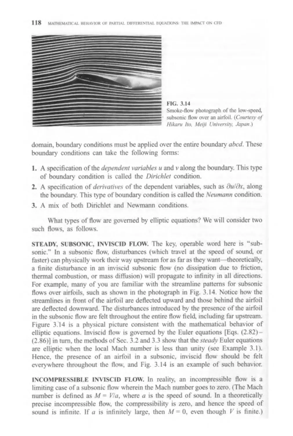
Schaum Division
McGraw-Hill, Inc.
1221 Avenue of the Americas
New York, NY 10020

COMPUTATIONAL FLUID
DYNAMICS
The Basics with
Applications
John D. Anderson, Jr.
Department of Aerospace Engineering
University of Maryland
McGraw-Hill, Inc.
New York St. Louis San Francisco Auckland Bogota Caracas
Lisbon London Madrid Mexico City Milan Montreal
New Delhi San Juan Singapore Sydney Tokyo Toronto

This book was set in Times Roman.
The editors were John I Corrigan and Eleanor Castellano;
the production supervisor was Denise L. Puryear.
The cover was designed by Rafael Hernandez.
R. R. Donnelley & Sons Company was printer and binder.
COMPUTATIONAL FLUID DYNAMICS
The Basics with Applications
Copyright © 1995 by McGraw-Hill, Inc. All rights reserved. Printed in the United States of
America. Except as permitted under the United States Copyright Act of 1976, no part of this
publication may be reproduced or distributed in any form or by any means, or stored in a data
base or retrieval system, without the prior written permission of the publisher.
This book is printed on acid-free paper.
234567890 DOC DOC 9 0 9 8 7 6 5
ISBN 0-07-001685-2
Library of Congress Cataloging-in-Publication Data
Anderson, John David.
Computational fluid dynamics: the basics with applications / John
D. Anderson, Jr.
p. cm. — (McGraw-Hill series in mechanical engineering—McGraw-Hill series in aero-
aeronautical and aerospace engineering)
Includes bibliographical references and index.
ISBN 0-07-001685-2
1. Fluid dynamics—Data processing. I. Title. II. Series.
QA911.A58 1995
532'.05'015118—dc20 94-21237

ABOUT THE AUTHOR
John D. Anderson, Jr., was born in Lancaster, Pennsylvania, on October 1, 1937.
He attended the University of Florida, graduating in 1959 with high honors and a
Bachelor of Aeronautical Engineering Degree. From 1959 to 1962, he was a
lieutenant and task scientist at the Aerospace Research Laboratory at Wright-
Patterson Air Force Base. From 1962 to 1966, he attended the Ohio State University
under the National Science Foundation and NASA Fellowships, graduating with a
Ph.D. in aeronautical and astronautical engineering. In 1966 he joined the U.S.
Naval Ordnance Laboratory as Chief of the Hypersonic Group. In 1973, he became
Chairman of the Department of Aerospace Engineering at the University of
Maryland, and since 1980 has been professor of Aerospace Engineering at
Maryland. In 1982, he was designated a Distinguished Scholar/Teacher by the
University. During 1986-1987, while on sabbatical from the university, Dr.
Anderson occupied the Charles Lindbergh chair at the National Air and Space
Museum of the Smithsonian Institution. He continues with the Museum in a part-
time appointment as special assistant for aerodynamics. In addition to his appoint-
appointment in aerospace engineering, in 1993 he was elected to the faculty of the
Committee on the History and Philosophy of Science at Maryland.
Dr. Anderson has published five books: Gasdynamic Lasers: An Introduction,
Academic Press A976), and with McGraw-Hill, Introduction to Flight, 3d edition
A989), Modern Compressible Flow, 2d Edition A990), Fundamentals of
Aerodynamics, 2d edition A991), and Hypersonic and High Temperature Gas
Dynamics A989). He is the author of over 100 papers on radiative gasdynamics, re-
reentry aerothermodynamics, gas dynamic and chemical lasers, computational fluid
dynamics, applied aerodynamics, hypersonic flow, and the history of aerodynamics.
Dr. Anderson is in Who's Who in America, and is a Fellow of the American Institute
of Aeronautics and Astronautics (AIAA). He is also a Fellow of the Washington
Academy of Sciences, and a member of Tau Beta Pi, Sigma Tau, Phi Kappa Phi, Phi
Eta Sigma, The American Society for Engineering Education (ASEE), The Society
for the History of Technology, and the History of Science Society. He has received
the Lee Atwood Award for excellence in Aerospace Engineering Education from
the AIAA and the ASEE.

To Sarah-Allen, Katherine, and Elizabeth
for all their love and understanding

CONTENTS
Preface
Part I Basic Thoughts and Equations
Philosophy of Computational Fluid Dynamics 3
1.1 Computational Fluid Dynamics: Why? 4
1.2 Computational Fluid Dynamics as a Research Tool 6
1.3 Computational Fluid Dynamics as a Design Tool 9
1.4 The Impact of Computational Fluid Dynamics—Some Other
Examples 13
1.4.1 Automobile and Engine Applications 14
1.4.2 Industrial Manufacturing Applications 17
1.4.3 Civil Engineering Applications 19
1.4.4 Environmental Engineering Applications 20
1.4.5 Naval Architecture Applications (Submarine Example) 22
1.5 Computational Fluid Dynamics: What Is It? 23
1.6 The Purpose of This Book 32
The Governing Equations of Fluid Dynamics:
Their Derivation, a Discussion of Their
PhySical Meaning, and a Presentation of Forms
Particularly Suitable to CFD 37
2.1
2.2
2.3
2.4
Introduction
Models of the Flow
2.2.1 Finite Control Volume
2.2.2 Infinitesimal Fluid Element
2.2.3 Some Comments
The Substantial Derivative (Time Rate of Change Following
a Moving Fluid Element
The Divergence of the Velocity: Its Physical Meaning
2.4.1 A Comment
38
40
41
42
42
43
47
48
XI

XU CONTENTS
2.5 The Continuity Equation 49
2.5.1 Model of the Finite Control Volume Fixed in Space 49
2.5.2 Model of the Finite Control Volume Moving with the
Fluid 51
2.5.3 Model of an Infinitesimally Small Element Fixed
in Space 53
2.5.4 Model of an Infinitesimally Small Fluid Element
Moving with the Flow 55
2.5.5 All the Equations Are One: Some Manipulations 56
2.5.6 Integral versus Differential Form of the Equations:
An Important Comment 60
2.6 The Momentum Equation 60
2.7 The Energy Equation 66
2.8 Summary of the Governing Equations for Fluid Dynamics:
With Comments 75
2.8.1 Equations for Viscous Flow (the Navier-Stokes
Equations) 75
2.8.2 Equations for Inviscid Flow (the Euler Equations) 77
2.8.3 Comments on the Governing Equations 78
2.9 Physical Boundary Conditions 80
2.10 Forms of the Governing Equations Particularly Suited for
CFD: Comments on the Conservation Form, Shock Fitting,
and Shock Capturing 82
2.11 Summary 92
Problems 93
3 Mathematical Behavior of Partial Differential
Equations: The Impact on CFD 95
3.1 Introduction 95
3.2 Classification of Quasi-Linear Partial Differential Equations 97
3.3 A General Method of Determining the Classification of
Partial Differential Equations: The Eigenvalue Method 102
3.4 General Behavior of the Different Classes of Partial
Differential Equations: Impact on Physical and
Computational Fluid Dynamics 105
3.4.1 Hyperbolic Equations 106
3.4.2 Parabolic Equations 111
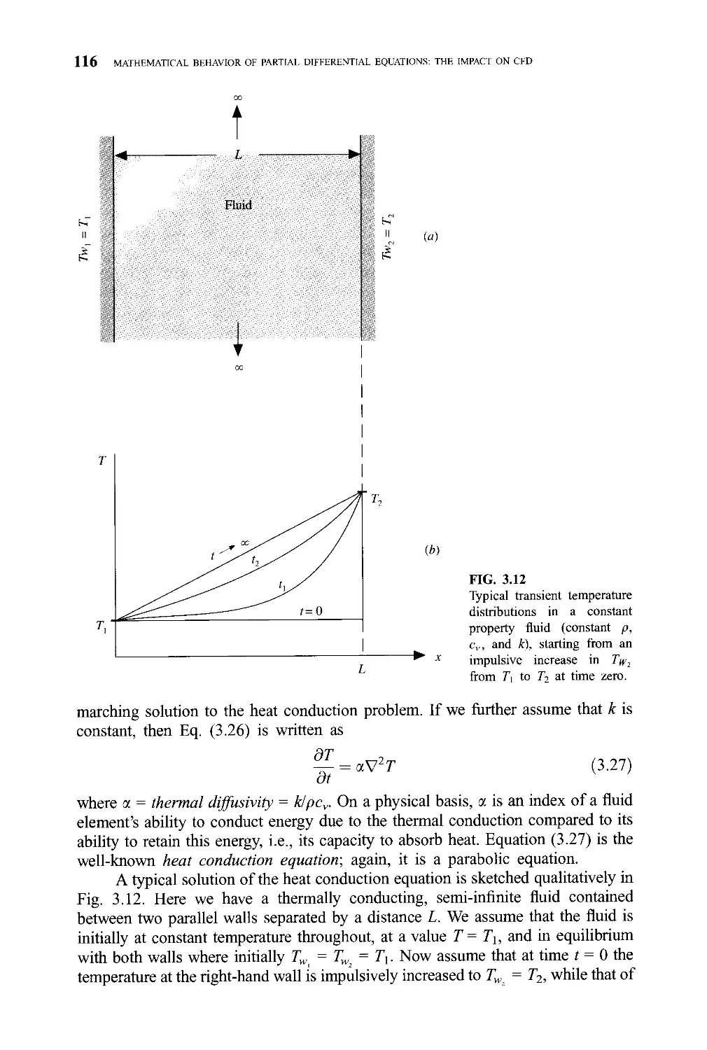
3.4.3 Elliptic Equations 117
3.4.4 Some Comments: The Supersonic Blunt Body
Problem Revisited 119
3.5 Well-Posed Problems 120
3.6 Summary 121
Problems 121
Part II Basics of the Numerics
Basic Aspects of Discretization 125
4.1 Introduction 125
4.2 Introduction to Finite Differences 128

CONTENTS Xlll
4.3 Difference Equations 142
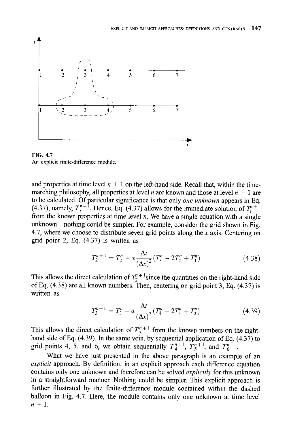
4.4 Explicit and Implicit Approaches: Definitions and Contrasts 145
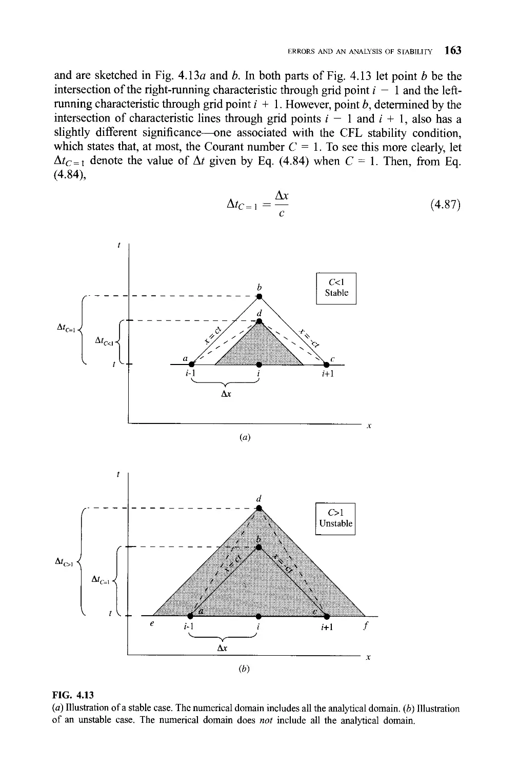
4.5 Errors and an Analysis of Stability 153
4.5.1 Stability Analysis: A Broader Perspective 165
4.6 Summary 165
GUIDEPOST 166
Problems 167
Grids with Appropriate Transformations 168
5.1 Introduction 168
5.2 General Transformation of the Equations 171
5.2 Metrics and Jacobians 178
5.4 Form of the Governing Equations Particularly Suited
for CFD Revisited: The Transformed Version 183
5.5 A Comment 186
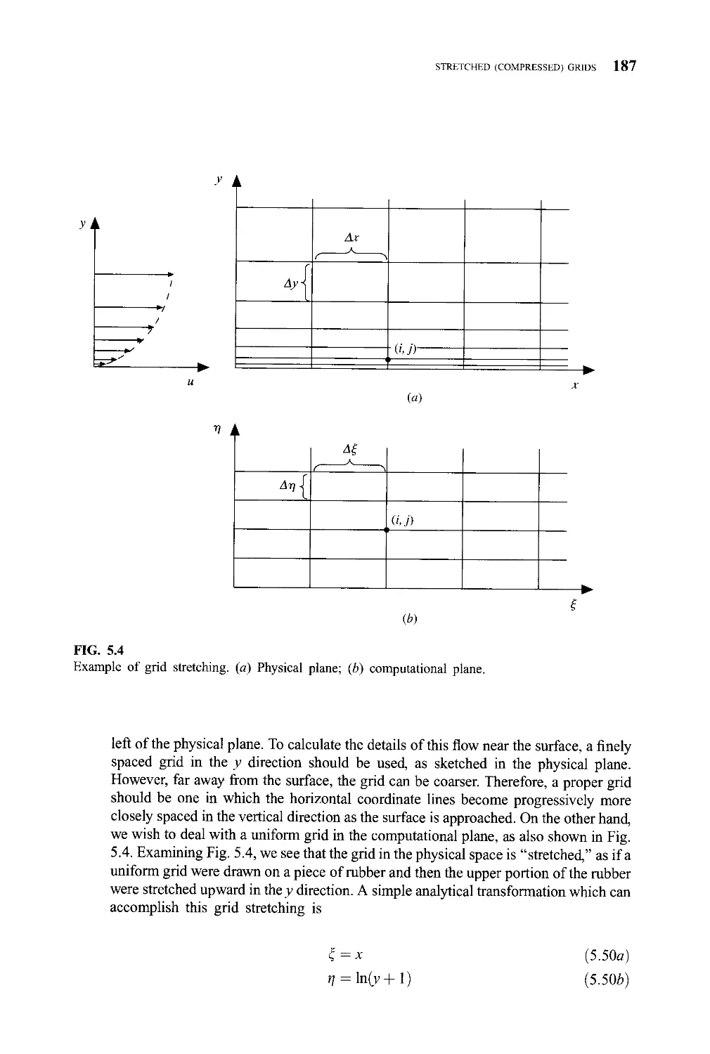
5.6 Stretched (Compressed) Grids 186
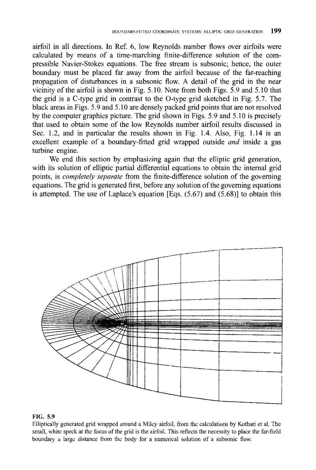
5.7 Boundary-Fitted Coordinate Systems; Elliptic Grid
Generation 192
GUIDEPOST 193
5.8 Adaptive Grids 200
5.9 Some Modern Developments in Grid Generation 208
5.10 Some Modern Developments in Finite-Volume Mesh
Generation: Unstructured Meshes and a Return to Cartesian
Meshes 210
5.11 Summary 212
Problems 215
Some Simple CFD Techniques: A Beginning 216
6.1 Introduction 216
6.2 The Lax-Wendroff Technique 217
6.3 MacCormack's Technique 222
GUIDEPOST 223
6.4 Some Comments: Viscous Flows, Conservation Form,
and Space Marching 225
6.4.1 Viscous Flows 225
6.4.2 Conservation Form 225
6.4.3 Space Marching 226
6.5 The Relaxation Technique and Its Use with Low-Speed
Inviscid Flow 229
6.6 Aspects of Numerical Dissipation and Dispersion; Artificial
Viscosity 232
6.7 The Alternating-Direction-Implicit (ADI) Technique 243
6.8 The Pressure Correction Technique: Application
to Incompressible Viscous Flow 247
6.8.1 Some Comments on the Incompressible
Navier-Stokes Equations 248

XIV CONTENTS
6.8.2 Some Comments on Central Differencing of the
Incompressible Navier-Stokes Equations; The Need
for a Staggered Grid 250
6.8.3 The Philosophy of the Pressure Correction Method 253
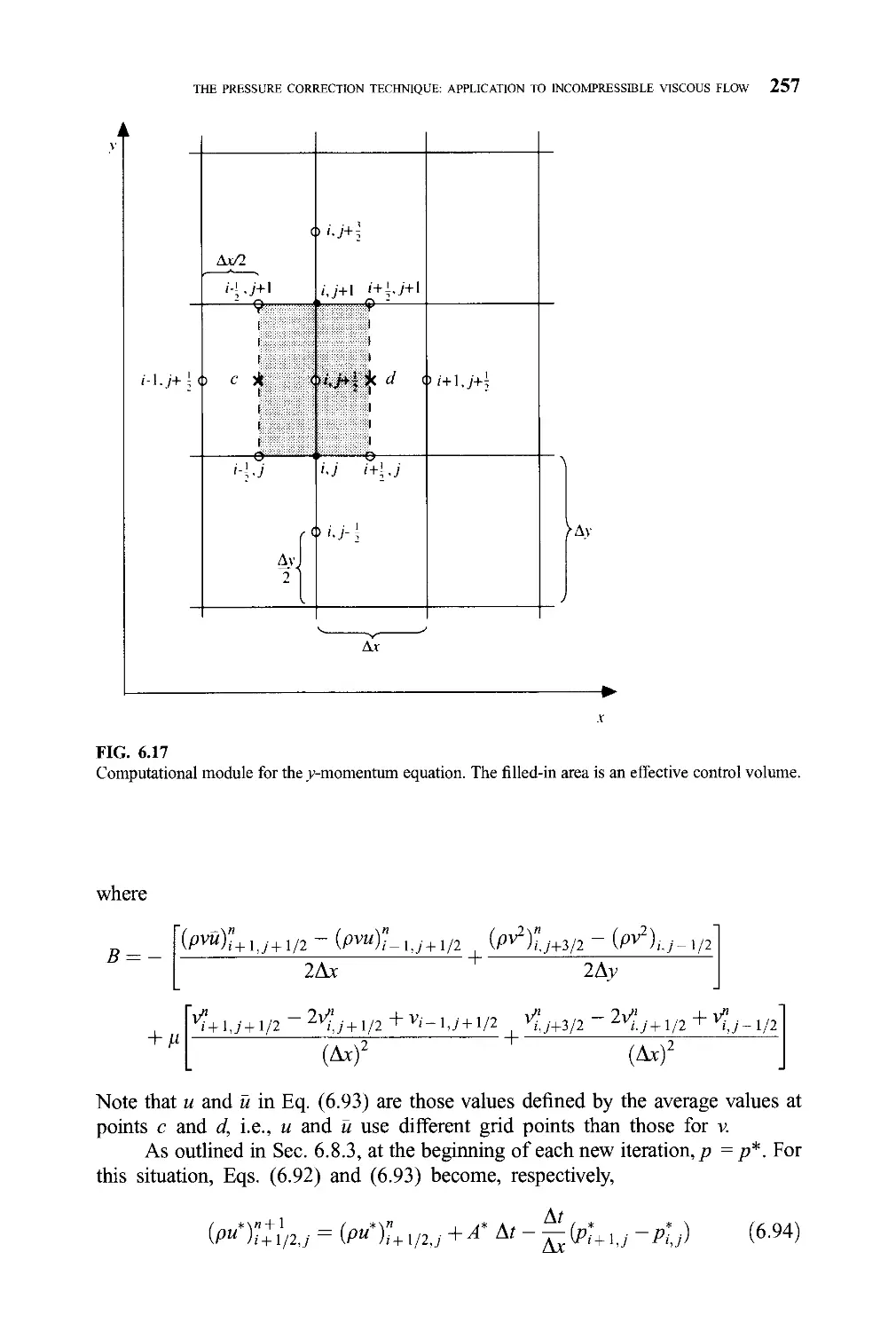
6.8.4 The Pressure Correction Formula 254
6.8.5 The Numerical Procedure: The SIMPLE Algorithm 261
6.8.6 Boundary Conditions for the Pressure Correction
Method 262
GUIDEPOST 264
6.9 Some Computer Graphic Techniques Used in CFD 264
6.9.1 xy Plots 264
6.9.2 Contour Plots 265
6.9.3 Vector and Streamline Plots 270
6.9.4 Scatter Plots 273
6.9.5 Mesh Plots 273
6.9.6 Composite Plots 274
6.9.7 Summary on Computer Graphics 274
6.10 Summary 277
Problems 278
Part III Some Applications
Numerical Solutions of Quasi-One-Dimensional
Nozzle Flows 283
7.1 Introduction: The Format for Chapters in Part III 283
7.2 Introduction to the Physical Problem: Subsonic-Supersonic
Insentropic Flow 285
7.3 CFD Solution of Subsonic-Supersonic Isentropic Nozzle
Flow: MacCormack's Technique 288
7.3.1 The Setup 288
7.3.2 Intermediate Results: The First Few Steps 308
7.3.3 Final Numerical Results: The Steady-State Solution 313
7.4 CFD Solution of Purely Subsonic Isentropic Nozzle Flow 325
7.4.1 The Setup: Boundary and Initial Conditions 327
7.4.2 Final Numerical Results: MacCormack's Technique 330
7.4.3 The Anatomy of a Failed Solution 325
7.5 The Subsonic-Supersonic Isentropic Nozzle Solution
Revisited: The Use of the Governing Equations in
Conservation Form 336
7.5.1 The Basic Equations in Conservation Form 337
7.5.2 The Setup 340
7.5.3 Intermediate Calculations: The First Time Step 345
7.5.4 Final Numerical Results: The Steady State Solution 351

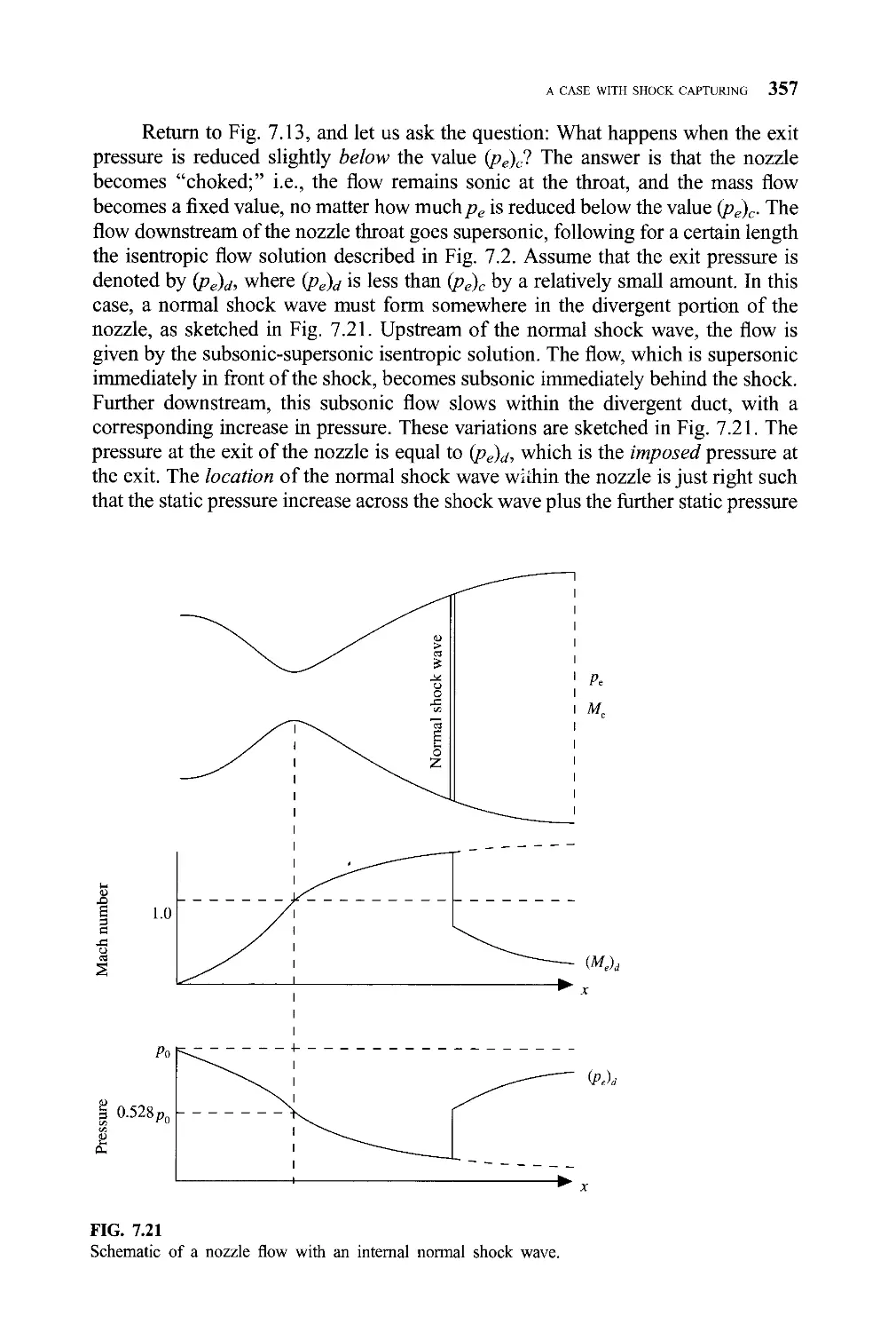
A Case with Shock Capturing
7.6.1 The Setup
7.6.2 The Intermediate Time-Marching Procedure:
The Need for Artificial Viscosity
7.6.3 Numerical Results
Summary
CONTENTS XV
356
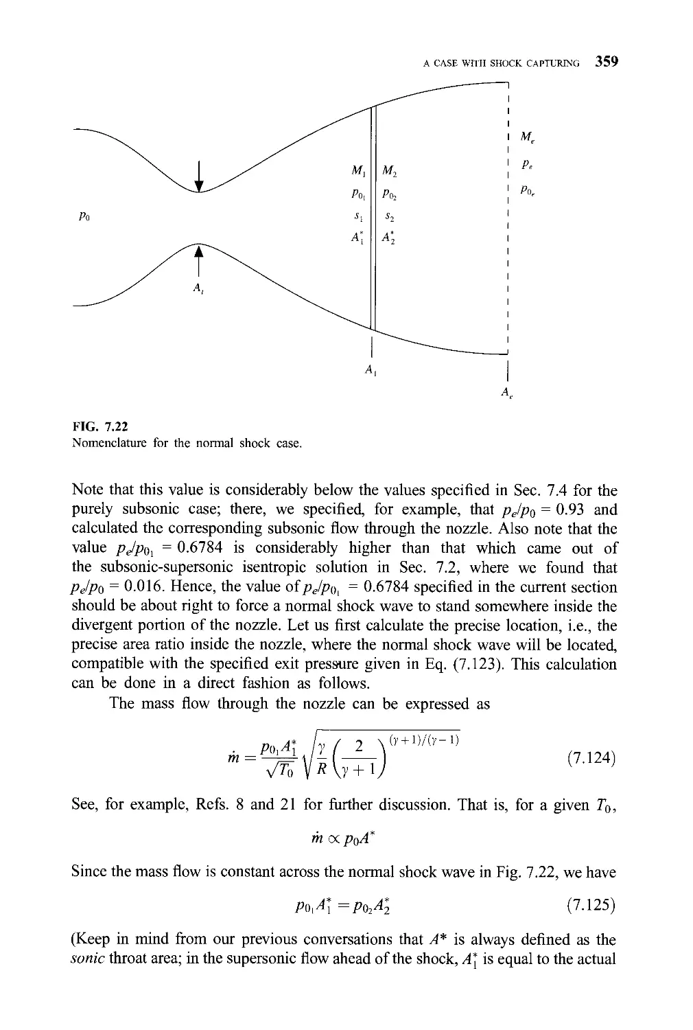
358
363
364
372
7.6
7.7
8 Numerical Solution of a Two-Dimensional
Supersonic Flow: Prandtl-Meyer Expansion
Wave 374
8.1 Introduction 374
8.2 Introduction to the Physical Problem: Prandtl-Meyer
Expansion Wave—Exact Analytical Solution 376
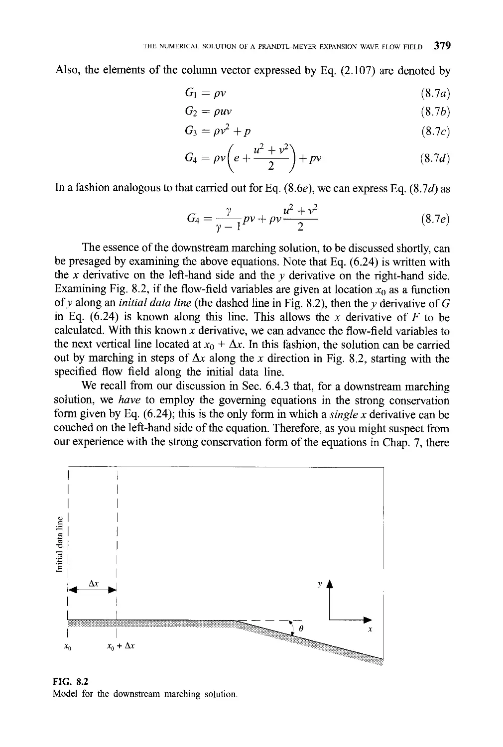
8.3 The Numerical Solution of a Prandtl-Meyer Expansion Wave
Flow Field 377
8.3.1 The Governing Equations 377
8.3.2 The Setup 386
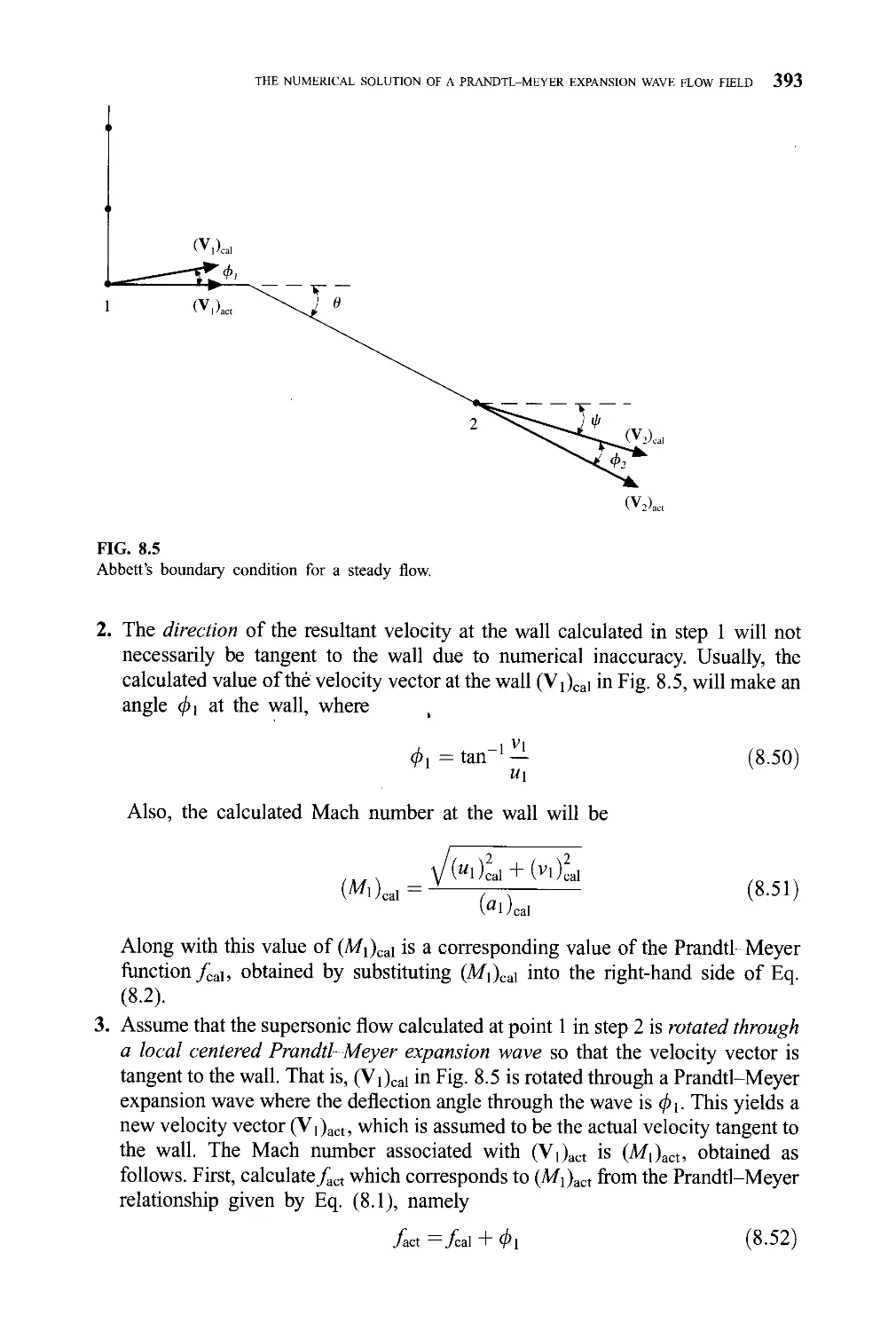
8.3.3 Intermediate Results 397
8.3.4 Final Results 407
8.4 Summary 414
9 Incompressible Couette Flow: Numerical
Solutions by Means of an Implicit Method
and the Pressure Correction Method 416
9.1 Introduction 416
9.2 The Physical Problem and Its Exact Analytical Solution 417
9.3 The Numerical Approach: Implicit Crank-Nicholson
Technique 420
9.3.1 The Numerical Formulation 421
9.3.2 The Setup 425
9.3.3 Intermediate Results 426
9.3.4 Final Results 430
9.4 Another Numerical Approach: The Pressure Correction Method 435
9.4.1 The Setup 436
9.4.2 Results 442
9.5 Summary 445
Problem 446
10 Supersonic Flow over a Flat Plate: Numerical
Solution by Solving the Complete Navier-Stokes
Equations 447
10.1 Introduction 447
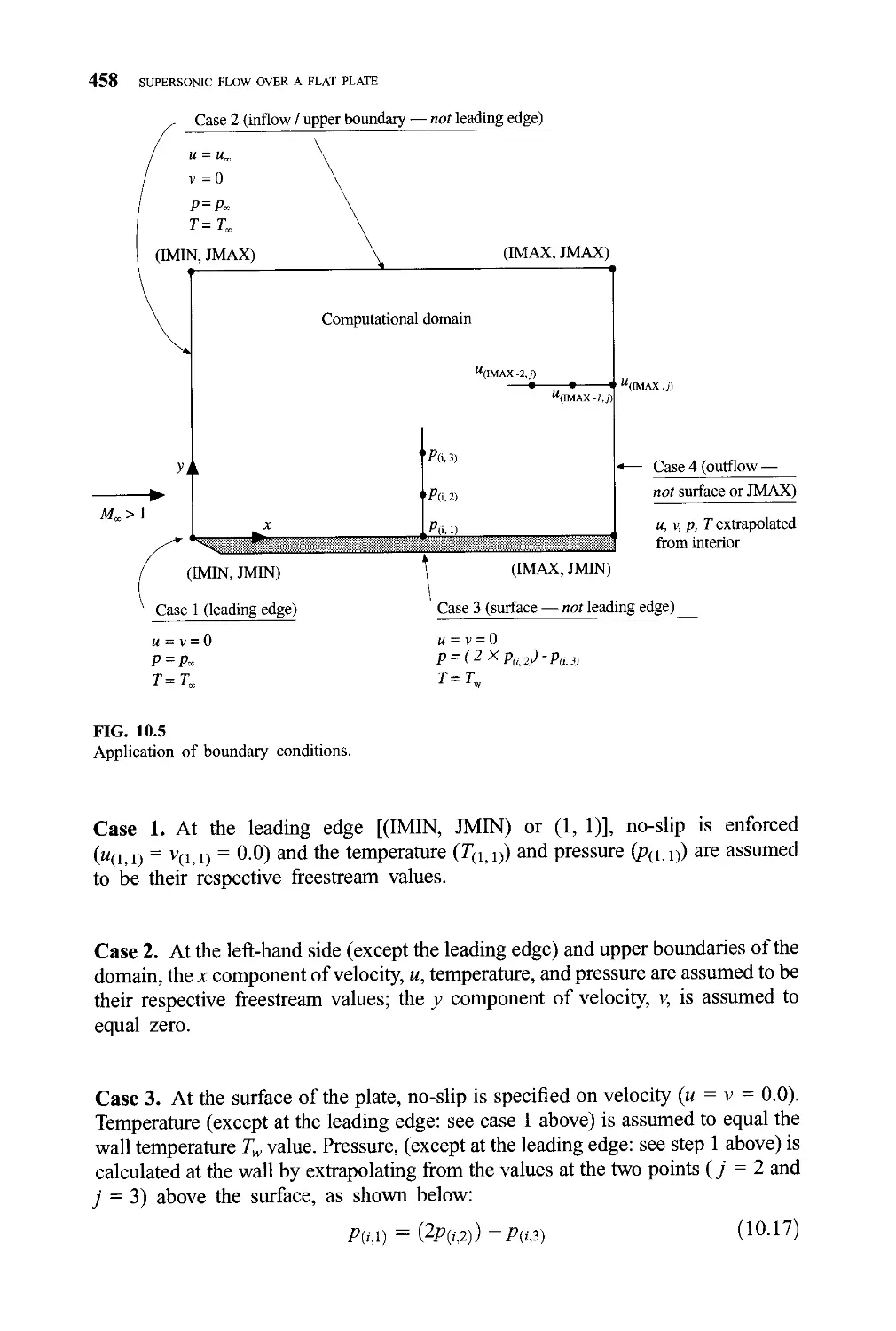
10.2 The Physical Problem 449
10.3 The Numerical Approach: Explicit Finite-Difference
Solution of the Two-Dimensional Complete Navier-Stokes
Equations 450
10.3.1 The Governing Flow Equations 450
10.3.2 The Setup 452

XVI CONTENTS
10.3.3 The Finite-Difference Equations 453
10.3.4 Calculation of Step Sizes in Space and Time 455
10.3.5 Initial and Boundary Conditions 457
10.4 Organization of Your Navier-Stokes Code 459
10.4.1 Overview 459
10.4.2 The Main Program 461
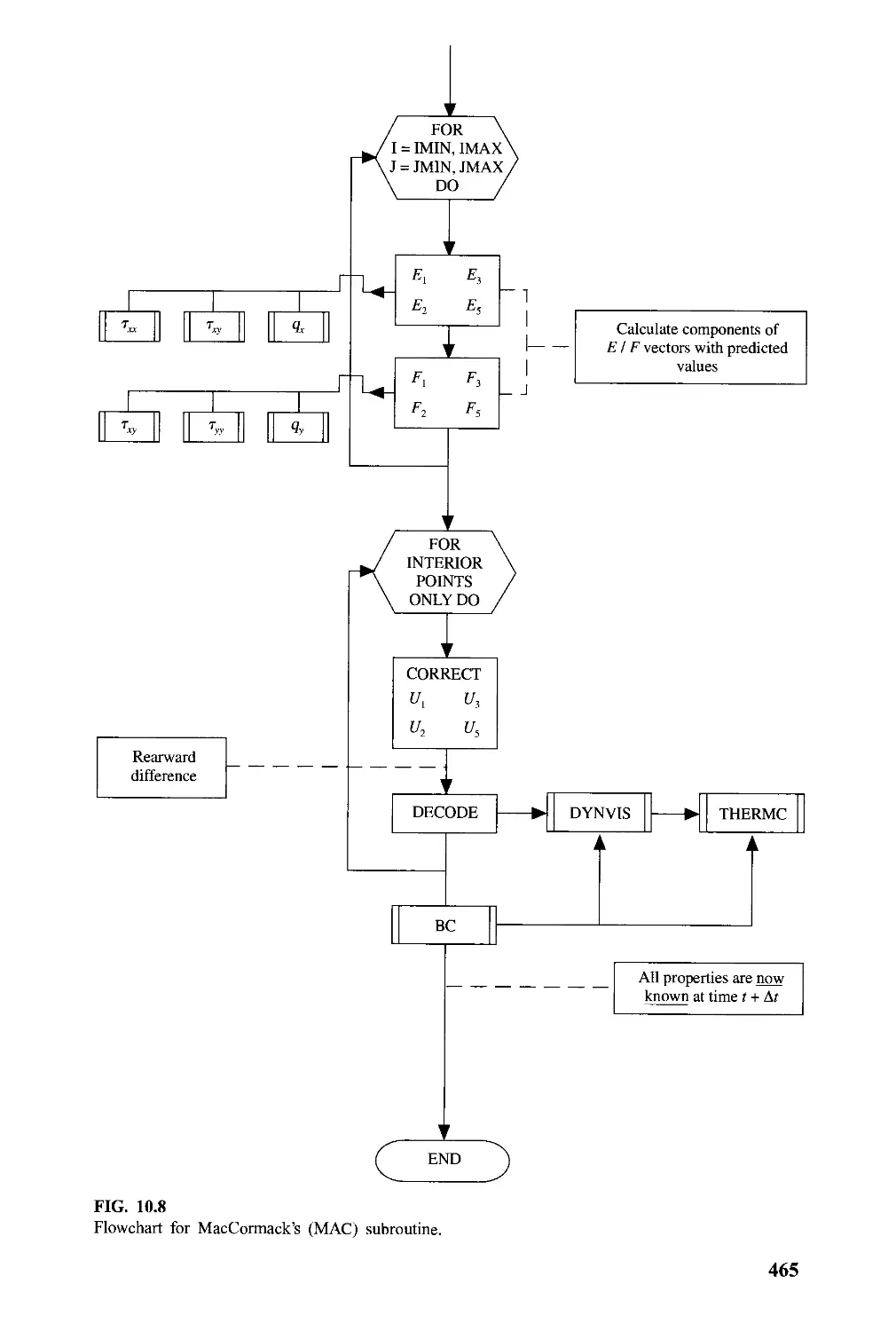
10.4.3 The MacCormack Subroutine 463
10.4.4 Final Remarks 466
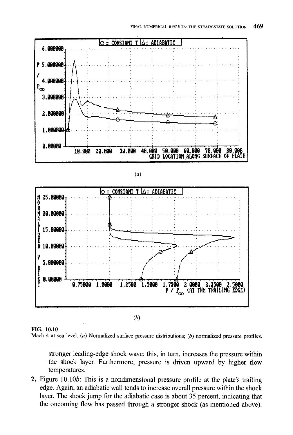
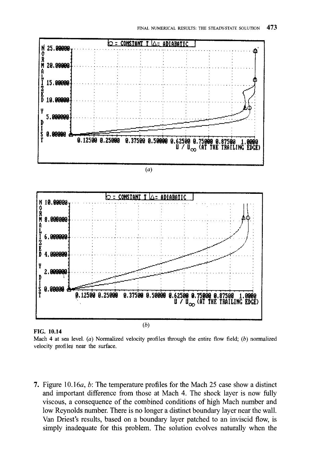
10.5 Final Numerical Results: The Steady State-Solution 466
10.6 Summary 474
Part IV Other Topics
11 Some Advanced Topics in Modern CFD:
A Discussion 479
11.1 Introduction 479
11.2 The Conservation Form of the Governing Flow Equations
Revisited: The Jacobians of the System 480
11.2.1 Specialization to One-Dimensional Flow 482
11.2.2 Interim Summary 489
11.3 Additional Considerations for Implicit Methods 489
11.3.1 Linearization of the Equations: The Beam and
Warming Method 490
11.3.2 The Multidimensional Problem: Approximate
Factorization 492
11.3.3 Block Tridiagonal Matrices 496
11.3.4 Interim Summary 497
11.4 Upwind Schemes 497
11.4.1 Flux-Vector Splitting 500
11.4.2 The Godunov Approach 502
11.4.3 General Comment 507
11.5 Second-Order Upwind Schemes 507
11.6 High-Resolution Schemes: TVD and Flux Limiters 509
11.7 Some Results 510
11.8 Multigrid Method 513
11.9 Summary 514
Problems 514
12 The Future of CFD 515
12.1 The Importance of CFD Revisited 515
12.2 Computer Graphics in CFD 516
12.3 The Future of CFD: Enhancing the Design Process 517
12.4 The Future of CFD: Enhancing Understanding 526
12.5 Conclusion 533

CONTENTS XV11
Appendix A Thomas' Algorithm for the
Solution of a Tridiagonal System of Equations 534
References 539
Index 543

PREFACE
This computational fluid dynamics (CFD) book is truly for beginners. If you have
never studied CFD before, if you have never worked in the area, and if you have no
real idea as to what the discipline is all about, then this book is for you. Absolutely
no prior knowledge of CFD is assumed on your part—only your desire to learn
something about the subject is taken for granted.
The author's single-minded purpose in writing this book is to provide a simple,
satisfying, and motivational approach toward presenting the subject to the reader
who is learning about CFD for the first time. In the workplace, CFD is today a
mathematically sophisticated discipline. In turn, in the universities it is generally
considered to be a graduate-level subject; the existing textbooks and most of the
professional development short courses are pitched at the graduate level. The
present book is a precursor to these activities. It is intended to "break the ice" for
the reader. This book is unique in that it is intended to be read and mastered before
you go on to any of the other existing textbooks in the field, before you take any
regular short courses in the discipline, and before you endeavor to read the existing
literature. The hallmarks of the present book are simplicity and motivation. It is
intended to prepare you for the more sophisticated presentations elsewhere—to give
you an overall appreciation for the basic philosophy and ideas which will then make
the more sophisticated presentations more meaningful to you later on. The
mathematical level and the prior background in fluid dynamics assumed in this
book are equivalent to those of a college senior in engineering or physical science.
Indeed, this book is targeted primarily for use as a one-semester, senior-level course
in CFD; it may also be useful in a preliminary, first-level graduate course.
There are no role models for a book on CFD at the undergraduate level; when
you ask ten different people about what form such a book should take, you get ten
different answers. This book is the author's answer, as imperfect as it may be,
formulated after many years of thought and teaching experience. Of course, to
achieve the goals stated above, the author has made some hard choices in picking
and arranging the material in this book. It is not a state-of-the-art treatment of the
modern, sophisticated CFD of today. Such a treatment would blow the uninitiated
reader completely out of the water. This author knows; he has seen it happen over
xix

XX PREFACE
and over again, where a student who wants to learn about CFD is totally turned off
by the advanced treatments and becomes unmotivated toward continuing further.
Indeed, the purpose of this book is to prepare the reader to benefit from such
advanced treatments at a later date. The present book provides a general
perspective on CFD; its purpose is to turn you, the reader, on to the subject, not to
intimidate you. Therefore, the material in this book is predominately an intuitive,
physically oriented approach to CFD. A CFD expert, when examining this book,
may at first think that some of it is "old-fashioned," because some of the material
covered here was the state of the art in 1980. But this is the point: the older, tried-
and-proven ideas form a wonderfully intuitive and meaningful learning experience
for the uninitiated reader. With the background provided by this book, the reader
can then progress to the more sophisticated aspects of CFD in graduate school and
in the workplace. However, to increase the slope of the reader's learning curve,
state-of-the-art CFD techniques are discussed in Chap. 11, and some very recent
and powerful examples of CFD calculations are reviewed in Chap. 12. In this
fashion, when you finish the last page of this book, you are already well on your
way to the next level of sophistication in the discipline.
This book is in part the product of the author's experience in teaching a one-
week short course titled "Introduction to Computational Fluid Dynamics," for the
past ten years at the von Karman Institute for Fluid Dynamics (VKI) in Belgium,
and in recent years also for Rolls-Royce in England. With this experience, this
author has discovered much of what it takes to present the elementary concepts of
CFD in a manner which is acceptable, productive, and motivational to the first-time
student. The present book directly reflects the author's experience in this regard.
The author gives special thanks to Dr. John Wendt, Director of the VKI, who first
realized the need for such an introductory treatment of CFD, and who a decade ago
galvanized the present author into preparing such a course at VKI. Over the ensuing
years, the demand for this "Introduction to Computational Fluid Dynamics" course
has been way beyond our wildest dreams. Recently, a book containing the VKI
course notes has been published; it is Computational Fluid Dynamics: An
Introduction, edited by John F. Wendt, Springer-Verlag, 1992. The present book is a
greatly expanded sequel to this VKI book, aimed at a much more extensive
presentation of CFD pertinent to a one-semester classroom course, but keeping
within the basic spirit of simplicity and motivation.
This book is organized into four major parts. Part I introduces the basic
thoughts and philosophy associated with CFD, along with an extensive discussion
of the governing equations of fluid dynamics. It is vitally important for a student of
CFD to fully understand, and feel comfortable with, the basic physical equations;
they are the lifeblood of CFD. The author feels so strongly about this need to fully
understand and appreciate the governing equations that every effort has been made
to thoroughly derive and discuss these equations in Chap. 2. In a sense, Chap. 2
stands independently as a "mini course" in the governing equations. Experience has
shown that students of CFD come from quite varied backgrounds; in turn, their
understanding of the governing equations of fluid dynamics ranges across the

PREFACE XXI
spectrum from virtually none to adequate. Students from the whole range of this
spectrum have continually thanked the author for presenting the material in Chap. 2;
those from the "virtually none" extreme are very appreciative of the opportunity to
become comfortable with these equations, and those from the "adequate" extreme
are very happy to have an integrated presentation and comprehensive review that
strips away any mystery about the myriad of different forms of the governing
equations. Chapter 2 emphasizes the philosophy that, to be a good computational
fluid dynamicist, you must first be a good fluid dynamicist.
In Part II, the fundamental aspects of numerical discretization of the governing
equations are developed; the discretization of the partial differential equations
(finite-difference approach) is covered in detail. Here is where the basic numerics
are introduced and where several popular numerical techniques for solving flow
problems are presented. The finite-volume discretization of the integral form of the
equations is covered via several homework problems.
Part III contains applications of CFD to four classic fluid dynamic problems
with well-known, exact analytical solutions, which are used as a basis for
comparison with the numerical CFD results. Clearly, the real-world applications of
CFD .are to problems that do not have known analytical solutions; indeed, CFD is
our mechanism for solving flow problems that cannot be solved in any other way.
However, in the present book, which is intended to introduce the reader to the basic
aspects of CFD, nothing is gained by choosing applications where it is difficult to
check the validity of the results; rather everything is gained by choosing simple
flows with analytical solutions so that the reader can fundamentally see the
strengths and weaknesses of a given computational technique against the
background of a known, exact analytical solution. Each application is worked in
great detail so that the reader can see the direct use of much of the CFD
fundamentals which are presented in Parts I and II. The reader is also encouraged to
write his or her own computer programs to solve these same problems, and to check
the results given in Chaps. 7 to 10. In a real sense, although the subject of this book
is computational fluid dynamics, it is also a vehicle for the reader to become more
thoroughly acquainted with fluid dynamics per se. This author has intentionally
emphasized the physical aspects of various flow problems in order to enhance the
reader's overall understanding. In some respect, this is an example of the adage that
a student really learns the material of course N when he or she takes course N + 1.
In terms of some aspects of basic fluid dynamics, the present book represents
course N + 1.
Part IV deals with some topics which are more advanced than those discussed
earlier in the book but which constitute the essence of modern state-of-the-art
algorithms and applications in CFD. It is well beyond the scope of this book to
present the details of such advanced topics—they await your attention in your
future studies. Instead, such aspects are simply discussed in Chap. 11 just to give
you a preview of coming attractions in your future studies. The purpose of Chap. 11
is just to acquaint you with some of the ideas and vocabulary of the most modern
CFD techniques being developed today. Also, Chap. 12 examines the future of

XXU PREFACE
CFD, giving some very recent examples of pioneering applications; Chap. 12
somewhat closes the loop of this book by extending some of the motivational ideas
first discussed in Chap. 1.
The matter of computer programing per se was another hard choice faced by
the author. Should detailed computer listings be included in this book as an aid to
the reader's computer programing and as a recognition of the importance of efficient
and modular programing for CFD? The decision was no, with the exception of a
computer listing for Thomas' algorithm contained in the solution for Couette flow
and listed in App. A. There are good and bad programming techniques, and it
behooves the reader to become familiar and adept with efficient programming.
However, this is not the role of the present book. Rather, you are encouraged to
tackle the applications in Part III by writing your own programs as you see fit, and
not following any prescribed listing provided by the author. This is assumed to be
part of your learning process. The author wants you to get your own hands "dirty"
with CFD by writing your own programs; it is a vital part of the learning process at
this stage of your CFD education. On the other hand, detailed computer listings for
all the applications discussed in Part III are listed in the Solutions Manual for this
book. This is done as a service to classroom instructors. In turn, the instructors are
free to release to their students any or all of these listings as deemed appropriate.
Something needs to be said about computer graphics. It was suggested by one
reviewer that some aspects of computer graphics be mentioned in the present book.
It is a good suggestion. Therefore, in Chap. 6 an entire section is devoted to
explaining and illustrating the different computer graphic techniques commonly
used in CFD. Also, examples of results presented in standard computer graphic
format are sprinkled throughout the book.
Something also needs to be said about the role of homework problems in an
introductory, senior-level CFD course, and therefore about homework problems in
the present book. This is a serious consideration, and one over which the author has
mulled for a considerable time. The actual applications of CFD—even the simplest
techniques as addressed in this book—require a substantial learning period before
the reader can actually do a reasonable calculation. Therefore, in the early chapters
of this book, there is not much opportunity for the reader to practice making
calculations via homework exercises. This is a departure from the more typical
undergraduate engineering course, where the student is usually immersed in the
"learning by doing" process through the immediate assignment of homework
problems. Insead, the reader of this book is immersed in first learning the basic
vocabulary, philosophy, ideas, and concepts of CFD before he or she finally
encounters applications—the subject of Part III. Indeed, in these applications the
reader is finally encouraged to set up calculations and to get the experience of doing
some CFD work himself or herself. Even here, these applications are more on the
scale of small computer projects rather than homework problems per se. Even the
reviewers of this book are divided as to whether or not homework problems should
be included; exactly half the reviewers said yes, but the others implied that such
problems are not necessary. This author has taken some middle ground. There are
homework problems in this book, but not very many. They are included in several

preface xxiii
chapters to help the reader think about the details of some of the concepts being
discussed in the text. Because there are no established role models for a book in
CFD at the undergraduate level for which the present book is aimed, the author
prefers to leave the generation of large numbers of appropriate homework problems
to the ingenuity of the readers and instructors—you will want to exercise your own
creativity in this regard.
This book is in keeping with the author's earlier books in that every effort has
been made to discuss the material in an easy-to-understand writing style. This book
will talk to you in a conversational style in order to expedite your understanding of
material that sometimes is not all that easy to understand.
As stated earlier, a unique aspect of this book is its intended use in
undergraduate programs in engineering and physical science. Since the seventeenth
century, science and engineering have developed along two parallel tracks: one
dealing with pure experiment and the other dealing with pure theory. Indeed, today's
undergraduate engineering and science curricula reflect this tradition; they give the
student a solid background in both experimental and theoretical techniques.
However, in the technical world of today, computational mechanics has emerged as
a new third approach, along with those of experiment and theory. Every graduate
will in some form or another be touched by computational mechanics in the future.
Therefore, in terms of fluid dynamics, it is essential that CFD be added to the
curriculum at the undergraduate level in order to round out the three-approach
world of today. This book is intended to expedite the teaching of CFD at the
undergraduate level and, it is hoped, to make it as pleasant and painless as possible
to both student and teacher.
A word about the flavor of this book. The author is an aerodynamicist, and
there is some natural tendency to discuss aeronautically related problems. However,
CFD is interdisciplinary, cutting across the fields of aerospace, mechanical, civil,
chemical, and even electrical engineering, as well as physics and chemistry. While
writing this book, the author had readers from all these areas in mind. Indeed, in the
CFD short courses taught by this author, students from all the above disciplines
have attended and enjoyed the experience. Therefore, this book contains material
related to other disciplines well beyond that of aerospace engineering. In particular,
mechanical and civil engineers will find numerous familiar applications discussed
in Chap. 1 and will find the ADI and pressure correction techniques discussed in
Chap. 6 to be of particular interest. Indeed, the application of the pressure
correction technique for the solution of a viscous incompressible flow in Chap. 9 is
aimed squarely at mechanical and civil engineers. However, no matter what the
application may be, please keep in mind that the material in this book is generic and
that readers from many fields are welcome.
What about the sequence of material presented in this book? Can the reader
hop around and cut out some material he or she may not have time to cover, say in a
given one-semester course? The answer is essentially yes. Although the author has
composed this book such that consecutive reading of all the material in sequence
will result in the broadest understanding of CFD at the introductory level, he
recognizes that many times the reader and/or instructor does not have that luxury.

Therefore, at strategic locations throughout the book, specifically highlighted
GUIDEPOSTS appear which instruct the reader where to go in the book and what
to do in order to specifically tailor the material as he or she so desires. The location
of these GUIDEPOSTS is also shown in the table of contents, for ready reference.
The author wishes to give special thanks to Col. Wayne Halgren, professor of
aeronautics at the U.S. Air Force Academy. Colonel Halgren took the time to study
the manuscript of this book, to organize it for a one-semester senior course at the
Academy, and to field-test it in the classroom during the spring of 1993. Then he
graciously donated his time to visit with the author at College Park in order to share
his experiences during this field test. Such information coming from an
independent source was invaluable, and a number of features contained in this
book came out of this interaction. The fact that Wayne was one of this author's
doctoral students several years ago served to strengthen this interaction. This author
is proud to have been blessed with such quality students.
The author also wishes to thank all his colleagues in the CFD community for
many invigorating discussions on what constitutes an elementary presentation of
CFD, and especially the following reviewers of this manuscript: Ahmed Busnaina,
Clarkson University; Chien-Pin Chen, University of Alabama-Huntsville; George
S. Dulikravich, Pennsylania State University; Ira Jacobson, University of Virginia;
Osama A. Kandil, Old Dominion University; James McDonough, University of
Kentucky; Thomas J. Mueller, University of Notre Dame; Richard Pletcher, Iowa
State University; Paavo Repri, Florida Institute of Technology; P. L. Roe, University
of Michigan-Ann Arbor; Christopher Rutland, University of Wisconsin; Joe F.
Thompson, Mississippi State University; and Susan Ying, Florida State University.
This book is, in part, a product of those discussions. Also, special thanks go to
Ms. Susan Cunningham, who was the author's personal word processor for the
detailed preparation of this manuscript. Sue loves to type equations—she should
have had a lot of fun with this book. Of course, special appreciation goes to two
important institutions in the author's life—the University of Maryland for providing
the necessary intellectual atmosphere for producing such a book, and my wife,
Sarah-Allen, for providing the necessary atmosphere of understanding and support
during the untold amount of hours at home required for writing this book. To all of
you, I say a most heartfelt thank you.
So, let's get on with it! I wish you a productive trail of happy reading and happy
computing. Have fun (and I really mean that).
John D. Anderson, Jr.

COMPUTATIONAL FLUID DYNAMICS
The Basics with Applications

PART
I
BASIC
THOUGHTS
AND
EQUATIONS
In Part I, we introduce some of the basic philosophy and ideas of computational
fluid dynamics to serve as a springboard for the rest of the book. We also derive
and discuss the basic governing equations of fluid dynamics under the premise that
these equations are the physical foundation stones upon which all computational
fluid dynamics is based. Before we can understand and apply any aspect of
computational fluid dynamics, we must fully appreciate the governing equations—
the mathematical form and what physics they are describing. All this is the essence
of Part I.

CHAPTER
l
PHILOSOPHY
OF
COMPUTATIONAL
FLUID
DYNAMICS
All the mathematical sciences are founded on
relations between physical laws and laws of
numbers, so that the aim of exact science is to
reduce the problems of nature to the determination
of quantities by operations with numbers.
James Clerk Maxwell, 1856
In the late 1970s, this approach (the use of
supercomputers to solve aerodynamic problems)
began to pay off. One early success was the
experimental NASA aircraft called HiMAT (Highly
Maneuverable Aircraft Technology), designed to
test concepts of high maneuverability for the
next generation of fighter planes. Wind tunnel
tests of a preliminary design for HiMAT
showed that it would have unacceptable drag
at speeds near the speed of sound; if built that
way the plane would be unable to provide any
useful data. The cost of redesigning it in further
wind tunnel tests would have been around
$150,000 and would have unacceptably delayed
the project. Instead, the wing was redesigned by a
computer at a cost of $6,000.
Paul E. Ceruzzi, Curator, National Air and Space
Museum, in Beyond the Limits, The MIT Press, 1989

4 PHILOSOPHY OF COMPUTATIONAL FLUID DYNAMICS
1.1 COMPUTATIONAL FLUID DYNAMICS:
WHY?
The time: early in the twenty-first century. The place: a major airport anywhere in
the world. The event: a sleek and beautiful aircraft roles down the runway, takes off,
and rapidly climbs out of sight. Within minutes, this same aircraft has accelerated to
hypersonic speed; still within the atmosphere, its powerful supersonic combustion
ramjet engines* continue to propel the aircraft to a velocity near 26,000 ft/s—
orbital velocity—and the vehicle simply coasts into low earth orbit. Is this the stuff
of dreams? Not really; indeed, this is the concept of a transatmospheric vehicle,
which has been the subject of study in several countries during the 1980s and 1990s.
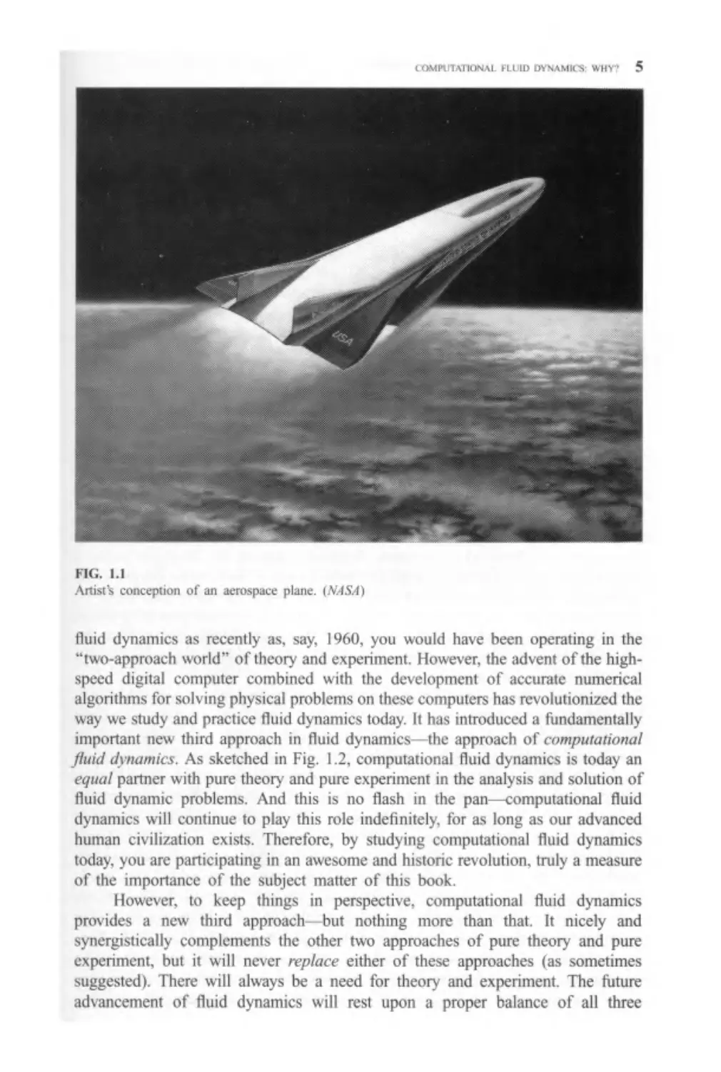
In particular, one design for such a vehicle is shown in Fig. 1.1, which is an artist's
concept for the National Aerospace Plane (NASP), the subject of an intensive study
project in the United States since the mid-1980s. Anyone steeped in the history of
aeronautics, where the major thrust has always been to fly faster and higher, knows
that such vehicles will someday be a reality. But they will be made a reality only
when computational fluid dynamics has developed to the point where the complete
three-dimensional flowfield over the vehicle and through the engines can be
computed expeditiously with accuracy and reliability. Unfortunately, ground test
facilities—wind tunnels—do not exist in all the flight regimes covered by such
hypersonic flight. We have no wind tunnels that can simultaneously simulate the
higher Mach numbers and high flowfield temperatures to be encountered by
transatmospheric vehicles, and the prospects for such wind tunnels in the
twenty-first century are not encouraging. Hence, the major player in the design
of such vehicles is computational fluid dynamics. It is for this reason, as well as
many others, why computational fluid dynamics—the subject of this book—is so
important in the modern practice of fluid dynamics.f
Computational fluid dynamics constitutes a new "third approach" in the
philosophical study and development of the whole discipline of fluid dynamics. In
the seventeenth century, the foundations for experimental fluid dynamics were laid
in France and England. The eighteenth and nineteenth centuries saw the gradual
development of theoretical fluid dynamics, again primarily in Europe. (See Refs. 3 -
5 for presentations of the historical evolution of fluid dynamics and aerodynamics.)
As a result, throughout most of the twentieth century the study and practice of fluid
dynamics (indeed, all of physical science and engineering) involved the use of pure
theory on the one hand and pure experiment on the other hand. If you were learning
* A supersonic combustion ramjet engine, SCRAMJET for short, is an air-breathing ramjet engine
where the flow through the engine remains above Mach 1 in all sections of the engine, including the
combustor. Fuel is injected into the supersonic airstream in the combustor, and combustion takes place
in the supersonic flow. This is in contrast to a conventional ramjet or gas turbine engine, where the flow
in the combustor is at a low subsonic Mach number.
f For a basic introduction to the principles of hypersonic flight, see chap. 10 of Ref. 1. For an in-depth
presentation of these principles, see Ref. 2.

H(. I.I
\ 1.1 I I
llvml dynamics .is recentK .is. viv ll'('(l. \ou <Aoukl base ''vci operating in the
"two approach work!" ol thcorv anil experiment However, the advcn" ot the high-
highspeed diL'ital computer combined wr.h the de\ clopment ol' accurate nunicneal
aleoiitlinis till sol1, hil' ph\ siea! prolilems on tl'.ese ^ivipniers has re\ niuiioni/ed I he
\mi\ uc stud\ aiul :iraet;ee tiiml tl\iiai;nes to<la\ :' las mlroduecd a liimlamenially
impot'tatit hcu thud approaeh m Iliiid dvnannes ihe iipproaeh ol ciimputuiumii!
flunt i/Vuiimiiv As sketehed ill lie. 1.2. coiiipi:tat:o!ial lluid dsiianucs is todas an
a/Hal partner with pure theop. and pure experiment 1:1 the anaKsis and solution ot~
tluid dynamie problems \nd this is no Hash ir. the pan eomputational fluid
dynamics will continue to play this roie indetimteK. tor Lis loiiy as our advanced
human ciuhAition exists. Therefore. b\ studs hij computational fluid d\narnics
toda\. \ou are participating in an awesome atn.l histirrc resolution. IruK a measure
of the importance ol the siih|cct matter ot this hook
Ho\u'\er, lo keep i'linns in perspecme. cn;nputattonal tkud d\namics
prmides a r.ew 'nird approach hut nothing more than that. I' tncel> and
synerL'isiiea!l\ complements the other ',\\\> approaches o; pure theory and pure
experiment, hui n will ne\er w:<i<i{'t: either oi'these approaches (as sometimes
suggested\ 1 here will always he a need for theory and experiment. The future
advancement ot fluid dynamics will resl upot- a proper balance of all three

PHILOSOPHY OF COMPUTATIONAL FLUID DYNAMICS
FIG. 1.2
The "three dimensions" of fluid dynamics.
approaches, with computational fluid dynamics helping to interpret and understand
the results of theory and experiment, and vice versa.
Finally, we note that computational fluid dynamics is commonplace enough
today that the acronym CFD is universally accepted for the phrase "computational
fluid dynamics." We will use this acronym throughout the remainder of this book.
1.2 COMPUTATIONAL FLUID DYNAMICS
AS A RESEARCH TOOL
Computational fluid dynamic results are directly analogous to wind tunnel results
obtained in a laboratory—they both represent sets of data for given flow con-
configurations at different Mach numbers, Reynolds numbers, etc. However, unlike a
wind tunnel, which is generally a heavy, unwieldy device, a computer program (say
in the form of floppy disks) is something you can carry around in your hand. Or
better yet, a source program in the memory of a given computer can be accessed
remotely by people on terminals that can be thousands of miles away from the
computer itself. A computer program is, therefore, a readily transportable tool, a
"transportable wind tunnel."
Carrying this analogy further, a computer program is a tool with which you
can carry out numerical experiments. For example, assume that you have a program
which calculates the viscous, subsonic, compressible flow over an airfoil, such as
that shown in Fig. 1.3. Such a computer program was developed by Kothari and
Anderson (Ref. 6); this program solves the complete two-dimensional Navier-
Stokes equations for viscous flow by means of a finite-difference numerical
technique. The Navier-Stokes equations, as well as other governing equations
for the physical aspects of fluid flow, are developed in Chap. 2. The computational
techniques employed in the solution by Kothari and Anderson in Ref. 6 are standard
approaches—all of which are covered in subsequent chapters of this book.
Therefore, by the time you finish this book, you will have all the knowledge
necessary to construct, among many other examples, solutions of the Navier-Stokes
equations for compressible flows over airfoils, just as described in Ref. 6. Now,
assuming that you have such a program, you can carry out some interesting
experiments with it—experiments which in every sense of the word are analogous to
those you could carry out (in principle) in a wind tunnel, except the experiments you

COMPUTATIONAL FLUID DYNAMICS AS A RESEARCH TOOL
(a) Laminar flow
(b) Turbulent flow
FIG. 1.3
Example of a CFD numerical experiment, (a) Instantaneous streamlines over a Wortmann airfoil
(FX63-137) for laminar flow. Re = 100,000; M^ = 0.5; zero angle of attack. The laminar flow is
unsteady; this picture corresponds to only one instant in time, (b) Streamlines over the same airfoil for
the same conditions except that the flow is turbulent.
perform with the computer program are numerical experiments. To provide a more
concrete understanding of this philosophy, let us examine one of these numerical
experiments, gleaned from the work of Ref. 6.
This is an example of a numerical experiment that can elucidate physical
aspects of a flow field in a manner not achievable in a real laboratory experiment.
For example, consider the subsonic compressible flow over the Wortmann airfoil
shown in Fig. 1.3. Question: What are the differences between laminar and turbulent
flow over this airfoil for Re = 100,000? For the computer program, this is a
straightforward question—it is just a matter of making one run with the turbulence
model switched off (laminar flow), another run with the turbulence model switched
on (turbulent flow), and then comparing the two sets of results. In this fashion you
can dabble with Mother Nature simply by turning a switch in the computer
program—something you cannot do quite as readily (if at all) in the wind tunnel.
For example, in Fig. 1.3a the flow is completely laminar. Note that the calculated
flow is separated over both the top and bottom surfaces of the airfoil, even though
the angle of attack is zero. Such separated flow is characteristic of the low Reynolds
number regime considered here (Re = 100,000), as discussed in Refs. 6 and 7.
Moreover, the CFD calculations show that this laminar, separated flow is unsteady.
The numerical technique used to calculate these flows is a time-marching method,
using a time-accurate finite-difference solution of the unsteady Navier-Stokes
equations. (The philosophy and numerical details associated with time-marching
solutions will be discussed in subsequent chapters.) The streamlines shown in Fig.

8 PHILOSOPHY OF COMPUTATIONAL FLUID DYNAMICS
1.3a are simply a "snapshot" of this unsteady flow at a given instant in time. In
contrast, Fig. 13b illustrates the calculated streamlines when a turbulence model is
"turned on" within the computer program. Note that the calculated turbulent flow is
attached flow; moreover, the resulting flow is steady. Comparing Fig. 13a and b, we
see that the laminar and turbulent flows are quite different; moreover, this CFD
numerical experiment allows us to study in detail the physical differences between
the laminar and turbulent flows, all other parameters being equal, in a fashion
impossible to obtain in an actual laboratory experiment.
Numerical experiments, carried out in parallel with physical experiments in
the laboratory, can sometimes be used to help interpret such physical experiments,
and even to ascertain a basic phenomenological aspect of the experiments which is
not apparent from the laboratory data. The laminar/turbulent comparison reflected
in part in Fig. 1.3a and b is such a case. This comparison has even more
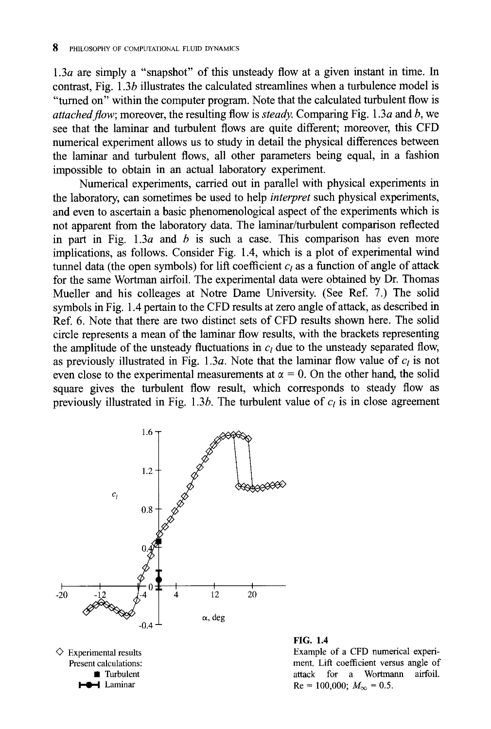
implications, as follows. Consider Fig. 1.4, which is a plot of experimental wind
tunnel data (the open symbols) for lift coefficient c/ as a function of angle of attack
for the same Wortman airfoil. The experimental data were obtained by Dr. Thomas
Mueller and his colleages at Notre Dame University. (See Ref. 7.) The solid
symbols in Fig. 1.4 pertain to the CFD results at zero angle of attack, as described in
Ref. 6. Note that there are two distinct sets of CFD results shown here. The solid
circle represents a mean of the laminar flow results, with the brackets representing
the amplitude of the unsteady fluctuations in ct due to the unsteady separated flow,
as previously illustrated in Fig. 1.3a. Note that the laminar flow value of q is not
even close to the experimental measurements at a = 0. On the other hand, the solid
square gives the turbulent flow result, which corresponds to steady flow as
previously illustrated in Fig. 13b. The turbulent value of q is in close agreement
1.6 T
-0.4^
O Experimental results
Present calculations:
¦ Turbulent
Laminar
FIG. 1.4
Example of a CFD numerical experi-
experiment. Lift coefficient versus angle of
attack for a Wortmann airfoil.
Re = 100,000; Mx = 0.5.

COMPUTATIONAL FLUID DYNAMICS AS A DESIGN TOOL 9
0.5 T
O Experimental results
Present calculations:
¦ Turbulent
Laminar
FIG. 1.5
Example of a CFD numerical
experiment. Drag coefficient ver-
versus angle of attack for a Wort-
mann airfoil. Re = 100,000;
M^ = 0.5.
with the experimental data. This comparison is reinforced by the results shown in
Fig. 1.5, which is a plot of the airfoil drag coefficient versus angle of attack. The
open symbols are Mueller's experimental data, and the solid symbols at a = 0 are
the CFD results. The fluctuating laminar values of the computed cd are given by the
solid circle and the amplitude bars; the agreement with experiment is poor. On the
other hand, the solid square represents the steady turbulent result; the agreement
with experiment is excellent for this case. The importance of this result goes beyond
just a simple comparison between experiment and computation. During the course
of the wind tunnel experiments, there was some uncertainty, based on the
experimental observations themselves, as to whether or not the flow was laminar
or turbulent. However, examing the comparisons with the CFD data shown in Figs.
1.4 and 1.5, we have to conclude that the flow over the airfoil in the wind tunnel was
indeed turbulent, because the turbulent CFD results agreed with experiment
whereas the laminar CFD results were far off. Here is a beautiful example of
how CFD can work harmoniously with experiment—not just providing a quanti-
quantitative comparison, but also in this case providing a means to interpret a basic
phenomenological aspect of the experimental conditions. Here is a graphic example
of the value of numerical experiments carried out within the framework of CFD.
1.3 COMPUTATIONAL FLUID DYNAMICS
AS A DESIGN TOOL
In 1950, there was no CFD in the way that we think of it today. In 1970, there was
CFD, but the type of computers and algorithms that existed at that time limited all
practical solutions essentially to two-dimensional flows. The real world of fluid

10 PHILOSOPHY OF COMPUTATIONAL FLUID DYNAMICS
dynamic machines—compressors, turbines, flow ducts, airplanes, etc.—is mainly a
?/iree-dimensional world. In 1970, the storage and speed capacity of digital
computers were not sufficient to allow CFD to operate in any practical fashion
in this three-dimensional world. By 1990, however, this story had changed
substantially. In today's CFD, three-dimensional flow field solutions are abundant;
they may not be routine in the sense that a great deal of human and computer
resources are still frequently needed to successfully carry out such three-dimen-
three-dimensional solutions for applications like the flow over a complete airplane config-
configuration, but such solutions are becoming more and more prevalent within industry
and government facilities. Indeed, some computer programs for the calculation of
three-dimensional flows have become industry standards, resulting in their use as a
tool in the design process. In this section, we will examine one such example, just to
emphasize the point.
Modern high-speed aircraft, such as the Northrop F-20 shown in Fig. 1.6, with
their complicated transonic aerodynamic flow patterns, are fertile ground for the use
of CFD as a design tool. Figure 1.6 illustrates the detailed pressure coefficient
variation over the surface of the F-20 at a nearly sonic freestream Mach number M^
of 0.95 and an angle of attack a of 8°. These are CFD results obtained by Bush,
Jager, and Bergman (Ref. 9), using a finite-volume explicit numerical scheme
developed by Jameson et al. (Ref. 10). In Fig. 1.6a, the contours of pressure
coefficient are shown over the planform of the F-20; a contour line represents a
locus of constant pressure, and hence regions where the contour lines cluster
together are regions of large pressure gradients. In particular, the heavily clustered
band that appears at the wing trailing edge and wraps around the fuselage just
downstream of the trailing edge connotes a transonic shock wave at that location.
Other regions involving local shock waves and expansions are clearly shown in Fig.
1.6. In addition, the local chordwise variations of the pressure coefficient over the
top and bottom of the wing section are shown for five different spanwise stations in
Fig. 1.6b to/ Here, the CFD calculations, which involve the solution of the Euler
equations (see Chap. 2), are given by the solid curves and are compared with
experimental data denoted by the solid squares and circles. Note that there is
reasonable agreement between the calculations and experiment. However, the major
point made by the results in Fig. 1.6 relative to our discussion is this: CFD provides
a means to calculate the detailed flow field around a complete airplane config-
configuration, including the pressure distribution over the three-dimensional surface. This
knowledge of the pressure distribution is necessary for structural engineers, who
need to know the detailed distribution of aerodynamic loads over the aircraft in
order to properly design the structure of the airftame. This knowledge is also
necessary for aerodynamicists, who obtain the lift and pressure drag by integrating
the pressure distribution over the surface (see Ref. 8 for details of such an
integration). Moreover, the CFD results provide information about the vortices
which are formed at the juncture of the fuselage strakes and the wing leading edge,
such as shown in Fig. 1.7, also obtained from Ref. 9. Here, the values of M^ and a
are 0.26 and 25°, respectively. Knowing where these vortices go and how they
interact with other parts of the airplane is essential to the overall aerodynamic
design of the airplane.

II
IK,, l.b
An L'xamplc '.i! L'n' ^.-ilLLi..ri,'ii '1 :h
NoitliH'p i -Z" Hl::J.c:. Il.m*. i ¦•titi hii -
.lie -iliu'.WL ¦:,1'n I < I l\u >r: n: 11L ¦- ;j:
l.sll!lJ ar. ', lllrlh >f'i'.l!'A l>f !i-L1-J.H!r
^. i-^j : 1 ¦_¦ i--j t i:
,. "l- ¦ ¦ i Mi 'i.r ii i •
-.iin.i.. i.' ¦: :hv .rr
i! 11 ¦ 11 ".¦ I j\\-]\ L L-t( :. i i" c
III short. ( H ) Is pi,l\ 'II:.! .1 v''M[l:! i"i • 1 l. ;ls
rcscaix'l; tovii ..is Ji's^n'ik'd mi V\ I 1. ' II* :ii.
wa\ tkiki Jynan'iklp.sts ;iru: L\>j{>, n.l v r
purposes nl this hook i^ U> .ntroduce v
power
V ,. |1, ''.¦, L'l ' ,ll I'lll .ICIILC Oil till'
II .M-s-. '! M v.n.lVvJ <lij I'T tllJ
d duv eh i|nr_' .itul tisiii'j 11m^

).O 0.1 0.2 0.3 0.4 0.5 0.6 0.7 0.8 0.9 1.0
X/C
(b) -n = 0.406
0.1 0.2 0.3 0.4 0.5 0.6 0.7 0.8 0.9 1.0
X/C
(c) ii = 0.531
1 0.2 0.3 0.4 0.5 0.6 0.7 0.8 0.9 1.0
0.1 0.2 0.3 0.4 0.5 0.6 0.7 0.8 0.9 1.0
X/C
(d)i\ = 0.656
(e) f\ = 0.769
¦ Test, upper surface
• Test, lower surface
— Euler
0.2 0.3 0.4 0.5 0.6 0.7 0.8 0.9 1.0
X/C
(/) -n = 0.891
12

IK.. \.t
I:J I [np ',
ile \ !t"A
1.4 THE I MPAC I Ol COMPL TATIONAL FLUID
DYNAMICS SOME OTHER EXAMPLES
Iiistonejlk. lliL' carls dLr\clopmc;it ol ( I \) in the >'hils aiul I'^Os \\as dn\cn h\
the needs ol the aerospace ciunmuni'v Indeed, the examples ol ( II) applications
described in Sec 11 u> I ¦> are trnrn llus coniinurn'1. However, modern CM) cuts
across ail' disciplines where the flow o! a tluid is important. The purpose of this
section is to hiyhliLiht some of these other, nmhu • ¦ '^/v/< c. applications oft ITJ.

14 PHILOSOPHY OF COMPUTATIONAL FLUID DYNAMICS
1.4.1 Automobile and Engine Applications
To improve the performance of modern cars and trucks (environmental quality, fuel
economy, etc.), the automobile industry has accelerated its use of high-technology
research and design tools. One of these tools is CFD. Whether it is the study of the
external flow over the body of a vehicle, or the internal flow through the engine,
CFD is helping automotive engineers to better understand the physical flow
processes, and in turn to design improved vehicles. Let us examine several such
examples.
The calculation of the external airflow over a car is exemplified by the paths of
air particles shown in Fig. 1.8. The outline of the left half of the car is shown by the
mesh distributed over its surface, and the white streaks are the calculated paths of
various air particles moving over the car from left to right. These particle paths were
calculated by means of a finite-volume CFD algorithm. The calculations were made
over a discrete three-dimensional mesh distributed in the space around the car; that
portion of the mesh on the center plane of symmetry of the car is illustrated in Fig.
1.9. Note that one of the coordinate lines of the mesh is fitted to the body surface, a
so-called boundary-fitted coordinate system. (Such coordinate systems are dis-
discussed in Sec. 5.7.) Figures 1.8 and 1.9 are taken from a study by C. T. Shaw of
Jaguar Cars Limited (Ref. 58). Another example of the calculation of the external
flow over a car is the workofMatsunagaetal. (Ref. 59). Figure 1.10 shows contours
of vorticity in the flow field over a car, obtained from the finite-difference
calculations described in Ref. 59.* (Aspects of finite-difference methods are
discussed throughout this book, beginning with Chap. 4.) Here, the calculations
are made on a three-dimensional rectangular grid, a portion of which is shown in
Fig. 1.11. The fundamentals of grid generation—an important aspect of CFD—are
discussed in Chap. 5, and special mention of cartesian, or rectangular, grids
wrapped around complex three-dimensional bodies is made in Sec. 5.10.
The calculation of the internal flow inside an internal combustion engine such
as that used in automobiles is exemplified by the work of Griffin et al. (Ref. 60).
Here, the unsteady flow field inside the cylinder of a four-stroke Otto-cycle engine
was calculated by means of a time-marching finite-difference method. (Time-
marching methods are discussed in various chapters of this book.) The finite-
difference grid for the cylinder is shown in Fig. 1.12. The piston crosshatched at the
bottom of Fig. 1.12 moves up and down inside the cylinder during the intake,
compression, power, and exhaust strokes; the intake valves open and close
appropriately; and an unsteady, recirculating flow field is established inside the
cylinder. A calculated velocity pattern in the valve plane when the piston is near the
bottom of its stroke (bottom dead center) during the intake stroke is shown in Fig.
1.13. These early calculations were the first application of CFD to the study of flow
* Recall that vorticity is defined in fluid dynamics as the vector quantity V x V, which is equal to twice
the instantaneous angular velocity of a fluid element. Contours of the x component of vorticity (in the
flow direction) are shown in Fig. 1.10.

15
IK,, 1.9
-¦'. ¦' I VlL'.I '. L1VJ J [r<I lll'J i. !l,
IK. Kill
< oit:pit.-d . i:rit,n|!'. . it tiiL '. tr'lrprli,:nl .it \ /ill.. ",
l'.'t- ''I i-i^lil R^N.ih-, ,.tj vinur t ,i u-Tk.il fl.j:c i
I ¦','. !'- .]!' <\ 1I1L1 tri T
. >i* li".mi :hi.1 ¦. .lhi.:

16
M(. Ill
\ p..i"ii.iTi til .1 r:.vl.in.ru.j: L.'.rlf-i ¦
imi.1 '/.ripped aio.jrui .> cj:. lima! *.irih'.'
,„; '!,,:¦¦!,if, ti;,m \ IJ .S/'-Vl.'S. j':,'V; I ,''
Lim-,'- •ou'.w. ill Hl
,.., ;, ." ' ,¦ 1/ i !l!i I'll ¦¦ i '1 1 f
I \li.nivi '..iIm
nc. 1 12
\ pi-i1n 'ii "I ill.' ."Till ¦
pisl.ni c, lindi" ,!™;!-:
^iui prinK in tl'r ', l
'¦ lli^ '..:'-'. c |'I ill k" 111 i.1'. Iii'kI" f.il i-'ini-dniiilc- Ma
ltu-^ -.Hultai :'.'. Kd i".l * »nl'- ih-.iu: lull: lilt

c
\ I /.
THE IMPACT OF COMPUTATIONAL FLUID DYNAMICS—SOME OTHER EXAMPLES 17
Intake valve
' ' ~ » k k
ji \\\::
FIG. 1.13
Velocity pattern in the valve plane near bottom dead center of the intake stroke for a piston-cylinder
arrangement in an internal combustion engine. {From Ref. 60.)
fields inside internal combustion engines. Today, the massive power of modern CFD
is being applied by automotive engineers to study all aspects of the details of
internal combustion engine flow fields, including combustion, turbulence, and
coupling with the manifold and exhaust pipes.
As an example of the sophistication of modern CFD applications to a gas
turbine engine, Fig. 1.14 illustrates a finite-volume mesh which is wrapped around
both the external region outside the engine and the internal passages through the
compressor, the combustor, the turbine, etc. (Grids and meshes are discussed in Sec.
5.10.) This complex mesh is generated by researchers at the Center for Computa-
Computational Field Simulation at Mississippi State University and is a precursor to a
coupled external-internal CFD calculation of the complete flow process associated
with a gas turbine. In the author's opinion, this is one of the most complex and
interesting CFD grids generated to date, and it clearly underscores the importance of
CFD to the automotive and the gas turbine industry.
1.4.2 Industrial Manufacturing Applications
Here we will give just two examples of the myriad CFD applications in manu-
manufacturing.
Figure 1.15 shows a mold being filled with liquid modular cast iron. The
liquid iron flow field is calculated as a function of time. The liquid iron is
introduced into the cavity through two side gates at the right, one at the center and
the other at the bottom of the mold. Shown in Fig. 1.15 are CFD results for the
velocity field calculated from a finite-volume algorithm; results are illustrated for
three values of time during the filling process: an early time just after the two gates
are opened (top figure), a slightly later time as the two streams surge into the cavity
(center figure), and yet a later time when the two streams are impinging on each

18
FIG. 1.14
A zonal mesh which smiult:uij,Hi-,A envoi-, the external rogior, .mmml .1 jet engine and the internal
p.TNsaeo'i through "In- i-nt'iML- i( Vm/,'-iVv. i ¦,' r/u1 Lc'iiif !ur CimipuHitinnul Fhiul Simulation. Mississippi
Stiltt' I 'J.".t'f\H*( I
other (bottom figure). These calculations were made by Vlampaey and Xu at the
WTCM foundarv Research (enter in Belgium (Ref. 61). Such CFD calculations
give a more detailed understanding of the real flow behavior of the liquid metal
dunne mold tlllm<.' and contribute to the design of improved casting techniques.
A second example of*(. FO in manufacturing processes is that pertaining to the
manufacture of ceramic composite materials One method of production involves
the chemical vapor infiltration technique wherein a gaseous material flows through a
porous substrate, depositing material on the substrate fibers and eventually forming
a continuous matrix for the composite, Of particular interest is the rate and manner
in which the compound silicon carbide. SiC . i> deposited within the space around
the fibers. Recently. Stensigcr et al (Ref 62 i have use CFD to model SiC deposition
in a chemical vapor deposition reactor. The computational mesh distribution within
the reactor is shown in Fig, i 1 (> The computed streamline pattern inside the reactor
is shown in Fiji, 1.17, Here, a gaseous mixture of CH,SiCU and H; flows into the
reactor from a pipe at the bottom The ensuing chemical reaction produces SiC.
which then deposits on the walls of the reactor. The calculations shown in Fig. 1.17

Till IMPACT ill < HMCI IAIH1NJV! H I III ITYNAMtt S -SOMF OTHER lAAMPLf.S 19
FIG. 1.15
Computed results at three different times tot the velocity field set up by liquid iron flow ing into a mold
from two gates on the right side of the mold. (After Ret 6/ )
are from a finite-volume solution of the governing flow equations, and they
represent an application of CFD as a research tool, contributing information
of direct application to manufacturing.
1.4J Civil Engineering Applications
Problems involving the rheology of rivers, lakes, estuaries, etc., are also the subject
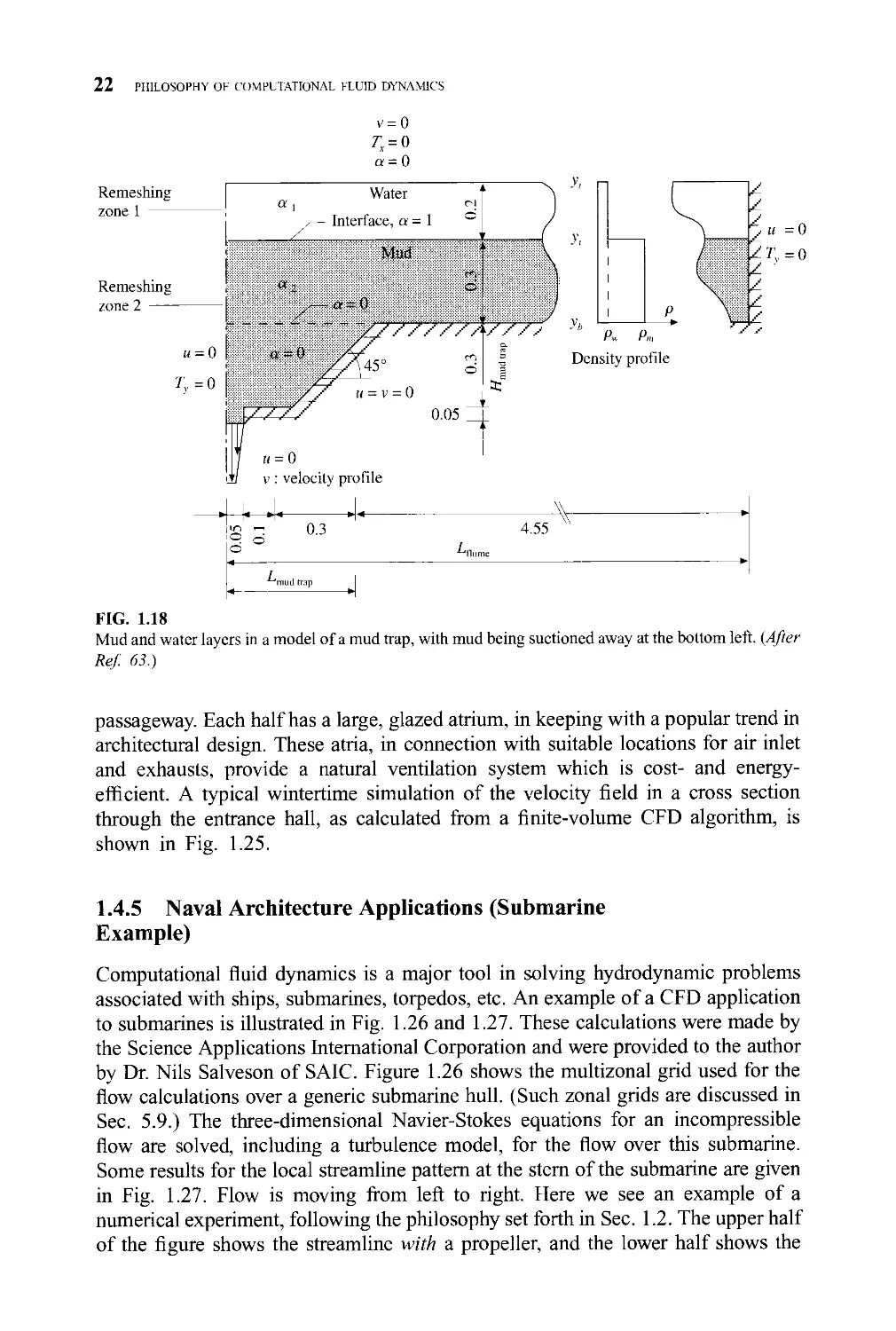
of investigations using CFD. One such example is the pumping of mud from an
underwater mud capture reservoir, as sketched in Fig. 1.18. Here, a layer of water
sits on top of a layer of mud. and a portion of the mud is trapped and is being sucked
away at the bottom left. This is only half the figure, the other half being a mirror
image, forming in total a symmetrical mud reservoir The vertical line of symmetry

20 PHILOSOPHY OF COMPUTATIONAL FLUID DYNAMICS
1.00
z(m) -
0.75
0.50
0.25 z.
0.00
-
-
-
_
-
-
_
_
-
1
1
1
1
1
1
1
' 1
1
1
1
1
1
1
1
1
1
1
1
1
1
-
-
-
_
-
-
_
-
-
1
-0.020 -0.010
0.000
0.010 0.020
r(m)
FIG. 1.16
Finite-volume mesh for the calculation of the flow in a chemical vapor deposition reactor.
(After Ref. 62.)
is the vertical line at the left of Fig. 1.18. As the mud is sucked away at the bottom
left, a crater is formed in the mud layer which fills with water. The only motion of
the water is caused by the filling of this crater. The computed velocity field in both
the water and mud at a certain instant in time is shown in Fig. 1.19, where the
magnitude of the velocity vectors are scaled against the arrow designated as 1 cm/s.
These results are from the calculations of Toorman and Berlamont as given in Ref.
63. These results contribute to the design of underwater dredging operations, such
as the major offshore dredging and beach reclamation project carried out at Ocean
City, Maryland, in the early 1990s.
1.4.4 Environmental Engineering Applications
The discipline of heating, air conditioning, and general air circulation through
buildings have all come under the spell of CFD. For example, consider the propane-

THE IMPACT OF COMPUTATIONAL FLUID DYNAMICS—SOME OTHER EXAMPLES 21
1.00 r-T
z(m)
0.75
0.50
0.25
0.00
-0.020
-0.010
0.000
0.010 0.020
r(m)
FIG. 1.17
Computed streamline pattern for the flow of CH3SiCl3 and H2 into a chemical vapor deposition reactor.
(After Ref. 62.)
burning furnace sketched in Fig. 1.20, taken from Ref. 64. The calculated velocity
field through this furnace is shown in Fig. 1.21; the velocity vectors emanating from
grid points in a perpendicular vertical plane through the furnace are shown. These
results are from the finite-difference calculations made by Bai and Fuchs (Ref. 64).
Such CFD applications provide information for the design of furnaces with in-
increased thermal efficiency and reduced emissions of pollutants.
A calculation of the flow from an air conditioner is illustrated in Fig. 1.22 and
1.23. A schematic of a room module with the air supply forced through a supply slot
in the middle of the ceiling and return exhaust ducts at both corners of the ceiling is
given in Fig. 1.22. A finite-volume CFD calculation of the velocity field showing
the air circulation pattern in the room is given in Fig. 1.23. These calculations were
made by McGuirk and Whittle (Ref. 65).
An interesting application of CFD for the calculation of air currents
throughout a building was made by Alamdari et al. (Ref. 66). Figure 1.24 shows
the cross section of an office building with two symmetrical halves connected by a

22 PHILOSOPHY OF COMPUTATIONAL FLUID DYNAMICS
Remeshing
zone 1
Remeshing
zone 2
v : velocity profile
0.3
4.55
Jmud trap
FIG. 1.18
Mud and water layers in a model of a mud trap, with mud being suctioned away at the bottom left. {After
Ref. 63.)
passageway. Each half has a large, glazed atrium, in keeping with a popular trend in
architectural design. These atria, in connection with suitable locations for air inlet
and exhausts, provide a natural ventilation system which is cost- and energy-
efficient. A typical wintertime simulation of the velocity field in a cross section
through the entrance hall, as calculated from a finite-volume CFD algorithm, is
shown in Fig. 1.25.
1.4.5 Naval Architecture Applications (Submarine
Example)
Computational fluid dynamics is a major tool in solving hydrodynamic problems
associated with ships, submarines, torpedos, etc. An example of a CFD application
to submarines is illustrated in Fig. 1.26 and 1.27. These calculations were made by
the Science Applications International Corporation and were provided to the author
by Dr. Nils Salveson of SAIC. Figure 1.26 shows the multizonal grid used for the
flow calculations over a generic submarine hull. (Such zonal grids are discussed in
Sec. 5.9.) The three-dimensional Navier-Stokes equations for an incompressible
flow are solved, including a turbulence model, for the flow over this submarine.
Some results for the local streamline pattern at the stern of the submarine are given
in Fig. 1.27. Flow is moving from left to right. Here we see an example of a
numerical experiment, following the philosophy set forth in Sec. 1.2. The upper half
of the figure shows the streamline with a propeller, and the lower half shows the

COMPUTATIONAL FLUID DYNAMICS: WHAT IS IT.'
23
FIG. 1.19
Computed velocity field for the two-
layer water and mud model shown in
Fig. 1.18; results after 240 s of suc-
tioning. (After Ref. 63.)
FIG. 1.20
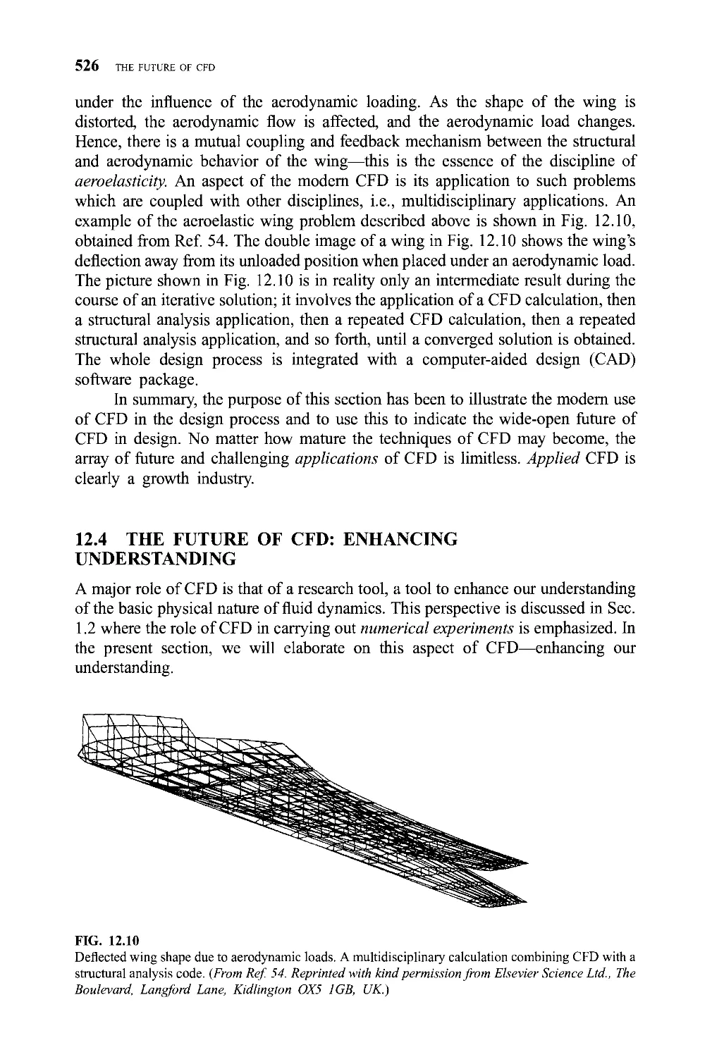
High-efficiency propane furnace model.
(From Ref. 64.)
streamlines without a propeller. In the latter case, flow separation is observed at the
first corner, whereas with the propeller no flow separation takes place.
1.5 COMPUTATIONAL FLUID DYNAMICS:
WHAT IS IT?
Question: What is CFD? To answer this question, we note that the physical aspects
of any fluid flow are governed by three fundamental principles: A) mass is
conserved; B) Newton's second law (force = mass x acceleration); and C) energy

24 PHILOSOPHY OF COMPUTATIONAL FLUID DYNAMICS
FIG. 1.21
Computed velocity field for the flow through the furnace in Fig. 1.20. Velocity vectors are shown
emanating from points in a vertical perpendicular plane through the furnace. (From Ref. 64.)
is conserved. These fundamental physical principles can be expressed in terms of
basic mathematical equations, which in their most general form are either integral
equations or partial differential equations. These equations and their derivation are
the subject of Chap. 2. Computational fluid dynamics is the art of replacing the
integrals or the partial derivatives (as the case may be) in these equations with
discretized algebraic forms, which in turn are solved to obtain numbers for the flow
Exhaust
Supply slot
Exhaust
FIG. 1.22
Schematic of a room module with air supply and
exhaust ducts in the ceiling. (After Ref. 65.)

COMPUTATIONAL FLUID DYNAMICS: WHAT IS IT?
25
FIG. 1.23
Velocity vector pattern for the room sketched in Fig. 1.22. (Reprinted by permission of the Council of
the Institution of Mechanical Engineers from Ref. 65. On behalf of the Institution of Mechanical
Engineers, United Kingdom.)
field values at discrete points in time and/or space. The end product of CFD is
indeed a collection of numbers, in contrast to a closed-form analytical solution.
However, in the long run, the objective of most engineering analyses, closed form or
otherwise, is a quantitative description of the problem, i.e., numbers. (It would be
appropriate at this state to review the quote by Maxwell given at the start of this
chapter.)
FIG. 1.24
Sketch of an office building. (Reprinted by permission of the Council of the Institution of Mechanical
Engineers from Ref. 66. On behalf of the Institution of Mechanical Engineers, United Kingdom)

26 PHILOSOPHY OF COMPUTATIONAL FLUID DYNAMICS
FIG. 1.25
A simulation of the wintertime airflow velocity vector field in the office building sketched in Fig. 1.24.
(Reprinted by permission of the Council of the Institution of Mechanical Engineers from Ref 66. On
behalf of the Institution of Mechanical Engineers, United Kingdom.)
FIG. 1.26
Multizone grid for the calculation of water flow over a generic submarine hull. (Courtesy of the Science
Applications International Corporation (SAIC) and Dr. Nils Salvesen.)
Of course, the instrument which has allowed the practical growth of CFD is
the high-speed digital computer. CFD solutions generally require the repetitive
manipulation of many thousands, even millions, of numbers, a task that is humanly
impossible without the aid of a computer. Therefore, advances in CFD, and its
applications to problems of more and more detail and sophistication, are intimately
related to advances in computer hardware, particularly in regard to storage and
execution speed. This is why the strongest force driving the development of new
supercomputers is coming from the CFD community. Indeed, the advancement in
large mainframe computers has been phenomenal over the past three decades. This
is nicely illustrated by the variation of relative computation cost (for a given
calculation) with years, as plotted in Fig. 1.28, taken from the definitive survey by

IK. ].2i
Slrv.tir.!::*ic pattern-, in iho si'ni Tty > <r /r
sticjn!L:.c pjIkTii v>nli ., pinp^lui. llu- Iliul
K. ¦•ii/fi'rv. i',' .S li'( ifri,:..' .'I;- \'ii'. .S.:.'V<"-, .1;
hni inn/ I I
t lhr-.lr.iii"-- ¦
!¦:!-
III.. I.2N
V i n ! 11 r 11 i' ¦ i..' I
Vj.
'.L1: a\ .: ..jN .¦
'1'i.lkl il.lI'J'.'. ..lh:
C'hapinaii (Rot. I 1 I. I he da la pomK on ttu-. iiraph i.'c>"\'spnn».; tn -p^v ili,t ^( itiipatci -.
startini! will) '.he \cncrable IBM h^O m 1^3. ti»riiininn;i2 (hmu^l: flic du\eK>pmer.t
t>l the pKiriLvntit? NupcrcDiiipukT, ilv ( R \^ 1. in ll'7<\ ami c\irLip.i .if.jtvj '.>¦• rlic
National Acroci\nairiK' Simulator, a taciht1. which was m>tallcu ..t '!ic \\S.\ \ircs
Research Laboraton in the late l''MK. Toda\. e\er 'iiore spceMeulai- ud\a;iccs are

ik;. 1.2**
An t:\umple (it a ni<i>1om super-
supercomputer. 1hc CR-Vl V\1P l< ,'vm
being made in supercomputer architecture An example of a supercomputer is the
(RAN Y MP, shown in Fit: 1.2^: this machine has M million words of directly
addressable central memory with an additional 512 million words available in a
companion SSD i.solid stale dcxice). The execution speed is close to one gigatlop
A0' floating-point operations per second I. this should be compared to the onc-
mcgaflop computers of the 1 "-'70s Moreover, new concepts in computer architecture
ate emerging The earlier hi^h-speed digital computers were serial machines,
capable ot one computational operation at a time: hence, all computations had to
"get m line" to lie processed. The finite speed of electrons, close to the speed ot
light, poses an inherent Imrtation on the ultimate execution speed of such serial
computers. To detour around tins limitation, two computer architectures arc now
being used
1. lir/ufpiii f,\or\. a configuration that allows a string of iiUn/nnl operations on
an arra\ of numbers ••nnnitiiiicoi^iv. thus sa\ing both time and memory
2. f'ititiiii'i ,'"v>i cswirs. a configuration that is really two or more fully functioning
central processing units i(_'PIJs). each of which can handle different instruction
and data streams and which can execute separate parts of a program simulta-
neousK. working independently or in concert with other (.PL's which belong to
the same machine
Vector ptocessors are in widespread use todav and parallel processors arc rapidly
eomtiu'. on the >ccne. I or example, the new Connection Machines, which are
massively parallel processors, are now in use by many agencies. Should you choose
to sohe am problems in \o:ar professional future using CTD. and these problems
aie ot ar.\ sophistication and complexity, the probability is high that you will be
usiiu1 either a \ ector compute! or a parallel processor.

COMPUTATIONAL FLUID DYNAMICS: WHAT IS IT?
29
Why is CFD so important in the modern study and solution of problems in
fluid mechanics, and why should you be motivated to learn something about CFD?
In essence, Sec. 1.1 to 1.4 were devoted to some answers to this question, but we
explicitly ask the question here in order to give another example of the revolution
that CFD has wrought in modern fluid dynamics—an example that will serve as a
focal point for some of our discussion in subsequent chapters.
Specifically, consider the flow field over a blunt-nosed body moving at
supersonic or hypersonic speeds, as sketched in Fig. 1.30. The interest in such
bodies is driven by the fact that aerodynamic heating to the nose is considerably
reduced for blunt bodies compared to sharp-nosed bodies; this is why the Mercury
and Apollo space capsules were so blunt and one of the reasons why the space
shuttle has a blunt nose and wings with blunt leading edges. As shown in Fig. 1.30,
there is a strong, curved bow shock wave which sits in front of the blunt nose,
detached from the nose by the distance <5, called the shock detachment distance. The
calculation of this flow field, including the shape and location of the shock wave,
was one of the most perplexing aerodynamic problems of the 1950s and 1960s.
Millions of research dollars were spent to solve this supersonic blunt body
problem—to no avail.
What was causing the difficulty? Why was the flow field over a blunt body
moving at supersonic and hypersonic speeds so hard to calculate? The answer rests
basically in the sketch shown in Fig. 1.30. The region of flow behind the nearly
normal portion of the shock wave, in the vicinity of the centerline, is locally
-> ¦«¦
FIG. 1.30
Schematic of the flowfield over a supersonic blunt-nosed body.

30 PHILOSOPHY OF COMPUTATIONAL FLUID DYNAMICS
subsonic, whereas further downstream, behind the weaker, more oblique part of the
bow shock, the flow is locally supersonic. The dividing line between the subsonic
and supersonic regions is called the sonic line, as sketched in Fig. 1.30. If the flow is
assumed to be inviscid, i.e., neglecting the dissipative transport processes of
viscosity and thermal conduction, the governing flow equations are the Euler
equations (to be derived in Chap. 2). Although these equations are the same no
matter whether the flow is locally subsonic or supersonic, their mathematical
behavior is different in the two regions. In the steady subsonic region, the Euler
equations exhibit a behavior that is associated with elliptic partial differential
equations, whereas in the steady supersonic region, the mathematical behavior of
the Euler equations is totally different, namely, that of hyperbolic partial differential
equations. Such mathematical behavior, the definition of elliptic and hyperbolic
equations, and the associated consequences to flow field analysis are discussed in
Chap. 3. The change in the mathematical behavior of the governing equations from
elliptic in the subsonic region to hyperbolic in the supersonic region made a
consistent mathematical analysis which included both regions virtually impossible.
Numerical techniques that worked for the subsonic region fell apart in the
supersonic region, and techniques for the supersonic region broke down in the
subsonic flow. Techniques were developed for just the subsonic portion, and other
techniques (such as the standard method of characteristics) were developed for the
supersonic region. Unfortunately, the proper patching of these different techniques
through the transonic region around the sonic line was extremely difficult. Hence, as
late as the mid-1960s, no uniformly valid aerodynamic technique existed to treat the
entire flow field over a supersonic blunt body.
However, in 1966, a breakthrough occurred in the blunt body problem. Using
the developing power of CFD at that time, and employing the concept of a time-
dependent approach to the steady state, Moretti and Abbett (Ref. 12) at the
Polytechnic Institute of Brooklyn (now the Polytechnic University) obtained a
numerical, finite-difference solution to the supersonic blunt body problem which
constituted the first practical, straightforward, engineering solution for this flow.
After 1966, the blunt body problem was no longer a real "problem." Industry and
government laboratories quickly adopted this computational technique for their
blunt body analyses. Perhaps the most striking aspect of this comparison is that the
supersonic blunt body problem, which was one of the most serious, most difficult,
and most researched theoretical aerodynamic problems of the 1950s and 1960s, is
today assigned as a homework problem in a CFD graduate course at the University
of Maryland.
Therein lies an example of the power of CFD combined with an algorithm
which properly takes into account the mathematical behavior of the governing flow
equations. Here is an answer to the questions asked earlier, namely, why is CFD so
important in the modern study of fluid dynamics, and why should you be motivated
to learn something about CFD? We have just seen an example where CFD and
proper algorithm development revolutionized the treatment of a given flow problem,
turning it from a virtual unsolvable problem into a standard, everyday analysis in the
nature of an extended homework problem. It is this power of CFD which is a
compelling reason for you to study the subject.

COMPUTATIONAL FLUID DYNAMICS: WHAT IS IT? 31
E.
Finite
difference
A.
B.
C.
D.
Basic philosophy
Fluid flow equations
Mathematical behavior
of the equations
Basic discretization
of the equations
Finite
volume
G.
H.
i.
Transformations
and grid generation
Some popular
techniques
Detailed applications
— worked examples —
J.
L.
Quasi-one-dimensional
nozzle flows
Viscous flow —
Couette flow
N.
K.
M.
Two-dimensional flow
through a supersonic
expansion wave
Viscous flow —
Boundary layer
The future of CFD
—
FIG. 1.31
Road map for the book.

32 PHILOSOPHY OF COMPUTATIONAL FLUID DYNAMICS
1.6 THE PURPOSE OF THIS BOOK
The previous discussions have been intended to put you in a proper frame of mind
regarding the overall nature of CFD and to provide a certain incentive to forge ahead
to the remaining chapters. As you read on, you will find sandwiched between the
covers of this book a very basic, elementary, and tutorial presentation of CFD,
emphasizing the fundamentals, surveying a number of solution techniques, and
treating various applications ranging from low-speed incompressible flow to high-
highspeed compressible flow. This book is truly an introduction to CFD; it is aimed at
the completely uninitiated reader, a reader who has little or no experience in CFD.
There are presently several very good texts on CFD at the graduate level, such as the
standard text by Anderson, Tannehill, and Pletcher (Ref. 13) and the more recent
books by Fletcher (Refs. 14 and 15) and by Hirsch (Refs. 16 and 17). A concise and
readable presentation is given by Hoffman (Ref. 18). The present book is aimed at a
level one notch below that of Refs. 13 to 17. Here we assume on the part of the
reader a physical understanding of general fluid dynamics equivalent to most junior-
level courses in mechanical and aerospace engineering and a mathematical under-
understanding equivalent to basic calculus and elementary differential equations. This is
intended to be a "first book" in the development of your thought processes in CFD.
Its purpose is fourfold; it is to provide you with:
1. Some insight into the power and philosophy of CFD
2. An understanding of the governing equations of fluid dynamics in forms
particularly suitable to CFD
3. A familiarity with some solution techniques
4. A working vocabulary in the discipline.
By the time you finish this book, this author hopes that you will be well-prepared to
launch into more advanced treatises (such as Refs. 13-17), to begin reading the
literature in CFD, to follow more sophisticated state-of-the-art presentations, and to
begin the direct application of CFD to your special areas of concern. If one or more
of the above is what you want, then you and the author share a common purpose—
simply move on to Chap. 2 and keep reading.
A road map for the material covered in this book is given in Fig. 1.31. The
purpose of this road map is to help chart the course for our thinking and to see how
the material flows in some logical fashion. It is the author's experience that when a
student is learning a new subject, there is a tendency to get lost in the details and to
lose sight of the big picture. Figure 1.31 is the big picture for our discussion on
CFD; we will frequently be referring to this road map in subsequent chapters simply
to touch base and to remind ourselves where the details fit into the overall scheme of
CFD. If at any stage you feel somewhat lost in regard to what we are doing, please
remember to refer to this central road map in Fig. 1.31. In addition, localized road
maps will be included in most chapters to provide guidance for the flow of ideas in
each chapter, in the same spirit as Fig. 1.31 provides guidance for the complete
book. In particular, referring to Fig. 1.31, note that blocks A through C represent
some basic thoughts and equations which are common to all of CFD; indeed, the

THE PURPOSE OF THIS BOOK 33
material of the present chapter is represented by block A. After these basic aspects
are understood and mastered, we will discuss the standard ways of discretizing the
fundamental equations to make them amenable to numerical solution (blocks D-F)
as well as the important aspects of grid transformation (block G). After describing
some popular techniques for carrying out numerical solutions of the equations
(block H), we will cover a number of specific applications in some detail in order to
clearly illustrate the techniques (blocks I-M). Finally, we will discuss the current
state of the art as well as the future of CFD (block N). Let us now proceed to work
our way through this road map, moving on to block B, which is the subject of the
next chapter.
Finally, Fig. 1.32a to/contains diagrams that illustrate the flow of various
concepts from parts I and II into the applications discussed in Part III. At this stage,
simply note that these figures exist; we will refer to them at appropriate times in our
discussions. They are located here simply for convenience and to indicate to you
that there is a logical flow of the basic ideas from Parts I and II into the applications
in Part III.
CFD IDEAS TO
UNDERSTAND
Explicit solutions
Implicit solutions
Conservation equations
Nonconservation equations
Transformations and grid
generation
Stability (CFL) criteria
Shock-capturing technique
Time marching
Space marching
Artificial viscosity
Relaxation idea
— Pressure-correction idea
L
(a)
HYPERBOLIC
APPLICATION
Convergent-
divergent
nozzle flow
APPLICATION
Prandtl-Meyer
expansion wave
Isentropic subsonic flow
Isentropic supersonic flow
Shock wave inside nozzle
APPLICATION
Incompressible
Couette flow
APPLICATION
Incompressible
flow over a
cylinder
FIG. 1.32
(a) Flow of ideas to the incompressible Couette flow application (implicit solution), (b) Flow of ideas to
the nozzle flow application (isentropic flow), (c) Flow of ideas to the nozzle flow application (with
shock wave), (d) Flow of ideas to the Couette flow application (pressure correction solution), (e) Flow
of ideas to the Prandtl-Meyer expansion wave application. (/) Flow of ideas to the incompressible
inviscid cylinder flow application (relaxation solution).

34
PHILOSOPHY OF COMPUTATIONAL FLUID DYNAMICS
1—¦
—
—
—
—¦
—
—
—
—
—
—
1—
—
—
—
—
—
—
—
—
—
—
CFD IDEAS TO
UNDERSTAND
Explicit solutions
Implicit solutions
Conservation equations
Nonconservation equations
Transformations and grid
generation
Stability (CFL) criteria
Shock-capturing technique
Time marching
Space marching
Artificial viscosity
Relaxation idea
Pressure-correction idea
CFD IDEAS TO
UNDERSTAND
Explicit solutions
Implicit solutions
Conservation equations
Nonconservation equations
Transformations and grid
generation
Stability (CFL) criteria
Shock-capturing technique
Time marching
Space marching
Artificial viscosity
Relaxation idea
Pressure-correction idea
HYPERBOLIC
J_
APPLICATION
Convergent-
divergent
nozzle flow
APPLICATION
Prandtl-Meyer
expansion wave
Isentropic subsonic flow
Isentropic supersonic flow
Shock wave inside nozzle
J
APPLICATION
Incompressible
Couette flow
APPLICATION
Incompressible
flow over a
cylinder
(b)
HYPERBOLIC
APPLICATION
Convergent-
divergent
nozzle flow
APPLICATION
Prandtl-Meyer
expansion wave
Isentropic subsonic flow
Isentropic supersonic flow
Shock wave inside nozzle
APPLICATION
Incompressible
Couette flow
APPLICATION
Incompressible
flow over a
cylinder
(c)

THE PURPOSE OF THIS BOOK 35
—
—
—
—
—
—
—
—
—
—
—
—
—
CFD IDEAS TO
UNDERSTAND
Explicit solutions
Implicit solutions
Conservation equations
Nonconservation equations
Transformations and grid
generation
Stability (CFL) criteria
Shock-capturing technique
Time marching
Space marching
Artificial viscosity
Relaxation idea
Pressure-correction idea
CFD IDEAS TO
UNDERSTAND
Explicit solutions
Implicit solutions
Conservation equations
Nonconservation equations
Transformations and grid
generation
Stability (CFL) criteria
Shock-capturing technique
Time marching
Space marching
Artificial viscosity
Relaxation idea
Pressure-correction idea
HYPERBOLIC
APPLICATION
Convergent-
divergent
nozzle flow
APPLICATION
Prandtl-Meyer
expansion wave
Isentropic subsonic flow
Isentropic supersonic flow
Shock wave inside nozzle
I
(d)
l_
APPLICATION
Incompressible
Couette flow
APPLICATION
Incompressible
flow over a
cylinder
HYPERBOLIC
J_
APPLICATION
Convergent-
divergent
nozzle flow
APPLICATION
Prandtl-Meyer
expansion wave
Isentropic subsonic flow
Isentropic supersonic flow
Shock wave inside nozzle
APPLICATION
Incompressible
Couette flow
APPLICATION
Incompressible
flow over a
cylinder
(e)

36
PHILOSOPHY OF COMPUTATIONAL FLUID DYNAMICS
—
—
—
—
—
—
—
—
—
—
CFD IDEAS TO
UNDERSTAND
Explicit solutions
Implicit solutions
Conservation equations
Nonconservation equations
Transformations and grid
generation
Stability (CFL) criteria
Shock-capturing technique
Time marching
Space marching
Artificial viscosity
Relaxation idea
Pressure-correction idea
HYPERBOLIC
J_
APPLICATION
Convergent-
divergent
nozzle flow
APPLICATION
Prandtl-Meyer
expansion wave
Isentropic subsonic flow
Isentropic supersonic flow
Shock wave inside nozzle
APPLICATION
Incompressible
Couette flow
I
APPLICATION
Incompressible
flow over a
cylinder

CHAPTER
2
THE
GOVERNING
EQUATIONS
OF FLUID
DYNAMICS:
THEIR
DERIVATION,
A
DISCUSSION
OF THEIR
PHYSICAL
MEANING,
AND A
PRESENTATION
OF FORMS
PARTICULARLY
SUITABLE
TO CFD
A fluid is any body whose parts yield to any
force impressed on it, and by yielding, are
easily moved among themselves.
Isaac Newton, from Section V, Book II of the
Principia, 1687
We are to admit no more causes of natural
37

38 THE GOVERNING EQUATIONS OF FLUID DYNAMICS
things than such as are both true and sufficient
to explain their appearances .... To this
purpose the philosophers say that Nature does
nothing in vain, and more is in vain when less
will serve; for Nature is pleased with
simplicity, and affects not the pomp of
superfluous causes."
Isaac Newton, from Rule I, Book II of the
Principia, 1687
2.1 INTRODUCTION
All of CFD, in one form or another, is based on the fundamental governing
equations of fluid dynamics—the continuity, momentum, and energy equations.
These equations speak physics. They are the mathematical statements of three
fundamental physical principles upon which all of fluid dynamics is based:
1. Mass is conserved.
2. Newton's second law, F = ma.
3. Energy is conserved.
The purpose of this chapter is to derive and discuss these equations.
The reason for taking the time and space to derive the governing equations of
fluid dynamics in this book is threefold:
1. Because all of CFD is based on these equations, it is important for each student
to feel very comfortable with these equations before continuing further with his
or her studies, and certainly before embarking on any application of CFD to a
particular problem.
2. This author assumes that the readers of this book come from varied background
and experience. Some of you may not be totally familiar with these equations,
whereas others may use them every day. It is hoped that this chapter will be some
enlightenment for the former and be an interesting review for the latter.
3. The governing equations can be obtained in various different forms. For most
aerodynamic theory, the particular form of the equations makes little difference.
However, for a given algorithm in CFD, the use of the equations in one form may
lead to success, whereas the use of an alternate form may result in oscillations
(wiggles) in the numerical results, incorrect results, or even instability. There-
Therefore, in the world of CFD, the various forms of the equations are of vital interest.
In turn, it is important to derive these equations in order to point out their
differences and similarities, and to reflect on possible implications in their
application to CFD.
The reader is warned in advance that this chapter may appear to be "wall-to-
wall" equations. However, do not be misled. This chapter is one of the most

INTRODUCTION
39
important in the book. It is driven by the question: If you do not physically
understand the meaning and significance of each of these equations—indeed, of
each term in these equations—then how can you even hope to properly interpret the
CFD results obtained by numerically solving these equations? The purpose of this
chapter is to squarely address this question. Here, we hope to present the
development of these equations and to discuss their significance in such detail
that you will begin to feel very comfortable with all forms of all the governing
equations of fluid flow. Experience has shown that beginning students find these
equations sometimes complex and mystifying. This chapter is designed to take the
mystery out of these equations for the reader and to replace it with solid under-
understanding.
The road map for this chapter is given in Fig. 2.1. Notice the flow of ideas as
portrayed in this map. All of fluid dynamics is based on the three fundamental
Fundamental physical principles
A.
C.
Mass is conserved
Newton's second lav
Energy is conserved
D.
Models of
the flow
E.
F.
G.
H.
Fixed finite
control volume
Moving finite
control volume
Directly leads to integral
equations ,n conservation fora,
Directly leads to integral
equations in nonconservation form
Fixed infinitesimally
small volume
Moving infinitesimally
small volume (moving
fluid element)
Directly leads to partial differentia]
equations in conservation form
Directly leads to partial differential
equations in nonconservation form
-I - 1
Boundary conditions
(a) Inviscid flow ,
(b) Viscous flow |
FIG. 2.1
Road map for Chapter 2.
Govering equations
of fluid flow
I Continuity |
I equation i
i ,
i |
I Momentum |
i equation i
i _______
i |
I Energy ,
i equation i
L _____ -i
L _
Forms of these
equations particularly
suited for CFD

40 THE GOVERNING EQUATIONS OF FLUID DYNAMICS
physical principles itemized at the top left of Fig. 2.1. These physical principles are
applied to a model of the flow; in turn, this application results in equations which
are mathematical statements of the particular physical principles involved, namely,
the continuity, momentum, and energy equations. Each different model of the flow
(bottom left in Fig. 2.1) directly produces a different mathematical statement of the
governing equations, some in conservation form and others in nonconservation
form. (The distinction between these two different forms of the governing equations
will be made clear by the end of this chapter.) After the continuity, momentum and
energy equations are obtained (the large box at the lower right side of Fig. 2.1),
forms particularly suited for use in formulating CFD solutions will be delineated
(small box at lower right side of Fig. 2.1). Finally, the physical boundary conditions
and their appropriate mathematical statements will be developed. The governing
equations must be solved subject to these boundary conditions. The physical aspects
of the boundary conditions are fundamentally independent of the forms of the
governing equations, and hence the box representing the boundary conditions
stands by itself at the bottom of Fig. 2.1, unconnected to any of the other boxes in
the road map. (However, the appropriate numerical form of the physical boundary
conditions is dependent on the particular mathematical form of the governing
equations as well as the particular numerical algorithm used to solve these
equations.) Such matters will be discussed as they naturally arise throughout this
book. The road map given in Fig. 2.1 will be helpful in guiding our flow of ideas in
this chapter. Also, when you finish this chapter, it would be useful to return to Fig.
2.1 to help consolidate your thoughts before proceeding to the next chapter.
2.2 MODELS OF THE FLOW
In obtaining the basic equations of fluid motion, the following philosophy is always
followed:
1. Choose the appropriate fundamental physical principles from the law of physics,
such as:
a. Mass is conserved.
b. F = ma (Newton's second law).
c. Energy is conserved.
2. Apply these physical principles to a suitable model of the flow.
3. From this application, extract the mathematical equations which embody such
physical principles.
This section deals with item 2 above, namely, the definition of a suitable model of
the flow. This is not a trivial consideration. A solid body is rather easy to see and
define; on the other hand, a fluid is a "squishy" substance that is hard to grab hold
of. If a solid body is in translational motion, the velocity of each part of the body is
the same; on the other hand, if a fluid is in motion, the velocity may be different at
each location in the fluid. How then do we visualize a moving fluid so as to apply to
it the fundamental physical principles?

MODELS OF THE FLOW 41
For a continuum fluid, the answer is to construct one of the four models
described below.
2.2.1 Finite Control Volume
Consider a general flow field as represented by the streamlines in Fig. 2.2a. Let us
imagine a closed volume drawn within a finite region of the flow. This volume
defines a control volume "V~; a control surface S is defined as the closed surface
which bounds the volume. The control volume may be fixed in space with the fluid
moving through it, as shown at the left of Fig. 2.2a. Alternatively, the control
volume may be moving with the fluid such that the same fluid particles are always
inside it, as shown at the right of Fig. 2.2a. In either case, the control volume is a
reasonably large, finite region of the flow. The fundamental physical principles are
applied to the fluid inside the control volume and to the fluid crossing the control
surface (if the control volume is fixed in space). Therefore, instead of looking at the
whole flow field at once, with the control volume model we limit our attention to
Control surface S
Finite control volume
fixed in space with the
fluid moving through it
(a)
Finite control volume moving
with the fluid such that the
same fluid particles are always
in the same control volume
Infinitesimal fluid element
fixed in space with the fluid
moving through it
(b)
Infinitesimal fluid element
moving along a streamline with
the velocity V equal to the
local flow velocity at each point
FIG. 2.2
Models of a flow, (a) Finite control volume approach; (b) infinitesimal fluid element approach.

42 THE GOVERNING EQUATIONS OF FLUID DYNAMICS
just the fluid in the finite region of the volume itself. The fluid-flow equations that
we directly obtain by applying the fundamental physical principles to a finite control
volume are in integral form. These integral forms of the governing equations can be
manipulated to indirectly obtain partial differential equations. The equations so
obtained from the finite control volume fixed in space (left side of Fig. 2.2a), in
either integral or partial differential form, are called the conservation form of the
governing equations. The equations obtained from the finite control volume moving
with the fluid (right side of Fig. 2.2a), in either integral or partial differential form,
are called the nonconservation form of the governing equations.
2.2.2 Infinitesimal Fluid Element
Consider a general flow field as represented by the streamlines in Fig. 2.2b. Let us
imagine an infinitesimally small fluid element in the flow with a differential volume
d"V. The fluid element is infinitesimal in the same sense as differential calculus;
however, it is large enough to contain a huge number of molecules so that it can be
viewed as a continuous medium. The fluid element may be fixed in space with the
fluid moving through it, as shown at the left of Fig. 2.2b. Alternatively, it may be
moving along a streamline with a velocity vector V equal to the flow velocity at each
point. Again, instead of looking at the whole flow field at once, the fundamental
physical principles are applied to just the infinitesimally small fluid element itself.
This application leads directly to the fundamental equations in partial differential
equation form. Moreover, the particular partial differential equations obtained
directly from the fluid element fixed in space (left side of Fig. 2.26) are again the
conservation form of the equations. The partial differential equations obtained
directly from the moving fluid element (right side of Figure 2.2b) are again called
the nonconservation form of the equations.
2.2.3 Some Comments
In the above discussion, we have introduced the idea that the governing equations
can be expressed in two general forms—conservation form and nonconservation
form—without even defining what this really means. Do not be flustered. At this
stage in our discussion, we do not have enough insight to understand what these two
different terms mean. The definition and understanding will come only while we are
actually deriving the different equation forms. So just hang on; at this stage it is
sufficient just to be aware of the existence of these two different forms.
In general aerodynamic theory, whether we deal with the conservation or
nonconservation forms of the equations is irrelevant. Indeed, through simple
manipulation, one form can be obtained from the other. However, there are cases
in CFD where it is important which form we use. In fact, the nomenclature which is
used to distinguish these two forms (conservation versus nonconservation) has
arisen primarily in the CFD literature.
The comments made in this section become clearer after we have actually
derived the governing equations. Therefore, when you finish this chapter, it would
be worthwhile to reread this section.

THE SUBSTANTIAL DERIVATIVE 43
As a final comment, in actuality the motion of a fluid is a ramification of the
mean motion of its atoms and molecules. Therefore, a third model of the flow can be
a microscopic approach wherein the fundamental laws of nature are applied directly
to the atoms and molecules, using suitable statistical averaging to define the
resulting fluid properties. This approach is in the purview of kinetic theory, which is
a very elegant method with many advantages in the long run. However, it is beyond
the scope of the present book.
2.3 THE SUBSTANTIAL DERIVATIVE
(TIME RATE OF CHANGE FOLLOWING A
MOVING FLUID ELEMENT)
Before deriving the governing equations, we need to establish a notation which is
common in aerodynamics—that of the substantial derivative. In addition, the
substantial derivative has an important physical meaning which is sometimes not
fully appreciated by students of aerodynamics. A major purpose of this section is to
emphasize this physical meaning. The discussion in this section follows that in Ref.
8, which should be consulted for more details.
As the model of the flow, we will adopt the picture shown at the right of Fig.
2.2b, namely, that of an infinitesimally small fluid element moving with the flow.
The motion of this fluid element is shown in more detail in Fig. 2.3. Here, the fluid
element is moving through cartesian space. The unit vectors along the x, y, and z
axes are i, j, and k, respectively. The vector velocity field in this cartesian space is
given by
V = u\ + vj + wk
Fluid element
at time t = t.
\
\
\
\
V,
Same fluid element
at time t - U
FIG. 2.3
Fluid element moving in the fluid flow—illustration for the substantial derivative

44 THE GOVERNING EQUATIONS OF FLUID DYNAMICS
where the x, y, and z components of velocity are given, respectively, by
u = u(x, y, z, t)
v = v{x, y, z, t)
w = w(x, y, z, t)
Note that we are considering in general an unsteady flow, where u, v, and w are
functions of both space and time /. In addition, the scalar density field is given by
p = p(x, y, z, t)
At time t\, the fluid element is located at point 1 in Fig. 2.3. At this point and time,
the density of the fluid element is
px =
At a later time t2, the same fluid element has moved to point 2 in Fig. 2.3. Hence, at
time t2, the density of this same fluid element is
Pi = P(*2,y2,z2, h)
Since p = p (x, y, z, t), we can expand this function in a Taylor series about point 1
as follows:
-\-\-p\ (h ~ h) + (higher-order terms)
V°Vi
Dividing by t2 — t\ and ignoring higher-order terms, we obtain
Pi ~ P\ _ fdP\ *2 - *i fdp\ yi-yi (dp\ z2-zx fdp
'a * i 'la l
dxjlt2-tl \dy)xt2-h \dzjlt2-tl
Examine the left side of the Eq. B.1). This is physically the average time rate of
change in density of the fluid element as it moves from point 1 to point 2. In the
limit, as t2 approaches t\, this term becomes
Km3
t2^h h-tx Dt
Here, DpIDt is a symbol for the instantaneous time rate of change of density of the
fluid element as it moves through point 1. By definition, this symbol is called the
substantial derivative D/Dt. Note that DpIDt is the time rate of change of density of
the given fluid element as it moves through space. Here, our eyes are locked on the
fluid element as it is moving, and we are watching the density of the element change
as it moves through point 1. This is different from (dpldt)\, which is physically the
time rate of change of density at the fixed point 1. For (dpldi)i, we fix our eyes on
the stationary point 1 and watch the density change due to transient fluctuations in
the flow field. Thus, DpIDt and dpldt are physically and numerically different
quantities.

THE SUBSTANTIAL DERIVATIVE 45
Returning to Eq. B.1), note that
lim = u
hm = v
t2^h h-h
,. Z2-Z1
lim = w
Thus, taking the limit of Eq. B.1) as t2 —> t\, we obtain
Dp dp dp dp dp
Examine Eq. B.2) closely. From it, we can obtain an expression for the substantial
derivative in cartesian coordinates:
D d d d d . „,
Dt dt dx dy dz
Furthermore, in cartesian coordinates, the vector operator V is defined as
V.4+j| + 4 B.4)
dx dy dz
Hence, Eq. B.3) can be written as
? = I+CV-V) B.5)
Equation B.5) represents a definition of the substantial derivative operator in vector
notation; thus, it is valid for any coordinate system.
Focusing on Eq. B.5), we once again emphasize that DIDt is the substantial
derivative, which is physically that time rate of change following a moving fluid
element; dldt is called the local derivative, which is physically the time rate of
change at a fixed point; V • V is called the convective derivative, which is
physically the time rate of change due to the movement of the fluid element
from one location to another in the flow field where the flow properties are spatially
different. The substantial derivative applies to any flow-field variable, for example,
DplDt, DTlDt, DulDt, etc., where p and Tare the static pressure and temperature,
respectively. For example
DT dT . . dT dT dT dT
— = — + V-V )= — + u— + v— + w—- 2.6
Dt dt dt dx dy dz
Convective
Local derivative
derivative
Again, Eq. B.6) states physically that the temperature of the fluid element is
changing as the element sweeps past a point in the flow because at that point the
flow-field temperature itself may be fluctuating with time (the local derivative) and
because the fluid element is simply on its way to another point in the flow field
where the temperature is different (the convective derivative).

46 THE GOVERNING EQUATIONS OF FLUID DYNAMICS
Consider an example which will help to reinforce the physical meaning of the
substantial derivative. Imagine that you are hiking in the mountains, and you are
about to enter a cave. The temperature inside the cave is cooler than outside. Thus,
as you walk through the mouth of the cave, you feel a temperature decrease—this is
analogous to the convective derivative in Eq. B.6). However, imagine that, at the
same time, a friend throws a snowball at you such that the snowball hits you just at
the same instant you pass through the mouth of the cave. You will feel an additional,
but momentary, temperature drop when the snowball hits you—this is analogous to
the local derivative in Eq. B.6). The net temperature drop you feel as you walk
through the mouth of the cave is therefore a combination of both the act of moving
into the cave, where it is cooler, and being struck by the snowball at the same
instant—this net temperature drop is analogous to the substantial derivative in Eq.
B.6).
The purpose of the above derivation is to give you a physical feel for the
substantial derivative. We could have circumvented most of the above discussion by
recognizing that the substantial derivative is essentially the same as the total
differential from calculus. That is, if
P = P(x, y, z, t)
then the chain rule from differential calculus gives
dp , dp , dp , dp , .„ .
dp = ^dx + ^-dy + ^-dz + ^-dt B.7)
dx dy dz dt
From Eq. B.7), we have
dP_^^P_ df^dx fy<fy dldz
dt dt dx dt dy dt dz dt { ' '
Since dxldt = u, dyldt = v, and dzldt = w, Eq. B.8) becomes
dp dp dp dp dp ,„ n.
dt dt dx dy dz
Comparing Eqs. B.2) and B.9), we see that dpldt and DpIDt are one and the same.
Therefore, the substantial derivative is nothing more than a total derivative with
respect to time. However, the derivation of Eq. B.2) highlights more of the physical
significance of the substantial derivative, whereas the derivation of Eq. B.9) is more
formal mathematically*
* Dr. Joe Thompson of Mississippi State University points out, with some justification, that the
terminology "substantial derivative" and "total derivative" are unnecessarily confusing, although this
terminology is very prevalent in fluid dynamics; indeed, we have followed the standard terminology
here. Based on the physical discussion in this section, Thompson suggests that the symbol
((9/(%)fluid element be used for the appropriate derivative in lieu of DIDt. This clearly emphasizes
the meaning of time rate of change of "something" following a moving fluid element.

THE DIVERGENCE OF THE VELOCITY: ITS PHYSICAL MEANING 47
2.4 THE DIVERGENCE OF THE
VELOCITY: ITS PHYSICAL MEANING
In Sec. 2.3 we examined the definition and physical meaning of the substantial
derivative; this is because the governing flow equations are frequently expressed in
terms of the substantial derivative, and it is important to have a physical under-
understanding of this term. In the same vein, and as one last item before deriving the
governing equations, let us consider the divergence of the velocity, V • V. This term
appears frequently in the equations of fluid dynamics, and it is well to consider its
physical meaning.
Consider a control volume moving with the fluid as sketched on the right of
Fig. 2.2a. This control volume is always made up of the same fluid particles as it
moves with the flow; hence, its mass is fixed, invariant with time. However, its
volume "V and control surface S are changing with time as it moves to different
regions of the flow where different values of p exist. That is, this moving control
volume of fixed mass is constantly increasing or decreasing its volume and is
changing its shape, depending on the characteristics of the flow. This control
volume is shown in Fig. 2.4 at some instant in time. Consider an infinitesimal
element of the surface dS moving at the local velocity V, as shown in Fig. 2.4. The
change in the volume of the control volume, AY", due to just the movement of dS
over a time increment At is, from Fig. 2.4, equal to the volume of the long, thin
cylinder with base area dS and altitude (V At) ¦ n, where n is a unit vector
perpendicular to the surface at dS. That is,
AY = [(VAt)-n}dS=(VAt)-dS B.10)
where the vector dS is defined simply as dS = n dS. Over the time increment At,
the total change in volume of the whole control volume is equal to the summation of
Eq. B.10) over the total control surface. In the limit as dS —> 0, the sum becomes
the surface integral
|J(VA0-dS
If this integral is divided by At, the result is physically the time rate of change of the
control volume, denoted by DYIDt; that is,
A/)'dS= f fv-dS B.11)
Dt At
s s
FIG. 2.4
Moving control volume used for the physical interpretation
of the divergence of velocity.

48 THE GOVERNING EQUATIONS OF FLUID DYNAMICS
Note that we have written the left side of Eq. B.11) as the substantial derivative of
"V, because we are dealing with the time rate of change of the control volume as the
volume moves with the flow (we are using the picture shown at the right of Fig.
2.2a), and this is physically what is meant by the substantial derivative. Applying
the divergence theorem from vector calculus to the right side of Eq. B.11), we
obtain
"\v-V)dr B.12)
Dt
¦r
Now, let us imagine that the moving control volume in Fig. 2.4 is shrunk to a very
small volume b"V, essentially becoming an infinitesimal moving fluid element as
sketched on the right of Fig. 2.2a. Then Eq. B.12) can be written as
7-V)d-T B.13)
Dt
Assume that by is small enough such that V • V is essentially the same value
throughout b"V. Then the integral in Eq. B.13), in the limit as b"V shrinks to zero, is
given by (V • V) bt~. From Eq. B.13), we have
Dt
or
V-V =
Dt
B.14)
Examine Eq. B.14) closely. On the left side we have the divergence of the velocity;
on the right side we have its physical meaning. That is,
V • V is physically the time rate of change of the volume of a moving fluid element,
per unit volume.
2.4.1 A Comment
It is useful to keep the physical meaning of the divergence of the velocity in mind
when you are dealing with the governing flow equations. Indeed, this is an example
of an overall philosophy which this author urges you to embrace, as follows.
Imagine that we are dealing with a vector velocity V in cartesian (x, y, z) space.
When a pure mathematician sees the symbol V ¦ \, his or her mind will most likely
register the fact that V • V = du/dx + dvldy + dw/dz. On the other hand, when a
fluid dynamicist sees the symbol V ¦ V, his or her mind should register first the
physical meaning—he or she should first see in the symbol V • V the words "time
rate of change of the volume of a moving fluid element, per unit volume." Indeed,
this philosophy is extrapolated to all mathematical equations and operations having
to do with physical problems. Always keep in mind the physical meaning of the

THE CONTINUITY EQUATION 49
terms in the equations you are dealing with. In this vein, note that in the phrase
"computational fluid dynamics" the word "computational" is simply an adjective to
"fluid dynamics"; when you are dealing with the discipline of CFD, it is vitally
important to keep the physical understanding oi fluid dynamics uppermost in your
mind. This, in part, is the purpose of the present chapter.
2.5 THE CONTINUITY EQUATION
Let us now apply the philosophy discussed in Sec. 2.2; that is, let us A) write down
a fundamental physical principle, B) apply it to a suitable model of the flow, and C)
obtain an equation which represents the fundamental physical principle. In this
section, we will treat the following case:
Physical principle: Mass is conserved.
The governing flow equation which results from the application of this physical
principle to any one of the four models of the flow shown in Fig. 2.2a and b is called
the continuity equation. Moreover, in this section we will carry out in detail the
application of this physical principle using all four of the flow models illustrated in
Fig. 2.2a and b; in this way we hope to dispel any mystery surrounding the
derivation of the governing flow equation. That is, we will derive the continuity
equation four different ways, obtaining in a direct fashion four different forms of the
equation. Then, by indirect manipulation of these four different forms, we will show
that they are all really the same equation. In addition, we will invoke the idea of
conservation versus nonconservation forms, helping to elucidate the meaning of
those words. Let us proceed.
2.5.1 Model of the Finite Control Volume Fixed in
Space
Consider the flow model shown at the left of Fig. 2.2a, namely, a control volume of
arbitrary shape and of finite size. The volume is fixed in space. The surface that
bounds this control volume is called the control surface, as labeled in Fig. 2.2a. The
fluid moves through the fixed control volume, flowing across the control surface.
This flow model is shown in more detail in Fig. 2.5. At a point on the control surface
in Fig. 2.5, the flow velocity is Vand the vector elemental surface area (as defined in
Sec. 2.4) is dS. Also let d'f be an elemental volume inside the finite control
volume. Applied to this control volume, our fundamental physical principle that
mass is conserved means
Net mass flow out time rate of
of control volume = decrease of mass B.15a)
through surface S inside control volume
or B = C B.156)
where B and C are just convenient symbols for the left and right sides, respectively,

50 THE GOVERNING EQUATIONS OF FLUID DYNAMICS
dS
FIG. 2.5
Finite control volume fixed in space.
of Eq. B.15a). First, let us obtain an expression for B in terms of the quantities
shown in Fig. 2.5. The mass flow of a moving fluid across any fixed surface (say,
in kilograms per second or slugs per second) is equal to the product of (densi-
(density) x (area of surface) x (component of velocity perpendicular to the surface).
Hence the elemental mass flow across the area dS is
pVHdS = pV-dS B.16)
Examining Fig. 2.5, note that by convention, dS always points in a direction out of
the control volume. Hence, when V also points out of the control volume (as shown
in Fig. 2.5), the product pV • dS is positive. Moreover, when V points out of the
control volume, the mass flow is physically leaving the control volume; i.e., it is an
outflow. Hence, a positive pV • dS denotes an outflow. In turn, when V points into
the control volume, pV • dS is negative. Moreover, when V points inward, the
mass flow is physically entering the control volume; i.e., it is an inflow. Hence, a
negative pV • dS denotes an inflow. The net mass flow out of the entire control
volume through the control surface S is the summation over S of the elemental mass
flow expressed in Eq. B.16). In the limit, this becomes a surface integral, which is
physically the left sides of Eqs. B.15a) and B.156); that is,
5=[[pV-dS B.17)
Now consider the right sides of Eqs. B.15a) and B.15b). The mass contained within
the elemental volume drV is p drV. The total mass inside the control volume is
therefore
f f f
p d-r
j
¦r
The time rate of increase of mass inside "V is then

THE CONTINUITY EQUATION
55
Time rate of mass increase = — (dx dy dz)
B.23)
The physical principle that mass is conserved, when applied to the fixed element in
Fig. 2.7, can be expressed in words as follows: the net mass flow out of the element
must equal the time rate of decrease of mass inside the element. Denoting the mass
decrease by a negative quantity, this statement can be expressed in terms of Eqs.
B.22) and B.23) as
d(pu) d(pv) d(pwj\ , ,
-^T1 + -^ + -^r1] dx dy
ox dy dz J
9p
=--?- {dx dy dz)
at
ot \_ ox oy oz
In Eq. B.24), the term in brackets is simply V • (pV). Thus, Eq. B.24) becomes
B.25)
Equation B.25) is a partial differential equation form of the continuity equation. It
was derived on the basis of an infinitesimally small element fixed in space. The
infinitestimally small aspect of the element is why the equation is obtained directly
in partial differential equation form. The fact that the element was fixed in space
leads to the specific differential form given by Eq. B.25), which is called the
conservation form. As stated earlier, the forms of the governing flow equations that
are directly obtained from a flow model which is fixed in space are, by definition,
called the conservation form.
Equation B.25) is displayed in box III in Fig. 2.6. It is the form that most
directly stems from the model of an infinitesimally small element fixed in space. On
the other hand, it can also be obtained by indirect manipulation from either of the
integral equations displayed in boxes I and II, as will be shown in Sec. 2.2.5.
2.5.4 Model of an Infinitesimally Small Fluid
Element Moving with the Flow
Consider the flow model shown at the right of Fig. 2.2b, namely, an infinitesimally
small fluid element moving with the flow. This fluid element has a fixed mass, but in
general its shape and volume will change as it moves downstream. Denote the fixed
mass and variable volume of this moving fluid element by dm and bt\ respectively.
Then
dm = p b1r
B.26)
Since mass is conserved, we can state that the time rate of change of the mass of the
fluid element is zero as the element moves along with the flow. Invoking the
physical meaning of the substantial derivative discussed in Sec. 2.3, we have

56 THE GOVERNING EQUATIONS OF FLUID DYNAMICS
D(8m)
Dt
Combining Eqs. B.26) and B.27), we have
= 0 B.27)
§^[^H
We recognize the term in brackets in Eq. B.28) as the physical meaning of V • \,
discussed in Sec. 2.4 and given in Eq. B.14). Hence, combining Eqs. B.14) and
B.28), we obtain
Dt
+ pV ¦ V = 0
B.29)
Equation B.29) is a partial differential equation form of the continuity equation,
different from that expressed by Eq. B.25). It was derived on the basis of an
infinitesimally small fluid element moving with the flow. Once again, the infmi-
tesimally small aspect of the fluid element is why the equation is obtained directly in
partial differential equation form. The fact that the element is moving with the flow
leads to the specific differential form given by Eq. B.29), which is called the
nonconservation form. As stated earlier, the forms of the governing flow equations
that are directly obtained from a flow model which is moving with the flow are, by
definition, called the nonconservation form.
Equation B.29) is displayed in box IV in Fig. 2.6. It is the form that most
directly stems from the model of an infinitesimally small fluid element moving with
the flow. On the other hand, it can also be obtained by indirect manipulation from
any of the equations in the other boxes in Fig. 2.6. It is now appropriate to examine
this indirect manipulation.
2.5.5 All the Equations Are One:
Some Manipulations
Examining Fig. 2.6, we see four different forms of the continuity equation, each one
a direct product of the flow model used in its derivation. Two of the forms are
integral equations; the other two are partial differential equations. Two of the
equations are in conservation form; the other two are in nonconservation form.
However, these four equations are not fundamentally different equations; rather,
they are four different forms of the same equation, namely, the continuity equation.
Any of these four forms can be derived by manipulation from any of the others. This
is symbolized by paths A through D sketched in Fig. 2.6. For a better understanding
of the meaning and significance of the governing flow equations, we need to
examine the details of these different paths. This is the purpose of the present
subsection.

THE CONTINUITY EQUATION 57
First, let us examine how the partial differential equation form can be obtained
from the integral equation form; i.e., let us examine path C in Fig. 2.6. Repeating
Eq. B.19),
r
Since the control volume used for the derivation of Eq. B.19) is fixed in space, the
limits of integration for the integrals in Eq. B.19) are constant, and hence the time
derivative dldt can be placed inside the integral.
pV • dS = 0 B.30)
¦r s
Applying the divergence theorem from vector calculus, the surface integral in Eq.
B.30) can be expressed as a volume integral:
(pV)-dS = jjjV-(pV)JiT B.31)
s -r
Substituting Eq. B.31) into B.30), we have
¦r
^ + V-(pV)^ = 0 B-32)
Since the finite control volume is arbitrarily drawn in space, the only way for the
integral in Eq. B.32) to equal zero is for the integrand to be zero at every point
within the control volume. Hence, from Eq. B.32)
f+ V-(pV) = 0
B.33)
Equation B.33) is precisely the continuity equation in partial differential equation
form that is displayed in box III in Fig. 2.6. Hence, we have shown how the integral
form in box I can, after some manipulation, yield the differential form in box III.
Again, note that both the equations in boxes I and III are in conservation form; the
above manipulation does not change that situation.
Next, let us examine a manipulation that does change the conservation form to
the nonconservation form. Specifically let us take the differential equation in box III
and convert it to the differential equation in box IV Consider the vector identity
involving the divergence of the product of a scalar times a vector, such as

58 THE GOVERNING EQUATIONS OF FLUID DYNAMICS
V • (pV) = (pV • V) + (V • Vp) B.34)
In words, the divergence of a scalar times a vector is equal to the scalar times the
divergence of the vector plus the vector dotted into the gradient of the scalar. (See
any good text on vector analysis for a presentation of this identity, such as Ref. 19.)
Substituting Eq. B.34) into Eq. B.33), we obtain
^+(V-Vp) + (pV-V) = 0 B.35)
The first two terms on the left side of Eq. B.35) are simply the substantial derivative
of density. Hence, Eq. B.35) becomes
^ + pV-V = 0 B.36)
Equation B.36) is precisely the equation displayed in box IV in Fig. 2.6. Hence, by
a slight manipulation of the partial differential equation in box III, which is in
conservation form, we obtained the partial differential equation in box IV, which is
in nonconservation form.
Can the same type of change be made to the integral forms of the equations;
e.g., can the equation in box II be manipulated to obtain the equation in box I? This
is represented by path A in Fig. 2.6. The answer is yes; let us see how. The equation
in box II is Eq. B.21), repeated below:
«- = O B.21)
Recall in Eq. B.21) that the volume integral is taken over the whole moving control
volume "V and that this volume is changing as it flows downstream. Indeed, the
moving finite control volume consists of an infinite number of infinitesimally small
volumes of fixed infinitesimally small mass, each of volume dV, where the magni-
magnitude of dV also changes as the control volume moves downstream. Since the
substantial derivative itself represents a time rate of change associated with a
moving element, and the limits of integration on the volume integral in Eq. B.21)
are determined by these same moving elements, then the substantial derivative can
be taken inside the integral. Hence, Eq. B.21) can be written as
Noting again that dV physically represents an infinitesimally small volume which
itself is variable, the substantial derivative inside the integral in Eq. B.37) is the
derivative of a product of two variables, namely, p and dV. The derivative must be
expanded accordingly; Eq. B.37) becomes

THE CONTINUITY EQUATION 59
Dividing and multiplying the second term by d"V, we have
. D{dV)~
d-f Dt
= 0
B.38)
y y
The physical meaning of the term inside the brackets is simply the "time rate of
change of volume of an infmitesimally small fluid element per unit volume." We
recall from Sec. 2.4 and Eq. B.14) that this term is the divergence of velocity.
Hence, Eq. B.38) becomes
~
B.39)
From the definition of the substantial derivative given by Eq. B.5), the first term in
Eq. B.39) can be expanded as
dp
dt
-V-Vp
B.40)
Substituting Eq. B.40) into B.39), and writing all terms under a single volume
integral, we have
~ + V- Vp + pV- v\dir = 0 B.41)
dt J
From the vector identity given in Eq. B.34), the last two terms in Eq. B.41) can be
written as
V • Vp + pV • V = V • (pV)
With this, Eq. B.41) becomes
^^ + |JJv(pV) dr = 0 B.42)
y y
Finally, employing the divergence theorem from vector analysis, which relates a
surface integral to a volume integral as
V-(pV)<frr= [ [pV-dS
r s
(again, see any good vector analysis text, such as Ref. 19), Eq. B.42) finally results
in
%dir+\\pV'dS = ° B43)
f S
Equation B.43) is essentially the form of the equation in box I in Fig. 2.6.

60 THE GOVERNING EQUATIONS OF FLUID DYNAMICS
We could go on, but we won't—for the sake of not boring you with essentially
repetitive manipulations. The major point of this subsection has been made. We see
that the four different equations displayed in the boxes in Fig. 2.6 in reality are not
different equations at all but rather four different forms of the same equation—the
continuity equation. However, each different form displayed in Fig. 2.6 comes most
directly from the particular model of the flow adjacent to each equation, and hence
the terms in each equation have slightly different physical implications. Also, the
philosophy associated with these different forms, and how they were derived, is not
limited to just the continuity equation—the same approach is used for the
development of the momentum and energy equations, to follow.
2.5.6 Integral versus Differential Form of the
Equations: An Important Comment
There is a subtle difference between the integral and differential forms of the
governing flow equations which is best noted at this stage. The integral form of the
equations allows for the presence of discontinuities inside the fixed control volume
(fixed in space); there is no inherent mathematical reason to assume otherwise.
However, the differential form of the governing equations assumes the flow
properties are differentiable, hence continuous. This is particularly evident when
we use the divergence theorem to derive the differential form from the integral
form—the divergence theorem assumes mathematical continuity. This is a strong
argument for the integral form of the equations to be considered more fundamental
than the differential form. This consideration becomes of particular importance
when calculating a flow with real discontinuities, such as shock waves.
2.6 THE MOMENTUM EQUATION
In this section, we apply another fundamental physical principle to a model of the
flow, namely:
Physical principle: F = ma (Newton's second law)
The resulting equation is called the momentum equation. Unlike the derivation of
the continuity equation in Sec. 2.5, where great pains were taken to illustrate the use
of all four models of the fluid and to highlight the different forms of the equations
obtained therein, in the present section we will restrain ourselves and choose only
one model of the flow. Specifically, we will utilize the moving fluid element model
shown at the right of Fig. 2.2b because this model is particularly convenient for the
derivation of the momentum equation as well as the energy equation (to be
considered in Sec. 2.7). The moving fluid element model is sketched in more detail
in Fig. 2.8. However, please keep in mind that the momentum and energy equations
can be derived using any of the other three models of the fluid in Fig. 2.2a and b; as
in the case of the continuity equation developed in Sec. 2.5, each different model of
the flow leads directly to a different form of the momentum and energy equations,
analogous to those for the continuity equation displayed in Fig. 2.6.

THE MOMENTUM EQUATION 61
, + -^ dy) dxdz
p + -J&- dxjdydz
^ dx) dy dz
FIG. 2.8
Infinitesimally small, moving fluid element. Only the forces in the x direction are shown. Model used
for the derivation of the x component of the momentum equation.
Newton's second law, expressed above, when applied to the moving fluid
element in Fig. 2.8, says that the net force on the fluid element equals its mass times
the acceleration of the element. This is a vector relation, and hence can be split into
three scalar relations along the x, y, and z axes. Let us consider only the x
component of Newton's second law,
Fx — max
B.44)
where Fx and ax are the scalar x components of the force and acceleration,
respectively.
First, consider the left side of Eq. B.44). We say that the moving fluid element
experiences a force in the x direction. What is the source of this force? There are two
sources:
1. Body forces, which act directly on the volumetric mass of the fluid element.
These forces "act at a distance"; examples are gravitational, electric, and
magnetic forces.
2. Surface forces, which act directly on the surface of the fluid element. They are
due to only two sources: (a) the pressure distribution acting on the surface,
imposed by the outside fluid surrounding the fluid element, and (b) the shear and
normal stress distributions acting on the surface, also imposed by the outside
fluid "tugging" or "pushing" on the surface by means of friction.

62 THE GOVERNING EQUATIONS OF FLUID I
+¦ x
-> x
(a) (b)
FIG. 2.9
Illustration of (a) shear stress (related to the time rate of charge of the shearing deformation and (b)
normal stress (related to the time rate of charge of volume).
Let us denote the body force per unit mass acting on the fluid element by f,
with fx as its x component. The volume of the fluid element is (dx dy dz); hence,
Body force on
fluid element acting = pfx(dx dy dz)
in x direction
B.45)
The shear and normal stresses in a fluid are related to the time rate of change
of the deformation of the fluid element, as sketched in Fig. 2.9 for just the xy plane.
The shear stress, denoted by xxy in Fig. 2.9a, is related to the time rate of change of
the shearing deformation of the fluid element, whereas the normal stress, denoted by
txx in Fig. 2.9b, is related to the time rate of change of volume of the fluid element.
As a result, both shear and normal stresses depend on velocity gradients in the flow,
to be designated later. In most viscous flows, normal stresses (such as txx) are much
smaller than shear stresses and many times are neglected. Normal stresses (say xxx in
the x direction) become important when the normal velocity gradients (say duldx)
are very large, such as inside a shock wave.
The surface forces in the x-direction exerted on the fluid element are sketched
in Fig. 2.8. The convention will be used here that %y denotes a stress in the
j direction exerted on a plane perpendicular to the / axis. On face abed, the only
force in the x direction is that due to shear stress, xyz dx dz. Face efgh is a distance
dy above face abed; hence the shear force in the x direction on face efgh is
\zyx + (dxyjdy) dy] dx dz. Note the directions of the shear force on faces abed and
efgh; on the bottom face, xyx is to the left (the negative x direction), whereas on the
top face, xyz + (dxyxldy) dy is to the right (the positive x direction). These directions
are consistent with the convention that positive increases in all three components of
velocity, u, v, and w, occur in the positive directions of the axes. For example, in Fig.
2.8, u increases in the positive y direction. Therefore, concentrating on face efgh, u
is higher just above the face than on the face; this causes a "rugging" action which
tries to pull the fluid element in the positive x direction (to the right) as shown in
Fig. 2.8. In turn, concentrating on face abed, u is lower just beneath the face than on
the face; this causes a retarding or dragging action on the fluid element, which acts
in the negative x direction (to the left) as shown in Fig. 2.8. The directions of all the
other viscous stresses shown in Fig. 2.8, including txx, can be justified in a like
fashion. Specifically on face degh, xzx acts in the negative x-direction, whereas on

THE MOMENTUM EQUATION 63
face abfe, xzx + (dxzxldz) dz acts in the positive x direction. On face adhe, which is
perpendicular to the x axis, the only forces in the x direction are the pressure force
p dy dz, which always acts in the direction into the fluid element, and xxx dy dz,
which is in the negative x direction. In Fig. 2.8, the reason why xxx on face adhe is to
the left hinges on the convention mentioned earlier for the direction of increasing
velocity. Here, by convention, a positive increase in u takes place in the positive x
direction. Hence, the value of u just to the left face of adhe is smaller than the value
of u on the face itself. As a result, the viscous action of the normal stress acts as a
"suction" on face adhe; i.e., there is a dragging action toward the left that wants to
retard the motion of the fluid element. In contrast, on face bcgf, the pressure force
[p + dpldx) dx] dy dz presses inward on the fluid element (in the negative x
direction), and because the value of u just to the right of the face bcgf is larger
than the value of u on the face, there is a "suction" due to the viscous normal stress
which tries to pull the element to the right (in the positive x direction) with a force
equal to [x^ + (dxxxldx) dx] dy dz.
With the above in mind, for the moving fluid element we can write
Net surface force [ / dp \ 1
,. . = \p - [ p + — dx } \ dy dz
inx direction y V dx \
+ I ( ixx + -rp dx) -xxx\dydz
dx
dy I - V dx dz
x + ^dz\- xzx\ dx dy B.46)
The total force in the x direction Fx, is given by the sum of Eqs. B.45) and B.46).
Adding, and cancelling terms, we obtain
dp dxxx dxyx dxzx]
1 1 — H dx dy dz + pf dx dy dz B-47)
dx dx dy dz J
Equation B.47) represents the left-hand side of Eq. B.44).
To summarize and reinforce the physical significance of the force on a moving
fluid element, let us display Newton's second law in diagramatic form as follows:
Body forces Surface forces
Weight (due I Electro- Pressure Viscous
to gravity) | magnetic *
Normal Shear
Considering the right-hand side of Eq. B.44), recall that the mass of the fluid
element is fixed and is equal to
m = pdxdydz B.48)
Also, recall that the acceleration of the fluid element is the time rate of change of its
velocity. Hence, the component of acceleration in the x direction, denoted by ax, is

64
THE GOVERNING EQUATIONS OF FLUID DYNAMICS
simply the time rate of change of u; since we are following a moving fluid element,
this time rate of change is given by the substantial derivative. Thus,
Combining Eqs. B.44) and B.47) to B.49), we obtain
Du
P Dt~
dp
dx
dXyx
dxyx
dy
dxzx
dz
B.50a)
which is the x component of the momentum equation for a viscous flow. In a similar
fashion, the y and z components can be obtained as
B.50b)
p
Dv
Dt
dp
dy
+
dXxy
dx
+
dXyy
dy
+
dxv
dz
ypfy
and
Dw dp dxxz dxyz dxz
= + + +
p
Dt dz dx
dy dz
B.50c)
Equations B.50a) to B.50c) are the x, y, and z components, respectively, of the
momentum equation. Note that they are partial differential equations obtained
directly from an application of the fundamental physical principle to an infinitesimal
fluid element. Moreover, since this fluid element is moving with the flow, Eqs.
B.50a) to B.50c) are in nonconservation form. They are scalar equations and are
called the Navier-Stokes equations in honor of two men—the Frenchman M. Navier
and the Englishman G. Stokes—who independently obtained the equations in the
first half of the nineteenth century.
The Navier-Stokes equations can be obtained in conservation form as follows.
Writing the left-hand side of Eq. B.50a) in terms of the definition of the substantial
derivative, we have
Du
du
B.51)
Also, expanding the following derivative,
du
dp
and rearranging, we have
du d(pu) dp
B.52)
Recalling the vector identity for the divergence of the product of a scalar times a
vector, we have
V • (puV) - mV ¦ (pV) + (pV) • Vm

THE MOMENTUM EQUATION 65
or PV.TJU = V ¦ (puV) - wV • (pV) B.53)
Substitute Eqs. B.52) and B.53) into B.51).
Dt
dt
dt
dt
V ¦ (puV)
B.54)
The term in brackets in Eq. B.54) is simply the left-hand side of the continuity
equation as Eq. B.25); hence the term in brackets is zero. Thus Eq. B.54) reduces to
Du
P~Dt~ dt
Substitute Eq. B.55) into B.50a).
B.55)
B.56a)
B.56b)
B.56c)
Equations B.56a) to B.56c) are the Navier-Stokes equations in conservation form.
In the late seventeenth century, Isaac Newton stated that shear stress in a fluid
is proportional to the time rate of strain, i.e., velocity gradients. Such fluids are
called newtonian fluids. (Fluids in which x is not proportional to the velocity
gradients are nonnewtonian fluids; blood flow is one example.) In virtually all
practical aerodynamic problems, the fluid can be assumed to be newtonian. For such
fluids. Stokes in 1845 obtained
Similarly
and
d(pu)
dt
Eqs. B
d(pv)
dt
d(pw) |
dt
V
(pwV) =
dx +
.506) and B.50c) can
V
-V
(nv\r\
[pvx)
¦ (pwV) -
dp
dy"
dx
be
dixy
dx
"fa
+ dy +
expressed
dXyy
' dy '
dz '
as
dXzy
dz
dxzz
dz
Vpfy
+ Pfz
x =
Tzz =
dv
dy
dw
dz
dv du
dy
• V) + 2/i
• V) + 2/i
B.57a)
B.576)
B.57c)
B.57d)

66 THE GOVERNING EQUATIONS OF FLUID DYNAMICS
(du dw\
= ^ = ^1 —+ —
\dz dx)
dw dv
dy dz
{2.51e)
B-57/)
where u is the molecular viscosity coefficient and X is the second viscosity
coefficient. Stokes made the hypothesis that
k=-\n
which is frequently used but which has still not been definitely confirmed to the
present day.
Substituting Eqs. B.57) into B.56), we obtain the complete Navier-Stokes
equations in conservation form;
d{pu)
dt
d{pv)
dt
d(pw)
dt
d(pu2)
1 dx
d(puv)
dx
d(puw)
1 dx
d(puv)
dy
+?("
dipv2)
1 r. 1
d(pvw)
dy
+ d\,
+ dx[l
d(puw)
dz
•V + 2,
d(pvw)
dz
dv du
d(pw2
1 dz
(du
l\d~z +
llTx)
+
I +
+
)
dw\
~dx~)
d
+ dz
dp
dx
d
dp
dy
d
dp
dz
1 ,
J +
1 /,'
d r
/
/dv dM\l
\cic oly/ J
du dw\
dz dx J
9w dv\ 1
6(y dzy J y
(dw dv\ 1
\_ dy dz) J
dw\
B.58a)
B.586)
B.58c)
2.7 THE ENERGY EQUATION
In the present section, we apply the third physical principle as itemized at the
beginning of Sec. 2.1, namely,
Physical principle: Energy is conserved.
In keeping with our derivation of the Navier-Stokes equations (i.e., the momentum
equation) in Sec. 2.6, we will use again the flow model of an infinitesimally small

THE ENERGY EQUATION 67
fluid element moving with the flow (as shown at the right of Fig. 2.2b). The physical
principle stated above is nothing more than the first law of thermodynamics. When
applied to the flow model of a fluid element moving with the flow, the first law states
that
Rate of change Net flux of Rate of work done on
of energy inside = heat into + element due to
fluid element element body and surface forces
or B.59)
A B + C
where A, B, and C denote the respective terms above.
Let us first evaluate C; that is, let us obtain an expression for the rate of work
done on the moving fluid element due to body and surface forces. It can be shown
that the rate of doing work by a force exerted on a moving body is equal to the
product of the force and the component of velocity in the direction of the force (see
Refs. 1 and 8 for such a derivation). Hence the rate of work done by the body force
acting on the fluid element moving at a velocity V is
pi ¦ V(dx dy dz)
With regard to the surface forces (pressure plus shear and normal stresses), consider
just the forces in the x direction, shown in Fig. 2.8. The rate of work done on the
moving fluid element by the pressure and shear forces in the x direction shown in
Fig. 2.8 is simply the x component of velocity, u, multiplied by the forces; e.g., on
face abed the rate of work done by xyx dx dz is uxyx dx dz, with similar expressions
for the other faces. To emphasize these energy considerations, the moving fluid
element is redrawn in Fig. 2.10, where the rate of work done on each face by surface
forces in the x direction is shown explicitly. To obtain the net rate of work done on
the fluid element by the surface forces, note that forces in the positive x direction do
positive work and that forces in the negative x direction do negative work. Hence,
comparing the pressure forces on face adhe and begf in Fig. 2.10, the net rate of
work done by pressure in the x direction is
up- [up + --^ dx\\dy dz=- -^J-L dx dy dz
\ ox J J ox
Similarly, the net rate of work done by the shear stresses in the x direction on faces
abed and efgh is
uxv
Considering all the surface forces shown in Fig. 2.10, the net rate of work on the
moving fluid element due to these forces is simply
d{up) 9(mt«) d{myx) d(inzx)] ,
~^ ' 5 ' ^~ + —a— dx dy dz
ox ox oy oz J
The above expression considers only surface forces in the x direction. When the
surface forces in the y and z directions are also included, similar expressions are

68 THE GOVERNING EQUATIONS OF FLUID DYNAMICS
[up -^— dx]dydz
FIG. 2.10
Energy fluxes associated with an infinitesimally small, moving fluid element. For simplicity, only the
fluxes in the x direction are shown. Model used for the derivation of the energy equation.
obtained. In total, the net rate of work done on the moving fluid element is the sum
of the surface force contributions in the x, y, and z directions, as well as the body
force contribution. This is denoted by C in Eq. B.59) and is given by
r-
dy
d(uxzx)
dz
9(wp)\
dz )
dx
dy
dx
d(vxx
d{wxzz)
dz
d{uxyx)
dy
dz
d(wxxz)
dx
dxdydz + pf-Vdxdydz B.60)
Note in Eq. B.60) that the first three terms on the right-hand side are simply
V • (P\).
Let us turn our attention to B in Eq. B.59), i.e., the net flux of heat into the
element. This heat flux is due to A) volumetric heating such as absorption or
emission of radiation and B) heat transfer across the surface due to temperature
gradients, i.e., thermal conduction. Define q as the rate of volumetric heat addition
per unit mass. Noting that the mass of the moving fluid element in Fig. 2.10 is
p dx dy dz, we obtain
Volumetric heating of element = pq dx dy dz
B-61)
In Fig. 2.10, the heat transferred by thermal conduction into the moving fluid
element across face adhe is qx dy dz, where qx is the heat transferred in the x
direction per unit time per unit area by thermal conduction. (The heat transfer in a

THE ENERGY EQUATION 69
given direction, when expressed in dimensions of energy per unit time per unit area
perpendicular to the direction, is called the heat flux in that direction. Here, qx is the
heat flux in the x direction.) The heat transferred out of the element across face bcgf
is \kx + {dqjdx) dx] dy dz. Thus, the net heat transferred in the x direction into the
fluid element by thermal conduction is
^-{** + d^dx^dydz=-d^dxdydz
Taking into account heat transfer in the y and z directions across the other faces in
Fig. 2.10, we obtain
Heating of , ~. ~ ¦ o • \
fluid element by — — I -—^ + -—^ + —- I dx dy dz B.62)
thermal conduction ^ j /
The term B in Eq. B.59) is the sum of Eqs. B.61) and B.62).
The heat flux due to thermal conduction, from Fourier's law of heat conduction, is
proportional to the local temperature gradient:
• _ udT ¦ _ k9T ¦ _ udT
dx y dy dz
where k is the thermal conductivity. Hence, Eq. B.63) can be written
** B64)
Finally, the term A in Eq. B.59) denotes the time rate of change of energy of
the fluid element. Pause for a moment and ask yourself the question: the time rate of
change of what energy? In classical thermodynamics, we generally deal with a
system that is stationary; in this case, the energy that appears in the first law of
thermodynamics is the internal energy. Let us examine more closely the source of
this internal energy. If the system is a gas, the atoms and molecules are moving
within the system, translating in a purely random fashion. That is, each atom or
molecule has translational kinetic energy, and this energy is associated with the
purely random motion of the particle. In addition, as they translate through space,
molecules (not atoms) can also rotate and vibrate, adding rotational and vibrational
energy to the molecule. Finally, the motion of electrons around the nuclei of the
atoms or molecules adds electronic energy to the particle. The total energy of a
given molecule is the sum of its translational, rotational, vibrational, and electronic
energies; the total energy of each atom is the sum of its translational and electronic
energy (see Ref. 2 for an extensive discussion of molecular and atomic energies).
The internal energy of the gas system is simply the energy of each molecule or
atom, summed over all the molecules and atoms in the system. This is the physical
significance of the internal energy that appears in the first law of thermodynamics.

70 THE GOVERNING EQUATIONS OF FLUID DYNAMICS
Now, return to Eq. B.59) and examine the term labeled A. We are now considering a
gaseous medium that is in motion; i.e., the energy term labeled A concerns the
energy of a moving fluid element. Hence, the fluid element has two contributions to
its energy:
1. The internal energy due to random molecular motion, e (per unit mass). This is
the energy we have described above.
2. The kinetic energy due to translational motion of the fluid element. The kinetic
energy per unit mass is simply V2/2.
Hence, the moving fluid element has both internal and kinetic energy; the sum
of these two is the "total" energy. In Eq. B.59), the energy in the term A is the
total energy, i.e., the sum of the internal and kinetic energies. The total energy is
e + V2/2. Since we are following a moving fluid element, the time rate of change of
total energy per unit mass is given by the substantial derivative. Since the mass of
the fluid element is p dx dy dz, we have
+ ^Pjdxdydz B.65)
The final form of the energy equation is obtained by substituting Eqs. B.60),
B.64), and B.65) into B.59), obtaining
D /
d(up)
dx
V2\
divp)
dy
¦ d (
dx \
d(wp) |
dz '
+
d{uxa
dx
d(vxzy
dz
<
- +
dy [k dy)
d(uxyx)
dy
d{wxxz) i
dx !
4z(
d[uxzx
dz
d(wxyz
dy
m
) d(v%)
' dx
) , d(wxzz]
1 &
I
d{VTyy)
dy
pi -V
B.66)
This is the nonconservation form of the energy equation; also note that it is in terms
of the total energy e + V2/2. Once again, the nonconservation form results from the
application of the fundamental physical principle to a moving fluid element.
The left-hand side of Eq. B.66) involves the substantial derivative of the total
energy, D(e + V2l2)/Dt. This is just one of the many different forms of the energy
equation; it is the form that comes directly from the principle of conservation of
energy applied to a moving fluid element. This equation can be readily modified in
two respects, as follows:
1. The left-hand side can be expressed in terms of the internal energy e alone, or the
static enthalpy h alone, or the total enthalpy h0 = h + V2/2 alone. In each case,

THE ENERGY EQUATION 71
the right-hand side of the pertinent equation also changes. [For example, in the
next paragraph we will examine the necessary manipulations to change Eq.
B.66) into one involving De/Dt.]
2. For each of the different forms of the energy equation mentioned above, there are
both nonconservation as well as conservation forms. The manipulation to
convert one form into the other is also discussed below.
Let us start with Eq. B.66) and first cast it in the form dealing with e only. To
accomplish this, multiply Eqs. B.50a), B.50&), and B.50c) by u, v, and w,
respectively.
..dP , -dx™ , .dxy* , .dxz* , ...r
D(u2/2)
—S—
Dt
Dt
D(w2/2)
' Dt
dx
dy~
dz
dx
dXXy
' dx '
dxxz
W dx
dy
dXyy
' dy '
dxv
dz
~dz~~
dx7,
dy
dz
pwfz
B.67)
B.68)
B.69)
Adding Eqs. B.67) to B.69), and noting that u2 + v2 + w2 = V2, we obtain
DV2
Dt
dp dp
dx dy
dp
dz
dxvx dxzx
+
dx dy
3lZy
dz
dx dy dz
XXZ dXyZ
dx dy
W
dz
B.70)
Subtracting Eq. B.70) from B.66), and noting that pi • V = p(ufx + vfy + wfz), we
have
De
pD~rp
¦ ^ d
dx
+
( dT\
K
\ ®x J
(du
P\dx^
dv
xxy^~-\-
dx
d f,dT\
+ dy{ ~dy~) +
dv dw\
dy dz J
dv dv
17 dy ^ dz
d
dz
du
K~dx
Vxxz
(kdT\
du
+ Xyx~dy~~
dw
~dx
+ x}
f Tzx
dw
z~dy
du
~dz
dw
"zz dz
dy dz
Equation B.71) is a form of the energy equation where the substantial derivative on
the left-hand side is strictly in terms of the internal energy only. The kinetic energy
and the body force terms have dropped out; indeed, it is important to emphasize that

72
THE GOVERNING EQUATIONS OF FLUID DYNAMICS
the energy equation when written in terms of e alone does not explicitly contain the
body force. Also note that in comparison with Eq. B.66), where the shear stresses
and normal stresses multiplied by velocities appear inside the x, y, and z derivatives,
in Eq. B.71) the viscous stresses appear by themselves, multiplied by velocity
gradients. Finally, we note that Eq. B.71) is in nonconservation form; the
manipulations which resulted in the derivation of Eq. B.71) from Eq. B.66)
do not change that situation. By similar approaches, the energy equation can be
couched also in terms of h and h + V2/2; the derivations are left to you (for your
leisure time).
Let us take Eq. B.71) a few steps further. Recall from Eqs. B.57d) to B.51 f)
that Txy = xyx, xxz = xzx, and xyz = xzy. [This symmetry between the shear stresses is
necessary to keep the angular velocity of a fluid element from going to infinity as
the volume of the element shrinks to a point—it is associated with the moments
exerted on the fluid element. See Schlichting (Ref. 20) for the details.] Hence, some
of the terms in Eq. B.71) can be factored, yielding
De
)rDt
d_
dx
dT\ d
dx) dy
du
dx~
Tyx
dv
dy
dT
dy
dw\
dz J
d / dT
+ —\k
dz\ dz
du
ct; r x
dx
dv
'W
dw
'~d~z
du dv\
dy dx)
Appealing again to Eqs. B.57a) to B.57/) in order to express the viscous stresses in
terms of velocity gradients, Eq. B.72) can be written as
De
PDt=P
d (, or
q-\ I k —
(du
\dx
\(dh
h
dv
dy
¦)
dy \ dy j
dw\
(dv\2
+ Wz
(du
[dx +
n(dv
~"\dl
(du
\oz
dv
dy"
v\2
'¦) ^
dw\
~dx)
(du
~[dy~ +
2 (dv
dv\2
dx)
dw\2'
+ W _
B.73)
Equation B.73) is a form of the energy equation completely in terms of the flow-
field variables. A similar substitution of Eqs. B.51a) to B.57/) can be made into
Eq. B.66); the resulting form of the energy equation in terms of the flow-field
variables is lengthy, and to save time and space it will not be given here.
We emphasize again that only the internal energy appears in the left-hand side
of Eq. B.73). Our derivation leading to Eq. B.73) is an example of how the left side

THE ENERGY EQUATION 73
of the energy equation can be couched in terms of different energy forms—for
example, in terms of total energy in Eq. B.66) and in terms of internal energy in Eq.
B.73). As stated earlier, other forms in terms of static enthalpy h and total enthalpy
h + V2I2 can be obtained by similar manipulations. (For example, see Ref. 2 for
these other forms.) This is one of the aspects of the energy equation mentioned
earlier, namely, that the left-hand side can be expressed in terms of different energy
forms; for each of these different forms, there is also a different form of the right-
hand side of the energy equation. Now, let us address another aspect of the energy
equation—an aspect common to the continuity and momentum equations as well—
namely, that the energy equation can be expressed in conservation form. The forms
of the energy equation given by Eqs. B.66), B.71), and B.73) are expressed in
terms of a substantial derivative on the left-hand side; hence these are noncon-
servation forms. They stem directly from our model of a moving fluid element.
However, with some manipulation, all these equations can be expressed in
conservation form. Let us examine this for the case of Eq. B.73). Consider the
left-hand side of Eq. B.73). From the definition of the substantial derivative,
However,

From the vector identity concerning the divergence of the product of a scalar times a
vector,
V ¦ (peV) = eV ¦ (pV) + pV • Ve
or pV • Ve = V • (peV) - eV ¦ (pV) B.76)
Substitute Eqs. B.75) and B.76) into B.74):
- V • (peV) B.77)
The term in brackets in Eq. B.77) is zero, from the continuity equation, Eq. B.33).
Thus, Eq. B.77) becomes
B.78)
Substituting Eq. B.78) into Eq. B.73), we have

74 THE GOVERNING EQUATIONS OF FLUID DYNAMICS
d(pe)
dt
+
V-
+ /
(peV)
fdu
i
\(di
"\dj
-pq
dv
A
cj
, d
1 dx
dw\
Ik)
^fdv
\dy
fdu
+ \dx
\2 A
) + V
/
\
d
dv
+ dy
dw\2
dz)
du
dz f
+
d\
a
'f)
aw\
*)
^a>>
v\
4
2
av\2
V~dx)
(dv
\dz +
dw\2]
B.79)
Equation B.79) is the conservation form of the energy equation, written in terms of
the internal energy.
Repeating the steps from Eq. B.74) to Eq. B.78), except operating on the total
energy e + V2I2 instead of just the internal energy e, we obtain
D(e + V2/2) _ a
B.80)
Substituting Eq. B.80) into the left-hand side of Eq. B.66), we obtain
a r / f2n
d(
a(Mix
1 ax
>-.
ar
a^
T
) '&(
d(myx)
dy
d{vxzy)
1 az
' f2^ 1
e+yJvJ:
; ar^ a(Mp
dz J dx
a(MT^) a<
az '
, 9(wtxz) r
1 dx '
) o
VTxy)
ax
a(wx
a^
a
+ a^
(vp)
a(
yz)
i
(dr\
d(wp
dz
VXyy)
dy
d{wxzz)
dz
)
+ pf • V
B.81)
Equation B.81) is the conservation form of the energy equation, written in terms of
total energy e + V2/2.
Note that the manipulations required to change the nonconservation form to
the conservation form change only the left-hand side of the equations; the right-
hand sides remain the same. For example, compare Eqs. B.73) and B.79). Both are
in terms of internal energy. Equation B.73) is in nonconservation form, and Eq.
B.79) is in conservation form. The left-hand sides are different forms, but the right-
hand sides are the same. The same comparison can also be made between Eqs.
B.66) and B.81).

SUMMARY OF THE GOVERNING EQUATIONS FOR FLUID DYNAMICS 75
2.8 SUMMARY OF THE GOVERNING
EQUATIONS FOR FLUID DYNAMICS:
WITH COMMENTS
By this point in our discussions, you have seen a large number of equations, and
they may seem to you to "all look alike." Equations by themselves can be tiring, and
this chapter would seem to be "wall-to-wall" equations. However, all of theoretical
and computational fluid dynamics is based on these equations, and therefore it is
absolutely essential that you are familiar with them and that you understand their
physical significance. That is why we have spent so much time and effort in deriving
the governing equations.
Considering this time and effort, it is important to now summarize the
important forms of these equations and to sit back and digest them. First of all, now
is a good time to reflect back to the chapter road map in Fig. 2.1. We have already
traveled our way through about 80 percent of this map. Starting at the top of Fig.
2.1, we have taken the three fundamental principles on which all of fluid dynamics
is based (boxes A-C) and applied these to various models of the flow (boxes D-H).
We have seen how each model of the flow leads directly to a particular form of the
governing equation (the routes from left to right at the bottom center of Fig. 2.1,
from boxes E-H to box /). We have also seen how these particular forms can be
reexpressed by suitable manipulation into other forms of the equations (as illustrated
for the continuity equation in Fig. 2.6). All routes lead to box / at the right of Fig.
2.1, which represents the basic continuity, momentum, and energy equations in all
their glorious forms. In our present discussion, this is where we are now. For
emphasis and clarity, in this section, we summarize those equations represented by
box /.
2.8.1 Equations for Viscous Flow
(the Navier-Stokes Equations)
A viscous flow is one where the transport phenomena of friction, thermal con-
conduction, and/or mass diffusion are included. These transport phenomena are
dissipative—they always increase the entropy of the flow. The equations that
have been derived and discussed up to this point in the present chapter apply to such
a viscous flow, with the exception that mass diffusion is not included. Mass
diffusion occurs when there are concentration gradients of different chemical
species in the flow. An example is a nonhomogeneous mixture of nonreacting gases,
such as the flow field associated with the injection of helium through a hole or slot
into a primary stream of air. Another example is a chemically reacting gas, such as
the dissociation of air that occurs in the high-temperature flow over hypersonic
vehicles; in such flows, concentration gradients are induced by different rates of
reaction and/or by the prominence of different types of reactions in different parts of
the flow at different pressures and temperatures. Chemically reacting flows as well
as nonhomogenous flows are discussed at length in Ref. 2. These types of flows are
not treated in the present book, simply for clarity. Our purpose here is to discuss the
basic aspects of CFD—we choose not to obscure the computational aspects by

76 THE GOVERNING EQUATIONS OF FLUID DYNAMICS
carrying along the extra complications and physics associated with chemically
reacting flows. For this reason, diffusion is not included in the equations in this
book. See Ref. 2 for an in-depth discussion of chemically reacting flows and
especially for a discussion of the physical and numerical effects of mass diffusion.
With the above restrictions in mind, the governing equations for an unsteady,
three-dimensional, compressible, viscous flow are:
Continuity equation
Nonconservation form
— + pV-V = 0 B.29)
Conservation form
— + V-(pV) = 0 B.30)
Momentum equations
Nonconservation form
Du dp dxxx dxyx dx^
x component: p — = ~^- + ^—+ ~^~ + ^- + P/x B.50a)
Dt dx dx dy dz
DV dp dXxy dXyy dXzy
.component: P7^=-^: + ^r + ^- + ^r + P/y i2-50^)
Dw dp dxxz dxvz dxzz . „ ,
zcomponent: p- =-- + — + -JL + — +pfx B.50c)
Conservation form
x component:
df d^ d^ d^ f B.56a)
dt dx dx dy dz
y component:
z component:
„ . dp dxxz dxvz dx
V(pwV) | + + ^ +
+ ^ + + P/z B.56c)

SUMMARY OF THE GOVERNING EQUATIONS FOR FLUID DYNAMICS 77
Energy equation
Nonconservation form
D ( V2\ d / dT\ d ( dT\ d /, dT
{ ) {k){k) Ak
d(up) d(vp) d(wp)
dx dy
d(uxyx)
dz
dx
i
, d(vzxy) i
dy
Conservation form
d_
dt
2
dz\ dz
dx dy
dy dz
¦ A (k—\ —
dx \ dx) dy
v) d(wp) d(uxxx)
dz dx
|
dy
x) | d{uxzx) |
d
dz
dx
dy
2.8.2 Equations for Inviscid Flow
(the Euler Equations)
Inviscid flow is, by definition, a flow where the dissipative, transport phenomena of
viscosity, mass diffusion, and thermal conductivity are neglected. If we take the
equations listed in Sec. 2.8.1 and simply drop all the terms involving friction and
thermal conduction, we then have the equations for an inviscid flow. The resulting
equations for an unsteady, three-dimensional, compressible inviscid flow are
displayed below.
Continuity equation
Nonconservation form
Conservation form
dp
B.82a)
B.826)

78 THE GOVERNING EQUATIONS OF FLUID DYNAMICS
Momentum equations
Nonconservation form
x component: p — = \- pfx B.83a)
Dt ox
y component: p — = V pfy B.836)
Dt ay
Dw dp
z component: p — = - — + pfz B.83c)
Dt oz
Conservation form
x component: -^ + V • (puV) = --j?- + pfx B.84a)
y component: ^^ + V • (pvV) = -j- + pfy BMb)
z component: ^P™' + V • (pwV) = --^- + pfz B.84c)
Energy equation
Nonconservation form
Conservation form
B.86)
2.8.3 Comments on the Governing Equations
Surveying all the equations summarized in Sec. 2.8.1 and 2.8.2, several comments
and observations can be made, as follows:
1. They are a coupled system of nonlinear partial differential equations, and hence
are very difficult to solve analytically. To date, there is no general closed-form
solution to these equations. (This does not mean that no general solution exists—
we just have not been able to find one.)
2. For the momentum and energy equations, the difference between the non-
conservation and conservation forms of the equations is just the left-hand side.

SUMMARY OF THE GOVERNING EQUATIONS FOR FLUID DYNAMICS 79
The right-hand side of the equations in the two different forms is the same.
3. Note that the conservation forms of the equations contain terms on the left-hand
side which include the divergence of some quantity, such as V • (pV) or
V • (pwV). For this reason, the conservation form of the governing equations
is sometimes called the divergence form.
4. The normal and shear stress terms in these equations are functions of the velocity
gradients, as given by Eqs. B.51 a-b).
5. Examine the equations in Sec. 2.8.1 and 2.8.2 closely. Count the number of
unknown, dependent variables in each section. In both cases, we have five
equations in terms of six unknown flow-field variables p, p, u, v, w, e. In
aerodynamics, it is generally reasonable to assume the gas is a perfect gas (which
assumes that intermolecular forces are negligible—see Refs. 1, 8, and 21). For a
perfect gas, the equation of state is
P = pRT
where R is the specific gas constant. This equation is sometimes labeled the
thermal equation of state. This provides a sixth equation, but it also introduces a
seventh unknown, namely, temperature T. A seventh equation to close the entire
system must be a thermodynamic relation between state variables. For example,
e = e{T,p)
For a calorically perfect gas (constant specific heats), this relation would be
e = cvT
where cv is the specific heat at constant volume. This equation is sometimes
labeled the caloric equation of state.
6. In Sec. 2.6, the momentum equations for a viscous flow were identified as the
Navier-Stokes equations, which is historically accurate. However, in the modern
CFD literature, this terminology has been expanded to include the entire system
of flow equations for the solution of a viscous flow—continuity and energy as
well as momentum. Therefore, when the CFD literature discusses a numerical
solution to the "complete Navier-Stokes equations," it usually is referring to a
numerical solution of the complete system of equations, say, for example Eqs.
B.33), B.56a) to B.56c), and B.81). In this sense, in the CFD literature, a
"Navier-Stokes solution" simply means a solution of a viscous flow problem
using the full governing equations. This is why the entire block of equations
summarized in Sec. 2.8.1 is labeled as the Navier-Stokes equations. This author
suspects that the CFD usage of this nomenclature will soon seep through all of
fluid dynamics. For this reason, and because the subject of this book is CFD, we
will follow this nomenclature. That is, when we refer to the Navier-Stokes
equations, we will mean the whole system of equations, such as summarized in
Sec. 2.8.1.
7. In a similar vein, the equations for inviscid flow in Sec. 2.8.2 are labeled as the
Euler equations. Historically, Euler derived the continuity and momentum
equations in 1753; he did not deal with the energy equation—indeed, he had

80 THE GOVERNING EQUATIONS OF FLUID DYNAMICS
very little to work with because the science of thermodynamics is a nineteenth
century product. Therefore, on a strictly historical basis, only the continuity and
momentum equations can be labeled as the Euler equations. Indeed, in much of
the fluid dynamics literature, just the momentum equations for an inviscid flow,
e.g., Eqs. B.83a) to B.83c), are labeled as the Euler equations. However, in the
modern CFD literature, solutions to the complete system of equations for an
inviscid flow, e.g., the equations summarized in Sec. 2.8.2, are called Euler
solutions, and the whole system of equations—continuity, momentum, and
energy—are called the Euler equations. We will follow this nomenclature in the
present book.
2.9 PHYSICAL BOUNDARY CONDITIONS
The equations given above govern the flow of a fluid. They are the same equations
whether the flow is, for example, over a Boeing 747, through a subsonic wind
tunnel, or past a windmill. However, the flow fields are quite different for these
cases, although the governing equations are the same. Why? Where does the
difference enter? The answer is through the boundary conditions, which are quite
different for each of the above examples. The boundary conditions, and sometimes
the initial conditions, dictate the particular solutions to be obtained from the
governing equations. When the geometric shape of a Boeing 747 is treated, when
certain physical boundary conditions are applied on that particular geometric
surface, and when the appropriate boundary conditions associated with the free-
stream far ahead of the airplane are invoked, then the resulting solution of the
governing partial differential equations will yield the flow field over the Boeing 747.
This is in contrast to the flow-field solutions that would be obtained for a windmill if
the geometric shape and freestream conditions pertinent to the windmill were
treated. Hence, once we have the governing flow equations as described in the
previous sections, then the real driver for any particular solution is the boundary
conditions. This has particular significance in CFD; any numerical solution of the
governing flow equations must be made to see a strong and compelling numerical
representation of the proper boundary conditions.
First, let us review the proper physical boundary conditions for a viscous flow.
Here, the boundary condition on a surface assumes zero relative velocity between
the surface and the gas immediately at the surface. This is called the no-slip
condition. If the surface is stationary, with the flow moving past it, then
u = v = w = 0 at the surface (for a viscous flow) B.87)
In addition, there is an analogous "no-slip" condition associated with the tem-
temperature at the surface. If the material temperature of the surface is denoted by Tw
(the wall temperature), then the temperature of the fluid layer immediately in contact
with the surface is also Tw. If in a given problem the wall temperature is known,
then the proper boundary condition on the gas temperature T is
T = TW (at the wall) B.88)

PHYSICAL BOUNDARY CONDITIONS 81
On the other hand, if the wall temperature is not known, e.g., if it is changing as a
function of time due to aerodynamic heat transfer to or from the surface, then the
Fourier law of heat conduction provides the boundary condition at the surface. If we
let qw denote the instantaneous heat flux to the wall, then from the Fourier law
qw = - U-jpj (at the wall) B.89)
where n denotes the direction normal to the wall. Here, the surface material is
responding to the heat transfer to the wall, qw, hence changing Tw, which in turn
affects qw. This general, unsteady heat transfer problem must be solved by treating
the viscous flow and the thermal response of the wall material simultaneously. This
type of boundary condition, as far as the flow is concerned, is a boundary condition
on the temperature gradient at the wall, in contrast to the stipulating the wall
temperature itself as the boundary condition. That is, from Eq. B.89),
=-^ (at the wall) B.90)
Finally, when the wall temperature becomes such that there is no heat transfer to the
surface, this wall temperature, by definition, is called the adiabatic wall temperature
Taw. The proper boundary condition for the adiabatic wall case comes from Eq.
B.90) with qw = 0, by definition. Hence, for an adiabatic wall, the boundary
condition is
—) =0 (at the wall) B.91)
Once again, we see that the wall boundary condition is the stipulation of the
temperature gradient at the wall; the actual adiabatic wall temperature Taw then falls
out as part of the flow-field solution.
Of all the temperature boundary conditions stated above, that of a fixed wall
temperature [Eq. B.88)] is the easiest to apply, with that of an adiabatic wall [Eq.
B.91)] being the next easiest. These two different cases represent two extreme ends
of the general problem, which is that associated with the boundary condition given
by Eq. B.90). However, the general problem, which involves the coupled solution of
the flow field with the thermal response of the surface material, is by far the most
difficult to set up. For these reasons, the vast majority of viscous flow solutions
assume either a constant wall temperature or an adiabatic wall. In summary, if Eq.
B.88) is used as the boundary condition, then the temperature gradient at the wall,
(dTldw)n, and hence qw fall out as part of the solution. If Eq. B.91) is used as the
boundary condition, then Taw falls out as part of the solution. If Eq. B.90) is used as
the boundary condition, along with a coupled solution with the thermal response of
the material, then Tw and (dT/dn)w fall out as part of the solution.
Finally, we note that the only physical boundary conditions along a wall for a
continuum viscous flow are the no-slip conditions discussed above; these boundary
conditions are associated with velocity and temperature at the wall. Other flow
properties, such as pressure and density at the wall, fall out as part of the solution.

82 THE GOVERNING EQUATIONS OF FLUID DYNAMICS
For an inviscid flow, there is no friction to promote its "sticking" to the
surface. Hence, the flow velocity at the wall is a finite, nonzero value. Moreover, for
a nonporous wall, there can be no mass flow into or out of the wall; this means that
the flow velocity vector immediately adjacent to the wall must be tangent to the
wall. If n is a unit normal vector at a point on the surface, the wall boundary
condition can be given as
V • n = 0 (at the surface) B.92)
Equation B.92) is simply a statement that the component of velocity perpendicular
to the wall is zero; i.e., the flow at the surface is tangent to the wall. This is the only
surface boundary condition for an inviscid flow. The magnitude of the velocity, as
well as values of the fluid temperature, pressure, and density at the wall, falls out as
part of the solution.
Depending on the problem at hand, whether it be viscous or inviscid, there are
various types of boundary conditions elsewhere in the flow, away from the surface
boundary. For example, for flow through a duct of fixed shape, there are boundary
conditions which pertain to the inflow and outflow boundaries, such as at the inlet
and exit of the duct. If the problem involves an aerodynamic body immersed in a
known freestream, then the boundary conditions applied at a distance infinitely far
upstream, above, below, and downstream of the body are simply that of the given
freestream conditions.
The boundary conditions discussed above are physical boundary conditions
imposed by nature. In CFD we have an additional concern, namely, the proper
numerical implementation of these physical boundary conditions. In the same sense
as the real flow field is dictated by the physical boundary conditions, the computed
flow field is driven by the numerical formulation designed to simulate these
boundary conditions. The subject of proper and accurate boundary conditions in
CFD is very important and is the subject of much current CFD research. We will
return to this matter at appropriate stages in this book.
2.10 FORMS OF THE GOVERNING
EQUATIONS PARTICULARLY SUITED FOR
CFD: COMMENTS ON THE CONSERVATION
FORM, SHOCK FITTING, AND SHOCK
CAPTURING
In this section, we finally address the significance of the conservation versus the
nonconservation forms of the governing flow equations vis-a-vis applications of
CFD. In the historical development of these equations, there was no reason for a
preference of one form over the other; indeed, theoretical fluid dynamics evolved
quite well over the last few centuries without paying any attention to this matter.
This is reflected in all the general fluid dynamics and aerodynamics textbooks up to
the early 1980s, where this author defies you to find any mention of, or reference to,
conservation versus nonconservation forms—the equations are there, but they are

FORMS OF THE GOVERNING EQUATIONS PARTICULARLY SUITED FOR CFD 83
simply not identified in these terms. The labeling of the governing equations as
either conservation or nonconservation form grew out of modern CFD, as well as
concern for when one form or the other should be used for a given CFD application.
Let us address this matter from two perspectives.
The first perspective is simply that the conservation form of the governing
equations provides a numerical and computer programing convenience in that the
continuity, momentum, and energy equations in conservation form can all be
expressed by the same generic equation. This can help to simplify and organize the
logic in a given computer program. To prepare us for this generic form, note that all
the previous equations in conservation form have a divergence term on the left-hand
side. These terms involve the divergence of the flux of some physical quantity, such
as
From Eq. B.33) : pV mass flux
From Eq. B.56a) : puV flux of x component of momentum
From Eq. B.566) : pvV flux of y component of momentum
From Eq. B.56c) : pwV flux of z component of momentum
From Eq. B.79) : peW flux of internal energy
( V2\
From Eq. B.81) : p I e -\ j V flux of total energy
Recall that the conservation form of the equations was obtained directly from a
control volume which was fixed in space rather than moving with the fluid. When
the volume is fixed in space, we are concerned with the flux of mass, momentum,
and energy into and out of the volume. In this case, the fluxes themselves become
important dependent variables in the equations, rather than just the primitive
variables such as p, p, V
Let us pursue this idea further. Examine the conservation form of all the
governing equations—continuity, momentum, and energy. This is perhaps most
conveniently done by returning to Sees. 2.8.1 and 2.8.2, where the governing
equations for viscous and inviscid flows, respectively, are compactly summarized.
Looking at the conservation forms, we note that they all have the same generic form,
given by
dU dF dG dH
-%- + -z- + -rr + -z- =
at ox oy oz
B.93)
Equation B.93) can represent the entire system of governing equations in con-
conservation form if U, F, G, H, and J are interpreted as column vectors, given
by

84 THE GOVERNING EQUATIONS OF FLUID DYNAMICS
u =
F= <
G =
H =
J =
P
pu
pv
pw
V2
pu
pu2 +p - xx
B.94)
pwu - xxz
( V2
dT
r\u +pu -k-—-uxxx
I J OX
- wxx
B.95)
pv
~ XyZ
V2
+ —
pw
puw - xzx
PVW - XZy
pw2 +p - xz
, dT
+PV - k-rT- UTyX - VXyy ~ WXyZ
B.96)
dT
p
0
Pfx
Pfy
Pfz
( V2\ , dT
I e + — I w +pw - k— uxzx -
- wxzz
B.97)
wfz) + pq d
B.98)
In Eq. B.93), the column vectors F, G, and H are called the flux terms (or flux
vectors), and /represents a source term (which is zero if body forces and volumetric
heating are negligible.) The column vector U is called the solution vector, for
reasons to be stated shortly. To help yourself get used to this generic equation
written in terms of column vectors, note that the first elements of the U, F, G, H, and
/ vectors, when added together via Eq. B.93), reproduce the continuity equation.
The second elements of the U, F, G, H, and / vectors, when added together via Eq.
B.93), reproduce the x-momentum equation, and so forth. Indeed, Eq. B.93) is

FORMS OF THE GOVERNING EQUATIONS PARTICULARLY SUITED FOR CFD 85
simply one large column vector equation which represents the whole system of
governing equations.
Let us explore the ramifications of Eq. B.93) further. It is written with a time
derivative dU/dt; hence it applies to an unsteady flow. In a given problem, the actual
transients in an unsteady flow may be of primary interest. In other problems, a
steady-state solution may be desired but wherein the best manner to solve for this
steady state is to solve the unsteady equations and let the steady state be approached
asymptotically at large times. (This approach is sometimes called the time-depen-
time-dependent solution of steady flows; the solution of the supersonic blunt body problem as
discussed at the end of Sec. 1.5 is one such example.) We will be exploring such
matters in depth in Part III of this book dealing with applications of CFD; we
mention them here only in passing. For either an inherent transient solution, or a
time-dependent solution leading to a steady state, the solution of Eq. B.93) takes the
form of a time-marching solution, i.e., where the dependent flow-field variables are
solved progressively in steps of time. For such a time-marching solution, we isolate
dUldt by rearranging Eq. B.93) as
j
dt ox dy dz
In Eq. B.99), U is called the solution vector because the elements in U (p, pu, p
v, etc.) are the dependent variables which are usually obtained numerically in steps
of time; the spatial derivatives on the right side of Eq. B.99) are considered in some
fashion as known, say from the previous time step. Please note that, in this
formalism, it is the elements of (/which are obtained computationally; i.e., numbers
are directly obtained for the density p and the products pu, pv, pw, and p(e + V2/2).
These are called the flux variables. This is in contrast to u, v, w, and e by themselves,
which are examples of primitive variables. Hence, in a com-putational solution of
an unsteady flow problem using Eq. B.99), the de-
dependent variables are the elements of the U vector as displayed in Eq. B.94), that is,
p, pu, pv, pw, and p(e + V2/2). Of course, once numbers are known for these
dependent variables (which includes p by itself), obtaining the primitive variables
is simple:
p = p B.100)
u = P-^
p
pv
v = —
p
pw
w = —
p
p{e + V2/2) u2+v2 + w2
e —
B.101)
B.102)
B.103)
B.104)
For example, the first element of the U vector is p itself; a number for p is obtained

86 THE GOVERNING EQUATIONS OF FLUID DYNAMICS
by solving Eq. B.99). The second element of U is pu; a number for the product pu
is obtained by solving Eq. B.99). In turn, a number for the primitive variable u is
easily obtained from Eq. B.101) by taking the number obtained for pu and dividing
it by the number obtained for p. The same approach can be used to obtain the
primitive variables v, w, and e from the numbers for the flux variables, as shown by
Eqs. B.102) to B.104).
For an inviscid flow, Eqs. B.93) and B.99) remain the same, except that the
elements of the column vectors are simplified. Examining the conservation form of
the inviscid equations summarized in Sec. 2.8.2, we find that
U = <
s~<
P
pu
pv
pw
p\e + -
\
pu
pu2+p
puv
puw
B.105)
( \
pu\e + — ] +pu
pv
puv
pj+p
pwv
+ PV
B.106)
B.107)
pw
puw%
pvw
pw2 +p
pw[e + —) +pw
B.108)

FORMS OF THE GOVERNING EQUATIONS PARTICULARLY SUITED K)R C'FD
87
J =
0
Pfx
Pfy
Pfz
. P{"fx
+ pq
B.109)
For the numerical solution of an unsteady inviscid flow, once again the solution
vector is U, and the dependent variables for which numbers are directly obtained are
p, pu, pv, pw, and p(e + V2/2).
In CFD, marching solutions are not limited to marching just in time. Under
certain circumstances, steady-state flows can also be solved by marching in a given
spatial direction. The circumstances that allow the use of a spatially marching
solution depend on the mathematical properties of the governing equation, and will
be developed in later chapters, beginning with Chap. 3. For our purposes at present,
simply imagine that we are dealing with a steady flow, for which dUldt = 0 in Eq.
B.93). If a marching solution in the x direction is allowed, then Eq. B.93) is
rearranged as
dF _ dG _dH_
dx dy dz
B.110)
Here, F becomes the "solution" vector; we can imagine that the terms on the right
side of Eq. B.110) are known, say by evaluation at the previous step, i.e., at the
previous upstream x location. This leaves the elements of the F vector at the next
step, i.e., at the next downstream x location, as the unknowns. For simplicity, let us
assume that we are dealing with an inviscid flow. In such a case, the dependent
variables are the elements of F as displayed in Eq. B.106), namely, pu, pu2 + p,
puv, puw, and pu(e + V2I2) + pu. The numerical solution of Eq. B.110) yields
numbers for these dependent variables, called the flux variables. From these
dependent variables, it is possible to obtain the primitive variables, although the
algebra is more complex than in our previously discussed case for unsteady flow. To
see this more clearly, let us denote the flux variables which appear as elements of F
as displayed in Eq. B.106) by
pu2 +p = ci
puv = ct,
puw = ca,
u2 + v2 + w2
pu[e
pu = c5
B.111a)
B.111ft)
B.111c)
B.11W)
B.1 lie)
A numerical solution of Eq. B.110) for an inviscid flow yields numbers for c\, C2,
c3, c4, and c5 at specific points throughout the flow. Consider just one of those
points. The numerical solution yields numbers for the right-hand sides of Eqs.
B.11 la) to B.11 le) at that point. In turn, Eqs. B.11 la) to B.11 le) can be solved

88 THE GOVERNING EQUATIONS OF FLUID DYNAMICS
simultaneously for the primitive variables p, u, v, w, and/), and e at that point. Note
that we have six unknowns. To Eqs. B.11 la) to B.11 le) must be added a thermo-
dynamic state relation; for a system in thermodynamic equilibrium, this relation can
be of the generic form
e = e(p,p) B.112a)
Indeed, if we are dealing with a calorifically perfect gas, i.e., a gas with constant
specific heats (see, for example, Ref. 21), this state relation is e = cvT, with cv =
R/(y - 1), where R is the specific gas constant. Also involving the perfect gas
equation of state, p = pRT, we have
T RT R v
e = cvl = ¦
7-1 y - 1 pR
B.1126)
1 P
or e =
y-l p
Equations B.111a) to B.1 lie) and Eq. B.112Z>) constitute all six equations from
which the six unknown primitive variables can be obtained. The algebra necessary
to solve these six equations for explicit relations for p, u, v, w, p, and e individually
in terms of the known c\, c2, c3, c4, and c5 is left to you as Prob. 2.1. Finally, we note
that the algebra is even more complex when we consider a viscous flow, where the
solution yields numbers for the elements of the F vector as displayed in Eq. B.95).
Here, we also have to contend with the viscous stresses, and the decoding for the
primitive variables becomes yet more involved.
We have emphasized the distinction between nonconservation and conserva-
conservation forms of the governing equations. Let us now expand the definition of the
conservation form into two categories: strong and weak. Notice that the governing
equations, when written in the form of Eq. B.93), have no flow variables outside the
single x, y, z, and t derivatives. Indeed, the terms in Eq. B.93) have everything
buried inside these derivatives. The flow equations in the form of Eq. B.93) are said
to be in strong conservation form. In contrast, examine the form of Eqs. B.56a) to
B.56c) and B.81). These equations have a number of x, y, and z derivatives
explicitly appearing on the right-hand side. These are the weak conservation form of
the equations.
At the beginning of this section, we stated that the matter of conservation
versus nonconservation forms of the governing equations within the framework of
CFD would be discussed from two perspectives. The ensuing material discussed the
first perspective—that the conservation form provides a numerical and computer
convenience due to the generic form of Eq. B.93). Now, let us consider the second
perspective—one that is much mpre compelling than the first. Also, this second
perspective is intertwined with two distinct and different philosophical approaches
for the calculation of flows with shock waves, namely, the shock-fitting approach
and the shock-capturing approach. Let us first define these different approaches to
handling shock waves. In flow fields involving shock waves, there are sharp,
discontinuous changes in the primitive flow-field variables/), p, u, T, etc., across the

FORMS OF THE GOVERNING EQUATIONS PARTICULARLY SUITED FOR CFD 89
shocks. Many computations of flows with shocks are designed to have the shock
waves appear naturally within the computational space as a direct result of the
overall flow-field solution, i.e., as a direct result of the general algorithm, without
any special treatment to take care of the shocks themselves. Such approaches are
called shock-capturing methods. This is in contrast to the alternate approach, where
shock waves are explicitly introduced into the flow-field solution, the exact
Rankine-Hugoniot relations for changes across a shock are used to relate the
flow immediately ahead of and behind the shock, and the governing flow equations
are used to calculate the remainder of the flow field between the shock and some
other boundary, such as the surface of an aerodynamic body. This approach is called
the shock-fitting method. These two different approaches are illustrated in Figs. 2.11
and 2.12. In Fig. 2.11, the computational domain for calculating the supersonic flow
over the body extends both upstream and downstream of the nose. The shock wave
is allowed to form within the computational domain as a consequence of the general
flow-field algorithm, without any special shock relations being introduced. In this
manner, the shock wave is "captured" within the domain by means of the
computational solution of the governing partial differential equations. Therefore,
Freestream boundary conditions
/
/
/
_,wb
oundary conditions
Shock
capturing
FIG. 2.11
Grid for the shock-capturing approach.
Shock
fitting
Body
conditions
FIG. 2.12
Grid for the shock-fitting approach.

90 THE GOVERNING EQUATIONS OF FLUID DYNAMICS
Fig. 2.11 is an example of the shock-capturing method. In contrast, Fig. 2.12
illustrates the same flow problem, except that now the computational domain is the
flow between the shock and the body. The shock wave is introduced directly into the
solution as an explicit discontinuity, and the standard oblique shock relations (the
Rankine-Hugoniot relations, see Ref. 21) are used to fit the freestream supersonic
flow ahead of the shock to the flow computed by the partial differential equations
downstream of the shock. Therefore, Fig. 2.12 is an example of the shock-fitting
method. There are advantages and disadvantages of both methods. For example, the
shock-capturing method is ideal for complex flow problems involving shock waves
for which we do not know either the location or number of shocks. Here, the shocks
simply form within the computational domain as nature would have it. Moreover,
this takes place without requiring any special treatment of the shock within the
algorithm and hence simplifies the computer programming. However, a disadvan-
disadvantage of this approach is that the shocks are generally smeared over a finite number of
grid points in the computational mesh, and hence the numerically obtained shock
thickness bears no relation whatsoever to the actual physical shock thickness, and
the precise location of the shock discontinuity is uncertain within a few mesh sizes.
In contrast, the advantage of the shock-fitting method is that the shock is always
treated as a discontinuity, and its location is well-defined numerically. However, for
a given problem you have to know in advance approximately where to put the shock
waves, and how many there are. For complex flows, this can be a distinct
disadvantage. Therefore, there are pros and cons associated with both shock-
capturing and shock-fitting methods, and both have been employed extensively in
CFD. In fact, a combination of these two methods is possible, wherein a shock-
capturing approach during the course of the solution is used to predict the formation
and approximate location of shocks, and then these shocks are fit with explicit
discontinuities midway through the solution. Another combination is to fit shocks
explicitly in those parts of a flow field where you know in advance they occur and to
employ a shock-capturing method for the remainder of the flow field in order to
generate shocks that you cannot predict in advance.
Again, what does all of this discussion have to do with the conservation form
of the governing equations as given by Eq. B.93)? Simply this, For the shock-
capturing method, experience has shown that the conservation form of the
governing equations should be used. When the conservation form is used, the
computed flow-field results are generally smooth and stable. However, when the
nonconservation form is used for a shock-capturing solution, the computed flow-
field results usually exhibit unsatisfactory spatial oscillations (wiggles) upstream
and downstream of the shock wave, the shocks may appear in the wrong location,
and the solution may even become unstable. In contrast, for the shock-fitting
method, satisfactory results are usually obtained for either form of the equations,
conservation or nonconservation.
Why is the use of the conservation form of the equations so important for the
shock-capturing method? The answer can be seen by considering the flow across a
normal shock wave, as illustrated in Fig. 2.13. Consider the density distribution
across the shock, as sketched in Fig. 2.13a. Clearly, there is a discontinuous increase
in p across the shock. If the nonconservation form of the governing equations were

FORMS OF THE GOVERNING EQUATIONS PARTICULARLY SUIT En K)R CFD 91
Flow
©
(a)
->*
P"
(b)
(c)
p + pu'
(d)
FIG. 2.13
Variation of flow properties through a
normal shock wave.
used to calculate this flow, where the primary dependent variables are the primitive
variables such as p and p, then the equations would see a large discontinuity in the
dependent variable p. This in turn would compound the numerical errors associated
with the calculation of p. On the other hand, recall the continuity equation for a
normal shock wave (see Ref. 8 and 21):
P\U\ — p2u2 B.. 115)
From Eq. B.113), the mass flux pu is constant across the shock wave, as illustrated
in Fig. 2.13b. The conservation form of the governing equations uses the product pu
as a dependent variable, and hence the conservation form of the equations see no
discontinuity in this dependent variable in the normal direction across the shock
wave. In turn, the numerical accuracy and stability of the solution should be greatly
enhanced. To reinforce this discussion, consider the momentum equation across a
normal shock wave (Refs. 8 and 21):
P\
B.114)
As shown in Fig. 2.13c, the pressure itself is discontinuous across the shock;
however, from Eq. B.114) the flux variable p + pu2 is constant across the shock.
This is illustrated in Fig. 2A3d. Examining the inviscid flow equations in the
conservation form given by Eq. B.93) with the flux vectors displayed as Eqs.

92 THE GOVERNING EQUATIONS OF FLUID DYNAMICS
B.105) to B.109), we clearly see from the F vector in Eq. B.106) that the quantity
p + pu2 is one of the dependent variables. Therefore, the conservation form of the
equations would see no discontinuity in this dependent variable in a normal
direction across the shock. Although this example of the flow across a normal
shock wave is somewhat simplistic, it serves to explain why the use of the
conservation form of the governing equations is so important for calculations
using the shock-capturing method. Because the conservation form uses flux
variables as the dependent variables and because the changes in these flux variables
are either zero or small across a shock wave, the numerical quality of a shock-
capturing method will be enhanced by the use of the conservation form in contrast
to the nonconservation form, which uses the primitive variables as dependent
variables.
In summary, the previous discussion is one of the primary reasons why CFD
makes a distinction between the two forms of the governing equations, conservation
and nonconservation. And this is why we have gone to great lengths in this chapter
to derive these different forms, to explain what basic physical models lead to the
different forms, and why we should be aware of the differences between the two
forms. Again, we emphasize that the distinction CFD places between conservation
and nonconservation forms of the equation is an outgrowth of the realities of
numerical solutions—it is germane to CFD only. In the world of purely theoretical
fluid dynamics, we could not care less.
Finally, recall the discussion in Sec. 2.5.6 regarding a fundamental difference
between the integral form and the differential form of the equations. The integral
form does not require mathematical continuity, whereas the differential form
assumes mathematical continuity. This situation imposes extreme conditions on
a solution with shock waves when the differential equations are used, no matter what
form they take. In contrast, a formulation that deals directly with the integral form,
such as the finite-volume method, is fundamentally more appropriate for such flows.
For reasons such as these, the integral form of the governing equations can be
considered as more fundamental than the differential form.
2.11 SUMMARY
This is a book on CFD; however, to this stage in our discussion we have yet to
address any computational techniques. The reason is straightforward; before we can
develop any computational solutions to any problem, we have to have the correct
governing equations, with an in-depth physical understanding of what these
equations mean. Such has been the purpose of this chapter. At this stage, it
is well to return to the road map given in Fig. 2.1. Study this road map carefully,
fixing in your mind the various aspects of our discussions that pertain to each box in
Fig. 2.1. Focus especially on the governing equations in boxes / and J, which are
summarized in Sec. 2.8 and 2.10, respectively. These equations are the "bread and
butter" of CFD—learn them well.

SUMMARY 93
Part I of this book has to do with the basic thoughts and equations which are
the foundation of CFD (indeed, the foundation of all theoretical fluid dynamics). We
are not quite finished with these basic thoughts. The partial differential equations for
continuity, momentum, and energy in a fluid flow (like any system of partial
differential equations) have certain mathematical behavior. This behavior may be
different from one case to another, depending, for example, on the local Mach
number of the flow—the same equations may have totally different mathematical
behavior depending on whether the flow is locally subsonic or supersonic. (The
supersonic blunt body problem described in Sec. 1.5 was, for a long time, the victim
of this totally different mathematical behavior in locally subsonic and supersonic
regions.) The behavior may be different depending on whether we are dealing with
the Euler equations (for an inviscid flow) or the Navier-Stokes equations (for a fully
viscous flow). The behavior may also be different depending on whether the flow
is unsteady or steady. Of course, as you may suspect, any differences in
mathematical behavior of these equations reflect different physical behavior as
well. What does all this mean? The answer is contained in the next chapter—simply
read on.
PROBLEMS
2.1. In conjunction with the spatially marching solutions of Eq. B.110) for an inviscid flow,
the elements of the solution vector F are given inEqs. B.111a) to B.1 lie) as pu = c\,
pu2 + p = c2, puv = c3, puw = c4, and pu[e + (u2 + v2 + w2)/2] + pu = c5. Derive
expressions for the primitive variables p, u, v, w, and p in terms of cu c2, c3, c4,
and c5. Assume a calorifically perfect gas (with constant y).
Answer:
where
p =
A =
D
C =
u =
v =
w =
-B±
2 \c\
ycxc2
7-1
(V +
2G
C\
P
C\
c4
C\
\IB2
2A
C\)
\)c]
-1)
~AAC
= c2- pu

94 THE GOVERNING EQUATIONS OF FLUID DYNAMICS
2.2. Derive the momentum and energy equations for a viscous flow in integral form. Show
that all three conservation equations—continuity momentum, and energy—can be put
in a single generic integral form.

CHAPTER
3
MATHEMATICAL
BEHAVIOR
OF PARTIAL
DIFFERENTIAL
EQUATIONS:
THE IMPACT
ON CFD
No knowledge can be certain, if it is not based
upon mathematics or upon some other knowledge
which is itself based upon the mathematical
sciences.
Leonardo da Vinci A425-1519)
Mathematics is the queen of the sciences.
Carl Friedrich Gauss, 1856
3.1 INTRODUCTION
A "rose is a rose is a rose ..." as Gertrude Stein wrote. In turn, a partial differential
equation is a partial differential equation is a partial difFerential equation—or is if?
In this chapter, we will emphasize the answer—not really. We will find that, beyond
just finding a solution to a given partial difFerential equation, we must be aware that
such solutions have mathematical behavior which can be quite different from one
circumstance to another. The same governing flow equations, when solved in one
region of a flow field, can exhibit completely different solutions in another region,
even though the equations themselves remain identically the same equations. It is
just their mathematical behavior that is different. This mysterious aspect of
differential equations was alluded to strongly in Sec. 2.11. The purpose of the
present chapter is to remove (we hope) some of the mystery.
95

96
MATHEMATICAL BEHAVIOR OF PARTIAL DIFFERENTIAL EQUATIONS: THE IMPACT ON CFD
The governing equations of fluid dynamics derived in Chap. 2 are either
integral forms [such as Eq. B.19) obtained directly from a finite control volume] or
partial differential equations [such as Eq. B.25) obtained directly from an
infinitesimal fluid element]. Before taking up a study of numerical methods for
the solution of these equations, it is useful to examine some mathematical properties
of partial differential equations themselves. Any valid numerical solution of the
equations should exhibit the property of obeying the general mathematical proper-
properties of the governing equations.
Examine the governing partial differential equations of fluid dynamics as
derived in Chap. 2. Note that in all cases the highest-order derivatives occur
linearly; i.e., there are no products or exponentials of the highest-order deriva-
derivatives—they appear by themselves, multiplied by coefficients which are functions of
the dependent variables themselves. Such a system of equations is called a quasi-
linear system. For example, for inviscid flows, examining the equations in Sec. 2.8.2
we find that the highest-order derivatives are first-order, and all of them appear
linearly. For viscous flows, examining the equations in Sec. 2.8.1 we find the
highest-order derivatives are second-order, and they always occur linearly. For this
reason, in the next section, let us examine some mathematical properties of a system
of quasi-linear partial differential equations. In the process, we will establish a
classification of three types of partial differential equations—all three of which are
encountered in fluid dynamics.
Finally, the road map for this chapter is given in Fig. 3.1. Here, we map out a
fairly straightforward course. We will discuss two separate techniques for deter-
determining the classification of partial differential equations: the method using Cramer's
rule, described in Sec. 3.2, and the eigenvalue method described in Sec. 3.3. Both
these methods lead to the same results. We will see that many partial differential
equations can be classified as either hyperbolic, parabolic, or elliptic; these
definitions as well as many other details will be given in Sec. 3.2. Other equations
are of a "mixed" type. We will then contrast the mathematical behavior of solutions
of these different classes of equations, giving examples from actual fluid dynamic
flows.
Classification of partial
differential equations
Technique 1:
Cramer's rule
1
Hyperbolic
equations
Parabolic
equations
Technique 2:
Eigenvalue method
Elliptic
equations
1
Mixed
types
FIG. 3.1
Road map for Chap. 3.

CLASSIFICATION OF QUASI-LINEAR PARTIAL DIFFERENTIAL EQUATIONS
97
3.2 CLASSIFICATION OF QUASI-LINEAR
PARTIAL DIFFERENTIAL EQUATIONS
For simplicity, let us consider a fairly simple system of quasi-linear equations. They
will not be the flow equations, but they are similar in some respects. Therefore, this
section serves as a simplified example.
Consider the system of quasi-linear equations given below.
a\
du
dx
du
dx
du
dy
du
b2 -?-
dy
dv
dx
dv
c2 —
dx
dv
d\ — =
dy
dv
d2 — =
dy
C.1a)
C.16)
where u and v are the dependent variables, functions of x and y, and the coefficients
ai,CL2,b\,b2, C2, C2, d\, d2,f\, and/2 can be functions oix,y, u, and v. Furthermore, u
and v are continuous functions of x and y; we can imagine that u and v represent a
continuous velocity field throughout the xy space. At any given point in the xy
space, there is a unique value of u and a unique value of v; moreover, the derivatives
of u and v, duldx, duldy, dv/dx, dvldy, are finite values at this given point. We could
imagine going into this flow field if it were set up in the laboratory and measuring
both the velocities and their derivatives at any given point.
However, we are now going to make a strange statement. Consider any point
in the xy plane, such as point P in Fig. 3.2. Let us seek the lines (or directions)
through this point (if any exist) along with the derivatives of u and v are
indeterminant and across which may be discontinuous. This sounds almost contra-
contradictory to our earlier statement in the previous paragraph, but it is not. If you are
confused, just hang on for the next few paragraphs. These special lines that we are
seeking are called characteristic lines. To find such lines, we recall that u and v are
continuous functions of x and y and write their total differentials as
C.2a)
C.26)
u
Characteristic
curve
f
/ 2 /
du
~"dx
dv
= dxdx~
. b
du
^dy
dv
'dy
dx
FIG. 3.2
Illustration of a characteristic curve.

98 MATHEMATICAL BbHAVIOR OF PARTIAL DIFFERENTIAL EQUATIONS: THE IMPACT ON CFD
Equations C.1a) and C.1b) and C.2a) and C.2b) constitute a system of four linear
equations with four unknowns (duldx, duldy, dvldx, and dvldy). These equations
can be written in matrix form as
ax by Cy dx
a2 b2 c2 d2
dx dy 0 0
0 0 dx dy
Let [A] denote the coefficient matrix.
du/dx
du/dy
dv/dx
dv/dy
f
fi
du
dv
C.3)
\A] =
a\ by Cy dx
a2 b2 c2 d2
dx dy 0 0
0 0 dx dy
C.4)
Let us solve Eq. C.3) for the unknown duldx, using Cramer's rule. To do this, we
define the matrix [B] as the matrix [A] with its first column replaced by the column
vector on the right-hand side of Eq. C.3), i.e.,
fx bx Cy dy
f2 b2 c2 d2
du dy 0 0
dv 0 dx dy
C.5)
Denoting the determinants of [A] and [B] by | A |and \B\, respectively, Cramer's rule
gives the solution for duldx as
du
dx
B
\A
C.6)
To obtain an actual number for duldx from Eq. C.6), we have to establish values of
du, dv, dx, and dy that appear in the matrices [A] and [B]. But what does this mean?
What are dx, dy, du, and dv? To answer this question, examine Fig. 3.2. Imagine a
curve ab drawn through point P in an abritrary direction. Let us move an
infinitesimally small distance away from point P, following the curve ab, say
to point 2. This small distance is denoted by ds in Fig. 3.2 and is the distance
between points P and 2. The change in x associated with moving from point P to
point 2 is dx = x2 — xp, and the associated change in y is dy = y2 — yp. These are
the values of ax and dy that appear in matrices [A] and [B] as displayed in Eqs. C.4)
and C.5). In addition, the values of u and v at point 2 are different than at point P;
they have changed by the amounts du = u2 — up and dv = v2 — vp. These are the
values of du and dv that appear in matrix [B] as displayed in Eq. C.5). Inserting
these numbers for dx, dy, du, and dv in Eqs. C.4) and C.5), we will obtain a solution
for duldx from Eq. C.6) in the limiting case as dx and dy go to zero. Now, draw
another arbitrary curve thorugh P in Fig. 3.2, say curve cd. We could go through the
same scenario, i.e., move an infinitesimally small distance ds away from point P
along curve cd,. and obtain the corresponding values of dx, dy, du, and dv. These
values will, of course, be different than those used earlier because we are moving in

CLASSIFICATION OF QUASI-LINEAR PARTIAL DIFFERENTIAL EQUATIONS 99
a different direction away from point P, namely, this time along curve cd rather than
curve ab. However, when these different values for dx, dy, du, and dv are inserted
into Eqs. C.4) and C.5), in the limiting case as dx and dy go to zero, the same value
for duldx is obtained from Eq. C.6) as obtained earlier. Indeed, this has to be the
case, since the value of duldx at point P is a fixed value, a point value if you wish,
that has nothing inherently to do with "directions through point P." We have only
used the idea of "directions through point P" to allow us to obtain a solution for dul
dx from Cramer's rule using Eq. C.6) The "direction" chosen is purely arbitrary,
such as curves ab and cd in Fig. 3.2.
However, there is one major exception to this formalism. What happens if we
choose to move in a direction away from point P such that | A | in Eq. C.6) is zero?
In Fig. 3.2, let ef be such a direction. Then in Eq. C.6) the denominator is zero, and
the calculation of duldx using this particular direction ef through point P is not
possible. At best, we have to say that duldx is indeterminant when we choose this
direction. By definition, curve e/is called a characteristic curve (or a characteristic
line) through point P. In this sense, we have now explained the statement made
earlier that might have seemed strange. Namely, if we consider any point P in the xy
plane, let us seek the lines or directions through this point (if any exist) along which
the derivatives of u and v are indeterminant and across which may even be
discontinuous. We now know that if we pick just the right direction through point P
such that dx and dy are just the right values to make \A\ = 0 in Eq. C.6), then we
have found the lines we were seeking—we have found the characteristic lines. In
this case, such characteristic lines indeed do exist, and we can find them by setting
^|=0 C.7)
Note that the characteristice lines are independent of whether we are solving Eq.
C.3) for duldx, or duldy, or dvldx, or dv/dy; in all four cases, \A | is the same
demoninator for Cramer's rule, and Eq. C.7) defines the same characteristic lines.
When the characteristic lines do exist for a given system of equations, note
that they are identifiable curves in the xy plane, such as curve e/sketched in Fig. 3.2.
Therefore, we should be able to calculate the equations of these curves, and
especially the slopes of the curves at point P. This calculation is readily made from
Eq. C.7). Recalling the elements of \A | from Eq. C.4), we have
ax bx a d\
a2 b2 c2 di
dx dy 0 0
0 0 dx dy
Expanding the determinant, we have
{a\c2 — a2c\)(dy) — (a\d2 — a2d\ + b\c2 — b2c\) dx dy
{bxd2 - b2dx)(dx) =0 C.8)
Divide Eq. C.8) by (dxJ.

100 MATHEMATICAL BEHAVIOR OF PARTIAL DIFFERENTIAL EQUATIONS: THE IMPACT ON CFD
(dy\ dy
— 1 - (aid2 -a2d{ + bic2-b2ci) —+ {bxd2-b2d\) = 0
C.9)
Equation C.9) is a quadratic equation in dy/dx. For any point in the xy plane, the
solution of Eq. C.9) will give the slopes of the lines along which the derivatives of u
and v are indeterminant. Why? Because Eq. C.9) was obtained by setting | A \ = 0,
which from the matrix Eq. C.3) ensures that the solutions for the derivatives du/dx,
du/dy, dv/dx, and dv/dy, are, at best, indeterminant. As stated earlier, these lines in
the xy space along which the derivatives of u and v are indeterminant are called the
characteristic lines for the system of equations given by Eqs. C.1a) and C.1Z>).
In Eq. C.9), let
a= (aic2-a2ci)
b — —[a\d2 — a2d\ + b\c2 —
c = {b\d2 - b2d\)
Then Eq. C.9) can be written as
Equation C.10) can, in principle, be integrated to give y = y(x), which is the
equation of a characteristic curve in the xy plane. However, for our purposes, we are
interested in only the slopes of the characteristics through point P in Fig. 3.2. Hence,
from the quadratic formula:
dy_-b±Vbi-4ac
dx 2a { j
Equation C.11) gives the direction of the characteristic lines through a given point
in the xy plane, such as point P in Fig. 3.2. These lines have a different nature,
depending on the value of the discriminant in Eq. C.11). Denote the discriminant by
D.
D = b2-4ac C.12)
The mathematical classification of the system of equations given by Eqs. C. la) and
C.1Z>) is determined by the value of D. Specifically:
If D > 0 Two real and distinct characteristics exist through each point in the xy
plane. The system of equations given by Eqs. C.1a) and C.1Z>) is
called hyperbolic.
If D = 0 Here the system of Eqs. C.1a) and C.1b) is called parabolic.
If D < 0 The characteristic lines are imaginary. The system of Eqs. C.1a)
and C.1Z>) is called elliptic.
The classification of quasi-linear partial differential equations as either
elliptic, parabolic, or hyperbolic is common in the analysis of such equations.

CLASSIFICATION OF QUASI-LINEAR PARTIAL DIFFERENTIAL EQUATIONS 101
It is this classification which has been the major focus of this section. These three
classes of equations have totally different behavior, as will be discussed shortly. The
origin of the words "elliptic," "parabolic," or "hyperbolic" used to label these
equations is simply a direct analogy with the case for conic sections. The general
equation for a conic section from analytic geometry is
ax2 + bxy + cy2 +dx + ey+f = O
where, if
b2 -4ac>0
b2 -4ac = 0
b2 - Aac < 0
the conic is a hyperbola
the conic is a parabola
the conic is an ellipse
We could end this section here, as far as our purposes in this book are
concerned. However, the temptation to extend the thoughts in this section one more
step is too overwhelming, since it pertains to one of the classic methods in the
solution of compressible flow problems—the method of characteristics. Return to
Eq. C.6). Note that, if only | A | were zero, then duldx would be infinite. However,
the definition of a characteristic line states that duldx be indeterminant along the
characteristic, not infinite. Thus, for duldx to be indeterminant, | B | in Eq. C.6)
must also be zero. Then, duldx is of the form
du
~dx
B\
0
0
C.13)
namely, an indeterminant form which can have a finite value. Hence, from Eq. C.5)
c2 d2
\B
/i bx
h h
du dy
dv 0
0 0
dx dy
= 0
C.14)
Expansion of the determinant in Eq. C.14) yields an ordinary differential equation
in terms of du and dv, where dx and dy are restricted to hold along a characteristic
line (see Prob. 3.1). [Since \B \ = 0 is a direct consequence of \A \ = 0 from Eq.
C.13), then whatever relation is derived from setting \B\ = 0 must be restricted to
hold along a characteristic line.] The equation for the dependent variables u and v
which comes from Eq. C.14) is called the compatibility equation. It is an equation
involving the unknown dependent variables which holds only along the character-
characteristic line; the advantage of this compatibility equation is that it is in one less
dimension than the original partial differential equations. Since the model equations
treated in this section [Eqs. C.1a) and C.1&)] are partial differential equations in
two dimensions, then the compatibility equation is in one dimension—hence it is an
ordinary differential equation—and the "one dimension" is along the characteristic
direction. Since ordinary differential equations are in general simpler to solve than
partial differential equations, then the compatibility equations provide some
advantage. This leads to a solution technique for the original system of equations

102 MATHEMATICAL BEHAVIOR OF PARTIAL DIFFERENTIAL EQUATIONS: THE IMPACT ON CFD
[Eqs. C.1a) and C.1Z>)] wherein the characteristic lines are constructed in the xy
space, and the simpler compatibility equations are solved along these character-
characteristics. This technique is called the method of characteristics. In general, the
successful implementation of the method of characteristics requires at least two
characteristic directions through any point in the xy plane, with different compat-
compatibility equations applicable to each different characteristic line; i.e., the method of
characteristics is useful for the solution of hyperbolic partial differential equations
only. This method is highly developed for the solution of inviscid supersonic flows,
for which the system of governing flow equations is hyperbolic. The practical
implementation of the method of characteristics requires the use of a high-speed
digital computer and therefore may legitimately be considered a part of CFD.
However, the method of characteristics is a well-known classical technique for the
solution of inviscid supersonic flows, and therefore we will not consider it in any
detail in this book. For more information, see Ref. 21.
3.3 A GENERAL METHOD OF
DETERMINING THE CLASSIFICATION
OF PARTIAL DIFFERENTIAL EQUATIONS:
THE EIGENVALUE METHOD
In Sec. 3.2 we developed a method based on Cramer's rule for analyzing a system of
quasi-linear equations in order to determine the classification of those equations.
However, there is a more general and slightly more sophisticated method for
assessing the classification of quasi-linear partial differential equations based on the
eigenvalues of the system. This approach is developed in the present section. In the
process, we will be using some basic matrix notation and manipulation, which is
assumed to be familiar to most junior or senior engineering and science students.
For a basic review of matrix algebra, see, for example, Ref. 22.
The eigenvalue method is based on a display of the system of partial
differential equations written in column vector form. For example, let us assume
that/i and/2 in Eqs. C.1a) and C.1ft) are zero for simplicity, such that the equations
become
du du dv dv , .
3-15a
C.15b)
Defining
a"Wx+ '
du
2 dx 2
W as the column vector
du
dy~ +
du
~dy~ +
dv
Cld~x +
dv
C2~d~x +
d
Xdy
d dv
2dy
the system of equations given by Eqs. C.15a) and C.15Z>) can be written as
,0 C.16)
c2\ dx b2 d

A GENERAL METHOD OF DETERMINING THE CLASSIFICATION OF PARTIAL DIFFERENTIAL EQUATIONS 103
dW dW
[K] —+[M] —= 0 C.17)
where [K] and [M] are the appropriate 2x2 matrices in Eq. C.16). Multiplying
Eq. C.17) by the inverse of [K\, we have
where by definition [N] = [Xp'fA/]. With the system of equations written in the
form of Eq. C.19), the eigenvalues of [N] determine the classification of the system.
If the eigenvalues are all real, the equations are hyperbolic. If the eigenvalues are all
complex, the equations are elliptic. This statement is made without proof; see Ref.
23 for more details.
Example 3.1. We will illustrate this procedure using an actual system of equations
from fluid dynamics. Consider the irrotational, two-dimensional, inviscid, steady flow
of a compressible gas. If the flow field is only slightly perturbed from its freestream
conditions, such as the flow over a thin body as small angles of attack, and if the
freestream Mach number is either subsonic or supersonic (but not transonic or
hypersonic), the governing continuity, momentum, and energy equations can be
reduced to the system
%-% = *
where u' and v' are small perturbation velocities, measured relative to the freestream
velocity. For example
u=Vx= + u'
v = v'
Also in Eq. C.20), M^ is the freestream Mach number; it can be subsonic or
supersonic. Equation C.21) is a statement that the flow is irrotational. For the
derivation of Eqs. C.20) and C.21), and a major discussion of the physical aspects of
these equations, see chap. 9 of Ref. 21 or chap. 11 of Ref. 8. However, for our
purposes here, we simply use these equations as an example of a system of quasi-
linear equations. Indeed, Eqs. C.20) and C.21) are precisely linear equations; these
equations have been the foundation of numerous linearlized aerodynamic analyses in
the past.
Question: How do we classify Eqs. C.20) and C.21)? First, let us utilize the
method developed in Sec. 3.2. Comparing Eqs. C.20) and C.21) with the standard
form given by Eqs. C.1a) and C.16), we have [in terms of the nomenclature of Eqs.
C.1a) and C.16)]

104 MATHEMATICAL BEHAVIOR OF PARTIAL DIFFERENTIAL EQUATIONS: THE IMPACT ON CFD
Z»i =0
c\ = 0 C2 = —
r\
b2 = \
Restating these values in terms of a, b, and c as given in Eq. C.10), we have
c=-l
Hence, Eq. C.11) yields
-2A-
C.22)
Examining Eq. C.22) for the case of supersonic flow, Mx > 1, we see that there are
2 1/2
two real characteristic directions through each point, one with slope =
1/2
— 1)~
and the other with slope = — (M2^ — 1) . Hence, for M^ > 1, the system of
equations given by Eqs. C.20) and C.21) is hyperbolic. On the other hand, if
Moo < 1, then the characteristics are imaginary, and the equations are elliptic.
Now, let us employ the eigenvalue method. Written in the form of Eq. C.16),
Eqs. C.20) and C.21) are
-Ml 0]dW , TO
-1 \dx
0J dy
or
where W -
To find [?]~\ we first replace the elements of [K\ with their cofactors, yielding
-1 0
0 l-Ml
The transpose of the above is also
-1 0
0 I-Ml
The determinant of [K\ is -A - M^,). Hence,
i r-j o
0 1 -A
or
1
I-Ml
0 -1

GENERAL BEHAVIOR OF THE DIFFERENT CLASSES OF PARTIAL DIFFERENTIAL EQUATIONS 105
In turn,
0
0 1
1 0
-1
0
This is the matrix [N] in the form given by Eq. C.19). Hence, we wish to examine the
eigenvalues of [N], denoted by X. These are found by setting
IM-A[/]|=0 C.23)
where [/] is the identity matrix. Hence
1
-X
1 -ML
-1 -I
Expanding the determinant, we have
,-, 1
1 -Ml
= 0
= 0
or
C.24)
Equation C.24) yields precisely the same result as obtained in Eq. C.22). Indeed, the
eigenvalues of [N] are precisely the slopes of the characteristic lines. Moreover, from
our rule stated above, if M^ > 1, then from Eq. C.24) the eigenvalues are all real, and
the system of equations given by Eqs. C.20) and C.21) is hyperbolic. If M^ < 1,
then from Eq. C.24) the eigenvalues are all imaginary, and the system of equations is
elliptic. This illustrates how the eigenvalue method can be used to classify partial
differential equations.
As a final note in this section, things are not always so clear-cut. For some
systems of equations, the eigenvalues may be a mix of both real and complex
values. In this case the system is neither hyperbolic nor elliptic. The mathematical
behavior of such equations then exhibits a mixed hyperbolic-elliptic nature.
Consequently, please keep in mind that systems of partial differential equations
cannot always be conveniently placed in just one of the classifications of hyperbolic,
parabolic, or elliptic; sometimes the equations have mixed behavior, as mentioned
above.
3.4 GENERAL BEHAVIOR OF THE
DIFFERENT CLASSES OF PARTIAL
DIFFERENTIAL EQUATIONS: IMPACT ON
PHYSICAL AND COMPUTATIONAL FLUID
DYNAMICS
In the previous sections, we discussed the classification of partial differential
equations, leading to the definition of hyperbolic, parabolic, and elliptic equations.
Why do we care about making such a distinction? What difference does it make in
terms of the analysis of a fluid dynamic problem whether the governing equations

106 MATHEMATICAL BEHAVIOR OF PARTIAL DIFFERENTIAL EQUATIONS: THE IMPACT ON CFD
are hyperbolic, parabolic, elliptic, or of some mixed nature? The answers to these
questions are the subject of the present section. The answers rest on the fact that
each type of equation has a different mathematical behavior, and this reflects
different physical behavior of the flow fields as well. In turn, this implies that
different computational methods should be used for solving equations associated
with the different classifications. This is a basic fact of life in CFD, and it is the
reason why we are discussing such matters before we address any particular
numerical techniques.
The mathematical behavior of partial differential equations is a lengthy subject
whose details can be found in many advanced mathematics textbooks, such as Refs.
19 and 24. In the present section, we will simply discuss, without proof, some of the
essential features of the behavior of hyperbolic, parabolic, and elliptic partial
differential equations and will relate this behavior to the physics of the flow and to
its impact on CFD.
3.4.1 Hyperbolic Equations
To begin with, let us consider a hyperbolic equation in two independent variables x
and y. The xy plane is sketched in Fig. 3.3. Consider a given point P in this plane.
Since we are dealing with a hyperbolic equation, there are two real characteristic
curves through point P; these are labeled as left- and right-running characteristics,
respectively. (The nomenclature "left- and right-running" stems from the following
idea. Imagine that you place Fig. 3.3 on the floor and that you stand on point P,
facing in the general x direction. You have to turn your head to the left to see one
characteristic curve running out in front of you—this is the left-running char-
characteristic. Similarly, you have to turn your head to the right to see the other
Initial data
along the y
axis upon
which P
depends
r a
Rqjion 111
Domain of
KcgioH I
% \ influunu.1 -
til
"' Rugidii II
Influenced l\v
point <
FIG. 3.3
Domain and boundaries for the solution of hyperbolic equations. Two-dimensional steady flow.

GENERAL BEHAVIOR OF THE DIFFERENT CLASSES OF PARTIAL DIFFERENTIAL EQUATIONS 107
characteristic running out in front of you—this is the right-running characteristic.) A
significance of these characteristics is that information at point P influences only the
region between the two characteristics. For example, if in Fig. 3.3 we jabbed point P
with a pin, i.e., if we set up a small disturbance at point P, then this disturbance is
felt at every point within region I in Fig. 3.3, but only in that region. In this sense,
region I is defined as the region of influence of point P. Now imagine the two
characteristics through P extended backward to thej axis. That portion of the y axis
which is intercepted by the two characteristics is labeled ab. This has a corollary
effect on boundary conditions for hyperbolic equations. For example, assume that
boundary conditions are specified on the y axis (x = 0). That is, the dependent
variables u and v are known along the y axis. Then the solution can be obtained by
"marching forward" in the distance x, starting from the given boundary. However,
the solution for u and v at point P will depend only on that part of the boundary
between a and b, as shown in Fig. 3.3. Information at point c, which is outside the
interval ab, is propagated along characteristics through c and influences only region
II in Figure 3.3. Point P is outside region II, and hence does not feel the information
from point c. Point P depends on only that part of the boundary which is intercepted
by and included between the two retreating characteristic lines through point P, that
is, interval ab. For this reason, the region to the left of point P, region III in Fig. 3.3,
is called the domain of dependence of point P; that is, properties at P depend only
on what is happening in region III.
In terms of CFD, the computation of flow fields that are governed by
hyperbolic equations is set up as "marching" solutions. The algorithm is designed
to start with the given initial conditions, say the y axis in Fig. 3.3, and sequentially
calculate the flow field, step by step, marching in the x direction.
In fluid dynamics, the following types of flows are governed by hyperbolic
partial differential equations and hence exhibit the behavior described above.
STEADY INVISCID SUPERSONIC FLOW. If the flow is two-dimensional, the
behavior is like that already discussed in Fig. 3.3. Imagine a supersonic flow over a
two-dimensional circular-arc airfoil as sketched in Fig. 3.4; the airfoil can be at an
angle of attack a, but a must not be so large as to cause the leading-edge shock wave
to become detached, or else there will be pockets of locally subsonic flow. (In a
steady flow field, any pockets of subsonic flow will be governed by elliptic
equations, and the downstream marching procedure originally established for the
solution of the hyperbolic equations will be mathematically ill-posed—the com-
computer program usually "blows-up" under such conditions.) To be more specific,
reflect again on the Euler equations given in Sec. 2.8.2, i.e., Eqs. B.82) to B.86).
When written for a steady flow in either conservation or nonconservation form,
these equations are hyperbolic when the local Mach number is supersonic (see
Example 3.1). [A case in point is Eq. C.20), which is derived from the Euler
equations for the special case of irrotational flow with small perturbations. We
proved in Sec. 3.3 that this equation is hyperbolic when M^ > 1. A more general
analysis of the eigenvalues associated with the general Euler equations for a steady
flow demonstrates that this system of equations is hyperbolic at every point where
the local Mach number > 1.] Hence, in Figs. 3.4, where the flow is assumed to be

108 MATHEMATICAL BEHAVIOR OF PARTIAL DIFFERENTIAL EQUATIONS: THE IMPACT ON CFD
FIG. 3.4
Illustration of initial data lines for the method of characteristics.
locally supersonic everywhere, the entire flow field is governed by hyperbolic
equations. The general flow direction is in the x direction. Therefore, the flow field
can be computed starting with given initial data at some location in the flow and
then solving the governing equations numerically, marching step by step, in the
general x direction downstream of the initial data. The location of the initial data line
is influenced somewhat by whether shock capturing or shock fitting is being used in
the calculation. (Recall the discussion of shock capturing and shock fitting in Sec.
2.10.) If shock capturing is being used, line ab upstream of the body can be used as
the initial data line, where the initial data are simply freestream conditions along ab.
If shock fitting is being used, lines cd and ef just downstream of the nose, and
reaching across the flow field from the body surface to the shock surface, can be
used as the initial data lines. In this case, the initial data usually specified along cd
or ef&TQ that associated with a classical solution of the oblique shock flow over a
wedge, with a wedge angle equal to the body angle at the nose relative to the
freestream direction. See Ref. 21 for such classical wedge solutions. The results of
these classical solutions yield a set of constant properties along cd and another
different set of constant properties along ef. In turn, the remainder of the flow field
in Fig. 3.4 is calculated by marching downstream from these initial data lines. These
matters will be made clearer when we discuss actual applications in Part III of this
book.
To extend the above discussion to three-dimensional, steady, supersonic,
inviscid flows, consider the picture shown in Fig. 3.5. In this three-dimensional xyz
space, the characteristics are surfaces, as sketched in Fig. 3.5. Consider point P at a
given (xyz) location. Information at P influences the shaded volume contained
within the advancing characteristic surface. In addition, if the yz plane is an initial
data surface, then only that portion of the initial data shown as the crosshatched area

GENERAL BEHAVIOR OF THE DIFFERENT CLASSES OF PARTIAL DIFFERENTIAL EQUATIONS 109
y
Initial data
in the yz
plane upon
which P
depends
FIG. 3.5
Domain and boundaries for the solution of hyperbolic equations. Three-dimensional steady flow.
in the xy plane, intercepted by the retreating characteristic surface, has any affect on
P. In Fig. 3.5, the dependent variables are solved by starting with data given in the yz
plane and "marching" in the x direction. For an inviscid supersonic flow problem,
the general flow direction would also be in the x direction.
UNSTEADY, INVISCID FLOW. Examine again the Euler equations summarized in
Sec. 2.8.2. If the time derivatives in these equations are finite, as would be the case
of an unsteady flow, then the governing equations are hyperbolic, no matter whether
the flow is locally subsonic or supersonic. More precisely, we say that such flows are
hyperbolic with respect to time. (The classification of the unsteady Euler equations
as hyperbolic with respect to time is derived in Sec. 11.2.1.) This implies that in
such unsteady flows, no matter whether we have one, two, or three spatial
dimensions, the marching direction is always the time direction. Let us examine
this more closely. For one-dimensional unsteady flow, consider point P in the xt
plane shown in Fig. 3.6. Once again, the region influenced by P is the shaded area
between the two advancing characteristics through P. The x axis (/ = 0) is the initial
data line. The interval ab is the only portion of the initial data along the x axis upon
which the solution at P depends. Extending these thoughts for two-dimensional
unsteady flow, consider point P in the xyt space as shown in Fig. 3.7. The region
influenced by P and the portion of the boundary in the xy plane upon which the
solution at P depends are shown in this figure. Starting with known initial data in
the xy plane, the solution "marches" forward in time. Indeed, the extension to three-
dimensional unsteady flow is made in the same fashion, although we cannot easily
draw a sketch of this case since we are dealing with four independent variables. In
this case, the full three-dimensional Euler equations summarized in Sec. 2.8.2 are
utilized, and the solution is still marched forward in time.

110 MATHEMATICAL BEHAVIOR OF PARTIAL DIFFERENTIAL EQUATIONS: THE IMPACT ON CFD
t
A
%. \ lafiueacedbyi* ,
W
Boundary data upon
which P depends
FIG. 3.6
Domain and boundaries for the solution of hyperbolic equations. One-dimensional unsteady flow.
h\ point /' /
I'h.n.icteristic
Initial data
in the xy
plane upon
which P
depends
FIG. 3.7
Domain and boundaries for the
solution of hyperbolic equations.
Two-dimensional unsteady flow.

GENERAL BEHAVIOR OF THE DIFFERENT CLASSES OF PARTIAL DIFFERENTIAL EQUATIONS 111
When do we encounter unsteady, inviscid flow? The classic case of one-
dimensional wave motion in a duct is one example; here, we are truly interested in
the transient variations (see, for example, chap. 7 of Ref. 21). The two-dimentional
unsteady flow over a napping or plunging airfoil is another example. However, by
far the most common use of unsteady time-marching solutions in CFD is to
ultimately obtain a steady flow result in the limit of large times, as long as the
boundary conditions are time-invariant. Here, the time marching is simply a means
to the end—the end being a steady-state flow field. At first glance, this would seem
inefficient. Why calculate a steady flow by going to the trouble of introducing time
as another independent variable? The answer is that sometimes this is the only way
to have a well-posed problem and hence the only way to obtain the steady-state
solution computationally. The solution of the supersonic blunt body problem
described in Sec. 1.5 is one such case. We will see many other examples of
this approach in Part III.
3.4.2 Parabolic Equations
Let us consider a parabolic equation in two independent variables x and y. The xy
plane is sketched in Fig. 3.8. Consider a given point P in this plane. Since we are
dealing with a parabolic equation, there is only one characteristic direction through
point P. Furthermore, in Fig. 3.8, assume that initial conditions are given along the
line ac and that boundary conditions are known along curves ab and cd. The
characteristic direction is given by a vertical line through P. Then, information at P
influences the entire region on one side of the vertical characteristic and contained
within the two boundaries; i.e., if we jab P with a needle, the effect of this jab is felt
throughout the shaded region shown in Fig. 3.8. Parabolic equations, like hyperbolic
y
nitial data line
Bound*
i
i
i
i
i
i
~——J...
Kvgion
inflik-ncul bv /'
^ b
>
FIG. 3.8
Domain and boundaries for the solution of parabolic equations in two dimensions.

112 MATHEMATICAL BEHAVIOR OF PARTIAL DIFFERENTIAL EQUATIONS: THE IMPACT ON CFD
equations as discussed in Sec. 3.4.1, lend themselves to marching solutions. Starting
with the initial data line ac, the solution between the boundaries cd and ab is
obtained by marching in the general x direction. The extension to the case of three
dimensions is straightforward, as sketched in Fig. 3.9. Here, the parabolic equation
has three independent variables, x, y, and z. Consider point P located in this space.
Assume that the initial conditions are given over the area abed in the yz plane.
Furthermore, assume boundary conditions given along the four surfaces abgh, cdef,
ahed, and bgfc, which extend in the general x direction away from the perimeter of
the initial data surface. Then, information at P influences the entire three-dimen-
three-dimensional region to the right off, contained within the boundary surfaces. This region is
crosshatched in Fig. 3.9. Starting with the initial data plane abed, the solution is
marched in the general x direction. Again, please make special note that parabolic
equations lend themselves to marching-type solutions, analogous to that of
hyperbolic equations.
What types of fluid dynamic flow fields are governed by parabolic equations?
Before answering this question, recall that the whole analysis is based upon the
governing equations derived in Chap. 2—the most general form of which are the
Navier-Stokes equations. Throughout the evolution of classical fluid dynamic
theory, various simplified (and usually approximate) forms of the Navier-Stokes
equations have been used, depending on the particular flow field to be analyzed.
Although the Navier-Stokes equations themselves exhibit a mixed mathematical
behavior, many of the approximate forms derived from the Navier-Stokes equations
are parabolic equations. Therefore, when we ask what types of fluid dynamic flow
fields are governed by parabolic equations, we are really asking what types of
approximate flow-field models are governed by parabolic equations. (Indeed, we
FIG. 3.9
Domain and boundaries for the solution of parabolic equations in three dimensions.

GENERAL BEHAVIOR OF THE DIFFERENT CLASSES OF PARTIAL DIFFERENTIAL EQUATIONS
113
were implicitly following a similar philosophy in Sec. 3.4.1 dealing with hyperbolic
equations, because the examples given in the two subsections all pertained to the
Euler equations, which are a simplified version of the Navier-Stokes equations
when applied to an inviscid flow.) If we delve into the various approximate forms of
the Navier-Stokes equations, then the following types of flow-field models are
governed by parabolic equations.
STEADY BOUNDARY-LAYER FLOWS. The concept of dividing a general flow
field into two regions, A) a thin layer adjacent to any solid surface wherein all the
viscous effects are contained and B) an inviscid flow outside this thin viscous layer,
was one of the most profound developments in fluid dynamics. It was presented by
Ludwig Prandtl at the Third Congress of Mathematicians at Heidelberg, Germany,
in 1904. The thin viscous layer adjacent to a surface is called a boundary layer. It is
assumed that you have been introduced to the idea of boundary layers; if not, you
are referred to the introductory discussion in chap. 17 of Ref. 8. A schematic of the
boundary layer on a generic aerodynamic body is given in Fig. 3.10. Under the
combined assumptions that his boundary layer is thin and that the Reynolds number,
Re, based on body length L is large (Re = pooVocL/fioc), the Navier-Stokes
equations reduce to an approximate set of equations called the boundary-layer
equations. Suffice it to say here that the boundary-layer equations are parabolic
Inviscid flow outside
the boundary layer
Flow
Flow
Boundary
layer
viscous
flow
(a)
(b)
FIG. 3.10
Schematic of a boundary-layer flow.

114 MATHEMATICAL BEHAVIOR OF PARTIAL DIFFERENTIAL EQUATIONS: THE IMPACT ON CFD
equations. These equations describe in an approximate (but usually sufficiently
accurate) fashion the flow in the thin shaded region sketched along the surface of the
body in Fig. 3.10a. Here, all the viscous effects are assumed to be contained within
the thin boundary layer, and the rest of the flow outside the boundary layer is
inviscid. Since the boundary-layer equations are parabolic, they can be solved by a
marching technique; starting from initial data at the nose of the body, the boundary-
layer equations are solved by marching downstream in the s direction, where s is the
distance along the surface of the body measured from the nose, as shown in Fig.
3.10a. A detail of the nose region is shown in Fig. 3.10ft. Here, initial conditions are
given along lines ab and ef across the boundary layer. These initial conditions are
obtained from an independent, specialized solution of the boundary-layer equations,
such as a self-similar solution for a flat wedge surface (if the body in Fig. 3.10 is
two-dimensional) or for a sharp cone (if the body is axisymmetric). Then, starting
from these initial conditions, the boundary-layer equations are solved by marching
downstream from lines ab and ef. Curves ad and eh represent one boundary, namely,
that along the surface at which the no-slip boundary conditions described in Sec. 2.9
are applied. Curves be sn&fg represent the other boundary, namely, the outer edge
of the boundary layer at which the (usually) known inviscid flow conditions are
applied. It is a tenet of first-order boundary-layer theory that the inviscid flow
conditions along be and^/g are the same as those obtained along the body surface in
a purely inviscid solution of the flow. In summary, examining Fig. 3.10, because the
boundary-layer equations are parabolic, they are solved by marching downstream in
the s direction from an initial data line, while at the same time satisfying the wall
and outer-edge boundary conditions at each s location.
"PARABOLIZED" VISCOUS FLOWS. What happens when the boundary layer is
not thin, indeed, when the entire flow field of interest is fully viscous? An example
is shown in Fig. 3.11, where a supersonic flow over a pointed-nose body is shown. If
the Reynolds number is low enough, the viscous effects will reach well into the flow
field far away from the surface. Indeed, the flow field between the shock wave and
Supersonic
flow
FIG. 3.11
Schematic of a totally viscous shock layer.

GENERAL BEHAVIOR OF THE DIFFERENT CLASSES OF PARTIAL DIFFERENTIAL EQUATIONS 115
the body surface might be totally viscous. For this case, a boundary-layer solution is
inappropriate; the boundary-layer equations are not valid for this flow. On the other
hand, if the flow field does not exhibit any regions of localized, reversed, separated
flow in the streamwise direction, still another simplified version of the Navier-
Stokes equations may suffice. For example, if all the viscous terms in Eqs. B.58a)
to B.58c) and Eq. B.81) that involve derivatives in the streamwise direction [such
terms as (d/dx) (AV • V + 2n duldx), (dldy) (ji dvldx), and (d/dx) (k dTldx)} are
assumed to be small and can be neglected, and if the flow is assumed to be steady,
then the resulting equations are called the parabolized Navier-Stokes (PNS)
equations. This is because the resulting simplified version of the Navier-Stokes
equations exhibit parabolic mathematical behavior. The PNS equations are derived
in Ref. 13 and are displayed and discussed in Ref 2, to cite just two of many
sources. The advantages of the PNS equations are A) they are simpler, i.e., contain
less terms, than the full Navier-Stokes equations and B) they can be solved by
means of a downstream marching procedure. On the other hand, because the viscous
terms involving derivatives in the flow direction have been neglected, and these
derivatives represent the physical mechanism by which information is fed upstream
due to viscous action in the flow, then the PNS equations are not appropriate for the
calculation of viscous flows that involve regions of flow separation in the
streamwise direction. This is a severe limitation for some applications. In spite
of this drawback, the downstream marching aspect of the PNS equations is such a
compelling advantage that this methodology is in widespread use. The type of well-
behaved, fully viscous flow sketched in Fig. 3.11 is perfect for a PNS solution, and
the accuracy of such solutions is usually quite acceptable.
UNSTEADY THERMAL CONDUCTION. Consider a stationary fluid (liquid or gas)
wherein heat is transferred by thermal conduction. Moreover, assume that the
temperature gradients in the fluid are changing as a function of time; this can be
imagined as due to a time-varying wall temperature, for example. Although this
example is not a flow per se, the governing conduction heat transfer equation is
easily obtained from Eq. B.73) applied to the case where V = 0. In this case, Eq.
B.73) becomes
de .
Furthermore, if there is no volumetric heat addition (q = 0), and assuming the state
relation e = cvT, Eq. C.25) becomes
dT _ 1 \d I dT\ d f ,dT\ d ( df
dt pcv dx \ dxj dy \ dyj dz\ c
Equation C.26) is the governing equation for the timewise and spatial variation of T
throughout the fluid; it is parabolic with respect to time, which allows a time-

116 MATHEMATICAL BEHAVIOR OF PARTIAL DIFFERENTIAL EQUATIONS: THE IMPACT ON CFD
t
Fluid
I
(a)
(b)
FIG. 3.12
Typical transient temperature
distributions in a constant
property fluid (constant p,
cv, and k), starting from an
x impulsive increase in TWl
from T\ to T2 at time zero.
marching solution to the heat conduction problem. If we further assume that k is
constant, then Eq. C.26) is written as
— = aV2r C.27)
where a = thermal diffusivity = k/pcv. On a physical basis, a is an index of a fluid
element's ability to conduct energy due to the thermal conduction compared to its
ability to retain this energy, i.e., its capacity to absorb heat. Equation C.27) is the
well-known heat conduction equation; again, it is a parabolic equation.
A typical solution of the heat conduction equation is sketched qualitatively in
Fig. 3.12. Here we have a thermally conducting, semi-infinite fluid contained
between two parallel walls separated by a distance L. We assume that the fluid is
initially at constant temperature throughout, at a value T = T\, and in equilibrium
with both walls where initially Tw< = TWi = T\. Now assume that at time t = 0 the
temperature at the right-hand wall is impulsively increased to TWi = T2, while that of

GENERAL BEHAVIOR OF THE DIFFERENT CLASSES OF PARTIAL DIFFERENTIAL EQUATIONS 117
the left-hand wall is held fixed at 7W = Tx. There will be an unsteady change in the
fluid temperature as a result of this impulsive increase in wall temperature; the
transient temperature distributions are governed by Eq. C.27) written in one spatial
dimension, i.e.,
dT &T
W = aa? C-28)
Several instantaneous distributions of T versus x are sketched in Fig. 3.12, starting
with the constant initial temperature at t = 0, and then progressing through
increasing time, t2 > t\ > 0, with the final steady-state distributions given by
the linear variation at infinite time.
3.4.3 Elliptic Equations
Let us consider an elliptic equation in two independent variables x and y. The xy
plane is sketched in Fig. 3.13. Recall from Sec. 3.2 that the characteristic curves for
an elliptic equation are imaginary—for the most part, the methodology associated
with the method of characteristics is therefore useless for the solution of elliptic
equations. For elliptic equations, there are no limited regions of influence or
domains of dependence; rather, information is propagated everywhere in all
directions. For example, consider point P in the xy plane sketched in Fig.
3.13. Assume that the domain of the problem is defined as the rectangle abed
shown in Fig. 3.13 and that P is located somewhere inside this closed domain. This
is already in contrast to the rather open domains considered in Figs. 3.3 and 3.8 for
hyperbolic and parabolic equations, respectively. Now assume that we jab point P in
Fig. 3.13 with a needle; i.e., we introduce a disturbance at point P. The major
mathematical characteristic of elliptic equations is that this disturbance is felt
everywhere throughout the domain. Furthermore, because point P influences all
points in the domain, then in turn the solution at point P is influenced by the entire
closed boundary abed. Therefore, the solution at point P must be carried out
simultaneously with the solution at all other points in the domain. This is in stark
contrast to the "marching" solutions germane to parabolic and hyperbolic equations.
For this reason, problems involving elliptic equations are frequently called jury
problems, because the solution within the domain depends on the total boundary
I
I
' FIG. 3.13
, i Domain and boundaries for the solution of elliptic equations in
—i two dimensions.

H(.. VI4
>• 11k lir..\--.p.-nL
domain, boundary conditions must be applied over the entire boundary i/.Vi/ Ihe>c
boundary conditions can take the following forms:
1. A specification ot the <;'i,"tvji.v /;,' w/ncv/Vo ¦'¦' and i alonu the boundary This type
of boundar\ condition i- called the Diriehlc! condition.
2. A specification ot 'Jem \itiic \ of the dependent variables, such as ihi <l\. along
the boundarw This t\pc of boundary' condition is called the \rumtinn condition.
}. A mix ot both Oinchlcl and Neumann conditions.
What Kpcs ot" flow are governed by elliptic equations' We will consider two
such Hows, as follows.
STEADY. SI BSONK . IWISCII) I-'I.OW. I he key. operable word here is "¦sub-
"¦subsonic" In a subsonic tlow. disturbances (which travel at the speed of sound or
faster) can physically work their wa\ upstream tor as far as they want theorcticalK.
a finite disturbance in an mviscid subsonic tlow ino dissipation due to friction,
thermal combustion, or mas- dilfusioni wil: propagate to infinity in all directions.
For example, main ot \ou are familiar with the streamline patterns tor subsonic
flows over airfoils, such as shown in the photograph in Fig. 3.14. Notice how the
streamlines in front of the auroil are deflected upward and those behind the air!oil
are deflected downward. The disturbances introduced b\ the presence of the airfoil
m the subsonic tlnw are fell throughout the entire flow field, incliidmii tar upstream,
figure v!4 is a physical picture consistent with the mathematical behavior ot
elliptic equations Imiscul flow :s governed by the l.uler equations fhqs B.N."Vi
B Sftij in turn, the methods ol Sec. .V2 and 3.3 show that the \,'t</</i Fuicr equations
are elliptic when the local Maeh number is less than unity i see i \ample 3.1 i.
Hence, the presence ot an airfoil in a subsonic, mviscid flow should be felt
everywhere* throughout ihe How. and lag. 3.!4 is an example of such behavior.
INC'OMI'HKSSIBI.K IN\ IS( ID FLOU. In realitv an incompressible flow is a
limiting case of a subsonic flow wherein the Mach number goes to zero. (The Mach
number is defined as M I' it. where >i is the speed ot sound. In a theoretically
precise incompressible flow, ihe compressibilitv is zero, and hence the speed o\'
sound is infinite If a is lnlinueK larL'e. then M 0. even thouuh I is finite j

GENERAL BEHAVIOR OF THE DIFFERENT CLASSES OF PARTIAL DIFFERENTIAL EQUATIONS 119
Therefore, it is no surprise that an incompressible inviscid flow is governed by
elliptic equations; indeed, such flows are the "queen" of elliptic behavior. All the
behavior of steady, subsonic, inviscid flows described above carries over to the case
of incompressible inviscid flow, and with a stronger effect at that.
3.4.4 Some Comments: The Supersonic Blunt
Body Problem Revisited
One of the most important problems in modern high-speed aerodynamics is the
solution of the inviscid flow over a supersonic or hypersonic blunt body. Some
background on this problem was provided in Sec. 1.5, where the difficulty
associated with obtaining a solution for the mixed subsonic-supersonic steady
flow was underscored. It would be very pertinent to reread the last half of Sec. 1.5
before progressing further. Also, turn back to Fig. 1.30. There, along with the
related text, you will find a discussion of the mixed nature of the supersonic blunt
body flow field, where the locally subsonic flow is identified as an elliptic region
and the locally supersonic flow is identified as a hyperbolic region. The problem in
solving this steady, inviscid flow field is due entirely to the extreme difficulty in
obtaining a solution technique that is valid in both regions. Now, with our vantage
point after our discussions of the mathematical behavior of partial differential
equations in the present chapter, we can fully understand and appreciate the source
of this difficulty. Because of the totally different mathematical behavior of elliptic
and hyperbolic equations, the sudden change in nature of the Euler equations across
the sonic line virtually precludes any practical steady flow solution of the blunt body
problem involving a uniform treatment of both the subsonic and supersonic regions.
However, in Sec. 1.5, a breakthrough in this problem was mentioned, which took
place in the middle 1960s. We are now in a position to understand the nature of this
breakthrough. Recall from Fig. 3.7 that unsteady inviscid flow is governed by
hyperbolic equations no matter whether the flow is locally subsonic or supersonic.
This provides the following opportunity. Starting with rather arbitrary initial
conditions for the flow field in the xy plane in Fig. 1.30, solve the unsteady,
two-dimensional inviscid flow equations, marching forward in time as sketched in
Fig. 3.7. At large times, the solution approaches a steady state, where the time
derivatives of the flow variables approach zero. This steady state is the desired
result, and what you have when you approach this steady state is a solution for the
entire flow field including both the subsonic and supersonic regions. Moreover, this
solution is obtained with the same uniform method throughout the entire flow. The
above discussion gives the elementary philosophy of the time-dependent technique
for the solution of flow problems. Its practical numerical implementation by Moretti
and Abbett in 1966 (see Ref. 12) constituted the major scientific breakthrough for
the solution of the supersonic blunt body problem as discussed in Sec. 1.5. At first
glance, the use of an additional independent variable, namely, time, may seem like
extra baggage, but nothing could be further from the truth. Without introducing time
as an independent variable, the problem cannot be solved. By introducing time as an
independent variable, the governing Euler equations become hyperbolic with
respect to time, thus allowing a straightforward marching solution in time, with
the proper steady flow results appearing in the limit of large times. For the blunt

120 MATHEMATICAL BEHAVIOR OF PARTIAL DIFFERENTIAL EQUATIONS: THE IMPACT ON CFD
body problem, this steady state obtained at large times is the desired result—the
time-marching procedure is simply a means to that end. Here is a classic example of
the importance of understanding the mathematical behavior of various types of
partial differential equations. In the blunt body problem, an intelligent application
of this understanding finally resulted in a practical solution, whereas none existed
before.
The time-marching approach described here, where the final steady state at
large times is the primary goal, is widely used in modern CFD for a whole host of
different applications—it is in no way unique to the blunt body problem. For
example, the mathematical behavior of the full Navier-Stokes equations for
unsteady flow is not easily placed in a single category. Rather, the Navier-Stokes
equations have both parabolic and elliptic behavior. The parabolic behavior is
through the time derivatives of velocity and internal energy, much in the same
manner as the heat conduction equation, Eq. C.27), is parabolic via the time
derivative of T. The partially elliptic behavior stems from the viscous terms, which
provide a mechanism for feeding information upstream in the flow. However, in
spite of the mixed nature of the Navier-Stokes equations, a time-marching solution
is well-posed; most of the existing numerical solutions to the full, compressible
Navier-Stokes equations use the time-marching methodology.
3.5 WELL-POSED PROBLEMS
We end this chapter with a definition—but a definition that we are in a position to
appreciate. In the solution of partial differential equations, it is sometimes easy to
attempt a solution using incorrect or insufficient boundary and initial conditions.
Whether the solution is being attempted analytically or numerically, such an "ill-
posed" problem will usually lead to spurious results at best and no solution at worst.
The supersonic blunt body problem discussed above is a classic example. When
considering the mixed subsonic-supersonic flow from a steady flow point of view,
any attempt to obtain a uniformly valid solution procedure for both regions was ill-
posed.
Therefore, we define a well-posed problem as follows: If the solution to a
partial differential equation exists and is unique, and if the solution depends
continuously upon the initial and boundary conditions, then the problem is well-
posed. In CFD, it is important that you establish that your problem is well-posed
before you attempt to carry out a numerical solution. When the blunt body problem
was set up using the unsteady Euler equations, and a time-marching procedure was
employed to go to the steady state at large times starting with essentially arbitrary
assumed initial conditions at time t = 0, the problem suddenly became well-posed.
3.6 SUMMARY
Examine again the road map sketched in Fig. 3.1, and think about the rather
straightforward course we mapped in order to discuss the mathematical behavior of
various types of partial differential equations. There are two standard methods for
determining the mathematical behavior of a given equation: the Cramer's rule

PROBLEMS 121
approach and the eigenvalue method, described in Sec. 3.2 and 3.3, respectively.
Many equations can be distinctly classified as either hyperbolic, parabolic, or
elliptic. Others, such as the unsteady Navier-Stokes equations, have mixed behavior.
The major mathematical behavior of hyperbolic and parabolic equations is that they
lend themselves quite well to marching solutions, beginning from a known initial
data plane or line. In contrast, elliptic equations do not. For elliptic equations, the
flow variables at a given point must be solved simultaneously with the flow
variables at all other points. Of course, the different mathematical behavior of
elliptic compared to parabolic and hyperbolic equations is a direct reflection of the
different physical behavior of the flows described by these equations.
Finally, we note that the present chapter brings us to an end of Part I of this
book. We have examined and derived some of the basic thoughts and equations
essential to an understanding and application of CFD. We are now ready to move on
to an emphasis on the numerical aspects of CFD—the subject of Part II.
PROBLEMS
3.1. By expanding the determinant in Eq. C.14), obtain the compatibility equation which
holds along the characterisitc lines.
3.2. The discussion in Unsteady Thermal Conduction (a subsection of Sec. 3.4.2) stated,
without proof, that the heat conduction equation given by Eqs. C.26) or C.27) are
parabolic equations. For simplicity, consider the one-dimensional heat conduction
equation
dT _ d2T
~di~a~dx2
Prove that this equation is a parabolic equation.
3.3. Consider Laplace's equation, given by
dx2 df
Show that this is an elliptic equation.
3.4. Show that the second-order wave equation
d2u _ 2d2u
is a hyperbolic equation.
3.5. Show that the first-order wave equation
du du
is a hyperbolic equation.

PART
IT
BASICS
OF THE
NUMERICS
In Part I we discussed the philosophy of CFD, derived and examined carefully
the governing equations of motion for fluid dynamics, and contrasted the
mathematical behavior of various types of partial differential equations. Such
background is essential to CFD, even though we have not as yet mentioned the first
thing about numerical techniques. However, now is the time! In Part II, we
emphasize the basic aspects of the numerics of CFD. Here we will present some
of the basic aspects of discretization, i.e., how to replace the partial derivatives (or
integrals) in the governing equations of motion with discrete numbers. Discretiza-
Discretization of the partial differential equations is called finite differences, and discretization
of the integral form of the equations is called finite volumes. Furthermore, many
applications of numerical solutions involve sophisticated coordinate systems and
grid networks laid out in these systems. Sometimes, the use of such coordinate
systems requires that the governing equations be suitably transformed into these
systems. Thus, another aspect to be discussed—one that is due entirely to the need
for dealing with sometimes fancy coordinate systems in CFD—is that dealing with
123

124
BASIC OF THE NUMERICS
transformations and grid generation. All the above matters come under the general
heading of the basic numerics of CFD—the subject of Part II.

CHAPTER
4
BASIC
ASPECTS
OF
DISCRETIZATION
Numerical precision is the very soul of science.
Sir D'Arcy Wentworth Thompson, Scottish biologist
and natural scientist, 1917
4.1 INTRODUCTION
The word "discretization" requires some explanation. Obviously, it comes from
"discrete," defined in The American Heritage Dictionary of the English Language
as "constituting a separate thing; individual; distinct; consisting of unconnected
distinct parts." However, the word "discretization" cannot be found in the same
dictionary; it cannot be found in Webster s New World Dictionary either. The fact
that it does not appear in two of the most popular dictionaries of today implies, at
the very least, that it is a rather new and esoteric word. Indeed, it seems to be unique
to the literature of numerical analysis, first being introduced in the German literature
in 1955 by W. R. Wasow, carried on by Ames in 1965 in his classic book on partial
differential equations (Ref. 24), and recently embraced by the CFD community as
found in Refs. 13, 14, and 16. In essence, discretization is the process by which a
closed-form mathematical expression, such as a function or a differential or integral
equation involving functions, all of which are viewed as having an infinite
continuum of values throughout some domain, is approximated by analogous
(but different) expressions which prescribe values at only a finite number of discrete
points or volumes in the domain. This may sound a bit mysterious, so let us
elaborate for the sake of clarity. Also, we will single out partial differential
equations for purposes of discussion. Therefore, the remainder of this introductory
section dwells on the meaning of "discretization."
125

126
BASIC ASPECTS OF DISCRETIZATION
Analytical solutions of partial differential equations involve closed-form
expressions which give the variation of the dependent variables continuously
throughout the domain. In contrast, numerical solutions can give answers at only
discrete points in the domain, called grid points. For example, consider Fig. 4.1,
which shows a section of a discrete grid in the xy plane. For convenience, let us
assume that the spacing of the grid points in the x direction is uniform and given by
Ax and that the spacing of the points in the y direction is also uniform and given by
Ay, as shown in Fig. 4.1. In general, Ax and Ay are different. Indeed, it is not
absolutely necessary that Ax or Ay be uniform; we could deal with totally unequal
spacing in both directions, where Ax is a different value between each successive
pairs of grid points, and similarly for Ay. However, the majority of CFD applications
involve numerical solutions on a grid which contains uniform spacing in each
direction, because this greatly simplifies the programming of the solution, saves
storage space, and usually results in greater accuracy. This uniform spacing does not
have to occur in the physical xy space; as is frequently done in CFD, the numerical
calculations are carried out in a transformed computational space which has uniform
spacing in the transformed independent variables but which corresponds to
nonuniform spacing in the physical plane. These matters will be discussed in
detail in Chap. 5. In any event, in this chapter we will assume uniform spacing in
each coordinate direction but not necessarily equal spacing for both directions; i.e.,
we will assume Ax and Ay to be constants, but Ax does not have to equal Ay. (We
should note that recent research in CFD has focused on unstructured grids, where
the grid points are placed in the flow field in a very irregular fashion; this is in
contrast to a structured grid which reflects some type of consistent geometrical
regularity. Figure 4.1 is an example of a structured grid. Some aspects of
unstructured grids will be discussed in Chap. 5.)
Returning to Fig. 4.1, the grid points are identified by an index / which runs in
the x direction and an index j which runs in the y direction. Hence, if (/, j) is the
index for point P in Fig. 4.1, then the point immediately to the right of/3 is labeled
as (z + 1, j), the point immediately to the left is (/ — 1, j), the point directly above is
(i,j + 1), and the point directly below is (i,j — 1).
Ay\
i-1,7+1
i-hj
MJ-1
Ax
i,;+l
P
'J
Uj-l
1+1,7+1
'+1,7
1+1,7-1
FIG. 4.1
Discrete grid points.

INTRODUCTION
127
We are now in a position to elaborate on the word "discretization." Imagine
that we have a two-dimensional flow field which is governed by the Navier-Stokes
equations, or as the case may be, the Euler equations, as derived in Chap. 2. These
are partial differential equations. An analytical solution of these equations would
provide, in principle, closed-form expressions for u, v, p, p, etc., as functions of x
andy, which could be used to give values of the flow-field variables at any point we
wish to choose in the flow, i.e., at any of the infinite number of (x, y) points in the
domain. On the other hand, if the partial derivatives in the governing equations are
replaced by approximate algebraic difference quotients (to be derived in the next
section), where the algebraic difference quotients are expressed strictly in terms of
the flow-field variables at two or more of the discrete grid points shown in Fig. 4.1,
then the partial differential equations are totally replaced by a system of algebraic
equations which can be solved for the values of the flow-field variables at the
discrete grid points only. In this sense, the original partial differential equations have
been discretized. Moreover, this method of discretization is called the method of
finite differences. Finite-difference solutions are widely employed in CFD, and
hence much of this chapter will be devoted to matters concerning finite differences.
So this is what discretization means. All methods in CFD utilize some form of
discretization. The purpose of this chapter is to derive and discuss the more
common forms of discretization in use today for finite-difference applications. This
constitutes one of the three main headings in Fig. 4.2, which is the road map for this
Discretization techniques
Finite
difference
Basic derivations
of finite differences:
order of accuracy
Finite-difference
equations:
truncation errors
Finite
volume
Finite
element
Basic derivations
of finite-volume
equations (Problem 4.7)
Types of solutions:
explicit and implicit
Stability analysis
FIG. 4.2
Road map for Chap. 4.

128 BASIC ASPECTS OF DISCRETIZATION
chapter. The second and third main headings are labeled finite volume and finite
element, respectively. Both finite-volume and finite-element methods have been in
widespread use in computational mechanics for years. However, we will not discuss
finite-volume or finite-element methods in this book, mainly because of length
constraints. The essential aspects of finite volume discretization are dealt with via
Problem 4.7 at the end of this chapter. It is important to note that CFD can be
approached using any of the three main types of discretization: finite difference,
finite volume, or finite element, as displayed in Fig. 4.2.
Examining the road map in Fig. 4.2 further, the purpose of the present chapter
is to construct the basic discretization formulas for finite differences, while at the
same time addressing the order of accuracy of these formulas. The road map in Fig.
4.2 gives us our marching orders—let's go to it!
4.2 INTRODUCTION TO FINITE
DIFFERENCES
Here, we are interested in replacing a partial derivative with a suitable algebraic
difference quotient, i.e., a finite difference. Most common finite-difference repre-
representations of derivatives are based on Taylor's series expansions. For example,
referring to Fig. 4.1, if uiyj denotes the x component of velocity at point (i,j), then
the velocity ui + \j at point (i + \,j) can be expressed in terms of a Taylor series
expanded about point (i,j) as follows:
Equation D.1) is mathematically an exact expression for ui+\j\i{\) the number of
terms is infinite and the series converges and/or B) Ax —> 0.
Example 4.1. Since some readers may not be totally comfortable with the concept of
a Taylor series, we will review some aspects in this example.
First, consider a continuous function of x, namely,/(x), with all derivatives
defined at x. Then, the value of/at a location x + Ax can be estimated from a Taylor
series expanded about point x, that is,
[Note in Eq. (E.I) that we continue to use the partial derivative nomenclature to be
consistent with Eq. D.1), although for a function of one variable, the derivatives in Eq.
(E.I) are really ordinary derivatives.] The significance of Eq. (E.I) is diagramed in
Fig. E4.1. Assume that we know the value of/atx (point 1 in Fig. E4.1); we want to
calculate the value of/at x + Ax (point 2 in Fig. E4.1) using Eq. (E.I). Examining the
right-hand side of Eq. (E4.1), we see that the first term,/(x), is not a good guess for
f(x + Ax), unless, of course, the function/(x) is a horizontal line between points 1
and 2. An improved guess is made by approximately accounting for the slope of the
curve at point 1, which is the role of the second term, df/dx Ax, in Eq. (E.I). To obtain
an even better estimate of/at x + Ax, the third term, d^f/dx2 (AxJ/2, is added, which
approximately accounts for the curvature between points 1 and 2. In general, to obtain

INTRODUCTION TO FINITE DIFFERENCES 129
/
fix)
<x + Ax)=f(x) -
First guess
(not very good)
H -jf- Ax
Add to capture
slope
Add to account
for curvature
A
FIG. E4.1
Illustration of behavior of the first
three terms in a Taylor series (for
Example 4.1).
more accuracy, additional higher-order terms must be included. Indeed, Eq. (E.I)
becomes an exact representation of/(x + Ax) only when an infinite number of terms
is carried on the right-hand side. To examine some numbers, let
f(x) = sin 2nx
Atx = 0.2: /(x) = 0.9511
(E.2)
This exact value of/@.2) corresponds to point 1 in Fig. E4.1. Now, let Ax = 0.02. We
wish to evaluate/(x + Ax) =/@.22). From Eq. (E.2), we have the exact value:
At x = 0.22 : f{x) = 0.9823
This corresponds to point 2 in Fig. E4.1. Now, let us estimate/@.22) using Eq. (E.I).
Using just the first term on the right-hand side of Eq. (E.I), we have
/@.22)«/@.2)= 0.9511
This corresponds to point 3 in Fig. E4.1. The percentage error in this estimate is
[@.9823 - 0.9511)/0.9823] x 100 = 3.176 percent. Using two terms in Eq. (E.I),
/@.22) «/@.2) +2?tcos [2tc@.2)]@.02)
w 0.9511 +0.388 = 0.9899
This corresponds to point 4 in Fig. E4.1. The percentage error in this estimate is
[0.9899 - 0.9823)/0.9823] x 100 = 0.775 percent. This is much closer than the
previous estimate. Finally, to obtain yet an even better estimate, let us use three terms
in Eq. (E.I).

130
BASIC ASPECTS OF DISCRETIZATION
@ 02 "I2
/@.22) «/@.2) +2t:cos [2^@.2)] @.02) - 4n2 sin [2^@.2)] ——
« 0.9511 +0.0388-0.0075
w 0.9824
This corresponds to point 5 in Fig. E4.1. The percentage error in this estimate is
[@.9824 - 0.9823)/0.9823] x 100 = 0.01 percent. This is a very close estimate of
/@.22) using just three terms in the Taylor series given by Eq. (E.I).
Let us now return to Eq. D.1) and pursue our discussion of finite-difference
representations of derivatives. Solving Eq. D.1) for (duldx)tj, we obtain
Qx j A „ \ a,.~> I o I a.A I n ' (.4.2J
Ui+Uj-Uij
Ax
Finite-
difference
representation
i
\ Ax /<9V
)ij2 \dx\
Truncation
\ (AxJ
),,. 6 '
error
In Eq. D.2), the actual partial derivative evaluated at point (i, j) is given on the left
side. The first term on the right side, namely, (w, + i;7 — uit!)/Ax, is a finite-
difference representation of the partial derivative. The remaining terms on the right
side constitute the truncation error. That is, if we wish to approximate the partial
derivative with the above algebraic finite-difference quotient,
dx)ij Ax
then the truncation error in Eq. D.2) tells us what is being neglected in this
approximation. In Eq. D.2), the lowest-order term in the truncation error involves
Ax to the first power; hence, the finite-difference expression in Eq. D.3) is called
first-order-accurate. We can more formally write Eq. D.2) as
du
Ax
In Eq. D.4), the symbol O(Ax) is a formal mathematical notation which represents
"terms of order Ax." Equation D.4) is a more precise notation than Eq. D.3), which
involves the "approximately equal" notation; in Eq. D.4) the order of magnitude of
the truncation error is shown explicitly by the notation. Also referring to Fig. 4.1,
note that the finite-difference expression in Eq. D.4) uses information to the right of
grid point (i,j); that is, it uses w,- + i,y as well as utj. No information to the left of
(i,j) is used. As a result, the finite difference in Eq. D.4) is called a forward
difference. For this reason, we now identify the first-order-accurate difference
representation for the derivative (du/dx)ij expressed by Eq. D.4) as a first-order
forward difference, repeated below.

INTRODUCTION TO FINITE DIFFERENCES 131
du
.r
Ax
O(Ax)
D-4)
Let us now write a Taylor series expansion for ut-\j, expanded about utj.
(AxJ
or
(AxJ
'&u\ (AxK
Solving for (duldx\j, we obtain
D.5)
Ax
¦ + O(Ax)
D.6)
The information used in forming the finite-difference quotient in Eq. D.6) comes
from the left of grid point (/, j); that is, it uses w, - i,7- as well as utj. No information
to the right of (i,j) is used. As a result, the finite difference in Eq. D.6) is called a
rearward (or backward) difference. Moreover, the lowest-order term in the trunca-
truncation error involves Ax to the first power. As a result, the finite difference in Eq. D.6)
is called a. first-order rearward difference.
In most applications in CFD, first-order accuracy is not sufficient. To
construct a finite-difference quotient of second-order accuracy, simply subtract
Eq. D.5) from Eq. D.1):
ui+\j-Ui-\j = 2
Equation D.7) can be written as
DJ)
dx
i}
2Ax
D.8)
The information used in forming the finite-difference quotient in Eq. D.8) comes
from both sides of the grid point located at (i,j); that is, it uses ui + \j as well as
ut- \j. Grid point (i,j) falls between the two adjacent grid points. Moreover, in the

132 BASIC ASPECTS OF DISCRETIZATION
truncation error in Eq. D.7), the lowest-order terms involves (AxJ, which is second-
order accuracy. Hence, the finite-difference quotient in Eq. D.8) is called a second-
order central difference.
Difference expressions for the y derivatives are obtained in exactly the same
fashion. (See Prob. 4.1 and 4.2.) The results are directly analogous to the previous
equations for the x derivatives. They are:
du
-Utj
Ay
Ay
2Ay
+ O(Ay) Forward difference D-9)
+ O(Ay) Rearward difference D.10)
— + O(AyJ Central difference D.11)
Equations D.4), D.6), and D.8) to D.11) are examples of finite-difference
quotients for first partial derivatives. Is this all that we need for CFD? Let us return
to Chap. 2 for a moment and take a look at the governing equations of motion. If we
are dealing with inviscid flows only, the governing equations are the Euler
equations, summarized in Sec. 2.8.2 and expressed by Eqs. B.82) to B.86). Note
that the highest-order derivatives which appear in the Euler equations are first partial
derivatives. Hence, finite differences for the first derivatives, such as those
expressed by Eqs. D.4), D.6), and D.8), are all that we need for the numerical
solution of inviscid flows. On the other hand, if we are dealing with viscous
flows, the governing equations are the Navier- Stokes equations, summarized in
Sec. 2.8.1 and expressed by Eqs. B.29), B.50), B.56), and B.66). Note that the
highest-order derivatives which appear in the Navier-Stokes equations are
second partial derivatives, as reflected in the viscous terms such as dx^ldx =
d/dx [\i(dvldx + duldy)] which appears in Eq. B.506), and dldx (k dTldx) which
appears in Eq. B.66). When expanded, these terms involve such second
partial derivatives as d2u/dx dy and d2T/dx2, just for example. Consequently,
there is a need for discretizing second-order derivatives for CFD. We can obtain
such finite-difference expressions by continuing with a Taylor series analysis,
as follows.
Summing the Taylor series expansions given by Eqs. D.1) and D.5), we have
S) ^
(Pu\ (Axl
c4/,, 12
Solving for
D.12)
In Eq. D.12), the first term on the right-hand side is a central finite difference for the
second derivative with respect to x evaluated at grid point (i, j); from the remaining
order-of-magnirude term, we see that this central difference is of second-order

INTRODUCTION TO FINITE DIFFERENCES 133
accuracy. An analogous expression can easily be obtained for the second derivative
with respect to y, with the result that
D13)
Equations D.12) and D.13) are examples of second-order central second
differences.
For the case of mixed derivatives, such as d2uldx dy, appropriate finite-
difference quotients can be found as follows. Differentiating Eq. D.1) with respect
to y, we have
D.14)
Differentiating Eq. D.5) with respect to y, we have
i-U \9yJij \dx
(AxK , x
rw-+- D15)
Subtracting Eq. D.15) from Eq. D.14) yields
Ax
Solving for (cfu/dx dy)tj, which is the mixed derivative for which we are seeking a
finite-difference expression, the above equation yields
t*.... D.6)
2Ax WdyJtj 12 +
In Eq. D.16), the first term on the right-hand-side involves duldy, first evaluated at
grid point (z + 1, j) and then at grid point (/ - 1, j). Returning to the grid sketched
in Fig. 4.1, we can see that duldy at each of these two grid points can be replaced
with a second-order central difference patterned after that given by Eq. D.11) but
using appropriate grid points first centered on (i + 1, j) and then on (/ — 1, j). To be
more specific, in Eq. D.16) first replace (duldy)i + \j with

134
BASIC ASPECTS OF DISCRETIZATION
and then replace (duldy)i-\j with the analogous difference,
i / 2Ay
In this fashion, Eq. D.16) becomes
\dx
~u
dy/
\
I
W/4
-1-7+1 ~
M+ 1,7- 1 ~ l
4AxA
't-ij+i +
y
+ O[(AxJ
AAy]
-i
2]
D.17)
The truncation error in Eq. D.17) comes from Eq. D.16), where the lowest-
order neglected term is of O(AxJ, and from the fact that the central difference
in Eq. D.11) is of O(AyJ, Hence, the truncation error in Eq. D.17) must be
O[(AxJ, (AyJ]. Equation D.17) gives a second-order central difference for the
mixed derivative, (d uldx dy),-j.
It is important to note that when the governing flow equations are used in the
form of Eq. B.93), only first derivatives are needed, even for viscous flows. The
dependent variables being differentiated are U, F, G, and //in Eq. B.93), and only as
first derivatives. Hence, these derivatives can be replaced with the appropriate finite-
difference expressions for first derivatives, such as Eqs. D.4), D.6), and D.8) to
D.11). In turn, some elements of/7, G, and //involve viscous stresses, such as txx,
Txy, and thermal conduction terms. These terms depend on velocity or temperature
gradients, which are also first derivatives. Hence, the finite-difference forms for first
derivatives can also be used for the viscous terms inside F, G, and H. In this fashion,
the need to use a finite-difference expression for second derivatives, such as Eqs.
D.12), D.13), and D.17), is circumvented.
To this stage, we have derived a number of different forms of finite-difference
expressions for various partial derivatives. To help reinforce these finite differences
in your mind, the graphical concept of finite-difference modules is useful. All the
above difference expressions can be nicely displayed in the context of the finite-
difference modules shown in Fig. 4.3. This figure is a concise review of the finite-
difference forms we have discussed, as well as illustrating on a grid the specific grid
points that participate in the formation of each finite difference. These participating
grid points are shown by large filled circles connected by bold lines; such a
schematic is called a finite-difference module. The plus and minus signs adjacent to
the participating grid points remind us of whether the information at each of these
points is added or subtracted to form the appropriate finite differences; similarly, a
(—2) beside a grid point connotes that twice the variable at that grid point is
subtracted in the formation of the finite-difference quotient. Compare the (+), (—),
and (—2) in the finite-difference modules with the corresponding formula for the
finite difference which appears to the left of each module in Fig. 4.3.
The finite-difference expressions derived in this section and displayed in Fig.
4.3 represent just the "tip of the iceberg." Many other difference approximations
can be obtained for the same derivatives we treated above. In particular, more

INTRODUCTION TO FINITE DIFFERENCES 135
First-order
forward
difference
with respect
to*
Ax
Ax
i+l.j
First-order
rearward
difference
with respect
to*
idu\ _ u,j - MM.,
\ax'i.;~ Ax
Ax
Second-order
central
difference
with respect
to*
"¦•¦,/ ' »--'.
Ax
'-1.7
Ax
FIG. 4.3
Finite-difference expressions with their appropriate finite-difference modules.
accurate finite-difference quotients can be derived, exhibiting third-order accuracy,
fourth-order accuracy, and more. Such higher-order-accurate difference quotients
generally involve information at more grid points than those we have derived. For
example, a fourth-order-accurate central finite-difference for cfu/dx2 is
'&U\ ~Ui+2,j
U ~ 3(K;
\2(AxY
D.18)
Note that information at five grid points is required to form this fourth-order finite
difference; compare this with Eq. D.12), where {d2uldx2)ij is represented in terms
of information at only three grid points, albeit with only second-order accuracy.
Equation D.18) can be derived by repeated application of Taylor's series expanded
about grid points (/ + \,j), (i,j), and (/ - l,y); the details are considered in Prob.
4.5. We are simply emphasizing that an almost unlimited number of finite-difference
expressions can be derived with ever-increasing accuracy. In the past, second-order
accuracy has been considered sufficient for most CFD applications, so the types of
difference quotients we have derived in this section have been, by far, the most

136 BASIC ASPECTS OF DISCRETIZATION
Second-order
central
second
difference
with respect
to*
Uj.l.i • 2U,.;
(AxJ
i-hj
Ax
1 () 1
i.j
Ax
First-order
forward
difference
with respect
toy
idu\ u,,M -
\dylu- Ay
First-order
rearward
difference
with respect
toy
Ay
Ay
Second-order
central
difference
with respect
toy
ldu\ _
2Ay
Ay
Ay
Second-order
central
second
difference
with respect
toy
(AyJ
Ay
(-2),
Ay
ij'+l
Second-
order
central (
mixed
difference
with
respect
toxandy
4AiAy
i+1.7-1
FIG. 4.3 (continued)

INTRODUCTION TO FINITE DIFFERENCES 137
commonly used forms. The pros and cons of higher-order accuracy are as follows:
1. Higher-order-accurate difference quotients, such as displayed in Eq. D.18), by
requiring more grid points, result in more computer time required for each time
wise or spatial step—a con.
2. On the other hand, a higher-order difference scheme may require a smaller
number of total grid points in a flow solution to obtain comparable overall
accuracy—a pro.
3. Higher-order difference schemes may result in a "higher- quality" solution, such
as captured shock waves that are sharper and more distinct—also a pro. In fact,
this aspect is a matter of current research in CFD.
For these reasons, the matter of what degree of accuracy is desirable for various
CFD solutions is not clear-cut. Because second-order accuracy has been previously
accepted in the vast majority of CFD applications, and because the purpose of this
book is to present a basic introduction to the elements of CFD without undue
complication, we will consider that second-order accuracy will be sufficient for our
purposes in this and subsequent chapters. For a detailed tabulation of many forms of
difference quotients, see pp. 44 and 45 of Ref. 13.
We have one more item of business before finishing this section on finite-
difference quotients. We pose the following question: What happens at a boundary?
What type of differencing is possible when we have only one direction to go,
namely, the direction away from the boundary? For example, consider Fig. 4.4,
which illustrates a portion of a boundary to a flow field, with the y axis
perpendicular to the boundary. Let grid point 1 be on the boundary, with points
2 and 3 a distance Ay and 2Ay above the boundary, respectively. We wish to
construct a finite-difference approximation for duldy at the boundary. It is easy to
construct a forward difference as
du
Av
O(Ay)
D.19)
Ay
Ay
x 2'
Boundary
FIG. 4.4
Grid points at a boundary

138 BASIC ASPECTS OF DISCRETIZATION
which is of first-order accuracy. However, how do we obtain a result which is of
second-order accuracy? Our central difference in Eq. D.11) fails us because it
requires another point beneath the boundary, such as illustrated as point 2' in Fig.
4.4. Point 2' is outside the domain of computation, and we generally have no
information about u at this point. In the early days of CFD, many solutions
attempted to sidestep this problem by assuming that w2' = «2- This is called the
reflection boundary condition. In most cases it does not make physical sense and is
just as inaccurate, if not more so, than the forward difference given by Eq. D.19).
So we ask the question again, how do we find a second-order-accurate finite-
difference at the boundary? The answer is straightforward, as we will describe here.
Moreover, we will seize this occasion to illustrate an alternative approach to the
construction of finite-difference quotients—alternative to the Taylor's series ana-
analyses presented earlier. We will use a polynomial approach, as follows. Assume at
the boundary shown in Fig. 4.4 that u can be expressed by the polynomial
u = a + by + cy2 D.20)
Applied successively to the grid points in Fig. 4.4, Eq. D.20) yields at grid point 1
where y = 0,
ux=a D.21)
and at grid point 2 where y = Ay,
u2 = a + bAy + c(AyJ D.22)
and at grid point 3 where y = 2Ay,
u3=a + b{2Ay) + cBAyf D.23)
Solving Eqs. D.21) to D.23) for b, we obtain
Returning to Eq. D.20), and differentiating with respect to y,
^ = b + 2cy D.25)
dy
Equation D.25), evaluated at the boundary where y = 0, yields
Combining Eqs. D.24) and D.26), we obtain
/'du\

INTRODUCTION TO FINITE DIFFERENCES 139
Equation D.27) is a one-sided finite-difference expression for the derivative at the
boundary—called one-sided because it uses information only on one side of the grid
point at the boundary, namely, information only above grid point 1 in Fig. 4.4. Also,
Eq. D.27) was derived using a polynomial expression, namely, Eq. D.20), rather
than a Taylor series representation. This illustrates an alternative approach to the
formulation of finite-difference quotients; indeed, all our previous results as
summarized in Fig. 4.3 could have been obtained using this polynomial approach.
It remains to show the order of accuracy of Eq. D.27). Here, we have to appeal to a
Taylor series again. Consider a Taylor series expansion about the point 1.
du\ fd2u\ y2 (diu\ y3
dyJi VWi2 V<9r/i6
Compare Eqs. D.28) and D.20). Our assumed polynomial expression in Eq. D.20)
is the same as using the first three terms in the Taylor series. Hence, Eq. D.20) is of
O(AyK. Now examine the numerator of Eq. D.27); here ux, u2, and w3 can all be
expressed in terms of the polynomial given by Eq. D.20). Since Eq. D.20) is of
O(AyK, then the numerator of Eq. D.27) is also of O(AyK. However, in forming the
derivative in Eq. D.27), we divided by Ay, which then makes Eq. D.27) of O(AyJ.
Thus, we can write from Eq. D.27)
2Ay
This is our desired second-order-accurate difference quotient at the boundary.
Both Eqs. D.19) and D.29) are called one-sided differences, because they
express a derivative at a point in terms of dependent variables on only one side of
that point. Moreover, these equations are general; i.e., they are not in any way
limited to application just at a boundary; they can be applied at internal grid points
as well. It just so happens that we have taken advantage of our discussion of finite-
difference quotients at a boundary to derive such one-sided differences. Of course,
as we have seen here, one-sided differences are essentially mandatory for a
representation of a derivative at a boundary, but such one-sided differences simply
offer another option when applied internally within the domain of the overall
calculations. Furthermore, Eq. D.29) displays a one-sided finite difference of
second-order accuracy; many other one-sided difference formulas for a derivative at
a point can be derived with higher orders of accuracy using additional grid points to
one side of that point. In some CFD applications, it is not unusual to see four- and
five-point one-sided differences applied at a boundary. This is especially true for
viscous flow calculations. In such calculations, the shear stress and heat transfer at
the wall, due to a flow over that wall, are of particular importance. The shear stress
at the wall is given by (see, for example, chap. 12 of Ref. 8)
<«•>

140 BASIC ASPECTS OF DISCRETIZATION
and the heat transfer at the wall is given by
*•=<?). D31)
In finite-difference solutions of a viscous flow (solutions of the Navier-Stokes
equations, parabolized Navier-Stokes equations, the boundary-layer equations, etc.),
the flow-field values of u and Tare calculated at all the grid points, internal as well
as boundary points. Then, after these flow-field values are obtained (by whatever
algorithm is chosen, such as one of the appropriate techniques discussed in Part III
of this book), the shear stress and heat transfer are calculated after the fact from Eqs.
D.30) and D.31). Clearly, the more accurate the one-sided finite difference used to
represent (duldy)w and (dT/dy)w in Eqs. D.30) and D.31), respectively, the more
accurate will be the calculated results for iw and qw.
Example 4.2. Consider the viscous flow of air over a flat plate. At a given station in
the flow direction, the variation of the flow velocity, u, in the direction perpendicular to
the plate (the y direction) is given by the expression
u= 1582A -e'ylL) (E.3)
where L = characteristic length = 1 in. The units of u are feet per second. The
viscosity coefficient p. = 3.7373 x 10~7 slug/(ft • s). We use Eq. (E.3) to provide the
values of u at discrete grid points equally spaced in they direction, with Ay = 0.1 in.
Specifically, we obtain from Eq. (E.3):
y, in
0
0.10
0.20
0.30
«, ft/s
0
150.54
286.77
410.03
Imagine that the values of u listed above are discrete values at the discrete grid points
located at y = 0, 0.1, 0.2, and 0.3, in the same nature as would be obtained from a
numerical finite-difference solution of the flow field. Indeed, assume that these
discrete values of u are all that we know; we have used Eq. (E.3) just to specify these
discrete values of u. Using these discrete values, calculate the shear stress at the wall
tw three different ways, namely:
(a) Using a first-order one-sided difference
(b) Using the second-order one-sided difference given by Eq. D.29)
(c) Using the third-order one-sided difference derived in Prob. 4.6.
Finally, compare these calculated finite-difference results with the exact value of tw as
specified from Eq, (E.3).

INTRODUCTION TO FINITE DIFFERENCES 141
Solution
(a) First-order difference:
(du
150.54-0
0.1
= 1505.4ft/(s-in)
= /i( — = C.7373 x 10)A505.4)A2)
°y)
6.7514 x 10"J lb/ft
(Note that the factor 12 has been used above to convert the velocity gradient to
units of ft/(s • ft), rather than per inch; in the calculation of tw, we must use
consistent units, in this case the English engineering system of units.)
(b) Second-order difference (from Eq. 4.29):
%w =
du
dy.
J
\ _
=
du\
dv L ,
-3uJ=i +4uJ=2 -uJ=i
2Ay
-3@)+4A50.54)-286.77
2@.1)
1577.0 ft/(s • in)
= C.7373 x 10)A577.0)A2)
7.072 x 10~3 lb/ft
(c) Third-order difference (from Prob. 4.6):
fdu\ _ -\\uj=\ + 18m;=2 -
-11@) + 18A50.54) - 9B86.77) +2D10.03)
6@.1)
- = /*( ^ ) = C-7373 x 10)A581.4)A2)
W
= 1581.4 ft/(s-in)
du
7.092 x 10~3 lb/ft2
Exact value [from Eq. (E.3)]:
du 1582
(E.4)

142 BASIC ASPECTS OF DISCRETIZATION
Recalling that L = 1 in, then at the wall (y = 0), Eq. (E.4) yields
^ =1582ft/(s-in)
= J~) = C.7373 x 1(T7)A582)A2)
7.095 x 1(T3 lb/ft
Important: Surveying the above results, we see that the use of progressively
higher-order-accurate difference expressions gives progressively more accurate
values of tw. Specifically, compared to the exact value of 7.095 x 10~3 lb/ft2,
we have:
Order of accuracy tw lb/ft2 % error
First order (part a) 6.7514 x 1(T3 4.8
Second order (part b) 7.072 x 1(T3 0.3
Third order (part c) 7.092 x 10~3 0.04
Exact [Eq. (E.4)] 7.095 x 10 3 0
Note from the above tabulation that the use of a second-order-accurate difference
formula gives a much better result for tw than a simple first-order difference and that
the use of a third-order difference formula further improves the accuracy, but it is
less dramatic. Here is an indication that, for most finite-difference solutions, at least
second-order accuracy is needed, and it turns out to be sufficient.
4.3 DIFFERENCE EQUATIONS
In Sec. 4.2, we discussed the representation of a partial derivative by means of an
algebraic finite-difference quotient. Most partial differential equations involve a
number of partial derivative terms. When all the partial derivatives in a given partial
differential equation are replaced by finite-difference quotients, the resulting
algebraic equation is called a difference equation, which is an algebraic repre-
representation of the partial differential equation. The essence of finite-difference
solutions in CFD is to use the difference quotients derived in Sec. 4.2 (or others
that are similar) to replace the partial derivatives in the governing flow equations,
resulting in a system of algebraic difference equations for the dependent variables at
each grid point. In the present section, we examine some of the basic aspects of a
difference equation.
For simplicity, we choose to examine a partial differential equation which is
less elaborate than the governing flow equations. For example, let us consider Eq.
C.28), which is the unsteady, one-dimensional heat conduction equation with
constant thermal diffusivity, repeated below.
dT &T ,
Tt=^ C-28)

DIFFERENCE EQUATIONS
143
We choose this simple equation for convenience; at this stage in our discussions
there is no advantage to be obtained by dealing with the much more complex flow
equations. The basic aspects of finite-difference equations to be examined in this
section can just as well be developed using Eq. C.28). As stated in the Unsteady
Thermal Conduction subsection of Sec. 3.4.2, this is a parabolic partial differential
equation. (See Prob. 3.2.) As such, it lends itself to a marching solution with respect
to time t as discussed in Chap. 3.
Let us replace the partial derivatives in Eq. C.28) with finite-difference
quotients. Equation C.28) has two independent variables, x and t. We consider the
grid sketched in Fig. 4.5. Here, i is the running index in the x direction and n is the
running index in the t direction. When one of the independent variables in a partial
differential equation is a marching variable, such as t in Eq. C.28), it is conventional
in CFD to denote the running index for this marching variable by n and to display
this index as a superscript in the finite-difference quotient. For example, let us
replace the time derivative in Eq. C.28) with a forward difference patterned after
Eq. D.4), i.e.,
dT
77 +' -Tf
At
D.32)
where the truncation error is the same as that displayed in Eq. D.2). Also, let us
replace the x derivative in Eq. C.28) with a central difference patterned after Eq.
D.12), i.e.,
#ry = ^,-277 + t^ _ fo^y (Axf^_ D33)
(Axf
12
where the truncation error is the same as that displayed immediately above Eq.
D.12). Let us write Eq. C.28) as
dT d2T
— -«^r = 0 D.34)
n+ 1
n- 1
At
i-l i i+1
- FIG. 4.5
x Grid for the differencing of Eq. C.28).

144 BASIC ASPECTS OF DISCRETIZATION
Inserting Eqs. D.32) and D.33) into D.34), we have
Partial differential
equation
QT &T _ T? + 1 - Jf aG7+1 - 277
dt " dx2 " A/ (AxJ
Difference equation
+ [-
Truncation error
Examining Eq. D.35), the left-hand side is the original partial differential equation,
the first two terms on the right-hand side are the finite-difference representation of
this equation, and the terms in the vertical brackets give the truncation error for the
difference equation. Writing just the difference equation from Eq. D.35), we have
-7;_a(?7V1-2?7 + ?^1)
At (AxJ { ' ;
Equation D.36) is a difference equation which represents the original partial
differential equation expressed in Eq. C.28). However, Eq. D.36) is just an
approximation for Eq. C.28); since each of the finite-difference quotients used
in Eq. D.36) has a truncation error, then the final form of the difference equation
has its own truncation error synthesized from the errors of each of the finite
differences. The truncation error for the difference equation given by Eq. D.36) is
displayed in Eq. D.35). Note that the truncation error for the difference equation is
O[At, (AxJ].
Important: The difference equation is not the same as the original partial
differential equation—it is a different thing altogether. The difference equation is an
algebraic equation, which when written at all the grid points in the domain sketched
in Fig. 4.5 yields a simultaneous system of algebraic equations. In turn, by some
fashion these algebraic equations are solved numerically for the dependent variable
at all grid points, i.e., solved for T?, T^+ uT?+\ 77+/, 77+2, etc. In principle, we
can only hope that the numerical results give values for 71 which represent those that
would be obtained from a closed-form analytical solution of the original partial
differential equation, at least within the truncation error. Some confidence in this
regard can be obtained if we can answer "yes" to the following question: Does the
difference equation reduce to the original differential equation as the number of grid
points goes to infinity, i.e., as Ax —> 0 and A; —> 0? Examining Eq. D.35), we note
that the truncation error approaches zero, and hence the difference equation does
indeed approach the original differential equation. When this is the case, the finite-
difference representation of the partial differential equation is said to be consistent.

EXPLICIT AND IMPLICIT APPROACHES: DEFINITIONS AND CONTRASTS
145
If the difference equation is consistent, if the numerical algorithm used to solve the
difference equation is stable, and if the boundary conditions are handled in a proper
numerical fashion, then the numerical solution of the difference equation should be
an appropriate representation of the analytical solution of the partial differential
equation, at least to within the truncation error. However, there are several big "ifs"
in the above statement. These "ifs," along with the undesirable propagation of
truncation errors throughout the domain, make any successful CFD solution
somewhat of a challenge and sometimes as much of an "art" as it is a "science."
The purpose of this section has been to introduce the idea of difference
equations. The general concept of a finite-difference solution is to represent the
governing partial differential equations by means of difference equations, and to
solve these difference equations for numerical values of the dependent variables at
each of the discrete grid points which cover the physical domain of interest. We
have not yet discussed any precise algorithms that might be used for such numerical
solutions; appropriate techniques (algorithms) for solving CFD problems by the
finite-difference approach will evolve as we work through Part II of this book and as
we deal with specific applications in Part III.
At this stage, it is worthwhile to return to the road map in Fig. 4.2. We have
discussed the material represented by the first three boxes in the left column of Fig.
4.2—we have covered the basic elements of finite differences and their use to
construct difference equations. There are several other important considerations to
be discussed, such as explicit versus implicit solutions, stability analyses, and
numerical dissipation.
4.4 EXPLICIT AND IMPLICIT
APPROACHES: DEFINITIONS AND
CONTRASTS
To this point in the present chapter, we have discussed some basic elements of the
finite-difference method. We have done nothing more than just create some
numerical tools for future use; we have not yet described how these tools can
be put to use for the solutions of CFD problems. The way that these tools are put
together and used for a given solution can be called a CFD technique, and we have
not yet discussed any specific techniques. Aspects of several difference techniques
commonly used in CFD will be discussed in Chap. 6. However, once you choose a
specific technique to solve your given problem, you will find that the technique falls
into one or the other of two different general approaches, an explicit approach or an
implicit approach. It is appropriate to introduce and define these two general
approaches now; they represent a fundamental distinction between various numer-
numerical techniques, a distinction for which we need to have some appreciation at this
stage of our discussion.
For simplicity, let us return to the one-dimensional heat conduction equation
given by Eq. C.28), repeated below.

146 BASIC ASPECTS OF DISCRETIZATION
We will treat Eq. C.28) as a "model equation" for our discussion in this section; all
the necessary points concerning explicit and implicit approaches can be made using
this model equation without going to the extra complexity of the governing flow
equations. In Sec. 4.3, we used Eq. C.28) to illustrate what was meant by a
difference equation. In particular, in that section we chose to represent dTldt with a
forward difference and cPT/dx2 with a central second difference, leading to the
particular form of the difference equation given by Eq. D.36), repeated below:
Ti+ ~Ti = <T"+}~2T" + Ti-i) D36)
A? (AxJ
With some rearrangement, this equation can be written as
j« + i = T» + a,_^L_(Tn+i_2T? + T?_l) D.37)
Let us examine the implications of Eq. C.28) and its difference equation
counterpart given by Eq. D.37). Recall from our previous discussion in Sec. 4.3 that
Eq. C.28) is a parabolic partial differential equation. Being parabolic, this equation
lends itself to a marching solution, as described in Sec. 3.4.2. The marching variable
here is time t. To be more specific, consider the finite-difference grid sketched in
Fig. 4.6. Assume that T is known at all grid points at time level n. Time marching
means that T at all grid points at time level n + 1 are calculated from the known
values at time level n. When this calculation is finished, we have known values at
time level n + 1. Then the same procedure is used to calculate Tat all grid points at
time level n + 2, using the known values at level n + 1. In this fashion, the solution
is progressively obtained by marching in steps of time. Casting our attention to Eq.
D.37), we see a straightforward mechanism to accomplish this time marching.
Notice that Eq. D.37) is written with properties at time level n on the right-hand side
Time-marching direction
n + 2
n + \
At
n
t
Properties at level n + 2
to be calculated from values
at level n + 1
Properties at level n + 1
to be calculated from known values
at level n
Ax
—' ¦_ ^ Properties known at
; ;. l time level n
FIG. 4.6
Illustration of time marching.

EXPLICIT AND IMPLICIT APPROACHES: DEFINITIONS AND CONTRASTS 147
FIG. 4.7
An explicit finite-difference module.
and properties at time level n + 1 on the left-hand side. Recall that, within the time-
marching philosophy, all properties at level n are known and those at level n + 1 are
to be calculated. Of particular significance is that only one unknown appears in Eq.
D.37), namely, T" + \ Hence, Eq. D.37) allows for the immediate solution of 7? +l
from the known properties at time level n. We have a single equation with a single
unknown—nothing could be simpler. For example, consider the grid shown in Fig.
4.7, where we choose to distribute seven grid points along the x axis. Centering on
grid point 2, Eq. D.37) is written as
72" +] = 72" + a-^2 {T1 - 272" + 7?) D.38)
(Ax)
This allows the direct calculation of 7^ +' since the quantities on the right-hand side
of Eq. D.38) are all known numbers. Then, centering on grid point 3, Eq. D.37) is
written as
73" +' = 73" + a -^ (Jl - 2TI + 72") D.39)
(Ax)
This allows the direct calculation of T^ +1 from the known numbers on the right-
hand side of Eq. D.39). In the same vein, by sequential application of Eq. D.37) to
grid points 4, 5, and 6, we obtain sequentially T+\ T + \ and Tn6 + \
What we have just presented in the above paragraph is an example of an
explicit approach. By definition, in an explicit approach each difference equation
contains only one unknown and therefore can be solved explicitly for this unknown
in a straightforward manner. Nothing could be simpler. This explicit approach is
further illustrated by the finite-difference module contained within the dashed
balloon in Fig. 4.7. Here, the module contains only one unknown at time level
n + 1.

148 BASIC ASPECTS OF DISCRETIZATION
In regard to grid points 1 and 7 in Fig. 4.7, the marching solution of a
parabolic partial differential equation presupposes the stipulation of boundary
conditions. In regard to Fig. 4.7, this means that T\ and T7, which represent Tat the
left and right boundaries, respectively, are known numbers at each time level, known
from the stipulated boundary conditions.
Equation D.36) is not the only difference equation that can represent Eq.
C.28); in fact, it is only one of many different representations of the original partial
differential equation. As a counterexample to the above discussion concerning the
explicit approach, let us be somewhat daring and return to Eq. C.28), this time
writing the spatial difference on the right-hand side in terms of average properties
between time levels n and n + 1. That is, we will represent Eq. C.28) by
I {fn+l i fn \ i i/_T fi+1 TT'l i i/T" + l j. T» "
=
(AxJ
The special type of differencing employed in Eq. D.40) is called the Crank-
Nicolson form. (Crank-Nicolson differencing is commonly used to solve problems
governed by parabolic equations. In CFD, the Crank-Nicolson form, or modified
versions of it, is used frequently for finite-difference solutions of the boundary-layer
equations.) Examine Eq. D.40) closely. The unknown T" +' is not only expressed in
terms of the known quantities at time level n, namely, T"+,, T", and T"_ {, but also
in terms of other unknown quantities at time level n + 1, namely, T"+l and 77+/.
In other words, Eq. D.40) represents one equation with three unknowns, namely,
r? +/, 77+1, and 77 + /. Hence, Eq. D.40) applied at a given grid point i does not
stand alone; it cannot by itself result in a solution for T" + \ Rather Eq. D.40) must
be written at all interior grid points, resulting in a system of algebraic equations from
which the unknowns T" + 'for all / can be solved simultaneously. This is an example
of an implicit approach. By definition, an implicit approach is one where the
unknowns must be obtained by means of a simultaneous solution of the difference
equations applied at all the grid points arrayed at a given time level. Because of this
need to solve large systems of simultaneous algebraic equations, implicit methods
are usually involved with the manipulations of large matrices. By now, it is easy to
get the feeling that the implicit approach involves a more complex set of
calculations than the explicit approach discussed earlier. In contrast to the simple
explicit finite-difference module shown in Fig. 4.7, the implicit module for Eq.
D.40) is sketched in Fig. 4.8, clearly delineating the three unknowns at level n + 1.
Let us be more specific, using the seven-point spatial grid shown in Fig. 4.8 as
an example. Equation D.40) can be rearranged to display the unknowns on the left-
hand side and the known numbers on the right-hand side. The result is
a At
2(Ax)
21i-\
1 +
a At
(AxI
+,
a At
D.41)

EXPLICIT AND IMPLICIT APPROACHES: DEFINITIONS AND CONTRASTS 149
i
1
1
1
1
1
1
1
1
1
1
\
\
2
2
3
3
4
4
5
f—
5
6
Ax
—" ,
6
7
7
>
FIG. 4.8
An implicit finite-difference module.
Simplifying the nomenclature by denoting the following quantities by A, B, and Kt,
a At
A =
2(Axf
B= 1+-
At
(AxJ
i = -lt -
a At
2{Axf'
we can write Eq. D.41) in the form
= Kt
D.42)
Note that Kt in Eq. D.42) consists of properties at time level n, which are known.
Hence, Kt is a known number in Eq. D.42). Returning to Fig. 4.8, we now apply Eq.
D.42) sequentially to grid points 2 through 6.
At grid point 2 :
ATl-BT2+ATi=K2
D-43)
Here, we have dropped the superscript for convenience; it is easy to remember that
T\, T2, and T3 represent three values at time level n + 1, and K2 is a known number
as stated before. Moreover, because of the stipulated boundary conditions at grid
points 1 and 7, T\ in Eq. D.43) is a known number. Hence, in Eq. D.43) the term
involving the known T\ can be transferred to the right-hand side, resulting in
-BT2 +AT3=K2- ATX D.44)
Denoting K2 — ATX by K'2, where K'2 is a known number, Eq. D.44) is written as
-BT2+AT3=K'2 D.45)

150 BASIC ASPECTS OF DISCRETIZATION
At grid point 3 : AT2 - BT3 + ATA = K3
At grid point 4 :
At grid point 5 :
At grid point 6 :
AT3 - BT4 + AT5 = K4
AT4 - BT5 + AT6 = K5
AT5 - BT6 + AT7 =
D.46)
D.47)
D.48)
D.49)
In Eq. D.49), since grid point 7 is on a boundary, T7 is known from the stipulated
boundary condition. Hence, Eq. D.49) can be rearranged as
ATS - BT6 = K6 - AT7 = K'
D.50)
0
0
0
^^
¦""'^-^
0
0
0
"•A.
0
0
-^ °
-""""^
" ** 'A
0
0
0
¦¦A
--B
T2
h
T4
T5
T6
=
K'2
K3
K4
K5
where K'6 is a known number.
Equations D.45) to D.48) and D.50) are five equations for the five unknowns
T2, T?,, T4, T5, and T6. This system of equations can be written in matrix form as
follows.
D.51)
The coefficient matrix is a tridiagonal matrix, defined as having nonzero elements
only along the three diagonals which are marked with the three dashed lines in Eq.
D.51). The solution of the system of equations denoted by Eq. D.51) involves the
manipulation of the tridiagonal arrangement; such solutions are usually obtained
using Thomas' algorithm, which has become almost standard for the treatment of
tridiagonal systems of equations. A description of this algorithm is given in App. A
of this book; it will be handy when we discuss the applications in Part III.
Clearly, on the basis of the above example, an implicit approach is more
involved than an explicit approach. Also, this is not the whole story. The model
equation we have chosen in this section, namely, Eq. C.28), is a linear partial
differential equation, and it leads to a linear difference equation, such as the forms
given by Eqs. D.37) and D.40). On the other hand, what happens when the
governing partial differential equation is nonlinear? For example, let us assume that
the thermal diffusivity a in Eq. C.28) is a function of temperature, i.e., we write
from Eq. C.28)
dT
d2T
D.52)
Equation D.52) is now a nonlinear partial differential equation. This has virtually
no effect on the explicit approach, where a difference equation can be written for Eq.
D.52), analogous to Eq. D.37), as
At
D.53)

EXPLICIT AND IMPLICIT APPROACHES: DEFINITIONS AND CONTRASTS 151
Equation D.53) is still linear in the single unknown T"+l, because a is evaluated at
time level n; that is, a = x(T"), where T" is a known number. On the other hand, if
the Crank-Nicolson method is used for Eq. D.52), the right-hand-side is evaluated
as an average between time levels n and n + 1, resulting in a(T) being represented
by j[aG1" + 1) + a(T")]. The resulting difference equation is given by Eq. D.41),
with the exception that now a is replaced everywhere in that equation by
j[oc(T" + 1) + a(T")]. Clearly, the new difference equation involves products of
the dependent variables, such as [a(J? +1)]77+1, [aA7 + l)]77+11, and
[a(T" + l)]T"^l[. In other words, the resulting difference equation is a nonlinear
algebraic equation. An implicit solution would therefore demand a simultaneous
solution of a large system of nonlinear equations—an exceptionally difficult task.
This is a tremendous disadvantage of an implicit approach. To circumvent this
problem, the difference equations are usually "linearized" in an approximate
fashion. For example, if in Eq. D.52) a is simply evaluated at time level n rather
than an average between levels n and n + 1, then no nonlinear algebraic
terms will appear in the difference equation; the resulting difference equation
will be identical to Eq. D.31), with a evaluated as <x(T"). Other linearlization
ploys for implicit methods appropriate to the governing flow equations are
discussed in Chap. 6.
With the complexity of the implicit approach relative to the explicit
approach in mind, the immediate question is: Why deal with the implicit approach
at all? Why not always use an explicit approach? Unfortunately, life is not that
simple. We have yet to mention the most important difference between the
explicit and implicit approaches. Note that the increments Ax and At appear
in all the above difference equations. For the explicit approach, once Ax is chosen,
then At is not an independent, arbitrary choice; rather, At is restricted to be equal
to or less than a certain value prescribed by a stability criterion. If At is taken
larger than the limit imposed by the stability criterion, the time-marching
procedure will quickly go unstable, and your computer program will quickly
shut down due to such things as numbers going to infinity or taking the square
root of a negative number. In many cases, At must be very small to maintain
stability; this can result in long computer running times to make calculations over a
given interval of time. On the other hand, there are no such stability restrictions on
an implicit approach. For most implicit methods, stability can be maintained over
much larger values of At than for a corresponding explicit method; indeed, some
implicit methods are unconditionally stable, meaning that any value of At, no
manner how large, will yield a stable solution. Hence, for an implicit method,
considerably fewer time steps are required to cover a given interval in time
compared to an explicit method. Therefore, for some applications, even though
the implicit approach requires more computations per time step due to its relative
complexity, the fact that considerably fewer time steps are required to cover a given
interval of time actually can result in a shorter run time on the computer compared
to an explicit approach.
There is a downside to the large values of At allowable for implicit methods.
To see this, we must recall that time marching in the context of CFD is used to
accomplish one or the other of the following purposes:

152 BASIC ASPECTS OF DISCRETIZATION
1. To obtain a steady-state solution by means of assuming some arbitrary initial
conditions for a flow field, and then calculating the flow in steps of time, going
out to a sufficiently large number of time steps until a final steady-state flow is
approached at large values of time. In this situation, the final steady state is the
desired result, and the time marching is simply a means to that end. The solution
to the supersonic blunt body problem is a case in point, as discussed in Sec.
3.4.4.
2. To obtain an accurate timewise solution of an inherently unsteady flow, such as
the time-varying flow field over a pitching airfoil or the naturally unsteady flow
pattern that results for many separated flows. A case in point is the unsteady
laminar separated flow over the airfoil shown in Fig. 1.3a, as discussed in Sec.
1.2. (Go back for a moment and review the short discussion in Sec. 1.2
associated with Fig. 1.3a—it will help you to form a better impression of our
current discussion.)
In regard to item 1 above, the time-marching procedure does not have to be
timewise-accurate; it only has to, by some means, ultimately approach the correct
steady-state flow field. On the other hand, for item 2 above, timewise accuracy of
the time-marching method is absolutely necessary—it is the time variation of the
flow field that we want to solve. Here is where the downside of an implicit approach
using a large value of At enters our considerations. Clearly, as At increases, so does
the truncation error associated with the difference expression for the time derivative.
In turn, an implicit method using large values of At may not accurately define the
timewise variation of the flow field. In this situation, the advantage of an implicit
approach may be totally negated.
So what does all this mean? It simply says that there are cases where the use of
an explicit method makes the most sense and others where an implicit method is
clearly the best choice. To help clarify this situation, the relative major advantages
and disadvantages of these two approaches are summarized as follows.
Explicit approach
Advantage Relatively simple to set up and program.
Disadvantage In terms of our above example, for a given Ax, At must be less
than some limit imposed by stability constraints. In some cases,
At must be very small to maintain stability; this can result in
long computer running times to make calculations over a given
interval of t.
Implicit approach
Advantage Stability can be maintained over much larger values of At, hence
using considerable fewer time steps to make calculations over a
given interval of t. This results in less computer time.
Disadvantage More complicated to set up and program.

ERRORS AND AN ANALYSIS OF STABILITY 153
Disadvantage Since massive matrix manipulations are usually required at each
time step, the computer time per time step is much larger than in
the explicit approach.
Disadvantage Since large At can be taken, the truncation error is large, and the
use of implicit methods to follow the exact transients (time
variations of the independent variable) may not be as accurate as
an explicit approach. However, for a time-dependent solution in
which the steady state is the desired result, this relative timewise
inaccuracy is not important.
During the period 1969 to about 1979, the vast majority of practical CFD solutions
involving marching solutions (such as in the above example) employed explicit
methods. Today, they are still the most straightforward methods for flow-field
solutions. However, many of the more sophisticated CFD applications—those
requiring very closely spaced grid points in some regions of the flow—would
demand inordinately large computer running times due to the small marching step
required. The calculation of high Reynolds number viscous flows, where extreme
changes in the flow field occur close to a surface and therefore require many closely
spaced points adjacent to the surface, is a case in point. This has made the advantage
listed above for implicit methods very attractive, namely, the ability to use large
marching steps even for a very fine grid. For this reason, implicit methods became
the major focus of CFD applications in the 1980s. However, today there is an
enhancement in computer architecture that may shift the emphasis back to explicit
solutions, namely, the development of massively parallel processor computers such
as the connection machine. (Recall the discussion on different types of modern
computers in Sec. 1.5.) For such massively parallel processors, explicit calculations
can be made at thousands of grid points in the flow all at the same instant on the
computer. Indeed, such computers are tailor-made for explicit methods. Again, in
retrospect, the choice between the explicit or the implicit approach for the solution
of a given problem is not always clear; when faced with such a choice, you will have
to use your best judgment. Our purpose in the present section has simply been to
define the general nature of the two approaches and to constrast some of the
advantages and disadvantages of both.
Finally, we note that the discussion in this section, although couched in terms
of the finite-difference method, is certainly not limited to that method. Finite-
volume methods also fall under the same classification; there are explicit finite-
volume techniques, and there are implicit finite-volume techniques. The distinc-
distinctions, advantages, and disadvantages are exactly the same as discussed throughout
this section.
,4.5 ERRORS AND AN ANALYSIS OF
STABILITY
Some ramifications of the stability behavior of numerical solutions were raised in
Sec. 4.4 in conjunction with explicit methods. There, we stated that such methods

154 BASIC ASPECTS OF DISCRETIZATION
would be numerically unstable if the increment in the marching direction (At in our
previous discussion) exceeded some prescribed value. The prescription for this
maximum allowable value comes, in principle, from a formal stability analysis of
the governing equations in finite-difference form. An exact stability analysis of the
difference representation of the nonlinear Euler or Navier-Stokes equations does not
exist. However, there are simplified approaches applied to simpler model equations
which can provide some reasonable guidance. In this author's opinion, rigorous
stability analyses of numerical methods is the purview of applied mathematics; it is
certainly outside the scope of the present book. However, it is important for workers
in CFD to have some appreciation of the nature of stability analyses and the results
obtained therein. This can be achieved by discussing a simple, approximate analysis
for a linear "model" equation. Such is the purpose of the present section.
Note: The stability analyses described in the following discussions are
applied to specific difference equations, and hence the results pertain directly to
those specific equations. In this sense, you might consider the remainder of Sec. 4.5
as a sequence of a few, rather extended, worked examples. However, these examples
reflect an approach which is more general than might appear at first. Therefore, we
will direct your attention to the forest as well as the trees.
For our model equation, we continue to choose the one-dimensional heat
conduction equation, namely, Eq. C.28) repeated below:
dT &T .
l*=a7tf C-28)
and for the difference representation of this equation we again choose the explicit
form given by Eq. D.36), also repeated below:
T T a{T 2\+T^ D.36)
Af (AxJ
What is this matter of stability all about? What is it that makes a given
calculation go unstable? By the time you reach the end of this section, it is hoped
that you will have a better idea about the answers to these questions. The answers
are, for the most part, dependent upon the concept of numerical errors that are
generated throughout the course of a given calculation and, more to the point, the
way that these errors are propagated from one marching step to the next. Simply
stated, if a given numerical error is amplified in going from one step to the next, then
the calculation will become unstable; if the error does not grow, and especially if it
decreases from one step to another, then the calculation usually has a stable
behavior. Therefore, a consideration of stability must first be prefaced by a
discussion on numerical errors—what they are and what they are like. Let us
proceed with such a discussion.
Consider a partial differential equation, such as, for example, Eq. C.28), given
above. The numerical solution of this equation is influenced by two sources of error:
Discretization error, the difference between the exact analytical solution of the
partial differential equation [for example, Eq. C.28)] and the exact (round-off-free)

ERRORS AND AN ANALYSIS OF STABILITY 155
solution of the corresponding difference equation [for example, Eq. D.36)]. From
our discussion in Sec. 4.3, the discretization error is simply the truncation error for
the difference equation plus any errors introduced by the numerical treatment of the
boundary conditions.
Round-off error, the numerical error introduced after a repetitive number of
calculations in which the computer is constantly rounding the numbers to some
significant figure.
If we let
A = analytical solution of partial differential equation
D = exact solution of difference equation
A^ = numerical solution from a real computer with finite accuracy
then
Discretization error = A — D
D.54)
Round-off error — e = N — D
From Eq. D.54), we can write
N = D + e D.55)
where, again, e is the round-off error, which for the remainder of our discussion in
this section we will simply call error for brevity. The numerical solution N must
satisfy the difference equation. This is because the computer is programmed to solve
the difference equation; in our example, the computer is programmed to solve Eq.
D.36), albeit the answer comes out with a round-off error cranked in. Hence from
Eq. D.36),
Dn+l+(» + lDn_en j)n+en^2Dn_2en+Dni+en_i
2
a At (Ax)
By definition, D is the exact solution of the difference equation; hence it exactly
satisfies the difference equation. Thus, we can write
"W ' n"- D.57)
a At (AxJ
Subtracting Eq. D.57) from D.56), we have
J! + 1 ,71
1 (
a At (Ax)
2
D.58)
From Eq. D.58), we see that the error e also satisfies the difference equation.
We now consider aspects of the stability of the difference equation, Eq. D.36).
If errors e, are already present at some stage of the solution of this equation (as they
always are in any real computer solution), then the solution will be stable if the e,-'s
shrink, or at best stay the same, as the solution progresses from step n to n + 1; on
the other hand, if the e,'s grow larger during the progression of the solution from

156 BASIC ASPECTS OF DISCRETIZATION
FIG. 4.9
Schematic of the variation of round-off error as a function of x.
steps n to n + 1, then the solution is unstable. That is, for a solution to be stable,
C' < 1 D.59)
For Eq. D.36), let us examine under what conditions Eq. D.59) holds.
First of all, we need to examine how the round-off error looks. For the
unsteady, one-dimensional problem exemplified by Eq. C.28), the round-off error
can be plotted versus x at any given time step. For example, one such representation
is sketched in Fig. 4.9. Here, we assume that the length of the domain on which the
equation is being solved is denoted by L. For convenience later on we place the
origin at the midpoint of the domain; hence the left boundary is located at — LI2 and
the right boundary is at + L12. The distribution of e along the x axis is represented
by the rather random variation sketched in Fig. 4.9. Note that e = 0 at x = —LI2
and L12, because there are specified boundary values at both ends of the domain,
and hence no error is introduced—the boundary values are always fed in as exact,
known numbers. At any given time, the random variation of e with x in Fig. 4.9 can
be expressed analytically by a Fourier series as follows:
e(x) = Y,A^kmX D-60)
m
Equation D.60) represents both a sine and a cosine series, since
eikmx _ cos fc^, + j sjn ^^ Ylere, km is called the wave number. The real part
of Eq. D.60) represents the error. Before proceeding further, let us examine the
meaning of the wave number. For simplicity, consider just the sine function plotted
as a function of x as shown in Fig. 4.10. By definition, the wavelength X is the
interval over x encompassing one complete wavelength, as sketched in Fig. 4.10.
Therefore, a form of this sine function which may seem more familiar to you is
7 = sin^ D.61)
A
In the wave number notation, this would be written as
y = sin&mx D.62)

ERRORS AND AN ANALYSIS OF STABILITY 157
y = sin -^H.
FIG. 4.10
Sine function.
(a)
\=L-
(b)
FIG. 4.11
Sine functions, (a) Wavelength is L. (b) Wavelength is 1/2.
Comparing Eqs. D.61) and D.62), clearly the wave number is given by
km=^ D.63)
In Eq. D.60), the wave number km is written with a subscript m. It remains to explain
the meaning of m. This is related to the number of waves that are fitted inside a
given interval. Consider an interval along the x axis of length L, as sketched in Fig.
4.11. If one sine wave is completely fitted within this interval, its wavelength is
X = L, as shown in Fig. 4.1 la. This sine wave is expressed by Eq. D.62), where km
is defined by Eq. D.63). For this case, since X = L, then km is given by km = 2n/L.

158 BASIC ASPECTS OF DISCRETIZATION
Now examine the case of two sine waves fitted within the interval L, as sketched in
Fig. 4.1 \b. The wavelength of the new sine waves in Fig. 4.11Z) is k = LI2. The
equation of these waves is given by
y = sin kmx
where now km = 2n/(L/2) = Bn/LJ. Extrapolating this thinking, if three waves
were fitted within the interval L, then km = Bn/LK, and so forth. Therefore, we can
write the wave number for these various sine waves of different wavelengths as
^ J
m=\,2, 3,
D.64)
This illustrates the meaning of the subscript m on the wave number; it is simply
equal to the number of waves fitted into the given interval L. Clearly, from Eq.
D.64), the wave number itself is proportional to the number of waves in a given
interval; the higher the wave number for a given L, the more waves we have fitted
inside the interval.
We are now in a better position to understand the significance of Eq. D.60),
where the summation over m denotes the sequential addition of sine and cosine
functions with sequentially increasing wave numbers. That is, Eq. D.60) is a sum of
terms, each representing a higher harmonic. When taken out for an infinite number
of terms, Eq. D.60) can represent a continuous variation of e as a function of x, as
sketched in Fig. 4.9. However, in regard to a practical numerical solution which
involves only a finite number of grid points, there is a constraint imposed on the
number of terms in Eq. D.60). To see this more clearly, consider Fig. 4.12, which
shows the interval L over which the numerical calculations are being made. The
largest allowable wavelength is kmax = L; this is the wavelength for the first term in
Eq. D.60) and corresponds to m = 1. In turn, the smallest possible wavelength is
that having all three zeros of the sine (or cosine) function going through three
adjacent grid points, as shown in Fig. 4.12. Hence, the smallest allowable
wavelength is Amin = 2Ax. If there are N + 1 grid points distributed over the
interval L, then there are N intervals between these grid points, and hence Ax = LIN.
FIG. 4.12
Illustration of maximum and minimum wavelengths for the Fourier components of the round-off error.

ERRORS AND AN ANALYSIS OF STABILITY 159
Thus, Amin = 2LIN. From Eq. D.63),
t... = = -- D.65)
Comparing Eqs. D.64) and D.65), we see that m in Eq. D.65) is equal to N/2. This
is the highest-order harmonic allowable in Eq. D.60). Hence, from Eq. D.60), we
have, for a grid with N + 1 grid points,
N/2
e(x) = J2^kmX D-66)
m= 1
We are not finished with the representation of the round-off error. Equation
D.66) gives the spatial variation at a given time level n. From Eq. D.59), for an
assessment of numerical stability, we are interested in the variation of e with time.
Therefore, we extend Eq. D.66) by assuming the amplitude Am is a function of time.
N/2
J2Am(t)eik«x D.67)
Moreover, it is reasonable to assume an exponential variation with time; errors tend
to grow or diminish exponentially with time. Therefore, we write
N/2
e(x, t) = ^2 ea'eikmX D-68)
m=\
where a is a constant (which may take on different values for different m's).
Equation D.68) represents a final, reasonable form for the variation of round-off
error in both space and time.
After all this work to construct e in terms of a truncated Fourier series with
amplitudes exponentially varying with time, we now make the following observa-
observation. Since the original difference equation, Eq. D.36), is linear and since the round-
roundoff error satisfies the same difference equation as proven by Eq. D.58), then when
Eq. D.68) is substituted into Eq. D.58), the behavior of each term of the series is the
same as the series itself. Hence, let us deal with just one term of the series and write
em(x,t) = eate'k"x D.69)
The stability characteristics can be studied using just this form for c with no loss in
generality. The value of our discussion leading to the more general form for e given
by Eq. D.68) is to tell us what we are really dealing with in terms of the round-off
error and to allow us to make the observation embodied in Eq. D.69). Let us now
proceed to find out how e varies in steps of time and therefore to find out what
conditions on At are necessary such that Eq. D.59) is satisfied.
To begin with, substitute Eq. D.69) into Eq. D.58).
+ Ax) _ 2ea'eikmx _|_ eateikm{x-Ax)

160 BASIC ASPECTS OF DISCRETIZATION
Divide Eq. D.70) by ea
Q-ikm Ax
or
eato _
(AxJ'
Recalling the identity
cos (km Ax) =
Eq. D.71) can be written as
eaAt _ j
Ax
e-ikmAx
Ax
(Ax)"
Recalling another trigonometric identity
(km Ax) - 1}
. 2 km Ax _ 1 — cos (km Ax)
sin —
Eq. D.72) becomes finally
e__< = l-^sin2^_
From Eq. D.73),
{Axf
7 At
Combining Eqs. D.59), D.73), and D.74), we have
_ i ji^t i
4a At 7 km Ax
1 - ^ sin —-—
(AxJ
< 1
D.71)
D.72)
D.73)
D.74)
D.75)
Equation D.75) must be satisfied to have a stable solution, as dictated by Eq. D.59).
In Eq. D.75) the factor
4a At . 2 km Ax
cm
sill _
(AxY
= G
is called the amplification factor and is denoted by G. Evaluating the inequality in
Eq. D.75), namely, G < 1, we have two possible situations which must hold
simultaneously:
1.
4a At . 2 K Ax
1 — sin < 1
Ax 2 ~

ERRORS AND AN ANALYSIS OF STABILITY 161
Thus
^sin2^>0 D.76)
Since 4a A//(AxJ is always positive, the condition expressed in Eq. D.76)
always holds.
4f/ At , iL. At
2. ]
Ax
Thus
At . 2 km Ax
sin — 1 < 1
Ax
For the above condition to hold,
a At 1
(Ax)
-> —
D-77)
Equation D.77) gives the stability requirement for the solution of the difference
equation, Eq. D.36), to be stable. Clearly, for a given Ax, the allowed value of At
must be small enough to satisfy Eq. D.77). Here is a stunning example of the
limitation placed on the marching variable by stability considerations for explicit
finite-difference models. As long as a A//(AxJ < |, the error will not grow for
subsequent marching steps in t, and the numerical solution will proceed in a stable
manner. On the other hand, if a A^/(AxJ > \, then the error will progressively
become larger and will eventually cause the numerical marching solution to "blow
up" on the computer.
The above analysis is an example of a general method called the von Neumann
stability method, which is used frequently to study the stability properties of linear
difference equations.
The exact form of the stability criterion depends on the form of the difference
equation. For example, let us briefly examine the stability characteristics of another
simple equation, this time a hyperbolic equation. Consider the first-order wave
equation (see Prob. 3.5):
| + 4 = 0 D.78)
at dx
Let us replace the spatial derivative with a central difference.
d_u = uJ±1-uU
Ox 2 Ax [ '
If we replace the time derivative with a simple forward difference, then the resulting
difference equation representing Eq. D.78) would be
u^-u^ = _u_1±1u^1
At 2 Ax v '

162 BASIC ASPECTS OF DISCRETIZATION
This is about as simple a difference equation as can be obtained from Eq. D.78); it is
sometimes called the Euler explicit form. However, the application of the von
Neumann stability analysis to Eq. D.80) shows that Eq. D.80) leads to an unstable
solution no matter what the value of At is—Eq. D.80) is therefore called
unconditionally unstable. Instead, let us replace the time derivative with a
first-order difference, where u(t) is represented by an average value between grid
points / + 1 and / — 1, i.e.,
Then
dt At
Substituting Eqs. D.79) and D.81) into D.78), we have
DJB)
The differencing used in the above equation, where Eq. D.81) is used to represent
the time derivative, is called the Lax method, after the mathematician Peter Lax who
first proposed it. If we now assume an error of the form em(x, t) = eatelkmt as done
previously and substitute this form in Eq. D.82), the amplification factor becomes
eat = cos {km Ax) - iC sin {km Ax) D.83)
where C = c AtlAx. The stability requirement is | eat \ < 1, which when applied to
Eq. D.83) yields
C = c^-<\ D.84)
Ax
In Eq. D.84), C is called the Courant number. This equation says that At < Axle for
the numerical solution of Eq. D.82) to be stable. Moreover, Eq. D.84) is called the
Courant-Friedrichs-Lewy condition, generally written as the CFL condition. It is an
important stability criterion for hyperbolic equations. The CFL condition dates back
to 1928; the original work can be found in Ref. 25.
The CFL condition, i.e., the Courant number must be less than or at most
equal to unity, is also the stability condition which holds for the second-order wave
equation (see Prob. 3.4),
There is a connection between the characteristic lines associated with Eq. D.85) and
the CFL condition, a connection which helps to elucidate the physical significance
of the CFL condition. Let us pursue this connection. These characteristic lines (see
Sec. 3.2) for Eq. D.85) are given by
_ ct (right-running) D.86a)
X = * -ct (left-running) D.866)

ERRORS AND AN ANALYSIS OF STABILITY
163
and are sketched in Fig. 4.13a and b. In both parts of Fig. 4.13 let point b be the
intersection of the right-running characteristic through grid point / - 1 and the left-
running characteristic through grid point / + 1. However, point b, determined by the
intersection of characteristic lines through grid points i — 1 and / + 1, also has a
slightly different significance—one associated with the CFL stability condition,
which states that, at most, the Courant number C = 1. To see this more clearly, let
Atc=i denote the value of At given by Eq. D.84) when C = 1. Then, from Eq.
D.84),
Ax
—
c
D.87)
(a)
r
d
¦*.
/ 'V.
/
e
/
'/
'K v
A.
i
, J
X
\ \
\.
t \^
1+1
s
/
x
(b)
FIG. 4.13
(a) Illustration of a stable case. The numerical domain includes all the analytical domain, (b) Illustration
of an unstable case. The numerical domain does not include all the analytical domain.

164
BASIC ASPECTS OF DISCRETIZATION
If in Fig. 4.13a and 6 we move a distance Atc=i directly above grid point i, we find
ourselves directly on top of point 6. This is because from the characteristic lines
given by Eqs. D.86a) and D.866)
A? = ±— D.88)
c
Obviously, the increment At in Eq. D.87), having to do with the CFL condition, and
the increment At in Eq. D.88), having to do with the intersection of characteristic
lines, are the same values, since the right-hand sides of Eqs. D.87) and D.88) are the
same. Therefore, Atc= i is exactly the distance between point b and grid point i in
Fig. 4.13a and b. Now assume that C < 1, which pertains to the sketch in Fig.
4.13a. Then from Eq. D.84), Atc< i < Atc=\, as shown in Fig. 4.13a. Let point d
correspond to the grid point directly above point / existing at time t + Atc<i- Since
properties at point d are calculated numerically from the difference equation using
information at grid points / - 1 and / + 1, the numerical domain for point d is the
triangle adc shown in Fig. 4.13a. The analytical domain for point d is the shaded
triangle in Fig. 4.13a, defined by the characteristics through point d. These
characteristics are parallel to those through point b. Note that in Fig. 4.13a, the
numerical domain of point d includes the analytical domain. In contrast, consider
the case shown in Fig. 4.136. Here, C > 1. Then, from Eq. D.84),
Afc>i > Afc = i, as shown in Fig. 4.136. Let point d in Fig. 4.136 correspond
to the grid point directly above point ;' existing at time t + Atc>l. Since properties at
point d are calculated numerically from the difference equation using information at
grid points i — 1 and i + 1, the numerical domain for point d is the triangle adc
shown in Fig. 4.136. The analytical domain for point d is the shaded triangle in Fig.
4.136, defined by the characteristics through point d. Note that in Fig. 4.136, the
numerical domain does not include all the analytical domain. Moreover, Fig. 4.136
is for C > 1, which leads to unstable behavior. Therefore, we can give the following
physical interpretation of the CFL condition:
For stability, the numerical domain must include all the analytical domain.
The above considerations dealt with stability. The question of accuracy, which
is sometimes quite different, can also be examined from the point of view of Fig.
4.13. Consider a stable case, as shown in Fig. 4.13a. Note that the analytical domain
of dependence for point d is the shaded triangle in Fig. 4.13a. From our discussion
in Chap. 3, the properties at point d theoretically depend only on those points within
the shaded triangle. However, note that the numerical grid points i — 1 and i + 1
are outside the domain of dependence for point d and hence theoretically should not
influence the properties at point d. On the other hand, the numerical calculation of
properties at point d takes information from grid points i — 1 and i + 1. This
situation is exacerbated when Atc< i is chosen to be very small, Atc<i -c Afc= {.
In this case, even though the calculations are stable, the results may be quite
inaccurate due to the large mismatch between the domain of dependence of point d
and the location of the actual numerical data used to calculate properties at d.

SUMMARY 165
In light of the above discussion, we conclude that the Courant number must be
equal to or less than unity for stability, C < 1, but at the same time it is desirable to
have C as close to unity as possible for accuracy.
4.5.1. Stability Analysis: A Broader Perspective
The preceding discussion focused on the behavior of errors as a means to analyze
the stability characteristics of a given difference equation; in particular, the behavior
of the round-off error e, as denned in Eq. D.55), was studied. This might leave the
incorrect impression that if we had a perfect computer with no round-off error, then
there would be no instabilities. Such is not the case. The general concept of
numerical stability is, in reality, based on the timewise behavior of the solution
itself; it does not inherently depend on the behavior of the round-off error per se. For
example, instead of considering Eq. D.60), we could set up a more general von
Neumann analysis where the solution itself is written as a Fourier series as follows:
U{x) = Y, VmeiKx D.89)
m
where Vm is the amplitude of the mth harmonic of the solution. In turn, the
amplification factor is written as
yn + \
For stability |G| < 1.
This, and other considerations of stability, are left for your future studies. Our
purpose here has been simply to introduce you to the basic thought that stability
considerations are important to CFD and to give you some idea, no matter how
incomplete, how these considerations can be approached.
4.6 SUMMARY
"Discretization" has been the key word in the present chapter. We have seen how to
discretize partial differential equations, including the governing flow equations.
Such discretization is the foundation of finite-difference methods. In addition, via
Problem 4.7, you will see how to discretize the governing flow equations in integral
form. Such discretization is the foundation of finite-volume methods. Both finite-
difference and finite-volume methods abound in CFD. However, keep in mind that
the discretizations discussed in this chapter are simply tools; they do not by
themselves constitute any specific technique for the solution of a given flow
problem. A CFD technique is defined by what tools we choose for a solution, how
and in what sequence we use these tools to pursue a solution, and how we handle the
boundary conditions. Some techniques that have been popular in CFD are discussed
in Chap. 6, and applications of these techniques to some classic fluid flow problems
are illustrated in detail in Part III of this book. On the other hand, in the present
chapter we have touched on a few important aspects of CFD techniques without

166 BASIC ASPECTS OF DISCRETIZATION
detailing the techniques themselves. For example, we have noted that any CFD
technique falls within one or the other of two general categories, explicit approaches
or implicit approaches. We have discussed to some extent just what we mean by
explicit and implicit approaches. Furthermore, we have touched on the stability
aspects of these approaches and have examined the von Neumann stability analysis
which gives us some insight to the stability restrictions and stability criterion for
explicit methods. So with this chapter we have taken a giant step in the world of
CFD.
Before progressing further, return to Fig. 4.2, the road map for this chapter,
and make certain that you feel comfortable with the material which constitutes each
block in this road map. Note that we have emphasized the finite-difference method
and have chosen not to address the finite-volume or finite-element methods. Finite-
element methods are still not used to any great extent in CFD; finite-difference and
finite-volume methods account for about 95 percent of all practical CFD solutions.
In time, this situation may change. We note that the situation is reversed in structural
mechanics, when the numerical method of choice is almost always the finite-
element method. The road map in Fig. 4.2 also emphasizes that the matters of
implicit versus explicit methods, as well as matters of stability, are common to both
the finite-difference and finite-volume methods.
Finally, we note that we are not quite ready to go directly to a discussion of
CFD techniques. There remains one item of unfinished business, namely, the
aspects of grid generation and the necessary transformations which it entails. This is
the subject of the next chapter.
GUIDEPOST
We have reached the stage where you have enough information to actually set up a
meaningful calculation for certain types of flows. This guidepost is intended for those of you
who want to get on the fast track toward "getting your hands dirty" with an actual computer
project. For those of you who want to add more depth to your background in CFD before
tackling a computer project, simply continue to read on. We will delve into the matters of grid
generation and transformation in the next chapter—very important material for the application
discussed in Chap. 8. However, for those of you who are really tired of reading at this stage
and want to work on a computer project, the following guidepost is suggested. This guidepost
will take you through implicit and explicit solutions of a special incompressible viscous flow
problem: Couette flow. To carry through this application, you need essentially no more
information than you already have. Therefore,
Go to Sees. 9.1 to Then go to
9.3. Couette flow solution —> Prob. 9.1, explicit
(implicit). solution of Couette flow.
The flow of information associated with the above guidepost is diagrammed in Fig. 1.32a,
which you should briefly reexamine at this time. Note that only a few essential aspects are
being driven home with this excursion, essentially only those associated with implicit and
explicit finite-difference philosophies.

PROBLEMS 167
There is yet another but more lengthy option that you can take from here. Another
guidepost will take you through an explicit, time-marching solution of the Euler equations for
a quasi-one-dimensional nozzle flow. This excursion is more demanding of your time, but
again it gives you an opportunity to tackle a computer project with essentially the information
you now have. Therefore,
Go to Sec. 6.3, Then go to Sec. 7.1 to 7.4, the
MacCormacks's —> computer solution of isentropic
technique. subsonic and supersonic nozzle flows.
The flow of information associated with the above guidepost is diagramed in Fig. 132b, which
you should briefly reexamine at this time. Note that the essential aspects being driven home are
those of time-marching finite-difference solutions, some of which involve the concept of
artificial viscosity.
Should you choose to undertake either or both of these computer projects at this stage,
make certain after you are finished to return to the point we are at now and continue with your
general reading in CFD. We will move on to the subject of grid generation in Chap. 5 and then
cover a number of different CFD techniques in Chap. 6.
PROBLEMS
4.1. Using Taylor's series, derive first-order forward-difference and rearward-difference
expressions for duldy.
4.2. Using Taylor's series, derive the second-order central difference for duldy.
4.3. Consider the function </> (x, y) = e" + ey. Consider the point (x, y) = A, 1).
(a) Calculate the exact values of dcp/dx and d<p/dy at this point.
(b) Use first-order forward differences, with Ax = Ay = 0.1, to calculate approximate
values ofd<p/dx and d(p/dy at point A, 1). Calculate the percentage difference when
compared with the exact values from part (a).
(c) Use first-order rearward differences, with Ax = Ay = 0.1, to calculate approximate
values of dcp/dx and dcp/dy at point A, 1). Calculate the percentage difference when
compared with the exact values from part (a).
(d) Use second-order central differences, with Ax = Ay = 0.1, to calculate approx-
approximate values for d(p/dx and dcpldy at point A, 1). Calculate the percentage
difference when compared with the exact value from part (a).
4.4. Repeat Prob. 4.3, but with Ax = Ay = 0.01. Compare the accuracy of the finite-
difference results obtained here with those obtained in Prob. 4.3.
4.5. Derive Eq. D.18).
4.6. Derive the following expression, which is a third-order-accurate one-sided difference.
) (-11«/.; + ! 8«<,y + i - 9m,.;+2 + 2a,-,y+3)
4.7. Derive a discretized form of the generic integral form of the continuity, momentum, and
energy equations obtained in Prob. 2.2. This discretized form is the essence of the finite
volume approach.

CHAPTER
5
GRIDS
WITH
APPROPRIATE
TRANSFORMATIONS
The area of numerical grid generation is relatively
young in practice, although its roots in
mathematics are old. This somewhat eclectic
area involves the engineer's feel for physical
behavior, the mathematician's understanding of
functional behavior, and a lot of imagination, with
perhaps a little help from Urania.
Joe F. Thompson, Z. V A. Warsi, and C. Wayne Mastin,
from Numerical Grid Generation, North-Holland,
New York, 1985
5.1 INTRODUCTION
Think about the finite-difference approach discussed in Chap. 4; it requires that
calculations be made over a collection of discrete grid points. The arrangement of
these discrete points throughout the flow field is simply called a grid. The
determination of a proper grid for the flow over or though a given geometric
shape is a serious matter—one that is by no means trivial. The way that such a grid
is determined is called grid generation. The matter of grid generation is a significant
consideration in CFD; the type of grid you choose for a given problem can make or
break the numerical solution. Because of this, grid generation has become an entity
by itself in CFD; it is the subject of numerous special conferences, as well as several
books (see Refs. 26 and 27).
The generation of an appropriate grid or mesh is one thing; the solution of the
governing flow equations over such a grid is quite another thing. Assume that (for
reasons to be discussed later) we construct a nonuniform grid in our flow field. We
168

INTRODUCTION 169
have seen in Sec. 4.2 that the standard finite-difference approach requires a uniform
grid. We do not have a direct way of numerically solving the governing flow
equations over a nonuniform grid within the context of a finite-difference method.
Instead, the nonuniform grid must (somehow) be transformed into a uniform,
rectangular grid. Moreover, along with this transformation, the governing partial
differential equations must be recast so as to apply in this transformed, rectangular
grid. Since the need for such grid transformations is inherent in the finite-difference
method, then much of what we have to say in this chapter concerning the
transformation of the governing partial differential equations pertains just to that
method. Let us proceed accordingly.
If all CFD applications dealt with physical problems where a uniform,
rectangular grid could be used in the physical plane, there would be no reason
to alter the governing partial differential equations derived in Chap. 2. We would
simply apply these equations in rectangular (x, y, z, t) space, finite difference these
equations according to the difference quotients derived in Sec. 4.2 and 4.3, and
calculate away, using uniform values of Ax, Ay, Az, and At. However, few real
problems are ever so accommodating. For example, assume we wish to calculate the
flow over an airfoil, as sketched in Fig. 5.1. In Fig. 5.1, we have placed the airfoil in
a rectangular grid. Note the problems with this rectangular grid:
1. Some grid points fall inside the airfoil, where they are completely out of the flow.
What values of the flow properties do we ascribe to these points?
2. There are few, if any, grid points that fall on the surface of the airfoil. This is not
good, because the airfoil surface is a vital boundary condition for the determi-
determination of the flow, and hence the airfoil surface must be clearly and strongly seen
by the numerical solution.
i
\ -t
} <
t — — — — — t
r~r-^=—\
FIG. 5.1
An airfoil in a purely rectangular grid.

170 GRIDS WITH APROPRIATE TRANSFORMATIONS
As a result, we can conclude that the rectangular grid in Fig. 5.1 is not appropriate
for the solution of the flow field. In contrast, a grid that is appropriate is sketched in
Fig. 5.2a. Here we see a nonuniform, curvilinear grid which is literally wrapped
around the airfoil. New coordinate lines ?, and r\ are defined such that the airfoil
surface becomes a coordinate line, n = constant. This is called a boundary-fitted
coordinate system, and will be discussed in detail in Sec. 5.7. The important point is
that grid points naturally fall on the airfoil surface, as shown in Fig. 5.2a. What is
equally important is that, in the physical space shown in Fig. 5.2a, the grid is not
rectangular and is not uniformly spaced. As a consequence, the conventional
difference quotients are difficult to use. What must be done is to transform the
curvilinear grid in physical space to a rectangular grid in terms of ^ and n. This is
(a)
At,"
c
a
b
(b)
FIG. 5.2
Schematic of a boundary-fitted coordinate system, (a) Physical plane; (b) computational plane.

GENERAL TRANSFORMATION OF THE EQUATIONS 171
shown in Fig. 5.2b, which illustrates a rectangular grid in terms of ? and n. The
rectangular grid shown in Fig. 5.2b is called the computational plane. The
transformation must be defined such that there is a one-to-one correspondence
between the rectangular grid in Fig. 5.2b and the curvilinear grid in Fig. 5.2a, called
the physical plane. For example, points a, b, and c in the physical plane (Fig. 5.2a)
correspond to points a, b, and c in the computational plane, which involves uniform
A? and uniform An. The governing partial differential equations are solved by a
finite-difference method carried out in the computational space (Fig. 5.2b). Then the
computed information is directly carried back to the physical plane via the one-to-
one correspondence of grid points. Moreover, when the governing equations are
solved in the computational space, they must be expressed in terms of the variables
t and r\ rather than of x and y. That is, the governing equations must be transformed
from (x, y) to (?, r\) as the new independent variables.
The purpose of this chapter is to first describe the general transformation of
the governing partial differential equations between the physical plane and the
computational plane. Following this, various specific grids will be discussed. As
stated earlier, this material is an example of a very active area of CFD research
called grid generation. In this sense, we can only scratch the surface of activity in
the present chapter; however, what is presented in this chapter is sufficient to give
you the basic ideas and philosophy of grid generation and how it relates to the
overall, larger picture of CFD in general.
The road map for this chapter is presented in Fig. 5.3. The general aspects of
the transformation process are reflected in the left column of boxes, all of which
then feed into the grid generation process reflected in the right column of boxes. We
now proceed to examine what is meant by the derivative transformation in the next
section; i.e., we proceed to the first box in the left-hand column.
5.2 GENERAL TRANSFORMATION OF THE
EQUATIONS
For simplicity, we will consider a two-dimensional unsteady flow, with independent
variables x, y, and /; the results for a three-dimensional unsteady flow, with
independent variables x, y, z, and t, are analogous and simply involve more terms.
We will transform the independent variables in physical space (x, y, t) to a new
set of independent variables in transformed space (?, rj, t), where
ri = ri(x,y,t) E.1b)
t = t@ E.1c)
Equations E.1a) to E.1c) represent the transformation. For the time being, the
transformation is written in generic form; for an actual application, the transforma-
transformation represented by Eqs. E.1a) to E.1c) must be given as some type of specific
analytical relation, or sometimes a specific numerical relation. In the above
transformation, x is considered a function of t only and is frequently given by
t = t. This seems rather trivial; however, Eq. E.1c) must be carried through the

172 GRIDS WITH APPROPRIATE TRANSFORMATIONS
Generalized aspects of transformations,
grids and meshes
The derivative
transformations
Metrics and
jacobians
Strong conservation
form of the flow
equations in
transformed space
FIG. 5.3
Road map for Chapter 5.
Grid generation
(for use in
finite-difference
calculations)
Stretched
grids
Boundary-fitted
coordinate systems;
elliptically
generated grids
Adaptive
grids
Zonal
grids
Mesh generation
(for use in
finite-volume
calculations)
Unstructured
meshes
Cartesian
meshes
transformation in a formal manner or else certain necessary terms will not be
generated.
Consider one or more partial differential equations written in terms of x, y, and
t as the independent variables—say, for example, the continuity, momentum, and
energy equations derived in Chap. 2. In these equations, the independent variables
appear in the form of derivatives, such as dpldx, duldy, deldt. Therefore, to
transform these equations from (x, y, t) space to (?, rj, t) space, we need a
transformation for the derivatives; i.e., we need to replace the x, y, and t derivatives
in the original partial differential equations with corresponding derivatives with
respect to ?, rj, and x. In other words, we need to replace duldy with some

GENERAL TRANSFORMATION OF THE EQUATIONS 173
combination of duld?,, duldr}, etc. This derivative transformation can be obtained
from the original transformation given by Eqs. E. la) to E.1c) as follows. From the
chain rule of differential calculus, we have
dx
dx
y,t
dx
y,t
dx
y,t
The subscripts in the above expression are added to emphasize what variables are
being held constant in the partial differentiation. In our subsequent expressions,
subscripts will be dropped; however, it is always useful to keep them in your mind.
Thus, we will write the above expression as
d
dx~
W)
{dx)
(dn\
{dx)
Similarly,
Also,
E.2)
E.3)
cT
E.4)
or
E.5)
Equations E.2), E.3), and E.5) allow the derivatives with respect to x, y, and t to be
transformed into derivatives with respect to ?, r\, and r. For example, in the
governing flow equations, such as Eqs. B.29), B.33), B.50a) to B.50c), B.56a) to
B.56c), B.66), and B.81), wherever you see a derivative with respect to x, replace it
with Eq. E.2); wherever you see a derivative with respect to y, replace it with Eq.
E.3); and wherever you see a derivative with respect to t, replace it with Eq. E.5).
The coefficients of the derivatives with respect to ?, rj, and r are called metrics; for
example, d^/dx, d^/dy, drj/dx, and dr\ldy are metric terms which can be obtained
from the general transformation given by Eqs. E.1a) to E.1c). If Eqs. E.1a) to
E.1c) are given as closed-form analytic expressions, then the metrics can also be
obtained in closed form. However, the transformation given by Eqs. E.1a) to E.1c)
is frequently a purely numerical relationship, in which case the metrics can be
evaluated by finite-difference quotients, typically central differences.
Examining the equations which govern a viscous flow, as derived in Chap.
2, we see that they involve second derivatives which appear in the viscous

174 GRIDS WITH APPROPRIATE TRANSFORMATIONS
terms. Examples are Eqs. B.58a) to B.58c), which involve terms such as
dldx (\y dvldx). Therefore, we need a transformation for these derivatives; they
can be obtained as follows. From Eq. E.2), let
dx
dx
f
dr,) \dx
Then,
d1
dx2~
dA
dx~
w
d
eg
(
\
m
{dx2
X
(dt\
{dx)
(dt\
{dx)
1 1 1
1 UJ
/ d2 \
{dx di)
B
(dn\\
{dx)\
{dr,){
d2r,\ fdr,\
f d2
\dx dr,
C
E.6)
The last step in Eq. E.6) is obtained from the simple rule for differentiation of a
product of two terms. The derivatives denoted by B and C in Eq. E.6) are a "mixed
bag"; they involve differentiation with respect to one variable in the (x, y, t) system
and another variable in the (?, r,, r) system. This is not desirable, because we want
to express cP/dx2 purely in terms of derivatives with respect to ?, r,, and t.
Therefore, we need to work further with the terms denoted by B and C. The mixed
derivatives denoted by B and C can be reexpressed as follows.
B =
d2
d
Recalling the chain rule given by Eq. E.2), we have
d2
Similarly,
c_
w)
. = U°-\ =
dr,
dx
E.7)
dx dr, dx \dr\
,
( ( (
dr,) \dxj \dr,2J \dx
E-8)
Substituting B and C from Eqs. E.7) and E.8) into Eq. E.6) and rearranging the
sequence of terms, we have

GENERAL TRANSFORMATION OF THE EQUATIONS 175
Equation E.9) gives the second partial derivative with respect to x in terms of first,
second, and mixed derivatives with respect to ? and r\, multiplied by various metric
terms. Let us now continue to obtain the second partial with respect to y. From Eq.
E.3), let
I
f d\ [dc\ I d
o=-='=j)y+UA*.
Then,
Using Eq. E.3),
and
f
dy\dt;
dy\dr]
dy) \dr\) \dv
d2
L (
a?) \dy
dn as) \dy
dy) \drj dy)
F E.10)
E.11)
E.12)
Substituting Eqs. E.11) and E.12) into Eq. E.10), we have, after rearranging the
sequence of terms,
d2
dy2~
\dd\dy2)
i l
1 W
(d2n
W
\dn)\
h
'dr,\
dy)
(d2
\de
2
i 9
) W
( 1 It )
{dy)
(dt\
\dy)
E.13)
Equation E.13) gives the second partial derivative with respect to y in terms of
first, second, and mixed derivatives with respect to ? and rj, multiplied by
various metric terms. We now continue to obtain the second partial with
respect to x and y.

176 GRIDS WITH APPROPRIATE TRANSFORMATIONS
d2 d (d\ dD d \( d \ (dt;\ / d \ fdrf^
dxdy ~~ dx \jfy) ~~dx~dx [\d$) {dy) + {drj) \~dy,
82
\dr\) \dx dy) + \dy) \drj dx
dx dy) \dy) \d? dx) \dr\) \dx dy) \dy) \dr\ dxj
B C
E.14)
Substituting Eqs. E.7) and E.8) for B and C, respectively, into Eq. E.14) and
rearranging the sequence of terms, we have
d2
dx dy
1 i
UJ
-r
(&
\dx
( d2
[drr
dy) \dr\)
f d-
\dx
¦n\ (
dy) + {
( Ql \
U on)
\(dn\
[{dx)
dH\F
\dy)
{dx)
E.15)
Equation E.15) gives the second partial derivative with respect to x and y in terms of
first, second, and mixed derivatives with respect to ? and r\, multiplied by various
metric terms.
Examine all the equations given in the boxes above. They represent all that is
necessary to transform the governing flow equations obtained in Chap. 2 with x, y,
and t as the independent variables to ?, r\, and t as the new independent variables.
Clearly, when this transformation is made, the governing equations in terms of ?, r\,
and t become rather lengthy. Let us consider a simple example, namely, that for
inviscid, irrotational, steady, incompressible flow, for which Laplace's equation is
the governing equation.
Example 5.1
rj2 1
Laplace's equation —-? + —-? = 0 E.16)
dx1 dy2
Transforming Eq. E.16) from (x, y) to (?, rf), where ? = f(x, y) and r\ = r](x, y), we
have from Eqs. E.9) and E.13),
d) \d) + W
W) \dx) + \ds dn) \dx) \dx) + W) \dx
,^ II i—« f I I *-» *h II i—«
\dn) W) W) \dy) U dV \dy) {dy) + W) W
(dcj>\(&n\

GENERAL TRANSFORMATION OF THE EQUATIONS 177
Factoring some of the terms in the above equation, we have finally
dy) I ¦ d?\\dxL\dy
Examine Eqs. E.16) and E.17); the former is Laplace's equation in the physical (x, y)
space, and the latter is the transformed Laplace's equation in the computational (?, t])
space. The transformed equation clearly contains many more terms. It is easy to
mentally extrapolate what the governing continuity, momentum, and energy equations
as derived in Chap. 2 would look like in the transformed space—lots and lots of terms.
Note: The need to apply the transformations for the second derivatives,
namely, those given by Eqs. E.9), E.13), and E.15), disappears when the governing
flow equations are used in the strong conservation form expressed by Eq. B.93). For
a moment, return to Sec. 2.10 and examine Eq. B.93), as well as the definitions of
the column vectors given by Eqs. B.94) to B.98). Note that the viscous terms
in F, G, and H, expressed by Eqs. B.95) to B.97), appear directly in the form
txx, ?xy, k dT/dx, etc. These terms involve only first derivatives of the velocity (such
as du/dx, duldy) or first derivatives of the temperature. For the general transforma-
transformation of these terms inside F, G, and H, only the transformation of the first
derivatives, such as given by Eqs. E.2) and E.3), is needed. In turn, the first
derivatives which appear in Eq. B.93) are also transformed via Eqs. E.2), E.3), and
E.5). Therefore, when the governing flow equations are used in the form of Eq.
B.93), the transformation is carried out via a dual application of the first derivatives,
i.e., a dual application of Eqs. E.2), E.3), and E.5). In contrast, the governing
equations expressed in the form of Eqs. B.58a) to B.58c), for example, have the
viscous terms appearing directly as second derivatives. For a transformation of the
governing equations in this form, both the first-derivative transformation, Eqs. E.2),
E.3), and E.5), and the second-derivative transformation, Eqs. E.9), E.13), and
E.15), are needed.
Once again we emphasize that Eqs. E.1) to E.3), E.5), E.9), E.13), and
E.15) are used to transform the governing flow equations from the physical plane
[(x, y) space] to the computational plane [(?, r\) space], and that the purpose of the
transformation in most CFD applications is to transform a nonuniform grid in
physical space (such as shown in Fig. 5.2a) to a uniform grid in the computational
space (such as shown in Fig. 5.26). The transformed governing partial differential
equations are then finite-differenced in the computational plane, where there exists a
uniform A? and a uniform Arj, as shown in Fig. 5.2b. The flow-field variables are
calculated at all grid points in the computational plane, such as points a, b, and c in
Fig. 5.26. These are the same flow-field variables which exist in the physical plane
at the corresponding points a, b, and c in Fig. 5.2a. The transformation that
accomplishes all this is given in general form by Eqs. E.1a) to E.1c). Of course, to

178 GRIDS WITH APPROPRIATE TRANSFORMATIONS
carry out a solution for a given problem, the transformation given genetically by
Eqs. E.1a) to E.1c) must be explicitly specified. Examples of some specific
transformations will be given in subsequent sections.
5.3 METRICS AND JACOBIANS
In Eqs. E.2) to E.15), the terms involving the geometry of the grid, such as d^/dx,
dt;ldy, dnldx, dnldy, are called metrics. If the transformation, Eqs. E.1a) to E.1c),
is given analytically, then it is possible to obtain analytic values for the metric terms.
However, in many CFD applications, the transformation, Eqs. E.1a) to E.1c), is
given numerically, and hence the metric terms are calculated as finite differences.
Also, in many applications, the transformation may be more conveniently
expressed as the inverse of Eqs. E.1a) to E.1c); that is, we may have available the
inverse transformation
x = x(?,n,x) E.18a)
y = y{^n,x) E.186)
t = t{x) E.18c)
In Eqs. E.18a) to E.18c), ?,, n, and x are the independent variables. However, in the
derivative transformations given by Eqs. E.2) to E.15), the metric terms d^/dx,
dnldy, etc., are partial derivatives in terms of x, y, and t as the independent variables.
Therefore, in order to calculate the metric terms in these equations from the inverse
transformation in Eqs. E.18a) to E.18c), we need to'relate d^/dx, drj/dy, etc., to the
inverse forms dxIdS,, dy/drj, etc. These inverse forms of the metrics are the values
which can be directly obtained from the inverse transformation, Eqs. E.18a) to
E.18c). Let us proceed to find such relations.
Consider a dependent variable in the governing flow equations, such as the x
component of velocity, u. Let u = u(x, y), where from Eqs. E.18a) and E.186),
x = x(?, n) and y = y(?, rf). The total differential of u is given by
du^dx^dy E.19)
dx dy
E.20)
It follows from Eq.
clllCi
E.19)
that
du _
d?~
du
drj =
du
dx
du
~dx
dx
d^
dx
_i
du
V~dy
du
'dy-
dy
d?
dy
dn
Equations E.20) and E.21) can be viewed as two equations for the two unknowns
duldx and du/dy. Solving the system of Eqs. E.20) and E.21) for duldx using
Cramer's rule, we have

METRICS AND JACOBIANS
179
du
~dx
du
du
dr,
dx
dx
dr,
dy
dy
dr,
dy
dy
dr,
E.22)
In Eq. E.22), the denominator determinant is identified as the jacobian determi-
determinant, denoted by
J =
dx
dt;
dx
dr,
dy
dy
dr,
E.22a)
Therefore, Eq. E.22) can be written in the following form, where the numerator
determinant is displayed in its expanded form
du __ \_ l/du\ (dy\ _ /du\ /dy
dx~ j[\dj)\d) WU
E.23a)
Now let us return to Eqs. E.20) and E.21) and solve for duldy.
du
dy
dx
dx
"dr,
dx
dx
dr.
du
du
dr,
dy
dy
dr,
or
du
du\
\ (dx\ /du\ /dx
E.23b)
Examine Eqs. E.23a) and E.236). They express the derivatives of the flow-
field variables in physical space in terms of the derivatives of the flow-field
variables in computational space. Equations E.23a) and E.236) accomplish the
same derivative transformations as given by Eqs. E.2) and E.3). However, unlike
Eqs. E.2) and E.3) where the metric terms are d^/dx, dr,/dy, etc., the new Eqs.
E.23a) and E.236) involve the inverse metrics dx/d?,, dy/dr,, etc. Also notice that
Eqs. E.23a) and E.236) include the jacobian of the transformation. Therefore,

d
dx
d
dy
1
J
\(
K
1
J
d\
dt)
\(L
[\d
fdy\
w~
)\ /dx\
i/w
m)\
)(dx)}
180 GRIDS WITH APPROPRIATE TRANSFORMATIONS
whenever you have the transformation given in the form of Eqs. E.18a) to E.18c),
from which you can readily obtain the metrics in the form dxIdZ,, dx/dt], etc., the
transformed governing flow equations can be expressed in terms of these inverse
metrics and the jacobian /. To make this discussion more generic, let us write Eqs.
E.23a) and E.236) in a slightly more general form.
{5.24a)
Since the dependent variable u was carried in Eqs. E.23a) and E.236) just as an
artifice to derive the inverse transformation, Eqs. E.24a) and E.246) emphasize that
the inverse derivative transformation can be applied to any dependent variable (not
just u). Finally, we note that the second-derivative transformation can also be
expressed in terms of the inverse metrics; i.e., there is the analog to Eqs. E.9),
E.13), and E.15) which contains the inverse metrics and the jacobian. We will not
take the space to derive these analogous expressions here.
It is worthwhile to state the obvious. When in the literature you see the
governing flow equations in the transformed coordinates and you see the jacobian J
appearing in the transformed equations, you usually know that you are dealing with
the inverse transformation and the inverse metrics in these equations. When you do
not see / in the transformed equations, you are usually dealing with the direct
transformation and the direct metrics as originally defined in Sec. 5.2. The only
exception to these statements is the material to be discussed in Sec. 5.4. Once again,
you are reminded that when you are given the direct transformation as represented
by Eqs. E.1a) to E.1c), then the direct metrics such as d^/dx, dr,ldy are most easily
obtained from this form of the transformation, and the derivative transformation
embodied in Eqs. E.2), E.3), and E.5) is the most straightforward. On the other
hand, when you are given the inverse transformation as represented by E.18a) to
E.18c), then the inverse metrics such as dx/d?, dy/dt, are most easily obtained, and
the derivative transformation embodied in Eqs. E.24a) and E.246) is the most
straightforward.
You are reminded that in this chapter we have been treating two spatial
variables, x and y. A similar but more lengthy set of results can be obtained for a
three-dimensional spatial transformation from (x, y, z) to (?, r,, (). Consult Ref. 13
for more details. Our discussion above has been intentionally limited to two
dimensions in order to demonstrate the basic principles without cluttering the
consideration with details.
Equations E.24a) and E.246) can be obtained in a slightly more formal
manner. Let us examine this more formal approach, because it leads to a general
method for dealing directly with the different metrics—a general method which is a
fairly direct way of extending the above results to three spatial dimensions, should
you need to do so. Again, in the following we will deal with two spatial dimensions
for simplicity. Consider the direct transformation for two dimensions, given as

METRICS AND JACOBIANS
181
n = i{x, y)
E.25a)
E.256)
{Note: Comparing Eqs. E.25a) to E.256) with E.1a) to E.1c), you will observe
that we have dropped x = t from the present discussion. Since we are interested in
only the spatial metrics in this discussion, the consideration of the transformation of
time is not relevant.) From the expression for an exact differential, we have from
Eqs. E.25a) and E.256)
dx
dr\
dx
dr,
dy
or, in matrix form,
dt;
dr,
¦dt;
dx
dt]
~dx
dt,~
dy
dr\
dy.
Now consider the inverse transformation, given by
Taking the exact differentials, we have
, dx je dx
E.26a)
E.266)
E.27)
E.28a)
E.286)
E.29a)
or, in matrix form,
'dx
'dt
dy
dx'
dn
dy
dn.
dr,
E.296)
E.30)
Solving Eq. E.30) for the right-hand column matrix, i.e., multiplying by the inverse
of the 2 x 2 coefficient matrix, we have
di;
dr,
'dx
d?
dy
M
dx'
dr,
dy
dr,
-\ -1
E.31)

182 GRIDS WITH APPROPRIATE TRANSFORMATIONS
Comparing Eqs. E.27) and E.31), we have
~d{
dx
drj
dx
df
dy
drj
dy
'dx
dy
dx'
~d~rj
dy
drj.
1 -1
E.32)
Following the standard rules for creating the inverse of a matrix, Eq. E.32) is
written as
'dZ
dn
dx
dn
dy
dn
dy~\
dy
dn
dy
r~di
dx
di,
dy
d{
dx
~d~n
dx
dZ.
dx
dn
dy
dn
E.33)
Consider the determinant in the denominator of Eq. E.33). Since the value of a
determinant is unchanged by transposing its terms, we have
dx
d?
dy
d{
dx
~dn
dy
drj
dx
dZ
dx
drj
dy
dZ
dy
drj
= J
E.34)
Note that the right-hand determinant of Eq. E.34) is precisely the jacobianJ of the
transformation, as can be seen from the definition of / given by Eq. E.22a).
Substituting Eq. E.34) into E.33), we have
dZ
dx
dr,
dx
dZ
dy
drj
dy.
1
~J
dy
drj
dy
dx
drj
dx
dZ
E.35)
Comparing like elements of the two matrices in Eq. E.35), we obtain the
relationships for the direct metrics in terms of the inverse metrics, namely,

FORM OF THE GOVERNING EQUATIONS PARTICULARLY SUITED FOR CFD REVISITED 183
E.36a)
E.366)
E.36c)
E.36a1)
Hence, the above formalism leads directly to the relationship between the direct and
inverse metrics. That the above results are consistent with our previous analyses can
be seen by substituting Eqs. E.36a) to E.360*) into Eqs. E.2) and E.3), obtaining
dx
drj
dx
d?
dy
dr,
dy
Idy
Jdrj
1 dy
~~J~dl
1 dx
~Jdy
1 dx
Jd^
d\(dy
d\(dy
d\fdx
d _ 1
dx~J
The above two equations are identically Eqs. E.24a) and E.246), which gives our
derivative transformation expressed in terms of the inverse metrics. The extension of
the above formalism to three spatial dimensions, leading to the three-dimensional
counterpart of Eqs. E.36a) to E.360*), is straightforward.
5.4 FORM OF THE GOVERNING
EQUATIONS PARTICULARLY SUITED FOR
CFD REVISITED: THE TRANSFORMED
VERSION
Return for a moment to Sec. 2.10, where we presented the strong conservation
form of the governing flow equations, represented by Eq. B.93). For the case
of unsteady flow in two spatial dimensions, with no source terms, this equation
reduces to
&U_ 9F ^-
dt dx dy
E.37)
(The treatment here of two spatial dimensions x and y rather than carrying all three
dimensions x, y, and z is just for simplicity; the extension of the following analysis
to three dimensions is straightforward.)
Question: When Eq. E.37) is written in the transformed (?, rj) space, can it
be recast in strong conservation form; i.e., can it be written in a transformed form
such that

184 GRIDS WITH APPROPRIATE TRANSFORMATIONS
f + § + ^ = 0 E.38)
dt dt, dr\
where F\ and G\ are suitable combinations of the original Fand G flux vectors? If
so, we will be able to retain in our transformed space all those advantages of the
strong conservation form that were ascribed to some CFD calculations discussed in
Sec. 2.10. The answer to the above question is yes. Let us see how and why.
First, transform the spatial variables in Eq. E.37) according to the derivative
transformation given by Eqs. E.2) and E.3).
^?() + ?() + ?()+?()() E.39)
dt d? \dxj dr\ \dxj d? \dyj dt] \dyj
Multiply Eq. E.39) by the jacobian J defined by Eq. E.22a):
dU (8F\ (d?\ fdF\ (dt]\ JdG\ (d?\ fdG\ fdtj\ n
E.40)
Putting Eq. E.40) on the shelf for a moment, consider the simple derivative
expansion of the term JF(d^/dx), that is,
Rearranging Eq. E.41), we have
Similarly, taking the r\ derivative of JF (drj/dx) and rearranging, we have
In a similar way, the terms JG(d^/dy) and JG(dt]/dy) can be expanded and
rearranged as
Substituting Eqs. E.42) to E.45) into Eq. E.40) and factoring, we have

FORM OF THE GOVERNING EQUATIONS PARTICULARLY SUITED FOR CFD REVISITED 185
au d
dt dt,
dx
dy
d
dn
j c
[JF?x^
-F
-G
M
d?>
dn
('air)
V dy)
\
)
4n
d
-i—
dn
= 0 E.46)
The last two terms in Eq. E.46), which appear in brackets, are zero, as follows.
Substituting Eqs. E.36a) to E.36J) into these terms, we have
dx
dn\dn
and
dy
dx\ d_ (dx
d2x d2x
dt]
Thus, Eq. E.46) can be written as
where
=JF
dx
-
dx
—
dy
—
dy
E.47)
E.48a)
E.48ft)
E.48c)
Equation E.47) is the generic form of the governing flow equations written in strong
conservation form in the transformed (^, n) space. Such a form was first obtained in
1974 by Viviand (Ref. 28) and Vinokur (Ref. 29).
Note in Eq. E.47) that the newly defined flux vectors Fx and G] are
combinations of the physical flux vectors F and G, where the combinations
involve the jacobian J and the direct metrics (not the inverse metrics, as denned
in Sec. 5.3). Here is the exception to one of the statements made in Sec. 5.3; there it
was stated that the appearance of the jacobian in the transformed equations signaled
the use of the inverse metrics. This is not the case when the transformed equations
are expressed in the strong conservation form given by Eq. E.47). Indeed, if Eqs.
E.36a) and E.366) are substituted into the forms for F] and G\, given by Eqs.

186 GRIDS WITH APPROPRIATE TRANSFORMATIONS
E.486) and E.48c), we have
^ ^- = F^-G^ E.49a)
and <*=JF*^JG?=_Fg + Gg E.496)
ox dy o? d?
Note that when F\ and G\ are expressed in terms of the inverse metrics as in Eqs.
E.49a) and E.496), the jacobian does not appear. These are not statements of
critical importance—they just come under the heading of "interesting observa-
observations."
5.5 A COMMENT
Return to our road map given in Fig. 5.3. Up to this point in the present chapter we
have dealt with the concept of a transformation from the physical (x, y) space to the
computational (?, tf) space, as reflected in the left column in Fig. 5.3. However, we
have yet to examine any actual example of such a transformation; this is the subject
of the center column in Fig. 5.3. In the previous sections, we have developed the
transformation expressions in very general and generic terms. Keep in mind that
such a transformation is consistent with the demands of finite-difference methods,
where the finite-difference expressions are evaluated on a uniform grid. If such a
uniform grid is compatible with the boundary geometry and the flow problem in the
physical plane, then a transformed grid is not necessary, and all that we have
discussed so far in this chapter is superfluous. However, for realistic problems with
realistic geometries, this is generally not the case; either the nature of the flow
problem itself (such as the viscous flow over a surface where a larger number of grid
points should be packed closer to the surface) and/or the shape of the boundary
(such as a curved surface that should be fitted with a curvilinear, boundary-fitted
coordinate system) will usually demand a transformation which carries a nonuni-
form grid in the physical plane to a uniform grid in the computational plane. Such a
transformation is inherently not required for finite-volume methods, which can deal
directly with a nonuniform mesh in the physical plane.
In the remainder of this chapter, we will examine some actual transformations,
i.e., some specific formulations represented by the generic form given by Eqs.
E.1a) to E.1c). In the process, we will be dealing with specific aspects of grid
generation. We will now be running down the center column of Fig. 5.3.
5.6 STRETCHED (COMPRESSED) GRIDS
Of all the grid generation techniques to be discussed, the simplest is treated in this
section. It consists of stretching the grid in one or more coordinate directions.
Example 5.2. Consider the physical and computational planes shown in Fig. 5.4.
Assume that we are dealing with the viscous flow over a flat surface, where the
velocity varies rapidly near the surface as shown in the velocity profile sketched at the

STRETCHED (COMPRESSED) GRIDS 187
Ax
('. J)
(a)
(b)
FIG. 5.4
Example of grid stretching, (a) Physical plane; (b) computational plane.
left of the physical plane. To calculate the details of this flow near the surface, a finely
spaced grid in the y direction should be used, as sketched in the physical plane.
However, far away from the surface, the grid can be coarser. Therefore, a proper grid
should be one in which the horizontal coordinate lines become progressively more
closely spaced in the vertical direction as the surface is approached. On the other hand,
we wish to deal with a uniform grid in the computational plane, as also shown in Fig.
5.4. Examining Fig. 5.4, we see that the grid in the physical space is "stretched," as if a
uniform grid were drawn on a piece of rubber and then the upper portion of the rubber
were stretched upward in the y direction. A simple analytical transformation which can
accomplish this grid stretching is
— X
rj=\n(y+l)
E.50a)
E.50*)

188 GRIDS WITH APPROPRIATE TRANSFORMATIONS
The inverse transformation is
x = ?, E.51a)
y = e"-l E.51*)
Examine these equations more closely with Fig. 5.4 in mind. In both the physical and
computational planes, the vertical grid lines are uniformly spaced in the x direction;
this is reflected in both Eqs. E.50a) and E.51a). In the physical plane, Ax is the same
throughout. In the computational plane, A? is the same throughout. Moreover,
Ax = A?. The grid is not stretched in the x direction. However, such is not the
case for the horizontal grid lines. The horizontal lines are uniformly spaced in
the computational plane by intent; we stipulate that A77 be the same everywhere in
the computational plane. In turn, what happens to the corresponding values of Ay
in the physical plane? The answer is easily seen by differentiating Eq. E.51ft) with
respect to r\.
or dy = en drj
Replacing dy and di\ with finite increments, we have approximately
Ay = ei At] E.52)
Note from Eq. E.52) that as r\ becomes larger, i.e., as we move further above the plate
in Fig. 5.4, the value of Ay becomes progressively larger for the same constant value of
A77. In other words, as we move in the vertical direction away from the plate, although
we have a uniform grid in the computational plane, we encounter progressively larger
values of Ay; that is, the grid in the physical plane appears to be stretched in the
vertical direction. This is what is meant by a stretched grid. Moreover, the direct
transformation given by Eqs. E.50a) and E.50ft), or the inverse transformation given
by Eqs. E.51a) and E.51ft), is the mechanics by which the stretched grid is generated.
This is the simplest essence of what is meant by grid generation.
Example 5.3. Let us examine what happens to the governing flow equations in both
the physical and the computational planes. For simplicity, we will assume steady flow,
and we will illustrate by means of the continuity equation. Taking the continuity
equation in the form of Eq. B.25), specializing it to a steady flow, and writing it in
cartesian coordinates, we have
^U^ = 0 E.53)
ox dy
This is the continuity equation written in terms of the physical plane. This equation
can be formally transformed to the computational plane using the generic derivative
transformation given by Eqs. E.2) and E.3); the resulting form is
d(pu) (d?\ d{pu) fdri\ d(pv) /5A d(pv)
y E-5}
The metrics in Eq. E.54) are obtained from the direct transformation given by Eqs.
E.50a) and E.50ft), namely,

STRETCHED (COMPRESSED) GRIDS 189
a* dy~° ftc dy'J^X E-55)
Substituting the metrics from Eqs. E.55) into E.54), we obtain
^U-^ = 0 E.56)
However, from Eq. E.50&), y + 1 = en. Therefore, Eq. E.56) becomes
d{Pu) i d(Pv)
dl; en dt]
Equation E.57) is the form of the continuity equation that holds in the computational
plane. For the first time in this chapter, we have just witnessed an actual transformation
of a governing flow equation from the physical plane to the computational plane; with
this, it is hoped that some of the generic ideas presented in the earlier sections of this
chapter are beginning to come more into focus.
Example 5.4. To illustrate further, let us repeat the above derivation but this time
from the point of view of the inverse transformation defined by Eqs. E.51a) and
E.5\b). Returning to Eq. E.53), and applying the generic inverse derivative
transformation given by Eqs. E.24a) and E.24Z>),
1 \d(pu) (dy\ d(pu) fdy\] 1 \d(pv) fdx\ d(pv) fdx\] _
The inverse metrics in Eq. E.58) are obtained from the inverse transformation given
by Eqs. E.51a) and E.51i>) as follows.
*=1 ^ = 0 ^ = 0 ^ = e» E59)
dl; dt] dZ dn { '
Substituting Eqs. E.59) into E.58), we have
This again is the transformed continuity equation. Indeed, Eq. E.60) is identical to Eq.
E.57). All that we have done here is to demonstrate how the transformed equation can
be obtained from either the direct transformation or the inverse transformation; the
results are exactly the same.
Note in the above derivations that the continuity equation was first trans-
transformed by means of the derivative transformations; the results were Eq. E.54) for
the direct transformation and Eq. E.58) for the inverse transformation. These are
still generic transformations at this stage. The transformation only becomes specific
when the specific metrics associated with the specific transformation are substituted
into Eq. E.54) or Eq. E.58). We can now recognize the following important aspect
of any transformation of the governing flow equations. It is the metrics that carry all
the specific information pertinent to a specific transformation. Let us imagine the

190 GRIDS WITH APPROPRIATE TRANSFORMATIONS
following division of effort. Assume you are responsible for numerically calculating
a given flow field over a given body. Assume that the responsibility for the
generation of the grid around the body rests with another person (or group) down
the hall. When you are ready to make your calculations, you go to your friendly grid
generation person, who will give you the metrics for the transformation. That is all
the information about the transformation which you need in order to numerically
solve the flow problem in the computational plane. On the other hand, you will also
need to know the one-to-one correspondence of the location of each grid point in
both the computational and physical planes in order to carry your solution back to
the physical plane. For example, consider again the stretched grid discussed above.
Solve the continuity equation in the form of Eq. E.57), as well as the appropriate
transformed versions of the momentum and energy equations (not shown here for
simplicity) for the dependent flow-field variables in the computational plane.
Among lots of other data from the solution, you will have the value of density at
grid point (/,/'), pij, where the point (i,f) is located in the computational plane, as
shown at the bottom of Fig. 5.4. However, from the one-to-one correspondence of
the location of the same grid point (i, j) in the physical plane shown at the top of
Fig. 5.4, you also know the value of the density at the point in the physical plane;
namely, it is the same value ptj obtained from the solution of the governing
equations at grid point (i,j) in the computational plane.
Example 5.5. Let us consider a more elaborate version of grid stretching. The
example is taken from Ref. 30 and 31, where the supersonic viscous flow over a blunt
base is studied. Here, grid stretching is carried out in both the x and y directions. The
physical and computational planes are illustrated in Fig. 5.5. The streamwise
stretching in the x direction is accomplished through a transformation used by
Hoist (Ref. 32), given below:
^ E.61)
where
A = sinh(&jco) E.62)
In Eq. E.61), ?o is the location in the computational plane where the maximum
clustering is to occur and fix is a constant which controls the degree of clustering at ?0,
with larger values of flx providing a finer grid in the clustered region. The transverse
stretching in the y direction is accomplished by dividing the physical plane into two
sections: A) the space directly behind the step and B) the space above (both in front of
and behind) the step. The transformation is based on that used by Roberts (Ref. 33)
and is given by
(/gy + l)-(/?y-l)e-'O»-i-«)/(i-O
y Ba + l)(l+e-c("-1-«)/A-«)) [ '

STRETCHED (COMPRESSED) GRIDS 191
Flow
Base
iffl
¦
p
lys
IP
Ian
e
X
Computational plane
FIG. 5.5
Comparison of uniform and compressed grids. (From Refs. 30 and 31.)
where
c = log-
In Eq. E.64), f}y and a are appropriate constants and are different for the two sections
identified above. The algebraic transformations given above result in the grid
stretching shown in Fig. 5.5. Note in Fig. 5.5 that the blunt base itself has no
active grid points inside it, for the obvious reason that no flow exists inside the solid
base. The grid generation formulas given by Eqs. E.61) to E.64) are shown here
strictly as an example of a more sophisticated stretched grid. This author is not
necessarily recommending them above all others; the choice of a particular stretched
grid is up to you as deemed most appropriate for your particular problem. Feel free to
use whatever artistic license you feel comfortable with.

192 GRIDS WITH APPROPRIATE TRANSFORMATIONS
Referring to our chapter road map in Fig. 5.3, we have just finished the first
item under grid generation, namely, stretched grids. We now move on to the next
item, the all-important concept of boundary-fitted coordinate systems in general. In
this context, it should be noted that the grids shown in Figs. 5.4 and 5.5 are
effectively boundary-fitted coordinate systems in that the solid surfaces are
coordinate lines in the grid. However, this is because the physical geometry
of the flat plate (Fig. 5.4) and the blunt base (Fig. 5.5) conveniently fit into an
already rectangular-configured grid. The next section treats the more general case of
curved boundary surfaces, which obviously do not fit a rectangular grid in the
physical plane.
5.7 BOUNDARY-FITTED COORDINATE
SYSTEMS: ELLIPTIC GRID GENERATION
To introduce this section, let us examine a boundary-fitted coordinate system within
the context of a straightforward problem. Consider the flow through the divergent
duct shown in Fig. 5.6a. Curve de is the upper wall of the duct, and line^g is the
centerline. For this flow, a simple rectangular grid in the physical plane is not
appropriate, for the same reasons discussed in Sec. 5.1. Instead, we draw the
curvilinear grid in Fig. 5.6a which allows both the upper boundary de and the
centerline fg to be coordinate lines, exactly fitting these boundaries. In turn, the
curvilinear grid in Fig. 5.6a must be transformed to a rectangular grid in the
computational plane, Fig. 5.6b. This can be accomplished as follows. Letj^ = f(x)
be the ordinate of the upper surface de in Fig. 5.6a. Then the following
transformation will result in a rectangular grid in (?, tf) space:
?=x E.65)
y
r\ = — where^ =f(x) E.66)
For example, consider point d in the physical plane, where y = yd = ys(xd). When
this coordinate is substituted into Eq. E.66), we have
_yd _ys(xd) _
Hence, in the computational plane, point d is located along t] = t]d = 1. Now move
to point c in the physical plane, where y = yc = ys(xc). The ordinate of point c is
obviously different from that at point d; that is, yc > yd. However, when yc is
substituted into Eq. E.66), we have
yc ys{xc) .
ys ys[Xc)
Hence, in the computational plane, point c is located along r\ = r\c = 1. This is the
same t] coordinate as point d in the computational plane. From the above discussion,
it is clear that all the points along the curved upper boundary in the physical plane
fall, via the transformation given by Eq. E.66), along the horizontal line t] = 1 in

BOUNDARY-FITTED COORDINATE SYSTEMS: ELLIPTIC GRID GENERATION 193
17
1.0
d
Upper boundary
c
b
a
e
• >
Centerline
(b)
FIG. 5.6
A simple boundary-fitted coordinate system, (a) Physical plane; (b) computational plane.
the computational plane. This allows a uniform rectangular grid in the computa-
computational plane. Such is the essence of curvilinear boundary-fitted coordinate systems
in the physical plane and their transformation to a uniform rectangular grid in the
computational plane.
GUIDEPOST
The following discussion on elliptic grid generation, as well as the treatment of adaptive
grids in Sec. 5.8, represents very important aspects of modern grid generation in CFD. This
author strongly encourages you to study this material, at least from the point of view of
understanding the basic ideas. However, because of the lack of sophistication, the applications
in Part III will not deal with these ideas. Therefore, if you are looking for a shortcut at this

194 GRIDS WITH APPROPRIATE TRANSFORMATIONS
stage, the following guidepost is suggested.
Go directly to Sec. 5.9.
The above is a simple example of a boundary-fitted coordinate system. A
more sophisticated example is shown in Fig. 5.7, which is an elaboration of the case
illustrated in Fig. 5.2. Consider the airfoil shape given in Fig. 5.7a. A curvilinear
system is wrapped around the airfoil, where one coordinate line n = t]\ = constant is
on the airfoil surface. This is the inner boundary of the grid, designated by Y\ in
both the physical and computational planes in Fig. 5.7. The outer boundary of the
grid is labeled F2 in Fig. 5.7 and is given by t] = n2 = constant. The shape and
location of the inner boundary Tx is fixed by the airfoil shape on which it is placed.
The shape and location of the outer boundary F2 is somewhat arbitrary—it is
whatever you choose to draw. Examining this grid, we see that it clearly fits the
boundary, and hence it is a boundary-fitted coordinate system. The lines which fan
out from the inner boundary r\ and which intersect the outer boundary F2 are lines
of constant ?, such as line e/for which ? = ?i = constant. The value of the constant
is also your choice. That is, for each of the ? = constant curves, you designate a
numerical value for ?. For example, along curve ef you might designate ? = 0.1.
Along curve gh you might designate ? = 0.2, and so forth. Also note that in Fig.
5.7a the lines of constant n totally enclose the airfoil, much like elongated circles;
such a grid is called an O-type grid for airfoils. Another related curvilinear grid can
have the r\ = constant lines trailing downstream to the right, not totally enclosing the
airfoil (except on the inner boundary Fj). Such a grid is called a C-type grid. We
will see an example of a C-type grid shortly.
Question: What transformation will cast the curvilinear grid in Fig. 5.7a into
a uniform grid in the computational plane as sketched in Fig. 5.76? To answer this
question, imagine that the curvilinear grid in the physical plane is drawn on top of a
piece of graph paper ruled in cartesian (x, y) coordinates. Therefore, along the inner
boundary F,, the physical coordinates are known:
(x, y) known along Fi
That is, for any given point on F1; there is a set of two known numbers, namely, the
x and y coordinates of that point. Similarly, the physical (jc, y) coordinates of the
outer boundary F2 are also known, because F2 is simply a rather arbitrarily drawn
loop around the airfoil. Once this loop F2 is specified, then the physical (jc, y)
coordinates along it are known:
(x, y) known along F2
This hints of a boundary-value problem where the boundary conditions (namely, the
values of* andy) are known everywhere along the boundary. Recall from Sec. 3.4.3
that the solution of elliptic partial differential equations requires the specification of
the boundary conditions everywhere along a boundary enclosing the domain.
Therefore, let us consider the transformation in Fig. 5.7 to be defined by an elliptic
partial differential equation [in contrast to the algebraic relations used in the case of
the stretched grids, namely, Eqs. E.51a) and E.516), and in the case of the simple

BOUNDARY-FITTED COORDINATE SYSTEMS: ELLIPTIC GRID GENERATION 195
Outer
boundary T
(a)
V "V2
k
s
r
r2
A
d
c
e
h
g
,P
r,
>
(b)
FIG. 5.7
Schematic of an elliptically generated, boundary-fitted grid, (a) Physical plane; (b) computational plane.
contoured duct in Fig. 5.6, namely, Eqs. E.65) and E.66)]. One of the simplest
elliptic equations is Laplace's equation
x2 + dy2
E.67)
—-H = 0
dx2 + dv2
E.68)

196
GRIDS WITH APPROPRIATE TRANSFORMATIONS
In Eqs. E.67) and E.68), ? and t] are dependent variables and* andy are dependent
variables. Let us switch these roles and write the inverse, where x and y become the
dependent variables. The result is
and
d2y „
<9?2 <9? dt] drj2
where
Equations E.69) and E.70) are elliptic partial differential equations with x, y as
dependent variables and ?, r\ as independent variables. Return to Fig. 5.7; a solution
of Eqs. E.69) and E.70) allows the calculation of the (jc, y) coordinates of grid
points in the physical plane as a function of the (?, t]) location of the same grid
points in the computational plane. However, for a properly posed problem dealing
with elliptic equations, we need to specify boundary conditions along the entire
boundary of the domain, as stated in Sec. 3.4.3. Consider as our domain the
computational plane shown in Fig. 5.76, bounded above and below by F2 and Fb
respectively, and on the side by F3 and F4. To this point in our discussion, we have
specified the values of x andy along the boundaries Fj and F2 only; we need also to
have some boundary conditions given along F3 and F4 to have a properly posed
problem. To accomplish this, return to the physical plane in Fig. 5.7a. Imagine that
we go to the extreme right of the O grid shown there, take a razor blade, and make a
"cut" to the trailing edge of the airfoil. This cut now introduces two additional
boundaries, namely, the curves qp and sr, denoted by F3 and F4, respectively. In Fig.
5.7a, the curves qp and sr are shown slightly separated; this is for clarity only. In
reality, qp and sr are the same curve in the xy plane; qp simply denotes the upper
surface of the cut and sr denotes the lower surface, but they lie on top of each other.
In the physical plane, the points q and s lie on top of each other, and the points/? and
r also lie on top of each other; indeed, the entirety of F3 lies on top of F4. However,
this is not the case in the ?r\ plane shown in Fig. 5.76. Here, F3 and F4 are totally
separated and form the right and left boundaries, respectively, of the domain in the
computational space. It is almost as if the O grid in the physical plane, after the cut
is made, is unwrapped, with F4 being swung below and out to the left. In the
computational plane, q and s are separate grid points and r and p are separate grid
points. Return for a moment to the physical plane. The cut has been made rather
arbitrarily, but once we make it, then we know the (jc, y) coordinates along the cut.

BOUNDARY-FITTED COORDINATE SYSTEMS: ELLIPTIC GRID GENERATION 197
That means we now have values of x andy specified along F3 and F4 in Fig. 5.1b.
Reviewing the relationship between the physical and computational planes, we can
state the following. The airfoil surface in the physical plane, curve pgecar, becomes
the lower straight line denoted by Fj in the computational plane. Similarly, the outer
boundary in the physical plane, curve qhfdbs, becomes the upper straight line
denoted by F2 in the computational plane. The left and right sides of the rectangle in
the computational plane are formed from the cut in the physical plane; the left side
is line rs denoted by F4 in Fig. 5.1b, and the right side is line qp denoted by F3 in
Fig. 5.7ft.
The computational plane is sketched again in Fig. 5.8, just to emphasize what
is happening. Here we emphasize that values of (x, y) are now known along all four
boundaries T\, F2, F3, and F4. This is the essence of a properly posed boundary-
value problem for the solution of elliptic partial differential equations. In turn, Eqs.
E.69) and E.70) are such elliptic equations. For each grid point inside the domain
shown in Fig. 5.1b, these equations can be solved numerically, along with the
specified boundary values of (x, y) along F1; F2, F3 and F4, to give the
corresponding (x, y) values of that same grid point in the physical plane. For
example, consider the internal grid point labeled A in Fig. 5.8; this corresponds to
the point labeled A in both the physical and computational planes in Fig. 5.7. At
point A in the computational plane, Eqs. E.69) and E.70) are solved for its (x, y)
coordinates. This now locates point A in the physical plane. In turn, for all the
uniformly spaced grid points in the t,r\ plane, the solution of Eqs. E.69) and E.70)
now locates these same points in a nonuniform manner in the xy plane. That is, a
given grid point (?,-, iy) in the computational plane corresponds to the calculated
grid point (jc,-, yj) in physical space. The solution of Eqs. E.69) and E.70) is carried
out by an appropriate finite-difference solution for elliptic equations; for example,
relaxation techniques are popular for such equations. Because this transformation is
being carried out via the solution of a system of elliptic partial differential
equations, it is called elliptic grid generation.
Note that the above transformation, using an elliptic partial differential
equation to generate the grid, does not involve closed-form analytic expressions;
rather, it produces a set of numbers which locate a grid point (xh yj) in physical
space which corresponds to a given grid point (?,, r\j) in computational space. In
turn, the metrics in the governing flow equations (which are solved in the
computational plane), such as dfydx, drj/dy, are obtained from finite differences;
central differences are frequently used for this purpose. For example, at any given
grid point located at (/, j) in both the physical and computational planes, we can
write for the metric at that point
and so forth. In turn, these values of the metrics are fed directly into the transformed
governing flow equations that are being solved in the transformed plane, i.e., in the
uniform grid in the ty\ plane, thus allowing the flow field around the airfoil to be
obtained.

198 GRIDS WITH APPROPRIATE TRANSFORMATIONS
17, _
I (x, v) known
(x, y) known
(x, >) calculated here from
solution of Eqs. E.69) and E.70)
(x, y) known
(x, y) known
FIG. 5.8
Computational plane, illustrating the boundary conditions and an internal point.
Once again, it is important to keep in mind what we are doing here. Equations
E.69) and E.70) have nothing to do with the physics of the flow field. They are
simply elliptic partial differential equations which we have chosen to relate ? and n
to x and y and hence constitute a transformation (a one-to-one correspondence of
grid points) from the physical plane to the computational plane. Because this
transformation is governed by elliptic equations, it is an example of a general class
of grid generation called elliptic grid generation, as stated earlier. Such elliptic grid
generation was first used on a practical basis by Joe Thompson at Mississippi State
University, and is described in detail in the pioneering article given in Ref. 34. This
reference gives a great deal more detail, as well as more generalization, than
presented in the present section; it is highly recommended that you examine this and
other references before embarking on any elliptic grid generation of your own. The
purpose of the present section is to help you understand the basic ideas.
The curvilinear, boundary-fitted coordinate system shown in Fig. 5.7a is
illustrated in a qualitative sense in that figure for purposes of instruction. An actual
grid generated about an airfoil using the above elliptic grid generation approach is
shown in Fig. 5.9, which is a computer graphic taken from Ref. 6. Using
Thompson's grid generation scheme (Ref. 34), Kothari and the present author
(Ref. 6) have generated a boundary-fitted coordinate system around a Miley airfoil.
(The Miley airfoil is an airfoil specially designed for low Reynolds number
applications by Stan Miley at Mississippi State University.) In Fig. 5.9, the white
speck in the middle of the figure is the airfoil, and the grid spreads away from the

BOUNDARY-FITTED COORDINATE SYSTEMS: ELLIPTIC GRID GENERATION
199
airfoil in all directions. In Ref. 6, low Reynolds number flows over airfoils were
calculated by means of a time-marching finite-difference solution of the com-
compressible Navier-Stokes equations. The free stream is subsonic; hence, the outer
boundary must be placed far away from the airfoil because of the far-reaching
propagation of disturbances in a subsonic flow. A detail of the grid in the near
vicinity of the airfoil is shown in Fig. 5.10. Note from both Figs. 5.9 and 5.10 that
the grid is a C-type grid in contrast to the O-type grid sketched in Fig. 5.7. The
black areas in Figs. 5.9 and 5.10 are densely packed grid points that are not resolved
by the computer graphics picture. The grid shown in Figs. 5.9 and 5.10 is precisely
that used to obtain some of the low Reynolds number airfoil results discussed in
Sec. 1.2, and in particular the results shown in Fig. 1.4. Also, Fig. 1.14 is an
excellent example of a boundary-fitted grid wrapped outside and inside a gas
turbine engine.
We end this section by emphasizing again that the elliptic grid generation,
with its solution of elliptic partial differential equations to obtain the internal grid
points, is completely separate from the finite-difference solution of the governing
equations. The grid is generated first, before any solution of the governing equations
is attempted. The use of Laplace's equation [Eqs. E.67) and E.68)] to obtain this
FIG. 5.9
Elliptically generated grid wrapped around a Miley airfoil, from the calculations by Kothari et al. The
small, white speck at the focus of the grid is the airfoil. This reflects the necessity to place the far-field
boundary a large distance from the body for a numerical solution of a subsonic flow.

200
GRIDS WITH APPROPRIATE TRANSFORMATIONS
FIG. 5.10
A small, detailed section of the boundary-fitted grid of Fig. 5.9, in the near vicinity of the airfoil.
grid has nothing to do whatsoever with the physical aspects of the actual flow field.
Here, Laplace's equation is simply used to generate the grid only.
5.8 ADAPTIVE GRIDS
The concept of a stretched grid as outlined in Sec. 5.6 is motivated by the desire to
cluster a large number of closely spaced grid points in those regions of the flow
where large gradients in the flow-field properties exist, hence improving the
numerical accuracy of a given CFD calculation. This motivation is driven by
more than just trying to minimize the truncation error with closely spaced points; it
is also a matter of simply having enough grid points to properly capture the physics
of the flow. A qualitative example of this is the viscous flow over a flat plate,
sketched in Fig. 5.11. In the real physical flow, there will be a boundary layer that
grows thicker with increasing downstream distance along the plate. Let x be the
distance along the plate measured from the leading edge. The local thickness of the
boundary layer is 8, where 8 = 8(x). Consider the grid shown in Fig. 5.11a; here we
see a coarse grid where not a single grid point is placed in the real boundary layer.
That is, Ay > 8 for the first row of grid points above the plate. When a numerical
calculation is made on this grid, and the no-slip condition of u = 0 is applied at the
wall, a velocity profile is obtained like that sketched at the right of Fig. 5.11a. Some
type of profile will be obtained, with u increasing in the y direction; it will be a
boundary-layer-like profile but indicating a thickness far in excess of the real
boundary-layer thickness. In contrast, consider the grid shown in Fig. 5.1 \b; this is
also a coarse grid, with an equal number of points in the y direction as used in Fig.
5.11a. However, in Fig. 5.1 \b the grid is compressed such that at least some points
are in the real boundary layer. That is, Ay < 5 Tor the first row of grid points above
the plate. When a numerical calculation is made on this grid, the resulting velocity
profile shown at the right of Fig. 5.1 \b will be a more realistic representation of the
real boundary layer. In essence, the coarse uniform grid shown in Fig. 5.1 la misses
the physical boundary layer altogether; the viscouslike velocity profile shown at the
right is simply due to the application of the no-slip condition at the wall. In contrast,

ADAPTIVE GRIDS
201
Flow
II
Computed
velocity
profile
(a)
±\:
k—#• i
— — —
__ — — -
i
— — -~~ —
M ^
"",7"
=*^.
Computed
velocity
profile
Physical
bouiSaiy
layer
FIG. 5.11
Two sketches demonstrating the need to concentrate a number of grid points in the boundary layer, (a)
No grid points in the boundary layer; (b) at least some points in the boundary layer.
the coarse but compressed grid shown in Fig. 5.lib at least captures some of the
features of the real boundary layer.
Obviously, the purpose of the compressed (or stretched) grid is to put grid
points in the flow field where the action is and to remove grid points from those
regions where there is little or no action. However, as discussed in Sec. 5.6, a
stretched grid is an algebraically generated grid which is set up before the solution
of the flow is calculated. Moreover, once it is set up, it is locked in place for the
entire flow-field solution. However, how do you know in advance where the major
action is going to occur in the flow without actually solving the problem first? You
may set up a stretched grid in advance, but you may miss completely the region

202 GRIDS WITH APPROPRIATE TRANSFORMATIONS
where the real action is; i.e., you may not be so lucky as to set up your more closely
spaced points so that they coincide with the regions of large gradients in the flow.
Therein lies the motivation for an adaptive grid, which is the subject of this section.
An adaptive grid is a grid network that automatically clusters grid points in
regions of high flow-field gradients; it uses the solution of the flow-field properties
to locate the grid points in the physical plane. An adaptive grid can be visualized as
one which evolves in steps of time in conjunction with a time-dependent solution of
the governing flow-field equations, which computes the flow-field variables in steps
of time. During the course of the solution, the grid points in the physical plane move
in such a fashion to "adapt" to regions of large flow-field gradients as these
gradients evolve with time. Hence, the actual grid points in the physical plane are
constantly in motion during the solution of the flow field and become stationary
only when the flow solution approaches a steady state. Therefore, unlike the
stretched grid discussed in Sec. 5.6 and the elliptic grid generation discussed in Sec.
5.7, where the generation of the grid is completely separate from the flow-field
solution, an adaptive grid is intimately linked to the flow-field solution and changes
as the flow field changes. The hoped-for advantages of an adaptive grid are
associated with the grid points being automatically clustered in regions where the
"action" is occurring. These advantages are A) increased accuracy for a fixed
number of grid points or B) for a given accuracy, fewer grid points are needed.
Adaptive grids are still very new in CFD, and whether or not these advantages are
always achieved is not well established.
An example of a simple adaptive grid is that used by Corda (Ref. 35) for the
solution of viscous supersonic flow over a rearward-facing step. Here, the trans-
transformation is expressed in the form
A^TT
where g is a primitive flow-field variable, such as p, p, or T. If g = p, then Eqs.
E.71) and E.72) cluster the grid points in regions of large pressure gradients; if
g = T, the grid points cluster in regions of large temperature gradients; and so forth.
In Eqs. E.71) and E.72), A? and At] are fixed, uniform grid spacings in the
computational ly\ plane, b and c are constants chosen to increase or decrease the
effect of the gradient in changing the grid spacing in the physical plane, B and C are
scale factors, and Ax and Ay are the new grid spacing in the physical plane. Because
dg/dx and dgldy are changing with time during a time-dependent solution of the
flow field, then clearly Ax and Ay change with time; i.e., the grid points move in the
physical space. Clearly, in regions of the flow where dg/dx and dgldy are large, Eqs.
E.71) and E.72) yield small values of Ax and Ay for a given A? and At]; this is the
mechanism which clusters the grid points. This process is illustrated in Fig. 5.12,
where the physical plane is shown in part (a) and the computational plane in part

ADAPTIVE GRIDS
203
(b). Consider the specific grid point labeled N in Fig. 5.126. This point is fixed in the
^t] space; it does not move with time. So is its adjacent grid point, labeled N + 1. As
usual, the distance between grid point N and N + 1 is A^. Now examine the
corresponding grid points in the physical plane, Fig. 5.12a. The location of points N
and N + 1 in the physical plane at time level t are denoted by the black dots. The
distance between these two points in the x direction is (Ax)', where the superscript t
denotes the time level t. The x location of point N at time level t, denoted by x'N,
depends on the various values of Ax between points 1 and 2, points 2 and 3, etc.
That is,
E.73)
Now consider the situation at the next time level, t + At. Because dgldx will in
general change from one time level to the next during the time-marching process,
1
•2
1 •
3
0
N
(Ax)HA<
•
2'
•
0(
<
N
(Ajc)'
> N +
>
(a)
k
1
2
(&)
3
N
A/
<- •
"- •
-^ ^
•
N +
1
FIG. 5.12
» Schematic of the mechanics of an adaptive
f grid, (a) Physical plane; (b) computationa
plane.

204 GRIDS WITH APPROPRIATE TRANSFORMATIONS
then Eq. E.71) yields a new value of Ax, denoted by (Ax)t + Al at time level t + At.
Hence, the x location of point N shifts to a new value at time t + At, denoted by
x^+A/. Of course, because of the simultaneous application of Eq. E.72), the y
location of point N shifts also. The new locations of points N and N + 1 at time
level t + At are shown by crossmarks in Fig. 5.12a; the new value of Ax, namely,
(Ax)' + At, is also shown. The new x location of point N at time level t + At is given
by
x'N+At = ?(Ax)| + A' E.74)
Equations analogous to E.73) and E.74) can be written for the y location.
You are reminded again that, in dealing with an adaptive grid, the computa-
computational plane consists of fixed points in the ty\ space; these points are fixed in time;
i.e., they do not move in the computational space. Moreover, AS, is uniform and Ar|
is uniform. Hence, the computational plane is the same as we have discussed in
previous sections. The governing flow equations are solved in the computational
plane, where the x, y, and t derivatives are transformed according to Eqs. E.2), E.3),
and E.5). In particular, examine the transformation given by Eq. E.5) for the time
derivative. In the case of stretched or boundary-fitted grids as discussed in Sees. 5.4
and 5.5, respectively, the metrics d^/dt and dr\ldt were zero, and Eq. E.5) yields
dldt = dldx. However, for an adaptive grid,
and -^~
are finite. Why? Because, although the grid points are fixed in the computational
plane, the grid points in the physical plane are moving with time. The physical
meaning of (d?/dt)x, y is the time rate of change of ^ at a fixed (x, y) location in the
physical plane. Similarly, the physical meaning of (dt]/dt)Xy y is the time rate of
change of r\ at a fixed (x, y) location in the physical plane. Imagine that you have
your eyes locked to a fixed (x, y) location in the physical plane. As a function of
time, the values of ?, and r\ associated with this fixed (x, y) location will change. This
is why dfydt and dr\ldt are finite. In turn, when dealing with the transformed flow
equations in the computational plane, all three terms on the right-hand side of Eq.
E.5) are finite and must be included in the transformed equations. In this fashion,
the time metrics d^/dt and dr\ldt automatically take into account the movement of
the adaptive grid during the solution of the governing flow equations.
The values of the time metrics in the form shown in Eq. E.5) are a bit
cumbersome to evaluate; on the other hand, the related time metrics
8x\ (dy\
A, md (A,
are much easier to evaluate numerically; they stem directly from the forms of the

ADAPTIVE GRIDS
205
adaptive grid transformation given by Eqs. E.71) and E.72). For example, return
to Fig. 5.12. We can represent the time metric (dx/dt)^ n by taking the relative
change in the x locations of points N and N + 1 and dividing by the time increment
A;. That is,
9A "" ~" E.75a)
where x'^At and x'N are given by Eqs. E.74) and E.73), respectively. An analogous
expression can be written for (dy/dt)^ n as follows:
d'h,. A,
where >>^Atand y'M are given by expressions analogous to Eqs. E.73) and
E.74), i.e.,
M
M
\t+At
and yT = ?DH
The meaning of M is as follows. Examine Fig. 5.12, where we have previously
focused on the grid point labeled N; here, N is simply the value of the x index,
namely, i = N. For the same grid point, M denotes the value of the corresponding y
index, namely, j = M. The above summations are taken in the y direction, summed
over points 1', 2', 3', etc., as shown in Fig. 5.12a. Since the time metrics (dxldf)^ n
and {dyldt)^ n are the ones most directly obtained from the transformation given by
Eqs. E.71) and E.72) and since the derivative transformation given by Eq. E.5)
involves the time metrics (dl;/dt)Xy y and (dr\ldi)x^ y, we must find the relationship
between these two sets of metrics. Let us proceed as follows.
Return to the general inverse transformation given by Eqs. E.18a) to E.18c).
In particular, examine Eq. E.18a), repeated below.
x = x(?,ti, t) E.18a)
Forming the exact differential, we have
In Eq. E.76), the change in x, dx, is expressed in terms of changes in ?, rj, and t,
namely, dt,, dr\, and dx, respectively. If these changes are taking place with respect to
time, holding x and y constant, Eq. E.76) can be written as
L <5J7)

206 GRIDS WITH APPROPRIATE TRANSFORMATIONS
In Eq. E.77), (dx/di)x>y is identically zero, because x is being held constant in this
partial derivative. We are also stipulating that the generic Eq. E.18c), where
t = t(x), is given by t = x. This is why (dxldt\ y = 1 in Eq. E.77). With these
values, Eq. E.77) becomes
i-i
dx
fdx
dj
E.78)
Note that we continue to carry the subscripts on the partial derivatives to avoid any
confusion over what variables are held constant. Now consider Eq. E.18Z>), repeated
below,
Hence
, (dy\ (dy
;,t
dy
dx
E.186)
E.79)
Thus, from this result we write
(dt
x,y
dy
dt
or
dx
df
dt
tr,-\dtSx,y
dt
E.80)
E.81)
x,y
Examine Eqs. E.78) and E.81); they have in common the metrics {d^ldt)x^y and
(dt]ldt\y Using Cramer's rule, we solve Eqs. E.78) and E.81) first for (dy'df)x>y.
x,y
fdx\
(dy)
We,
A1
(%)
(dx\
(dy\
(dx\
(dy\
E.82)
Recognizing that x = t, and that the denominator is the jacobian J, Eq. E.82)
becomes (dropping subscripts)
dt J
dtj\drjj \dt)\dn)\
dy\ (dx
E.83)

ADAPTIVE GRIDS 207
In a similar fashion, solving Eqs. E.78) and E.81) for (dr\ldt\y, we find that
E.84)
Let us recapitulate. For an adaptive grid which is designed to evolve during
the course of a time-marching solution, the governing flow equations, when
transformed for solution in the computational t,r\ plane, must contain all the
terms in the time transformation given by Eq. E.5). We note that the time metrics in
Eq. E.5) are d^/dt and dr\ldt. These time metrics can be evaluated from Eqs. E.83)
and E.84), respectively. In turn, in Eqs. E.83) and E.84), the terms dxidt and dyldt
are calculated via Eqs. E.75a) and E.756), respectively. The spatial metrics dx/di;,
dxldrj, dy/d?, and dy/drj which appear in Eqs. E.83) and E.84) as well as in the
jacobian J can be replaced by central differences. For example,
dx x
drj
dy y
dy y
dn
2Ar\
',-,;+1 -ytj-\
2An
where, in the above equations, i = N and j = M.
An example of an adapted grid for the supersonic flow over a rearward-facing
step is given in Fig. 5.13, taken from the work of Corda (Ref. 35). Flow is from left
to right. The adapted grid shown in Fig. 5.13 is the final, steady-state grid obtained
after the time-marching flow-field solution has reached its steady state at large time.
Note that, as the steady state is approached, the time metrics d^ldt, dr\ldt, dxidt, and
dyldt all approach zero; i.e., the grid points in the physical xy plane cease to move.
Note in Fig. 5.13 that the grid points cluster around the expansion wave emanating
from the top corner of the step and around the reattachment shock wave downstream
of the step. It is interesting to note that the adapted grid itself is a type offlow-field
visualization method that helps to identify the location of waves, shear layers, and
other gradients in the flow. Returning to the original adaptive grid transformation
••
EE=y||
T/,'/ffftf 111!
m
i
Hen
i
FIG. 5.13
Adapted grid for the rearward-facing step problem from Corda.

208 GRIDS WITH APPROPRIATE TRANSFORMATIONS
given by Eqs. E.71) and E.72), if g = p, then the grid points in the physical plane
cluster in regions of large density gradients—this is the computational analog to a
schlieren photograph taken in the laboratory. Note that the grid in Fig. 5.13 takes on
the trappings of a type of "CFD schlieren" picture.
As a final note in this section, there are many different approaches for the
generation of adaptive grids. The above discussion is just one; it is based on the
ideas presented by Dwyer et al. in Ref. 36. Adaptive grids are in a current state of
rapid development in modern CFD; you are encouraged to consult the modern
literature on this extensive subject before embarking on any serious adaptive grid
efforts of your own. The adaptive grid technique described in the present section
was chosen for its simplicity, because our interest here is to give you just a feeling
for the general idea.
5.9 SOME MODERN DEVELOPMENTS IN
GRID GENERATION
As stated in Sec. 5.1, grid generation is a very active research and development
activity within the general discipline of CFD. In this chapter, we have only
introduced some of the basic ideas. However, let us take a quick look at two
examples which reflect modern applications of grid generation within the practical
world of aerodynamics.
The first example is the grid used to calculate the flow-field results over the
Northrop F-20 airplane as presented in Figs. 1.6 and 1.7. Return to Chap. 1 for a
moment and examine these figures. They were obtained by means of a numerical
solution to the three-dimensional Euler equations, as described in Ref. 9. It is always
a major challenge to construct a three-dimensional grid around a complex con-
configuration such as the F-20. For the cases shown in Figs. 1.6 and 1.7, a three-
dimensional boundary-fitted coordinate system is chosen with an elliptic grid
generation following the ideas presented in Sec. 5.7, combined with an adaptive
grid scheme following the ideas presented in Sec. 5.8. Sections of the grid are
shown in Fig. 5.14, taken from Ref. 9. Here we see the grid coordinate lines in the
surface of the body, the centerline plane, and the plane of the wing.
The fuselage is angled diagonally across the figure, with the nose at the lower
left. The wing, tail, and rear portion of the fuselage appear solid white, due to the
dense clustering of grid points in those regions where the grid has adapted to large
flow-field gradients. Figure 5.14 represents a combination of grid generation ideas
presented in this chapter, cast in the framework of a modern application of CFD.
Figure 5.14 also sheds more light on how the results of Figs. 1.6 and 1.7 were
obtained, thus helping to close the loop on some of the introductory discussion in
Chap. 1.
A complete airplane is, in general, a complex geometric configuration, which
sometimes requires grid generation even more elaborate than the single boundary-
fitted grid discussed in Sec. 5.7 and as exemplified by Fig. 5.14. In many practical
fluid dynamic applications, modern CFD solutions have employed a grid made up
of two or more separate grids, with interfaces between each other. That is, the grid
consists of two or more blocks, where each block is a separate grid different from

209
IK.. 5.14
Ls /c:iC'.Ui\i iit.iptiv/ ^rn.t skipped .ti;iuiu! an t -.'M ,urpl:tiU
lcilir.f pl.nn', ut.i w n^ pl.mi: jic -ilmu-; ii'<nni ,'¦'.,' ¦ i
the titlicrs. Hiese different blocks cover different /ones of the flow field and
hence such grids are frequently called rnmi! ,i,'/7i/v An example i>t a zonal grid i-
shown in Fiy 5,1 5. taken from Kefs, I7 and 3S. I lere v\e see onl> part of ,i 20-bloek
grid system tor the computation of the flow over an i-16 fighter airplane We see
seven ol the upper blocks in [ ig, 5.15. I he remaining blocks are used to help define
the flow over the inlet, etc. One ol the major problems encountered in the use of
zonal block methods is the proper geometric interfacing across adiacent /ones, a
proper "connectivity" so that the accuracy of the t.'FD calculation is not com-
compromised, furthermore, each block can in principle be generated b\ a different
scheme; i.e., one block might he an algebraic, stretched grid using cartesian
coordinates (see Sec, M>i, an adiacent block might be an algebraic tnul usum
cylindrical coordinates: and vet another adiacent block might be an elliptically
generated grid isee Sec. x7i, | his compounds the connectivity problems A further
discussion of these matters is beyond the scope of this book; for more details, see
tor example. Kefs. >~ and >K.

210
H(,. 5.15
A Air:Lil Lnd '.'.rjppcd iromr. ar I -1'¦< .urpLiii^. Surlacc 'diic
p:irl i
5.10 SOMI MODERN DEVELOPMENTS IN
I INME-VOI I ME MESH GENERATION:
UNSTRUCTURED MESHES AND A RETl RN
TO CARTESIAN Ml SHKS
[o this pmnt in ( hap 5. all the i:r.<Js <iisniNsal and tl splayed have been couched in
term> ot tinitc-ditVcrcncc alizonihm applicaiions. with the underMandintz thai
whate\cr nonunitorni grul exists in the physical space, there exists a transformation
which will recast it as a uniform rectangular urid in the computational space The
finite-difference calculations arc then made o\er this uniform grid in the computa-
computational space, after which the flov\-field results are transferred directly hack to the
corresponding points in the physical space, do hack and look at some of the
noiuiniform grids in the ph\steal space, such as I:ig>. 5.5. 5». 5.10. and .V H to
5,1 5 Mthouizh they are nonuniform. there is a certain "regularity" to them; the grid
lines in physical space peruun to constant coordinate values _. i/. and .. in the
transt'omied space Moreover, a given tamiK of coordinate lines do not inter-
intersect; i.e.. lines o\ constant : do not cross, lines {)( constant »/ do not cross, etc
Hence, there is a certain "structure" to all these unds; such grids are called
structural' ^ruis
Here is another thought. The noiumifonn grids you arc looking at in physical
space cati also be visualized as a mo/i of tinue-volume cells. Since the finite-
voluine method does not demand a uniform, rectangular grid tor computations ia^

SOME MODERN DEVELOPMENTS IN FINITE-VOLUME MESH GENERATION
211
does the finite-difference method), then such finite-volume calculations can be
made directly in the physical plane on a nonuniform mesh. No transformations are
necessary. Therefore, in the context of a finite-volume method, mesh generation
simply involves the construction of the mesh in physical space. (Recall that our
treatment of the finite volume method is introduced in this book via Problems 2.2
and 4.7.) Thus, if we wish, we can view Fig. 5.9 (for example) as a picture of a
finite-volume mesh, on which the finite-volume calculations can be made directly.
Moreover, in the same vein as described in the previous paragraph, the mesh
represented by Fig. 5.9 is a structured mesh.
Here is yet another thought. There is nothing about the finite-volume method
that demands a structured mesh; it can be applied to mesh cells of any arbitrary
shape. This has given rise to the use of unstructured meshes. Perhaps the best way to
describe what is meant by an unstructured mesh is to look at some. An unstructured
mesh around a multielement airfoil is shown in Fig. 5.16, taken from Ref. 39.
Another unstructured mesh for the calculation of the flow over a compression corner
is shown in Fig. 5.17, taken from Ref. 40. Clearly, there is no regularity to these
meshes. There are no coordinate lines that correspond to a constant ?,, r\, and (.
These grids are totally unstructured. This allows for maximum flexibility in
matching mesh cells with the boundary surfaces and for putting cells where you
want them. Constructing an unstructured mesh might be viewed in some sense as a
work of art—you can shape the mesh cells as you like and put them wherever you
want in the physical space. Of course, you have to develop the computer logic to
automate the cell generator. Although unstructured meshes have been used for
FIG. 5.16
An unstructured mesh around a multielement airfoil. (From Ref. 39. Copyright © 1991, AIAA.
Reprinted with permission.)

212 GRIDS WITH APPROPRIATE TRANSFORMATIONS
-, / T ^ ~ '
FIG. 5.17
An unstructured mesh around a compression corner. (From Ref. 40. Copyright © 1991, AIAA.
Reprinted with permission.)
finite-element calculations in structural mechanics for a number of years, they are
relatively new to the field of CFD. Indeed, in the field of grid or mesh generation for
CFD, unstructured meshes are, at the time of writing, receiving a great deal of
attention.
It is somewhat ironic that, at the same time that unstructured meshes have
become popular, current advances are also being made in the extreme opposite
direction: the use of cartesian meshes with the maximum degree of structure. At the
beginning of this chapter, we momentarily considered a cartesian grid, such as
shown in Fig. 5.1, and then immediately rejected it for general use because of the
difficulty posed by grid points appearing inside the body, as well as the lack of grid
points on the boundary surface. However, if we view Fig. 5.1 as a finite-volume
mesh, then it takes on a new dimension, so to speak. The mesh cells away from the
body can be rectangular, and those cells adjacent to the body can be modified in
shape such that one side of each cell is along the body surface. This is shown
schematically in Fig. 5.18. A cartesian mesh for the calculation of the flow over an
airfoil (including flap deflection) is shown in Fig. 5.19, taken from Ref. 41. The
generation of this mesh also incorporates some adaptation following the philosophy
discussed in Sec. 5.8. A cartesian mesh around a double ellipsoid (a body shape
somewhat like the space shuttle) is shown in Fig. 5.20, also taken from Ref. 41. In
this case, the cartesian mesh is for the calculation of supersonic flow over the body,
and the mesh adaptive procedure clusters the rectangularlike cells around the bow
and canopy shock waves, as clearly seen in Fig. 5.20. Reference 41 represents one
of the most recent investigations of cartesian meshes at the time of writing; for more
details, consult this reference.
5.11 SUMMARY
This ends our general discussion of grid and mesh generation for the numerical
computation of fluid-flow problems. Returning to the road map in Fig. 5.3, recall
that our presentation has followed three general routes, as reflected by the three

SUMMARY 213
FIG. 5.18
Section of a cartesian mesh near a surface. Those mesh cells adjacent to the surface are highlighted by
bold lines; they are modified so that one side of the cell lies along the surface.
vertical columns. Knowing that finite-difference solutions usually require that the
computations be made in a transformed plane—the computational plane—the first
column dealt with the general aspects of derivative transformations, along with the
related aspects of metrics and jacobians. As part of this discussion, we demonstrated
that the governing flow equations can be cast in a strong conservation form in the
transformed space, analogous to their strong conservation form in the physical space
presented in Chap. 2. Moving to the second column in Fig. 5.3, we discussed in
some detail the various aspects of grid generation for use in finite-difference
solutions, with examples given for stretched grids, elliptically generated boundary-
fitted grids, adaptive grids, and zonal grids. Moving to the third column in Fig. 5.3,
pertaining to mesh generation for finite-volume calculations, we note that the
previously mentioned grids in physical space can also be viewed as finite-volume
meshes. This is represented by the connecting lines from the various grid boxes to
the main vertical trunk line under mesh generation in Fig. 5.3. However, in addition
under the third column, we have the very modern considerations of unstructured
meshes and cartesian meshes. The material presented in this chapter, as reflected in
Fig. 5.3, is an important element of CFD; if you are uncertain or confused about any
aspects represented by the various boxes in Fig. 5.3, make certain to review the
relevant sections in this chapter before progressing further.

214 GRIDS WITH APPROPRIATE TRANSFORMATIONS
U.DU-
0.20-
Y
-0.20-
-0.60-
IE
IE
It
1
I
It
|ffifflg|ffi
111.1.1 III IIHHITInTmnffffl
TnllllittufflTr
X
±
4l
Iff
X
X
X
il
t
--
I
—
--
—
IE
It
It
f
X
ht
tt
4
X
It
4
ilil
i
m
mjiuiiuuilimiji.
i
1
—
X
-¦•
X
X
X
}
1
I
T
-
1
r
t
TTTr"
-PmffflPPiTll
1
1
f
-
-
-
0.00
0.40
0.80
1,20
FIG. 5.19
A cartesian mesh for the calculation of the subsonic flow over a multielement airfoil. (From Ref. 41.
Copyright © 1991, AIAA. Reprinted with permission.)
0.100
0.000
-O.050
-0.I0Q
-o.oso
0 000
o.oso
FIG. 5.20
A cartesian mesh for the calculation of
the hypersonic flow over a double ellip-
ellipsoid, a configuration somewhat like
the space shuttle. {From Ref. 41. Copy-
Copyright © 1991, AIAA. Reprinted with
permission.)

PROBLEM 215
PROBLEM
5.1. Consider a polar coordinate system drawn in the space about a circular cylinder.
Discuss this system in relation to the general idea of a boundary-fitted coordinate
system. Also, calculate the metrics for this system. Note: We will deal with such a
coordinate system in Prob. 6.2, wherein the inviscid incompressible flow around a
circular cylinder is calculated. The results obtained here are useful for Prob. 6.2.

CHAPTER
6
SOME
SIMPLE
CFD
TECHNIQUES:
A BEGINNING
Technique—The systematic procedure by which a
complex or scientific task is accomplished.
The American Heritage Dictionary of the English
Language, 1969
6.1 INTRODUCTION
This chapter is the last stepping-stone of Part II of this book; Part III deals with
applications of CFD to various flow problems. To deal with any such applications, it
is necessary to first understand the basic form and nature of the governing equations
of fluid dynamics; this was the purpose of Part I. Second, it is necessary to
understand the basics of various numerical discretizations that can be applied to
these equations; this is the purpose of Part II. With the present chapter, we fulfill this
purpose. Here we will take the basic numerical discretization approaches discussed
earlier and mold them into various techniques that will allow the numerical solution
of flow problems. It is in this chapter that we polish off the tools necessary for the
various applications to be discussed in Part III.
Modern CFD is awash with different techniques—some old, some new, some
quite simple and straightforward, and some very sophisticated and elaborate. They
all have their strengths and weaknesses. In this light, let us set forth the philosophy
of this chapter, and indeed the philosophy for the remainder of this book. This book
is not intended to be an exposition of the latest state of the art in CFD. The state of
the art can be found in the vast journal and technical report literature. This book is
also not intended to be a source book for all the existing CFD techniques. (There are
216

THE LAX-WENDROFF TECHNIQUE 217
several advanced-level textbooks in CFD that provide a wide survey of many
techniques, such as Refs. 13-18.) Rather, the purpose of this book is to provide
the reader with a simple, uncluttered introduction to CFD and to establish a base
from which the reader can move on to more advanced texts and courses in the
field. Its role is somewhat analogous to a first undergraduate course in fluid
dynamics, namely, to provide the student with some basic ideas, as well as the
interest and motivation to go further with more advanced courses and state-of-the-
art studies. Therefore, the CFD techniques discussed in this chapter are chosen for
their simplicity as well as their usefulness. Our purpose here is to develop some
CFD tools that are not overly sophisticated—tools that can be appreciated and
understood at the introductory level adopted for this book but which are utilitarian
enough to allow the solution of a variety of flows discussed in Part III. More
sophisticated, state-of-the-art CFD techniques are discussed in Chap. 11, near the
end of the book.
Finally, we note that any one particular CFD technique will not be appropriate
for all problems; the diverse mathematical nature of different partial differential
equations (such as described in Chap. 3) will ensure that some algorithms will work
best for hyperbolic equations, others will work best for elliptic equations, etc. We
will make this type of distinction as we progress.
Let us now begin to construct some techniques suitable for applications in
CFD. We will do this in a generic way, leaving specific applications to specific
problems for Part III. For simplicity, we will consider only two-dimensional flows;
the extra work brought on by including a third dimension is not important for our
purposes here. Wherever necessary, we will assume a calorically perfect gas (one
with constant specific heats).
Finally, the road map for this chapter can be found in Fig. 6.35; note that it
itemizes the techniques to be discussed here, along with the general nature of their
applicability. Remember to consult this road map as you progress to each new
section.
6.2 THE LAX-WENDROFF TECHNIQUE
The Lax-Wendroff technique is an explicit, finite-difference method particularly
suited to marching solutions. The idea of numerical solutions obtained by marching
in steps of time or space was discussed in Chap. 3; such marching solutions are
associated with the solution of hyperbolic and parabolic partial differential
equations. A good example of a flow-field problem governed by hyperbolic
equations is the time-marching solution of an inviscid flow using the unsteady
Euler equations. The behavior of such a time-marching solution is discussed in the
Unsteady, Inviscid Flow Subsection of Sec. 3.4.1 and is sketched in Fig. 3.7. (It is
recommended that you review this subsection before progressing further.)
For purposes of illustration, let us consider an unsteady, two-dimensional
inviscid flow. The governing Euler equations are derived in Chap. 2 and itemized in
Sec. 2.8.2. They are rearranged below in nonconservation form, obtained from Eqs.
B.82), B.83a), B.83?), and B.85).

218 SOME SIMPLE CFD TECHNIQUES: A BEGINNING
Continuity :
x momentum :
y momentum :
Energy :
dp ,
& = ~'
du |
?=-'
dv |
dt~ '
^ dv
\ dx
( de
\ dx
dp
U dx
du
dv
Vdy
de
V~dy
dv
dy
\dp\
p dx)
p dy)
pdu
pdx
dy
1
p dv
p dy
F-1)
F.2)
F.3)
F.4)
In the above equations, we have assumed no body forces and no volumetric heat
addition; that is, f = 0 and q = 0. Equation F.4) is obtained from Eq. B.85) by
multiplying the momentum equation by velocity and then subtracting the result
from Eq. B.85)—the same type of derivation that generated Eq. B.73) from Eq.
B.66). Equations F.1) to F.4) are hyperbolic with respect to time.
We now proceed to set up a numerical solution of Eqs. F.1) to F.4) using a
time-marching approach; note that these equations are already arranged in a
convenient form, with the time derivatives isolated on the left-hand side and the
spatial derivatives on the right-hand side. The Lax-Wendroff method is predicated
on a Taylor series expansion in time, as follows. Choose any dependent flow
variable; for purposes of illustration, let us choose density p. Consider the two-
dimensional grid shown in Fig. 6.1. Let p'Uj denote the density at grid point (i,j) at
time t. Then the density at the same grid point (/, j) at time t + At, denoted by p ¦ + At,
is given by the Taylor series
dp
dt
9B
F.5)
When employing Eq. F.5), we assume that the flow field at time t is known, and Eq.
F.5) gives the new flow field at time t + At. In Eq. F.5), p\ is known from the
i
(
&y\
1
i-1.7
1-1,7-1
1,7+1
Ax
1,7
i,7~l
1+1,7+1
i+l,7
i+1,7-1
FIG. 6.1
x Rectangular grid segment.

THE LAX-WENDROFF TECHNIQUE 219
existing flow field at time t. If we can find numbers for (dp/dt)^ and (d2p/dt2)'i •,
then the value of density at the next step in time, p\ + A' can be calculated explicitly
from Eq. F.5). Analogous Taylor series are written for all the other dependent
variables. For example,
Equations F.5) to F.8) can be used to advance the flow-field variables at each grid
point to the next step in time, based on known values of p\ , u\ , Vt , and e\ at time
t, as long as we can find numbers for the time derivatives evaluated at time t, that is,
as long as we have numbers for {dpldt)\ ., (duldt)\ , (cFu/dt2)^ , etc., which appear
on the right side of Eqs. F.5) to F.8). Since Eqs. F.5) to F.8) are just mathematics,
clearly the physics of the flow must enter the calculation somehow. Physics is what
determines the time derivatives (dpldt)\ , (d2p/dt2)'i ., etc., where the physics is
embodied in the governing flow equations given by Eqs. F.1) to F.4). To be more
specific, let us concentrate on the calculation of density at time t + At as stipulated
by Eq. F.5). In this equation, a number for {dpldt)\ is obtained from the continuity
equation, Eq. F.1), where the spatial derivatives are given by second-order central
differences. That is, from Eq. F.1),
_ _ (n,
dtjtj V'J 2Ax '¦' 2Ax
In Eq. F.9), all quantities on the right-hand side are known because the flow field at
time / is known. Hence, Eq. F.9) provides a number for (dp/dt)^ , which is inserted
into Eq. F.5). This takes care of the second term on the right side of Eq. F.5). The
third term, (d2p/dt2)'i , is obtained in a similar fashion but requires more effort.
Specifically, differentiate Eq. F.1) with respect to time.
d2p d2u du dp d2p dp du d2v
dt2 ydxdt + dx dt + Udxdt + dx dt + Pdy dt
The mixed second derivatives in Eq. F.10), such as d2u/(dx dt), are obtained by
differentiating Eqs. F.1) to F.4) with respect to the proper spatial variable. For
example, d2ul(dx dt) is obtained by differentiating Eq. F.2) with respect to x.

220 SOME SIMPLE CFD TECHNIQUES: A BEGINNING
d2u d2u (du\ c^u dudv 1 d2p I dp dp ,^,,.
,. _i_ / 1 _i_ ,, i i ?_ ?L L- / f. 1 1 I
ax ot dxz \dxj dx dy dy dx p dxz pL ox ox
In Eq. F.11), all terms on the right side are expressed as second-order, centered
finite-difference quotients at time /; that is,
= -u\ ~9" M"
• dt)UJ "'•> (AxJ
+
2 Ax ) iJ 4 (Ax) (Ay)
2Ay 2Ax p\ j (AxJ
""¦¦' '"' ' l F-12)
(pt. J 2Ax 2Ax
Examine Eq. F.12); all terms on the right-hand side are known from the known
flow field at time t. This provides a number for the left-hand side, i.e., a number for
(cP'uldx di)\ . In turn, this number is substituted for the term d^ulidx dt) which
appears in Eq. F.10). Continuing with the evaluation of Eq. F.10), a number for
cPplidx dt) is found by differentiating Eq. F.1) with respect to x and replacing all
derivatives on the right side with second-order central differences, analogous to the
form of Eq. F.12). To conserve space, we will not write out the full result here.
Continuing further with Eq. F.10), a number for d^vKdy dt) is found by differ-
differentiating Eq. F.3) with respect to y and replacing all derivatives on the right side
with second-order central differences. The last mixed derivative in Eq. F.10), d2pl
(dy dt), is found by differentiating Eq. F.1) with respect to y and replacing all
derivatives on the right side with second-order central differences. The only
remaining derivatives on the right side of Eq. F.10) are the first spatial derivatives,
namely, du/dx, dvldy, dp/dx, and dpldy, replaced by second-order central differ-
differences
2Ax
and so forth, as well as the first time derivatives dpidt, duldt, and dv/dt. A number
for dpidt has already been obtained from Eq. F.9). Numbers for duldt and dv/dt are
obtained in like fashion by inserting second-order central differences into the right-
hand side of Eqs. F.2) and F.3), respectively. With all this, we finally obtain a
number for d^p/dt2 from Eq. F.10). In turn, this is substituted into Eq. F.5). Since
dpidt was obtained earlier from Eq. F.9), we now have known values at time t for
all three terms on the right side of Eq. F.5), namely, p\ •, (dpldt)\j, and
{d1pldi2)ti . This allows the calculation of density at time t + At, namely,
p'+At, obtained from Eq. F.5).

THE LAX-WENDROFF TECHNIQUE
221
To find the remaining flow-field variables at grid point (/, j) at time t + At, we
simply repeat the above procedure. For example, to find the value of the x
component of velocity at time t + At, u\ +jAt, go to Eq. F.6) and insert values
for (duldt)' and (cFuldi1)' obtained from Eq. F.2) in a like fashion as described
above for the density. As you can see, the algebra marches on, but the idea is the
same. To obtain the y component of velocity at time t + At, v'yAf, use Eq. F.7),
where values for (dvldtf and (d2vld^)' are obtained from Eq. F.3). To obtain the
internal energy at time t + At, e-^A', use Eq. F.8), where values for (deldtf and
(cfe/dt2)' are obtained from Eq. F.4). With this, the flow-field variables at grid
point (/, j) are now known at time t + At. This is illustrated schematically in Fig.
6.2, where the spatial grid in two time planes t and t + At is shown. Examining this
figure, we clearly see that the Lax-Wendroff method allows us to obtain explicitly
the flow-field variables at grid point (i, j) at time t + At from the known flow-field
variables at grid points (/, j), (i + \,j), (i - \,j), (i, j - 1), and (/, j + 1) at time t.
The flow-field variables at all other grid points at time t + At are obtained in like
fashion.
This is the essence and the details of the Lax-Wendroff method. It has second-
order accuracy in both space and time. The idea is straightforward, but the algebra is
lengthy; as you can see, most of the lengthy algebra is associated with the second
time derivatives in Eqs. F.6) to F.8). Fortunately, there is a shortcut around much of
this algebra—this is the subject of the next section.
t —
FIG. 6.2
A schematic of the grid for time marching.

222 SOME SIMPLE CFD TECHNIQUES: A BEGINNING
6.3 MACCORMACK'S TECHNIQUE
MacCormack's technique is a variant of the Lax-Wendroff approach but is much
simpler in its application. Like the Lax-Wendroff method, the MacCormack method
is also an explicit finite-difference technique which is second-order-accurate in both
space and time. First introduced in 1969 (Ref. 43), it became the most popular
explicit finite-difference method for solving fluid flows for the next 15 years. Today,
the MacCormack method has been mostly supplanted by more sophisticated
approaches, some of which will be discussed in Chap. 11. However, the
MacCormack method is very "student friendly;" it is among the easiest to un-
understand and program. Moreover, the results obtained by using MacCormack's
method are perfectly satisfactory for many fluid flow applications. For these reasons,
MacCormack's method is highlighted here and will be used for some of the
applications in Part III. It is an excellent method for introducing the fresh learner to
the joys of CFD.
Consider again the two-dimensional grid shown in Fig. 6.1. For purposes of
illustration, let us address again the solution of the Euler equations itemized in Eqs.
F.1) to F.4). In Sec. 6.2 we discussed a time-marching solution using the Lax-
Wendroff technique. Here, we will address a similar time-marching solution but
using MacCormack's technique. As before, we assume that the flow field at each
grid point in Fig. 6.1 is known at time t, and we proceed to calculate the flow-field
variables at the same grid points at time t + At, as illustrated in Fig. 6.2. First,
consider the density at grid point (i, j) at time t + At. In MacCormack's method, this
is obtained from
where (dp/dt)av is a representative mean value of dpldt between times t and t + At.
Compare Eq. F.13) with its counterpart for the Lax-Wendroff method, Eq. F.5).
In Eq. F.5), the time derivatives are evaluated at time t, and the carrying of the
second derivative (d^p/dt1)^ is necessary to obtain second-order accuracy. In
contrast, in Eq. F.13), the value of(dp/dt)av is calculated so as to preserve second-
order accuracy without the need to calculate values of the second time derivative
(oPp/dfy :, which is the term which involves a lot of algebra. With MacCormack's
technique, this algebra is circumvented.
Similar relations are written for the other flow-field variables.
* F15)
A' F16)
Let us illustrate by using the calculation of density as an example. Return to
Eq. F.13). The average time derivative, (dp/dt)av, is obtained from a predictor-
corrector philosophy as follows.

MACCORMAK'S TECHNIQUE 223
Predictor step. In the continuity equation, Eq. F.1), replace the spatial derivatives
on the right-hand side with forward differences.
dt)i}~ \Pi'J Ax +Ui'J Ax
F.17)
In Eq. F.17), all flow variables at time t are known values; i.e., the right-hand side is
known. Now, obtain ^predicted value of density, (p)'+ At, from the first two terms of
a Taylor series, as follows.
In Eq. F.18), p\ j is known, and (dpldi)\ . is a known number from Eq. F.17);
hence {p)\ +j At is readily obtained. The value of (p)' + Ai is only a predicted value of
density; it is only first-order-accurate since Eq. F.18) contains only the first-order
terms in the Taylor series.
In a similar fashion, predicted values for u, v, and e can be obtained, i.e.,
F-20)
/' F.20a)
In Eqs. F.19) to F.20a), numbers for the time derivatives on the right-hand side are
obtained from Eqs. F.2) to F.4), respectively, with forward differences used for the
spatial derivatives, similar to those shown in Eq. F.17) for the continuity equation.
Corrector step. In the corrector step, we first obtain a predicted value of the time
derivative at time t + At, (dpldt)\j , by substituting fas predicted values of p, u,
and v into the right side of the continuity equation, replacing the spatial derivatives
with rearward differences.
t + At
rAt+At
- (rAt+
Wi-
y
)i'J Ax
Ay
I 0) ¦ ¦ t
A, <"'>

224 SOME SIMPLE CFD TECHNIQUES: A BEGINNING
The average value of the time derivative of density which appears in Eq. F.13) is
obtained from the arithmetic mean of (dpldt)\ ¦, obtained from Eq. F.17), and
(dp/dtY+j^, obtained from Eq. F.21).
F.22)
From Eq. From Eq.
F.17) F.21)
This allows us to obtain the final, "corrected" value of density at time t + At from
Eq. F.13), repeated below:
(ll4< <613)
The predictor-corrector sequence described above yields the value of density
at grid point (i,j) at time t + At, as illustrated in Fig. 6.2. This sequence is repeated
at all grid points to obtain the density throughout the flow field at time t + At. To
calculate u, v, and e at time t + At, the same technique is used, starting with Eqs.
F.14) to F.16) and utilizing the momentum and energy equations in the form of
Eqs. F.2) to F.4) to obtain the average time derivatives via the predictor-corrector
sequence, using forward differences on the predictor and rearward differences on
the corrector.
MacCormack's technique as described above, because a two-step predictor-
corrector sequence is used with forward differences on the predictor and with
rearward differences on the corrector, is a second-order-accurate method. Therefore,
it has the same accuracy as the Lax-Wendroff method described in Sec. 6.2.
However, the MacCormack method is much easier to apply, because there is no need
to evaluate the second time derivatives as was the case for the Lax-Wendroff
method. To see this more clearly, recall Eqs. F.10) and F.11), which are required
for the Lax-Wendroff method. These equations represent a large number of
additional calculations. Moreover, for a more complex fluid dynamic problem
such as the flow of a viscous fluid, the differentiation of the continuity, momentum,
and energy equations to obtain the second derivatives, first with respect to time, and
then the mixed derivatives with respect to time and space, can be very tedious and
provides an extra source for human error. MacCormack's method does not require
such second derivatives and hence does not deal with equations such as F.10) and
F.11).
In MacCormack's technique, the use of forward differences on the predictor
and rearward differences on the corrector is not sacrosanct; the same order of
accuracy is obtained by using rearward diffences on the predictor and forward
differences on the corrector. Indeed, a time-marching solution can be carried out by
alternating between these two sequences at every other time step, if you so choose.
GUIDEPOST
I If you are anxious to start a computer project using MacCormack's technique, you can
I follow this guidepost now and return to Chap. 6 at a later time. I

SOME COMMENTS: VISCOUS FLOWS, CONSERVATION FORM, AND SPACE MARCHING 225
^ . c c c Then go to all
Go to Sec. 6.6, f Jt -,
artificial viscosity. ^ ot y^" 7'
' nozzle flows.
On the other hand, if you want a broader perspective on various CFD techniques before you
start the applications in Part III, simply continue to read the remaining sections in the present
chapter.
6.4 SOME COMMENTS: VISCOUS FLOWS,
CONSERVATION FORM, AND SPACE
MARCHING
We have chosen to illustrate the Lax-Wendroff (Sec. 6.2) and MacCormack (Sec.
6.3) techniques by assuming an inviscid flow, using the nonconservation form of the
Euler equations, and discussing a computational time-marching step. None of these
have to be the case; these techniques can be applied just as well to viscous flows, to
the conservation form of the governing flow equations, and to space marching. Let
us examine each of these comments in turn.
6.4.1 Viscous Flows
Viscous flows are governed by the Navier-Stokes equations, summarized in Sec.
2.8.1. Written in the form for steady flow, these equations have a mathematical
behavior which is partially elliptic. The Lax-Wendroff and MacCormack techniques
are not appropriate for the solution of elliptic partial differential equations.
However, the unsteady Navier-Stokes equations have a mixed parabolic and elliptic
behavior, and therefore the Lax-Wendroff and MacCormack techniques are suitable.
Indeed, the MacCormack technique has been used extensively for solutions of the
unsteady Navier-Stokes equations by means of time-marching solutions. The idea is
the same as discussed in Sec. 6.3; the Navier-Stokes equations are written with the
time derivatives on the left side and spatial derivatives on the right side of the
equations. The spatial derivatives are replaced in turn by forward and rearward
differences on the predictor and corrector steps, respectively.* The approach is
exactly the same as discussed in Sec. 6.3; the only difference is the larger number of
spatial derivatives that are present in the Navier-Stokes equations compared to the
Euler equations.
6.4.2 Conservation Form
For simplicity, we will continue to use the Euler equations in our discussion. The
conservation form of the Euler equations suitable for CFD calculations was
* This statement is true for the convective terms. However, it has been the author's experience, as well
as that of many others, that the viscous terms should be centrally differenced on both the predictor and
corrector steps.

226
SOME SIMPLE CFD TECHNIQUES: A BEGINNING
discussed in Sec. 2.10; this form was embodied in the generic equation given by Eq.
B.93). Rearranging this equation, and considering a two-dimensional flow, we have
dU _ dF dG
dt dx dy
F.23)
where the elements of the column vectors U, F, G, and /are given by Eqs. B.105) to
B.109), respectively. Clearly, values for the elements of U, namely, p, pu, pv, and
p(e + V2/2), can be calculated in steps of time using either the Lax-Wendroff or the
MacCormack technique. The approach is exactly the same as discussed in Sees. 6.2
and 6.3. Keep in mind that since the dependent variables in Eq. F.23) are flux
variables, the primitive variables have to be decoded at the end of each time step in
the fashion given in Eqs. B.100) to B.104). At this stage, please return to Sec. 2.10
where such matters associated with the conservation form of the equations are
discussed and review that material before progressing further. You will find that, by
now, with the technical maturity you have obtained in the ensuing chapters, Sec.
2.10 will have renewed significance for you and your understanding will be
enhanced. There is another reason for reviewing Sec. 2.10 right now—it leads
directly into the material in the next subsection.
6.4.3 Space Marching
To illustrate the space-marching idea, let us apply MacCormack's technique to the
two-dimensional flow shown in Fig. 6.3. The general flow direction is from left to
right in the xy plane. For simplicity, assume the flow is inviscid; hence the governing
flow equations are the Euler equations. In the generic, conservation form, this
system of equations is given by Eq. B.110), reduced to a two-dimensional form as
T = J~f F-24)
dx dy
l
o IS
li1

General flow direction
i-lj+l
i-hj
u+i
Ax
ij
ij-l
i+ij
FIG. 6.3
A schematic of the grid for space
marching.

SOME COMMENTS: VISCOUS FLOWS, CONSERVATION FORM, AND SPACE MARCHING 227
For a subsonic flow, Eq. F.24) is elliptic, and MacCormack's technique does not
apply; indeed, any space-marching technique will not apply. However, as mentioned
in Chap. 3, for a flow that is locally supersonic everywhere, Eq. F.24) is hyperbolic.
In this case, space marching is appropriate, and MacCormack's technique is
applicable. With this in mind, notice that Eq. F.24) is written with the x derivative
isolated on the left-hand side and the source term and the y derivative on the right-
hand side. Return to Fig. 6.3. Assume that the flow-field variables are known along
the vertical line in the xy plane; this line is the initial data line. Also assume that the
flow is locally supersonic everywhere. Then a solution can be obtained, starting with
the initial data line and marching downstream in the x direction. We will illustrate
the process for a single spatial step using MacCormack's technique. The ideas are
the same as discussed in Sec. 6.3, except that here the spatial variable x performs the
same role as the time variable / in Sec. 6.3. For example, in Fig. 6.3 assume the flow
variables are known along a vertical line at a given x location. (The calculation was
started using the initial data along the vertical line x = x0.) Let this vertical line run
through the grid points (i,j + 1), (i,j) and (i,j - 1) in Fig. 6.3. That is, the flow
variables at these three grid points are considered known. MacCormack's technique
allows the calculation of the flow variables at grid point (z + \,j) from the known
values at (i,j +1), (i,j) and (i,j — 1), as follows. The value of the solution vector
F in Eq. F.24) at grid point (i + l,y) can be found from
— J Ax F.25)
Note that, in keeping with our previous notation, the index for the marching
variable, in this case i, is used as a superscript. In Eq. F.25), (dFldx)aw is a
representative average value of the x derivative of F evaluated between x and
x + Ax. It is found from Eq. F.24) by means of a predictor-corrector approach, as
follows.
Predictor step. In Eq. F.24), replace the y derivative with a forward difference:
In Eq. F.26), all terms on the right side are known numbers, because the flow is
known along the vertical line through point (i, j). Calculate a predicted value for Fat
point (/ + \,j) from a Taylor series:
\x F.27)
where, as in Sec. 6.3, the barred quantity represents a predicted quantity. Keep in
mind that the shorthand vector notation shown in Eqs. F.26) and F.27) represents
these operations on the individual continuity, momentum, and energy equations,
where the elements of F and G are given by Eqs. B.106) and B.107), respectively.
That is, F'+' represents the predicted values of its individual elements, given for

228 SOME SIMPLE CFD TECHNIQUES: A BEGINNING
the present two-dimensional case by
(puv)J+1
pu\e
+pu
¦i+1
F.28)
Before progressing further, the calculated values on the right side of Eq. F.28) must
be decoded to obtain predicted values of the primitive variables, as discussed in that
part of Sec. 2.10 associated with Eqs. B.111a) to B.1 lie). These primitive
variables are needed to form the numbers for the flux vector G in the corrector
step, as follows.
Corrector step. Calculate a predicted value of (dF/dx)j+ at location x + Ax,
denoted by (dFldx)'j+', by inserting the predicted values for/and G into Eq. F.24),
using rearward differences. That is,
0F
F.29)
In Eq. F.29), the values of Gj + 1 and G'jt] are constructed from the predicted
primitive variables which had been decoded earlier in the predictor step. The
average value, (dF/dx)av, is now formed as an arithmetic mean
'OF
1
Ih
i + l1
F.30)
From Eq. From Eq.
F.26) F.29)
In turn, the final, corrected value of Fi+\ j is obtained from Eq. F.25), repeated
below:
Ax
F.25)
Clearly, this spatial, downstream marching solution using MacCormack's technique
is a direct analog of the time-marching solution discussed in Sec. 6.3, with the
marching variable x playing the role of the earlier marching variable t.
There are two noteworthy differences associated with the downstream
marching approach compared to the time-marching approach. The first has already
been mentioned; it is associated with the need to decode the primitive variables from
the flux variables. This decoding is simple when a time-marching solution of the
conservation form of the equations is employed, as reflected in Eqs. B.100) to
B.104), but it is more elaborate when a spatial-marching solution of the con-

THE RELAXATION TECHNIQUE AND ITS USE WITH LOW-SPEED INVISCID FLOW 229
servation form equations is used, as reflected in Eqs. B.111a) to B.1 lie). Of
course, for a time-marching solution using the nonconservation form of the
equations, no decoding is needed at all; the dependent variables are the primitive
variables themselves, as we have seen in Sees. 6.2 and 6.3. The second difference
between the two marching procedures, at least for explicit solutions, is that the
downstream marching procedure demands the use of the conservation form of the
governing equations so that the x derivative can be isolated as a single term, as
displayed in Eq. F.24). This can not be done with the nonconservation form of the
equations, as a quick examination of Eqs. F.1) to F.4) will show. Here, with the
time derivatives set to zero, three out of the four equations have two terms each
involving x derivatives, and therefore a single x derivative can not be isolated on the
left-hand side without another x derivative still appearing on the right-hand side.
This, of course, destroys the explicit nature of the downstream marching approach
as discussed here.
6.5 THE RELAXATION TECHNIQUE AND
ITS USE WITH LOW-SPEED INVISCID
FLOW
The relaxation technique is a finite-difference method particularly suited for the
solution of elliptic partial differential equations. Low-speed, subsonic inviscid flow
is governed by elliptic partial differential equations, as discussed in Sec. 3.4.3.
Therefore, the relaxation technique is frequently applied to the solution of low-
speed subsonic flow. Relaxation techniques can be either explicit or implicit. See
Ref. 13 for an in-depth discussion of various relaxation techniques as applied to
CFD problems. In the present section, we will describe an explicit relaxation
technique, sometimes called a point-iterative method.
For purposes of illustration, let us consider an inviscid, incompressible, two-
dimensional irrotational flow. For such a flow, the governing flow equations reduce
to a single partial differential equation, namely, Laplace's equation, in terms of the
scalar velocity potential O, where O is defined such that V = VO. We will not
provide the details here but rather make the assumption that you have some
familiarity with such matters. If not, or if you simply need a review of the derivation,
see, for example, Sec. 3.7 of Ref. 8. We will simply state here that the governing
equation is
We wish to solve Eq. F.31) numerically on the grid shown in Fig. 6.4.
Replace the partial derivatives in Eq. F.31) with second-order, central second
differences, given by Eqs. D.12) and D.13).
(AxJ (A^J
Examining the grid in Fig. 6.4, note that grid points 1 through 20 constitute the

230 SOME SIMPLE CFD TECHNIQUES: A BEGINNING
i
V
Boundary
k
17
18
19
20
1
16
24
21
2
Boundary
15 14
25
22
3
<
23
4
13
A
9
u
u-i
5
12
6
11
10
00 NO
Boundary
J- >
Boundary
FIG. 6.4
Schematic for relaxation technique.
boundary of the domain. As discussed in Sec. 3.4.3, boundary conditions must be
stipulated over the entire boundary enclosing the domain in order for the solution of
an elliptic equation to be well-posed. In terms of the grid shown in Fig. 6.4, this
means that O, through <J>2o are known values, equal to the given boundary
conditions at points 1 through 20. The values of O at all other grid points—
the internal grid points—are unknown. Equation F.32), centered around grid point
(i,j), contains five of these unknowns, namely, O,-_iw-, O,7, O,- + iw-, $>ij + \,
O, y i - In principle, Eq. F.32) can be written around each of the internal grid
points (there are 15 such points in Fig. 6.4), leading to a system of 15 linear
algebraic equations with a total of 15 unknowns. There are several direct methods
for solving these simultaneous equations. One is the standard Cramer's rule;
however, the number of calculations required for the implementation of Cramer's
rule is very large, due to the need to evaluate determinants of the size 15 x 15 for
the present example. For any real calculation, hundreds or even thousands of grid
points may be employed. Clearly, the use of Cramer's rule is out of the question for
such applications. Another, and much more reasonable, direct solution is gaussian
elimination (see, for example, Ref. 13). However, the simplest approach is to use a
relaxation technique, as described below.
The relaxation technique is an iterative method, wherein values of four of the
quantities in Eq. F.32) are assumed to be the known values at iteration step n and
only one of the quantities is treated as an unknown at iteration step n + 1. In Eq.
F.32), let us choose O,-w- as that unknown. Solving Eq. F.32) for O, 7, we have
(AxJ(AjJ
2(AjJ + 2(AxJ
F.33)

THE RELAXATION TECHNIQUE AND ITS USE WITH LOW-SPEED INVISC1D FLOW 231
In Eq. F.33), the superscripts n and n + 1 indicates the iteration step; it has nothing
to do with our previous use of the superscript to designate a time- or space-marching
step. Indeed, as we know, such marching is not appropriate for the solution of
elliptic equations. Rather, in Eq. F.33), O"t' represents the unknown to be
calculated at the next iteration step, n + 1, in terms of the known quantities O"+ x ,
O"_ j ,-, O" .+,, and O? •_ [ from the previous step n. (This approach is called the
Jacobi method.) To get the whole process started, we first assume values for O at all
grid points except one, at which O is treated as the unknown. Equation F.33) is
used to calculate that unknown. After repeated application of Eq. F.33) to all the
grid points, we have finished the first iteration, n = 1, and we go on to the next step,
n = 2. This whole process is repeated for as many iterations as are necessary to
converge to a solution. To be more specific, consider Eq. F.33) applied at grid point
21 in Fig. 6.4. Assume that we have already carried out n iterations. Then, for the
n + 1 iteration, Eq. F.33) yields
(AxJ (AyJ
2(AyJ + 2(AxJ
?>2+$20 + ^4 + '
(Ax)z
(Ay)
F.34)
In Eq. F.34), $2i+' *s tne unknown; O^ and $24 are known from the previous
iteration, and $20 and O2 are known from the stipulated boundary conditions.
It is suggested that updated values of O be used as soon as possible on the
right-hand side of Eq. F.33). For example, after we have calculated 3>2i+' fr°m Eq.
F.34), we move on to grid point 22, where an application of Eq. F.33) yields
(Axf(AyJ
2(Ayf + 2(AxJ
(AxI
(AyY
F.35)
In Eq. F.35), O^"' is the unknown; O^ and O^ are known from the previous
iteration, O3 is known from the stipulated boundary condition, and Q^tl is known
from Eq. F.34), which was the immediately preceding calculation. In this fashion,
the unknown O's at iteration n + 1 are progressively calculated along a given
horizontal line, sweeping from left to right. (This approach is called the Gauss-
Seidel method.) There is nothing magic about this sweeping direction. During the
progressive solution of Eq. F.33), we could just as well set up sequences that sweep
from right to left, from top to bottom, or from bottom to top.
The above procedure is repeated for a number of iterations; convergence is
achieved when O"t' — O" • becomes less than some prescribed value at all grid
points. The degree to which you wish convergence to be achieved is up to you; the
more iterations you take, the greater will be the accuracy.
Frequently, the convergence to a solution sometimes can be enhanced by a
technique called successive overrelaxation. This is an extrapolation procedure based
on the following idea. We interpret Eq. F.33) as yielding an intermediate value of
<&ij, denoted by <3>"j\ where
(AxJ
(AyJ
F.36)

232 SOME SIMPLE CFD TECHNIQUES: A BEGINNING
Note that we have chosen to write the value of 0"+/ in Eq. F.36) at iteration level
n + 1 with the assumption that we are sweeping from left to right as discussed
earlier, and hence the value of 0"+/ is known at this stage. Similarly, ®"t}i is
known at this stage because we are starting our sweeping procedure at the bottom of
the grid, and sequentially stepping to the next higher row of grid points. Then we
use the value of O?y. obtained at the end of the previous iteration, and O" +' obtained
from Eq. F.36), to extrapolate a value for ®"t' as follows:
d)"+1=(T)n + io(<hn + x — Sf \ ('6 37s)
In Eq. F.37), co is a relaxation factor whose value is usually found by trial-and-error
experimentation for a given problem. If co > 1, the above process is called
successive overrelaxation. If co < 1, the process is called underrelaxation and
is usually used when the convergence behavior is oscillating back and forth between
some value. For overrelaxation, generally the value of co is bounded by 1 < co < 2
(see Ref. 13). In any event, the use of Eq. F.37) with an appropriate value for co can
reduce the number of iterations necessary to achieve convergence and therefore
reduce the computational time—in some problems by a factor of 30 according to
Ref. 13.
6.6 ASPECTS OF NUMERICAL
DISSIPATION AND DISPERSION;
ARTIFICIAL VISCOSITY
Many aspects of life are never quite what they appear to be at first impression—
CFD is no different. For example, in the present chapter we have discussed
several techniques for the numerical solution of the governing flow equations.
We have approached these discussions, as well as those in previous chapters,
from the point of view that numerical solutions of the Euler or Navier-Stokes
equations are being obtained within an accuracy determined by the truncation and
round-off errors. The focus has been on the fact that we are solving some specific
partial differential equations but that the numerical solutions are always somewhat
in error.
There is a different perspective that we can take on this matter, one with a
shade of difference compared to our previous discussions. For simplicity, let us
consider a model equation, namely, the one-dimensional wave equation given by
% + at = ° F38)
with a > 0. We consider F.38) to be the specific partial differential equation that
we want to solve numerically. Let us choose to discretize this equation by using a
first-order forward difference in time and a first-order rearward difference in space.
Then Eq. F.38) is represented by the following difference equation:
j.t + At _ t ./ _ t
1 . l + a ' . '"'=0 F.39)
At Ax K

ASPECTS OF NUMERICAL DISSIPATION AND DISPERSION; ARTIFICIAL VISCOSITY 233
From our previous perspective, a solution of Eq. F.39) represents a numerical
solution of Eq. F.38) within a certain accuracy as determined by the truncation and
round-off errors. From our discussions in Chap. 4, we know that the accuracy of Eq.
F.39) is given by O(At, Ax). Let us now take a slightly different point of view. To
help establish this view, we replace w'+A'and u\_ [in Eq. F.39) with Taylor series
expansions as follows:
, (du\ A (&u\ (AtJ /d3u\' (AtK , x
= '[+\~dt) \~dfl) 2~+ (W) C +"' ^ ^
v<9x3
Substituting Eqs. F.40) and F.41) into F.39), we have
'duV (d2u< At
(Ax) f „ „ , v^, i F.41)
2u\ Ax ,„ „, ,_, , =Q F42)
Rearranging Eq. F.42), we obtain
dt31, 6
Ax
¦+••• F.43)
*h 2
Pause for a moment and examine Eq. F.43). The left-hand side is exactly the left-
hand side of the original partial differential equation given by Eq. F.38); the right-
hand side of Eq. F.43) is the truncation error associated with the difference
equation given by Eq. F.39). Clearly, this truncation error is O(A?, Ax). Let us now
replace the time derivatives on the right-hand side of Eq. F.43) with x derivatives as
follows. First, differentiate Eq. F.43) with respect to /. (We will drop the subscript i
and superscript t, since we know that all derivatives are being evaluated at point i
and at time t.)
d2u d3u At
a-
dt2 dxdt dt3 2 dt4 6
d3u a Ax cftu a (Ax)
+ dx2 dt 1~ ~ dx3 dt ~~6~
F.44)

234 SOME SIMPLE CFD TECHNIQUES: A BEGINNING
Also, differentiate Eq. F.43) with respect to x and multiply by a.
2d2u_ d3u a At tfu a(AtJ
ra The2 ~ ~Wdx~ ~ dfi dx ~1T~
d3u a2 Ax tfu a2(AxJ
+ ^x3 2
Subtracting Eq. F.45) from F.44), we have
2c?udhi.Ald*u(Atf d3u a Ax
a(Ax) d3u a At cfiu a(At)
+ ¦¦¦ F.45)
dt 6 +dt2dx 2 +dfidx 6
d3ua2Ax
dx3 2
We can express Eq. F.46) in a more compact form by displaying only the first-order
terms, i.e.,
d2u , d2u At
= a 1
dt2 dx2 2
Ax [ d3u , d3u
Equation F.47) provides the expression for d2uldf' which is to be substituted for
the first term on the right-hand side of Eq. F.43). Before carrying out this
substitution, however, let us treat the second term on the right-hand side of Eq.
F.43), namely, the third time derivative. We do this by differentiating Eq. F.47)
with respect to time, yielding
^ <648>
Differentiating Eq. F.45) with respect to x and multiplying by a, we have
, d3u ,d3u
u d^wr" dx
Adding Eqs. F.48) and F.49), we have
F.49)
^g F.50)
Equation F.50) provides an expression for the third time derivative to be inserted
into both Eqs. F.47) and F.43). Returning to Eq. F.47), we see two mixed
derivatives with respect to t and x that must be treated. Differentiating Eq. F.47)
with respect to x, we have
'U ^ F.51)
dx

ASPECTS OF NUMERICAL DISSIPATION AND DISPERSION; ARTIFICIAL VISCOSITY 235
Also, rearranging Eq. F.48), we have
F.52)
dx2 dt a2 dt3
Substituting Eq. F.50) into F.52), we have
dx2 dt
Substituting Eqs. F.50), F.51) and F.53) into F.47), we obtain
d2u __ 2d2u At
F.53)
ZAX i t^h. t \s m. , , .xi /?. CA\
Substituting Eqs. F.54) and F.50) into F.43), we have
du du _ d2u a2 At d3u a3(At) d3u a2(Ax)(At)
~dt +a~dlc~~~dx2^2 dx3 2 + ~dx3 2
d3ua3(AtJ d2u a Ax d3u a (AxJ
+ ~dx3 6 +^x2 ~2 'dx3 6
+O[(A03, (AtJ(Ax), (At)(AxJ, (AxK} F.55)
A rearrangement of Eq. F.55), along with the definition of v as v = a At/Ax, yields
du du a Ax,, , d2u a (AxJ , &*u
jr + a7T = ^- 0-v TT2+^^ 3v-2v2 - 1) ^T
dt dx 2 dx2 6 ox3
+ O[(AtK, (AtJ(Ax), (At)(AxJ, (AxK}
F.56)
Note that Eq. F.56) is apartial differential equation in its own right, containing the
terms du/dt, duldx, d^u/dx2, d^u/dx3, etc. Finally, with Eq. F.56) in mind, we are
ready to emphasize the different perspective mentioned at the beginning of this long
paragraph. Previously, we viewed an exact solution (no round-off error) of the
difference equation, Eq. F.39), as constituting a numerical solution of the original
partial differential equation given by Eq. F.38) but with an error given by the
truncation error. However, there is another way of looking at this matter. In reality,
the exact solution (no round-off error) of the difference equation, Eq. F.39),
constitutes an exact solution (no truncation error) of a different partial differential
equation, namely, Eq. F.56). Eq. F.56) is called the modified equation. To repeat,
when the difference equation, Eq. F.39), is used to obtain a numerical solution of
the original partial differential equation, Eq. F.38), in reality this difference
equation is solving quite a different partial differential equation—it is solving
Eq. F.56) instead of Eq. F.38).
The derivation and display of the modified equation, as obtained above, is of
more importance than just establishing a different perspective on the meaning of the

236 SOME SIMPLE CFD TECHNIQUES: A BEGINNING
exact solution of a difference equation. Equation F.56) also gives us some
information on the behavior to be expected of the numerical solution of the
difference equation. For example, examine Eq. F.56) closely. On the right-hand
side there is a term involving d2u/dx2. For a moment, shut out all other con-
considerations from your mind and just visualize the governing equations for a viscous
flow, namely, the Navier-Stokes equations given by Eqs. B.58a) to B.58c). These
equations have terms such as d2uldx2 multiplied by the viscosity coefficient //.
These terms represent the dissipative aspect of the physical viscosity on the flow.
Now return to Eq. F.56). The term d2uldx2 appearing here acts as a dissipative
term, much like the viscous terms in the Navier-Stokes equations. However, in Eq.
F.56), this term is a consequence of the numerical discretization embodied in the
difference equation, Eq. F.39), and is therefore purely of numerical origin, with no
physical significance. For this reason, the appearance of this term (and those like it)
within the framework of a numerical solution is called numerical dissipation. In
turn, the coefficient in this term, such as {a Axil) A - v) in Eq. F.56), acts much
like the physical viscosity and is therefore called the artificial viscosity. In CFD, the
terms "numerical dissipation" and "artificial viscosity" are frequently used
interchangeably and generally connote the diffusive behavior of a numerical
solution—a behavior that is purely numerical in origin. For example, the original
partial differential equation with which we began this section, Eq. F.38), describes
the propagation of a wave through an inviscid fluid in one dimension. In reality, if
we start at time zero with an exact discontinuous wave as sketched in Fig. 6.5, then
during the course of the solution the effect of numerical dissipation will be to spread
out this wave in much the same way that real physical viscosity would spread the
wave. Of course, the reason why the wave will spread in our numerical solution has
nothing to do with physical viscosity; rather, it has everything to do with the fact
that the exact numerical solution of the difference equation, Eq. F.39), is a solution
of Eq. F.56) instead of the original partial differential equation given by Eq. F.38),
and Eq. F.56) has some terms on the right-hand side that play the role of
-> x
-> x
(a)
(b)
FIG. 6.5
Effect of numerical dissipation, (a) Initial wave at time t = 0. (b) Shape of the wave at some time t > 0
from the numerical solution as affected by numerical dissipation.

ASPECTS OF NUMERICAL DISSIPATION AND DISPERSION; ARTIFICIAL VISCOSITY 237
dissipation. Many algorithms used in CFD contain this effect of artificial viscosity
implicitly in their procedure.
Somewhat related to the above concepts is the effect of numerical dispersion,
which creates a numerical behavior different from that of numerical dissipation.
Dispersion results in a distortion of the propagation of different phases of a wave,
which shows up as "wiggles" in front of and behind the wave. This is illustrated
schematically in Fig. 6.6. One of the values of deriving and displaying the modified
equation associated with a given difference equation is that the relative behavior of
diffusion and dispersion can be assessed. Numerical dissipation is the direct result
of the even-order derivatives on the right-hand side of the modified equation
(d2u/dx2, (fuldxA, etc.), and numerical dispersion is the direct result of the odd-
order derivatives (d^u/dx3, etc.). Since the right-hand side of the modified equation
is the truncation error, we can state that generally when the leading term of the
truncation error is an even-order derivative, the numerical solution will display
mainly dissipative behavior, and when the leading term is an odd-order derivative,
the solution will display mainly dispersive behavior.
We come now to the bottom line of the discussion in this section. We have
shown that artificial viscosity can appear within a given algorithm simply because
of the form of the modified equation—such artificial viscosity is said to be present
implicitly in the numerical solution. Although such artificial viscosity compromises
the accuracy of a solution (which is a bad thing), it always serves to improve the
stability of a solution (which is a good thing.) Indeed, for many applications in CFD,
the solution does not have enough artificial viscosity implicitly in the algorithm, and
the solution will go unstable unless more artificial viscosity is added explicitly to the
calculation. This raises one of the most perplexing aspects of CFD. As you
intentionally add more artificial viscosity to a numerical solution, you are increasing
the probability of making the solution more inaccurate. On the other hand, by
adding this artificial viscosity, you are at least able to obtain a stable solution,
whereas without it, in some cases no solution would be attainable. (Flow problems
with very strong gradients, such as shock waves, wherein such shock waves are
-> x
(a)
(b)
FIG. 6.6
Effect of numerical dispersion, (a) Initial wave at t = 0. (b) Shape of the wave at some time t > 0 from
the numerical solution as affected by numerical dispersion.

238 SOME SIMPLE CFD TECHNIQUES: A BEGINNING
captured within the flow by using a shock-capturing approach, are particularly
sensitive and usually require the explicit addition of artificial viscosity for a stable
and smooth solution.) Is any solution, no matter how inaccurate, better than no
solution at all? The answer to this question for any given problem is a matter of
circumstance and judgment. It is this author's opinion, backed up by the collective
experience of the CFD community, that in those applications where the use of
artificial viscosity has been necessary, the judicious use of this quantity has led, for
the most part, to reasonable and sometimes very accurate numerical solutions.
However, you have to know what you are doing in this regard.
Let us examine a specific form of artificial viscosity which has been
reasonably successful in many applications and which has been used fre-
frequently in connection with MacCormack's technique described in Sec. 6.3. For
purposes of illustration, assume that we are dealing with the governing flow
equations in the form of Eq. B.93), written below for an unsteady, two-dimensional
flow.
where U is the solution vector, U = [p, pu, pv, p(e + V2/2)]. At each step of the
time-marching solution, a small amount of artificial viscosity can be added in the
following form:
Equation F.58) is a fourth-order numerical dissipation expression; it is designed to
"tweak" the calculations by a magnitude equivalent to a fourth-order term in the
truncation error; i.e., it is equivalent to adding an extra fourth-order term to the
right-hand side of the modified equations for the system of difference equations
which are being solved. The fourth-order nature of Eq. F.58) can be seen in the
numerators, which are products of two second-order central difference expressions
for second derivatives. In Eq. F.58), Cx and Cy are two arbitrarily specified
parameters; typical values of Cx and Cy range from 0.01 to 0.3. The choice is up to
you and is usually determined after some experimentation with different values,
assessing their effect on the particular calculation. In Eq. F.58), U denotes the
individual elements of the solutions vector, taken separately. To see this more
clearly, assume that we are using MacCormack's technique. On the predictor step,
S\ is evaluated based on the known quantities at time t; on the corrector step, the

ASPECTS OF NUMERICAL DISSIPATION AND DISPERSION; ARTIFICIAL VISCOSITY 239
values on the right-hand side of Eq. F.58) are the predicted (barred) quantities, with
the corresponding value of S? . so obtained denoted by S't^A'.
C\nt + At — 2n'.+.At 4- n' + At
^U /L+U>
r I
The values of 5J . and S'^ Ataxe added to MacCormack's technique at the following
stages of the calculation. Using the calculation of density from the continuity
equation as an example, calculate S\ j from Eq. F.58) with U = p. Then add the
artificial viscosity term to Eq. F.58), which now becomes
On the corrector step, the corrected value of density at time t + At is obtained from
Eq. F.13) with the artificial viscosity5j ^'calculated from Eq. F.59) added as an
extra term, that is,
Note: There is nothing sacrosanct about the form for artificial viscosity expressed
by Eqs. F.58) and F.59). It happens to be an empirically based expression which is
given here just for the sake of discussion.
To what extent does the addition of artificial viscosity affect the accuracy of a
problem? There is no pat answer to this question; it depends in a large part on the
nature of the flow problem itself. However, some feel for the extent to which
artificial viscosity can impact the solution of a flow problem can be obtained from
Ref. 44; there, a series of numerical experiments are reported wherein the value of
artificial viscosity was progressively varied and the resulting effects on the flow-
field variables were examined. Some of the results are reviewed here so that you can
obtain some of this feel. The flow problem is that of the supersonic viscous flow
over a rearward-facing step, as shown in Fig. 6.7a. The finite-difference grid used
for this study is shown in Fig. 6.7b. The flow field is calculated by means of a time-
marching numerical solution of the Navier-Stokes equations using the MacCormack
technique described in Sec. 6.3. The expression for artificial viscosity is given by
Eqs. F.58) and F.59), and various calculations are made with values of Cx and Cy
ranging from 0 to 0.3. The calculations are made for a freestream Mach number of
4.08 and a Reynolds number (based on step height) of 849. The step height is
0.51 cm, and the calculations are made for a surface which extends 12.5 cm
upstream of the step and 2.04 cm downstream of the step. A calorically perfect gas
with the ratio of specific heats equal to 1.31 is used (this is to partially simulate the
"effective gamma" for partially dissociated air in a supersonic combustion ramjet
environment). Figure 6.8 shows the computed pressure contours for the flow, using
MacCormack's technique. Here, four different contour pictures are shown, one each

240 SOME SIMPLE CFD TECHNIQUES: A BEGINNING
Flow
1
(a)
(b)
FIG. 6.7
(a) Rearward-facing step geometry, (b) 51 x 21 grid used for the calculations.
for a different value of Cx and Cy ranging from 0 to 0.3. At the top of Fig. 6.8 we see
the computed flow field using zero artificial viscosity. The frame immediately below
it gives the results wherein Cx = Cy = 0.1. The next frame corresponds to
Cx = Cy = 0.2, and the final frame has Cx = Cy = 0.3. The expansion wave from
the top corner and the recompression shock wave downstream of the step can be
seen in all frames. However, careful examination of Fig. 6.8 shows that as Cx and Cy
are progressively increased (the magnitude of the artificial viscosity is increased),
the quantitative and qualitative aspects of the flow are perturbed. In Fig. 6.8a, where
zero artificial viscosity is used, the recompression shock wave is fairly sharp and
distinct, but there are wiggles ahead of and behind the shock. It is not easy to obtain
a stable, converged solution in this case; the calculations are sensitive, and some
"nursing" of the program is required. As the magnitude of the artificial viscosity is
progressively increased, as shown in Fig. 6.8Z> to d, the solution behaves in a more
stable fashion, but the structures of the resulting steady-state flows are somewhat
different. This can be seen by comparing Fig. 6.8a and d; in Fig. 6.8a7 with heavy
artificial viscosity, the recompression shock has been smoothed by the increased
numerical dissipation. In contrast to Fig. 6.8a, we see no wiggles in Fig. 6.8a7, and
the shock wave is much more diffuse, while at the same time its location has
translated upward. In Fig. 6.7a, three different axial locations are denoted by the
numbers 1, 2, and 3. The velocity profiles (velocity versus vertical location y) for
these three locations are shown in Fig. 6.9a to c. In each figure, the profiles are
given for four different values of the artificial viscosity. Note that the velocity
profiles are affected by artificial viscosity. Finally, the wall pressure distribution—
the variation of pressure on the wall versus x location measured along the surface—
is given in Fig. 6.10. Here, x = 1 cm is the location of the step, and the pressure
distributions shown are those downstream of the step. The pressure at x = 1 cm is
essentially the base pressure, i.e., the pressure on the vertical step itself. Four
different curves are shown in Fig. 6.10, each one corresponding to a different value

ASPECTS OF NUMERICAL DISSIPATION AND DISPERSION; ARTIFICIAL VISCOSITY 241
CjC.CY - 0.0
CX.CY - 0.1
CX.CY - 0.2
CX.OY- 0,3
FIG. 6.8
Numerical experiment on the effects of artificial viscosity. Pressure contours calculated with values of
the dissipation factors Cx and Cy ranging from 0 to 0.3. The freestream conditions are Mx = 4.08,
Too = 1046 K, ratio of specific heats y = 1.31, and Reynolds number = 849 (based on a step height of
0.51 cm). The wall temperature Tw = 0.2957Tx.
of artificial viscosity. Although the pressure distribution farther downstream of the
step is relatively insensitive to the amount of artificial viscosity, the base pressure
itself is quite sensitive to the artificial viscosity.
Note: The impact of artificial viscosity on the qualitative aspects of a flow
solution is like that of the physical viscosity fi By increasing the artificial viscosity,
shock waves are thickened and smoothed, just like an increased physical coefficient
of viscosity would cause. The details of separated flow regions are affected by
artificial viscosity, just like an increase in physical viscosity would cause. By adding
artificial viscosity, we are changing the overall entropy level of the flow field, just as
physical viscosity would cause. Finally, by increasing the artificial viscosity in a
numerical solution, we are in effect reducing the effective Reynolds number of the
flow, just as an increase in // would cause.

242 SOME SIMPLE CFD TECHNIQUES: A BEGINNING
U velocity profiles at location 1
1.1
1.2
U velocity profiles at location 3
1.2
U velocity profiles at location 2
0.0 0.25 0.50 0.75 1.0 1.25
U velocity
(b)
1.25
FIG. 6.9
Numerical experiment on the effects of artificial viscosity. Velocity profiles at the three locations
marked in Fig. 6.7a. Same freestream conditions as listed in Fig. 6.8. The velocity given here is the
nondimensional value referenced to freestream velocity.
The purpose of this section has been to introduce you to the concepts of
numerical dissipation and the use of artificial viscosity for the stabilization and
smoothing of some numerical solutions. Many applications in CFD do not require
the addition of artificial viscosity. On the other hand, artificial viscosity, both
implicit in an algorithm and explicitly added as needed, is a fact of life in many
other CFD solutions. Such matters still remain a highly empirical aspect of CFD

1.0
0.0
THE ALTERNATING-DIRECTION-IMPLICIT (ADI) TECHNIQUE 243
Surface pressure downstream of step
0.0 U
x location, cm
FIG. 6.10
Numerical experiment on the effects of arti-
artificial viscosity. Surface pressure distributions
downstream of the step. Pressure given here is
the nondimensional pressure referenced to
freestream pressure. Same freestream condi-
conditions as listed in Fig. 6.8.
solutions; you will usually want to play around with various amounts of artificial
viscosity until you are satisfied with the quality of the solution. Finally, this rather
arbitrary, almost capricious aspect of CFD has been a thorn in the side of practioners
for the past several decades. However, in the past few years, innovative methods in
applied mathematics have addressed the problem of artificial viscosity in an
intelligent fashion, leading to new algorithms which automatically use only the
proper amount of artificial viscosity only in regions where it is needed. An example
is the TVD (total-variation-diminishing) concept. Such aspects are discussed in
Chap. 11. As you proceed further with your studies of CFD in the future, you will
most likely reap the benefits of such mathematical advancements.
6.7 THE ALTERNATING-DIRECTION-
IMPLICIT (ADI) TECHNIQUE
Let us return to the consideration of implicit solutions as exemplified by the Crank-
Nicolson technique, introduced in Sec. 4.4. In this section, an example of a
marching solution is given; Eq. C.28) is used as a model equation with / as the
marching variable. There exists only one other independent variable in the equation,
namely, x. As long as we are dealing with linear equations, the implicit solutions
using the Crank-Nicolson scheme are directly obtained from the use of Thomas'
algorithm (see App. A). This is the case in Sec. 4.4, where a finite-difference
representation of Eq. C.28) is given in the tridiagonal form by Eq. D.42). This
tridiagonal form is readily solved by the use of Thomas' algorithm.
Note that the difference equation is linear. In Sec. 4.4, the original partial
differential equation, Eq. C.28), is linear, hence leading to a linear difference
equation. In cases governed by nonlinear partial differential equations, a more
general idea for obtaining linear difference equations is discussed in Sec. 11.3.1.
When solving an inherently nonlinear problem by means of an implicit scheme, the
matter of linearizing the difference equations is of utmost importance so that
Thomas' algorithm (or some equivalent) can be used to expedite the calculations.

244 SOME SIMPLE CFD TECHNIQUES: A BEGINNING
Such matters are discussed in Sec. 11.3.1; it is not necessary for us to elaborate
further in this section.
The main thrust of the present section is concerned with the other aspect that
destroys the tridiagonal nature of the difference equations, namely, multidimen-
sionality involving more than one variable in addition to the marching variable. To
see this more clearly, consider a model equation based on the unsteady, two-
dimensional heat conduction equation, Eq. C.27), written in two spatial dimensions
as follows:
dT (d2T d2T\ .„„,
+) F'62)
Paralleling the Crank-Nicolson development in Sec. 4.4, Eq. F.62) can be written in
finite-difference form as
2
At " (Ax)
W+l. + Tlj^+^-lTlf-lT^+^T^ + Tl^)
(AyJ
Equation F.63) is the equivalent in xy space to the one-dimensional form given
by Eq. D.40). However, unlike Eq. D.40) which reduces to the tridiagonal form
given by Eq. D.42), Eq. F.63) contains five unknowns, namely, T"+l,, T"^1,
T"-\.p T1j + v and T1"j-v wnere the last two unknowns prevent a tridiagonal
form. Hence, Thomas' algorithm can not be used. Although matrix methods exist
which can solve Eq. F.63), the computer time is much longer than that for a
tridiagonal system. As a result, there is a distinct advantage in developing a scheme
that will allow Eq. F.62) to be solved by means of tridiagonal forms only. Such a
scheme, namely, the alternating-direction-implicit (ADI) scheme, is the main
subject of this section.
Recall that Eq. F.62) is being solved by means of a marching technique;
that is, T(t + At) is being obtained in some fashion from the known values of
T(t). Let us achieve the solution of T(t + At) in a two-step process, where
intermediate values of T are found at an intermediate time, t + At/2, as follows.
In the first step over a time interval At/2, replace the spatial derivatives in
Eq. F.62) with central differences, where only the x derivative is treated implicitly.
That is, from Eq. F.62),
m Tn + l/2 jTn+1/2 . j,n +1/2 j,n jTn , rpn
2
+
At/2 (AxJ (AyJ
F.64)
Equation F.64) reduces to the tridiagonal form
jj,n+\/2 r>T

THE ALTERNATING-DIRECTION-IMPLICIT (ADI) TECHNIQUE 245
where
A =
a. At
2{Axf
a At
(AxI
a. At
B= 1
Equation F.65) yields a solution for f\11 ' for all /, keepings fixed, using Thomas'
algorithm. That is, examining Fig. 6.11, at a fixed value of j, we "sweep" in the x
direction, using Eq. F.65) to solve for T"^ ' for all values of /. If there are TV grid
points in the x direction, then we sweep from i = 1 to N. This sweep utilizes
Thomas's algorithm once. This calculation is then repeated at the next row of grid
points designated by j + 1. That is, replace j in Eq. F.65) by 7 + 1 and solve for
f\11+ \ for all values of / from 1 to N, using Thomas' algorithm. If there are M grid
points in the y direction, this process is repeated Mtimes; i.e., there are Msweeps in
the x direction, resulting in Thomas' algorithm being used Mtimes. This sweeping
n + i-
In this plane,
Eq. F.65)
leads to
values of
FIG. 6.11
First step in the ADI process. Sweeping in the x direction to obtain T at time t + A?/2.

246 SOME SIMPLE CFD TECHNIQUES: A BEGINNING
in the x direction is shown schematically in Fig. 6.11. At the end of this step, the
values of Tat the intermediate time t + At/2 are known at all grid points (/, j); that
is, T"jl/2 is known at all (i,j).
The second step of the ADI scheme takes the solution to time t + At, using the
known values at time t + At/2. For this second step, the spatial derivatives in Eq.
F.62) are replaced with central differences, where the y derivative is treated
implicitly. That is, from Eq. F.62),
i-j ~ 'J — a i + ij ~ ij "*" i-lj | a iJ + i ~ 'J ',7~1
At/2 (AxJ (AyJ
F.66)
Equation F.66) reduces to the tridiagonal form
CTn + }< ~ DTn + l + CTn + \ = L, F.67)
l,J ¦+¦ 1 /. J l,J — 1 J V /
where
c= «Af
2(AyJ
a At
D=l +
T _ Tn+l/2 a A? ,Tn + l/2 ~Tn + \/2 ™« + 1/2n
1 ~ ~ U ~ 2{Axf i + lJ ~ iJ '¦"Uj
Note that Tn + U2 is known at all grid points from the first step. Equation F.67)
yields a solution for T"Jl for ally, keeping i fixed, using Thomas' algorithm. That
is, examining Fig. 6.12, at a fixed value of i, we sweep in the y direction, using Eq.
F.67) to solve for T" +' for all values of j, where j goes from 1 to M. This sweep
utilizes Thomas's algorithm once. This calculation is then repeated at the next
column of grid points designated by / + 1. That is, replace / in Eq. F.67) by i + 1
and solve for T\+1 . for all values of j from 1 to M, using Thomas's algorithm. This
process is repeated TV times; i.e., there are N sweeps in the y direction, resulting in
Thomas' algorithm being used TV times. This sweeping in the y direction is shown
schematically in Fig. 6.12. At the end of this step, the values of Tat time t + At are
known at all grid points (i,j); that is, T"jl is known at all (/,/).
At the end of this two-step process, the dependent variable T has been
marched a value A; in the direction of t. Although there are two independent spatial
variables x and y in addition to the marching variable t, this marching scheme
involves only tridiagonal forms, and the solution has been achieved by the repeated
application of Thomas' algorithm. Because the scheme involves two steps, one in
which the difference equation is implicit in x and the other in which the difference
equation is implicit in y, the source of the name of the scheme—alternating-
direction-implicit—is obvious.
The ADI scheme is second-order-accurate in t, x, and y; that is, the truncation
error is of O[(A?J, (AxJ, (AyJ]. See Refs. 13 to 17 for details.

THE PRESSURE CORRECTION TECHNIQUE: APPLICATION TO INCOMPRESSIBLE VISCOUS FLOW 247
In this plane
Eq. F.67)
leads to
values of
(;,y) = (/V,M)
FIG. 6.12
Second step in the ADI process. Sweeping in the y direction to obtain T at time t + At.
This scheme has found application in many fluid flow problems. In the form
described above, it is particularly useful for the solution of problems described by
parabolic partial differential equations. Also, the scheme described above is a
special form of a general class of schemes involving a splitting of two or more
directions in an implicit solution of the governing flow equations so as to obtain
tridiagonal forms. Hence, ADI can represent a general descriptor of a whole class of
schemes, one of which has been described in this section. Another popular version
of an ADI scheme is called approximate factorization; this is a more advanced topic
which is discussed in Sec. 11.3.2.
6.8 THE PRESSURE CORRECTION
TECHNIQUE: APPLICATION TO
INCOMPRESSIBLE VISCOUS FLOW
A numerical technique for the solution of inviscid, incompressible flow was
discussed in Sec. 6.5, namely, the relaxation technique. Inviscid, incompressible
flow is governed by elliptic partial differential equations, and the relaxation
technique, which is essentially an iterative process, is a classical numerical method
for solving elliptic problems. In contrast, viscous, incompressible flow is governed

248 SOME SIMPLE CFD TECHNIQUES: A BEGINNING
by the incompressible Navier-Stokes equations, which exhibit a mixed elliptic-
parabolic behavior, and hence the standard relaxation technique as described in Sec.
6.5 is not particularly helpful. The purpose of the present section is to describe an
iterative process called the pressure correction technique, which has found wide-
widespread application in the numerical solution of the incompressible Navier-Stokes
equations. The pressure correction technique has been developed for practical
engineering solutions by Patankar and Spalding (Ref. 67) and is discussed at length
in Ref. 68. The technique is embodied in an algorithm called SIMPLE (semi-
implicit method for pressure-linked equations), pioneered by Patankar and Spald-
Spalding, which has found widespread application over the past 20 years for both
compressible and incompressible flows. However, in the present section we will
focus on the use of the pressure correction method to solve incompressible, viscous
flow.
Before describing the pressure correction method, there are two considerations
associated with an incompressible flow solution that need to be addressed. They are
the subject of the next two subsections.
6.8.1 Some Comments on the Incompressible
Navier-Stokes Equations
The compressible Navier-Stokes equations are derived in Chap. 2 and summarized
in Sec. 2.8.1. The incompressible Navier-Stokes equations can be obtained from the
compressible form simply by setting density equal to a constant. That is, with
p = constant, Eq. B.29) becomes
V • V = 0 F.68)
With the further assumption that \i is constant throughout the flow, Eqs. B.50a) to
B.50c) combined with Eqs. B.57a) to B.57/) become
Du dp „ d2u d fdv du\ d fdu dw\ , ,,,-,
+ 2^ + "b + + ^h + H +^ 6-69
?>? dx dx2 dy \dx dy) dz \dz dx)
Dv dp d fdv du\ d2v d fdw dv
Dt dy dx \dx dy) dy2 dz \dy dz
Dw dp d fdu dw\ d fdw dv\ d2w
Dt dz ox \dz dx) dy \dy dz) dz2
Note that in writing Eqs. F.69) to F.71), the terms in Eqs. B.57a) to B.57/)
explicitly involving V • V have been set to zero due to Eq. F.68). The fact that
V • V = 0 for incompressible flow allows a further reduction of Eqs. F.69) to F.71),
as follows.
dx dy dz
Rearranging Eq. F.72), we have

THE PRESSURE CORRECTION TECHNIQUE: APPLICATION TO INCOMPRESSIBLE VISCOUS FLOW 249
du dv dw
dx dy dz
Differentiating Eq. F.72a) with respect to x, we obtain
d2u d2v
F.72a)
F.73)
dx2 dx dy dx dy
Adding cfuldx2 to both sides of Eq. F.73) and multiplying by ^ we obtain
d2v d2w
cPu d2u
F.74)
Substituting Eq. F.74) for the second term on the right side of Eq. F.69) and
expanding other terms in Eq. F.69), we obtain
Du
dp d2u d2\
d2w
d2v
Dt ox ox1 ox oy ox oy ox oy
d2u d2u d2w r lc .
+ ''flI + ''flT + ''FT+^ 6J5
a^ az2 ax ay
Canceling terms in Eq. F.75), we obtain a convenient form of the x-momentum
equation for a viscous, incompressible flow as
Du_ dp fd2u t d2u
P~Dt~~~dx + IX\d.
Du_ dp , _
dy2 dz2
or
F.76)
where V2« is the laplacian of the x component of velocity, u. Equations F.70) and
F.71) can be treated in a similar fashion. The resulting system of equations is the
incompressible Navier-Stokes equations, summarized below.
F.77)
F.78)
F.79)
F.80)
Note that Eqs. F.77) to F.80) are self-contained; they are four equations for
the four dependent variables u, v, w, and^. Through the assumptions of p = constant
and ft = constant, the energy equation has been completely decoupled from the
analysis. The implication here is that the continuity and momentum equations are all
that are necessary to solve for the velocity and pressure fields in an incompressible
flow, and that if a given problem involves heat transfer, and hence temperature
Continuity :
x momentum :
y momentum :
z momentum :
V-V=0
Du
Dv
Dw
dp 2
dp 2
dp 2

250 SOME SIMPLE CFD TECHNIQUES: A BEGINNING
gradients exist in the flow, the temperature field can be obtained directly from the
energy equation after the velocity and pressure fields are obtained. In this section,
we will not deal with a temperature field; rather, we will assume that T = constant,
which is compatible with our earlier assumption that \i = constant [because
\i =f(T)]. Hence, Eqs. F.77) to F.80) are sufficient for our discussion here.
Clearly, from the above discussion we see that the incompressible Navier-
Stokes equations are derived in a straightforward fashion from the compressible
Navier-Stokes equations. In turn, this might lead us to think that a numerical
solution of the incompressible equations might be obtained in a straightforward
fashion from a numerical technique fashioned for the compressible equations.
Unfortunately, this is not the case. For example, if we write a computer code to solve
the compressible Navier-Stokes equations using a time-marching MacCormack's
technique as described in Sec. 6.3, the explicit time step At is restricted by stability
conditions. An approximate stability condition for an explicit Navier-Stokes
solution is given in Ref. 13 as
1 F.81)
f 2
For a compressible flow, the speed of sound a is finite, and Eq. F.81) will yield a
finite value of A^ for the numerical solution. However, for an incompressible flow,
the speed of sound is theoretically infinite, and hence Eq. F.81) would yield A? = 0
for such a case. Clearly, for the numerical solution of an incompressible flow,
something else must be done. This phenomenon is further reinforced by the
observation that a compressible-flow CFD solution technique, when applied to a
flow field where the Mach number is progressively reduced toward zero, takes
progressively more time steps to converge; it is the author's experience that a
compressible-flow code run for a flow which is everywhere at a local Mach number
of about 0.2 or less takes a prohibitive amount of time to converge, and indeed has a
tendency to be unstable at such a low Mach number.
For such reasons, in CFD, solution techniques for the incompressible Navier-
Stokes equations are usually different from those used for the solution of the
compressible Navier-Stokes equations. The pressure correction method, to be
described shortly, transcends this difficulty; it has been used with reasonable
success for compressible flow but with even more success for incompressible flow.
It is an accepted and widely used technique for incompressible, viscous, CFD
applications. Therefore, we focus on this method in the present section.
6.8.2 Some Comments on Central Differencing of
the Incompressible Navier-Stokes Equations: The
Need for a Staggered Grid
The incompressible continuity equation is given by Eq. F.77), which in two
dimensions is

THE PRESSURE CORRECTION TECHNIQUE: APPLICATION TO INCOMPRESSIBLE VISCOUS FLOW 251
A central difference equation representing Eq. F.82) is
Uj+ij-Uj-j
2Ax
Vjj + j -Vj,j-\
F.83)
This difference equation numerically allows the checkerboard velocity distribution
given in Fig. 6.13. Illustrated there is a zigzag type of distribution of both the x
component andy component of the velocity, u and v, respectively. In the x direction,
u varies as 20, 40, 20, 40, etc., at successive grid points, and in the y direction, v
varies as 5, 2, 5, 2, etc., at successive grid points. If these numbers are substituted
into Eq. F.83), both terms are zero at every grid point; i.e., the discrete velocity
distribution shown in Fig. 6.13 satisfies the central difference form of the continuity
equation. On the other hand, the checkerboard velocity distribution in Fig. 6.13 is
basically nonsense in terms of any real, physical flow field.
The problem described above does not occur for compressible flow, where the
inclusion of the density variation in the continuity equation would generally wipe
out the checkerboard pattern illustrated in Fig. 6.13 after the first time step.
A related problem is encountered in regard to central differences in the
momentum equations, Eqs. F.78) to F.80). Imagine a two-dimensional discrete,
checkerboard pressure pattern as illustrated in Fig. 6.14. In particular, consider the
central difference formulation for the pressure gradients:
dp _Pt+\j -Pi-i
dx~
dy
2Ay
F.84a)
F.846)
ik
5
2
5
2
y
20
20
20
20
20
5
2
5
2
-.
40
40
40
40
40
5
2
v = 5
2
20
20
u =
20
20
5
2
20
5
2
5'
40
40
40
40
40
5
2
LA
2
5
120
20
20
20
20
>
FIG. 6.13
Discrete checkerboard velocity distribution at each grid point; the number at the upper right is u and
that at the lower left is v.

252 SOME SIMPLE CFD TECHNIQUES: A BEGINNING
1
50 1
8
50
8
50
100 1
20
100
20
100
150 1
8
50
8
50
100 1
20
100
20
100
50
8
50
8
50
>
FIG. 6.14
Discrete checkerboard pressure distribution.
For the checkerboard pressure distribution illustrated in Fig. 6.14, Eqs. F.84a) and
F.84Z>) give zero pressure gradients in the x andy directions, respectively. Clearly,
the pressure field discretized in Fig. 6.14 would not be felt by the Navier-Stokes
equations; rather, the numerical solution would effectively see only a uniform
pressure in x and y.
In short, when central differences are used for the incompressible Navier-
Stokes equations, the resulting difference equations are of a form that, when
presented with the nonsensical velocity and pressure distributions shown in Figs.
6.13 and 6.14, will tend to perpetuate these distributions. Admittedly, some early
central difference algorithms for incompressible viscous flow ignored this problem,
and successful solutions were still obtained, presumably because of special
treatment of the boundary conditions or by some other fortuitous aspect of the
numerical procedure. However, given the weakness of the central difference
formulation described above, we should justifiably feel uncomfortable, and we
should look for some "fix" before embarking on the solution of a given problem.
Two such fixes are suggested. If upwind differences are used instead of central
differences, the problem immediately goes away. A discussion of upwind differ-
differences is given in Sec. 11.4. However, another fix is to maintain central differencing
but stagger the grid, as described below.
A staggered grid is illustrated in Fig. 6.15. Here, the pressures are calculated
at the solid grid points, labeled (i — \,j), (i,j), (i + 1,7'), (i,j + 1), (i,j — 1), etc.,
and the velocities are calculated at the open grid points, labeled (/ - \,j), (i + \,j),
(hj + i)>
\j \
~~ ?)' etc- Specifically, u is calculated at points (/ — \,j), (i + f, j),

THE PRESSURE CORRECTION TECHNIQUE: APPLICATION TO INCOMPRESSIBLE VISCOUS FLOW 253
i
(
(
1 '4->+1
'-1,7+1
> 1-1,7+1
i-hj
"•-1,74 <
'4,7-1
1-1,7-1" ]
i+i,7+l
'¦,7+1
) i, j- ~ c
'+1,7-1
uj-i °
Ax
A»2
1+1,7+1
>i+l,7+j <
"+1,74 <
'+1,7-1
1+1,7-1 '
)
}&y
—>
FIG. 6.15
Staggered grid.
etc., and v is calculated at different points (z, j + i), (/, 7 — i), etc. The key feature
here is that pressures and velocities are calculated at different grid points. In Fig.
6.15, the open grid points are shown equidistant between the solid grid points, but
this is not a necessity. An advantage of this staggered grid is, for example, that when
ut + \/2j is calculated, a central difference for dpldx yields (pi + ij — Pi,y)/Ax; that
is, the pressure gradient is based on adjacent pressure points, which eliminates the
possibility of a checkerboard pressure pattern as sketched in Fig. 6.14. Also, a
central difference expression for the continuity equation, Eq. F.82), centered
around point (i,f) becomes
1/2,7
>'- 1/2J + Vi,7+l/2
F.85)
Because Eq. F.85) is based on adjacent velocity points, the possibility of a
checkerboard velocity pattern as sketched in Fig. 6.13 is eliminated.
6.8.3 The Philosophy of the Pressure Correction
Method
The pressure correction technique is basically an iterative approach, where some
innovative physical reasoning is used to construct the next iteration from the results
of the previous iteration. The thought process is as follows:

254 SOME SIMPLE CFD TECHNIQUES: A BEGINNING
1. Start the iterative process by guessing the pressure field. Denote the guessed
pressures by p*.
2. Use the values of p* to solve for u, v, and w from the momentum equations.
Since these velocities are those associated with the values of;?*, denote them by
u*, v*, and w*.
3. Since they were obtained from guessed values of;?*, the values u*, v*, and w*,
when substituted into the continuity equation, will not necessarily satisfy that
equation. Hence, using the continuity equation, construct a pressure correction;/
which when added top* will bring the velocity field more into agreement with
the continuity equation. That is, the "corrected" pressure p is
P=P*+P F.86)
Corresponding velocity corrections u', v', and w' can be obtained from;/ such
that
u = u*+ u' F.87a)
v = v* + v F.876)
w = w* + w' F.87c)
4. In Eq. F.86), designate the new value/" on the left-hand side as the new value of
p*. Return to step 2, and repeat the process until a velocity field is found that
does satisfy the continuity equation. When this is achieved, the correct flow field
is at hand.
6.8.4 The Pressure Correction Formula
The pressure correction;/ was introduced in Eq. F.86). The calculation of the value
of p' is the subject of this subsection. For simplicity, we will consider a two-
dimensional flow; the additional terms associated with the third dimension are
treated in a like manner. Also, we will neglect body forces.
The x- and ^-momentum equations for an incompressible viscous flow are
given by Eqs. F.78) and F.79), respectively. These equations are in nonconserva-
tion form. In conservation form, they are (see Sec. 2.8)
d(pu) d(pu2) d(puvl dp (d2u d2u\
and
F.89)
dt ' dx dy dy ^\dx2 dy2
As discussed in Chap. 2, the conservation form follows directly from the model of
an infinitely small volume fixed in space. Because of this model, a finite-difference
form of Eqs. F.88) and F.89) will be somewhat akin to the discretized equations
obtained from a finite-volume approach. The original formulation of the pressure
correction method by Patankar and Spalding (Refs. 67 and 68) involved a finite-

THE PRESSURE CORRECTION TECHNIQUE: APPLICATION TO INCOMPRESSIBLE VISCOUS FLOW 255
volume approach. In the present section, we will continue with a finite-difference
approach; by using the conservation form of the governing partial differential
equations, this finite-difference approach gives essentially the same discretized
equations as would be obtained in a finite-volume method. We proceed to develop
the discretized equations which are the basic tools of the pressure correction
method. We choose to use a forward difference in time, and central differences for
the spatial derivatives. Note that the pressure correction method is really a certain
philosophy, i.e., a certain approach, as explained in Sec. 6.8.3, and the choice of any
particular differencing scheme within this philosophy is generally satisfactory. That
is, the scheme developed below is not the only approach; it is just a reasonable
choice out of several.
Consider a region in a staggered grid as illustrated in Fig. 6.16. Recall that the
pressures are evaluated at the solid grid points and the velocities at the open grid
points. We will difference Eq. F.88) centered around the point (i + i, j) in Fig.
6.16. (For reference purposes, an equivalent finite-volume approach would deal
with the shaded cell in Fig. 6.16.) We will need average values of v at the points a
and b on the top and bottom, respectively, of the shaded cell. These are defined by
linear interpolation between the two adjacent points; i.e., define
At point a :
At point b :
vj+l/2 = 2(V!,7+l/2 +
= 2 (V',7- 1/2
F.90a)
F.906)
i,M c
¦ ] j
1+1,7+1
^o
a
h X <
i- H <
b
*• v
) i+1, j-1
H
>
FIG. 6.16
Computational module for the x-momentum equation. The filled-in area is an effective control volume.

256 SOME SIMPLE CFD TECHNIQUES: A BEGINNING
Centered around point (/ + \, j) a difference representation of Eq. F.88) is
At
2Ax
' + 1/2,7 + 1
2Ay
1/2,7-1
Ax
"+ 1/2,;+ 1 - 2u1+ 1/2,; +
1/2J- 1
(AxJ
or
At
F.91)
F.92)
where, from Eq. F.91),
A = -
/- 1/2J
~ 2u"
"+ 1/2,/ + "'+ 1/2,7-1
Equation F.92) is a difference equation representing the x-momentum equation.
Note that v and v in Eqs. F.91) and F.92) are those values defined by Eqs. F.90a
and b), i.e., v and v use different grid points than those for u.
In like manner, a difference equation for the ^-momentum equation is
obtained. Here, we will difference Eq. F.89) centered around point (i,j + j)
as shown in Fig. 6.17. We define average values of u at the points c and d on the left
and right sides of the shaded cell in Fig. 6.17 as follows:
At point c :
At point d :
" = 2 ("'+1/2,./ + "< +1/2,7 +
Using a forward difference in time and central differences in space, Eq. F.89)
becomes
F.93)

THE PRESSURE CORRECTION TECHNIQUE: APPLICATION TO INCOMPRESSIBLE VISCOUS FLOW 257
M*rf <
'•7 1+5.7
) 1+1,7+5
>Ay
FIG. 6.17
Computational module for the y-momentum equation. The filled-in area is an effective control volume.
where
D
+ ¦
i-7-1/2
2Av
^
J!y+ 1/2
Note that u and m in Eq. F.93) are those values defined by the average values at
points c and d, i.e., u and u use different grid points than those for v.
As outlined in Sec. 6.8.3, at the beginning of each new iteration,^ = p*. For
this situation, Eqs. F.92) and F.93) become, respectively,
F.94)

258 SOME SIMPLE CFD TECHNIQUES: A BEGINNING
and (Pv*)"y+i/2 = (Pv*)!j+\i2 +-^* ^ ~~\~{p*i j + i ~P*i j) F.95)
Ay
Subtracting Eq. F.94) from Eq. F.92), we have
(pm')"+"i/2 , = (pu')"+ w2 ,¦ + A' At — — (p'i+ [ . — p\ j)n F.96)
where
(P"')?+1/2.V = Mh-1/2.7 " (P")?+1/2,7
P/ + 1.7 —P'+hj ~P*i+\,j
Pi,j = Pi-J ~ P*.j
Subtracting Eq. F.95) from Eq. F.93), we obtain
Vjl 1/2 = (pvO,+ 1/2 + 5 ^ - ^ (p'iJ+, -/,;.,) F.97)
where
(PV)«,7 + l/2 = (PV)i,7 + l/2 - (PV
(PV')-+l/2 = (Pv)+i/2 - (PV
B' = B - B*
P'i.j = PUJ ~ Pi.j
Eqs. F.96) and F.97) are the x- and ^-momentum equations expressed in terms of
the pressure and velocity corrections ;/, u', and v' defined by Eqs. F.86), F.87a),
and F.876), respectively.
We are now in a position to obtain a formula for the pressure correction/?' by
insisting that the velocity field must satisfy the continuity equation. However, we are
reminded that the pressure correction method is an iterative approach, and therefore
there is no inherent reason why the formula designed to predict/?' from one iteration
to the next be physically correct; rather, we are concerned with only two aspects: A)
the formula for/?' must yield the values that ultimately lead to the proper, converged
solution, and B) in the limit of the converged solution, the formula for/?' must
reduce to the physically correct continuity equation. That is, we are allowed to
construct a formula for/?' which is simply a numerical artifice designed to expedite
the convergence of the velocity field to a solution that satisfies the continuity
equation. When this convergence is achieved, p' —> 0, and the formula for p'
reduces to the physically correct continuity equation.
With the above aspects in mind, let us proceed to obtain the pressure
correction formula. Following Patankar (Ref. 68), let us arbitrarily set A', B',

THE PRESSURE CORRECTION TECHNIQUE: APPLICATION TO INCOMPRESSIBLE VISCOUS FLOW 259
(pu')n, and (pv')n equal to zero in Eqs. F.96) and F.97), obtaining
At
Considering that we are simply constructing a numerical artifice which will provide
some guidance in the iterative procedure, the above should not make you totally
uncomfortable. Returning to the definition of (pu')"^,2 given just below Eq.
F.96), namely,
we can write Eq. F.98) as
Returning to the definition of (pv')"t^j ,2given just below Eq. F.97), namely,
/ l\n + 1 / \n + 1 / *\n+1
\PV kj+ 1/2 = O)/J + 1/2 " (PV )i,j+ 1/2
we can write Eq. F.99) as
Returning to the continuity equation
d(pu) d(pv)
Ox 6(y
and writing the corresponding central difference equations centered around point
(i,j), we have
2,y
Ax 7
Substituting Eqs. F.100) and F.101) into F.102) and dropping the superscripts,

260 SOME SIMPLE CFD TECHNIQUES: A BEGINNING
we have
Ax
-P'ij)-(pv*)ij-1/2 +
Ay
= 0
Rearranging Eq. F.103), we obtain
cp'u-i
F.103)
F.104)
where
a = 2
b = -
At At
¦ + ¦
(AxJ (A>>J
A?
(Axf
At
c — — ¦
- (PV*
iJ-
Equation F.104) is the pressure correction formula. It has an elliptic behavior,
consistent with the fact that a pressure disturbance will propagate everywhere
throughout an incompressible flow. Thus, Eq. F.104) can be solved for;?' by means
of a numerical relaxation technique, such as described in Sec. 6.5.
Note that d in Eq. F.104) is the central difference formulation of the left-hand
side of the continuity equation expressed in terms of u* and v*. During the course
of the iterative process, u* and v* define a velocity field that does not satisfy
the continuity equation; hence in Eq. F.104), d ^ 0 for all but the last iteration.
In this sense, d is a mass source term. By definition, in the last iteration, the
velocity field has converged to a field that satisfies the continuity equation, and
hence, theoretically, d = 0 for this last iteration. In this sense, although a
mathematical artifice was used to obtain Eq. F.104), in the last iterative step
we can construe Eq. F.104) as being a proper physical statement of the con-
conservation of mass.
It is interesting to note that the pressure correction formula, Eq. F.104), is a
central difference formulation of the Poisson equation in terms of the pressure
correction p'.
If the second partial derivatives in Eq. F.105) are replaced by central differences
and if Q = d/(At Ax), then Eq. F.104) is obtained. (This short derivation is left as

THE PRESSURE CORRECTION TECHNIQUE: APPLICATION TO INCOMPRESSIBLE VISCOUS FLOW 261
Prob. 6.1.) Poisson's equation is one of the well-known equations from classical
physics and mathematics, and it is worthwhile to observe that the pressure
correction formula is nothing more than a difference equation representation
of the Poisson equation for p'. We also note that the Poisson equation is an
elliptic equation, which mathematically verifies the elliptic behavior of the pressure
correction formula.
6.8.5 The Numerical Procedure: The SIMPLE
Algorithm
To bring all the above discussion into perspective, we now summarize the numerical
steps for the pressure correction method. The following description is the essence of
the SIMPLE algorithm as set forth in Patankar (Ref. 68). The acronym SIMPLE
stems from semi-implicit method for pressure-linked equations. The semi-implicit
terminology refers to our arbitrary setting of A', B', (pu')n, and (pv')n equal to zero
in Eqs. F.96) and F.97), thus allowing the pressure correction formula, Eq. F.104),
to have;/ appearing at only four grid points. If this artifice had not been used, the
resulting pressure correction formula would have included velocities at neighboring
grid points. These velocities are in turn influenced by pressure corrections in their
neighborhood, and the resulting pressure correction formula would have reached
much further into the flow field, essentially coupling the entire pressure correction
field in one equation. This would have represented a "fully implicit" equation.
Instead, because of the above artifice, Eq. F.104) contains pressure corrections at
only four grid points, and hence it is termed as only semi-implicit by Patankar (Ref.
68).
The step-by-step procedure for the SIMPLE algorithm is as follows:
1. Keeping in mind the staggered grid as sketched in Fig. 6.15, guess values of
(p*f at all the "pressure" grid points (the filled points in Fig. 6.15). Also,
arbitrarily set values of (pu*)n and (pv*)n at the proper "velocity" grid points
(the open points in Fig. 6.15). Here, we are considering the grid points internal to
the flow field; the treatment of points on the boundaries will be discussed later.
2. Solve for (pu*)"+1 from Eq. F.94) and (pv*)n+l from Eq. F.95) at all
appropriate internal grid points.
3. Substitute these values of (pu*)n+l and (pv*)"+1 into Eq. F.104), and solve for
p' at all interior grid points. (This solution can be carried out by a relaxation
procedure such as described in Sec. 6.5.)
4. Calculate pn+1 at all internal grid points from Eq. F.86), i.e.,
5. The values ofpn+l obtained in step 4 are used to solve the momentum equations
again. For this, we designatep"+l obtained above as the new values of (p*f to be
inserted into Eqs. F.94) and F.95). With this interpretation, return to step 2 and
repeat steps 2 to 5 until convergence is achieved. A reasonable criterion to use
for a measure of convergence is when the mass source term d approaches zero.

262 SOME SIMPLE CFD TECHNIQUES: A BEGINNING
When convergence is achieved, the velocity distribution has been obtained
which satisfies the continuity equation. The whole function of the pressure
correction formula, Eq. F.104), is to aim the iteration process in such a direction
that, when the velocity distribution is calculated from the momentum equations, it
will eventually converge to the correct distribution which satisfies the continuity
equation.
Something needs to be said in regard to the superscripts n and « + 1 used in
the above equations. Equations F.88) and F.89) are the unsteady momentum
equations, and hence the corresponding difference equations, Eqs. F.92) and F.93),
utilize the standard superscript notation, n for a given time level and n + 1 for the
next time level. On the other hand, the terms that were neglected in the derivation of
the pressure correction formula, Eq. F.104), result in a stepwise iteration process
(the process described by steps 2-5 above) which in no way is timewise-accurate.
However, this is no problem, because the pressure correction method is designed to
solve for a steady flow, and we obtain this steady flow via an iterative process. From
this point of view, it is best to interpret the superscripts n and n + 1 in the above
equations as simply designating sequential iteration steps, with no significance to
any real transient variation. Also in this sense, the value of At that appears in the
above equations can be viewed simply as a parameter which has some effect on the
speed at which convergence is achieved.
On a related matter, Eq. F.104) may exhibit a divergent (rather than a
convergent) behavior for some applications. Patankar suggests using some under-
relaxation in such cases; i.e., instead of using Eq. F.86) in step 4, use the equation
/," + 1 = (?*)" +a,// F.106)
where ap is an underrelaxation factor; a value of about 0.8 is suggested. It may also
be helpful in some cases to underrelax the values of u* and v* obtained from Eqs.
F.94) and F.95).
6.8.6 Boundary Conditions for the Pressure
Correction Method
How are boundary conditions specified consistent with the philosophy of the
pressure correction method? This question is addressed here. For geometric
simplicity, consider the constant-area duct sketched in Fig. 6.18; a staggered grid
is distributed inside the duct. For an incompressible viscous flow, the physical
problem is uniquely specified if:
1. At the inflow boundary, p and v are specified and u is allowed to float. If p is
specified, then p' is zero at the inflow boundary. Hence, in Fig. 6.18,
V2, V4; V6 are specified and held fixed.
2. At the outflow boundary, p is specified and u and v are allowed to float. Hence
P's = P'w = P'n = P'u = °

THE PRESSURE CORRECTION TECHNIQUE: APPLICATION TO INCOMPRESSIBLE VISCOUS FLOW 263
Wall: u = v = 0; f?= 0;
dy
I Outflow
11CD
p specified
Wall: u = v = 0; ~- = 0;
dy
FIG. 6.18
Grid schematic for the discussion of boundary conditions for the pressure correction method.
3. At the walls, the viscous, no-slip condition holds at the wall. Hence, the velocity
at the wall is zero.
5 = 7 = «19 = 1 = 2 = 4 = 6 = 8 = 0
For the numerical solution, we need one more boundary condition at the wall. Since
Eq. F.104) has elliptic behavior and is solved by a relaxation technique, a boundary
condition associated with p' must be specified over the complete boundary
containing the computational domain. From items 1 and 2 above, we have
p' = 0 at the inflow and outflow boundaries. A condition associated with p' at
the walls can be derived as follows. Evaluate the ^-momentum equation at the wall,
where u = v = 0. With these velocity values inserted into Eq. F.79), we have at the
wall (neglecting body forces)
dp
fd2v d2v\
+
F.107)
Since vw = 0, then in Eq. F.107), (d"vldx)w = 0. Also, in the near vicinity of the
wall, v is small; hence, in Eq. F.107) we can reasonably assume that (d1vldy)w is
small. Thus, from Eq. F.107) we can comfortably state the approximate (but
reasonable) pressure boundary condition at the wall to be given by
F.108)
Discretizing Eq. F.108), we have (refering to Fig. 6.18)
P[=P3 P\6=P29 Pi=Pl

264 SOME SIMPLE CFD TECHNIQUES: A BEGINNING
With this, a pressure boundary condition is numerically specified over the complete
boundary enclosing the computational domain.
GUIDEPOST
The previous discussion on the pressure correction method is all that you need to know
to tackle the incompressible viscous flow problem in Sec. 9.4, namely, the solution of Couette
flow by means of an iterative solution of the two-dimensional incompressible Navier-Stokes
equations. Therefore, if you are anxious to set up a computer project using the pressure
correction method, you can
Go directly to Sec. 9.4.
However, if you choose this route, make certain to afterward return to the present location in
the book and resume your general reading with the next section on computer graphics.
6.9 SOME COMPUTER GRAPHIC
TECHNIQUES USED IN CFD
We end this chapter on simple CFD techniques with a discussion of some computer
graphic "techniques" that are frequently employed in the presentation of CFD data.
This section is different from the preceding sections in that we are not going to
present any specific numerical technique for the solution of a flow problem; rather,
in the present section we discuss how computer graphics is used as an essential tool
by the computational fluid dynamicist to display the results of a CFD calculation.
There are various graphical techniques used for the presentation of data, and hence
it seems appropriate to include in this chapter on techniques an overview of such
graphical techniques that are most frequently encountered in CFD.
We can classify the ways that CFD data are usually presented under six
categories, to be discussed below. The computational fluid dynamicist usually
implements these various modes of graphical representation via the use of existing
computer graphic software rather than developing the details of new computer
graphic programs himself or herself. It is generally not the purview of CFD to be
involved with the development details of computer graphic software but rather to
simply use this software as a tool. We will reflect this attitude in the present section.
There are many existing software packages used by computational fluid dynamicists
today. In the case of this author's students, TECPLOT, a software package provided
by Amtec Engineering, is used. For this reason, many of the various computer
graphic figures presented in this section were generated with TECPLOT; this is not
to be construed as an endorsement of a specific product but rather simply as an
example of a standard graphics software approach. New techniques and software for
computer graphics are evolving as rapidly as those for CFD itself, so when your
time comes, you will want to make your own choice of an appropriate graphics
software package.
The majority of ways that CFD results are presented graphically can be
classified under six general categories. Illustrations of these categories constitute the
remainder of this section.

SOME COMPUTER GRAPHIC TECHNIQUES USED IN CFD 265
6.9.1 xy Plots
You are perhaps most familiar with xy plots; you have been dealing with them at
least since your first course in algebra. On a two-dimensional graph, they represent
the variation of one dependent variable versus another independent variable. Return
for a moment to Fig. 1.6b to/ These are good examples of xy plots. In this case they
are plots of pressure coefficient versus nondimensional chordwise distance; each
different plot, from Fig. 1.6b tof corresponds to a different spanwise station. Such
xy plots are the simplest and most straightforward category of computer graphical
representation of CFD results. Although such graphs are not particularly sophis-
sophisticated, they still remain the most precise quantitative way to present numerical data
on a graph; that is, another person can readily read quantitative data from curves on
an xy plot without making any mental or arithmetic interpolation.
6.9.2 Contour Plots
A disadvantage of xy plots as described above is that they usually do not illustrate
the global nature of a set of CFD results all in one view. On the other hand, contour
plots do provide such a global view.
A contour line is a line along which some property is constant. We have
already seen some contour plots. For example, return to Fig. 1.6a. This is a contour
plot for pressure coefficient on the surface of an F-20 fighter airplane. Each line
corresponds to a constant value of pressure coefficient. Generally, contours are
plotted such that the difference between the quantitative value of the dependent
variable from one contour line to an adjacent contour line is held constant. In this
fashion, in regions where the dependent variable is rapidly changing in space, the
adjacent contour lines are closely spaced together; in contrast, in regions where the
dependent variable is slowly changing in space, the adjacent contour lines are
widely spaced. In Fig. 1.6a, the regions where the contour lines are bunched
together indicate regions of large pressure gradients on the surface—in this case
pinpointing regions where shock waves are present on the surface of the airplane.
Another example of contour plots is given in Fig. 6.8a to d. Here, pressure contours
are shown for the two-dimensional, viscous, supersonic flow over a rearward-facing
step. The regions of large gradients in the flow—the expansion wave from the top
edge of the step and the recompression shock wave further downstream—are clearly
seen in these contour plots.
It is clear from examining these contour plots that the global nature of the flow
is seen in one single view; to obtain the same global feeling for the results from xy
plots, say to ascertain the locations of the shock and expansion waves, we would
have to examine a number of xy plots. Contour plots are clearly a superior graphical
representation from this point of view. On the other hand, it requires more effort to
read precise quantitative data from a contour plot as compared to a curve in an xy
plot. Although each contour may be labeled as to the constant numerical value of
the property it represents, the obtaining of numerical values between contour lines
requires some mental and/or numerical interpolation in space, an imprecise process
to say the least.

266 SOME SIMPLE CFD TECHNIQUES: A BEGINNING
The plotting of a contour diagram by hand is a long, laborious process,
although such plots were made (very infrequently) by some intrepid souls before the
advent of the computer. This is in contrast to xy plots, which have been made by
hand with aplomb since the days of Rene Descartes in the seventeenth century.
Therefore, the proliferation of contour plots with the advent of the computer is
understandable; in CFD, contour plots are one of the most commonly found
graphical representations of data.
Let us examine a few more examples of contour plots from some modern CFD
applications, pointing out various nuances and subcategories. For example, consider
Fig. 6.19a and ft. These are contour plots of the transverse velocity (the y
component of velocity, v) in the flow field behind a detonation wave propagating
through a combustible mixture of H2, O2, and argon. The detonation wave is
propagating from left to right; the front of the wave is seen as the almost
perpendicular cluster of contours at the right of the figures. The detonation wave
is propagating into a uniform gas, which is the region to the right of the front; by
definition there are no contours in this uniform, constant-property region—it
appears as a totally clear region at the extreme right in the figures. Combustion
of the hydrogen and oxygen occurs behind the detonation front. Because of the
physical presence of slight disturbances in the flow behind the front, the flow field
becomes two-dimensional, with transverse waves, along with various slip lines, as
can be seen in the contour plot. The purpose of including Fig. 6.19a and ft in this
discussion is to point out the effect of the number of contour lines chosen for a given
graph. Figure 6.19a contains 15 different contour levels; each contour is labeled
with a number or letter, and the value of the transverse velocity in centimeters per
second is given in the table of contour values at the right of the graph. Now examine
Fig. 6.19ft; this is the same set of data but plotted with 35 contour levels. Clearly,
Fig. 6.19ft gives a sharper, clearer picture of the flow field than Fig. 6.19a. This
comparison clearly illustrates the value of including a sufficiently large number of
contour lines in your plot.
Figure 6.19a and ft is an example of line contour plots. Another type of
contour plot is a flooded contour, illustrated in Fig. 6.20. This figure shows the same
data for the transverse velocity as presented in Fig. 6.19ft, but instead of using lines,
a constant property is denoted by a constant intensity of color shading. In this case,
gray is the color, and Fig. 6.20 is called a gray-scale color map. Therefore, instead
of illustrating the flow with a discrete number of contour lines, the regions between
these lines are simply filled with a color intensity that denotes the value of the flow-
field property—the regions between the lines are "flooded" with color intensity.
The color-coded velocity scale is shown at the right of Fig. 6.20.
The author wishes to thank James Weber, one of his graduate students at the
University of Maryland, for providing these figures obtained as part of his doctoral
research. These calculations were made using a finite-volume scheme called the
flux-corrected transport (FCT) method, as described in Ref. 69.
Let us examine contour plots for another type of flow-field situation, in this
case the shock-shock interaction problem sketched in Fig. 6.21. Here, the straight
oblique shock from a wedge in a Mach 8 flow impinges on the bow shock from a
cylinder placed above the wedge. The interaction of the shock waves from the

34
35 36
X-Coordinate (cm)
37
38
I
?
.1 3
o
o
O
33
34
35 36
X-Coordinate (cm)
(b)
38
cm/s
F
E
D
C
B
A
9
8
7
6
5
4
3
2
1
46659.4
43548.8
40438.1
37327.5
34216.9
31106.3
27995.6
24885
21774.4
18663.8
15553.1
12442.5
9331.87
6221.25
3110.62
cm/s
1
H
G
U_
E
D
C
B
A
9
8
7
6
5
4
3
2
1
48387.5
45622.5
42857.5
40092.5
37327.5
34562.5
31797.5
29032.5
26267.5
23502.5
20737.5
17972.5
15207.5
12442.5
9677.5
6912.5
4147.5
1382.5
FIG. 6.19
Transverse velocity line contours in the flow behind a detonation wave propagating into a 20% H2, 10%
O2, and 70% A mixture: (a) 15 contour levels; (b) 35 contour levels. The comparison between (a) and (b)
shows the clarity obtained by using an increased number of contour lines. (Calculations made by, and
figure obtained from, James Weber, University of Maryland.)
267

34
35 36
X Coordinate (cm)
37
38
cm/s
268 M>Mh S1MPI I '-lit 'IX HNl
«387S
456225
428575
400924
37M75
345624
31797 5
29032 5
262S7.5
23SC2 5
J0737.5
17972.5
FIG. 6.20
Flooded contours on a gray-«:ale color map Same data for transverx velocity as gi\cn in hig r>. I 9/j.
((akukitknis hv. unit (igurr ohiwnetl /mm. Minus lU'ht'i] I :niversit\' "I Muniuml.\
NunKTic.il domain
lor shock impingen»tnt
calculation
Cvliiuler
FIG. 6.21
Schcmanc of ihe shock shock, interaction from a wedge shock impinjjinj! on a bow shock from
cylinder mounted above the wedge iOhtainrJ from Charles L\ml. L:nnvrsit\ nf Maryland.}

SOME COMPUTER GRAPHIC TECHNIQUES USED TN CFD
269
0.4 -
FIG. 6.22
Boundary-fitted grid for the shock interaction cal-
calculation. (Obtained from Charles Lind, University
of Maryland.)
0.4
0.2
0.0
-0.2
-0.4
-0.6
-0.8 -
Outer
boundary
of grid
Trace
of incident
wedge shock
-2.0
-1.5
-1.0
FIG. 6.23
Density contour plot of the type IV shock-shock interaction; Mx = 5.04, Reynolds number (based on
cylinder diameter) = 3.1 x 105. (Calculations by, and figure obtained from, Charles Lind, University
of Maryland.)

270 SOME SIMPLE CFD TECHNIQUES: A BEGINNING
wedge and the cylinder creates a complex flow field in the region of interaction.
Notice in Fig. 6.21 that the curved shock wave from the cylinder becomes kinked in
the region where the wedge shock impinges. The boundary-fitted coordinate system
shown in Fig. 6.22 is created to solve the Navier-Stokes equations in this interaction
region, using a finite-difference method. Density contours for this flow field
(designated a type IV shock interaction because of the special geometric features
of the angles made by the two intersecting shocks) are shown in Fig. 6.23. The
incident wedge shock enters the computational grid from the lower left, as shown.
The bow shock from the cylinder is identified by the very sharp clustering of
contour lines bordering the left of the interaction region. The flow downstream of
the bow shock is a complex region of refracted shocks and slip lines. However, the
details of this type of flow can be made clearer by constructing a contour plot not of
density but of the density gradient. Such a plot is shown in Fig. 6.24. This is a
flooded contour plot on a gray-scale color map of density gradient. It is interesting
to note that, in a physical laboratory situation, actual photographs of shock waves
can be made by means of a special optical system called a schlieren system. In a
schlieren photograph, shock and expansion waves are made visible by the refraction
of light waves through the flow, which creates a pattern of various dark and light
intensities proportional to the magnitude of the local gradient of density in the flow.
Hence, the flooded contour plot in Fig. 6.24 is really a CFD-generated schlieren
picture of the flow-field, analogous in every sense to a schlieren photograph
that would be obtained in the laboratory. This illustrates another subcategory of
contour plots and shows the tremendous versatility of the whole concept of contour
plotting.
The author wishes to thank Charles Lind, a graduate student at the Uni-
University of Maryland, for providing these figures obtained as part of his doctoral
research.
The contour plots shown in Figs. 6.8 and 6.19 to 6.24 are made from two-
dimensional flow-field calculations; the representation of these contour lines in the
plane of the paper is therefore sufficient to give a global picture covering the whole
geometric extent of the flow. But what happens when you have a three-dimensional
flow? One answer is a multizone three-dimensional contour plot, such as shown in
Fig. 6.25, taken from Ref. 70. Here we see pressure contours drawn for the transonic
flow over an airplane wing, where the graphic shows the three-dimensional flow in
perspective. Contours in three vertical planes at different spanwise stations are
shown, along with contours on the upper surface of the wing. Such a plot gives a
reasonable global picture of the three-dimensional flow over the wing, including the
location of a shock wave on the upper surface near the leading edge, evidenced by
the bunching up of some of the contour lines. An improvization of such a three-
dimensional perspective plot is the "straight-on" composite view shown in Fig.
6.26, taken from Ref. 71. Here we see helicity density contours shown directly (not
in perspective) in four different cross-flow planes for the flow over an ogive-cylinder
in low-speed, subsonic flow at a 40° angle of attack. The side view of the body is
also shown, with the axial locations of the four cross-flow planes clearly marked. In
addition, some of the streamlines in the separated flow over the top of the body are
shown in the side view.

SciMi: (UMPl'im (i«AMII<: IlXllMUliKS 1M-I) W CFD 271
Shock Interaction
= 8.144, Re/ft = 3.788E06
181 x 160 Grid
FIG. 6.24
Computer-produced schlicrcn of the type IV interaction; a flooded contour plot of density gradient from
a CFD calculation (Calculations by, and figure obtained [mm, Charles Lind, innxrsitv of Mankind )
6.9.3 Vector and Streamline Plots
A vector plot is a display of a vector quantity (in CFD, usually velocity) at discrete
grid points, showing both magnitude and direction, where the base of each vector is
located at the respective grid point. We have already seen examples of vector plots
for two-dimensional flows in Figs. 1.13, 1.15, 1.19, 1.23, and 1.25, and fora three-
dimensional flow in Fig. 1.21. Return to these figures, and examine them from the
point of view of examples of a computer graphic technique. For convenience, a
vector plot for the compressible subsonic flow over a forward-facing step is shown

272 SOME SIMPLE CFD TECHNIQUES: A BEGINNING
FIG. 6.25
Pressure contours in the three-dimensional transonic flow over an ONERA M6 wing. Euler solution.
Mx = 0.835, angle of attack = 3.06°. (From Ref. 70. Courtesy of Elsevier Science Publishers.)
x/D = 6.0
5.0
FIG. 6.26
Off-surface streamlines and helicity density contours around an ogive cylinder. Mx = 0.28, angle of
attack = 40°, Reynolds number based on body diameter = 3 x 106. (From Ref. 71. Copyright © 1991,
AIAA. Reprinted with permission.

SOME COMPUTER GRAPHIC TECHNIQUES USED IN CFD 273
' ¦ ¦ ¦ j_
FIG. 6.27
1\vo-dimensional vector plot and streamlines for the compressible subsonic flow over a forward-facing
step. (After Ref. 72. Courtesy of Amtec Engineering, Bellevue, Washington.)
in Fig. 6.27, obtained from Ref. 72. Two streamlines are also shown in Fig. 6.27—
an example of a composite plot illustrating two variables on the same graph.
In CFD, as in all aspects of fluid dynamics in general, illustrations of
streamlines are excellent tools for examining the nature of a flow. We have already
seen two-dimensional streamline plots in Figs. 1.3, 1.10, 1.17, and 1.27. An
example of a three-dimensional streamline plot is seen in Fig. 1.7. The three-
dimensional particle tracks shown in Fig. 1.8 are essentially in this same category.
Return to these figures, and examine them in light of our discussion here. For
further illustration, Fig. 6.28 shows a composite of both streamlines and velocity
vectors for the inviscid flow over the surface of a three-dimensional hypersonic
body shape, obtained from Ref. 72.
6.9.4 Scatter Plots
In a scatter plot, a symbol (square, circle, etc.) is drawn at discrete grid points in the
flow, where the magnitude of some scalar quantity (pressure, temperature, etc.) is
indicated by either the size of the symbol, its shading, its color, or some
combination thereof. For example, Fig. 6.29 is a scatter plot for the compressible
subsonic flow over a forward-facing step, obtained from Ref. 72. The diameter of
each circle indicates the magnitude of they component of velocity, and the shading
of each circle indicates the magnitude of the density.
6.9.5 Mesh Plots
Mesh plots consist of lines connecting grid points in either a two- or three-
dimensional grid. We have already seen examples of two-dimensional mesh plots in
Figs. 1.9, 1.11, 5.9, 5.10, 5.13 to 5.17, 5.19, and 5.20. A three-dimensional mesh
plot is shown in Fig. 1.26. Examine again these figures, this time as examples of a
computer graphic technique. A computer graphic display of a mesh for a three-

274 SOME SIMPLE CFD TECHNIQUES: A BEGINNING
FIG. 6.28
Three-dimensional vectors and streamlines on the surface of a hypersonic body. (From Kef. 72.
Courtesy of Amtec Engineering, Bellevue, Washington.)
dimensional flow calculation over a wing is shown in Fig. 6.30, obtained from Ref.
70. This mesh was used for the calculation of the transonic flow results shown in
Fig. 6.25. Another type of mesh plot is that showing only the mesh on the surface of
a body, such as illustrated in Fig. 6.31. Here, the mesh covers the entire body,
including both top and bottom surfaces, but the computer graphic display is
designed to remove the hidden lines, therefore obtaining a clearer picture. Finally,
another improvization is shown in Fig. 6.32, which illustrates a three-dimensional
mesh with the body shape shown as a light-source-shaded surface. This figure is a
dramatic example of the quality and sophistication of modern computer graphics.
6.9.6 Composite Plots
Many of the categories of different plots described above can be combined into a
single plot, called a composite plot. Figure 6.27 is a simple example of a composite
plot, where two quantities are overlaid in the same graph. Figure 6.33 illustrates a
composite plot showing four different zones on a body surface, where different
graphical results are shown in each zone.

SOME COMPUTER GRAPHIC TECHNIQUES USED IN CFD 275
s
Diameter • Y-vefoctty
Shade-Den tity
-0.01 -0.00 0.00
X (Motors)
0.01
FIG. 6.29
A two-dimensional scatter plot showing the magnitude of the y component of velocity (diameter of
circles) and the value of density (shading of circles) for the compressible subsonic flow over a forward-
facing step. (From Ref. 72. Courtesy of Amtec Engineering, Bellevue, Washington.)
FIG. 6.30
A three-dimensional mesh plot for the calculation of the flow over an airplane wing used to obtain the
flow field results shown in Fig. 6.25. {From Ref. 70. Courtesy of Elsevier Science Publishers.)

276 SOME SIMPLE CFD TECHNIQUES: A BEGINNING
FIG. 6.31
A three-dimensional mesh plot on the surface of a body. The mesh is wrapped completely over the body,
but the computer graphic shown here is designed to remove the hidden lines, for clarity. (From Ref. 72.
Courtesy of Amtec Engineering, Bellevue, Washington)
6.9.7 Summary on Computer Graphics
Computer graphics is a dynamically evolving discipline, and the CFD community is
constantly taking advantage of any new techniques for the display of its data. The
graphical display of three-dimensional CFD results, a dream in the minds of
researchers just 20 years ago, is commonplace today. As one final example, we offer
Fig. 6.34, obtained from Ref. 73. Here we see a complete airplane displayed in
three-dimensional perspective, with contours of pressure coefficient displayed over
its surface. Such a computer graphics display is not only a technical record of
quantitative results, it is also an aesthetic work of art.
Yes, a work of art—that is part of modern computer graphics. Perhaps no
better example of this can be given than the Engineering Research Center for
Computational Field Simulation—a National Science Foundation Center for engi-
engineering research established at Mississippi State University for the purpose of
enhancing the methods of grid generation, CFD, and computer graphics. Under the
direction of Dr. Joe Thompson at Mississippi State, this interdisciplinary center has
become one of the world's leading sources of new advancements in CFD and in
graphical displays. An important and unique aspect of this center is that on its staff
are faculty from the university's department of art—a true testimonial that computer
graphics today is a work of art.

SUMMARY 277
FIG. 6.32
A three-dimensional mesh plot for the calculation of the flow over a body, where the body is shown as a
light-source-shaded surface. (From Ref. 72. Courtesy of Amtec Engineering, Bellevue, Washington.)
Finally, we note that Chap. 12 contains many additional examples of CFD
results displayed by computer graphic techniques; you may want to turn to Chap. 12
at this point in your reading and just flip through those results to further enhance
your appreciation of the roll of computer graphics in CFD.
6.10 SUMMARY
In this chapter, we have taken the final steps in our discussion of the basics of the
numerics necessary for the numerical solution of the governing flow equations. In
particular, we have tied together the fundamental aspects of numerical discretization
discussed in Chap. 4 and shown how they can be put together to form various
techniques for the numerical solution of the continuity, momentum, and energy
equations. We have seen that the choice of an appropriate numerical technique is
closely related to the mathematical behavior of the original partial differential
equations. (Is the problem driven by elliptic, parabolic, or hyperbolic behavior, or
some combination thereof?) The techniques discussed in this chapter have been
well-established over the past two decades (and longer for some cases). They are
intentionally chosen for their relative simplicity and straightforward aspects—they
establish a certain foundation that will enable you to better appreciate the more

278 SOME SIMPLE CFD TECHNIQUES: A BEGINNING
FIG. 6.33
A composite plot, illustrating four different zones on a body surface, where different graphical results
are shown in each zone. (From Ref. 72. Courtesy of Amtec Engineering, Bellevue, Washington.)
modern, more sophisticated techniques which you will find in more advanced
studies of CFD and in the modern applications of CFD in industry and research
laboratories.
We did not begin this chapter with a road map, but it is fitting that we end with
one. Figure 6.35 gives the general path; look over this road map and make certain
that you feel comfortable with the details associated with each box in the map. If
you are not quite certain about any aspects, return to the appropriate section in this
chapter and review the material again. After you have done this, you will be ready to
forge ahead to Part III of this book.
Remember the techniques in this chapter were chosen on the basis of their
relative simplicity, while at the same time being sufficient for the applications to be
treated in Part III. These techniques are essentially "student-friendly," and they have
a great deal to offer in opening up the joys and power of CFD to the beginning
student. Indeed, the material in Parts I and II of this book is intended to introduce
the reader to some of the philosophy, the definitions, and concepts of the discipline
in a (hopefully) easy-to-understand manner. The intent is to make you feel
comfortable with the material, not to overwhelm you with some of the more

279
FIG. 6.34
Three-dimensional pressure coefficient contours over the surface of a generic fighter aircraft.
Mx = 0.85, angle of attack = 10°, angle of yaw = 30°. (From Ref. 73. Courtesy of Elsevier Science
Publishers.)
mathematically sophisticated new techniques that represent the current state-of-the-
art of CFD. However, you will not be left totally in the dark about the modem CFD;
Part IV will introduce you to some aspects of this modem state-of-the-art, but at a
proper stage in your learning process so that it hopefully will make sense to you. So
press on to Parts III and IV; Part III will serve to reinforce what you have already
learned, and Part IV will inform you about some of the new techniques that
characterize CFD today.
PROBLEMS
6.1. Show that the pressure correction formula, Eq. F.104), is a central difference
formulation of Poisson's equation for the pressure correction, namely, Eq. F.105).
6.2. The velocity potential for an incompressible, inviscid, irrotational flow over a circular
cylinder is governed by Laplace's equation, as described in Sec. 6.5. Write Laplace's
equation in polar coordinates. Write a computer program that numerically solves this
equation for the velocity potential in the flow field around the cylinder. Plot the velocity

280 SOME SIMPLE CFD TECHNIQUES: A BEGINNING
Some techniques for numerical
solutions of flow problems
Lax-Wendroff
technique
MacCormack
technique
Applicable to time-and
space-marching solutions,
especially hyperbolic
equations
Crank-Nicolson
technique
Applicable to time-and
space-marching solutions,
especially parabolic
equations
Relaxation
technique
Some amount of artificial
viscosity frequently must
be added to enhance the
stability aspects of the solution
FIG. 6.35
Road map for Chap. 6.
Applications to elliptic
equations
ADI
technique
Applicable to time-and
space-marching solutions,
hyperbolic and parabolic
equations
Pressure correction
technique
Application to elliptic,
parabolic, and hyperbolic
equations
potential as a function of radial distance away from the cylinder, at several angular
positions. Calculate and plot the pressure coefficient distribution along the surface of
the cylinder. Finally, compare all these numerical results with exact results from the
classical analytical solution for the flow over a cylinder.

PART
III
SOME
APPLICATIONS
We are now ready to examine precisely how CFD can be used to solve
various flow problems. We have had to wait to do this until we
completed our study of the governing flow equations and their mathematical
behavior in Part I. We have also had to wait until we completed our study of the
basic numerical aspects of discretization of partial differential equations (finite
differences) or of integral equations (finite volumes), our discussion of grid
generation and transformations, and our development of various techniques in
Part II. We have had to wait for all these aspects to fall into place before we could
address some applications, because the application of CFD generally requires the
simultaneous knowledge of all the above aspects. However, we are now ready to
launch into the world of applications—the subject of Part III of this book. The
applications chosen in Part III all have a common theme; they are flow problems
which are relatively basic and straightforward and which, for the most part, have
exact analytical or semianalytical solutions obtained from an independent, theore-
theoretical study. These choices are made for three reasons: A) they allow the clear
illustration of the details of application of CFD to flow problems without muddying
these applications with complex fluid dynamic details; B) they are flow problems
281

282
SOME APPLICATIONS
which you are most likely to be familiar with from previous studies, and therefore
feel somewhat comfortable with; and C) the known, exact solutions allow a direct
comparison with our CFD results, thus allowing us to obtain a feeling for how
accurate CFD can be and what it takes to achieve this accuracy. Therefore, each of
the chapters in Part III treats a specific flow problem and highlights the application
of CFD to that specific problem. The applications will involve one or more of the
techniques discussed in Chap. 6. In the process, you will have the opportunity to see
the detailed implementation of these techniques, to see their strengths and weak-
weaknesses, to obtain a better understanding of what these techniques really mean, and to
obtain a feeling for the real "nitty-gritty" aspects of working through CFD solutions
for various types of flows. No effort is made to deal with the complex three-
dimensional flows which constitute the bulk of modern CFD attention today—this is
left to more advanced studies and workplace applications well beyond the scope of
this book. Some of these modern applications were discussed in Chap. 1 and serve
as an incentive for you to pursue further studies of CFD after finishing this book
(further studies in the form of advanced books, courses, and applications in the
workplace).

CHAPTER
7
NUMERICAL
SOLUTIONS
OF QUASI-
ONE-
DIMENSIONAL
NOZZLE
FLOWS
When you measure what you are speaking
about, and express it in numbers, you know
something about it; but when you cannot
measure it, when you cannot express it in
numbers, your knowledge is of a meager and
unsatisfactory kind: it may be the beginning of
knowledge, but you have scarcely, in your
thoughts, advanced to the stage of science.
William Thomson, Lord Kelvin, from Popular Lectures
and Addresses, 1891-1894
7.1 INTRODUCTION: THE FORMAT FOR
CHAPTERS IN PART III
For the next four chapters, which constitute Part III, the following format will be
followed. Each chapter will deal with a specific flow field; for example, the present
chapter deals with the quasi-one-dimensional flow through a convergent-divergent
nozzle. Each chapter will be subdivided into three main parts:
1. Physical description of the flow. The physical aspects of the flow will be
described, and pertinent equations and relationships obtained from the analytical
solution will be reviewed. If experimental data are appropriate, they will be
283

284 NUMERICAL SOLUTIONS OF QUASI-ONE-DIMENSIONAL NOZZLE FLOWS
discussed. The purpose here is to give you a physical understanding of the flow
field, to be calculated subsequently with our CFD techniques.
2. CFD solution: intermediate steps. A specific CFD technique (one of those
discussed in Chap. 6) will be chosen for the numerical solution of the flow
problem. The pertinent partial differential equations or the integral form of
the equations, as the case may be, most suited for the specific CFD technique
as applied to the specific flow problem will be set forth. The solution will be
set up, step by step, and the numerical operations will be carried through in
detail for the first few steps. Numbers will be given for all stages of the
calculation during these intermediate steps so that you can compare them
directly with your own calculations. Such matters as the calculations at internal
points, at the boundaries, the numerical implementation of boundary condi-
conditions, and the determination of step size (if appropriate) will be covered in
detail.
3. CFD solution: final results. Tabulations and graphs of the final numerical
solution to the flow field will be given. These final results will be compared with
the exact analytical (and/or experimental) results, and an evaluation of the
accuracy of the CFD solution will be made.
Note: You have an option at this stage. You can decide simply to read these
chapters, obtain a detailed understanding of the implementation of various CFD
techniques to various problems, and get a feeling for the results. Or, you can also
decide to write your own computer programs to calculate the answers yourself. It is
for those of you who make the latter decision that some of the intermediate numbers
obtained on the way toward a solution will be given. These numbers will be boxed
and easy to follow so that you can check on the early calculational aspects of the
problem. Also, the final answers will be given in some detail so that you can check
the final results obtained from your computer program. You are strongly encouraged
to make this latter decision: to write your own computer programs for the various
solutions as we progress through the next four chapters. Simply reading the material
is certainly worthwhile, but it is analogous to sitting on the sidelines watching a
football game. By writing your own programs and calculating along with the steps
given in the book, you will be playing the game yourself and getting your hands
dirty. To really learn CFD, you must get your hands dirty; i.e., you must wade into
the calculations and do them yourself. The flow problems and their CFD solutions
given in the next four chapters are suitable for personal computers; you do not need
a powerful mainframe or even a major workstation for their solution. Indeed, the
present author has used his own Macintosh computer for the solutions described
herein.
In some cases, more than one CFD technique will be used to solve the same
flow problem. This is done to give you some comparison of the strengths and
weaknesses of one technique versus another and a feeling for the relative difficulty
of setting up one technique on the computer compared to another.
We are finally ready to go. This author wishes you happy computing!

INTRODUCTION TO THE PHYSICAL PROBLEM: SUBSONIC-SUPERSONIC ISENTROPIC FLOW 285
7.2 INTRODUCTION TO THE PHYSICAL
PROBLEM: SUBSONIC-SUPERSONIC
ISENTROPIC FLOW
The flow problem discussed here can be found in any gas dynamic textbook; for
example, it is covered in detail in Chap. 10 of the author's book Fundamentals of
Aerodynamics, 2d ed. (Ref. 8), as well as in Chap. 5 of the author's book Modern
Compressible Flow, 2d ed. (Ref. 21). In the present section, we will review some of
the important physical and analytical aspects of this flow.
We consider the steady, isentropic flow through a convergent-divergent nozzle
as sketched in Fig. 7.1. The flow at the inlet to the nozzle comes from a reservoir
where the pressure and temperature are denoted by p0, and To, respectively. The
cross-sectional area of the reservoir is large (theoretically, A —> oc ), and hence the
velocity is very small (V —> 0). Thus, p0 and To are the stagnation values, or total
pressure and total temperature, respectively. The flow expands isentropically to
supersonic speeds at the nozzle exit, where the exit pressure, temperature, velocity,
and Mach number are denoted by pe, Te, Ve, and Me, respectively. The flow is
locally subsonic in the convergent section of the nozzle, sonic at the throat
(minimum area), and supersonic at the divergent section. The sonic flow
(M = 1) at the throat means that the local velocity at this location is equal to
Convergent
Divergent
FIG. 7.1
Schematic for subsonic-supersonic isentropic nozzle flow.

286 NUMERICAL SOLUTIONS OF QUASI-ONE-DIMENSIONAL NOZZLE FLOWS
the local speed of sound. Using an asterisk to denote sonic flow values, we have at
the throat V = V* = a*. Similarly, the sonic flow values of pressure and temperature
are denoted by p* and T*, respectively. The area of the sonic throat is denoted by
A*. We assume that at a given section, where the cross-sectional area is A, the flow
properties are uniform across that section. Hence, although the area of the nozzle
changes as a function of distance along the nozzle, x, and therefore in reality the
flow field is two-dimensional (the flow varies in the two-dimensional xy space), we
make the assumption that the flow properties vary only with x; this is tantamount to
assuming uniform flow properties across any given cross section. Such flow is
defined as quasi-one-dimensional flow.
The governing continuity, momentum, and energy equations for this quasi-
one-dimensional, steady, isentropic flow can be expressed, respectively, as
Continuity: p] V\A\ = P2A2V2 G.1)
Momentum : P\A\ + px V2A\ + p dA = P2A2 + p2V%A2 G.2)
ja,
Vf V\
Energy: hl+ — = h2 + — G.3)
where subscripts 1 and 2 denote different locations along the nozzle. In addition, we
have the perfect gas equation of state,
p = pRT G.4)
as well as the relation for a calorically perfect gas,
h = cpT G.5)
Equations G.1) to G.5) can be solved analytically for the flow through
the nozzle. Some results are as follows. The Mach number variation through
the nozzle is governed exclusively by the area ratio A/A* through the
relation
1 r i / *,< 1 \ i (v+i)/(t -i)
G.6)
M2 [y + 1
where y = ratio of specific heats = cplcv. For air at standard conditions, y = 1.4. For
a nozzle where A is specified as a function of x, hence A/A* is known as a function
of x, then Eq. G.6) allows the (implicit) calculation of Mas a function of x. This is
sketched in Fig. 7.2b. In turn, the variation of pressure, density, and temperature as a
function of Mach number (and hence as a function of A/A*, thus x) is given,

INTRODUCTION TO THE PHYSICAL PROBLEM: SUBSONIC-SUPERSONIC ISENTROPIC FLOW 287
I
Inlet
0.528
& Pe'Po
0.634
PjPo
1.0
0.833
T./Tn
-> x
Calculated from Eq G.7)
Calculated from Eq G.8)
Calculated from Eq G.9)
Exit
(a)
(b)
(c)
(d)
(e)
FIG. 7.2
Qualitative aspects of quasi-one-dimensional nozzle flow: isentropic subsonic-supersonic solution.

288 NUMERICAL SOLUTIONS OF QUASI-ONE-DIMENSIONAL NOZZLE FLOWS
respectively, by
These variations are sketched in Fig. 7.2c to e.
The nozzle flow described above just does not "happen" by itself. That is, if
you take the nozzle sketched in Fig. 7.2a and place it on a desk in front of you, the
air does not just start flowing through the nozzle by itself. As with all mechanical
systems, it takes a force to accelerate a given mass; the nozzle flow is no different. In
this case, the force exerted on the gas to accelerate it through the nozzle is supplied
by the pressure ratio across the nozzle,po/pe. For a nozzle with a specified area ratio
AJA*, the pressure ratio required to establish the subsonic-supersonic isentropic
flow sketched in Fig. 7.2 must be a very specific value, namely, that value shown in
Fig. 7.2c. This pressure ratio is a boundary condition applied to the flow; in the
laboratory, it is provided by a high-pressure air reservoir at the inlet and/or a vacuum
source at the exit.
7.3 CFD SOLUTION OF SUBSONIC-
SUPERSONIC ISENTROPIC NOZZLE FLOW:
MACCORMACK'S TECHNIQUE
At this point, you are reminded that any numerical solution of the steady, isentropic
quasi-one-dimensional nozzle flow is overkill; we have a closed-form analytical
solution as described in Sec. 7.2, and therefore in general a numerical solution is not
needed. However, that is not the point. What we want to accomplish here is to
illustrate the application of various CFD techniques, and we are intentionally
choosing a flow problem with a known analytic solution for this illustration. That is,
we are following the philosophy as set forth in Sec. 7.1.
In this section we choose to illustrate the application of MacCormack's
technique as described in Sec. 6.3. In particular, we will set up a time-marching,
finite-difference solution for the quasi-one-dimensional nozzle flow. Before pro-
progressing further, pause at this point, return to Sec. 6.3, and read it again, carefully. In
the present section, we will assume that you fully understand MacCormack's
technique to the extent described in Sec. 6.3. Also, reexamine Fig. 1.32ft, which
illustrates the major ideas that feed into this application.
7.3.1 The Setup
In this section, we will set up three eschelons of equations as follows:

CFD SOLUTION OF SUBSONIC-SUPERSONIC ISENTROPIC NOZZLE FLOW: MACCORMACK'S TECHNIQUE 289
1. The governing flow equations will be couched in terms of partial differential
equations suitable for the time-marching solution of quasi-one-dimensional flow
(the closed-form algebraic equations discussed in Sec. 7.2 are for a steady flow
and are not suitable for the present purpose).
2. The finite-difference expressions pertaining to MacCormack's technique as
applied to this problem will be set up.
3. Other details for the numerical solution (such as the calculation of the time step
and the treatment of boundary conditions) will be formulated.
THE GOVERNING FLOW EQUATIONS. Beginning with step 1 above, recall that
we have derived the governing partial differential equations for inviscid flow (the
Euler equations) in Chap. 2; these are summarized in Eqs. B.82) to B.86). Since we
are dealing with a one-dimensional inviscid flow for our nozzle problem, it would
seem appropriate to take Eqs. B.82) to B.86), simply write them down for one-
dimensional flow, and proceed ahead. After all, these equations have been derived in
Chap. 2 in the most general sense, and we should be able to make use of them.
However, such is not the case with quasi-one-dimensional nozzle flow. Why? The
answer lies with the simplifying assumption we have made with quasi-one-
dimensional flow as described in Sec. 7.2, namely, we assume that the flow
properties are uniform across any given cross section of the nozzle. In so doing, we
have somewhat twisted the physics of the flow.* Return to Fig. 7.1 for a moment.
Note that, in reality, the real nozzle flow is a two-dimensional flow because, with the
area changing as a function of x, in actuality there will be flow-field variations in
both the x andy directions. This is the real physics of the flow, and Eqs. B.82) to
B.86) properly describe such a two-dimensional flow. On the other hand, the
assumption of quasi-one-dimensional flow dictates that the flow properties are
functions of x only. Since this assumption twists the real physics of the flow, then
Eqs. B.82) to B.86) are not necessarily appropriate for quasi-one-dimensional flow.
On the other hand, for the equations that are appropriate for quasi-one-dimensional
flow, we would at least like for the overall physical principles of A) mass
conservation, B) Newton's second law, and C) energy conservation to hold
exactly, in spite of our twisted physics due to the quasi-one-dimensional assump-
assumption. To ensure that these physical principles are satisfied, we must return to the
integral forms of the governing equations derived in Chap. 2 and apply these
integral forms to a control volume consistent with the quasi-one-dimensional
assumption. Let us proceed.
* To say that we are "twisting" the physics of the flow is a rather strong statement in order to emphasize
a point. What we are really doing with our quasi-one-dimensional assumptions is constructing a
simplified engineering model of the flow. Such modeling to simplify more complicated problems is
done very frequently in engineering and physical science. Of course, the price we pay for such modeling
is usually some compromise with the real physics of the flow.

290 NUMERICAL SOLUTIONS OF QUASI-ONE-DIMENSIONAL NOZZLE FLOWS
We start with the integral form of the continuity equation given by Eq. B.19),
repeated below:
i: \\\pdr +
B.19)
We apply this equation to the shaded control volume shown in Fig. 7.3. This control
volume is a slice of the nozzle flow, where the infinitesimal thickness of the slice is
dx. On the left side of the control volume, consistent with the quasi-one-dimen-
quasi-one-dimensional assumption, the density, velocity, pressure, and internal energy, denoted by p,
V,p, and e, respectively, are uniform over the area A. Similarly, on the right side of
the control volume, the density, velocity, pressure, and internal energy, denoted by
p + dp, V + dV, p + dp, and e + de, respectively, are uniform over the area
A + dA. Applied to the control volume in Fig. 7.3, the volume integral in Eq.
B.19) becomes, in the limit as dx becomes very small,
G.10)
i''
where A dx is the volume of the control volume in the limit of dx becoming
vanishingly small. The surface integral in Eq. B.19) becomes
p\ ¦ dS = -pVA + (p + dp)(V + dV){A + dA)
G.11)
A + dA
FIG. 7.3
Control volume for deriving the partial differential equations for unsteady, quasi-one-dimensional flow.

CFD SOLUTION OF SUBSONIC-SUPERSONIC ISENTROPIC NOZZLE FLOW: MACCORMACK'S TECHNIQUE 291
where the minus sign on the leading term on the right-hand side is due to the vectors
V and dS pointing in opposite directions over the left face of the control volume,
and hence the dot product is negative. (Recall from Chap. 2 that dS always points
out of the control volume, by convention.) Expanding the triple product term in Eq.
G.11), we have
pV ¦ dS = - pVA + pVA + pV dA + pAdV + p dV dA
s
+ AVdp + V dAdp + AdV dp + dpdVdA G.12)
In the limit as dx becomes very small, the terms involving products of differentials
in Eq. G.12), such as p dV dA, dp dV dA, go to zero much faster than those terms
involving only one differential. Hence, in Eq. G.12), all terms involving products of
differentials can be dropped, yielding in the limit as dx becomes very small
pV • dS = pV dA + pA dV + AV dp = d(pAV) G.13)
s
Substituting Eqs. G.10) and G.13) into B.19), we have
— {pA dx) + d(pAV) = 0 G.14)
Dividing Eq. G.14) by dx and noting that d(pAV)/dx is, in the limit as dx goes to
zero, the definition of the partial derivative with respect to x, we have
G.15)
Equation G.15) is the partial differential equation form of the continuity equation
suitable for unsteady, quasi-one-dimensional flow. It ensures that mass is conserved
for this model of the flow.
It is interesting to pause for a moment and compare this with the general
continuity equation for three-dimensional flow, Eq. B.82ft), specialized for one-
dimensional flow. For such a case, Eq. B.82ft) becomes
where u is the x component of velocity. Clearly, Eq. G.16) is different from Eq.
G.15). Equation G.16) applies to a truly one-dimensional flow, where A is constant
with respect to x. It does not represent a proper statement of the conservation of
mass for our model of quasi-one-dimensional flow, where A = A(x); instead, Eq.
G.15) is a proper statement of mass conservation for our model. Of course, note that
for the special case of constant-area flow, Eq. G.15) reduces to Eq. G.16).
We now turn to the integral form of the x component of the momentum
equation, (from Prob. 2.2) written below for an inviscid flow (neglecting the viscous

292 NUMERICAL SOLUTIONS OF QUASI-ONE-DIMENSIONAL NOZZLE FLOWS
stress terms) with no body forces,
|J|J(p«)rfTr + |J(pMV)-dS = -J|(prf1S)JC G.17)
where the term (p dS)x denotes the x component of the vector/? dS. We apply Eq.
G.17) to the shaded control volume in Fig. 7.3. In Eq. G.17), the integrals on the
left side are evaluated in the same manner as discussed above in regard to the
continuity equation. That is,
{VAdx) G.18)
and
J(
dS = -pV2A + (p + dp)(V + dVJ(A + dA) G.19)
The evaluation of the pressure force term on the right-hand side of Eq. G.17) is best
carried out with the aid of Fig. 7.4. Here, the x components of the vector/? dS are
shown on all four sides of the control volume. Remember that dS always points
away from the control volume; hence any x component (p dS)x that acts toward the
left (in the negative x direction) is a negative quantity, and any x component (p dS)x
that acts toward the right (in the positive x direction) is a positive quantity. Also note
that the x component of p dS acting on the top and bottom inclined faces of the
control volume in Fig. 7.4 can be expressed as the pressure p acting on the
component of the inclined area projected perpendicular to the x direction, (dA)/2;
hence, the contribution of each inclined face (top or bottom) to the pressure integral
in Eq. G.17) is —p(dAIT). All together, the right-hand side of Eq. G.17) is expressed
as follows:
(p dS)x = -pA + (p + dp)(A + dA) - 2p (y) G.20)
Substituting Eqs. G.18) to G.20) into G.17), we have
— (pVA dx) - pV2A + (p + dp)(V + dVJ{A + dA)
= pA-(p + dp)(A + dA)+pdA G.21)
Canceling like terms and ignoring products of differentials, Eq. G.21) becomes in
the limit of dx becoming very small
— (pVA dx) + d(pV2A) = -A dp G.22)

CFD SOLUTION OF SUBSONIC-SUPERSONIC ISENTROPIC NOZZLE FLOW: MACCORMACK'S TECHNIQUE 293
'V
I \
(p dS\ = -pA
dA
2
Positive x direction
>x
dp)(A+dA)
dA
2
' ^ FIG. 7.4
i / The forces in the x direction act-
i' ing on the control volume.
Dividing Eq. G.22) by dx and taking the limit as dx goes to zero, we obtain the
partial differential equation
d{pVA) d(pV2A)
dt
dx
dx
G.23)
We could live with Eq. G.23) as it stands—it represents the conservation form of
the momentum equation for quasi-one-dimensional flow. However, let us obtain the
equivalent nonconservation form. This is done by multiplying the continuity
equation, Eq. G.15), by V, obtaining
and then subtracting Eq. G.24) from Eq. G.23).
d(pA)
V
dt
d(pV*A) d(pVA) _ dp
—dx V~dx~~ ~Adx

294 NUMERICAL SOLUTIONS OF QUASI-ONE-DIMENSIONAL NOZZLE FLOWS
Expanding the derivatives on the left-hand side of Eq. G.25) and canceling like
terms, we have
dV dV _ dp
pA ~r; r pA V -7— = A ——
dt dx dx
Dividing Eq. G.26) by A, we finally obtain
G.26)
G.27)
Equation G.27) is the momentum equation appropriate for quasi-one-dimensional
flow, written in nonconservation form.
One of the reasons for obtaining the nonconservation form of the momentum
equation is to compare it with the general result expressed by Eq. B.83a). For one-
dimensional flow with no body forces, Eq. B.83a) is written as
du
du
p — + pu— =
dt dx
dp
—
dx
G.28)
This is stylistically the same form as Eq. G.27) for quasi-one-dimensional flow.
Equations G.27) and G.28) simply demonstrate that the classic form of Euler's
equation, generically written as
dp = -pV dV
holds for both types of flow.
Finally, let us consider the integral form of the energy equation, as obtained in
Prob. 2.2. For an adiabatic flow (q = 0) with no body forces and no viscous effects,
the integral form of the energy equation is
d_
di
P \e + ^
G.29)
r
Applied to the shaded control volume in Fig. 7.3, and keeping in mind the pressure
forces shown in Fig. 7.4, Eq. G.29) becomes
- p[e + —\VA
d
-
(p + dp)
e + de
dvy
dV)(A
= -\-pVA
dV)(A + dA)-2[PV
dA
G.30)
Neglecting products of differentials and canceling like terms, Eq. G.30) becomes
d
dt
p[e+ V-^\A dx] + d(peVA)
= -d(pAV)
G.31)

CFD SOLUTION OF SUBSONIC-SUPERSONIC ISENTROPIC NOZZLE FLOW: MACCORMACK'S TECHNIQUE 295
or
d
dt
V2
—)Adx
d\p[e+lj)VA
= -d(pAV) G.32)
Taking the limit as dx approaches zero, Eq. G.32), becomes the following partial
differential equation:
/2 /o> a] pt\n<^ i V212\VA\
d[p(e
dt
V2/2)A] | d[p(e-
djpAV)
dx
dx
G.33)
Equation G.33) is the conservation form of the energy equation expressed in terms
of the total energy e + V 2/2, appropriate for unsteady, quasi-one-dimensional flow.
Let us obtain from Eq. G.33) the nonconservation form expressed in terms of
internal energy by itself. The latter can be achieved by multiplying Eq. G.23) by V,
obtaining
d[p(V2/2)A]
+
dt dx
and subtracting Eq. G.34) from G.33), yielding
= -AV
dx
d(peA) d(peVA) _ d(AV)
G.35)
dt dx r dx
Equation G.35) is the conservation form of the energy equation expressed in terms
of internal energy e, suitable for quasi-one-dimensional flow. The nonconservation
form is then obtained by multiplying the continuity equation, Eq. G.15), by e,
d(pA) d(pAV)
e—— Ye— = 0 G-36)
dt dx
and subtracting Eq. G.36) from Eq. G.35), yielding
de ,__de
pA
dt
G.37)
Expanding the right-hand side and dividing by A, Eq. G.37) becomes
de Tde dV V dA
or
G.38)
Equation G.38) is the nonconservation form of the energy equation expressed in
terms of internal energy, appropriate to unsteady, quasi-one-dimensional flow.
The reason for obtaining the energy equation in the form of Eq. G.38) is that,
for a calorically perfect gas, it leads directly to a form of the energy equation in
terms of temperature T. For our solution of the quasi-one-dimensional nozzle flow of
a calorically perfect gas, this is a fundamental variable, and therefore it is convenient

296 NUMERICAL SOLUTIONS OF QUASI-ONE-DIMENSIONAL NOZZLE FLOWS
to deal with it as the primary dependent variable in the energy equation. For a
calorically perfect gas
e = cvT
Hence, Eq. G.38) becomes
G.39)
pcv — + pVcy— = -p
As an interim summary, our continuity, momentum, and energy equations for
unsteady, quasi-one-dimensional flow are given by Eqs. G.15), G.27), and G.39),
respectively. Take the time to look at these equations; you see three equations with
four unknown variables p, V,p, and T. The pressure can be eliminated from these
equations by using the equation of state
p = pRT G.40)
along with its derivative
With this, we expand Eq. G.15) and rewrite Eqs. G.27) and G.39), respectively, as
Continuity: ^ + ^ + p^+W| = 0 G.42)
Momentum: p% + pV^ = -*(pf + r|) G.43)
dT dT \dV d(\nA)\ . A,
Energy: pcv ^ + ^v- = -pRT^- + K-L^j G.44)
At this stage, we could readily proceed to set up our numerical solution of
Eqs. G.42) to G.44). Note that these are written in terms of dimensional variables.
This is fine, and many CFD solutions are carried out directly in terms of such
dimensional variables. Indeed, this has an added engineering advantage because it
gives you a feeling for the magnitudes of the real physical quantities as the solution
progresses. However, for nozzle flows, the flow-field variables are frequently
expressed in terms of nondimensional variables, such as those sketched in Fig.
7.2, where the flow variables are referenced to their reservoir values. The
nondimensional variables p/po, p/po, and T/To vary between 0 and 1, which
is an "aesthetic" advantage when presenting the results. Because fluid dynamicists
dealing with nozzle flows so frequently use these nondimensional terms, we will
follow suit here. (A number of CFD practitioners prefer to always deal with
nondimensional variables, whereas others prefer dimensional variables; as far as the
numerics are concerned, there should be no real difference, and the choice is really a
matter of your personal preference.) Therefore, returning to Fig. 7.1, where the

CFD SOLUTION OF SUBSONIC-SUPERSONIC ISENTROPIC NOZZLE FLOW: MACCORMACK'S TECHNIQUE 297
reservoir temperature and density are denoted by To and p0, respectively, we define
the nondimensional temperature and density, respectively, as
Y p
where (for the time being) the prime denotes a dimensionless variable. Moreover,
letting L denote the length of the nozzle, we define a dimensionless length as
*' = !
Denoting the speed of sound in the reservoir as a0, where
we define a dimensionless velocity as
v<=v-
Also, the quantity L/a0 has the dimension of time, and we define a dimensionless
time as
L/a0
Finally, we ratio the local area A to the sonic throat area A* and define a
dimensionless area as
A'-A
Returning to Eq. G.42) and introducing the nondimensional variables, we
have
d(p'A>) (PoA*\ dV fPoA*ao\ dA'fpoaoA'
~w \^j +pA^ \ir)+pv^ \~r
Note that A' is a function of x' only; it is not a function of time (the nozzle geometry
is fixed, invariant with time). Hence, in Eq. G.45) the time derivative can be written
as
d(p'A') dp'
dt> dt<

298 NUMERICAL SOLUTIONS OF QUASI-ONE-DIMENSIONAL NOZZLE FLOWS
With this, Eq. G.45) becomes
Continuity :
have
G.46)
Returning to Eq. G.43) and introducing the nondimensional variables, we
or
In Eq. G.47), note that
RT0 = yRT0 = tig ^ 1
«o 7al 7al 7
Hence, Eq. G.47) becomes
Momentum :
G.48)
have
Returning to Eq. G.44) and introducing the nondimensional variables, we
df \L/aoJ d
df \
9
L
G.49)
[dx' dx' J V L
In Eq. G.49), the factor R/cv is given by
R R
cv R/(y-l)
Hence, Eq. G.49) becomes
Energy :
dT
df
r,dT'
J dx'
-G-
\)T'
j
dx'
-v'c
)(ln A')-]
dx' J
G.50)
That is it! We are finally finished with the first eschelon as itemized at the
beginning of this subsection. After what may seem like an interminable manip-
manipulation of the governing equations, we have finally set up that particular form of the
equations that will be most appropriate as well as convenient for the time-marching
solution of quasi-one-dimensional nozzle flow, namely, Eqs. G.46), G.48), and
G.50).

CFD SOLUTION OF SUBSONIC-SUPERSONIC ISENTROPIC NOZZLE FLOW: MACCORMACK'S TECHNIQUE 299
THE FINITE-DIFFERENCE EQUATIONS. We now proceed to the next
eschelon, namely, the setting up of the finite-difference expressions using Mac-
Cormack's explicit technique for the numerical solution of Eqs. G.46), G.48), and
G.50). To implement a finite-difference solution, we divide the x axis along the
nozzle into a number of discrete grid points, as shown in Fig. 7.5. (Recall that in our
quasi-one-dimensional nozzle assumption, the flow variables across the nozzle
cross section at any particular grid point, say point i, are uniform.) In Fig. 7.5, the
first grid point, labeled point 1, is assumed to be in the reservoir. The points are
evenly distributed along the x axis, with Ax denoting the spacing between grid
points. The last point, namely, that at the nozzle exit, is denoted by N; we have a
total number of N grid points distributed along the axis. Point i is simply an arbitrary
grid point, with points / — 1 and i + 1 as the adjacent points. Recall from Sec. 6.3
that MacCormack's technique is a predictor-corrector method. In the time-marching
approach, remember that we know the flow-field variables at time t, and we use the
difference equations to solve explicitly for the variables at time t + At.
First, consider the predictor step. Following the discussion in Sec. 6.3, we set
up the spatial derivatives as forward differences. Also, to reduce the complexity of
the notation, we will drop the use of the prime to denote a dimensionless variable. In
what follows, all variables are the nondimensional variables, denoted earlier by the
prime notation. Analogous to Eq. F.17), from Eq. G.46) we have
dp
V' - V
1 Ax
Ax
FIG. 7.5
Grid point distribution along the nozzle.

300 NUMERICAL SOLUTIONS OF QUASI-ONE-DIMENSIONAL NOZZLE FLOWS
From Eq. G.48), we have
{ ]
From Eq. G.50), we have
Analogous to Eqs. F.18) to F.21), we obtain predicted values of p, V, and T,
denoted by barred quantities, from
G.55)
In Eqs. G.54) to G.56), p\, Fj, and 7* are known values at time t. Numbers for the
time derivatives in Eqs. G.54) to G.56) are supplied directly by Eqs. G.51) to
G.53).
Moving to the corrector step, we return to Eqs. G.46), G.48), and G.50) and
replace the spatial derivatives with rearward differences, using the predicted (barred)
quantities. Analogous to Eq. F.22), we have from Eq. G.46)
dt)t Pi Ax Pi ' Ax
_ yt + AtPi Pi- I
Ax
From Eq. G.48), we have
'OT/\t + A' T/t+^t f/t+At i fj-t + At j-t + At ^rt + At-T.t + At n' +
aV \ = yt + AtVi ~Vi-\ l\li ~ li-\ . li Pi - Pi-
dt)i ' Ax y y Ax p\+du ^x )
G.58)
From Eq. G.50), we have
dt)i ' Ax [y
xW+6t-W?+ ?<+«**-**-*) G.59)
V Ax Ax J

CFD SOLUTION OF SUBSONIC-SUPERSONIC ISENTROPIC NOZZLE FLOW: MACCORMACK'S TECHNIQUE 301
Analogous to Eq. F.22), the average time derivatives are given by
)
= 0.5
dt
From Eq.
G.51)
7r-N t + Af
)
From Eq.
G.57)
t + Af
G.60)
G.61)
From Eq.
G.52)
From Eq.
G.58)
t + Af
G.62)
From Eq.
G.53)
From Eq.
G.59)
Finally, analogous to Eqs. F.13) to F.16), we have for the corrected values of the
flow-field variables at time t + At
dp
~
At
G-63)
G.64)
G.65)
Keep in mind that all the variables in Eqs. G.51) to G.65) are the nondimensional
values. Also, Eqs. G.51) to G.65) constitute our second eschelon of equations,
namely, the finite-difference expressions of the governing equations in a form that
pertains to MacCormack's technique.
CALCULATION OF TIME STEP. We now proceed to the third and final eschelon
of equations mentioned at the beginning of this section, namely, the setting up of
other details necessary for the numerical solution of the quasi-one-dimensional
nozzle flow problem. First, we ask the question: What about the magnitude of At ?
The governing system of equations, Eqs. G.42) to G.44), is hyperbolic with respect
to time. Recalling our discussion of stability considerations in Sec. 4.5, a stability
constraint exists on this system analogous to that found in Eq. D.84), namely,
At = C
Ax
a+V
G.66)

302 NUMERICAL SOLUTIONS OF QUASI-ONE-DIMENSIONAL NOZZLE FLOWS
Recall from Sec. 4.5 that C is the Courant number, the simple stability analysis of a
linear hyperbolic equation carried out in Sec. 4.5 gives the result that C < 1 for an
explicit numerical solution to be stable. The present application to subsonic-
supersonic isentropic nozzle flow is governed by nonlinear partial differential
equations, namely, Eqs. G.46), G.48), and G.50). In this case, the exact stability
criterion for a linear equation, namely, that C < 1, can only be viewed as general
guidance for our present nonlinear problem. However, it turns out to be quite good
guidance, as we shall see. Also note that, in contrast to Eq. D.84), Eq. G.66) is
written with the sum a + V in the denominator. Equation G.66) is the Courant-
Friedrichs-Lowry (CFL) criterion for a one-dimensional flow, where V is the local
flow velocity at a point in the flow and a is the local speed of sound. Equation
G.66), along with C < 1, simply states that At must be less than, or at best equal to,
the time it takes a sound wave to move from one grid point to the next. Equation
G.66) is in dimensional form. However, when t, x, a, and Fare nondimensionalized,
the nondimensional form of Eq. G.66) is exactly the same form as the dimensional
case. (Prove this to yourself.) Hence, we will hereafter treat the variables in Eq.
G.66) as our nondimensional variables denned earlier. That is, in Eq. G.66), At is
the increment in nondimensional time and Ax is the increment in nondimensional
space; At and Ax in Eq. G.66) are precisely the same as appear in the non-
dimensional equations G.51) to G.65). Examining Eq. G.66) more carefully, we
note that, although Ax is the same throughout the flow, both Fand a are variables.
Hence, at a given grid point at a given time step, Eq. G.66) is written as
At an adjacent grid point, we have from Eq. G.66)
(A)|+1 = C **r G-68)
Clearly, (A/)' and (At)'i+1 obtained from Eqs. G.67) and G.68), respectively are, in
general, different values. Hence, in the implementation of the time-marching
solution, we have two choices:
1. In utilizing Eqs. G.54) to G.56) and G.63) to G.65), we can, at each grid point /,
employ the local values of (Atfi determined from Eq. G.67). In this fashion, the
flow-field variables at each grid point in Fig. 7.5 will be advanced in time
according to their own, local time step. Hence, the resulting flow field at time
t + At will be in a type of artificial "time warp," with the flow-field variables at a
given grid point corresponding to some nonphysical time different from that of
the variables at an adjacent grid point. Clearly, such a local time-stepping
approach does not realistically follow the actual, physical transients in the flow
and hence cannot be used for an accurate solution of the unsteady flow. However,
if the final steady-state flow field in the limit of large time is the only desired
result, then the intermediate variation of the flow-field variables with time is
irrelevant. Indeed, if such is the case, the local time stepping will frequently lead

CFD SOLUTION OF SUBSONIC-SUPERSONIC ISENTROPIC NOZZLE FLOW: MACCORMACK'S TECHNIQUE 303
to faster convergence to the steady state. This is why some practitioners use the
local time-stepping approach. However, there is always a philosophical question
that arises here, namely, does the local time-stepping method always lead to the
correct steady state? Although the answer is usually yes, there is still some
reason for a small feeling of discomfort in this regard.
2. The other choice is to calculate (At)\ at all the grid points, i = 1 to i = N, and
then choose the minimum value for use in Eqs. G.54) to G.56) and G.63) to
G.65). That is,
At = minimum(A4, At'2,..., At\, ..., At'N) G-69)
The resulting At obtained from Eq. G.69) is then used in Eqs. G.54) to G.56)
and G.63) to G.65). In this fashion, the flow-field variables at all the grid points
at time t + At all correspond to the same physical time. Hence, the time-
marching solution is following the actual unsteady flow variations that would
exist in nature; i.e., the solution gives a time-accurate solution of the actual
transient flow field, consistent with the unsteady continuity, momentum, and
energy equations. This consistent time marching is the approach we will use in
the present book. Although it may require more time steps to approach the steady
state in comparison to the "local" time stepping described earlier, we can feel
comfortable that the consistent time-marching approach is giving us the
physically meaningful transient variations—which frequently are of intrinsic
value by themselves. Thus, in our subsequent calculations, we will use Eq. G.69)
to determine the value of At.
BOUNDARY CONDITIONS. Another aspect of the numerical solution is that of
boundary conditions—an all-important aspect, because without the physically
proper implementation of boundary conditions and their numerically proper
representation, we have no hope whatsoever in obtaining a proper numerical
solution to our flow problem. First, let us examine the physical boundary conditions
for the subsonic-supersonic isentropic flow shown in Fig. 7.2, which is the subject
of this section. Returning to Fig. 7.5, we note that grid points 1 and N represent the
two boundary points on the x axis. Point 1 is essentially in the reservoir; it represents
an inflow boundary, with flow coming from the reservoir and entering the nozzle. In
contrast, point N is an outflow boundary, with flow leaving the nozzle at the nozzle
exit. Moreover, the flow velocity at point 1 is a very low, subsonic value. (The flow
velocity at point 1, which corresponds to a finite area ratio A\IA*, cannot be
precisely zero; if it were, there would be no mass flow entering the nozzle. Hence,
point 1 does not correspond exactly to the reservoir, where by definition the flow
velocity is zero. That is, the area for the reservoir is theoretically infinite, and we are
clearly starting our own calculation at point 1 where the cross-sectional area is
finite.) Hence, not only is point 1 an inflow boundary, it is a subsonic inflow
boundary. Question: Which flow quantities should be specified at this subsonic
inflow boundary and which should be calculated as part of the solution (i.e., allowed
to "float" as a function of time)? A formal answer can be obtained by using the
method of characteristics for an unsteady, one-dimensional flow, as introduced in

304
NUMERICAL SOLUTIONS OF QUASI-ONE-DIMENSIONAL NOZZLE FLOWS
Chap. 3. We did not develop the method of characteristics in Chap. 3 to the extent
necessary to precisely study this question about the boundary conditions; indeed,
such a matter is beyond the scope of this book. However, we will mention the result
of such a study, which you will find to be physically acceptable. In a subsection of
Sec. 3.4.1, we indicated that unsteady, inviscid flow is governed by hyperbolic
equations, and therefore for one-dimensional unsteady flow there exist two real
characteristic lines through any point in the xt plane. This is illustrated in Fig. 3.6;
return to this figure and examine it carefully before continuing on. Note that the two
characteristic lines through point P in Fig. 3.6 are labeled left- and right-running
characteristics, respectively. Physically, these two characteristics represent infinitely
weak Mach waves which are propagating upstream and downstream, respectively.
Both Mach waves are traveling at the speed of sound a. Now turn to Fig. 7.6, which
shows our convergent-divergent nozzle (Fig. 7.6a) with an xt diagram sketched
below it (Fig. 1.6b). Concentrate on grid point 1 in the xt plane in Fig. 1.6b. At point
Subsonic
inflow
boundary
Subsonic
outflow
boundary
J
V
\ \ \ \ \
Streamline
1
direction
At point 1
(b)
J.c»0,
/'' ><*¦
' \ \ \ \ \
N
At point N
VN>aN
FIG. 7.6
Study of boundary conditions: subsonic inflow and supersonic outflow.

CFD SOLUTION OF SUBSONIC-SUPERSONIC ISENTROPIC NOZZLE FLOW: MACCORMACK'S TECHNIQUE 305
1, the local flow velocity is subsonic, V\ < a\. Hence, the left-running characteristic
at point 1 travels upstream, to the left in Fig. 7.6; i.e., the left-running Mach wave,
which is traveling toward the left (relative to a moving fluid element) at the speed of
sound easily works its way upstream against the low-velocity subsonic flow, which
is slowly moving from left to right. Hence, in Fig. 1.6b, we show the left-running
characteristic running to the left with a combined speed a\ — V\ (relative to the
fixed nozzle in Fig. 7.6a). Since the domain for the flow field to be calculated is
contained between grid points 1 and N, then at point 1 we see that the left-running
characteristic is propagating out of the domain; it is propagating to the left, away
from the domain. In contrast, the right-running characteristic, which is a Mach wave
propagating to the right at the speed of sound relative to a fluid element, is clearly
moving toward the right in Fig. 7.6b. This is for two reasons: A) the fluid element at
point 1 is already moving toward the right, and B) the right-running Mach wave
(characteristic) is moving toward the right at the speed of sound relative to the fluid
element. Hence, the right-running characteristic is propagating to the right (relative
to the nozzle) at a combined velocity of V\ + a\. What we see here is that the right-
running characteristic is propagating from point 1 into the domain of the calcula-
calculation.
What does all this have to do with boundary conditions? The method of
characteristics tells us that at a boundary where one characteristic propagates into
the domain, then the value of one dependent flow-field variable must be specified at
that boundary, and if one characteristic line propagates out of the domain, then the
value of another dependent flow-field variable must be allowed to float at the
boundary; i.e., it must be calculated in steps of time as a function of the timewise
solution of the flow field. Also, note that at point 1 a streamline flows into the
domain, across the inflow boundary. In terms of denoting what should and should
not be specified at the boundary, the streamline direction plays the same role as the
characteristic directions; i.e., the streamline moving into the domain at point 1
stipulates that the value of a second flow-field variable must be specified at the
inflow boundary. Conclusion: At the subonic inflow boundary, we must stipulate the
values of two dependent flow-field variables, whereas the value of one other variable
must be allowed to float. (Please note that the above discussion has been
intentionally hand-waving and somewhat intuitive; a rigorous mathematical devel-
development is deferred for your future studies, beyond the scope of this book.)
Let us apply the above ideas to the outflow boundary, located at grid point A^ in
Fig. 7.6. As before, the left-running characteristic at point Npropagates to the left at
the speed of sound a relative to a fluid element. However, because the speed of the
fluid element itself is supersonic, the left-running characteristic is carried down-
downstream at the speed (relative to the nozzle) of VN — aN. The right-running
characteristic at point N propagates to the right at the speed of sound a relative
to the fluid element, and thus it is swept downstream at the speed (relative to the
nozzle) of Vn + aN. Hence, at the supersonic outflow boundary, we have both
characteristics propagating out of the domain; so does the streamline at point N.
Therefore, there are no flow-field variables which require their values to be
stipulated at the supersonic outflow boundary; all variables must be allowed
to float at this boundary.

306 NUMERICAL SOLUTIONS OF QUASI-ONE-DIMENSIONAL NOZZLE FLOWS
The above discussion details how the inflow and outflow boundary conditions
are to be handled on an analytical basis. The numerical implementation of this
discussion is carried out as follows.
Subsonic inflow boundary (point 1). Here, we must allow one variable to float; we
choose the velocity V\, because on a physical basis we know the mass flow through
the nozzle must be allowed to adjust to the proper steady state, and allowing V\ to
float makes the most sense as part of this adjustment. The value of V\ changes with
time and is calculated from information provided by the flow-field solution over the
internal points. (The internal points are those not on a boundary, i.e., points 2
through N — 1 in Fig. 7.5). We use linear extrapolation from points 2 and 3 to
calculate V\. This is illustrated in Fig. 7.7. Here, the slope of the linear extrapolation
line is determined from points 2 and 3 as
Slope —
V3-V2
Ax
Using this slope to find Vx
by linear extrapolation, we have
rr „ V3 ~ V2
or
= V2 A
Ax
= 2V2 - V3
-Ax
G.70)
All other flow-field variables are specified. Since point 1 is viewed as essentially the
reservoir, we stipulate the density and temperature at point 1 to be their respective
stagnation values, p0 and To, respectively. These are heldfixed, independent of time.
Hence, in terms of the nondimensional variables, we have
Pi = 1
r, = 1
\ fixed, independent of time
G.71)
Ax
FIG. 7.7
Sketch for linear extrapolation.

CFD SOLUTION OF SUBSONIC-SUPERSONIC ISENTROPIC NOZZLE FLOW: MACCORMACK'S TECHNIQUE
307
Supersonic outflow boundary (point N). Here, we must allow all flow-field
variables to float. We again choose to use linear extrapolation based on the flow-
field values at the internal points. Specifically, we have, for the nondimensional
variables,
2Pn-\ ~ Pn~2
27V -1 — 7V-2
G.72a)
{1.12b)
G.72c)
NOZZLE SHAPE AND INITIAL CONDITIONS. The nozzle shape, A = A(x), is
specified and held fixed, independent of time. For the case illustrated in this section,
we choose a parabolic area distribution given by
= l+2.2(x- 1.5J 0<x<3
G.73)
Note that x = 1.5 is the throat of the nozzle, that the convergent section occurs for
x < 1.5, and that the divergent section occurs for x > 1.5. This nozzle shape is
drawn to scale in Fig. 7.8.
To start the time-marching calculations, we must stipulate initial conditions
for p, T, and Fas a function of x; that is, we must set up values of p, T, and Fat time
t = 0. In theory, these initial conditions can be purely arbitrary. In practice, there are
4-
0.3 0.6 0.9 1.2 1.6 0.8 2.1 2.4
Nondimensional distance along nozzle
2.7 3.0
FIG. 7.8
Shape of the nozzle used for the present calculations. This geometric picture is not unique; for a
calorically perfect gas, what is germane is the area ratio distribution along the nozzle. Hence, assuming
a two-dimensional nozzle, the ordinates of the shape shown here can be ratioed by any constant factor,
and the nozzle solution would be the same.

308 NUMERICAL SOLUTIONS OF QUASI-ONE-DIMENSIONAL NOZZLE FLOWS
two reasons why you want to choose the initial conditions intelligently:
1. The closer the initial conditions are to the final steady-state answer, the faster the
time-marching procedure will converge, and hence the shorter will be the
computer execution time.
2. If the initial conditions are too far away from reality, the initial timewise
gradients at early time steps can become huge; i.e., the time derivatives
themselves are initially very large. For a given time step At and a given
spatial resolution Ax, it has been the author's experience that inordinately large
gradients during the early part of the time-stepping procedure can cause the
program to go unstable. In a sense, you can visualize the behavior of a time-
marching solution as a stretched rubber band. At early times, the rubber band is
highly stretched, thus providing a strong potential to push the flow field rapidly
toward the steady-state solution. As time progresses, the flow field gets closer to
the steady-state solution, and the rubber band progressively relaxes, hence
slowing down the rate of approach [i.e., at larger times, the values of the time
derivatives calculated from Eqs. G.60) to G.62) become progressively smaller].
At the beginning of the calculation, it is wise not to pick initial conditions which
are so far off that the rubber band is "stretched too far," and may even break.
Therefore, in your choice of initial conditions, you are encouraged to use any
knowledge you may have about a given problem in order to intelligently pick some
initial conditions. For example, in the present problem, we know that p and T
decrease and Vincreases as the flow expands through the nozzle. Hence, we choose
initial conditions that qualitatively behave in the same fashion. For simplicity, let us
assume linear variations of the flow-field variables, as a function of x. For the
present case, we assume the following values at time t = 0.
p= 1-0.3146* \ G.74a)
T = 1 - 0.23 14jc >initial conditions at t — 0 G.74b)
V = @.1 + 1.09x)r'/2 J G.74c)
7.3.2 Intermediate Numerical Results: The First
Few Steps
In this section, we give a few numerical results which reflect the first stages of the
calculation. This is to give you a more solid impression of what is going on and to
provide some intermediate results for you to compare with when you write and run
your own computer solution to this problem.
The first step is to feed the nozzle shape and the initial conditions into the
program. These are given by Eqs. G.73) and G.74); the resulting numbers are
tabulated in Table 7.1. The values of p, V, and T given in this table are for t = 0.
The next step is to put these initial conditions into Eqs. G.51) to G.53) to
initiate calculations pertaining to the predictor step. For purposes of illustration, let
us return to the sketch shown in Fig. 7.5 and focus on the calculations associated

CFD SOLUTION OF SUBSONIC-SUPERSONIC ISENTROPIC NOZZLE FLOW: MACCORMACK'S TECHNIQUE 309
TABLE 7.1
Nozzle shape and initial conditions
X
L
0
0.1
0.2
0.3
0.4
0.5
0.6
0.7
0.8
0.9
1.0
1.1
1.2
1.3
1.4
1.5
1.6
1.7
1.8
1.9
2.0
2.1
2.2
2.3
2.4
2.5
2.6
2.7
2.8
2.9
3.0
A
A*
5.950
5.312
4.718
4.168
3.662
3.200
2.782
2.408
2.078
1.792
1.550
1.352
1.198
1.088
1.022
1.000
1.022
1.088
1.198
1.352
1.550
1.792
2.078
2.408
2.782
3.200
3.662
4.168
4.718
5.312
5.950
?_
Po
1.000
0.969
0.937
0.906
0.874
0.843
0.811
0.780
0.748
0.717
0.685
0.654
0.622
0.591
0.560
0.528
0.497
0.465
0.434
0.402
0.371
0.339
0.308
0.276
0.245
0.214
0.182
0.151
0.119
0.088
0.056
V
«o
0.100
0.207
0.311
0.412
0.511
0.607
0.700
0.790
0.877
0.962
1.043
1.122
1.197
1.268
1.337
1.402
1.463
1.521
1.575
1.625
1.671
1.713
1.750
1.783
1.811
1.834
1.852
1.864
1.870
1.870
1.864
T
1.000
0.977
0.954
0.931
0.907
0.884
0.861
0.838
0.815
0.792
0.769
0.745
0.722
0.699
0.676
0.653
0.630
0.607
0.583
0.560
0.537
0.514
0.491
0.468
0.445
0.422
0.398
0.375
0.352
0.329
0.306
with grid point i. We will choose / = 16, which is the grid point at the throat of the
nozzle drawn in Fig. 7.8. From the initial data given in Table 7.1, we have
Pi = Pl6 = 0.528
ft+i=Pi7 = 0.497
Vi = Vi6 = 1.402
Vi+i = Vn = 1.463
Tt = Tl6 = 0.653
Tl+l=Tn = 0.630
Ax = 0.1
4-= ,4,6 = 1.0 ln^16 = 0
A,+l =Ai7 = 1.022 In An = 0.02176

310 NUMERICAL SOLUTIONS OF QUASI-ONE-DIMENSIONAL NOZZLE FLOWS
Substitute these values into Eq. G.51).
dtj
16
o.i
0.1
0.1
-0.0445
Substitute the above values into Eq. G.52)
16
L4
0.1
0.630 - 0.653 0.653 /0.497 - 0.528
0.1
0.528
0.1
-0.418
Substitute the above values into Eq. G.53).
= -L402r0630-,"-653)-A.4-l)@.«3)
1.463- 1.402
ol
1.402
0.02176 - 0
0.1
0.0843
Please note: The numbers shown in the boxes above are the precise numbers,
rounded to three significant figures, that came out of the author's Macintosh
computer. If you choose to run through the above calculations with your hand
calculator using all the above entries, there will be slight differences because the
numbers you feed into the calculator are already rounded to three significant
figures, and hence the subsequent arithmetic operations on your calculator will lead
to slight errors compared to the computer results. That is, your hand-calculator
results may not always give you precisely the numbers you will find in the boxes,
but they will certainly be close enough to check the results.
The next step is to calculate the predicted values (the "barred" quantities)
from Eqs. G.54) to G.56). To do this, we first note that At is calculated from Eq.
G.69), which picks the minimum value of Att from all those calculated from Eq.
G.67) evaluated for all internal points i = 2,3, ..., 30. We do not have the space to
show all these calculations here. As a sample calculation, let us calculate (A/)'1(r °
from Eq. G.67). At present, we will assume a Courant number equal to 0.5; that is.
C ~ 0.5. Also, in nondimensional terms, the speed of sound is given by
a = y/f
G.75)

CFD SOLUTION OF SUBSONIC-SUPERSONIC 1SENTROPIC NOZZLE FLOW: MACCORMACK'S TECHNIQUE 311
where in Eq. G.75) both a and Tare the nondimensional values {a denotes the local
speed of sound divided by a0). Derive Eq. G.75) for yourself. Thus, from Eq. G.67),
we have
(At)\f = C
Ax
'16
= 0.5
0.1
@.653I/2 +1.402
= 0.0226
This type of calculation is made at all the interior grid points, and the minimum
value is chosen. The resulting minimum value is
At = 0.0201
With this, we can calculate p, V, and T as follows. From Eq. G.54), noting that
t = 0 + At = At,
dpV-
At = 0.528 + (-0.0445)@.0201)
From
From
Eq.
Eq.
—
G.55)
^16 ~
=
G.56)
^16 =
=
0.527
H«=° +
1.39
Tt = o ,
1 16 "T"
0.655
Wl6
(-T
— ) At= 1.402+ (-0.418X0.0201)
At = 0.653 + @.0843) @.0201)
At this stage, we note that the above calculations are carried out over all the
internal grid points i = 2 to 30. The calculations are too repetitive to include here.
Simply note that when the predictor step is completed, we have p, V, and T at all
the internal grid points / = 2 to 30. This includes, of course, pjJA? ,V{^At , and
f{5=A( . Focusing again on grid point 16, we now insert these barred quantities at
grid points 15 and 16 into Eqs. G.57) to G.59). This is the beginning of the
corrector step. From Eq. G.57) we have
~\t=At
) = -0.527@.653) - 0.527A.39)(-0.218) - 1.39(-0.368)
716
= | 0.328~]
From Eq. G.58) we have
at)
16
-0.400

312 NUMERICAL SOLUTIONS OF QUASI-ONE-DIMENSTONAL NOZZLE FLOWS
From Eq. G.59) we have
= -1.39(-0.257) - A.4 - l)@.655)[0.653 + 1.39(—0.218)]
0.267
With these values, we form the average time derivatives using Eqs. G.60) to G.62).
From Eq. G.60), we have at grid point i = 16,
= 0.5(-0.0445 +0.328) =
V
From Eq. G.61), we have at grid point i = 16,
0.142
= 0.5(-0.418 + 0.400) =
-0.409
From Eq. G.62), we have at grid point i = 16,
fdT\
l — \ =0.5@.0843 + 0.267) =
\ / av
0.176
We now complete the corrector step by using Eqs. G.63) to G.65). From Eq. G.63),
we have at i = 16,
p[~&t = 0.528 + 0.142@.0201) =
0.531
From Eq. G.64), we have at i = 16,
V\=M = 1.402 + (-0.409) @.0201) =
1.394
From Eq. G.65), we have at i = 16,
r[ = At = 0.653 + 0.176@.0201) =
0.656
Defining a nondimensional pressure as the local static pressure divided by the
reservoir pressure p0, the equation of state is given by
p = PT
where/?, p, and Fare nondimensional values. Thus, at grid point / = 16, we have
= 0.531@.656) =
0.349
This now completes the corrector step for grid point i = 16. When the above
corrector-step calculations are carried out for all grid points from / = 2 to 30, then
we have completed the corrector step for all the internal grid points.
It remains to calculate the flow-field variables at the boundary points. At the
subsonic inflow boundary (/ = 1), V\ is calculated by linear extrapolation from grid

CFD SOLUTION OF SUBSONIC-SUPERSONIC ISENTROPIC NOZZLE FLOW: MACCORMACK'S TECHNIQUE 313
points 2 and 3. At the end of the corrector step, from a calculation identical to that
given above, the values of V2 and Vj, at time t = At are V2 = 0.212 and F3 = 0.312.
Thus, from Eq. G.70), we have
=2F2-F3 =2@.212)-0.312= 0.111
At the supersonic outflow boundary (/ = 31) all the flow-field variables are
calculated by linear extrapolation from Eqs. G.72a) to G.72c). At the end of
the corrector step, from a calculation identical to that given above, F29 = 1.884,
F30 = 1.890, p29 = 0.125, p30 = 0.095, T29 = 0.354, and T30 = 0.332. When these
values are inserted into Eqs. A.12a) to G.72c), we have
j/31 = 2F30 - V29 = 2A.890) - 1.884 =
P31 = 2fto ~ P29 = 2@.095) -0.125 =
Tn = 2r30 - T29 = 2@.332) - 0.354 =
1.895
0.066
0.309
With this, we have completed the calculation of all the flow-field variables at
all the grid points after the first time step, i.e., at time t = At. A tabulation of these
variables is given in Table 7.2. Note that the Mach number is included in this
tabulation. In terms of the nondimensional velocity and temperature, the Mach
number (which is already a dimensionless parameter defined as the local velocity
divided by the local speed of sound) is given by
M = -?= G.76)
Examine Table 7.2 closely. By reading across the line labeled / = 16, you will find
the familiar numbers that we have generated for grid point i = 16 in the above
discussion. Take the time to make this comparison. The entries for all other internal
grid points are calculated in a like manner. Also note the values at the boundary
points, labeled 7=1 and 7 = 31 in Table 7.2. You will find the numbers to be the
same as discussed above.
7.3.3 Final Numerical Results: The Steady-State
Solution
Compare the flow-field results obtained after one time step (Table 7.2) with the
same quantities at the previous time (in this case the initial conditions given in Table
7.1). Comparing these two tables, we see that the flow-field variables have changed.
For example, the nondimensional density at the throat (where A = 1) has changed
from 0.528 to 0.531, a 0.57 percent change over one time step. This is the natural
behavior of a time-marching solution—the flow-field variables change from one
time step to the next. However, in the approach toward the steady-state solution, at
larger values of time (after a large number of time steps), the changes in the flow-
field variables from one time step to the next become smaller and approach zero in

314 NUMERICAL SOLUTIONS OF QUASI-ONE-DIMENSIONAL NOZZLE FLOWS
TABLE 7.2
Flow-field variables after the first time step
/
1
2
3
4
5
6
7
8
9
10
11
12
13
14
15
16
17
18
19
20
21
22
23
24
25
26
27
28
29
30
31
X
I
0.000
0.100
0.200
0.300
0.400
0.500
0.600
0.700
0.800
0.900
1.000
1.100
1.200
1.300
1.400
1.500
1.600
1.700
1.800
1.900
2.000
2.100
2.200
2.300
2.400
2.500
2.600
2.700
2.800
2.900
3.000
A
A*
5.950
5.312
4.718
4.168
3.662
3.200
2.782
2.408
2.078
1.792
1.550
1.352
1.198
1.088
1.022
1.000
1.022
1.088
1.198
1.352
1.550
1.792
2.078
2.408
2.782
3.200
3.662
4.168
4.718
5.312
5.950
P_
P«
1.000
0.955
0.927
0.900
0.872
0.844
0.817
0.789
0.760
0.731
0.701
0.670
0.637
0.603
0.567
0.531
0.494
0.459
0.425
0.392
0.361
0.330
0.301
0.271
0.242
0.213
0.184
0.154
0.125
0.095
0.066
V
«o
0.111
0.212
0.312
0.411
0.508
0.603
0.695
0.784
0.870
0.954
1.035
1.113
1.188
1.260
1.328
1.394
1.455
1.514
1.568
1.619
1.666
1.709
1.748
1.782
1.813
1.838
1.858
1.874
1.884
1.890
1.895
T
To
1.000
0.972
0.950
0.929
0.908
0.886
0.865
0.843
0.822
0.800
0.778
0.755
0.731
0.707
0.682
0.656
0.631
0.605
0.581
0.556
0.533
0.510
0.487
0.465
0.443
0.421
0.398
0.376
0.354
0.332
0.309
P_
Po
1.000
0.928
0.881
0.836
0.791
0.748
0.706
0.665
0.625
0.585
0.545
0.506
0.466
0.426
0.387
0.349
0.312
0.278
0.247
0.218
0.192
0.168
0.146
0.126
0.107
0.090
0.073
0.058
0.044
0.032
0.020
M
0.111
0.215
0.320
0.427
0.534
0.640
0.747
0.854
0.960
1.067
1.174
1.281
1.389
1.498
1.609
1.720
1.833
1.945
2.058
2.171
2.282
2.393
2.504
2.614
2.724
2.834
2.944
3.055
3.167
3.281
3.406
the limit of large time. At this stage, the steady state (for all practical purposes) has
been achieved, and the calculation can be stopped. This termination of the
calculation can be done automatically by the computer program itself by having
a test in the program to sense when the changes in the flow-field variables become
smaller than some prescribed value (prescribed by you, depending on your desired
accuracy of the final "steady-state" solution). Another option, and that preferred by
the present author, is to simply stop the calculation after a prescribed number of time
steps, look at the results, and see if they have approached the stage where the flow-
field variables are not materially changing any more. If such is not the case, simply
resume the calculations, and carry them out for the requisite number of time steps
until you do see that the steady-state results have been reached.
What patterns do the timewise variations of the flow-field variables take?
Some feeling for the answer is provided by Fig. 7.9, which shows the variation of p,

0.9 T
Po
400
600
Exact
800
1000
LOT
P_
Po
200
400
600
600
Exact
800
1000
800
Exact
1000
M
1.3 t
1.2 --
400 600
Number of time steps
Exact
800
1000
FIG. 7.9
Timewise variations of the density, temperature, pressure, and Mach number at the nozzle throat (at grid
point i = 15, where A = 1).
315

316 NUMERICAL SOLUTIONS OF QUASI-ONE-DIMENSIONAL NOZZLE FLOWS
T,p, and Mat the nozzle throat plotted versus the number of time steps. The abscissa
starts at zero, which represents the initial conditions, and ends at time step 1000.
Hence, the abscissa is essentially a time axis, with time increasing to the right. Note
that the largest changes take place at early times, after which the final, steady-state
value is approached almost asymptotically. Here is the "rubber band effect"
mentioned previously; at early times the rubber band is "stretched" tightly, and
therefore the flow-field variables are driven by a stronger potential and hence
change rapidly. At later times, as the steady state is approached, the rubber band is
less stretched; it becomes more "relaxed", and the changes become much smaller
with time. The dashed lines to the right of the curves shown in Fig. 7.9 represent the
exact, analytical values as obtained from the equations discussed in Sec. 7.2. Note
that the numerical time-marching procedure converges to the proper theoretical
steady-state answer. We also note that no artificial viscosity has been explicitly
added for these calculations; it is not needed.
It is interesting to examine the variation of the time derivatives as a function of
time itself, or equivalently as a function of the number of time steps. Once again
focusing on the nozzle throat (at grid point / = 16), Fig. 7.10 gives the variation of
the time derivatives of nondimensional density and velocity as a function of the
io-1
io-3
3
2 10'4
io-5 - -
106 - -
io-7
0 200 400 600 800 1000 1200 1400
Number of time steps
FIG. 7.10
Timewise variations of the absolute values of the time derivatives of nondimensional density and
velocity at the nozzle throat (at grid point i = 16).

CFD SOLUTION OF SUBSONIC-SUPERSONIC ISENTROPIC NOZZLE FLOW: MACCORMACK'S TECHNIQUE 317
number of time steps. These are the average time derivatives calculated from Eqs.
G.60) and G.61), respectively. The absolute value of these time derivatives is shown
in Fig. 7.10. From these results, note two important aspects:
1. At early times, the time derivatives are large, and they oscillate in value. These
oscillations are associated with various unsteady compression and expansion
waves which propagate through the nozzle during the transient process. (See
Chap. 7 of Ref. 21 for a discussion of unsteady wave motion in a duct.)
2. At later times, the time derivatives rapidly grow small, changing by six orders of
magnitude over a span of 1000 time steps. This is, of course, what we want to see
happen. In the theoretical limit of the steady state (which is achieved at infinite
time), the time derivatives should go to zero. However, numerically this will
never happen over a finite number of time steps. In fact, the results shown in Fig.
7.10 indicate that the values of the time derivatives plateau after 1200 time steps.
This seems to be a characteristic of MacCormack's technique. However, the
values of the time derivatives at these plateaus are so small that, for all practical
purposes, the numerical solution has arrived at the steady-state solution. Indeed,
in terms of the values of the flow-field variables themselves, the results of Fig.
7.9 indicate that the steady state is realistically achieved after 500 time steps,
during which the time derivatives in Fig. 7.10 have decreased only by two orders
of magnitude.
Return to Eqs. G.46) and G.48) for a moment; we might visualize that what is being
plotted in Fig. 7.10 are the numerical values of the right-hand side of these
equations. As time progresses and as the steady-state is approached, the right-hand
side of these equations should approach zero. Since the numerical values of the
right-hand side are not precisely zero, they are called residuals. This is why the
ordinate in Fig. 7.10 is labeled as the residual. When CFD experts are comparing the
relative merits of two or more different algorithms for a time-marching solution to
the steady state, the magnitude of the residuals and their rate of decay are often used
as figures of merit. That algorithm which gives the fastest decay of the residuals to
the smallest value is usually looked upon most favorably.
Another insight to the mechanics of the timewise variation of the flow and its
approach to the steady state is provided by the mass flow variations shown in Fig.
7.11. Here, the nondimensional mass flow pVA (where p, V, and A are the
nondimensional values) is plotted as a function of nondimensional distance
through the nozzle. Six different curves are shown, each for a different time
during the course of the time-marching procedure. The dashed curve is the variation
of pVA which pertains to the initial conditions, and hence it is labeled 0A?. The
strange-looking, distorted sinelike variation of this dashed curve is simply the
product of the assumed initial values for p and V combined with the specified
parabolic variation of the nozzle area ratio A. After 50 time steps, the mass flow
distribution through the nozzle has changed considerably; this is given by the curve
labeled 50A?. After 100 time steps A00A?), the mass flow distribution has changed
radically; the mass flow variation is simply flopping around inside the nozzle due to

318 NUMERICAL SOLUTIONS OF QUASI-ONE-DIMENSIONAL NOZZLE FLOWS
OAf
I 1 1
Steady-flow
analytic result
0 0.3 0.6 0.9 1.2 1.5 1.8 2.1 2.4 2.7 3.0
Nondimensional distance through nozzle (x)
FIG. 7.11
Instantaneous distributions of the nondimensional mass flow as a function of distance through the
nozzle at six different times during the time-marching approach to the steady state.

CFD SOLUTION OF SUBSONIC-SUPERSONIC ISENTROPIC NOZZLE FLOW: MACCORMACK'S TECHNIQUE 319
the transient variation of the flow-field variables. However, after 200 time steps
B00A?), the mass flow distribution is beginning to settle down, and after 700 time
steps G00A?), the mass flow distribution is a straight, horizontal line across the
graph. This says that the mass flow has converged to a constant, steady-state value
throughout the nozzle. This agrees with our basic knowledge of steady-state nozzle
flows, namely, that
pVA = constant
Moreover, it has converged to essentially the correct value of the steady mass flow,
which in terms of the nondimensional variables evaluated at the nozzle throat is
given by
pVA = p*Vf* (at throat) G.77)
where p* and T* are the nondimensional density and temperature at the throat, and
where M = 1. [Derive Eq. G.77) yourself—it is easy.] From the analytical equations
discussed in Sec. 7.2, when M= 1 and y = 1.4, we have p* = 0.634 and
T* = 0.833. With these numbers, Eq. G.77) yields
pVA = constant = 0.579
This value is given by the dark square in Fig. 7.11; the mass flow result for 700At
agrees reasonably well with the dark square.
Finally, let us examine the steady-state results. From the discussion above and
from examining Fig. 7.9, the steady state is, for all practical purposes, reached after
about 500 time steps. However, being very conservative, we will examine the results
obtained after 1400 time steps; between 700 and 1400 time steps, there is no change
in the results, at least to the three-decimal-place accuracy given in the tables herein.
A feeling for the graphical accuracy of the numerically obtained steady state is
given by Fig. 7.12. Here, the steady-state nondimensional density and Mach number
distributions through the nozzle are plotted as a function of nondimensional
distance along the nozzle. The numerical results, obtained after 1400 time steps,
are given by the solid curves, and the exact analytical results are given by the circles.
The analytical results are obtained from the equations discussed in Sec. 7.2; they
can readily be obtained from the tables at the back of most compressible flow texts,
such as Ref. 21. They can also be obtained by writing your own short computer
program to calculate numbers from the theoretically derived equations in Sec. 7.2.
In any event, the comparison shown in Fig. 7.12 clearly demonstrates that the
numerical results agree very well with the exact analytical values, certainly to within
graphical accuracy.
The detailed numerical results, to three decimal places, are tabulated in Table
7.3. These are the results obtained after 1400 time steps. They are given here for you
to compare numbers from your own computer program. It is interesting to note that
the elapsed nondimensional time, starting at zero with the initial conditions, is, after
1400 time steps, a value of 28.952. Since time is nondimensionalized by the
quantity L/a0, let us assume a case where the length of the nozzle is 1 m and the
reservoir temperature is the standard sea level value, T = 288 K. For this case,
L/a0 = A m)/C40.2 m/s) = 2.94 x 10~3 s. Hence, the total real time that has

320 NUMERICAL SOLUTIONS OF QUASI-ONE-DIMENSIONAL NOZZLE FLOWS
1.0-
? 0.7--
Code:
• Exact analytical value
Numerical result
E 0.4--
o
0.3 0.6 0.9 1.2 1.5 1.8 2.1 2.4
Nondimensional distance through nozzle (x)
2.7 3.0
FIG. 7.12
Steady-state distributions of nondimensional density and Mach number as a fiinction of nondimensional
distance through the nozzle. Comparison between the exact analytical values (circles) and the numerical
results (solid curves).
elapsed over the 1400 time steps is B.94 x 10 3)B8.952) = 0.0851 s. That is, the
nozzle flow, starting from the assumed initial conditions, takes only 85.1 ms to
reach steady-state conditions; in reality, since convergence is obtained for all
practical purposes after about 500 time steps, the practical convergence time is more
on the order of 30 ms.
A comparison between some of the numerical results and the corresponding
exact analytical values is given in Table 7.4; this provides you with a more detailed
comparison than is given in Fig. 7.12. Compared are the numerical and analytical
results for the density ratio and Mach number. Note that the numerical results, to
three decimal places, are not in precise agreement with the analytical values; there is
a small percentage disagreement between the two sets of results, ranging from 0.3 to
3.29 percent. This amount of error is not discernable on the graphical display in Fig.
7.12. At first thought, there might be three reasons for these small numerical
inaccuracies: A) a small inflow boundary condition error, B) truncation errors
associated with the finite value of Ax, such as discussed in Sec. 4.3, and C) possible
effects of the Courant number being substantially less than unity (recall that in the

CFD SOLUTION OF SUBSONIC-SUPERSONIC ISENTROPIC NOZZLE FLOW: MACCORMACK'S TECHNIQUE 321
TABLE 7.3
Flow-field variables after 1400 time steps (nonconservation form of the
governing equations)
J
1
2
3
4
5
6
7
8
9
10
11
12
13
14
15
16
17
18
19
20
21
22
23
24
25
26
27
28
29
30
31
X
—
L
0.000
0.100
0.200
0.300
0.400
0.500
0.600
0.700
0.800
0.900
1.000
1.100
1.200
1.300
1.400
1.500
1.600
1.700
1.800
1.900
2.000
2.100
2.200
2.300
2.400
2.500
2.600
2.700
2.800
2.900
3.000
A
A*
5.950
5.312
4.718
4.168
3.662
3.200
2.782
2.408
2.078
1.792
1.550
1.352
1.198
1.088
1.022
1.000
1.022
1.088
1.198
1.352
1.550
1.792
2.078
2.408
2.782
3.200
3.662
4.168
4.718
5.312
5.950
p
Po
1.000
0.998
0.997
0.994
0.992
0.987
0.982
0.974
0.963
0.947
0.924
0.892
0.849
0.792
0.721
0.639
0.551
0.465
0.386
0.318
0.262
0.216
0.179
0.150
0.126
0.107
0.092
0.079
0.069
0.061
0.053
V
0.099
0.112
0.125
0.143
0.162
0.187
0.215
0.251
0.294
0.346
0.409
0.485
0.575
0.678
0.793
0.914
1.037
1.155
1.263
1.361
1.446
1.519
1.582
1.636
1.683
1.723
1.759
1.789
1.817
1.839
1.862
T
To
1.000
0.999
0.999
0.998
0.997
0.995
0.993
0.989
0.985
0.978
0.969
0.956
0.937
0.911
0.878
0.836
0.789
0.737
0.684
0.633
0.585
0.541
0.502
0.467
0.436
0.408
0.384
0.362
0.342
0.325
0.308
Po
1.000
0.997
0.996
0.992
0.988
0.982
0.974
0.963
0.948
0.926
0.895
0.853
0.795
0.722
0.633
0.534
0.434
0.343
0.264
0.201
0.153
0.117
0.090
0.070
0.055
0.044
0.035
0.029
0.024
0.020
0.016
M
0.099
0.112
0.125
0.143
0.163
0.187
0.216
0.252
0.296
0.350
0.416
0.496
0.594
0.710
0.846
0.099
1.167
1.345
1.528
1.710
1.890
2.065
2.233
2.394
2.549
2.696
2.839
2.972
3.105
3.225
3.353
lit
0.590
0.594
0.589
0.591
0.589
0.589
0.588
0.588
0.587
0.587
0.586
0.585
0.585
0.584
0.584
0.584
0.584
0.584
0.585
0.586
0.587
0.588
0.589
0.590
0.590
0.591
0.591
0.592
0.592
0.595
0.585
calculations discussed so far, the Courant number is chosen to be 0.5), such as
discussed at the end of Sec. 4.5. Let us examine each of these reasons in turn.
INFLOW BOUNDARY CONDITION ERROR. There is a "built-in" error at the
inflow boundary. At the first grid point, at x = 0, we assume that the density,
pressure, and temperature are the reservoir properties po,Po, and To, respectively.
This is strictly true only if M = 0 at this point. In reality, there is a finite area ratio at
x = 0, namely, A/A* = 5.95, and hence a finite Mach number must exist at x = 0,
both numerically and analytically (to allow a finite value of mass flow through the
nozzle). Hence, in Table 7.4, the numerical value of p/p0 at x = 0 is equal to 1.0—

322
NUMERICAL SOLUTIONS OF QUASI-ONE-DIMENSIONAL NOZZLE FLOWS
TABLE 7.4
Density ratio and Mach number distributions through the nozzle
X
L
0.000
0.100
0.200
0.300
0.400
0.500
0.600
0.700
0.800
0.900
1.000
1.100
1.200
1.300
1.400
1.500
1.600
1.700
1.800
1.900
2.000
2.100
2.200
2.300
2.400
2.500
2.600
2.700
2.800
2.900
3.000
A
A*
5.950
5.312
4.718
4.168
3.662
3.200
2.782
2.408
2.078
1.792
1.550
1.352
1.198
1.088
1.022
1.000
1.022
1.088
1.198
1.352
1.550
1.792
2.078
2.408
2.782
3.200
3.662
4.168
4.718
5.312
5.950
P_
Po
(numerical
results)
1.000
0.998
0.997
0.994
0.992
0.987
0.982
0.974
0.963
0.947
0.924
0.892
0.849
0.792
0.721
0.639
0.551
0.465
0.386
0.318
0.262
0.216
0.179
0.150
0.126
0.107
0.092
0.079
0.069
0.061
0.053
P
Po
(exact
analytical
results)
0.995
0.994
0.992
0.990
0.987
0.983
0.978
0.970
0.958
0.942
0.920
0.888
0.844
0.787
0.716
0.634
0.547
0.461
0.382
0.315
0.258
0.213
0.176
0.147
0.124
0.105
0.090
0.078
0.068
0.059
0.052
Difference,
%
0.50
0.40
0.30
0.40
0.50
0.40
0.41
0.41
0.52
0.53
0.43
0.45
0.59
0.63
0.69
0.78
0.73
0.87
1.04
0.94
1.53
1.39
1.68
2.00
2.38
1.87
2.17
1.28
1.45
3.29
1.89
M
(numerical
results)
0.099
0.112
0.125
0.143
0.163
0.187
0.216
0.252
0.296
0.350
0.416
0.496
0.594
0.710
0.846
0.999
1.167
1.345
1.528
1.710
1.890
2.065
2.233
2.394
2.549
2.696
2.839
2.972
3.105
3.225
3.353
M
(exact
analytical
results)
0.098
0.110
0.124
0.140
0.160
0.185
0.214
0.249
0.293
0.347
0.413
0.494
0.592
0.709
0.845
1.000
1.169
1.348
1.531
1.715
1.896
2.071
2.240
2.402
2.557
2.706
2.848
2.983
3.114
3.239
3.359
Difference,
%
1.01
1.79
0.08
2.10
1.84
1.07
0.93
1.19
1.01
0.86
0.72
0.40
0.34
0.14
0.12
0.10
0.17
0.22
0.20
0.29
0.32
0.29
0.31
0.33
0.31
0.37
0.32
0.37
0.29
0.43
0.18
this is our prescribed boundary condition. On the other hand, the exact analytical
value of p/p0 at x = 0 is 0.995, giving a 0.5 percent error. This built-in error is not
viewed as serious, and we will not be concerned with it here.
TRUNCATION ERROR: THE MATTER OF GRID INDEPENDENCE. The matter
of grid independence is a serious consideration in CFD, and this stage of our data
analysis is a perfect time to introduce the concept. In general, when you solve a
problem using CFD, you are employing a finite number of grid points (or a finite
mesh) distributed over the flow field. Assume that you are using N grid points. If
everything goes well during your solution, you will get some numbers out for the

CFD SOLUTION OF SUBSONIC-SUPERSONIC 1SENTROPIC NOZZLE FLOW: MACCORMACK'S TECHNIQUE 323
flow-field variables at these N grid points, and these numbers may look qualitatively
good to you. However, assume that you rerun your solution, this time using twice as
many grid points, 2N, distributed over the same domain; i.e., you have decreased the
value of the increment Ax (and also Ay in general, if you are dealing with a two-
dimensional solution). You may find that the values of your flow-field variables are
quite different for this second calculation. If this is the case, then your solution is a
function of the number of grid points you are using—an untenable situation. You
must, if at all practical, continue to increase the number of grid points until you
reach a solution which is no longer sensitive to the number of points. When you
reach this situation, then you have achieved grid independence.
Question: Do we have grid independence for the present calculation? Recall
that we have used 31 grid points distributed evenly through the nozzle. To address
this question, let us double the number of grid points; i.e., let us halve the value of
Ax by using 61 grid points. Table 7.5 compares the steady-state results for density,
temperature, and pressure ratios, as well as for Mach numbers, at the throat for both
the cases using 31 and 61 grid points. Also tabulated in Table 7.5 are the exact
analytical results. Note that although doubling the number of grid points did
improve the numerical solution, it did so only marginally. The same is true for all
locations within the nozzle. In other words, the two steady-state numerical solutions
are essentially the same, and therefore we can conclude that our original calculations
using 31 grid points is essentially grid-independent. This grid independent solution
does not agree exactly with the analytical results, but it is certainly close enough for
our purposes. The degree of grid independence that you need to achieve in a given
problem depends on what you want out of the solution. Do you need extreme
accuracy? If so, you need to press the matter of grid independence in a very detailed
fashion. Can you tolerate answers that can be a little less precise numerically (such
as the 1 or 2 percent accuracy shown in the present calculations)? If so, you can
slightly relax the criterion for extreme grid independence and use fewer grid points,
thus saving computer time (which frequently means saving money). The proper
decision depends on the circumstances. However, you should always be conscious
of the question of grid independence and resolve the matter to your satisfaction for
any CFD problem you solve. For example, in the present problem, do you think you
can drive the numerical results shown in Table 7.5 to agree exactly with the
analytical results by using more and more grid points? If so, how many grid points
TABLE 7.5
Demonstration of grid independence
Conditions at the nozzle throat
? T- P- M
Po 'o Pt>
Case 1: 31 points 0.639 0.836 0.534 0.999
Case 2: 61 points 0.638 0.835 0.533 1.000
Exact analytical solution 0.634 0.833 0.528 1.000

324 NUMERICAL SOLUTIONS OF QUASI-ONE-DIMENSIONAL NOZZLE FLOWS
will you need? You might want to experiment with this question by running your
own program and seeing what happens.
COURANT NUMBER EFFECTS. At the end of Sec. 4.5, we broached the
possibility that if the Courant number were too small, and hence the analytical
domain for a given grid point were much smaller than the numerical domain, there
might be problems in regard to the accuracy of the solution, albeit the solution will
be very stable. Do we have such a problem with the present calculations? We have
employed C = 0.5 for the present calculations. Is this too small, considering that the
stability criterion for linear hyperbolic equations (see Sec. 4.5) is C < 1.0? To
examine this question, we can simply repeat the previous calculations but with
progressively higher values of the Courant number. The resulting steady-state flow-
field values at the nozzle throat are tabulated in Table 7.6; the tabulations are given
for six different values of C, starting at C = 0.5 and ranging to 1.2. For values
ranging to as high as C = 1.1, the results were only marginally different, as seen in
Table 7.6. By increasing C to as high as 1.1., the numerical results do not agree any
better with the exact analytical results (as shown in Table 7.6) than the results at
lower values of C. Hence, all our previous results obtained by using C = 0.5 are not
tainted by any noticeable error due to the smaller-than-necessary value of C. Indeed,
if anything, the numerical results for C = 0.5 in Table 7.6 are marginally closer to
the exact analytical solution than the results for higher Courant numbers. For the
steady-state numerical results tabulated in Table 7.6, the number of time steps was
adjusted each time C was changed so that the nondimensional time at the end of
each run was essentially the same. This adjustment is necessary because the value of
At calculated from Eqs. G.66) and G.69) will obviously be different for different
values of C. For example, when C = 0.5 as in our previous results, we carried out
the time-marching procedure to 1400 time steps, which corresponded to a
nondimensional time of 28.952. When C is increased to 0.7, the number of
time steps carried out was 1400(|) = 1000. This corresponded to a nondimensional
time of 28.961—essentially the same as for the previous run. In the same manner,
all the numerical data compared in Table 7.6 pertain to the same nondimensional
time.
TABLE 7.6
Courant number effects
Courant number
0.5
0.7
0.9
1.0
1.1
1.2
Exact analytical solution
Pi
P«
0.639
0.639
0.639
0.640
0.640
Program
0.634
r
To
0.836
0.837
0.837
0.837
0.837
p*
Po
0.534
0.535
0.535
0.535
0.535
went unstable and
0.833
0.528
M
0.999
0.999
0.999
0.999
0.999
blew up
1.000

CFD SOLUTION OF PURELY SUBSONIC ISENTROPIC NOZZLE FLOW 325
It is interesting to note that for the present application, the CFL criterion as
first introduced by Eq. D.84), namely, that C < 1, does not hold exactly. In Table
7.6, we show results where C = 1.1; a stable solution is obtained in spite of the fact
that the CFL criterion is violated. However, as noted in Table 7.6, when the Courant
number is increased to 1.2, instabilities do occur, and the program blows up.
Therefore, for the flow problem we have been discussing in this chapter, which is
governed by nonlinear hyperbolic partial differential equations, the CFL criterion
(which is based on linear equations) does not hold exactly. However, from the above
results, we can see that the CFL criterion is certainly a good estimate for the value of
At; it is the most reliable estimate for At that we can use, even though the governing
equations are nonlinear.
7.4 CFD SOLUTION OF PURELY
SUBSONIC ISENTROPIC NOZZLE FLOW
In this section we treat the case of purely subsonic flow through a duct. The physical
aspects of such a flow are described in detail in Refs. 8 and 21. They differ from the
subsonic-supersonic isentropic solution described in Sec. 7.2 in the following ways:
1. For subsonic flow in the duct, there are an infinite number of possible isentropic
flow solutions, each one corresponding to a specific pressure ratiopjpo, between
the exit and the reservoir. Two such solutions are sketched in Fig. 7.13. For one
case, labeled case a, the exit pressure is (pe)a, where (pe)a is only slightly smaller
than the reservoir pressure p0. This small pressure difference across the nozzle
causes a "gentle wind" to blow through the duct, with the local Mach number
increasing with distance in the convergent portion of the duct, reaching a peak
value at the minimum area section (where this peak value of M is considerably
less than 1), and then decreasing in the divergent section, resulting in the value of
the Mach number at the exit (Me)a, being very small. If the exit pressure is
reduced, hence creating a larger pressure difference across the nozzle, the flow
through the nozzle will be faster. For example, for the case labeled b in Fig. 7.13,
where (pe)b < (pe)a, the Mach number is larger through the nozzle, albeit still
purely subsonic throughout. If the exit pressure is further reduced, there will be
some value ofpe, say (pe)c, which results in the Mach number at the throat just
barely grazing unity, such as sketched in Fig. 7.13. At the same time, the pressure
at the minimum area section will equal 0.528/>0, which corresponds to local
sonic conditions. Examining Fig. 7.13 carefully, we note that for exit pressurespe
such that (pe)c < pe <po, the flow through the duct will be purely subsonic.
There are an infinite number of such flows, corresponding to the infinite choice
of pe in the range from p0 to (pe)c ¦ Therefore, when the flow is totally subsonic
throughout the duct, the local flow properties are dictated by both the local area
ratio AIAt (where A, is the minimum area—the throat area) and the pressure ratio
across the nozzle pjpo- This is in contrast to the subsonic-supersonic case
described in Sec. 7.2, where the local Mach number is strictly a function of the
area ratio only [from Eq. G.6)].

326 NUMERICAL SOLUTIONS OF QUASI-ONE-DIMENSIONAL NOZZLE FLOWS
A,
O.528po
FIG. 7.13
Schematic of purely subsonic flow in a convergent-divergent nozzle.
2. In the subsonic case, the Mach number at the minimum area At is less than 1.
Hence, At is not the same as A*, which is defined in Sec. 7.2 as the sonic throat
area; that is, A* is the throat area which corresponds to sonic flow. Hence, in the
purely subsonic flow case, A* is simply a reference area; moreover, in this
situation, A* < At.
The exact analytical solution of the purely subsonic flow case proceeds as
follows. The exit-to-reservoir pressure ratio must be specified; that is,pjpo is given.
Since the total pressure is constant through the nozzle, the value ofpjpo defines Me
through Eq. G.7), i.e.,
Po
= 1
-Mi
-}'/(¦/-1)
G.78)
Once Me is known from a solution of Eq. G.78), the value of A* can be calculated
from Eq. G.6) as
()' +!)/()'-1)
G.79)

CFD SOLUTION OF PURELY SUBSONIC ISENTROPIC NOZZLE FLOW 327
where A* is simply a reference value in this case; A* is smaller than the throat area
A,. In turn, with A* known, the local area divided by A*, namely, A/A*, determines
the local Mach number Mvia Eq. G.6). Finally, this local value of Mdetermines the
local values of p/p0, p/po, and T/To from Eqs. G.7) to G.9).
7.4.1 The Setup: Boundary and Initial Conditions
For this calculation, we will specify a nozzle with the following area distribution,
where all symbols are in dimensional terms:
forO<-<1.5 G.80a)
At 1 1 ' n^^f--1.5NJ for 1.5 <-
XL ) ~ L
1+0.2223(--1.5) for 1.5 <-< 3.0 G.8Oi)
In the above equations, A, denotes the area of the nozzle throat. Keep in mind that as
long as the flow is subsonic at the throat, A, is not equal to A*; indeed, A, > A*. A
plot of the area distribution given by Eqs. G.80a) and G.806) is shown in Fig. 7.14.
The governing flow equations are the same as used for the subsonic-super-
subsonic-supersonic solutions discussed in Sec. 7.3, namely, Eqs. G.46), G.48), and G.50).
The treatment of the boundary conditions for the present subsonic flow
solution must reflect the need to specify the pressure ratio across the nozzle in order
to have a unique solution, as discussed at the beginning of Sec. 7.4. Referring to
Fig. 7.15, the subsonic inflow boundary, point 1, is treated exactly as discussed in
the Boundary Conditions subsection to Sec. 7.3.1. However, in the present problem,
the outflow boundary is also subsonic. In the context of the discussion of the
Boundary Conditions subsection, we have at the subsonic outflow boundary one
characteristic line (the right-running characteristic) propagating to the right and the
other characteristic line (the left-running characteristic) propagating to the left.
Also, the streamline at point N is moving toward the right. Examining Fig. 7.15, we
see at point N one characteristic moving out of the domain, namely, the right-
running characteristic, as well as the flow along the streamline moving out of the
domain. Consistent with our discussion in the Boundary Condition subsection to
'/>=
FIG. 7.14
Sketch of nozzle for the purely subsonic flow solution discussed in Sec. 7.4.

328
NUMERICAL SOLUTIONS OF QUASI-ONE-DIMENSIONAL NOZZLE FLOWS
Subsonic flow
Supersonic flow
4'
Subsonic
inflow
boundary
'4? / ^^ ~T =
Streamline
' / / directioi
l
Subsonic
outflow
boundary
— -a + V
FIG. 7.15
Study of boundary conditions for subsonic inflow and outflow.
Sec. 7.3.1 this means that two flow variables should be allowed to float at the
boundary point N. On the other hand, we also see at point N one characteristic
moving into the domain, namely, the left-running characteristic. As discussed in the
Boundary Conditions subsection, this means that the value of one flow variable
must be specified at the boundary point N. Of course, this is consistent with our
earlier physical discussion, namely, that to have a unique solution of the purely
subsonic flow in the duct, we need to specify the pressure ratio across the nozzle,
Po/pe', that is, for a fixed p0, we need to specify the exit pressure pe.
How do we implement the specification of pe within the numerical solution?
Returning to the governing equations, Eqs. G.46), G.48) and G.50), we note that
the dependent variables in these equations are density, velocity, and temperature—
not pressure. However, through the equation of state,
p = pRT G.81)
Hence, specifying the value of pe is the same as specifying the product PeRTe. In
terms of the nondimensional variables in Eqs. G.46), G.48), and G.50), we can

CFD SOLUTION OF PURELY SUBSONIC ISENTROPIC NOZZLE FLOW 329
express Eq. G.81) evaluated at the duct exit as
P'e = P'eT'e G-82)
The numerical implementation of the boundary conditions is carried out as
follows. The subsonic inflow boundary is treated exactly as in the Boundary
Conditions subsection to Sec. 7.3.1; that is, Eqs. G.70) and G.71) are used here. For
the subsonic outflow boundary, we have
p'N = specified value G.83)
Since p'N and T'N are the dependent variables appropriate to our governing
equations, we must make certain that both p'N and T'N, which will vary as a
function of time, are strongly coupled to the pressure boundary condition given by
Eq. G.83); that is, no matter how p'N and T'N vary from one time step to the next, at
each time step they must satisfy the constraint that
p'NT'N ~p'N = specified value G-84)
One way to accomplish this strong coupling is as follows. Let us linearly extrapolate
T'N obtaining
T'N = 2rN_x-rN_2 G.85)
From this value of T'N , calculate p'N from the equation of state such that Eq. G.83)
is satisfied, i.e.,
, p'N specified value
The values of T'N from Eq. G.85) along with p'N from Eq. G.86) ensure that p'N
remains constant at the specified value. Alternatively, we could obtain p'N by linear
extrapolation,
p'N = 2p'N_{-p'N_2 G.87)
and calculate T'N from the equation of state,
p'N specified value
n~v = —n> ( '
Pn Pn
The values of p'N and T'N obtained from Eqs. G.87) and G.88), respectively, also
ensure that p'N remains constant at the specified value. (It has been the author's
experience that either combination works equally as well, i.e., the combination of
Eqs. G.85) and G.86) where temperature is extrapolated or the combination of Eqs.
G.87) and G.88) where density is extrapolated.) Finally, as before, the velocity at
the downstream boundary is extrapolated:
V^ = 2V'N_,-V'N_2 G.89)
Note: There is more than meets the eye to the way we have set up the boundary
conditions to this problem. We will return to this point in Sec. 7.4.2.

330
NUMERICAL SOLUTIONS OF QUASI-ONE-DIMENSIONAL NOZZLE FLOWS
Finally, for the initial conditions, let us somewhat arbitrarily set up the
following variations:
p' = 1.0-0.023*'
T' = 1.0-0.009333*'
V = 0.05 + 0.1 be'
G.90a)
G.90ft)
G.90c)
These specify the initial flow field at time t = 0.
We will carry out a time-marching solution of the purely subsonic flowfield
using MacCormack's predictor-corrector explicit finite-difference method just as
utilized for the previous subsonic-supersonic solution. The details are exactly the
same. Indeed, to treat the subsonic flow described in this section, only a slight
modification is needed to the computer program you might have written for the
previous case—just the initial conditions, the nozzle shape, and the downstream
boundary conditions need to be changed. Therefore, no further details are needed
here.
7.4.2 Final Numerical Results: MacCormack's
Technique
In Sec. 7.3.2 we discussed some intermediate results pertaining to the detailed
calculations on the first time step. Since exactly the same method is being used here,
there is no need to discuss the intermediate calculations. Let us proceed to the final
numerical results.
A feeling for the timewise variation of the flow field as it marches toward the
steady-state solution is provided by Fig. 7.16 and 7.17. These results pertain to a
S.
0.6 t
0.3
0.2 --
0.1 --
0.6
1.2 1.8 2.4
xlL
3.0
FIG. 7.16
Variation of mass flow through the nozzle at different times; purely subsonic flow case with
pjpo = 0.93.

p_
p.
1.0 ¦
0.9 --
0.8 --
CFD SOLUTION OF PURELY SUBSONIC ISENTROPIC NOZZLE FLOW 331
OAt
xlL
FIG. 7.17
Variation of the pressure distribution through the nozzle at different times; purely subsonic flow case
with pjpo = 0.93. Circles indicate exact analytical values.
specified pressure ratio across the nozzle of pjpo = 0.93. The distribution of the
nondimensional mass flow through the nozzle at three different times is shown in
Fig. 7.16. The dashed curve labeled OAt corresponds to the initial condition. Note
that after 500 time steps (the curve labeled 5 00A?) the mass flow is moving toward
the steady-state value. After 5000 time steps, the mass flow has converged to a
horizontal line; that is, pAV = constant. The dark circle is the exact analytical value;
note that good agreement is achieved between the numerical and the analytical
results. The timewise variation of the pressure distribution through the nozzle at four
different times is shown in Fig. 7.17. Again, the dashed line is the initial
distribution. Note that the initial condition for the pressure ratio at the exit is
slightly below the specified value of 0.93; however, after the first time step, the
boundary condition imposed by Eq. G.84) is in effect, with pjpo = 0.93. This is
reflected in the fact that the pressure distributions for 5 00A?, 1000 A?, and 5 000A? all
meet at the same point at the nozzle exit. The dark circles in Fig. 7.17 give the exact
analytical values.
The final, steady-state values of the flow-field variables, including the mass
flow, as a function of distance through the nozzle are tabulated in Table 7.7. For
these calculations, 31 grid points are distributed through the nozzle, and the Courant
number is 0.5. These results are for time step 5000. This is a conservative number of
time steps; in reality, convergence is obtained for all practical purposes after 2500
time steps. The convergence behavior of the solution is further indicated by the
values of the residuals (the average nondimensional time derivatives), which are on
the order of 10~2 after 500 time steps, 10 after 2500 time steps, and 10 after
5000 time steps.
A comparison of the numerical results after 5000 time steps with the exact
analytical results is tabulated in Table 7.8. The accuracy of the numerical results for

332 NUMERICAL SOLUTIONS OF QUASI-ONE-DIMENSIONAL NOZZLE FLOWS
TABLE 7.7
Flow-field variables after 5000 time steps—subsonic flow
/
1
2
3
4
5
6
7
8
9
10
11
12
13
14
15
16
17
18
19
20
21
22
23
24
25
26
27
28
29
30
31
X
Z
0.000
0.100
0.200
0.300
0.400
0.500
0.600
0.700
0.800
0.900
1.000
1.100
1.200
1.300
1.400
1.500
1.600
1.700
1.800
1.900
2.000
2.100
2.200
2.300
2.400
2.500
2.600
2.700
2.800
2.900
3.000
A
A,
5.950
5.312
4.718
4.168
3.662
3.200
2.782
2.408
2.078
1.792
1.550
1.352
1.198
1.088
1.022
1.000
1.002
1.009
1.020
1.036
1.056
1.080
1.109
1.142
1.180
1.222
1.269
1.320
1.376
1.436
1.500
P_
Po
1.000
0.998
0.998
0.996
0.995
0.992
0.989
0.984
0.977
0.968
0.955
0.938
0.916
0.892
0.871
0.862
0.863
0.865
0.869
0.875
0.881
0.888
0.896
0.903
0.911
0.918
0.925
0.932
0.938
0.944
0.949
V
«o
0.079
0.089
0.099
0.113
0.128
0.147
0.170
0.197
0.229
0.268
0.314
0.367
0.424
0.480
0.524
0.542
0.540
0.535
0.526
0.516
0.502
0.487
0.470
0.453
0.434
0.416
0.398
0.379
0.362
0.344
0.327
T
To
1.000
0.999
0.999
0.998
0.998
0.997
0.995
0.993
0.991
0.987
0.982
0.975
0.966
0.955
0.946
0.942
0.943
0.944
0.946
0.948
0.951
0.954
0.957
0.960
0.963
0.966
0.970
0.972
0.975
0.977
0.980
?_
P»
1.000
0.997
0.997
0.995
0.992
0.989
0.984
0.977
0.968
0.955
0.937
0.914
0.885
0.853
0.824
0.812
0.814
0.816
0.822
0.829
0.838
0.847
0.857
0.867
0.877
0.887
0.897
0.906
0.915
0.923
0.930
M
0.079
0.089
0.099
0.113
0.128
0.147
0.170
0.197
0.230
0.270
0.317
0.371
0.431
0.491
0.539
0.559
0.556
0.551
0.541
0.530
0.515
0.499
0.481
0.462
0.443
0.423
0.404
0.385
0.366
0.348
0.331
m
0.469
0.472
0.467
0.468
0.467
0.467
0.466
0.466
0.466
0.465
0.465
0.465
0.465
0.466
0.467
0.467
0.467
0.467
0.467
0.467
0.467
0.467
0.467
0.467
0.467
0.467
0.467
0.467
0.467
0.467
0.466
this purely subsonic case is about the same as that obtained for the subsonic-
supersonic isentropic flow case (see Table 7.4).
It is interesting to note the values of time required to come to a reasonable
steady state. For the present case, t' = t/(L/a0) - 84.3. This is to be compared with
the nondimensional time required for convergence in the subsonic-supersonic flow
case calculated earlier, which after 500 time steps was 10.3. For the same nozzle
length L and reservoir speed of sound a0, the subsonic flow takes a much longer
time to converge to the steady state. That is, in part, a reflection of the time it takes
for a fluid element to travel through the nozzle, which we will call the transit time.
For the steady state to be reached, there should be a time lapse of several transit
times—this is required for the history of the initial conditions to "flush through" the
nozzle. For a purely subsonic flow, the fluid elements have an average velocity much

CFD SOLUTION OF PURELY SUBSONIC ISENTROPIC NOZZLE FLOW 333
TABLE 7.8
Comparison between numerical and analytical values
X
l ;
0.000
0.100
0.200 '
0.300 <
0.400 .
0.500 .
0.600 :
ojoo :
0.800 :
0.900
1.000
1.100
1.200
1.300
1.400
1.500
1.600
1.700
1.800
1.900
2.000
2.100
2.200
2.300
2.400
2.500
2.600
2.700
2.800
2.900
3.000
A
\t
5.950
5.312
1.718
U68
5.662
5.200
2.782
2.408
2.078
.792
1.550
1.352
1.198
1.088
1.022
1.000
1.002
.009
1.020
1.036
1.056
.080
.109
.142
.180
.222
.269
.320
.376
.436
.500
?_
Po
(numerical
results)
1.000
0.998
0.998
0.996
0.995
0.992
0.989
0.984
0.977
0.968
0.955
0.938
0.916
0.892
0.871
0.862
0.863
0.865
0.869
0.875
0.881
0.888
0.896
0.903
0.911
0.918
0.925
0.932
0.938
0.944
0.949
P^
Pa
(exact
analytical
results)
0.997
0.996
0.995
0.994
0.992
0.990
0.986
0.981
0.975
0.966
0.953
0.936
0.916
0.893
0.875
0.867
0.868
0.870
0.874
0.879
0.885
0.892
0.898
0.906
0.913
0.920
0.926
0.933
0.939
0.944
0.949
Difference,
%
0.30
0.20
0.30
0.20
0.30
0.20
0.30
0.30
0.20
0.20
0.21
0.21
0.00
0.11
0.46
0.58
0.58
0.57
0.58
0.46
0.45
0.45
0.33
0.33
0.22
0.22
0.11
0.11
0.11
0.00
0.00
M
(numerical
results)
0.079
0.089
0.099
0.113
0.128
0.147
0.170
0.197
0.230
0.270
0.317
0.371
0.431
0.491
0.539
0.559
0.556
0.551
0.541
0.530
0.515
0.499
0.481
0.462
0.443
0.423
0.404
0.385
0.366
0.348
0.331
M
(exact
analytical
results)
0.077
0.086
0.097
0.110
0.126
0.144
0.167
0.194
0.226
0.265
0.312
0.365
0.423
0.480
0.524
0.541
0.539
0.534
0.526
0.514
0.500
0.485
0.468
0.450
0.431
0.413
0.394
0.376
0.358
0.340
0.324
Difference,
%
2.50
3.30
2.00
2.65
1.56
2.04
1.76
1.52
1.74
1.85
1.58
1.62
1.86
2.24
2.78
3.22
3.06
3.09
2.77
3.02
2.91
2.81
2.91
2.60
2.71
2.36
2.48
2.34
2.19
2.30
2.11
lower than for the subsonic-supersonic case; hence the transit time for the subsonic
case is much larger. For this reason, nature simply takes a longer time to establish a
steady subsonic flow compared to that for a steady supersonic flow. Such a trend is
clearly evident in our results here.
7.4.3 The Anatomy of a Failed Solution
In our discussion of the way we have set up the boundary conditions in Sec. 7.4.1,
we noted that there was more to it than meets the eye. Let us examine this comment
further.

334 NUMERICAL SOLUTIONS OF QUASI-ONE-DIMENSIONAL NOZZLE FLOWS
Consider a case where pjpo = 0.9; this is a stronger pressure ratio across the
nozzle than the case discussed in Sec. 7.4.2, where pjpo - 0.93. Therefore, the flow
Mach number inside the nozzle will be larger. However, according to the exact
analytical solution, the steady flow through our nozzle withpjpo = 0.9 should still
be subsonic everywhere; the highest Mach number, which occurs at the throat, is
theoretically Mt = 0.721, and the theoretical Mach number at the exit is 0.391.
Nevertheless, under the same conditions as those used in Sec. 7.4.2 (same initial
conditions, Courant number, and boundary condition treatment) the case with
pjpo = 0.9 goes unstable and blows up. It is instructional to investigate the behavior
of the blowup and to surmise the reasons for this behavior.
The distribution of pressure through the nozzle at four different times is shown
in Fig. 7.18. The dashed line labeled 0A^ is the initial distribution at time / = 0.
After 400 time steps (the curve labeled 400A/), the flow appears to be moving
toward a qualitatively proper solution. After 800 time steps, for the most part, the
solution appears to be approaching a proper steady-state result; for example, at
800A/, the numerical results show the Mach number at the throat Mt = 0.704, very
close to the theoretical value of 0.721. A further comparison is given by the solid
circles in Fig. 7.18, which represent the exact analytical results forp/po. Note that in
the convergent section of the nozzle (xlL < 1.5), the proper steady state is almost
achieved. However, tracing through the curve for 800A?, we see a small but
disturbing oscillation forming at the downstream boundary. At 1200A?, this
oscillation has escalated enormously, and shortly thereafter the solution blows
up. This behavior, which occurs vthsnpJpQ = 0.9, is completely different than the
behavior shown in Fig. 7.17 for the case ofpjpo = 0.93, where the steady state is
successfully approached after about 2500 time steps.
Why do the oscillations shown in Fig. 7.18 develop? In short, they are due to
finite waves that reflect off the downstream boundary, where the reflection is due to
purely numerical reasons. Since we are holding the exit pressure pe constant
throughout the calculation, there is every reason to expect that finite, unsteady
compression and expansion waves that are traveling to the right in the unsteady
nozzle flow will reflect off this constant-pressure boundary. If these waves are strong
enough, massive oscillations will occur near the downstream boundary. Given
enough time, the oscillations eventually lead to a blowup of the calculations.
Obviously, for a less severe pressure ratio across the nozzle, such as pjpo = 0.93,
the weaker unsteady waves produced within the nozzle, when reflected from the
downstream boundary, do not set up an oscillation.
Let us reexamine the downstream boundary condition on a physical basis. Our
stipulation of a fixed, constant pressure at the exit is physically valid only in the
steady-state case. During the unsteady flow, finite compression and expansion
waves travel up and down the nozzle. As these waves travel out of the nozzle at the
downstream boundary, all the flow variables, including the pressure, fluctuate with
time. This is the real physical situation. (See Chap. 7 of Ref. 21 for a discussion of
unsteady, one-dimensional, finite-wave properties.) In the numerical calculation
discussed above, we are not allowing the pressure at the downstream boundary to
fluctuate; we are stipulating that it is fixed, independent of time. This is the proper
boundary condition as the flow approaches the steady state, but it is physically

CFD SOLUTION OF PURELY SUBSONIC ISENTROPIC NOZZLE FLOW 335
P_
ft
FIG. 7.18
Variation of the pressure distribution through the nozzle at different times; purely subsonic flow case
v/ithpe/p0 = 0.90. Note the oscillatory behavior after 1200 time steps. Circles indicate exact analytical
values.
improper during the unsteady flow variations that take place during the time-
marching process. As a result, with the numerically fixed pressure at the exit, we are
in part "bottling up" the waves inside the nozzle. When the pressure ratio pjpo is

336 NUMERICAL SOLUTIONS OF QUASI-ONE-DIMENSIONAL NOZZLE FLOWS
strong enough (such as in the case of pjpo = 0.9), the unsteady finite waves
produced at early times in the nozzle are sufficiently strong, and the nonphysical
reflections from the constant-pressure boundary eventually grow into the type of
oscillations shown in Fig. 7.18, with the result that the calculations blow up. On the
other hand, if the pressure ratio pjpo is milder (such as in the case ofpjpo = 0.93),
the unsteady finite waves are weaker, and we are able to obtain a proper, steady
state, as described earlier.
There are several "fixes" that we could try in order to improve the behavior of
the attempted solution for pjpo = 0.9. First, we could simply try different initial
conditions, ones that are closer to the steady-state answers. In this fashion, the
unsteady finite waves set up during the transient approach to the steady state will be
weaker, therefore diminishing the tendency for the oscillation buildup as reflected in
Fig. 7.18. Second, we could add some artificial viscosity for the reasons discussed
in Sec. 6.6. Note that so far in the our nozzle calculations, we have not explicitly
added artificial viscosity. However, one of the purposes of artificial viscosity is to
help damp the type of oscillations shown in Fig. 7.18. Such a ploy may be effective
for the present case.
We will not pursue either of these possible fixes here because we need to turn
our attention to other, more pressing matters. We will have the opportunity to
explore the matter of adding artificial viscosity to our nozzle calculation in Sec. 7.6,
which deals with a shock-capturing case.
7.5 THE SUBSONIC-SUPERSONIC
ISENTROPIC NOZZLE SOLUTION
REVISITED: THE USE OF THE GOVERNING
EQUATIONS IN CONSERVATION FORM
In Chap. 2 we made a distinction between the nonconservation form and the
conservation form of the governing flow equations. We made the point that,
theoretically, either form of the equations is a suitable representation of the
fundamental physical principles of mass conservation, Newton's second law, and
energy conservation. However, in CFD, there are some good numerical reasons to
use one form or the other for the solution of certain flow problems. An important
example is the case of shock capturing (see Sec. 2.10), where we noted that the
conservation form of the equations is the proper form to employ; the nonconserva-
nonconservation form will lead to poor numerical results.
In the present section, we take the opportunity to examine the differences
between results obtained from the nonconservation form of the equations and those
obtained from the conservation form. We will first cast the governing equations for
quasi-one-dimensional flow in conservation form. Then we will set up the numerical
solution of these equations using MacCormack's technique, as applied to the
subsonic-supersonic isentropic flow case. The matter of shock capturing within the
nozzle will be deferred until Sec. 7.6. Finally, we will compare the numerical results
obtained from the conservation form of the equations to those obtained from the
nonconservation form.

THE SUBSONIC-SUPERSONIC ISENTROPIC NOZZLE SOLUTION REVISITED 337
7.5.1 The Basic Equations in Conservation Form
Returning to Eq. G.15), repeated below.
This is the continuity equation for quasi-one-dimensional flow. It is already in
conservation form. Nondimensionalizing the variables according to the forms given
in Sec. 7.2, we have
\Po A*) fp0A*a0\ \Po A* apj (poA*ao^ =
(_L\ { L )+ d(x/L) \ L
\L/aoJ
or
d(p'A') + d(p'A'V')
dt'
dx'
G.91)
As before, the primes in Eq. G.91) denote the nondimensional variables.
Return to Eq. G.23), repeated below.
d(pAV) djpAV2) _ dp
~~dT + ~&r~ Adx
This is the momentum equation for quasi-one-dimensional flow. It is already in
conservation form. Let us combine the two x derivatives in Eq. G.23) as follows.
Since
we can add Eq. G.92) to Eq. G.23), obtaining
d(pAV) t d(pAV2+pA)
~^r+ dx
Nondimensionalizing Eq. G.93), we have
Po A* a0
8A
G-93)
p d(A/A*) fPoA*
Po d(x/L)
or
d(p'A'V')
dt'
+p'A'{po/p0al)}
dx'
~P
dx' {poa2

338 NUMERICAL SOLUTIONS OF QUASI-ONE-DIMENSIONAL NOZZLE FLOWS
Po PoRTo p0RT0 1
= = L^ =
d(P'A'
dt'
V)
d[p
'A'
V'2
+
dx
(\/y)p'A>]
1 ,
~yP
dA>
dx'
However,
Thus, Eq. G.94) becomes
Aln'A'V'2 -L (\ /v\n'A'] 1 f)A'
G.95)
y ua
Returning to Eq. G.33), repeated below.
d[p(e + V2/2)A] d[p(e + V2/2)AV] _ djpAV)
dt dx dx
This is the energy equation for quasi-one-dimensional flow. It is already in
conservation form. Combining the x derivatives in Eq. G.33), we have
d[p(e + V2/2)A] d[p(e + V2/2)AV +pAV] ^
dt dx [ ' '
Let us define a nondimensional internal energy as follows:
e' = — where e0 = cvTq = —
e0 y-\
With this, the nondimensional form of Eq. G.96) is obtained as follows.
d
'.\
L/a0J
G.97)
Since e0 = RT0/(y - 1), Eq. G.97) becomes
dt'
3, =0 G.98)

THE SUBSONIC-SUPERSONIC ISENTROPIC NOZZLE SOLUTION REVISITED 339
Divide Eq. G.98) by p0A*a0RT0/L.
d\p'
7-1 2
] d L
y-1 '2
Lv'2)v'A'+p'A'V
However, in Eq. G.99),
Thus, Eq. G.99) becomes
dx'
G.99)
= 1
d
['
\y
e'
-
df
y
2
y,l
V
i
'( e>
\y-
i+
y ^
dx'
V'A'
+p'A'
r]
o
G.100)
Equations G.91), G.95), and G.100) are the nondimensional conservation
form of the continuity, momentum, and energy equations for quasi-one-dimensional
flow, respectively. Return to Eq. B.93), which is a generic form of the governing
equations for unsteady, three-dimensional flow. The equations for quasi-one-
dimensional flow can be expressed in a similar generic form. Let us define the
elements of the solutions vector U, the flux vector F, and the source term J as
follows.
t/i = p'A'
U2=p'A'V'
F,=p'A'V'
F2 = p'A'V'2+-p'A'
= p'
,dA'
+ 7- V'A V'A' +p'A'V'
With these elements, Eqs. G.91), G.95), and G.100) can be written, respectively, as
G.101a)
G.1016)
G.101c)
dux
dt'
dU2
df
dU3
dt'
dx'
dF2
dF3
dx'

340 NUMERICAL SOLUTIONS OF QUASI-ONE-DIMENSIONAL NOZZLE FLOWS
We are now finished with the governing equations for quasi-one-dimensional flow.
Equations G.101a) to G.101c) represent the continuity, momentum, and energy
equations for quasi-one-dimensional flow, in conservation form. These are the
equations we wish to numerically solve using MacCormack's technique.
Before setting up this numerical solution, keep in mind from our discussions
in Chap. 2 that in the conservation form of the equations the dependent variables
(the variables for which we directly obtain numbers) are not the primitive variables.
For example, in Eqs. G.101a) to G.101c), our numerical solution will give us
numbers directly for Uu U2, and t/3 in steps of time; this is why U is called the
solutions vector. To obtain the primitive variables (p, V, T,p, etc.), we must decode
the elements U\, U2, and U3 as follows. From the definitions of U\, U2, and ?/3
given above, we have
p' = ~ G-102)
V' = ^ G.103)
G.104)
p' = p'T' G.105)
Note in Eq. G.104) that we have recognized the fact that e' = T', or
d _ e = cvT = T = T,
eo cvT0 Tq
Therefore, after we obtain U\, U2, and t/3 at each time step from the numerical
solution of Eqs. G.101a) to G.101c), we can immediately calculate the corre-
corresponding primitive variables at each time step, p', V, T', and/)', from Eqs. G.102)
to G.105).
7.5.2 The Setup
Return to Eqs. G.101a) to G.101c) for a moment; we note that the flux vector
elements F\, F2, and F3 are couched in terms of the primitive variables [see the
relations for F1; F2, and F3 immediately preceding Eqs. G.101a) to G.101c). It has
been the author's experience that when the computer program is written with F\,F2,
andF3 expressed directly in terms of p', V',p', and e', instabilities develop during
the course of the time-marching solution. For example, in the present example of
quasi-one-dimensional, subsonic-supersonic, isentropic nozzle flow, instabilities
develop in the subsonic section which finally cause the program to blow up after
about 300 time steps. This behavior is an example of a lack of "purity" in the
formulation of the governing equations in conservation form, a lack which
eventually causes numerical problems. If we were to write a computer program
to implement the equations exactly as written in Sec. 7.5.1, we would set up the

THE SUBSONIC-SUPERSONIC ISENTROPIC NOZZLE SOLUTION REVISITED 341
numerical solution of Eqs. G.101a) to G.101c) for U\, U2, and U3 at each time step.
We would then decode these elements of the solutions vector to obtain the primitive
variables at each time step, as shown in Eqs. G.102) to G.105). These primitive
variables p',V',e', and p' would, in turn, be used to construct FX,F2, and F3 for use
in the solution of Eqs. G.101a) to G.101c) for the next time step, and so forth. As
stated above, in the author's experience, when the primitive variables are used to
construct Fu F2, and F3, numerical difficulties occasionally arise. This is somehow
connected to the fact that the dependent variables which appear explicitly in Eqs.
G.101a) to G.101c) are U\, U2, and U3—not the primitive variables. For this
reason, it is best to couch F\, F2, and F3 directly in terms of the dependent variables
U\, U2, and U3 and avoid the use of the primitive variables in Eqs. G.101a) to
G.101c). That is, in Eqs. G.101a) to G.101c), we will write
Fx = FX(UU U2, U3)
F2=F2(UUU2,U3)
F3 = F3(UU U2, U3)
U U2,U3)
G.106a)
G.106ft)
G.106c)
G.106a1)
such that the governing equations are "purely" in terms of the elements of the
solution vector, i.e., in terms of U\, U2, and U3 only. Let us proceed to obtain the
specific forms indicated by Eqs. G.106a) to G.106a7).
"PURE" FORM OF THE FLUX TERMS. Consider the flux term Fu given in Sec.
7.5.1 by
Fi=p'A'V' G.107)
Substituting Eqs. G.102) and G.103) for p' and V\ respectively, into Eq. G.107),
we have
=U2
Consider the flux term F2, given in Sec. 7.5.1 by
F2 = p'A>V'2+-p'A>
G.108)
G.109)
From Eq. G.105), the pressure in Eq. G.109) can be replaced by the product p'T'.
In turn, p', V, and T' can be expressed in terms of Uu U2, and U3 via Eqs. G.102)
to G.104). Hence, Eq. G.109) becomes
ri 2 I CA
or
G.110)

342 NUMERICAL SOLUTIONS OF QUASI-ONE-DIMENSIONAL NOZZLE FLOWS
Consider the flux term F3, given in Sec. 7.5.1 by
e' y
F3=p'
V'A' +p'A'V'
V7 - 1 2
Substituting Eqs. G.102) to G.105) into Eq. G.111), we have
U2T'
2"
U2U3
C/i
(y -
y_ Oh
2lf/i
or
Finally, the source term J2 was given in Sec. 7.5.1 as
J2 — P <-i 1
y dx'
From Eq. G.105), this becomes
T l >T>dA'
j2=-pT —
y dx1
Substituting Eqs. G.102) and G.104) into G.114), we have
dA'
'dx1
or
G.111)
G.112)
G.113)
G.114)
G.115)
We now return to our governing flow equations in conservation form as given
by Eqs. G.101a) to G.101c). With Fu F2, F3, andJ2 given by Eqs. G.108), G.110),
G.112), and G.115), respectively, then Eqs. G.101a) to G.101c) are expressed in
terms of U\, U2, and t/3 only—the primitive variables are nowhere to be found. This
is the "pure" form of the governing equations in conservation form; it is the form
which we will use in the following sections. When a computer program is written to
solve the equations in this pure form, the solution is stable and convergence to a
steady state is achieved.
A comment: The behavior discussed above, namely, that instabilities are
sometimes encountered when F\, F2, and F3 are constructed in terms of the
primitive variables, whereas a stable solution is obtained when F\, F2, and Fj, are
constructed in terms of Uu U2, and t/3, is one of those nonintuitive peculiarities of
CFD. So what if F\, F2, and F3 are written in terms of p', V, T', andp' instead of

THE SUBSONIC-SUPERSONIC ISENTROPIC NOZZLE SOLUTION REVISITED 343
Ui, U2, t/3? On a theoretical basis, there is no difference. However, on a numerical
basis, there is a big difference—the difference between instability and stability. This
author has no simple mathematical explanation for this behavior. Let us simply
consider it as part of the "art" of CFD. On the other hand, we have here an example
of the advantages to be obtained by writing our CFD programs using the most
consistent, or pure, form of the equations and by treating all steps in the computer
program in a consistent fashion, i.e., by not changing horses in midstream.
BOUNDARY CONDITIONS. The boundary conditions for the subsonic-supersonic
isentropic flow solution using the conservation form of the governing equations are
theoretically the same as discussed in the Boundary Conditions subsection in Sec.
7.3.1; i.e., at the subsonic inflow boundary two properties are held fixed and one is
allowed to float, and at the supersonic outflow boundary all properties are allowed to
float. In the present formulation, as before, we hold p' and T' fixed at the inflow
boundary, both equal to 1.0, and allow V to float. By holding p' fixed, then U\ at
grid point i = 1 is fixed, independent of time, via JJ\ = p'A'. That is,
U\ (i= l) = {p'A')i=i = A= i = flxed value
The floating value of V at the inflow boundary is calculated at the end of each time
step by linearly extrapolating U2 from the known values at the internal grid points
i = 2 and 3, that is,
and then obtaining V at i = 1 from Eq. G.103). Since V floats at the inflow
boundary, so does the value of t/3, which is given by
G.117)
Since p'A' = UX and e' = T', Eq. G.117) is written as
The value of U3 (i = 1) is found by inserting the value of V at / = 1, calculated
above, as well as the fixed value T = 1, into Eq. G.118). Note that the values of Uu
U2, and C/3 calculated at grid point / = 1 are used in turn to obtain the values of the
flux terms F\, F2, and F3 at grid point / = 1. These values of the flux terms at the
inflow boundary are needed to form the rearward differences that appear in Eqs.
G.101a) to G.101c) during the corrector step of MacCormack's technique. The
values of Fi, F2, and F3 at the inflow boundary are calculated from Eqs. G.108),
G.110), and G.112), respectively, using Uu U2, and U3 at grid point i = 1.

344 NUMERICAL SOLUTIONS OF QUASI-ONE-DIMENSIONAL NOZZLE FLOWS
The flow properties at the downstream, supersonic outflow boundary are
obtained by linear extrapolation from the two adjacent internal points. If N denotes
the grid point at the outflow boundary, then
N_l-(Ul)N_2 G.119a)
= 2(U2)N_l-(U2)N_2 G.119*)
N_l-(U3)N_2 G.119c)
The values of F{, F2, and F3 at grid point i = N are obtained from the values of U\,
U2, and U3 at point i = N, using Eqs. G.108), G.110), and G.112), respectively.
These flux values are needed to form the forward differences that appear in Eqs.
G.101a) to G.101c) during the predictor step of MacCormack's technique. Of
course, the primitive variables at the downstream outflow boundary are obtained
from Eqs. G.102) to G.105).
INITIAL CONDITIONS. Since the dependent variables being solved in Eqs.
G.101a) to G.101c) are Ux, U2, and U3, we need initial conditions for these
same variables at time t = 0 in order to start the finite-difference solution. The
initial conditions for U\, U2, and t/3 also allow initial conditions forF\,F2, andF3
to be obtained from Eqs. G.108), G.110), and G.112), respectively. Such initial
conditions for FX,F2, and F3 are needed to form the x derivatives on the right-hand
sides of Eqs. G.101a) to G.101c) at the first time step.
For the present calculations the same nozzle shape as given by Eq. G.73) is
used. The initial conditions for U\, U2, and U3 were synthesized by assuming the
following variations of p' and 7":
for0<x'<05 (
S S ^ G.120*)
p'=1.0-0.366(*'-0.5) lfor05<x,<15 G.120c)
r=1.0-0.167(x'-0.5) JroruD^x ^ lD G.120J)
pf = 0.634 - 0.3879(x' -1.5) 1 , G.120*)
r = 0.833-0.3507(jc'-1.5) J " S G.120/)
These variations are slightly more realistic than those assumed in the Nozzle Shape
and Initial Conditions subsection of Sec. 7.3.1; this is in anticipation that the
stability behavior of the finite-difference formulation using the conservation form of
the governing equations might be slightly more sensitive, and therefore it is useful to
start with more improved initial conditions than those given in Sec. 7.3.1 by Eqs.
G.74a) to G.74c). The initial condition for the variation of V is synthesized by
taking advantage of the fact that one of the dependent variables in our governing
equations, namely, U2, is physically the local mass flow; that is, U2 = p'A'V.
There fore, for the initial conditions only, let us assume a constant mass flow through
the nozzle and calculate V as

THE SUBSONIC-SUPERSONIC ISENTROPIC NOZZLE SOLUTION REVISITED 345
The value 0.59 is chosen for U2 because it is close to the exact analytical value of
the steady-state mass flow (which for this case is 0.579). Therefore, the initial
condition for V' as a function of x' is obtained by substituting the p' variation given
by Eqs. G.120a), G.120c), and G.120e) into Eq. G.121). Finally, the initial
conditions for U\, U2, U3 are obtained by substituting the above variations for p',
7", and V into the definitions given in Sec. 7.5.1, namely,
Ux=p'A' G.122a)
U2 = p'A'V' A22*)
' G.122c)
where e' = 7". Of course, for the initial conditions described above, V is calculated
such that U2 = p'A'V = 0.59.
TIME STEP CALCULATION. The governing equations for unsteady, quasi-one-
dimensional flow in conservation form are hyperbolic partial differential equations,
just as are the governing equations in nonconservation form which are employed in
Sec. 7.3. Therefore, for an explicit finite-difference solution, the stability criterion
for the time step increment At is specified by the CFL criterion. In turn, for the
calculations in the present section, the value of At is obtained precisely as described
in Sec. 7.3.1 and given by Eqs. G.67) to G.69). Hence, no further elaboration is
given here.
7.5.3 Intermediate Calculations:
The First Time Step
In the same spirit as Sec. 7.3.2, which gave some intermediate calculations using the
nonconservation form of the governing equations, we carry out the same idea in the
present section for the conservation form. Since the sequence of calculations is
somewhat modified when the conservation form is used, it will be useful to go
through some of the details of the computation for the first time step. As explained
earlier, the presentation of these intermediate results will not only be instructional
but they will also allow you to check the accuracy of your computer program,
should you choose to write one for the solution of the present problem.
The nozzle shape and initial conditions for the present calculations are given
in Table 7.9. The nozzle shape is the same as used for the calculations in Sec. 7.3
and is sketched in Fig. 7.8. The current initial conditions are different from those
used in Sec. 7.3, principally to take advantage of the fact that U2 is the local mass
flow, and following the adage that we should choose initial conditions as intelli-
intelligently as possible, we assume an initial constant mass flow distribution through the
nozzle. This is obvious from the column labeled m in Table 7.9. Here, m is
nondimensional, denoted by m = pAV/p0A*a0. The values of p', 7", and V in
Table 7.9 are obtained from Eqs. G.120a) to G.120/) and G.121), respectively. Also
shown in Table 7.9 are the corresponding initial conditions for U\, U2, and t/3,
obtained from Eqs. G.122a) to G.122c), respectively.

346 NUMERICAL SOLUTIONS OF QUASI-ONE-DIMENSIONAL NOZZLE FLOWS
TABLE 7.9
Initial conditions for the case using the conservation form
X
A
1 A*
0.000 .
0.100 .
5.950
5.312
0.200 4.718
0.300 4.168
0.400 :
o.5oo :
0.600 :
5.662
5.200
>.782
0.700 2.408
0.800 2.078
0.900
1.000
1.100
1.200
1.300
1.400
1.500
1.600
1.700
1.800
1.900
2.000
2.100
.792
.550
.352
.198
.088
.022
.000
.022
.088
.198
.352
.550
.792
2.200 2.078
2.300 2.408
2.400 2.782
2.500 :
5.200
2.600 3.662
2.700 4.168
2.800 4.718
2.900 i
3.000 i
5.312
5.950
?_
Po
1.000
1.000
1.000
1.000
1.000
1.000
0.963
0.927
0.890
0.854
0.817
0.780
0.744
0.707
0.671
0.634
0.595
0.556
0.518
0.479
0.440
0.401
0.362
0.324
0.285
0.246
0.207
0.169
0.130
0.091
0.052
V
«o
0.099
0.111
0.125
0.142
0.161
0.184
0.220
0.264
0.319
0.386
0.466
0.559
0.662
0.767
0.861
0.931
0.970
0.975
0.951
0.911
0.865
0.821
0.783
0.757
0.744
0.749
0.777
0.840
0.964
1.221
1.901
T
1.000
1.000
1.000
1.000
1.000
1.000
0.983
0.967
0.950
0.933
0.916
0.900
0.883
0.866
0.850
0.833
0.798
0.763
0.728
0.693
0.658
0.623
0.588
0.552
0.517
0.482
0.477
0.412
0.377
0.342
0.307
nt
0.590
0.590
0.590
0.590
0.590
0.590
0.590
0.590
0.590
0.590
0.590
0.590
0.590
0.590
0.590
0.590
0.590
0.590
0.590
0.590
0.590
0.590
0.590
0.590
0.590
0.590
0.590
0.590
0.590
0.590
0.590
5.950
5.312
4.718
4.168
3.662
3.200
2.680
2.232
1.850
1.530
1.266
1.055
0.891
0.769
0.685
0.634
0.608
0.605
0.620
0.647
0.682
0.719
0.753
0.779
0.793
0.788
0.759
0.702
0.612
0.483
0.310
U2
0.590
0.590
0.590
0.590
0.590
0.590
0.590
0.590
0.590
0.590
0.590
0.590
0.590
0.590
0.590
0.590
0.590
0.590
0.590
0.590
0.590
0.590
0.590
0.590
0.590
0.590
0.590
0.590
0.590
0.590
0.590
14.916
13.326
11.847
10.478
9.222
8.076
6.679
5.502
4.525
3.728
3.094
2.604
2.241
.983
.811
1.705
.614
.557
.521
.498
.479
.458
.430
.389
1.333
1.259
1.170
1.071
0.975
0.917
1.023
To illustrate the intermediate calculations, let us focus on grid point i = 16,
which, as seen in Fig. 7.8, is at the throat of the nozzle. We will follow
MacCormack's explicit predictor-corrector technique, described at length in pre-
previous sections.
Predictor step. To start the calculation, we use the initial conditions for U\, U2,
and t/3 to calculate the initial values of Fx, F2, and F3 at grid points / = 16 and 17.
From Table 7.9, the initial values for the IPs are
= 0.634
= 0.608
(U2)i=16 = 0.590
(U2)i=i7 = 0.590
(C/3)/=16 = 1.705
(C/3),= 17 = 1.614

From Eq. G.108)
From Eq. G.110)
From Eq. G.112)
THE SUBSONIC-SUPERSONIC 1SENTROP1C NOZZLE SOLUTION REVISITED 347
0.590
0.590
y
2 ?/,
1/Ji = 16
@.590J 04
0.634 +L4
0.926
@.590J 04
0.608 +L4
1.705-0.7
1.614-0.7
@.590J
0.634
@.590J
0.608
0.919
_ \yU2U3 y(y- 1)u\
1.4@.590)A.705) 1.4@.4)@.590K
0.634
2@.634J
2.078
1.4@.590)A.614) 1.4@.4)@.590)J
0.608
2.036
2@.608)'
From Eq. G.113) we have
1 dA' \,T,dA'
d1 1
Hence
G2)/=16 = ^@.634)@.833)
= 0.083
Note that by using Eq. G.113) for J2 rather than the expression given by Eq.
G.115), we are breaking slightly with the purity of the governing equations as
described in the first subsection of Sec. 7.5.2. This is being done for simplicity [Eq.
G.113) is much shorter than Eq. G.115)]. The results are not compromised. The

348 NUMERICAL SOLUTIONS OF QUASI-ONE-DIMENSIONAL NOZZLE FLOWS
value of Ax' is LIN, where L is the length of the nozzle and N is the number of
increments along the nozzle, which for the present case is 30. Hence
From Eq. G.101a), using forward differences for the x derivatives, we have
{Fi)i=xi-(Fi)i=
i6
U'V,-=i6
From Eq. G.101Z?), we have
0.590 - 0.590
01
)i=v - (F2)i=
16
dt'Ji=
l6
Ax'
0.919-0.926
0.1
+ 0.083 =
0.156
{Please note: Once again, remember that since we are giving the numbers in the
present section to three decimal places, if you are following along with a hand
calculator using these three-place figures, some small numerical errors may result in
your hand calculations. In the above, and throughout this section, the numbers that
appear in boxes are the exact numbers that came from the author's Macintosh
computer.) Finally, from Eq. G.101c), we have
df
(F,)l=11-(F3)i=
l6
i=X6
Ax'
2.036-2.078
0.1
0.416
To obtain the predicted values of the flow quantities, we must first obtain the value
of the time step At'. This is carried out as mentioned in the last subsection of Sec.
7.5.2 and as given by Eqs. G.67) to G.69) in Sec. 7.3.1. After scanning all the grid
points from i = 1 to i = 31, the minimum value of At' is found to be, using a
Courant number of C = 0.5,
At' = 0.0267
We proceed to find the predicted values of U\, U2, and U3, denoted by the barred
quantities.
¦j-T \t'+At'
At'
= 0.634 + OAt' =
0.634
\Ot J i=16
= 0.590 + 0.156@.0267) =
0.594
>i=\6
At'
= 1.705 + 0.416@.0267) = | 1.716

THE SUBSONIC-SUPERSONIC ISENTROPIC NOZZLE SOLUTION REVISITED 349
At this stage, the predicted values of the primitive variables can be decoded from
Uu U2, and U3, using Eqs. G.102) to G.105). For example, from Eq. G.102),
fT \t'+&t'
Ul)
0.634
1.0
0.634
and from Eqs. G.103) and G.104),
TT \t'+At'
t'+At'
(=16
J'+At'
'( = 16 .
= 0.4
1.716
0.634
0.634
0.837
The above numbers for the predicted p' and 7" will be needed on the corrector step.
Before we move on to the corrector step, we need to find the predicted values of Fu
F2, and F3 at grid points / = 15 and 16; these values for / = 16 are based on the
predicted values of Uu U2, and U3 found above, and for i = 15 are based on the
predicted values of U\, U2, and U3 for i = 15 (not recorded above in order to not let
the length of this section get out of hand). The predicted fluxes, obtained from Eqs.
G.108), G.110), and G.112) using Uu U2, and U3, are
(F,),.= 16 = 0.594 (F2)i=l6 = 0.936 (F3),=16 = 2.105
(F,).=15 = 0.585 (F2)/=15 = 0.915 (F3), = 15 = 2.037
Corrector step. The predicted time derivatives of U\, U2, and U3 are obtained from
Eqs. G.101a) to G.101c), respectively, using rearward differences for the x
derivatives. From Eq. G.101a)
t'+At'
i=16
i= 16
i=15
Ax'
0.594 - 0.585
0.1
-0.0918
From Eq. G.1016)
t'+At'
OU;
(F2)i=l6-(F2)i=
l5
i = 16
Ax'
dx'
0.936 - 0.915 1 ,„ ,. _x /1.0 - 1.022
0.1
.-@.634)@.837)l
-0.290

350 NUMERICAL SOLUTIONS OF QUASI-ONE-DIMENSIONAL NOZZLE FLOWS
From Eq. G.101c)
dU3\''+At'_ (F3)/=16-(F3),=15
dt'
1=16
Ax'
2.105-2.037
01
-0.679
The average time derivatives are formed as follows.
dU
dUA'
= 0.5@-0.0918) =
t'+At"
1=16
-0.0459
dUA =1
tL 2
(dUA
t'+At"
= 0.5@.156-0.290) =
-0.0668
dUA'' + fdUA
t'+At'
16
= 0.5@.416-0.679) =
-0.131
The final corrected values of UUU2, and t/3 at time step t' + At' (here, since f = 0
to start with, we are calculating the final corrected values at time t' = At') are
obtained from
= 0.634 + (-0.0459)@.0267) =
0.633
= 16
j
At
= 0.590 + (-0.0668)@.0267) =
0.588
t'+At' fjrst1
i= 16 = (f/3)i= 1
= 1.705 + (-0.131)@.0267) =
1.701
Finally, the corrected values of the primitive variables are obtained by decoding U\,
U2, and U3, obtained above, via Eqs. G.102) to G.105). That is, from Eq. G.102),
i\t'
i i\t'+ar _
[P ),-=i6 -
0.633
0.633

THE SUBSONIC-SUPERSONIC ISENTROPIC NOZZLE SOLUTION REVISITED 351
From Eq. G.103)
"+At' 0.588
-, .-16 0-633
From Eq. G.104)
0.930
t'+At'
i= 16
1.701
0.4^-0.7@.930)^ = 0.833
This brings to an end the calculations of the flow properties at grid point; = 16 at
time t' - At'. This process is repeated for all the interior grid points distributed
along the nozzle. The properties at the inflow and outflow boundaries are calculated
as described in the Boundary Conditions subsection of Sec. 7.5.2. By this stage,
since you are most likely saturated with numbers, we will spare you the details.
For the sake of reference and so that you can check the numbers from you own
computer program, the now-field variables, including U\, U2, and t/3, obtained after
the first time step at all the grid points are tabulated in Table 7.10. Comparing the
numbers in Table 7.10 with the initial conditions given in Table 7.9, we see that the
largest changes over the first time step have taken place near the exit of the nozzle
and that the mass flow distribution, originally choosen as constant at t' = 0, is no
longer constant after the first time step.
7.5.4 Final Numerical Results:
The Steady-State Solution
The steady-state results obtained from the time-marching solution of the governing
equations in conservation form are essentially the same as those obtained using the
nonconservation form (described in Sec. 7.3.3), with a few slight, but notable
differences. The present converged solution is tabulated in Table 7.11, which are the
results obtained after 1400 time steps. A quick comparison of the numbers given in
Tables 7.11 (for conservation form) and 7.3 (for nonconservation form) show little
material difference. We conclude that, for all practical purposes, both forms of the
governing equations give the same results. This is as it should be; the flow problem
studied in both tables is the isentropic, subsonic-supersonic flow through a nozzle,
and for such a flow the choice of the form of equations is not important. However, as
described in Sec. 2.10, an important numerical distinction between the noncon-
nonconservation and conservation forms of the equations is related to problems dealing
with shock capturing, and we are not capturing any shocks in the present problem.
Let us highlight some of the slight but notable differences mentioned above.
The most dramatic difference is in the mass flow distribution. First of all, with the
initial conditions assuming a constant mass flow, it is interesting to examine the
variation of m with xlL at a few different times during the convergence toward the

352 NUMERICAL SOLUTIONS OF QUASI-ONE-DIMENSIONAL NOZZLE FLOWS
TABLE 7.10
Flow-field variables at the end of the first time step
X
1
0.000
0.100
0.200
0.300
0.400
0.500
0.600
0.700
0.800
0.900
1.000
1.100
1.200
1.300
1.400
1.500
1.600
1.700
1.800
1.900
2.000
2.100
2.200
2.300
2.400
2.500
2.600
2.700
2.800
2.900
3.000
A
A*
5.950
5.312
4.718
4.168
3.662
3.200
2.782
2.408
2.078
1.792
1.550
1.352
1.198
1.088
1.022
1.000
1.022
1.088
1.198
1.352
1.550
1.792
2.078
2.408
2.782
3.200
3.662
4.168
4.718
5.312
5.950
p
Pa
1.000
1.000
1.000
1.000
1.000
0.999
0.963
0.927
0.891
0.854
0.818
0.781
0.744
0.707
0.670
0.633
0.594
0.555
0.517
0.478
0.440
0.401
0.362
0.324
0.285
0.246
0.208
0.169
0.131
0.093
0.063
V
flo
0.099
0.111
0.125
0.141
0.160
0.187
0.228
0.271
0.325
0.389
0.467
0.557
0.656
0.759
0.854
0.930
0.979
0.992
0.975
0.939
0.893
0.848
0.809
0.781
0.766
0.768
0.791
0.846
0.949
1.133
1.438
T
To
1.000
1.000
1.000
1.000
1.000
1.000
0.983
0.967
0.950
0.934
0.917
0.900
0.883
0.866
0.849
0.833
0.800
0.766
0.731
0.695
0.660
0.625
0.590
0.554
0.519
0.484
0.448
0.412
0.375
0.324
0.200
Po
1.000
1.000
1.000
1.000
1.000
0.999
0.947
0.897
0.846
0.798
0.750
0.703
0.657
0.613
0.569
0.527
0.475
0.425
0.377
0.333
0.290
0.251
0.214
0.179
0.148
0.119
0.093
0.070
0.049
0.030
0.013
M
0.099
0.111
0.125
0.141
0.160
0.187
0.230
0.276
0.333
0.403
0.487
0.587
0.698
0.815
0.927
1.018
1.094
1.134
1.141
1.126
1.099
1.073
1.054
1.049
1.063
1.104
1.182
1.318
1.551
1.990
3.217
in
0.588
0.588
0.588
0.587
0.587
0.598
0.611
0.606
0.601
0.596
0.592
0.588
0.585
0.584
0.585
0.588
0.594
0.599
0.604
0.607
0.609
0.610
0.610
0.609
0.607
0.605
0.601
0.595
0.584
0.560
0.536
5.950
5.312
4.718
4.168
3.662
3.197
2.679
2.233
1.851
1.531
1.268
1.056
0.892
0.770
0.685
0.633
0.607
0.604
0.619
0.647
0.682
0.719
0.753
0.780
0.793
0.788
0.760
0.704
0.616
0.494
0.373
0.588
0.588
0.588
0.587
0.587
0.598
0.611
0.606
0.601
0.596
0.592
0.588
0.585
0.584
0.585
0.588
0.594
0.599
0.604
0.607
0.609
0.610
0.610
0.609
0.607
0.605
0.601
0.595
0.584
0.560
0.536
U}
14.916
13.326
11.846
10.478
9.221
8.067
6.682
5.513
4.534
3.735
3.098
2.605
2.238
1.977
1.804
1.701
1.621
1.572
1.542
1.523
1.506
1.485
1.456
1.413
1.354
1.278
1.184
1.078
0.965
0.846
0.726
steady state. This is shown in Fig. 7.19, where the nondimensional mass flow is
plotted verus xlL for several different values of time. The dashed line labeled OAt
represents the assumed initial conditions. Note that the transient mass flow deviates
away from the initial conditions; the result after 100 time steps (labeled 100At)
shows a somewhat "humped" distribution. After 200 time steps (labeled 200 At), the
mass flow distribution is becoming more constant, and after 700 time steps (labeled
700A?), it is almost (but not quite) equal to a constant value. Moreover, it is quite
close to the exact analytical value of 0.579. Comparing Fig. 7.19 with the
corresponding results obtained with the nonconservation form of the equations
as plotted in Fig. 7.11, we see that the present variations in mass flow are much less
severe. Of course, this is comparing apples and oranges, because Figs. 7.11 and 7.19
correspond to different initial conditions. We can suppose that the milder behavior

THE SUBSONIC-SUPERSONIC ISENTROPIC NOZZLE SOLUTION REVISITED 353
TABLE 7.11
Steady-state results, using the conservation form
X
L
0.000
0.100
0.200
0.300
0.400
0.500
0.600
0.700
0.800
0.900
1.000
1.100
1.200
1.300
1.400
1.500
1.600
1.700
1.800
1.900
2.000
2.100
2.200
2.300
2.400
2.500
2.600
2.700
2.800
2.900
3.000
A
A*
5.950
5.312
4.718
4.168
3.662
3.200
2.782
2.408
2.078
1.792
1.550
1.352
1.198
1.088
1.022
1.000
1.022
1.088
1.198
1.352
1.550
1.792
2.078
2.408
2.782
3.200
3.662
4.168
4.718
5.312
5.950
P
Po
1.000
0.999
0.997
0.995
0.992
0.988
0.982
0.974
0.962
0.946
0.923
0.891
0.847
0.789
0.718
0.648
0.548
0.462
0.384
0.316
0.260
0.214
0.177
0.148
0.124
0.106
0.090
0.078
0.068
0.060
0.052
V
«o
0.098
0.110
0.124
0.141
0.161
0.184
0.213
0.249
0.292
0.344
0.408
0.485
0.577
0.682
0.798
0.904
1.046
1.164
1.272
1.368
1.452
1.524
1.586
1.639
1.685
1.725
1.760
1.790
1.817
1.840
1.863
T
To
1.000
0.999
0.999
0.998
0.997
0.995
0.993
0.989
0.985
0.978
0.969
0.955
0.935
0.909
0.874
0.839
0.783
0.731
0.679
0.628
0.581
0.538
0.500
0.466
0.436
0.409
0.384
0.363
0.344
0.327
0.310
L M
Po
1.000 (
0.998 (
0.996 (
).O98
1110
5.124
0.993 0.141
0.989 0.161
0.983 (
0.975 (
0.964 (
0.948 (
0.926 (
0.894 (
0.851 (
0.792 (
0.718 (
0.628 (
0.544 (
0.429
0.338
0.261
0.198
0.151
0.115 ;
5.185
5.214
5.250
5.294
5.348
5.415
5.496
5.596
5.715
5.854
5.987
.182
.361
1.544
.726
.905
ion
0.088 2.243
0.069 2.402
0.054 2.554
0.043 2.698
0.035 2.838
0.028 2.969
0.023 3.100
0.019 3.216
0.016 :
5.345
hi
0.583
0.583
0.583
0.583
0.583
0.583
0.583
0.584
0.584
0.584
0.584
0.585
0.585
0.585
0.586
0.586
0.586
0.585
0.585
0.585
0.584
0.584
0.583
0.583
0.583
0.583
0.582
0.582
0.582
0.582
0.582
5.950
5.306
4.704
4.147
3.633
3.161
2.732
2.345
2.000
1.696
1.431
1.205
1.015
0.859
0.734
0.648
0.560
0.503
0.460
0.427
0.402
0.383
0.368
0.356
0.346
0.338
0.331
0.325
0.320
0.316
0.312
Ui
0.583
0.583
0.583
0.583
0.583
0.583
0.583
0.584
0.584
0.584
0.584
0.585
0.585
0.585
0.586
0.586
0.586
0.585
0.585
0.585
0.584
0.584
0.583
0.583
0.583
0.583
0.582
0.582
0.582
0.582
0.582
u3
14.915
13.301
11.798
10.404
9.118
7.941
6.869
5.903
5.043
4.287
3.632
3.075
2.609
2.231
1.932
1.730
1.525
1.396
1.301
1.231
1.178
1.138
1.107
1.083
1.064
1.048
1.035
1.025
1.015
1.008
1.001
illustrated in Fig. 7.19 is due predominantly to our assumed initial condition of
constant mass flow.
Let us compare the steady-state variations of mass flow obtained with the
nonconservation and conservation forms of the governing equations (both after
1400 time steps—well beyond the time required to converge to the steady state).
This comparison is shown in Fig. 7.20, in which the scale of the ordinate for mass
flow is greatly magnified. Here we see that the steady-state mass flow distribution
predicted by the conservation form of the equations is much more satisfactory than
that obtained from the nonconservation form, on two accounts:
1. The conservation form gives a distribution that is much closer to being a
constant. In contrast, the nonconservation results have (on the magnified scale) a

354 NUMERICAL SOLUTIONS OF QUASI-ONE-DIMENSIONAL NOZZLE FLOWS
0.7
lOOAf
0.3
FIG. 7.19
Variation of mass flow distribution through the nozzle at different times during the time-marching
process; solution of the conservation form of the governing equations. Circle indicates exact analytical
value.
0.595 t
0.3
FIG. 7.20
A detailed comparison of the steady-state mass flow variations (on a magnified scale) obtained with the
nonconservation and conservation forms of the governing flow equations.
sizeable variation, with some spurious oscillations at both the inflow and outflow
boundaries. Of course, on a practical basis, when plotted on the scale shown in
Fig. 7.11, these variations are not apparent, and the mass flow essentially appears
to be a constant.

THE SUBSONIC-SUPERSONIC ISENTROPIC NOZZLE SOLUTION REVISITED
355
2. The steady-state mass flow results obtained with the conservation form are, on
the whole, much closer to the exact analytical solution of p'A'V = 0.579, shown
in Fig. 7.20 by the dashed line.
The comparison shown in Fig. 7.20 illustrates a general advantage of the con-
conservation form of the equations. The conservation form does a better job of
preserving mass throughout the flow field, mainly because the mass flow itself is
one of the dependent variables in the equations—the mass flow is a primary result
from these equations. In contrast, the dependent variables in the nonconservation
form of the equations are the primitive variables, and the mass flow is obtained only
as a secondary result. Because the conservation form of the equations does a better
job of conserving mass throughout the flow field, we can begin to understand why
they are labeled the conservation form.
Caution: The above discussion does not necessarily establish a definite
superiority of the conservation form results over the nonconservation form results.
Quite the contrary, let us take a look at the primitive variables; in particular,
temperature, pressure, and Mach number at the nozzle throat, as tabulated in Table
7.12. The first row gives the exact, analytical results. The second and third rows give
the numerical results for the nonconservation and the conservation forms, respec-
respectively. Note that the nonconservation form results are distinctly closer to the exact
values. The last row in Table 7.12 gives conservation form results for a grid with
twice as many grid points F1 in comparison to 31 points). A comparison of the last
two rows are an indication of grid independence for the conservation form results.
Note that, by doubling the number of grid points, the steady-state numerical results
are slightly closer to the exact, analytical values (but still not as close as the
nonconservation form results with half as many grid points). For all practical
purposes, we have grid independence with 31 grid points.
TABLE 7.12
Comparison of steady-state results; conservation
versus nonconservation form
Po
T- » M
Exact analytical
solution 0.634 0.833 0.528 1.000
Nonconservation
form, numerical
results C1 points) 0.639 0.836 0.534 0.999
Conservation
form, numerical
results C1 points) 0.648 0.839 0.544 0.987
Conservation
form, numerical
results F1 points) 0.644 0.838 0.540 0.989

356 NUMERICAL SOLUTIONS OF QUASI-ONE-DIMENSIONAL NOZZLE FLOWS
The behavior of the residuals for the conservation form is not as good as that
for the nonconservation form of the equations. For the nonconservation form, recall
from Fig. 7.10 that at early times the residuals are on the order of 10, but they
decay to about 1CT6 after 1400 time steps. In contrast, for the conservation form of
the equations, the residuals at early times are on the order of 10 but decay only to
about 10~3 after 1400 time steps. However, this is sufficient to produce the steady-
state results, for all practical purposes.
In summary, for the given flow problem, we cannot establish a clear
superiority of the conservation form of the governing equations over the non-
conservation form. In essence, from all our previous discussions, we can only make
the following observations:
1. The conservation form yields a better mass flow distribution. The conservation
form simply does a better job of conserving mass.
2. The nonconservation form leads to smaller residuals. The amount by which the
residuals decay is often used as an index of "quality" of the numerical algorithm.
In this sense, the nonconservation form does a better job.
3. There is no clear superiority of either form in terms of accuracy of the results.
The nonconservation form seems to produce slightly more accurate results for
the primitive variables, and the conservation form seems to produce slightly
more accurate results for the flux variables. The results in either case are certainly
satisfactory.
4. Comparing the amount of calculational effort to achieve a solution, as reflected
in our extended discussions in Sec. 7.3 (nonconservation form) and Sec. 7.5
(conservation form), we note that the solution of the conservation form requires
marginally more work. Most of this is due to the need to decode the primitive
variables from the flux variables; such decoding is not necessary when you are
solving the nonconservation form.
7.6 A CASE WITH SHOCK CAPTURING
In Sec. 7.2 we discussed the physical aspects of subsonic-supersonic isentropic flow.
We emphasized that for a given nozzle shape there exists only one unique solution;
the qualitative aspects of that solution are sketched in Fig. 7.2. Return to Fig. 7.2,
and in particular focus on the pressure distribution shown in Fig. 7.2c. The pressure
ratio across the nozzle, pJPo, comes out as part of the solution; i.e., we do not have
to specify it to obtain the solution. (On the other hand, in the laboratory we would
have to make certain that this particular pressure ratio somehow is maintained
across the nozzle, or else the subsonic-supersonic isentropic solution may not
occur.) In contrast, in Sec. 7.4 we discussed the physical aspects of purely subsonic
flow through the nozzle and emphasized the fact that there are an infinite number of
possible isentropic flow solutions to this problem, each one corresponding to a
specific value of the pressure ratio pjpo. In this case, we have to specify pjpo to
obtain a unique solution. The qualitative behavior of such subsonic flow solutions is
sketched in Fig. 7.13.

A CASE WITH SHOCK CAPTURING
357
Return to Fig. 7.13, and let us ask the question: What happens when the exit
pressure is reduced slightly below the value (pe)J! The answer is that the nozzle
becomes "choked;" i.e., the flow remains sonic at the throat, and the mass flow
becomes a fixed value, no matter how much/?e is reduced below the value ipe)c. The
flow downstream of the nozzle throat goes supersonic, following for a certain length
the isentropic flow solution described in Fig. 7.2. Assume that the exit pressure is
denoted by (pe)d, where (pe)d is less than (pe)c by a relatively small amount. In this
case, a normal shock wave must form somewhere in the divergent portion of the
nozzle, as sketched in Fig. 7.21. Upstream of the normal shock wave, the flow is
given by the subsonic-supersonic isentropic solution. The flow, which is supersonic
immediately in front of the shock, becomes subsonic immediately behind the shock.
Further downstream, this subsonic flow slows within the divergent duct, with a
corresponding increase in pressure. These variations are sketched in Fig. 7.21. The
pressure at the exit of the nozzle is equal to (pe)d, which is the imposed pressure at
the exit. The location of the normal shock wave within the nozzle is just right such
that the static pressure increase across the shock wave plus the further static pressure
0.528
Pa
FIG. 7.21
Schematic of a nozzle flow with an internal normal shock wave.

358 NUMERICAL SOLUTIONS OF QUASI-ONE-DIMENSIONAL NOZZLE FLOWS
increase downstream of the shock results in precisely (pe)d at the exit. (In contrast,
the full subsonic-supersonic isentropic solution is shown by the dashed line in Fig.
7.21.) As in the case of the purely subsonic flow case, the present solution depends
on the value of (pe)d- To have a unique solution, (pe)d must be specified. For more
details on the physical nature of this type of flow, see the extensive discussion in
Refs. 8 and 21.
In the present section, we will numerically solve a nozzle flow with pe
specified such that a normal shock wave will form within the nozzle. In terms of our
overall development of the basics of CFD in this book, this case is important
because it will illustrate the aspect of shock capturing within a numerical solution of
the flow. The nature of shock capturing was described in Sec. 2.10. Make certain to
review that section before progressing further; it is important for you to have clearly
in mind the idea of shock capturing and why it is necessary to use the conservation
form of the governing equations to numerically capture shock waves within a flow
field. Also, reexamine Fig. 1.32c, which itemizes those various ideas that feed into
this application.
7.6.1 The Setup
Consider the nomenclature shown in Fig. 7.22. The normal shock wave is located at
area .4 j. Conditions immediately upstream of the shock are denoted with a subscript
1, and those immediately downstream of the shock are denoted with a subscript
2. The flow from the reservoir, where the pressure isp0, to station 1 is isentropic
(with constant entropy s\). Hence, the total pressure is constant in this flow; that is,
/?o, = Po- The total pressure decreases across the shock (due to the entropy increase
across the shock). The flow from station 2 downstream of the shock to the nozzle
exit is also isentropic (with constant entropy s2, where s2 > S\). Hence the total
pressure is constant in this portion of the flow, with (po)e = Po2 ¦ Keep in mind
that po2 < pol . For the flow in front of the shock, A* is a constant value, equal
to the area of the sonic throat, A\ = At. However, due to the entropy increase
across the shock, the value of A* in the subsonic flow downstream of the shock,
denoted by A\ , takes on the role of a reference value (just as in the purely subsonic
case discussed in Sec. 7.4). Indeed, A\ > A\ .
In this section, we will numerically calculate the flow through a convergent-
divergent nozzle under the condition where a normal shock wave exists in the
divergent portion. The nozzle shape will be the same as used in Sec. 7.3, namely,
that given by Eq. G.73). We will use the governing equations in conservation form
and will employ the philosophy of shock capturing. However, before jumping into
the numerical solution, let us examine the exact analytical results.
EXACT ANALYTICAL RESULTS. For the nozzle shape specified by Eq. G.73), the
area of the exit is AJAt = 5.95. Let us calculate the flow where pe is specified as
follows:
— = 0.6784 (specified) G.123)

T
FIG. 7.22
Nomenclature for the normal shock case.
M2
Po2
s2
A"
l CASE WITH SHOCK CAPTURING 359
Me
Pe
Pa,
Note that this value is considerably below the values specified in Sec. 7.4 for the
purely subsonic case; there, we specified, for example, that pjpo = 0.93 and
calculated the corresponding subsonic flow through the nozzle. Also note that the
value pjpoi = 0.6784 is considerably higher than that which came out of
the subsonic-supersonic isentropic solution in Sec. 7.2, where we found that
Pe/po = 0.016. Hence, the value of pe/pOl = 0.6784 specified in the current section
should be about right to force a normal shock wave to stand somewhere inside the
divergent portion of the nozzle. Let us first calculate the precise location, i.e., the
precise area ratio inside the nozzle, where the normal shock wave will be located,
compatible with the specified exit pressure given in Eq. G.123). This calculation
can be done in a direct fashion as follows.
The mass flow through the nozzle can be expressed as
G.124)
See, for example, Refs. 8 and 21 for further discussion. That is, for a given To,
m oc p0A*
Since the mass flow is constant across the normal shock wave in Fig. 7.22, we have
POlA\ =P02A*2 G.125)
(Keep in mind from our previous conversations that A* is always defined as the
sonic throat area; in the supersonic flow ahead of the shock, A\ is equal to the actual

360 NUMERICAL SOLUTIONS OF QUASI-ONE-DIMENSIONAL NOZZLE FLOWS
throat area At, because the flow is actually sonic at A,, whereas behind the shock A\
is the area the flow behind the shock would have to be reduced to in order to make it
locally sonic. Since the flow behind the shock is always subsonic, then A*2 never
equals the actual physical throat area in the nozzle itself, because the entropy in
region 2 is higher than in region 1.) Forming the ratioPeAJpoe A\ , where A* = A*2 ,
and invoking Eq. G.125), we have
PeAe _ peAe _ peAe _ p^A^
pOeA*e po2A*2 pOiA\ pOlAt
The right-hand side of Eq. G.126a) is known, because pjp$x is specified as 0.6784
and AJAt = 5.95. Thus, from Eq. G.126a)
^-^ = 0.6784E.95) = 4.03648 G.126*)
P$e e
From the isentropic relations given by Eqs. G.6) and G.7), we have, respectively,
G.127)
A*e Me[y + \
and ^1=M+^—— M2e) G.128)
POe V 2 /
Substituting Eqs. G.127) and G.128) in G.126*), we have
9 \ ("/+ l)/2(y — 1) r i -i —1/2
7^M^ =4.03648 G.129)
Solving Eq. G.129) for Me, we have
Me = 0.1431 G.130)
From Eq. G.128), we have
1-3.5
P
e
P0e
l
@.1431)
¦1-J.5
J - o.
@.1431)' =0.9858 G.131)
The total pressure ratio across the normal shock can be written as
Eh. = P^± = P^l El. (i 132)
P0i P0i Pe POi
Substituting the numbers from Eqs. G.123) and G.131) into Eq. G.132), we have
po2 _ 0.6784
pOl 0.9858
= 0.6882 G.133)

A CASE WITH SHOCK CAPTURING 361
The total pressure ratio across a normal shock is a function of Mi in front of the
shock, given by (see Ref. 45)
Po2
7/(y-1}
1"'
G.134)
Combining Eqs. G.133) and G.134) and solving for Mx, we have
M,=2.07 G.135)
Substituting Eq. G.135) into G.6), we have
1 = ^1=1.790
G.136)
The exact, analytical location of the normal shock wave is now known—it stands at
a location in the nozzle where the area ratio is 1.79. From Eq. G.73) for our nozzle
shape, this corresponds to a station of xlL = 2.1. All other properties across the
shock wave now fall out from the result that Mi = 2,01. For example, from Ref. 21,
the static pressure ratio across the shock and the Mach number immediately behind
the shock are obtained from
—
P\
- 1) = l + 1.167[B.07J-l] =4.83
G.137)
and
M? =
- 1)/2]M2
yM\ - (y -
1/2
l + 0.2B.07J
1.4B.07) -0.2
1/2
= 0.566
G.138)
The exact, analytical solution obtained above will be compared with the
numerical solution in subsequent sections.
BOUNDARY CONDITIONS. The subsonic inflow boundary conditions are treated
exactly as described in Sec. 7.5.2 and given by Eqs. G.116) and G.118); hence, no
elaboration will be given here.
The outflow boundary condition for the present problem is also subsonic. A
generic discussion of a subsonic outflow boundary was given in Sec. 7.4.1, where
we emphasized that the exit pressure pe must be specified, but all other properties
are allowed to float. The same applies to the present calculation. However, in Sec.
7.4.1 we proceeded to couch the details of the numerical implementation of the
subsonic outflow boundary condition in terms of the solution of the nonconserva-
tion form of the governing equations. In contrast, in the present calculation we are
using the conservation form of the equations; hence the numerical implementation

362 NUMERICAL SOLUTIONS OF QUASI-ONE-DIMENSIONAL NOZZLE FLOWS
is slightly different, as follows. Keep in mind that U\, U2, and U3 are the primary
dependent variables in the governing equations. Hence, we obtain U\ and U2 at the
downstream boundary by linear extrapolation from the adjacent two interior points.
N_l-(U,)N_2 G.139a)
(U2)N = 2(U2)N_1-(U2)N_2 G.139b)
Next, we decode V'N from (U\)N and (U2)N using Eq. G.103).
The value of t/3 at grid point i = N is determined from the specified value of
p'N = 0.6784 as follows. From the definition of t/3,
However, e' = 7", and from the equation of state, p' = p'T'. Hence, Eq. G.141)
becomes
^=~-x+\p'A'V12 G.142)
Since U2 = p'A'V, Eq. G.142) becomes
o'A'
Evaluating Eq. G.143) at the downstream boundary, we have
Since p'N is specified as 0.6784, Eq. G.144) becomes
G.143)
G.144)
Equation G.145) is the manner in which the specified exit pressure is folded into the
numerical solution.
INITIAL CONDITIONS. For the present calculations, we choose the following
initial conditions, which are qualitatively similar to the final solution. From x' = 0
to 1.5, we use the same initial conditions as given by Eqs. G.120a) to G.120J).
However, for x' > 1.5, we use
p'= 0.634-0.702(*'-1.5) 1 f , G.146a)
r'= 0.833-0.4908(jc'-1.5) J " " G.146*)
p' = 0.5892 + 0.10228(x' - 2.1) \ , G.146c)
r = 0.93968+ 0.0622(x'-2.1) J S S G.146J)

A CASE WITH SHOCK CAPTURING 363
As before, the initial condition for V is determined by assuming a constant mass
flow; it is calculated from Eq. G.121).
7.6.2 The Intermediate Time-Marching
Procedure: The Need For Artificial Viscosity
Perhaps the most dramatic distinction between the present shock-capturing case and
our previous calculations in this chapter is the matter of artificial viscosity. Think
back about our calculations so far; they have been carried out with no artificial
viscosity explicitly added to the numerical calculations. The solutions of the
subsonic-supersonic isentropic flow (Sec. 7.3) and the purely subsonic flow (Sec.
7.4) did not require additional numerical dissipation—there was enough dissipation
inherent in the algorithm itself to yield stable and smooth solutions. Furthermore, it
made no difference whether the governing equations were used in nonconservation
form (Sec. 7.3 and 7.4) or in conservation form (Sec. 7.5). The requirement for
artificial viscosity is essentially disconnected with which form of the equations is
used. However, as we will see in the next section, when we practice the art of shock
capturing, the smoothing and stabilization of the solution by the addition of some
type of numerical dissipation is absolutely necessary. At this stage, return to Sec. 6.6
where the matter of artificial viscosity is introduced. Read this section again before
proceeding further so that you can more fully understand what we have to do to
obtain a reasonable solution for the nozzle flow with a normal shock wave standing
inside the nozzle.
To proceed with this solution, we will add artificial viscosity in the manner
described in Sec. 6.6. Specifically following Eq. F.58), we form an expression
H-\
Whereas beforehand we would calculate a predicted value (using MacCormack's
technique) from
we now replace this with
y;+Atl
(u2y; (^pj
+A''r(^jAf'+E3):' G.150

364 NUMERICAL SOLUTIONS OF QUASI-ONE-DIMENSIONAL NOZZLE FLOWS
where U\, U2, and U3 are our dependent variables in Eqs. G.101a) to G.101c) and
Su S2, and 53 in Eqs. G.148) to G.150) are obtained from Eq. G.147) by using,
respectively, U\, U2, and U-$ on the right-hand side. Similarly, on the corrector step,
whereas beforehand we would calculate the corrected values from
we now replace this with
= (U2y:+[^\ At' + (S2)\ G.152)
/ av
where 5i, 52, and 53 are obtained from an equation patterned after Eq. F.59),
namely,
5f'A" Cx
The values of 5i, 52, and 53 are obtained from Eq. G.154) by using, respectively,
the values of Ui, U2, and U3 on the right-hand side.
The rest of the shock-capturing solution proceeds in exactly the same manner
as our previously described case in Sec. 7.5; hence no further elaboration will be
given here. We will proceed directly to a discussion of the steady-state results.
7.6.3 Numerical Results
The following numerical results were obtained with 61 grid points distributed
evenly through the nozzle rather than the 31-point grid used for most of our
previous results. Since in the shock-capturing approach using MacCormack's finite-
difference technique the captured shock wave is spread over several grid points, it is
desirable to have a finer grid so as to more precisely define the location of the shock.
Also, for the following results, a Courant number of 0.5 was employed. The
conservation form of the governing flow equations was used in exactly the same
manner as in Sec. 7.5 (except for the numerical implementation of the downstream
boundary conditions, which has already been described in Sec. 7.6.1 and for the
addition of artificial viscosity as described in Sec. 7.6.2). The pressure ratio at the
nozzle exit is specified as p'e = pjpo = 0.6784 and is held fixed, invariant of time.
To begin with, it is instructional to examine what happens when no artificial
viscosity is added to the calculations. Figure 7.23 shows the numerical solution for
the pressure distribution through the nozzle (the solid line) compared with the exact,

l CASE WITH SHOCK CAPTURING 365
Shock location
0.3
FIG. 7.23
Shock-capturing numerical results (solid line) for the pressure distribution through the nozzle. No
artificial viscosity. Results shown are for 1600 time steps. Comparison with the exact analytical results
(solid circles connected by dashed curve).
analytical results (the solid circles connected by the dashed curve). The numerical
solution is that obtained after 1600 time steps, corresponding to a nondimensional
time of 17.2. No artificial viscosity has been added to this calculation. At 1600 time
steps, the numerical results are not steady-state results. Although the numerical
results are trying to capture the shock wave in about the right location, the residuals
are still fairly large—on the order of 10. Moreover, as time progresses beyond
1600 time steps, the residuals start to grow instead of decreasing as they should. By
2800 time steps, the attempted solution has not blown up, but the oscillations have
grown much more pronounced, and some of the residuals have grown to 101. This is
a totally unsatisfactory solution, and we will not discuss it further. It needs to be
fixed by the addition of artificial viscosity, as discussed below.
When artificial viscosity is added to the calculation via Eqs. G.147) to G.154)
and the adjustable constant Cx is set equal to 0.2, the following results are obtained.
The steady-state pressure distribution through the nozzle is shown in Fig. 7.24. The
numerical results (the solid curve) are shown after 1400 time steps-the converged,
steady state. The exact, analytical results are given by the solid circles connected by
the dashed curve. From Fig. 7.24, we make the following observations:

366 NUMERICAL SOLUTIONS OF QUASI-ONE-DIMENSIONAL NOZZLE FLOWS
1.0-
0.9 --
0.8 --
0.7 --
0.6 --
0.5 --
0.4 --
0.3--
0.2--
0.1--
Shock location
0 0.3 0.6 0.9 1.2 1.5 1.8 2. 2.4 2.7 3.0
FIG. 7.24
Shock-capturing numerical results (solid curve) for the pressure distribution through the nozzle. With
artificial viscosity; Cx = 0.2. Results shown are for 1400 time steps. Comparison with exact, analytical
results (solid circles connected by dashed curve).
1. The addition of artificial viscosity has just about eliminated the oscillations that
were encountered in the case with no artificial viscosity. The contrast between
the numerical results in Fig. 7.24 (with Cx = 0.2) and those in Fig. 7.23 (with
Cx = 0.0) is dramatic. This is what artificial viscosity does—smooth the results
and decrease (if not virtually eliminate) the oscillations.
2. Close examination of Fig. 7.24 shows that the oscillations are not completely
eliminated. There is a small oscillation in the pressure distribution just down-
downstream of the shock; however, it is not that bothersome. Results obtained with
more artificial viscosity (Cx = 0.3) show that even this small oscillation virtually
disappears. However, too much artificial viscosity can compromise other aspects
of the solution, as noted below.
3. The numerical results in Fig. 7.24 show that artificial viscosity tends to smear the
captured shock wave over more grid points. The more extreme changes across
the shock that are predicted by the exact, analytical results are slightly
diminished by the inclusion of artificial viscosity in the numerical results.
This increased smearing of the shock wave due to increased artificial viscosity is
one of the undesirable aspects of adding extra numerical dissipation to the

A CASE WITH SHOCK CAPTURING
367
solution. Some modern CFD methods (beyond the scope of this book) have
successfully improved this situation; by using innovative ideas from applied
mathematics, current researchers are able to reap the benefits of adding
numerical dissipation when and where in the flow field it is really needed
and still preserve the sharpness of the captured shock wave. Such matters are left
to your future advanced studies of CFD.
The steady-state Mach number distribution is shown in Fig. 7.25; these results
simply reinforce the comments made above.
The detailed steady-state numerical results, obtained after 1400 time steps, are
tabulated in Table 7.13 for comparison with numbers obtained with your own
computer program. Just as a reminder, these results are obtained by using the
conservation form of the governing equations, artificial viscosity where Cx = 0.2, a
Courant number of 0.5, and 61 points evenly distributed along the nozzle. The
solution corresponds to a specified exit pressure ratio pjpo = 0.6784. Scanning
down the various columns for p',p', etc., in the vicinity of the shock wave (which is
theoretically located at grid point i = 43, i.e., &tx' = 2.1) we see just how small is
the slight oscillation downstream of the shock. However, focus for a moment on the
column for mass flow; here we see that m = p'A'V is essentially constant upstream
of the shock wave at a value of p'A'V = 0.582. (Recall that the exact, analytical
2.0 T
1.5-"
l.o--
0.5--
FIG. 7.25
Shock-capturing numerical results (solid curve) for the Mach number distribution through the nozzle.
With artificial viscosity; Cx = 0.2. Results shown here are for 1400 time steps. Comparison with the
exact, analytical results (solid circles connected by dashed curve).

368 NUMERICAL SOLUTIONS OF QUASI-ONE-DIMENSIONAL NOZZLE FLOWS
TABLE 7.13
Shock capturing, steady-state numerical results
/
1
2
3
4
5
6
7
8
9
10
11
12
13
14
15
16
17
18
19
20
21
22
23
24
25
26
27
28
29
30
X
I
0.000
0.050
0.100
0.150
0.200
0.250
0.300
0.350
0.400
0.450
0.500
0.550
0.600
0.650
0.700
0.750
0.800
0.850
0.900
0.950
1.000
1.050
1.100
1.150
1.200
1.250
1.300
1.350
1.400
1.450
A
A*
5.950
5.626
5.312
5.010
4.718
4.438
4.168
3.910
3.662
3.425
3.200
2.985
2.782
2.589
2.408
2.237
2.078
1.929
1.792
1.665
1.550
1.445
1.352
1.270
1.198
1.138
1.088
1.050
1.022
1.006
?_
Po
1.000
0.999
0.999
0.998
0.997
0.996
0.995
0.994
0.992
0.990
0.988
0.985
0.982
0.979
0.974
0.969
0.963
0.956
0.947
0.936
0.924
0.909
0.892
0.872
0.848
0.821
0.791
0.757
0.719
0.679
V
«o
0.098
0.103
0.110
0.116
0.124
0.132
0.140
0.150
0.160
0.172
0.184
0.198
0.213
0.230
0.248
0.268
0.291
0.316
0.343
0.373
0.407
0.443
0.483
0.526
0.573
0.624
0.678
0.734
0.793
0.854
T
To
1.000
1.000
1.000
0.999
0.999
0.998
0.998
0.997
0.997
0.996
0.995
0.994
0.993
0.991
0.990
0.987
0.985
0.982
0.978
0.974
0.969
0.963
0.955
0.946
0.936
0.924
0.910
0.894
0.876
0.856
P_
Po
1.000
0.999
0.998
0.997
0.996
' 0.995
0.993
0.991
0.989
0.986
0.983
0.979
0.975
0.970
0.964
0.957
0.948
0.938
0.926
0.912
0.895
0.875
0.852
0.825
0.794
0.759
0.720
0.677
0.630
0.581
M
0.098
0.103
0.110
0.116
0.124
0.132
0.140
0.150
0.160
0.172
0.184
0.198
0.214
0.231
0.249
0.270
0.293
0.319
0.347
0.378
0.413
0.452
0.494
0.541
0.593
0.649
0.710
0.776
0.847
0.923
m
0.582
0.582
0.582
0.582
0.582
0.582
0.582
0.582
0.582
0.582
0.582
0.582
0.582
0.582
0.582
0.582
0.582
0.582
0.582
0.582
0.582
0.582
0.583
0.583
0.583
0.583
0.583
0.583
0.583
0.583
value is 0.579—the numerical result is very close.) But in the vicinity of the shock
wave, m takes a substantial jump and seems to settle in to a value of about 0.632
further downstream of the shock wave.
A further look at this spurious mass flow behavior is provided in Fig. 7.26.
Here, the nondimensional mass flow p'A'V is plotted versus distance through the
nozzle. The scale of the graph is the same as that used in Fig. 7.19 for the subsonic-
supersonic isentropic flow case. The solid line corresponds to the numerical results
(obtained after 1600 time steps) for the case with no artificial viscosity (Cx = 0); the
dashed line gives the numerical results for the case with artificial viscosity
(Cx = 0.2). Note that with no artificial viscosity the mass flow exhibits a
massive, vibratory behavior in the general vicinity of the shock wave—totally
unacceptable, as stated before. In contrast, the case with artificial viscosity exhibits
excellent mass flow behavior upstream of the shock wave, with a quality and
accuracy every bit as good as that reflected in the steady-state results for the

A CASE WITH SHOCK CAPTURING 369
/
31
32
33
34
35
36
37
38
39
40
41
42
43
44
45
46
47
48
49
50
51
52
53
54
55
56
57
58
59
60
61
X
Z
1.500
1.550
1.600
1.650
1.700
1.750
1.800
1.850
1.900
1.950
2.000
2.050
2.100
2.150
2.200
2.250
2.300
2.350
2.400
2.450
2.500
2.550
2.600
2.650
2.700
2.750
2.800
2.850
2.900
2.950
3.000
A
A*
1.000
1.005
1.022
1.049
1.088
1.137
1.198
1.269
1.352
1.445
1.550
1.665
1.792
1.929
2.078
2.237
2.408
2.589
2.782
2.985
3.200
3.425
3.662
3.909
4.168
4.437
4.718
5.009
5.312
5.625
5.950
P_
Po
0.633
0.596
0.549
0.507
0.462
0.424
0.383
0.351
0.315
0.289
0.256
0.318
0.524
0.619
0.613
0.643
0.643
0.660
0.662
0.671
0.675
0.680
0.682
0.687
0.687
0.690
0.692
0.694
0.694
0.697
0.698
V
«o
0.921
0.973
1.040
1.096
1.159
1.210
1.268
1.311
1.368
1.398
1.462
1.207
0.697
0.521
0.501
0.436
0.410
0.368
0.344
0.314
0.294
0.271
0.253
0.235
0.221
0.206
0.194
0.182
0.171
0.161
0.152
T
To
0.832
0.812
0.786
0.761
0.734
0.709
0.680
0.658
0.628
0.611
0.574
0.677
0.872
0.925
0.926
0.939
0.943
0.950
0.953
0.959
0.958
0.964
0.965
0.965
0.969
0.970
0.970
0.971
0.973
0.972
0.972
P. j
Pi>
0.527 :
0.484 :
0.431 :
0.386 !
0.339
0.301 :
0.261 :
0.231 !
0.198 I
0.177 1
0.147 :
0.215 ;
0.457 (
0.573 (
0.567 (
0.604 (
0.607 (
0.627 (
0.631 (
0.643 (
M
1.009
1.080
1.173
1.256
1.353
1.437
1.538
1.617
1.725
1.788
1.930
1.467
).747
).542
).521
).45O
).422
).378
).353
).321
0.647 0.300
0.655 (
0.658 (
0.663 (
0.666 (
).276
).258
).239
).224
0.669 0.209
0.671 C
0.674 (
0.675 (
0.677 (
0.678 (
).197
).184
).174
).164
).154
m
0.583
0.583
0.583
0.584
0.583
0.584
0.582
0.584
0.582
0.584
0.581
0.639
0.655
0.622
0.638
0.627
0.635
0.629
0.635
0.629
0.634
0.630
0.633
0.632
0.632
0.631
0.633
0.631
0.631
0.632
0.632
subsonic-supersonic isentropic flow solution shown in Fig. 7.19 and tabulated in
Table 7.11. However, in the vicinity of the shock wave, the case with artificial
viscosity takes an almost quantum jump in mass flow, leveling out at the nozzle exit
to a value about 8.6 percent higher than at the nozzle inlet. Clearly, the artificial
viscosity terms added to the numerical solution of the governing equations are
acting like a source of mass flow in the vicinity of the shock wave. This is not hard
to imagine when you again examine Eqs. G.147) to G.154). Note that the values of
Sf obtained from Eq. G.147) and those for S'/+At' obtained from Eq. G.154) are
large in those regions of the flow where the change in pressure gradients are large;
this is the role of the leading factor involving pressure in these expressions—it plays
the role of a "sensor" which increases the amount of artificial viscosity in those
regions where the pressure gradients are changing rapidly (the second derivative of
the pressure), such as when the oscillatory behavior discussed earlier tries to occur.
Furthermore, these values of 5f and S ¦ +At are directly added to the calculated

370 NUMERICAL SOLUTIONS OF QUASI-ONE-DIMENSIONAL NOZZLE FLOWS
0.7 T
0.6 -"
0.5 -¦
Location of shock wave
^
\-
H
h
1
0.3 0.6 0.9 1.2
1.5
xlL
1.8 2.1 2.4
2.7 3.0
FIG. 7.26
Comparison of mass flow distributions with artificial viscosity (dashed line; Cx = 0.2) and without
artificial viscosity (solid line; Cx = 0). Solid circle indicates exact analytical result.
values of the U/s via Eqs. G.148) to G.150) and G.151) to G.154). In particular,
recall that U2 = p'A'V is the mass flow. Therefore, it is no surprise that the artificial
viscosity governed by the scheme originally described in Sec. 6.6 would lead to
source terms for mass flow
Is this mass flow behavior for cases with artificial viscosity acceptable? The
answer is essentially yes when you consider the alternative. Clearly, shock capturing
leads to unacceptable oscillations (and sometimes unstable behavior) when no
artificial viscosity is used in the calculations. So we have to use artificial viscosity,
at least for the explicit MacCormack technique we have been illustrating in this
chapter. In general, the results for the primitive variables that are obtained via a
shock-capturing solution with artificial viscosity are acceptable. This is shown in
Tables 7.14 and 7.15. In Table 7.14, we tabulate the steady-state flow-field values at
the nozzle throat for the cases with Cx ranging from 0 to 0.3 and compare them with
the exact analytical values. The case with no artificial viscosity, Cx = 0, has already
TABLE 7.14
Shock-capturing solution; values at the nozzle throat
Exact analytical values
Numerical values:
c* = o
c* = o.i
Cx = 0.2
Cx = 0.3
0.634
0.735
0.629
0.633
0.640
V
«o
0.913
0.784
0.926
0.921
0.911
T
To
0.833
0.879
0.831
0.832
0.836
Pa
0.528
0.646
0.523
0.527
0.535
M
1.0
0.836
1.016
1.009
0.997
m
0.579
0.576
0.583
0.583
0.583

A CASE WITH SHOCK CAPTURING 371
TABLE 7.15
Shock-capturing solution; values at the nozzle exit
Exact analytical values
Numerical values:
Cx = 0
CX = OA
Cx = 0.2
Cx = 0.3
P_
P»
0.681
0.672
0.694
0.698
0.698
V
«o
0.143
0.148
0.151
0.152
0.153
T
To
0.996
1.009
0.978
0.972
0.972
?
P»
0.678
0.678
0.678
0.678
0.678
M
0.143
0.147
0.153
0.154
0.155
m
0.579
0.591
0.624
0.632
0.634
been affected at the throat by the oscillations working their way upstream from the
shock wave; the comparison with the exact analytical values shows that the
numerical results with no artificial viscosity are totally unacceptable. In contrast,
the results with artificial viscosity are quite good. Indeed, the results at the nozzle
throat obtained for the case with Cx = 0.2 are the most accurate of any case we have
examined in this chapter! In Table 7.15, we tabulate the steady-state flow-field
values at the nozzle exit, downstream of the captured normal shock wave. It is
interesting to note (but not too surprising) that as the artificial viscosity is increased,
the numerical results for the exit flow-field variables progressively move further
away from the exact analytical values. Indeed, the results from the case with no
artificial viscosity give the best comparison with the exact analytical results. On the
other hand, the case for Cx = 0 is tabulated after 1600 time steps; as we have
mentioned earlier, this case further deviates away from the steady state as time
progresses and may very well blow up after enough time steps are taken. Therefore,
the comparison associated with Cx = 0 in both Tables 7.14 and 7.15 is really moot.
With this, we end our discussion of shock capturing in a convergent-divergent
nozzle. This has been a particularly relevant section, because:
1. It is an illustration of the shock-capturing philosophy as first discussed in Sec.
2.10. This is one of the two basic approaches for handling shock waves in CFD,
the other being shock fitting. The shock-capturing philosophy is, by far, the most
prevalent in CFD today.
2. It was our first application of artificial viscosity, which allowed us to examine
some of the pros and cons of explicitly increasing the amount of numerical
dissipation in the solution.
3. It allowed us the opportunity to calculate yet another flow using the conservation
form of the governing equations. This form of the equations is, by far, the most
prevalent in CFD today.
Also, let us wax philosophical for a moment. In this section, we have calculated a
flow which contains a shock wave without doing anything special to account for the
shock; that is, we have employed a form of the governing Euler equations for an
inviscid flow and have imposed boundary conditions across the nozzle that, in

372 NUMERICAL SOLUTIONS OF QUASI-ONE-DIMENSIONAL NOZZLE FLOWS
nature, calls for a shock wave to be present in the nozzle. The numerical solution of
the Euler equations senses this need for a shock wave and establishes it within the
flow. Of course, this is the essence of shock capturing. But isn't it rather awesome
that a set of equations for an inviscid flow, namely, the Euler equations, will allow
the solution of such a flow with shock waves without us adding some additional
theoretical baggage to the equations to alert them to the existence of the shock? Of
course, some of the awesomeness is diminished when we realize that the numerical
solution is really not solving the exact Euler equations, but rather a set of modified
differential equations in the spirit of our discussion in Sec. 6.6, and that these
modified equations have viscouslike terms on the right-hand side. Moreover, during
the numerical solution, we are adding even more numerical dissipation via the
artificial viscosity terms. Therefore, what we think is the numerical solution of the
Euler equations is really a solution of some "mildly viscouslike" equations, which
in turn have the mechanism (through these viscouslike terms) to create a shock
wave. In any event, it is still somewhat a marvel to this author that not only will
shock waves form in such a numerical solution, but they will be the correct shock
waves with (more or less) the correct jump conditions across the wave as well as
standing at the correct location in the flow.
7.7 SUMMARY
This brings to a conclusion our application of CFD to the time-marching solution of
quasi-one-dimensional nozzle flows. Such flows are particularly useful in this regard
because, within the framework of a relatively familiar flow problem, many of the
important facets of CFD as discussed in Chaps. 1 to 6 can be illustrated. The flow of
ideas in the present chapter can be diagrammed on the road map shown in Fig. 7.27.
Once again we put the road map at the end of the chapter because it has the most
significance after we have labored through our various cases. Examining Fig. 7.27,
we make the following observations about the content of Chap. 7:
1. It has provided a nonstop illustration of the philosophy of time marching to
obtain steady-state solutions in the limit of large times. The use of time-marching
solutions in CFD is extensive.
2. Reading across the top row of blocks in Fig. 7.27, we have four of the most
important aspects of CFD, namely, the choice between the nonconservation form
and the conservation form of the governing equations, the use of the con-
conservation form in conjunction with the shock-capturing philosophy, and the
corresponding need for artificial viscosity.
3. We applied both the nonconservation and the conservation forms for solutions of
the subsonic-supersonic isentropic nozzle flow and compared the results. For all
practical purposes, the results are the same, except that the conservation form
yielded a slightly better mass flow distribution. Artificial viscosity is not needed
to obtain solutions for this flow, and none was used.
4. The solution of the purely subsonic flow provided an opportunity to explore the
effect of the numerical implementation of boundary conditions—a vital aspect of

SUMMARY 373
Nonconservation
form of the
governing
equations
FIG.
Road
Time-marching solutions
Conservation
form of the
governing
equations
Subsonic-supersonic
isentropic nozzle flow
Purely subsonic
isentropic nozzle flow
Subsonic-supersonic
nozzle flow with a normal
shock standing inside
the nozzle
7.27
map for Chap.
7.
Shock
capturing
Artificial
viscosity
CFD. Here, the subsonic flow case is driven by a. fixed pressure ratio between the
exit and inlet, invariant with time. This case provided a further opportunity to
discuss the various aspects of subsonic and supersonic inflow and outflow
boundary conditions. We chose to use the nonconservation form of the equations
for this solution—we could have just as well used the conservation form.
5. The case with a normal shock wave standing inside the nozzle was an
opportunity for the confluence of four important streams in CFD, namely,
(a) the necessary use of the conservation form of the governing equations, (b) the
application of the shock-capturing philosophy, (c) the necessary use of artificial
viscosity to obtain a quality solution, and (d) once again, the way that a subsonic
outflow boundary condition can be implemented.

CHAPTER
8
NUMERICAL
SOLUTION
OF A
TWO-
DIMENSIONAL
SUPERSONIC
FLOW:
PRANDTL-MEYER
EXPANSION
WAVE
The error therefore lyeth neither in the abstract
nor in geometry, nor in physicks, but in the
calculator, that knoweth not how to adjust his
accompts.
Galileo Galilei, 1632
8.1 INTRODUCTION
In the above quote, Galileo was expressing a concern with the role of mathematics
in the analysis of real physical problems. Prior to the seventeenth century, driven by
the concepts of Aristotelian physics, the prevailing method was to accept geometric
purity as the explanation for much physical phenomena. The concepts of the
physical world were bent and adjusted so as to be in harmony with perfect geometry.
For example, a perfect sphere touches a plane at only one point, whereas a real ball
(such as a basketball) touches the floor over a finite surface area—the basketball has
a small finite flat region in contact with the floor; hence it is not a perfect sphere.
Early mathematicians would have assumed the basketball to be a perfect sphere
374

INTRODUCTION
375
Expansion corner
FIG. 8.1
Centered Prandtl-Meyer expansion wave.
touching the floor at only one point; they would not have considered an analysis of a
ball with a flat spot to be of any value in mathematics, or in nature. In the early
seventeenth century, Galileo was reacting to this altitude. In his Dialogue Con-
Concerning the Two Chief Systems of the World, the Ptolemaic and the Copernican,
from which the above quote is taken, Galileo argued that the role of mathematics is
to adjust to the real physical world, and not vice versa. The mathematics for
studying the basketball should be adjusted to account for the flat spot, not rule it
away. The person making the calculation (the "calculator" in the above quote) must
know how to adjust his or her mathematical analysis (the "accompts" in the above
quote) to match the physics. Little did Galileo realize that he was estabilishing a
basic tenet of CFD, namely, the effort to adjust numerical mathematics to the real
physical problem. We will see a graphic example of such a philosophy in the present
chapter.
The type of flow highlighted in the present chapter is a two-dimensional,
inviscid, supersonic flow moving over a surface. In this type of problem, it is
particularly vital to couple the surface boundary condition into the flow-field
calculation—to make certain that the inviscid flow readily sees the shape of the
surface over which it is flowing. Here we will be seriously concerned with how to
"adjust" the numerical mathematics to properly "see" the shape of the boundary.
The discussion in the present chapter is an illustration of the downstream
marching {or space marching) philosophy described in Sec. 6.4.3. This is in
contrast to the time-marching technique illustrated in Chap. 7. Downstream
marching is used in many standard CFD codes today, so this chapter has much
relevance. Make certain to review Sec. 6.4.3 before proceeding further. MacCor-
mack's space marching technique as described in Sec. 6.4.3 will be applied for the
solution of the two-dimensional supersonic flow problem highlighted in the present
chapter.
Specifically, we choose to numerically solve the inviscid flow over an
expansion corner, as sketched in Fig. 8.1. This problem is in keeping with our

376 NUMERICAL SOLUTION OF A TWO-DIMENSIONAL SUPERSONIC FLOW
philosophy of choosing flow problems for which an exact analytical solution exists
in order to obtain a reasonable feeling for the accuracy of the numerical technique.
Finally, the road map for this chapter is given as Fig. 8.9, near the end of the
chapter. Make certain to examine this road map as you progress through the various
sections. In addition, reexamine Fig. 132e, which illustrates the flow of various
ideas that impact this application.
8.2 INTRODUCTION TO THE PHYSICAL
PROBLEM: PRANDTL-MEYER EXPANSION
WAVE—EXACT ANALYTIC SOLUTION
A centered, Prandtl-Meyer expansion wave is illustrated in Fig. 8.1. Here, a
supersonic flow is expanded around a sharp expansion corner. An expansion wave,
made up of an infinite number of infinitely weak Mach waves, fans out from the
corner, as shown in Fig. 8.1. The leading edge of the expansion fan makes an angle
,Ui with respect to the upstream flow direction, and the trailing edge of the wave
makes an angle /z2 with respect to the downstream flow direction. The angles Hi and
/i2 are Mach angles, defined by
and
where M] and M2 are the upstream and downstream Mach numbers, respectively.
The flow through an expansion wave is isentropic. As the flow passes through the
expansion wave, the Mach number increases and the pressure, temperature, and
density decrease; these trends are noted in Fig. 8.1. The flow in front of the centered
expansion wave is uniform at a Mach number M\ and is parallel to the wall in front
of the wave. The flow behind the expansion wave is also uniform at a Mach number
of M2 and is parallel to the wall behind the wave. Inside the wave itself, the flow
properties change smoothly, and the streamlines are curved, as sketched in Fig. 8.1.
Inside the wave, the flow is two-dimensional. The only exception to the above
discussion is right at the corner itself; this is a singular point at which the streamline
at the wall experiences a discontinuous change in direction and where the flow
properties are discontinuous. This singularity has some impact on the numerical
solution of the flow field, as you might suspect. Such matters will be addressed in a
subsequent section. For given supersonic upstream conditions and a given flow
deflection angle 9 at the corner, the downstream conditions (denoted by a subscript
2) are uniquely defined. For a calorically perfect gas, there is an exact, analytical
solution for the conditions behind the expansion wave, as outlined below. Many
more details associated with a Prandtl—Meyer expansion can be found in Refs. 8 and
21.
The analytical solution of the flow across a centered expansion wave hinges on
the simple relation
/2=/i+0 (8-1)

THE NUMERICAL SOLUTION OF A PRANDTL-MEYER EXPANSION WAVE FLOW FIELD 377
where/is the Prandtl-Meyer function and 9 is the flow deflection angle shown in
Fig. 8.1. For a calorically perfect gas, the Prandtl-Meyer function depends on Mand
y and is given by
-(M2- l)-tan-'\/M2- 1 (8.2)
The analytical solution proceeds as follows. For the given M\, calculate f\ from
Eq. (8.2). Then, for the given 6, calculate^ from Eq. (8.1). The Mach number
in region 2 is then obtained by solving (implicitly, by trial and error) Eq. (8.2) for
M2, using the value of f2 obtained above. Once M2 is obtained, then the pressure,
temperature, and density behind the wave are calculated from the isentropic flow
relations
(8'3)
and the equation of state
With Eqs. (8.1) to (8.5), the flow behind the centered expansion wave is completely
determined.
8.3 THE NUMERICAL SOLUTION OF A
PRANDTL-MEYER EXPANSION WAVE
FLOW FIELD
In this chapter we will carry out a downstream marching solution for the supersonic
flow over an expansion corner. The solution technique will be MacCormack's
predictor-corrector explicit finite-difference method. The details of this downstream
(or space) marching approach are given in Sec. 6.4.3. Make certain that you feel
comfortable with the contents of Sec. 6.4.3 before progressing further.
8.3.1 The Governing Equations
The governing Euler equations for a steady, two-dimensional flow in strong
conservation form can be expressed in the generic form given by Eq. F.24),
repeated below:
dx ay

378 NUMERICAL SOLUTION OF A TWO-DIMENSIONAL SUPERSONIC FLOW
where F and G are column vectors with elements defined by Eqs. B.106) and
B.107), respectively, repeated below.
F =
(pu
pu2+p
puv
B.106)
G =
pv
puv
B.107)
We are considering isentropic (hence adiabatic) flow with no body forces; therefore,
the source term denoted by ./in Eq. F.24) is, from Eq. B.109), equal to zero. For
clarity in our subsequent calculations, we will denote each of the elements in the
column vector expressed by Eq. B.106) as follows:
F\ = pu
F2 = pu2 +p
F3 = puv
(
F4 = pu\ e-\
+ v\
—j+pu
(8.6a)
(8.66)
(8.6c)
(8.6c/)
For a calorically perfect gas, it is convenient to eliminate e in Eq. (8.6d) in favor
of p and p as follows.
e = cvT =
Hence, Eq. (8.6d) can be written as
1
RT
7-1 7-1/9
v2
pu + pu-
Combining the terms involving pu, we have
Vpu
7 u2 + v2
pu + pu —-—
7-1
(8.6e)

THE NUMERICAL SOLUTION OF A PRANDTL-MEYER EXPANSION WAVE FLOW FIELD 379
Also, the elements of the column vector expressed by Eq. B.107) are denoted by
Gi = pv (8.7a)
Gi — puv
Gi = pv2 +p
G4 = pvl e + -
(8.76)
(8.7c)
V2
+ pv
In a fashion analogous to that carried out for Eq. (8.6e), we can express Eq. (SJd) as
/- y , m2 + v2 .
G4 = pv + pv (8. le)
y- 1 2
The essence of the downstream marching solution, to be discussed shortly, can
be presaged by examining the above equations. Note that Eq. F.24) is written with
the x derivative on the left-hand side and the y derivative on the right-hand side.
Examining Fig. 8.2, if the flow-field variables are given at location x0 as a function
of y along an initial data line (the dashed line in Fig. 8.2), then the y derivative of G
in Eq. F.24) is known along this line. This allows the x derivative of F to be
calculated. With this known x derivative, we can advance the flow-field variables to
the next vertical line located at x0 + Ajc. In this fashion, the solution can be carried
out by marching in steps of Ax along the x direction in Fig. 8.2, starting with the
specified flow field along the initial data line.
We recall from our discussion in Sec. 6.4.3 that, for a downstream marching
solution, we have to employ the governing equations in the strong conservation
form given by Eq. F.24); this is the only form in which a single x derivative can be
couched on the left-hand side of the equation. Therefore, as you might suspect from
our experience with the strong conservation form of the equations in Chap. 7, there
A*
y a
xo + Ax
FIG. 8.2
Model for the downstream marching solution.

380 NUMERICAL SOLUTION OF A TWO-DIMENSIONAL SUPERSONIC FLOW
is some extra baggage that goes along with the numerical solution of this form of
the equations, namely, A) the need to decode the primitive variables from the flux
variables Fx, F2, F3, and F4, and B) the corresponding desirability of expressing
the elements of the G vector, Gi, G2, G3, and G4, in a "pure" form involving F\,
F2,F3, and F4 rather than the primitive variables as originally defined in Eqs. (8.7a)
to (8.7e). Let us proceed with a discussion of these two items.
For decoding the primitive variables from the flux variables, we will simply
write down the results because the derivation is assigned as Prob. 2.1; i.e., the
answer to Prob. 2.1 is as follows:
where
f = -B+W-«C (88)
A = 2F ~Fa
7 r. ,
B =
r*i
7-1
7+1
2G"
U = ~p ^
v = ^ (8.10)
p = F2-FlU (8.11)
and from the equation of state
Note that the solution for p involves a quadratic equation. Because of this, the
decoding for the primitive variables for the present case of the steady flow equations
in the form of Eq. F.24) requires a more rigorous derivation than the rather
straightforward decoding when the unsteady flow equations are used in the form of
Eq. B.99), where the decoding is given by Eqs. B.100) to B.104). We took
advantage of this more straightforward decoding in Chap. 7 where in part we dealt
with the unsteady equations in the form of Eqs. G.101a) to G.101c), with the
decoding given by Eqs. G.102) to G.105).
As we have noted before, when the strong conservation form of the governing
equations is used for a numerical solution, specifically when Eq. F.24) is used,
numbers are directly obtained for the fluxes Fu F2, F3, and F4—not the primitive
variables. The corresponding values of p, u, v,p, and Thave to be obtained after the
fact from Eqs. (8.8) to (8.12).
We now address a related matter, namely, the way in which the values of G in
Eq. F.24) are calculated. Since values of Fx ,F2,F^, and F4 are directly calculated

THE NUMERICAL SOLUTION OF A PRANDTL-MEYER EXPANSION WAVE FLOW FIELD 381
at a given grid point from our numerical solution of Eq. F.24), it makes sense to
return these numbers back to the equation in the form of G\, G2, G3, and G4 for the
calculation at the next downstream-located grid point. That is, it makes sense to
calculate numbers for G\, G2, G3, and G4 directly from the numbers obtained for
Fi,F2,F3, and F4, rather than going through the intermediate step of extracting the
primitive variables by using Eqs. (8.8) to (8.12) and then synthesizing Gx, G2, G3,
and G4 from these primitive variables as given in the definitions of the G's in Eqs.
(8.7a) to (8.7e). Indeed, the G's are clearly functions of the F's; let us obtain these
functions.
To begin with, from Eqs. (8.7a) and (8.10), we have
Gl=pv = p^ (8.13)
In Eq. (8.13), p can be expressed in terms of F\, F2, F3, and F4 via Eq. (8.8); since
this is a quadratic relationship, we will not bother to substitute the complicated
expression into Eq. (8.13). From Eqs. (8.6c) and (8.7Z>), we can write directly for
G2,
G2=F3 (8.14)
From Eqs. (8.7c) and (8.10), we can write
() (8.15)
We can eliminate/? from Eq. (8.15) by combining Eqs. (8.6Z>) and (8.9) as follows:
F2
p = F2-pu2 = F2--t (8.16)
Substituting Eq. (8.16) into (8.15), we have
Finally, an expression for G4 can be constructed as follows. From Eqs. (8.7e),
(8.10), and (8.16), we have
G4 = ——pv + pv —-—
; n f, r/f,\2 /^\21
(8.18)
y - 1 V pJFi 2F
In summary, Eqs. (8.13), (8.14), (8.17), and (8.18) give expressions for G\,
G2, G3, and G4 as functions of F\, F2, F3, and F4 [keeping in mind that p in these
equations is itself a function of F\ ,F2,F3, and F4 via Eq. (8.8)]. When the values of
G\, G2, G3, and G4 are calculated from these equations [rather than from the
primitive variables by using Eqs. (8.7a) to (8.7e)], then we are using a "purer"
formulation of the strong conservation form of the governing equations, in the same
spirit as discussed in Sec. 7.5.2.

382 NUMERICAL SOLUTION OF A TWO-DIMENSIONAL SUPERSONIC FLOW
Flow
y'
unda
o
¦s
0
Av
Ax
mmmisiis$mmmmm
X
Expansion corner
>
Upper boundary
y,=y
I '
i-hj
(x)
)
Physical plans
——_
'i+rr
—^.
———
—_
h
. _^
- h(x)
¦—
r
-*—
¦——
—-—_
H
1 («)
1.0
i
ATI
i-Uj
i+hj
(b)
>
0 Computational plane ?
FIG. 8.3
The (a) physical and (b) computational planes for the numerical solution of the centered expansion
wave problem.
THE TRANSFORMATION. The present problem affords us an opportunity to
exercise some of the aspects of grid generation and equation transformation that
were discussed in Chap. 5. In particular, to set up a finite-difference solution for the
flow over an expansion corner, we must use a boundary-fitted coordinate system, as
sketched in Fig. 8.3. The physical plane using anxy cartesian coordinate system is
shown in Fig. 8.3a. The surface including the expansion corner forms the lower

THE NUMERICAL SOLUTION OF A PRANDTL-MEYER EXPANSION WAVE FLOW FIELD 383
boundary in this physical space. The inflow boundary occurs at x = 0, and the
outflow boundary is at x = L. The upper boundary is chosen as a horizontal line at a
rather arbitrary value of y = H. Clearly, the physical space, due to the downward-
sloping wall downstream of the expansion corner, does not lend itself to a
completely rectangular grid. Therefore, we must transform the physical plane
to a computational plane where the finite-difference grid is rectangular, as shown in
Fig. 8.3Z>. The computational plane is couched in terms of ? and tj as the
independent variables. The bottom surface in the physical plane should correspond
to a constant rj coordinate curve; i.e., we need to establish a boundary-fitted
coordinate system. Boundary-fitted coordinate systems are discussed in some detail
in Sec. 5.7. In the present application, we need only a simple boundary-fitted
coordinate system, much along the lines given by Eqs. E.65) and E.66). Before
continuing further, return to Sec. 5.7 and review the first part having to do with a
simple boundary-fitted, algebraically generated grid.
Examining Fig. 8.3a, we can readily construct a proper transformation as
follows. Let h denote the local height from the lower to the upper boundary in the
physical plane; clearly, h = h(x). Denote the y location of the solid surface (the
lower boundary in the physical plane) by ys, where ys = ys(x). With this, we define
the transformation as
(8.19)
(8,o,
With this transformation, in the computational plane ? varies from 0 to L and tj
varies from 0 to 1.0; r\ = 0 corresponds to the surface in the physical plane, and
r\ = 1.0 corresponds to the upper boundary. The lines of constant ? and tj form a
regular rectangular grid in the computational plane (Fig. 8.3Z>). The lines of constant
? and r] are also sketched in the physical plane (Fig. 8.3a); they form a rectangular
grid upstream of the corner and a network of divergent lines downstream of the
corner.
As discussed in Chap. 5, we carry out the finite-difference calculations on
the rectangular grid in the ?tj plane. The partial differential equations for the
flow are numerically solved in the transformed space and therefore must
be appropriately transformed for use in the transformed, computational plane.
That is, Eq. F.24) must be transformed into terms dealing with ? and tj.
The derivative transformation is given by Eqs. E.2) and E.3), repeated
below.
d__d_ f(K\ d_ fdrA
,5.3)

384 NUMERICAL SOLUTION OF A TWO-DIMENSIONAL SUPERSONIC FLOW
The metrics in Eqs. E.2) and E.3) are obtained from the transformation given by
Eqs. (8.19) and (8.20), that is,
dx
= 1
7T = 0
dy
dt] 1 dys t] dh
dx h dx h dx
dt] _ 1
~dy~l
The metric dt]ldx in Eq. (8.23) can be expressed in a simpler way, as follows.
Examining Fig. 8.3a, and denoting the x location of the expansion corner by x = E,
we have
(8.21)
(8.22)
(8.23)
(8.24)
For x < E :
For x > E :
ys = 0
h = constant
= H-
Differentiating these expressions, we have
For x < E : —^ = (
dx
For x > E :
^=-tan0
dx
dh
~dx
= tan0
Hence, the metric drj/dx can be written as
0
tan0
dx
(l-i,)-
h
for x < E
for x > E
(8.25a)
(8.25ft)
The complete derivative transformation is obtained by substituting Eqs. (8.21),
(8.22), (8.24), and (8.25) into E.2) and E.3), obtaining
(8.26)

THE NUMERICAL SOLUTION OF A PRANDTL-MEYER EXPANSION WAVE FLOW FIELD
385
and
(8.27)
where in Eq. (8.26), dnldx is given by either one of Eqs. (8.25a) or (8.25ft), as
appropriate.
Return to the governing flow equations in conservation form, given in the
physical plane by Eq. F.24). With J = 0, this equation becomes
dx dy
Transforming Eq. (8.28) via Eqs. (8.26) and (8.27), we have
dF (dn\ dF 1 dG
~dZ+\dx~)~dn~ = ~h~dn~
or
(8.28)
(8.29)
where the metric term dr\ldx is given by Eq. (8.25a) or (8.25ft), as appropriate.
Written in terms of the elements of the column vectors F and G, Eq. (8.29)
represents the following system of equations, where the labels are added to remind
you of the physical origin of each equation.
Continuity :
x momentum :
y momentum :
Energy :
dF2
dF3
drf\ dFj | 1 dGj
dxj dn h dn
dn\ dF2 1 dG2
dxj dn h dn
dn\ dFi 1 dGi
dxj dn h dn
9F±_ _\(dn\9F± 1 dG4
dxj dn h dn
(8.30)
(8.31)
(8.32)
(8.33)
Equations (8.30) to (8.33) are the governing flow equations which are to be solved
numerically in the computational plane sketched in Fig. 8.3ft.
Note: Equations (8.30) to (8.33) are in dimensional form; we have not
bothered to nondimensionalize the variables in the equations, in contrast to the
approach taken in Chap. 7. Indeed, in the present solution, we will continue to treat
all variables in their dimensional form—just to illustrate that a CFD solution can
just as well be carried out using numbers with units attached to them and that the use
of dimensionless variables is in no way necessary for the integrity of a CFD

386 NUMERICAL SOLUTION OF A TWO-DIMENSIONAL SUPERSONIC FLOW
solution. In fact, an advantage of using dimensional variables in a numerical
solution is that you quickly obtain an engineering feeling for the magnitudes of the
physical properties in a given flow problem. The choice of using nondimensional
variables is simply up to you; for some problems it makes more sense than others—
for example, the convenience of dealing with nondimensional variables for the
quasi-one-dimensional flow problem was amply demonstrated in Chap. 7. However,
when you use dimensional variables, it is vitally important that you keep the units
straight. For this reason, it is strongly recommended that you use a consistent set of
units throughout your calculation. The equations discussed in this section hold in
their precise form as long as consistent units are employed; i.e., there is no need to
insert any "conversion factor" in the equations as would be the case when
inconsistent units are employed. See, for example, Chap. 2 of Ref. 1 for a
discussion of what is meant by consistent and inconsistent units. Two common
sets of consistent units are the English engineering system (pound, slug, foot,
second, degree Rankine) and the international, SI system (newton, kilogram, meter,
second, kelvin). In this present solution, we will use SI units. Again, keep in mind
that when you choose to use dimensional properties in your CFD calculation, you
incur the necessity to handle the units correctly.
This finishes our development of the general equations germane to the given
problem. Let us now proceed with the solution.
8.3.2 The Setup
We need to establish some details of the particular, problem to be solved. We
consider the detailed physical plane drawn to scale in Fig. 8.4. The flow at the
m2
, = 286.1 K
4
dat
tial
Ini
6
?
X
10 m
65 m
—— — •>
J 8=5.352°
FIG. 8.4
Physical plane, drawn to scale.

THE NUMERICAL SOLUTION OF A PRANDTL-MEYER EXPANSION WAVE FLOW FIELD 387
upstream boundary is at Mach 2 with a pressure, density, and temperature equal to
1.01 x 105 N/m2, 1.23 kg/m3, and 286 K, respectively. The supersonic flow is
expanded through an angle of 5.352°, as shown in Fig. 8.4. This is a rather mild
expansion angle; the reasons for this choice will be discussed later. The calculations
will be made in the domain from x = 0 to x = 65 m and from the wall to y = 40 m,
as shown in Fig. 8.4. The location of the expansion corner is at x = 10 m. For this
geometry, the variation of h = h(x) is given by
D0 m 0<x<10m (8.34)
~ \40 + (x- lO)tan0 10<x<65m (8.35)
Equation (8.34) or (8.35), as appropriate, is needed to define the value of the
metric drj/dx expressed by Eq. (8.25ft).
INITIAL DATA LINE. The initial data line is given by x = 0; along this vertical
line at each grid point, the initial data are fed in, equal to the uniform upstream
flow conditions. The calculation starts at this initial data line and marches
downstream in steps of Ax. For our application, we will divide the x = 0 initial
data line into 40 increments by evenly spacing 41 grid points (y = 1 to 41)
along this line. To reinforce this picture, the initial data at x = 0 is tabulated in
Table 8.1 versus j.
FINITE-DIFFERENCE EQUATIONS. We are following the technique set forth in
Sec. 6.4.3, which outlines MacCormack's predictor-corrector technique applied to
space marching (note that space marching and downstream marching are synon-
synonymous terms). Hence, the finite-difference forms of Eq. (8.30) to (8.33) are as
follows.
Predictor step. Analogous to Eq. F.26), Eqs. (8.30) to (8.33) are written in terms
of forward differences.
a, + h a,
h Arj
1 (G3)tJ - (G3)iJ
dn\

388
NUMERICAL SOLUTION OF A TWO-DIMENSIONAL SUPERSONIC FLOW
TABLE
Initial
l
2
3
4
5
6
7
8
9
10
11
12
13
14
15
16
17
18
19
20
21
22
23
24
25
26
27
28
29
30
31
32
33
34
35
36
37
38
39
40
41
8.1
conditions
ii, m/s
.678E+03
.678E+03
.678E+03
.678E+03
.678E+03
.678E+03
.678E+03
.678E+03
.678E+03
.678E+03
.678E+03
.678E+03
.678E+03
.678E+03
.678E+03
.678E+03
.678E+03
.678E+03
.678E+03
.678E+03
.678E+03
.678E+03
.678E+03
.678E+03
.678E+03
.678E+03
.678E+03
.678E+03
.678E+03
.678E+03
.678E+03
.678E+03
.678E+03
.678E+03
.678E+03
.678E+03
.678E+03
.678E+03
.678E+03
.678E+03
.678E+03
at x = 0
v, m/s
.000E+00
.OOOE+00
.OOOE+00
.OOOE+00
.OOOE+00
.OOOE+00
.OOOE+00
.OOOE+00
.000E+00
.000E+00
.OOOE+00
.000E+00
.000E+00
.000E+00
.000E+00
.000E+00
.000E+00
.000E+00
.OOOE+00
.OOOE+00
.000E+00
.OOOE+00
.000E+00
.000E+00
.000E+00
.000E+00
.000E+00
.000E+00
.000E+00
.000E+00
.OOOE+00
.OOOE+00
.000E+00
.000E+00
.000E+00
.000E+00
.000E+00
.000E+00
.000E+00
.000E+00
.000E+00
p, kg/m3
.123E+01
.123E+01
.123E+01
.123E+01
.123E+01
.123E+01
.123E+01
.123E+01
.123E+01
.123E+01
.123E+01
.123E+01
.123E+01
.123E+01
.123E+01
.123E+01
.123E+01
.123E+01
.123E+01
.123E+01
.123E + 01
.123E+01
.123E+01
.123E+01
.123E+01
.123E+01
.123E+01
.123E+01
.123E+01
.123E+01
.123E+01
.123E+01
.123E+01
.123E+01
.123E+01
.123E+01
.123E+01
.123E+01
.123E+01
.123E+01
.123E+01
p, N/m2
.101E+06
.101E+06
.101E+06
.101E+06
.101E+06
.101E+06
.101E+06
.101E+06
.101E+06
.101E+06
.101E+06
.101E+06
.101E+06
.101E+06
.101E+06
.101E+06
.101E+06
JOlE+06
.101E+06
.101E+06
.101E+06
.101E+06
.101E+06
.101E+06
.101E+06
.101E+06
.101E+06
.101E+06
.101E+06
.101E+06
.101E+06
.101E+06
.101E+06
.101E+06
.101E+06
.101E+06
JOlE+06
.101E+06
.101E+06
.101E+06
.101E+06
T, K
.286E+03
.286E+03
.286E+03
.286E+03
.286E+03
.286E+03
.286E+03
.286E+03
.286E+03
.286E+03
.286E+03
.286E+03
.286E+03
.286E+03
.286E+03
.286E+03
.286E+03
.286E+03
.286E+03
.286E+03
.286E+03
.286E+03
.286E+03
.286E+03
.286E+03
.286E+03
.286E+03
.286E+03
.286E+03
.286E+03
.286E+03
.286E+03
.286E+03
.286E+03
.286E+03
.286E+03
.286E+03
.286E+03
.286E+03
.286E+03
.286E+03
M
.200E+01
.200E+01
.200E+01
.200E+01
.200E+01
.200E+01
.200E+01
.200E+01
.200E+01
.200E+01
.200E+01
.200E+01
.200E+01
.200E+01
.200E+01
.200E+01
.200E+01
.200E+01
.200E+01
.200E+01
.200E+01
.200E+01
.200E+01
.200E+01
.200E+01
.200E+01
.200E+01
.200E+01
.200E+01
.200E+01
.200E+01
.200E+01
.200E+01
.200E+01
.200E+01
.200E+01
.200E+01
.200E+01
.200E+01
.200E+01
.200E+01

THE NUMERICAL SOLUTION OF A PRANDTL-MEYER EXPANSION WAVE FLOW FIELD 389
The predicted values of F are obtained as follows, analogous to Eq. F.27).
A? (8.37a)
(8.37ft)
(8.37c)
At
Before proceeding to the corrector step, we need to decode the values of Fi + l j.
This is carried out using Eq. (8.8).
where
(P\-
A =
-B
2 - 4AC
Ya
(8.38)
With the predicted values of p obtained above, we can form the predicted values of
G, which are needed for the corrector step. From Eqs. (8.13), (8.14), (8.17), and
(8.18), we have, respectively,
(Gi),-
+ U Pi +
(G2)l+1J = (F3)l+lJ
Pi+lJ
y
p.
2
(FA2
(Fi)Ui.j:
\Fji+ij
( - I
Pt+hj
(FA
'fJ 1
(8.39)
(8.40)
(8.41)
(8.42)
Corrector step. On the corrector step, we return to Eqs. (8.30) to (8.33), with

390 NUMERICAL SOLUTION OF A TWO-DIMENSIONAL SUPERSONIC FLOW
rearward differences used for the rj derivatives. Analogous to Eq. F.29), we have
dF\ = (
dtJl+lJ \dx
+h
dx
Arj
Arj
(8.43a)
dn\
dx)
Ar,
Arj
(8.43ft)
1
h
At]
Arj
(8.43c)
+h
(8.43J)
Forming the average derivatives analogous to Eq. F.30), we have
OF A
0F2\
^Av
dF,\
^Av
8FA
1
2
1
2
1
2
1
~2
BF2
),
u
Lj
Lj
1,
(8.44a)
(8.44ft)
(8.44c)
where the derivatives on the right-hand side of Eqs. (8.44a) to (8.44J) are known
numbers, known from Eqs. (8.36a) to (8.366?) and Eqs. (8.43a) to (8.436?). Finally,

THE NUMERICAL SOLUTION OF A PRANDTL-MEYER EXPANSION WAVE FLOW FIELD 391
analogous to Eq. F.25), we have
A? (8.45a)
Our calculation of the flow field (via the flux variables F{ to F4) at the next
downstream location z + 1 is now complete, except for one remaining aspect—
artificial viscosity. In the present problem, the sharp expansion corner located at
x = 10 m (see Fig. 8.4) is a singular point; it introduces a discontinuous change in
the surface flow properties at that point. The system of finite-difference equations
developed above sees this discontinuity through a discontinuous change in the
metric term drj/dx, which from Eqs. (8.25a) and (8.25ft) is zero just ahead of the
corner and A - ^)(tan Q)lh just behind the corner. Such a discontinuous change
always has the potential to introduce oscillations in the numerical solution. Indeed,
this author's experience in solving the present problem has shown that such
oscillations do indeed develop in the flow field—oscillations which are virtually
eliminated by including some artificial viscosity in the solution. The formulation of
the artificial viscosity term for the present case follows the discussion given in Sec.
6.6 and is patterned after Eqs. F.58) to F.61). For the present case, we formulate
the artificial viscosity term as follows. On the predictor step,
__Cy\PU+l - 2Pi,j
x[(F2)iJ+l-2(F2).J + (F2)iJ_l} (8.46ft)
Similar expressions are obtained for EF3),y and (SF^jj; we do not need to take the
space to write the corresponding equations. The values of (SF\)tj, (SF2)ij, etc., are
added to Eqs. (8.37a) to (8.37c?) as follows:
(8.47a)
- (F2)u + (|^ A? + (SF2)U (8.47ft)

392 NUMERICAL SOLUTION OF A TWO-DIMENSIONAL SUPERSONIC FLOW
and similarly for [F{\i+\j and [F4],-+1 j. Artificial viscosity is also added on the
corrector step as follows.
1,7-11
+ (^i)/+ii_i] (8.48a)
\ _ ^^ + 1,7
l + lJ pi+ij
Similar expressions are obtained for EF3),-+1 j and (SF4)i+ij. Finally, these values
of artificial viscosity are added to Eqs. (8.45a) to (S.45d) as follows:
! + i,7 (8-49a)
= (^),/+(^) H + (SF2)i+lJ
and similarly for {F^)i+\j and (F^i+ij- This completes the addition of artificial
viscosity to the above algorithm.
Finally, the primitive variables at grid point (/ + \,j) can be decoded from the
values oi(F{)i+lj, (F2)i+XJ, (F3)i+hj, and (F4)i+Uj using Eqs. (8.8) to (8.12). This
totally completes the calculation of the flow field at the next downstream location
i + 1 at all the vertically arranged grid points in the internal part of the flow, from
grid pointy = 2 toy = 40. We have one remaining item to discuss, namely, the flow
solution for the grid points at the boundaries, i.e., at 7 = 1 and 41.
BOUNDARY CONDITIONS. At the wall, the physically proper boundary condition
for an inviscid flow is that the flow be tangent to the wall. This is the only boundary
condition at the wall; all other flow properties at the wall must be obtained as part of
the solution. As innocent as this may sound, in terms of the CFD calculation the
proper numerical treatment of this wall boundary condition is not always straight-
straightforward; indeed, it has been the subject of much research in CFD. In the present
case, we will employ a treatment of the wall boundary condition patterned after that
suggested by Abbett (Ref. 46). For a steady flow, the steps in Abbett's boundary
condition treatment are as follows.
1. Consider point 1 on the wall, as sketched in Fig. 8.5. Calculate trial values of u\
and V! at point 1 using one-sided differences in the internal flow algorithm, i.e.,
using Eqs. (8.36a) to (8.49ft), except modifying the corrector step to use forward
differences just as on the predictor step. At the wall, this is the only choice,
because we have no grid points below the wall and hence no way of forming the
rearward differences called for on the corrector step. This use of forward-forward
differences on the predictor-corrector sequence at the wall compromises slightly
the second-order accuracy of the algorithm at the wall.

THE NUMERICAL SOLUTION OF A PRANDTL-MEYER EXPANSION WAVE FLOW FIELD 393
(V,)a
(V2)cal
(V2)acl
FIG. 8.5
Abbett's boundary condition for a steady flow.
2. The direction of the resultant velocity at the wall calculated in step 1 will not
necessarily be tangent to the wall due to numerical inaccuracy. Usually, the
calculated value of the velocity vector at the wall (Vi)cai in Fig. 8.5, will make an
angle (f>\ at the wall, where t
4>x = tan ' —
Ml
Also, the calculated Mach number at the wall will be
(8.50)
(8.51)
cal
Along with this value of (Mi)cal is a corresponding value of the Prandtl-Meyer
function /cal, obtained by substituting (Mi)cai into the right-hand side of Eq.
(8.2).
3. Assume that the supersonic flow calculated at point 1 in step 2 is rotated through
a local centered Prandtl—Meyer expansion wave so that the velocity vector is
tangent to the wall. That is, (Vi)cai in Fig. 8.5 is rotated through a Prandtl-Meyer
expansion wave where the deflection angle through the wave is (f>x. This yields a
new velocity vector (V^,, which is assumed to be the actual velocity tangent to
the wall. The Mach number associated with (Vi)act is (M,)act, obtained as
follows. First, calculate fact which corresponds to (Mi)act from the Prandtl-Meyer
relationship given by Eq. (8.1), namely
fact =fcnl + <t>\
(8.52)

394 NUMERICAL SOLUTION OF A TWO-DIMENSIONAL SUPERSONIC FLOW
In Eq. (8.52),_/cai is known from step 2, and (pi is the deflection angle shown in
Fig. 8.5 and known from Eq. (8.50). The value offact calculated from Eq. (8.52)
is that value corresponding to (M{)act, namely, the Mach number which exists
after the flow is rotated to be parallel to the wall. The value of (Mi)act must be
backed out of Eq. (8.2) by substituting/ac, into the left-hand side and solving Eq.
(8.2) by trial and error for (M{)cai.
4. Let the values of pressure, temperature, and density as originally calculated in
step 1 (using one-sided differences) be denoted by pcal, Tcai, and pcal,
respectively. These values must be changed to correspond to the new,
"actual" conditions after the calculated velocity vector is rotated through the
expansion wave to be parallel to the wall. These new values, denoted by pact,
Tact, and pact, are obtained from Eqs. (8.3) to (8.5), respectively, using Mcal and
Mact as follows:
( }
[(y-l)/2]Mc2al
(8.54)
Pact = P~ (8.55)
The values of pacX, Tact, and pact calculated from Eqs. (8.53) to (8.55),
respectively, are interpreted to be the final values of p, T, and p at grid point
1 at the wall.
Interpretation: What are we really doing by imposing the above boundary
condition calculation? Returning to Fig. 8.5, we recall that the velocity at the wall as
calculated from the internal flow algorithm using one-sided, forward differences on
both the predictor and corrector steps will, in general, not be tangent to the wall.
That is, there will be a finite normal component of velocity at the wall, vi. The
function of Abbett's boundary condition as described above is to simply cancel this
calculated finite vertical velocity component by means of an imaginary, local,
Prandtl-Meyer expansion wave at the wall. This local expansion wave is just an
artifice which we use in the numerical calculation; it does not say that nature is
actually doing this in the real flow. (Indeed, nature always does the right thing and
never requires such an artifice.) However, consistent with this artifice of a local
expansion wave, we must slightly modify the values of/?, T, and p originally
calculated at point 1 to be somewhat compatible with the cancellation of the finite V]
at the wall by the expansion wave. Hence, at the flow boundary, namely, at point 1,
when the calculation is finished, not only is the velocity now tangent to the wall but
the pressure, temperature, and density at the wall are taken to be pact, Tact, and pact
as calculated from Eqs. (8.53) to (8.55).
Note that, in the above procedure, if (Vi)cal turns out to point into the wall,
rather than out of the wall as sketched in Fig. 8.5, then a local Prandtl-Meyer
isentropic compression wave is assumed. This implies only that 4>\ is now

THE NUMERICAL SOLUTION OF A PRANDTL-MEYER EXPANSION WAVE FLOW FIELD 395
considered to be a negative value in Eq. (8.52); all other steps in the calculation
remain the same.
For that portion of the wall behind the expansion corner, the above technique
is still the same. Focusing on point 2 in Fig. 8.5, (V2)cai is rotated through the angle
<j>2 to be tangent to the wall. Equation (8.52) now becomes
/act =/cal + 4>2 (8-56)
All aspects of the calculation at point 2 are carried out exactly as described above
for point 1, with the exception that $2 is not given by Eq. (8.50). Instead, from the
geometry shown at point 2 in Fig. 8.5, we have
(A = tan-1^ (8.57)
and (jJ = 9-il/ (8.58)
CALCULATION OF DOWNSTREAM MARCHING STEP SIZE. As discussed in
Sec. 3.4.1, the governing flow equations for steady, inviscid, supersonic flow are
hyperbolic; this is why a downstream-marching solution is well-posed. Moreover, in
Sec. 4.5 we indicated that the proper stability criterion for linear hyperbolic
equations is the CFL (Courant-Friedrichs-Lewy) criterion. An equation for the
maximum allowable marching step according to the CFL criterion was developed in
Sec. 4.5 for the case of time marching. We have stated that, on a physical basis, the
maximum allowable time step for an explicit time-marching solution (based on the
CFL criterion) should be less than, or at best equal to, the time required for a sound
wave to move from one grid point to the next, adjacent grid point.
With this interpretation involving the propagation of sound waves, we can
intuitively develop the CFL criterion for steady flow. Consider the sketch shown in
Fig. 8.6, which shows a vertical array of grid points at a given x station. A small
disturbance (e.g., a sound wave) introduced at point 1 will propagate along the two
characteristic lines through point 1 (recall our discussion in the Steady, Inviscid
Supersonic Flow subsection of Sec. 3.4.1); the characteristic lines are Mach lines in
the flow, which are at the Mach angle n relative to the streamline direction. If the
angle made by the streamline at point 1 is 9 relative to the x axis, then the angles
made by the left- and right-running Mach waves relative to the x axis are 9 + /x and
9 — [i, respectively. In Fig. 8.6, only the left-running Mach line is shown at point 1.
Consider a horizontal line through point 2; the left-running characteristic from point
1 intersects this horizontal line at point a. Point a is therefore located a distance
(Ax)! from point 2, where
^^ (8-59)
Based on the CFL criterion applied locally at point 2, the downstream value chosen
for Ax should be no more than (Ax)! for stability; in this fashion the distance
between points 2 and a is less than, or at most equal to, the distance required for a
sound wave from point 1 to reach the level denned by the y location of point 2. A

396
NUMERICAL SOLUTION OF A TWO-DIMENSIONAL SUPERSONIC FLOW
FIG. 8.6
Sketch in the physical plane for the calculation of the marching step size.
similar argument regarding the right-running Mach wave through point 3 shows
that it intersects the horizontal line through point 2 at point b. Point b is therefore
located a distance (AxK from point 2, where
(AxK =
tan@ -
(8.60)
For stability of the downstream marching calculations locally at point 2, the chosen
value of the step size Ac should be no more than the minimum of (Ax)i and (AxK.
Expanding this argument to all the grid points arrayed along the vertical line at x0,
we can express the value of Ax to be chosen for the next downstream marching step
at x0 to be given by
Ax =
Ay
(8.61)
where | tan (9 + fi) |max is the maximum of the absolute values of tan (9 ± fi)
evaluated for all the grid points arrayed along the vertical line at x = x0. Since the
transformation defined by Eqs. (8.19) and (8.20) states that ?, = x, then the proper
step size for downstream marching in the computational plane shown in Fig. 8.3ft is
< Ax
(8.62)

THE NUMERICAL SOLUTION OF A PRANDTL-MEYER EXPANSION WAVE FLOW FIELD 397
where Ax is given by Eq. (8.61). Combining Eq. (8.62) with Eq. (8.61) and
introducing the Courant number C, we have as our stability criterion for the value
of A?
(8.63)
where the CFL criterion states that C < 1. The value of A? obtained from
Eq. (8.63) is the value that goes into Eqs. (8.37a) to (8.37c?) and Eqs. (8.45a)
to (8.45d).
8.3.3 Intermediate Results
Once again, we will follow our philosophy of giving some intermediate
results during the course of a calculation so that you can check some inter-
intermediate numbers from your own computer program; if you are not writing
your own program for this application, the present section still provides educational
value for you—it is essentially a glorified flow diagram for the numerical
solution.
Starting from the initial conditions given in Table 8.1 at x = 0 and using a
Courant number C = 0.5 in Eq. (8.63), we find that after taking 16 marching steps
downstream, we are located at x = 12.928 m. Examining Fig. 8.4, this station is
located 2.928 m downstream of the expansion corner. Let us focus on the
calculations associated with the second grid point at this station, i.e., the grid
point labeled./ = 2 in Fig. 8.7, which shows the local grid in the vicinity of the wall
in the region around I, = 12.928 m. In the finite-difference procedure, the station
Z, = 12.928 m represents the location at which the flow is to be calculated from the
known values at the previous station. Hence, ?, = 12.928 m corresponds to location
/ + 1 in the finite-difference equations given in Sec. 8.3.2, and the previous station
corresponds to location i.
Using the stability criterion given by Eq. (8.63), with C = 0.5, the value of A?
between stations / and / + 1 in Fig. 8.7 is A<j; = 0.818 m. Hence, at station i,
? = 12.928 - 0.818 = 12.11 m. At this station /, we have from Eq. (8.35),
h = 40 + A2.11 - 10) tan 5.352° = 40.20 m
Also, the metric dr/Idx evaluated at grid pointy = 2 at station / is, from Eq. (8.25ft),
At station /, the values of F\ at points j = 1, 2, and 3 are known from the
calculations at the previous step. These values are {F\)n — 0.696 x 3

398
NUMERICAL SOLUTION OF A TWO-DIMENSIONAL SUPERSONIC FLOW
(+1
FIG. 8.7
Local grid adjacent to the wall at station x = { = 12.928 m.
(Fi),i2 = 0.744 x
have
, and (F,).^ = 0.798 x 103^. From eq. (8.36a), we
/, 2 Ml, 2
= B.272 x 10"
1
\3 , 1
40.20
_3^ [(Q.744 - 0.798) x 103
0.025
;-0.435 +0.193) x 103
0.025
= -4.908 - 24.080 =
-28.99 kg/(m3 • s)

THE NUMERICAL SOLUTION OF A PRANDTL-MEYER EXPANSION WAVE FLOW FIELD 399
From Eq. (8.37a), we have
,, 2
', 2
= 0.744 x 103 + (-28.99)@.818)
= 0.720 x 103 kg/(m2 • s)
At this stage, we add some artificial viscosity. From Eq. (8.46a) we have, where
Cy = 0.6,
Cy\Pi+l, 3 — 2p,-+i,:
= 0.001 x 103
From Eq. (8.47a), we have
dF
= 0.720 x 103 + 0.001 x 103
0.721 x 103 kg/(m2 • s)
Note how small is the value of the artificial viscosity compared to the magnitude of
the variable to which it is being added. This is as it should be, since the calculations
are being made in a region where only small gradients of the flow-field variables
exist, and hence artificial viscosity is not a strong player here. From the same
calculations applied at grid points (/, 1) and (z, 3), we have
(^i),- + i,i =0.703 x 103 kg/(m2 • s)
(^iI-+1,3=0.783xl03kg/(m2-s)
Also, from the sequential application of Eqs. (8.36ft) to (8.36a7) and Eqs. (8.37ft) to
(8.37o0 we find that
i x 106N/m2
1,2 =-0-388 xlO5 kg/(m-s2)
1J = 0.372 x 109N/(m-s)

400 NUMERICAL SOLUTION OF A TWO-DIMENSIONAL SUPERSONIC FLOW
The predicted density at point (i + 1, 2) is obtained from Eq. (8.38), where
(^fi +1,2 ,=,.
(-0.388 x 105J
~ 2@.721 x 103)
= -0.37095 x 109-
N
m • s
7
= — @.721 x 103)@.585 x 106
= 1.476 x 109
c= -¦* "
N2-s
2G-1)
2.4
2@.4)
@.721 x 1O3K = 1.124 x
and
Pi+1,2 =
2A
-1.476 x 109 + ^A.476 x 109J - 4@.372 x 109)A.124 x 109)
2(-0.37095 x 109)
1.02 kg/m3
With this, we can form the predicted values for G, for example, from Eq. (8.39):
0.721 x 103
-0.552 x 102 kg/(m2 • s)
In a similar manner, we find that [Gi]!+i,i = -0.658 x 102 kg/(m2 • s).
With the above information, we move to the corrector step. From Eq. (8.43a),
'dF\
i+1,2
8rj\
dxj
Arj
| i
h
Arj
At this stage we have a choice to make; in the above equation, do we evaluate dt]/dx
and h at station / or i + 1? It is not immediately obvious which choice to make. It

THE NUMERICAL SOLUTION OF A PRANDTL-MEYER EXPANSION WAVE FLOW FIELD 401
appears that we are evaluating the left-hand side of the equation at station i + 1. On
the other hand, this equation is simply one element of a calculation that seeks to
represent an average value of the flow-field derivatives between locations i and
/ + 1, and hence it might be appropriate to treat drj/dx and h consistently as those
values at station / on both the predictor and corrector step. Faced with this choice,
we make the latter. Hence, in the above equation we will use the value of the metric
and the value of h as those existing at station i. With this, we obtain
dF,
= B.272 x 10-
_3>i [@.703-0.721) x
0.025
1 [(-0.658 + 0.552) x 10
40.2
0.025
-0.122 x 102kg/(m3-s)
From Eq. (8.44a), we have
'0FA 1
fdFA (\
-r-r) + -
\d{
i,2
= \ (-28.99- 12.2) =
-20.5 kg/(m3 • s)
From Eq. (8.45a)
= 0.744 x 103 + (-20.5)@.818)
= 0.727 x 103 kg/(m2 • s)
At this stage, we add some artificial viscosity. From Eq. (8.48a), we find that
/or \ no
[pr\)i , j 2 = — U.o
Hence, from Eq. (8.49a)
0.728 x 103 kg/(m2 • s)
In a similar manner, we obtain
- 0.590 xlO64
(+1.2
A+1,2
= -0.36 x 105
= 0.375 x 109
kg
m • s:
N
m • s

402 NUMERICAL SOLUTION OF A TWO-DIMENSIONAL SUPERSONIC FLOW
Decoding the primitive variables as described earlier, we have from Eq. (8.8)
_
05J
(-0.36 xlOY O375;;1Q9
2@.728x103) °-375xl°
= -0.374 x 109
N
m • s
y
y-1
1.4
04
@.728 x 103)@.590 x 106) = 1.503 x
QN-s
-B-4)
0.8
@.728 x 1O3K = 1.152 x
rrV • s
Thus,
1,2 =
-B + VB2 - AAC
1A
-1.503 x 109 + y (-1.50 x 109J - 4(-0.374 x 109)A.152 x 109)
2(-0.374 x 109)
1.04 kg/m3
From Eq. (8.9)
From Eq. (8.10)
Vi+1,2 = ¦
From Eq. (8.11)
)i + i,2_ 0-728 x 103
ft+ i,
701 m/s
0.728x103
-49.4 m/s
= 0.590 x 106 - @.728 x 103)G01)
|5 XT /rv,2
0.795 x 105 N/m

THE NUMERICAL SOLUTION OF A PRANDTL-MEYER EXPANSION WAVE FLOW FIELD 403
Finally, from Eq. (8.11) we have
Pi+1,2
^i+1,2 =
'i+l,2
0.795 x 105
287A.04)
267 K
Return to Fig. 8.7. In the above calculations, we have illustrated how the flow-
field values at grid pointy = 2 located at station / + 1 are computed from the known
flow field at station i. Let us now concentrate on the calculation of the flow field at
the boundary, i.e., at grid point j = I at station i + 1 in Fig. 8.7. To avoid
repetitiveness, we will examine the calculation on the corrector step; the treatment
of the boundary condition on the predictor step follows the same approach.
We first need to calculate the values of F\, F2, etc., at the boundary using one-
onesided, forward differences on both the predictor and corrector steps. We will pick up
the calculation on the corrector step. From Eq. (8.43a), but with forward differ-
differences, we have
dF\\
dx
At]
, l
h
Arj
From the predictor step, we have values for the quantities on the right-hand side of
the above equations; they are
= 0.703 x 103
kg
m2 • s
= 0.721 xlO3
kg
m2 • s
= -0.658 xlO2
kg
m2 • s
10
,2 kg
m2 • s
Thus,
ofa
= B.272 x 10
_3 [@.703-0.721) x 103
0.025
1 [(-0.658 + 0.552) x 102
40.20 [ 0.025
= -1.64— 10.55 = -12.18 kg/(m3 • s)
Also from the predictor step, we have
'dF\
\h
= -26.1kg/(mj-s)
From Eq. (8.44a),
*) ~ 2
= /av ^
= \ [(-26.1) + (-12.18)] = -19.14 kg/(m3 • s)

404 NUMERICAL SOLUTION OF A TWO-DIMENSIONAL SUPERSONIC FLOW
From Eq. (8.45a)
= 0.696 x 103 + (—19.14)@.818)
= 0.680 x 103 kg/(m2 • s)
This is the value of Ft at the boundary as obtained from the algorithm designed for
the internal flow-field points, modified for one-sided differences at the wall.
Analogous results are obtained for F2, F3, and F4 at the boundary. These values are
then decoded to obtain the primitive variables at the wall. The results are
Mca, = 2.22
p^\ = 0.705 x 105 N/m2
Feu = 255 K
pcal = 0.963 kg/m3
vCai = -74.6 m/s
«cai = 707 m/s
Note that the calculated values of vcal and wcai yield a velocity vector in the direction
defined by the angle i// in Fig. 8.5. From Eq. (8.57),
, . _i I Vcal I . -1 74.6
^ t t 602
However, the wall downstream of the expansion corner is at an angle 9 = 5.353°
(see Fig. 8.5). Thus, after the use of the one-sided differences at the wall as
described above, we see that the calculated velocity vector is pointing into the wall,
since \jj > 6 (again, see Fig. 8.5). From Eq. (8.58), we have
(jJ = 0 - ii = 5.352 - 6.02 = -0.668°
Hence, we need to imagine that the calculated supersonic flow at the wall must be
rotated through an angle </>2 = -0.668° (an upward rotation) in order to be tangent
to the wall; this rotation is carried out by means of a local Prandtl-Meyer
compression wave, since the calculated flow is into the wall. From Eq. (8.56)
fact = fcal + </>2
Since /cal = 32.24° for Mca] = 2.22, we have
/^ = 32.24-0.668 = 31.57°
From Eq. (8.2), this yields

THE NUMERICAL SOLUTION OF A PRANDTL-MEYER EXPANSION WAVE FLOW FIELD 405
The actual values of pressure, temperature, and density at the wall are obtained from
Eqs. (8.53) to (8.55), respectively.
Pi+1,1 —Pact — Peal
[{y-\)/2]Ml
= @.705 x 10:
0.4B.22J
1+0.4B.19)'
3.5
0.734 x 105 N/m2
+ [(y-i)/2]Mc2al
= 255
0.4B.22J
Pi + 1,1 — Pact —
+0.4B.19J
pact _ 0.734 x 105
RT&ct~ 287B58)
258 K
0.992 kg/m3
The use of the local Prandtl-Meyer wave at the wall to rotate the calculated velocity
vector so that it becomes tangent to the wall is purely a conceptual matter; it is
simply a way to imagine that the component of the calculated velocity perpendi-
perpendicular to the wall, which is usually a finite value when the one-sided differences are
used, is canceled by means of the local Prandtl-Meyer wave. (Keep in mind that the
proper flow tangency boundary condition can be expressed by stating that the
component of velocity normal to the wall must be zero.) The actual values oip, T,
and p obtained above represent a small adjustment to the originally calculated
values to be consistent with this cancellation of the normal velocity component.
Finally, since the local Prandtl-Meyer wave is functioning to simply cancel
the normal component of velocity, and this cancellation involves only a small
velocity change, we choose to leave the x-component velocity, as calculated from
one-sided differences, alone. That is, we will stipulate that
"i + i,i = Mcai = 707 m/s
From this, the corresponding y component of velocity at the wall must be the
following value, after the normal component is effectively canceled and the flow is
therefore tangent to the wall.
v/+M = -m,-+i.i tan 0 = -707 tan5.352° = -66.2 m/s
Note that this value of v is slightly smaller than vcal = -74.6 m/s as listed above,
calculated from one-sided differences. The value v,+11 = —66.2 m/s is compatible
with the flow tangency boundary condition.
This ends our sample, intermediate calculations. For completeness, the results
obtained at all the grid points from j = 1 to j = 41 at the station located at

406
NUMERICAL SOLUTION OF A TWO-DIMENSIONAL SUPERSONIC FLOW
x = ?, = 12.928 m are tabulated in Tables 8.2 and 8.3. The numbers tabulated here
are the final flow-field values obtained from the downstream-marching technique at
the station x = 12.928 m; this corresponds to the sixteenth marching step starting
from the given initial conditions at x = 0. We will return to Tables 8.2 and 8.3
during our final analysis of the results as discussed in the next section.
TABLE 8.2
Results at x = 12.928 m
i
i
2
3
4
5
6
7
8
9
10
11
12
13
14
15
16
17
18
19
20
21
22
23
24
25
26
27
28
29
30
31
32
33
34
35
36
37
38
39
40
41
y, m
-0.274
0.733
1.739
2.746
3.753
4.760
5.767
6.774
7.781
8.787
9.794
10.801
11.808
12.815
13.822
14.829
15.835
16.842
17.849
18.856
19.863
20.870
21.877
22.883
23.890
24.897
25.904
26.911
27.918
28.925
29.931
30.938
31.945
32.952
33.959
34.966
35.973
36.979
37.986
38.993
40.000
n
0.000
0.025
0.050
0.075
0.100
0.125
0.150
0.175
0.200
0.225
0.250
0.275
0.300
0.325
0.350
0.375
0.400
0.425
0.450
0.475
0.500
0.525
0.550
0.575
0.600
0.625
0.650
0.675
0.700
0.725
0.750
0.775
0.800
0.825
0.850
0.875
0.900
0.925
0.950
0.975
1.000
«, m/s
.707E+03
.701E+03
.691E+03
.683E+03
.679E + 03
.678E+03
.678E+03
.678E+03
.678E+03
.678E+03
.678E+03
.678E+03
.678E+03
.678E+03
.678E+03
.678E+03
.678E+03
.678E+03
.678E+03
.678E+03
.678E+03
.678E+03
.678E+03
.678E+03
.678E + 03
.678E+03
.678E+03
.678E+03
.678E+03
.678E+03
.678E+03
.678E+03
.678E+03
.678E+03
.678E+03
.678E+03
.678E+03
.678E+03
.678E+03
.678E + 03
.678E+03
v, m/s
-.662E+02
-.494E + 02
-.266E+02
-.869E + 01
-.131E+01
-.148E-01
.326E-05
-.167E-03
.472E-04
-.702E-04
-.195E-04
.180E-04
-.598E-04
-.642E-04
-.325E-13
.000E+00
.000E+00
.000E+00
.000E+00
.000E+00
.000E+00
.000E+00
.000E+00
.000E+00
.217E-10
.118E-03
.120E-03
.354E-05
.125E-03
-.193E-04
-.607E-04
.242E-03
.160E-03
.161E-03
.401E-04
-.848E-04
-.128E-03
-.342E-04
-.107E-03
-.636E-04
.000E+00
p, kg/m3
.992E+00
.104E+01
.112E+01
.119E+01
.122E+01
.123E+01
.123E+01
.123E+01
.123E+01
.123E+01
.123E+01
.123E+01
.123E+01
.123E + 01
.123E+01
.123E+01
.123E+01
.123E+01
.123E+01
.123E+01
.123E+01
.123E+01
.123E+01
.123E+01
.123E+01
.123E+01
.123E+01
.123E+01
.123E+01
.123E+01
.123E + 01
.123E+01
.123E + 01
.123E+01
.123E+01
.123E+01
.123E+01
.123E+01
.123E+01
.123E+01
.123E+01
p, N/m3
.734E+05
.795E+05
.891E+05
.969E+05
.100E+06
.101E + 06
.101E+06
.101E+06
.101E+06
.101E+06
.101E+06
.101E+06
.101E+06
.101E+06
.101E+06
.101E+06
.101E+06
.101E+06
.101E+06
.101E+06
.101E + 06
.101E + 06
.101E+06
.101E+06
.101E+06
.101E+06
.101E+06
.101E+06
.101E+06
.101E+06
.101E+06
.101E+06
.101E+06
.101E+06
.101E+06
.101E+06
.101E+06
.101E+06
.101E + 06
.101E+06
.101E+06

THE NUMERICAL SOLUTION OF A PRANDTL-MEYER EXPANSION WAVE FLOW FIELD 407
TABLE 8.3
Flux values at x = 12.928 m
i
1
2
3
4
5
6
7
8
9
10
11
12
13
14
15
16
17
18
19
20
21
22
23
24
25
26
27
28
29
30
31
32
33
34
35
36
37
38
39
40
41
T, K
.258E+03
.267E+03
.277E+03
.283E+03
.286E+03
.286E+03
.286E+03
.286E+03
.286E+03
.286E+03
.286E+03
.286E+03
.286E + 03
.286E+03
.286E+03
.286E+03
.286E+03
.286E+03
.286E+03
.286E+03
.286E+03
.286E+03
.286E+03
.286E+03
.286E+03
.286E + 03
.286E+03
.286E+03
.286E+03
.286E+03
.286E+03
.286E+03
.286E+03
.286E+03
.286E+03
.286E+03
.286E+03
.286E+03
.286E+03
.286E + 03
.286E+03
M
.220E+01
.215E+01
.208E+01
.203E+01
.200E+01
.200E+01
.200E+01
.200E+01
.200E+01
.200E+01
.200E+01
.200E+01
.200E+01
.200E+01
.200E+01
.200E+01
.200E+01
.200E+01
.200E + 01
.200E+01
.200E+01
.200E+01
.200E+01
.200E+01
.200E+01
.200E+01
.200E+01
.200E+01
.200E+01
.200E+01
.200E+01
.200E+01
.200E+01
.200E + 01
.200E+01
.200E+01
.200E+01
.200E+01
.200E+01
.200E + 01
.200E+01
kg/'(m2 s)
.701E + 03
.728E+03
.776E+03
.815E + 03
.831E + 03
.834E + 03
.834E + 03
.834E+03
.834E+03
.834E+03
.834E+03
.834E+03
.834E+03
.834E+03
.834E+03
.834E+03
.834E+03
.834E+03
.834E+03
.834E+03
.834E + 03
.834E + 03
.834E + 03
.834E + 03
.834E+03
.834E+03
.834E+03
.834E+03
.834E+03
.834E+03
.834E+03
.834E+03
.834E+03
.834E+03
.834E + 03
.834E+03
.834E+03
.834E+03
.834E + 03
.834E+03
.834E+03
N/m2
.569E+06
.590E + 06
.626E + 06
.654E+06
.665E+06
.667E + 06
.667E + 06
.667E+06
.667E+O6
.667E+06
.667E+06
.667E+06
.667E+06
.667E+06
.667E+06
.667E + 06
.667E+06
.667E+06
.667E + 06
.667E + 06
.667E+06
.667E+06
.667E+06
.667E + 06
.667E + 06
.667E+06
.667E+06
.667E+06
.667E+06
.667E+06
.667E + 06
.667E+06
.667E + 06
.667E+06
.667E+06
.667E+06
.667E+06
.667E+06
.667E+06
.667E+06
.667E+06
kg/'(m s2)
-.464E+05
-.360E + 05
-.207E + 05
-.708E + 04
-.109E + 04
-.123E + 02
.272E-02
-.140E + 00
.394E-01
-.586E-01
-.162E-01
.150E-01
-.499E-01
-.535E-O1
-.271E-10
.000E+00
.000E+00
.000E+00
.000E+00
.000E + 00
.000E+00
.000E+00
.000E+00
.000E+00
.181E-07
.988E-01
.100E + 00
.295E-02
.104E+00
-.161E-01
-.506E-01
.201E+00
.133E+00
.134E+00
.335E-01
-.707E-01
-.106E+00
-.285E-01
-.891E-01
-.530E-01
.000E + 00
F4,
N/(m • s)
.358E+09
.375E+09
.402E+09
.422E+09
.430E + 09
.431E+09
.431E+09
.431E+09
.431E + 09
.431E + 09
.431E + 09
.431E + 09
.431E + 09
.431E + 09
.43 IE+ 09
.431E+09
.431E + 09
.431E+09
.431E+09
.431E+09
.431E+09
.431E+09
.431E+09
.431E+09
.431E+09
.431E+09
.431E+09
.431E+09
.431E + 09
.431E+09
.431E+09
.431E+09
.431E+09
.431E+09
.431E + 09
.431E + 09
.431E+09
.431E+09
.431E+09
.431E+09
.431E+09
8.3.4 Final Results
Let us examine the results of the present downstream marching calculations in a
more global fashion. Such a global picture is shown in Fig. 8.8. Here the x
component of the velocity, u, is plotted versus the vertical distance^ at five different
stations in the x direction, namely, x = 0, 16.17, 32.31, 48.99, and 66.23 m. The

o
90
40-
36
32'
28
24
20
16
12
8
4
0
u (m/s)
685 700
Expansion corner
x= 10m
_ A
40-
36-
32-
28-
24-
20-
16-
12-
8 -
4 -
/
<
i
<
<
i
i
<
<
-
«(m/s)
685 700 715
¦ i
1 1
i
»
i
i
t
i
I
i
I
I
>
: ^
A
40-
36-
32-
28-
24 -
20-
16-
4 -
- —rt -
V
(
<
1
(
1
4
<
<
1
I
|
m (m/s)
685 700
15
1
1
i
>
¦ ^
1
)
(
40-
36-
32-
28-
24-
^20-
12-
! 8"
i
-A ¦ i^i
""¦¦fc
r 1 i *
r i
4 -
a _
f
¦ Illl 1....
^
i
i
<
•
685
i
i
i
t
(
»
>
»
¦^
-4
h( m/s)
700
1
I
715
H
(
1
<
i
i
i
I
i
»
•
>
»
k
-A.
40-
36-
32;
28-
24-
20-
16-
12-
8 -
4 -
—0—
-4
(
i
i
¦
68
I
I
i ^
/—
«(m/s)
5 700
,._}.,. .. .
M5
H
\ ^
\i
i
<
I
(
l
(
i
(
(
1
i
i *i
1 ^
-———.—__
t
i
i
i
i
>
t—
i
i i
x = 0
16.17 m
32.21 m
48.99 m
66.23 m
FIG. 8.8
Comparison between the CFD results and the exact, analytical solution (dark circles) for supersonic flow through a centered expansion wave. Solid lines are
numerical results.

THE NUMERICAL SOLUTION OF A PRANDTL-MEYER EXPANSION WAVE FLOW FIELD 409
geometry of the wall, with the expansion corner at x = 10 m, is also plotted to scale.
Moreover, the leading and trailing edges of the centered expansion wave (exact
solution) are drawn to scale and superimposed on the figure. For each of the five
velocity profiles shown, a comparison between the exact analytical results (the dark
circles) and the numerical downstream marching, finite-difference results (the solid
line) is given. Make certain to orient yourself with regard to what is shown in Fig.
8.8 before progressing further.
In Fig. 8.8, the velocity profile at x = 0 shows the uniform inflow conditions
where u = 678 m/s. The velocity profile at x = 16.17 m is just slightly downstream
of the expansion corner, which is located at x = 10 m. The station at x = 16.17 m
corresponds to 20 marching steps downstream of the inlet. It is intuitively obvious
that the most severe demands on the numerical solution are in the vicinity of the
expansion corner, which analytically is a singular point. Reflecting back to the
governing flow equations expressed by Eqs. (8.30) to (8.33), note that the metric
dr\ldx experiences a discontinuous change at the expansion corner, as is clearly seen
in Eqs. (8.25a) and (8.25Z>). Also, just behind the expansion corner, there are only a
few vertically arrayed grid points between the wall and the trailing edge of the wave,
and fewer points yet inside the wave itself. As a result, not only is the numerical
solution in this region effectively hit over the head with a sledgehammer (i.e., in the
form of the singular point and the discontinuity in the metric), there are also very
few grid points available in that region to absorb the blow. The net result is the
partial lack of definition of the wave at the x = 16.17 m station; the agreement
between the numerical calculation and the exact, analytical results inside and behind
the wave is not very good. This behavior is one of the reasons why a relatively mild
expansion corner with a deflection angle of 5.352° is chosen for the present test
case. For a larger deflection angle, the problems discussed above are exacerbated.
Consider the case for a corner deflection angle of 23.38° with the same Mach 2
upstream flow in the present example. This flow deflection will expand the flow to
Mach 3 downstream of the corner. However, when 6 = 23.38° is fed into the current
setup, the calculations develop some strong oscillations and eventually (about 6 or
8 m downstream of the corner) blow up. Presumably there is some combination of
number of grid points with an appropriately heavy numerical damping (via large
artificial viscosity) that might result in a successful solution downstream of the
expansion corner for this large deflection case. This matter is left for you to
examine.
At this stage, we recall that Tables 8.2 and 8.3 give the flow-field variables
even closer to the expansion corner, namely, at x = 12.928 m. The numbers
tabulated in those tables simply reinforce the above discussion.
As the numerical solution progressively marches further downstream, where
the expansion wave is wider and the distance between the wall and the trailing edge
of the wave is larger, the agreement between the exact, analytical results and the
numerical computations improves considerably. Concentrating on the velocity
profile at the x = 66.23 m station, we see good agreement; the numerical solution
is capturing the wave in the right location, the variation of the computed velocity
inside the wave nicely follows the exact, analytical solution, and the velocity
downstream of the wave is uniform at the correct value.

410 NUMERICAL SOLUTION OF A TWO-DIMENSIONAL SUPERSONIC FLOW
There is a slightly disturbing phenomenon occurring right at the wall as the
numerical calculations progress downstream. The exact, analytical value for u2
downstream of the wave is 710.2 m/s. At x = 16.17 m, the numerical value of u2
right at the wall is 711 m/s—very close to the exact result. However, as we march
downstream, the value of u2 at the wall begins to deviate; at the subsequent three
downstream stations (x = 32.3, 48.99, and 66.23 m), the respective values of u2 at
the wall are 708, 707, and 705 m/s. This can be seen in Fig. 8.8 as a small "velocity
layer" right at the wall, which departs from the exact solution. The thickness of this
layer is only one grid increment, i.e., the thickness is only Ay. At the first grid point
above the wall, the flow velocity comes into very good agreement with exact results.
This small velocity layer, which is certainly a numerically induced phenomenon and
not a physical result, may be due to the history of the expansion corner singularity
being propagated downstream by the numerical computations. It also may be due to
a progressive accumulation of numerical error owing to the numerical implementa-
implementation of the boundary condition. Since the solution uses a downstream marching
philosophy, numerical errors that occur upstream are simply carried along as the
solution marches downstream. If a certain type of numerical error, no matter how
slight, is repeatedly generated at the wall, it will have a tendency to accumulate as
we march downstream. Perhaps a slight improvement in our numerical imple-
implementation of the flow tangency boundary condition is in order. This would be an
interesting matter for you to examine.
Note from Fig. 8.8 that the leading edge of the exact expansion wave exits the
computational domain through the downstream boundary, i.e., at about a height
y = 32.5 m. The geometry of our computational space is chosen intentionally to
allow this to happen. Recall that the boundary condition we are imposing at the
upper boundary (at r\ = 1.0) is simply the specification of uniform conditions equal
to those in the uniform flow upstream of the expansion wave. This is appropriate as
long as the expansion wave completely exits the computational space along the
vertical, downstream boundary at x = 66.23 m. Imagine what would happen if we
were to continue marching downstream, say to a station x = 100 m. By examining
Fig. 8.8, we can easily see that the leading edge and part of the internal portion of
the expansion wave will exit through the upper boundary. If and when such a
situation exits, we must use a different boundary condition along the upper
boundary—different from that which we have used so far. In this case, what
changes would you make along the upper boundary? A simple thought is the
calculation of the flow properties along the upper boundary from the flow equations
using one-sided differences (in this case requiring one-sided rearward differences on
both the predictor and corrector steps). Another possibility is to extrapolate the
values to the upper boundary from information at the internal grid points; however,
in this case, rather than using a linear extrapolation in the vertical direction, it would
be more appropriate to extrapolate along characteristic lines from the internal grid
points. This is something else with which you might want to experiment.
Return to the results shown in Fig. 8.8. For the sake of completeness, all the
computed flow-field variables at the x = 66.23 station (which corresponds to 80
marching steps from the inlet) are tabulated in Tables 8.4 and 8.5. When examining
these tabulated results, it is useful to note that the exact, analytical values

THE NUMERICAL SOLUTION OF A PRANDTL-MEYER EXPANSION WAVE FLOW FIELD 411
TABLE 8.4
Results at x = 66.278 m
i
1
2
3
4
5
6
7
8
9
10
11
12
13
14
15
16
17
18
19
20
21
22
23
24
25
26
27
28
29
30
31
32
33
34
35
36
37
38
39
40
41
y, m
-5.272
-4.140
-3.009
-1.877
-0.745
0.387
1.519
2.650
3.782
4.914
6.046
7.178
8.309
9.441
10.573
11.705
12.837
13.968
15.100
16.232
17.364
18.496
19.627
20.759
21.891
23.023
24.155
25.287
26.418
27.550
28.682
29.814
30.946
32.077
33.209
34.341
35.473
36.605
37.736
38.868
40.000
1
0.000
0.025
0.050
0.075
0.100
0.125
0.150
0.175
0.200
0.225
0.250
0.275
0.300
0.325
0.350
0.375
0.400
0.425
0.450
0.475
0.500
0.525
0.550
0.575
0.600
0.625
0.650
0.675
0.700
0.725
0.750
0.775
0.800
0.825
0.850
0.875
0.900
0.925
0.950
0.975
1.000
«, m/s
.705E+03
.710E+03
.711E+03
.711E + 03
.711E+03
.711E+03
.711E+03
.711E+03
.711E+03
.711E+03
.711E+03
.711E+03
.711E+03
.711E+03
.711E+03
.711E+03
.711E+03
.711E+03
.712E + 03
.713E+03
.713E+03
.713E+03
.711E+03
.709E + 03
.707E+03
.705E+03
.702E+03
.699E+03
.696E+03
.693E+03
.690E+03
.688E+03
.685E+03
.683E+03
.681E+03
.680E+03
.679E+03
.679E+03
.678E + 03
.678E+03
.678E+03
v, m/s
-.661E+02
-.682E+02
-.690E+02
-.688E+02
-.689E + 02
-.688E+02
-.689E + 02
-.690E+02
-.690E+02
-.688E+02
-.686E+02
-.688E+02
-.694E+02
-.696E+02
-.690E+02
-.678E+02
-.672E+02
-.683E+02
-.708E+02
-.732E + 02
-.740E + 02
-.726E+02
-.693E+02
-.647E+02
-.591E+02
-.531E + 02
-.468E + 02
-.405E+02
-.343E+02
-.283E+02
-.227E+02
-.175E+02
-.129E + 02
-.901E+01
-.591E + 01
-.361E+01
-.203E+01
-.105E+01
-.499E+00
-.229E+00
.000E+00
p, kg/m3
.109E + 01
.107E+01
.969E+00
.977E + 00
.976E + 00
.976E+00
.976E+00
.976E+00
.976E+00
.977E + 00
.977E+00
.977E+00
.975E+00
.974E + 00
.976E+00
.980E+00
.982E+00
.978E+00
.970E+00
.963E + 00
.960E+00
.964E+00
.975E+00
.990E+00
.101E + 01
.103E+01
.105E+01
.107E+01
.110E+01
.112E+01
.114E + 01
.116E + 01
.118E+01
.119E+01
.121E+01
.121E+01
.122E+01
.123E + 01
.123E + 01
.123E+01
.123E+01
p, N/m3
.731E+05
.730E+05
.732E+05
.731E + 05
.731E+05
.731E+05
.731E+05
.731E+05
.731E + 05
.731E + 05
.732E + 05
.731E + 05
.729E+05
.729E+05
.731E+05
.735E+05
.737E+05
.733E+05
.725E+05
.717E+05
.714E+05
.719E+05
.730E + 05
.746E+05
.765E+05
.787E+05
.810E + 05
.834E+05
.859E+05
.883E+05
.907E+05
.930E + 05
.950E+05
.968E+05
.982E+05
.993E+05
.100E+06
.100E+06
.101E+06
.101E + 06
.101E+06

412 NUMERICAL SOLUTION OF A TWO-DIMENSIONAL SUPERSONIC FLOW
TABLE 8.5
Flux values at x = 66.278 m
/
1
2
3
4
5
6
7
8
9
10
11
12
13
14
15
16
17
18
19
20
21
22
23
24
25
26
27
28
29
30
31
32
33
34
35
36
37
38
39
40
41
T, K
.233E+03
.237E+03
.263E+03
.261E+03
.261E+03
.261E+03
.261E+03
.261E + 03
.261E+03
.261E+03
.261E+03
.261E+03
.261E+03
.261E+03
.261E+03
.261E+03
.261E+03
.261E+03
.260E+03
.259E+03
.259E+03
.260E+03
.261E+03
.262E+03
.264E+03
.266E+03
.269E+03
.271E + 03
.273E + 03
.275E+03
.277E+03
.279E+03
.281E+03
.283E+03
.284E+03
.285E+03
.285E+03
.286E+03
.286E+03
.286E+03
.286E+03
M
.231E+01
.231E+01
.220E+01
.221E+01
.221E+01
.221E+01
.221E+01
.221E+01
.221E+01
.221E+01
.221E+01
.221E+01
.221E+01
.221E+01
.221E+01
.220E+01
.220E+01
.221E+01
.221E+01
.222E+01
.222E+01
.222E+01
.221E+01
.219E+01
.218E+01
.216E+01
.214E+01
.212E+01
.210E+01
.209E+01
.207E+01
.205E+01
.204E+01
.203E+01
.202E+01
.201E+01
.201E+01
.200E+01
.200E+01
.200E+01
.200E+01
Fu
kg/(m2 s)
.769E+03
.760E+03
.689E+03
.694E+03
.694E + 03
.694E+03
.694E+03
.694E+03
.694E+03
.694E+03
.695E+03
.695E+03
.693E + 03
.693E+03
.694E+03
.697E+03
.698E+03
.696E+03
.691E+03
.686E+03
.685E+03
.687E+03
.694E+03
.703E+03
.713E+03
.725E+03
.737E+03
.750E+03
.763E+03
.775E+03
.786E+03
.797E+03
.807E+03
.815E+03
.822E+03
.826E+03
.830E+03
.832E+03
.833E+03
.834E+03
.834E+03
F2,
N/m2
.616E + 06
.612E+06
.563E+06
.567E+06
.567E+06
.567E+06
.567E+06
.567E+06
.567E+06
.567E+06
.567E+06
.567E+06
.566E+06
.566E+06
.567E+06
.569E+06
.569E+06
.568E+06
.564E+06
.561E+06
.560E+06
.562E+06
.566E+06
.573E+06
.581E+06
.590E+06
.599E+06
.608E+06
.617E+06
.625E+06
.634E+06
.641E+06
.648E+06
.654E + 06
.658E+06
.661E+06
.664E+06
.665E+06
.666E+06
.666E+06
.667E+06
^3,
kg/(m • s2)
-.508E+05
-.519E+05
-.475E+05
-.478E+05
-.478E+05
-.478E+05
-.478E+05
-.479E+05
-.479E+05
-.478E+05
-.477E+05
-.478E+05
-.481E+05
-.483E+05
-.479E+05
-.472E+05
-.469E+05
-.475E+05
-.489E+05
-.502E+05
-.506E+05
-.499E+05
-.481E+05
-.454E+05
-.422E+05
-.385E+05
-.345E+05
-.304E+05
-.262E+05
-.220E+05
-.178E+05
-.139E+05
-.104E+05
-.734E+04
-.485E+04
-.298E+04
-.169E+04
-.877E+03
-.416E+03
-.191E+03
.000E + 00
F4,
N/(m • s)
.374E+09
.374E+09
.358E+09
.359E + 09
.359E+09
.359E+09
.359E+09
.359E+09
.359E+09
.359E+09
.359E+09
.359E+09
.359E+09
.358E+09
.359E+09
.360E+09
.361E+09
.360E+09
.357E+09
.355E+09
.354E+09
.356E+09
.359E+09
.363E+09
.369E+09
.375E+09
.382E+09
.388E+09
.394E+09
.401E+09
.407E+09
.412E+09
.417E+09
.422E+09
.425E+09
.428E+09
.429E+09
.430E+09
.431E+09
.431E+09
.431E+09

THE NUMERICAL SOLUTION OF A PRANDTL-MEYER EXPANSION WAVE FLOW FIELD 413
downstream of the expansion wave are
M2 = 2.20
p2 = 0.739 x 105 N/m2
p2 = 0.984 kg/m3
T2 = 262 K
u2 = 710 m/s
v2 = —66.5 m/s
In Tables 8.4 and 8.5, if we compare the numerical results in the uniform region
downstream of the wave (say between/ = 2 and 23) with the exact analytical results
listed above, we find the following percentage errors.
Quantity
M2
P2
P2
T2
«2
v2
% error
0.45
1.08
0.813
0.038
0.141
3.76
This agreement between the exact analytical solution for the flow behind an
expansion wave and the corresponding numerical results is reasonable; indeed, the
percentage errors listed above are on par with those obtained in Chap. 7 for our
time-marching solutions of nozzle flows. The only disturbing feature shown in
Tables 8.4 and 8.5 are the values at the wall (j = 0). Here we see the presence of
some type of "error layer" at the wall, as discussed earlier in regard to the velocity
profiles in Fig. 8.8. The velocity is not the only variable affected by this phenomena;
the other flow variables exhibit a slight change at the wall compared to the values
immediately above it (except for the pressure, which is virtually constant in the
region of the wall, including the wall point.) Our earlier discussion on this matter is
sufficient; we will not repeat it here. Suffice it to say that such behavior is an
example that CFD is not perfect—a fact which is important for you to appreciate.
In regard to the matter of grid independence, a solution was carried out where
the number of grid points in the;/ direction was doubled; i.e., the value of Ay (hence
Ay) was halved. This led to 81 points being distributed in the y direction. Also, since
the marching step A? is related to Arj through the stability criterion (see Eq. 8.63),
this also doubled the number of grid points in the ? direction. The net result was an
increase in the number of grid points by a factor of 4. The calculated results for the
flow field in this case were not materially different from those discussed earlier.
Therefore, the earlier results basically reflect grid independence.
As a final comment in this section, note that the geometric units chosen to
describe the size of the computational space for the above calculations, namely, a
height of about 40 m and a length of about 65 m, is irrelevant to the answer. Instead

414 NUMERICAL SOLUTION OF A TWO-DIMENSIONAL SUPERSONIC FLOW
of using meters, we could just as well as chosen millimeters, with a computational
space of 40 mm by 65 mm, or any other length units for that matter. The flow
problem of the supersonic flow through an expansion wave does not depend on any
particular length scale. Since in the present calculations we chose to solve the
governing equations in dimensional variables, we had to stipulate some geometric
length; to maintain consistent units, we chose the unit of meters. So if a length of
65 m sounds very large to you, do not worry; it is totally irrelevant to the solution of
the problem.
8.4 SUMMARY
The major items discussed and illustrated in this chapter are diagrammed in the road
map shown in Fig. 8.9. The main thrust of this chapter is to highlight the philosophy
of space marching in contrast to that of time marching discussed in Chap. 7. Such
space marching required us to use the conservation form of the steady flow
equations. The geometry of the problem requires a boundary-fitted coordinate
system, so this gave us a chance to work with some aspects of grid generation and to
use the governing equations in the transformed space. Moreover, we used the
technique of wave capturing, albeit here we captured an expansion wave rather than
a shock wave as done in Chap. 7; with wave capturing, we already appreciate the
need to use the conservation form of the governing equations. We also applied some
artificial viscosity to smooth the results; this is mainly needed in the vicinity of the
expansion corner, which itself is a mathematical singularity. For the rest of the
expansion wave, we most likely could do without the artificial viscosity. Finally, for
the inviscid flow at the boundary, we utilized Abbett's numerical treatment of the
boundary condition, which involved the use of a local, imaginary, Prandtl-Meyer
wave at the wall to rotate the calculated velocity vector to be parallel to the wall. All
Space-marching solution
Conservation
form of the
governing
equations
Grid generation:
boundary-fitted
coordinate
system
Wave
capturing
Solution of the flow
through a Prandtl-Meyer
expansion wave
Artificial
viscosity
Abbett's w
boundar;
conditioi
all
l
FIG. 8.9
Road map for Chap. 8.

SUMMAKY 415
these elements went into the calculation of the supersonic flow through a centered,
Prandtl-Meyer expansion wave, which was the featured flow problem in this
chapter.
At this stage, we are reminded that the CFD techniques used in both Chaps. 7
and 8 are explicit finite-difference techniques. To expand our horizons, it is time for
us to explore an implicit solution applied to an appropriate flow problem. This leads
us directly to the next chapter.

CHAPTER
9
INCOMPRESSIBLE
COUETTE
FLOW:
NUMERICAL
SOLUTIONS
BY MEANS
OF AN
IMPLICIT METHOD
AND THE
PRESSURE
CORRECTION
METHOD
The most dangerous of our calculations are those
we call illusions.
George Bernanos, from Dialogue des Carmelites, 1949
9.1 INTRODUCTION
The numerical techniques illustrated in Chaps. 7 and 8 are explicit finite-difference
methods. Moreover, the mathematical nature of the governing equations for the
problems treated in both chapters is hyperbolic. For an explicit solution of
hyperbolic partial differential equations, we have seen that the CFL stability
criterion essentially limits the size of the marching step (At in Chap. 7 and
Ax in Chap. 8). Furthermore, the flows studied in Chaps. 7 and 8 have been inviscid
flows.
416

THE PHYSICAL PROBLEM AND ITS EXACT ANALYTICAL SOLUTION 417
The present chapter provides a contrast to the previous two chapters in the
following respects:
1. It deals with an implicit finite-difference solution to the governing equations.
2. The governing equations for the present problem are parabolic partial differ-
differential equations.
3. The present problem is a viscous flow.
In particular, we will deal with incompressible Couette flow, which represents an
exact analytical solution of the Navier-Stokes equations. Couette flow is perhaps the
simplest of all viscous flows, while at the same time retaining much of the same
physical characteristics of a more complicated boundary-layer flow. The numerical
technique that we will employ for the solution of the Couette flow is the Crank-
Nicolson implicit method discussed in Sec. 4.4. As discussed in Chap. 3, parabolic
partial differential equations lend themselves to a marching solution; in addition, the
use of an implicit technique allows a much larger marching step size than would be
the case for an explicit solution. Hence, in the present chapter we will have the
opportunity to explore some aspects of CFD different from those discussed in the
previous two chapters.
Near the end of this chapter, we will carry out a second solution of Couette
flow, this time using the pressure correction technique described in Sec. 6.8. We will
deal with the two-dimensional Navier-Stokes equations for incompressible flow and
set up a solution of these equations for the incompressible flow between two parallel
plates in relative motion to each other using the pressure correction method. This
method is an iterative approach, and we will set up the initial conditions to be a two-
dimensional flow field. This will give us the opportunity to examine the behavior of
the pressure correction method to an incompressible flow problem which is treated
as two-dimensional during the iterative solution but which converges to an answer
that is a function of only the vertical coordinate across the flow—it converges to the
Couette flow solution.
9.2 THE PHYSICAL PROBLEM AND ITS
EXACT ANALYTICAL SOLUTION
Couette flow is defined as follows. Consider the viscous flow between two parallel
plates separated by the vertical distance D, as sketched in Fig. 9.1. The upper plate is
moving at the velocity ue, and the lower plate is stationary; i.e., its velocity is u = 0.
The flow in the xy plane is sketched in Fig. 9.1. The flow field between the two
plates is driven exclusively by the shear stress exerted on the fluid by the moving
upper plate, resulting in a velocity profile across the flow, u = u(y), as sketched in
Fig. 9.1.
The governing equation for this flow is the x-momentum equation, given by
Eq. B.50a), repeated below.
Du dp dx^ dxyx 8tzx
Dt dx dx dy dz

418 INCOMPRESSIBLE COUETTE FLOW
FIG. 9.1
Schematic of Couette flow.
K=0
When applied to Couette flow, this equation is greatly simplified, as follows.
Examining Fig. 9.1, we note that the model for Couette flow stretches to plus and
minus infinity in the x direction. Since there is no beginning or end of this flow, the
flow-field variables must be independent of x; that is, dldx = 0 for all quantities.
Moreover, from the continuity equation, Eq. B.25), written for steady flow,
d(pu) d{pv) _
¦ -\—^— — >J
dx
dy
Since d(pu)ldx = 0 for Couette flow, Eq. (9.1) becomes
d(pv) dv dp
ay ay ay
Evaluated at the lower wall, where v = 0 at y = 0, Eq. (9.2) yields
(9.1)
(9.2)
or
If we expand v in a Taylor series about the point y = 0, we have
Evaluated at the upper wall, Eq. (9.4) becomes
y=o
?>2
(9.3)
(9.4)
(9.5)

THE PHYSICAL PROBLEM AND ITS EXACT ANALYTICAL SOLUTION
419
Since both v(D) = 0 and v@) = 0, as well as [dv/dy]y=0 = 0 from Eq. (9.3), the
only result that makes sense in Eq. (9.5) is that [cFv/dy^y^o = 0 for all n, and hence
v = 0 (9.6)
everywhere. This is a physical characteristic of Couette flow, namely, that there is no
vertical component of velocity anywhere. This states that the streamlines for
Couette flow are straight, parallel streamlines—a result which is almost intuitively
obvious simply by inspecting Fig. 9.1. Finally, from the y-momentum equation, Eq.
B.50b), repeated below,
Dv dp d-Zxy dTyy dxzy
p—= 1 H H + pjy B.50b)
we have, for Couette flow with no body forces,
dp dTyy
dy dy
where, from Eq. B.51b),
i dv\ _ dv
dy) dy
Hence, with xyy = 0, Eq. (9.7) yields
dp
-^- = 0 9.9
dy
Conclusion: For Couette flow, there are no pressure gradients in either the x or y
direction. With all the above information, we return to the x-momentum equation,
displayed earlier as Eq. B.50a). From this equation, for steady, two-dimensional
flow with no body forces, we have
p4 + pv| = -| + ^ + ^ (9.10)
dx dy dx dx dy
From Eqs. B.57a) and B.57a7), applied for the case of Couette flow, we have
Substituting Eqs. (9.11) and (9.12) into (9.10), we have, for Couette flow,

420 INCOMPRESSIBLE COUETTE FLOW
At this stage, we will now assume an incompressible, constant-temperature flow for
which n = constant. With this, Eq. (9.13) becomes
(9.14)
Equation (9.14) is the governing equation for incompressible, constant-temperature,
Couette flow.
The exact analytic solution of Eq. (9.14) is straightforward. Integrating twice
with respect to y, we have
u = ciy + c2 (9.15)
where c\ and c2 are constants of integration; their values are found by applying the
boundary conditions. Specifically, at the lower plate (see Fig. 9.1), we know that
u = 0 for y = 0. From Eq. (9.15), this yields c2 = 0. At the upper plate, we know
that u = ue for y = D. From Eq. (9.15), this yields c\ = uJD. With these values for
c\ and c2, Eq. (9.15) becomes
(9.16)
Equation (9.16) is the exact, analytical solution for the velocity profile for
incompressible Couette flow. Note from Eq. (9.16) that the exact result is a
linear profile; u varies directly as y. Such a linear profile is sketched in Fig. 9.1.
We now proceed to set up a numerical solution for this flow; the exact
analytical result given by Eq. (9.16) will be used as a standard of comparison for the
numerical results.
9.3 THE NUMERICAL APPROACH:
IMPLICIT, CRANK-NICOLSON
TECHNIQUE
We will pose the numerical solution as follows. Imagine that we assume a velocity
profile which is not linear, i.e., a different velocity profile than the exact solution
given by Eq. (9.16). Specifically, let us assume a velocity profile defined as
u =
0
Ue
for 0 < y < D
fory = D
(9.17a)
(9.176)
This will be identified as our initial profile; it is shown by the solid line in Fig. 9.2a.
We will consider this to be the initial condition at time t = 0. We will set up a time-
marching solution for the flow field, starting from this initial condition. We would
expect to see the velocity profile change in steps of time, as reflected in Fig. 9.2b
and c. Finally, after enough time steps are taken, the velocity profile will approach
its steady-flow value, as sketched in Fig. 9.2d.

THE NUMERICAL APPROACH: IMPLICIT, CRANK-NICOLSON TECHNIQUE 421
y *
D
i
Time t
= 0
1
1
1
1
1
1
-H—>
(a)
D
Time t = t,
'='. |
(b)
FIG. 9.2
Schematic of the velocity profiles at various times in an unsteady Couette flow.
The flow illustrated by the timewise-changing velocity profiles in Fig. 9.2 is
unsteady Couette flow. The governing equation for this flow is obtained from Eq.
B.50a), making the Couette flow assumptions of dldx = 0 and v = 0 but carrying
along the time derivative. The resulting governing equation, the x-momentum
equation for unsteady, incompressible, Couette flow, is
du
d2u
(9.18)
Equation (9.18) is a parabolic partial differential equation; hence a time-marching
solution represents a well-posed problem.
9.3.1 The Numerical Formulation
It will be convenient to deal with a nondimensional form of Eq. (9.18). Defining the
following nondimensional variables
, u , y
u=— y=-
ue D
t' =
D/ue

422 INCOMPRESSIBLE COUETTE FLOW
Eq. (9.18) is nondimensionalized as follows.
d(u/ue)
d[t/(D/ue)]\D
du1
d2iu/ue) (u
d2u>
or
(9.19)
df pueDdy'2
However, in Eq. (9.19), we recognize the quantity
A* _ 1
pueD ReD
where Re^ is the Reynolds number based on the height D between the two plates.
Thus, Eq. (9.19) becomes
du'_ 1 dV
W ~ ReD dy'2
(9.20)
Equation (9.20) is the equation for which we will obtain a numerical solution.
We choose to use an implicit finite-difference technique for this numerical
solution; specifically, we will employ the Crank-Nicolson method introduced in
Sec. 4.4 (in conjunction with Eq. D.40)). In the present calculation, we will find that
the incompressible Couette flow solution illustrates all the pertinent features of an
implicit solution using the Crank-Nicolson technique. Make certain to review Sec.
4.4 before progressing further; it is important that you understand the basic ideas
behind the Crank-Nicolson technique.
As we have done several times in previous sections of this book, for simplicity
of notation we will drop the primes in Eq. (9.20) and treat all subsequent variables
in the remainder of this section as the nondimensional variables. That is, we will
write Eq. (9.20) as
du
~dt
d2u
dy2
(9.21)
where u, y, and t are identically the nondimensional variables u', y', and t' that
appear in Eq. (9.20).
Following the Crank-Nicolson technique, the finite-difference representation
of Eq. (9.21) is
i (',,«+!
' 2 \uj-\
"y-i,
At
ReD
or
At
= M,
V+i
+
(9.22)

THE NUMERICAL APPROACH: IMPLICIT, CRANK-NICOLSON TECHNIQUE 423
Grouping all terms at time level n + 1 in Eq. (9.22) on the left-hand side and
factoring both sides appropriately, Eq. (9.22) becomes
At
2(AyY RcD
"/-I
At
1 -
(AyI ReD
At
At
2(Ayf ReD
(Ay)z
Equation (9.23) is of the form
At
UJ
„« + !
uj+\
*j-i>
+ Bu]
where
At
B= 1 +
At
At
(AyI ReD
At
2(Ay)? ReD
(9.23)
(9.24)
(9.25a)
(9.256)
(9.25c)
Equation (9.24) is solved on a grid such as that sketched in Fig. 9.3. The
vertical distance (the y direction) across the duct is divided into N equal increments
of length Ay by distributing N + 1 grid points over the height D, that is,
N
(9.26)
"n+i =1
u, =0
FIG. 9.3
Labeling of points for the grid.

424 INCOMPRESSIBLE COUETTE FLOW
From the boundary conditions, u\ and uN+\ are known:
Ml =0
uN+l = 1
(9.27a)
(9.27b)
(Keep in mind that in Eqs. (9.21) to (9.27), u denotes the nondimensional velocity.)
Hence, the system of equations represented by Eq. (9.24) represents N — \
equations with N — I unknowns, namely, u2, w3, ..., uN. We can write this system
in more detail as follows. The first equation is
(9.28)
(9.29)
(9.30)
+ Bun2 + [ +Aun3 + l =K2
However, Mi = 0. Thus, Eq. (9.28) becomes
n. ,n + 1 I a . ,n + 1 y
DU2 + AU^ = K2
The last equation in the system represented by Eq. (9.24) is
Au"N+_\+BuN
¦n + i+Au"A\=KN
*N+l
However, uN+x = 1. Thus, Eq. (9.30) becomes
AunN++\+BunN+x=KN-Aue
(9.31)
With this, the system of equations represented by Eq. (9.24) can be written, in
matrix form, as
5,40000000
.45.4000000
0,45,400000
00.45,40000
000000.45.4
0000000.45
UN-\
un+l
L UN
K2
— Aue
(9.32)
Clearly, the system represented by Eq. (9.32) is in tridiagonal form. It can be solved
using Thomas' algorithm, derived in App. A. Thomas' algorithm has been
mentioned in Chap. 4 in connection with the Crank-Nicolson method, but now
is the first chance we have had to actually solve a specific problem using this
algorithm. Therefore, stop where you are, turn to App. A, and study the derivation
of Thomas' algorithm before proceeding further; it will make all the difference in
the world in your mental comfort for the ensuing sections dealing with the
numerical solution of Couette flow.
After applying Thomas' algorithm to the system of equations represented by
Eq. (9.32), we have the solution for wlj, u" + 1, ..., w" + 1. These are the values of
the velocities at the time step n + 1. The whole process is then repeated for a
number of time steps until the velocity profile converges to a steady state, as
illustrated in Fig. 9.2.

THE NUMERICAL APPROACH: IMPLICIT, CRANK-NICOLSON TECHNIQUE 425
9.3.2 The Setup
For our specific solution, we choose to use 21 grid points across the flow; i.e., in
Fig. 9.3, N + 1 =21. Since y is nondimensional, it varies from 0 to 1; hence
For initial conditions, we will use Eqs. (9.17a) and (9.176), which yield
Mi, u2, M3, •••, «20 = 0
aU = 0
M21 = 1
The calculation of the "proper" time step At for the present solution is not as
stringent as that in our previous applications in Chap. 7 or for the spatially marching
step in Chap. 8. Unlike the explicit methods used in Chaps. 7 and 8, our current
application involves an implicit method. A stability analysis similar to our
discussion in Sec. 4.5 shows that the Crank-Nicolson technique is unconditionally
stable; i.e., it is stable for all values of At. This is the main advantage of an implicit
method, as described in Sec. 4.4. That is, stability considerations tell us that we can
use as large a value of At as we wish. On the other hand, if we would want to
simulate with any accuracy the actual transient variation of the flow field starting
from the given initial conditions, we should keep At small in order to minimize the
truncation error with respect to time. Of course, when we are interested in the steady
state only, timewise accuracy is not a major concern. So what shall we choose for
At? For an answer, we will be guided by the stability criterion based on an explicit
basis. For our unsteady Couette flow, the governing equation, Eq. (9.20), is a
parabolic partial differential equation in exactly the same form as one of the model
equations used in Chap. 3, namely, Eq. C.28). The corresponding finite-difference
equation for an explicit method is given by Eq. D.36). In turn, the stability criterion
for Eq. D.36) was found to be, from Eq. D.77), repeated below,
D-77)
(AxJ " 2
By analogy with Eq. (9.20) and continuing with our modified notation that all
variables in the following equation are nondimensional, we can write, for an explicit
method,
or At<{ReD(AyJ (9.34)
Taking a cue from Eq. (9.34), for our present implicit method, we will calculate At
as
&t = E ReD(A^J (9.35)
where E is a parameter. Since the Crank-Nicolson technique is unconditionally
stable, we could choose E to be any value. Indeed, in the next section, we will

426 INCOMPRESSIBLE COUETTE FLOW
examine the results obtained from a numerical experiment where E is varied from 1
to 4000.
The definition of E given in Eq. (9.35), namely,
E = ^-^ (9.36)
R(AJ
and its subsequent use as a parameter simplify the coefficients that appear in Eq.
(9.24). In particular, inserting Eq. (9.36) into Eqs. (9.25a) to (9.25c), we have
A = ~\ (9-37a)
B=\+E (9.37b)
Kj = {\- E)u" + - (u"+ j + w"_ !) (9.37c)
Another aspect of the definition of E from Eq. (9.36) is that it includes the Reynolds
number ReD. The final steady-state velocity profile for Couette flow is independent
of Re?>; notice that the exact, analytical result given by Eq. (9.16) does not contain
ReD. On the other hand, the transient approach to the steady state does depend on
Reo, and it is interesting to note that this Reynolds number effect is buried
exclusively in the definition of E.
9.3.3 Intermediate Results
Let us examine the calculation of the velocity profile for the first time step n = 1.
We choose E = 1 and ReD = 5000. Also, since we are using 21 grid points across
the flow, Ay = jq = 0.05. With these values, we have for At from Eq. (9.35),
At = E ReD(AyJ = lE000)@.05J = 12.5
From Eqs. (9.37a) and (9.37b),
E _
~ ~~2 ~ ~
B = 2
These are the values of A and B that appear in the system of equations represented
by Eq. (9.32).
We now invoke Thomas' algorithm as given in App. A. Using the notation of
App. A and keeping Eq. (9.32) always in eyesight, the first line in Eq. (9.32) is
unchanged, i.e.,
=K2 (9.38)
From Eq. (9.37c) and the fact that u\=u\= u\= 0, we have

THE NUMERICAL APPROACH: IMPLICIT, CRANK-NICOLSON TECHNIQUE 427
So Eq. (9.38) becomes
2un2 + l -0.5^+' =0 (9.39)
The second line in Eq. (9.32) is
-0.5un2 + l +2un3 + l -0.5u+l =Ki (9.40)
where, since u" = u" = u\ = 0,
and Eq. (9.40) becomes
-0.5u + l+2un3 + l -0.5un4 + l =0 (9.41)
However, using the nomenclature of App. A, Eq. (A.21), repeated below,
4 = 4-^ (A.21)
"i-l
when applied to Eq. (9.41) becomes
^ (9-42)

From the coefficients in Eqs. (9.39) and (9.41), we have J3 = 2, b3 = -0.5,
a2 = —0.5, and d'2 = 2. Thus, from Eq. (9.42), we have
Also, Eq. (A.22) in App. A, repeated below,
"i-l
when applied to Eq. (9.41) becomes
(A.22)
^ (9.43)

From the coefficients in Eqs. (9.39) and (9.41), we have c3 = 0, ^ = 0, 62 = 0, and
d'2 = 2. Hence, from Eq. (9.43),
c'3 =0
From the values of J'3and c3obtained above, the new, bidiagonal form of Eq. (9.41)
becomes
=0 (9.44)
Let us proceed to the third line of Eq. (9.32), which is
un4 + l-0.5un5 + 1 =K4 (9.45)

428 INCOMPRESSIBLE COUETTE FLOW
Since u\ = u\ = un5 = 0, then KA = 0, and Eq. (9.45) becomes
-0.5un3 + l+2un4+i-0.5un5 + l =0 (9.46)
Equation (9.46) is put in bidiagonal form as follows. From Eq. (A.21) applied to Eq.
(9.46),
< = *"? (9-47)
The values in Eq. (9.47) are obtained from the coefficients in Eqs. (9.46) and (9.44)
as follows: d4 = 2, b4 = -0.5, a3 = -0.5, and d\ = 1.875. Hence
-0.5(-0.5)
d = 1=
Also, from Eq. (A.22) applied to Eq. (9.46),
4 = *"^ (9-48)

where from Eqs. (9.46) and (9.44), we have c4 = 0, c'3 = 0, b4 = —0.5, and
d'3 = 1.875. Thus, from Eq. (9.48), we have
c; = o
From the values of d'4and c'4 obtained above, the new, bidiagonal form of Eq. (9.46)
becomes
1.867k3+1 -0.5m^ + 1 =0 (9.49)
For the remaining bidiagonalization of the system given by Eq. (9.32), the
coefficients turn out to be exactly the same (to three significant figures) as
calculated above, except for the last line in Eq. (9.32). This last line corresponds
to the equation
-0.54+' + 2un2 +l = K20 - (-0.5H (9-50)
where, from Eq. (9.37c),
From the initial conditions, we have u"9 = 0, un2Q = 0, and un2x =1. Hence, from
Eq. (9.51),
?20 = 0.5
and Eq. (9.50) becomes
-0.5m'[9+1+2m^+1 = 1.0 (9.52)
Equation (A.21) applied to Eq. (9.52) is written as
rr (9-53)
9

THE NUMERICAL APPROACH: IMPLICIT, CRANK-NICOLSON TECHNIQUE 429
where d2Q = 2, b20 = —0.5, a19 = —0.5, and d\9 = 1.866. Thus
From Eq. (A.22) applied to Eq. (9.52), we have
/ c\9b20
C 20 = C20 Ti
(9.54)
(9.55)
*19
where in Eq. (9.55) we have c20 = 1.0, c'l9 = 0, b20 = —0.5, and d\9 = 1.866. Thus,
from Eq. (9.55), we have
c'2o = 1.0
With this, Eq. (9.52) becomes, in upper bidiagonal form,
1.866*4+! = 1.0
(9.56)
We are now ready to solve for the velocities u"+', j = 2 to 20. Obviously,
can be obtained directly from Eq. (9.56) as
0
1.0
1.866
0.536
Note that this result is exactly the same that is obtained by using Eq. (A.25),
repeated below.
um =
(A.25)
This should be no surprise; the above calculation has essentially followed the same
path as the derivation of Eq. (A.25) in App. A. The next (and final) step of Thomas'
algorithm is to calculate the other unknown velocities using the recursion formula
given by Eq. (A.27), repeated below.
ut = ¦
(A.27)
For example, from Eq. (A.27),
d\
(9.57)
19
In Eq. (9.57), we have c'19 = 0, al9 = -0.5, u20 = 0.536, and d'l9 = 1.866. Thus,
from Eq. (9.57),
n+1_0-(-0.5X0.536) _
M19 =
1.866
0.144
The remaining velocities, m18, m17, ..., u2, are calculated in the same fashion.
The numbers for by, d'j, ay, and cj are tabulated versus grid pointy in Table 9.1,
along with the corresponding calculated velocities Uj. (Note that the subscript / was
used in App. A, whereas the subscript j is used in our present calculation. This is
done intentionally to reinforce the fact that i andy are simply running indices; what

430 INCOMPRESSIBLE COUETTE FLOW
TABLE 9.1
Velocity profile after the first time step
/
1
2
3
4
5
6
7
8
9
10
11
12
13
14
15
16
17
18
19
20
21
yID
.000E+00
.500E-01
.100E+00
.150E+00
.200E+00
.250E+00
.300E+00
.35OE+OO
.400E+00
.450E+00
.500E+00
.55OE+OO
.600E + 00
.650E+00
.700E+00
.750E+00
.800E+00
.85OE+OO
.900E + 00
.950E+00
.100E+01
U/Ue
.000E+00
.252E-01
.101E-09
.378E-09
.141E+00
.527E + 08
.197E-07
.734E-07
.274E-06
.102E-05
.382E-05
.142E-04
.531E-OO
.198E-03
.740E-03
.276E-02
.103E-01
.385E-O1
.144E+00
.536E+00
.100E+01
bj
.000E+00
-.500E+00
-.500E+00
-.500E+00
-.500E+00
-.500E+00
-.500E+00
-.500E+00
-.500E+00
-.500E+00
-.500E+00
-.500E+00
-.500E+00
-.500E+00
-.500E+00
-.500E+00
-.500E+00
-.500E+00
-.500E+00
di
.200E+01
.188E+O1
.187E+01
.187E+01
.187E+01
.187E+01
.187E+01
.187E + 01
.187E+01
.187E + 01
.187E+01
.187E+01
.187E+01
.187E+01
.187E+01
.187E + 01
.187E+01
.187E+01
.187E+01
aJ
.500E+00
-.500E + 00
-.500E+00
-.500E+00
-.500E+00
-.500E+00
-.500E+00
-.500E+00
-.500E+00
-.500E+00
-.500E+00
-.500E+00
-.500E+00
-.500E+00
-.500E+00
-.500E+00
-.500E+00
-.500E+00
.000E+00
.000E + 00
.000E+00
.000E+00
.000E+00
.000E+00
.000E+00
.000E+00
.000E+00
.000E+00
.000E+00
.000E+00
.000E+00
.000E+00
.000E+00
.000E+00
.000E+00
.000E+00
.000E+00
.lOOE+01
symbol is used for the running index is irrelevant.) Note that the answers obtained
in the above calculation appear in the table; for example, in Table 9.1, reading
across the line for j = 20, we see entered that m2o = 0.536, b2o - —0.5,
d20 = 1.866 « 1.87 (to three significant figures), a2o = 0, and c'2O = 1.0—all
as calculated above. Reading across the line for j = 19 in Table 9.1, we see
that m19 = 0.144, 6,9 = -0.5, d'lg = 1.87, a19 = -0.5, and c'19 = 0. And so forth,
for the remainder of the grid points.
The velocities tabulated in Table 9.1, calculated as shown above for
j = 1,2,..., 21 (including the known boundary values aty = 1 and 21), represent
the velocity profile in the unsteady Couette flow after time t = At, starting from the
specified initial conditions. The above calculations are subsequently carried out for
a number of time steps until the velocity profile reaches a steady state.
9.3.4 Final Results
Starting from the assumed initial conditions given by Eqs. (9.27a) and (9.27b), the
velocity is calculated in steps of time, using the approach described in Sees. 9.3.1
and 9.3.2. Some results for the velocity profiles are various stages in the time-
marching process are shown in Fig. 9.4. The initial conditions at time t = 0 are
given in Fig. 9.4 and labeled as 0A?. The velocity profile after two time steps is
labeled 2Af; note that the velocity is changing most rapidly near the upper plate, as

THE NUMERICAL APPROACH: IMPLICIT, CRANK-NICOLSON TECHNIQUE 431
0.2
0.2
u/u.
FIG. 9.4
Velocity profiles for unsteady Couette flow at various stages in the time-stepping process. Solid circles
are exact analytical solution (steady state); solid lines are numerical solutions.
to be expected. Other profiles are shown in Fig. 9.4 after 12, 36, 60, and 240 time
steps, labeled 12A/, 36At, 60At, and 240A?, respectively. The driving influence of
the shear stress exerted by the upper plate is gradually communicated to the rest of
the fluid, resulting in a final, steady-state profile after 240 time steps. This steady-
state profile is linear, as to be expected; it agrees perfectly with the exact, analytical
solution. To provide a more direct comparison of your computations with the
present calculations. Table 9.2 gives a tabulation of the velocity profiles at a number
of different times throughout the time-marching solution.
All the above calculations were carried out with E = 1. Question: What is the
effect of using a larger time step; i.e., reflecting on Eq. (9.35), what is the effect of
using a larger value of El In terms of stability, there should be no difference in the
behavior of the solutions—the Crank-Nicolson technique is unconditionally stable.
However, when E is increased, the accuracy of the transients may be compromised,
and the number of marching steps required to obtain a steady state may change, for
better or for worse. To address these matters, a numerical experiment is carried out
wherein a number of different cases are calculated, each with a different value of E,
with E ranging as high as 4000. From Eq. (9.35), we can interpret the effect of

432 INCOMPRESSIBLE COUETTE FLOW
TABLE 9.2
Velocity profiles at later time steps
j
1
2
3
4
5
6
7
8
9
10
11
12
13
14
15
16
17
18
19
20
21
y/o
.000E+00
.500E-01
.100E+00
.150E+00
.200E+00
.250E+00
.300E+00
.35OE+OO
.400E+00
.450E+00
.500E+00
.55OE+OO
.600E+00
.650E+00
.700E+00
.750E+00
.800E+00
.85OE+OO
.900E+00
.950E+00
.100E+01
12At
.000E+00
.124E-03
.313E-03
.661E-03
.132E-02
.254E-02
.474E-02
.859E-02
.151E-01
.256E-01
.422E-01
.672E-01
.103E+00
.154E+00
.221E+00
.3O8E+OO
.414E+00
.540E+00
.683E+00
.838E+OO
.lOOE+01
36At
.000E+00
.119E-01
.245E-01
.386E-01
.549E-01
.741E-01
.970E-01
.124E+00
.157E+00
.194E+00
.238E+00
.289E+00
.346E+00
.409E+00
.479E+00
.556E+00
.637E+00
.724E+00
.814E+00
.906E+00
.100E+01
Velocity profiles u/ue
60At
.000E+00
.276E-01
.557E-01
.849E-01
.116E+00
.148E+00
.184E+00
.222E+00
.263E+00
.307E+00
.355E+OO
.407E+00
.462E+00
.520E+00
.582E+00
.647E+00
.714E+00
.783E+00
.855E+OO
.927E+00
.100E+01
120At
. .000E+00
.448E-01
.898E-01
.135E+OO
.181E+00
.227E+00
.273E+00
.321E+00
.369E+00
.417E+00
.467E+00
.517E+00
.569E+00
.621E+00
.673E+00
.727E+00
.781E+00
.835E+OO
.890E+00
.945E+00
.100E+01
240At
.000E+00
.497E-01
.995E-01
.149E+00
.199E+00
.249E+00
.299E+00
.348E+00
.398E+00
.448E+00
.498E+00
.548E+00
.598E+00
.648E+00
.699E+00
.749E+00
.799E+00
.849E+00
.899E+00
.950E+00
.100E+01
360At
.000E+00
.500E-01
.100E+00
.150E+00
.200E+00
.250E+00
.300E+00
.35OE+OO
.400E+00
.450E+00
.500E+00
.55OE+OO
.600E+00
.650E+00
.700E+00
.750E+00
.800E+00
.85OE+OO
.900E+00
.950E+00
.100E+01
increasing E the same as increasing At for fixed Ay and ReD. We will use this
interpretation; whenever we refer to our increase in E, it will be synonymous with
taking a larger time step, i.e., a larger At.
With this in mind, consider the velocity profiles tabulated in Table 9.3. Three
profiles are given, one each for E = 1, 5, and 10. These are transient profiles, all
corresponding to the same nondimensional time t = 1.5 x 103; this is an inter-
intermediate time—the steady-state profile corresponds to a nondimensional time on the
order of t = 4.5 x 103. Of course, since different values of E correspond to
different values of At, then the three velocity profiles given in Table 9.3, which
correspond to the same value of t, consequently correspond to a different number of
time steps. Specifically, in Table 9.3 the column labeled E = 1 corresponds to the
results obtained after 120 time-marching steps, E = 5 corresponds to 24 time-
marching steps, and E = 10 corresponds to 12 steps. Examine these three columns
carefully. The columns labeled E = 1 and E = 5 are exactly the same. Since E = 1
corresponds to a relatively small time step—one that is only twice the value allowed
for an explicit solution [see Eq. (9.34)]—we can readily construe the results for
E = 1 as being relatively time-accurate. This is reinforced by the comparison in
Table 9.3 for E = 1 and E = 5, which give identical transient results at
t = 1.5 x 103. We can feel comfortable that a value as high as E = 5 provides
timewise accuracy for the present implicit calculations. However, examine the last

THE NUMERICAL APPROACH: IMPLICIT, CRANK-NICOLSON TECHNIQUE 433
TABLE 9.3
Comparison of transient velocity profiles
j
1
2
3
4
5
6
7
8
9
10
11
12
13
14
15
16
17
18
19
20
21
y/o
.000E + 00
.500E-01
.100E+00
.150E+00
.200E + 00
.250E+00
.300E+00
.35OE+OO
.400E+00
.450E + 00
.500E+00
.55OE+OO
.600E+00
.650E+00
.700E+00
.750E + 00
.800E+00
.85OE+OO
.900E+00
.950E+00
.100E+01
E = l
.000E+00
.448E-01
.898E-01
.135E+00
.181E+00
.227E + 00
.273E+00
.321E+00
.369E + 00
.417E+00
.467E+00
.517E+00
.569E+00
.621E+00
.673E+00
.727E+00
.781E+00
.835E+OO
.890E+00
.945E+00
.100E+01
U/Ue
E = 5
.000E+00
.448E-01
.898E-01
.135E+00
.181E+00
.227E+00
.273E+00
.321E+00
.369E+00
.417E+00
.467E + 00
.517E + 00
.569E+00
.621E+00
.673E + 00
.727E+00
.781E+00
.835E+OO
.890E + 00
.945E + 00
.100E+01
E = 10
.000E+00
.449E-01
.899E-01
.135E + 00
.181E+00
.227E+00
.274E+00
.321E+00
.369E+00
.418E+00
.467E+00
.518E + OO
.569E+00
.622E+00
.674E + 00
.725E+00
.777E+00
.838E+00
.915E+00
.905E+00
.100E + 01
column in Table 9.3 for E = 10. There are some differences between these results
and those for E = 1 and 5, especially near the upper wall (e.g., fory = 19 and 20).
Apparently E = 10 corresponds to a large-enough value of At to cause some
noticeable inaccuracy for the transient results. This inaccuracy continues to grow as
E is further increased.
Let us examine an extreme case, namely, one for E = 4000. Here, the value of
At is so large that no timewise accuracy can be expected, and none is obtained.
Some results are plotted in Fig. 9.5. Two intermediate, transient velocity profiles are
shown, one after 40 time steps and the other after 200 time steps; both profiles
exhibit totally nonphysical behavior, especially near the top plate. Compare these
results in Fig. 9.5, obtained for E = 4000, with the more realistic transient results
shown in Fig. 9.4, obtained for E = 1—there is no real comparison. The transient
results in Fig. 9.5 are clearly nonphysical. However, after a very large number of
time steps—on the order of 1000—the implicit solution will finally converge to the
proper steady-state velocity profile, given by the solid circles in Fig. 9.5.
This last statement highlights another aspect of the implicit solution as E is
increased to large values, an aspect involving the number of marching time steps
required to obtain the steady-state solution. For E = 1, over 240 time steps are
required to obtain the steady state; this is reflected in the results shown in Table 9.2.
For E = 5, only about 50 steps are necessary to obtain the steady state, a

434 INCOMPRESSIBLE COUETTE FLOW
ulu.
FIG. 9.5
Totally nonphysical transient velocity profiles obtained when E = 4000; comparison with exact steady-
state results (dark circles).
tremendous savings in calculation time. For E = 10, the steady state is obtained
after 36 time steps, even better yet. However, for large values of E, the story reverses
itself. For E = 20, about 60 steps are required; iorE = 40, more than 120 steps are
required. And it gets worse as E is further increased.
From the above numerical experiment associated with increasing the value of
At (via increasing E), we can make the following two conclusions regarding the
behavior of the Crank-Nicolson implicit method as applied to the present problem:
1. Time accuracy is lost when At is made too large; for the present results, time
accuracy is lost when E is about 10 or greater. This is no surprise, because the
truncation error with respect to time is greatly increased when At is increased.
We can conclude from this result that implicit methods with large values of A? are
not the methods to use for problems wherein the transients are of interest. Of
course, time accuracy can be obtained for smaller values of At, but at the cost of
requiring more steps to reach the steady state. Recall that the practical value of
implicit methods is that a large step size can be used and still maintain stability,
thus resulting in fewer marching steps to achieve the steady state. Therefore,

ANOTHER NUMERICAL APPROACH: THE PRESSURE CORRECTION METHOD 435
when using small values of At in an implicit solution, we are totally com-
compromising the very advantage that makes implicit methods attractive. Note: At
the time of writing, there are major efforts being made to develop new implicit
methods that are time-accurate and to modify existing implicit methods to obtain
better time accuracy—all for the application of implicit methods to the study of
transient fluid dynamic problems. This is currently a state-of-the-art research
problem.
2. By simply increasing the value of A; (that is, increasing E), we first see a
reduction in the number of time steps required to obtain a steady-state; this is
consistent with the practical advantage of using an implicit method. However, for
a large-enough value of A? (in the present results, for E > 20), the trend reverses
itself, and as E increases further, more (not less) time steps are required to obtain
the steady state. When we reach this condition, the practical value of using an
implicit method is lost. In other words, there is some optimum value of ? which
leads to the most efficient implementation of the Crank-Nicolson method. For
the present results, that optimum value of E is about 10.
9.4 ANOTHER NUMERICAL APPROACH:
THE PRESSURE CORRECTION METHOD
The pressure correction technique is described in Sec. 6.8. It is recommended that
you review Sec. 6.8 before progressing further. In the present section, we will apply
this method to the solution of the incompressible, viscous flow between two parallel
plates as sketched in Fig. 9.6. The upper plate is located a distance D above the
lower plate and is in motion with velocity ue relative to the lower plate. Although the
plates are theoretically infinite in extent, the computational domain is finite, with
length L and height D, as shown by the shaded region in Fig. 9.6. We will treat the
boundary conditions around this finite computational domain in the same fashion as
described in Sec. 6.8.6, with p and v fixed and u allowed to float at the inflow
boundary, and with only p fixed at the outflow boundary.
The pressure correction method is an iterative method, starting from arbitrarily
assumed initial conditions. We will induce a two-dimensional flow within the
Computational domain
(shaded region)
Inflow boundary / «,
X
0 = 0.01ft
FIG. 9.6
The finite computational domain for the application of the pressure correction method for the solution
of the incompressible flow between two plates in relative motion.

436
INCOMPRESSIBLE COUETTE FLOW
computational domain by setting the initial conditions to be an arbitrary two-
dimensional flow field. Then, during the iterative procedure, we will watch this
originally two-dimensional flow field converge to the exact solution for Couette
flow.
9.4.1 The Setup
The physical problem is sketched in Fig. 9.6. We will carry out the present solution
in dimensional terms, rather than nondimensionalizing the governing equations and
dealing with a nondimensional space. We offer this calculation in part as an example
that CFD solutions are frequently carried out using dimensional terms throughout
the calculation. Hence, as shown in Fig. 9.6, we will treat a computational domain
which is 0.5 ft long in the x direction and 0.01 ft high in the y direction. The upper
plate is moving with velocity ue, and the lower plate is stationary. The fluid is air at
standard sea level conditions, with a density p = 0.002377 slug/ft3. Since we will
employ a very coarse grid for the example, we treat the case of a low velocity; e.g.,
we set ue = 1 ft/s for the present calculation. At this low velocity, there is absolutely
no doubt about the assumption that the flow is incompressible. Also, nothing is to be
gained in terms of the objective of this example by considering higher values of ue.
Based on the height D of 0.01 ft, the Reynolds number for this case is 63.6.
The computational grid is shown in Fig. 9.7. Based on the reasons discussed
in Sec. 6.8.2, we choose a staggered grid. There are three systems of grid points
shown in Fig. 9.7; the solid points are where p is calculated, the open points are
where u is calculated, and the points denoted by x are where v is calculated. The use
X-u- -
X-
X X X -X X- ' \ X X
I i n ! I I ' / I I 11 il 7
^e—t— v -e^i
?¦-+•-
i O
-e-
-e-
- f-
-e-
-X-
-e-
_ H _ _j
-X
-X
a--0
i i
i O
X- - + -
i O
x---1--
i rV
I
-e-
J^ I _
A
I
-e-
-e-
A 4.2
I
-e-
I
-e-
-e-
A-
I
-^-
I
-e-
-o
1 x- k
~X
0.01ft
0.5ft
FIG. 9.7
Staggered computational grid, p points, solid circles; u points, open circles; v points, x.

ANOTHER NUMERICAL APPROACH: THE PRESSURE CORRECTION METHOD 437
of a staggered grid requires careful attention to the indexing system that identifies
each set of points, and somewhat complicates the coding of the computer program.
There are various ways of setting up the logic dealing with the proper bookkeeping
for a staggered grid. In Fig. 9.7, each set of points has its own independent indexing.
For example, the "p points" run from 1 to 21 in the x direction and from 1 to 11 in
they direction, the "m points" run from 1 to 22 in the x direction and from 1 to 11 in
the y direction, and the "v points" run from 1 to 23 in the x direction and from 1 to
12 in the y direction.
The pressure correction method is an iterative solution for the flow field.
Hence, we need to set the initial conditions for the flow variables in order to start the
iterative process. The choice is arbitrary. For the present calculation, we set the
following initial conditions on all interior points, except for point (i,j) = A5, 5),
which will be addressed later:
u = v = 0
p*=p' = 0
The specification of the initial conditions for the pressure correction/)' equal to zero
seems reasonable. But why is the pressure itself, p*, set equal to zero? The answer
is—simply for convenience. An examination of the x- and _y-momentum equations,
Eqs. F.94) and F.95), respectively, shows that only the pressure difference between
adjacent grid points appears. Therefore, the individual values of p* are not so
important—it is the pressure difference that counts. Therefore, it is totally appro-
appropriate to setp* = 0 for the initial conditions, because the pressure difference will be
dictated by the values of the pressure correction calculated for subsequent iterations.
The boundary values are as follows:
v = 0 J
at the upper wall
u = v — 0 at the lower wall
p' = 0 ,
at the inflow boundary
v- ¦¦ ¦
= 01
= 0/
p' = 0 at the outflow boundary
These boundary values are constants, held fixed during the iteration process. In the
present example, we make a slight modification to the pressure boundary condition
at the upper and lower walls. Instead of employing the zero-pressure gradient
condition as expressed by Eq. F.108), we simply assume p' = 0 at the wall. This is
done for mathematical convenience; in this fashion, p' is specified over the
complete boundary of the domain, as opposed to a mixed boundary condition
of pressure specified on the outflow and inflow boundaries and the pressure gradient
specified at the walls. A constant-pressure boundary condition is allowable in the
present example because the final steady-state flow is one where the pressure is
uniform. It is not appropriate, however, for a more general flow, where the pressure
at the wall varies with distance along the wall and is one of the unknowns to be
numerically obtained.

438 INCOMPRESSIBLE COUETTE FLOW
To complete our discussion of the initial conditions for the present calculation,
we note that v is set equal to zero at all interior grid points except at the point
(i,j) = A5, 5). Here, we initially set v = 0.5 ft/s, one-half the magnitude of the
upper plate velocity. This "velocity spike" is inserted at point A5, 5) to produce a
two-dimensional flow during the iterative process. The location and magnitude of
the vertical velocity spike are arbitrarily chosen. We are interested in examining the
behavior of the pressure correction method for a two-dimensional flow; hence the
insertion of the velocity spike in the initial conditions guarantees the existence of
such a two-dimensional flow. Moreover, the subsequent dampening and eventual
total decay of this velocity spike is an excellent demonstration that the pressure
correction philosophy is working as intended. We also want to apply the pressure
correction method to a problem for which we have an exact analytical solution—
hence the choice of Couette flow. This is in keeping with the philosophy throughout
all the applications chapters in this book.
Combining the above initial and boundary conditions, we see that the iterative
process begins from a state of zero velocity everywhere, except at the upper
boundary where the velocity is ue = 1 ft/s and except for the v velocity spike at
(/, j) = A5, 5). Also, the pressure field is uniform throughout the domain and is set
equal to zero. Hence, the iterative process starts with the picture of an impulsively
started upper plate at velocity ue, with no flow everywhere else except for the v
velocity spike at point A5, 5). Keep in mind that, although we identify the starting
values at the beginning of the first iteration as "initial conditions," the pressure
correction method is not a time-accurate method. The calculation of the flow field at
each subsequent iteration is analogous to a time-marching procedure, but the
calculated flow values are not accurate representations of the actual flow transients.
You are reminded that the pressure correction method is simply an iterative
approach to obtain the steady flow field.
We now follow the steps outlined in Sec. 6.8.5.
Step 1. Guess at values of p* at all interior grid points. Also, arbitrarily set values
of (pu*)n and (pv*)" at all the appropriate grid points. As stated above, p*, pit*,
and pv* are all set to zero for the beginning of the iterative process, except for
ue = 1 ft/s at the upper wall and for v\5 5 = 0.5 ft/s at the velocity spike.
Step 2. Solve for (pu*)n+l from Eq. F.94) and (pv*)"+1 from Eq. F.95) at all
interior grid points. Let us set up this calculation by first repeating Eqs. F.94) and
F.95) below:
WitllU = iPu*)"+ i/2,y +A*At-^+lJ- pi) F.94)
and

ANOTHER NUMERICAL APPROACH: THE PRESSURE CORRECTION METHOD 439
where
A* = -
2Ax
u"^n ,--2«" ,,, ,. + «"_
—+ ¦
2Ay
u
- 2u",
+ 3/2,7 ' + 1/2,7 "*" '-1/2,7 '+ 1/2.7+1 ' + 1/2,7 ^ '+ 1/2,7-1
¦ +
X+1,7+1/2)
and
B* = -
+ ¦
1,7 + 1/2 ZV/,7+I/2 Mi-1,7+1/2
2Ay
-I- v
i,j+ 1/2 ^ Vi,y- 1/2
S = j(M'- 1/2.7 + «?- l/2.7+l)
Return to Fig. 9.7, and let us write the above equations using the pressure grid point
C, 3) as a focus. This grid point is drawn oversize in Fig. 9.7. Using this grid point
to represent the pressure point G, j), Eq. F.94) is written in the following form,
keeping in mind the three different indexing systems for the staggered grid shown in
Fig. 9.7.
At
(9.58)
A* = -
2Ax
~ {PUV)a,2
2Ay
«5,3«3.3
(AxJ

440 INCOMPRESSIBLE COUETTE FLOW
Using the same pressure point (/, j) = C, 3) as the focus, Eq. F.95) is written in the
following form.
At ' * * N (9.59)
B* = -
(pvu)4 -
2Ay
(AxJ
• +
^,5-2^,4
(AyJ
U = \ (W33 + M34)
Keep in mind when examining the above equations in light of Fig. 9.7 that the
indexing on/?* corresponds to the solid points, the indexing on u corresponds to the
open points, and the indexing on v corresponds to the x points. The points that
appear in the above equations are explicitly numbered in Fig. 9.7. (Although
straightforward, you can already sense the extra bookkeeping necessary to deal with
a staggered grid in comparison to a conventional single grid.)
After pu* and pv* are obtained at all interior grid points, values for u* and v*
are obtained by dividing these values by p. Then, the values of u* at the inflow
boundary (which are being allowed to float) are obtained by zeroth-order extra-
extrapolation from the interior; i.e.,
'l, J = U2,j
for all j
Similarly, the values of u* and v* at the outflow boundary (which are being allowed
to float) are obtained by zeroth-order extrapolation; i.e.,
2., = «
''kj = V22J
for ally
In the above equations, the values of Ax, Ay, and At for the present
calculations are
Ax = ^ = 0.025 ft
Ay = ^ = 0.001 ft
At = 0.001 s
The value of A; was chosen somewhat arbitrarily. However, if A? is chosen to be too
large, experience with the present calculation shows that the calculation becomes
unstable. Examining Eqs. F.94) and F.95), we see that At plays the role of a

ANOTHER NUMERICAL APPROACH: THE PRESSURE CORRECTION METHOD 441
"relaxation factor"; the larger At, the larger is the change in pu* and pv* from one
iteration to the next. It seems reasonable that if this change becomes too large,
instabilities could arise. The value At = 0.001 s was found to be acceptable for the
present calculation; no effort was made to optimize this value.
Step 3. Using the values for pu* and pv* obtained from step 2, solve for p' from
the pressure correction formula, Eq. F.104), repeated below,
ap'u + bP'i + lJ + bp'^u + cp'ij+l + cp'tJ_x +d = 0 F.104)
where
' At
(AxJ
h At
At
(AyJ
A; "
1
(AyJ
Again, we illustrate the above equation by focusing on the pressure grid point C, 3)
shown in Fig. 9.7. At this point, Eq. F.104) becomes, after solving for p\ ,
^3,3 = - " (Ha + ^2,3 + CP3,4 + CP3,2 + d)
where
Equations like (9.60) are solved forpj at every interior grid point by means
of a relaxation approach, as described in Sec. 6.5. This, too, is an iterative process,
one that takes place nested within the main iterative sequence being described here.
Experience with the present problem shows that after approximately 200 relaxation
steps, the values of ptj have converged.
Step 4. Calculate pn+l at all internal grid points from Eq. F.106),
P"f = (P% + ZpP' F-106)
where ap is an underrelaxation factor. In the present calculations, the value of ap was
set as 0.1, which is conservatively lower than that suggested in Sec. 6.8.5. For the
present calculations, no effort was made to optimize <xp.

442
INCOMPRESSIBLE COUETTE FLOW
Step 5. Designate the values of p"^1 obtained from step 4 as the new values of
(p*)n to be inserted into the equivalents of Eq. (9.58) and (9.59) written at all
interior grid points. Return to step 2, and repeat steps 2 to 5 until convergence is
achieved. For the present calculation, convergence of this primary iteration loop was
achieved after approximately 300 iterations. Again, no effort was made to optimize
the calculation so as to obtain the smallest number of iterations necessary for
convergence.
9.4.2 Results
Because of the insertion of the v velocity spike at point (i,j) = A5, 5) in the initial
conditions, the flow field is two-dimensional during the ensuing iterations. This is
illustrated in Fig. 9.8, which shows v profiles as a function of distance y across the
duct at the axial station where i = 15. Hence, these profiles include the grid point
A5, 5) where the initial value of the velocity spike, v155 = 0.5 ft/s, was inserted.
Indeed, this velocity spike is shown in Fig. 9.8 by the dashed line at y = 0.004 ft
extending to a value of v = 0.5 ft/s. In Fig. 9.8, K denotes the iteration number;
hence the velocity spike at the zeroth iteration (the initial conditions) is denoted by
K = 0. Three other velocity profiles are shown in Fig. 9.8, each one corresponding
to the results obtained after K iterations. Note that the peak value of v has already
been reduced to 0.343 ft/s after only one iteration, as seen in the profile labeled
K = 1. The profile labeled K = 4 shows that the peak value of v continues to be
o.oi
0.05
0.1 0.15 0.2 0.25
y component of velocity, v, ft/s
0.30
0.35
FIG. 9.8
Profiles of the y component of velocity v across the duct at the axial station denoted by i = 15. Profiles
are shown at various stages during the iterative process. The iteration number is denoted by K.

ANOTHER NUMERICAL APPROACH: THE PRESSURE CORRECTION METHOD 443
reduced and that finite values of v are spreading both upward and downward away
from grid point A5, 5); indeed, the region of two-dimensional flow introduced by
the velocity spike is spreading throughout the flow field in both the x and y
directions, although the magnitude of v progressively gets smaller as the iterations
progress. Note in Fig. 9.8 that the profile labeled K = 50 shows a major reduction in
v by the end of the fiftieth iteration. Finally, after 300 iterations, when convergence
is obtained throughout the entire flow field, v has essentially gone to zero at all grid
points. Reflecting on the results shown in Fig. 9.8, the pressure correction formula,
Eq. (9.60) and its equivalent at each grid point, is certainly doing its intended job—
it is setting up a pressure field that pushes the velocity field in the correct direction,
in this case in the direction of v going toward zero.
In Sec. 6.8.5, the mass source term d was identified as a valuable diagnostic to
determine when the pressure correction method has converged to the correct
velocity field. As introduced in Eq. F.104), and as expressed in Eq. (9.61) for grid
point C, 3), d acts as a mass source term in the continuity equation when a velocity
field is present that does not satisfy the continuity equation. The object of the
pressure correction method is to modify the velocity field through a series of
iterations which, when converged, will satisfy the continuity equation. When this
occurs, the mass source term goes to zero; that is d = 0. Hence, examining the
variation of d at each grid point throughout the iterative process is a reasonable way
of ascertaining when convergence is achieved. An example from the present
calculation is shown in Fig. 9.9. Here, the mass source term at grid point A5, 5)—
the point at which the initial velocity spike was introduced—is shown as a function
of iteration number. Three different sets of iteration numbers are shown in Fig. 9.9.
The first set pertains to the early part of the iterative process and gives the values of
^15,5 for the first five iterations. Note that d is relatively large for these early
iterations, as would be expected, and that it exhibits a rather wide variation from one
iteration to the next. The second set of iteration numbers covers the range from
K = 8 to 20. Here we see a general reduction of d compared to the earlier iterations,
but the values of d15 5 in this set are still relatively large. The third set of iteration
numbers covers the range from K = 50 to 300 and shows dl5>5 converging to zero at
K = 300. (In reality, J155 = -0.172 x 10~5 at K = 300, close enough to zero for
our purposes.) Reflecting on Fig. 9.9, we again see that the pressure correction
method is doing its job—driving the velocity field to a distribution which satisfies
the continuity equation and hence resulting in the mass source term going to zero.
Finally, let us examine some profiles of the x component of velocity, u, across
the duct. Figure 9.10 illustrates such profiles at the axial location corresponding to
/ = 15. Note that as the iterations progress, the velocity profiles monotonically
approach a linear variation across the duct; i.e., they approach the exact Couette
flow solution. Indeed, the numerical iterative process has solidly converged to the
Couette flow solution at K = 300. It is interesting to note that the numerical solution
has also converged to the same Couette flow result at all axial stations along the
duct, from i = 1 to 22, including at the inflow and outflow boundaries. Reflecting on
the results shown in Fig. 9.10, we feel quite comfortable that the pressure correction
method is working as intended—all aspects of the numerical solution have
converged to the exact analytical solution for incompressible Couette flow.

444 INCOMPRESSIBLE COUETTE FLOW
0.4 T
0 12 3 4 5
12 16 20
Iteration number
50 100 150 200 250 300
FIG. 9.9
Variation of the mass source term at grid point (/,_/) = A5, 5) as a function of iteration number.
0.008""
0.006-"
0.004
0.002-"!
FIG. 9.10
Velocity profiles for the x component of velocity as a function of vertical distance across the duct.
Profiles are shown for various iteration numbers, ranging from 4 to 300. At K = 300, the velocity
profile has converged to the Couette flow solution.

SUMMARY 445
In summary, in the present section we have illustrated the use and behavior of
the pressure correction method for the solution of an incompressible viscous flow.
From our results, it is interesting to observe the relative roles played by pressure and
viscosity in the formulation of the velocity field. In Fig. 9.8 we see the vertical
velocity spike decaying fairly rapidly; the values of v throughout the whole flow
field became small after about 50 iterations. The rapid decay of v is due to pressure
gradients being set up in the flow and propagating via pressure waves that move
rapidly throughout the flow field. Again, the calculated pressure corrections are
acting to rapidly reduce v. In contrast, in Fig. 9.10 we see the horizontal velocity
profiles more slowly converging to the proper solution. Here, the values of u are
dominated by viscosity (shear stress), the effects of which are propagated more
slowly than those due to pressure waves. Indeed, the values of u do not converge to
the proper solution until about 300 iterations, well after the values of v have become
very small. This numerical behavior is directly analogous to actual physical
behavior in real flows. Flow fields are driven under the impetus of pressure
gradients and shear stress, and generally the influence of pressure propagates more
rapidly throughout the flow field than that of viscosity.
9.5 SUMMARY
The primary purpose of this chapter was to illustrate the use of an implicit finite-
difference method for the solution of a fluid flow problem; this is in contrast to the
explicit methods demonstrated in Chaps. 7 and 9. In addition, the flow problem
chosen in the present chapter was a viscous flow; this is in contrast to the inviscid
flows calculated in Chaps. 7 and 8. The major results of the application of the
Crank-Nicolson implicit method to the solution of incompressible Couette flow in
the present chapter underscored the following trends:
1. Theoretically, the method is unconditionally stable; this situation is clearly
supported by the present calculations, wherein stable results were obtained even
when At was abnormally large (equivalent to E = 4000).
2. A general advantage of an implicit over an explicit method is that much larger
marching steps can be used, hopefully resulting in fewer steps needed to reach
the steady state. For the present calculations, an optimum value of At which led
to the shortest convergence time was found to be about equal to 20 times the
maximum value of At allowed by an explicit approach. The implicit method used
here becomes less efficient (i.e., requiring more marching steps, hence more
computer time, to reach a steady state) when At is either made too small or too
large.
3. Timewise accuracy is a problem with implicit methods. This problem disappears
when At is made small enough. On the other hand, the calculations wherein At
was large produced some nonphysical transient results. If all that you are
interested in is the final steady-state values, such nonphysical transients are not a
problem.

446
INCOMPRESSIBLE COUETTE FLOW
This has been our first detailed calculation using an implicit method, with Thomas'
algorithm employed for the solution of the governing equations. For simplicity, we
intentionally chose to solve a simple flow problem: incompressible Couette flow.
However, this simple problem illustrated the main aspects of implicit finite-
difference calculations. You are reminded that many modern CFD calculations
employ implicit methods, and therefore it is well worth your while to feel at home
with the basic concept.
Another primary purpose of this chapter was to illustrate the use of the
pressure correction technique for the solution of the two-dimensional, incompres-
incompressible, Navier-Stokes equations. We set up a solution of these equations for the
incompressible flow between two parallel plates in relative motion to each other.
The pressure correction method is an iterative solution. We set up the initial
conditions to be a two-dimensional flow field, and hence the pressure correction
method was carried out in this chapter for a two-dimensional flow during the
iterative process. However, the physical problem was that of Couette flow, and the
pressure correction method converged to the proper Couette flow solution. With this
example, we have illustrated that the pressure correction method is a viable
technique for the solution of incompressible, viscous flows.
PROBLEM
9.1 Solve the Couette flow problem using an explicit finite-difference approach. Compare
the computer time required for both the implicit and explicit solutions.

CHAPTER
10
SUPERSONIC
FLOW
OVER A FLAT
PLATE*
NUMERICAL
SOLUTION BY
SOLVING THE
COMPLETE
NAVIER-STOKES
EQUATIONS*
Capstone: The crowning or final stroke;
culmination.
From The American Heritage Dictionary of
the English Language, 1969
10.1 INTRODUCTION
If you waded into the CFD solutions in the previous chapters, you are indeed
"dirty"—congratulations! You are now in a position to take the next step, that is, to
apply your experience to solve the complete Navier-Stokes equations.
* This chapter was written by Lt. Col. Wayne Hallgren, a professor in the department of aeronautics at
the U.S. Air Force Academy. Colonel Hallgren field-tested the preliminary manuscript of this book at
the Academy and kindly agreed to write this chapter in the spirit of the rest of the book. This chapter is a
capstone chapter for the applications in Part III; also, it contains some helpful programming hints which
are not mentioned in any of the previous chapters. The author is indebted to Colonel Hallgren for
contributing this chapter to the present book.
447

448 SUPERSONIC FLOW OVER A FLAT PLATE
In the present chapter a two-dimensional, laminar, viscous, supersonic flow
over a flat plate, at zero incidence, is examined. In effect, this problem serves as a
capstone to your understanding (at the level of this text), in the following ways:
1. You just solved the classic incompressible Couette flow problem. That problem
introduced the effect of viscosity. This problem also includes viscous effects but
now accounted for in both the x and y directions (two-dimensional). Additionally,
thermal conduction is included in the flow equations.
2. By solving the conservative form of the governing equations, your solution will
capture the leading-edge shock wave. This is analogous to your capturing the
expansion fan in the Prandtl-Meyer expansion wave problem presented in
Chap. 8.
3. Based on your experience from Chaps. 7 and 8, you should feel relatively
comfortable with MacCormack's explicit finite-difference technique. Because his
technique is "student-friendly," it is used as well in this chapter. However, the
complexity of considerably more terms is added. If not already, you will soon
appreciate this point. You have an understanding of numerical stability; once
again, you will be exposed to this key aspect of explicit numerical approaches.
4. Recall that despite the mixed mathematical nature of the complete Navier-Stokes
equations, a time-marching solution is well-posed; hence, this approach is again
taken.
The supersonic flow over a flat plate is a classic fluid dynamic problem.
However, no exact analytical solution exists! A flat plate at zero incidence is a
simple geometry. Isn't it surprising that no one has solved this problem without
making limiting assumptions? Herein lies the real benefit of CFD. Traditionally, a
boundary-layer-solution technique has been used to "solve" this problem (for
example, see Ref. 8). Although results obtained from boundary-layer techniques are
reasonably good for certain applications, their approximate nature is extremely
limiting in terms of flight condition and geometry. Navier-Stokes solutions
overcome this inherent shortfall.
As you can see by now, we have slightly diverged from our philosophy of
solving problems that have exact solutions. This serves two purposes:
1. This is a capstone problem to tie in your previous learning. At the same time, it
pushes you toward greater understanding.
2. This chapter provides a logical and clear link between Chaps. 7 to 9 (relatively
simple numerical schemes and physical problems) and the following chapter,
which serves to summarize some of the latest, more sophisticated computational
techniques and challenges.
As a final note, due to the relative complexity of this problem, this chapter is
organized differently from the preceding. A section of "intermediate results" is
simply not practical considering the number of equations and steps involved in
solving the complete Navier-Stokes equations. That's not to say you are on your

THE PHYSICAL PROBLEM
449
own ... indeed, detail is provided when discussing the more challenging aspects
of the solution process. Additionally, flowcharts, containing a considerable
amount of detail, are provided to help you structure your code. Recognizing that
you are experienced in applying MacCormack's technique, the emphasis
here is to highlight the more difficult facets of the problem and give you
sufficient direction to ensure your success. You have come to a crossroad—simply
read the chapter to get a sense of understanding of what a complete
Navier—Stokes solution entails (remember, this is arguably the easiest applica-
application), or start wadingl
10.2 THE PHYSICAL PROBLEM
Consider the supersonic flow over a thin sharp flat plate at zero incidence and of
length L, as sketched in Fig. 10.1. A laminar boundry layer develops at the leading
edge of the flat plate and remains laminar for the case of relatively low Reynolds
number. The oncoming freestream no longer "sees" a sharp flat plate. Rather, due to
the presence of the viscous boundary layer, the plate possesses a fictitious curvature.
Consequently, a curved induced shock wave, as shown in Fig. 10.1, is generated at
the leading edge (Ref. 2).
The region between the surface and the shock is called the shock layer.
Depending on (for example) Mach number, Reynolds number, and surface
temperature, the shock layer can be characterized by a region of viscous flow
and inviscid flow (refer to Fig. 10.2a), or the entire layer can be fully viscous,
a so-called merged shock layer (Fig. 10.26). Furthermore, dissipation of
kinetic energy within the boundary layer (viscous dissipation) can cause high
flow-field temperatures and thus high heat-transfer rates. Bottom line: Although
we are dealing with a simple geometry, capturing and understanding the
physics of this problem is indeed a significant challenge. So, let us get on
with it!
FIG. 10.1
Illustration of supersonic flow over a sharp leading-edged flat plate at zero incidence.

450 SUPERSONIC FLOW OVER A FLAT PLATE
(a)
Merged shock layer (fully viscous)
(b)
FIG. 10.2
(a) Supersonic flow over a flat plate with a distinct boundary layer and region of inviscid flow, (b)
Supersonic flow over a flat plate with a merged shock layer.
10.3 THE NUMERICAL APPROACH:
EXPLICIT FINITE-DIFFERENCE SOLUTION
OF THE TWO-DIMENSIONAL COMPLETE
NAVIER-STOKES EQUATIONS
This problem is packed with interesting fluid phenomena. The advantage of using a
time-dependent Navier-Stokes approach is its inherent ability to evolve to the
correct steady-state solution. Of course, in the process the shock location is
determined, as well as the physical characteristics of the shock layer.
10.3.1 The Governing Flow Equations
Neglecting body forces and volumetric heating, the two-dimensional forms of the
Navier-Stokes equations are repeated below. (Note: It may be useful at this point to
review Sec. 2.8.)
Continuity :
B.33)
d
d
d
x Momentum : — (pu) + — (pu +p — rxx) + — (puv — xyx) — 0 B.56a)
dt
dx

THE NUMERICAL APPROACH
451
y Momentum : — (pv) + — (puv — xxy) +-—(pv2 + p — Xyy) — 0 B.56b)
Energy:
— (Et) + — [(Et +p)u + qx- uxxx - vxxy\ + — \(Et +p)v + qy - uxyx - vxyy] = 0
B.81)
In the above equation, Et is physically the sum of the kinetic energy and internal
energy e per unit volume; it is defined as
V2\
T) (ici)
The shear and normal stress, expressed in terms of velocity gradients, are repeated
below for convenience:
dy dx)
W) + 2H-^ B.51a)
V) + 2n -^ B.576)
Likewise, the components of the heat flux vector (from Fourier's law of heat
conduction) are repeated below:
dT
qx = ~fc M
dx
,dT
dy
Let us pause for a minute. At this point, the system consists of four equations:
continuity, x and y momentum, and energy. Nine unknowns are embedded in the
equations: p, u, v, \ V |, p, T, e, p., and k. To close the system, five additional
equations are needed, as described below:
1. A perfect gas is assumed. From Chap. 2, the equation of state is
p = pRT
2. Furthermore, if we assume the air is calorically perfect, then the following
relation holds (also from Chap. 2):
e = cvT
3. The x andy components of the velocity vector are u and v, respectively, such that
| V | = \Jul + v2 A0.2)

452 SUPERSONIC FLOW OVER A FLAT PLATE
4. To evaluate the viscosity, assuming a calorically perfect gas, Sutherland's law is
typically used. fi0 and To are reference values at standard sea level conditions
(Ref. 8).
T\3/2T0
110
no
A0.3)
5. One additional equation is required. If the Prandtl number, defined below, is
assumed constant (approximately equal to 0.71 for calorically perfect air),
thermal conductivity can be calculated from the equation (Ref. 8)
Pr = 0.71 = El
k
where cp is the specific heat at constant pressure (like cv, a constant as long as the air
is assumed calorically perfect).
The system of equations is now closed: nine equations with nine unknowns. As in
Sec. 2.10, the governing equations, expressed in vector notation, are especially
suited for numerical application. In a slightly different form, the equations are
repeated below:
dU dE dF
where U, E, and F are column vectors given by
' P
pu
pv
UJ
pu
U =
A0.4ft)
E =
+p-Tx
. (E, +p)u -
pv
• + <lx)
A0.4c)
F =
pv2 +p-
- VTyy +
A0.4J)
10.3.2 The Setup
Now for the problem at hand. Consider the computational domain, in this case a
rectangular structured grid, as shown in Fig. 10.3. The flow at the upstream
boundary (x = 0.0 or i = 1 = IMIN) is at Mach 4 with pressure, temperature, and
speed of sound equal to their respective sea level values.

A, 70) or (IMIN, JMAX )
THE NUMERICAL APPROACH 453
G0, 70) or (IMAX, JMAX )
Com
X
wtatic
(U)
nal dc
main
A, 1) or (IMIN, JMIN )
G0, 1) or (IMAX, JMIN )
FIG. 10.3
Computational domain.
The length of the plate is 0.00001 m. This is extremely small, but large
compared to the mean free path of the oncoming air molecules, and sufficient to
capture the desired physics. The Reynolds number is about 1000. We want a low
Reynolds number in order to keep computational running times relatively short
compared to high Reynolds number applications requiring considerably finer
grids (Ref. 13).
10.3.3 The Finite-Difference Equations
In Chap. 7, you applied MacCormack's time-marching technique in one spatial
direction: down the length of a convergent-divergent nozzle. In Chap. 8, you used
his technique to march downstream, effectively solving for flow properties in two
spatial dimensions without any time dependency. This problem takes you one step
further. As in the convergent-divergent nozzle problem, you will march in time to a
steady-state solution but in the process solve the flow properties at every (i,j)
spatial location. So, a third dimension is introduced.
Following the presentation in Chap. 6, the key steps in applying MacCor-
MacCormack's technique are shown below. The governing equation [Eq. A0.4a)] is
rewritten, in vector notation as
dU__ dE OF
dt dx dy
A0.4a)
By means of a Taylor series expansion, the flow-field variables are advanced at each
grid point (i, j) in steps of time, as shown below:
Tjt+At _ Jjt
A0.5)

454 SUPERSONIC FLOW OVER A FLAT PLATE
where, once again, U is a flow-field variable (from the governing equations)
assumed known at time t, either from initial conditions or as a result from the
previous iteration in time. (dUldt)ay is defined as
dU\ _ 1
t+Af
dt /,. i \dt J. .
A0.6)
To obtain a value of (dUldt)ay (above) so that the solution can be advanced, the
following steps are taken:
1. (dU/dtfj j is calculated using forward spatial differences on the right-hand side of
the governing equations (refer to the vector form above) from the known flow
field at time t.
2. From step 1, PREDICTED values of the flow-field variables (denoted by a bar)
can be obtained at time t + At, as follows:
^j At A0.7)
Combining steps 1 and 2, predicted values are determined as follows:
3. Using rearward spatial differences, the predicted values (from step 2) are inserted
into the governing equations such that a predicted time derivative (dUldt)'^1
can be obtained.
4. Finally, substitute (dU/dt)'^' (from step 3) into Eq. A0.6) to obtain COR-
CORRECTED second-order-accurate values of U at time t + At. As in Eq. A0.8),
steps 3 and 4 are combined as follows:
jjt+At _ M jjt , fjt+At Ai ,pt+At pt+At \ Ar rpt+At pt+At
u [u + u V -^l-V -t
u 2[ fo fy
A0.9)
Steps 1 to 4 are repeated until the flow-field variables approach a steady-state value;
this is the desired steady-state solution.
To maintain second-order accuracy, the x-derivative terms appearing in E are
differenced in the opposite direction to that used for dEldx, while the j-derivative
terms are approximated with central differences. Likewise, the j-derivative terms
appearing in Fare differenced in the opposite direction to that used for dFldy, while
the x-derivative terms in Fare approximated with central differences (Ref. 13). For
example, in the predictor step (see step 1 above), dEldx is forward-differenced.
However, E has terms like zxy> which includes derivatives of velocity in both the x
and y directions [refer to Eq. B.57J)]. Therefore, in the predictor step, dv/dx is
rearward-differenced and duldy is central-differenced. (Note: use first-order differ-
differencing in both cases.)

THE NUMERICAL APPROACH 455
After each predictor or corrector step, the primitive variables are obtained by
decoding the U vector, as shown below; U4 is reserved for a three-dimensional
application (another challenge for you) and is therefore omitted.
p = Ui A0.10a)
•=?-? <"•¦¦*>
y) =U5
+ V2
3
or
With p, u, v, and e determined, the remaining flow-field properties can be obtained
by using the equations in Sec. 10.3.1 as follows:
T=e-
Cv
p = pRT
/i and k are functions of temperature T. n can be determined by applying
Sutherland's law. Once \i is known, a constant Prandtl number assumption leads
directly to k, as shown below.
10.3.4 Calculation of Step Sizes in Space and
Time*
As shown in Fig. 10.3 the domain is 70 x 70. The following notation describes the
grid size in the streamwise direction:
IMIN = 1 (inflow x location)
IMAX = 70 (outflow x location)
With the length of the plate known (LHORI), the step size in the x direction (Ax) is
determined as follows:
* Several of the suggestions in this section were provided by James Weber, a graduate fellow at the
University of Maryland.

456 SUPERSONIC FLOW OVER A FLAT PLATE
Likewise, JMIN = 1 and JMAX = 70 describe the grid normal to the plate's
surface (JMIN = 1 is the surface and JMAX the upper boundary of the domain).
Refer again to Fig. 10.3. To obtain an accurate solution, the shock wave must lie
within the computational domain. It is reasonable to assume that a domain of at least
five times the height of a boundary layer, as predicted by a Blasius calculation at the
trailing edge, will satisfy this computational constraint (refer to Fig. 10.4).
Therefore, the vertical height of the domain (LVERT) is determined as follows:
LVERT = 5x<5 A0.12a)
where 5 is given by
5(LHORI)
5 =
Therefore, the step size in the y direction is
LVERT
JMAX-1
A0.12ft)
A0.13)
Using the grid size above (plate length of 0.00001 m) results in a step size in the x
and y directions of 0.145 x 10~6 and 0.119 x 10~6, respectively. How do you
know if your grid is sized correctly? Cell Reynolds numbers (defined below) in the x
and y directions are calculated at each point, for each time step.
A0.14a)
A0.146)
Hi
jvu Ay
Hi
(IMIN, JMAX)
(MAX, JMAX)
5.0X8
(IMIN, JMIN)
(IMAX, JMIN)
FIG. 10.4
Illustration of how to size the computational domain.

THE NUMERICAL APPROACH
457
The magnitude of the cell Reynolds numbers provides insight into correctly sizing
the computational grid; for this problem cell Reynolds numbers of the following
order are used:
ReAx< 30-40
ReAy<3-4
A0.15a)
A0.15ft)
Note that the requirement in the y direction is much smaller; this is a consequence of
the stronger gradients in the direction normal to the plate. Thus, to capture the flow
field, especially near the surface, typically more grid points are necessary per-
perpendicular to the surface—makes sense!
Because this method is an explicit formulation, the time step is subject to a
stability criterion. To determine the size of the time step, the following version of
the Courant-Friedrichs-Lewy (CFL) criterion (Ref. 74) is used. atj is the local
speed of sound in meters per second, and K is the Courant number. K acts as a
"fudge factor," if you will, to make sure the solution remains stable.
-, -1
where
A0.16)
for 0.5 < K < 0.8.
A* ' Ay
At = mm[K(AtCFL) Lj
10.3.5 Initial and Boundary Conditions
We are solving a system of partial differential equations. They are first-order in time
and second-order in space. Therefore, initial and boundary conditions (on velocity
and temperature) are necessary.
Because our solution is marched from a set of initial conditions, we must
specify the flow properties at each (i,j) location at time t = 0.0. Except as noted
below, properties at each grid point are initialized at their respective freestream
values. At the surface (JMIN =1), the no-slip boundary condition is enforced and
the wall temperature Tw is a given value.
T = TW
B.87)
B.88)
Having specified the initial conditions (t = 0.0), our equations are marched in
time to the steady-state solution. In that process, conditions must be enforced at the
boundary of our computational domain. Referring to Fig. 10.5 (cases \-A, as noted
below), the following boundary conditions are detailed:

458 SUPERSONIC FLOW OVER A FLAT PLATE
Case 2 (inflow / upper boundary — not leading edge)
« = «„
v =0
T= 7V
N, JMAX)
X
\
(IMAX, JMAX)
Computational domain
W(IMAX-2,fl
W(IMAX-i,j)
'P(i, 2)
P(U,
(IMIN, JMIN)
Case 1 (leading edge)
« = v = 0
"(IMAX.j)
Case 4 (outflow —
not surface or JMAX)
«, v, p, T extrapolated
from interior
(IMAX, JMIN)
Case 3 (surface — not leading edge)
« = v = 0
FIG. 10.5
Application of boundary conditions.
Case 1. At the leading edge [(IMIN, JMIN) or A, 1)], no-slip is enforced
(«(!,!) = vA !) = 0.0) and the temperature G(i,i)) and pressure (P(i,i)) are assumed
to be their respective freestream values.
Case 2. At the left-hand side (except the leading edge) and upper boundaries of the
domain, the x component of velocity, u, temperature, and pressure are assumed to be
their respective freestream values; the y component of velocity, v, is assumed to
equal zero.
Case 3. At the surface of the plate, no-slip is specified on velocity (u = v = 0.0).
Temperature (except at the leading edge: see case 1 above) is assumed to equal the
wall temperature Tw value. Pressure, (except at the leading edge: see step 1 above) is
calculated at the wall by extrapolating from the values at the two points (j = 2 and
j = 3) above the surface, as shown below:
))-PM) A0.17)

ORGANIZATION OF YOUR NAVIER-STOKES CODE 459
Case 4. Finally, all properties at the right-hand side of the domain (not including
JMIN = 1 and JMAX = 70) are calculated based on an extrapolation from the
two interior points, at the same j location. For example, u is determined as
follows:
"(iMAx.y) = B«(iMAx-i,y)) ~ "(imax-2,./) A0.18)
From these known values, the balance of the flow properties at the boundaries are
calculated from the additional equations presented in Sec. 10.3.1. For example,
density is calculated from the equation of state.
In the above, a constant-temperature wall boundary condition is specified. As
mentioned in Chap. 2, this is the easiest boundary condition to enforce on
temperature. As an aside, one of the most significant advantages of CFD is the
ability to make simple changes to, for example, freestream and boundary con-
conditions, and then watch to see what happens. By conducting numerical experiments,
you gain a better physical understanding of the implications of changing a flow
parameter. Therefore, it makes sense to structure your code in such a fashion that
simplifies your natural interest to pursue further numerical experiments. For
example, a convenient and well-written subroutine to apply boundary conditions
allows you to relatively easily make code changes to see the impact on, for example,
an adiabatic wall (refer to Sec. 2.9) boundary condition.
10.4 ORGANIZATION OF YOUR NAVIER-
STOKES CODE
10.4.1 Overview
At this point, you have a much better appreciation for what is behind a complete
Navier-Stokes numerical solution. With the finite-difference equations in place,
as well as step-size constraints and initial and boundary conditions, we are in a
position to discuss how you might proceed with organizing your code. As
mentioned in Sec. 10.1, flowcharts are used to guide you. By the way, if you
typically approach coding without flowcharting, or at least using some form of
pseudocode, now is the time to reconsider your process. Codes involving this much
detail, with the extensive passing of values between subprograms, require thorough
organization up front.
In terms of the "big picture," you may want to structure your code as shown
in Fig. 10.6. Let us proceed by highlighting key components of the code. Keep
in mind that a considerable amount of effort is involved in writing each
subprogram.
1. The MAIN program drives the entire code. Its primary functions are:
a. Establishing flow conditions, sizing the computational domain, and
initializing the flow properties at each (i,j) spatial location following the
presentation in Sec. 10.3.5.
b. Marching the code in time and calling the following subroutines:
i. TSTEP to determine the proper time step (as described in Sec. 10.3.4)

460 SUPERSONIC FLOW OVER A FLAT PLATE
Main program
TSTEP
BC
MAC
TAUXX
TAUXY
DYNVIS
(function)
THERMC
(function)
CONVER
MDOT
OUTPUT
TAUYY
(Tyy)
QX
QY
(q,)
FIG. 10.6
An approach to structuring your code.
Functions -
ii. MAC (for MacCormack) to update the flow properties at each (i,j)
location by using the predictor-corrector technique, as detailed in Sec.
10.3.3
iii. CONVER to check for flow-field convergence
2. DYNVIS and THERMC are function subprograms; they are called to solve for
dynamic viscosity and thermal conductivity at each (/, j) location following the
discussion in Sec. 10.3.3. The MAIN program calls these functions only during
the flow-field initialization process. As shown, MAC uses these functions each
time it is called.
3. Viscous effects are accounted for in the five functions TAUXX, TAUXY,
TAUYY, QX, and QY. Each time one of these stress or heat conduction terms
needs to be evaluated, the respective function is called. For example, in
determining E3 [the third component of the E vector: refer to Eq. A0.4c)],
TAUXY is called. Remember from our discussion in Sec. 10.3.3 that the
derivatives in these equations are differenced either forward, central, or backward
depending on your position within MacCormack's scheme (e.g., in the predictor
step); more later.
4. Once the internal flow-field properties are determined (either through the
predictor or the corrector step), boundary conditions are applied by calling
subroutine BC, which implements the boundary conditions as described in Sec.
10.3.5.

ORGANIZATION OF YOUR NAVIER-STOKES CODE 461
5. After each time step, CONVER is called to check for a converged solution. The
solution is considered converged when the density, at each (i,J) grid point,
changes no more than 1.0 x 10~8 between time steps. Subroutine CONVER
also "asks" if the main program has reached a specified number of maximum
iterations. If it has, even though the solution has not converged, the subroutine
calls MDOT and OUTPUT to assess how the solution is progressing.
6. MDOT provides a check of the validity of the numerical solution. An integration
scheme (trapezoidal rule) is used to confirm conservation of mass. The rate of
mass inflow across the entrance to the computational domain is compared to the
rate of mass outflow across the exit plane. For this case, the deviation between
mass flow rate at the entrance and exit is less than 1 percent.
7. Finally, subroutine OUTPUT generates data files for plotting results.
10.4.2 The Main Program
A recommended approach to organizing your main program is provided in Fig.
10.7. IMAX and JMAX size the computational grid. MAXIT is a maximum number
of iterations you want the code to execute prior to "kicking out" and stopping; this
technique is convenient for testing your code through a couple of iterations prior to
extended running times. To begin code execution, freestream conditions, as well as
several thermodynamic constants, must be specified (or calculated). For the results
presented in the next section (as "set up" in Sec. 10.3.3), the following values were
used (SI units):
Mach number = 4.0
Plate length (LHORI) = 0.00001 m
Sea level values for the freestream speed of sound, pressure, and temperature,
respectively = 340.28 m/s, 101325.0 N/m2, 288.16 K
The ratio of wall temperature to freestream temperature (TJTJ) was set equal
to 1.0; this ratio is convenient for investigating the impact of changing wall-
temperature boundary conditions.
The ratio of specific heats (y) = 1.4
The Prandtl number (Pr) = 0.71
Reference values (sea level) for dynamic viscosity and temperature, respec-
respectively = 1.7894 x 10 kg/(m • s), 288.16 K)
Specific gas constant (R) = 287 J/(kg • K)
Once the above values are specified, the remaining constants are determined by
using the equations as shown in Fig. 10.7.
As seen in the flowchart, TSTEP is called prior to executing MacCormack's
algorithm. For this code, K [the fudge factor in Eq. A0.16)] is set equal to 0.6. Only
internal points are used to determine the appropriate time step in applying
MacCormack's technique.

462 SUPERSONIC FLOW OVER A FLAT PLATE
Begin main
IMAX
JMAX
MAXIT
a- LHORI
Size grid / dimension flow
properties as (IMAX, JMAX)
Enter value
of constants
Enter freestream
conditions / plate length
Pr
R
DYNVIS
Sutherland's
law
„ p.V. LHORI
Ket-
K,
i
r
8 = 5 (LHORI) /Ret
LVERT = 58
DX = LHORI / (IMAX -
DY = LVERT/(JMAX-
\
f
—
1)
1)
THERMC
Constant
Prandtl
number
' For
ITER = 1 to
MAXIT
, DO
Calculate step
sizes in x and y
For
I = IMIN, IMAX
J = JMIN, JM/
DO /
Initialize
all
flow field
variables

ORGANIZATION OF YOUR NAVIER-STOKES CODE
463
r
TSTEP
r
MAC
r
CONVER
i
/\
conv
^V
erged,
NO
s
—v ;
\
YES
End main
c
FIG. 10.7
Flowchart for the main pr(
)gram
(MAIN).
Subroutine to
calculate At
Subroutine to
execute MacCormack's
technique
\
r
Subroutine to
check for
convergence
MDOT
1
r
OUTPUT
\
Subroutine
to verify
continuity
Subroutine to
generate
data files
for plotting
r
Stop J
10.4.3 The MacCormack Subroutine
You are well-versed in applying MacCormack's technique but not to the extent
required to perform a full Navier-Stokes solution. So, Fig. 10.8 may help you
organize your subroutine. If you follow the structure, as presented in Fig. 10.6, you
will find this is, quite naturally, your longest subroutine; it is on the order of 150
lines of executable code, not including the subprograms (e.g., TAUXX, BC, and
DYNVIS) that are called in the process of executing the algorithm.

Forward
difference
Arrays, (two-dimensional) in / out
u, v, p, p, e, t, p., k
FOR \
' I = IMIN, IMAX\
, J = JMIN, JMAX/
DO /
E,
Change primitive variables
to fluxes, for example: U2 = p«
I
Calculate components of
EIF vectors; for example:
?3 = puv - tv
/
FOR
^J INTERIOR
^v POINTS
\
ONLY DO /
1
PREDICT
G1 G3
G2 G5
f
DECODE
BC
\
7
/
DYNVIS
i
1
THERMC
i
L
All properties are now
predicted at each (;', j )
464

FOR \
' I = IMIN, IMAX\
, J = JMIN, JMAX/
DO /
I
I
Calculate components of
EIF vectors with predicted
values
Rearward
difference
FOR
INTERIOR
POINTS
ONLY DO
CORRECT
u, u3
DECODE
>¦ DYNVIS
THERMC
BC
All properties are now
known at time t + At
END
FIG. 10.8
Flowchart for MacCormack's (MAC) subroutine.
465

466 SUPERSONIC FLOW OVER A FLAT PLATE
The flowchart follows directly from the discussion in Sec. 10.3.3. U5, E2, and
F\, for example, correspond to terms found in the U, E, and F vectors [refer to Eqs.
A0.4a) to (lOAd)]. Recall that the fourth subscript is reserved for a three-
dimensional application, consistent with Eqs. A0.10a) to (\0.\0d). Therefore,
for example, t/5 is equal to Et. The flowchart is self-explanatory; however, a couple
of pointers follow:
1. In addition to the nine flow-field properties, you should dimension C/^2,3,5,
?1,2,3,5) and ^1,2,3,5 as (IMAX, JMAX). Additionally, predicted values of U
(e.g., U\P) for all four A, 2, 3, 5) components should be dimensioned as
(MAX, JMAX).
2. Be careful to difference the derivatives found in the shear stress and heat
conduction terms in accordance with Sec. 10.3.3. This becomes rather messy! To
help give you an idea of how to go about this, Fig. 10.9 is an approach to
organizing function TAUXY, the function most frequently called by MAC. Case
1 is executed when xxy is needed to evaluate E3 and E5 in the predictor step (refer
to the example in Sec. 10.3.3 on how second-order accuracy is maintained—this
is precisely the same).
3. When you decode your flux terms to obtain primitive variables, follow the
procedure outlined at the end of Sec. 10.3.3.
10.4.4 Final Remarks
Now you are really ready! For most, this is the longest code you have ever tackled.
A few hints: A) start (logically) by coding the main program, B) use lots of
comment statements, C) put all the "call" statements in place and write short,
dummy subprograms to simply return you to the main program, and D) one by one
begin building your subprograms. Flowchart (or pseudocode) each subprogram in
detail, code, and then test to make sure each one is doing precisely what you expect.
Once you are confident that each specific piece of code is accurately in place,
proceed with the next. For all practical purposes, there is no other way to take on
this problem!
10.5 FINAL NUMERICAL RESULTS:
THE STEADY-STATE SOLUTION
Before discussing the specific steady-state results, a few general comments are in
order:
1. The solution converged after 4339 times steps F651 for the adiabatic wall case
described below). Remember, this case is for a 70 x 70 grid. Reducing the
number of grid points to, for example, 40 x 50, speeds up convergence while
still adequately capturing the physics of the flow field. As an aside, to ensure
your code is grid-independent, running it with different grid sizes is always
appropriate.

TAUXY
CASE tells the code how to
difference the derivatives
depends on when called by MAC
I 1
CASE = 2 CASE = 3 CASE = 4
FIG. 10.9
Flowchart for TAUXY function subprogram.
467

468 SUPERSONIC FLOW OVER A FLAT PLATE
2. In plotting the profiles of various flow-field properties, a normalized y
distance, is used. Suggested by Van Driest (Ref. 75), y is defined as
A0.19)
3. Throughout, profiles of various flow-field properties are presented, frequently
nondimensionalized by the freestream value (for example, p/pj). This is in
contrast to using boundary-layer edge conditions, as frequently done in bound-
boundary-layer-type analysis. Here, the entire shock layer is treated as fully viscous.
Depending on flow conditions, a well-defined boundary layer is sometimes
indistinguishable. Furthermore, even in the case of a distinct boundary layer, the
definition of "edge conditions" is somewhat vague.
4. Results are also presented for an adiabatic wall case. This serves two purposes:
a. An adiabatic wall boundary condition causes significant changes in the flow
field. When compared to the constant-temperature wall case, interesting
physical insight is gained.
b. Remember, CFD allows you to "throw switches." Once you have a code in
place, numerical experiments are relatively easy to perform. These results are
typical of the "next step" in expanding your code for further study. The
boundary condition is applied precisely as explained in Sec. 2.9.
Mathematically, an adiabatic wall is enforced as follows:
5. A Mach 25 flow at 200,000 ft (LHORI = 0.005 m) case is presented. Once
again, a well-designed code allows you to take a look at other interesting cases.
Representative results are presented in Figs. 10.10a to 10.17. Certainly, you
can think of other plots that are of specific interest to you.
1. Figure 10.10a: Nondimensional surface pressure distribution is plotted as a
function of distance from the leading edge. A few notes about the figure:
a. Oscillations are apparent in the leading-edge region; conventional rationa-
rationalization is that this is a consequence of a continuum assumption in a
noncontinuum region. Whether the oscillations are a real phenomenon or a
numerical effect is not clear. Although this point is of academic interest,
results show the effect of these oscillations, aft of the leading edge, is
unimportant.
b. Note that the adiabatic wall tends to increase the overall pressure above (by
about 30 percent) the constant-temperature wall case. Physically, an adiabatic
wall increases the boundary-layer temperatures above the constant-
temperature wall values. (Note: the usual assumption is made that the
adiabatic wall temperature is much greater than the constant-temperature
value). The result is a relatively lower density and hence thicker boundary
layer. Therefore, the oncoming flow "sees" a blunter body, thus creating a

FINAL NUMERICAL RESULTS: THE STEADY-STATE SOLUTION 469
6.
b : CONSIftNI I lA= ADIABAIIC
10.000 20.000 39.080 40.000 50.000 60.880 70.900 ,80,008
GRID LOCATION ALONG SURFACE OF PLATE
(a)
N 25
0
R
M 20
A
L
1 15,
Z
E
D 10,
V
D
S 8.
T
= CONSTANT T lA: ADIABATIC
¦A ¦ ¦ ¦ ¦
.75800 1.0008 1.2588 1.5800 1.7500 2,0080 2,2580 2.5888
P / P_ (AT THE TRAILING EME)
(*)
FIG. 10.10
Mach 4 at sea level, (a) Normalized surface pressure distributions; (b) normalized pressure profiles.
stronger leading-edge shock wave; this, in turn, increases the pressure within
the shock layer. Furthermore, pressure is driven upward by higher flow
temperatures.
2. Figure 10.1 Oft: This is a nondimensional pressure profile at the plate's trailing
edge. Again, an adiabatic wall tends to increase overall pressure within the shock
layer. The shock jump for the adiabatic case is about 35 percent, indicating that
the oncoming flow has passed through a stronger shock (as mentioned above).

470
SUPERSONIC FLOW OVER A FLAT PLATE
The typical assumption of a zero pressure gradient through the boundary layer is
questionable (about a 15 percent change) under these conditions.
3. Viscous interaction is a name given to a flow field in which considerable
interaction takes place between a growing boundary layer and the outer inviscid
flow (for detail, refer to Ref. 2). Figure 10.11 (from Ref. 76) shows good
agreement between this solution for both the constant-temperature wall case
(solid triangle) and the adiabatic wall case (solid square).
4. Figure 10.12a, b: These are the temperature profiles at the trailing edge. Figure
10.12a has an expanded ordinate; note that the profiles capture the leading-edge
shock wave, as well as show classic boundary-layer behavior near the wall (for
more detail, refer to Ref. 8). As expected, the temperature gradient is zero at the
wall for the adiabatic case; also, temperatures within the thermal boundary layer
are about three times higher! Figure 10.12Z? is presented for comparison to Van
Driest's results, as shown in Fig. 10.13a, b. Qualitatively, the agreement is
excellent. An interesting point—Van Driest's solution, based on classic super-
supersonic boundary-layer theory, stops short (perpendicular to plate) of the leading-
edge shock. This is a direct consequence of the "self-similar" boundary-layer
techniques typical of the 1950s and 1960s. In direct contrast to this Navier-
Stokes solution, these approximate methods typically required coupling an
100
10 -
1 -
0.1
.-
\
\
OOOQv
oo c
o°
M = 20
i
cP
D
Af =10
A= iG-
Strong viscous
interaction
A
A
A
A
1
lH.664(l+2.6ru/r0)
X-, Weak viscous
^On interaction
\
Current results
i i
0.01
0.10
1.0
10
100
FIG. 10.11
Induced pressures on a flat plate (Ref. 76.)

FINAL NUMERICAL
RESULTS: THE STEADY-STATE SOLUTION 471
NIB
0
S
H8.
a
L
I 6,
Z
E
D4.
2.
S
I
S 8.
T
hi 95 fiflOfifi
il u J i VvEFvir'
0
R
1 20.09000
»
L
i ic Qoaoa
Z
E
D 10.00000
y
5 000000
D
I
S 0.00000 -
|Q =
CONSTANT T !A= ADIABATIC 1
S :
/
: ¦ '! 1 ¦ :
: T --,_. :
. . ; . . .:. .'-... . . ~~-—4-—^^ ....
:!> : '
. i ."'A. . ;——,
1.0808 1.5000 2,0000 2.5000 3.0008 3.5090 4
I / T^ (AT THE TRAILING EDGE)
(a)
b: CONSTANT TlA= ADIABATIC
1.0008 1.5000 2.0800 2.5080 3.0800 3.5000 4.0080
T / U, (AT THE TRAILING EKE)
(b)
FIG. 10.12
Mach 4 at sea level, (a) Normalized temperature profiles through the entire flow field; (b) normalized
temperature profiles near the surface.
inviscid solution to a boundary layer-solution (note that the temperatures are
normalized by the edge conditions in Fig. 10.13a, b.
5. Figure 10.14a, b: Similarly, the u component of velocity is plotted. The boundary
layer is indeed thicker for the adiabatic case.
6. Figure 10.15: Mach number profiles graphically illustrate the relative strength of
the two leading-edge shock waves.

472 SUPERSONIC FLOW OVER A FLAT PLATE
/Ret 20
10
\
V
\
V
M
I
\M =20
\
8
TIT,
(a)
12 16 20
40
20
\
\
1
\
\
\\
8
\
N
12
\
\
= 20
\
\
0 10 20 30 40 50 60 70
77 7",
(b)
FIG. 10.13
Temperature profiles in a laminar compressible boundary layer, (a) Constant-temperature wall; (b)
adiabatic wall. (Ref. 75.)

FINAL NUMERICAL RESULTS: THE STEADY-STATE SOLUTION 473
D
I
s e.c
T
b = CONSENT T IAi ftPIftMTIC
.12500 0.25000 0.37500 0.50000 0.62500 0.75000 0.87508 1.0000
U / IU <AT THE TRAILING EDGE)
(a)
fo : CONSTANT 1 IA= ADIftBAIIC I
0.12500 0.25000 0.37500 0.50000 0.62500 8.75,000 8.87500 1.0000
? 0 / U^, <AT THE TRAILING EDGE)
(*)
FIG. 10.14
Mach 4 at sea level, (a) Normalized velocity profiles through the entire flow field; (b) normalized
velocity profiles near the surface.
7. Figure 10.16a, b: The temperature profiles for the Mach 25 case show a distinct
and important difference from those at Mach 4. The shock layer is now fully
viscous, a consequence of the combined conditions of high Mach number and
low Reynolds number. There is no longer a distinct boundary layer near the wall.
Van Driest's results, based on a boundary layer patched to an inviscid flow, is
simply inadequate for this problem. The solution evolves naturally when the

474 SUPERSONIC FLOW OVER A FLAT PLATE
lo = CONSTflNT I lA= flDIftMTIC
Z¦8800 2¦5000 3 * 0000 3¦5000 410000
LOCAL MACH NUMBER <AI THE TRAILING EDGE)
FIG. 10.15
Mach 4 at sea level: local Mach number profiles at the trailing edge.
complete Navier-Stokes equations are used. Mach number profiles are shown
(Fig. 10.17) for this case as well. The leading-edge shock is well-defined. Again,
the adiabatic wall case results in a considerably stronger shock wave.
10.6 SUMMARY
The primary goal of this chapter was to introduce you to a complete Navier-Stokes
solution for the supersonic flow over a flat plate. A flat plate, at zero incidence, is a
simple geometry, yet the solution unveils an enormous amount of interesting
physics. Building on your previous work, MacCormack's explicit time-marching
technique was used to march the flow field to the steady-state solution. All viscous
terms were included, and the flow was allowed to vary in both the x andy directions.
Even if you do not go on to code this problem, you have benefited immensely.
You certainly have an idea of the magnitude of effort behind planning and
implementing a full Navier-Stokes numerical solution. And remember, this is
a relatively easy problem!
Sufficient guidance is in place to ensure your success in solving this problem.
If you have made the decision to, one more time, go wading: A) be very deliberate
in your approach, and B) good luck!

SUMMARY 475
b= CONSTftNT T la= ftDIABftTIC
¦4-i
68.888 88.888
I / 1^ (AT IHE TRAILING EDGE)
(a)
b = CONSTANT fiA= flDIflBflTIC I
.12588 8.25888 8.37588 8,58888 8.62588 8.75008 8.87508 1.0080
U / U^ (fll IHE TRAILING EDGE)
(b)
FIG. 10.16
Mach 25 at 200,000 ft. (a) Normalized temperature profiles; (b) normalized velocity profiles.

476 SUPERSONIC FLOW OVER A FLAT PLATE
H 25
0
R
H 29,
A
L
I 15,
Z
E
D 10,
V
5.
D
S @,
.00800-
.88888
flfiflflfl
.88088
000000
88888 4
I
y
y--~~
h =
¦i —
CONSTANT T
.—t—
lA=
ADIABATIC 1
; &
: : O
' -: !
. . 1 . , , . 1 , r—-, , 1
5.
18.880 15.698 20.888 25.000
LOCAL HACH NUMBER (AI THE TRAILING EDGE)
FIG. 10.17
Mach 25 at 200,000 ft: local Mach number profiles at the trailing edge.

PART
IV
OTHER
TOPICS
T
I he main purpose of this book is to introduce the reader to the basic
_1_. philosophy and some of the elementary concepts of CFD. In a study of
CFD, this book is just a beginning. Indeed, it represents a launching platform from
which the reader can now progress to more advanced concepts in the form of more
sophisticated courses in CFD and/or the computational realities of the workplace.
The purpose of Part IV is to enhance this launching process. In particular, Chap. 11
deals with some topics which are more advanced than those discussed previously in
this book but which constitute the essence of modern algorithms in CFD. It is well
beyond the scope of this book to present in detail such advanced topics—they await
your attention in your future studies. Instead, such aspects are simply discussed in
Chap. 11 just to give you a preview of coming attractions and to acquaint you with
some of the ideas and vocabulary of the most modern CFD techniques being
developed today. Finally, Chap. 12 examines the future of CFD and somewhat
closes the loop of the book by extending some of the motivational ideas first
discussed in Chap. 1. Chapter 12 is intended to focus your thoughts on the
expanding future of CFD, with its impact on all aspects of fluid dyanmics. The
application of CFD is a growth industry, and you are encouraged to grow with it.
477

CHAPTER
li
SOME
ADVANCED
TOPICS
IN MODERN
CFD:
A DISCUSSION
Over the last twenty to thirty years considerable
progress has been achieved, and the field of
Computational Fluid Dynamics (CFD) is reaching
a mature stage, where most of the basic
methodology is, and will remain, well established.
Charles Hirsch, Professor of Fluid Mechanics,
Vrije Universiteit Brussel, Belgium, 1990
11.1 INTRODUCTION
In Chaps. 1 through 10, you were introduced to the basic philosophy and some of
the elementary concepts of CFD. To repeat some of the thoughts given in Sec. 6.1,
where we began to introduce some simple CFD techniques, our purpose has been to
develop some CFD tools that are not overly sophisticated—tools which can be
appreciated and understood at the introductory level adopted for this book but
which are utilitarian enough to allow the solution of a variety of flow problems
typified by those presented in detail in Part III.
In comparison to those techniques discussed earlier, we find that the modern
world of CFD is awash with relatively new and exciting algorithms which we have
not highlighted in this book, until now. For the most part, these modern techniques
have been the product of advanced applications of applied mathematics in order to
correct some of the deficiencies of the older methods and to greatly increase the
speed at which a given problem can be solved on a given computer. Because these
479

480 SOME ADVANCED TOPICS IN MODERN CFD: A DISCUSSION
modern algorithms are steeped in the principles of applied mathematics—much
more so than the methods we have discussed so far—they are properly the subject of
considerations which are more advanced than the scope of this book. On the other
hand, we would be remiss not to introduce some of the ideas associated with these
modern techniques, just to give you some clue as to what you may encounter in your
future studies and work in CFD.
Therefore, the purpose of this chapter is to provide a window into your future
exposure to CFD. We cannot go into anything like the detail we have presented in
the preceding chapters; rather, the present chapter simply discusses some of the
more modern ideas. We hope to give you some of the essential thoughts and the
nomenclature—that is all. The details await you in your future studies.
Finally, we note that the modern CFD techniques of today are all a product of
the basic principles which we have covered in the present book. This chapter
provides a window for you to look into your future studies in CFD, but all the
previous chapters provide the solid footing for you to stand on as you leap through
that window.
11.2 THE CONSERVATION FORM OF THE
GOVERNING FLOW EQUATIONS
REVISITED: THE JACOBIANS OF THE
SYSTEM
Most of the CFD state-of-the-art numerical algorithms in use today have their
origins deeply embedded in the mathematical properties of the governing flow
equations. We have touched on these mathematical properties in Chap. 3. In
particular, we described in Sec. 3.3 how a system of quasi-linear partial differential
equations can be described by examining the eigenvalues of the system. If the
eigenvalues are all real and distinct, the equations are hyperbolic; if the eigenvalues
are real and equal, the equations are parabolic; if the eigenvalues are all imaginary,
the equations are elliptic. If the eigenvalues are a mixed set of the above, then the
system of partial differential equations is of a mixed nature. Moreover, we gave an
example at the end of Sec. 3.3 which showed that the eigenvalues themselves are the
slopes of the characteristic lines; i.e., the eigenvalues themselves give the
characteristic directions for the system of partial differential equations. It is
important for you to review Sec. 3.3 before proceeding further, because we
need to expand this line of thought to the actual governing flow equations as
derived in Chap. 2.
We will concentrate on the conservation form of the governing equations;
because of the prevalence of CFD applications to high-speed flows with shock
waves, and the preference of most investigators to calculate such flows using the
shock-capturing philosophy, which virtually mandates the use of the governing
equations in conservation form (see the discussion at the end of Sec. 2.10), we find
that most CFD applications today use the conservation form of the equations. This
seems to be frequently the case even when shock waves are not part of the flow
picture; it has simply become more or less a habit, and many standard finite-

THE CONSERVATION FORM OF THE GOVERNING FLOW EQUATIONS REVISITED 481
difference codes today are based on the conservation form of either the Euler or the
Navier-Stokes equations.
Therefore, let us consider the conservation form of the governing equations
represented by the generic form given by Eq. B.93), repeated below.
8U dF dG dH . „.
dt dx dy dz
Recall that U, F, G, H, and J are column vectors involving the flux variables, as
displayed in Eqs. B.94) to B.98) for the Navier-Stokes equations and Eqs. B.105)
to B.109) for the Euler equations. Also recall that the dependent variables for the
system are those contained in the solutions vector U, namely, p, pu, pv, pw, and
p[e + (u2 + v2 + w2)/2]. The flux vectors F, G, and H are obviously not equal to U,
but the elements of/7, G, and //can be expressed as functions of the elements U, that
is, as functions of p, pu, pv, pw, and p[e + (u2 + v2 + w2)/2]. You can easily see this
by inspection of the elements of F, G, and //as displayed in Eqs. B.106) to B.108)
for the Euler equations. Hence, we can write F = F(U), G = G(U), and H = H{U).
These are generally nonlinear functions, and for this reason the form of Eq. B.93)
shown above is not that of a quasi-linear equation, in the spirit described in Chap. 3.
To examine the mathematical characteristics of Eq. B.93), we must first cast it in
quasi-linear form, as follows.
Since F, G, and H are functions of U, then Eq. B.93) can be written as
dU_ dF^dU_ dG_dU_ dHdU _
In Eq. A1.1), the terms dF/dU, dGldU, and dH/dUare called the jacobian matrices
of the flux vectors F, G, and //, respectively. As shorthand notation, we will
designate the following:
A = — B = — C = — A1.2)
where A, B, and C designate the respective jacobian matrices identified in Eq.
A1.2). [Note that these jacobians are totally different entities than those defined in
Chap. 5 associated with the inverse transformation. For example, the jacobian
determinant defined by Eq. E.22a) is the jacobian of a given transformation,
whereas the jacobian matrices defined by Eqs. A1.2) are the jacobians of the flux
vectors—something totally different. When you are dealing with the CFD literature,
be on the lookout for these two different uses of the word "jacobian".] With the
definitions given in Eqs. A1.2), Eq. A1.1) can be written as
A1.3)
where A, B, and C are the jacobian matrices. Recall that Eq. A1.3) represents five
equations: continuity; x, y, and z components of the momentum equation; and the
energy equation. Hence, U is a 1 x 5 column vector, and A, B, and C are 5 x 5
matrices. For example, looking at the elements that appear in [/and F given by Eqs.

482 SOME ADVANCED TOPICS IN MODERN CFD: A DISCUSSION
B.105) and B.106), respectively, the 25 elements that appear in the 5 x 5 A matrix
are obtained by taking each one of the given elements in F and differentiating them
one by one by each of the five elements in U, leading to 25 separate elements
making up the A matrix. We will not take the time or space to develop the A, B, and
C jacobian matrices. They are displayed in detail for the Euler equations by Hirsch
in Ref. 17.
The advantage of Eq. A1.3) is that the derivatives of the dependent variables
(the elements of U) appear linearly; hence, Eq. A1.3) is in quasi-linear form, similar
to the form of the model equations treated in Chap. 3. As a result, following the
argument given in Sec. 3.3, we can accept the fact that the mathematical nature of
Eq. A1.3) is dictated by the values of the eigenvalues of the jacobian matrices A, B,
and C. In the development of many of the modern techniques in CFD, these
eigenvalues play a vital role.
11.2.1 Specialization to One-Dimensional Flow
For a general unsteady, three-dimensional flow as treated above, the development of
the jacobian matrices A, B, and C, and especially their eigenvalues, is labor-
intensive; we will spare you the effort. Instead, we will illustrate the above thoughts
by specializing to an unsteady, one-dimensional, inviscid flow with no body forces,
for which the Euler equations in conservation form, from Eqs. B.93), B.105), and
B.106), are (with E denoting the total energy per unit mass = e + V2/2)
Continuity: # + ^ = 0 A1.4)
dt dx
Momentum: ^_ + Q^p)_ = Q
dt dx .
Energy: d^^ipuE+pu) = Q (n6)
Equations A1.4) to A1.6), written in the form of Eq. B.93), are
where
U=lpu } A1.8)
and F = { pu2 +p )¦ A1.9)
puE +pu

THE CONSERVATION FORM OF THE GOVERNING FLOW EQUATIONS REVISITED 483
To help us remember that the elements of U, namely, p, pu, and pE, are the
dependent variables, let us introduce the more compact notation
pu — m
pE — e
A1.10a)
A0.10ft)
With this, the column vectors U and F denned by Eqs. A1.8) and A1.9),
respectively, become
A1.11)
and
A1.12)
We can eliminatep in the column vector F in favor of p, m, and ?, as follows. From
the calorically perfect gas relations cv = R/(y — 1) and e = cvT, the perfect gas
equation of state can be written as
= (y-l).
R
y-
= (y - \)pcvT = (y - \)pe
From the definitions of e and E, we have
e = pE = p I e
Solving Eq. A1.14) for pe, we have
u2\ pu2
—\ = pe + —
pu2 m2
-T- = e - —-
2 2p
A1.13)
A1.14)
A1.15)
Substituting Eq. A1.15) in A1.13), we have
Yp
A1.16)
This expression forp is substituted into the flux column vector, Eq. A1.12), yielding
m
F=
m2 ( m2
— + (y-\ U- —
P \ 2p
A1.17)

484 SOME ADVANCED TOPICS IN MODERN CFD: A DISCUSSION
The governing system of equations for unsteady, one-dimensional flow is now
expressed by Eq. A1.7), with U and F given by Eqs. A1.11) and A1.17),
respectively. Analogous to the general form of the equations given by Eq.
A1.1) written in terms of the jacobian matrices, Eq. A1.7) can be expressed as
dU dU
— + A— = 0
dt ox
where, for completeness, we write
~dt
and
~dx~
dp]
dt
dm
de
dp
dx
dm
~dx~
de
A1.18)
A1.19)
A1.20)
The jacobian matrix A in Eq. A1.18) is obtained by differentiating each of the flux
terms in Eq. A1.17) one by one by each of the independent variables in.Eq. A1.11).
That is, if we use the following shorthand notation for two of the three elements in
Eq. A1.17),
m2
m
then the jacobian matrix in Eq. A1.18) is
dm\ fdm\
°Jms \PmJn
A =
A1.21a)
pe
dm
dM\ fdM\ fdM
dN\ fdN\ fdN
p,m
A1.22)

THE CONSERVATION FORM OF THE GOVERNING FLOW EQUATIONS REVISITED 485
where the subscripts on the partial derivatives are added to remind you which
independent variables are held constant for a given partial derivative. Each of these
partial derivatives is evaluated as follows.
dm\
dp)
= 0
p,e
dm\
ds)
= 0
p,m
From Eq. A1.21a) we have
(dM\
\9m)e
~&)o.m ~
From Eq. A1.216) we have
\9p)
m2 (y 3\ m
m,e
2\
m
m m
dN\ m
— =-
dJ
P.
3{puf | PE
2p2 p
- \)u2 +yE
¦ ^m-..m_..Pu
VJV p
A1.23a)
A1.236)
A1.23c)
A1.23d)
A1.23e)
A1.23/)
(H.23g)
3m2
A1.23A)
A1.23/)

486 SOME ADVANCED TOPICS IN MODERN CFD: A DISCUSSION
Equations A1.23a) to A1.23/) give the nine elements of the jacobian matrix; in light
of Eq. A1.22), this matrix can now be displayed as
A =
0
1 0
C-y)u y-l
(y - l)w — yuE —\{y — \)u+yE yu
A1.24)
To close the loop on the above equations, let us return to the governing flow
equations in the form of Eq. A1.18), where [/is given by Eq. A1.8) and A by Eq.
A1.24). Fully displayed in terms of all its elements, Eq. A1.18) is
0 1 0
u2
(y-3)y C-y)« y-l
(y — l)w3 — yuE — |(y — \)u2 + yE yu
=0 AL25)
Using the rules for matrix multiplication, Eq. A1.25) becomes
(dp d(pu)
dt dx
d(pE)
dt
dx
d(pE)
' dx J
= 0
A1.26)
The expressions in Eq. A1.26) can be simplified using Eq. A1.13) and the
definition pE = p{e + u2/2), that is,
= (y- \)pe= (y- \)[ pE - p —
Hence,
"?^+t
A1.27)

THE CONSERVATION FORM OF THE GOVERNING FLOW EQUATIONS REVISITED
487
Inserting Eq. A1.27) into the expressions in Eq. A1.26) and simplifying, we obtain
(the details are left to you as Prob. 11.1):
dp
dt
d{pu)
dt
d{PE)
dt
d(pu)
dx
, d(pu2
dx
d(puE +pu)
dx
= 0
A1.28)
This column vector expression represents the following three scalar equations:
dp , d(pu) n
d{pu) d{pu2
¦ +
dt dx
d(pE) d(puE+pu)
dt
dx
= 0
A1.29)
A1.30)
A1.31)
Compare Eqs. A1.29) to A1.31) with the original governing equations for unsteady,
one-dimensional flow given by Eqs. A1.4) to A1.6); they are identical, as they
should be. We have just demonstrated that the writing of the governing equations in
the quasi-linear form given by (Eq. 11.18) involving the jacobian matrix A, along
with our explicit evaluation of the elements of A given by Eq. A1.24), is totally
consistent with the original equations. By dealing with the forms of the equations in
terms of the jacobian, we have lost nothing—the original equations are still
preserved.
Finally, let us examine the eigenvalues of the jacobian matrix. These are found
from
\A-XI\ =
A1.32)
where / is the identify matrix and X is, by definition, an eigenvalue of the matrix A.
The jacobian A is given by Eq. A1.24). Hence, Eq. A1.32) becomes
—A
1
0
= 0
(y-3)y C-y)u-X y-1
(y — 1)«3 — yuE —^(y—\)u2+yE yu — X
Expanding the above determinant, we obtain
-X{[C - y)u - X}(yu - X) - (y - !)[-§ (y - \)u2 + yE}}
-\(y-3)-(yu- X) - (y - 1) [(y - 1)M3 - yuE} \=0 A1.33)

488 SOME ADVANCED TOPICS IN MODERN CFD: A DISCUSSION
Equation A1.33) is a cubic equation in terms of the unknown A; hence there are
three solutions for A:
h=u A1.34a)
X2 = u + c A1.346)
A3=«-c A1.34c)
where c is the speed of sound. That Eqs. A1.34a) to A1.34c) are solutions of Eq.
A1.33) can be verified by substituting these answers into Eq. A1.33) and noting that
Eq. A1.33) is satisfied.
The eigenvalues of the jacobian play an important role in understanding the
mathematical characteristics of the governing equations. As noted in Sec. 3.3, they
serve to classify the equations; in the present example, since X\, A2, and A3 are real
and distinct, the system of governing equations for unsteady, one-dimensional
inviscid flow given by Eqs. A1.4) to A1.6) are hyperbolic. This provides the
statement originally made on faith in the subsection of Sec. 3.4.1 dealing with
unsteady, inviscid flow. Moreover, the eigenvalues give the slopes of the char-
characteristic lines in the xt space, as sketched in Fig. 11.1. At a given point in the xt
plane, there are three characteristic lines with slopes dtldx = 1/AX = 1/w, 1/A2 =
l/(w + c), and 1/A3 = l/(w — c), respectively. On a physical basis, the eigenvalues
give the directions in which information is propagated in the physical plane. In the
present example, X\ = u tells us that information is carried by a fluid element
moving at velocity u; in Fig. 11.1, the curve with local slope equal to \lu is called a
particle path. Also, X2 = u + c and A3 = u - c tell us that information is
propagated to the right and left, respectively, along the x axis at the local speed
of sound relative to the moving fluid element; in Fig. 11.1, the curves with slopes
\l(u + c) and l/(w — c) are right- and left-running Mach waves. It is important to
FIG. 11.1
Illustration of the characteristic
lines for unsteady, one-dimen-
sional flow.

ADDITIONAL CONSIDERATIONS FOR IMPLICIT METHODS 489
recognize that the directions in which information travels in a flow field are given to
us by the eigenvalues ofthejacobian. Because many of the modern CFD techniques
have differencing schemes that are associated with the direction of propagation of
information in the flow, then the eigenvalues become of primary importance in the
development of such schemes. Your appreciation of this fact will grow as you
extend your study and application of CFD. This is the primary reason why we have
chosen to discuss the jacobian and its eigenvalues at some length in this section.
11.2.2 Interim Summary
Because the jacobians and their eigenvalues play a strong role in the fundamental
aspects of modern CFD algorithms, such matters have been discussed at some
length in the present section. In particular, we have:
1. Introduced the form of the governing equations in terms of the jacobian matrices.
The advantage of this form is that it is quasi-linear, involving the derivatives of
the dependent variables appearing linearly. In this form, the mathematical
characteristics of the governing flow equations are directly revealed, in the
spirit discussed in Chap. 3.
2. Discussed the meaning and the structure of the jacobian matrix and illustrated
the specific terms of the jacobian for unsteady, one-dimensional inviscid flow.
3. Showed that the eigenvalues of the jacobian give the direction and velocities of
the propagation of information throughout the flow. These eigenvalues play a
strong role in the theoretical development of many of the modern CFD
techniques in use today.
11.3 ADDITIONAL CONSIDERATIONS FOR
IMPLICIT METHODS
The contrast between explicit and implicit methods was first introduced in Sec. 4.4,
where the one-dimensional heat conduction equation, Eq. C.28), was used as a
model equation to illustrate both the explicit and implicit approaches. With a
constant value of thermal diffusivity a, Eq. C.28) is a linear equation with one
spatial dimension, namely, x; this equation can be solved by means of a marching
solution where the marching variable is time t. The implicit differencing applied to
this linear equation in Sec. 4.4 was the Crank-Nicolson form, given by Eq. D.40).
Using this technique, we presented a detailed implicit solution to Couette flow in
Chap. 9. We emphasize that in this solution we dealt with finite-difference equations
which were linear, and when centered about a grid point (/, j), only three points
were needed to support the finite-difference expression. Both of these aspects are
necessary for the system of algebraic finite-difference equations to be in tridiagonal
form. In turn, it is the ready solution of this tridiagonal form which makes such
implicit solutions practical.
What happens when the governing flow equations for a given problem are
nonlinear? Also, what happens in a multidimensional problem where there is more

490 SOME ADVANCED TOPICS IN MODERN CFD: A DISCUSSION
than just one spatial variable in addition to the marching variable? One or both of
the above situations will destroy the convenient, linear, tridiagonal system described
earlier, and the computational work required for an implicit solution will increase
astronomically—unless something is done about it. Fortunately, several novel ideas
have been used to "do something about it" and to preserve the tridiagonal nature of
the implicit solution in spite of the nonlinearity and multidimensionality of a given
problem. The purpose of this section is to discuss these ideas.
11.3.1 Linearization of the Equations: The Beam
and Warming Method
For simplicity, let us consider an inviscid flow, where the governing flow equations
are the Euler equations itemized in Sec. 2.8.2. First, consider the Euler equations in
nonconservation form, as given by Eqs. B.82), B.83a) to B.83c), and B.85). Let us
choose one of these equations for display, say Eq. B.83a); any of the others would
do. Repeating Eq. B.83a),
and writing out the substantial derivative, we have
du du du du dp ...
Pm+pud-x + pv^ + pwdz = -d-x + pfx A135)
Note in Eq. A1.35) that the dependent variables are the primitive variables and that
they appear in a linear form inside the derivatives. This will be true for all the
equations in nonconservation form; they can all be written such that the primitive
variables appear linearly inside the derivatives. The same is true for the non-
conservation form of the Navier-Stokes equations as well. In both cases, the
governing equations are nonlinear, but with the primitive variables appearing
linearly inside the derivatives, and with these derivatives multiplied by coefficients
which are made up of the primitive variables (or made up of functions of the
primitive variables). As a result, when an implicit numerical solution of these
equations is set up, the resulting algebraic difference equations can be made linear
by evaluating the coefficients using known values at the previous step; this is called
the "lagging coefficients" method.
In stark contrast is the situation that results when the conservation form of the
governing equations is used, which employs the flux variables as the dependent
variables. For example, consider the momentum equation given by Eq. A1.5),
which is in conservation form, repeated below.
g(H + g(p«2+^o
dt dx
Since pu = m is one of the dependent variables, we choose to write Eq. A1.5) as
0 AU6)

ADDITIONAL CONSIDERATIONS FOR IMPLICIT METHODS 491
An implicit finite-difference expression for Eq. A1.36) would involve terms such as
[m2/p + pYi-l and [m2lp + p\"+l at time level n + 1. These terms involve the
dependent variables m and p appearing in a nonlinear fashion, namely, m2lp. This
will make the practical solution of the resulting system of algebraic difference
equations virtually out of the question. Therefore, something must be done in this
situation to "linearize" the finite-difference equations.
A widely used method for achieving this linearization was first suggested by
Beam and Warming in 1976 (Ref. 77). For purposes of discussion, let us consider
the system of Euler equations given by Eqs. A1.4) to A1.6) for unsteady, one-
dimensional flow and represented by Eq. A1.7), repeated below.
where F = F(U). Using the Crank-Nicolson differencing scheme (see Sec. 4.4), Eq.
A1.7) can be written in finite-difference form as
dF\" fdF\
~) +
,n+l
A1.37)
(Sometimes the representation of the spatial derivatives as an average between time
levels n and n + 1, as in Eq. A1.37), is called the trapezoidal rule.) Equation
A1.37), as it stands, is a nonlinear difference equation. However, the Beam and
Warming approach leads to a local linearization as follows. Expand F in a series
expansion around time level n, that is,
Ff + 1 = Ff + (^-\ (?/," + ' -?/") + ... A1.38)
where the higher-order terms are neglected. The term dFldU is recognized as the
jacobian as defined in Sec. 11.2.
(f)F\"
— J = A" = jacobian of F at time level n
Thus, Eq. A1.38) becomes
Ff + 1 =F? +A1{U? + l -U?) A1.39)
Substituting Eq. A1.39) for F" + 1 which appears in Eq. A1.37), we have
or

492 SOME ADVANCED TOPICS IN MODERN CFD: A DISCUSSION
Replacing the x derivatives in Eq. A1.40) with central differences, we have
/pn _ pn \ \t /An 77"+1 — A" Un+i
ur,=u,_ A,(^^) - - (¦.¦¦.¦2At--
i Tin An Jjn
+ 1G1+1 ~ Ai-\Ui-\
Putting the unknowns at time level n + 1 on the left-hand, Eq. A1.41) becomes
An Tjn + l j^Jjn+i ^ An Tj
n Tjn + 1
4Ax i+] /+1 + '¦ 4Ax '
— TJn (pn _ pn \ j (jn rjn _ in j jn
~ ' 2Ax ' + 1 '"'^ 4Ax i + 1 ! + 1 '-' '-
A1.41a)
Note in Eq. A1.41a) that the right-hand side is a known value at time level n and the
left-hand side contains three unknowns at time level n + 1, namely, U"+f, U" + \
and U"+l. Of most importance is that Eq. A1.41a) is linear. Moreover, it is in the
familiar tridiagonal form which, for example, can be solved by means of Thomas'
algorithm.
Therefore, we have achieved what we wanted. We have taken a nonlinear
difference equation, namely, Eq. A1.37), and by means of a Taylor series expansion
have linearized this equation, obtaining the linear difference equation given by Eq.
A1.41a). This is one way of achieving the linearization; there are others. However,
the purpose of this subsection is to emphasize that implicit finite-difference
solutions of the conservation form of the governing flow equations lead to nonlinear
difference equations which must in some fashion be linearized before a practical
numerical solution can be obtained.
It should be noted that a similar idea for linearization was carried out by Briley
and McDonald (Ref. 78). In contrast to Beam and Warming, who treated the
function, Briley and McDonald treated the time derivative; the results are effectively
the same.
11.3.2 The Multi-Dimensional Problem:
Approximate Factorization
The second question addressed in the present section is the following: For an
implicit solution of a multidimensional problem involving more than one spatial
variable in addition to the marching variable, how do we arrange the finite-
difference algorithm to still be of a tridiagonal nature? An illustration of the problem
is given by considering unsteady, two-dimensional flow with the governing
equations written in the conservation form given by Eq. B.93), namely,
at ox ay

ADDITIONAL CONSIDERATIONS FOR IMPLICIT METHODS 493
We can set up an implicit difference equation by averaging dFldx and dGldy
between time levels n and n + 1 using the trapezoidal rule; i.e., from Eq. A1.42) we
have
jjn+l = ljn_
At
dF_ dG\" f8F_ dG\"
dx dy J \dx dy J
A1.43)
This is a nonlinear difference equation; it can be linearized using the procedure
developed in Sec. 11.3.1 as follows:
=F"+ l^—\ (Un+l - U") = F" + An{Un + l - U") A1.44a)
— J {Un + 1 - Un) = Gn
and Gn+1 = Gn + I — J {U
Un) = Gn + Bn(Un + l -IP) A1.446)
where An and Bn are the corresponding jacobians at time level n. Substituting Eqs.
A1.44a) and A1.446) into A1.43), we have
At
y
A1.45)
Grouping all terms involving IP on the left side, Eq. A1.45) becomes
Introducing the identity matrix /,
/ =
1 0 0
0 1 0
0 0 0
Eq. A1.46) can be written as
At_
~2
+fJ

494 SOME ADVANCED TOPICS IN MODERN CFD: A DISCUSSION
Equation A1.47) is written in operator form; for example, the expression
is an operator which, when acting on LT+X as on the left-hand side of Eq. A1.47),
represents
and similarly on the right-hand side of Eq. A1.47). Examining Eq. A1.47) more
closely, we note that the right-hand side is a known number at time level n; all the
unknowns are on the left-hand side. Question: How many unknowns do we have on
the left-hand side? The answer, of course, depends on what type of finite-difference
expression we choose to represent the derivatives. For example, if we use the
familiar central difference form, then because of both the x and y derivatives
appearing on the left-hand side, a^ve-point difference module will be needed to
support the difference scheme, as sketched in Fig. 11.2. In turn, we will have^zve
unknowns on the left-hand side of Eq. A1.47), namely, Ul+lj, U?j\ tf+lp
C^t+i, and Ulj\. Clearly, we have lost the tridiagonal form; in the above
expression, in addition to the terms involving the three diagonals, namely,
U"i-l j, Uljl> and U"t+\ ;, we also have terms off the three diagonals, name-
namely, Uu\.\ and U^V-i- Indeed, these terms lead to a pentadiagonal matrix. The
matrix manipulation associated with the solution of such a system is very
computational-intensive—we have lost the tremendous computational advantage
of the tridiagonal form. The reason for this problem is simply the multidimensional
nature of the equations: the simultaneous appearance of both the x and y derivatives
in Eq. A1.47).
A solution to this problem involves the idea of approximate factorization,
described below. This idea has its roots in the classic alternating-direction-implicit
i-lj
i,j
i+lj
— FIG. 11.2
x Five-point difference module for Eq. A1.47).

ADDITIONAL CONSIDERATIONS FOR IMPLICIT METHODS 495
(ADI) procedure developed in the middle 1950s by Peaceman, Rackford, and
Douglas (Refs. 79 and 80). The ADI method is discussed in Sec. 6.7; this method
essentially splits the unsteady two-dimensional problem described by Eq. A1.42)
into two separate one-dimensional problems at each time step: the first stage deals
with the unknowns associated with the x derivative evaluated at an intermediate time
level n + \, namely, if^x ,-, ifjj , and lft^x ¦, which yields an easily solved
tridiagonal form; the second stage deals with the unknowns associated with the y
derivatives evaluated at time level n + 1, namely, C?,/+i> U?j\ and U"ijl\, which
also yields an easily solved tridiagonal form. In this process, the time marching from
time level n to level n + 1 is achieved by two applications of the tridiagonal solution
procedure. The concept of the ADI method is nicely described in Ref. 13, which
should be consulted for more details.
The ADI philosophy described above has been extended to the solution of the
governing flow equations via the Beam and Warming scheme described in Sec.
11.3.1, leading to a procedure called approximate factorization. In this procedure,
we represent Eq. A1.47) in a somewhat "factored form," namely,
¦--(A")
2 dx{A)_
A^d_
2 dx
IF
¦n+l
dx 8yJ
If you mentally carry out the multiplication of the two factors on both the left and
right sides of Eq. A1.48), you will see that Eq. A1.48) is not precisely the same as
Eq. A1.47); indeed, Eq. A1.48) has some extra terms, namely,
and
4 \px ~ tfy ' ' J
which do not appear in Eq. A1.47). On the other hand, these terms involve (AtJ,
and they do not affect the second-order accuracy which is originally embodied by
Eq. A1.47). Therefore, we can replace Eq. A1-47) with Eq. A1.48). The factored
form appearing in Eq. A1.48) is called approximate factorization (approximate
because of the aforementioned leftover terms that we simply live with).
Before we underscore the advantage of Eq. A1.48), let us introduce the
notation
AU" = Un + l - Un A1.49)
The factors on the left and right sides of Eq. A1.48) are identical; hence, bringing
the right-hand-side factors to the left-hand side, we can factor out the expression
Un+1 — Un, and using the notation of Eq. A1.49), we can write A1.48) as
'+=r^") i+wir.m Au» = -Atr^+~ (n.50)

y|"(^")| At/" = AU
496 SOME ADVANCED TOPICS IN MODERN CFD: A DISCUSSION
Equation A1.50) is in delta form, so-called because the dependent variable is no
longer U but rather the change in U, namely, AU. A numerical solution of Eq.
A1.50) provides numbers for AU"; in turn, the value of U"+1 at each time step is
obtained from Eq. A1.49), written as
Un + l = U" + AU" A1.51)
The final step in this process is to write Eq. A1.50) as
A1.52)
A1.53)
(It is noted that there are other possible factorizations; the above is just one
example.) Equations A1.52) and A1.53) represent a two-step process for solving
Eq. A1.50), as follows:
1. Solve Eq. A1.52) for AU. Since the spatial operator in Eq. A1.52) contains only
a derivative with respect to x, and if this were replaced by a central difference,
then a tridiagonal system in terms of AU is obtained, which can be readily solved
for A~U.
2. Insert the above results for AU into Eq. A1.53). Since the spatial operator in Eq.
A1.53) contains only a derivative with respect toy, and if this were replaced by a
central difference, then a tridiagonal system in terms of At/" is obtained, which
can be readily solved for AU".
Hence, Eqs. A1.52) and A1.53) represent a two-step process for the solution of
AU", and therefore for Un + 1 via Eq. A1.51). The underlying advantage of this
process is that only a tridiagonal form is encountered at each step, hence allowing a
relatively straightforward solution to the multidimensional flow.
11.3.3 Block Tridiagonal Matrices
We need to expand our concept of the tridiagonal form mentioned in the previous
sections. If Eq. A1.42) represents a single equation with one unknown, then a
purely tridiagonal matrix will result from an implicit scheme. This was the situation
for the Couette flow calculations made in Chap. 9. On the other hand, if Eq. A1.42)
represents a system of equations, such as the continuity, the three momentum, and
the energy equations for fluid flow, then Uis a solutions vector with five elements as
given by Eq. B.94). Each one of these equations with their particular solution
element will give rise to a tridiagonal matrix, and the whole system of equations
therefore leads to a large matrix with three diagonals, where each of the elements of
these diagonals is itself a tridiagonal matrix associated with the particular element of
U Such a matrix is called a block tridiagonal matrix. This type of matrix is solved in

UPWIND SCHEMES 497
a standard manner, albeit requiring a much lengthier algorithm and calculation than
Thomas' algorithm derived in App. A. When you continue your studies and work in
CFD, you most likely will have to deal with such block tridiagonal matrices. A
FORTRAN subroutine for solving block tridiagonal matrices is given in App. B of
Ref. 13.
11.3.4 Interim Summary
This section has discussed two problems that arise from the attempt to set up an
implicit finite-difference solution of the governing flow equations. The first
problem, that of dealing with nonlinear difference equations, can be handled
by a local linearization process such as the Beam and Warming method discussed in
Sec. 11.3.1. The second problem, that of dealing with multidimensional flows and
thus suffering the apparent loss of the tridiagonal structure of the algorithm, can be
handled by the approximate factorization method discussed in Sec. 11.3.2, which
recaptures the tridiagonal form via a splitting of the spatial operators and which
requires a two-step process at each time level, sweeping first in the x direction and
then in the y direction. Also, it is important to note that Eqs. A1.52) and A1.53) are
written in a somewhat generic form; the x and y derivatives are not written in any
specific finite-difference form—you can choose whatever expression you want:
central differences, one-sided differences, upwind differences (to be discussed in
Sec. 11.4), etc.
11.4 UPWIND SCHEMES
Recall the discussion in Chap. 3 concerning the definition of characteristic curves
and the emphasis in Sec. 11.2 that information concerning a flow field travels along
these characteristic curves. Moreover, we have seen that the eigenvalues of the
jacobian matrices give the slopes of the characteristic lines; for an unsteady flow, the
values of these eigenvalues represent the velocity and direction of propagation of
information. It would seem natural that a numerical scheme for solving the flow
equations should be consistent with the velocity and direction with which informa-
information propagates throughout the flow field. Indeed, this is nothing more than obeying
the physics of the flow.
Strictly speaking, the central difference schemes which have been highlighted
throughout this book do not always follow the proper flow of information
throughout the flow field. In many cases, they draw numerical information from
outside the domain of dependence of a given grid point; as discussed at the end of
Sec. 4.5, this can compromise the accuracy of the solution. For flow fields which
involve smooth, continuous variations of the flow-field variables, this does not
appear to cause a major problem. We have seen some examples where a central
difference scheme works quite well: the shock-free nozzle flows in Chap. 7, the
continuous expansion wave in Chap. 8, and the smoothly varying Couette flow in
Chap. 9. In all these cases, a central difference scheme (such as MacCormack's
scheme in Chaps. 7 and 8) works reasonably well. In fact, there is a mathematical
reason for this, dealing with the analytic continuation properties of smooth

498 SOME ADVANCED TOPICS IN MODERN CFD: A DISCUSSION
functions which validates the Taylor series expansions upon which the central
difference schemes are based.
On the other hand, when discontinuities exist in the flow, such as shock waves
treated in the context of a shock-capturing approach, central difference schemes do
not work quite so well. Witness the undesirable severe oscillations around the shock
wave as shown in Fig. 7.23, which result from shock capturing with a central
difference scheme with no explicit artificial viscosity. Even with the addition of
artificial viscosity, the results given in Figs. 7.24 to 7.26 still show some
oscillations, albeit much smaller than in Fig. 7.23.
It is this problem which has paced the development of upwind difference
schemes in modern CFD. Upwind schemes (or simply upwinding) are designed to
numerically simulate more properly the direction of the propagation of information
in a flow field along the characteristic curves. As a result, if the upwinding is carried
out in a proper fashion, the calculation of very sharp discontinuities (spread over
only two grid points) with no oscillations is possible.
Perhaps the simplest illustration of the philosophy of upwind differencing can
be given in conjunction with the first-order wave equation, Eq. D.78), repeated
below.
| + 4 = 0 D.78)
dt dx
For a positive value of c, this equation describes the propagation of a wave in the
positive direction along the x axis, as sketched in Fig. 11.3. There is a discontinuity
in u across the wave, as also sketched in Fig. 11.3. On a physical basis, properties at
grid point i in Fig. 11.3 should depend only on the upstream flow field, i.e., on
properties at grid point i — 1. Grid point i — 1 is within the domain of dependence
of point i. The properties at grid point / + 1 do not physically influence point i, and
a proper numerical scheme should reflect this fact. However, if duldx is replaced
with a central difference, then the properties at point i + 1 are made to influence
point / by virtue of the numerics. Such central differencing is shown by Eq. D.80).
However, as described in the text surrounding Eq. D.80), the difference equation
given by Eq. D.80) leads to an unstable solution. Here, the improper propagation of
Propagating wave \
i - 1 i J i + 1
FIG. 11.3
Propagation of a wave in the positive x
direction. Sketch shows the flow field at a
given instant of time.

UPWIND SCHEMES 499
information forced by the central differencing causes the solution to blow up. In
contrast, if in Eq. D.78) a one-sided difference is used, i.e., if
dx
then the resulting difference equation
u" - u"
a7
= — c-
i-l
Ax
A1.55)
is stable. The one-sided difference in Eq. A1.54) is an upwind difference—it
contains points only within the domain of dependence of grid point i. Hence, Eq.
A1.55) is a suitable difference equation for the original first-order wave equation,
Eq. D.78).
The use of Eq. A1.55) will result in a numerical calculation with no
oscillations in the vicinity of the discontinuity. However, Eq. A1.55) has some
disadvantages. It is first-order-accurate and is also highly diffusive. This means that,
as a function of time, the original discontinuity at time t = 0 will spread out, as
sketched in Fig. 11.4. Although the numerical results show a monotone variation (no
oscillations), the diffusive property is undesirable.
To reduce or eliminate this undesirable property, while at the same time
retaining the inherent advantages of an upwind scheme, some rather mathematically
elegant algorithms have been developed over the past decade. These modern
algorithms have introduced such terminology as total-variation-diminishing (TVD)
schemes, flux splitting, flux limiters, Godunov schemes, and approximate Riemann
solvers. These ideas are all broadly classified as upwind schemes since they attempt
to properly account for the propagation of information throughout the flow. The
mathematical rigor behind these schemes is well beyond this book; indeed, the
mechanics of the schemes themselves are generally beyond our present scope—
these matters are left to your more advanced studies of CFD. Instead, in the
«2
u2
Exact solution
FIG. 11.4
x Diffusive properties of the difference equa-
equation given by Eq. A1.55).

500 SOME ADVANCED TOPICS IN MODERN CFD: A DISCUSSION
following subsections, we will only discuss the general nature of these ideas so as to
familiarize you with just the essence of each. The purpose of these discussions is to
ease your transition to more advanced studies.
11.4.1 Flux-Vector Splitting
To introduce the idea of flux-vector splitting, we need to examine some additional
matrix properties from linear algebra. The definition of the eigenvalues kj of the
matrix A is given by Eq. A1.32). We can further define the eigenvector associated
with a specific eigenvalue kj as the column vector V which is a solution of the
equation
[LJf[A - Xjl] = 0 A1.56)
where [LJ]T is the transverse of the column vector V; hence [LJ]T is a row vector.
Since A and kj are known in Eq. A1.56), the elements of V are obtained directly
by solving Eq. A1.56). For each different eigenvalue of the matrix A, there will
be a different eigenvector V. To be more specific, since [LJ]Tappears on the left of
Eq. A1.56), then V is called a left eigenvector of the matrix A, There are as many
eigenvectors as there are eigenvalues, each one defined by Eq. A1.56). Let us now
define a matrix T whose inverse T~l has elements that are the elements of all the
eigenvectors. Specifically, the jth row of T~1 consists of the elements of the left
eigenvector for kj. The matrix Thas the property of "diagonalizing" the matrix A
through the equation
T-lAT=[k] A1.57)
where [k] is a diagonal matrix with the eigenvalues of A as the diagonal terms. For
example, if there are three eigenvalues associated with A, then
/i 0 0
0 X2 0
0 0 a3
A1.58)
We will not prove Eq. A1.57); you will have to take it on faith or appeal to a
study of linear algebra for its proof. Multiplying the matrix equation given by Eq.
A1.57), first by Ton the left of both sides and then by T~' on the right of both sides,
we have
A = T[k]T~l A1.59)
Hence, the matrix A can be recovered by taking the matrix of eigenvalues and
multiplying on the left and right by T and T~l, respectively.
Independent of the above formalism, we note an interesting property of the
jacobian matrix A for the Euler equations. Consider the Euler equations for
unsteady, one-dimensional flow written as Eq. A1.7), repeated below.

UPWIND SCHEMES
501
As described by Eq. A1.18), A is the Jacobian of F; A = dFldU. For an inviscid
flow, the flux vector F can be expressed directly in terms of its jacobian as
F=AU A1.60)
This relation can be proven by direct substitution of Eq. A1.24) for ,4 and Eq. A1.8)
for U into Eq. A1.60), obtaining an expression for F from Eq. A1.60) that is
identical to that for F given by Eq. A1.9). (This is left for you as Prob. 11.2.)
The two lines of thought expressed in the above two paragraphs can be
combined as follows. Let us define two matrices [X+] and [X~] made up of the
positive and negative eigenvalues of A, respectively. For example, if we have a
subsonic flow, then from Eqs. A1.34a) to A1.34c), we have Xx = u and X2 = u + c,
both positive values, and X3 = u — c, a negative value. Therefore, in this case, by
definition
u 0 0
0 u + c 0
0 0 0
and
0 0 0
0 0 0
0 0 u-c
From Eq. A1.59), we can define A+ and A as
A+ = T[X+}T~l
and A~ = T[X~}T~l
With this, we can split the flux vector F into two parts, F+ and F~:
F = F+ + F~
where F+ and F~ are defined from Eq. A1.60) as
F+ =A+U
F~ =A~U
Hence, Eq. A1.7) can now be written as
A1.61)
A1.62)
A1.63)
A1.64)
A1.65)
A1.66)
where F+ andF are defined by Eqs. A1.64) and A1.65), respectively. Equation
A1.66) is an example of flux-vector splitting.
In Eq. A1.66), F+ corresponds to a flux in the positive x direction, with
information being propagated from left to right by the positive eigenvalues Xx = u
and X2 = u + a. Hence, when dF+ldx is replaced by a difference expression, a

502 SOME ADVANCED TOPICS IN MODERN CFD: A DISCUSSION
backward (rearward) difference should be used since F+ is associated only with
information coming from upstream of grid point (/, j). Similarly, F ~ corresponds to
a flux in the negative x direction, with information being propagated from right to
left by the negative eigenvalue X3 = u - a. Hence, when dF ~ldx is replaced by a
difference expression, a forward difference should be used since F ~ is associated
only with information coming from downstream of grid point (/, j). This is why the
flux-vector-splitting scheme described by Eq. A1.66) is a type of upwind scheme;
flux-vector splitting is a numerical algorithm which attempts to account for the
physically proper transfer of information throughout the flow.
There are various improvisations on flux-vector splitting in the modern CFD
literature. One such example is Van Leer's flux splitting which imposes certain
conditions on F+ and F~ to improve the performance of the numerical scheme for
local Mach numbers near 1. The details, which are beyond the scope of this book,
can be found in Ref. 17.
11.4.2 The Godunov Approach
In 1959, S. K. Godunov suggested an approach for the numerical solution of fluid
flows (Ref. 81) which is philosophically completely different than the finite-
difference solutions that we have discussed so far in this book. Instead of solving a
general flow field by implementing directly a numerical solution of the Euler
equations written in partial differential equation form (discretized by the finite-
difference approach), Godunov suggested that exact solutions of the Euler equations
for a local region of the flow be pieced together to synthesize the general flow field.
Imagine that you "step into" a flow field at some local point; if you look around at a
small region surrounding that point, you will see a localized exact solution for the
flow, valid in just that local region. If you then patch together these localized exact
solutions for all regions of the flow, a picture of the complete solution of the general
flow field can be obtained. The operative concept here is that you are constructing a
general flow field from elements that are themselves solutions of the Euler equations
in a local region of the flow. To construct the general flow field, you are piecing
together local solutions of a smaller problem, rather than visualizing a widely
sweeping solution of the governing partial differential equations or integral
equations over the whole space of the flow as we have considered in all other
parts of this book.
Question: What is the exact solution of the local region of the flow? As
strange as it may seem, the answer is related to what is called the shock tube
problem. Therefore, before we proceed further, let us examine the shock tube
problem.
THE SHOCK TUBE PROBLEM. The flow process in a shock tube is usually a
subject of study in advanced courses in compressible flow. In this book, we assume
that most readers are not familiar with shock tubes or their flow processes.
Therefore, the purpose of this subsection is to provide a brief description of the
salient aspects of shock tube flows. An extended discussion of the shock tube and its
flow properties, starting from first principles, is given in Chap. 7 of Ref. 21.

UPWIND SCHEMES
503
A shock tube is a closed tube initially divided into a high-pressure section (the
driver section with pressure p4) and a low-pressure section (the driven section with
pressure/»]), as sketched in Fig. 11.5a. A fixed diaphragm divides the high- and
low-pressure sections. The pressure distribution in the tube for this case is sketched
in Fig. 11.5b. There is no flow velocity anywhere; both the high- and low-pressure
sections are initially at velocity u = 0. The situation sketched in Fig. 11.5a and b is
the initial condition at time t = 0.
Driver section Driven section time t - U
High pressure, p4
Low pressure, p.
Diaphragm
(a)
time t = 0
(b)
->¦ x
Expansion wave Contact
propagating to the left surface
t=t.
1 --. 1
D) <
t
(D |-^«(D
Normal shock wave
propagating to the right
(c)
P3=/>2
t=t.
-> X
(d)
o
E
I
FIG. 11.5
Schematic of flow in a shock tube.

504 SOME ADVANCED TOPICS IN MODERN CFD: A DISCUSSION
Imagine that the diaphragm is instantaneously removed. The initial pressure
discontinuity will propagate to the right in the form of an unsteady normal shock
wave traveling at a wave velocity W, as sketched in Fig. 11.5c. Simultaneously, an
unsteady, isentropic expansion wave will propagate to the left, as also sketched in
Fig. 11.5c. The gas in the tube is now divided into four regions as shown in Fig.
11.5c: region 1, which is the undisturbed portion of the driven section at pressure/>!;
region 2, which has been processed by the shock wave propagating through it and
which is now at pressure p2, equal to the pressure behind the normal shock; region
3, which has been processed by the expansion wave propagating through it and
which is also now at pressure />3 = p2 since the gas in regions 2 and 3 cannot support
any pressure discontinuities; and region 4, which is the undisturbed portion of the
driver section at pressure p4. Regions 2 and 3 are at the same velocity and pressure;
however, since region 2 is processed by a shock, and region 3 by an isentropic
expansion wave, the entropy, temperature, and density in regions 2 and 3 are
different. Thus, regions 2 and 3 are divided by a contact surface as sketched in Fig.
11.5c. The picture in Fig. 11.5c to/pertains to some value of time t = tu where
t\ > 0. The corresponding pressure distribution is sketched in Fig. 11.5d, and the
flow velocity induced by the passage of the waves through the initially stagnant gas
is sketched in Fig. 11.5e. Note that both/> and u change discontinuously across the
shock wave, but their variations are finite and continuous through the expansion
wave. As the shock wave propagates to the right, it remains a discontinuity. As the
expansion wave propagates to the left, it becomes wider (the expansion wave
literally expands with time). The gas between the backs of the shock and expansion
waves (regions 2 and 3) is set into motion toward the right by the passage of the
waves, with an induced velocity equal to u2 = w3. The velocity increases dis-
discontinuously across the shock, whereas it increases continuously (indeed, linearly)
across the expansion wave. Note that the density changes discontinuously across the
contact surface; that is, p3 > p2, as sketched in Fig. 11.5/
In Fig. 11.5c, the instantaneous location of the shock wave, contact surface,
and expansion wave at time t = t\ is shown. The paths which these waves and
contact surface follow as a function of time are sketched in Fig. 11.6, which is called
a wave diagram; it is sometimes called an xt diagram. The picture of the shock tube
at time t = 0 is given in Fig. 11.6a, and the paths of the waves and contact surface
for later time t > 0 are shown in the wave diagram sketched in Fig. \\.6b.
The solution of the flow field in the shock tube as sketched in Figs. 11.5 and
11.6 is frequently called the Riemann problem, named after the German math-
mathematician G. F. Bernhard Riemann who first attempted its solution in 1858. The
Riemann problem lends itself to a direct analytic solution of the unsteady, one-
dimensional Euler equations, as given in detail in many compressible flow texts
such as Ref 21. The precise aspects of this exact solution are left to your future
studies.
RELATION OF THE SHOCK TUBE PROBLEM TO THE GODUNOV
APPROACH. Think about the nature of the numerically discretized solutions that
we have discussed throughout this book. With finite-difference solutions, we have
calculated the flow-field properties at discrete points in space. The numerical

UPWIND SCHEMES
505
' Diaphragm
Pa
(a)
Expansion wave
' Contact surface
/
/ Shock wave
/
/
_>. x
(b) FIG. 11.6
Wave diagram.
i- 1
FIG. 11.7
Piecewise constant variation at time
level n in a time-marching solution.
solution is essentially apiecewise-constant distribution in space; i.e., the flow-field
variables are treated essentially as step changes from the vicinity of one grid point to
another. This variation is sketched in Fig. 11.7. Here we illustrate the piecewise
distribution of the velocity u in the x direction through some arbitrary flow field; this
is essentially the nature of the finite-difference and finite-volume numerical
solutions that have been discussed previously. Figure 11.7 is drawn in the spirit
of a certain spatial variation at time level n, within the course of a time-marching
solution of the flow field.
Examine Fig. 11.7 closely. If the distribution of u shown here were to actually
exist in real life, it would trigger a series of mini-shock-tube flows, each one of the
nature described in the previous Shock Tube Problem subsection. This is sketched
in Fig. 11.8, which shows some miniwave diagrams superimposed on the piecewise
variation of u. For example, across the interface a, we have a weak shock wave
propagating to the right into the region centered about point i. Across the interface

506 SOME ADVANCED TOPICS IN MODERN CFD: A DISCUSSION
Shock wave
Contact surface
Expansion wave
i- 1
(a)
FIG. 11.8
The existence of the Riemann problem at
each interface.
b, we have an expansion wave propagating to the left into the same region. Hence,
the value of w" + !at grid point i at time level n + 1 can be calculated as an average
of the properties created by these waves coming from the left and right. This
is illustrated in Fig. 11.9, where the new values of u"+l, u" + l, and »"_+/ at time
level n + 1 (solid lines) are compared with the old values at time level n (dashed
lines).
Look at what is happening here! The numerical solution of the general flow
field is being constructed by a local application of exact solutions of the Riemann
problem (the shock tube problem), wherein the Riemann problem itself is an exact
solution of the unsteady, one-dimensional Euler equations in a local region of the
i
i
—>
FIG. 11.9
Piecewise constant variation at time level
i- 1

SECOND-ORDER UPWIND SCHEMES 507
flow. This is precisely the philosophy of the Godunov method described at the
beginning of this section. And the answer to our question posed just prior to the
previous subsection is now clear. What is the exact solution of the local region of the
flow? Answer. The solution of the localized Riemann problem.
INTERIM SUMMARY. This is as far as we will take this line of reasoning. The
actual implementation of the Godunov approach requires attention to details beyond
the scope of this book; only the general philosophy is discussed here. See Ref. 17
for a good presentation of such details. However, it is important to note that the
Godunov approach is a type of upwind method. By applying solutions of the
Riemann problem in local regions of the general flow field, the physically proper
propagation of information throughout the flow is being accounted for in the
numerical solution.
We should mention that the local solution of the Riemann problem involves
the solution of the Euler equations, which are nonlinear. Such solutions take
computer time. In efforts to reduce this computer time, several investigators have
suggested that approximate solutions to the Riemann problem be applied within the
Godunov approach, where these approximate solutions are computationally more
efficient. Of particular note are the approximate Riemann solvers developed by
Stanley Osher in 1980 and by Philip Roe, also in 1980. See Ref. 17 for details.
11.4.3 General Comment
The upwind schemes discussed in this section are all first-order methods. The
advantage of these first-order methods is that a monotone variation is achieved for
the numerical flow-field properties in the vicinity of discontinuities (shock waves
and contact surfaces); i.e., no oscillations appear in the numerical solutions around
these discontinuities. This is good! However, these first-order schemes are diffusive
and tend to smear out the flow-field variables, particularly in the vicinity of contact
surfaces. This is bad! (Hirsch presents some excellent examples of such diffusive
results in Ref. 17.) An approach to mitigate this diffusive effect is to go to the
second-order upwind schemes. This is discussed in the next section.
11.5 SECOND-ORDER UPWIND SCHEMES
In the upwind schemes discussed in Sec. 11.4, the first-order accuracy is due to the
use of first-order one-sided differences in the flux-vector-splitting method or to the
assumption of a constant variation of flow properties across a grid cell in the
Godunov approach. These constraints can be removed as follows.
In the case of one-sided differences, we can simply employ second-order one-
onesided differences. For example, Eq. D.29) is a second-order-accurate one-sided
difference. Based on this result, when written in the x direction, we have
du
dx /,. 2 Ax

508 SOME ADVANCED TOPICS IN MODERN CFD: A DISCUSSION
which is appropriate for information propagated from right to left into point /, and
similarly,
(du\ _ 3ut - 4m,-
A1.68)
which is appropriate for information propagated from left to right into point /. For
example, in place of Eq. A1.55) as a finite-difference representation of the first-
order wave equation, we could instead write
3m" - 4m"
At
= —c-
¦i-l
Ai-\
A1.69)
Equation A1.69) is an example of a second-order upwind difference formula.
In the case of the Godunov scheme, second-order accuracy can be obtained by
assuming a linear variation of flow properties across a given grid cell. For example,
the variation originally sketched in Fig. 11.7 can be replaced with the piecewise-
linear variation shown in Fig. 11.10. The local Riemann solver is then applied to
this variation in an appropriate fashion.
There is a problem in regard to these second-order upwind schemes.
Numerical results obtained with such schemes exhibit the oscillatory behavior
in the vicinity of discontinuities similar to that encountered with second-order
central difference schemes. Hence, the disappearance of oscillations when the first-
order upwind schemes discussed in Sec. 11.4 are employed is more due to the first-
order accuracy than to the philosophy ofupwinding. When second-order upwinding
is employed as an effort to diminish the diffusive character of the solution, then
oscillations reappear. (This just reinforces the old adage that in life, nothing is
simple.) However, one should never give up. Indeed, the CFD community, when
faced with this situation, did not give up. Instead, the resolution of this problem has
led to a class of new algorithms called high-resolution schemes. The idea of these
schemes is discussed in the next section.
i- 1
FIG. 11.10
Piecewise linear variation at time
(second-order Godunov method.)
level

HIGH-RESOLUTION SCHEMES: TVD AND FLUX LIMITERS 509
11.6 HIGH-RESOLUTION SCHEMES: TVD
AND FLUX LIMITERS
For simplicity, consider a model equation somewhat like the Euler equations in
conservation form, that is,
where / = /(«). Visualize the variation of u with x at a given time level n. At any
given point along the x axis, both u and its derivative, duldx, are known at time level
n. An important and rather interesting property of physical solutions governing by
Eq. A1.70) is that | duldx | integrated over the entire domain on the x axis does not
increase with time. This integrated quantity is called the total variation, denoted by
TV That is,
TV
-\
du
dx
dx
A1.71)
Hence, for a physically proper solution, TV does not increase with time. In
terms of a numerical solution of Eq. A1.70), where duldx can be discretized by
(w,+i — m,)/Ax, then Eq. A1.71) can be written as
TV(«) =
A1.72)
Indeed, Eq. A1.72) defines the total variation in x of a discrete numerical
solution. If TV(«"+1) and TV(«") represent Eq. A1.72) evaluated at time level
n + 1 and n, respectively, and if
<TV(m")
A1.73)
the numerical algorithm is said to be total-variation-diminishing (TVD). From the
above discussion, if a numerical solution is to properly follow the physical behavior
of a given flow field, then the scheme should be a TVD scheme.
A physical flow field with discontinuities, such as shock waves, does not
exhibit oscillations in the vicinity of the discontinuities. On the other hand, many
numerical schemes, when used to solve such flow fields, do exhibit such oscilla-
oscillations. These oscillations are of purely numerical origin. In light of the above
discussion, any numerical scheme that gives rise to such oscillations does not satisfy
the TVD condition. For example, the central difference schemes we have empha-
emphasized in earlier chapters are not TVD schemes. The second-order upwind schemes
referred to in Sec. 11.5 are not TVD schemes. On the other hand, the first-order
upwind schemes discussed in Sec. 11.4, which do not result in oscillations in the
vicinity of discontinuities, can readily be shown to obey the TVD condition.
To enjoy the advantages of a second-order upwind scheme, while at the same
time not generating any nonphysical oscillations, we need to modify the second-
order approach such that it obeys the TVD condition. This has been the goal of
many researchers in CFD over the past decade; their efforts have resulted in several

510 SOME ADVANCED TOPICS IN MODERN CFD: A DISCUSSION
modern TVD schemes with second-order (and in a few cases, higher-than-second-
order) accuracy. These schemes constitute the cutting edge of CFD algorithms
today. Although the details of these state-of-the-art schemes are beyond the scope of
this book, they remain a very inviting area for your future studies in CFD.
In regard to the philosophy of TVD schemes, we note a distinct difference
between their role and that of artificial viscosity (discussed in Sec. 6.6). When a
scheme incorporates the TVD feature, numerically induced oscillations are simply
prevented from happening; this is due to the nature in which the TVD feature is
incorporated into the basic differencing procedure. This is in contrast to the role of
artificial viscosity, such as discussed in Sec. 6.6. For example, central difference
schemes, which do not reflect TVD behavior, result in oscillations no matter what,
and the addition of artificial viscosity simply suppresses these oscillations but does
not totally eliminate them. In this sense, artificial viscosity acts something like a
"filter" after the oscillations are produced by the basic numerical scheme.
Finally, we note that one way to take a second-order scheme and make it TVD
is to simply multiply selected elements of the difference equation—those elements
involving the flux terms—by a nonlinear function and then find appropriate forms
for these functions by forcing the difference equation to satisfy the TVD condition
described by Eq. A1.73). The purpose of these nonlinear functions is to restrict the
amplitude of the gradients appearing in the original second-order difference
equations so as to make certain that the TVD condition holds. Since these
functions are intended to limit gradients by modifying the flux terms in the
difference equations, they are called, quite naturally, flux limiters. The use of flux
limiters in modern CFD algorithms is quite widespread; you will encounter them
frequently in your future studies of CFD.
11.7 SOME RESULTS
Return to the flow process in a shock tube, as illustrated in Fig. 11.5. Assuming a
one-dimensional flow, this flow field can be calculated by numerically solving the
unsteady, one-dimensional Euler equations using the shock-capturing philosophy.
(For a calorically perfect gas, there is also a closed-form analytical solution; see
Chap. 7 of Ref. 21 for a development of this exact analytical solution.) Study Fig.
11.5 carefully. Note that the flow includes a shock wave, a contact surface, and an
expansion wave; hence, it makes a wonderful model problem on which to study the
performance of various numerical schemes for the solution of the Euler equations.
In light of our present discussion on first- and second-order upwind difference
schemes, let us examine solutions of the shock tube problem using these schemes in
order to assess their various attributes. These solutions are taken from Hirsch (Ref.
17), which should be consulted for more details. Results obtained from the first-
order upwind flux-vector-splitting scheme discussed in Sec. 11.4.1 are shown in
Fig. 11.11a to d, which compares the numerical results (the discrete data points)
with exact analytical results (the solid lines) for the pressure, density, velocity, and
Mach number distributions, respectively, as a function of x at a time equal to 6.2 ms
after the removal of the diaphram. These numerical results exhibit the following
behavior:

SOME RESULTS
511
- 1.00
0.00 2.00 4.00 6.00 8.00 10.00
0.00 2.00 4.00 6.00 8.00 10.00
x
(d)
0.00 2.00 4.00 6.00 8.00 10.00
x
3.00X 102
2.50
2.00
1.50
1.00
0.50
0.00
fa
1
c
•O
1
¦ 1 d^\
0
0
¦ ?
&
'¦—Jl
-, ~:
\™_ ~
G
C
... 1
_
1
1.00
0.80
0.60
0.40
0.20
0.00
0.00 2.00 4.00 6.00 8.00 10.00
x
FIG. 11.11
Solution for the shock tube problem using flux-vector splitting. Solution at time = 6.2 ms. (After Ref.
17.)
1. There are no oscillations in the numerical results; in particular, the variations of
the flow properties in the vicinity of the two discontinuities—the shock wave and
the contact surface—are monotonic, with no oscillations. (Note that the shock
wave is a discontinuity in all the flow properties, whereas across the contact
surface pressure and velocity are unchanged, but that discontinuities in density
and Mach number occur.) The oscillation-free numerical solution is a hallmark
of the first-order upwind schemes, as discussed earlier.
2. There is a slight smearing of the numerical results across the shock and a
substantial smearing across the contact surface. This smearing is due to the
diffusive character of first-order solutions and is not a desirable quality of the
scheme.

512 SOME ADVANCED TOPICS IN MODERN CFD: A DISCUSSION
In contrast, results obtained from a second-order upwind scheme using flux limiters
to achieve the TVD property are shown in Fig. 11.12a to d, which compares the
numerical results (the discrete data points) with exact analytical results (the solid
lines) for the pressure, density, velocity, and Mach number distributions, respec-
respectively, as a function of x at a time equal to 6.1 ms (the difference between 6.1 ms
here and 6.2 ms for Fig. 11.11 is small and does not compromise the comparison of
results between the two cases). These numerical results exhibit the following
behavior:
1. There are no oscillations in the numerical results; the oscillations which would
ordinarily be produced in the second-order solution are completely prevented by
the flux limiters.
2. At the same time, the second-order scheme does not have the massive diffusive
behavior exhibited by the first-order results shown in Fig. 11.11. As a result, the
0.00
2.00 4.00 6.00 8.00 10.00
x
0.00 2.00 4.00 6.00 8.00 10.00
x
0.00
0.00
2.00 4.00 6.00 8.00 10.00
x
.12
0.00 2.00 4.00 6.00 8.00 10.00
x
FIG. 11.
Solution for the shock tube problem using a TVD scheme. Solution at time = 6.1 ms. (After Ref. 17.)

MULTIGRID METHOD 513
agreement between the numerical results and the exact analytical solution is
excellent, as clearly seen in Fig. 11.12.
By comparing the numerical results shown in Figs. 11.11 and 11.12, the second-
order TVD results shown in Fig. 11.12 are clearly superior, especially in the vicinity
of the contact surface. Indeed, the results shown in Fig. 11.12 are typical of the high-
resolution TVD schemes that represent the cutting edge of CFD research at the time
of this writing. These results are indicative of the best that CFD has to offer today.
11.8 MULTIGRID METHOD
The vast majority of CFD techniques utilize some type of iterative or time-stepping
approach that requires multiple sweeps through the flow field. The time-marching
methods described in Sees. 6.2 and 6.3 and applied in Chap. 7 are one such
example. The relaxation method described in Sec. 6.5 is another example. The
convergence of these techniques can be greatly enhanced by the use of a technique
called multigridding. The multigrid method has been used in many different
solutions of a vast array of flow fields; it has become a fixture in some areas
of modern CFD, especially for the solution of transonic flow fields.
The philosophy of the multigrid method is to carry out the early iterations on a
fine grid and then to progressively transfer these results to a series of coarser grids.
Since the coarser grids have fewer grid points, fewer calculations are needed for a
given sweep of the flow field, and hence computer time is saved. Then the results on
the coarsest grid are transfered back to the fine grid, and the process is repeated a
sufficient number of times until satisfactory convergence on the fine grid is
obtained.
On a mathematical basis, the advantage of the multigrid method is associated
with the exhanced damping of numerical errors through the flow field. Recall the
discussion of numerical errors at the beginning of Sec. 4.5 and the fact that a whole
spectrum of such errors can propagate through a numerical solution of a flow field;
considering a one-dimensional problem in x, the wavelength of an error can vary
from the smallest value of lmin = 2 Ax to the largest value of Amax = L, where Ax is
the increment in x between two grid points and L is the length of the whole domain
along the x axis. Errors associated with wavelengths near /.mm are called high-
frequency errors, and those associated with wavelengths near /.max are called low-
frequency errors. For a stable solution, the errors of all frequencies—high, low, and
in-between—are damped during the course of the iterative or stepping process.
However, in most cases the high-frequency errors are reduced much faster than the
low-frequency errors. Therefore, the speed of convergence would be enhanced if
something could be done to increase the damping of the low-frequency errors. Now
imagine that, after you carry out a few iterations on a fine grid you transfer the
intermediate results to a coarser grid. The high-frequency errors are essentially lost,
or hidden, in the coarse grid, and the low-frequency errors, because of the larger Ax
and hence larger lmiB = 2Ax, begin to be damped at a faster rate than would have
taken place in the fine grid. Therefore, by going to progressively coarser grids, the
low-frequency errors are more readily damped. Then, when the intermediate coarse

514 SOME ADVANCED TOPICS IN MODERN CFD: A DISCUSSION
grid results are transfered back to the fine grid, the low-frequency errors are smaller
than they would have been for an equal number of sweeps just on the fine grid itself.
The details of just how you can transfer data properly between fine and coarse
grids are beyond the scope of this book. See Ref. 16 for such details.
11.9 SUMMARY
The purpose of this chapter was to introduce you to some of the concepts and
nomenclature associated with the modern CFD of today. We have identified and
discussed such matters as:
Local linearization
Jacobian matrices and their eigenvalues
Approximate factorization
Upwind schemes
Flux-vector splitting
Wave-based flux methods: The Riemann approach
Total-variation-diminishing (TVD) schemes
Flux limiters
Multigrid method
As you glance over this list, if the basic ideas behind each item do not easily come
to mind, then return to the appropriate sections and review our discussion.
The material in the first 10 chapters constitutes a basic foundation of concepts
in CFD—an essential foundation on which to build the pillars of modern CFD. The
present chapter provided some windows into the modern CFD. Our purpose in this
chapter was not to give you every detail; in fact, you are not expected to run right
out and implement these modern algorithms based on just the information provided
in this chapter. Rather, our purpose was simply to give you some clue as to what to
expect when you undertake more advanced studies and readings in CFD. The
present chapter has been essentially a discussion chapter, an effort to introduce
some of the modern CFD concepts with a minimum of detail. We encourage you
with all vigor to pursue these more advanced concepts further.
PROBLEMS
11.1. Starting with the form given by Eq. A1.26), derive the form given by Eq. A1.28).
11.2. Verify Eq. A1.60) using the expressions given by Eqs. A1.8), A1.9), and A1.24).

CHAPTER
12
THE
FUTURE
OF
CFD
We should all be concerned about the future
because we will have to spend the rest of
our lives there.
Charles F. Kettering, 1949
It is expected that the next decade will witness
the emergence of CFD as the critical
technology for aerodynamic design. There
should be a dramatic change and shortening of the
design process, which will enhance and enable
concurrent engineering and the optimization of air
vehicle systems in terms of overall economic
performance. This will require a significant
advance in CFD algorithm research and code
development.
From Aeronautical Technologies far the Twenty-First
Century, National Research Council, 1992
12.1 THE IMPORTANCE OF CFD
REVISITED
Now that you have reached a certain plateau in your understanding of and
appreciation for CFD, let us reiterate some of the philosophy discussed right
at the beginning of our studies, namely, Sec. 1.1. (Indeed, you are encouraged to
read again all of Chap. 1 at this stage—it will mean so much more to you now than
when you first read it.) In particular, we emphasize that CFD is without a doubt a
515

516
THE FUTURE OF CFD
new "third dimension" in fluid dynamics, equally sharing the stage with the other
dimensions of pure theory and pure experiment. Computational fluid dynamics is
with us to stay; it will only grow in importance with time. Your understanding of
CFD at the level presented in this book should stand you in good stead, no matter
what direction you take in the future. Whether you eventually work as an
experimentalist, a theoretician, a manager, or a teacher, or in whatever capacity
dealing in any aspect of fluid dynamics, your life will be impacted by CFD. If you
choose to proceed further with your studies of CFD, and become a CFD specialist,
the material in this book simply becomes a first steppingstone for you. In any event,
this author feels strongly that all your efforts to learn CFD from this book will serve
you well in your present or future professional career. The importance and massive
proliferation of CFD virtually ensures the validity of this feeling.
In the remaining sections of this chapter, we will reflect on the future of CFD.
In a sense, this chapter is simply a continuation of Chap. 1, fleshed out by the
material contained in the chapters in between.
12.2 COMPUTER GRAPHICS IN CFD
We interject a somewhat parenthetical thought at this stage, but an important one
nonetheless. The types of flow fields calculated and discussed in Chaps. 7 to 10 are
either one- or two-dimensional flows. Hence, the amount of data collected during
the calculations is reasonably moderate, and the graphical and tabular displays of
this data are relatively straightforward. However, the story is different for three-
dimensional flows; the addition of the third dimension increases the amount of data
by orders of magnitude, and the proper graphical displays of this data require much
thought and effort (tabular displays of three-dimensional data are totally imprac-
impractical). This situation has driven much research and development in the discipline of
computer graphics, the art of displaying quantitative data on a two-dimensional
computer screen in a clear and meaningful fashion. Computer graphics is a subject
by itself; whole books have been written on it. This subject is discussed in Sec. 6.9.
However, we remind you of the importance of good computer graphics to the
effective practice of CFD. As you progress further in your studies and work in CFD,
you will quickly come to appreciate the value of good graphics packages (software)
when you want to examine your CFD data. As you read through the remainder of
this chapter, note the various styles in which data are presented in the figures; these
are examples of modern computer graphics mated with CFD. Of particular note are
contour plots, so frequently used in presenting CFD results. Keep in mind that
contour plots are simply lines of constant properties drawn in two- or three-
dimensional space; pressure contours are lines of constant pressure, density
contours are lines of constant density, etc. Regions in which contour lines are
bunched together are simply regions,where the flow property is rapidly changing;
i.e., dark regions in a contour plot are regions of high gradients in the flow. Hence,
in addition to displaying quantitative data, contour plots are wonderful flow-field
visualization pictures. You will see a lot of various contour plots in this chapter.
Finally, we note that modern CFD is a great user of color graphics, the
displaying of different magnitudes of flow-field properties by different colors. In

THE FUTURE OF CFD: ENHANCING THE DESIGN PROCESS 517
color contour plots, the contour lines are replaced by a continuous changing in color
shades so that the entire flow-field picture becomes a continuous "painting." Some
of these color graphic results can be absolutely spectacular—literally works of art.
12.3 THE FUTURE OF CFD: ENHANCING
THE DESIGN PROCESS
Computational fluid dynamics has already had a major impact on airplane design,
and a recent prediction from the National Research Council calls for CFD to
become the critical technology for aerodynamic design over the next decade (see the
second quotation at the beginning of this chapter). There is no doubt that a major
focus of CFD is to enhance the design process for any machine that deals with fluid
flow. The design role played by CFD was discussed in Sec. 1.3, which should be
reviewed before progressing further. The purpose of the present section is to
elaborate further on the design matters set forth in Sec. 1.3.
Today, CFD is used to calculate complete three-dimensional flow fields over
real airplanes. An excellent example is illustrated in Figs. 1.6 and 1.7, where the
flow over a Northrop F-20 is shown as calculated from a solution of the unsteady,
three-dimensional Euler equations by means of an explicit finite-volume scheme.
Such complete flow-field calculations over entire airplane configurations is a major
step in enhancing the overall airplane design process. In this fashion, the amount of
experimental wind tunnel testing required for the development of a new airplane is
greatly reduced; the burden of "testing" various design options and parameters is
instead shouldered by CFD.
The calculations shown in Figs. 1.6 and 1.7, albeit for a complete airplane, are
for an inviscid flow (they are from an Euler solution). The next major step forward is
the complete solution of an entire airplane flow field using the Navier-Stokes
equations, i.e., a fully viscous flow solution. Such solutions have been carried out.
Historically, the first complete Navier-Stokes solution for a complete airplane
configuration was carried out by Shang and Scherr in 1986 (see Ref. 47). The
airplane was the X-24C hypersonic test vehicle shown in Fig. 12.1. As a sample of
the results obtained, the calculated surface streamlines are shown in Fig. 12.2; here,
only half the airplane is shown since the other half is symmetrical. The calculations
were made using the time-marching explicit MacCormack finite-difference tech-
technique as described in Sec. 6.3 and as utilized throughout Chap. 7. An elliptically
generated grid was used, as described in Sec. 5.7; over 500,000 grid points were
employed in the calculation. The pioneering aspect of this calculation cannot be
emphasized enough; it achieved a major goal sought by the CFD community—a
complete Navier-Stokes solution of an entire airplane flow field. Today, a number
of such calculations exist, but the results of Shang and Scherr were the first. (This
author takes pride in having had Joe Shang as a valued classmate while we were
both graduate students at The Ohio State University.)
A recent example of a complete airplane Navier-Stokes solution is that by
Schroder and Mergler from Messerschmett-Bolkow-Blohm in Germany (see Ref.
48). This is indeed a "double plane calculation" in the sense that a multivehicle
configuration was used based on the Sanger concept in Germany. Called generically

518 THE FUTURE OF CFD
FIG. 12.1
Three-dimensional view of the X-24C hypersonic test vehicle.
0.0
X 1.0
0.4 0.3 0.2 0.1 0.0
Y
FIG. 12.2
Computed surface streamlines over the X-24C. (After Ref. 47.)

THE FUTURE OF CFD: ENHANCING THE DESIGN PROCESS 519
a space-transportation system (STS), a three-dimensional graphical rendition of this
configuration is shown in Fig. 12.3. Here you see a large first-stage carrier vehicle,
with a smaller second stage which is intended to go into orbit around the earth; the
second stage is mounted above the first stage. This concept for a two-stage
aerodynamic lifting vehicle designed to go into orbit was first advanced in 1929 by
Eugen Sanger, an Austrian engineer who pursued the idea for more than a decade
until World War II broke out. The idea has been revived in Germany in recent years.
Recent CFD calculations of the hypersonic flow field over the configuration shown
in Fig. 12.3 are illustrated in Fig. 12.4, taken from Ref. 48. Both inviscid (Euler
solution) and viscous (Navier-Stokes solution) cases are compared in Fig. 12.4 for a
freestream Mach number of 6. These calculations are made with a high-resolution
second-order accurate TVD scheme using Roe averaging as discussed in Sec. 11.6.
At the left of Fig. 12.4 is a side view of the STS, where the upper-stage vehicle is
inclined at three different angles of attack relative to the lower stage vehicle, namely,
Aa = 0, 2, and 4°, respectively, top to bottom. The angle of attack of the lower stage
relative to the freestream is zero. Figure 12.4 gives density contours in the flow
field. The side view in Fig. 12.4a shows the shock wave pattern on the two stages,
and illustrates how the bow shock from the lower stage impinges on the nose of the
upper stage for Aa = 2 and 4° but passes above the upper stage where Aa = 0°.
Moreover, the reflecting and interacting shock pattern in the gap between the two
stages is clearly evident. The results shown in Fig. 12.4a are for inviscid flow;
viscous flow results are also presented in Ref. 48 and show very little difference in
the shock pattern from that shown in Fig. 12.4a. This is because the Reynolds
number for these calculations is quite high, namely, Re = 2.98 x 107 based on a
total vehicle length of 71.1 m. Now imagine that you take a plane perpendicular to
the page of Fig. 12.4a and cut the flow field at a location x = 68.42 m downstream
from the nose of the lower stage. The density contours you see in this perpendicular
2nd stage Orbital Vehicle
1 st stage Carrier Vehicle
FIG. 12.3
A generic two-stage Space Transportation System.

Aa = 0°
inviscid
inviscid
inviscid
viscous
VISCOUS
FIG. 12.4
Density contours for the solution of the flow field around the two-stage STS. Freestream Mach number is 6. (a) Side view. Flow is from left to right, (b)
View in a cross-flow plane; comparison between inviscid and viscous results. (From Ref. 48. Reprinted with permission from F.lscvicr .Science
Publishers, Amsterdam.)

THE FUTURE OF CFD: ENHANCING THE DESIGN PROCESS 521
plane, called a cross-flow plane, are shown in Fig. 12.4ft for the same three cases of
Aa = 0, 2, and 4°. Also compared in Fig. 12.4ft are the viscous results (right half of
each picture) and the inviscid results (left half of each picture). The major difference
between the inviscid and viscous results is the appearance of the viscous boundary
layer on the body surface, as clearly seen in the right half of these pictures (the dark
regions adjacent to the body surface). The type of CFD results illustrated in Fig.
12.4 are vital to the proper design of the mating of the two stages, and they are
simply another example of the role of CFD in the overall design process.
Another example of three-dimensional flow-field calculations is that carried
out by Turkel et al. in Ref. 49. Using an explicit Runge-Kutta scheme in
combination with the multigrid technique (as discussed in Sec. 11.8), the
three-dimensional Navier-Stokes equations were solved for the flow field over
a blunt-nosed biconic shape at an angle of attack, as shown in Fig. 12.5. The
freestream Mach number is 6, and the Reynolds number referred to the base
diameter is 2.89 x 105. Figure 12.5 is chosen for display because it represents a
good example of computer graphics (see Sec. 12.2) as applied to CFD results. In
Fig. 12.5 we see a three-dimensional perspective of the body shape with an overlay
of constant-pressure contour lines in the flow field. Moreover, we also see in
perspective two planes perpendicular to the body axis on which are drawn pressure
contour lines. In this fashion, the pressure variation in three-dimensional space is
clearly seen, although the figure is simply a picture in the two-dimensional plane of
the page. In particular, the three-dimensional shape of the bow shock wave is clearly
evident. Moreover, the calculations presented in Ref. 49, with Fig. 12.5 being just a
sample of the results, is another example of modern CFD being applied to Navier-
Stokes solutions over three-dimensional bodies.
The airplane design process is aided not only by using CFD to calculate the
flow field about a complete airplane configuration but also by concentrating on
smaller elements of an airplane. For example, consider the two-dimensional
FIG. 12.5
Three-dimensional view of pressure contours over a blunt-nosed biconic configuration. Mach
number = 6. Angle of attack is 5°. (From Ref. 49. Copyright © 1991AIAA. Reprinted with permission.)

522 THE FUTURE OF CFD
compressible flow over an airfoil with a flap, as shown in Fig. 12.6, taken from Ref.
50. The results shown in Fig. 12.6 are from a Navier-Stokes solution by Vilsmeier
and Hanel, employing an unstructured grid (such as discussed in Sec. 5.10) and
using a finite-volume algorithm with Runge-Kutta time stepping. The freestream
Mach number is 0.3. The unstructured grid is shown in Fig. 12.6a, and the Mach
number contours are shown in Fig. 12.6b. Note the upward flow through the gap
between the main wing and the flap; also note the vortices which are formed at the
trailing edge of the flap. Details of the grid and the Mach number contours in the
vicinity of the gap are shown in Fig. 12.6c and d, respectively. These calculations are
for a low Reynolds number of 104, which puts them in the same category as the low
Reynolds number airfoil Navier-Stokes calculations by Kothari and Anderson as
described in Sec. 1.2. The usefulness of the detailed application of CFD over an
element of an airplane, such as the flapped airfoil in Fig. 12.6, is that it can show
flow imperfections in a localized region, which can then be sometimes corrected
by proper modifications of the design. For example, Fig. 12.66 clearly shows
flow separation from the top and bottom surface ahead of the midchord location
of the airfoil. Moreover, Vilsmeier and Hanel make reference that "an almost
steady flow establishes," indicating some degree of flow unsteadiness in the
calculation. These phenomena are associated with the physical aspects of low
Reynolds number laminar flow over an airfoil—they are very similar to the
results obtained by Kothari and Anderson as discussed in Sec. 1.2 and described
in detail in Ref. 6.
Another application of CFD to a local element of an airplane is shown in Fig.
12.7, which gives the pressure contours in the vicinity of the engine-pylon-wing
region of the McDonnell Douglas Tri-Jet transport aircraft, from the calculations of
Vassberg and Dailey (Ref. 51). An unstructured grid was used for the calculations.
The mutual aerodynamic interaction between the engine nacelle, the pylon attaching
it to the wing, and the wing itself is an important consideration in airplane design.
The application of CFD to this geometry, as shown in Fig. 12.7, is an invaluable aid
to the design of the nacelle-pylon-wing configuration.
Figure 12.7 shows an application of CFD to the outside of a jet engine. In
contrast, Fig. 12.8 is an application of CFD to the inside of a jet engine. Indeed, the
use of CFD in the calculation of internal flows through compressors, burners, and
turbine blades is not as mature as that for external flows over airplane components
and is just now receiving serious attention by the world's aircraft engine manu-
manufacturers. Great strides are being made in this regard, and the three largest engine
makers—Pratt and Whitney, General Electric, and Rolls-Royce—have very active
CFD groups. The application of CFD to turbomachinery flows is particularly
challenging; such flows are inherently unsteady, and viscous effects are particularly
important. As an illustration of such turbomachinery flows, Fig. 12.8 shows the
Mach number contours around two adjacent turbine blades. These calculations were
made by Petot and Fourmaux (Ref. 52) and involved a solution of the Euler
equations using a finite-volume scheme with explicit Lax-Wendroff time marching
(the Lax-Wendroff method is described in Sec. 6.2). The fishtail shock wave pattern
at the trailing edge of each blade in Fig. 12.8 is a standard feature of such flows and
is readily captured by the numerical technique.

THE FUTURE OF CFD: ENHANCING THE DESIGN PROCESS
523
(a)
(b)
(d)
FIG. 12.6
Navier-Stokes solution for the flow over an airfoil with a flap. Re = 104; M^ = 0.3. (a) Unstructured
grid, (b) Mach number contours, (c) Details of grid in the vicinity of the flap-airfoil junction, (d) Mach
number contours for the region shown in part (c). (From Ref. 50. Reprinted with permission from
Elsevier Science Publishers, Amsterdam.)

524 THE FUTURE OF CFD
FIG. 12.7
Pressure contours in the nacelle-pylon-wing region on the MDC tri-jet.
FIG. 12.8
Mach number contours around two adjacent turbine blades in an axial flow jet engine. (From Ref 52.
Reprinted with permission from Elsevier Science Publishers, Amsterdam.)
Let us consider another design application of CFD, namely, the design of
experiments and experimental apparatus. An example is Fig. 12.9, which shows the
configuration of a model supersonic engine inlet connected to a supersonic wind
tunnel nozzle. In Fig. 12.9, flow is from left to right. The results in Fig. 12.9 were
obtained by Enomoto and Arakawa (Ref. 53) using an implicit Beam-Warming
scheme with approximate factorization (see Sec. 11.3) for the solution of the three-

THE FUTURE OF CFD: ENHANCING THE DESIGN PROCESS
525
FIG. 12.9
Density contours in a model supersonic engine inlet connected to a supersonic wind tunnel nozzle (the
nozzle is out of sight to the left). (From Ref. 53. Reprinted with permission from Elsevier Science
Publishers, Amsterdam.)
dimensional Navier-Stokes equations. Sections A, B, C, D, and E in Fig. 12.9
correspond to the laterally spaced planes sketched at the top of the figure. The
density contours shown in these five planes are different and hence clearly show a
three-dimensional effect of the flow in different lateral planes along the test facility.
The mainstream Mach number at the entrance to the test section (the extreme left of
the sections A-E) is 1.85. The wind tunnel nozzle is not shown in Fig. 12.9; only the
test section with the model of the supersonic inlet is shown. The results obtained
from this type of CFD application can be used to help design the physical test
apparatus itself, to help establish proper running conditions for the test facility, and
to help interpret the data when the experiments are run.
We end this section with an example of how CFD is being coupled with other
disciplines to enhance the design process on a broader base. When CFD is used to
predict the pressure and shear stress distribution over an airplane wing, and thus to
predict the aerodynamic loading on the wing, the actual design of the wing does not
stop there. The wing is a physical structure which can bend and flap back and forth

526 THE FUTURE OF CFD
under the influence of the aerodynamic loading. As the shape of the wing is
distorted, the aerodynamic flow is affected, and the aerodynamic load changes.
Hence, there is a mutual coupling and feedback mechanism between the structural
and aerodynamic behavior of the wing—this is the essence of the discipline of
aeroelasticity. An aspect of the modern CFD is its application to such problems
which are coupled with other disciplines, i.e., multidisciplinary applications. An
example of the aeroelastic wing problem described above is shown in Fig. 12.10,
obtained from Ref. 54. The double image of a wing in Fig. 12.10 shows the wing's
deflection away from its unloaded position when placed under an aerodynamic load.
The picture shown in Fig. 12.10 is in reality only an intermediate result during the
course of an iterative solution; it involves the application of a CFD calculation, then
a structural analysis application, then a repeated CFD calculation, then a repeated
structural analysis application, and so forth, until a converged solution is obtained.
The whole design process is integrated with a computer-aided design (CAD)
software package.
In summary, the purpose of this section has been to illustrate the modern use
of CFD in the design process and to use this to indicate the wide-open future of
CFD in design. No matter how mature the techniques of CFD may become, the
array of future and challenging applications of CFD is limitless. Applied CFD is
clearly a growth industry.
12.4 THE FUTURE OF CFD: ENHANCING
UNDERSTANDING
A major role of CFD is that of a research tool, a tool to enhance our understanding
of the basic physical nature of fluid dynamics. This perspective is discussed in Sec.
1.2 where the role of CFD in carrying out numerical experiments is emphasized. In
the present section, we will elaborate on this aspect of CFD—enhancing our
understanding.
FIG. 12.10
Deflected wing shape due to aerodynamic loads. A multidisciplinary calculation combining CFD with a
structural analysis code. (From Ref. 54. Reprinted with kind permission from Elsevier Science Ltd., The
Boulevard, Langford Lane, Kidlington OX5 1GB, UK.)

THE FUTURE OF CFD: ENHANCING UNDERSTANDING
527
For example, consider the flow through a convergent-divergent nozzle, where
the pressure ratio across the nozzle is large enough to produce a region of
supersonic flow downstream of the throat but small enough that shock waves
appear somewhere in the divergent section—the case of the overexpanded nozzle
flow as described in Sec. 7.6. Indeed, a calculation was made in Sec. 7.6 wherein a
standing normal shock wave exists in the divergent section. A qualitative sketch of
this flow field is given in Fig. 7.21, which shows a straight, normal shock wave
reaching from top to bottom across the nozzle. However, this picture is consistent
only with our assumption of inviscid, quasi-one-dimensional flow, which was the
case treated throughout Chap. 7.
In reality, the real flow through a convergent-divergent nozzle is multi-
multidimensional, and for the overexpanded case viscous effects can be important. Let us
expand our understanding of such nozzle flows by again using CFD, but this time
assuming a two-dimensional viscous flow inside the nozzle. An example of such a
calculation is shown in Fig. 12.11, taken from Ref. 55. Here we see Mach number
contours from a Navier-Stokes solution calculated by means of a finite-volume
(b)
FIG. 12.11
Two-dimensional viscous flow in an overexpanded supersonic nozzle. Mach number contours.
Conditions of the flow: p^pe = 50, AJA* = 7, y = 1.2, To = 1800 K. (From Ref. 55. Reprinted
with permission from Elsevier Science Publishers, Amsterdam.)

528 THE FUTURE OF CFD
scheme using second-order upwinding but which is reduced to first-order upwind-
ing in the vicinity of the shock waves. Two solutions are shown in Fig. 12.11; the
results in Fig. 12.1 la are for a fixed mesh, whereas the results in Fig. 12.116 are for
an adaptive mesh (adaptive grids are described in Sec. 5.8). Examining Fig. 12.11,
clearly the adaptive mesh results in a sharper definition of the flow structure. From
this point of view, Fig. 12.11 simply augments our discussion in Sec. 5.8. However,
for the purpose of the present section, we are interested in the physical flow
structure shown in Fig. 12.11. It is completely different from that resulting from the
simple quasi-one-dimensional flow assumption shown in Fig. 7.21. The flow shown
in Fig. 12.11 is the real case that will actually occur in nature for the conditions
listed in the figure caption. It is characterized by flow separation from the walls of
the nozzle, curved oblique shocks that transit into a normal shock in the middle of
the flow (a region called the Mach disk), and a pocket of subsonic flow downstream
of the disk. The resulting flow that leaves the exit of the nozzle is simply a
supersonic jet full of wave structure, where the diameter of the jet is much smaller
than the exit of the nozzle. This is quite a complex flow. When you add questions as
to the effect of turbulent flow versus laminar flow, the complexity is further
increased. (The calculations shown in Fig. 12.11 are for a turbulent flow using a
two-equation turbulence model.) Figure 12.11 is simply an example of how
numerical experiments run with CFD can be used to enhance our understanding
of the basic nature of flow fields.
Another interesting flow is that associated with a vortex which passes through
a shock wave, and the question as to whether the shock wave will cause breakdown
of the vortex downstream of the shock. Some CFD calculations of this flow field are
shown in Fig. 12.12, taken from Ref. 56. Shown in Fig. 12.12 are streamlines in a
flow which is moving from left to right through a cylindrical duct, where the flow
has a swirling component in the plane perpendicular to the page. Hence, this
swirling, cylindrical flow field simulates a vortex. Immediately to the left of the duct
is a shock wave which spans the inlet to the duct; this shock is not seen in Fig.
12.12. The shock wave is bending and pulsing with time, and each frame shown in
Fig. 12.12 is a "snapshot" of the flow at various times, with time increasing from
top to bottom. The calculations were made by Kandil, Kandil, and Liu (Ref. 56)
wherein the full compressible Navier-Stokes equations are solved using an implicit,
upwind, finite-volume scheme based on the approximate Riemann solver of Roe
(see the discussion in the Interim Summary subsection of Sec. 11.4.2). The
interaction of the shock wave at the inlet with the swirling flow (the vortex)
creates a vortex breakdown bubble which can be seen in the snapshot labeled t = 3.
This bubble subsequently splits into multiple bubbles as it is convected downstream
(snapshot t = 8). New bubbles are formed behind the shock, with the same type of
behavior as they flow downstream (snapshots t = 10 to 36). Finally, the shock wave
at the inlet becomes steady, and no new bubbles are formed (snapshot t = 45).
These results once again show how CFD can be used to enhance our basic
understanding of the physical nature of flows. See Ref. 56 for a detailed discussion
of this very interesting problem.
One of the greatest unsolved problems in fluid dynamics, indeed in all of
classical physics, is the understanding and prediction of turbulence. Here is where

THE FUTURE OF CFD: ENHANCING UNDERSTANDING 529
FIG. 12.12
Streamlines for a swirling flow that has passed
through a shock wave (which is out of sight to the
left). Flow is from left to right. Results show
multibubble breakdown (vortex breakdown). (From
Ref. 56. Copyright ? 1991 A1AA. Reprinted with
permission.)

530 THE FUTURE OF CFD
CFD can make, perhaps, its greatest contribution in the future to our understanding
of fluid dynamics. This hope rests upon the idea that turbulence, with all its
complicated large- and small-scale structure, is nothing other than a viscous flow
that locally obeys the Navier-Stokes equations, and that if a grid fine enough is
used, all the details of this turbulent flow can be calculated directly from the Navier-
Stokes equations with no artificial "modeling" of the effects of turbulence. This
class of CFD calculation is called direct numerical simulation (DNS) of turbulent
flows. An excellent recent example of DNS calculations can be found in Ref. 57.
Here, Rai and Moin solve the three-dimensional Navier-Stokes equations for the
flow over a flat plate using an upwind-biased finite-difference scheme. An
exceptionally fine grid was used for the calculations in order to resolve the
smallest scale of the turbulence structure. Some results are shown in Fig. 12.13. In
this figure, we are looking at a side view of a flat plate, where the surface of the plate
is the bottom horizontal line in each picture. Flow is from left to right, with a
freestream Mach number of 0.1. The axial location along the plate, instead of being
given in terms of distance x, is quoted in terms of the local Reynolds number,
Re^ = p^Vjcln^. Shown in Fig. 12.13 are the contours of local vorticity. (Recall
that local vorticity, by definition, is equal to V X V, and what is given in Fig. 12.13
are contours of the component of vorticity perpendicular to the page.) Each segment
of Fig. 12.13 (parts a-d) corresponds to a later time. The Reynolds number range
shown here corresponds to the region of the flat plate where transition from laminar
to turbulent flow is taking place. These plots illustrate the rather random, transient
nature of the flow process. Another perspective of this same flow is shown in Fig.
12.14. Here we are looking down on the top of the plate. Flow is still from left to
right. Contours of the same component of vorticity are plotted in the figure, except
that we are looking down from the top. In actuality, the pictures shown in Fig. 12.14
are in a plane parallel to the surface of the flat plate but elevated a small distance
above the surface. Hence, the contours shown in Fig. 12.14 are in the flow and not
right at the surface of the plate. Moreover, the data shown in Fig. 12.14 are all for
the same time; they are simply plotted for regions of the flat plate that progressively
are located downstream. For example, in Fig. 12.14a, the flow is still mainly of a
laminar nature, with only isolated patches of vorticity. Further downstream, Fig.
12.146 shows the transition process, where the flow at the right (the downstream
side) of Fig. 12.146 is essentially all turbulent. Finally, Fig. 12.14c applies even
further downstream, where the flow is clearly fully turbulent. Note a very important
physical property of turbulence shown in Fig. 12.14; although the laminar viscous
flow over a flat plate is theoretically two-dimensional (properties vary only in the
directions along the flow and also perpendicular to the plate surface), turbulence is
clearly three-dimensional, no matter what the geometry of the body and the external
flow. Note particularly the spanwise variations of vorticity across the plate shown in
Fig. 12.14a and b, in spite of the flat surface geometry and a uniform freestream
above the plate.
The above results, wherein the transition from laminar to turbulent flow over a
flat plate is calculated directly from a solution of the Navier-Stokes equations, look
encouraging. But here is the problem: The number of grid points used by Rai and
Moin for these calculations was 16,975,196, and the amount of computer execution

y id -
350,000
* in -
375,000
y 1d -
400,000
y Id -
400,000
FIG. 12.13
Direct numerical simulation (DNS) of turbulent flow. Vorticity contours at four different times during
the calculation of flow over a flat plate: (a) t = 20.5; (b) t = 41; (c) t = 51.25; (d)t = 6\.5. Time is
nondimensionalized by S*/Vao where S* is the displacement thickness of the boundary layer. Side view
of the flat plate flow. (From Ref. 57. Copyright © 1991 AIAA. Reprinted with permission.)

532 THE FUTURE OF CFD
(a)
27.50
32.50
37.50 x 104
Re.
41.251
46.251
51.252 x104
time was 400 hours on a CRAY-YMP! Clearly, these astronomical computer
requirements currently prevent DNS calculations from becoming a practical
technique for practical configurations. Clearly, the future is ripe for CFD break-
breakthroughs on this problem.
12.5 CONCLUSION
On the above note, we end our discussion of the future of CFD. We repeat that CFD
is a growth industry, with an unlimited number of new applications and new ideas
just waiting in the future.

CONCLUSION
533
(c)
65.00 x 10'
FIG. 12.14
Direct numerical simulation (DNS) of turbulent flow. Vorticity contours looking down at the top of the
plate. Parts (a) to (c) correspond to the same time but cover sequentially downstream portions of the
plate, (a) Mostly laminar flow; (b) transition from laminar to turbulent flow (transition region); (c)
turbulent flow. (From Kef. 57. Copyright © 1991 AIAA. Reprinted with permission.)
With this, we also end this book. We hope that this book has opened the horizons of
CFD to you and that you have a deeper appreciation for the basic ideas than you had
before we started. This author wishes you the best of success in your future contacts
and interaction with CFD. In this modern world, you will most certainly have such
interactions no matter what path your career takes.

APPENDIX
A
THOMAS'
ALGORITHM
FOR THE
SOLUTION
OF A
TRIDIAGONAL
SYSTEM
OF
EQUATIONS
Consider a system of M linear, simultaneous algebraic equations with M unknowns,
Mi, u2, m3, ..., uM, given in the form below.
d\U\ + a\u2 = c\ (A-l)
b2u\ + d2u2 + a2ui — c2 (A.2)
= c3 (A.3)
_ 2 + fi?M -1 um -1 + aM _ i mm = cm - i (A.4)
-\ + dMuM = cm (A.5)
This is a tridiagonal system, i.e., a system of equations with finite coefficients only
on the main diagonal (the d/s), the lower diagonal (the 6,'s), and the upper diagonal
(the a,-'s).
A standard method for solving a system of linear, algebraic equations is
gaussian elimination. Thomas' algorithm is essentially the result of applying
534

THOMAS' ALGORITHM FOR THE SOLUTION OF A TRIDIAGONAL SYSTEM OF EQUATIONS 535
gaussian elimination to the tridiagonal system of equations. Specifically, we
wish to eliminate the lower-diagonal term (the bis), as follows. Multiply
Eq. (A.I) by b2.
b2d\U\ + b2a\u2 = c\bi (A.6)
Multiply Eq. (A.2) by dx.
d\b2U\ + d\d2ii2 + d\a2uj, = C2d\ (A.7)
Subtract Eq. (A.6) from (A.7).
[d\d2 — b2a\)ii2 + d\ci2U->, = C2d\ — C\b2 (A.8)
Divide Eq. (A.8) by dx.
d2 -r— u2 + a2U2 = c2 -j— (A.9)
Note that Eq. (A.9) no longer has a lower-diagonal term—it has been eliminated by
our multiplication and subtraction process above. Let us denote some of the
coefficients in Eq. (A.9) as follows:
and
d\
d2 c2 (A.11)
d\
Then Eq. (A.9) is written in a simpler form as
d2u2 + a2u3 = c2 (A. 12)
Let us continue with our elimination process by multiplying Eq. (A. 12) by 63.
b},d'2U2 + 63^2^3 — b3c'2 (A. 13)
Multiply Eq. (A.3) by d'2.
d'2b^u2 + d'2diU3 + d'2a-iUA = d'2CT, (A. 14)
Subtract Eq. (A. 13) from (A. 14).
{d'2d^ - 6302)^3 + d'2aiu4 = d'2c-i - bic'2 (A.15)
Divide Eq. (A. 15) by d'2.
d3 - —— w3 + a3u4 = c3 -
w3 + a3u4 c3
 /
2
Note that Eq. (A.16) no longer has a lower-diagonal term; it has been eliminated in
the same fashion as was the case for Eq. (A.9).

536 APPENDIX A
Before we go any further, notice the pattern that is developing here. Equation
(A.9) can be viewed as obtained from Eq. (A.2) by dropping the first term (the term
involving u{), replacing the main-diagonal coefficient with
instead of d2, keeping the third term unchanged (a2u3), and replacing the term on
the right-hand side of the equation by
c\b2
c2 -¦
(A.18)
instead of c2. Comparing Eqs. (A. 16) and (A.3), we see exactly the same pattern,
where in Eq. (A.3) the first term is dropped F3w2), the diagonal coefficient is
replaced by
b3a2
d'
(A.19)
the third term remains unchanged (a3u4), and the right-hand side is replaced by
c3 -
d>
(A.20)
The pattern is clear. Compare the forms given by (A.17) and (A.19); they are the
same. Compare the forms given by (A.18) and (A.20); they are the same. Starting at
the top of our system of equations represented by Eqs. (A.I) through (A.5), we leave
Eq. (A. 1) alone, but in all the following equations we drop the first term, replace the
coefficient of the main-diagonal term by
(A.21)
d'r-
m on
<-
¦4
the
«-
d'i-\
right-hand
side
of
,3,
the
equation
3,«
(A.22)
This will result in an upper bidiagonal form of equations given by
d\U\ + a\u2 = c\
d'2u2 + a2u2 = c2
d'3u3 + a3u4 = c3'
'm-iwm-i
a
M-\UM
d'Muu = c\
— CM-\
M
(A.23)
(A.24)

THOMAS1 ALGORITHM FOR THE SOLUTION OF A TRIDIAGONAL SYSTEM OF EQUATIONS 537
Examining the above system of equations, we note that the last equation, Eq.
(A.24), contains only one unknown, namely, uM; hence
(A.25)
The solution of the remaining unknowns is obtained by working upward in the
above system. For example, after uM is obtained from Eq. (A.25), the value of uM- \
can be found from Eq. (A.23) as
-^ (A.26)
dM-\
Indeed, by inspection we can see that Eq. (A.26) can be replaced by the general
recursion formula
Ui =
ci-aiui+\
d',
(A.27)
for the calculation of ut, where w,-+1 has already been calculated from the previous
application of Eq. (A.27).
In summary, Thomas' algorithm is as follows. Given a system of linear,
simultaneous, algebraic equations in tridiagonal form represented by Eqs. (A.I) to
(A.5), we first change this system into an upper bidiagonal form by dropping the
first term in each equation (involving the b/s), replacing the coefficient of the main-
diagonal term by Eq. (A.21), and replacing the right-hand side with Eq. (A.22). This
will result in the last equation in the system in having only one unknown, namely,
uM. Solve for uM from Eq. (A.25). Then, all other unknowns are found in sequence
from Eq. (A.27), starting with ut = uM-\ and ending with ut = u\.
For your reference, the computer listing used to solve the Couette flow
problem described in Sec. 9.3 is listed below. This computer program is essentially a
program for Thomas' algorithm and can be used as a guide to construct your own
computer program for Thomas' algorithm.
FORTRAN Computer Listing: solution of Couette flow by means of Thomas'
algorithm
REAL UD1) ,AD1) ,BD1) , DD1), YD1), CD1)
N=20
NN=N+1
YA)=0.0
DEL=1.0/FLOAT(N)
RE=5.0E+O3
EE-1.0
TIME=0.0
DELTIM=EE*RE*DEL**2
BOUNDARY CONDITIONS

538 APPENDIX A
UA)=0.0
U(NN)=1.0
AA=-0.5*EE
BB=1.0+EE
KKEND=2
KKMOD=1
INITIAL CONDITIONS
DO1 J=2,N
U(J)=K.0
CONTINUE
C(l)=1.0
D(l)=1.0
DO5 KK=1,KKEND
C SET ORIGINAL COEFFICIENTS
DO2 J=2,N
Y(J)=Y(J-1)+DEL
A(J)=AA
IF(J.EQ.N) A(J)=0.0
D(J)=BB
B (J)=AA
IF(J.EQ.2) B(J)=0.0
C(J) = A.0-EE) *U(J)+0.5*EE* @ (J+l) +0 (J-l) )
IF(J.EQ.N) C (J)=C (J)-AA*U(NN)
2 CONTINUE
C UPPER BIDIAGONAL FORM
D03 J=3,N
D(J)=D(J) -B(J) *A(J-1) /D(J-l)
C (J)=C(J) -C(J-l) *B(J) /D(J-l)
3 CONTINUE
C CALCULATION OF U(J)
D04 K=2,N
M=N-(K-2)
U(M) = (C(M)-A(M) *U(M+1) ) /D(M)
4 CONTINUE
Y=A)=0.0
Y(NN)=Y(N) +DEL
TIME=TIME+DELTIM
TEST=MOD(KK,KKMOD)
IF(TEST.GT.0.01) GO TO 5
WRITE F, 100) KK, TIME,DELTIM
WRITE(*,100) KK,TIME,DELTIM
WRITEF,101)
WRITE(*,101)
WRITE F, 102) (J,Y(J) ,U(J) ,B(J) ,D(J) ,A(J) , C (J) , J=1,NN)
WRITE (*, 102) (J,Y(J) ,U(J) ,B(J) ,D(J) ,A(J) ,C(J) , J=1,NN)
5 CONTINUE
100 FORMATEX//5X, 'SOLUTION AT',5X, 'KK=',13,5X, 'TIME=',E10.3, 5X
+ 'DELTIM=',E10.3//)
101 FORMATCX, 'J',6X, rY',9X, 'U',9X, 'B',9X, 'D',9X, 'A',9X, 'C)
102 FORMAT BX, 13, 6E10.3)
END""N

REFERENCES
1. Anderson, John D., Jr.: Introduction to Flight, 3d ed., McGraw-Hill, New York, 1989.
2. Anderson, John D., Jr.: Hypersonic and High Temperature Gas Dynamics, McGraw-Hill, New
York, 1989.
3. Rouse, Hunter, and Simon Ince: History of Hydraulics, Iowa Institute of Hydraulic Research,
Ames, Iowa 1957.
4. Tokaty, G. A.: A History and Philosophy of Fluid Mechanics, G. T. Foulis, Henly-on-Thames,
England, 1971.
5. Anderson, John D., Jr.: The History of Aerodynamics, and Its Impact on Flying Machines,
Cambridge University Press, New York (in preparation).
6. Kothari, A. P., and J. D. Anderson, Jr.: "Flows Over Low Reynolds Number Airfoils—Com-
Airfoils—Compressible Navier-Stokes Numerical Solutions," AIAA paper 85-0107, presented at AIAA 23rd
Aerospace Sciences Meeting, Reno, Nev, Jan. 14-17, 1985.
7. Pohlen, L. J., and T. J. Mueller: "Boundary Layer Characteristics of the Miley Airfoil at Low
Reynolds Numbers," J. Aircr, vol. 21, no. 9, pp. 658-664, September 1984.
8. Anderson, John D., Jr.: Fundamentals of Aerodynamics, 2d ed., McGraw-Hill, New York, 1991.
9. Bush, Richard J., Jr., Merle Jager, and Brad Bergman: "The Application of Computational Fluid
Dynamics to Aircraft Design," AIAA paper 86-2651, 1986.
10. Jameson, A., W. Schmidt, and E. Turkel: "Numerical Solutions of the Euler Equations by Finite
Volume Methods Using Runge-Kutta Time Stepping Schemes," AIAA paper 81-1259, 1981.
11. Chapman, Dean R.: "Computational Aerodynamics Development and Outlook," AIAA J., vol. 17,
no. 12, pp. 1293-1313, December 1979.
12. Moretti, G., and M. Abbett: "A Time-Dependent Computational Method for Blunt Body Flows,"
AIAA I, vol. 4, no. 12, pp. 2136-2141, December 1966.
13. Anderson, Dale A., John C. Tannehill, and Richard H. Pletcher: Computational Fluid Mechanics
and Heat Transfer, McGraw-Hill, New York, 1984.
14. Fletcher, C. A.: Computational Techniques for Fluid Dynamics, vol. I: Fundamental and General
Techniques, Springer-Verlag, Berlin, 1988.
15. Fletcher, C. A.: Computational Techniques for Fluid Dynamics, vol. II: Specific Techniques for
Different Flow Categories, Springer-Verlag, Berlin, 1988.
16. Hirsch, Charles: Numerical Computation of Internal and External Flows, vol. I: Fundamentals of
Numerical Discretization, Wiley, New York, 1988.
17. Hirsch, Charles: Numerical Computation of Internal and External Flows, vol. II: Computational
Methods for Inviscid and Viscous Flows, Wiley, New York, 1990.
18. Hoffmann, K. A.: Computational Fluid Dynamics for Engineers, Engineering Education System,
Austin, Tex., 1989.
19. Hildebrand, Francis B.: Advanced Calculus for Applications, 2d ed., Prentice-Hall, Englewood
Cliffs, N.J., 1976.
20. Schlichting, H.: Boundary Layer Theory, 7th ed., McGraw-Hill, New York, 1979.
21. Anderson, John D., Jr.: Modern Compressible Flow: With Historical Perspective, 2d ed., McGraw-
Hill, New York, 1990.
22. Kreyszig, E.: Advanced Engineering Mathematics, Wiley, New York, 1962.
23. Whitham, G. B.: Linear and Nonlinear Waves, Wiley, New York, 1974.
24. Ames, W F: Nonlinear Partial Differential Equations in Engineering, Academic, New York, 1965.
25. Courant, R., K. O. Friedrichs, and H. Lewy: "Uber die Differenzengleichungen der Mathema-
tischen Physik," Math. Ann, vol. 100, p. 32, 1928.
26. Thompson, Joe F. (ed.): Numerical Grid Generation, North-Holland, New York, 1982.
539

540 REFERENCES
27. Thompson, Joe E, Z. V A. Warsi, and C. Wayne Mastin: Numerical Grid Generation: Foundations
and Applications, North-Holland, New York, 1985.
28. Viviand, H.: "Conservative Forms of Gas Dynamic Equations," Rech. Aerosp., no. 1971-1, pp.
65-68, 1974.
29. Vinokur, M.: "Conservation Equations of Gas Dynamics in Curvilinear Coordinate Systems," J.
Comput. Phys., vol. 14, pp. 105-125, 1974.
30. Sullins, G. A., J. D. Anderson, Jr., and J. P. Drummond: "Numerical Investigation of Supersonic
Base Flow with Parallel Injection," AIAA paper 82-1002, 1982.
31. Sullins, G. A.: "Numerical Investigation of Supersonic Base Flow with Tangential Injection" M.S.
thesis, Department of Aerospace Engineering, University of Maryland, College Park, 1981.
32. Hoist, T. L.: "Numerical Solution of Axisymmetric Boattail Fields with Plume Simulators," AIAA
paper 77-224, 1977.
33. Roberts, B. O.: "Computational Meshes for Boundary Layer Problems," Lecture Notes in Physics,
Springer-Verlag, New York, pp. 171-177, 1971.
34. Thompson, J. E, F. C. Thames, and C. W. Mastin: "Automatic Numerical Generation of Body-
Fitted Curvilinear Coordinate Systems for Fields Containing Any Number of Arbitrary Two-
Dimensional Bodies," J. Comput. Phys., vol. 15, pp. 299-319, 1974.
35. Corda, Stephen: "Numerical Investigation of the Laminar, Supersonic Flow over a Rearward-
Facing Step Using an Adaptive Grid Scheme" M.S. thesis, Department of Aerospace Engineering,
University of Maryland, College Park, 1982.
36. Dwyer, H. A., R. J. Kee, and B. R. Sanders: "An Adaptive Grid Method for Problems in Fluid
Mechanics and Heat Transfer," AIAA paper 79-1464, 1979.
37. Steinbrenner, John P., and Dale A. Anderson: "Grid-Generation Methodology in Applied
Aerodynamics," in P. A. Henne (ed.), Applied Computational Aerodynamics, Progress in Astro-
Astronautics and Aeronautics Series, vol. 125, AIAA, Washington, D.C., chap. 4, pp. 91-130, 1990.
38. Karman, S. L., Jr., J. P. Steinbrenner, and K. M. Kisielewski: "Analysis of the F-16 Flow Field by a
Block Grid Euler Approach," AGARD Conf. Proc. 412, 1986.
39. Venkatakrishnan, V, and D. J. Mavriplis: "Implicit Solvers for Unstructured Meshes," AIAA
paper 91-1537-CP, Proc. AIAA 10th Comput. Fluid Dyn. Conf., pp. 115-124, June 24-27,
1991.
40. Hassan, O., K. Morgan, J. Peraire, E. J. Probert, and R. R. Thareja: "Adaptive Unstructured Mesh
Methods for Steady Viscous Flow," AIAA paper 91-153 8-CP, Proc. AIAA 10th Comput. Fluid Dyn.
Conf, pp. 125-133, June 24-27, 1991.
41. DeZeeuw, Darren, and Kenneth G. Powell: "An Adaptively-Refined Cartesian Mesh Solver for
the Euler Equations," AIAA paper 91-1542-CP, Proc. AIAA 10th Comput. Fluid Dyn. Conf, pp.
166-180, June 24-27, 1991.
42. Rubbert, Paul, and Dockan Kwak (eds): AIAA 10th Computational Fluid Dynamics Conference,
June 24-27, 1991.
43. MacCormack, R. W: "The Effect of Viscosity in Hypervelocity Impact Cratering," AIAA paper
69-354, 1969.
44. Kuruvila, G., and J. D. Anderson, Jr.: "A Study of the Effects of Numerical Dissipation on the
Calculation of Supersonic Separated Flows," AIAA paper 85-0301, 1985.
45. Ames Research Staff: "Equations, Tables, and Charts for Compressible Flow," NACA Rep. 1135,
1953.
46. Abbett, M. J.: "Boundary Condition Calculation Procedures for Inviscid Supersonic Flow Fields,"
Proc. 1st AIAA Comput. Fluid Dyn. Conf, pp. 153-172, 1973.
47. Shang, J. S., and S. J. Scherr: "Navier-Stokes Solutions for a Complete Re-Entry Configuration,"
J. Aircr, vol. 23, no. 12, pp. 881-888, December 1986.
48. Schroder, W., and F. Mergler: "Comparative Study of Inviscid and Viscous Flows Over an STS," in
C. Hirsch, J. Periaux, and W. Kordulla (eds.), Computational Fluid Dynamics '92, vol. 1, Elsevier,
Amsterdam, 1992, pp. 323-330.
49. Turkel, E., R. C. Swanson, V N. Vatsa, and J. A. White: "Multigrid for Hypersonic Viscous Two-
and Three-Dimensional Flows," AIAA paper 91-1572-CP, Proc. AIAA 10th Comput. Fluid Dyn.
Conf, 1991.
50. Vilsmeier, R., and D. Hanel: "Adaptive Solutions for Compressible Flows on Unstructured,

REFERENCES
541
Strongly Anisotropic Grids," in C. Hirsch, J. Periaux, and W. Kordulla (eds.), Computational Fluid
Dynamics '92, vol. 2, Elsevier, Amsterdam, 1992, pp. 945-951.
51. Vassberg, J. C, and K. R. Dailey: "AIRPLANE: Experiences, Benchmarks and Improvements,"
AIAA paper 90-2998, 1990.
52. Petot, B., and A. Fourmaux: "Validation of Viscous and Inviscid Computational Methods Around
Axial Flow Turbine Blades," in C. Hirsch, J. Periaux, and W. Kordulla (eds.), Computational Fluid
Dynamics '92, vol. 2, Elsevier, Amsterdam, 1992, pp. 611-618.
53. Enomoto, S., and C. Arakawa: -D and 3-D Numerical Simulation of a Supersonic Inlet
Flowfield," in C. Hirsch, J. Periaux, and W. Kordulla (eds.), Computational Fluid Dynamics '92,
vol. 2, Elsevier, Amsterdam, 1992, pp. 781-788.
54. Borland, C. J.: "A Multidisciplinary Approach to Aeroelastic Analysis," in A. K. Noor and
S. L. Venneri (eds.), Computing Systems in Engineering, vol. 1, Pergamon, New York, 1990, pp.
197-209.
55. Vandromme, D., and A. Saouab: "Implicit Solution of Reynolds-Averaged Navier-Stokes
Equations for Supersonic Jets on Adaptive Mesh," in C. Hirsch, J. Periaux, and W. Kordulla
(eds.), Computational Fluid Dynamics '92, vol. 2, Elsevier, New York, 1992. pp. 727-731.
56. Kandil, O. A., H. A. Kandil, and C. H. Liu: "Supersonic Quasi-Axisymmetric Vortex Breakdown,"
AIAA paper 91-3311-CP, Proc. AIAA 9th Appl. Aerodyn. Conf, pp. 851-863. 1991.
57. Rai, M. M., and P. Moin: "Direct Numerical Simulation of Transition and Turbulence in a Spatially
Evolving Boundary Layer," AIAA paper 91-1607-CP, Proc. AIAA 10th Comput. Fluid Dyn. Conf,
pp. 890-914, 1991.
58. Shaw, C. T: "Predicting Vehicle Aerodynamics Using Computational Fluid Dynamics—A User's
Perspective," Research in Automotive Aerodynamics, SAE Special Publication 747, pp. 119—132,
February 1988.
59. Matsunaga, K, H. Mijata, K. Aoki, and M. Zhu: "Finite-Difference Simulation of 3D Vortical
Flows Past Road Vehicles," Vehicle Aerodynamics, SAE Special Publication 908, pp. 65-84,
February 1992.
60. Griffin, M. E., R. Diwaker, J. D. Anderson, and E. Jones: "Computational Fluid Dynamics Applied
to Flows in an Internal Combustion Engine," AIAA paper 78-57, presented at AIAA 16th
Aerospace Sciences Meeting, January 1978.
61. Mampaey, F., and Z. A. Xu: "An Experimental and Simulation Study of a Mould Filling Combined
with Heat Transfer," in C. Hirsch, J. Periaux, and W. Kordulla (eds.). Computational Fluid
Dynamics '92, vol. 1, Elsevier, Amsterdam, 1992, pp. 421-^128.
62. Steijsiger, C, A. M. Lankhorst, and Y. R. Roman: "Influence of Gas Phase Reactions on the
Deposition Rate of Silicon Carbide from the Precursors Methyltrichlorosilane and Hydrogen," in
C. Hirsch, O. C. Zienkiewicz, and E. Onate (eds.), Numerical Methods in Engineering '92,
Elsevier, Amsterdam, 1992, pp. 857-864.
63. Toorman, E. A., and J. E. Berlamont: "Free Surface Flow of a Dense, Natural Cohesive Sediment
Suspension," in C. Hirsch, J. Periaux, and W. Kordulla (eds.), Computational Fluid Dynamics '92,
vol. 2, Elsevier, Amsterdam, pp. 1005-1011, 1992.
64. Bai, X. S., and L. Fuchs: "Numerical Model for Turbulent Diffusion Flames with Applications," in
C. Hirsch, J. Periaux and W. Kordulla (eds.), Computational Fluid Dynamics '92, vol. 1, Elsevier,
Amsterdam, 1992, pp. 169-176.
65. McGuirk, J. J., and G. E. Whittle: "Calculation of Buoyant Air Movement in Buildings—Proposals
for a Numerical Benchmark Test Case, Computational Fluid Dynamics for the Environmental and
Building Services Engineer—Tool or Tor? The Institution of Mechanical Engineers, London, pp.
13-32, November 1991.
66. Alamdari, F, S. C. Edwards, and S. P. Hammond: "Microclimate Performance of an Open Atrium
Office Building: A Case Study in Thermo-Fluid Modeling." Computational Fluid Dynamics for
the Environmental and Building Services Engineer—Tool or Toy? The Institution of Mechanical
Engineers, London, pp. 81-92, November 1991.
67. Patankar, S. V, and D. B. Spalding: "A Calculation Procedure for Heat, Mass and Momentum
Transfer in Three-Dimensional Parabolic Flows," Int. J. Heat Mass Transfer, vol. 15, pp. 1787-
1806, 1972.
68. Patankar, S. V: Numerical Heat Transfer and Fluid Flow, Hemisphere, New York, 1980.

542 REFERENCES
69. Oran, Elaine S., and Jay P. Boris: Numerical Simulation of Reactive Flow, Elsevier, New York,
1987.
70. Jacquotte, O. P., and G. Coussement: "Structural Grid Variation Adaption: Reaching the Limit?" in
C. Hirsch, J. Periaux, and W. Kordulla (eds.), Computational Fluid Dynamics '92, vol. 2, Elsevier,
Amsterdam, 1992, pp. 1077-1087.
71. Degani, D. and Y. Levy: "Asymmetric Turbulent Vortical Flows over Slender Bodies," Proc. AIAA
9th Appl. Aerodyn. Conf, pp. 756-765, September 1991.
72. TECPLOT Users Manual, version 5, Amtec Engineering, Inc., Bellevue, Wash., 1992.
73. Selmin, V, E. Hettena, and L. Formaggia: "An Unstructured Node Centered Scheme for the
Simulation of 3-D Inviscid Flows," in C. Hirsch, J. Periaux, and W. Kordulla (eds.), Computational
Fluid Dynamics '92, vol. 2, Elsevier, Amsterdam, 1992, pp. 823-828.
74. MacCormack, R. W.: "Current Status of Numerical Solutions of the Navier-Stokes Equations,"
AIAA paper 88-0513, 1988.
75. Van Driest, E. R.: "Investigation of Laminar Boundary Layer in Compressible Fluids Using the
Crocco Method," NACA Tech. Note 2579, January 1952.
76. Stollery, J. L.: "Viscous Interaction Effects and Re-entry Aerothermodynamics: Theory and
Experimental Results," Aerodynamic Problems of Hypersonic Vehicles, vol. 1, AGARD Lecture
Series 42, pp. 10-1-10-28, July 1972.
77. Beam, R. M., and R. F. Warming: "An Implicit Finite-Difference Algorithm for Hyperbolic
Systems in Conservation Law Form," J. Comput. Phys., vol. 22, pp. 87-110, 1976.
78. Briley, W R., and H. McDonald: "Solution of the Three-Dimensional Navier-Stokes Equations by
an Implicit Technique," Proceedings of the Fourth International Conference on Numerical
Methods in Fluid Dynamics, Lecture Notes in Physics, vol. 35, Springer-Verlag, Berlin, 1975.
79. Peaceman, D. W, and H. H. Rackford: "The Numerical Solution of Parabolic and Elliptic
Differential Equations," J. Soc. Ind. Appl. Math., vol. 3, pp. 28^1, 1955.
80. Douglas, I, and H. H. Rackford: "On the Numerical Solution of Heat Conduction Problems in Two
and Three Space Variables," Trans. Am. Math. Soc, vol. 82, pp. 4231^239, 1956.
81. Godunov, S. K.: "A Difference Scheme for Numerical Computation of Discontinuous Solution of
Hydrodynamic Equations," Math. St., vol. 47, pp. 271-306, 1959, in Russian; translated U.S. Joint
Publications Research Service, JPRS 7226, 1969.

INDEX
Adaptive grid (see Grids)
ADI (see Alternating-direction-implicit
technique)
Adiabatic wall condition, 81, 468
Adiabatic wall temperature, 81
Aeroelasticity, 526
Aircraft flowfields:
generic fighter, 279
hypersonic body, 274, 278
Northrop F-20, 10-13, 209
space transportation system, 519, 520
X-24C, 517, 518
Alternating-direction-implicit (ADI) technique,
243-247, 494-^95
Amplification factor, 160, 165
Analytical domain, 163, 164
Approximate factorization, 247, 492^96
Approximate Riemann solver, 499, 507, 528
Artificial viscosity, 236, 238-243
for MacCormack's technique, 238, 363-364,
366-370
Automobile flowfields, 14-17
Backward difference (see Finite differences)
Base flow, 191
(See also rearward-facing step)
Beam-Warming method (see Implicit methods)
Block tridiagonal matrices, 496-497
Blunt body, supersonic, 29, 30, 119, 120
Body forces, 61
Boundary conditions:
Abbett's condition (inviscid flow over walls),
392-395
for conservation form, 343
no-slip, 80, 457
physical, 90-92, 392
for pressure correction method, 262, 263, 437
reflection, 138
for subsonic inflow, 303-306
for subsonic outflow, 327-328
for supersonic outflow, 305-307
Boundary-fitted grid (see Grids)
Boundary layer flows, 113, 114, 450, 472
Caloric equation of state, 79
Cartesian grid (see Grids)
Cell Reynolds number, 456-451
Central difference (see Finite differences)
CFD (see Computational fluid dynamics)
CFD-generated schlieren, 270, 271
CFL condition (see Courant-Friedrichs-Levy
condition)
Characteristic lines, 97, 99, 162, 488
Civil engineering applications, 19, 20, 22
Compatibility equation, 101
Composite plots, 274, 278
Computational costs, 27
Computational fluid dynamics:
definition of, 23, 25, 26
as design tool, 9-13
new approach in, 2-3
as research tool, 6-9
Computational plane, definition of, 170, 171
Computer graphic techniques, 264-279, 516-517
Computer programming (see Programming
procedures)
Conservation form:
of continuity equations, 51, 55
of energy equation, 74
general discussion of, 42, 90, 225, 480-^182
generic form of, 83, 481
of momentum equation, 65, 66
for quasi-one-dimensional nozzle flow, 336-
356
strong form of, 88, 183, 185, 377, 452
transformed form of, 185
weak form of, 88
Consistent equation (see Finite differences)
Continuity equation, 49-60
differential form, 55, 56
integral form, 51, 53
one-dimensional flow, 482
quasi-one-dimensional flow, 286, 291
Contour plots:
density, 272, 520, 525
flooded, 266, 268
general discussion of, 265-270, 516
543

544
INDEX
Contour plots (Cont.):
gray-scale color, 266
Mach number, 523, 524, 527
pressure, 11, 241, 272, 279, 521, 524
velocity, 267, 268
vorticity, 15, 530-533
Control surface, 41
Control volume, 41
Convective derivative, 45
Couette flow, 416-445
Courant-Friedrichs-Levy (CFL) condition, 162,
302, 395, 457
Courant number, 162, 324-325
Cramer's rule, 98, 178, 230
Crank-Nicolson method (see Implicit methods)
CRAY computers, 28, 533
Delta form, 496
Detonation wave, 266-268
Diagonalization, 500
Difference equation (see Finite differences)
Direct metrics (see Metrics)
Direct numerical simulation, 530-533
Dirichlet condition, 118
Discretization, 125, 165
Dispersion, 237
(See also Numerical dissipation)
Dissipation (see Numerical dissipation)
Divergence form, 79
Divergence of velocity, 47, 48
Domain of dependence, 106, 107
Eigenvalues, 102, 482, 487^89
Eigenvector, 500
Elliptic nature:
definition of, 100, 103
equations, 30, 104, 105
general discussion of, 117-119
of pressure correction formula, 160
regions in flow, 29, 277
Energy equation, 66-74
differential form, 70, 71
one-dimensional flow, 482
quasi-one-dimensional flow, 286, 295, 296
Engine calculations, 14, 16, 17
Engineering Research Center for Computational
Field Simulation, 276
Environmental engineering applications, 20—23,
25,26
Errors:
boundary condition, 321-322
discretization, 154, 155
general discussion of, 153-165
Errors (Cont.):
high-frequency, 513
low-frequency, 513
round-off, 155
Euler equations, 77-79, 154
Euler explicit form, 162
Explicit methods, general discussion of, 145-153
(See also Lax-Wendroff technique;
MacCormack's technique)
Finite differences:
based on Taylor's series, 128
consistent difference equation, 144
difference equations, 142-145
first-order forward, 130
first-order rearward, 131
fourth-order central, 135
general concept, 123, 127
modules, 134-136, 147, 149, 494
one-sided, 139
second-order central, 132
second-order second central, 132-134
upwind, 499
Finite volumes:
discretized equations, 167
general concept, 123
Flat plate flow, 447^76
Flowcharts, 459-^166
(See also Programming procedures)
Fluid element model, 41, 42
Flux-corrected transport (FCT) method, 266
Flux limiters, 509, 510, 512
Flux terms, 84, 185, 339, 341, 380
Flux variables, 85
Flux-vector splitting, 500-502, 510, 511
Forward difference (see Finite differences)
Furnace applications, 21
Gauss-Seidel method, 231
Godunov schemes, 499, 502-508
Governing flow equations:
generic form, 83
introduction to, 38-40
for quasi-one-dimensional flow, 296
summary of, 75-80
transformed generic flow, 185
Grid independence, 322-324, 355
Grid points, 126, 137, 299, 423
Grids:
adaptive, 200-208
boundary-fitted, 15, 18, 170, 192-200, 269
C-type, 194
compressed, 15, 186-192

INDEX 545
Grids (Cont.):
elliptically generated, 194-200
finite volume, 20
generation of, 124, 168, 171
O-type, 194
rectangular (cartesian), 16, 169, 212-214, 240
staggered, 250-253, 436
structured, 126, 210
unstructured, 126, 210-212, 523
Heat conduction equation, 116, 121, 142, 145
High-resolution schemes, 508-510
Hyperbolic nature:
definition of, 100, 103
from eigenvalues, 488
equations, 30, 104, 105
general discussion of, 106-111, 416
regions in flow, 29, 277
Implicit methods:
Beam-Warming method, 490-492, 497
Crank-Nicolson method, 148-151, 244, 420-
425, 489, 491
general discussion of, 145-153, 489
lagging coefficients method, 490
linearization, 490-492
Initial conditions, 307-308, 344, 362, 420
Initial data lines, 108, 226, 227, 379, 386, 387
Inverse metrics, 183
Inverse transformation (see Transformations)
Jacobi method, 231
Jacobian:
determinant of the transformation, 179, 180,
206
of the flux vector, 481, 493
for one-dimensional flow, 486
Laminar flow, 7-9
Laplace's equation, 121, 176
Lax-Wendroff technique, 217-221
Local time stepping, 302-303
MacCormack's technique, 222-229, 238, 288,
330, 336, 375, 387, 448, 449, 453^155, 460,
461, 463-465, 474, 497, 517
Mach angle, 376
Mach disk, 528
Mach number profiles, flat plate flow, 474, 476
Mach wave, 376
Manufacturing applications, 17-19
Marching solutions:
general, 146, 153
space marching, 225-232, 375
time marching, 30, 85, 119, 146, 221
Marching variables, 143
Mass source term in pressure correction method,
260, 443, 444
Mathematical behavior of equations, 95-121, 277
Mesh (see Grids)
Mesh plots, 273, 275-277
(See also Computer graphic techniques)
Method of characteristics, 102
Metrics, 173, 178-183, 206, 207
Miley airfoil, 198, 199
Models of the flow, 40-42
Modified equation, 235
Momentum equation:
differential form, 64
general discussion of, 60-66
one-dimensional flow, 482
quasi-one-dimensional flow, 286, 294
Monotone variation, 499
Multigrid method, 513-514, 521
Naval architecture applications, 22, 23, 26
Navier-Stokes equations, 64, 66, 75-77, 79, 154,
225, 236, 239, 249, 250, 266, 417, 450, 451,
490
Neumann condition, 118
Nonconservation form:
of continuity equation, 53, 56
of energy equation, 70, 72
general discussion of, 42
of momentum equation, 64
Normal shock wave, 91, 357, 359
Nozzle flow (see Quasi-one-dimensional nozzle
flows)
Numerical dispersion, 237
Numerical dissipation, 232-243
Numerical domain, 163, 164
One-dimensional flow, 482-489
Parabolic equations:
boundary-layer equations, 113
for Couette flow, 417, 421
definition of, 100
general discussion of, 111-117
heat conduction equation, 116
parabolized Navier-Stokes equations, 115
regions in flow, 277

546
Parabolized Navier-Stokes equations (see
Parabolic equations)
Parallel processors (see Processors)
Particle paths, 15
Physical plane, definition of, 170, 171
Point-iterative method, 229
Poisson equation, 260
Prandtl-Meyer expansion wave, 374-415
Prandtl-Meyer function, 377
Pressure contours (see Contour plots)
Pressure correction formula, 260, 441
Pressure correction technique, 247-264, 435-445
Pressure profiles, 469, 475
Primitive variables, 85, 340, 380, 490
Processors:
parallel, 28, 153
vector, 28
Programming procedures, 459^67
Quasi-one-dimensional nozzle flows:
general discussion of, 283-372
with shock wave, 356—372
subsonic isentropic flow, 325-336
subsonic-supersonic isentropic flow, 285-325,
336-356
Rearward-facing step, 240-243
(See also Base flow)
Rectangular grid (see Grids)
Region of influence, 106, 107, 110
Relaxation technique, 229-232
Residual, 316, 317
Riemann problem, 504
Runge-Kutta scheme, 521
Step size:
spatial, 395-397
time, 301-303, 455-457
Streamlines, 21, 271-274
Structured grid (see Grids)
Submarine flow field, 27
Substantial derivative, 43-46
Successive overrelaxation, 231
Supersonic nozzle flow, two-dimensional, 527
Taylor's series, 128
TECPLOT, 264
Temperature profiles, 471, 472
Thermal diffusivity, 116
Thermal equation of state, 79
Thomas' algorithm, 150, 243, 245, 246, 424,
426-429, 534-538
Time marching (see Marching solutions)
Time step calculation, 301-303, 455-457
(See also Courant-Friedrichs-Levy condition)
Total-variation-diminishing schemes, 499, 509-
510, 512
Transformations:
of first derivatives, 173
general discussion of, 124, 171-178
inverse, 178
of second derivative, 175, 176
Trapezoidal rule, 491, 493
Tridiagonal matrix, 150, 424, 496
Truncation error:
of difference equation, 144
of finite difference, 130
for grid independence, 322
Turbulent flow, 7-9
TVD schemes (see Total-variation-diminishing
schemes)
Scatter plots, 273, 275
(See also Computer graphic techniques)
Schlieren (see CFD-generated schlieren)
Shock-capturing method, 89-92, 356-372
Shock-fitting method, 89
Shock interaction, 268-270
Shock layer, 449
Shock tube problem, 502-504, 511, 512
SIMPLE algorithms, 248, 261-262
(See also Pressure correction technique)
Solutions vector, 84, 87, 340
Source term, 84
Space marching (see Marching solutions)
Stability criterion, 151
Stability of solutions, 153-165
Staggered grid (see Grids)
Unconditional instability, 162
Unconditional stability, 151, 425
Underrelaxation, 233
Unstructured grid (see Grids)
Upwind schemes, 497-508
Upwinding (see Upwind schemes)
Van Leer's flux splitting, 502
Vector plots, 270-274
(See also Computer graphic techniques)
Vector processors (see Processors)
Velocity profiles:
for flat plate flow, 473, 475
for rearward-facing step, 242
for unsteady Couette flow, 431

547
Viscous interaction, 470
von Neumann stability method, 161
Vortex-shock interaction, 528, 529
Wave number, 156-158
Well-posed problems, 120
Wave diagram, 504, 505
Wave equation, 121, 161, 498
xy plots, 264, 265
(See also Computer graphic techniques)