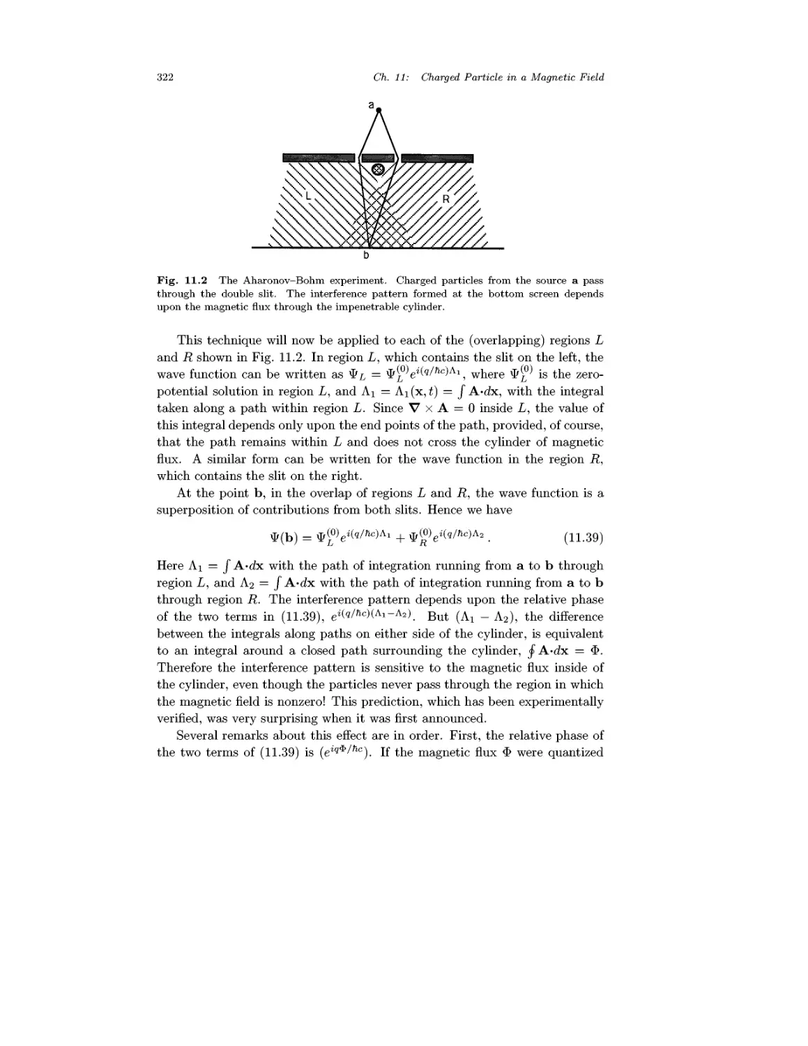
/


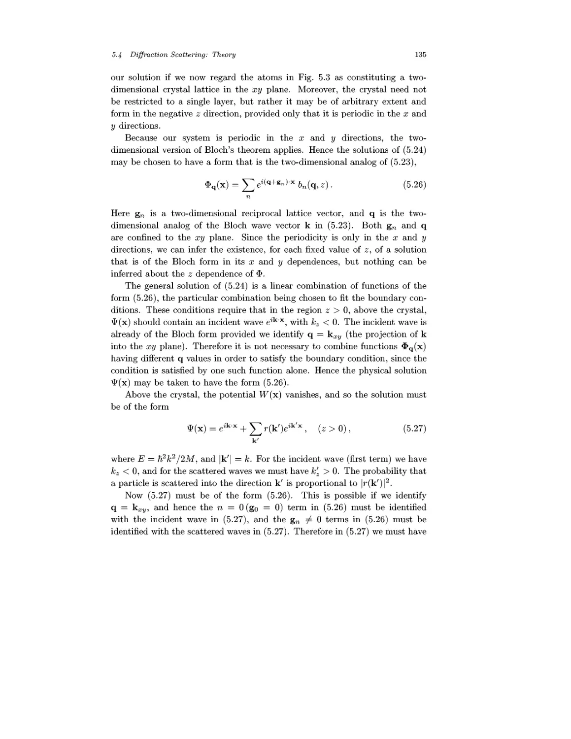


Текст
Quantum
Mechanics
A
Modern
Devetopment
K. HuHenune
Simon Frflser Universitv
Quantum
Mechanics
A Modern Development
This Page Intentionally Left Blank
Quantum
Mechanics
A Modern Development
Leslie E. Ballentine
Simon Fraser University
Published by
World Scientific Publishing Co. Pte. Ltd.
POBoi 128, Farrer Road, Singapore 9! 2805
USA office: Suite !B, 1060 Main Street, River Edge, NJ 07661
UK office: 57 Sbelton Street, Covent Garden, London WC2H 9HE
British Library Cataloguing-in-Publication Data
A catalogue record for this book is available from the British Library.
First published 1998
Reprinted 1999,2000
QUANTUM MECHANICS: A MODERN DEVELOPMENT
Copyright © 1998 by World Scientific Publishing Co. Pte. Ltd.
All rights reserved. This book, or parts thereof, may not be reproduced in any form or by any means,
electronic or mechanical, including photocopying, recording or any information storage and retrieval
system now known or to be invented, without written permission from the Publisher.
For photocopying of material in this volume, please pay a copying fee through the Copyright
Clearance Center, Inc., 222 Rosewood Drive, Danvers, MA 01923, USA. In this case permission to
photocopy is not required from the publisher.
ISBN 981-02-4105-4 (pbk)
Contents
Preface xi
Introduction: The Phenomena of Quantum Mechanics 1
Chapter 1 Mathematical Prerequisites 7
1.1 Linear Vector Space 7
1.2 Linear Operators 11
1.3 Self-Adjoint Operators 15
1.4 Hilbert Space and Rigged Hilbert Space 26
1.5 Probability Theory 29
Problems 38
Chapter 2 The Formulation of Quantum Mechanics 42
2.1 Basic Theoretical Concepts 42
2.2 Conditions on Operators 48
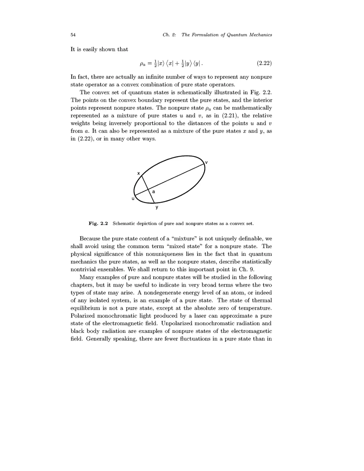
2.3 General States and Pure States 50
2.4 Probability Distributions 55
Problems 60
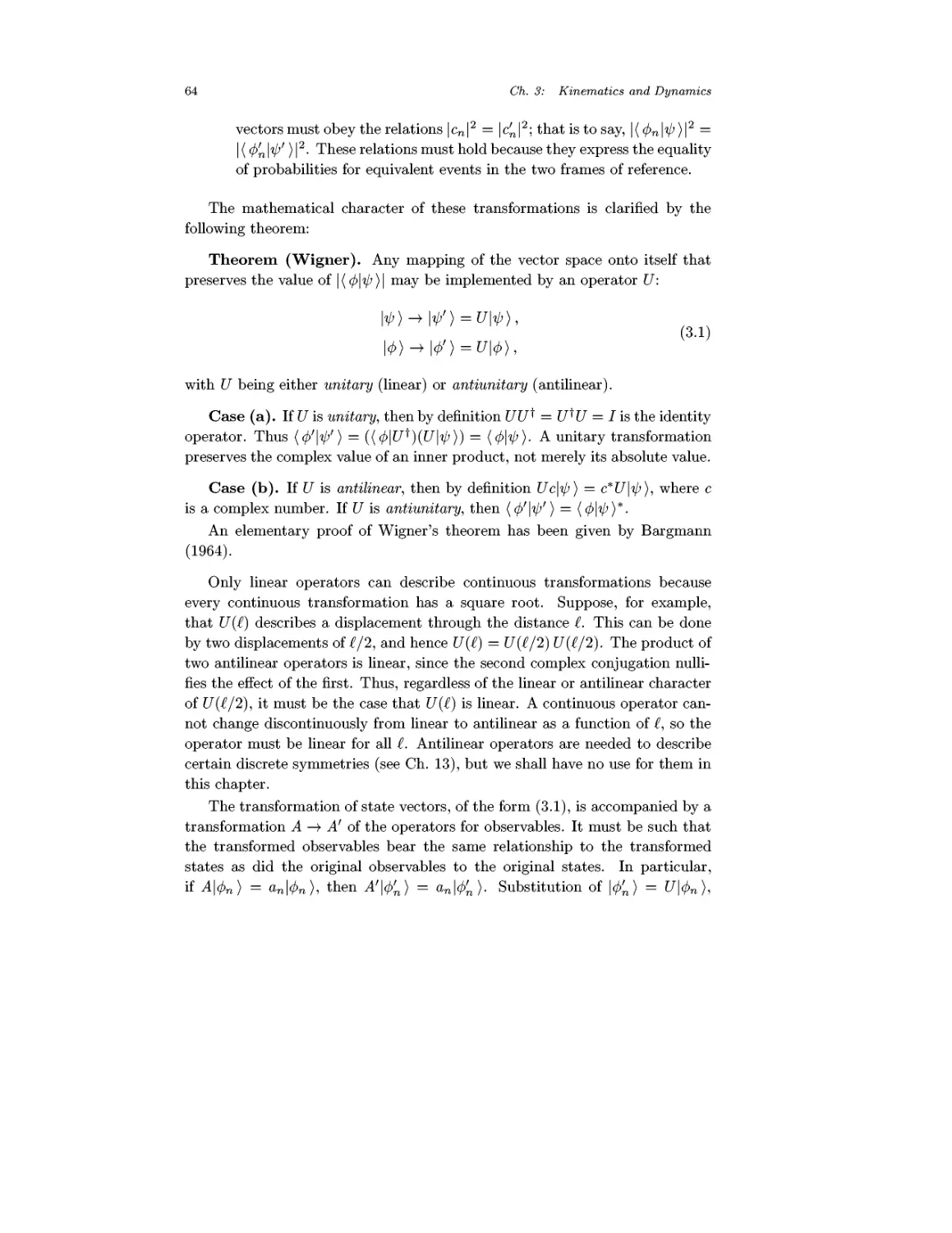
Chapter 3 Kinematics and Dynamics 63
3.1 Transformations of States and Observables 63
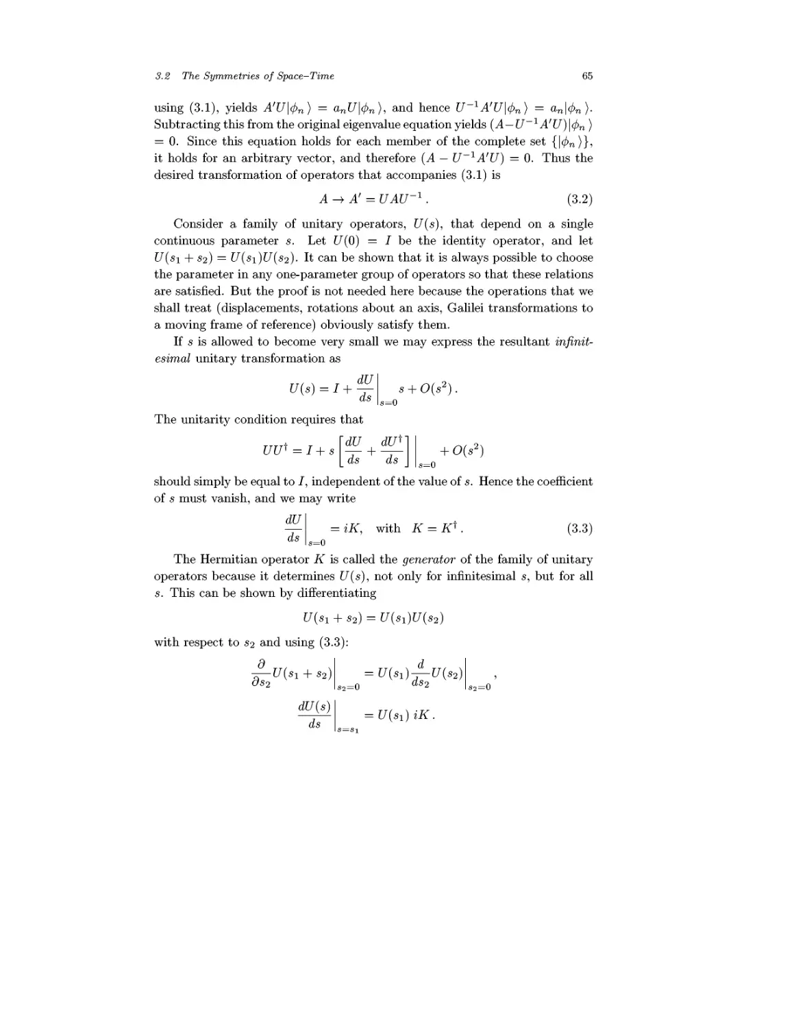
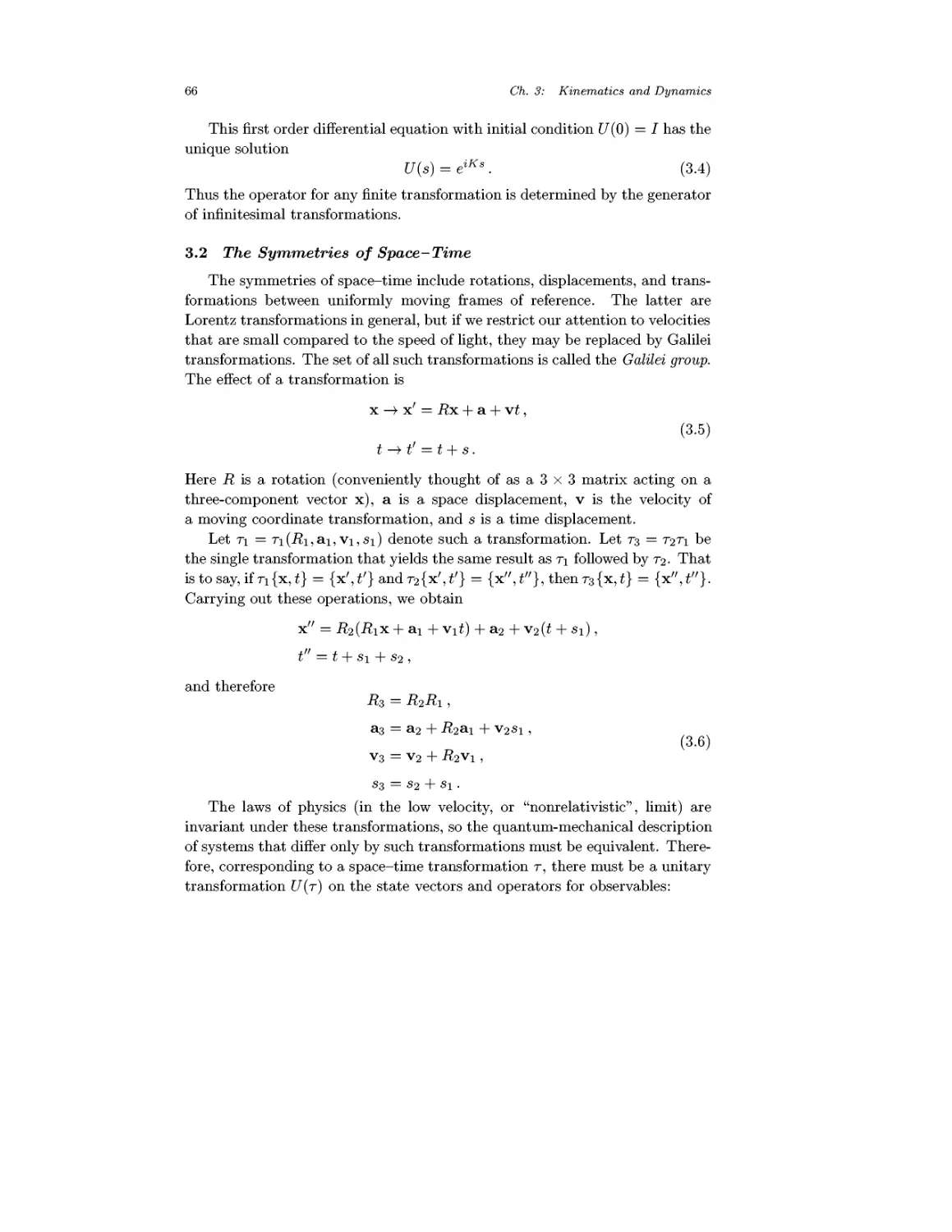
3.2 The Symmetries of Space-Time 66
3.3 Generators of the Galilei Group 68
3.4 Identification of Operators with Dynamical Variables 76
3.5 Composite Systems 85
3.6 [[ Quantizing a Classical System ]] 87
3.7 Equations of Motion 89
3.8 Symmetries and Conservation Laws 92
Problems 94
Chapter 4 Coordinate Representation and Applications 97
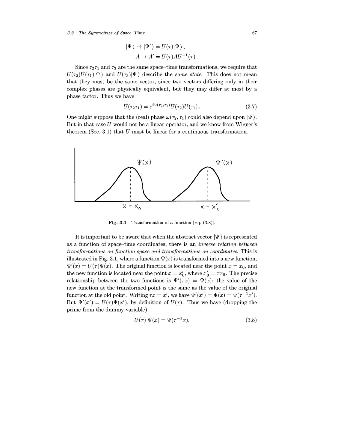
4.1 Coordinate Representation 97
4.2 The Wave Equation and Its Interpretation 98
4.3 Galilei Transformation of Schrodinger's Equation 102
Chapter 5
Chapter 6
Chapter 7
Chapter 8
4.4
4.5
4.6
4.7
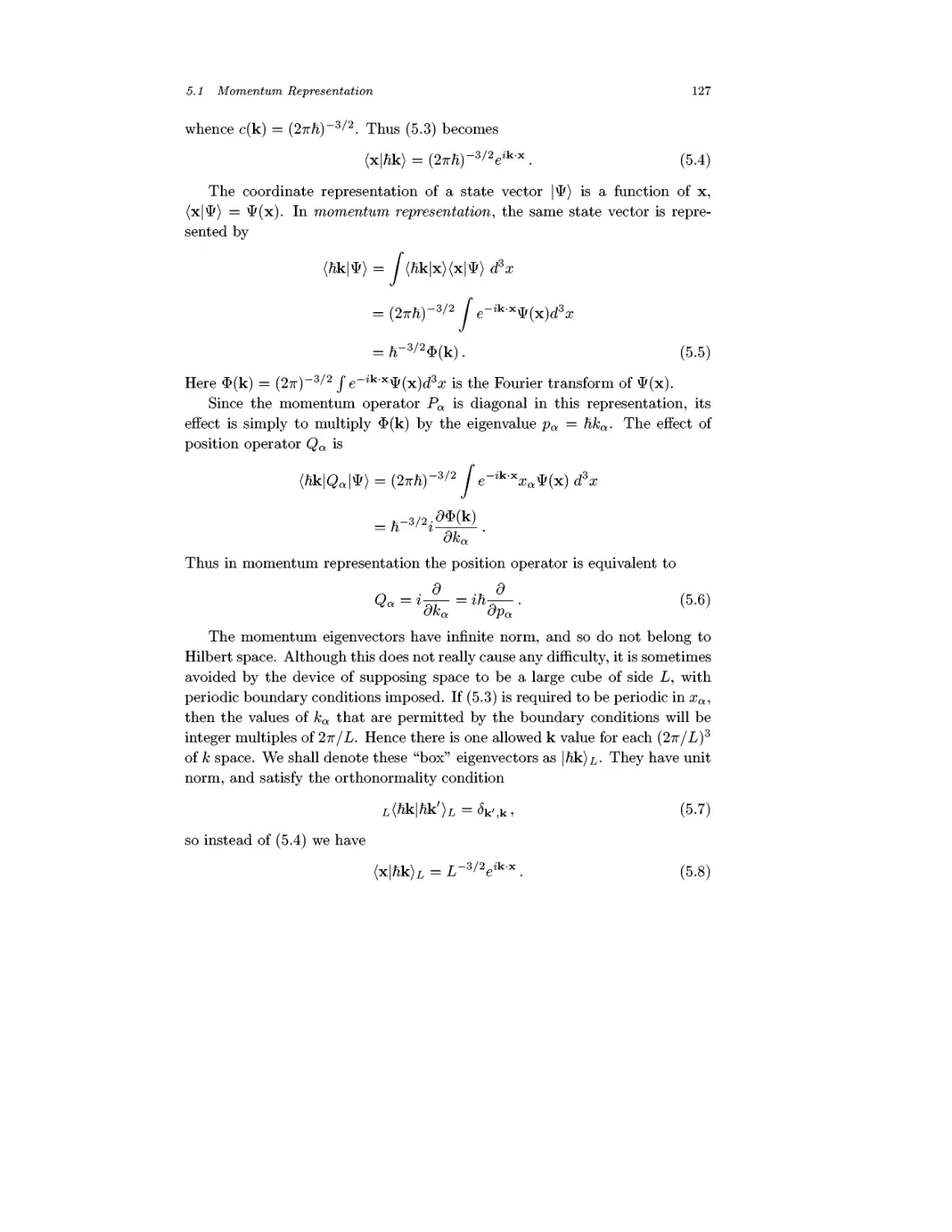
4.8
Probability Flux
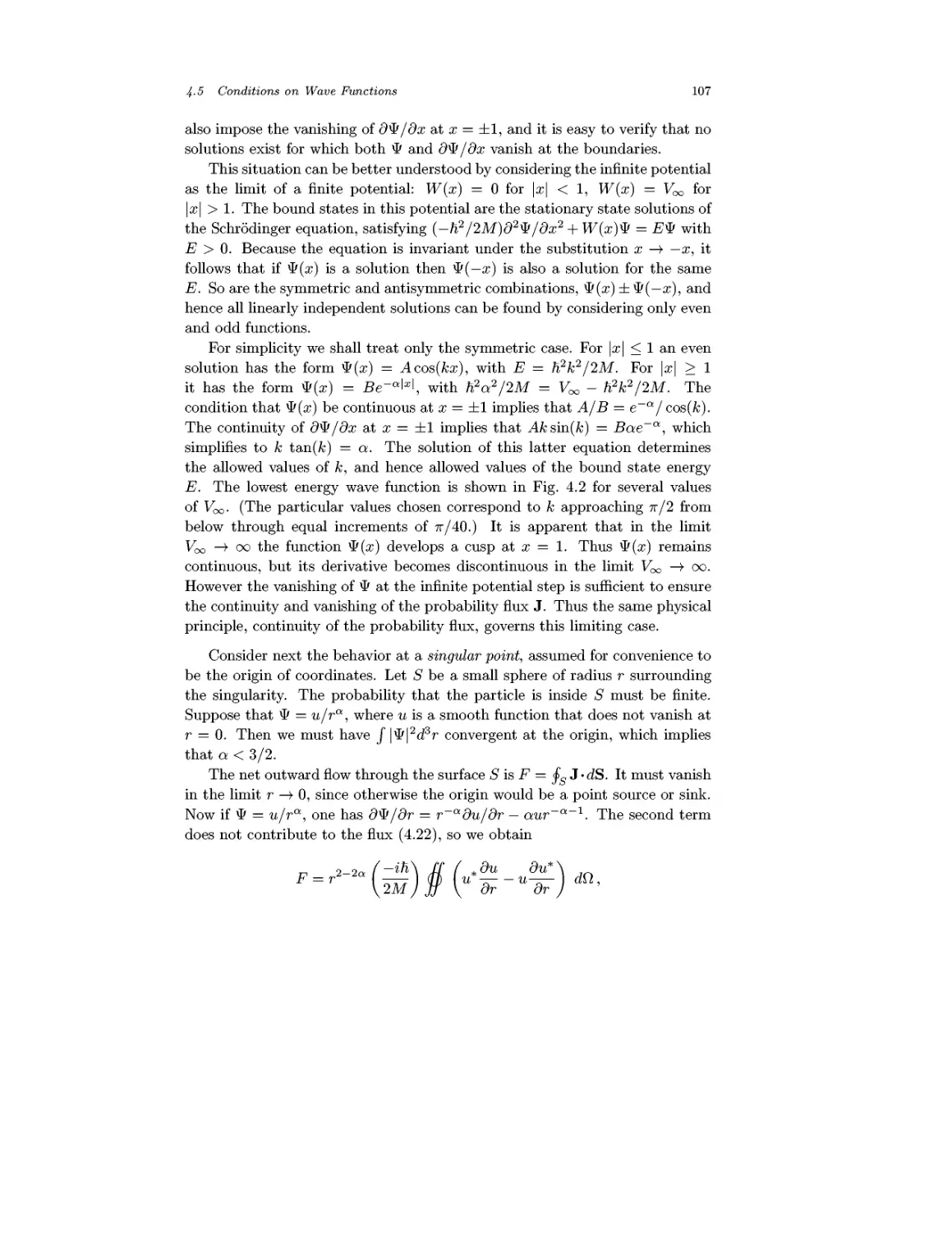
Conditions on Wave Functions
Energy Eigenfunctions for Free Particles
Tunneling
Path Integrals
Problems
Contents
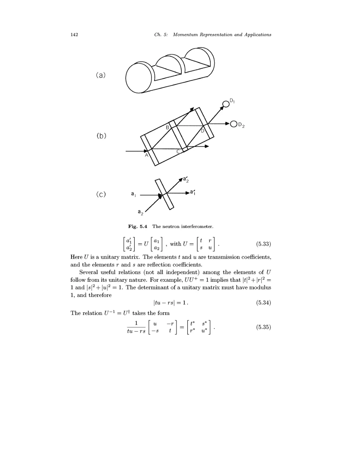
Momentum Representation and Applications
5.1
5.2
5.3
5.4
5.5
5.6
Momentum Representation
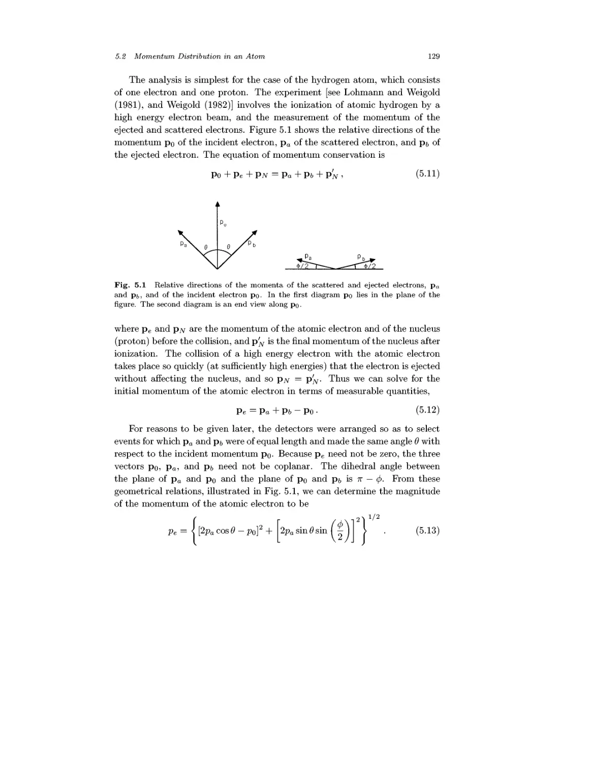
Momentum Distribution in an Atom
Bloch's Theorem
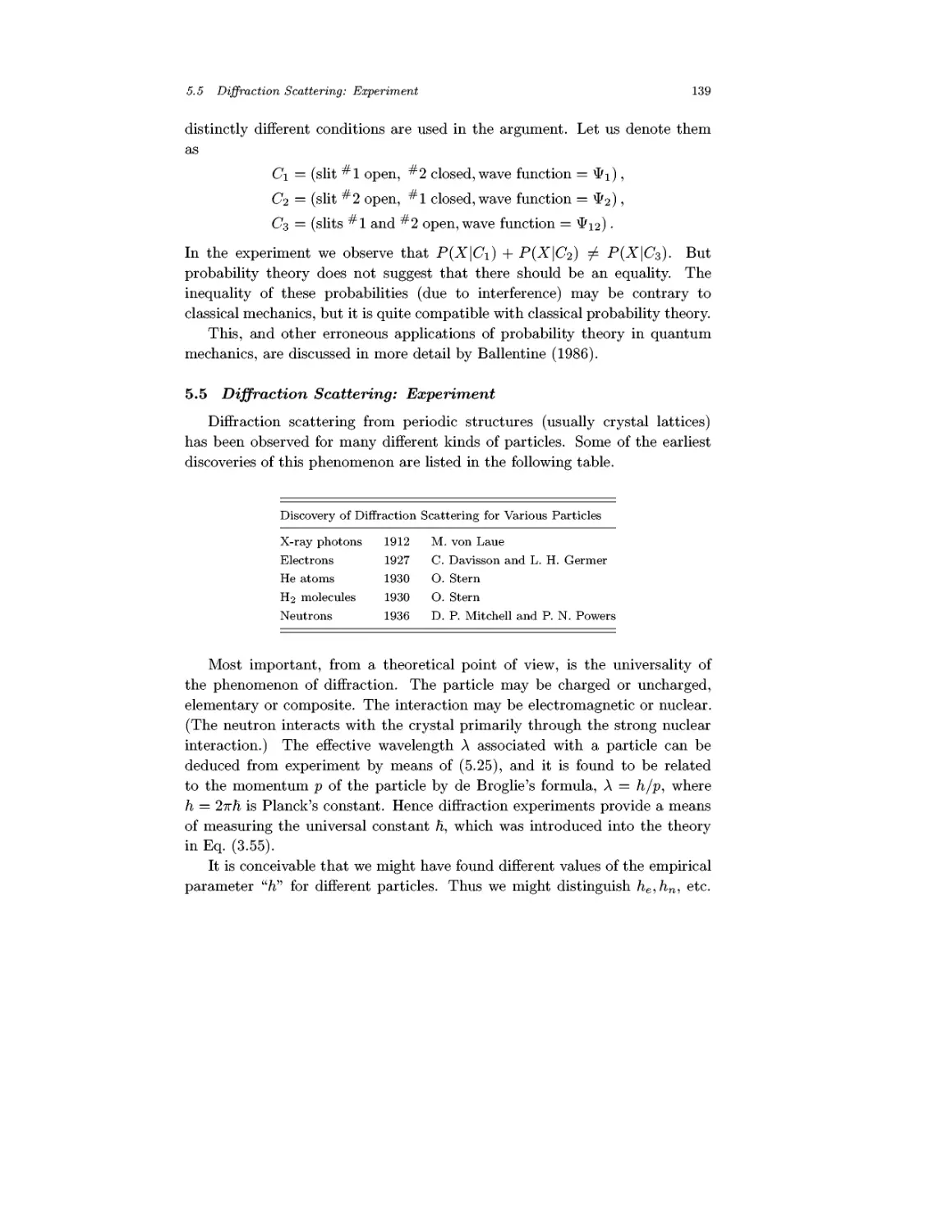
Diffraction Scattering: Theory
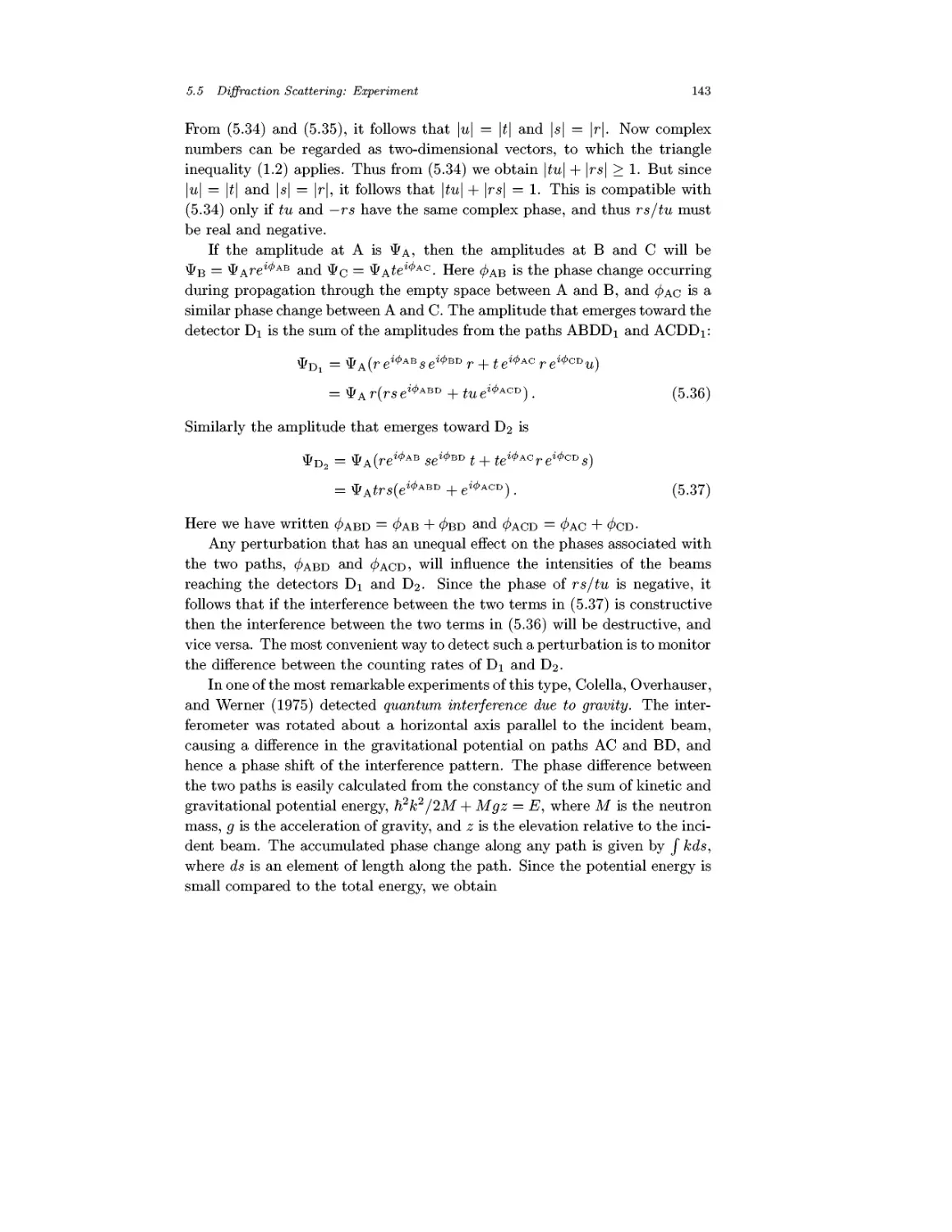
Diffraction Scattering: Experiment
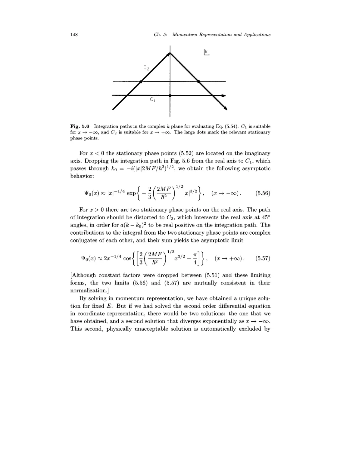
Motion in a Uniform Force Field
Problems
The Harmonic Oscillator
6.1
6.2
6.3
Algebraic Solution
Solution in Coordinate Representation
Solution in H Representation
Problems
Angular Momentum
7.1
7.2
7.3
7.4
7.5
7.6
7.7
7.8
7.9
Eigenvalues and Matrix Elements
Explicit Form of the Angular Momentum
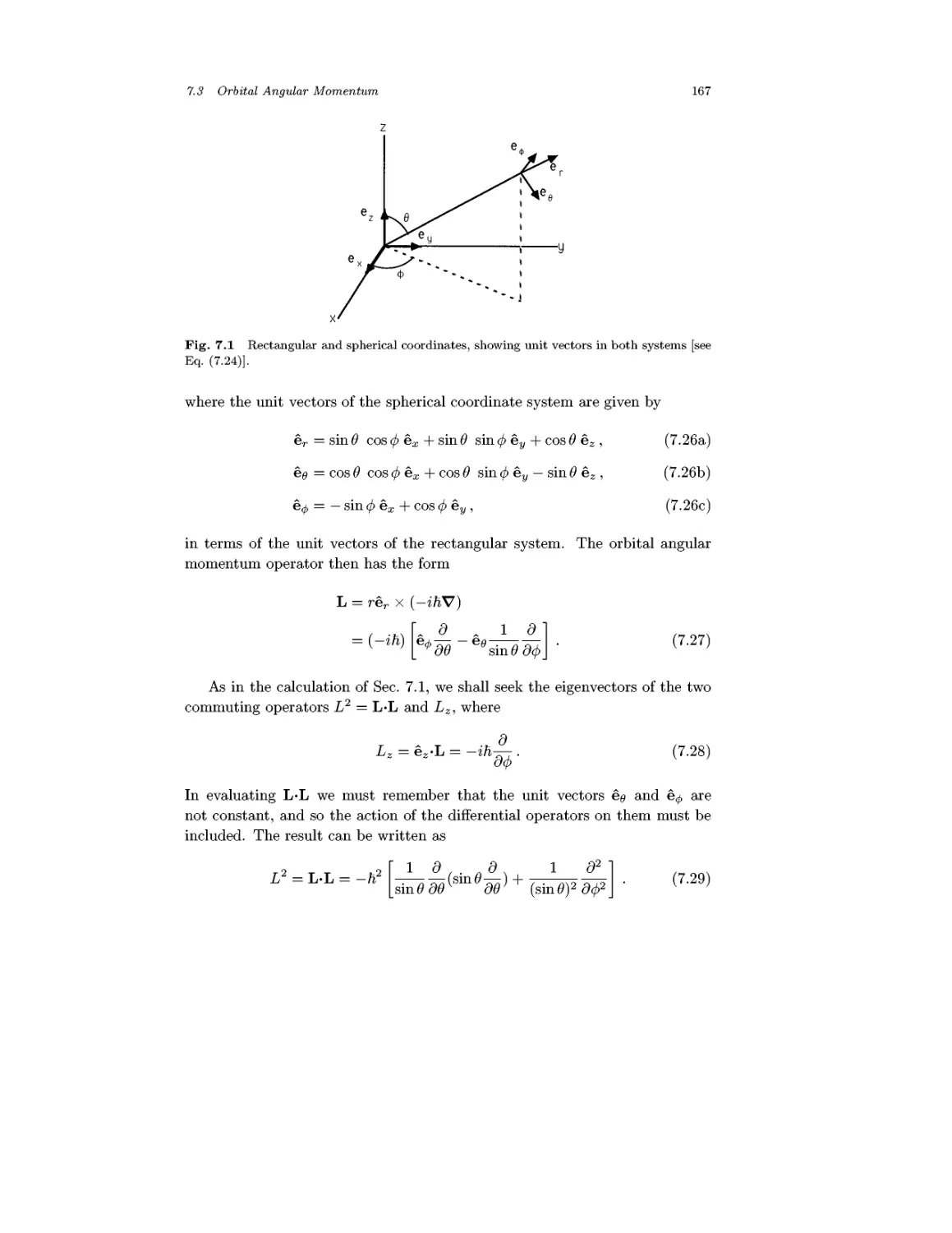
Orbital Angular Momentum
Spin
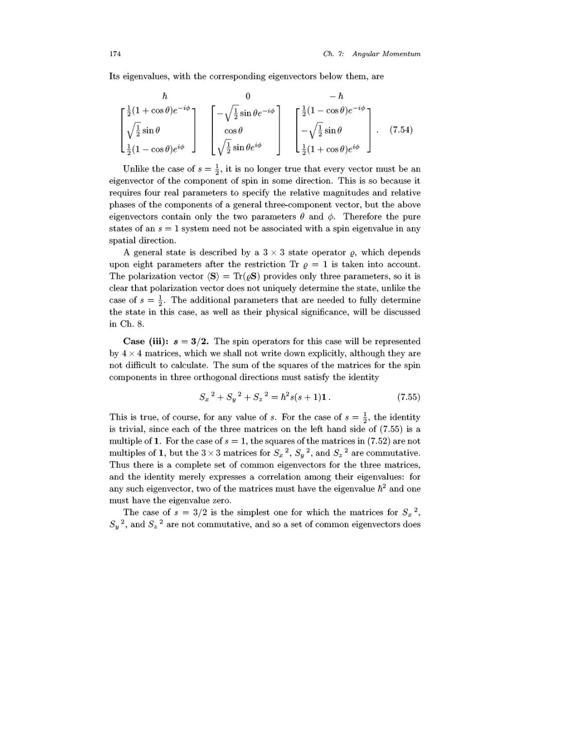
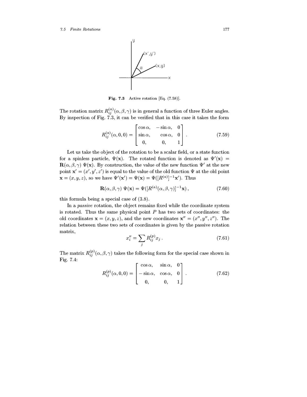
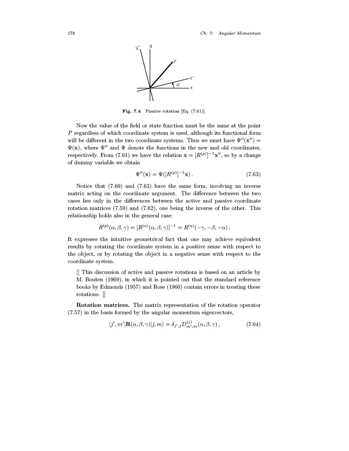
Finite Rotations
Rotation Through 2?r
Addition of Angular Momenta
Irreducible Tensor Operators
Rotational Motion of a Rigid Body
Problems
State Preparation and Determination
8.1
8.2
8.3
8.4
State Preparation
State Determination
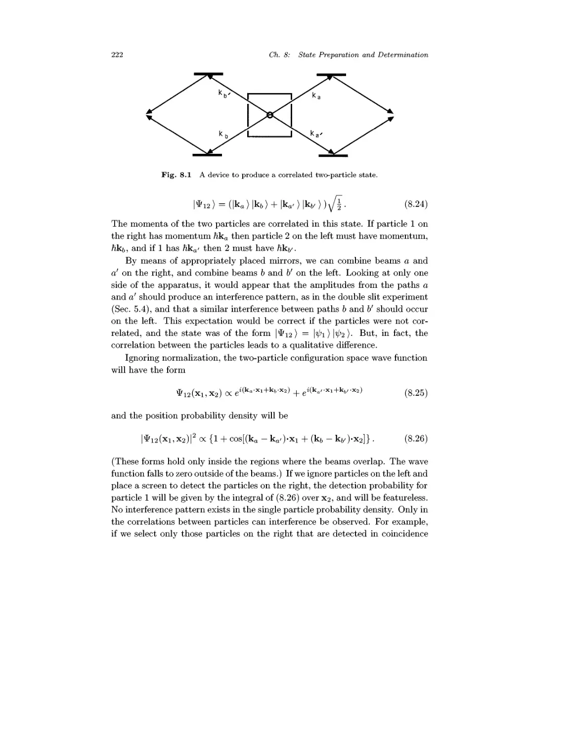
States of Composite Systems
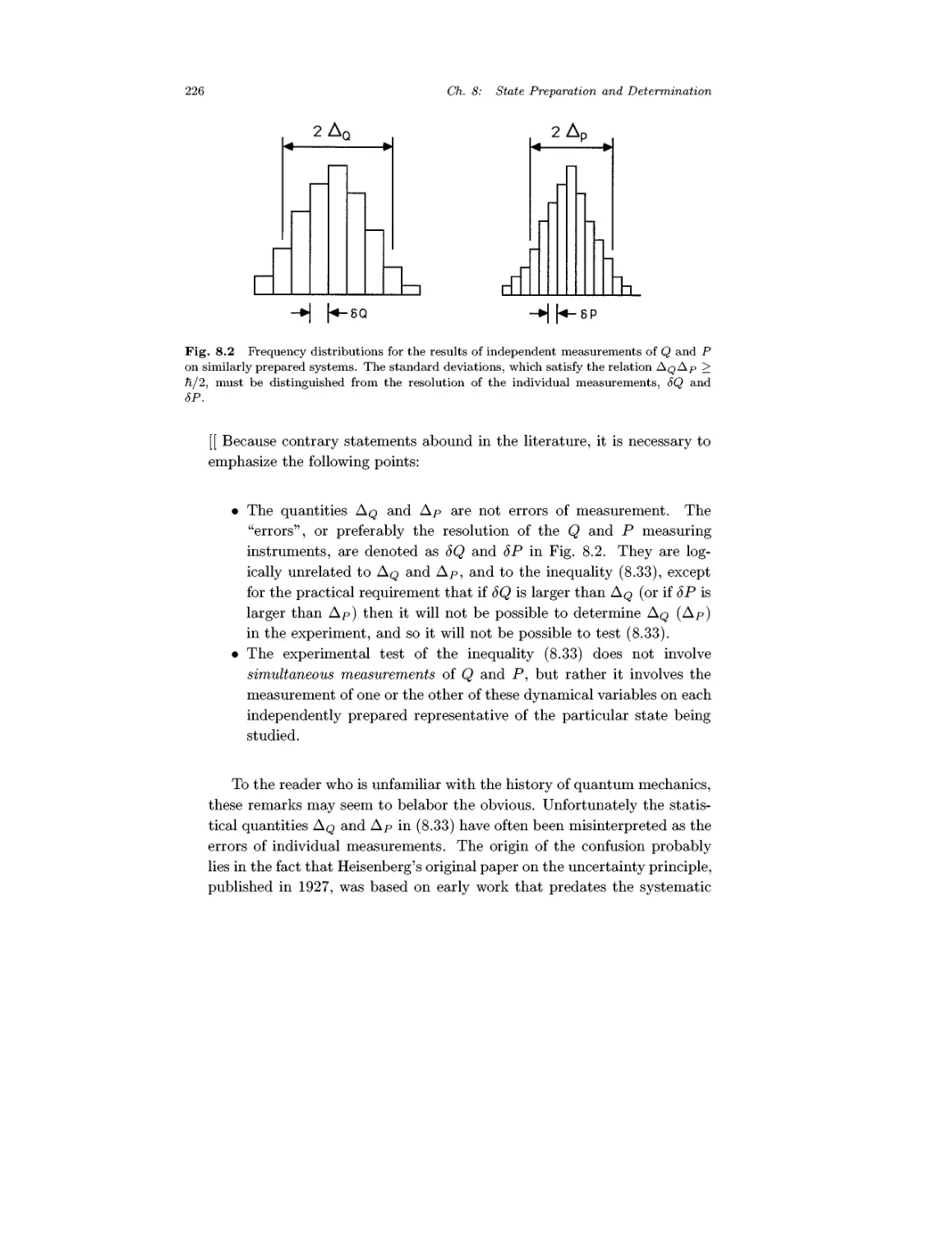
Indeterminacy Relations
Problems
Operators
104
106
109
110
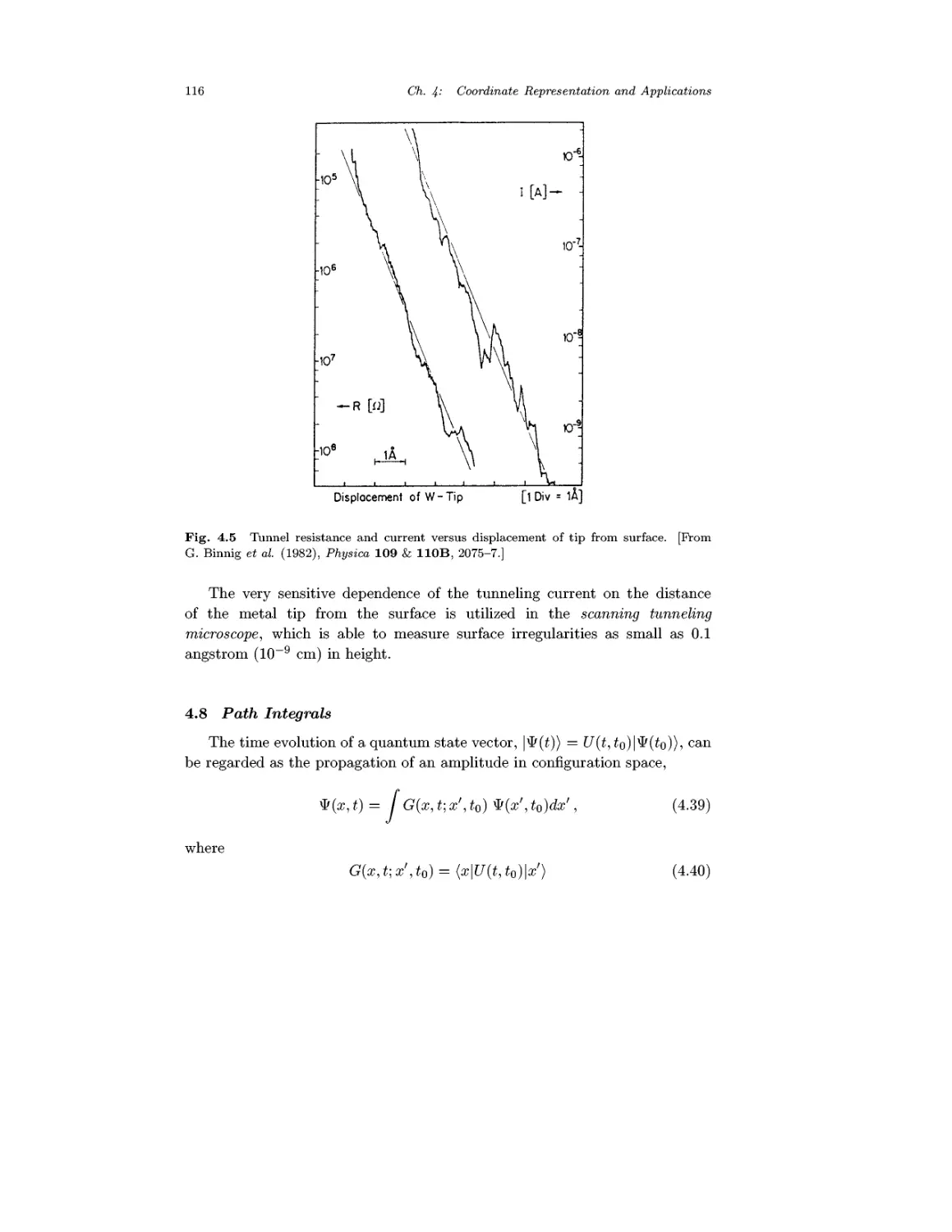
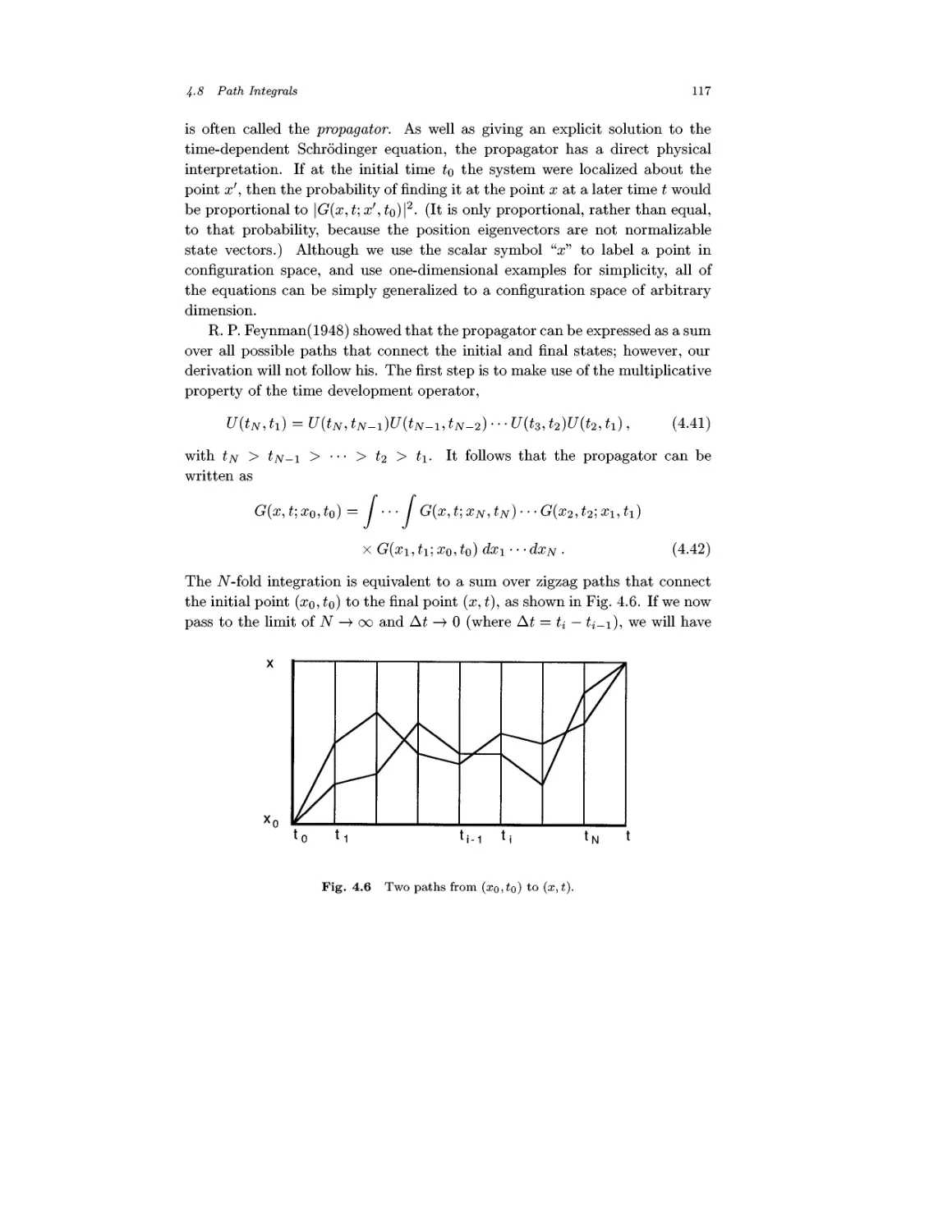
116
123
126
126
128
131
133
139
145
149
151
151
154
157
158
160
160
164
166
171
175
182
185
193
200
203
206
206
210
216
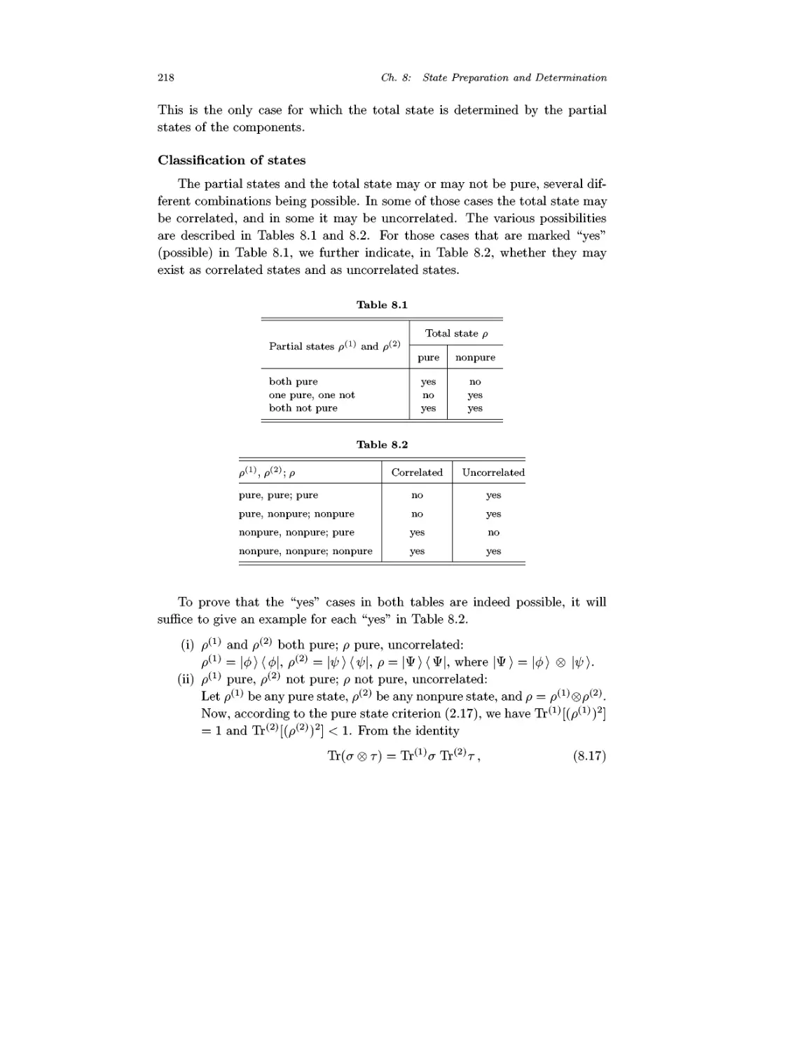
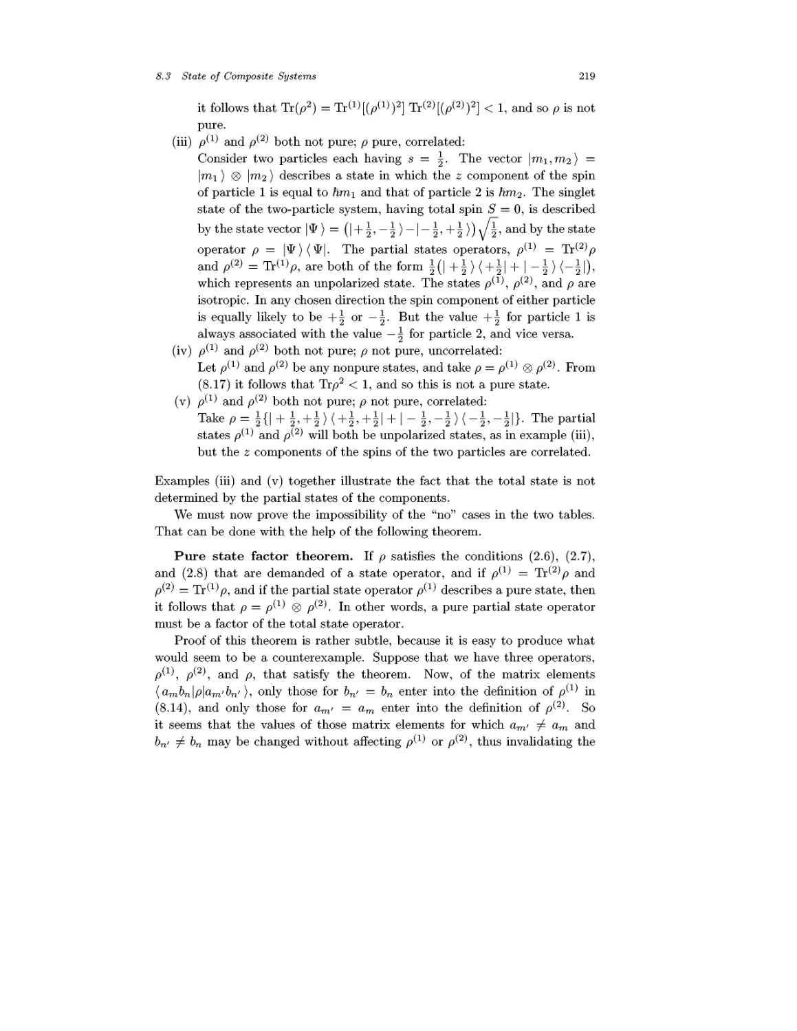
223
227
Contents vii
Chapter 9 Measurement and the Interpretation of States 230
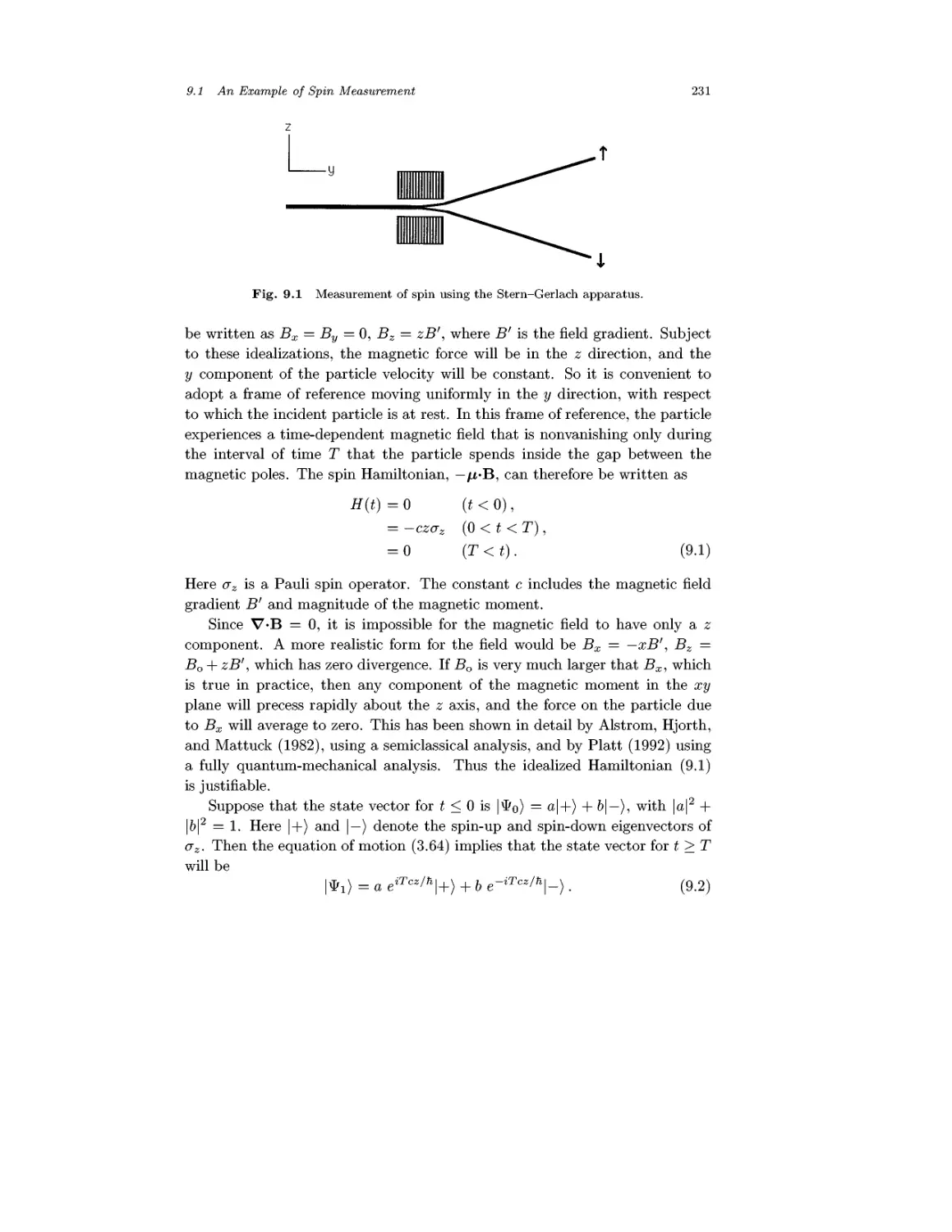
9.1 An Example of Spin Measurement 230
9.2 A General Theorem of Measurement Theory 232
9.3 The Interpretation of a State Vector 234
9.4 Which Wave Function? 238
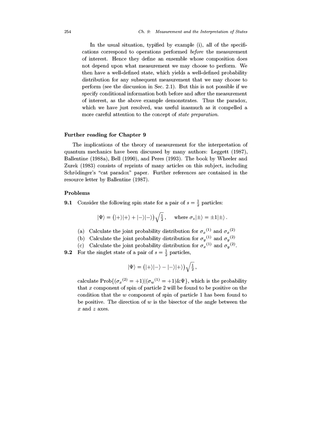
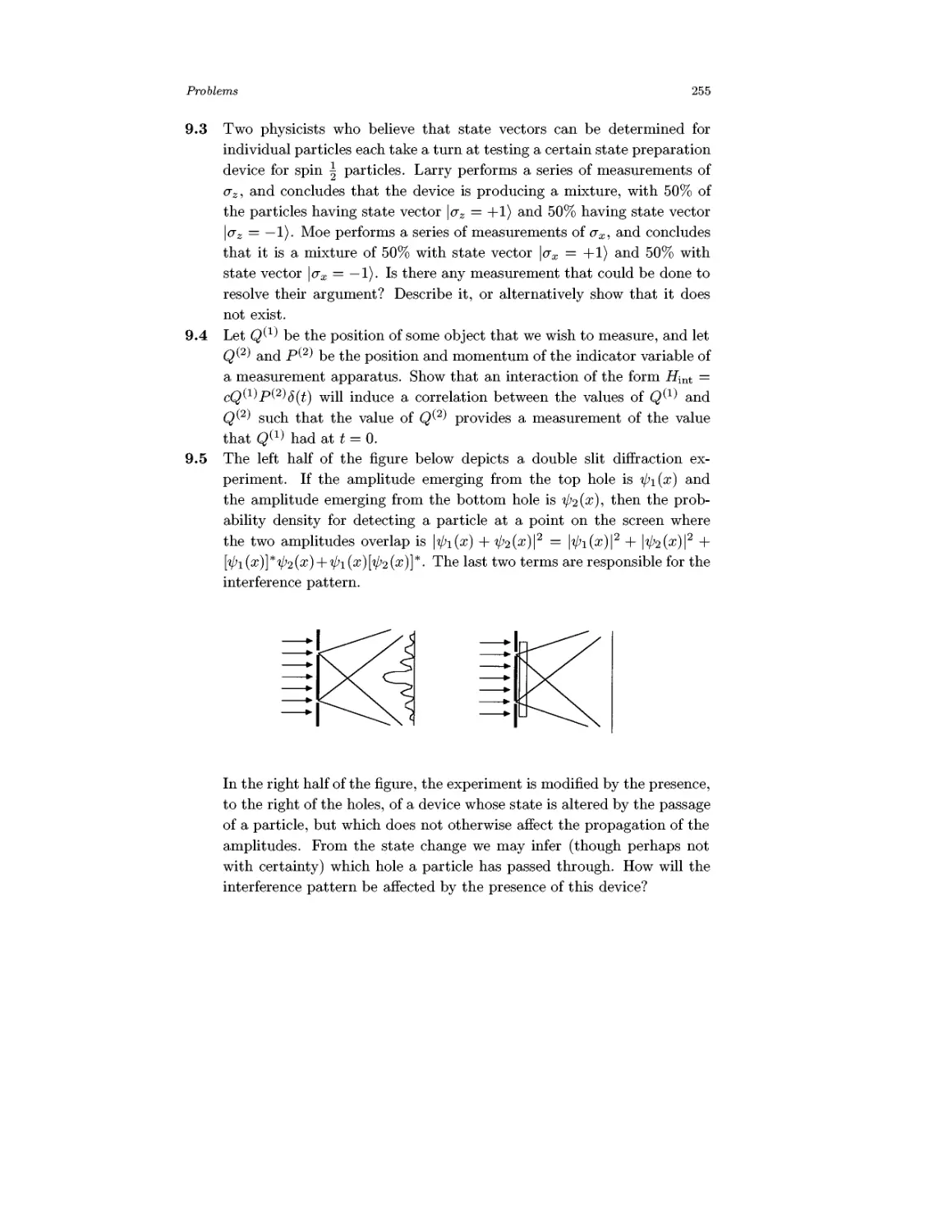
9.5 Spin Recombination Experiment 241
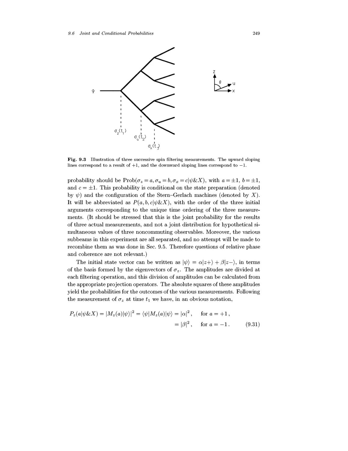
9.6 Joint and Conditional Probabilities 244
Problems 254
Chapter 10 Formation of Bound States 258
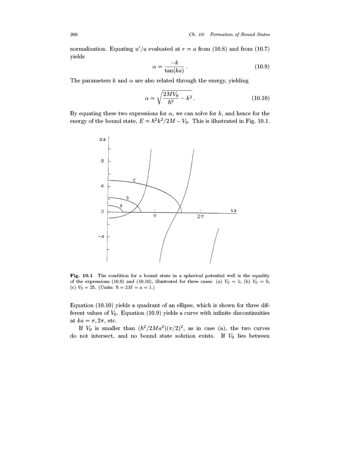
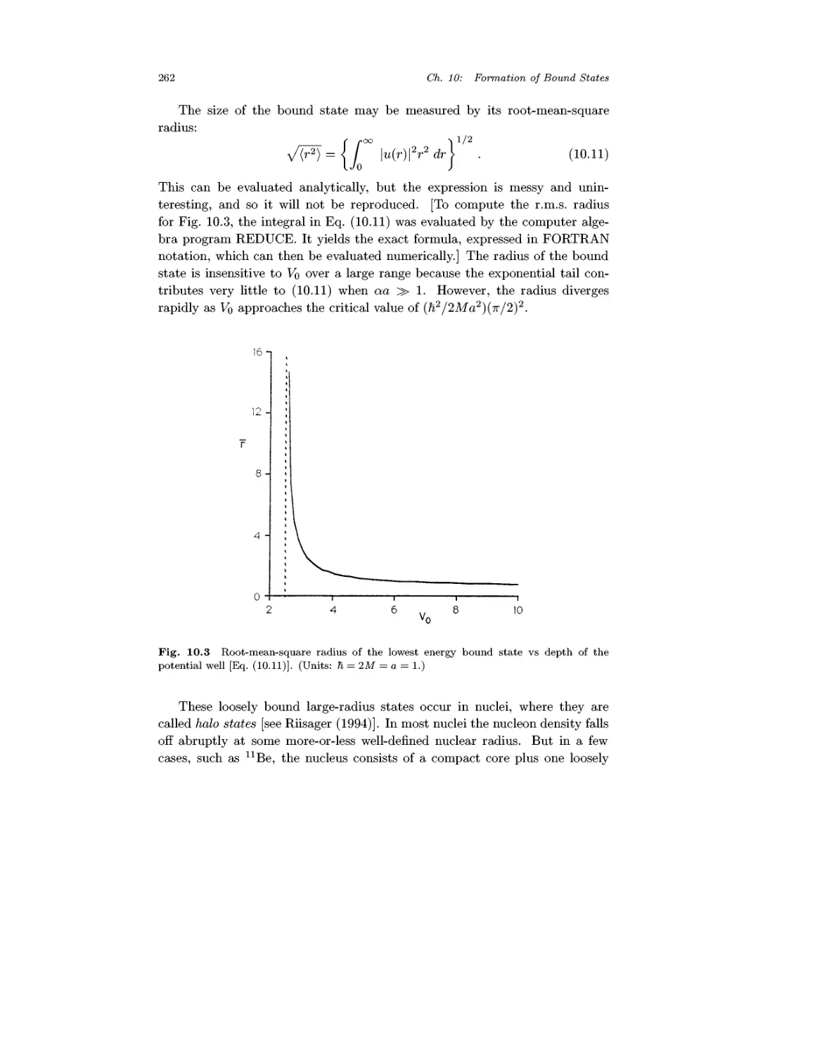
10.1 Spherical Potential Well 258
10.2 The Hydrogen Atom 263
10.3 Estimates from Indeterminacy Relations 271
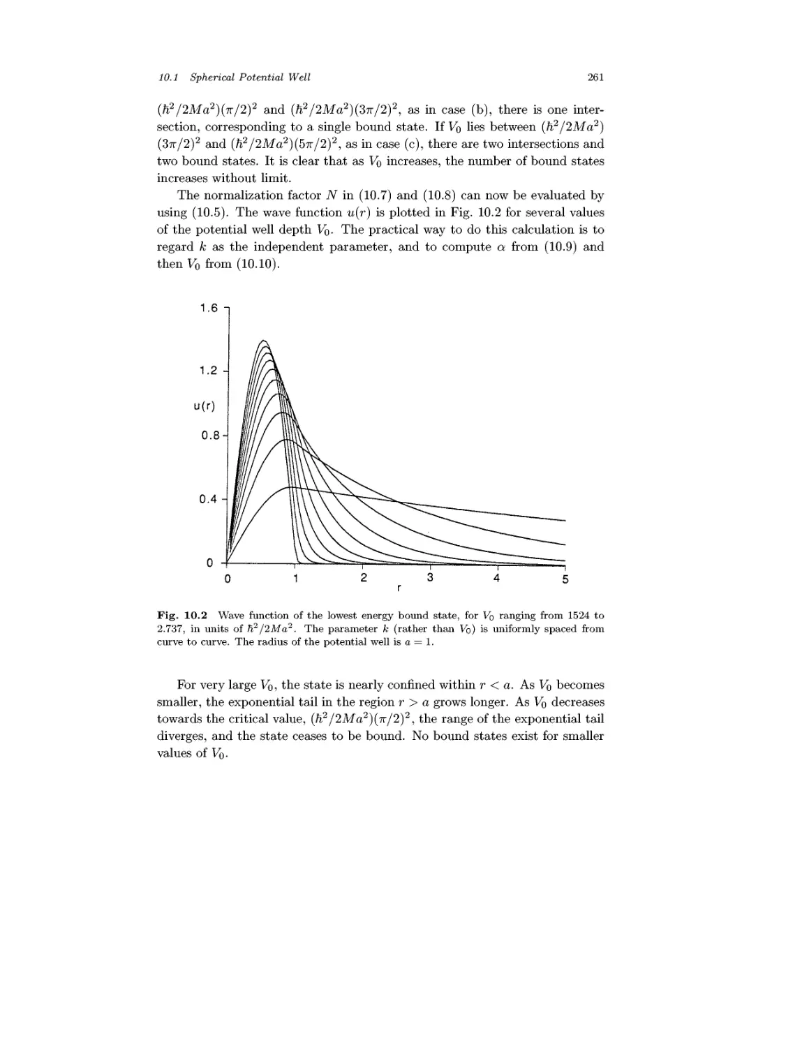
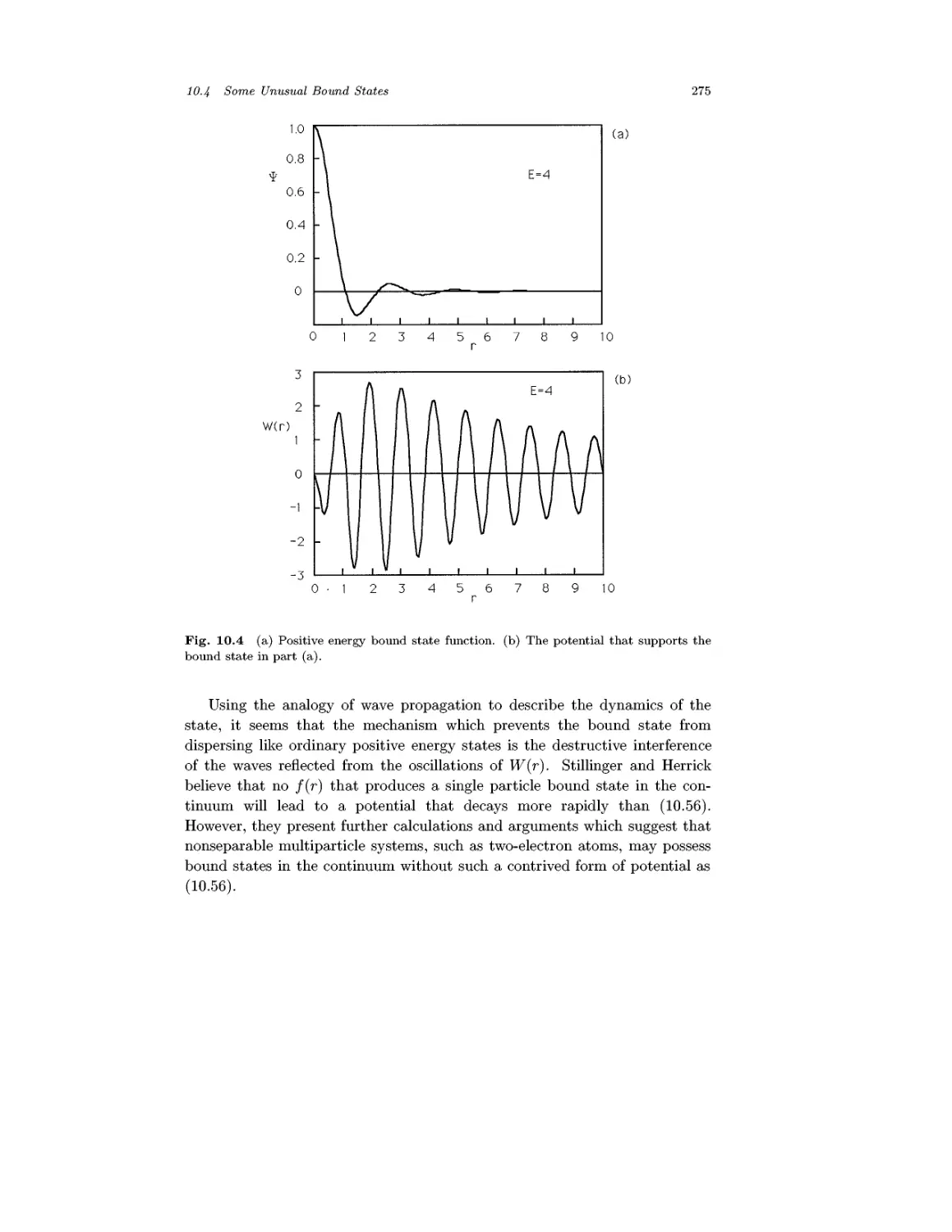
10.4 Some Unusual Bound States 273
10.5 Stationary State Perturbation Theory 276
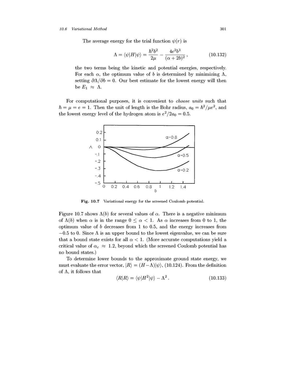
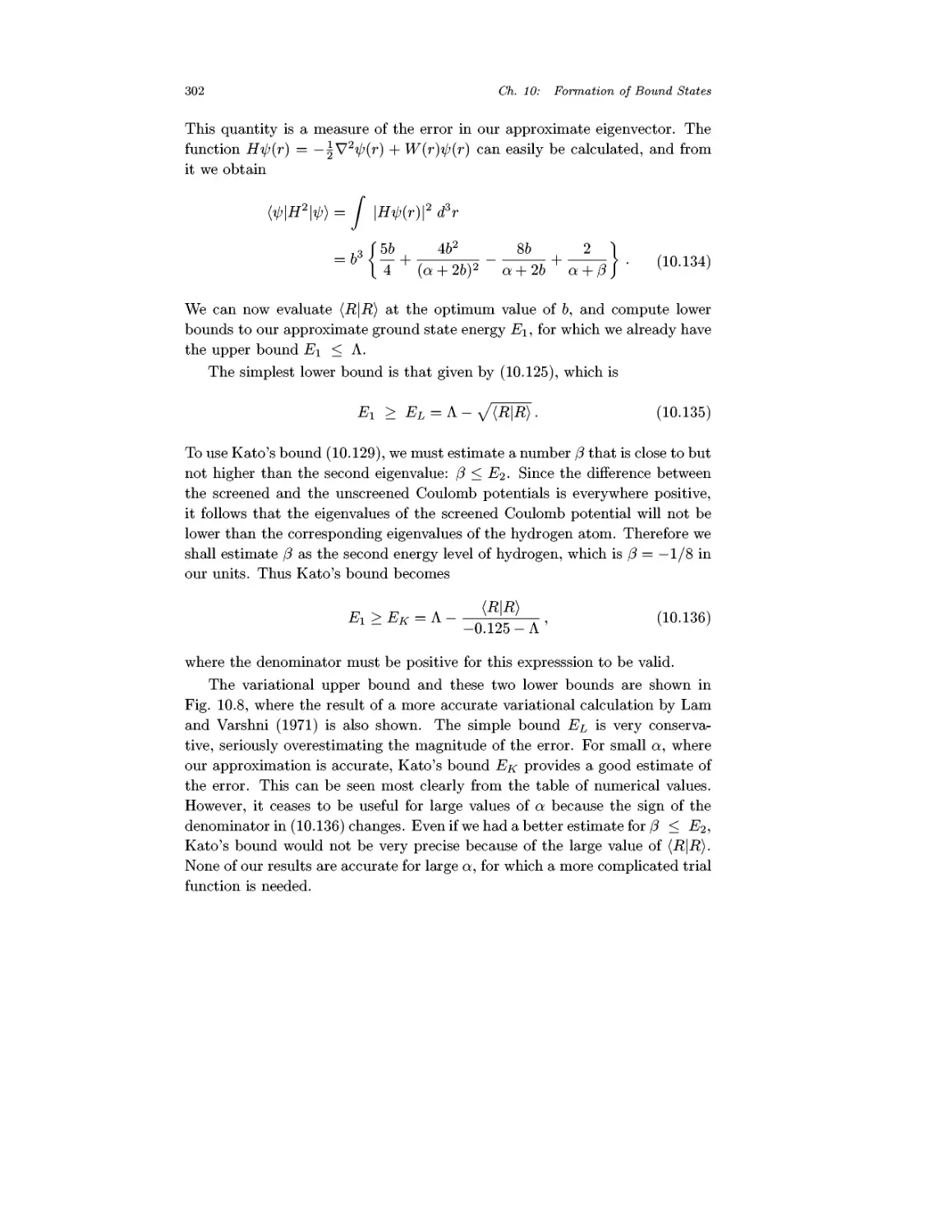
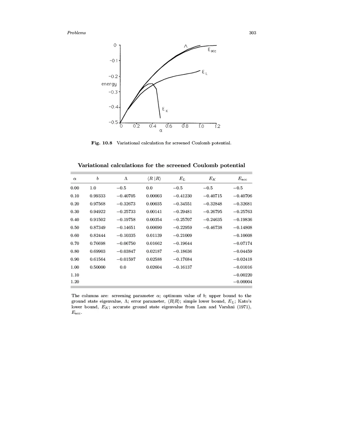
10.6 Variational Method 290
Problems 304
Chapter 11 Charged Particle in a Magnetic Field 307
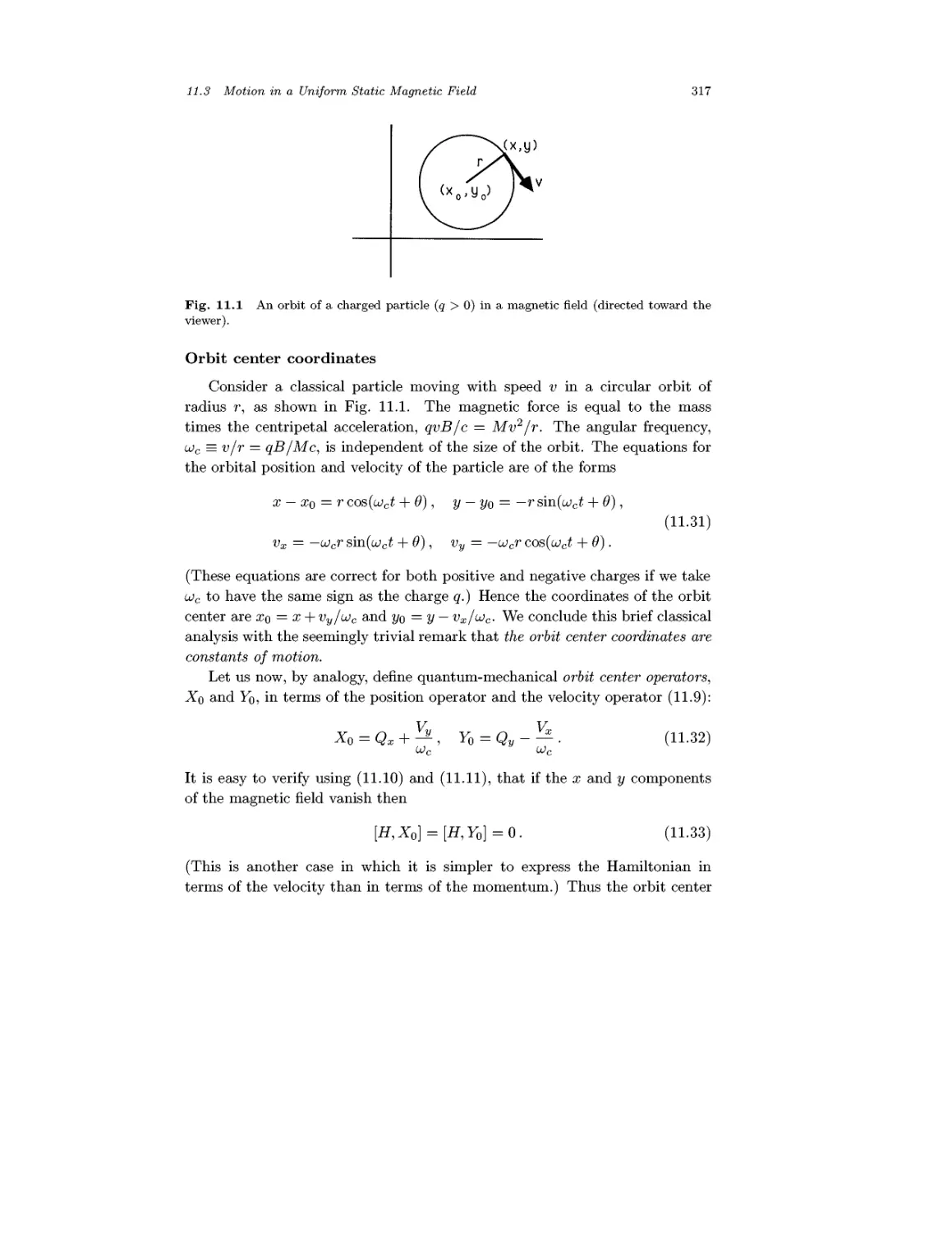
11.1 Classical Theory 307
11.2 Quantum Theory 309
11.3 Motion in a Uniform Static Magnetic Field 314
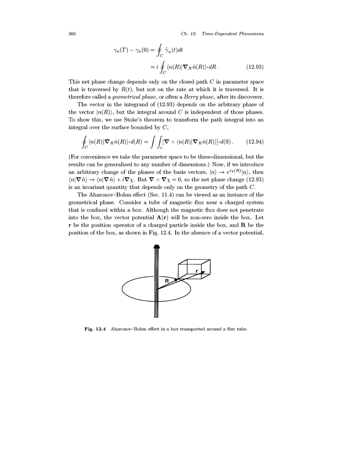
11.4 The Aharonov-Bohm Effect 321
11.5 The Zeeman Effect 325
Problems 330
Chapter 12 Time-Dependent Phenomena 332
12.1 Spin Dynamics 332
12.2 Exponential and Nonexponential Decay 338
12.3 Energy-Time Indeterminacy Relations 343
12.4 Quantum Beats 347
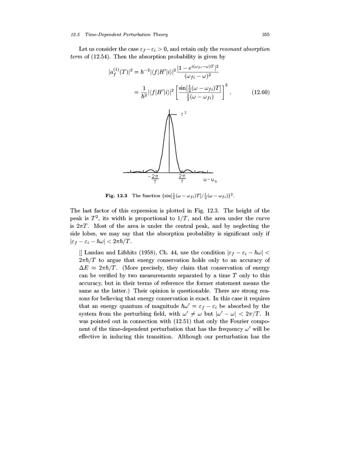
12.5 Time-Dependent Perturbation Theory 349
12.6 Atomic Radiation 356
12.7 Adiabatic Approximation 363
Problems 367
Chapter 13 Discrete Symmetries 370
13.1 Space Inversion 370
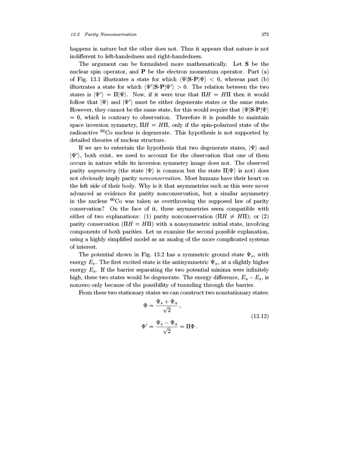
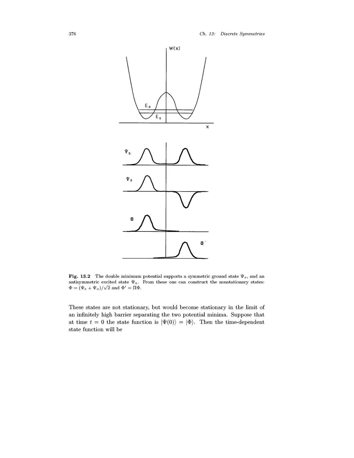
13.2 Parity Nonconservation 374
13.3 Time Reversal 377
Problems 386
viii Contents
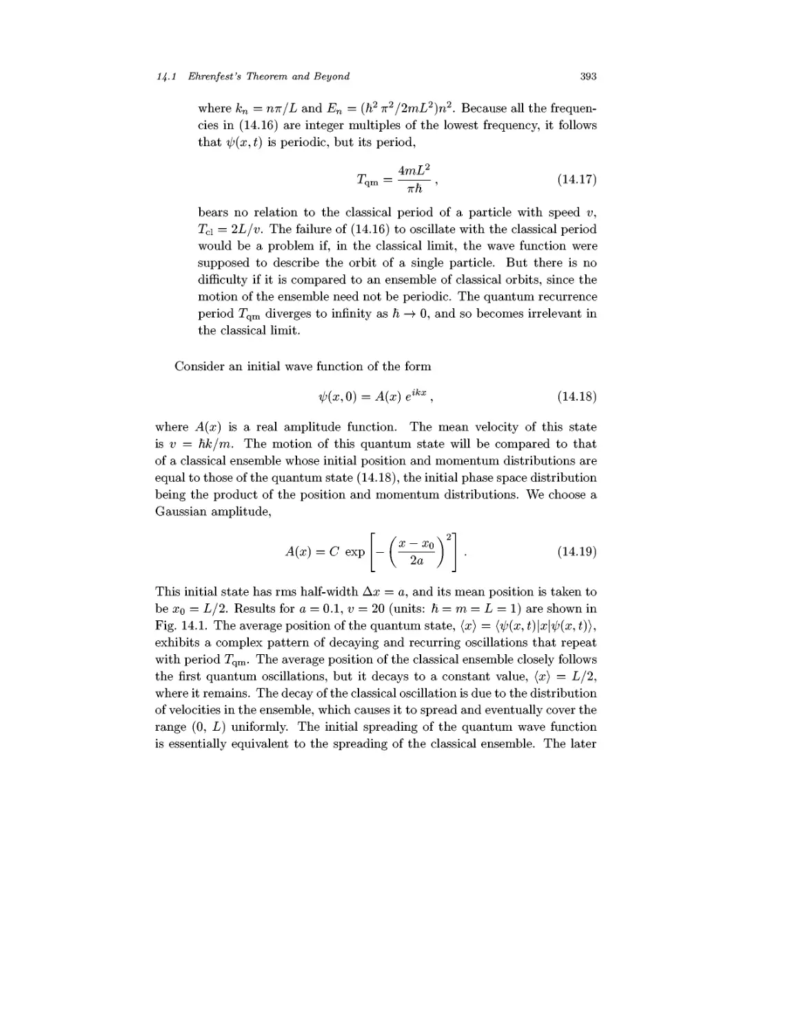
Chapter 14 The Classical Limit 388
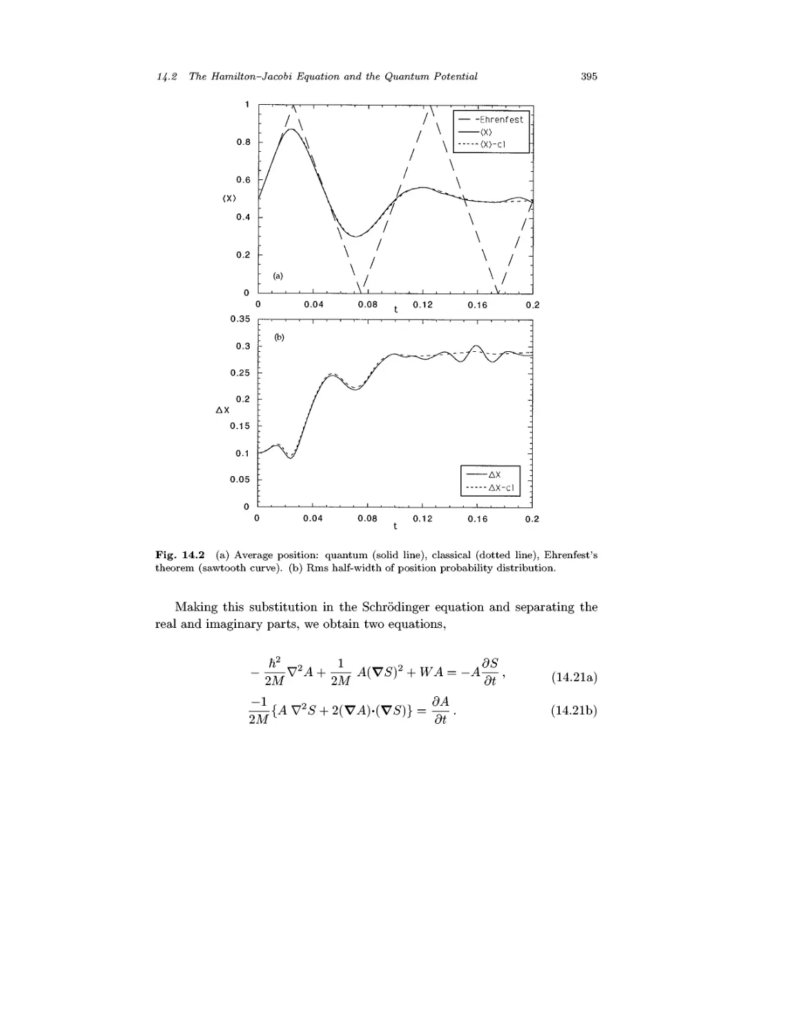
14.1 Ehrenfest's Theorem and Beyond 389
14.2 The Hamilton-Jacobi Equation and the
Quantum Potential 394
14.3 Quantal Trajectories 398
14.4 The Large Quantum Number Limit 400
Problems 404
Chapter 15 Quantum Mechanics in Phase Space 406
15.1 Why Phase Space Distributions? 406
15.2 The Wigner Representation 407
15.3 The Husimi Distribution 414
Problems 420
Chapter 16 Scattering 421
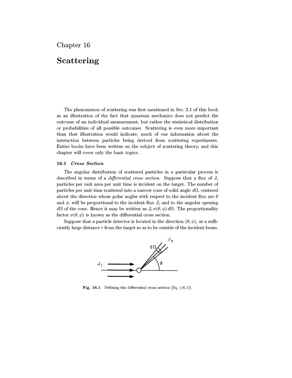
16.1 Cross Section 421
16.2 Scattering by a Spherical Potential 427
16.3 General Scattering Theory 433
16.4 Born Approximation and DWBA 441
16.5 Scattering Operators 447
16.6 Scattering Resonances 458
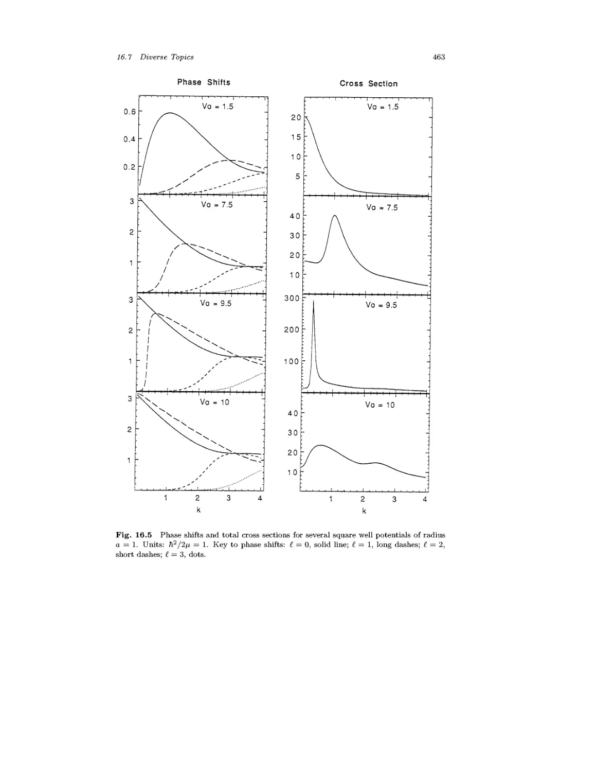
16.7 Diverse Topics 462
Problems 468
Chapter 17 Identical Particles 470
17.1 Permutation Symmetry 470
17.2 Indistinguishability of Particles 472
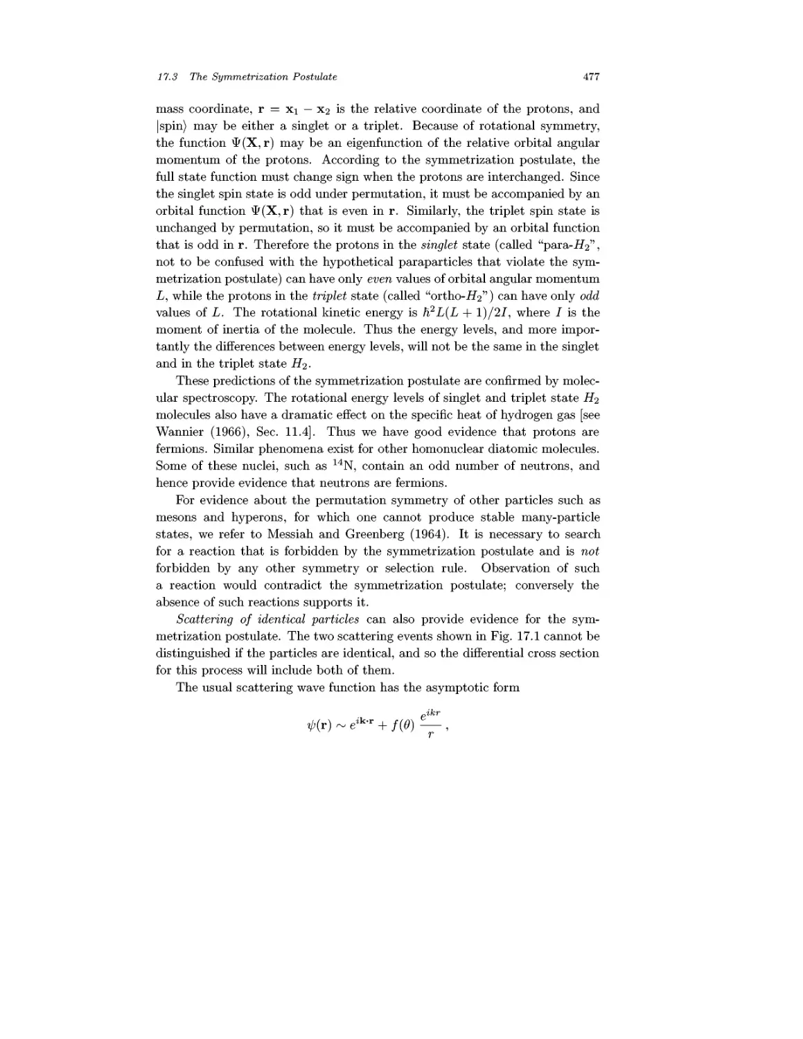
17.3 The Symmetrization Postulate 474
17.4 Creation and Annihilation Operators 478
Problems 492
Chapter 18 Many-Fermion Systems 493
18.1 Exchange 493
18.2 The Hartree-Fock Method 499
18.3 Dynamic Correlations 506
18.4 Fundamental Consequences for Theory 513
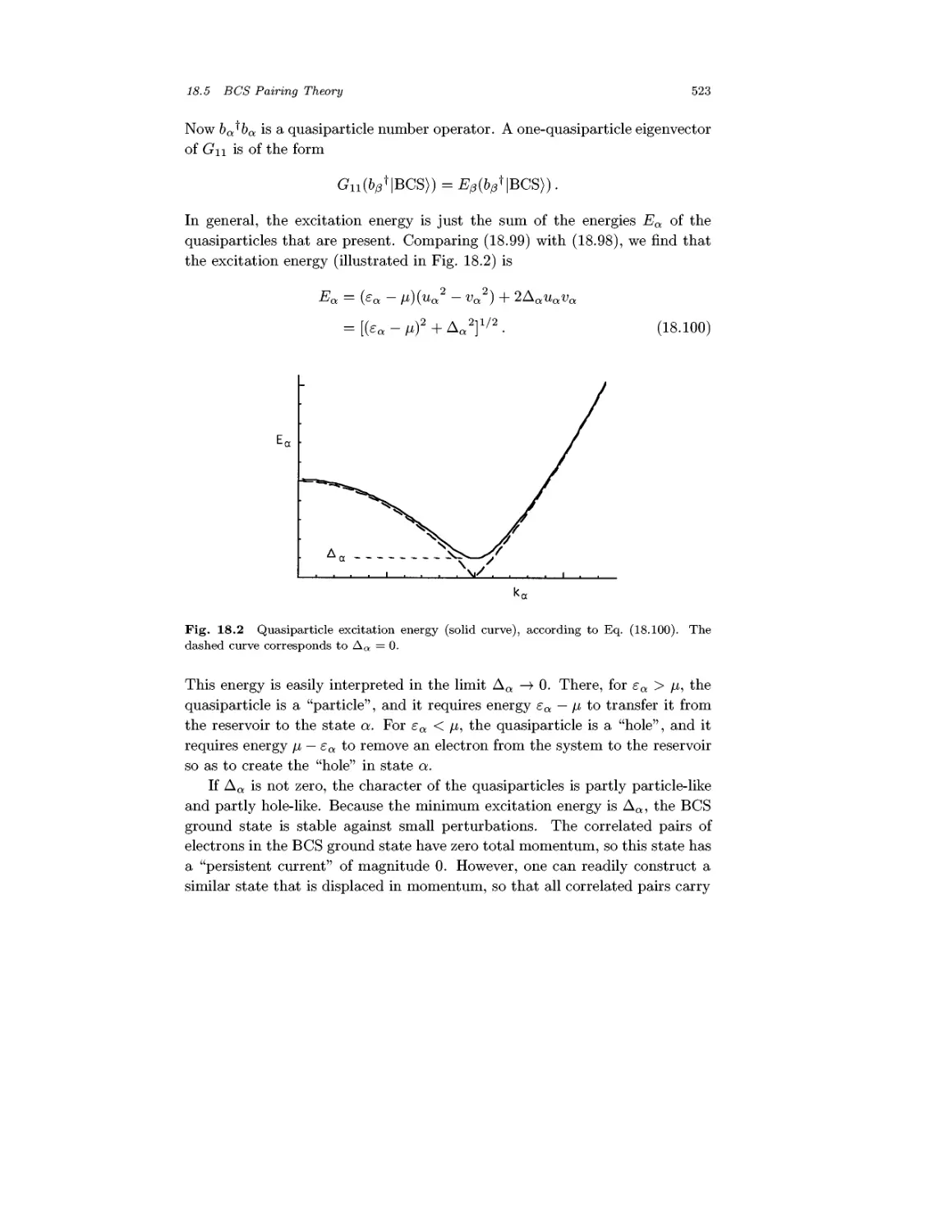
18.5 BCS Pairing Theory 514
Problems 525
Chapter 19 Quantum Mechanics of the
Electromagnetic Field 526
19.1 Normal Modes of the Field 526
19.2 Electric and Magnetic Field Operators 529
Contents ix
19.3 Zero-Point Energy and the Casimir Force 533
19.4 States of the EM Field 539
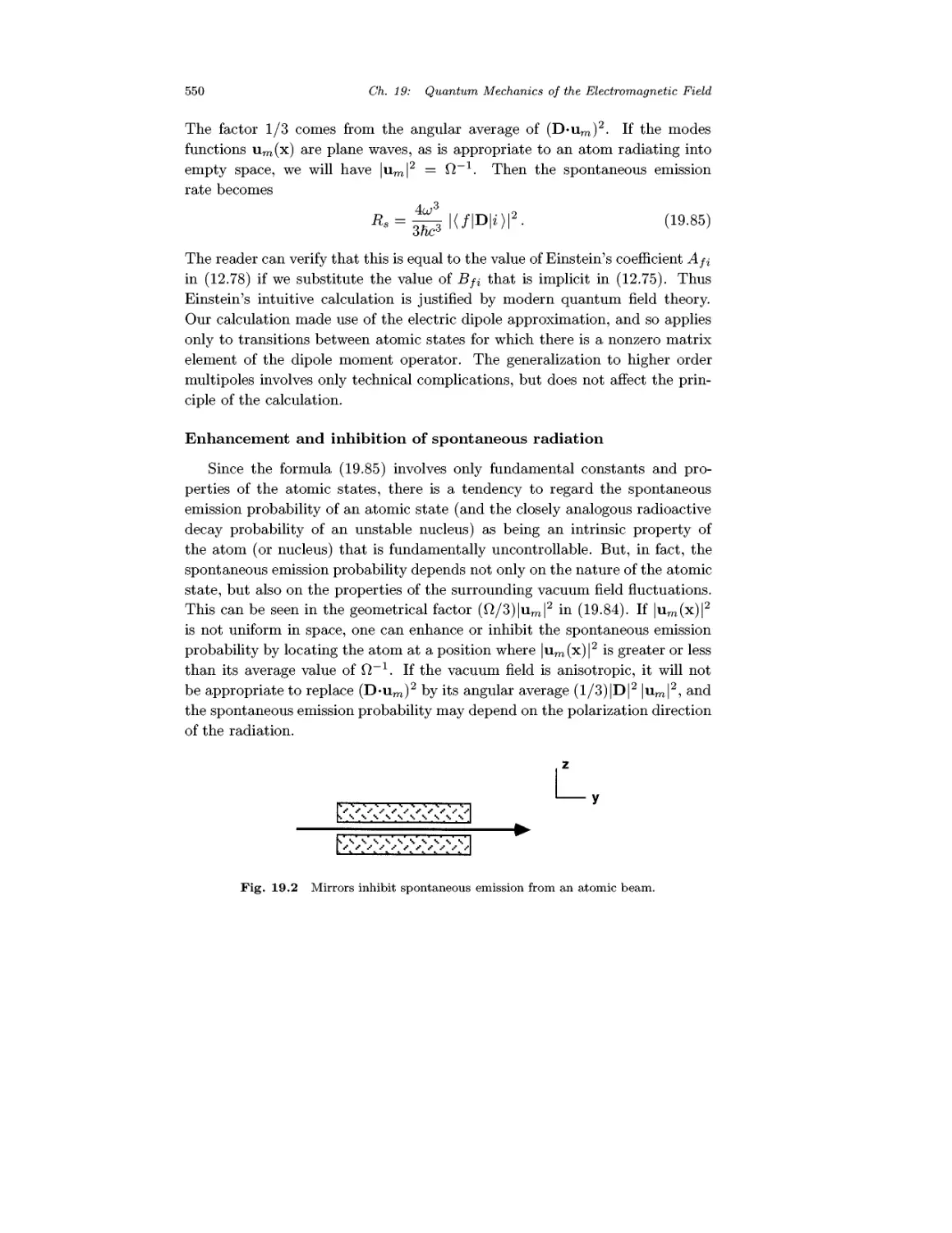
19.5 Spontaneous Emission 548
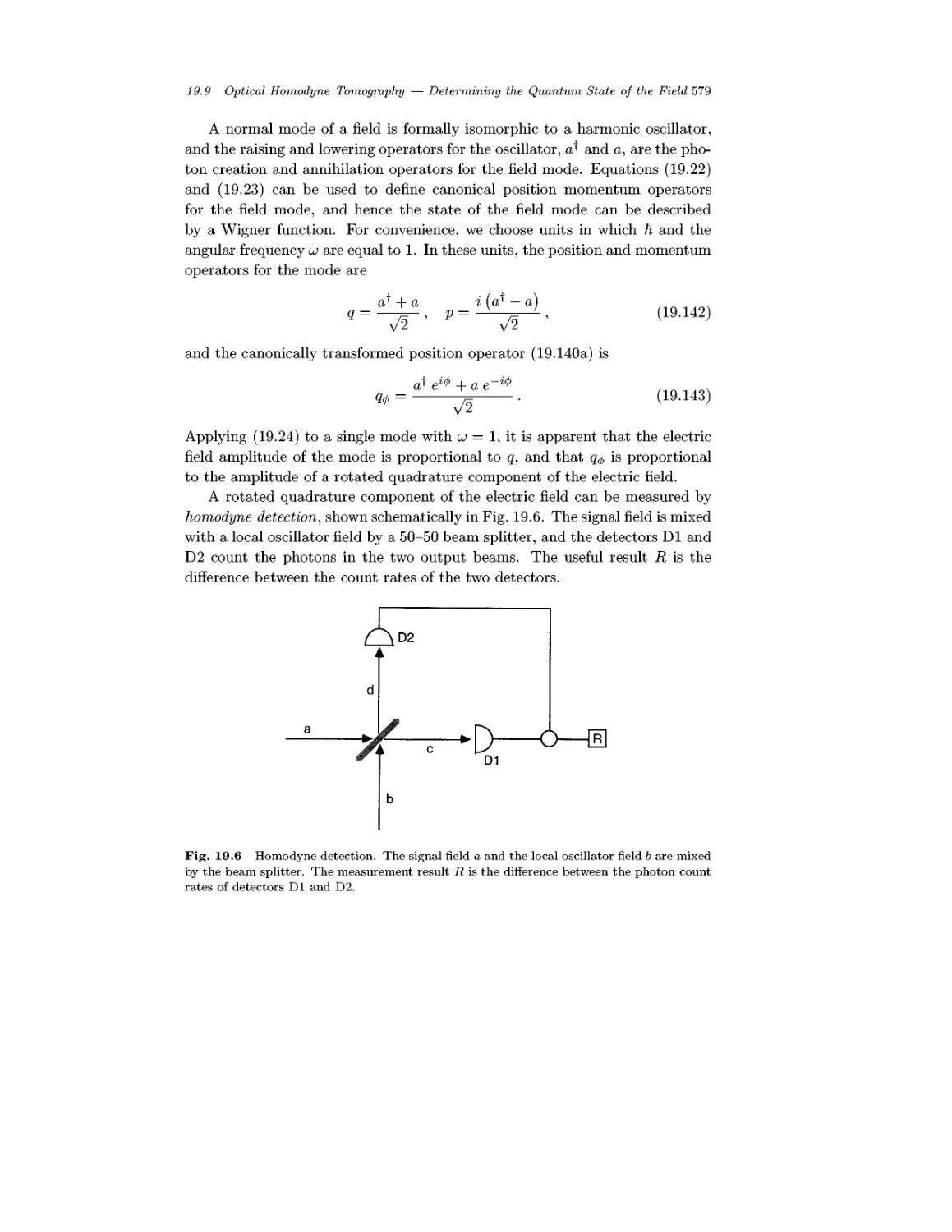
19.6 Photon Detectors 551
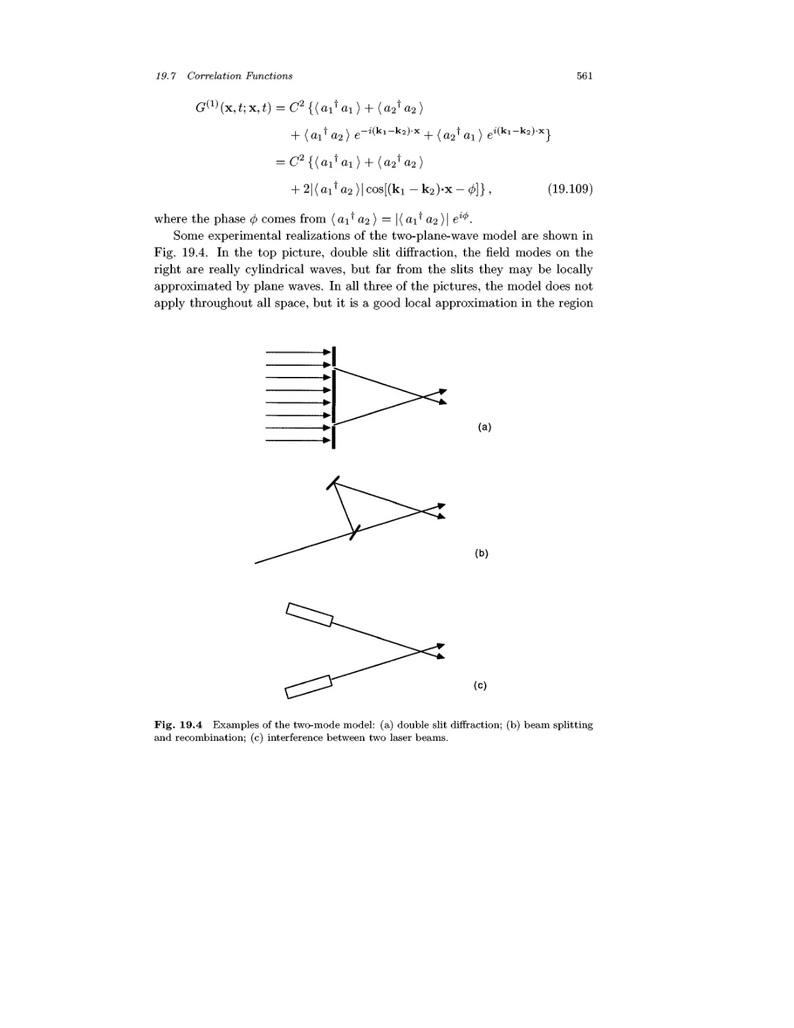
19.7 Correlation Functions 558
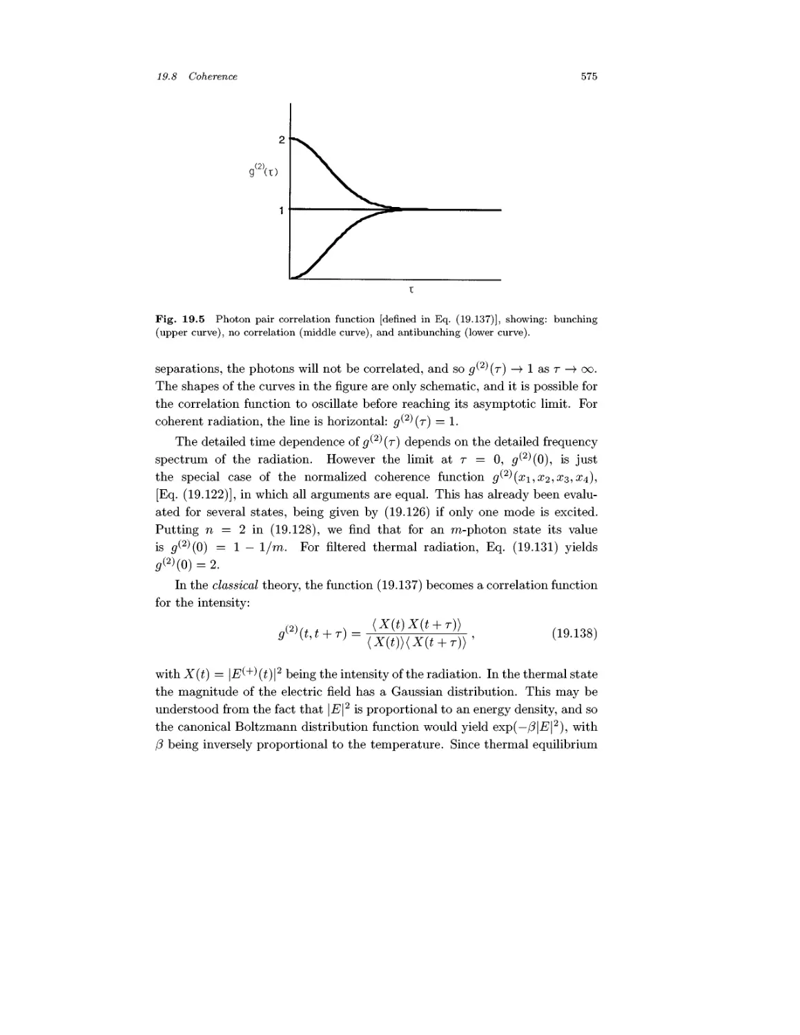
19.8 Coherence 566
19.9 Optical Homodyne Tomography —
Determining the Quantum State of the Field 578
Problems 581
Chapter 20 Bell's Theorem and Its Consequences 583
20.1 The Argument of Einstein, Podolsky, and Rosen 583
20.2 Spin Correlations 585
20.3 Bell's Inequality 587
20.4 A Stronger Proof of Bell's Theorem 591
20.5 Polarization Correlations 595
20.6 Bell's Theorem Without Probabilities 602
20.7 Implications of Bell's Theorem 607
Problems 610
Appendix A Schur's Lemma 613
Appendix B Irreducibility of Q and P 615
Appendix C Proof of Wick's Theorem 616
Appendix D Solutions to Selected Problems 618
Bibliography 639
Index 651
This Page Intentionally Left Blank
Preface
Although there are many textbooks that deal with the formal apparatus of
quantum mechanics and its application to standard problems, before the first
edition of this book (Prentice-Hall, 1990) none took into account the devel-
developments in the foundations of the subject which have taken place in the last
few decades. There are specialized treatises on various aspects of the founda-
foundations of quantum mechanics, but they do not integrate those topics into the
standard pedagogical material. I hope to remove that unfortunate dichotomy,
which has divorced the practical aspects of the subject from the interpreta-
interpretation and broader implications of the theory. This book is intended primarily
as a graduate level textbook, but it will also be of interest to physicists and
philosophers who study the foundations of quantum mechanics. Parts of the
book could be used by senior undergraduates.
The first edition introduced several major topics that had previously been
found in few, if any, textbooks. They included:
A review of probability theory and its relation to the quantum theory.
Discussions about state preparation and state determination.
- The Aharonov-Bohm effect.
- Some firmly established results in the theory of measurement, which are
useful in clarifying the interpretation of quantum mechanics.
A more complete account of the classical limit.
- Introduction of rigged Hilbert space as a generalization of the more familiar
Hilbert space. It allows vectors of infinite norm to be accommodated
within the formalism, and eliminates the vagueness that often surrounds
the question whether the operators that represent observables possess a
complete set of eigenvectors.
- The space-time symmetries of displacement, rotation, and Galilei transfor-
transformations are exploited to derive the fundamental operators for momentum,
angular momentum, and the Hamiltonian.
A charged particle in a magnetic field (Landau levels).
xii Preface
Basic concepts of quantum optics.
- Discussion of modern experiments that test or illustrate the fundamental
aspects of quantum mechanics, such as: the direct measurement of the
momentum distribution in the hydrogen atom; experiments using the sin-
single crystal neutron interferometer; quantum beats; photon bunching and
antibunching.
- Bell's theorem and its implications.
This edition contains a considerable amount of new material. Some of the
newly added topics are:
An introduction describing the range of phenomena that quantum theory
seeks to explain.
- Feynman's path integrals.
The adiabatic approximation and Berry's phase.
- Expanded treatment of state preparation and determination, including the
no-cloning theorem and entangled states.
- A new treatment of the energy-time uncertainty relations.
- A discussion about the influence of a measurement apparatus on the envi-
environment, and vice versa.
- A section on the quantum mechanics of rigid bodies.
- A revised and expanded chapter on the classical limit.
- The phase space formulation of quantum mechanics.
- Expanded treatment of the many new interference experiments that are
being performed.
- Optical homodyne tomography as a method of measuring the quantum
state of a field mode.
- Bell's theorem without inequalities and probability.
The material in this book is suitable for a two-semester course. Chapter 1
consists of mathematical topics (vector spaces, operators, and probability),
which may be skimmed by mathematically sophisticated readers. These topics
have been placed at the beginning, rather than in an appendix, because one
needs not only the results but also a coherent overview of their theory, since
they form the mathematical language in which quantum theory is expressed.
The amount of time that a student or a class spends on this chapter may vary
widely, depending upon the degree of mathematical preparation. A mathe-
mathematically sophisticated reader could proceed directly from the Introduction to
Chapter 2, although such a strategy is not recommended.
Preface xiii
The space-time symmetries of displacement, rotation, and Galilei trans-
transformations are exploited in Chapter 3 in order to derive the fundamental
operators for momentum, angular momentum, and the Hamiltonian. This
approach replaces the heuristic but inconclusive arguments based upon
analogy and wave-particle duality, which so frustrate the serious student. It
also introduces symmetry concepts and techniques at an early stage, so that
they are immediately available for practical applications. This is done without
requiring any prior knowledge of group theory. Indeed, a hypothetical reader
who does not know the technical meaning of the word "group", and who
interprets the references to "groups" of transformations and operators as
meaning sets of related transformations and operators, will lose none of the
essential meaning.
A purely pedagogical change in this edition is the dissolution of the old
chapter on approximation methods. Instead, stationary state perturbation
theory and the variational method are included in Chapter 10 ("Formation of
Bound States"), while time-dependent perturbation theory and its applications
are part of Chapter 12 ("Time-Dependent Phenomena"). I have found this to
be a more natural order in my teaching. Finally, this new edition contains
some additional problems, and an updated bibliography.
Solutions to some problems are given in Appendix D. The solved problems
are those that are particularly novel, and those for which the answer or the
method of solution is important for its own sake (rather than merely being
an exercise).
At various places throughout the book I have segregated in double
brackets, [[•••]], comments of a historical comparative, or critical nature.
Those remarks would not be needed by a hypothetical reader with no
previous exposure to quantum mechanics. They are used to relate my
approach, by way of comparison or contrast, to that of earlier writers, and
sometimes to show, by means of criticism, the reason for my departure from
the older approaches.
Acknowledgements
The writing of this book has drawn on a great many published sources,
which are acknowledged at various places throughout the text. However, I
would like to give special mention to the work of Thomas F. Jordan, which
forms the basis of Chapter 3. Many of the chapters and problems have been
"field-tested" on classes of graduate students at Simon Fraser University. A
special mention also goes to my former student Bob Goldstein, who discovered
xiv Preface
a simple proof for the theorem in Sec. 8.3, and whose creative imagination was
responsible for the paradox that forms the basis of Problem 9.6. The data
for Fig. 0.4 was taken by Jeff Rudd of the SFU teaching laboratory staff. In
preparing Sec. 1.5 on probability theory, I benefitted from discussions with
Prof. C. Villegas. I would also like to thank Hans von Baeyer for the key idea
in the derivation of the orbital angular momentum eigenvalues in Sec. 8.3, and
W. G. Unruh for point out interesting features of the third example in Sec. 9.6.
Leslie E. Ballentine
Simon Fraser University
Introduction
The Phenomena of
Quantum Mechanics
Quantum mechanics is a general theory. It is presumed to apply to every-
everything, from subatomic particles to galaxies. But interest is naturally focussed
on those phenomena that are most distinctive of quantum mechanics, some
of which led to its discovery. Rather than retelling the historical develop-
development of quantum theory, which can be found in many books,* I shall illustrate
quantum phenomena under three headings: discreteness, diffraction, and
coherence. It is interesting to contrast the original experiments, which led
to the new discoveries, with the accomplishments of modern technology.
It was the phenomenon of discreteness that gave rise to the name "quan-
"quantum mechanics". Certain dynamical variables were found to take on only a
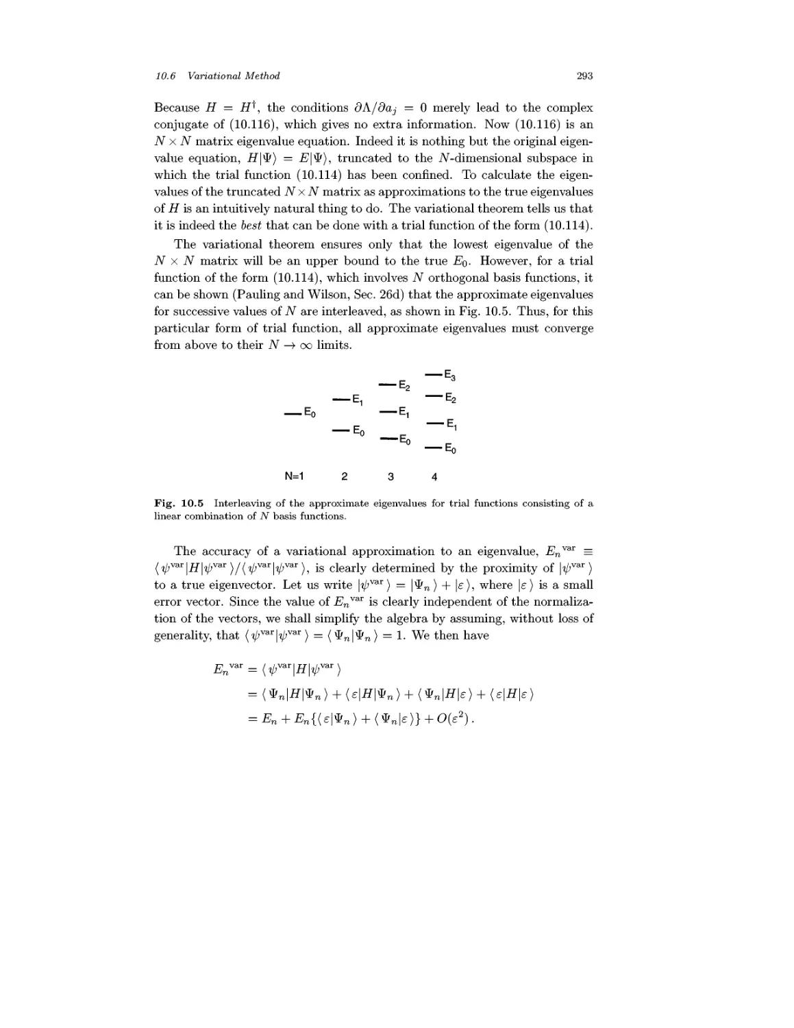
300
a.
? 2C0
3
100
10
VsKs
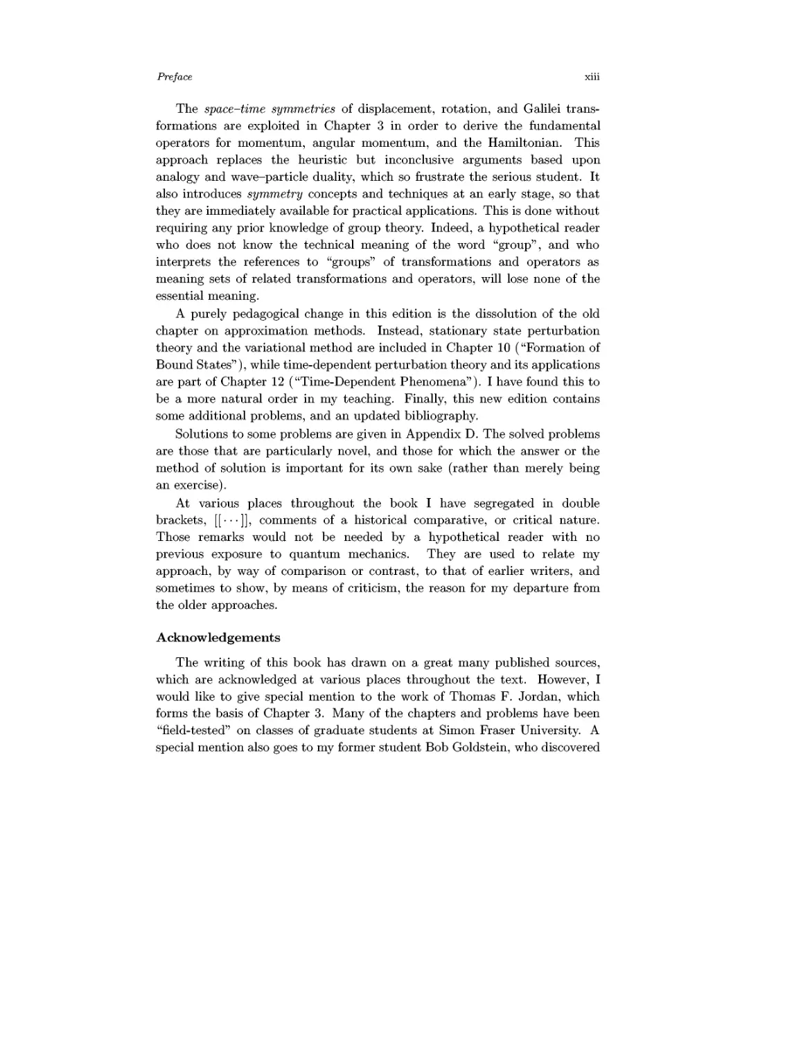
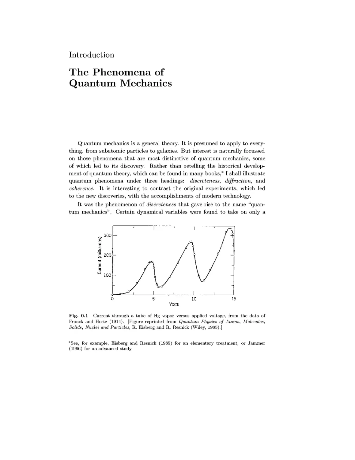
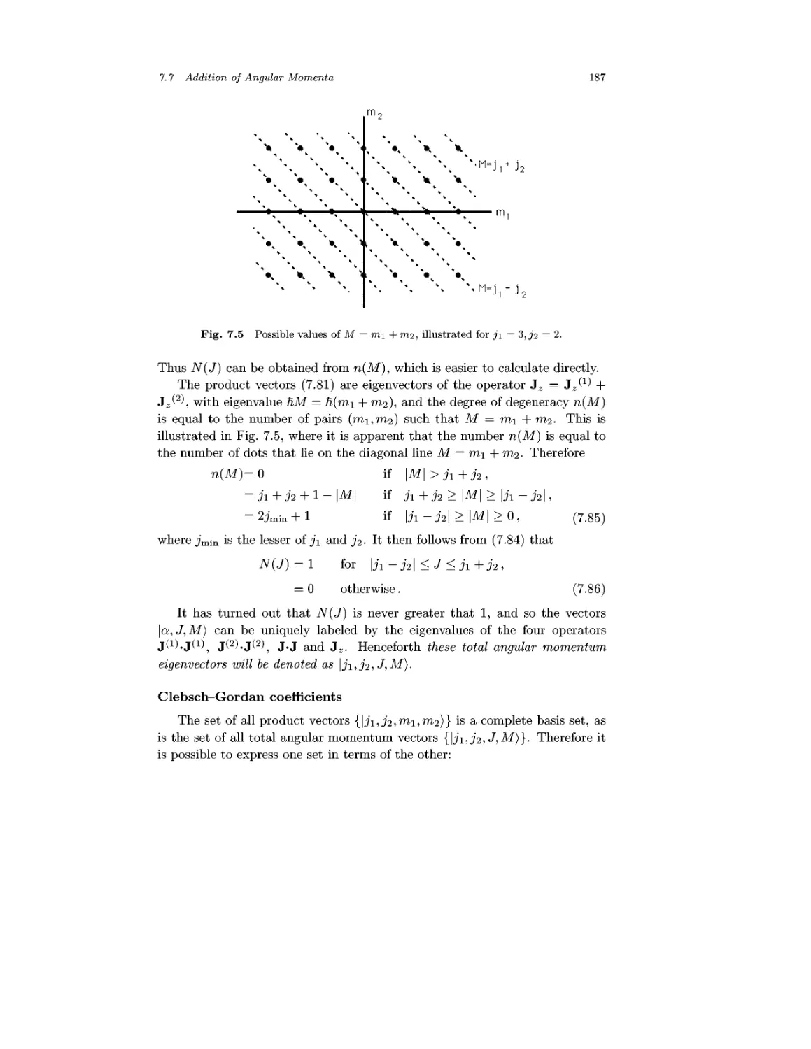
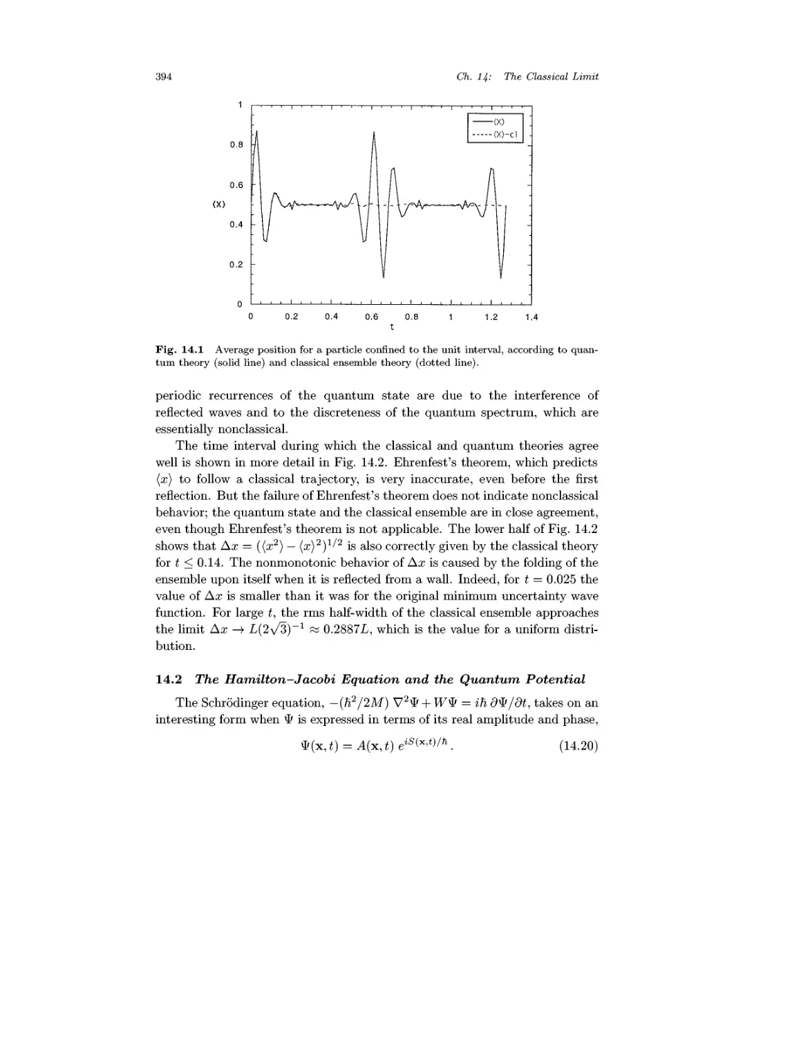
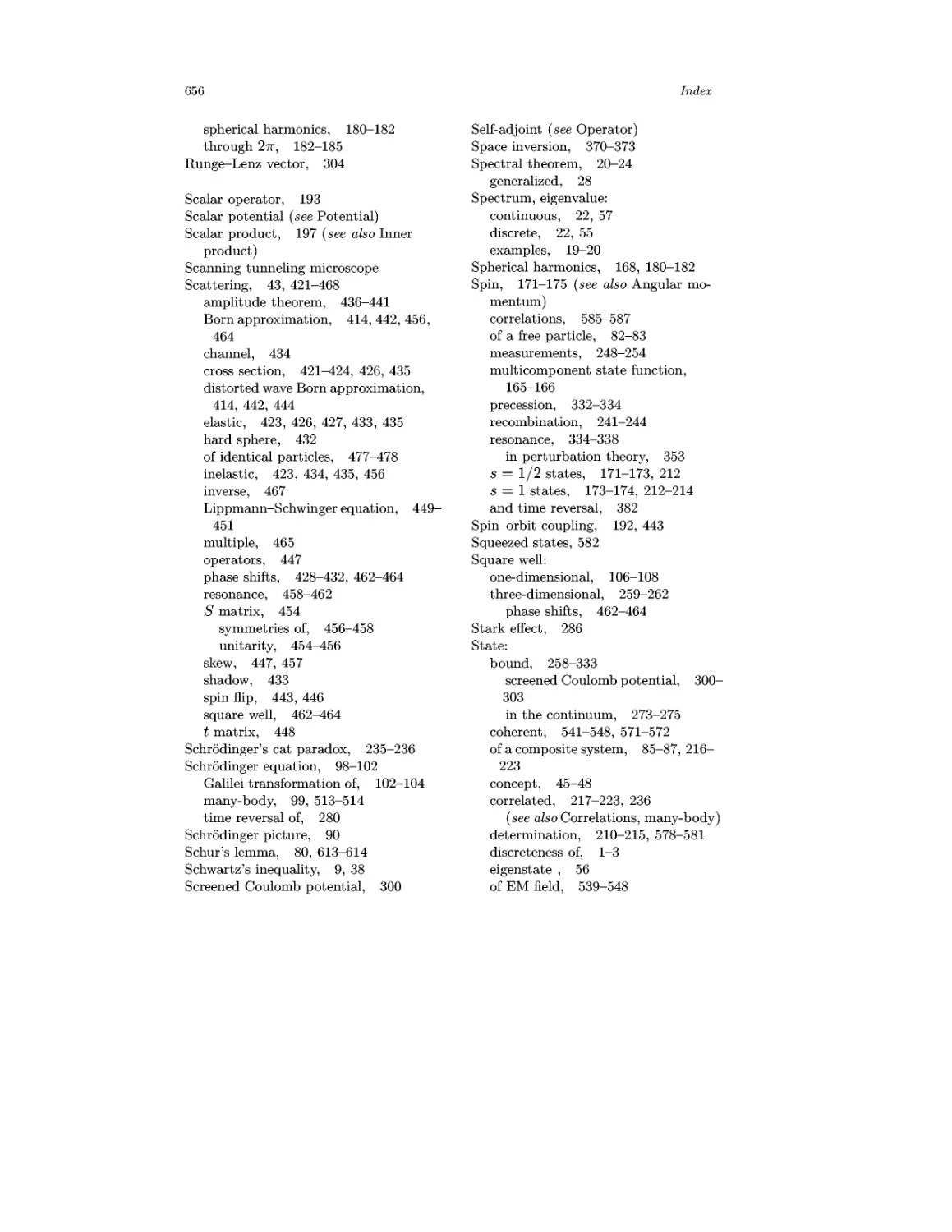
Fig. 0.1 Current through a tube of Hg vapor versus applied voltage, from the data of
Pranck and Hertz A914). [Figure reprinted from Quantum Physics of Atoms, Molecules,
Solids, Nuclei and Particles, R. Eisberg and R. Resnick (Wiley, 1985).]
*See, for example, Eisberg and Resnick A985) for an elementary treatment, or Jammer
A966) for an advanced study.
2 Introduction: The Phenomena of Quantum Mechanics
discrete, or quantized, set of values, contrary to the predictions of classical
mechanics. The first direct evidence for discrete atomic energy levels was
provided by Franck and Hertz A914). In their experiment, electrons emitted
from a hot cathode were accelerated through a gas of Hg vapor by means of an
adjustable potential applied between the anode and the cathode. The current
as a function of voltage, shown in Fig. 0.1, does not increase monotonically,
but rather displays a series of peaks at multiples of 4.9 volts. Now 4.9 eV is
the energy required to excite a Hg atom to its first excited state. When the
voltage is sufficient for an electron to achieve a kinetic energy of 4.9 eV, it is
able to excite an atom, losing kinetic energy in the process. If the voltage is
more than twice 4.9 V, the electron is able to regain 4.9 eV of kinetic energy
and cause a second excitation event before reaching the anode. This explains
the sequence of peaks.
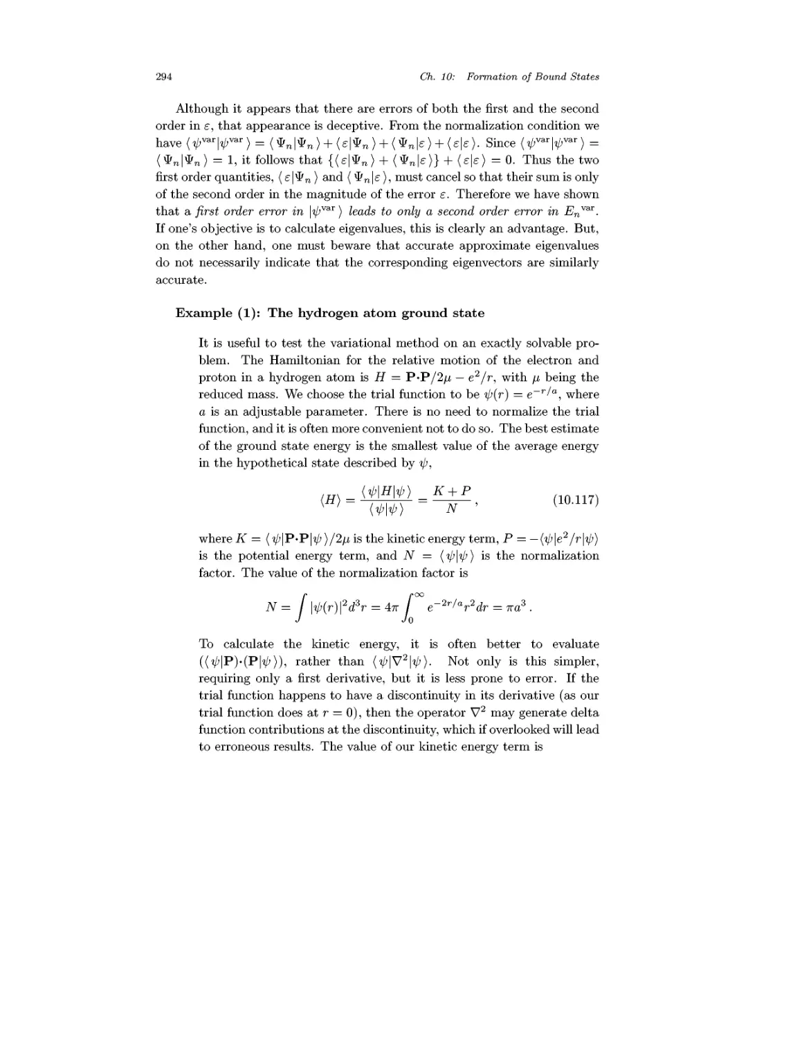
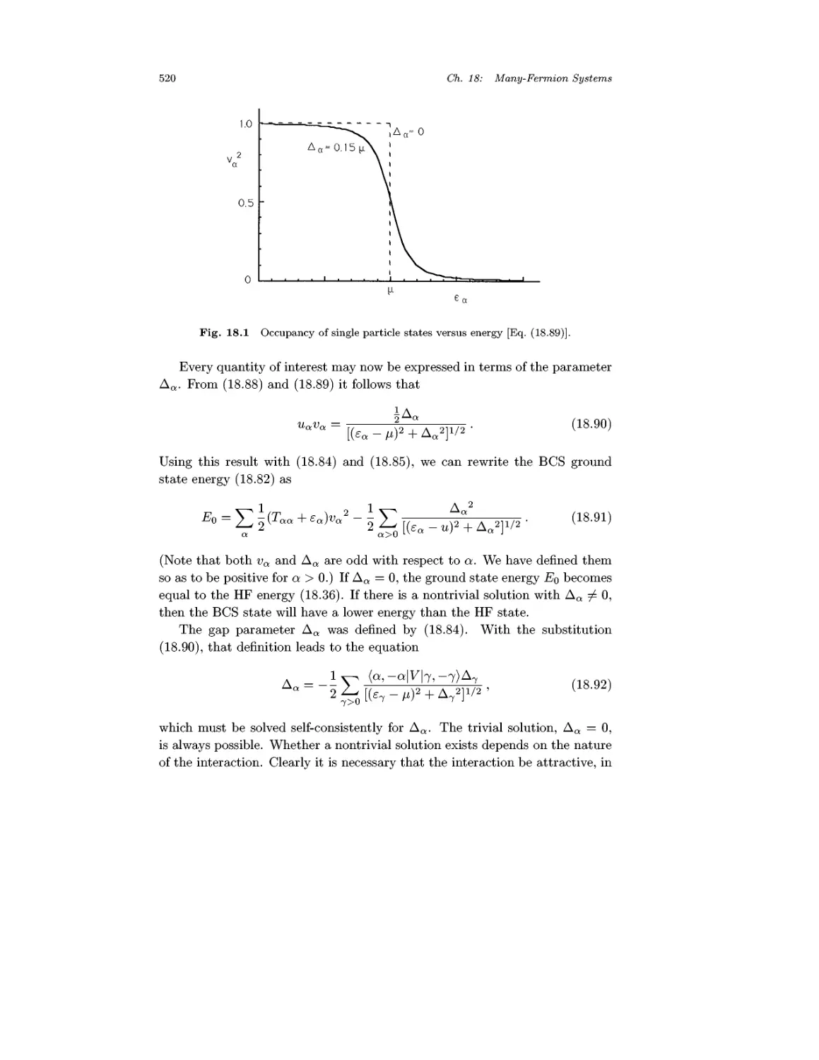
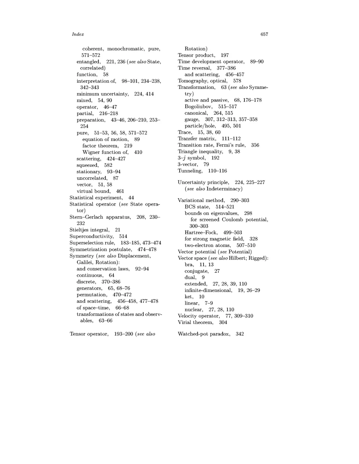
The peaks in Fig. 0.1 are very broad, and provide no evidence for the
sharpness of the discrete atomic energy levels. Indeed, if there were no better
evidence, a skeptic would be justified in doubting the discreteness of atomic
energy levels. But today it is possible, by a combination of laser excitation
and electric field filtering, to produce beams of atoms that are all in the same
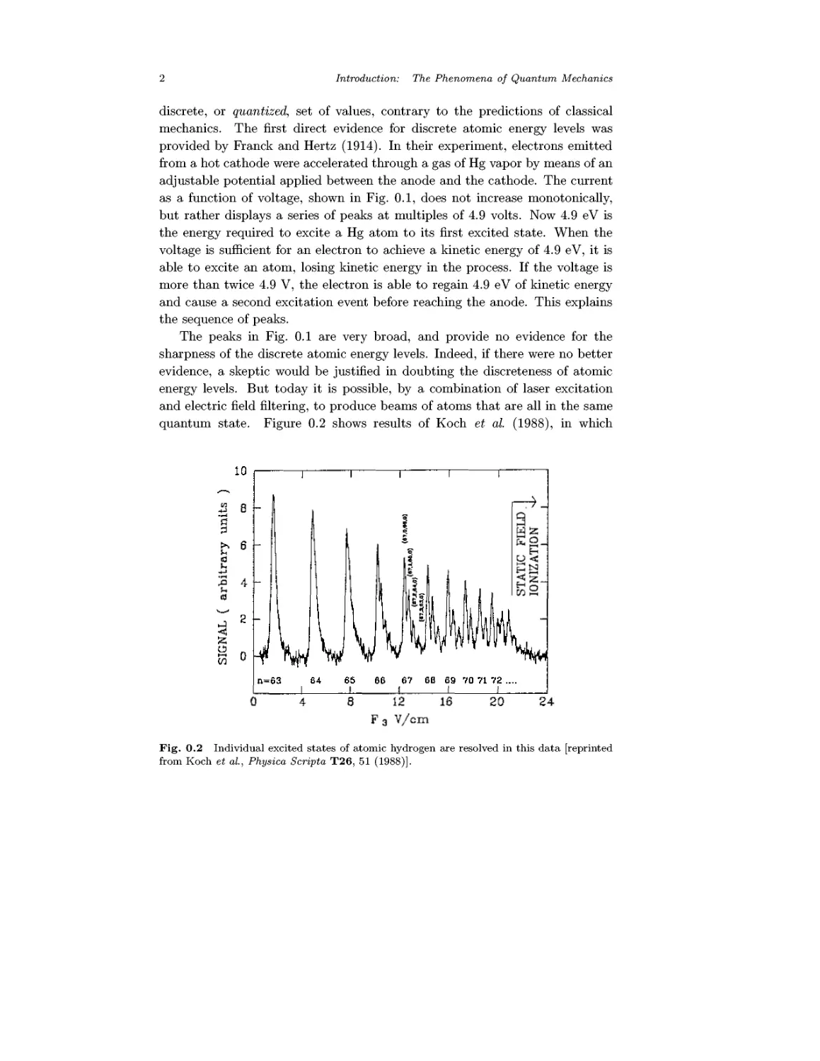
quantum state. Figure 0.2 shows results of Koch et al. A988), in which
Fig. 0.2 Individual excited states of atomic hydrogen are resolved in this data [reprinted
from Koch et al, Physica Scripta T26, 51 A988)].
Introduction: The Phenomena of Quantum Mechanics 3
the atomic states of hydrogen with principal quantum numbers from n = 63
to n = 72 are clearly resolved. Each n value contains many substates that
would be degenerate in the absence of an electric field, and for n = 67 even
the substates are resolved. By adjusting the laser frequency and the various
filtering fields, it is possible to resolve different atomic states, and so to produce
a beam of hydrogen atoms that are all in the same chosen quantum state. The
discreteness of atomic energy levels is now very well established.
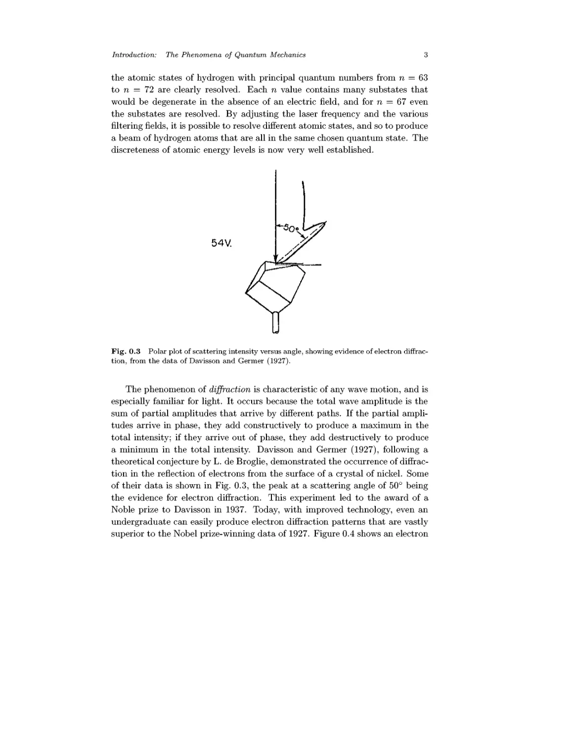
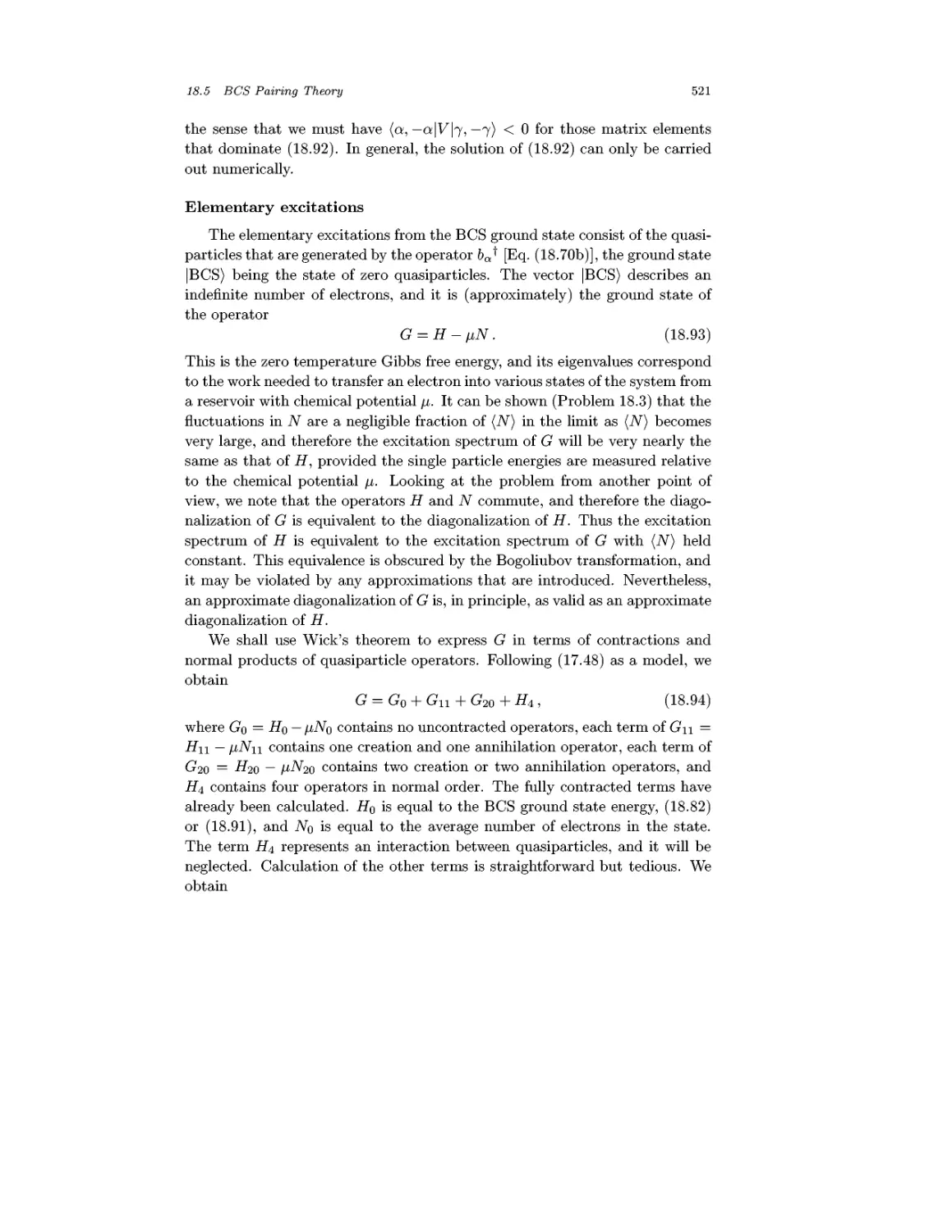
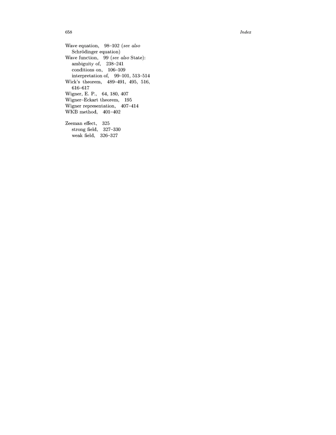
54V
Fig. 0.3 Polar plot of scattering intensity versus angle, showing evidence of electron diffrac-
diffraction, from the data of Davisson and Germer A927).
The phenomenon of diffraction is characteristic of any wave motion, and is
especially familiar for light. It occurs because the total wave amplitude is the
sum of partial amplitudes that arrive by different paths. If the partial ampli-
amplitudes arrive in phase, they add constructively to produce a maximum in the
total intensity; if they arrive out of phase, they add destructively to produce
a minimum in the total intensity. Davisson and Germer A927), following a
theoretical conjecture by L. de Broglie, demonstrated the occurrence of diffrac-
diffraction in the reflection of electrons from the surface of a crystal of nickel. Some
of their data is shown in Fig. 0.3, the peak at a scattering angle of 50° being
the evidence for electron diffraction. This experiment led to the award of a
Noble prize to Davisson in 1937. Today, with improved technology, even an
undergraduate can easily produce electron diffraction patterns that are vastly
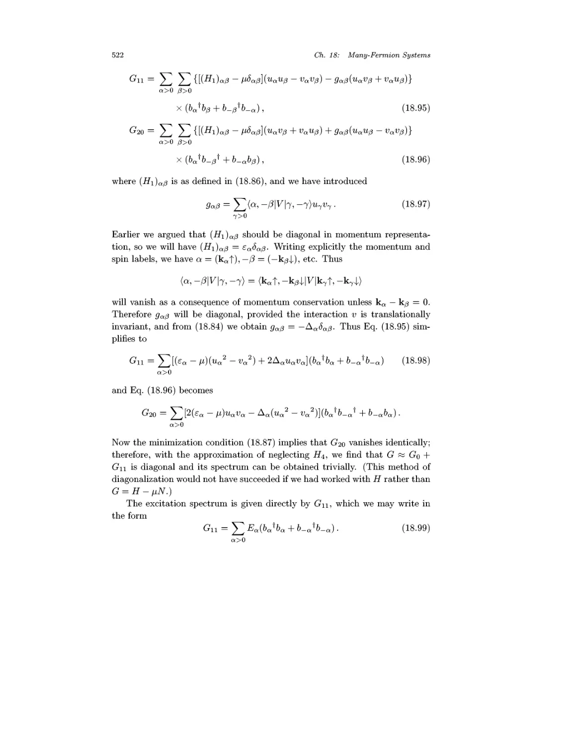
superior to the Nobel prize-winning data of 1927. Figure 0.4 shows an electron
Introduction: The Phenomena of Quantum Mechanics
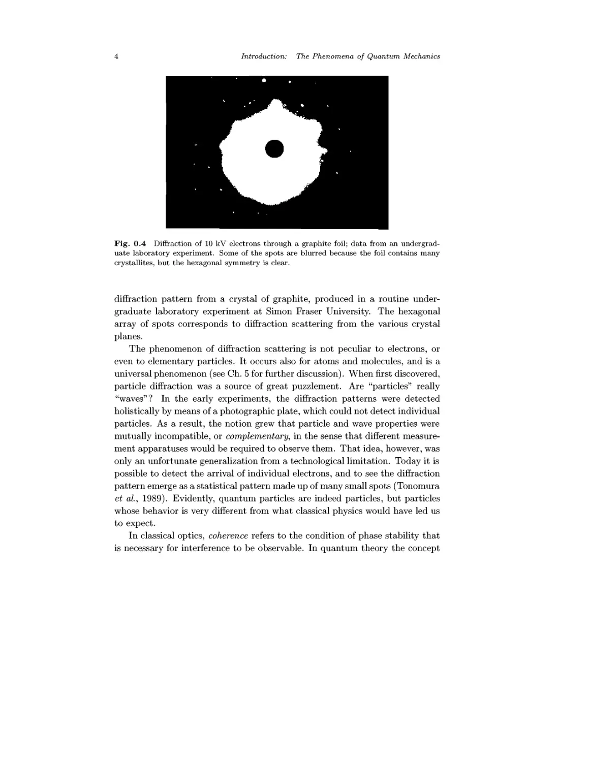
Fig. 0.4 Diffraction of 10 kV electrons through a graphite foil; data from an undergrad-
undergraduate laboratory experiment. Some of the spots are blurred because the foil contains many
crystallites, but the hexagonal symmetry is clear.
diffraction pattern from a crystal of graphite, produced in a routine under-
undergraduate laboratory experiment at Simon Fraser University. The hexagonal
array of spots corresponds to diffraction scattering from the various crystal
planes.
The phenomenon of diffraction scattering is not peculiar to electrons, or
even to elementary particles. It occurs also for atoms and molecules, and is a
universal phenomenon (see Ch. 5 for further discussion). When first discovered,
particle diffraction was a source of great puzzlement. Are "particles" really
"waves"? In the early experiments, the diffraction patterns were detected
holistically by means of a photographic plate, which could not detect individual
particles. As a result, the notion grew that particle and wave properties were
mutually incompatible, or complementary, in the sense that different measure-
measurement apparatuses would be required to observe them. That idea, however, was
only an unfortunate generalization from a technological limitation. Today it is
possible to detect the arrival of individual electrons, and to see the diffraction
pattern emerge as a statistical pattern made up of many small spots (Tonomura
et al, 1989). Evidently, quantum particles are indeed particles, but particles
whose behavior is very different from what classical physics would have led us
to expect.
In classical optics, coherence refers to the condition of phase stability that
is necessary for interference to be observable. In quantum theory the concept
Introduction: The Phenomena of Quantum Mechanics
of coherence also refers to phase stability, but it is generalized beyond any
analogy with wave motion. In general, a coherent superposition of quantum
states may have properties than are qualitatively different from a mixture of
the properties of the component states. For example, the state of a neutron
with its spin polarized in the +x direction is expressible (in a notation that will
be developed in detail in later chapters) as a coherent sum of states that are
polarized in the +z and —z directions, | + x) = (| + z) + | — z))/V2. Likewise,
the state with the spin polarized in the +z direction is expressible in terms of
the +x and —x polarizations as | + z) = (| + x) + | — x))/a/2.
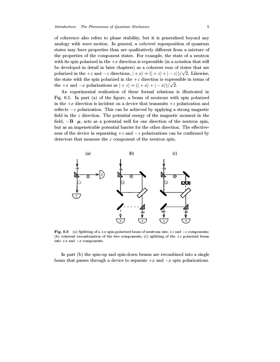
An experimental realization of these formal relations is illustrated in
Fig. 0.5. In part (a) of the figure, a beam of neutrons with spin polarized
in the +x direction is incident on a device that transmits +z polarization and
reflects —z polarization. This can be achieved by applying a strong magnetic
field in the z direction. The potential energy of the magnetic moment in the
field, —B • /x, acts as a potential well for one direction of the neutron spin,
but as an impenetrable potential barrier for the other direction. The effective-
effectiveness of the device in separating +z and —z polarizations can be confirmed by
detectors that measure the z component of the neutron spin.
(a)
O
(b)
V
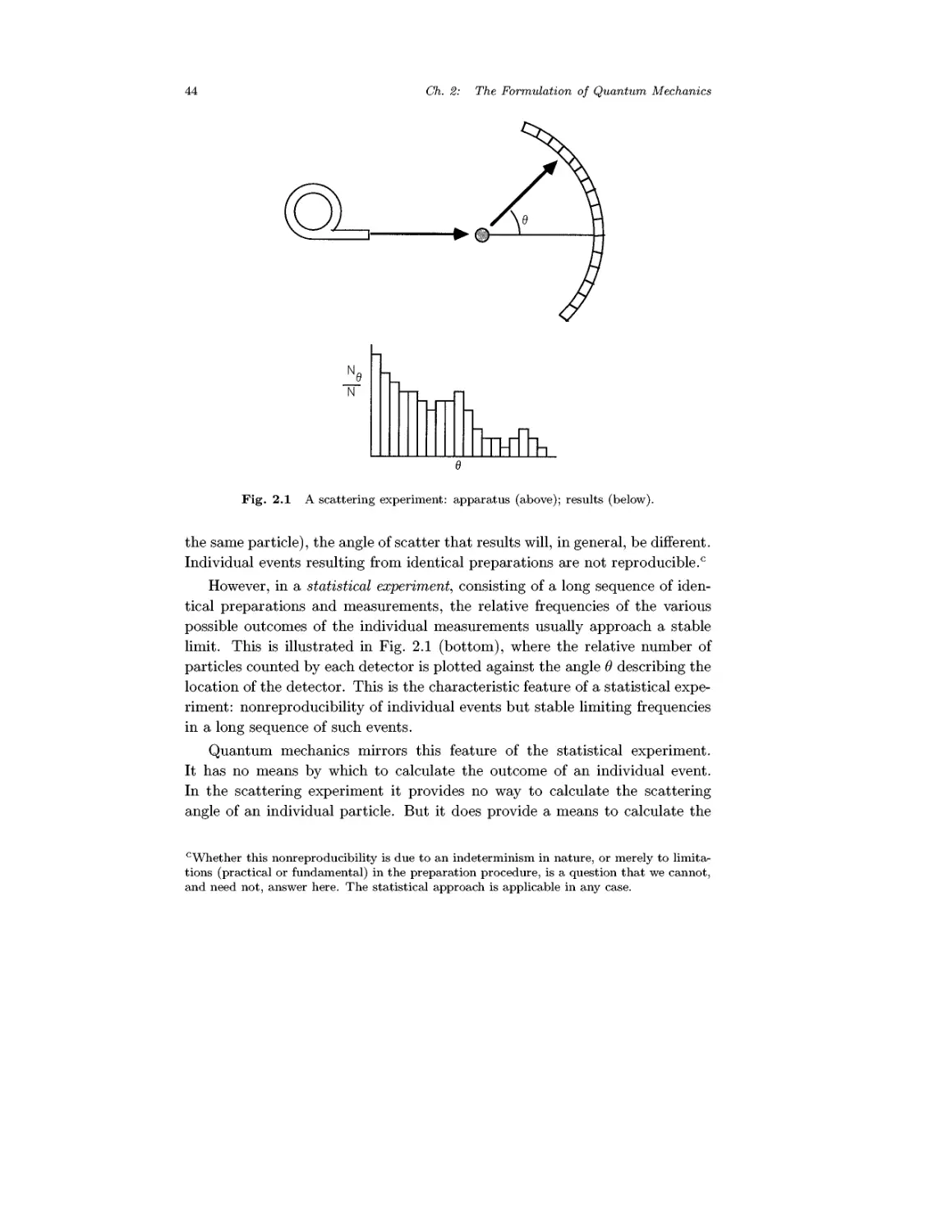
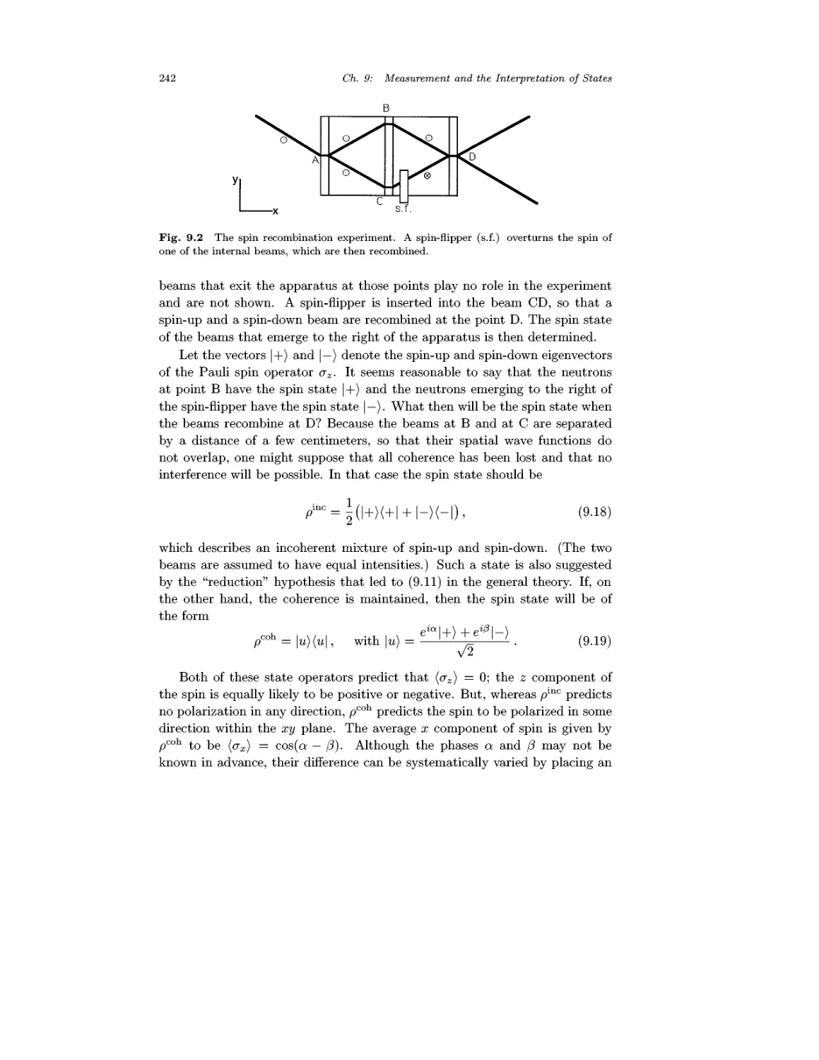
Fig. 0.5 (a) Splitting of a +x spin-polarized beam of neutrons into +z and — z components;
(b) coherent recombination of the two components; (c) splitting of the +z polarized beam
into +x and — x components.
In part (b) the spin-up and spin-down beams are recombined into a single
beam that passes through a device to separate +x and —x spin polarizations.
6 Introduction: The Phenomena of Quantum Mechanics
If the recombination is coherent, and does not introduce any phase shift
between the two beams, then the state | + x) will be reconstructed, and only
the +x polarization will be detected at the end of the apparatus. In part (c)
the | — z) beam is blocked, so that only the | + z) beam passes through the
apparatus. Since \ + z) = (| + x) + | — x))/y/2, this beam will be split into
+ x) and | — x) components.
Although the experiment depicted in Fig. 0.5 is idealized, all of its
components are realizable, and closely related experiments have actually been
performed.
In this Introduction, we have briefly surveyed some of the diverse phenom-
phenomena that occur within the quantum domain. Discreteness, being essentially
discontinuous, is quite different from classical mechanics. Diffraction scatter-
scattering of particles bears a strong analogy to classical wave theory, but the element
of discreteness is present, in that the observed diffraction patterns are really
statistical patterns of the individual particles. The possibility of combining
quantum states in coherent superpositions that are qualitatively different from
their components is perhaps the most distinctive feature of quantum mechan-
mechanics, and it introduces a new nonclassical element of continuity. It is the task
of quantum theory to provide a framework within which all of these diverse
phenomena can be explained.
Chapter 1
Mathematical Prerequisites
Certain mathematical topics are essential for quantum mechanics, not only
as computational tools, but because they form the most effective language in
terms of which the theory can be formulated. These topics include the theory
of linear vector spaces and linear operators, and the theory of probability.
The connection between quantum mechanics and linear algebra originated as
an apparent by-product of the linear nature of Schrodinger's wave equation.
But the theory was soon generalized beyond its simple beginnings, to include
abstract "wave functions" in the 3iV-dimensional configuration space of N
paricles, and then to include discrete internal degrees of freedom such as spin,
which have nothing to do with wave motion. The structure common to all
of those diverse cases is that of linear operators on a vector space. A unified
theory based on that mathematical structure was first formulated by P. A. M.
Dirac, and the formulation used in this book is really a modernized version of
Dirac's formalism.
That quantum mechanics does not predict a deterministic course of events,
but rather the probabilities of various alternative possible events, was recog-
recognized at an early stage, especially by Max Born. Modern applications seem
more and more to involve correlation functions and nontrivial statistical dis-
distributions (especially in quantum optics), and therefore the relations between
quantum theory and probability theory need to be expounded.
The physical development of quantum mechanics begins in Ch. 2, and the
mathematically sophisticated reader may turn there at once. But since not
only the results, but also the concepts and logical framework of Ch. 1 are
freely used in developing the physical theory, the reader is advised to at least
skim this first chapter before proceeding to Ch. 2.
1.1 Linear Vector Space
A linear vector space is a set of elements, called vectors, which is closed
under addition and multiplication by scalars. That is to say, if <j> and tp are
8 Ch. 1: Mathematical Prerequisites
vectors then so is a<f> + hp, where a and b are arbitrary scalars. If the scalars
belong to the field of complex (real) numbers, we speak of a complex (real)
linear vector space. Henceforth the scalars will be complex numbers unless
otherwise stated.
Among the very many examples of linear vector spaces, there are two classes
that are of common interest:
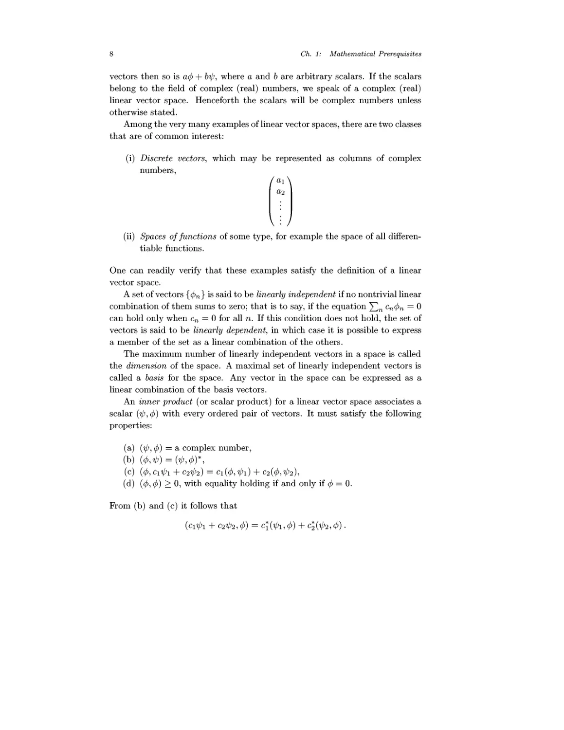
(i) Discrete vectors, which may be represented as columns of complex
numbers,
I
\
(ii) Spaces of functions of some type, for example the space of all difieren-
tiable functions.
One can readily verify that these examples satisfy the definition of a linear
vector space.
A set of vectors {<f>n} is said to be linearly independent if no nontrivial linear
combination of them sums to zero; that is to say, if the equation ^n cn(f>n = 0
can hold only when cn = 0 for all n. If this condition does not hold, the set of
vectors is said to be linearly dependent, in which case it is possible to express
a member of the set as a linear combination of the others.
The maximum number of linearly independent vectors in a space is called
the dimension of the space. A maximal set of linearly independent vectors is
called a basis for the space. Any vector in the space can be expressed as a
linear combination of the basis vectors.
An inner product (or scalar product) for a linear vector space associates a
scalar (ip, cf>) with every ordered pair of vectors. It must satisfy the following
properties:
(a) (ip,<f>) = a complex number,
(b) @,V) = (V,0)*,
(c) @,CiV>l +C21p2) = Ci@,Vl) + C2@,V2),
(d) @, cf>) > 0, with equality holding if and only if cf> = 0.
From (b) and (c) it follows that
1.1 Linear Vector Space 9
Therefore we say that the inner product is linear in its second argument, and
antilinear in its first argument.
We have, corresponding to our previous examples of vector spaces, the
following inner products:
(i) If ip is the column vector with elements a\, a2, ¦ ¦ ¦ and <f> is the column
vector with elements b\, b2,..., then
(V>, <t>) = a^h + a*2b2 H .
(ii) If tp and <p are functions of x, then
(xp,4>)= / xp*(x)(f>(x)w(x)dx,
where w(x) is some nonnegative weight function.
The inner product generalizes the notions of length and angle to arbitrary
spaces. If the inner product of two vectors is zero, the vectors are said to be
orthogonal.
The norm (or length) of a vector is defined as \\<f>\\ = (</>,(fI^2- The inner
product and the norm satisfy two important theorems:
Schwarz's inequality,
\^,4>)\2<^^){4>,4>). A.1)
The triangle inequality,
A-2)
In both cases equality holds only if one vector is a scalar multiple of the other,
i.e. tp = c<p. For A.2) to become an equality, the scalar c must be real and
positive.
A set of vectors {fa} is said to be orthonormal if the vectors are pair-
wise orthogonal and of unit norm; that is to say, their inner products satisfy
(<f>i,<f>j) = Sij.
Corresponding to any linear vector space V there exists the dual space of
linear functionals on V. A linear functional F assigns a scalar F(<f>) to each
vector <j), such that
F(a<f> + inp) = aF(<f>) + bF^) A.3)
10 Ch. 1: Mathematical Prerequisites
for any vectors <f> and ip, and any scalars a and b. The set of linear functionals
may itself be regarded as forming a linear space V if we define the sum of two
functionals as
{F1 + F2){4>) = F^) + F2{4>). A.4)
Riesz theorem. There is a one-to-one correspondence between linear
functionals F in V' and vectors / in V, such that all linear functionals have
the form
/ being a fixed vector, and <p> being an arbitrary vector. Thus the spaces V and
V are essentially isomorphic. For the present we shall only prove this theorem
in a manner that ignores the convergence questions that arise when dealing
with infinite-dimensional spaces. (These questions are dealt with in Sec. 1.4.)
Proof. It is obvious that any given vector / in V defines a linear functional,
using Eq. A.5) as the definition. So we need only prove that for an arbitrary
linear functional F we can construct a unique vector / that satisfies A.5). Let
{4>n} be a system of orthonormal basis vectors in V, satisfying (<f>n, <j>m) = 6njm.
Let ip = ^2n xn<t>n be an arbitrary vector in V. From A.3) we have
Now construct the following vector:
Its inner product with the arbitrary vector ip is
and hence the theorem is proved.
Dirac's bra and ket notation
In Dirac's notation, which is very popular in quantum mechanics, the
vectors in V are called ket vectors, and are denoted as \4>). The linear
1.2 Linear Operators 11
functionals in the dual space V are called bra vectors, and are denoted as
(F\. The numerical value of the functional is denoted as
F{4>) = (F\4>). A.6)
According to the Riesz theorem, there is a one-to-one correspondence between
bras and kets. Therefore we can use the same alphabetic character for the
functional (a member of V) and the vector (in V) to which it corresponds,
relying on the bra, (F\, or ket, \F), notation to determine which space is
referred to. Equation A.5) would then be written as
(F\<f>) = (F,<f>), A.7)
\F) being the vector previously denoted as /. Note, however, that the Riesz
theorem establishes, by construction, an antilinear correspondence between
bras and kets. If (F\ o \F), then
c\{F\ + c*2{F\^c1\F) + c2\F). A.8)
Because of the relation A.7), it is possible to regard the "braket" (F\<j)} as
merely another notation for the inner product. But the reader is advised that
there are situations in which it is important to remember that the primary
definition of the bra vector is as a linear functional on the space of ket vectors.
[[ In his original presentation, Dirac assumed a one-to-one correspondence
between bras and kets, and it was not entirely clear whether this was a
mathematical or a physical assumption. The Riesz theorem shows that
there is no need, and indeed no room, for any such assumption. Moreover,
we shall eventually need to consideer more general spaces (rigged-Hilbert-
space triplets) for which the one-to-one correspondence between bras and
kets does not hold. 11
1.2 Linear Operators
An operator on a vector space maps vectors onto vectors; that is to say, if A
is an opetator and tp is a vector, then <j> = Atp is another vector. An operator
is fully defined by specifying its action on every vector in the space (or in its
domain, which is the name given to the subspace on which the operator can
meaningfully act, should that be smaller than the whole space).
A linear operator satisfies
+ C2V2) = ci(^Vi) + c2(Ail>2) • A-9)
12 Ch. 1: Mathematical Prerequisites
It is sufficient to define a linear operator on a set of basis vectors, since everly
vector can be expressed as a linear combination of the basis vectors. We shall
be treating only linear operators, and so shall henceforth refer to them simply
as operators.
To assert the equality of two operators, A = B, means that Atp = Btp for
all vectors (more precisely, for all vectors in the common domain of A and B,
this qualification will usually be omitted for brevity). Thus we can define the
sum and product of operators,
(A
ABi\> = A(Bip),
both equations holding for all tp. It follows from this definition that operator
mulitplication is necessarily associative, A(BC) = (AB)C. But it need not be
commutative, AB being unequal to BA in general.
Example (i). In a space of discrete vectors represented as columns, a
linear operator is a square matrix. In fact, any operator equation in a space
of N dimensions can be transformed into a matrix equation. Consider, for
example, the equation
\4>). A.10)
Choose some orthonormal basis {\ui),i = 1...N} in which to expand the
vectors,
Operating on A.10) with (wj| yields
which has the form of a matrix equation,
ijaj = bi, A.11)
with Mij = (ui\M\uj) being known as a matrix element of the operator M.
In this way any problem in an iV-dimensional linear vector space, no matter
how it arises, can be transformed into a matrix problem.
1.2 Linear Operators 13
The same thing can be done formally for an infinite-dimensional vector
space if it has a denumerable orthonormal basis, but one must then deal with
the problem of convergence of the infinite sums, which we postpone to a later
section.
Example (ii). Operators in function spaces frequently take the form of
differential or integral operators. An operator equation such as
8 1 8
—2; = l + x —
ox ox
may appear strange if one forgets that operators are only defined by their
action on vectors. Thus the above example means that
(/ (/ib (ir)
— [x ip(x)} = ip(x) + x———- for all ip(x).
C/X C/X
So far we have only defined operators as acting to the right on ket vectors.
We may define their action to the left on bra vectors as
for all <p and tp. This appears trivial in Dirac's notation, and indeed this
triviality contributes to the practival utility of his notation. However, it is
worthwhile to examine the mathematical content of A-12) in more detail.
A bra vector is in fact a linear functional on the space of ket vectors, and
in a more detailed notation the bra (<t>\ is the functional
iW = (&•), A-13)
where <j> is the vector that corresponds to F$ via the Riesz theorem, and the
dot indicates the place for the vector argument. We may define the operation
of A on the bra space of functionals as
AF0(V) = F^Aip) for all V- A-14)
The right hand side of A.14) satisfies the definition of a linear functional of
the vector tp (not merely of the vector Atp), and hence it does indeed define a
new functional, called AF$. According to the Riesz theorem there must exist
a ket vector % such that
A.15)
14 Ch. 1: Mathematical Prerequisites
Since \ is uniquely determined by cf> (given A), there must exist an operator
A^ such that \ = A^<j>. Thus A.15) can be written as
H A.16)
From A.14) and A.15) we have {4>,Aip) = (x, V0> and therefore
= (<f>, Aip) for all 0 and V • A.17)
This is the usual definition of the adjoint, A^, of the operator A. All of this
nontrivial mathematics is implicit in Dirac's simple equation A.12)!
The adjoint operator can be formally defined within the Dirac notation by
demanding that if (<j>\ and \<j>) are corresponding bras and kets, then (<j)\A^ =
(u>\ and A\4>) = \ui) should also be corresponding bras and kets. From the fact
that (u>\ip)* = (i>\oj), it follows that
@1^1^)* = (il>\A\<t>) for all 0 and V, A-18)
this relation being equivalent to A.17). Although simpler than the previous
introduction of A^ via the Riesz theorem, this formal method fails to prove the
existence of the operator A^.
Several useful properties of the adjoint operator that follow directly from
A.17) are
(cAy = c*A\ where c is a complex number,
(A + By" = A^ + B^,
In addition to the inner product of a bra and a ket, (<f>\ip), which is a scalar,
we may define an outer product, \tp)(<f>\. This object is an operator because,
assuming associative multiplication, we have
(|V)@|)|A) = |V)(@|A)). A.19)
Since an operator is defined by specifying its action on an arbitrary vector to
produce another vector, this equation fully defines |V')@| as an operator. From
A.18) it follows that
In view of this relation, it is tempting to write (IV'))^ = (V'l- Although no real
harm comes from such a notation, it should not be encouraged because it uses
1.3 Self-Adjoint Operators 15
the "adjoint" symbol, *, for something that is not an operator, and so cannot
satisfy the fundamental definition A.16).
A useful characteristic of an operator A is its trace, defined as
where {|«j)} may be any orthonormal basis. It can be shown [see Prob-
Problem A.3)] that the value of Tr A is independent of the particular orthonormal
basis that is chosen for its evaluation. The trace of a matrix is just the sum
of its diagonal elements. For an operator in an infinite-dimensional space, the
trace exists only if the infinite sum is convergent.
1.3 Self-Adjoint Operators
An operator A that is equal to its adjoint A^ is called self-adjoint. This
means that it satisfies
D>\A\<I>) = y>\A\<f>)* A.21)
and that the domain of A (i.e. the set of vectors <j> on which A<f> is well defined)
coincides with the domain of A^. An operator that only satisfies A.21) is called
Hermitian, in analogy with a Hermitian matrix, for which My = Mji*.
[[ The distinction between Hermitian and self-adjoint operators is rele-
relevant only for operators in infinite-dimensional vector spaces, and we shall
make such a distinction only when it is essential to do so. The operators
that we call "Hermitian" are often called "symmetric" in the mathematical
literature. That terminology is objectionable because it conflicts with the
corresponding properties of matrices. ]]
The following theorem is useful in identifying Hermitian operators on a
vector space with complex scalars.
Theorem 1. If (ip\A\ip) = (ip\A\ip)* for all |V>), then it follows that
* for all |0i) and \cf>2), and hence that A = A*.
Proof. Let \ip) = a\4>\) + b\<j>2) for arbitrary a, b, \<j>i), and
Then
16 Ch. 1: Mathematical Prerequisites
must be real. The first and second terms are obviously real by hypothesis, so
we need only consider the third and fourth. Choosing the arbitrary parameters
a and b to be a = b = 1 yields the condition
(<f>i\A\<f>2) + D>2\A\4>i) = (<h\A\fa)* + (fa\A\<f>
Choosing instead a = 1, b = i yields
i{4>i\A\4>2) - i{(h\A\(f>i) = -i(<f>i\A\<f>2y + i<
Canceling the factor of i from the last equation and adding the two equations
yields the desired result, (<j)i\A\(jJ} = (<jJ\A\<j)i}*.
This theorem is noteworthy because the premise is obviously a special case
of the conclusion, and it is unusual for the general case to be a consequence of
a special case. Notice that the complex values of the scalars were essential in
the proof, and no analog of this theorem can exist for real vector spaces.
If an operator acting on a certain vector produces a scalar multiple of that
same vector,
A\<f>) = a\<f>), A.22)
we call the vector \<f>) an eigenvector and the scalar a an eigenvalue of the
operator A. The antilinear correspondence A.8) between bras and kets, and
the definition of the adjoint operator A^, imply that the left-handed eigenvalue
equation
@|At=a*@| A.23)
holds if the right-handed eigenvalue equation A.22) holds.
Theorem 2. If A is a Hermitian operator then all of its eigenvalues
are real.
Proof. Let A\<j>) = a\<j>). Since A is Hermitian, we must have {<t>\A\<f>) =
{<t>\A\<f>)*. Substitution of the eigenvalue equation yields
a(</#)= a* (</#),
which implies that a = a*, since only nonzero vectors are regarded as nontrivial
solutions of the eigenvector equation.
The result of this theorem, combined with A.23), shows that for a self-
adjoint operator, A = A^, the conjugate bra (<j>\ to the ket eigenvector \<j)} is
also an eigenvector with the same eigenvalue a: (<j)\A = a{4>\.
1.3 Self-Adjoint Operators 17
Theorem 3. Eigenvectors corresponding to distinct eigenvalues of a Her-
mitian operator must be orthogonal.
Proof. Let A\<j>i) = a\\4>\) and A\(f>2) = a,2\<t>2)- Since A is Hermitian, we
deduce from A.21) that
Therefore ((fel^i) = 0 if ai 7^ a2.
If ai = a2 (= a, say) then any linear combination of the degenerate
eigenvectors |0i) and \<f>2) is also an eigenvector with the same eigenvalue
a. It is always possible to replace a nonorthogonal but linearly independent
set of degenerate eigenvectors by linear combinations of themselves that are
orthogonal. Unless the contrary is explicitly stated, we shall assume that
such an orthogonalization has been performed, and when we speak of the set
of independent eigenvectors of a Hermitian operator we shall mean an
orthogonal set.
Provided the vectors have finite norms, we may rescale them to have unit
norms. Then we can always choose to work with an orthonormal set of eigen-
eigenvectors,
D>i,4>j) = 5ij. A.24)
Many textbooks state (confidently or hopefully) that the orthonormal set
of eigenvectors of a Hermitian operators is complete; that is to say, it forms a
basis that spans the vector space. Before examining the mathematical status
of that statement, let us see what useful consequences would follow if it were
true.
Properties of complete orthonormal sets
If the set of vectors {fa} is complete, then we can expand an arbitrary
vector \v) in terms of it: \v) = Y^i Vi\fa). From the orthonormality condition
A.24), the expansion coefficients are easily found to be Vi = (<f>i\v). Thus we
can write
18 Ch. 1: Mathematical Prerequisites
V) =
A-25)
for an arbitrary vector \v). The parentheses in A.25) are unnecessary, and are
used only to emphasize two ways of interpreting the equation. The first line
in A.25) suggests that \v) is equal to a sum of basis vectors each multiplied
by a scalar coefficient. The second line suggests that a certain operator (in
parentheses) acts on a vector to produce the same vector. Since the equation
holds for all vectors \v), the operator must be the identity operator,
A-26)
If A\<j>i) = ai\<j>i) and the eigenvectors form a complete orthonormal set —
that is to say, A.24) and A.26) hold — then the operator can be reconstructed
in a useful diagonal form in terms of its eigenvalues and eigenvectors:
A = Y,ai\4>i)D>i\- A-27)
i
This result is easily proven by opeating on an arbitrary vector and verifying
that the left and right sides of A-27) yield the same result. One can use the
diagonal representation to define a function of an operator,
A-28)
The usefulness of these results is the reason why many authors assume, in
the absence of proof, that the Hermitian operators encountered in quantum
mechanics will have complete sets of eigenvectors. But is it true?
Any operator in a finite iV-dimensional vector space can be expressed as
an N x N matrix [see the discussion following Eq. A.10)]. The condition for
a nontrivial solution of the matrix eigenvalue equation
\<t>, A.29)
where M is square matrix and <p is a column vector, is
det|M-J|=0. A.30)
1.3 Self-Adjoint Operators 19
The expansion of this determinant yields a polynomial in A of degree N, which
must have N roots. Each root is an eigenvalue to which there must corre-
correspond an eigenvector. If all N eigenvalues are distinct, then so must be the
eigenvectors, which will necessarily span the iV-dimensional space. A more
careful argument is necessary in order to handle multiple roots (degenerate
eigenvalues), but the proof is not difficult. [See, for example, Jordan A969),
Theorem 13.1].
This argument does not carry over to infinite-dimensional spaces. Indeed,
if one lets N become infinite, then A.30) becomes an infinite power series
in A, which need not possess any roots, even if it converges. (In fact the
determinant of an infinite-dimensional matrix is undefinable except in special
cases.) A simple counter-example shows that the theorem is not generally true
for an infinite-dimensional space.
Consider the operator D = —id/dx, defined on the space of difierentiable
functions of x for a < x <b. (The limits a and b may be finite or infinite.) Its
adjoint, D\ is identified by using A.21), which now takes the form
ip*(x)D(j>(x)dx
x)]\ba. A.31)
The last line is obtained by integrating by parts. If boundary conditions are
imposed so that the last term vanishes, then D will apparently be a Hermitian
operator.
The eigenvalue equation
^<j>{x) \<j>{x) A.32)
dx
is a differential equation whose solution is <j>{x) = cetXx, c = constant. But in
regarding it as an eigenvalue equation for the operator D, we are interested only
in eigenfunctions within a certain vector space. Several different vector spaces
may be defined, depending upon the boundary conditions that are imposed:
VI. No boundary conditions
All complex A are eigenvalues. Since D is not Hermitian this case is of no
further interest.
20 Ch. 1: Mathematical Prerequisites
V2. a = —oo, b = +00, |0(a:)| bounded as |a:|—>cx>
All real values of A are eigenvalues. The eigenfunctions <j>(x) are not nor-
malizable, but they do form a complete set in the sense that an arbitrary
function can be represented as a Fourier integral, which may be regarded as a
continuous linear combination of the eigenfunctions.
V3. a = —L/2, b = -\-L/2, periodic boundary conditions <p(—L/2)
The eigenvalues form a discrete set, A = Xn = 2irn/L, with n being an
integer of either sign. The eigenfunctions form a complete orthonormal set
(with a suitable choice for c), the completeness being proven in the theory of
Fourier series.
V4. a = —00, b = +00, <p(x)—>0 as x—*-±oo
Although the operator D is Hermitian, it has no eigenfunctions within this
space.
These examples suffice to show that a Hermitian operator in an infinite-
dimensional vector space may or may not possess a complete set of eigenvec-
eigenvectors, depending upon the precise nature of the operator and the vector space.
Fortunately, the desirable results like A.26), A.27) and A.28) can be reformu-
reformulated in a way that does not require the existence of well-defined eigenvectors.
The spectral theorem
The outer product \<f>i){<f>i\ formed from a vector of unit norm is an example
of a projection operator. In general, a self-adjoint operator p that satisfies
p2 = p is a projection operator. Its actionis to project out the component
of a vector that lies within a certain subspace (the one-dimensional space of
\<j>i) in the above example), and to annihilate all components orthogonal to
that subspace. If the operator A in A.27) has a degenerate spectrum, we may
form the projection operator onto the subspace spanned by the degenerate
eigenvectors corresponding to a; = a,
P{a) = Y,\<t>i){<t>i\5a,ai A-33)
i
and A-27) can be rewritten as
^2 A.34)
The sum on a goes over the eigenvalue spectrum. [But since P(a) = 0 if a is
not an eigenvalue, it is harmless to extend the sum beyond the spectrum.]
1.3 Self-Adjoint Operators
21
The examples following A.32) suggest (correctly, it turns out) that the
troubles are associated with a continuous spectrum, so it is desirable to rewrite
A.34) in a form that holds for both discrete and continuous spectra. This
can most conveniently be done with the help of the Stieltjes integral, whose
definition is
/b
g{x)da{x)= lim
- cr(xk-i)
A-35)
the limit being taken such that every interval (xk — xk-i) goes to zero as
n —> oo. The nondecreasing function a(x) is called the measure. If <r(x) = x,
then A.35) reduces to the more familiar Riemann integral. If da/dx exists,
then we have
/ g(x)da(x) = / g(x) ( -?
J (Stieltjes) J (Riemann) \UJb
dx.
The generalization becomes nontrivial only when we allow <r(x) to be discon-
discontinuous. Suppose that
a(x) = h6(x - c), A.36)
where 6{x) = 0 for x < 0, 6{x) = 1 for x > 0. The only term in A.35) that
will contribute to the integral is the term for which xk-i < c and xk > c. The
value of the integral is hg(c).
<T(X)
h
k-1 c
Fig. 1.1 A discontinuous measure function [Eq. A.36)].
We can now state the spectral theorem.
Theorem 4. [For a proof, see Riesz and Sz.-Nagy A955), Sec. 120.] To
each self-adjoint operator A there corresponds a unique family of projection
operators, E(X), for real A, with the properties:
22 Ch. 1: Mathematical Prerequisites
(i) If Ai < A2 then E(X1)E(X2) = E(X2)E(X1) =
[speaking informally, this means that E(X) projects onto the subspace
corresponding to eigenvalues < A];
(ii) If e > 0, then E(X + e)|V>) -> ?(A)|V>) as e -> 0;
(iii) E(X)\tp) -> 0 as A -> -oo;
(iv) E(X)\tp) -> IV') as A -> +oo;
(v) JZoXdE(X)=A. A.37)
In (ii), (iii) and (iv) \ip) is an arbitrary vector. The integral in (v) with respect
to an operator-valued measure E(X) is formally defined by A.35), just as for
a real valued measure.
Equation A.37) is the generalization of A-27) to an arbitrary self-adjoint
operator that may have discrete or continuous spectra, or a mixture of the two.
The corresponding generalization of A-28) is
f(X)dE(X). A.38)
Example (discrete case)
When A.37) is applied to an operator with a purely discrete spectrum,
the only contributions to the integral occur at the discontinuities of
ai). A.39)
These occur at the eigenvalies, the discontinuity at A = a being just
P(a) of Eq. A.33). Thus A.37) reduces to A.34) or A.27) in this case.
Example (continuous case)
As an example of an operator with a continuous spectrum, consider
the operator Q, defined as Qip(x) = xtp(x) for all functions ip(x). It is
trivial to verify that Q = Q^. Now the eigenvalue equation Q<f>(x) =
X<t>(x) has the formal solutions <t>(x) = 6(x — A), where A is any real
number and 6(x — A) is Dirac's "delta function". But in fact 6(x — A)
is not a well-defined function* at all, so strictly speaking there are no
eigenfunctions <t>(x).
aIt can be given meaning as a "distribution", or "generalized function". See Gel'fand and
Shilov A964) for a systematic treatment.
1.3 Self-Adjoint Operators 23
However, the spectral theorem still applies. The projection operators for
Q are defined as
E(X)tp(x) = 0(X - x)tp(x), A.40)
which is equal to ip{x) for x < A, and is 0 for x > A. We can easily verify
A.37) by operating on a general functionh ip{x):
/¦OO /-OO
/ XdE(X)ip(x) = / Xd[0(X - x)ip(x)}
J — OO J — OO
= xtp(x) = Qip(x).
(In evaluating the above integral one must remember that A is the integration
variable and x is constant.)
Following Dirac's pioneering formulation, it has become customary in
quantum mechanics to write a formal eigenvalue equation for an operator such
as Q that has a continuous spectrum,
Q\q) = q\q). A.41)
The orthonormality condition for the continuous case takes the form
(q'\q") = S(q'-q"). A.42)
Evidently the norm of these formal eigenvectors is infinite, since A-42) implies
that (q\q) = oo. Instead of the spectral theorem A.37) for Q, Dirac would
write
/¦OO
Q= q\q)(q\dq, A.43)
J — OO
which is the continuous analog of A-27).
Dirac's formulation does not fit into the mathematical theory of Hilbert
space, which admits only vectors of finite norm. The projection operator A.40),
formally given by
E(X)= f \q)(q\dq, A.44)
J — OO
is well defined in Hilbert space, but its derivative, dE(q)/dq = \q)(q\, does not
exist within the Hilbert space framework.
Most attempts to express quantum mechanics within a mathematically
rigorous framework have restricted or revised the formalism to make it fit
within Hilbert space. An attractive alternative is to extend the Hilbert space
24 Ch. 1: Mathematical Prerequisites
framework so that vectors of infinite norm can be treated consistently. This
will be considered in the next section.
Commuting sets of operators
So far we have discussed only the properties of single operators. The next
two theorems deal with two or more operators together.
Theorem 5. If A and B are self-adjoint operators, each of which possesses
a complete set of eigenvectors, and if AB = BA, then there exists a complete
set of vectors which are eigenvectors of both A and B.
Proof. Let {|an)} and {|6m)} be the complete sets of eigenvectors of A
and B, respectively: A\an) = an\an), B\bm) = bm\bm). We may expand any
eigenvector of A in terms of the set of eigenvectors of B:
(In) =
where the coefficients cm depend on the particular vector \an). The eigenvalues
bm need not be distinct, so it is desirable to combine all terms with bm = b
into a single vector,
\(an)b) =
We may then write
an) = ^2\(an)b), A.45)
b
where the sum is over distinct eigenvalues of B. Now
(A-an)\an) = 0
an)\{an)b) • A-46)
b
By operating on a single term of A-46) with B, and using BA = AB,
B(A - an)\{an)b) = (A- an)B\{an)b)
= b(A - an)\(an)b),
we deduce that the vector (A—an) \ (an)b) is an eigenvector of B with eigenvalue
b. Therefore the terms in the sum A.46) must be orthogonal, and so are linearly
independent. The vanishing of the sum is possible only if each term vanishes
separately:
(A-an)\(an)b}=0.
1.3 Self-Adjoint Operators 25
Thus \{an)b) is an eigenvector of both A and B, corresponding to the eigenval-
eigenvalues an and b, respectively. Since the set {|an)} is complete, the set {|(anN)}
in terms of which it is expanded must also be complete. Therefore there exists
a complete set of common eigenvectors of the commuting operators A and B.
The theorem can easily be extended to any number of mutually commu-
commutative operators. For example, if we have three such opeators, A, B and C,
we may expand an eigenvector of C in terms of the set of eigenvectors of A
and B, and proceed as in the above proof to deduce a complete set of common
eigenvectors for A, B and C.
The converse of the theorem, that if A and B possess a complete set of
common eigenvectors then AB = BA, is trivial to prove using the diagonal
representation A.27).
Let (A, B,...) be a set of mutually commutative operators that possess a
complete set of common eigenvectors. Corresponding to a particular eigenvalue
for each operator, there may be more than one eigenvector. If, however, there
is no more than one eigenvector (apart from the arbitrary phase and normal-
normalization) for each set of eigenvalues (an, bm,...), then the operators (A, B,...)
are said to be a complete commuting set of operators.
Theorem 6. Any operator that commutes with all members of a complete
commuting set must be a function of the operators in that set.
Proof. Let (A, B,...) be a complete set of commuting operators, whose
common eigenvectors may be uniquely specified (apart from phase and nor-
normalization) by the eigenvalues of the operators. Denote a typical eigenvector
as \an,bm,...}. Let F be an operator that commutes with each member of
the set (A, B,...). To say that F is a function of this set of operators is to
say, in generalization of A.28), that F has the same eigenvectors as this set
of operators, and that the eigenvalues of F are a function of the eigenvalues
of this set of operators. Now since F commutes with (A,B,...), it follows
from Theorem 5 that there exists a complete set of common eigenvectors of
(A,B,...,F). But since the vectors \an, bm,...) are the unique set of eigen-
eigenvectors of the complete commuting set (A,B,...), it follows that they must
also be the eigenvectors of the augmented set (A,B,...,F). Thus
r drit m) • • •/ = Jnm ' ' ' \&ni Vmi • • •/ •
Since the eigenvector is uniquely determined (apart from phase and nor-
normalization) by the eigenvalues (an,bm,...), it follows that the mapping
(an, bm,...) —> fnm... exists, and hence the eigenvalues of F maybe regarded
26 Ch. 1: Mathematical Prerequisites
as a function of the eigenvalues of (A,B,...). That is to say, fnm ¦ ¦ ¦ =
f(an,bm,---)- This completes the proof that the operator F is a function
of the operators in the complete commuting set, F = f(A, B,...).
For many purposes a complete commuting set of operators may be regarded
as equivalent to a single operator with a non-degenerate eigenvalue spectrum.
Indeed such a single operator is, by itself, a complete commuting set.
1.4 Hilbert Space and Rigged Hilbert Space
A linear vector space was defined in Sec. 1.1 as a set of elements that
is closed under addition and multiplication by scalars. All finite-dimensional
spaces of the same dimension are isomorphic, but some distinctions are neces-
necessary among infinite-dimensional spaces. Consider an infinite orthonormal set
of basis vectors, {</>„ : n = 1,2,...}. From it we can construct a linear vec-
vector space V by forming all possible finite linear combinations of basis vectors.
Thus V consists of all vectors of the form ip = Y^n Cnfin, where the sum may
contain any finite number of terms.
The space V may be enlarged by adding to it the limit points of convergent
infinite sequences of vectors, such as the sums of convergent infinite series. But
first we must define what we mean by convergence in a space of vectors. The
most useful definition is in terms of the norm. We say that the sequence {V'i}
approaches the limit vector \ as i —> oo if and only if lim^oo \\ipi — x\\ = 0.
The addition of all such limit vectors to the space V yields a larger space,
%. For example, the vectors of the form
n=l
are members of V for all finite values of i. The limit vector as i —> oo is not a
member of V, but it is a member of "H provided ^n \cn |2 is finite. The space "H
is called a Hilbert space if it contains the limit vectors of all norm-convergent
sequences. (In technical jargon, "H is called the completion of V with respect
to the norm topology.)
A Hilbert space has the property of preserving the one-to-one correspon-
correspondence between vectors in "H and members of its dual space "H', composed of
continuous linear functionals, which was proved for finite-dimensional spaces
in Sec. 1.1. We omit the standard proof (see Jordan, 1969), and proceed
instead to an alternative approach that is more useful for our immediate needs,
although it has less mathematical generality.
1.4 Hilbert Space and Rigged Hilbert Space 27
Let us consider our universe of vectors to be the linear space E which
consists of all formal linear combinations of the basis vectors {<f>n\- A general
member of E has the form ? = ^2ncn(f>n, with no constraint imposed on the
coefficients cn. We may think of it as an infinite column vector whose elements
cn are unrestricted in either magnitude or number. Of course the norm and
the inner product will be undefined for many vectors in H, and we will focus
our attention on certain well-behaved subspaces.
The Hilbert space V. is a subspace of E defined by the constraint that
h = Y^n cn<t>n is a member of H if and only if (h, h) = ^n \cn\2 is finite. We
now define its conjugate space, "Hx, as consisting of all vectors / = J2n ^nfyn
for which the inner product (/, h) = J2n Kicn is convergent for all h in H,
and (/, h) is a continuous linear functional on H. It is possible to choose the
vector h such that the phase of cn equals that of bn, making b*ncn real positive.
Thus the convergence of (/, h) = ^n 6*cn will be assured if \bn\ goes to zero
at least as rapidly as \cn\ in the limit n —> oo, since ^n \cn\2 is convergent.
This implies that ^n \bn\2 will also be convergent, and hence the vector / (an
arbitrary member of Hx) is also an element of "H. Therefore a Hilbert space
is identical with its conjugate space,b "H = "Hx.
Let us now define a space fl consisting of all vectors of the form ui =
Sn Untpn, with the coefficients subject to the infinite set of conditions:
%\2nm < oo for m = 0,1,2,... .
The space fl, which is clearly a subspace of "H, is an example of a nuclear space.
The conjugate space to fl, flx, consists of those vectors a = ^2nvn<f>n such
that (<7,ui) = J2nv^un is convergent for all ui in fl, and (a, •) is continuous
linear functional on fl. It is clear that flx is a much larger space than fl, since
a vector a will be admissible if its coefficients vn blow up no faster than a
power of n as n —> oo.
Finally, we observe that the space V x, which is conjugate to V, is the entire
space E, since a vector in V has only a finite number of components and so
The conjugate space Hx is closely related to the dual space H'. The only important
difference is that the one-to-one correspondence between vectors in H and vectors in H1 is
antilinear, A.8), whereas H and Hx are strictly isomorphic. So one may regard H1 as the
complex conjugate of Hx . Our argument is not quite powerful enough to establish the strict
identity of H with Hx ¦ Suppose that cn ~ n r and bn ~ n~@ for large n. The convergence
of ^ \cn\2 requires that 7 > 1/2. The convergence of ^ b^cn requires that j3 + 7 > 1.
Thus /3 > 1/2 is admissible and /3 < 1/2 is not admissible. To exclude the marginal case
of j3 = 1/2 one must invoke the continuity of the linear functional (/,•)> as m the standard
proof (Jordan, 1969).
28 Ch. 1: Mathematical Prerequisites
no convergence questions arise. Thus the various spaces and their conjugates
satisfy the following inclusion relations:
The important points to remember are:
(a) The smaller or more restricted is a space, the larger will be its conju-
conjugate, and
(b) The Hilbert space is unique in being isomorphic to its conjugate.
Of greatest interest for applications is the triplet fl C "H C flx, which
is called a rigged Hilbert space. (The term "rigged" should be interpreted
as "equipped and ready for action", in analogy with the rigging of a sailing
ship.) As was shown in Sec. 1.3, there may or may not exist any solutions
to the eigenvalue equation ^4|an) = an\an) for a self-adjoint operator A on an
infinite-dimensional vector space. However, the generalized spectral theorem
asserts that if A is self-adjoint in "H then a complete set of eigenvectors exists in
the extended space flx. The precise conditions for the proof of this theorem are
rather technical, so the interested reader is referred to Gel'fand and Vilenkin
A964) for further details.
We now have two mathematically sound solutions to the problem that a
self-adjoint operator need not possess a complete set of eigenvectors in the
Hilbert space of vectors with finite norms. The first, based on the spectral
theorem (Theorem 4 of Sec. 1.3), is to restate our equations in terms of pro-
projection operators which are well defined in Hilbert space, even if they cannot
be expressed as sums of outer products of eigenvectors in Hilbert space. The
second, based on the generalized spectral theorem, is to enlarge our mathemat-
mathematical framework from Hilbert space to rigged Hilbert space, in which a complete
set of eigenvectors (of possibly infinite norm) is guaranteed to exist. The first
approach has been most popular among mathematical physicists in the past,
but the second is likely to grow in popularity because it permits full use of
Dirac's bra and ket formalism.
There are many examples of rigged-Hilbert-space triplets, and although the
previous example, based on vectors of infinitely many discrete components, is
the simplest to analyze, it is not the only useful example. If H is taken to be the
space of functions of one variable, then a Hilbert space W. is formed by those
functions that are square-integrable. That is, V. consists of those functions
ip(x) for which
/¦OO
(ip,ip) = / \tp(x)\2dx is finite.
J — OO
1.5 Probability Theory 29
A nuclear space fl is made up of functions <f>{x) which satisfy the infinite set
of conditions,
/¦oo
x)\2{l + \x\)mdx < oo (m = 0,1,2,...) •
The functions <j>{x) which make up fl must vanish more rapidly than any inverse
power of x in the limit \x\ —> oo. The extended space flx, which is conjugate
to fl, consists of those functions x(x) f°r which
finite for all (f> in fl.
/¦OO
(x> 0) = / X*{xL>{x)dx is finite for all (f>
J— CO
In addition to the functions of finite norm, which also lie in "H, flx will
contain functions that are unbounded at infinity provided the divergence is no
worse than a power of x. Hence flx contains e%kx, which is an eigenfunction
of the operator D = id/dx. It also contains the Dirac delta function, 6(x — A),
which is an eigenfunction of the operator Q, defined by Qip(x) = (x)tp(x).
These two examples suffice to show that rigged Hilbert space seems to be
a more natural mathematical setting for quantum mechanics than is Hilbert
space.
1.5 Probability Theory
The mathemetical content of the probability theory concerns the proper-
properties of a function Prob(^4|-B), which is the probability of event A under the
conditions specified by event B. In this Section we will use the shortened
notation P(A\B) = Prob(^4|-B), but in later applications, where the symbol P
may have other meanings, we may revert to the longer notation. The meaning
or interpretation of the term "probability" will be discussed later, when we
shall also interpret what is meant by an "event". But first we shall regard
them as mathematical terms defined only by certain axioms.
It is desirable to treat sets of events as well as elementary events. Therefore
we introduce certain composite events: ~ A ("not A") denotes the nonoccur-
rence of A; AhB ("A and B") denotes the occurrence of both A and B; A\/B
(UA or i?") denotes the occurrence of at least one of the events A and B.
These composite events will also be referred to as events. The three operators
(~, &, V) are called negation, conjunction, and disjunction. In the evalua-
evaluation of complex expressions, the negation operator has the highest precedence.
Thus ~ A&B = (~ A)kB, and ~ Ay B = (~ A)VB.
30 Ch. 1: Mathematical Prerequisites
The axioms of probability theory can be given in several different but math-
mathematically equivalent forms. The particular form given below is based on the
work of R. T. Cox A961)
Axiom 1: 0 < P(A\B) < 1
Axiom 2: P(A\A) = 1
Axiom 3a: P(~ A\B) = 1 - P{A\B)
Axiom 4: P(AkB\C) = P(A\C)P(B\AkC)
Axiom 2 states the convention that the probability of a certainty (the occur-
occurrence of A given the occurrence A) isl, and Axiom 1 states that no probabilties
are greater than the probalitity of a certainty. Axiom 3a expresses the intuitive
notion that the probability of nonoccurrence of an event increases as the prob-
abitily of its occurrence decreases. It also implies that P(~ A\A) = 0; that
is to say, an impossible event (the nonoccurrence of A given that A occurs)
has zero probability. Axiom 4 states that the probability that two events both
occur (under some condition C) is equal to the probabitily of occurrence of
one of the events multiplied by the probability of the second event given that
the first event has already occurred.
The probabilities of negation (~ A) and conjunction (A&B) of events each
required an axiom. However, no further axioms are required to treat disjunc-
disjunction because A VB = ~ (^A & ~B); in other words, UA or "B" is equivalent
to the negation of "neither A nor B". From Axiom 3a we obtain
P(AvB\C) = 1-P(~A & ~B\C), A.47)
which can be evaluated from the existing axioms. First we prove a lemma,
using Axioms 4 and 3a:
P{XkY\C) + P{Xk ~Y\C) = P{X\C)P{Y\XkC) + P(X\C)P(~Y\XkC)
= P(X\C){P(Y\X&C)+P(~Y\XkC)}
= P(X\C). A.48)
Using A.48) with X=~A and Y=~B, we obtain P(~A& ~B\C)= P(~A\C)-
P(~ AfaB\C). Applying Axiom 3a to the first term, and using A.48) with
X = B, Y = A in the second term, we obtain P(~A& ~B\C) = 1 - P{A\C) -
P{B\C) + P(BkA\C), and hence A.47) becomes
P(A V B\C) = P(A\C) + P(B\C) - P(AkB\C). A.49)
1.5 Probability Theory 31
If P(A&B\C) = 0 we say that the events A and B are mutually exclusive
on condition C. Then A.49) reduces to the rule of addition of probabilities for
exclusive events, which may be used as an alternative to Axiom 3a.
Axiom 3b: P(A V B\C) = P(A\C) + P(B\C). A.49a)
The two axiom systems A, 2, 3a, 4) and A, 2, 3b, 4), are equivalent. We have
just shown that Axioms 3a and 4 imply Axiom 3b. Conversely, since A and
^A are exclusive events, and A V ~ A is a certainty, it is clear that Axiom 3b
implies Axiom 3a. Axiom 3a is more elegant, since it applies to all events,
whereas Axiom 3b offers some practical advantages.
Since A&B = B&A, it follows from Axiom 4 that
P{A\C)P{B\AkC) = P{B\C)P{A\BkC). A.50)
If P(A\C) 7^ 0 this leads to Bayes' theorem,
P{B\AkC) = P{A\BkC)P{B\C)/P{A\C). A.51)
This theorem is noteworthy because it relates the probability of B given A to
the probability of A given B, and hence it is also known as the principle of
inverse probability.
Independence. To say that event B is independent of event A means that
P(B\A!kC) = P(B\C). That is, the occurrence of A has no influence on the
probability of B. Axiom 4 then implies that if A and B are independent (given
C) then
P{AkB\C) = P(A\C)P(B\C). A.52)
The symmetry of this formula implies that independence is a mutual relation-
relationship; if B is independent of A then also A is independent of B. This form
of independence is called statistical or stochastic independence, in order to
distinguish it from other notions, such as causal independence.
A set of n events {^4fe}(l < k < n) is stochastically independent, given C,
if and only if
- ¦ -kAk\C) = P(^|C)P(^|C) • ••P(Ak\C). A.53)
holds for all subsets of {^4fe}. It is not sufficient for A.53) to hold only for the
full set of n events; neither is it sufficient only for A.52) to hold for all pairs.
Interpretations of probability
The abstract probability theory, consisting of axioms, definitions, and
theorems, must be supplemented by an interpretation of the term "proba-
"probability" . This provides a correspondence rule by means of which the abstract
32 Ch. 1: Mathematical Prerequisites
theory can be applied to practical problems. There are many different inter-
interpretations of probability because anything that satisfies the axioms may be
regarded as a kind of probability.
One of the oldest interpretations is the limit frequency interpretation. If
the conditioning event C can lead to either A or ~ A, and if in n repetitions
of such a situation the event A occurs m times, then it is asserted that
P(A\C) = limn_i.oo(rnjn). This provides not only an interpretation of prob-
probability, but also a definition of probability in terms of a numerical frequency
ratio. Hence the axioms of abstract probability theory can be derived as
theorems of the frequency theory. In spite of its superficial appeal, the limit
frequency interpretation has been widely discarded, primarily because there
is no assurance that the above limit really exists for the actual sequences of
events to which one wishes to apply probability theory.
The defects of the limit frequency interpretation are avoided without losing
its attractive features in the propensity interpretation. The probability P(A\C)
is interpreted as a measure of the tendency, or propensity, of the physical con-
conditions describe by C to produce the result A. It differs logically from the older
limit-frequency theory in that probability is interpreted, but not redefined or
derived from anything more fundamental. It remains, mathematically, a fun-
fundamental undefined term, with its relationship to frequency emerging, suitably
qualified, in a theorem. It also differs from the frequency theory in viewing
probability (propensity) as a characteristic of the physical situation C that
may potentially give rise to a sequence of events, rather than as a property
(frequency) of an actual sequence of events. This fact is emphasized by always
writing probability in the conditional form P(A\C), and never merely as P(A).
The propensity interpretation of probability is particularly well suited for
application to quantum mechanics. It was first applied to statistical physics
(including quantum mechanics) by K. R. Popper A957).
Another application of abstract probabilty theory that is useful in science
is the theory of inductive inference. The "events", about which we can make
probability statements, are replaced by propositions that may be either true
or false, and the probability P(a\j) is interprtated as the degree of reason-
reasonable belief in a given that 7 is true. Some of the propositions considered
in this theory are trivially related to the events of the propensity theory;
proposition a could mean "event A has occurred". But it is also possible
to assign probabilities to propositions that do not relate to contingent events,
but rather to unknown facts. We can, in this theory, speak of the probability
that the electronic charge is between 1.60 x 10~9 and 1.61 x 10~9 coulombs,
1.5 Probability Theory 33
conditional on some specific experimental data. The theory of inductive infer-
inference is useful for testing hypotheses for inferring uncertain parameters from
statistical data.
The applications of probability theory to physical propensities and to
degrees of reasonable belief may be loosely described as objective and sub-
subjective interpretations of probability. (This is an oversimplification, as some
theories of inductive inference endeavor to be objective.) A great deal of
acrimonious and unproductive debate has been generated over the question
of which interpretation is correct or superior. In my view, much of that debate
is misguided because the two theories address different classes of problems.
Any interpretation of probability that conforms to the axioms is "correct".
For example, probability concepts may be employed in number theory. The
probability that two integers are relatively prime is 6/it2. Yet clearly this
notion of "probability" refers neither to the propensity for physical variability
nor to subjective uncertainty!
Probability and frequency
Suppose that a certain experimental procedure E can yield either of two
results, A or ~A, with the probability (propensity) for results A being P{A\E)
= p. In n independent repetitions of the experiment (denoted as En) the result
A may occur ua times @ < ua < n). The probability of obtaining a particular
ordered sequence containing A exactly r times and ~ A exactly n — r times is
prqn~r, where q = 1 — p. The various different permutations of the sequence
are exclusive events, and so we can add their probabilities to obtain
P(nA = r\En) = n' prqn~r. A.54)
r'.(n — r)\
This is known as the binomial probability distribution.
The frequency of A in the experiment En, fn = ua/ti, is conceptually
distinct from the probability p; nevertheless a relationship exists. Consider
the average of n^ with respect to the probability distribution A.54),
r=0
This sum can be easily evaluated by a generating function technique, using the
binomial identity,
34 Ch. 1: Mathematical Prerequisites
nl
It is apparent that
P q=i-p
Hence the average frequency of A is
This result provides the first connection between frequency and probability,
but it is not sufficient to ensure that the frequency /„ will be close to p.
Consider next a more general experiment than the previous case, with
the outcome being the value of a continuous variable X, whose probability
density is P{x < X < x + dx\E) = g{x)dx. A discrete variable can formally be
included by allowing the probability density g(x) to contain delta functions, if
necessary.
Lemma. If X is a nonnegative variable [so that g(x) = 0 for x < 0], then
for any e > 0 we have
g(x)xdx > / g(x)xdx
Je
/¦oo
> e I g{x)dx = eP(X > e\E).
Thus P{X > e\E) < (X)/s.
Applying this lemma to the nonnegative variable \X — c\, where c is a
constant, we obtain
P(\X-c\>e\E)<(\X-c\)/e. A.56)
Furthermore, by considering the nonnegative variable \X — c\a, with a > 0, we
obtain
P(\X -c\> e\E) = P(\X - c\a > ea\E)
<«M. (,57)
1.5 Probability Theory 35
This result is known as Chebyshev's inequality. It is most often quoted in
the special case for which a = 2, c = (X) is the mean of the distribution,
(\X — c\2) = a2 is the variance, and e = ka:
P(\X-(X)\>k*\E)<±.
The probability of X being k or more standard deviations from the mean is
no greater than I/A;2, regardless of the form of the probability distribution.
We now return to the experiment En (n independent repetitions of a proce-
procedure E) to determine a closer relationship between the frequency of occurrence
of outcome A and the probability P(A\E) = p. We use A.57) with a = 2 and
X = tia = Yh=i Ji- Here Jj = 1 if the outcome of the ith repetition of E is
A, and J; = 0 otherwise. We also choose c = (X), which is now equal to np,
according to A.55). Thus
Now we have
Since the various repetitions of E are independent, we obtain
{(Ji-p)(Jj-p)) = {Ji-p){Jj-p)=O for i^j.
Hence
((nA-npJ) = (JT(Ji-pJ\<n.
Thus P(\ua — np\ > s\E) < n/e2. In terms of the relative frequency of A,
fn = nA/n, this result becomes P(\fn —p\ > s/n\E) < n/e2. Putting 6 = s/n,
we see that it becomes
P(\fn-P\>S\E)<-^. A.58)
This important result, which is an instance of the law of large numbers, asserts
that the probability of /„ (the relative frequency of A in n independent repe-
repetitions of E) being more than e away from p converges to zero as n —> oo. It
is interesting to note that the proof of this theorem requires the independence
36 Ch. 1: Mathematical Prerequisites
condition A.52) and Axioms 1, 2, and 3b. But it does not require Axiom 4,
provided that Axiom 3b is adopted instead of Axiom 3a.
It should be emphasized that the law of large numbers does not assert that
fn ever becomes strictly equal to p, or even that /„ must remain close to p
as n —? oo. It merely asserts that deviations of fn from p become more and
more improbable, with the probability of any deviation becoming arbitrarily
small for large enough n. From probability theory one derives only statements
of probability, not of necessity.
Estimating a probability
In the preceding examples, the propensity p was supposed to be known, and
the argument proceeded deductively to obtain other probabilities from it. This
is methodologically analogous to quantum theory, many of whose predictions
are probabilities. But in order to test those theoretical predictions, we must
be able to infer from experimental data some empirical probabilities that may
be compared with the theoretical probabilities. For this we need the theory of
inductive inference.
Suppose that the propensity p for the result A to emerge from the procedure
E is unknown. By repeating E independently n times we observe the result A
on r occasions. What can we infer about the unknown value of p?
Let us denote E = (C,p = 6), where C symbolizes all conditions of the expe-
experiment except the value of p, and D = (ua occurrences of A in n repetitions)
are the data. Then, using Bayes' theorem A.51), we obtain
(Strictly speaking, we should consider p to lie within a narrow range 6 centered
on 0, and should define probability densities in the limit S —> 0.) Since we are
interested only in the relative probabilities for different values of p, we may
drop all factors that do not involve 6, obtaining
Pip = e\DkC) oc er(i - e)n-rp(P = o\c). A.59)
As might have been anticipated, this result does not tell us the value of p,
but only the probabilities of the various possible values. But there is a further
indeterminacy, since we cannot compute the final (or posterior) probability
P(p = 0\D!kC) that is conditioned by the data D until we know the initial (or
prior) probability P{p = 0\C), which represents the degree of reasonable belief
that p = 6 in the absence of the data D. If we choose the initial probability
Further Reading for Chapter 1 37
density to be uniform (independent of 6), then the most probable value of p,
obtained by maximizing the final probability with respect to 0, is
P = 0m = -. A.60)
n
The justification for the choice of a uniform initial probability is controver-
controversial, but it may be noted that if P(p = 6\C) is any slowly varying function of
6, the location of the maximum of A.59) will still be close to A.60) provided
n is reasonably large. That is to say, the final reasonable belief about p is
dominated by the data, with the initial belief playing a very small practical
role. Of course, A.60) is just equal to the intuitive estimate of the probability
p that most persons would make without the help of Bayes' theorem. Even so,
the systematic application of Bayes' theorem has advantages:
(a) In addition to yielding the most probable value of p, A.59) allows us
to calculate the probability that p lies within some range. Thus the
reliability of the estimate A.60) can be evaluated.
(b) Depending upon the use that is to be made of the result, the most
probable value, 0m, might not be the most appropriate estimate of p.
If, for example, the "cost" of a deviation of the estimate 0 from the
unknown true value p were proportional to \6 — p\, or to \6 — p\2, then
the best estimates would be, respectively, the median, or the mean, of
the final probability density.
(c) Instead of wanting to obtain a purely empirical value of p from the
experiment for comparison with a theoretical value, we might want to
obtain the best estimate of p, taking into account both an imprecise
theoretical calculation of it and a limited set of experimental data.
The uncertain theoretical estimate could be expressed in the initial
probability density, and the most probable value would be obtained by
maximizing the final probability density A.59).
Further reading for Chapter 1
Full references are given in the Bibliography at the end of the book.
Vectors and operators
Dirac A958): an exposition of the bra and ket formalism by its originator.
Jauch A972): a reformulation of Dirac's formalism in the mathematical frame-
framework of Hilbert space.
38 Ch. 1: Mathematical Prerequisites
Jordan A969): a concise account of those aspects of Hilbert space theory that
are most relevant to quantum mechanics.
Bohm, A. A978): the use of rigged Hilbert space in quantum mechanics.
Probability
There are a very large number of books on this subject, of which only a few of
special interest are listed here.
Cox A961): a development of the quantitative laws of probability from more
elementary qualitative postulates.
Renyi A970): a rigorous development of probability theory, based upon its
relationship to measure theory.
Fine A973): a critical analysis of several approaches to probability theory.
Kac A959): applications of probability to unusual subjects such as number
theory.
Problems
1.1 (a) Prove Schwartz's inequality and the triangle inequality from the
axioms that define the inner product.
(b) Demonstrate the necessary and sufficient conditions for these in-
inequalities to become equalities.
1.2 Consider the vector space that consists of all possible linear combina-
combinations of the following functions: 1, sin a;, cos a;, (sin a;J, (cos a;J, sinBa;),
and cosBa;). What is the dimension of this space? Exhibit a possible
set of basis vectors, and demonstrate that it is complete.
1.3 Prove that the trace of an operator A, Tr A = ^n(un\A\un), is inde-
independent of the particular orthonormal basis {|wn)} that is chosen for
its evaluation.
1.4 Since a linear combination of two matrices of the same shape is another
matrix of that shape, it is possible to regard matrices as members of a
linear vector space. Show that any 2x2 matrix can be expressed as a
linear combination of the following four matrices.
I=\0 l\ ' ax=[l 0
0 -i~\ [10
i 0 ' ^=10-1
1.5 If A and B are matrices of the same shape, show that (A, B) = Ti(A^B)
has all of the properties of an inner product. Hence show that the
Problems
39
1.10
0
1—1
0
1—1
0
1—1
0
1—1
0_
four matrices of Problem 1.4 are orthogonal with respect to this inner
product.
1.6 Find the eigenvalues and eigenvectors of the matrix
M =
Construct the corresponding projection operators, and verify the spec-
spectral theorem for this matrix.
1.7 Show that the symmetrizer S, defined for an arbitrary function <f>{x)
as Sf(x) = ^[<f>(x) + <f>(—x)], and the antisymmetrizer A, defined as
A(f>(x) = \[<t>(x) — <j>{—x)\, are projection operators.
1.8 Using the definition of a function of an operator, f(A) = ^ f(ai)\a,i)(ai\,
with A\a,i) = a,i\a,i) and (a,i\a,j) = %, prove that the power function
fn(A) = An satisfies the relation (An)(Am) = An+m.
1.9 (a) Consider a Hilbert space "H that consists of all functions ip(x) such
that
/¦oo
\xp(x)\2dx < oo.
Show that there are functions in H. for which Qip(x) = xip(x) is not
in ft.
(b) Consider the function space fl which consists of all <j>{x) that satisfy
the infinite set of conditions,
(x)\2(l
oo for n =
Show that for any <j)(x) in Q, the function Q4>(x) = x<j)(x) is also in
fl. (These results are expressed by the statement that the domain
of the operator Q includes all of fl, but not all of "H.)
The extended space flx consists of those functions x(x) which satisfy
the condition
for all (f> in Q..
The nuclear space fl and the Hilbert space "H have been defined in the
previous problem. Which of the following functions belong to fl, to H,
and/or to flx? (a) sin(a;); (b) sin(a;)/a;; (c) a;2cos(a;); (d) e~ax(a > 0);
(e) [log(l + \x\)}/(l + \x\); (f) eM-x2); (g) x4e~^.
40 Ch. 1: Mathematical Prerequisites
1.11 What boundary conditions must be imposed on the functions {0(x)},
defined in some finite or infinite volume of space, in order that the
Laplacian operator V2 be Hermitian?
1.12 Let (ip\A\ip) = (ip\B\ip) for all ip. Prove that A = B, in the sense that
{fa\A\fa) = {<t>i\B\<h) for all fa and fa.
1.13 The number of stars in our galaxy is about iV = 1011. Assume that:
the probability that a star has planets is p = 10~2, the probability
that the conditions on a planet are suitable for life is q = 10~2, and
the probability of life evolving, given suitable conditions, is r = 10~2.
(These numbers are rather arbitrary.)
(a) What is the probability of life existing in an arbitrary solar system
(a star and its planets, if any)?
(b) What is the probability that life exists in at least one solar system?
[Note: A naive argument against a purely natural origin of life is
sometimes based on the smallness of the probability (a), whereas it
is the probability (b) that is relevant.]
1.14 This problem illustrates the law of large numbers.
(a) Assuming the probability of obtaining "heads" in a coin toss is 0.5,
compare the probability of obtaining "heads" in 5 out of 10 tosses
with the probability of obtaining "heads" in 50 out of 100 tosses.
(b) For a set of 10 tosses and for a set of 100 tosses, calculate the
probability that the fraction of "heads" will be between 0.445 and
0.555.
1.15 The probability density for decay of a radioactive nucleus is P(t) =
ae~at, where t > 0 is the (unpredictable) lifetime of the nucleus, and
a is the mean lifetime for such a decay process. Calculate the proba-
probability density for \t\ — ?2), where t\ and ?2 are the lifetimes of two such
identical independent nuclei.
1.16 Let X±, X2, ... , Xn be mutually independent random variables, each
of which has the probability density
Pi (a;) = ae~ax (x > 0)
= 0 (x < 0)
under some condition C. That is to say, Prob(a; < X, < x + dx\C) =
P\(x)dx for 1 < j < n. Show that the probability density for the sum
of these variables, S = X\ + X2 + • • • + Xn, is
Pn(x)=a(ax)n-1e-ax/(n-l)\.
Problems 41
Use this result to demonstrate directly (without invoking the law of
large numbers) that the mean, S/n, of these variables will probably be
close to (Xj) = a when n is large.
1.17 A source emits particles at an average rate of A particles per second;
however, each emission is stochastically independent of all previous
emission events. Calculate the probability that exactly n particles will
be emitted within a time interval t.
Chapter 2
The Formulation of
Quantum Mechanics
2.1 Basic Theoretical Concepts
Every physical theory involves some basic physical concepts, a mathemati-
mathematical formalism, and set of correspondence rules which map the physical concepts
onto the mathematical objects that represent them. The correspondence rules
are first used to express a physical problem in mathematical terms. Once the
mathematical version of the problem is formulated, it may be solved by purely
mathematical techniques that need not have any physical interpretation. The
formal solution is then translated back into the physical world by means of the
correspondence rules.
Sometimes this mapping between physical and mathematical objects is so
obvious that we need not think about it. In classical mechanics the position of
a particle (physical concept) is mapped onto a real number or a set of real num-
numbers (mathematical concept). Although the notion of a real number in pure
mathematics is not trivial, this correspondence rule can be grasped intuitively
by most people, without any risk of confusion. The mathematical formalism
of quantum mechanics is much more abstract and less intuitive than that of
classical mechanics. The world does not appear to be made up of Hermi-
tian operators and infinite-dimensional state vectors, and we must give careful
and explicit attention to the correspondence rules that relate the abstract
mathematical formalism to observable reality.
There are two important aspects of quantum theory that require mathe-
mathematical expression: the mechanical aspect and the statistical aspect.
Mechanical aspect
Certain dynamical variables, which should take on a continuum of values
according to classical mechanics, were found to take on only discrete or
"quantized" values. Some of the experimental evidence was reviewed in the
2.1 Basic Theoretical Concepts 43
Introduction. A good example is provided by atomic spectra. According to
classical mechanics and electromagnetism, an electron in an atom should emit
radiation at a continuously variable frequency as it loses energy and spirals
toward the nucleus. But actually only a discrete set of frequencies is observed.
From this fact N. Bohr inferred that a bound electron in an atom can occupy
only a discrete set of energy levels, with the frequency of the radiation emitted
during a transition between two such allowed energies being proportional to
the difference between the energies.
However, energy is not always quantized, since a free electron can take on a
continuous range of energies, and when accelerated can emit radiation with a
continuous frequency spectrum. Evidently we need some means of calculating
the allowed values of dynamical variables, and it should treat the discrete and
continuous cases on an unbiased footing. This is accomplished by:
Postulate 1. To each dynamical variable (physical concept) there corre-
corresponds a linear operator (mathematical object), and the possible values of the
dynamical variable are the eigenvalues of the operator.
The only justification for this postulate, so far, is that there are operators that
possess discrete eigenvalue spectra and continuous spectra, or a combination
of discrete and continuous spectra. Thus all possibilities can be accounted for.
This postulate will not acquire much content until we obtain rules assigning
particular operators to particular dynamical variables.
Statistical aspect
We need some means of calculating the probability, or relative frequency
of occurrence, of the various allowed values of the dynamical variables in a
specific physical situation. This is also illustrated in atomic spectra, since the
observed intensity of a spectral line is proportional to the number of transitions
per unit time, which is in turn proportional to the probability of a transition
from one energy level to another. However, it is perhaps better illustrated by
a scattering experiment.
A particle is subjected to the preparation consisting of acceleration and
collimation in the apparatus shown schematically at the upper left of Fig. 2.1.
It scatters off the target through some angle 6, and is finally detected by one
of the detectors at the right of the figure. A single measurement consists in the
detection of the particle and hence the determination of the angle of scatter, 0.
If the same preparation is repeated identically on a similar particle (or even on
44
Ch. 2: The Formulation of Quantum Mechanics
Fig. 2.1 A scattering experiment: apparatus (above); results (below).
the same particle), the angle of scatter that results will, in general, be different.
Individual events resulting from identical preparations are not reproducible.0
However, in a statistical experiment, consisting of a long sequence of iden-
identical preparations and measurements, the relative frequencies of the various
possible outcomes of the individual measurements usually approach a stable
limit. This is illustrated in Fig. 2.1 (bottom), where the relative number of
particles counted by each detector is plotted against the angle 6 describing the
location of the detector. This is the characteristic feature of a statistical expe-
experiment: nonreproducibility of individual events but stable limiting frequencies
in a long sequence of such events.
Quantum mechanics mirrors this feature of the statistical experiment.
It has no means by which to calculate the outcome of an individual event.
In the scattering experiment it provides no way to calculate the scattering
angle of an individual particle. But it does provide a means to calculate the
cWhether this nonreproducibility is due to an indeterminism in nature, or merely to limita-
limitations (practical or fundamental) in the preparation procedure, is a question that we cannot,
and need not, answer here. The statistical approach is applicable in any case.
2.1 Basic Theoretical Concepts 45
probabilities of the various possible outcomes of a scattering event. The funda-
fundamental connection between probability and frequency (see Sec. 1.5) allows us
to compare the theoretical probabilities with the observed relative frequencies
in a statistical experiment.
It is useful to divide the statistical experiment into two phases: preparation
and measurement. In the scattering experiment the preparation consists of
passing a particle through the acceleration and collimation apparatus and
allowing it to interact with the target. The measurement consists of the
detection of the particle and the subsequent inference of the angle of scatter.
This subdivision of the experiment is useful because the two phases are essen-
essentially independent. For the same preparation one could measure the energy
instead of the position of the particle, by means of a different kind of detector.
Conversely, the same array of detectors shown in Fig. 2.1 could have been used
to measure the positions of particles from some other kind of preparation,
involving a different target or even an entirely different preparation apparatus.
Having distinguished preparation from measurement, we need to be more
precise about just what is being prepared. At first, one might say that it
is the particle (more generally, the object of the subsequent measurement)
that is prepared. While this is true in an obvious and trivial sense, it fails
to characterize the specific result of the preparation. Two identical objects,
each subjected to an identical preparation, may behave differently in the
subsequent measurements. Conversely, two objects that yield identical results
in measurement could have come from entirely different preparations. In the
example of Fig. 2.1, the measurement determines only the direction from which
the particle leaves the scatterer. One cannot infer from the result of such a
measurement what the direction of incidence onto the target may have been
(supposing that the preparation apparatus is not visible). If we want to
characterize a preparation by its effect, we must identify that effect with
something other than the specific object that has experienced the preparation,
because the same preparation could lead to various measurement outcomes,
and the same measurement outcome could be a result of various preparations.
A specific preparation determines not the outcome of the subsequent mea-
measurement, but the probabilities of the various possible outcomes. Since a
preparation is independent of the specific measurement that may follow it,
the preparation must determine probability distributions for all such possible
measurements. This leads us to introduce the concept of a state, which is iden-
identified with the specification of a probability distribution for each observable.
(An observable is a dynamical variable that can, in principle, be measured.)
46 Ch. 2: The Formulation of Quantum Mechanics
Any repeatable process that yields well-defined probabilities for all observ-
ables may be termed a state preparation procedure. It may be a deliberate
laboratory operation, as in our example, or it may be a natural process not
involving human intervention. If two or more procedures generate the same set
of probabilities, then these procedures are equivalent and are said to prepare
the same state.
The empirical content of a probability statement is revealed only in the
relative frequencies in a sequence of events that result from the same (or an
equivalent) state preparation procedure. Thus, although the primary definition
of a state is the abstract set of probabilities for the various observables, it
is also possible to associate a state with an ensemble of similarly prepared
systems. However, it is important to remember that this ensemble is the
conceptual infinite set of all such systems that may potentially result from
the state preparation procedure, and not a concrete set of systems that coexist
in space. In the example of the scattering experiment, the system is a single
particle, and the ensemble is the conceptual set of replicas of one particle
in its surroundings. The ensemble should not be confused with a beam of
particles, which is another kind of (many-particle) system. Strictly speaking,
the accelerating and collimating apparatus of the scattering experiment can
be regarded as a preparation procedure for a one-particle state only if the
density of the particle beam is so low that only one particle at a time is in
flight between the accelerator and the detectors, and there are no correlations
between successive particles.
The mathematical representation of a state must be something that allows
us to calculate the probability distributions for all observables. It turns out to
be sufficient to postulate only a formula for the average.
Postulate 2. To each state there corresponds a unique state operator. The
average value of a dynamical variable R, represented by the operator R, in
the virtual ensemble of events that may result from a preparation procedure
for the state, represented by the operator p, is
Here Tr denotes the trace. The state operator is also referred to as the
statistical operator, and sometimes as the density matrix, although the latter
term should be restricted to its matrix form in coordinate representation.
There are some restrictions on the form that a state operator p may have;
2.1 Basic Theoretical Concepts 47
these will be developed later. The wording of this postulate is rather
verbose because I have deliberately kept separate the physical concepts from
the mathematical objects that represent them. When no confusion is likely to
occur from a failure to make such explicit distinctions, we may say, "The
average of the observable R in the state p is ••• B.1)."
[[ The concept of state is one of the most subtle and controversial concepts
in quantum mechanics. In classical mechanics the word "state" is used to
refer to the coordinates and momenta of an individual system, and so early
on it was supposed that the quantum state description would also refer to
attributes of an individual system. Since it has always been the goal of
physics to give an objective realistic description of the world, it might seem
that this goal is most easily achieved by interpreting the quantum state
function (state operator, state vector, or wave function) as an element
of reality in the same sense that the electromagnetic field is an element of
reality. Such ideas are very common in the literature, more often appear-
appearing as implicit unanalyzed assumptions than as explicitly formulated
arguments. However, such assumptions lead to contradictions (see Ch. 9),
and must be abandoned.
The quantum state description may be taken to refer to an ensemble
of similarly prepared systems. One of the earliest, and surely the most
prominent advocate of the ensemble interpretation, was A. Einstein. His
view is concisely expressed as follows [Einstein A949), quoted here without
the supporting argument]:
"The attempt to conceive the quantum-theoretical description as
the complete description of the individual systems leads to unnatural
theoretical interpretations, which become immediately unnecessary
if one accepts the interpretation that the description refers to
ensembles of systems and not to individual systems."
Criticisms of the ensemble interpretation have often resulted from a
confusion of the ensemble as the virtual infinite set of similarly prepared
systems, with a concrete sequence or assembly of similar systems. These
criticisms, misguided though they are, may be alleviated by a slightly
more abstract interpretation in which a state is identified with the prepara-
preparation procedure itself. "State" is then an abbreviation for "state preparation
procedure". This definition has merit, but it is a bit too operationalis-
tic. It does not, without modification, allow for two procedures to yield
the same state. Moreover, it seems to restrict the application of quantum
48 Ch. 2: The Formulation of Quantum Mechanics
mechanics to laboratory situations, with an experimenter to carry out
preparations and measurements. But surely the laws of quantum mecha-
mechanics must also govern atoms in stars, or on earth before the evolution of
life!
By identifying the state concept directly with a set of probability
distributions, it should be possible to avoid all of the old objections. This
approach also makes clear the fact that the interpretation of quantum
mechanics is dependent upon choosing a suitable interpretation of prob-
probability. ]]
2.2 Conditions on Operators
Postulates 1 and 2 of the previous section associate an operator with each
state and with each dynamical variable, but it is necessary to impose some
conditions on these operators in order that they be acceptable.
The first condition imposed on state operators is a conventional normaliza-
normalization,
Tr p = 1, B.2)
which allows us to omit the denominator from B.1).
The next two conditions are less trivial. Consider a hypothetical observable
represented by the projection operator, Pu = \u){u\, where \u) is some vector of
unit norm. This operator may be regarded as describing some dynamical vari-
variable that takes on only the values 0 and 1. Now the average of a variable that
takes on only real values must certainly be real. Hence Ti(pPu) = (u\p\u) must
be real. If this requirement is imposed for all vectors \u), then by Theorem 1
of Sec. 1.3, we have
P = Pf • B-3)
Furthermore, the average of a variable that takes on only nonnegative values
must itself be nonnegative. Hence
(u\p\u)>0. B.4)
If this holds for all vectors \u), then p is called a nonnegative operator.
If we knew that every projection operator onto an arbitrary unit vector
corresponds to an observable, then the necessity of B.3) and B.4) would be
proved. In fact, we have no justification for supposing that all projection
2.2 Conditions on Operators 49
operators correspond to observables, so we shall have to be content to introduce
Postulate 2a (so labeled because it is a strengthened version of Postulate 2).
Postulate 2a. To each state there corresponds a unique state operator,
which must be Hermitian, nonnegative, and of unit trace.
Although this postulate has not been proven to be necessary, it is very strongly
motivated, and the possibility of proof remains open if the set of observables
turns out to be large enough.
From the fact that the values of dynamical variables are real, and hence
any average of them must be real, we can deduce a condition on the operators
that correspond to dynamical variables. Consider a special state operator of
the form p = |^)(^|, where \$>) is a vector of unit norm. Clearly this p satisfies
the three conditions required of a state operator in Postulate 2a. The average,
in this state, of a dynamical variable represented by the operator R is
Tr (pR) = Tr (|*)(*|iJ) = <*|-R|*) •
If this expression is required to be real for all |^), then by Theorem 1 of Sec. 1.3
we have
R = R). B.5)
At this early stage of the theory we cannot justify the assumption that every
vector \ty) corresponds to a physically realizable state, so we shall introduce a
strengthened version of Postulate 1:
Postulate la. To each dynamical variable there is a Hermitian operator
whose eigenvalues are the possible values of the dynamical variable.
The preceding argument, or some variation of it, is the most common reason
given for requiring the operators corresponding to observables to be Hermitian.
Unfortunately, the argument has less substance than it might appear to have.
The use of real numbers to represent the values of physical quantities is really a
convention. Two related physical variables could be represented by a complex
number; one physical variable could be described by a set of nested intervals,
representing its uncertainty as well as its value. Just because dynamical vari-
variables are "real", in the metaphysical sense of "not unreal", it does not follow
that they must correspond to "real numbers" in the mathematical sense.
In fact, the property of Hermitian operators that is essential in formulating
quantum theory is the existence of a spectral representation, in either the
50 Ch. 2: The Formulation of Quantum Mechanics
discrete form A.27) or the continuous form A.37). The probability calculation
in Sec. 2.4 depends essentially on the spectral representation. Whether the
eigenvalues are real or complex is incidental and unimportant. Problem 2.1
contains an example of an operator with purely real eigenvalues, but lacking
a complete set of eigenvectors, and thus having no spectral representation. If
reality of eigenvalues were the only relevant criterion, then that operator would
be acceptable. But no consistent statistical interpretation of it is possible
because its "average" calculated from B.1) can be complex, even though all
eigenvalues are real.
[[ I have been careful to use the term observable as a physical concept,
meaning a dynamical variable that can, in principle, be measured, and
to distinguish it from the mathematical operator to which it corresponds
in the formalism. Dirac, to whom we are indebted for so much of the
modern formulation of quantum mechanics, unfortunately used the word
"observable" to refer indiscriminately to the physical dynamical variable
and to the corresponding mathematical operator. This has sometimes led
to confusion. There is in the literature a case of an argument about whether
or not the electromagnetic vector potential is an observable, one party
arguing the affirmative on the grounds that the operator satisfies all of the
required conditions, the other party arguing the negative on the grounds
that the vector potential cannot be measured. ]]
2.3 General States and Pure States
As was shown in the preceding section, a mathematically acceptable state
operator must satisfy three conditions:
Tr p = 1, B.6)
P = Pf, B-7)
(u\p\u) > 0 for all \u). B.8)
Several other useful results can be derived from these. Being a self-adjoint
operator, p has a spectral representation,
n\4>n){4>n\, B.9)
in terms of its eigenvalues and orthonormal eigenvectors (assumed, for conve-
convenience, to be discrete). To each of the three definitive properties of p there
corresponds a property of the eigenvalues:
2.3 General States and Pure States 51
B.6) implies ^pn = 1; B.10)
n
B.7) implies pn = pn ; B.11)
B.8) implies pn > 0 . B.12)
Not only does B.8) imply B.12), as can be seen by choosing \u) = \4>n)
in B.8), but conversely B.12) implies B.8). This is proven by using B.9)
to evaluate (u\p\u) = ^2n Pn\{u\4>n)\2 for arbitrary |w). The result is clearly
nonnegative, provided that all pn are nonnegative. Equation B.12) provides
a more convenient practical test for the nonnegativeness of p than does the
direct use of B.8). Combining B.10) with B.12), we obtain
0 < pn < 1 • B.13)
The second inequality holds because no term in a sum of positive terms can
exceed the total.
The set of all mathematically acceptable state operators forms a convex set.
This means that if two or more operators {p^} satisfy the three conditions
B.6)-B.8), then so does p = J2t aiP^> provided that 0 < a; < 1 and J2% a% =
1. Such an operator p is called a convex combination of the set {p^}-
Pure states
Within the set of all states there is a special class, called pure states, which
are distinguished by their simpler properties. A pure state operator, by defini-
definition, has the form
P=l*><*|, B-14)
where the unit-normed vector |\I>) is called a state vector. The average value
of the observable R, in this pure state, is
(R) = Tr (|*)(*|i?) = (*|i?|*) • B.15)
The state vector is not unique, any vector of the form e*a|^) with arbitrary
real a being physically equivalent. However, the state operator B.14) is inde-
independent of this arbitrary phase.
A second, equivalent characterization of a pure state is by the condition
p2 = p. B.16)
This condition is necessary because it is satisfied by B.14). That it is also
sufficient may be proven by considering the eigenvalues, which must satisfy
52 Ch. 2: The Formulation of Quantum Mechanics
p\ = pn if B.16) holds. The only possible eigenvalues are pn = 0 or pn = 1.
But since, according to B.10), the sum of the eigenvalues is 1, it must be the
case that exactly one of them has the value 1 and all others are 0. Thus
the spectral representation B.9) consists of a single term, and so is of the pure
state form B.14).
A third condition for identifying a pure state, apparently weaker but actu-
actually equivalent, is
Tr(p2) = l. B.17)
Clearly it is a necessary condition, so we need only prove sufficiency. Because
of B.13) we have p\ < pn. Now Tr (p2) = ?n p\ < ?n pn = 1. Thus we have
Tr (p2) < 1 for a general state. Equality can hold only if p2 = pn for each n.
But, by the argument used in proving the second characterization, this can be
so only for a pure state.
A fourth way to distinguish a pure state from a general state is by means
of the following theorem:
Theorem. A pure state cannot be expressed as a nontrivial convex com-
combination of other states, but a nonpure state can always be so expressed.
Proof. The latter part of the theorem is trivial, since the spectral represen-
representation B.9) of a nonpure state has the form of a nontrivial convex combination
of pure states. To prove the former part we assume the contrary: that a pure
state operator p may be expressed as a convex combination of distinct state
operators,
^(i) ^2i = l. B.18)
We shall then use B.17) to demonstrate a contradiction.
From B.18) we obtain
Tr (p2) = ?J>a/rr {pV>}. B.19)
* i
Now each operator in the sum B.18) has its own spectral representation,
P(i) =Y,nPn)\<t>{n)){<t>{n)\- Thus
Tr
= 1
2.3 General States and Pure States 53
Moreover, the inequality becomes an equality if and only if \{4>n \4>m)\ = 1 for
all n and m such that pi pin 7^ 0. Since the eigenvectors have unit norm, the
Schwarz inequality A.1) implies that \<f>n } and \4>m) differ by at most a phase
factor. But each set of eigenvectors is orthogonal, so the foregoing conclusion
is impossible unless there is only one n and one m that contributes to the
double sum above. The conclusion of this analysis may be stated thus:
Lemma. For any two state operators, pW and p^\ we have
< 1, B.20)
with the upper limit being reached if and only if pW = p^~> is a pure state
operator.
Applying the lemma to B.19), we obtain
But, by hypothesis, p represents a pure state, so according to B.17) the upper
limit of the inequality must be reached. According to the lemma, this is pos-
possible only if pW = p(fi for all i and j. This contradicts the assumption that
we had a nontrivial convex combination of state operators in B.18); in fact all
operators in that sum must be identical. Thus we have proven the theorem
that a pure state cannot be expressed as a nontrivial convex combination.
This theorem suggests that the pure states are, in a sense, more funda-
fundamental than nonpure states, and that the latter may be regarded as statistical
mixtures of pure states. However, this interpretation cannot be taken literally,
because the representation of a nonpure state operator as a convex combination
of pure state operators is never unique. A two-dimensional example suffices to
demonstrate this fact. Consider the state operator
= a
u)(u\ + (l-a)\v)(v\, B.21)
where 0 < a < 1, and where |w) and \v) are orthogonal vectors of unit norm.
Define two other vectors,
\x) = i/a|w) + a/1 — a\v),
\y) = y/a\u) - Vl -a\v).
54 Ch. 2: The Formulation of Quantum Mechanics
It is easily shown that
pa = \\x)(x\ + \\y)(y\. B.22)
In fact, there are actually an infinite number of ways to represent any nonpure
state operator as a convex combination of pure state operators.
The convex set of quantum states is schematically illustrated in Fig. 2.2.
The points on the convex boundary represent the pure states, and the interior
points represent nonpure states. The nonpure state pa can be mathematically
represented as a mixture of pure states u and v, as in B.21), the relative
weights being inversely proportional to the distances of the points u and v
from a. It can also be represented as a mixture of the pure states x and y, as
in B.22), or in many other ways.
Fig. 2.2 Schematic depiction of pure and nonpure states as a convex set.
Because the pure state content of a "mixture" is not uniquely definable, we
shall avoid using the common term "mixed state" for a nonpure state. The
physical significance of this nonuniqueness lies in the fact that in quantum
mechanics the pure states, as well as the nonpure states, describe statistically
nontrivial ensembles. We shall return to this important point in Ch. 9.
Many examples of pure and nonpure states will be studied in the following
chapters, but it may be useful to indicate in very broad terms where the two
types of state may arise. A nondegenerate energy level of an atom, or indeed
of any isolated system, is an example of a pure state. The state of thermal
equilibrium is not a pure state, except at the absolute zero of temperature.
Polarized monochromatic light produced by a laser can approximate a pure
state of the electromagnetic field. Unpolarized monochromatic radiation and
black body radiation are examples of nonpure states of the electromagnetic
field. Generally speaking, there are fewer fluctuations in a pure state than in
2.4 Probability Distributions 55
a nonpure state. The nature of the information needed to determine the state,
and hence to determine whether or not it is pure, will be studied in Ch. 8.
2.4 Probability Distributions
According to Postulate 2, the average value in the state represented by p,
of the observable R represented by the Hermitian operator R, is equal to
(R) = Tr (pR). B.23)
We have chosen the state operator p to be normalized as in B.2). This formula
for the average is sufficient for us to deduce the entire probability distribution,
provided we may assume that the function -F(R) is an observable represented
by the operator F(R), constructed according to the spectral representation
A.28) or A.38). This assumption is entirely reasonable because if the physical
quantity R has the value r then a function -F(R) must have the value F(r),
and precisely this relation is satisfied by the eigenvalues of the operators R
and F(R).
Let g(r)dr be the probability that the observable R lies between r and
r + dr. Then, by definition,
/¦oo
= / F{r')g{r')dr'. B.24)
But the application of B.23) to the observable F(R) yields
(F(R))=Tr{pF(R)}. B.25)
By choosing a suitable function -F(R), it is possible to use these two equations
to extract the probability density g(r). We shall treat separately the cases of
discrete and continuous spectra.
Discrete spectrum. Let R be a self-adjoint operator with a purely
discrete spectrum. It may be expressed in terms of its eigenvalues rn and
orthonormal eigenvectors \rn) as
Consider the function -F(R) = 0(r — R), which is equal to one for R < r and
is zero for R> r. The average of this function, according to B.24), is
<0(r-R)>= f g{r')dr'
= Prob (R > r\p).
56 Ch. 2: The Formulation of Quantum Mechanics
This is just the probability that the value of observable R is less than r. But
from B.25) we obtain
= Tr
= ^2(rn\p\rnN(r-rn).
n
Hence the probability density is
9(r) = ^-Prob (R < r\p)
The only reason for calculating the probability density for a discrete observable
is to show that g(r) = 0 if r is not an eigenvalue. The probability is zero that
a dynamical variable will take on a value other than an eigenvalue of the
corresponding operator. This is a pleasing demonstration of the consistency of
the statistical Postulate 2 with the mechanical Postulate 1.
The probability that the dynamical variable R will have the discrete value
r in the virtual ensemble characterized by the state operator p is
Prob (R = r\p) = lim{Prob (R < r + e\p) - Prob (R < r - e\p)}
n\p\rnNr,rn. B.26)
This result can be more concisely expressed in terms of the projection operator
-f>(r) = Y^n \rn}(rn\<>r,rn, which projects onto the subspace spanned by all
degenerate eigenvectors with eigenvalue rn = r,
Prob (R = r\p)= Tr {pP(r)} . B.27)
In the special case of a pure state, p = |^)(^|, and a non-degenerate
eigenvalue rn, these results reduce to
Prob(R = rn|*) = |(rn|*)|2. B.28)
Eigenstates. A particular dynamical variable will have a non-vanishing
statistical dispersion in most states. But in the case of a discrete variable it is
possible for all of the probability to be concentrated on a single value. If the
2.4 Probability Distributions 57
dynamical variable R takes on the unique value ro (assumed for simplicity to
be a nondegenerate eigenvalue) with probability 1, in some state, then from
B.26) the state operator p must satisfy (ro\p\ro) = 1. Since any state operator
must satisfy Trp2 < 1, we must have
^2{rn\p\rm}{rm\p\rn} = ^ \(rn\p\rm\2 < 1 •
m,n m,n
This limit is exhausted by the single term (ro\p\ro) = 1, so all other diagonal
and nondiagonal matrix elements of p must vanish. Therefore the only state
for which R takes on the nondegenerate eigenvalue ro with probability 1 is the
pure state p = |ro)(ro|. Such a state, whether described by the state operator
p or the state vector |ro), is referred to as an eigenstate of the observable R.
Continuous spectrum. Let Q be a self-adjoint operator having a purely
continuous spectrum:
Q = j q'W){q'\dq'.
Its infinite length eigenvectors satisfy the orthonormality relation {q'\q") =
8{q' — q"). Let g{q)dq be the probability that the corresponding observable Q
lies between q and q + dq. As in the previous case, we obtain
@(q - Q)> = f g(q')dqr
J — OO
= Prob (Q < q\p),
which is the probability that observable Q is less than q. But we also have the
relation
= Ti{p6(q-Q)}
= Tr {p^ 6(q-q')\q')(q'\dq'}
= f www.
J — OO
Therefore the probability density for the observable Q in the virtual ensemble
characterized by the state operator p is
g(q) = j^Prob (Q < q\p)
= (q\p\q) ¦ B-29)
58
Ch. 2: The Formulation of Quantum Mechanics
For the special case of a pure state, p = |*)(*|, this becomes
B-30)
Although these expressions for probability and probability density have
various detailed forms, they always consist of a relation between two factors:
one characterizing the state, and one characterizing a portion of the spectrum
of the dynamical variable being observed. We shall refer to them as the state
function and the filter function, respectively. In B.27) these two factors are
the state operator p and the projection operator P(r). In B.28) and B.30)
they are the state vector ^ and an eigenfunction belonging to the observable.
The symmetrical appearance of the two factors in these equations should not
be allowed to obscure their distinct natures. In particular, the state vector ^
must be normalized, and so belongs to Hilbert space. But the filter function
in B.30) does not belong to Hilbert space, but rather to the extended space
f2x of the rigged Hilbert space triplet (see Sec. 1.4).
Verification of probability axioms. Several formulas for quantum prob-
probabilities have been given in this section. But we are not justified in asserting
that a formula expresses a probability unless we can show that it obeys the
axioms of probability theory. To do this, it is useful to construct a general
probability formula that includes all of the special cases given previously.
Associated with the any dynamical variable R and its self-adjoint oper-
operator R is a family of projection operators Mr (A) which are related to the
eigenvalues and eigenvectors of R as follows:
MR(A)=
)(rn\.
B.31)
The sum is over all eigenvectors (possibly degenerate) whose eigenvalues lie
in the subset A. (In the case of a continuous spectrum the sum should be
replaced by an integral.) The probability that the value of R will lie within A
is given by
Prob (R e A\p) = Tr {pMR(A)} . B.32)
If the region A contains only one eigenvalue, then this formula reduces to B.26)
or B.27). In the case of a continuous spectrum, B.32) is equal to the integral
of the probability density over the region A.
It is easy to verify that B.32) satisfies the probability axioms 1, 2, and 3
of Sec. 1.5. We note first that since MR(A) is a projection operator, the trace
2.4 Probability Distributions 59
operation in B.32) is effectively restricted to the subspace onto which MR(A)
projects. This fact, combined with the normalization B.6) and nonnegative-
ness B.8) of p, implies that 0 < Tv{pMR(A)} < Tip = 1. This confirms
Axiom 1.
The situation of Axiom 2 is obtained if we choose a state prepared in such
a manner that the value of R is guaranteed to lie within A. This will be so
for those states which satisfy
p = MR(A)pMR(A). B.33)
In the special case where A contains only a single eigenvalue, this reduces to
the condition that p be an eigenstate of R. It is clear that B.32) becomes
identically equal to 1 whenever B.33) holds.
To verify Axiom 3b (from which Axiom 3a follows) we consider two disjoint
sets, Ai and A2, so that R € Ai and R € A2 are mutually exclusive events.
Now (R € Ai) V (R € A2) is equivalent to R € (Ai U A2), where Ai U A2
denotes the union of the two sets. Since the sets Ai and A2 are disjoint it
follows that MR(Ai)MR(A2) = 0, and the projection operator corresponding
to the union of the sets is just the sum of the separate projection operators,
MR(A1 U A2) = Mfl(Ai) + MR(A2). Hence in this case B.32) becomes
Prob {(R e Ai) V (R e A2)|p} = Tr {pMR{A1 U A2)}
= Tr {pMfl(A1)} + Tr {pMR(A2)} ,
which satisfies Axiom 3b.
This last calculation may be illuminated by a simple example. Instead of
an arbitrary Hermitian operator R, let us consider the operator Q, defined by
Q^(x) = x^(x), which will be identified in Ch. 3 as the position operator.
Let Ai be the interval a < x < /?, and let A2 be 7 < x < 6. Then the effect
of the projection operator Mq{A1) is
^(x)=^(x) ioia<x<j3,
MQ{A1)^{x) =0 for x <a or j3 < x.
A similar definition holds for Mq(A2), with a replacing a, and 6 replac-
replacing /?. The projection operator Mq(Ai U A2) yields Mq(Ai U A2)*(a;) =
^(x) for a < x < j3 or 7 < x < S, and MQ(A1 U A2)*(a;) = 0 otherwise. If
a</3<7<<5or7<<5<a</3, so that Ai and A2 do not overlap, it is clear
that Mq(A1)^(x) + Mq(A2)^(x) = Mq(A1UA2)^(x), and so the above cal-
calculation verifying Axiom 3b will be valid. But suppose, on the other hand, that
60 Ch. 2: The Formulation of Quantum Mechanics
a < 7 < /3 < 6, so that the intervals Ai and A2 overlap and the events x € Ai
and x € A2 are not independent. Then in the region of overlap, 7 < x < /?,
we will have Mq(Ai)*(a;) + Mq(A2)V(x) = 2*(a;), but MQ(A1 U A2)*(a;) =
^(a;). Thus the probabilities of nonindependent events will not be additive.
The remaining Axiom 4 will be discussed in Sec. 9.6.
Further reading for Chapter 2
The interpretation of the concept of "state" in quantum mechanics, and
some of the related controversies, have been discussed by Ballentine A970),
Rev. Mod. Phys. 42, 358-381. The article by Ballentine A986), Am. J. Phys.
54, 883-889, examines the use of probability in quantum mechanics, and gives
some examples of erroneous applications of probability theory that have been
made in that context. References to many papers on the foundations of quan-
quantum mechanics are contained in the "Resource Letter" by Ballentine A987),
Am. J. Phys. 55, 785-791.
Problems
2.1 (a) Show that the non-Hermitian matrix M = 0 1 has only real eigen-
eigenvalues, but its eigenvectors do not form a complete set.
(b) Being non-Hermitian, this matrix must violate the conditions of
Theorem 1, Sec. 1.3. Find a vector \v) such that (v\M\v) is complex.
(This example illustrates the need to represent real observables by
Hermitian operators, and not merely by operators that have purely
real eigenvalues. Since (M) = (v\M\v) can be complex, it clearly
cannot be interpreted as an average of the eigenvalues of M.)
2.2 Show that Tr(AB) = Tr(BA); and, more generally, that the trace of
a product of several operators is invariant under cyclic permutation of
those operators, Tr(ABC¦ ¦ ¦ Z) = Ti(ZABC¦¦¦).
2.3 Prove that Tv(\u)(v\) = (v\u).
2.4 The nonnegativeness property, B.8) or B.13), of a general state operator
p implies that Tr(p2) < 1, as was shown in the course of proving B.17).
Show, conversely, that the condition Tr(p2) < 1, in conjunction with
B.6) and B.7), implies that p is nonnegative when p is 2 x 2 matrix.
Show that these conditions are not sufficient to ensure nonnegativeness
of p if its dimensions are 3 x 3 or larger.
2.5 Which of the following are acceptable as state operators? Find state
vectors for any of them that represent pure states.
Problems
61
Pi =
1
4
3
. 4
3
4
ICO
4 .
> P2 =
9
25
12
. 25
12
25
16
25 .
2 . , . . V2W a/2 w ,
g \v)(v\ + — \u)(v\ + — \v)(u\
where (u u) = (v v) = 1 and (u\v) = 0,
1
2
0
1
. 4
0
1
2
0
1
4
0
0_
, P5 =
1
2
0
1
. 4
0
1
4
0
1
4
0
1
4 .
2.6 Consider a dynamical variable cr that can take only two values, +1 or —1.
The eigenvectors of the corresponding operator are denoted as |+) and
—). Now consider the following states: the one-parameter family of pure
states that are represented by the vectors \6) = \A(|+) + e%e\—)) for
arbitrary 6; and the nonpure state p = |(|+)(+| + |—)(— |). Show that
(a) = 0 for all of these states. What, if any, are the physical differences
between these various states, and how could they be measured?
2.7 It will be shown in Ch. 7 that the matrix operator ay = L q corre-
corresponds to a component of the spin of an electron, in units of H/2. For a
state represented by the vector |^) = \ @ , where a and /3 are complex
numbers, calculate the probability that the spin component is positive.
2.8 Suppose that the operator
M =
represents a dynamical variable. Calculate the probability Prob(M:
0|p) for the following state operators:
(a) p =
0
1—1
0
1
0
1—1
0
1—1
0_
1
2
0
0
0
1
4
0
0
0
1
4 .
; (b)
p =
1
2
0
1
. 2
0
0
0
1
2
0
1
2 .
; (c) p =
i
2
0
0
0
0
0
0
0
1
2
62 Ch. 2: The Formulation of Quantum Mechanics
2.9 Let R = \ _2' g represent a dynamical variable, and |\I>) = ? be
an arbitrary state vector (with \a\2 + \b\2 = 1). Calculate (R2) in two
ways:
(a) Evaluate (R2) = (*|i?2|*) directly.
(b) Find the eigenvalues and eigenvectors of R,
R\rn) = rn\rn),
expand the state vector as a linear combination of the eigenvectors,
I*) =ci|ri)+c2|r2),
and evaluate (R2) = r\\ci\2 + r||c2|2.
2.10 It was shown by Eqs. B.21) and B.22) that any nonpure state
operator can be decomposed into a mixture of pure states in at least
two ways. Show (by constructing an example depending on a continuous
parameter) that this can be done in infinitely many ways.
Chapter 3
Kinematics and Dynamics
The results of Ch. 2 constitute what is sometimes called "the formal
structure of quantum mechanics". Although much has been written about its
interpretation, derivation from more elementary axioms, and possible general-
generalization, it has by itself very little physical content. It is not possible to solve a
single physical problem with that formalism until one obtains correspondence
rules that identify particular dynamical variables with particular operators.
This will be done in the present chapter.
The fundamental physical variables, such as linear and angular momentum,
are closely related to space-time symmetry transformations. The study of these
transformations serves a dual purpose: a fundamental one by identifying the
operators for important dynamical variables, and a practical one by introducing
the concepts and techniques of symmetry transformations.
3.1 Transformations of States and Observables
The laws of nature are believed to be invariant under certain space-time
symmetry operations, including displacements, rotations, and transformations
between frames of reference in uniform relative motion. Corresponding to each
such space-time transformation there must be a transformation of observables,
A —> A', and of states, |\I>) —> |*'). (We shall consider only pure states,
represented by state vectors, since the general case adds no novelty here.)
Certain relations must be preserved by these transformations.
(a) If A\(j)n) = an\4>n), then after transformation we must have A'\<f)'n) =
an\(j)'n). The eigenvalues of A and A' are the same because A' repre-
represents an observable that is essentially similar to A, differing only by
transformation to another frame of reference. Since A and A' represent
equivalent observables, they must have the same set of possible values.
(b) If a state vector is given by \ip) = ^ncn\4>n), where {|0n)} are the
eigenvectors of A, then the transformed state vector will be of the form
|V>') = J2n Cnl^n)> m terms of the eigenvectors of A'. The two state
64 Ch. 3: Kinematics and Dynamics
vectors must obey the relations \cn\2 = \c'n\2; that is to say, |D>n\ip)|2 =
|( 4>'nW )|2- These relations must hold because they express the equality
of probabilities for equivalent events in the two frames of reference.
The mathematical character of these transformations is clarified by the
following theorem:
Theorem (Wigner). Any mapping of the vector space onto itself that
preserves the value of 1@1^I may be implemented by an operator U:
with U being either unitary (linear) or antiunitary (antilinear).
Case (a). If U is unitary, then by definition UU^ = Wll = I is the identity
operator. Thus {(f>'\ip') = {{(f>\U^){U\ip)) = {(f>\ip). A unitary transformation
preserves the complex value of an inner product, not merely its absolute value.
Case (b). If C/ is antilinear, then by definition Uc\ip) = c*U\ip), where c
is a complex number. If U is antiunitary, then D>'W) = D>\fy )*•
An elementary proof of Wigner's theorem has been given by Bargmann
A964).
Only linear operators can describe continuous transformations because
every continuous transformation has a square root. Suppose, for example,
that U{?) describes a displacement through the distance ?. This can be done
by two displacements of ?/2, and hence U(?) = U(?/2) U(?/2). The product of
two antilinear operators is linear, since the second complex conjugation nulli-
nullifies the effect of the first. Thus, regardless of the linear or antilinear character
of U(?/2), it must be the case that U(?) is linear. A continuous operator can-
cannot change discontinuously from linear to antilinear as a function of ?, so the
operator must be linear for all ?. Antilinear operators are needed to describe
certain discrete symmetries (see Ch. 13), but we shall have no use for them in
this chapter.
The transformation of state vectors, of the form C.1), is accompanied by a
transformation A —> A' of the operators for observables. It must be such that
the transformed observables bear the same relationship to the transformed
states as did the original observables to the original states. In particular,
if A\<j>n) = an\<j>n), then A'\<j>'n) = an\<f>'n). Substitution of \<j>'n) = U\<f>n),
3.2 The Symmetries of Space-Time
65
using C.1), yields A'U\(f>n) = anU\<f>n), and hence U 1A'U\(f>n) = an\4>n).
Subtracting this from the original eigenvalue equation yields (A—U~1 A' U) \ 4>n )
= 0. Since this equation holds for each member of the complete set {\(j>n}},
it holds for an arbitrary vector, and therefore (^4 — U~1A'U) = 0. Thus the
desired transformation of operators that accompanies C.1) is
= UAU
-l
C.2)
Consider a family of unitary operators, U(s), that depend on a single
continuous parameter s. Let U@) = I be the identity operator, and let
U(s\ + s2) = U(si)U(s2). It can be shown that it is always possible to choose
the parameter in any one-parameter group of operators so that these relations
are satisfied. But the proof is not needed here because the operations that we
shall treat (displacements, rotations about an axis, Galilei transformations to
a moving frame of reference) obviously satisfy them.
If s is allowed to become very small we may express the resultant infinit-
infinitesimal unitary transformation as
dU
U(s) =
O(s2).
s=0
The unitarity condition requires that
~dU
ds
=i
ds
O(s2
s=0
should simply be equal to I, independent of the value of s. Hence the coefficient
of s must vanish, and we may write
dU
ds s=o
= iK, with K =
C.3)
The Hermitian operator K is called the generator of the family of unitary
operators because it determines U(s), not only for infinitesimal s, but for all
s. This can be shown by differentiating
with respect to s2 and using C.3):
d
——U(s\ + s2)
os2
dU(s)
ds
S2=0
S2=0
= U(Sl)iK.
66 Ch. 3: Kinematics and Dynamics
This first order differential equation with initial condition U@) = I has the
unique solution
U(s) = eiKs. C.4)
Thus the operator for any finite transformation is determined by the generator
of infinitesimal transformations.
3.2 The Symmetries of Space-Time
The symmetries of space-time include rotations, displacements, and trans-
transformations between uniformly moving frames of reference. The latter are
Lorentz transformations in general, but if we restrict our attention to velocities
that are small compared to the speed of light, they may be replaced by Galilei
transformations. The set of all such transformations is called the Galilei group.
The effect of a transformation is
x —> x' = i?x + a + vi,
C.5)
t -> i! = t + s.
Here R is a rotation (conveniently thought of as a 3 x 3 matrix acting on a
three-component vector x), a is a space displacement, v is the velocity of
a moving coordinate transformation, and s is a time displacement.
Let n = Ti(i?i,ai, vi,si) denote such a transformation. Let T3 = t2ti be
the single transformation that yields the same result as t\ followed by r2. That
is to say, if n{x, i) = {x', t'} and r2{x', t'} = {x", t"}, then r3{x, t} = {x", t"}.
Carrying out these operations, we obtain
a2 + v2(i
t" = t + si + s2 ,
and therefore
i?3 = R2R1 ,
a3 = a2
C.6)
V3 = V2 + i?2Vi ,
S3 = S2 + Si .
The laws of physics (in the low velocity, or "nonrelativistic", limit) are
invariant under these transformations, so the quantum-mechanical description
of systems that differ only by such transformations must be equivalent. There-
Therefore, corresponding to a space-time transformation r, there must be a unitary
transformation U(t) on the state vectors and operators for observables:
3.2 The Symmetries of Space-Time
67
Since tiT\ and T3 are the same space-time transformations, we require that
U{t2)U{t\)\^) and U{tz)\^) describe the same state. This does not mean
that they must be the same vector, since two vectors differing only in their
complex phases are physically equivalent, but they may differ at most by a
phase factor. Thus we have
U(t2Ti) =
C.7)
One might suppose that the (real) phase ui (t2 , t\ ) could also depend upon | ^).
But in that case U would not be a linear operator, and we know from Wigner's
theorem (Sec. 3.1) that U must be linear for a continuous transformation.
X = X,
X X,
Fig. 3.1 Transformation of a function [Eq. C.8)].
It is important to be aware that when the abstract vector |^) is represented
as a function of space-time coordinates, there is an inverse relation between
transformations on function space and transformations on coordinates. This is
illustrated in Fig. 3.1, where a function ^(x) is transformed into a new function,
^'(x) = U(t)^(x). The original function is located near the point x = xo, and
the new function is located near the point x = x'o, where x'o = txq . The precise
relationship between the two functions is ^'(rx) = ^(x); the value of the
new function at the transformed point is the same as the value of the original
function at the old point. Writing tx = x', we have ^'(a;') = ^(x) = ^{t~1x').
But ^'(x1) = U(t)^(x'), by definition of U(r). Thus we have (dropping the
prime from the dummy variable)
U(t)
C.8)
68 Ch. 3: Kinematics and Dynamics
which exhibits the inverse correspondence between transformations on function
space and on coordinates.
The transformation just described is in the active point of view, in which
the object (in this case a function) is transformed relative to a fixed coordinate
system. There is also the passive point of view, in which a fixed object is
redescribed with respect to a transformed coordinate system. The two points
of view are equivalent, and the choice between them is a matter of taste. (The
only danger, which must be carefully avoided, is to inadvertently switch from
one point of view to the other in the same analysis!) We shall generally adhere
to the active point of view in developing the theory. (Exceptions are Sec. 4.3,
where the passive point of view is used in a self-contained exercise, and Sec. 7.5,
where both active and passive rotations are discussed.)
3.3 Generators of the Galilei Group
As was shown in Sec. 3.1, any one parameter group of unitary operators can
be expressed as an exponential of a Hermitian generator. The set of space-time
symmetries described in Sec. 3.2, called the Galilei group, has ten parameters:
three rotation angles, three space displacements, three velocity components,
and one time displacement. The most general transformation of this kind is
equivalent to a sequence of ten elementary transformations, and the corre-
corresponding unitary operator can be expressed as a product of ten exponentials,
10
U{t) = n eis»K» . C.9)
Here sM(/i = 1,2,...,10) denotes the ten parameters that define the trans-
transformation r, and K^ = K^ t are the ten Hermitian generators. The properties
of the unitary operators are determined by these generators. Moreover, these
generators will turn out to be very closely related to the fundamental dynamical
variables, such as momentum and energy.
If we let all the parameters s^ become infinitesimally small, we obtain a
general infinitesimal unitary operator,
10
sllKll. C.10)
The multiplication law C.7) for the U operators expresses itself as a set of
commutation relations for the generators.
3.3 Generators of the Galilei Group 69
Consider the following product of two infinitesimal operators and their
inverses:
eieK» eieKv ^,-ieK^ e~ieKv = j + ?2^^ _ K^KV) + O(?3) . C.11)
Since any sequence of space-time transformations is equivalent to another
transformation in the group, it follows from C.7) that the operator product in
C.11) must differ at most by a phase factor from some operator of the form
C.9). That is to say, there must be a set of values for the 11 parameters {u>, s^}
that will make e%wTJ(j) equal to C.11). It is clear that all 11 parameters must
be infinitesimal and of order e2 so that C.11) will be expressible in the form
10
eiuU = I + i^2s^K^ + icoI. C.12)
n=i
The equality of C.11) and C.12) requires that the commutator of two
generators be a linear combination of generators and the identity operator.
Hence we can write
vKx+ibtu/I. C.13)
The constants c*v are determined from the multiplication rules C.6) for the
space-time transformations t(R, a, v, s). The multiple of the identity, b^v,
arises from the phase factor in C.7), and would vanish if ui were equal to zero.
These general principles will be applied to each specific pair of generators.
It is convenient to introduce a more descriptive notation than C.9) for the
unitary operators that correspond to particular space-time transformations.
Space-Time Transformation
Rotation about axis a (a = 1, 2,3)
x —> RaFa)x
Displacement along axis a
Velocity along axis a
Time displacement
t —> t + s
Unitary Operator
e-i$aJa
e-iaaPa
eivaGa
eisH
70 Ch. 3: Kinematics and Dynamics
The ten generators {—Ja,—Pa,Ga,H}(a = 1,2,3) are specific forms of the
generic generators K^(fj, = 1,..., 10). The minus signs are introduced only to
conform to conventional notations.
Evaluation of commutators
The method for evaluating the commutation relations of the form C.13) is
as follows. We choose a pair of generators and substitute them into C.11). We
then carry out the corresponding sequence of four space-time transformations
in order to determine the single transformation that results. The commuta-
commutator of the chosen pair of generators must therefore differ from the generator
corresponding to this resultant transformation by no more than a multiple of
the identity.
Several pairs of space-time transformations obviously commute. This is
the case for pure displacements in space and time, for which Eqs. C.6) reduce
to a form that is independent of the order of transformations T\ and r2 : a% =
a2 = ai, S3 = S2 + s±. The commutators of the corresponding generators must
vanish, apart from a possible multiple of identity, and hence
C.14)
[Pa,H] = 0 + (?)I. C.15)
The unknown multiples of identity, (?)/, will be dealt with later.
A similar argument applies for space displacements and velocity trans-
transformations, for which C.6) reduce to a3 = a2 + ai, V3 = v2 + vi, and hence
C.16)
C.17)
It is also evident that rotations commute with time displacements, and hence
[Ja,H] = O + (?)I. C.18)
Furthermore, a rotation commutes with a displacement or a velocity trans-
transformation along the rotation axis, and hence
[Ja,Pa} = O+(?)I, C.19)
[Ja,Ga] = O+(?)!. C.20)
3.3 Generators of the Galilei Group
71
Consider now a less trivial case,
eieH
= J
which corresponds (from right to left) to a velocity —e along the x axis, a
time displacement of —e, and their inverses. The effect of these four successive
transformations is
(Xx,X2,X3,t) -> (Xx - St, X2,X3,t)
—> (Xi — St, X2, X3, t — e)
-? (xi - et + e(t - e), x2, x3, t - e)
-> (Xi -S2,X2,X3,t).
This is just a space displacement by —e2 along the x axis, so the product of
the four unitary operators must differ by at most a phase factor from
A similar conclusion holds for each of the three axes, so we have
[Ga,H]=iPa + (?)I.
C.21)
A rotation consists of the transformation
3
fc=i
For each of the three axes there is a rotation matrix:
Ri@) =
1
0
0
R?
0
cos
sin
@) =
0
0
0
—sin 0
cos 0
cos 0 -
sin 0
0
-sin 0
cos 0
0
i{0) =
0'
0
cos
0
—sin
0
0
0
1
0
sin
0
cos
0
0
The rotation matrices can be expanded in a power series,
Ra{0)=I-i0Ma + --- ,
where Ma = idRa/d0\e=o:
Mi =
0 0 0
0 0 -i
M2 =
0
0
-i
0
0
0
i
0
0
A//~o —
0
0
—i
0
0
0
0
0
72 Ch. 3: Kinematics and Dynamics
To the second order in the small angle e, we have
R2(-e)R1(-e)R2(e)R1(e) =1 + e2(M1M2 - M2MX)
= I + e2iM3
u
= Rz(s2).
The corresponding unitary rotation operators must satisfy a similar relation
to within a phase factor,
and so their generators must satisfy
The corresponding relations for other combinations of rotation generators can
be deduced by cyclic permutation of the three axes, and by the antisymmetry
of the commutator under interchange of its two arguments. This allows us
to write
[Ja,J0]=iea01J1 + (?)/, C.22)
where 7 is to be chosen unequal to a or /3, with ?123 = ?231 = ?312 = 1,
?213 = ?132 = ?321 = -1, and ?a/?7 = 0 if a = j3.
Consider next
eieG2 eieJ, e-ieG2 e~ieJ, = I + e*[J^G2) + • • • ,
which corresponds to a rotation by e about the x\ axis, a velocity — e along
the x2 axis, and their inverses. The effects of these transformations are
{x\,x2,xz) —> (xi,x2 cos ? — X3 sin s,x2 sin s + X3 cos e)
—> (xi,x2 cos ? — X3 sin ? — et,x2 sin e + X3 cos e)
—> (xi,x2 — et cos ?, X3 + et sin e)
—> (xi,x2 — et cos ? + et,x$ + et sin e)
-> (xi,x2,x3+e2t),
to the second order in e. This is equivalent to a velocity e2 along the X3 axis,
so the operator product must differ by at most a phase factor from
3.3 Generators of the Galilei Group 73
Hence we have
[Ji,G2] = iG3
A similar treatment of other components yields
C.23)
The treatment of a rotation and a space displacement is very similar, and
the result is
[Ja, Pp) = iea07P7 + (?)/. C.24)
Multiples of identity
We must now deal with the undetermined multiples of identity in C.14)-
C.24), which result from the unknown phase factor in the operator multipli-
multiplication law C.7). The terms of the form (?)/ are of three types:
(a) Those that can be determined by consistency conditions;
(b) Those that are arbitrary but may be eliminated by a suitable conven-
conventional choice of the phases of certain vectors; and
(c) Those that are irremovable and physically significant.
We shall deal first with the cases of type (a). All commutators are anti-
antisymmetric,
[Kli,Kv] = -[Kv,Kli],
and satisfy the Jacobi identity,
\[K»,KV],KX] + [[Kv,Kx],K^] + [[KX,K^],K,] =0.
Antisymmetry implies that every operator commutes with itself, so when a = j3
there can be no multiple of identity in C.14), in C.17), or in C.22).
The Jacobi identity can be written more conveniently as
\[K»,KV],KX] = [[KX,K,],K^] + [[K^,KX},K,]. C.25)
As an example of its use, let K^ = J2, Kv = P3, and Kx = H. With the help
of C.24), C.15), and C.18), it yields
[[J2,PZ],H] = [[H,P3],J2] + [[J2,H},P3],
?/),ff]= V-^M +[?/,p3],
i[Pi,H}= 0 + 0.
74 Ch. 3: Kinematics and Dynamics
A similar result holds for each axis, and hence
[Pa,H]=0. C.26)
The way to apply this method in general should be evident from this
example. Choose K^ and Kv so that their commutator generates one of the
operators of interest, and choose K\ as the other operator. The unknown
multiples of identity have no effect inside the commutators. In this way we
can obtain the following:
[Pa,Pp}=0, C.27)
[Ga,Gp]=0, C.28)
[Ja,H]=0. C.29)
We next consider type (b), which consists of those multiples of identity
that remain arbitrary but can be transformed to zero by redefining the phases
of certain vectors. Such a case is C.22). Antisymmetry of the commutator
implies that the multiple of identity can be expressed thus:
[Ja, Jfl] = iSaP-yJ-y + iSaP^I,
where 67G = 1,2,3) are real numbers. The multiple of identity can be removed
by the substitution Ja + bal —> Ja for a = 1,2,3. Then one obtains
[Ja, Jfl] = iSaP-yJ-y ¦ C.30)
This substitution has the effect of replacing the unitary rotation operator
U(Ra) = e-i$Ja by em"e-iej<'; that is to say, we are replacing |*' ) = C7|* )
by e%0hoL |*'). Since the absolute phase of the transformed vector |*') has no
physical significance, this redefinition of phase is permitted.
Similar considerations apply to C.23) and C.24), although the necessary
argument is somewhat longer. Using C.25) for the generators J±, J<i and G3
yields
[[Ji, J2},G3] = [[G3, J2], Ji] + [[Ji,G3},J2],
The latter equation has the form
X3 = Xi + X2 ¦
3.3 Generators of the Galilei Group 75
Since the three axes may be cyclically permuted we also have
X± = X2 + X3 ,
X2 = X3 + Xi.
This set of homogeneous linear equations has only the solution zero, and
therefore
[Ja,Ga]=0.
Using C.25) with J3, Jx and G3 yields
[[J3, Ji},G3] = [[G3, Ji], J3] + [[Js,G3},Ji],
This result, combined with the previous one, allows us to write
[Ja,Gp] = — [J/3, Ga].
Therefore the multiples of identity in C.23) must have the form
[Ja,
The substitution Ga + bal —> Ga{a = 1,2,3), which is equivalent to redefining
the phase of the transformed vector |*') = e%VtxGtx |\I>), then yields
[Ja, Gp] = iSa/SjGj . C.31)
A similar calculation yields
[Ja,P0]=iea07P7. C.32)
Having established the above result, we can now evaluate the commutator
of Ga and H, by using C.25) with Ji,G2 and H:
[[J1,G2},H} = [[H,G2},J1} + [[J1,H},G2],
i[G3,H] = -i[P2,J1]+0
= --P3-
Since all three axes are equivalent, we conclude that
[Ga,H}=iPa. C.33)
76 Ch. 3: Kinematics and Dynamics
We now encounter a case of type (c), which involves an irremovable multiple
of identity. Using C.25) with Ji,G2 and Pi, we obtain
i[G3, Pi] =0 + 0.
Thus [Ga,P/3] = 0 for a ^ A. Next we repeat the calculation with P3 instead
of Pi:
[[Ji,G2],P3] = [[P3,G2], Ji] + [[Ji,P3],G2],
i[Gz,Pz\=0-i[P2,G2\.
Thus [Ga,Pa] = [Gp,Pp]. These results may be combined with C.16) to yield
C.34)
M being a real constant.
The value of M is not determined by any of the equations at our disposal. It
cannot be eliminated by adding multiples of I to any of the generators. (That
option is, in any case, no longer available to us, since we have already used up
such freedom for all generators except H.) It is mathematically irremovable,
and will turn out to have a physical significance.
For convenience the final commutation relations are summarized in the
following table.
Commutation Relations for the Generators
of the Galilei Group of Transformations @.00)
(a) [Pa,P/3}=Q (f) [Ga,Pl3} = iSa
(b) [Ga,Gp]=Q (g) [Pa,H]=0
(c) [Ja,JC\=ieaC1J-l (h) [Ga,H]=iPa
(d) {Ja,Pl3]=ieal31P-/ (i) [Ja,H]=0
(e) [Ja,G{3\=ieaf}1G~l
3.4 Identification of Operators with Dynamical Variables
In the preceding Section we determined the geometrical significance of the
operators P, J, G and H as generators of symmetry transformations in state
vector space. However, they have not yet been given any dynamical signifi-
significance as operators representing observables, although the notation has been
3.4 Identification of Operators with Dynamical Variables 77
suggestively chosen in anticipation of the results that will be established in
this section.
The dynamics of a free particle are invariant under the full Galilei group of
space-time transformations, and this turns out to be sufficient to completely
identify the operators for its dynamical variables. The method is based on a
paper by T. F. Jordan A975).
We assume the position operator for the particle to be Q = (Qi, Q2, Qz),
where by definition
Qa|x)=za|x) (a = 1,2,3) C.36)
has an unbounded continuous spectrum. Two assumptions are involved here:
first, that space is a continuum; and second, that all three components of the
position operator are mutually commutative, and so possess a common set of
eigenvectors. The first assumption is unavoidable if we are to use continuous
transformations. Although it may need revision in a theory that attempts to
treat gravitation, and hence space-time, quantum-mechanically, there is no
reason to doubt it at the atomic and nuclear levels. The second assumption
will be discussed later in the context of composite systems (Sec. 3.5).
We now seek to introduce a velocity operator V such that
I (Q) = (V) C.37)
for any state. In particular, for a pure state represented by the vector
we want
\dt
Corresponding to the time displacement t —> t' = t + s, there is a vector
space transformation of the form C.8),
Putting s = t, we obtain |*(i)) = e~itH\^@)), and hence
jt |*(t)> =-iiJ|*(t)>. C.38)
From this result we obtain
78
Therefore
Ch. 3: Kinematics and Dynamics
C.39)
fulfills the role of a velocity operator for a free particle. But it is only expressed
in terms of H, whose form is not yet determined.
The space displacement x —> x' = x + a involves a displacement of the
localized position eigenvectors,
x)
x =
x + a).
C.40)
(As in Fig. 3.1, we are using the active point of view, in which states are
displaced with respect to a fixed coordinate system.) The displaced observables
bear the same relationship to the displaced vectors as the original observables
do to the original vectors, as was discussed in Sec. 3.1. In particular,
Q -> Q' = e
C.41)
with
But since
x ' =
y (a = 1,2,3). C.42)
x + a), a comparison of C.42) with C.36) implies that
Q' = Q-aJ. C.43)
In view of C.42) and C.43), one may think of the operator Q' as measuring
position with respect to a displaced origin.
Equating terms of first order in a from C.43) and C.41), we obtain
[Qa, a-P] = ia I, which can hold for arbitrary directions of a only if
[Qa,Pp] =iSa0
C.44)
A rotation through the infinitesimal angle 6 about the axis along the unit
vector fi has the effect x —> x' = x + #n x x. There is a corresponding
transformation of the position eigenvectors,
x)
X
C.45)
and of the position operator,
Qa -> Q'a =
C.46)
3.4 Identification of Operators with Dynamical Variables 79
[The conceptual difference between the notations |x)'and|x') is that the former
is regarded as an eigenvector of Q', while the latter is regarded as one of the
eigenvectors of Q in C.36). The distinction is only for emphasis, since the
two vectors are equal.] As in the previous argument for space displacements,
we have
Q'a |x)' = xa |x)'.
But also
Qa |x') = x'a |x') = (x + On x x)a |x')
Since the vectors |x') = |x)' form a complete set, we have Q = Q' + Oh x Q'.
To the first order in 0 this yields
Q' = Q - <9n x Q. C.47)
Comparing C.47) with C.46), we obtain [n-J, Q] = —in x Q. This result
can be written in a more convenient form by taking the scalar product with a
unit vector u, to obtain
[n-J, u-Q] = i(n x u)Q. C.48a)
Expressed in terms of rectangular components, this becomes
i?a01Q1- C.48b)
This relation of the components of Q to the generators of rotation is charac-
characteristic of the fact that Q is a 3-vector.d
The operator G generates a displacement in velocity space,
much as P generates a displacement in ordinary space [cf. Eq. C.43)]. The
analysis is simplified if we treat only the instantaneous effect of this transfor-
transformation at t = 0. [Since there is nothing special about the instant t = 0, there is
no real loss of generality in this choice. The general case is treated in Problem
Any object that transforms under rotations in the same way as the coordinate x or position
operator Q is called a 3-vector, or simply a vector if there is no likelihood of it being confused
with a member of the abstract state vector space. Any operator that satisfies C.48b) in place
of Q is a 3-vector operator. Thus C.35c,d,e) imply that J, G and P are 3-vector operators.
80 Ch. 3: Kinematics and Dynamics
C.7) at the end of the chapter.] In this case the position will be unaffected by
the instantaneous transformation, and hence
[Ga,Qp]=0. C.50)
The commutation relations of the position operator Q (the only operator so
far identified with a physical observable) with the symmetry generators have
now been established.
We shall next obtain more specific forms for the symmetry generators, and
their physical interpretations will be deduced from their relation to Q. Con-
Consider first the generator G. In view of C.44), we see that C.35f), [Ga,P/3] =
idapMI, will be satisfied by Ga = MQa, but it is not apparent whether this
solution is unique. However, it is apparent that G — MQ will commute with P,
and because of C.50) it also commutes with Q. Further analysis now depends
upon whether or not the particle possesses internal degrees of freedom.
Case (i): A free particle with no internal degrees of freedom
In this case the operators {Q,P} form an irreducible set, and according to
Schur's lemma any operator that commutes with such a set must be a multiple
of the identity. Precise statement and proof of these mathematical assertions
are contained in Apps. A and B. Roughly speaking, the argument is as follows.
If an operator commutes with Qa then it must not be a function of Pa, since
the commutator of Qa and Pa never vanishes on any vector. Similarly, if
it commutes with Pa it must not be a function of Qa. If the operator is
independent of both Q and P, and if there are no internal degrees of freedom,
then it can only be a multiple of the identity.
Since G — MQ commutes with both Q and P, it must be a multiple of the
identity, and hence Ga = MQa + cal. But Ga must satisfy C.35e); that is
to say, it must transform as a component of a 3-vector. Now the term MQa
transforms as a component of a 3-vector because of C.48b). But the term ca I
cannot do so because it commutes with Ja, and therefore the multiple ca must
vanish. Thus we must have
Ga = MQa C.51)
for a particle without internal degrees of freedom.
One can readily verify, by using C.44), that J = Q x P satisfies the relations
C.35c,d,e) and C.48). It then follows from C.35d) and C.48b) that J - Q x P
commutes with the irreducible set {Q,P}. Hence Schur's lemma implies that
Ja = (Q x P)a + cal. The constants ca must vanish in order to satisfy C.35c).
Therefore we must have
3.4 Identification of Operators with Dynamical Variables 81
J = Q x P C.52)
for a particle without internal degrees of freedom.
The form of the remaining generator H can be determined from C.35h),
which, after we substitute C.51) for Ga, becomes
It is readily verified that this equation is satisfied by H = P-P/2M, but
this solution may not be unique. However, the above equation implies that
H — P-P/2M will commute with Q, and C.35g) implies that it must commute
with P, and so by Schur's lemma it is a multiple of the identity. Thus we have
where E$ is a multiple of the identity.
The velocity operator can now be calculated from C.39) to be
C.54)
The appropriate physical interpretations of P, H and J follow from this
result . We now have
P = MV,
H=\ MV-V + Eo ,
J = Q x MV,
where Q and V are the operators for position and velocity, respectively. If
M were the mass of the free particle, these would be the familiar forms of
the momentum, the energy, and the angular momentum. But since M is not
identified, we can only infer a proportionality:
M P H J
mass momentum energy angular momentum
= a fundamental constant
= /r\ say. C.55)
The parameter h is hereby by introduced into the theory as a fundamental
constant. Its value can only be determined from experiment. The accepted
82 Ch. 3: Kinematics and Dynamics
value, as of 1986, is h = 1.054573 x 10~34 joule-seconds. The first example
that we shall consider that permits a measurement of h is the phenomenon of
diffraction scattering, or Bragg reflection, of particles by a crystal (see Ch. 5).
(The parameter h is sometimes referred to as "Planck's constant", but strictly
speaking, Planck's constant is h = 2irh.) We have now obtained the complete
quantum-mechanical description of a free particle without internal degrees
of freedom.
Case (ii): A free particle with spin
Internal degrees of freedom, by definition, are independent of the center of
mass degrees of freedom, and they must be represented by operators that are
independent of both Q and P. That is to say, they are represented by operators
that commute with both QandP. The set {Q,P} is not irreducible in this
case because an operator that commutes with that set may be a function of
the operators of the internal degrees of freedom.
Spin is, by definition, an internal contribution to the angular momentum,
so that instead of C.52) the rotation generators are of the form
J = QxP + S C.56)
with [Q, S] = [P, S] = 0. These operators will be studied in greater detail in
Ch. 7.
The operator J must satisfy C.35c) in order to be the rotation generator.
Since the first term, Q x P, satisfies C.35c), it is necessary that S must also
satisfy it, and hence
[Sa,S0] = iea01S1. C.57)
The relation C.35f), [Ga,Pp] = iSa0MI, is satisfied by G = MQ, and
as in case (i), the three components of G — MQ commute with Q and P.
But now there are operators, other than the identity, which commute with
Q and P, namely the operators describing the internal degrees of freedom.
Therefore G — MQ may be a function of S. The only function of S that is a
3-vector is a multiple of S itself. [It follows from C.57) that S x S = iS, so no
new vector operator can be formed by taking higher powers of S.] Therefore
G = MQ + cS, where c is a real constant. According to C.35b) the three
components of G commute with each other, and therefore we must have c = 0.
Hence we obtain G = MQ in this case too.
The argument that led to C.53), H = P-P/2M+E0, goes through as in the
previous case, except that Eo may now be a function of S. Because of C.35i),
3.4 Identification of Operators with Dynamical Variables 83
[3,H] = 0, we must have [S,.Eo] = 0, and so Eo can only be a multiple of
S-S. This has no effect on the velocity operator, V = i[H, Q], C.39), because
[Eo, Q] = 0, so the identification V = P/M remains valid. The identification
of the momentum and energy operators proceeds as in the previous case, but
with E(, now corresponding to an internal contribution to the energy.
Case (iii): A particle interacting with external fields
For simplicity we shall consider only a spinless particle. The interactions
modify the time evolution of the state (and hence the probability distributions
of the observables). We shall treat this by retaining the form of the equation
of motion for the state vector,
! |*(t)> =-iiJ|*(t)>, C.38)
but modifying the generator H (now called the Hamiltonian) in order to
account for the interactions. This means that we must give up the commuta-
commutation relations C.35g,h,i), which involve H. The velocity operator is still defined
as
V = i[H,Q], C.39)
since this form was derived from C.38), but its explicit value may be expected
to change when that of H is changed to include interactions.
One may ask why only the time displacement generator H should be
changed by the interactions, while the space displacement generators P are
unchanged. If the system under consideration were a self-propelled machine,
we could imagine it displacing itself through space under its own power, con-
consuming fuel, expelling exhaust, and dropping worn-out parts along the way.
If P generated that kind of displacement, then the form of the operators P
certainly would be altered by the interactions that were responsible for the
displacement. But that is not what we mean by the operation of space dis-
displacement. Rather, we mean the purely geometric operation of displacing the
system self-congruently to another location. This is the reason why P and
the other generators of symmetry operations are not changed by dynamical
interactions. However, H is redefined to be the generator of dynamic evolution
in time, rather than merely a geometric displacement along the time axis.
The only constraint on H arises from its relation C.39) to the velocity
operator V, whose form we must determine. Now V transforms as in C.49)
under a transformation to another uniformly moving frame of reference.
84 Ch. 3: Kinematics and Dynamics
Expansion to the first order in the velocity shift parameter v, yields [iv-G, V]
= — v I, and hence
[Ga,V0}=i6a0I. C.58)
The identification of Ga = MQa, C.51), is still valid beacuse its derivation
did not make use of any commutators involving H.
Now the earlier result, Va = Pa/M, still represents a possible solution
for V, but it is no longer unique. From C.58) and C.35f) it follows that
V — P/M commutes with G. But G = MQ, and since we have assumed that
there are no internal degrees of freedom, the three operators Q = (Qi, Q2, Qz)
form a complete commuting set. Since V —P/M commutes with this complete
commuting set, it follows from Theorem 6 of Sec. 1.3 that it must be a function
of Q. Thus the most general form of the velocity operator is
V = M" " A(Q)'
where A(Q) is some function of the position operators.
We must now solve C.39) to obtain H. One possible solution is
{(P-A)}2
H° 2M '
as may be directly verified. From C.39) it then follows that [H — Ho, Q] = 0.
Thus H — Ho commutes with the complete commuting set (Qi, Q2, Q3), and
so it must be a function of Q. Therefore the most general form of the time
evolution generator, or Hamiltonian, for a spinless particle interacting with
external fields is
•TCP — AH2
H U n + W(Q). C.60)
With this result, we have deduced that the only forms of interaction con-
consistent with invariance under the Galilei group of transformations are a scalar
potential W(Q) and a vector potential A(Q). Both of these may be time-
dependent. As operators they may be functions of Q but must be independent
of P.
It is well known that the electromagnetic field may be derived from a
vector potential and a scalar potential, so the electromagnetic interaction has
the form demanded by C.60). But A and W cannot necessarily be identified
with the electromagnetic potentials because A(Q) and W(Q) are arbitrary
functions that need not satisfy Maxwell's equations. For example, the Newton-
Newtonian gravitational potential can also be included in the scalar W.
3.5 Composite Systems 85
Although we have treated only the interaction of a single particle with an
external field, this does not restrict the generality of the theory. Interactions
between particles can be included by regarding other particles as the sources
of fields that act on the particle of interest. Thus the Coulomb interaction
between two electrons of charge e is described by the operator W = e2/\Q^' —
QB)|, where Q^ and QB) are the position operators of the two electrons.
Conventional notation adopted
As a final step, we adopt a more conventional notation by redefining the
symbols M, P, J, and H so that they are equal to the mass, momentum, angu-
angular momentum, and energy of the system, instead of merely being proportional
to them as in C.55). This means that wherever we previously wrote these four
symbols, we should henceforth write M/K, P/h, 3/K, and H/K. In particular,
unitary operators for space displacement, rotation, and time evolution now
become exp(—ia-P/h), and exp(—i6h-J/h), and exp(—itH/h). This changed
notation will be used in all subsequent sections of this book. When using
the equations of Sec. 3.3 in future, one should first perform the substitutions
M —> M/h, P —> P/h, 3 —> 3/h, and H —> H/h. Alternatively one may simply
think of them as being expressed in units such that h = 1.
3.5 Composite Systems
Having obtained the operators that represent the dynamical variables of
a single particle, we must now generalize those results to composite systems.
Consider a system having two components that can be separated. Let the
operator A^ represent an observable of component 1, and let B^ represent
an observable of component 2. If the two components can be separated so
that they do not influence each other, then it should be possible to describe
one without reference to the other. Moreover, the description of the combined
system must be compatible with the separate descriptions. In particular, it
must be possible to prepare states for the separate components independently.
(This is not to say that all states of the composite system must be of this
character, but only that such independent state preparations must be possible.)
It is possible to prepare a state in which the observable corresponding to
A( ) has a unique value (with probability 1). As was shown on Sec. 2.4, the
appropriate state vector is an eigenvector of the operator A^\ A similar state
vector exists for the operator B^2\ Since components 1 and 2 can be manip-
manipulated independently, there must exist a joint state vector for the combined
86 Ch. 3: Kinematics and Dynamics
system that is a common eigenvector of A^> and B^2\ and this must be true
for all combinations of eigenvalues of the two operators. That is to say, if
AW |am)W = am |am)« and B^ \bn)W = bn \bn)W, then for every m and n
there must be a joint eigenvector such that
-A \&mi Un) = &m &mi Un) •>
C.61)
B^2) \am, bn) = bn \am, bn).
These equations are satisfied if the joint eigenvectors are of the product form
\am,bn) = \am)^\bn)M. C.62)
This product is known as the Kronecker product, and is often denoted as
«m)(-1-)(S||frn)(-2-)- The Kronecker product between a vector in an M-dimensional
space and a vector in an iV-dimensional space is a vector in an MiV-dimensional
space. (M and N may be infinite.) If the sets of vectors {|am)(-1-)} and (l^n)'-2-'}
span the state vector spaces of the separate components, then the product
vectors of the form C.62) span the state vector space of the composite system.
Let {A\ '} be the set of operators pertaining to component 1, and let {B^ '}
be the set of operators pertaining to component 2. An operator of the first set
acts only on the first factor of C.62), and an operator of the second set acts
only on the second factor:
Bf] \am,bn) =
We can also define a Kronecker product between operators by the relation
{Ai ® B^a^bn) = D1} |am)«) ® {Bf} \bn)W).
In this notation an operator pertaining exclusively to component 1 is denoted
as Ay = Ai 0 I, and one pertaining exclusively to component 2 is denoted
as Bj = I <g> Bj. It is essential that the notation makes clear which factor
of a product vector is acted on by any particular operator. Whether this is
done by means of superscripts (A^\ B^) or by position in a "<g>" product
(A<g)I,I<g)B) is a matter of taste. We shall usually prefer the former notation.
Of course, not all important operators have this simple form; in particular,
interaction operators act nontrivially on both factors.
The common eigenvectors C.62) form a complete basis set, and hence
the operators A^~> and B^ must commute. Indeed it must be the case that
3.6 [[ Quantizing a Classical System ]] 87
[Af ,Bj '] = 0 for all i and j. In particular, the position, momentum, and
spin operators for particle 1 commute with the position , momentum, and spin
operators for particle 2.
These properties of operators that pertain to separable components also
hold for any operators that pertain to kinematically independent (not to be
confused with noninteracting) degrees of freedom, even if they are not physi-
physically separable. That this is so for the relation between orbital variables (posi-
(position and momentum) and internal degrees of freedom (spin) emerged naturally
in Case (ii) of Sec. 3.4, and indeed it formed a part of the definition of internal
degrees of freedom. It is also true for the relation of the three components
of position between each other, having been introduced by assumption [see
Eq. C.36)]. In physical terms, this is equivalent to assuming that it is possible
to prepare a state that localizes a particle arbitrarily closely to a point. (This
assumption may not be acceptable in relativistic quantum theory, but it will
not be examined here.)
Corresponding to the state preparations of a two-component system, there
must be joint probability distributions. If the preparations of components 1 and
2 are independent and do not influence each other, then the joint probability
distribution for the observables A and B, corresponding to the operators A^~>
and i?B), should obey the condition of statistical independence A.52). If the
state is represented by a vector of the factored form, |\I>) = 1^)^ <8> \<t>)^2\ then
the joint probability distribution of A and B, obtained from B.28), is
Prob{(A = am)&(B = &n)|tf} = \(am,bn\*}\2
2 C.63)
which satisfies A.52). This factorization holds more generally if the state,
which need not be pure, is represented by an operator of the factored form
p = pW <g>pB). It should be emphasized that this factored, or uncorrelated,
state is a very special kind of state, corresponding to independent preparations
of the separate components. A full classification of all the possible kinds of
states of composite systems is carried out in Sec. 8.3.
3.6 [[ Quantizing a Classical System]]
[[ We may contrast the method of the preceding sections for obtaining the
operators that correspond to particular dynamical variables, with an older
method based on the Poisson bracket formulation of classical mechanics.
The Poisson bracket of two functions, r(q,p) and s(q,p), of the generalized
coordinates and momenta, qj and pj, is defined as
Ch. 3: Kinematics and Dynamics
, , v-^ T dr ds dr ds 1
{r, s} = > — — — .
\_OQj vpj dpj dqj \
It possesses many formal algebraic similarities to the commutator of two
operators in quantum mechanics. In particular, the classical relation
{<la,P/3} = <5a/3 corresponds to the quantum-mechanical relation [Qa, Pp] =
ihdap. This analogy suggests that there should be a rule for assigning to
every classical function r(q,p) a quantum-mechanical operator O(r) such
that the commutation relation
[O{r),O{s)} =ihO{{r,s})
is obeyed. Such a general substitution rule, r(q,p) —> O(r), is referred to
as quantizing the classical system.
There are two kinds of objections to this quantization program. The first
is an epistemological objection. If the quantum-mechanical equations can
be obtained from those of classical mechanics by a substitution rule, then
the content of quantum theory must be logically contained within classical
mechanics, with only a translation key, r(q,p) —> O(r), being required
to read it out. This seems implausible. Surely quantum theory is more
general in its physical content than is classical theory, with the results of
the classical theory being recoverable as a limiting case of quantum theory,
but not the other way around.
By way of contrast, our method of obtaining operators for particu-
particular dynamical variables is not based on "quantizing" a classical theory.
Although analogies with classical expressions for the momentum and kinetic
energy of a particle were used to interpret certain operators, the derivation
of the operators was based entirely on quantum-mechanical principles, with
no use being made of the equations of classical mechanics.
The second objection is of a technical nature. The Poisson bracket
equations of classical mechanics are independent of the particular choice
of generalized coordinates, so one would like the operator substitution rule
to also be independent of the choice of coordinates. Moreover, if r(q,p)
is mapped onto the operator O(r), then for consistency one would like a
classical function f(r(q,p)) to be mapped onto the same function of that
operator, f(O(r)), as defined by A-28) or A.38). That is, one should have
O(f(r)) = f(O(r)). But there are several theorems proving the impossibil-
impossibility of such general "quantization" rules that satisfy these conditions. For
details of these impossibility theorems, see Abraham and Marsden A978),
Arens and Babbitt A965), and Margenau and Cohen A967).
3.7 Equations of Motion 89
Our method, based on the symmetries of space-time, does not yield a
general rule for assigning an operator to an arbitrary classical function of
coordinates and momenta. But the theory does not appear to suffer from
the lack of such a rule, C.60) being the most general case encountered in
practice. ]]
3.7 Equations of Motion
Time dependence was introduced into the theory when we defined the
velocity operator C.39), making use of a differential equation of motion, C.38),
for the state vector,
! (^) C-64)
If an initial state vector is given at time t = to, then the solution can be
expressed formally by means of a time evolution operator,
. C.65)
It satisfies the same differential equation as does | *(?)),
o), C.66)
with the initial condition U(to,to)=l. From C.66) it follows that
If H(t) = H^(t) then this time derivative vanishes, and we will have WU =
1 for all time. Thus U(t,t0) is unitary (W = U'1) provided that H(t)
is Hermitian.
If H is independent of t, then
If H(t) is not independent of t, then, in general, no simple closed form can be
given for U(t,to).
The corresponding equation for a state operator can be obtained directly
for the special case of a pure state,
90 Ch. 3: Kinematics and Dynamics
Therefore
p(t) = U(t, to)p(to)U\t,to). C.67)
Differentiating this expression with the help of C.66) yields the differential
equation
tf i C.68)
Equations C.67) and C.68), which have been derived for pure states, will be
assumed to hold also for general states.
[[ Some justification can be given for this assumption. If non-pure states
are interpreted as mixtures of pure states, then C.67) and C.68) must
hold because they hold for each pure component of the mixture. But the
"mixture" interpretation is ambiguous, as was pointed out in Sec. 2.3, so
this argument is suggestive but not fully compelling. ]]
Physical significance is attached, not to operators and vectors, but to the
probability distributions of observables, and in particular to averages. The time
dependence of the average of the observable R, represented by the operator R,
is given by
(R)t = Tx{p(t)R} . C.69)
Substituting C.67) into C.69) and using the invariance of the trace of a product
with respect to cyclic permutation, we obtain two equivalent expressions:
(R)t = Ti{U(t, to)po C/f (t, to)R} C.70a)
= Tr{p0 U\t, to)R U(t, t0)} . C.70b)
Here the state operator at time t = to is denoted as p{to) = po- From these two
expressions follow two different formalisms for time dependence in quantum
theory.
Schrodinger picture. In this approach, which we have been implicitly
using all along, the time dependence is carried by the state operator. The first
three factors inside the trace in C.70a) are taken to be the time-dependent
state operator, as given by C.67). The differential equation of motion is C.68)
for the state operator p(t), and C.64) for the state vector |*(i)) in the case of
a pure state.
Heisenberg picture. In this approach, we group the last three operators
in C.70b) together and to write
(R)t=Ti{poRH(t)}, C.71)
3.7 Equations of Motion 91
with RH (t) defined as
RH(t) = U\t,t0)RU(t,t0). C.72)
(This is called the Heisenberg operator corresponding to the Schrodinger
operator R.) In this formalism, the state is independent of time, and the
time dependence is carried by the dynamical variables. Differentiating with
respect to t and using C.66), we obtain
^L = UtfHRU- U^RHU) + U^U.
at n at
This can be written in the standard form of the Heisenberg equation of motion,
dRH{t) i fdR
where we have introduced Hh = WHU in analogy with C.72). The last
term, (dR/dt)H = U^(t, to)(dR/dt)U(t,to), occurs only if the operator R has
an intrinsic time dependence. This would be the case if it represented the
potential of a variable external field, or if it were the component of a tensor
defined with respect to a moving coordinate system.
In the Heisenberg picture the time development is carried by the opera-
operators of the dynamical variables, while the state function (por^) describes the
initial data provided by state preparation. In the Schrodinger picture the state
function must serve both of these roles. The two pictures are equivalent because
the physically significant quantity (R)j depends only on the relative motion of
p and R. It makes no difference whether p moves "forward" (Schrodinger
picture) or R moves "backward" (Heisenberg picture). It is the oppositeness
of these two possible motions that is responsible for the difference of sign
between the commutator terms of C.68) and C.73). It should be obvious that
those two equations are mutually exclusive and will never be used together.
One may use either the Schrodinger picture or the Heisenberg picture, but one
must not combine parts of the two.
The rate of change of the average value of an observable has a similar form
in the two pictures. From C.69) of the Schrodinger picture, we obtain
92 Ch. 3: Kinematics and Dynamics
Therefore we have
in the Schrodinger picture.
On the other hand, from C.71) of the Heisenberg picture, we obtain
= Tr \-po[H,RH{t)]+po (^)J • C.75)
For the special case of a pure state we can restate these results in terms of
the state vector. Let |^o) be the initial state vector at time t = to. Then in
the Shcrodinger picture we have
<R)t = <*(*) |iJ|*(t)>, C.76)
with !*(?)) = U(t,to)\^o). Substitution of this expression into C.76) yields
which can be written in the Heisenberg picture as
<R)t = <*o|iiff(t)|*o>, C.77)
with Rait) given by C.72). The equivalence of the two pictures is obvious.
3.8 Symmetries and Conservation Laws
Let U(s) = e%sK be a continuous unitary transformation with genera-
generator K = K^. [This operator U(s) should not be confused with the time
development operator U(t, to) of the previous Section.] Several examples of
such transformations were discussed in Sec. 3.3. To say that the Hamiltonian
operator H is invariant under this transformation means that
U(s)HU-1(s) = H, C.78)
or, equivalently, that [H, U(s)} = 0. By letting the parameter s be infinit-
esimally small, so that U(s) = 1 + isK + O(s2), the condition for invariance
reduces to
3.8 Symmetries and Conservation Laws 93
[H, K}=0. C.79)
The invariance of H under the continuous transformation U(s) for all s clearly
implies invariance under the infinitesimal transformation, and hence the com-
commutation relation C.79). The converse is also true. Since U(s) is a function
of K, it follows from C.79) that H commutes with U(s) for all s. Thus
invariance under an infinitesimal transformation implies invariance under the
corresponding finite continuous transformations.
In order to draw useful consequences from invariance in cases where H =
H(t) is time-dependent, it is necessary for C.78) and C.79) to hold for all
t. Usually H will be independent of t in the practical cases that we shall
encounter.
The Hermitian generators of symmetry transformations often correspond to
dynamical variables. The generator of space displacements is the momentum
operator, and the generator of rotations is the angular momentum operator.
The symmetry generators have no intrinsic time dependence (dK/dt = 0), so
C.74) and the invariance of H under the transformation generated by K imply
that the average of the corresponding dynamical variable K is independent
of time:
|(K)t = 0. C.80)
Since H commutes with K it also commutes with any function f(K), and
hence not only is (K) independent of time, but so is (/(K)). For the particular
function 6{x — K), which is equal to 1 for positive arguments and is 0 for
negative arguments, we have F(x — K)} = Prob(K < x\p). (Similar arguments
were used in Sec. 2.4.) Therefore the probability distribution Prob(K < x\p) is
independent of time, regardless of the initial state. Such a quantity K is called
a constant of motion.
Specific examples of this theorem include the following. Invariance of H
under space displacements implies that momentum is a constant of motion.
Invariance of H under rotations implies that angular momentum is a constant
of motion. If H is independent of t — or, in other words, if H is invariant under
time displacements — then C.74) implies that H itself represents a conserved
quantity, namely energy of the system.
The concept of a constant of motion should not be confused with the
concept of a stationary state. Suppose that the Hamiltonian operator H is
independent of t, and that the initial state vector is an eigenvector of H,
= \En) with H\En) = En\En). This describes a state having a unique
94 Ch. 3: Kinematics and Dynamics
value of energy En. The solution of the equation of motion C.64) in this case
is simply
|tf (*)) = e-iE^h\En). C.81)
From this result it follows that the average of any dynamical variable R,
is independent of t for such a state. By considering functions of R we can
further show that the probability distribution Prob(R < a;|^) is independent
of time. In a stationary state the averages and probabilities of all dynamical
variables are independent of time, whereas a constant of motion has its average
and probabilities independent of time for all states.
Further consequences can be deduced for a constant of motion in a
stationary state. If [K, H] = 0 then Theorem 5 of Sec. 1.3 implies that the
two operators possess a complete set of common eigenvectors. Since the eigen-
eigenvectors of H describe stationary states, this means that it is possible to prepare
stationary states in which both the energy and the dynamical variable
described by K have unique values without statistical dispersion. The eigen-
eigenvalues of such constants of motion are very useful in classifying stationary
states.
Further reading for Chapter 3
The principal sources for this chapter are T. F. Jordan A969) and A975).
Problems
3.1 Space is invariant under the scale transformation x —> x' = ecx, where
c is a parameter. The corresponding unitary operator may be written
as e~lcD, where D is the dilation generator. Determine the commutator
[D, P] between the generators of dilation and space displacements. (Not
all of the laws of physics are invariant under dilation, so this symmetry
is less common than displacements or rotations.)
3.2 Use the Jacobi identity to show that there are no multiples of the iden-
identity to be added to the commutators [Pa,Pp], [Ga,Gp], and [Ja,H].
3.3 Prove the following identity, in which A and B are operators, and x is
a parameter:
Problems 95
3.4 Prove that eA+B = eAeBe~^A>B\ provided the operators A and B
satisfy [A, [A, B}} = [B, [A, B}} = 0.
3.5 Verify the identity [AB, C] = A[B, C] + [A, C]B.
3.6 Verify that the operator Q x P satisfies Eqs. C.35c,d,e) when it is sub-
substituted for J.
3.7 The unitary operator U(y) = exp(iv-G) describes the instantaneous
(t = 0) effect of a transformation to a frame of reference moving at the
velocity v with respect to the original reference frame. Its effects on
the velocity and position operators are:
UVU'1 = v - vJ, UQU~1 = Q.
Find an operator Gt such that the unitary operator [7(v, t) =
exp(iv-Gj) will yield the full Galilei transformation:
UVU-1 = V - vJ, UQU~1 = Q-vtI.
Verify that Gj satisfies the same commutation relation with P, J, and
H as does G.
3.8 Calculate the position operator in the Heisenberg picture, Qjj(i), for a
free particle.
3.9 Use the equation of motion for a state operator p{t) to show that a pure
state cannot evolve into a nonpure state, and vice versa.
3.10 If the Hamiltonian is of the form H = Hq + H\, the so-called interaction
picture may be obtained by the following transformation of the states
and dynamical variables of the Schrodinger picture:
Pl{t) =
Find the equation of motion for the state vector |^/(i)) and the state
operator pi(t), and show that their time dependence is due only to the
"interaction" term Hi. Show that the time dependence of the average
of the observable represented by the operator R, (R)t, is the same in
the interaction picture as in the Schrodinger or Heisenberg pictures.
3.11 The Kronecker product of two matrices, M = A<g>B, is defined in terms
of their matrix elements as Mai^§ = Aa0B7g, the rows of M being
96 Ch. 3: Kinematics and Dynamics
labeled by the pair cey and its columns being labeled by /3S. Show that
the traces of the matrices satisfy the relation TrM = (TiA)(TiB).
3.12 If the Hamiltonian of a two-component system is of the form H =
Hi <g> I + I <g> i?2 (i-e. no interaction between the components), show
that the time development operator has the form U{t) = U\{t) <g> ^(i),
where U^t) = exp(-iii?i/fi,) and U2(t) = exp(-itH2/K).
Chapter 4
Coordinate Representation and
Applications
4.1 Coordinate Representation
To form a representation of an abstract linear vector space, one chooses a
complete orthonormal set of basis vectors {|«j)} and represents an arbitrary
vector \ip) by its expansion coefficients {c;}, where \ip) = J2% ci\ui)- The array
of coefficients c; = (ui\ip) can be regarded as a column vector (possibly of
infinite dimension), provided the basis set is discrete.
Coordinate representation is obtained by choosing as the basis set the
eigenvectors {|x)} of the position operator C.36). Since this is a continu-
continuous set, the expansion coefficients define a function of a continuous variable,
(x\ip) = ip(x). It is a matter of taste whether one says that the set of functions
forms a representation of the vector space, or that the vector space consists of
the functions ip(x).
The action of an operator A on the function space is related to its action
on the abstract vector space by the rule
Atp(x.) = (x.\A\ip}, where V(x) = (x|V>) • D.1)
For simplicity of notation we use the same symbol for the corresponding
operators on the abstract vector space and on the function space. Applica-
Application of D.1) to the position operator Qa, and using C.36), yields (xjQalV')
= xa{~x\ip), so the action of the position operator in function space is merely
to multiply by the position coordinate,
Q«V(x) = zaV(x). D.2)
The form of the momentum operator is determined from its role as the
generator of displacements, exp(—ia-P//i)|x) = |x + a), C.40). (The constant
h was introduced at the end of Sec. 3.4.) Thus we have
Ch. 4: Coordinate Representation and Applications
(x + a\w) = ( x
= x
exp ( z
rt
1 + |
Therefore, according to 4.1, we have
(i \ „
V>(x + a) = iphq + -a-P iphq + 0{a ).
\h )
Comparing this with the Taylor series in a for ?/>(x + a) then yields
., d
D.3)
dxa
as the form of the momentum operator in coordinate representation.
It should be noted that the second expression in D.3) is valid only in
rectangular coordinates. The momentum conjugate to an arbitrary gener-
generalized coordinate q is, in general, not represented by —ihd/dq. This may
be illustrated by expressing the scalar operator P-P = —7i2V2 in spherical
coordinates and writing it in the form P-P = (PrJ + L2r~2, where the opera-
operator Pr involves d/dr and the operator L2 involves d/dO and d/d<f>. In this way
we obtain Pr = —ihr~1(d/dr)r. The apparently privileged status of the rectan-
rectangular components of the momentum operator is due to their role as generators
of symmetry transformations of space. The commutation relation [x, Px] = ih
is satisfied by any operator of the form Px = —ih[g{x)]~1{d/dx)g{x). But the
space is invariant under the displacement x —> x + a, and so the generator Px
of that transformation should also be form-invariant under x —> x + a. Hence
we must take g{x) = 1. No such argument can be made for an arbitrary gener-
generalized coordinate. In particular, for the radial coordinate r the transformation
r —> r + a is not a symmetry of space, since it would tear a hole at the origin.
Thus there is no reason to expect Pr to have the simple form —ihd/dr.
4.2 The Wave Equation and Its Interpretation
The equation of motion for a pure state has the form il|^(i)) = ih(d/dt)
|^(i)). The most general form of the Hamiltonian H for a spinless particle,
given by C.60), is the sum of the kinetic and potential energy operators. If
there is no vector potential (and hence no magnetic field), the kinetic energy
operator for a particle of mass M is P-P/2M = (—H2/2M)V2. For a par-
particle in the scalar potential W(x), the equation of motion in the coordinate
representation is Schrodinger's wave equation,
4-2 The Wave Equation and Its Interpretation 99
iji(x i) = ifi \t(x t). D.4)
Because D.4) has the mathematical form of a wave equation, it is very
tempting to interpret the wave function *(x, t) as a physical field or "wave"
propagating in real three-dimensional space. Moreover, it may seem plausible
to assume that a wave field is associated with a particle, and even that a
particle may be identified with a wave packet solution of D.4). To forestall
such misinterpretations we shall immediately generalize D.4) to many-particle
systems.
Coordinate representation for a system of N particles is obtained by
choosing as basis vectors the common eigenvectors of the position operators
QA), QB),..., QW. As was discussed in Sec. 3.5, these eigenvectors have the
product form |xW,... ,#') = |xW)<g>- •• |xW). The state vector |*) is then
represented by a "wave" function of many variables,
/ A) -u-(-^OliTr\ iTrfv(l) -w(-^0 ^ (A K\
ix ,. .. , x St) — St ^x ,.. ., x i . y^.o \
The Hamiltonian is the sum of the single particle kinetic and potential
energies plus the interparticle interaction V(xW,... ,x^). Thus the equa-
equation of motion becomes
N . 9 N
n=l
= ^*(xA>,...,xW,*). D.6)
The iV-particle equation D.6) does not admit some of the interpretations
that may have seemed plausible for D.4). If a physical wave field were
associated with a particle, or if a particle were identified with a wave packet,
then corresponding to N interacting particles there should be N interacting
waves in ordinary three-dimensional space. But according to D.6) that is not
the case; instead there is one "wave" function in an abstract 3iV-dimensional
configuration space. The misinterpretation of ^ as a physical wave in ordinary
space is possible only because the most common applications of quantum
mechanics are to one-particle states, for which configuration space and
ordinary space are isomorphic.
The correct interpretation of ^ is as a statistical state function, a function
from which probability distributions for all observables may be calculated. In
particular, Eq. B.30) implies that ^(xW,... ,xW)|2 is the probability density
100
Ch. 4: Coordinate Representation and Applications
1 r
1 2
n n
¦
_¦_
n n
1 2
¦
n n
M H
(b)
D, ¦
1 2
n n n
n n
n
(c)
1 2
¦
Fig. 4.1 Expected results of a coincidence experiment according to interpretations (a),
(b), and (c) discussed in the text.
in configuration space for particle 1 being at the position xW, particle 2 being
at xB),... and particle N being at x^.
The need for a purely statistical interpretation of the wave function can
be demonstrated by the experiment shown schematically in Fig. 4.1, in which
particles are directed at a semitransparent, semireflecting barrier, with
transmitted and reflected particles being counted by detectors Di and D2,
respectively. The potential W(x) of the barrier is such that an incident
wave packet [a solution of D.4)] is divided into distinct transmitted and
reflected wave packets. [Such a potential is easy to construct in one dimension.
Schiff A968), pp. 106-9, shows a series of computer-generated images of the
development of the two wave packets.] For simplicity of analysis we assume
that the integrated intensities of the two wave packets are equal.
4-2 The Wave Equation and Its Interpretation 101
We shall suppose that the action of the source S can be described by
the emission of identical, normalized wave packets at random times, at an
average rate of r per second, but no more than one in a small interval Ai. The
probability of an emission in any particular interval of duration Ai is p = rAt.
In every such interval each of the detectors may or may not record a count.
If both ?>i and D2 record counts in a particular interval, then the coincidence
counter C\2 also records a count. We shall now examine the results to be
expected in three different interpretations.
(a) Suppose that the wave packet is the particle. Then since each packet
is divided in half, according to the solution of D.4), the two detectors will
always be simultaneously triggered by the two portions of the divided wave
packet. Thus the records of Di,D2, and C\2 will be identical, as shown in (a)
of Fig. 4.1.
(b) Suppose the wave function of D.4) is a physical field in ordinary space,
but one that is not directly observable. However, it leads to observable effects
through a stochastic influence on the detectors, the probability of a detector
recording a count being proportional to the integral of |^(x, i) |2 over the active
volume of the detector. Since the emission probability within an interval Ai is
p = rAt, and since the wave packet divides equally between the transmitted
and reflected components, the probability of D\ recording a count during an
interval Ai is p/2, as is also the probability for D2- If the two detectors (and
hence also the two wave packets) are sufficiently far apart, the triggering of
?>i and of D2 should be independent events. Therefore the probability of a
coincidence will be
c=j, D-7)
as shown in (b) of Fig. 4.1.
(c) Suppose, finally, that the object emitted by the source S is a single particle,
and that |*(x, i) |2 is the probability per unit volume that at time i the particle
will be located within some small volume about the point x. Since the particle
cannot be in two places at once, the triggering of D\ and of D2 at the same
time i are mutually exclusive events. Thus the probability of a coincidence will
be zero, as shown in (c) of Fig. 4.1.
Although this experiment is practicable and of considerable importance
for the interpretation of quantum mechanics, it does not seem to have ever
been performed for electrons or any massive particle. However, an analogous
102 Ch. 4: Coordinate Representation and Applications
experiment has been done for photons by Clauser A974), and the result is
consistent only with interpretation (c).
4.3 Galilei Transformation of Schrodinger's Equation
Because the requirement of invariance under space-time symmetry trans-
transformations was used in Ch. 3 to derive the basic operators and equations of
quantum mechanics, there is no doubt that the form of Schrodinger's equation
must be invariant under those transformations. Nevertheless it is useful to
explicitly demonstrate the invariance of D.4) under Galilei transformations,
and to exhibit the nontrivial transformation undergone by the wave function.
For simplicity we shall treat only one spatial dimension. Let us consider
two frames of reference: F with coordinates x and t, and F' with coordinates
x' and t'. F' is moving uniformly with velocity v relative to F, so that
x = x' + vt', t = t'. D.8)
The potential energy is given by W(x,t) in F, and by W'(x',t') in F', with
W'(x',t') = W(x,t). D.9)
In F' the Schrodinger equation D.4) has the form
+ W>&)*'&,*) = i*?p*W), D-10)
where ^'(x',t') is the wave function in F'. In F the wave function will be
i&(x,t), and the equation that it satisfies must be determined by substitution
of D.8) and D.9) into D.10). If it turns out to be of the same form as D.10),
only expressed in terms of unprimed variables, then we will have demonstrated
the invariance of the Schrodinger equation under Galilei transformations.
The probability density at a point in space-time must be the same in the
two frames of reference (since the Jacobian of the transformation between
coordinate systems is 1),
|*(a;,i)|2 = |*V,i')|2, D.11)
and hence we must have
*(x,t)=eif *'(»',*'), D-12)
where / is a real function of the coordinates. The differential operators
transform as
d d d d d .
ox' ox of ot ox
4-3 Galilei Transformation of Schrodinger's Equation
103
so the substitution of D.9) and D.12) into D.10) yields
n df
2M dx2
Mdx
dx
2M dx2 2M\dx\ V dx dt
It will be possible for this equation to reduce to
dt
D.14)
only if there exists a real function f(x, t) such that all of the extra terms vanish
from D.14). Thus three conditions must be satisfied:
-1 <
= 0,
D.16b)
The first two conditions are both satisfied by / = Mvx/h+g(t), where g(t)
is an arbitrary function. The third condition then yields
Mvx - \MvH
f(x,t) =
D.17)
apart from an irrelevant constant term. That one function could be found to
satisfy all three conditions was possible only because of the Galilean-invariant
quality of the Schrodinger equation. For a more general differential equation
it would not necessarily have been possible.
Levy-Leblond A976) has pointed out that these results resolve a minor
paradox. If the potential W is identically zero, the solution of D.10) is
^'{x',t') = ei{kx'-ut'). D.18)
This is an eigenfunction of both the momentum and energy operators, with
eigenvalues P = hk and E = Hoj = h2k2/2M. Now Eq. D.18) has the form
of a wave with wavelength A = 2ir/k, so we obtain Louis de Broglie's relation
between momentum and wavelength,
D19)
104 Ch. 4: Coordinate Representation and Applications
Upon transforming between the relatively moving frames F' and F, the
wavelength of an ordinary wave is unchanged, as can be demonstrated from
the relation between the wave amplitudes in F and F',
a(x, t) = a'(x',t') = a'(x - vt, t). D.20)
But the momentum undergoes the transformation P —> P + Mv. Thus it
appears as if the de Broglie relation D.19) is incompatible with Galilean
invariance.
The paradox is resolved by the fact that the Schrodinger wave function is
not a classical wave amplitude, and the familiar properties of wave propagation
do not necessarily apply to it. In particular, it does not satisfy D.20), but
rather D.12). When applied to the particular function D.18), the latter yields
MvJ
t
which is in perfect agreement with the transformation of momentum under
a Galilei transformation, hk —> hk + Mv. Thus the particle momentum
transforms exactly as expected. The wavelength of ^ is able to transform
and to maintain the relation D.19) precisely because ^ is not a wave in the
ordinary classical sense.
4.4 Probability Flux
For a one-particle state the probability of the particle being located within
a region fl is equal to JQ |^(x, t)\2dsx. The rate of change of this probability
can be calculated from the rate of change of ^ as given by D.4),
?- / ^*^d3x =
ot ./o .in
[**
2M Jn
= —- / di
dzx.
Since the region f2 is arbitrary, this implies a continuity equation,
44 Probability Flux 105
where
—ifr
J(i) (
= — Im(tf*Vtf) D.22a)
is the probability flux vector.
Expressing ^ in terms of its real amplitude and phase, *(x,t) = Afct)
exp[iS(x.,t)/h], we obtain another useful form for the flux,
D.22b)
1V1
Applying the divergence theorem, which relates the volume integral of the
divergence of a vector to the surface integral of the vector, we obtain
[x, t)-ds, D.23)
where a is the bounding surface of fi. The rate of decrease of probability
for the particle to be within f2 is equal to the net outward flux through the
surface a.
The probability flux vector can be expressed conveniently in terms of the
velocity operator C.54), V = P/M = (-ih/M)V:
J(x,i) = Re[tf*(x,t)Vtf(x,t)]. D.24)
If the state function is normalized so that J \^\2d3x = (\Er|\Er) = 1, then the
integral of J(x, t) over all configuration space is equal to the average velocity
in the state
J(x,i) dzx =
Since D.4) omits any vector potential, the expressions D.22) for the
probability flux vector are valid only if there is no magnetic field. However,
we shall see in Ch. 11 that D.24) remains correct in the presence of magnetic
fields.
Example (i). Consider the state function ^ = Ce*kx, which is an
eigenfunction of the momentum operator D.3). The probability flux vector,
J = |C|2/ik/M, is equal to the probability density \C\2 multiplied by the
velocity. This is analogous to hydrodynamics, in which the fluid flux is equal
106 Ch. 4: Coordinate Representation and Applications
to the density of the fluid multiplied by its velocity. However this simple
interpretation applies only to quantum states that have a unique velocity.
Example (ii). Consider next the superposition state
^ = C\ exp(iki • x) + C2 exp(ik2 • x).
The corresponding probability flux vector is
3 = Jl [|Cl|2kl + |C2|2k2 + (kl + k2)
x {Re(CiC2) cos[(ki - k2)-x] - Im(CiC2) sin[(ki - k2)-x]}] .
In general the flux is not additive over the terms of a superposition state,
although an exception to this rule occurs if ki = —k2.
4.5 Conditions on Wave Functions
The equations of continuity, D.21) and D.23), require that the probability
flux J(x, t) be continuous across any surface, since otherwise the surface would
contain sources or sinks. Although this condition applies to all surfaces,
implying that J(x, t) must be everywhere continuous, its practical applications
are mainly to surfaces separating regions in which the potential has different
analytic forms.
Let us consider the constraint on ^ imposed by continuity of J. The wave
function ^ = Cexp(ik • x) has associated with it a flux vector J = |C|2k/M.
Continuity of J would seem to allow discontinuities in C and k provided the
product (Cpk remained constant. More generally, continuity of D.22a) would
seem to permit compensating discontinuities in ^ and V^. But if we insist
on maintaining the relation j(d^>/dx) dx = ^, then a jump discontinuity in
^ of magnitude A at x = xo implies a singular contribution of A6(x — xo) to
d^ /dx. Therefore we need to require continuity of both ^ and V^ in order
to keep J(x, t) continuous.
An exception occurs if the potential is infinite in some region, which is
therefore forbidden to the particle. Consider the simplest example of such a
potential in one dimension: W(x) = 0 for \x\ < 1, W(x) = +oo for \x\ > 1.
In the forbidden region, \x\ > 1, one must have ^(x) = 0. The solution
to the Schrodinger equation in the allowed region, \x\ < 1, must match at the
boundaries to the necessary result in the forbidden region. Since the differential
equation is second order in spatial derivatives, one may impose two boundary
conditions, usually chosen to be * = 0 at x = ±1. But it is not possible to
4-5 Conditions on Wave Functions 107
also impose the vanishing of d^/dx at x = ±1, and it is easy to verify that no
solutions exist for which both ^ and d^/dx vanish at the boundaries.
This situation can be better understood by considering the infinite potential
as the limit of a finite potential: W(x) = 0 for \x\ < 1, W(x) = V^ for
x\ > 1. The bound states in this potential are the stationary state solutions of
the Schrodinger equation, satisfying (-ft2/2M)d2^/dx2 + W(x)V = E^ with
E > 0. Because the equation is invariant under the substitution x —> —x, it
follows that if ^(a;) is a solution then *&(—x) is also a solution for the same
E. So are the symmetric and antisymmetric combinations, ^(x) ± ^(—x), and
hence all linearly independent solutions can be found by considering only even
and odd functions.
For simplicity we shall treat only the symmetric case. For \x\ < 1 an even
solution has the form *(a;) = ^4cos(fca;), with E = h2k2/2M. For \x\ > 1
it has the form *(a;) = Be~a\x\ with h2a2/2M = V^ - H2k2/2M. The
condition that ^(x) be continuous at x = ±1 implies that A/B = e~a/ cos(fc).
The continuity of d^/dx at x = ±1 implies that Aksin{k) = Bae~a, which
simplifies to k tan(fc) = a. The solution of this latter equation determines
the allowed values of k, and hence allowed values of the bound state energy
E. The lowest energy wave function is shown in Fig. 4.2 for several values
of T^oc,. (The particular values chosen correspond to k approaching it/2 from
below through equal increments of tt/40.) It is apparent that in the limit
T^oo —> oo the function ^(x) develops a cusp at x = 1. Thus ^(x) remains
continuous, but its derivative becomes discontinuous in the limit V^ —> oo.
However the vanishing of ^ at the infinite potential step is sufficient to ensure
the continuity and vanishing of the probability flux J. Thus the same physical
principle, continuity of the probability flux, governs this limiting case.
Consider next the behavior at a singular point, assumed for convenience to
be the origin of coordinates. Let S be a small sphere of radius r surrounding
the singularity. The probability that the particle is inside S must be finite.
Suppose that * = u/ra, where u is a smooth function that does not vanish at
r = 0. Then we must have J \^\2dsr convergent at the origin, which implies
that a < 3/2.
The net outward flow through the surface S is F = §s 3 • dS. It must vanish
in the limit r —> 0, since otherwise the origin would be a point source or sink.
Now if ^ = u/ra, one has d^/dr = r~adu/dr — aur~a~1. The second term
does not contribute to the flux D.22), so we obtain
108
Ch. 4: Coordinate Representation and Applications
Fig. 4.2 Bound state wave functions in a step potential: W(x) = 0, |x| < 1; W(x) — Voo,
\x\ > 1; with an expanded view near the step at x = 1. The curves (from top to bottom at
x = 1) correspond to Voo = 9.48, 16.54, 32.7, 81.7, 361.7, and oo. (Units: h = 2M = 1.)
where the integration is over solid angle. If the integral does not vanish, then
we must have a < 1 in order for F to vanish in the limit r -? 0. This is
a stronger condition than that derived from the probability density. But if
u{r) is real, or if the above integral vanishes for any other reason, then this
argument does not yield a useful condition.
Since |*|2 is a probability density, it must vanish sufficiently rapidly at
infinity so that its integral over all configuration space is convergent and equal
to 1. The requirement that / \^\2dzx = (*|*) = 1 is equivalent to asserting
that * lies in Hilbert space (see Sec. 1.4).
The conditions that we have discussed apply to wave functions *(x)
which represent physically realizable states, but they need not apply to the
4-6 Energy Eigenfunctions for Free Particles 109
eigenfunctions of operators that represent observables. Those eigenfunctions,
x(x), which play the role of fitter functions in computing probabilities
(see Sec. 2.4), are only required to lie in the extended space, f2x, of the
rigged-Hilbert-space triplet (fi C V. C f2x). As was shown in Sec. 1.4, a
function x(x) belongs to f2x if {x\4>) = J'X*(x) 0(x)d3x is well defined for all
0(x) in the nuclear space fi. Since |(x|*)|2 is to be interpreted as a probability
B.28) or probability density B.30), and so should be well defined, it has been
suggested that * be restricted to the nuclear space Q, rather than merely to
the Hilbert space H. In many cases this would amount to requiring that *
should vanish at infinity more rapidly than any inverse power of the distance,
for example like exp(—c\x\). We shall see that the common examples of bound
states do indeed satisfy that condition; however, it is not known whether the
condition is satisfied for all physically realizable states.
4.6 Energy Eigenfunctions for Free Particles
The calculation of energy eigenfunctions for free particles provides a
good illustration of the rigged-Hilbert-space formalism. The energy eigenvalue
equation for a free particle, H\^$>) = E\^$>), becomes
^ D.25)
when expressed in the coordinate representation. The solutions of this equation
are well known. By separating variables in rectangular coordinates, we obtain
a set of solutions of the form
*k = eik'x . D.26)
By separating variables in spherical polar coordinates, we obtain another set
of solutions (linearly dependent on the first),
*ktm=je(kr)Yem(O,<l>), D.27)
where je(kr) is a spherical Bessel function and Y™F, <j>) is a spherical harmonic,
with .? = 0,1,2,..., and m = —?, —?+!,...,?. The energy eigenvalue is
The problem is that these are mathematically valid solutions of D.25)
for all complex values of k, and hence all complex values of E. (Solutions
110 Ch. 4: Coordinate Representation and Applications
for noninteger and complex values of ? and m also exist, but they are
excluded by the theory of angular momentum in Ch. 6, and so will not be
considered.) Moreover, one cannot select the acceptable solutions by imposing
the normalization criterion, J \^\2d3x = 1, because the integral is divergent
in all cases. Evidently none of the superabundant solutions belong to Hilbert
space.
Let us now consider the problem within the broader framework of a
rigged-Hilbert-space triplet (fi C V. C f2x). The nuclear space Q is chosen
to be the set of functions {</>(x)} which satisfy an infinite set of conditions:
that / |0(x)|2(l + r2)nd3x be convergent for all n = 0,1,2,.... (Here r = |x
is the radial distance.) The Hilbert space V. consists of the larger set of
functions that need only satisfy this condition for the single case of n = 0. The
extended space f2x consists of those functions x(x) such that Jx*(xH(x) d?x
is convergent for all <f> in fl. Clearly fl consists of functions that vanish at
infinity more rapidly that any inverse power of r, whereas flx contains
functions that may be unbounded at infinity provided that their divergence
is no more rapid than some arbitrary power of r.
The solutions D.26) and D.27) are bounded at infinity if the components
of k are all real, and so ^k and ^ktm belong to flx in this case. But if any
component of k is not real, then ^k(x) will diverge exponentially at large
distances for some directions of x. Similarly, if k is not real, then je(kr) will
diverge exponentially for large r. Such functions do not belong to flx, and
hence they are excluded. Thus we have determined that k must be real, and
so the energy D.28) of a free particle must be nonnegative.
4.7 Tunneling
One of the most striking illustrations of the qualitative difference between
quantum mechanics and classical mechanics is the phenomenon of tunneling of
a particle through a region in which the potential energy function exceeds the
total energy of the particle. This would be impossible according to classical
mechanics.
We shall consider the simplest example of tunneling through a one-
dimensional rectangular potential barrier.
W{x) = 0, x < 0,
= Vo , 0 < x < a,
= 0, a < x. D.29)
4-7 Tunneling 111
If the energy is E, then the wave function ^(x) must be a solution of
-h2 d2*
2M dx2
+ W{x) tf (a;) = E tf (a;). D.30)
We shall consider only the case of 0 < E < Vo, for which crossing through
the barrier would be classically forbidden. The solution of D.30) is of the form
*(») = A1 eikx + B1 e~ikx , x < 0, D.31a)
<&(x) = C e0x + D e~0x , 0<x<a, D.31b)
*(») = A2 eifea; + ?2 e~ikx , a < a;. D.31c)
Here h2k2/2M = E and h2C2/2M = Vo - E. The probability flux D.22) of
this wave function does not vanish at infinity, and so we must imagine that
there are distant sources and sinks, not described by D.30), and that D.30)
really describes the propagation of a particle within some finite region of space
between the distant sources and sinks.
The three pairs of unknown constants are restricted by two pairs of
equations that impose continuity of ^ and d^/dx at x = 0 and at x = a.
These can most conveniently be written in matrix form. At x = 0 we obtain
1,11 Miiri, 11 re
ik, -ik\ [BiJ [/?, -/?J [D
and at x = a we obtain
Cl _ [ eika , e~ika
d\~ [ikeika , -ifce-ife
For brevity let us write these two equations as
[MA\i1]=[M*]\CD[ D-32)
D.33)
The transmission and reflection characteristics of the potential barrier are given
by the transfer matrix [P], defined by
t} = w[t
112
Ch. 4: Coordinate Representation and Applications
with
[P] = [Mi] [M2] [M3]-1 [M4].
The elements of the transfer matrix are
'a) + Jisinh(/3a)(^-^H,
D.34)
P12 = \% e~ika sinh(/3a) (j- + | V
~ika
cosh(/3a) - \ i sinh(/3a) (f - |
P22 = e
This transfer matrix method can obviously be generalized to calculate the
transmission through any series of potential wells and barriers in one dimen-
dimension.
There will always be one more pair of constants than the number of
equation pairs. The two remaining constants must be determined by the
boundary conditions that describe the configuration of the distant sources and
sinks. The terms in ^(x) proportional to Ai and B2 describe, respectively,
flux incident from the left and from the right. If there is a source on the left
but no source on the right of the potential barrier, then we must have B2 = 0.
The transmitted flux on the right (x > a) is l^bl2 hk/M. The flux on the left
(x < 0) is (\Ai|2 — |-E?i|2) hk/M, with the first term being the incident flux
and the second term being the reflected flux. We define the reflection coefficient
Ras
R =
and the transmission coefficient T as
T =
A2
Ax
2
1
Pll
D.35)
D.36)
Flux conservation implies that R + T = 1, and indeed this can be verified from
the specific form of [P] in D.34).
Some examples of tunneling wave functions are shown in Figs. 4.3a and 4.3b.
Contrary to the qualitative sketches that are sometimes seen, the behavior of
^(x) inside the barrier is not simply an exponential decay. In Fig. 4.3a the real
4-7 Tunneling
113
?
1
_2
3
o
0.5
0.0
-0.5
-1.0
1.4
1.2
1.0
0.8
0.6
0.4
0.2
Re ^
Im ^
i i i i 1 / t i i
,. -0.5 0
-
—¦— -
. 1 . 1 1 ....
0 0.5 1
.... r ....
-
-
0 1 5
phase ,-
/'
.........
- -0.2
- -0.4
- -0.6
-O.o
-0.5 0.0 0.5 t.O
x
1.5
Fig. 4.3a Tunneling wave function for particle energy E = 0.16. The potential barrier is
Vo = 1.0, 0 < x < 1. (Units: h = 2M = 1.)
part of * first decreases, and then begins to increase. Figure 4.3b shows the
case E = Vo, for which \I>(a;) varies linearly with x. Nevertheless, |\I>| always
decreases monotonically across the barrier.
The complex nature of \I>(a;) and the progressive increase of its phase are
essential for it to carry a nonzero flux. The variation of the amplitude |\I>|
for x < 0 is a consequence of interference between the incident and reflected
terms. The amplitude for x > a is, of course, constant. Since * and d^/dx
114
Ch. 4: Coordinate Representation and Applications
1.0
0.5
I °-o
1.0
0.5
Im
-4—t-i—I—(—1—(—t-
I ¦ ¦ I | I ¦ I
y phase
0.5
0.0
-0.5
-0.5 0.0
0.5 1.0
x
1.5
Fig. 4.3b Tunneling wave function for particle energy E = 1.0. The potential barrier is
Vo = 1.0, 0 < x < 1. (Units: h = 2M = 1.)
are continuous, so are |\I>| and d\^\/dx. Hence it is always the case that |\I>|
has a zero slope at the exit surface of the barrier, which implies that the decay
can never be exactly exponential.
The transmission coefficient D.36) for this potential barrier is
T= 1 +
V02[sinh(/3a)]-
4E(V0-E)
2-1-1
D.37)
115
-10 -
Fig. 4.4 Natural logarithm of the transmission coefficient versus the thickness of the barrier
for several energies. (Units: h = 2M = 1.)
with /32 = (Vb - EJM/h2. For Ca » 1 this reduces to
UE{V0 - E)
V2
D.38)
This exponential decrease of T with increasing barrier thickness a is evident
in Fig. 4.4. The nonexponential variation of T with the barrier thickness for
small a would be different for different forms of the barrier potential, but the
exponential variation for large values of a can be shown to be independent of
the detailed form of the potential.
The exponential dependence of D.38) on distance has been experimentally
confirmed in the phenomenon of vacuum tunneling (Binnig et al, 1982). The
energy of an electron inside a metal is lower than the energy of a free electron in
vacuum. Hence a narrow gap between a sharp metal tip and a metal plate acts
as a barrier potential through which electrons may tunnel. The difference
between the vacuum potential and the Fermi energy of an electron inside
the metal is called the work function, and it corresponds to the parameter
Vo — E = h2f32 JIM in our model. Thus the slope of log T versus a provides
a means of measuring the work funciton of the surface. Figure 4.5 illustrates
the verification of the exponential distance dependence over four orders of
magnitude of T.
116
Ch. 4: Coordinate Representation and Applications
Displacement of W-Tip
Fig. 4.5 Tunnel resistance and current versus displacement of tip from surface. [Prom
G. Binnig et al. A982), Physica 109 & HOB, 2075-7.]
The very sensitive dependence of the tunneling current on the distance
of the metal tip from the surface is utilized in the scanning tunneling
microscope, which is able to measure surface irregularities as small as 0.1
angstrom A0~9 cm) in height.
4.8 Path Integrals
The time evolution of a quantum state vector, \^(t)} = U(t, to)\^(to)}, can
be regarded as the propagation of an amplitude in configuration space,
where
tf (a;, t)= I G(x, t; x', t0) -$(x', to)dx',
G(x,t;x',to) = {x\U(t,to)\x')
D.39)
D.40)
4-8 Path Integrals
117
is often called the propagator. As well as giving an explicit solution to the
time-dependent Schrodinger equation, the propagator has a direct physical
interpretation. If at the initial time to the system were localized about the
point x', then the probability of finding it at the point a; at a later time t would
be proportional to \G(x, t; x', to) |2. (It is only proportional, rather than equal,
to that probability, because the position eigenvectors are not normalizable
state vectors.) Although we use the scalar symbol "a;" to label a point in
configuration space, and use one-dimensional examples for simplicity, all of
the equations can be simply generalized to a configuration space of arbitrary
dimension.
R. P. FeynmanA948) showed that the propagator can be expressed as a sum
over all possible paths that connect the initial and final states; however, our
derivation will not follow his. The first step is to make use of the multiplicative
property of the time development operator,
U(tN, h) = U(t
N,
v-i, tN-2) ¦ ¦ ¦ U(t3, t2)U(t2, h),
D.41)
with tN > tN-i > ¦¦¦ > t2 > t\. It follows that the propagator can be
written as
G(x, t; x0, t0) = / ''' / <^(a;' *! xn, tN)--- G(x2, t2; x±, h)
xG(xi,ti;xo,to)dx1---dxN. D.42)
The iV-fold integration is equivalent to a sum over zigzag paths that connect
the initial point (xo, to) to the final point (x, t), as shown in Fig. 4.6. If we now
pass to the limit of N -> oo and At -> 0 (where At = U - U-i), we will have
Fig. 4.6 Two paths from (xo,*o) to (x,t).
118 Ch. 4: Coordinate Representation and Applications
the propagator expressed as a sum (or, rather, as an integral) over all paths
that connect the initial point to the final point.
To complete the derivation, we must obtain an expression for the propaga-
propagator for a short time interval At = ti — U-\:
= (x\e-iHAt/h\x'). D.43)
(If the Hamiltonian H depends on t it may be evaluated at the midpoint of
the interval.) The Hamiltonian is the sum of kinetic and potential energy
operators, H = T + V, which do not commute. Nevertheless, we can write
where e = iAt/h is a very small number. The error term (which is proportional
to the commutator of T and V) will become negligible in the limit At —> 0
because it is of the second order in e. Thus D.43) becomes
e-iHAt
= {x\e-iTAt'h\x')e-iV^At'h, D.45)
with the error of the approximation6 vanishing in the limit At —> 0.
The kinetic energy factor of D.45) can be evaluated by transforming to the
momentum representation^ where the operator is diagonal. Thus we obtain
e-iTM'h
x') = j{x\e-iTAt'h\p){p\x') dp
= f(x\p)e-ip2At/2mh(p\x'} dp
= {2-Kh)-1 f e-iP2*t/2mheip(x-
Here we have used
(x\p) = {2Trh)-1/2eipx/h , D.47)
eThe error estimates in our limiting processes have been treated very loosely. A rigorous
derivation is given in Ch. 1 of Schulman A981).
See Sec. 5.1 for the derivation of the momentum representation. The author apologizes for
this unavoidable forward reference.
4-8 Path Integrals 119
which is the one-dimensional version of Eq. E.4). The Gaussian integral in
D.46) is of a standard form,
/¦OO
/ e-av*+b«dy = (Tr/aI/2 e^1^ , D.48)
J-OO
so D.46) simplifies to
1'* exp |im^? } . D.49)
We now take the limit of D.42) as N, the number of vertices in the path,
becomes infinite:
f f N
G(x,t;xo,to) = lim / • • • / JJ G(xj+i, tj+i;Xj,tj) dxx ¦ ¦ ¦ dxN . D.50)
N^ccJ J ,=o
Here we denote x = xn+i, t = <jv+i- Since At becomes infinitesimal in the
limit N —> oo, we may substitute D.43), D.45), and D.49) into D.50). Replac-
Replacing the product of exponentials by the exponential of a sum, we then obtain
G(x,t;xo,to) = lim
x exp
m )
2-rrihAt i
N , . ,
j=0
dx\ ¦¦ ¦ dxr
D.51)
The propagator is now explicitly expressed as an integral over all (N + l)-step
paths from the initial point to the final point. With a slight transformation,
the sum in the argument of the exponential can be interpreted as the Riemann
sum of an integral along the path, which remains well defined in the continuum
limit (N —> oo):
*¦ D-52)
The integral on the right is over the path x = x(t), which is the continuum
limit of the (N+ l)-step zigzag path. Now the integrand is just the Lagrangian
function of classical mechanics,
120 Ch. 4: Coordinate Representation and Applications
?(x, x) = -m(xJ - V(x), D.53)
with x = dx/dr. The integral of ? over the path x = x(t),
S[x{t)} = f ?{x,x)dr, D.54)
Jx(t)
is the action associated with the path. Thus in the continuum limit the
quantum propagator is expressible as an integral over all possible classical
paths that connect the initial and final points, the contribution of each path
having the phase factor exp(iS[x(T)]/h).
The result is often expressed in a disarmingly simple form:
G(x, t; xo, to) = f eiS^T
D.55)
where the integral is a functional integration over all paths x = x(t) which
connect the initial point (xo, to) to the final point (x, t). Some remarks about
this formula are in order.
(a) The class of paths to be included is very large, and includes some very
irregular paths. This is evident from the fact that Xj = x(tj) and Xj+i
= x(tj + At) were treated as independent variables of integration, regardless
of how small At became.
(b) The measure d[a;(r)] over the set of all paths is difficult to define in a
mathematically rigorous fashion. Furthermore, the convergence of the integral
is questionable, since the integrand has absolute value 1 for all paths. In
practice, to evaluate D.55) we must revert to forms like D.50) and D.51),
which involve discrete approximations to the paths.
Classical limit of the path integral
The classical limit will be discussed in detail in Ch. 14, but it is useful
to briefly consider its implications for the path integral formula. Roughly
speaking, we may expect classical mechanics to hold to a good approximation
when the classical action, S, is much larger than the quantum of action, K.
Now, in that regime, the phase factor in D.55) will be very sensitive to small
fractional changes in S due to small variations of the path, and so there will
be a high degree of cancellation in the integral. An exception occurs if the
action is stationary with respect to small variations of a particular path, in
which case all paths in a neighborhood of the path of stationary action will
4-8 Path Integrals 121
contribute to D.55) with the same phase. Thus the integral will be dominated
by a narrow tube of paths.
The condition for S"[a;(r)] to be stationary when the path suffers an
infinitesimal variation, x(t) —> x(t) + Sx(t), is just Hamilton's principle of
classical mechanics [see, for example, Goldstein A980)], which leads to
Lagrange's equation for the classical path. Thus, in the limit that the action
is large compared to h, the path integral is dominated by the contribution of
the classical path. This fact is the basis for many useful approximations.
Imaginary time and statistical mechanics
If the Hamiltonian is independent of time then the propagator D.40) can
be written as follows:
D.56)
where H^n{x) = En^n{x). Substitution of t = —ih/3 then yields
G(x,-ih/3;x',0) =
= p0(x,x'). D.57)
This is the thermal density matrix, pe(x,x') (coordinate representation of
the state operator), which describes the canonical ensemble for a system in
equilibrium with a heat reservoir at the temperature T, (/? = 1/kT). It is
the starting point for most systematic calculations in quantum statistical
mechanics.
In the limit A —> oo (low temperature) the sum is dominated by the ground
state term, which allows us to extract the ground state energy and position
probability density from the diagonal part of the thermal density matrix,
pp{x,x)^e-^\^0{x)\2. D.58)
Although none of these interesting relations require the path integral
formalism, it is possible to evaluate them by path integral summation. Let
t = —iu be an imaginary "time" variable. In terms of this imaginary time, the
classical Lagrangian becomes ? = —\m{dx/du)'2 — V(x), which has the same
form as the negative of the classical energy. Equation D.55) then becomes an
integration over imaginary time paths,
122 Ch. 4: Coordinate Representation and Applications
Pg (X,X ) =
1 fdx\2
V(x)
du } d[x(u)). D.59)
This path integral has a major computational advantage over D.55) in that
there are no subtle cancellations, since all contributions are real and positive.
Moreover, the path integral is expected to be convergent because paths of large
energy will make only an exponentially small contribution. Gerry and Kiefer
A988) have used this method, along with D.58), to calculate the ground state
energy and position probability density for several simple potentials, and their
results compare reasonably well with more accurate solutions obtained from
Schrodinger's differential equation.
Discussion of the path integral method
The path integral method has few practical calculational uses in ordinary
quantum mechanics. There are some examples that can be solved by that
method, but the more traditional solutions, based on operator or differential
equation techniques, are usually simpler. Nevertheless, the path integral form
of quantum mechanics has some significant merits.
The first is its great generality. Although we have developed the method for
a one-dimensional configuration space, it is obvious that for a system with n
degrees of freedom we would obtain very similar formulas involving a sum over
paths in n-dimensional configuration space. The essence of the formula D.55)
is a sum over all possible histories that can connect the initial and final states
of the system. Each history carries the phase factor exp(iS/K), where S is the
classical action associated with that particular history. The system need not
consist of particles, and need not have a finite number of degrees of freedom.
The system could be a field, </>(x, t), in which case a history consists of any
continuous sequence of functions, {</>(x)}, arranged in a time order. It is clearly
impractical to sum over all such histories, each of which has infinitely many
degrees of freedom. But it is possible to sum over a representative sample of
histories, and with the growth of computer power this is becoming a practical
technique.
Perhaps the most important consequence of the path integral formulation
is not its potential computational uses, but the point of view that it supports.
It is common to all formulations of quantum mechanics that the probability of
a process is given by the squared modulus of a complex amplitude. In the path
integral form it is clear that if a process can occur through two or more paths,
then the amplitudes along each path will generally interfere. Moreover, the
Further Reading for Chapter 4 123
phase associated with each partial amplitude is simply related to the action
along that path. Since path integrals are often dominated by the classically
allowed paths, it is often easy to gain insight into the essential features of an
experiment by summing the factor e^q>(iS/h) over the classical paths.
Lastly, we raise the question of the physical status of the infinity of
Feynman paths (as the possible histories are often called). Does the system
really traverse all paths simultaneously? Or does it sample all paths and
choose one? Or are these Feynman paths merely a computational device,
lacking any physical reality in themselves? In the case of imaginary time
path integrals it is clear that they are merely a computational device. This is
most likely also true for real time path integrals, although other opinions no
doubt exist.
Further reading for Chapter 4
Several detailed calculations of transmission through potential wells and
barriers are given by Draper A979, 1980). The power of the transfer matrix
technique is illustrated by Walker and Gathright A994), who also provide an
interactive Mathematica notebook.
Two good books about the path integral method are Feynman and Hibbs
A965) and Schulman A981). The former derives quantum mechanics from
path integrals; the latter derives path integrals from quantum theory. Both
contain many applications.
Problems
4.1 Show that the commutator of the momentum operator with a function
of the position operator is given by [f(x), Px] = iK df/dx.
4.2 Calculate the energy eigenvalues and eigenfunctions for a particle in
one dimension confined by the infinite potential well: W(x) = 0 for
0 < x < a, otherwise W(x) = oo. Calculate the matrices for the posi-
position and momentum operators, Q and P, using these eigenfunctions as
a basis.
4.3 The simplest model for the potential experienced by an electron at the
surface of a metal is a step:
W(x) = — Vb for x < 0 (inside the metal)
= 0 for x > 0 (outside the metal).
124
Ch. 4: Coordinate Representation and Applications
4.4
4.5
4.6
4.7
4.8
For an electron that approaches the surface from the interior, with
momentum hk in the positive x direction, calculate the probability that
it will escape.
For a spherical potential of the form W(r) = C/r2, obtain the
asymptotic form of the spherically symmetric solutions of the wave
equation in the neighborhood of r = 0, and hence determine the range
of C for which they are physically admissible.
For a spherical potential of the form W(r) = C/rn, n > 2, obtain
the asymptotic form of the spherically symmetric solutions of the wave
equation in the neighborhood of r = 0. For what range of n are they
physically admissible? Does the answer depend on the value of C?
The result D.22) for the probability flux J(x, t) is not uniquely deter-
determined by the continuity equation D.21), since D.21) is also satisfied
by J(x, t) + f(x, t), where div f (x, t) = 0 but f (x, t) is otherwise
arbitrary. Show that if the motion is only in one dimension this for-
formal nonuniqueness has no effect, and so the result D.22) is practically
unique in this case.
Calculate the transmission and reflection coefficients for an attractive
one-dimensional square well potential: W(x) = —Vo < 0 for 0 < x <
a; W(x) = 0 otherwise. Give a qualitative explanation for the vanishing
of the reflection coefficient at certain energies.
Use the transfer matrix method to calculate the transmission coefficient
for the system of two rectangular barriers shown, for energies in the
range 0 < E < Vo.
0
b+a
4.9 (a) Determine the condition on the state function ^(x) at the one-
dimensional deta function potential, W{x) = c8{x). [Hint: this
can be done directly from the properties of the delta function;
alternatively the potential can be considered as the e —> 0 limit of
the finite potential: We{x) = c/s for \x\ < \s, We{x) = 0 for
\x\ > \e]
(b) Calculate the ground state of a particle in the one-dimensional
attractive potential W{x) = c8{x) with c < 0.
Problems 125
4.10 What is the action associated with the propagation of a free particle
along the classical path from (x±,ti) to (?2, ?2)? Use the result to
express the Feynman phase factor in Eq. D.55) in terms of the de
Broglie wavelength.
4.11 Show, from its definition D.40), that the propagator G(x, t; x', to) is the
Green function of the time-dependent Schrodinger equation,
— ) \ G{x, t; x', t0) = -ihd{x - x') S(t - t'),
dtj )
where Hx is the Hamiltonian expressed as a differential operator in the
x representation. Calculate the propagator for a free particle by this
method.
4.12 Use the path integral method to calculate the propagator for a free
particle approximately, by including only the classical path. {Note: It
is not generally true that this approximation will always yield the exact
result.)
Chapter 5
Momentum Representation and
Applications
5.1 Momentum Representation
Momentum representation is obtained by choosing as basis vectors the
eigenvectors of the three components of the momentum operator,
Pa|p} = Pa|p} (a = 1,2,3). E.1)
Since the eigenvalues form a continuum, the orthonormality condition takes
the form
P'), E.2)
and the norm of an eigenvector is infinite.
We must now determine the relation between the momentum eigenvectors
and the position eigenvectors by evaluating their inner product (x|p). Using
D.1) and D.3), and writing the momentum eigenvector as p = Hk, we obtain
= hk(x\hk),
which has the solution
= c(k)eik'x . E.3)
The normalization factor c(k) is determined from E.2):
S(hk - hk!) = (hk\hk') = f(hk\x)(x\hk')d3x
= c*(k)c(k') f exp{i(k' - k) • x.}d3x
= c*(k)c(k')B7rKE(k-k'),
5.1 Momentum Representation 127
whence c(k) = BttK)-zI2. Thus E.3) becomes
B7r/i)-3/Vk-x. E.4)
The coordinate representation of a state vector \*&) is a function of x,
(x|^) = ^(x). In momentum representation, the same state vector is repre-
represented by
= /"
d3x
f
= 7r3/2$(k). E.5)
Here $(k) = Btt)/2 /e"ik'x*(x)d3a; is the Fourier transform of *(x).
Since the momentum operator Pa is diagonal in this representation, its
effect is simply to multiply 3>(k) by the eigenvalue pa = Kka. The effect of
position operator Qa is
/
d3x
dka
Thus in momentum representation the position operator is equivalent to
Qa = iJL=ih7?-. E.6)
dka dpa
The momentum eigenvectors have infinite norm, and so do not belong to
Hilbert space. Although this does not really cause any difficulty, it is sometimes
avoided by the device of supposing space to be a large cube of side L, with
periodic boundary conditions imposed. If E.3) is required to be periodic in xa,
then the values of ka that are permitted by the boundary conditions will be
integer multiples of 2ir/L. Hence there is one allowed k value for each Bir/LK
of k space. We shall denote these "box" eigenvectors as |fi.k)L. They have unit
norm, and satisfy the orthonormality condition
L=<5k')k, E.7)
so instead of E.4) we have
(x|/ik)L = Ir3/Vk'x . E.8)
128 Ch. 5: Momentum Representation and Applications
In the limit L —> oo the results of the "box" method should agree with the
results for unbounded space. Now clearly E.8) does not go into E.4) in this
limit, but that is not necessary. What is required is that the average in state
|*) of some observable such as /(p) should have the same value according
to both methods of calculation. Now |(p|*)|2 is the probability density in
momentum space, according to B.30), so the first method yields
In the second (box) method, |i(?ik|^)|2 is the probability that the momentum
takes on the discrete value /Ik, where k is one of the values allowed by the
periodic boundary conditions. Hence
where the sum is over the lattice of allowed values. As L becomes large the
allowed k values [one per Btt/L)s of k space] become very dense, and if the
summand is a smooth function of k we may make the replacement
in the limit of large L. Comparison of E.8) with E.4) shows that
and so the second method yields the same answer as the first. We shall not
make much use of this "box normalization" technique, but it can be helpful if
the complications of a continuous eigenvalue spectrum and vectors of infinite
norm are not essential to the physics of the problem.
5.2 Momentum Distribution in an Atom
According to the theory, the momentum probability distribution in the
state represented by |\I>) is
d3x
E.10)
with ftk = p being the momentum of the particle. It is desirable to subject
this prediction to an experimental test.
5.2 Momentum Distribution in an Atom
129
The analysis is simplest for the case of the hydrogen atom, which consists
of one electron and one proton. The experiment [see Lohmann and Weigold
A981), and Weigold A982)] involves the ionization of atomic hydrogen by a
high energy electron beam, and the measurement of the momentum of the
ejected and scattered electrons. Figure 5.1 shows the relative directions of the
momentum po of the incident electron, pa of the scattered electron, and pf, of
the ejected electron. The equation of momentum conservation is
PO + Pe + PJV = Pa + Pb + Pjv >
E.11)
Fig. 5.1 Relative directions of the momenta of the scattered and ejected electrons, pa
and pb, and of the incident electron po. In the first diagram po lies in the plane of the
figure. The second diagram is an end view along po.
where pe and pjv are the momentum of the atomic electron and of the nucleus
(proton) before the collision, and p^ is the final momentum of the nucleus after
ionization. The collision of a high energy electron with the atomic electron
takes place so quickly (at sufficiently high energies) that the electron is ejected
without affecting the nucleus, and so pjv = Pjv- Thus we can solve for the
initial momentum of the atomic electron in terms of measurable quantities,
Pe = Pa + Pb - PO
E.12)
For reasons to be given later, the detectors were arranged so as to select
events for which pa and pf, were of equal length and made the same angle 6 with
respect to the incident momentum po Because pe need not be zero, the three
vectors po, pa, and pf, need not be coplanar. The dihedral angle between
the plane of pa and po and the plane of po and pf, is it — <j>. From these
geometrical relations, illustrated in Fig. 5.1, we can determine the magnitude
of the momentum of the atomic electron to be
E-13)
130 Ch. 5: Momentum Representation and Applications
In the experiment pe is varied by varying <f>, the angle 6 begin held constant.
The probability of occurrence of such a scattering event is proportional to
the electron-electron scattering cross-section, aee, for the collision of the inci-
incident and atomic electrons, multiplied by the probability that the momentum
of the atomic electron will be pe. Thus the observed detection rate for such
events will be proportional to
^eeKPeWI2. E.14)
The scattering cross-section aee for electron collision is a function of the
energies of the electrons and the scattering angle 6. But all of these are held
constant in the experiment, since only <f> is varied. Thus the detection rate
should simply be proportional to the atomic electron momentum distribution,
|(pe|^)|2, and a direct comparison between theory and experiment is possible.
Some further remarks about the experiment are relevant. First, all electrons
are identical, so it is not possible to determine which is the scattered electron
and which is the ejected electron. But by choosing |po| = |p{,| and 6a = Of, = 6
this ambiguity does not complicate the analysis. Second, we have assumed that
the electron-atom collision can be regarded as an electron-electron collision,
with the proton being a spectator. An electron-proton collision is also possible,
but in that case a spectator electron would be left behind with very little
energy. By selecting only events with |po| = |p{,| such unwanted collisions
are eliminated.
The theory of the hydrogen atom will be treated in detail in Ch. 10. How-
However, it is easy to verify that ^(r) = ce~r^a° (c is a normalization constant,
and ao = H2/Me2) is a stationary state solution of Schrodinger's equation for
a particle of mass M in the spherically symmetric potential W(r) = —e2/r.
According to E.10) the momentum probability distribution is proportional to
the square of the Fourier transform of ^(r), and thus
|(pe|*)|2=c'(l + a2fc2)-4, E.15)
where pe = ftk is the momentum of the electron in the atom, and c' is another
normalization constant.
Figure 5.2 compares the theory with experimental data taken at three dif-
different electron energies (all of which are large compared to the hydrogen atom
binding energy of 13.6 eV). Since absolute measurements were not obtained,
the magnitudes of each of the three sets of data were fitted to the theoretical
curve at the low k limit. It is apparent that the experimental confirmation of
the theory is very good.
5.3 Block's Theorem
131
c
o
D
&>
t/t
t/>
t/t
j
o
C
-
5
0.8
0.6
0.4
0.2
0
JrlL.
_
i i
0.2 0.4
Electron
%
\
i i
0.6 0.8
momentum
HI 1s)
x 1200 eV
o 800 eV
a 400 eV
— 8ttA+p2)
1.0 1.2 1.4
p (O
Fig. 5.2 Measured momentum distribution for the hydrogen ground state, for several
incident electron energies. [Prom E. Weigold, AIP Conf. Proc. No. 86 A982), p. 4.]
5.3 Block's Theorem
This theorem concerns the form of the stationary states for systems that
are spatially periodic. It is particularly useful in solid state physics and crystal-
crystallography. A crystal is unchanged by translation through a vector displacement
of the form
Rn = niai + n2a2 + nsas , E.16)
where ni, n2, and ri3 are integers, and ai, a2, and a3 form the edges of a
unit cell of the crystal. Corresponding to such a translation, there is a unitary
operator, f/(Rn) = exp(—ip-Rn/h), which leaves the Hamiltonian of the crys-
crystal invariant:
U(Rn)HU-1(Iin) = H. E.17)
These unitary operators for translations commute with each other (as was
shown in Sec. 3.3), as well as with H, so according to Theorem 5, Sec. 1.3, there
must exist a complete set of common eigenvectors for all of these operators,
E.18a)
E.18b)
The composition relation of the translation operators, C/(Rn)C/(Rn') =
C/(Rn + Rn'), implies a similar relation for the eigenvalues, c(Rn)c(Rn') =
c(Rn + Rn')- This equation is satisfied only by the exponential function,
132 Ch. 5: Momentum Representation and Applications
c(Rn) = exp(-ik-Rn). E.19)
Because t/(Rn) is unitary, we must have |c(Rn)| = 1, and hence the vector k
must be real. These results apply to a system of arbitrary complexity, provided
only that it has periodic symmetry.
If the system is a single particle interacting with a periodic potential field,
the usual form of Block's theorem may be obtained by expressing the eigen-
eigenvector of E.18) in coordinate representation, (x|\I>) = *(x). By definition,
we have C/(Rn)*(x) = \I>(x — Rn), and hence the theorem asserts that the
common eigenfunctions of E.18) have the form
*(x - Rn) = exp(-ik-Rn)*(x). E.20)
The vector k is called the Block wave vector of the state. Note that the theorem
does not say that all eigenvectors of the periodically symmetric operator H in
E.18a) must be of this form, but rather that they may be chosen to also be
eigenvectors of E.18b) and hence have the form E.20). A linear combination
of two eigenfunctions corresponding to the same value of E but different values
of k will satisfy E.18a), but it will not be of the form E.20).
Let us now expand a function of the Bloch form E.20) in a series of
plane waves,
^ik''x. E.21)
Substitution of this expansion the into E.20) yields
k' k'
which is consistent if and only if a(k') vanishes for all values of k' that do not
satisfy the condition exp[i(k' — k)-Rn] = 1 for all Rn of the form E.16). The
vectors that satisfy this condition are of the form
k' - k = Gm , E.22)
where Gm is a vector of the reciprocal lattice. A detailed theory of lattices and
their reciprocals can be found in almost any book on solid state physics [for
example, Ashcroft and Mermin A976)]. For the simplest case, in which the
vectors {Rn} of E.16) form a simple cubic lattice whose unit cell is a cube of
side a, the reciprocal lattice vectors {Gm} form a simple cubic lattice whose
unit cell is a cube of side 2-rr/a.
5.4 Diffraction Scattering: Theory 133
In light of this result, we can rewrite E.21) in the form
*(x) = ^ o(k + Gmy(k+Gm)-X. E.23)
Gm
Since an expansion in plane waves is in fact an expansion in momentum eigen-
functions, it follows that the momentum distribution in a state described by
E.23) or E.20) is discrete, with only momentum values of the form 7i(k + Gm)
being present. This result will be important in the next Section.
5.4 Diffraction Scattering: Theory
The phenomenon of diffraction-like scattering of particles was very
important in the historical development of quantum mechanics, and it remains
important as an experimental technique. In this Section we are concerned
with the theory of the phenomenon and its implications for the interpretation
of quantum mechanics.
Diffraction by a periodic array
Diffraction scattering from a periodic array, such as a grating or a crystal,
can be analyzed by two different (though mathematically equivalent) methods,
which tend to suggest different interpretations.
(a) Position probability density
The first method is to solve the Schrodinger equation,
, E.24)
with boundary conditions corresponding to an incident beam from a certain
direction, and hence determine the position probability density, |^(x)|2, at the
detectors. An exact solution of this equation would be very difficult to obtain,
but the most important features of the solution can be found by the method
of physical optics. A derivation of optical diffraction theory from a scalar wave
equation similar to E.24) can be found in Ch. 8 of Born and Wolf A980).
We may apply those methods of diffraction theory to E.24) as a mathemati-
mathematical technique, without necessarily assuming the physical interpretation of the
equation and solution to be the same as in optics.
Figure 5.3 depicts an incident beam of particles, each having momentum
p = hk, which is diffracted by a periodic line of atoms. The source and
134
Ch. 5: Momentum Representation and Applications
the detectors are so far away that the rays can be regarded as parallel. The
difference in path length from the source to the detector along the two rays
shown is a(sin02 — sin#i). If this path difference is an integer multiple, n, of
the wavelength of the incident beam, A = 2irh/p = 2ir/k, then the amplitudes
scattered by the separate atoms will interfere constructively, yielding a large
value of |^|2 at the detector. Therefore diffraction maxima in the scattering
probability will be observable at angles that satisfy the condition
a(sin#2 - sintfi) = nX. E.25)
Fig. 5.3 Diffraction by a periodic array of atoms.
The interpretation suggested by this analysis is best described by the phrase
wave^particle duality. It suggests that there is a wave associated with a par-
particle, although the nature of the association is not entirely clear. Indeed, it
suggests that the Schrodinger "wave function" \t(x) might be a physical wave
in ordinary space. However, as was pointed out in Sec. 4.2, such an interpreta-
interpretation of ^ does not make sense for other than one-particle states. Moreover, we
should not forget that it is only the particles that are observed. To "observe"
the diffraction pattern, we actually count the relative numbers of particles that
are scattered in various directions.
(b) Momentum probability distribution
The second method is to calculate the momentum probability distribution,
since the probability that a particle will have momentum p' = hh' is also the
probability that it will emerge in the direction of k'. It will not complicate
5.4 Diffraction Scattering: Theory 135
our solution if we now regard the atoms in Fig. 5.3 as constituting a two-
dimensional crystal lattice in the xy plane. Moreover, the crystal need not
be restricted to a single layer, but rather it may be of arbitrary extent and
form in the negative z direction, provided only that it is periodic in the x and
y directions.
Because our system is periodic in the x and y directions, the two-
dimensional version of Bloch's theorem applies. Hence the solutions of E.24)
may be chosen to have a form that is the two-dimensional analog of E.23),
6n(q> Z). E.26)
Here gn is a two-dimensional reciprocal lattice vector, and q is the two-
dimensional analog of the Bloch wave vector k in E.23). Both gn and q
are confined to the xy plane. Since the periodicity is only in the x and y
directions, we can infer the existence, for each fixed value of z, of a solution
that is of the Bloch form in its x and y dependences, but nothing can be
inferred about the z dependence of i>.
The general solution of E.24) is a linear combination of functions of the
form E.26), the particular combination being chosen to fit the boundary con-
conditions. These conditions require that in the region z > 0, above the crystal,
^(x) should contain an incident wave elk'x, with kz < 0. The incident wave is
already of the Bloch form provided we identify q = \s.xy (the projection of k
into the xy plane). Therefore it is not necessary to combine functions 3?q(x)
having different q values in order to satisfy the boundary condition, since the
condition is satisfied by one such function alone. Hence the physical solution
^(x) may be taken to have the form E.26).
Above the crystal, the potential W(x) vanishes, and so the solution must
be of the form
*(x) = eik'x + ^ r(k')eik'x , (z > 0), E.27)
where E = h2k2/2M, and |k'| = k. For the incident wave (first term) we have
kz < 0, and for the scattered waves we must have k'z > 0. The probability that
a particle is scattered into the direction k' is proportional to |r(k')|2.
Now E.27) must be of the form E.26). This is possible if we identify
q = ksj,, and hence the n = 0 (go = 0) term in E.26) must be identified
with the incident wave in E.27), and the gn ^ 0 terms in E.26) must be
identified with the scattered waves in E.27). Therefore in E.27) we must have
136 Ch. 5: Momentum Representation and Applications
k^ = \s.Xy + gn, where gn is a nonvanishing two-dimensional reciprocal lattice
vector. The remaining component, k'z, is determined by the value of k'xy and
the energy conservation condition |k'| = k. Thus we see that the allowed values
of k' are restricted to a discrete set, and so scattering can occur into only a
discrete set of directions.
The reason for the discrete set of scattering directions, according to this
analysis, is that the change in the x and y components of the momentum must
be a multiple of a two-dimensional reciprocal lattice vector,
d - h\i)xy = hgn . E.28)
Momentum transferred to and from a periodic object (the lattice) is quantized
in the direction of the periodicity. The z component of momentum is not
subject to any such quantization condition because the lattice is not periodic
in the z direction. (However, k'z is fixed by energy conservation.)
For comparison with the result from the first method, we specialize to a
one-dimensional array of atoms along the y axis, and we consider only motion
in the yz plane. Then the reciprocal lattice vectors lie in the y direction, and
their magnitudes are gn = 2irn/a, where n is an integer and a is the interatomic
separation distance. Thus E.28) yields
hk'y - hky = — E.29)
Qj
for the change of the particle momentum along the direction of the periodicity.
In the result E.25) of the first method, we may substitute A = 2ir/k and obtain
2irhn
nk(sm02 — sint'i) = ,
(X
which is precisely the same as E.29).
The two methods have thus been shown to yield the same results, but they
suggest different interpretations. In particular, the explanation of diffraction
scattering by means of quantized momentum transfer to and from a periodic
object does not suggest or require any hypothesis that the particle should be
literally identified as a wave or wave packet.
The explanation of diffraction scattering by means of a hypothesis of quan-
quantized momentum transfer was first proposed by W. Duane in 1923, before
quantum mechanics had been formulated by Heisenberg and Schrodinger.
That hypothesis is no longer needed, since it has now emerged as a
theorem of quantum mechanics. There are three common examples of the
relationship between periodicity and quantization:
5.4 Diffraction Scattering: Theory 137
(i) Spatial periodicity, of period a, implies that
E-30)
where p and p' are the initial and final momentum components in the
direction of the periodicity, and n is an integer,
(ii) Periodicity in time, of period T, implies that
E, _ E = rrtKh = nhu ^ E31)
where u> = 2tt/T, and E and E' are the initial and final energies. This
fact is illustrated by the harmonic oscillator (Ch. 6), and by the effect
of a harmonic perturbation (Ch. 12).
(iii) Rotational periodicity about some axis, of period 2?r radians, implies
that
J'-J=T^ = nh, E.32)
where J and J' are the initial and final angular momentum components
about the axis of rotation. This is demonstrated in Ch. 7.
Some points to note are:
• The size of the quantum is inversely proportional to the period;
• This quantization is not a universal law, but rather it holds only in the
presence of an appropriate periodicity [which will always be present in case
(iii)];
• Only the changes in the dynamical variables are quantized by periodicity,
not their absolute magnitudes.
Double slit diffraction
The diffraction of particles by a double slit has become a standard example
in quantum mechanics textbooks. In it, we consider the passage of an ensemble
of similarly prepared particles through a screen that has two slits. If only one
of the slits is open, then the particles that are detected on the downstream side
of the screen will have a monotonic spatial distribution whose width is related
to the width of the slit. But if both slits are open, the spatial distribution of the
detected particles will be modulated by an interference pattern. The positions
of the maxima and minima can be calculated by considering the constructive
and destructive interference between the partial waves that originate from the
two slits.
138 Ch. 5: Momentum Representation and Applications
The double slit diffraction pattern of electrons has been measured by Tono-
mura et al. A989), using a technique that allows one to see the interference
pattern being built up from a sequence of spots as the electrons arrive one at a
time. The electron arrival rate is sufficiently low that there is only a negligible
chance of more than one electron being present between the source and the
detector at any one time. This effectively rules out any hypothetical expla-
explanation of the diffraction pattern as being due to electron-electron interaction.
Nor can an electron be literally identified with a wave packet, for the posi-
positions of the individual electrons are resolved to a precision that is much finer
than the width of the interference fringes. The interference pattern is only a
statistical distribution of scattered particles.
A remarkable result is that when both slits are open there are places
(diffraction minima) where the probability density is nearly zero — particles
do not go there — whereas if only one slit were open many particles would
go there. This is certainly a remarkable physical phenomenon with interesting
theoretical consequences. However, it has unfortunately generated a falla-
fallacious argument to the effect that what we are seeing is a violation of "classi-
"classical" probability theory in the domain of quantum theory. The argument goes
as follows:
Label the two slits as #1 and #2. If only slit #1 is open the probability of
detecting a particle at the position X is P\(X). Similarly, if only slit #2
is open the probability of detection at X is P2(X). If both slits are open
the probability of detections at X is P12{X). Now passage through slit
#1 and passage through slit #2 are exclusive events, so from the addition
rule, Eq. A.49a), we conclude that P12{X) should be equal to P\(X) +
P2(X). But these three probabilities are all measurable in the double slit
experiment, and no such equality holds. Hence it is concluded that the
the addition rule A.49a) of probability theory does not hold in quantum
mechanics.
This would appear to be a very disturbing conclusion, for probability theory
is very closely tied to the interpretation of quantum theory, and an incompati-
incompatibility between them would be very serious. But, in fact, the radical conclusion
above is based on an incorrect application of probability theory.
One is well advised to beware of probability statements expressed in the
form P{X) instead of P{X\C). The second argument may safely be omitted
only if the conditional information C is clear from the context, and is constant
throughout the problem. But that is not so in the above example. Three
5.5 Diffraction Scattering: Experiment 139
distinctly different conditions are used in the argument. Let us denote them
as
C\ = (slit #1 open, #2 closed, wave function = ^i),
Ci = (slit *2 open, *1 closed, wave function = ^2),
C3 = (slits *1 and *2 open, wave function = ^12) •
In the experiment we observe that P(X\d) + P(X\C2) ^ P(X\C3). But
probability theory does not suggest that there should be an equality. The
inequality of these probabilities (due to interference) may be contrary to
classical mechanics, but it is quite compatible with classical probability theory.
This, and other erroneous applications of probability theory in quantum
mechanics, are discussed in more detail by Ballentine A986).
5.5 Diffraction Scattering: Experiment
Diffraction scattering from periodic structures (usually crystal lattices)
has been observed for many different kinds of particles. Some of the earliest
discoveries of this phenomenon are listed in the following table.
Discovery of Diffraction
X-ray photons
Electrons
He atoms
H2 molecules
Neutrons
1912
1927
1930
1930
1936
Scattering for Various Particles
M.
C.
O.
O.
D.
von Laue
Davisson and L. H. Germer
Stern
Stern
P. Mitchell and P. N. Powers
Most important, from a theoretical point of view, is the universality of
the phenomenon of diffraction. The particle may be charged or uncharged,
elementary or composite. The interaction may be electromagnetic or nuclear.
(The neutron interacts with the crystal primarily through the strong nuclear
interaction.) The effective wavelength A associated with a particle can be
deduced from experiment by means of E.25), and it is found to be related
to the momentum p of the particle by de Broglie's formula, A = h/p, where
h = 2irh is Planck's constant. Hence diffraction experiments provide a means
of measuring the universal constant H, which was introduced into the theory
in Eq. C.55).
It is conceivable that we might have found different values of the empirical
parameter "ft" for different particles. Thus we might distinguish he,hn, etc.
140 Ch. 5: Momentum Representation and Applications
for electrons, neutrons, etc. We might also distinguish ft7 for photons by
means of the Bohr relation, h^v = E2 — E\, for the frequency v of radiation
emitted during a transition between two energy levels. Although it is possible
to measure these "ft" parameters by directly measuring the quantities in their
defining equations, more accurate values can be obtained from a combination
of indirect measurements [Fischbach, Greene, and Hughes A991)]. From them,
it has been shown that the ratios he/h7 and hn/h7 differ from unity by no more
than a few parts in 10~8.
The results for He atoms and H2 molecules are particularly significant,
because they demonstrate that the phenomenon of particle diffraction is not
peculiar to elementary particles. Diffraction scattering of composite particles
is also relevant to the interpretation of quantum mechanics. The effective
wavelength associated with a particle is A = h/p, where p is its total momen-
momentum. Thus a particle of mass Mj moving at the speed Vi (small compared to the
speed of light) exhibits the wavelength Aj = h/MiVi in a diffraction experiment.
If there were a real physical wave in space propagating with this wavelength,
then one would expect that a composite of several particles would be associ-
associated with several waves, and that all of the wavelengths {A; = h/MiVi} would
appear in the diffraction pattern. But that does not happen. In fact only the
single wavelength A = h/(s}2iMiVi), associated with the total momentum of
the composite system, is observed. This result would be very puzzling from
the point of view of a real wave interpretation. On the other hand, accord-
according to interpretation (b) of Sec. 5.4, diffraction scattering is due to quantized
momentum transfer to and from the periodic lattice. The size of the quan-
quantum is determined entirely by the periodicity of the lattice, and is independent
of the nature of the particle being scattered. Thus the observed results for
diffraction of composite particles are exactly what one would expect according
to this interpretation.
The classic example of diffraction is that of light by a grating, which is a
periodic distribution of matter. The inverse of this phenomenon, i.e. the diffrac-
diffraction of matter by light, is known as the Kapitza-Dirac effect. Gould, Ruff, and
Pritchard A986) demonstrated that neutral sodium atoms are deflected by
a plane standing wave laser field, and have confirmed that the momentum
transfer is given by Eq. E.30). The atom interacts with the field through its
electric polarization, the interaction energy being proportional to the square
of the electric field. Thus the spatial period in E.30) is that of the intensity
(square of the amplitude), which is half the wavelength of the light from the
laser.
5.5 Diffraction Scattering: Experiment 141
Atom interferometry is now a growing field. Many experiments have
recently been performed that are the atomic analogs of earlier optical and
electron interference experiments. For example, the double slit experiment
has been carried out using He atoms with two slits of 1/zm width and 8/zm
separation [Carnal and Mlynek, A991)]. (One /zm is 10~6 m.) The de Broglie
wavelength in these experiments is typically much smaller than the size of the
atom, whereas in electron or neutron diffraction the de Broglie wavelength is
much larger than the diameter of the particle. Evidently, the de Broglie wave-
wavelength is in no sense a measure of the size of the particle. This is yet another
argument against the literal identification of a particle with a wave packet.
In the future, we may expect atomic interferometry to provide new funda-
fundamental tests of quantum theory. But, so far, neutrons have been more useful.
Single slit and double slit neutron diffraction patterns have been measured, and
have accurately confirmed the predictions of diffraction theory [see Zeilinger
et al. A988), and Galer and Zeilinger A991)].
Very sensitive neutron interference experiments are now possible with the
single crystal interferometer. It is cut into the shape shown in Fig. 5.4(a) from
a crystal of silicon about 10 cm long. The crystal is "perfect" in the sense
that it has no dislocations or grain boundaries. (It may contain vacancies but
they do not affect the experiment.) The various diffraction beams are shown
in Fig. 5.4(b). The incident beam at A is divided into a transmitted beam AC
and a diffracted (Bragg-reflected) beam AB. Similar divisions occur at B and
C, with transmitted beams leaving the apparatus and playing no further role
in the experiment. The diffracted beams from B and C recombine coherently
at D, where a further Bragg reflection takes place. The interference of the
amplitudes of the two beams is observable by means of the two detectors, Di
and D2. The amplitude at Di is the sum of the transmitted portion of CD plus
the diffracted portion of BD, and similarly the amplitude at D2 is the sum of
the transmitted portion of BD plus the diffracted portion of CD.
To analyze the interferometer, we shall assume that the transmission and
reflection coefficients are the same at each of the vertices A, B, C, and D, and
that free propagation of plane wave amplitudes takes place between those ver-
vertices. As is apparent from the figure, only two distinct propagation directions
are involved, and at each diffraction vertex the amplitudes are redistributed
between these two modes. Figure 5.4(c) depicts a general diffraction vertex.
Because the evolution and propagation are governed by linear unitary opera-
operators, it follows that the relation between the amplitudes of the outgoing and
incoming waves is of the form
142
Ch. 5: Momentum Representation and Applications
(a)
(b)
(c)
Fig. 5.4 The neutron interferometer.
i _
= U
, with U =
t
E.33)
Here U is a unitary matrix. The elements t and u are transmission coefficients,
and the elements r and s are reflection coefficients.
Several useful relations (not all independent) among the elements of U
follow from its unitary nature. For example, UU+ = 1 implies that \t\2+ \r
2 _
1 and
|2 _
= 1. The determinant of a unitary matrix must have modulus
1, and therefore
| tu — rs | = 1.
The relation U~1 = W takes the form
u —r
tu — rs\—s t
u*
E.34)
E.35)
5.5 Diffraction Scattering: Experiment 143
From E.34) and E.35), it follows that \u\ = \t\ and \s\ = \r\. Now complex
numbers can be regarded as two-dimensional vectors, to which the triangle
inequality A.2) applies. Thus from E.34) we obtain \tu\ + \rs\ > 1. But since
u\ = \t\ and \s\ = \r\, it follows that \tu\ + \rs\ = 1. This is compatible with
E.34) only if tu and —rs have the same complex phase, and thus rs/tu must
be real and negative.
If the amplitude at A is \I>a, then the amplitudes at B and C will be
^B = ^Are^AB and \I>c = *hte%^AC. Here 0ab is the phase change occurring
during propagation through the empty space between A and B, and 0ac is a
similar phase change between A and C. The amplitude that emerges toward the
detector Di is the sum of the amplitudes from the paths ABDDi and ACDDi:
u)
tuei<pACD). E.36)
Similarly the amplitude that emerges toward D2 is
*D2 = *A(rei0AB sei<pBD t + tei<pAC r ei<f>CD s)
ip ^E.37)
Here we have written 0abd = 0ab + 0bd and 0acd = 0ac + 0cd-
Any perturbation that has an unequal effect on the phases associated with
the two paths, </>abd and 0acd, will influence the intensities of the beams
reaching the detectors Di and D2. Since the phase of rs/tu is negative, it
follows that if the interference between the two terms in E.37) is constructive
then the interference between the two terms in E.36) will be destructive, and
vice versa. The most convenient way to detect such a perturbation is to monitor
the difference between the counting rates of Di and D2.
In one of the most remarkable experiments of this type, Colella, Overhauser,
and Werner A975) detected quantum interference due to gravity. The inter-
interferometer was rotated about a horizontal axis parallel to the incident beam,
causing a difference in the gravitational potential on paths AC and BD, and
hence a phase shift of the interference pattern. The phase difference between
the two paths is easily calculated from the constancy of the sum of kinetic and
gravitational potential energy, h2k2/2M + Mgz = E, where M is the neutron
mass, g is the acceleration of gravity, and z is the elevation relative to the inci-
incident beam. The accumulated phase change along any path is given by J kds,
where ds is an element of length along the path. Since the potential energy is
small compared to the total energy, we obtain
144
Ch. 5: Momentum Representation and Applications
M2gz
The phase difference between the two paths is 3>abd — $acd = §k ds, to
which the only contribution is from the term above that contains z. Now the
integral around a closed path, § z ds, is just the vertical projection of the area
bounded by the path. Hence the phase difference is
^ABD —
M2g A sin a A M2gA sin a
E.38)
where A is the area of the loop ABDC and a is the angle of its plane with
respect to the horizontal. In the second equality, A = 2irK/BMEI/2 is the de
Broglie wavelength of the incident neutrons.
The interference pattern shown in Fig. 5.5 was the first demonstration that
quantum mechanics applies to the Newtonian gravitational interaction, which
has now been shown to function in the Schrodinger equation as does any other
potential energy.
o
o
o
1200-
1000-
800-
600 -
-30
-20
Fig. 5.5 Interference pattern due to the gravitational potential energy of a neutron. Here
$ is the angle (in degrees) of rotation of the interferometer about its horizontal axis. [Prom
Colella, Overhauser, and Werner, Phys. Rev. Lett. 34, 1472 A975).]
5.6 Motion in a Uniform Force Field 145
5.6 Motion in a Uniform Force Field
Whenever a physical system is invariant under space displacements, we may
expect momentum representation to be simpler that coordinate representation.
For example, consider the motion of a free particle in one dimension, with some
given initial state |^@)). In coordinate representation, this problem requires
the solution of a second order partial differential equation. The momentum
representation of the state vector is the one-dimensional version of Eq. E.5),
= h~1/2<^{k,t), and the Schrodinger equation becomes
It has the trivial solution
ihk2/2M ). E.40)
The coordinate representation of the state function is then obtained by an
inverse Fourier transform,
,*) = Btt)-1/2 f e(ik
As an example, we consider a Gaussian initial state,
*(»,0) = B7ra2)/4 e~x2/4a2 , E.42a)
whose Fourier transform is
/2a2\/4
$(jfe,0)= e~ak . E.42b)
V 7T y
These are normalized so that /|^|2 dx = /13>|2 dk = 1. The time-dependent
state function, from E.41), is
This integral can be transformed to a standard form by completing the square
in the argument of the exponential function. The result is
-1/2
e~x2'Aa2, E.44)
146 Ch. 5: Momentum Representation and Applications
Now let us consider a particle in a homogeneous force field. Since the
components of momentum in the directions perpendicular to the force will
remain constant, it is only necessary to treat the motion in the direction of
the force, and so the problem becomes essentially one-dimensional. Choose
the force to be in the x direction, and so that the potential is W = —Fx. The
stationary states are described by the eigenvectors of
- Fx\ |*B) = E\*E). E.45)
Even though the force is invariant under the displacement x —> x + a, the
Hamiltonian is not. However, E.45) is invariant under the combined transfor-
transformations
x^x + a, E^E-Fa. E.46)
Therefore we need only to calculate one energy eigenfunction, since all energy
eigenfunctions can be obtained from one such eigenfunction by displacement.
In momentum representation, E.45) becomes
E.47)
using the form E.6) for the position operator. This is a first order differential
equation, whereas a second order equation would be obtained in coordinate
representation. The solution of E.47) is
|]j E.48)
where A is an arbitrary constant. The state function in coordinate represen-
representation is obtained by a Fourier transformation,
Since the normalization of this function is arbitrary, we shall drop constant
factors in the following analysis. ^ e{x) is real because i>(—k) = $*(fe). It is
apparent that E.49) is invariant under the transformation E.46), and hence
the eigenfunctions for different energies are related by
+ a). E.50)
Thus it is sufficient to evaluate E.49) for E = 0.
5.6 Motion in a Uniform Force Field 147
The function ^o(x) is equivalent to the Airy function, apart from scale
factors multiplying ^ and x. It has no closed form expression in terms of
simpler functions, but its asymptotic behavior in the limits x —? ±00 can be
determined by the method of steepest descent. Let us write
E.51)
k^.
The integrand is an analytic function of k, and so the path of integration C,
from —00 to +00 along the real axis, may be continuously deformed, provided
only that Im(fc3) < 0 as k —> ±00, so as not to disrupt the convergence of
the integral.
As Ix I —> 00 the integrand eia^ oscillates very rapidly as a function of
k, and so its contribution to the integral is nearly zero. An exception to this
cancellation occurs at any point where da/dk = 0. Near such a point of
stationary phase, the contributions to the integral from neighboring k values
add coherently, rather than canceling, and so the integral will be dominated
by such regions. The stationary phase condition da/dk = 0 has two roots,
\ . E.52)
In the neighborhood of one of the points k = ko(x) we may approximate a(k)
by second order Taylor series,
(^y-kof. E.53)
[Writing a(k) this way, without substituting the explicit value of ko, yields
an expression that is valid for either sign in E.52).] The contribution to the
integral from the neighborhood of this point will be
A2kox/3 I -a(fe-feoJ Al. in — ih.. I (%l ^4"!
e ; e an, \a — ikq \ ¦ ^0.04;
The path of integration C should be deformed to pass through k = ko at an
angle such that a(k — koJ is real and positive along C, so that the magnitude
of the integrand decreases rapidly from its maximum at k = ko ¦ Then we will
have, approximately,
/ e-a(fe-fe°) dk« / e~az dz =[-) ¦ E.55)
Jc J-00 \aj
148
Ch. 5: Momentum Representation and Applications
Fig. 5.6 Integration paths in the complex k plane for evaluating Eq. E.54). C\ is suitable
for x —> —oo, and Ci is suitable for x —> +oo. The large dots mark the relevant stationary
phase points.
For x < 0 the stationary phase points E.52) are located on the imaginary
axis. Dropping the integration path in Fig. 5.6 from the real axis to C\, which
passes through fco = — i^x^MF/h2I^2, we obtain the following asymptotic
behavior:
exp< -
A
1/2
(x —> —oo .
E.56)
For x > 0 there are two stationary phase points on the real axis. The path
of integration should be distorted to Ci, which intersects the real axis at 45°
angles, in order for a(k — koJ to be real positive on the integration path. The
contributions to the integral from the two stationary phase points are complex
conjugates of each other, and their sum yields the asymptotic limit
2a
r1/4
cos
2BMF\
A & )
1/\
xS/2 _ *
(x -> +oo). E.57)
[Although constant factors were dropped between E.51) and these limiting
forms, the two limits E.56) and E.57) are mutually consistent in their
normalization.]
By solving in momentum representation, we have obtained a unique solu-
solution for fixed E. But if we had solved the second order differential equation
in coordinate representation, there would be two solutions: the one that we
have obtained, and a second solution that diverges exponentially as x —> —oo.
This second, physically unacceptable solution is automatically excluded by
Further Reading for Chapter 5 149
the momentum representation method. It can be obtained mathematically by
diverting the path of integration in E.54) from the positive real axis to the
positive imaginary axis. The stationary phase point at fco = +i{\x\2MF/h2I/2
would then yield a contribution that diverges exponentially as x —> — oo. But
this new path cannot be reached by continuous deformation from the real axis
through regions in which Im(fc3) < 0 at infinite k, and therefore it is excluded
as a solution to our problem.
Further reading for Chapter 5
Some of the earliest diffraction experiments have been described by Trigg
A971), Ch. 10. These may be contrasted with the capabilities of the modern
single crystal neutron interferometer, described by Staudenmann et al. A980),
and by Greenberger A983). The accomplishments and potential of atom
interferometry have been discussed by Prichard A992).
Problems
5.1 Show that the commutator of the position operator with a function of
the momentum operator is given by [Qx, f(P)] = iKdf/dPx (cf. Prob-
Problem 4.1).
5.2 How does the momentum representation of the state vector |^), 3>(k) =
(fi,k|^), transform under the Galilei transformation D.8)?
5.3 A local potential is described by an operator W whose matrix in coor-
coordinate representation is diagonal, (x|W|x') = <5(x — x')W(x). What is
the corresponding property of the matrix in momentum representation,
{p\W\p')?
5.4 The Hamiltonian of an electron on a crystal is H = P2/2M + W, where
the potential W has the symmetries of the crystal lattice. In particular,
it is invariant under displacement by any lattice vector of the form E.16).
Write the eigenvalue equation H\^f) = E]1^) in momentum representa-
representation, and show that it leads naturally to eigenvectors of the Bloch form.
Do not invoke Bloch's theorem, since the purpose of the problem is to
give an alternative derivation of that theorem.
5.5 For the state function ^(x) = c exp(iqx — ax2), where c is a normal-
normalization constant, and q and a are real parameters, calculate the average
momentum in two ways:
(a) Using coordinate representation,
(P)= /'**
150 Ch. 5: Momentum Representation and Applications
(b) Use momentum representation to obtain the momentum probability
distribution, and then calculate the average momentum (P) from
that distribution.
(c) Calculate (P2) using appropriate generalizations of the methods (a)
and (b).
5.6 Use momentum representation to calculate the ground state of a parti-
particle in the one-dimensional attractive potential W(x) = c 6(x), (c < 0).
(Compare this solution with that in coordinate representation, Prob-
Problem 4.9.)
5.7 Determine the time evolution, ^(x, t), of the one-dimensional Gaussian
initial state E.42a) in a constant homogeneous force field.
5.8 (a) For a particle in free space, calculate the time evolution of a Gaus-
Gaussian initial state that has a nonzero average momentum hq, ^(x, 0) =
B7ra2)~1/4 e~x ^2a') e%qx. Use the method of completing the square,
as was done to evaluate the integral in E.43).
(b) Check your answer by applying a Galilei transformation (Sec. 4.3)
to E.44), which is the solution for q = 0.
Chapter 6
The Harmonic Oscillator
A harmonic oscillator is an object that is subject to a quadratic potential
energy, which produces a restoring force against any displacement from equi-
equilibrium that is proportional to the displacement. The Hamiltonian for such an
object whose motion is confined to one dimension is
where P is the momentum, Q is the position, and M is the mass. It is easily
shown, by solving the classical equations of motion, that ui is the frequency
of oscillation (in radians per unit time). The harmonic oscillator is important
because it provides a model for many kinds of vibrating systems, including
the electromagnetic field (see Ch. 19). Its solution also illustrates important
techniques that are useful in other applications.
6.1 Algebraic Solution
The eigenvalue spectrum of the Hamiltonian F.1) can be obtained alge-
algebraically, using only the commutation relation
[Q,P]=ih F.2)
and the self-adjointness of the operators P and Q,
P = pt, Q = Qt. F3)
We first introduce dimensionless position and momentum operators,
l/2
p'
152 Ch. 6: The Harmonic Oscillator
which satisfy the commutation relation
[q,p}=i. F.6)
In terms of these new variables the Hamiltonian becomes
±2 + q2). F.7)
We next introduce two more operators,
a = ^ , F.8)
That these operators are Hermitian conjugates of each other follows from F.3).
From F.6) it follows that
[a,af] = l. F.10)
The Hamiltonian F.7) can be written in several equivalent forms:
H = -hu>(aa'!< + a* a)
aa) — -
F-n)
the last of these being the most useful. The problem of finding the eigenvalue
spectrum of H is thus reduced to that of finding the spectrum of
N = o)a. F.12)
Using the operator identity, [AB, C] = A[B, C] + [A, C]B, along with F.10),
we obtain the commutation relations
[N,d\=-a, F.13)
[JV.a^at. F.14)
The spectrum of N can be easily calculated from these relations.
6.1 Algebraic Solution
153
Let N\v) = v\v), with {v\v) ^ 0. Then from F.13) it follows that
Na\v) = a(N - l)\v) = (v - \)a\v).
Hence a\v) is an eigenvector of N with eigenvalue v — 1, provided only that
a\v) ^ 0. The squared norm of this vector is
({v\cJ)(a\v)) = {v\N\v) = v{v\v).
Since the norm must be nonnegative, it follows that v > 0, and thus an eigen-
eigenvalue cannot be negative. By applying the operator a repeatedly, it would
appear that one could construct an indefinitely long sequence of eigenvectors
having the eigenvalues v—\, v — 2, v — 3,.... But this would conflict with the
fact, just shown above, that an eigenvalue cannot be negative. The contradic-
contradiction can be avoided only if the sequence terminates with the value v = 0, since
a|0) = 0 is the zero vector and further applications of a will produce no more
vectors.
From F.14) it follows that
Na \u) = af(JV + l)|i/) = (y + l)af \u).
The squared norm of the vector a)\v) is
«i/|a)(at\v)) = {v\{N + l)|i/> = {y + 1){V\V),
which never vanishes because v > 0. Thus a)\v) is an eigenvector of N with
eigenvalue u + 1. By repeatedly applying the operator a*, one can construct an
unlimited sequence of eigenvectors, each having an eigenvalue one unit greater
than that of its predecessor. The sequence begins with the eigenvalue v = 0.
Therefore the spectrum of N consists of the nonnegative integers, v = n.
The orthonormal eigenvectors of N will be denoted as \n):
N\n) = n\n), n = 0,1,2,
F.15)
We have already shown that aJ\n) is proportional to \n + 1), and so we may
write a<\n} = Cn\n + 1). The proportionality factor Cn can be obtained from
the norm of this vector, which was calculated above:
Hence \Cn\ = (n+ II/2. The phase of the vector \n + 1) is arbitrary because
the vector is only defined by F.15). Thus we are free to choose its phase so
that Cn is real and positive, yielding
at|n) = (n+lI/2\n + l). F.16)
154 Ch. 6: The Harmonic Oscillator
From this result it follows that
|n) = (n!)-1/2(at)n|0). F.17)
From F.16) and the orthonormality of the eigenvectors, we obtain the matrix
elements of a*,
<nV|n> = (n + lI/26nl,n+1. F.18)
Because a is the adjoint of a*, its matrix elements must be the transpose of
F.18), and may be written as
(nr\a\n) = n1/26n/,n-1. F.19)
When written as a matrix, Eq. F.18) has its nonzero elements one space below
the diagonal, and F.19) has its nonzero elements one space above the diagonal.
It follows from F.19) that
a\n) = n1/2\n - 1), (n ^ 0),
F.20)
a|0)=0.
Finally we note that the eigenvalues and eigenvectors of the harmonic
oscillator Hamiltonian are
H\n) = En\n),
with En = fkj(n+ \), n = 0,1, 2,.... This confirms the assertion in E.31) that
energy transfer to and from a temporally periodic system will be quantized.
6.2 Solution in Coordinate Representation
If the eigenvalue equation H\ip) = E\ip) for the Hamiltonian F.1) is written
in the coordinate representation, it becomes a differential equation,
The solution of this equation is treated in many standard references [Schiff
A968), Ch. 4, Sec. 13; Merzbacher A970), Ch. 5], so we shall only treat it
briefly.
We first introduce a dimensionless coordinate [as in F.4)],
6.2 Solution in Coordinate Representation 155
and a dimensionless eigenvalue,
IE
A = —. F.23)
Two
If we write ip{x) = u(q), then F.21) becomes
(X-q2)u = 0. F.24)
i2u
dq2
An estimate of the asymptotic behavior of u(q) for large q can be obtained
by neglecting A compared with q2 in the second term of F.24). This yields
two solutions, e^q and e~^q . The first of these is unacceptable, because it
diverges so severely as to be outside of both Hilbert space and the extended, or
"rigged," Hilbert space (Sec. 1.4). Thus it seems appropriate to seek solutions
of the form
u(q) = H(q)e-iq2. F.25)
[The traditional notation H(q) for the function introduced here should not be
confused with the Hamiltonian, also denoted as H.] Substitution of F.25) into
F.24) yields
H" - 2qH' + (A - \)H = 0, F.26)
where the prime denotes differentiation with respect to q.
It is shown in the theory of differential equations that if the equation is
written so that the coefficient of the highest order derivative is unity, as in
F.26), then the solution may be singular only at the singular points of the
coefficients of the lower order derivatives. Since there are no such singularities
in the coefficients of F.26), it follows that H(q) can have no singularities for
finite q, and a power series solution will have infinite radius of convergence.
We therefore substitute the power series
nqn F.27)
n=0
into F.26), and equate the coefficient of each power of q to zero. This yields
the recursion formula
(The cases of n = 0 and n = 1 must be treated separately, but it turns out
that this formula holds for them too.)
156 Ch. 6: The Harmonic Oscillator
If the series F.27) does not terminate, then F.28) yields the asymptotic
ratio for the coefficients to be
F.29)
This is the same as the asymptotic ratio in the series for qkeq with any positive
value of k, and indeed the ratio F.29) is characteristic of the exponential factor.
Such behavior of H(q) would yield an unacceptable divergence of u(q) in F.25)
at large q. The only way that this unacceptable behavior can be avoided is for
the series to terminate. If
A = 2n + 1 F.30)
for some nonnegative integer n, then H(q) will be a polynomial of degree n,
and u(q) will tend to zero at large q. Thus we have an eigenvalue condition
for A, and also for E through F.23),
,1,2,.... F.31)
This is precisely the same result obtained by an entirely different method in
the previous section.
For future reference we record the normalized eigenfunctions, which are
x)e-^o?x'2. F.32)
Here a = (Mw/fiI/2, and Hn{z) is the Hermite polynomial of degree n. These
polynomials and their properties can be obtained from a generating function,
^ps". F.33)
n=0
Derivations of these results are contained in standard references already cited.
The methods of this section and of the previous section are very different,
and yet they lead to precisely the same energy eigenvalue spectrum. It is inter-
interesting to inquire why this is so. Part of the equivalence is easy to trace. The
differential equation F.21) is just the eigenvalue equation for the Hamiltonian
F.1) with the operators P and Q expressed in coordinate representation as
-ihd/dx and x, respectively. The commutation relation F.2) is, of course,
obeyed in this representation. But it is well known that a differential equation
such as F.21) possesses solutions for all complex values of the parameter E.
Problems
157
The eigenvalue restriction came about only by imposing the boundary condi-
condition that ip{x) should tend to zero as \x\ —> oo. But there is no direct reference
to a boundary condition in Sec. 6.1. However equivalent information is con-
contained in the requirement P = P^. The condition for the operator —ihd/dx to
be equal to its Hermitian conjugate is exhibited in A.31). It is the vanishing of
the last term of A.31), which arose from integration by parts. In unbounded
space, it is just the condition ip{x) —> 0 as \x\ —> oo that ensures the vanishing
of that term. Thus, in spite of appearances to the contrary, the two methods
are closely related.
6.3 Solution in H Representation
In the method of Sec. 6.2 the properties of the position operator Q were
supposed to be known. By expressing the Hamiltonian H in the representation
in which Q is diagonal, we then calculated the eigenvalues of H. The eigen-
functions, ipn{x) = (x\n), may be thought of as the expansion coefficients of
the abstract eigenvectors of H, \n), in terms of the eigenvectors of Q.
The spectrum of H is independently known from the results of Sec. 6.1. So
instead of calculating the eigenvalues of H in the representation that diago-
nalizes Q, was done in Sec. 6.2, we could just as well calculate the eigenvalues
of Q in the representation that diagonalizes H. This unusual route will be
followed here.
Using F.4), F.8), and F.9), one can express the position operator as
Q =
h
2Mu>)
1/2
F.34)
Its matrix elements in the basis formed by the eigenvectors of H, and of N =
a)a, can then be obtained from F.18) and F.19). Thus
(n'\Q\n) =
= uu
1/2
2Moj\
0
x/1
0
0
0
VI
0
a/2
0
0
0
a/2
0
a/3
0
0
0
a/3
0
Vi
0
0
0
yi
0
F.35)
The eigenvalue equation, Q\x) = x\x), now takes the form
<!\Q\n){n\x) = x(n'\x),
158 Ch. 6: The Harmonic Oscillator
which upon the use of F.35) becomes
J
l\x)\ = x(ri\x). F.36)
)
This equation may be solved recursively beginning with an arbitrary value for
@|a;), from which we can calculate (l|a;), and then B|a;), etc. Finally the set
{(n\x)}, for all n but fixed x, may be multiplied by a factor so as to achieve
some conventional normalization. This recursive solution of F.36) works for
all x, so the eigenvalue spectrum of the operator Q is continuous from -co to
+oo. (Reality of x is required because of the assumed Hermitian character of
Q-)
In this method, we calculate {n\x) as a function of n for fixed x, whereas
in Sec. 6.2 we calculated ipn(%) = (n\x)* as a function of x for fixed n. It is
not immediately obvious that the two are in agreement. To demonstrate their
agreement, we take the result F.32) of Sec. 6.2 and substitute it into F.36).
For present purposes F.32) can be written as
(n\x) = c(x)Bnnl)-^2Hn(ax),
where c{x) includes all factors that do not depend on n. Substituting this into
F.36) yields
i(ax) + -Hn+1(ax) = axHn(ax).
This is a standard identity satisfied by the Hermite polynomials, and so the
results of the two methods are indeed consistent.
Problems
6.1 Calculate the position and momentum operators for the harmonic oscil-
oscillator in the Heisenberg picture, Qn(t) and Pjj(i).
6.2 Calculate the matrices for the position and momentum operators, Q and
P, in the basis formed by the energy eigenvectors of the harmonic oscilla-
oscillator. Square these matrices, and verify that the matrix sum A/2M)P2 +
{Moj2/2)Q2 is diagonal.
6.3 (a) For finite-dimensional matrices A and B, show that Tr[^4, B] = 0.
(b) Paradox. From this result it would seem to follow, by taking the
trace of the commutator [Q, P] = ih, that one must have h = 0. Use
the infinite-dimensional matrices for Q and P, found in the previous
problem, to calculate the matrices QP and PQ, and hence explain
in detail why the paradoxical conclusion h = 0 is not valid.
Problems 159
6.4 Express the raising operator a) as a differential operator in coordinate
representation. Taking the ground state function ipo(x) from F.32) as
given, use a* to calculate ipi(x), ip2(x), and ipz{x).
6.5 Write the eigenvalue equation H\ip) = E\ip) in momentum representa-
representation, and calculate the corresponding eigenfunctions, (p\ipn)-
6.6 The Hamiltonian of a three-dimensional isotropic harmonic oscillator
is H = A/2M)P-P + (Mu2/2)Q-Q. Solve the eigenvalue equation
H^{x) = E^{x) in rectangular coordinates.
6.7 Solve the eigenvalue equation for the three-dimensional isotropic har-
harmonic oscillator in spherical coordinates. Show that the eigenvalues and
their degeneracies are the same as was obtained in rectangular coordi-
coordinates in the previous problem.
6.8 (a) For any complex number z, a vector \z) may be defined by the
following expansion in harmonic oscillator energy eigenvectors:
2
Use Eq. F.20) to show that \z) is a right eigenvector of the lowering
operator a.
(b) Show that the raising operator a) has no right eigenvectors. {Note:
The vector \z) is called a coherent state. It will play an important
role in Ch. 19.)
Chapter 7
Angular Momentum
In Ch. 3 we showed that the generators of space-time symmetry operations
are related to fundamental dynamical variables. In particular, the generators
of rotations are the angular momentum operators (in units of K). Rotational
symmetry plays a very important role in many physical problems, especially
in atomic and nuclear physics. Many useful conclusions can be deduced from
the transformation properties of various observables under rotations. There-
Therefore it is useful to develop the theory of angular momentum and rotations in
considerable detail.
7.1 Eigenvalues and Matrix Elements
In Ch. 3 the commutation relations among the angular momentum opera-
operators were found to be
[Jx,Jy]=iHJz, G.1a)
[Jy,Jz]=iHJx, G.1b)
These three operators are self-adjoint:
rt_ / ft- r j \ — j
ux — <-> x y "y — "y y "z — "z •
The eigenvalue spectrum of the angular momentum operators can be deter-
determined using only the above equations.
We first introduce the operator J2 = J-J = Jx2 + Jy2 + Jz2. It is easily
shown, by means of G.1), that [J2, J] = 0. Thus there exists a complete set
of common eigenvectors of J2 and any one component of J. We shall seek the
solutions of the pair of eigenvalue equations:
J2\f3,m) = h2f3\f3,m), G.3a)
Jz\j3,m) = hm\j3,m). G.3b)
1.1 Eigenvalues and Matrix Elements 161
The factors of h have been introduced so that j3 and m will be dimensionless.
Of course the eigenvalue spectrum would be the same if any component of J
were used instead of Jz, since one component can be transformed into another
by a rotation.
From the definition of J2 we obtain
{/3,m\ J2|/3,m) = </?,m|Jx2|/?,m) + </?,m|Jy2|/?,m) + (/3,m|J,2|/3,m).
Now (/3,m\Jx2\/3,m) = {(C,m\JJ){Jx\C,m)) > 0, since the inner product of
a vector with itself cannot be negative. Using a similar condition for Jy2, and
the eigenvalue conditions G.3), we obtain
/3 > m2 . G.4)
Thus for a fixed value of j3 there must be maximum and minimum values
for m.
We next introduce two more operators,
J+ = Jx + iJy , G.5a)
J- =JX- iJy . G.5b)
They satisfy the commutation relations
[Jz,J+] = hJ+, G.6a)
[Jz,J-} = -hJ-, G.6b)
[J+, J_] = 2hJz , G.6c)
the relations G.6) and G.1) being equivalent.
Using G.6a) we obtain
JZJ+1/3, m) = (J+Jz + hJ+)\C,m)
= h(m + l)J+\f3,m). G.7)
Therefore, either J+\/3,m) is an eigenvector of Jz with the raised eigenvalue
h(m + 1), or J+l/3,m) = 0. Now for fixed j3 there is a maximum value of m,
which we shall denote as j. It must be the case that
J+\0,j)=O, G.8)
162 Ch. 7: Angular Momentum
since if it were not zero it would be an eigenvector with eigenvalue h(j + 1).
But that exceeds the maximum, and so is impossible. The precise relation
between /3 and j can be obtained if we multiply G.8) by J_ and use
u —1/_|_ — u% ~\~ fJy \ ^\"X"y "y"x)
= J2 - J2 - hJz . G.9)
Thus 0 = J_ J+\f3,j) = h2(f3 - j2 - j)\/3,j), and since the vector |/3, j) does
not vanish we must have
C = j{j + l). G.10)
By a similar argument using G.6b), we obtain
JzJ-\f3,m) = (J-Jz - hJ-)\C,m)
= h(m - l)J-\C,m). G.11)
Therefore, either J_ \/3, m) is an eigenvector of Jz with the lowered eigenvalue
h(m — 1), or if m = k (the minimum possible value of m) then J-\j3,k) = 0.
In the latter case we have
0 = J+J-1/3, jfe) = h2(i3-k2 + k) |/3, jfe).
Hence we must have j3 + k(—k + 1) = 0, which, in the light of G.10), implies
that k = -j.
We have thus shown the existence of a set of eigenvectors corresponding
to integer spaced m values in the range —j < m < j. Since the difference
between the maximum value j and the minimum value —j must be an integer,
it follows that j = integer/2. The allowed values of j and m are
j=0 , TO = 0,
j=l/2, m= 1/2, -1/2,
j= l , TO= 1,0,-1,
j=3/2, m = 3/2,1/2, -1/2, -3/2,
etc.
For each value of j there are 2j + 1 values of m.
Henceforth we shall adopt the common and more convenient notation of
labeling the eigenvectors by j instead of by /3 = j(j +1). Thus the vector that
was previously denoted as |/3, m) will now be denoted as \j,m).
1.1 Eigenvalues and Matrix Elements 163
We have shown above that
J+\j,m) = C\j,m + l), G.12)
where C is some numerical factor that may depend upon j and m. The value
of \C\ can be determined by calculating the norm of G.12),
With the help of G.9), this yields
2 2 l)-m(m + l)}. G.13)
Notice that this expression vanishes for m = j, as it must according to a
previous result.
The phase of C is arbitrary because Eqs. G.3), which define the eigenvec-
eigenvectors, do not determine their phases. It is convenient to choose the phase of C
to be real positive, thereby fixing the relative phases of \j, m) and \j, m +1) in
G.12). Thus we have
J+\j,m)=h {j(j + 1) - m(m + 1)}1/2 \j,m + 1)
= h {(j + m + 1H? - m)}1'2 \j, m + 1). G.14)
Applying J_ to G.12) and using G.9), we obtain
C2\j,m)=CJ-\j,m + l).
Replacing the dummy variable m by m — 1 then yields
J_ \j, m) = H {j(j + 1) - m{m - I)}1'2 \j, m - 1)
= h {(j - m + l)(j + m)Y'2 \j,m-l). G.15)
Explicit matrix representations for any component of J can now be con-
constructed, using as basis vectors the eigenvectors of G.3). The matrix for Jz is
clearly diagonal, (j', m!\ Jz \j, m) = hrndfj 6mijm. The matrices for all compo-
components of J must be diagonal in (j',j) since J2 commutes with all components
of J. To prove this we consider
(f,mr\J23\j,m} = (f,mr\3 J2\j,m),
tfftf + l)(/,m'|J|i,m) = (jr,mr\3\j,m)h2j(j + 1).
164
Ch. 7: Angular Momentum
Hence (j',m'\3\j,m) = 0 if f ^ j. (A similar argument clearly holds for any
other operator that commutes with J2.) The matrices for Jx = (J+ + J-)/2
and Jv = (J+ - J-)/2i are most easily obtained from those for J+ and J_.
The matrix (j',m'\J+\j,m)/h is directly obtainable from G.14), and it has
the form
/ =0, m' =
•/ 1 /
j — 5, rn —
j' = 1, to' =
„•/ _ 3 / _
j — 2, in —
m
0
i
2
1
2
1
0
-1
3
2
1
2
~2
3
2
= 0
= 0;
0
l
2'
0
0
1
2
2~' '
1
0
0 <
0
0
1
o,
/2
0 a
0
i. 3
x' 2
0
/2
0
0
0
0
0
1
' 2
V3
0
0
0
3
2
' ~2'
0
v^
0
0
3
2
0
0
73
0
G.16)
All nonvanishing matrix elements are one position removed from the diagonal.
Since J_ = (</+)*, the matrix for J_ is the transpose of G.16).
7.2 Explicit Form of the Angular Momentum Operators
The angular momentum operators were introduced in Sees. 3.3 and 3.4
as generators of rotations, and their fundamental commutation relations G.1)
derive from their role as rotation generators. The unitary operator correspond-
corresponding to a rotation through angle 6 about an axis parallel to the unit vector
ii is
RnF) = ei$ii-3/h. G.17)
By examining this rotational transformation in more detail, it is possible to
derive a more explicit form for the angular momentum operators.
Case (i): A one-component state function
Let ^(x) be a one-component state function in coordinate representation.
When it is subjected to a rotation it is transformed into
7.2 Explicit Form of the Angular Momentum Operators
165
Rtf (x) = tf (iJ^x
G.18)
where R is an operator of the form G.17) and Rr1 is the inverse of a 3 x 3
coordinate rotation matrix. The specific form of the matrix R for rotations
about each of the three Cartesian axes is given in Sec. 3.3. [Equation G.18) is
a special case of C.8), written in a slightly different notation.]
For a rotation through angle e about the z axis, G.18) becomes
Hz(e)^(x,y,z) = *(a; coss + y sine, —x sine + y cose,z).
If e is an infinitesimal angle we may expand to the first order, obtaining
Rz(e)tf (a:,y, z) =
, y, z) + e ly— -x-^-
Comparison of this equation with a first order expansion of G.17), Hz(e) =
1 — ieJz/H, leads to the identification of Jz with —ih(xd/dy — yd/dx). This
is, of course, just the z component of the orbital angular momentum operator,
L = Q x P, with Q and P being expressed in the coordinate representation,
D.2) and D.3).
Case (ii): A multicomponent state function
The rotational transformation of a multicomponent state function can be
more complicated than G.18). In the most general case we may have a trans-
transformation of the form
R
= D
?-l
x
?-l
X
G.19)
In addition to the coordinate transformation R 1x, we may have a matrix
D that operates on the internal degrees of freedom; that is, it forms linear
combinations of components of the state function. Thus the general form of
the unitary operator G.17) will be
Rn(#) = eie&'^/hDn@). G.20)
The two factors commute because the first acts only on the coordinate x and
the second acts only on the components of the column vector.
The matrix D must be unitary, and so it can be written as
Dn{0) =
G.21)
166 Ch. 7: Angular Momentum
where S = (SX,SV,SZ) are Hermitian matrices. Substituting G.21) into G.20)
and comparing with G.17), we see that the angular momentum operator J has
the form
J = L + S, G.22)
with L = Q x P and [La, Sp] = 0 (a, /3 = x, y, z). In the particular representa-
representation used in this section, we have L = — ihx x V, and the components of S are
discrete matrices. The operators L and S are called the orbital and spin parts
of the angular momentum. It can be shown by direct calculation (Problem 3.6)
that the components of L satisfy the same commutation relations, G.1), that
are satisfied by J. Therefore it follows that the components of S must also
satisfy G.1).
The orbital part of the angular momentum is the angular momentum due
to the motion of the center of mass of the object relative to the origin of
coordinates. The spin may be identified as the angular momentum that
remains when the center of mass is at rest.
7.3 Orbital Angular Momentum
The orbital angular momentum operator is
L = Q x P , G.23)
where Q is the position operator and P is the momentum operator. In the
coordinate representation, the action of Q is to multiply by the coordinate
vector, and P has the form —iKV.
It is frequently desirable to express these operators in spherical polar coor-
coordinates (r,O,(j)), whose relation to the rectangular coordinates (x,y,z) is
x = r sin# cos0, G.24a)
y = r sm.6 sin0, G.24b)
z = r cosfl, G.24c)
as shown in Fig. 7.1.
The form of the gradient operator in spherical coordinates is
V = er— +e9-— +e0 ^^-, G.25)
or r 86 r sin 6 o<j)
1.3 Orbital Angular Momentum
167
• i
Fig. 7.1 Rectangular and spherical coordinates, showing unit vectors in both systems [see
Eq. G.24)].
where the unit vectors of the spherical coordinate system are given by
er=sin0 cos <f> ex + sin 0 sin <f> ey + cos 0 ez , G.26a)
e$ = cos 6 cos <p ex + cos 6 sin <f> ey — sin 6 ez , G.26b)
§0 = — sin cf> ex + cos (f> ey , G.26c)
in terms of the unit vectors of the rectangular system. The orbital angular
momentum operator then has the form
L = rer
= {—in)
d
eA-—
v d6
d
smd d<t>\
G.27)
As in the calculation of Sec. 7.1, we shall seek the eigenvectors of the two
commuting operators L2 = L-L and Lz, where
d
Lz = ez-L = -ih— .
G.28)
In evaluating L-L we must remember that the unit vectors e# and e^ are
not constant, and so the action of the differential operators on them must be
included. The result can be written as
L2 = LL = -/
sine
+
d2
d6}+ {sin6J 8<t>2
G.29)
168 Ch. 7: Angular Momentum
We must now solve the two coupled differential equations,
G.30)
L2Y{6, cf>) = h2?(? + l)Y{6, <f>) ¦ G.31)
(No assumption has been made about the values of I or m, which need not be
integers at this point.) Substitution of G.28) into G.30) yields dY/d<j> = imY,
and hence
w=-m*Y- (TJB)
This allows us to simplify G.31) to
sin<9— (sin<9 — ) F + {(sin<9J^+1) - m2}F = 0. G.33)
ou \ ou J
The 6 and <j> dependences, which were coupled in G.31), are completely
separated in G.32) and G.33), so it is clear that YF,<f>) may be taken to
be a product of a function of <j> satisfying G.32) and a function of 6 satisfying
G.33). The solution of G.32) is obviously eim<t>. Equation G.33) is equiv-
equivalent to the associated Legendre equation, whose solution will be denoted as
Pim (cos 6). (The standard form of the Legendre equation is obtained by chang-
changing from the variable 6 to u = cos 6.) Thus, apart from normalization, we have
YF,<t>) = eim<f>Pem(cos0).
So far nothing has been said about the values of I and m. As is well known,
the differential equations G.32) and G.33) possess solutions for all values of
the parameters I and m. Eigenvalue restrictions come about only from the
imposition of boundary conditions. If we assume that the solution must be
single-valued under rotation — that is, we assume that YF, <f> + 2tt) = YF, <f>)
— then it will follow that m must be an integer. If we further assume that
it must be nonsingular at the singular points of Eq. G.33), 6 = 0 and 6 = it,
then from the standard theory of the Legendre equation it will follow that I
must be a nonnegative integer in the range I > \m\. The normalized solutions
that result from these assumptions are the well-known spherical harmonics,
1 /O
m\)\
Here Pem(u) is the associated Legendre function. It is derivable from the
Legendre polynomial,
@(u2-lY, G.35)
1.3 Orbital Angular Momentum 169
by the relation
jA Pe(u). G.36)
The arbitrary phase of YemF, <f>) has been chosen so that
Ye-mF,4>) = (-l)m{YemF,4>)Y , G.37)
which allows it to satisfy G.14) and G.15). The spherical harmonics form an
orthonormal set:
/ {Yem{0,4>)YYr{0,<t>)sineded<t> = 6e,e>6m,m>. G.38)
Jo
The assumptions of single-valuedness and nonsingularity can be justified
in a classical field theory, such as electromagnetism, in which the field is an
observable physical quantity. But in quantum theory the state function ^
does not have such direct physical significance, and the classical boundary
conditions cannot be so readily justified. Why should ^ be single-valued under
rotation! Physical significance is attached, not to ^ itself, but to quanti-
quantities such as (^|^4|^), and these will be unchanged by a 2?r rotation even if
m is a half-integer and ^ changes sign. Why should ^> be nonsingular? It
is clearly desirable for the integral of |^|2 to be integrable so that the total
probability can be normalized to one. But Y = (sin^I/2^/2, which is every-
everywhere finite, satisfies G.23) and G.33) for I = m = \. Is it therefore to be
admitted as as eigenfunction of orbital angular momentum? It is difficult to
give an adequate justification for the conventional boundary conditions in this
quantum-mechanical setting.
The orbital angular momentum eigenvalues. The orbital angular
momentum operators are Hermitian and satisfy the commutation relation
[La,Lf}\ = ihea/37L7, just as do the components of the total angular momen-
momentum operator J. It was shown in Sec. 7.1 that this information by itself implies
that an eigenvalue of a component of the angular momentum operator must be
hm, with m being either an integer or a half-integer. Any further restriction
of the orbital angular momentum eigenvalues to only the integer values must
come from a special property of the orbital operators that is not possessed
by the general angular momentum operators. This special property can only
be the relation G.23) of the orbital angular momentum to the position and
momentum operators, L = Q x P, and the commutation relation satisfied by
position and momentum.
170 Ch. 7: Angular Momentum
We shall seek the eigenvalues of the orbital angular momentum operator
Lz = QxPy - QyPx , G.39)
and shall use only the commutation relations
[Qx, Qy] = [Px,Py] = 0 , [Qa, P0] = ihSa,0 G.40)
and the Hermitian nature of the operators.
For convenience, we shall temporarily adopt a system of units in which Q
and P are dimensionless and h = 1. We introduce four new operators:
ft = ^5t, G.41a)
r*' G-41c)
P2 = ^±^L . G.41d)
It can be readily verified that
[Qi, A2\ = \pi,P2]=0, [qa,P0] = iSa,0 ¦ G.42)
In terms of these new operators, Eq. G.39) becomes
Lz = \{p12 + q12)-\{p22 + q22). G.43)
Comparing this expression with F.1), we see that it is the difference of two
independent harmonic oscillator Hamiltonians, each having mass M = 1 and
angular frequency ui = 1. Since the two terms commute, the eigenvalues of
Lz are just the differences between the eigenvalues of these two terms. The
eigenvalue spectrum of an operator of the form \{pi2 + qi2) was calculated in
Sec. 6.1 using only the equivalent of G.42). From that result we infer that the
eigenvalues of G.43) are equal to
+ ^ ) =n1-n2,
7.4 Spin 171
where n\ and n^ are nonnegative integers. Thus we have shown, directly from
the properties of the position and momentum operators, that the orbital angu-
angular momentum eigenvalues must be integer multiples of h, and that half-integer
multiples cannot occur. This approach avoids any problematic discussion of
boundary conditions on the state function ^; it could, however, be regarded
as an indirect justification for the conventional boundary conditions that lead
to the same result.
7.4 Spin
The components of the spin angular momentum S obey the general angular
momentum commutation relations, [Sx, Sv] = ihSz, etc., and so the analysis
of Sec. 7.1 applies. The eigenvalue equations for S2 = S-S and Sz,
S2\s,m) = h2s(s+ l)\s,m), Sz\s,m) = hm\s,m), G.44)
have solutions for m = s,s—l,...,—s, with s being any nonnegative integer or
half-integer. Because a particular species of particle is characterized by a set
of quantum numbers that includes the value of its spin s, it is often sufficient
to treat the spin operators Sx, Sy, and Sz as acting on the space of dimension
2s + 1 that is spanned by the eigenvectors of G.44) for a fixed value of s. We
shall treat the most common cases in detail.
Case (i): s = 1/2. In this case it is customary to write S = \ttir, where
cr = (ax,av,az) are called the Pauli spin operators. Explicit matrix represen-
representations, in the basis formed by the eigenvectors of G.44), can be deduced for
these operators from the 2x2 block of G.16) and the analogous matrices for
other angular momentum components:
ro ii ro -i] ri 01
a*=[i oj' "Hi oj' "=[o -ij- G'45)
The Pauli spin operators satisfy several important relations:
o-x 2 = av 2 = az 2 = 1 G.46)
(here 1 denotes the identity matrix),
o~x°~y = —o~yO~x = io~z , o~yo~z = —o~zo~y = io~x , o~zo~x = —o~x°~z = i°~y ¦ G.47)
These relations are operator equalities, which do not depend upon the use of
the particular matrix representation G.45).
172
Ch. 7: Angular Momentum
The operator corresponding to the component of spin in the direction fi =
(sin0 cos0, sin0 sin</>, cos0) is fi-S = j/rn-cr, with
n-cr =
I"cos0,
^ sin 01
|_ei0sin0, -cos^J
G.48)
A direct calculation shows that the eigenvalues of this matrix are +1 and —1,
and that the corresponding (unnormalized) eigenvectors are
e"^ sin 01
l-cos6»J
-e"^ sin 01
1 + COS0 J
With the help of the trigonometric half-angle formulas, these vectors may be
replaced by equivalent normalized eigenvectors:
2 cos@/2)
¦ sin@/2)
2 sin@/2)
cos@/2)
G.49)
Only the relative magnitudes and relative phases of the components of
a state vector have physical significance, the norm and the overall phase
being irrelevant. Now it is apparent by inspection of the first vector of G.49)
that all possible values of the relative magnitude and relative phase of its two
components can be obtained by varying 0 and 0; and, conversely, the relative
magnitude and phase of the components of any two-component vector uniquely
determine the values of 0 and <j>. Therefore any pure state vector of an s = \
system can be associated with a spatial direction fi for which it is the +\h
eigenvector for the component of spin.
We turn now to general states described by a state operator g. A 2 x 2
matrix has four parameters, and so can be expressed as a linear combination
of four linearly independent matrices such as 1, ax, av, and az. Therefore we
may write any arbitrary state operator in the form
-h
G.50)
The factor \ has been chosen so that Tr g = 1. The parameters (ax,av,az)
must be real to ensure that g = g^. To determine the values and significance
of these three parameters, we calculate
7.4 Spin
173
(ax) = Tr (gax)
- Tr (ax + axl- ayiaz + aziay)
= o,x
Here we have used G.46), G.47), and the fact that the Pauli operators have
zero trace. Similar results clearly hold for the y and z components, and so
we have
/ __\ TV* ( n*r\ r* f T K1 ^
The vector a is called the polarization vector of the state.
Since the eigenvalues of G.48) are +1 and —1, it follows at once that the
eigenvalues of q are |A + |a|) and |A — |a|). Since an eigenvalue of a state
operator cannot be negative, the length of the polarization vector must be
restricted to the range 0 < |a| < 1. The pure states are characterized by the
condition |a| = 1, corresponding to maximum polarization. The unpolarized
state, having a = 0, is isotropic, and the average of any component of spin
is zero in this state. The unpolarized state is the simplest and most common
example of a state that cannot be described by a state vector.
Case (ii): s = 1. The matrices for the spin operators can be determined
from the 3x3 block of G.16) and related matrices. They are
1
2
1
.0
1
0
1
0"
1
0.
1
i
0
—i
0
i
0"
—i
0
, sz = h
"i
0
0
0
0
0
0
0
-1
Sx =
G.52)
The matrix for the component of spin in the direction fi = (sin 6 cos 0,
sin6 sincf), cos6) is
cos 6, sinfle-^/^, 0
smOe^ J \, 0, sinfle^
0, smOe1^ \\, —cosO
G.53)
174
Ch. 7: Angular Momentum
Its eigenvalues, with the corresponding eigenvectors below them, are
0
-h
2 k
cos#
¦"!(!-cos 0)e"
— \J\ sin 6
G.54)
Unlike the case of s = \, it is no longer true that every vector must be an
eigenvector of the component of spin in some direction. This is so because it
requires four real parameters to specify the relative magnitudes and relative
phases of the components of a general three-component vector, but the above
eigenvectors contain only the two parameters 6 and <j>. Therefore the pure
states of an s = 1 system need not be associated with a spin eigenvalue in any
spatial direction.
A general state is described by a 3 x 3 state operator q, which depends
upon eight parameters after the restriction Tr q = 1 is taken into account.
The polarization vector (S) = Tr(?>S) provides only three parameters, so it is
clear that polarization vector does not uniquely determine the state, unlike the
case of s = \. The additional parameters that are needed to fully determine
the state in this case, as well as their physical significance, will be discussed
in Ch. 8.
Case (iii): s = 3/2. The spin operators for this case will be represented
by 4 x 4 matrices, which we shall not write down explicitly, although they are
not difficult to calculate. The sum of the squares of the matrices for the spin
components in three orthogonal directions must satisfy the identity
1I.
G.55)
This is true, of course, for any value of s. For the case of s = |, the identity
is trivial, since each of the three matrices on the left hand side of G.55) is a
multiple of 1. For the case of s = 1, the squares of the matrices in G.52) are not
multiples of 1, but the 3x3 matrices for Sx 2, Sy 2, and Sz 2 are commutative.
Thus there is a complete set of common eigenvectors for the three matrices,
and the identity merely expresses a correlation among their eigenvalues: for
any such eigenvector, two of the matrices must have the eigenvalue h2 and one
must have the eigenvalue zero.
The case of s = 3/2 is the simplest one for which the matrices for Sx 2,
Sv 2, and Sz 2 are not commutative, and so a set of common eigenvectors does
1.5 Finite Rotations
175
not exist. Therefore the identity G.55) does not reduce to a relation among
eigenvalues. Indeed, it is clear that no such relationship among eigenvalues
can hold in this case. This is so because an eigenvalue of each term on the left
hand side must be either 9h2/4 or h2/4, and no sum of three such numbers
can add up to the eigenvalue 15fi,2/4 on the right. This arithmetical fact has
implications for the interpretation of quantum mechanics. One might have
been inclined to regard quantum-mechanical variables as classical stochastic
variables, each of which takes on one of its allowed eigenvalues at any instant
of time. (The particular values would, presumably, fluctuate randomly over
time in accordance with the quantum-mechanical probability distributions.)
But the above example shows that this interpretation cannot be correct, at
least not for angular momentum. Questions of interpretation will also arise in
later chapters, where they will be treated in more detail.
7.5 Finite Rotations
Three parameters are required to describe an arbitrary rotation. For
example, they may be the direction of the rotation axis (two parameters) and
the angle of rotation, as in G.17). Another common parameterization is by
the Euler angles, which are illustrated in Fig. 7.2. From the fixed system of
axes Oxyz, a new rotated set of axes Ox'y'z' is produced in three steps:
(i) Rotate through angle a about Oz, carrying Ow into Ow;
(ii) Rotate through angle A about Ow, carrying Oz into Oz';
(iii) Rotate through angle 7 about Oz', carrying Ow into Ow'.
Fig. 7.2 The Euler angles.
176 Ch. 7: Angular Momentum
At the end of this process Ox will have been carried into Ox'. The correspond-
corresponding unitary operators for these three rotations are TLz(a), RM(/3), and TLzi(j),
in the notation of G.17). The net rotation is described by the product of these
three operators,
(In this section it is convenient to choose units such that h = 1.)
This expression for the rotation operator is inconvenient because each of the
three rotations is performed about an axis belonging to a different coordinate
system. It is more convenient to transform all the operators to a common coor-
coordinate system. Applying the formula C.2) to the rotation (i) above, we obtain
Ju = Rz(a)JyIlz(-a), and hence R«(/3) = Rz(a) Rj,(/3) Rz(-a). Similarly,
since Jz< is the result of performing rotations (i) and (ii) on Jz, it follows that
Rz,G) = RM(/3) Rz(a) Rzd) Rz(-a) R« (-/?)• After substitution of these
expressions into G.56), considerable cancellation becomes possible, and the
result is simply
= e-iaJ* e"i/3J" e-ilJ*. G.57)
Now all of the operators are expressed in the original fixed coordinate system
Oxyz.
Active and passive rotations
Transformations may be considered from either of two points of view: the
active point of view, in which the object is rotated with respect to a fixed
coordinate system, or the passive point of view, in which the object is kept
fixed and the coordinate system is rotated. In this book we normally adhere
to the active point of view, but both methods are valid, and it is desirable to
understand the relation between them. For ease of illustration we shall use
two-dimensional examples, but the analysis has more general validity.
Under the active rotation shown in Fig. 7.3, the object is rotated through
a positive (counterclockwise) angle a, so that a physical point in the object is
moved from location (x, y) to a new location (xr, y'). The relation between the
coordinates of these two points is given by the active rotation matrix,
1.5 Finite Rotations
177
Fig. 7.3 Active rotation [Eq. G.58)].
The rotation matrix R>y (a, /?,7) is in general a function of three Euler angles.
By inspection of Fig. 7.3, it can be verified that in this case it takes the form
(a, 0,0) =
cos a,
sin a,
°>
— sin a,
cos a,
0,
0
0
1
G.59)
Let us take the object of the rotation to be a scalar field, or a state function
for a spinless particle, 'f(x). The rotated function is denoted as ^'(x) =
R(a, /3,7) *(x). By construction, the value of the new function *' at the new
point x' = (x1, y',z') is equal to the value of the old function ^ at the old point
x = (x,y, z), so we have *'(x') = *(x) = *([#(«)]"V). Thus
R(a,/3,7)
G.60)
this formula being a special case of C.8).
In a passive rotation, the object remains fixed while the coordinate system
is rotated. Thus the same physical point P has two sets of coordinates: the
old coordinates x = (x,y,z), and the new coordinates x" = (x",y",z"). The
relation between these two sets of coordinates is given by the passive rotation
matrix,
?gV G.61)
The matrix
Fig. 7.4:
, j3,7) takes the following form for the special case shown in
G.62)
0,
0) =
cos a,
— sin a,
. 0,
sin a,
cos a,
0,
0
0
1—1
178
Ch. 7: Angular Momentum
Fig. 7.4 Passive rotation [Eq. G.61)].
Now the value of the field or state function must be the same at the point
P regardless of which coordinate system is used, although its functional form
will be different in the two coordinate systems. Thus we must have ^"(x") =
^(x), where ^" and ^ denote the functions in the new and old coordinates,
respectively. From G.61) we have the relation x = [i?(-p-']~1x", so by a change
of dummy variable we obtain
\t"(x) = ^(fi?(-p-)]~1x). G.63)
Notice that G.60) and G.63) have the same form, involving an inverse
matrix acting on the coordinate argument. The difference between the two
cases lies only in the differences between the active and passive coordinate
rotation matrices G.59) and G.62), one being the inverse of the other. This
relationship holds also in the general case:
a,
?,7) = [R{a) (a, ft 7)]"' = #(a) (, -ft -a).
It expresses the intuitive geometrical fact that one may achieve equivalent
results by rotating the coordinate system in a positive sense with respect to
the object, or by rotating the object in a negative sense with respect to the
coordinate system.
[[ This discussion of active and passive rotations is based on an article by
M. Bouten A969), in which it is pointed out that the standard reference
books by Edmonds A957) and Rose A960) contain errors in treating these
rotations. ]]
Rotation matrices. The matrix representation of the rotation operator
G.57) in the basis formed by the angular momentum eigenvectors,
(/,m'|R(a,/3,7)U,m) =
G.64)
1.5 Finite Rotations
179
gives rise to the rotation matrices,
n^) (n ft *v\ — l-i m'\p~iaJ*p~it
_ -t(aro'+7ro)j(j)
— m' '
where
G.65)
{C) = {j,m'\e-i0Jy\j,m). G.66)
The matrix G.64) is diagonal in (j',j) because R commutes with the operator
J2, and the final simplification in G.65) takes place because the basis vectors
are eigenvectors of Jz.
The matrix element G.66) is easy to evaluate for the case of j = \, for
which we can replace Jy by \hay. Here ay is a Pauli matrix G.45). From the
Taylor series for the exponential function and the identity (ayJ = 1 (the 2x2
unit matrix), it follows that
e i/3Jy = exp
Hence we obtain
= 1 cos I — I — iav
Sm|f
cos(/3/2), -sin(/3/2)
sin(/3/2), cos(/3/2)
G.67)
G.68)
Notice that this matrix is periodic in (i with period 4?r, but it changes sign
when 2tt is added to A. This double-valuedness under rotation by 2tt is a
characteristic of the full rotation matrix G.65) whenever j is a half odd-integer.
The matrix is single-valued under rotation by 2tt whenever j is an integer.
For the case of j = 1, we can replace Jy by the 3x3 matrix Sy of G.52),
which satisfies the identity (Sy)s = Sy. (Recall that we are using K = 1 in this
section.) By a calculation similar to that leading to G.67), we obtain
exp(-i/3Sy) = 1 - (SvJ(l ~ cos/3) - iSy sin/3.
Hence we have
cos/3), —(w |) sin/3, |A —cos/3)
sin/3, cos/3, — (\/^)sin/3
|A- cos/3),
§) sin/?,
cos/3)
G.69)
180 Ch. 7: Angular Momentum
The matrix element G.66) was evaluated in the general case by E. P.
Wigner. A concise derivation is given in the book by Sakurai A985). The prop-
properties of the rotation matrices can be most systematically derived by means of
group theory [see Tinkham A964)]. The only specific result from group theory
that we shall use is the orthogonality theorem,
{^v,{R) dR = Bj + lr^V.Av JdR- G.70)
Here R denotes the Euler angles of the rotation, (a, /3,7), and dR = da
sin /3d/3 dj. The range of /3 is from 0 to tt. The ranges of a and 7 must cover
4tt radians, in general, although 2?r will suffice if both j and j' are integers.
Rotation of angular momentum eigenvectors
The rotation matrices arise naturally when a rotation operator is applied
to the angular momentum eigenvectors:
R(a,/3,7)|i,m)=
G.71)
The reader can verify that the eigenvectors of an angular momentum compo-
component in a general direction, G.49) and G.54), are obtainable from this equation.
The Bj + l)-dimensional space spanned by the set of vectors {\j,m}}, for
fixed j and all m in the range (—j < m < j), is an invariant irreducible
subspace under rotations. To say that the subspace is invariant means that a
vector within it remains within it after rotation. This is so because no other
values of j are introduced into the linear combination of G.71). To say that the
subspace is irreducible means that it contains no smaller invariant subspaces.
Proof of irreducibility is left as an exercise for the reader.
Relation to spherical harmonics
The spherical harmonics G.34), introduced in G.30) and G.31) as the eigen-
functions of orbital angular momentum, are by definition the coordinate rep-
representation of the angular momentum eigenvectors \?, m) for integer values of t
and m. Hence they must transform under rotations according to G.71). From
that equation one can derive a useful relation between the spherical harmonics
and the rotation matrices. It is slightly more convenient to write the equation
for the inverse of the transformation specified in G.71),
7.5 Finite Rotations 181
R-V,^) Ytm{0,<j>) = YemF',4>')
tm\e,4>) {D^ml(a,0,7)r , G.72)
where the rotation R(a,/3,j) takes a vector in the direction @,0) into the
direction {6',<j>'). [Note once again the inverse relation between the rotation
on function space and on the coordinate arguments of the function, as in
G.60). We use the active point of view.] We have made use of the fact that
the rotation matrix D is unitary, and so its inverse is obtained by taking the
transpose complex conjugate.
In fact, the spherical harmonics are fully determined by G.72), except for
their conventional normalization. By putting (i = 7 = 0 we obtain
Rr1(a,Q,Q)YemF,<t>) = R@,0, -a)Yem F, <f>) = YemF,<f> +a)
= eiamYem{6,4>).
The final step follows from G.65). Setting <f> = 0 then yields
Yem(e, a) = eiam Yem(e, 0), G.73)
which determines the dependence of the spherical harmonic on its second
argument. Since the direction 6 = 0 is the polar axis, continuity of the spheri-
spherical harmonic requires that lfm@, a) be independent of a. Therefore we must
have lfm@,0) = 0 for m/0, and so we can write
Ytm(O,O) = ctSm,o. G.74)
We next put 6 = 0 in G.72), so that the direction @, cf>) is the z axis. The
equation now reduces to
where R(a, /?, 7) carries a vector parallel to the z axis into the direction (#', </>').
Clearly this requires a = <p' and C = 6', with 7 remaining arbitrary. But
?)^ q(q!,/3, 7) is independent of 7, so we may simply write
Yim{6,4>) = ci{D%{4>,6,Q)Y, G.75)
182 Ch. 7: Angular Momentum
thus obtaining a simple relation between the spherical harmonics and the
rotation matrices. Conventional normalization is obtained if we put
ce =
7.6 Rotation Through 2tt
According to G.17), the operator for a rotation through 2tt about an axis
along the unit vector fi is RnB?r) = e-27™n-J/?i. its effect on the standard
angular momentum eigenvectors is
RnB7r)|j,m) = (-lJ^,m). G.77)
That is to say, it has no effect if j is an integer, and multiplies by —1 if j is
half an odd integer. The truth of G.77) is self-evident if n points along the
z axis because the vectors are eigenvectors of Jz. To show it for an arbitrary
direction of fi, we can express the vector \j, m) as a linear combination of the
eigenvectors of n-J, which can be obtained from \j, m) by a rotation as in
G.71). Since different values of j are never mixed by that rotation, it follows
that G.77) also holds for an arbitrary direction of fi. For this reason we may
drop any reference to the axis of rotation, and write simply
RnB7r)=RB7r). G.78)
We are accustomed to thinking of a rotation through 2?r as a trivial opera-
operation that leaves everything unchanged. Corresponding to this belief, we shall
assume that all dynamical variables are invariant under 2tt rotation. That is,
we postulate
RBn)AIT1Bn) = A, or [RBtt),A\ = 0, G.79)
where A may represent any physical observable whatsoever. But RB?r) is not
a trivial operator (that is, it is not equal to the identity), and so invariance
under transformation by RB?r) may have some nontrivial consequences.
It is important to distinguish consequences of invariance of the observable
from those that follow from invariance of the state. Since it is difficult to
visualize states that are not invariant under 2tt rotation, we shall digress to
treat the consequences of an arbitrary symmetry. Let U be a unitary operator
that leaves a particular dynamical variable F invariant, and hence [U, F] = 0.
Consider some state that is not invariant under the transformation U. If it is
7.6 Rotation Through 2tt 183
a pure state, with state vector |\I>), then |*') = U\^$>) is not equal to |\I>). The
average of the dynamical variable F in the transformed state is
(F) = {
Thus we see that observable statistical properties for F are the same in the
two states |^) and |^'), even though the states are not equal. Similarly, for
a general state described by the state operator q, for which we assume that
q' = UqW is not equal to q, the average of F is
(F) = Tr (q'F) = Tr (UgU^F) = Tr (gU^FU)
= Tr (qF) .
Thus we see again, in this more general case, that the observable statistical
properties for F will be the same in these two symmetry-related but unequal
states. Now of course this sort of conclusion holds for the symmetry operation
RBtt), but this is not of interest here. We seek rather something that is
peculiar to RBtt).
According to G.77), the operator RB?r) divides the vector space into two
subspaces. A typical vector in the first subspace (integer angular momentum),
denoted as |+), has the property RBtt)|+) = |+), whereas a typical vector in
the second subspace (half odd-integer angular momentum), denoted as |—), has
the property RBtt)|—) = — |—). Now, if A represents any physical observable,
we have
<+|RBtt)^|-> = <+|ARB7r)|-),
(+\A\-) =-(+\A\-),
and hence it must be the case that (+|^4|—) = 0. Thus no physical observable
can have nonvanishing matrix elements between states with integer angular
momentum and states with half odd-integer angular momentum. This fact
forms the basis of a super selection rule.
One statement of this superselection rule is that there is no observable
distinction among the state vectors of the form
|*w) = |+) + eH-) G.80)
184 Ch. 7: Angular Momentum
for different values of the phase ui. This is true because for any physical
observable A whatsoever we have (^W\A\*S>w) = (+\A\+) + (—\A\—), since
(+|^4|—) = (— \A\+) = 0, and this does not depend on the phase ui.
An analogous statement can be made for a general state represented by the
state operator g = ?\. Qij\i}(j\- The matrix g^ and the similar matrix for a
physical observable A can be partitioned into four blocks:
Q++
Q-+
Q—
0
Now the average of the dynamical variable A in this state is
(A) = Tr (qA) = Tr+ (q++A++) + Tr_ {g__A__) ,
where Tr+ and Tr_ denote traces over the subspaces. The cross matrix
elements g+- and ?_+ do not contribute to the observable quantity (A)
because the corresponding matrix elements of the operator A are all zero.
This is another, more general way of saying that interference between vectors
of the |+) and |—) types is not observable.
It is sometimes asserted that states that would be described by vectors of
the form G.80) do not exist. This is equivalent to asserting that the matrix
elements g+- and ?_+ of a state operator must vanish. The correct statement
of the superselection rule is that such matrix elements of g, and the phase ui
in G.80), have no observable consequences. But since they have no observable
consequences, we are free to assume any convenient values, such as g+- =
g |_ = 0. If this assumption is made as an initial condition at t = 0, it will
remain true for all time because the generator of time evolution H is itself
a physical observable and so obeys the invariance condition [J?,RB?r)] = 0.
Therefore the equation of motion decouples into two separate equations in
each of the two subspaces, and no cross matrix elements of g between the two
subspaces will ever develop.
Superselection versus ordinary symmetry
It is important to understand the difference between a generator of a
superselection rule like RBtt), and a symmetry operation that is generated by
a universally conserved quantity, such as the displacement operator e~m'p/ft,
which is generated by the total momentum P. Since the Hamiltonian of any
closed system must be invariant under both of these transformations, there is
an apparent similarity between them. Both give rise to a quantum number
7.7 Addition of Angular Momenta 185
that must be conserved in any transition: the eigenvalue ±1 of the operator
RBtt) in the first case, and the total momentum eigenvalue in the second case.
The difference is that there exist observables that do not commute with
P, such as the position Q, but there are no observables that fail to commute
with RBtt). By measuring the position one can distinguish between states
that differ only by a displacement, but there is no way to distinguish between
states that differ only by a 2?r rotation.
[[ The superselection rule generated by RB?r), which separates states of
integer angular momentum from states of half odd-integer angular momen-
momentum, is the only superselection rule that occurs in the quantum mechanics
of stable particles. In quantum field theory, in which particles are regarded
as field excitations that can be created and destroyed, it can be shown that
the total electric charge operator generates a superselection rule, provided
one assumes that all observables are invariant under gauge transformations.
(See Sec. 11.2 for the notion of gauge transformation.) In that case, no
interference can be observed between states of different total charge
because there are no physical observables that do not commute with the
charge operator. In a theory of stable particles the charge of each particle,
and hence the total charge, is invariable. Therefore the total charge opera-
operator is a multiple of the identity. Every operator commutes with it, and so
the charge superselection rule becomes trivial. ]]
7.7 Addition of Angular Momenta
Let us consider a two-component system, each component of which has
angular momentum degrees of freedom. For convenience we shall speak of
these two components as "particle 1" and "particle 2", and shall denote the
corresponding angular momentum operators as jW and jB\ although they
could very well be the orbital and spin degrees of freedom of the same particle.
As was discussed in Sec. 3.5, basis vectors for the composite system can be
formed from the basis vectors of the components by taking all binary products
of a vector from each set:
\ji,J2,m1,m2) = |ji,mi)W|j2,m2)B). G.81)
These vectors are common eigenvectors of the four commutative operators
j(i).j(i), jB).jB)> jz(i)} and J,B), with eigenvalues 7l2ji(ji + l),/i2j2(j2
hm\, and hni2, respectively.
186 Ch. 7: Angular Momentum
It is often desirable to form eigenvectors of the total angular momentum
operators, J-J and 3Z, where the total angular momentum vector operator is
G.82)
[A more formal mathematical notation would be J = jW <g> 1 + 1 <g> jB). The
essential point of either notation is to indicate that J*-1-* operates only on the
first factor of G.81) and that J*-2-* operates only on the second factor.] This is
useful when the system is invariant under rotation as a whole, but not under
rotation of the two components separately, so that the components of J are
constants of motion but the components of J*-1-* and J*-2-* are not constants
of motion.
The eigenvectors of J-J and 3Z may be denoted as \a, J, M), where H2J{J+
1) and KM are the eigenvalues of the two operators and a denotes any other
labels that may be needed to specify a unique vector. These eigenvectors
can be expressed as linear combinations of the product vectors G.81). It is
easy to verify that the four operators jW-jW, jB)-jB), J-J, and 3Z are
mutually commutative, and hence they possess a complete set of common
eigenvectors. Since the set of product vectors of the form G.81) and the new
set of total angular momentum eigenvectors are both eigenvectors of jW-jW
and jB)-jB), the eigenvalues j± and ji will be constant in both sets. Therefore
we may confine our attention to the vector space of dimension B?i +1) Bj2 +1)
that is spanned by those basis vectors G.81) having fixed values of j± and ji.
This vector space is invariant under rotation, and so it must be decompos-
decomposable into one or more irreducible rotationally invariant subspaces. (See Sec. 7.5
for the concept of an irreducible invariant subspace.) Now the 2J+ 1 vectors
a,J,M), with M in the range —J<M<J, span an irreducible subspace.
Therefore if the vector \a,J,M), for a particular value of M, can be con-
constructed in the space under consideration, then so can the entire set of 2 J + 1
such vectors with M in the range —J<M< J.
For a particular value of J, it might be possible to construct one such set
of vectors, two or more linearly independent sets, or none at all. Let N(J)
denote the number of independent sets that can be constructed. Let n{M)
be the degree of degeneracy, in this space, of the eigenvalue M. The relation
between these two quantities is
n(M)= Y, N(J) G-83)
J>\M\
and hence
N(J)=n(J)-n(J+l). G.84)
7.7 Addition of Angular Momenta
187
¦• •
\ v \— m,
•- •• * |, \ \ V
k > * ^
* > k M= i — i
Fig. 7.5 Possible values of M = mi + TO2, illustrated for ji = 3, J2 = 2.
Thus N(J) can be obtained from n(M), which is easier to calculate directly.
The product vectors G.81) are eigenvectors of the operator 3Z = 3Z^' +
3ZB\ with eigenvalue KM = fi(mi + raj), and the degree of degeneracy n(M)
is equal to the number of pairs (mi,m.2) such that M = m,\ + m.2- This is
illustrated in Fig. 7.5, where it is apparent that the number n{M) is equal to
the number of dots that lie on the diagonal line M = m\ + v%2 ¦ Therefore
n(M)=0
= 2imin + 1
where jmin is the lesser of j\ and
if \M\>j1+j2,
if J!+j2 > \M\ > \jl~j2\,
if \j! - j2\ > \M\ > 0,
It then follows from G.84) that
N{J) = 1 for |ji - j21 < J < h + h ,
= 0 otherwise.
G.85)
G.86)
It has turned out that N(J) is never greater that 1, and so the vectors
a, J, M) can be uniquely labeled by the eigenvalues of the four operators
jW-jW, jB)-jB), J-J and 3Z. Henceforth these total angular momentum
eigenvectors will be denoted as \ji,J2,J,M).
Clebsch-Gordan coefficients
The set of all product vectors {\ji,J2,mi,m2}} is a complete basis set, as
is the set of all total angular momentum vectors {\ji,J2, J, M}}. Therefore it
is possible to express one set in terms of the other:
188 Ch. 7: Angular Momentum
\ji,J2,J,M) = ^2 \h,J2,m1,m2}{j1,j2,m1,m2\j1,j2,J,M). G.87)
rr»i,rr»2
The coefficients of this transformation are called the Clebsch-Gordan coeffi-
coefficients, and they will be written as
(ji,J2,m1,m2\J,M) = {ji,j2,mi,m2\ji,J2,J,M). G.88)
The phases of the CG coefficients are not yet defined because of the indetermi-
indeterminacy of the relative phases of the vectors \ji,J2, J, M), which have been defined
only as eigenvectors of certain operators. For different values of M but fixed
J we adopt the usual phase convention that led to G.14). This leaves one
arbitrary phase for each J value, which we fix by requiring that
(ji, J2,ji, J — ji| J, J) be real and positive. G.89)
It can be shown that all of the CG coefficients are now real, although this is
not obvious.
The relation G.87) and its inverse can now be written as
\J!,j2,J,M) = ^ \Ji,J2,m1,m2)(J1,j2,m1,m2\J,M), G.90)
\ji,J2,m1,m2) = ^2\j1,j2,J,M)(j1,j2,m1,m2\J,M). G.91)
J,M
Since this is a unitary transformation from one orthonormal set of vectors to
another, the coefficients must satisfy the orthogonality relations
X] Uij2,m1,m2\J,M)(j1,J2,m1,m2\J',M') = SJyj'6M,M', G.92)
mi,777-2
'^2(ji,J2,m1,m2\J,M)(j1,j2,m1',m2'\J,M) = 6mi,mi,,6m2,m2, ¦ G.93)
J,M
The CG coefficient (ji,j2,mi,m2\ J, M) vanishes unless the following con-
conditions are satisfied:
(a) m1+m2 = M, G.94)
(b) \ji-h\<J<ji+j2, G.95)
(c) ii +J2 + J= an integer. G.96)
Conditions (a) and (b) have already been derived above. Condition (b) is
actually symmetrical with respect to permutations of (ji,j2,J), and it can
be re-expressed as requiring that the triad (ji,J2,J) should form the sides
7.7 Addition of Angular Momenta
189
of a triangle. Condition (c) follows from considering the behavior of G.87)
under rotation by 2tt. According to G.77), the left hand side of G.87) must
be multiplied by (—1JJ, whereas the right hand side must be multiplied by
(_lJ(ji+j2) These two factors will be identical under condition (c), which may
now be restated by saying that in the triad (ji,J2, J) only an even number of
members can be half odd-integers.
Recursion relations
It is possible to calculate the values of the CG coefficients by successive
application of the raising or lowering operator to the defining equation,
\juj2,J,M)= Y, \Ji,m1)(-1)\J2,m2)(-2\ji,J2,m1,m2\J,M). G.97)
This is illustrated most simply for the case j\ = J2 = \ ¦ When J and M take
on their maximum possible values, J = M = 1, the sum in G.97) will contain
only one term,
I I
2> 2'
i i
- (I I I I
\2' 2' 2' 2
I IN
2' 2/
I
I 2' 2
G.98)
The phase condition G.89) and the fact that the vectors have unit norm imply
that (|, \, \, \\ 1,1) = 1. We next apply the lowering operator, J_ = J_W +
J_B), to G.98) and use G.15) to obtain
V L\ 2' 2' ' / — I 2' 2/ I 2' 2 /
Applying J_ again to this equation yields
I
2'
By comparing these results with G.97) we obtain the first three columns in
the following table.
Values of (i, \,vni,m,2 \ J,M)
J,M =
m1,m,2= +\i+\
+ - --
T2' 2
-1 +1
1 1
2' 2
(triplet)
1,+ 1
1
0
0
0
1,0
0
fT
V 2
fT
V 2
0
1,-1
0
0
0
1
(singlet)
0,0
0
fT
V 2
fT
v 2
0
G.99)
190 Ch. 7: Angular Momentum
The fourth column is obtained requiring the singlet state |0,0) to be orthogonal
to the three triplet states, and using the phase condition G.89).
By applying the lowering operator, J_ = J_W + J_B), to the general case
of G.97), we obtain
[(J-M+ 1)(J + M)}1/2\j1,j2, j, M - 1)
{itii-m1+l)(j1+m1)}1/2\j1,m1-l}V\J2,m2}{2)
+ [(J2 - m2
x(ji,J2,m1,m2\J,M). G.100)
This may be compared to G.97) with M replaced by M — 1:
\juJ2,J,M-l}= ^ |ji,mi)W \j2,m2){2) (ji,j2,m1,m2\J,M-l),
mi,rri2
which yields
= [(ji -mi)(ji+mi +
+ [(J2 ~ m2){J2 + m2 + 1)]1/2 (ji,J2,m1,m2 + 1\J,M). G.101)
A similar calculation using the raising operator J+ = J+*-1-* + J+*-2-* yields
[(J + M + 1)(J - M)}1/2 (j1,J2,m1,m2\J,M + 1)
= [(ii+mi)(ji-mi + lI/2 (j1,J2,m1-l,m2\J,M)
+ [(J2 + m2)(J2 - m2 + I)]1'2 (ji,J2,m1,m2 - 1\J,M). G.102)
A useful application of these recursion relations may be made to the case
of ji = (-,32 = \, which arises in the study of spin-orbit coupling. If we put
m,2 = \, its largest possible value, then the second term on the right hand side
of G.101) will vanish, leaving
[{J-M+ 1)(J + M)]1'2 (?, i, M - §, || J, M - 1)
7.7 Addition of Angular Momenta 191
Upon the substitution M —> M + 1 this yields
(?,\,M-\,\\J,M)
' (?-M+\)(? + M+\
(J-M)(J + M+1)
For the case of J = ? + \ we use this equation recursively until the maximum
value of M is reached:
f I
-i 2'
|
2' 2 I
2' /
The final CG coefficient on the right is of the form (ji,J2,ji,J2\ji+J2,ji+J2) =
1, so the calculation of (?, |, M — |, 11^ + |, M) is complete, and its value is
entered in the upper left corner of the following table.
Values of (?, \, M - ms, ms J, M)
ms-\
ms - -\
J = ?+\
m + M+\)y
[ B* + l) J
U?-M+\)y
[ B^ + 1) J
J - ? i
— 2
m-M+\)y
[ B^+1) J
[ B^ + 1) J
G.103)
The lower left entry in this table can be determined similarly from the recursion
G.102) with m,2 = — \- However its magnitude is more easily determined from
192
Ch. 7: Angular Momentum
the fact that the vector | J = i + |, M) is normalized, and hence sum of the
squares of the entries in the left column of the table must must be 1. The entries
in the right column are determined, apart from an overall sign, by requiring
the vector \J = ?— |, M) to be normalized and orthogonal to \J = t+\, M).
The phase convention G.89) determines that it is the ms = — \ term that
is positive.
The spin-orbital eigenfunctions will be denoted as 3^J>M. Their explicit
form, in the standard matrix representation, is
G.104a)
J-h,M -
-(i-M+\yi2Y<,M-\(e,
G.104b)
By construction, they are eigenfunctions of L-L,S-S, J-J, and 3Z. They are
also eigenfunctions of the spin-orbit coupling operator L-S, since
= i(J-J-L.L-S-S).
Its eigenvalues are
\h2 [
- ?(? + 1) - 3/4] = \hH
G.105)
G.106)
3-j symbols
The CG coefficient is related to a more symmetrical coefficient called the
3-j symbol,
Ji
Jz
(-i)J
G.107)
Rotenberg et al. A959) have provided extensive numerical tables of these and
some more complicated coefficients, as well as listing the principal relations
that they satisfy. In accordance with G.94), G.95), and G.96), the 3-j symbol
must vanish unless m\ + m<i + m.3 = 0, {j\,J2,jz) form the sides of a triangle,
and ji + J2 + J3 is an integer.
Let us use the abbreviation A 2 3) to denote the 3-j symbol G.107). Its
principal symmetries are:
7.8 Irreducible Tensor Operators 193
(i) Even permutation:
A 2 3) = B 3 1) = C 1 2);
(ii) Odd permutation:
C 2 1) = B 1 3) = A 3 2) = A 2 3) x(-l)^-^-m3 ;
(iii) Reversal of the signs of mi,iri2, and m^ causes the 3-j symbol to be
multiplied by {-\)n-h-™3%
Although symmetry under interchange of 1 and 2 in G.107) is to be
expected from the definition of the CG coefficient in terms of the addition
of two angular momenta, the three-fold permutation symmetry would not be
expected from that point of view. Other symmetries, whose interpretation is
more obscure, have been listed by Rotenberg et al.
7.8 Irreducible Tensor Operators
One of the reasons why the set of 2j + 1 angular momentum eigenvectors
{\j,m) : (—j < m < j)} are important is that they transform under rotations
in the simple manner G.71), forming the basis for an invariant irreducible
subspace. A set of 2k + 1 operators {Tq(k> : (—k < q < k)} which transform in
an analogous fashion,
) V ^^^a^,^ , G.108)
are said to form an irreducible tensor of degree k.
A scalar operator S, which is (by definition) invariant under rotations,
R(a,/3,7MR-1(a,/3,7) = 5, G.109)
is an irreducible tensor of degree k = 0. A vector operator V is an irreducible
tensor of degree k = 1, since the three components of a vector transform into
linear combinations of each other under rotation. The spherical components of
the vector, which satisfy G.108), are
V+1=-(Vx+iVv)yJ±, VO = VZ, V-1=(Vx-iVv)yf^. G.110)
Although an irreducible tensor was defined in terms of its transformation
under finite rotations, it may also be characterized by its transformation under
infinitesimal rotations. Recalling the definition of the rotation matrix G.64),
we may rewrite G.108) as
,,'*) (k,qr\TL\k,q).
194 Ch. 7: Angular Momentum
For a rotation through the infinitesimal angle e about an axis in the direction
of the unit vector fi, the rotation operator is R = 1 — i e n-J/h, to the first
order in s, and hence the above equation yields
qW (k,qr\h.J\k,q). G.111)
By applying this result for fi in the z, x, and y directions, and using the fun-
fundamental properties G.14) and G.15) of the operators J+ = Jx + iJv and
J- = Jx — iJy, we obtain
[J+,T^] = h{(k - q)(k + q + I)}1'2 Tq+1« , G.112a)
[Jz,TqW} = hqTq(k\ G.112b)
[J-,TqW] = h{(k + q)(k -q + I)}1'2 Tq_^ . G.112c)
These commutation relations may be used as an alternative definition of the
spherical components of an irreducible tensor, in place of G.108).
Several useful results follow from the simple rotational properties of the
tensor operators. But in order to deduce them, we must first derive some
important relations between the rotation matrices and the CG coefficients.
Let us apply a rotation to a product vector of the form G.91):
R\k,q)\j,m) = ^2^2R\k,j,J,M) (k,j,q,m\J,M).
J M
Using G.71) then yields
q' m'
= EEElfc'^J'M'> Dm}>,m(R) (k,j,q,m\J,M).
M' J M
In the right hand side we now substitute
k,q') \j,m') (k,j,q',m'\J,M')
q' m'
and equate coefficients of \k,qf)\j,mf), obtaining
,i,«',mV,M')D<;!M (R)(k,j,q,m\J,M). G.113)
M' J M
1.8 Irreducible Tensor Operators 195
(This reduction of a product of rotation matrices into a sum of rotation
matrices is sometimes called the Clebsch-Gordan series.) With the help of
the orthogonality theorem G.70), we can now evaluate the integral over all
rotations of a product of three rotation matrices,
7~~l \ ) ( ~D \ 7~~| \3 ) ( D \ A D
= {k,j,q',m'\J,M')(k,j,q,m\J,M)BJ+l)-1 f dR. G.114)
Matrix elements of tensor operators
The evaluation of matrix elements of tensor operators can be considerably
simplified by means of these results. Let \r, J, M) be an eigenvector of (total)
angular momentum. The eigenvalue r represents any other operators that
may be combined with J-J and Jz to form a complete commutative set. Using
G.71), G.108), and Rf = R, we obtain
r', J', M'\TqW \t, J, M) = (t1, J', M'|Rf R^R^r, J, M)
The left hand side is independent of the rotation R, so we may integrate over
all rotations and use G.114) to obtain
x (t, J',At'|TCT(fe)|r5^M) (J,k,M,q\J',M').
The final CG coefficient may be taken out of the sum as a factor, and the sum
over remaining factors depends only upon t',t, J', k, and J. Thus the matrix
element may be written in the form
(r', J',M'\TqW\T, J,M) = (t',J'\\T^\\t,J) (J,k,M,q\J',M'), G.115)
which is known as the Wigner-Eckart theorem. The quantity (r', J'||r(fe^||r, J)
is called the reduced matrix element. It is independent of M', q, and M, with
the dependence of the full matrix element on these variables being explicitly
given by the CG coefficient.
196 Ch. 7: Angular Momentum
Example A). The simplest example of the WE theorem is provided by
the scalar operator S, of degree k = 0. It is evident from the defining equation
G.90) and the phase convention G.89) that (J,0,M,0|J',M') = 6j>,j6M',m,
and hence the matrix element
(r', J', M'\S\t, J, M) = (t', J\\S\\t, J) 6j.,j 6m>,m G.116)
is diagonal in angular momentum indices and is independent of M' = M.
Example B). Although the equation leading to G.115) implicitly provides
a closed form expression for the reduced matrix element, it is more convenient
to deduce it by evaluating the left hand side of G.115) for one special case.
We shall illustrate this procedure for the angular momentum operator J, for
which G.115) becomes
("r',J',M'|JqW|T,J,M) = (t',J'\\3\\t,J) (J, l,M,q\ J',M'). G.117)
But we know that
(t1, J', M'\ J0W|r, J, M) = (t1, J',M'\Jz\t, J, M) = HM 6j.,j 6m>,m 5t,,t ,
so it suffices to evaluate G.117) for the case of J = M = M' = J'. The relevant
CG coefficient can be found in standard references to be (J, 1, J, 0\J, J) =
{J/(J+1)}1/2, so we obtain (r', J||J||r, J) = h{J(J+ 1)}1/2St/}T for this case.
In the general case, the total matrix element vanishes for J' ^ J. Since the
CG coefficient need not vanish for J' ^ J, it follows that the reduced matrix
element must do so, and hence
(t, J'\\3\\t, J) = H{J(J + 1)}1/2 ST',T 5j',j . G.118)
Example C). The relation G.75) between spherical harmonics and
rotation matrix elements allows us to deduce an integral of a product of three
spherical harmonics. From G.114) we obtain
{D^0(a,f3,j)}* D^(a,f3,j) D^0(a,f3,j) da sin/3 df3 dj
= (k,?,q,m\L,M) (k,?,0,0\L,0) B1,+I)
x / / / da sin /3 dfi dj.
7.8 Irreducible Tensor Operators 197
Since the right hand side is real, we may formally replace the left hand side by
its complex conjugate. Substitution of G.75) then yields
{YLMF,4>)Y YkqF, <t>) sin<9 dQ d<f>
. ^,k,0,0\L,0)(e,k,m,q\L,M), G.119)
which is known as Gaunt's formula. This integral can also be regarded as
a matrix element of irreducible tensor operator, to which the Wigner-Eckart
theorem applies, yielding (L,M\Yk9\?,m) = (L\\Yk\\?)(?,k,m,q\L,M). Thus
Gaunt's formula is an instance of the Wigner-Eckart theorem.
Products of tensors
The product of two irreducible tensor operators will usually not be a irre-
irreducible tensor. However, it is easy to construct irreducible tensors from such
a product. Let Xq^k~> and ZmW be irreducible tensor operators of rank k and
? respectively. Then
G.120)
is an irreducible tensor of rank L. This equation is closely analogous to G.90).
Its proof, using G.113), is left as an exercise for the reader.
The special case To*-0-* is a scalar:
I)-1'2 ^2(-iy-mX_m^Zjri . G.121)
[The CG coefficient here can be obtained from (j,0,m, 0\j, m) = 1 by using
G.107) and the permutation symmetry of the 3-j symbol.] If X and Z are
ordinary vectors, then the usual scalar product is X-Z = — a/3 To (°).
Example D). As a final example, we consider the matrix elements of the
operator J-V, where J is the angular momentum operator and V is any vector
operator. Since J-V is a scalar, G.116) tells us that matrix will be diagonal
in angular momentum indices, and hence we need only consider
198
(t1, J, M\3-V\t, J, M) = ?y, J, M\(-l)
m
= E E E Et-1
Ch. 7: Angular Momentum
Vj1*)\t, J, M)
t" J" M" m
The matrix for any component of J is diagonal in J and r, so the sums on
t" and J" will involve only r" = r' and J" = J. Moreover, its value is
independent of r. Using the WE theorem G.115) for the matrix element of
Vm^, we obtain
(r', J, M|J-V|r, J, M) =
-l)m(J, M| J_m« | J, M")
M"
x (J,l,M,m\J,M")(t', J\\V\\t, J)
= Cjm{t',J\\V\\t,J). G.122)
It is clear apparent that Cjm is independent of r' and r, and of the particular
nature of the vector operator V. Therefore we may evaluate it by substituting
J for V:
(t,J,M\3-3\t,J,M) = CjM(t,J\\3\\t,J} .
Using G.118), we see that this yields
G.123)
This may be substituted into G.122) to obtain the reduced matrix element of
V (for J' = J) in terms of a matrix element of the scalar J-V, which is often
simpler to calculate.
The WE theorem, applied to the operators V and J, yields
(r, J, M'\
t, J, M) = (t, J\\3\\t, J) (J, 1, M, m\J, M').
In the latter equation, we have taken t' = t and J' = J to avoid the trivial
identity 0 = 0. Thus we have
t',J,M'\vJV\t,J,M) = ^'
r,J,M'|JmA)|r,J,M). G.124)
7.8 Irreducible Tensor Operators 199
For the case of J' = J, the reduced matrix elements can be obtained from
G.118) and G.122), yielding
',J,M'\vJV\t,J,M) = {T''J^fJlT^M) (J,M'\JmW\J,M). G.125)
Since the matrix element of the scalar product J-V is in fact independent of M,
this equation asserts that for fixed t' ,t and J = J' the matrix elements of any
vector operator are proportional to those of the angular momentum operator.
Most practical uses of this result are for the case r' = r. If the dynamics of
a system are such that the state is approximately confined within a subspace
of fixed r and J, then G.125) implies that it can be described by a model
Hamiltonian involving only angular momentum operators. For example, the
magnetic moment operator for an atom has the form
^ 5sS). G.126)
Here the operators L and S correspond to the total orbital and spin angular
momenta of the atom. The charge and mass of the electron are —e and me,
and c is the speed of light. The parameters gh and gs have approximately the
values 5l = 1 and gs = 2. Using G.125), we can write
(t,J,M'\h\t,J,M) = -^- geS(J,M'\3\J,M) G.127)
2mec
where J = L + S is the total angular momentum operator, and
(t, J, M\h-3\t, J, M)
_
9eS~
h2J(J + i)
= (T,J,M\(gLL-3+gsS-3)\T,J,M)
H2J(J + 1)
But LJ = 1C-3 + L-L - S-S) and S-J = |(J-J + S-S - L-L); hence we have
(T,J,M\{(gL+gsK-3+(gL-gs)(L.L-S-S)}\T,J,M)
9eS= 2h*J(J+l) • G'128)
In the L — S coupling approximation, the atomic state vector is an eigenvector
of L-L and S-S, with eigenvalues H2L(L + 1) and h2S(S + 1), respectively.
With the values gh = 1 and gs = 2, G.128) then reduces to
200 Ch. 7: Angular Momentum
1)-L(L + 1) + S(S + 1)]
2J(jTTJ J ' G-129)
which is known as the Lande g factor. These results are useful in atomic
spectroscopy and in magnetic resonance.
7.9 Rotational Motion of a Rigid Body
The quantum theory of a many-particle system, such as a polyatomic
molecule or a nucleus, is necessarily very complicated. But if the system is
tightly bound it will rotate as a rigid body, and the quantum theory of that
rotational motion is independent of the other details of the system. The Hamil-
tonian for such motion is
where Ia,Ib, and Ic are the principal moments of inertia, and Ja, </{>, and Jc are
the angular momentum operators for the components along the corresponding
body-fixed axes.
Although the theory of body-fixed angular momentum operators is not
difficult, it presents a couple of surprises. The commutation relation of the
angular momentum operators for components along three mutually orthogonal
space-fixed axes is well known to be
[Jx,Jv}=ihJz. G.131)
There is nothing special about the x, y, and z directions, and the orthogonal
triplet of axes may have any spatial orientation. Since, at any instant of time,
the principle axes a, b, and c form such an orthogonal triplet, one might expect
the same commutation relation to hold for Ja,Jb, and Jc. But in fact, the
commutation relation for body-fixed axes has the opposite sign:
[Ja,Jb] = -ihJc. G.132)
The reason for this difference is that a body-fixed component has the form
Ja = J-a, where the body-fixed unit vector a represents a dynamical variable
of the body, analogous to a position operator. To evaluate the commutator of
Ja and Jf,, we need the following, easily verified identity:
[AB, CD] = A[B, C]D + AC[B, D] + [A, C]DB + C[A, D]B. G.133)
1.9 Rotational Motion of a Rigid Body 201
Now let u and v be two position-like vector operators. They commute with
each other, and their commutators with the angular momentum operators have
the form typical of three-vector operators,
[Ja,Up] = ifea/3-fU-f , G.134)
where ea/37 is the antisymmetric tensor, introduced in Sec. 3.3. By substitution
into G.133) we obtain
UaVp[Ja, Jp] + [ua, Vp\JpJa + Vp[ua, Jp]Ja
i3 + UaV f}(ihe afj-jj-j) + 0
u1)Ja. G.135)
Summing over a, /?, and 7, and interchanging dummy indices in some of the
terms, we obtain
[u-J, vJ] = ^{ifea/37(-l + 1 + 0 - l)uavpJ7}
a/37
pJj . G.136)
a/37
If we now choose u and v to be unit vectors along the principle axes a and b,
we obtain Eq. G.132). If u and v had been numerically fixed vectors in space,
without any operator properties, then only the second term of G.135) would
occur, and we would have obtained the familiar commutation relations G.131)
for space-fixed axes. The change of sign for body-fixed axes comes from the
first and fourth terms of G.135), which are nonzero because the body-fixed
vectors are dynamical variables, with nontrivial commutation properties.
The eigenvalue spectrum for body-fixed angular momentum components
can be obtained by the methods of Sec. 7.1. It turns out that the eigenvalues
are the same as for space-fixed components, but the extra minus sign in G.132)
leads to some sign changes in the matrix elements.
There are several interesting special cases of G.130), corresponding to
different symmetries of the moment-of-inertia tensor. The spherical top has
all principal moments of inertia equal: Ia = If, = Ic = I. The Hamiltonian
takes the form H = h23-3/2I, and its eigenvalues are
21
202 Ch. 7: Angular Momentum
Our second surprise concerns the degeneracy of these eigenvalues, which
can be determined if we know a complete set of commuting operators for the
system. This set consists of:
(i) The magnitude of the angular momentum (the same in both space-fixed
and body-fixed coordinates), J-J = Jx2 + Jv2 + Jz2 = Ja2 + J&2 + Jc2;
(ii) One space-fixed component, usually chosen to be Jz;
(iii) One body-fixed component, usually chosen to be Jc.
The first and second operators were expected; the third is a surprise, since
Jc appears to be an angular momentum component in a direction different
from z, which ought not to commute with Jz. But in fact, Jc = c-J is a
scalar operator, which commutes with all the space-fixed rotation generators,
including Jz. Thus the degeneracy of the energy eigenvalues is Bj + lJ, rather
that only 2j + 1, as might have been expected.
The symmetric top has two equal principal moments of inertia, Ia = If, ^
Ic. Since Ja2 + J&2 = J-J — Jc2, the Hamiltonian can be written as
1 2J^J lft2T2[l 1] c
h --n — +-n jc \y--j-\- (
^ -'a ^ |_ c aj
The energy eigenvalues are
where hk is the eigenvalue of Jc, ranging from —j to j. The degree of degen-
degeneracy is 2j + 1, corresponding to the eigenvalues of Jz.
A linear molecule can be modeled as the limit Ic —> 0. Only the states with
k = 0 are allowed in this limit, since the energies for k ^ 0 become arbitrarily
large, and would never be realized. The surviving energy levels have the same
values, G.137), as for the spherical top, but now the degree of degeneracy is
only 2j + l.
The asymmetric top has all three principal moments of inertia unequal. No
general closed-form expression for the eigenvalues of G.130) exists. But Landau
and Lifshitz A958, Sec. 101) have given formulas for the energy eigenvalues in
the special cases of total angular momentum j = 1,2, and 3.
Further reading for Chapter 7
Quantum Theory of Angular Momentum, edited by L. C. Biedenharn and
H. Van Dam A965), is a collection of interesting reprints and original papers.
Problems
203
The previously unpublished papers by E. P. Wigner and by J. Schwinger are
particularly interesting.
Problems
7.1 Find the probability distributions of the orbital angular momentum
variables L2 and Lz for the following orbital state functions:
(a) *(x) = /(r)sin0 cos0,
(b) *(x) = /(r)(cos0J,
(c) 'f(x) = f(r) sin 6 cos 6 sin<f>.
Here r, 6,4> are the usual spherical coordinates, and /(r) is an arbitrary
radial function (not necessarily the same in each case) into which the
normalization constant has been absorbed.
7.2 Can there be an internal linear momentum analogous to the internal
angular momentum (known as spin)?
Rationale for the question: The mathematical origin of spin is in the ro-
rotational transformation properties of a multicomponent state function,
as in G.19):
*i(x)
*2(x)
= Dn{0)
?-l
The form of the rotation operator is RnF) = e~i(i^lhDn{6). The
first factor produces the coordinate transformation on the argument of
each component, and the latter factor is a unitary matrix that replaces
the components with linear combinations of each other. Letting 6
become infinitesimal, we obtain the rotation generator, which is the
angular momentum operator, J = L+S, with L = — ihxx V and S being
a matrix derived from Dn{6). These two terms of J are interpreted as
the orbital and spin parts of the angular momentum.
Now let us treat space displacement in the same way. The displacement
operator is T(a) = e~*a'p/ft, and its most general effect could be of the
form
T(a)
*i(x)
*2(x)
tfi(x-a)
where F(&) is a matrix. Specializing to an infinitesimal displacement,
we find the generator of displacements to be P = — i/iV + M, where the
204 Ch. 7: Angular Momentum
matrix M is obtained from F(a) = e~ia'M/ft. The second term, M,
would be interpreted as an internal linear momentum.
What can you prove about M? How is it related to S? Does M really
exist, or can you prove that necessarily M = 0?
7.3 Let A and B be vector operators. This means that they have certain
nontrivial commutation relations with the angular momentum opera-
operators. Use those relations to prove that A-B commutes with Jx, Jv, and
Jz-
7.4 Prove that if an operator commutes with any two components of J it
must also commute with the third component.
7.5 The spin matrices for $ = 1 are given in Eq. G.52). Show that their
squares, SX2,SV2, and Sz2, are commutative. Construct their common
eigenvectors. What geometrical significance do those vectors possess?
7.6 Find the s = 1 spin matrices in the basis formed by the eigenvectors of
Problem 7.5.
7.7 Consider a two-particle system of which one particle has spin s\ and
the other has spin S2-
(a) If one particle is taken from each of two sources characterized by
the state vectors |si,mi) and \s2,Tri2), respectively, what is the
probability that the resultant two-particle system will have total
spin S?
(b) If the particles are taken from unpolarized sources, what is the
probability that the two-particle system will have total spin S?
7.8 Prove the identity (<7-A)(<7-B) = A-B + ia-(A x B), where (ax,ay,<jz)
are the Pauli spin operators, and A and B are vector operators which
commute with a but do not necessarily commute with each other.
7.9 Consider a system of two spin | particles. Calculate the eigenvalues
and eigenvectors of the operator a^-a^. Use the product vectors
\m\) <g> \rri2) as basis vectors.
7.10 Two spin | particles interact through the spin-dependent potential V(r)
= Vi(r)+V2(r)a^•aB\ Show that the equation determining the bound
states can be split into two equations, one having the effective potential
Vi (r) + V2 (r) and the other having the effective potential V\ (r) — 3V2 (r).
7.11 Prove that the operator defined in G.120) is indeed an irreducible tensor
operator of rank L.
7.12 Use G.120) to evaluate the spherical tensor components of L = Q x P,
regarding the vector operators as tensors of rank 1, and the product as
an irreducible tensor product.
Problems 205
7.13 What irreducible tensors can be formed from the nine components of
the bivector AaBp (a, /3 = x, y, zI
7.14 Prove that a nucleus having spin 0 or spin | cannot have an electric
quadrupole moment. (The "spin" of a nucleus is really the resultant
of the spins and relative orbital angular momenta of its constituent
nucleons.)
7.15 An electric quadrupole moment couples to the gradient of the electric
field, or equivalently to the second derivative of the scalar potential 4>.
If the axes of coordinates are chosen to be the principal axes of the field
gradient, the quadrupole Hamiltonian may be taken to be of the form
where <j> satisfies the Laplace equation, and the second derivatives are
evaluated at the location of the particle.
(a) Show that this Hamiltonian can be written as
Hq = A(ZS2 - S-S) + B(S+2 + S-2),
where A and B are related to C and the derivatives of <j>.
(b) Find the eigenvalues of Hq for a system with spin s = 3/2.
7.16 Consider a system of three particles of spin \. A basis for the states of
this system is provided by the eight product vectors, |mi)<g> |m2)
where the m's take on the values ±|. Find the linear combinations of
these product vectors that are eigenvectors of the total angular momen-
momentum operators, J-J and Jz, where J = S^ + S^2) +
Chapter 8
State Preparation and Determination
In this chapter we return to the fundamental development of quantum
theory. The formal structure of the theory, set forth abstractly in Ch. 2,
involves two basic concepts, dynamical variables and states, and their mathe-
mathematical representations. In Ch. 3 we determined the particular operators that
correspond to particular dynamical variables. It would have been logical to
proceed next to the discussion of the mathematical representation of parti-
particular physical states. That discussion has been delayed until now because the
intervening four chapters have made it possible to treat some specific cases,
instead of merely discussing state preparation and state determination in
general terms.
Postulate 2 of Sec. 2.1 asserts that "to each state there corresponds a unique
state operator". The term "state" was identified with a reproducible prepara-
preparation procedure that determines a probability distribution for each dynamical
variable. Thus we are faced with two problems:
A) The problem of state preparation — what is the procedure for preparing
the state that is represented by some chosen state operator (or state
vector)?
B) The problem of state determination — for some given situation, how
do we determine the corresponding state operator?
8.1 State Preparation
If at time t = to we have a known pure state represented by the state vector
|^o)) then it is possible in principle to construct a time development operator
U(ti,to) that will produce any desired pure state, |^i) = f/(ii,io)|^o )> at
some later time t\. But it is not obvious whether this U(ti,to) can be realized
in practice, or whether it is only a mathematical construct. In some special
cases it clearly can be realized. For example, if we have available the ground
state of an atom, then it is possible to prepare an excited state, or a linear
8.1 State Preparation 207
combination of excited states, by means of a suitable pulse of electromagnetic
radiation from a laser. In the context of quantum optics, Reck et al. A994)
have shown how an arbitrary N x N unitary transformation can be realized
from a sequence of beam splitters, phase shifters, and mirrors. Although their
constructive proof was done for photon states, analogous methods exist for
electrons, neutrons, and atoms. So this demonstrates that, at least for finite-
dimensional state spaces, it is indeed possible to produce any desired state
from a given initial state.
But these methods rely on having a known initial state. The more funda-
fundamental problem is how to prepare a particular state from an arbitrary unknown
initial state. This involves a many-to-one mapping from any arbitrary state to
the particular desired state. Since this mapping is not invertible, its realization
must involve an irreversible process. Since the fundamental laws of nature are
reversible, as far as we know, the effective irreversibility that we need must
come about by coupling the system to a suitable apparatus or environment,
to which entropy or information can be transferred. Thus, even in a micro-
microscopically reversible world, it is possible to achieve an effectively irreversible
transformation on the system of interest.
It is possible to prepare the lowest energy state of a system simply by
waiting for the system to decay to its ground state. The decay of an atomic
excited state by spontaneous emission of radiation takes place because of
the coupling of the atom to the electromagnetic field. If the survival proba-
probability of an excited state decays toward zero (usually exponentially with time,
but see Sec. 12.2 for exceptions), then the probability of obtaining the ground
state can be made arbitrarily close to 1 by waiting a sufficiently long time.
Success of this method is based on the assumption that the energy of the
excited state will be radiated away to infinity, never to return. If it is possi-
possible for the energy to be reflected back, then the method will not be reliable.
It is also necessary to assume that the electromagnetic field is initially in its
lowest energy state. If that is not the case, then there will be a nonvanishing
probability for the atom to absorb energy from the field and become re-excited.
In thermal equilibrium the probability of obtaining an excited atomic state
will be proportional to exp(—Ex/k-E,T), where Ex is the lowest excitation
energy of the atom, fee is Boltzmann's constant, and T is the effective tem-
temperature of the radiation field. This factor is normally quite small, but the
presence of cosmic background radiation at a temperature of 3K provides a
lower limit unless special shielding and refrigeration techniques are used. This
208 Ch. 8: State Preparation and Determination
problem will be much more serious if, instead of an atom, we consider a system
like a metallic crystal, for which the excitation energy Ex is very small.
If the strategy of waiting can be successfully used to produce a ground
state, then a wide variety of states for a spinless particle can be prepared by a
generalization of it. Suppose we wish to prepare the state that is represented
by the function *i(x) = R(x)eiSW, where R(x) and S(x) are real. The first
step is to construct a potential W± (x) for which the ground state — that is,
the lowest energy solution of the equation (-fi,2/2M)v2*0 + Wi\I>o = E^o —
is *o(x) = i?(x). We must restrict i?(x) to be a nodeless function, otherwise
it will not be the ground state. The required potential is
We then wait until the probability that the system has decayed to its ground
state is sufficiently close to 1.
The next step is to apply a pulse potential,
W2(x,t) =-hS(xNe(t), (8.2)
where 6e(t) = e~x for the short interval of time, 0 < t < s, and otherwise is
equal to zero. The Schrodinger equation D.4) can be approximated by
ih— = w2(x,t)*(x,t)
at
during the short time interval 0 < t < e, because Wi will overwhelm any
other interactions in the limit e —> 0. Integrating this equation with the initial
condition *(x,0) = i?(x) yields *(x,0 + e) = R{x)eiS(-x\ which is the state
that we want to prepare. Of course any realization of this technique will be
limited by the kinds of potential fields that can be produced in practice.
Another method of state preparation is filtering. A prototype of this
technique is provided by the Stern-Gerlach apparatus. It will be analyzed
in greater detail in Sec. 9.1, but the principle is very simple. The potential
energy of a magnetic moment fx in a magnetic field B is equal to —B-/x. If the
magnetic field is spatially inhomogeneous, then the negative gradient of this
potential energy corresponds to a force on the particle,
F = V(B-/*). (8.3)
The magnitude and sign of this force will depend upon the spin state, since
the magnetic moment \x is proportional to the spin S, and hence different spin
8.1 State Preparation 209
states will be deflected by this force into sub-beams propagating in different
directions. By blocking off, and so eliminating, all but one of the sub-beams
(an irreversible process), we can select a particular spin state. The method
of preparing particular discrete atomic states [Koch et al. A988)], which was
discussed in the Introduction, is similar in principle, although the techniques
are much more sophisticated.
No-cloning theorem
A superficially attractive method of state preparation would be to make
exact replicas, or "clones", of a prototype of the state (provided that one
can be found). This method is common in the domain of classical physics:
for example, the duplication of a key, or the copying of a computer file.
Surprisingly, the linearity of the quantum equation of motion makes the cloning
of quantum states impossible.
In order to clone an arbitrary quantum state |0), we would require a
device in some suitable state |\I>) and a unitary time development operator U
such that
U\4>) ® I*) = |0) <8> \<t>) <8> I*'). (8.4)
[The dimension of the space of the final device state vector \$>') will be smaller
than that of | ^), since the overall dimension of the vector space must be
conserved. For example, if \<j>) is a one-particle state and |^) is an iV-particle
state, then |^') will be an (N — l)-particle state.] To prove that such a device
is impossible, we assume the contrary. Assume that there are two states, |0i)
and |02 ), for which (8.4) holds:
U\<h) ® I*) = l0i) ® |0i) ® I*'), (8.5a)
> |* ) = |02 ) ® |02 ) ® I*" ) • (8.5b)
(We allow for the possibility that the final device state, ^' or ty", may depend
on the state being cloned.) Now the linear nature of U implies that for the
superposition state |0S) = (|0i) + |02 ) )\ \ we must obtain
U\4>
s
2 •
But this contradicts (8.4), according to which we ought to obtain
U\(f>s) ® |*) = |08) ® |0S) ® I*'")-
210 Ch. 8: State Preparation and Determination
Therefore it is impossible to build a device to clone an arbitrary, unknown
quantum state.
But classical states are special limiting cases of quantum states, so how is
this theorem consistent with the ability to copy an unknown classical state?
Clearly, the ability to form linear combinations of quantum states played an
essential role in the impossibility proof, which would not apply if we required
only that cloning work on a discrete set of states {\<j>i), \<j>2 ), • • •}• In fact, the
discrete set of allowed states must also be orthogonal. This follows from the
fact that the inner product between state vectors is conserved by a unitary
transformation. Equating the inner product of the initial and final states in
(8.5) yields
( 0! |02 ) ( tf |tf ) = ( 0! |02 J ( tf'|tf" ) . (8.6)
Here we have <tf |tf) = 1, |<tf'|tf") | < 1, and | @i|02) | < 1. This will be
consistent only if @i|02) = 0. Now states that are classically different will
certainly be orthogonal, so the no-cloning theorem for quantum states is not
in conflict with the well-known possibility of copying classical states.
So far we have discussed only the preparation of pure states. If we can
prepare ensembles corresponding to several different pure states, |*j), then
by simply combining them with weights Wi we can prepare the mixed state
represented by the state operator p = S; u>; |\I>j) (^j |. There is no additional
difficulty of principle here. In practice nature usually presents us with states
that are not pure, and it is the preparation of pure states that provides the
greatest challenge.
8.2 State Determination
The problem of state determination may arise in different contexts. We
may have an apparatus that has been designed to produce a certain state, and
it is necessary to test or calibrate it, in order to determine what state is actually
produced. Or we may have a natural process that produces an unknown state.
In any case there must be a procedure that is repeatable (whether under the
control of an experimenter, or occurring spontaneously in nature), and can
yield an ensemble of systems, upon each of which a measurement may be
carried out. Because a measurement involves an interaction with the system,
it is likely to change the values of some of its attributes, and so will change
the state of which it is a representative. Therefore any further measurements
on the same system will be of no use in determining the original state. It is
necessary to submit a system to the preparation and subsequently to perform
8.2 State Determination 211
a single measurement on it. To obtain more information, it is necessary to
repeat the same state preparation before another measurement is performed.
Whether the same system is used repeatedly in this preparation-measurement
sequence, or another identical system is used each time, is immaterial. The
objective of this section is to determine what sort of measurements provide
sufficient information to determine the state operator p associated with the
preparation.
Let us first consider the information provided by the measurement of
a dynamical variable R, whose operator R has a discrete nondegenerate
eigenvalue spectrum, R\rn) = rn\rn). Clearly a single measurement, pro-
producing a result such as R = r$, say, is not very helpful because this result
could have come from any state for which there is a nonzero probability of
obtaining R = r$. This result could have come from a state represented
by any state vector |\I>) for which (rz\*S>) ^ 0, or more generally, repre-
represented by any state operator p for which (rz\p\rz) ^ 0. But if we repeat
the preparation-measurement sequence many times, and determine the rela-
relative frequency of the result R = rn, we will in effect be measuring the
probability Prob(R = rn\p), where p denotes the unknown state operator.
[The inference of an unknown probability from frequency data is discussed in
Sec. 1.5, in the paragraphs preceding Eq. A.60).] But, according to B.26), we
have Prob(R = rn\p) = (rn\p\rn ) for the case of a nondegenerate eigenvalue.
Thus the measurement of the probability distribution of the dynamical vari-
variable R determines the diagonal matrix elements of the state operator in this
representation.
To obtain information about the nondiagonal matrix elements (rm\p\rn),
it is necessary to measure some other dynamical variable whose operator does
not commute with R. It is not difficult to formally construct a set of operators
whose corresponding probability distributions would determine all the matrix
elements of p. Consider the following Hermitian operators:
r ) r
+
rn){rm
rm)(rn
—
r ) r
It follows directly that
Tv(pAmn) =Re(rm\p\rn), Tv(pBmn) = -Im (rm\p\rn ).
Thus if Amn and Bmn represent observables, then the measurement of their
averages would determine the matrix elements of the state operator p. But
it is not at all clear that those operators do indeed represent observables, nor
212 Ch. 8: State Preparation and Determination
is it apparent how one would perform the appropriate measurements, so this
formal approach has little practical value. We shall, therefore, examine some
particular cases, where the nature of the required measurements is clear.
Spin state s = |
As was shown in Sec. 7.4, the most general state operator for a system
having spin s = \ is of the form
p=i(l + a.<r). (8.7)
Here 1 denotes the 2x2 unit matrix, and a = (ax,ay,az) are the Pauli
spin operators G.45). The state operator depends on three real parameters,
a = (dx^dy, az), which must be deduced from appropriate measurements. From
G.51), the average of the x component of spin is equal to (Sx ) = Ti{p\hax) =
\hax, with similar expressions holding for the y and z components. Therefore,
in order to fully determine the state operator, it is sufficient to measure the
three averages (Sx), (Sy), and (Sz), which can be done by means of the
Stern-Gerlach apparatus (introduced in Sec. 8.1, and analyzed in greater detail
in Sec. 9.1). More generally, the averages of any three linearly independent
(that is, noncoplanar) components of the spin will be sufficient.
Spin state s = 1
The state operator p is a 3 x 3 matrix that depends on eight independent
real parameters. These consist of two diagonal matrix elements (the third
being determined from the other two by the condition Trp = 1), and the
real and imaginary parts of the three nondiagonal matrix elements above the
diagonal (the elements below the diagonal being determined by the condition
Pji = pij *). Three of these parameters can be determined from the averages
(Sx), (Sy), and (Sz). Because (S) transforms as a vector, it is clear that no
more independent information would be obtained from the average of a spin
component in any oblique direction.
The five additional parameters needed to specify the state may be obtained
from the averages of the quadrupolar operators, which are quadratic in the
spin operators: (SaS/3 + SpSa), where a,/3 = x,y,z. Only five of these
operators are independent, since Sx2 + Sv2 + Sz2 = 2h2. Using the stan-
standard representation G.52) for the spin operators, in which Sz is diagonal,
we can express the most general state operator in terms of eight parameters,
{ax,ay,az,qxx,qyy,qXy,qyz, and qzx}, where
8.2 State Determination 213
aa= (a = x,y,z),
) (a = x,y), (8.8)
'xx+qyy, ( \\J\ )[ax-qzx-i(ay -qVz)]
(az+qxx+qyy)
(8.9)
It should be pointed out that the nonnegativeness condition B.8) imposes
some interrelated limits on the permissible ranges of the eight parameters in
this expression. For certain values of some parameters, the range of others
can even be reduced to a point, so the number of independent parameters may
sometimes be less than eight.
Having parameterized the statistical operator, we must next consider how
the parameters can be measured. If we use a Stern-Gerlach apparatus with the
magnetic field gradient along the x direction to perform measurements on an
ensemble of particles that emerge from the state preparation, we will be able
to determine the relative frequency of the three possible values of Sx: h, 0, and
—h. We can then calculate the averages (Sx)/h= ax and (Sx2)/h2 = qxx.
By means of similar measurements with the field gradient along the y and z
directions, we can determine ay, qyy, and az. (The relation qzz = 2 — qxx — qyy
can be used as a consistency check on our measurements.)
It is less obvious how we can measure qxy, qyz, and qzx. One method is
to make use of the dynamical evolution of our unknown state p in a uniform
magnetic field B. The Hamiltonian is H = —/x-B, where the magnetic moment
operator fx is proportional to the spin operator S. If the magnetic field points
in the z direction, then the Hamiltonian becomes H = cSz, where the constant
c includes the strength of the field and the proportionality factor between the
magnetic moment and the spin. Suppose that the initial value of the state
operator is p, and that the magnetic field is turned on for a time interval t,
after which we measure Sx2. By doing this many times for each of several
values of the interval t, we can estimate (d/dt)(Sx2 ) |4=o from the data.
214 Ch. 8: State Preparation and Determination
From the equation of motion C.74) we obtain
= t-T*{p[cSz,Sx2]}
= -ch2qxy (8.10)
when the uniform magnetic field is along the z direction. By measuring Sy2
or Sz2, with the magnetic field in the x or y direction, respectively, we can
similarly obtain qyz or qzx. Thus we have a method, at least in principle, by
which an unknown $ = 1 state can be experimentally determined.
Some generalizations can now be made about the minimum amount of
information needed to determine a spin state. Except for the case of s = \,
the average spin (S) is not sufficient, as it provides only three parameters, one
for each of the three linearly independent components of the spin vector. If our
information is obtained in the form of averages of tensor operators, then we
require three dipole (vector) operators for the case of s = \; three dipole and
five quadrupole operators for the case of s = 1; three dipole, five quadrupole,
and seven octupole operators for s = 3/2; etc.
However, our information need not be restricted to the averages of
tensor operators, since an ensemble of measurements determines not only the
average, but the entire probability distribution of the dynamical variable that
is measured. If that variable can take on n different values, then there are
n — 1 independent probabilities, and so the probability distribution will convey
more information than does the average (except when n = 2, as is the case
for $ = |). It is possible to determine all of the matrix elements of the state
operator, for any spin s, from the probability distributions of spin components
in a sufficiently large number of suitably chosen directions. The results are
obtained as the solution of several simultaneous linear equations. For details
see the original paper [Newton and Young, A968)].
Orbital state of a spinless particle
The orbital state of a spinless particle can be described by the coordi-
coordinate representation of the state operator, (x|p|x'). This function of the two
8.2 State Determination 215
variables, x and x', is called the density matrix, because its diagonal elements
yield the position probability density. It is clear that the determination of the
density matrix for an arbitrary state will require the probability distributions
for position and one or more variables whose operators do not commute with
the position operator.
In 1933 W. Pauli posed the question of whether the position and momentum
probability densities are sufficient to determine the state. Several counterex-
counterexamples are now known, showing that the position and momentum distributions
are not sufficient. One such counterexample is a pure state that is an eigen-
function of orbital angular momentum, *m(x) = f(r)Yfm@,(j)). It is easy to
show that ^m and \&_m have the same position and momentum distributions.
An even simpler, one-dimensional example is provided by any function ^(x)
that is linearly independent of its complex conjugate \I>*(a;), and has inversion
symmetry, ^(x) = ^(—x). The two states described by ^ and vt* have the
same position and momentum distributions.
There still remain several interesting but unanswered questions. The simple
examples of states with the same position and momentum distributions are all
related to discrete symmetries, such as space inversion or complex conjugation.
Are there examples that are not related to symmetry? Do such states occur
only in discrete pairs, or are there continuous families of states with the same
position and momentum distributions? The problem has been reviewed by
Weigert A992), who says that the claims made in the literature are not all
compatible. A sufficient set of measurements to determine the orbital state of
a particle does not seem to be known. In many papers it is assumed that the
unknown state is pure, and hence that there is a wave function. That makes
an interesting mathematical problem, but in practice, if you do not know the
state you are unlikely to know whether it is pure.
[[ Band and Park A979) have shown that for a free particle the infi-
infinite set of quantities, (d/dt)n ((Qa)m+n ) |t=o> f°r aU positive integers m
and n, are sufficient to determine the state at time t = 0. Here Qa is
a component of the position operator, and a = x,y, z. They claim that
their result also holds in the presence of a scalar potential that is an
analytic function of position, but that claim cannot be correct. Consider
a stationary state, for which all of the time derivative terms with n/0
will vanish. Their claim would then be that the state is fully determined
by the moments, ((Qa)m), of the position probability distribution. But
we know that the position probability distribution does not fully determine
the state. 11
216 Ch. 8: State Preparation and Determination
8.3 States of Composite Systems
The characterization of the states of composite systems presents some
additional problems beyond those that exist for simple systems. Can one
define states for the components, or merely states for the system as a whole?
Is the state of a composite system determined by the states of its parts?
To answer the first question, we consider a two-component system whose
components will be labeled 1 and 2. The state vector space is spanned by a
set of product vectors of the form
\ambn} = \am)®\K), (8.11)
where {|am) } is a set of basis vectors for component 1 alone, and similarly
{|6n)} is a basis set for component 2 alone. The average of an arbitrary
dynamical variable R is given by
(R)=Ti{pR)= Yl (ambn\p\am>bn')(am>bn.\R\ambn). (8.12)
If we consider a dynamical variable that belongs exclusively to component 1,
then its operator R^> will act nontrivially on only the first factor of the basis
vector (8.11). Therefore in this case (8.12) will reduce to
m,n,mr ,nr
= 2^f / J {(i"rrfin\p\(i"m'^n) {a>m'\R^\o>m)
m,mr n
= TrW(pW.RW), (8.13)
where p^' is an operator in the factor space of component 1, and is defined as
(8.14)
and Tr^2) signify traces over the factor spaces of components 1 and 2,
respectively.
We shall refer to p^ as the partial state operator for component 1. (It is
sometimes also called a reduced state operator.) In order to justify referring
to it as a kind of state operator, we must prove that it satisfies the three basic
8.3 State of Composite Systems 217
properties, B.6), B.7), and B.8). These follow directly from the definition
(8.14) and the fact that the total state operator p satisfies those properties.
= Trp = l,
and hence p^ satisfies B.6). The Hermitian property B.7), [p^]1' = p^\ is
evident from the definition (8.14). To prove nonnegativeness B.8), we assume
the contrary and demonstrate that it leads to a contradiction. Suppose that
(u\p^\u) < 0 for some vector |w). Instead of the basis {|am)} in the factor
space of component 1, we use an orthonormal basis {|wm)} of which |w) =
«i) is the first member. Instead of (8.11), we now use the product vectors
umbn ) = \um ) <g> \bn ). By hypothesis, we should have
0>
but this is impossible because p is nonnegative. Therefore the initial supposi-
supposition, that (u\p^\u) < 0, must be false, and so pW must also be nonnegative.
We have now shown that p^ satisfies the three basic properties that must be
satisfied by all state operators. According to (8.13), p*-1-* suffices for calculating
the average of any dynamical variable that belongs exclusively to component 1.
Therefore it seems appropriate to call pW the partial state operator for com-
component 1.
Now the partial state operators, pW = TrB)p and pB) = TrWp, are suffi-
sufficient for calculating the averages of any dynamical variables that belong exclu-
exclusively to component 1 or to component 2. But these two partial state operators
are not sufficient, in general, for determining the state of the composite system,
because they provide no information about correlations between components
1 and 2. Let R^ represent a dynamical variable of component 1, and let R^
represent a dynamical variable of component 2. If it is the case that
(RWrW) = (RW)(RM) (8.15)
for all i?W and RB\ then the state is said to be an uncorrelated state. It is
easy to show that in this case the state operator must be of the form
p = pW ® pB). (8.16)
218
Ch. 8: State Preparation and Determination
This is the only case for which the total state is determined by the partial
states of the components.
Classification of states
The partial states and the total state may or may not be pure, several dif-
different combinations being possible. In some of those cases the total state may
be correlated, and in some it may be uncorrelated. The various possibilities
are described in Tables 8.1 and 8.2. For those cases that are marked "yes"
(possible) in Table 8.1, we further indicate, in Table 8.2, whether they may
exist as correlated states and as uncorrelated states.
Table 8.1
Partial states pW and pB)
both pure
one pure, one not
both not pure
Total state p
pure
yes
no
yes
nonpure
no
yes
yes
Table 8.2
pA),pB);p
pure, pure; pure
pure, nonpure; nonpure
nonpure, nonpure; pure
nonpure, nonpure; nonpure
Correlated
no
no
yes
yes
Uncorrelated
yes
yes
no
yes
To prove that the "yes" cases in both tables are indeed possible, it will
suffice to give an example for each "yes" in Table 8.2.
= \<f>)
(i) pW and pB) both pure; p pure, uncorrelated:
pW = \4>) {<f>\, PW = |V) (VI, p = I* ><* |, where
(ii) pW pure, pB) not pure; p not pure, uncorrelated:
Let pW be any pure state, pB) be any nonpure state, and p =
Now, according to the pure state criterion B.17), we have
= 1 and TrB)[(pB)J] < 1. From the identity
Tr(<7 <8> r) = Tr*1 V
(8.17)
8.3 State of Composite Systems 219
it follows that Tr(p2) = TrA)[(pA)J] TrB)[(pB)J] < 1, and so p is not
pure,
(iii) pW and pB) both not pure; p pure, correlated:
Consider two particles each having s = \. The vector \rn\,rn<i) =
|toi ) <g> \rri2) describes a state in which the z component of the spin
of particle 1 is equal to Km\ and that of particle 2 is hni2- The singlet
state of the two-particle system, having total spin S = 0, is described
by the state vector |^)= (} + \->~\)~\~\->+\))\J\-> and by the state
operator p = \i$>)(i$>\. The partial states operators, pW = TrB)p
andpB) =TrAV, are both of the form |(| +\ ) <+§| + | -\ ) <-§|),
which represents an unpolarized state. The states pW, p^2\ and p are
isotropic. In any chosen direction the spin component of either particle
is equally likely to be +| or — \. But the value -\-\ for particle 1 is
always associated with the value — \ for particle 2, and vice versa.
(iv) pW and pB) both not pure; p not pure, uncorrelated:
Let pW and pB) be any nonpure states, and take p = pW <g> pB). From
(8.17) it follows that Trp2 < 1, and so this is not a pure state.
(v) pW and pB) both not pure; p not pure, correlated:
Take p = |{| + |, +|) (+|, +|| + | - |, -\ ) (-|, -||}. The partial
states pW and p^2^ will both be unpolarized states, as in example (iii),
but the z components of the spins of the two particles are correlated.
Examples (iii) and (v) together illustrate the fact that the total state is not
determined by the partial states of the components.
We must now prove the impossibility of the "no" cases in the two tables.
That can be done with the help of the following theorem.
Pure state factor theorem. If p satisfies the conditions B.6), B.7),
and B.8) that are demanded of a state operator, and if p^ = TrB)p and
pB) _ TrWp, anci jf the partial state operator pW describes a pure state, then
it follows that p = p^ <g> pB). In other words, a pure partial state operator
must be a factor of the total state operator.
Proof of this theorem is rather subtle, because it is easy to produce what
would seem to be a counterexample. Suppose that we have three operators,
pi1) ? pi2) ? anci p? that satisfy the theorem. Now, of the matrix elements
@"mbn\p\0"m'bn'), only those for bn> = bn enter into the definition of p*-1-* in
(8.14), and only those for am/ = am enter into the definition of pB). So
it seems that the values of those matrix elements for which ami ^ am and
bn> 7^ bn may be changed without affecting pi1) or pB), thus invalidating the
220
Ch. 8: State Preparation and Determination
theorem. In fact, any such change would violate the nonnegativeness condition
B.8), but this is not at all obvious.
Proof. To prove the theorem, we use a representation of p that ensures its
nonnegativeness. The spectral representation B.9),
Pk\4>k)D>k
(8.18)
guarantees nonnegativeness provided the eigenvalues pk are nonnegative. The
eigenvectors of p can be expanded in terms of product basis vectors of the
form (8.11),
t>k > =
m,n
and so we have
ambn)(am,bn,
m,n m',n'
Evaluating p^> by means of (8.14) now yields
(8.20)
(8.21)
m,mr k
But this is a pure state, and so must be of the form pW = \ip) (ip\- Since the
original basis {\am)} was arbitrary, we are free to choose it so that \a\) = \ip).
In that case we will have ^2k pk ^2n c^n (c^, n)* = 0 unless m = m! = 1.
For m = m' ^ 1 this becomes ^2k pk XL \cm n\2 = 0> which is possible only if
Pk
|2 _
= 0 for rn/1. Thus for m/1 and any k such that
0 we
must have c^ n = 0. Therefore (8.20) reduces to
= \ai)(ai\ ® ^pfe E Ect" «"')* IM(M, (8.22)
fe n n'
which is the form asserted by the theorem. The first factor in the Kronecker
product is p^\ and the second factor may be identified with pB\
Using the result of this theorem, we can now prove all of the "no" cases in
which at least one of the partial states is pure. Correlated states in the first
and second lines of Table 8.2 are impossible because, according to the theorem,
8.3 State of Composite Systems 221
the total state operator must be of the product form. The two "no" cases in
Table 8.1 are excluded by the relation
Tr[(p« ® pB)J] = TrWKpWJ] TrB)[(pB)J], (8.23)
which is a special case of (8.17). If both pW and p^ are pure then both factors
on the right are equal to 1, and so according to B.17) the total state operator
must also be pure, which proves the first line of Table 8.1. If one of the partial
states is not pure then the product of the traces will be less than 1, and so
the total state operator cannot be pure, proving the second line of Table 8.1.
The third "no" in Table 8.2 is also excluded by this same trace relation. This
completes the proofs for the classifications given in Tables 8.1 and 8.2.
In summary, we have shown that partial states for the components of a
system can be defined, but the states of the components do not suffice for
determining the state of the whole. Indeed, the relation between the states
of the components and the state of the whole system is quite complex. Some
simplification is provided by the theorem that a pure partial state must be a
factor of the total state operator. Since a factorization of the form p = pW <g>
pB) means that there are no correlations between components 1 and 2, this
implies that a component described by a pure state can have no correlations
with the rest of the system. This may seem paradoxical. Consider a many-
particle spin system described by the state vector |^) = |t)®|t)®|t)®----
All of the spins are up (in the z direction), and so this seems to be a high degree
of correlation. Yet the product form of the state vector is interpreted as an
absence of correlation among the particles. The paradox is resolved by noting
that the correlation is defined by means of the quantum-mechanical probability
distributions. Since |^) is an eigenvector of the z components of the spins,
there are no fluctuations in these dynamical variables, and where there is no
variability the degree of correlation is undefined. If we consider the components
of the spins in any direction other than z, they will be subject to fluctuations
and those fluctuation will indeed be uncorrelated in the state | ^).
Correlated states of multicomponent systems (also called "entangled
states") are responsible for some of the most interesting and peculiar phe-
phenomena in quantum mechanics. Figure 8.1 illustrates schematically how such
a state could be prepared. A source in the box emits pairs of particles in vari-
variable directions, but always with opposite momentum (kb = — ka,kb< = —ka<).
The two output ports on each side of the box restrict each particle to two
possible directions, so the state of the emerging pairs is
222
Ch. 8: State Preparation and Determination
Fig. 8.1 A device to produce a correlated two-particle state.
(8.24)
The momenta of the two particles are correlated in this state. If particle 1 on
the right has momentum Kka then particle 2 on the left must have momentum,
Kkf,, and if 1 has hhai then 2 must have Tikf/.
By means of appropriately placed mirrors, we can combine beams a and
a' on the right, and combine beams b and b' on the left. Looking at only one
side of the apparatus, it would appear that the amplitudes from the paths a
and a' should produce an interference pattern, as in the double slit experiment
(Sec. 5.4), and that a similar interference between paths b and b' should occur
on the left. This expectation would be correct if the particles were not cor-
correlated, and the state was of the form |\I>12) = |V>i) \i>i )• But, in fact, the
correlation between the particles leads to a qualitative difference.
Ignoring normalization, the two-particle configuration space wave function
will have the form
*12(xi,X2) OC
+e
i(ka,.x1+ki),.x2)
and the position probability density will be
|*i2(xi,x2)|2 oc {1 + cos[(ka - ka/)-xi + (ke, -
(8.26)
(These forms hold only inside the regions where the beams overlap. The wave
function falls to zero outside of the beams.) If we ignore particles on the left and
place a screen to detect the particles on the right, the detection probability for
particle 1 will be given by the integral of (8.26) over x2, and will be featureless.
No interference pattern exists in the single particle probability density. Only in
the correlations between particles can interference be observed. For example,
if we select only those particles on the right that are detected in coincidence
8.4 Indeterminacy Relations 223
with particles on the left in a small volume near X2 = 0, then their spatial
density will be proportional to {1 + cos[(ka — ka<)-Xi]}.
8.4 Indeterminacy Relations
In its most elementary form, the concept of a state is identified with the
specification of a probability distribution for each observable, as was discussed
in Sec. 2.1. However, the probability distributions for different dynamical
variables may be interrelated, and cannot necessarily be varied independently.
The most important and simplest of these interrelations will now be derived.
Let A and B be two dynamical variables whose corresponding operators
are A and B, and let
[A,B]=iC. (8.27)
(The factor of i is inserted so that C* = C.) In an arbitrary state represented
by p, the mean and the variance of the A distribution are (A) = Tr(p^4)
and A a2 = ((A — (A) J ), respectively. Similar expressions hold for the B
distribution. If we define two operators, Ao = A — (A) and Bo = B — (B),
then the variances of the two distributions are given by A^2 = Tr(p^402) and
AB2 = Tx(pB02).
For any operator T one has the inequality Tv(pTT^) > 0. This is most
easily proven by choosing the basis in which p is diagonal. Now substitute
T = A(, + iuiBo and T^ = Aq — iuiBo, where u> is any arbitrary real number.
The inequality then becomes
Tr (pTT^) = Tr (pA02) - ito Ti{p[A0,B0}) + u>2 Tr (pB02) > 0. (8.28)
The commutator in this expression has the value [^4o5-Bo] = iC. The strongest
inequality will be obtained if we choose ui so as to minimize the quadratic form.
This occurs for the value
and in this case the inequality may be written as
This is equivalent to
(8.30)
224 Ch. 8: State Preparation and Determination
which may be more compactly written as
AAAB>±\(C)\. (8.31)
This result holds for any operators that satisfy (8.27).
Example (i): Angular momentum
In this case the commutator (8.27) becomes [JX,JV] = ihJz, and the
inequality (8.30) becomes
2-(Jy)J}>m2 (Jzf. (8.32)
This result is particularly interesting for the state p = \j,m) (j,m\,
which is an eigenstate of J-J and Jz. Because this state is invariant
under rotations about the z axis, we have (Jx) = {Jy) = 0 and
(Jx2 ) = (Jy2 ). Thus (8.32) reduces to (Jx2}> \h2\m\. But because
this is an eigenstate of J-J = Jx2 + Jy2 + Jz2, we also have the relation
(Jx2 ) + (Jy2) + (hmJ = H2j(j + 1). Hence (Jx2) = (Jy2 ) = \h2{j2 +
j — m2). It is apparent that if \m\ takes on its largest possible value,
j, the inequality becomes an equality.
Example (ii): Position and momentum
For simplicity, only one spatial dimension will be considered. The
commutator (8.27) then takes the form [Q, P] = ih, and the inequality
(8.31) becomes
AQAP>lh. (8.33)
This formula is commonly called "the uncertainty principle", and is
associated with the name of Heisenberg.
A state for which this inequality becomes an equality is called a minimum
uncertainty state. It is apparent from the derivation of (8.31) that this will
happen if and only if the nonnegative expression in (8.28) vanishes at its min-
minimum. By appropriately choosing the frame of reference we can have (Q) = 0
and (P) =0, so the condition for a minimum uncertainty state may be taken
to be
Tr(pTTt)=0, with T = Q + icoP, u> =-—^. (8.34)
As a first step in classifying all minimum uncertainty states, we consider a
pure state, p = \ip) (ip\, for which the condition (8.34) becomes (ip\TT^\ip) =
0. This is satisfied if and only iiT^\ip) =0. In coordinate representation, for
8.4 Indeterminacy Relations 225
which Q —> x and P —> —ihd/dx, the condition becomes {x + ad / dx)ip{x) = 0,
with a = h2/2Ap2. This differential equation has the general solution ip(x) =
Cexp(—x2/2a), where the constant C could be fixed by normalization. It can
easily be shown that Aq2 = (ip\x2\ip)/(ip\ip) = a/2 = h2/4AP2, verifying
that the minimum uncertainty condition is indeed satisfied. By transforming
back to an arbitrary uniformly moving frame of reference in which (Q) =
xo and (P) = hko, we obtain the most general minimum uncertainty pure
state function,
i/>(x) = Cexp i-^X~AX°J + ikOx\ . (8.35)
A general state operator can be written in the form p = ^2n pn\4>n} @n|>
where the eigenvalues pn are nonnegative, and the eigenvectors {<f>n} are
orthonormal. The minimum uncertainty condition (8.34) then becomes
f>n)=O. (8.36)
This condition can be satisfied only if T^\<f>n ) =0 for all n such that pn ^ 0.
Now that is just the condition that determined the minimum uncertainty pure
state functions; therefore <f>n(x) must be of the form (8.35). But it is easily
verified that no two functions of the form (8.35) are orthogonal. Since all
the eigenvectors {<f>n} must be orthogonal, it is not possible to have more
that one distinct term in (8.36). Hence p must contain just a single term,
p = \(f>n) {(f>n\. Thus we have shown that a minimum uncertainty state for
position and momentum must be a pure state, a result first proven by Stoler
and Newman A972).
Operational significance
The empirically testable consequence of an indeterminacy relation such
as (8.33) is illustrated in Fig. 8.2. One must have a repeatable preparation
procedure corresponding to the state p which is to be studied. Then on each of a
large number of similarly prepared systems, one performs a single measurement
(either of Q or of P). The statistical distributions of the results are shown as
histograms, and the root-mean-square half-widths of the two distributions,
Aq and Ap, are indicated in Fig. 8.2. The theory predicts that the product
of these two half-widths can never be less that h/2, no matter what state
is considered.
226
Ch. 8: State Preparation and Determination
2 An
k
Fig. 8.2 Frequency distributions for the results of independent measurements of Q and P
on similarly prepared systems. The standard deviations, which satisfy the relation Aq Ap >
h/2, must be distinguished from the resolution of the individual measurements, SQ and
SP.
[[ Because contrary statements abound in the literature, it is necessary to
emphasize the following points:
• The quantities Aq and Ap are not errors of measurement. The
"errors", or preferably the resolution of the Q and P measuring
instruments, are denoted as SQ and SP in Fig. 8.2. They are log-
logically unrelated to Aq and Ap, and to the inequality (8.33), except
for the practical requirement that if SQ is larger than Aq (or if SP is
larger than Ap) then it will not be possible to determine Aq (Ap)
in the experiment, and so it will not be possible to test (8.33).
• The experimental test of the inequality (8.33) does not involve
simultaneous measurements of Q and P, but rather it involves the
measurement of one or the other of these dynamical variables on each
independently prepared representative of the particular state being
studied.
To the reader who is unfamiliar with the history of quantum mechanics,
these remarks may seem to belabor the obvious. Unfortunately the statis-
statistical quantities Aq and Ap in (8.33) have often been misinterpreted as the
errors of individual measurements. The origin of the confusion probably
lies in the fact that Heisenberg's original paper on the uncertainty principle,
published in 1927, was based on early work that predates the systematic
Further Rending for Chapter 8 227
formulation and statistical interpretation of quantum theory. Thus the
natural derivation and interpretation of (8.33) that is given above was not
possible at that time. The statistical interpretation of the indeterminacy
relations was first advanced by K. R. Popper in 1934.
It is also sometimes asserted that the quantum lower bound (8.33) on
Aq and Ap is far below the resolution of practical experiments. That
may be so for measurements involving metersticks and stopwatches, but
it is not generally true. An interesting example from crystallography has
been given by Jauch A993). The rms atomic momentum fluctuation, Ap,
is directly obtained from the temperature of the crystal, and hence (8.33)
gives a lower bound to Aq, the rms vibration amplitude of an atom. The
value of Aq can be measured by means of neutron diffraction, and at low
temperatures it is only slightly above its quantum lower bound, H/2Ap.
Jauch stresses that it is only the rms ensemble fluctuations that are limited
by (8.33). The position coordinates of the atomic cell can be determined
with a precision that is two orders of magnitude smaller than the quantum
limit on Aq. ]]
Further reading for Chapter 8
State preparation
Lamb A969).
State determination
Newton and Young A968); Band and Park A970, 1971);
Weigert A992) — spin states.
Band and Park A979) — orbital state of a free particle.
Band and Park A973) — inequalities imposed by nonnegativeness.
Correlated states
Greenberger, Home, and Zeilinger A993).
History of the indeterminacy relation
Jammer A974), Ch. 3.
Problems
8.1 What potentials would be required to prepare each of the following
(unnormalized) state functions as ground state? (a) *(r) = exp(—ar2);
(b) *(r) = exp(—ar); (c) ^(x) = l/cosh(a;). Cases (a) and (b) are
three-dimensional. Case (c) is one-dimensional. What restrictions, if
228 Ch. 8: State Preparation and Determination
any, must be imposed on the assumed ground state energy E, in order
that the potentials be physically reasonable?
8.2 A source of spin s = 1 particles is found to yield the following results:
(Sx) = (Sy) = 0, (Sz) = a, with 0 < a < 1. This information is
not sufficient to uniquely determine the state. Determine all possible
state operators that are consistent with the given information. Consider
separately the three cases: a = 0, 0 < a < 1, a = 1. Identify the pure
and nonpure states in the three cases.
8.3 Prove that if for some state of a two-component system one has
(RWrM ) = (ijW ) (i?B)) for all Hermitian operators RW and R^,
then the state operator must be of the form p = pW <g> pB\ (As usual,
the superscript 1 or 2 signifies that the operator acts on the factor space
of component 1 or 2, respectively.)
8.4 Consider a system of two particles, each having spin s = \. The single
particle eigenvectors of az are denoted as |+) and |—), and their pro-
products serve as basis vectors for the four-dimensional state vector space
of this system. The family of state vectors of the form
l
2 '
with \c\ = 1 but otherwise arbitrary, all share the property
(a) Can two such states, |\I>C) and |\I>C/), be distinguished by any com-
combination of measurements on the two particles separately?
(b) Can they be distinguished by any correlation between the spins of
the two particles?
8.5 Show that the three-dimensional single particle state functions *m(x) =
f(r)YemF,<f>) and ^_m(x) have the same position and momentum
distributions.
8.6 Consider a two-component system that evolves under a time develop-
development operator of the form U(t) = U^ (t) <g> I. (This could describe a
system with no interaction between the two components, subject to an
external perturbation that acts on component 1 but not on component
2.) Let p(t) be an arbitrary correlated state of the two-component sys-
system evolving under the action of U(t). Prove that the partial state of
component 2, pB) = Tr^p(t), is independent of t.
Problems 229
8.7 Consider a system of two particles, each of which has spin s = \. Sup-
Suppose that (cr^1)) = (crB)) = 0. (This gives six independent pieces of
data, since the spin vectors each have three components.)
(a) Construct a pure state consistent with the given data, or prove that
none exists.
(b) Construct a nonpure state consistent with the given data, or prove
that none exists.
8.8 For a system of two particles, each of which has s = \, suppose that
(azW) = (azM) = l.
(a) Construct a pure state consistent with the given data, or prove that
none exists.
(b) Construct a nonpure state consistent with the given data, or prove
that none exists.
8.9 It is possible to prepare a state in which two or more dynamical variables
have unique values if the corresponding operators have common eigen-
eigenvectors. A sufficient condition is that the operators should commute,
in which case the set of common eigenvectors forms a complete basis.
But a smaller number of common eigenvectors may exist even if the
operators do not commute.
(a) For a single spinless particle find all the common eigenvectors of
the angular momentum operators, Lx, Ly, and Lz.
(b) Find the common eigenvectors of the angular momentum and linear
momentum operators, L and P.
8.10 Generalize the derivation leading to (8.30) by taking T = Ao + iuiBo
with ui complex, and then minimizing Ti(pTT^). This leads to a stronger
inequality than (8.30).
Chapter 9
Measurement and the Interpretation
of States
A typical experimental run consists of state preparation followed by
measurement. The former of these operations was analyzed in the preceding
chapter, and the latter will now be treated. An analysis of measurement is
required for completeness, but even more important, it turns out to be very
useful in elucidating the correct interpretation of the concept of a state in
quantum mechanics.
9.1 An Example of Spin Measurement
The measurement of a spin component by means of the Stern-Gerlach
apparatus is probably the simplest example to analyze. A particle with a
magnetic moment passes between the poles of a magnet that produces an
inhomogeneous field. The potential energy of the magnetic moment \x in the
magnetic field B is equal to —B-ft. The negative gradient of this potential
energy corresponds to a force on the particle, equal to F = V(B-/x). Since the
magnetic moment ft is proportional to the spin s, the magnitude of this force,
and hence the deflection of the particle, will depend on the component of spin
in the direction of the magnetic field gradient. Hence the value of that spin
component can be inferred from the deflection of the particle by the magnetic
field. In practice this method is useful only for neutral atoms or molecules,
because the deflection of a charged particle by the Lorentz force will obscure
this spin-dependent deflection.
In Fig. 9.1, the velocity of the incident beam is in the y direction, and
the magnetic field lies in the transverse xz plane. To simplify the analysis,
we shall make some idealizations. We assume that the magnetic field vanishes
outside of the gap between the poles. We assume that only the z component
of the field is significant, and that within the gap it has a constant gradient
in the z direction. Thus, relative to a suitable origin of coordinates (located
some distance below the magnet), the components of the magnetic field can
9.1 An Example of Spin Measurement
231
Fig. 9.1 Measurement of spin using the Stern-Gerlach apparatus.
be written as Bx = Bv = 0, Bz = zB', where B' is the field gradient. Subject
to these idealizations, the magnetic force will be in the z direction, and the
y component of the particle velocity will be constant. So it is convenient to
adopt a frame of reference moving uniformly in the y direction, with respect
to which the incident particle is at rest. In this frame of reference, the particle
experiences a time-dependent magnetic field that is nonvanishing only during
the interval of time T that the particle spends inside the gap between the
magnetic poles. The spin Hamiltonian, — /x-B, can therefore be written as
H(t) =0 (t < 0),
= -czaz @<t<T),
= 0 (T<t).
(9.1)
Here az is a Pauli spin operator. The constant c includes the magnetic field
gradient B' and magnitude of the magnetic moment.
Since V-B = 0, it is impossible for the magnetic field to have only a z
component. A more realistic form for the field would be Bx = —xB', Bz =
Bo + zB', which has zero divergence. If Bo is very much larger that Bx, which
is true in practice, then any component of the magnetic moment in the xy
plane will precess rapidly about the z axis, and the force on the particle due
to Bx will average to zero. This has been shown in detail by Alstrom, Hjorth,
and Mattuck A982), using a semiclassical analysis, and by Platt A992) using
a fully quantum-mechanical analysis. Thus the idealized Hamiltonian (9.1)
is justifiable.
Suppose that the state vector for t < 0 is
= al+) + &|~)> with
\b\2 = 1. Here |+) and |—) denote the spin-up and spin-down eigenvectors of
az. Then the equation of motion C.64) implies that the state vector for t >T
will be
(9.2)
= a (?Tczlh\+) + b e-iTcz/h\-).
232 Ch. 9: Measurement and the Interpretation of States
The effect of the interaction is to create a correlation between the spin and
the momentum of the particle. According to (9.2), if az = +1 then Pz = +Tc,
whereas if az = — 1 then Pz = —Tc. Thus the trajectory of the particle will
be deflected either up or down, as illustrated in Fig. 9.1, according to whether
az is positive or negative, and so by observing the deflection of the particle we
can infer the value of az.
In this analysis, the initial state of motion was assumed to be a momentum
eigenstate, namely P = 0 in the comoving frame of the incident particle. More
realistically, the initial state vector |*0) should be multiplied by an orbital wave
function ^>(x) which has finite beam width and yields an average momentum
of zero in the z direction. If the width of the initial probability distribution
for Pz is small compared to the momentum ±Tc which is imparted by the
inhomogeneous magnetic field, then it will still be true that a positive value
of az will correspond to an upward deflection of the particle and a negative
value of az will correspond to a downward deflection. The essential feature of
any measurement procedure is the establishment of a correlation between the
dynamical variable to be measured (the spin component az in this example),
and some macroscopic indicator that can be directly observed (the upward or
downward deflection of the beam in this example).
9.2 A General Theorem of Measurement Theory
The essential ingredients of a measurement are an object (I), an apparatus
(II), and an interaction that produces a correlation between some dynamical
variable of (I) and an appropriate indicator variable of (II). Suppose that we
wish to measure the dynamical variable R (assumed to be discrete for conve-
convenience) which belongs to the object (I). The corresponding operator R possesses
a complete set of eigenvectors,
R\r)W = r|r)W . (9.3)
The apparatus (II) has an indicator variable A, and the corresponding operator
A has a complete set of eigenvectors,
A|a,m)<n>=a|a,m)<n>. (9.4)
Here a is the "indicator" eigenvalue, and m labels all the many other quantum
numbers needed to specify a unique eigenvector.
The apparatus is prepared in an initial premeasurement state, |0,m)(n),
with a = 0. We then introduce an interaction between (I) and (II) that
9.2 A General Theorem of Measurement Theory 233
produces a unique correspondence between the value r of the dynamical
variable R of (I) and the indicator ar of (II). The properties of the
interaction are specified implicitly by defining the effect of the time develop-
development operator U, and since only the properties of U enter the analysis, there
is no point in discussing the interaction in any more detail. The analysis may
be done with various degrees of generality.
Suppose that the initial state of (I) is an eigenstate of the dynamical
variable R, \r)^\ Then the initial state of the combined system (I) + (II) will
be |r)W <g> |0, m)(n). If we require that the measurement should not change the
value of the quantity being measured, then we must have
U\r)W <8> |0, m)<n> = \r)(I) <8> \ar, m')(II). (9.5)
Here the value of r is unchanged by the interaction, but the value of m may
change. The latter merely represents the many irrelevant variables of the
apparatus other than the indicator.
An assumption of the form (9.5) is often made in the formal theory of
measurement, but many of the idealizations contained in (9.5) can be relaxed
without significantly complicating the argument. There is no reason why the
state of the object (I) should remain unaffected by the interaction, and indeed
this is seldom true in practice. Nor is it necessary for the state of the apparatus
(II) to remain an eigenvector corresponding to a unique value of m'. The most
general possibility is of the form
t/|r)W ® |0,m)<n> =
= \ar;(r,m)), say. (9.6)
The labels (r,m) in \ar; (r,m)) do not denote eigenvalues, since the vector is
not an eigenvector of the corresponding operators. They are merely labels to
indicate the initial state from which this vector was derived.
The only restrictions expressed in (9.6) are that the final state vector be
related to the initial state vector by a unitary transformation, and that the
particular value of r in the initial state vector should correspond to a unique
value of the indicator ar in the final state vector. The latter restriction is the
essential condition for the apparatus to carry out a measurement. The values
of ar that correspond to different values of r should be clearly distinguishable
to the observer, and will be referred to as macroscopically distinct values.
In the example of Sec. 9.1, the dynamical variable being measured is the
spin component az, and the indicator variable is the momentum Pz. This
234 Ch. 9: Measurement and the Interpretation of States
shows that the indicator variable need not be physically separate from the
object of measurement; rather, it is sufficient for it to be kinematically
independent of the dynamical variable being measured. A more complete
analysis of that example would treat the deflected trajectories explicitly, and
would use the position coordinate z as the indicator variable.
Consider next a general initial state for the object (I),
(I), (9.7)
which is not an eigenstate of the dynamical variable R that is being measured.
From (9.6) and the linearity of the time development operator U, it follows
that the final state of the system will be
J), say. (9.8)
This final state is a coherent superposition of macroscopically distinct indicator
eigenvectors, and this is the theorem referred to in the title of this section.
The probability, in the final state, that the indicator variable A of the
apparatus (II) has the value ar is equal to \cr |2, just the same as the probability
in the initial state (9.7) that the dynamical variable R of the object (I) had
the value r. This a consequence of the requirement that there be a faithful
mapping from the initial value of r to the final value of ar.
9.3 The Interpretation of a State Vector
The preceding simple theorem, that if the initial state is not an eigenstate
of the dynamical variable being measured, then the final state vector for the
whole system (object of measurement plus apparatus) must be a coherent
superposition of macroscopically distinct indicator eigenvectors, has important
implications for the interpretation of the quantum state concept. It allows us
to discriminate between the two principal classes of interpretations.
A. A pure state |^) provides a complete and exhaustive description of an
individual system. A dynamical variable represented by the operator Q
has a value (q, say) if and only if Q|*) = q\^}.
B. A pure state describes the statistical properties of an ensemble of
similarly prepared systems.
9.3 The Interpretation of a State Vector 235
Interpretation A is more common in the older literature on quantum mechanics,
although it is often only implicit and not formulated explicitly. Interpretation
B has been consistently adopted throughout this book, but it is only now that
the reasons for that choice will be examined.
Since the state vector plays a very prominent role in the mathematical
formalism of quantum mechanics, it is natural to attempt to give it an equally
prominent role in the interpretation. The superficial appeal of interpretation
A lies in its attributing a close correspondence between the properties of the
world and the properties of the state vector. However, it encounters very
serious difficulties when confronted with the measurement theorem. Because
the final state (9.8) of the measurement process is not an eigenstate of the
indicator variable, one must conclude, according to interpretation A, that the
indicator has no definite value. Moreover this is not a microscopic uncertainty,
which could be tolerated, but rather a macroscopic uncertainty, since the final
state vector (9.8) is a coherent superposition of macroscopically distinct
indicator eigenvectors. In a typical case, the indicator variable ar might be the
position of a needle on a meter or a mark on a chart recorder, and for two
adjacent values of the measured variable, r and r', the separation between
ar and ar> could be several centimeters. It would be apparent to any casual
observer that the indicator position ar is well defined to within at least a
millimeter, but the state vector (9.8) would involve a superposition of terms
corresponding to values of ar that differ by several centimeters. Thus the
interpretation of (9.8) as a description of an individual system is in conflict
with observation. There is no such difficulty with interpretation B, accor-
according to which the state vector is an abstract quantity that characterizes the
probability distributions of the dynamical variables of an ensemble of similarly
prepared systems. Each member system of the ensemble consists of an object
and a measuring apparatus.
[[ The prototype of the measurement theorem was given by E. Schrodinger
in 1935. He considered a chamber containing a cat, a flask of poison gas,
a radioactive atom, and an automatic device to release the poison when
the atom decays. If the atom were isolated, then after a time equal to one
half-life its state vector would be (\u) + \d))J\, where the vectors \u) and
\d) denote the undecayed and decayed states. But since the atom is coupled
to the cat via the apparatus, the state of the system after one half-life is
(|w)atom|live)cat + |«0atom |dead)c
1
2 '
236 Ch. 9: Measurement and the Interpretation of States
This is a correlated (or entangled) state like those that were discussed in
Sec. 8.3. It is also a superposition of macroscopically distinct states (live
cat and dead cat) that is typical of the measurement process. Schrodinger
argued that a seemingly plausible interpretation — that an individual quan-
quantum system's properties are smeared over the range of values contained in
the state vector — cannot be accepted, because it would necessarily imply
a macroscopic smearing for classical objects such as the unfortunate cat.
Correlated states that involve a superposition of macroscopically distinct
terms are often metaphorically called "Schrodinger cat states". ]]
The subject could now be concluded, were it not for the persistence of the
defenders of the old interpretation (A). In order to save that interpretation,
they postulate a further process that is supposed to lead from the state (9.8)
to a so-called "reduced state",
\^mf)^ K0;(r0,m)), (9.9)
which is an eigenvector of the indicator variable A, with the eigenvalue
aro being the actual observed value of the indicator position. This postulate
of reduction of the state vector creates a new problem that is peculiar to
interpretation A: namely, how to account for the mechanism of this reduction
process. Some of the proposed explanations are as follows:
(i) The reduction process (9.9) is caused by an unpredictable and uncontrol-
uncontrollable disturbance of the object by the measuring apparatus. [Such an
argument is offered by Messiah A964), see p. 140.]
In fact, any interaction between the object (I) and the apparatus (II) that
might serve as the cause of such a disturbance is implicitly included in the
Hamiltonian from which the time development operator U is constructed. If
the interaction satisfies the minimal condition (9.6) for it to be a measurement
interaction, then it must lead to the superposition (9.8), and not to the reduced
state (9.9). So the disturbance theory is untenable.
(ii) The observer causes the reduction process (9.9) when he reads the result
of the measurement from the apparatus.
This is really just a variant of (i) with the observer, rather than the apparatus,
causing the disturbance, and it is refuted simply by redefining (II) to include
both the apparatus and the observer. But while it circulated, this proposal
led to some unfruitful speculations as to whether quantum mechanics can be
applied to the consciousness of an observer.
9.3 The Interpretation of a State Vector 237
(iii) The reduction (9.9) is caused by the environment, the "environment"
being defined as the rest of the universe other than (I) and (II).
This proposal is a bit vague, because it has not been made clear just what
part of the environment is supposed to be essential. But it is apparent that if
we formally include in (II) all those parts of the environment whose influence
might not be negligible, then the same argument that defeated (i) and (ii) will
also defeat (iii).
(iv) In proving the measurement theorem, the initial state of the apparatus
was assumed to be a definite pure state, |0,m)(n). But in fact m is an
abbreviation for an enormous number of microscopic quantum numbers,
which are never determined in practice. It is very improbable that they
will have the same values on every repetition of the state preparation.
Therefore the initial state should not be described as a pure state, but
as a mixed state involving a distribution of m values. This, it is hoped,
might provide a way around the measurement theorem.
In order to respond to argument (iv), it is necessary to repeat the analysis of
Sec. 9.2 using general state operators.
The measurement theorem for general states
Instead of the pure state vector, |*m*) = IV')® ® |0, m)(n), which was
taken to represent the initial state in (9.8), we now assume a more general
initial state for the system (I) + (II):
i\. (9.10)
Here wm can be regarded as the probability associated with each of the
microscopic states labeled by m, which represents the enormously many
quantum numbers of the apparatus other than the indicator a.
The hope of an advocate of interpretation A who defended it by means of
argument (iv) is that final state would be a mixture of "indicator" eigenvectors,
perhaps of the form
pd = ^|cr|2 ^2vm\ar;(r,m))(ar;(r,m)\, (9.11)
r m
but certainly diagonal with respect to ar. (Any terms that were nondiagonal
in ar would correspond to coherent superpositions of macroscopically distinct
238 Ch. 9: Measurement and the Interpretation of States
"indicator position" eigenvectors, the avoidance of which is essential to the
maintenance of interpretation A.) The conjectured achievement of (9.11) as
final state of the measurement process is more plausible than (9.9). The latter
would have prescribed a unique measurement result, aro. But it is universally
agreed that quantum mechanics can make only probabilistic predictions, and
(9.11) is consistent with a prediction that the result may be ar with probability
Id2.
However, the conjectured form (9.11) is not correct. The actual final state
of the measurement process is
pf = UpiU^ = Y^wm\^J)^J\, (9.12)
where |*m/) = [/|V). From (9.8) it follows that
pf = ^2^2crl*cr2^2wm\arl;(r1,m))(ar2;(r2,m)\. (9.13)
t\ tI m
The terms with ar\ 7^ aTi indicate a coherent superposition of macroscopically
distinct indicator eigenvectors, just as was the case in (9.8). It is clear that the
nondiagonal terms in (9.13) cannot vanish so as to reduce the state to the form
of (9.12), and therefore the measurement theorem applies to general states
as well as to pure states. In all cases in which the initial state is not an
eigenstate of the dynamical variable being measured, the final state must
involve coherent superpositions of macroscopically distinct indicator eigenvec-
eigenvectors. If this situation is unacceptable according to any interpretation, such as
A, then that interpretation is untenable.
Perhaps the best way to conclude this discussion is to quote the words of
Einstein A949):
"One arrives at very implausible theoretical conceptions, if one attempts
to maintain the thesis that the statistical quantum theory is in principle
capable of producing a complete description of an individual physical
system. On the other hand, those difficulties of theoretical interpreta-
interpretation disappear, if one views the quantum-mechanical description as the
description of ensembles of systems."
9.4 Which Wave Function?
Once acquired, the habit of considering an individual particle to have its
own wave function is hard to break. Even though it has been demonstrated
to be strictly incorrect, it is surprising how seldom it leads to a serious error.
9.4 Which Wave Function? 239
This is because the predictions of quantum mechanics that are derived from
a wave function consist of probabilities, and the operational significance of a
probability is as a relative frequency. Thus one is, in effect, bound to invoke
an ensemble of similar systems at the point of comparison with experiment,
regardless of how one originally interpreted the wave function. Because so
many of the results do not seem to depend in a critical way on the choice of
interpretation, some "practical-minded" physicists would like to dismiss the
whole subject of interpretation as irrelevant. That attitude, however, is not
justified, and a number of practical physicists have been led into unnecessary
confusion and dispute because of inattention to the matters of interpretation
that we have been discussing.
An interesting case is to be found in the subject of electron interference.
Electrons are emitted from a hot cathode, and subsequently accelerated to
form a beam, which is then used for various interference experiments. The
energy spread of the beam can be accounted for on either of two assumptions
(both based on interpretation A of Sec. 9.3):
(a) Each electron is emitted in an energy eigenstate (a plane wave), but the
particular energy varies from one electron to the next;
(b) Each electron is emitted as a wave packet which has an energy spread
equal to the energy spread of the beam.
One might expect that these two assumptions would lead to quantitatively
different predictions about the interference pattern, and so they could be
experimentally distinguished.
To simplify the analysis, we shall treat the electron beam as moving from
left to right in an essentially one-dimensional geometry. According to assump-
assumption (a), each electron has a wave function of the form ipk(x,t) = e%(kx-ut).
The energy of this electron is hui = h2k2/2M, and the observed energy dis-
distribution of the beam allows us to infer the appropriate probability density
W{ui). The state operator corresponding to the thermal emission process will
be p = J \ipk)(ipk\W{u))du). (Remember that A; is a function of ui.) In coordi-
coordinate representation, this becomes
p(x,x') = (x\p\x') = f i/;k(x,t)il>k*(x,t)W(u;)du;
= f eik^-x^W{oj)doj. (9.14)
240 Ch. 9: Measurement and the Interpretation of States
Notice that the time dependence has canceled out, indicating that this is a
steady state. All observable quantities, including the interference pattern, can
be calculated from the state function p(x, x').
According to assumption (b), an individual electron will be emitted in a
wave packet state, ipto{xi t) ~ f A(u))el^kx~"^t~t°^du), a particular wave packet
being distinguished by the time to at which it is emitted. The energy distri-
distribution of such a wave packet state is |^4(<j;)|2 = W(ui). The state function for
the emission process is obtained by averaging over the emission time to, which
is assumed to be uniformly distributed:
1 fT/2
{x\p\x'}= lim - / ^to(x,t)^to*(x,t)dt0
Y-s-oo 1 J_T/2
= lim - / Aiuy^-^-^du / vl*(cy
T^oo T J_T/2 J J
l-T/2
Performing the integral over to first and then taking the limit T —> oo yields
zero unless ui = ui' (and so also k = k'). Therefore the state function reduces
to
p(x, x')= f e<fc(*-*') \A(u>) \2du>,
(9.15)
which is the same as the result (9.14) which was obtained from assumption (a).
Thus it is apparent that assumptions (a) and (b) do not lead to any observable
differences, and the controversy over the form of the supposed wave functions
of individual electrons was pointless.
If we now adopt interpretation (B) and regard the state operator p as
the fundamental description of the state generated by the thermal emission
process, which yields an ensemble of systems each of which is a single electron,
we can obtain p(x, x') directly, without ever speculating about individual wave
functions. First we recognize that it is a steady state process, so we must
have dp/dt = 0. (The Schrodinger picture is being used here.) Therefore
it follows that [H, p] = 0, and so p and H possess a complete set of common
eigenvectors. These are just the free particle states, \ipw), having the coordinate
representation (x\ipw) = e%kx, and satisfying the eigenvalue equation H\ipw) =
hui\ipw). Therefore the state operator must have the form
P= J\^){ipu\W(w)du;, (9.16)
9.5 Spin Recombination Experiment 241
where, as before, W{ui) describes the energy distribution in the beam. In
coordinate representation this becomes
p(x,x') = (x\p\xr) = f eik(x-x'>W{u>)(L>, (9.17)
where k is related to ui by the relation hui = h2k2/2M. The fact that the
source was assumed to emit particles from left to right serves as a boundary
condition and restricts k to be positive. This is, of course, just the same result
as was obtained by the other methods, but it is conceptually superior because it
avoids any pointless speculation about the form of any supposed wave function
of an individual electron.
[[ I am indebted to Professor R. H. Dicke for providing me with some of
the historical background for the incident upon which the above exam-
example is based. It took place at a conference in 1956. Apparently, many of
the participants in the discussion had neglected to perform the calculation
leading to the identity of the results (9.14) and (9.15), but had relied on
their intuitions about wave functions. Hence they expended considerable
effort debating the size and coherence length of the supposed wave packets
of the individual electrons. Someone espoused the view that a spread in
the energy of the beam leaving the cathode was essential for the occurrence
of interference, whereas, in fact, the energy spread tends to wash out the
interference pattern. None of the confusion would have occurred were it
not for the habit of associating a wave function with an individual electron
instead of an ensemble. It goes to show that questions of interpretation in
quantum mechanics are not devoid of practical utility.
A similar situation occurred more recently, in which a neutron inter-
interference measurement was incorrectly interpreted as providing information
about the size of the supposed wave packets of individual neutrons. [See
Kaiser et al. A983) and Cosma A983).] ]]
9.5 Spin Recombination Experiment
Some evidence that the state vector retains its integrity, and is not subject
to any "reduction" process, is provided by the spin recombination experiments
that are possible with the single crystal neutron interferometer (see Sec. 5.5).
A beam of neutrons with spin polarized in the +z direction is incident from
the left (Fig. 9.2). At point A it is split into a transmitted beam AC and
a Bragg-reflected beam AB. Similar splittings occur at B and at C, but the
242
Ch. 9: Measurement and the Interpretation of States
B
s.f.
Fig. 9.2 The spin recombination experiment. A spin-flipper (s.f.) overturns the spin of
one of the internal beams, which are then recombined.
beams that exit the apparatus at those points play no role in the experiment
and are not shown. A spin-flipper is inserted into the beam CD, so that a
spin-up and a spin-down beam are recombined at the point D. The spin state
of the beams that emerge to the right of the apparatus is then determined.
Let the vectors |+) and |—) denote the spin-up and spin-down eigenvectors
of the Pauli spin operator az. It seems reasonable to say that the neutrons
at point B have the spin state |+) and the neutrons emerging to the right of
the spin-flipper have the spin state |—). What then will be the spin state when
the beams recombine at D? Because the beams at B and at C are separated
by a distance of a few centimeters, so that their spatial wave functions do
not overlap, one might suppose that all coherence has been lost and that no
interference will be possible. In that case the spin state should be
(9.18)
which describes an incoherent mixture of spin-up and spin-down. (The two
beams are assumed to have equal intensities.) Such a state is also suggested
by the "reduction" hypothesis that led to (9.11) in the general theory. If, on
the other hand, the coherence is maintained, then the spin state will be of
the form
u)(u\, with \u) =
(9.19)
Both of these state operators predict that (az) = 0; the z component of
the spin is equally likely to be positive or negative. But, whereas pinc predicts
no polarization in any direction, pcoh predicts the spin to be polarized in some
direction within the xy plane. The average x component of spin is given by
pcoh to be (ax) = cos (a — A). Although the phases a and A may not be
known in advance, their difference can be systematically varied by placing an
9.5 Spin Recombination Experiment 243
additional phase-shifter in one of the beams. The experiment [Summhammer
et al. A982)] found a periodic dependence of (ax) on the phase shift, and no
such dependence of (az), confirming that the coherent superposition (9.19) is
the correct state.
Let us examine the neutron state function for this experiment in more
detail. If both position and spin variables are accounted for, the state function
should be written, in place of (9.19), as
V+(x)|+)+V-(x)|-). (9.20)
The wave functions VM-(x) and V'- (x) vanish outside of the beams. Along AB,
AC, and from B to the left of D, we have V'-(x) = 0; from the right of s.f. to
the left of D, we have VM-(x) = 0- Both components are nonzero to the right
of D. The spin state operator, written in the standard basis, is
P =
(9.21)
At point D the nondiagonal terms are nonzero, indicating the coherent nature
of the superposition. The preservation of this coherence over a distance of
several centimeters is possible because the neutron spectrometer is cut from a
large single crystal of silicon, and the relative separations of the various parts
are stable to within the interatomic separation distance.
Suppose, contrary to the conditions of the actual experiment, that the
spectrometer were not such a high precision device, and that the relative
separations of the points A, B, C and D were subject to random fluctuations
that were larger that the de Broglie wavelength of the neutron wave function.
This would give rise to random fluctuations in the phases a and A in (9.19),
and in the phases of the nondiagonal terms of (9.21). Different neutrons pass-
passing through the spectrometer at different times would experience different
configurations of the spectrometer, and the observed statistical distributions
of spin components would be an average over these fluctuations. If we
regard these noise fluctuations as a part of the state preparation process, then
p should be averaged over the noise. If the phase difference (a — /3) fluctuates
so widely that (tp+tp-*) is uniformly distributed over a circle in the complex
plane, then the average of p will be diagonal and will reduce to the incoherent
state (9.18). Thus we see that the so-called "reduced" state is physically signifi-
significant in certain circumstances. But it is only a phenomenological description
of an effect on the system (the neutron and spectrometer) due to its environ-
environment (the cause of the noise fluctuations), which has for convenience been left
244 Ch. 9: Measurement and the Interpretation of States
outside of the definition of the system. This "reduction" of the state is not a
new fundamental process, and, contrary to the impression given in some of the
older literature, it has nothing specifically to do with measurement.
Instead of considering the influence of the environment on the spectrometer
as an external effect, we may include the environment within the system. Now
the neutrons that follow the path ABD will interact differently with the envi-
environment than those that follow the path ACD. These interactions will affect
the state of the environment, and the final state (9.20) must be generalized to
include environment thus:
Here the vector fa) is the state of the environment that would result if the
neutron followed path ABD, and fa) is the environmental state that would
result if the neutron followed path ACD. If fa) = fa) then the formal inclusion
of the environment has no effect, and we recover (9.21). (This is a good
approximation to the conditions of the actual experiment.) But, in general,
the spin state (9.21) must be replaced by
P I . /. . /. * / _ I _ \ I,;. 12 I '
This p is obtained form the total state operator |^)(^| by taking the partial
trace over the degrees of freedom of the environment. If the difference between
the effects of taking paths ABD and ACD on the environment is so great that
ei) and fa) are orthogonal, then the state reduces to the incoherent mixture
pinc (9.18).
Thus we have two methods of treating the influence, if any, of the environ-
environment on the experiment. In the first method, the environment is regarded as
a perturbation from outside of the system, which introduces random phases.
Coherence will be lost if the phase fluctuations are of magnitude 2?r or larger.
In the second method, we include the environment within the system. The
crucial factor then becomes the action of the apparatus on the environment,
rather than the reaction of the environment on the apparatus. Because of the
general equality of action and reaction, we may expect these two approaches
to be related. Stern, Aharonov, and Imry A990) have demonstrated their
equivalence under rather broad conditions.
9.6 Joint and Conditional Probabilities
In the previous discussions, an experimental run was taken to consist of
state preparation followed by the measurement of a single quantity. If instead
9.6 Joint and Conditional Probabilities 245
of a single measurement, it involves a sequence of measurements of two or
more dynamical variables, then in addition to the probability distributions
for the individual quantities, we may also consider correlations between the
values of the various quantities. This can be expressed by the joint probability
distribution for the results of two or more measurements, or by the probability
for one measurement conditional on both the state preparation and the result
of another measurement.
These joint and conditional probabilities are related by Axiom 4 of Sec. 1.5,
Piob(AkB\C) = Piob(A\C) Piob(B\AkC). (9.22)
It is appropriate here to take the event denoted as C to be the preparation
that corresponds to the state operator p, and we shall indicate this by writing
p in place of C. The events A and B shall be the results of two measurements
following that state preparation. Let R and S be two dynamical variables with
corresponding self-adjoint operators R and S,
R\rn) = rn\rn), S\sm) = sm\sm). (9.23)
Associated with these operators are the projection operators,
MR(A)= ? \rn)(rn\, (9.24a)
MS(A)= ^2 \sm)(sm\, (9.24b)
smeA
which project onto the subspaces spanned by those eigenvectors whose
eigenvalues lie in the interval A. Let A denote the event of R taking a value
in the range Aa(R € Aa), and let B denote the event of S taking a value in
the range Ab(S € Ab). Suppose the first of these events takes place at time
ta and the second takes place at time %. If these times are of interest, then
it is convenient to use the Heisenberg picture, and to regard the specification
of ta as implicit in the operators R and MR(A), and the specification of % as
implicit in the operators S and MS(A).
According to the general probability formula B.32), the first factor on the
right hand side of (9.22) is
Prob(^|C) = Prob(R € Aa\p) = Ti{pMR{Aa)} . (9.25)
The joint probability on the left hand side of (9.22) can be evaluated from
the established formalism of quantum mechanics only if we can find a projection
246 Ch. 9: Measurement and the Interpretation of States
operator that corresponds to the compound event AkB. This is possible if the
projection operators MR(Aa) and Ms(Ab) are commutative. In that case
the product MR(Aa)Ms(Ab) is a projection operator that projects onto the
subspace spanned by those common eigenvectors of R and S with eigenvalues
in the ranges Aa and Ab, respectively. We then have
Piob(A&B\C) = Prob{(R € Aa)&(S € Ab)\p}
= Ti{pMR(Aa)Ms(Ab)}. (9.26)
This is the joint probability that both events A and B occur on the condition
C; that is to say, it is the probability that the result of the measurement of R
at time ta is in the range Aa and the result of the measurement of S at time
tb is in the range Ab, following the state preparation corresponding to p. This
calculation will be possible for arbitrary Aa and Ab if and only if the operators
R and S are commutative.
The remaining factor in (9.22),
Vvoh(B\AkC) = Prob^S € A6)|(R € Aa)kp\ , (9.27)
is the probability for a result of the S measurement, conditional on the state
preparation and a certain result of the R measurement. This is a kind of
probability statement that we have not previously considered, since the general
quantum-mechanical probability formula B.32) involves only conditioning on
the state preparation. There are two possibilities open to us. We can regard
the preparation of state p and the following measurement of R as a composite
operation that corresponds to the preparation of a new state p'. Alternatively,
we can use (9.22) to define Pvoh(B\Akp) in terms of the other two factors,
both of which are known.
Filtering-type measurements
If we are to regard the initial p-state preparation followed by the R
measurement as a composite operation that prepares some new state p', then
we will require a detailed description of the R measurement apparatus and a
dynamical analysis of its operation. This can be done for any particular case,
but no general treatment seems possible. However, there is one kind of
measurement that can be treated quite easily. It is a measurement of the
filtering type, in which the ensemble of systems generated by the p-state
preparation is separated into subensembles according to the value of the
dynamical variable R. (The Stern-Gerlach apparatus provides an example of
9.6 Joint and Conditional Probabilities 247
this type of measurement.) If we consider the result of the subsequent S
measurement on only that subensemble for which R € Ao, and ignore the
rest, we shall be determining the conditional probability (9.27). This filtering
process, which has the effect of removing all values of R except those for which
R € Ao, can be regarded as preparing a new state that is represented by
MR{Aa)pMR{Aa)
9 Tx{MR(Aa)pMR(Aa)} { ¦ }
and the conditional probability (9.27) can be calculated by means of B.33):
Piob(B\Akp) = Prob{(S € Ab)|(R € Aa)kp}
= Prob{S e Ab)\p'} = Tv{p'Ms(Ab)} . (9.29)
[[ The similarity between measurement and state preparation in the case
of filtering is probably the reason why some of the earlier authors failed to
distinguish between these two concepts. Indeed, the statement by Dirac
A958, p. 36) to the effect that the state immediately after an R measure-
measurement must be an eigenstate of R, seems perverse unless its application is
restricted to filtering-type measurements. But this type of measurement is
of a very special kind. A more general measurement, of the sort contem-
contemplated in Sec. 9.2, must be expected to have a much more drastic effect on
the state, which need not be of the simple form (9.28). ]]
We can now calculate a joint probability for two filtering-type measurements
by substituting (9.25) and (9.29) into (9.22):
Piob(A&B\C) = Piob(A\C) Piob(B\A&C)
= Ti{pMR(Aa)} Ti{p'Ms(Ab)}
= Tr{p MR(Aa)Ms(Ab)MR(Aa)} . (9.30)
The last line has been simplified by using the cyclic permutation invariance
of the trace of an operator product. If the projection operators MR(Aa) and
Ms (A;,) commute, then this expression reduces to (9.26), verifying the con-
consistency of the quantum-mechanical probabilities with Axiom 4 of probability
theory.
The joint probability (9.26) was obtained under the condition that the
operators R and S be commutative, whereas no such restriction needs
to be imposed on the conditional probability (9.29). However, the latter is
248 Ch. 9: Measurement and the Interpretation of States
restricted to filtering-type measurements. We have just seen that these two
results are consistent with (9.22) when all of these conditions are satisfied
together; nevertheless it seems rather strange that the conditions for evaluating
the left and right sides of (9.22) should be different. The answer to this puzzle
is that the derivation of (9.26) was implicitly based on the assumption that
the measurements of R and S were equivalent to, or at least compatible with,
a joint filtering according to the eigenvalues of both R and S. That will be
possible only if R and S possess a complete set of common eigenvectors, that
is, only if R and S commute. In this case, the order of the times ta and if, at
which the two measurements are performed is irrelevant, as is apparent from
symmetry of (9.26) with respect to the two projection operators. (Recall that
these operators are in the Heisenberg picture, but their time dependence is not
explicitly indicated so as not to complicate the notation.)
If the operators R and S do not commute, then (9.26) does not apply. We
can still use (9.22) as a definition of the joint probability Prob(Afcf?|C), since
the factors on the right hand side are both well defined, in principle. However,
it must be remembered that the definition of the event A includes its time of
occurrence ta, and the definition of B includes its time %. It is now essential
that the time order ta < % be observed, because it is the R measurement that
serves as (part of the) state preparation for the S measurement, and not vice
versa. This is evident, in the case where the R measurement is of the filtering
type, from the lack of symmetry of (9.30) with respect to the two projection
operators.
Application to spin measurements
Some of these ideas will now be illustrated for an s = \ spin system.
Consider that a state represented by \ip) is prepared. It is then subjected to
three successive measurements of the filtering type: a measurement of az at
time t±, a measurement of au at time ?2, and a measurement of ax at time
?3. The u direction is in the zx plane, making an angle 0 with respect to the
z axis. These filtering measurements will split the initial beam first into two,
then into four, and finally into eight separated subbeams (see Fig. 9.3). Seven
Stern-Gerlach machines will be required. For simplicity we assume that the
spin vector is a constant of motion between the measurements.
Each of the eight final outcomes of this experiment corresponds to a particu-
particular combination of results (+1 or — 1) for the three (az, au, ax) measurements,
and the probability of these various outcomes is, in fact, the joint probability
for the results of the three measurements. The full notation for this joint
9.6 Joint and Conditional Probabilities
249
Fig. 9.3 Illustration of three successive spin filtering measurements. The upward sloping
lines correspond to a result of +1, and the downward sloping lines correspond to —1.
probability should be Pvoh(az = a,au = b,ax=c\ipkX), with a = ±l, b=±l,
and c = ±1. This probability is conditional on the state preparation (denoted
by V) and the configuration of the Stern-Gerlach machines (denoted by X).
It will be abbreviated as P(a,b, c\iphX), with the order of the three initial
arguments corresponding to the unique time ordering of the three measure-
measurements. (It should be stressed that this is the joint probability for the results
of three actual measurements, and not a joint distribution for hypothetical si-
simultaneous values of three noncommuting observables. Moreover, the various
subbeams in this experiment are all separated, and no attempt will be made to
recombine them as was done in Sec. 9.5. Therefore questions of relative phase
and coherence are not relevant.)
The initial state vector can be written as \ip) = a\z+) + (i\z—), in terms
of the basis formed by the eigenvectors of az. The amplitudes are divided at
each filtering operation, and this division of amplitudes can be calculated from
the appropriate projection operators. The absolute squares of these amplitudes
yield the probabilities for the outcomes of the various measurements. Following
the measurement of az at time t\ we have, in an obvious notation,
= |M,(a)|V)|2 =
= \a\2 , for a = +1,
= |/3|2, fora=-l. (9.31)
250 Ch. 9: Measurement and the Interpretation of States
The projection operators here are Mz{+\) = \z+)(z+\, and Mz{—\) =
z—)(z—\. Similarly, after the measurement of au at time ti we have
Pzu(a,b\iptX) = \Mu{b)Mz{a)\^)\2 = {^\Mz{a)Mu{b)Mz{a)\^). (9.32)
[Notice that this is equivalent to the form (9.30).] Here Mu(b) is a projection
operator onto an eigenvector of au,
\u+)(u+\, Mu(-1) = \u-)(u-\,
and the eigenvectors are given by G.49) to be
u+) = cos ( - I z+) + sin I - ) z-)
u-) = - sin - \z+) + cos - \z-).
\z/ \z/
Finally, after completion of the measurement of ax at time ?3, we have
= \Mx(c)Mu(b)Mz(ay~IM2
= (iP\Mz(a)Mu(b)Mx(c)Mu(b)Mz(aM), (9.33)
Mx{c) being a projection operator onto an eigenvector of ax.
There is an obvious redundancy in explicitly indicating that the probability
(9.33) is conditional on the configuration X of the Stern-Gerlach filtering
apparatuses, since the mere fact that az, au, and ax were measured implies
that the appropriate apparatus was in place. The inclusion of X in (9.32) is
not entirely redundant, since it indicates the presence of the ax filter, as well
as the az and au filters that are necessary for the measurement. But to the
extent that it is not redundant, it is irrelevant because the results of the az
and au measurements cannot be affected by a possible future interaction with
the ax filter. This follows formally from the fact that Mx(+1) + Mx(-1) = 1,
and hence
Pzu(a,b\TpkX) = ^ P(a,b,c)ipkX)
c=±l
(iP\Mz(a)Mu(b)Mx(c)Mu(b)Mz(a)\iP)
c=±l
= (ip\Mz(a)Mu(b)Ma(a)\ip) = Pzu(a,b\ip). (9.34)
9.6 Joint and Conditional Probabilities 251
The fact that Mx{c) drops out of this expression indicates that the presence
or absence of the ax filter has no effect on the measurements of az and au.
Similarly, we have
Pz(a\^kX) = ^ Yl {il>\Mx(a)Mu(b)Mx(c)Mu(b)Mx(a)\il>)
b=±lc=±l
= (V|M,(a)|V)=P,(a|V), (9.35)
since the presence or absence of the au and ax filters has no effect on the
measurement of az. However, the explicit notation X, which is redundant or
irrelevant here, will be relevant in some later examples.
Several conditional probabilities can be calculated from these joint proba-
probability distributions, using the general formula
Example (i): Conditioning on a prior measurement
In (9.36), let us take C to be the preparation of the state tp, A
to be the result az = +1 for the first measurement, and B to be a
result for the measurement of au. Then the probability that the second
measurement will yield au = +1, conditional on both the state prepa-
preparation and the result az = +1 in the first measurement, is
a
This is clearly equivalent to the probability of obtaining au = +1
conditional on a new state, \ip') = \z+), and indeed this is a special
case of (9.28) and (9.29).
Example (ii): Probability distribution for ax regardless of az
and au
The probability of the result ax = +1 in the final measurement,
regardless of the results of the prior measurements, is
(9.38)
252 Ch. 9: Measurement and the Interpretation of States
From (9.33) we obtain
P(+l,+l,+l\ipkX)= |a|2 Tcos (| jl ^(l + sin0), (9.39a)
P(-l, +1, +1|V&X) = |/3|2 [sin (i\\ 1A + sintf), (9.39b)
P(+l, -1, +1|V&X) = H2 [sin @1 1A - sintf), (9.39c)
(
l(l-sinfi). (9.39d)
These results, which were obtained directly from (9.33), can be
understood more intuitively by noting that at each filtering node of
Fig. 9.3 an outgoing branch intensity is multiplied by [cos(</>/2)]2,
where <j> is the relative angle between the polarization directions of the
incoming amplitude and the outgoing branch. Note that |A + sin0) =
[cos@'/2)]2, where 6' = tt/2 — 6 is the angle between the x and u
directions.
Thus we obtain
Px(+l\^kX) = ^{l + (\a\2-\f3\2)sm0cos0}. (9.40)
This is the probability of obtaining the result ax = +1 with the az and
au filters in place, but ignoring the results of the az and au measure-
measurements. It is not equal to the probability of obtaining ax = +1 with the
az and au filters absent, which is
Px(+m = (V|M,(+1)|V) = \\a + /3|2 .
The reason why this case differs from (9.35) is clearly that in this case
the particle must pass through az and au filters before reaching the ax
filter, and so the presence of the other filters is relevant.
[[ Although these examples are quite simple, they serve as a
warning against formal axiomatic theories of measurement that
do not explicitly take the dynamical action of the apparatus into
account. 11
9.6 Joint and Conditional Probabilities 253
Example (iii): Conditioning on both earlier and later measurements
We can calculate the probability for a particular result of the interme-
intermediate au measurement, conditional on specified results of both the pre-
preceding az measurement and the following ax measurement. Of course
the later measurement can have no causal effect on the outcome of an
earlier measurement, but it can give relevant information because of the
statistical correlations between the results of successive measurements.
In (9.36) we take C = ipkX,A = (az(h) = +l)k(ax(t3) = +1), and
B = (au(t2) = +1).
The numerator on the right hand side is given by (9.39a), and the
denominator is the sum of (9.39a) plus (9.39c). Thus we obtain
Pvoh{(au = +l)\(az = +l)t(ax =
Although the probability distribution for au is well defined for all 6
under these conditions, there is no quantum state p' such that (9.41)
would be equal to Piob(au = +l\p'), as is evident from the fact that
(9.41) yields probability 1 for both 6 = 0 and 6 = tt/2. This is in sharp
contrast to example (i).
To resolve this paradox, we must remember that a quantum state
is characterized by a well-defined state preparation procedure that can
yield a statistically reproducible ensemble of systems, and not merely
by the specification of abstract information. This is why the proba-
probabilities in these examples have been described as conditional on the
apparatus configuration X. But the angle 6 specifies the direction of
the au filter, and so it must be included in X, which might better be
written as X$. By conditioning on the final result ax = +1, we select
a subensemble by discarding those cases in which the result was —1.
But a part of the specification of this subensemble is that its members
have passed through the au filter. Thus the conditions that define the
subensemble include the value of the angle 6, which therefore may not
be changed.
254 Ch. 9: Measurement and the Interpretation of States
In the usual situation, typified by example (i), all of the specifi-
specifications correspond to operations performed before the measurement
of interest. Hence they define an ensemble whose composition does
not depend upon what measurement we may choose to perform. We
then have a well-defined state, which yields a well-defined probability
distribution for any subsequent measurement that we may choose to
perform (see the discussion in Sec. 2.1). But this is not possible if we
specify conditional information both before and after the measurement
of interest, as the above example demonstrates. Thus the paradox,
which we have just resolved, was useful inasmuch as it compelled a
more careful attention to the concept of state preparation.
Further reading for Chapter 9
The implications of the theory of measurement for the interpretation of
quantum mechanics have been discussed by many authors: Leggett A987),
Ballentine A988a), Bell A990), and Peres A993). The book by Wheeler and
Zurek A983) consists of reprints of many articles on this subject, including
Schrodinger's "cat paradox" paper. Further references are contained in the
resource letter by Ballentine A987).
Problems
9.1 Consider the following spin state for a pair of s = \ particles:
+ \-)\~))y/l, where az\±) = ±1|±).
(a) Calculate the joint probability distribution for ax^' and ax
(b) Calculate the joint probability distribution for ay^ and <Tj/
(c) Calculate the joint probability distribution for ax^ and o-y(
9.2 For the singlet state of a pair of s = \ particles,
calculate Piob{(axW = +l)\(aw^ = +1)&*}, which is the probability
that x component of spin of particle 2 will be found to be positive on the
condition that the w component of spin of particle 1 has been found to
be positive. The direction of w is the bisector of the angle between the
x and z axes.
Problems
255
9.3 Two physicists who believe that state vectors can be determined for
individual particles each take a turn at testing a certain state preparation
device for spin \ particles. Larry performs a series of measurements of
az, and concludes that the device is producing a mixture, with 50% of
the particles having state vector \az = +1) and 50% having state vector
az = —1). Moe performs a series of measurements of ax, and concludes
that it is a mixture of 50% with state vector \ax = +1) and 50% with
state vector \ax = — 1). Is there any measurement that could be done to
resolve their argument? Describe it, or alternatively show that it does
not exist.
9.4 Let QW be the position of some object that we wish to measure, and let
QB) and P^2) be the position and momentum of the indicator variable of
a measurement apparatus. Show that an interaction of the form H{nt =
will induce a correlation between the values of Q^ and
such that the value of Q^ provides a measurement of the value
that QW had at t = 0.
9.5 The left half of the figure below depicts a double slit diffraction ex-
experiment. If the amplitude emerging from the top hole is ipi(x) and
the amplitude emerging from the bottom hole is ip2(x), then the prob-
probability density for detecting a particle at a point on the screen where
the two amplitudes overlap is \ipi(x) + ip2(x)\2 = |V>i(a;)|2 + |V>2(a;)|2 +
[tpi(x)}*tp2(x) + ipi(x)[ip2(x)}*
interference pattern.
The last two terms are responsible for the
In the right half of the figure, the experiment is modified by the presence,
to the right of the holes, of a device whose state is altered by the passage
of a particle, but which does not otherwise affect the propagation of the
amplitudes. From the state change we may infer (though perhaps not
with certainty) which hole a particle has passed through. How will the
interference pattern be affected by the presence of this device?
256 Ch. 9: Measurement and the Interpretation of States
9.6 The figure below depicts a novel proposal for an interference experiment
using particles of spin s = \. The source produces correlated pairs of
particles, one of which enters an interferometer on the right, and the
other enters a Stern-Gerlach magnet on the left.
Source
Let us first consider only the right side of the diagram. The first mirror
transmits particles whose spin is up (in the z direction) and reflects
particles whose spin is down. The other reflectors are of the ordinary
spin-independent variety. The upper (spin down) beam passes through
a spin-flipper (f), so that both beams have spin up when they reach the
screen.
Suppose that the state of the particles emitted to the right of the
source were polarized with spin up. Then all particles would take the
lower path through the interferometer, and there would be no interfer-
interference pattern on the screen. Similarly, if the state were polarized with
spin down, all particles would take the upper path, and there would be
no interference. But if the state were polarized in the x direction, yield-
yielding a coherent superposition of spin-up and spin-down components, then
there would be amplitudes on both paths of the interferometer, and an
interference pattern would be formed on the screen.
Now let the source produce correlated pairs in the singlet spin state,
(I t)I V) — I 4-) I t))/V2, for which the two particles must have oppositely
oriented spins. If we align the magnetic field gradient of the Stern-
Gerlach magnet so as to measure the z component of the spin of the
particle emitted to the left, we may infer the z component for the particle
emitted to the right. Regardless of the result, the above analysis suggests
that there should be no interference pattern on the screen. On the other
hand, we can rotate the Stern-Gerlach magnet so as to measure the x
component of the spin of the particle on the left, and hence infer the value
of the x component for the particle on the right. The above analysis now
Problems 257
suggests that there should be an interference pattern on the screen.
Hence the behavior of the particles going to the right seems to depend on
another measurement that may or may not be performed on the particles
that go to the left. Resolve this paradox.
Chapter 10
Formation of Bound States
One of the distinctive characteristics of quantum mechanics, in contrast
to classical mechanics, is the existence of bound states corresponding to dis-
discrete energy levels. Some of the conditions under which this happens will be
discussed in this chapter.
10.1 Spherical Potential Well
The stationary states of a particle in the potential W are determined by the
energy eigenvalue equation, — (fi,2/2M)V2^ + W^> = E^>. We shall consider
this equation for a spherically symmetric potential W = W(r). The spheri-
spherical polar coordinates (r,0,<f>), shown in Fig. 7.1, are most convenient for this
problem. With the well-known spherical form of V2,
„, 1<9,<9 1 a „ a 1 a
V = r — M \sinO— -\
r2 dr [ dr J r2sin6d6 |_ d6\ (r sin6J dcfr
the eigenvalue equation becomes
-h2 1 d 2 d I?
2M r2 dr dr 2Mr2
Here the operator L2, the square of the orbital angular momentum G.29),
arises automatically from the angle derivative terms in V2.
It can be verified by direct substitution that the solution of A0.1) may be
chosen to have the factored form
11 {1*\
M,0) y(M)
r
where the angular factor Y(mF,4>) is an eigenfunction of L2 satisfying G.30)
and G.31). The form u(r)/r for the radial factor is chosen so as to eliminate
first order derivatives from the equation. The radial function then satisfies
the equation
-H2
2M
+
10.1 Spherical Potential Well 259
This has the same form as the equation for a particle in one dimension, except
for two important differences. First, there is a repulsive effective potential
proportional to the eigenvalue of L2, H2?{? + 1). Second, the radial function
must satisfy the boundary condition
w@) = 0 , A0.4)
since ^{r,6,<f>) would otherwise have anr singularity at the origin. It was
argued in Sec. 4.5 that such a singularity is unacceptable. The normalization
(\Er|\Er) = 1 implies that
/¦OO
/ \u(r)\2dr = l. A0.5)
Jo
Square well potential
The principles may be illustrated by an exact solution for the simplest case,
the square well potential. Let the potential be
W(r)=-V0, r<a,
= 0, r>a. A0.6)
Consider the solution of A0.3) for ? = 0. Inside the potential well, the two
linearly independent solutions are sin(Ax) and cos (Ax), with h2k2/2M = E—Vq.
Only sin(Ax) satisfies the boundary condition A0.4), so the solution will be of
the form
u(r)=NSm) T\ , r<a. A0.7)
sin(fca)
Here N is a normalization factor. The denominator is included for convenience,
so that A0.7) and A0.8) will be equal at r = a.
Outside of the potential well, the solutions of A0.3) take different forms for
positive or negative energies. Bound states may occur in the negative energy
region, with the solution of A0.3) being of the form
u{r) = N e~a{r-a\ r>a, E<0, A0.8)
with h2a2/2M = —E. The other solution, of the form ear, is not allowed
because it diverges strongly at infinity.
The wave function and its derivative must be continuous at r = a, for rea-
reasons that were given in Sec. 4.5. It is more convenient to apply this continuity
requirement to the ratio u'/u (with u' = du/dr), since it is independent of
260
Ch. 10: Formation of Bound States
normalization. Equating u'/u evaluated at r = a from A0.8) and from A0.7)
yields
~* A0.9)
a =
tan(Ka)
The parameters k and a are also related through the energy, yielding
a=
,2
k2.
A0.10)
By equating these two expressions for a, we can solve for k, and hence for the
energy of the bound state, E = h2k2/2M — Vq. This is illustrated in Fig. 10.1.
cca
Fig. 10.1 The condition for a bound state in a spherical potential well is the equality
of the expressions A0.9) and A0.10), illustrated for three cases: (a) Vq = 1; (b) Vq = 5;
(c) Vo = 25. (Units: h = 2M = a = l.)
Equation A0.10) yields a quadrant of an ellipse, which is shown for three dif-
different values of Vq. Equation A0.9) yields a curve with infinite discontinuities
at ka = 7T, 2tt, etc.
If Vo is smaller than (h2/2Ma2)(ir/2J, as in case (a), the two curves
do not intersect, and no bound state solution exists. If Vq lies between
10.1 Spherical Potential Well
261
(fi,2/2Ma2)(?r/2J and (fi,2/2Ma2)C?r/2J, as in case (b), there is one inter-
intersection, corresponding to a single bound state. If Vb lies between {h2 /2Ma2)
Ctt/2J and Gi2/2Ma2)E7r/2J, as in case (c), there are two intersections and
two bound states. It is clear that as Vb increases, the number of bound states
increases without limit.
The normalization factor N in A0.7) and A0.8) can now be evaluated by
using A0.5). The wave function u{r) is plotted in Fig. 10.2 for several values
of the potential well depth Vb. The practical way to do this calculation is to
regard k as the independent parameter, and to compute a from A0.9) and
then Vb from A0.10).
1.6 i
Fig. 10.2 Wave function of the lowest energy bound state, for Vb ranging from 1524 to
2.737, in units of H2/2Ma2. The parameter k (rather than Vb) is uniformly spaced from
curve to curve. The radius of the potential well is a = 1.
For very large Vb, the state is nearly confined within r < a. As Vb becomes
smaller, the exponential tail in the region r > a grows longer. As Vb decreases
towards the critical value, (h2/2Ma2)(?r/2J, the range of the exponential tail
diverges, and the state ceases to be bound. No bound states exist for smaller
values of Vq.
262
Ch. 10: Formation of Bound States
The size of the bound state may be measured by its root-mean-square
radius:
-.1/2
\u(r)\2r2 dr\ . A0.11)
This can be evaluated analytically, but the expression is messy and unin-
uninteresting, and so it will not be reproduced. [To compute the r.m.s. radius
for Fig. 10.3, the integral in Eq. A0.11) was evaluated by the computer alge-
algebra program REDUCE. It yields the exact formula, expressed in FORTRAN
notation, which can then be evaluated numerically.] The radius of the bound
state is insensitive to Vq over a large range because the exponential tail con-
contributes very little to A0.11) when aa » 1. However, the radius diverges
rapidly as Vq approaches the critical value of (fi,2/2Ma2)Gr/2J.
16 -i
12 -
10
Fig. 10.3 Root-mean-square radius of the lowest energy bound state vs depth of the
potential well [Eq. A0.11)]. (Units: h = 2M = a = 1.)
These loosely bound large-radius states occur in nuclei, where they are
called halo states [see Riisager A994)]. In most nuclei the nucleon density falls
off abruptly at some more-or-less well-defined nuclear radius. But in a few
cases, such as 11Be, the nucleus consists of a compact core plus one loosely
10.2 The Hydrogen Atom 263
bound neutron. The characteristic of these nuclear halos is a component of
the density that falls off quite slowly as a function of radial distance, and
consequently a nuclear surface that is diffuse and not well defined.
We have just seen how, for E < 0, bound states may exist at only a discrete
set of energies. It is useful to perform a similar calculation for E > 0 in order
to show why the energies of unbound states are not similarly restricted. For
r < a the solution of A0.3) and A0.4) is of the form A0.7), for both E < 0
and E > 0. But for r > a the solution of A0.3) has the form
u(r) = A' e-ar + B' ear, E<0, A0.12a)
u(r) = A sin(Ax) + B cos(Ax), E > 0, A0.12b)
where h2k2/2M = E. By matching the value of u'/u at r = a to that from
A0.7), we are able to fix the ratios A'/B' and A/B.
It is not possible, in general, to require the eigenfunctions of a self-adjoint
operator such as the Hamiltonian to have a finite norm. This fact was discussed
in Sec. 1.4, and illustrated for the case of a free particle in Sec. 4.6. In the
present case, it is evident that no choice of A and B in A0.12b) will satisfy
the normalization condition A0.5). But although the eigenfunctions cannot
be restricted to Hilbert space (the space of normalizable functions), they must
always lie within the extended space Clx, which consists of functions that may
diverge at infinity no more strongly than a power of r. This implies, for the
case of E < 0, that we must have B' = 0, thus reducing A0.12a) to A0.8), for
which solutions exist for at most a discrete set of eigenvalues E. But in A0.12b)
both terms are acceptable, and neither A nor B needs to be eliminated. This
extra degree of freedom makes it possible to obtain a solution for any value
of E > 0.
10.2 The Hydrogen Atom
Since the hydrogen atom is treated in almost every quantum mechanics
book, our treatment will be brief and will refer to others for derivation of some
of the detailed results. Much of our treatment is similar to that of Schiff A968).
For more extensive results, see Bethe and Salpeter A957).
The hydrogen atom is a two-particle system consisting of an electron and
a proton. The Hamiltonian is
2
Qe-Q,
A0-13)
264 Ch. 10: Formation of Bound States
where the subscripts e and p refer to the electron and the proton. The problem
is simplified if we take as independent variables the center of mass and relative
coordinates of the particles,
Qr = Qe"QP- A0.15)
The corresponding momentum variables, which satisfy the commutation
relations
[Qca,Pc0\ = [Qra,Pr0\ = iSa0l,
[Qca, Pr0] = [Qra,Pc0] = 0 (a, C = I, 2, 3) ,
are
Pc = Pe + Pp, A0.16)
(This change of variables, which preserves the usual commutation relations, is
an example of a canonical transformation.) In terms of these center of mass
and relative variables, the Hamiltonian becomes
P2 P2 e
2
where \i is called the reduced mass, and is defined by the relation
- = -L + -L. (io.i9)
\x Me Mp '
It is apparent that the center of mass behaves as a free particle, and its
motion is not coupled to the relative coordinate. Therefore we shall confine our
attention to the internal degrees of freedom described by the relative coordinate
Qr.
The Hamiltonian for the internal degrees of freedom is Pr2/2/z — e2/|Qr|,
and the energy eigenvalue equation in coordinate representation is
_fe2 2
V2 *(r) *(r) = E *(r), A0.20)
10.2 The Hydrogen Atom 265
where r is the position of the electron relative to the proton. This is just the
equation for a particle of effective mass fj, in a Coulomb potential centered at
the origin. In contrast to the spherical potential well studied in Sec. 10.1, the
Coulomb potential decays toward zero very slowly at large distances, and we
shall see that this is responsible for some qualitatively different features.
Solution in spherical coordinates
When written in spherical coordinates, Eq. A0.20) takes the form of A0.1)
with M = /j, and W(r) = —e2/r. We can separate the radial and angular
dependences by substituting ^(r, #,</>) = YemF,<f>)R(r). [For the Coulomb
potential it happens to be more convenient not to remove the factor of 1/r
as was done in A0.2).] The radial equation for angular momentum quantum
number I is
-h2 1 dr2dRi h2t(t+l)R e2R = ?R
2/j, r2 dr dr 2\ir2 r
We shall be interested in bound state solutions, for which E = —\E\.
When solving an equation such as A0.21), it is usually helpful to change
to dimensionless variables. Therefore we introduce a dimensionless distance
p = ar, where a2 = 8/j,\E\/h2, and a dimensionless charge-squared parameter,
A = 2iie2/ah2 = (iie4/2h2\E\I/2. Equation A0.21) then becomes
1 = 0. A0.22)
p2 dp dp [p 4 p2
The term 1/4 in the brackets is all that remains of the eigenvalue E, since E
was used to define the dimensionless units.
The singular points of this equation at p = 0 and p = oo require special
attention. For very large values of p the terms proportional to p~x and p~2
can be neglected compared with 1/4, and one can easily verify that R(p) =
p«g±p/2 becomes a solution in the asymptotic limit p —> oo. Only the decaying
exponential is physically acceptable, and so we shall look for solutions of that
form. The possible singularity of the solution at p = 0 is taken into account
by the substitution into A0.22) of
R{p) = pk L{p) e-o'2 , A0.23)
where k may be negative or fractional, and L(p) is expressible as a power
series, L{p) = Y^v avpv. (This is equivalent to the standard Frobenius method
266 Ch. 10: Formation of Bound States
of substituting pk multiplied by a power series, since the exponential function
has a convergent power series.) This yields the equation
p2L"{p) + p[2{k + 1) - p}L'(p) + [p(X -k-l) + k(k + l)-?(? + l)}L{p) = 0,
where primes denote differentiation with respect to p. When p is set equal
to zero here, it follows that k(k + 1) —1A + 1) = 0, and hence there are two
possible roots for k : k = ? and k = — (? + 1). It was argued in Sec. 4.5 that
the singularities that would correspond to the negative root are unacceptable,
so we must have k = ?. The above equation then becomes
pL"(p) + [2A + 1) - p)L'(p) + (X-?- l)L(p) = 0. A0.24)
By substituting the power series for L(p) into A0.24) and collecting powers
of p, we obtain a recurrence relation between successive terms in the series,
/+{ X A°25)
If the series does not terminate, the ratio of successive terms will become
av+\/av « 1/v for large enough values of v. This is the same asymptotic ratio
as in the series for pnep with any positive value of n. Thus the exponential
increase of L(p) will overpower the decreasing exponential factor in A0.23),
leaving a net exponential increase like ep/2. Such unacceptable behavior can
be avoided only if the power series terminates.
It is apparent from A0.25) that if A has the integer value
\ = n = n'+? + l A0.26)
then L(p) will be a polynomial of degree n!'. Referring back to the definition
of A in terms of E, we see that the energy eigenvalues are
^ (« = M,3,...). A0.27)
The integer n is known as the principal quantum number of the state. There
are infinitely many bound states within an arbitrarily small energy of E = 0.
This limit point in the spectrum exists because of the very long range of the
Coulomb potential. No such behavior occurs for short range potentials. The
degree of degeneracy of an energy eigenvalue with fixed n' and ? is 2? + 1,
corresponding to the values of m = —?, —?+!,...?. Therefore the degeneracy
of an eigenvalue En is
n-l
e=o
10.2 The Hydrogen Atom 267
This is the degeneracy of an eigenvalue of Eq. A0.20). The degeneracy of an
energy level of a hydrogen atom is greater than this by a factor of 4, which
arises from the two-fold orientational degeneracies of the electron and proton
spin states. This four-fold degeneracy is modified by the hyperfine interaction
between the magnetic moments of the electron and the proton. Those effects
of spin will not be considered in this chapter.
The eigenfunctions L(p) of A0.24) are related to the Laguerre polynomials,
which satisfy the equation
pLr"(p) + A - p)Lr'(p) + rLr(p) = 0. A0.28)
The rth degree Laguerre polnomial is given by the formula
Lr(p)=e"^(pre-"). A0.29a)
The associated Laguerre polynomials are defined as
L'r{p) = ^Lr(p). A0.29b)
[[ This is the notation used by Pauling and Wilson A935) and by
Schiff A968). Messiah A966) and Merzbacher A970) used the notation
(-l)sLsr_s(p) for the function defined in A0.29). ]]
It satisfies the differential equation
pLf(p) + (s + 1 - p)Lsr\p) + (r - s)Lsr{p) = 0. A0.30)
Comparing this with A0.24), we see that apart from normalization, the func-
function L(p) is equal to L^l(p). For more of the mathematical properties of
these functions, we refer to the books cited above.
The orthonormal energy eigenfunctions for the hydrogen atom are
e~p/2 Yr^> <10-31)
where p = ar = 2r/nao, and ao = h2//j,e2 is a characteristic length for the
atom, known as the Bohr radius. Detailed formulas and graphs for these
functions can be found in Pauling and Wilson A935). The ground state wave
function is
*100 = Grao3)-1/2 e-r'ao, A0.32)
268 Ch. 10: Formation of Bound States
a result that can more easily be obtained directly from the eigenvalue equation
A0.20) than by specializing the general formula A0.31). It should be empha-
emphasized that the infinite set of bound state functions of the form A0.31) is not a
complete set. To obtain a complete basis set we must include the continuum
of unbound state functions for E > 0.
A measure of the spatial extent of the bound states of hydrogen is given
by the averages of various powers of the distance r:
^^l 1 A0-33)
nz
(r2) = {^nim\r \^nim) = n4a02 1+ - ^ 1 -
2 I "" -"J A0.34)
(r) = (*ntm\r-1\*ntm) = -^— ¦ A0.35)
[These results, as well as formulas for other powers of r, have been given by
Pauling and Wilson A935).] Apparently the characteristic size of a bound
state function is of order n2ao. This n2 dependence arises from two sources:
the strength of the radial function L{p) extends over a region that increases
roughly linearly with n; and the scale factor that converts the dimensionless
distance p into real distance, r = a~1p, is a = nao/2.
These solutions for the hydrogen atom can be generalized to any one-
electron hydrogen-like atom with nuclear charge Ze by substituting e2 —> Ze2.
Thus the energies scale as Z2, and the lengths (including the Bohr radius ao)
scale as Z~x.
Solution in parabolic coordinates
Equation A0.20) for the energy eigenfunctions and eigenvalues of the
hydrogen atom can also be separated in the parabolic coordinates (?, 77,0),
which are related to spherical polar coordinates thus:
? = r — z = r(l — cos 6),
v = r + z = r(l + cos 6), A0.36)
The surfaces of constant ? are a set of confocal paraboloids of revolution about
the z axis, opening in the direction of positive z, or 0 = 0. The surfaces
of constant 77 are similar confocal paraboloids that open in the direction of
10.2 The Hydrogen Atom 269
negative z, or 0 = it. All of the paraboloids have their focus at the origin. The
surface ? = 0 degenerates into a line, the positive z axis; and the surface 77 = 0
degenerates into the negative z axis.
Parabolic coordinates obscure the spherical symmetry of the problem, and
so they are less commonly used than are spherical coordinates. But they
have the advantage that the equation remains separable in the presence of a
uniform electric field along the z axis, which adds to the Hamiltonian the scalar
potential eDz = \eD{r] — ?), with D being the electric field strength and —e
being the charge of the electron. We shall solve the equation only for D = 0.
The form of A0.20) in parabolic coordinates is
d d l 1 d21 T 2e T „ T .
\ + \** E* A0.37)
This may be separated into a set of ordinary differential equations by the
substitution ^(?, 77, <f>) = /(?) g(r/) &(<f>). We may anticipate that the third
factor will be $@) = eim<p, so that (d2/^2)* = -m2*. Multiplying by
—M? + *?)/2ft2* and substituting i? = — |i?|, we obtain
2ft2 " ft2 • UU-^j
Since (? + rj)/^ = ?-1 + J?, the above equation has the form: (function of
?) + (function of 77) = (constant), and so it separates into a pair of equations,
where K\ + K2 = lie2/h2. These two equations are identical in form, so we
need only solve one of them.
We shall solve A0.39a) by the same method that was used to solve A0.21).
First, introduce a dimensionless length variable ( = j?, where j2 = 2/j,\E\/h2.
This substitution yields
where Ai = Ki/j. It is easily verified that the asymptotic form /(?) «
satisfies the equation for very large values of (. Therefore, as was done for
A0.22), we substitute
270 Ch. 10: Formation of Bound States
/(C) = Cfe i(C) e"C/2 , A0-41)
where L(Q is a power series. The two roots for k turn out to be k = ±^m.
Since the negative root would yield an unacceptable singularity at ? = 0, we
must take k = \\m\. The resultant equation for L(Q is
(L"(() + (M + 1 - C)i'(C) + [Ai - |(H + 1)]L(C) = 0. A0.42)
This is exactly the same form as A0.24) except that now \m\ replaces 2? + 1.
Therefore we can immediately conclude that the only solutions that do not
diverge exponentially at infinity are the associated Laguerre polynomials,
where Ai has a value such that
m = Ai-^(|m| + l) A0.43)
is a nonnegative integer.
Similarly, an acceptable solution to A0.39b) exists whenever A2 has a value
such that
n2 = A2-i(|m| + l) A0.44)
is a nonnegative integer. From the definitions of Ai and A2, we deduce A1+A2 =
(Ki + K2)/j = /J,e2/h2j. The energy eigenvalues are related to 7 through its
original definition, E = — \E\ = —h2/y2/2ii. Hence we obtain
From A0.43) and A0.44) it follows that
Ai + A2 =rn +n2+ \m\ + 1 = n A0.46)
may be any nonnegative integer. Therefore A0.45) agrees with the result
A0.27) which was obtained from the solution in spherical coordinates.
The energy eigenfunctions in parabolic coordinates are
ij, (f n 6) - N f?«l|m|/2 p—Kf+'?)/2L|m| (<ye) L|m| (ryn) eim<t>
*iHi!n)W)'/)W-iv Vi'l) e ljn1 + \m\^i^'n2 + \m\^i'l't '
A0.47)
where N is a normalization constant. Here 1/7 = ao(ni +ri2 + |m| + l)= nao
is the characteristic length for a state of principal quantum number n.
The unnormalized ground state function ^000 has the form e~^+ri^2ao =
e-r/ao. This agrees with A0.32), which was calculated in spherical coordinates.
10.3 Estimates from Indeterminacy Relations 271
In general, however, an eigenfunction from one system of coordinates will be
a linear combination of degenerate eigenfunctions from the other system. A
parabolic eigenfunction A0.47) with quantum numbers (ni,ri2,m) is equal to
a linear combination of spherical eigenfunctions A0.31) which have the same
m and have n given by A0.46), but may have any value of I. Conversely,
a spherical eigenfunction with quantum numbers (n,?,m) is equal to a linear
combination of parabolic eigenfunctions that have the same m and have n\+ri2
fixed to give the correct value of n, but may have any value for m —ni-
The sum n\ + n<i of the parabolic quantum numbers plays a role similar
to the radial quantum number n' in A0.26). The significance of the difference
n\ — ri2 of the parabolic quantum numbers can be seen by considering the
average of the z component of position, (z) = |(r? — ?) = K1?) ~ §(?)• ^ow
the average of the dimensionless variable ? = 7^ is approximately proportional
to n\, at least for large quantum numbers, because the strength of a Laguerre
polynomial extends over a region that increases with n\. Therefore (?) = (C)/7
is proportional to the product nn\. Similarly, we have G7) approximately
proportional to nn<i- Thus (z) is approximately proportional to n(n<i — n\).
Among all states with fixed values of n and m, the state with the largest value
of ri2 — ni will exhibit the greatest polarization. These state functions are
useful in describing a hydrogen atom in an external electric field.
10.3 Estimates from Indeterminacy Relations
It is possible to make estimates relating the size and energy of bound states
by means of the position-momentum indeterminacy relation, commonly called
the uncertainty principle. The indeterminacy relations are precisely defined
statistical inequalities, and many arguments that purport to be based on the
uncertainty principle are really order-of-magnitude dimensional arguments.
A typical example of a dimensional argument has the following form: rp ~
H, where r is a typical dimension of the bound state, p is a typical momentum,
and the symbol ~ denotes order-of-magnitude equality. For the hydrogen
atom, this argument yields E = p2/2/j, — e2/r ~ H2/2/j,r2 — e2/r. Minimization
of this expression with respect to r yields Emin = —/j,e4/2h2, at the optimum
distance of r = h2/lie2. You should not be impressed by the fact that this crude
argument led to the exact ground state energy. All that should be expected
is an order-of-magnitude estimate that is neither an upper nor a lower bound.
Such dimensional arguments have their uses, but they should not be confused
with the indeterminacy relation, which yields a strict inequality.
272 Ch. 10: Formation of Bound States
From the commutation relations satisfied by the relative coordinates and
the corresponding momentum of any two-particle system [see A0.15)-A0.17)],
it follows from (8.31) that there is an indeterminacy relation of the form
<(r« - (r«)J) {{Pp - {Pp)J) > Saph2/4.
If the state is bound we must have {Pp) = 0, and the origin of coordinates can
be chosen so that (ra) = 0. Summing over a and /3 then yields
(r-r) (P-P) > ^ .
If there is no vector potential, this result can be expressed in terms of the
relative kinetic energy of the two bound particles, Trel = P-P/2/z:
(r.r)(Trel)>^. A0.48)
This asserts that the product of the mean square radius of the state and the
average kinetic energy is bounded below. The smaller the size of the state, the
greater must be its kinetic energy.
A stronger inequality can be obtained for a state whose orbital angular
momentum is zero, and which is therefore spherically symmetric. We then
have (ra2) = (r-r)/3 and {Pp2) = (P-P)/3, from which it follows that
(r-r) (Trel) > ^- . A0.49)
This result was first presented by Wolsky A974).
Examples
As a first example, we apply A0.49) to the ground state of the hydrogen
atom A0.32), for which we have
(r-r)= /r2|*(r)|2d3r = 3a02,
n2
(P-P) =
dr
2 ^2
d3r =
a0
2
and hence (r-r) (Trel) = 3fi,2/2/z. This exceeds the lower bound A0.49) by
a factor of 1.333.
10.4 Some Unusual Bound States 273
As a second example, we consider the deuteron, which is a nuclear par-
particle consisting of a proton and a neutron bound together. From scattering
data, it has been deduced that the root-mean-square radius of the deuteron
is ((Dli-rlD)I/2 = 2.11 x 103cm. Here |?>) denotes the deuteron state.
Then A0.49) implies that (D\Tiel\D) > 28.4 MeV. (One MeV is 106 eV.
For comparison, the binding energy of the hydrogen atom is 13.6 eV.) Since
the binding energy of the deuteron is known to be 2.2 MeV, it follows that
the average potential energy must satisfy (D\W\D) < —30.6 MeV. When
nuclear forces were not yet understood this was a very valuable piece of
information.
10.4 Some Unusual Bound States
All of the bound states considered so far have the property that the total
energy of the state is less than the value of the potential energy at infinity.
The system remains bound because it lacks sufficient energy to dissociate. This
same property characterizes classical bound states. However, it is possible in
quantum mechanics to have bound states that do not possess this property,
and which therefore have no classical analog.
Let us choose the zero of energy so that the potential energy function
vanishes at infinity. The usual energy spectrum for such a potential would be
a positive energy continuum of unbound states, with the bound states, if any,
occurring at discrete negative energies. However, Stillinger and Herrick A975),
following an earlier suggestion by Von Neumann and Wigner, have constructed
potentials that have discrete bound states embedded in the positive energy
continuum. Bound states are represented by those solutions of the equation
(-5V2 + W) * = E^f for which the normalization integral / |*|2 d3x is finite.
[To follow the notation of Stillinger and Herrick, we adopt units such that
h = 1 and (particle mass) = 1.]
We can formally solve for the potential,
For the potential to be nonsingular, the nodes of * must be matched by zeros of
V2^. The free particle zero-angular-momentum function ^o(x) = sin(kr)/kr
satisfies A0.50) with energy eigenvalue E = \k2 and with W identically equal
to zero, but it is unacceptable because the integral of |*o|2 is not convergent.
This defect can be remedied by taking
*(x) = *0(x) /(r) A0.51)
274 Ch. 10: Formation of Bound States
and requiring that /(r) go to zero more rapidly than r/2 as r —> oo. Substi-
Substituting A0.51) into A0.50), we obtain
W(r) = E-\k2 + k cot(fcr)ffl + \^ . A0.52)
For W(r) to remain bounded, f'(r)/f(r) must vanish at the poles of cot(Ax);
that is, at the zeros of sin(Ax). This can be achieved in may different ways.
One possibility is to choose /(r) to be a differentiable function of the variable
sir) =
= 8k2 / r'{sin(?x')}2 dr'
Jo
= -BkrJ - 2kr sinB?x) - cosB?x) + 1. A0.53)
The principles guiding this choice (which is far from unique) are: that the
integrand must be nonnegative, so that s(r) will be a monotonic function of r;
and that the integrand must be proportional to sin(Ax), so that ds(r)/dr will
vanish at the zeros of sin(Ax).
We choose
/(r) = [A2 + s(r)}~1, A0.54)
where A is an arbitrary real parameter. ^ decreases like r~3 as r —> oo, which
ensures its square integrability. The potential A0.52) then becomes
_ 64fc4r2[sin(fcr)]4 4fc2{[sin(fcr)]2 + 2kr sinBfcr)}
\A2 + sir)]2 ~ A2 + sir) ' (.-1-0.55)
At large r we have
W(r) « ——— . A0.56)
r
The energy of the bound state is E = \k2, independent of A.
Figures 10.4a and 10.4b illustrate the bound state function and the poten-
potential. The state function has been arbitrarily normalized so that ^@) = 1. The
parameter A has been given the value A = k4. In this case the total energy,
E = 4, is higher than the maximum of the potential W(r), so the classical
motion of a particle in such a potential would be unbounded. Clearly this
bound state has no classical analog.
10-4 Some Unusual Bound States
275
W(r)
0 • 1
10
Fig. 10.4 (a) Positive energy bound state function, (b) The potential that supports the
bound state in part (a).
Using the analogy of wave propagation to describe the dynamics of the
state, it seems that the mechanism which prevents the bound state from
dispersing like ordinary positive energy states is the destructive interference
of the waves reflected from the oscillations of W(r). Stillinger and Herrick
believe that no /(r) that produces a single particle bound state in the con-
continuum will lead to a potential that decays more rapidly than A0.56).
However, they present further calculations and arguments which suggest that
nonseparable multiparticle systems, such as two-electron atoms, may possess
bound states in the continuum without such a contrived form of potential as
A0.56).
276 Ch. 10: Formation of Bound States
10.5 Stationary State Perturbation Theory
In this section, and the next, we develop methods for approximate calcula-
calculation of bound states and their energies. These methods are necessary because
many important problems cannot be solved exactly.
Let us consider an energy eigenvalue equation of the form
(Ho + XH^n) =?n|tfn>, A0.57)
in which the Hamiltonian is of the form H = Ho + \H\, where the solutions
of the "unperturbed" eigenvalue equation
H0\n)=en\n) A0.58)
are known, and the perturbation term \H\ is small, in some sense that has
yet to be made precise. The parameter A which governs the strength of the
perturbation may be a variable such as the magnitude of an external field;
it may be a fixed parameter like the strength of the spin-orbit coupling in
an atom; or it may be a fictitious parameter introduced for mathematical
convenience, in which case we will set A = 1 at the end of the analysis.
Our technique will be to expand the unknown quantities En and \®n) in
powers of the "small" parameter A:
En = ?n(°) + \EnW + A2 EnW + ¦¦¦ , A0.59)
«) + A2|*n<2>> + • • • A0.60)
Substituting these expansions into A0.57) and collecting powers of A yields
the following sequence of equations:
@): (Jffo-
A) : (Ho -
B) : (H0-
: A0.61)
(r) : (Ho - ?n@)() A) ^1)
The known eigenvectors of Ho form a complete orthonormal basis, satisfy-
satisfying (n\n'} = Sn'tn. Therefore we shall express the exact eigenvector of H in
terms of these basis vectors,
10.5 Stationary State Perturbation Theory 277
'}(nr\^n), A0.62)
and shall use a similar expansion for each of the terms in the series A0.60).
Nondegenerate case. Suppose, for simplicity, that the eigenvalues of Ho
in A0.58) are nondegenerate; that is to say, en ^ en> if n ^ nl'. (The additional
complication created by degeneracy will be treated later.) The solution of the
zeroth member of the sequence A0.61) is obviously En^ = en, \^n^) = \n).
The zeroth order eigenvector has the usual normalization, (\I'n@)|\I'n@)) = 1.
It is more convenient to choose an unusual normalization for the exact
eigenvector A0.60):
(*n@)|*n) = (n|*n) = 1. A0.63)
In view of A0.62), we see that this implies that {^!n\^n) > 1. It is permissible
to choose an arbitrary normalization because the eigenvalue equation A0.57)
is homogeneous, and so is not affected by the normalization. It is easier to
renormalize \^n) at the end of the calculation than to impose the standard
normalization at each step of the perturbation series. The normalization con-
convention A0.63), when applied to A0.60), yields
/„ xU \ — (n\xTf @)\ _|_ \(n\\T/ A)\ _|_ \2 / 1,7/ B)\ _i
= 1 for all A.
Therefore we obtain
(n|*n(r))=0forr >0. A0.64)
This is the reason why the nonstandard normalization A0.63) is so convenient.
To solve the first member of the sequence A0.61), we introduce the expan-
expansion
~ ), A0.65)
from which the term n' = n may be omitted because of A0.64). Using A0.65)
and A0.58) we obtain
A0.66)
5m,n - {m\Hi\n).
278 Ch. 10: Formation of Bound States
For the case m = n, this yields
?nA) = (n|i?i|n). A0.67)
For the case m/nwe obtain
and hence the first order contribution to the eigenvector is
W, A0.68)
This result suggests that a suitable definition of "smallness" for the perturba-
perturbation is that the relevant matrix element {m\\H\\ri) should be small compared
to the corresponding energy denominator (en — em).
It is possible to proceed mechanically through the sequence A0.61) and
thereby derive formulas for arbitrarily high orders of the perturbation series.
That calculation will not be pursued here because the Brillouin-Wigner for-
formulation of perturbation theory provides a more convenient generalization to
higher orders. However, a very useful formula can be derived from the general
rth member of A0.61). By taking its inner product with the unperturbed bra
vector (n\ we obtain
where all but the first and last terms on the right hand side have vanished
because of A0.64). The left hand side of this equation is zero because Ho can
operate to the left to yield the eigenvalue en = En^\ and therefore we have
En^ = (n\H1\^n(-r-1')} (r > 0). A0.69)
To obtain the energy En to order r we need only know \^n) to order r — 1.
Taking r = 2 and using A0.68), we obtain the second order energy,
10.5 Stationary State Perturbation Theory 279
Example A): Perturbed harmonic oscillator
We wish to calculate the eigenvalues of the Hamiltonian H = Ho + Hi,
where the unperturbed Hamiltonian is Ho = P2/2M+ \Mu>2Q2, with
Q and P being the position and momentum operators for a harmonic
oscillator (see Ch. 6), and the perturbation is H\ = bQ, with b a con-
constant. Such a linear perturbation could be due to an external electric
field if the oscillator is charged. This problem can be solved exactly,
since the linear perturbation merely shifts the position of the minimum
of the parabolic potential energy. Thus we may write
from which it is apparent that the eigenvalues are merely lowered from
their unperturbed values by a constant shift of —b2/2Mui2. Solving
this problem by perturbation theory will only serve to illustrate the
technique.
In Sec. 6.1 it was shown that the eigenvalues of Ho\n) = en\n)
are en = hu(n + |), (n = 0,1,2,...). The matrix elements of the
perturbation, b(n'\Q\n), can most easily be obtained from the relation
of Q to the raising and lowering operators, Q = (h/2Mu)I/2(aJ + a).
From F.16) it follows that
1/2
) Vn+1,
A0.72)
/ h \1/2
{n^n-1)=\2M^) ^'
and all other matrix elements are zero. The perturbed energy eigen-
eigenvalues are of the form En = en+ En^ + En^ -\ . From A0.67) we
have
?„« =b{n\Q\n} = 0.
From A0.70) we obtain
En{2)=tf\(n\Q\n-l}\2 , b2\(n\Q\n + l}\2
2Mw2'
which is the exact answer.
hu) (
A0.73)
280 Ch. 10: Formation of Bound States
Example B): Induced electric dipole moment of an atom
Most atoms have no permanent electric dipole moments. As will be
shown in Ch. 13, this follows from space inversion symmetry (Sec. 13.1),
or from rotational symmetry combined with time reversal invariance
(Sec. 13.3). However, an external electric field will break these sym-
symmetries, and will induce a dipole moment that is proportional to the
field. The polarizability a is defined as the ratio of the induced dipole
moment to the electric field, (d) = aE. The potential energy of the
polarized atom in the electric field is lowered from that of a free atom
by the amount — |a|E|2. (This is the sum of the potential energy of
the dipole in the field, — (d)-E, plus the work done by the field on the
atom in polarizing it, |a|E|2.) Thus we have two methods to calculate
the polarizability a: (a) calculate the energy to the second order in E;
or (b) evaluate the perturbed state function to the first order in E and
calculate (d) in the perturbed state. We shall carry out both of these
calculations for the ground state of a hydrogen-like atom.
(a) The unperturbed energy levels of the hydrogen atom are
determined by the eigenvalue equation A0.20). For a one-electron
hydrogen-like atom they will be determined by a similar equation, of
the form
H0\n?m) = sne\n?m),
where n is the principal quantum number, and i and m are the orbital
angular momentum quantum numbers, as in Sec. 10.2. It follows from
rotational invariance, and in particular from the fact that Ho commutes
with J+ and J_, that the eigenvalue sne is independent of m. For the
hydrogen atom, the eigenvalue is given by A0.27), which is also inde-
independent of L This is a special property of the Coulomb potential, and it
does not hold for any central potential that is not exactly proportional
to r.
The perturbation due to the electric field is
Hx = -dE = eEr, A0.74)
where d = —er is the dipole moment operator, —e is the charge of the
electron, and r is the position of the electron relative to the nucleus.
It is convenient to choose the direction of E to be the axis of polar
coordinates. Then A0.74) becomes H\ = e|E|r cos 6, which is clearly
a component of an irreducible tensor of the type To^. (See Sec. 7.8
10.5 Stationary State Perturbation Theory 281
for the definition of an irreducible tensor.) It follows from the Wigner-
Eckart theorem that the matrix element (n?m\Hi\n'?'mr) must vanish
unless m = m' and three numbers (?, ?', 1) form the sides of a triangle.
Moreover, since cos 6 changes sign under inversion of coordinates (r —>
—r), it is necessary that the two state vectors in the matrix element
have opposite parity, one being even and the other odd. Thus we
must have ?' = ? ± 1 and rn! = m in order for the matrix element
(n?m\Hi\n'?'m'} to be nonzero.
It follows that the first order A0.67) contribution to the energy
vanishes:
EntJV = {n?rn\Hx\n?rn) =0.
The second order A0.68) contribution to the ground state energy is
Equating this expression to the change in energy of the polarized atom,
— |a|E|2, we find the polarizability of the atom in its ground state
to be
()
^f — e10
It must be emphasized that the sum in A0.70) is over all of the eigen-
eigenvectors of Ho except for the particular state whose perturbed energy is
being calculated. Therefore the sum over n' in A0.75) and A0.76)
should include an integral over the continuum of unbound positive
energy states, as well as a sum over the discrete bound states. We
shall shortly return to consider this problem, which seriously compli-
complicates the evaluation of second order perturbation formulas.
(b) As an alternative to the second order energy calculation, we
can evaluate (d) in a first order perturbed state. To the first order, the
ground state vector is
|*ioo} = |*ioo (o)) + |*iooA)>, A0.77)
with the first order contribution being [from Eq. A0.68)]
A0.78)
282 Ch. 10: Formation of Bound States
(The minus sign comes from reversing the sign of the denominator in
order to make it positive.) The zeroth order term in A0.77) is even
under inversion of coordinates, and the first order term is odd. The
dipole moment operator itself is odd, so the average dipole moment in
the ground state,
N '" <*ioo|*ioo> '
evaluated to first order in the electric field, is
(d) = (*1Oo(o)|d|*1OoA)) + (*iooA)|d|*loo(o)) • A0.79)
(The normalization of the perturbed state vector is (*ioo|*ioo) = 1 +
0(|E|2) « 1 to the first order.) Because of symmetry, we know that
the only nonvanishing component of (d) will be directed along the
polar axis, and so it is sufficient to evaluate A0.79) for the component
(d)z = er cosO. Substituting A0.77) into A0.79), we obtain once again
the expression A0.76) for the polarizability a. It is no coincidence that
these two calculations of a, from the second order energy and from the
first order state vector, have led to exactly the same answer. Their
compatibility is guaranteed by A0.69), which asserts that the r — 1
order approximation to the eigenvector contains sufficient information
for determining the eigenvalue to the rth order.
Example C): Second order perturbation energy in closed form
The expression A0.70) for the second order perturbation energy
generally involves an infinite summation. In the case of an atom it
involves both a sum over the discrete bound states and an integral
over the continuum of unbound states. Since these are rather difficult
to evaluate, it is sometimes preferable to adopt an alternative method
based upon A0.69). Specializing it to a hydrogen-like atom, as in the
previous example, we use instead of A0.75),
.E100B) = (lOO|i?i|*iooA)) • A0.80)
This will be useful only if we can somehow obtain the first order
correction to the eigenvector.
Of course there is no use trying to obtain it from the perturbation
expression A0.68), since we have just seen in the previous example that
10.5 Stationary State Perturbation Theory 283
this would lead to exactly the same computational problem involving
the summation and integration over an infinity of states. However, we
can make direct use of the first member of the sequence A0.61), which
for this case becomes
(Ho - eio)|*iooA)) = «100|iJi|100> - ffi)|100), A0.81)
where eio is the ground state eigenvalue of Ho. All quantities on the
right hand side of this equation are known, so the problem has been
transformed into one of solving an inhomogeneous differential equation.
The solution of this equation is not unique, since we can always add to it
an arbitrary multiple of the solution of the homogeneous equation (Ho —
?io)|1OO) = 0. However, uniqueness is restored by the condition A0.64),
which requires that AOO|\I>ioo^) = 0. This method will be effective
only if A0.81) is easier to solve than the full eigenvalue equation A0.57).
Fortunately there are cases in which this is so.
Let us take Ho to be the internal Hamiltonian of a hydrogen-like
atom with reduced mass fj, and a central potential W(r), and Hi to be
the electric dipole interaction A0.74). Then A0.81) becomes
^V2 + W(r) - eiol *A) = -e|E|r cos<9 tf <°). A0.82)
(The state labels n?m = 100 are omitted to simplify the notation.)
The only angular dependence on the right hand side is cos 6, since the
ground state function ^^°> is rotationally symmetric. The operator of
the left hand side is also rotationally symmetric, and hence it cannot
change the angular dependence of 'jW, which must therefore be of the
form
AN>,0) = cos 6f(r). A0.83)
The subsidiary condition (J^(o)|^A)) = 0 is automatically satisfied
because of the angular dependence. Since A0.83) is an angular
momentum eigenfunction with I = 1, Eq. A0.82) reduces to
-h2 1 d o d
-r
2/j, r2 dr' drJ v ' \_/j,r2
A0.84)
Even if this differential equation must be solved approximately, it may
be more tractable than the infinite sum in A0.75).
284 Ch. 10: Formation of Bound States
We shall solve A0.84) for the hydrogen atom, for which W(r) =
-e2/r, eio = -e2/2a0, and *(°)(r) = Grao3)~1/2e-r/a°, with a0 =
H2/lie2. We anticipate that the solution will be of the form
fir) = p(r) e~r'aa, A0.85)
wherep(r) is a power series. Substituting these expressions into A0.84),
we obtain
r2p"(r) + 2 (r - — \ p'(r) - 2p(r) = ~'^/2 . A0.86)
It is easily verified that the only polynomial solution to this equation
is
p{r) = -Gra03r1/2 ( — ) (aor + \r2 ) . A0.87)
(There is also a solution in the form of an infinite series, but it increases
exponentially as r —> oo, and so is unacceptable.) The second order
energy can now be evaluated from A0.80):
A
a0r2 +r3) er/a° d3r
A0.
This energy is related to the electric polarizability a by the relation
-E'loo'-2-' = §ct|E|2, and therefore the polarizability of a hydrogen atom
in its ground state is
a = la03 . A0.89)
Degenerate case. Formulas such as A0.68) and A0.70) may not be appli-
applicable if there are degeneracies among the unperturbed eigenvalues, since that
would permit the denominator en — em to vanish. The formal perturbation
theory must now be re-examined to determine what modifications are needed
in the degenerate case.
The formal expansion of the eigenvalues and eigenvectors in powers of the
strength of the perturbation is still valid, up to and including A0.62). When
we attempt to solve the zeroth member of the sequence A0.61), it is clear that
the zeroth order eigenvalue is given by En^ = sn, as in the nondegenerate
10.5 Stationary State Perturbation Theory 285
case. But we cannot identify the zeroth order eigenvector, except to say that it
must be some linear combination of those degenerate eigenvectors of Hq which
all belong to the same eigenvalue en. Because the energy en is not sufficient
for identifying a unique eigenvector of Ho, it is necessary to introduce a more
detailed notation. Instead of A0.58), we now write
H0\n,r) =en\n,r), A0.90)
where the second label r distinguishes between degenerate eigenvectors. The
range of the second label will generally be different for each value of n, cor-
corresponding to the degree of degeneracy of that eigenvalue. The zeroth order
eigenvectors in the sequence A0.61) must be of the form
r'), A0.91)
but the coefficients cry are not yet determined.
The first member of A0.61) will now be written as
(Ho ~ en)|*n,rA)> = (?„« - Hx) |*n,r<°>> .
Let us consider the inner product of this equation with (n, s\ for fixed n but
for all values of s. Using A0.91) we obtain
(n,s\(H0 - en)\*n,rw) = ^2{n,s\(En^ -H1)\n,rt)cr,r',
68,r> -
Thus we have
2, s\Hi \n, r') Cr,r> = En^ cr,s. A0.92)
This has the form of a matrix eigenvector equation that is restricted to the
subspace of degenerate unperturbed vectors belonging to the unperturbed
energy en. Thus the appropriate choice of zeroth order eigenvectors in A0.91)
is those that diagonalize the matrix (n, s\Hi\n, r') in the subspace of fixed n.
If we now use as basis vectors the zeroth order eigenvectors A0.91) with
the coefficients determined by A0.92), then the perturbation formulas A0.68)
and A0.70) become usable because the diagonalization of A0.92) ensures that
(m\Hi\n) = 0 whenever en — em = 0. Thus the potentially troublesome terms
in the perturbation formulas do not contribute.
286
Ch. 10: Formation of Bound States
Example D): Linear Stark effect in hydrogen
The shift in the energy levels of an atom in an electric field is known as
the Stark effect. Normally the effect is quadratic in the field strength, as
was shown in Example B). But the first excited state of the hydrogen
atom exhibits an effect that is linear in the field strength. This is due
to the degeneracy of the excited state.
If we neglect spin, the stationary states of a free hydrogen atom
may be represented by the vectors \n?m), where n is the principal
quantum number, and ? and m are orbital angular momentum quantum
numbers. The first excited state is four-fold degenerate, the degenerate
states being |200), |211), |210), and |21-1). Specialized to this problem,
Eq. A0.91) may be written as
= Ci|200) + c2|211) + c3|210) + c4|21 -1).
A0.93)
The coefficients are to be determined by diagonalizing the matrix of
the perturbation, H\ = eE-r = e|E|r cosO, in the four-dimensional
subspace spanned by the four degenerate basis vectors.
The matrix element {n?m\H\\n!?'m') vanishes unless m = m', and
therefore the only nonvanishing elements in the 4x4 matrix in A0.92)
are B10|i?i|200) = B00|i?i|210)*. The evaluation of these matrix
elements requires only a simple integration over hydrogenic wave func-
functions, yielding the value B10|i?i|200) = -3e|E|a0 = -w, say. The
condition for nontrivial solutions of the eigenvalue equation A0.92) is
the vanishing of the determinant
0
w
0
0
-?«
0
0
—w
0
-?(!)
0
0
0
0
= 0.
A0.94)
It yields four roots: w, —w, 0, 0. The corresponding eigenvectors are
(V^'0'-^'0)' (\/^'0'V^'0)' (°' lj °' °')' and (°' °' °' "^ Hence
the four-fold degenerate energy level e2 of the hydrogen atom is split
by the electric field into two perturbed states: (|200) — 210))/v/2 with
energy e2 + 3e|E|a0, and (|200) + |210))/a/2 with energy e2 - 3e|E|a0;
and two states that remain degenerate at the energy e2 : |211) and
10.5 Stationary State Perturbation Theory 287
The two states whose energies depend linearly on the electric field
exhibit a spontaneous electric dipole moment. The average of the dipole
moment in the lowest energy state |\I>) = (|200) + |210))/a/2 has a non-
vanishing z component,
^(-er cos6>)|210) + ^B10|(-er cos<9|)|200)
Zi Zi
= 3eao,
and the corresponding potential energy is — (d)-E = — 3e|E|ao. The
state (|200) — |210))/a/2 has a dipole moment of the same magnitude
but pointing antiparallel to the electric field, so its energy is raised by
3e|E|a0.
Brillouin-Wigner perturbation theory
The form of perturbation theory described above, which is often called
Rayleigh-Schrodinger perturbation theory, is based upon an expansion in
powers of the perturbation strength parameter. Although it can, in princi-
principle, be extended to arbitrarily high orders, the forms of the higher order terms
become increasingly complicated as the order increases. The Brillouin-Wigner
form has the advantage that the generalization to arbitrary order is easy.
Let us put A = 1 and rewrite A0.57) as
(?n-iZo)|*r,>=-ffl|*r,>. A0.95)
From the eigenvectors of H0\n) = sn\n), we construct the projection operators
A0.96)
An eigenvector of A0.95), normalized according to A0.63), satisfies
|*n> = |n> + Qr,|*r,>. A0-97)
It is clear that QnH0 = H0Qn, since they share the same eigenvectors. Thus
we obtain from A0.95)
Qn(En - H0)\*n) = (En - H0)Qn\*n)
288
Ch. 10: Formation of Bound States
and hence Qn\^n) = (En — Ho) 1QnH1\^n). Substitution of this result into
A0.97) yields
*n), A0.98)
where we have defined
Rn = (En —
)
Qn = Qn(En ~
A0.99)
Equation A0.98) can be solved by iteration, on the assumption that the
perturbation Hi is small. Neglecting Hi on the right hand side yields
the zeroth order approximation, |\I>n) « \n). Substitution of this zeroth order
approximation on the right then leads to a first order approximation, and so
on. Continuing the iteration yields the series
3|n) + '-- A0.100)
A0.101)
|) \) \) + (RnHi)\)
We can formally sum this infinite series to obtain
however, this exact formal solution seldom has much computational value.
From A0.95) we obtain (n\(En - H0)\^n) = (n\Hi\^n), which yields an
expression for the energy eigenvalue,
A0.102)
which becomes a series in powers of Hi when we substitute A0.100) for
By introducing the spectral representation of the operator Rn,
\m)(m
E - r
J-/n cm
'IIL-f-'IL
we obtain a more familiar form of the perturbation expansion,
- Hi\m)(m\Hi
En=en
(n\Hi
n
E
in
n
y y
(En — em)
n\Hi\m)(m\Hi\m')(m'\Hi
n
(En — em) (En — e
m')
A0.103)
Notice that the unknown energy En appears in the denominators on the right
hand side, and hence this is not an explicit expression for En. If one wishes
to calculate En to third order accuracy, then it is sufficient to substitute the
10.5 Stationary State Perturbation Theory
289
zeroth value, En = sn, into the denominator of the third order term of A0.103);
but the first order value, En = sn + (n\Hi\ri), must be used in the denominator
of the second order term. A more practical way to compute En from A0.103)
is to make an estimate of En, which is then substituted into all denominators,
and the sums are evaluated numerically. The resulting new value of En is then
substituted into the denominators, and the process is continued iteratively
until the result converges to the desired accuracy.
If we formally expand all factors such as (En — Em) on the right hand side
of A0.103) in powers of the strength of the perturbation, we will recover the
Rayleigh-Schrodinger perturbation series. In all orders beyond second it will
contain many more terms than does A0.103), and so it is much less convenient
to handle than is the Brillouin-Wigner perturbation formalism. Some of the
higher order terms of Rayleigh-Schrodinger perturbation theory can be found
in Ch. 8 of Schiff A968).
Example E): Near degeneracy
Consider a simple 2x2 matrix Hamiltonian for which
0 v
v* 0
A0.104)
are given
ei 0
0 e2
The exact eigenvalues of the equation (Ho
by the vanishing of the determinant
sx-E v
= 0.
V* E2-E
The expansion of this determinant yields the quadratic equation
E2 - (?i + e2)E + (?i?2 - M2) = 0, A0.105)
whose solution is
' ^ A0.106)
In the degenerate limit, E\ = e2 = s, this becomes
E = e±\v .
A0.107)
The application of Brillouin-Wigner perturbation theory yields
2
A0.108)
?l-?2
290 Ch. 10: Formation of Bound States
and a similar equation for E2- Equation A0.108) is equivalent to the
exact quadratic equation A0.105), and therefore Brillouin-Wigner per-
perturbation theory yields the exact answer to this problem, in both the
degenerate and nondegenerate cases.
For comparison, the application of Rayleigh-Schrodinger perturbation
theory to this problem yields
E1=s1 + —] . A0.109)
E\ — ?2
This is correct to the second order, and will be accurate provided that
v\l\e\ — e<i\ <C 1. But it is nonsense in the limit E\ —f Ei.
Rayleigh-Schrodinger perturbation theory provides two distinct formalisms
for the degenerate and nondegenerate cases, and so its application to situations
of near degeneracy can be problematic. Brillouin-Wigner perturbation theory
is superior in such situations. If the degree of degeneracy is greater than 2 the
Brillouin-Wigner theory is no longer exact in the degenerate limit; however, it
may still form a usable approximation.
10.6 Variational Method
The perturbation methods of the previous section rely on there being a
closely related problem that is exactly solvable. The variational method is
subject to no such restriction, and it is often the method of choice for studying
complex systems such as multi-electron atoms and molecules. Although we
shall use simple examples to illustrate the method, the overwhelming majority
of its practical applications involve numerical computation.
In the variational method, we consider the functional
A0.110)
Here H is a linear operator, <j> and tp are variable functions. We seek the condi-
conditions under which the value of A will be stationary with respect to infinitesimal
changes in the functions <j> and tp. These conditions can be formally expressed
as the vanishing of two functional derivatives: 8h./8<j> = 0 and SA/Stp = 0.
Since functional differentiation may not be a familiar concept to all readers,
some explanation is appropriate. Consider the change in A when (<f>\ is replaced
by (<j)\ + e(a\, where e is a small number and (a\ is an arbitrary vector. To
first order in e, we obtain
10.6 Variational Method 291
A0.111)
Formally dividing by s(a\ and letting e —> 0, we obtain the definition of the
functional derivative SA/S(p. The condition for A0.111) to vanish to the first
order in e for arbitrary (a\ is equivalent to the eigenvalue equation
= 0. A0.112a)
Similarly, requiring the functional A((p,ip) to be stationary under first order
variations of ip leads to the condition
(<f>\H - (<f>\\ = 0, or rf\<j>) - A*|0) = 0. A0.112b)
Thus the conditions for the functional to be stationary are that <f> and ip be,
respectively, left and right eigenvectors of H, with the eigenvalue A having the
value A((p,ip).
If H = H\ as is true in most cases of interest, then at the condition of
stationarity we will have A = A* and \<j>) = \ip). But even in such a case it
is useful to regard the variations of the left hand vector <p> and the right hand
vector ip as being independent, as we shall see in later applications.
If we choose trial functions <p and ip which depend on certain parameters,
and vary those parameters to find the stationary points of the functional A,
we will obtain approximations to the eigenvalues of H. But, in general, those
stationary points are neither maxima nor minima, but only inflection points or
saddle points in a space of very high dimension (possibly infinite). Such points
are not easy to determine numerically, so further developments are needed
to make the method useful. Most practical applications are based upon the
following theorem.
Variational theorem. If H = H^ and Eq is the lowest eigenvalue of H,
then for any ip we have the inequality
Proof. To prove this theorem we use the eigenvector expansion of
IV'), W) = En l*n)(*nh/'), where H\V>n) = En\^n). Using the orthonormality
and completeness of the eigenvectors, we obtain
292 Ch. 10: Formation of Bound States
>e0
from which the theorem follows at once.
The variational method, applied to the calculation of the lowest eigenvalue,
consists of choosing a trial function ip that depends on one or more parameters,
and varying those parameters to obtain the minimum value of the expression
on the right hand side of A0.113). Alternatively, one may try several different
functions for ip, based upon whatever information one may have about the
problem, or even on intuitive guesses. Regardless of how the trial functions
are chosen, the theorem guarantees that the lowest value obtained is the best
estimate for Eo.
A common type of variational trial function consists of a linear combination
of a finite subset of a set of orthonormal basis vectors,
N
\^) = Y/an\n). A0.114)
n=\
Stationary values of the functional
(V>var|.ff"|V'var)
A =
an*am(n\H\m)_ A0.115)
En an*dn
are then sought by varying the parameters {an}. As was explained earlier,
the left and right vectors in the functional A may be varied independently.
This implies, for our current problem, that we may vary an* independently of
an. [It may seem strange to regard an* and an as independent variables. The
strangeness is alleviated if one realizes that the real and imaginary parts of an
are certainly independent variables. But an* and an are just two independent
linear combinations of Re(an) and Im(an), and so they too are acceptable
choices as independent variables.] The set of N conditions, dA/daj* = 0,
(j = l,...,N), yields
) am = A aj (j = l,...,N). A0.116)
10.6 Variational Method 293
Because H = H\ the conditions dA/daj = 0 merely lead to the complex
conjugate of A0.116), which gives no extra information. Now A0.116) is an
NxN matrix eigenvalue equation. Indeed it is nothing but the original eigen-
eigenvalue equation, H\^$>) = E\^$>), truncated to the iV-dimensional subspace in
which the trial function A0.114) has been confined. To calculate the eigen-
eigenvalues of the truncated NxN matrix as approximations to the true eigenvalues
of H is an intuitively natural thing to do. The variational theorem tells us that
it is indeed the best that can be done with a trial function of the form A0.114).
The variational theorem ensures only that the lowest eigenvalue of the
NxN matrix will be an upper bound to the true Eq. However, for a trial
function of the form A0.114), which involves N orthogonal basis functions, it
can be shown (Pauling and Wilson, Sec. 26d) that the approximate eigenvalues
for successive values of N are interleaved, as shown in Fig. 10.5. Thus, for this
particular form of trial function, all approximate eigenvalues must converge
from above to their N —> oo limits.
— E,
-E
N=1
Fig. 10.5 Interleaving of the approximate eigenvalues for trial functions consisting of a
linear combination of N basis functions.
The accuracy of a variational approximation to an eigenvalue, E^1 =
(Vvar|-H#var)/(V'var|V'var)> is clearly determined by the proximity of |V>var)
to a true eigenvector. Let us write IV*™1") = |*n) + |e), where |e) is a small
error vector. Since the value of EnvaT is clearly independent of the normaliza-
normalization of the vectors, we shall simplify the algebra by assuming, without loss of
generality, that (V>var|V'var) = (*n|*n) = 1- We then have
(e\H\e
294 Ch. 10: Formation of Bound States
Although it appears that there are errors of both the first and the second
order in e, that appearance is deceptive. From the normalization condition we
ar|V'var) = (*nl*n) + (e|*n) + (*nk) + (ek)- Since (Vvar|V'var) =
= 1, it follows that {(e|*n) + (*n|e)} + (e|e) = 0. Thus the two
first order quantities, (e\^n ) and (^n\e), must cancel so that their sum is only
of the second order in the magnitude of the error e. Therefore we have shown
that a first order error in \ipvar) leads to only a second order error in Envax.
If one's objective is to calculate eigenvalues, this is clearly an advantage. But,
on the other hand, one must beware that accurate approximate eigenvalues
do not necessarily indicate that the corresponding eigenvectors are similarly
accurate.
Example A): The hydrogen atom ground state
It is useful to test the variational method on an exactly solvable pro-
problem. The Hamiltonian for the relative motion of the electron and
proton in a hydrogen atom is H = P-P/2/z — e2/r, with fj, being the
reduced mass. We choose the trial function to be ip{r) = e~r/°, where
a is an adjustable parameter. There is no need to normalize the trial
function, and it is often more convenient not to do so. The best estimate
of the ground state energy is the smallest value of the average energy
in the hypothetical state described by ip,
K + P
A
where K = (i/>|P-P|i/>)/2/z is the kinetic energy term, P = —{tp^/rl'ip}
is the potential energy term, and N = (ip\ip) is the normalization
factor. The value of the normalization factor is
N= f | V(r) \2d3r = 4tt f e~2r/ar2dr = tto3 .
To calculate the kinetic energy, it is often better to evaluate
((V'|P)*(P|V'))> rather than (V>|V2|V>)- Not only is this simpler,
requiring only a first derivative, but it is less prone to error. If the
trial function happens to have a discontinuity in its derivative (as our
trial function does at r = 0), then the operator V2 may generate delta
function contributions at the discontinuity, which if overlooked will lead
to erroneous results. The value of our kinetic energy term is
10.6 Variational Method
295
n2
-2r/a
dr
h2wa
d6r
The value of the potential energy term is
p — / \ih\ d T
/•OO
- / e-2r'ardr =
Jo
-TreV .
Thus we obtain
h2
2/ia2
e
a
A0.118)
The minimum of this expression is determined by the condition
d(H)/da = 0, which is satisfied for a = H2/iJ,e2 and corresponds to
the energy (i?)min = —/j,e4/2h2. This is the exact value of the ground
state energy of the hydrogen atom A0.27). It is unusual for the vari-
variational method to yield an exact eigenvalue. In this case it happened
because the true ground state function A0.32) happens to be a special
case of the trial function, ip(r) = e~r^a, for a particular value of a.
Messiah A966, Ch. 18) has treated some other trial functions which illus-
illustrate the effect on the variational energy of certain errors in the trial functions.
Some of his results are summarized in the table below, along with the exact
results of the above example. The parameter C in the trial functions is to be
chosen so that (ip\ip) = 1. The parameter a is to be varied so as to minimize
the energy.
Variational
V'(r)
(-ff)min/ \Eioo
1— (V> *ioo) 2
calculations
Ce"r
-1
0
of
la
the
hydrogen
C(r2^
-0
0
atom
-a2)
.81
.21
ground
state
C re~r/a
-0.75
0.05
The energies in the second row, evaluated for the optimum value of a, are
expressed in units of |i?ioo| = /J,e4/2h2. The last row contains a measure of
296 Ch. 10: Formation of Bound States
the overall error in the approximate eigenvector. The first trial function is our
example above, which yields the exact ground state. The second trial function
decays much too slowly at large r, and is a rather poor overall approximation to
the ground state. The third trial function has the correct exponential decay at
large r, but is qualitatively incorrect near r = 0. However, its overall measure
of error in the last row is only 5%. Nevertheless the second trial function, with
a 21% overall error, yields a better approximation to the energy than does
the apparently more accurate third function. This illustrates the fact that a
better approximate energy is no guarantee of a better fit to the state function.
In this case the anomaly occurs because the dominant contributions to the
potential energy come from small distances, and hence in order to get a good
approximate energy it is more important for the state function to be accurate
at small distances than at large distances. Although these examples are rather
crude, it is more generally true that variational calculations of atomic state
functions tend to be least accurate at large distances.
Although the variational theorem A0.113) applies to the lowest eigenvalue,
it is possible to generalize it to calculate low-lying excited states. In proving
that theorem, we formally expressed the trial function as a linear combination
of eigenvectors of H, so that {ip\H\ip) = ^2n En\(ip\$> n)\2. Suppose that we
want to calculate the excited state eigenvalue Em. If we can constrain the trial
function \ip) to satisfy (ip\^n'} = 0 for all n' such that Eni < Em, then it will
follow that (ip\H\tp) < Em ^n KV'l^n)J = ?m(*/#)• Hence we can calculate
Em by minimizing (H) = (ip\H\ip)/(ip\ip) subject to the constraint that \ip) be
orthogonal to all state functions at energies lower than Em. This is easy to do
if the constraint can be ensured by symmetry. For a central potential one can
calculate the lowest energy level for each orbital angular momentum quantum
number ?, with no more difficulty than is required to calculate the ground
state energy. One simply chooses a trial function whose angular dependence
is proportional to YemF,<f>). If the upper and lower states have the same
symmetry, as do the Is and 2s atomic states, the orthogonality constraint is
not so easy to impose, but the calculation may still be feasible.
As an application of this generalized variational theorem, we prove a theo-
theorem on the ordering of energy levels.
Theorem. For any central potential one must have
Eemin <^+1min, A0.119)
where Efmin denotes the lowest energy eigenvalue corresponding to orbital
angular momentum i.
10.6 Variational Method
297
Proof. Substitute *(x) = Yem@, (f>) ue(r)/r into the eigenvalue equation
— (H2/2ii)V2^ + W(r)^ = E^$>, as was done in Sec. 10.1, and so obtain another
eigenvalue equation,
Ki ut{r) = E ut{r), A0.120)
where
h2 \-d2 ?(?+!)'
_ff_jzd2^ ?(?+!¦)}
2fj, [ arz rz )
W{r).
A0.121)
W(r)
Fig. 10.6 A typical interatomic potential.
Now, at first sight, the theorem A0.119) may seem unsurprising, since the
angular momentum term, ?(? + l)/r2, is positive and increases with I. But the
situation is really more complicated, since a change in I will change the whole
balance between kinetic and potential energy. Consider a central potential of
the form shown in Fig. 10.6, which has a strongly repulsive core at short dis-
distances and an attractive potential well near r = tq. (The potentials that bind
atoms into molecules are of this form.) Near the origin ue(r)/r is proportional
to re. Thus a particle in an I = 0 state can penetrate into the region of positive
potential energy near the origin, whereas a particle in a state of I > 0 will tend
to be excluded from that region. It seems plausible that the lowest energy
would be obtained for a state in which the particle was more-or-less confined
in a circular orbit of radius r = tq. This would necessarily correspond to I ^ 0.
The theorem A0.119) proves that this plausible scenario cannot occur.
Continuing with the proof, we apply the variational theorem to A0.121).
Using the boundary conditions ue@) = ue(oo) = 0, it can be shown that K( =
K^, and hence the variational theorem applies to A0.121), as well as to the
original equation. Let ue+i(r) be the true eigenfunction of the operator K^+1
298 Ch. 10: Formation of Bound States
corresponding to the lowest eigenvalue, ?^+imin. Choosing the normalization
Jo u^+i(r)| ar = 1, we may write
/•OO /"OO
in = / ue+i(r) Ke+1ue+i(r) dr = ue+i(r
Jo Jo
/¦O
/
Jo
i() ee+i() dr
dr.
According to the variational theorem, the first term is an upper bound to
Eemin. The second term is equal to /0°° \ue+i(r)\2[(?+l)(?+2)-?(?+l)]r-2dr,
which is positive. Therefore we conclude that ?^+imin > .E^mm, which is the
theorem A0.119).
Upper and lower bounds on eigenvalues
The variational theorem A0.113) gives a convenient upper bound for the
lowest eigenvalue, but does not give any lower bound. It is possible, with-
without a great deal more labor, to obtain both upper and lower bounds to any
eigenvalue. To solve, approximately, the eigenvalue equation
iJ|tffc)=Afc|tffc>, A0.122)
we use a trial function \ip). It is convenient for this analysis to normalize this
function, (ipl'ip) = 1, so our approximation to the eigenvalue is
A = (ip\H\tp). A0.123)
To estimate the accuracy of this value, we define an error vector,
\R) = (H - A.)\r/>), A0.124)
which would clearly be zero if the trial vector \ip) were a true eigenvector.
From the spectral representation of H we deduce that
(R\R) =
3
Let Afe be the closest eigenvalue to A. Then we may write
(R\R) > E |(V|*i)|2 (Afc - AJ = (Afc - AJ .
10.6 Variational Method 299
Hence we deduce the upper and lower bounds,
A-A<Afe<A + A, A0.125)
where A = y/(R\R). The assumption that A& is the closest eigenvalue to A
means that this method can be applied only if we are already sure that our
approximate value A is closer to the desired eigenvalue A& than to any other
eigenvalue. If this is not true, then the uncertainty in A is so large that there
is really no point in calculating upper and lower bounds. It is a feature of
all such methods that they cannot be applied blindly, but rather they require
certain minimally accurate information in order to be used.
More precise bounds than A0.125) can be deduced, without significantly
greater computational effort, by a method due to Kato A949). It must be
assumed, for this method, that we know two numbers, a and /3, such that
\j<a<f3< Ai+i. A0.126)
That is to say, we know enough about the eigenvalue spectrum to be sure that
there are no eigenvalues between a and A. This is a reasonable requirement,
for if the uncertainty in our estimated eigenvalues is greater than the spacing
between eigenvalues, then our calculation is too crude to be of any value.
To deduce the bounds we make use of the error vector \R) A0.124), and
two auxiliary vectors: \A) = {H — a)\ip) and \B) = {H — C)\ip). Now we have
(A\B) = (r/>\(H - a)(H -
3
Under the hypothesis A0.126), that there is no eigenvalue between a and /?,
it follows that Xj — a and Xj — /3 have the same sign, and hence
(A\B)>0. A0.127)
This inequality can be made more useful by writing
(A\B) = (r/>\{(H - A) - (a - \)}{(H - A) - (/? - A)}|V>)
= (r/>\(H - A)» - (r/>\(H - A)|V>) [(a - A) + (/? - A)]
+ (a-A)(/3-A)
= {R\R) + (a-A)@-A)>O. A0.128)
The final inequality comes from A0.127).
300 Ch. 10: Formation of Bound States
Our objective is to calculate the eigenvalue A&, so we choose the trial vector
|V>) to approximate |\I>fc) as best we can, and our estimate will be Afc « A =
(ip\H\ip). To obtain a lower bound we set j = k in A0.126) and put a = Afc.
From A0.128) we then obtain
and thus if j3 > A we have
Afe > A - ^|, with A < 13 < Afe+i. A0.129)
To obtain an upper bound we set j = k — 1 in A0.126) and put /3 =
From A0.128) we obtain
(A-a)(Xk-A)<(R\R),
and thus if a < A we have
Afc<A+pKV, withAfe-i < a<A. A0.130)
A — a
To make these bounds on Afe as strong as possible, we should choose a as close
as possible to the next lower eigenvalue, and /3 as close as possible to the next
higher eigenvalue. The order of magnitude of the error bounds is determined
by (R\R), and in practice the uncertainties in the choice of a and /3 are not
critical. If Afe is the lowest eigenvalue then we may let a go to —oo, in which
case we recover the upper bound A0.113), which is Ao < A.
Example B): The screened Coulomb potential
The calculation of the ground state energy of an electron bound in the
screened Coulomb potential,
e2
W(r)=e-ar— ,
r
provides a nontrivial test of these methods. We choose the normalized
trial function to be
/7>3\1/2
( - 1 e"br, A0.131)
71/
which has the form of the hydrogen atom ground state function. Our
answer will be exact in the limit a = 0, which is just the hydrogen
atom, but the error will grow as a increases. Hence this example will
illustrate both the strengths and the limitations of the method.
10.6 Variational Method
301
The average energy for the trial function i/j(r) is
ffib 46 b
~~ ^7 ~ (a + 26J '
A0.132)
the two terms being the kinetic and potential energies, respectively.
For each a, the optimum value of b is determined by minimizing A,
setting dA/db = 0. Our best estimate for the lowest energy will then
be?i « A.
For computational purposes, it is convenient to choose units such that
% = /j, = e = 1. Then the unit of length is the Bohr radius, a® = H2/iJ,e2, and
the lowest energy level of the hydrogen atom is e2/2ao = 0.5.
0 0.2 0.4 0.6 0.8 I 1.2 1.4
Fig. 10.7 Variational energy for the screened Coulomb potential.
Figure 10.7 shows A(b) for several values of a. There is a negative minimum
of A(b) when a is in the range 0 < a < 1. As a increases from 0 to 1, the
optimum value of b decreases from 1 to 0.5, and the energy increases from
—0.5 to 0. Since A is an upper bound to the lowest eigenvalue, we can be sure
that a bound state exists for all a < 1. (More accurate computations yield a
critical value of ac « 1.2, beyond which the screened Coulomb potential has
no bound states.)
To determine lower bounds to the approximate ground state energy, we
must evaluate the error vector, \R) = (H-A)\if>}, A0.124). From the definition
of A, it follows that
<.R|.R) = (ip\H2\iP) - A2 . A0.133)
,3
= b
302 Ch. 10: Formation of Bound States
This quantity is a measure of the error in our approximate eigenvector. The
function Hip{r) = — \V2ip{r) + W{r)ip{r) can easily be calculated, and from
it we obtain
|2 d3r
73 . 5b 4b2 8b 2 1
= | T + (a + 2bJ ~ ^+Zb + ^VQ J ' A0-134)
We can now evaluate (R\R) at the optimum value of b, and compute lower
bounds to our approximate ground state energy E\, for which we already have
the upper bound E\ < A.
The simplest lower bound is that given by A0.125), which is
Ei > EL = A- y/(R\R) ¦ A0.135)
To use Kato's bound A0.129), we must estimate a number /3 that is close to but
not higher than the second eigenvalue: j3 < E^- Since the difference between
the screened and the unscreened Coulomb potentials is everywhere positive,
it follows that the eigenvalues of the screened Coulomb potential will not be
lower than the corresponding eigenvalues of the hydrogen atom. Therefore we
shall estimate /3 as the second energy level of hydrogen, which is /3 = —1/8 in
our units. Thus Kato's bound becomes
=o^' A(U36)
where the denominator must be positive for this expresssion to be valid.
The variational upper bound and these two lower bounds are shown in
Fig. 10.8, where the result of a more accurate variational calculation by Lam
and Varshni A971) is also shown. The simple bound E^ is very conserva-
conservative, seriously overestimating the magnitude of the error. For small a, where
our approximation is accurate, Kato's bound Ek provides a good estimate of
the error. This can be seen most clearly from the table of numerical values.
However, it ceases to be useful for large values of a because the sign of the
denominator in A0.136) changes. Even if we had a better estimate for (i < E2,
Kato's bound would not be very precise because of the large value of (R\R).
None of our results are accurate for large a, for which a more complicated trial
function is needed.
Problems
303
-0.1-
-0.2
energy
-0.3
-0.4-
-0.5
0 0.2 0.4 0.6 0.8 1.0 1.2
a
Fig. 10.8 Variational calculation for screened Coulomb potential.
Variational calculations for the screened Coulomb potential
a
0.00
0.10
0.20
0.30
0.40
0.50
0.60
0.70
0.80
0.90
1.00
1.10
1.20
b
1.0
0.99333
0.97568
0.94922
0.91502
0.87349
0.82444
0.76698
0.69903
0.61564
0.50000
A
-0.5
-0.40705
-0.32673
-0.25733
-0.19758
-0.14651
-0.10335
-0.06750
-0.03847
-0.01597
0.0
(R\R)
0.0
0.00003
0.00035
0.00141
0.00354
0.00690
0.01139
0.01662
0.02187
0.02588
0.02604
EL
-0.5
-0.41230
-0.34551
-0.29481
-0.25707
-0.22959
-0.21009
-0.19644
-0.18636
-0.17684
-0.16137
EK
-0.5
-0.40715
-0.32848
-0.26795
-0.24635
-0.46738
Ea.cc
-0.5
-0.40706
-0.32681
-0.25763
-0.19836
-0.14808
-0.10608
-0.07174
-0.04459
-0.02418
-0.01016
-0.00220
-0.00004
The columns are: screening parameter a; optimum value of b; upper bound to the
ground state eigenvalue, A; error parameter, (R\R); simple lower bound, E^; Kato's
lower bound, Ek\ accurate ground state eigenvalue from Lam and Varshni A971),
304 Ch. 10: Formation of Bound States
Problems
10.1 The attractive square well potential is defined to be W(r) = —Vo for
r < a, W(r) = 0 for r > a. In Sec. 10.1 it was shown that in three
dimensions there is a minimum value of Voa2 below which there are no
bound states. What are the corresponding situations in one dimension
and in two dimensions?
10.2 For the square well potential in three dimensions, find the minimum
value of Voa2 needed to produce a bound state of angular momentum
?=1.
10.3 The Hamiltonian for the hydrogen atom is H = P2/2/j, — e2/r. Show
that the Runge-Lenz vector, K = B/ze2) {LxP—PxL}+r/r, com-
commutes with H. [It is the existence of this extra symmetry and the
associated conserved quantity that is responsible for the peculiar de-
degeneracy of the eigenvalues of H, with En being independent of I. See
Schiff A968), pp. 236-239 for a full treatment of this topic]
10.4 For the ground state of the hydrogen atom, calculate the probabil-
probability that the electron and the proton are farther apart than would be
permitted by classical mechanics at the same total energy.
10.5 Calculate explicitly the n = 2 (first excited state) functions of the
hydrogen atom in parabolic coordinates and in spherical coordinates.
Express the parabolic functions as linear combinations of the spherical
functions.
10.6 Show that the average momentum vanishes, i.e. (P) = 0, in any bound
state of the Hamiltonian H = P2/2M + W(s).
10.7 The following alleged solution to Problem 10.6 is given in a certain
texbook.
Since Px = (iM/h) [H, x], it follows that
Using #|tf) = E\V) and (V\H = (V\E, we obtain (Px) = 0, and
hence (P) = 0.
This argument, if valid, would establish that (P) = 0 for all stationary
states, bound and unbound.
But the counterexample W(x) = 0, ^(x) = exp(ik-x) proves that
the argument must be unsound. But just where and why does the
argument break down?
10.8 Prove the virial theorem for a particle bound in a potential W, 2(T) =
(x-V W), where T = P2/2M is the kinetic energy. Hence show that if
Problems 305
W = W(r) oc rn, one has the following relation between the average
kinetic and potential energies: 2(T) = n(W).
10.9 Show that in one dimension the bound state energy spectrum must be
nondegenerate.
10.10 A harmonic oscillator, which has the unperturbed Hamiltonian Ho =
P2/2M + \Mui2Q2, is given the quadratic perturbation Hi = cQ2.
Evaluate the perturbed energy eigenvalues to the second order in H±,
and compare the result with the exact values.
10.11 Use the variational method to prove that first order perturbation theory
always gives an upper bound to the ground state energy of a system,
no matter how large the perturbation may be.
10.12 The Hamiltonian for two interacting spins (both $ = |) in a magnetic
field B directed along the z axis is
H = B(ai a,™ + <W2)) + Ktr^-tr^ ,
where a\ and a2 are the negatives of the magnetic moments (assumed
to be unequal to avoid degeneracy), and K is the interaction strength.
(a) Use second order perturbation theory to calculate the energy eigen-
eigenvalues, assuming that B is small.
(b) Use second order perturbation theory to calculate the energy
eigenvalues, under the opposite assumption that K is small.
(c) Find the exact energy eigenvalues for this Hamiltonian, and verify
the correctness of your answers in parts (a) and (b).
10.13 Use the variational method to obtain an approximate ground state
energy for a particle bound in the one-dimensional potential: W(x) = x
for x > 0, W(x) = +oo for x < 0.
10.14 The three-fold degenerate energy level of the hydrogen atom, with the
eigenvectors \n = 2,? = l,m = ±1,0), is subjected to a perturbation of
the form V = b{x2 — y2). Use degenerate perturbation theory to deter-
determine the zero order eigenvectors and the splitting of the energy levels
to the first order in b. (You need not evaluate the radial integrals that
occur in the matrix elements of V, but you should determine which are
zero, which are nonzero, and which nonzero matrix elements are equal.)
10.15 Calculate the quadratic Zeeman effect for the ground state of atomic
hydrogen by treating the perturbation of a uniform magnetic field to the
second order. By writing the second order energy as E^2~> = — \ \B2
we see that this yields the diamagnetic susceptibility \.
306 Ch. 10: Formation of Bound States
10.16 Use the variational method to calculate the energy and eigenfunction
for the second excited state (n = 2) of a one-dimensional harmonic
oscillator. (Remember that your function must be orthogonal to the
eigen functions corresponding to n = 1 and n = 0.)
10.17 Calculate the shift in atomic energy levels due to the finite size of the
nucleus, treating the nucleus as a uniformly charged sphere.
10.18 Use the variational method to calculate the ground state energy of
a particle bound in the one-dimensional attractive potential W(x) =
—c 8{x) with c > 0.
10.19 Apply the variational method to the one-dimensional truncated
Coulomb potential, W(x) = — l/(a+ |a;|). (There are many possible
trial functions that could reasonably be used. Your answer should be
accurate enough to prove that the lowest energy eigenvalue approaches
—oo in the limit a —> 0.)
Chapter 11
Charged Particle in a Magnetic Field
The theory of the motion of a charged particle in a magnetic field presents
several difficult and unintuitive features. The derivation of the quantum theory
does not require the classical theory; nevertheless it is useful to first review the
classical theory in order to show that some of these unintuitive features are
not peculiar to the quantum theory, but rather that they are characteristic of
motion in a magnetic field.
11.1 Classical Theory
The electric and magnetic fields, E and B, enter the Lagrangian and Hamil-
tonian forms of mechanics through the vector and scalar potentials, A and <f>:
1 FIX
E = -V0--- (ll.la)
B = VxA. A1.1b)
(The speed of light c appears only because of a conventional choice of units.)
The potentials are not unique. The fields E and B are unaffected by the
replacement
<t> ^<t>= <t> ? , (H-2)
c at
where % = x(x> t) is an arbitrary scalar function. This change of the potentials,
called a gauge transformation, has no effect upon any physical result. It thus
appears, in classical mechanics, that the potentials are only a mathematical
construct having no direct physical significance.
The Lagrangian for a particle of mass M and charge q in an arbitrary
electromagnetic fields is
?(x, v, t) = —- - q<t> (x, t) + ± vA (x, t), A1.3)
308 Ch. 11: Charged Particle in a Magnetic Field
where x and v = dx/dt are the position and velocity of the particle. The
significance of A1.3) lies in the fact that Lagrange's equation of motion,
=0 (« = 1,2,3), A1.4)
dt \_dva\ dxa
leads, after an elementary calculation, to the correct Newtonian equation of
motion, Mdv/dt = q(E + v x B/c).
From the Lagrangian, we can define the canonical momentum, pa =
dC/dva. For a particle in a magnetic field it has the form
p = Mv+-A. A1.5)
c
Since p, like A, is changed by a gauge transformation, it too lacks a direct
physical significance. However, it is of considerable mathematical importance.
Lagrange's equation A1.4) can be written as dpa/dt = dC/dxa. Hence it
follows that if C is independent of xa (or in other words, if C is invariant under
a coordinate displacement of the form xa —> xa + aa), then it is the canonical
momentum pa that is conserved, and not the more intuitive quantity Mva.
The Hamiltonian for a particle in an electromagnetic field is
H = vp-?
^+#(x,t), A1.6)
with the terms involving A canceling out of the final expression. Since the
magnetic force on a moving particle is perpendicular to the velocity of
the particle, the magnetic field does no work and hence does not enter
into the expression for the total energy H. How then can the Hamiltonian
generate the motion of the particle, which does depend upon the magnetic
field, when the magnetic field apparently does not enter into A1.6)? The
answer lies in the fact that Hamiltonian is to be regarded as a function of
position and momentum, not of position and velocity. Hence it is more proper
to rewrite A1.6) using A1.5) as
Hamilton's equations, dp/dt = —dH/dx and dx/dt = dH/dp, then yield the
familiar Newtonian equation of motion.
Two important results from this classical theory, which also hold in the
quantum theory, are the relation A1.5) between velocity and canonical momen-
momentum, and the fact that the apparently more complicated Hamiltonian A1.7) is
11.2 Quantum Theory 309
really just equal to the sum of kinetic plus potential energy. One should also
remember that in the presence of a magnetic field the momentum p is not an
observable quantity, but nevertheless it plays an important mathematical role.
11.2 Quantum Theory
It was shown in Sec. 3.4 that the requirement of Galilei invariance restricts
the possible external interactions of a particle to a scalar potential and a vector
potential. Since the coupling of the particle to the electromagnetic field is
proportional to the particle's charge q, the generic form of the Hamiltonian
C.60) should be rewritten as
H = (?- -AJ/2M + q<f> A1.8)
in this case. (The factor 1/c is present only because of a conventional choice
of units.) Here P is the momentum operator of the particle. The vector
and scalar potentials, A = A(Q,i) and <j> = </>(Q,i), are operators because
they are functions of the position operator Q. Their dependence (if any) on t
corresponds to the intrinsic time dependence of the fields. (Here we are using
the Schrodinger picture.)
The velocity operator, defined in units of K by C.39), is
(a = x>y>z)- (n-9)
As was the case for the classical theory, the momentum P is mathemati-
mathematically simpler than the velocity V. But the velocity has a more direct physical
significance, so it is worth examining its mathematical properties.
The commutator of the position and velocity operators is
[Qa,V0}=i-^6a0. A1.10)
Apart from the factor of M, this is the same as the commutator for position
and momentum. However the commutator of the velocity components with
each other presents some novelty:
^-c{[Ax,Py] + [Px,Ay]}.
310 Ch. 11: Charged Particle in a Magnetic Field
The first and second terms vanish. The remaining terms can be evaluated most
easily by adopting the coordinate representation (Ch. 4), in which a vector
is represented by a function of the coordinates, V(x)> and the momentum
operator becomes Pa = —ihd/dxa. Thus we have
[Vx, Vv}ip = i —pr- \ Ax — - — Ax + — Av - Av — \ ip
yi M2c { dy dy dx y y dx J
Since this result holds for an arbitrary function ip, it may be written as an
operator equation, valid in any representation: [Vx, Vv] = i (hq/M2c) Bz. This
may clearly be generalized to
^a01B1, A1.11)
where ea01 is the antisymmetric tensor [introduced in Eq. C.22)]. The
commutator of two components of velocity is proportional to the magnetic
field in the remaining direction.
Heisenberg equation of motion
The velocity operator A1.9) is equal to the rate of change of the position
operator, calculated from the Heisenberg equation of motion C.73). Similarly,
an acceleration operator can be calculated as the rate of change of the velocity
operator. The product of mass times acceleration may naturally be regarded
as the force operator,
(For simplicity of notation we shall not distinguish between the Schrodinger
and Heisenberg operators. This equation should therefore be regarded as refer-
referring to the instant of time t = to when the two pictures coincide.) To evaluate
the commutator in A1.12), it is useful to rewrite the Hamiltonian A1.8) as
H = \MV-V + qcp. Thus we have
11.2 Quantum Theory 311
[H, Va)=l-MY, [Vl Va] + q [<f>, Va]
0
\{v0 [v0, va] + [v0, va] v0} + jj [<t>, pa]
0
0,1
The last term of A1.12) has the value MdVa/dt = -(q/c)dAa/dt. Combining
these results and writing A1.12) in vector form, we have
^r = l()(VxBBxV)+qE. A1.13)
at 2 \cJ
This is just the operator for the Lorentz force, the only complication being
that the magnetic field operator B (and also the electric field operator E) is a
function of Q, and so B does not commute with V.
Coordinate representation
The Hamiltonian A1.8) may be written as
P-P - (<?/c)(P-A + A-P) + (<7/cJA.A
H =
2M
The difference between P-A and A-P can be determined by the action of these
operators on an arbitrary function ip(x):
P-Aip = -ihV-Aip = -ihA-Vip - ihip (V-A).
Since tp is an arbitrary function, this may be written as an operator relation,
P-A - A-P = - ih divA, (H-14)
which holds in any representation. (It is always possible to choose the vector
potential so that divA = 0, and this is often done.) The general form of the
Hamiltonian in coordinate representation is
^ ^ ^ !^2+#. A1.15)
312 Ch. 11: Charged Particle in a Magnetic Field
In interpreting this expression, it should be remembered that, in spite
of the apparent complexity, the sum of the first four terms is just the
kinetic energy, ^MV2. Sometimes the first term is described as the kinetic
energy, and the next three terms are described as paramagnetic and diamag-
netic corrections. That is not correct, and indeed the individual terms have no
distinct physical significance because they are not separately invariant under
gauge transformations. For many purposes, it is preferable not to expand the
quadratic term of the Hamiltonian, but rather to write it more compactly as
Gauge transformations
The electric and magnetic fields are not changed by the transformation
A1.2) of the potentials. On the basis of our previous experience, we may
anticipate that there will be a corresponding transformation of the state
function that will, at most, transform it into a physically equivalent state
function. Since the squared modulus, |^(x, i)|2, is significant as a probability
density, this implies that only the phase of the complex function ^ (x, t) can be
affected by the transformation. (This is similar to the Galilei transformations,
which were studied in Sec. 4.3.)
The Schrodinger equation,
is unchanged by the combined substitutions:
A->A'=A + Vx, A1.18a)
0->0' = 0--|-f, A1.18b)
c at
*->*' = ^ei{q/hc)x, A1.18c)
where % = x(x> t) 1S an arbitrary scalar function. It is this set of transforma-
transformations, rather than A1.2), which is called a gauge transformation in quantum
mechanics. That the transformed equation
11.2 Quantum Theory 313
is equivalent to the original A1.17) can be demonstrated in two steps. First,
on the right hand side of A1.17') the time derivative of the phase factor from
A1.18c) exactly compensates for the extra term introduced on the left hand
side by the scalar potential A1.18b). Second, it is easily verified that
'h a \ fh a \
V - -A' I ei(*q/he)x^ = ei(*q/hc)x I - V - -A I * A1.19)
i c J \i
since the gradient of the phase factor on the left hand side compensates for
the extra term in the vector potential introduced by A1.18a). Hence it follows
that A1.17') differs from A1.17) only by an additional phase factor on both
sides of the equation, and so the original and the transformed equations are
equivalent.
From A1.19) it follows that the average velocity,
P qA'
f MC/
is invariant under gauge transformations, whereas the average momentum
(\Er|P|\Er) is not. For this reason, the physical significance of a result will
usually be more apparent if it is expressed in terms of the velocity, rather
than in terms of the momentum.
We can also show that the eigenvalue spectrum of a component of velocity
is gauge-invariant, even though the form of the velocity operator, (P/M —
qA/Mc), depends on the particular choice of vector potential. Suppose that
V>(x) is an eigenvector of Vz,
a A, \
kM McJ
Consider now another equivalent vector potential, A' = A +V%- From A1.19)
and A1.20) we obtain
'P, qA'A
m Me) nv-e yM Mcj
= vzei{-q/hc^{-K). A1.21)
Thus the operators Pz — qAz/c and Pz — qA'z/c must have the same eigenvalue
spectrum.
Probability current density
The probability current density J(x, t) was introduced in Sec. 4.4 through
the continuity equation, divJ + (<9/<9i)|\I'|2 = 0, which expresses the conser-
conservation of probability. In the presence of a nonvanishing vector potential, the
314 Ch. 11: Charged Particle in a Magnetic Field
expressions D.22) and D.24) are no longer equal, and it is the latter that is
correct:
(Proof that this expression satisfies the continuity equation is left for
Problem 11.2.) It is apparent from A1.19) that this expression for J(x, t)
is gauge-invariant.
11.3 Motion in a Uniform Static Magnetic Field
In this section we treat in detail the quantum theory of a charged particle
in a spatially homogeneous static magnetic field. Only the orbital motion will
be considered, and any effects of spin or intrinsic magnetic moment will be
omitted.
Throughout this section the magnetic field will be of magnitude B in the
z direction. There are, of course, many different vector potentials that can
generate this magnetic field. Some of the following results will depend only
upon the magnetic field, whereas others will depend upon the particular choice
of vector potential. Although the vanishing of the electric field requires only
that the combination A1.1a) of scalar and vector potentials should vanish, we
shall assume that the vector potential is static and that the scalar potential
vanishes.
Energy levels
The most direct derivation of the energy levels can be obtained by writing
the Hamiltonian A1.8) in terms of the components of the velocity operator
A1.9): H = Hxy + Hz, with Hxy = \M(V2 + V2) and Hz = \MV2. Since
Bx = By = 0, it follows from A1.11) that Vz commutes with Vx and Vy. Hence
the operators Hxy and Hz are commutative, and every eigenvalue of H is just
the sum of an eigenvalue of Hxy and an eigenvalue of Hz.
By introducing the notations 7 = (K\q\B/M2cI/2, Vx = jQ' and Vy = jP',
we formally obtain Hxy = \ (h\q\B/Mc)(P'2+Q'2) with Q'P'-P'Q' = i. (Note
that Q' and P' are only formal symbols and do not represent the position and
momentum of the particle.) These equations are isomorphic to F.7) and F.6)
for the harmonic oscillator (Sec. 6.1), and therefore the eigenvalues of Hxy
must be equal to (n + \)K\q\B/Me, where n is any nonnegative integer.
The eigenvalue spectrum of Hz is trivially obtained from that of Vz. The
spectrum of Vz = Pz/M — qAz/Mc has been shown to be gauge-invariant.
Because the magnetic field is uniform and in the z direction, it is possible to
11.3 Motion in a Uniform Static Magnetic Field 315
choose the vector potential such that Az = 0. Therefore the spectrum of Vz is
continuous from —oo to oo, like that of Pz.
Thus the energy eigenvalues for a charged particle in a uniform static
magnetic field B are
+l^qW l (n = 0,l,2,...). (H.23)
This result is independent of the particular vector potential that may be used
to generate the prescribed magnetic field.
This form for the energies is easily interpreted. The motion parallel to
the magnetic field is not coupled to the transverse motion, and is unaffected
by the field. The classical motion in the plane perpendicular to the field is
in a circular orbit with angular frequency uic = qB/Mc (called the cyclotron
frequency), and it is well known that periodic motions correspond to discrete
energy levels whose separation is \huc\.
If we want not only the energies but also the corresponding state functions,
it is necessary to choose a particular coordinate system and a particular form
for the vector potential.
Solution in rectangular coordinates
Let us choose the vector potential to be Ax = —yB, Av = Az = 0. One can
easily verify that V-A = 0 and that V x A = B is in the z direction. The
Hamiltonian A1.8) now becomes
vqBi^+pi + P? (n24)
It is apparent that Px and Pz commute with H (and that Py does not), so it
is possible to construct a complete set of common eigenvectors of H, Px, and
In coordinate representation, the eigenvalue equation H]^) = E\^} now
takes the form
Since ^ can be chosen to also be an eigenfunction of Px and Pz, we may
substitute
tf (a;, y, z) = e-xv{i{kxx + kzz)}<f>(y), A1.26)
316 Ch. 11: Charged Particle in a Magnetic Field
thereby reducing A1.25) to an ordinary differential equation,
2d2(f>(y) HqBk \ q2B2
A1.27)
The term linear in y can be removed by shifting the origin to the point yo =
—hkxc/qB. The equation then takes the form
(y - yoJ - ?'] <j>(y) = 0 , A1.28)
2M
where a;c = qB/Mc is the classical cyclotron frequency, and E' = E—h2k2/2M
is the energy associated with motion in the xy plane. This is just the form of
Eq. F.21) for a simple harmonic oscillator with angular frequency ui = \uic\,
whose eigenvalues are E' = ftu)(n+\),n = 0,1,2,.... Thus the energies for the
charged particle in the magnetic field must be E' = h\uic\{n +\) + h2k2z/2M,
confirming the result A1.23). The function <f>(y) is a harmonic oscillator
eigenfunction, of the form F.32). Apart from a normalization constant, the
eigenfunction A1.26) will be
<b(x,y,z) = exp{i(kxx+kzz)} Hn{a(y-y0)} exp l--a2(y - yoJ\ , A1.29)
with a = (Mlucl/HI/2 = {^B/hcI/2), and y0 = -Hkxc/qB. Here Hn is a
Hermite polynomial. It is useful to define a characteristic magnetic length,
(h \ xl2
w) ¦ AL30)
In terms of this length, the center of the Hermite polynomial in A1.29) is
located at y0 = -(q/\q\)kxa2m.
The interpretation of this state function is far from obvious. The classical
motion is a circular orbit in the xy plane. But A1.29) does not reveal such
a motion, the x dependence of ^ being an extended plane wave, while the y
dependence is that of a localized harmonic oscillator function. The x and z
dependences of ^ are the same; nevertheless the energy E is independent of
kx while kz contributes an ordinary kinetic energy term. These puzzles can be
resolved by considering the orbit center coordinates.
11.3 Motion in a Uniform Static Magnetic Field
317
Jx.y)
Fig. 11.1 An orbit of a charged particle (q > 0) in a magnetic field (directed toward the
viewer).
Orbit center coordinates
Consider a classical particle moving with speed v in a circular orbit of
radius r, as shown in Fig. 11.1. The magnetic force is equal to the mass
times the centripetal acceleration, qvB/c = Mv2/r. The angular frequency,
uic = v/r = qB/Mc, is independent of the size of the orbit. The equations for
the orbital position and velocity of the particle are of the forms
x — xo = r cos(u>ct + 6), y — yo = —r sin(<j;c? + 6),
vx = —u>cr sin(uct + 6), vy = —u>cr cos(u>ct + 6).
A1.31)
(These equations are correct for both positive and negative charges if we take
u>c to have the same sign as the charge q.) Hence the coordinates of the orbit
center are xo = x + vv/uic and yo =y — vx/uic. We conclude this brief classical
analysis with the seemingly trivial remark that the orbit center coordinates are
constants of motion.
Let us now, by analogy, define quantum-mechanical orbit center operators,
Xo and Yq, in terms of the position operator and the velocity operator A1.9):
Xo = Qx + ^ , Yo = Qy - — .
U)r U)r
A1.32)
It is easy to verify using A1.10) and A1.11), that if the x and y components
of the magnetic field vanish then
[H,Xo] = [H,Yo]=Q. A1.33)
(This is another case in which it is simpler to express the Hamiltonian in
terms of the velocity than in terms of the momentum.) Thus the orbit center
318 Ch. 11: Charged Particle in a Magnetic Field
coordinates are quantum-mechanical constants of motion, a result that is
independent of the particular choice of vector potential.
It is not possible to construct eigenfunctions corresponding to a definite
orbit center because the operators Xo and lo do not commute. A simple
calculation yields
[*o,>o] = ^ = -^. A1.34)
In accordance with (8.27) and (8.31), there is an indeterminacy relation con-
connecting the fluctuations of the two orbit center coordinates: AXoAlo > \a?m-
It is possible to construct common eigenfunctions of H and Xo, or of H and
lo, but not of all three operators.
For the particular vector potential Ax = —yB, Ay = Az = 0, the orbit
center operators become Xo = Qx + cPy/qB, lo = —cPx/qB. Thus it is
apparent that the energy eigenfunction A1.29) is also an eigenfunction of lo
with eigenvalue yo = —chkx/qB. This result illustrates the nonintuitive nature
of the canonical momentum in the presence of a vector potential. The reason
why the energy eigenvalue of A1.27) does not depend on kx is that in this case
the momentum component Hkx does not describe motion in the x direction,
but rather position in the y direction! Roughly speaking, we may think of
the state function A1.29) as describing an ensemble of circular orbits whose
centers are distributed uniformly along the line y = yo. (That this picture is
only roughly accurate can be seen from the quantum fluctuations in the orbit
size, as evidenced by the exponential tails on the position probability density
in the y direction.)
Degeneracy of energy levels
Even for fixed n and vz, the energy eigenvalue A1.23) is highly degene-
degenerate. Although the degree of degeneracy must be gauge-invariant, it is easier
to calculate it for the particular coordinate system and vector potential corre-
corresponding to A1.29). These degenerate energy levels (for fixed n and kz) are
often called Landau levels, after Lev Landau, who first obtained the solution
A1.29).
With kz held constant, the problem is effectively reduced to two dimen-
dimensions. For convenience, we assume that the system is confined to a rectangle of
dimension Dx x Dy and subject to periodic boundary conditions. The allowed
values of kx are kx = 2imx/Dx, with nx = 0, ±1, ±2,... Now the orbit center
coordinate, yo = — (i/liD^a^ = —{q/\q[ja^limx/Dx, must lie in the range
0 < yo < Dy. In the limit as Dx and Dy become large, we may ignore any
11.3 Motion in a Uniform Static Magnetic Field 319
problems associated with orbits lying near the boundary, since they will be a
negligible fraction of the total. In this limit the number of degenerate states
corresponding to fixed n and kz will be D^cDy/Sira"^.
This result suggests a simple geometrical interpretation, namely that each
state is associated with an area of magnitude 27ra2ra in the plane perpendicular
to the magnetic field. The quantity 3>o = 2-rrhc/q = hc/q is a natural unit of
magnetic flux. In a homogeneous magnetic field B, the area 27ra2ra encloses one
unit of flux. Thus the degeneracy factor of a Landau level is simply equal to
the number of units of magnetic flux passing through the system.
Orbit radius and angular momentum
It is possible to obtain a more direct description of the circular orbital
motion of the particle than that contained implicitly in the state functions of
the form A1.29). We may confine our attention to motion in the xy plane,
since it is now apparent that the nontrivial aspect of the problem concerns
motion perpendicular to the magnetic field. From the position operators, Qx
and Qy, and the orbit center operators, Xo and Yo, we construct an orbit radius
operator, rc:
r\ = (Qx - X0J + (Qy - loJ • A1-35)
From A1.32) we obtain r2 = u>~2(V2 + V2), and hence the transverse Hamil-
tonian satisfies the relation
12 2122c, A1.36)
a relation that also holds in classical mechanics. From the known eigenvalues
of Hxy, which are equal to 7i|wc|(n+|), we deduce that the eigenvalues of r2 are
a2m{2n + 1), with n = 0,1,2,.... The degeneracy of the energy levels is due to
the fact that the energy does not depend upon the position of the orbit center.
Since the operators Xo and lo commute Hxy but not with each other, it follows
that the degenerate eigenvalues of Hxy form a one-parameter family (rather
than a two-parameter family, as would be the case if the two constants of
motion, Xo and Yo, were commutative). To emphasize the rotational symmetry
of the problem, we introduce the operator
R02 = X02 + lo2 , A1-37)
whose interpretation is the square of the distance of the orbit center from
the origin. The degenerate eigenfunctions of Hxy can be distinguished by the
eigenvalues of i?o2- [These will not be the particular functions A1.29).]
320 Ch. 11: Charged Particle in a Magnetic Field
The set of three operators {Xo/am,Yo/am,Hr = \(X0/amJ + \{Y0/amJ}
are isomorphic in their commutation relations to the position, momentum, and
Hamiltonian of a harmonic oscillator (see Sec. 6.1). Hence the eigenvalues of
H' are equal to I + \ with I = 0,1,2,.... Thus the eigenvalues of i?o2 are
equal to a2j2? + 1), (? = 0,1,2,...).
Suppose that the system is a cylinder of radius R. Since the orbit
center must lie inside the system, we must impose the condition i?o2 < R2-
If we ignore any problems with orbits near the boundary, since they will be
a negligible fraction of the total in the limit of large R, then the degener-
degeneracy factor of an energy level (the number of allowed values of ?) is equal to
|(i?/amJ = irR2/2iTa2n. This agrees with our previous conclusion that each
state is associated with an area 2-Ka2m.
The orbital angular momentum in the direction of the magnetic field is
Lz = QxPy ~QyPx = M(QxVy -QyVx) + (q/c)(QxAy -QyAx). It will be con-
constant of motion if we choose the vector potential to have cylindrical symmetry.
Therefore we take the operator for the vector potential to be A(Q) = |B x Q,
which has components {—\BQy, ^BQx,0). Thus we obtain
Lz = M(QxVy - QyVx) + yc(QI + Ql)
= —{R02-r2). A1.38)
[The second line is obtained by using A1.32) to eliminate the velocity
operators.] It is apparent that the angular momentum is indeed a constant
of motion, but it is not independent of those already found. Recall that r2 is
proportional to the energy of transverse motion, and that i?o2 is an orbit center
coordinate that distinguishes degenerate states. Those degenerate states could
equally well be distinguished by the orbital angular momentum eigenvalue hm.
It is now apparent that the angular momentum can have a very unintuitive
significance in the presence of a magnetic field. If we consider it to vary at
fixed energy, it has little to do with rotational motion, but is instead related
to the radial position of the orbit center. Suppose the radius R of the system
becomes infinite. Then for fixed energy (fixed rc2) the allowed values of angular
momentum will be bounded in one direction and unbounded in the other, since
i?o2 is bounded below. (If i?o2 is fixed at its minimum value, and the energy and
angular momentum are allowed to vary together, then the angular momentum
plays a more familiar role.)
It is possible to solve the Schrodinger equation directly in cylindrical
coordinates, verifying in detail the results obtained above, and also obtaining
11.4 The Aharonov-Bohm Effect 321
explicit eigenfunctions (Problem 11.6). But the interpretation of those eigen-
functions as physical states would be very obscure without knowledge of the
relation A1.38).
11.4 The Aharonov-Bohm Effect
In classical electrodynamics, the vector and scalar potentials were intro-
introduced as convenient mathematical aids for calculating the electric and
magnetic fields. Only the fields, not the potentials, were regarded as having
physical significance. Since the fields are not affected by the substitution
A1.2), it follows that the equations of motion must be invariant under that
substitution. In quantum mechanics these changes to the vector and scalar
potentials must be accompanied by a change in the phase of the wave func-
function ^. The theory is then invariant under the gauge transformation A1.18).
Because of its classical origin, it is natural to suppose that the principle of
gauge invariance merely expresses, in the quantum mechanical context, the
notion that only the fields but not the potentials have physical significance.
However, Aharonov and Bohm A959) showed that there are situations in which
such an interpretation is difficult to maintain.
They considered an experiment like that shown in Fig. 11.2, which consists
of a charged particle source and a double slit diffraction apparatus. A long
solenoid is placed perpendicular to the plane of the figure, so that a magnetic
field can be created inside the solenoid while the region external to the solenoid
remains field-free. The solenoid is located in the unilluminated shadow region
so that no particles will reach it, and moreover it may be surrounded by a
cylindrical shield that is impenetrable to the charged particles. Nevertheless
it can be shown that the interference pattern depends upon the magnetic flux
through the cylinder.
Let ^W(x, t) be the solution of the Schrodinger equation and boundary
conditions of this problem for the case in which the vector potential is every-
everywhere zero. Now let us consider the case of interest, in which the magnetic field
is nonzero inside the cylinder but zero outside of it. The vector potential A
will not vanish everywhere in the exterior region, even though B = V x A = 0
outside of the cylinder. This follows by applying Stokes's theorem to any path
surrounding the cylinder: § A-dx = //(V x A)-dS = //B-dS = i>. If the
flux i> through the cylinder is not zero, then the vector potential must be
nonzero on every path that encloses the cylinder. However in any simply
connected region outside of the cylinder, it is possible to express the vector
potential as the gradient of a scalar, from the zero-potential solution by means
of a gauge transformation, * = ijr(o)ei(«//»c)A#
322
Ch. 11: Charged Particle in a Magnetic Field
Fig. 11.2 The Aharonov—Bohm experiment. Charged particles from the source a pass
through the double slit. The interference pattern formed at the bottom screen depends
upon the magnetic flux through the impenetrable cylinder.
This technique will now be applied to each of the (overlapping) regions L
and R shown in Fig. 11.2. In region L, which contains the slit on the left, the
wave function can be written as ^l = ^L'le*(9/ftc)Ai? where W-L' is the zero-
potential solution in region L, and Ai = Ai (x, t) = J A-dx, with the integral
taken along a path within region L. Since V x A = 0 inside L, the value of
this integral depends only upon the end points of the path, provided, of course,
that the path remains within L and does not cross the cylinder of magnetic
flux. A similar form can be written for the wave function in the region R,
which contains the slit on the right.
At the point b, in the overlap of regions L and R, the wave function is a
superposition of contributions from both slits. Hence we have
*(b) = \I>L e% q c 1+^Reiq c 2. A1.39)
Here Ai = J A-dx with the path of integration running from a to b through
region L, and A2 = J A-dx with the path of integration running from a to b
through region R. The interference pattern depends upon the relative phase
of the two terms in A1.39), e*(9/fic)(Al~A2). But (Ai — A2), the difference
between the integrals along paths on either side of the cylinder, is equivalent
to an integral around a closed path surrounding the cylinder, <f A-dx = i>.
Therefore the interference pattern is sensitive to the magnetic flux inside of
the cylinder, even though the particles never pass through the region in which
the magnetic field is nonzero! This prediction, which has been experimentally
verified, was very surprising when it was first announced.
Several remarks about this effect are in order. First, the relative phase of
the two terms of A1.39) is (e%q^lhc). If the magnetic flux i> were quantized
11.4 The Aharonov-Bohm Effect 323
in multiples of 2-rrhc/q then this phase factor would be equal to 1, and there
would be no observable dependence of the interference pattern upon the flux.
This possibility, which would have given quantum-mechanical significance to
Faraday's lines of magnetic force, has been experimentally demonstrated to be
false. Magnetic flux is not quantized.
[[ The phenomenon in superconductivity known as "flux quantization" is
that the total flux enclosed by a ring of superconducting material must
be a multiple of irhc/e. The extra factor of \ occurs because current is
carried by correlated pairs of electrons, whose charge is q = 2e. This "flux
quantization" phenomenon is a peculiar property of the superconducting
state, and is not a general property of the electromagnetic field. ]]
Second, the existence of the Aharonov-Bohm effect is surprising because
the particle never enters the region in which the magnetic field is nonzero.
Therefore the classical Lorentz force on the particle is zero, and the classical
trajectory would not be deflected by the inaccessible magnetic field in the
cylinder. This remains true in quantum mechanics on the average. According
to A1.13), the ensemble average rate of change of the particle velocity for this
state is
lddj)= \ (m) <*KVxB-Bx v)i*> = °- AL4°)
This expression vanishes because ^(x) is zero wherever B(x) is nonzero and
vice versa. Although the magnetic flux inside the cylinder affects the motions
of the individual particles, it produces zero average deflection. The positions
of the fringes within the diffraction pattern shift systematically as the flux i>
is varied, but their intensities change simultaneously, so that the centroid of
the diffraction pattern does not move.
Bound state Aharonov-Bohm effect
The above analysis of the AB diffraction experiment was rather schematic.
However, it is possible to give a bound state version which can be easily and
rigorously analyzed. This example demonstrates more clearly that the AB
effect (the influence on charged particles of inaccessible magnetic fields) is an
inevitable consequence of the principles of quantum mechanics. Unfortunately,
it is not so easy to realize it experimentally.
Consider a particle of charge q confined to the interior of a torus of
rectangular cross section. We use cylindrical coordinates (p,<f>,z), whose rela-
relations to the rectangular coordinates are p = \Jx2 + y2 and cf> = ta,n~1(y/x).
(There should be no confusion between the present use of the symbol 4> as
324 Ch. 11: Charged Particle in a Magnetic Field
a coordinate, and its use in previous sections as the electromagnetic scalar
potential. No scalar potential will occur in this section.) The z axis is the
rotational symmetry axis of the torus. The charged particle is confined within
the region defined by the limits
a<p<b, -s<z<s. A1-41)
The state function ^ = ^ (p, <f>, z) vanishes outside of these limits. A magnetic
flux i> threads the "donut hole" of the torus, but the magnetic field is zero in
the region A1.41). The vector potential is necessarily nonzero in the region
A1.41), and the cylindrically symmetric potential
p = Az=0 A1.42)
0 " 2np '
is consistent with such a magnetic field.
The Hamiltonian A1.15) now takes the form
v2 4. im A ,
2M2 df
2M 2-nMcp2 dcf> 8tt2McV ' K '
with V2 = {d/dpf + p-^d/dp) + p-2{d/d4>J + {d/dzJ in cylindrical
coordinates. The state functions are eigenfunctions oiH, satisfying H^> = E^>.
It can be verified by direct substitution that the eigenfunctions are of the form
= Rn(p)eim*sm j^ff^} • A1-44)
Here j must be a positive integer in order to satisfy the boundary condition
^ = 0at^ = ±s. The value of m must be an integer in order for ^ to be single-
valued under rotation by 2tt. (It was shown in Sec. 7.3 that the restriction
of m to integer values also follows from the fundamental properties of the
orbital angular momentum operators.) The radial function Rn(p) satisfies the
boundary conditions Rn(a) = Rn(b) = 0, and is a solution of the equation
d2R ldRn (m-FJ 2 -~2MFR m4^
where kz = jir/2s, and F = &q/2irhc is the magnetic flux expressed in natural
units. The radial function Rn(p) can be given explicitly in terms of Bessel
functions, but that is not necessary for present purposes. It is sufficient to
note that, according to A1.45), the energy E of the stationary state clearly
must depend on the magnetic flux, even though the Schrodinger equation has
been solved in the region a < p <b and the flux is confined to the inaccessible
region p < a.
11.5 The Zeeman Effect 325
The AB effect is a topological effect, in that the effect depends on the flux
encircled by the paths available to the particle, even though the paths may
never approach the region of the flux. Since the magnetic force on the charge
q, qv x B, vanishes on all possible paths of the particle, one might wonder
whether the charge is necessary for the effect. According to the theory, the
effect depends on the dimensionless ratio <&q/hc, which is proportional to the
charge, and it has been experimentally confirmed that no AB effect occurs if
neutrons are used instead of electrons.
Many analogs of the AB effect have now been observed. One of these, the
Aharonov-Casher (AC) effect, is interesting because it is the dual of the AB
effect. The flux in Fig. 11.2 can be produced by a thin cylinder of magne-
magnetized material, which is really a line of magnetic dipoles. So the AB effect
can be viewed as the relative phase shift between two charged particle beams
that enclose a line of magnetic dipoles. The AC effect is the relative phase
shift between two magnetic dipole beams that enclose a line of electric charge.
That the AB and AC effects are mathematically exact duals of each other was
shown by Hagen A990). The effect was first demonstrated experimentally by
Cimmino et al. A989), using neutrons to form the electrically neutral beam of
magnetic dipoles. The effect has been confirmed, with much greater precision,
by Sangster et al. A993) using a beam of T1F molecules.
How should we interpret the electromagnetic potentials in light of the
Aharonov-Bohm effect? If we adhere to the classical view that only the
electric and magnetic fields are physically significant, then we must admit
that in quantum mechanics they can have a nonlocal influence. That is to say,
they can influence the motions of charged particles even though the particles
do not enter any region of space where the fields exist. Alternatively, we may
grant that the potentials themselves are physically significant; however, they
are subject to the requirement that all observable effects be invariant under
gauge transformations. Both points of view are logically tenable. However, the
second view seems more natural, since the Hamiltonian and the Schrodinger
equation are naturally expressed in terms of the potentials. This view is also
more in keeping with the modern non-Abelian gauge theories of fundamental
processes.
11.5 The Zeeman Effect
The name of this effect is derived from the discovery by P. Zeeman in 1896,
that the spectral lines of atoms were often split when the atom was placed in
a magnetic field. We shall use the term to refer to the effect of a magnetic
326 Ch. 11: Charged Particle in a Magnetic Field
field on atomic states and energy levels. To study it mathematically, we must
add the spherically symmetric atomic potential W(r) to the Hamiltonian of
an electron in a uniform magnetic field.
The Hamiltonian for an electron in the atom is
+y(r)
P2 e p2A2
+ A*+
where the mass of the electron is M, and its charge is —e = — |e|. We have
used the simplification P-A = A-P, which is valid if divA = 0 [see Eq. 11.14].
In order to proceed further, it is necessary to choose a specific form for the
vector potential. We shall take it to be A(x) = |(B x x). It then follows that
AP = |(B x x)-P = |B-(x x P) = jB-L, with L being the orbital angular
momentum operator. The Hamiltonian then becomes
H=WT7 + ^TB'L + FTF^ (B x xJ + W(r). A1.47)
2M 2Mc 8Mc2V ' w v '
For weak magnetic fields it is convenient to write this Hamiltonian in the
form
where Ha = P2/2M + W(r) is the Hamiltonian of the free atom. Its eigen-
functions are similar in form to those of the hydrogen atom, and they will
be denoted as ^nem, where n is the principal quantum number, and ? and m
are the orbital angular momentum quantum numbers. The function ^nem is
a common eigenfunction of the operators H, L-L, and Lz. If we neglect the
last term of A1.48), which is of the second order in the magnetic field, and
choose the magnetic field to lie along the z axis, then ^nim will also be an
eigenfunction of H. To the first order in the magnetic field, the atomic energy
levels will be displaced by an amount
and the eigenfunctions will be unchanged. Thus the degeneracy of the
fold multiplet of fixed n and ?, due to the spherical symmetry of the atom, is
broken by the magnetic field.
The term linear in B in A1.48), which gives rise to A1.49), is equivalent
to the potential energy — /Xl*B of the orbital magnetic dipole moment /Xl =
(—e/2Mc)L. There is also a magnetic dipole moment associated with the spin,
11.5 The Zeeman Effect 327
Us = (—e/Mc)S, and so in practice one must also add the spin term —|ts-B
to the Hamiltonian. The net effect of the orbital and spin magnetic moments
was treated in an example at the end of Sec. 7.8, and the dynamics of spins
are treated in Ch. 12.
Although the calculation leading to A1.49) appears very simple, the
approximation that was made is not above suspicion. We have, in effect,
neglected the A2 term in A1.46) compared with the term that is linear in
A. But the division between those two terms is not gauge-invariant, and so
the effect of neglecting the second order term is ambiguous. Since we first
specialized to a particular vector potential, A = |B x x, it could be argued
that we are really neglecting a term that is second order in the magnetic field
strength B. But the second order term in A1.47) becomes arbitrarily large
at large distances, no matter how small B may be, and so its neglect is not
obviously justified. In this particular problem, we are saved by the fact that
the eigenfunctions ^nim decay exponentially at large distances, and this over-
overpowers the divergence of (B x xJ. But, in general, an expansion in powers
of B can be very dangerous, no matter how small B may be. For example,
the eigenfunction A1.29) for an unbound particle in a magnetic field has no
reasonable limit for B —> 0.
For strong magnetic fields the term in the Hamiltonian that is proportional
to B2 becomes important. This term is (e2/8Mc2)(B x xJ = (e2/8Mc2)
(Br sinOJ, where the angle 0 is measured from the axis of cylindrical sym-
symmetry, defined by the magnetic field. It has the form of an attractive potential
that increases in proportion to the square of the perpendicular distance from
the axis of symmetry, p = r sin 0. Its effect is to squeeze the atom into a thin
elongated shape.
For very strong magnetic fields, the atomic potential W{r) can be treated
as a small correction. In this case it is convenient to write the Hamiltonian
A1.47) as
P2
H = H± + -^- + W(r), A1.50)
where
is the Hamiltonian for motion in the plane perpendicular to the magnetic
field, which is in the z direction. The common eigenfunctions of H±_ and Lz
can be obtained in polar coordinates, and will be denoted as ipn,m(p,9)- The
corresponding energy eigenvalues are given by
328 Ch. 11: Charged Particle in a Magnetic Field
= hu)c\n+-(m+ M) + - Vn,m(p, 4>) • A1-52)
(This result is a part of Problem 11.6.) Here n is the number of radial nodes
in the eigenfunction, hm is the orbital angular momentum eigenvalue, and
u>c = eB/Mc is the cyclotron frequency of the electron.
Now if the atomic potential W(r) is small compared to those terms in
A1.51) involving B, the eigenfunctions of the full Hamiltonian A1.50) should
closely resemble those of H±. Therefore, in the eigenvalue equation
,z), A1.53)
we shall seek approximate eigenfunctions having the form
y(p,<f>,z)mpn,m(p,6)f(z). A1.54)
When this function is operated on by the Hamiltonian A1.50), we obtain
[H±
)
A1.55)
where f"(z) is the second derivative of f{z). It is clear that we do not have
an exact eigenfunction of H because W depends on both p and z. But if we
substitute A1.54) into A1.53), multiply by [ipn,m(p,0)]* and integrate over p
and <f>, we obtain an equation that determines the function f(z):
[^ ^ , A1.56)
where
Vm(z) = JJ \ipn,m{p,4>)\2W (Vp2 + z2) pdpd<f>. A1.57)
Alternatively, we can use A1.54) as a trial function in the variational method
(Sec. 10.6). Variation of the unknown function f(z) leads to A1.55) as the
condition for minimizing the energy. Thus, in the strong-magnetic-field limit,
the problem reduces to that of finding the bound states of an effective
one-dimensional potential, A1.57). The corresponding approximate energy
eigenvalue for Eq. A1.53) is E « E± + En.
11.5 The Zeeman Effect 329
To proceed further we specialize to the hydrogen atom, for which W(r) =
—e2/r, and calculate the ground state energy. Since the angular momentum
quantum number m is exactly conserved, it is no more difficult to calculate
the lowest energy level for an arbitrary value of m. The corresponding trans-
transverse function, ipOtm(p,(j)), has no radial nodes (n = 0), and is of the form
(Problem 11.6)
i / i\ t\t \m\
Inn in m\ — /V pyh
where am = {Kc/eBI/2 is the magnetic length, and N is a normalization
factor. The factor \ipOtm(p,(j))\2p m the integrand of A1.57) is peaked at
p = pm = [B|m| + Vjhc/eB}1/2. If we replace the variable p in A1.57) with
the dominant value pm, the effective one-dimensional potential will become
Vm(z) « — e2/(p2n + z2I/2. It is more convenient, and should be no worse an
approximation, to further replace this by
Vm(z) « ~g2 , , A1.58)
Pm +
which agrees with the previous expression at large z and at z = 0. This is the
so-called truncated Coulomb potential in one dimension, whose bound state
eigenvalues can be determined exactly [Haines and Roberts A969)]. Its lowest
eigenvalue, in the limit of interest to us, is
fc2 r /n \12
where ao = H2/M2 is the Bohr radius. More accurate estimates of the large-
magnetic-field limit of the lowest eigenvalue for the true potential A1.57) are
similar to A1.59), but with a slightly different numerical factor.
Adding E± and E\\, and substituting the value of pm, we obtain the lowest
energy eigenvalue for a fixed of m,
1
m
' (u-6o)
this expression being valid for large magnetic fields. The ground state is
apparently the state with m = 0, and its energy is
heB h2 f [Bl\~\2
E Wh
330 Ch. 11: Charged Particle in a Magnetic Field
(These expressions omit the contribution from the spin.)
The energies for a hydrogen-like atom, whose potential is W(r) = —Ze2/r,
can be obtained from those of the hydrogen atom by the scaling relation
E(Z,B) = Z2EA,B/Z2) (see Problem 11.8). Hence the ground state energy
of a hydrogen-like atom in a strong magnetic field is
heB Z2h2 W
the second term being the contribution of the atomic potential. Note that its
dependence on the potential strength Z is not analytic, being proportional to
{Zlog(Z)}2. This is a consequence of the singular character of the Coulomb
potential.
Although both the low and high field limits can be treated analytically,
there is no simple theory for the spectrum of the hydrogen atom at intermediate
field strengths. As the field is varied from zero to near infinity, the energy
levels must continuously rearrange themselves from the familiar hydrogenic
multiplets (Sec. 10.2) into the Landau level structure (Sec. 11.3). Between
these two, relatively simple limits, the spectrum displays great complexity, for
which no analytic formula is known. For a review of the theory, which is still
a subject of active research, see Friedrich and Wintgen A989).
Further reading for Chapter 11
Peshkin A981) gives a good discussion of the Aharonov-Bohm effect,
including its close relation to the conservation of the total angular momentum
for the particle and electromagnetic field. The first experimental confirmation
of the AB effect was by Chambers A960). Even more striking experimental
conformation has been obtained by Tonomura et al. A983), using the technique
of electron holography. Silverman A995) discusses many ingenious interference
experiments, several of which involve the AB effect.
Problems
11.1 (a) Evaluate Lagrange's classical equation of motion for a charged
particle in an arbitrary electromagnetic field, and show that it
leads to Newton's equation of motion,
(b) Do the same for Hamilton's equations.
11.2 Show that the formula A1.22) for the probability current J(x, t) sat-
satisfies the continuity equation, divJ + d\^\2/dt = 0.
Problems 331
11.3 Generalize Eq. D.22b) so that it becomes correct in the presence of a
vector potential and a magnetic field.
11.4 Determine the energy spectrum and wave functions corresponding to
a charged particle in uniform crossed electric and magnetic fields, with
B in the z direction and E in the x direction. (Hint: This problem
may be easy or difficult, depending upon the vector potential that is
chosen.)
11.5 Evaluate the average velocity for the states of Problem 11.4.
11.6 Use cylindrical coordinates to solve the Schrodinger equation for a
charged particle in the magnetic field generated by the vector poten-
potential A = |Bx x. Note particularly the allowed values of angular
momentum corresponding to a particular energy eigenvalue.
11.7 Consider the bound state Aharonov-Bohm effect (Sec. 11.4) for a par-
particle confined to a thin cylindrical shell (b — a <C a < s). Identify the
quantum numbers of the ground state and the first excited state, and
determine their energies as a function of the magnetic flux threading
the center of the shell.
11.8 An energy eigenvalue for a hydrogen-like atom with nuclear charge Ze
in a magnetic field B may be denoted as E(Z, B). Show that E(Z, B)
= Z2EA, B/Z2), and that hence it is sufficient to consider only Z = 1.
11.9 Find the probability current density for the eigenstates of Problem 11.6.
11.10 The Hamiltonian for a charged particle in a homogeneous magnetic
field is
with V x A(x) = B being a constant. Although the physical situa-
situation (a homogeneous magnetic field) is translationally invariant, it is
apparent that the operator H is not translationally invariant. Show,
however, that the displaced Hamiltonian H', obtained by the trans-
transformation x —> x + a, is related to H by a gauge transformation.
11.11 Consider a hydrogen atom in a very strong magnetic field, such that
the magnetic-field-dependent terms are much stronger than the atomic
potential. Formally treat the atomic potential, —e2/r, as a perturba-
perturbation, and show in detail why perturbation theory fails.
Chapter 12
Time-Dependent Phenomena
Because of their obvious importance, stationary states (energy eigenstates)
have played a prominent role in most of the cases treated so far. But there
are many phenomena in which the time dependence is the most interesting
feature.
In the simplest case of a pure state and a time-independent Hamiltonian,
it is possible to formally express the time dependence in terms of energy levels
and the corresponding stationary states. The equation of motion for this case
is {d/dt)\^{t)) = —{i/h)H\*S>{t)). If the eigenvalues and eigenvectors of H
are known, H\En) = En\En), and if we can expand the initial state vector
as a series of these eigenvectors, |^@)) = ^2n an\En), an = {En\$>(Q)), then
the time-dependent state vector is simply given by |^(i)) = ^2n ane~%Ent][En\
This method has important uses, but it is not adequate in all cases, and it
is necessary to devise methods that treat time-dependent states in their own
right, without attempting to reduce them to stationary states.
12.1 Spin Dynamics
Many particles (such as electrons, neutrons, atoms, and nuclei) possess an
intrinsic angular momentum, or spin. The properties of the spin operator S and
the spin states were discussed in Sec. 7.4. A particle that has a nonzero spin
also has a magnetic moment proportional to the spin, fx = 7S. The magnetic
moment interacts with any applied magnetic field B, yielding a Hamiltonian
of the form H = —/x-B = —7B-S. The quantity 7 may be of either sign,
depending on the particle. For an electron it is approximately equal to je =
—e/Mec, where — e is the electronic charge, Me is the electronic mass, and c is
the speed of light. For a proton it is jp = 2.79e/Mpc, and for a neutron it is
7n = —1.91e/Mpc, where Mp is the proton mass.
Spin precession
The simplest case, a particle of spin \ in a constant magnetic field, can be
solved by the method described in the introduction to this chapter. Choose
12.1 Spin Dynamics 333
the magnetic field to point in the z direction with magnitude -Bo. The spin
operator can be written in terms of the Pauli operators as S = \hu. The
Hamiltonian then becomes H = — ^hBoaz. The eigenvalues of az are ±1,
and the corresponding eigenvectors may be denoted as |+) and |—). The
vector |+) corresponds to the energy E± = — ^jhB0, and |—) corresponds to
the energy E2 = ^jhB0 . A time-dependent state vector has the form
aieiwot'2\+) + a2e-iwot'2\-), A2.1)
where uiq = jB0 = (E2 — E\)/K, and the constants a± and a2 are determined
by the initial conditions. In the 2x2 matrix notation of G.45), this state
vector would become
Suppose that a,\ = a2 = \ \- Then a simple calculation shows the average
magnetic moment in this state to be (/j,x) = ^fvycos(u>ot), {ny) = —^ftrf s\n(u)Qt),
(/j,z) = 0. The magnetic moment is precessing at the rate of u>o radians per
second about the axis of the static magnetic field.
A much more general treatment is possible in the Heisenberg picture, in
which the states are independent of time and the time dependence is carried
by the operators that represent dynamical variables. In Sec. 3.7 the time-
dependent Heisenberg operators were distinguished by a subscript, h. That
notation would be cumbersome here because of other subscripts, so we shall
use a "prime" notation, Sx' being equivalent to (Sx)h in the original notation
of C.72). The equation of motion C.73) for the x component of spin in an
arbitrary magnetic field now becomes
jtSj = %-[H,Sj] = ^[-7B-S,?/] = j(-Sx'Bv + SV'BZ).
This result clearly generalizes to
4s' = S'x7B. A2.3)
at
This equation is valid for arbitrary time-dependent magnetic fields.
If we specialize to a constant field of magnitude -Bo in. the z direction, as
in the simple example above, it is easily verified that the solution is
Sx'(t) = Sx'{0) cos{to0t) + Sv'{0) sm{to0t),
Sy'{t) = Sy'@) cos(co0t) - Sx'@) sm(coot), A2.4)
Sz'(t) = Sz'@),
334 Ch. 12: Time-Dependent Phenomena
where uiq = jB0. It is apparent that the magnetic moment precesses at the rate
of u>o radians per second about the direction of the magnetic field, regardless
of the magnitude of the spin, and regardless of the initial state (which need
not be a pure state). This rotating magnetic moment can, in principle, be
detected with an induction coil, although it might not be practical to do so for
a single particle.
Spin resonance
As long as only a static magnetic field is present, there can be no gain or
loss of energy by the particle, and hence no transitions between the energy
levels. Real transitions become possible if a time-dependent field is applied.
Let us consider the effect of a magnetic field of the form Bo +Bi(i), where Bo
is a static field in the z direction, and Bi(i) is a rotating field in the xy plane:
Bi (t) = i -Bi cos(ut) +]B1 sin(ut). A2.5)
Here i and j are unit vectors along the x and y axes, respectively. [This
rotating field is the simplest to analyze. Another common case, an oscillating
field along, say, the x direction, can be represented as a superposition of Bi(i)
and a counterrotating field, \B\ cos{uit) — j-Bi sin(uit).]
With this combination of magnetic fields, the Hamiltonian is H = —7S-{Bo
+ Bi(i)} = —jBoSz — jBiSy,, where Su is the component of spin in the
direction of Bi. The u direction is obtained from the x axis by a rotation
through the angle tot. The corresponding rotation operator, g-^i-W^ may be
replaced by e~%utSz^h since only spin operators occur in this problem. Thus
the Hamiltonian can be written as
H = -iB0Sz - 7.B1 e-i«>t
We shall now solve the dynamical problem using the Schrodinger picture,
in which the dynamics is carried by the state function. (The solution in the
Heisenberg picture is the subject of Problem 12.3) The equation of motion is
ih^\*) = H\V). A2.7)
Because of the rotating magnetic field, both H and ^ are now time-dependent.
But since the axis of rotation is the direction of Bo, it is possible to eliminate
the time dependence of H by a compensating rotation of the system so as to
bring Bi to rest. Applying that rotation to A2.7) yields
12.1 Spin Dynamics 335
iheiutSz/h — |*) = eiutSz/h He~iutSz/h eiutSz/h |*)
C/v
= -{jB0Sz+jB1Sx}\$), A2.8)
where |3>) = e^*5*/'*!*), or^ eqUivaiently,
Evaluating the time derivative of |^) in A2.8) then yields
m {(jB0 + lo)Sz + 7Bi
at
= HeS\$), say. A2.10)
Thus we have shown that, with respect to a frame of reference rotating along
with Bi at the rate ui, the motion of the magnetic moment is the same as it
would be in an effective static magnetic field whose x component is f?i and
whose z component is -Bo + uj/j. The solution to the equation of motion in
the rotating frame A2.10) is formally given by \&(t)) = exp(—itHeff/H)\&@)),
from which the solution in the static frame may be obtained from A2.9).
Example: spin |
The formal solution above will now be applied to a specific problem. A
particle of spin \ in the static magnetic field Bo is initially prepared so
that Sz = +\h. (This corresponds to the lowest energy state if 7 > 0.)
The rotating field A2.5) is applied during the time interval 0 < t < T,
after which it is removed. What is the probability that the particle will
absorb energy from (or, if 7 < 0, emit energy to) the rotating field and
flip its spin?
According to the specifications of the problem, the initial state at
t = 0 is |*@)) = |$@)) = |+). The final state at t = T, in the rotating
frame of reference is \&(T)} = exp(—iTHes/h)\+). In the original static
frame of reference, it is |*(T)) = exp(-iu>TSz/H) exp(-iTHeS/h)\+)
from A2.9). If we substitute S = \ttir, and denote 7-B0 = u>o, 7-Bi =
ui\, then the effective Hamiltonian in the rotating frame can be written
as
±- A2-11)
A reminder of the meanings of the frequency parameters may be in
order: ui is the angular frequency of the rotating field in the xy plane;
336 Ch. 12: Time-Dependent Phenomena
u>o is the frequency at which the magnetic moment would precess if
only the static field -Bo were present; ui\ is the frequency at which the
magnetic moment would rotate if only a static field of magnitude B\
were present. (We shall see that at resonance it actually does oscillate
at the frequency ui\.)
Since az and ax are components of the vector cr, it is apparent
that .Heff is proportional to some component, aa, at an intermediate
direction in the zx plane. Thus we have
HeS=-±tuxaa, A2.12)
with
(w0 + u)az + u>i<jx , ,
aa = , {12.16)
a
a = {(to0+toJ+LO12}1/2. A2.14)
Note that aa2 = 1, as a consequence of G.47). Therefore we have the
identity e^q>(ixaa) = cos(x)+ iaa sin(a;), which was first used in G.67).
This makes it easy to express the time development operator in 2 x 2
matrix form:
exp -
h
= 1 cos (\at) +iaa sin (\at)
{\cd) + H"o+<^) gjn Qq,^ ? i^i sjn (|ai)
A2.15)
sm(lat), cos (\at) - ^±^ sin (\at) J
The initial state vector |+) corresponds to the two component vector,
( 0 J. Hence for the duration of the field Bi(i),0 < t < T, the time-
dependent state vector in the rotating frame is
= exp (~1-^) 1+) = ai(t)|+) + a2(t)\-},
where the coefficients a\(t) and a,2(t) are the elements of the first
column of A2.15). The state vector in the static frame is given by
eiwt'2a2{t)\-), A2.16)
12.1 Spin Dynamics 337
valid for 0 < t < T. For t >T, after the rotating field has been removed
and only the static field remains, the amplitudes of |+) and |—) remain
constant with only their phase changing, as in A2.1). Thus, for t >T,
we have
A2.17)
The probability that the spin Sz will have the value — \h at any
time t > T is
sin (\aT)
V2 ; . A2.18)
a
This is the probability that a particle prepared at t = 0 in the spin-up
state and subjected to the rotating field during the interval 0 < t < T
will, at the end of the experiment, be found to have its spin flipped
down.
If we consider the spin flip probability A2.18) as a function of the
duration T of the rotating field, then its maximum possible value will
be
a2 (u>0 +u>J +u>i2 ~
This expression achieves its maximum value when u>o +ui = 0 or, equiv-
alently, ui = —jBo, which is known as the resonance condition. Now
7 may be of either sign, and so may ui. A positive value of ui means
that the field Bi in A2.5) rotates in the positive (counterclockwise)
direction in the xy plane. Unfortunately the situation is complicated
by the following fact: from A2.3) it follows that a positive magnetic
moment in a positively directed magnetic field will precess in the neg-
negative sense, and hence a positive value of uiq implies precession in the
negative (clockwise) direction.
At resonance the spin flip probability A2.18) becomes
|(-|*(t >T))|2 = |sin(iWlT)|2. A2.19)
The origin of this result can be most easily seen by reference to the
effective Hamiltonian A2.11) in the rotating frame. When u>o + ui = 0,
the effect of the rotation exactly cancels the effect of the static field
-Bo in the z direction, and the magnetic moment precesses around field
338 Ch. 12: Time-Dependent Phenomena
B\ which points along the x axis of the rotating frame. By choosing a
suitable value of the product ui\T = jBiT, one can rotate the magnetic
moment through any desired angle with respect to the z axis. This
technique is very useful in nuclear magnetic resonance experiments.
The only property of a spin \ system that was essential to this analysis is
that the state space be two-dimensional, and hence analogous results will hold
for any two-state system. One such useful analog is the so-called two-state
atom, in which the excitation mechanism is such that only the ground state
and one excited state are significantly populated. If we denote those state
vectors as \E±) and \E2), then we can define spin-like operators cr±, <72, and
a3 such that ct3|.Ei) = |.Ei), a3\E2) = -\E2), a^E^ = \E2), a^E*) = l^),
a2\Ei) = i\E2), and a2\E2) = —i\Ei). These are just the same relations that
are satisfied by the spin angular momentum operators ax, av, and az on the
eigenvectors of az. Hence the formalism of spin resonance can also be applied
to a two-state atom or to any two-state system.
12.2 Exponential and Nonexponential Decay
There are many examples of spontaneous decay of unstable systems:
radioactive disintegration of nuclei and the decay of atomic excited states are
the most familiar cases. These decay processes are commonly found to be
describable by an exponential formula. The survival probability of an unde-
undecayed state is an exponentially decreasing function of time, or, in the case of
a large number of noninteracting unstable systems, the number of surviving
systems decreases exponentially with time.
The exponential decay law
The exponential decay law can be derived from a simple plausible argument.
Denote by the symbol u(t) the event of the system being in the undecayed state
at time t. Then P(t2,ti) = Piob{u(t2)\u(ti)}, (t2 > t\), is the probability
that the system remains undecayed at time t2 conditional on its having been
undecayed at t\. Implicit in this notation is the assumption that the probability
in question depends only on the information specified at time t±, and that the
history earlier than t\ is irrelevant. Since the laws of nature do not depend on
the particular epoch, the probability should not depend separately on t2 and
t\, but only on their difference, and hence P(t2, t±) = P{t2 —1\). Now, for any
three times, t± < t2 < ?3, it must be the case that
Prob{w(?3) ku{t2)\u{h)} =
12.2 Exponential and Nonexponential Decay 339
since if it was undecayed at time ?3 it must also have been undecayed at
the earlier time ?2. But a fundamental rule of probability theory (Sec. 1.5,
Axiom 4) implies that
Prob{w(?3) &u(?2)|u(?i)}
= Prob{w(?3)|w(i2)&w(?i)} x Prob{u(?2)|u(ii)}.
Thus, by combining these two equations, we obtain
t3-t1) = P(t3-t2)P(t2-t1).
The only continuous solution to this functional equation is the exponential,
P(t) = e~xt, with A > 0 so that P does not exceed 1.
From this result, we can calculate the probability that the system will decay
within an arbitrary time interval from t\ to ?2. This is the probability that it
is decayed at ?2 conditional on its having been undecayed at t±,
Prob{~ u(t2)\u(h)} = 1 -
= l-exp{-A(*2-*i)},
which is approximately equal to A(?2 — h) if (?2 — h) is very small. Thus the
decay probability per unit time, for a small time interval, is just equal to the
constant A. This is another way in which the exponential decay law may be
characterized.
We have seen that the exponential decay law follows necessarily from the
one assumption above, namely that the probability of survival from t\ to
?2, Prob{w(?2)|w(?i)}, depends only on the condition (undecayed rather than
decayed) of the system at t\, and does not depend on the previous history.
Although this assumption is very plausible, the existence of nonexponential
decays must be interpreted as exceptions to the validity of that assumption.
The decay probability in quantum mechanics
Suppose that a system is prepared at time t = 0 in a state *„. This
might be an atomic state that has been excited by a laser pulse, or it might
be the naturally occurring state of a radioactive nucleus. A system that has
been subjected to this preparation, be it artificial or natural, will exhibit some
distinctive characteristic, which we will designate by "u" (for "undecayed").
(For the radioactive nucleus the property "u" would be the existence of the
nucleus as a single particle, rather than in several fragments.) At time t,
the state vector (in the Schrodinger picture) will evolve to be e~lHt/tl\i$!u},
and the probability that the system retains the property "u" at time t will be
340 Ch. 12: Time-Dependent Phenomena
Pu(t) = \A{t)\2 , with A{t) = (*u|e-im/n|*u). A2.20)
We are interested in spontaneous decays, so it is appropriate to assume that
the Hamiltonian H is independent of time, since any time dependence in H
would be due to some external force.
It is easy to show that the quantum-mechanical decay law A2.20) is not
exactly exponential. For small t we may use a Taylor expansion of the
amplitude, A(t) = l-i(H)t/H - (H2)t2/2h2 + •••, and hence the survival
probability is
= l, A2.21)
where the averages are taken in the state ^u. Therefore, if (H) and (.ffJ are
finite, it follows that Pn(t) must be parabolic in form, rather than exponential,
for short times.
Further insight into the nonexponential component of the decay law can be
obtained by writing the time-independent state vector in the form
e-«H/»|*u) = A(t)|*u) + |*(t)>, A2.22)
where |$(?)) is orthogonal to the undecayed state,
(*u|*(t))=0, A2.23)
and so should be interpreted as describing decay products. Now, by apply-
applying the operator e~%Ht /fi to A2.22) and taking the inner product with (^u|,
we obtain
A(t + t') = A{t)A{t') + (yu\e-iHt'/h|$(t)). A2.24)
If the last term were to vanish, then the amplitude A(t) would necessarily be
an exponential function. The deviations from exponential decay are therefore
due to the fact that upon further evolution from time t to t + t' the previous
state of the decay products, described by the vector | $(?)), does not remain
orthogonal to the original state |*u)- In other words, the undecayed state is
being at least partially regenerated.
The survival probability as a function of time is fully determined by the
energy spectral content of the initial state. To see this, we expand the initial
state vector in terms of the energy eigenvectors,
L), A2.25)
12.2 Exponential and Nonexponential Decay 341
where H\En) = En\En). The amplitude in A2.20) may then be written as
= fr](E)e-iEnt/hdE, A2.26)
where
~ En) A2.27)
is the spectral function for the state ^u. If the spectrum of H is continuous,
then the sum in A2.27) should be an integral, and r/(E) may be a continuous
function. Since A{t) and n(E) are related by a Fourier transform, and the
only restriction on r)(E) is that it cannot be negative, it appears that there
can be no universal decay law for unstable states. Every different choice for
the spectral content of the initial state leads to a different time dependence of
the decay. Attention must therefore be shifted to the nature of the unstable
states that are likely to occur in practice.
Suppose that the spectral function of the state were to have the form of a
Lorentzian distribution,
iffW A2-28)
Then A2.26) could be evaluated as a contour integral, yielding
, A2.29)
and an exponential survival probability, P(t) = e~xt. Since the Fourier trans-
transform relation between r/(E) and A(t) is a one-to-one correspondence, it follows
that only a state with a Lorentzian spectral function can have an exactly
exponential decay law. The short time result A2.21) is not applicable to the
Lorentzian distribution because it has no finite moments. That is to say,
the integrals (Hn) = J Enrj{E)dE (n > 0) are not convergent at their infinite
upper and lower limits. Therefore the Taylor series expansion A2.21) does not
exist in this case.
Any real physical system has a lower bound to its energy spectrum, and so
we must have r](E) = 0 for E < -Bmin- This will clearly cause some deviation
from exponential decay. Indeed, it can be shown (Khalfin, 1958) that the
existence of a lower bound to the spectrum implies that at sufficiently long
times the decay must be slower than any exponential.
342 Ch. 12: Time-Dependent Phenomena
This analysis has shown that the familiar exponential "law" of decay must,
in fact, be an approximation whose validity depends on special properties of
the unstable states that occur commonly. One such example, the virtual bound
state of resonant scattering, will be discussed in Sec. 16.6. Winter A961)
has analyzed an exactly solvable model of an unstable state that decays by
tunneling through a potential barrier. The analysis is too lengthy to reproduce
here, but if the results may be taken as typical, then the course of a decay is as
follows. For a short time the decay will be nonexponential, initially parabolic
as is A2.21). This phase lasts a relatively short time, and in many cases, such
as natural radioactivity, it will have escaped observation. The second phase is
one of approximately exponential decay. It lasts several times as long as the
characteristic exponential "lifetime", A, and during this phase the undecayed
population decreases by many orders of magnitude. This is followed by a final
phase of slower-than-exponential decay. The radioactive intensity is by now so
small that, although observable in principle, it may escape observation because
it is so weak.
The "watched pot" paradox
This paradox is amusing, but also instructive since it has implications
for the interpretation of quantum mechanics. The paradox arises within the
interpretation (A) in Sec. 9.3, according to which a state vector is attributed
to each individual system. If any system is observed to be undecayed, it will
be assigned the state vector |*u), within that interpretation. Although that
interpretation has superficial plausibility, and was once widely accepted, it has
been rejected in this book. Some of the reasons were given in Ch. 9, and this
paradox provides further evidence against it.
Suppose that an unstable system, initially in the state |*u)> is observed
n times in a total interval of duration t; that is to say, it is observed at the
times t/n, 2t/n, ..., t. Since t/n is very small, the probability that the system
remains undecayed at the time of the first observation is given by A2.21) to
be Pu(t/n) = 1 - (at/nhJ, where a2 = ((H - (H)J}. Now, according to the
interpretation (A), whose consequences are being explored, the observation of
no decay at time t/n implies that the state is still |*u)- Thus the probability
of survival between the first and the second observation will also be equal to
Pu(t/n), and so on for each successive observation. The probability of survival
in state |^u) at the end of this sequence of n independent observations is the
product of the probabilities for surviving each of the short intervals, and thus
12.3 Energy—Time Indeterminacy Relations
343
Pu(i) = [Pn(t/n)}n =
nh I
A2.30)
We now pass to the limit of continuous observation by letting n become
infinite. The limit of the logarithm of A2.30) is
logPu(i) =nlog
tin J
= n
\hn
—> 0 as n —> oo.
Thus we obtain Pu(i) = 1 in the limit of continuous observation. Like the old
saying "A watched pot never boils," we have been led to the conclusion that
a continuously observed system never changes its state!
This conclusion is, of course, false. The fallacy clearly results from the
assertion that if an observation indicates no decay, then the state vector must
be |*u)- Each successive observation in the sequence would then "reduce" the
state back to its initial value |^uM and in the limit of continuous observation
there could be no change at all. The notion of "reduction of the state vector"
during measurement was criticized and rejected in Sec. 9.3. A more detailed
critical analysis, with several examples, has been given by Ballentine A990).
Here we see that it is disproven by the simple empirical fact that continuous
observation does not prevent motion. It is sometimes claimed that the rival
interpretations of quantum mechanics differ only in philosophy, and cannot be
experimentally distinguished. That claim is not always true, as this example
proves.
12.3 Energy-Time Indeterminacy Relations
The rms half-widths of a function /(?) and its Fourier transform g(u>) =
femtf(t)dt are related by the classical inequality A/Aff > \. Since the
position and momentum representations are connected by a Fourier transform,
this classical inequality can be used to derive the position-momentum inde-
indeterminacy relation (8.33), AgAp > \h. The putative identification of ui with
E/H would then lead, by analogy, to an energy-time indeterminacy relation.
But the analogy between (P, Q) and (E, t) breaks down under closer scrutiny.
The meaning, and even the existence, of an energy-time indeterminacy rela-
relation has long been a subject of confusion. [Peres A993, Sec. 12.8) gives a lucid
analysis of the controversy.]
344 Ch. 12: Time-Dependent Phenomena
The derivation of an energy-time relation by analogy with the properties
of Fourier transforms is unsound because the relation between frequency and
energy is not ui = E/h, but rather ui = (Ei — E2)/h. A frequency is not
associated with an energy level, but with the difference between two energy
levels. The significance of this distinction is apparent from the fact that a
frequency is directly measurable, whereas the energy can be altered by the
addition of an arbitrary constant without producing observable effects.
The position-momentum indeterminacy relation, Aq Ap > ^h, asserts that
the product of the rms half-widths of the position and the momentum prob-
probability distributions cannot be less than the constant \h. But there is no
probability distribution for time, which is not a dynamical variable. (Indeed,
the term dynamical variable refers to something that can vary as a function of
time, thereby excluding time itself.) So any analogy between (P, Q) and (E, t)
can only be superficial.
In the formalism of quantum theory, time enters as a parameter, and is not
represented by an operator. One might want to restore the symmetry between
space and time by introducing a time operator T, which would be required to
satisfy the commutation relation [T, H] = ih. However, it was shown by W.
Pauli in 1933 that the operator T does not exist if the eigenvalue spectrum
of H is bounded below. Suppose that a self-adjoint operator T satisfying the
desired commutation relation were to exist. Then the unitary operator e%aT
would generate a displacement in energy, just as the operator ezf}Q produces
a displacement in momentum and e%lP produces a displacement in position.
Thus if H\E) = E\E), then we should have HeiaT\E) = (E + ah) eiaT\E) for
arbitrary real a. But this is inconsistent with the existence of a lower bound
to the spectrum of H, and so the initial supposition that the operator T exists
must be false.
In practice, the quantitative determination of the passage of time is not
obtained by measuring a special time variable, but rather by observing the
variation of some other dynamical variable, which can serve as a clock. This
suggests another approach to the problem. Let us apply the general form of the
indeterminacy relation (8.31), which applies to an arbitrary pair of dynamical
variables, to the Hamiltonian H and any other dynamical variable whose oper-
operator R does not commute with H. From (8.31) we have A^A^ > ||([i?,il] )|,
where Ar and A# are the rms half-widths of the probability distributions for
R and for energy, respectively, in the state under consideration. With the help
of C.74), this inequality can be written as
12.3 Energy—Time Indeterminacy Relations 345
ARAE > \^
This is often called the Mandelstam-Tamm inequality.
We can define a characteristic time for the variation of R,
from which we obtain an energy-time indeterminacy relation of the form
TRAE>\h. A2.33)
In this relation, AE is a standard measure of the statistical spread of energy
in the state, but tr is not an indeterminacy or statistical spread in a time
variable. It is, rather, a characteristic time for variability of phenomena in this
state. Note that tr depends on both the particular dynamical variable R and
the state, and that it may vary with time.
Several other useful results can be derived from A2.31). [See Uffink A993)
for a survey.] Let the initial state at t = 0 be pure, and substitute its projection
operator, |V>(O))(V>(O)|, for R in A2.31). Then we obtain (ARJ = (R2)-(RJ =
(R)(l - (R)), with (R) = \(ip(t)\ip@))\2. This is the survival probability of the
initial state, introduced in A2.20), which we shall here denote as
P(i) = |(V(i)|V@))|2. A2.34)
From A2.31), we now obtain {P(l - P)y/2AE > \h\dP/dt\. Solving for AE
and integrating with respect to t then yields
1 /"* dP
AEt > -h / {P(l - P)}-1/2—dt = hcoa^iVP) ¦ A2.35)
2 Jo dt
The shortest time at which the survival probability drops to \ is called the
half-life, ti/%. From A2.35) we obtain the inequality
Aim/2 > ^ • A2.36)
The shortest time required for \ip{t)) to become orthogonal to the initial state,
denoted as to, is the minimum time for destruction of the initial state to be
complete. It is restricted by
Aet0 > ™ . A2.37)
346 Ch. 12: Time-Dependent Phenomena
These inequalities are useful if the second moment of the energy distribu-
distribution, (A#J, is finite. But there are cases, such as the Lorentzian distribution
A2.28), that have no finite moments, and so A# is infinite. Therefore another
approach that does not rely on moments is needed. Consider an initial state
vector IV'(O)) with an arbitrary energy distribution \(E\ip{0))\2, which will be
independent of time. Define W(a) to be the size of the shortest interval W
such that
w
A reasonable measure of the width of the energy distribution is W(a) for some
value of a, such as a = 0.9. Let t$ be the minimal time for the survival
probability A2.34) to fall to the value /3. Let Pw be the projection operator
onto the subspace spanned by those energy eigenvectors in the energy range
W, and let Pw± be the projector onto the complementary subspace. We can
then write the state vector as
= Va \ikv(t)) + V(l - a) \^w±(t)) ¦ A2.38)
The vectors \ipw{t)) and \ipw±(t)} are orthogonal, and are chosen to have
unit norms. Since P\vP\v± = 0, the inner product of A2.38) with (V>@)|
is (V>(O)|V>(i)) = a(ipw@)\ipw(t)) + A - a)(ipw±(O)\ipw±(t)), from which we
obtain the inequality
We evaluate this expression for t = rp, so the first term has the value a/3. The
absolute value in the second term is bounded by 1, so we obtain
1~a + ^3 > \(^w(O)\^w(t0))\ . A2.39)
Now the inequality A2.35) can be applied to the survival probability of
), instead of |^@)), yielding
cos J\(tPw(OMw(t0)}\ <
Here Aw is the rms half-width of the energy distribution of the state
But, by construction, its absolute width is W(a). Therefore Aw < ^
Taking the inverse cosine of A2.39), we obtain
W{a)T0 > 2/lcos-1 f1"""^ ) , A2.40)
124 Quantum Beats 347
with the restriction y/J3 < 2a — 1, since the argument of the inverse cosine
cannot exceed 1. This result can be applied to all states, regardless of whether
their energy distributions have finite moments. If, for illustration, we take
/3 = \ and a = 0.9, then it yields the inequality W(a)Ti/2 > 0.917/1.
Perhaps it is now possible to resolve the long-standing controversy over
energy-time indeterminacy relations with the following conclusion. There is
no energy-time relation that is closely analogous to the well-known position-
momentum indeterminacy relation (8.33). However, there are several useful
inequalities relating some measure of the width of the energy distribution to
some aspect of the time dependence. But none of these inequalities has such
a priority as to be called the energy-time indeterminacy relation.
12.4 Quantum Beats
If a coherent superposition of two or more discrete energy states is excited,
the resulting nonstationary state will exhibit a characteristic time dependence
at the frequencies corresponding to the differences between those energy levels.
The resulting modulations of observable phenomena at those frequencies are
known as quantum beats.
The time dependence of such nonstationary states can be observed in neu-
neutron interferometry. Strictly speaking this is not an example of quantum beats,
but it is a simpler case that exhibits similar phenomena. The experimental
setup is similar to that of Fig. 9.2. A neutron beam with spin polarized in
the z direction is split by Bragg reflection into two spatially separated beams.
The spin of one beam is flipped, and the two beams are then recombined. But
whereas in Sec. 9.5 the spin flip was accomplished by precession in a static
magnetic field, it is now accomplished by spin resonance. The entire appara-
apparatus is immersed in a static magnetic field of magnitude Bo in the z direction,
and a small radio frequency (r.f.) coil supplies a perturbation to one of the
beams at the resonant frequency uiq = jB0. After spin flip the energies of the
two beams will differ by AE = ftr/B^. The spin state of the recombined beam
will now be of the form
!*(*)> = ]±Ljl — , A2-41)
where the vectors |+) and |—) are eigenvectors of the z components of spin.
This is a nonstationary state with the spin polarization rotating in the xy
plane: (ax) = cos(u>ot), (av) = —sin(u>ot),(az} = 0. If the x component of
spin is analyzed, the probability of obtaining a positive value will have an
348 Ch. 12: Time-Dependent Phenomena
oscillatory dependence on the time elapsed since the particle emerged from
the r.f. coil. This prediction has been experimentally confirmed by Badurek
et al. A983).
A similar time-dependent effect can be observed in atomic spectroscopy.
Consider an atom that has a ground state \a), and two closely spaced excited
states \b) and \c) (Fig. 12.1).
Fig. 12.1 Quantum beats. The atom is excited into a coherent superposition of the two
upper states. Its spontaneous emission intensity will be modulated at the beat frequency
(Ec - Eb)/h.
A short laser pulse can excite the atom into a coherent superposition of the
two upper states. This will be a nonstationary state, of the form
|tf (t)) = ae~iEbt\b) + pe~iEct\c). A2.42)
The atom will decay from this excited state by spontaneous emission of
radiation.
If the spontaneous emission radiation could be treated classically, the radi-
radiation field would be described as a sum of two components whose frequencies
are u>ba = (Ef, — Ea)K and uica = (Ec — Ea)/K. In view of the identity
sin(wcai) + sin(wbai) = 2 sin - (u>ca + u>ba)t cos - (u>ca - u>ba)t
\l J lz
we should expect a radiation field at the mean frequency, \{u>Ca + ^ba)^ with its
amplitude modulated at the frequency |(wm —uiba) = \(EC — E^h. The radi-
radiation intensity is the square of the field, and so the intensity will be modulated
at twice that frequency, uicb = (Ec — Eb)K.
A complete theory of this quantum beat effect requires that the radiation
field be treated quantum-mechanically. This will be done in Ch 19. However,
a qualitative description can be obtained if we recognize that the measured
intensity of a classical radiation field is proportional to the probability of the
detector absorbing a photon from the field. Thus the probability of detecting
12.5 Time-Dependent Perturbation Theory
349
a photon will not be a monotonic function of the time elapsed since the atom
was excited; rather, it will be modulated at the quantum beat frequency uicb =
(Ec — Eb)h, as illustrated in Fig. 12.2. The smaller the spacing of the energy
levels, Ec and Eb, the longer will be the period of the modulation Tm,
_ 2tt _
m = ~T~ =
A2.43)
Fig. 12.2 Intensity versus time for a quantum beat signal.
This fact has made possible the technique of quantum beat spectroscopy,
which can resolve two very closely spaced energy levels, so close that it would
be impossible to resolve the separate radiation frequencies, uica and uiba.
12.5 Time-Dependent Perturbation Theory
It is possible to solve time-dependent problems by a form of perturbation
theory. Consider a time-dependent Schrodinger equation,
ih
dt
A2.44)
in which the Hamiltonian is of the form H = Ho + XHi(t), with the time
dependence confined to the perturbation term \H\ (t). We may anticipate that
the perturbation must be small, but it is not yet obvious what the appropriate
condition of smallness might be.
The eigenvalues and eigenvectors of Ho are assumed to be known:
-Hoi") =?n\n)
A2.45)
350 Ch. 12: Time-Dependent Phenomena
Since the set of eigenvectors {\n}} is complete, it can be used as a basis for
expansion of | *(?)):
. A2.46)
If A = 0 the general solution of A2.44) is of the form A2.46) with the coef-
coefficients an being constant in time. Therefore, if A is nonzero but small, we
expect the time dependence of an(t) to be weak, or, in other words, dan(t)/dt
should be small. This is the intuitive idea that motivates time-dependent per-
perturbation theory.
Substituting A2.46) into A2.44), performing the differentiation, and using
the eigenvalue equation A2.45), we obtain
= $>„ an{t) + Affi
n
where the second and third terms cancel. The orthonormality of the basis
vectors leads to a matrix equation for the coefficients,
ih^df^ = X EH#i(i)Weiw-*an(i), A2.47)
where uimn = (em — en)/K. This equation, which is exact, shows that the time
dependence of an(t) is entirely due to the perturbation XH\, confirming our
intuitive notions. The phase factors in A2.46) have absorbed all of the time
dependence due to Ho.
The perturbation approximation is introduced by expanding the coefficients
in powers of A,
an(t) = an<°> + A1 an« + A2aJ2) + • • • , A2.48)
substituting this expansion into A2.47), and collecting powers of A. In zeroth
order we merely recover the known result dan^ jdt = 0. In the first order we
obtain
iKdam^{t) = ^HtfiWI")^"*^ , A2.49)
n
and in order r + 1 we obtain
= EH#i(i)l«}eiw-Wr)(i)- A2-50)
12.5 Time-Dependent Perturbation Theory 351
The zeroth order coefficients an^ are obtained from the initial state, |))
Enan'°V)) which must be given in any particular problem. These are fed
into A2.49), which can then be integrated to obtain the first order coefficients
drS^it)- The first order coefficients can then be used to calculate the second
order coefficients, and so on.
A typical problem is of the following form. For times t < 0 the Hamiltonian
is Ho, and the system is in a state of energy ?;, described by the stationary
state vector |^(i)) = e~ieit^\i). The perturbation XHi(t) is applied during
the time interval 0 < t < T, during which the coefficients an(t) in A2.46) will
be variable. For times t > T the perturbation vanishes, and the coefficients
will retain the constant values an{t) = an{T). The probability that, as a
result of this perturbation, the energy of the system will become ?/, is equal to
a/(T)|2. (We assume for simplicity that the eigenvalue e/ is nondegenerate.)
The required amplitude is obtained to the first order from A2.49):
t^e^^dt (/ ? i). A2.51)
Notice that it involves only the Fourier component of the perturbation at the
frequency corresponding to the difference between the final and initial energies,
The amplitude ai(T) will be diminished from its initial value of aj@) = 1.
Although it can also be calculated from A2.49), its magnitude is more easily
obtained from the normalization of the state vector A2.46),
Now |otn(i)| = O(X) for n / i, so we have
\oi(t)\ = [1 - 0{\2)Y'2 = 1 - O(A2). A2.52)
To the first order the perturbation affects aj(i) only in its phase.
[[ When problems of this sort are discussed formally, it is common to speak
of the perturbation as causing transitions between the eigenstates Ho. If
this means only that the system has absorbed from the perturbing field (or
emitted to it) the energy difference huifi = Sf — s^, and so has changed
its energy, there is no harm in such language. But if the statement is
interpreted to mean that the state has changed from its initial value of
\i) to a final value of |*(T)) = |/), then it is incorrect. The
352 Ch. 12: Time-Dependent Phenomena
perturbation leads to a final state |*(t)), for t > T, that is of the form
A2.46) with an(t) replaced by an(T). It is not a stationary state, but
rather it is a coherent superposition of eigenstates of Ho. The interference
between the terms in A2.46) is detectable, though of course it has no effect
on the probability |a/(T)|2 for the final energy to be E = Sf. The spin-
flip neutron interference experiments of Badurek et al. A983), which were
discussed in Sec. 12.4, provide a very clear demonstration that the effect of
a time-dependent perturbation is to produce a nonstationary state, rather
than to cause a jump from one stationary state to another. The ambiguity
of the informal language lies in its confusion between the two statements,
"the energy is ?/" and "the state is |/)". If the state vector |^) is of the
form A2.46) it is correct to say that the probability of the energy being
Sf is |a/|2. In the formal notation this becomes Prob(.E = e/|*) = |a/|2,
which is a correct formula of quantum theory. But it is nonsense to speak
of the probability of the state being |/) when in fact the state is |\I>). ]]
Harmonic perturbation
Further analysis is possible only if we choose a specific form for the time
dependence of the perturbation. We shall now specialize to a sinusoidal time
dependence, since it is often encountered in practice. We shall put A = 1, since
A was only a bookkeeping device for the derivation of A2.49) and A2.50). The
perturbation is taken to be
Hx (t) = H'e~iwt + H'hiojt @ < t < T), A2.53)
and to vanish outside the interval 0 < t < T. Both positive and negative fre-
frequency terms must be included in order that the operator Hi (i) be Hermitian.
At any time t > T, the first order amplitude of the component |/) (/ ^ i) in
A2.46) will be
= {ih)-1{f\H'\i) /
Jo
+ {ih)-1(f\H"l\i} f ei{u^+
Jo
(f\H'[ ^
A2.54)
1-
n uifi — ui a uifi + ui
The square of this amplitude, ja/^^T)!2, is the probability that the final
12.5 Time-Dependent Perturbation Theory 353
energy of the system will be ?/, on the condition that the initial energy was ?j
(assuming nondegenerate energy eigenvalues).
Example: Spin resonance
The problem of spin resonance, which was solved exactly in Sec. 12.1,
will now be used to illustrate the conditions for the accuracy of time-
dependent perturbation theory. The system is a particle of spin s = \
and a static magnetic field -Bo in the z direction. The unperturbed
Hamiltonian is .Ho = —^IvyBoaz. The perturbation is due to a mag-
magnetic field, of magnitude B\, rotating in the xy plane with angular
velocity ui. The perturbation term in the Hamiltonian has the form
H\{t) = — 2fvjBi[ax cos(ojt) + o~y sin(wt)].
In the standard basis formed by the eigenvectors of az, and using the
notation
the perturbation becomes
H1{t) = -\h1B1 [ efwt e"^*] . A2.55)
The initial state at t = 0 was chosen to be \i) = |+), which corresponds
to spin up and energy ?j = —^H'fBo. At the end of the interval 0 <
t < T during which the perturbation acts, the probability that the spin
will be down and the energy will be ?/ = ^hjBo is given by A2.18) to
be
n( -aTj I (— j A2.56)
where a2 = (u>o + wJ + u>i2, u>o = 7-Bo, and ui\ = jBi. The lowest
order perturbation approximation for this probability can be obtained
from A2.54). Comparing A2.53) with A2.55), we see that (f\H'\i) =
(-\H'\+) = 0, {f\H*\i) = (-|-H"'f|+) = -\h1B1 = -\hux, and u>fi =
(sf — Si)/h = uiq. Thus the square of A2.54) reduces to
= (sin (i(u,o+u,)rH "'' 2- A2-57)
The conditions for validity of the perturbation approximation can be
determined by comparing the exact and approximate answers. If the exact
354 Ch. 12: Time-Dependent Phenomena
probability A2.56) is expanded to the lowest order in u>i, which is proportional
to the strength of the perturbation, then we obtain A2.57), the approximation
being accurate if \uii/(u>o+ui)\ «C 1- This condition can be satisfied by making
the perturbing field B\ sufficiently weak, provided that wo + w ^ 0.
At resonance we have u>o + ui = 0, and the above condition cannot be
satisfied. The exact answer A2.56) then becomes
MT)!^ jsinf-aTlj , A2.58)
and the result of perturbation theory A2.57) becomes
A2.59)
It is apparent that perturbation theory will be accurate at resonance only if
ui\T\ <c 1. No matter how weak the perturbing field may be, perturbation
theory will fail if the perturbation acts for a sufficiently long time.
There is another condition under which perturbation theory is accurate. If
A2.56) and A2.57) are expanded to the lowest order in T, both expressions
reduce to (u)\TJ /A. So perturbation theory is correct for very short times, no
matter how strong the perturbation may be. The reason for this surprising
result is that the effect of the perturbation depends, roughly, on the product
of its strength and duration. This effect can be made small if the perturbation
is allowed to act for only a very short time.
Harmonic perturbation of long duration
Let us now consider the behavior of the amplitude A2.54) in the limit
uiT\ >> 1. Provided the denominators do not vanish, this amplitude remains
bounded as T increases. But if uifi — ui —> 0 the first term of A2.54) will grow
in proportion to T, and if uifi + ui —> 0 the second term will grow in proportion
to T. These are both conditions for resonance. If u> > 0 then the first of
them, hu> = Sf — Si, is the condition for resonant absorption of energy by the
system; and the second, hui = ?j — ?/, is the condition for resonant emission
of energy. Near a resonance it is permissible to retain only the dominant term.
By analogy with the example of spin resonance, we infer that the validity of
perturbation theory at resonance is assured only if \(f\H'\i)T\ and |(/|il'^|i)r|
are small. We shall assume that the matrix elements are small enough to ensure
these conditions.
12.5 Time-Dependent Perturbation Theory
355
Let us consider the case ?/ — ?; > 0, and retain only the resonant absorption
term of A2.54). Then the absorption probability is given by
- U>J
A2.60)
Fig. 12.3 The function
; - u)ji)T}/\{u) - ojfi)}2.
The last factor of this expression is plotted in Fig. 12.3. The height of the
peak is T2, its width is proportional to 1/T, and the area under the curve
is 2-kT. Most of the area is under the central peak, and by neglecting the
side lobes, we may say that the absorption probability is significant only if
\sf-Si-hu>\< 2ttH/T.
[[ Landau and Lifshitz A958), Ch. 44, use the condition \sf — s^ — hu>\ <
2irh/T to argue that energy conservation holds only to an accuracy of
AE m 2irh/T. (More precisely, they claim that conservation of energy
can be verified by two measurements separated by a time T only to this
accuracy, but in their terms of reference the former statement means the
same as the latter.) Their opinion is questionable. There are strong rea-
reasons for believing that energy conservation is exact. In this case it requires
that an energy quantum of magnitude Hu>' = Sf — ?j be absorbed by the
system from the perturbing field, with ui' ^ ui but \ui' — ui\ < 2tt/T. It
was pointed out in connection with A2.51) that only the Fourier compo-
component of the time-dependent perturbation that has the frequency u>' will be
effective in inducing this transition. Although our perturbation has the
356 Ch. 12: Time-Dependent Phenomena
nominal frequency u>, its duration is restricted to the finite time interval
0 < t < T. Its Fourier transform is peaked at the frequency u>, but it is
nonzero at other frequencies. Indeed, the function shown in Fig. 12.3 arose
from the Fourier transform of the perturbation. Thus the reason why our
perturbation can induce transitions for which Ef — ?j = Hu>' ^ Hu> is simply
that it has components at the frequency u>', which is required for energy
conservation. ]]
Formally passing to the limit T —> oo, we can define a "transition rate" or,
more correctly, a transition probability per unit time. For T —> oo we obtain
{sin[|(w - wfi)T]/±(u> - u>fi)}2 -> 2ttT5(u> - u>fi), and thus
lim T-Vj^T)!2 = h-2\(f\H'\i}\22Trd{u)-u)fi)
= ^\(f\H'\i)\25(hco-ef+ei). A2.61)
This expression is infinite whenever it is not zero, indicating that it cannot
be applied if both the initial and final energies belong to the discrete point
spectrum. But suppose that we want to calculate the transition rate from
the discrete initial energy level Si to an energy Sf in the continuum. The
eigenvalue e/ will now be highly degenerate, and we must integrate over all
possible degenerate final states.
Let n(E) be the density of states per unit energy in the continuum. That
is to say, n(E)dE is the number of states in the energy range of E to E + dE.
Then the total transition rate from the discrete energy level E{ by absorption
of an energy quantum hui will be
R = J ^\(f\H'\i)\25(hco -ef + eM
^2 A2.62)
This result is known as Fermi's rule for transition rates. It has proven to
be very useful, in spite of its humble origin as a lowest order perturbation
approximation.
12.6 Atomic Radiation
One of the earliest applications of time-dependent perturbation theory was
to study the absorption and emission of radiation by matter. In this section
12.6 Atomic Radiation 357
we shall develop the theory of a single charged particle interacting with a
classical electromagnetic field. Correlations and cooperative effects among the
electrons will not be considered here. The electromagnetic field will be treated
as a quantum-mechanical system in Ch. 19, but not in this section.
The Hamiltonian describing an electron in an atom interacting with a
radiation field is
g=+# + H| A263)
where q = — e is the charge of the electron, W is the potential energy that
binds it to the atom, and A and <f> are the vector and scalar potentials
that generate the electric and magnetic fields of the radiation:
1 <9A
E=-V0 — , B = VxA.
c at
To use perturbation theory, the Hamiltonian A2.63) is written as
H = Hq + Hi,
where
Ho = ^M + w A2'64)
is the Hamiltonian of the free atom, and
Hl = k(PA + AP) +
describes the interaction of the atom with the radiation field.
The gauge problem
The electromagnetic potentials are not unique. As was discussed in
Sec. 11.2, the electromagnetic fields and the time-dependent Schrodinger equa-
equation A2.44) are invariant under a gauge transformation of the form A1.18):
A->A'=A + Vx, A2.66a)
0^0' = 0-i§, A2.66b)
c at
*->*' = ^ei{q/hc)x, A2.66c)
where % = x(x> t) is an arbitrary scalar function. This leads to ambiguities
in applying the methods of Sec. 12.5. The first step was to expand the state
vector in terms of the eigenvectors of Hq ,
358 Ch. 12: Time-Dependent Phenomena
and to interpret \cn\2 as a probability. [The coefficients cn{t) are equal to
an(t)e~%entlh in the notation of A2.46).] Suppose that we use different poten-
potentials, related to the old potentials by the gauge transformation A2.66). The
transformed state vector A2.66c) can also be expanded,
(t)\n), A2.68)
and the relation between the new coefficients and the old is
m) Crn{t) . A2.69)
<4(*) = E
m
Since x(x^) is an arbitrary function, it is clear that \c'n\2 and \cn\2 need not
be equal. Then \cn\2 cannot be physically meaningful, in general, because it is
not gauge-invariant. The solution to this gauge problem is discussed in detail
by Kobe and Smirl A978).
We shall restrict our attention to the effects of perturbing fields that act only
during the finite time interval 0 < t < T. For t > T, when the field vanishes,
it is natural to take A = cf> = 0, although any potentials of the form A = V%,
(j) = —{l/c)dx/dt would be consistent with vanishing electromagnetic fields.
Provided we choose xCM) = 0 for i > T, we shall have |*'(i)) = |*(i)) for
t > T, and the interpretation of \cn\2 as the probability that the final energy
is en will be unambiguous. So, for our restricted class of problems, we shall
slightly restrict the kind of gauge transformations permitted.
Although, in our problem, an exact calculation of cn (t) would yield gauge-
invariant probabilities for t > T, this need not be true in any finite order
of perturbation theory, such as A2.50), because the form of the perturbation
A2.65) is not gauge-invariant. So there still remains a practical problem of
choosing an appropriate gauge.
The electric dipole approximation
Because the wavelength of atomic radiation is very much longer than the
diameter of an atom, we may neglect the variation of the fields throughout
the volume of an atom. Although the magnetic and electric components of a
radiation field are of equal magnitude (in Gaussian units), the magnetic force
on an electron with speed v is smaller than the electric force by a factor of v/c.
Thus the magnetic effects are usually negligible compared with the electric
effects. The so-called electric dipole approximation can be derived under the
12.6 Atomic Radiation 359
conditions that (a) the variation of the electric field over the size of the atom
is negligible, and (b) the magnetic field can be neglected.
If the magnetic field is negligible, then the fields E = E(x, t) and B = 0
can be generated by the potentials
=- f E(x',i)-dx'. A2.70)
Jo
A = 0, f f
Jo
The integral is independent of the path because V x E = — (l/c)<9B/<9i = 0.
It is easy to verify that any other potentials that generate the same electric
and magnetic fields can be gauge-transformed into the form A2.70). If the
spatial variation of the electric field can be neglected, these potentials can be
simplified to
A = 0, 0=-x-E(O,i). A2.71)
The atomic nucleus is here assumed to be located at the origin. These poten-
potentials are valid whenever the conditions for the electric dipole approximation
hold, and are almost always the most convenient choice. The electric field need
not be weak for A2.71) to be valid, but if it is weak then the potential may be
treated as a perturbation, with the perturbation Hamiltonian A2.65) being
A2.72)
[[ Another common approach is to treat A2.65) as the perturbation, and
to expand in powers of the potentials. Since V-E = 0 for a radiation field,
it is possible to choose 0 = 0 and V-A = 0 (by a gauge transformation,
if necessary). The perturbation expansion is then in powers of A. This
is always a hazardous thing to do, because A is not gauge-invariant. The
first order term of A2.65), Hx' = -(q/2Mc)(P-A + A-P) = -(q/Mc)A-P,
yields the so-called "A-P" form of the interaction.
Let us compare this approach with the recommended method based
on A2.72). When the electric dipole approximation is valid, the fields
E = E(x, t) « E@,i) and B = 0 can be generated by the alternative
potentials A(x, t) = — c /E(x, t)dt and 0(x, t) = 0. If the time dependence
of the electric field is taken to be e~tu't, then we may write A = cE/iu.
Using the relation P/M = (i/h)[H0,x\, weobtainili' = -(^/w?l)[iIo,x]-E.
The matrix elements of this operator in the basis formed by the eigenvectors
of Ho are
~~ u>h m
u>
360 Ch. 12: Time-Dependent Phenomena
where uimn = {em — en)/h. Since the matrix element of the A-P interaction,
Hi', differs from the matrix element of A2.72) by the factor {uimn/ui),
it follows that transition probabilities calculated to the lowest order in
H[ will be incorrect, except at resonance {ui = u>mn). One reason why
the A-P interaction gives incorrect results is that we have assumed the
perturbation to be zero for t < 0 and t >T. No difficulty is caused by Hi
[Eq. A2.72)] jumping discontinuously to zero. But if the A-P interaction
jumps discontinuously to zero, then the relation E = —c~1dA/dt generates
a spurious delta function impulse electric field.
That calculations based upon A2.72) agree with the experimental shape
of the resonance curve, whereas those based on the A-P interaction do not,
was noted by W. E. Lamb in 1952. The relation between the two forms of
interaction has been studied in greater detail by Milonni et al. A989). ]]
Induced emission and absorption
In order to use the analysis of a harmonic perturbation in Sec. 12.5, we
assume that the time dependence of the perturbation A2.72) is of the form
Hi(t) = -4x-E0 (e-i0Jt + ei0Jt) @ < t < T)
= 0 (t < 0 or t > T). A2.73)
Here Eo is a constant vector, giving the strength and polarization of the
radiation field. This form is appropriate for describing monochromatic laser
radiation. In the notation of A2.53), we have H' = H'^ = — gx-Eo If the
initial state at t = 0 is an eigenstate of the atomic Hamiltonian Ho [Eq. 12.64]
with energy ?j, then the probability that at any time t >T the atom will have
the final energy Sf is equal to |<A (T)|2, where the amplitude a* (T) is given
by A2.54). If Sf > Si this is the probability of absorbing radiation; if Sf < Si
it is the probability of emitting radiation.
The theory of transitions between two discrete atomic states is very similar
to the theory of spin resonance. In the so-called rotating wave approximation,
we retain only one of the terms of A2.73). Then the two-level atom problem
becomes identical to the spin resonance problem with a rotating magnetic
field, and this analogy leads to the term "rotating wave" approximation. The
dependence of the transition probability on the duration T of the perturbation
is quite complicated, as was seen in Sec. 12.1.
If, instead of monochromatic laser radiation, we have incoherent radiation
with a continuous frequency spectrum, a different analysis is appropriate. We
12.6 Atomic Radiation
361
consider the case of near-resonant absorption
first term of A2.54), and hence
u>fi) and retain only the
A2.74)
where we have substituted q = —e. This expression applies to radiation
of a single angular frequency ui. But we actually have a continuous spec-
spectrum of radiation whose energy density in the angular frequency range Aui
is u(u))Aoj. Strictly speaking, we should integrate the amplitude aK (T) over
the frequency spectrum, and then square the integrated amplitude. But if
the radiation is incoherent, the cross terms between different frequencies will
average to zero, and the correct result will be obtained by integrating the
probability A2.74) over the frequency spectrum. If the radiation is unpolar-
ized, we may average over the directions of Eo, and so replace |(/|x-Eo|i)|2
with (l/3)|E0|2|(/|x|i)|2 = (l/3)|E0|2(/|x|i).(/|x|i)*. The instantaneous
energy density in a radiation field is |E|2/4tt, including equal contributions
from the electric and magnetic fields. The electric field in A2.73) is E =
2Eo cos(u>t), so the average of |E|2 over a cycle of the oscillation is 2|Eo|2.
Therefore it is appropriate to replace |Eo|2 by 2iru(u>)du>, where u{ui) is the
time average energy density per unit ui. In the limit of very large T, we
replace {sin[|(<j; — u)fi)T]/^(oj — ojfi)}2 by 2ttTS(u) — ojfi), as was done in
deriving A2.61). In this way we obtain the transition rate for absorption of
radiation at the angular frequency Uff.
4tt2
A2.75)
An almost identical calculation yields the same transition rate for stimulated
emission of radiation.
Spontaneous emission
It is well known that an atom in an excited state will spontaneously emit
radiation and return to its ground state. That phenomenon is not predicted
by this version of the theory, in which only matter is treated as a quantum-
mechanical system, but the radiation is treated as an external classical field.
If no radiation field is present, then Hi = 0 and all eigenstates of Ho are
stationary.
362 Ch. 12: Time-Dependent Phenomena
When the electromagnetic field is also treated as a dynamical system, it
has a Hamiltonian Heru. If there were no coupling between the atom and the
electromagnetic field, the total Hamiltonian would be H = Hat + Hem, where
-ffat is the atomic Hamiltonian (previously denoted as Ho). The two terms
.Hat and Hem act on entirely different degrees of freedom, and so the operators
commute. The stationary state vectors would be of the form | atom) <g> | em)
which are common eigenvectors of Hat and Heru. Thus the atomic excited
states would be stationary and would not decay. But of course there is an
interaction between the atomic and electromagnetic degrees of freedom. The
total Hamiltonian is of the form H = Hat + Heru + HllA, where the interaction
term HllA does not commute with other two terms. Now an eigenvector of
.Hat is not generally an eigenvector of H, since i?at and H do not commute.
Therefore the excited states of the atom are not stationary, and will decay
spontaneously.
A calculation based upon these ideas requires a quantum theory of the
electromagnetic field, some aspects of which will be developed in Ch. 19.
Nevertheless, Einstein was able to deduce some of the most important
features of spontaneous emission in 1917, when most of the quantum theory
was unknown. The argument below, derived from Einstein's ideas, is based
on the principle that the radiation mechanism must preserve the statistical
equilibrium among the excited states of the atoms.
Let the number of atoms in state n be N(n), and consider transitions
between states i and / involving the emission and absorption of radiation at the
frequency uifi = (e/ — ?i)/K > 0. We have calculated the probability per unit
time for an atom to absorb radiation [Eq. 12.75]. It has the form Bifu(uifi),
where u(uifi) is the energy density of the radiation at the angular frequency
uifi. Therefore the rate of excitation of atoms by absorption of radiation will
be Bifu(uifi)N(i). Einstein assumed that the rate of de-excitation of atoms
by emitting radiation is of the form Bfiu(uifi)N(f) + AfiN(f). The first term
corresponds to induced emission, which we have shown how to calculate. The
second term, which is independent of the presence of any radiation, describes
spontaneous emission. At equilibrium the rates of excitation and de-excitation
must balance, so we must have
Bfiu(ufi)N(f) + AfiN(f) = Bifu(ufi)N(i). A2.76)
Invoking the principle of detailed balance, Einstein assumed that the prob-
probabilities of induced emission and absorption should be equal: Bfi = Bif. This
12.7 Adiabatic Approximation 363
relation was confirmed by our quantum-mechanical calculation above. There-
Therefore we may solve for energy density of the radiation field at equilibrium:
AfiN(f)
But we know that in thermodynamic equilibrium the relative occupation of the
various atomic states is given by the Boltzmann distribution, so we must have
N(i)/N(f) = exp[(e/ — ei)/kT] = exp(fkJfi/kT), where T is the temperature.
Therefore the energy density of the radiation field can be written as
Except for the numerator, this has the form of the Planck distribution for
black body radiation. Since Afi and Bfi are elementary quantum-mechanical
probabilities, they do not depend on temperature. Therefore it is sufficient
to equate the low frequency, high temperature limit of u(uifi) to the classical
Rayleigh-Jeans formula, u(uifi) = (u>'ji/iT2cs)kT, which says that in this limit
the energy density is equal to kT per normal mode of the field. We thus obtain
Afi = -^Bfi, A2.78)
which relates the spontaneous emission probability to the induced emission
probability that has already been calculated. This relation, derived before
most of quantum mechanics had been formulated, remains valid in modern
quantum electrodynamics.
12.7 Adiabatic Approximation
The perturbation theory of Sec. 12.5 was based on the assumed small
magnitude of the time-dependent part of the Hamiltonian. The adiabatic
approximation is based, instead, on the assumption that the time dependence
of H is slow.
Suppose that the Hamiltonian H(R(t)) depends on time through some
parameter or parameters R(t). The state vector evolves through the Schrod-
inger equation,
*ft^p = H(R(t))\*(t)) ¦ A2-79)
Now the time-dependent Hamiltonian has instantaneous eigenvectors \n(R)},
which satisfy
H(R)\n(R)) = En(R)\n(R)). A2.80)
364
Ch. 12: Time-Dependent Phenomena
It is intuitively plausible that if R{t) varies sufficiently slowly and the system
is prepared in the initial state |n(i?@)), then the time-dependent state vector
should be \n(R(t)}, apart from a phase factor.
To give this intuition a firmer footing, we use the instantaneous eigenvectors
of A2.80) as a basis for representing a general solution of A2.79),
A2.81)
A2.82)
Here the so-called dynamical phase,
an{t) = -\ f En(R(t'))dt',
ft Jo
has been introduced, generalizing the phase that would be present for a time-
independent Hamiltonian. Substituting A2.81) into A2.79), we obtain
n)=0.
A2.83)
[Here, for simplicity, we do not indicate the implicit time dependences of the
various quantities, and we denote the time derivatives of an{t) and \n(R(t)))
bydn and \n), respectively.] Taking the inner product of A2.83) with another
instantaneous eigenvector, (m\ = (m(R(t))\, yields
n
Now the time derivative of the eigenvalue equation A2.80) yields
H
n
¦H\n)=En+En\n),
where H = dH/dt, etc. The inner product with (m\ then yields
(m\n)(En — Em) = (m\H\n) (m ^ n),
which may be substituted into A2.84) to obtain
P*('^-^){m\H\n)(Em-En)-1 (m^n).
= Yl anei
A2.84)
A2.85)
A2.86)
A2.87)
Let us now choose the initial state to be one of the instantaneous eigen-
eigenvectors, |*@)) = |n(R@))), so that an@) = 1 and am@) = 0 for m ^ n. Then
for m ^ n we will have, approximately,
J(an-am)
(m\H\n) (Em - En
A2.88)
12.7 Adiabatic Approximation 365
which can be integrated (bearing in mind the implicit time dependences in
all quantities) to obtain am(t). To estimate the magnitude of the excitation
probability |am(?)|2, we assume that the time dependences of (m\ H\n) and
Em — En are slow. Then the most important time dependence will be in
the exponential, which can be approximated by el(an~am^ « e%(Em-En)t/h_
Neglecting the other slow time dependences then yields
am(t) « -ih(m\H\n) (Em - Eny2{ei(-E™-E^h - 1} , A2.89)
which will be small provided the rate of variation of H(R(t)) is slow compared
to the transition frequency uimn = {Em—En)/h. In fact, this simple estimate is
often much too large. If the time dependence of H(R(t)) is sufficiently smooth,
and characterized by a time scale r, then am(t) may be only of order e~0JmnT.
An example is given in Problem 12.11.
The Berry phase
In the adiabatic limit, where excitation to other instantaneous eigen-
eigenvectors is negligible, the choice of initial state |^@)) = |n(R@))) will im-
imply that \an(t)\ = 1, am(t) = 0 for m ^ n. Then Eq. A2.84) will reduce to
Q-n = —an(n\n). If we write an = e%ln^\ we obtain
jn(t) = i(n(R(t))\n(R(t))}, A2.90)
and the adiabatic evolution of the state vector becomes
*)] \n(R(t))). A2.91)
Now the vector \n(R)} is defined only by the eigenvalue equation A2.80), so its
phase is arbitrary and can be modified to have any continuous dependence on
the parameter R{t). Hence the phase j(t) is not uniquely defined, and many
older books assert that it can be transformed to zero. However, M. V. Berry
A984) showed that not to be so.
Equation A2.90) can be written as
7n(t) = i(n(R(t))\VR n(R(t)))-R(t), A2.92)
where the gradient is taken in the space of the parameter R, and R(t) is the
time derivative of R. Now suppose that R{t) is carried around some closed
curve C in parameter space, such that i?@) = R(T). The net change in the
phase 7n (t) will be
366
Ch. 12: Time-Dependent Phenomena
= I jn(t)dt
Jc
= i <? (n(R)\VRh(R))-dR. A2.93)
Jc
This net phase change depends only on the closed path C in parameter space
that is traversed by R(t), but not on the rate at which it is traversed. It is
therefore called a geometrical phase, or often a Berry phase, after its discoverer.
The vector in the integrand of A2.93) depends on the arbitrary phase of
the vector \n(R)), but the integral around C is independent of those phases.
To show this, we use Stoke's theorem to transform the path integral into an
integral over the surface bounded by C,
I {n{R)\VRn{R))-d{R) = j f[V x (n(R)\VRh(R))}-d(S). A2.94)
(For convenience we take the parameter space to be three-dimensional, but the
results can be generalized to any number of dimensions.) Now, if we introduce
an arbitrary change of the phases of the basis vectors, \n) —> elx^ \n), then
(n\Vn) -> (n\Vn) + iV\- But V x V% = 0, so the net phase change A2.93)
is an invariant quantity that depends only on the geometry of the path C.
The Aharonov-Bohm effect (Sec. 11.4) can be viewed as an instance of the
geometrical phase. Consider a tube of magnetic flux near a charged system
that is confined within a box. Although the magnetic flux does not penetrate
into the box, the vector potential A(r) will be non-zero inside the box. Let
r be the position operator of a charged particle inside the box, and R be the
position of the box, as shown in Fig. 12.4. In the absence of a vector potential,
Fig. 12.4 Aharonov-Bohm effect in a box transported around a flux tube.
Further Rending for Chapter 12 367
the Hamiltonian of the charged particle would be a function of its position
and momentum: H = H(p, r — R). In the presence of the vector potential, it
would have the form H = H(p — qA(r)/c,r — R).
The box is then transported adiabatically along a closed path encircling
the flux tube, with R playing the role of the parameter that is carried around
a closed path. The geometrical phase change of the wave function turns out to
be equal to the Aharonov-Bohm phase, q<&/hc, where i> is the magnetic flux
in the tube (Problem 12.12).
Further reading for Chapter 12
The following are extensive reviews of certain topics in this chapter.
"Theory of the decay of unstable quantum systems", Fonda, Ghirardi and
Rimini A978).
"Generalized energy-time indeterminacy relations", Pfeifer A995).
"Applications and generalizations of the geometrical phase", Shapere and
Wilczek A989).
Problems
12.1 Suppose the complex coefficients in Eq. A2.1) have the values a± =
ae*a, a<i = ae%l3. Evaluate the three components of the average mag-
magnetic moment (/x) as a function of time. What are the polar angles of
the instantaneous direction in which this vector points?
12.2 The most general state operator for a spin | system has the form given
in Eq. G.50), p = \{1 + a-cr), where a is a vector whose length is not
greater than 1. If the system has a magnetic moment \x = \^hcr and
is in a constant magnetic field B, calculate the time-dependent state
operator p(t) in the Schrodinger picture. Describe the result geomet-
geometrically in terms of the variation of the vector a.
12.3 To treat a magnetic moment acted on by a static magnetic field Bo in
the z direction and a field Bi rotating in the xy plane at the rate of
ui radians per second, it is useful to treat the problem in the rotating
coordinate system defined by orthogonal unit vectors u, v, and k. Here
u = i cos{u)t) + j sin(wi),v = —i sin(wi) + j cos(wi), with i,j, and k
being the unit vectors of the static coordinate system. Obtain the
Heisenberg equations of motion for the spin components Su = S-u
and Sv = S-v. Show that they are equivalent to the equations of
motion for Sx and Sy in an effective static magnetic field.
368 Ch. 12: Time-Dependent Phenomena
12.4 Show that the following set of nine operators forms a complete ortho-
normal set for an s = 1 spin system. This means that Ti(Ri^Rj) = Sij,
and that any operator on the three-dimensional state vector space can
be written as a linear combination of the operators Rj(j = 0,..., 8).
The operators are i?0 = I/VS, Ri = Sx/hV2,R2 = Sy/hV2,R3 =
Sz/hV2, Ri = [3(SZ/HJ - 2]/V6,i?5 = (SXSZ + SzSx)/H2V2,Re =
(SvSz+SzSv)/h2V2,R7 = (S2x-S2)/h2V2,Rs = (SxSy+SvSx)/h2V2.
Of these, i?o is a scalar, the next three are components of a vector,
and the last five are components of a tensor of rank 2.
12.5 The state operator for an s = 1 system can be written in terms of the
nine operators defined in Problem 12.4: p{t) = Y^j cj{t)Rj- Determine
the time dependence of the coefficients Cj (t) for the magnetic dipole
Hamiltonian, H = —^BoSz.
12.6 Repeat the previous problem for the axially symmetric quadrupole
Hamiltonian, H = ^.(SS^2 — 2). [Notice how vector and tensor terms
of p(t) become mixed as time progresses.]
12.7 The spin Hamiltonian for a system of two s = \ particles is H =
Cx^Cx^ + Py^Py^- Find the time dependence of the state vector
|*(t)) if its initial value is |*@)) = |+)A)|-)B), and hence evaluate
the time dependence of the spin correlation function (az^az^).
12.8 Show that for a charged particle with spin in a spatially uniform,
time-varying magnetic field, the time-dependent state function can be
separated into the product of a position-dependent factor and a spin
function. (It is assumed, of course, that the initial conditions are
compatible with this separation.)
12.9 Evaluate W(a) and rp of Sec. 12.3 for the Lorentzian distribution
A2.28). Compare the inequality A2.40) with the exact values, by
evaluating the various quantities for several representative values of a
and /3.
12.10 Consider a one-dimensional harmonic oscillator of angular frequency
u>o that is perturbed by the time-dependent potential W(t) = bx cos(uit),
where x is the displacement of the oscillator from equilibrium. Eval-
Evaluate (a;) by time-dependent perturbation theory. Discuss the validity
of the result for ui « u>o and for ui far from u>o.
12.11 A hydrogen atom is placed in a time-dependent homogeneous electric
field, of magnitude |E(i) | = Ar/(t2 +r2). (Note that the total impulse
of the force is independent of r.) If at t = — oo the atom is in its ground
state, calculate the probability that at t = +oo it has been excited to
the first excited state.
Problems 369
12.12 Calculate the geometrical phase of the wave function of a charged
particle in a box when the box is adiabatically transported around a
magnetic flux tube that does not enter the box. (See Fig. 12.4.)
Chapter 13
Discrete Symmetries
When symmetry transformations were first considered in Sec. 3.1, it was
pointed out that a theorem due to Wigner proves that such a transformation
may, in principle, be implemented by a unitary (linear) operator or by an
antiunitary (antilinear) operator. An operator U is said to be unitary or
antiunitary if the mapping |*) -> U\%) = |*') is one-to-one and
| (*'!*') |. A linear operator L, by definition, satisfies the relation
, A3.1)
whereas an antilinear operator A satisfies
c2M|*2). A3.2)
In previous chapters we considered only continuous symmetry transformations,
which must be represented by linear operators. However, in this chapter we
will need both possibilities.
13.1 Space Inversion
The space inversion transformation is x —> —x. The corresponding
operator on state vector space is usually called the parity operator. It will
be denoted by II (since the symbol P is already in use for momentum, and
also for probability). By definition, the parity operator reverses the signs of
the position operator and the momentum operator,
= -Q, A3.3)
nprr1 = -p. A3.4)
It follows that the orbital angular momentum, L = Q x P, is unchanged by
the parity transformation. This property is extended, by definition, to any
angular momentum operator,
= j. A3.5)
13.1 Space Inversion 371
We must next determine whether the operator II should be linear or anti-
linear. Under the operation of II the commutator of the position and momen-
momentum operators, QaPa — PaQa = ih, becomes
By the use of A3.3) and A3.4), this becomes QaPa - PaQa = UiU-1^ which
is compatible with the original commutation relation provided that ffill = i.
This will be true if II is linear, but not if II is antilinear. Therefore the parity
operator is a unitary operator, and cannot be an antiunitary operator. Hence
11-!= nt.
Since two consecutive space inversions produce no change at all, it follows
that the states described by |^) and by II21^) must be the same. Thus the
operator II2 can differ from the identity operator by at most a phase factor.
This phase factor is left arbitrary by the defining equations A3.3)-A3.5), since
any phase factor in II would be canceled by that in II-1. It is most convenient
to choose that phase factor to be unity, and hence we have
n = n-1=nt. A3.6)
The effect of the parity operator on vectors and wave functions will now
be determined. Consider its effect on an eigenvector of position, IIQa|x) =
ILra|x) = a;an|x). Now from A3.3) we have nQa|x) = Il^II^nix) =
—QaII|x), and thus Qa(II|x)) = — a;a(II|x)). But we know that Qa\ — x) =
—xa\ — x), and that these eigenvectors are unique. Therefore the vectors II|x)
and | — x) can differ at most by a phase factor, which may conveniently be
chosen to be unity. Hence we have
n|x) = |-x). A3.7)
The effect of II on a wave function, ^(x) = (x|^), is now easily determined.
From D.1), A3.6), and A3.7), we obtain
n*(x) = <x|II|tf) = <-x|tf) = *(-x). A3.8)
[If instead of n2 = 1, we had chosen some other phase, say n2 = ez<>, then we
would have obtained n^(x) = e^/2^(—x). This would only be a complicating
nuisance, without any physical significance.]
From the fact the n2 = 1, it follows that n has eigenvalues ±1. Any even
function, *e(x) = *e(—x), is an eigenfunction on n with eigenvalue +1, and
any odd function, *o(x) = — *o(—x), is an eigenfunction of n with eigenvalue
372 Ch. 13: Discrete Symmetries
— 1. A function corresponding to parity +1 is also said to be of even parity,
and a function corresponding to parity —1 is said to be of odd parity.
Example (i). Orbital angular momentum
Under space inversion, x —> —x, the spherical harmonic G.34) under-
undergoes the transformation
Yem@, $) -> Yem(ir - 0, <f> + tt) = (-l)eYem@, <f>). A3.9)
Hence the single particle orbital angular momentum eigenvector \?, m)
is also an eigenvector of parity,
n\?,m) = (-l)%m). A3.10)
This vector is said to have parity equal to (—l)e.
The same result does not extend to the eigenfunctions of total
angular momentum for a multiparticle system. For example, according
to G.90) a total orbital angular momentum eigenvector for a two-
electron atom is of the form
\11,12,L,M)= Y, (ti,t2,m1,m2\L,M)\l1,m1)®\l2,m2).
mi,rri2
It is apparent that
and that (—1)^1+^2 ^ (—1)L. Thus we see that, in general, the parity
of an angular momentum state is not determined by its total angular
momentum.
Example (ii). Permanent electric dipole moments
The electric dipole moment operator for a multiparticle system has
the form d = J2j QjQj> where qj and Qj are the charge and position
operator of the jth particle. Thus it follows from A3.3) that the
operator d has odd parity: Ildll = —d. If, in the absence of any
external electric field, a stationary state |\I>) has a nonzero average
dipole moment, (d) = (\I>|d|\I>), we say that the state has a permanent
or spontaneous dipole moment.
Consider now the implications of space inversion symmetry on the
average dipole moment:
13.1 Space Inversion 373
<* |d|*) = (*|rr1ndrr1n|'i') = -(*'|d|*'), A3.11)
where |^') = n|^). We are considering a stationary state, and so
H\$>) = E\$). Now assume that the Hamiltonian is invariant
under space inversion, HffTI = H. Then we can make the following
derivation:
Thus both I*) and |*') = II|\I>) describe stationary states with the
same energy, E. If this energy level is nondegenerate then these two
eigenvectors cannot be independent, and hence we must have II|^) =
c|\I>). The constant c must be equal to one of the parity eigenvalues,
c = ±1. Equation A3.11) for the average dipole moment then yields
and hence (\Er|d|\Er) = 0. Therefore we have proven that if the
Hamiltonian is invariant under space inversion, and if the state
is nondegenerate, then there can be no spontaneous electric dipole
moment in that state.
The second condition of nondegeneracy must not be forgotten, because the
theorem fails if it does not hold. This is illustrated by Example D) of Sec. 10.5.
The atomic states of hydrogen, denoted \n, ?, m), have parity (—l)e, and so,
by the above argument, they should have no spontaneous dipole moment.
However, the first excited state (n = 2) is fourfold degenerate, and one can
easily verify that the eigenvector (|2,0,0) + |2, 1,0))/a/2 has a nonvanishing
average dipole moment. Thus hydrogen in its first excited state can exhibit a
spontaneous electric dipole moment.
The necessary condition for a state to exhibit a spontaneous electric
dipole moment is that it be a linear combination of even parity and odd parity
components. This can be seen most easily for a single particle state function,
*(x). If *(x) has definite parity, whether even or odd, the probability den-
density |*(x)|2 is inversion-symmetric, and so the average dipole moment,
q J \^(x.)\2xdsx, is zero. But if ^(x) is a linear combination of even and odd
terms, ^(x) = a^e(x)+^o(xM then |^(x)|2 willnot have inversion symmetry,
and the average dipole moment will not be zero.
374
Ch. 13: Discrete Symmetries
13.2 Parity Nonconservation
If the parity operator II commutes with the Hamiltonian H, then parity
eigenvalue ±1 is a conserved quantity. In that case an even parity state
can never acquire an odd parity component, and an odd parity state can
never acquire an even parity component. This will be true regardless of the
complexity of H, provided only that HH = HH.
For a long time it was believed that the fundamental laws of nature
were invariant under space inversion, and hence that parity conservation was a
fundamental law. This is equivalent to saying that if a process is possible, its
mirror image is also possible. In rather loose language, one could say that
nature does not distinguish between left-handedness and right-handedness.
However, in 1956 an experiment was performed which showed that nature
does not obey this symmetry.
(a)
I
Fig. 13.1 (a) In the actual experiment electrons are emitted preferentially into the hemi-
hemisphere opposite the nuclear spin, (b) Under space inversion the electron momentum is
reversed but the nuclear spin is unchanged.
The radioactive nucleus 60Co undergoes /3 decay. This is essentially a
process whereby a neutron within the nucleus decays into a proton plus an
electron plus a neutrino. Only the emitted electron can be readily detected.
The nuclei have nonzero spin and magnetic moment, and hence their spins can
be aligned at low temperatures by means of a magnetic field. It was found
that the electrons were emitted preferentially in the hemisphere opposite to
the direction of the nuclear spin, as shown in Fig. 13.1 (a). The operation
of space inversion reverses the electron momentum but does not change the
direction of the nuclear spin, as shown in Fig. 13.1 (b). These two processes,
(a) and (b), are images of each other with respect to space inversion, yet one
13.2 Parity Nonconservation 375
happens in nature but the other does not. Thus it appears that nature is not
indifferent to left-handedness and right-handedness.
The argument can be formulated more mathematically. Let S be the
nuclear spin operator, and P be the electron momentum operator. Part (a)
of Fig. 13.1 illustrates a state for which (*|S-P|*) < 0, whereas part (b)
illustrates a state for which (^'|S-P|^') > 0. The relation between the two
states is \fy') = II \ty). Now, if it were true that nil = .HTI then it would
follow that \fy) and \fy') must be either degenerate states or the same state.
However, they cannot be the same state, for this would require that (\I>|SvP|\I>)
= 0, which is contrary to observation. Therefore it is possible to maintain
space inversion symmetry, nil = HH, only if the spin-polarized state of the
radioactive 60Co nucleus is degenerate. This hypothesis is not supported by
detailed theories of nuclear structure.
If we are to entertain the hypothesis that two degenerate states, |^) and
^'), both exist, we need to account for the observation that one of them
occurs in nature while its inversion symmetry image does not. The observed
parity asymmetry (the state |^) is common but the state n|^) is not) does
not obviously imply parity nonconservation. Most humans have their heart on
the left side of their body. Why is it that asymmetries such as this were never
advanced as evidence for parity nonconservation, but a similar asymmetry
in the nucleus 60Co was taken as overthrowing the supposed law of parity
conservation? On the face of it, these asymmetries seem compatible with
either of two explanations: A) parity nonconservation (nil ^ HIV); or B)
parity conservation (nil = .HTI) with a nonsymmetric initial state, involving
components of both parities. Let us examine the second possible explanation,
using a highly simplified model as an analog of the more complicated systems
of interest.
The potential shown in Fig. 13.2 has a symmetric ground state ^s, with
energy Es. The first excited state is the antisymmetric ^a, at a slightly higher
energy Ea. If the barrier separating the two potential minima were infinitely
high, these two states would be degenerate. The energy difference, Ea — Es, is
nonzero only because of the possibility of tunneling through the barrier.
From these two stationary states we can construct two nonstationary states:
A3.12)
<i>' = = n$
V2
376
Ch. 13: Discrete Symmetries
W(X)
/
"
Fig. 13.2 The double minimum potential supports a symmetric ground state \I/S, and an
antisymmetric excited state ^a. Prom these one can construct the nonstationary states:
and *' = n$.
These states are not stationary, but would become stationary in the limit of
an infinitely high barrier separating the two potential minima. Suppose that
at time t = 0 the state function is |^@)) = |3>). Then the time-dependent
state function will be
13.3 Time Reversal 377
A3.13)
This nonstationary state can be described as oscillating back and forth
between |i>) and |3>') at the frequency ui = (Ea — Es)/h.
Now, for one's heart, which is initially on the left side of the body, the
barrier against tunneling to the right side is very large, and the energy
difference Ea — Es is extremely small. (It can be shown to be an exponentially
decreasing function of the barrier height.) Hence the tunneling time from left
to right, irh/(Ea — Es), is enormously large, even when compared to the age of
the universe. Therefore the observed parity asymmetry in the location of the
heart in the body can be explained by an unsymmetric initial state, and does
not require nonconservation of parity for its explanation.
We can formally carry this line of argument over to the case of A decay of a
nucleus or a neutron. But in such a case the supposed tunneling barrier would
be very much smaller, and the tunneling time between the analogs of the "left"
and "right" states should be quite short. We would therefore expect to find the
"left-handed" state of Fig. 13.1 (a) and the "right-handed" state of Fig. 13.1 (b)
to be equally common. Since this is contrary to observation, we are led to
prefer explanation A), according to which the weak interaction responsible for
/3 decay does not conserve parity. We see from this analysis that the logical
path form the observed parity asymmetry to the inferred nonconservation of
parity in /3 decay is considerably more complex than the popular presentations
would indicate.
It should be emphasized that the violation of inversion symmetry, and the
related nonconservation of parity, occur only for the weak interactions that are
responsible for phenomena such as A decay. There is still a large domain of
physics in which inversion symmetry holds to a very good approximation.
13.3 Time Reversal
One might suppose that time reversal would be closely analogous to space
inversion, with the operation t —> — t replacing x —> — x. In fact, this simple
analogy proves to be misleading at almost every step.
In the first place, the term "time reversal" is misleading, and the opera-
operation that is the subject of this section would be more accurately described as
motion reversal. We shall continue to use the traditional but less accurate
expression "time reversal", because it is so firmly entrenched. The effect of the
time reversal operator T is to reverse the linear and angular momentum while
leaving the position unchanged. Thus we require, by definition,
378 Ch. 13: Discrete Symmetries
A3.14)
A3.15)
A3.16)
Consider now the effect that T has on the commutator of the position and
momentum operators, QaPa — PaQa = ih:
T-1 = TihT'1.
According to A3.14) and A3.15), this becomes Qa(-Pa) + PaQa = TiT^h,
which is compatible with the original commutation relation provided that
TiT~x = —%. Therefore it is necessary for T to be an antilinear operator.
This same conclusion will be reached if we consider the commutation relations
between the components of J, or between components of P and J.
Properties of antilinear operators
An antilinear operator is one that satisfies A3.2). It is similar to a linear
operator except that it takes the complex conjugate of any complex number
on which it acts. Hence we have
Ac = c*A, A3.17)
where A is any antilinear operator and c is any complex number. The product
of two antilinear operators A2 and A±, defined by the relation
(A2A1)\u) = A2(A1\u)) for all |w),
is a linear operator, since the second operation of complex conjugation undoes
the result of the first.
An operator A is antiunitary if it is antilinear, its inverse A~x exists, and
it satisfies || \u) \\ = \\A\u)\\ for all \u). It follows from this definition (see
Problem 13.4) that if \u') = A\u) and \v') = A\v), then (u'\v') = (v\u) = (u\v)*.
The time reversal operator T is antiunitary.
The action of an antilinear operator to the right on a ket vector is defined
by A3.2), but no action to the left on a bra vector has yet been defined. In
fact this cannot be done in the simple way that was used in Sec. 1.2 to allow
linear operators to act to the left. Recall that a bra vector (?| is defined as a
linear functional on the space of ket vectors; that is to say, it must satisfy the
relation (?|(a|u) + b\v}) = a(?\u) + b(?\v). For any linear operator L we can
13.3 Time Reversal 379
define another linear functional, (w| = (?\L (with L operating to the left), by
requiring it to satisfy the relation {r}\<j>) = {?\(L\<j>)) or, equivalently, ((^\L)\<f>)
= (?\(L\<f)}) = (?\L\<f)}. But this is possible only because this expression is
indeed a linear functional of \<j>), satisfying (?\L(a\u) + b\v}) = a(?\L\u) +
b(?\L\v). Thus (?\L really does satisfy the definition of a bra vector.
If we attempt to carry out the same construction using an antilinear oper-
operator A in place of the linear operator L, we formally obtain (?|^4(a|«) + b\v}) =
a*(t\A\u} + b*(t\A\v). Thus if we were to define «?|A)|0) = (?P|0)) we would
not obtain a linear functional of \<j>), and therefore the object {?\A so defined
would not be a bra vector. We shall deal with this complication by adopting
the convention that antilinear operators act only to the right, and never to the
left. Because of this convention, we shall not make use of the adjoint, A\ of
an antilinear operator.
[[ This convention is not the only way of dealing with the problem. Messiah
A966) allows antilinear operators to act either to the left or to the right, but
as a consequence he must caution his readers that ((?|^4)|</>) ^ {?\(A\4>)),
and hence the common expression (?|^4|</>) becomes undefined. Both his
approach and ours impose a certain inconvenience on the reader, which is
ultimately not the fault of either author, but rather a reflection of the fact
that antilinear operators do not fit into the bra-ket notation as neatly as
do linear operators. ]]
The complex conjugation operator is the simplest example of an antilinear
operator. Unlike a linear operator, it is not independent of the phases of the
basis vectors in terms of which it is defined. Consider an orthonormal set of
basis vectors, {|n)}, and an arbitrary vector, \ip) = ^2nan\n). The complex
conjugation operator in this n-basis, K^, is defined by the equation
K(n)\^) = Y,an*\n)- A3.18)
n
Consider next some other orthonormal set of basis vectors, {1^)}, in terms of
which the same vector is given by \ip) = ^2V av\v). In this i^-basis the complex
conjugation operator K^ is defined by
To determine whether these two complex conjugation operators are equiv-
equivalent, we shall express the i^-basis vectors in terms of the n-basis:
\v) = ^2\n){n\v). A3.20)
380 Ch. 13: Discrete Symmetries
Thus we obtain \ip) = Y^v &v En \n)(n\v)i and so the relation between the two
sets of coefficients is an = ^2V av{n\v). Substitution of A3.20) into A3.19)
yields K{v)\ip) = J2vav * En \n)inW) = EnE,,^ * <«WI«>- This is not
equal to A3.18) unless the inner product {n\v) is real for all n and v. Thus
we have shown that the complex conjugate operators defined with respect to
two different sets of basis vectors are, in general, not equivalent. This is true,
in particular, if the two basis sets are identical except for the complex phases
of the vectors.
Time reversal of the Schrodinger equation
Contrary to what is suggested by the name, the application of the time
reversal operator T to the Schrodinger equation,
iJ|tt(t)>=^|*(*)>, A3.21)
does not change t into —t. Indeed, since t is merely a parameter it cannot be
directly affected by an operator, and so the connection between the action of
T and the parameter t can only be indirect. The time reversal transformation
of A3.21) yields
—\
at
= -ih-T\^{t)). A3.22)
Suppose that THT~1 = H, or, in words, that H is invariant under time
reversal. If we rewrite A3.22) with the dummy variable t replaced by —t, then it
is apparent that T|*(—?)) is also a solution of A3.21). Whereas the invariance
of H under a linear transformation gives rise to a conserved quantity (the parity
eigenvalue in the case of space inversion), there is no such conserved quantity
associated with invariance under the antilinear time reversal transformation.
Instead, the solutions of the Schrodinger equation occur in pairs, |^(i)) and
So far we have not obtained the explicit form of the time reversal operator,
except that it is antilinear and so must involve complex conjugation. Indeed the
explicit form of T depends upon the basis, and so we shall consider separately
the most common cases.
In coordinate representation the Schrodinger equation takes the form
(x, t) = i^*(x, t).
13.3 Time Reversal 381
Its complex conjugate is
2 + W*(x)| **(x,t) = -ift-**(x,t).
The condition for the Hamiltonian to be invariant under complex conjugation
is that the potential be real: W* = W. In that case it is apparent that if *(x, t)
is a solution then so is ^*(x, — t). This suggests that we may identify the time
reversal operator with the complex conjugation operator in this representation,
T = K0, A3.23)
where, by definition, Ko^fe, t) = ^*(x, t). In this case T is its own inverse.
In coordinate representation the effect of the position operator is merely
to multiply by x, and therefore A3.14) is satisfied. The momentum operator
has the form — i/iV. Its sign is reversed by complex conjugation and so A3.15)
is satisfied. It is also apparent that A3.16) holds for the orbital angular
momentum operator, L = x x (—iKV). Therefore A3.23) is valid in coor-
coordinate representation for spinless particles.
The formal expression for an arbitrary vector in coordinate representation
is |*) = J*(x)|x)d3a;, where the basis vector |x) is an eigenvector of the
position operator. Since T is equal to the complex conjugation operator, its
effect is simply T|*) = f ^*(x)\x)d3x, with T|x) = |x). [cf. A3.18).]
In momentum representation an arbitrary vector can be written as |^) =
f^(p)\p)d3p, where the basis vector |p) is a momentum eigenvector E.1).
The effect of the time reversal operator is T|*) = f^*(p)T\p)d3p, and so T
will be completely defined as soon as we determine its effect on a momentum
eigenvector. To do this we transform back to coordinate representation, where
the form of T is already known.
T\p) = T f |x)(x|p)d3x = />T|x)eip-x/n
= />|x)e-ip-x/nB7rft)-3/2d3x= />
Therefore the time reversal operator in momentum representation is not merely
complex conjugation; rather, its effect is given by
. A3.24)
382 Ch. 13: Discrete Symmetries
Time reversal and spin
The time reversal operator must reverse the angular momentum, as is
asserted by A3.16). This condition has been shown to hold for the orbital
angular momentum, and for consistency it must be imposed on the spin
angular momentum:
TST~1 = -S. A3.25)
Since the form of the time reversal operator is representation-dependent, we
choose coordinate representation for orbital variables, and the standard repre-
representation of the spin operators in which Sz is diagonal. In this representation
the matrices for Sx and Sz are real, and the matrix for Sy is imaginary. This
was shown explicitly for s = \ in G.45), and for s = 1 in G.52). That it is
true in general may be shown from the argument leading up to G.16), which
demonstrates that the matrices for S+ = Sx + iSy and S- = Sx — iSy are
real, and hence Sx must be real and Sy must be imaginary. The time reversal
operator T cannot be equal to the complex conjugation operator Kq in this
representation, since the effect of the latter is
KOSXKO = SX, K0SyK0 = -Sy, KOSZKO = SZ. A3.26)
(Note that Ko'1 = Ko.)
Let us write the time reversal operator as T = YKo, where Y is a linear
operator because it is the product of two antilinear operators, TK$. To satisfy
A3.25), Y must have the following properties:
YSXY-X = -Sx , YSyY'1 = Sy , YSzY'1 = -Sz . A3.27)
The correct transformation of the orbital variables is produced by the complex
conjugation operator Ko by itself, and so in order that Y should not spoil this
situation, we must have
yQy-1 = Q, ypy-1 = p. A3.28)
Thus Y must operate only on the spin degrees of freedom. It is apparent that
A3.27) and A3.28) are satisfied by the operator Y = e-i7rS'y/h, whose effect is
to rotate spin (and only spin) through the angle it about the y axis. Therefore
the explicit form of the time reversal in this representation is
T = e-inSy/hK0 . A3.29)
13.3 Time Reversal 383
Time reversal squared
Two successive applications of the time reversal transformation, i.e. two
reversals of motion, leave the physical situation unchanged. Therefore the
vectors |^) and T2\^) must describe the same state, and hence we must have
T2|tf)=c|tf) A3.30)
for some c that satisfies \c\ = 1. To determine the possible values of c, we
evaluate T3|^) using the associative property of operator multiplication and
A3.30), obtaining
T2(T|*)) = T(T2|*)) = T(c|tf)) = c*T|tf). A3.31)
Now an equation of the form A3.30) must hold for every state vector, so we
must have T2(|*) + T|*)) = c'(|*) + T|*)) for some d. But from A3.30) and
A3.31) we obtain T2(|*) + T|*)) = c|*) + c*T|*), which is consistent with
the previous requirement only if d = c = c*. Thus we must have c = ±1, and
hence A3.30) can be rewritten as
T2|tf) = ±|tf). A3.32)
Although two successive time reversals is a seemingly trivial transformation,
the corresponding operator T2 is not the identity operator. In Sec. 7.6 we
encountered a similar operator, RBtt), which corresponds to rotation through
a full circle. In fact the relation between these two operators is much stronger
than analogy. From A3.29) and A3.26) we obtain
T2 = e-"sy/h Ko e-"sy/h Ko
_ e-iirSy/h e+m(-Sy)/h
_ e-i2irSy/h _
This may equivalently be written as
since Jy is the sum of two commutative operators, Jy = Lv + Sv, and e-%2'KLv/h
= 1. Thus the operator T2 is equal to the rotation operator for a full revolution
about the y axis, and so we have an identity
T2 = RBw). A3.33)
384 Ch. 13: Discrete Symmetries
These two identical operators have eigenvalue +1 for any state of integer total
angular momentum, and have eigenvalue —1 for any state of half odd-integer
total angular momentum.
Example (i). Kramer's theorem
It has been shown that invariance of the Hamiltonian under the unitary
operator of space inversion gives rise to a conserved quantity, the parity
of the state. Invariance under the antiunitary time reversal operator
does not produce a conserved quantity, but it sometimes increases the
degree of degeneracy of the energy eigenstates. Let us consider the
energy eigenvalue equation, H\^) = -Ej'I'), for a time-reversal-invariant
Hamiltonian, TH = HT. Then HT\V) = TH\^} = ET\V), and so
both \ty) and T\^f) are eigenvectors with energy eigenvalue E. There
are two possibilities: (a) \$>) and T\$>) are linearly dependent, and so
describe the same state, or (b) |\I>) and T|\I>) are linearly independent,
and so describe two degenerate states. It will now be shown that case
(a) is not possible in certain circumstances.
Suppose that (a) is true, in which case we must have T\$) = a\$>)
with \a\ = 1. A second application of T yields T2|*) = Ta|*) =
a*T |\I>) = a*a|\I>) = |*). Thus case (a) is possible only for those states
that satisfy T2|*) = |*). But for those states that satisfy T2|*) =
— |*) it is necessarily true that |\I>) and T|\I>) are linearly independent,
degenerate states. This result is known as Kramer's theorem: any
system for which T2|\I>) = — |\I>), such as an odd number of s = \
particles, has only degenerate energy levels.
In many cases the degeneracy implied by Kramer's theorem is
merely the degeneracy between states of spin up and spin down, or
something equally obvious. The theorem is nontrivial for a system
with spin-orbit coupling in an unsymmetrical electric field, so that
neither spin nor angular momentum is conserved. Kramer's theorem
implies that no such field can split the degenerate pairs of energy levels.
However, the degeneracy can be broken by an external magnetic field,
which couples to the magnetic moment and contributes a term in the
Hamiltonian like 7S-B, which is not invariant under time reversal.
Example (ii). Permanent electric dipole moments
It was shown in Sec. 13.1 that there can be no permanent electric dipole
moment in a nondegenerate state if the Hamiltonian is invariant under
13.3 Time Reversal
385
space inversion. However, it is known that the weak interactions, which
are responsible for (i decay, are not invariant under space inversion, so
this raises the possibility that elementary particles might have electric
dipole moments. Such moments, if they exist, are very small and have
not been detected. It can be shown that electric dipole moments are
excluded by invariance under both rotations and time reversal.
If the Hamiltonian is rotationally invariant it must commute with
the angular momentum operators, which are the generators of rota-
rotations. Thus there is a complete set of common eigenvectors of H, 3-3,
and Jz, which we shall denote as \E,j,m). We assume that the only
degeneracy of these energy eigenvectors is associated with the 2j + 1
values of m. The electric dipole moment operator d is an irreducible
tensor operator of rank 1, so we may invoke G.125) to write the average
dipole moment in one of these states as
(E,J,m\d\E,j,m)=CE,j(E,j,m\3\E,j,m)
A3.34)
where Cej is a scalar that does not depend on m.
It is shown in Problem 13.4 that if \u') = T\u) and \v'} = T\v) then
(u'\v'} = (u\v)*. Let us take |w) = |\I>) and \v) = da\^}, where da is
a component of the electric dipole operator. Then \u') = \%') =
and \v') = Tda\<i>) = daT\ty = da\V'}. Thus (^'Kl*')
But da is a Hermitian operator, so we may write
<tf'|d|tf') = <*|d|tf), where |tf') = T|tf). A3.35)
A similar calculation may be performed using Ja (a component of
angular momentum) in place of da, except that because of A3.16)
we now have TJa = —JaT, and so we obtain
A3-36)
From the relation Jz\E,j,m) = hm\E,j,m), we obtain
TJzT^TlEJim) = hmT\E,j,m),
and hence Jz(T\E,j,m}) = —hm(T\E,j,m)). Under the previous
assumption restricting the degeneracy, the vector T\E,j,m) can
differ from \E,j, —m) by at most a phase factor. Therefore, by taking
|*) = \E,j,m), we see from A3.35) that (E,j,-m\d\E,j,-m) =
(E,j,m\d\E,j,m), and from A3.36) we obtain (E,j,—m\3\E,j,—m)
= —(E,j,m\3\E,j,rn). But these two results imply that under the
386 Ch. 13: Discrete Symmetries
substitution m —> —m, the right hand side of A3.34) changes sign
while the left hand side does not. This is possible only if both sides
vanish. Hence the spontaneous dipole moment of the state must vanish
under the combined assumptions of rotational invariance, time reversal
invariance, and the degeneracy of the state being only that due to m.
This would suffice to prove that elementary particles cannot have electric
dipole moments, but for the fact that there is indirect evidence for a superweak
interaction that violates time reversal invariance. Thus experiments to detect
very small electric dipole moments are of considerable interest.
Further reading for Chapter 13
The discrete symmetries of parity and time reversal (and also charge conju-
conjugation, not treated in this book) find many of their applications in nuclear and
particle physics. Many such applications are discussed in Ch. 3 of the book by
Perkins A982).
Problems
13.1 Show that mirror reflection is equivalent to the combined effect of space
inversion and a certain rotation.
13.2 Show in detail that if UH = Iffl and if the initial state |*@)) has
definite parity (either even or odd), then the state vector |^(i)) remains
a pure parity eigenvector at all future times.
13.3 An unstable particle whose spin is S decays, emitting an electron
and possibly other particles. Consider the angular distribution of the
electrons emitted from a spin-polarized sample of such particles. It may
depend upon S, <r, and p, where a and p are the electron spin and mo-
momentum, (a) Write down the most general distribution function that
is consistent with space inversion symmetry, (b) Write down the most
general distribution function that is consistent with time reversal sym-
symmetry, (c) Write down the most general distribution consistent with
both symmetries.
13.4 An operator A is antiunitary if it is antilinear, its inverse A~x exists,
and it satisfies |||w)|| = ||-A|«)|| for all \u). Prove from this definition
that if \v!) = A\u) and \v') = A\v) then (u'\v') = (u\v)*.
13.5 Kramer's theorem states that if the Hamiltonian of a system is invariant
under time reversal, and if T2\^} = — |\I>) (as is the case for an odd
number of electrons), then the energy levels must be at least doubly
Problems 387
degenerate. In fact the degree of degeneracy must be even. Show
explicitly that threefold degeneracy is not possible.
13.6 In Example (ii) of Sec. 13.3 it was proved, under certain assumptions,
that a state of the form |\I>) = \E,j,m) cannot possess a permanent
electric dipole moment. Since the 2j + 1 states having different m
values are degenerate, one can also have stationary states of the form
I*) = J2mcm\E,j,'m}. Prove, under the same assumptions, that a
state of this more general form cannot have a permanent electric dipole
moment.
13.7 Suppose that the Hamiltonian is invariant under time reversal:
[H, T] = 0. Show that, nevertheless, an eigenvalue of T is not a con-
conserved quantity.
13.8 Use the explicit form of the time reversal operator T for a particle of
\ a~\
spin | to evaluate T \ ~ , where the vector is expressed in the standard
representation in which az is diagonal.
13.9 The probability of tunneling through a potential barrier from left to
right is clearly equal to the probability of tunneling from right to left
if the barrier potential possesses mirror reflection symmetry. (In one
dimension this is the same as space inversion.) But if the barrier
potential is asymmetric, having no mirror reflection symmetry, it is not
apparent that these two probabilities should be equal. Use time rever-
reversal invariance to prove that the left-to-right and right-to-left tunneling
probabilities must be equal, even if the barrier potential is asymmetric.
Chapter 14
The Classical Limit
Classical mechanics has been verified in a very wide domain of experience,
so if quantum mechanics is correct it must agree with classical mechanics in
the appropriate limit. Ideally we would like to exhibit quantum mechanics as
a broader theory, encompassing classical mechanics as a special limiting case.
Loosely stated, the limit must be one in which h is negligibly small compared
with the relevant dynamical parameters. However, the matter is quite subtle.
One cannot merely define h —> 0 to be the classical limit. That limit is not
well defined mathematically unless one specifies what quantities are to be held
constant during the limiting process. Moreover, there are conceptual problems
that are at least as important as the mathematical problem.
It is useful to first examine the manner in which special relativity reduces
to classical Newtonian mechanics in the limit where the speed of light c becomes
infinite. Consider a typical formula of relativistic mechanics, such as the
kinetic energy of a particle of mass M moving at the speed v: KE = Mc2[(l —
v2 /c2)~x^2 — 1]. In the limit c —> oo, this formula reduces to the Newtonian
expression KE = \Mv2. More generally, all the results of classical Newton-
Newtonian mechanics are recovered in the limit where v/c <C 1 or, equivalently, in
the limit where kinetic and potential energies are small compared to the rest
energy Me2. In this limit, the trajectories predicted by relativistic mechanics
merge with those predicted by Newtonian mechanics, and it is quite correct
to say that relativistic mechanics includes Newtonian mechanics as a special
limiting case.
Bohr and Heisenberg stressed the analogy between the limits c —> oo and
h —? 0, both of which supposedly lead back to the familiar ground of Newton-
Newtonian mechanics, in an attempt to convert Einstein to their view of quantum
mechanics. Einstein was unmoved by such arguments, and indeed the pro-
proposed analogy seriously oversimplifies the problem. Newtonian mechanics and
relativistic mechanics are formulated in terms of the same concepts: the contin-
continuous trajectories of individual particles through space-time. Those trajectories
14-1 Ehrenfest's Theorem and Beyond 389
differ quantitatively between the two theories, but the differences vanish in the
limit c —? oo. But quantum mechanics is formulated in terms of probabilities,
and does not refer directly to trajectories of individual particles. A conceptual
difference is much more difficult to bridge than a merely quantitative difference.
14.1 Ehrenfest's Theorem and Beyond
The term classical limit of quantum mechanics will be used, broadly, to
refer to the predictions of quantum mechanics for systems whose dynamical
magnitudes are large compared to K. Often these will be macroscopic systems
whose dimensions and masses are of the order of centimeters and grams. The
concepts of classical and macroscopic systems are distinct, as the existence of
macroscopic quantum phenomena (such as superconductivity) demonstrates,
but the behavior of most macroscopic systems can be described by classical
mechanics. Throughout this book, we have stressed that quantum theory does
not predict the individual observed phenomenon, but only the probabilities
of the possible phenomena. This fact is particularly relevant in studying the
classical limit, where we will see that, in a generic case, the classical limit of
a quantum state is an ensemble of classical trajectories, not a single classical
trajectory.
If quantum mechanics were to yield an individual trajectory in its classical
limit, it would be necessary for the probability distributions to become arbi-
arbitrarily narrow as h —> 0. The indeterminacy relation, Ax Ap > h/2, allows
the possibility that the widths of position and momentum distributions might
both vanish as h —> 0. But whether or not this actually happens depends
on the particular state. Some special states behave in that way, but there
are many physically realistic states that do not. A good example is provided
by a measurement process (see Ch. 9), in which a correlation is established
between the eigenvalue r of the measured dynamical variable R and the indi-
indicator variable a of the measuring apparatus. The indicator is a macroscopic
object, such as the position of a pointer on an instrument. If the initial state is
not an eigenstate of the measured variable R, but is rather a state in which two
(or more) eigenvalues, r± and r2, have comparable probability, then in the
final state there will be two (or more) indicator positions, a± and 0:2, that
have comparable probability. The values ot\ and a<i are macroscopically dis-
distinct, being perhaps centimeters apart, and hence the probability distribution
for the indicator variable will be spread over a macroscopic range.
Even though the indicator may be an ordinary classical object, like a
pointer on an instrument, its quantum-mechanical description will be a broad
390 Ch. 14: The Classical Limit
probability distribution, quite unlike any classical trajectory. Therefore we
should not expect to recover an individual classical trajectory when we take the
classical limit of quantum mechanics. Rather, we should expect the probability
distributions of quantum mechanics to become equivalent to the probability
distributions of an ensemble of classical trajectories.
Ehrenfest's theorem
This theorem is the first step in relating quantum probabilities to
classical mechanics. It is sufficient for our purposes to consider only the
simplest example, a single particle in one dimension, whose Hamiltonian is
H = P2/2M + W(Q). Using the Heisenberg picture (Sec. 3.7), in which
the operators for dynamical variables are time-dependent and the states are
time-independent, the equations of motion for the position and momentum
operators are
§=->•«=?• <»"
% = i[H,PI = F(Q), A4.2)
where F(Q) = —dW(Q)/dQ is the force operator. [The result of Problem 4.1
has been used in deriving A4.2).] Taking averages in some state, we obtain
dt M
d(P)
dt
A4.4)
Now, if we can approximate the average of the function of position with the
function of the average position,
(F(Q)) * F((Q)), A4.5)
then A4.4) may be replaced by
d(P)
dt
A4.6)
Equations A4.3) and A4.6) together say that the quantum-mechanical aver-
averages, (Q) and (P), obey the classical equations of motion. The approximation
A4.5) is exact only if the force F(Q) is a linear function of Q, as is the case for
14-1 Ehrenfest's Theorem and Beyond 391
a harmonic oscillator or a free particle. But if the width of the position proba-
probability distribution is small compared to the typical length scale over which the
force varies, then the centroid of the quantum-mechanical probability distri-
distribution will follow a classical trajectory. This is Ehrenfest's theorem.
It is sometimes asserted that the conditions for classical behavior of a quan-
quantum system are just those required for Ehrenfest's theorem. But, in fact,
Ehrenfest's theorem is neither necessary nor sufficient to define the classical
regime (Ballentine, Yang, and Zibin, 1994). Lack of sufficiency — that a sys-
system may obey Ehrenfest's theorem but not behave classically — is proved by
the example of the harmonic oscillator. It satisfies A4.6) exactly for all states.
Yet a quantum oscillator has discrete energy levels, which make its thermo-
dynamic properties quite different from those of the classical oscillator. Lack
of necessity — that a system may behave classically even when Ehrenfest's
theorem does not apply — will be demonstrated below.
Corrections to Ehrenfest's theorem
Let us introduce operators for the deviations from the mean values of
position and momentum,
SQ = Q-{Q), A4.7)
SP = P-(P), A4.8)
and expand A4.1) and A4.2) in powers of these deviation operators. Taking
the average in some chosen state then recovers A4.3), and yields, in place of
A4.4),
^T = F(<*>) + l((SQJ) ^2 F(q0) + ¦¦¦, A4.9)
at z c^o
where the average position and momentum are go = (Q) and po = (P)- If
(FQJ} and higher order terms are negligible, we recover Ehrenfest's theorem,
with q0 and po obeying the classical equations.
The terms in A4.9) beyond F(qo) are corrections to Ehrenfest's theorem.
But they are not essentially quantum-mechanical in origin, as is evidenced
by the fact that they do not depend explicitly on K. Indeed, (FQJ} is just
a measure of the width of the position probability distribution, which need
not vanish in the classical limit. The proper interpretation of these correction
terms can be found by comparison with a suitable classical ensemble.
Let PciiiPit) be the probability distribution in phase space for a classi-
classical ensemble. It satisfies the Liouville equation, which describes the flow of
probability in phase space,
392 Ch. 14: The Classical Limit
d d d
— Pc{q,P,t) = -q — pc{q,p,t) - p — pc{q,P,t)
_ p d d
From it, we can calculate the classical averages,
qc= qpc(q,p,t)dqdp, (i4.n)
Pc = Jl ppc{q,P,t)dqdp. A4.12)
Differentiating these expressions with respect to t, using A4.10), and integrat-
integrating by parts as needed, we obtain
^7 = - , A4.13)
dt m
-j^ = JJ F(q) pc(q,p,t) dq dp, A4.14)
which are the classical analogs of A4.3) and A4.4). Expanding A4.14) in
powers of dq = q — qc then yields
4>c = F(qc) + \ {{5qf)c ~^F{qc) + ¦¦¦ , A4.15)
where ((SqJ)c = JJFqJpc(q,p, t) dqdp is a measure of the width of the clas-
classical probability distribution.
The significance of the terms involving 6q is now clear. The centroid of
a classical ensemble need not follow a classical trajectory if the width of the
probability distribution is not negligible. The quantal equation A4.9) has
exactly the same form as the classical A4.15), and its appropriate interpre-
interpretation is simply that the centroid of the quantal probability distribution does
not follow a classical trajectory unless it is very narrow.
Example: Particle between reflecting walls
Consider a particle confined to move between two impenetrable walls,
at x = 0 and x = L. A general time-dependent state function can be
expanded in terms of the energy eigenfunctions,
i>(x,t) = y^ cn sin(fcna;) exp I ^- ] , A4.16)
14-1 Ehrenfest's Theorem and Beyond 393
where kn = nir/L and En = (h2 ir2/2mL2)n2. Because all the frequen-
frequencies in A4.16) are integer multiples of the lowest frequency, it follows
that ip(x, t) is periodic, but its period,
T,^4^, A4.17)
bears no relation to the classical period of a particle with speed v,
Tc\ = 2L/v. The failure of A4.16) to oscillate with the classical period
would be a problem if, in the classical limit, the wave function were
supposed to describe the orbit of a single particle. But there is no
difficulty if it is compared to an ensemble of classical orbits, since the
motion of the ensemble need not be periodic. The quantum recurrence
period Tqm diverges to infinity as K —> 0, and so becomes irrelevant in
the classical limit.
Consider an initial wave function of the form
ip{x, 0) = A(x) eikx , A4.18)
where A(x) is a real amplitude function. The mean velocity of this state
is v = hk/m. The motion of this quantum state will be compared to that
of a classical ensemble whose initial position and momentum distributions are
equal to those of the quantum state A4.18), the initial phase space distribution
being the product of the position and momentum distributions. We choose a
Gaussian amplitude,
A(x) = C exp
x —
2a
A4.19)
This initial state has rms half-width Aa; = a, and its mean position is taken to
be xo = L/2. Results for a = 0.1, v = 20 (units: K = m = L = 1) are shown in
Fig. 14.1. The average position of the quantum state, (a;) = (tp(x,t)\x\'ip(x,t)},
exhibits a complex pattern of decaying and recurring oscillations that repeat
with period Tqm. The average position of the classical ensemble closely follows
the first quantum oscillations, but it decays to a constant value, (a;) = L/2,
where it remains. The decay of the classical oscillation is due to the distribution
of velocities in the ensemble, which causes it to spread and eventually cover the
range @, L) uniformly. The initial spreading of the quantum wave function
is essentially equivalent to the spreading of the classical ensemble. The later
394
Ch. 14: The Classical Limit
Fig. 14.1 Average position for a particle confined to the unit interval, according to quan-
quantum theory (solid line) and classical ensemble theory (dotted line).
periodic recurrences of the quantum state are due to the interference of
reflected waves and to the discreteness of the quantum spectrum, which are
essentially nonclassical.
The time interval during which the classical and quantum theories agree
well is shown in more detail in Fig. 14.2. Ehrenfest's theorem, which predicts
(a;) to follow a classical trajectory, is very inaccurate, even before the first
reflection. But the failure of Ehrenfest's theorem does not indicate nonclassical
behavior; the quantum state and the classical ensemble are in close agreement,
even though Ehrenfest's theorem is not applicable. The lower half of Fig. 14.2
shows that Aa; = ((a;2) — (a;JI/2 is also correctly given by the classical theory
for t < 0.14. The nonmonotonic behavior of Aa; is caused by the folding of the
ensemble upon itself when it is reflected from a wall. Indeed, for t = 0.025 the
value of Aa; is smaller than it was for the original minimum uncertainty wave
function. For large t, the rms half-width of the classical ensemble approaches
the limit Aa; —> L{2^/^)~1 « 0.2887.L, which is the value for a uniform distri-
distribution.
14.2 The Hamilton-Jacobi Equation and the Quantum Potential
The Schrodinger equation, -(h2/2M) V2* + WV = ih dV/dt, takes on an
interesting form when ^ is expressed in terms of its real amplitude and phase,
*(x, t) = Afc t) eiS^/h. A4.20)
H.2 The Hamilton-Jacobi Equation and the Quantum Potential
1
395
AX
0.8
0.6
0
0.4
0.2
0
0.35
0.3
0.25
0.2
0.15
0.1
0.05
0
¦ (a)
0.04
0.08 t 0.12
0.16
0.2
1 1 1 1 1 1 1 1 1 1 1 1 1 1
: (b)
:
¦ . , . i ... i ... i
AX
AX-cl
-_
-_
0.04
0.08 0.12
0.16
0.2
Fig. 14.2 (a) Average position: quantum (solid line), classical (dotted line), Ehrenfest's
theorem (sawtooth curve), (b) Rms half-width of position probability distribution.
Making this substitution in the Schrodinger equation and separating the
real and imaginary parts, we obtain two equations,
.OS
1M
8 A
—
A4.21b)
396 Ch. 14: The Classical Limit
The second of these can be rewritten in terms of the probability density, P =
= A2, as dP/dt + {P\72S + (VP)-(VS)}/M = 0, or, equivalent^,
This is the continuity equation D.21) for conservation of probability, since it
was shown in Sec. 4.4 that the probability flux is given by J = P'VS/M.
Equation A4.21a) can conveniently be written in the form
0. A4.23)
where
is called the quantum potential, because it enters the equation in the same
way as does the ordinary potential W. Equation A4.23) has the form of the
Hamilton-Jacobi equation of classical mechanics. If we introduce a velocity
field j vs
V^t) = p- = W A425)
and take the gradient of A4.23), we obtain
<9v
M— + Jlf(vV) v + V(W + Wq) = 0.
Cfv
A particle following the flow defined by the velocity field A4.25) would obey
the equation of motion
dv
M— =-V (W + Wq). A4.26)
Therefore, if Wq —> 0 in the limit as h —> 0, the particle trajectories will obey
Newton's law of motion.
There are two major logical steps involved in demonstrating, on the basis
of this result, that quantum mechanics has the correct classical limit. One is
to show that the quantum potential vanishes in the limit H —> 0, which is not
trivial in spite of its formal proportionality to H2. This problem will be exam-
examined later. The other is a deeper conceptual question regarding the meaning
of the state function ^ and its relation to Hamilton's principle function.
We have shown that the phase of ^ and Hamilton's principal function in
classical mechanics (both denoted by the symbol S) obey the same mathe-
mathematical equation in the limit of vanishing Wq . Now the physical significance
14-2 The Hamilton-Jacobi Equation and the Quantum Potential 397
of Hamilton's principal function is as a generator of trajectories through its
gradient in A4.25). The classical version of A4.23) is
+ W=-—. A4.27)
If W does not depend explicitly on t, then this equation has a solution for which
S is linear in t, so that dS/dt = —Et, and E may be any constant not less
than the minimum value of W. Then, in view of A4.25), the classical equation
for S becomes \Mv2 + W = E. Thus it is apparent that in classical mechanics
the function S determines the set of all possible trajectories for a particle
with energy E. To make contact between classical mechanics and quantum
mechanics through this route, it seems necessary to interpret the phase of the
state function ^ as a generator of trajectories. But no such interpretation
has been given to the phase function Sr(x, t) in the usual interpretations of
quantum mechanics, where * is interpreted only as a probability amplitude.
The relation D.22b) between <Sr(x, t) and the probability flux is compatible with
the interpretation of Sr(x, t) as a generator of trajectories, and this suggests a
possible generalization of quantum mechanics, which will be discussed in the
next section.
We now return to the behavior of the quantum potential Wq in the limit
h —> 0. This evidently may depend on the nature of the particular state
function. There does not seem to have been a systematic study of this problem,
so we shall consider only a couple of simple examples that illustrate the essential
features.
The first example is a free particle in one dimension whose initial state is
a Gaussian wave packet of half-width a, \I>(a;,0) oc exp(a;2/4a2). The time-
dependent wave function ^(x,t) was calculated in Sec. 5.6, and is given by
E.44). Because the quantum potential A4.24) is independent of the nor-
normalization of vt, we may drop all factors from E.44) that do not depend on
x. In dropping such factors, the real amplitude of ^(x,t) takes the form
A = exp(-a;2/4/32), where /32 = a2[l + (Ht/2Ma2J}. Therefore the quantum
potential is
ft ( X
Wq = AMf32 V1 ~ ~]P t
Taking the limit K —> 0 with a fixed, we find that the quantum potential does
indeed vanish. Therefore A4.26) does indeed reduce to the classical equation
in that limit.
Roughly speaking, the criterion for smallness of the quantum potential
is that h2/M/32 be small compared to other energy terms. Here /3(t) =
398 Ch. 14: The Classical Limit
((x — (a;)JI/2 is the half-width of the state. Thus the broader the position
probability density, the more accurate will be the approximation provided by
the classical limit. This is a very different perspective on the classical limit
from that suggested by Ehrenfest's theorem, which attempted to obtain clas-
classical behavior by concentrating the probability in the neighborhood of a single
classical trajectory, and so would require a small value of /3. The approach
via the Hamilton-Jacobi equation is more powerful because it recognizes that
a quantum state generally corresponds to an ensmble of classical trajectories
rather than to a single trajectory.
The important features of ^(x,t) in this example, which will also apply
to a much broader class of states, are: (a) a very rapid oscillation in the
phase of \I>(a;, t) on a scale that vanishes with h; and (b) an amplitude A(x,t)
varying smoothly on a scale that is not sensitive to h. If a state satisfies these
conditions, then it will obey the correct classical limit.
However, there are many quantum states that do not satisfy these condi-
conditions. Consider the state function ^(a;) = sin(px/h), which can describe a
particle of energy E = p2/2M confined between reflecting walls at x = 0 and
x = L, with L = nhw/p for some large integer n. The quantum potential for
this state is Wq = p2/2M, which does not vanish when we take the limit K —> 0
withp fixed. Moreover Eq. A4.25) would yield a velocity v = M~x dS/dx = 0,
contrary to the classical velocity v = p/M. The failure of this method to
yield the expected classical limit in this case is clearly due to the formation
of a standing wave, which is a manifestation of the quantum-mechanical phe-
phenomenon of interference between the leftward- and rightward-reflected waves
that make up vt.
14.3 Quantal Trajectories
In the previous section, the classical limit of a pure quantum state was
obtained as an ensemble of classical trajectories. The Hamilton-Jacobi equa-
equations A4.23) and A4.25) are formally capable of generating trajectories from
the total potential W + Wq, and there is no apparent reason to restrict
their application to the cases where Wq vanishes. This suggests that quan-
quantum mechanics can be extended beyond its purely statistical role, to describe
microscopic trajectories of individual particles. The continuity equation
A4.22) guarantees that if a probability density is assigned on this ensemble of
quantal trajectories such that at some initial time it agrees with the quantum
probability postulate, P = |*|2, then the motion along the trajectories will pre-
preserve this agreement for all time. Thus this model of deterministic trajectories
14.3 Quantal Trajectories 399
of individual particles is consistent with the statistical predictions of quan-
quantum mechanics. Only if the quantum potential vanished would the quantal
trajectories be the same as classical trajectories.
This extension of quantum mechanics was proposed by David Bohm A952).
In such a distinctively quantum-mechanical problem as two-slit diffraction
(Philippidis, Dewdney, and Hiley, 1979) it yields an intuitively reasonable set
of trajectories, the bunching of the trajectories into diffraction peaks being due
to the force produced by the quantum potential.
It is less satisfactory for bound states. Time reversal invariance (Sec. 13.3)
of the Hamiltonian implies that stationary bound state functions can always be
chosen to have form ^(x, i) = VKX) elEt^, with ^>(x) real. Therefore VS1 = 0,
and so Eq. A4.25) implies that the particle is at rest, in neutral equilibrium
through an exact cancellation between 'VW and VWq. Thus we see that
although Bohm's theory yields the same position probability distribution as
does quantum mechanics, the momentum distribution is very different. (For
Bohm's response to this difficulty through an analysis of the measurement
process, see the references at the end of this chapter.)
The source of this trouble may lie in an ambiguity in the interpretation
of the velocity A4.25), which is defined as the ratio of the probability flux
vector to the probability density. To see the problem in its simplest form, we
consider a surface across which the probability flux J is zero. This could occur
because no particles cross the surface, or alternatively it could occur because,
on average, equal numbers cross from left to right as from right to left. In the
general case where J is not zero, the two alternatives are to interpret A4.25) as
the velocity of an individual particle trajectory, or to interpret it as the average
velocity of a web of intersecting trajectories. The analogy with the classical
Hamilton-Jacobi equation encouraged us to choose the first alternative, and
that was done in Bohm's theory. But the unnatural picture which emerges, of
particles in bound states begin motionless, suggests that perhaps the wrong
alternative was chosen. If so, it follows that the approach to classical limit via
the Hamilton-Jacobi theory of Sec. 14.2, though helpful, cannot be regarded
as definitive.
Another unintuitive feature of the quantum potential is that it need not
vanish at infinite distances. Consider the ground state function of a hydrogen-
like atom, which has the form ^(r) = A(r) = e~ar. For this state the quantum
potential A4.24) is WQ(r) = (H2a2/2M) [B/or) - 1], which does not go to
zero as the interparticle separation r becomes infinite. This nonseparability
was for a long time regarded as fatal defect of Bohm's theory. However, it
400 Ch. 14: The Classical Limit
has been discovered through the study of Bell's theorem that nonseparability
is not peculiar to Bohm's specific model, but rather it seems to be inherent in
quantum mechanics. (This matter will be discussed in Ch. 20.)
The most important consequence of Bohm's theory is its demonstration
that, contrary to previous belief, it is logically possible to give a more detailed
account of microscopic phenomena than that given by the statistical quan-
quantum theory. The significance and utility of the resulting quantal trajectories,
however, remain controversial.
14.4 The Large Quantum Number Limit
The attempts in the preceding sections to establish full dynamical equiva-
equivalence between classical mechanics and quantum mechanics in the limit h —> 0
have met with partial success. The approach in this section is to examine
specific quantum-mechanical results in the limit where classical mechanics is
expected to be valid. This is the limit in which dynamical variables such as
angular momentum, energy, etc. are large compared to the relevant quantum
unit, and thus it is the limit of large quantum numbers.
We first consider the example of a particle in one dimension confined
between reflecting walls at x = 0 and x = L, for which the method based on
the Hamilton-Jacobi equation (Sec. 14.2) failed most drastically. The normal-
normalized stationary state function is \I>(a;) = B/Z,I/2 sin(fcna;), where kn = nir/L,
and the quantum number n is a positive integer. In this quantum state the
energy is E = h2kn2/2M, and the two values of momentum p = ±hkn are
equally probable. These values are the same as in a stationary classical sta-
statistical ensemble. But whereas the classical position probability density would
be uniform on the interval 0 < x < L, the probability density in the quantum
state is |^(a;)|2 = 2[sm(knx)]2/L. The rapid oscillations are a manifestation
of quantum-mechanical interference. It is clear that the quantal probability
density does not converge pointwise to the classical value in any limit. But if
we calculate the probability that the particle is in some small interval,
„
it will converge to the classical value, Ax/L, in the limit n —> 00.
The conclusion suggested by this example is that, strictly speaking, quan-
quantum mechanics does not converge to classical mechanics, but that in the clas-
classical limit the distinctive quantum phenomena like interference fringes become
so finely spaced as to be practically undetectable. Any real measurement
14-4 The Large Quantum Number Limit 401
involves some kind of coarse-grained average which will eventually obscure the
quantum effects, and it is this average that obeys classical mechanics. The fact
that this example failed to yield the correct classical limit by the Hamilton-
Jacobi method should, therefore, not be regarded as evidence for a failure
of classical mechanics or of quantum mechanics; nor does it constitute an
unbridgeable gap between the two theories. Rather, it indicates that in the
previous sections we did not adequately characterize the subtle nature of
the classical limit.
We shall apply the lesson of this simple model to a wider class of problems.
The property of the state function that we shall exploit is the existence, in
the large quantum number limit, of two length scales: a very rapid fine scale
oscillation modulated by a slowly varying envelope. The local wavelength of
the fine scale oscillation decreases as the quantum number increases, whereas
the envelope varies on the scale of the potential. Unfortunately, the math-
mathematical technique that is most convenient for such a problem is applicable
only to ordinary differential equations, so we shall treat only one-dimensional
problems.
The Schrodinger equation for stationary states in one dimension has the
form
,72.,/.
+ k2(x) ip{x) =0, A4.29)
dx2
with
k{x)= A430)
It is most convenient to first obtain the two complex linearly independent
solutions of this equation without regard to boundary conditions, and then
to form the actual state function as a linear combination of them. Hence we
substitute tp(x) = e**^), so that A4.29) becomes
If the potential W were constant, the solution would be &(x) = ±kx with k
constant, and so we would have (PQ/dx2 = 0. If W(x) is not constant but
changes very little over the distance of the local wavelength, A = 2ir/k(x), we
may expect d2&/dx2 to be small compared with the other terms in A4.31).
Since A decreases as E increases, this approximation should be valid in the
large quantum number limit. The approximation scheme based upon this idea
is called the WKB method (after Wentzel, Kramers, and Brillouin).
402 Ch. 14: The Classical Limit
As a first approximation we drop d2<&/dx2 from A4.31), obtaining
d<5>
— « ±jfe(a;). A4.32)
ax
To obtain the second approximation, we substitute d2^ jdx2 = ±dk(x)/dx into
A4.31), obtaining
= ±k(x)' i{dk/dx)
2k(x) '
= ± / k(x) dx + i - log[fc(a;)].
Thus the approximate complex solutions of A4.29) are
ip(x) = e**^) = [^(a;)]/2 exp< ±i / k{x)dx > , A4.33)
I J )
and the real bound state functions will have the form
*(a;) = n , mt/9 cos \ I k(x) dx + <f> > . A4.34)
The constant <p will be determined by the boundary conditions, and c will be
determined by normalization. The rapid fine scale oscillations and the smooth
envelope are exhibited explicitly in this form. The average of |^(a;)|2 over
a short distance Aa; yields the coarse-grained probability density \\c\2/k{x).
The higher the energy, the smaller will be the wavelength of the fine scale
oscillation, and hence smaller may Aa; be chosen.
The classical position probability density is proportional to the time that
the particle spends in an interval Aa;, and so is proportional to dt/dx = 1/v,
with the constant of proportionality being determined by normalizing the total
probability to 1. Since \Mv2 = E — W(x), it is apparent from A4.30) that the
classical velocity is equal to v = hk(x)/M, and so the coarse-grained quantal
probability density agrees with the classical probability density. The coarse-
graining length Aa; may become arbitrarily small in the limit of high enough
energy. But even though classical and quantal position probability densities
Further Rending for Chapter H 403
become indistinguishable in the high energy (large quantum number) limit,
quantum mechanics need not become identical with classical mechanics in this
limit. In the example of a particle between reflecting walls, the allowed energies
remain discrete and the separation between energy levels does not go to zero.
The approach of the position probability to its classical limit has been
studied explicitly in simple systems. Pauling and Wilson A935, p. 76) illustrate
it for the harmonic oscillator. Rowe A987) has examined the hydrogen atom,
illustrating the large n limit for the cases of minimum angular momentum (? =
0) and maximum angular momentum (? = n— 1). The ? = 0 states correspond
to narrow ellipses that have degenerated into straight lines through the center
of the orbit, and the radial position probability density is broad. The states of
maximum ? correspond to circular orbits, and the radial position probability
density sharpens about the classical orbit radius in the limit n —> oo. This can
be deduced from the formulas A0.33) and A0.34) for (r) and (r2). The mean
radius (r) in the atomic state \n?m) is of order n2ao, where ao is the Bohr
radius and n is the principal quantum number. The mean square fluctuation
in the radial variable is
/ 2\ / \2 «o(n + 2n -1 - 2?3 - ?2)
(r ) ~ (r) = 1 " >
with both terms on the left being of order n4ao. But for ? = n — 1 the
mean square fluctuation reduces to (r2) — (rJ = \a>o2 ns A + l/2n), and
thus in the limit n —> oo the relative fluctuation, ((r2) — (rJ)/(rJ, van-
vanishes like n~x. The angular dependence of the probability density is given
by \YemF,<f>)\2 oc \Pem(cos6)\2. It is apparent from Eq. G.36) that when m
has its maximum value, m = ?, the angular density reduces to \Y/@, <j))\2 oc
(sinO)e, which becomes arbitrarily sharp about 0 = tt/2 in the limit ? —> oo.
Thus we see that in the limit n —> oo the position probability distribution of
the atomic state with m = ? = n — 1 approximates an equatorial circular orbit.
Since the width of the probability distribution is a vanishing fraction of the
mean radius (r), the classical limit of this quantum state appears to be a single
orbit. This example is not typical because of its high degree of symmetry. It is
more common for the limit of a quantum state to be an ensemble of classical
orbits, and a coarse-grained smoothing of the probability density is usually
required.
Further reading for Chapter 14
The classical limit for a particle confined between reflecting walls was
used by Einstein to demonstrate the need for an ensemble interpretation of
404 Ch. 14: The Classical Limit
quantum state functions. This led to an inconclusive correspondence with
Max Born, who seems to have missed Einstein's point. The debate was even-
eventually concluded through the mediation of W. Pauli, who endorsed most of
Einstein's specific arguments, and yet dissented from his conclusion. See items
103-116 of The Born-Einstein Letters (Born, 1971). This debate is discussed
in a broader context by Ballentine A972).
D. Bohm's quantum potential theory is published in Phys. Rev. 85,166-193
A952), and is reprinted in the book by Wheeler and Zurek A983).
The use of the WKB method as a calculational tool is treated in more detail
in the textbooks by Merzbacher A970) and Messiah A966).
Problems
14.1 (a) The initial state function (not normalized) for a free particle in one
dimension is *(a;, 0) = exp(-a;2/2a). Calculate Aa; = ((a;-(a;)JI/2
as a function of time.
(b) Construct a classical probability distribution in phase space,
P(x,p), which has the same position and momentum distributions
at t = 0 as does quantum state in part (a). From it calculate the
classical variation of Aa; as a function of t, and compare with the
quantum-mechanical result.
14.2 According to quantum mechanics, the frequency of radiation emitted
by a system is given by ui = (En — En-\)/K, where En is an energy
eigenvalue. According to classical mechanics, ui should be equal to
the frequency of some periodic motion, such as an orbit. Show that the
quantum-mechanical value of ui for the hydrogen atom approaches
the classical value in the large quantum number limit, and calculate
the order of magnitude of the difference.
14.3 Do the same calculations as in the previous problem for: (a) a particle
confined between reflecting walls in one dimension; (b) a spherically
symmetric rotator whose Hamiltonian is H = J2/2I, where J is the
angular momentum and I is the moment of inertia.
14.4 Apply the WKB method (Sec. 14.4) to the linear potential of Sec. 5.6,
and show that it yields the correct asymptotic forms at x —? 00 and
x —> —00.
14.5 The position probability density for the hydrogen atom state with quan-
quantum numbers m = ? = n — 1, in the limit n —? 00, is concentrated in
a toriodal tube in the equatorial plane. (This was shown in Sec. 14.4.)
The thickness of the tube, Ar = ((r2) — (rJI/2, diverges in the limit
Problems 405
n —? oo. (It was shown, however, that the fractional thickness, Ar/(r),
vanishes in that limit.) Modify the theory of the hydrogen atom so as
to describe two objects bound together by gravity, and estimate the
principal quantum number n for the earth-moon system. Supposing
it to be described by an m = ? = n — 1 quantum state, calculate the
magnitude of the quantum fluctuation Ar in the radius of the moon's
orbit.
Chapter 15
Quantum Mechanics in Phase Space
15.1 Why Phase Space Distributions?
In the previous chapter, we studied probability distributions in configura-
configuration space, and showed how they can approach the classical limit. Similar
calculations could be done for the momentum probability distribution, and
for the probability distributions of other dynamical variables. But even if
the probability distribution of each dynamical variable were shown to have
an appropriate classical limit, this would not constitute a complete classical
description. In classical mechanics we also have correlations between dynamical
variables, such as position and momentum, and these are described by a joint
probability distribution in phase space, pc(q,p)- If a full classical description
is to emerge from quantum mechanics, we must be able to describe quantum
systems in phase space.
It would be desirable if, for each state p, there were a quantum phase space
distribution Pq(q,p) with the following properties: its marginal distributions
should yield the usual position and momentum probability distributions,
/ PQ(q,p)dp = (q\p\q), A5.1)
J pQ{q,p)dq=<J>\p\p), A5.2)
and it should be nonnegative,
Pq(q,p)>0, A5.3)
so as to permit a probability interpretation.
It is sometimes said that such a quantum phase space distribution cannot
exist because of the indeterminacy principle (Sec. 8.4), but that is not true. In
order to satisfy the Heisenberg inequality (8.33), it is sufficient that PQ(q,p)
should have an effective area of support in phase space of order 2irh (the
15.2 The Wigner Representation 407
numerical factor depends on the shape of the area), so that the product of the
rms half-widths of A5.1) and A5.2) is not less than ^h. In fact, for any p, there
are infinitely many functions pq (q, p) which satisfy the three equations above
(Cohen, 1986). The problem is that no principle has been found to single out
any one of them for particular physical significance.
To obtain a unique form for PQ(q,p), one may try imposing additional
conditions. For a pure state, p = \ip}D>\, the familiar probability formulas
are bilinear in \ip) and (V>|, having the form (%p\P\%p), where P is a projection
operator. For example, the position probability density is (ip\q) (q\i>) ¦ Hence
one might require the phase space distribution to be expressible in the form
Pq{1iP) = (V'l M(q,p) |V>), where M(q,p) is some self-adjoint operator. Wigner
A971) has proven that any such PQ(q,p) could not satisfy A5.1), A5.2), and
A5.3). The bilinearity condition is mathematically attractive, but it lacks
physical motivation. However, the theorem has been generalized (Srinivas,
1982), with the bilinearity condition being replaced by the mixture property.
This is motivated by the fact that the representation of a nonpure state opera-
operator as a mixture of pure states is not unique (Sec. 2.3). If p is not a pure state,
it can be written in the form p = ^ u>j|V'i)(V'i| m infinitely many ways. The
mixture property is the requirement that the phase space distribution should
depend only on the state operator p, and not on the particular way that it is
represented as a mixture of some set of pure states {ipi}.
In view of these negative results, two approaches have been pursued. The
Wigner function of Sec. 15.2 satisfies the mixture property, but not A5.3). It
cannot be interpreted as a probability, but it is still useful for calculations.
The Husimi distribution of Sec. 15.3 has a probability interpretation, but does
not satisfy A5.1) and A5.2).
15.2 The Wigner Representation
The state operator p can be given several matrix representations, the
position representation (q\p\qr) and the momentum representation (p\p\p'}
being the most common. The Wigner representation is, in a sense, inter-
intermediate between these two. For a single particle in one dimension, it is
defined as
/¦OO
pw(q,p) = B7rft)-1 / (q - \y\p\q + \y)
J — OO
A5.4)
[The generalization to N particles in three dimensions is straightforward, and
is given in the original paper (Wigner, 1932). It requires that all variables be
408 Ch. 15: Quantum Mechanics in Phase Space
interpreted as 3iV-dimensional vectors, and that the factor Btt?i)~1 become
Birh)~3N.] The Wigner representation can also be obtained from the momen-
momentum representation,
/¦oo
pw(q,P) = B7rft)-1 / (p- \k\p\p + \k) e~iqk'hdk, A5.5)
J — oo
showing that it is, indeed, intermediate between the position and momentum
representations. It follows directly from these two relations that the Wigner
function satisfies A5.1) and A5.2):
Pw(q,p)dp= (q\p\q), A5.6)
Pw(q,p)dq=(p\p\p). A5.7)
— OO
The three basic properties of the state operator, B.6), B.7), and B.8), can
all be expressed in the Wigner representation. From the definition A5.4), it
follows that the trace of p is given by
ffpw{q,p)dqdp = j{q\p\q)dq = Tr(p). A5.8)
The first property, Tr p = 1, becomes JJpw(q,p)dqdp = 1. The second
property, p = p*, corresponds to the fact that pw(q,p) is real. The third,
(u\p\u) > 0, however, does not imply nonnegativity for pw(q,p). We shall
return to it after certain necessary results have been obtained.
The Wigner representation for any operator R, other than p, is defined as
/¦OO
) = (q~ \y\R\q + \v) eipv/hdy. A5.9)
J — oo
The omission of the factor B/kK)~1, as compared with A5.4), is done to simplify
the normalization in the case of a function of q only, such as a potential energy
V(q), for which (x\V\xr) = V(xN(x - x'). Equation A5.9) then yields
Vw(q,p) = Jv{q-\y) 5{yy™lhdy = V(q).
Similarly, the Wigner representation for a function of p only, K (p), is simply
Kw(q,p) = K(p).
The average of the dynamical variable R in the state p is (R) = Tv(pR).
Thus we need to express the trace of a product of two operators in terms of
15.2 The Wigner Representation 409
their Wigner representation. To do this, we first write the trace in the position
representation:
Tv(pR) = JJ(q\p\q')(q'\R\q)dqdq'.
We next express the position representations of R and p in terms of the Wigner
representation, using the Fourier inverse of A5.4),
and a similar Fourier inverse of A5.9). The resulting expression for Ti(pR) is
initially cumbersome, but it simplifies to
(R) = Ti{pR) = ff pw{q,p)Rw{q,p)dqdp. A5.10)
The similarity of this formula to a classical phase space average is responsible
for much of the intuitive appeal and practical utility of the Wigner represen-
representation. It should be stressed, however, that the Wigner function pw(q,p) is
not a probability distribution because it typically takes on both positive and
negative values.
We now return to the nonnegativeness property B.8) of the state operator
p, and its consequences in the Wigner representation. It is convenient to
replace this property with a generalization B.20), which states that for any
pair of state operators that satisfy B.6), B.7), and B.8), the trace of their
product obeys the inequality 0 < Tr(pp') < 1. If we put p' = \u)(u\, this
yields the nonnegativeness condition B.8), 0 < (u\p\u) < 1. Substituting
Rw(q,p) = 2irhp'w(q,p) into A5.10), we obtain
Tr(pp') = 2TThffpw(q,p)p'w(q,p)dqdp, A5.11)
and hence B.20) implies that
0 < ffpw(q,p)p'w(q,p)dqdp < {2-kK)-1 . A5.12)
The special case p = p', for which
{pw(Q,P)}2dqdp<Bwh)-1, A5.13)
is particularly interesting, since it implies that the Wigner function cannot
be too sharply peaked. Suppose, for example, that pw(q,p) approximately
410 Ch. 15: Quantum Mechanics in Phase Space
vanishes outside of some region in phase space, of area A, and has the value
A~x inside that region. Then the integral in A5.13) would be equal to A~x.
Therefore the area of support cannot be too small: A > 2irh, a result that is
related to the indeterminacy principle.
These results have several interesting consequences if we specialize to pure
states, p = \ip}(i>\ and p' = |0)@|- Then A5.11) becomes
= 2-rrh // pw(q,p)p'w(q,p)dqdp. A5.14)
Both sides must vanish if the two state vectors are orthogonal, which proves
that the Wigner functions take on both positive and negative values, and so
cannot be probabilities. The derivation of B.20) also implies that upper limit
of A5.12) is achieved if and only if p = p' is a pure state. Therefore we have
{Pw{q,p)}2 dqdp = {2ttK)~1 A5.15)
for a pure state, p = \ip){ip\. This corresponds to the property B.17), Tr(p2) =
1 for a pure state.
Here are some simple examples of Wigner functions. For a pure state,
Eq. A5.4) can be written as
/¦oo
pw(q,p) = B7rft)-1 / tf (q - \y) ** (q + \v) eipy/hdy, A5.16)
J — oo
where ^(q) = (q\^) is the wave function of the state.
Example (i): Gaussian wave packet
Consider first a Gaussian wave packet of the form
*(«) = B7ra2)-1/4e-<?2/4a2 . A5.17)
From A5.16), its Wigner function is
, , e-«2/2«2
The values of the rms half-widths of the position and momentum
distributions, Aq = a and Ap = h/2a, have been introduced in the
last line to better show the symmetry between q and p.
15.2 The Wigner Representation 411
The most general Gaussian wave function is obtained by displacing
the centroid of the state to an arbitrary point in phase space, (q) = qo
and (p)=p0:
BTra2)-1/4e-{q-qoJ/4a2eipoq/h . A5.19)
The Wigner function becomes
tt/i
This is just the product of the position and momentum distributions,
and is everywhere positive. Unfortunately, such a simple result is
not typical. It has been proven (Hudson, 1974) that Gaussian wave
functions are the only pure states with nonnegative Wigner functions.
Example (ii): Separated Gaussian wave packets
Consider next a superposition of two Gaussian packets centered at
q = ±c:
The normalization factor N occurs because the two Gaussians are not
orthogonal: N = [1 + e"c2/2a2]/2. When the Wigner function is
evaluated from A5.16), there will be four terms: the Wigner functions
of the two separate Gaussian packets, and two interference terms. The
result is
" r ,-(q-cJ/2(AqJ
COS ^ | . A5.22)
Here again we use Ag = a and Ap = h/2a. In addition to the expected
peaks at q = ±c, there is another peak at q = 0. It is multiplied
by an oscillatory factor that represents interference between the two
Gaussian packets. Clearly this Wigner function takes both positive
and negative values, and so cannot be interpreted as a probability
distribution. Moreover, it retains this character in the macroscopic
limit, in which the separation c between the packets becomes macros-
copically large. As c —> oo the amplitude of the interference term
does not diminish, so the Wigner function does not approach a classi-
classical phase space probability distribution even in the macroscopic limit.
412 Ch. 15: Quantum Mechanics in Phase Space
This does not prevent it from yielding the expected two-peak position
distribution, since the interference term averages to zero upon integra-
integration over momentum.
Time dependence of the Wigner function
The time evolution of the Wigner function can be deduced from that of
the state vector, or, more generally, of the state operator C.68), dp/dt =
(i/h)(pH — Hp). Since the Hamiltonian, H = P2/2M + V, is the sum of
kinetic and potential energies, it is convenient to write
dt dt dt '
where
dKP _ i /.O2 D2
dt 2M^P-P^> A5-24^
A5.25)
It is most convenient to evaluate A5.24) in the momentum representation,
where it becomes
Using A5.5) to transform to the Wigner representation, we obtain
We may replace the factor k inside the integral with the operation {—h/i)d/dq
outside the integral, obtaining
^(t) j^(q,p,t). A5.27)
Equation A5.25) is most easily evaluated in position representation:
15.2 The Wigner Representation 413
Using A5.4) to transform to the Wigner representation, we obtain
If V(a;) is analytic, it can be expressed as a Taylor series,
V (a + \y) - V (q - \y) = ^ I (\y)n ^ • A5-28)
n=odd
When this series expansion is substituted into the integral above, we may
replace the factor {\y)n inside the integral with the operation [(h/2i)(d/dp)]n
outside the integral. This yields
%pW(d,P,t)= ? iDC1^?A.(«.l'.')- A5.29)
n=odd
The sum of A5.27) and A5.29) yields the equation for time evolution of the
Wigner function.
There are several points worth noting about this result. First, the factor
i = 1/—T m A5.29) appears to an even power, so all terms are real. Second,
the sum is a formal power series in h, which suggests that this equation should
have a simple classical limit. Combining A5.27) and A5.29), we obtain
g-tPw(q,P,t) = -^-^pw{q,p,t) + ——pw{q,p,t)+O{h2). A5.30)
If the correction O(h2) can be neglected, this is just the classical Liouville
equation A4.10). But the form of this equation is misleading. The correction
terms, formally of order hn, also involve an nth order derivative of pw(q,p, t)
with respect to p. This can generate factors of 1/h, and so cancel the explicit
h factors. Equation A5.22) is an example of a Wigner function that behaves
in this way. In such cases the corrections terms in A5.30) do not vanish in the
limit h —> 0. This is very similar to the possible nonvanishing of the quantum
potential (Sec. 14.2) in the limit K —> 0, in spite of its formal proportionality
to h.
The harmonic oscillator is an interesting special case. Since the third
and higher derivatives of V(q) vanish, the terms in A5.29) for n > 1, which
explicitly contain h, are all zero. Hence its Wigner function satisfies the
classical Liouville equation exactly, even if the state is not nearly classical.
414 Ch. 15: Quantum Mechanics in Phase Space
This is analogous to the situation noted in Sec. 14.1, that the harmonic oscil-
oscillator satisfies Ehrenfest's theorem exactly, even for states that are not nearly
classical. The harmonic oscillator is a very special case, and its approach to
the classical limit is not typical.
In summary, the Wigner representation has the virtue of providing infor-
information about the state of the system in phase space. This contrasts with the
more conventional representations, which may provide information about posi-
position only, or about momentum only, but not both together. It can be a useful
calculational tool. In the original paper, Wigner A932) used it to calculate the
quantum corrections to the equation of state of a gas of interacting atoms. But
one must remember that the Wigner function is not a probability distribution,
being both positive and negative, and in general it does not become equal to
the classical phase space distribution function in the classical limit. In spite
of some attractive formal properties of the Wigner representation, it does not
seem to provide a good approach to the classical limit.
15.3 The Husimi Distribution
The Husimi distribution is defined in a manner that guarantees it to be non-
negative, and gives it a probability interpretation. To motivate its definition,
we first recall how the configuration space distribution is constructed. This is
done by introducing the position eigenvectors {|^)}, which satisfy the orthonor-
mality relation (q\qr) = S(q — q'), and the completeness relation J \q)(q\dq = 1.
The position probability density for the state p is then given by (q\p\q), which
becomes |(^|^)|2 in the special case of a pure state (p = |^)(^|).
The obstacle to constructing a phase distribution is, apparently, the nonex-
istence of eigenvectors of both position and momentum together. But although
exact eigenvectors do not exist, we can use the next best thing — a set of mini-
minimum uncertainty states localized in phase space. We shall denote these vectors
as \q,p). In position representation, they have the form A5.19), apart from a
slight change of notation,
(x\q,p) = BTTS2)-1/4e-^-^2/4s2eipx/h . A5.31)
This function is centered at the point (q,p) in phase space, with Gaussian
distributions in both position and momentum, and with rms half-widths 6q = s
and dp = h/2s. The parameter s is arbitrary, and each choice of s yields a
different basis function set {\q,p}}. In the following discussion, we shall regard
the parameter s as having been fixed.
15.3 The Husimi Distribution 415
The functions A5.31) are clearly not orthogonal. They form an overcom-
plete set, satisfying the completeness relation
q,p){q,p\dqdp=2irK. A5.32)
[This identity is equivalent to A9.68), whose proof is given in detail.] For the
state operator p, the Husimi distribution is defined as
pH(q,p) = Bwn)-1(q,p\p\q,p). A5.33)
For the special case of a pure state, p = |*)(*|, it becomes
A5.34)
The normalizing factor in the definition is necessary because of the factor on
the right hand side of A5.32). It ensures that f pii(q,p) dqdp = 1.
The Husimi distribution, pH(q,p), can be interpreted as the probability
density for the system to occupy a fuzzy region in phase space, of half-widths
6q = s and dp = h/2s, centered at (q,p). In the limit s —> 0 the minimum
uncertainty function A5.31) becomes vanishingly narrow in position, and so
approximates a position eigenfunction. Alternatively, in the limit s —> oo
it approximates a momentum eigenfunction. Thus the Husimi representation,
like the Wigner representation, is intermediate between the position and
momentum representations.
The Husimi distribution is also equal to a Gaussian smoothing of the
Wigner function. To see this, we write Ph(q,p) = BTrh)~1(q,p\p\q,p) =
{2ttH)~1 Tv(\q,p)(q,p\p), and then use A5.11) to express the trace as an integral
of two Wigner functions:
Pti(q,p) = PqPw(q',p')Pw(q',p')dq' dp'. A5.35)
Here pw(q\p') is the Wigner function for the state p, and pqpw(q',p') is the
Wigner function for the minimum uncertainty state \q,p). From A5.20), the
latter is
pqpw(q',p') = frh)-1e-«-tf'2°*e-V-*fW'K
Thus the Husimi distribution PH(q,p) is derivable from the Wigner function
Pw(q,p) by a Gaussian smoothing in both position and momentum. This
property of the Wigner function may explain why it has been found to provide
a qualitatively useful description of phase space structures, even though it has
416 Ch. 15: Quantum Mechanics in Phase Space
no probability interpretation. Any strongly pronounced feature of the Husimi
distribution will also show up in the Wigner function, although the latter may
also contain unphysical structures (as in Example ii of the previous section).
The Husimi distribution does not obey A5.1) and A5.2); the momentum
integral of pn (q, p) does not yield the quantal position probability distribution,
and the position integral does not yield the momentum distribution. We shall
demonstrate this for a pure state, p = |*)(*|, the extension to a general state
operator being straightforward. From A5.34) we find the Husimi position
distribution to be
H
(«) = Jpn(q,p) dp = B7rh)-1 f \{q,p\^)\2dp
= {2ttK)-1 I dp ff\q,p\x)(x\*)(*\x')(x'\q,p) dxdx'. A5.36)
Now use A5.31) to substitute for (q,p\x) and (x'\q,p). The dependence of the
integrand on p is exponential, and upon integration yields a factor 6 (x — x').
Thus we obtain
PH(q) = J\(x\q,p)\2\(x\*)\2dx
= fBTTS2)-1/2e-{x-qJ/2s2\(x\^)\2dx. A5.37)
This is a Gaussian-broadened version of the quantal position probability
distribution |(a;|^)|2, which approaches |(^|^)|2 in the limit s —> 0.
Similarly, one can show that the Husimi momentum distribution, Ph (p) =
J Ph (q, p) dq, is a Gaussian-broadened version of the quantal momentum
distribution |(p|^)|2, and it approaches |(p|^)|2 in the limit s —> oo.
Indeterminacy relation for the Husimi distribution
In general, averages calculated from the Husimi distribution will differ from
standard quantum state averages because of the above-noted broadening of the
probabilities. Nevertheless, the Husimi averages are of some interest.
For a normalized state vector |^), we define the average position and
momentum to be (q) = (*|Q|*) and (p) = (|*|P|*). We may also define
averages for the Husimi distribution, {q)H = / qPH (<?) dq and (p) h =
JpPr(p) dp. In fact, the Husimi averages of q and p are equal to the quantum
averages. To show this, notice that Pii(q) has the form of a convolution,
= f f{x)g{q -x)dx, A5.38)
15.3 The Husimi Distribution 417
with f(x) = \(x\^)\2 and g(q-x) = \(x\q,p)\2 = BTrs2)-1l2e-^-^ I2s\ Thus
we have
(q)h = / / qf(x) g(q - x) dx dq
f \ f 1
= / f(x) / Q9(Q-x)dq\ dx
= I f(x)xdx= (q). A5.39)
The third equality follows because g{q—x) is symmetric about q = x. A similar
argument shows that
{p)H = (p). A5.40)
The variances of the quantum position and momentum distributions are
(A,?J = (*|(Q - (q)J\y) and (ApJ = (*|(P - (p)J|*). The variances for
the Husimi distribution are
(AqJH = J(q - (q)JPH(q) dq, A5.41)
(ApJH = J(p - {p)JPH{p) dp. A5.42)
We may expect these to be larger than the quantum state variances because of
the Gaussian broadening of the probabilities. For simplicity, and without loss
of generality, we displace the state so that (q) = 0. Then (A<?J = (*|Q2|*),
and
(AqJH = Jq2PH(q) dq = JJq2f(x)g(q - x) dxdq
/If 1
f(x) I q2g{q-x)dq\ dx
lJ J
= f f(x)[x2 + (SqJ}dx
= (AqJ + (dqJ . A5.43)
Here 6q is the rms half-width of the basis state \q,p), whose position probability
density is g(q — x), and Ag is the rms half-width of the quantum state |^). By
a similar argument, we can show that
(ApJH = (ApJ + (dpJ . A5.44)
418 Ch. 15: Quantum Mechanics in Phase Space
The indeterminacy product for the Husimi distribution is
{AqJH{ApJH = [(AsJ + (SqJ][(ApJ + (dpJ}
= (AqJ(ApJ + EqJEpJ + (AqJ(SpJ + (SqJ(ApJ .
Since \q,p) is a Gaussian state, we have 6q = s,6p = h/2s. This yields
(AqJH(ApJH = (AqJ(ApJ + ^ + ^g^ + s2(ApJ .
The first term on the right is bounded below by fi.2/4, according to the standard
indeterminacy relation (8.33). Minimizing the last two terms with respect to
s then yields (AqJH(ApJH > h2. Thus the indeterminacy product for the
Husimi distribution,
(Aq)H(Ap)H>h, A5.45)
has twice as large a lower bound as that for a quantum state,
A^Ap > - . A5.46)
A physical interpretation of this result will be suggested later.
We now consider the Husimi distributions for the same examples that were
treated for the Wigner function in the previous section.
Example (i): Gaussian wave packet
The Gaussian wave packet centered at the origin is A5.17):
tf (a) = B7ra2)-1/4e-a;2/4a2,
from which the Husimi distribution is calculated using A5.34):
PH(q,p) =
\-l
r
(q,p\x)(x\^)da
A5.47)
The result is
Ph(Q,P) = fi/ 2 i S2>
This is similar in form to the Wigner function A5.18), but with Aq
and Ap replaced by (Aq)n and (Ap)jj, as would be expected from the
Husimi distribution being equivalent to a broadened Wigner function
A5.35).
15.3 The Husimi Distribution 419
Example (ii): Separated Gaussian wave packets
Consider next a superposition of two Gaussian packets A5.21) centered
at x = ±c,
N r-(x-cJ/4a2 (x+cJ/4a2l
e +e >•
21/2B7ra2I/4
Using A5.47) to calculate the Husimi distribution, we obtain
. N2as \ -2p2 1 f \-(q-cJ
PH(Q,P) = ^77^-^ ^P [ft2(a_2 + s_2) j jexp [2(a2 + g2)
x cos Lyj 1 • A5.49)
L%2 + s2)J/ ;
This consists of the Husimi distributions for the two Gaussian packets
at q = ±c plus an interference term centered at q = 0. But, in contrast
with the Wigner function A5.22), the amplitude of the interference
term vanishes rapidly in the limit c —> oo. Thus the macroscopic limit
of the Husimi distribution is a proper classical phase space distribution.
It is possible to derive an equation of motion for the Husimi distribution
PH(q,P,t) [O'Connell and Wigner, 1981; O'Connell, Wang, and Williams,
1984]. It will not be given here, since the derivation and the form of the
equation are rather complicated. In practice it is usually more efficient to
solve the Schrodinger equation for the state vector or state operator, and then
calculate the Husimi distribution from A5.33) or A5.34).
In summary, the Husimi distribution is a true phase space probability den-
density, representing the probability that the system occupies a certain area of
magnitude 2irh in phase space. The boundaries of this area are fuzzy, being
defined by a Gaussian function in both position and momentum. The shape
of the fuzzy region is elliptical, with its semimajor axes being 6q = s and
dp = H/2s. In the limit s —> 0 the quantal position probability density is
resolved without broadening, but no information is given about momentum.
In the opposite limit of s —> oo the momentum probability density is resolved
faithfully, but no information is given about position. By varying the para-
parameter s, we can get a variety of complementary images of the phase space
structures.
420 Ch. 15: Quantum Mechanics in Phase Space
A nearly classical description will be obtained if it is possible to choose s
such that dq is small compared to the significant structures in position space,
and dp is small compared to the significant structures in momentum space.
Whether this is possible depends on both the system Hamiltonian and the
state.
The notion that the parameter s governs the degree of position resolution
vs momentum resolution suggests an interpretation of the indeterminacy prin-
principle A5.45) for the Husimi distribution. It suggests that the vector \q,p)s,
for some value of s, is a highly idealized state vector for a measuring appara-
apparatus that performs simultaneous but imprecise measurements of position and
momentum. The extra factor of 2 in A5.45), compared with the standard
indeterminacy relation A5.46), is then due to the fact that both the system
and the measuring apparatus are subject to quantum indeterminacies, each
contributing a minimum of h/2. This idea can be made precise. Stenholm
A992) has given a detailed analysis of the simultaneous coupling of a system
to idealized position- and momentum-measuring devices. If the initial states of
these devices are chosen optimally, the joint distribution of the measurement
outcomes is just the Husimi distribution for the state of the system.
Further reading for Chapter 15
K. Husimi A940) first introduced the phase space distribution that bears
his name, although it was not widely recognized for several years. A review of
the Wigner representation is given by Hillery, O'Connell, Scully, and Wigner
A984). Lee A995) reviews the relations among the Wigner, Husimi, and other
phase space functions that have been defined.
Problems
15.1 Carry out the derivation of Eq. A5.10), which states that Tv(pR) =
JJ Pw(q,P)Rw (q,P) dq dp.
15.2 Calculate the Wigner function for the first excited state of a harmonic
oscillator. Notice that it takes on both positive and negative values.
15.3 Show that the Husimi momentum distribution, Ph{p) = f Pti(q,p) dq,
is a Gaussian broadening of the quantal momentum distribution | (p| ^) |2.
15.4 Calculate the Wigner and Husimi functions for the state ^(x) =
Asin(kx). (Normalization may be ignored, since this state function
is not normalizable over —oo < x < oo.) Compare the interference
terms in the two phase-space functions.
Chapter 16
Scattering
The phenomenon of scattering was first mentioned in Sec. 2.1 of this book
as an illustration of the fact that quantum mechanics does not predict the
outcome of an individual measurement, but rather the statistical distribution
or probabilities of all possible outcomes. Scattering is even more important
than that illustration would indicate, much of our information about the
interaction between particles being derived from scattering experiments.
Entire books have been written on the subject of scattering theory, and this
chapter will cover only the basic topics.
16.1 Cross Section
The angular distribution of scattered particles in a particular process is
described in terms of a differential cross section. Suppose that a flux of Jj
particles per unit area per unit time is incident on the target. The number of
particles per unit time scattered into a narrow cone of solid angle dCl, centered
about the direction whose polar angles with respect to the incident flux are 6
and <f>, will be proportional to the incident flux Jj and to the angular opening
dfl of the cone. Hence it may be written as Jj aF, <j>) dCl. The proportionality
factor aF, (f>) is known as the differential cross section.
Suppose that a particle detector is located in the direction @,0), at a suffi-
sufficiently large distance r from the target so as to be outside of the incident beam.
Fig. 16.1 Defining the differential cross section [Eq. A6.1)].
422 Ch. 16: Scattering
If it subtends the solid angle d?l it will receive J; a@,4>) d?l scattered particles
per unit time. Dividing this number by the area of the detector, we obtain
the flux of scattered particles at the detector, Js = Ji a@,4>) d?l/r2 dCl.
Thus the differential cross section can be written as
a{6,4>) = 1-^, A6.1)
from which it is apparent that it has the dimensions of an area. Its value is
independent of the distance r from the target to the detector because Js
is inversely proportional to r2. This expression is convenient because the fluxes
Js and Ji are measurable quantities, and can also be calculated theoretically.
By integrating over all scattering directions we obtain the total cross
section,
a =
J
/Z7T /T
/ a{0,4>) sin 0d0d<t>. A6.2)
Jo
Laboratory and center-of-mass frames
In defining a@, <j>) above, we have reasoned as if the target were fixed at rest.
This is never exactly true, because the total momentum of the projectile and
the target particles is conserved. For theoretical analysis it is most convenient
to use a frame of reference in which the center of mass (CM) of the two particles
is at rest. The description of the scattering event is then symmetric between
the projectile and the target. The distance r and the direction @, cf>) in the
above expressions refer to the relative separation of the projectile from
the target. However, @, (f>) is also the direction of the scattered projectile
from the fixed CM, and the recoil of the target particle is in the opposite
direction (?r — 0, (j) + tt). Scattering cross sections are almost always calculated
in this CM frame.
Experimental results are obtained in the laboratory frame of reference, in
which the target particle is initially at rest (see Fig. 16.2). In the laboratory
frame we have, initially, the projectile particle with mass Mi and velocity vi,
and the target particle with mass M2 at rest. The velocity of the CM with
respect to the laboratory frame is Vo = Mi v/(Mi + M2).
To transform from laboratory coordinates to the frame of reference in which
the CM is at rest, we must subtract Vq from all velocities. Thus in the CM
16.1 Cross Section 423
Lab
C. of ti.
Fig. 16.2 Scattering event in the laboratory frame (top), and in the center-of-mass frame
(bottom).
frame the initial velocity of the projectile is v — Vo = M2 v/(Mi + M2), and the
initial target velocity is —M\ v/(Mi + M2). It is apparent from Fig. 16.2 that
the final velocity and direction of the projectile in the two frames of reference
are related by
x>\ cos 6\ = v' cos 6 + Vo ,
A6.3)
v± sin 0i = v' sin 6 .
Taking the ratio of these two equations, we obtain
tan 6X = S™6 , with /3 = ^ . A6.4)
cos 9 + p v'
In an elastic collision the speeds of the particles relative to the CM are
unchanged, and so v' = M2 v/(M± + M2). Thus /3 = Mi/M2 in this case.
In a general inelastic collision the internal energy of the particles may
change, and so the total kinetic energy need not be conserved. In a rearrange-
rearrangement collision between composite particles there is a transfer of mass between
the particles. (Examples are nuclear reactions, chemical reactions between
424 Ch. 16: Scattering
molecules, and charge exchange between atoms and ions.) Suppose that the
masses of the incoming particles are Mi and M2, and the masses of the outgoing
particles are M3 and M4. Since we are treating only nonrelativistic kinematics,
we have M\ + M2 = M3 + M4. It can be shown that
1/2
Here Mi is the mass of the projectile, M2 is the initial mass of the target, M3
is the mass of the detected particle (whose direction is 0 in the CM frame), and
M4 is the mass of the (usually undetected) recoil particle. The initial kinetic
energy in the CM frame is E = Mi M2 v2/2(Mi + M2), and Q is the amount of
internal energy that is converted into kinetic energy in the reaction. The limit
of an elastic collision is obtaining by putting Q = 0, Mi = M3, and M2 = M4.
The relation between the differential cross sections in the laboratory and
CM frames can be determined from the fact that the number of particles scat-
scattered into a particular cone must be the same in the two coordinate systems.
The incident flux (particles per unit area per unit time) is the same in the two
frames, so we have
01 @i, 4>i) sin 0i (I0i #1 =a@,(f>) sinOdOdcf). A6.6)
The relation between 0i and 0 is given by A6.4), and it is clear that <f>\ = <f>.
After some algebra it follows that the cross section in the laboratory frame is
given by
The total cross section must be the same the two frames of reference because
the total number of scattered particles is independent of the coordinate system.
The quantum state function in scattering
No specific reference was made to quantum mechanics in the previous dis-
discussions, which were concerned with the formal definitions of cross sections
in terms of numbers of scattered particles, and with the transformation of
velocity vectors between frames of reference. Those results are independent
of the differences between classical and quantum mechanics. We must now
relate those definitions to the quantum state function.
The Hamiltonian for a system of two interacting particles is
16.1 Cross Section 425
where the first term involves derivatives with respect to xi and the second term
involves derivatives with respect to x2. (For simplicity, the internal degrees
of freedom of the two particles are not indicated). The first step is to change
variables from the coordinates of the individual particles to the CM and relative
coordinates,
X = Ml";+^2X2 , A6.9a)
Mi+M2 K '
r = xi - x2 . A6.9b)
This transformation was performed in Sec. 10.2 by a canonical transformation
of the position and momentum operators, but it can be done simply by intro-
introducing the new variables A6.9) into the differential operators of A6.8). The
result is
!2-iv* + v{r>- (mo)
The first term is the kinetic energy of the CM, and is of no present interest.
The second term is the kinetic energy of relative motion, with the derivatives
taken with respect to the relative coordinate r. It involves the reduced mass,
/j, = Mi M<il{M\ + M2). The eigenfunctions of H can be chosen to have the
separated form ^(X, r) = $(X) tp(r). The second factor satisfies
where E is the energy associated with the relative motion of the two particles
in the CM frame.
The appropriate boundary condition for A6.11) is determined from the
experimental conditions, shown in Fig. 16.1, that are used to define the differ-
differential cross section A6.1). There must be an incident flux Jj directed from the
source to the target, and a scattered flux Js radiating outward in all directions.
The particle source is not included in Eq. A6.11), so the value of the incident
flux must be imposed as a boundary condition. Therefore we require that the
solution of A6.11) be of the form
V(r)=Vi(r) + Vs(r), A6.12)
where the "incident wave" tpi (r) represents the flux of the incident beam, and
ips (r) is an outgoing "scattered wave".
The quantum state does not describe the position of the incident particle,
but rather it gives the probability density, |V>(r)|2, for it to be a distance r from
426 Ch. 16: Scattering
the target. Similarly the state does not describe the actual flux of particles,
but rather the probability flux, which is the net probability per unit time that
a particle crosses a unit area. Applying D.22) to our problem, we can write
the probability flux in A6.11) as
J = - Im(V>* Vip). A6.13)
M
The incident beam can be described by ipi = Aelkv, for which the flux,
Jj = \A\2 Kk/iJ,, is uniform. If the scattering potential V{r) is of finite range,
then for large values of r, Eq. A6.11) will reduce to the free particle equation,
— (h2/2/j,) V2 ip(r) = Eip{v), and we may expect ip{v) to become asymptotically
equal to some solution of the free particle equation/ An outgoing spherical wave
at large r has the asymptotic form ips ~ AfF,<p)e%kr jr, where the angular
function f@, <f>) is not yet specified. The radial component of the flux for this
function is (Js)r = {h//i) lm(ip*dips/dr) = \A\2 {hk//i) \fF,ip)\2/r2. Therefore
we seek a solution of A6.11) that satisfies the asymptotic boundary condition
A6.14)
in the limit of large r. Substituting the fluxes of these two terms into A6.1)
yields the differential cross section
aF,4>) = \f@,4>) I2- A6-15)
Thus the solution to a scattering problem is reduced to determining the asymp-
asymptotic behavior of the scattering state function. The amplitude A is irrelevant,
and is usually set equal to 1 for convenience. Since we have neglected any
internal degrees of freedom of the particles, we have implicitly restricted our
solution to the case of elastic scattering. The result A6.15) will be modified
when we treat inelastic scattering.
The alert reader will have noticed that we did not calculate the flux by
substituting A6.14) into A6.13). Instead, we calculated separate fluxes for the
two terms of A6.14), and thereby apparently omitted certain cross terms. This
is not an error; rather, it is a recognition of the fact that the incident beam
must be of finite width, as is indicated in Fig. 16.1. Thus, strictly speaking,
we have ipi = AetUv within the incident beam, and ipi = 0 elsewhere. At
the detector we will have ip(r) = ipi(r) + ips(r) = V's(rM provided the detector
This is not true for the Coulomb potential, which goes to zero very slowly, being proportional
to 1/r. See the references at the end of this chapter for the special treatment that it needs.
16.2 Scattering by a Spherical Potential 427
is located outside of the incident beam. This is always done in practice, for
obvious reasons, but if it were not the case then the cross terms involving both
ipi (r) and ips (r) in J would have to be included.
Most of scattering theory is concerned with the solution of A6.11), sub-
subject to a boundary condition like A6.12) or A6.14). When concentrating on
the technical details of that solution, one may be inclined to think of ip(r) as
describing the motion of the scattered particle, and regard the target particle
as a fixed force center supporting the potential V{r). Strictly speaking, that
interpretation is not correct. Equation A6.11) describes the relative motion of
the two particles, and the description is completely symmetrical with respect
to the two particles (except for the change of sign of r when they are inter-
interchanged). Thus, even though calculations can be done as if the target were
fixed at the origin, we are in fact working in the CM frame of reference, and the
state function tp(r) describes the quantum-mechanical properties of the target
particle as well as of the incident particle.
16.2 Scattering by a Spherical Potential
In this section we consider in detail the scattering of particles which interact
by a potential V(r) that depends only on the magnitude of the distance between
the particles. Since no internal degrees of freedom of the particles can be
excited by such an interaction, they may be ignored. Only elastic scattering is
possible in this model.
Equation A6.11), which governs the state of relative motion of the two
particles, will, for convenience, be rewritten as
V2V>(r) + [k2 - U(r)] V>(r) = 0, A6.16)
where k = B/iE/h2I/2 and U(r) = B/i/h2) V(r). The relative velocity of the
particles is hk/ii. The solution of A6.16) can be written as a series of partial
waves,
V(r) = ^ aem YemF, <f>) ^ , A6.17)
where the radial functions satisfy the equation
>] MO-0. («.»)
[A substitution like A6.17) was previously used in Sec. 10.1.]
We must now determine the asymptotic behavior of the radial function
ut(f). At sufficiently large r, the U and ? terms will be negligible compared
428 Ch. 16: Scattering
with k2, suggesting that the asymptotic form of the radial function should be
e±tkr. To verify this intuitive but nonrigorous estimate, we put
ut{r) = eh^ e±ikr , A6.19)
and we expect the first exponential to be slowly varying at large r, compared to
the second exponential. Substitution of A6.19) into A6.18) yields a differential
equation for h(r),
h"(r) + [h'(r)}2 ± 2ikh'(r) = U(r) + W±H , A6.20)
where the primes indicate differentiation. This is really a first order differential
equation for h'(r), since h{r) does not appear in it. If U{r) falls off at large r at
least as rapidly as r~2, then the third term on the left will be dominant, with
h'(r) going to zero like r~2. Then at large r we will have h(r) = b+c/r, which
becomes a constant in the limit r —> oo. In this case our intuitive estimate is
correct, and ue(r) does indeed go as e±%kr for large r, which is compatible with
the asymptotic form A6.14).
We can also see from this argument why the Coulomb potential, for which
U(r) oc r~1, requires special treatment. In that case, we see from A6.20)
that h'(r) falls off like r~x at large r, and hence h(r) goes as log(r) and does
not have a finite limit as r —> oo. Therefore the first exponential in A6.19)
does not become constant at large r, and consequently the asymptotic form
A6.14) cannot be obtained. References to the special treatment needed for
the Coulomb potential are given at the end of this chapter. Henceforth our
discussion will be confined to short range potentials, which means potentials
that fall off at large r at least as rapidly as r~2.
Phase shifts
It is convenient to consider a more restricted class of potentials which vanish
[or at least become negligible compared to the ?{?+l)/r2 term] for r > a. Later
we will indicate how the principal results can be generalized to any short range
potential.
Let us return to the problem of solving A6.16) with the boundary condition
A6.14). If the scattering potential were identically zero, the unique (apart from
normalization) solution would be
^ = eik'r = VB^ + 1) ieje(kr) Pe(cos6), A6.21)
16.2 Scattering by a Spherical Potential 429
where jg is a spherical Bessel function, Pg is a Legendre polynomial, and 0
is the angle between k and r. Let us write the solution of A6.16) with the
scattering potential in the form
?+1)ieAeRe(r)Pe(cos6), A6.22)
i
where the radial function Rg(r) satisfies the partial wave equation,
-2 T r" T R^ + I*2 " u^ ~ ^T
r1 dr dr |_ r1
If the potential U(r) were not present, this would be the equation satisfied by
the spherical Bessel functions, je(kr) and ng(kr). [For the many formulas and
identities satisfied by these functions, see Morse and Feshbach A953).] Hence,
for r > a, where U(r) = 0, the solution of A6.23) must be a linear combination
of these two Bessel functions, which we write as
Re(r) = cosFe)je(kr) - sm(Se)ne(kr), (r > a). A6.24)
Since the differential equation is real, the solution Rg(r) may be chosen real,
and so 6g is real.
The asymptotic forms of the Bessel functions in the limit kr —> oo are
, , sin(?x — i tt?)
je(kr) -»• K 2 ' , A6.25a
kr
, s — cosikr — \ ir?)
ne(kr) -> 5— ?—- , A6.25b)
kr
and therefore the corresponding limit of Rg (r) is
Rg{r) -> Mkr-yi + 6t)
kr
If the scattering potential were exactly zero, the form A6.24) would be valid all
the way in to r = 0. But the function ng(kr) has an r~x singularity at r = 0,
which is not allowed in a state function, so we must have 6g = 0 if U(r) =0 for
all r. Comparing the asymptotic limit of the zero scattering solution, jg(kr),
with A6.26), we see that the only effect of the short range scattering potential
that appears at large r is the phase shift of the radial function by 6g. Since
the differential cross section is entirely determined by the asymptotic form
of the state function, it follows that the cross section must be expressible in
terms of these phase shifts.
430 Ch. 16: Scattering
If we substitute the series A6.22) and A6.21) into A6.14) with A = l, and
replace the Bessel functions with their asymptotic limits, we obtain
l)iePe(cos 0)A
sin(?x - \ ir? + 6e)
V
kr
ieP@) Sin{kr-l*w?) +fFj)
l)iePe(cos0)
kr
We next express the sine functions in terms of complex exponentials, using
sin(a;) = (elx + e~tx)/2i. Equating the coefficients of e~%kr in the above equa-
equation yields
^2 B? + 1) ie Pe(cos0) Ae exp (i\irt- iSe)
i
= ^2 B? + l)ie Pe(cos 0) exp (i\ w?) .
i
This equality must hold term by term, since the Legendre polynomials are
linearly independent, and so we have
At = exp(iSe). A6.28)
Equating the coefficients of e%kr in A6.27) and using A6.28) then yields
exP {~\ ™?) [expBidt) - 1] Pt(cos6)
i
= B1k)-1 ^2 Bi+ l)[expBi^) - 1] Pe(cos6)
i
Pe(cos 0). A6.29)
Notice that this expression is unchanged by the substitution 6e —> 6e + it, and
hence all scattering effects are periodic in Se with period it (rather than 2tt,
as might have been expected). The differential cross section is now given by
A6.15) to be
2- A6.30)
16.2 Scattering by a Spherical Potential 431
This is independent of 4> because the potential is spherically symmetric, and
we have measured the angle 6 from the direction k of the incident beam.
The total elastic cross section is obtained by integrating a@) over all
directions, as in A6.2). Because the Legendre polynomials are orthogonal,
there are no terms involving different values of i, and we have
Calculation of phase shifts
The phase shift Se for a scattering potential U(r) that may be nonzero for
r < a but vanishes for r > a, is obtained by solving A6.23) for the radial
function Re(r) in the region r < a and matching it to the form A6.24) at
r = a. There are two linearly independent solutions to A6.23), but only one
of them remains finite at r = 0, and so the solution for Re(r) in the interval
0 < r < a is unique except for normalization. It can be obtained numerically,
if necessary. Although the boundary condition at r = a is that both Re and
dRe/dr must be continuous (see Sec. 4.5), it is sufficient for our purposes to
impose continuity on the so-called logarithmic derivative,
d log(Re) 1 dRt
It = -i = -5- —r- , A6.32)
dr Re dr
which is independent of the arbitrary normalization. This yields the condition
k[cos(Se) j'e(ka) - sin(^) n'e(ka)}
It = (s \ • n \ • (x \—TT~\— ' A6.33)
cos(de) je(ka) — sin{de) ne(ka)
where a prime indicates differentiation of a function with respect to its
argument, and je now denotes the logarithmic derivative evaluated from the
interior at r = a. The phase shift is then given by
If the scattering potential is not identically zero for r > a, but is still of short
range, it is still possible to define phase shifts as the limit of A6.34) as a —> 00,
remembering of course that je depends on a. This limit will exist provided the
potential falls off more rapidly than r~x.
It can be shown that, for sufficiently large values of ?, the phase shift be
decreases as the reciprocal of a factorial of L [See Schiff A968), Sec. 19.] This
432 Ch. 16: Scattering
is a very rapid decrease, being faster than exponential, and it ensures that the
series A6.29) is convergent. However, this "sufficiently large" value of ? may
be very large, and the phase shift series is practical only if it converges in a
small number of terms. To estimate the condition under which this will occur,
let us suppose the potential U(r) to be identically zero. Then we would have
Re(r) = je(kr), which is proportional to (kr)e in the regime kr <c ?, and is
very small in that regime for large ?. We now reintroduce the potential U(r),
of range a, into A6.23). If ka <c ? then U(r) will be multiplied by the small
quantity Re(r), and so will have little effect on the solution. By this rather
loose argument, we can see that the phase shift Se will be small provided that
ka <c ?¦ Therefore the phase shift series will be most useful when ka is small.
Example: hard sphere scattering
Consider scattering by the potential V{r) = +oo for r < a, V{r) = 0
for r > a. Then the boundary condition becomes Re(a) = 0, from
which A6.24) yields
a result that also follows from A6.34) by taking the limit jc —>• oo.
In the low energy limit, for which ka <c 1, we may use the
approximate values je(ka) « (fca)^/l-3-5- • • B^+1) and n^(fca) « —1-3-
5 • • • B?- l)/{ka)e+1, whence A6.35) becomes tan(^) « -{kaJe+1/[l ¦
3 • 5 • • • B? - I)]2B^ + 1). This proportionality of tan(^), and hence
also of Se to (kaJe+1 in the low energy limit, is actually a general
feature of short range potentials. Therefore in this limit the phase
shift series converges in only a few terms. When k —> 0 only the ? = 0
term contributes to A6.31), so the zero energy limit of the total elastic
scattering cross section is a = 4ira2, four times the geometric cross
section. The de Broglie wavelength, A = 2ir/k, is very large in this
limit, so the difference of a from the classical value should not be
surprising.
The high energy limit of the cross section is more difficult to
evaluate because it involves a very large number of phase phase shifts
(see Sakuri, 1982). The result is a = 2ira2, twice the geometric area.
This is a surprise, since we expect the classical limit to be recovered
when the de Broglie wavelength is very small. A simple explanation
that applies to all rigid scatterers was given by Keller A972). The
16.3 General Scattering Theory 433
scattered wave is equal to the total wave function minus the incident
wave:
V(r)-Vi(r)=Vs(r). A6.36)
The flux lines associated with the three terms are depicted pictorially in
Fig. 16.3. These lines become straight trajectories in the limit A —> 0.
Since the flux associated with ipi is not affected by changing the sign of
tpi, the subtraction of this term gives tps an ongoing flux in the region
of the geometric shadow of the scatterer. It is apparent that the total
flux associated with ips consists of a reflected flux and a "shadow" flux,
each equal in magnitude to the incident flux, and so the conventional
definition of the scattering cross section, A6.1) and A6.2), results in a
being equal to twice the geometric cross section of the scatterer. One
would not normally count an undeviated flux as being scattered, so the
definition of a seems unreasonable in this case. However, if A = 2ir/k
is small but nonzero the "shadow" flux lines will be slightly deflected
as a result of diffraction, and so the "shadow scattering" really must
be counted as a part of the scattering cross section.
Fig. 16.3 Flux lines of the total, incident, and scattered waves for a rigid scatterer.
16.3 General Scattering Theory
In the previous section we treated only scattering by a central potential,
which cannot change the internal states of the particles, and so produces only
elastic scattering. We shall now consider a more general interaction between
the two particles. It may depend on variables other that the separation
distance, such as spin and orientation, and may change the internal states
of the particles.
Collision events may be classified into several types:
(a) Elastic scattering, symbolized as ^4 + X —> A + X, in which the internal
states of the particles are unchanged.
434 Ch. 16: Scattering
(b) Inelastic scattering, A + X —> A' + X', which involves a change of the
internal states.
(c) Rearrangement collisions, A+X —> B+Y, in which matter is exchanged
and the outgoing particles may be of different species from the incoming
particles. Nuclear and chemical reactions are examples.
(d) Particle production, A + X —> B + Y+ Z-\— •, in which there are three
or more particles in the final state.
Each mode of breakup of the system into a set of separate particles is termed
a channel. Instead of having only one differential cross section, we must now
define differential cross sections for each channel.
We shall treat only the elastic and inelastic channels (a) and (b). The
theory of (c) and (d) presents considerably greater technical difficulties, and
would be too lengthy for his chapter. It may be found in the specialized
references at the end of the chapter.
As in the previous section, the CM variable is of no interest, and we may
consider only the Hamiltonian for the relative motion of the particles, as well
as their internal degrees of freedom. It has the form
H = |- V2 + /ii + h2 + V
= H0 + V. A6.37)
Here hi and hi are the Hamiltonian operators for the internal degrees of
freedom of the two particles (labeled 1 and 2), and fj, is the reduced mass
(/z = Mi + M2~x). The differential operator V2 acts on the relative
coordinate r. For reasons discussed in the previous section, we consider only
interactions V that decrease at large separations more rapidly than r,
however the dependence of V on internal variables such as spin is unrestricted.
It would make for a very cumbersome notation if all of the labels for
particles and states were always explicitly indicated, so we shall keep the
notation as compact as possible. We shall write
(h1 + h2)wa = eawa, A6.38)
where wa is a state vector for the internal degrees of freedom of both particles,
and ea is the sum of their internal energies. Frequently, but not always, wa
will be factorable into a product of state vectors for each particle; however,
this will not be indicated in the notation. If the initial and final internal states
16.3 General Scattering Theory 435
are wa and Wb, the condition of energy conservation will be
+ eb. A6.39)
The collision will be called elastic if the internal states wa and u>{, are the
same. If the internal states are different it will be called inelastic, even if there
is no change in the internal and kinetic energies. The kinetic energy terms in
A6.39) are, of course, the kinetic energies of relative motion in the CM frame.
Scattering cross sections
We seek steady state solutions of the Schrodinger equation,
ZTtf/(+) _ E7\l/(+) f-\a A(]\
±± -a a ±J ^a ' llu'™^
The boldfaced label a is a composite of internal and motional state labels,
a = (ko,a), with fjk/fj, being the velocity of the incident particle relative to
the target, and with a being the internal state label. The solution of A6.40)
must satisfy an asymptotic boundary condition analogous to A6.14), but now,
instead of a single outgoing scattered wave, we may have an outgoing wave
with components for each of the possible internal states that may be produced
in the collision. Therefore we shall write the state function as
>v, A6-41)
where the wave functions have the following asymptotic behavior as the sepa-
separation r becomes very large:
^ } A6.42a)
r) - A fJ+> (O.) — , (b^a). A6.42b)
r
Here flr denotes the angles of the vector r. The first of these expressions,
corresponding to the elastic scattering channel, contains the incident beam
and an outgoing scattered wave. The second expression, describing inelastic
scattering, contains only an outgoing wave since there is no incident beam
corresponding to the internal state Wb with b ^ a.
436 Ch. 16: Scattering
As was discussed in Sec. 16.1, the magnitude of the flux of the incident beam
is Jj = \A\2 hka/iJ,. The scattered flux corresponding to the internal state u>{,
is Jb = \A\2{hkb/At)|/af/+H^r)|2A*2• Therefore, according to the definition
A6.1), we have the differential cross section
aa^b(n) = ^ \fj+\n)\2 A6.43)
for the collision process involving the change of internal state a —> b. Here fl
denotes the angular direction of the detector from the target, relative to the
direction ka of the incident beam. If a = b then A6.43) reduces to the elastic
scattering cross section A6.15).
Scattering amplitude theorem
Although the scattering cross sections depend only on the asymptotic limit
of the state function at large distance, through the angular functions /af/+H^)
known as scattering amplitudes, the values of those amplitudes are determined
by the scattering interaction at short distances. We will now derive a theorem
relating the asymptotic limit of the scattering state function to an integral
involving the interaction.
As a technical step in the derivation, we must introduce new scattering-like
functions, ^b^~\ which are eigenfunctions of H,
, A6.44)
but which satisfy different asymptotic boundary condition from A6.41):
w«' , A6-45)
with
A6.46a)
V'b,a(") (r) - A /ba("} (f^r) ?—- , (a ^ 6). A6.46b)
r
These new functions consist of an incident beam plus incoming spherical waves.
Although they do not correspond to any state that is likely to be produced in
an experiment, they play an essential mathematical role in the theory.
16.3 General Scattering Theory 437
The two sets of functions, {*a^+^} and {^b^"-1}, each span the subspace
of positive energy eigenfunctions of H. If the interaction V is strong enough
to produce bound states of the two particles, then these bound states must
be added to each of the sets to make them complete. The existence of two
complete sets of eigenfunctions of H can be understood from the fact that an
eigenvector problem is fully determined by an operator plus boundary condi-
conditions. Thus A6.40) plus b.c. A6.42) is one such well-defined problem, and
A6.44) with b.c. A6.46) is another, and each problem has its own complete
set of eigenfunctions. One of the sets, {*a^+^} or {\I>b(~)}, can be expressed
as linear combinations of the other.
None of the scattering functions has a finite norm, and thus none belongs
to Hilbert space (see Sec. 1.4). The internal state functions are properly
normalized, (wa\wa) = 1, but the wave functions are not square-integrable
because of their behavior as r —> oo. Thus (^a(-+-)|^a(-+-)) = oo for all
scattering states. This unnormalizability is an essential part of their nature,
and not merely a technical detail.
[[ Some writers try to avoid this essential unnormalizability of the scattering
functions by supposing the universe to be a large cube, subject to periodic
boundary conditions, with the length of its sides being allowed to approach
infinity at the end of the calculation. All eigenfunctions of H are then
normalizable. But if periodic boundary conditions are imposed on a finite
space, then the incoming and outgoing wave solutions of A6.40) and
A6.44) do not exist, and all eigenfunctions of H must be standing waves.
Although the users of the "box normalization" technique seldom derive
wrong answers from it, their method is fundamentally inconsistent at its
outset. Therefore we shall not use it in scattering theory. ]]
The operator V2 is Hermitian only within a space of functions that
satisfies certain boundary conditions (see Problem 1.11) that are violated by
the scattering state functions. (This situation is not anomalous; indeed, the
generalized spectral theorem, discussed in Sec. 1.4, applies to operators like V2
that are self-adjoint in Hilbert space but whose eigenvectors belong to a larger
space. This is the normal situation for operators that have a continuous eigen-
eigenvalue spectrum.) This fact will prove to be crucial in deriving the scattering
amplitude theorem.
To derive our theorem we shall compare two Hamiltonians, both of
the form A6.37), but with different scattering potentials: H = Ho + V and
438 Ch. 16: Scattering
H' = Ho + V'. We consider an outgoing wave eigenfunction of H and an
incoming wave eigenfunction of H', for the same energy:
iJ*a(+) =?tfa(+), #'*{/-)=?*{/-). A6.47)
The wave vectors of the incident beams in these functions are, respectively, ka
and kf,.
Because the scattering functions have infinite norms, it is useful to define a
partial inner product, (\Er/|\Er )#, which comprises an ordinary inner product for
the internal degrees of freedom such as spin, and an integration of the relative
coordinate r over the finite sphere |r| < R. The ordinary inner product would
be given by (^' | ^) = limij_j.oo (^' | ^) r provided the limit exists, which cannot
be assumed in advance. Equations A6.47) can be rewritten as
J- v2 *;,(-> = (h, + h2 + v
Z/J,
We now form the partial inner products between ^'b^ and the first of these
equations, between the second equation and ^J+\ and substract the results,
obtaining
= (<(-)|(y-y')l*a(+))fl. A6.48)
The left hand side of this equation would vanish if the operator V2 were Hermi-
tian in the space of scattering functions, but that is not the case. To evaluate
it, we use A6.41) and A6.45):
- [V2^H]>^(+)} d3r(wa,\wb,}. A6.49)
Because the internal states vectors are orthonormal, we can reduce the double
sum to a single sum over the dummy variable c. The volume integrals can
16.3 General Scattering Theory 439
be transformed into surface integrals by using the divergence theorem and the
identity V-{fVg) = {Vf)-Vg + fV2g. This yields
| E §r_R {[^cHrV^W - [V<c<->r^,c(+)}-dS. A6.50)
We now let the radius R of the sphere be sufficiently large so that the asymp-
asymptotic forms, A6.42) and A6.46), can be substituted for the wave functions.
Three types of terms will arise: those involving two spherical waves, those
involving two plane waves, and those involving a plane wave and a spherical
wave. Apart from a constant factor, the terms of the first type yield
The integration is over all directions on the spherical surface. As R —? oo,
the exponential will oscillate infinitely rapidly as a function of kc, and may
be regarded as averaging to zero. This can be justified by observing that any
physical state will contain a distribution of energies over some range, however
narrow it may be, and so it will always be necessary to integrate over some
small range of kc, which will contain infinitely many oscillations in the limit
R —? oo. A similar argument can be used to eliminate the term involving two
plane waves. Alternatively, one can transform the surface integral back into
a volume integral, going back from A6.50) to A6.49) for this term, and use
the orthogonality of plane waves when R —? oo. Finally, we must evaluate
the terms involving a plane wave and a spherical wave, which turn out to be
nonzero. The plane wave term of ^'b^ gives rise to the integrals
[e*fc-p]*/-6(+)(fir)
r=R
A6.51)
r=R
To evaluate them, we use the spherical harmonic expansion of a plane wave,
which is equivalent to A6.21):
eik'r = 4tt Y, E [^"W]* Yem(nk) ieje(kr). A6.52)
I m
Here flk and f2r denote the angles of k and r, respectively. For r —> oo we can
use the asymptotic form A6.25a),
440 Ch. 16: Scattering
to obtain an asymptotic expansion for a plane wave in the limit r —> oo:
ikr ^—' ^—'
It consists of outgoing and incoming spherical waves. When it is substituted
into A6.51), the incoming (e~tkr) terms of A6.54) will produce a factor e*2kbR,
which oscillates infinitely rapidly as R —> oo, and so may be regarded as
averaging to zero. Therefore we may substitute only the e%kr terms of A6.54)
into A6.51), which then yields
-4?r Y E if*b{+)]em Yem(Q,kb) + 0{R~x), A6.55)
I m
where
But this is just a coefficient in the spherical harmonic expansion of the scat-
scattering amplitude,
so A6.55) is equal to — 47r/ab^+H^feb) in the limit R —> oo. Here fifcf, denotes
the angles of the direction kf,. The plane wave term of ^a^+^ yields a con-
contribution to A6.50) that is similar in form to A6.51), and can be similarly
evaluated. Its value, in the limit R —> oo, is 4?r[/|J(a(-~-)(—f2fea)]*, where — flka
denotes the angles of the direction of —ka. Combining these results, restoring
the constant factors that have been omitted for brevity, and taking the limit
R —> oo in A6.48), we finally obtain
2^|2
A6.56)
which is the scattering amplitude theorem that we have been seeking. The
right hand side is finite because V and V' go to zero more rapidly than r
as r —> oo. The normalization factor A, defined in A6.42) and A6.46), is
arbitrary, but does not affect A6.56) because it is implicitly contained as a
factor in the scattering state functions on the right. The most common (but
not universal) choice is A = 1.
16.4 Born Approximation and DWBA 441
The theorem A6.56) has several useful applications. As its first application,
we put V = V, so that also /' = /. It then follows that
[/ba(-}(-^a)]* = fj+\nkb) ¦ A6.57)
We shall use this result to eliminate the amplitude f^~\ which corresponds
to a physically unrealistic incoming spherical wave state, in favor of the more
intuitively meaningful scattering amplitude f(+~>. With this understanding, we
may simplify the notation by writing /ab = /a{/+).
For the second application, we put V = 0, so that H' = Ho and H =
Ho + V. The eigenfunctions in the absence of any scattering potential are
given by
H0<$>b = E<$>b, <$>b = Aeikb-rwb. A6.58)
Since there is no scattered wave, there is no distinction between $(+) and <f>(~\
Then A6.56), with A = 1, yields
^ +)). A6.59)
Although ?lkb (the angles of kb) appears explicitly as a variable, this amplitude
also depends implicity on the fixed direction of ka (the direction of the incident
beam), as is indicated by the subscript a = (ko, a). If the interaction is spheri-
spherically symmetric, then the amplitude will depend only on the relative direction
of ka and kf,. This important formula expresses the scattering amplitude in
terms of an integral over the scattering potential and the state function. It is
a remarkable result, since it relates the asymptotic behavior of the state func-
function at large distance A6.42) to the scattering interaction, which is a short
range quantity.
16.4 Born Approximation and DWBA
Two useful approximations can be derived from the scattering amplitude
theorem of the previous section. The first of them, called the Born approxi-
approximation, is derived by observing that if the scattering potential is weak, then
the difference between the operators Ho and H = Ho + V is small, and so the
difference between their eigenfunctions, 3>a and ^J-+\ should be small too.
Hence, from A6.59), we obtain an approximation for the scattering amplitude
by replacing *a^+^ with i>a:
^, A6.60)
where 3>a = e*ka'r wa and 3>b = etkb'r Wb are eigenvectors of Ho.
442 Ch. 16: Scattering
The second approximation, called the distorted wave Born approximation
(DWBA), is useful when the scattering potential can be written as V = V1 + V2,
and V2 is small. We shall apply the theorem A6.56) to the Hamiltonians
H = Ho + Vi and H' = H + V2. The A6.56) becomes
2ttH2
But A6.57) can be used to transform the first of the scattering amplitudes,
yielding
This is an exact expression for the change in the scattering amplitude due to
the extra scattering potential V2. If V2 is small, we may replace the eigenfunc-
tion of H', ^$>'h(~\ by the corresponding eigenfunction of H, and so obtain the
approximation
^*b(-y2|*aW), A6.62)
where the right hand side involves only quantities corresponding to the Hamil-
tonian H = Ho + V\. This is the DWBA. It is useful if the scattering problem
for H is simpler than that for H'.
Example A): Spin-spin interaction
As an example of a problem involving both elastic and inelastic
scattering, we consider two particles of spin s = \ whose interaction
is of the form V = V0(r) + Vs(r) cr^-cr^. Both the orbital and spin
interactions are of short range in the interparticle separation r. To use
the Born approximation A6.60) we evaluate the matrix element
,-\s.a){wb\wa) +vs(kb-'ka)(wb\o-( >-cr(
A6.63)
where
f 3
and a similar definition relates vs(q) to V8(r). The internal state vector
\wa ) is a two-particle spin state vector: | ft), | ti), | it), or | JJ.), where
the arrows refer to the z components of spin of the two particles. (A
more formal mathematical notation would be | fi) = 11) ® I i), etc.)
16.4 Born Approximation and DWBA 443
The eigenvectors of the operator cr^-cr^ are the triplet {| tT)>
(I n) + I ;t»A/2, | ii)} and the singlet (\ U) ~ \ it))/y/2, and its
eigenvalues are 1 and —3, respectively. (The triplet and singlet vectors
are eigenvectors of total spin, with s = 1 and s = 0, respectively. These
were discussed in Sec. 7.7, using a slightly different notation.) Therefore
if in the initial state the spins of the two particles are parallel, there can
be no change of spin state, since it is an eigenstate of the Hamiltonian.
Hence if \wa) = | TT) the scattering will be purely elastic, and the
amplitude in the Born approximation is
^j2 [vo(K-K)+Vs(K-K)} , A6.64)
where 6 denotes the angle between kf, and ka.
For antiparallel spin states we obtain, after a simple calculation,
ini<r(iw2)|n> = -i, {nkA)-<rB)i;t> = 2.
Therefore the elastic scattering amplitude, in the Born approximation,
is
fn,n@) = ^2 N(kb - ka) - vs(kb - ka)] , A6.65)
and the inelastic, or spin flip, amplitude is
fn,lt@) = -2^vs(K - K) ¦ A6.66)
No energy change takes place in the flipping of the spins, so the kinetic
energy does not change and we have fcf, = ka. The scattering cross
sections are equal to the absolute squares of these amplitudes.
Example B): Spin-orbit interaction
In this example we consider the scattering of an electron by a spinless
target, but we include the small spin-orbit interaction. The scattering
interaction is taken to be V = Vo(r) + Vso. The physical origin of
the spin-orbit interaction is discussed by Fisher A971). If the other
interactions are spherically symmetric, it has the form
V * i^W, A6.67)
4me c r dr
where me is the mass of the electron and c is the speed of light.
444 Ch. 16: Scattering
We shall assume that the phase shifts of the central potential Vq (r)
are known, and shall treat Vso as a perturbation, using the DWBA.
The scattering amplitude due to Vo(r) alone is of the form A6.29):
/ab(#) = t- Sa b V B? + 1) sinFe) eiSe Pe(cos 6), A6.68)
k ' ^
where a and b refer to the spin states, and 6 is the angle between kb and
ka. The Kronecker delta <5aj{, indicates that there is no change of spin.
The outgoing and incoming wave eigenfunctions of H = Ho + Vo (r) are
[Ye m(Clka)]*Yem(Clr)\a), A6.69)
where Q,ka and f^r denote the angles of ka and r, and \a) is an electron
spin state. The radial function Re(r) is real and has the asymptotic
form
~ cosFe) je(kr) — sinFc)nc(kr)
in the limit r —> oo. It is left as an exercise to verify that A6.69) does
indeed have the asymptotic limit A6.42) for *(+) and A6.46) for *(").
The additional scattering amplitude due to the spin-orbit interac-
interaction is given by the DWBA to be
^ *„(-)Iy8O|tfa(+>). A6.70)
This amplitude will now be evaluated by substituting A6.67) and
A6.69):
47rJ E E *('~
t',m' t,m
A6.71)
The radial functions are contained in A^, which we define below. The
notation (<r){,a denotes the standard 2x2 matrix representation of
the Pauli spin operators. The orbital angular momentum operator,
L = — ihv x V, is the generator of rotations, so it does not produce any
new i values when it operates on the spherical harmonic to its right.
16.4 Born Approximation and DWBA 445
Hence the angular integral over flr will vanish unless (.' = i. We have
anticipated this result in defining the radial integral only for I' = t.
A6.72)
dr
This integral is convergent at the upper limit provided Vq (r) is of short
range. At the lower limit, where usually Vo(r) oc r, it is convergent
for i > 1. There is no term with i = 0 because the operator L yields
zero in that case.
Using the identity
4tt ^2[Yem(nk)]*Yem(nr) = Be+l)Pe (^\ A6.73)
m
we can simplify A6.71) to
Since P^(ka-r/A;ar) depends only on the relative direction of ka and
r, a rotation of r is equivalent to the opposite rotation of ka. Now
L = ihr x V is the generator of rotations in r-space, and so L/fe) =
—ihh x <9/<9k generates similar rotations in k-space, therefore we have
the relation LP<(k-r/fcr) = — L(fe) P^k-r/Ax). Using this relation and
the identity A6.73), we can simplify the integral in A6.74):
446 Ch. 16: Scattering
I) L(fea) Pe (^P) • A6-75)
Let us introduce the scattering angle 9, defined by
cosfl=^^. A6.76)
Then we have
L(fe<l) Pe(cos9) = -ihK x -—Pe(cos9)
<9(cos6») dPe(cos9)
x —— — —
k a(cos 9)
dPe(cos9)
A677)
Substituting this sequence of results back to A6.74), we finally obtain
the additional scattering amplitude due to the spin-orbit interaction:
5ab(+) (fifcb) = -ih(<r)ba'Qt-a X kbXfcafcf,) —^
¦tW + l)*^™^ . A6.78a)
The total scattering amplitude is the sum of A6.68) and A6.78), and the
scattering cross section is
aa^b{K, kb) = \fab + gab\2 , A6.78b)
since ka = kb. The most interesting part of the spin-orbit amplitude A6.78a)
is the factor (<T)f,a-(ka x kf,). We shall choose the spin states to be the eigen-
eigenvectors of az, denoted as | t) and \ I}- If the initial and final spin states
are the same, then only the z component of a contributes, and the factor
becomes (<r)fp(ko x kb) = (ka x kb)z, or (cr)^-(ka x kb) = -(ko x kb)z. If
the spin states are different, then ax and av contribute. The spin flip cross
section is equal to o^-^ = \9tl\2- Of greater interest is the non-spin flip,
or elastic scattering cross section, <7-f_^(ka,kb) = \f^ + g^\2. It is apparent
16.5 Scattering Operators 447
that the potential scattering amplitude fa is symmetric under interchange of
ka and kf,, whereas the spin-orbit amplitude g^ is antisymmetric. Therefore
the probabilities of the scattering events ka —> kf, and ka —> kf, will not be
equal. This inequality is known as skew scattering, and it causes the principle
of detailed balance to fail. It is caused by the interference between the two
amplitudes fa and and g^.
It is worthwhile to examine the symmetries of the operator i<r-(ka x kf,),
which is responsible for the antisymmetry of the spin-orbit amplitude, and
hence for the existence of skew scattering. It is a scalar product of three vectors,
and hence is rotationally invariant. It is invariant under space inversion, with
both ka and kf, changing sign. It is invariant under time reversal, under which
all four factors change sign. It is not easy to construct a function that obeys all
of these symmetries and yet is not symmetric under interchange of ka and kf,,
and so there are not many examples of skew scattering. Skew scattering can be
important in the Hall effect, which is a phenomenon that accompanies electrical
conduction in crossed electric and magnetic fields (Ashcroft and Mermin, 1976;
Ballentine and Huberman, 1977).
Suppose that we had calculated the scattering cross section by means of
the Born approximation instead of the DWBA. Then, apart from a constant
factor, the cross section would have been given by |(^>b|(^/o + Vrso)|i>a)|2. Since
both terms of the scattering interaction are Hermitian, we have C>a | (Vo +
Vrso)|i>b) = (^bK^o + V^o)|$a )*> and so the cross section would be symmetric
under interchange of ka and kf,. Therefore the phenomenon of skew scattering,
and the consequent failure of detailed balance, cannot be detected by the
Born approximation.
16.5 Scattering Operators
The theory of the preceding sections has relied heavily on the coordinate
representation of the Schrodinger equation. That is a natural thing to do,
because the asymptotic conditions at large separation play an essential role.
However, it is possible to formulate an elegant and general theory in terms of
operators, avoiding for the most part any need to invoke detailed representa-
representations. This section presents an outline of the operator formalism.
As in the preceding sections, we consider a Hamiltonian of the form
H = H0 + V, A6.79)
448 Ch. 16: Scattering
where V is the scattering interaction, and Ho is translationally invariant so
that momentum would be conserved were it not for V. We introduce two
resolvent operators,
G(z) = (z - H)-1, G0(z) = (z - Ho)-1. A6.80)
It is necessary to take the energy parameter z to be complex, in general,
because the inverse operator does not exist when z is equal to an eigenvalue
of H or Ho, respectively. It will be shown that the operators A6.80) have
different limits when z is allowed to approach the positive real axis from above
and from below in the complex plane.
We now define an operator T(z) by the relation
G(z) = G0(z) + G0(z) T(z) G0(z). A6.81)
T(z) is called, rather unimaginatively, the t matrix, which is short for "transi-
"transition matrix". Its properties and its relation to scattering will now be demon-
demonstrated. From the definition, Go T Go = G — Go, we deduce that
T = Go GG0 — Go
= (z-Ho)(GGo1-l)
= (z-Ho)(GGo1-GG-1)
= {z-Ho)GV.
Because the first line of this calculation reads the same from right to left as
from left to right, a mirror image sequence of steps will lead to
T = VG{z-Ho).
This left-right symmetry exists even though the factors do not commute. From
these results we obtain
G0T = GV, TG0 = VG. A6.82)
Hence A6.81) may be written as
G{z) = Go{z) + G{z) V Go{z) = G0(z) + G0(z)VG(z). A6.83)
16.5 Scattering Operators 449
Now, from A6.82), or from the intermediate results above it, we obtain
= VGV,
and hence
T = V + VGV. A6.84)
Equation A6.83) can easily be solved iteratively to obtain a formal pertur-
perturbation series,
G = G0 + G0VG0 + G0VG0VG0 + --- , A6.85)
which can be substituted into A6.84) to obtain
T = V + VG0V + VG0VG0V + --- A6.86)
These series can be used as the basis for systematic approximations.
From the first equation A6.83) we have G(z) = [1 + G(z)V]G0(z),
and hence
G(z)G0(z)-1 = l + G(z)V. A6.87)
Rewriting the second equation A6.83) as Gq(z) = G{z) — G${z)VG{z) =
[l-G0(z)V}G(z), we obtain
G0(z)G(z)-1 =l-G0(z)V. A6.88)
Multiplying A6.87) and A6.88) yields
[1 + G(z) V}[1 - G0{z) V] = [1 - G0(z) V}[1 + G{z) V} = 1. A6.89)
One must remember that these relation hold for z not on the real axis, and
that any use of them for z = E (real) must be done as a limiting process, either
from above or from below the real axis.
To relate the t matrix to scattering, we introduce the scattering eigenvec-
eigenvectors, rewriting A6.40) as
+)). A6.90)
From this we obtain the Lippmann-Schwinger equation,
(+) G0(E+) V|tfa<+> ) . A6.91)
450 Ch. 16: Scattering
Here |3>a) satisfies the homogeneous equation (E — H0)\^a} =0. The nota-
notation E+ in Go(E+) signifies that we are to take the limit of Go(E + is) as
e —> 0 through positive values. The compatibility of A6.91) with A6.90) can
be verified by operating with E — Hq, to prove that any |\I'a(-+-)) that is a
solution of A6.91) will also satisfy A6.90). However, A6.91) contains more
information than does A6.90). In coordinate representation Eq. A6.90) would
be a differential equation, for which boundary conditions must be specified to
make the solution unique. But A6.91) is an inhomogeneous equation, and the
relevant asymptotic boundary conditions are already built into it. If we put
V = 0 in A6.91) the solution becomes |3>a), which is an eigenvector of the free
particle Hamiltonian Ho, and represents the incident beam. Thus the solution
of A6.91) will be of the following form: incident beam + scattered wave. By
evaluation Go(E+) in the limit from the positive imaginary side of the real axis,
we ensure that the scattered wave is outgoing rather than incoming. (This will
be demonstrated below.)
The Lippmann-Schwinger equation A6.91) can be rewritten as
which can be formally solved by means of A6.89):
(). A6.92)
Therefore we have V|*a(+)) = [V + VG(E+) V]|$a) = T(.E+)|$a), where
the last step used A6.84). Finally we obtain the connection between the t
matrix and the scattering amplitude through A6.59):
A6.93)
Outgoing waves and the limit E + is
The operator Go(z) has two limits on the positive real axis, Go(E+) and
Go(E~), obtained from the two limits z —> E±is as the nonnegative quantity
e vanishes. We stated that the choice of Go(E+) in the Lippmann-Schwinger
equation corresponds to outgoing scattered waves, and this will now be demon-
demonstrated. For simplicity we shall ignore the internal degrees of freedom of the
particles for this calculation. The Lippmann-Schwinger equation A6.91) can
then be rewritten in coordinate representation as
16.5 Scattering Operators 451
A6.94)
where Gq{t,v';E+) = {r\(E+ — iJ0)—1 |i"'} is called a Green's function. We
place the superscript (+) on \I'a(-+-) in anticipation of the result that we shall
obtain, even though we have not yet determined its asymptotic form.
The free particle Hamiltonian is Hq = P2/2/i, and its eigenvectors are
the momentum eigenvectors, P|/ik) = hk.\hk.). The Green's function can be
constructed from the spectral representation of the resolvent. Let e be an
arbitrary small positive quantity that will be allowed to vanish at the end of
the calculation. Then we have
(Rk|r')
h2k2/2n '
G0(r, r ;hj + te) = I . ,„ a k
J E + ie — h2k2
exp[ik • (r — r')]
W
'* f°° o r exp(ifci?cos^) . 2 ,, /„
-^ / 2tt / —^—: —^- sin 0 dO k dk , (R =
TfJ Jo Jo ^ ' ^ ^
JO JO
I i{K2+ie-k2)kdk-
The last integrand is an even analytic function of A;, so we may change the
lower limit to —oo, multiply by |, and use the residue theorem to evaluate
the integral. The first term, involving etkR, vanishes as the imaginary part of
k approaches +oo, so we may close the contour of integration from —oo to oo
with an infinite semicircle in the upper half of the complex k plane. In the
limit e —> 0 this contour encloses a simple pole at k = K. For the second term
we must close the contour with an infinite semicircle in the lower half of the k
plane, and it will enclose a pole at k = —K. The final result for the Green's
function is
exp(i/C|r — r'|
•-r'|
Had we chosen e to be negative we would have obtained
G0(r,r
A6.95)
h2 4tt
We now substitute A6.95) into the Lippmann-Schwinger equation A6.94) and
choose the incident wave to be 3>a(r) = e*ka-r, where a now denotes ka, since
452 Ch. 16: Scattering
internal states are not considered. Then the energy will be E = h2ka2/2ii, and
so K. = ka.
*„(+)(r) = eik-r - ^- [ eXPfo|r~r/|) V(r') *„(+)(r') dV. A6.96)
Now the integration variable r' is effectively confined within the range of the
iteration V, so in the limit of large r we can use the approximation ka |r — r' | «
kr — kb-r', where we define kb = kav/r to have the magnitude of ka but the
direction of r. Therefore the asymptotic limit of A6.96) for large r is
tf a<+> (r) - eik°'r - ^2 f e~iUb-r' V{r') *a(+) (r') d3r' *—— , A6.97)
which consists of the incident wave plus an outgoing scattered wave. Thus we
have shown that the E + ie prescription does indeed yield outgoing scattered
waves, as was claimed earlier. The coefficient of etk"r/r is, by definition, the
scattering amplitude. It is of the form — (/z/27r?l2)(i>b|V|^a(-+-)), so we have
also rederived A6.59) for this case of purely elastic scattering.
Properties of the scattering states
We have just shown that the outgoing and incoming scattering states, ^a*-"-*
and ^b , can be calculated from the Lippmann-Schwinger equation A6.91)
using the E —> E±is prescription. The scattering functions are eigenfunctions
of H,
but we have already noted that they are not all linearly independent. We shall
use the Lippmann-Schwinger equation to derive their orthogonality and linear
dependence relations.
From the formal solution A6.92) to the Lippmann-Schwinger equation, and
the relation [G(.E+)]t = G(E~), we obtain
(*a(+)| = <*a|[l + G(E + is) Vf = ($a|[l + V G{Ea - is)} .
Hence we obtain
( *a(+) |*b(+) ) = ( $a|*b(+) ) + ( *a| V(Ea - IS - H)-1^^ )
= ($a|*b(+) ) + {Ea-ie- 1 ()
From A6.91) we have |*b(+)) = |$b > + (Eb + ie - Ho)-1 V|tfb(+)), which we
now substitute into the first term of the result above, obtaining
16.5 Scattering Operators
453
is - Ho)
-1
= BttK <5(ka - kb) Sa>b.
A6.98)
[This normalization is a consequence of the choice A = 1 in A6.14), A6.42), and
A6.46).] Thus we have shown that the outgoing scattering functions {^a*-"-*}
are mutually orthogonal. A similar calculation for the incoming scattering
functions {^b*-"-*} shows that
(tfa(-) |tf
= BttK 6(K - kb) 6a,b.
A6.99)
The linear dependence of the set {^a*-"-*} on the set {^b*-"-*} can be
demonstrated by calculating the inner product of an incoming function with
an outgoing function, (^b(-~-)|^a(-+-) )• For the vector on the left, substitute
(*b(-) | = ($b|[i + G(Eb - ie) V]t, obtaining
( *b("} |*a(+) ) = ( $b|*a(+) ) + ( *b| V{Eb +IS- H)-1 |*a(+) )
= ( $b|*a(+) ) + (Eb + is - Ea)-X ()
We next substitute |*a(+)) = |$a) + (Ea +ie- Ho)'1
term of this expression, obtaining
into the first
- i2e{(Ea - Ebf
)
A6.100)
In the limit e —> 0 this becomes
= BttK 6(K - kb) 6a,b - i 2tt5{Ea - Eb)
In the last line we have introduced the t matrix from A6.93).
)\)
A6.101)
454 Ch. 16: Scattering
The two sets of scattering functions {*a^+^} and {^b^} are linearly
dependent on each other, and it is possible to express the members of one
set as linear combinations of the other. Neither set is complete, since they
span only the subspace of positive energy eigenfunctions of H, but both can
be completed by including the bound states of H, {^n^}, which span the
negative energy subspace.
Let us define the S matrix:
5b,a = (*b(")|*i+)). A6.102)
Then, in view of the orthogonality relation A6.99), the expression for the
outgoing scattering functions in terms of the incoming functions is
= Btt)
-3
f l^-^^ad3^, A6.103)
where the sum is over the discrete internal states. According to A6.101),
\I'a(-+-) and ^b are orthogonal if Ea ^ Ef,, so in fact only functions belonging
to the same energy are mixed in A6.103), but it is inconvenient to indicate
this explicitly in the notation.
Unitarity of the S matrix
Because the S matrix is the linear transformation between two orthogonal
sets of functions, which span the same space, it follows that it must be unitary.
This can be demonstrated more easily if we introduce an abbreviated notation:
<*a,b <->• BttK 6(ka - kb) 6a,b. A6.104)
Then A6.103) can be symbolically written as
b b
and the inverse relation can similarly be written as
16.5 Scattering Operators 455
Therefore we must have
(S~%,b = < *a(+) |*b(-} ) = Eb,a)* , A6.105)
which is to say that the S matrix is unitary. Note that <Sb,a is a unitary
matrix, rather than the matrix representation of a unitary operator, because
it has been defined only on the positive energy scattering functions, which are
not a complete set if H has any bound states.
The S matrix is related to the t matrix, and hence to the scattering ampli-
amplitudes, through A6.102) and A6.101):
5b,a = BttK S(ka - kb) Sa>b - i 2wS(Ea - Eb) ($b\T(Ea+)\$a). A6.106)
(Notice that the S matrix elements are defined only between states of equal
total energy, whereas the t matrix has elements between any two states.)
In the abbreviated notation A6.104), the S matrix is denoted as <Sb,a =
5b,Bl-i2n6(Ea-Eb)TbyBl, with Tb,a = ($b\T(Ea+)\$Bl). The unitary matrix
condition S* S = 1 becomes J2c(Sc,b)* ^ca = <^b,a, from which we obtain
*,- + * ^5(Eb - Ec) (TC)b)*] Pa,c " * 2ir6(Ea - Ec) Tc,a]
b,a + i 2wS(Ea - Eb) [(Ta,b)* - Tb,a]
4tt2 Y, S(Eb ~ Ec) S(Ea - Ec) (TC)b)* Tc,a.
We may put S(Eb - Ec) S(Ea - Ec) = S(Ea - Eb) S(EC - Ea), since the effect
of either part of 6 functions is to require Ea = Eb = Ec. Therefore we obtain
- Ea) (TC)b)* Tc,a = Bm)-1 [(Ta,b)* - Tb,a] A6.107)
as the condition on the t matrix that is imposed by unitarity of the S matrix.
We shall evaluate A6.107) for a = b. On the left side of A6.107) we have
6(EC - Ea)\Tc,a\2 = Btt)-3 Y J d^kc J kc2dkc6(Ec - Ea)\Tc,a\2
= Btt)-3 Y ? fcc / ^fec|Tc,a|2 . A6.108)
In the last line, kc takes the value that is required by the energy conserva-
conservation condition: h2kc2/2/j, + ec = h2ka2/2/j, + ea. Now the differential cross
456 Ch. 16: Scattering
section for scattering into channel c is <7a_j.c(f2fcc) = (fccAa)|/ac(f2fcc)|2 =
{li/2-n:h2J{kc/ka)\Tc, a|2, so A6.108) is equal to {h2/2-n:ii)ka J2C I d^kc x
cro_>c(fifcc) = (H2/2iriJ,)ka <jt (a), where aT (a) = ^c / ^fe^c (^fec) is the
iota? cross section for scattering from the initial state a, integrated over all
scattering angles and summed over all channels. Putting a = b on the right
side of A6.107), we have -tt Im [Tb,a] -> Bh2/» Im [/aa(<9 = 0)]. Therefore
0-T(a) = ^Im[/aa(# = O)]. A6.109)
Stated in words, this relation says that the total cross section for scattering
into all channels, both elastic and inelastic, is equal to 4:ir/ka multiplied by
the imaginary part of the elastic scattering amplitude in the forward direction.
This relation, which we have derived from the unitary nature of the S matrix,
is often called the optical theorem, because an analogous theorem for light
scattering was known before quantum mechanics.
One consequence of the optical theorem is that a purely inelastic scatterer
is impossible. For example, a perfectly absorbing target is impossible, and even
a black hole must produce some amplitude for elastic scattering. It is easily
verified that the phase shift expressions A6.29) and A6.31) for scattering by
a central potential satisfy the optical theorem, even if the phase shifts are not
calculated exactly. One the other hand, the Born approximation A6.60) does
not satisfy theorem.
Symmetries of the S matrix
It is clear from A6.106) that the S matrix carries the same information
about scattering probabilities as does the t matrix or the scattering amplitude.
However, the compact form A6.102) of the S matrix, 5b,a = (*b(~>|*a(+)),
makes it particularly convenient for studying the consequences of symmetry.
The S matrix is a function of the Hamiltonian H, and therefore the S matrix
is invariant under all the transformations that leave H invariant.
Consider the effect of time reversal (Sec. 13.3). The time reversal operation
involves the taking of complex conjugates. Its effect is to transform |*a^+^)
into |*Ta("}) and |*b("}) into |*Tb(+)). If a = (ka, a) then T& = (-ka,Ta),
where a denotes the labels of the internal state and Ta denotes the labels of the
time-reversed internal state. (Because the symbol T could represent the time
reversal operator or the t matrix, we shall not use the t matrix in this discussion
of symmetries.) Because the time reversal operator is anti-unitary, it follows
16.5 Scattering Operators 457
that (*Tb(+)|*Ta("}) = (*bH|*a(+))* (see Problem 13.4). Therefore it
follows that
5Ta,Tb = 5b,a. A6.110)
The meaning of this relation is illustrated in Fig. 16.4. "Time reversal"
is more accurately described as motion reversal. The scattering event (b) in
the figure is derived from the event (a) by interchanging the initial and the
final states, and reversing all velocities and spins. Time reversal invariance
implies that these two events have equal scattering amplitudes. Note that the
equality is between the amplitudes rather than the cross sections. In view of
the relation A6.43) between scattering amplitudes and cross sections, we have
ka2 aa^b = kb2 o-Tb^Ta ¦ A6.111)
The effect of space inversion on the event (a) is to reverse the velocities and
leave the spins unchanged, as shown in (c). The cross sections for the events
(a) and (c) are equal.
(b)
(c) ® (d)
"ka
kb
Fig. 16.4 (a) A collision event; (b) time-reversed collision; (c) space-inverted collision; (d)
inverse collision. The transition probabilities of (a), (b), and (c) are equal.
The event (d) in the figure is the inverse collision of (a), obtained from
(a) by interchanging the initial and the final states. We saw in Sec. 16.4 that
the direct and inverse collision rates need not be equal, the difference being
described as skew scattering. Thus, of the four collision events in Fig. 16.4, the
cross sections for the first three are related by symmetry, but the fourth is not
related. If, however, the particles were spinless, it is apparent from the figure
that (d) could be derived from (b) by a rotation in the plane of the vectors.
458 Ch. 16: Scattering
Therefore a central potential that does not affect spin cannot produce skew
scattering. For this common special case, the cross sections for the direct and
inverse collisions will be equal. This is called detailed balance. But detailed
balance does not hold generally.
16.6 Scattering Resonances
The scattering cross sections can exhibit a great variety of behaviors as a
function of energy. One of the most striking is the appearance of a sharp peak
superimposed on a smooth background. This occurs when one of the phase
shifts passes rapidly through tt/2. The nature and cause of this phenomenon
are the subject of this section. We shall treat only scattering by a spherical
potential, and shall neglect any internal degrees of freedom of the particles;
however the phenomenon of resonant scattering also occurs in more general
systems.
The phase shift Sg is determined by the logarithmic derivative of the partial
wave function, j( = (l/R()(dRe/dr), as is shown by Eqs. A6.32)-A6.34), and
so we must study the energy dependence of j(. Consider the partial wave
equation A6.23) for two energies, E± = h2ki2/2/j, and E2 = h2k22/2/j,. The
corresponding solutions are Re,E! and Re,E2- Multiplying the first equation by
Re,E2 and the second equation by Re,Et, and then subtracting, we obtain
(fci2 - k22) Rt,El Re,E2 = Re,E, ^ ^r r2 ^ Ri'E* ~ Ri'E* ^dr^dr Re'El'
(fci2 - k22) Re,El Re,E2 r2 = ^ W2 U^ ^ Re,E2 - Re,E2 ^ Re,El
Integrating from r = 0 to r = a, the distance beyond which V(r) is assumed
to vanish, we obtain
{ki2-k22) [ Re,ElRe,E2r2dr
Jo
= a2 Re,El (a) Re,E2 (a) [ie(E2, a) - ^e{Eua)},
where je{E,a) = [^^(a)] [dRi}E{r)/dr]\r=a. In the limit E1 - E2 -> 0
this becomes
2M I" \2
I
| Jo
\Re,E\2 r2 dr, A6.112)
from which it follows that dje/dE < 0. The logarithmic derivative je is a
monotonically decreasing function of E, except that it jumps discontinuously
16.6 Scattering Resonances 459
from —oo to +00 whenever Ri^e{o,) vanishes. Its qualitative behavior is similar
to that of cot(fea).
For Sg to achieve the value tt/2, which maximizes the contribution to the
cross section from the partial wave ?, it is necessary for the denominator of
A6.34) to vanish. Suppose this happens at the energy E = Er. Then in a
neighborhood of E = Er we may write, approximately, j( « c — b{E — Er),
where c = kne'(ka)/ne(ka). We must have b > 0, since dje/dE < 0, and
it is clear that the approximation can be valid only if ng(ka) 7^ 0. In the
neighborhood of E = Er, Eq. A6.34) becomes
-cje
~ neb(E-Er)
_ k(j/ne-n/je)
~ (ne)H(E-Er) '
where for brevity we have omitted the argument ka of the Bessel functions and
their derivatives. This expression can be simplified by means of the Wronskian
relation, je'(z)ne(z) — ne'(z)je(z) = —z~2, which follows directly from the
differential equation satisfied by the Bessel functions. Thus we obtain
tan(fc) « -^-^ , A6.113)
where \ T = {k a2 b[ne(ka)}2}~1 and h2 k2/2/j, = Er. Without further approxi-
approximation this yields
r
sin(^) exp(i Se) « _ _ ^ , A6.114)
which may be substituted into the expression A6.29) for the scattering ampli-
amplitude. The contribution of this resonant partial wave ? to the total cross section
4421 + 1) r2
ae = k2 4(Er - EJ + T2 ¦ A6'115)
If F is small this term will produce a sharp narrow peak in the total
cross section.
Decay of a resonant state
The physical nature of a resonant scattering state can be understood by
examining its behavior in time. Instead of a stationary (monoenergetic) state,
460 Ch. 16: Scattering
we now consider a time-dependent state involving a spectrum of energies that
is much broader that T,
= f
A6.116)
where *k^+Hr) is a stationary scattering state of the type we have previously
been considering, and E = h2 k2 J2\i. The function A(h) should be nonzero
only for values of k that are collinear with the incident beam. This state
function can be divided into an incident wave and a scattered wave, in the
manner of A6.12) and A6.14), and the scattered wave will be of the form
*8(r, t) ~ y A(k) fk@, <f>) tL e-iEi/hdz k A6.117)
in the limit of large r.
Suppose now that all phase shifts are small except the one that is resonant.
Then the scattering amplitude will be dominated by that one value of ?, and
using the resonance approximation A6.114) we obtain
Here 6 is the angle of r relative to the incident beam. This integral can most
conveniently be analyzed by going to polar coordinates and using E = h2k2/2/j,
as a variable of integration, so we put
A V* — \c /7O i flic — /7O i lc f\T^i
h2
This yields
*s(r, t) ~ ^ B? + l)Pe(cos6) ^' ' , A6.118)
where
r [r. t) = I OllHj) L 7^= zr; —— (Xhi , ID.lit)
v ' ' \ v ' 2(E E) iT
with
a{
*m-J
The precise time dependence of F(r, t) is determined by the details of the
initial state through the function a(E), and can be quite complicated. We
16.6 Scattering Resonances 461
have assumed that a(E) is a smooth function of energy, nearly constant over an
energy range F, and so it is reasonable to replace a(E) by a{Er) in the integral.
In the resonance approximation the integral is dominated by contributions in
the energy range Er ± F. Therefore we replace k in the exponential by its
Taylor series, k « kr + (E — Er)/hvr, where Er = h2kr2/2ii and vr = hkrj'\i.
Introducing a dimensionless variable of integration, z = (E — Er)/T, and a
retarded time r = t — r/vr, we can rewrite Eq. A6.119) as
F(r, t) = -a(Er) F exp(i?;rr - iErt/h) [ exp(ZTFz/ft) ^ ^ A6 120)
J-Er/r 2z + t
If F <C Er, the lower limit can be replaced by — oo. The integral can then
evaluated for positive r by closing the contour of integration with an infinite
semicircle in the lower half of the complex z plane. From the residue of the
pole at z = —i/2 we obtain the time dependence exp(—rT/2h). For negative r
the contour must be closed in the upper half-plane, where there are no poles,
and so the integral vanishes. Thus we have determined the time dependence
of the scattered wave A6.118) at large distances to be
*s(r,i)oce-r*/2fi fori>—,
vr
*s(r,t) = 0 fori<—.
vr
It is zero before t = r/vr because that is the time needed for propagation from
the scattering center to the point of detection. For times greater than this,
the detection probability goes like |*s|2 oc e~Tt/n. Thus we see that resonant
scattering provides an example of approximately exponential decay, such as
was discussed in Sec. 12.2.
Virtual bound states
The physical picture of a scattering resonance, which we derive from the
above analysis, is of a particle being temporarily captured in the scattering
potential in a virtual bound state whose mean lifetime is K/T. It is possible to
exhibit a closer connection between bound states and resonances. Suppose that
the potential supports a bound state at the negative energy E = —Eb- As the
strength of the potential is reduced, the binding energy Eb will decrease and
eventually vanish. As the potential strength is further reduced, a resonance,
or virtual bound state, appears at positive energy. Further reduction in the
potential strength results in F increasing, so that the virtual bound state has
so short a lifetime that it is no longer significant.
462 Ch. 16: Scattering
We shall illustrate this connection only for E = 0, which is the boundary
between bound states and scattering states. It is apparent from A6.34) that
in the limit k —> 0 we have tan(<5^) —> 0 for almost all values of the logarithmic
derivative jg. The exception occurs if the denominator vanishes, in which
case the phase shift has the zero energy limit tt/2, and we have a zero energy
resonance. In this case we must have j( = kne'(ka)/ne(ka) —> —(? + \)/a in
the limit k —> 0.
A bound state function for negative energy must match onto the exponen-
exponentially decaying solution of the free particle wave equation. These functions are
just the spherical Bessel functions evaluated for imaginary values of k = in,
such that h2k2/2n = —h2K2/2ii = —Eb < 0. It is well known that the Hankel
function he(z) = je(z) + ine(z) is proportional to e%z for large z. There-
Therefore he(inr) is proportional to e~lir for large r. Its logarithmic derivative is
je = iK,h/(iKa)/hg(iKa), which has the limit je —> —(I + l)/a when k —> 0.
We have thus shown that the conditions for a zero energy resonance and a zero
energy bound state are identical. Of course this zero energy bound state may
not be square-integrable over all space, and so may not be a genuine bound
state. Its significance is in its being the intermediate case between genuine
bound states and resonance states, which we now see to be closely related.
16.7 Diverse Topics
We present here some examples that apply and illustrate various aspects
of the theory developed in the preceding sections.
General behavior of phase shifts
The general behavior of phase shifts as function of energy and potential
strength can be illustrated by the example of the square well potential,
V(r) = -V0 {r<a),
= 0 (r>a). A6.121)
The solution to the radial wave equation A6.23) for r < a is Re(r) = cje(ar),
where a2 = B/j,/h2)(E + Vo). Its logarithmic derivative at r = a is j( =
Re'(a)/Re(a) = aje'(aa)/je(aa), from which the tanget of the phase shift
6e is calculated by means of A6.34). In Fig. 16.5 the phase shifts and total
scattering cross sections for several square wells are plotted against k, which
16.7 Diverse Topics
Phase Shifts
463
0.6
0.4
0.2
2 "
1 -
Vo = 7.5
Vo = 1.5
h-H i i r-rf
Vo = 9.5
2
k
300
200 r
100 -
Cross Section
Fig. 16.5 Phase shifts and total cross sections for several square well potentials of radius
a = 1. Units: h2/2[i = 1. Key to phase shifts: (. = 0, solid line; (. = 1, long dashes; I = 2,
short dashes; ? = 3, dots.
464 Ch. 16: Scattering
is a more convenient variable than the energy E = h2k2/2ii. The potential
strength Vo increases from the top of the figure to the bottom.
At the top of Fig. 16.5, we illustrate a potential (Vo = 1.5) that has no
bound states. All phase shifts rise from 6e = 0 at zero energy and fall back to
zero at infinite energy. The larger the value of ?, the higher is the energy at
which 6e has its strength. The cross section is smooth and structureless.
It was shown in the previous section that tan(<5^) = 0 at E = 0, except when
there is a zero energy bound state, in which case tan(<^) = oo at E = 0. As
Vo increases, we reach a critical value at which a bound state for a particular ?
appears at E = 0, and the zero energy limit oiSe is tt/2. For a slightly stronger
potential the zero energy limit of Sg is it. In general, the zero energy limit of
6e is equal to ttN(, where N( is the number of bound states for that value of
?, provided we adopt the convention that 6c vanishes at infinite energy. The
first such critical value for ? = 0 is Vo a2 = (H2/2ij,)(it/2J. All examples in
Fig. 16.5 except the first have one bound state with ? = 0.
The second and third rows of Fig. 16.5 show the development of a resonance
for ? = 1, which is associated with the capture and decay of the particle in
a virtual bound state. For Vo = 7.5 the phase shift 6\ barely reaches tt/2,
and the resonance is very broad in energy. When Vo has increased to 9.5
the phase shift 6\ rises very steeply through tt/2, and the resonance is much
narrower. Moreover, the resonance occurs at a lower energy, reflecting the
greater tendency of the potential to bind. At a critical value of Vo, between
9.5 and 10, the resonance reaches zero energy, and the virtual bound state
becomes a genuine bound state. For Vo = 10 we have 6\ = it at k = 0, and the
resonance peak is no longer present in the cross section.
Validity of the Born approximation
The Born approximation for the scattering amplitude, derived in Sec. 16.4,
can also be obtained from the operator formalism of Sec. 16.5. The substitution
of A6.86) into A6.93) yields an infinite series for the scattering amplitude,
the first term of which is the Born approximation (sometimes called the first
Born approximation). That series can alternatively be obtained by an iterative
solution of the Lippmann-Schwinger equation A6.91):
|*a(+) > = |*a > + G0(E+) V\$a) + G0(E+) V G0(E+) V\$a ) + •••, A6.122)
which is then substituted into A6.93). [Notice the similarity of this series to
Eq. A0.100) of Brillouin-Wigner perturbation theory. The main difference is
that there we treated a discrete spectrum, whereas now we are dealing with the
16.7 Diverse Topics 465
continuum.] A sufficient condition for the Born approximation to be accurate
is that the higher order terms of A6.122) be small compared with the leading
term.
The first order term of A6.122) for a central potential V(r), in coordinate
representation, is equal to
where Go(r,r';E+) is given by A6.95). The Born approximation will be
accurate if |/i(r)| <C 1. We can most easily evaluate /i(r) at the point r = 0,
which should be representative of the region where /i(r) is largest.
/ e-ikr'V(r') sin(jfer') dr'. A6.123)
If V(r) does not change sign, the largest value of A6.123) will occur for
k = 0. This yields the condition B/i/h2) J \V(r')\r'dr' < 1, which would
ensure the validity of the Born approximation for all values of k. Expressed as
an order of magnitude, this condition can be written as \Vo\iJ,a2/h2 <C 1, where
Vo measures the strength of the potential and a is its range. This condition
is very restrictive, and it is seldom useful. A much more useful condition is
obtained from the fact the A6.123) becomes small at large k, not only because
of the factor A;, but also because of oscillations of the integrand. If ka ;s> 1
there will be many oscillations within the range of V(r), which will reduce the
value of the integral. Although a precise estimate is difficult to obtain, it is
clear that the Born approximation will become accurate in the high energy
limit, and it is in that regime that it is most useful.
Multiple scattering
Suppose that the scattering potential is a sum of identical potentials cen-
centered on different atoms, V(r) = ^ v(r — Hi), with Rj being the position of
the ith atom. The series A6.86) for the t matrix is then of the form
T = ? vi + ? ? vi °o Vj + Y, ? ? vi °o vi Go vm + ¦ ¦ ¦ , A6.124)
i i 3 i j m
where Vi = v(r — R;). We would like to describe the total scattering process
as a series of multiple scattering from the various atoms. But A6.124) cannot
466 Ch. 16: Scattering
be so interpreted because of the terms with i = j, or j = m, etc. These do
not represent "repeated scattering by the same atom", for no such process
exists. They are actually an artifact of expanding the scattering amplitude
from a single atom in powers of the atomic potential. Let us define the t
matrix of atom i, which is the t matrix that would exist if only the potential V{
were present:
ti = Vi + Vi Go Vi + ViGoViGoVi-{ A6.125)
Then the complete t matrix of the system can be written as
T =Y, U + Y,YstiGoti + YsYsYstiGotiG°tm + ' " • A6-126)
The restriction on the summations is that adjacent atoms in a term must be
distinct. (Note that i = m is allowed in the third term.) The terms of this
series can indeed be interpreted contributions to the total scattering amplitude
from multiple scattering from the various atoms.
According to A6.93) the scattering amplitude is equal to —/j,/2irh2 multi-
multiplied by
<*k'|T|*k) = (I exp(-ik'.r') (r'|T|r) exp(ik-r)d3r'd3r
where Kk is the initial momentum of the incident particle, and Kk' is its final
momentum. The simplest approximation is to include only the first term of
A6.126). Now the contribution of the ith atom is
<*k'|*<l*k ) = If exp(-ik'.r') (r' - R;|io|r - Hi) exp(ik-r)d3r'd3r
= exp[i(k-k')-Ri]
= exp[i(k-k/)-RJ]<*k'|*o|*k),
where io is the t matrix of an atom located at the origin of coordinates. Hence
the first term of A6.126) yields
<*k'|r|*k)«(|*k/|*o|*k) ^exp^k-kO-R,-]. A6.127)
The scattering probability, which is the absolute square of the amplitude,
depends upon the positions of the atoms through the factor
Problems 467
exp[i(k-k')-Rj]
3
Thus it is possible to obtain information about the relative positions of the
atoms by means of scattering measurements. This technique is very useful for
determining the structures of solids and liquids.
The inverse scattering problem
In all of our theory and examples, we have proceeded from an assumed
knowledge of the scattering interaction to a calculation of the scattering cross
sections. In practice, one often wants to infer the interaction from observed
scattering data, this being called the inverse problem of scattering theory.
The mathematical theory of the inverse scattering problem is too lengthy and
complex to present here, so we shall only summarize the main results for the
scattering of spinless particles by a central potential.
The first problem is to deduce the phase shifts from the differential cross
section. If the scattering amplitude were known, we could easily obtain the
phase shifts by expanding it in Legendre polynomials, as in A6.29). But
the amplitude is complex, and experiment yields only its magnitude but not
its phase. From the unitarity condition A6.107), it is possible to deduce an
integral equation relating to the phase. But it is usually more practical to fit
the differential cross section data to a model involving a small number of phase
shifts as adjustable parameters, using as many (or, rather, as few) parameters
as are needed to reproduce the data within experimental accuracy. In this
sense, the phase shifts can be regarded as measurable quantities.
It is possible to determine V{r) uniquely from a knowledge of 8g{E) for all
E and only one value of ?, provided there are no bound states. If there are Ng
bound states of angular momentum ? then the solution is not unique, and there
is an iV^-parameter family of potentials all of which produce the same Sg(E)
for all E. It is also possible to determine V(r) from a knowledge of 6e(E) for
all ? at one value of E. Although in principle any value of E can be used, it is
clear that a small value of E is unsuitable because all phase shifts beyond ? = 0
or 1 will be too small to measure. For details of these theorems, the reader is
referred to Newton A982, Ch. 20) or Wu and Ohmura A962, Ch. 1, Sec. G).
These theorems are of considerable mathematical interest. They are useful
for telling us how much information is required to determine the scattering
potential. However, their practical utility is limited because, in practice, one
468 Ch. 16: Scattering
knows only a finite number of phase shifts over a limited range of energy, and
this does not allow one to apply either of the theorems.
Further reading for Chapter 16
Goldberger and Watson A964) has long been regarded as the authoritative
reference on scattering theory, although it has now been superseded to some
extent by Newton A982). Both of them are research tomes. The beginning
student may find the treatment by Rodberg and Thaler A967) to be more
accessible. Wu and Ohmura A962) is intermediate between the textbook and
research levels.
Problems
16.1 Derive Eq. A6.5) from momentum and energy conservation.
16.2 Calculate the I = 0 phase shift for the repulsive 6 shell potential,
V(r) = cS(r — a). Determine the conditions under which it will be
approximately equal to the phase shift of a hard sphere of the same
radius a, and note the conditions under which it may significantly
differ from the hard sphere phase shift even though c is very large.
16.3 Show that *(+) and *(~), defined by A6.69), have the correct asymp-
asymptotic forms, A6.42) and A6.46), respectively.
16.4 Use the Born approximation to calculate the differential cross section
for scattering by the Yukawa potential, V(r) = Vo e~ar jar.
16.5 In Example 1 of Sec. 16.4 (spin-spin interaction), assume that the two
particles are an electron and a proton, and add to Ho the magnetic
dipole interaction —B-(|te + y,v). Calculate the scattering cross sec-
sections in the Born Approximation, taking into account the fact that
kinetic energy will not be conserved.
16.6 For Example 1 of Sec. 16.4 (without a magnetic field), assume that
the phase shifts for the central potential Vo (r) are known, and use the
DWBA to calculate the additional scattering due to the spin-spin
interaction Vs(r)tr^-tr^. Does skew scattering occur?
16.7 Show that Example 2 of Sec. 16.4 (spin-orbit interaction) can be solved
"exactly" by introducing the total angular momentum eigenfunctions
G.104) as basis functions, and computing a new set of phase shifts
that depend upon both the orbital angular momentum I and the total
angular momentum j. The solution will be as "exact" as the com-
computation of the phase shifts. [Ref.: Goldberger and Watson A964),
Sec. 7.2.1
Problems 469
16.8 Use phase shifts to evaluate the total cross section in the low energy
limit (E —> 0) for the square well potential: V{r) = —Vo for r <
a, V(r) = 0 for r > a.
16.9 (a) Calculate the differential cross section of the square well potential
using the Born approximation, (b) Evaluate the total cross section in
the low energy limit. Explain any differences between this result and
that of Problem 16.8.
16.10 Express the mean lifetime, h/T, of a virtual bound state of angular
momentum i in terms of the energy derivative of the phase shift Sg.
Chapter 17
Identical Particles
In this chapter we discuss the properties of systems of identical particles,
following principles that were first expounded by Messiah and Greenberg
A964). Three successively stronger expressions of particle identity can be
distinguished: A) permutation symmetry of the Hamiltonian, which leads to
degeneracies and selection rules, as does any symmetry; B) permutation
symmetry of all observables, which leads to a superselection rule; and C)
the symmetrization postulate, which restricts the states for a species of par-
particle to be of a single symmetry type (either symmetric or antisymmetric).
The stronger principles in this sequence cannot be deduced from the weaker
principles, and some misleading arguments in the literature will be corrected.
17.1 Permutation Symmetry
All electrons are identical in their properties; the same is true of all protons,
all neutrons, etc. Two physical situations that differ only by the interchange
of identical particles are indistinguishable. One of the consequences of this
fact is that any physical Hamiltonian must be invariant under permutation of
identical particles.
Consider first a system of two identical particles. Basis vectors for the state
space may be constructed by taking products of single particle basis vectors,
a) |/3) = | a) <g> |/3). In this notation the order of the factors formally distin-
distinguishes the two particles, the eigenvalue a corresponding to the first particle
and the eigenvalue /3 corresponding to the second particle. Any arbitrary vec-
vector in the two-particle state space can be expressed as a linear combination of
these basis vectors, |^) = ^a ^ caj/3|a)|/3). A state function in the two-particle
configuration space will be of the form
2) = «Xl| ® <x2|)|*> = ^2ca,0 (Xl|a) (x2|/3).
11.1 Permutation Symmetry 471
We next define a permutation operator Pi 2 by the relation
|/3)|a). A7.1)
Clearly Pi2 is its own inverse, and Pi2 is a both unitary and Hermitian. Its
effect on a two-particle state function is
P12*(x1,x2) = *(x2,x1). A7.2)
If the Hamiltonian H is invariant under interchange of the two particles, it
must be the case that P\iH = HP\2- It follows (Theorem 5, Sec. 1.3) that the
operators H and Pi2 possess a complete set of common eigenvectors. Because
(P12J = /, the only eigenvalues of Pi2 are +1 and —1, and its eigenfunctions
are either symmetric, \Er(x2,xi) = \Er(xi,X2), or antisymmetric, \Er(x2,xi) =
—^(xi, X2), under interchange of the two particles. Hence it follows that for a
system of two identical particles, the eigenvectors of H can be chosen to have
either symmetry or antisymmetry under permutation of the particles.
The situation is more complicated if there are more than two particles,
and the general principles can be illustrated by considering a system of three
identical particles. Basis vectors for the state space will now be of the form
a) \0) It)- There are six distinct permutations of three objects, so we can define
six different permutation operators. These are the identity operator I, the pair
interchange operators Pi2,P23, and P31, and the cyclic permutations P123 and
(P123J. The effects of these operators on a typical basis vector are
Pi2|a)|/3)|7) = 1/3)
It is easily verified that the six permutation operators are not mutually
commutative, for example P12P23 7^ P23pi2- Therefore a complete set of com-
common eigenvectors for these operators does not exist, and so it is not possi-
possible for every eigenvector of H to be symmetric or antisymmetric under pair
interchanges. However, we can divide the vector space into invariant subspaces,
which have the property that a vector in any invariant subspace is transformed
by the permutation operators into another vector in the same subspace. The
basis vector |a)|/3)|7) (with a, /3, and 7 all unequal) and its permutations A7.3)
span a six-dimensional vector space. This may be reduced into four invariant
subspaces, spanned by the following vectors, all of which are orthogonal:
472 Ch. 11: Identical Particles
Symmetric:
\i)\a)\0)
Partially symmetric:
)|a)|7)-|a)|7)|/3)-|
+ \l)\a)\f3) -
Partially symmetric:
i - \j)\a)\C)
In these expressions, we have always written the basis vectors in the same order
as they appear in A7.3), with zeros as place holders where necessary. The
symmetric subspace is invariant under all permutations. The antisymmetric
subspace changes sign under the pair interchanges Pi2,-p23, and P31, and is
unchanged by the other permutations. In general, the action of permutation
operators on the vectors in a partially symmetric subspace is to transform them
into linear combinations of each other; however, under P12 the first member in
each subspace is even, and the second member is odd.
Because the Hamiltonian commutes with the permutation operators,
it is possible to form the eigenvectors of H so that each eigenvector is
constructed from basis vectors that belong to only one of these invariant
subspaces. Thus the stationary states may be classified according to their
symmetry type under permutations; moreover this symmetry type will be con-
conserved by any permutation-invariant interaction. This is so because H^ has
the same permutation symmetry as does ^, since H is permutation-invariant,
and hence d^/dt = (ih)~x H^ must also have the same symmetry as ^.
Therefore the symmetry type does not change. These conclusions can easily
be generalized to any number of particles by means of group representation
theory.
17.2 Indistinguishability of Particles
If a set of particles are indistinguishable, then their Hamiltonian must be
unchanged by permutations of the particles. However, the converse is not true.
17.2 Indistinguishability of Particles 473
The Hamiltonian H = (Pe2 + Pp2)/2M — e2/r of a positronium atom, which
consists of an electron and a positron, is invariant under interchange of the
two particles. Therefore all of the conclusions of the previous section apply
to positronium. But of course an electron and a positron are not identical
particles, and they can be distinguished by applying an electric or a magnetic
field.
Following Messiah and Greenberg A964), we state the principle of
indistinguishability of identical particles: Dynamical states that differ only by
a permutation of identical particles cannot be distinguished by any observation
whatsoever. This principle implies the permutation symmetry of the Hamil-
Hamiltonian, which was discussed in the previous section, but it also implies much
more. Let A be an operator that represents an observable dynamical vari-
variable, and let |^) represent a state of a system of identical particles. The state
obtained by interchanging particles i and j is described by the vector Pjj|^).
Then according to the principle of indistinguishability we must have
(*\A\*) = (*\(Pij)iAPij\*), A7.4)
and this must hold for any vector |^). Therefore we deduce (Problem 1.12)
that A = (Py)t APij. Since P{j = (P;i)t = (Py), it follows that
Pij A = AP^ . A7.5)
Since A represents an arbitrary observable, we have shown that all physical
observables must be permutation-invariant.
An example of a dynamical variable that satisfies A7.5) is a component of
the total spin, Sx = ^- sx(j), where the sum is over all identical particles in
the system. On the other hand, a spin component of one particular particle,
sx^¦', is not permutation-invariant, and so is not observable according to our
criterion. This does not mean that the spin of a single particle cannot be
measured. If, for example, there were particles localized in the neighborhoods
of xi, X2,..., Xj,..., then "the spin of the particle located at xi" would be
a permutation-invariant observable. It is only the attachment of labels to
distinguish the individual particles themselves that is forbidden by the principle
of indistinguishability.
The Hamiltonian H is itself an observable, and must be permutation-
invariant. Thus all of the consequences of Sec. 17.1, such as the classification of
states by symmetry type and the conservation of symmetry type, follow from
the principle of indistinguishability. But in addition to those properties, which
we may term "selection rules", there is a supers election rule which states that
474 Ch. 11: Identical Particles
interference between states of different permutation symmetry is not observ-
observable. For symmetric and antisymmetric states, this can be shown by the same
methods that were used in Sec. 7.6 to derive the R{2ir) superselection rule.
Let \s) be a symmetric vector, P%j\s) = \s), and let \a) be an antisymmetric
vector, Pij\a) = —\a). For any observable A we have, from A7.5),
ij A\a) =
(s\A\a) = -(s\A\a).
This is possible only if (s|^4|a) = 0. Now consider a superposition state,
|*) = \s) + c\a),
where c is a complex constant with \c\ = 1. The average of the arbitrary
observable A in this state is
(y\A\^) = (s\A\s) + (a\A\a),
which is independent of the phase of c because (s|^4|a) =0. Thus even if the
state vector was a superposition of symmetric and antisymmetric components,
no interference would be observed. Using the methods of group representation
theory, Messiah and Greenberg A964) generalize this result to apply to all
permutation symmetry types, including the partially symmetric states that
are neither symmetric nor antisymmetric under all permutations.
17.3 The Symmetrization Postulate
It was shown in the first section of this chapter that the invariance of the
Hamiltonian under permutation of identical particles implies that state vec-
vectors can be classified according to their permutation symmetry type. This is
a mathematical deduction from the principles of quantum mechanics. In the
second section we introduced the principle of indistinguishability, which implies
that no interference can occur between states of different permutation symme-
symmetry. This principle cannot be deduced from the other principles of quantum
mechanics, although it could be argued that it merely defines what we mean
by calling particles "identical". We now introduce an even stronger principle,
which asserts that the states of a particular species of particles can only be of
one permutation symmetry type. The symmetrization postulate states that:
17.3 The Symmetrization Postulate 475
(a) Particles whose spin is an integer multiple of h have only symmetric
states. (These particles are called bosons.)
(b) Particles whose spin is a half odd-integer multiple of h have only anti-
antisymmetric states. (These particles are called fermions.)
(c) Partially symmetric states do not exist. (Nevertheless they give rise to
the name paraparticles.)
The superselection rule deduced in Sec. 17.2 is trivialized by the symmetriza-
symmetrization postulate, since obviously no interference between symmetry types is
possible if only one symmetry type exists. The three parts of this postulate
cannot be deduced from the other principles of quantum mechanics, so we shall
examine their consequences and the empirical evidence that supports them.
[[ Many books contain arguments that purport to derive one or more
parts of the symmetrization postulate from other principles of quantum
mechanics. A typical argument begins with the assertion that permutation
of identical particles must not lead to a different state. (This is stronger
than the principle of indistinguishability, which asserts only that such a
permutation must not lead to any observable differences.) Hence it is
asserted that an allowable state vector must satisfy Pij\^} = c|^). Since
(PijJ = 1, it follows that c = ±1, and so the argument concludes that only
symmetric and antisymmetric states are permitted.
Implicit in this argument is the assumption that a state must be
represented by a one-dimensional vector space, i.e. by a state vector with
at most its overall phase being arbitrary. But this is equivalent to excluding
by fiat the partially symmetric state vectors, which belong to multidimen-
multidimensional invariant subspaces. So it practically equivalent to the assumption
of (c), which was to be proven. If one drops the assumption that a state
must be represented by a one-dimensional vector space, the conclusion no
longer follows. Consider an n-dimensional permutation-invariant subspace.
(Examples with n = 2 were given in Sec. 17.1.) From it we construct a
state operator p,
p = n~
with the sum being over all the basis vectors of the the invariant subspace.
Clearly the state described by p is not changed by permutation of identical
particles, since P^ pPij = p.
476 Ch. 11: Identical Particles
Another common argument claims that the special properties of the
states of identical particles, such as their restriction to be either symmetric
or antisymmetric, are related to the indeterminacy principle. According
to this argument, identical particles could be distinguished in classical
mechanics by continuously following them along their trajectories. But
in quantum mechanics the indeterminacy relation (8.33) does not allow
position and momentum to both be sharp in any state. Therefore we can-
cannot identify separate trajectories, and so the argument concludes that we
cannot distinguish the particles. However, the pragmatic indistinguishabil-
ity that is deduced from this argument implies nothing about the symmetry
of the state vector. The derivation of the indeterminacy relations in Sec. 8.4
uses no property of the state vector or state operator except its existence.
Even if we used an absurd state vector, having the wrong symmetry and
violating the Schrodinger equation, we would still not violate the indetermi-
indeterminacy relations. Therefore the indeterminacy relations tell us nothing about
the properties of the state vector. ]]
We now examine the empirical consquences of the symmetrization postulate.
Consider the three-particle antisymmetric function given in Sec. 17.1. ^a/37 =
{|a)|/3)|7> - |/3)|a)|7> - |a)|7)|/9) - \l)\/3)\a) + |7>|a>|/?> + |/?>|7>|a»/vft If
we put a = /3 we obtain ^ p^ = 0. A similar result clearly holds for an
antisymmetrized product state vector for any number of particles. This is the
basis of the Pauli exclusion principle, which asserts that in a system of identical
fermions no more than one particle can have exactly the same single particle
quantum numbers. The exclusion principle forms the basis of the theory of
atomic structure and atomic spectra, and so is very well established. Thus we
have strong empirical evidence that electrons are fermions.
The rotational spectra of diatomic molecules provides evidence about the
permutation symmetry of nucleons. Consider the molecule Hi, which consists
of two protons and two electrons. The spin of a proton is \ (in units of ft),
and the set of two-proton spin states comprises a singlet with total spin 5 = 0
and a triplet with total spin 5 = 1. The Clebsch-Gordan coefficients for
constructing these states are given by G.99). If we denote the single particle
spin states by |+) and |—), then the singlet state vector is (|+)|—) — |—)|+))/v/2,
and the members of the triplet are |+)|+), (|+)|-) + \-)\+))/V2, and |-)|-).
Transitions between the singlet and triplet states are very rare under ordinary
conditions, and over a time scale of a day or so it is possible to regard the singlet
and triplet states of H2 as two different stable molecules. The two-proton state
function will be of the form ^(X, r)|spin), where X = (xi + X2)/2 is the CM
17.3 The Symmetrization Postulate 477
mass coordinate, r = xi — x2 is the relative coordinate of the protons, and
spin) may be either a singlet or a triplet. Because of rotational symmetry,
the function ^(X, r) may be an eigenfunction of the relative orbital angular
momentum of the protons. According to the symmetrization postulate, the
full state function must change sign when the protons are interchanged. Since
the singlet spin state is odd under permutation, it must be accompanied by an
orbital function ^(X, r) that is even in r. Similarly, the triplet spin state is
unchanged by permutation, so it must be accompanied by an orbital function
that is odd in r. Therefore the protons in the singlet state (called "para-i^",
not to be confused with the hypothetical paraparticles that violate the sym-
symmetrization postulate) can have only even values of orbital angular momentum
L, while the protons in the triplet state (called rth.0-.H2") can have only odd
values of L. The rotational kinetic energy is H2L(L + 1)/2J, where I is the
moment of inertia of the molecule. Thus the energy levels, and more impor-
importantly the differences between energy levels, will not be the same in the singlet
and in the triplet state H^.
These predictions of the symmetrization postulate are confirmed by molec-
molecular spectroscopy. The rotational energy levels of singlet and triplet state H2
molecules also have a dramatic effect on the specific heat of hydrogen gas [see
Wannier A966), Sec. 11.4]. Thus we have good evidence that protons are
fermions. Similar phenomena exist for other homonuclear diatomic molecules.
Some of these nuclei, such as 14N, contain an odd number of neutrons, and
hence provide evidence that neutrons are fermions.
For evidence about the permutation symmetry of other particles such as
mesons and hyperons, for which one cannot produce stable many-particle
states, we refer to Messiah and Greenberg A964). It is necessary to search
for a reaction that is forbidden by the symmetrization postulate and is not
forbidden by any other symmetry or selection rule. Observation of such
a reaction would contradict the symmetrization postulate; conversely the
absence of such reactions supports it.
Scattering of identical particles can also provide evidence for the sym-
symmetrization postulate. The two scattering events shown in Fig. 17.1 cannot be
distinguished if the particles are identical, and so the differential cross section
for this process will include both of them.
The usual scattering wave function has the asymptotic form
V(r) ~ eik-r + f{0) ^ ,
478 Ch. 11: Identical Particles
n-B
Fig. 17.1 Indistinguishable scattering events.
where r is the relative coordinate of the two particles. The differential cross sec-
section is then obtained as the square of the scattering amplitude: a{6) = \f@)\2.
But if the two particles are identical, it is necessary for the spatial wave func-
function to be symmetric or antisymmetric under interchange of particles (r —> — r),
according to the permutation symmetry of the spin state. After symmetriza-
tion/antisymmetrization of the spatial wave function, the scattering amplitude
(defined as the coefficient of elkr/r) will be fF)±f(ir—6). Thus the differential
cross section will be
a@) = \f@)±f(w-0)\2
= \f@)\2 + l/fr " 0)\2 ± 2 Re [f*{0) /(tt - 6)]. A7.6)
The plus sign applies for spin \ particles in the singlet state. The minus sign
applies for spin | particles in the triplet state, or for spinless particles. The first
and second terms of A7.6) are just the differential cross sections that would be
calculated for the two events in Fig. 17.1 if the particles were distinguishable.
The third term, which is a consequence of the symmetrization postulate, man-
manifests itself most clearly as an enhancement (+ sign) or diminution (— sign) of
the cross section near 6 = tt/2.
17.4 Creation and Annihilation Operators
The symmetrization postulate restricts the states of a species of particles
to a single permutation symmetry type, either symmetric or antisymmetric
under pair interchanges. This greatly simplifies the theory of many-particle
states, and allows us to introduce an elegant formalism involving creation and
annihilation operators. This formalism is not restricted to systems with a fixed
number of particles. Instead, it treats the number of particles as a dynami-
dynamical variable, and it treats states having any number of particles. This is a
useful technique even in the theory of stable particles, for which the number of
17.4 Creation and Annihilation Operators 479
particles is constant; moreover it is easily extended to describe the physical
creation and annihilation of particles that occur at high energies. However we
shall not be treating such applications in this book.
The orthonormal basis vectors of the state space (known as Fock space) con-
consist of: the vacuum or no-particle state, |0); a complete set of one-particle state
vectors, {\4>a) '¦ (a = 1,2,3,...)}, where the label a is actually an abbrevia-
abbreviation for all the quantum numbers needed to specify a unique state; a complete
set of two-particle state vectors; a complete set of three-particle state vectors;
etc. However, these complete sets of many-particle states contain only vectors
of the correct permutation symmetry, and hence they are complete within the
appropriate permutation-invariant subspace. There is no need for them to span
the full vector space considered in Sec. 17.1, which is physically irrelevant in
light of the symmetrization postulate. There are technical differences between
the formalisms for fermions and for bosons, which make it convenient to treat
the two cases separately. Nevertheless, we shall see that a very strong analogy
exists between the two formalisms, and many results will apply to both cases.
Fermions
We define the creation operator Ca^ by the relations
Cj\0) = \a) = \</>a), A7.7a)
Cj |/3) = Cj <V |o) = \aC}=- \pa), A7.7b)
CJm = Cj Cj C7t|0) = \aCj), A7.7c)
etc.
These vectors are defined to be antisymmetric under interchange of adjacent
arguments, and thus \a/3j) = — | cry/3) = \ja/3). The antisymmetric three-
particle example given Sec. 17.1 is equal to \a/3j). In coordinate representation,
these vectors become
(x|a) =0a(x),
¦a(xi) <jH (x2)
(xi,x2|a/3) =
We shall refer to the function <f>a (x) as an orbital, and we shall say that in the
vector \a/3j) the a,/3, and 7 orbitals are occupied, while all other orbitals are
unoccupied. The infinite sequence of equations A7.7) can be summarized by
the formula
480 Ch. 11: Identical Particles
Cj !•••) = \a---), A7.8)
where the string denoted as "• • •" (which may be of any length, or null) is the
same on both sides of the equation.
If we operate with Cj on a vector in which the a orbital is occupied, we
aa- ¦ •) must change
aa- ¦ ¦) = — \aa- ¦ •),
formally obtain Ca^\a ¦ ¦ ¦) = \aa ¦ ¦ ¦). Since the vector
sign upon interchange of its first two arguments, we have
and therefore
Cj\a-- -)=0. A7.9)
Thus the Pauli exclusion principle is automatically satisfied, it being impossi-
impossible for an orbital to be more than singly occupied.
The operator Ca^ is fully defined by A7.8) and A7.9), from which the
properties of its adjoint, Ca = (Cat)t, can be deduced. From A7.8) and A7.9)
we have
In these two lines, the string denoted by "• • •" is the same in both instances
within the same line. The notation | • • • (~ a)) signifies that the a orbital is
unoccupied. From A7.9) we have
{a---\Ca=0.
The three relations above yield, respectively,
((-a)---|Ca|a---) = l, A7.10)
((-a)---|Ca|V)=0, if (V|a-••) = (), A7.11)
(a---|Ca|V)=0. A7.12)
Applying these relation with \ip) = |0), we deduce from A7.11) that the vector
Ca |0) is orthogonal to any basis vector in which the a orbital is unoccupied,
and from A7.12) it follows that Ca|0) is orthogonal to any basis vector in
which the a orbital is occupied. Therefore we have
Ca|0) = 0. A7.13)
Applying A7.12) with \ip) = \a), we deduce that vector Ca\a) is orthogonal
to all basis vectors in which the a orbital is occupied. From A7.11) we deduce
17.4 Creation and Annihilation Operators 481
that Ca\a) is orthogonal to all but one basis vector in which tha a orbital is
unoccupied, the single exception being @\Ca\a) = 1. Therefore we have
Ca\a) = \0). A7.14)
By means of a similar argument we deduce that
Ca\a---) = |---(- a)). A7.15)
Finally we examine the case of \ip) = | • • • (~ a)), for which A7.11) and A7.12)
imply that
Ca\---(~a))=0. A7.16)
Thus we see that the effect of the operator Ca is to empty the a orbital if it
is occupied, and to destroy the vector if that orbital is unoccupied. Hence Ca
may be called an annihilation operator.
To summarize, the creation operator Cj adds a particle to the a orbital
if it is empty, and the annihilation operator Ca removes a particle from the a
orbital if it is occupied. Otherwise these operators yield zero.
If the creation operator C,J acts twice in succession on an arbitrary vector,
it would create a doubly occupied orbital, C,J C,J\ip) = \aatp), and so the
result must vanish, as was pointed out in deriving A7.9). Since the initial
vector \ip) was arbitrary, we have the operator equality
CjCj=0. A7.17)
The adjoint of this equation is
CaCa=0. A7.18)
Consider next the operator combination Ca^ C^ + C^ Cj (which is
called the anticommutator of Ca^ and C^) acting on an arbitrary vector:
= \af3tp) - \af3tp) = 0.
Thus we obtain the operator relations
CjC^ + C^Cj = 0, A7.19)
CaC0 + C0Ca = O. A7.20)
482 Ch. 11: Identical Particles
Finally, we consider the anticommutator of a creation operator and an
annihilation operator, Ca C^ + C$ Ca. For a ^ /3 it is apparent from our
previous results that this operator will yield zero if either the a orbital is empty
or the /3 orbital is occupied. Hence we need only consider its effect on a vector
of the form \a ¦ ¦ ¦ (~ /?)).
= -Ca\af3-
For a = /3 we consider separately the cases of the a orbital being occupied
or empty:
{Ca Cj + Cj Ca)\a ¦ ¦ ¦) = 0 + Cj| • • • (~ a)) =
a-
(Ca Cj + Cj Ca)\ ¦ ¦ ¦ (~ a)) = Ca\a ¦ ¦ ¦) + 0 = | • • • (~ a)).
Thus it is apparent that Ca C,J + C,J Ca is the identity operator.
These last few results are summarized by the equation
A7.21)
All of the Fock basis vectors are eigenvectors of the operator C,J Ca. It is
easily verified that if the a orbital is empty the operator C,J Ca has eigenvalue
0, and if the a orbital is occupied the operator C,J Ca has eigenvalue 1. Thus
Ca* Ca functions as the number operator for the a orbital. The total number
operator is therefore equal to
jCa. A7.22)
A vector that is an arbitrary linear combination of these basis vectors need not
be an eigenvector of N, in which case there will be a probability distribution
for N, as there is for any dynamical variable.
Change of basis. The creation and annihilation operators have been
defined with respect to a particular set of single particle basis functions, Ca^|0)
= a) corresponding to the function 0a(x). Let us introduce another set of
creation and annihilation operators, 6/ and bj, with fr/|0) = \j) corresponding
to the function /j(x). The two sets of functions {0a(x)} and {/j(x)} are both
17.4 Creation and Annihilation Operators 483
complete and orthonormal, and the members of one set can be expressed as
linear combinations of the other:
or, equivalently,
^ ^j\0){a\j). A7.23)
The new creation and annihilation operators must also satisfy the anticom-
mutation relations A7.19), A7.20), and A7.21), since these characterize the
essential properties of creation and annihilation operators. All of these require-
requirements are satisfied by the linear transformation,
1«> Ca . A7.24)
a a
As an example of such a change of basis, we consider the family of operators
that create position eigenvectors,
V(x)|0) = |x). A7.25)
Applying A7.24) to this case, we obtain
Cj (a|x), f (x) = ? (x|a) Ca .
Now (x|a) = <f>a (x) is just the original basis function in coordinate repesenta-
tion, and hence we have
These new operators, which create and annihilate at a point in space, are
often called the field operators. The product i|r*(x)i|r (x) is the number density
operator (not to be confused with the occasional use of the term "density
matrix" as a synonym for "state operator"), and the total number operator
A7.22) is equal to
N= I ft(x)f(x)(|3a;. A7.27)
It should be noted that by introducing these "field" operators, we have not
made a transition to quantum field theory, but have merely introduced
another representation for many-particle quantum mechanics. However, this
representation provides a close mathematical analogy between particle quan-
quantum mechanics and quantum field theory.
484 Ch. 11: Identical Particles
Bosons
The construction of the Fock space basis vectors proceeds very similarly
in this case as it did for fermions, except that now the multiparticle states
must be symmetric under interchange of particles. This implies that multiple
occupancy of orbitals is now possible, since, for example, \a) <g> \a) <g> \a) is
acceptable as a symmetric three-particle state vector. So whereas we could
label the antisymmetric states of fermions by merely specifying the occupied
orbitals, we must now also specify the degree of occupancy. If the single particle
basis vectors consist of the set of orbitals {\<f>a} '¦ {ot = 1,2,3,...)}, we may
denote a many-boson state vector as \n\,ri2,nz,...) where the nonnegative
integer na is the occupancy of the orbital <j>a. (This notation might also have
been used for fermion states, in which case we would have restricted na to be
0 or 1. However, a different notation was more convenient in that case.)
We now define creation operators with the following properties:
a«f|0) = \4>a} = |0,0,...,na = l,0,...),
aj\n1,n2,...,na,...) oc \n1,n2,. ¦ ¦ ,na + l,...). A7.28)
Since these vectors are symmetric under permutation of particles, we must
have aa^ a^ = a^ a,J. It follows from arguments similar to those used for
fermions that the adjoint operator, aa = (oa^, functions as an annihilation
operator, with the properties
aa\4>a) = |0),
aa\n1,ri2,. ¦¦ ,na,...} oc \n1,n2,. ¦ ¦ ,na -1, • • •), (na > 0),
A7.29)
aa\n1,n2,...,na = 0,...) =0.
The unspecified proportionality factor in these equations is fixed by requiring
the product a,J aa to serve as the number operator for the a orbital:
aj aa\n1,n2,...,na,...} = na|ni,n2,... ,na,...). A7.30)
Thus from the relation
,n2,.. .,na,... \aj) (aa|ni,n2,... ,na, ...))= na
17.4 Creation and Annihilation Operators 485
we obtain
aa\n1,n2,...,na,...} = (naI/2 \n1,n2,...,na-l,...). A7.31)
(The arbitrary phase factor has been set equal to 1, since that is the simplest
choice.) The single equation A7.31) embodies all three of the equations A7.29).
We can now determine the proportionality factor in A7.28), which we
rewrite as
aj\n1,n2,...,na,...} = c\n1,n2,... ,na + l,...). A7.32)
Operating with aa and using A7.31), we obtain
aa aj \n1,n2,...,na,...} = (na + 1I/2 c\n\, n2,..., na,...).
Operating again with a,J and using A7.32), we obtain
aj aa aj\n1,n2,.. ¦ ,na,...) = c2 (na + 1I/2 \ni,n2,.. .,na+l,...).
A7.33)
But the left side of this equation can alternatively be evaluated using A7.30),
obtaining
(aj aa)aj \m, n2, ¦ ¦ ¦, na,...) = (na + 1) c|ni, n2,..., na +1,...). A7.34)
Equating A7.33) and A7.34), we obtain c = (na + II/2, and hence
aat|ni,n2,... ,na,...) = (na + 1I/2 \ni,n2,...,na + l,...}. A7.35)
From A7.31) and A7.35) we deduce the commutation relation
da 0,0 — 0,0 O,a = Sa0 I, A7.36)
which complements the previously determined commutation relations
<W <J/3 — <J/3 «a = aa ap — ap aa = 0. A7.37)
Comparing with A7.19), A7.20), and A7.21), we see that the essential differ-
difference between the creation and annihilation operators for fermions and those
for bosons is that the former satisfy anticommutation relations while the latter
satisfy commutation relations. We also note that boson creation and anni-
annihilation operators are mathematically isomorphic to the raising and lowering
operators of a harmonic oscillator, which were introduced in Sec. 6.1.
486 Ch. 11: Identical Particles
Representation of operators
Much of the formalism of creation and annihilation operators is the same
for bosons as for fermions. For example, the linear transformation A7.24) for
a change of basis is applicable to both cases. The expression of arbitrary dyna-
dynamical variables in terms of creation and annihilation operators is essentially the
same for bosons and fermions. We shall demonstrate it explicitly for fermions
because their anticommutation relations require more care about + or — signs
than is necessary for bosons.
The simplest dynamical variables are those that are additive over the
particles. Some examples of additive one-body operator are:
n
Momentum Vj Pj
" s2n2
Kinetic energy ^ ~2M
i=\
n
External potential V^ W{~x.i)
n
General form R = \J R4 A7.38)
The conventional form of such an operator is a sum of operators, each of
which acts only on one individual labeled particle. But this labeling has no
significance for identical particles. The representation of an additive one-body
operator in terms of creation and annihilation operators is
R = Y^ ^ D>a\Rl |0/3) Cj Cf3 . A7.39)
It has advantage of not referring to fictitiously labeled particles, and its form
does not depend on the number of particles. We shall prove the equivalence of
A7.38) and A7.39) by demonstrating that they have the same matrix elements
between any pair of n-particle state vectors.
We first show that the form A7.39) is invariant under change of basis by
considering a similar operator defined in another basis,
17.4 Creation and Annihilation Operators 487
j k
Using the substitution A7.24), we obtain
j k a 0
Since the form A7.39) is independent of the basis, as has just been shown,
we may choose any convenient basis in which to demonstrate the equivalence
of A7.38) and A7.39). Therefore we choose the new basis functions {|/fe)}
to diagonalize the single particle operator R\: R\\fk) = 7*fc|/fc)j which yields
R = ^2k rk b^bk- In this basis, the diagonal matrix elements of the operator
R are equal to ^2krknki where nk is the occupancy of the orbital /&, and
the nondiagonal matrix elements are zero. This is clearly in agreement with
the matrix elements of A7.38), provided the number of particles ^2knk = n
is definite.
The next kind of dynamical variable that must be considered is an additive
pair operator, of which the interaction potential is the most important example:
We assume no self-interaction, so there are no terms in this expression having
i = j. The representation of this operator in terms of creation and annihilation
operators is
l^c c^c$cA741)
(Note that the order of the last two operators, Cg C7, is reversed relative to the
order of the indices in the matrix element. This is necessary for anticommuting
fermion operators.) The matrix element in the above expression is calculated
for unsymmetrized product vectors,
zxx d3x2 ¦ A7.42)
488 Ch. 17: Identical Particles
It has certain symmetries:
The matrix element between antisymmetric two-particle state vectors, of the
form \a(i) = (\<t>a)\<t>p) - \<t>p)\<t>a))/y/2, is
(aj3\v(x1,x2)\'jS) =vaj3tl5-vaj3,51. A7.43)
Using these antisymmetric matrix elements, we may write A7.41) as
\Y,Y, j C? CS C7. A7.44)
a 0 7 5
To prove the equivalence of the forms A7.40) and A7.44), we choose a
representation that diagonalizes the pair interaction (a/3\v\jS}, so that we
obtain (a/3\v\jS} = (a/3\v\a/3) 8aptls. Here we have introduced a variant
of the Kronecker delta, with the property that Sa/3i7s = 1 if and only if
a/3) and \jS) describe the same state, and Sa/3i7s = 0 otherwise. Note that
the vector \(ia) = — \a(i) describes the same state as does |a/3), so that
<5a/3,a/3 = <5a/3,/3a = 1- In this diagonal representation A7.44) reduces to
V = \ E E {(aP\v\aP) C« C^ C0 C« + WWa) Cj Cj Ca C0}
a 0
\ E
a 0
In simplifying this expression, we have relied on the antisymmetry of the states
to ensure that terms with a = j3 do not occur. The diagonal matrix element
of this operator is equal to ^« J2p \nanp (a/3|v|a/3). Since \nan@ is just the
number of pairs of particles occupying the orbitals a and /3, it is apparent that
the above form for V is equivalent to the sum-over-pairs form A7.40).
Example
Very commonly the pair interaction depends only on the relative separation
of the two particles, -y(xi,x2) = -y(x2 — xi). This translational invariance
of the interaction makes it convenient to choose momentum eigenfunctions
as basis vectors, 0a(x) = B?r)~3/2exp(ik>x). Introducing the central and
relative coordinates, R = (x2 + xi)/2 and r = x2 — xi, the unsymmetrical
matrix element A7.42) becomes
17.4 Creation and Annihilation Operators 489
fa/3,7<5 = Btt)-6 /7exp{i [-ka- (R- |r) -V (R+ |r)
+ k7- (R - |r) + k5- (R + |r)]} «(r) d3r d3R
= B?r) / exp[-iR-(ka + k^ - k7 - k5)] <l3i?
x Btt)-3 / exp[-%-(k7 - ka + k^ - k5)] d3r
= <5(ka + k0 - k7 - k5) u(q), A7.45)
with q = k7 — ka = k^ — k§ and u(q) = B?r)~3 Jexp(—iq-r) u(r) <l3r. The
relations among the variables are illustrated in Fig. 17.2. The initial and final
momentum (in units of K) of the first particle are k7 and ka, the initial and
final momentum of the second particle are k^ and k^, and the momentum
transferred by the interaction between the particles is q.
Fig. 17.2 Graphical representation of the interaction.
Wick's theorem
This theorem is very useful in performing calculations involving creation
and annihilation operators. Before stating the theorem, we must define two
preliminary notions. The normal product of a set of creation and annihilation
operators is a product of those operators reordered so that all creation oper-
operators are to the left of all annihilation operators, multiplied by a factor (—1)
for every pair interchange of fermion operators that is required to produce the
reordering. Thus, for example, we have
N(aa a<J) = a<J aa (bosons),
N(Ca Cj) = -Cj Ca (fermions),
N(Ca G0 Cj CV C7) = Cj C^ Ca G0 G1
= — cy ca< ca Op c7.
490 Ch. 11: Identical Particles
There may be several orderings all of which are normal, as in the last
example, but all of them are equivalent. Operators within a normal product
may be reordered as if all boson operators were commutative and all fermion
operators were anticommutative. Indeed, any difference between the values of
an ordinary product and the normal product of the same operators is due to
nonvanishing commutators (for bosons) or anticommutators (for fermions).
The contraction of a pair of operators is defined to be their vacuum matrix
element,
(ABH = @\AB\0). A7.46)
It is easily verified that the only nonvanishing contractions involve a creation
operator and an annihilation operator for the same orbital in antinormal order,
i.e.
All other contractions are equal to zero.
We can now state Wick's theorem:
An ordinary product of any finite number of creation and annihilation operators
is equal to the sum of normal products from which 0,1,2,... contractions have
been removed in all possible ways.
A few examples will make this abstract statement more comprehensible.
For two operators Wick's theorem becomes
AB = N(AB) + (ABH . A7.47)
This is evidently true if A and B are both creation operators, or if A and B
are both annihilation operators. In either case, we have AB = N(AB) and the
vacuum matrix element is zero. The same is true if A is a creation operator
and B is an annihilation operator. If A is an annihilation operator and B is a
creation operator, we may write
_ct c + [C, Cf]+ for fermions,
aa1 = a1 a+ [a, a^]_ for bosons.
(Here [A, B}+ = AB + BA debotes the anticommutator, and [A, f?]_ = AB —
BA denotes the commutator.) But the terms [C,C^]+ and [a,a1']- are
multiples of the identity operator, and so they are equal to their vacuum matrix
elements. Thus we obtain
Further Reading for Chapter 11 491
CCt = _c\ c + (joj^C7t]+|o) = _c-t c + @|C Cf |0) = -C^ C+ (C CtH ,
aaf =af a+ @|[a,af]_|0) = af a+ @|aaf|0) = af a + (aa^o ,
which confirms A7.47). Therefore we have proven Wick's theorem for two
operators.
Consider next Wick's theorem applied to a product of four fermion opera-
operators:
ABCD = N(ABCD)
+ N{AB) (CDH - N{AC) (BD}0 + N{BC) (AD}0
+ N(AD) (BC)o - N(BD) (AC}0 + N{CD) (AB}0
+ (ABH (CDH - (ACH (BDH + (AD}0 (BC}0 . A7.48)
The minus signs are due to the permutations of the operators that are needed
to remove the contracted operators from the remaining factors. A similar
expression without minus signs applies to four boson operators.
A general proof of Wick's theorem is given in App. C. It proceeds by
induction, assuming the theorem true for n operators and proving that it must
then be true for n + 1 operators. The proof uses only the following properties
of the operators:
(a) Any annihilation operator acting on the vector |0) yields zero;
(b) The commutator of two boson operators and the anticommutator of two
fermion operators are multiples of the identity operator.
This will allow us to make useful generalizations of the theorem. Some
applications of the creation and annihilation operator formalism to systems
of fermions will be given in Ch. 18, and the boson operators will be used in
Ch. 19.
Further reading for Chapter 17
The theoretical and experimental status of the symmetrization postulate is
treated in considerable detail by Messiah and Greenberg, Phys. Rev. B136,
248-267 A964). Of particular interest is the difficulty in experimentally
disentangling the consequences of various symmetry principles. In the main
text of this paper the authors cite the absence of decays of K\ mesons into
two pions as evidence that pions are bosons. Between the times of submis-
submission and publication of the paper, those two-pion decays were observed, and
492 Ch. 11: Identical Particles
were generally interpreted as a violation of CP invariance ["charge conjuga-
conjugation" combined with "parity" (space inversion)] in weak interactions. In a
note-added-in-proof, Messiah and Greenberg point out that the experiments
could also be interpreted as evidence that pions are not bosons.
Problems
17.1 Prove that the formulas A7.22) and A7.27) for the number operator
are equal.
17.2 The proof of equivalence of the forms A7.40) and A7.44) for an additive
pair interaction that was given in the text used specific properties of
fermion operators. Show that the equivalence also holds for bosons.
17.3 Show that the total number operator commutes with the Hamiltonian
of a system of particles that interact via arbitrary pair interactions.
17.4 To what extent is a bound pair of fermions equivalent to a boson? (Some
specific points to consider are: the permutation symmetry of many-
particle states under interchange of fermion pairs; the commutation
relations of the operators that create and annihilate bound pair states.)
17.5 Show that the anticommutation relations of the field operators A7.26)
are f (x) f(x') + f(x') f (x) = 0 and
f f(x) f (x') + f (x') f f(x) = <5(x - x').
17.6 Show that for two particles of spin s the ratio of the number of sym-
symmetric states to the number of antisymmetric states is (s + l)/s.
Chapter 18
Many-Fermion Systems
Most of the problems and applications of quantum mechanics that we con-
considered prior to Ch. 17 effectively involved only single particle states. This was
due in part to a deliberate selection of simple problems. In other cases the
degrees of freedom could be decoupled, resulting in an effective one-particle
problem. The separation of the two-particle scattering problem into CM and
relative coordinates is a good example of this decoupling. In this chapter we
shall consider some many-body problems that cannot be reduced to effective
one-body problems. The new features that emerge are of both practical and
fundamental significance.
18.1 Exchange
The term exchange is commonly used for those properties of many-fermion
systems that are a direct consequence of the antisymmetry of the state
function under interchange of particles. Consider the simplest example, a
system of two free electrons, whose Hamiltonian in coordinate representation is
H = —(fi,2/2M)(Vi2 + V22)- Because H contains no coupling between the two
electrons, the eigenvalue equation iI^(xi,X2) = .EMr(xi,X2) can be separated
into a pair of single particle equations, with the eigenfunctions of H having
the product form \Ef(xi,X2) = exp(ik-Xi) exp(ik'-X2). If the symmetrization
postulate could be ignored, these product eigenfunctions would describe sta-
stationary states of the system, and the position probability density |^(xi,x2)|2
would exhibit no correlation between the positions of the two particles.
However, the symmetrization postulate requires the total state function to
change sign when the two electrons are interchanged. So, instead of the product
functions, we must take an appropriately symmetrized linear combination of
them,
*±(xi,x2) = 2/2 [eik'Xl e*'-X2 ± eik'X2 eik''Xl]
= 2-l/2ei(k+k')-R Li(k-k')-r/2 ± e-i(k-k')-r/2
494 Ch. 18: Many-Fermion Systems
where R = (xi + x2)/2 is the center of mass, and r = xi — x2 is the
separation between the electrons. The plus sign must be chosen with the
antisymmetric singlet spin state, and the minus sign must be chosen
with the symmetric triplet spin state. The position probability density is
|*+(xi,x2)|2 = 2|cos[(k-k')-r/2]|2 for the singlet state, and |*_(xi,x2)|2 =
2|sin[(k — k')-r/2]|2 for the triplet state. Thus, as a consequence of anti-
antisymmetry, the positions of the two electrons are correlated, even though the
Hamiltonian contains no interaction between them.
The Fermi sea
Let us now consider an arbitrary number of noninteracting electrons. With-
Without increasing the complexity of the problem, we may assume the electrons to
be bound in an external potential W(x) which yields a set of single particle
energy eigenfunctions {</>j(x)} (called "orbitals"). These may be used as basis
functions, with corresponding creation operators Ca^|0) = \<j>a)- Here we use a
composite label, a = (j,cr), where j labels the eigenfunction </>j(x) and a = ±1
labels the eigenvalue of the spin component az. The ground state of a system
of N noninteracting electrons is a "Fermi sea" in which the N lowest single
particle energy levels are filled:
a<JV
(The condition a < N is to be interpreted symbolically to mean that a ranges
over the N lowest single particle energy levels. Assuming that the energy of
an electron does not depend on the direction of its spin, the condition could
also be written as j < N/2, provided N is even.)
The correlation functions can be calculated with the help of the number
density operators. It is useful to introduce spin density operators,
where we have defined a spin-dependent field operator, in generalization of
A7.26), as
fCT(x) = ^0i(x)CiCT. A8.4)
j
For the "Fermi sea" ground state, the single particle distribution is (F|ncr(x)|F),
and the pair distribution is (F|ncr(xi)ncr'(x2)|F). These quantities can be
evaluated by means of Wick's theorem.
18.1 Exchange 495
The calculation is made easier if we perform a particle/hole transformation.
We define a new set of creation and annihilation operators, {b<J, ba}:
bJ=Ca, ba =Ca^, if a is occupied in \F), A8.5a)
bj= Cj , ba= Ca, if a is empty in \F), A8.5b)
We say that the new creation operator bj creates a hole if a corresponds
to an occupied energy level in the Fermi sea, and that it creates a particle if
the a orbital is outside the Fermi sea. The new annihilation operator has the
property
ba\F}=0 A8.6)
for all a. Thus the Fermi sea ground state is analogous to a vacuum state for
the particle/hole operators. This makes it possible to apply Wick's theorem
(Sec. 17.4) with the following modifications:
A) Normal ordering is taken with respect to the particle/hole operators,
with b^ taken to the left of bp:
B) Contractions are defined as matrix elements in the "Fermi sea" ground
state,
(AB)F = (F\AB\F). A8.7)
The only nonvanishing contraction is (baba^)F- Since the field operators and
other dynamical variables are naturally expressed in terms of the original elec-
electron creation and annihilation operators, Ca^ and Ca, it is useful to express
the nonvanishing contractions in terms of them:
{Cj Ca)F = 1, for a < N (a in the Fermi sea), A8.8a)
(Ca Cj)F = 1, for a < N (a outside of the Fermi sea). A8.8b)
All other contractions are zero.
The one-particle distribution function is
3 k
j<N/2
(For convenience, we assume that N is even.)
496 Ch. 18: Many-Fermion Systems
The two-particle distribution function is
(F|nCT(x1)nCT,(x2)|JF) = (F\f^(Xl)fa(Xl)f^(X2)fa,(X2)\F). A8.10)
Direct evaluation of this expression from the definitions A8.2) and A8.4) would
be tedious, but it is made almost trivial by the particle/hole transformation
and Wick's theorem. The product of the four field operators is expressed by
Wick's theorem in terms of normal products and contractions [see Eq. A7.48)].
The Fermi ground state matrix element of any normal product is zero by virtue
of A8.6), so only the fully contracted terms survive. Thus we obtain
- (f CTt(Xl) f CT,(x2))F (f CT,t(x2) +<7(x1))i,. A8.11)
There are two cases to consider. For electrons of opposite spin orientation
(a = —a'), the second term in A8.11) is zero. [None of the nonvanishing
contractions A8.8) can occur in it because a ^ a'.} Therefore we have
(F|nT(Xl)n;(x2)|F) = (F|nT(Xl)|F) (F|n;(x2)|F). A8.12)
There is no correlation between the positions of electrons with opposite spin
orientation.
For electrons of parallel spin (a = a'), both terms of A8.11) contribute.
The first term is the product of the one-particle distributions, as before. The
first factor of the second term becomes
j<N/2
Hence the pair distribution for electrons with parallel spins is
Yl E {I
j<N/2 k<N/2
A8.13)
The positions of the electrons are correlated as a consequence of the antisym-
antisymmetry of the state, and it is apparent that the pair distribution vanishes in
the limit xi —> x2. Although the particles have been described as electrons,
18.1 Exchange 497
these results clearly apply to any particle of spin \. In particular, they would
apply to protons and neutrons in a nucleus if the interparticle interaction
were neglected.
The exchange interaction
For our next example, we consider two atoms, each having one electron.
The nuclei of the atoms will be regarded as fixed force centers located at the
positions Ra and Rb, so this becomes a two-particle problem. The Hamilto-
nian of the two-electron system is
H = E {^Vi2 + W^ ~ R^) + W^ " Rb)| + nxi - x2), A8.14)
where W(x — Ha) is the interaction between an electron and the nucleus at
Ha, and V(xi — x2) = e2/|xi — x2| is the interaction between electrons.
We wish to take the isolated atoms as a starting point, and to treat the
interaction between them as a perturbation. Therefore it would seem reason-
reasonable to separate the Hamiltonian into two terms, H = Ho + H', with
Ho = ~^2 ^ '
H' = W{*2 - HA) + W(xi - RB) + V(xi - x2). A8.16)
The eigenfunctions of Ho are products of atomic eigenfunctions,
Ho ^-(xi - Ra) 0fe(x2 - RB) = (ej + ek) ^-(xi - RA) 4>k{*2 - Rb) , A8.17)
with
||^2 J (x) = ?i^(x), A8.18)
so Ho does indeed describe two isolated atoms. Unfortunately this particular
separation of the Hamiltonian leads to technical difficulties because the terms
Ho and H' are not symmetric under permutation of the two electrons (although
of course their sum H is symmetric). Therefore the symmetrized function
0j(xi — RAHfe(x2 — RB) ± 0j(x2 — RAHfe(xi — RB) is not an eigenfunction
offfo-
Instead of perturbation theory, we shall use the variational method with
the trial function suggested by the above argument:
^±(xi, x2) = 0AAHBB) ± <t>B(l)<t>AB) ¦ A8.19)
498 Ch. 18: Many-Fermion Systems
Here we have introduced an abbreviated notation, (j)A(l) = 0(xi — Ha),
0bB) = 0(x2 -Rb), etc., where 0 denotes the atomic orbital that is normally
occupied in the isolated atom. The energies of the symmetric and antisym-
antisymmetric states are then given by
(V>±|g|V>±)
• A8.20)
If the atomic orbitals are conventionally normalized, {<j>a\4>a) = {4>b\4>b) = lj
we have
(V'±IV'±) = 2A±|@a|0b)|2). A8.21)
Then, using the permutation symmetry of H, we see that the energies reduce
to
p {4>a{iL>b{2)\h\4>a{iL>b{2)) ± {4>A{iL>B{2)\H\4>B{iL)A{2))
E± = i±\{4>a\4>b)? • A8'22)
A detailed evaluation of this expression is not difficult in principle, but the
result involves many terms. [See Pauling and Wilson A935), Sec. 43, for details,
and for calculations with other trial functions.] The most interesting result of
the calculation is the difference between the energies of the spatially symmetric
and antisymmetric states. In the limit of small overlap between the atoms, for
which we may neglect |@a|<Ab)| <C 1, we obtain
E+ - E_ « IK, A8.23)
K = {4>a{1L>b{2)\V\4>b{1L>a{2))
>* (x2 - RB) V(Xl - x2)
- Ra) d3xi d3x2 ¦ A8.24)
This energy difference, whose existence is due entirely to the permutation
symmetry of the state function, is called the exchange interaction. It should be
emphasized that this is not a new kind of interaction, but is really only a mani-
manifestation of the Coulomb interaction between the two electrons. The average of
the Coulomb interaction in one of the states tp± is (V) = (V'±|^/|V'±)/(V'±|V'±)-
In the approximation of small atomic overlap, this becomes (V) « C ± K,
where
C= f f |0(xi - Ra)|20(x2 - RB)|2V(Xl - X2)d3a;i d3x2 . A8.25)
18.2 The Hartree-Fock Method 499
Now C would be the average Coulomb interaction energy if the positions of
the two electrons were statistically independent (i.e. if the joint probability
density for xi and x2 was equal to the product of the single particle probability
densities). But, in fact, the positions of the two electrons are correlated as a
consequence of the symmetrization postulate, and hence their average Coulomb
energy is not C, but rather C ±K.
The functions ip+ and ip- [Eq. A8.19)] are only approximate eigenfunctions
of the Hamiltonian A8.14). But because H is permutation-invariant, the exact
eigenfunctions will also be of the symmetric or antisymmetric form. Hence we
can define exact energies E+ and E_. A spatially symmetric function must cor-
correspond to the antisymmetric singlet spin state, and a spatially antisymmetric
function must correspond to the symmetric triplet spin state, and hence we
may describe E+ as the singlet state energy and E_ as the triplet state
energy. Now the scalar product of the Pauli spin operators for the two electrons
has the following eigenvalues (Problem 7.9):
<tA)-<7B) (singlet) = -3 (singlet),
<rA)-<rB) (triplet) = +1 (triplet).
Therefore, within the four-dimensional subspace spanned by these state
vectors, we can use the effective Hamiltonian
HeS = a-b<T^-crW, A8.26)
with a = (E+ + 3?L)/4, b = (E+ - E_)/4. (Note that b « \K in the
approximation of small overlap between the atoms.) This form of the exchange
interaction is commonly used in the study of magnetism. If b > 0 the triplet
state has the lowest energy and ferromagnetism (parallel spins) is favored.
If b < 0 antiferromagnetism is favored. It is important to realize that this
interaction, which is responsible for magnetism in matter, is not a magnetic
interaction. The true Hamiltonian of the system is A8.14), which does not
involve the spins of the electrons. The use of the spin-dependent effective
Hamiltonian A8.26) is possible only because the symmetrization postulate
correlates a symmetric spatial state function with an antisymmetric spin state
function, and vice versa.
18.2 The Hartree-Fock Method
In the previous section, we described the states of an iV-fermion system by
vectors of the form
|*) = Ct1Ct2---CtJV|0), A8.27)
500 Ch. 18: Many-Fermion Systems
which are the simplest state vectors that are antisymmetric under interchange
of particles. The basis vectors, \<j>a) = Ca^\0), were chosen to represent the
single particle states in the presence of the external fields (or approximations
to such states). Thus the iV-particle state vector |\I>) takes account of the
symmetrization postulate and the external fields, but omits the effect of the
interparticle interactions. The Hartree-Fock (HF) method retains the simple
form A8.27) while using the variational principle to choose the best single
particle basis vectors {\(j>a}}- Therefore it takes account of the interactions as
well as possible under the restriction imposed by the form A8.27).
A change in the basis vectors that preserves their orthonormal character can
be effected by a unitary matrix, the vector \<j>a) being replaced by ^^ \<j>p)upa.
The creation operator C,J transforms the same way as does the basis vector
\<j>a)- An infinitesimal unitary matrix has the form upa = Spa+ir/pa, where the
small quantities r]pa form a Hermitian matrix. Thus the infinitesimal variations
of the vector |^) consist of substitutions of the form
%a A8.28)
0
for each of the creation operators. To the first order in t]^a, one of the inde-
independent variations in the vector |\I>) — call it \S^)^a — will be obtained by
replacing a particular operator Ca^ in A8.27) by iCpir)pa. This is achieved by
writing
^<b), A8.29)
the effect of the multiplication by Ca being to remove C,J from A8.27). It is
clear that a must correspond to an occupied one-fermion state, and A must
correspond to an empty one-fermion state for this variation to be nonzero.
The variational method (Sec. 10.6) requires that (H) should be stationary
to the first order in \S^}. The variation \S^} has been obtained from a unitary
transformation, which preserves (\Er|\Er) = 1, and hence the variational condition
becomes (^>\H\6^) = 0. In view of A8.29), this yields the set of conditions
{*\HCSCll\*)=0, A8.30)
where |\I>) is as given by A8.27), fj, labels any occupied one-fermion state, v
labels any empty one-fermion state, and H is equal to
^ = E E T^CjC0 + ^ ? E E E V^sCjCjCsC^ , A8.31)
a 0 a 0 7 S
18.2 The Hartree-Fock Method 501
where Ta$ is a matrix element of the one-body additive operators (T =
P2/2M + W is the sum of kinetic energy plus any external potential), and
Va/3,-yS is the matrix element of the pair-additive interaction between unsym-
metrized product vectors A7.41).
The expression A8.30) can be evaluated by Wick's theorem if we make use
of a particle/hole transformation of the form A8.5), with the vector |^) now
taking the place of \F). As was discussed in other examples in Sec. 18.1, only
fully contracted terms in the normal product expansion of A8.30) will survive,
and the only nonvanishing contractions are
(C^C/j,) =1 for fi occupied,
{CVCV\ = 1 for v empty.
Substituting A8.31) into A8.30) and forming all possible contractions, we see
that the variational condition reduces to
(v ^M ~ v\n,v\) = ° > for M occupied and v empty, A8.32)
A<JV
where the sum over A covers the occupied one-fermion states. This condition
acquires a simpler form if we define an effective one-particle Hamiltonian,
HHF = T+VHF, A8.33)
where the HF effective potential is defined as
CF = E I^A, - *Wa] • A8.34)
A<JV
The variational condition A8.32) then asserts that the effective Hamiltonian
iJHF has no matrix elements connecting occupied one-fermion states with
empty states. This can be achieved by diagonalizing iJHF, i.e. by choosing
the basis vectors to be the eigenvectors of iJHF,
HHF\<j>a) = ea\<j>a). A8.35)
The occupied states must correspond to those eigenvectors that have the lowest
eigenvalues. Since the operator iJHF depends on its own eigenvectors through
the sum over interaction matrix elements in A8.34), it follows that A8.35) is
really a nonlinear equation that must be solved self-consistently.
502 Ch. 18: Many-Fermion Systems
The energy of an iV-fermion HF state can also be calculated using Wick's
theorem and the particle/hole transformation:
2 \ E E (<w* - vm) • A8-36)
<JV A<JV
The single particle eigenvalue of A8.35) is equal to
= Taa + V™ = Taa+Y/ Ka,«a - vaX>Xa). A8.37)
A<JV
The relation between the total energy E and the single particle energy eigen-
eigenvalues is apparently
The reason why the total energy is not merely equal to the sum of the single
particle energies is implicit in A8.37), where it is apparent that s\ includes the
interaction of particle 1 with all other particles, and ?2 includes the interaction
of particle 2 with all other particles, and so the energy of interaction between
particles 1 and 2 is counted twice in the sum s\ + ?2- The final term of A8.38)
corrects for this double counting.
It is useful to rewrite some of these results in coordinate spin representation.
A label such as \x then becomes (k, a), where k labels the orbital function and a
labels the z component of spin. The single particle eigenfunctions are denoted
0fc<r(x) = (x, crj^fecr). The total energy A8.36) becomes
her
://'
x Server' 4>ja' (xiHfeCT(x2)d3a;i d3x2 ¦ A8.39)
All of the sums are over the occupied single particle states. The condition that
the value of E should be stationary with respect to variations in the form of
18.2 The Hartree-Fock Method 503
[0fecr(x)]* (recall from Sec. 10.6 that 4> and 4>* may be varied independently),
subject to the constraint that /[0fc<r(x)]* <j)k(T(-x.)d3x is held fixed, yields the
integro-difierential equation
jcr'
V (x). A8.40)
This equation could also have been deduced from A8.35) by directly trans-
transforming to coordinate spin representation. Notice that the "exchange" term
(the last one on the left side) connects only states of parallel spin. This
integro-differential equation must be solved self-consistently. We may begin
by guessing plausible eigenfunctions, from which the integrals are evaluated.
The eigenvalue equation is then solved, and the new eigenfunctions are used
to re-evaluate the integrals. This procedure is carried out iteratively until it
converges to a self-consistent solution. (Much of quantum chemistry is based
upon sophisticated computer programs that solve such problems for atoms and
molecules.)
Example: Coupled harmonic oscillators
We consider a model that was proposed and solved by Moshinsky
A968): two particles bound in a parabolic potential centered at the
origin, and interacting with each other through a harmonic oscillator
force. The Hamiltonian of the system is
H = l(Pl2 + n2) + i(p22 + r22) + l-K{vx - r2J . A8.41)
This model can be solved exactly and also by the HF method, and so
the accuracy of the HF approximation can be assessed.
An exact solution can be obtained by transforming to the coordi-
coordinates and momenta of the normal modes, which is achieved by the
transformation
n + r2 ri - r2
A8.42)
¦p _ Pi +P2 _ Pi ~P2
(Notice that this differs by numerical factors from the familiar trans-
transformation to CM and relative coordinates. We use this form to agree
504 Ch. 18: Many-Fermion Systems
with Moshinsky's notation. Notice also that it is a canonical transfor-
transformation, preserving the commutation relations between coordinates and
momenta.) In terms of these new variables, the Hamiltonian becomes
H = 1 (P2 + R2) + \ [p2 + A + 2K)v2}, A8.43)
which describes two uncoupled harmonic oscillators. Comparing with
the standard form F.1) of the harmonic oscillator Hamiltonian, we see
that the two terms of A8.43) describe oscillators with mass M = 1,
and that their angular frequencies are u>' = 1 and u>" = A + 2KI/2,
respectively. The exact ground state energy consists of the sum of the
zero-point energies of the six degrees of freedom:
Eo = \(u>'+ u;") = ^ [1 + A + 2KI'2] A8.44)
(in units of h = 1). The corresponding eigenfunction of H is
^A + 2KI'2r
A8.45)
Since this function is symmetric under interchange of the two particles,
it must be multiplied by the antisymmetric singlet spin state.
The HF state function for the singlet state has the form
*oHF = 0(riH(r2), A8.46)
where 4>(t\) is obtained by applying A8.40) to this problem. Because
the two particles have oppositely directed spins, the exchange term
drops out, and A8.40) becomes
J l-
A8.47)
Within the integral is the factor (ri — r2J = r\2 + r22 + 2ri-r2. The
term involving rvr2 vanishes upon integration, so A8.47) reduces to
(Pl + nH(n) + J K{vx v2)\4>{v2)\d?r20(n) = e0
A8.48)
18.2 The Hartree-Fock Method 505
The solution of this equation is
Li /J A849)
§^| A8.50)
[This can be obtained from the usual HF iterative procedure, which
converges after one step, or by substituting the "intelligent guess"
0(ri) oc exp(—wi2) and solving for the parameter a.] Thus the HF
state function is
= tt-3/2A + i^K/4exp [-1A + ifI/2(i?2 + r2)] . A8.51)
The HF approximation to the ground state energy is
771 HF i<\, HF i TrliTf HF\ o/i i tv^\ 1/2 /in ro\
Eq = (Wo \tl |Wo / = o(l + K) ' . A8.52)
This last calculation is made easier by rewriting H in the form
H = ± [Pl2 + A + KW]2 + 1 [p22 + A + ^)r22]2 - ifn-ra ,
since the last term does not contribute to A8.52) because of symmetry.
A comparison between the exact and HF solutions is now possible.
Clearly the two become identical when the interaction vanishes (K =
0), and so the approximation will be most accurate for small K. To
the lowest order in K, we have
771 7Ti HF oil i TT' \ i r\( Z^2\
-C/o = -&0 =o I 1+ —iv I + U\K ) .
The error of the HF approximation increases with K, but even for
K = 1 we obtain E0HF/Eo = 1.035, which is quite good. The over-
overlap between the exact and approximate ground state functions has
been calculated and plotted by Moshinsky A968) (see the erratum).
The quantity |(^oHF|^o)|2 is a decreasing function of K, having the
value 0.94 for K = 1. The parameter K characterizes the ratio of
the strength of the interaction between the particles to the strength
of the binding potential. Hence it is analogous to the parameter Z~x
506 Ch. 18: Many-Fermion Systems
in an atom, where Z is the atomic number. This analogy suggests that
the HF approximation should be quite good for atoms, improving as Z
increases.
18.3 Dynamic Correlations
The antisymmetry of the state function under permutation of identical
fermions leads to a correlation between the positions of two such particles
whose spins are parallel, even if there is no interaction between the particles.
An interaction among the particles causes their positions to be correlated,
even if there were no symmetrization postulate. The combination of these
two effects is referred to by the jargon words "exchange" and "correlation" —
"exchange" referring to the effect of antisymmetry and "correlation" refer-
referring to the effect of the interaction. But since both effects lead to a kind
of correlation, the interaction effect is sometimes distinguished as "dynamic
correlations". The two effects are not additive, and so a separation of them into
"exchange" and "correlation" is only conventional. The usual separation is to
describe as "exchange" those effects that are included in the HF approximation,
and as "dynamic correlations" those effects that cannot be represented in a
state function of the form A8.27). This separation is natural, in as much
as the HF approximation is the simplest many-body theory that respects the
symmetrization postulate, but we shall see that it is not always useful.
The HF approximation is quite accurate for atoms, making it possible to
regard dynamic correlations as a higher order correction. However, it is a very
poor approximation for electrons in a metal, not merely inaccurate, but even
pathological in some respects. To see how the HF approximation can serve so
well in one case yet fail so badly in another, we shall treat dynamic correlations
as a perturbation on the HF state. Write the Hamiltonian as H = HHF + Hi,
with HHF = T + VHF and Hx = V - VHF. The HF effective Hamiltonian
A8.33) has the form of a one-body additive operator:
+ V^J)C,JCV ¦ A8.53)
Its eigenvectors, solutions of
are of the form A8.27). The interaction V [second term of A8.31)] is not a
one-body operator, and so the perturbation
H1=V- VHF A8.54)
18.3 Dynamic Correlations 507
leads to perturbed eigenfunctions that are linear combinations of the eigenvec-
eigenvectors of iJHF. The first order correction to the HF ground state can be formally
obtained from A0.68), its order of magnitude being determined by the ratio
(*mHF|Jff1|*0HF }/(EmHF ~ ?oHF)- K the energy denominator ?mHF - ?0HF
is not too small, the perturbation correction to the HF state will be small.
This is usually true for atoms. But for electrons in bulk matter the spacing
between the energy levels is very small, and they practically form a continuum.
Thus we have no assurance that the perturbation of the HF ground state by
the residual interaction Hi will be small. This argument does not tell us how
large the error of the HF approximation should be for electrons in a metal, but
at least it warns us that the approximation cannot be trusted in such a case.
Two-electron atoms
The simplest problem involving dynamic correlations is the helium atom,
which has two electrons. Ions such as H~ or Li+ also have two electrons. If the
motion of the nucleus is neglected, the Hamiltonian of the two-electron system
becomes
H = -±W --- ±V22 - - + — , A8.55)
2 ri 2 r2 r12
where r\ and r2 are the distances of the electrons from the fixed nucleus, and
r*i2 is the distance between the electrons. We have chosen atomic units in
which h = e = Me = 1. The atomic unit of energy is Mee4/h2 « 27.2 eV
(electron volts). (Unfortunately the atomic unit and the Rydberg unit, Ry =
Mee4/2h2 « 13.6 eV, seem to be equally common in the literature of atomic
physics, so one must beware of factors of 2. On my bookshelf there is a
report by a well-known quantum chemist in which one-electron energy levels
are expressed in Ry while the total atomic energies are in a.u.!)
The lowest energy eigenfunction of A8.55), ^0A*1,1^), is symmetric
under permutation of the electronic coordinates, and so must correspond to
the antisymmetric spin singlet. The variational method (Sec. 10.6) is the most
powerful and convenient way to attack this problem. We shall compare the
results of several different trial functions. According to the variational theorem,
the approximate energy will be an upper bound to the true lowest eigenvalue,
and so the lowest of the approximate values will be the best.
If the interaction between the electrons were neglected, the two-electron
state function would be the product of hydrogen-like states for each elec-
electron, appropriately rescaled for the atomic number Z. Therefore our first trial
function (unnormalized) is
508 Ch. 18: Many-Fermion Systems
V>(ri,r2) = e-ari e~ar2 = e-^ri+r^ . A8.56)
The parameter a will be varied to obtain the best approximate energy, rather
than fixing it at the value a = Z, which would be obtained by scaling the
hydrogenic function. The variational method was applied to the hydrogen
atom in Sec. 10.6, and we may adapt that calculation to obtain (in atomic
units)
2 '
= -Za.
The electronic interaction term can be evaluated with the help of the well-
known identity
, r1>r2,
A8.57)
, ri<r2,
where 6 is the angle between ri and r2. Because the function ip does not
depend on 6, it is clear that only the ? = 0 term will contribute to the average
interaction energy, which can easily be evaluated to be
5a
Adding all terms, we have
5a
A8.58)
o
The minimum energy is obtained for
a = Z-^- A8.58)
and its value in atomic units is
/ 5 \2
E=(H)inin = -(Z- — \ . A8.59)
18.3 Dynamic Correlations 509
If the interaction between the electrons had been neglected, the value of
a would have been Z, corresponding to the hydrogen-like ground state for a
nucleus of charge Ze. The smaller value A8.58) can be understood as a screen-
screening of the nucleus by the electrons. If one of the electrons is instantaneously
closer to the nucleus, then the more distant electron will experience the attrac-
attraction of the net charge (Z — l)e. In fact, both of the electrons are in motion, and
on the average the net attraction corresponds to approximately (Z — 5/16)e.
An obvious improvement over the previous approximation would be
V>(ri,r2) = 0(nH(r2), A8.60)
where the best possible function <j>(r) is determined by the HF equation A8.40).
Because the spins of the electrons are oppositely directed in the singlet state,
the exchange term of the HF equation does not contribute. The factored form
of A8.60) implies that correlations between the electrons are not taken into
account in this approximation, so it will serve as a reference point from which
to judge the importance of dynamic correlations. The HF equation can be
solved numerically, yielding a total energy of E = —2.86168 (a.u.) for He
(Z = 2). [This number was obtained from two different computer programs,
one of which integrated A8.40) numerically, and the other expressed <f>{r) as
a linear combination of several basis functions and thereby converted A8.40)
into a matrix equation.]
To improve on the HF approximation, we must introduce correlations into
the trial function. The ground state function ^o(ri5r2) actually depends on
only the three distances that form the sides of the triangle whose corners are
the two electrons and the nucleus, r\, r2, and r*i2. It is more convenient to use
the variables s = r\ + r2, t = r2 — r\, and u = r*i2. By 1930 E. A. Hylleraas
had carried out a series of calculations using functions of the form
ip(s,t,u) = e-as p(s,t,u), A8.61)
where p(s, t, u) is a power series in its variables. Only even powers of t are
permitted because the function must be symmetric under permutation of elec-
electrons. Some of his results are summarized in the following table. In view of
the fact that Hylleraas worked long before the invention of the digital com-
computer, his work is very impressive. Modern computations have made only small
improvements to his results. The results in the table are taken from the book
by Pauling and Wilson A935), and from the review paper by Hylleraas A964).
Hylleraas points out that a computational error was responsible for one of his
510
Ch. 18: Many-Fermion Systems
Variational calculations of the binding energy of
two-electron systems.
Trial function
(unnormalized)
p—(XV\ p — OLT<2 p — OLS
4>(ri) 4>(r2)
e~asx C terms)
e~asx F terms)
e~asx A2 terms)
Best modern value
Experiment
Energy
H"
-0.94531
-1.0506
-1.05284
-1.05550
-1.055
(Ry)
He
-5.69531
-5.72336
-5.8048
-5.80648
-5.807449
-5.80744
results (line 10 in Table 29.1 of Pauling and Wilson) being lower than the
experimental value.
The rows in the table above the dashed line do not include correlations,
whereas those below the dashed line do. Even though the correlation effect
on the total energy is small, it is clearly significant. More precise calculations
than these are possible, and it then becomes necessary to take into account
the motion of the nucleus and certain relativistic effects.
The stability of the H~ ion is determined by the difference between its
total energy and the energy of a neutral hydrogen atom plus a free electron,
which is —1 Ry. If the energy of the H~ ion were greater than —1 Ry, it would
spontaneously eject an electron and go to the state of lowest energy. We see
from the results in the table that the negative ion is only marginally stable,
and that its stability is due to the correlation between electrons.
Electrons in a metal
We have just seen that the HF approximation provides a useful start-
starting point for atoms, the corrections due to dynamic correlations being small,
although not negligible. However, the HF approximation yields a qualitatively
incorrect description of the behavior of the conduction electrons in a metal, as
will now be demonstrated.
The simplest model of a metal is obtained by neglecting the periodic poten-
potential of the lattice, and regarding the conduction electrons as a fluid of charged
particles confined within the interior of the metal. We choose the specimen
18.3 Dynamic Correlations 511
to be a cube of side L. The specific boundary condition imposed on the state
functions at the surface of the metal is not critical when the length L is large,
and it is convenient to use periodic boundary conditions. The single particle
state functions will then be plane waves (momentum eigenfunctions),
0fe(x)=i:-3/2eik-x, A8.62)
with the three rectangular components of k being each an integer multiple of
2tt/L, in order to satisfy the periodic boundary condition.
Because of the translational invariance of this system, these momentum
eigenfunctions also satisfy the HF equation A8.40), which now takes the form
2M
k' "
k' J
The sum over the occupied single particle states includes all values of the vector
k such that |k| < ftp, where Uf is called the Fermi wave vector. The factor
2 multiplying the third term accounts for summing over both orientations of
the electron spin. No such factor occurs in the fourth term because the spin
orientations associated with </>k and </>k' must be the same in the exchange
term. The third term of A8.63) is equivalent to the potential of a negative
charge density — 2e^k' |0k'(x')|2, which is the average charge density of the
conduction electrons. This will be neutralized by the positive charge of the
lattice, whose potential W(x) makes up the second term. In our simplified
model, we take W(x) to be a constant, so the second and third terms of
A8.63) cancel each other.
When A8.62) is substituted into A8.63), the fourth (exchange) term
becomes
1,9/2
oik-x i f Jl
•flr_lr'1.fV_-«-1 C
?3/2 ?
512 Ch. 18: Many-Fermion Systems
Here we have defined the exchange energy of the state 0k (x) as
<"¦«>
Since L is very large, we may convert the sum into an integral, as in Eq. E.9),
and so obtain
?x(k) = t^^j
k-k'2
where
2
1-x
A8.66)
Therefore the single electron energy eigenvalues, as determined from the HF
equation A8.63), are
^ex(k). A8.67)
This approximation for e(k) is unsatisfactory in many respects:
(a) The conduction bandwidth, ?(fep) —?@), is much too large. Indeed the
free electron value, obtained from the first term of A8.67) alone, gives
a much better result than does the HF approximation. [See Ashcroft
and Mermin A976), Fig. 17.1, for an illustration of this point.]
(b) One can easily verify that dex(k)/dk is infinite at k = Uf. Now the
density of one-electron states is uniform in k space, and therefore the
density of states per unit energy is proportional to [de(k)/dk^1. Thus
the HF approximation predicts that the density of electronic states goes
to zero at fe = ftp- There is plenty of evidence from conductivity and
specific heat data, as well as from spectroscopic measurements, that
this is not true.
Evidently the HF approximation is not merely inaccurate, but is pathologically
bad as a description of the dynamics of the conduction electrons in a metal.
This is an extreme illustration of the fact that the variational method, of
18.4 Fundamental Consequences for Theory 513
which the HF approximation is a particular case, is bound to yield as good an
estimate as possible for the total energy, but it need not yield equally good
results for other quantities.
In the physics of condensed matter, we have a situation in which the con-
conventional division between exchange and correlation is inappropriate. The free
electron model, which treats the electrons as independent noninteracting par-
particles, is clearly a gross oversimplification, yet it yields better results than does
the HF approximation. This can only mean that there is a cancellation taking
place, and that the sum of exchange plus correlation effects is smaller than
the exchange term of the HF approximation. The problem of dynamic corre-
correlations among electrons in a metal is too difficult to discuss in detail in this
book. Overhauser A971) has shown, by means of a simple model, that the
logarithmic singularity in ex(k) [Eq. A8.65)] is indeed canceled by the effects
of dynamic correlations. The net effect of the Coulomb interaction between
electrons on the single particle energy e{k) is not negligible, but it is much
smaller than the misleading HF result.
18.4 Fundamental Consequences for Theory
The results of the previous section are important, not merely for their
applications, but for what they imply about quantum theory. They provide
evidence that the many-body Schrodinger equation is correct. This remark is
not so trite as it may seem. In Sec. 4.2 we cautioned against too literal an
interpretation of the notion of wave-particle duality, stressing that a system of
N interacting particles does not correspond to N interacting waves in three-
dimensional space, but rather to a single wave function in 3iV-dimensional
configuration space. But that was merely a theoretical assertion, which was
not justified by any empirical evidence at that time.
It is logically possible that the HF equation could have been the correct
theory for N interacting particles. The HF equation satisfies all of the essential
principles of quantum mechanics, including the symmetrization postulate. It
reduces to the Schrodinger equation for N = 1, and most of the applications
and experiments that we have considered may be described, at least approxi-
approximately, as one-particle states. Thus, prior to the results of Sec. 18.3, someone
might have maintained that the HF equation, rather than the Schrodinger
equation, was true. But in the HF theory, N interacting particles are
described by N interacting wave functions in three-dimensional space. More-
Moreover the HF equation is nonlinear, and so would undermine much of
the analysis of the measurement process in Ch. 9, which was based on the
514 Ch. 18: Many-Fermion Systems
linearity of the Schrodinger equation of motion. Thus there is a tremendous
conceptual difference between the HF equation and the Schrodinger equation.
Therefore the experimental confirmations of the dynamic correlation effects
that are predicted by the many-body Schrodinger equation are of fundamental
significance for our understanding of quantum mechanics.
18.5 BCS Pairing Theory
The topic of this section is perhaps the most striking and important
application of the quantum-mechanical many-body theory. It is the expla-
explanation of the remarkable phenomenon of superconductivity — the persistence
of resistanceless electrical currents. The principal idea of this theory, intro-
introduced in 1957 by J. Bardeen, L. N. Cooper, and J. R. Schrieffer (BCS), is that
an attractive interaction between electrons causes the system to condense into
a state of correlated paris, whose energy is lower that of the weakly correlated
normal ground state of a fermion system. The BCS state is stable because it
is separated by an energy gap from its lowest excitations. We shall not discuss
the detailed physics of superconductivity and the mechanisms that can lead to
an effective attraction between electrons. (These involve a polarization of the
material by the Coulomb force of an electron, and the subsequent attraction
of another electron to that polarization.)
BCS ground state
The ground state of the BCS theory has the form
|BCS)= ~[[(ua + vaCjC-J)\0}. A8.68)
a>0
Here the label a signifies the quantum numbers of a one-electron state, a =
(k,a), and —a signifies the time-reversed state, —a = (—k, —a). The restric-
restriction a > 0 ensures that the pair (a, —a) is included only once in the product.
One may interpret the set of values in the range a > 0 as including all values
of k but only positive a. The parameters ua and va are real and must satisfy
ua2 + va2 = l A8.69)
in order to ensure the normalization (BCSjBCS) = 1. The values of ua and va
will be determined by the variational principle. It is apparent that the BCS
18.5 BCS Pairing Theory 515
state consists of correlated pairs of electrons, since the one-electron states a
and —a are always associated together. However, it reduces to the HF state
A8.27) in the limit: ua = 0, va = 1 for ka < 1$f; ua = 1, va = 0 for
ka > Uf. We shall refer to this HF limit of the BCS state as the trivial case of
A8.68). The criterion for the existence of the superconductivity will be that
some nontrivial BCS state should have a lower energy than the HF state.
The number of particles in the BCS state A8.68) is not definite, since
the state contains a superposition of components having any number of pairs
of electrons. The use of a state containing a variable number of electrons
is a matter of computational convenience, analogous to the use of the grand
canonical ensemble in statistical thermodynamics. The minimization of the
average energy (H) in the variational calculation should be subject to the
constraint that the average number of electrons (N) be held constant. This
constraint can most easily be handled by means of a Lagrange multiplier,
which allows us to minimize instead the quantity (H — fiN), with the Lagrange
multiplier \i ultimately playing the role of a chemical potential.
Bogoliubov transformation
The calculation of the ground state energy and the excitation spectrum is
simplified by introducing a canonical transformation (named after its inventor,
N. N. Bogoliubov):
ba = uaCa - vaC-J , A8.70a)
bj = uaCj - vaC-a . A8.70b)
For this transformation to be canonical, it must preserve the anticommutation
relations, A7.19), A7.20), and A7.21), which may be written as [Ca, C0}+ = 0,
[Ca,C/3t]+ = Sa0I ([A,B}+ = AB + BA). From A8.70) and A8.69) we obtain
C^}+ + vav0[C-J ,C-0}+
= (uaup + vav0Na0I = 5apl,
[ba,bp]+ = -uavp[Ca,C-^)+ - vau0[C-J,C0}+
For this expression to have the canonical value (zero) for the case j3 = —a, it
is necessary that uav-a = —U-ava. Therefore we shall require that
516 Ch. 18: Many-Fermion Systems
Ua = U-a , Va = -V-a . A8.71)
(The opposite choice of ua odd and va even merely changes the phase of the
vector |BSC), and so is not a real alternative.) It will be useful to rewrite the
canonical transformation A8.70) in light of this result:
K = uaCa - vaC-J , b-a = uaC-a + vaCj , A8.72a)
bj = uaCj - vaC-a , b-J = uaC-J + vaCa . A8.72b)
These operators annihilate and create a kind of quasiparticle excitation. Its
character is difficult to grasp intuitively, but it is apparently a linear combi-
combination of the "particle" and "hole" excitations that were discussed in Sec. 18.1.
Indeed, in the trivial (HF) limit of the BCS state, these quasiparticles
become either "particle" or "hole" excitations. The inverse of the transfor-
transformation A8.72) will also be useful:
Ca = uaba + vab-J , C-a = uab-a - vabj , A8.73a)
Cj = uabj + vab-a , C-J = uab-J - vaba . A8.73b)
It is easy to verify that the BCS state satisfies
6a|BCS)=0, A8.74)
and hence it is the state of zero quasiparticles. This fact, and the fact that the
quasiparticle operators satisfy the canonical anticommutation relations, allow
us to adapt Wick's theorem (Sec. 17.4 and App. C) to the BCS state and the
Bogoliubov transformation, much as we did for the Fermi sea state and the
particle/hole transformation in Sec. 18.1. For present purposes we have:
A) Normal ordering is taken with respect to the Bogoliubov quasiparticle
operators, with bj taken to the left of ba;
B) The contraction of two operators X and Y is defined as the matrix
element in the BCS state:
(xy)BCS = (BCS|xy|BCS). A8.75)
The only nonvanishing contraction of the quasiparticle operators is (baba^ )bcs
= 1.
18.5 BCS Pairing Theory 517
The contractions of the original electron creation and annihilation operators
are obtained by using A8.73). Because the Bogoliubov transformation mixes
creation and annihilation operators, it follows that two creation operators or
two annihilation operators can have a nonvanishing contraction. Thus we have
(CaC0)BCs = uav0 (bab-^)Bcs
= UaV05-a0 = -UaVa5-a0 , A8.76)
= VaUf38-af3 = UaVa6-a/3 , A8.77)
= ua26a0, A8.78)
= va2Sa0. A8.79)
It follows from A8.79) that the average number of electrons in the state
labeled a = (k, a) is
na = (CjCa)BCs = va2 . A8.80)
The physical significance of the parameters ua and va in A8.68) is now appar-
apparent: va2 is the average occupancy of the state (k, a), and ua2 = 1 — va2 is its
average vacancy rate.
Energy minimization
The Hamiltonian of the system is
a 0 a 0 7 5
where Ta$ is a matrix element of the kinetic energy plus any external potential,
T = P2/2M + W, and (aC\V|7<5) = va/3,7<5 — ^a/3,57 is a matrix element of the
interaction between antisymmetric states, as in A7.43). The average energy in
the BCS ground state A8.68), (BCS|i?|BCS), can easily be evaluated if we use
Wick's theorem to rewrite H in terms of normal products and contractions, as
in A7.48). Only the fully contracted terms will contribute to the ground state
energy. Using Eq. A8.76) through Eq. A8.79) to evaluate the contractions, we
obtain
518 Ch. 18: Many-Fermion Systems
a 0
\
i E E<a' "«l^' "^ {tVC-o^BCS (C_7C7)
E E<a' «l^' ^ {tVC-o^BCS (C_7C7)bcs
7
7)MaVaM7V7 • A8-82)
The first and second terms of the final expression above are very similar to
the ground state energy in the HF approximation A8.36), and they become
identical with it in the trivial limit (ua = 0, va = 1 for occupied states; ua =
l,va = 0 for empty states). The last term, which vanishes in the trivial limit,
corresponds to the energy of pair correlations in the BCS state.
Since the number of electrons in the BCS state is not fixed, we subtract
/z(BCS|iV|BCS) = fi ^2a va2 from the above energy, and vary ua and va so as
to minimize (H) — /j,{N). From the relation A8.69), ua2 + va2 = 1, it follows
that dua/dva = —va/ua. Thus we obtain
d(H-
ova
(a,-a\V\'j,-'y)u7v7(ua2 -va2)
7
The vanishing of this expression is the minimization condition.
The above condition will become easier to understand if we introduce two
definitions. We first define
a. — „ / y\Q!) Oi\V |7, J)U^Vj
7
a, -a\V\j, -7)w7v7. A8.84)
7>0
18.5 BCS Pairing Theory 519
This parameter (called the gap parameter, for reasons that will become
apparent) characterizes the strength of the pair correlation energy, which is
the most important feature of the BCS state. The minus sign is conventionally
introduced because V will be negative for an attractive interaction. Second,
we define
ea = Taa + Y,{aP\V\aC)v02 . A8.85)
0
This is analogous to the HF single particle energy A8.37). It will be an eigen-
eigenvalue of an effective one-electron Hamiltonian if we choose the single particle
basis vectors \a) so as to diagonalize the matrix
= sa6a0. A8.86)
The operator Hi is analogous to the effective Hamiltonian HHF A8.33), and
the basis vectors that diagonalize it are the best single particle vectors for
this problem. (In a translationally invariant system, they will be momentum
eigenvectors.) The eigenvalue ea is usually interpreted as the single parti-
particle energy in the normal (nonsuperconducting) state because it excludes the
pairing energy term proportional to Aa, although this interpretation is only
approximately correct because v72 implicitly depends upon Aa.
When these two definitions are substituted into A8.83), the minimization
condition d(H — /j,N)/dva = 0 becomes
2uava{ea - m) - Aa(wa2 - va2) = 0. A8.87)
From this equation and the normalization A8.69) we obtain
[These results are easily verified by substitution into A8.87) and A8.69).] The
average occupancy of the single particle state \a), va2, is shown in Fig. 18.1.
The chemical potential \i is chosen so that (N) = Y^,a v»2 ^ ^e number of
electrons in the system.
520
Ch. 18: Many-Fermion Systems
Aa=0
Fig. 18.1 Occupancy of single particle states versus energy [Eq. A8.89)].
Every quantity of interest may now be expressed in terms of the parameter
Aa. From A8.88) and A8.89) it follows that
uava =
A8.90)
Using this result with A8.84) and A8.85), we can rewrite the BCS ground
state energy A8.82) as
A8.91)
(Note that both va and Aa are odd with respect to a. We have defined them
so as to be positive for a > 0.) If Aa = 0, the ground state energy E$ becomes
equal to the HF energy A8.36). If there is a nontrivial solution with Aa ^ 0,
then the BCS state will have a lower energy than the HF state.
The gap parameter Aa was defined by A8.84). With the substitution
A8.90), that definition leads to the equation
A8.92)
7>0
which must be solved self-consistently for Aa. The trivial solution, Aa = 0,
is always possible. Whether a nontrivial solution exists depends on the nature
of the interaction. Clearly it is necessary that the interaction be attractive, in
18.5 BCS Pairing Theory 521
the sense that we must have (a, — a|V|7, —7) < 0 for those matrix elements
that dominate A8.92). In general, the solution of A8.92) can only be carried
out numerically.
Elementary excitations
The elementary excitations from the BCS ground state consist of the quasi-
particles that are generated by the operator b,J [Eq. A8.70b)], the ground state
|BCS) being the state of zero quasiparticles. The vector |BCS) describes an
indefinite number of electrons, and it is (approximately) the ground state of
the operator
G = H-/iN. A8.93)
This is the zero temperature Gibbs free energy, and its eigenvalues correspond
to the work needed to transfer an electron into various states of the system from
a reservoir with chemical potential \i. It can be shown (Problem 18.3) that the
fluctuations in N are a negligible fraction of (N) in the limit as (N) becomes
very large, and therefore the excitation spectrum of G will be very nearly the
same as that of H, provided the single particle energies are measured relative
to the chemical potential \i. Looking at the problem from another point of
view, we note that the operators H and N commute, and therefore the diago-
nalization of G is equivalent to the diagonalization of H. Thus the excitation
spectrum of H is equivalent to the excitation spectrum of G with (N) held
constant. This equivalence is obscured by the Bogoliubov transformation, and
it may be violated by any approximations that are introduced. Nevertheless,
an approximate diagonalization of G is, in principle, as valid as an approximate
diagonalization of H.
We shall use Wick's theorem to express G in terms of contractions and
normal products of quasiparticle operators. Following A7.48) as a model, we
obtain
G = Go + Gn + G20 + H4, A8.94)
where Go = H0—/j,N0 contains no uncontracted operators, each term of Gn =
-ffii — /jNii contains one creation and one annihilation operator, each term of
G20 = H20 — M-^20 contains two creation or two annihilation operators, and
Hi contains four operators in normal order. The fully contracted terms have
already been calculated. Ho is equal to the BCS ground state energy, A8.82)
or A8.91), and No is equal to the average number of electrons in the state.
The term H4 represents an interaction between quasiparticles, and it will be
neglected. Calculation of the other terms is straightforward but tedious. We
obtain
522 Ch. 18: Many-Fermion Systems
a>0 /3>0
x (bjb0 + b-^b-a), A8.95)
G20 = X X {[(Hl)<*P - M<WKWa*>/3 + *>a«/3) + 3a/3(«a«/3 ~ «a^)}
a>0 /3>0
X Fat6_^t+6_a^), A8.96)
where (H\)ap is as defined in A8.86), and we have introduced
g*0 = X<a' -P\vh -7>«7«7 • A8-97)
7>0
Earlier we argued that (H\)ap should be diagonal in momentum representa-
representation, so we will have (H\)ap = sada/3. Writing explicitly the momentum and
spin labels, we have a = (kat), —/3 = (—k^), etc. Thus
(a, -0\V\j, -7) = <kat, -k^lV|k7t, -k7;)
will vanish as a consequence of momentum conservation unless ka — k^ = 0.
Therefore gap will be diagonal, provided the interaction v is translationally
invariant, and from A8.84) we obtain ga$ = —Aa5a/3. Thus Eq. A8.95) sim-
simplifies to
Gn = ^2i(ea - m)(««2 - va2) + 2Aauava](bJba + b-Jb-a) A8.98)
a>0
and Eq. A8.96) becomes
G20 = Xt2(e« ~ M)w«v« - Aa(wa2 - va2)}(bjb-j + b-aba).
a>0
Now the minimization condition A8.87) implies that G20 vanishes identically;
therefore, with the approximation of neglecting H4, we find that G « Go +
Gu is diagonal and its spectrum can be obtained trivially. (This method of
diagonalization would not have succeeded if we had worked with H rather than
G = H- iiN.)
The excitation spectrum is given directly by Gn, which we may write in
the form
Gn = ^ Ea{bjba + b-Jb.a). A8.99)
a>0
18.5 BCS Pairing Theory
523
Now bc^ba is a quasiparticle number operator. A one-quasiparticle eigenvector
of Gn is of the form
In general, the excitation energy is just the sum of the energies Ea of the
quasiparticles that are present. Comparing A8.99) with A8.98), we find that
the excitation energy (illustrated in Fig. 18.2) is
= (ea -
- va
2Aauava
A8.100)
Fig. 18.2 Quasiparticle excitation energy (solid curve), according to Eq. A8.100). The
dashed curve corresponds to Aa = 0.
This energy is easily interpreted in the limit Aa —> 0. There, for ea > /i, the
quasiparticle is a "particle", and it requires energy ea — \i to transfer it from
the reservoir to the state a. For ea < /i, the quasiparticle is a "hole", and it
requires energy /j, — ea to remove an electron from the system to the reservoir
so as to create the "hole" in state a.
If Aa is not zero, the character of the quasiparticles is partly particle-like
and partly hole-like. Because the minimum excitation energy is Aa, the BCS
ground state is stable against small perturbations. The correlated pairs of
electrons in the BCS ground state have zero total momentum, so this state has
a "persistent current" of magnitude 0. However, one can readily construct a
similar state that is displaced in momentum, so that all correlated pairs carry
524 Ch. 18: Many-Fermion Systems
a nonzero momentum and a nonzero current. This state will have a higher
energy than the zero-current ground state, but provided its additional energy
per electron is small compared with Aa, this persistent current state will also
be stable against the multitude of small perturbations that would produce
electrical resistance in the nonsuperconducting state.
Simple model
Equation A8.92) for the gap parameter Aa can be solved for a simple but
useful model. We assume that
(a, -a\V\j, -7) = -Vq for \ea - fj,\ < u>,
= 0 for \ea-n\>oj. A8.101)
Here Vq is a positive constant characterizing the strength of the attractive
interaction. Substituting this model interaction into A8.92), we find that
Aa = Ao for \ea — fj,\ < u>, Aa = 0 for \ea — fj,\ > ui. The constant value of the
gap parameter Ao is determined by the condition
*- A8'102)
Here x = ea — \i is the energy relative to the chemical potential (or Fermi
energy). In deriving this equation from A8.92), we have converted the sum
into an integral by introducing the density of one-electron states, n(x). If we
further approximate n(x) by a constant n@) within the integral, then A8.102)
reduces to
—
and hence the gap parameter is
A° = sinh[Vn@)V0] •
If the interaction strength Vq is small, this becomes
This formula is notable because it has an essential singularity at Vq = 0, and
therefore the results of the BCS theory could never have been obtained if the
interaction V had been treated by perturbation theory. This is a valuable
Further Reading for Chapter 18 525
lesson to remember when studying the elegant systematic perturbation for-
formalisms that have been developed for many-body theory and for quantum field
theory. There may be phenomena that cannot be discovered by perturbation
theory, even if it can be summed to arbitrarily high order.
Further reading for Chapter 18
Many-body theory is a very large subject. The books by March, Young,
and Sampanthar A967), and by Fetter and Walecka A971) cover many aspects
of it.
Problems
18.1 Evaluate the normalized pair correlation function for a Fermi sea of free
electrons with parallel spins,
5n(Xl,x2) = (F|nT(x1)nT(x2)|F)/(F|nT(x1)|F)(F|nT(x2)|F).
[This can be done by evaluating A8.13) with the orbitals 0j(x) being
plane waves.]
18.2 It was shown in Eq. A8.12) that in a system of N noninteracting elec-
electrons, there is no correlation between the positions of particles hav-
having opposite spin orientation. Yet Eq. A8.1) shows a correlation be-
between two electrons in the singlet spin state. Resolve this apparent
contradiction.
18.3 Evaluate mean square fluctuation in the number of particles,
((N - (iV)J), in the BCS state. Hence show that the relative fluctua-
fluctuation,
((N — (N)J}/(NJ, becomes negligible in the limit of a very large
system.
18.4 Generalize the virial theorem (Problem 10.8) to a many-body system,
and hence show that the average kinetic and potential energies of a
system of particles that interact by Coulomb forces are related by (V) =
Chapter 19
Quantum Mechanics of the
Electromagnetic Field
The development of electromagnetic theory from Coulomb's law to Max-
Maxwell's equations is accompanied by a change in the concept of the field from
a merely passive agent that mediates the interactions between particles to a
dynamical system in its own right. One may expect the dynamics of the EM
field to be governed by quantum mechanics, as is the dynamics of particles.
This expectation, however, cannot be justified a priori, and we shall need to
seek experiments which can distinguish between classical and quantum elec-
electrodynamics.
We shall develop the theory in a form that is most convenient for
application to quantum optics, because that subject is rich in experiments
that illustrate the distinctive features of quantum electromagnetism, as well
as being of considerable practical importance. Since the optical reflectors
and cavities define a natural frame of reference for the description of the
experiments, we need not pay such close attention to Lorentz invariance as
is necessary in those formulations of quantum electrodynamics that are
designed for application to particle physics. Although our theory will in fact be
Lorentz-invariant in its content (except for specific approximations), its form
will not be kept manifestly Lorentz-invariant.
In some respects the quantized EM field behaves as a system of bosons,
although these particle-like excitations, called photons, play a less fundamental
role than is suggested by some informal accounts of the subject. In particular,
we shall see the quantum EM field is not describable as merely a gas of photons.
19.1 Normal Modes of the Field
Maxwell's equations for the electric and magnetic fields, E and B, in empty
space are
19.1 Normal Modes of the Field 527
1 /9P
VxB=--, A9.2)
V-E = O, A9.3)
V-B = O. A9.4)
Although the values of E and B at each point in space are the fundamental
dynamical variables of the theory, it is convenient to decompose the fields into
normal modes before attempting a quantum-mechanical description.
By taking the curl of A9.1) and the time derivative of A9.2), we obtain
V x (V x E) = -c-2<92E/(<9iJ. Using the vector identity V x (V x v) =
V(V-v) — V2v and A9.3), we then obtain the wave equation for E,
V*E-i^=0. A9.5)
An identical wave equation holds for B.
The solution of the wave equation A9.5) can be facilitated by representing
the electric field as a sum of mode functions, um(x), which are defined by the
following eigenvalue equation and subsidiary conditions:
V2um(x) = -km2 um(x), A9.6a)
V-um(x)=0, A9.6b)
n x um(x) = 0 on any conducting surface, A9.6c)
where fi is the unit normal to the surface. The latter condition is imposed
because the tangential component of E must vanish on a conducting surface. It
can readily be shown that Eqs. A9.6) describe a Hermitian eigenvalue problem,
and so the mode functions that correspond to unequal eigenvalues must be
orthogonal. Hence we may choose the set of mode functions to satisfy the
orthonormality condition
d3x = 5m'>m. A9.7)
We now represent the electric field as a sum of mode functions,
E(x, t) = ^ fm(t) um(x), A9.8)
m
and substitute this series into the wave equation. Since the mode functions
are linearly independent, the coefficients of each mode must separately add up
528 Ch. 19: Quantum Mechanics of the Electromagnetic Field
to zero in order to satisfy A9.5). Thus we obtain a separate equation for the
amplitude of each mode,
^fm(t)+c2k2mfm(t) = 0. A9.9)
This is the equation of motion for a harmonic oscillator with angular frequency
tdrn = ? fcm •
The magnetic field can be determined from the electric field by means of
A9.1). Substitution of A9.8) into A9.1) yields
B(x, t) = 2^ hm(t) V x um(x), A9.10)
m
with
7 = -cfm(t). A9.11)
The curl of a mode function, V x um, has many useful properties. Since
the divergence of a curl is zero, it follows that Maxwell's equation A9.4) is
automatically satisfied by A9.10). From the boundary condition A9.6c), it
follows that fc um-d? = //g(V x um)-c?S = 0, where C is the closed curve
bounding any portion S of a conducting surface. Hence it follows that
n-(Vxum) = 0, A9.12)
where fi is a unit vector normal to the conducting surface. Thus the dynamic
boundary condition for the magnetic field, n-B = 0, is automatically satisfied.
Moreover, the curls of the mode functions satisfy an orthogonality relation,
(V x iw)-(V x um) d3x = km2 Sm',m ¦ A9.13)
To prove this relation, we integrate the identity
(V x um/)-(V x um) = um/-V x (V x um) + V-[um/ x (V x um)]
over the volume of the system. Because of the eigenvalue equation A9.6a), the
integral of the first term on the right hand side becomes
/ ii /.n
h 2 / ii /.n /73t — h
The divergence theorem can be used to convert the volume integral of the
second term into a surface integral, which vanishes by virtue of the boundary
conditions A9.6c) and A9.12).
19.2 Electric and Magnetic Field Operators 529
Substitution of A9.8) and A9.10) into A9.2) leads to the relation
=ckjhm{t), A9.14)
at
When combined with A9.11), this yields
d2
-^ hm(t) + c2 km2 hm(t) = 0, A9.15)
which has the same form as A9.9).
This analysis into normal modes has shown that the electromagnetic field
is dynamically equivalent to an infinite number of independent harmonic
oscillators. This result will be used in the next section to obtain a quantum-
mechanical description of the field.
19.2 Electric and Magnetic Field Operators
To identify appropriate operators for the electric and magnetic fields, we
first obtain the Hamiltonian by calculating the total energy of the EM field:
+ B2) d3x
f
= (8?r) 2_^ fm1 fm I um'*um
m' ,m
I
+ (87T) ^^ hm' ^ I (V X Um/)-(V X Um) (fix
m' ,m
= (Stt) ^ (/m2 + fcm2 hm2). A9.16)
m
The Hamiltonian for a set of harmonic oscillators, each having unit
mass, is
with Qm being the coordinate and Pm = dQm/dt being the momentum or
velocity. If we use A9.14) to eliminate hm in A9.16), then Hem will have the
form of A9.17) provided we make the identification
Qm ^ fm . A9.18)
2 u>m \/ir
530 Ch. 19: Quantum Mechanics of the Electromagnetic Field
On the other hand, if we use A9.11) to eliminate fm in A9.16), then Hem will
also have the form of A9.17), but with the alternative identification
Jh. A9.19)
2 c^J-k
The strategy is to use the known forms of the operators for a harmonic
oscillator to deduce appropriate operators for the EM field. But the ambiguity
associated with these two possible identifications must be resolved before we
can be sure that we have the correct operators.
From the results of Sec. 6.1, the Hamiltonian operator for a system of
independent oscillators is of the form
( ^ A9.20)
where the raising and lowering operators, am^ and am, satisfy the commutation
relation
[<W,amt] =Sm>,m- A9.21)
We shall assume that this form holds for the Hamiltonian of the modes of
the EM field. Using F.4), F.5), F.8), and F.9), the position and momentum
operators for the normal mode oscillators are
2
(aj+am), A9.22)
1/2
(aj-am). A9.23)
(The masses of the oscillators have been set equal to 1. This amounts only to
a choice of units.) Now either of the identifications A9.18) and A9.19) will
give us forms for the electric and magnetic field operators. But which choice
is correct? We shall investigate both choices.
Case (i). If we choose A9.18), then we obtain
fm = B u>m a/tt) Qm = Btt Hu>mI/2 (amf + am) .
The electric field operator, obtained from A9.8), is then
um(x). A9.24)
19.2 Electric and Magnetic Field Operators 531
Note that E(x, t) is now an operator field; that is to say, an electric field
operator is defined at each space-time point (x, t). The space coordinate x is
not an operator. The time dependence of these operators is interpreted in the
sense of the Heisenberg picture (Sec. 3.7).
Case (ii). If we choose A9.19), then we obtain hm = B Ca/tt) Qm. Then
from A9.11), it follows that
= - B 0r) Pm = -iBTrhu>mI/2 (aj - am) .
With this identification, A9.8) yields
{aj(t)-am(t)} um(x). A9.25)
The apparent conflict between A9.24) and A9.25) is now easily resolved.
The Heisenberg equation of motion C.73) for the operator am is
d i
-r, am(t) = t [H,am(t)} = -iujm am(t).
Its solution is am{t) = am exp(—iu>mt). Similarly, we obtain am^{t) =
am^exp(iu>mt). Because of this simple time dependence of the raising and
lowering operators, it is apparent that A9.25) differs from A9.24) only in the
phases of the modes. Since the initial phase of a mode is arbitrary, there is
no physically significant difference between case (i) and case (ii). In case (i)
the electric field is analogous to the position of the oscillator. In case (ii)
it is analogous to the momentum. Since the Hamiltonian of a harmonic
oscillator is symmetric with respect to position and momentum (provided they
are expressed in suitable units), the two analogies lead to the same physical
results.
Henceforth we shall use only case (i), and A9.24) will be the appropriate
form for the electric field operator. The corresponding form for the magnetic
field operator is found from A9.10) to be
B fr\1/2
— ) {aj(t)-am(t)} Vxum(x). A9.26)
Comparing the way in which the raising and lowering operators enter A9.24)
and A9.26) with the way they enter A9.22) and A9.23), we may say that,
532 Ch. 19: Quantum Mechanics of the Electromagnetic Field
roughly speaking, the electric field is analogous to the position and the
magnetic field is analogous to the momentum of an oscillator.
[[ The operators for the electric and magnetic fields have been obtained here
by analogy with those for a mechanical oscillator. The operators for the
dynamical variables of particles were deduced in Ch. 3 from the symmetry
transformations of space-time. It is worth pointing out that the principle of
invariance under transformations such as Q —> Q + a, which certainly holds
for the dynamics of a particle, has no apparent justification for the abstract
oscillator of a field mode. Therefore our identification of the operators
for the fields must be regarded as a plausible hypothesis, rather than a
deduction from established principles. Perhaps the weaker status of the
field operators should be kept in mind when we encounter some difiiculties
in the next section. ]]
Complex basis functions
Since the electric and magnetic fields are real, it is natural to chose the basis
functions um(x) to be real, as we have done above. However, it is sometimes
convenient to use complex basis functions. The complex exponential e*kx is the
most common example of such a function, but we shall present the necessary
mathematics in a more general form.
For the introduction of complex basis functions to be possible, it is neces-
necessary that for every frequency there should be two independent mode functions.
For the frequency uik we denote the two degenerate mode functions as Cfc(x)
and Sfc(x) (k > 0). We denote the corresponding creation operators as aj and
as. We now define a complex mode function,
(fc>0), A9.27)
so that Cfe = J|(efe + efe*) and s^ = \J\{ek — efc*)A- It is convenient to define
/|, (k > 0). A9.28)
The most common example of these functions iscfe(x) = B/f2I/2ucos(k-x),
Sfc(x) = B/QI/2 u sin(k-x), and e^(x) = uetk'x/VQ, where u is a polariza-
polarization vector, and fl is the volume over which the functions are normalized. The
symbolic restriction k > 0 is to be interpreted as restricting the vector k to a
half-space, since the replacement of k by — k does not yield independent mode
19.3 Zero-Point Energy and the Casimir Force 533
functions. It is convenient to think in terms of these functions, although the
mathematics does not require us to be so specific.
Apart from the numerical factor B?r hoJkI^2, the contribution of the two
degenerate modes to the electric field operator A9.24) is
(aj + ac) cfc(x) + (aj + as) sfc(x)
= efc(x) (a^-^ + ^A^ I + efe*(x
ac — ias\ faj+iaj ac + ias
+ e (x 1
V2
A9.29)
It is now convenient to define
A9.30)
aj+iaj t aj-iaj
from which it follows that
ac-ias ac + ias /inQ-n
ak = —7r, a.k = —^. A9.31)
Then A9.29) becomes
(aj + ac) cfc(x) + (aj + as) sfc(x)
= (afef + a_fe) efe*(x) + (a-J + ak) efc(x). A9.32)
Defining w_fe = wfe and using A9.28), we may extend the range of k to negative
values and rewrite A9.24) as
E(x,i) = ^2Bwhcok)^2 {(**(*) efc*(x) + afc(t)efc(x)} . A9.33)
k
19.3 Zero-Point Energy and the Casimir Force
The Hamiltonian operator A9.20) for the EM field has the form of a har-
harmonic oscillator for each mode of the field. As was shown in Sec. 6.1, the lowest
energy of a harmonic oscillator is \hui. Since there are infinitely many modes
of arbitrarily high frequency in any finite volume, it follows that there should
be an infinite zero-point energy in any volume of space. Needless to say, this
conclusion is unsatisfactory.
In order to gain some appreciation for the magnitude of the zero-point
energy, we shall calculate the zero-point energy in a rectangular cavity due
534 Ch. 19: Quantum Mechanics of the Electromagnetic Field
to those field modes whose frequency is less than some cutoff uic. The mode
functions u(x), solutions of A9.6) for a cavity of dimensions Li x L2 x L3,
have the vector components
ux = A\ cos{k\x) sin(A;22/) sin^z),
uy = A2 sin(fcia;) cos(k2y) sin(k3z), A9.34)
uz = A3 sin(feia;) sin(k2y) cos(k3z).
They may be labeled by a wave vector k whose components are
niTT n2TT n37r
h = —— , k2 = -r- , k3 = —— , A9.35)
L\ Li2 J-13
with ni, ri2, and n^ being nonnegative integers in order to satisfy the boundary
condition A9.6c). The frequency of the mode is uik = c\/k\2 + k22 + k^2. At
least two of the integers must be nonzero, otherwise the mode function would
vanish identically. The amplitudes of the three components of A9.34) are
related by the divergence condition A9.6b), which requires that
^1^1+^2^2+^3^3 = 0. A9.36)
This condition can be written as A-k = 0, from which it is clear that there are
two linearly independent polarizations (directions of A) for each k, and hence
there are two independent modes for each set of positive integers (ni,n2,ri3)
in A9.35). If one of the integers is zero, it is clear from A9.34) that two of the
components of u(x) will vanish, so there is only one mode in this exceptional
case.
If the dimensions of the cavity are large, the allowed values of k approximate
a continuum, and the density of modes in the positive octant of k space is
2Q/tt3. Here fl = L\ L2 ?3 is the volume of the cavity. The zero-point energy
density for all modes of frequency less that uic is then given by
2 1 9 /* 1
— 7 — huih = —77 I — hck Airk dk = ^— , A9.37)
ft ^ 2 8?r3 J 2 8?r2 v ;
k k<kc
with fcc = 2tt/Ac = wc/c. [The sum in A9.37), over the allowed vectors k in
the positive octant, has been approximated by one eighth of an integral over
the full sphere.]
The factor kc4 indicates that this energy density is dominated by the
high-frequency, short-wavelength modes. Taking a minimum wavelength of
19.3 Zero-Point Energy and the Casimir Force 535
Ac = 0.4 x 10~6 m, so as to include the visible light spectrum, yields a zero-
point energy density of 23 J/m3. This may be compared with energy density
produced by a 100 W light bulb at a distance of 1 m, which is 2.7 x 10~8
J/m3. Of course it is impossible to extract any of the zero-point energy, since
it is the minimum possible energy of the field, and so our inability to perceive
that large energy density is not incompatible with its existence. Indeed, since
most experiments detect only energy differences, and not absolute energies, it
is often suggested that the troublesome zero-point energy of the field should
simply be omitted and the Hamiltonian A9.20) should be replaced by
H = ^2 h^m drJ am .
One phenomenon that depends on absolute energies is gravitation, since
all forms of mass-energy act as gravitational sources. Of course an infinite
energy density is not acceptable, but there is reason to believe that quantum-
gravitational effects may lead to a minimum wavelength for all fields no greater
than the Planck length, (/iG/c3I/2 = 1.6 x 10~33 cm. According to general
relativity, the geometry of the universe will be curved into closure if the mass
density of the universe exceeds pc « 5 x 10~30 g/cm3 [see Misner, Thorne,
and Wheeler A973), Ch. 27]. The known mass density is a factor of 10 or 20
smaller than this, but some people speculate that dark matter may bring the
total up to pc. Suppose that the zero-point energy were responsible for this
"missing mass". A minimum wavelength, Ac = 2ir/kc, might be estimated by
setting pcc2 equal to A9.37), obtaining Ac « 0.02 cm. Needless to say, this is
much too large a value for a minimum wavelength!
Although these calculations suggest that the zero-point energy of the elec-
electromagnetic field cannot be real, an argument by Casimir A948) leads to the
opposite conclusion. We consider a large cavity of dimensions L x L x L
bounded by conducting walls (Fig. 19.1). A conducting plate is inserted at a
distance R from one of the yz faces (R <C L). The new boundary condition at
x = R alters the energy (or frequency) of each field mode. Following Casimir,
we shall calculate the energy shift as a function of R.
Let Wx denote the electromagnetic energy within a cavity whose length
in the x direction is X. The change in the energy due to the insertion of the
plate at x = R will be
AW = WR + WL-R - WL . A9.38)
536
Ch. 19: Quantum Mechanics of the Electromagnetic Field
OR L
Fig. 19.1 A large cavity with a plate inserted near one end.
Each of these three terms is infinite, but the difference will turn out to be finite.
Each mode has a zero-point energy of \f\LO = ^hck, and the total energy is the
sum of zero-point energies for all modes. If the linear dimensions of the cavity
are very large we can replace the sum over discrete modes by an integral. Thus
we have, formally,
WL = —g- / / / \ hck dkx dkv dkz ,
2L2(L-R)
\ Hck dkx dkv dkz
with k = \Jkx2 + ky2 + kz2. The discreteness of kx must be taken into account
in calculating Wr, so we have
L2
WR =
n=0
t r r°°
^n^ / / \
* J JO
T^hck dky dkz
with k = ^(nir/RJ + kv2 + kz2, and 0n = 1 for n > 0, 0n = \ for n = 0.
The factor 6n must be included because there are two polarization states for
n > 0 but only one for n = 0. (This single exceptional point does not affect
the values of the integrals.)
Because the sum and integrals are divergent it is necessary to introduce a
smooth cutoff function, f(k/kc), having the properties
"i
-> 1, k < kc
-> 0, k » kc.
A9.39a)
A9.39b)
19.3 Zero-Point Energy and the Casimir Force 537
This is not merely a mathematical artifice. For sufficiently high frequencies
(u> ;s> ckc), a metal plate will not behave as a conductor, and so will not affect
the EM field at those frequencies. Thus the plate at x = R will have no
effect on the energies of very high frequency modes, and hence they will not
contribute to AW. The detailed form of f(k/kc), and the value of kc depend
upon the nature of the material, but these details do not affect VW in the
lowest order approximation.
Combining the above results, we have
g(kx) dkx } , A9.40)
'"" {~0 v -"- ' '" JO J
where
=I r
and k = ^Jkx2 + ky2 + kz2. The integral expression for g(kx) can be simplified
by means of a few substitutions. First we introduce k = ^Jky2 + kz2 and use
polar coordinates in the yz plane, to obtain
4^ poo (\/kx2 + K2\
g(kx) = — / v kx2 + k2 f I I k dk .
8 Jo \ kc J
We next introduce dimensionless variables n and a in place of kx = nir/R and
k = air/R:
Finally we substitute w = n2 + a2, dw = 2a da, and obtain
yvx> ~ 4i?3 '
with
F(n)= f VW(tttH dw. A9.41)
Jn2 \R kc J
Thus A9.40) becomes
AW = 2^- <^ ^2 °n F(n) ~ / F(n) dn \ . A9.42)
4?r R U=o ^ J
538 Ch. 19: Quantum Mechanics of the Electromagnetic Field
The discrete sum in the expression A9.42) is a common numerical approx-
approximation to the integral, known as the trapezoidal rule. The difference between
the sum and the integral may be estimated by means of the Euler-Maclaurin
formula,
On F{n) - J F{n) dn = ^^ F'@) + ^^ F'"@) - ¦ ¦ ¦ A9.43)
From A9.41) we obtain
where the prime notation on a function indicates the derivative with respect
to its own argument. Because of A9.39a), this yields -F'(O) = 0 and F'"@) =
—4. Therefore the shift of the electromagnetic zero-point energy due to the
conducting plate inserted at x = R is
It is clear from the above calculations that the contributions of the higher
derivative terms that are omitted from A9.43) will all be proportional to some
power of 1/Rkc, and therefore the result A9.44) will be valid provided Rkc » 1.
Equivalently, we may say that the result holds for R ;s> Ac, where Ac = 2ir/kc
is the wavelength of radiation at the cutoff frequency uic.
In the limit L —> oo, the energy shift produces a force per unit area between
the conducting plates at x = 0 and x = R:
F
L2 dR ~ 240 R4 ¦
The minus sign indicates that the force is attractive.
The Casimir force A9.45) is difficult to measure. The surfaces must be flat
and clean, and free from any electrostatic charge. However, the measurements
194 States of the EM Field 539
carried out by Sparnaay A958) confirm Casimir's theoretical prediction, the
greatest uncertainty being in the determination of the distance between the
surfaces (of order 10~6 m). These results indicate that the notion of a zero-
point or vacuum energy is not spurious, and cannot be discarded. We are left
with a conundrum that has never been adequately resolved: an infinite zero-
point energy density is nonsensical, but finite parts of it yield experimentally
confirmed consequences. (In the above calculation only field modes whose
frequencies are less than uic contribute significantly to the result.)
[[ The infinities of quantum field theory, of which we have here seen only
the first, are somewhat of a hidden scandal. Most physicists seem content
to ignore them because there are procedures (the so-called renormalization
theory) which allow us to avoid the infinities in many practical cases. One
prominent physicist who was not complacent about the infinities was Dirac.
On the last page of his book he says of renormalization theory, "the rules
... do not fit in with the logical foundations of quantum mechanics. They
should therefore not be considered as a satisfactory solution of the diffi-
difficulties." In the final sentence of his book Dirac states, "The difficulties,
being of a profound character, can be removed only by some drastic change
in the foundations of the theory, probably a change as drastic as the passage
from Bohr's orbit theory to the present quantum mechanics." ]]
19.4 States of the EM Field
It was shown in Sec. 19.2 that the electromagnetic field can be analyzed into
normal modes, each of which is dynamically equivalent to a harmonic oscillator.
Thus the EM field equivalent to a denumerably infinite set of independent
harmonic oscillators, and a state for the EM field can be specified in terms of
the states of the modes.
Photon number eigenstates
The Hamiltonian of the mth mode of the EM field is Hm = tkjm(am^ am +
\). Its eigenvectors, denoted as \nm ) with nm = 0,1,2,..., are the eigenvec-
eigenvectors of the number operator Nm = am^ am. The field Hamiltonian A9.20) is
the sum of the mode Hamiltonians, and its eigenvectors are of the form
\{n}) = \n1,n2,...,nm,...) = |«i ) <g> \n2 ) ® • • • \nm) <g> • • • A9.46)
540 Ch. 19: Quantum Mechanics of the Electromagnetic Field
This is similar in form to the state vectors for a system of bosons, which were
treated in Sec. 17.4. Therefore the mth mode of this state is described as
containing nm photons. These elementary excitations of the EM field behave
in many respects like particles, carrying energy and momentum. However, the
analogy is incomplete, and it is not possible to replace the EM field by a gas
of photons.
[[ A very similar situation occurs in the theory of harmonic vibrations of
a crystalline solid. The coupled motions of the atoms may by analyzed
into independent normal modes, each of which is treated as a quantized
harmonic oscillator. The elementary excitations of these normal modes
carry energy and momentum, and are called photons. When introducing
this term, J. Frenkel A932) added the following remark (p. 267): "It is not
in the least intended to convey the impression that such photons have a
real existence. On the contrary, the possibility of their introduction rather
serves to discredit the belief in the real existence of photons." ]]
In a state with definite photon numbers, the electric and magnetic fields
are indefinite and fluctuating. The probability distributions for the electric
and magnetic fields in such a state are analogous to the distributions for the
position and momentum of an oscillator in an energy eigenstate. A simple
calculation using the operator A9.24) shows that the average electric field is
zero in a photon number eigenstate:
(E(x,i)) = (ni,n2,...,nm,...|E(x,t)|m,n2,...,nm,...) =0. A9.47)
The mean square of the electric field amplitude is
om0JnI/2 um-un ((amf + am) (aj + an))
= 2tt/i> wm|um(x)| (nm\(am +am) \nm)
_ m(x)|2 Bnm + l). A9.48)
m
The sum over all modes is infinite. If nm = 0 for all m, this is the vacuum
state, with the infinite zero-point energy that was discussed in Sec. 19.3.
This divergence problem can often be circumvented (but not solved) by
recognizing that a particular experiment will effectively couple to the EM
field only over some finite bandwidth. In quantum optics we usually excite
194 States of the EM Field 541
only a finite number of modes, or even a single mode. The mean square field
associated with the mth mode, averaged over the normalization volume fl, as
well as over the ensemble described by the state vector, is
= n-1 J {\Bm{x)\2)
-~ nu>m {nm + 2)
= ~
The result can be understood in terms of an equal division of the mode
energy, huim{nm + \), between the energy densities of the electric and magnetic
fields.
Coherent states —Mathematical relations
Photon number eigenvectors form a complete orthonormal basis for the
state space, but of course not all states of the EM field need to be eigenstates
of the photon number operators. It is possible to define eigenvectors of the
electric field (analogous to position eigenvectors of a mechanical oscillator),
but the fluctuations of the magnetic field would be unbounded in such states.
Of much greater use are the coherent states, in which the fluctuations of both
the electric and magnetic fields are comparably small.
We shall first treat a single mode of the EM field. This is equivalent to a
single harmonic oscillator, and it is convenient to use the language appropriate
to an oscillator and then to apply the results to the EM field using the rela-
relations developed in Sec. 19.2. The field mode oscillator has unit mass, angular
frequency ui, creation and annihilation operators a^ and a, and ground state
|0), with the property
a|0) = 0. A9.49)
In the ground state, the position and momentum distributions have zero mean,
@|Q|0) = @|P|0)=0, A9.50)
and the variances satisfy the indeterminacy relation (8.33) as an equality,
@|Q2|0)@|P2|0) = ^. A9.51)
The latter result follows from the fact that the ground state function, the case
n = 0 of F.32), is an example of a minimum uncertainty state function (8.35).
542 Ch. 19: Quantum Mechanics of the Electromagnetic Field
We now introduce a unitary operator,
D(z) = exp (z af - z*a), A9.52)
where z is a complex parameter whose significance will soon be determined.
Using the relations A9.22) and A9.23), we may express D(z) in terms of the
position and momentum operators of the oscillator:
D{z) = exp {(Re z) (at - a) + i(Im z) (at + a)}
r i -\
= exp ^ - (p0Q - q0P) \
= D(qo,po), A9.53)
where
/2h\1/2
qo=l — \ Rez, A9.54)
po = BhcoI/2lmz. A9.55)
We shall use the notations D(z) and D(qo,po) interchangeably. The operator
D(qo,po) is a displacement operator in phase space, with the properties
(qo,po) = Q-qoI, A9.56)
D(qo,po)PD-1(qo,po)=P-PoI- A9-57)
These relations are easily derived from the identity (Problem 3.3)
eY X e~Y = X + [Y, X] + 1 [Y, [Y, X}} + ¦ ¦ ¦ A9.58)
Substituting Y = (i/K)(poQ ~ QoP) and X = Q, we obtain A9.56). Substitut-
Substituting X = P, we obtain A9.57).
The coherent state vectors are obtained by displacing the ground state of
the oscillator in phase space,
z)=D(z)\0), A9.59)
where z = (u>/2hI/2 qo + i(l/2hu>I/2po may be any complex number. Because
the operator D(z) is unitary, it is clear that (z\z) = @|0) = 1. The average
position in a coherent state is
19.4 States of the EM Field 543
(z\Q\z) = (O\D\z)QD(z)\O) = {O\D~\z)Q D{z)\O)
= (O\D(-z)QD-1(-z)\O)
= q0. A9.60)
Similarly, we can show that the average momentum is
(z\P\z)=p0. A9.61)
In fact, the entire position and momentum probability distributions are those
of the ground state, diaplaced from the origin of phase space to the point
(Qo,Po)-
The coherent state vectors are eigenvectors of the annihilation operator.
To show this we operate on A9.49) with D(z):
0 = D(z)a\0)
= D(z)aD-1(z)D(z)\0)
= {a-zl)\z).
[In the last step we have use the identity A9.58) with Y = za^ — z*a and
X = a.} Thus we have
a\z) = z\z). A9.62)
Since the operator a is not Hermitian, the eigenvalue z need not be real, and
the eigenvector is right-handed only. The dual equation is
{z\a< = z*{z\. A9.63)
It follows that any normally ordered function of creation and annihilation
operators can be trivially evaluated in a coherent state:
(z\f(ai)g(a)\z) = f(z*)g(z). A9.64)
A coherent state \z) can be expanded in terms of the number eigenvectors
{\n)} with the help of the Baker-Hausdorff identity (Problem 3.4), from which
it follows that
D(z) = ezaf~z'a = exp {-\ \z\2) eza' e~z'a . A9.65)
544
Thus we have
Ch. 19: Quantum Mechanics of the Electromagnetic Field
D(z)\O) = expHH2) e*ot e~*'a\0)
exp(-i|^|2) ezat\0), (using o|0)=0),
n=0
Using F.17) we obtain our desired expansion,
n=0
|n).
A9.66)
The set of coherent state vectors {\z}} can be used as basis vectors, but
its properties are very different from those of the familiar orthonormal sets.
Although the coherent state vectors have the usual normalization, (z\z) = 1,
they are not orthogonal. Using A9.66) we deduce that
m
{z*)n {z')m
(n! mlI/2
The absolute value of the inner product is
= exp
A9.67a)
A9.67b)
from which we see that, although no two coherent states are orthogonal, the
overlap between them is very small if they are reasonably far apart in the
complex z plane.
The coherent state vectors obey a completeness relation,
z\d2z = I,
A9.68)
where I is the identity operator. The integration is over the area of the complex
z plane. If z = x + iy = r e%6', then d2z = dx dy = r d6 dr. To prove A9.68),
we once again use the expansion A9.66):
194 States of the EM Field
545
,m
(n! mlI/2
d2z
— J J 6Xp I i
Jo Jo
/¦oo
i){n\ I exp(—r2
Jo
n)(n\ = w I,
r2n+l
¦ dr
nl
which proves the completeness relation. Using this relation, we can express an
arbitrary vector \ip) as a linear combination of the set {|z)}:
d2z.
However, this representation is not unique, because the set {\z}} is overcom-
plete; that is to say, it is not linearly independent. The vector \z) can be
expressed as a linear combination of other vectors in the set {|z)}:
z)=.
= tt~1 f\z')(z'\z}d2z'.
One important consequence of this overcompleteness is that the usual formula
for the trace of an operator does not apply in the coherent state basis:
Tr(A) + f(z\A\z)d2z.
A9.69)
Coherent states —Physical properties
A coherent state of the EM field is obtained by specifying a coherent state
for each of the mode oscillators of the field. Thus the coherent state vector
will have the form
\{z} ) = \z±, Z2, ¦ ¦ ¦ , Zm, . . .) =
A9.70)
It is parameterized by a denumberably infinite sequence of complex numbers.
The electric field operator A9.24) in the Heisenberg picture may be written as
E(x,t) =
A9.71)
546 Ch. 19: Quantum Mechanics of the Electromagnetic Field
where the time dependence has been removed from the creation and annihi-
annihilation operators into explicit factors. It follows from A9.64) that the average
electric field in the coherent state A9.70) is
{zm* eiu^ + zm e"^*} um(x). A9.72)
This is exactly the same form as a normal mode expansion of a classical solution
of Maxwell's equations, with the parameter zm representing the amplitude
of a classical field mode. However, it must be emphasized that, in spite of
this similarity, a coherent state of the quantized EM field is not equivalent
to a classical field. Equation A9.72) gives only the average field in the state,
and there are also the characteristic quantum fluctuations. A coherent state
provides a good description of the EM field produced by a laser. (We shall not
treat laser theory in this book.)
We have already seen that there are nonvanishing zero-point fluctuations of
a field mode in its ground state (represented by the vector |n = 0) = |z = 0)),
and that the sum of these fluctuations over all modes leads to an infinite
mean square fluctuation. To avoid that complication, we shall calculate the
fluctuations of a single field mode. We use the notation Em(x, t) to indicate
the mth term of the operator A9.71). The average of the square of the field is
(|Em(x,i)| ) = {zm\Eim-'Eim\zm)
f\2 i2u>mt ,( \2 -i2u>mt
n ) c -|- \am) e
+ amtam + amam'!<j\zm}2irhujm |um(x)|2
= {{zm*J ei2w-* + (zmJ e-i2w-* + zm*zm + {zm*zm + 1)}
x2Trhu>m |um(x)|2. A9.73)
(Here we have used the commutation relation am am^ = am^ am+l to rearrange
the last term into normal order.) The mean square fluctuation is
|um(x)|2. A9.74)
This is independent of zm, and is equal to the mean square fluctuation in the
ground state. This result was to be expected, since the coherent state was
obtained by displacing the ground state in phase space.
194 States of the EM Field
547
The ratio of the rms fluctuation to the mean field, (A(EmJ
Em |), is
of order
zm\
, and so the fractional fluctuation of the field becomes negligible
in the large amplitude limit, \zm\ —> oo. In this way the classical limit of the
EM field is reached.
The photon number distribution for each mode in a coherent state can be
determined directly from the expansion A9.66), from which we obtain
Prob(n\z) = \(n\z)\2 =
n\
A9.75)
The probability of finding a total of n photons in the field is apparently
governed by the Poisson distribution. The averages (n) and (n2) can be
obtained from the properties of this well-known distribution (see Problem 1.17).
However we shall calculate them directly from the quantum-mechanical
operators. The average number of photons contained in a field mode in a
coherent state is
(n) = (z\a? a\z) =z*z= \z\2 . A9.76)
The average of n2 is
(n2
= (z\a'aa'a\z)
= z* (z\a at\z) z
= \z\2 (z\ (af a+l) \z)
= \z\2 (
+ l). A9.77)
Thus the mean square fluctuation in the photon number of this mode is
A9.78)
The fluctuations in the fields in a coherent state are as small as possible. We
see that this entails a fluctuation in the number of photons, and that the
magnitude of the photon number fluctuation increases as the field amplitude
z increases. However, the relative fluctuation of the photon number is
A9.79)
which becomes small in the large amplitude (classical) limit.
548 Ch. 19: Quantum Mechanics of the Electromagnetic Field
The photon number eigenstates A9.46) and the coherent states A9.70) are
not the only possible states of the EM field. Other pure states are described
by superpositions of these vectors, and nonpure states are represented by state
operators that are formally mixtures of these basic states. We shall not develop
any formal theory of such general states, but some examples will be treated in
the following sections.
19.5 Spontaneous Emission
In Sec. 12.6 we treated atomic radiation in a model in which the EM field
was regarded as an external classical field. (An "external" field is one that
acts on the atom but is not affected by it.) That model describes the changes
of the atomic state corresponding to absorption and to stimulated emission
of radiation, but is unable to predict spontaneous emission. However, it was
possible to relate the probability of spontaneous emission to that of stimulated
emission by means of a statistical argument due to Einstein. Now we shall
show that the phenomenon of spontaneous emission emerges simply from a
more complete theory in which both the atom and the EM field are treated as
quantum-mechanical systems.
The Hamiltonian of our system is of the form
H = Hat + Hera + Hint. A9.80)
Here Hat is the Hamiltonian of the atom, and Hein is the Hamiltonian of
the EM field A9.20). These two operators commute because they operate on
separate degrees of freedom. If there were no interaction between the atom
and the field, the stationary state vectors of the system would be of the form
|^) = |atom)<g)| field ), which is an eigenvector of both Hat and Hein. However,
the interaction term H{nt does not commute with Hat or Hein, and so a product
eigenvector of Hat and Hein is not an eigenvector of H and does not represent
a stationary state. In general, the interaction must be expressed in terms of
the vector potential, which is now represented by an operator like those for the
electric and magnetic fields. The gauge problem, discussed in Sec. 12.6, also
occurs in quantum field theory, but fortunately the solutions discussed earlier
are applicable here too. We shall confine our treatment to the electric dipole
approximation, which is valid whenever the wavelength of the radiation is very
much larger that the diameter of the atom. Thus we shall take the interaction
operator to be
-T>-E, A9.81)
19.5 Spontaneous Emission 549
where D is the dipole moment operator of the atom, and E is the electric field
operator A9.71) evaluated at the position of the atom.
We shall calculate the spontaneous transition rate in lowest order pertur-
perturbation theory using Fermi's rule A2.62):
2tt
Rs = -f- |(*/|-ffint|*i)|2n(e/). A9.82)
That formula was derived under the assumption that the perturbation acted
only for a duration T, with the limit T —> oo then being taken. Presumably
we may use it for an interaction that is always present and cannot be switched
on and off. The factor n(e/) is the density of final states per unit energy. Our
system now includes the EM field, whose states are continuous, as well as the
atom whose states are discrete, so n(e/) will be the density of photon states.
If the field modes are confined within a cavity of volume fl, there will be one
allowed value of k in a portion of k space whose volume is B?rK/f2. (This is
most easily verified for a cubic cavity with periodic boundary conditions, but
the result is actually independent of the shape and the particular boundary
condition.) Thus the density of photon states per unit energy is
n{sf) = 2 x f2B7r)-3 x 4-rrk2 x j-
The initial factor of 2 is for the two polarization states; the next factors are
the density of states per unit k space times that volume element. We have
introduced the angular frequency ui = ck, and the photon energy e = hui.
The initial state we take to be \^i) = \i) <S> |0), where \i) is the initial
atomic state, and |0) is zero-photon state of the EM field. The final state in
the formula A9.82) will be of the form |*/) = \f) <g> \nm = 1), where \f) is the
final state of the atom, and \nm = 1) is a one-photon state such that the energy
conservation condition, ?j — Sf = hu>, is satisfied. [The energy conservation
condition is implicit in A9.82), and it appeared explicitly in the derivation of
Fermi's rule A2.62).] Thus the matrix element squared is
Substituting for the various factors in A9.82), we obtain
^J2 A9.84)
550 Ch. 19: Quantum Mechanics of the Electromagnetic Field
The factor 1/3 comes from the angular average of (D-umJ. If the modes
functions um(x) are plane waves, as is appropriate to an atom radiating into
empty space, we will have |um|2 = fl~1. Then the spontaneous emission
rate becomes
4oj3
^ = 3^3 K/IDN)|2- A9-85)
The reader can verify that this is equal to the value of Einstein's coefficient Afi
in A2.78) if we substitute the value of Bfi that is implicit in A2.75). Thus
Einstein's intuitive calculation is justified by modern quantum field theory.
Our calculation made use of the electric dipole approximation, and so applies
only to transitions between atomic states for which there is a nonzero matrix
element of the dipole moment operator. The generalization to higher order
multipoles involves only technical complications, but does not affect the prin-
principle of the calculation.
Enhancement and inhibition of spontaneous radiation
Since the formula A9.85) involves only fundamental constants and pro-
properties of the atomic states, there is a tendency to regard the spontaneous
emission probability of an atomic state (and the closely analogous radioactive
decay probability of an unstable nucleus) as being an intrinsic property of
the atom (or nucleus) that is fundamentally uncontrollable. But, in fact, the
spontaneous emission probability depends not only on the nature of the atomic
state, but also on the properties of the surrounding vacuum field fluctuations.
This can be seen in the geometrical factor (f2/3)|um|2 in A9.84). If |um(x)|2
is not uniform in space, one can enhance or inhibit the spontaneous emission
probability by locating the atom at a position where |um(x)|2 is greater or less
than its average value of fl~1. If the vacuum field is anisotropic, it will not
be appropriate to replace (D-umJ by its angular average A/3)|D|2 |um|2, and
the spontaneous emission probability may depend on the polarization direction
of the radiation.
L
Fig. 19.2 Mirrors inhibit spontaneous emission from an atomic beam.
19.6 Photon Detectors 551
The most spectacular effect is obtained by placing the atom in a small
optical cavity in which there are no field modes whose frequency satisfies
the condition ftui = ?j — ?/. As shown in Fig. 19.2, a beam of atoms of
atoms in an excited state is directed between two closely spaced mirrors. The
reflecting surfaces are parallel to the xy plane. Let us suppose that the
excited state has angular momentum quantum numbers ? = 1, m = 1 (in
the original experiments much larger values were used), and that the ground
state has ? = 0, m = 0. The atoms can be oriented by means of an electric or
magnetic field in the z direction. From elementary considerations of symmetry
(or from the Wigner-Eckart theorem if a more formal argument is preferred),
it is apparent that the matrix element of the dipole moment operator between
the excited and the ground state will vanish for Dz, and hence the electric
field of the radiation must lie in the xy plane. Because the tangential com-
component of the electric field vanishes on the reflecting surfaces (assumed to be
perfect conductors), the z dependence of the mode functions between the mir-
mirrors must be proportional to sin(nirz/d), where d is the separation between the
reflecting surfaces and z is the distance from the lower surface. The angular
frequency of such a mode is ui = c(kx2 + kv2 + A^2I/2, with kz = nir/d
(n is a positive integer). Therefore there are no modes of suitable polarization
whose frequencies are less than uic = irc/d. Hence, if energies of the atomic
states satisfy E{ — Ef > hu>c, then the effect of the mirrors will be to "turn
off" the spontaneous emission. In the original experiments of Hulet, Hilfer,
and Kleppner A985), the spontaneous emission rate was decreased (and the
lifetime of the excited state increased) by a factor of 20 by this technique.
19.6 Photon Detectors
In later sections we shall discuss experiments that involve photon counting
and photon correlations. It is therefore necessary to understand the principle
of the photoelectric detector. This analysis will also serve to motivate the
introduction of the correlation functions of the electric field, which turn out to
be closely related to photoelectric detection.
Reduced to its simplest essence, a photoelectric detector consists of an
atom that can be ionized by absorption of a photon. (In practice the signal of
a single electron must be amplified in order to be detectable, but we shall not
consider the necessary technique in detail.) We shall calculate the probability
of ionization in first order perturbation theory, and so we write the Hamiltonian
of the system as
552 Ch. 19: Quantum Mechanics of the Electromagnetic Field
where
-Ho = -Hat + -Hem
is the sum of the Hamiltonians of the isolated atom and the EM field. For the
interaction between them, we use the electric dipole approximation,
V = -DE,
which was discussed in the previous section.
It is convenient to transform to the interaction picture, which is obtained
from the standard Schrodinger picture by the unitary transformation
Vi(t) = eiHot/h V e-iHot/h = -D/(t)-E/(t). A9.86)
It is readily shown (Problem 3.10) that the equation satisfied by the state
vector in the interaction picture is
VI(t)\*I(t)) = ih^\*I(t)), A9.87)
and thus this transformation draws attention to the effects of the interaction.
Since the two terms of Hq commute, we have
where Hem is given by A9.20). Therefore the interaction picture operator E/(i)
is the same operator A9.24), which we previously described as "Heisenberg
picture" when our system consisted of only the EM field. Similarly the atomic
dipole moment operator is
Let \a) and \b) be eigenvectors of Hat with energy eigenvalues ea and ?&,
respectively. Then the matrix element of the dipole moment operator is
F|D/(t)|o)=e<Wfc-*F|D|o), A9.88)
where huiba = Sf, — sa and F|D|a) is the matrix element in the Schrodinger
picture.
19.6 Photon Detectors 553
From A9.87) it follows that the time dependence of the state vector is
given by
|*,@)) + (ih)-1 [ Vi{t') dt' 1*7@)), A9.89)
Jo
[
Jo
where the first line is exact, and second line is correct to the first order in
V. We assume that at t = 0 the detector atom is prepared in a state that is
not correlated with the state of the EM field, so the initial state vector of the
system is
Since our objective is to measure something about the field, we must allow the
initial state of the field \tpi) to be arbitrary. Let \b;tpf) = \b) ($> \tpf) denote
some possible final state, orthogonal to \a;tpi). The transition amplitude to
this final state, to the first order, is
f
Jo
dt'
ft
Jo
dt'. A9.90)
Here and henceforth, we omit the subscript I from the electric field operator,
since it is in fact the same operator that we denoted as E in previous sections.
The electric field operator A9.71) consists of two parts, which are called
the negative and position frequency components,
A9.91)
where
(} ^1/2 j e^\ A9.92)
e~i^t. A9.93)
The negative frequency part contains the creation operators, and the positive
frequency part contains the annihilation operators. (Since the conventional
frequency factor is e~mt with ui positive, we must define the positive frequency
554 Ch. 19: Quantum Mechanics of the Electromagnetic Field
part E(+) to contain the exponential with the minus sign. One must also
avoid confusing the superscript (+) with the Hermitian conjugate sign t in the
creation operator. To get the notational conventions right, just remember that
everything is the opposite of what would be suggested by visual association!)
It is apparent that the transition amplitude A9.90) involves the Fourier
component of the field at the frequency uiba. If the atom had only two states, it
would function as a detector of radiation only at this frequency. In an actual
photoelectric detector, the initial state \a) is the ground state of the atom,
and the final state |6) of the ionized atom is in a continuum, and therefore we
have u>ba > 0. Thus the integral in A9.90) is dominated by components of the
electric field whose frequencies are near ui,a. The contributions of the nega-
negative frequency components of the field operator to the integrand are rapidly
oscillating as a function of t', and their net contribution to the integral is very
small. In any optical measurement the observation time will be much longer
than the period of oscillation of the radiation, so that u>t,at ;s> 1, and it will be a
good approximation to neglect the contribution of the negative frequency com-
components to A9.90). Thus only the annihilation operator (positive frequency)
components of the electric field operator A9.91) will contribute significantly to
the ionization probability. This is intuitively understandable from the fact that
an atom in its ground state can only absorb radiation, annihilating a photon,
but cannot emit radiation. Therefore it will be very good approximation to
replace the electric field operator E(i) by its positive frequency part ()
Thus instead of A9.90) we will now have
A9.94)
The square of the amplitude A9.94) gives the probability of a transition to
a particular final state of the system (atom + field). But only the state of the
atom, and not the state of the field, will be detected, since it is only through
its effect on matter that we obtain information about the field. Therefore we
sum the transition probability over all final states of the field. Let M(b) be the
probability that a photoelectron, excited to state b, will be registered by the
counters. (This factor allows for the necessary amplification and electronics
that we are not considering in detail.) Then the probability at time t that such
an event has occurred and been registered by our apparatus is
Pb(t) =M{b) V |F;V/|*/(<))|2- A9.95)
19.6 Photon Detectors 555
This is the probability that an electronic transition a —> b has occurred and
been detected, regardless of the final state of the field. The dependence of this
probability on the EM field will clearly be through the quantity
f
= (^\E^-\t")Ej+\t'M). A9.96)
Here we have used the relation [.EAt(+)]1' = E^~\ A broadband detector does
not discriminate the final state b of the electron, so the probability that it has
been registered by the time t is
P(t) = J Pb{t) n{eb) dsb,
where n{eb) is the density of states available to the photoelectron at the energy
?b = ?a + luoba- Combining A9.94), A9.95), and A9.96), we can write the
detection probability as
= f f E E 8"»V - t")(E^-\t") Ej+\t')) dt' dt". A9.97)
Jo Jo ^ „
It involves a function that characterizes the detector, and a function that
depends on the state of the electric field.
The properties of the detector are summarized in the sensitivity function,
$vlx[t' -f) = I M(b) h~2 (b\Dv\a)(b\D^\a)* e^*'"*") n{eb) deb, A9.98)
which determines the selectivity of the detector to the frequency and polariza-
polarization of the radiation.
The state of the field enters through the correlation function
(_EM(~)(?")?„(+)(<'))• If the initial state of the field is the pure state |V>i),
as was assumed above, the correlation function is
(E^-\t")Ev(+\tr)} = (iPi\E^-\t")Ej+^t'Mi). A9.99)
If the initial state of the field is not a pure state, but is instead described by a
state operator of the form pem = J^i wi I V'i) (V'i I > then the correlation function
will be
}. A9.100)
556 Ch. 19: Quantum Mechanics of the Electromagnetic Field
The general form A9.97) of the detection probability is valid regardless of
the nature of the state of the field. Since Ev^+\t') contains only annihilation
operators, the field correlation function will vanish identically in the vacuum
state. More generally, it will contain no contribution from the zero-point fluc-
fluctuations of any field mode that is in its ground state. (This is not to say that
vacuum field fluctuations have no physical effects, but only that they cannot
be detected by absorption of photons.)
It is apparent from A9.97) that the probability of absorbing a photon
at some instant t does not depend merely upon the field at time t, but upon
the fields over some range of times that depends on the nature of the absorb-
absorbing device. If the integrand of A9.98) was independent of frequency (or
energy) except for the explicit factor e%Uha^ ~* \ then the sensitivity function
Svn(t' — t") would be proportional to 6(t' — t"), and the probability would
not involve the correlation of fields at two different times. This ideal limit
is strictly impossible because, as was stated earlier, only positive frequencies
{uiba > 0) correspond to absorption of photons, and all frequencies from —oo
to +oo would be needed to make up a delta function of time. However this
limitation of principle can often be practically overcome. Let us write the
sensitivity fucntion A9.98) as
Sv (t' - t") =
where sVIJ,{ui) is called the frequency response function of the detector. Then
the detection probability A9.97) can be written as
= V E f
P(t) = V E fdt' [^ s^) f eM*'~*") (E^-\t")Ei+\t')) dt".
J J J
The integral furthest to the right in this expression will usually be appreciably
greater than zero only over some finite frequency range, which we call the
bandwidth of the radiation. Only the values of sVIJ,(u>) over this bandwidth will
influence the value of P{t). Therefore, if the frequency response of the detector
is nearly constant over the bandwidth of the radiation, we may replace sv/J, {ui)
with that constant value, sVIJ,, and formally extend the range of integration
over ui from —oo to +oo. It is apparent that this is equivalent to replacing the
sensitivity function sVIJ,{t' — t") by sv/J, 8{t' — t"). With this approximation, we
obtain a detection rate (probability per unit time) equal to
R(t) = ^ = E E ^{?<.HWE^+\t)), A9.101)
19.6 Photon Detectors 557
which depends only on the electric field correlation function at one time. One
should remember that this expression, which will be used henceforth, is valid
only under the assumption that the bandwidth of the detector is greater than
the bandwidth of the radiation. The sensitivity function svtl{t' — t") must be
nonvanishing for a time interval of order \t' — t"\ ~ r, where r is the reciprocal
of the bandwidth of the detector. The derivation of A9.101) will be valid
provided (E^~\t + 6t) E^+\t)} is approximately constant for \6t\ < r.
Detection of n photons
We can generalize the above analysis to treat the detection of n photons at
n different space-time points. Without going into details, it should be clear
that this involves the positive frequency components of the electric field at
the positions of the n different atoms that will make up our idealized detector,
and the transition amplitude will involve (ipf\E(+\yLn,tn) ¦ ¦ ¦ E(+\-Xi,ti)\ipi).
(For simplicity we omit the polarization subscripts.) When this amplitude is
squared and summed over all final states of the field, it will yield
Thus the probability of detecting n photons in coincidence (or delayed coinci-
coincidence) is directly related to a higher order correlation function of the electric
field.
Semiclassical theory
We shall be seeking experiments that can distinguish quantum electrody-
electrodynamics from the semiclassical theory, which treats quantum-mechanical matter
interacting with a classical EM field. The response of a photoelectric detector
to a classical EM field can be obtained by applying time-dependent perturba-
perturbation theory to an atom perturbed by a classical electric field. The essential
parts of this calculation were already carried out in Sec. 12.6, where we calcu-
calculated the transition rate for absorption of energy by an atom. The separation
of the electric field into positive and negative frequency components occurred
naturally in Sec. 12.5 when we distinguished the conditions for resonant
absorption and resonant emission.
The positive and negative frequency components of a real time-dependent
field Ev{t) can be formally defined through the Fourier integral
558 Ch. 19: Quantum Mechanics of the Electromagnetic Field
= Btt)-3 /'Ev(t) eiut dt.
The Fourier transform must satisfy the reality condition Ev(—u>) = [Ev(ui)
The positive and negative frequency components are defined to be
/¦OO
?„(+)(?)=/ Ev(u) e~ut do:, A9.102)
Jo
r°
/ Ev(u) e~iut dco
J — oo
[Ev(u>)}* eiojt du>. A9.103)
/
Jo
— oo
0
If there were no noise, the electric field correlation function (E^~~) (t) Ev^ (t))
for a classical field would simply be equal to the product of the fields,
E\J*~\t) Ev(+\i). The ensemble average brackets (• • •) now are interpreted
as an average over the probability distribution of the noise. With this defini-
definition, the formulas A9.97) and A9.101) remain valid.
19.7 Correlation Functions
We saw in the previous section that the probability of absorbing one or
more photons is determined by certain correlations of the EM field. We shall
now define the field correlation functions generally, and show how they are
useful in various optical experiments. It is convenient to adopt an abbreviated
notation, writing .E^(xn,?n) = E(xn). The single label xn is now an alias for
the space, time, and polarization variables (xn, tn,/j,). We define the correlation
function of degree n to be
= (E(-\Xl) ¦ ¦ ¦ E(~\xn) E(+\xn+1) ¦ ¦ ¦ E(+\x2n)}. A9.104)
(Some authors call this correlation function G^2n\) Notice that the operators
are in normal order, with all creation operators to the left of all annihilation
operators. The average is calculated from the state vector or the state operator
in the usual way. In the classical theory, the electric field operators are replaced
by classical fields, and the average is over the appropriate ensemble to account
for noise fluctuations.
It was shown in the previous section that the probability of detecting a
photon at each of the space-time points x±,...,xn is proportional to the
19.7 Correlation Functions 559
diagonal correlation function G^n\x\,... ,xn;xn,... ,x±), with the factor of
proportionality depending on the sensitivity of the detector. If our only means
of measuring the EM field is photon counting, then the diagonal correlation
functions are the only measurable quantities. However, if we can sample and
combine the fields from two or more space-time points, then interference
between them in effect allows us to measure nondiagonal correlations. This
is illustrated in Fig. 19.3, where two signals are extracted from points x±
and X2 in the optical cavity and combined at a detector. The signal at the
detector will be Ed = E(x±) + E(x2), and so the photon detection rate at the
detector will be proportional to (Ed(~^ Ed^} = G^\x\\x\) + G^\x2\X2) +
G(-1\xi;x2) + G(-1\x2;xi). Thus the nondiagonal correlations can be deter-
determined. This interpretation assumes that signals can be extracted without
significantly perturbing the original field distribution. Strictly speaking, the
introduction of the mirrors to sample the field introduces new boundary condi-
conditions and sets up new mode functions satisfying these new boundary conditions,
and strictly speaking, we really measure only the diagonal correlation function
at the position of the detector, G^(xd\Xd)- However, the two points of view
are practically equivalent in many cases.
Fig. 19.3 Extraction of signals from points xi and xi so as to measure
Several mathematical properties of these correlation functions are easily
proven:
(a) G(n\xi,.. .,xn;xn+i,. ..,X2n) is invariant under permutation of the
variables {x±,..., xn} among themselves, and of {xn+i,..., X2n} among
themselves. This is so because all creation operators commute among
themselves, as do all annihilation operators.
^ \X2n>'•••> <En+li Xn, • • • , X\)
= [G{n\x1,...,xn;xn+1,...,X2nT ¦ A9.105)
560 Ch. 19: Quantum Mechanics of the Electromagnetic Field
Taking n = 1 as an example, this follows from the fact that E^~\x2)
E(+\Xl) = [E(-\Xl)E(+\x2^.
(c) The diagonal correlation function is nonnegative:
G(n)(a:i, ...,xn;xn,..., Xl) > 0. A9.106)
This follows from the fact that Tr(pA^A} > 0 for any operator p. In
classical theory it follows from E^~\x) E^+^x) = |^(+)(a;)|2 > 0.
(d) G(n)(a;i,..., xn; xn,..., xx) G^n)(xn+1,..., x2n; x2n,---, xn+i)
> \G^\x1,...,xn;xn+1,...,x2n)\2- A9.107)
The proof is similar to that for the Schwarz inequality.
First order correlations: Interference
The rate of detecting photons (of a certain polarization that is not explicitly
indicated in the notation) at the space-time point x = (x, t) is proportional to
Gw(x;x) =
The spatial form of the interference pattern is given by the product of the mode
functions, wn(x) wm(x), and is the same as in classical electromagnetic theory.
However, the amplitude of the interference pattern reflects the quantum state
through the quantity (an^ am). Clearly at least two modes must be excited in
order for interference to occur.
A simple but very useful model consists of two plane wave modes. In this
model, the only modes excited above the ground state are e*kl'x and e*k2'x, with
ki| = |ki21 = ui/c. Since field modes in their ground state do not contribute to
the photon detection probability; we need to consider only those terms of the
field operators that correspond to excited modes. Thus we may substitute
?(+)(x,i) = C{a1 eikl-x + a2eik2-x)e-iwt,
A9.108)
?(-)(x, t)=C (a^ e"ikl-x + a2f e"*2^) eiwt,
where several constants have been absorbed into the factor C. The photon
detection rate for this model will be proportional to
19.7 Correlation Functions
561
a2
(a2t
2|(ait a2 )| cos[(ki - k2)-x -
A9.109)
where the phase <j> comes from (a^ a2 ) = | (a^ a2) | e%^.
Some experimental realizations of the two-plane-wave model are shown in
Fig. 19.4. In the top picture, double slit diffraction, the field modes on the
right are really cylindrical waves, but far from the slits they may be locally
approximated by plane waves. In all three of the pictures, the model does not
apply throughout all space, but it is a good local approximation in the region
(a)
(b)
(c)
Fig. 19.4 Examples of the two-mode model: (a) double slit diffraction; (b) beam splitting
and recombination; (c) interference between two laser beams.
562 Ch. 19: Quantum Mechanics of the Electromagnetic Field
of overlap between the two beams. According to Eq. A9.109), the photon
detection rate may vary periodically in space in the direction of ki — k2, which
is the vertical direction in the picture.
Example (i): One-photon state
Consider a state vector for the EM field of the form
|*i)=a|l,0) + /?|0,l>, (|a|2 + |/3|2 = l), A9.110)
where the vector |l,0) = a^\0) describes one photon in mode 1 and
|0,1) = c^lO) describes one photon in mode 2. The vacuum state is
denoted as |0). The state vector |^i) is an eigenvector of the total
photon number operator N = Y^,m am* «m, even though the number
of photons in each mode is indefinite. One can also write |^i) = 6*|0),
where the creation operator is tf = aa^+/3a2^. Evaluating A9.109) for
the state |*i), we obtain a photon detection probability proportional
to
GW(x, t; x, t) = C2 {\a\2 + |/3|2 + 2 Re[/3* a e<(*i-*>)-*]} . A9.111)
The interference pattern, identical in form to that of classical optics,
exists even for a one-photon state. Of course this interference pattern
cannot be observed by detecting a single photon. We must perform
an ensemble of measurements, preparing the state and detecting the
photon in each repetition, and the statistical distribution of the
detected photons will take the form of an interference pattern. The
method of preparing a one-photon state will be discussed in the next
section.
Example (ii): Two-photon state
Consider now the state vector
2 + |/3|2 + |7|2 = l), A9.112)
where the three component vectors describe two photons in mode 1,
one photon in each mode, and two photons in mode 2, respectively.
Evaluating A9.109) for this state vector, with the help of F.16) and
F.20), yields a photon detection probability proportional to
19.7 Correlation Functions 563
+ 2 Re [V2 (/?* a + 7* /3)
L
The interference pattern is generally similar to that in Example (i), but
two particular cases deserve special attention. For a = 7 = 0, /3 = 1,
corresponding to exactly one photon in each mode, there is no
interference. For /3 = 0, a^O, 7 / 0 the interference pattern also
disappears. However we shall see that higher order correlations exist
in these states.
Example (iii): Independent laser beams
The EM field produced by a single mode laser is described by a coherent
state vector \zm). The state of the field produced by two intersecting
laser beams, shown in Fig. 19.4(c), is therefore described by the state
vector
|*) = |*i>®|*2>. A9.114)
This product form is appropriate because the lasers are independent,
and each laser excites one mode of the field. Equation A9.109) can
easily be evaluated using A9.64), obtaining
GW(x, f, x, t) = C2{\Zl|2 + \z2\2 + 2 Re[*2* *i e^1"^'*]} . A9.115)
This result is derived under the assumption that the frequencies of the
lasers are equal and state. If we consider the possibility that their
frequencies might differ, then the space-dependent exponential should
be multiplied by the time-dependent factor e"'^1"''. Although we
may have ui\ — 0J2 = 0 on the average, the two frequencies will be
subject to independent random fluctuations, which will produce a ran-
random drift of the interference pattern. Thus the interference pattern
can be observed only if a sufficient number of photons can be collected
before the phase factor e-*(wi-w2)* drifts too much. The interference
between independent lasers has been observed, but it requires careful
experimental technique.
[[ On page 9 of his textbook, Dirac states, "Each photon then inter-
interferes only with itself. Interference between two different photons
never occurs." There is no evidence in the context that he intended
564 Ch. 19: Quantum Mechanics of the Electromagnetic Field
that remark to be very deep or profound, much less controversial. It
seems intended only to indicate, rather loosely and metaphorically,
the direction in which quantum theory would proceed. Neverthe-
Nevertheless, some people have treated it as an oracular pronouncement,
and have argued as to whether or not it is strictly true. In view of
the casual manner in which Dirac made the assertion, that degree
of scholastic scrutiny seems misplaced.
Let us examine Dirac's statement in the light of the three
examples above. Interference in a one-photon state is clearly com-
compatible with Dirac's statement. The absence of interference in
the two-photon state |1,1) is consistent with his statement that
interference between two different photons does not occur. But
what about Example (iii), which seems to involve interference
between photons from two different lasers? Some people were led by
Dirac's statement to predict that such interference could not occur.
(Presumably they were unaware that their prediction would have
led them to contradict classical wave theory.) In this case Dirac's
overworked metaphor ceases to be helpful. Strictly speaking, it is
not photons that interfere, neither with themselves nor with each
other, but rather the interference pattern is in the electromagnetic
field. Recall that it is the electric and magnetic fields that are the
fundamental dynamical variables of the theory, and it is these (and
not positions and momenta of photons) that are represented by
quantum-mechanical operators. The photon enters the theory as a
secondary quantity, namely as an elementary excitation of the field.
We have here an example in which the primary nature of the fields
is emphasized, and it is not helpful to regard the field as merely a
stream of particles.]]
Second order correlations
If two detectors are placed at xi and X2, the probability of both
detecting a photon is proportional to the second order correlation function,
G(-2\x1,x2;x2,x1) = (E(--\x1)E(--\x2)E(-+\x2)E(-+\x1)). A9.116)
Adopting the two-plane-wave mode model, we substitute A9.108) for the field
operators. The resulting expression for G^ has 16 terms. If we specialize to
the state vector |1,1), which corresponds to one photon in each mode, only
four of them survive and we obtain
19.7 Correlation Functions 565
A, l\E(-\Xl) E(-\x2) E<-+\x2) E<-+\Xl)\l, 1)
= C4 (aif a2f a2 ax) 2{1 + cos[(ki - k2)-(xi - x2)]}
= C4 2{1 + cos[(ki - k2)-(xi - x2)]} . A9.117)
We have already seen from A9.113) (for the case a = 7 = 0) that G^(x; x) is
constant for this state. Therefore the photon detection probability for any one
detector will be independent of position, and no ordinary diffraction pattern
will be observed. Nevertheless we see from A9.117) that the two photons are
correlated and an interference-like pattern appears in the second order corre-
correlation function. Indeed there are values of the separations (xi — x2) between
detectors for which the joint probability goes to zero. These correlations in a
two-photon state have been observed by Ghosh and Mandel A987), who point
out that the correlations are stronger by a factor of 2 than those predicted by
classical optics.
Quantum beats
In Sec. 12.4 we discussed quantum beats as an interesting time-dependent
phenomenon that exhibits a striking departure from exponential decay. Since
we could give only a semiclassical treatment in Sec. 12.4, we now briefly
reexamine the phenomenon with a quantum-mechanical treatment of the EM
field. We are interested in first order correlations, but as a function of time
rather than space.
Referring to Fig. 12.1, we have an atom with ground state \a) and two
closely spaced excited states \b) and \c). The energies of these atomic states
(neglecting the interaction with the EM field) are ea, ?;,, and ec. For simplicity,
we shall consider only two modes of the field: mode 1 having frequency u>\ =
(ej, — sa)/H, and mode 2 having frequency u>2 = (ec ~~ ?a)/^-
Suppose that the initial state of the atom + field system is \b) <S> |0,0).
Because of the interaction between the atom and the field, this is not a sta-
stationary state, and in the course of time it will evolve into the linear combination
C(t)\b) x |0,0) + a1(t)\a) 0 |l,0), with |/3|2 + |ai|2 = 1. The coefficients C(t)
and a±(t) are smoothly varying functions of t, which could be calculated from
A9.89). (The interaction picture is used here.) The quantity |ai(i)|2 represents
the probability that a photon of frequency ui\ has been emitted spontaneously.
Alternatively let us suppose that the initial state of the system is \c) <S> |0,0).
This would evolve into the linear combination 7(i)|c)<g)|0,0) + a2(i)|a)<g) |0,1),
with J7J2 + |a2|2 = 1, and |a2(i)|2 being the probability that a photon of
frequency w2 has been emitted spontaneously.
566 Ch. 19: Quantum Mechanics of the Electromagnetic Field
In the actual problem of interest, the initial state of the system is
|tf/@)> = (B\b) + C\c)) ® |0,0) A9.118)
with |i?|2 + \C\2 = 1. Since this is a linear combination of the two cases
considered above, the state of the system after a time t will be
|tf/(t)> =B0(t)\b) <8> |0,0) + Bai{t)\a) ® |l,0)
O |0,0) + Ca2(t)|a)<8> |0,1). A9.119)
(In reality, there will be many more terms corresponding to atomic decays
involving other field modes that the two that we have considered, but these four
terms are sufficient to illustrate the phenomenon of interest.) The probability
of detecting a photon at the time t is proportional to G^> (x, t; x, t), which we
shall now write as G^ (t; t) since we keep the detector fixed in space. Only
two modes need to be retained in the field operators, so we may write
?(+)(i) oc ax e-i0Jlt+a2 e~ioJ2t,
?<">(*) oc aite<Wl* + a2te<Wa*.
In the state A9.119), the first order correlation function is
) =(*/(*)l^(")(t) ?(+)(i)|*/(i)}
oc \Bai{t)\2 + \Ca2{t)\2 + 2 Re{BC* ai(t)[a2(t)]* e^1"^*} .
A9.120)
Thus the photon detection probability will be modulated at the beat frequency
l)± — u>2, and hence the phenomenon is called quantum beats. Note that the
phase of the quantum beat depends on the relative phase of the constants
B and C which determine the initial state A9.118). Therefore, in order to
observe the beats, it is essential that one be able to prepare the initial state
of the atom with a well-defined relative phase between the two components.
If the phase were to fluctuate, this would in effect average over the phase of
BC*, and the beats would not be seen.
19.8 Coherence
The difference between coherent and incoherent radiation is, roughly speak-
speaking, due to the absence or presence of noise fluctuations. But since no quantum
19.8 Coherence 567
state can be entirely free of fluctuations, this informal notion of coherence is
not apparently applicable. A precise definition of coherence that is applicable
in both classical and quantum theories was given in a pair of papers by R. J.
Glauber A963). According to this definition, coherence is not a single condition
but an infinite sequence of conditions.
Let us recall the definition A9.104) of the nth order correlation function,
G(n)(a;i,. ..,xn; xn+1,..., x2n)
= (?(-> (a*) • • • E^(xn)E^ (xn+1 ¦ ¦ • ?(+> (x2n)) ¦
Following Glauber, we say that the state of the field has nth order coherence
if and only if there exists a function f(x) such that
n In
G^(x1,...,xn;xn+1,...,x2n) = l[r(xj) n f(xk), A9.121)
j=l k=n+l
and similar relations hold for all correlations of lower degree. If this condition
holds for all n, we say the state is fully coherent. A noiseless classical field
is fully coherent, since then the average bracket (• • •) is redundant and f(x)
is simply equal to the positive frequency part of the classical field. Since all
quantum states contain fluctuations, it is not obvious that full coherence is
possible in quantum mechanics. However, a quantum-mechanical "coherent"
state \z\,..., zm,...) A9.70) is also fully coherent according to this definition.
This is so because of the eigenvalue relation A9.62), am\zm) = zm\zm ). Thus
A9.121) holds with f(x) = ?(+\x), where ?(+\x) is obtained by replacing the
annihilation operators {am} in the electric field operator E^+\x) with their
eigenvalues, the complex numbers {zm}.
A quantitative measure of the degree of coherence is provided by the nor-
normalized coherence functions,
G{n)^XXX^. A9.122)
fc=i
{GW(xk;xk)}
1/2
A fully coherent state satisfies the condition \g(n\xi,... ,X2n\ = 1 for all n
and all values of the variables {xk}. When this condition is satisfied only
approximately, or only over some limited region, we may speak of the state as
being approximately coherent, in some finite order, within some finite volume
of space-time. Having thus given the term "coherent" a precise meaning, we
568 Ch. 19: Quantum Mechanics of the Electromagnetic Field
have deprived its opposite, "incoherent", of its usefulness, since it makes much
more sense to speak of various degrees of partial coherence than to lump them
together under the label "incoherent".
First order coherence
If A9.121) is satisfied for n = 1, we have first order coherence,
A9.123)
From this, it obviously follows that the inequality A9.107) for n = 1 holds as
an equality,
^ W ^2 A9.124)
The converse is also true, i.e. A9.124) implies A9.123), although this is not
obvious. [For the proof of this result and the next, see Klauder and Sudarshan
A9.68), pp. 159-162]. First order coherence also implies that the higher order
correlation functions must have the form
n In
G^\x1,...,Xn;Xn+1,...,X2n)=9n J[ f*{Xj) J[ f(xk), A9.125)
j=l k=n+l
where gn is independent of the variables {xk} and gn > 0. By definition, we
have <7i = 1 in a first order coherent state, but for n > 1 the nonnegative
values of gn may be greater or less than 1. Substituting A9.125) into A9.122),
we see that the normalized coherence function for a first order coherent state
is independent of {xk} : g^n\x\,..., x2n) = gn. Thus if the state is known to
be coherent in the first order, the nature of its higher order coherence depends
only upon the values of the constants 52,53, etc.
If only one mode of the field is excited, then the numerator and denominator
of A9.122) will contain identical space- and time-dependent factors, and hence
the normalized coherence function reduces to a constant,
g^(Xl,.. .,x2n) = 5(«) = ^y , A9.126)
where a1 and a are the creation and annihilation operators for the relevant
field mode. The constant g^ is defined for a field with only one mode excited,
whereas gn in A9.125) is defined for a first order coherent state. However, it
is apparent from A9.126) that g^> = 1, and so a single mode field necessarily
has first order coherence. A first order coherent state need not correspond
19.8 Coherence 569
to a single excited normal mode. However, if we generalize the notion of a
mode function to an arbitrary linear combination of normal modes, of the form
/(x,t) = Y^m cm«m(x) e~tUmt, then it can be shown that any first order
coherent state corresponds to the excitation of a single generalized mode.
[Proof is given by Klauder and Sudarshan as part of their derivation of
A9.125).]
We now consider some examples of partially coherent states.
(a) Single mode m-photon state. The normalized coherence function for a
single mode field A9.126) can be evaluated by means of the identity
(Problem 19.4)
aUan = N(N _ ^N _ 2)... (iV - n + 1), A9.127)
where N = a^ a is the number operator for the mode. Thus for the
m-photon state, N\m) = m\m), we obtain
= (n<m),
y {m-n)\mn K ~ '
= 0, (n>m). A9.128)
Some values of this function are listed in the following table:
to photons
TO = 1
2
3
4
gW
1—1
1—1
1
1—1
gW
0
2
2
3
3
4
9C)
0
0
2
9
3
8
gW
0
0
0
3
32
A single mode state necessarily has g^ = 1, so all these photon number
eigenstates for m > 0 have first order coherence. For fixed n, we have
g(n) —> 1 in the limit as the number of photons, m, becomes infinite.
However, no photon number eigenstate can be fully coherent,
(b) Filtered thermal radiation. The state operator for blackbody thermal
radiation is pT = e--fWfesT [Tr(e--fWCBT)]-1. The frequency band-
bandwidth of thermal radiation can be reduced by means of a narrow passband
filter. The ultimate limit of filtering (not attainable in practice) would
570 Ch. 19: Quantum Mechanics of the Electromagnetic Field
be a single field mode. The resultant state operator for the mode would
be that of a harmonic oscillator in thermal equilibrium,
v^ p-am\m\l m\
^" JlZ (a = tu,/kBT), A9.129)
The normalized coherence function (constant because this is a single
mode field) is
9
(The sums over m are from 0 to oo.) This expression can be evaluated
with the help of the identity A9.127). Putting A = e~a, the first sum in
the numerator of A9.130) can be written as
_
— A
m=0
1 n\\n
d\n 1 - A A - A)"+1 '
The sum in the denominator of A9.130) is a special case of this result
with n = 1, and the second sum in the numerator is another special case
with n = 0. Therefore A9.130) simplifies to
gW = n!. A9.131)
We now have examples of states with g^> = 1 (coherent states), g^ < 1
(photon number eigenstates), and g^ > 1 (thermal states). There are quali-
qualitative differences among these three types of states, and it clearly would make
no sense to lump together all states for which g^> ^ 1 under the label
"incoherent". All of these states are coherent in the first order. Therefore
the differences between them cannot be detected by means of ordinary inter-
ferometry, which measures the intensity (or photon-counting rate) distribution,
since this depends only upon the first order correlations. We shall see later
that these various radiation states can be distinguished in experiments that
measure second-order correlations.
19.8 Coherence 571
Coherence and monochromaticity
In practice, the improvement of the coherence of radiation sources is often
closely linked with narrowing the frequency bandwidth. Hence there is a dan-
danger of confusion between the concepts of coherent radiation and monochromatic
(monofrequency) radiation. A coherent state clearly need not be monochro-
monochromatic. Coherence implies (in the first order) that
&1Xt1,t2) = r(t1)f(t2), A9.132)
with no restriction being imposed on the time dependence of /(?). (Since we
are concerned here with the time dependence, we shall omit space variables.)
Suppose, however, that we have a stationary state, which is one that is invari-
invariant under displacements in time. Then the correlation function must satisfy
G^ih + r, t2 + t) = G(-1\h,t2), and hence
GA)(«i,t2) = GA)(<i-<2). A9.133)
A coherent stationary state must satisfy both of these conditions, and hence
it satisfies
GA)(ti-t2)=/*(ti)/(*2). A9.134)
Let us write f(t) = exp[a(t)}. Then f*(h)f(t2) = exp[a*(<i) + a(t2)]. This
will be a function of the difference t\ — t2 only if a(t) is a linear function of t
with the coefficient of t being pure imaginary, i.e. of the form a(t) = a + iui,
with ui real. In this case f(t) has only one frequency. Thus we have shown
that a coherent stationary state must be monochromatic.
Coherent states versus Pure states
In addition to the distinction between coherent and incoherent (or, prefer-
preferably, partially coherent) states of the EM field, there is the broad distinction
between pure states and nonpure (or mixed) states. Both coherent states and
pure states differ from their opposites by having smaller statistical fluctuations.
(Recall the discussion in Sec. 8.4 of minimum uncertainty states, which were
shown to necessarily be pure states.) In spite of this superficial similarity, the
classes of pure states and of coherent states are not identical. Pure states need
not be coherent, and coherent states need not be pure. Examples can be given
in each of the four logical categories.
(i) Coherent and pure. The coherent state, denoted by the vector \z) in
Sec. 19.4, is both pure and coherent. This is also true of the multimode
state
Zi,.,
572 Ch. 19: Quantum Mechanics of the Electromagnetic Field
(ii) Coherent but not pure. Write the complex amplitude z of a coherent state
in terms of its real magnitude and phase, z = r ez<t>. Using a nonnegative
weight function w{4>) we now construct a (nonpure) state operator,
'= I w{4>)\rei<p)(rei
It is easily verified that the correlation functions for this nonpure state
are identical with those in the pure coherent state \z). Therefore p
describes a coherent nonpure state. (Note that the coherent state vectors
r e%^) and \r e%^ ) are linearly independent if <p ^ <f>'. The physically
significant phase of the field mode amplitude z is not to be confused with
the physically insignificant phase of the vector \z). \r e%<^) ^ e%<^\r).)
A similar construction is possible for a multimode coherent state. The
nonpure state described by the operator
1 = / w((f>) \e
has the same field correlation functions as does the pure coherent state
Z\,... ,zm,...). The essential point in this example is that only the
overall phase of the mode amplitudes has statistical dispersion, but the
relative phases of the modes are well defined. The correlations depend
only upon relative phases.
(iii) Pure but not coherent. As was shown in Example (a) above, and espe-
especially by A9.128), the photon number eigenstates are not fully coherent.
The single mode states are coherent only in the first order. The two-
mode state |1,1), with one photon in each mode, is not coherent even in
the first order. This can be verified by putting a = 7 = 0 in A9.113).
(iv) Neither pure nor coherent. There are numerous examples of such states,
blackbody radiation being the most familiar example.
Classical theory
We have seen that quantum field theory presents us with a rich variety
of states, whose qualitatively different properties can be distinguished experi-
experimentally. It is of interest to determine whether classical field theory could also
account for the same phenomena. Any experiment that uses only one detec-
detector, and so measures only the first order correlation function, can in principle
be described by classical field theory. We need only reinterpret the "photon
detection probability" as a measure of the intensity of the classical radiation
19.8 Coherence 573
field. The discrete detection events (the clicks of the photoelectric counting
device) are accounted for by the quantum nature of matter, with its discrete
energy levels, and do not provide compelling evidence for quantization of the
EM field. (Recall Sees. 12.1 and 12.6, which treated quantum-mechanical
spin systems and atoms in a classical external EM field.) Only by considering
second and higher order correlations can we distinguish between the predictions
of classical and quantum field theories.
We shall first examine the normalized coherence function A9.122) for a
classical field in the case where all the variables are equal: x± = x<i = ¦ ¦ ¦ =
xin = x. This special case can be expressed in terms of the intensity of the
classical field, X = E^\x)E^+\x) = \E^+\x)\2, thus:
Q(n)(x) = Jn), x) _ G(n\x,...,x;x,...,x) (X^
[Note that g^\x) = 1 by definition, but this does not imply first order coher-
coherence because it applies only to equal values of the arguments, x± = • • • = X2n]
The classical averages can be calculated from any arbitrary nonnegative prob-
probability density, w(x) > 0:
/¦oo
(Xn)= / Xnw{X)dX.
Jo
From these definitions, it follows that
Y "I Y
(X)
-
Therefore classical field theory leads to a nondecreasing sequence,
< g{2){x) < g^(x) ¦ ¦ ¦ A9.136)
This contrasts with the photon number eigenstates, for which we have shown
that g(n) < 1 for n > 2. Thus any state containing only a finite number of
photons has properties that are incompatible with classical field theory.
574 Ch. 19: Quantum Mechanics of the Electromagnetic Field
Photon bunching and antibunching
The probability of n photons being detected by n separate detectors is
G(n\x±,... ,xn;xn,... ,xi), apart from a factor that depends upon instru-
instrumental details. It follows from A9.121) that if a state is coherent, this prob-
probability will factor, G^n\x\,... ,xn;xn,... ,x±) = G^(xi;xi) G^fa; X2) ¦ ¦ ¦
G^\xn\xn), indicating that the detections of the photons are statistically
independent and uncorrelated. This conclusion applies to the response of
detectors at different points in space, and also to one detector at n differ-
different times. The arrival times of photons in a coherent state of the field are
uncorrelated events. This may seem counterintuitive, on the first encounter.
After all, a coherent state with no fluctuations in the mode amplitudes would
seem to be the most regular and least random state of the field, and one
might expect the photons in such a regular field to arrive at uniform inter-
intervals. This paradox is resolved by recognizing that the relation between the
amplitude of the field and the detection of a photon is a probabilistic
relation. If the field amplitude fluctuates, one is likely to observe a burst
of photons when the amplitude is high (bunching), and few or no photons
when the amplitude is low. Therefore correlations among the photons is a
characteristic of incoherence, and statistical independence is a characteristic
of coherence. In fact, a periodic stream of photons would be an extreme case
of antibunching.
The correlations of photons in time are most conveniently described by
means of the following normalized correlation function [which is really a special
case of the normalized coherence function A9.122):
This function is a measure of the probability of detecting another photon at a
time r later than the detection of the first photon, but divided by the single
photon-counting rates so that its value is 1 for uncorrelated photons. For a
stationary state, both the numerator and the denominator are independent of
t, and we may write g^2\t, t + r) = gB\r).
Three possible behaviors of the correlation function gB\r) are shown in
Fig. 19.5. If gB\r) > 1 for small r, then the photons tend to arrive close
together: this is called bunching. If g^ (r) < 1 for small r, then the photons
tend to be separated; this is called antibunching. At sufficiently long time
19.8 Coherence
575
Fig. 19.5 Photon pair correlation function [defined in Eq. A9.137)], showing: bunching
(upper curve), no correlation (middle curve), and antibunching (lower curve).
separations, the photons will not be correlated, and so g^2\r) —> 1 as r —> oo.
The shapes of the curves in the figure are only schematic, and it is possible for
the correlation function to oscillate before reaching its asymptotic limit. For
coherent radiation, the line is horizontal: g^2'(r) = 1.
The detailed time dependence of g^{r) depends on the detailed frequency
spectrum of the radiation. However the limit at r = 0, gB\Q), is just
the special case of the normalized coherence function gB\xi,X2,xs,X4),
[Eq. A9.122)], in which all arguments are equal. This has already been evalu-
evaluated for several states, being given by A9.126) if only one mode is excited.
Putting n = 2 in A9.128), we find that for an m-photon state its value
is #B)@) = 1 - 1/m. For filtered thermal radiation, Eq. A9.131) yields
In the classical theory, the function A9.137) becomes a correlation function
for the intensity:
J2U^,_,_ (X(t)X(t + r))
(X(t)){X(t-
A9.138)
withX(i) = \E(+~> (t) |2 being the intensity of the radiation. In the thermal state
the magnitude of the electric field has a Gaussian distribution. This may be
understood from the fact that \E\2 is proportional to an energy density, and so
the canonical Boltzmann distribution function would yield exp(—fl\E\2), with
C being inversely proportional to the temperature. Since thermal equilibrium
576 Ch. 19: Quantum Mechanics of the Electromagnetic Field
is a steady state, gB\t, t + r) in A9.138) does not depend upon t. For r = 0
it reduces to g^@) = (X2)/(XJ. The averages in this expression are easily
calculated from the integral
/¦OO
Sr= Xre~0xdX,
Jo
since it is apparent that (X) = Si/So and (X2) = S2/S0. The relevant values
of the integral Sr are So = C~1,S1 = -dS0/dj3 = l3~2,S2 = -dS1/dj3 =
2/3~3. Therefore the classical theory yields g^2'@) = 2 for thermal radiation,
in agreement with the quantum-theoretical value. Thus classical field theory
is able to account for the phenomenon called photon bunching. But we have
already shown in A9.136) that classical theory can never yield a value for
gB\0) that is less than 1, and therefore classical theory cannot account for
antibunching.
Experimental evidence for the bunching of photons from a thermal light
source was first found by Hanbury-Brown and Twiss in 1956, and has been
confirmed in several more recent experiments. The demonstration of anti-
antibunching proved to be more difficult, but Diedrich and Walther A987) showed
that the fluorescence radiation from a single atom exhibits a value for g^ @)
that is near zero. The reason for antibunching is easy to understand. After
an atom has just emitted a photon, it cannot emit another photon until it
has been re-excited. Thus it is unlikely that the time interval between the
emission of two photons will be less than the characteristic time for the atom
to be excited from its ground state. It is important to be able to observe the
radiation from a single atom, since if several atoms radiate at once it is possible
for two different atoms to emit photons at an arbitrary time separation, thus
obscuring the antibunching in the radiation from a single atom.
We have already noted that the arrival times of photons in a coherent state
are statistically independent events. In a stationary coherent state, the photon
detection probability per unit time would be a constant (call it A), and the
number of photons detected in a fixed time interval would be governed by the
Poisson distribution (see Problem 1.17). The probability of finding n photons
in the field at one instant of time is also governed by the Poisson distribu-
distribution A9.75). Different states of the field have different photon distributions,
which can be characterized, in part, by their mean (n) and variance a2 =
((n — (n )J) = (n2) — (n J. For a single excited mode, the r = 0 limit of the
photon pair correlation function is given by A9.126):
19.8 Coherence 577
(a'zaz) (a' aaT-l a)
(ataJ
(ataJ
_ ((at aJ-at a) _ (n2)-(n)
For a coherent state (Poisson distribution), we have a2 = (n) [see A9.76)
and A9.77)]. It is apparent that photon bunching [gB\0) > 1] is associated
with a larger photon number variance, and that antibunching [g^2\0) < 1] is
associated with a reduced photon number variance, compared to the Poisson
distribution. This so-called sub-Poissonian photon statistics has also been
observed in the fluorescence radiation of a single atom. The extreme case (not
yet realized in any experiment) of completely regular photon emission would
have zero variance, and hence g^2\0) = 0.
The single-photon state
There is an obvious sense in which the one-photon state is the most dis-
distinctively quantum-mechanical, most anticlassical state of the EM field. This
has long been recognized, and hence many experiments have been performed
to verify the persistence of interference at light intensities so low that (n) < 1,
where (n) is the average number of photons present in the system at one time.
Those experiments confirm that the form of the interference pattern is inde-
independent of the intensity, thus ruling out the notion that diffraction might be
due to some cooperative interaction among photons. While we do not deny
the value of those experiments, it should be emphasized that the mere attenu-
attenuation of light from a conventional source cannot yield an anticlassical state of
the field. If we attenuate laser light, which is described by the coherent state
vector \z), we reduce the amplitude \z\ and hence reduce the average photon
number, (n) = \z\2. But this does not change the coherence properties of the
state, and a fully coherent state is compatible with classical field theory. If we
attenuate thermal radiation, we will reduce the mean square electric field. But
this will not alter the Gaussian form of the electric field distribution, which
leads to the prediction gB\0) = 2 and is compatible with the classical theory.
Even though the condition (n)<l may be achieved by such means, it will
not produce a state of the field whose coherence properties are incompatible
with classical field theory.
578 Ch. 19: Quantum Mechanics of the Electromagnetic Field
A clever method of producing a single photon state was devised by Grangier
et al. A986). Certain atomic excited states cannot decay directly to the
ground state, but must decay via an intermediate state, emitting two photons
of frequencies u>\ and u>2 within a very short time of each other. (This will occur
if the excited state and the ground state both have angular momentum J = 0,
in which case the dipole selection rule prohibits a direct transition, but allows
a cascade through an intermediate state of J = 1.) Because the two photons
have different frequencies, they can be separated into different directions by
a diffraction grating. The detection of the first photon (hu>i) is then a signal
that the second photon (tkO2) will be emitted a fraction of second later. The
first photon can be used as a signal to turn on the detectors associated with an
interferometer. By this method, it has been possible to confirm the existence
of an interference pattern such as A9.111) in a single photon state.
19.9 Optical Homodyne Tomography — Determining the
Quantum State of the Field
It is possible to determine the state of an ensemble of similarly prepared
systems by measuring a sufficient number of dynamical variables (Sec. 8.2),
although it may not be obvious what constitutes a sufficient number of
measurements for any particular system. Smithey, Beck, Raymer, and Fari-
dani A993) have used Wigner's phase-space representation to devise a method
for determining the state of a field mode.
The Wigner function pw(q,p) [Eq. 15.4] is not a probability distribution,
and is not directly observable; nevertheless, its marginal integrals, / pw(q,p) dp
and / pw (q, p) dq, are measurable, being the position and momentum distri-
distributions, respectively. Similar relations hold if we define new position and
momentum variables by the linear canonical transformation
q<j, = q cos (j) + p sin (j), A9.140a)
p<p = — q sin0 + p cos0. A9.140b)
The probability distribution for the new position q$ is given by the integral of
the Wigner function over the conjugate momentum p^:
/¦OO
= / Pw{q<f> cos(f>-p,p sin cf>, q,p sm(f>+p,p coscf>) dp<p. A9.141)
J — OO
This fact is not very useful unless q$ is a measurable quantity, which is usually
not the case for a mechanical particle. But is turns out that the analogous
variable for a field mode is measurable.
19.9 Optical Homodyne Tomography — Determining the Quantum State of the Field 579
A normal mode of a field is formally isomorphic to a harmonic oscillator,
and the raising and lowering operators for the oscillator, a* and a, are the pho-
photon creation and annihilation operators for the field mode. Equations A9.22)
and A9.23) can be used to define canonical position momentum operators
for the field mode, and hence the state of the field mode can be described
by a Wigner function. For convenience, we choose units in which h and the
angular frequency ui are equal to 1. In these units, the position and momentum
operators for the mode are
aJ + a i (af — a)
y 2 y 2
and the canonically transformed position operator A9.140a) is
A9.142)
A9.143)
Applying A9.24) to a single mode with ui = 1, it is apparent that the electric
field amplitude of the mode is proportional to q, and that q^ is proportional
to the amplitude of a rotated quadrature component of the electric field.
A rotated quadrature component of the electric field can be measured by
homodyne detection, shown schematically in Fig. 19.6. The signal field is mixed
with a local oscillator field by a 50-50 beam splitter, and the detectors Dl and
D2 count the photons in the two output beams. The useful result R is the
difference between the count rates of the two detectors.
D2
Fig. 19.6 Homodyne detection. The signal field a and the local oscillator field b are mixed
by the beam splitter. The measurement result R is the difference between the photon count
rates of detectors Dl and D2.
580 Ch. 19: Quantum Mechanics of the Electromagnetic Field
The output modes, c and d, are orthogonal linear combinations of the input
modes, a and b. Therefore (with a suitable choice of the phases of the mode
functions) the photon creation operators for the output modes will be related
to those of the input modes thus:
ct = ^, dt = Z^. A9.144)
/2 /2 '
The photon number operators for detectors Dl and D2 are N\ = rf c and
N2 = (ft d. In terms of the input modes, these are
TVi = cf c = \ (^ a + 6+ b + a* 6 + 6+ a), A9.145)
7V2 = df (I = | (at a + 6+ b - a* 6 - 6+ a). A9.146)
The first and second terms in the parentheses on the right are the photon
number operators for the signal and local oscillator, respectively, while the
third and fourth terms are interference terms. The difference between the
outputs of detectors Dl and D2 is represented by the operator
R=N1-N2 =aH + tfa. A9.147)
The states of the signal and local oscillator are uncorrelated, and there-
therefore we have (eft b) = (eft )(b). If we choose the state of the local oscillator
to be a coherent state \z), with z = r el<^, then we will have (b) = r e%<^
and (tf) = re"!f If the amplitude r of the coherent state is large, the rela-
relative fluctuations of the field will be small, and the field in the coherent state
will behave approximately as a classical electromagnetic field. Then A9.147)
will become
= r{ai ei4> + ae
i4>)
A9.148)
Thus the rotated quadrature component of the field mode, q^ [Eq. A9.143)],
is measured by the homodyne detector. In the experiment, the signal consists
of a sequence of identically prepared pulses, which serve as an ensemble for
which the probability distribution of q$, P<p(q<p), can be determined.
From A9.141) it is apparent that P(p(q(p) is a one-dimensional projection
of the two-dimensional Wigner function pw(q,p) along the direction <f>. The
Wigner function can be reconstructed from its projections P(p(q(p) along a large
number of directions 0 by a technique known as tomography. In medical
science, tomography is used to construct a three-dimensional model of the
Further Rending for Chapter 19 581
interior of a patient's body from a large number of x-ray images, each of
which is a two-dimensional projection of the tissue density. The mathematical
transformation from P<p(q<p) to pw(q,p) is the inverse Radon transform (Vogel
and Risken, 1989), which is a one-to-one transformation. Thus the Wigner
representation of the quantum state of the field mode is measurable. Any
other representation of the state can be calculated from the Wigner function.
Further reading for Chapter 19
The calculation of the Casimir force between two conducting plates
(Sec. 19.3) can be generalized to nonzero temperatures, and to the calcula-
calculation of the forces between atoms. See Spruch A986). The book by Knight
and Allen A983) contains a concise introduction to the principles of quan-
quantum optics, as well as reprints of 17 important original papers. The nontrivial
nature of the quantum vacuum is investigated in detail by Milonni A984,1994).
Silverman A995) describes many ingenious experiments involving two-photon
correlations and interference.
Problems
19.1 In the limit fl —> oo, the normal modes of the EM field approach a
continuum. Sum the expression A9.48) for the mean square zero-point
field over the modes within a small but finite bandwidth Aui, and so
obtain the value of (E2) per unit bandwidth.
19.2 If the initial state vector of a harmonic oscillator is the coherent state,
|V>@)) = \z), show that the state remains coherent, and the time
evolution of \ip{t)) corresponds to a classical orbit in (qo,Po) space.
19.3 Generalize the theory of spontaneous emission in Sec. 19.5 to treat
stimulated emission and absorption. Do this by taking the initial
state of the field to contain n photons, and calculating the transition
probability to states of n +1 and n — 1 photons. (Compare your result
with that obtained in Sec. 12.6, where the field was not quantized.)
19.4 Prove the identity A9.127), atn a" = N(N-l)(N-2) ¦ ¦ ¦ (N-n + 1),
where N = a^ a.
19.5 Use the quantum theory to calculate the zero-time limit of the photon
pair-correlation function, gB\0), for unfiltered blackbody radiation.
19.6 We have shown that the state |*) = a\2,0) + t|0, 2) of the two-plane-
wave model exhibits no interference pattern in the (first order) photon
detection probability G^2^(a;i;a;i). (The vector |2,0) represents two
photons in mode #1, and |0, 2) represents two photons in mode #2).
582 Ch. 19: Quantum Mechanics of the Electromagnetic Field
Determine whether there is an interference pattern in the spatial cor-
correlation of photons by evaluating the second order correlation function
19.7 The field produced by two fully coherent single mode lasers is described
by the state vector \z±, z<i) = \z±) <g> \z2) or, equivalently, by the state
operator p = \zi,Z2)(zi,Z2\- Suppose that the two lasers are subject
to independent phase fluctuations, described by the probability density
w(<j)i)w(<jJ), where z± = \z±\ ez<t>1 and z<i = \z2\ ez<t>2. Investigate the
effect of this noise on the interference pattern.
19.8 Investigate the effect of fluctuations in the amplitudes \z±\ and j^l
on the interference pattern of the two lasers of the previous problem.
What is the difference, if any, between the effects of phase fluctuations
and amplitude fluctuations?
19.9 Evaluate the average number of photons (n) in a field mode of angular
frequency ui in the thermal equilibrium state.
19.10 The operator D{z) = exp(za^ — z*a), for a harmonic oscillator or a
single field mode, is a displacement operator in phase space. This
is apparent from A9.56) and A9.57). Determine the composition
law for the product of two successive displacements in phase space,
D(z\) D{z2)- Why is the result not simply equal to D(z± + ?2)?
19.11 This problem and the next two involve the squeezing operator, S(Q =
exp[|(C aa — C* a* a1')], where ( may be a complex number. Show that
if ? is replaced by a real number r, the effect of the unitary transfor-
transformation S(r) is to rescale the position operator Q of the oscillator by
a constant factor, and to rescale the momentum operator P by the
reciprocal of that factor. (Hint: use the result of Problem 3.3.)
19.12 Consider the action of the squeezing operator on a coherent state vec-
vector, \z) = D(z)\Q), for an oscillator or field mode. Show that for any
real value of r, the vector \r,z) = S(r)\z) describes a state of mini-
minimum uncertainty [in the sense that the indeterminacy relation (8.33)
becomes an equality], but is not a coherent state. (It is known as a
squeezed state.)
19.13 For the field mode (harmonic oscillator) Hamiltonian H = tkj(a^ a +
\), determine the time evolution of an initial state vector of the form
|C, 0) = )S(C)|O), where ? may be complex. For this nonstationary
state (known as a squeezed vacuum state), calculate the variance of the
electric field of the mode as a function of time. How does it compare
the variance of the electric field in the vacuum?
Chapter 20
Bell's Theorem and Its Consequences
In this chapter we shall show that some simple results about correlations
turn out to have very profound and puzzling consequences about the nature
of the world, as it is described by quantum mechanics. Certain ideas that
seem natural, and indeed almost inevitable, from the point of view of special
relativity have consequences that are contradicted by quantum mechanics. The
starting point of the investigation was an argument by Einstein, Podolsky, and
Rosen in 1935, but it was not pursued until 30 years later, by J. S. Bell, who
obtained much more significant results that had not been anticipated in any
previous work. Bell's work has led to an interesting series of experiments,
which have confirmed the numerical correctness of the predictions of QM, but
have not made the implications of the results seem any less strange.
20.1 The Argument of Einstein, Podolsky, and Rosen
In 1935 Einstein, Podolsky, and Rosen (EPR) posed the question "Can
quantum-mechanical description of reality be considered complete?" The
meaning of the term complete, in this context, is specified by their require-
requirement that in a complete theory "every element of physical reality must have a
counterpart in the physical theory". As a sufficient condition for recognizing an
element of physical reality, they proposed: "//, without in any way disturbing
a system, we can predict with certainty the value of a physical quantity, then
there exists an element of physical reality corresponding to this physical quan-
quantity." Note that this is only a sufficient condition for recognizing the existence
of an element of physical reality, and it should not be construed as a necessary
condition or as a definition of an element of reality.
EPR then considered a system of two particles prepared in a state in which
the relative position, x\ — x<i, and the total momentum, p\ + P2, have definite
values. (Since the operators for x\ — x<i and p\ + pi commute, it follows that
such an eigenstate exists.) After the state preparation has been completed,
there is to be no interaction between the two particles. By measuring the
584 Ch. 20: Bell's Theorem and Its Consequences
position of particle #1 we can predict with certainty the position of particle
#2. Since the second particle is spatially separated from the first and there
is no interaction between them, the measurement on particle # 1 does not dis-
disturb particle #2. Therefore, according to the criterion above, the position of
particle #2 must be an element of reality. Alternatively, we could measure the
momentum of particle #1 and predict with certainty the value of the momen-
momentum of particle #2. We therefore infer that the momentum of particle #2 is
an element of reality. By hypothesis, there is no interaction between the two
particles, so any measurement on particle #1 should have no physical effect on
the condition of particle #2. It would be most unreasonable for the reality of
the attributes of particle #2 to depend on operations that do not disturb it in
any way. Therefore EPR concluded that, in this situation, the values of both
the position x<i and the momentum p2 of particle #2 are elements of reality.
Since the corresponding operators have no common eigenvectors that could
describe sharp values for both of these elements of reality, it follows that the
description of reality that is provided by the quantum-mechanical state vector
is not complete, in the sense defined above.
[[ The original version of the EPR argument made use of the notion
of reduction of the state vector during measurement, not because the
authors believed it to be true, but because their purpose was to criticize
the then current interpretation of QM, of which that notion was a compo-
component. Several arguments against that notion have been given in this book
(see Ch. 9 and Sec. 12.2). The version of the EPR argument given above
does not employ reduction of the state vector in order to make it clear that
the main thrust of their argument is still relevant even after the notion of
state reduction has been discarded. ]]
The EPR argument and its conclusion no longer seem so startling or
controversial as they did in 1935. Indeed, the question of completeness is
of only secondary interest. Bohm's theory of the quantum potential and
associated quantal trajectories (discussed briefly in Sec. 14.3) is an example
of a more complete description than the statistical state description of stan-
standard quantum theory. We are now accustomed to a hierarchy of theoretical
models, each of which provides a more detailed description of reality than
the one before: we may describe the atom as a point nucleus surrounded by
electrons; the idealization of a point nucleus is then replaced by a system of
protons and neutrons; the nucleons are then constructed out of quarks; the
quarks themselves are not elementary particles, but only transitory excitations
20.2 Spin Correlations 585
of an underlying field. There is no reason to believe that the latest stage of
theory building represents a complete edifice.
The greater importance of the EPR argument is that it first confronted
quantum mechanics with a principle of locality, which Einstein later expressed
in the words "The real factual situation of the system S2 is independent of
what is done with the system S±, which is spatially separated from the former."
This principle is motivated by special relativity, which prohibits instantaneous
action at a distance. Such a principle was implicitly invoked in the EPR
argument when it was asserted that a measurement on particle #1 cannot
affect the condition of the spatially separated particle #2, since there is no
interaction between the particles.
The locality principle may seem so abstract and metaphysical that one may
be inclined to doubt that it can be experimentally tested, and it was not until
several decades after the EPR argument that its empirical consequences were
deduced.
20.2 Spin Correlations
The idealized experiment proposed by EPR is not a suitable model from
which to design a real experiment. It is not practical to prepare their initial
state (an eigenstate of relative position and total momentum), and even if it
could be prepared, it would have only a transitory existence, since an eigenstate
of relative position cannot be a stationary state. A more realistic experiment,
illustrating the same principles, was proposed by Bohm. He considered a
system of two atoms, each having spin s = \, prepared in a state of zero total
spin. (Certain diatomic molecules have unstable excited states with the desired
properties.) This singlet spin state vector for the two particles has the form
B0.1)
where the single particle vectors |+) and |—) denote "spin up" and "spin down"
with respect to some coordinate system. Even though the orbital state is not
stationary, the interactions do not involve spin and so the spin state will not
change. The particles are allowed to separate, and when they are well beyond
the range of interaction we can measure the z component of spin of particle
#1. Because the total spin is zero, we can predict with certainty, and without
in any way disturbing the second particle, that the z component of spin of
particle #2 must have the opposite value. Thus the value of az^ is an element
of reality, according to the EPR criterion. But the singlet state is invariant
586 Ch. 20: Bell's Theorem and Its Consequences
under rotation, and it has the same form B0.1) in terms of "spin up" and "spin
down" vectors if the directions "up" and "down" are referred to the x axis, or
y axis, or any other axis. Thus, following EPR, we may argue that the values
of crx^2\cry^, and any number of other spin components are also elements
of reality, and hence that the quantum state description is not a complete
description of physical reality.
Except for this restatement of the EPR argument in terms of a practicable
experiment, no further progress was made until 1964, when it occurred to J. S.
Bell to consider the correlations not only between the components of spin in the
same spatial direction, such as az^ and az^2\ but also between components
of spin in arbitrary directions. Let aa = <r-a denote the component of the
Pauli spin operator in the direction of the unit vector a, and <7b = cr-b denote
the component in the direction of the unit vector b. If we measure the spin of
particle #1 along the direction a and the spin of particle #2 along the direction
b, the results will be correlated, and for the singlet state the correlation is
<tfoK«>ofe|*o} = -cos@o6), B0.2)
where #ab is the angle between the directions a and b. This result can be cal-
calculated from the properties of the Pauli spin matrices by brute force.
Alternatively, we can invoke the rotational invariance of the singlet state, and
without loss of generality, choose a to be in the z direction. Then the two
terms of B0.1) each become eigenvectors of aa, and we obtain
<*oka ®CTb|tfo> = 2^~|c&|-) " (+Wb\+)) = -cosF>ab).
This innocuous expression for spin correlations was shown by Bell to conflict
with Einstein's locality principle.
We shall examine Bell's arguments in the next section, but first we show
the existence of a conflict using a simple argument, similar to one introduced
by N. Herbert A975). We idealize the source of the singlet state as a generator
of two correlated signals, and two spin-measuring devices are used as detectors
of those signals. Detector A measures the component of the spin of particle
#1 in the direction a, and detector B measures the component of the spin of
particle #2 in the direction b. The message recorded by detector A is the value
of — (Ta^, and the message recorded by detector B is the value of <7{/2). When
the two detectors are aligned in the same direction @ab = 0), the two messages
(strings of + 1 and —1) will be identical because of the correlation B0.2). If
20.3 Bell's Inequality 587
detector B is rotated by an angle 6, the two messages will no longer agree, and
the fractional rate of disagreement will be d{6) = [1 — cos@)]/2.
We now introduce a form of the locality postulate, assuming that any change
in the message recorded by B is due only to the change in the orientation of B,
and does not depend upon the orientation of the spatially separated detector
A. Hence the rotation of B through the angle 6 may be said to introduce an
error rate dF) in the message that it records. (The term "error" is only
figurative, since the whole setup is rotationally invariant, and there is no
"correct" direction.) If detector A is also rotated through the angle 6 (so
that once again 6ab = 0), an error rate d{6) is also introduced into message A,
but the errors in the A and B messages exactly cancel, and the two messages
agree. If detector B is rotated through a further angle 6, another set of errors
will be introduced into message B, so that the disagreement rate will again be
dF). Now consider the error rate in message B if the detector were originally
rotated through the angle 20, d{26). This must be equivalent to the cumulative
effect of the errors introduced by two steps of 6. However, some of those errors
might cancel, so we have an inequality,
d{20) < 2d{0). B0.3)
This result has been deduced from the assumption that the error production
is only local.
Although this result applies for all 6, a comparison with quantum mechanics
is easiest at small angles. Suppose that d{6) oc 6a. Then the inequality yields
2a < 2, or a < 1. But for the singlet state, we have d{6) = \ [1 — cos(<?)], which
for small 6 becomes d@) oc 02. Thus the predictions of quantum mechanics for
this state are in conflict with the inequality that was derived from the locality
assumption.
20.3 Bell's Inequality
The argument leading to Herbert's inequality B0.3) has the merit of being
very brief. But since the conclusion — a conflict between quantum mechanics
and locality — is so surprising and potentially far-reaching, it is important to
seek more general arguments that can indicate more precisely the source of
the conflict. The original arguments by J. S. Bell are more effective for this
purpose. Here we shall follow, approximately, his second A971) argument.
Although inspired by the spin correlation model of Sec. 20.2, it is generalized
so as to apply to systems other than spins.
588 Ch. 20: Bell's Theorem and Its Consequences
We consider a two-component system and a pair of instruments that can
measure a two-valued variable on each of the components. The components
will for convenience be called particles, although no specific particle model is
assumed. The possible results of a measurement are taken to be ±1. Each
instrument has a range of settings, corresponding to the possible orientations
of a spin-measuring apparatus such as a Stern-Gerlach magnet (described in
Sec. 9.1). These will be denoted as a for the first instrument and b for the sec-
second instrument. The result of a measurement may depend on the controllable
parameters a and b, and on any number of uncontrolled parameters denoted
collectively as A. The result A(= ± 1) of the measurement on the first particle
may depend on the setting a of the first instrument and on the uncontrolled
parameters A. Therefore we assume that there is a function A(a, A) = ± 1
which determines the result of the measurement on the first particle. Simi-
Similarly we assume that there is a function B(h, A) = ±1 which determines the
result of the measurement on the second particle. But, in accordance with
Einstein's principle of locality (introduced in Sec. 20.1), we assume that the
result of a measurement on the first particle does not depend on the setting
b of the second instrument, and that the result of a measurement on the sec-
second particle does not depend on the setting a of the first instrument. Thus
we exclude functions of the form A(a,b, A) and -B(a,b, A). Nothing need be
assumed about the uncontrollable parameters A. They may be associated with
the particles, with the instruments, with the environment, or jointly with all
of these. It makes no difference to the argument.
It is possible, in principle, that the two measurements (including the setting
up of instruments) could be carried out in spatially separated regions of space-
time, so that no light signal could communicate the value of the setting of
the first instrument to the region of the second instrument before the second
measurement was completed. Thus our assumption that the result B(h, A)
of the measurement on the second particle is independent of the setting a
of the first instrument seems well motivated by special relativity. The first
surprise may be that any nontrivial physical conclusions can be drawn from
the assumption that the result of one measurement should not depend on the
setting of another distant instrument. It was Bell's great accomplishment to
show not only that such a bland assumption has testable consequences, but
also that it conflicts with the predictions of quantum mechanics.
We wish to study the correlation between the results of the measurements
on the two particles. The uncontrollable parameters A are subject to some
probability distribution p(A), so for fixed settings of the instruments, the
correlation function is of the form
20.3 Bell's Inequality 589
C(a, b) = I A(sl, A) B(h, A) p(A) <A, B0.4)
where A(a, A) = ± 1, B(b, A) = ±1, p(A) > 0, and / p(A) d\ = 1. The problem
of determining the properties of C(a, b) is now reduced to a mathematical
exercise. In fact, we shall not use the restrictions A(a, A) = ± 1 and B(h, A) =
± 1, but only the weaker restrictions
\A(a, A) | < 1, \B(b, A) | < 1. B0.5)
This will permit an important generalization of the result that we are about
to derive.
We consider two alternative settings, a and a', for the first instrument, and
two settings, b and b', for the second instrument. Then
C(a, b) - C(a, b') = [[A(sl, A) B(b, A) - A(sl, A) B(W, A)] p(A) dX
= f[A(8L,X) B(b,X) {1± A(sl',X) B(h',X)}] p(X) dX
- f[A(a, A) B(b', A) {1 ± A(a.', A) B(b, A)}] p(A) dX.
Using B0.5) we obtain
|C(a,b) -C(a,b')| < /[1± A(a!,\) B{W,X)} p(A) dX
l± A(a.r,X)B(b,X)}p(X)dX
A
= 2± [C(a',b') + C(a',b)],
which can be written as
|C(a,b) -C(a,b')| + |C(a',b') + C(a',b)| < 2. B0.6)
This result is known as Bell's inequality.
The derivation of Bell's inequality made no use of quantum mechanics, but
only some much simpler postulates, among which Einstein's locality principle
was the most prominent. Hence it is not obvious whether quantum mechanics
is consistent with the inequality. We shall compare B0.6) with the quantum-
mechanical correlation in the singlet spin state B0.2). Since the state is
spherically symmetric, the correlation function depends only upon the relative
angle between the orientations of the spin-measuring instruments, C(a, b) =
CFab)- We choose the four directions a, b, a', and b' to be coplanar, with
relative directions as shown in Fig. 20.1.
590 Ch. 20: Bell's Theorem and Its Consequences
k
b-a'
¦b'
Fig. 20.1 Spin directions chosen to test Bell's inequality, Eq. B0.7).
Then Bell's inequality B0.6) reduces to
\C{6) - C{26)\ + \C{6) + C@)| < 2. B0.7)
If we were to substitute the quantum-mechanical value B0.2) for the spin
correlation function in the singlet state, C{6) = — cos(#), we would obtain
2 cos(fl) - cosBfl) < 1.
But this inequality is violated for a wide range of 6. The maximum violation
occurs for 6 = tt/3, for which the expression on the left is equal to 3/2. There-
Therefore quantum mechanics is in conflict with at least one of the assumptions that
were used in the derivation of Bell's inequality. The proof that such a conflict
with quantum mechanics exists is known as Bell's theorem.
Since Bell's inequality is violated by a large amount in the singlet state, it
would seem that an experimental test would not be difficult. No measurements
have yet been performed on a spontaneously dissociating molecule in the singlet
state, but an analogous two-photon state has been studied (see Sec. 20.5). The
most serious limitation of those experiments is the inefficiency of the detectors;
many particles go undetected. To show what effect this has, we redefine the
functions that describe the results of the measurements, A(sl, A) and B(h, A),
to have three possible values: +1, —1, and 0. The instruments can record only
the values ± 1; the value ^4 = 0 means that the first particle was not detected,
and B = 0 means that the second particle was not detected. Bell's inequality
B0.6) remains valid with this redefinition because the only properties of the
functions A (a, A) and B(h,X) that were used in the derivation were \A\ < 1
and \B\ < 1.
The experimental value of the correlation is
C^,b) = N+++N—NN+-N-\ B0.8)
204 A Stronger Proof of Bell's Theorem 591
where N++ is the number of events for which both instruments recorded
+l,iV_| is the number of events for which the first instrument recorded + 1
and the second instrument recorded —1, etc. The total number of pairs emitted
by the source is N = N++ + N + iV+_ + iV_+ + N+o + iV_0 + No+ + iV0_ +
Noo, where the subscript 0 means that the corresponding particle was not
detected. The number of events iVoo for which neither particle was detected is
unknown, and so the true value Cexp(a, b) is unknown. If Noo is very large, the
magnitude of Cexp (a, b) will be so small that it will automatically satisfy
the inequality B0.6). But if we assume that the detected particles are a statis-
statistically representative sample of the whole, then we may compare the quantity
C-P(a, b) = „ , „ , „ , „ B0.9)
with the theoretical predictions, and this quantity (or its analog in photon
experiments) has usually been found to agree with quantum theory and to
disagree with Bell's inequality.
It is possible to construct theoretical models for which the detected particles
are not representative of the whole, and for which CgXp (a, b) would agree with
quantum theory but the true correlation function B0.8) would obey Bell's
inequality. These models are somewhat artificial, but some theorists argue
that the strange features of their models are more plausible than would be the
consequences of rejecting Einstein's locality principle. It appears more likely
that the question will be settled by designing better detectors than by further
theoretical arguments.
20.4 A Stronger Proof of Bell's Theorem
As the theoretical significance of Bell's theorem became known, many other
derivations of it were given. Often the same theorem can be proven from dif-
different sets of assumptions. A proof is considered stronger or weaker according
as it invokes fewer or more assumptions. The proof of Bell's theorem to be
given in this section is superior to that of the previous section in two respects.
On the theoretical side, it eliminates the assumption of determinism. On the
practical side, it leads to an inequality that refers only to detected results, and
does not involve the number of undetected particles, thereby making experi-
experimental tests more feasible. The ideas were first published by Clauser, Home,
Shimony, and Holt A969), and by Clauser and Home A974).
In the previous section, it was assumed that for fixed settings of the instru-
instruments, the results of the measurements A(a, A) and B(h, A) are determined by
592 Ch. 20: Bell's Theorem and Its Consequences
the uncontrollable parameters A. (The simpler argument presented in Sec. 20.2
also implicitly contains such an assumption, but it is not so clearly formulated.)
The question of whether the statistical distributions of quantum mechanics
can be realized as averages over uncontrollable hidden variables was posed in
the early days of quantum mechanics. That question was usually dismissed
on the grounds that it is futile to speculate about things that are unobserv-
able. Bell's work shows that attitude to be mistaken, since the hypothetical
existence of hidden variables can have testable consequences, namely Bell's
inequality. Strictly speaking, quantum mechanics is silent on the question of
determinism versus indeterminism: the absence of a prediction of deter-
determinism is not a prediction of indeterminism. But the fact that the predictions
of quantum mechanics are in the form of probabilities has led to a bias in favor
of indeterminism. Hence one might reasonably suspect that the source of the
conflict between Bell's inequality and quantum mechanics is in the assumption
of a hidden determinism. That, however, is not the case.
The experimental arrangement envisaged by Clauser and Home is shown
schematically in Fig. 20.2. A source emits correlated pairs of particles, each
-z —
Fig. 20.2 Schematic apparatus for testing the Clauser—Home inequality. A source at the
origin emits a pair of correlated particles, each of which must pass through an analyzer
(a or b) before reaching one of the detectors (Di or D2).
of which must pass through an analyzer before reaching a detector. In the
previously considered example of two spin \ particles, the analyzers would
be Stern-Gerlach magnets. In the case of photons (to be treated in the next
section), they are polarization filters. The detectors merely record counts
(unlike those in Bell's analysis which were to record two possible results, + 1
or -1).
We suppose that the probability of detector D\ recording a count may
depend on the setting of the analyzer a and on some uncontrollable parameters
A. This probability is denoted as pi(a, A). Likewise the probability of detector
D2 recording a count is P2Q0, A). The values of the functions pi(a, A) and
P2(b, A) are bounded between 0 and 1. Unlike the analysis in Sec. 20.3, we
204 A Stronger Proof of Bell's Theorem 593
do not assume that the outcome (count or no count) at D\ is determined by
a and A, but only that the probability of the outcome is determined by those
parameters. The hypothesis of a hidden determinism could be recovered if we
required the functions pi(a, A) and p2(b, A) to take on only the value 0 or 1,
but such a restriction will be avoided here. The probability of a coincidence,
i.e. of simultaneous detection by both D\ or D2, is denoted as Pi2(a, b, A).
The uncontrolled parameters have some probability distribution p(A).
Upon averaging over this distribution, we obtain the probability of detecting
a count at D\ to be
y>A. B0.10)
Similarly the probability of detecting a count at D2 is
P2(b) = Jp2(b,X)p(X)dX, B0.11)
and the probability of detecting a coincidence is
P12(a,b) = fp12(a,b,X) p(X) dX. B0.12)
We now make use of Einstein's locality principle. It has, of course, implicitly
been used through the assumption that p\ (a, A) does not depend on b and
p2(h,X) does not depend on a. It is now invoked again, so that we may
assume that
P12 (a, b, A) = pi (a, A) p2 (b, A). B0.13)
This factorization of the coincidence probability expresses the idea that there
is no action at a distance between instrument #1 (consisting of analyzer a and
detector D\) and instrument #2 (analyzer b and detector D2). Therefore the
propensity of instrument #1 to detect a count should be independent of
the setting of instrument #2, and vice versa. It should be emphasized that the
assumption of B0.13) in no way denies the possibility that the result of one of
the measurements could give information about the other. The parameters A
may contain information about both particles, and indeed the observable joint
probability for the two measurements B0.12) may show correlations and need
not factor.
To derive their principal result, Clauser and Home first prove a lemma. If
x,x',y,y',X,Y are real numbers such that 0 < x,x' < X and 0 < y,y' < Y,
then the following inequality holds:
-XY <xy- xy' + x'y + x'y' - Yx' - Xy < 0. B0.14)
594 Ch. 20: Bell's Theorem and Its Consequences
This awkward-looking inequality is established through examination of the
various special cases. To prove the upper bound, we rewrite the quantity to
be bounded as (x — X)y + (y — Y)x' + (x' — x)y', which is clearly nonpositive
for x > x'. In the case of x < x' we rewrite it as
x'{y'-Y)
< x(y - y') + (x' - X)y + x(y' -Y) = (x' - X)y -x(y-Y)<0.
Thus the upper bound of B0.14) is proven. The lower bound will not be
used in the experiment, so we omit the proof. This lemma is now applied by
substituting x = Pi(sl,X),x' = pi(sL',X),y =p2{b,X),y' =p2{b',X),X = Y =
1. Using B0.13), multiplying by p(A) and integrating over A, we then obtain
-1 < P12(a, b) - P12(a, b') + P12(a', b) + P12(a', b') - Pi (a') - P2(b) < 0 ,
B0.15)
which is known as the Clauser-Horne inequality (or CH inequality). It is
very closely related to Bell's inequality, although the two are not precisely
equivalent. The relation between them is discussed in detail by Clauser and
Home A974).
The experimental data will consist of the number of counts by each
detector, iVi(a) and iV2(b), and the number of coincidences iVi2(a, b), for
various settings a and b of the analyzers. The appropriate comparison
between theory and experiment is
P2(b)
JV '
JV2(b)
JV '
JVi2(a,b)
JV
where N is the total number of pairs emitted by the source. Since the number
of undetected particles is unknown, it would appear that a rigorous test of the
CH inequality will encounter the same difficulty that was encountered with
Bell's inequality in Sec. 20.3. But since the upper bound of B0.15) is zero, we
can write an inequality involving only the ratio
P12(a,b) - P12(a,b') + P12(a',b) + P12(a',b')
P!(a') + P2(b) - [M-W)
20.5 Polarization Correlations 595
This may be compared with the experimental quantity
iV12(a, b) - iV12(a, b') + iV12(a', b) + iV12(a',b')
which is independent of the unknown number N. Thus an experimental test of
the CH inequality is more easily achieved than is a test of the Bell inequality.
Following the example of the previous section, it is easy to obtain a conflict
between the predictions of quantum mechanics for the singlet state and the CH
inequality. (This is one of the problems at the end of the chapter.) Since no use
was made of any form of determinism in the derivation of the CH inequality,
the possible sources of the conflict have been correspondingly narrowed, with
the locality postulate, as embodied in B0.13), appearing to be the most likely
source.
20.5 Polarization Correlations
Most of the experiments that have been performed to test the Bell and
CH inequalities are based on correlations between the polarizations of pairs
of photons. Suitably correlated photons can be produced in several different
processes. A commonly used source involves systems that decay from an initial
state of angular momentum J = 0 to a final state of J = 0 by emitting a pair
of photons. One example is positronium (an atom consisting of an electron
and a positron), which annihilates predominantly into two photons. (Energy
and momentum could not be conserved by annihilation into a single photon.)
Another example is an atom in an excited state of zero angular momentum
that decays by means ofaJ = 0—> J = 1 —> J = 0 cascade, emitting two
photons in rapid succession. In both of these examples, the initial angular
momentum is zero, and so the final state of the two-photon system must have
zero angular momentum; equivalently, it must be spherically symmetric.
The states of the electromagnetic field can conveniently be described by
complex basis functions of the form ue*kx, where the unit vector u represents
the polarization of the mode, and k is the propagation vector. A state with one
photon in this mode will be denoted as |u, k). The condition A9.6b) requires
that the polarization be transverse, u-k = 0, and so there are two linearly
independent polarizations corresponding to each value of k. The one-photon
state vector |u,k) behaves as an ordinary three-vector in its dependence on
the polarization vector u (but not with respect to its dependence on k). That
is to say, for example, the one-photon state vector for a field mode polarized
596 Ch. 20: Bell's Theorem and Its Consequences
in the direction u = cos# iii +sin# u2 is |u,k) = cos<?|iii,k) + sin#|u2,k).
Thus we may think of the state vector |u,k) as being proportional to u.
The most general state vector describing one photon in each of two modes
is of the form
Y^ c(ui,ki;u2,k2)|ui,ki)<8>|u2,k2), B0.18)
where the sum is over all values of the propagation vectors and polariza-
polarizations of the two modes. For the state vector to be rotationally invariant
(i.e. to have zero total angular momentum), it is necessary for the coefficient
c(iii,ki; U2,k2) to be a scalar function of its arguments. It must also be
linear in Ui and U2, these factors arising from the polarization dependence
of |ui,ki) <g> |u2,k2). The number of possibilities is considerably reduced if
we may work in the center-of-momentum frame, in which ki = k, k2 = —k,
and the magnitude k = |k| is fixed by conservation of energy. This is the
case for the decay of positronium from a state of zero total momentum (spin
singlet and orbital angular momentum I = 0). The only nontrivial scalars
that can be constructed under these conditions are k-(iii x u2) and ui-U2,
since the transversality condition requires that k-Ui = k-U2 = 0. Under space
inversion, the first of these functions has odd parity, and the second has even
parity. Both functions can be multiplied by an arbitrary function of k.
Positronium decay
The parity of a state of a particle-antiparticle system is opposite to that
of a similar state of a two-particle system. This follows from Dirac's rela-
tivistic quantum theory, which treats both electron and positron states. [See
Gasiorowicz A966), p. 46.] Thus the ground state of positronium has nega-
negative parity, whereas the similar ground state of hydrogen has positive parity.
Therefore the ground state of positronium decays into two photons in the odd
parity state,
[ *(Ul xfi2) |ui,k)O|u2,-k)(infe, B0.19)
where C is a normalization factor, 2k is the relative momentum of the photons,
the integral is over the directions of k, and the sum is over the polarizations.
The experimental setup, shown in Fig. 20.2, selects those values of k that are
close to the z axis, so if we neglect the small spread in propagation directions,
we may write the relevant part of the state vector as
|*'_) = (|xi,k)<8>|y2-k)-|yi,k)<8>|x2,-k))*/i, B0.20)
20.5 Polarization Correlations 597
where x and y are unit vectors in the x and y directions, respectively, and it
is understood that k is in the z direction.
According to quantum theory, the probability that a photon in the state
u, k) will pass through an ideal polarization filter oriented in the direction
a is |cos(#aM)|2, where 6au is the angle between the directions a and u. It
is apparent that the polarizations of the two photons in the state |^'_) are
correlated. If the first photon passes through a filter oriented in the x direction,
then the second photon will pass through a filter oriented in the y direction
but will not pass a filter oriented in the x direction. But the state |*'_) is
invariant under rotations about the z axis, and so this correlation exists not
only for the x and y directions, but for any pair of orthogonal directions in
the xy plane. Let us next consider the first filter oriented in the x direction
(a = x), and the second filter in some other direction b in the xy plane. By
inspection of B0.20), we see that the probability of the first photon passing
through the a filter is |, and the conditional probability of the second photon
passing through the b filter is | sin@o{,)|2 if the first photon passes. Thus the
joint, or coincidence, probability is equal to || sin@o{,)|2. But because of the
rotational invariance of the state, this result cannot depend upon the absolute
direction of a, but only upon the relative angle 6ab. Thus the coincidence
probability is equal to
[-Pi2(a,b)]qm = || sin (eab)\2 B0.21)
for arbitrary directions of a and b. We shall see that, for certain angles, this
result violates the CH inequality B0.15).
J = 0 —> 1 —> 0 cascade
There are many atoms that have an excited state of angular momentum
J = 0, which decays to an intermediate state of J = 1 by emitting a photon
of angular frequency ui\, and then reaches the J = 0 ground state by emitting
a second photon of angular frequency u>2- There is no net change of angular
momentum or parity of the atom in this process. Let us adopt the frame of
reference in which the initial linear momentum of the atom is zero. If the recoil
of the atom could be neglected, it would follow that the final state of the two
photons would have total linear and angular momentum equal to zero, and even
parity. The only state with these properties is similar in form to B0.19) but
with the even function Ui-U2 replacing the odd function k-(ui x 112). However,
the recoil of the atom may take up a significant amount of momentum, and so
this simple argument is not valid.
598 Ch. 20: Bell's Theorem and Its Consequences
Because of the recoil momentum of the atom, the directions of the photon
momenta, fiki and ftk2, are not strongly correlated. In order to emphasize
the transversality conditions, Ui-ki = 0 and u2-k2 = 0, we shall write the
polarization vectors as
= U_L i = Ui -
_ - k2(k2-u2)
U2 = U_|_2 = U2 —
k22
Now, in addition to the even parity scalar function uj_i*uj_2 which we have
already identified, there is another possibility of the form (uj_i*k2)(uj_2-ki).
An admixture of this second function in the state would diminish the corre-
correlation between the polarizations of the two photons. However, if we use the
experimental arrangement shown in Fig. 20.2 to select ki in the z direction and
k2 in the — z direction, then this second function vanishes, and the relevant
part of the state vector becomes
|u2,k2
B0.22)
The sum in the first line is over the independent directions of the polarization
vectors, and it is understood that ki is in the z direction and k2 is in the — z
direction. It is apparent that the two photons in the state \^'+) have parallel
linear polarizations. The joint probability that the first photon passes through
the filter oriented in the direction a and the second photon passes through the
filter oriented in the direction b (both in the xy plane) depends only on
the relative angle #a{,, and is equal to
[Pi2(a,b)]qm = || cos(flab)|2 • B0.23)
Experimental tests
In the experiment depicted in Fig. 20.2, the directions of the polarization
analyzers a and b lie in the xy plane. Since the states that we shall consider are
invariant under rotations about the z axis, the CH inequality B0.16) may be
simplified for these cases. The single-count probabilities Pi and P2 will now be
independent of the orientation of the analyzers, and the coincidence detection
probability will depend only on the relative angle, Pi2(a, b) = Pi2@ob)- If
20.5 Polarization Correlations
599
we choose the alternative directions of the polarization analyzers as shown in
Fig. 20.3, the CH inequality B0.16) becomes
B0.24)
Fig. 20.3 Polarization directions chosen to test the Clauser-Horne inequality, Eq. B0.24).
If we substitute into B0.24) the ideal quantum-mechanical predictions for
the state B0.22), P1 = P2 = \, P12@) = ||cos(fl)|2, we obtain the result
shown in Fig. 20.4. The CH inequality is violated whenever S@) exceeds 1.
The maximum violation occurs at the angle 6 = tt/8. Similar results hold for
the state B0.20), with violations of the CH inequality occurring at a different
range of angles.
0 -
Fig. 20.4 The ideal value of S@) B0.24), calculated from quantum theory, violates the
CH inequality whenever it exceeds 1.
600 Ch. 20: Bell's Theorem and Its Consequences
The values of S@) shown in Fig. 20.4 are ideal in the sense that they ignore
several essential features of an actual experiment. A more realistic analysis,
taking account of the limitations of the apparatus, yields predictions of the
forms
[-Pl]exp = \ T?l /l ?l+,
[-P2]exp = |»72/2 ?2+ , B0.25)
[-Pi2F»)]exP = \ Vi m h 9i2 {ef ?2+ + e^e^F cosB6>)} .
The subscripts 1 and 2 refer to the two photons and the two halves of the
apparatus in Fig. 20.2. The efficiencies of the detectors are 771 and 772- A
polarization filter is described by the parameters e+ = eM + em and e~ =
?m _ ?m^ where eM is the transmission coefficient for radiation polarized par-
parallel to the axis of the filter, and em is the transmission coefficient for radiation
polarized perpendicular to the axis of the filter. /1 is the probability that a
photon of frequency ui\ emitted by the source will enter the analyzer-detector
instrument on the right, and J2 is the similar probability for a photon of fre-
frequency u>2 to enter the instrument on the left. These two parameters are
determined by the acceptance angles of the instruments. The directional cor-
correlation between the momenta of the two photons determines the parameter
(/12, which is the conditional probability that the second photon will enter the
left instrument, given that the first photon enters the right instrument. Thus
the probability that both members of a photon pair enter the two instruments
is /1 #i2 = J2 921- The parameter F is a measure of the degree of correla-
correlation between the polarizations of the photons in the initial state. If we put
r/i = r/2 = ?i+ = ?2+ = ?i~ = ?2" = F = /1 = J2 = 9\2 = 1, we would recover
the ideal quantum-mechanical result: Pi = P2 = \,P\2{0) = [1 + cosB#)]/4 =
i|cos(fl)|2.
Let us assume, for simplicity, that the two instruments are identical, so that
the subscripts 1 and 2 can be omitted from the parameters. Then substituting
B0.25) into B0.24), we obtain
Pt = ^: {2(?+J + (?-J^[3 cosB#) - cosF#)]} . B0.26)
Although the ideal quantum-mechanical value of SF) has a maximum value
that exceeds 1.2 (see Fig. 20.4), it is apparent from B0.26) that the experi-
experimental value may fail to violate the CH inequality, S@) < 1, merely because
of the various instrumental parameters, and hence the experiment would not
distinguish between quantum mechanics and the class of theories that obey
20.5 Polarization Correlations 601
the locality hypothesis of Bell's theorem. Each kind of experiment must be
examined separately.
Positronium decay looks like a favorable case because the relative directions
of the two photons are constrained by momentum conservation (hence g «
1), and the polarizations are strongly correlated as a consequence of angular
momentum and parity conservation (hence F « 1). Unfortunately, efficient
linear polarization filters do not exist for such high energy photons (hence
e~ <C 1), and the polarization can only be inferred, indirectly and imprecisely,
through Compton scattering of electrons. Hence values of [SF)]expt greater
than 1 cannot be obtained in this experiment.
The optical photons emitted in an atomic cascade are of much lower
energies than those from positronium decay. Efficient polarization filters are
readily available (e~ = eM — em > 0.95). However, there are several other
difficulties. Because of the variable recoil momentum of the atom, the direc-
directions of the two photons are not strongly correlated, and thus it is difficult to
detect both members of a pair (hence g is small). If we increase the accep-
acceptance angles of the instruments so as to capture more pairs (increase g),
then the directions of ki and k2 need not be opposite, and the state vector
will not be accurately given by B0.22). An admixture of the term propor-
proportional to (u_Li-k2)(u_L2*ki) will be allowed, and the correlation between the
polarizations of the photons will be diminished (F will be reduced). Lastly, the
quantum efficiency of detectors of optical photons is not high enough. It has
been shown (Garg and Mermin, 1987) that for an unambiguous demonstration
of the violation of Bell's inequalities by quantum theory, we need detectors
with efficiency rj > 0.83. The highest reported efficiency is rj = 0.76 (Kwiat
et al, 1993).
For these reasons, it is difficult to perform an experiment that discriminates
strictly between quantum mechanics and the inequalities of Bell's theorem,
and some supplementary assumptions have been invoked in order to draw
conclusions from the feasible experiments. Those supplementary assumptions
have been given in various forms, but in all cases their effect is to justify the
conclusion that the photon pairs which are detected constitute a statistically
representative sample of the whole ensemble of photons emitted by the source.
[In Sec. 20.3 such an assumption allowed us to pass from B0.8) to B0.9).] If
such an assumption is granted, then there are many experiments that confirm
the predictions of quantum mechanics, such as B0.23), to a high degree of
accuracy, and those predictions imply a violation of the Bell and CH inequal-
inequalities. The need to invoke a supplementary assumption arises only because of
602 Ch. 20: Bell's Theorem and Its Consequences
technical limitations, not for any reason of principle, and there is every reason
to expect that these limitations will be overcome in new experiments.
It has been proposed (Lo and Shimony, 1981) that one should study the
spin correlations of an atomic pair that results from the dissociation of a
diatomic molecule in a metastable singlet state. The efficiency of counting
atoms approaches rj = 1, but other technical difficulties make this a difficult
experiment to realize.
Parametric down conversion of photons is an alternative source of corre-
correlated photon pairs. This is a nonlinear optical phenomenon in which a photon
of frequency ui and wave vector k is converted into a pair of photons whose
frequencies and wave vectors satisfy ui\ + u>2 = u> and ki + k2 = k. This
method is superior to atomic cascade decay, in that the relative directions of
the photons in the pair are better correlated, and the emission times of the
photons are governed by the pumping of the nonlinear crystal, whereas the
emission time is random for cascade decays. Shin and Alley A988) have used
this technique to demonstrate the violation of Bell's inequalities (subject, of
course, to a supplementary assumption about the detection process).
It should be emphasized that, technical problems notwithstanding, there is
no doubt that the ideal results of quantum mechanics are incompatible with
the simple assumptions used to derive Bell's theorem.
20.6 Bell's Theorem Without Probabilities
In the preceding sections, Bell's theorem has been obtained as inequalities
restricting correlations or probabilities, and the violation of these inequali-
inequalities by quantum mechanics indicates that the set of assumptions (including
Einstein's locality principle) used to derive the inequalities are not compatible
with quantum mechanics. It seems peculiar that such a deep and fundamental
conclusion should be accessible only through detailed quantitative calculations.
In Fig. 20.4, for example, Bell's theorem follows from the fact that SF) exceeds
1 by a few percent over a rather small range of 6. In the simple, symmetric
configurations for which the correlations can be deduced by qualitative reason-
reasoning, such as 6 equal to it or tt/2, the quantum-mechanical predictions obey the
inequalities. The contradication can only be obtained through a fully quanti-
quantitative calculation. Thus neither the theory nor the experiments provide any
qualitative understanding of why quantum mechanics violates the intuitively
reasonable principles that lead to Bell's theorem.
An important step forward was made by Greenberger, Home, and Zeilinger,
who were able to derive Bell's theorem without using probabilities or
20.6 Bell's Theorem Without Probabilities 603
inequalities. This new method also connects Bell's theorem with another
theorem, also proved by Bell, but usually attributed to Kochen and Specker.
The derivation presented here closely follows that of Mermin A993). A proof
of the Kochen-Specker (KS) theorem will be given first, because it generalizes
directly into the new proof of Bell's theorem.
The KS theorem
The KS theorem arises in the following context. It is well known that
quantum theory does not predict the result of an individual measurement of
a dynamical variable. An exception occurs if the state is an eigenstate of the
dynamical variable being measured, in which case the corresponding eigenvalue
is the uniquely predicted result. But, in general, only the probabilities of
the various possibilities are predicted. Now, in the general case (not an
eigenstate), may we think of the dynamical variable as having a definite (but
unknown) value before it is measured! That is, given any quantum state
of a system with dynamical variables A, B,C,..., can we assign numerical
values v(A), v(B), v(C),... to these observables? (The next stage of this
program would be to construct a statistical ensemble of these hypothetical
values that agrees with the quantum-mechanical probabilities, but we shall
not be concerned with the probabilistic aspects here.)
The answer to the question in italics will be trivially affirmative if no
conditions are imposed on the valuation function v(A). But there are some
conditions that clearly should be applied, the first being:
(i) The value v(A) should be an eigenvalue of the operator A.
The second condition preserves some of the functional relations that hold
among dynamical variables:
(ii) If a set of mutually commuting observables satisfies a functional relation
of the form f(A, B, C,...) = 0, then the same relation should be satisfied
by the values, f(v(A),v(B),v(C),...) =0.
It is important that this condition be imposed only on commuting observables,
otherwise trivial contradictions would arise. Consider, for example, the relation
o~u = {°~x+o~y)\J\-, where au is the component of spin along an axis at an angle
of 45° to the x and y axes. The eigenvalues of ax,ay, and au are ± 1, and so
cannot satisfy the inappropriate condition v(au) = [v(ax) +v(ay)]J\. But if
the operators are mutually commutative, then they possess a complete set of
604 Ch. 20: Bell's Theorem and Its Consequences
common eigenvectors, and their eigenvalues satisfy condition (ii). The content
of assumption (ii) is then to extend an identity among eigenvalues, which holds
for measured values in eigenstates, to the conjectured valuation functions in
arbitrary states. I shall not present the arguments for and against the physical
plausibility of this condition, since the KS theorem is being proved only as a
precursor for the new proof of Bell's theorem.
The proof involves three independent spins of magnitude \, and makes use
of the elementary properties of the Pauli spin operators, Eqs. G.46) and G.47).
The ten observables that we need are shown in Fig. 20.5.
ala?ffv
Fig. 20.5 These observables, lying on the sides of a pentagram, provide a proof of the KS
theorem. The four on each line are mutually commutative. The product of the four on a
line is 1, except for the horizontal line, where the product is —1.
The steps in the proof are as follows:
(a) The four operators on each of the five lines are mutually commutative.
This is obvious for all but the horizontal line, since the spin operators on
different particles commute. For an interchange of any pair of the observables
on the horizontal line, it follows from the anticommutation of different spin
components on the same particle, and the fact that the interchange will involve
an even number of such anticommutations.
(b) The product of the four operators on each line is 1, except for the
horizontal line, where it is —1. These facts are easily verified.
(c) Since the values assigned to mutually commuting observables must obey
the functional relations satisfied by the operators, it follows that the
20.6 Bell's Theorem Without Probabilities 605
values assigned to the observables must obey (b). The product of the
four values on a line must be 1, except for the horizontal line, where it
must be —1.
(d) From (c) it follows that the product of the values over all five lines must
be-1.
(e) But each observable will appear exactly twice in this product, since each
lies on the intersection of two lines, and so the value of the product in
(d) must be +1, not —1.
This is a contradiction. Therefore the assumed valuation satisfying (i) and (ii)
must be impossible. This concludes the proof of the KS theorem.
The consequence of the KS theorem is often expressed by saying that the
values of quantum-mechanical observables are contextual. This means that, in
a given situation, the value of one of the observables will depend on what com-
commuting set is being measured along with it. To have supposed, prior to the KS
theorem, that the values of quantum-mechanical observables were noncontex-
noncontextual, may have been plausible. But such a belief would have been based only
on a hope for simplicity, and not on any compelling argument. This situation
changes when we move on to Bell's theorem.
Bell's theorem — new proof
The KS theorem may be summarized by saying that the assumption of
noncontextual values for commutative quantum-mechanical observables leads
to a contradiction. In the new proof of Bell's theorem, no such assumption is
made. Instead, Einstein's locality principle is used to derive a limited degree
of noncontextuality.
We now interpret the three vector operators, cr\ whose components are
used in Fig. 20.5, as the spins of three distantly separated spin \ particles. Let
us temporarily ignore the four observables on the horizontal line of Fig. 20.5.
Each of the remaining six is a local observable on one of the particles. They
belong to four sets (the nonhorizontal lines), each set consisting of one observ-
observable for each of the three particles. It can now be argued, invoking Einstein
locality, that a local measurement on one of the particles cannot affect the
value of an observable on either of the other two distant particles. Now each of
these single particle observables belongs to two commutative sets (intersecting
nonhorizontal lines) that differ in the choice of the observables belonging to
the two distant particles. The locality principle asserts that the value of the
606 Ch. 20: Bell's Theorem and Its Consequences
first observable cannot depend on which spin component is or is not measured
on the other distant particles. Hence we conclude that these six single
particle observables should possess noncontextual values, this degree of non-
contextuality being deduced from locality.
No such conclusion can be deduced for the four observables on the
horizontal line, since they are not local observables on any of the particles.
But since they are commutative, they possess a set of common eigenvectors.
We therefore consider a special state: one of the eigenstates of these four
operators. Each observable on the horizontal line now has a definite value,
namely its eigenvalue. We next pick one of the nonhorizontal lines, and
independently measure a local observable on each of the three particles, the
product of the three measured values necessarily being equal to the eigenvalue
of the nonlocal operator on that line. So far, we have done nothing but ortho-
orthodox quantum theory. The next step is to invoke the locality argument given
above, which says that the value obtained in a single local measurement at
one particle cannot depend on which other distant particles are also measured.
We thus obtain a unique, noncontextual value for each of ten observables in
Fig. 20.5. These values will satisfy step (c) in the KS theorem: the product of
the values on a nonhorizontal line will be 1, and the product of the eigenvalues
on the horizontal line will be —1. We then proceed directly to steps (d) and
(e), and derive the contradiction.
However, in this case, the noncontextuality of the measurement values was
not assumed, but rather derived from locality. Therefore the contradiction
is between quantum mechanics and the locality principle. Since the locality
principle has strong physical motivation (unlike noncontextuality), the con-
conclusion of Bell's theorem is much more impressive and surprising than is the
conclusion of the KS theorem.
[[ The first proof of Bell's theorem without probabilities or inequalities
was presented at a conference by Greenberger, Home, and Zeilinger, with
a full exposition being published by Greenberger, Home, Shimony, and
Zeilinger A990). It uses a four-particle system. The simpler proof given
here, involving only three particles, is due to Mermin A993), who also
reviews the history of the problem. Hardy A992, 1993) has devised a proof
that uses only two spin | particles. It is elaborated by Mermin A994).
The KS theorem requires a state vector space of at least three
dimensions, a system of spin 1 being the smallest for which the concept
of contextuality can be formulated. (For spin \, there are no independent
20.7 Implications of Bell's Theorem 607
operators that commute with a spin operator, so the "context" of mutually
commuting operators is trivial.) The theorem was proved by Bell A966),
who presented it as a version of a theorem by Gleason (who, however,
had not developed its physical significance). Independently, Kochen
and Specker A967) provided the most celebrated proof, involving spin
components in 117 distinct spatial directions. This tour de force reigned
for over two decades before simpler proofs were found. Peres A991)
found an elegant proof using only 33 directions; J. Conway and S. Kochen
(unpublished) have achieved 31. The use of a larger system allows a
simpler proof. With a system of two spin \ particles (four-dimensional state
vector space), Mermin A993) gives an elegant proof using only nine
observables. ]]
20.7 Implications of Bell's Theorem
If the results of the preceding sections are taken at face value, they seem
to imply that quantum mechanics is incompatible with Einstein's principle of
locality: " The real factual situation of the system S2 is independent of what is
done with the system S±, which is spatially separated from the former." For
the experimental setup shown in Fig. 20.2, this principle is implemented by the
assumption that the result of a measurement performed with the instrument
on the left is not affected by the setting of the instrument on the right, and vice
versa. This seems to be a very reasonable assumption, since the instruments
could be very far apart. The setting of the two instruments could, in principle,
be carried out at a spacelike separation, so that within the measurement time
it would be impossible for information about the setting of one instrument to
be transmitted to the other instrument at any speed not exceeding the speed
of light. So to deny the locality assumption would be a very extreme measure.
Yet that assumption leads to Bell's inequality, which is violated by certain
predictions of quantum theory. Such a radical conclusion cannot be accepted
without the most rigorous scrutiny.
Is the contradiction due to some hypothesis other than locality?
Although we said above that Bell's theorem follows from the locality
assumption, it is seldom the case that a theorem depends on only one hypoth-
hypothesis. So our conclusion should have been that at least one of the hypotheses
used in the derivation of Bell's theorem is violated by quantum mechanics.
Many assumptions, other than locality, that seem to be implicit in Bell's
608 Ch. 20: Bell's Theorem and Its Consequences
original argument have been identified, but in every case it has been possible to
deduce a contradiction of quantum mechanics without that assumption. Some
example are:
Determinism. In Sec. 20.3 it was assumed that the result of a measure-
measurement by one instrument was determined by the setting of that instrument and
some uncontrolled parameters (denoted as A). In Sec. 20.4 that assumption of
a hidden determinism was relinquished, and we derived the theorem asasuming
only that the probability of the result, but not the result itself, was determined
by the setting of the instrument and the uncontrolled parameters A. Therefore
determinism cannot be the cause of the contradiction.
Probability factorization. There has been some debate as to whether
the factorization of the probability in B0.13) is justified by locality alone, or
whether it requires some additional, stronger assumptions. If so, the contra-
contradiction might be blamed on those additional assumptions. The issue here is
subtle, but fortunately it is now irrelevant, since the new proof in Sec. 20.6
does not make use of probability.
Counterfactual definiteness. This term (abbreviated to CFD) is used
to describe the character of statements about "what would have occurred" in
a measurement that we could have performed, but did not actually perform.
CFD occurs in the EPR argument when they assert that if we had measured
the position of particle #lwe could have learned the position X2 of particle #2,
and if we had measured the momentum of particle * 1 we could have learned
the momentum p2 of particle #2. Although only one of these measurements
can actually be carried out in a single case, the conclusion that both of the
values X2 and P2 are well defined in nature is an instance of CFD. EPR do not
assume CFD; rather, they deduce it from locality and some results taken from
quantum mechanics.
In the proof of Bell's theorem in Sec. 20.6, CFD would imply that the
measured values of the various local observables are not contextual. But, here
also, no assumption of this form was needed, since the necessary degree of
noncontextuality was deduced from locality.
H. P. Stapp A985, 1988) has devoted considerable effort to reducing the
number of assumptions needed to derive Bell's theorem. He dispenses entirely
with the hidden parameters A of Sees. 20.3 and 20.4, and works only with
sequences of possible measurement results that are statistically compatible
with quantum mechanics. From this he argues that quantum mechanics contra-
contradicts the locality postulate alone, without any assumption of hidden variables.
20.7 Implications of Bell's Theorem 609
Are the experiments conclusive?
If we accept the theoretical arguments that quantum mechanics is incom-
incompatible with locality, the next question is whether the experiments are adequate
for ruling out locality. We have already seen that, strictly speaking, they are
not, because of inefficiencies of the detectors and other instrumental problems.
However, the fact that those photon pairs that are detected are correlated
in the manner predicted by quantum theory is certainly strong evidence for
the correctness of those predictions. Although it is possible to devise local
models that would obey Bell's inequality for ideal detectors, but which agree
with quantum theory for the imperfect instruments presently available, such
models seem rather contrived. This is especially true in view of the fact that
the effect of the various systematic errors that experimentalists have studied
is to reduce the coincidence detection rate. But quantum theory predicts a
coincidence rate that is greater than is permitted by Bell's inequality.
Another concern is that most of the experiments were not carried out under
one of the conditions specified by the locality postulate: that the settings of
the two instruments be adjusted, and the two measurements carried out, in
spacelike separated regions of space-time, so that it would be impossible for any
light speed signal to "inform" one instrument about the setting of the other.
It is under such conditions that the assumptions used to derive Bell's theorem
are most compelling. To answer this objection Aspect, Dalibard, and Roger
A982) have carried out an experiment in which the instruments in Fig. 20.2
are rapidly switched between two polarizer orientations: a and a' on the right,
and b and b' on the left. The switchings on the two sides are performed
by two independent oscillators running at incommensurate frequenices, and
presumably with independent phase drifts. The lifetime of the intermediate
energy level in the cascade E x 10~9 sec) and the switching time between
polarizers A0 x 10~9 sec) were both smaller than the time for a light signal
to pass from one instrument to the other D0 x 10~9 sec). The polarization
correlations were found to be the same as in experiments with static settings
of the analyzers, and to agree with quantum theory.
Is quantum mechanics incompatible with relativity?
Einstein's locality postulate, which is the key to Bell's theorem, is strongly
motivated by special relativity. Thus the conflict between quantum mechanics
and locality suggests a deep incompatibility between quantum mechanics and
relativity. We are now entering an area of uncertainty, and hence of controversy.
It is not valid to object that we have based our analysis on nonrelativis-
tic quantum mechanics. In fact, only the properties of spin and polarization
610 Ch. 20: Bell's Theorem and Its Consequences
have been used, and these are essentially identical in both the relativistic and
nonrelativistic theories.
If quantum mechanics implies nonlocality, i.e. influences that are not
restricted by the speed of light between distant regions, can we make use of
them to send messages at superluminal speeds? No! Several people have shown
that quantum correlations cannot be used to transmit messages at superlumi-
superluminal speeds. This is so because the locality principle used in the derivation of
Bell's inequality is stronger than the weaker locality principle that prevents
superluminal transmission of information, and quantum mechanics satisfies
the latter (Ballentine and Jarrett, 1987). However, it is not clear that the
requirements of special relativity are exhausted by excluding superluminal
signals. Nor is it clear how there can be superluminal "influences" (so as to
violate Bell's inequality and satisfy quantum mechanics) that in principle
cannot be used as signals. [A hint is provided by Bohm's quantum
potential, (discussed in Sees. 14.2 and 14.3), which depends on the entire
arrangement of the apparatus, and so would in principle depend on the settings
of both polarizers.] Whether or not there is a deeper incompatibility between
quantum mechanics and relativity is not certain, but it is clear that the
concepts that seem natural in one theory may not seem natural in the other.
It is truly remarkable that such deep questions should have arisen from the
simple sinusoidal correlations between spins and between polarizations!
Further reading for Chapter 20
All of J. S. Bell's papers on this subject are reprinted in a single volume
(Bell, 1987). The review by Clauser and Shimony A978) is an excellent account
of both theory and experiment up to that date. The first experimental test of
the Bell inequality was by Freedman and Clauser A972); more comprehensive
experiments are reported by Aspect et al. A981, 1982). Rarity and Tapster
A990) have tested a version of Bell's theorem that does not involve spin or
polarization. The Resource Letter by Ballentine A987) contains an annotated
bibliography of papers on this subject, some of which are contained in the
reprint book (Ballentine, 1989). Wheeler and Zurek A983) also reprint some
of the early papers on this subject.
Problems
20.1 Show that Herbert's inequality B0.3) is a special case of Bell's inequal-
inequality B0.6).
Problems 611
20.2 For two s = \ particles in a singlet state, evaluate the left hand side
of the CH inequality B0.16) for the configuration shown in Fig. 20.1.
Evaluate it also for the configuration shown in Fig. 20.3. For which con-
configuration does the greatest violation of the inequality occur? Can you
devise a configuration for which the violation would be even greater?
20.3 Consider the two-photon state vector |xi,k) <g> |x2, — k), which is
essentially the first term of B0.22). Although this state lacks rota-
rotational invariance about the direction of k, the correlation of the po-
polarizations in this state bears some similarity to the correlation in the
state B0.22). Evaluate the coincidence probability [Pi2(a, b)]qm for this
state, and show that it obeys the CH inequality B0.16). Note that it
must
depend on the directions of both a and b, and not only on their relative
angle.) For what orientations of the analyzers would the coincidence
probability for this state be the same as that for the state B0.22)?
20.4 For a system of two particles with spin s = \, the vector 111 )u = 11 )«®
\i)u describes a state in which the component of spin in the direction
of the unit vector u is positive for the first particle and negative for
the second particle. Thus the total spin in the direction u is zero.
This state is not rotationally invariant, but we can construct from it
a rotationally invariant state operator (not a pure state) by averaging
over all directions, p = Dtt)~1 J \ ti)u(ti \u dClu. Calculate the spin
correlation function C(#a{,) = Tr(paa <g> erf,) for this state, and compare
with the corresponding function for the singlet state, B0.2). Verify that
for this state, unlike the singlet state, Bell's inequality is obeyed.
20.5 A classical body whose total angular momentum is zero breaks up into
two fragments: fragment #1 carries angular momentum J and frag-
fragment #2 carries angular momentum — J. The direction of the classical
angular momentum vector J is not reproducible, and is described by
a probability distribution p(J). The two fragments separate. On the
first we measure the sign of the component of its angular momentum in
the direction a, and on the second we measure the sign of its angular
momentum component in the direction b. The two results may be
denoted as aa = sgn(J-a) and at, = sgn(—J-b), and their possible
values are +1 and —1. Calculate the correlation function (cra<7{,) as a
function of the angle between the directions of a and b if the probability
distribution p(J) is isotropic. Does it obey the Bell inequality?
This Page Intentionally Left Blank
Appendix A
Schur's Lemma
Schur's lemma states that a self-adjoint set of operators is irreducible if and
only if any operator that commutes with all members of the set is a multiple of
the identity operator.
A self-adjoint set S is defined by the condition that if the operator T is a
member of S then so is T^. To say that a set of operators is irreducible on
a vector space V means that no subspace of V is invariant under the action
of all operators in the set. If there is a subspace V\ (other than V itself) such
that if |0) € V\ then also T\<j>) € V\ for every operator T in S, we say that the
set S is reducible (and also that S reduces V). Otherwise S is irreducible.
Let S be a self-adjoint set, and let S' be the set of operators that commute
with all members of S. Thus if R € S' then [T, R] = 0 for all T G S. Since S
is a self-adjoint set, it follows that R^ is also a member of S'. Without loss of
generality, we may consider only those operators in S' that are Hermitian, since
an arbitrary member of S' is expressible as a linear combination of Hermitian
operators in S' : R = Ri + iR2, with R1 = \(R + R)) and R2 = (R- R))/2i.
Hence we take R to be Hermitian.
Let {|0n)} be a complete orthogonal set of eigenvectors of R, with R\<j>n) =
rn\<t>n). Define Vm to be the subspace spanned by those eigenvectors of R whose
eigenvalue is rm, and denote by V^ the complementary subspace of vectors
orthogonal to Vm. Since [T,R] = 0, we obtain 0 = (<t>m\(TR - RT)\4>n) =
(rn ~ rm){4>m\T\(f>n) for all T in the set S, where \<f>m) € Vm and \<f>n) € V?.
Now if rn ^ rm we would have T\<f>n) orthogonal to \<j>m)- This would hold for
all T in the set S and all of the eigenvectors \<j>n) that span V^, and hence
the subspace V^ would be invariant. But that is impossible if the set S is
irreducible, so in this case we must have rn = rm for all m and n. If R has
only one distinct eigenvalue, then R is a multiple of the identity operator. Thus
any operator R that commutes with all members of the irreducible set S can
only be a multiple of the identity.
614 App. A: Schur's Lemma
Conversely, if the set S were to reduce the space V into nontrivial invariant
subspaces V± and V-1, we could choose two unequal numbers, r± and r2, and
define an operator R such that R\4>m) = r± \4>m) for any \<j)m) € V± and i?|0n) =
7*2|0n) for any |0n) € V. Now T|0m) € Vi and T|0n) € V for every operator
T in S, and hence it follows from the definition of R that [T, R] = 0. Thus
we have an operator (not a multiple of the identity) that commutes with all
members of the set S if S is not irreducible. So the lemma is proven.
Appendix B
Irreducibility of Q and P
For a single particle without internal degrees of freedom, we may use the
coordinate representation (Ch. 4), in which the effect of the position operator
Q is to multiply by the coordinate x, and the momentum operator P is the
differential operator —ihd/dx. (For simplicity we consider only one spatial
dimension.) To prove that the set of operators {a;, d/dx} is irreducible in the
sense of Schur's lemma, we shall show that any operator which commutes with
both x and d/dx must be a multiple of the identity.
Let M be an operator that commutes with both x and d/dx. Then
Mxip{x) = xMip{x) for all ip{x). (B.I)
If M commutes with x, it must also commute with any function of a;, f(x), and
hence Mf{x)ip{x) = f{x)Mip{x). Choosing the particular function ip{x) = 1,
we obtain
Mf(x) = f{x)m{x), (B.2)
where by definition m(x) = Ml is the function that is produced by the operator
M when acting on the particular function ip(x) = 1. By hypothesis, we also
have
Now (B.2) holds for any function f(x), so it holds in particular for the functions
ip(x) and dip/dx. Thus (B.3) yields
—m(x)ip(x) = m{x)— ,
dx dx
which is consistent only if dm/dx = 0. Therefore m(x) is a constant, and the
effect of the operator M is only to multiply by this constant. In other words,
any operator M that commutes with both x and d/dx must be a multiple of
the identity, and so by Schur's lemma the set {a;, d/dx} is irreducible.
Appendix C
Proof of Wick's Theorem
This theorem, discussed in Sec. 17.4, will first be proved for generalized
fermion operators. Let each of the operators Ai,A2,A3,...,An be either a
creation operator (Ca^) or an annihilation operator (Ca). We assume that:
(a) There is a vector |0) such that Ca|0) =0 for all a.
(b) The anticommutator of any two of the operators, [A,-,^4fc]+ = AjA^ +
AjAk, is a multiple of the identity.
Define the normal-ordered product, N(Ai,A2,...), of a set of operators as
the product of those operators reordered so that all creation operators are to
the left of all annihilation operators, multiplied by a factor (—1) for each pair
interchange needed to produce the normal order. Define the contraction of two
operators as (A1A2} = @|^4i^J.2|0). Then the theorem states that any product
of these operators is equal to its normal product expansion, which has the form
A1A2A3 ¦¦¦An = N(Ai,A2,AZ,...,An)
(—l)pB contracted pairs) x (iV-product of n-4 operators)
+ ^(—l)pC contracted pairs) x (iV-product of n-6 operators)
+ ••• (C.I)
Here P denotes the number of pair interchanges (modulo 2) needed to
remove the contracted terms from the product. We shall prove the theorem
by induction.
App. C: Proof of Wick's Theorem 617
We first establish that
N(A1,A2,...,An)An+1 =N(A1,A2,...,An,An+1)
n
Yj..., Aj-uAj+u. ..,An). (C.2)
If An+\ is an annihilation operator the product on the left is already in
normal order, and all of the contractions {AjAn+i) are zero by virtue of
assumption (a), and so (C.2) is true in this case. If An+1 is a creation op-
operator, then we have
N(A1,A2,..., An)An+1 = (-l)nAn+1N(AuA2, ...,An)
But N(A1,A2,...,An,An+1) = (-l)nAn+1N(A1,A2,...,An), and from (a)
and (b) we have (AjAn+1) = [Aj,An+i}+, so (C.2) is true in this case too.
The effect of multiplying (C.I) on the right by An+i is to produce in every
term of (C.I) a product of the form N(A1, A2,.. .)An+1. According to the
result (C.2), this is equal to
U A2,.. .)An+1 = N(Ai, A2,..., An+1)
(all terms containing a contraction involving An+i).
Thus (C.I) remains true upon right multiplication by An+i, provided it was
true for n operators. It was demonstrated in Sec. 17.4 that Wick's theorem is
true for n = 2, so by induction the theorem is true for all n > 2.
The proof of Wick's theorem for boson operators follows the same
pattern, except that anticommutators must be replaced by commutators, and
the factors of (—1) for permutations do not appear.
[[ Wick's theorem is often stated for a time-ordered product of operators,
rather than for a general product as we have done. This is because of
the context in which the theorem was first applied. Actually the notions
of time dependence and time ordering are extraneous to the mathematics,
and there is no gain in simplicity in return for the loss of generality. To
apply the theorem to time-ordered products (not considered in this book),
we simply substitute that particular product in place of the general product
A1A2A3---An in (G.I). ]]
Appendix D
Solutions to Selected Problems
1.10 Because of the inclusion relation fl c H. C flx, we need only identify
the smallest of the three spaces that contains the vector, (a) flx.
(b) H. (c) flx. (d) None of the three. To prove this, consider the
function (f>{x) = e'^', which clearly belongs to fl provided c > 0. For
f(x) to belong to flx, it is necessary that @,/) = j^>oo4>*{x)f{x)dx
be finite for all cf> in fl. But f^0^ e~c^e~axdx diverges if a > c, so
e-ax jg noj. jn qx^ ^-g-j -^ por any ? > q, there is a constant C such
that log(l + |a;|) < C\x\e as \x\ —> oo. Hence it is easy to show that
the function log(l + |a;|)/(l + \x\) is square-integrable. (f) fl. (g) fl.
1.11 According to Theorem 1, Sec. 1.3, an operator H is Hermitian if
{ip\H\ip) — (ip\H\ip)* = 0 for all complex functions ip. Therefore we
shall calculate the quantity
r= /{
within some volume, and determine the conditions under which it will
vanish. Using the identity V-(ip*Vip) = (Vip)*-Vip + ip*V24>, we
obtain
«¦/¦
= fI"(
where the last integral is over the closed surface bounding the volume
of the first integration. Therefore we will have R = 0 for all tp, and
the operator V2 will be Hermitian, if ip and all functions in the linear
space to which it belongs satisfy some boundary condition that ensures
the vanishing of the surface integral. Some satisfactory boundary con-
conditions for a finite volume are: (a) ip = 0 on the bounding surface;
(b) n-Vip = 0, where n is normal to the surface; (c) periodic boundary
App. D: Solutions to Selected Problems 619
conditions on a surface whose opposite sides are parallel. If the volume
is infinite, then we must have: (d) the integrand of the surface integral
must go to zero more rapidly than r~2 in the limit as r —> oo, so that
the surface integral vanishes in the limit r —> oo.
1.13 (a) The probability of life in the vicinity of some arbitrarily selected
star is equal to pqr = 10~6, assuming that the three conditions
are independent.
(b) The probability P that life exists in the vicinity of at least one
star is given by P = 1 — Po, where Po is the probability that no
stars have life about them. The probability of no life about some
arbitrarily selected star is 1 — pqr, so we have Po = A — pqr)N.
Thus we have
log(Po) = JV log(l - pqr) « N(-pqr) = -HT5 ,
Po = e-pqrN = exp(-l(T5) «: 1.
Hence P = l — e~pqrN, which is very close to 1. Even a very rare event
is almost certain to occur in a large enough sample.
1.17 Denote the probability that exactly n particles are emitted in the
time interval t as Pn(t)- Since the average emission rate is A particles
per second and each emission event is independent of all others, the
probability of an event must be the same in any short time interval of
duration h. It seems intuitively clear that this probability should be
equal to Xh (neglecting corrections that vanish more rapidly than h),
and that the probability of more than one event occurring within the
interval h should be of higher order in h, and hence negligible in the
limit h —> 0. (These simplifying assumptions will be confirmed in the
final solution.)
Suppose that there are n events (n > 0) during the interval t + h.
This could happen in two ways: there could have been n events in
the interval t and none in the following interval h, or there could have
been n — 1 events in the interval t and one in the interval h. Since the
occurrence of events in the intervals t and h are independent, we have
Pn{t + h) = Pn(t)(l ~ Aft) + Pn-i{t)Xh, (n > 0).
620 App. D: Solutions to Selected Problems
Dividing by h and taking the limit h —> 0, we obtain
where Pn'(t) is the derivative of Pn(t) with respect to t. For n = 0 we
have simply
P0'(t) = -XP0(t).
These differential equations can easily be solved successively, subject
to the boundary conditions Po(O) = 1, -Pn@) = 0 for n > 0. The
solutions are Po(t) = e~xt, P\{t) = Xte~xt, and in general
This is known as the Poisson distribution. It is apparent that it is
correctly normalized: T,nPn(t) = 1. The average number of events in
the time interval t may now be calculated to be
d ¦t-^ (Xt)n _,,, . d
= e-xtXt—^- > ' ^f- = e-xtXt—^-ext
d(Xt) ?-* n\ d(Xt)
= Xt,
which confirms our initial hypothesis. The Poisson distribution plays
an important role in the study of photon statistics in Ch. 19.
2.5 (a) Not acceptable, has a negative eigenvalue; (b) pure state, with state
vector C/5, 4/5); (c) pure state, with state vector (|w) + a/2|v))/a/3;
(d) not acceptable, has a negative eigenvalue; (e) acceptable, not a
pure state.
3.3 Let f(x) = exABe~xA. We wish to expand this operator in powers of
the parameter x:
x2d2f
fix) =
x=0
2 dx2
x=0
From the definition of f(x), we obtain
df(x
dx
= Af(x)-f(x)A=[A,f(x)}.
App. D: Solutions to Selected Problems 621
Differentiating again with respect to a;, we obtain
Clearly this kind of result generalizes to any order of derivative.
Since /@) = B, the power series is
3.4 Consider the operator f(x) = exAexB, where a; is a parameter. Then
df(x)/dx = AexAexB + exABexB
= {A + exABe~xA)f{x).
Using the result of Problem 3.3, and assuming that [A, [A, B]] = 0, we
obtain „, ,
We now assume also that [B, [A, B}} = 0, so that (A + B) and [A, B]
commute. The solution of the above differential equation then becomes
f(x) = exAexB = exp j (A + B)x + [-^^
Putting x = 1, we deduce that if [A, [A,B]} = 0 and [B, [A,B]} = 0
then
e{A+B) = eAeBe-[A,B]/2
B A \A,B]/2
the last time being obtained by interchanging A and B.
3.7 The desired transformation, U(v,t) = exp(iv-Gj), is a combination
of an instantaneous Galilei transformation, which affects the velocity
operator but not the position operator, and a space displacement
through the distance vi. In view of the result of Problem 3.4, it seems
appropriate to try Gt = MQ — iP, which is the sum of the generators
of the two transformations.
622 App. D: Solutions to Selected Problems
(We take h = 1 for convenience.) We can now use the result of Prob-
Problem 3.3 to calculate the effect of this transformation.
exp(ivGt)Qaexp(-ivGt) = Qa + [iv-Gt, Qa] -\
The commutator has the value [iv'Gt,Qa] = — [iv-Pi,Qa] = —vatl.
Since this is a multiple of the identity operator, all the higher order
commutator terms are zero, and hence
exp(ivGt)Qaexp(-ivGt) = Qa - vatl.
Similarly we have
exp(ivGt)Paexp(-ivGt) = Pa + [ivGt,Pa] H
The commutator has the value [iv-Gt,Pa] = [iMv-Q,Pa] = —Mval.
Again all higher order commutator terms are zero, and hence
exp(ivGt)Paexp(-ivGt) = Pa - Mval.
Dividing this equation by M yields the correct transformation for
velocity operator Va = Pa/M, so our choice of Gj = MQ — iP for the
generator has proved to be correct.
We note in passing that Gt is not equal to the Heisenberg time-
dependent operator obtained from the Schrodinger operator G =
MQ. According to C.72), that operator is eiHtMQe~iHt, with H =
P2/2M. Using Problem 3.3, we determine this Heisenberg operator
to be MQ + iP.
4.5 Let us choose units such that K = 2M = 1, and write the spherically
symmetric state function as ip(r) = u(r)/r. Then the stationary state
Schrodinger equation, in spherical coordinates, becomes
u"(r) + [E-W(r)]u(r) =0,
where u"(r) is the second derivative of u(r). For the potential W(r) =
C/rn with n > 2, this differential equation has an irregular singular
point at r = 0, and it is easily verified that u(r) cannot behave as any
power of r (positive, negative, or fractional) in the neighborhood of
r = 0. Instead we shall try u{r) = exp(—a/r7)/(r), where /(r) is a
smooth function, and 7 > 0. In the limit r —> 0 the dominant con-
contribution to u"{r) is u"{r) « (a272/r27+2)exp(—a/r1)f{r). Collecting
App. D: Solutions to Selected Problems 623
the coefficients of the dominant singular terms in the differential equa-
equation, we obtain
n
r27+2 r
Therefore we must have 2j + 2 = n, and a2iy2 = C. Thus we have
7 = \n — 1. (Since 7 > 0 is a condition for validity of our solution, it
is apparent that the case n > 2 is qualitatively different from that of
n<2.)
For C > 0 (repulsive potential) we obtain a = C1/2/^ > 0. Thus
u{r) vanishes rapidly as r —> 0, yielding a physically acceptable solution.
For C < 0 (attractive potential) the parameter a = i\a\ is pure
imaginary. Thus the state function is of the form ip(r) = A(r)e~s(r\
with amplitude A(r) = f(r)/r and phase S(r) = — i\a\/r7. From
D.22b), J = A2VS, the radial probability flux goes as Jr oc l/r7+3.
The integrated flux over a small sphere of radius r will be proportional
to l/r7+1. For any 7 > 0 this would correspond to a sink (or source)
at r = 0, and so it is physically unacceptable. In physical terms, for
n > 2 the attractive potential is so strong that any state would collapse
into the center.
4.6 In one spatial dimension, the condition div f = 0 reduces to df/dx =
0. Hence the continuity equation for the flux J(x, t) is also satisfied if
we add to J(x, t) an arbitrary function /(i), provided only that /(?) is
independent of position. For any physically realizable state we must
have ^(x, t) —> 0 and J(x,t) —> 0 as \x\ —> 00. Since /(?) does not
depend on x, this condition can be satisfied only if /(?) =0. Thus the
usual identification of the probability flux is unique in one dimension,
but this argument does not generalize to three dimensions.
4.10 The Lagrangian of a free particle is C = \mv2, where v = dx/dt.
Since the velocity is constant along the classical path, we have v =
(x2—xi)/(t2—ti), and the action is S = J Cdt = \m(x2—x\J/(t2—t\).
The de Broglie wavelength is A = mv/2irh, and hence the Feynman
phase factor, eiS'h, is equal to ei7r(-X2-Xl^x.
Surprise? The quantity @52 — x\)/X is equal to the number of
wavelengths in the path. But one would expect each wavelength to
contribute 2?r to the phase, rather that only it as in the above answer.
624 App. D: Solutions to Selected Problems
The paradox is resolved by noting that we are dealing with a path in
space-time, for which the action can be written as J(pdx — Edt). The
first (momentum) term contributes the expected 2?r per wavelength,
and the second (energy) term cancels half of the first term.
5.4 For convenience we shall adopt units such that h = 2M = 1. We shall
also use box normalization in a cube of side L, so that our (discrete)
momentum eigenvectors are orthonormal: (k'|k) = Ek',k- In momen-
momentum representation the eigenvalue equation {H — E)\*S>) =0 becomes
{k2 - ?)<k|tf) + Y^ (kl^lk') (k'l*) = 0 •
k'
The lattice periodicity of the potential W is expressed by the equation
where U(Rn) = exp(—iP-Rn) and Rn is given by E.16). The periodi-
periodicity of the potential implies that its matrix in momentum representa-
representation must satisfy
<k|W|k'> = <k|[/(Rn) Wt(Rn)|k)
= exp[(k'-k).Rn](k|W|k').
This is possible only if exp[(k' — k)-Rn] = 1 for all lattice vectors Rn.
Therefore the matrix element (k|W|k') must vanish unless k' —k = G,
where G is some reciprocal lattice vector. Thus the energy eigenvalue
equation becomes
(k2 - ?)<k|tf) + Y, <k|W|k + G)(k + G|tf) = 0,
G
the sum being over all reciprocal lattice vectors. It is apparent that
those components (k'|^) for which k' ^ k + G for any reciprocal
lattice vector are decoupled from the equation, and so are irrelevant.
Therefore we may conveniently set them equal to zero, in which case
the eigenvector will be of the form
G
In coordinate representation, this becomes
App. D: Solutions to Selected Problems 625
?3
which is equivalent to the representation E.23) for a Bloch type func-
function. Thus even if we did not know Bloch's theorem, it would emerge
naturally in the momentum representation solution of a periodic
equation.
5.6 The stationary state Schrodinger equation in one dimension can be
written as (E - P2/2M)|*) = W\^}, where P is the momentum
operator. In momentum representation this becomes
where p is an eigenvalue of P, and ^(p) = (p|^)- For a delta function
potential, W(x) = c6(x), we have (p|W[p') = c/2irh, so the above
integral equation reduces to the simple form
where we have introduced
Me
Anticipating that E will be negative for the ground state in an attrac
tive potential (c < 0), we write E = —/32/2M. The equation for
then becomes (p2 + /32)^(p) = —a, which has the solution
Substituting this result into the definition of a above, we obtain a =
— (Mc/h/3)a, which fixes the value of /3 and so determines the energy
to be
626 App. D: Solutions to Selected Problems
The parameter a remains arbitrary, since it is only a normalization
constant. The coordinate space state function ^(x) can be obtained
from ^(p) by means of a Fourier transformation. Appropriately nor-
normalized, it is
1/2
M\cx\
[This problem and solution are due to M. Lieber, Am. J. Phys. 43,
486-491 A975).]
Question: Why was the solution for the state function unique, when
it is usual to have a whole family of energy eigenfunctions?
7.2 The angular momentum and linear momentum operators have the
forms J = x x (—iKV) + S and P = —iKV + M, respectively. The
internal contributions, S and M, commute with the external terms,
and so they must satisfy the same commutation relations as the total
angular and linear moment operators:
[Ma, M0] = 0, [Sa, Sp] = ihea01 S1, [Sa, M0] = ihea01 M1.
Because the components of M are commutative, we can choose a
basis that diagonalizes the three matrices Mx, My, Mz. In that basis,
we have (Ma)jk = (Ma)j Sjk, (ct = x,y,z). From the third commu-
commutation relation, we obtain (Sx)jk(My)k - (My)j(Sx)jk = ih(Mz)j 6jk-
Putting j = k yields (Mz)j = 0. Clearly a similar result holds for Mx
and My, and therefore we have shown that Ma = 0. Thus there is no
such thing as "internal linear momentum".
Since the external, or "orbital", contributions to linear and
angular momentum satisfy the same commutation relations as do M
and S, one may ask why this argument cannot be extended to prove
that P = 0. The crucial difference is that the internal momentum
operator M must be represented by a discrete matrix, since it was
assumed to operate in the same space as S. However the momentum
eigenvectors have infinite norms, and form a continuous basis. In that
basis, the matrix element of the momentum operator is of the form
(k'|Pa|k) = hka E(k' — k), and the matrix element of the position
operator is even more highly singular. The diagonal matrix element of
the commutator [Jx,Py] involves the difference of two infinite terms.
However, one cannot validly conclude that oo — oo = 0, so one escapes
the incorrect conclusion that Pa = 0.
App. D: Solutions to Selected Problems 627
7.16 The three-spin basis vectors, \m\) <g> \1ri2} <S> \1ri3}, where the m's take
on the values ±^, are eigenvectors of SZA\SZB\ and SzC\ We shall
abbreviate them to |±)|±)|±), with the position of the factor indicat-
indicating which particle it refers to. The total angular momentum operator
is J = SW + S^2) + S^3). We wish to form the eigenvectors of J-J
and Jz, whose eigenvalues (in units of K = 1) are J{J + 1) and M,
respectively.
Let us begin with the state in which all three spins are in the positive
z direction, |+)|+)|+). This is an eigenvector of J-J and Jz, with both
J and M taking the maximum value, 3/2, as can easily be verified,
and so we shall write
!§,§> = l+>l+>l+>-
Applying the lowering operator J_ = S-^ +S-^ +S-^ and using
G.15), we obtain
Repeating this procedure twice more we obtain a set of four eigenvec-
eigenvectors with j = 3/2.
To determine the remaining eigenvectors of J-J and Jz, we must
combine the spins two at time using the Clebsch-Gordan coefficients,
as in G.90). Combining first spins of particles 2 and 3, we obtain
\J23,M23)= ^2 (!>!>to2,to3|J23,M23) |m2)|m3).
The relevant CG coefficients are given in G.99), and so we have a
triplet with J23 = 1 and a singlet with J23 = 0. These can now be
combined with the spin of the first particle, yielding the total angular
momentum eigenvectors for three spins,
|J23;J,M)=
The necessary CG coefficients can be obtained from G.103). The J =
3/2 eigenvectors that were obtained above by a more direct method
correspond to J23 = 1. The three-spin eigenvectors are summarized in
the following table.
This example illustrates the fact that when three or more angular
momenta are combined, the total angular momentum quantum numbers
628
App. D: Solutions to Selected Problems
J
3/2
1/2
1/2
M
3/2
1/2
-1/2
-3/2
1/2
-1/2
1/2
-1/2
J23
1
1
0
1 +> 1 +>
g-1/2 (
g-l/2 (
+>
+> 1 +> 1 -> +
+>!->!-> +
l->l->
->
6-1/2 B | -> +> | +> -
6-1/2 (
2-1/2 (
2-1/2 (
-> 1 +> 1 -> +
+> 1 +> 1 -> -
->!+>!->-
+> 1 -> 1 +> + 1 -> 1 +>
+»
+»
+> +> 1 -> -
-> | -> +> - 2
+> 1 "> 1 +»
+>!->! -»
+> 1 -> 1 +>)
"> 1 "> 1 +»
J and M are insufficient to uniquely label the vectors, whereas they
are sufficient when only two angular momenta are combined.
8.2 For a system of spin s = 1, the state operator p can be represented as
a 3 x 3 matrix, which depends on eight independent real parameters
after the conditions Tr p = 1 and pt = p have been imposed. The three
data conditions, (Sx) = 0, (Sy) = 0, (Sz) = a (in units K = 1), reduce
the number of real free parameters to five, and the most general matrix
satisfying all of these conditions can be written in the following form
[using the standard representation G.52) in which Sz is diagonal]:
P =
The five parameters are pu and the real and imaginary parts of pi2
and P13. This is not yet the solution to the problem, because the
nonnegativeness condition has not yet been imposed on p, and its
effect is different in the various special cases.
a = 1: Clearly we must have p\\ = 1, since no diagonal element of
p may be negative. The nonnegativeness condition also implies that
Trp2 < 1 (see Problem 2.4), which in turn implies that P12 = P13 = 0.
This corresponds to the eigenvector of Sz with eigenvalue +1, and so
is a pure state. The solution is unique, and the appearance of five free
parameters was illusory.
a < 1: In this case the solution does depend on five parameters,
although their allowed ranges are restricted by several inequalities
Pll
Pl2*
Pl3*
1-
Pl2
ha- 2pu
-Pl2*
Pl3
-Pl2
Pu - a
App. D: Solutions to Selected Problems
629
8.9
that are derivable from the nonnegativeness condition. The general
solution is given in terms of more physically significant parameters in
Eq. (8.9).
Pure states: A separate enumeration of these can be done, using their
representation by state vectors. The most general three-dimensional
state vector depends on four real parameters, since the norm is fixed
and the absolute phase is irrelevant. We may write that vector as
uei]
v e%{
w
w
2 _
= 1. The data condition (Sz) = a implies that
MV-<P —
with u2 + v2
u2 —w2 = a. The conditions (Sx) = (Sv) = 0 imply that uv e
—vw e%^. This equation has two solutions: (i) v = 0; or (ii) u = w and
0 — (f> = (f> ± 7t. We must now examine the various special cases.
a^O: If u2—w2 = a ^ 0 then u ^ w, and so we must have v = 0. This
makes the phase <p irrelevant. The normalization condition becomes
u2 + w2 = 1, and we obtain u2 = \{1 + a),w2 = \{1 — a). Only the
parameter 6 remains free, and so we have a one-parameter family of
pure states,
a = 1: In this limit, only the first element of the vector is nonzero,
and so the phase 6 has no significance. There is only one possible state
in this case, as was already proven above.
a = 0: Since u2 = w2 we can use solution (ii) with » / 0, ^ =
@ ± tt)/2. Hence in this case we have a two-parameter family of pure
states,
I" eieu
±i e^/Vl - 2u2
If \ip) is a common eigenvector of the operators A and B, and if
[A, B] = iC, then it follows trivially that \ip) is an eigenvector of
C with eigenvalue zero, C\ip) = 0.
630 App. D: Solutions to Selected Problems
(a) Hence if \ip) is a common eigenvector of the angular momentum
operators Lx and Ly it must be the case that Lz\ip) = 0. By an
extension of this argument, it follows that \ip) can be a common
eigenvector of Lx,Ly, and Lz only if Lx\ip) = Ly\ip) = Lz\ip) = 0.
Hence it must also satisfy the relation L2\ip) = 0. Therefore the
only single particle eigenfunctions of Lx,Ly, and Lz must be of
the form (in coordinate representation) ip(r) = f(r) Yo°F,<f>) =
/(t^/a/Itf, with the radial function /(r) being arbitrary.
(b) From the commutation relations [Lx,Py] = ihPz, etc., it fol-
follows that any common eigenfunctions of L and P must satisfy
P|?/>) = 0. The eigenfunctions of linear momentum have the form
(in coordinate representation) ce*k'x, and therefore the unique
solution to our problem is the unnormalizable function ip = c
(a constant). Looking at the problem from a geometrical point
of view, for ip to be an eigenfunction of linear (angular) momen-
momentum with eigenvalue zero means that ip must be invariant under
displacements (rotations). Only a constant function is both trans-
lationally and rotationally invariant.
8.10 As in the derivation of (8.30), we minimize Ti(pTT^). But now we have
T = A(, + iuiBo and T^ = Aq — iui*Bo, and we must minimize with
respect to both the real and imaginary parts of ui. The final result is
a stronger inequality,
AA2 AB2;
where A0 = A-(A), Bo = B-(B), and iC = AB -BA. The second
term on the right hand side of the inequality describes the correlation
between the dynamical variables A and B, which must be zero in order
to obtain a minimum uncertainty state.
9.5 Let the state vector for the detector be |«i) or |w2), according to
whether the particle goes through the top hole or the bottom hole.
Then the state vector for the system consisting of the particle and
the detector will be |*) = \4>i(x)} <g> |«i) + ^2B:)) ® |«2)- The partial
state operator for the particle (p) is p^ = Tr(d)(|*)(*|), where the
trace is over the state vector space of the detector (d). The position
probability density is then given by the diagonal element of the density
matrix,
^ |2 + \Mx)\2 + 2 Re{[V>i(:c)]* rfo{x
App. D: Solutions to Selected Problems 631
If the detector is to discriminate unambiguously between the two holes,
then its two possible final states must be orthogonal, («i|«2) =0, and
there will be no interference pattern. At the other extreme, if the
detector is totally insensitive, \u±) = \u2), the interference pattern
will be unaffected. More interesting is the intermediate case of par-
partial discrimination, |(u1|u2)| < 1- In this case the probability of cor-
correctly inferring which hole the particle passed through is 1 — e2, where
e = |(mi|«2)| is proportional to the strength of the interference pat-
pattern. If we demand an unambiguous determination of which hole each
particle passes through, then no interference pattern will be formed.
But if we are satisfied with 90% confidence in determining which hole
a particle passes through, then the interference pattern will persist
with its strength reduced only by a factor of about 1/3.
9.6 If the input to the interferometer is a polarized spin-up state, the
amplitude reaching the screen (via the lower path) will be ipi(x)\ t),
and the probability density will be |V'i(a;)|2- If the input to the inter-
interferometer is a polarized spin-down state, the amplitude reaching the
screen (via the upper path and the spin flipper) will be ^(x)]^), and
the probability density will be \tp2 (x) \2¦ The functions ip\ (x) and tp2 (x)
characterize the geometric distributions of the amplitudes in the two
paths. Suppose that the Stern-Gerlach magnet is oriented to measure
the z component of the spin of the particle on the left. The spins
of the two particles must be opposite in the singlet state. Hence we
deduce that the probability density on the screen, conditional on the
result az = — 1 on the left, is |V'i(a;)|2; and the probability density on
the screen, conditional on the result az = +1 on the left, is 1^2B)|2-
Since the two results az = +1 and az = — 1 are equally probable,
the probability density on the screen for the whole ensemble will be
[^(a;)!2 + 1^2BI2]/2, which exhibits no interference.
Now let us rotate the Stern-Gerlach magnet so as to measure
the x component of spin of the particle on the left. Recall that the
relevant eigenvectors are \ax = +1) = (|t) + W))/^ and \&x = —1) =
(It) ~ \i))/^2- F°r a singlet state the result ax = —1 on the left im-
implies the value ax = +1 for the particle emerging to the right, so
it follows that the amplitude at the screen (after spin flip of the
upper beam) will be [il>i(x) + ^2B)]It)/1/^, and the probability den-
density, conditional on the result ax = —1 on the left, will be ^\xpi(x) +
632 App. D: Solutions to Selected Problems
Similarly the probability density, conditional on the result ax = +1
on the left, will be \\ip\{x) — ip2{x)\2¦ Since the two results are equally
probable, the probability density on the screen for the whole ensem-
ensemble will be [||^i(a;) + xp2{x)\2 + ||^i(a;) — xp2{x)\2]/2 = [\xpi(x)\2 +
IV'a(a;) |2] /2. This is the same result as was obtained for the z orienta-
orientation of the Stern-Gerlach magnet. Thus there is no paradox, since the
pattern on the screen does not depend on a measurement that may or
may not be performed on the other particle on the left.
But instead of merely looking at the total density on the screen,
we could detect the pairs of particles in concidence. Then we would
find those particles that were detected in coincidence with the result
ax = —1 on the left to be distributed over the screen in the form of
the interference pattern ^\ipi(x) + ip2(x)\2, and those particles that
were detected in coincidence with the result ax = +1 on the left to
be distributed over the screen in the form of the interference pattern
^\xpi(x) — xp2{x)\2- The modulations of these two patterns cancel out
when they are added together.
The coincidence measurement would detect no interference pattern
if az was measured on the left.
10.8 In a bound state, which is an eigenstate of the Hamiltonian H =
P2/2M+W, the average of any dynamical variable will be independent
of time. In particular, we must have d(x-P)/dt = (i/H)([H, x-P]) = 0.
Using the result of Problem 4.1, we then obtain 2{T) - (x-V?) = 0.
If W is proportional to rn, we have (x-VW) = n{W), and hence
2(T) = n(W). This relation can be verified in the explicit solutions
for the harmonic oscillator (n = 2) and the hydrogen atom (n = —1).
11.6 We use cylindrical coordinates (p,<j),z), where p = ^/x2 + y2 is the
perpendicular distance from the z axis, and <j> is the angle of rotation
about the z axis. The cylindrical components of the vector potential
are Ap = 0,^4^ = \Bp, Az = 0. The energy eigenvalue equation then
becomes
" '* Q2B2 2t
2M [dp2 p dp p2 d<f>2 dz2 \ 2Mc dp
We substitute ^(p,<f>,z) = R(p)eim4> eikz, and thereby reduce the
partial differential equation to an ordinary differential equation,
App. D: Solutions to Selected Problems
633
d2R ldR [ q m m2 p
dp2 p dp [ \q\ am2 p2 4:(i
= 0,
where C = BME/H2) - k2, and am = (Hc/\q\BI/2 is the magnetic
length. The behavior of the solution in the limit p —> 0 can be
determined by substituting R{p) « pa, which yields a = ±m. Since
R2 must be integrable, only the value a = \m\ is acceptable. In the
limit p —> oo, it can easily be verified that the asymptotic behavior
of the solution is dominated by a factor exp[±(p/2amJ]. Only the
solution with the negative sign is acceptable, so our solution must be
of the form
R(p) = pM exp ' P
where f(p) is a regular analytic function, which can be expressed in a
power series:
oo
n=0
From the differential equation, we obtain the recurrence relation
[n2 + B|m| + 4)n + 4|m| + 4] cn+2
+ < C + a,
-2
rr )m — \m\ — n — 1
kl
(That only even values n are relevant could have been anticipated from
the fact that the differential equation is invariant under the substitu-
substitution p —> —p.) If the series does not terminate, the asymptotic ratio as
n —> oo is cn+2/cn ~ nam2, like the function exp(p2/am2). This unac-
unacceptable divergence at p —> oo is avoided only if the series terminates.
This happens if the coefficient of cn in the recurrence relation vanishes
for some (even) integer n = 2r:
2 I Q
I3am + ( —r I m -
m
- 2r - 1 = 0.
The energy eigenvalue can now be obtained from j3:
H2k2 1
where u>c = qB/Me is the cyclotron frequency, and the ranges of r
634 App. D: Solutions to Selected Problems
and m are r = 0,1,2,3,...; m = 0, ±1, ±2, ±3,.... Notice that for
fixed E, the allowed range of the angular momentum eigenvalue m
is unbounded above (for q > 0), but is bounded below, in agreement
with Eq. A1.38).
11.7 This problem is treated by Peshkin A981), to whom we refer for
details.
12.11 The perturbation is of the form
where the charge of the electron is — e. The first order transition
amplitude is given by Eq. A2.51), modified to account for the fact
that the perturbation acts from —oo to oo, rather than from 0 to T.
Thus the probability of excitation is
fc-2
{f\Hx{t)\i) e^ dt
The frequency u> is determined by the energy difference between the
initial and final states, ui = (e/ — Si)/h. The initial state is \i) =
1100). The first excited state is degenerate, but the matrix element
is nonvanishing only for the final state |/) = |210). The value of
the matrix element for this case, obtained by integrating the relevant
hydrogenic functions, is
B10|r cos@)|lOO>= l-p-j a0.
Hence the probability is
215 e2 A2 T2 a 2
P
To evaluate the integral, we may close the contour by an infinite semi-
semicircle in the upper half of the complex t plane. Its value is (tt/t) e~"T.
Therefore the excitation probability is
_ 2" e2 A* r2 a0 2wr
Notice that Pj/ becomes exceedingly small if lot ^> 1, i.e. if the char-
characteristic time of the perturbation r is large. This is an example of
the adiabatic principle, according to which a perturbation that varies
smoothly and slowly in time leaves the state of the system unchanged.
App. D: Solutions to Selected Problems
635
17.4
18.3
13.4 Let A be an antilinear operator which satisfies || cf)\\ = \\A cf>)\\ for all
\<j>). Denote |w') = A\u) and \v') = A\v). We shall consider the vectors
|0) = \u) + \v) and \<f>') = A\<f>) = \u') + \v').
2 =
= (u
= (u\u) + (v\v) + (u\v) + (v\u)
u)
(v\v)
- 2 Re (u\v).
By hypothesis this must be equal to
|||0')||2 = (</>']</>') = (u'\uf) + (v'\vf) + 2 Re («>'),
and hence it follows that Re(u\v) = Re (u'\v'}.
We next consider the vectors
= \u)
\W) - IV
This time the condition
+ i\v) and \<j>'} = A\<j>) =
2 leads us to
2 =
V) = (U
conclude that lm.(u\v) = — lm.(u'\v'}, and so we have
A fermion pair state is created by the operator A^ = C^ Ca\ and is
annihilated by the operator A = CaC$. A simple calculation shows
their commutation relation to be AA^ — A^ A = l — Ca^ Ca — C^ Cp.
This is not equivalent to the correct boson commutation relation,
AA^ — A^A = 1, except when operating on a state vector for which
both a and A orbitals are empty. Moreover A^A^ = 0, indicating that
no more than one such bound pair can occupy the same state, con-
contrary to the behavior of real bosons. R. Penney [J. Math. Phys. 6,
1031-1034 A965)] has proved the more general result that one can-
cannot construct boson creation and annihilation operators from a finite
number of fermion operators.
The number operator is N = Y^,a ^^ ^a, and it follows from A8.80)
that in the BCS state one has (N) = J2a va2- The average of N2
can readily be evaluated by means of Wick's theorem and Eqs. A8.76)
through A8.79).
BCS)
(CaC0)
ua2va2.
636 App. D: Solutions to Selected Problems
Thus <(JV - (N)J) = (N2) - (NJ =2J2a ua2va2. If we now use
A8.88) and A8.89) and convert this sum into an integral, we will
obtain an extensive quantity (a quantity of order (N)). Therefore the
relative mean square fluctuation, ((N — (N)J}/(NJ, will go to zero
as (N) becomes infinite.
19.7 The state operators that describe the noisy lasers in these two problems
& are special cases of the state operator
19.8
f f
P = // w(ri,<t>i) w(ri,4>i)\zi,z2) (zi,z2\ dri d<j>i dr2 d(f>2 .
Here z\ = r\ e^1 ,z2 = r2 e^2, and w(r, <j>) is a nonnegative probability
density that describes the noise fluctuations. Equation A9.115) gives
the interference pattern for the pure state operator \zi,z2)(zi,z2\. For
this problem, that result must be averaged over the noise fluctuations.
Thus we obtain
G«(x,x) = C2 JJwirufa) w(r2,<f>2)
x {n2 + r22 + 2nr2 cos[(ki - k2)-x + <f>1- <f>2]}
x dr\ d<p\ dr2 d<p2 .
It is apparent that small fluctuations in the phases <j>i and 4>2 will
tend to wash out the interference pattern, and if the fluctuations are
so great that the phase difference <j>i — 4>2 is uniformly distributed
over a range of 2?r, the interference pattern will be totally destroyed.
On the other hand, fluctuations in the amplitudes r± and r2 cannot
destroy the interference pattern, but can only alter the contrast or
visibility of the pattern. The usual measure of contrast is the ratio
(/max - Imm)/(Imax + -fmin), where Jmax and Jmin are the maximum
and minimum intensities. In the absence of any fluctuation in phase
or amplitude, this ratio is equal to 2r\r2/{ri2 + r22). Amplitude fluc-
fluctuations cause this to be replaced by 2(rir2)/((ri2) + (r22)).
20.5 For the first fragment we measure aa, the sign of the projection of its
angular momentum in the direction a. For the second fragment we
measure <7{,, the sign of the projection of its angular momentum in the
direction b. If the angular momentum of the first fragment is J and
that of the second fragment is — J, then aa will be positive if J points
in the hemisphere centered on a, and erf, will be positive if J points in
the hemisphere opposite to b.
App. D: Solutions to Selected Problems
637
Let the angle between a and b be 6. As can seen from the figure,
aa and <7{, will both be positive if J lies in the intersection of those
hemispheres. If the direction of J is uniformly distributed, then the
probability that aa and <7{, will both be positive is 6/2tt. (Note that
the angle is defined so that 0 < 6 < it) . Similarly the probability that
aa and <7{, will both be negative is also 6/2tt. Thus the probability that
Ca&b = +1 is 0/tt, and the probability that aavb = —1 is 1—0/tt. Hence
the correlation function is C{6) = (<ra<7{,) = B6/tt) — 1, @ < 6 < it).
The appropriate form of Bell's inequality is Eq. B0.7). It is satisfied
as an equality, indicating that the correlation between the angular
momenta of the two fragments is as strong as is possible for a system
that obeys locality.
This Page Intentionally Left Blank
Bibliography
Abraham, R. and Marsden, J. E. A978), Foundations of Mechanics, 2nd edn.
(Benjamin, Reading, Massachusetts).
Aharonov, Y. and Bohm, D. A959), "Significance of Electromagnetic Potentials
in the Quantum Theory", Phys. Rev. 115, 458-491.
Alstrom, P., Hjorth, P., and Mattuck, R. A982), "Paradox in the Classical
Treatment of the Stern-Gerlach Experiment", Am. J. Phys. 50, 697-698.
Arens, R. and Babbitt, D. A965), "Algebraic Difficulties of Preserving
Dynamical Relations when Forming Quantum-Mechanical Operators",
J. Math. Phys. 6, 1071-1075.
Ashcroft, N. W. and Mermin, N. D. A976), Solid State Physics (Holt, Rinehart,
and Winston, New York).
Aspect, A., Grangier, P., and Roger, G. A981), "Experimental Tests of
Realistic Local Theories via Bell's Theorem", Phys. Rev. Lett. 47, 460-463.
Aspect, A., Grangier, P., and Roger, G. A982), "Experimental Realization of
Einstein-Podolsky-Rosen-Bohm Gedankenexperiment: A New Violation
of Bell's Inequality", Phys. Rev. Lett. 49, 91-94.
Aspect, A., Dalibard, J., and Roger, G. A982), "Experimental Test of Bell's
Inequalities Using Time-Varying Analyzers", Phys. Rev. Lett. 49, 1804-
1807.
Badurek, G., Rauch, H., and Summhammer, J. A983), "Time-Dependent
Superposition of Spinors", Phys. Rev. Lett. 51, 1015-1018.
Ballentine, L. E. A970), "The Statistical Interpretation of Quantum
Mechanics", Rev. Mod. Phys. 42, 358-381.
Ballentine, L. E. A972), "Einstein's Interpretation of Quantum Mechanics",
Am. J. Phys. 40, 1763-1771.
Ballentine, L. E. A986), "Probability in Quantum Mechanics", Am. J. Phys.
54, 883-889.
Ballentine, L. E. and Jarrett, J. P. A987), "Bell's Theorem: Does Quantum
Mechanics Contradict Relativity?", Am. J. Phys. 55, 696-701.
Ballentine, L. E. A987), "Resource letter IQM-2: Foundations of Quantum
Mechanics Since the Bell Inequalities", Am. J. Phys. 55, 785-791.
640 Bibliography
Ballentine, L. E. A988), "What Do We Learn About Quantum Mechanics
from the Theory of Measurement?", Int. J. Theor. Phys. 27, 211-218.
Ballentine, L. E. A990), "Limitations of the Projection Postulate", Found.
Phys. 20, 1329-1343.
Ballentine, L. E. and Huberman, M. A977), "Theory of the Hall Effect in
Simple Liquid Metals", J. Phys. C: Solid State Phys. 10, 4991-5002.
Ballentine, L. E., Yang, Y., and Zibin, J. P. A994), "Inadequacy of Ehrenfest's
Theorem to Characterize the Classical Regime", Phys. Rev. A50, 2854-
2859.
Band, W. and Park, J. L. A970), "The Empirical Determination of Quantum
States", Found. Phys. 1, 133-144.
— A971), "A General Method of Empirical State Determination in
Quantum Physics", Found. Phys. 1, 339-357.
— A973), "Relations Among the Elements of the Density Matrix. 1.
Definiteness Inequalities", J. Math. Phys. 14, 551-553.
— A979), "Quantum State Determination: Quorum for a Particle in One
Dimension", Am. J. Phys. 47, 188-191.
Bargmann, V. A964), "Note on Wigner's Theorem on Symmetry Operators",
J. Math. Phys. 5, 862-868.
Bell, J. S. A966), "On the Problem of Hidden Variables in Quantum
Mechanics", Rev. Mod. Phys. 38, 447-452.
Bell, J. S. A987), Speakable and Unspeakable in Quantum Mechanics (Cam-
(Cambridge University Press, Cambridge).
Bell, J. S. A990), "Against 'Measurement'", in Sixty-Two Years of Uncer-
Uncertainty, ed. A. J. Miller (Plenum, New York), pp. 17-30.
Berry, M. V. A984), "Quantal Phase Factor Accompanying Adiabatic
Changes", Proc. R. Soc. Lond. A392, 45-57.
Bethe, H. A. and Salpeter, E. E. A957), Quantum Mechanics of One-and Two-
Electron Atoms (Springer-Verlag, Berlin).
Biedenharn, L. C. and VanDam, H. A965), Quantum Theory of Angular
Momentum (Academic, New York).
Binnig, C, Rohrer, H., Gerber, C, and Weibel, E. A982), "Vacuum Tunnel-
Tunneling", Physica 109 & HOB, 2075-2077.
Bohm, A. A978), The Rigged Hilbert Space and Quantum Mechanics, Lecture
Notes in Physics Vol. 78 (Springer-Verlag, Berlin).
Bohm, D. A952), "A Suggested Interpretation of the Quantum Theory in
Terms of 'Hidden' Variables", Phys. Rev. 85, 166-193.
Bibliography 641
Born, M. A971), The Born-Einstein Letters (MacMillan, London).
Born, M. and Wolf, E. A980), Principles of Optics, 6th edn. (Pergamon,
Oxford).
Bouten, M. A969), "On the Rotation Operators in Quantum Mechanics",
Physica 42, 572-580.
Carnal, O. and Mlynek, J. A991), "Young's Double-Slit Experiment with
Atoms: A Simple Atom Interferometer", Phys. Rev. Lett. 66, 2689-2692.
Casimir, H. B. G. A948), "On the Attraction Between Two Perfectly Conduct-
Conducting Plates", Proc. Kon. Ned. Akademie van Wetenschappen (Amsterdam)
51, 793-795.
Chambers, R. G. A960), "Shift of an Interference Pattern by Enclosed Magnetic
Flux", Phys. Rev. Lett. 5, 3-5.
Cimmino, A., Opat, G. I., Klein, A. G., Kaiser, H., Werner, S. A., Arif, M.,
and Clothier, R. A989), "Observation of the Topological Aharonov-Casher
Phase Shift by Neutron Interferometry", Phys. Rev. Lett. 63, 380-383.
Clauser, J. F. A974), "Experimental Distinction Between the Quantum and
Classical Field-Theoretic Predictions for the Photoelectric Effect", Phys.
Rev. D9, 853-860.
Clauser, J. F., Home, M. A., Shimony, A., and Holt, R. A. A969), "Proposed
Experiment to Test Local Hidden-Variable Theories", Phys. Rev. Lett. 23,
880-884.
Clauser, J. F., and Home, M. A. A974), "Experimental Consequences of
Objective Local Theories", Phys. Rev. D10, 526-535.
Clauser, J. F. and Shimony, A. A978), "Bell's Theorem: Experimental Tests
and Implications", Rep. Prog. Phys. 41, 1881-1927.
Cohen, L. A986), "Positive and Negative Joint Quantum Distributions", pp.
97-117, in Frontiers of Nonequilibrium Statistical Physics, ed. G. T. Moore
and M. O. Scully (Plenum, New York).
Colella, R., Overhauser, A. W., and Werner, S. A. A975), "Observation of
Gravitationally Induced Quantum Interference", Phys. Rev. Lett. 34,
1472-1474.
Cosma, G. A983), "Comment on 'Direct Measurement of the Longitudinal
Coherence Length of a Thermal Neutron Beam' ", Phys. Rev. Lett. 51,
1105.
Cox, R. T. A961), The Algebra of Probable Inference (Johns Hopkins Press,
Baltimore).
Davisson, C. and Germer, L. A927), Phys. Rev. 30, 705.
642 Bibliography
Diedrich, F. and Walther, H. A987), "Nonclassical Radiation of a Single Stored
Ion", Phys. Rev. Lett. 58, 203-206.
Dirac, P. A. M. A958), "The Principles of Quantum Mechanics", 4th edn.
(Clarendon, Oxford).
Draper, J. E. A979), "Use of |*|2 and Flux to Simplify Analysis of Transmission
Past Rectangular Barriers or Wells", Am. J. Phys. 47, 525-530.
Draper, J. E. A980), "Quantal Tunneling Through a Rectangular Barrier Using
|*|2 and Flux", Am. J. Phys. 48, 749-751.
Duane, W. A923), "The Transfer in Quanta of Radiation Momentum to
Matter", Proc. Nat. Acad. Sci. (USA) 9, 158-164.
Edmonds, A. R. A957), Angular Momentum in Quantum Mechanics (Princeton
University Press, Princeton, New Jersey).
Einstein, A., Podolsky, B., and Rosen, N. A935), "Can Quantum-Mechanical
Description of Reality Be Considered Complete?", Phys. Rev. 47, 777-780.
Einstein, A. A949), in Albert Einstein: Philosopher-Scientist, ed. P. A. Schilpp
(Harper & Row, New York).
Eisberg, R. and Resnick, R. A985), Quantum Physics (Wiley, New York).
Fetter, A. L. and Walecka, J. D. A971), Quantum Theory of Many-Particle
Systems (McGraw-Hill, New York).
Feynman, R. P. A948), "Space-Time Approach to Non-relativistic Quantum
Mechanics", Rev. Mod. Phys. 20, 367-387.
Feynman, R. P. and Hibbs, A. R. A965), " Quantum Mechanics and Path
Integrals (McGraw-Hill, New York).
Fine, T. L. A973), Theories of Probability, an Examination of Foundations
(Academic, New York).
Fischbach, E., Greene, G. L., and Hughes, R. J. A991), "New Test of Quantum
Mechanics: Is Planck's Constant Unique?", Phys. Rev. Lett. 66, 256-259.
Fisher, G. P. A971), "The Electric Dipole Moment of a Moving Magnetic
Dipole", Am. J. Phys. 39, 1528-1533.
Fonda, L., Ghirardi, G. C, and Rimini, A. A978), "Decay Theory of Unstable
Quantum Systems", Rep. Prog. Phys. 41, 588-631.
Franck, J. and Hertz, G. A914), Verhandl. deut. physik. Ges. 16, 512.
Freedman, S. J. and Clauser, J. F. A972), "Experimental Test of Local Hidden-
Variable Theories", Phys. Rev. Lett. 28, 938-941.
Frenkel, J. A932), Wave Mechanics, Elementary Theory (Clarendon, Oxford).
Friedrich, H. and Wintgen, D. A989), "The Hydrogen Atom in a Uniform
Magnetic Field — An Example of Chaos", Phys. Rep. 183, 37-79.
Bibliography 643
Gahler, R. and Zeilinger, A. A991), "Wave-Optical Experiments with Very
Cold Neutrons", Am. J. Phys. 59, 316-324.
Garg, A. and Mermin, N. D. A987), "Detector Inefficiencies in
the Einstein-Podolsky-Rosen Experiment", Phys. Rev. D35, 3831-3835.
Gasiorowicz, S. A966), Elementary Particle Physics (Wiley, New York).
Gel'fand, I. M. and Shilov, G. E. A964), Generalized Functions, Vol. 1
(Academic, New York).
Gel'fand, I. M. and Vilenkin, N. Ya. A964), Generalized Functions, Vol. 4
(Academic, New York).
Ghosh, R. and Mandel, L. A987), "Observation of Nonclassical Effects in the
Inteference of Two Photons", Phys. Rev. Lett. 59, 1903-1905.
Glauber, R. J. A963a), "The Quantum Theory of Optical Coherence", Phys.
Rev. 130, 2529-2539.
Glauber, R. J. A963b), "Coherent and Incoherent States of the Radiation
Field", Phys. Rev. 131, 2766-2788.
Goldberger, M. L. and Watson, K. M. A964), Collision Theory (Wiley, New
York).
Goldstein, H. A980), Classical Mechanics (Addison-Wesley, Reading,
Massachusetts).
Gould, P. L., Ruff, G. A., and Princhard, D. E. A986), "Diffraction of Atoms
by Light: The Near-Resonance Kapitza-Dirac Effect", Phys. Rev. Lett.
56, 827-830.
Grangier, P., Roger, G., and Aspect, A. A986), "A new Light on Single Pho-
Photon Interferences", in New Techniques and Ideas in Quantum Measurement
Theory, ed. D. M. Greenberger, Ann. NY Acad. Sci. 480, 98-107.
Greenberger, D. M. and Overhauser, A. W. A979), "Coherence Effects in Neu-
Neutron Diffraction and Gravity Experiments", Rev. Mod. Phys. 51, 43-78.
Greenberger, D. M. A983), "The Neutron Interferometer as a Device for
Illustrating the Strange Behaviour of Quantum Systems", Rev. Mod. Phys.
55, 875-905.
Greenberger, D. M., Home, M. A., Shimony, A., and Zeilinger, A. A990),
"Bell's Theorem Without Inequalities", Am. J. Phys. 58, 1131-1143.
Greenberger, D. M., Horn, M. A., and Zeilinger, A. A993), "Multi-particle
Interferometry and the Superposition Principle", Phys. Today 46(8),
22-29.
Hagen, C. R. A990), "Equivalence of Spin | Aharonov-Bohm and Aharonov-
Casher Effects", Phys. Rev. Lett. 64, 2347-2349.
644 Bibliography
Haines, L. K. and Roberts, D. H. A969), "One-Dimensional Hydrogen Atom",
Am. J. Phys. 37, 1145-1154.
Hardy, L. A992), "Quantum Mechanics, Local Realistic Theories, and Lorentz-
Invariant Realistic Theories", Phys. Rev. Lett. 68, 2981-2984.
Hardy, L. A993), "Nonlocality for Two Particles Without Inequalities for
Almost All Entangled States", Phys. Rev. Lett. 71, 1665-1668.
Herbert, N. A975), "Cryptographic Approach to Hidden Variables", Am. J.
Phys. 43, 315-316.
Hillery, M., O'Connell, R. F., Scully, M. O., and Wigner, E. P. A984), "Dis-
"Distribution Functions in Physics: Fundamentals", Phys. Rep. 106, 121-167.
Hudson, R. L. A974), "When Is the Wigner Quasi-probability Density
Non-negative?", Rep. Math. Phys. 6, 249-252.
Hulet, R. G., Hilfer, E. S., and Kleppner, D. A985), "Inhibited Spontaneous
Emission by a Rydberg Atom", Phys. Rev. Lett. 55, 2137-2140.
Husimi, K. A940), "Some Formal Properties of the Density Matrix", Proc.
Phys.-Math. Soc. Japan 22, 264-283.
Hylleraas, E. A. A964), "The Schrodinger Two-Electron Atomic Problem",
Adv. Quantum Chem. 1, 1-33.
Jammer, M. A996), The Conceptual Development of Quantum Mechanics
(McGraw-Hill, New York); 2nd edn. (American Institute of Physics, New
York, 1989).
Jammer, M. A974), The Philosophy of Quantum Mechanics (John Wiley &
Sons, New York).
Jauch, J. M. A972), "On Bras and Kets", in Aspects of Quantum Theory, ed.
A. Salam and E. P. Wigner (Cambridge University Press), pp. 137-167.
Jauch, W. A993), "Heisenberg's Uncertainty Relation and Thermal Vibrations
in Crystals", Am. J. Phys. 61, 929-932.
Jordan, T. F. A969), Linear Operators for Quantum Mechanics (John Wiley &
Sons, New York; and T. F. Jordan, 2249 Dunedin Ave., Duluth, Minnesota).
Jordan, T. F. A975), "Why -iV Is the Momentum", Am. J. Phys. 43,
1089-1093.
Kac. M. A959), Statistical Independence in Probability, Analysis and Number
Theory (Mathematical Association of America, and John Wiley & Sons).
Kaiser, H., Werner, S. A., and George, E. A. A983), "Direct Measurement of
the Longitudinal Coherence Length of a Thermal Neutron Beam", Phys.
Rev. Lett. 50, 560-563.
Kato A949), J. Phys. Soc. Japan 4, 334.
Bibliography 645
Keller, J. B. A972), "Quantum Mechanical Cross Sections for Small Wave-
Wavelengths", Am. J. Phys. 40, 1035-1036.
Khalfin, L. A. A958), "Contribution to the Decay Theory of a Quasistationary
State", Sov. Phys. JETP 6, 1053-1063.
Klauder, J. R. and Sudarshan, E. C. G. A968), Fundamentals of Quantum
Optics (Benjamin, New York).
Knight, P. L. and Alen, L. A983), Concepts of Quantum Optics (Pergamon,
Oxford).
Koba, D. H. and Smirl, A. L. A978), "Gauge Invariant Formulation of the
Interaction of Electromagnetic Radiation and Matter", Am. J. Phys. 46,
624-633.
Koch, P. M., Galvez, E. J., van Leuwen, K. A. H., Moorman, L., Sauer, B.
E., and Richards, D. A989), "Experiments in Quantum Chaos: Microwave
Ionization of Hydrogen Atoms", Physica Scripta T26, 51-58.
Kochen, S. and Specker, E. P. A967), "The Problem of Hidden Variables in
Quantum Mechanics", J. Math. Mech. 17, 59-87.
Kwiat, P. G., Steinberg, Chiao, R. Y., Eberhard, P. H. and Petroff, M. D.
A993), "High-Efficiency Single-Photon Detectors", Phys. Rev. A48, R867-
870.
Lam, C. S. and Varshni, Y. P. A971), "Energies of s Eigenstates in a Static
Screened Coulomb Potential", Phys. Rev. A4, 1875-1881.
Lamb, W. E. A969), "An Operational Interpretation of Nonrelativistic
Quamtum Mechanics", Phys. Today. 22D), 23-28.
Landau, L. D. and Lifshitz, E. M. A958), Quantum Mechanics, Non-relativistic
Theory (Addison-Wesley, Reading, Massachusetts).
Lee, H.-W. A995), "Theory and Applications of the Quantum Phase-Space
Distribution Functions", Phys. Rep. 259, 147-211.
Leggett, A. J. A987), "Reflections on the Quantum Measurement Paradox",
in Quantum Implications, ed. B. J. Hiley (Routledge & Kegan Paul, New
York).
Levy-Leblond, J.-M. A976), "Quantum Fact and Fiction: Clarifying Lande's
Pseudo-paradox", Am. J. Phys. 44, 1130-1132.
Lo, T. K. and Shimony, A. A981), "Proposed Molecular Test of Local Hidden-
Variables Theories", Phys. Rev. A23, 3003-3012.
Lohman, B. and Weigold, E. A981), "Direct Measurement of the Electron
Momentum Probability Distribution in Atomic Hydrogen", Phys. Lett.
86A, 139-141.
646 Bibliography
March, N. H., Young, W. H., and Sampanthar, S. A967), The Many-Body
Problem in Quantum Mechanics (Cambridge University Press).
Margenau, H. and Cohen, L. A967), "Probabilities in Quantum Mechanics", in
Quantum Theory and Reality, ed. M. Bunge (Springer-Verlag, New York),
pp. 71-89.
Mermin, N. D. A993), "Hidden Variables and the Two Theorems of John Bell",
Rev. Mod. Phys. 65, 803-815.
Mermin, N. D. A994), "What's Wrong with This Temptation?", Phys. Today
47F), 9-10.
Merzbacher, E. A970), Quantum Mechanics, 2nd edn. (John Wiley & Sons,
New York).
Messiah, A. A966), Quantum Mechanics (John Wiley & Sons, New York).
Messiah, A. and Greenberg, O. W. A964), "Symmetrization Postulate and Its
Experimental Foundation", Phys. Rev. 136, B248-267.
Milonni, P. W. A984), "Why Spontaneous Emission?", Am. J. Phys. 52,
340-343.
Milonni, P. W. A994), The Quantum Vacuum (Academic, Boston).
Milonni, P. W., Cook, R. J., and Ackeralt, J. R. A989), "Natural Line Shape",
Phys. Rev. A40, 3764-3768.
Misner, C. W., Thorne, K. S., and Wheeler, J. A. A973), Gravitation (Freeman,
San Francisco).
Mitchell, D. P. and Powers, P. N. A936), "Bragg Reflection of Slow Neutrons",
Phys. Rev. 50, 486-487.
Morse, P. M. and Feshbach, H. A953), Methods of Theoretical Physics
(McGraw-Hill, New York).
Moshinsky, M. A968), "How Good Is the Hartree-Fock Approximation?", Am.
J. Phys. 36, 52-53; erratum, p. 763.
Newton, R. G. A982), Scattering Theory of Waves and Particles, 2nd edn.
(Springer, New York).
Newton, R. G. and Young, B. L. A968), "Measurability of the Spin Density
Matrix", Ann. Phys. 49, 393-402.
O'Connell, R. F. and Wigner, E. P. A981), "Some Properties of a Non-negative
Quantum-Mechanical Distribution Function", Phys. Lett. 85A, 121-126.
O'Connell, R. F., Wang, L., and Williams, H. A. A984), "Time Dependence
of a General Class of Quantum Distribution Functions", Phys. Rev. A30,
2187-2192.
Overhauser, A. W. A971), "Simplified Theory of Electron Correlations in
Metals", Phys. Rev. 3, 1888-1897.
Bibliography 647
Pauling, L. and Wilson, E. B. A935), Introduction to Quantum Mechanics
(McGraw-Hill, New York).
Penney, R. A965), "Bosons and Fermions", J. Math. Phys. 6, 1031-1034.
Peres, A. A991) "Two Simple Proofs of the Kochen-Specker Theorem",
J. Phys. A: Math. Gen. 24, L175-178.
Peres, A. A993), Quantum Theory: Concepts and Methods (Kluwer,
Dordrecht).
Perkins, D. H. A982), Introduction to High Energy Physics, 2nd edn. (Addison-
Wesley, Reading, Massachusetts).
Peshkin, M. A981), "The Aharonov-Bohm Effect: Why It Cannot Be
Eliminated from Quantum Mechanics", Phys. Rep. 80, 375-386.
Pfeifer, P. A995), "Generalized Time-Energy Uncertainty Relations and
Bounds on Lifetimes of Resonances", Rev. Mod. Phys. 67, 759-779.
Philippidis, C., Dewdney, C., and Hiley, B. J. A979), "Quantum Interference
and the Quantum Potential", Nuovo Cimento 52, 15-28.
Platt, D. E. A992), "A Modern Analysis of the Stern-Gerlach Experiment",
Am. J. Phys. 60, 306-308.
Popper, K. R. A957), "The Propensity Interpretation of the Calculus of Pro-
Probability, and the Quantum Theory", in Observation and Interpretation,
ed. S. Korner (Butterworths, London), pp. 65-70.
Pritchard, D. E. A992), "Atom Interferometers", in Atomic Physics 13: Thir-
Thirteenth International Conference on Atomic Physics, Munich, Germany, 1992
(H. Walther, T. W. Hanch and B. Neizert, eds.), American Institute of
Physics, New York, pp. 185-199.
Rarity, J. G. and Tapster, P. R. A990), "Experimental Violation of Bell's
Inequality Based on Phase and Momentum", Phys. Rev. Lett. 64, 2495-
2498.
Reck, M., Zeilinger, A., Bernstein, H. J., and Bertani, P. A994), "Experimental
Realization of Any Discrete Unitary Operator", Phys. Rev. Lett. 73,58-61.
Renyi, A. A970), Foundations of Probability (Holden-Day, San Francisco).
Riesz, F. and Sz.-Nagy, B. A955), Functional Analysis (Fredrick Ungar, New
York).
Riisager, K. A994), "Nuclear Halo States", Rev. Mod. Phys. 66, 1105-1116.
Rodberg, L. S. and Thaler, R. M. A967), Introduction to the Quantum Theory
of Scattering (Academic, New York).
Rose, M. E. A957), Elementary Theory of Angular Momentum (John Wiley &
Sons, London).
648 Bibliography
Rotenberg, M., Bivins, R., Metropolis, N., and Wooten, J. K. A959), The
3-j and 6-j Symbols (Technology Press, M.I.T., Cambridge, Massachusetts).
Rowe, E. G. P. A987), "The Classical Limit of Quantum Mechanical
Hydrogenic Radial Distributions", Eur. J. Phys. 8, 81-87.
Sakuri, J. J. A982), Modern Quantum Mechanics (Benjamin/Cummings,
Menlo Park, California).
Sangster, K., Hinds, E. A., Barnett, S. M., and Riis, E. A993), "Measurement
of the Aharonov-Casher Phase in an Atomic System", Phys. Rev. Lett. 71,
3641-3644.
Schiff, L. I. A968), Quantum Mechanics, 3rd edn. (McGraw-Hill, New York).
Shih, Y. H. and Alley, C. O. A988), "New Type of Einstein-Podolsky-Rosen-
Bohm Experiment Using Pairs of Light Quanta Produced by Optical
Parametric Down Conversion", Phys. Rev. Lett. 26, 2921-2924.
Schulman, L. S. A981), Techniques and Applications of Path Integrals (Wiley,
New York).
Shapere, A. and Wilczek, F. A989), Geometric Phases in Physics (World
Scientific, Singapore).
Silverman, M. P. A995), More Than One Mystery (Springer-Verlag, New York).
Smithey, D. T., Beck, M., Raymer, N. G., and Faridani, A. A993), "Measure-
"Measurement of the Wigner Distribution and the Density Matrix of a Light Mode
Using Optical Homodyne Tomography: Application to Squeezed States and
the Vacuum", Phys. Rev. Lett. 70, 1244-1247.
Sparnaay, M. J. A958), "Measurements of Attractive Forces Between Flat
Plates", Physica 24, 751-764.
Spruch, L. A986), "Retarded, or Casimir, Long-Range Potentials", Phys.
Today 39A1), 37-45.
Srinivas, N. D. A982), "When Is a Hidden Variable Theory Compatible with
Quantum Mechanics?", Pramana 19, 159-173.
Stapp, H. P. A985), "Bell's Theorem and the Foundations of Quantum
Physics", Am. J. Phys. 53, 306-317.
Stapp, H. P. A988) "Quantum Nonlocality", Found. Phys. 18, 427-447.
Staudenmann, J.-L., Werner, S. A., Colella, R., and Overhauser, A. W. A980),
"Gravity and Inertia in Quantum Mechanics", Phys. Rev. A21, 1419-1438.
Stenholm, S. A992), "Simultaneous Measurement of Conjugate Variables",
Ann. Phys. (NY) 218, 233-254.
Stern, A., Aharonov, A., and Imry, J. A990), "Dephasing of Interference by a
Back Reacting Environment", in Quantum Coherence, ed. J. S. Anandan
(World Scientific, Singapore), pp. 201-219; "Phase Uncertainty and Loss of
Interference", Phys. Rev. A41, 3436-3448.
Bibliography 649
Stillinger, F. H. and Herrick, D. R. A975), "Bound States in the Continuum",
Phys. Rev. All, 446-454.
Stoler, D. and Newman, S. A972), "Minimum Uncertainty and Density
Matrices", Phys. Lett. 38A, 433-434.
Summhammer, J., Badurek, G., Rauch, H., and Kischko, U. A982), "Explicit
Experimental Verification of Quantum Spin-State Superposition", Phys.
Lett. 90A, 110-112.
Tinkham, M. A964), Group Theory and Quantum Mechanics (McGraw-Hill,
New York).
Tonomura, A., Umezaki, H., Matsuda, T., Osakabe, N., Endo, J., and Sugita,
Y. A983), "Electron Holography, Aharonov-Bohm Effect and Flux Quan-
Quantization", in Foundations of Quantum Mechanics in the Light of New
Technology, ed. S. Kamefuchi (Physical Society of Japan, Tokyo, 1984).
Tonomura, A., Endo, T., Matsuda, T., and Kawasaki, T. A989), "Demonstra-
"Demonstration of Single-Electron Buildup of an Interference Pattern", Am. J. Phys.
57,117-120.
Trigg, G. L. A971), Crucial Experiments in Modern Physics (Van Nostrand
Reinhold, New York).
Uffink, J. A993), "The Rate of Evolution of a Quantum State", Am. J. Phys.
61, 935-936.
Vogel, K. and Risken, H. A989), "Determination of Quasiprobability Distri-
Distributions in Terms of Probability Distributions for the Rotated Quadrature
Phase", Phys. Rev. A40, 2847-2849.
Walker, J. S. and Gathright, J. A994), "Exploring One-Dimensional Quantum
Mechanics with Transfer Matrices", Am. J. Phys. 62, 408-422.
Wannier, G. H. A966), Statistical Physics (Wiley, New York).
Weigert, S. A992), "Pauli Problem for a Spin of Arbitrary Length: A Simple
Method to Determine Its Wave Function", Phys. Rev. A45, 7688-7696.
Weigold, E. A982), "Momentum Distributions: Opening Remarks", in AIP
Conference Proceedings, No. 86, Momentum Wave Functions - 1982,
pp. 1-4.
Wheeler, J. A. and Zurek, W. H. eds. A983), Quantum Theory and Measure-
Measurement (Princeton University Press, Princeton, New Jersey).
Wigner, E. P. A932), "On the Quantum Correction for Thermodynamic Equi-
Equilibrium", Phys. Rev. 40, 749-759.
650 Bibliography
Wigner, E. P. A971), "Quantum Mechanical Distribution Functions Revisited",
pp. 25-36 in Perspectives in Quantum Theory, ed. W. Yourgrau and A. van
der Merwe (Dover, New York).
Winter, R. G. A961), "Evolution of a Quasistationary State", Phys. Rev. 123,
1503-1507.
Wolsky, A. M. A974), "Kinetic Energy, Size, and the Uncertainty Principle",
Am. J. Phys. 42, 760-763.
Wu, T.-Y. and Ohmura, T. A962), Quantum Theory of Scattering (Prentice-
Hall, Englewood Cliffs, New Jersey).
Zeilinger, A., Gahler, R., Shull, C. G., and Treimer, W. A988), "Single- and
Double-Slit Diffraction of Neutrons", Rev. Mod. Phys. 60, 1067-1073.
Index
Action, 120
Adiabatic approximation, 363-365, 634
Adjoint (see Operator)
Aharonov-Bohm effect, 321-325
(see also Magnetic field)
Aharonov-Casher effect, 325
Angular momentum, 160-205
(see also Rotation; Spin)
addition of, 185-193
three spins, 627
body-fixed axes, 200-201
conservation, 93
eigenvalues, 160-164, 169
observable, 81
operators, 164-166
orbital, 166-171
eigenvalues, 169
of a particle in a magnetic
field, 319-321
of a rigid body, 200-202
spin, 165-166, 171-175
Antilinear operators, 64, 370, 378-380
Baker-Hausdorff identity, 543, 621
BCS theory, 514-525
Bell's theorem, 583-611
Bell inequality, 589
Clauser-Horne inequality, 594
counterfactual definiteness, 608
determinism, 591-593, 608
experimental test, 598-602, 609
implications of, 607-610
and relativity, 609-610
without probabilities, 602-607
Berry phase, 365
Bloch's theorem, 131-133, 135, 624
Bohm, D., 399, 400
Bohr, N., 43, 388
Bohr radius, 267
Born, M., 7, 404
Bound state, 258-333 (see also State)
Bra vector, 10-11, 13
Bosons, 475, 484-485
Boundary conditions:
on electromagnetic field, 527, 528
on wave functions, 106-109
orbital angular momentum, 168
scattering, 425
Casimir force, 533-539
Classical limit, 388-405
of Husimi distribution, 419, 420
of hydrogen states, 403
of path integrals, 120
of Wigner function, 411, 413-414
Clebsch-Gordan coefficient, 187-193
Cloning states, 209-210
Coherence, 4-6, 566-573
Coherent states, 541-548
Collisions (see Scattering)
Completeness of eigenvectors, 17-20
Composite systems, 85-87
states of, 216-223
Contextuality, 605, 606
Correlations, many-body:
in atoms, 507-510
BCS theory, 514-525
dynamic, 506-514
in the Fermi sea, 494-499
in metals, 510-513
Correspondence rules, 42, 63
Cross section, defined, 421-422
(see also Scattering)
Cyclotron frequency, 315
Davisson-Germer experiment, 3
651
652
Index
de Broglie wavelength, 103
Decay:
exponential and nonexponential,
338-342
of a resonance, 459-461
Density matrix, 46, 215
(see also State operator)
Detailed balance, 362, 458
Deuteron, 273
Dicke, R. H., 241
Diffraction, 3 (see also Interferome-
Interferometer):
double slit, 137
experiment, 139-144
theory, 133-139
Dipole approximation, 358-360, 548
Dipole moment:
electric, 372, 384-386
induced, 280-282
spontaneous, 287, 372-373, 384-
386
magnetic, 332
dynamics of, 322-338
Dirac, P.A.M., 7, 10, 11, 50, 247, 539,
563
Displacement, 66, 70, 78
in velocity space, 79
Duane, W., 136
Dynamical phase, 364
Dynamical variable, 43
(see also Observable)
operators for, 76-85
Dual space, 9 (see also Linear
functional)
Ehrenfest's theorem, 389-394
Eigenstate, 56
Eigenvector, denned, 16
(see also Operator, Hermitian)
Einstein, A., 47, 238, 362, 388, 404
Einstein-Podolsky-Rosen argument,
583-585
Electromagnetic field, 526-582
classical modes, 526-529
classical theory, limitations, 572-
573, 575
coherence, 566-578
coherent states, 541-548, 571-572
correlation functions, 555, 558-566
interference, 560-564
operators, 529-533
photon states, 539-541, 562, 569,
577
photon bunching, 574-577
pure states, 571-572
zero-point energy, 533-539
Ensemble, 46, 47, 234-238, 389
(see also State)
Energy conservation, 355
Energy observable, 81
Environment, role of, 237, 243-244
EPR paradox, 583-585
Equation of motion, 89-92
interaction picture, 95, 552
Heisenberg picture, 90
Schrodinger picture, 90
Exchange, 493-499
in metals, 510-513
Exponential decay, 338, 461-462
Fermions, 475, 479-482, 493
Fermi's rule for transition rates, 356,
549
Fermi sea, 494
Feynman, R. P., 117
Filter function, 58, 109
Flux, probability, 104-106, 313
in scattering, 426
Fock space, 479, 482, 484
Franck-Hertz experiment, 1-2
Free particle:
dynamics, 77
energy eigenfunctions, 109-110
spin, 82
spinless, 80
Frenkel, J., 540
Functional, linear, 9, 13, 378
Galilei group, 66
Index
653
commutation relations, 76
generators, 68-76
Galilei transformation, 66, 102-104
Gauge transformation, 307, 312-313,
357-358
Gaunt's formula, 197
Gaussian state:
Husimi distribution, 418
minimum uncertainty, 224
time development, 145
Wigner function, 410-411
Geometrical phase, 366
Gibbs free energy, 521
h = 1.054573 x 10⁴ J-s, 82
introduced, 81, 85
universality of, 139-140
Halo states, 262
Hamilton-Jacobi equation, 394-398
Hamiltonian:
denned, 83
in coordinate representation, 98-
99, 311
effective, 499, 501
of the EM field, 529-530
for a particle in an EM field, 309,
311
Harmonic oscillator, 151, 159
coupled, 503
eigenfunctions, 156
EM field mode, 526-529
perturbed, 279
Hartree-Fock theory, 499-506
failure in metals, 510-513
Heisenberg, W., 224, 226, 388
Heisenberg picture, 90-92
particle in an EM field, 310
spin precession, 333
Helium atom, 507-510
Hermitian (see Operator)
Hilbert space, 26-29, 39, 58
(see also Vector space)
Husimi distribution, 414-420
Hydrogen atom, 263-271
atomic beam in pure state, 2
classical limit, 403
eigenfunctions:
parabolic, 268-217
spherical, 265-268
linear Stark effect, 286
in a magnetic field, 325-330
polarizability, 284
variational approximations to,
294-296
Hydrogen ion, 507-510
Hydrogen molecule, ortho and para,
476-477
Hylleraas, E. A., 509
Identical particles, 470-492
Indeterminacy relations, 223-227
application to bound states,
271-273
energy-time, 343-347
for Husimi distribution, 416-418,
420
and particle identity, 476
Inductive inference, 32
Inner product, 8
Interaction:
exchange, 479-499
with external fields, 83-85
spin-dependent, 442-447
Interference (see also Diffraction):
double slit
photon, 560-564, 577-578
Interferometer:
atom, 141
neutron, 141-143
gravitational effect, 143-144
spin recombination, 241-244, 347
Invariant subspace, 180, 186, 613-641
under permutation, 471-472
Irreducible set, 613, 615
Jacobi identity, 73
140
Kapitza-Dirac effect,
Ket vector, 10
Kochen-Specker theorem, 603-605,
606-607
654
Index
Kramer's theorem, 384
Kronecker product, 86, 95
KS theorem, 603-605, 606-607
Lande g factor, 200
Landau levels, 318 (see also Magnetic
field)
Linear functional, 9, 13, 378
Linear vector space (see Vector space)
Linear operator, 11-15
(see also Operator)
Locality, Einstein, 585, 588, 593, 605-
606, 607, 609
Magnetic field, particle in, 307-331
angular momentun, 320
Aharonov-Bohm effect, 321-325
energy levels, 314
degeneracy, 318, 320
eigenfunctions, 315-316, 632-634
Heisenberg equation, 310-311
orbit center operators, 317-318, 319-
321
orbit radius operator, 319-321
probability flux, 313-314
Zeeman effect, 325-330
Magnetic length, 316
Magnetic flux quantization, 323
Madelstam-Tamm inequality, 345
Measurement, 230-254
as part of an experiment, 43
distinguished from preparation, 45,
247
filtering, 246-248
general theorem of, 232-234, 237-
238
and interpretation, 234-237
sequential, 248-254
Stern-Gerlach, 230-232
Mixture, 54, 90 (see also State)
Momentum:
angular (see Angular
momentum)
canonical, 308
linear, 81, 93
internal, 203, 626
operator, 97-98, 127
probability distribution, 128, 134
representation, 126, 145
Motion reversal, 377-386 (see also
Time reversal)
No-cloning theorem, 209-210
Nonlocality (see Locality)
Norm of a vector, defined, 9
Normal product, 489, 495, 516, 616
Observable, 49, 50 (see also Dynam-
Dynamical variable)
Operator:
adjoint, 14
annihilation, 478-485
antilinear, 64, 370, 378-380
antiunitary, 64, 378
commuting sets of, 24-26
creation, 478-485
electromagnetic field, 529-532
Hermitian, 15-26
eigenvalues, 16, 19-20
eigenvectors, 17-20
linear, 11, 370
one- and two-body, 486-489
projection, 20, 23, 58
self-adjoint, 15-26
spin density, 494
state (see State operator)
statistical (see State operator)
unitary, 64
Optical theorem, 456
Optical homodyne tomography, 578
Orthogonal, denned, 9
Orthonormal, denned, 9
Outer product, 14
Parity, 370
nonconservation, 374-377
Partial state operator, 216-218
Path integrals, 116-123
and statistical mechanics, 121
Index
655
Pauli, W., 215, 344, 404
Pauli exclusion principle, 476, 480
Pauli spin operators, 171
Perturbation theory:
failure in BCS theory, 524-525
stationary state, 276-290
degenerate, 284-287
Brillouin-Wigner, 287-290
time-dependent, 349-356
accuracy, 353-354
Phase:
Aharonov-Bohm, 322, 366-367
Berry, 365-367
dynamical, 364
and Hamilton's principle function,
396-397
Phase space:
displacement operator, 542
distributions, 406-420
Photon, 526, 539-541 (see also Elec-
Electromagnetic field)
bunching, 574-577
correlations, 595-602
detectors, 551-558
polarization correlations, 595
states, 539, 562, 569, 577
Planck's constant, 82
universality of, 139-140
Planck length, 535
Poisson bracket, 87
Poisson distribution, 547, 619-620
Popper, K. R., 32, 227
Position operator, 77, 97, 127
Positronium decay, 596
Postulates of quantum mechanics, 43,
46, 49, 474
Potential (see also Gauge transforma-
transformation)
electromagnetic, 307, 312
scalar and vector, 84
quantum, 394-398, 610
Preparation (see State preparation)
Probability, 29-37
axioms, 30
satisfied in quantum theory, 58-
60, 247
binomial distribution, 33
conditional, 244-254
in double-slit diffraction, 138-139
estimating, 36
flux, 104-106, 313-314
and frequency, 33-36
interpretations of, 31-33
joint, 87, 244-254
law of large numbers, 35, 41
Poisson distribution, 547, 619-620
and quantum states, 46-48, 55-60
Propagator, 117
Propensity, 32 (see also Probability)
Pure state factor theorem, 219
Quantum beats, 347-349, 565-566
Quantum potential, 394-398, 610
Quantal trajectories, 398
Quasiparticle, 516, 521-524
Radiation, 356-363
dipole approximation, 358-360
induced, 360-361
spontaneous, 361-363, 548-551
enhancement and inhibition of,
550-551
Reduced state, 216
Reduction of state, evidence against,
236-238, 241-244, 343
Representation:
coordinate, 97, 311
momentum, 126, 145
Riesz theorem, 10
Rigged Hilbert space, 26-29, 58, 109-
110 (see also Vector space)
Rotating wave approximation, 360
Rotation, 66, 71, 175-185 (see also
Angular momentum)
active and passive, 176-178
Euler angles, 175
infinitesimal, 78
matrices, 178-180
of multicomponent state, 165
656
Index
spherical harmonics, 180-182
through 2tt, 182-185
Runge-Lenz vector, 304
Scalar operator, 193
Scalar potential (see Potential)
Scalar product, 197 (see also Inner
product)
Scanning tunneling microscope
Scattering, 43, 421-468
amplitude theorem, 436-441
Born approximation, 414, 442, 456,
464
channel, 434
cross section, 421-424, 426, 435
distorted wave Born approximation,
414, 442, 444
elastic, 423, 426, 427, 433, 435
hard sphere, 432
of identical particles, 477-478
inelastic, 423, 434, 435, 456
inverse, 467
Lippmann-Schwinger equation, 449-
451
multiple, 465
operators, 447
phase shifts, 428-432, 462-464
resonance, 458-462
S matrix, 454
symmetries of, 456-458
unitarity, 454-456
skew, 447, 457
shadow, 433
spin flip, 443, 446
square well, 462-464
t matrix, 448
Schrodinger's cat paradox, 235-236
Schrodinger equation, 98-102
Galilei transformation of, 102-104
many-body, 99, 513-514
time reversal of, 280
Schrodinger picture, 90
Schur's lemma, 80, 613-614
Schwartz's inequality, 9, 38
Screened Coulomb potential, 300
Self-adjoint (see Operator)
Space inversion, 370-373
Spectral theorem, 20-24
generalized, 28
Spectrum, eigenvalue:
continuous, 22, 57
discrete, 22, 55
examples, 19-20
Spherical harmonics, 168, 180-182
Spin, 171-175 (see also Angular mo-
momentum)
correlations, 585-587
of a free particle, 82-83
measurements, 248-254
multicomponent state function,
165-166
precession, 332-334
recombination, 241-244
resonance, 334-338
in perturbation theory, 353
s = 1/2 states, 171-173, 212
s = 1 states, 173-174, 212-214
and time reversal, 382
Spin-orbit coupling, 192, 443
Squeezed states, 582
Square well:
one-dimensional, 106-108
three-dimensional, 259-262
phase shifts, 462-464
Stark effect, 286
State:
bound, 258-333
screened Coulomb potential, 300-
303
in the continuum, 273-275
coherent, 541-548, 571-572
of a composite system, 85-87, 216-
223
concept, 45-48
correlated, 217-223, 236
(see also Correlations, many-body)
determination, 210-215, 578-581
discreteness of, 1-3
eigenstate , 56
of EM field, 539-548
Index
657
coherent, monochromatic, pure,
571-572
entangled, 221, 236 (see also State,
correlated)
function, 58
interpretation of, 98-101, 234-238,
342-343
minimum uncertainty, 224, 414
mixed, 54, 90
operator, 46-47
partial, 216-218
preparation, 43-46, 206-210, 253-
254
pure, 51-53, 56, 58, 571-572
equation of motion, 89
factor theorem, 219
Wigner function of, 410
scattering, 424-427
squeezed, 582
stationary, 93-94
uncorrelated, 87
vector, 51, 58
virtual bound, 461
Statistical experiment, 44
Statistical operator (see State opera-
operator)
Stern-Gerlach apparatus, 208, 230-
232
Stieltjes integral, 21
Superconductivity, 514
Superselection rule, 183-185, 473-474
Symmetrization postulate, 474-478
Symmetry (see also Displacement,
Galilei, Rotation):
and conservation laws, 92-94
continuous, 64
discrete, 370-386
generators, 65, 68-76
permutation, 470-472
and scattering, 456-458, 477-478
of space-time, 66-68
transformations of states and observ-
ables, 63-66
Rotation)
Tensor product, 197
Time development operator, 89-90
Time reversal, 377-386
and scattering, 456-457
Tomography, optical, 578
Transformation, 63 (see also Symme-
try)
active and passive, 68, 176-178
Bogoliubov, 515-517
canonical, 264, 515
gauge, 307, 312-313, 357-358
particle/hole, 495, 501
Trace, 15, 38, 60
Transfer matrix, 111-112
Transition rate, Fermi's rule, 356
Triangle inequality, 9, 38
3-j symbol, 192
3-vector, 79
Tunneling, 110-116
Uncertainty principle, 224, 225-227
(see also Indeterminacy)
Variational method, 290-303
BCS state, 514-521
bounds on eigenvalues, 298
for screened Coulomb potential,
300-303
Hartree-Fock, 499-503
for strong magnetic field, 328
two-electron atoms, 507-510
Vector potential (see Potential)
Vector space (see afeo Hubert; Rigged):
bra, 11, 13
conjugate, 27
dual, 9
extended, 27, 28, 39, 110
infinite-dimensional, 19, 26-29
ket, 10
linear, 7-9
nuclear, 27, 28, 110
Velocity operator, 77, 309-310
Virial theorem, 304
Tensor operator, 193-200 (see also
Watched-pot paradox, 342
658 Index
Wave equation, 98-102 (see also
Schrodinger equation)
Wave function, 99 (see also State):
ambiguity of, 238-241
conditions on, 106-109
interpretation of, 99-101, 513-514
Wick's theorem, 489-491, 495, 516,
616-617
Wigner, E. P., 64, 180, 407
Wigner-Eckart theorem, 195
Wigner representation, 407-414
WKB method, 401-402
Zeeman effect, 325
strong field, 327-330
weak field, 326-327