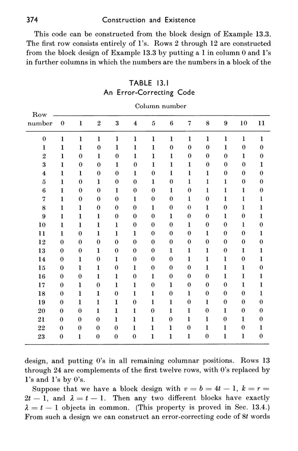
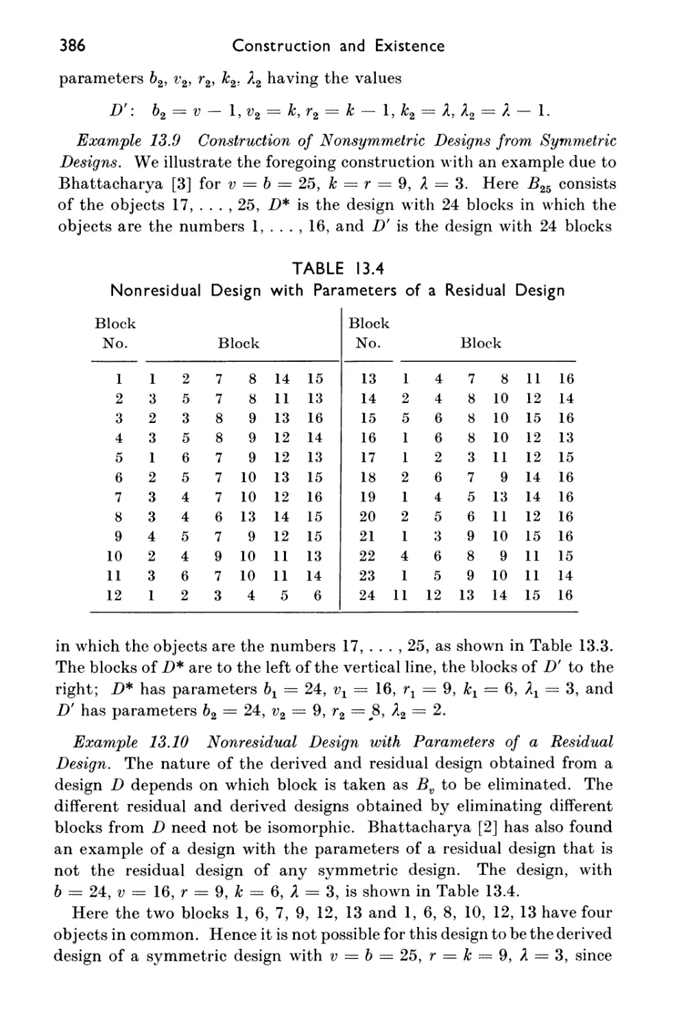
/


Текст
I
I
APPLIED COMBINATORIAL
MATHEMATICS
The Authors
GEORGE POLYA
DERRICK H. LEHMER
MONTGOMERY PHISTER, Jr.
JOHN RIORDAN
ELLIOTT W. MONTROLL
N. G. DE BRUIJN
FRANK HARARY
RICHARD BELLMAN
ROBERT KALABA
EDWIN L. PETERSON
LEO BREIMAN
ALBERT W. TUCKER
EDWIN F. BECKENBACH
MARSHALL HALL, Jr.
JACOB WOLFOWITZ
CHARLES B. TOMPKINS
KENNETH N. TRUEBLOOD
GEORGE GAMOW
HERMANN WEYL
JOHN WILEY AND SONS, INC., NEW YORK • LONDON • SYDNEY
Editor
EDWIN F. BECKENBACH
Professor of Mathematics
University of California
Los Angeles
Copyright © 1964 by John Wiley & Sons, Inc.
All Rights Reserved. This book or any part thereof
must not be reproduced in any form
without the written permission of the publisher.
Library of Congress Catalog Card Number: 64-23826
Printed in the United States of America
To Professor Clifford Bell, Head
Physical Sciences Extension
University of California
in recognition of his imaginative and tireless devotion
to the Engineering and Physical Sciences Lecture Series
this book is affectionately dedicated
at the time of his retirement
THE AUTHORS _
IN ORDER OF PRESENTATION
GEORGE POLYA, Ph.D., Emeritus Professor of Mathematics, Stanford
University
DERRICK H. LEHMER, Ph.D., Professor of Mathematics, University of
California, Berkeley
MONTGOMERY PHISTER, JR., Ph.D., Chief Engineer, Scantlin
Electronics, Inc., and Lecturer in Engineering, University of California,
Los Angeles
JOHN RIORDAN, Ph.D., Member of Technical Staff, Bell Telephone
Laboratories, Inc., Murray Hill, New Jersey
ELLIOTT W. MONTROLL, Ph.D., Vice President for Research, Institute
for Defense Analyses, Washington, D.C.
N. G. DE BRUIJN, Ph.D., Professor of Mathematics, Technical
University, Eindhoven, Netherlands
FRANK HARARY, Ph.D., Professor of Mathematics, University of
Michigan
RICHARD BELLMAN, Ph.D., Mathematician, The RAND Corporation,
Santa Monica, California
ROBERT KALABA, Ph.D., Mathematician, The RAND Corporation,
Santa Monica, California
EDWIN L. PETERSON, M.S., Member of Professional Staff, Defense
Research Corporation, Santa Barbara, California
LEO BREIMAN, Ph.D., Associate Professor of Mathematics, University
of California, Los Angeles
ALBERT W. TUCKER, Ph.D., Professor of Mathematics, Princeton
University
vi
The Authors vii
EDWIN F. BECKENBACH, Ph.D., Professor of Mathematics, University
of California, Los Angeles
MARSHALL HALL, JR., Ph.D., Professor of Mathematics, California
Institute of Technology
JACOB WOLFOWITZ, Ph.D., Professor of Mathematics, Cornell
University
CHARLES B. TOMPKINS, Ph.D., Professor of Mathematics, University
of California, Los Angeles
KENNETH N. TRUEBLOOD, Ph.D., Professor of Chemistry, University
of California, Los Angeles
GEORGE GAMOW, Ph.D., Professor of Physics, University of Colorado
HERMANN WEYL, Ph.D., Late Member, Institute for Advanced Study
FOREWORD
Engineering achievement depends on the extent to which knowledge
generated through research, in universities, in industry, and in
government, knowledge expanded through the use of knowledge in
industry, and knowledge handed to us through the ages is utilized
effectively and at the proper time.
Modern studies in biological, social, physical, and mathematical
sciences are uncovering exciting problems in combinatorial
mathematics, a subject that is concerned with arrangements, operations,
and selections within a finite or discrete system. It includes problems
of systems analysis, information transmission, behavior of neural
networks, and many others. These problems are yielding to new attacks,
based in part on the availability of high-speed automatic computers.
To keep pace with this progress, University Extension, Engineering
and Physical Sciences Divisions, offered a Statewide Lecture Series
on Applied Combinatorial Mathematics in the spring of 1962. This
book is an outgrowth of the lecture series; it presents valuable aspects
of the underlying theory and also some significant applications of this
increasingly important and vital subject.
FRANCIS E. BLACET
Professor of Chemistry
Dean, Division of Physical Sciences
University of California
Los Angeles
GEORGE J. MASLACH
Professor of Aeronautical Engineering
Acting Dean, College of Engineering
University of California
Berkeley
L. M. K. BOELTER
Professor of Engineering
Dean, College of Engineering
University of California
Los Angeles
PAUL H. SHE ATS
Professor of Education
Dean, University Extension
University of California
Statewide
IX
PREFACE
. . . We will therefore refer to this group
of problems as those of organized
complexity.
Warren Weaver, "Science and Complexity/'
American Scientist 36 (1948), 538
In the article quoted above, Warren Weaver first points out that
the physical sciences of the sixteenth, seventeenth, and eighteenth
centuries were largely concerned with the analysis of two-variable,
or few-variable, problems: The relation between distance and
gravitational force, between voltage and electric current, between pressure
and the volume of a gas, and so on. These great problems were those
of simplicity. The life and social sciences were still largely in the
preliminary, observational stages of the scientific method.
At about the beginning of this century, however, the pendulum
swung far in the other direction, and much scientific progress was
made through statistical techniques in the analysis of problems of
disorganized complexity. The exact solution of a ten-body problem,
say the problem of the motion of ten pool balls on a pool table, can
be quite complicated; but statistical mechanics can give good answers
for average behavior when we are dealing with huge numbers of
molecules or of subatomic particles. Statistical methods also are quite
effective in some aspects of the life sciences, as exemplified by the
general reliability of mortality tables.
This leaves the middle ground of organized complexity, which is
largely in the scientific foreground today. The operation of a
petroleum-processing plant or of a military organization might in-
xi
XII
Preface
volve hundreds or even thousands of variables, but such a problem
is tractable by modern mathematical techniques through the use of
high-speed computing machines. In the same way, complex
mathematical models of subsystems of human physiology, essential to space-
age technology, are showing promise of far-reaching results in the
diagnosis and prevention of disease.
For a simple example involving some typical combinatorial
problems, let us consider a round-robin tennis tournament with a given
number of players and a given number of courts. Is it possible to
arrange the schedule so that no player participates twice
consecutively? This is an existence problem. If there is such a schedule,
how do we go about determining it? This is a construction or
evaluation problem. For variety in subsequent tournaments, it might be
desirable to list all the different possible schedules. This is an
enumeration problem. Of all schedules, it might be desirable to hit
on the most enjoyable one, as measured, for example, by sustaining
interest through having the best players meet each other last. This
is an extremization problem. Most combinatorial problems are of one
or another of these types, although, of course, the distinction is not
always precise.
Analytic problems, involving continuous variables, are often solved
approximately through the use of digital computing machines. Thus
these problems are of concern to the combinatorial mathematician.
The first two chapters of this book are definitely machine-oriented;
the rest are not. It is only this point that separates these two chapters
from the other four chapters of Part 1, for all six chapters are
concerned with computation and evaluation, just as all six are concerned
with counting and enumeration.
The six chapters of Part 2 are also concerned with computational
problems, but now the emphasis has turned toward the determination
of the solution that, in some sense, is best. Similarly, the six chapters
of Part 3 are concerned with these same problems, but with greater
emphasis on the construction of examples of which the existence
initially was more in doubt. The last portion of Part 3 deals also with
problems of physical existence and finally with more philosophical
considerations.
Unfortunately, two of the lecturers in the Statewide Lecture Series
were unable to spare the time required for the preparation of
manuscripts. These would have been concerned with error-correcting codes
and network-flow problems, respectively. The former subject,
however, is treated in part in the chapter on block designs; for the latter
Preface
xiii
subject, the chapter contributed by the editor is a partial substitute.
On the other hand, the material in the Lecture Series has been
augmented by the addition of Chapters 5, 6, and 18, for the subjects
treated in these chapters were not included in the Series.
The editor wishes to express his gratitude to the authors for their
diligent work in preparing the material for publication; to the other
Advisory Committee members, John L. Barnes, Clifford Bell, Richard
E. Bellman, John C. Dillon, Delbert R. Fulkerson, Harold M. Heming,
Magnus R. Hestenes, and Charles B. Tompkins for their efforts and
excellent ideas; to the Course Coordinators, Clifford Bell, Julius J.
Brandstatter, Robert Goss, and Stanley B. Schock for their efficient
handling of lecture arrangements; and to Mrs. Caryl Ruenker for her
painstaking secretarial work on the manuscript.
August, 1964
Edwin F. Beckenbach
CONTENTS
INTRODUCTION 1
PART 1A COMPUTATION AND EVALUATION
chapter 1 THE MACHINE TOOLS OF COMBINATORICS 5
DERRICK H. LEHMER
1.1 Introduction 5
1.2 Representation and Processing of Digital Information 6
1.3 Application of Representations 11
1.4 Signatures and Their Orderly Generation 17
1.5 Orderly Listing of Permutations 19
1.6 Orderly Listing of Combinations 24
1.7 Orderly Listing of Compositions 24
1.8 Orderly Listing of Partitions 25
1.9 The Back-Track Procedure 26
1.10 Ranking of Combinations 27
chapter 2 TECHNIQUES FOR SIMPLIFYING LOGICAL
NETWORKS 32
MONTGOMERY PHISTER, JR.
2.1 Introduction 32
Simplifying a Given Sequential Circuit 37
2.2 Simplest AND-OR Gates 37
2.3 Multiple-Output Function Simplifications 40
2.4 Elimination of Memory Elements 42
2.5 Alternative Methods of Assigning Flip-Flop States 49
Choosing Decision and Memory Elements 53
2.6 Memory Elements Other Than Delay Flip-Flops 53
xv
xvi Contents
2.7 Decision Elements Other Than AND and OR Gates
2.8 Conclusion
PART IB COUNTING AND ENUMERATION
chapter 3 GENERATING FUNCTIONS
JOHN RIORDAN
3.1 Introduction
3.2 Generating Functions for Combinations
3.3 Generating Functions for Permutations
3.4 Elementary Relations: Ordinary Generating Function
3.5 Elementary Relations: Exponential Generating Function
3.6 Generating Functions in Probability and Statistics
3.7 Polya's Enumeration Theorem
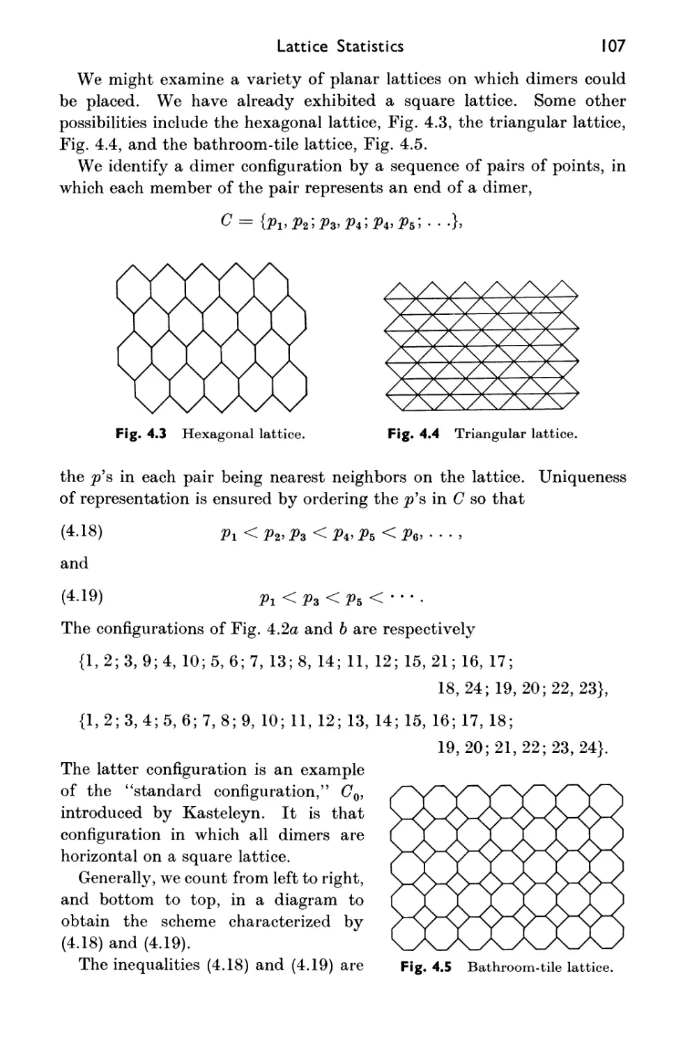
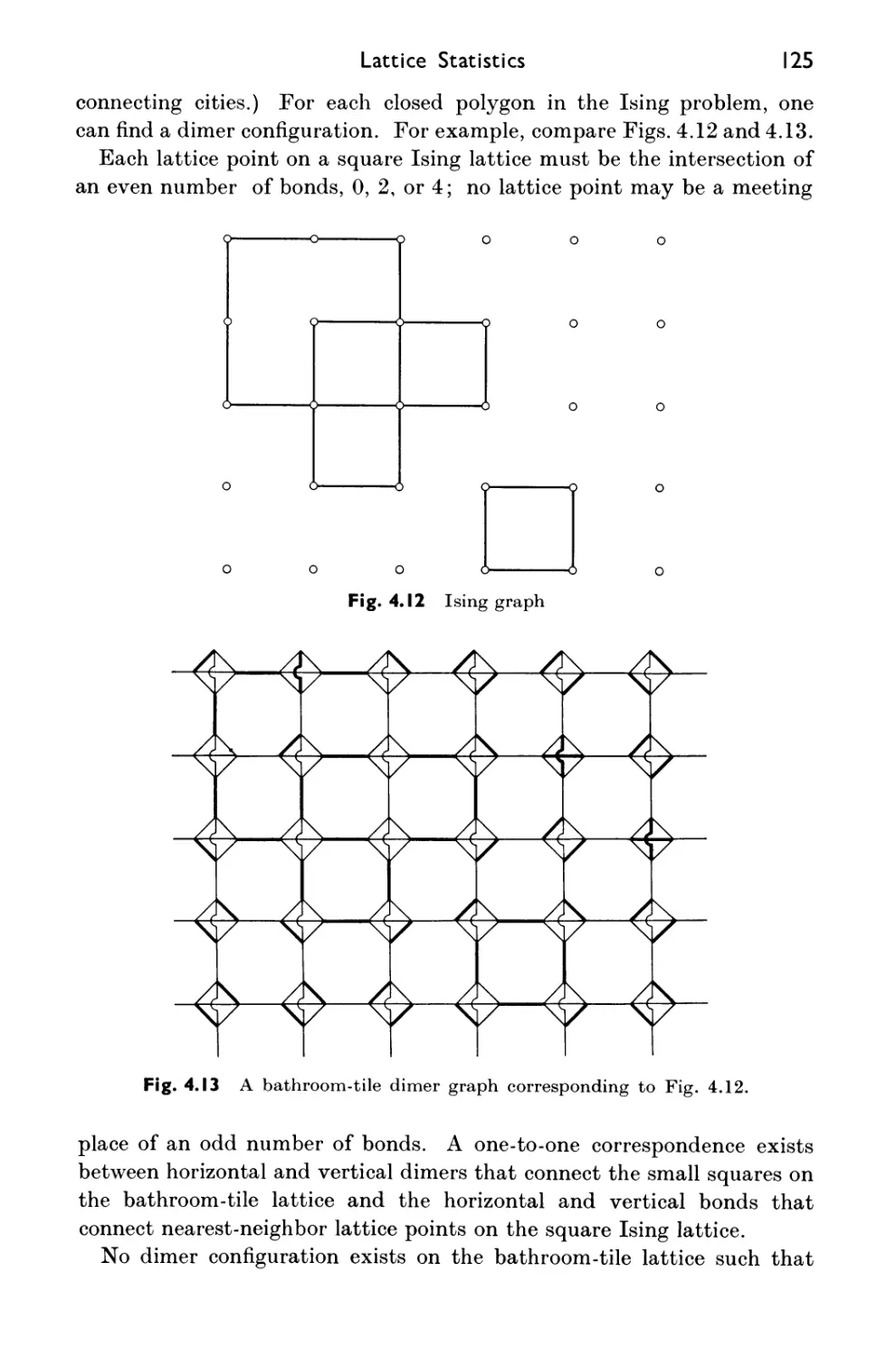
chapter 4 LATTICE STATISTICS
ELLIOTT W. MONTROLL
4.1 Introduction
4.2 Random Walks on Lattices and the Polya Problem
4.3 More General Random Walks on Lattices
4.4 The Pfaffian and the Dimer Problem
4.5 Cyclic Matrices
4.6 Evaluation of Dimer Pfaffian
4.7 The Ising Problem
4.8 Some Remarks on Periodic Boundary Conditions
4.9 Lattice Statistics of Slightly Defective Lattices
chapter 5 POLYA'S THEORY OF COUNTING
N. G. DE BRUIJN
5.1 Introduction
5.2 Cycle Index of a Permutation Group
5.3 The Main Lemma
5.4 Functions and Patterns
5.5 Weight of a Function; Weight of a Pattern
5.6 Store and Inventory
5.7 Inventory of a Function
5.8 The Pattern Inventory; Polya's Theorem
5.9 Generalization of Polya's Theorem
5.10 Patterns of One-to-One Mappings
5.11 Labeling and Delabeling
Contents xvii
5.12 The Total Number of Patterns 171
5.13 The Kranz Group 176
5.14 Epilogue 180
chapter 6 COMBINATORIAL PROBLEMS IN GRAPHICAL
ENUMERATION 185
FRANK HARARY
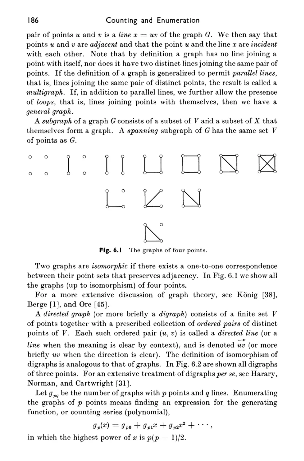
6.1 Introduction 185
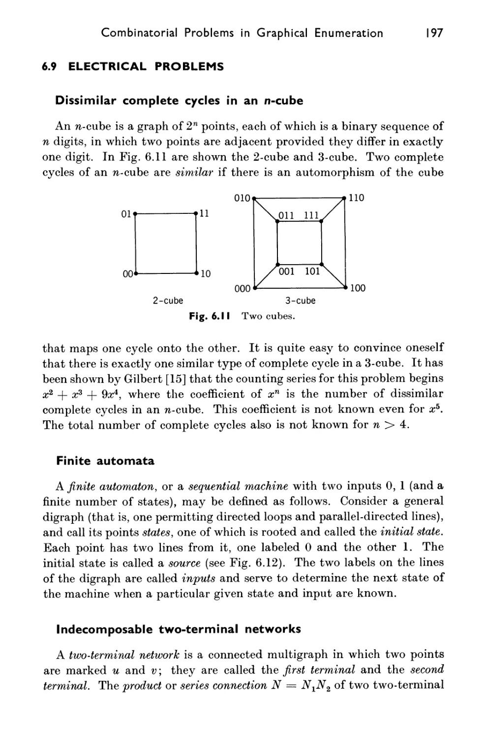
6.2 Graphical Preliminaries 185
6.3 Some Unsolved Pre'!ems 189
6.4 Problems Involving L rected Graphs 189
6.5 Problems Involving Partitions 190
6.6 Topological Problems 191
6.7 Problems Involving Connectivity 193
6.8 Problems Involving Groups 195
6.9 Electrical Problems 197
6.10 Physical Problems 199
6.11 Graph-Counting Methods 202
6.12 Tree-Counting Methods 205
6.13 Comparison of Solved and Unsolved Problems 208
6.14 Some Applications of Enumeration Problems to Other Fields 212
PART 2 CONTROL AND EXTREMIZATION
chapter 7 DYNAMIC PROGRAMMING AND MARKOVIAN
DECISION PROCESSES, WITH PARTICULAR
APPLICATION TO BASEBALL AND CHESS 221
RICHARD BELLMAN
7.1 Introduction 221
7.2 Baseball as a Multistage Decision Process; State Variables 221
7.3 Decisions 222
7.4 Criterion Function 223
7.5 Policies, Optimum Policies, and Combinatorics 224
7.6 Principle of Optimality 226
7.7 Functional Equations 226
7.8 Existence and Uniqueness 227
7.9 Analytic Aspects 227
7.10 Direct Computational Approach 229
7.11 Stratification 229
7.12 Approximation in Policy Space 230
xviii Contents
7.13 Utilization of Experience and Intuition 231
7.14 Two-Team Version of Baseball 232
7.15 Probability of Tying or Winning 232
7.16 Inventory and Replacement Processes and Asymptotic Behavior 232
7.17 Chess as a Multistage Decision Process 233
7.18 Computational Aspects 234
chapter 8 GRAPH THEORY AND AUTOMATIC CONTROL 237
ROBERT KALABA
8.1 Introduction 237
8.2 Time-Optimal Control and the Nature of Feedback 238
8.3 Formulation 239
8.4 Uniqueness 240
8.5 Successive Approximations 241
8.6 Observations on the Approximation Scheme 242
8.7 Other Approaches 242
8.8 Arbitrary Terminal States 243
8.9 Preferred Suboptimal Trajectories 243
8.10 A Stochastic Time-Optimal Control Process 244
8.11 Minimax Control Processes 246
8.12 Use of Functional Equations 246
8.13 A Special Case 246
8.14 Minimal Spanning Trees 247
8.15 Comments and Interconnections 248
8.16 Multiple Stresses 249
8.17 Discussion 250
chapter 9 OPTIMUM MULTIVARIABLE CONTROL 253
EDWIN L. PETERSON
9.1 Problem Structure 253
9.2 Alternative Approaches 257
9.3 Polynomial Approximation 264
9.4 Linearization and Successive Approximation 272
9.5 Physical Implementation 279
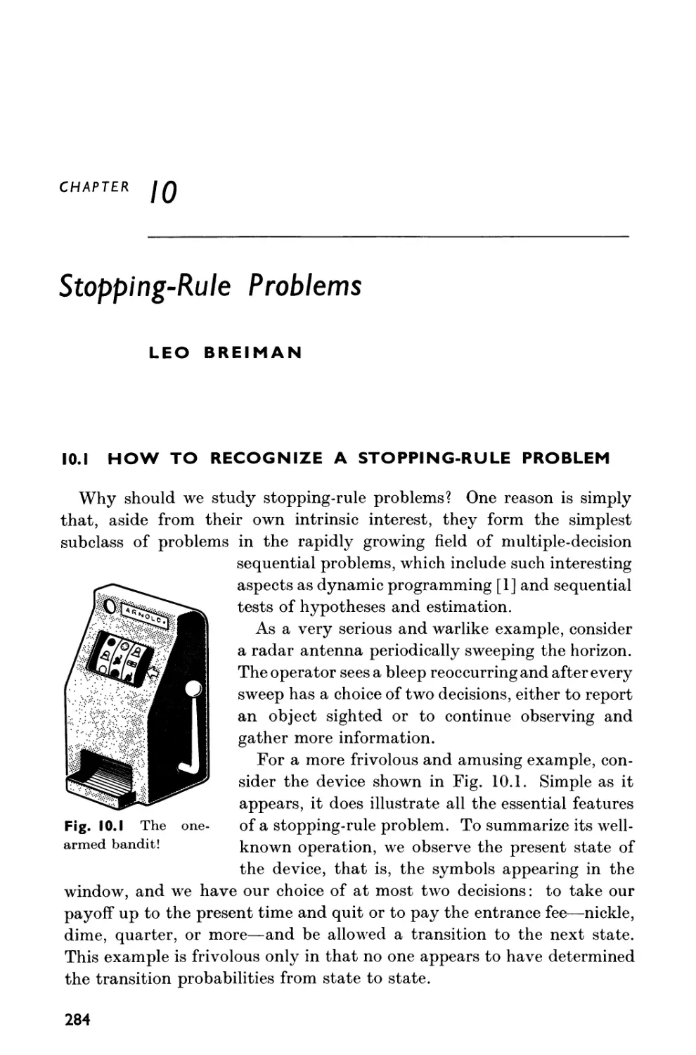
chapter 10 STOPPING-RULE PROBLEMS 284
LEO BREIMAN
10.1 How to Recognize a Stopping-Rule Problem 284
10.2 Examples 285
10.3 Formulation 287
10.4 What Is a Stopping Rule? 290
Contents xix
10.5 What Is a Solution? 291
10.6 Stop When You Are Ahead; the Stability Problem 292
10.7 The Functional Equation 294
10.8 Elimination of Forced Continuation 296
10.9 Entrance-Fee Problems and Reduction to Them 298
10.10 The Linear-Programming Solution 302
Binary Decision Renewal Problems 305
10.11 Introduction and Examples 305
10.12 Formulation 306
10.13 What Is a Solution? 307
10.14 Reduction to a Stopping-Rule Problem by Cycle Analysis 308
10.15 A Direct Approach 312
10.16 The Linear-Programming Solution 314
10.17 A Duality Relation 317
chapter 11 COMBINATORIAL ALGEBRA OF MATRIX GAMES
AND LINEAR PROGRAMS 320
ALBERT W. TUCKER
11.1 Introduction 320
11.2 Game Example 320
11.3 Key Equation and Basic Solutions 322
11.4 Schematic Representation 324
11.5 Equivalence by Pivot Steps; Simplex Method 327
11.6 Linear Programming Examples 331
11.7 Key Equation and Basic Solutions for Linear Programs 333
11.8 Canonical Forms 336
11.9 Inverse Basis Procedure 340
11.10 General Formulations 343
chapter 12 NETWORK FLOW PROBLEMS 348
EDWIN F. BECKENBACH
12.1 Introduction 348
12.2 Networks 348
12.3 Cuts 350
12.4 Flows 351
12.5 Flows and Cuts 352
12.6 Bounds on Capacities of Cuts and on Values of Flows 355
12.7 The Max-Flow—Min-Cut Theorem 357
12.8 The Ford-Fulkerson Algorithm 358
12.9 Example 359
12.10 Extensions and Applications 361
12.11 Graph Theory and Combinatorial Problems 362
XX
Contents
PART 3 CONSTRUCTION AND EXISTENCE
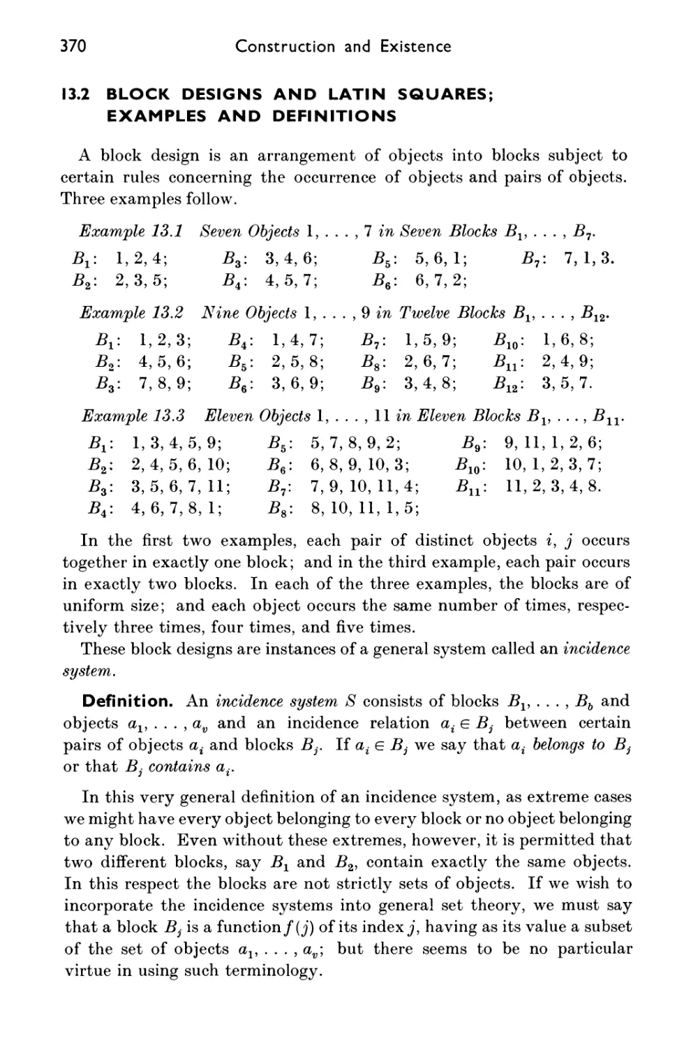
chapter 13 BLOCK DESIGNS 369
MARSHALL HALL, JR.
13.1 Introduction 369
13.2 Block Designs and Latin Squares; Examples and Definitions 370
13.3 Applications of Block Designs 373
13.4 General Theory of Block Designs 377
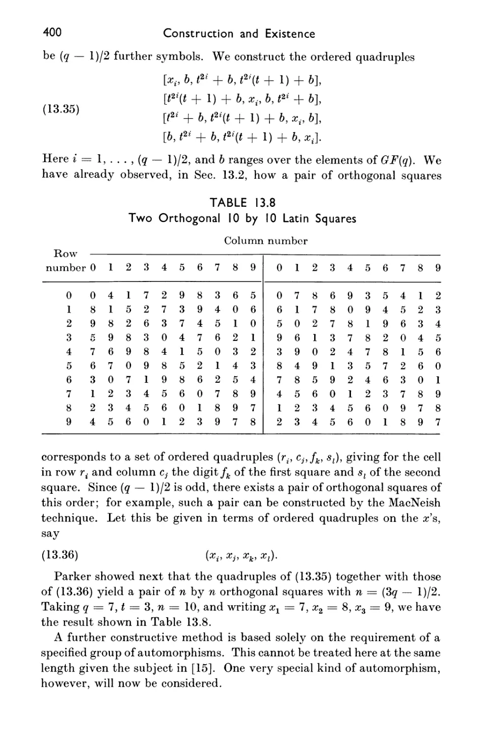
13.5 Construction of Block Designs and Orthogonal Latin Squares 387
chapter 14 INTRODUCTION TO INFORMATION THEORY 406
JACOB WOLFOWITZ
14.1 Introduction 406
14.2 Channels 406
14.3 Codes 407
14.4 Entropy; Generated Sequences 408
14.5 The Discrete Memoryless Channel 410
14.6 Compound Channels 412
14.7 Other Channels 414
chapter 15 SPERNER'S LEMMA AND SOME EXTENSIONS 416
CHARLES B. TOMPKINS
15.1 Introduction 416
15.2 Sperner's Lemma 418
15.3 Brouwer's Fixed-Point Theorem 424
15.4 Subdivisions of a Simplex 427
15.5 Review of Position—Second Introduction 430
15.6 Oriented Simplexes, Their Boundaries, and Oriented Simplicial
Mappings 434
15.7 Homology—x-Chains, Cycles, Bounding Cycles 437
15.8 The Fundamental Index Theorem 441
15.9 Some Applications 445
15.10 Toward Greater Rigor 453
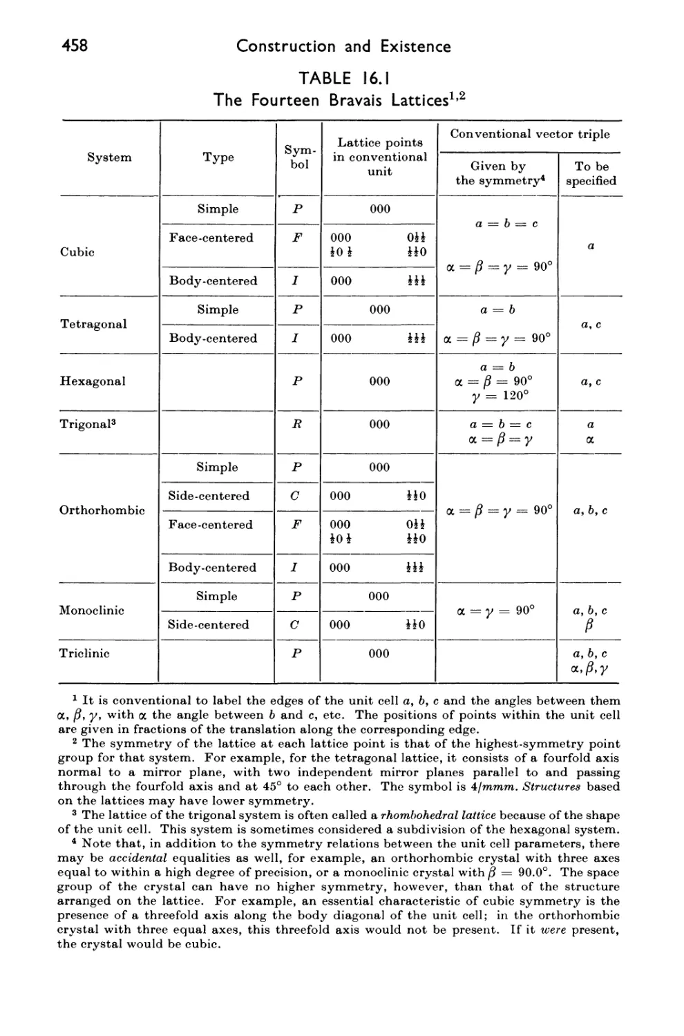
chapter 16 CRYSTALLOGRAPHY 456
KENNETH N. TRUEBLOOD
16.1 Introduction 456
Nature of the Crystalline State 457
16.2 Lattices 457
Contents xxi
16.3 Point Symmetry 461
16.4 Space Symmetry 465
16.5 Antisymmetry 467
Crystal Structure Analysis by X-Ray Diffraction 468
16.6 Diffraction 468
16.7 Fourier Transforms of Atoms and Groups of Atoms 474
16.8 The Phase Problem 478
Approaches to Solving the Phase Problem 482
16.9 The Patterson Function 482
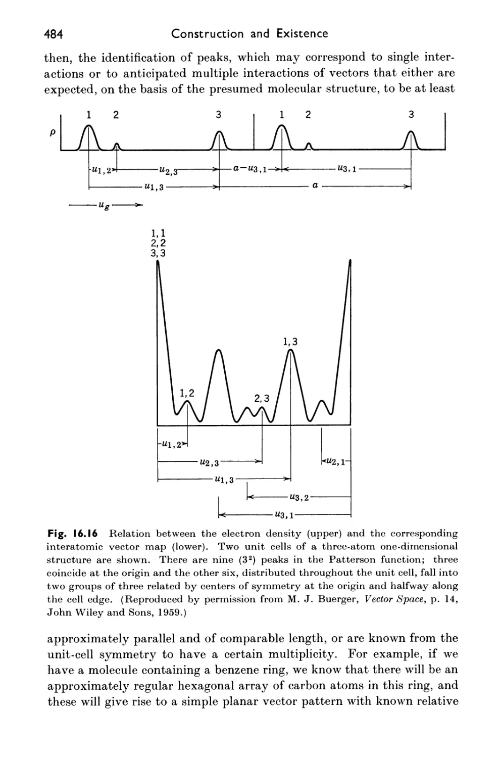
16.10 Heavy-Atom Methods 485
16.11 Isomorphous Replacement 488
16.12 Direct Methods 491
16.13 Refinement 495
Some Aspects of Atomic Arrangements 500
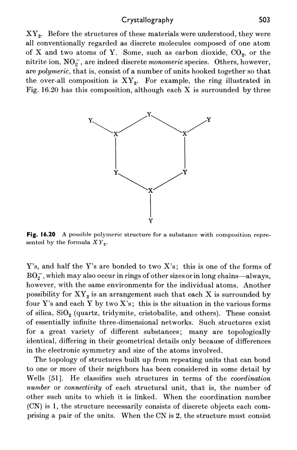
16.14 Topology and Shapes of Molecules and Assemblies of Molecules 500
16.15 Packing of Spheres, Molecules, and Polyhedra 504
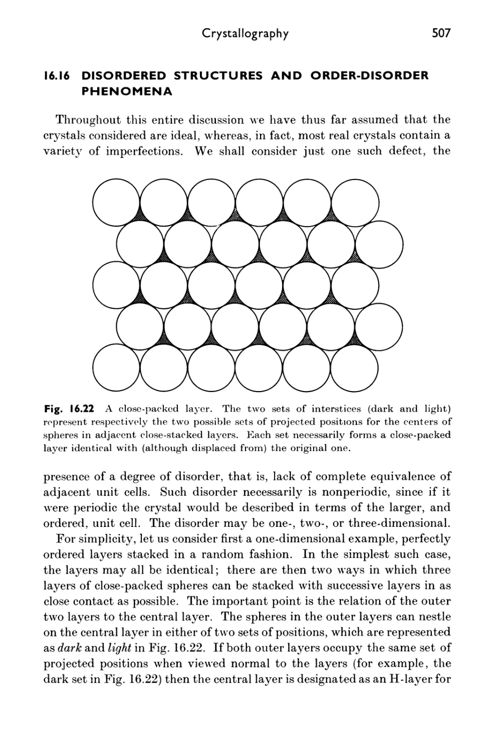
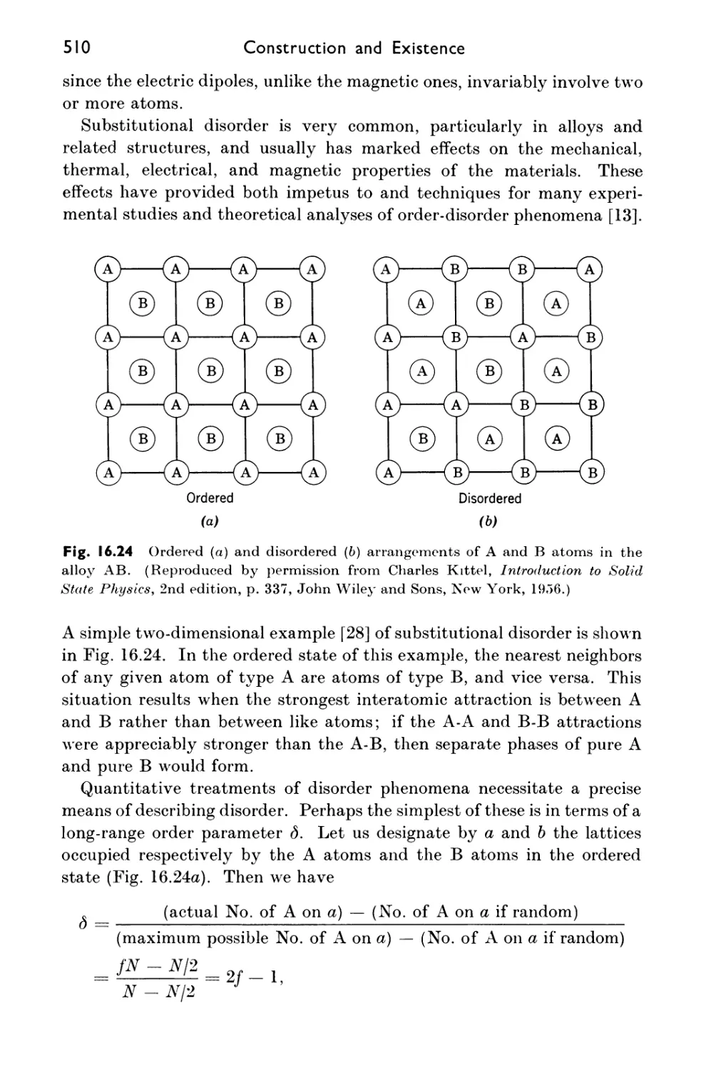
16.16 Disordered Structures and Order-Disorder Phenomena 507
chapter 17 COMBINATORIAL PRINCIPLES IN GENETICS 515
GEORGE GAMOW
17.1 Introduction 515
17.2 Amino-Acid Sequences in Proteins 515
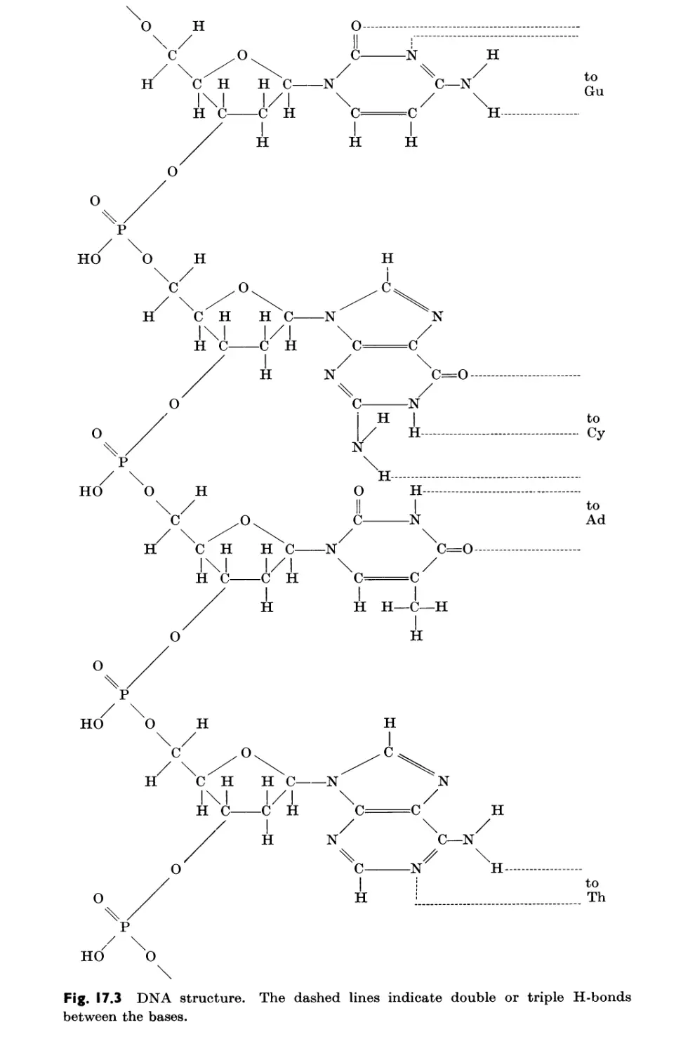
17.3 Double-Stranded Sequences in DNA 519
17.4 Combinatorial Principles 522
17.5 The Overlapping-Code Hypothesis 522
17.6 Statistical Investigations 523
17.7 Geometric Implications 525
17.8 Statistical Assignments 526
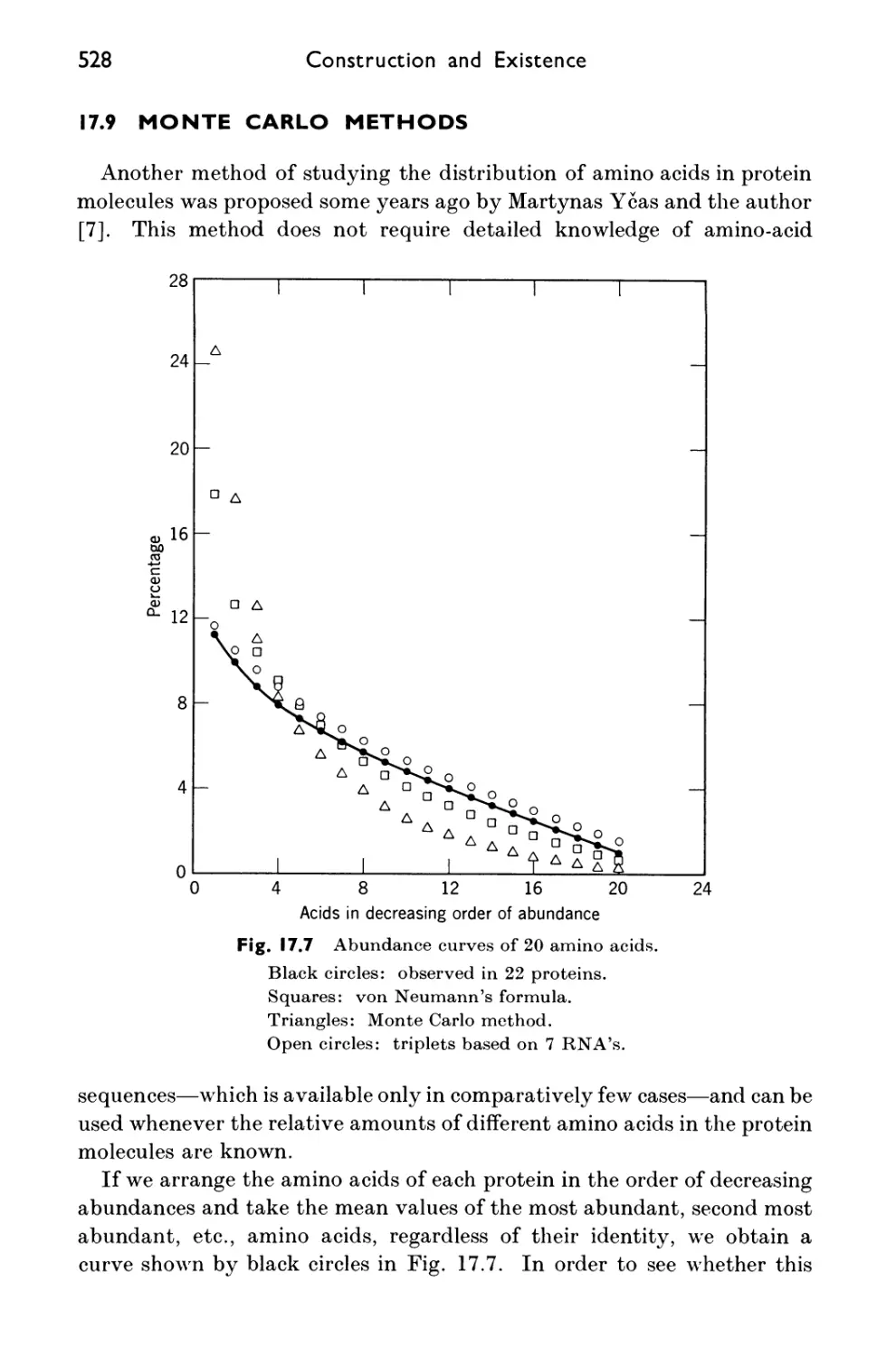
17.9 Monte Carlo Methods 528
17.10 Experimental Results 532
chapter 18 APPENDICES 536
HERMANN WEYL
18.1 Ars Combinatoria 536
18.2 Quantum Physics and Causality 551
18.3 Chemical Valence and the Hierarchy of Structures 563
18.4 Physics and Biology 572
ANSWERS TO MULTIPLE-CHOICE REVIEW PROBLEMS 583
AUTHOR INDEX 585
SUBJECT INDEX
591
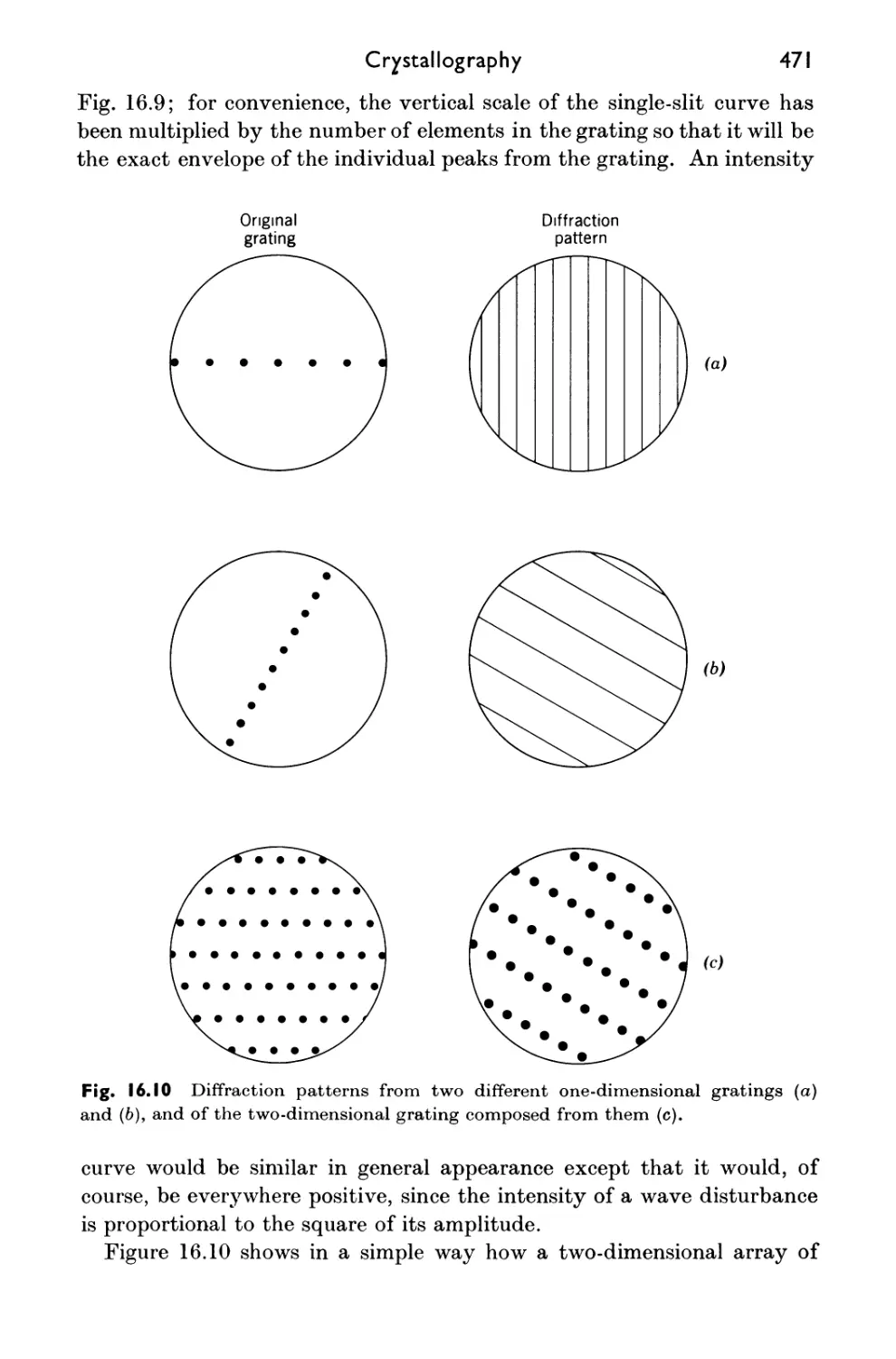
Introduction
GEORGE POLYA
The celebrated Leibnitz possessed many real insights by
which he has enriched the sciences, but he had still more and greater
projects for the execution of which the world has waited in vain.
IMMANUEL KANT
Werke 2 (1867), p. 385
Gottfried Wilhelm Leibnitz was the first author, it seems, who used the
term "combinatorial" in the same meaning as we use it today in speaking
of combinatorial analysis, or combinatorial mathematics. Leibnitz was
scarcely twenty years old when he wrote his Dissertatio de Arte Combina-
toria, which was printed in 1666. The title page promises "applications to
the whole sphere of sciences" and "new germs of the logic of invention."
The summary announces applications to locks, organs, and syllogisms,
to the mixing of colors and to protean verses, to logic, geometry, military
art, grammar, law, medicine, and theology.
In fact, the Dissertatio contains, besides a bewildering show of scholastic
erudition, some mathematical results. It explains and solves the basic
combinatorial problems that lead to the binomial coefficients and to the
factorial, but there is not much more. These problems were not so
trivial in 1666 as they are today, but many of Leibnitz's results were
known before him. The mathematical propositions are followed by
applications, almost all of which appear as futile or fantastic to the
modern reader and a few of which appeared so to Leibnitz himself.
The Dissertation on the Combinatorial Art, however, was just the
beginning of a great project that Leibnitz entertained through his life.
I
2 Introduction
He often mentions this project in his letters and in his printed work, and
many notes found among his manuscripts that he left unpublished are
concerned with it. Some of these notes have been printed posthumously.
We see from them that Leibnitz planned more and more applications of
his combinatorial art, or "combinatorics": to coding and decoding, to
games, to mortality tables, to the combination of observations. Also,
he widened more and more the scope of the subject. He sometimes
regards combinatorics as one-half of a general Art of Invention; this half
should deal with Synthesis, whereas the other half would deal with
Analysis. Combinatorics should deal, he says in another passage, with
the same and the different, the similar and the dissimilar, the absolute
and the relative, whereas ordinary mathematics deals with the one and
the many, the great and the small, the whole and the part. Eventually
he assigns to combinatorics the widest scope in regarding it as coinciding,
or almost coinciding, with the Characteristica Universalis. He planned
"the universal characteristic" as a sort of generalized mathematics, which
would deal with everything thinkable and would reduce thinking, by the
use of appropriate signs and characters, to a sort of calculation.
Were these projects of Leibnitz mere dreams? There was some
substance in his projects and there was, perhaps, some prophetic vision in his
dreams. With his Characteristica Universalis he intended to reduce
concepts to symbols, symbols to numbers—and, eventually, through
symbols and numbers, he intended to subject all concepts to mechanical
computation. This project appeared fantastic and absurd to many people
with usually sound judgment, but today's computing machines are
realizing some portion of the visionary scheme. Leibnitz possessed some
elements of mathematical logic, of which he recognized the importance
long before anybody else; now, mathematical logic lies somehow on the
way to the Characteristica Universalis. It is true that the applications he
made of his Ars Combinatoria are trivial, futile, or fantastic; but he
certainly foresaw the immense variety of applications and the expanding
scope of combinatorics. And so the name of Gottfried Wilhelm Leibnitz,
the great mathematician, philosopher, and project monger, may fittingly
introduce the present book.
PART IA
COMPUTATION
AND EVALUATION
Maybe it has become too hard for us unless we
are given some outside help, be it even by such
devilish devices as high-speed computing machines.
HERMANN WEYL
(from an address delivered at the Princeton University Bicentennial
Coyiference on the Problems of Mathematics, December 17—19, 1946)
CHAPTER
The Machine Tools of Combinatorics
DERRICK H. LEHMER
I.I INTRODUCTION
It is the purpose of this chapter, as its title implies, to set forth a few
of the known devices that enable us to pursue the subject of combinatorial
analysis in its rudimentary as well as its more advanced stages. The
title, however, is a double-entendre, because we shall relate our discussions
very closely to the modern digital computer, without which many of our
devices would be mere curiosities. Until recently, in fact, most of
combinatorial analysis was concerned with the number of different ways that
a certain thing could be done. With high-speed flexible computers, we are
now prepared to ask: What are these ways and which is optimal? To
bring questions like these to a computer primarily designed to do so-called
scientific computing involves problems of procedure and even
programming that are not entirely straightforward. In trying to make
combinatorial mathematics workable, there is also the fundamental difficulty
of complexity, which increases multiplicatively or exponentially with any
slight increase in the domain of a parameter. Thus there is often the
urgent need to keep to a minimum the execution time of basic subroutines.
Still more urgent is the use of optimum methods. Factors of 1020 in
performance are sometimes purchased by a good idea.
In spite of the numerous discouraging problems that confront the
combinatorial analyst, there are some inherent advantages for him to
appreciate. No longer does he have to simulate the real-number system.
Gone are the headaches caused by truncation error, round-off noise,
floating-point arithmetic, information fadeout, and divide checks. There
is a certain cleanliness to the subject that agrees well with the very nature
5
6 Computation and Evaluation
of a digital computer. Although most of his mathematical friends find
refuge in infinity, the combinatorial analyst finds refuge from infinity.
This presentation assumes that the reader is acquainted with computers
and their programming. In fact, we do not hesitate to give procedures or
actual brief coding, in SHARE Assembly Program (SAP) language, of
subroutines to illustrate a procedure. On the other hand, many facts
that are well known to such a reader are mentioned. Of course, some of
the tools we need are basic and therefore very simple; they are easily
discovered with a little native ingenuity. It is hoped that a treatment
along somewhat different lines may add a dimension to the reader's
understanding of even the more obvious aspects of our subject. For
further readings, see [2] to [5].
1.2 REPRESENTATION AND PROCESSING OF
DIGITAL INFORMATION
The basic format of information in combinatorial problems is the
vector with integer components. We use the term vector in the simple
sense of a one-rowed matrix, or a lattice point in a finite-dimensional
space. We shall need no vector analysis or even geometric interpretation
of vectors.
The representation of integers
The integer components may have various useful representations which
themselves may be vectors. Conversely, the basic vector itself may stand
for an integer. We begin by considering that most familiar representation
of the nonnegative integers, the machine-based polynomial representation
n = d0b° + dxbl + d2b2 + • • • , 0 < dt < b,
where the inequalities on the coefficients di are imposed to ensure
uniqueness. Because this method came to Europe through Arabia, we write the
d's backward, so that, for b = 10, we have
30147 = 7 • 10° + 4 • 101 + 1 • 102 + 0 • 103 + 3 • 104,
and for b = 2,
110101 = 1 • 2° + 0 • 21 + 1 • 22 + 0 • 23 + 1 • 24 + 1 • 25.
The arithmetic unit of our machine is based on this representation. By
addition the successor of n is n + 1; thus (according to Peano) the machine
can methodically generate the integers by the famous operation n + 1 -> n.
Eventually this will cause overflow, but usually our numbers n will be of
The Machine Tools of Combinatorics 7
moderate size. One important feature of the polynomial representation
is that it is easy to recognize which of two numbers is the larger by
inspecting their digits. This makes the card sorter sometimes
competitive to an expensive computer. The polynomial representation is so
familiar in the case 6 = 10 that one is in danger of identifying a number
with its set of digits dv
Machines ordinarily have either b = 2 or b = 10, and because their
arithmetic units perform both arithmetical and logical operations it is
possible to exploit this fact for combinatorial purposes. For these
purposes, base-2 machines are superior to base-10 machines. In the latter
the digits are coded in binary form, but the user does not have access to
the four bits of each digit. Of course, one may deal with decimal numbers
having only 0's and l's as digits, but this is wasteful and sometimes
cumbersome. One may go further and devote a whole machine word to
a single digit. In fact, this is what one is driven to if, for example, b = 7
or b = 12. Many of the devices we shall describe imply a binary arithmetic
unit.
Another representation of integers, useful in combinatorics, is called
the factorial representation. Here we have
n = ax - 1! + a2 • 2! + a3 • 3! + • • • , 0 < ai < i.
The inequalities 0 < at < i are imposed to ensure uniqueness. The a/s
are called the factorial digits of n. We can write
n = {a^, a2, • • •) j
for example, we have
1,000,000 = (0, 2, 2, 1, 5, 2, 6, 6, 2).
Conversion from decimal or binary representation to factorial
representation is simple. There are two possible methods. One divides n by 2 and
the remainder is a1. The quotient is next divided by 3 and the remainder
is a2, etc. Alternatively, if p\ < n < (p -\- 1)!, then one may divide n by
p\ and the quotient is ap. The remainder is now divided by (p — 1)! and
the quotient is aJ)_1, etc. Conversion from factorial to polynomial
representation is equally simple.
Two numbers in factorial representation can be compared for size by
simply inspecting their leading (right-hand) digits. Thus the largest
number having p digits is (1, 2, 3, . . . , p). By uniqueness, this number
must be (p -\- 1)! — 1. Thus we have the possibly unfamiliar identity
1 • 1! + 2 • 2! + 3 • 3! + • • • + p • p{ = (p + 1)! - 1.
In Sec. 1.5, we shall see how very useful this factorial representation
is in dealing with permutation problems.
8 Computation and Evaluation
Yet another representation, unfamiliar to almost everyone, we call the
combinatorial representation of given nome. Let k > 1 be a fixed integer,
called the nome. Then there is the representation in terms of binomial
coefficients,
»- (?)+(?)+(?)+•■■+d').
with the side condition
0 < ax < a2 < • • • < ak
for uniqueness. If we write
n = \al9 a2, • . . , ak}>
then, for example, with k = 6 and k = 8, we have
1,000,000 = {9, 11, 14, 25, 27, 32}
and
1,000,000 = {0, 1, 3, 6, 12, 18, 23, 25},
respectively.
We shall explain the use of this representation method in connection
with combinations of things taken A: at a time.
A still wider variant of polynomial representation is the so-called
Chinese or modular representation with its interesting associated
arithmetic. Since
375 = 1 (mod 2)
= 0 (mod 3)
= 0 (mod 5)
= 4 (mod 7)
= 1 (mod 11)
= 11 (mod 13)
= 1 (mod 17),
we could write
375 ~ {1,0, 0,4, 1,11,1};
similarly, we have
243-(1,0,3,5, 1,9,5}.
Adding, subtracting, and multiplying corresponding components of these
two vectors, and reducing with respect to the corresponding moduli,
give at once
375 + 243 — {0, 0, 3, 2, 2, 7, 6} — 618,
375 - 243 — {0, 0, 2, 6, 0, 2, 13} — 132,
375 • 243 — {1, 0, 0, 6, 1, 8, 5} — 91,125.
The Machine Tools of Combinatorics 9
We note the absence of the carry-propagation problem. This truly parallel
arithmetic has aroused some interest among machine designers because
a simple set of matrices of cores enables one to perform addition,
subtraction, or multiplication in only one pulse time. We note also that
multiplication does not produce a noticeably larger vector. In fact, the vector for
375 looks, if anything, smaller than the vector for 243. This points up
one of the drawbacks of the system: The seven moduli up to 17 are more
than adequate to represent numbers up to the foregoing 91,125, so there
is redundancy for checking purposes. Actually, these seven-dimensional
vectors give a unique representation for each nonnegative integer less
than the product of the moduli, namely
2-3-5-7- 11 • 13- 17 = 510,510.
Converting from decimal to Chinese is simple enough. Reversing the
process is an old Chinese trick that the reader may wish to rediscover for
himself.
The representation of vectors
We turn now to the more complex question of vector representation.
If the vectors in question are short, that is, have low dimension, and
have only small integers as components, then it is often advantageous to
use fractional precision or packing to store a whole vector into one machine
word. In this way vectors can be sent from one place to another in a
minimum of time. Certain operations on the components, such as limited
addition, shifting, and Boolean operations, can be done in parallel by
means of the machine's logical operations. Some of these ideas are
illustrated in the next section. On the debit side, fractional precision often
involves "unpacking," or extraction of some of the components of the
vector, a process that in some cases is fussy and time-consuming. Vectors
with limited components, but with too many components to fit into one
machine word, can be stored in two or more consecutive words. Such
vectors may be sent from one place to another by use of multiprecise
arithmetic subroutines. Some machines have variable word length, but
unfortunately these are decimal machines. In the worst case, a single
word may be devoted to each component, and then one can take advantage
of the machine's address-arithmetic facilities. In many problems the
components are restricted to the values 0, 1. This offers a very compact
representation. Here a table of values of a two-valued function f(n)
can be stored as a long binary number whose nth bit is essentially/(n).
In some problems vectors are long but sparse or with limited
components. For such a case, one can program an inversion of information.
10 Computation and Evaluation
The long vector (av a2, a3, . . .) is then replaced by a list of component
values. After each such value, there is given a sublist of those integers n
for which an has this value. For example, the coefficients ai in the
expansion
00 00
TT(i-^) = 2v"
ra=l 7i=0
are mostly zero. For the nonzero an, we have
an = 1 for n = 0, 5, 7, 22, 26, 51, 57, 92, 100, 145, 155, 210, ...,
an = -1 for n = 1, 2, 12, 15, 35, 40, 70, 77, 117, 126, 176, 187,
Thus the problem of dealing with the vector {an} is transformed into a
question of set inclusion, as discussed on pages 12 to 15.
Another form for the designation of sparse vectors is the rank-and-value
representation, where the vector is replaced by a sequence of ordered pairs
in which the first member of the pair indicates the rank, or subscript, of
a nonzero component, and the second member of the pair gives the value
of the component. For example, the vector
(0, 3, 0, 0, 0, 1, 0, 0, 0, 4, 0, 0, 0, 0, 1, 0, 0, 0, 0, 0, 5, 9, 0, 0)
can be written in one word as
(2, 3; 6, 1; 10,4; 15, 1; 21, 5; 22, 9; 0).
The number 0 at the end is used to indicate "end of message." This
scheme is particularly helpful when one knows in advance that every
vector to be stored has at most a certain small number of nonzero
components.
In some problems the question, Have we seen this number before?, is
important. This can be answered almost instantly if one uses a registration
technique and a certain amount of memory. Suppose that a sequence
{an} of positive integers is being generated, and we wish to ask whether
the current value an has previously occurred. To begin with, we set
to zero a block B of consecutive words of the memory. If an < N for all
n under discussion, and if we can afford to allocate N words to B, then we
fetch the kth word of B, where k = an. If this word is zero, then an has
not previously occurred. A nonzero number, say 1, is then sent to the
kth word of B. If the word fetched is not zero, then an has already occurred.
In case N is too large, we can use the kth bit of the block B instead of the
kth word.
More generally, we may have a reservoir of N words, no one of
which is supposed to be used more than h times. Here, registration may be
effected by reserving part of each word as a tag. Every time the word is
The Machine Tools of Combinatorics 11
used, a unit (in the appropriate position) is added to the tag. When this
tally becomes h, the machine, which inspects the tally before using the
word, knows that the word is no longer usable. If h = 1, we may also
use the sign bit to distinguish new words from used ones.
In random walks without return, we have to ask: Have we seen this
vector before? In such cases, it is convenient, if possible, to pack each
vector into one word with a tag by means of fractional precision.
Another use of tagging is the device of attaching a tag to a number and
then storing the number in the address equal to the tag. In this way,
numbers may be called from storage and processed, and the result returned
to storage, without our having to remember the source of each number.
By tagging the number n with n -\- const., we can rearrange a sequence
of numbers to produce a monotone sequence in a single pass, as illustrated
in the first example of the next section.
1.3 APPLICATION OF REPRESENTATIONS
A number of simple combinatorial problems, in which the representation
schemes mentioned may be used, will now be discussed. In order to
illustrate the solutions, formal procedures with numbered steps will be
employed. It is to be understood that one proceeds from step n to step
n + 1 unless ordered otherwise in step n. We use the notation C(A) to
denote the word stored in address A. Occasionally, in addition to formal
procedures, we also give short routines written in SAP language, with
which the reader might or might not be familiar. We begin with a brief
description of a single-pass ordering routine, to which we referred at the
end of the preceding section.
Monotone arrangement
Suppose that M positive integers <L, not necessarily distinct, have
been generated and stored in addresses 10,000 + A, A = 0(l)(M — 1).
We wish to put out a list of these numbers arranged in increasing order,
eliminating all duplicates. We assume that M < 10,000, and that the
addresses 20,000 to 20,000 + L are free for the time being. The problem
is solved by the following formal procedure:
1. Store 0 in address 20,000 + A for A = 1(1 )L.
2. Store 0 in T.
3. Store 0(10,000 + T) in address 20,000 + C( 10,000 + T),
4. Replace T by T + 1.
5. If T ^ M, go to step 3.
12
Computation and Evaluation
6. Store 1 in T.
7. If ¢(20,000 + T) is 0, go to step 9.
8. Put out ¢(20,000 + T).
9. Replace T by T + 1.
10. If T < L, go to step 7.
11. Exit.
In SAP, the code might be
KL
CONST
KM
LXA
STZ
TIX
LXA
CLA
ADD
STA
SUB
STO
TIX
WRS
LXA
CLA
TZE
CPY
TIX
TRA
DEC
DEC
DEC
KL, 1
20001 + L, 1
* — 1 1 1
KM, 1
10000 + M, 1
CONST
* + 2
CONST
**
* - 5, 1, 1
(Address of desired output device)
KL, 1
20001 + L, 1
* + 2
20001 + L, 1
*-3, 1,1
EXIT
L
20000
M
It is easy to modify this procedure so that we put out, with each distinct
element of the original set of M numbers, an indication of the number of
elements having this value. This frequency-tally tag can be part of the
word stored in 20,000 + C, and it is increased by a suitable unit each time
this address is revisited.
Set-inclusion problems
The general problem of set inclusion is the following: Given a set S
consisting of M nonnegative integers,
and given a nonnegative integer x, does X belong to SI This fundamental
The Machine Tools of Combinatorics 13
question arises in a number of ways. If nothing more is known about the
set S or the number X, there can be no better way of answering the
question than the "house-to-house" search through S for an Sk = X. On the
average, Mj2 inquiries will have to be made in case X e S, and M inquiries
otherwise.
If, however, we apply the routine for a monotone arrangement, just
described, to the set S, then we can answer our question in only log2 M
inquiries at most, somewhat like locating a word in a dictionary. Of
course, rearrangement of S could be more expensive than one house-to-
house search; but if more than one number X is involved, then the
rearrangement is a good investment. In many natural problems, the vector
{SK} is already monotone.
In any case, if we know that the monotone vector is stored in addresses
10,000 + A, A = 0(l)(M — 1), then the following formal procedure will
answer our set-inclusion question at a cost proportional to log2 M. Here
we use [6] to denote the greatest integer <0.
1. 0-*a.
2. M + 1 -> b.
3. [(a + b)/2] -> k.
4. If X < 0(10,000 + k), go to step 8.
5. If X = ¢(10,000 + k), exit with X e S.
6. k-+ a.
7. Go to step 9.
8. k-+b.
9. If b — a = 1, go to exit with X £ S.
10. Go to step 3.
By a succession of bisections, the number X either is identified with
one of the members of S or is placed, in value, between two neighboring
members of S. It is perhaps worth noting that if X e S, then we have no
mere existence statement; the routine exits with the actual Sk = X in
hand.
If the set S is fairly permanent and there will be a large number of X's
to try, we can inversely prepare a characteristic binary number, of a
possibly large number of words, in which the &th bit bk is 1 or 0 according
as k G S or k ^ S. In this way, we have answered all possible set-inclusion
questions in advance. Later, when an X arises, we have only to extract
and examine bx. There is now only one step to take; that is, the cost of
answering our question is no longer a function of M.
The foregoing characteristic binary number belonging to S can be so
stored that the last few bits in each word are reserved for a tag giving
the number of l's in the rest of the word. Routines for obtaining this
14 Computation and Evaluation
bit sum are described later; it is a tag that can be very helpful in evaluating
the function S(X), which gives the number of members of S that do not
exceed X.
If we are asking our set-inclusion question about a sequence of X's
that are merely consecutive integers, as is often the case in practice, it
would be wasteful to use expensive address arithmetic to fetch the same
word of our characteristic binary number over and over again. Obviously
we should fetch it only once and leave it handy for immediate use. This
suggests, at first glance, the following procedure, which uses intentional
overflow. We let B stand for the selected binary word, and we suppose
that X takes the values 1, 2, 3, . . . .
1. 1->Z.
2. B-+A.
3. A + A-+ A.
4. If overflow does not occur, go to step 6.
5. Go to use X as a member of S and return to step 6.
6. 1 + X^X.
7. Go to step 3.
This procedure is limited by the fact that the temporary word A soon
consists wholly of O's and so must be replenished from time to time by a
new word B. To express the same thing another way, the operations in
steps 2 and 3 must be interpreted as multiprecise operations in case the
largest member SM of S exceeds the number of bits in a word, as it usually
does.
An interesting phenomenon occurs if between steps 4 and 5 we interpose
the following step.
4a. A + 2-p-+ A.
This keeps alive the information in the word A, which now becomes
cyclic of period p, and we get a periodic pattern of signals from step 4.
This simple device is very useful. A number of these electronic wheels
with different p's can be used in parallel for Monte Carlo problems,
diophantine equations, and Chinese arithmetic.
Let us now consider a particular case of the set-inclusion problem that
has several applications. We are given a set S of integers, of which the
least is m and the greatest is 31, and we are also given a parameter r. It is
desired to find all runs of r consecutive integers
N — r + l,N — r + 2, . . . , N,
each of which belongs to S. We attach a cost to answering the question:
The Machine Tools of Combinatorics
15
Does N belong to #? The problem is to minimize the total cost of
determining all these runs. A procedure for this is the following:
1.
2.
3.
4.
5.
6.
7.
8.
9.
10.
11.
12.
13.
14.
15.
16.
17.
18.
19.
20.
21.
22.
m + r — 1 —>-.
If N > M, go
HNeS, go to
N + r-+N.
Go to step 2.
1-*(T.
N 1-+N.
UNeS, go to
N + a + 1 ->
UN ¢8, go to
cr + 1 -> o*.
If o* = r, go to
iV + 1 -> iV.
Go to step 10.
a + 1 -> <r.
If o* 7^ r, go to
iV + r 1 ->
Go to use run
N + 1-+N.
UN ¢8, go to
Go to step 18.
Halt.
N.
to step 22.
> step 6.
step 15.
N.
» step 4.
step 18.
> step 7.
iV.
of r members of S; return to 19.
► step 4.
Bit-sum procedures
There are occasions when one wants to count the number of l's in a
binary word. This sum of the bits is, unfortunately, often referred to as
the bit count.
Suppose we denote the word in question by W and its address by WORD.
One way to obtain the bit sum b( W) is to use intentional overflow, shifting
left until a zero word is produced. A formal procedure for this is the
following:
1. 0->6.
2. W +W-+W.
3. If no overflow occurs, go to step 6.
4. b+l-+b.
5. Go to step 2.
6. If W ^ 0, go to step 2.
7. Put out/> = b(W).
16 Computation and Evaluation
In SAP coding, this might be written
LXA
CLA
ALS
TOV
TNZ
TRA
TXI
ZERO, 1
WORD
1
* + 3
* — 2
EXIT
*-4, 1,1
On exit, index register 1 has b(W). (A similar code can be written for
counting the sign bit if logical words are used.) The time required to find
b(W) by this routine depends on the position of the right-most nonzero
bit. The following method has an execution time depending on ft(W). It
uses the logical and operation, which we denote by 0. Thus, for example,
we write
(1 0 1 1 0 1) © (1 1 0 1 0 0) = (1 0 0 1 0 0).
The procedure is as follows:
1. 0->ft.
2. If W = 0, go to step 6.
3. ft + 1 -> ft.
4. W © W - 1 -> W.
5. Go to step 2.
6. Put out ft = b(W).
In SAP language, we might write
LXA
CLA
TRA
STO
SUB
ANA
TZE
TXI
TEMP DEC 0
UNIT DEC 1
(For logical words,
ZERO, 1
WORD
* + 4
TEMP
UNIT
TEMP
EXIT
*-4, 1,1
replace CLA and STO by CAL and SLW.)
This routine is faster than the first in processing sparse words W. If W
tends to have more than half of its bits equal to 1, the complement of W
may be processed instead.
If one is very serious about obtaining b(W) in the smallest average time,
one can employ a table look-up method. For example, if one has a 35-bit
The Machine Tools of Combinatorics 17
word, a table of 128 entries can be quickly generated, giving in address
10,000 + a the value b(a), for a = 0(1)127. By breaking up a given word
W into 5 subwords of 7 bits each, and referring to the table five times, one
quickly accumulates the value of b(W).
1.4 SIGNATURES AND THEIR ORDERLY GENERATION
We use the word signature to denote a vector having indices as
components. For example, in the matrix {aij}n the vector (i,j) is a signature.
In the expansion of the determinant
£> = I (-i)/,,fp' \S' • • • ' a»V
the vector (iv i2, . . . , in) is another kind of signature. In the cross-
classification formula
^o = Z, 2, \ 1) ^ilf*2,... ,«y
k=0 l<*i<^2< • • • <ik—n
the vector (i1, i2, ..., ik) is a third kind of signature. In the first example,
i and j range independently over the positive integers <n. In the second
example, the indices have the same range, but no two indices have the
same value. In the third example, the components of the signature are
not only distinct but also strictly monotone. These verbal specifications
easily convey what is wanted to other human beings. To convey this
simple understanding to a machine takes a small amount of basic coding.
We consider a few familiar types of signatures and their orderly generation.
The unrestricted m-cube
In this very common case, the signature (i1? i2, ..., im) is specified by
ij == 0(l)(n - 1) forj = l(l)m;
that is, the signature ranges over the nm lattice points of an m-dimensional
cube of side n. This occurs in tables of functions of m variables, multiple
sums, etc. We have only to write
ix + i2n -\- izn2 + • • • + imnm~l = N
to realize that we are dealing here with the m-digit integers written to
base n. These may be methodically generated by performing the operation
N + 1 -+ N and obeying the ordinary carry rules for numbers to base n.
The basic procedure is simply the following:
1.0-^ ijf j = 1(1 )ra.
2. Use signature (iv i2, ..., im) and go to step 3.
18 Computation and Evaluation
3. 1 -* j.
4. 1 + ij -> iy
5. If ij = n, go to step 8.
6. 0 -> ik, k = 1(1)(.7 — 1) (f°r J = 1» this is no operation).
7. Go to step 2.
8. 1+j-j.
9. If j < m, go to step 4.
10. Halt.
In case we have a noncubical "m-box" in which
ij = 0(1)(71, - 1) forj= l(l)m,
we have to change step 5 to read thus:
5. If ij = Uj, go to step 8.
The orderly generation of factorial digits is the special case in which
^i =j + 1.
If our signature is the vector of m independent variables of a dependent
symmetric function f(ilf i2, • • • , im), our table of/ will need only 1/2W
of the usual space. This gives the simplicial or monotone signature
h > i2 > • • • > im > 0.
We can assume that the subscripts have been chosen so that the upper
limits Uj satisfy
^i > n2 > n3 > • • • > nm.
To generate these signatures methodically, we need only to change step
6 of our basic procedure to read
6. ij-+ik, k = 1(1)0" — 1)-
For strict monotoneity,
h > i2 > • • • > im > 0, nl > n2 > • • • > nm,
we merely change steps 1 and 6 to read
1. m — j-+ij, j = l(l)m.
6. j + ij - k-+ik, k= 1(1)0" - !)•
Other special conditions
If the component ij is not to be allowed to assume some values between
0 and Uj, this is easily accommodated. Suppose that there are Vj < Uj
permitted values for ijm These may be stored in Vj consecutive addresses.
The Machine Tools of Combinatorics 19
We then replace n^ by Vj and deal with the addresses instead. This
amounts to changing step 4 to read
4. Take next permissible value for ij%
Suppose that for the m-cube we impose the side condition that the sum
of the components has a fixed value, so that
I1-1) h + h + * * * + *m = °-
In this case, we replace m by m — 1 and n by a + 1, and generate
monotone signatures
$i > d2 > * • * > dm_1 > 0, dt < a.
Then we set
h = K-i - 0 > 0,
• • • •
*'ro-l = ^1 — ^2 > °.
im = a — d1> 0.
Adding, we find that (1.1) is automatically satisfied. Conversely, every
solution of (1.1) is obtained in this way, with
Oj = a im lm-i * * ' i>m+i-j > oj+1 > 0.
If instead of (1.1) we have
h + h + * * ' + *m < ^'»
we may apply this procedure with a = 1, 2, . . . , a .
1.5 ORDERLY LISTING OF PERMUTATIONS
Permutations are fundamental to many combinatorial problems.
Applications to optimal arrangements are widespread. By an orderly
listing of permutations we mean a generation for which it is possible to
obtain the &th permutation directly from the number k, and conversely,
given a permutation, it is possible to determine at once its rank, or serial
number, in the list without generating any of the other permutations.
One simple example of problems in which one needs an orderly list is that
of generating isolated random permutations for Monte Carlo procedures.
There are n\ permutations of n distinct marks and also there are n\
(n — l)-digit numbers of the form
axl! + a22\ + • • • + an_x(n - 1)!, 0 < ai < i, i = l(l)(n — 1).
Hence, to make an orderly list of permutations on n marks, we have only
20 Computation and Evaluation
to set up a one-to-one correspondence between these n\ permutations
and the n\ signatures
(av a2, ..., #n_i)
for the (n — l)-box. There are many different ways of setting up such a
correspondence. Here we shall briefly mention four. The problem of
coding each of the four methods is left to the natural ingenuity of the
reader.
We can suppose without real loss of generality that the n marks being
permuted are 0, 1, 2, . . . , n — 1.
Tompkins-Paige method
The simple permutation on ten marks
0 12345678 9N
0 12678934 5/
may be said to be of order 7 and degree 3, since only the last 7 marks are
disturbed and these have been subjected to an end-around shift of 3 to
the left. Each permutation on n marks is the result of compounding
n — 1 simple permutations of order k -\- 1 and degree ak, where
0 <ak < k, k = l(l)(w - 1).
These ak are then factorial digits, and thus the correspondence is
established [6].
Derangement method of M. Hall
In any permutation we may ask, for each k,\ < k < n — 1, how many
of the k marks less than k actually follow k. This number we may denote
by ak. Clearly we have 0 < ak < k, so this establishes another
correspondence between factorial digits and permutations.
Lexicographical method of D. N. Lehmer
The purpose of this method is to produce an alphabetized list of all
the n\ permutations on n marks. To find, for example, the millionth
permutation on ten marks, we first consider the factorial digits of
1,000,000, which we have already found (see page 7) to be
0,2,2, 1,5,2,6,6,2.
The Machine Tools of Combinatorics 21
These are made the column headings of the array displayed in the box.
2
67
678
2223
56789
111111
2334445
23445556
000000000
(0)111223334
The array is formed by successive columns beginning from the left. Each
column is formed from its left-hand neighbor by attaching its new column
heading, copying those elements that are less than this heading, and
increasing all other elements by 1. The last column is the millionth
permutation, namely 2783915604, the zeroth permutation being 0123456789.
Conversely, starting from the right-most column of our triangular array,
we can rediscover the rest of it and so read off the factorial digits of the
serial number of the permutation with which we started.
Transposition method of M. B. Wells
This recent method [8] generates the permutations in succession in
such a way that each is obtained from its predecessor by a single
interchange of two marks. Moreover, in more than half of the interchanges the
two marks are already adjacent. Incidentally, this solves an interesting
transportation problem.
For each integer ra, 0 < ra < n, with factorial digits
we define the function h = h(m) to be the least subscript i for which
at 7^ i. To obtain the (ra + l)st permutation from the rath one, we
carry out one of the following instructions:
1. Interchange the marks in places h and h — 1 if h is odd or if h is
even and ah+1 < 2.
2. Otherwise interchange the marks in places h and h — ah+v
Places are numbered from 0 to n — 1, and a negative place is interpreted
as 0.
22
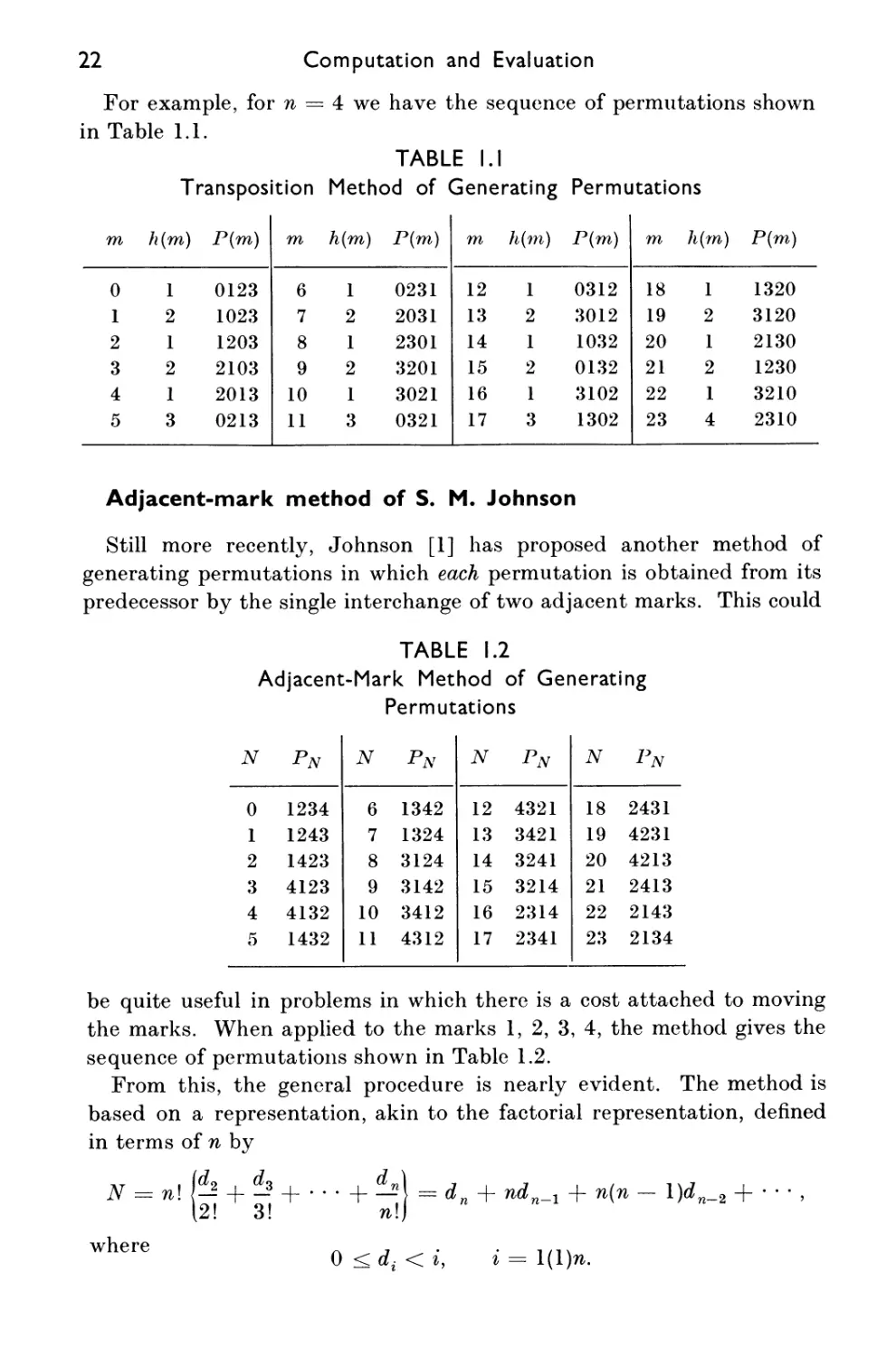
Computation and Evaluation
For example, for w = 4we have the sequence of permutations shown
in Table 1.1.
TABLE I.I
Transposition Method of Generating Permutations
m
0
1
2
3
4
5
h(m)
1
2
1
2
1
3
P(m)
0123
1023
1203
2103
2013
0213
m
6
7
8
9
10
11
h(m)
1
2
1
2
1
3
P(m)
0231
2031
2301
3201
3021
0321
m
12
13
14
15
16
17
h(m)
1
2
1
2
1
3
P(m)
0312
3012
1032
0132
3102
1302
m
18
19
20
21
22
23
h(m)
1
2
1
2
1
4
P(m)
1320
3120
2130
1230
3210
2310
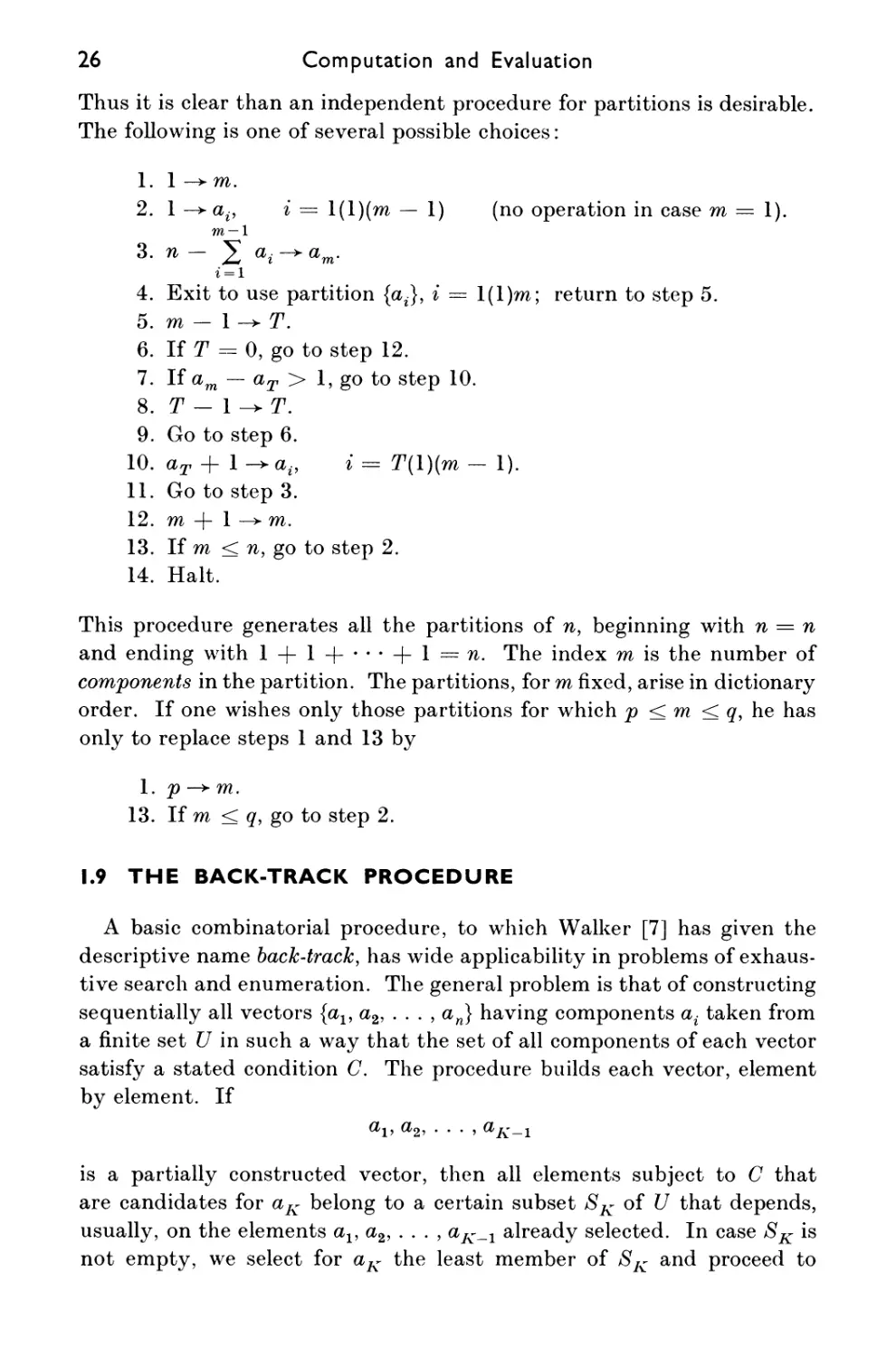
Adjacent-mark method of S. M. Johnson
Still more recently, Johnson [1] has proposed another method of
generating permutations in which each permutation is obtained from its
predecessor by the single interchange of two adjacent marks. This could
TABLE 1.2
Adjacent-Mark Method of Generating
Permutations
N
0
1
2
3
4
5
Pn
1234
1243
1423
4123
4132
1432
N
6
7
8
9
10
11
Pn
1342
1324
3124
3142
3412
4312
N
12
13
14
15
16
17
Pn
4321
3421
3241
3214
2314
2341
N
18
19
20
21
22
23
Pn
2431
4231
4213
2413
2143
2134
be quite useful in problems in which there is a cost attached to moving
the marks. When applied to the marks 1, 2, 3, 4, the method gives the
sequence of permutations shown in Table 1.2.
From this, the general procedure is nearly evident. The method is
based on a representation, akin to the factorial representation, defined
in terms of n by
+ — \ = dn + ndn-l + nin - l)dn-2 +
N
where
n\ (½ + d-*
2! 3!
n\
0 < cL < i.
1(1)71.
The Machine Tools of Combinatorics 23
For each N, 0 < N < n\, there is a k = k(N) such that dk ^ 0, whereas
di = 0 for i > k, so that dk is the last nonzero digit of N. The permutation
PN is formed from PiV-i by simply interchanging the mark k with its
right-hand or left-hand neighbor in P,V-i according to whether
dfc_i + (A: — 1)^-2 is odd or even. The actual place occupied by the mark
k in Pv is aN(k) + bx(k), wnere
ay(k) = dk if dk_x + (k — l)dk_2 is odd,
= k — 1 — dk otherwise,
and
bx(k) = 1 if k = n — 1 and dn_1 -\- (n — l)dn_2 is odd,
= 1 if A; < w — 1 and k(dk + dk_±) is odd,
= 2 if A; < w — 1 and (A: — l)dk is odd,
= 0 otherwise.
The method can be realized by the following procedure. The marks
being permuted may be arbitrary.
1. 0-* (5,., 1-+6,., 1 + i-*a,., i = 1(1)(71 - 1).
2. Go to use current permutation; return to step 3.
3. n — 1 ->j.
4. a,- — €,- -> a,-.
5. If oLj = 1 -{• j, go to step 10.
6. If oij = 0, go to step 10.
n — 1
7. a,- + 2 ^i ~*" ^-
8. Interchange the A:th and (A: + l)st marks.
9. Go to step 2.
10. — €j -> e;.
11. 1 - dj-^dj.
12. j - i -> j.
13. If j ^ 0, go to step 4.
14. Halt.
The method has connections with the so-called Gray codes of switching
theory.
24 Computation and Evaluation
1.6 ORDERLY LISTING OF COMBINATIONS
Before one can begin to perform permutations, in many problems he
has first to select the objects to be permuted from a larger population.
The problem is then methodically to select k words from n words stored
in addresses 10,000 -\- a, a = l(l)n, in all 11 ways and to deliver each
sample of size k to the addresses 20,000 -\- b, b = l(l)k, for processing.
One way to get the machine to do this is given by the following procedure:
1.
2.
3.
4.
5.
6.
7.
8.
9.
1 -+t.
10,001-^.
¢(,4,)-> ¢(20,000 + t).
If t = k, go to step 12.
At + l-+At+1.
If At+1 = 10,001 + n, go to step 9
t + 1 -+t.
Go to step 3.
t 1 -+t.
10. lit = 0, go to step 16.
11. Go to step 13.
12. Exit to process ¢(20,000 + b), b = 1(1 )k, and return to step 13.
13. At + \^At.
14. If At = 10,001 + n, go to step 9.
15. Go to step 3.
16. Halt.
This procedure has the following lexicographical feature: If the n objects
are the n letters of the alphabet, then each ^-letter word selected will
have its letters in alphabetical order, ready for permuting, and the
complete list of J I words will be in alphabetical order.
1.7 ORDERLY LISTING OF COMPOSITIONS
A composition of the positive integer n is a vector of positive integers,
the sum of whose components is n. Compositions occur frequently as
conditions on multiple sums. We have already, in connection with
signatures, considered the case where the compositions have components
restricted as to number and size.
If the compositions are quite unrestricted, then there are precisely 2n_1
compositions of n. These can be generated methodically by using binary
The Machine Tools of Combinatorics 25
representation as follows. To each of the nonnegative integers less than
2n_1, we make correspond the vector
where ai is 1 plus the number of 0 bits between the (i — l)st and ith 1 bit.
Thus if n = 10, corresponding to the 9-bit binary number
(0 11000 10 1),
we have
ax = 2, a2= 1, a3 = 4, a4 = 2, a5 = 1.
It is not a coincidence, but an obvious theorem, that the sum of these
components is 10. In fact, consider a rope n units long with n — \ knots
tied in it at unit intervals. If we paint those knots red that correspond to
the unit digits of some (n — l)-digit binary number, and then proceed
to cut the rope at each red knot, then the sum of the lengths of the pieces
is, of course, still n units. It is also obvious that all possible cuttings
arise from all possible binary numbers. In some problems the number of
parts in the composition, that is, the dimension of the vector, is specified.
Suppose that the number is k. This means that we are to use only those
(n — l)-bit numbers that have precisely k — 1 bits equal to 1. We can
manage to arrange for this restriction in three different ways. First, we
can use our bit-sum routine to reject all numbers of n — 1 bits having
bit-sum different from k — 1. Second, we can use our orderly listing of
combinations to select those k — 1 positions, out of n — 1, that we make
equal to 1. Third, these k — 1 positions form a strictly monotone vector
of k — 1 components, the largest being less than n, and we have seen how
to generate these.
1.8 ORDERLY LISTING OF PARTITIONS
Those compositions of n whose components are monotone nondecreasing
are called the unrestricted partitions of n. These occur also as conditions
of summation of multiple sums. They are much less numerous than
compositions. Although it is impractical to produce all the compositions of
n = 35, the number of partitions of 35 is only 14,883. In general, the
number of unrestricted partitions of n is asymptotic to
1
= exp
4^3
'2nv/2
77
26 Computation and Evaluation
Thus it is clear than an independent procedure for partitions is desirable.
The following is one of several possible choices:
1. 1 -> m.
2. 1 -> ap i = l(l)(ra — 1) (no operation in case m = 1).
m — 1
3. n - J «,- -* «m-
4. Exit to use partition {a J, i = l(l)m; return to step 5.
5. m — 1 -> 77.
6. If T = 0, go to step 12.
7. If am — aT > 1, go to step 10.
8. T —1-+T.
9. Go to step 6.
10. aT + 1 -> a., i = T(l)(m - 1).
11. Go to step 3.
12. m + 1 —>• m.
13. If m < w, go to step 2.
14. Halt.
This procedure generates all the partitions of n, beginning with n = n
and ending with 1 + 1 + --- + 1= w. The index m is the number of
components in the partition. The partitions, for m fixed, arise in dictionary
order. If one wishes only those partitions for which p < m < q, he has
only to replace steps 1 and 13 by
1. p —> m.
13. If m < q, go to step 2.
1.9 THE BACK-TRACK PROCEDURE
A basic combinatorial procedure, to which Walker [7] has given the
descriptive name back-track, has wide applicability in problems of
exhaustive search and enumeration. The general problem is that of constructing
sequentially all vectors {al5 } having components ai taken from
a finite set U in such a way that the set of all components of each vector
satisfy a stated condition C. The procedure builds each vector, element
by element. If
ttj, a2, • • • j #/v'_i
is a partially constructed vector, then all elements subject to C that
are candidates for aK belong to a certain subset SK of U that depends,
usually, on the elements _! already selected. In case SK is
not empty, we select for aK the least member of SK and proceed to
The Machine Tools of Combinatorics 27
determine aK+1 from SK+1. In case SK is empty, we back-track to
consider the set SK_1 that goes with the partially constructed vector
If necessary, we may have to back-track still further,
etc. The general back-track procedure in complete detail is as follows:
1. 1-+K.
2. Oj —> Bj{>
3. If SK is empty, go to step 9.
4. The least member of SK -> aK.
5. If K = n, go to step 14.
6. K + 1-+K.
7. Determine the set SK.
8. Go to step 3.
9. If K = 1, halt.
10. if _ l_>if.
11. Determine SK.
12. Remove from SK all elements <aK.
13. Go to step 3.
14. Exit to use vector {av }; return to step 12.
Often this procedure is very much better than the two-stage process of
first forming vectors {av a2, . . . , an} from U and then applying C to
eliminate the unwanted vectors.
1.10 RANKING OF COMBINATIONS
We have already seen how to program all the combinations of n things
taken A: at a time in alphabetical order. In some problems involving
combinations, it is useful to have a way of assigning rank or a serial
number to each combination. We give two connected instances of this.
Example 1.1 A matrix has 20 rows and 12 columns. It is required to
process all 12 x 12 minors of this matrix. Two machines are to be used,
one being five times as fast as the other. At what point must the job be
split in two so that both machines working simultaneously will finish the
job as soon as possible?
Example 1.2 In timing the fast machine in the processing of minors,
it is found that in five minutes it processed all the minors from the minor
determined by rows
1,2,4,5,8, 10, 11, 12, 13, 15, 16, 18
to the minor determined by rows
1, 2, 7, 8, 9, 10, 12, 14, 15, 16, 18, 19.
How long will the whole job take?
28 Computation and Evaluation
Such problems are easily solved in terms of the concept of combinatorial
representation of integers, to which we have already alluded. We need
the following facts; their easy proofs will be left to the reader. Throughout
the discussion A: is a fixed positive integer.
1. Each nonnegative integer n has a unique representation of k terms,
-61 + (^)+-+^
in which the "combinatorial digits" bt are subject to monotoneity:
0 < b1 < b2 < • - - < bk.
2. The combinatorial digits bt of n are found recursively as follows
[bk\
bk is the greatest integer such that I I < n,
, I K-i \ IK
bk_1 is the greatest integer such that I I < n — I
\rC 1/ \fC
• •••••••••
lb \ k lb
br is the greatest integer such that I r I < n — £ I J
\r J j=r+l\j
k /b\
bx is the greatest integer such that b± < n — 2 I 31 •
3. Let (av a2, a3, . . . , ak) be a combination of the n integers
0, 1, 2, . . . , n — 1.
We may assume that
0 < ax < a2 < • * • < ak < n.
Let Rk(av ), satisfying
0 < Rk(ava2, ...,ak)< I
denote the rank or serial number of the combination in the alphabetized
list of all ( J possible combinations. Then
Rk(av a2,..., ak) =(*)-! - 2 (* " ' ~ "^
The Machine Tools of Combinatorics 29
so that n — 1 — ak_j+i,j = 1(1)&, are the unique combinatorial digits bj of
71
' 1 — #*.(«!, a2, . . . , afc).
We are now in a position to answer the questions of Examples 1.1 and
1.2.
For Example 1.1 we may assume that the slow machine starts at the
beginning of the problem. Since there are altogether
2°^ = 125,970
12/
minors to process, the fast machine must be set to start with the minor
having serial number
l(20) =20,995 = R.
6\12/
Hence we need the combinatorial digits of the number
201 - 1 - 20,995 = 104,974.
12/
These are found to be
{&,} = {1 2 3 4 6 7 8 13 14 17 18 19},
from which we obtain
{a,} = {19 - &18_,.} = {0 1 2 5 6 11 12 13 15 16 17 18}.
Therefore, the fast machine should begin by processing the minor whose
rows are numbered
1,2,3,6,7, 12, 13, 14, 16, 17,18, 19.
For Example 1.2, the serial number of the first minor is found as follows.
The rows of this minor correspond to the vector
{a,} = {0, 1, 3, 4, 7, 9, 10, 11, 12, 14, 15, 17},
and therefore
{&,.} = {19 - a13_,} = {2, 4, 5, 7, 8, 9, 10, 12, 15, 16, 18, 19},
Similarly, the second minor has serial number 42,921. Hence 42,921 —
29,936, or 12,985, minors were processed in 5 minutes. The whole run will
30 Computation and Evaluation
therefore require 104,975/12,985 5-minute intervals, or about 40 minutes,
25 seconds. Incidentally, we now see that the timing test took place
between 11 minutes, 32 seconds, and 16 minutes, 32 seconds, after starting.
MULTIPLE-CHOICE REVIEW PROBLEMS
1. The factorial representation of 794,283 is
(a) (1, 1,0,0,3,4,5,1,2),
(b) (1, 1,0,0,4,4,5, 1,2),
(c) (1, 1,0,0,2,4,5,1,2),
(d) (1,1,0,0, 1,4,5, 1,2).
2. In modular representation, {1, 2, 0, 4, 10, 3, 5} + {0, 2, 2, 4, 2, 3, 10} is
(a) {1,4,2,8, 12,6, 15},
(b) {1,1,2,1,1,6, 15},
(c) {1, 4, 2, 8, 10, 6, 10},
(d) none of the above.
3. In logical addition, (0, 1, 0, 1) 0 (0, 1, 1, 0) is
(a) (1,1,0,0), (b) (0, 1,0,0),
(c) (0, 1, 1, 1), (d) none of the above.
4. The number of unrestricted partitions of 7 is
(a) 5, (b) 10, (c) 15, (d) 20.
5. With 0123456789 as zeroth permutation in a lexicographical list, the
serial number of the permutation 8592174603 is
(a) 4,297,417, (b) 3,141,592,
(c) 2,938,406, (d) 3,251,722.
REFERENCES
1. Johnson, S. M., Generation of Permutations by Adjacent Transposition, RM-3177-
PR, The RAND Corporation, Santa Monica, Calif., 1962; Math. Comp. 17 (1963),
282-285.
2. Lehmer, D. H., "The Sieve Problem for All-Purpose Computers," Math. Tables
and Other Aids to Computation, 7 (1953), 6-14.
3. Lehmer, D. H., "Combinatorial Problems with Digital Computers," Proc. Fourth
Canadian Mathematical Congress, 1957, 160-173, University of Toronto Press,
Toronto, Canada, 1960.
4. Lehmer, D. H., "Discrete Variable Methods in Numerical Analysis," Proc.
Internat. Congress Math., 1958, 545-552, Cambridge University Press, New York,
1960.
5. Lehmer, D. H., "Teaching Combinatorial Tricks to a Computer," Chapter 15 in
R. Bellman and M. Hall, Jr. (editors), Combinatorial Analysis, Proc.Sympos. Appl.
Math., 10, 179-193, American Mathematical Society, Providence, Rhode Island,
1960.
The Machine Tools of Combinatorics 31
6. Paige, L. J., and C. B. Tompson, "The Size of the 10 X 10 Orthogonal Latin
Square Problem," Chapter 5 in R. Bellman and M. Hall, Jr. (editors), Combinatorial
Analysis, Proc. Sympos. Appl. Math., 10, 71-83, American Mathematical Society,
Providence, Rhode Island, 1960.
7. Walker, 11. J., "An Enumerative Technique for a Class of Combinatorial
Problems," Chapter 7 in R. Bellman and M. Hall, Jr. (editors), Combinatorial Analysis,
Proc. Sympos. Appl. Math., 10, 91-94, American Mathematical Society,
Providence, Rhode Island, 1960.
8. Wells, M. B., "Generation of Permutations by Transposition," Math. Comp., 15
(1961), 192-195.
CHAPTER
Techniques for Simplifying
Logical Networks
MONTGOMERY PHISTER, Jr.
2.1 INTRODUCTION
Digital systems, from the largest, multimillion-dollar general-purpose
computers down to the few-hundred-dollar laboratory frequency counters,
are constructed from standard building blocks with a common property:
The inputs to and outputs from these blocks have two states. Since the
mathematics of logic is also primarily two-valued, these building blocks
have been called logical elements, the art of organizing them has been
called logical design, and the systems themselves are called logical networks.
Since the late 1940's, an ever-increasing effort has gone into attempting
to convert the art of logical design into a science, with the objectives of
making the designer's work easier, his products more efficient, and his
profession more respectable. In this chapter, we shall attempt to describe
the current state of this activity.
There are basically only two kinds of logical elements: memory elements
and decision elements. A memory element stores one unit of information
and thus can at any time exist in precisely one of two states. For
convenience, and without loss of generality, we shall here discuss only
synchronous systems, in which the state of a memory element is significant
only at discrete instants of time known as bit times or clock-pulse times.
Various kinds of memory elements differ from one another in cost, speed
with which they can change from one state to another, power-handling
capacity, and logical properties. We shall be interested only in this last
characteristic. The simplest memory element is a delay flip-flop; its
32
Techniques for Simplifying Logical Networks
33
DQ
^
Q
Q
^
^
logical properties are indicated in Fig. 2.1. The element has one input,
Dq, and two outputs, Q and Q. The outputs are always the opposite of
one another, so that if Q = 1, then Q = 0, and vice-versa. If Q = 1,
then the flip-flop is said to be set, or in its 1 state. If Q = 0, then it is
reset, or in its 0 state. At any bit time,
the input Dq is either 0 or 1. As the
table of Fig. 2.1 indicates, if DQ is 0 at
any bit time n, then Q is 0 (reset) at
time n + 1; if DQ = 1 at any bit time
n, then Q is 1 (set) at time n + 1. Later
in the chapter, we shall discuss the use
of memory elements with other logical
properties.
A decision element is a component
whose output is some specified function
of its inputs, but which introduces no
delay. Of the variety of decision elements available, probably the most
widely used are the and gate and the or gate. The output of an and gate
is 1 if and only if all its inputs are 1; the output of an or gate is 1 if and
only if one or more of its inputs are 1. The properties of the simplest
o
l
,n + l
Q"T1 Q
l
n + l
0
Fig. 2.1 Delay flip-flop.
B
C = A- B = AB
C = A + B
A" B" C"
0
0
1
1
0
1
0
1
0
0
0
1
An
0
0
1
1
Bn
0
1
0
1
cn
0
1
1
1
(a) (b)
Fig. 2.2 and gate (a) and or gate (b).
(two-input) and and or gates are illustrated in Fig. 2.2. Note that the
circuits can be defined by listing what their outputs will be for each of
the four possible states of the two input lines. Note also that the output
of each circuit is available at the same bit time the inputs are present—
there is no storage or delay of information.
A digital system is a network of decision and/or memory elements.
The most interesting of these contain both kinds of elements and are
called sequential circuits. To be able to refer to something specific in the
34 Computation and Evaluation
following discussion, let us describe a particular sequential circuit.
Suppose we have available a binary communication channel X (perhaps
a signal from outer space or an encoded message from an enemy agent),
and we want to monitor it for three classes of 5-bit patterns. Class 1 will
cause output line Z1 to be 1 whenever either of the two patterns shown in
the first column of Table 2.1 has appeared on line X. The bit patterns
that cause output lines Z2 and Z3 to be 1 are more complicated in that
they contain more than two members, as shown in the table.
TABLE 2.1
Monitoring of a Sequential Circuit for Three Classes
of Five-Bit Patterns
Z± = 1 for any
of these patterns
0000 1
1000 1
^2
, = 1 for any
of these patterns
0000 1
1000 1
00101
10 10 1
0 110 1
1110 1
000 10
10010
0 10 10
110 10
00111
z*
5 = 1 for any
of these patterns
00000
10000
0 1000
11000
00 100
10 100
0 1100
11100
000 10
10010
0 10 10
110 10
00111
We can easily construct a circuit to do the required job in the following
way (see Fig. 2.3). First, we provide a four-flip-flop shift register
consisting of flip-flops A, B, C, and D. At each bit time we store the bit on
X in A, shift the contents of A to B, the contents of B to C, and the
contents of C to D. Thus at each bit time we have available the last
five bits that have appeared on line X: The most recent is on X itself,
the previous bit is in A, the next earlier is in B, the next before that is in
C, and the least recent of the five is in D. The circuits necessary to perform
this shifting are very simple:
(2.1) DA = X
(2.2) DB = A
(2.3) Dc = B
(2.4) DD = G
Techniques for Simplifying Logical Networks
35
Now let us see what logic is necessary to recognize the patterns for
which Zx must equal 1. Suppose the pattern . . . 110100001 . . . appears
on X. Then the input line and flip-flops will take on the states shown in
Table 2.2, on page 36.
X
D
r
r
L
1^
B
B D
B ^
£t£
D
D
D
~l
->
->
->
■>
■>
./v
/\.
r\.
■>
■>
Decision-element network for Z\
i !
r
Decision-element network for Z2
~i
j
■~i
Decision-element network for Z3
■^1
-^Z2
^3
Fig. 2.3 A sequential circuit.
At the ninth bit time, the first of the two patterns that stimulate
Zj—the pattern 00001—appears in flip-flops D, C, B, and A, and on line
X. Note that the pattern is shown backward because the bit that
appeared first has shifted to the right to flip-flop D. We can recognize
this pattern with a single and gate (see Fig. 2.3) having inputs X, A, B,
C, and D, for it is only when all five inputs to this gate are 1, that is,
36 Computation and Evaluation
TABLE 2.2
Input Line X with Flip-Flops
A, 8, C, D
Bit time X A B C D
1 1
2 11...
3 Oil..
4 10 11.
5 0 10 11
6 0 0 10 1
7 0 0 0 10
8 0 0 0 0 1
9 10 0 0 0
when X = I, A = 0, B = 0, C = 0, and D = 0, that its output will be
1. Similarly, we can recognize the other Zx pattern, 10001, by providing
an aistd gate with inputs X, A, B, C, and D. Since Zx must equal 1 when
either one or the other of these circuits has output 1, we combine their
outputs in an or gate, with the result that
(2.5) Z1 = XABCD + XABCD.
In an exactly similar way, although the circuits are too complicated to
reproduce conveniently in Fig. 2.3, we can provide decision-element
circuits for Z2 and Z3:
Z2 = XABCD + XABCD + XABCD
+XABCD+XABCD+XABCD
( ' +XABCD+XABCD+XABCD
+ XABCD + XABCD,
Zz = XABCD + XABCD + XABCD
+XABCD+XABCD+XABCD
(2.7) +XABCD + XABCD + XABCD
+XABCD+XABCD+XABCD
+ XA BC B.
Equations (2.1) to (2.7) thus represent the complete design of our
sequential circuit.
In general, a sequential circuit may differ from the circuit in Fig. 2.3
in that it might contain a larger number of inputs, a larger or smaller
number of outputs, and a larger or smaller number of memory elements.
For any such circuit, however, the designer is faced with certain problems.
In increasing order of complexity, he may ask the following.
Techniques for Simplifying Logical Networks 37
1. What is the cheapest circuit, composed of delay flip-flops and and-
or gates, that is equivalent to a given circuit?
2. What is the cheapest circuit that is equivalent to a given circuit,
provided the designer may take his choice of types of decision and
memory elements to implement the design?
3. What is the cheapest circuit that can be found to perform a given
function?
The first two problems are problems of analysis; they will be discussed
in the two parts into which this chapter has been divided. The last is a
problem of synthesis; it will be briefly discussed in Sec. 2.8.
One difficulty inherent in all three problems is that of finding a suitably
realistic definition of the word cheapest. Presumably the designer would
like to minimize a function that includes the costs of development, tooling,
packaging, checkout, and maintenance, in addition to the costs of specific
decision and memory elements. In practice, no one has even tried to do
more than minimize the number of and-or gates and the number of
memory elements necessary, and these two costs have been minimized
only individually; no one has been able to minimize their sum, except
by exhaustively trying all combinations.
SIMPLIFYING A GIVEN SEQUENTIAL
CIRCUIT
2.2 SIMPLEST AND-OR GATES
A great deal has been written on the problem of simplifying and-or
networks, with the definition of simplest usually taken to mean the
circuit with fewest inputs to gates. The circuit that determines Zx in
Fig. 2.3, for example, contains two and gates with five inputs each and
an or gate with two inputs. Two times 5, plus 2, that is, 12, is thus a
measure of its complexity. In a similar way, we find from (2.6) and (2.7)
that Z2 has a count of 66 and Z3 a count of 78, so that the entire sequential
circuit, excluding flip-flops, has a count of 156. Standard procedures are
available for minimizing this count if we allow no more than two gates
in series in a circuit.
One of the simplest of these procedures (see [5]) makes use of a Veitch
diagram or Karnaugh map. In Fig. 2.4a a five-variable diagram is shown
that is suitable for use in our five-variable problem. Note that groups of
squares are labeled with the five variables in such a way that one square
Computation and Evaluation
B
X
y^A
28
29
25
24
30
31
27
26
22
23
19
18
C
20
21
17
16
A
12
13
9
8
14
15
11
10
6
7
3
2
C
4
5
1
0
\
)
D
= XABC
= XAB + XAC + XAB
+ XBCD
= XA + XB + XABCD
X
+ BCD + ABCZ) + ABD + ACD
c c
Fig. 2.4 Five-variable Veitch diagrams.
Techniques for Simplifying Logical Networks 39
corresponds to each of the 25 = 32 different products of the five variables.
Each square is given a number as follows: First, write the variables in a
prescribed sequence, for example, X A B C D. Next, see whether the
square in question is in group X. If it is not, put a bar over the X; if it
is, leave X unchanged. In either event, repeat the process for the variable
A, putting a bar over the A if the square is not in group A. Repeat for
B, C, and D. The resulting term is a description of the and gate
corresponding to that square. Now replace each unbarred letter in this term
by a 1, and each barred letter by a 0. The resulting binary number,
converted to a decimal number, is the label for that square. For example,
look at square 26 in Fig. 2.4a. It is in group X, in group A, outside group
B, in group C, and outside group D. Therefore it represents the term
X A EC D. Replacing with 0's and 1 's, we get 11010, which is decimal 26.
All numbers in Fig. 2.4a are found in this fashion.
Now let us look at equation (2.5) for Zx. It is composed of two
terms, XAECD (10000, or 16) and XAECD (10001, or 17). In
Fig. 2Ab we have plotted Zx by marking squares 16 and 17 with l's.
In a similar way, Z2 and Z3 are plotted in Fig. 2.4c, d.
The Veitch-diagram simplification procedure is based on the fact that
groups of 2, or 4, or 8, . . . , or 2n, squares, grouped adjacent to one
another in certain ways horizontally and vertically, can be combined
and represented by terms containing 1, or 2, or 3, . . . , or n letters less
than the number required to describe a single square. For example, the
two squares marked 1 in Fig. 2Ab are adjacent vertically; they are both
in X, both in A, both in E, and both in C (one is in D, the other in D).
They can thus be defined by
(2.8) Zx = X A EC.
Next looking at Z2, we find that square 10 (X A E C D) combines with
the three squares 8, 9, and 11, with which it forms a larger square, to
give the term X A E. Thus if we write
Z2 = X A S + • • •,
we have taken care of four of the eleven terms in Z2. Next look at square
16 in Z2. It combines with the three vertically above it (17, 21, and 20)
to form X A C, so we write
Z2 = XA E + XAC + -• .
Similarly, square 23 combines with 22, 20, and 21 to add X A B; thus,
Z2 = XAE + XlC + XAB + --.
The fact that squares 20 and 21 are included both in X A C and in X A B
40 Computation and Evaluation
makes no difference; it merely means that the outputs of these two and
gates will both be 1 if X A B C D = 1 or if X A B C D = 1, and either
one or both will make Z2 = 1 in the final or gate. We have now included
every marked square except 28, which has no other l's immediately
adjacent horizontally or vertically with which to combine. It will,
however, combine horizontally across the X = 1 group with square 20, for
both are in X, both in B, both in C, and both in D. Adding (or rather,
ORing) this final term, we get
(2.9) Z2 = XAB + XAC + XAB + XBCD.
Finally, and in quite a similar fashion, we find
(2.10) Zz = X A + X B + X A B C D.
Now (2.8), (2.9), and (2.10) represent the simplest and-or forms for Zv
Z2, and Z3. The reader should verify that they have a count of only 33
compared with 156 for (2.5), (2.6), and (2.7).
In using Veitch diagrams to simplify switching functions, it is not
enough simply to look for large numbers of l's that can be covered by a
single term The dangers inherent in such a procedure are indicated in
Fig. 2.4e, in which we have plotted a function that contains eight l's on
the left in X D. Nevertheless, the simplest expression for / does not
contain X D, and may be found as follows. Look at each individual
marked square, determining all possible ways it can be combined with
other marked squares. If a 1 combines only with a single group, that
group is an essential term and must appear in the final simplest expression
for the function. The correct simplification procedure requires that all
marked squares be examined for essential terms first, and that then any
remaining l's be covered as efficiently as possible. In Fig. 2Ae,
examination of squares 17, 21, 19, 23, 27, 31, 25, and 29 will reveal that each
combines into term XD and also into one other term. For example, 29
combines with 28 to form X A B C, and 21 combines with 1, 5, and 17
to form A C D. Squares 28, 22, 26, 9, 15, 3, and 5 each combine in only
one group of terms, and these essential terms cover all l's and comprise
the simplest expression for the function, namely
(2.11) f=XABC + XABC+XAEC+ECD
+ A BCD + A BD + ACD.
2.3 MULTIPLE-OUTPUT FUNCTION SIMPLIFICATIONS
In finding the simplest expressions for Zx, Z2, and Z3 in Sec. 2.2, we
considered these three functions independently, ignoring the fact that
Techniques for Simplifying Logical Networks
41
x
A
B
C
X
A
B
X
A
B
C
D
X
A
B
X
^
^
^
^
^
^
>
J
^
^-
^
•
•
•
•
•
*s^
' ^
>
+
' $*"
s
1 ^23
>
7>
+
+
>
•*
Fig. 2.5 Multiple-output circuit.
they were all part of a single circuit. It is possible (see [1]) to take
advantage of their common parts and obtain still further simplification, as
follows.
Referring again to Fig. 2Ab, c, d, we make the following observations:
Z2 and Z3 have squares 28, 8, 9, 10, and 11 in common.
Zx and Z2 have squares 16 and 17 in common.
We can make use of these facts to produce a further savings in the
following way, and the resulting circuit is shown in Fig. 2.5. If we define Z23 by
(2.12)
then we have
(2.13)
(2.14)
(2.15)
Z23 = X A B C B + X A B,
Zx = XA EC,
Z2=Z,+ Z23 + XA B,
%3 = ^23 + X A.
42
Computation and Evaluation
The circuit now has a count of only 24, compared with 33 for (2.8), (2.9),
and (2.10).
2.4 ELIMINATION OF MEMORY ELEMENTS
Let us now return to the sequential circuit of Fig. 2.3 and ask: Can the
function performed by this circuit be achieved with fewer than four
flip-flops? Huffman [3] first solved this problem in a very neat and
complete fashion, and we shall carry out his quite systematic procedure in the
following.
TABLE 2.3
Sequential Circuit Representation
Outputs
A
0
0
0
0
0
0
0
0
1
1
1
1
1
1
1
1
Present state
B
0
0
0
0
1
1
1
1
0
0
0
0
1
1
1
1
c
0
0
1
1
0
0
1
1
0
0
1
1
0
0
1
1
D
0
1
0
1
0
1
0
1
0
1
0
1
0
1
0
1
Label
a
b
c
d
e
f
9
h
i
k
I
m
n
V
r
s
Ne
X =
a
a
b
b
c
c
d
d
e
e
J
f
9
9
h
h
xt state
0
X = 1
i
i
k
k
I
I
m
?n
n
n
V
V
r
r
s
s
X =
0
0
0
0
0
0
0
0
0
0
0
0
0
0
0
0
^1
0 X
= 1
1
1
0
0
0
0
0
0
0
0
0
0
0
0
0
0
X =
0
0
0
0
0
0
0
0
1
1
1
1
0
0
0
0
z2
0 X
= 1
1
1
0
0
1
1
1
1
0
0
0
0
1
0
0
0
X =
0
0
0
0
z*
0 X = 1
0
0
0
0
0
0
0
0
0
0
0
0
1
0
0
0
To begin the process, the circuit must be described in general terms, with
all references to flip-flops eliminated so that we are concerned only with
a circuit that has certain states. First, we draw up the sequential-circuit
pattern shown in Table 2.3. The left-hand columns of this table we label
"Present state." Each row in those columns corresponds to a particular
state in which the circuit can be at any bit time; and since the circuit
contains four flip-flops, there must be sixteen rows. The center columns we
label "Next state." For each possible value of the input variable (or
variables) X, we now enter, on each row, the name of the state to which the
circuit will next go as a result of that value. The last columns are labeled
Techniques for Simplifying Logical Networks 43
' 'Outputs.'' For each value of the input variable, we must enter the proper
value of each output variable.
We start by defining the sixteen states, corresponding to the sixteen
discrete combinations of flip-flops A, B, C, and D. Each of these states is
labeled with a letter of the alphabet, as shown. We now proceed to fill in
the next-state entries by remembering that the circuit is a shift register:
At each bit time, X shifts to A, A to B, B to C, and C to D. Suppose that
we are in state a (see Fig. 2.6), so that A = B = C = D = 0, and suppose
that X = 0. At the next bit time, each of the 0's will have shifted to the
1 ^
1 >
x
0
1
1
0
1
0
A
I -.
1
0
0
1
1
0
1
0
B
1
1 -,
i ^
0
0
0
1
1
0
1
c
0
0
0
0
1
1
0
D
0
0
0
0
0
1
1
State
a
a
i
n
g
m
f
Fig. 2.6 Derivation of sequential-circuit table entries.
right, and therefore at the next bit time we will still be in state a.
Therefore in row a of Table 2.3, under X = 0, we enter an a in the next-state
column. Suppose next that we are in state a, but that X = 1. At the
following bit time, the 1 will shift from X to A, the 0 in A to B, the 0 in
B to C, and the 0 in C to D, as shown in Fig. 2.6. We will thus be in state
A = 1, B = C = D = 0, which is state i. We therefore enter an i in row
a under column X = 1 in the next-state part of the table. Now suppose
X = 1 again. At the following bit time, the 1 in X will have shifted to A,
the 1 in A to B, the 0 in B to C, and the 0 in C to D. We are thus in state
1100, or state n, and we enter an n in the next state column on row i for
X = 1. The other entries are determined in a similar fashion.
Table 2.3 can now be completed by determining the output entries.
Referring back to our original description of the circuit, we find that we
want Zx = 1 whenever we have just received the pattern 00001 or 10001.
We recognize the first of these when four 0's have successively shifted
through into A, B, C, and D, and then X = I. This means we are in
state a and X = 1, and so at that entry in the Zx portion of the output
part of the table we enter a 1. The second pattern we will recognize by the
fact that a 1 has shifted in followed by three 0's (so that A = B = C = 0
and D = 1), and that X then equals 1. Therefore there must be a 1 in
state b under column Zx for X = 1. These are the only combinations for
44 Computation and Evaluation
which Z± = I, so all the other entries in the Zx columns can be made 0.
The entries in the Z2 and Z3 columns are determined in a similar way.
We are now ready to try to eliminate one or more flip-flops, that is, to
eliminate enough states from Table 2.3 that the remaining states can be
distinguished from one another with three or fewer flip-flops, and still
constitute a circuit that is the same, from all outward appearances, as our
original circuit. Such a circuit can contain at most 23 = 8 states.
What do we mean by "the same, from all outward appearances"?
Clearly the "inward appearance" of the two circuits will be different, for
one contains four flip-flops and the other three or less. We mean that, if
we connect the inputs of both circuits together, put any conceivable
sequence of 0's and l's on X, and monitor the outputs of both circuits, we
shall always find outputs Z1, Z2, and Z3 of one circuit exactly the same as
the corresponding outputs of the other circuit. If this is the case, we shall
say that the two circuits are equivalent.
With the foregoing considerations in mind, we can easily specify the
rules for finding a simpler circuit equivalent to that described by Table 2.3.
1. Each state in the equivalent circuit must correspond to one or more
states in the original circuit. Our job is thus to find sets of states in the
original circuit, each of which is equivalent to a single state in the
equivalent circuit.
2. A set of two or more states in the original circuit can correspond to a
single state in the equivalent circuit only if all members of the set have
the same outputs for each possible input combination. For example,
states s1 and s2 in our original circuit can correspond to state S in the
equivalent circuit only if, whether the input X is 0 or 1, the outputs Zl9
Z2, and Z3 are the same from states s1 and s2 as from state S. Applying
this rule to Table 2.3, we see that states a and b provide the same outputs
whether X = 0 or X = 1, and therefore may perhaps correspond to a
new state A in the equivalent circuit. For the same reason, states c and d
may correspond to an equivalent state C, states e,f, g, and h to a new state
E, states i, k, I, and m to a new state I, and states p, r, and s to a new
state P. State n in the original circuit has a different output combination
from each other state in the original table, and so must, all by itself, have
a corresponding new state N in the equivalent circuit. Thus tentatively
we can note the associations shown in Table 2.4.
3. In step (2) we have shown that, if our new equivalent circuit has
states A, C, E, I, N, and P, equivalent to the sets of states in the original
circuit as shown in Table 2.4, then any input will result in the correct
output on Zv Z2, and Z3 at that bit time. We must now be sure that any
continuing sequence of inputs will continue to provide the same outputs
Techniques for Simplifying Logical Networks 45
from the two circuits. We do this by following through to see what the
equivalent next state is for each value of X applied to the original circuit.
Referring again to Table 2.3, we see that, if we are in state a or b, and
X = 0, we stay in state a. Therefore, if our equivalent circuit is in state A,
TABLE 2.4
Proposed and Original Circuit States
Proposed circuit
state
A
C
E
I
N
P
Set of
original circuit
states
(a, b)
(c,d)
(e,f,g,h)
(i, k, I, m)
(n)
(P,r,s)
and X = 0, it will stay in state A. If we are in state a or b, and X = 1,
we go to state i. Therefore, if our equivalent circuit is in state A, and
X = 1, then this circuit will go to state I. States a and b are thus
equivalent to A in their next-state action as well as in their output combinations.
We repeat this analysis for each of the states in our original table, as
shown in Table 2.5.
TABLE 2.5
Next-State Analysis of Proposed Circuit
. . . Next state in proposed circuit
Proposed circuit Original circuit
state
A
C
E
I
N
P
state
(a,b)
(c,d)
(e,f,g,h)
(i, k, I, m)
(n)
(P, r> »)
X = 0
(A, A)
(A, A)
(C, C, C, C)
(E, E, E, E)
(E)
(E, E, E)
X = 1
(1,1)
(1,1)
(I, I, I, I)
(N, N, P, P)
(P)
(P, P, P)
All the sets of original states except (i, k, I, m) have the property
that either value of the input will result in the same next state in the
proposed circuit. If, however, we are in state i, and X = 1, then we go to
state n, which is the proposed next state N; but if we are in state m, and
X = 1, then we go to state p, which is included in the proposed next
46
Computation and Evaluation
state P. Since P and N give different outputs, our assumption that i, k, I,
and m can be equivalent to a common state I is false. The pairs (i, k)
and (I, m) may still be equivalent to a couple of new states, but not to
one another. Let us assume that (i, k) correspond to state /', and (I, m)
to state L'. We now repeat the next-state analysis, as shown in Table 2.6.
TABLE 2.6
Revised Next-State Analysis of Proposed Circuit
_ ,.. ~ n . . , Next state in proposed circuit
Proposed circuit Set of original
state
Present
state
A
C
E
I
L
N
P
A
C
E
r
L'
N
P
circuit states
(a,
(c,
(e,
(i,
(I,
(n
(V
b)
d)
/, 9, h)
k)
m)
)
, r, s)
TABLE
X = 0
(A, A)
(A, A)
(C, C, C, C)
(E, E)
(E, E)
(E)
(E, E, E)
2.7
Reduced Sequential Circuit
Next state
X =
A
A
C
E
E
E
E
0
X = 1
I
I
L
N
P
P
P
^i
X = 0 X
0
0
0
0
0
0
0
1
0
0
0
0
0
0
Outpu
^2
= 1 X = 0 X
0
0
0
1
1
0
0
t
=
1
0
1
0
0
1
0
X = 1
(*', n
(i\ P)
(L\ L', L\ L')
(N,N)
(P, P)
(P)
{P, P, P)
^3
1 X = 0 X = 1
1 0
1 0
1 0
1 0
1 0
0 1
0 0
We now see that all sets are consistent and that our equivalent circuit
must have seven states. The sequential-circuit table for the equivalent
circuit is shown in Table 2.7, in which the primes are omitted from I and
L for simplicity.
The fact that there are only seven states in our reduced table implies
that only three memory elements are required to mechanize it—and that
Techniques for Simplifying Logical Networks
47
we have achieved our goal of eliminating a memory element. To
construct the circuit, we must specify three flip-flops, say, V, W, and Y,
and assign a different binary combination of V, W, and Y to each of the
seven states in Table 2.7. Suppose we make the assignment shown in
Table 2.8, where we simply write the seven binary numbers 000 to 110
and assign them to states A through P. We now have a table, the "Next-
state" portion of which tells what values V, W, and Y should assume at
each bit time as a function of their states and the state of X at the previous
bit time. We shall now see how to write the input logic for the three delay
flip-flops, V, W, and Y, from this table.
TABLE 2.8
Reduced Sequential Circuit with Flip-Flops
Present state Next state Output
Label
A
C
E
I
L
N
P
Fli
V
0
0
0
0
1
1
1
p-flop
W
0
0
1
1
0
0
1
Y
0
1
0
1
0
1
0
X =
V
0
0
0
0
0
0
0
w
0
0
0
1
1
1
1
0
Y
0
0
1
0
0
0
0
X
V
0
0
1
1
1
1
1
=
w
1
1
0
0
1
1
1
1
Y X
1
1
0
1
0
0
0
=
0
0
0
0
0
0
0
^1
0 X =
1
0
0
0
0
0
0
1 X =
0
0
0
1
1
0
0
z2
0 X =
1
0
1
0
0
1
0
1 X =
0
0
z*
OX = 1
0
0
0
0
0
1
0
We begin, in Fig. 2.7a, by drawing a Veitch-diagram map for the four
variables X, V, W, and Y, and plotting the seven states A, C, E, I, L, N,
and P on it. Each state appears twice, once for X = 0 and once for X = 1.
For example, in Table 2.8 we see that state I is specified by V = 0,
W = Y = 1. Therefore we find the two squares on the Veitch diagram
of Fig. 2.7a for which K = 0, W = Y = 1, and label them both I.
Continuing in this way, we ultimately find two squares that do not
correspond to any of the seven states. This combination, for which V = Wr =
Y = 1, is the eighth state of the three flip-flops. Since we need only seven
states, we shall arrange that V, W, and Y are never all 1 at any bit time.
We enter a 0 in each of these last squares to signify that these
configurations of X, V, W, and Y can never occur, and that we can use those squares
where desired to simplify our logic.
We are now ready to plot, in Fig. 2.1b, the next state of V, that is,
Vn+1, as a function of Xn, Vn, Wn, and Yn. We do this by referring back
to Table 2.8 and finding the next-state entries for which V = 1. There
48 Computation and Evaluation
are five such entries: If at time n we have X = 1 and we are in state E, I,
L, N, or P, then we find that Vn+1 = 1. We therefore enter l's in Fig.
2.1b on the X = 1 side of the diagram in squares E, /, L, N, and P. For
all other squares, we have Vn+1 = 0, and for convenience we leave them
blank.
'(
(a)
X
L
N
C
A
P
0
I
E
P
0
I
E
L
N
C
A
\
)
w
<
(b)
X
1
1
1
0
1
1
0
^
)
w
Vn+1=D,
=XW+XV
v(
(c)
X
1
1
1
1
1
0
1
0
1
1
\
)
w
Wn+1=D
w — -
=V+XW+XWY
(d)
X
1
1
0
1
0
1
^
)
w
yn+1=D,
= XVW + XVY + XVWY
v(
(e)
X
1
$
0
^
J
X
w
Z± = XVWY
(f)
1
1
0
1
0
1
1
^
)
w
Z2 = XVY+X_VY_+_
XWY+XVWY
V
(g)
X
1
0
0
1
1
1
1
1
^
)
w
Z3 = XVY + XWY + XV
Fig. 2.7 Derivation of input equations for circuit of Table 2.8.
The plot in Fig. 2.76 of Vn+1 can also be considered as a plot of the input
to a delay flip-flop V, for if we want V at time n + 1 to be 1, we see, on
referring back to Fig. 2.1, that Dv at time n must equal 1. Therefore if
we write the simplest Boolean expression for Fig. 2.76, we are also writing
the simplest input equation for flip-flop V. In finding the simplest
expression, we must keep in mind that flip-flops V, W, and Y can never all be 1,
and therefore that the squares labeled 0 may be regarded as containing
either O's or l's, whichever results in a simpler equation. The simplest
expression is
(2.16)
Dv
XW + XV.
Techniques for Simplifying Logical Networks 49
Similarly, the simplest expressions for Dw and DY are found from the
Veitch-diagram plots of Wn+1 and Yn+X; they are
(2.17) Dw= V + XW + XW Y,
(2.18) DY = XVW + XVY + XVWY.
We can also use Table 2.8 and Fig. 2.7a to plot Zv Z2, and Z3, as shown
in Figs. 2.7e, /, and g. Their simplest expressions are
(2.19) Z1 = X V W Y,
(2.20) Z2 = X V Y + X V Y + X W Y + X V W Y,
(2.21) Z3 = X V Y + XW Y + XV.
Now (2.16) to (2.21) require gates with a total of 59 inputs. We can
employ still fewer gates by making use of the multiple-output simplification
procedures described previously. These give
(2.22)
(2.23)
(2.24)
(2.25)
(2.26)
(2.27)
(2.28)
(2.29)
Dv
Dw
Y,
DY
V
£2
Y2
z*
= X W + X V,
= V + XW+Y19
= XW Y,
= X V Y + X V W Y + Z±
= XV W Y,
= XVY+Y,+ Y2,
= XVY + XVWY,
= Y2 + X V.
This set of gates has only 47 inputs. We have thus reduced a circuit
containing 4 flip-flops (2.1) to (2.4) and 24 gating inputs (2.12) to (2.15) to one
requiring only 3 flip-flops and 47 gating inputs. Since flip-flops are
generally more expensive than gates, this represents a net simplification.
2.5 ALTERNATIVE METHODS OF ASSIGNING
FLIP-FLOP STATES
The gate count for the circuit we now have stems entirely from the
assignment of flip-flop states we made in Table 2.8. Another assignment—
and there are 40,319 others—would result in a different count, perhaps
better, perhaps worse. Hartmanis [2] has suggested a procedure that will
sometimes lead to a good choice of states, although it is not guaranteed to
do so. He begins with the suggestion that we ignore the output logic for
50 Computation and Evaluation
the circuit and attempt to find an assignment that will simplify the input
logic to the memory elements. He argues that the input logic for a given
memory element is likely to be simple if it is not a function of all the other
memory elements. Thus, if a circuit contains three flip-flops Qv Q2, and Q3,
then in general we have an assignment of the form
#r+1 = Q(Qv %. Qv £)■
If we can find an assignment of the form
Qi+1 = Q'(Q2, X),
then the resulting input logic for Qx is likely to be simple. Obviously this
is not generally true, since, for example, Q}{ + 1 = Qx Q2 Q3 X requires only
four inputs, whereas Q™+l = Q2 X + Q2 X requires six; but it seems a
reasonable thing to try. Applied to the circuit of Table 2.7, his procedure
may be described as follows.
Ignoring circuit outputs, we want to arrange our seven states in four
groups so that no group contains more than two members, and so that the
next-state entries for the two states in a group are again members of a
common group, whether the input X is 0 or 1. If we can find four such
groups, we can assign the four combinations of flip-flops V and W to them,
use flip-flop Y to distinguish between the two states in a group, and have
the desired result that the next state of V and W will be independent of Y.
To find four such groups, we try every combination of pairs of groups,
noting for each pair what other pairs of terms must be grouped together in
order that next-state entries shall be members of a common group. The
results are indicated in Table 2.9. Referring to Table 2.7, we can see how
the entries of Table 2.9 are derived. The entry in the upper left-hand
corner specifies what conditions must be satisfied if A and C are to be
grouped together. Since both A and C go to state A when X = 0 and to
state I when X = 1, no special grouping conditions are required, and we
place a check mark in the square of Table 2.9 corresponding to the
grouping of A and C. Next consider the possibility of grouping states A and E.
Since A stays in state A, but E goes to state C when X = 0, the collection
of A and E into a group implies that A and C must also be in the same
group. We therefore enter AC in the square corresponding to the grouping
of A and E. Furthermore, since A goes to state I and E to state L when
X = 1, the grouping of A and E implies that I and L must also be grouped
together. We therefore add IL to the square corresponding to the grouping
of A and E. Similarly, we write the implications of each possible group of
two states and thus complete Table 2.9.
We now examine Table 2.9 to identify all possible consistent groupings
of states. Choosing the pair AC &s one obvious first choice, because it
Techniques for Simplifying Logical Networks 51
implies nothing about any other groupings, perhaps we try EI next.
Referring to Table 2.9, we see that if EI are in the same group, then so
must CE and also IL be in the same group. Since we started with E and I
together and found that C must be grouped with E, and L with I, then
C, E, I, and L must all be together. A quick survey of Table 2.9 with this
in mind leads to the conclusion that E and I being in the same group
implies that all states are in the same group.
TABLE 2.9
Determination of State Groupings
One member of pair
Other
member ACE I L N
c
E
I
L
N
P
V
AC
IL
AE
IN
AE
IP
AE
IP
AE
IP
AC
IL
AE
IN
AE
IP
AE
IP
AE
IP
CE
LN
CE
LP
CE
LP
CE
LP
NP
NP
NP
V
s/
v/
If we start with AC again, but try adding IL as a group instead of EI,
we fare better. Having I and L in the same group implies that N and P
must be in the same group, but a look in the table for the implications of
an NP grouping indicates that there are none. We can therefore call our
four groups AC, E, IL, and NP, and meet all necessary conditions. Stated
in another way, we could build a four-state machine with next-state
entries as those shown in Table 2.10. We could make the flip-flop
assignments as shown, and write input equations for flip-flops V and W that
would be functions of X, V, and W alone.
We can now add another flip-flop Y as shown in Table 2.11 and use it to
distinguish between A and C, I and L, and N and P. The addition of
52
Computation and Evaluation
TABLE 2.10
Next-State Pattern for a Four-State Machine
with Pair Groupings
Present state Next state
Label
AC
E
IL
NP
Fl
V
0
0
1
1
ip
-flop
W
0
1
0
1
X = 0
AC
AC
E
E
X = 1
IL
IL
NP
NP
TABLE 2.11
Hartmanis's Procedure for Choosing State Assignments
Present state Next state Output
T.fihpl -
XucUkJKZL
A
c
E
I
L
N
P
flip-flop
fl.nrl «n 1
Fli
V
0
0
0
1
1
1
1
Y
p-flop
W Y
0 0
0 1
1 0
0 1
0 0
1 1
1 0
X
V
0
0
0
0
0
0
0
: = o
W Y
0 0
0 0
0 1
1 0
1 0
1 0
1 0
X
V
1
1
1
1
1
1
1
=
w
0
0
0
1
1
1
1
will obviously not chan
lncrin -for V anH W^ i« ii
1
Y
1
1
0
1
0
0
0
X =
0
0
0
0
0
0
0
£l
ox
1
0
0
0
0
0
0
the input
»npnrlpn+, r
= 1X =
0
0
0
1
1
0
0
z2
ox =
ogic for fli
1
0
1
0
0
1
0
IX
p-flops
rp«nlt, t,
^3
= 01=1
1 0
1 0
1 0
1 0
1 0
0 1
0 0
V and W,
hn.t, TTn.rt,-
2),
D
w
X,
V,
manis's procedure guarantees.
The Veitch diagrams for this new flip-flop assignment are shown in
Fig. 2.8, and the simplest equations are
(2.30)
(2.31)
(2.32)
(2.33)
(2.34)
(2.35)
(2.36)
DY = XW Y + Z,-\- XV W,
ZX = XV W Y,
Z2 = XV Y +YX,
YX = XW Y + XV W,
Z^Y. + XV.
Techniques for Simplifying Logical Networks
53
x
v(
(b)
X
1
1
1
1
1
1
0
1
0
^
;
w
Vn + l=Dv=X
v(
(e)
X
1
0
0
\
)
V
(a)
L
I
C
A
P
N
0
E
P
N
$
E
L
C
A
)
)
Y
W
vf
(c)
X
1
1
1
1
$
l
l
$
l
^
)
w
Wn + l=Dw=V
X
1
1
0
1
0
1
^
)
X
(d)
1
1
1
0
0
1
\
)
w
n + 1 _
= XWY + Zi + XVW
<
(g)
X
1
0
0
1
1
1
1
^
)
v{
(f) .,.,.
www
Zi = XVWY Z2 = XVY + XWY + XVW Z3 = XWY + XVW + XV
Fig. 2.8 Derivation of input equations for circuit of Table 2.11.
This set of gates has only 30 inputs, compared with the 47 of equations
(2.22) to (2.29).
CHOOSING DECISION AND MEMORY
ELEMENTS
2.6 MEMORY ELEMENTS OTHER THAN
DELAY FLIP-FLOPS
Thus far we have very artificially limited our attention to circuits that
use delay flip-flops as memory elements, and and and or gates as decision
elements. This enabled us to concentrate on some of the various
manipulations and rearrangements that have been devised for simplification, but
we completely ignored the fact that computer designers have invented
many other decision and memory elements with other logical properties.
54 Computation and Evaluation
In this section and the next, we shall show how these other circuit elements
can be used to develop still other mechanizations of a given sequential
circuit.
To begin with, let us continue to use the and and or decision elements,
but allow ourselves the freedom of using some new type of memory
element, different from the delay flip-flop, in building the circuit described by
X
rp n
1Y
0
1
yl + 1
yn
(
\
1
1
0
1
0
1
1
1
^
)
w
TY = Zi+WY + XY + XVW
Fig. 2.9 Trigger memory element for the flip-flop Y of Table 2.11,
r> n
ity
0
0
1
1
Sy"
0
1
0
1
y/l+1
y"
l
0
?
V
(a)
X
0
0
1
<D
0
<D
l
0
0
l
(D
^
)
V
(b)
X
<D
0
l
<D
0
1
\
)
Y
W
W
SY = XVW + Zi
Fig. 2.10 Reset-set memory element for the flip-flop Y of Table 2.11.
(2.30) to (2.36). Since the logic (2.30), (2.31) for flip-flops V and W is about
as simple as anything can be, let us see what can be done with the logic
(2.32) of flip-flop Y.
Two of the most commonly used delay elements are the trigger and the
reset-set (R-S) flip-flop; their truth tables are shown in Figs. 2.9 and 2.10,
respectively. The trigger, like the delay element, has a single input. The
trigger, however, has the property that when its input is 0, the flip-flop
remains in whatever state is held previously; but when its input is 1, the
circuit changes state, or "triggers." It can be shown algebraically, and
should be evident from a quick look at the logic of the circuit, that the
input T can be expressed as
(2.37)
T
yn yw+i _i_ yn yn+i.
that is, the trigger input must be 1 if and only if the circuit is in the 0
state and must be in the 1 state at the next bit time, or if it is in the 1
Techniques for Simplifying Logical Networks 55
state and must be in the 0 state at the next bit time. To make flip-flop Y
of (2.32) a trigger flip-flop, we need merely to substitute the equation for
Yn+1, plotted in Fig. 2.8d, into (2.37) and then simplify the resulting
function. Alternatively, we can use a simple trick to plot TY directly on a
Veitch diagram, so we can use previously described simplification
techniques. To construct the Veitch diagram for T, we merely copy the l's
from the Y portion of Yn+1 onto the diagram, Fig. 2.9b, and the O's
from the Y portion of Yn+1. The simplest resulting equation is
(2.38) TY = Z1+WY + XY + XVW,
which requires eleven inputs and is clearly no improvement over the nine
inputs required in (2.32) for the delay flip-flop.
The R-S flip-flop, whose truth table is given in Fig. 2.10, has two inputs.
The R input (R = 1, S = 0) resets the circuit to the 0 state, whatever its
previous state has been. The S input (R = 0, S = 1) sets the circuit to the
1 state. If both inputs are 0, the circuit remains in its preceding state.
Finally, if both inputs are 1, the circuit designer shrugs his shoulder and
says he is not sure what will happen—the flip-flop may remain in its
previous state or may change states. This combination—both inputs
1—must therefore be avoided by the logical designer in his use of the R-S
flip-flop.
Again, it is possible to derive algebraic expressions for R and S as a
function of the current state and desired next state of a flip-flop. Thus we
have
(2.39) RY = 7"7"+i + aYnYn+\
(2.40) SY = YnYn^ + bYnYn+\
where a and b are arbitrary Boolean constants that may be chosen so as to
obtain the simplest possible circuit mechanization. These equations,
like (2.38), are simply explained. Equation (2.39), for example, states that
the reset input must be 1 if the circuit is in the 1 state and must be in the
0 state at the next bit time, and that the input may be 1 if the circuit is in
the 0 state and is to remain in that state until the next bit time.
Plots of RY and SY are shown in Fig. 2.10(a) and (b), and the resulting
simplest input equations are
(2.41) RY = X Y + Yl9
(2.42) SY = XV W + Zv
These circuits have nine inputs, the same as the circuit (2.32) for the delay
element, and therefore represent no improvement over the delay flip-flop.
56
Computation and Evaluation
Obviously, many additional types of memory elements are possible, at
least from a logical point of view. If we consider two-input memory
elements only, and restrict our discussion to those in which there are no
forbidden input combinations, such as R = S = 1 in the R-S flip-flop,
then we can describe each circuit with a table such as shown in Fig. 2.10.
Since each entry in the F?+1 column can have one of four different values—
0, 1, Yn, and Yn—there are 44 = 256 possible columns. Some of these
columns represent trivial elements, some represent basically one-input
memory elements, and some are duals of others. Wrzesinski [8] has shown
X
X
T n T n
IlY 12Y
0 0
0 1
1 0
1 1
yn + 1
1
0
0
1
V
/ 1
1
IlY*
1
1
$
l
= z
(c
0
1
V
3 +
I)
1
1 S
1
1
YX
V
1
<D
l
l
<D
l
^
)
w
I2y = Zl+ WX
(b)
Fig. 2.11 Wrzesinski's memory element for the flip-flop Y of Table 2.11.
that there are 108 basically distinct two-input circuits, and has made
some progress on a solution to the interesting problem: Given a job to be
done and a set of decision elements, which memory elements should be
used so that the resulting logic is as simple as possible?
Wrzesinski's procedure is too complicated to be presented here.
Application of his scheme led, however, to the choice of the two-input circuit
having a truth table shown in Fig. 2.11. For this circuit, the output at
time n -\- 1 is 1 only if the inputs are equal at time n; that is, only if I1
and I2 are both 0 or both 1. The generalized input equations for this
circuit are
(2.43) I1Y = C^Y^1 + C2YnYn^ + K^Y^1 + K2YnYn+\
(2.44) I2Y = CyY"?"*1 + C2YnYn+l + K^Y^1 + K2YnYn+\
where Clf C2, Kv and K2 are arbitrary Boolean quantities. Proper choice
of these arbitrary terms leads to the Veitch diagrams of Fig. 2.11a, b
and to the solutions
(2.45) I1Y = Z3+YX,
(2.46) I2Y = Zx+W X.
Since these circuits require only eight inputs compared to the ten of the
Techniques for Simplifying Logical Networks 57
delay circuit (2.25), they represent a slight improvement, assuming that we
can persuade the circuit designer to devise a memory element having the
Ii-I2 logical properties.
2.7 DECISION ELEMENTS OTHER THAN AND
AND OR GATES
Because the and and or gates have been cheap and easy to construct,
and because they are easy for the designer to use, they were for many years
the only decision elements employed to any great extent by the computer
industry. The development of the transistor, however, has made a
variety of other circuits practical and economical, and has given rise to
many new and interesting problems for the mathematicians and engineers
working in this field. Two of the most important new decision elements,
the nor circuit and the nand circuit, are most widely used and are easy
to treat because they can easily be derived from and-or circuits. A third,
the threshold element, presents a much more difficult problem.
The nor and nand decision elements are easily specified as follows:
(2.47) nor: AlB[Cl...lX = A + B + C+--- + X,
(2.48) nand: A\B\C\...\X = A-B-C---X.
Because of the close relationship of these circuits to and and or circuits,
as indicated by these definitions, it is very easy to transform a simplified
and-or circuit into a nand or nor circuit. For example, from (2.35) and
(2.36) we have
(2.35) Y± = XW Y + XV W
(2.49) =(X\W\Y)\(X\V\W),
and
(2.36) Z3= Y1 + XV
= (7, + 1)(7, + 7)
(2.50) =(Y1IX)[(Y1[V).
The reader can verify that (2.49) and (2.50) are correct by applying the
definitions (2.47) and (2.48).
The threshold decision element [7] has attracted particular interest
because it is said to be a mathematical model of the neuron, the decision
element in living things. The element can be thought of as having three
parts, as shown in Fig. 2.12: a set of weights applied to the various inputs,
58 Computation and Evaluation
an algebraic adder, and a discriminator. Each of the circuit inputs, with
value 0 or 1, is multiplied by a positive or negative weight. The resulting
signals are added algebraically in the adder, which may also have a
constant input or bias. The result is applied to the discriminator, with
Fig. 2.12 Threshold decision element.
output 0 or 1, depending on whether its input is less than or greater than a
threshold value assigned to the discriminator. If the two-valued inputs
are Xv X2, X3, ..., Xn, the weights are Wv W2, W3, ..., Wn, the
constant term is W0, and the threshold is T,
then the output Z will be 1 if and only if
(2.51) f WtXt +W0>T.
The obvious problem, then, is to find values
for W0, Wv . . . , Wn, and T appropriate to
mechanize a given Boolean function.
It should be evident that a single
threshold element of the kind described by
(2.51) cannot realize every Boolean function.
For example, consider the simple two-
variable function
(2.52) f=X1X2 + X1 X2.
In Fig. 2.13 this function is plotted as two points on a rectangular
coordinate system. The threshold element of (2.51) is a straight line in this
coordinate system, and the slope and intercept of the line are determined
by the weights and threshold. The graphical equivalent of the design
problem is this: Can we draw a straight line in Fig. 2.13 in such a way
Fig. 2.13 Threshold-logic
example.
Techniques for Simplifying Logical Networks
59
that points (0. 1) and (1,0) lie on one side of the line, and points (0, 0) and
(1, 1) on the other? Obviously this is not possible, and so the function
(2.52) is not realizable with a single threshold element.
As the number of variables in a function increases, the likelihood that it
can be realized with a single threshold decision element becomes very
TABLE 2.12
Partitioning of Output Z3 into
Simpler Outputs Z\ and Z§
Input
Output
V
0
0
0
0
0
0
0
0
w
0
0
0
0
1
1
1
1
Y
0
0
1
1
0
0
1
1
X
0
1
0
1
0
1
0
1
^3
1
0
1
0
1
0
0
0
*i
1
0
1
0
1
0
1
0
3§
0
0
0
0
0
0
0
1
1 0
1 0
1 0
1 0
1 1
1 1
1 1
1 1
0
0
1
1
0
0
1
1
0
1
0
1
0
1
0
1
1
0
1
0
0
0
0
1
1
0
1
0
0
0
0
0
0
0
0
0
0
0
0
1
small indeed, and so investigators have turned to the problem of designing
circuits containing more than one such element. Minnick [4] and Strain
[6] have published papers describing a design procedure, and we shall
conclude this section by showing how a threshold circuit can be constructed
for the function Z3 of Fig. 2.8.
We begin by constructing a truth table for the function Z3, as is shown
in Table 2.12. The general procedure will be to find two or more functions
Z\ that are simpler than Z3, that can be mechanized with threshold
elements, and that have Boolean sum equal to the desired function. We can
60 Computation and Evaluation
then combine these subfunctions, or partitions, with a simple or circuit,
or with another threshold element, to form Z3.
The two-variable circuits that are realizable by means of single threshold
elements are easily found and tabulated, as in Table 2.13. Therefore we
divide Table 2.12 into four groups of four terms each, as indicated by the
dashed lines, where the four terms within a group differ only in the values
of the last two variables Y and X. We now look for a function that is
TABLE 2.13
Two-Variable Circuits ft That Are Realizable by Means of
Single Threshold Elements, with Solutions
Input Subscript i
Xl X2
0 0
0 1
1 0
1 1
Parameter
T
^0
W,
w2
0
0
0
0
0
0
0
0
0
1
1
0
0
0
0
1
-1
-1
2
0
1
0
0
0
0
-1
1
3
1
1
0
0
0
1
-1
0
4
0
0
1
0
0
0
1
-1
5
1
0
1
0
0
1
0
-1
7
1
1
1
0
Solut:
0
1 -
l
2
1
"2
8
0
0
0
1
ion
0
-1
1
1
10
0
1
0
1
0
0
0
1
11
1
1
0
1
0
1
-1
1
12
0
0
1
1
0
0
1
0
13
1
0
1
1
0
1
1
-1
14
0
1
1
1
0
0
1
1
15
1
1
1
1
0
1
0
0
included in Z3 and that is easy to construct by means of the two-variable
circuits of Table 2.13. The appearance of the function/5 in the top three
groups suggests that it might be used with good effect, and so we
construct the function Z\ of Table 2.12. This new function is equal to /5
except for V = W = 1, and this in turn suggests the use of function /7
of V and W since, in Boolean algebra,
(2.53) Z\ = U Y,X)-UV,W) = X-(V+W).
Referring to Table 2.13, we find how /5 and f1 can be constructed; see
Table 2.14a, b. We read off the threshold mechanizations
/5:1-X>0, fci-iV-lWXi,
and then combine these two into a single one, obtaining the mechanization
(2.54) z\:\ - X - \V - \W > 0.
Techniques for Simplifying Logical Networks 61
The design of our circuit can be completed by adding to Table 2.12 a
second column Z\ having the property that
(2.55) Z3 = Z\ + Z\.
This new function is easily constructed by using the threshold circuit
(2.56) Z\: W + Y + X - 2 > 0.
TABLE 2.14
Threshold Circuits fz for the Output Z\, with Solutions
(a) Circuit/5 (6) Circuit /7
Input
Y
0
0
1
1
X
0
1
0
1
Parameter
T
^0
Wx
w2
Mechanization 1
I
5
1
0
1
0
Solution
0
1
0
-1
- X > 0
V
0
0
1
1
Input
W
0
1
0
1
Parameter
T
w»
Wx
w2
Mechanization 1 -
i
7
1
1
1
0
Solution
-iv
0
1
1
2
1
2
- \w > 0
The finished circuit, which makes use of the function/14 in Table 2.13 to
mechanize the logical sum, is shown in Fig. 2.14.
The procedure sketched does not guarantee a minimal circuit in any
sense, and can be applied to many-variable logical circuits with only the
help of computing devices. So far, threshold circuits have been used in
existing computers in relatively few circumstances when their unique
properties make it possible to construct a circuit that would be
substantially more expensive if derived in any other way. The tools we have for
determining such circumstances are thus far very primitive.
2.8 CONCLUSION
The sequential-circuit model devised by Huffman and others provides
a very general approach to the design of any digital system. Starting with
62
Computation and Evaluation
Wo rs>f >(~i-
Fig. 2.14 Threshold circuit for Z3.
a general verbal description of the functions such a system is to perform,
we can draw up a table that specifies precisely how the circuit is to function,
and can then manipulate the table to derive additional tables specifying
other equivalent circuits. Furthermore, going from such a table to a
practical working circuit is a simple step for which adequate procedures
are available. The problem of finding the simplest such circuit, however,
is one that has been tackled only in the most primitive fashion, and is a
problem of considerable difficulty because of the variety and complexity
of devices available.
MULTIPLE-CHOICE REVIEW PROBLEMS
1. Memory element is to flip-flop as decision element is to
(a) trigger, (b) diode, (c) and gate, (d) output.
2. The simplest and-or circuit for/ = AC + AB + BC is
(a) f = AC + BC,
(b) f = AB + BC,
(c) f = AC + AB + BC,
(d) f =C + AB.
3. The circuit described in the table, shown on the next page, can be built with
no fewer than
(a) 3 flip-flops, (b) 2 flip-flops,
(c) 1 flip-flop, (d) no flip-flops.
Techniques for Simplifying Logical Networks 63
Next state Output
Present state
a
b
c
d
e
X
=
d
a
e
e
b
0
X
=
e
b
d
c
c
1
X
—
0
1
1
1
0
0
X =
1
0
0
0
1
1
4. A majority logic circuit is described by the following algebraic inequality:
2 - 2A + B - C > 0 means/ = 1.
Which of the Boolean functions shown below correctly describes /?
(a) A + BC,
(b) AB + ABC,
(c) AC + ABC,
(d) AC + AB.
5. The correct input logic for a delay flip-flop is
DA = ABC + AB.
If we want to substitute a trigger flip-flop for this delay flip-flop, its logic
should be
(a) TA = A_+ BJ- C,
(b) TA = AC_ + AC,
(c) TA = ABC + AB,
(d) TA = B + AC.
REFERENCES
1. Bartee, T. C, "Computer Design of Multiple-Output Logical Networks," IRE
Trans, on Electronic Computers EC-10 (1961), 21-30.
2. Hartmanis, J., "On the State Assignment Problem for Sequential Machines, I,"
IRE Trans, on Electronic Computers EC-10 (1961), 157-164.
3. Huffman, D. A., "The Synthesis of Sequential Switching Circuits. I. II," J.
Franklin Inst. 257 (1954), 161-190, 275-303.
4. Minnick, R. C, "Linear-Input Logic," IRE Trans, on Electronic Computers
EC-10 (1961), 6-16.
5. Phister, M., Jr., Logical Design of Digital Computers, John Wiley and Sons,
New York, 1958.
6. Stram, O. B., "Arbitrary Boolean Functions of N Variables Realizable in Terms
of Threshold Devices," Proc. IRE 49 (1961), 210-220.
7. Winder, R. 0., "Some Recent Papers in Threshold Logic," Proc. IRE 49 (1961),
1100.
8. Wrzesinski, J. P., "Selection of a Computer Memory Element to Minimize Input
Logic," M.S. Thesis, University of California, Los Angeles, 1961.
PART IB
COUNTING
AND ENUMERATION
Let me count the ways.
ELIZABETH BARRETT BROWNING
Sonnets from the Portuguese, XLIII
CHAPTER
Generating Functions
JOHN RIORDAN
3.1 INTRODUCTION
Generating functions were invented by Laplace. He gave them their
name and their first systematic treatment in the course of his great work
[10] on the theory of probability. The idea involved is simple: A sequence
of numbers a0, av a2, . . . , which is a finitely or infinitely multiple entity
in this separated form, is replaced by the function
(3.1) A(t) = a0 + axt + a2t* + • • • + antn + • • • ,
which is called its generating function; inversely, the coefficient an as a
function of n is called the determined function. The object of the
replacement is simplification. Operations on the sequences correspond to simpler
operations on their generating functions: The generating function becomes
a tool in an algebra of sequences.
Several examples of such a simplification are given in this chapter.
Because of its origin, and because of its kinship with probability and
classical combinatorial analysis, the generating function has great
combinatorial significance. Indeed, it is implicit in the following informal
definition given by De Morgan [6, p. 335]: "Combinatorial analysis
mainly consists in the analysis of complicated developments by means of
a priori consideration and collection of the different combinations of
terms which can enter the coefficients." This statement, by the way, is
one-sided, as noticed in the preface to the author's book [13]; it recognizes
the fact that the coefficients of the terms of generating functions may be
determined by combinatorial considerations, but ignores the reverse
possibility that combinatorial problems may be solved by generating
67
68 Counting and Enumeration
functions. As discussed later, even in the simplest part of the theory of
combinations and permutations, generating functions are essential to
presenting this theory in a simple general form.
For permutations, moreover, a form differing from (3.1) is convenient,
namely,
(3.2) A(t) = a0 + aj + ^ + • • • + ^ + • • • .
2! n\
For obvious reasons this is called an exponential generating function.
Both (3.1) and (3.2) are instances of the general form
(3.3) A(t) = «0/0(<) + aMt) + aJS) + '■•+ ajn(t) + ■■-.
In order that fn(t) should be associated uniquely with the coefficient an,
it is required that the set of functions {/0(£),/i(£), . . .} be linearly
independent.
Another instance of (3.3) is provided by
/oW = 1. /«(*) = Ht ~ 1) •••(*- n + 1), «=1,2,...,
the falling factorial. The two forms (3.1) and (3.2), however, dominate
both combinatorial analysis and probability.
It is clear that there is an easy extension of (3.3) to several variables.
For concreteness, the extension to two variables is as follows:
(3.4) A{t, u) = a00f0(t)g0(u) + • • • + anmfn(t)gm(u) + • • • .
A different kind of extension to many variables is MacMahon's
introduction of symmetric functions, the basis of his original development of
combinatory analysis [11]. The idea may be seen in the following very
special case. A simple two-variable generating function with a finite
number of terms is
A{t, u) = a0o + aio* + aoiu + a2o*2 + an^ + a02^2-
This is not symmetrical in t and u for arbitrary coefficients, but the sum
A{t, u) + A(u,t) clearly is symmetrical; in fact, we have,
A(t, u) + A(u, t) = 2a00 + (a10 + a01)(t + u)
+ («20 + ao2)(*2 + u2) + 2anfa.
This is MacMahon's form; it is mentioned here only for completeness.
Because of its great generality, it is not adapted either to easy explanation
or to easy manipulation for interesting results.
The course of development to be presented is as follows. The use of
generating functions is examined first in the intuitively simple setting of
combinations, and then in the setting of permutations. Next, elementary
Generating Functions 69
relations governing their uses are given and exemplified in a variety of
results. Then, a number of kinds of generating function appearing in
probability and statistics are described; consideration of their
interrelations provides further examples of the chameleonic character of the
subject. Finally, to indicate how intricate and elaborate the use of
generating functions may become, a brief resume is given of a theorem due
to George Polya [12], which N. G. de Bruijn [4] has called the "fundamental
theorem in enumerative combinatorial analysis," and which will be
developed much more fully in Chapter 5. It is hoped that the examples
given here will persuade the reader that, knowingly and unknowingly,
he has been using generating functions all his life.
3.2 GENERATING FUNCTIONS FOR COMBINATIONS
Consider the combinations of three objects, say a, b, c. These may be
shown as follows:
a ab abc
b ac
c be
This tabular presentation, although perhaps natural for engineers and
scientists, is not a mathematical object. Its generating function, namely
(unity is added by convention),
1 + (a + b + c)t + (ab + ac + bc)t2 + abet3,
has a closely similar look, expresses exactly the same information, and is
a mathematical object, a familiar third-degree polynomial.
Now the function
Cz(t) = (1 + at)(\ + bt)(\ + ct)
is readily generalized, on labeling objects o1? o2, . . . , on, to
(3.5) Cn(t) = (1 + 0lt)(l + oj) ---(1+ ont)
= l+ajt + ajP + • • • + antn,
where ak is the &th elementary symmetric function of the n variables o1 to
on. Note that Cn(t), after multiplication of its factors, contains the actual
exhibition of combinations. If only the number of combinations is in
question, the object labels may be ignored, and the generating function
(now an enumerating generating function—or enumerator, for short)
becomes
(3.6) Cn(0 = (l+On=ic(n,*)(\
fc=0
70 Counting and Enumeration
with C(n, k) the number of combinations of n things taken A: at a time. It
is clear from (3.6) that C(n, k) is a binomial coefficient. Even at this
early stage, the generating function can be interesting, as is shown by
the following examples.
Example 3.1 Since
cn(t) = (l + tr = (i + oc„-iM,
it follows from (3.6) that
C(n, k) = C(n - 1, &) + C(n - 1, k - 1),
which is the basic recurrence relation for binomial coefficients.
Example 3.2 Since Cn{\) = 2n, it follows that
2» = £c(n, *) = £(*).
A:=0 0 \K/
In addition, we have
C„(-l) = 0 = | {-\)kC(n, k) = 2 {-\?{n\ ■
The last expression in each case employs the usual notation for the
binomial coefficients.
Define the even function Cen(t) by
[tt/2]
2Cen(t) = (1+ t)n + (1 - t)n = 2 2 C(n, 2k)t2k,
and the odd function C°n(t) by
[(n-l)/2]
2C°n(t) = (1+ t)n - (1 -- t)n = 2 2 C(n, 2k + l)t2k+1.
Then we have
[n/2]/ \ [U-D/2]/ \
n{ } nK } k=o \2kJ k% \2k + 1/
Example 3.3 Write n = n — m + m. Then the relation
(1 + t)n = (1+ t)n-m(l + t)m
implies the Vandermonde identity
(n\ i In — m\ / m \
k)=Po\ j )\k-j)'
Now, look again at (3.5), the generating function for combinations of
n distinct objects. In its factored form, each object is represented by a
binomial and each binomial spells out the fact that its object has two
possibilities in any combination: Either it is absent (the term 1) or it is
Generating Functions 71
present (the term ott for object ot). Equation (3.5) is the generating
function for combinations without repetition, a qualification previously
unnecessary. It is clear that repetitions of any kind are accounted for
by a corresponding generating function. For example, if an object may
appear in a combination zero, one, or two times, then the function is the
polynomial 1 + o£ + o2t2\ if the number of repetitions is unlimited, it is
the function I -\- ot -\- o2t2 -|- • • • = (1 — ot)~x\ if the number of
repetitions must be even, it becomes 1 + o2t2 + o4£4 + • • • ; if the number
is specified as 1 or a prime, it is ot + o2t2 + o3t3 + oH5 + • • • ; etc.
Moreover, the specification of repetitions may be made arbitrarily for
each object; the generating function is a representation of this specification
in its factored form as well as a representation of the corresponding
combinations in its developed form. The possibilities are endless, and the
following examples are merely for concreteness.
Example 3.4 For combinations of n objects with no restriction on the
number of repetitions for any object, the enumerating generating function
is (1 + t -\- t2 + • • -)w, and we have
The number of combinations with repetition of n objects, A: at a time, is
the same as the number of combinations without repetition of n + k — 1
objects, A: at a time.
Example 3.5 For the problem of Example 3.4, with the added
specification that each object must appear at least once, the enumerator is
(t + t2 + • • -)n, and we have
3.3 GENERATING FUNCTIONS FOR PERMUTATIONS
For permutations, the generating function is a little less inclusive;
it is reduced to an enumerator. In the simplest case, for n distinct things
and no repetitions, the number of permutations A: at a time is P(n, k),
Where P(n, k) = k\C(n, k),
72 Counting and Enumeration
since the positions of the objects in a combination of k may be permuted
in k(k — 1) • • • 1 = &! ways. Hence we have
(3.7) (l+tr=fc(n,k)tk = fP{n'k)t
fc=o fc=o A:!
The enumerator for permutations is an exponential generating function.
When repetitions are allowed, the enumerator for any object is a series
containing a term tkjk\ for each k in the specification of repetitions. If
an object may appear zero, one, or two times, the enumerator is the
polynomial 1 + £ + t2/2\; if unlimited repetition is specified, it is
1 + £ + t2/2\ + • • • = e'; etc. The following examples illustrate a few of
the possibilities.
Example 3.6 Consider permutations A: at a time of n objects with
repetition. The enumerator is (el)n = ent, and
^ = 2
00 nktk
k
=okl
The number of permutations in question is nk, a result easily found by
other means.
Example 3.7 Consider again the permutations of Example 3.6, with
the added condition that each object must appear at least once. The
enumerator is (el — l)n, and we have
n _ y / U\ ( l \jjn-j)t
(e'-l)n=l .\(-l)'e
A:=o k\ j=o \J /
If E is the shift operator, Ef(n) =f(n + 1) and A = E — I, then the
inner sum may be written as An0fc, which is equal to n\S(k,n), with S(k, n)
a Stirling number of the second kind, a ubiquitous number in combinatorics.
Thus
(e*-l)n ™S{k,n)tk
I
n\ fc=o
k\
is the exponential generating function for Stirling numbers of the second
kind.
3.4 ELEMENTARY RELATIONS: ORDINARY
GENERATING FUNCTION
Considered as a tool in an algebra of sequences, a point of view made
familiar in papers (see [1]) and a book by E. T. Bell [2], the ordinary
Generating Functions
73
generating function, namely the formal power series, is an element of a
commutative ring, provided addition and multiplication are properly
defined.
The definition of addition is the natural one: If A(t) is the generating
function of the sequence (an), n = 0, 1, 2, . . . , and B(t) is the generating
function of the sequence (bn), n = 0, 1, 2, . . . , then we have
(3.8)
provided
C(t) =A(t) + B(t)
n
«« + &
n»
n
\j, j. , ^, . . . .
Similarly, multiplication is defined by stating that
(3.9) C(t) = A(t)B(t)
provided
n
anb0 + an-A + * * * + an-k bk+ ' * * + a0bn>
n
u, j.,^, ....
The coefficient cn is often called the Cauchy product, which is the same as
the convolution, of the sequences (an) and (bn).
The zero of the ring is of course 0 + Ox -\- • • • , whereas the unity is
1 + Ox + Ox2 + • • • . The inverse A\t) corresponding to the sequence
(a'n), n = 0, 1, 2, . . . , is defined by
(3.10) A(t)A'{t) = Af(t)A(t) = 1,
so that if a0 ^ 0, then
a0a'0 = 1
ana0 + an-la'l + * * * + «!<-! + «0< = °>
n = 1, 2, . .
Solution of these equations shows that a'n may be written as the
determinant (given in [1])
a
n
= (-1)¾
n„—n—1
H
H
0
•
0
0
a2
ai
a0
•
0
0
a3
a2
•
0
0
an-2 an-l
an-3 an-2
an-4 an-3
a
n
a
a
n-\
n-2
a
o
a,
a<
0
a
o
a,
In this ring, the derivative DA{t), D = d/dt, is defined by
DA(t) = ax + 2a2t + • • • + naj"-1 + • • • ,
and its ^'th iterate is
D>A(t) = j^ + • • • + (n)pntn-* + • • • ,
74 Counting and Enumeration
with {n)j = n(n — 1) • • • (n —j + 1), the falling factorial with j factors.
These iterates correspond to term-by-term differentiation. When the
series has a positive radius of convergence, the formal operations
correspond to the same operations on the sum of the series. Results, however,
obtained by equating coefficients after formal manipulations of generating
functions are true apart from convergence, a fact that seems to have
been a folk-theorem before the appearance in 1923 of the fine paper by
E. T. Bell [1] to which we have already referred.
Some examples may be useful in giving substance to these formal
statements.
Example 3.8 (a) Suppose B(t) — 1 + t + t2 + • • • . Then the function
C(t) = A(t)B(t) generates the sequence (cn), where
Cn = an + an-l + ' " + <*0> n = 0, 1, 2, . . . ,
and
Cn Cn-1 == an' U = 1,2,....
Thus cn is the cumulation of coefficients ak, k = 0, 1, . . . , n, and the
difference formula corresponds to (1 — t)C(t) = A(t), consistent with
B(t) = (1 — £)-1, the natural expectation.
(b) If cn is the complementary cumulation given by
Cn = an+l + an+2 + ' ' ' >
and if
,4(1) = a0 + ax + a2 + • • • ,
then we have
(1 _ t)C(t) = A(l) - A(t),
a form useful in probability, usually with ^4(1) = 1.
(c) U A(t) is finite, A(t) = a0 + axt + • • • + antn, and B(t) = (1- t)~l,
as in part a, then we obtain
C(t) = A(t)(l - «)-i
= C0 + Cjt + • ■ ■ + cntn + 4(l)*"+i(l - t)"1.
We write
C*(t) = c0 + cj + • • • + cntn
= [A(t) - ^(i)r+1](i -1)-1.
In particular, let A(t) = (1 + t)n, the generating function for
combinations. Then
cn(t) = [(1 + t)n - 2"r+!](i - t)~l
= (1 + t)C»-i(0 + 2n~H\
Generating Functions
Iterating the last result leads to
75
n
Cn(t) = (1 + t)n + 2 2fc"V(l + t)n~k.
From the definition we have
fc=i
*-\3 + u-i)+"-+1' ^O'1--*'
and from the iterated result, on equating coefficients of tk, we obtain
\k/ j=i \k — jj
Equating the two expressions for ck leads to the identity
<~=i(?)=i2"'—'
j=0 \IC/ j=l
£ - ^
Moreover, we have
Ck ~ Ck-1
n
>L
k
I*
j=0
'n—1— f
k—i
'n - 1
Jc - 1
J
i<
_^2jU~ 2k+-Un- l —f
j=o n — k \ k — j
Example 3.9 The Fibonacci numbers may be defined by f0 = fx
fn — fn-i + /w-2> ^ = 2,3,..., Hence their generating function is
F(t) = 1 + t + 2t2 + 3*3 + 5*4 + 8*5 + 13*6 + 2lt7 + Mt8 + • •
The function F(t), however, also satisfies the equation
F(t) = i + t + (jl +/0)<2 + • • • + (/„_! +/n_2r + • • •
= 1 + (* + t*)F(t)
Thus, if 1 — t — t2 = (1 — at)(l — bt), so that a + b = 1, ab
1+V5
= 1,
— 1, and
a
(3.11)
2
1-,/5
then the partial-fraction expansion
[(1 - at)(\ - bt)]-1 = (a - 6)-Xl - at)-1 - b(l - bt)-1]
76 Counting and Enumeration
shows that
F(t)=l- ^t*.
Accordingly, we have
(a - b)fk = a*+* - ^+1,
an explicit and well-known formula, with a, b given by (3.11). Incidentally,
the procedure we have followed has a natural extension to the solution
of linear recurrence relations of any order.
The formula provides an easy proof of a familiar identity. First, we
have
(a - bff2k = a2k+2 + b2k+2 - 2(ab)k+1,
from which we obtain
(« - b)%_Jk+1 = a2fc+2 + 62*+2 - (abf(a* + b%
so that, since ab = —1,
J k Jk-lJk+1 = ( 1) > & = 0, 1, 2, . . . .
Example 3.10 Continuing with Fibonacci sequences, we note that the
generating function for/n+m, n = 0, 1, 2, . . . , m > 0 is
O0
F(t; m) = I/n+mr = [F(t) - (1 + t + ■ ■ ■ +/^,4-1 )]t~m
= [1 - (1 - t - <2)(1 + * + ••• +1^-^1-^(1)
= (/„ + tfm^)F(t).
Equating coefficients of tn leads to the recurrence relation
J n+m J mJ n TJm-lin-1'
a result that can be verified by iteration of the basic recurrence relation
for these numbers.
Example 3.11 Still another kind of relation for Fibonacci numbers is
provided by the study of the equation (1 — t)~mF(t) = Fm(t). First, we
have
Ft(t) = (1 - t)-iF(t)
= (2 + t)F(t) -(1- t)~\
by partial-fraction expansion. Now notice that 2 + ^=/2 + tfi> and
therefore equating the two forms yields
[(1 - t)(ft + tfj - f0)F(t) = fv
Generating Functions 77
This suggests looking for a generalization of the latter, which turns out
to be
[(1 — 0(/2m + #2ro-l) ~ /2*1-2 ~ ^m-^IO =/2*1-1»
an identity verified by use of the basic recurrence relation. Now we
obtain
Ft(t) = (1 - q-iFtf)
= (2 + t)(l - t)~>F(t) -(1- t)~2
= (/4 + tf3)F(t) -/3(1- 0-1 -(1- t)~2,
since, by the identity with m = 2, we have
[(/4 + th) -(1- t)-\k + tfx)]F(t) =/3(1 - I)"1-
The general result is now evident, namely
FJt) = (f2m + tUm_t)F(t) -/2m_x(l - 0"1 -/,„_,(! - t)~2
-/ta+i-»(i - *r* /1(1 - «)-m;
this is easily proved by mathematical induction and the identity. Since
Example 3.4 has shown that
(i-«nTO=i(m + w-lu
w=o \ n
and Example 3.10 that F(t;m) = (fm + tfm_1)F(t), the corresponding
Fibonaccian identity is
"/m + i-n _ »/i + »-l\
^ I , I J n-k J n+2m 2i I I J Im+l-lk'
k=0\ k / k=1\ n /
Its first two instances are
Jn + Jn-1 + ' ' ' + JO =Jn+2 *>
/» + 2/«-! + • • • + (» + l)/o = /,,+4 -/3 - (» + 1) =/n+4 - (n + 4).
Example 3.12 While we are on the Fibonaccian theme, it is interesting
to solve Problem 3, Chapter 2, of [13] in an alternative way. The problem
asks for the generating functions of (an) and (bn), where
(3.12) an=i(n + k), bn = z(* + k), »=1,2,...,
fc=o\ 2k / k=o\2k + 1/
and a0 = 1, b0 = 0. By the simple recurrence relation for binomial
coefficients (Example 3.1), it is found that
an+l = an + °n+l>
hn+l = an + bn>
78 Counting and Enumeration
so the first few values in the number sequences are as shown in Table 3.1.
The table is seen to be a zigzag way of writing the Fibonacci sequence.
TABLE 3.1
The Number
Sequences (3.12)
n an bn
0
1
2
3
4
5
1
2
5
13
34
89
0
1
3
8
21
55
Indeed, by inspection we have an = /2w, bn = f2n_v If we write A2n =
an, A2n_1 = bn, then the two recurrence relations are instances of the
single (Fibonacci) recurrence relation A n = An_1 + An_2, and we have
00
Mt) = 2 Antn = (1 - t - t2)'1 = F(t).
n=0
The generating functions asked for,
00 00
a(t)=J,antn, b(t)=Zbnt",
n=0 n=0
are given by the relations
a(t2) = i[A(t) + A(-t)] = (1- t2)(l - 3t2 + «4r\
b(t2) = - [A(t) - A(-t)] = t2(l - 3t2 + t*)-1.
2
These expressions are in agreement with those obtained in the book [13],
which, however, does not identify their Fibonaccian character. In a
notation like that of Example 3.2, we have
a
(t) = Fe(yft) (e for even), b{t) = ty*F0(yJt) (o for odd),
A further result of the identification is that the definitions of an and bn
specified in the problem coalesce into the single relation
™/n-k'
fn=Z\ 7 » < m
k=0 \ K
n
2
a result a trifle disguised in Problem 1, Chapter 1, of [13].
Generating Functions 79
The relations for a(t2), b(t2) used previously are instances of a process
that De Morgan [6] has called multisection of series. Briefly, if
A(t) = a0 + axt + a2t2 + • • •
is an ordinary power-series generating function, and a is a primitive nth
root of unity, a = exp (27ri/n), where i = \ — 1, then the kth n-sectional
series,
Ak(t; n) = aktk + ak+ntk+n + • • • , k = 0, 1, . . . , n - 1,
is given by
Ak(t;n) = n-1foL-kjA(oLjt).
3 = 1
3.5 ELEMENTARY RELATIONS: EXPONENTIAL
GENERATING FUNCTION
The chief difference of exponential generating functions from what was
given in Sec. 3.4 flows from the definition of a product of generating
functions, namely if
±k
A(t) = a0 + ait + ... +^L_ + .-.,
k\
and B(t), C(t) are the similar series with coefficients bk, ck, k = 0, 1. 2, . . . ,
then we have „, v ,,,^,,
C(t) = A(t)B(t),
provided
ck = aA + kak-A + •••+(. W-A- + • • • + «()&*•
Because of the presence of binomial coefficients in the last expression, it
is more easily remembered and used in the symbolic form
Cfc = (a + f>)k, ak = ak, bk = bk.
Actually this is a standard form of the Blissard or umbral calculus, or
algebra, the basic structure of which is developed in [3]. For working
purposes, it is sufficient to proceed as follows: In any sequence (an),
replace ak by ak, k = 0, 1, . . . , treating the exponent as a power for all
formal operations; at the completion of this, restore the indexes. The
procedure, of course, is suggested by the fact that it makes exponential
generating functions look like and behave like exponential functions;
thus we have
*'
A(t) = exp at, a = a
DA(t) = aexpat = 2an+ltn
n-
=0 n\
80 Counting and Enumeration
and so on. As with the exponential function, for convenience we shall
represent A(t) interchangeably by exp at or eat. It should be noted that
a0 == a0 is not necessarily unity as in ordinary algebra, and that
(a + a)n =2,r)an_kak.
k=0\k/
The temptation of the following sequence of operations must be resisted:
(a + a)»=i(ja»-V=iha« =!(?)«- = 2X-
k=o\k/ k=o\k/ k=o\/c/
The unit generating function is I -\- Ot -\- 0t2/2\ + • • • , while the zero
has all coefficients 0. The inverse function,
A\t) = exp a% (a')n =~ an,
is defined by
(3.13) 1 = A(t)A'(t) = e{a+a,)t,
or by
a0a'0 = l, (a + a')n = 0, an^an, (a')n =
Hence we have
a' - l a' - a* 4- 2a*
u0 — > a2 — 2 ' 3 '
a0 aQ a0
a* , «o , 6a9a,
a J = * , a* = 3 _^ 2 l
«2 ^2 a3
■<
6a?
aj
71 = 1,2,
A concise expression for a^, using the multi variable polynomials Y n of
E. T. Bell, is given in Problem 24, Chapter 2, of [13]. These polynomials
will be described later.
Example 3.13 Suppose that
a>"tn
B(t) = 1+a*+••• + — + ••.,
n\
A(t) = eat, an = an;
then by definition we have
C(t) = A(t)B(t) = ect, cn = cn,
provided
n "n
cn = (a + (x)n =2 7 K-/
fc=o VA;,
Note, however, that we also have
,4(0 = C(t)B(—t) = e(c_a)<, cn == cn,
Generating Functions 81
and
«B = (c-a)»=i(*)cn_fc(-a)*;
k=o\k/
the latter is an inverse relation easily proved by substitution. Thus we
obtain
c»=i (")«-*«*=i (?)«"-*! (*)(-«)'-%
k=o\/c/ k=o\k/ j=o\j/
3=0 k=J\fC/ \J /
,-=o k=j \j / \k — j/
Example 3.14 The inverse relation for
cn = (a + b)n, a" ^ an, bn = bn,
is
an = (6' + c)», (6')" = 6'„, c" = c„,
since for/n = fn, f = a, b, c, we have
/>c£ __ />(a+&)< __ pat pbt
e(b'+c)t __ gb'< pet _ g(&'+&)f gO< __ pat
In the particular case bn = xn, we have b'n = (— <x)n, and the result is the
same as that of Example 3.13.
Example 3.15 Suppose that bn = n\\ then B(t) = (1 — t)~l, B\t) =
1 — t, and the dual relations are
4r ln\
Cn =Z 7 )(n - k)[alc>
k=o \k/
an — Cn nCn-V
The joint implication of these relations is readily verified.
Example 3.16 Make the substitution t = log (1 + m). Then operating
formally, we obtain
eat = ea[iogd+u)] = (i + U)*9 an = an,
=i(<V=i(a)X
= e
k=o\k/ k=o k\
(a)u
82 Counting and Enumeration
where the falling factorial (a)k is defined by
(a)k = a(a — 1) • • • (a — k + 1);
k
= ^s(k,j)a^ an = a
3=0
with s(k,j) the Stirling number of the first kind defined by the relation
just given. The formal operations are verified by
-a[log(l+?*)]
- [Iog(l+t0]*
e — Z< ak —
fc-o k\
oo oo .. n
00 un
2—2 s(n> k)ak-
n
=0 n\
The exponential generating function for the Stirling numbers used on the
second line is well known; a sketch of its derivation appears as Problem
13a, Chapter 2, of [13].
Example 3.17 (a) Bernoulli numbers bn, n = 0, 1, 2, . . . , have the
exponential generating function
bt t in l
e = , b = 6n.
ef — 1
Hence we have
(e* - l)ebt = t,
or, equating coefficients,
(b +1)" -bn = snV b« = bn,
with dnl the Kronecker delta. Instances of this equation are
&o — &o = °>
bi + bo — bi = *>
62 + 26! + b0 - 62 = 0,
362 + 36x + 60 = 0,
so that 60 = 1,6!= — |, 62 = J. Except for bv all Bernoulli numbers of
odd index are zero, as shown by
t[e« _ *-«] = 1(-^ + -^-) = * '-^ = -*,
2 2V- 1 e-'- 1/ 2 e'- 1
or by
2 r — 1
Generating Functions 83
(b) Make the substitution t = log (1 + u) as in Example 3.16. Then
we have
e
(b)u
10g(l +U)_y(~U)n
u n=0 7l + 1
and
(b)n=Z S^ k)bk = —- •
n -\- 1
Instances of this are
K = -J,
&2 — bl = §'
63-362 + 261= -f.
(c) Now use the exponential generating function for Stirling numbers of
the second kind appearing in Example 3.7:
ew = * = log(l +e*-l)
ef — 1 e* - 1
= IL-L17(«<-l)n
n=o n + I
n=o (w- + 1) fc=o A:!
Equating coefficients, we obtain
"(-l)kk\S(n, k)
b
n
k=o k + 1
This relation is a dual to the one of part b of this example in the sense that
each of the relations
n n
an = lL s(n, k)bk and bn = £ S(n > k)ak
k=0 k=0
implies the other. The duality is a consequence of the orthogonality
relations
n n
2 s(n, k)S(k, m) = ^, S(n> k)s(k, m) = 6^
k=0 k=0
with d the Kronecker delta. In their turn these relations follow directly
from the definitions of the Stirling numbers, which it may be useful to
display together; they are
n n
(x)n = ^ s(n, k)xk and xn = ^ S(n, k)(x)k.
k=0 k=0
84 Counting and Enumeration
3.6 GENERATING FUNCTIONS IN PROBABILITY
AND STATISTICS
As is proper to their origin, generating functions are endemic in
probability and statistics. The first form is the probability generating
function
(3.14) P(t) =p0 + P!t + pJ* + ••*.
The coefficients pn, n = 0, 1, 2, . . . , as probabilities, are nonnegative and
at most 1. Usually we take P(l) = 1.
The next form is the generating function of ordinary moments, a sequence
of numbers mn, n = 0, 1, 2, . . . , with
00
(3.15) »»»= 2 *"*>*•
fc=0
Then we have
(3.16) m(t) = emt = £-^ = P(el).
w=o n\
The central moments Mn, n = 0, 1, 2, . . . , are defined by
(3.17) Mn = (m — m^)71, mk = mk.
Hence we have
(3.18) M(t) = em = e{m~m^ = e-m*P(e').
The factorial moments, (m)n, n = 0, 1, 2, . . . , are defined by
oo oo
(3.19) (m)n =J,s(n, k)mk =J,(k)npk.
k=0 k=0
It follows from Example 3.16 that
(3.20) exp (m)t = exp [m log (1 + t)] = P(l + t).
Use of (3.14) gives the same result.
The closely related (and frequently more convenient) binomial moments
are defined by
(3.21) Bn = ^=±(%k, m« = mk-
n\ k=o\n/
for them, we have
00
(3.22) B(t) = 2 Bntn = e{m)t = P(l + t).
71 = 0
Note that B{t) is an ordinary generating function.
Generating Functions 85
A further kind of moment, useful only in special circumstances, deserves
notice for formal reasons; this is the figurate moment, defined by
(3.23) Cn = f (* + n ~ *W
The word figurate is intended to suggest the figurate numbers, with
generating function (1 — t)~n, just as binomial suggests binomial coefficients.
We have
00
(3.24) C(t) = 2,0^ = 1^(1-1)-1].
w=0
The interrelations of the four generating functions, probability, ordinary
moment, binomial moment, and figurate moment, are shown in Table 3.2.
TABLE 3.2
Interrelations of Generating Functions
Function P(-) m(-) B(-) (7(-)
P(t) t log£ t - \ (t - l)t~l
m(t) el t el — 1 1 — erl
B(t) 1 + t log (1 + t) t t(t + I)"1
C(t) (1 - t)-1 log (1 - t)-1 t(l - t)-1 t
The table hides interesting relations. In the first place, the relation in
the third column of the first row,
Pit) = B(t - 1),
corresponds to a formula inverse to (3.21), namely
(3.25) ?»=I(-lfftVB+,
Next, the relation m(t) = B(el — 1) implies the generating function for
Stirling numbers of the second kind, just as the inverse relation
m[log (1 + 0] = B(t)
implies that for Stirling numbers of the first kind as already developed in
Example 3.16.
Finally, the relation
Cit) = B[t(l - ()-1]
fc>
86 Counting and Enumeration
is a disguised form of Euler's transformation of series. This follows from
the fact that
00
-i.-z f:V.
n=0 fc=0 \ K /
Hence we obtain
(3.26)
w_1 in — 1 \
Cn = I\ 7 )Bk+1 = B(B+ir-1=(B+l)n-(B + ir-\ Bk=Bt
and
(3.27) 0, + C, + tf2 + • • • + Cn = (B + 1)" = (E + 1)-5, = fin,
with E the s^/£ operator: EBn = Bn+1. The corresponding genera ting-
function relation, with /3(t) written for the generating function of /?n, is
(3.28) P(t) = (1- 1)^0(1) = (1 - «)_1^P(1 - *)-1].
Since by Example 3.13, (B + l)n = fin implies
Bn = {p-l)n = AVo> j8* - fik,
we have
|8(*) = A> + ft< + • • • + ft,*" + • • •
= 00(1 - *)-x + A"j9o»"(l - O-"-1 + • • •.
which is Euler's transformation of series. Note that the inverse to (3.28) is
(l + <rw(i + «)_1] = B(t).
Note also that iteration of (3.28) leads to
/?,(«) = (l - <rwi - *)-*] = (i - 20-^(1 - 20-1],
(3.29) /?m(*) = (1 - t)-^m_S(l - 0-1] = (1 - mO-^Wl - m*)"1]
= 2 iW"-
Clearly we have
Pn(m) = (B + m)«, B* = Bk.
This is the generalization given by Touchard [15].
Another important generating function is the cumulant or semi-invariant
generating function. If Xn is the nth cumulant, with XQ = 0, and X(t) is its
exponential generating function, then the cumulants are defined by
(3.30) m(t) = emt = em, mn = m
Generating Functions 87
Differentiation leads to
m'(t) = m emt = X'{t) emt,
so that
(3.31) mn+1 = X(m + X)n, mn = mn, Xn = Xn.
Instances of (3.31) are
mi ~ ^1> m3 = ^Im2 + ^Ag^i + ^3>
m2 = ^7% + X2, m4 = Axm3 + 3A2ra2 + 3^7^ + A4.
Hence we have
mx = Xv m3 = A3 + 3^! + ij,
^2 = ^2 + ^i > ra4 = A4 + 4^3^! + 3Ag + 6A2A^ + A*,
and
Xx = m1} A3 = ra3 — 3m2m1 -\- 2m\,
X2 = m2 — mif, A4 = m4 — ^m^m^ — 3m| + \2m2m\ — 6ra*.
If the Bell polynomial Yn(fyvfy2, . . . ,/2/n) is defined by
(3.32) 7n= 2 ^« (*f... (y,tfk,
partitions A^! * • • kn\ \ 1 / \tt!/
Of W
where A: = A:a + k2 + • • • + kn, n = kx + 2&2 + • • • + nkn, and the
summation extends over all solutions of the latter in nonnegative integers,
that is, over all partitions of n, then
(3.33) mn = Yn(Xv X2, . . . , Xn),
(3.34) Xn = FJM.M, • • • ,fmn), fk =fk = (-l)*-»(* - 1)!
Extensions to many variables are made in a simple way, as exemplified
by
B(t, u) = P(l + t, 1 + u).
Example 3.18 (a) The simplest probability generating function is
q + pt, q + p = 1, associated with the toss of a single coin. For n
independent tosses, the generating function is that of the Bernoulli
distribution, namely
The simplest moment-generating function is the binomial
B(t) = P(l + t)
= (1 +pt)n=f(n)pktk.
k=o \k
88 Counting and Enumeration
The binomial moments themselves are
Bk = l?)^*' & = 0, 1, . . . ,n.
The ordinary moments follow at once from
n
= is(k,j)j\B,
= fs(k,j)(n)y,
with (n)j the falling factorial.
(b) Alternatively, ordinary moments may be found by recurrence. It
is desirable to indicate the independent variables n and p explicitly by
writing mk(n, p) for mk and etm{n>p) for the generating function. Then we
have
etm(n,v) = | mk(n> V)tk =(q+p «,<)».
fc=o A:!
With Dv = d/dp, Dt = d/dt, it may be verified that
vqD etm(n,v) = D etm(n,p) np etm^n>v^
which corresponds to
w*+i(n> P) = nPmjc(n> V) + V<lDvmk(n> P)-
The first few instances are
m1 = np,
m2 = (np)2 + npq,
m3 = (np)3 + 3n2p2q -\- npq(q — p).
Example 3.19 Consider the geometric or Pascal probability generating
function, defined by
•> -•■ •>
Pn=P<ln> p + q=\, 71 = 0,1
For this, we have
P(t) = p(l + qt + q2t2 + '")
= p(l -qt)~\
n
Generating Functions 89
and
oo nnf^
B(t) = p(p - qt)-1 = 2—„
m(t)= p{\ — qel)~l = p + q{\ — q)(e~t — q)~x
= p + qH(q, —t),
where H(x, t) = (I — x)(et — x)~* is a generating function used by Euler
for polynomials with coefficients closely related to Eulerian (as
distinguished from Euler) numbers. More exactly, if
H(x, 0 = (1- x)(e% - x)-1 = 2An{x){X l) "'"
n=0 n\
then the Eulerian numbers Ank are given by
An(x)=ZA
k=i
n
Jc-1
nkX
A concise summary of properties of these numbers and polynomials
appears in [5].
By definition, we have
n n
k=0 fc=0
and therefore, by the formula for m(t), we get
mn = q(-l)n(q - l)~nAn(q)
= q(l-q)-nAn(q);
hence we obtain
¢^,,(9-) = (l-g)"+1iiV.
an identity found, working from the other end, in Problem 2, Chapter 2,
of [13].
It is interesting to notice that
00
k
#(2,^) = (2-^=2(^-
fc=0
_V v k\S(j,k)tj
k=0 3=0 j\
-1)
Thus we have
Hn(2) = An(2) =2k\S(n, k) = lAnk2k~\
fc=0 fc=l
Example 3.20 The mean of the Bernoulli distribution with parameters
90 Counting and Enumeration
n and p is np. If n increases while np = X, a constant, the limiting distri-
bution is Poisson, as is apparent from
limP(f; n, p) = lim
n->ao
\ { Mt-iy
n
= exp X(t — 1)
_ ^ e-\Xt)n
n=0 n\
The Poisson binomial moment-generating junction is
oo 2nfn
B(t) = expXt= 2 — >
n
from which we obtain
Xn
Bn = —
nl
n
("On = %
n
mn="E ^(n' k)Xk.
k=0
Then we have mn = mn(X) = an(X), where an(X) is the enumerator of
permutations by number of ordered cycles.
3.7 POLYA'S ENUMERATION THEOREM
The theorem in question is that already described in Sec. 3.1 as the
fundamental theorem in enumerative combinatorial analysis. It was
discovered in 1937 by George Polya in his study [12] of the enumeration of
trees, linear graphs, and chemical structures. It is concerned with the
enumeration of collections of objects, subject to prescribed order
equivalence, according to properties inherent in the objects. A presentation, with
a number of exemplifications, is given in the author's book [13], and also
in a later expository paper [14]. Frank Harary has used the theorem on
numerous occasions, notably in [9]; see also Chapter 6. It has been
generalized in the elegant paper of de Bruijn [4], which will be reviewed in
Chapter 5. Numerous variations of a lemma with almost the same
content as the theorem appear in Golomb's paper [8]. Part of de Bruijn's
generalization is developed from a specific context in Gilbert and
Riordan [7].
Because an understanding of the theorem adequate for its intelligent
use seems to require prolonged exposure, it is probable that the brief
presentation given in this chapter will have low carrying power. It will
Generating Functions 91
not be wasted if it begins the exposure for some readers, or reinforces a
dormant fascination in others. In any case, it will be thoroughly developed
in Chapter 5.
The theorem is perhaps clearest in the intuitive setting given by Polya
himself. The objects are figures, and their totality s is called a figure-store
(Figurenvorrat). The figures may be distinct or may be classifiable
according to one or more properties. If these properties are measured by
integers, so that the weight (w1, U/n, ..., IV „ ) represents an arbitrary class,
when p properties are in question, having N(wv U/n, ..., IV „ ) members,
then the multivariate ordinary generating function (or one of its more
general relatives),
s
may be taken as the store enumerator.
A fixed set of n labeled points in space serves for the configuration, which
is made by placing a figure from the store at each point. The figures are
chosen independently, hence with replacement. The configurations are
grouped into equivalence classes in the following way: For a given
permutation group H, two configurations C± and C2 are equivalent, or
equivalent (H), if there is a permutation of the n labeled points P such that
PC1 = C2. Two equivalent configurations must contain the same figures.
For the purposes of the theorem, the group H is specified by a cycle index,
which is a multivariate generating function,
(3.36) H{tlt t2,..., tn) = r1 2 *»„», t\H\* ■■■,
with h the total number of permutations in the group, and hk k the
number with kx cycles of length 1, k2 of length 2, and so on. If H contains
just one permutation, the identity, then we have H = t". At the other
extreme, if H contains all n\ permutations of n elements, so that H is the
symmetric group, then
(3.37) H = Sn(tvt2,
partitions k1! * * * Kn\ \Z / \n /
of n
n
yk = (k- l)\t
*:>
the last by comparison with (3.32). If S0 = 1, then this cycle index has
the generating function
(3.38) 2 Sn(h> *»■..> *>n = exp Uu + ±- + ^- + • •
n=0 \ 2 3
92 Counting and Enumeration
The weight of a configuration is the sum of the weights of its figures, in
the sense that the sum of (w1, w2, ...) and (w[, w'2, ...) is (wx -\- w[,
w2 + w!2, . . .). This entails the result that if the cycle index is ^, so that
there are no order equivalences, then the configuration enumerator
Tn(xv x2, . . . , xv) is given by
The store enumerator is multiplicative, as is usual for independent
choices.
The theorem may now be stated. If, purely for convenience, the
variables of the enumerator are limited to two, it is as follows.
Theorem (Polya). If n figures are chosen independently from a
store of figures having multiplicative enumerator s(x, y), and if the order
equivalence of choices is specified by a group of permutations with cycle
index Hn(tv ..., tn), then the enumerator of inequivalent configurations is
given by
with
sk = s(xk, yk).
For completeness, it is useful to have a statement of the corresponding
lemma.
Lemma. If G is a finite group, of order g, of transformations operating
on a finite set of objects, and if two objects are equivalent when one is
transformed into the other by a transformation of G, then the number of
inequivalent objects is
T = g~1I /(0,
where I(t) is the number of objects left invariant by transformation t of G,
and the sum is over all g members of G.
A single but rather nice use of the theorem is the following.
Example 3.21 Suppose that the store enumerator is a function of a
single variable, namely
s(x) = lJrxJrx2-{-'-- = (I— #)-1.
As noted in Sec. 3.2, this is the enumerator for any object in combinations
with unlimited repetition. It is also the enumerator for parts of a
partition, with zero parts permitted, where a partition of a given number is
defined to be a collection of numbers 1, 2, . . . , with sum equal to the
Generating Functions 93
number, without regard to order. (When order is considered, MacMahon's
term is composition.)
If H = tnv so that there is no order equivalence, then by Polya's theorem
we have
TJx) = six) = (1 - *)-»,
as in Example 3.4. Note that Tn(x) is the enumerator of compositions
with n parts, zero parts permitted, or—what is the same thing—with
at most n parts and zero parts excluded.
If H = Sn(t1, t2, . . . , tn), so that all orders are alike, then
-* n\X) ~ ^n\SV 52' • • ' > 5rc)> Sk == (* X ) >
and, by the above remark, Tn(x) is the enumerator of partitions with at
most n parts. Now by an early theorem in the theory of partitions, the
number of partitions with at most n parts equals the number with largest
part n\ its enumerator is 1/[(1 — #)(1 — x2), . . . , (1 — xn)]. Thus there
is an identity, namely
Sn[(l - x)~\ ...,(1- X*)-*] = (1- x)~i .--(I- xn)~\
This is the formula actually developed, quite differently, by MacMahon
for finding simple general formulas for the number of partitions with
largest part n. The simplest nontrivial instance of the identity, namely
the one with n = 2, is given by
2 1 1
+
2
(1 - z)(l-*2) (l-x)2 l-x
since 2S2(tv t2) = t\-\- t2. If we write D(k\ 1, 2, . . . , n) for the denumer-
ant oik into parts 1, 2, . . . , n, that is, the number of partitions of A: with
largest part n, then the identity shows that
2D(k; 1, 2) = k + 2 for k = 2j,
= k+l forife = 2j+l.
The next instance may be written as
1 +- *—.r+ 2
v.3
(1 - x){l - x<)(\ - x6) (1 - xy (1 - z)(l — xA) 1 - X*
1 3,3,2
+ — -o + — -r +
(l - xy 2(i - xy 2(i — x£) l - x6
Equating coefficients of xk shows that D(k; 1, 2, 3) is the nearest integer
to (k + 3)2/12, a result due to De Morgan.
94 Counting and Enumeration
MULTIPLE-CHOICE REVIEW PROBLEMS
1. The combinatorial interest in generating functions lies in
(a) their aid to mathematical rigor,
(b) their use as a tool in the algebra of sequences,
(c) their reproductive suggestiveness,
(d) none of the above.
2. The ordinary generating function is related to
(a) Cauchy products,
(6) umbral calculus,
(c) differential calculus,
(d) none of the above.
3. The variable t of a generating function A(t) is to be regarded as
(a) a real variable,
(b) a complex variable,
(c) an abstract mark,
(d) none of the above.
4. The generating function for Fibonacci numbers is
(a) (I - t)~\
(b) (1 -t -t*)-\
(C) (1 _* -,3)-1,
(d) none of the above.
5. The binomial-moment generating function B(t) is related to the probability
distribution function P(t) by
(a) B(t) = P(l +0,
(b) B(t) = P(e«),
(c) B(t) =P[log(l + *)],
(d) none of the above.
REFERENCES
1. Bell, E. T., "Euler Algebra," Trans. Amer. Math. Soc. 25 (1923), 135-154.
2. Bell, E. T., Algebraic Arithmetic, Amer. Math. Soc. Colloquium Publications 7,
American Mathematical Society, Providence, Rhode Island, 1927.
3. Bell, E. T., "Postulational Bases for the Umbral Calculus," Amer. J. Math.
62 (1940), 717-724.
4. de Bruijn, N. G., "Generalization of Polya's Fundamental Theorem in Enumera-
tive Combinatorial Analysis," Nederl. Akad. Wetensch. Proc. Ser. A 62 = Indag.
Math. 21 (1959), 59-69.
5. Carlitz, L., "Eulerian Numbers and Polynomials," Math. Mag. 32 (1959),
247-260.
6. De Morgan, A., Differential and Integral Calculus, Kegan Paul, Trench, Triibner
and Company, Ltd., London, 1842.
Generating Functions 95
7. Gilbert, E. N., and J. Riordan, "Symmetry Types of Periodic Sequences,"
Illinois J. Math. 5 (1961), 657-665.
8. Golomb, S. W., "A Mathematical Theory of Discrete Classification," in C.
Cherry (editor), Information Theory, Butterworths, London, 1961.
9. Harary, F. "The Number of Linear, Directed, Rooted and Connected Graphs,"
Trans. Amer. Math. Soc. 78 (1955), 445-463.
10. Laplace, P. S., Theorie analytique des probabilities, Mme. ve. Courcier, Paris, 1812.
11. MacMahon, P. A., Combinatory Analysis, Cambridge University Press, Vol. I,
London, 1915; Vol. II, London, 1916.
12. Polya, G., "Kombinatorische Anzahlbestimmungen fiir Gruppen, Graphen, und
Chemische Verbindungen," Acta Math. 68 (1937), 145-253.
13. Riordan, J., An Introduction To Combinatorial Analysis, John Wiley and Sons,
New York, 1958.
14. Riordan, J., "The Combinatorial Significance of a Theorem of Polya," J. Soc.
Indust. Appl. Math. 5 (1957), 225-237.
15. Touchard, J., "Sur certaines equations fonctionelles," Proc. Int. Math. Congress,
Toronto, Canada, 1924, 465-472.
CHAPTER
Lattice Statistics
ELLIOTT W. MONTROLL
4.1 INTRODUCTION
This chapter is concerned with the counting of the number of ways
certain events can occur on lattices. Approximation methods will be
avoided; we shall be interested only in the exact solutions of the problems
presented in the limit of large lattices. Much of the analysis will be valid
only for one- and two-dimensional lattices. The difference between most
two- and three-dimensional lattice problems seems to be enormous.
Generating functions (see Chapter 3) will be exploited throughout this
chapter.
A lattice is defined in the usual way. Consider a set of three non-
coplanar unit vectors i, j, and k. The endpoints of the vectors
i = (*i, h> h) = Wi + y + y*>
with all Ts ranging through the integers 0, ±1, ±2, ^3, ..., generate a
space lattice. Lattices of arbitrary dimensionality can be defined in a
similar manner.
A crystalline solid (see Chapter 16) is essentially a collection of atoms or
molecules that have equilibrium positions at lattice points on some space
lattice. Many of the problems in lattice statistics have their origin in
solid-state physics. One can distinguish the devoted solid-state physicist
from the devoted problem solver, however, by seeing how the quest for
"exact solutions" is carried out. The true solid-state physicist is willing
to make all kinds of approximations, even reckless ones if necessary, so
that he can get to a qualitative answer that will help him understand
96
Lattice Statistics 97
certain experiments. The problem solver puts his emphasis on the
boundary condition—the solution must be exact even though he loses sight of
the physics of the problem and gets lost in a jungle of mathematics. Each
has his strength and each has his weaknesses.
4.2 RANDOM WALKS ON LATTICES AND
THE POLYA PROBLEM
Let us consider the problem of the random walker on a one-dimensional
lattice. He starts at the origin (Fig. 4.1) and he takes a step either to the
right or to the left with probability \ each. We ask for the probability
Start
i
-3-2-10123
Fig. 4.1 Random walk.
that after t steps he is located at a lattice point I units from the origin. In
the expression
the coefficient of e^, |, represents the probability of a step to the right,
the probability that 1 = 1 after the first step, and the coefficient of e~^, |,
that of a step to the left. The coefficient of e2t(f> in
[i(e<* + e-^)f,
J, represents the probability of the walker being at I = 2 after two steps,
the coefficient \ of e01* that he has returned to the origin, and the
coefficient \ of e~2l(f> that he ends at I = —2 after two steps. Indeed, we have
Pt(l) = prob. that walker is at I after I steps
(4.1)
= coefficient of ei4>l in [^ + e~^)]'.
An integral representation of this coefficient is immediately apparent
from the identity
If'e-^^i^f ifm=°'
\0 if m is a nonvanishing integer.
If we operate with the integral operator
1
e-m(-)d<f>
-n
98 Counting and Enumeration
on the expression in (4.1), it filters out the coefficient of el<f>1 in (4.1), so that
pt(i)
TT
_L_
2*77 *
7t R L
(cos ^)V*1 d<f>.
TT
This argument can be applied immediately to the investigation of
walks on a two-dimensional square lattice in which the walker can go to
any one of his four nearest-neighbor points with probability J at any
step. Then the probability of going from the origin to lattice point
1 = (ll9 l2) is
Pt(l) = Pt(lv l2)
1 (*TT (*7T
(2nf
-TT J
■TT
[i(ei<tfl + e-^1 + e*** + e^**)]^*1'1**2^^ dj>2.
R L U D
Indeed, on an ^-dimensional simple cubic lattice, with 2S possible steps
from each lattice point to a nearest-neighbor lattice point, we have
pt(lv I
1
(2tt)sJ
1
(2nf J
j, . . . , 1
• • •
-TT
*oo
• • •
— 00 «
w
*oo
— 00
' 1 s
— 2 (e#m + e~
_2S ra=l
ri,
- (Ci + c2 + • •
"^m\
' + <
t
e~l*'x d<f)1 • • • d</>£
3s)
V**"^,
where
cj = cos 0,. = \(e**i + e'***) and ds<|> = d<f>x d<f>2- • d^.
The generating function for all walks ending at 1, which involve
successive jumps to nearest-neighbor points on an ^-dimensional simple cubic
lattice, is
(4.2)
00
Us(z,l) = ZPt(l)z< = —-
t=0 (Z7T)
'TT
'TT
i4>-\jS
d*$
-n 1 - (z/£)(Cl + C2 + ' ' ' + Cg)
Tables [17] of these functions exist for S = 3. In particular, the generating
function for those walks that originate and terminate at the origin is
(4.3) U8(z)
1
(27T)
s
'TT
-TT
f-
J-rrl
IS
d*$
(z/£)(cOS <f>x + ' ' ' + COS (f>s)
If we analyze a more exotic walk than to nearest-neighbor points, we
Lattice Statistics
99
easily gets dizzy in generating our steps, and a more systematic approach
is advantageous. This is done in Sec. 4.3, where it is shown [19] that if
P(l) = prob. of steps from a point Y to 1" = 1' -|- 1,
then
(4.4)
with
/•»■
UJz, 1) =
(2tt)
s
-It
r«t> -1 jS.
d*4>
n 1 — zX(<f>v c/>2, . . . , cf)s)
i
r<t> -1
For a walk on a three-dimensional body-centered cubic lattice, we have
(4.5)
H<t>) = CiW
3>
whereas on a face-centered cubic lattice we have
(4.6)
*(4>) = 3(C1C2 + C1C3 + C2C3);
see Sec. 4.3.
An interesting question concerning random walks on lattices was asked
many years ago by Polya [26], and indeed to some extent answered by
him. Does a random walker whose steps are from one lattice point to a
nearest-neighbor lattice point eventually return to his starting point? If
not, what is his escape probability for a given lattice?
To answer this question, we use some ideas of Feller [5] concerning the
theory of recurrent events. Let e be an event that might occur over and
over again. Let
fj = probability e occurs for the first time on the jth trial,
Uj = probability e occurs on the jth trial whether or not it has
previously occurred.
Also define u0 = 1, and construct the generating functions of the sets
{Uj} and {/,},
(4.7)
tf(*)=2V and F(z)=Zfjzj.
J=0 j=l
Then we have
Uj = Uofj + Ulfj-1 + U2fj-2 + ' * ' + Uj-lfl-
Each term on the right-hand side represents an independent way in which
s occurs on the jth trial. Since u0 = 1, u{sjj is the probability that e occurs
for the first time on the jth trial, u1fj_1 is the probability that it occurs on
100 Counting and Enumeration
the (j — l)th trial for the first time and that it reoccurs again after one
more trial, etc. Now multiply both sides by zj and sum these equations
from j = 1 to j = oo. Then we get
00 oo
I V =2 K(/^') + KzKJViz'-1) + • • • + K-iz'-1)/^
3=1 j=l
or
U(z) - 1 = F(z)U(z),
so that
U(z) -- Y
1 - F[z)
and
F(z) = 1 - [U(z)]~K
The interpretation of i^(l) is quite clear, for the probability that e ever
occurs is
since^, /2, etc., represent the probabilities of the independent events that e
occurs for the^rstf time on the first trial,/2 for the first time on the second
trial, etc. Hence we have
prob. e ever occurs = i^(l) = 1 — [£/(1)]-1.
Two situations arise:
1. If U(l) = oo, then i^(l) = 1 and e is certain to occur.
2. If ¢7(1) < oo, then F(l) < 1 so that a positive probability [*7(1)]-1
of nonoccurrence of e exists.
In our random-walk problem, the walker is certain to return to the
origin and indeed to return infinitely often, if the integral £/(1) of (4.3)
[or (4.4)] diverges, since (4.3) [or (4.4)] is just the required generating
function defined in (4.7). On the other hand, if (4.3) [or (4.4)] converges,
then there is a positive probability for the escape of the walker without his
ever returning to the origin.
Before proceeding to the exact calculation of probabilities of return to
the origin on several lattices, let us examine the qualitative behavior of
(4.3) when 2=1, namely the behavior of
"•"'-ii^j
(*n
'»■ JS
d*$
-u 1 — (l/S) (COS </>! + •*•+ COS (f)s)
Lattice Statistics
101
The convergence of this integral depends on the behavior of the
denominator of the integrand, which, since
cos <f}j = 1 — \<f>) + • • • ,
behaves like
U4>\ + -.. + 4,%)
¥*
as (</>l5 cf>2, . . . , <f)s) -> 0. We define r to be the radius variable in S-
dimensional polar coordinates. The integral Us(l) can be expressed as
the sum over two components, the first an integral over an S sphere of
small radius a, with center at the origin, and the second the integral over
the ^-dimensional hypercube of volume (27t)s, with the central sphere
excluded. In a region not including the origin, the integrand is well
behaved; no divergence can come from the second component of the
integral. We calculate the contribution of the integral over a small
spherical shell about the origin of the <f> space in the neighborhood of
0 = 0, but we omit the contribution of the sphere of radius e and then
let e -> 0. As long as the exterior radius of the shell is small, the integrand
depends only on r; hence we can use polar coordinates in the integration,
and ds<f> is proportional to rs_1 dr. The required integral is then
proportional [7, 19, 20] to
1(e) =
"a rS-l
dr =
"a 11
rs~3 dr =
c r je € a
= —log-
a
- 1 ,
,S-2
S-2>
S-2
(a*"38 - €»-*)
iorS = 1
for £ = 2.
for S > 3.
As e -> 0, so that the neighborhood of the origin is included in the
integration, we see that /(e) —>■ oo for S = 1 or 2, whereas /(e) < oo for
S > 3. Hence Us(l) diverges for S = 1, 2 and converges for S > 3. This
is just Polya's result: A random walker who walks in the manner prescribed
above is certain to return to his point of origin if he walks on a one- or two-
dimensional lattice. A nonvanishing escape probability exists in n-dimen-
sional lattices for n > 3.
We now go beyond Polya to the exact calculation of Us(l) for the three
three-dimensional cubic lattices: simple cubic, body-centered cubic, and
face-centered cubic. By good fortune, G. N. Watson [30] has done all the
102 Counting and Enumeration
work for us. He evaluated the three integrals
(4.8) Ix
1
(277)=
/*JT
■n J
dcf)1 dcf)2 d<f><.
■IT J
77 1 — ^(COS 0! + COS (j>2 + COS (f>3)
3tt2
[18 + 12^2 - 10^3 - 1^]K\{2 - 73)(^3 - V2)]
1.5163860591,
(4.9)
h =
(4.10) /,
1
(277)3 J
mm4
4773
1
(277)3 J
mv
— 7
I
m7T
— 3
9tm)]6
(*v
rr J
d<pi d(f>2 d<pr.
-7T J
2UA7T*
it 1 — COS ¢1 COS <j)2 COS (/)3
1.3932039297,
dcpi d<p2 d<p%
it J—it J—tt 1 3(C^C2 -p ^2^3 1 ^3^1 ]
1.3446610732,
where if(&) is the complete elliptic integral of the second kind. At first
glance, it is strange that anyone of his own free will would have
investigated such integrals. Actually van Peype [25] encountered the above
integrals in devising a theory of ferromagnetic anistropy based on spin-
wave theory. Unable to evaluate them in closed form, he resorted to
graphical integration. H. A. Kramers, van Peype's thesis supervisor, then
put the problem of the evaluation of the three integrals (4.8), (4.9), and
(4.10) to R. H. Fowler, who communicated it to G. H. Hardy; whereupon,
to quote Watson [30], "the problem then became common knowledge in
Cambridge and subsequently in Oxford, whence it made the journey to
Birmingham without difficulty."
If we examine (4.2) for S = 3 and z = 1, and if we combine (4.5) and
(4.6) with (4.4) for z = 1, we see that Il9 I2, and I3 are respectively the
generating functions U3(l) for random walks on simple body-centered and
face-centered cubic lattices. Then since, as we have shown, the probability
of eventual return of a walker to his origin is given by -F(l) = 1 — [^(1)]_1,
for the various cubic lattices [19] we have
prob. of return to origin = 0.340537330 for simple cubic lattice,
= 0.282229985 for body-centered cubic lattice,
= 0.256318237 for face-centered cubic lattice.
The number of nearest neighbors to a lattice point in a simple cubic lattice
is 6; in a body-centered cubic lattice, it is 8; and in a face-centered cubic
Lattice Statistics 103
lattice it is 12. It is not surprising that the return probability diminishes
as the number of nearest neighbors increases, since more ways for escape
exist. The escape probability also increases with dimensionality for a
fixed number of nearest neighbors to each lattice point. For example,
the probability of return in a four-dimensional simple cubic lattice, for
which there are eight nearest neighbors to each lattice point, is 0.20 as
compared with the 0.28 figure given on page 102. Earlier estimates of
return probabilities on simple cubic lattices have been 0.35 by McCrea
and Whipple [16] and 0.34054 by Domb [2].
4.3 MORE GENERAL RANDOM WALKS ON LATTICES
Consider a simple cubic lattice of infinite extent in S dimensions. Let
1 and T be typical lattice vectors that characterize lattice points. The
components of 1 and 1' are integers:
1 = (lv 12, . . . , ls), where 1, = 0, ±1, ±2, ...,
with an analogous expression for 1'. Let
p(l — Y) = prob. of step from 1' to 1
at any stage of the walk if the walker is at Y. Furthermore, let
Pt(l) = prob. that the walker is at 1 after t steps.
Then
(4.11) 2^-^) = 1 for all 1',
i
where 1 extends over the entire lattice, and similarly
2^,(1) = 1.
1
The probability of a walker being at 1 after t -\- 1 steps is
(4.12) *Vi(l) = 2>(i - iW)-
r
Let <J> be a vector of S components,
<|> = ((/>!, (f)2, . . . , </>s),
where the ^ are real numbers, j = 1, 2, . . . , S. If
and
A(4>) = 2p(l)e'*",
104
Counting and Enumeration
then from (4.12) we obtain
n,+1(4>) = n,(<t>)A(<t>).
If, however, the walk starts at the origin when t = 0, then we have
no(<|>) = 1, so that
n,(4>) = U(<t>)](.
This expression can be inverted to find Pt(l) by using the well-known
formula: If
00
allL=—oo
then
/»2tt
/(1) =
(2,7)
s
/•2ir
• • •
so that
^,(1) =
i
(2^)
0
/»2tt
giW*'1 d8+
0
S
/*2tt
• • •
0
<„-t'4>'l ,7<S.
0
UWfe '<* ♦•
The random-walk generating function is then
00
u8(t,i) = 2,z*pt{i)
t=o
1
(27T)
S
/•2 b-
0
/•2s-
-t4>«l j£
<P<|>
o 1 - zA(^lf 02, . . . , 0S) '
the formula referred to in (4.4).
The random walk between nearest neighbors on a three-dimensional
body-centered cubic lattice is equivalent to one on a simple cubic lattice
of lattice spacing 1 on which a walker can take only steps that correspond
to the eight displacement vectors
(±1, ±1,±1).
If each step can occur with the same probability 1/8, then we have
/(<!>) = 2PWe 'l — cos 01 COS 02 cos 03'
i
The random walk between nearest neighbors on a face-centered cubic
lattice is equivalent to one on a single cubic lattice of lattice spacing 1
on which the walker can take only steps that correspond to the twelve
displacements (±1, ±1,0), (±1,0, ±1), (0, ±1, ±1), each with
probability 1/12. Then we have
A(<|>) = 2 ^9(l)e = 3(°Os 01 cOs 02 + COS 01 COS 03 + COS 02 COS 03)'
Lattice Statistics
105
4.4 THE PFAFFIAN AND THE DIMER PROBLEM
At the turn of the century a variety of algebraic objects similar to
determinants were studied; but finding no place in applied mathematics
nor having any connection with the foundations of mathematics, they
sank into oblivion. One of these, the Pfaffian, has recently been revived
by Caianiello [1] because of its natural appearance in quantum field
theory, in which one is sometimes concerned with certain anticommuting
operators.
o
-o
Q
O
O
Q
O
0—o o
6 o——o
19 20 21 22 23
-o
24
o
-o
13 14 15 16
o o
17 18
-o
8
10 11
-o
12
o
1
■o
2
-o
(a) (b)
Fig. 4.2 Dimer covering configurations.
An interesting property of a Pfaffian is that it is just the right kind of
quantity for enumerating the number of ways dimers can be placed on a
two-dimensional lattice. This connection was discovered independently
by H. N. V. Temperley and M. E. Fisher [29] and P. Kasteleyn [11].
The dimer problem had first been mentioned by Fowler and Rushbrooke
[8] in 1937. It is remarkable that its solution on a two-dimensional lattice
should have been found twice simultaneously twenty-five years later,
and by essentially the same methods.
The dimer problem originated in the investigation of the adsorption of
diatomic molecules on surfaces. It is the following: To find the number
of ways diatomic molecules, which we henceforth call dimers, can cover a
doubly periodic lattice, of lattice spacing equal to a dimer length, so that
each dimer covers two adjacent lattice points and no lattice point remains
uncovered. Two covering configurations of a 4 X 6 lattice are shown in
Fig. 4.2. Since each dimer occupies two lattice points, covering
configurations can exist only on lattices with an even number of lattice points.
Thus a quadratic lattice with square unit cells must have an even number
of lattice points in at least one direction to be coverable by dimers. We
choose this to be the horizontal direction.
In order to connect the dimer problem with a Pfaffian, it is appropriate,
of course, to define a Pfaffian. Consider a set of antisymmetric quantities
106 Counting and Enumeration
{a(p, p')}, with values given for all pairs p and p' that are selected from
the integers 1, 2, 3, . . . , 2N. The antisymmetry of the a's implies that
(4.13) a(p, p') = -a(p', p) if p ^ p\
= 0 if p = p'.
Indeed, the set {a(p, p')} might be thought of as being composed of the
elements of the antisymmetric matrix
a(l, 1) a(l,2) ••• a(l,2JV)
a(2, 1) a(2,2) ••• a(2,2N)
a{2N, 1) a(2N, 2) • • • a(2N, 2N)_
with the a(p,p') satisfying (4.13). In one notation, the Pfaffian is exhibited
as half a determinant—a thing that started out to be a determinant but
did not quite succeed:
|a(l,2) a(l,3) a(l, 4) ••• a{l,2N)
P{a(p,p')}= a(2,3) a(2,4) ... a(2,2N)
a(2N — 1,2N)
It is defined, however, as
(4.14) P{a(p, p')} = 2' &MP\P*Mp*Pa) ' ' ' «(l>2A-i» 2>2a0>
p
the summation extending over all permutations P = (pv p2, ..., p2N) of
the integers (1, 2, 3, . . . , 2N) such that
(4.15) p1 < p2, pz < pi, p5 < p6, . . . , p2N_x < p2N,
(4.16) p1 < p3 < p5 < • • • < p2N_v
The factor dv is chosen to be +1 or —1 depending on whether P is an
even or an odd permutation of (1, 2, . . . , 2N), an odd permutation being
a sequence of integers that can be obtained by an odd number of
interchanges of pairs in the set (1, 2, . . . , 2N). The sequence 1324 is an odd
permutation of 1234, being the result of interchanging 2 and 3. The
expansion of the Pfaffian [1] for N = 2 is
(4.17)
a(l,2) a(l,3) a(l,4)
a(2,3) o(2,4)
o(3,4)
a(l,2)a(3,4) — a(l, 3)o(2, 4) + a(l, 4)a(2, 3).
Lattice Statistics 107
We might examine a variety of planar lattices on which dimers could
be placed. We have already exhibited a square lattice. Some other
possibilities include the hexagonal lattice, Fig. 4.3, the triangular lattice,
Fig. 4.4, and the bathroom-tile lattice, Fig. 4.5.
We identify a dimer configuration by a sequence of pairs of points, in
which each member of the pair represents an end of a dimer,
c = {Pi>P2; p&p* ',p*,Ps; • • •}>
Fig. 4.3 Hexagonal lattice. Fig. 4.4 Triangular lattice.
the p's in each pair being nearest neighbors on the lattice. Uniqueness
of representation is ensured by ordering the p'a in C so that
(418) Pi < P* P* < P*> Ps < PQ, • • • ,
and
(4.19) Pl <p3<p5 < ....
The configurations of Fig. 4.2a and b are respectively
{1, 2; 3, 9; 4, 10; 5, 6; 7, 13; 8, 14; 11, 12; 15, 21; 16, 17;
18,24; 19, 20; 22, 23},
{1, 2; 3, 4; 5, 6; 7, 8; 9, 10; 11, 12; 13, 14; 15, 16; 17, 18;
19, 20; 21, 22; 23, 24}.
The latter configuration is an example
of the "standard configuration," O0,
introduced by Kasteleyn. It is that
configuration in which all dimers are
horizontal on a square lattice.
Generally, we count from left to right,
and bottom to top, in a diagram to
obtain the scheme characterized by
(4.18) and (4.19).
The inequalities (4.18) and (4.19) are Fig. 4.5 Bathroom-tile latti
108 Counting and Enumeration
exactly those in (4.15) and (4.16). Therefore a one-to-one correspondence
exists between a dimer configuration and the terms in the expansion of
a Pfaffian. The elements a(p, p') must be chosen to be 0 for those values
of p and p' that cannot be connected by a dimer. In view of this
correspondence, we might hope to express the generating function for dimers
on a rectangular lattice,
(4.20) On..»(*i>*2)= 2 9(N19 N2)z?*z*\
Nl3N2
as a Pfaffian. Here g(Nv N2) represents the number of dimer
configurations with Nx horizontal and N2 vertical dimers in a rectangular lattice
with m horizontal lattice points and n vertical ones. The summation
extends over all Nx and N2 such that
\nm = Nx + N2.
There is a one-to-one correspondence between the terms in (4.20) and
those in a Pfaffian of order nm, determined by
\a(p, p')\ = z1 ifp and p', with p < p', are horizontal nearest neighbors,
\a(p, p')\ = z2 if p and p', with p < p\ are vertical nearest neighbors,
a(p, p) = 0 otherwise.
Actually, we would like to show that
(4.21) P{A} = <$>mn(zvz2).
This, however, requires all terms in the expansion (4.14) to be positive.
The fundamental issue is then the following. Can phase factors of modulus
unity of a(p, p') be found, such that all terms in the expansion of P{A)
can be made positive as is required?
Kasteleyn [12] has shown that signs can be given to a(p, p') in such a
way that all terms in P{A} are positive, provided that the lattice is
planar with no articulation points and no bridges; that is, no bonds can
cross over or bridge other bonds. We shall now review his ideas, which
he kindly conveyed to the author in several informative discussions.
Let us start with the identity permutation P0 and its corresponding
dimer configuration, Fig. 4.2b, and assign the value zx to certain matrix
elements, as follows
a(l, 2) = a(3, 4) = a(5, 6) = • • • = a(23, 24) = z±;
that is, the matrix elements associated with all horizontal bonds that
connect an odd numbered point on the left with an even numbered point
on the right are given the value z1. On a general square lattice with m
Lattice Statistics 109
lattice points in the horizontal direction, this term in the Pfaffian has the
value z™1'2.
Any term in the Pfaffian can be expressed in a variety of equivalent
ways. Consider the term associated with the permutation
(4.22) P: dj/iip&JaiptPi) • • • a(p2N_v p2N),
where the ps are arranged in the canonical Pfaffian order (4.15) and (4.16).
This term remains invariant under a violation of the inequalities (4.16).
For example, suppose we replace the pair (plf p2) by (p3, pA) to obtain a
new permutation P'. Then dP = dP> since it involves an even number of
interchanges. Also, the only change in the a's is associated with replacing
a{PiP2)a{PzPi) ' ' ' by a(PzPi)a(PiP2) " * " '> hence the value of the new
representation of the term (4.22) is the same as that of (4.22).
Furthermore, (4.22) is invariant to violations of the inequalities (4.15) and (4.16).
Suppose the first is violated; then
<*(Pi> P*)-+"(P* Pi) = —a(PiP2),
so that the sign of the product of the a's is changed. However, this
permutation, which we denote by P", involves one additional interchange
of ^9's. Hence we have dP = —dP». This —1 factor just compensates
for the —1 that results from the antisymmetry of the a's, and the new
representation of (4.21) has the same numerical value as (4.22). All the
representations of P that result from (4.15) and (4.16) are associated with
the same dimer configuration, because the same letters are connected in
the a's. It is convenient to distinguish various representations by replacing
dimer graphs such as those shown in Fig. 4.2 by graphs with directed
bonds such that a(p, p') is identified by a directed bond with arrow
pointing from p to p .
We have prescribed signs for one-fourth of the bonds that connect
neighboring lattice points. The designation of the remaining three-fourths
is made by comparing the sign of a term associated with an arbitrary
permutation (4.22) and that of P0, or indeed the signs of any two arbitrary
permutations, say P1 and P2. Note that if the dimer configuration
corresponding to P1 is superimposed on that corresponding to P2, the resulting
graph is composed of unchanged dimers and closed polygons. Figure 4.6
is the superposition of Fig. 4.26 on Fig. 4.2a, the dimers of Fig. 4.26
being the dotted lines. Those dimers that are the same in Px and P2 do
not contribute any difference between the terms in the Pfaffian
corresponding to Px and P2. We have seen that all representations of P1 and
P2 that correspond to various arrangements of directed bonds yield the
same numerical terms as those that appear in the Pfaffian from Px and P2.
Let us then choose representations P[ and P'2 such that all closed polygons
110 Counting and Enumeration
are pointed in a clockwise direction and the indices representing lattice
points are ordered in a cyclic fashion in all polygons. We call the polygons
of the superposition graphs superposition polygons. Let P3 be the
permutation that converts P[ to P'2\ that is, we have P2 = P^P'i* It is
well known in the theory of permutations that dP> = (5P dP> .
Now in each closed polygon the dotted-line dimers of P2 can be
converted into the solid-line dimers of P[ by cyclic permutations,
corresponding to each polygon being rotated clockwise through one bond length. The
Fig. 4.6 Superposition of polygons of Fig. 4.2.
cyclic permutations associated with each polygon are independent of each
other, no common indices appearing in different cycles. Hence dP is the
product ^^2¾ ' * " dj> being +1 if the jth cyclic permutation is even and
— 1 if it is odd. To discover the sign of a given cyclic permutation,
consider
~Pl P2 Pz " ' Pn-l Pn
_P2 Pz Pa ' ' * Pn Pi. •
The final state (p2Pz * * • Pi) is derived from {pxp2' ' ' pn) by interchanging
p2 and pv then p3 and pv then p4 and pv etc., until p1 appear on the
right. Since each interchange yields a factor ( — 1), we have d = ( —l)n_1.
Each superposition polygon in Fig. 4.6 spans an even number of lattice
points, since every polygon must be an alternating one, the same number
of sides coming from the P[ as from the P'2 dimer configurations. Hence
each dj is — 1, and we have
«5i>, = (-1)8.
s being the total number of polygons generated by the superposition.
Our requirement that all terms in the Pfaffian be positive can be
achieved if we can make one term positive, which we have already done
with the standard configuration on a square lattice, and find bond-sign
Lattice Statistics 111
prescriptions that give all terms the same sign. The sign of P± is the
same as that of P2 if in a given superposition polygon the sign of
the factor associated with the terms in Pv or P[, is the same as that of the
factor associated with the terms of P2, or P%. If the factor associated
with the dotted lines, that is, P[, on the jth superposition polygon is
d^lai'ptfzWpzPt) • • • a(p2n._xp2n),
then that associated with the solid lines, that is, P%, on the jth
superposition polygon is
bp\a(P2PsMP*Ps>) * * ' a(P2nj> Pi)>
since each superposition polygon is an alternation of dotted and solid
lines. The condition that the signs of these two terms are the same is
&p\ sign a(pxp2) sign a(p3p4) • • • sign a(p2nj_l9 p2n.)
= d(p>2 sign a(p2p3) sign a(p4p5) • • • sign a(p2n., px).
Since all signs are +1 or —1, and since
^1 = ^,^ = -1,
this condition is equivalent, with p2n +1 = pl9 to
2n}
(4.23) IJ sign a(Pk> Pk+i) =—1.
fc=i
Thus the problem of the prescription of signs is solved if the product of
the signs over any closed polygon that can be a superposition polygon
is —1. This is the case if an odd number of —l's appears on any
superposition polygon.
The appropriate sign prescription for a square lattice is given in Fig.
4.7. Then we have
fzx for horizontal bonds with p > p,
(-1)¾ for vertical bonds with p > p,
0 if p and p are not nearest neighbors,
K-a(p',p).
The product of signs over any of the three superposition polygons of
Fig. 4.6 is —1, as required. The proof that this is a correct prescription,
and indeed the proof that it is always possible to find an appropriate
prescription on any planar lattice with no articulation points or bridges
follows [12].
a(P>P') = {
112
Counting and Enumeration
The sign of a given matrix element can be identified by an arrow such
that its pointing from p to p implies that a(p, p) > 0. For example,
the arrow assignment of Fig. 4.7 is given in Fig. 4.8. Note that in the
remainder of this chapter all arrow arguments are to be interpreted in
this way; the discussion of arrows used in the derivation of (4.23) has
been completed and is to be forgotten. Any polygon with an even number
of clockwise sides is called clockwise even; one with an odd number of
+
+
+
+
+
+
+
+
+
+
+
+
+
+
+
Fig. 4.7 Sign prescription for a square lattice.
clockwise sides is called clockwise odd. Since all superposition polygons
contain an even number of sides, they are counterclockwise odd if they
are clockwise odd. Now (4.23) is equivalent to the statement that every
superposition polygon must be clockwise odd; that is, in a complete
circulation around a superposition cycle an odd number of arrows must
point from pj to pj+1.
It is possible to arrange arrows so that all lattice polygons that do not
surround interior lattice points and that do not contain double points
are clockwise odd. On the first such polygon selected, introduce an odd
number of clockwise arrows, the remainder being counterclockwise. An
adjacent polygon has a certain number of bonds in common with its
neighbor, and at least one new unlabeled bond exists. Of the bonds that
are not common, label all except one in an arbitrary manner. The last
one can then be pointed in the required direction so that the polygon is
clockwise odd. This process can be continued in such a way that at each
stage we have a simply connected domain, until all polygons are labeled
Lattice Statistics 113
with no bonds remaining unlabeled. Arrow assignments will be given
to the square, hexagonal, and triangular lattices at the end of this section.
With this assignment of arrows, it can now be proved [12] that the
number of clockwise arrows on a closed polygon and the number of
enclosed lattice points have opposite parity. This is done by induction.
We have just proved it on the assumption that there are no enclosed
lattice points, since 0 is even and the number of clockwise arrows is odd.
Now consider a polygon Vn that encircles n polygons of the type discussed
above, and suppose that our theorem is true for this polygon. We can
construct a new polygon rn+1 that borders Fn and a single adjacent
polygon rx with no enclosed lattice points; we must prove that the
validity of our theorem for Fn implies its validity for Tn+1. Suppose Fn
surrounds y lattice points, contains a clockwise arrows, and has /3 bonds
in common with I\, which has a' (an odd number, as we saw) clockwise
bonds. The number of lattice points interior to Tn+1 is y -\- ft — 1. The
number of clockwise bonds in Tn+1 is the number in Fn, plus the number
in Fv minus the number lost to 1^ as a result of their becoming inside
Tn+1, minus the number lost to Fn by their becoming inside Tn+1. Since
clockwise bonds of Fn that are common to T± are counterclockwise on
F1, each common bond is clockwise to either Tn or Tv We then find that
the number of clockwise bonds in Tn+1 is a + a' — ft. The assumption
that our theorem is valid for Fn implies that a and y have opposite parity.
Since a' was proved above to be odd, as is the —1 in y + /? — 1, it follows
that (a + a' — ft) and (y -\- fi — 1) have opposite parity, as was required,
and our assertion is valid.
The problem of the signs will now be solved by showing that a
superposition polygon necessarily encloses an even number of lattice points,
for this will imply that all superposition polygons are clockwise odd and
therefore that (4.23) holds for all such polygons. The superposition of
two arbitrary dimer configurations yields only superposition polygons,
which span an even number of lattice points and superimposed isolated
dimers while leaving no lattice points uncovered. Hence a superposition
polygon can surround other superposition polygons and dimers only in
such a way that an even number of lattice points are surrounded. This
is what we set out to prove.
The directed graphs in Figs. 4.8 and 4.9 give the sign prescriptions for
square, hexagonal, and triangular lattices.
4.5 CYCLIC MATRICES
An nth-order matrix A, with elements
a(j,k) =a(k — j)
114
Counting and Enumeration
> > > > >
\f A V A V
> > > > >
V A y A V
> > > > >
V A V A X
> > > > ^
V A V A V
Fig. 4.8 Directed bonds on a square lattice.
Fig. 4.9 Directed bonds on hexagonal and triangular lattices.
that depend only on A: — j, and that are periodic so that
a(k -\- n) = a(k),
is called cyclic [22]. An example is
a(0) a(l) a(2) a(3)"
a(3) a(0) a(l) a(2)
a(2) a(3) a(0) a(l)
a(l) a(2) a(3) a(0)
The matrix elements might be numbers or matrices. Suppose they are
Lattice Statistics
IIS
mth-order matrices. Such cyclic matrices can easily be transformed to
matrices in which the diagonal elements are mth-order matrices and the
off-diagonal elements vanish. Let R be an orthogonal matrix in which
the elements are mth-order matrices,
R(k,l) = n-lAIme27rikl/n,
where Im is the mth-order identity matrix. The elements of jR-1 are
R-\k, I) = n-XAIme~2niklln.
The elements of
B = R-^AR
are
n
B(j, k) = 2 ^-1(i. W» - l)S(8, k)
1.8=1
n
n
_ V g[2n'(HH]/nyfl/g _ Ag [2jri(s-l)fc]/n
n 1=1 s=i
djk*
(n)
which are m X m matrices that vanish unless j = k, so that
B
'2ttn
n
0
0
x&
n
o h
o
0
n
The s summation is independent of I because of the periodicity of a(k);
indeed, we have
n
H4>) = 2 «(«)«"*■
s=l
Since the determinant of A is invariant under an orthogonal
transformation, we obtain
det A = det B = f[ det x(^
j=i \ n
In the limit as n -> 00, we let <f> = 27Ts/n so that d<f> = 2irjn. Then we
have
1 /*2tt
- log det A = - 2, log det Al -^-
n n 3=1 \ n J 2tt *
log det X(<f>) d<j>.
0
116 Counting and Enumeration
This result is easily generalized to the situation in which j and k are
vectors with S components and the matrix elements satisfy
a(j, k) = a(k — j),
a(k -(- n) = a(k),
k = (klf k2, . . .) and n = (nv n2, . . . , ns).
Then A is diagonalized by the orthogonal matrix
s 1
R(Kl) = ImTl — *
a=l n
J2.nikalalntx
'2
so that
a
K(\ \r\ A A 1i277il 2^2
nx n2
where
Then
/(</>!, cf)2,...) = 2a(u)etu"*-
u
(4.24) det A = det B = J\ JJ • • • det I [=^ , -^-2 , . .
In the limit as nx -> oo, w2 -> oo, . . . , we let </>a = 2iTJjna, so that e?<£a
27r/na. Then we have
(4.25)
1 log det ^ = f | •••logdeU^1 ^
7^2 ' * * ^1^2 * ' ' h = 1 ^2=1 \ ^1 n2
1
/•2b-
(277)
s
0
r2n-
log det /(</>!, 02, . . . , ^g) ds<
0
4.6 EVALUATION OF DIMER PFAFFIAN
The most convenient algorithm [1] for the evaluation of the Pfaffian
P{A} is the relation
(4.26) det ,4 = [P{A}f.
Hence our dimer problem would be solved if det A could be evaluated. The
lattice of directed bonds in Fig. 4.8 has lost the translational symmetry
of a lattice of undirected bonds in that a translation one step to the right
changes the direction of the vertically directed bonds. If, however, we
introduce new unit cells containing a pair of horizontal lattice points,
Lattice Statistics
117
then the lattice is invariant under horizontal translations of an integral
number of unit cells.
It is convenient to work with a new numbering system of lattice points.
We represent the lattice point p by three indices: p1, the x coordinate of
the unit cell; p2, the y coordinate of the unit cell; and T, which is L for
the left-hand member of the unit cell and R for the right-hand member.
Finally, we define the matrix A(p; p'), in which the elements connect
lattice points of unit cell p with those of unit cell p', by
A(Pi> p*\ pi pi)
a(pl9 p2, L; p{, p2, L) a(pl9 p2,L; p[, p2, R)
MPi,P2> R;p'l9P2,L) a{pl9p29 R;p[,p2, R)m
All these matrix elements vanish except those associated with nearest-
neighbor pairs. Hence we have
fP\ =Pi±l> Pz = Pi
(4.27) A{pl9 p2\ p'l9 p'2) = 0 unless \p2 = P2±l> Pi = Pi or
<Pi = Pi Pz = Pi
Notice that A(pl9 p2\ p[, p'2) depends only on (p[ —pi) and (p'z — pi)\
that is, every unit cell (pv p2) is related to its neighbors in a manner that
depends only on direction (except for end effects, which will be discussed
later) and not explicitly on (pl9 p2).
Consider -^(^1,^2^1^2)- This corresponds to the bonding between
two points in the same unit cell. The two nonvanishing elements are
a(pl9p29L\pl9p29 R) = z2 = —a(pl9p29 R;pvp2, L)9
since the first of these elements corresponds to a horizontal bond pointing
from the left-hand member to the right-hand member of cell [p\,pi)>
Thus
L R
0 z,
(4.28) MPvP*\PvP*)
where a(u, v) is defined by
L
R
"i
0
a(0, 0);
(4.29) A(pl9 p2; p'l9 p2) = a(p[ — pl9 p2 — p2) = a{p' — p).
Next consider A(pv p2; p± + 1, p2). This connects a given unit cell with
one to its right. The right-hand member of the left-hand cell can be
bonded by a horizontal dimer to the left-hand member of the right-hand
cell, so that
a(pl9 p2, R\p1+ l9 p2, L) = zv
118
Counting and Enumeration
Since no other bonds can exist between cells (pvp2) and (px + \,p2),
we have
L R
(4.30)
MPl>P*\Pl + 1>2>2)
Similarly, we obtain
(4.31) A(Pi>Pi',Pi — hPz) =
R
0
0 0'
Lz1 0
a(l,0).
0 0
a(-l,0).
Now consider a(^x, ^2 j Pi» P2 + 1)- This connects a given unit cell with
the one above it by vertical bonds. Here
a(pvp2, R;pvp2 + 1, R) = z2,
corresponding to an upwardly directed vertical bond, whereas
a(p1,p2;L;p1,p2 + 1, L) = —z2,
corresponding to a downwardly directed bond in the vertical direction.
The off-diagonal elements vanish in this case because no dimer can
connect the left-hand member of the lower cell with the right-hand
member of the upper one. Hence we have
(4.32) A(p±,p2; pvp2+ 1)
and similarly
(4.33) MPi> P*'> Pv P* ~1)--
Now (4.27) is equivalent to
-¾ °"
0 z
2j
= a(0, 1),
z2 0
0
'2j
a(0, -1).
a(u, v) = 0,
unless either (1) u = v = 0, (2) m = 0 and v = ±1» or (3) v = 0 and
u = ±1.
Suppose the lattice has m points in each horizontal row, m being
even, and n in each vertical column. As the lattice becomes very large,
with m —> 00 and n -> 00, one would expect the exact nature of boundary
conditions to have little influence on the problem. We shall discuss this
at length in Sec. 4.8. Here, however, for simplicity we choose periodic
boundary conditions, so that
a(k± + \m, k2 + n) = a{klt k2),
our lattice having ra/2 unit cells in the x direction and n in the y direction.
Lattice Statistics
119
Then we can immediately apply (4.25) for the evaluation of det A
(4.34) — log det A ~ —!—
mn (27r)2,
/»2tt
0
/»2jt
log det 2.(</>1, </>2) dcj>1 d<f>
2?
0
where, from (4.24) and (4.28), (4.30), (4.31), (4.32), and (4.33), we have
H<ki> ¢2)
(4.35)
: 2 «K> u2)ei{u^+u^]
ultu2
■■ a(0, 0) + a(l, 0)e'*1 + a( —1, 0)^1
+ a(0, l)e*» + a(0,
1 )e-,-*s
•z2e^2
*'^2 _l * />-2^2 z z e~i(^1
+ z2e"
>^i
"Zl ~~J~~ ZlO ^2
2^2 £ g_^2
so that
(4.36)
and
det X{<f)v <f>2) = 4(z2 sin2 £^ + z2. sin2 <j>2)
mn
log det A
1
/»2jt
(2tt)'
/»2n-
./0 ./
2 „-2
log 4(z2 sin ^x + z2 sm ^2) ^^1 ^</>
0
1
/»2tt
(27T)1
/*2tt
log 2[(z2 + z\) — z\ cos dx — z\ cos 02] dd± d62.
0 J
0
Our Pfaffian (4.26) then has the form
(4.37)
P{^4}~exp
mn
\(2nf
'n
log 2[(z2 + z2) — z\ cos 0X — z2 cos 62] ddi dd{
0 J
0
which, from (4.21), is just the generating function
<&«»(*!> Z2) = P{A)
for dimer configurations.
The integral in (4.37) is evaluated as follows. Let
/*7T
F(Xlt X2)
Note that
7t\
(*TT
0
log (X1 + X2 — Xx cos 0! - X2 cos 02) d6x d62.
0
f(Z1; 0)
7T./
0
and similarly
logfZ^l - cosfli)]^
= log iXlf
F(0, X2) = log 1Z2.
120
Counting and Enumeration
Also, we have
dF
1
'n
0
(1 - cos B1)dB1dB<t
dXx TT J
The 02 integration leads to
3F _ 1 C'
dXx TT *
o X1 -\- X2 — Xx cos dx — X2 cos 0<
(1 - cosd1)dd1
o[X2 + Zx(l - cos^)]2- X\
Let y = I — cos 6X; then
dF _ l r2
9Xa 7T *
dy
o LXa(2 - */)(2X2 + Xl2,]* *
Since
2 <* . _!
— tan
it follows that
dF
1
f*i(2 - y)
2X2 + */Xj [X2(2 - y)(2X2 + ^/)]
W '
dX1 7tX1
2 , -i/*it
tan ' '
X
2
7tX1
X,
X
lp^y* i/ay
3\X,
5\X,
By integrating term by term and employing the boundary condition A
we find
F(Xlt Xt) = log ^ + -
7T
,X2/ 32U2/ 52U2/
In particular F(2, 2), as required in (4.37), where zx = z2 = 1, has the
value
4( 1 1
F(2,2) = -1 (--
tt I 32 52
4£
7T
The sum, abbreviated here by G, is called Catalan's constant. A
computation yields
G = 1 - 3-2 + 5
7-2 _|_
= 0.915965594.
We now find the number of dimer configurations [6, 11] to be
mn
®m n(l> l)~ eXP
mn
~2
(2tt):
log 2(2 — cos d1 — cos 02) dd1 d0<
o J
o
,2.01
TT
Lattice Statistics 121
where mnj'2 is the number of dimers filling our n X m lattice. Numerically,
we have
e2G/7r = 1.791623.
This is close to the original estimate of Fowler and Rushbrooke [8] of the
integral (4.37), which was obtained by extrapolating results from small-
circumference infinite cylinders, with m ranging from 2 to 8 and n -> oo.
The exact results for finite rectangles and toruses have also been
obtained, by Fisher [6] and Kasteleyn [11]. One interesting numerical
result due to Fisher is the number of ways a chess board (8x8 squares)
can be covered by 32 dominoes, each domino covering two squares; it is
088(1, 1) = 12,988,816 = 24 x (901)2.
Results also exist for several other types of lattices.
4.7 THE ISING PROBLEM
This section contains a discussion [3, 23] of the thermodynamic
properties of the Ising model of ferromagnetism. In this primitive model
of ferromagnetism, we associate an elementary magnet or electron spin
with each lattice point, and we identify the state of the jth spin through
a variable a^ with the property that
+ 1 if the magnetic moment is "up," f,
— 1 if the magnetic moment is "down," \.
Furthermore, each spin is postulated to interact with its neighboring
spins so that the preferred spin orientation is the parallel one; that is,
the state of lowest energy of a pair of spins, a and a , is that in which they
are parallel. An interaction energy J is then introduced, so that
energy of parallel state f f or H = —J )
\ = —Jaa'.
energy of antiparallel state \\ or \\ = J)
The ferromagnetic state of a lattice is one with a nonvanishing residual
magnetic moment, the nonmagnetic state that with a random distribution
of spin orientations with no residual magnetic moment. If only nearest-
neighbor pairs interact, and if the energy of interaction is additive, then
the energy of a lattice spin state {a1, a2, . . .} is
E{av o*2, . . . , o*v} = —J 2 ajak >
n.n.
a.
122 Counting and Enumeration
where the sum is taken over all pairs j and k that are nearest neighbors
(n. n.) in the lattice. Thermodynamic properties of the lattice are obtained
[3] from the partition function
z= 2 • • • 2 exP \2K 2 ajk<7j<7k)
<ri=±l <ta=±1 \ 3,k=l /
= 2---2 T[eK°>°*,
<ri=±l <rjv=±l n.n.
ajk = 1 if j and k are nearest neighbors,
= 0 otherwise,
where
and
k = L
kT
in which k is Boltzmann's constant and T the absolute temperature.
If Z is considered to be a function of the temperature, then the internal
energy of the Ising ferromagnet is given by
U = kT2— In Z,
dT
and the heat capacity is
dT
Other thermodynamic properties are obtained in the standard way from Z.
Let c be the number of nearest neighbors to a given lattice point.
Then since a2n = 1 and a2n+1 = a, we have
(4.38) Z = (cosh KyN'2Z XT (1 + zap,),
{<t} n.n.
where cN/2 is the total number of nearest-neighbor pairs and
z = tanh K.
On a square lattice, and on a simple cubic lattice, we have c = 4, and
c = 6, respectively.
Let us now expand the product in (4.38):
(4.39) Z = (cosh K)N°i* 2---2 QiWv ■ ■ •- <rN),
where
Q(al9a2, • • -,aN) =1+^2 (<W) + z* 2 (<W 2 (<W + * * *•
n.n. n.n. n.n.
The coefficient of zs is the sum of all products of 2s (t's. The (t's occur in
Lattice Statistics
123
pairs corresponding to nearest-neighbor pairs, and no pair occurs more
than once in the same product.
A diagram can be associated with any product of o"'s by introducing
a bond to connect each pair of points i and j that go with each (o^-cr,,).
Since each nearest-neighbor a pair occurs at most once in a given product,
no bond appears more than once in a given graph. In Fig. 4.10, we have
constructed the graph associated with the term
(^0-6)(0-60-7)(0-70-8)(0-80-3)(0-90-^)(^2^3)(0-90-^)(0-^0-^)(0-^^4),
0
-o
11
0
12 13
0 0
14 15
0 0
0
7 8
6
1
0
2
6
3
0
4
10
0
5
O \& O
6 & 6
O
■o
Fig. 4.10 Typical graph
in expansion of Ising
partition function.
Fig. 4.11 Typical non-
vanishing (closed) graph
in expansion of Ising
partition function.
which is typical of the terms that occur in (4.39). Since
2>
0
and
2*:
<T = ±1
2.
the only terms of (4.39) that contribute to Z are those in which each aj
appears an even number of times. Since a bond can appear only once in
a term, a^ can occur at most c times (for example, four times on a square
lattice). This also means that the only graphs of interest for a square net
are those in which each lattice point is attached to an even number of
bonds (0, 2, or 4). Then all contributing graphs must be a superposition
of simple closed polygons (polygons that do not cross themselves) that
have no common sides but that can meet at vertices. Conversely, there
is a nonzero term in Z for each superposition of simple closed polygons.
Polygons that are the superposition of simple polygons may cross each
other provided no "double" or higher-order bonds occur. For simplicity,
we call such graphs dosed graphs (Fig. 4.11). Each closed graph of m
bonds contributes a term zm2N to Z after we sum over a1 - - - ax. Hence
the partition function can be written as
(4.40) Z = 2A'(cosh K)Xc/2 2 n(r)zr,
124 Counting and Enumeration
where n(r) is the number of closed graphs of r bonds that can be
constructed on the lattice. We have n(0) = 1, and on a square or simple
cubic lattice we have n(r) = 0 unless r is even.
We can generalize (4.40) to include an anisotropic interaction constant
[23]. If, for example, K represents the interaction between lattice points
of a square lattice that lie on the same row, and K' the interaction between
pairs in the same column, then we have
(4.41) Z = (cosh K cosh K')N2N 2 n(r, s)z[zs2,
r>s
zx = cosh K, z2 = cosh K',
where n(r, s) is the number of closed graphs with r -\- s bonds, r in the
horizontal and s in the vertical direction.
We might first apply (4.40) to the calculation of the partition function
of a ring of N points. Clearly, the only graph that can be drawn on a
ring, without introducing double bonds, is one with N bonds that encircles
the ring completely. Such a graph can be constructed in only one way.
Since c = 2 on a ring, we have
Z = 2^(cosh K)x[n(0) + n(N) tanh* K]
= (2 cosh K)x + (2 sinh K)x ~ (2 cosh K)N as N -> oo.
The thermodynamics of the two-dimensional Ising model was first
determined by L. Onsager [13, 24]. This calculation was very important
because it was the first example clearly indicating that statistical
mechanics is capable of describing a phase transition, here from the ordered
ferromagnetic to a disordered nonferromagnetic state. Kac and Ward
expressed the partition function as a certain determinant and obtained
the Onsager results in an alternative manner [10, 23, 27]. Some gaps
existed in their analysis. These were recently filled in by S. Sherman [28].
Hurst and Green [9, 4] re-expressed the Kac-Ward theory in terms
of Pfaffians in a paper that inspired the work of Fisher and Kasteleyn
on dimers. Finally, Kasteleyn [12] has recently shown the connection
between the Ising problem and the dimer problem. We now derive
Onsager's results by using this connection.
Consider dimers on a "bathroom-tile" lattice and the closed graphs
that are significant for the Ising problem on a square lattice. We allow
one more degree of freedom of bond arrangement than previously. We
permit bonds to appear as diagonals in the small squares, and allow one
diagonal bond to bridge another; but as usual no lattice point can be
occupied by two bonds. (We might consider the small squares as cities
and the horizontal and vertical bonds connecting small squares as roads
Lattice Statistics
125
connecting cities.) For each closed polygon in the Ising problem, one
can find a dimer configuration. For example, compare Figs. 4.12 and 4.13.
Each lattice point on a square Ising lattice must be the intersection of
an even number of bonds, 0, 2, or 4; no lattice point may be a meeting
4
Fig. 4.12 Ising graph
0 O O O
¢¢00
&
<
4-
^
Fig. 4.13 A bathroom-tile dimer graph corresponding to Fig. 4.12.
place of an odd number of bonds. A one-to-one correspondence exists
between horizontal and vertical dimers that connect the small squares on
the bathroom-tile lattice and the horizontal and vertical bonds that
connect nearest-neighbor lattice points on the square Ising lattice.
No dimer configuration exists on the bathroom-tile lattice such that
126
Counting and Enumeration
only two vertical dimers and one horizontal dimer, or vice versa, come
together, for then point 1 (or its analogue) of Fig. 4.14a would be left
uncovered. Similarly, no dimer configuration can exist with only one
horizontal (or vertical) dimer being connected to a small square of the
bathroom-tile lattice (see Fig. 4.14a, b). Hence forbidden configurations
(a)
(b)
Fig. 4.14 Demonstration that no configuration exists in which an odd number of
external bonds are connected to the small square, for then one point on the small
square remains uncovered.
(a)
(b)
(c)
Fig. 4.15 Correspondence between dimer configurations an 1 Ising configurations.
on the square Ising lattice are forbidden configurations on the bathroom-
tile lattice.
The complete equivalence between dimer and Ising configurations
would be established if a one-to-one correspondence were shown to exist
among all configurations at lattice points on an Ising lattice and dimer
configurations at small squares on the bathroom-tile lattice. Each lattice
point on a quadratic Ising lattice must be in one of four possible states,
with four bonds attached, with two in the same direction attached, with
two at right angles attached, or with none attached. The meeting of two
horizontal bonds is in one-to-one correspondence with the dimer
configuration of Fig. 4.15. The meeting of a vertical bond and a horizontal bond is
Lattice Statistics 127
in one-to-one correspondence with a dimer configuration (see Fig. 4.156.)
The meeting of four bonds on the square Ising lattice are in one-to-one
correspondence with the configuration of Fig. 4.15c in the bathroom-tile
lattice.
Only one situation remains to be examined, that in which no bonds are
attached to an Ising lattice point. If the one-to-one correspondence could
be made in this case, then that between all square Ising configurations and
all bathroom-tile configurations would be complete. But here difficulty
arises. It is clear from Fig. 4.16 that three dimer configurations exist in
o o <&■ 4>
Fig. 4.16 Three dimer configurations in which a small square is not connected to
its neighbor.
which a small square is not connected to its neighbor. This gives a three-
to-one correspondence. Fortunately, one ray of hope remains. We are
still free to prescribe signs to our various dimer configurations. If the
elements of the Pfaffian that we use to generate dimer configurations are
chosen so that configurations of Figs. 4.16a, b are positive while that of
Fig. 4.16c is negative, then the contributions of two of the configurations
cancel and only one is left, as is required. The remaining problem is to
give a prescription of signs that makes all terms positive in the expansion
of the Pfaffian except those that have bridges, which must be negative.
It can be immediately verified that the array of arrows given in Fig.
4.17 satisfy our requirements. First consider all directed bonds except
those that are crossed in the interior of the small squares. Each small
square, such as {1, 2, 3, 4}, and each octagon, such as {4, 3, 5, 6, 7, 8, 9, 10},
is clockwise odd, so that all superposition polygons that do not have sides
in the interior of small squares are also clockwise odd and indeed contribute
positively to the Pfaffian associated with dimers on this lattice. Now
introduce the horizontal bonds directed to the left in each small square.
The triangles into which they dissect the squares are still clockwise odd,
as are those that result from the downwardly directed vertical bonds.
Hence all superposition polygons that do not contain bridges are clockwise
odd, and all dimer configurations that are in one-to-one correspondence
with Ising configurations occur with a positive sign in the expansion of the
dimer Pfaffian.
Now consider in detail the contribution of each of the configurations of
128
Counting and Enumeration
Fig. 4.16. Suppose all lattice points other than those of a single small
square are covered by some dimer configuration. Such a configuration
occurs in three terms of the dimer-generating function, one for each of the
arrangements of Fig. 4.16 of the specified square. Each term factors into
two parts, one factor being associated with the small square and the other
with contributions from all other lattice points, the latter being the same
Fig. 4.17 Array of arrows satisfying prescribed requirements.
in all three terms. The sum of the three also has two factors, one being
the Pfaffian associated with the small square given by (4.17), and the
other being the contribution of the remaining dimers. The first term in
(4.17) corresponds to Fig. 4.16a, the second to Fig. 4.166, and the third to
Fig. 4.16c.
We prescribe the values
(4.42)
a(i,j) = 1
to each bond directed from i to ji on a small square, so that a(j, i) = —1 in
view of the antisymmetry of the a's. From the bond directions assigned
in Fig. 4.16, we note that (4.17) has the value
(-1)(-1) — (—i)(—i) -h (i)(i) = i.
Hence, with the assignment (4.42), our small square—and indeed any
Lattice Statistics
129
small square covered by two dimers—contributes a factor 1 to a given
overall lattice configuration.
If we assign the following values to horizontal and vertical bonds of the
large octagons on the bathroom-tile lattice,
(4.43) a{i,j) = zl
= z
for each horizontal bond directed from i to j,
2 for each vertical bond directed from i to j,
4
u
o
■+
U
L\SR
\D
D
"t
4-
D
U
lv/r
ID
-h
1-
Fig. 4.18 Dotted squares corresponding to unit cell in bathroom-tile lattice.
then we can show that the Ising partition function [see (4.41)] is
(4.44)
Z = (2 cosh K cosh KyP(A)
where P(A) is the dimer-generating function with the preceding weights.
Consider a term in the expansion of the Pfaffian. It corresponds to a
dimer configuration in which a certain number of small squares are covered
by internal dimer configurations without being connected to other small
squares. Such squares merely contribute a factor 1 to the term. Other
small squares are connected by either vertical or horizontal bonds with
respective weights z2 and zv as required in the Ising problem. These
dimers make up a pattern that corresponds to some closed polygon
configuration of the Ising partition function. From our earlier discussion,
each term in (4.44) corresponds to a term in (4.41) and vice versa; the
sign of each term in (4.42) has been made positive, as required, through our
sign prescription.
We now proceed with the evaluation of the Pfaffian P(A) by calculating
its associated antisymmetrical determinant (4.26), with value [P(A)]2.
Our bathroom-tile lattice has the symmetry of a square lattice if each
unit cell is chosen to contain a small square of four lattice points (see
Fig. 4.18). A typical unit cell is characterized by (pv p2), as was done in
130 Counting and Enumeration
Sec. 4.6. Here, however, the index T takes on four values, L, R, U, D,
instead of two, since we now have four instead of two points per unit cell;
L represents the left, R the right, U the top, and D the bottom point in
each small square. The 2x2 matrices A(p, p') of the dimer problem on a
single square lattice must be replaced by 4 X 4 matrices of the form
A(Pi,P2'>PvPi) =
R
L
U
D
R L
a(Pl,P2> R-PvP2> R)
U
D
-a(Pi>P2> D'-PvPv R)
As in Sec. 4.6, the only nonvanishing A(plf p2; p[, p2) are those listed in
(4.27), and A(p1, p2; p[, p2) depends only on p[ — pv and p2 — p2, that is,
on the vector p' — p, so that, repeating (4.29), we abbreviate
A(Pi, P2'>Pi> P2) = a(Pl — Pv P2 — P2)'
We again employ periodic boundar}^ conditions. First we find
R L U D
R
A(PlP2> P1P2)
u
D
0
1
1
1
0
1
1
1
1
0
1
1
1
1
0
a(0, 0).
The top row corresponds to connections between the left-hand corner of a
small square and various other corners. Since a given point cannot connect
with itself, the (R, R) element is zero. The (R, L) element corresponds to a
dimer bond from the right-hand to the left-hand point. It is given the
value +1 because it is directed from R to L in Fig. 4.17. The (R, U) and
(R, D) elements are negative because the bonds are directed toward R.
Generally, the element in the Tth row and T'th column is positive if the
bond conecting T and T' is directed toward T', and negative if it is directed
toward T.
Next consider A(p±, p2; px -\- 1, p2). This connects a given unit cell with
one to its right. The R corner of the left-hand cell can be bonded to the L
corner of the right-hand cell. No other bonding can take place. Since this
is a horizontal bond between two small squares, it is weighted by z1 [see
(4.43)]; thus we have
a(pv p2, R\px+ 1, p2, L) = zx
Lattice Statistics
131
and
AiPl>P2'>Pl + 1>P2)
R
L
U
D
R
'0
0
0
L
zi
0
0
u
0
0
0
D
0'
0
0
Similarly, we obtain
A{Pi\P*\Pi - 1>2>2)
0 0 0 0
0 0 0 0'
a(l,0).
MPi> P*\ Pi> P* + l)
A(Pv 2V> Pi, P2 — 1)
~zl
0
0
0 0
0 0
0 0
0 0
'0 0
0 0
0 0
0 0
0 0
0
0 0 0
0 0 0
0 0"
0 0
0 z2
0 0_
0 0
0 0
0 0
— Z9
0
a(-l,0),
«(1,0),
a(0, —1).
All other a(u, v) vanish. In a lattice with n x n = N unit cells,
corresponding to an n X n Ising lattice, the value of [P(A)]2 = det A is given
by (4.25) with n1 = n2 = n, so that
(4.45) [P(A)Y~exp
where
N
.(27,)2
(*2n
•/0 */
'2b-
log det a((/)v </>2) dfadfa
o
l(<f>v <j,t) = o(0, 0)+0(1, 0)e'*» + o(-l, 0)e"'*>
+ o(0, l)e''*2 + o(0, — l)e_,'*»
0
(1 +Z1*-'*1)
1
1
1
+ z^
0
-1
1
-(1
-1
1
0
+ z2e~
-*02\
-1
-1
1 + Ztf***
0
132 Counting and Enumeration
From this we obtain
(4.46) det Ufa, fa) = (1+ z\){\ + z\)
— 2z1(l — z2) cos fa — 2z2(l — z2) cos fa.
Combining (4.44), (4.45), (4.46), and (4.41), we find the celebrated equation
first derived by Onsager:
log Z = log 2 +
1
(*27T
0
/»2tt
0
Q d(f>1 dcf)2,
N ~ ~ " (2tt)2
where
Q = log (cosh 2K1 cosh 2if 2 — sinh 2K1 cos 0! sinh 2K2 cos </>2) ¢^ d<£2.
In the symmetrical case, we have K2 = K1 = K = J/kT, and the
internal energy per lattice point is found to be
E J:T2 d(N~i log Z)
dT
= -J coth 2K[l + (277)^(2 tanh2 2K - 1)^(^)1,
where
kx = 2 sinh 2K cosh"2 2K,
and Kxikx) is the complete elliptic integral of the first kind, namely,
/•ar/2
A\(*x)
(1 - k2± sin2 fay1 dfa.
o
A critical point exists at 2 tanh2 2K = 1, at which the system changes its
state; the state is ordered (ferromagnetic) at lower temperatures and
disordered at higher. There is no latent heat.
The heat capacity is C = dE/dT. Since one of the terms of E is
proportional to \T — Tc\ log \T — Tc\ near T = Tc, there is a term in C
proportional to log \T — Tc\, the heat capacity thus having a logarithmic
singularity, a so-called A-point, at Tc.
The Ising-model partition function in a magnetic field is the generating
function for any lattice problem in which a two-state variable is defined at
each lattice point and some interaction exists between nearest-neighbor
lattice points.
4.8 SOME REMARKS ON PERIODIC BOUNDARY
CONDITIONS
The calculations of Sees. 4.6 and 4.7 were made by using periodic
boundary conditions. It is of interest to outline some justification for this
Lattice Statistics 133
simplification. The central problem of both those sections was the
calculation of the determinant of an antisymmetric matrix, the determinant
being the square of a desired Pfaffian. The elements of the antisymmetric
matrix A, of course, satisfy
a(P>P') = —a(p',P) = ei7ra(p',p).
The eigenvalue problem
(4.47) 2 a(P> P')x(p') = Ax(p)
V'
can be converted to a new eigenvalue problem
(4.48) Ib(p,p')cl>(p')=ttcl>(p),
V'
the b(p, p) being elements of a Hermitian matrix B.
Let
b(p,p') = 6^(^0),
where a(p, p') is real, as was the case in Sees. 4.6 and 4.7. Then
b(p',p) = ei7r/2a(p',p) = e-inl2a(p,p')
= b*(p,p'),
b* being the complex conjugate of b. If we let
<f>(p) = e~iir/2x(p), ix = eiir/%
then (4.47) implies (4.48). Let {AJ and {ud) be the set of eigenvalues of A
and of B, respectively. Then
det A = Uh = e-^TIVi
= e-inNI2 det B
if A, and therefore B, are N X N matrices.
Clearly, we have
log (ei7rN/2 det A) = log det B
g(/u) log judju,
where g(/u) is the distribution function of the eigenvalues /Uj of B; that is,
g(/u) dju is the number of eigenvalues of B with values between ju and ju +
dju. Since B is Hermitian, all /u are real.
The basic theorem needed to justify the replacement of A by another
matrix A' with periodic elements is the following:
134 Counting and Enumeration
Ledermann's Theorem [14]. If in a Hermitian matrix the elements of
r rows and their corresponding columns are modified in any way whatever,
provided that the matrix elements remain Hermitian, then the number of
eigenvalues that lie in any given interval cannot increase or decrease by
more than 2r.
Let B' be the matrix with periodic elements that replaces B. The
eigenvalues of B' occur in pairs,
/M<£i> ¢2) = ±2(z? sin2 \<f>x + z\ sin2 <f>2)y\
where ^ = ^nj/n and <f>2 = 27r&/ra, with N = nm; see (4.35) and (4.36).
As N —> 00, the distribution of ^'s becomes everywhere dense in the interval
[-2(z* + zl)'A, 2(zf + zt)'A].
Hence any small subinterval A^ of this interval contains the order of N
eigenvalues. In the employment of periodic boundary conditions, however,
matrix elements from all elementary cells on the boundary of the lattice
have been artificially changed. Since the number of boundary cells is
2(n + m) = 0( V#),
Ledermann's theorem implies that at most 0(\ N) of the N eigenvalues
move in or out of the subinterval A// as a result of the change in boundary
conditions. Therefore g(/u), which is 0(N), changes only by 0(\/N),
which is negligible in the limit as N -> 00. Thus one is justified in using
periodic boundary conditions.
4.9 LATTICE STATISTICS OF SLIGHTLY
DEFECTIVE LATTICES
Up to this point we have been concerned with perfectly periodic lattices
Sometimes we wish to understand the influence of a small number of
defective points or bonds in a lattice. A variety of important properties of
solids results from a small number of defects such as impurities or vacancies.
Much of semiconductor technology is based on such properties. Localized
vibrations of crystals often exist around defects. Many mathematical
techniques have been developed for investigating such problems. Some of
them will be reviewed here through their application to lattice statistics.
Because of space limitations, only very simple examples will be considered.
The result of a few defect points on random walks is discussed first. In
accordance with Sees. 4.2 and 4.3, the probability that a random walker
Lattice Statistics 135
is at a point 1 after t steps, Pt(l), is determined from a set of equations
(4.49) P(+1(l) = 2/(1, Y)Pt(V),
where^(l, 1') is the probability of a step from V to 1 by a walker known to be
at T. In a perfect lattice, ^(1, V) was postulated to be a function of only
1 — T. Since in an imperfect lattice some points differ from others, this is
no longer the case. We express^((l, V) as
(4.50) /(1,1') = p(l - V) + q(l, 1'),
the component p(\ — 1') being that of the perfect lattice and g(l, V) the
perturbation. After any step a walker is certain to be somewhere; hence
2/(1,1') = 1 for all T.
i
This corresponds to the conservation of walkers. For a perfect lattice, it
was expressed in (4.11) as
2>d-i') = i.
1
Hence we take
2 q(l, V) = 0 for all 1'.
l
Let (2(1, z) be the generating function for {Pt(l)}:
00
G(l, z) = 2 z'PtV).
On the supposition that at t = 0, before the first step, the walker is at 10,
we have
(4.51) P0(l) = <5Uo.
Multiplication of (4.49) by zt+1, summation from t = 0 to oo, and
incorporation of (4.50) and (4.51) yields
G(l z) - ($,,, = z 2/(1, l')G(l', z),
or l
0(1, z)-z2pQ- 1W, z) = eJMo + z 2 <?(1, V)G(V, z).
r v
This set of linear equations can be solved in terms of the Green's
function U(\, z), which is the solution of
(4.52) C7(l, z) - z 2>(1 - V)U(l',z) = (5,,0-
r
The exact formula for £/(1, z) has been given for nearest-neighbor walks on
136 Counting and Enumeration
various cubic lattices in Sec. 4.2 and for general lattice walks in Sec. 4.3.
The inhomogeneous equation
(4.53) 0(1, z) - z 2 p(l - l')G(V, z) = F(Y)
has the solution
(4.54) 0(1, z) = 2 U(l - V, z)F{V),
r
as can be verified by substituting this expression into the left-hand side of
(4.53) and employing (4.52) to obtain the right-hand side of (4.53). Now
if we let
F(l) = dUo + zZq(l,Y)G(V,z)
r
in (4.53), then (4.54) becomes
0(1, z) = 2 U(l - Y, z)
r
or
\.M + z2,q(V,\")G(Y',z)
(4.55) 0(1, 2) = £7(1 - 10, 2) + 2 2 £7(1 - 1', 2)?(1', l")G(Y', z).
Generally, this equation can be solved by iteration. Under the special
condition, however, that c/(l, 1') vanish except for a few points, say
1 — lp l2, . . . , ln> and 1 — ll5 l2, . . . , l
n>
a closed-form solution can be derived. Let the various l's run through their
set of possible values. Then for j = 1, 2, . . . , n', we obtain
n n
0(1,, z) = £7(1, - 10, z) + z 2 2 U(h ~ !*- z)?(l*.UG(l«. *)•
fc=l m=l
This set of n equations can be solved for the n unknowns G(\j, z). When
they are substituted into (4.55), we find
(4.56) 0(1, 2) = £7(1 - 10, Z) + z2 2 ^(1 - h, *Mh> UG(lu z).
k=l m=l
To demonstrate an application of this result, we derive a formula for the
result of defects on the solution of the Polya problem. Let a walker start
from the origin. With 10 = 0, the probability that he never returns was
shown in Sec. 4.2 to be
(4.57) —-— .
0(0,1)
In a perfect lattice, this is l/U(0, 1); but in the defective lattice, the
Lattice Statistics
137
generating function G(l, z) plays the same role as £7(1, z) does in the perfect
lattice. Hence the probability of never returning to origin is
n n
"1-1
u(o, i) + 22 u(-ik, i)q(ik, ijG(im, l)
fc=l ra=l
We now apply this formula to a special example. Let the nonvanishing
q's be
and
?(U)
2S
if 1 is a nearest neighbor to lx
in an ^-dimensional simple cubic lattice in which a walker jumps at each
step to any nearest-neighbor point with equal probability. If e = 1, then
the point lx is an absorbing trap for walkers. If e < 1, a walker at lx
remains there with a probability e at the moment that he might normally
take a step.
Then from (4.56), with 10 = 0, we have
G(l,z)= U(l,z) + zcG(ll9z)
£7(1 - 1,, z) - — 2 U(l - 1,, z)
where {lk} represents the set of points that are nearest neighbors of lx.
From (4.52), however, as applied to this special case, we obtain
^1^(1-1^)=^(1-11.3)-4-1,.0.
Zb lk
so that
0(1, z) = £7(1, z) + e[(z - \)U(\ - lv z) + 3,.,,,010¾. z).
An expression can be found for G(\v z) by setting 1 = 1^ Then we have
# (ii. *)
0(1,, z)
so that, if 1 zfc. lj,
0(1, 2) = C/(l, 2) +
(1 - €)+ €(1-2) C/(0, Z)
€{Z-\)U(\-\1,Z)U{\1,Z)
(1 -6)+6(1 -2)C/(0,2)
The central quantity in the Polya problem of the probability of escape
from a starting position is O(0, 1), which has the form
6(2-1)1^,2)12
£(0, 1) = lim
z->l
[/(0,2) +
(1-6)+6(1 -2)[/(0,2)J
As would be expected, the dimensionality plays an important role in a
discussion of the influence of the defect on the unperturbed solution £7(0,1).
138 Counting and Enumeration
The function \U(l, z)\ is bounded in a three-dimensional lattice, and
£(0, 1) = £7(0, 1) ife < 1,
= £/(0,1)-1^12 ife = 1.
U(0, 1)
Hence, ife < 1, then the perturbation has no effect on the probability of
return to the origin. On the other hand, if the point lx is a trap from which
a particle never escapes (e = 1), then there is a correction to £/(0, 1). Let
I1J represent the distance of the trap from the origin. Then as |la| —> oo,
we have
this asymptotic formula as well as other properties and tables of £7(1, z)
are given in [18]. From Sec. 4.1, however, we have
£7(0, 1) = 1.51638 ... = u.
Then as |la| -> oo, the escape probability from the origin becomes
U \ 4:7T2U2ll
so that the probability of never returning to the origin is augmented by an
amount inversely proportional to the square of the distance of the trapping
defect from the origin.
In a one-dimensional lattice, we have
£/(/,2) = -
C" coslxdx (-1 + Vl -z2)1
n Jo I — z cos x ZlsJ\
Hence we obtain
22
G(0, z) = (1 - zV* - «d-z)[l->/l-^d-^)^
22i[(l -6)>/l -22 + €(1-2)]
As z -> 1, we get
£(0, 2) ~ (1 - z2)-XA if € < 1,
2(1-6)
~2ZX if e = 1.
Then from (4.57), the probability of a walker never returning to the origin
is 1/(2^) for e = 1.
Certain functions that appear in lattice statistics can be expressed as
additive functions of the eigenvalues of appropriate matrices. Let [Xj] be
Lattice Statistics 139
the set of eigenvalues of a matrix M. Then such an additive function F has
the form
f = 2/(^)-
3
An example is the characteristic function of the distribution of the
eigenvalues of the matrix
iV(expiaA)av = 2VaA'-
3
The Fourier transform of this average (a being the Fourier-transform
variable) is just the distribution function of the A's. The determinant of
the matrix M is
det M = JJ Aj,
3
so that
log det M = 2 loS h
is also an additive function of the A's. The generating function for dimer
configurations is such a function [see (4.34)], as is the Ising partition
function.
The detailed calculations of the influence of defects on the number of
dimer configurations and on properties of the Ising model are rather
lengthy and will not be discussed here. Instead, a formalism for the
investigation of sums of additive functions will be outlined. It has been used in
the theory of the result of defects on lattice vibrations as well as in the
meson-pair theory of nucleon interactions.
Let the Xj be roots of a characteristic equation,
g(X) = 0.
If
g(X) = n u - a,),
3
then
d\ogg v 1
and
dX X — Xj
1
2tti
f(z)dl°gg(z)dz- l
mi—^-dz
c z — A;
'3
c dz 2tti
= lf(h) = F-
The contour C is to be taken in a clockwise direction around a domain that
includes all Xj. It has been assumed that f(z) has no poles in this domain.
Let det M0(X) = g(X) for a perfect lattice. Suppose that the
corresponding matrix for a defective lattice is
M = M0 + A.
140
Then we have
Counting and Enumeration
M = 31,(1 + 31-1 A),
det M = (det Jf0)[det (I + M'1 A)],
log det M = log det M0 + log det (I + M'1 A).
If F0 is the additive function of interest for a perfect lattice, namely
1
F
o
2m
f (z)d log det M0(z)^
c dz
then the variation in F due to the existence of defects is
1
&F = F — Fn =
o
2m
c dz
The elements of M^1 are essentially the Green's functions discussed at
the beginning of this section and are assumed to be known. Then,
although det Mo is a determinant with a large number of rows and columns,
det (I + Mq1^) can be reduced to one of a small number of rows and
columns if only a small number of defects exists, that is, if A has only a
small number of nonvanishing elements.
The simplest example is
Afcfc = €,
and all other A,-,- = 0.
13
Then we have
I + M-'A
1
0
0
0
1
0
0 . . .
0 . . .
1 . . .
+
Mil
Mil
1 0 0
0 1 0
0 0 1
0
0
0
Mil
Mil
Mil
^kk
^kk
^kk
0
0
0
1 0
0 1
Lattice Statistics
141
The value of det (I -\- M0 *A) is found by expanding by columns to
obtain
so that
det (I + M~^)=I + iff"1 Afcfc = 1 + eM~k\
A*7
1
2m
c
md log [1 +eM™(2)] dZ.
dz
A variety of applications of formulas such as these has been made to the
theory of lattice vibrations. The functions Mj~kx for simple cubic lattices
have recently been tabulated.
MULTIPLE-CHOICE REVIEW PROBLEMS
1. A dimer is
(a) a method for covering a doubly periodic lattice,
(b) a diatomic molecule,
(c) a ten-cent article,
(d) none of the above.
2. A Pfaffian is a particular kind of
(a) matrix,
(b) determinant,
(c) quadratic form,
(d) none of the above.
3. A certain Hermitian matrix (ai:j) of order 5 has eigenvalues —3, 0, 3, 5, 8.
If the value a33 is increased by 7, then the resulting matrix necessarily has,
in the interval (4, 9),
(a) at least one eigenvalue,
(b) exactly two eigenvalues,
(c) at most four eigenvalues,
(d) none of the above.
4. The value of the Pfaffian
is
5
7
(a) 3,
(b) 4(3 - A)2 - 2(1 - A)2 + 5(7 - If,
(c) the same as the value of the corresponding skew symmetric
determinant,
(d) none of the above.
142 Counting and Enumeration
5. A superposition polygon
(a) necessarily is clockwise odd,
(b) necessarily is clockwise even,
(c) might be either clockwise odd or clockwise even,
(d) cannot logically have clockwise parity assigned to it.
REFERENCES
1. Caianiello, E. R., "Theory of Coupled Quantized Fields," Nuovo Cimento (10)
14 (1959), Supplement, 177-191.
2. Domb, C, "On Multiple Returns in the Random-Walk Problem," Proc.
Cambridge Philos. Soc. 50 (1954), 586-591.
3. Domb, C, "On the Theory of Cooperative Phenomena in Crystals," Advances
in Phys. 9 (1960), 149-244.
4. Dyhne, A. M., and Ju. B. Rumer, "Thermodynamics of a Plane Ising-Onsager
Dipole Lattice," Soviet Physics Uspekhi 4 (1962), 698-705.
5. Feller, W., An Introduction to Probability Theory and Its Applications, John Wiley
and Sons, New York, 1951.
6. Fisher, M. E., "Statistical Mechanics of Dimers on a Plane Lattice," Phys. Rev.
124 (1961), 1664-1672.
7. Foster, F. G., and I. J. Good, "On a Generalization of Polya's Random-Walk
Theorem," Quart. J. Math. (2) 4 (1953), 120-126.
8. Fowler, R. H., and G. S. Rushbrooke, "Statistical Theory of Perfect Solutions,"
Trans. Faraday Soc. 33 (1937), 1272-1294.
9. Hurst, C. A., and H. S. Green, "New Solution of the Ising Problem for a
Rectangular Lattice," J. Chem. Phys. 33 (1960), 1059-1062.
10. Kac, M., and J. C. Ward, "A Combinatorial Solution of the Two-dimensional
Ising Model," Phys. Rev. 88 (1952), 1332-1337.
11. Kasteleyn, P. W., "The Statistics of Dimers on a Lattice," Physica 27 (1961),
1209-1225.
12. Kasteleyn, P. W., "Dimer Statistics and Place Transitions," J. Math. Phys.
(1963), 287-293.
13. Kaufman, B., and L. Onsager, "Crystal Statistics. II. Partition Function
Evaluated by Spinor Analysis," Phys. Rev. 76 (1949), 1232-1252.
14. Ledermann, W., "Asymptotic Formulae Relating to the Physical Theory of
Crystals," Proc. Roy. Soc. London, Series A 182 (1943-1944), 362-377.
15. Lifshitz, I. M., "Some Problems of the Dynamic Theory of Non-ideal Crystal
Lattices," Nuovo Cimento (10) 3 (1956), Supplemento, 716-734.
16. McCrea, W. H., and T. F. W. Whipple, "Random Paths in Two and Three
Dimensions," Proc. Roy. Soc. Edinburgh 60 (1940), 281-298.
17. Maradudin, A. A., P. Mazur, E. W. Montroll, and G. H. Weiss, "Remarks on the
Vibrations of Diatomic Lattices," Rev. Mod. Phys. 30 (1958), 175-196.
18. Maradudin, A. A., E. W. Montroll, G. H. Weiss, R. Herman, and H. W. Milnes,
"Green's Functions for Monatomic Simple Cubic Lattices," Acad. Roy. Belg. CI.
Sci. Mem. Coll. in-4° (2), 14 (1960), No. 7, 1-176.
19. Montroll, E. W., "Random Walks in Multidimensional Spaces, Especially on
Periodic Lattices," J. Soc. Indust. Appl. Math. 4 (1956), 241-260.
20. Montroll, E. W., "Topics on Statistical Mechanics of Interacting Particles,"
in Cecile de Witt (editor), La theorie des gaz neutres et ionises: Le probleme des n
corps a temperature non nulle, John Wiley and Sons, New York, 1960.
Lattice Statistics 143
21. Montroll, E. W., and R. B. Potts, "Effect of Defects on Lattice Vibrations,"
Phys. Rev. 100 (1955), 525-543.
22. Montroll, E. W., and R. B. Potts, "Effect of Defects on Lattice Vibrations:
Interaction of Defects and an Analogy with Meson Pair Theory," Phys. Rev.
102 (1956), 72-84.
23. Newell, G. F., and E. W. Montroll, "On the Theory of the Ising Model of
Ferromagnetism," Rev. Mod. Phys. 25 (1953), 353-389.
24. Onsager, L., "Crystal Statistics. I. A Two-Dimensional Model with an Order-
Disorder Transition," Phys. Rev. 65 (1944), 117-149.
25. Peype, W. F. van, "Zur Theorie der magnetischen Anistropie kubisher Kristalle
beim absoluten Nullpunkt," Physica 5 (1938), 465-483.
26. Polya, G., "Ober eine Aufgabe der Wahrscheinlichkeitsrechnung betreffend die
Irrfahrt im Strassennetz," Math. Ann. 84 (1921), 149-160.
27. Potts, R. B., and J. C. Ward, "The Combinatorial Method and the
Two-Dimensional Ising Model," Progr. Theoret. Phys. 13 (1955), 38-46.
28. Sherman, S., "Combinatorial Aspects of the Ising Model for Ferromagnetism
I. A Conjecture of Feynman on Paths and Graphs," J. Math. Phys. 1 (1960)
202-217.
29. Temperley, H. N. V., and M. E. Fisher, "Dimer Problem in Statistical Mechanics
—An Exact Result," Phil. Mag. 6 (1961), 1061-1063.
30. Watson, G. N., "Three Triple Integrals," Quart. J. Math. Oxford Ser. 10 (1939)
266-276.
31. Wentzel, G., "Pair Theory of Nuclear Forces," Helvetic Phys. Acta 15 (1942)
111-126.
CHAPTER
Polya's Theory of Counting
N. G. DE BRUIJN
5.1 INTRODUCTION
A large part of combinatorial analysis is concerned with counting:
counting numbers of possibilities, numbers of solutions, numbers of sets
of a given type, etc.
Frequently the technical difficulty of finding general formulas for the
required numbers can be overcome by the method of generating functions,
which is a tool, in the sense that it does the work for us after a small
amount of organization on our part, as indicated in Chapters 3 and 4.
Many of the difficulties in combinatorial analysis, however, are of a
conceptual rather than of a technical nature. This happens when counting
becomes confused because of different objects that have to be considered
as being equal. In modern language this means that we have an
equivalence relation in a set of objects, and that we are no longer counting the
number of objects themselves but the number of equivalence classes. For
example, if we say that there are exactly five regular solids, we tacitly use
equivalence induced by geometric similarity. Sometimes the equivalence
relation is given by a group of permutations of a finite set of objects, and
then we have a simple result (Lemma 5.1, p. 150): The number of classes
is equal to the average, taken over the group, of the number of elements
that are left invariant by a group element.
A third type of difficulty in counting is that we are not always counting
all objects with the same weight. For instance, if we say that every
algebraic equation of degree n has exactly n roots, we have provided each
root with a weight equal to its multiplicity.
144
Polya's Theory of Counting 145
These three aspects of counting—generating functions, equivalences
introduced by groups, and weights—meet each other in a very elegant
theorem due to Polya [10]. Since it has this central position in counting,
we have called it the fundamental theorem in enumerative combinatorial
analysis. Sections 5.2 to 5.8 are devoted to this theorem, and most of the
remaining sections deal with results obtained in the same spirit as Polya's
and lead to formulas of similar structure.
A large and important part of Polya's paper [10] dealt with the counting
of trees. These questions will not be discussed here, for the possible
notions of equivalence of trees are all quite complicated; these questions
are reserved for Chapter 6. In this chapter, we shall aim at a complete
description and an elementary presentation of combinatorial concepts,
replacing primitive intuitive notions by concrete things such as sets and
mappings. In questions about equivalence classes of trees, however, it
seems hard to carry out such a program in a first introduction; what is
worse, it might detract from the elegance of a subject in which intuition
plays such a great part. We refer the reader to Chapter 6 and to some of the
references cited in Sec. 5.14.
Little knowledge of group theory is expected of the reader, and on the
whole we have tried to present the theory as simply as possible, fortified
by numerous examples.
We follow the usual modern conventions concerning notation of
mappings. If/ is a mapping of a set S into a set T, then for each s e S
we denote the image of s under this mapping by f(s). Thus/(5) is an
element of T, and the symbol/(5) will never be used for the mapping itself.
If/ is a mapping of S into T, and if g is a mapping of T into U, then gf is
the composite mapping defined by the property that, for each s e S, it
maps s onto g[f (s)]. If, moreover, h is a mapping of U into a set V, then
we have h(gf) = (%)/• Accordingly, we can omit parentheses completely,
if we so desire, and we can even write hgfs for the image of the element
s G S under the mapping hgf.
The set of all mappings of S into T is denoted by Ts.
If S is a finite set, then \S\ denotes the number of its elements. If G is a
group, then \G\ is called the order of the group. If we have a group of
permutations of a set S, then \S\ is called the degree of the permutation
group.
5.2 CYCLE INDEX OF A PERMUTATION GROUP
Let S be a finite set. A permutation of S is a one-to-one mapping of S
onto itself. If -n is a permutation, and s is any element of S, then its
denotes the element onto which s is mapped by -n. If tt1 and ir2 are
146 Counting and Enumeration
permutations, then the product 77^2 is defined as the composite mapping
obtained by applying first 772, then tt1 ; thus for all s e S we have
It is well known that if 77 is given, then we can split S in a unique way
into cycles, that is, subsets of S that are cyclically permuted by 77. If I
is the length of such a cycle, and if s is any element of that cycle, then the
cycle consists of
S, 775, 77 S, . . . , 77 S,
where 772 = 7777, etc.
If S splits into b± cycles of length 1, b2 cycles of length 2, etc., then we
say that 77 is of type {bv b2, b3, . . .}. Obviously, b{ = 0 for all but at most a
finite number of i's; certainly, bt = 0 for i > m, where m stands for the
number of elements of S. Furthermore, we clearly have
&! + 2b2 + 363 + • • • = m,
the sum of the lengths of the cycles being the total number of elements
in S.
We now define the cycle index of a permutation group. Letting G be a
group whose elements are the permutations of S, the group operation
being the multiplication introduced previously, we define a special
polynomial in m variables xv . . . , xm, with nonnegative coefficients, as
follows. For each g e G we form the product x\lx\2, ..., xbnf, if {bv b2,
b3, . . .} is the type of g. Taking the sum of these terms and dividing by the
number of elements of G, we get the polynomial
G\"^V *^2» • • • 5 ^m) == 1^1 2-i ^1 ^2 ' ' ' ^m >
ge G
which we call the cycle index of G.
Example 5.1 IfG consists of the identity permutation only, then we
have PG = a^™, since this identity permutation is of type {m, 0, 0, . . .}.
Since here PG depends on m, this simple example illustrates the fact that
the cycle index of G depends not only on the structure of G as an abstract
group but also on the interpretation of its elements as permutations of a
set S.
Example 5.2 Let S be the set of vertices of a cube, so that m = 8, and
let G be the set of all those permutations of S that can be produced by
rotations of the cube. There are 6 X 4 = 24 such rotations. These can
be divided into the following five categories.
(a) The identity.
(b) Three 180° rotations around lines connecting the centers of opposite
faces.
Pdlya's Theory of Counting 147
(c) Six 90° rotations around lines connecting the centers of opposite
faces.
(d) Six 180° rotations around lines connecting the midpoints of opposite
edges.
(e) Eight 120° rotations around lines connecting opposite vertices.
Since 1+3 + 6 + 6 + 8 = 24, this list is exhaustive.
It is easy to visualize the cycles of S in each case. In (a) there are eight
cycles of length 1; a permutation of category (b) produces four cycles of
length 2; in (c) there are two cycles of length 4; (d) contains four cycles
of length 2; and in (e) there are two cycles of length 1 and two of length 3.
Therefore, the cycle index is
Example 5.3 Let S be the set of edges of a cube, so that m = 12, and
let G be the set of all 24 permutations of S that can be produced by
rotations of the cube.
The rotations are the same as in Example 5.2. It is now necessary to see
what the rotations do with the edges. The identity produces a permutation
of type {12, 0, 0, . . .}. A rotation of category (b) produces the type
{0, 6, 0, 0, . . .}, (c) gives {0, 0, 0, 3, 0, . . .}. (d) gives {2, 5, 0, 0, . . .}, and
(e) gives {0, 0, 4, 0, . . .}. Therefore we have
Example 5.4 Again we take rotations of the cube, but now S is the set
of all faces. Our five categories now produce the types {6, 0, 0, . . .},
{2,2,0,0,...}, {2,0,0,1,0,...}, {0,3,0,0,...}, {0,0,2,0,...},
respectively, and therefore
Example 5.5 Let S be a set of m elements, and let G be the group of all
permutations of S. That is, G is the so-called symmetric group of degree m.
Its cycle index turns out to be equal to the coefficient of zm in the
development of
(5.2) exp izx, + _* + _* + ...
as a power series in z.
We shall show in Example 5.17 that this is a consequence of Polya's
theorem. It is also possible to give a direct proof, a sketch of which follows.
The expression (5.2) can be written as
i>l=o bx\ b~ob2\2b2
148 Counting and Enumeration
The coefficient of zm is obtained by summing the expression
(5.3) x\* ^1 • • • (by\bi\2h* 63!3&3 • • -)"1
over all possible bl9 b2, . . . , satisfying bx + 2b2 + 3b3 + • • • = ra. Apart
from a factor ra!, the coefficient in (5.3) is equal to the number of
permutations of type {blf b2, . . .}. This proves our statement.
Example 5.6 Let S be any finite group, and again let \S\ = m. If a is a
fixed element of S, then the mapping s -> as is easily seen to be a
permutation of S. Denoting this permutation by ga, we observe that if a runs
through S, then the ga's form a permutation group G. We have gagb = gab,
and thus this G is isomorphic to S itself, the isomorphism being defined by
ga<r-> a. The group G is called the Cayley representation of the group S.
We are interested in its cycle index.
If a E S, then the order of a is the least positive integer k such that ak = e,
where e stands for the unit element of S. Denote this order by k(a). The
permutation ga splits S into cycles that are all of length k(a): If s is any
element of S, then it belongs to the cycle obtained by
s —>■ as -> a2s —>•••—> ak{a)s = s.
It follows that k(a) divides m, and that there are m/k(a) cycles of length
k(a). Thus we get the cycle index
(5.4) PG = - 2 [*«.»]m/Wa>.
m ae S
This sum can also be written as
(5.5) PG = ~ I v(d)(xd)mld,
m d\m
where d runs through the divisors of m, and v(d) represents the number of
elements a E S with order k(a) = d.
Example 5.7 As a special case of Example 5.6, we take the following
cyclic permutation group. Let S be the group of all rath roots of unity,
e2nt^m, where j = 1, . . . , ra, and i is the imaginary unit. Then for each
a E S, the mapping s —► as is a permutation of S, and the group of these
permutations is a cyclic group.
If a = e27rli/m5 then the order of a is k(a) = m/(m,j), where (m,j) stands
for the greatest common divisor of ra and j. Thus by (5.4) the cycle index
is
1 m
*G = 2* (Xm/(m,j)) ' •
Polya's Theory of Counting 149
A second expression is obtained from (5.5):
Po = -2<t>(d)(xd)mld,
m<i\ m
where <f> is Euler's function; that is, cf>(d) is the number of integers n with
1 < n < d, (n, d) = 1.
Example 5.8 Let G be a group of permutations of a set S, and let H
be a group of permutations of a set T. Assume that S and T have no
elements in common, and let U be their union. To each choice of g G G and
h G H there corresponds a permutation of U, defined by
u -> gu if u G S, u —>■ hu if u G T.
Denote this permutation of U by g X h. It is easy to see that these
permutations form a group whose order is the product of the orders of G and H.
It is called the direct product of G and H, and is denoted by G X H.
If g G G and h G H, and if # is of type {bv b2, . . .} and A is of type
{cv c2, . . .}, then g X h is of type {b1 + c1? 62 + c2, . . .}, since each cycle
in U lies either entirely in S or entirely in T. Hence the term of the cycle
index of G X H corresponding to the element g X h is equal to the product
of the term in Pa corresponding to g and the term in PH corresponding to
h. Applying this to all terms of PG and all terms of PH, we obtain the
product formula
Remark
The type of a permutation g tells something about the permutation and
about its powers g2, g3, . . . , but we can say very little about the type of a
product gxg2 from the types of the factors. Accordingly, although the
cycle index may give information about combinatorial questions
concerning the permutation group, it does not reveal a great deal about the
multiplicative structure of the group. Actually, Polya ([10], p. 176) gives
an example of two nonisomorphic permutation groups with identical cycle
indexes. Therefore the cycle index does not always determine the group
uniquely. Polya takes two nonisomorphic groups of order p3, where p is a
prime >2, which both have the property that each element has order p,
apart from the unit elements. The effect is that the expression (5.5) for
the cycle index of the Cayley representation gives the same result in the
two cases.
150 Counting and Enumeration
5.3 THE MAIN LEMMA
An essential part of Polya's theory consists of a simple lemma,
presumably published for the first time by Burnside ([3], Sec. 145, Theorem VII).
For convenience we give here a more general lemma; it is, however, a
trivial consequence of the original one. It does not deal with a group of
permutations, but with a group having elements that act as permutations.
Let (rbea finite group. Assume that the elements of G act as
permutations on S; that is, there is a mapping of G into the symmetric group of S.
In other words, to each g e G we have attached a permutation of S. We
denote that permutation by irg. Assume that the mapping is homomor-
phic, that is,
(5.6) TTgg. = 7Tg7Tg,
for all g e G, g' e G. Notice that different elements of G need not
correspond to different permutations.
In this situation, G introduces an equivalence relation on the elements of
S. Two elements sv s2 of S are called equivalent, written s1 ~ s2, if there
exists a group element g with 7rgs1 = s2. It is easy to prove these results:
1. s ~ s for all s e S [since (5.6) shows that if e is the unit element of G,
then 7Te is the identity permutation, that is, the one that leaves S pointwise
fixed].
2. If s± ~ s2, then s2 ~ s± [since (5.6) shows that if g' = g~x, then we
have 7v = (^)-1].
3. If s1 ~ s2 and s2 ~ s3, then s± >—' s3 [for if iTgs1 = s2, Trg>s2 = s3, then
we have -nWg)sx = tt^tt^) =- irg>s2 = s3].
It is well known that (1), (2), and (3) together imply that ^ is an
equivalence relation, by virtue of which S can be split into a number of
equivalence classes. Two elements are equivalent if and only if they belong
to the same class.
In this special situation the equivalence classes are called transitive sets.
We can now formulate the lemma.
Lemma 5.1. The number of transitive sets equals
— I v>(g)>
\G\ geG
where \G\ denotes the number of elements of G, and, for each g, yj(g)
denotes the number of elements of S that are invariant under irg, that is,
the number of s e S for which irgs = s.
Polya's Theory of Counting 151
proof. We consider all pairs (g, s) with g E G, s e S, irgs = s. The
number n of these pairs can be counted in two ways. First, for each fixed
g, we can count the number of s satisfying irgs = s, and therefore the
number of pairs is
ge G
On the other hand, for each s e S, we can count the number of g with
irgs = s. Denoting this number by rj(s), we infer that
(5.7) 2 >?(«) = 2 V(9)-
se S g e G
For fixed s, the elements of G with the property 7Tgs = s form a subgroup
of G, which we shall denote by Gs. Its order |6rs| equals r)(s).
If sx is equivalent to s, then the number of g with irgs = sx is equal to
\GS\. This follows from the fact that there is an element h e G with 77^ =
s, and now irgs = s1 means the same thing as hg e Gs; thus if s± and s are
fixed, then the number of possibilities for g is exactly equal to the number
of elements of Gs.
Accordingly, G can be divided into subsets, each having |6rs| elements
and each corresponding to just one element of the equivalence class to
which s belongs. It follows that this equivalence class has |6r|/|6rs| elements.
Hence we have
* / V 7 •
number of elements in equivalence class of s
Summing with respect to s, we find that the sum of the r)(s), for all s
belonging to one and the same equivalence class, equals \G\. Therefore
the sum of all r)(s) equals \G\ times the number of equivalence classes, and
now (5.7) proves the lemma.
5.4 FUNCTIONS AND PATTERNS
Let D and R be finite sets. We consider functions defined on D, with
values in R; in other words, we consider mappings of D into R. The set D
is called the domain, and R is called the range. The set of all such
functions is denoted by RD. The number of elements of RD is IjRI'^', since if
we want to construct a function / we have, for each element d e D, \R\
possible choices for f(d), and these choices are independent.
Furthermore, we suppose that we are given a group G of permutations
of D. This group introduces an equivalence relation in R D: Two functions
/u/2 (both in RD) are called equivalent (denoted^ ^ f2) if there exists an
element g E G such that
(5.8) fx{gd) = f2(d) for all d e D.
152 Counting and Enumeration
Equation (5.8) can be abbreviated, of course, to f±g = /2, since fxg is the
notation for the composite mapping "first g, then/p" It is easy to check
the usual equivalence conditions: (1)/^/; (2) if fi^f& then/2 ^/^
(3) if/i ~ f2 and/g ~/3, then/x ~/3. The first condition follows from the
fact that the identity permutation belongs to G, the second from the fact
that if g belongs to G, then also the inverse permutation g~x belongs to G,
and the third from the fact that if gx e G, g2 e G, then the composite
mapping g±g2 belongs to G.
Thus ~ is an equivalence relation, by virtue of which the set RD splits
into equivalence classes. These equivalence classes will be called patterns.
Example 5.9 Let D consist of the set of all six faces of a cube, and let
G be the group of all permutations of D that can be produced by rotations
of the cube (see Example 5.4). Let R consist of the two words red and
blue. An element f e RD can be considered as a way of painting the cube
so that each face is painted either red or blue. This can be done in 26 ways.
If two such cubes, placed in parallel positions, are colored in different
ways, it may happen that one of them can be rotated in such a fashion that
we can no longer see their differences. In that case they belong to the
same pattern.
There are ten patterns, which can be described as follows (in parentheses
we give the number of functions in each pattern): (a) all faces red (1);
(b) five faces red, one face blue (6); (c) two opposite faces blue, the other
four faces red (3); (d) two adjacent faces blue, the other four faces red (12);
(e) three faces, meeting at one vertex, red, the three meeting at the
opposite vertex blue (8); (f) two opposite faces, and one of the remaining faces,
red, the three others blue (12); (g), (h), (i), (j) obtained from (d), (c), (b), (a)
on interchanging the words red and blue. As a check, note that
1+6 + 3 + 12+ 8 + 12+ 12+ 3 + 6 + 1= 26.
Example 5.10 Let D consist of the three elements {1, 2, 3}, let G be
the symmetric group of D (that is, the group of all six permutations of D),
and let R consist of two elements x and y. There are eight functions, but
only four patterns. These can be denoted by the symbols x3, x2y, xy2, y*,
respectively. For example, x2y represents the class of mappings/such that
two of the values/(l),/(2),/(3) are equal to x, and the remaining one is y.
The pattern x3 consists of one function only, the one defined by /(1) =
/(2)=/(3)=¾.
There may be some advantage in considering x and y as independent
variables and in attaching to each/the product/(1)/(2)/(3), which does
not depend on the order of the factors. In other words, since the
symmetric group is involved, saying that two functions/l5/2 are equivalent means
Polya's Theory of Counting 153
the same thing as saying that the products/^ 1)/^2)/^3) and/2(l)/2(2)/2(3)
are identical. Therefore the patterns are characterized by the possible
values of the product, namely, the monomials x3, x2y, xy2, y3.
5.5 WEIGHT OF A FUNCTION; WEIGHT OF A PATTERN
We again take finite sets D and R, and a permutation group G of D.
To each element of R we assign a weight. This weight may be a number,
or a variable, or, more generally, an element of a commutative ring
containing the rational numbers. Thus we can form sums and products of
weights, and rational multiples of weights, and these operations satisfy
the usual associative, commutative, and distributive laws. The weight
assigned to element r e R will be called w(r).
Once these weights have been chosen, we can define the weight W(f )
of a function / e RD as the product
(5.9) WU) = l[w[f(d)l
de n
If/i and/2 are equivalent in the sense of Sec. 5.4, that is, if they belong
to the same pattern, then they have the same weight. This follows from
the fact that if fxg =/2, g G G [see (5.8)], then we have
TTwt/iWl = TTM/iM)] = U^lMd)],
de D del) de D
since the first and the second product have the same factors, in a different
order only, and since multiplication of weights is commutative.
Since all functions belonging to one and the same pattern have the same
weight, we may define the weight of the pattern as this common value.
Thus if F denotes a pattern, we shall denote the weight of F by W(F);
using the same symbol W both for weights of functions and for weights of
patterns can hardly cause confusion.
Example 5.11 We take the cube-coloring case of Example 5.9, and
form the ring of all polynomials in two variables x and y, with rational
coefficients. The set R has the elements red and blue, to which we assign
as weights the values x and y, respectively. The ten patterns (a), . . . , (j)
now get as weights
x6, x5y,x*y2, x4y2, x3y3, xzy3, x2y*, x2y*, xy5, x*,
respectively. From this it can be seen that different patterns need not
have different weights.
154 Counting and Enumeration
Example 5.12 In Example 5.10, R had two elements, x and y. If we
consider x and y as variables, there is no objection to assigning the element
x the weight x and the element y the weight y. Now the symbols x3, x2y,
xy2, y2 actually become pattern weights. In this case, the weight
characterizes the pattern: Different patterns have different weights.
Example 5.13 If we take w(r) = 1 for all r e R, then we have W(f) = 1
for all functions and W(F) = 1 for all patterns.
5.6 STORE AND INVENTORY
As before, we have sets D and R, and each r e R has a weight. Thinking
of R as a set from which we have to choose function values, we call R the
store. Since the weights can be added, a weight sum exists; this sum is
called the store enumerator, or the inventory of R:
(5.10) inventory of R = 2 w(r).
re it
Example 5.14 The terminology suggests that the inventory gives a
reasonably accurate description of what R contains, but this might be
only partially true. Let R be a set consisting of three boxes of soap
(called sv s2, s3), two packages of tea (called tv t2), and four bottles of wine
(called w1, w2, w3, iv4). When we take nine variables s1? s2, Ǥ3, tv t2, w1,w2,
w'3, w^, and give st the weight s[, etc., the inventory becomes
si + s2 + 4 + h + h + w\ + w2 + ws + w'*>
and the value of this sum gives complete information about the store.
A storekeeper will usually apply a simpler system, for he is not much
interested in fine distinctions between completely equivalent objects. He
defines symbols s, t, w, standing for the abstract notions "box of soap,"
"package of tea," "bottle of wine"; he gives s1, s2, s3 each the weight
s\ t1, t2 each the weight t; w1, w2 the weight w; and w3, w4 the weight \w
(because w3 and w± are half bottles, a distinction thus far irrelevant). His
inventory is 3s + 2£ + 3w. Sometimes, however, the storekeeper, or the
tax inspector, has a keen interest in the value of the store in dollars. If
he estimates a box of soap at 3, a package of tea at 1, a bottle of wine at 2,
and a half bottle at 1, then his inventory becomes 9 + 2 + 4 + 2 = 17.
Now the inventory is just a number; it gives no information about what
the store consists of, apart from the fact that its total value is $17.
Finally, there is the possibility that he is instructing his clerk in counting;
then, he gives a weight 1 to each object, and his inventory becomes just
the number of objects, that is, 9.
2 w(r)
Lre R
Polya's Theory of Counting 155
5.7 INVENTORY OF A FUNCTION
We have finite sets D and R, and we want to consider the set RD of all
mappings of D into R. Each r e R has a weight w(r); hence, each / e RD
has a weight
de D
Now the inventory of RD is just a power of the inventory of R, the
exponent being the number of elements of D:
-ilz>l
(5.11) inventory oiRD = J,W{f)
f
This can be seen as follows. The \D\th power can be written as the product
of \D\ factors. If in each factor we select a single term, and if we take the
product of these terms, then we get one term of the full expansion of the
product—which consists of li^l'^' terms, according to the number of
choices that can be made. We take some one-to-one correspondence
between the factors of (5.11) and the elements of D\ by virtue of that
correspondence, we can say that the selection of a term from each factor
can be described by a mapping/ of D into R. Now to f there corresponds
the term
IT «>[/(«*)]
<?e D
of the full product expansion. Since this term is exactly W(f), we notice
that the full product equals the sum of all W(f), which is the inventory
of RD.
We next evaluate the inventory of a certain subset S of RD. Let D be
dissected into a number of disjoint components Dv ..., Dk, whence
\D\ = \D,\ + ■ ■ ■ + \Dk\.
We want to consider the set S of all functions/ with the property that/is
constant on each component; / may be, but need not be, different on
different components. These / can be considered as composite functions
/ = 0^, where \p and <f> are defined as follows: \p is the function that maps
d onto the index of the component to which d belongs, so that we always
have d e Dw^d), and <f> is a mapping of the set {1,...,^} into R. Notice
that yj is a fixed function, and that there are \R\k possibilities for <f>.
We have the following result:
k
(5.12) inventory of 8 = JJ 2 Mr)]'Al-
2-1 re R
This can be seen again by investigating the full expansion of the product.
156 Counting and Enumeration
A term of that expansion is obtained by selecting a term in each factor of
(5.12), and this means selecting a mapping <f> of the set {1,...,^} into R.
Thus this c/> produces the term
(H^i)]}1^1- • • M#*)]}17*' =A {«W)]}|D''.
If (f>yj = /, then this term is exactly W(f), since obviously
{w[<f>(i)]yD<l=Hw{<l>[y,(d)]},
dsDi
and
n u^u(d)] = w(f).
i=l de Di
In this way, each/ e $ is obtained exactly once. Thus the sum of W(f) for
all/ G # is equal to the sum of all terms of the expansion of the product in
(5.12), and this proves (5.12).
Example 5.15 We want to distribute m counters over three persons
Pl5 P2, and P3, with the condition that Px obtains the same number as P2.
In how many ways is this possible? We are not interested in the individual
counters, but only in the number of counters each person gets. That is to
say, we want to have functions / defined on the set D = {Plf P2, P3},
with range R = {0, 1, 2, . . .}, and with the restrictions/(Px) = /(P2) and
J(PX) +/(P2) +/(P3) = ». ?"* {Pv P2} = A. {p3} = D2.
We take a variable x, and we assign to the elements 0, 1, 2, . . . of R
the weights 1, respectively. Thus the functions we are
interested in have weight xm.
By (5.12), the inventory of all functions that are constant on each Di
equals
(5.13) (1 + x2 + x* + • • -)(1 + x + x2 + • • •).
The number we were seeking is the coefficient of xm in this expansion.
Since
(1 - ^)-1(1 - *)-i = J(l + z)-i + |(1 - x)~* + J(l - x)~\
for the required number of functions we obtain
Um +1) + hi + (-in
that is, \m + 1 if m is even, and \m + \ if m is odd. It is very easy to
verify this result directly. It might be remarked that the required number
can also be interpreted as the number of partitions of m into parts 1 and 2.
The fact that the store is an infinite set, and that the inventory is the
sum of an infinite series, need not greatly disturb us. We can just cut off
Polya's Theory of Counting 157
the store, replacing it by {0, 1, . . . , m}; the remaining elements cannot
play any role in our problem because of the restriction/(Px) + f(P2) +
/(P3) = m. Moreover, the coefficient of xm in (5.13) is identical to the
coefficient of xm in
(1 + x2 + a:4 + • • • + x2m)(l +a: + --- + xm).
5.8 THE PATTERN INVENTORY; POLYA'S THEOREM
Again we take finite sets D and R, and we have a permutation group G of
D. The elements of R have weights w(r), and according to (5.9) the
functions /e RD and the patterns F have weights W(f) and W(F). Instead
of the function inventory ^ W(/) determined in (5.11), we now ask for
f
the inventory ^ W(F) of the set of all patterns. This inventory is given
F
by the following result.
Theorem 5.1 (Polya's Fundamental Theorem). The pattern
inventory is
(5.14) 2 WW = Pol 2 »W> 2 Mr)]'. 2 Mr)?, . . .),
F \re R re R re R )
where PG is the cycle index. In particular, if all weights are chosen to be
equal to unity, then we obtain
(5.15) the number of patterns = PG(\R\, \R\, \R\, . . .).
proof. Let co be one of the possible values that the weight of a function
may have. Let S be the set of all functions/,/ e RD, satisfying W(f) = co.
If g e G, and /x = /^, then f± and /2 have the same weight (Sec. 5.5).
Hence if /x e S, then f±g~l e S. Thus to each g e G there corresponds a
mapping -ng of S into itself, defined by
here ttq is a permutation, since it has an inverse, ttq-\.
The mapping g —>■ ng satisfies the homomorphy condition (5.6). Thus
if g g G, g' e G, then (5.6) holds since for each / e S we have
*.-•/ = /(raT\ »>,-/) = ^(/sT1) = /iTV"1. (raT1 = (TV-1-
flfflf.
Two elements/! and/2 of S are equivalent in the sense of Sec. 5.3 if and
only if they are equivalent in the sense of Sec. 5.4: The existence of a
group element g with 7Tgf2 = fx means the same thing as the existence of a
group element g with /2 = fxg. Accordingly, the patterns, as far as they
are contained in S, are the equivalence classes of Sec. 5.3. Now Lemma 5.1
158 Counting and Enumeration
shows that the number of patterns, as far as they are contained in S,
equals
(5.16) — Zyjg),
\(jr\ geG
where y^g) denotes the number of functions f with W(f) = co, fg~l = f
(or, what amounts to the same thing, / = fg).
The patterns contained in S all have weight co; therefore, if we multiply
(5.16) by co and sum over all possible values of co, we obtain the pattern
inventory
2W(F) = ±Y 2y,Jg)<o.
|Or| <d ge G
Obviously, we have
2 v>Jg)<» = I wtf),
where 2 means that summation is taken over all / e RD that satisfy
f
f = fg. It follows that
(5.17) 2W(F) = ± 2 IW(f).
\G\geG f
(g)
In order to evaluate ^ W(f), we remark that g is a permutation of D,
f
and therefore D splits into cycles that are cyclically permuted by g. The
condition f = fg means that
f{d)=f(gd)=f(gV) = ---,
whence f is constant on each cycle of D. Conversely, each/ that is constant
on every cycle automatically satisfies fg = f, since g(d) always belongs
to the same cycle as d itself. Thus if the cycles are Dv D2, ..., Dk, then
the sum ^ W(/) is just the inventory evaluated in Sec. 5.7 and expressed
by (5.12).
Let {b1, b2, . . .} be the type of g. This means that, among the numbers
|Dx\, . . . , | Dk\, the number 1 occurs b± times, the number 2 occurs b2 times,
etc. Consequently, we have
(5.18)
The number of factors is finite, but we do not bother to invent a notation
for the last one; after all, we may take the point of view that all bt are
zero from a certain i onward, that powers with exponent 0 are equal to 1,
and that the product of infinitely many factors 1 is still equal to 1.
(a)
I W(f) =
f \bli \b2
2>(r) 2 Mr)]2
jg R ) \reK )
Polya's Theory of Counting 159
The expression (5.18) can be obtained by substitution of
xi = 2 w(r)> x2 = 2 [w(r)]2> xz = 2 Mr)]8,
re R re R re R
into the product x\lx^x\z ..., which is the term corresponding to g in
\G\ PG (see Sec. 5.2). Summing with respect to g and dividing by \G\, we
infer that the value of (5.17) is obtained by making the preceding
substitution into PG(xv x2, £3, . . .), and this proves Polya's theorem.
Example 5.16 We consider Example 5.9. Here D is the set of faces of
a cube, G the rotational substitution group, R the set of two colors, red
and blue. According to (5.15), the number of color schemes is equal to
PG(2, 2, 2, . . .), and PG was given in Example 5.4. We obtain
24(26 + 3.24 + 6.23 + 6.23 + 8.22) = 10,
the same number found, by inspection, in Example 5.9.
We next propose the question: How many color patterns show four
red faces and two blue faces? To this end, we give weight x to red and y
to blue and we ask for the pattern inventory. By (5.14) and (5.1), this
inventory is
-kl(* + 2/)6 + 3(* + y)2(x2 + y2)2 + 6(* + y)2(x* + y*)
+ 6(*2 + y2)3 + 8(z3 + I/3)2].
The coefficient of x*y2 is
-i4.(15 + 9 + 6 + 18 + 0) = 2.
Indeed, there are just two patterns with four red faces [(c) and (d) in
Example 5.9]. For the complete pattern inventory, we easily obtain
x6 + x5y -\- 2x4y2 + 2x3y3 + 2x2y^ + xy5 + y6,
and this is in accordance with Example 5.11.
Example 5.17 Let D have m elements, and let G be the symmetric
group of D. Let R have n elements, R = {1, . . . , n}, and let these
elements have weights respectively. (The special case m = 3,
n = 2 was considered in Example 5.10.) The pattern inventory is
(5.19) PG(ux + u2 • • • + un, u\ + • • • + u2n, . . . , <<+ • • • + <).
It is our purpose to determine PG by comparing (5.19) with an expression
for the inventory that can be found independently.
Two functions fx and f2 of RD are equivalent if and only if each r e R
occurs as often as a value of/1(c?) as it occurs as a value off2(d). In other
words, they are equivalent if and only if they have the same weight.
160 Counting and Enumeration
Therefore, a pattern F can be adequately described as a function r\ defined
on R, with values in N = {0, 1, 2, . . .}, under the restriction that
2 ^(r)= m-
re ft
The weight of F is
W(F) = u'l{1)'-'u'*n\
and thus it is easy to see that the pattern inventory 2 W(F) is equal to
the coefficient of zm in the expansion of
fl (1 + zut + Z2u2t + ■ ■ ■).
i=l
This expression is
n
IJ exp (z%. + \£u\ + izV* + • • •)
(n n \
2 2 ttf + i^2 2 ^ + * * * >
which can be described as the result of the substitution
n n
(5.20) «i = 2 Mi> *2 = 2 tt?> • • •
i=l i=l
into
exp (z^ + \z2x2 + ^z3^ +•••)•
The coefficient of zm in the power series expansion of this expression is a
polynomial Q(xv x2, . . .). Comparing our result with (5.19), we infer that
PG and Q have the same value under the substitution (5.20). By taking
n = m, we can now show that PG and Q, as polynomials ill jO-t ,..., VU~y.^
are identical; this follows from the fact that if xv . . . , xm are given
complex numbers, then we can find such that (5.20) holds
with n = m. Thus we have proved the result indicated in Example 5.5,
that is, that (5.2) is the generating function for the cycle index of the
symmetric group.
Example 5.18 Let D be a finite set, and let (rbea permutation group
of D. Two subsets Dx and D2 are called equivalent if, for some g e G, we
have ^Z^ = D2. This means that D2 is the set of all elements gd obtained
by letting d run through Dv As usual, we can form classes of equivalent
subsets, and we ask for the number of classes.
The subsets can be brought into one-to-one correspondence with
functions. Let R consist of two elements, "yes" and "no," and assign
the weight 1 to each. If / is a mapping of D into R, then to / we let
correspond the subset of all d e D with/(d) = yes. We evidently get all
Polya's Theory of Counting 161
subsets in this way, and equivalence of functions corresponds to
equivalence of subsets. Each function has weight 1, so the number of subset
classes equals the pattern inventory. By Polya's theorem, it equals
If we take as weights w{no) = 1, w(yes) = w, where w is a variable,
then the subsets of k elements correspond to functions f with W(f) = wk.
Thus the number of classes that consist of subsets with k elements each
equals the coefficient of wk in the pattern inventory, which is PG(l + w,
1 + w2, 1 + w3, . . .) in this case. Summing over all k, we obtain PG(2, 2,
2, . . .) again, since the sum of the coefficients of a polynomial p(w) equals
A detailed example is provided by our painted cube (see Example 5.16).
The subsets correspond, in an obvious way, to colorings of the cube. In
each coloring, the red faces form a subset; and from each subset we can
make a coloring by painting it red and its complement blue.
5.9 GENERALIZATION OF POLYA'S THEOREM
In the preceding sections we considered mappings of D into R, with an
equivalence notion introduced by a permutation group G of D. We shall
now treat a more general situation, in which there is also given a
permutation group H of jR, and in which equivalence of mappings is defined
with the aid of both groups. Two mappings, f± e RD and/2 e RD, will be
called equivalent, fl >—/2, if there exist elements g e G and h e H such that
fi9 = %> that ™,
(5.21) f^gd) = hf2(d) for all d e D.
We shall show that this is an equivalence relation.
1. The relation/x ^ fx is shown by taking for g the unit element of G,
and for h the unit element of H,
2. If/j <~^/2 then, for some g e G, h e H, we have /J^-1 d)] = hf2(g~l d)
for all d e D, since g_1 d e D for all d e D. It follows that f2(g~1 d) =
^_1/i(^) f°r a^ d e D; since g_1 e G, hrl e H, this implies that/2 ~fv
3. If /x ^/2, /2 ^/3* then there exist g, g', both gG, and h, h', both
G H, such that
fi(9 d') = hf2(d'), f2(g' d) = h'f3(d)
for all d e D, d' e D. Taking d' = g' d, we infer that
Mgg' d) = hf2(g' d) = hh'f3(d)
for all d e D. Since gg e G, hti e H, it follows that/x <—'/3.
162 Counting and Enumeration
By virtue of these properties of the equivalence defined by (5.21), we
can say that RD splits into equivalence classes, and again these
equivalence classes will be called patterns.
Next we assume that each f e RD has a certain weight W(f), and that
all these weights are elements of one and the same commutative ring.
At present we do not assume, as we did in the earlier sections, that these
W(f) are obtained from certain weights of the elements of R by a formula
of the type (5.9); but we shall still make a quite strong assumption, that
equivalent functions have the same weight:
(5.22) /x ~/2 implies W(f,) = W(f2).
If F denotes a pattern, we define its weight W(F) as the common value
of all W(f) with / G F, just as we did in Sec. 5.5. Again, the problem is
to evaluate the pattern inventory, that is, the sum of the weights of all
patterns. In analogy to (5.17), we shall establish the following result.
Lemma 5.2. The pattern inventory is
(g,h)
(5.23) ZW(F) = \G\-1\H\-12 2 2W{f),
geG heH f
where ^ W(f) means the sum of W(f) extended over all / that satisfy
fg = hf.
proof. The proof is a straightforward extension of the proof of (5.17).
Let co be a possible value of W, and let S be the set of all / G RD with
W(f) = co. Furthermore, we consider the direct product G X H (see
Example 5.8), consisting of all products g X h for g G G, h G H. We have
the multiplication rule
(g x h)(g' x h') = (gg') X (M').
To each g x h e G x H we let correspond a permutation 7TgXh of £,
defined by the assertion that
"gxhfi = h means that /2 = hf^1.
If/2 = Vi£_1> then W(/i) = ^(/2)» by (5.15); consequently, 7TgXh
transforms S into itself. Furthermore, 7TgXh has an inverse, since
h-HVig-'Hg-1)-1 = U
Hence 7TgXh is a permutation of S.
The mapping g x h -> ngXh satisfies the homomorphy condition (5.6).
This follows from the fact that if g G G, g G G, he II, h' G H, then for
Polya's Theory of Counting 163
each / G S we have
^igXhHg'xhlf = ^gy'Xhh'f = (^)/(^)-1
and
"gXhfag'xh'f) = ngXhWQ''1) = Wfg''1)^1,
and therefore
^igXhHg'xh') = ^gXh^g'xh''
Furthermore, that two elements f1 and /2 are equivalent in the sense
of (5.21) means that there exist g and h such that 7TgXhf2 = /i- Therefore,
by application of Lemma 5.1 to the group G X H, the number of patterns
belonging to S turns out to be
(5-24) \G X H]-1 2 I Y„(9, h),
geG hell
where ipjj), h) is the number of/ with W(f) = co, 7TgXhf = f. The latter
condition means hf = fg.
Finally, when we multiply (5.24) by co, sum over all possible co, and use
2fJg,h)a>=ZW(f),
o> f
we have completed our proof.
Example 5.19 We shall give a fairly general example of attaching a
weight W(f) to each / e RD in such a way that the invariance property
(5.22) holds.
Assume that D is divided into disjoint subsets D1, . . . , Dt such that
each Dt is invariant under G, that is, that for all g e G, d e Dt, i = 1, . . ., Z,
we have g(d) e D{. Similarly, assume that R is divided into pieces
Rv . . . , Rk such that each Rjf j = 1, . . . , k is invariant under H.
Let yj(j; n1, . . . , nz) be a function of the integer variables j, nv . . . , nv
where 1 <j < &, 0 < nx < oo, . . . , 0 < nl < oo. The function values
are supposed to lie in a commutative ring.
If/ G RJ), 1 < i < l,r e R, then 7^(/, r) denotes the number of elements
d G Di that satisfy /(d) = r. Now we define as the weight of/ the value
(5.25) W(f) =]in ytr. «i(/, »•),..., »,(/, r)].
j=lreRj
In order to establish (5.22), we first remark that, for all i, g, h, and r,
i = 1, . . . , I; g G G; h G II; r G jR, we have
(5.26) n^A/Jr1, r) = n{(f, h~h),
since the number of d e D2 with hfg~l{d) = r equals the number of d G Di
with V(^) — r' D{ being permuted by g, and this equals the number of
d G Di with f(d) = h~xr (the d's in the two cases are the same).
164 Counting and Enumeration
It follows from (5.26) that if in (5.25) we replace / by hfg-1, then the
factors of the product
IT VlJ'>ni(Lr)> • • • >*M/,r)l
re Kj
are only permuted, for if r runs through Rjy then ^_1r runs through R^
Thus replacing / by hfg~x does not affect the product. This proves that
Wihfg-1) = W(f); that is, W satisfies (5.22).
In [2], a special case of (5.25) was considered; it was assumed that
I = 1 and that H is the direct product H1 x • • • X Hk of permutation
groups of jR1? . . . , Rk, respectively. Under these assumptions the result
(5.23) could still be expressed in terms of the cycle indexes of the groups
involved. We shall not treat this here; we only remark that by further
specialization we can obtain Polya's fundamental theorem and two other
results that will be considered in Sees. 5.10 and 5.12. Polya's theorem is
obtained by taking Rv . . . , Rk to be one-element sets, so that k = \R\,
and by taking for each Hi the group consisting of the unit element only,
with
W[y,n{f,r)] = (wif(f-r\
Here n(f, r) is the number ofdeD with f(d) = r; wj is some weight
assigned to Rp but as each Rj has only one element, this means the same
thing as assigning weights to the elements of R.
The weights used in Sees. 5.10 and 5.12 can be considered as special
cases of (5.25). Both for Sec. 5.10 and for Sec. 5.12 we have k = I = 1,
and thus xp depends only on one variable n, and
re R
n(f, r) is the number of d e D with f(d) = r. In order to get the case of
Sec. 5.10, we have to take y(0) = 1, y(l) = 1, y(2) = y(3) = • • • = 0,
where W(f) = 1 if/ is one-to-one, and W(f) = 0 otherwise. This case of
Sec. 5.12 can be obtained by taking simply yj(n) = 1 for all n, and
therefore W(f) = 1 for all /.
5.10 PATTERNS OF ONE-TO-ONE MAPPINGS
As in Sec. 5.9, we have finite sets D and R, subject to permutation
groups G and H. We now define the weight W(f) of any / e RD by
W(/) = 1 if / is a one-to-one mapping,
= 0 otherwise.
Obviously, if g e G, h e H, then the mapping hfg~x is one-to-one if and
only if/is one-to-one, and thus W satisfies (5.22). The inventory TtW(F)
Pdlya's Theory of Counting 165
is just the number of patterns of one-to-one functions (pattern being
defined as in Sec. 5.9 with the aid of equivalence induced by G and H).
In order to determine this number, we shall apply (5.23), and accordingly
we must first evaluate ^ W(/)-
f
Let g and h be fixed for the time being, g e G, h e H. Let g be of type
{blyb2i . . .}, where b{ indicates the number of cycles of length i; see Sec. 5.2.
Furthermore, let h be of type {cv c2, c3, . . .}. We want to find the number
of one-to-one mappings /of R into D that satisfy fg = hf.
Let/ be such a mapping, and let d be some element of D, belonging to
a cycle of length j. This cycle consists of the elements
(5.27) d, gd, g2d, ..., gj~x d,
and we have g3d = d. We notice that fg = hf implies
fg2 = fgg = hfg = hhf = h*f, fg3 = hf,
etc. Hence/maps the elements (5.27) onto
(5.28) hfd, h2fd, ..., hf-yd,
and we have h3fd = fgJd = fd. It follows that the length of the cycle
of R to which fd belongs is a divisor of j.
As yet we have not used the condition that/ is one-to-one, and therefore
this first part of the argument can also be used in Sec. 5.12. In this
situation, however, we do assume that / is one-to-one. It follows that
there are no repetitions in the sequence (5.28), and therefore the length
of the cycle to which fd belongs is equal to j itself. Thus a cycle of D of
length j is mapped onto a cycle of R of length j. Different cycles of D
are mapped onto different cycles of R, since/ is one-to-one.
It is now easy to get a survey over all one-to-one mappings / that
satisfy fg = hf. In order to construct such an /, for each cycle of D we
can select a cycle of R having the same length, taking care that each
cycle of R is selected at most once. Each time a selection has been made,
if j is the length of the cycles under consideration, then there are still j
possibilities for fixing the correspondence between the j elements of the
D-cycle and the j elements of the jR-cycle. This follows from the fact that
if d is an element of the Z)-cycle, then we can map it onto any element r
of the jR-cycle, provided we map gd onto hr, g2d onto h2r, etc.
The number of one-to-one mappings of a set of bi elements into a set
of Cj elements equals
(5.29) 0,(0, - l)(c, -2)--- (c, - b, + 1),
166 Counting and Enumeration
which is zero if c^ < bjm Therefore for the number of one-to-one mappings
/ of D into R subject to fg = hf, we have
(5.30) 2 W(f) = PIJb'Ci(c, -1)--- (c, - 6, + 1).
f }
The product runs over all j for which b3- > 0; but if we interpret (5.29)
as unity if bj = 0, we can take the product over all values j = 1, 2, 3, . . .
as well.
We can write jbc(c — 1) • • • (c — b + 1) as the 6th derivative of (1 + jz)c
at the point z = 0. Accordingly, (5.30) can be expressed as the result of
a number of partial differentiations with respect to variables zv z2, . . . at
the point zx = z2 = • • • = 0:
(5.31) /AJ^AJVAJ3. ..(1 + 2l)«.(i + 2z,)«.(l + 32,)«» • • • .
Thus far g and ^ have been fixed. Now summing with respect to g and
h and dividing by the orders \G\ and \H\, we obtain the pattern inventory
(5.23), which is, in this case, the number of patterns of one-to-one
mappings. The differential operator in (5.31) is obtained from a term of
the cycle index PG(xv x2, . . .) of G upon substitution of x1 = d/dzv
x2 = d/dz2, ..., and the operand in (5.31) is obtained upon substitution of
xx = 1 + z1, x2 = 1 + 2z2, . . . into a term of the cycle index PH(xx, x2,...)
of H. Thus by summation we obtain the following result.
Theorem 5.2. The number of patterns of one-to-one mappings of D
into R [pattern being defined by equivalence induced by permutation
groups G of D and H of R according to (5.21)] equals
(5.32) P0(A , A , A , . . \pn(\ + Zl> 1 + 2z2, 1 + 3¾. . . .),
\dz1 dz2 dz3 /
evaluated at zx = z2 = z3 • • • = 0.
The expression given in Theorem 5.2 can be simplified slightly if
|jR| = |D|. (If |jR| < \D\, the number of one-to-one mappings is zero,
of course.) Then we always have
2 bj = 2 cv
so that in (5.31) we have either b± = c1, b2 = c2, . . . , or at least once
bj > Cj. In the latter case, (5.31) vanishes. Thus it is easy to see that
(5.31) is always equal to
(± f(Af(Af... *(&l)W... •
\dzj \dz2/ \dzj
Polya's Theory of Counting 167
evaluated at Zj = z2 = z3 = • • • = 0. Hence we have established the
following result.
Theorem 5.3. If the assumptions of Theorem 5.2 hold, and if moreover
\R\ = \D\, then the number of patterns is equal to
(0.33) PG\—— , —— , -— , . . . IrH(zl, 2z2, 3z3, . . .),
\dz1 d-2 dz3 /
evaluated at z2 = z2 = z3 = • • • = 0.
In this case the situation is entirely symmetrical; if |jR| = \D\, then
the one-to-one mappings of D into R are mappings of D onto R, and their
inverse mappings are one-to-one mappings of R onto D. Indeed, one can
verify directly that at the point zx = z2 = z3 = • • • = 0, the expression
(5.33) is equal to
(5.34) *n\~— > ~z > ~z > • • • )*g\zi> *z2> 3z3, . . .).
\dz1 dz2 dz3 /
Example 5.20 In how many geometrically different ways can we
arrange the faces of a cube in cyclic order? This means that we want to
know the number of patterns of one-to-one mappings in the following
situation: D is the set of faces of a cube and G is the group of permutations
induced by rotations (Example 5.4); R is the set of the 6th roots of
unity, and again H is the group of permutations induced by rotations in
the complex plane (Example 5.7, with m = 6).
The cycle indexes are
±q = "24(^1 I tK^2 -J- ^^3 -\- oX±X2 -j- lXE]#4),
and thus (5.33) gives
£ • -2^(61 + 6 • 23 • 3! + 16 • 32 • 2!) = 9
as the number of patterns.
Example 5.21 We take a finite group S, and we consider all
permutations of S. Two permutations ttx and n2 are said to be equivalent if there
are group elements a, b e S such that a-n^b = it2. Here the left-hand side
a-n^b is the permutation that turns any s e S into air^bs); notice that bs
is the product of the group elements b and s and that air-^bs) is the
product of the group elements a and ir^bs).
We ask for the number of equivalence classes. It is easily verified that
this means just the number of patterns of one-to-one mappings in the
168 Counting and Enumeration
following situation: D = R = S,G = H = the Cayley representation of
the group S. By (5.5), we have
PG=PH= nr1 2 v(k)(xkr'k,
k\m
where m = \S\ and, for each divisor k of ra, the symbol v(k) represents
the number of elements s e S having order k. From (5.33), we obtain
™~22 [v(k)fkmlk(-)\
k\m \k/
as the number of patterns.
5.11 LABELING AND DELABELING
At the very beginning of combinatorial analysis we find situations of
the type studied in the preceding sections. Sometimes the formulations
in old-fashioned combinatorial analysis are obscure, and often we can
clarify them only by making careful statements about the groups and
equivalences under consideration. For example, in all situations where
expressions such as "the order of the elements is not taken into account"
are used, this means that in a certain set of objects we introduce an
equivalence relation defined by a permutation group (often the symmetric
group) and that we pass from the original set of objects to the set of
equivalence classes. Similarly, if it is stated that some objects are identified,
or considered as equal, or if it is stated that some objects are different
but indistinguishable, we again are concerned with the procedure of
introducing equivalence classes. In this context, the words labeling and
delabeling are useful. Vaguely speaking, labeling gives means of
identification in a set where the elements are too much alike, and delabeling is the
converse procedure of simplification by means of neglecting unimportant
differences. Furthermore, there are intermediate cases in which the
elements of a set bear labels, but in which some of the labels are confusingly
alike.
Let D and R be finite sets. Any one-to-one mapping f of D into R is
called a labeled subset of R. If S is the subset of R onto which/is mapped,
then S is the subset that has been labeled, and D is called the set of labels.
Notice that a labeled subset of R is not a subset of R. If one wishes, it
can be considered as a set, the set of pairs [d,f(d)], where d runs through
D. Indeed, it might be better to speak of a "subset with a labeling"
instead of a "labeled subset." If, in particular, D is the set {1, 2, . . . , m},
then the labeled subsets are often called variations or m-permutations.
If we take a permutation group H of R, then we can define equivalence
classes of labeled subsets, and these classes are just the patterns of one-
to-one mappings studied in Sec. 5.10, with the specialization that the
Polya's Theory of Counting
169
permutation group of D consists of the unit element only. Thus we have
PG = x™, if m is the number of elements of D, and by Theorem 5.2 we
obtain, for the number of patterns,
(5.35)
d\m
-\ PH(l+z,l,l,...)
z=0
If, in addition, H consists of the unit element only, then, if R has n
elements, we have
n(n — 1)(^ — 2) • • • (n — m + 1).
z=0
which is the well-known result for the number of variations of m elements
chosen from a set of n elements.
In the special case m = n, by virtue of Theorem 5.3 we may replace
(5.35) by
d\m
- \PH(z, 0,0, ...) ,
kCLz/ Jz=0
and this is easily seen to be equal to |i/|_1ra!. We can verify this result
directly as follows. From each labeling f we can obtain the equivalence
class to which / belongs. It is the set of all hf, where h runs through H.
As all these hf, with f fixed, are different, the equivalence class contains
exactly \H\ elements. Thus there are \H\~~lm\ equivalence classes.
An example is the number of possible dice. Here R is the set of faces
of a cube, H is the group of permutations induced by rotations, D =
{1, . . . , 6}; the number of patterns is 6!/24 = 30.
We next discuss complete delabeling; that is, we introduce the
symmetric group in the set of labels and we form patterns with respect to
this group—and, at the same time, with respect to the group H on R.
It does not matter which labels are attached to elements of R, only which
elements of R do get labels and which do not. Accordingly, the number
of patterns is just the number of subset patterns, restricted to subsets
of m elements. According to Example 5.18, this is equal to the
coefficient of wm in the polynomial
PH(l + w, 1 + w2> 1 + w3, . . .).
As a check, we show that the same result can be obtained from Theorem
5.2. Now G is the symmetric group of degree m, so PG(x1, x2, . . .) equals
the coefficient of wm in the expansion of
exp (wx1 + \w2x2 + \w*xz + • • •);
170 Counting and Enumeration
see Example 5.5. In order to evaluate the effect of the differential
operator in (5.32), we notice that, by Taylor's series,
= /(0) + a/'(0) + ^ /"(0) + • • • = /(a),
provided / is a polynomial, for then there is no trouble about the
convergence. Thus, in our case, (5.32) becomes the coefficient of wm in
PH[l +w,l+ 2(^), 1 + 3(>3), . . .],
and this is exactly what we obtained previously.
In the special case that the group H consists of the identity only, we
have
whence the number of patterns becomes the coefficient of wm in the
expansion of (1 + w)n- This is a well-known result, for here the patterns
are just the (unlabeled) subsets of m elements taken from R. In
combinatorial analysis one usually calls these things "combinations"—a
rather superfluous expression nowadays since they can be called just
"subsets."
We next discuss a single example of incomplete delabeling.
Example 5.22 We have six labels, dv d2, d3, d4, d5, d6, to be pasted on
the faces of a cube, one on each face. The labels have colors. Label d± is
yellow and d2 is black. The labels d3 and dA are both violet and cannot be
distinguished from each other since the lettering has become illegible.
The same thing holds for d5 and d6, which are both purple. To make it
more difficult, the whole experiment is conducted by someone who does
not know what is violet and what is purple. He is not colorblind; although
he does see the difference, he just does not know which color is which.
Furthermore, he is not interested, since the people who are supposed to
admire his color pattern are in the same state. Of course, labelings that
can be obtained from each other by rotations of the cube are to be
identified. We ask for the number of patterns.
Now D is the set of 6 labels, and R is the set of 6 faces. The group G
consists of 8 permutations, characterized by the conditions that d± and d2
are fixed and that the subset {d3, d4} is mapped either onto itself or onto
the set {d5, d6}. The cycle index of this group is
and PH is given by the right-hand side of (5.1).
The number of patterns is given by (5.34). This is easily evaluated
since, for example, the operator {djdz1Y{djdz2) has a nonzero effect only
exp (a —)/(«)
dz,
Pdlya's Theory of Counting 171
on the term in z\z2. For the number of patterns, we obtain
I • h{& + 3 • 3 • 2!22 • 2! + 6 • 2 • 2!4 • 1!} = 5.
We can check this by describing the patterns as follows. (1) Yellow and
black are on opposite faces, and of the remaining faces opposites have
equal colors. (2) Yellow and black are opposite, and of the remaining faces
opposites have different colors. (3) Yellow and black are on adjacent
faces and the one opposite yellow has the same color as the one opposite
black. (4) The bottom face is black, the front face is yellow, and the top
face and the face on the left have the same color. (5) The bottom face is
black, the front face is yellow, and the top face and the face on the right
have the same color.
5.12 THE TOTAL NUMBER OF PATTERNS
We again have finite sets D and R, and permutation groups G and H
of D and R, respectively. These groups define an equivalence notion
[see (5.21)] in the set RD of all mappings of D into R, and we ask for the
number of patterns. Thus the question is the same as in Sec. 5.10,
except that we no longer restrict our attention to one-to-one mappings.
In other words, we are asking for the pattern inventory, based on the
weight W(f) defined to be 1 for a\\feRD.
We again apply (5.23), and in order to evaluate ^ W(/)> we use the
first part of Sec. 5.10. This shows the following: If/ satisfies fg = hf,
then each cycle of D is mapped onto a cycle of R with length equal to a
divisor of the length of the first-mentioned cycle of D. Moreover, within
the cycles the correspondence is cyclic in the following sense. If d is an
element of the cycle of D, and if f(d) = r, then the mapping is given by
f(gd) = hr,f(g2d) = h2r, etc.
Conversely, every function/with this property satisfies fg = hf.
Therefore we can easily compute the number of possibilities we have for /.
In each cycle of D we select an element, called the selected element. The
number of possibilities for the element of R onto which a selected element
can be mapped by an / is
(5.36) 2jc„
where i is the length of the cycle of D to which the selected element
belongs, the c's are taken from the type {c1, c2, . . .} of h, and the sum is
taken over all divisors j of i. Because the choices of function values for
the various selected elements are independent, and because these choices
determine / completely, the number of / equals the product of (5.36)
172 Counting and Enumeration
taken over all selected elements. Since there are bi cycles of length i,
we obtain
(g.h) / \bj
yg.h) / y
(5.37) 2^(/) = 11(1^)
f i \i\i /
= (c^c, + 2c2p(Cl + 3c3)&3(Cl + 2c2 + 4c4)ft«(Cl + 5c5)b*
Notice that a power with exponent 0 has to be interpreted as 1 in this
context even if the base is zero. Therefore there is no difficulty about
the interpretation of the infinite product.
As in Sec. 5.10, we can interpret (5.37) as a derivative. A power ab
can be written as the 6th derivative of eaz at z = 0; if a = b = 0, this
still gives the desired value 0° = 1. Accordingly, the expression (5.37)
can be written as
3\l
x)zj \dz2J \dz,
evaluated at z± = z2 = z3 = • • • = 0. The exponent can be expressed as
3\t
Now notice that the differential operator is obtained from
on substitution of xx = d/dz1, x2 = d/dz2, ..., and that the operand is
obtained from x\l x%2 #33 • • • on substitution of
X __ gZl+Z2+Z3+« ' ' X = 0,Z(Z2+Z4+ZG+' m ') X = g3(Z3+z6+z9+« • •)
X. ' & ?ii j • • • •
Thus, summing with respect to g and h, and using (5.23), we obtain the
following result.
Theorem 5.4. The total number of patterns of mappings of D into E
["patterns" being defined by equivalence induced by permutation groups
G of D and H of R according to (5.21)] equals
\321 oz2 dz3 /
evaluated at z1 = z2 = z3 = • • • = 0.
There is a second expression for the number of patterns, which
sometimes may turn out to be simpler to handle. Notice that (5.37) is obtained
by substituting xx = cv x2 = cx + 2c2, . . . into x\l x%2 • • • . Summing for
g and dividing by \G\, we obtain
Pdlya's Theory of Counting 173
in which the ith argument is
Thus, again using (5.23), for the number of patterns we have
(5.38) \H\~l 2 P0(cv c± + 2c2, cx + 3c3, cx + 2c2 + 4c4, . . .).
heH
Here it has to be remembered that {cly c2, c3, . . .} is the type of h.
We shall discuss some examples. In all of them, m and n stand for the
numbers of elements of D and R, respectively:
m = \D\, n = \R\.
Example 5.23 We specialize by taking for G the group consisting of
the identity only, where PG = xf. Then the patterns can be called
patterns of variation with repetition, for if we write D as a sequence
{1,..., m}, then for each/e RD the sequence {/(1), . . . ,f(m)} may show
repetitions, since our functions / are not required to be one-to-one. For
the number of patterns, Theorem 5.4 gives the expression
(5.39)
J \m
-\ PH(e>, 1,1,.. .)
z=0
If we make a further specialization by requiring also that H consists
of the unit element only, then the patterns will be nothing other than
functions f e RD. Indeed, (5.39) reduces to nm in this case, for PH(ez, 1,
1, . . .) becomes enz.
A second specialization of (5.39) is obtained by keeping R and H
general but requiring that D has only one element dv Now two functions
/x and /2 are equivalent if and only if f^d^ and f2(d1) belong to the same
transitive set of R, that is, if and only if/1(c?1) can be mapped onto/2(^)
by some permutation of H. Consequently, the number of patterns is
just the number of transitive sets. Indeed, if we take m = 1 in (5.39), it
specializes to our main lemma, Lemma 5.1, since any term
l/7l_1rcirC2rC3 • • •
produced by a permutation h of the type {cl5 c2, . . .} gives as its
contribution to (5.39) nothing but l^l-1^, and cx is the number of elements
of R that are invariant under the permutation h.
Example 5.24 We specialize by taking for G the symmetric group of
D, but H is not specialized. The effect of the symmetric group is, roughly
speaking, that we are interested only in the number of elements of D that
a function f maps onto a given element of R and not in the elements
174 Counting and Enumeration
themselves. Thus our patterns can be described as patterns of mappings
<j> of R into the set N = {0, 1, 2, . . .}, with the restriction
2 <f>{r) = m,
re R
whereas patterns are formed with respect to the group H acting on the
domain, which is R in this case. Thus our number of patterns can be
computed either from Theorem 5.4 or from Theorem 5.1, and we shall
show that the results are the same in the two cases. Theorem 5.1 can be
applied by providing N with weights I, w1, w2, w*, . . . and asking for
patterns with weight wm; the result is the coefficient of wm in
PH(l -\- w -\- w2 ^ w3 -\- - - • , I -\- w2 -\- w4 -\- - - - ,
1 + w3 -\- w6 -\- • • • , . . .).
If we apply Theorem 5.4, we have as differential operator the coefficient
of wm in
( d , 1 2 d ,
exp I w 1- \w h • •
\ dzx dz2
see Example 5.5. The effect of this operator on a function cf)(z1, z2, . . .)
at zx = z2 • • • = 0 is
cf)(w, \w2, \wz, . . .).
Therefore substitution of z± = w, z2 = \w2, z3 = ^wz, ..., into the
arguments of PH in Theorem 5.4 is easily seen to produce
exp (z± + z2 + z3 + • • •) = exp (w + \w2 + \w* + • • •)
-(1- w)~\
exp {2(z2 + z4 + z6 + • • •)} = exp (w2 + ±w4 + \w* + • • •)
= (1- w2)-\
etc. Thus we obtain PH[(l — w)-1, (1 — w2)-1, (1 — w3)-1, . . .]; that is,
we have the same result as was previously obtained.
Strictly speaking, the application of Taylor's series should require
somewhat more care than in Sec. 5.11, for here we are not applying it to
a polynomial, but to a sum of exponential functions.
Example 5.25 Next we specialize by taking for H the symmetric group
of all permutations of R, and for G we take the identity only. Now the
patterns turn out to be class partitions of D into at most m parts, where
a class partition is defined as a set of disjoint subsets (classes) of D whose
union is D\ we use the term "class partition" instead of the simpler
"partition" because we shall employ that word later with a different
meaning. The foregoing result follows from the fact that if/ e RD, then /defines
Polya's Theory of Counting 175
a class partition by putting into one class all d that are mapped by / onto
one and the same element of R.
According to (5.39) and Example 5.5, we find that the number of
patterns is the coefficient of wn in
exp (wez + \w2 -\- \wz -\- • • •)
2 = 0
and this is easily seen to be m! times the coefficient oizmwn in the expansion
of (1 - w)-1^^-1*.
From this result on the number of class partitions into at most n parts,
it is not difficult to deduce that the number of class partitions into exactly
n parts equals m\ times the coefficient of zmwn in ew{eZ~1], and that the
total number of class partitions equals m! times the coefficient of zm in
ee _1. This is a special case of a result due to Hadwiger [7] for the number
of class partitions of n objects into m subsets of at most k each.
Example 5.26 If we take for H the symmetric group, but now without
any specialization of G, we get patterns of class partitions of D.
Unfortunately, it seems impossible to simplify the result of Theorem 5.4 [or
(5.38)] essentially in this situation.
If we specialize G to the symmetric group of D, the patterns become
class partitions of a set of unidentifiable objects. That is, the only thing
that is of concern now is the size of the classes, not the contents. Thus
our patterns can be brought into one-to-one correspondence with the
partitions of the number m into at most n parts. A partition of m is a
solution {b1, b2, . . .} of the equation
bt + 2b2 + 363 + • • • = m,
in nonnegative integers b1, b2, b3, . . . . We say that m has been
partitioned into bx l's, b2 2's, b3 3's, ..., and accordingly, bx + b2 -\- b3 -\- • • •
is called the number of parts of the partition.
The number of patterns can be obtained from Example 5.24 by
specializing H to be the symmetric group. We obtain the coefficient of zm in
which becomes, in this case, the coefficient of zmwn in
exp [w{\ - z)~l + \w2{\ - z2)-1 + ±w*(l - z3)-1 + •••],
and this expression can be reduced to
exp [log (1 — w)'1 + log (1 — wz)~l + log (1 — wz2^1 + • • •]
00
n
fc=i
1
="i 1 — wzk
176 Counting and Enumeration
This is the well-known result for the generating function of the number
of partitions of a given number into a given number of components
(see [13], page 112).
Example 5.27 We again consider the situation at the beginning of
Example 5.26, but we now specialize by taking n = 2. Thus we get patterns
of class partitions into at most two parts. By (5.38), the number of these
is
\PQ% 2, 2, . . .) + |PG,(0, 2, 0, 2, . . .),
since ± jr — 2^i i- 2^2*
If we compare this to the number of patterns of partitions into two
labeled classes (see Example 5.18), Pq(2, 2, 2, . . .), we observe that the
term PG(0, 2, 0, 2, . . .) represents the number of symmetric partitions of
D into two classes Dx and D2. That is, PG(0, 2, 0, 2, . . .) represents the
number of patterns of subsets Dx that are equivalent to their complement,
where equivalence is defined by the permutations of G and patterns are
defined by this equivalence.
As a particular example, we take for D the set of the 10th roots of
unity, and for G the group of 10 rotations. The cycle index (see Example
5.7) is
± G ~ To (^1 i ^2 i 4#5 -\- 4#10),
and therefore
Pa(0, 2, 0,2,...) = -i0-(25 + 4 • 2) = 4.
Letting co denote a primitive 10th root of unity, we describe the patterns
by indicating a representative from each pattern.
{1, co, co2, co3, co4}, {1, co2, co4, co6, co8}, {1, 0), co4, co7, co8}, {1, co, co2, co4, co8}.
5.13 THE KRANZ GROUP
In this section, which will be independent of Sees. 5.8, 5.9, 5.10, 5.11,
and for the larger part independent of Sees. 5.2 and 5.7, we shall derive
Polya's result for the cycle index of his so-called Kranz group.
Let S and T be finite sets, and let G and H be permutation groups of
S and T, respectively. We consider the cartesian product S X T, that is,
the set of all pairs (s,t), seS, teT. We can construct special
permutations of S X T as follows: Choose an element g e G, and to each
s e S choose an element hs e H. These elements determine a permutation
of S X T, defined by
(s, t) -> (gs, hst), s G S,t G T.
Pdlya's Theory of Counting 177
There are \G\ \H\^S^ such permutations, and they form a group, which
Polya [10] called the Kranz G[H]. Its cycle index can be expressed very
elegantly in terms of the cycle indexes of G and H.
Theorem 5.5 (Polya [10]). We have
(5.40)
G[H]\X1> ^2> • • •) ~ -* G\- H\X1> X2> ^3» ' * •)> * H\X& ^4» ^6» •••/»•• 'J'
where the right-hand side is obtained on substitution of
Uk = *H\xk-> xik-> x3k> - - ■) int° IJa(y1, y2, y3, . . .).
proof. We fix an element y of G[H] by selecting g e G, hxs H, . . . ,
Am G //. We want to find its type. Let sl9 . . . , sk be a cycle of g, with
length A:. That is, we have
<§]_£&, . . . , <sfc G o, ^5]_ = s2, g $i = <s3, . . . , g si = <Sfc> £7 51 ~ ^1 •
It follows that the set of all pairs (sif t), for i = 1, . . . , k; t G T , is
transformed onto itself by y. We call this set a block and we want to find
in what cycles this block splits under the influence of y. We claim that
this depends only on the product
h* = h„ h„ • • • h„ hq ,
sk sk-l s2 SV
in the following way: Let h* be of type {c1, c2, c3, . . .}; then the block
splits into c1 cycles of length k, c2 cycles of length 2k, etc. This is shown
by investigating what y and its powers do to an element (sv t). Successive
applications of y give
(sv t) -> (s2, hst) -> (s3, hshst) -►•..-> (sv h*t).
Thus (sl5 £) is reproduced for the first time after kl applications of y, if I is
the first exponent for which (h*)H = t. It follows that (s1, t) generates a
cycle of length kl. Noting that (s±,1) and (s1, t') generate the same cycle
under application of y if and only if t and t' generate the same cycle
under application of h*, we infer that our block contains exactly ct
cycles of length kl, and this holds for each I.
Accordingly, we attach the product 1//]-¾^¾ • • • to this block. If we
sum this for hs , . . . , hs , where g, sv . . . , sk are fixed, we obtain PH(xk,
x2k, x3k, . . .). This follows from the fact that if hs , . . . , hs all run through
A /C
H, then the product h* runs \H\k~x times through H.
Next we consider all elements y of G[H] arising from a single g of type
{bv b2, . . .}. It is not difficult to show, by a technique analogous to the
one of Sec. 5.7, that the contribution of these elements to the cycle index
178 Counting and Enumeration
\.*H\X1> «2> ' ' '/J l \.*H\X2> ^4> * * *)J 2 L*H\X3> *^6' * * vJ 3 " " " *
Finally, by summing over all g e G, we complete the proof of the theorem.
Polya's original proof of Theorem 5.5 consisted of a very elegant,
although not very easy, application of his fundamental theorem, Theorem
5.1. A brief sketch follows.
Let R be some finite set, and provide its elements r with weights w(r).
We consider mappings of T into R, and we form patterns X by means of
the equivalence defined by H. Let A be the set of these patterns. Its
inventory is
(5.41) 2 WW = PH{2 w(r), I \w(r)]\ . . .}.
AgA
Next consider mappings of S into A, and form patterns yj by means of the
equivalence defined by G. Defining weights W*(ip) in the obvious way,
for the inventory of the ip's we obtain
(5-42) 2 Pail Wm, IW(A)f, I [wa)t,...}.
The sums
ItHW.ZtwW,---.
can be obtained by application of (5.41) to new weights, w2, w3,
Therefore (5.42) equals the expression we obtain by substituting
(5.43) «i = 2 w(r)> x* = 2 [w(r)]*>
into the right-hand side of (5.40).
The next step is to construct a one-to-one correspondence between the
set of ^'s and that of patterns that arise from the equivalence introduced
by G[H] in the set R{SxT\ Once this has been done, we can infer that
our yj inventory is also equal to the effect of (5.43) on the left-hand side
of (5.40). Finally, (5.40) can be deduced from the fact that R and w are
arbitrary in a way similar to that in Example 5.17.
Example 5.28 In n-dimensional vector space we consider the set R
consisting of the 2n points
(1, 0, 0,. . . , 0), (-1, 0,.. ., 0), (0, 1, 0,. . . , 0), (0, -1, 0,. . . , 0), ...,
(0,...,0,1),(0,...,0,-1).
Let G be the group of all linear homogeneous transformations of the space
that map R onto itself. We can consider R as the cartesian product of a
set {1, . . . , n} of n objects and the set {—1, 1}, by making a pair (k, e)
for I < k < n, £=^1 correspond to the point (xv ..., xn) defined by
Polya's Theory of Counting 179
xk = e and xi = 0 if i ^ k. Furthermore, the group G, considered as a
permutation group of R, is easily seen to be #n[#2]> where Sn is the
symmetric group of degree n and S2 is the one of degree 2.
By Theorem 5.5 and Example 5.5, we observe that the cycle index of
G equals the coefficient of wn in the power series development of
exp [\w(x\ + x2) + \w\x\ + x4) + \w*{x\ + «6) + • • -J.
Example 5.29 We have n cubes, whose faces we want to color red or
blue. We ask for the number of ways to do this when equivalences are
defined by permutations of the set of cubes and rotations of the separate
cubes.
The group under consideration is Sn[G], where Sn is the symmetric
group of degree n and G is the cube-face group of Example 5.4. By (5.15)
we have to substitute x± = x2 = • - - = 2 into its cycle index in order to
find the required number. If we make this substitution in any of the
polynomials
(0.4:4) rq\X^, X2, X$, . . .), ±q\X2, X^, Xq, . . .), ± q\X§, Xq, Xg, . . .), . . . ,
we always get Pg(%, 2, 2, . . .), and this equals 10 (see Example 5.16).
Thus the answer to our question is #n(10, 10, 10, . . .). This number
equals the coefficient of wn in the development of
exp (10m? + £ • I0w2 + £ • 10w3 + ---) = (1- w)~10,
and therefore
^(io,io, 10,...) = (7l + 9)!.
n\9\
We ask a second question, connected with Example 5.27. How many
of the preceding patterns have the property that they do not change if we
interchange the colors? According to Example 5.27, this number is found
by substituting
/y« /y« /y« • • • C\ *** 'V* f • • • V
*A/-| fOo *As C ^5 *4/0 »A/ A (\
into the cycle index. Under this substitution, the polynomials (5.44)
become PG(0, 2, 0, 2, . . .) and PG(2, 2, 2, . . .), alternately. As
PG(0, 2, 0, 2, . . .) = 2,
we obtain
PSn[G](0, 2, 0, 2, . . .) = PSn(2, 10, 2, 10, . . .).
180 Counting and Enumeration
This is the coefficient of wn in
exp (2w + \ • I0w2 + £ • 2w* + J • 10w4 + • • •)
= exp [2 log (1 - w)-1 + 8 log (1 - w2)-l/i] = (1- w)~\\ - w2)~*
= (1 +2w + w2)(\ - w2)-6
= 1 + 2w + lw2 + 12w3 + 27w4 + 42w5 + 77w6
+ 112w7 + 182w8 + 252w9 +
For example, if n = 5, the required number of patterns is 42.
5.14 EPILOGUE
We shall make some comments about the material presented in this
chapter and about related subjects.
It was pointed out by Harary ([9], Addendum 1; see also Sec. 6.11) that
many important aspects of Polya's theory were anticipated by Redfield
[12] in a slightly different terminology. Redfield seems to have been the
first to introduce the cycle index of a group, which he called the "group
reduction function."
The main lemma (Lemma 5.1) has, of course, been rediscovered quite
often. It is basic for all questions about numbers of equivalence classes.
A discussion of this lemma, with a number of examples, has been given
by Golomb [6]; the cycle index has been used in most of these examples,
although not explicitly.
Polya's fundamental theorem was presented by Polya [10], by Riordan
[13] (see also [14] for applications), by Uhlenbeck and Ford [16], and, in a
more sophisticated form, by Riguet (Appendix V in [1]). For applications
to trees and graphs, initiated by Polya [10], we refer to the survey by
Harary [9] and to the references given there; see also Uhlenbeck and
Ford [16] and Chapter 6 of this book. Presently we shall discuss only
applications and generalizations that do not refer to the counting of trees
and graphs.
First we give some general considerations. If we have one or more
permutation groups, operating on sets of objects, then we can often
consider new sets of objects that are, in a natural way, subject to permutations
induced by the original permutations. For this new situation, we can try
to find the number of transitive sets, and we can also ask for the cycle
index. A typical example is Sec. 5.12, where D and R are the original
sets, with groups G and H, whereas the new objects are mappings of D into
B, and the group elements g and h induce the permutation given by
/-> hfg~x. These permutations form a group, and the transitive sets are
what we called the patterns.
Polya's Theory of Counting 181
As a further example, we mention the permutations induced by G and H
on the cartesian product of D and R, where g e G, h e H induce the
mapping (d, r) —>■ (gd, hr). This permutation group is what Harary [8] calls
the direct product of G and H (he uses the term direct sum for the group of
our Example 5.8). This group induces a group of permutations of the
subsets of D X R. If, instead of all subsets, we consider only subsets that
are graphs of mappings of D into R, we are back to the case of Sec. 5.12.
Similarly, the Kranz G[H] of Sec. 5.13 generates a group that Harary [8]
calls the exponentiation HG. Any element of G[H] permutes the cartesian
product S X T, and therefore it permutes the subsets of S X T. A subset
that is a graph of a mapping of S into T is transformed into another
subset of that type. Now these graphs form the new objects, and their
permutation group is H°. It does not seem easy to get a simple
expression for the cycle index of HG, although the way the elements of G[H]
have been grouped together in the first proof of Theorem 5.5 can be of
some help.
A relatively simple example is the following. Let (?bea permutation
group of R, and let O be the set of mappings of R into itself. Any g e G
induces a permutation of O by j>-+gj>g~~x\ see [4] and, for one-to-one
mappings, [2].
An essential aspect of Polya's theory is the use of weights, of such a
general nature that we can take them to be variables. A result of this is
that we can ask questions about the numbers of patterns subject to some
extra conditions, such as the condition about four red faces and two blue
faces in Example 5.16. That is, the use of variable weights enables us to
get generating functions. This aspect was lacking in Sees. 5.10 and 5.12,
but these are special cases of more general theorems presented in [2], where
generating functions do occur.
A further application of Polya's theory has been given by Polya [11]
and Slepian [15]. Their papers consider symmetry types of Boolean
functions of n Boolean variables. A function of n Boolean variables is a
function defined on a set of 2n elements, and on this set we can define a
permutation group of order n\2n and of degree 2W by taking all
permutations of the variables and all possible ways of replacing a number of
variables by their negation. (Using Harary's exponentiation, we can
denote this group by #fn, where S2 and Sn are the symmetric groups of
degrees 2 and n, respectively.) The "symmetry types" are just the patterns
of mappings of the domain set of 2n elements into a range consisting of 2
elements, where patterns are taken with respect to equivalences
introduced by the permutation group #fn of the domain. Needless to say, we
can also determine the number of patterns in case the equivalences are
extended by taking each Boolean function to be equivalent to its negation.
182 Counting and Enumeration
This refers to the symmetric group in the two-element range, and the
answer is given by Example 5.27.
Finally, we mention an application of Theorem 5.4 (see Example 5.26)
to the case where G is a cyclic or dihedral permutation group and H is a
symmetric group, by Gilbert and Riordan [5]. These authors also give
applications to musical chords.
Note added in proof. After this chaper was written, the author
published a new generalization of Polya's theory in a paper that has
meanwhile appeared ["Enumerative Combinatorial Problems concerning
Structures," Nieuw Archie/ Wiskunde (3) 11, (1963) 142-161]. It gives a large
number of applications of a method based on attaching a polynomial
U(y1, y2, . . .) to a given class of structures provided with a permutation
group. (The reader may think of the class of all labeled graphs with n
nodes and k edges, and may take for the permutation group the group of
all permutations of the labels.) An element of the permutation group
either transforms a structure into an equivalent structure or leaves the
structure invariant. In the latter case the permutation belongs to the
automorphism group of the structure. We select a complete set of non-
equivalent structures from our class, and for each one of these we
determine Pz, that is, the cycle index of the automorphism group. The sum
of all these Pz is the polynominal U. This polynomial gives the solution
to many combinatorial problems concerning our structures, in a way that
is completely analogous to the way in which PG gives the solution for a
single set of objects permuted by a permutation group.
For example, considering the special case of graphs previously
mentioned, we can ask for the number of essentially different colored graphs
with n nodes and k edges, where the nodes are to be colored with colors
from a store containing r colors. The answer is simply U(r, r, r, . . .),
which is analogous to (5.15). In this example, and in many other cases,
the polynomial U can be determined explicitly.
MULTIPLE-CHOICE REVIEW PROBLEMS
1. Let m be a fixed integer, and let n = 2ra + 1. Consider the 10n numbers
of n digits (a number might start with one or more zeros), each one being
printed on a slip of paper. Two slips are considered to be the same if one of
them can be transformed into the other by putting it upside down (thus
0698161 is identified with 1918690, as the up-side-down 0, 6, 9, 8, 1 cannot be
distinguished from 0, 9, 6, 8, 1, respectively). The number of different slips is
(a) 10w - \ • 5W + f • 5m,
(b) 5n + 3 • 5™,
(c) 10" + J(5m+1 - 5W),
(d) none of the above.
Polya's Theory of Counting 183
2. Let S be a, finite set, and let Gbea permutation group of S. Consider the
set T of all ordered pairs (a, b) with a £ S, b £ S. To any permutation g £ G,
let there correspond a permutation h of T, defined by h(a, b) = (ga, gb).
These h's form a permutation group H of T. Its cycle index PH is
(a) exactly the same as Pq,
(b) entirely determined by Pq, but not by the structure of G as an
abstract group,
(c) not properly defined by the preceding statements since the structure
of T depends on the structure of S and not only on the structure of G,
(d) entirely determined by the structure of G as an abstract group.
3. Consider a hollow cube with thin walls, which we want to paint both on the
inside and on the outside. Thus twelve faces have to be painted. The amount
of paint available suffices for seven red and five blue faces. If Pq denotes the
cycle index, the number of patterns (with respect to the orthogonal group)
equals the coefficient of r765 in
(a) [Pa(r + b,r2 + 62, r3 +&,...)]*,
(b) PG[(r + bf, (r2 + 62)2, (r3 + 63)2, . . .],
(c) PG(r2 +br + b2, r4 + b2r2 + 64, r6 + 63r3 + 66, . . .),
(d) PG(r2 + b2, r4 + 64, r6 + &6, . . .)•
4. Consider patterns of mappings of a set S into the set of residue classes mod
6, with equivalence induced by a permutation group G of S. Assume that
\G\ > 1. The weight of a function is a residue class mod 6, simply defined as
the product of the function values IIS esf(s)- Now we conjecture that the sum
of the weights of the patterns is mod 6 congruent to Pq(3, 1, 3, 1, . . .), since
the sum of the &th powers of the numbers 1, 2, 3, 4, 5, 6 is mod 6 congruent
to 3 if k is odd, and to 1 if A: is even. This is
(a) a consequence of Polya's fundamental Theorem 5.1,
(6) true, but not a consequence of Theorem 5.1, because of the restrictions
made in that theorem on the ring to which the weights belong,
(c) nonsense, since the residue classes are function values, and cannot
be used as weights at the same time,
(d) nonsense, since we have not defined division in the ring of residue
classes mod 6.
5. In the ring of polynomials in the six variables zv z2» z& z^ zv z& with integer
coefficients, we consider the polynomial <f> = Z\Z2Z3 + ^4^5^6- Furthermore, we
consider a permutation group G of the six symbols 1, 2, 3, 4, 5, 6, consisting
of all permutations 77 that satisfy
^(ztt(1)> ztt(2)> Ztt(3)> ztt(4)> Ztt(5)> Z7r(6)) = ^(Zl> z2» Z3> Z4> Z5' Z^
as an identity in zl9 . . . , z6. This group is
(a) the direct product S2 x S2 x S2,
(b) the direct product £3 x S3,
(c) the Kranz $3(¾],
(<:/) the Kranz aS2[£3].
184 Counting and Enumeration
REFERENCES
1. Berge, C, Theorie des graphes et ses applications, Collection Universitaire de
Mathematiques 2, Dunod, Paris, 1958. Translation by Alison Doig, The Theory
of Graphs and Its Applications, John Wiley and Sons, New York, 1962.
2. de Bruijn, N. G., "Generalization of Polya's Fundamental Theorem in Enumera-
tive Combinatorial Analysis," Nederl. Akad. Wetensch. Proc. Ser. A 62 =
Indag. Math. 21 (1959), 59-69.
3. Burnside, W., Theory of Groups of Finite Order, 2nd edition, Cambridge
University Press, Cambridge, England, 1911; Dover Publications, New York, 1955.
4. Davis, R. L., "The Number of Structures of Finite Relations," Proc. Amer. Math.
Soc. 4 (1953), 486-495.
5. Gilbert, E. N., and Riordan, J., "Symmetry Types of Periodic Sequences,"
Illinois J. Math. 5 (1961), 657-665.
6. Golomb, S. W., "A Mathematical Theory of Discrete Classification," in C. Cherry
(editor), Information Theory, Fourth London Symposium, Butterworths, London,
1961.
7. Hadwiger, H., "Gruppierung mit Nebenbedingungen," Mitt. Verein. Schweiz.
Versich.-Math. 43 (1943), 113-122.
8. Harary, F., "Exponentiation of Permutation Groups," Amer. Math. Monthly
66 (1959), 572-575.
9. Harary, F., "Unsolved Problems in the Enumeration of Graphs," Magyar Tud.
Akad. Mat. Kutato Int. Kozl. = Publ. Math. Inst. Hungarian Acad. Sci. 5
(1960), 63-95.
10. Polya, G., "Kombinatorische Anzahlbestimmungen flir Gruppen, Graphen und
chemische Verbindungen," Acta Math. 68 (1937), 145-254.
11. Polya, G., "Sur les types des propositions composees," J. Symbolic Logic 5
(1940), 98-103.
12. Redfield, J. H., "The Theory of Group-Reduced Distributions," Amer. J. Math.
49 (1927), 433-455.
13. Riordan, J., An Introduction to Combinatorial Analysis, John Wiley and Sons,
New York, 1958.
14. Riordan, J., "The Combinatorial Significance of a Theorem of Polya," J. Soc.
Indust. Appl. Math. 5 (1957), 225-237.
15. Slepian, D., "On the Number of Symmetry Types of Boolean Functions of n
Variables," Canadian J. Math. 5 (1953), 185-193.
16. Uhlenbeck, G. E., and G. W. Ford, "Theory of Linear Graphs with Application
to the Theory of the Virial Development of the Properties of Gases," in J. de
Boer and G. E. Uhlenbeck (editors), Studies in Statistical Mechanics, Vol. 1,
123-211, North Holland Publishing Company, Amsterdam, 1962.
CHAPTER
Combinatorial Problems in
Graphical Enumeration
FRANK HARARY
6.1 INTRODUCTION
Our object in this chapter is to present several unsolved problems in the
enumeration of graphs in the hope of stimulating additional active interest
in this area. It is not likely that all these problems will be settled in the
near future, for included among their solutions there would in particular
be enough information to settle the four-color conjecture.
We first illustrate what is meant by a graphical enumeration problem,
using graphs and directed graphs. We then develop the preliminary
concepts concerning graphs in order to be able to state the unsolved
problems concisely. Statements (without proofs) of several methods that
have been used in the enumeration of graphs are given. The most
important tool in this area is provided by the elegant and powerful enumeration
method of Polya. This method or a variation thereof has been used in
most known solutions to such problems. We compare problems involving
the number of trees of various kinds with analogous problems for graphs.
Lists of 27 solved problems and 27 unsolved problems are presented.
The importance of the unsolved problems and the nature of their essential
difficulties are indicated. A comprehensive bibliography concludes this
chapter.
6.2 GRAPHICAL PRELIMINARIES
A graph G consists of a finite set V of points vlt v2, . . . , vp, together with
a prescribed set X of unordered pairs of distinct points of V. Each such
185
186
Counting and Enumeration
pair of points u and v is a line x = uv of the graph G. We then say that
points u and v are adjacent and that the point u and the line x are incident
with each other. Note that by definition a graph has no line joining a
point with itself, nor does it have two distinct lines joining the same pair of
points. If the definition of a graph is generalized to permit parallel lines,
that is, lines joining the same pair of distinct points, the result is called a
multigraph. If, in addition to parallel lines, we further allow the presence
of loops, that is, lines joining points with themselves, then we have a
general graph.
A subgraph of a graph G consists of a subset of V arid a subset of X that
themselves form a graph. A spanning subgraph of G has the same set V
of points as G.
o
o
o
o
6
O
O
o
6
0-
0
6-
O
■O
Fig. 6.1 The graphs of four points.
Two graphs are isomorphic if there exists a one-to-one correspondence
between their point sets that preserves adjacency. In Fig. 6.1 we show all
the graphs (up to isomorphism) of four points.
For a more extensive discussion of graph theory, see Konig [38],
Berge [1], and Ore [45].
A directed graph (or more briefly a digraph) consists of a finite set V
of points together with a prescribed collection of ordered pairs of distinct
points of V. Each such ordered pair (u, v) is called a directed line (or a
line when the meaning is clear by context), and is denoted uv (or more
briefly uv when the direction is clear). The definition of isomorphism of
digraphs is analogous to that of graphs. In Fig. 6.2 are shown all digraphs
of three points. For an extensive treatment of digraphs per se, see Harary,
Norman, and Cartwright [31].
Let gvq be the number of graphs with p points and q lines. Enumerating
the graphs of p points means finding an expression for the generating
function, or counting series (polynomial),
9P{%) = 9Po + 9vix + 9V&2 + "• >
in which the highest power of x is p(p — 1)/2.
Combinatorial Problems in Graphical Enumeration 187
Denote by gvq the number of digraphs with p points and q lines. Then
9p(x) = 9vo + 9vix + 9V2^2 + " '
is the counting series for digraphs with p points, and here the highest
power of x is p(p — 1). From Figs. 6.1 and 6.2 we see that the counting
series for the graphs of four points and the digraphs of three points are
respectively
g4(x) = 1 + x + 2x2 + 3x3 + 2x* + X5 + X6,
g3(x) = 1 + x + 4x2 + 4#3 + 4x* + x5 + x6.
A walk of a graph is a sequence, beginning with a point and ending with
a point, in which points and lines alternate and each line is incident with
.°. /„ A A A A
AAA
A L, A
Fig. 6.2 The digraphs of three points.
the points immediately preceding and following it. A walk of the form
v0, xv vv x2, . . . , vn is said to join v0 with vn. The length of a walk is the
number of lines in it. A trajectory is a walk in which all lines are distinct;
a path is a walk in which all points are distinct. An open walk has distinct
first and last points; a closed walk is not open. A cycle is a closed walk in
which all points are distinct, except the first and last, which coincide. A
complete walk contains all the points of G. A graph is connected if each pair
of its points are joined by a path. A tree is a connected graph that has no
cycles. The distance between two points is the length of a shortest path
joining them. The degree of a point is the number of lines incident with it;
the partition of a graph is the sequence of degrees of its points.
If each pair of points of a graph is joined by a line, the graph is called
complete and is denoted by Kv.
There are corresponding definitions for digraphs. For example, a
directed path from vx to vn consists of a sequence of directed lines v±v2,
v2v3, ..., vn_1vn, together with the n distinct points. If there is a directed
188
Counting and Enumeration
path from u to v, then v is reachable from u. The outdegree of a point v is
the number of directed lines from v; the indegree is the number of directed
lines to v. The partition of a digraph is the sequence of ordered pairs
consisting of the outdegree and indegree of each point.
TABLE 6.1
Unsolved Problems in the Enumeration of Graphs
Category Problem Number
Digraph
Strong digraphs
Unilateral digraphs
Digraphs with a source
1
2
3
Partition
Graphs with a given partition
Homeomorphically irreducible graphs
Regular graphs
Eulerian graphs
4
5
6
7
Topological
A;-colored and A;-colorable graphs
Planar graphs
Planar graphs with additional properties
Biplanar graphs
Simplicial complexes
8
9
10
11
12
Connectivity
Graphs with given diameter and girths
Graphs with given index and connectivity
Nonseparable graphs
Line graphs
13
14
15
16
Group
Symmetric graphs
Identity graphs
Graphs with a given group
Latin squares
17
18
19
20
Electrical
Types of complete cycles in an n-cube
Finite automata
Indecomposable two-terminal networks
21
22
!3
Physical
Ising problem of dimension n
Ising problem with magnetic field
Paving problem
Cell-growth problem
24
25
26
27
In Sees. 6.4 to 6.10, we shall describe these 27 problems in more detail.
Combinatorial Problems in Graphical Enumeration 189
6.3 SOME UNSOLVED PROBLEMS
We regard a solution of each of the unsolved problems of Table 6.1 as
a generating function in closed form for the number of graphs of each given
kind with a given number p of points and a given number q of lines (or
directed lines for digraphs). These problems are partitioned into seven
categories combining related problems, as shown in Table 6.1.
6.4 PROBLEMS INVOLVING DIRECTED GRAPHS
A digraph D is strongly connected or strong if each point is reachable
from each other point; D is unilaterally connected or unilateral if for any
AAA/.
Strong Unilateral Weak Disconnected
Fig. 6.3 Digraphs with various kinds of connectedness.
two points, at least one is reachable from the other; D is weakly connected
or weak if, for any division of its set of points into two nonempty subsets,
there is a line from a point of one subset to a point of the other. Finally,
D is disconnected if it is not weak. (See Fig. 6.3.) A source of a digraph is a
point from which all other points are reachable. Consider the following
categories.
Strong digraphs
Unilateral digraphs
Digraphs with a source
For each of these, we obtain from Fig. 6.2 the counting series for
digraphs of three points. For strong digraphs this is
x* + 2xA + x5 + x6,
since, for example, there are two strong digraphs with three points and
four lines. For unilateral digraphs, this counting series is
x2 + 4z3 + 4x* + x5 + x«,
and for those with a source it is
2x2 + 4x3 + 4.t4 + x5 + x6.
190 Counting and Enumeration
6.5 PROBLEMS INVOLVING PARTITIONS
Graphs with a given partition
From Fig. 6.1, we see that each graph of four points has a different
partition. For example, the graph consisting of a single cycle of length 4
has partition (2, 2, 2, 2) and is the only graph with this partition. Starting
with graphs of five points, however, there exist partitions that belong to
Z\
Fig. 6.4 Two graphs with the same partition.
more than one graph. An example is given by the two graphs shown in
Fig. 6.4, each of which has the partition (1, 1, 2, 2, 2).
Homeomorphically irreducible graphs
A graph is homeomorphically irreducible if it has no point of degree 2.
Inspection of Fig. 6.1 shows that the counting series for
homeomorphically irreducible graphs of four points is
1 + x + %2 + ^3 + #6-
Regular Graphs
A regular graph is one in which all points have the same degree; it is
called cubic if each point has degree 3. Regular graphs are an interesting
special case of graphs with a given partition.
Every regular graph of degree 1 has an even number 2n of points, which
are joined by n lines to form n connected components. Every regular
graph of degree 2 has a cycle for each of its components. The first
interesting case of regular graphs is given by cubic graphs. The only cubic graph
of four points is the complete graph shown in Fig. 6.1; hence the counting
series for cubic graphs of four points is simply x6.
Combinatorial Problems in Graphical Enumeration 191
Eulerian graphs and digraphs
Euler himself proved that a graph has a complete closed trajectory
containing all its lines if and only if it is connected and every point has even
degree. For this reason such graphs are called Eulerian. From Euler's
result it follows that Eulerian graphs are subsumed in the category of
Fig. 6.5 An Eulerian graph and an Eulerian digraph.
graphs with a given partition. A digraph is Eulerian if and only if it is
strong and each point has equal indegree and outdegree. In Fig. 6.5, an
Eulerian graph and an Eulerian digraph are shown.
6.6 TOPOLOGICAL PROBLEMS
k-colored and k-colorable graphs
A graph is k-colored if each of its points has been assigned one of k
colors in such a way that no two points of the same color are adjacent
and all k colors have been used. Two ^-colored graphs are regarded as
• • • • • •
• • • • • •
Fig. 6.6 The bicolored graphs with two points of each color.
isomorphic if there is an isomorphism between them as graphs such that
two points of the first graph have the same color if and only if their image
points have the same color. A graph is ^-colorable if it can be ^-colored.
For example, the bicolored graphs with two points of each color are shown
in Fig. 6.6, in which the two points to the left in each graph are regarded
x
192 Counting and Enumeration
as colored with the first color, whereas the two points to the right are
colored with the second color.
Only the numbers of bicolored and bicolorable graphs have been found
[25, 33]. It is clear that there is a one-to-one correspondence between
connected bicolored graphs and connected bicolorable graphs, but there
are more disconnected bicolored graphs than disconnected bicolorable
graphs. By a theorem of Konig [38], a graph is bicolorable if and only if all
Fig. 6.7 Two nonplanar graphs.
its cycles have even length. Thus we see from Fig. 6.1 that the number of
bicolorable graphs of four points is given by the series
1 + x + 2x2 + 2x3 + x4.
Just as Kv denotes the complete graph with p points, we let Kmn
denote the complete bicolored graph having m points of one color and n
points of the other, in which two points are adjacent if and only if they are
of different colors. In general, we let K„ „ „ denote the complete
^-colored graph, with ni points of the ith. color.
Planar graphs
A plane graph is a subset of the plane containing a set of nodes (vertices)
and a set of closed arcs (edges), with the property that any two arcs
intersect in at most one point, which is a node. A graph is called planar if it
is isomorphic with a plane graph.
The subdivision of a line uv of a graph is accomplished when this line is
replaced by two lines uw and wv together with a new point w. A
subdivision of a graph is the result of successive subdivisions of its lines. Two
graphs are called homeomorphic if they have isomorphic subdivisions.
Kuratowski has shown that a graph is planar if and only if it contains no
subgraph homeomorphic to either of the graphs Kz 3 or K5 shown in Fig.
6.7. For a very clear proof of this theorem, see Dirac and Schuster [10].
Another criterion for a graph to be planar was discovered by Whitney [69].
Since every graph of four points is planar, the counting series for the
Combinatorial Problems in Graphical Enumeration 193
planar graphs of five points is obtained from that of all graphs of five
points by subtracting x10.
Planar graphs with additional properties
These problems include planar cubic graphs, planar Eulerian graphs,
and planar ^-colorable graphs. They are of interest mainly because of
their connection with the four-color conjecture.
Biplanar graphs
A graph is biplanar if it is the union of two spanning planar subgraphs.
Thus the graph K5 shown in Fig. 6.7 is biplanar since it is the union of
two planar subgraphs, for example, two cycles of length 5. Of course,
every planar graph is biplanar, but not conversely. There is no known
combinatorial criterion for a graph to be biplanar.
Simplicial complexes
An (abstract) simplicial complex consists of a set P of points and a
collection S of subsets of P called simplexes, which satisfy the following
two conditions:
1. Each point is a simplex.
2. Each nonempty subset of a simplex is a simplex.
The dimension of a simplex is one less than the number of points it
contains. The problem is to find the number of isomorphism types of
simplicial complexes with a given number of simplexes of each dimension.
We illustrate this by using Fig. 6.1 to write the counting series for the
simplicial complexes with four points, and a given number of 1-simplexes
(lines) and 2-simplexes (triangles). Letting x and y be the variables
representing the 1-simplexes and 2-simplexes, respectively, we find that this
series is
1 + x + 2x2 + 3r* + x*y + 2x* + x*y + x5 + x5y
-\- x5y2 -\- x6 + x%y + xV + xV + x*y4-
6.7 PROBLEMS INVOLVING CONNECTIVITY
Graphs with given diameter and given girths
The diameter of a connected graph is the maximum distance between
any two of its points. The lower girth is the length of any shortest cycle,
194 Counting and Enumeration
and the upper girth is the length of a longest cycle. From Fig. 6.1 we see
that the counting series for connected graphs of four points with diameter
2 is #3 + 2x* -\- x5, that exactly three of these connected graphs have lower
girth 3, and also that there is the same number with upper girth 4.
Graphs of given index and given connectivity
The removal of a point v, and of the lines incident with v, from a graph G
results in the graph G — v, which is the maximal subgraph of G not
containing v. Similarly, the graph G — x obtained on the removal of a line
x from G is the maximal subgraph of G not containing x. The connectivity
of G is the smallest number of points whose removal results in a graph
that is disconnected or consists of a single point. The index of a connected
graph is the smallest number of lines whose removal results in a tree.
From Fig. 6.1, we find that the counting series for connected graphs of
four points with connectivity 1 is 2x3 + x*. Among the connected graphs
of four points, there are two graphs of index 1, one of index 2, and one of
index 3.
Nonseparable graphs
A cut point of a connected graph is a point whose removal results in a
disconnected graph. A block of a graph is a maximal connected subgraph
with no cut points.
A nonseparable graph has exactly one block. Since a connected graph
has connectivity 1 if and only if it has a cut point, it follows at once that
nonseparable graphs have connectivity greater than 1. From Fig. 6.1,
the counting series for nonseparable graphs of four points is x* + x5 + #6.
Line graphs
Two lines of a graph G are called adjacent if they both are incident with a
common point of G. The line graph of G is the graph with points
corresponding to the lines of G, in which two points are adjacent whenever the
corresponding lines of G are adjacent (see Fig. 6.8). A graph is called a
line graph if it is the line graph of some graph. It might be noted that here
different authors employ different terminology, with some more descriptive
than others. Thus the line graph of G is called its interchange graph by
Ore [45] and its derivative graph by Sabidussi [61].
The concept of the line graph of a graph was introduced by Whitney [68],
who showed that a line graph H is the line graph of only one graph unless
H = K3. Krausz [39] has obtained the following elegant characterization
Combinatorial Problems in Graphical Enumeration
195
of line graphs: A graph G is a line graph if and only if there exists a
partition of the set of lines of G into complete subgraphs such that no point
of G lies in more than two of these subgraphs.
G
H:
Fig. 6.8 A graph G and its line graph H.
The present problem is to find the number of line graphs with a given
number of points and lines.
6.8 PROBLEMS INVOLVING GROUPS
Symmetric graphs
An automorphism of a graph is an isomorphism with itself. Two points
of a graph are similar if there is an automorphism that maps one of the
points onto the other; similarity of two lines is defined analogously.
Point symmetric
Line symmetric
Fig. 6.9 Symmetric graphs.
Symmetric
A graph is point-symmetric if all its points are similar; it is line-symmetric
if all its lines are similar; and it is symmetric if it is both point-symmetric
and line-symmetric. In Fig. 6.9 are graphs of each type. The problem is to
enumerate each of these three kinds of graphs having a given number of
points and lines.
Identity graphs
In an identity graph the only automorphism is the identity mapping.
In Fig. 6.10 are shown the smallest identity graphs respectively without
and with cycles.
196
Counting and Enumeration
Graphs with a given group
The group of a graph is the collection of all its automorphisms; it is a
permutation group acting on the set of points. It is known [13] that every
finite group is abstractly isomorphic to the group of some graph, but it is
not known generally whether a given permutation group is a graph group.
The general problem, which includes this one, is to find the number of
graphs with a given permutation group.
Fig. 6.10 Identity graphs.
The line group of G is the permutation group whose objects are the lines
of G and whose permutations are induced by those of the group of
automorphisms. We may also ask for the number of graphs with a given line
group.
Latin squares
A Latin square of order n is a square matrix of order n in which each row
and each column is a permutation of the integers 1, 2, . . . , n. Let Ln
be the number of Latin squares in which the first row and first column
are in the standard order 1, 2, . . . , n. The only known terms of the
counting series for Latin squares are the first seven:
x
+ x2 + x* + 4x* + 56z5 + 9408a:6 + 16,942,080a:7 + • • • .
Every Latin square may be regarded as a bicolored graph Knn in which
the lines are also colored. The points ui of the first color correspond to the
rows of the Latin square, whereas the points vi correspond to the columns.
Each line of Knn is colored with one of n colors so that each point is
incident with exactly one line of each color. The matrix interpretation of
such a graph is that the color of the line utVj is the (i,j) entry of the
matrix.
Combinatorial Problems in Graphical Enumeration
197
6.9 ELECTRICAL PROBLEMS
Dissimilar complete cycles in an n-cube
An n-cube is a graph of 2n points, each of which is a binary sequence of
n digits, in which two points are adjacent provided they differ in exactly
one digit. In Fig. 6.11 are shown the 2-cube and 3-cube. Two complete
cycles of an n-cube are similar if there is an automorphism of the cube
010
Olt
00
11
♦10
000
011 111
001 101
110
100
2-cube 3-cube
Fig. 6.11 Two cubes.
that maps one cycle onto the other. It is quite easy to convince oneself
that there is exactly one similar type of complete cycle in a 3-cube. It has
been shown by Gilbert [15] that the counting series for this problem begins
x2 -\- x* -\- 9#4, where the coefficient of xn is the number of dissimilar
complete cycles in an n-cube. This coefficient is not known even for x5.
The total number of complete cycles also is not known for n > 4.
Finite automata
A finite automaton, or a sequential machine with two inputs 0, 1 (and a
finite number of states), may be defined as follows. Consider a general
digraph (that is, one permitting directed loops and parallel-directed lines),
and call its points states, one of which is rooted and called the initial state.
Each point has two lines from it, one labeled 0 and the other 1. The
initial state is called a source (see Fig. 6.12). The two labels on the lines
of the digraph are called inputs and serve to determine the next state of
the machine when a particular given state and input are known.
Indecomposable two-terminal networks
A two-terminal network is a connected multigraph in which two points
are marked u and v; they are called the first terminal and the second
terminal. The product or series connection N = NXN2 of two two-terminal
198
Counting and Enumeration
networks N1 and N2 is the network obtained on identifying the points vx
and u2. The sum or parallel connection N = Nx + N2 is obtained on
identifying ux with u2 and also vx with v2. These two operations on networks
are illustrated in Fig. 6.13.
Initial state
Fig. 6.12 A finite automaton.
A two-terminal network is series-parallel if it can be constructed from a
finite succession of series and parallel connections starting with the network
having exactly two adjacent points u and v. It is well known [57] that a
two-terminal network is series-parallel if and only if it is unidirectional;
Nn
NiN2:
N2:
Nx + N2:
Ni (N2):
Fig. 6.13 The product, sum, and composition of two-terminal networks.
that is, no two paths from u to v contain any two points wx and w2 in
opposite orders.
The composition N = N1(N2), where N± is series-parallel, is obtained on
replacing each line of Nl9 using unidirectionality, by the network N2. In
Combinatorial Problems in Graphical Enumeration
199
Fig. 6.13, the composition of two networks, the first of which is series-
parallel, is also illustrated.
A network N is indecomposable if it is not possible to write it in the form
N = N1(N2). Vetuchnovsky [67] has obtained upper and lower bounds
for the number of indecomposable two-terminal series-parallel networks
with a given number of points. The exact number is not known; its
determination constitutes the present problem.
6.10 PHYSICAL PROBLEMS
The Ising problem of dimension n
In a labeled graph each point is colored with a different color so that
it will be distinguished from all others. In a two-dimensional lattice
<> <►
o <>
4 1 O
Fig. 6.14 A two-dimensional lattice graph.
graph, the points are ordered pairs (i,j), i = 1, 2, . . . , m; j = 1,
2, . . . , n. Two points are adjacent if the Euclidean distance between them
is 1. An example is shown in Fig. 6.14; we note that in physical
applications this would usually be considered as drawn on a torus, that is, with
both pairs of opposite sides identified. An n-dimensional lattice graph is
defined similarly.
Consider a labeled graph that is an n-dimensional lattice. A subgraph
of this lattice is called admissible if and only if each of its points has even
degree. Let Aq be the number of different labeled admissible subgraphs
with q lines. The n-dimensional Ising problem is to find a generating
function for the quantity AQ. This problem was proposed by Ising in [36].
For n = 2, Onsager [44] obtained a solution that did not use combinatorial
methods. His procedure has not been generalized to higher dimensions.
Recently, a purely combinatorial solution for n = 2 was derived by
Sherman [63]. No real beginning has been made toward the solution of the
problem for n > 3.
200 Counting and Enumeration
The Ising problem with magnetic field
By the area of an admissible labeled subgraph of a two-dimensional
lattice we mean the minimum area enclosed by disjoint cycles constituting
this subgraph. Let AQr be the number of admissible labeled subgraphs
with q lines and area r. The problem is to find a generating function for the
Fig. 6.15 A two-dimensional lattice graph with diagonals added.
quantities Aq r. In the physical literature, this is shown to be the two-
dimensional Ising problem with a magnetic field.
As a variation of the Ising problem, we also have the case known in the
literature as the interaction between nonnearest neighbors. In Fig. 6.15
is shown the graph obtained from the lattice of Fig. 6.14 by joining those
pairs of nonadjacent points that are nearest to each other. The problem
is to determine the counting series for admissible subgraphs of such
graphs.
A paving problem
Begin with a two-dimensional lattice having N squares, and consider %
squares and n2 double squares (like dominoes) such that nx-\- n2^= N.
In how many ways can the labeled lattice be paved by these?
The cell-growth problem
Consider a one-celled animal that has a square shape and that can grow
in the plane by adding a square cell of the same size to any of its sides.
How many connected animals Ar with r cells are there, up to isomorphism?
The animals are assumed to be simply connected in that they have no
holes. In Fig. 6.16 are shown all such animals with up to five cells.
Recently, Read [54] has ingeniously extended the known results, which
are now as shown in Table 6.2.
Combinatorial Problems in Graphical Enumeration 201
□
Fig. 6.16 The animals with at most five cells.
TABLE 6.2
The Number An of Simply Connected Animals of Area n
n
An
1
1
2
1
3
2
4
5
5
12
6
35
7
107
8
363
9
1248
10
4271
202 Counting and Enumeration
6.11 GRAPH-COUNTING METHODS
In the preceding chapter, de Bruijn [4] discussed Polya's theory of
counting and developed his own generalization [3]. We shall now state
Polya's theorem without proof in order that the present exposition be
self-contained, and shall then mention a special case derived by Davis [8]
and Slepian [64].
A theorem of Otter [46] for trees has been generalized by Norman [43]
to arbitrary graphs. These have served as useful combinatorial lemmas in
the solution of several graphical enumeration problems. Recently, Read
[51] developed his superposition theorem in order to enumerate certain
classes of general graphs. For historical reasons, we note that the counting
theorem of Polya and several other related enumeration techniques were
anticipated in the remarkable paper of Redfield [56], which appears
largely to have been overlooked.
We shall state Polya's theorem in a form that is useful in deriving the
counting polynomials for various kinds of graphs. The desired form is a
specialization of Polya's statement to one variable. For some enumeration
problems, however, the statement of the theorem for two or more variables,
as in Polya's original paper [47], is required. Let D be the domain and R
the range of a collection of functions. The elements of the range are the
figures, and the range itself is the figure collection, in Polya's terminology.
The elements of the domain are the places at which the figures are to be
located. A configuration is one of the functions from D into R. Let Y be a
permutation group acting on D. Two configurations fx and /2 are called
Y-equivalent if there is a permutation a in Y such that, for all x in D,
Thus Y is called the configuration group.
To each figure there is assigned a nonnegative integer called its content.
Let ak denote the number of different figures of content k. Then the figure-
counting series a(x) is defined by
00
(6.1) a(x) = 2 akxk-
k=0
Let Y be a permutation group of degree s and order h. Thus a
configuration is a sequence of s figures. The content of a configuration is the sum of
the contents of its figures. Let Fk denote the number of 7-inequivalent
configurations of content k. The configuration-counting series F(x) is
defined by
00
(6.2) F(x)=ZFkxk.
fc=0
Combinatorial Problems in Graphical Enumeration 203
The object of Polya's theorem is to express F(x) in terms of a(x) and Y.
This is accomplished by means of the cycle index of Y, defined as follows.
Let h(j) denote the number of elements of Y of type (j) = (jvj2, • • • >is)>
that is, having jk cycles of length k, for 1c = 1, 2, . . . , s, so that
(6-3) jx + 2j2 + • • • + sjs = 8.
Let y1, y2, . . . , ys be s indeterminates. Then Z(Y), the cycle index of Y,
is defined as
(6.4) Z(Y) = ]-2h(j)yJX^ . . #,
hU) * 2
where the sum is taken over all partitions (j) of s satisfying (6.3). For any
function f(x), let Z[Y,f(x)] denote the function obtained from Z(Y) by
replacing each indeterminate yk by f(xk).
Polya's Theorem. The configuration series is obtained by substituting
the figure-counting series into the cycle index of the configuration group.
Symbolically, we have
(6.5) F(x) = Z[Y,a(x)].
This theorem reduces the problem of finding the configuration-counting
series to the determination of the figure-counting series and the cycle
index of the configuration group.
The following special case of Polya's theorem has been independently
discovered by Davis and Slepian. Very simply stated, the special case is
obtained from Polya's theorem (6.5) by substituting x = 1. Formally,
this gives ^( 1) = Z[Y,a(l)]. From (6.2) wehavei^(l) = 2 Fk, and from
(6.1) we obtain a(l) = Safc; but F(l) is the total number of inequivalent
configurations, without regard to content, and similarly a(l) is the total
number of figures, without regard to content. Hence the substitution of
x = 1 in (6.5) results in the following formula for the total number of
configurations, in terms of the total number of figures and the
configuration group. Using the notation of [20], let B = F(l) and b = a(l). Then
(6.5) becomes
(6.6) B = \l hU)b*ik'
h a)
Thus B is obtained at once from the cycle index of the configuration
group.
Polya [49] has written a beautiful and clear exposition of picture writing
which gives an aid to intuition in thinking about graphical-enumeration
problems.
204 Counting and Enumeration
The generalization of Polya's theorem by de Bruijn considers the
situation in which there is a permutation group acting on the range R, as well
as the group Y acting on D.
Otter's dissimilarity characteristic theorem for trees, given in (6.7),
was used as a lemma in his elegant enumeration [46] of trees in terms of
rooted trees, that is, trees in which one point is distinguished from all others.
A generalization (6.8) of this theorem by Norman [43] enabled him to
solve the more general enumeration problem of finding the number of
graphs with given blocks. These theorems and other formulas are derived
in [30].
By the number of dissimilar points of a graph we mean the number of
equivalence classes of similar points; analogous definitions may be given
for lines, blocks, etc.
Dissimilarity characteristic theorem for trees
Let p and q be the numbers of dissimilar points and lines of a tree, and
let q" be the number of lines having points that are similar. Then we have
(6.7) p' - (qf - q") = 1.
Dissimilarity characteristic theorem for graphs
Let (?bea connected graph with k dissimilar blocks. Let p be the total
number of dissimilar points in G, and let p\ be the number of dissimilar
points in the ith dissimilar block of G. Then we have
k
(6.8) 2 (ft'-1)= 3»'-I-
« = 1
The application of equations (6.7) and (6.8) to graph-counting problems
is made by summing each of these equations over the collection of all
graphs to be enumerated. The term 1 when summed over all graphs
obviously gives the total number of graphs, whereas the term p' becomes
the number of rooted graphs under consideration. Combinatorial devices
then serve to yield formulas for the summation of the remaining terms in
these formulas.
Read [51] has developed his superposition theorem to treat an interesting
class of enumeration problems that do not appear to be solvable by the
preceding methods. The superposition of a collection of graphs all on the
same set of points is the union of their sets of lines, including multiplicity.
For example, in Fig. 6.17 is shown the multigraph G, which is the result of
the superposition of graphs G1, G2, and (¾. One interpretation of
superposition is that the lines of Gi have color i which is different from color j
Combinatorial Problems in Graphical Enumeration
205
for j ^ i, and these colors are preserved in G. If the points of any of the
graphs Gi are labeled differently, the resulting superposed graph need not
be isomorphic to the given one. Thus one can ask the question: Given n
graphs Gv G2, ..., Gn, how many nonisomorphic superposed graphs can
be formed from them? This number, it turns out, depends only on the
automorphism groups Yl9 Y2, . . . , Yn of the graphs; it is given by an
expression that we denote by N(Y±, Y2, ..., Yn). Let ht be the order of
<*:
• •
G*
G:
Fig. 6.17 Three graphs and their superposed multigraph G.
the group Y{, and let h{(j) be the number of permutations of type (j) in the
group Y{ as defined by (6.4).
Superposition Theorem. For n graphs Gv G2, . . . , Gn, with
automorphism groups Yv Y2, ..., Yn, let hi be the order of the group Y{, and
let h{(j) be the number of permutations of type (j) in the group Yt. Then
the number of nonisomorphic superposed graphs that can be formed from
Gv G2, . . . , Gn is given by
Q
(6.9)
where
l\ [ X i, 12, . . . , I n)
hihc
h
n
a)
•j.O
Kn-l
6.12 TREE-COUNTING METHODS
We now present some of the results that have been obtained relative to
the counting series for trees. Let Tv be the number of rooted trees with p
points; then the counting series for rooted trees is denoted by
00
T(x) = £ T„
X
v
v=i
We define tp and t(x) similarly for unrooted trees,
combinatorial identity [47],
The well-known
oo
00
(6.10)
f(xr)
2 £[#„,/(*)] = exp 2
w=0 r=l r
206 Counting and Enumeration
where by definition Z[S0,f(x)] = 1, is useful in obtaining some of the
following formulas as well as in solving other counting problems.
Polya showed that T(x) satisfies the functional equation
(6.11) T(x) = xexp2^¥-±.
r=l r
This equation is also readily derived from the earlier result of Cayley [6]
that
00
(6.12) T(x) = x JJ (1 - xr)~Tr>
r=l
Both Cayley and Polya found expressions for tp, but a simpler equation for
t(x) in terms of T(x) was first obtained by Otter [46], namely
(6.13) t(x) = T(x) - \[T2(x) - T(x2)].
In [19] it is shown that this equation may be derived from the formulas of
Polya by straightforward manipulations. Explicitly, we find
T(x) = x + x2 + 2a:3 + 4a:4 + 9a:5 + 20a:6 + 48a:7 + 115a:8
+ 286a:9 + 719a:10 + 1842a:11 + 4766a:12 + • • • ,
and
t(x) = x + x2 + a:3 + 2a:4 + 3a:5 + 6a:6 + 11a:7 + 23a:8
+ 47a:9 + 106a:10 + 235a:11 + 551a:12 + • • • .
The methods of Polya and Otter can be extended to count other kinds
of trees. Let h(x), H(x), and S(x) be the counting series for homeo-
morphically irreducible trees, rooted trees, and planted trees, respectively,
where a planted tree is a rooted tree in which the root has degree 1. Harary
and Prins [32] show that R(x) satisfies the functional equation
(6.14) H(x) = -£- exp | ^ .
1 -(- X r=l rx
They next obtain the following expression for H(x) in terms of S(x):
(6.15) H(x) = ]—^ H(x) - — [H2(x) + H(x2)].
X ljJC
Otter's Theorem, (6.7), then yields
(6.16) h(x) = H(x) - — [H2(x) - H(x2)].
x2
Explicitly, we have
h(x) = x + x2 + x* + x5 + 2a:6 + 2a:7 + 4a:8
5a:9 + 10a:10 -(- 14a:11 + 26a:12 + • • • .
Combinatorial Problems in Graphical Enumeration 207
By an abuse of notation, let
Z(An - Sn) = Z(An) - Z(Sn),
where A n denotes the alternating group of degree n. Riordan has
established the following formula, which is related to (6.10):
oo oo / ]\r+1f(rr)
(6.17) IZ[An-Sn,f(x)] = exp2- '-^-^ .
w=0 r=l r
Let u(x) and U(x) be the counting series for trees and rooted trees for
which the automorphism group is the identity group. Using (6.17),
Harary and Prins [32] show that U(x) satisfies the functional equation
(6.18) U(x) = x exp f (-ir1*7^) 9
r=l r
and that u(x) may be expressed in terms of U(x) as follows:
(6.19) u(x) = U(x) - \[U2(x) + U(x2)].
Explicitly, we have
u(x) = x + x7 + xs + 3x9 + 6x10 + 15a:11 + 29a:12 + • • • .
Riordan [58, 60] has counted some other kinds of trees, including various
types of labeled and colored trees. In addition to homeomorphically
irreducible trees and identity trees, Harary and Prins [32] have enumerated
the following:
Trees with a given partition.
Trees with a given diameter.
Directed trees.
Oriented trees.
Signed trees.
Trees of given strength.
Trees of given type.
A directed tree is obtained from a tree by assigning to each line either one
or both directions. An oriented graph is one in which each line is assigned
a unique direction. A signed graph is one in which the lines are designated
as either positive or negative. A graph of strength n is a multigraph in which
no more than n lines join any pair of points. A graph of type n is obtained
from a graph of strength n by assigning colors to its lines in such a way
that any two distinct lines joining the same pair of points have different
colors.
There is an interesting extension of trees that has also been enumerated.
A cactus is a connected graph in which no line is in more than one cycle.
208 Counting and Enumeration
Thus each block of a cactus is a cycle or a single line. These graphs were
formerly called Husimi trees. The cacti in which every block is a triangle
were enumerated first in [29] and [34]; the general problem was solved by
Norman [43], and its solution also was given by Ford, Norman, and Uhlen-
beck [11-11].
6.13 COMPARISON OF SOLVED AND
UNSOLVED PROBLEMS
We now present a list of solved enumeration problems, omitting the
tree solutions mentioned previously (See Table 6.3). The rest of this
section is devoted to an indication of the methods that have been used in
solving these problems, and to a comparison of these solved problems with
the unsolved problems listed earlier in Table 6.1.
Polya's theorem is used to obtain the number of graphs of p points as
follows. The pairs of distinct points among the p given points are taken
as the figures, and the content of a figure is taken as 0 or 1, corresponding
to nonadjacency or adjacency of these two points. Thus the figure series is
1 + x. The configuration group that serves to count graphs is next
obtained from the symmetric group of degree p by considering as the
objects to be permuted the pairs of distinct points. The cycle index of
the resulting group is then readily found, and Polya's theorem gives the
counting polynomial for the number of graphs with p points and a given
number of lines.
The counting of rooted graphs is now an easy modification; it is obtained
by taking any one of the objects permuted in the symmetric group as
fixed before forming its pair group. The number of digraphs also is readily
obtained from the number of graphs by constructing the ordered pair group
analogous to the pair group.
Connected graphs are enumerated in terms of the total number of
graphs by a combinatorial method that is exactly parallel to the
enumeration of rooted trees in terms of themselves, as derived by Polya. The
procedure makes use of the identity (6.10). This result turns out to be
particularly important because of its wide applicability. In general, it
serves to count the number of connected graphs, or other configurations,
having a given property when the total number, both connected and
disconnected, is known. If desired, the formula can also serve to give the
total number of graphs of a given kind in terms of the number of connected
graphs of this kind.
The enumeration of signed graphs offers no difficulty and is obtained
immediately, from the formula for the number of graphs, by a
modification of the figure-counting series to 1 + x -\- y, where the terms 1, x,
Combinatorial Problems in Graphical Enumeration
209
and y indicate respectively no line, a positive line, and a negative line
joining two points.
Using the line group of a graph as the configuration group and 1 + x as
the figure-counting series, we immediately obtain the number of dissimilar
Category
TABLE 6.3
Solved Enumeration Problems
Problem
Reference
Graph
Digraph
Partition
Group
Topological
Electrical
Labeled
Graphs
Rooted graphs
Connected graphs
Graphs of given strength
Graphs of given type
Signed graphs
Subgraphs of a given graph
Supergraphs of a given graph
Graphs with given blocks
Directed graphs
Weak digraphs
Oriented graphs
Tournaments
Transitive digraphs
Functional digraphs
General graphs with a given partition
Tree groups
Bicolored and bicolorable graphs
Self-complementary graphs
Rooted planar triangulations
Two-terminal series-parallel networks
Types of Boolean functions
Spanning trees of a given graph
Labeled graphs
Labeled series-parallel networks
Labeled graphs with a given partition
Labeled nonseparable graphs
[18]
[18]
[18]
[18]
[18]
[17]
[21]
[22]
[43], [11-11]
[18]
[18]
[23]
[9]
[68]
[26], [53]
[51]
[50]
[25], [33]
[55]
[65], [66]
[57], [59]
[48], [64]
[37]
[14],[11-I]
[5]
[51]
[ll-III]
subgraphs of a given graph. Analogous formulas for the number of
dissimilar supergraphs of a given graph, and in general for the number of
types of graphs between a given graph-subgraph pair, are readily formulated
[24].
210 Counting and Enumeration
The methods described also enumerate weak digraphs, although
unsolved problems 1 and 2 of Table 6.1, which ask for the number of
strong and unilateral digraphs, have not been found amenable to this
approach. Problem 3, which asks for the number of digraphs with a
source, can be regarded as a generalization of problem 1, since any point of
a strong digraph is a source. Problem 22, which asks for the number of
finite automata, was recently (1963) solved by M. Harrison, but the
enumeration of the important class of automata that are strongly connected
remains unsolved.
The determination of the number of oriented graphs is analogous to the
determination of the number of digraphs, but involves a modification of
both the configuration group and the figure-counting series in order to take
account of the condition that each line of an oriented graph has exactly
one of two possible directions. Again, a figure is a pair of distinct points
that either are nonadjacent or are joined by a line in exactly one direction.
Hence the figure-counting series is 1 + 2x, where the content of a figure
is the number of lines it contains.
There are other special cases of digraphs that have been counted.
Tournaments are complete oriented graphs, and were counted by Davis
[9]. The result is also readily obtained as a special case of the formula
given by Harary [23] for the number of oriented graphs. Moon [40] has
observed that the counting series for strong tournaments can be expressed
in terms of the counting series for all tournaments, and Moser [70] has
shown that the total number of transitive oriented graphs with p points is
p + l\p J
A functional digraph is a digraph in which each point has outdegree 1.
The number of functional digraphs has been found [26] by means of the
characterization that each weak component of a finite functional digraph
contains exactly one directed cycle together with rooted trees located at
each point of the cycle. It follows that the configuration group for this
problem is the cyclic group and that the figure-counting series is the known
generating function for rooted trees. A simplification of this formula was
obtained by Read [53].
We have already noted that the number of trees with a given partition
is known. Read [51] has also determined the number of general graphs
with a given partition, using his superposition theorem. His method does
not appear to be applicable, however, when loops and parallel lines are not
permitted. Thus there are solutions to two variations to Problem 4 of
Table 6.1, which itself remains unsolved. Read's results also serve to
Combinatorial Problems in Graphical Enumeration 211
enumerate general graphs that are homeomorphically irreducible, regular,
or Eulerian, corresponding to unsolved Problems 5, 6, and 7.
The problem of enumerating bicolored and bicolorable graphs has
recently been handled by the construction of a new binary operation on
permutation groups, called exponentiation. An elementary exposition of
the algebraic interaction between this operation and other already known
operations on permutation groups is given in the note [25].
An intuitive indication of the difficulties involved in the enumeration
of planar graphs is the relationship to the four-color conjecture. If the
generating functions for the number of planar graphs and four-colorable
planar graphs were obtained and shown to be equal, the four-color
conjecture would be proved true. On the other hand, if these numbers were
shown to be unequal, the conjecture would be disproved.
Tutte [65, 66] has recently attacked with enthusiasm and vigor the
problem of enumerating planar graphs. A triangulation of the sphere is
called simple if every triangle is a face. Tutte has counted simple triangu-
lations of the sphere in which the exterior triangle is rooted, by
distinguishing it from the other faces.
The complement G of a graph G has the same set of points as G, and two
points are adjacent in G if and only if they are nonadjacent in G. A
self-complementary graph is isomorphic to its complement. The
complement of a digraph is defined similarly, as is a self-complementary digraph.
Read [55] has recently counted self-complementary graphs and digraphs,
solving what was one of the unsolved problems listed earlier, in [28].
By means of equation (6.9), Norman [43] has derived a formula for the
number of connected graphs with given blocks. Nevertheless, no one has
succeeded in deriving a formula for the number of nonseparable graphs
with a given number of points and lines, Problem 15 of Table 6.1. The
enumeration of graphs with given index and connectivity, Problem 14, is
conceptually similar. There is a rather complete set of theorems involving
the index of a graph and its connectivity, but these have not proven
helpful in finding the kind of permutation-group characterizations of such
graphs that would be useful in counting them.
Prins [50] has characterized those groups that are permutation groups
of trees. In addition, he found the number of trees belonging to each
such group. A corresponding criterion for graph groups is unknown. Such
a criterion would provide a partial answer to Problem 19, which is that of
finding the number of graphs with a given permutation group.
In general, it is conceptually simpler to enumerate labeled graphs of
various kinds than to enumerate the corresponding unlabeled graphs.
Of course, there are also very difficult problems for labeled graphs, for
example the Ising problem. Some enumeration problems for labeled
212 Counting and Enumeration
graphs are so simple, however, that they can be done instantly. For
example, the counting series for labeled graphs with p points is
since each distinct line of Kv is either in or not in a particular spanning
subgraph.
The enumeration, by Gilbert [14], of connected labeled graphs in terms
of all labeled graphs involves exactly the same combinatorial lemma used
in [18] to count connected graphs in terms of all graphs.
As in [18], let y(x, y) count all the graphs with a given property, and let
k{x, y) count the connected graphs among these; then we have
(6.20) 1 + y(x, y) = exp
The number of labeled trees with p points is pv~2, a fact apparently
first discovered by Cayley [6] and subsequently independently
rediscovered many times. Recently, very elementary proofs have been given
by Husimi [35], Clarke [7], and Moon [41].
Although labeled graphs with a given partition have been counted, by
Read [51], the enumeration of unlabeled graphs in terms of this interesting
and important parameter remains untouched. Similarly, Read [52] has
obtained the enumeration of labeled ^-colored graphs; the unlabeled case,
Problem 8 of Table 6.1, is unsolved.
Asymptotic formulas are often of interest in enumeration problems.
Such formulas have been derived for the number of trees by Polya [47]
and Otter [46], and for graphs and labeled graphs by Ford and Uhlenbeck
[11-IV]. Several other scientists have derived asymptotic formulas for
various kinds of graphs, mainly in order to apply the results to problems in
theoretical physics and chemistry.
6.14 SOME APPLICATIONS OF ENUMERATION
PROBLEMS TO OTHER FIELDS
The Ising problems
Newell and Montroll [42] give a very clear exposition of Ising problems,
showing how they can be regarded as graphical-enumeration problems,
and accordingly we shall follow their formulation of these problems—
problems that have been found so compulsively interesting by many
theoretical physicists as to give rise to a malady humourously called "The
Ising Disease." The corresponding disease for mathematicians is probably
"The Four Color Disease."
00
2
n=l
k(x", yn)
n
Combinatorial Problems in Graphical Enumeration 213
Criteria are known for a partition to be graphical. This subject was
studied by Senior [62] in an attempt to classify chemical compounds by
means of their configurations, that is, multigraphs in which the points are
the atoms of a molecule and the number of lines joining a pair of points is
the number of electrons shared by the corresponding two atoms. With
saturated hydrocarbons, CnH2n+2> each configuration is a tree in which
each point has degree 1 or degree 4. The problem of finding the number
of such isomers, that is, different compounds with the same atomic
constituents, was solved by Cayley [6], and in a more powerful way by Polya
[47]. Each of them began by generalizing the problem to finding the
number tn of unrooted trees. In this context, the number of such planted
trees is equal to the number of monosubstituted saturated hydrocarbons.
Problem 27 of Table 6.1, the cell-growth problem, was proposed to the
author by G. E. Uhlenbeck, who wanted to determine the number of
different shapes of paving blocks for application to Problem 26, and through
an intermediary by an anonymous biologist, who was curious concerning
the number of different shapes of such animals with a given number of
cells. Very recently, a computer was programmed to count the total
number of such animals, multiply connected as well as simply connected. The
resulting counting series, as far as it is known, is
x + x2 + 2a:3 + 5x* + 12a:5 + 35a:6 + 108a;7
+ 369a:8 + 1285a:9 + 4655a:10 + 17073a:11 + 63600a:12.
The problem has also been studied by Golomb [16] under the name of
polyominoes, or generalized dominoes, in order to handle the version of
the paving problem in which each paving stone has the same area.
Combinatorial considerations play an important part in the statistical
design of experiments. Two Latin squares (see Chapter 13) S and S' of
order n are called orthogonal if their superposition contains each of the n2
ordered pairs (i,j'), i, j' = 1, 2, . . . , n, exactly once. In former days, one
of two orthogonal Latin squares was written with Latin letters, the other
with Greek letters, and their superposition was called a Graeco-Latin
square.
A closed formula for the number of distinct Latin squares of arbitrary
order n, Problem 23 of Table 6.1, appears to be extremely difficult. The
numbers have been found through n = 7 by exhaustive methods.
Further enumeration problems are suggested by the recent work of
Bose, Parker, and Shrikhande [2], in which they disproved Euler's
longstanding conjecture that there are no orthogonal Latin squares or order
4n -\- 2 for n > 1, by providing examples for each positive integer n.
Their work will be discussed in greater detail in Chapter 13.
214 Counting and Enumeration
Although the author of this chapter has tried to solve each of the open
problems of Table 6.1, without success thus far, he feels that several of
them are not intrinsically impossible. It is his hope and expectation that
at least a few of them will be solved in the near future.
MULTIPLE-CHOICE REVIEW PROBLEMS
1. The graph G shown in the accompanying figure is
(a) nonplanar because it contains a subgraph homeomorphic to K5,
(b) nonplanar because it contains a subgraph homeomorphic to if 3 3,
(c) nonplanar because it contains too many lines for its ten points,
(d) planar.
2. The connectivity of the graph G shown in the accompanying figure is
(a) 1, (b) 2, (c) 3, (d) 4.
3. The number of trees with seven points is
(a) 48, (6) 12, (c) 11, (d) 16,807.
4. The following partition is graphical:
(a) (1, 2, 3, 3, 4), (b) (0, 2, 2, 2, 4), (c) (1, 1, 2, 4, 4), (d) (2, 2, 3, 3, 4).
5. The cycle index of the alternating group of degree 4 is
(a) i2(<J + St\t\ + 4*| + 2*§ + 2*6),
(b) i2(<} + 3¾ +8*1),
(c) &(t\ + 8¾ +3*1),
REFERENCES
1. Berge, C, Theorie des graphes et ses applications, Collection Universitaire de
Mathematiques, 2, Dunod, Paris, 1958. Translation by Alison Doig, The Theory
of Graphs and Its Applications, John Wiley and Sons, New York, 1962.
2. Bose, R. C, E. V. Parker, and S. S. Shrikhande, "Further Results on the
Construction of Mutually Orthogonal Latin Squares and the Falsity of Euler's
Conjecture," Canadian J. Math. 12 (1960), 189-203.
Combinatorial Problems in Graphical Enumeration 215
3. de Bruijn, N. G., "Generalization of Polya's Fundamental Theorem in Enumera-
tive Combinatorial Analysis," Nederl. Akad. Wetensch, Proc. Ser. A 62 = Indag.
Math. 21 (1959), 59-69.
4. de Bruijn, N. G., "Polya's Theory of Counting," Chapter 5 in E. F. Beckenbach
(editor), Applied Combinatorial Mathematics, John Wiley and Sons, New York,
1964.
5. Carlitz, L., and J. Riordan, "The Number of Labeled Two-Terminal Series-
Parallel Networks," Duke Math. J. 23 (1956), 435-446.
6. Cayley, A., Collected Mathematical Papers, Cambridge University Press,
Cambridge, England, 1889-1897; 3, 242-246; 9, 202-204, 427-460; 11, 365-367;
13, 26-28.
7. Clarke, L. E., "On Cayley's Formula for Counting Trees," J. London Math. Soc.
33 (1958), 471-474.
8. Davis, R. L., "The Number of Structures of Finite Relations," Proc. Amer.
Math. Soc. 4 (1953), 486-495.
9. Davis, R. L., "Structures of Dominance Relations," Bull. Math. Biophysics
16 (1954), 131-140.
10. Dirac, G. A., and S. Schuster, "A Theorem of Kuratowski," Nederl. Akad.
Wetensch. Proc. Ser. A 57 = Indag. Math. 16 (1954), 343-348.
11. Ford, G. W., and G. E. Uhlenbeck, "Combinatorial Problems in the Theory of
Graphs. I. II. III. IV," Proc. Nat. Acad. Sci. TJ. S. A. (R. Z. Norman is the
third co-author of Paper II) 42 (1956), 122-128, 203-208, 529-535; 43 (1957),
163-167.
12. Erdos, P., and T. Gallai, "Graphen mit Punkten vorgeschriebenen Grades,'*
Mat. Lapok 11 (1960), 264-274.
13. Frucht, R., "Graphs of Degree 3 with a Given Abstract Group," Canadian J.
Math. 1 (1949), 365-378.
14. Gilbert, E. N., "Enumeration of Labeled Graphs," Canadian J. Math. 8 (1956),
405-411.
15. Gilbert, E. N., "Gray Codes and Paths on the n-cube," Bell System Tech. J.
37 (1958), 815-826.
16. Golomb, S. W., "Checker Boards and Polyominoes," Amer. Math. Monthly 61
(1954), 675-682.
17. Harary, F., "On the Notion of Balance of a Signed Graph," Michigan Math. J.
2 (1953-54), 143-146.
18. Harary, F., "The Number of Linear, Directed, Rooted, and Connected Graphs,"
Trans. Amer. Math. Soc. 78 (1955), 445-463.
19. Harary, F., "Note on the Polya and Otter Formulas for Enumerating Trees,"
Michigan Math. J. 3 (1955-56), 109-112.
20. Harary, F., "Note on an Enumeration Theorem of Davis and Slepian," Michigan
Math. J. 3 (1955-56), 149-153.
21. Harary, F., "On the Number of Dissimilar Line-subgraphs of a Given Graph,"
Pacific J. Math. 6 (1956), 57-64.
22. Harary, F., "The Number of Dissimilar Supergraphs of a Linear Graph,"
Pacific J. Math. 7 (1957), 903-911.
23. Harary, F., "The Number of Oriented Graphs," Michigan Math. J. 4 (1957),
221-224.
24. Harary, F., "On the Number of Dissimilar Graphs between a Given Graph-
Subgraph Pair," Canadian J. Math. 10 (1958), 513-516.
25. Harary, F., "On the Number of Bicolored Graphs," Pacific J. Math. 8 (1958),
743-755.
216 Counting and Enumeration
26. Harary, F., "The Number of Functional Digraphs," Math. Annalen. 138 (1959),
203-210.
27. Harary, F., "The Exponentiation of Permutation Groups," Amer. Math. Monthly
66 (1959), 572-575.
28. Harary, F., "Unsolved Problems in the Enumeration of Graphs," Magyar Tud.
Akad. Mat. Kutato Int. Kozl = Publ. Math. Inst. Hungar. Acad. Sci. 5 (1960),
63-95.
29. Harary, F., and R. Z. Norman, "The Dissimilarity Characteristic of Husimi
Trees," Ann. of Math. 58 (1953), 134-141.
30. Harary, F., and R. Z. Norman, "Dissimilarity Characteristic Theorems for
Graphs," Proc. Amer. Math. Soc. 11 (1960), 332-324.
31. Harary, F., R. Z. Norman, and D. Cartwright, Structural Models: An
Introduction to the Theory of Directed Graphs, John Wiley and Sons, New York,
1965.
32. Harary, F., and G. Prins, "The Number of Homeomorphically Irreducible Trees,
and Other Species," Acta Math. 101 (1959), 141-162.
33. Harary, F., and G. Prins, "Enumeration of Bicolourable Graphs," Canadian. J.
Math. 15 (1963), 237-248.
34. Harary, F., and G. E. Uhlenbeck, "On the Number of Husimi Trees. I," Proc.
Nat. Acad. Sci., U.S.A. 39 (1953), 315-322.
35. Husimi, K., "Note on Mayer's Theory of Cluster Integrals," J. Chem. Phys.
18 (1950), 682-684.
36. Ising, E., "Beitrag zur Theorie des Ferromagnetismus," Z. Physik 31 (1925),
253-258.
37. Kirchhoff, G. "Uber die Auflosung der Gleichungen, auf welche man bei der
Untersuchung der linearen Verteilung galvanischen Strome gefiihrt wird,"
Ann. Phys. Chem. 72 (1847), 497-508.
38. Konig, D., Theorie der endlichen und unendlichen Graphen. Kombinatorische
Topologie der Streckenkomplexe. Mathematik in Monographien 16, Akademische
Verlagsgesellschaft, Leipzig, 1936; reprinted by Chelsea Publishing Company,
New York, 1950.
39. Krausz, J., "Demonstration nouvelle d'une theoreme de Whitney sur les resaux,"
(Hungarian), Mat. Fiz. Lapok 50 (1943), 75-85.
40. Moon, J. W., "On Some Combinatorial and Probabilistic Aspects of Bipartite
Graphs," Doctoral Dissertation, University of Alberta, 1962.
41. Moon, J. W., "Another Proof of Cayley's Formula for Counting Trees," Amer.
Math. Monthly 70 (1963), 846-847.
42. Newell, G. F., and E. W. Montroll, "On the Theory of the Ising Model of Ferro-
magnetism," Rev. Modern Phys. 25 (1953), 353-389.
43. Norman, R. Z., "On the Number of Linear Graphs with Given Blocks," Doctoral
Dissertation, University of Michigan, 1954.
44. Onsager, L., "Crystal Statistics. I. A Two-Dimensional Model with an Order—
Disorder Transition," Phys. Rev. 65 (1944), 117-149.
45. Ore, 0., Theory of Graphs, Amer. Math. Soc. Colloq. Pubis. 38, American
Mathematical Society, Providence, Rhode Island, 1962.
46. Otter, R., "The Number of Trees," Ann. of Math. 49 (1948), 583-599.
47. Polya, G., "Kombinatorische Anzahlbestimmungen fur Gruppen, Graphen, und
chemische Verbingungen," Acta Math. 68 (1937), 145-254.
48. Polya, G., "Sur les Types des Propositions Composees," J. Symbolic Logic 5
(1940), 98-103.
Combinatorial Problems in Graphical Enumeration 217
49. Polya, G., "On Picture-Writing," Amer. Math. Monthly 63 (1956), 689-697.
50. Prins, G., "The Automorphism Group of a Tree," Doctoral Dissertation,
University of Michigan, 1957.
51. Read, R. C, "The Enumeration of Locally Restricted Graphs. I. II," J.
London Math. Soc. 34 (1959), 417-436, and 35 (1960), 344-351.
52. Read, R. C, "The Number of fc-Colored Graphs on Labeled Nodes," Canadian
J. Math. 12 (1960), 409-413.
53. Read, R. C, "A Note oh the Number of Functional Digraphs." Math. Ann. 143
(1961), 109-110.
54. Read, R. C, "Contributions to the Cell-Growth Problem," Canadian J. Math.
14 (1962), 1-20.
55. Read, R. C, "On the Number of Self-complementary Graphs and Digraphs,"
J. London Math. Soc. 38 (1963), 99-104.
56. Redfield, J. H., "The Theory of Group-reduced Distributions," Amer. J. Math.
49 (1927), 433-455.
57. Riordan, J., and C. E. Shannon, "The Number of Two-Terminal Series-parallel
Networks," J. Math. Phys. 21 (1942), 83-93.
58. Riordan, J., "The Numbers of Labeled Colored and Chromatic Trees," Acta
Math. 97 (1957), 211-225.
59. Riordan, J., An Introduction to Combinatorial Analysis, John Wiley and Sons,
New York, 1958.
60. Riordan, J., "The Enumeration of Trees by Height and Diameter," IBM J. Res.
Dev. 4 (1960), 473-478.
61. Sabidussi, G., "Graph Derivatives," Math. Z. 76 (1961), 385-401.
62. Senior, J. K., "Partitions and Their Representative Graphs," Amer. J. Math.
73 (1951), 663-689.
63. Sherman, S., "Combinatorial Aspects of the Ising Model for Ferromagnetism, I,
A Conjecture of Feynman on Paths and Graphs," J. Math. Phys. 1 (1960), 202-217.
64. Slepian, D., "On the Number of Symmetry Types of Boolean Functions of n
Variables," Canadian J. Math. 5 (1953), 185-193.
65. Tutte, W. T., "A Census of Planar Triangulations," Canadian J. Math. 14 (1962),
21-38.
66. Tuttle, W. T., "A New Branch of Enumerative Graph Theory," Bull. Amer.
Math. Soc. 68 (1962), 500-504.
67. Vetuchnovsky, F. Y., "On the Number of Indecomposable Nets and Some of
Their Properties," Doklady Akad. Nauk, U.S.S.R. 123 (1958), 391-394.
68. Whitney, H., "Congruent Graphs and the Connectivity of Graphs," Amer. J.
Math. 54 (1932), 150-168.
69. Whitney, H., "Non-separable and Planar Graphs," Trans. Amer. Math. Soc. 34
(1932), 339-362.
70. Wine, R. L., and J. E. Freund, "On the Enumeration of Decision Patterns
Involving n Means," Ann. Math. Stat. 28 (1957), 256-259.
PART 2
CONTROL
AND EXTREMIZATION
Fundamentally, improvements in control are really improvements
in communicating information within an organization or mechanism,
JOHN VON NEUMANN
Fortune, June, 1955, p. 108
CHAPTER
Dynamic Programming and Markovian
Decision Processes, with Particular
Application to Baseball and Chess
RICHARD BELLMAN
7.1 INTRODUCTION
The introduction of big-league baseball to California in 1960 revived, at
least in the minds of aficionados, a long-standing question, "Are managers
really necessary?" Do they exist solely to enforce curfew and to provide
copy for sportswriters, or do they possess a crystal ball and a dowsing bat
that enable them to make the right decisions at the right time?
Since baseball is a multistage decision process of stochastic type, as will
be explained later, we can go a long way toward answering this question
with the help of the theory of dynamic programming and digital
computers.
We shall describe various formulations in some detail and then examine
some of the analytic and computational aspects, none of which are trivial.
Then we shall briefly point out that the same mathematical apparatus
can be used to treat inventory, repair, and replacement processes, of
interest in the areas of operations research and economics, and turn to a
brief discussion of chess as a multistage decision process that illustrates
the limitations of our methods.
7.2 BASEBALL AS A MULTISTAGE DECISION PROCESS;
STATE VARIABLES
To simplify the discussion, let us begin with an analysis of the problems
confronting the manager of the team at bat. Later, we shall consider the
221
222 Control and Extremization
full problem, in which attention must be paid to the characteristics of the
team in the field, to the particular abilities of the pitcher, to the
arrangement of the fielders, etc. Initially, let us average over different pitchers,
different defensive arrangements, etc., and assume therefore that we are
facing an average pitcher, who delivers a strike with a certain probability^)
and a ball with a certain probability 1 — p, and an average team.
With this as the background, what data does the manager require to
carry out his tactical and strategic maneuvering? The full information
pattern is the following:
1. The score.
2. The inning.
3. The batter.
4. The number of outs.
5. The count on the batter, that is, the number of balls and strikes.
6. The men on base and their location.
Let us first ignore the inning, which is to say we are initially
contemplating the early stages of the game, and also let us ignore the score. We
shall discuss these assumptions in more detail in Sec. 7.4.
We now proceed to enumerate the possible situations that can arise in a
particular inning as far as the team at bat is concerned.
There are three possibilities for the number of outs, four possibilities for
the number of balls, three possibilities for the number of strikes, eight
possible ways in which there can be 0, 1, 2, or 3 men on base, nine possible
batters (supposing, as we shall, that pinch hitters will not be used in the
early innings). There are then
3x4x3x8x9 = 2592
different possible situations that can occur within an inning. Were we to
take into account the inning, nine additional possibilities, this would
increase the number to at least 23,328, whereas variations in scores would
increase this total to a number in excess of 105, a respectably large number.
Let us for the moment denote these possibilities, in no particular order,
by the symbols i, i = 1, 2, . . . , 2592, and call them the states of the system.
Subsequently, we shall point out that for conceptual and computational
purposes, some arrangements are far preferable to others. The preferential
labelings arise very naturally from the structure of the game, as is to be
expected.
7.3 DECISIONS
We shall assume that the manager is responsible for every action taken
by the batter and the base runners. In each of the foregoing situations,
Dynamic Programming and Markovian Decision Processes 223
we suppose that he signals the players, and that they then follow his
instructions as best they can.
In each state, the fundamental initiating action is the delivery of a
pitch by the pitcher. The batter has the prerogative of taking the pitch,
without swinging at it, or of swinging and attempting to hit the ball (we
shall not distinguish between a full swing and a bunt). The men on base
have the prerogative of attempting to steal, or not.
The manager then has the responsibility of deciding among the following
alternatives:
1. The batter accepts the next pitch.
2. The batter swings at the next pitch if it is a strike.
3. The batter swings at the next pitch in any event, that is, he carries
out a hit-and-run play.
4. Men on base are instructed to steal.
As a result of these decisions, certain events can take place:
1. The batter has a ball or strike added to his count, which for three balls
or two strikes may mean respectively a walk or a strikeout.
2. The batter swings and misses—a strike and possibly an out.
3. The batter swings and hits a foul—a strike or not, depending on the
count.
4. The batter swings and hits a fair ball; this may be a single, double,
or triple out, and it may be a hit—a single, double, triple, or homer.
Let us enumerate the possible decisions D in some fashion and denote
the set of all decisions by {D}.
In each of these eventualities, a certain number of runs may be scored,
depending on the type of hit or out and the location of the runners.
Observe, however, that whatever happens, we return to one of the 2592
possible situations enumerated in the previous section—or else the inning
is over as a consequence of three outs.
A characteristic feature of baseball is that it is a stochastic process.
Starting in a given state and having made a particular decision, we
cannot possibly predict exactly what the next state is going to be. We
can, however, determine the set of possible states that can result from a
given decision in a particular state.
7.4 CRITERION FUNCTION
Let us now examine various ways of evaluating the decisions that are
made. Our over-all objective, of course, is to win the game. Since this is a
stochastic event, we must employ an averaging technique. The two most
224 Control and Extremization
immediate measures are the probability of winning the game, and the
probability of maximizing the expected number of runs scored. Clearly
these are not equivalent criteria.
Both objectives possess important invariance properties that greatly
aid the mathematical determination of optimal strategies. With either
criterion, regardless of what has transpired in the past, one continues from
the present state according to the same criterion. Strategy based on
the probability of winning requires the additional state variables of the
score and the inning, whereas that based on the expected number of runs
does not require this information, an advantage that we shall exploit to
reduce the number of state variables to a manageable size.
It is a reasonable approximation to suppose that in the early innings a
team will play so as to maximize the number of runs that it scores in an
inning, whereas in later innings it will play to either maximize the
probability of scoring a run (protecting a lead) or maximize the probability of
at least tying the score.
7.5 POLICIES, OPTIMAL POLICIES, AND COMBINATORICS
In any particular situation, specified by a state i, i = 1, 2, . . . , 2592,
we have a choice of any of a number of possible decisions. Since the
decision D that is made is clearly dependent on the state i, it is a function of i,
i
ooo oo o >■
12 N = 2592
Fig. 7.1 Schematic representation of baseball states.
which we shall denote by D(i). Any function of this type, which maps the
set of states onto the set of decisions, is called a policy. A policy that
maximizes the criterion function is called an optimal policy.
The determination of winning strategies is equivalent to the
determination of optimal policies.
The problem of obtaining optimal policies can in turn be conceived of as
a combinatorial question along the following lines. Each sequence of
events in an inning can be represented by a set of integers (il9 i2, . . . , ik).
Let us arrange the states in a linear order, as indicated in Fig. 7.1. Then this
sequence of events can be represented by a graph, as shown in Fig. 7.2.
This is a generalized random-walk process in which the transition
probabilities from state to state change over time in accordance with the
decisions that are made.
A priori, since each decision has a number of possible consequences,
we have a stochastic graph, as indicated in Fig. 7.3.
Dynamic Programming and Markovian Decision Processes 225
Fig. 7.2 Representation of a deterministic sequence of events.
It is theoretically possible to obtain policies by tracing out the
consequences of various policies and averaging over the outcomes of these
alternatives. This would be a laborious process, inelegant at best, and
impossible to execute computationally. The number of possible paths
increases in an alarming way.
Generally speaking, we cannot handle combinatorial processes on a
computer in a routine fashion. To encompass the enormous numbers of
cases that arise in dealing with even the simplest problems (see [6] for a
discussion), we must consider the structure of the problem; that is, we
must introduce sophisticated mathematical techniques.
Fig. 7.3 Representation of a stochastic sequence of events.
226 Control and Extremization
One systematic technique is to transform combinatorial problems into
analytic problems that are amenable to the classical methods of analysis.
Can we perform this metamorphosis here in order to obtain optimal
policies without actual enumeration?
7.6 PRINCIPLE OF OPTIMALITY
To accomplish this transformation, we employ the theory of dynamic
programming, relying on the following fundamental characterization of
optimal policies.
An optimal policy has the property that whatever the initial state and
initial decisions are, the remaining decisions must constitute an optimal
policy with regard to the state resulting from the decisions already made.
This simple and intuitive statement leads to a functional equation that
permits us to determine optimal policies by analytic means.
7.7 FUNCTIONAL EQUATIONS
Let us begin with the obvious remark that the expected number of runs
scored starting in a particular state i depends on this state. Define
therefore the function
f(i) = expected number of runs scored in an inning,
starting in state i and employing an optimal policy.
A decision D in state i results directly in an expected number of runs
scored r{(D) and, with probability p{j(D), a transition into state j. The
principle of optimality, cited in the foregoing section, asserts that if
decision D is made in state i, and thereafter an optimal policy is followed,
then the expected number of runs to be scored in the rest of the inning
is given by the expression
(7-2) rt(D) + 2Pii(D)f(j).
Since this holds for any choice of D, clearly in an optimal policy D is
chosen so as to maximize (7.2). Hence, we have
(7.3) f(i) = max
D
ri(D) + ^pii(D)f(j)
an equation determining optimal baseball strategy. Although we hardly
expect Casey Stengel to solve equations of this nature, it may be that we
can obtain significant results with the aid of digital computers. As we
Dynamic Programming and Markovian Decision Processes 227
shall see, this is the case as far as baseball is concerned, but not as far as
chess is concerned.
7.8 EXISTENCE AND UNIQUENESS
Before we devote time to the analytic and computational solution of
equations of this type, it is essential that we make sure that the equation
has a solution, and that either it has a unique solution or we know how to
focus on the solution that corresponds to the multistage decision process
we are examining.
The general study of existence and uniqueness of equations of this
nature leads to some very difficult problems; see [4, 5, 8, 9, 11, 12] and
Chapter 8. In this case, however, using the analytic device discussed in
the following section, we readily obtain the desired results. They are
simple consequences of the fact that any policy has nonzero probability
of leading to the "trap" state—three outs in this case.
7.9 ANALYTIC ASPECTS
Consider now the question of obtaining an exact analytic expression
for f(i), and thus a direct determination of the optimal policy. To
illustrate the basic idea, let us start with the one-dimensional version, the
scalar equation
(7.4) u = max [a(q) + b(q)u],
Q
where to avoid extraneous questions of continuity we suppose that q
ranges over a discrete set S of values, that a(q) is finite on this set, and
that 0 < b(q) < 1 on this set. Provided that (7.4) has a solution, we have
the relation
(7.5) u > a(q) + b(q)u
for each q e S, and therefore
(7.6) u — b(q)u > a(q),
or
(7.7) u > .
Since equality holds for one q, we have
a(q)
(7.8) u = max
Q
Li - %)J
228 Control and Extremization
On the other hand, the method of successive approximations [2], or a
fixed-point method [5], establishes the existence of a solution. As the
reader can verify, one can go directly from (7.8) to (7.4).
Can we extend this explicit representation to the vector-matrix case?
Suppose that
(7.9) x = max [a(g) + B(q)x],
Q
where q again ranges over a discrete set, x is an w-dimensional vector,
as is a(g), and B(q) an n X n matrix with nonnegative elements. Then,
as previously, we have
(7.10) x >a(g) + B(q)x
for all q e S, and
(7.11) [I - B(q)]x > a(g),
where I is the n X n identity matrix. The problem thus reduces to an
examination of the conditions under which (7.11) implies
(7.12) x > [I - B(q)]-^(q).
This question is part of the general theory of positive operators; see
[2, 3, 13, 15] for extensive discussions and many additional references.
Matrices possessing this positivity property arise naturally in probability
theory and mathematical economics and have been the subject of much
research.
It is clear that (7.12) is a consequence of the nonnegativity of the
elements of the matrix [I — B(q)]~1. A simple and meaningful condition
that guarantees this is
(7.13) 2b{i(q)<l, i = 1,2,..., n,
3
with bij(q) > 0 for all i and j. Condition (7.13) is not directly satisfied
in our case, but there is no difficulty in circumventing this obstacle.
Under the foregoing hypothesis, we can write the solution of (7.9) in
the form
(7.14) x = max [I - £(g)]~la(g),
Q
a result first observed by Shapley [15]. Particular cases, such as (7.8),
were given in [4].
In general, the explicit solution (7.14) is as useful as the explicit
solution by Cramer's rule for solving systems of linear equations. As in
this case, approximate methods bypassing matrix inverses are more useful
and, as we shall see, more significant relative to the actual process.
Dynamic Programming and Markovian Decision Processes 229
7.10 DIRECT COMPUTATIONAL APPROACH
Let us now examine a direct computational approach to the solution
of (7.2) based on the classical method of successive approximations,
which will be discussed further in Chapter 8. Write
f0(i) =maxri(D),
(7.15) D
fn+1(i) = max U(D) + 2Pu(D)fnU)l n = 0, 1, 2, . . .
The interpretation of these equations, as far as the original process is
concerned, is quite direct. The first function f0(i) represents the maximum
average number of runs scored on a particular play, whereas fn(i)
represents the maximum expected number of runs scored under the
constraint that at most n -\- 1 additional men will come to bat. Since the
probability of going through the batting order in a particular inning is
quite small, we see that/8(i) should be an extremely good approximation
to f(i), and probably even/5(i) will also be in excellent agreement.
The foregoing approach avoids discussions of existence and uniqueness
of solution. If, however, one is interested in obtaining/(i) rather than
fs(i), it is worth noting that the convergence is monotone and geometric;
that is, we have
(7.16) /(t) -/„(») < Clr», 0 < r < 1, e1>0.
Now let us examine the storage aspects. To compute /n+1(i), we must
store fn(i) and the quantities r{(D) and pij(D). Since 1 < i < 2592, we
see that each matrix [p^D)] involves (2592)2 entries, a number in excess
of 6,250,000, which is a sizable number insofar as rapid access storage is
concerned. What saves the situation is the fact that most of the p^D)
are zero, regardless of the choice of D. In other words, from any particular
state i one can go to only a small number of other states.
For calculations of this nature in connection with inventory and
replacement processes, see [10] and [8].
7.11 STRATIFICATION
In many processes of this nature, some parts of the problem can be
solved independently of others. There are very natural decompositions
that enable us to determine the optimal policy in pieces. In the present
case, one such decomposition is clear. First we can determine what to do
when there are two out. The optimal policy for any state with two out
230 Control and Extremization
is independent of any decision made for a smaller number of outs, since
no action within an inning can decrease the number of outs.
Having calculated those values of f(i) involving two outs in the state
variable, we can then calculate the values off(i) involving one out, using
the previously computed values. Once this is done, we turn to the
calculation of those values of f(i) involving no outs. The computational
advantage of doing this is great, since sometimes we can reduce an
involved problem, for which the storage requirements when considered
in a straightforward fashion exceed modern computers, to one that is
quite tractable.
The theoretical importance of stratification is that we can often use it
to transform a formidable problem, in which a condition of the type
(7.17) 2pti(D)<l
does not hold for all i and all D, into a sequence of subproblems within
each of which a condition of this nature—which, as pointed out, ensures
nonnegativity of [I — P{D)]~1—does hold.
This is the case here, since with two out all "swing" decisions involve a
nonzero probability of an out and thus an end to the inning. Some of
the "take" decisions, however, do not immediately involve the probability
of an out. By means of successive elimination of these states, and use of
(7.5) to (7.8), we can reduce all remaining equations to those for which
(7.17) holds.
7.12 APPROXIMATION IN POLICY SPACE
In what has preceded, we have employed the classical method of
successive approximations with some small modifications. Let us now
turn to a method of successive approximations that has no counterpart
in classical analysis, the technique of approximation in policy space.
Returning to (7.2), let us begin by guessing an initial policy D0(i) and
compute the return function f0(i) obtained on the basis of this policy.
The return function f0(i) satisfies the functional equation
(7.18) f0(i) = r^Do) + 2>„(2Wo(J).
an equation that we can solve by direct iteration—or perhaps, if we wish
to avoid some storage difficulties, by Monte Carlo methods. We now
determine a superior policy D^i) by carrying out the maximization
(7.19) max
D
»•<(£) + 5>„U>)/o(i)
fori = 1,2.
Dynamic Programming and Markovian Decision Processes 231
Having obtained Dx(i) in this fashion, we compute the new return
function f±(i) by means of the equation
(7.20) /,(») = ri(Dx) + 2Pu(D1)f1(j).
3
It is not difficult to establish rigorously the inequalities
(7-21) /„(*')<AW <•••,
for all i. Approximation in policy space yields monotone convergence, a
most important property. Discussions of the general idea will be found
in [4, 6, 8], and comments pertinent to processes of the present type are
given in [8, Chapter 11], [5], and [11]. For the connection between this
concept and the powerful technique of quasilinearization, see [13].
7.13 UTILIZATION OF EXPERIENCE AND INTUITION
A most important attribute of approximation in policy space is that it
allows us to take maximum advantage of actual experience in carrying
out the process. Consider, for example, the game of baseball. In many
of the 2592 situations that might arise, the optimal decision is obvious.
Consequently, we start immediately with the correct value of D(i), the
optimal policy, for many values of i. This excellent first guess speeds up
the calculation of the solution to a vast extent.
Furthermore, it should be emphasized that human beings think
automatically in terms of policies, and not immediately in terms of return
functions. Actually, in most significant processes in the economic,
industrial, and military spheres, the return functions do not exist, but
policies are still meaningful. The concept of optimal policy, however,
must then be modified.
Let us point out, finally, that very seldom is the return function, or
indeed the optimal policy, of major significance. In many situations, it is
impossible, or prohibitively expensive, to change from one policy to a
policy of quite different type in a short space of time. What is often
desired is a technique for changing the policy slowly while improving it
uniformly. The technique of approximation in policy space, which permits
one to maximize for some of the z's in (7.19) while using the old policy for
the others, possesses the most important property of gradualism.
How many fanatics and would-be reformers deduce oversimplified and
incorrect policies from incomplete models, which neglect the costs of rapid
transition from state to state and ignore the dangers of transient effects—
effects that can easily destroy the entire system!
232 Control and Extremization
7.14 TWO-TEAM VERSION OF BASEBALL
The actual game of baseball involves two teams that are constantly
maneuvering and countermaneuvering to gain an advantage. This means
that the determination of optimal baseball strategy requires the analysis
and computational solution of multistage games. There is no difficulty in
applying dynamic programming to the analytic formulation of processes
of this nature [4]. The computing time per stage goes up a little but not
drastically. Since there is no difficulty in principle, we shall bypass this
excursion, however inviting, and turn to some other matters.
7.15 PROBABILITY OF TYING OR WINNING
Suppose that we are interested in determining optimal play in
connection with tying the score. We then introduce the functions
(7.22) fk(i) = probability of scoring at least k runs,
starting in state i and using an optimal policy,
k — j. . ^. . . . .
> ~->
The outcome of a decision D will, with probability pijr(D), be a new state
j and a certain number r of runs scored. Hence the equation for fk(i),
obtained from the principle of optimality, is
(7.23) /,(1) = max £ Ipiir(D)fk_r(j),
0<r<k j
with/0(i) = 1. These equations are quite easy to solve computationally,
starting with those for/1(i), as an application of the stratification technique
mentioned in Sec. 7.11.
Equations of this nature will be particularly useful in analyzing strategy
in late-inning and extra-inning play.
7.16 INVENTORY AND REPLACEMENT PROCESSES
AND ASYMPTOTIC BEHAVIOR
In a number of important processes carried out daily on the economic
and industrial scene, we meet equations of the type
r(i,D)^2Pii(JD)fn-iU)
n > 1
(7.24) fn(i) = max
D
f0(i) = max [r(i, D)],
D
in which the functions fn(i), representing the minimum cost of carrying
Dynamic Programming and Markovian Decision Processes 233
out a process, increase without bound as n -> oo. Here n is not a variable
introduced to keep account of the degree of approximation, as previously;
rather, it is a significant state variable equal to the number of stages
through which the process has yet to pass. Frequently, if a process is
carried out repeatedly day after day, year after year, a certain pattern
emerges. In other words, for large n we expect a steady-state behavior,
as opposed to the transient behavior observed when n is small.
We suspect then that in many cases we can establish asymptotic
relations of the type
(7.25) fn(i)~nf(i)
as n -> oo, and, in other cases, of the more precise type
(7-26) /„(») ~»Ci+/(»),
where c1 is independent of i. As in ordinary Markovian processes, if there
is enough opportunity for mixing, the asymptotic behavior is independent
of the initial state.
Results of this sort have been established under various assumptions
[5, 12]. The asymptotic form, the quantity cx and the f(i), can be
determined by means of linear-programming techniques, which sometimes
may be quicker or more convenient. This fact has been noted and used
by a number of authors, including Beckmann, Howard, Manne, and
Dantzig-Wolfe [14].
For the computational solution of inventory, repair, and replacement
problems using (7.1) directly, see [8, 10, 11]. In many cases, the analytic
structure of the optimal policy can be obtained from (7.24); see [4] and
the extensive work of Arrow, Karlin, Scarf, and others in [1].
7.17 CHESS AS A MULTISTAGE DECISION PROCESS
Let us conclude with a brief discussion of the game of kings as a multi-
decision process. It turns out that it is much simpler to describe than the
game of baseball.
The state of the system is the position of the pieces and pawns, with
some slight additional data concerning castling and en passant. A move
by either side constitutes a transformation of the position, and the
criterion is simple: Win (or at least draw).
Let p denote the position at any time, and introduce the function f(p)
defined by the relations
(7.27) f(p) = 1, if p is a winning position,
= —1, if p is a losing position,
= 0, if p is a draw position.
234 Control and Extremization
Assuming that a move by white and a move by black constitute a stage,
and using the principle of optimality, we can write the equation
(7.28) f(p) = max min f[TWB(p)].
W B
Here TWB(p) denotes the new position resulting from a move by white
(W), and then a move by black (B). To avoid any difficulties caused by
uncertainties concerning the length of the game, we can introduce a
constraint on the number of moves and define the sequence of functions
(7.29) fn(p) = 1, if p is a winning position within at most n moves,
etc. Then, in place of (7.28), we have the relation
(7.30) fn(p) = max min fn.1[TWB(p)], n > 1,
W B
with f0(p) determined by inspection of the position p.
This then is a complete and mathematically precise formulation of
chess. Is it of any value?
7.18 COMPUTATIONAL ASPECTS
The question in the foregoing section pertains to the use of (7.30) for
computational purposes. From the beginning, because of the inherent
instability of chess, manifesting itself in the rather wild behavior of f(p)
(a function that is an excellent approximation to a continuous non-
differentiable function), we can reject any hope of an analytic solution
of (7.28) or (7.30).
The question of analytic or computational solution should not be
rejected immediately because of the very large (1060?) number of possible
games. After all, the function f(x) = x(l — x) has a very large (oo)
number of possible values for 0 < x < 1, and yet we can determine its
maximum value quite easily. It is not the number of possibilities, but
the structure of the process that matters.
By using dynamic programming, we concentrate not on the number of
possible games, but on the number of possible states. This latter is a
much smaller quantity, but still incredibly huge. Any perfunctory count
will make evident a lower bound for the order of magnitude of the number
of possible positions.
We can nevertheless use the stratification technique of Sec. 7.11 to
obtain the solution to a large number of interesting chess problems.
Most likely, we can solve all king-pawn endings using the foregoing
equations. Let us discuss this briefly.
Dynamic Programming and Markovian Decision Processes 235
Aside from the possibility of a pawn queening, or transforming into
another piece, the number of pieces on the board decreases over time, as
does the number of pawns. Furthermore, pawns move down the board.
We see then that the situation is ideally suited for the employment of
the stratification method.
Combining this approach with the reduction of dimensionality presented
in [7], we feel that we now possess a straightforward approach to the
mathematical treatment of much of the end game of chess. The number
of possible states in the middle game prevents us, however, from applying
the foregoing approach successfully. As far as the full game of chess is
concerned, we are as far away from any kind of precise mathematical
analysis as we ever were.
MULTIPLE-CHOICE REVIEW PROBLEMS
1. In the study of multistage decision processes occurring in the real world,
(a) any process can be accurately treated by mathematics,
(6) it is only a question of how much we are willing to spend on
computations to obtain a complete solution,
(c) dynamic-programming techniques will always yield a feasible
computational algorithm,
(d) there are often formidable conceptual difficulties that prevent a
quantitative approach.
2. The computational feasibility of a dynamic-programming solution hinges
on
(a) a combination of analytic formulation and digital computers,
(6) nothing but the availability of a digital computer with a fast memory,
(c) the use of ingenious approximation techniques,
(d) the use of linear-programming techniques.
3. An analytic treatment of a multistage decision process is often facilitated by
(a) the use of a digital computer,
(6) a study of the asymptotic or steady-state behavior,
(c) a formulation as an optimization process,
(d) sheer inspiration.
4. Baseball
(a) can be completely analyzed as a one-person multistage decision
process by means of dynamic programming,
(6) can be completely analyzed as a two-person multistage decision
process by means of dynamic programming,
(c) contains psychological features that make a complete analysis
difficult,
(d) has none of the above properties.
236 Control and Extremization
5. Chess
(a) can be completely analyzed, given computers 106 times as fast as
those we now have,
(b) can be completely analyzed, given computers 106 times as big as
those we now have,
(c) is a multistage decision process devoid of psychological aspects,
(d) has been the subject of much Sunday Supplement discussion.
REFERENCES
1. Arrow, K. J., S. Karlin, and H. Scarf, Studies in the Mathematical Theory of
Inventory and Production, Stanford University Press, Stanford, Calif., 1958.
2. Beckenbach, E. F., and R. Bellman, Inequalities, Ergebnisse der Math., J.
Springer-Verlag, Berlin, 1961.
3. Bellman, R., "Functional Equations in the Theory of Dynamic Programming—V:
Positivity and Quasi-linearity," Proc. Nat. Acad. Sci. U.S.A. 41 (1955), 743-746.
4. Bellman, R., Dynamic Programming, Princeton University Press, Princeton,
New Jersey, 1957.
5. Bellman, R., "A Markovian Decision Process," J. Math. Mech. 6 (1957), 679-684.
6. Bellman, R., Adaptive Control Processes: A Guided Tour, Princeton University
Press, Princeton, New Jersey, 1961.
7. Bellman, R., "On the Reduction of Dimensionality for Classes of Dynamic
Programming Processes," J. Math. Anal. Appl. 3 (1961), 358—360.
8. Bellman, R., and S. Dreyfus, Applied Dynamic Programming, Princeton
University Press, Princeton, New Jersey, 1962.
9. Blackwell, D., "On the Functional Equation of Dynamic Programming," J.
Math. Anal. Appl. 2 (1961), 273-276.
10. Dreyfus, S., "A Note on an Industrial Replacement Process," Operational Res.
Quart. 8 (1957), 190-193.
11. Howard, R., Dynamic Programming and Markov Processes, John Wiley and Sons,
New York, 1960.
12. Inglehart, D., "Dynamic Programming and Stationary Analyses of Inventory
Problems," Doctoral Dissertation, Stanford University, Stanford, Calif., 1961.
13. Kalaba, R., "On Nonlinear Differential Equations, the Maximum Operation,
and Monotone Convergence," J. Math. Mech. 8 (1959), 519-574.
14. Manne, A. S., "Linear Programming and Sequential Decisions," Management
Sci. 6 (1960), 259-267.
15. Shapley, L. S., "Stochastic Games," Proc. Nat. Acad. Sci. U.S.A. 39 (1953),
1095-1100.
CHAPTER
Graph Theory and Automatic Control
ROBERT KALABA
8.1 INTRODUCTION
A problem of central importance in the theory of automatic control
involves the transforming of a system from an initial state into a desired
terminal state in the most efficient fashion. If, for example, a gust of
wind causes an aircraft to begin rolling, then the automatic pilot is
supposed to send control signals to the control surfaces in an effort to
restore the craft as rapidly as possible to the horizontal position with no
angular velocity about its longitudinal axis. Again, consider a spacecraft
that is about to re-enter the earth's atmosphere. It is desired to fly along
a trajectory that will bring the craft to the surface of the earth while
keeping the maximum temperature to which the surface of the craft is
exposed as low as possible. One might also wish to select a path that will
minimize the maximum deceleration during descent.
From the mathematical viewpoint, it seems natural to consider such
problems as belonging to the calculus of variations. Toward this end we
introduce a state vector x(t), with x(0) = c, a control vector y(t), and a
dynamical equation
(8.1) x = f(x,y).
We wish to determine the control vector y(t) in such a manner that the
system is transformed from the initial state c to some desired terminal
state, say x = 0, as rapidly as possible. An extensive literature now
exists concerning such problems [4, 17], especially for the case in which
the function f is linear in x and y, and the components of the control
vector y are subject to certain constraints. Alternatively, we might wish
237
238 Control and Extremization
to determine the control vector y(t) in such a way that we minimize the
maximum value of some function g[x(t), y(t)] during the course of
transforming the system from the initial state to the terminal state. There is
a less extensive literature associated with such problems [1, 2].
If we keep in mind that the treatment of significant problems in this
area will ultimately involve the use of digital computers, where all
variables are rendered discrete, and that some control systems operate
in a discrete fashion by design, it becomes of interest to consider a discrete
formulation and treatment of an automatic control process as opposed
to a continuous one. The aim of this chapter is to give an indication of the
current state of affairs in this program.
8.2 TIME-OPTIMAL CONTROL AND THE
NATURE OF FEEDBACK
Let us consider a system S that may be found in any of a finite number
N of possible states. We represent these states by the nodes of a graph
[9, 15] and number them 1, 2, . . . , N. In the course of time, the system
changes its state; that is, it undergoes a sequence of transformations,
which we call a process. When the system is in state i, we assume that a
control decision can be made, the result of which is that the system is
transformed into some new state. In general, when the system is in state
i, only certain new states may be attained as the result of making a
control decision; see Chapter 7.
In the passage from state i to state j, a certain amount of a resource
such as energy must be consumed during the transformation. This
assigns a number t{j to the directed arc from i to j Let us consider that
we wish to control the system S in such a way that if the system is
disturbed from its equilibrium (or most desirable) state, say the state
N, then we shall return it to the equilibrium state in the least possible
time.
At first glance it might seem that we wish merely to find a shortest
trajectory through phase space leading from the initial state i to the
desired terminal state N. Actually, this is not so. Frequently, we shall
have no prior knowledge of what the particular initial state i will be, so
that we must be prepared to transform the system from any initial state
i into the desired terminal state, and do so in minimum time. Now we
may go one step further and note that if the system is in state i, it is not
necessary to specify the entire trajectory from i to N. Indeed, all we
need do is specify that if the system is in state i, then the next state into
which to transform the system is a particular state j.
These considerations enable us to distinguish between open-loop control
Graph Theory and Automatic Control 239
and feedback control. In an open-loop process, the entire sequence of
transformations is specified ahead of time. This type of control is useful
when one has great confidence that the system will perform as specified
and that random external influences are negligible. In practice this means
that all control influences will be exerted in a prescribed fashion as a
function of time, that is', according to the reading of a clock, no notice
being taken of the actual state of the system. A simple example of this
is the control of the temperature of a room by turning a furnace on and
off at certain fixed times. Open-loop control is usually economical to
provide, but it may fail to yield satisfactory control because it neglects
external factors.
A more sophisticated type of control is achieved by carrying out the
following cycle of operation: (1) determine the state of the system
(measure the temperature of the room); (2) decide on a control action
(turn the furnace on or off); (3) return to (1). A control system that
operates on this principle is termed a feedback-control system. There is an
extensive theory of such processes, going back to Maxwell [6, 19, 20].
For the most part, this is a theory describing how a system would act if
controlled in a certain way, the notion of stability playing a major role [18].
It is clear, however, that we wish to control in optimal fashion, so that
emphasis has turned from stability to optimality considerations—although,
of course, there is an intimate relation between the two.
8.3 FORMULATION
We introduce the following nomenclature [3]:
£ . = the time required to transform the system
from state i to state j over a direct link.
ut = the time to transform the system from state
i to state N (the desired state) in optimal
fashion, i = 1, 2, . . . , N.
To derive relations among these quantities, we note that if the system
is in state i and the decision to transform it into state j is made, j 7^ i,
then the process will have to continue optimally from state j to state N
if the entire process is to be optimal. Furthermore, the choice of the
next state, state j, is made on the basis of minimizing the sum
for t{j is the time to pass directly from state i to state j, and ui is the
minimal time required to pass from state j to the terminal state N.
240
Control and Extremization
These observations, manifestations of Bellman's principle of optimality
(see Chapter 7 or [4]), lead to the nonlinear system of equations
(8.2) u{ = min (ttj + Uj), i = 1, 2, . . . , N — 1,
uN = 0.
8.4 UNIQUENESS
Since we contemplate solving the equations (8.2) by way of various
successive-approximation techniques, it is important to establish the
uniqueness [3] of the solution. Suppose that {u^ and {£/\} represent two
solutions of the system of equations (8.2), and that k is an index for
which the difference
ui — ui
achieves its maximum. Let
(8.3) uk = min {tkj + %} = tkr + ur
and
(8.4) Uk = min {tkj + 17,} = tks + U8.
Since we are assuming that
Ui > °>
it is clear that
T —f— K) S —f— Km
We have the relations
(8-5) uk = tkr + ur< tks + us,
(8.6) Uk = tks + Us,
which lead to the inequality
(8.7) uk - Uk < us - Us.
Since k is an index for which the difference u, — U, is maximized, equality
must hold in (8.7),
(8-8) uk-Uk = us- U„
which implies that equality also holds in (8.5),
(8.9) uk = tks + us.
Now, however, we may repeat the same reasoning for the state s and
establish that there is another state, state m, for which
(8-10) um - Um = «, - Us = uk - Uk.
Graph Theory and Automatic Control 241
Furthermore, m ^ s and m ^ k since
(8-11) Uk = hs "T" hm ~\~ Um'
Continuing in this way, we must eventually come on the state N, for
which
(8.12) uw - Ux = 0,
and this completes the proof.
8.5 SUCCESSIVE APPROXIMATIONS
We can use Picard's method of successive approximations to establish
the existence of a solution of the system of equations (8.2) and to provide
a practical computational scheme. As our initial approximation u\°\
we make the decision to transform the system directly from state i to
state N,
(8.13) uf] = tiN, 1=1,2,...,^.
Of course, if no such direct link exists, we assume that the elapsed time
is M, a suitably large number.
The higher-order approximations are obtained in the usual way,
f+1* = min {ta + uf}, i = 1, 2, . . . , N - 1
(8.14) | >**
' ^v
m\?+1) = 0,
for k = 0, 1, 2, . . . . The physics of the problem enables us to see some
of the properties of the successive approximations. For example, since
u
(i) _
i
min {ti} + tjV}, i = 1, 2, . . . , JV — 1,
«jj» = 0,
we see that
^.1) = the minimal time to transform the system from
state i to state N by way of at most one
intermediate state, i = 1, 2 N.
•> *■*>
In general, we have
u[k) = the minimal time to transform the system from
state i to state N by way of at most k intermediate states.
242 Control and Extremization
From this it follows that the approximations are monotone decreasing,
(8.15) u(k+l) <u{k\ i=l,2,...,N,
which is easy to establish by induction. Since u\k) is bounded from below,
(8.16) u(k) >0, i= 1,2, . . . ,N,
the convergence of the approximating sequence is established. As a
matter of fact, however, an optimal trajectory from any state i to state
N has at most N — 2 intermediate states, since an optimal trajectory does
not cross itself to form a loop. Thus the convergence of the process is
assumed after at most N — 2 stages. That the limiting values satisfy
equations (8.2) is clear.
8.6 OBSERVATIONS ON THE APPROXIMATION SCHEME
Use of the equations (8.14) involves only addition and comparison of
numbers, two operations for which a digital computer is well suited.
Furthermore, in calculating the value of u[k+l\ only the ith row of the
matrix (ti5) and the vector (u[k), u{k\ ..., uffl) need be in high-speed
storage. In this way, problems for which N is of the order of several
thousand can be solved by an IBM-7090 computer in a few minutes.
Efficient programs will exploit special features of a given problem. This
is certainly true if each state is directly connected to only a small number
of its neighbors. In some instances the values of the successive
approximations are more important than the solution of the original problem.
If the optimal trajectory from state i to state N has many intermediate
states, a complex instrumentation might be required to achieve it, so that a
knowledge of both the successive approximations and the limiting values
may be of importance in designing a control system.
Finally, let us note that our solution consists not so much in the
production of the values U-I, %9) ..., u\r, as in the knowledge of the value
of j that minimizes the expression t{j + ujf for each value of i. This is
precisely the knowledge that is required for determining optimal feedback
control.
8.7 OTHER APPROACHES
Many other approaches to this problem have been devised, in particular
by Dantzig [10] and Ford and Fulkerson [11]; see Chapter 12. In
particular, it is possible to fan out from the destination and determine, one
Graph Theory and Automatic Control 243
after the other, the nearest, second nearest, and so on, states to the
terminal state.
A variety of analogue devices can be used. Some of these are described
in [13], where many references are provided.
8.8 ARBITRARY TERMINAL STATES
If we wish to determine optimal trajectories from any initial state to
any terminal state, we might apply the foregoing procedures N times, in
each case letting a different state be the desired terminal state.
Alternatively, we might let
u\p = the time to transform a system in state i into state j
using a trajectory with at most k intermediate states.
Using the principle of optimality, we see that
(8.17) ««"-» = min (««> + «<,»), i ^ j.
Since k will be at most N — 1, and since we can easily determine the
matrices [w^],^]^, [w^],^/*], [%£}5)], . • ., the problem is readily handled,
at least computationally.
8.9 PREFERRED SUBOPTIMAL TRAJECTORIES
One of the key difficulties in applying these ideas to a concrete physical
situation lies in deciding on the number and nature of the physical
states of the system to be considered [16]. In particular, if the number of
states chosen is too small, that is, if the grid in phase space is too coarse,
then the time to traverse a next-to-shortest path may be considerably
larger than the time to traverse an optimal path. On the other hand, if
these times are not too different then one's confidence in the
reasonableness of the mathematical model of the physical process may be increased.
In addition, we must recognize that even if we determine an exact
solution to the mathematical problem, since we have neglected a variety
of physical factors we have only an approximate solution of the physical
problem. If a mathematically optimal trajectory that we have found is
unsatisfactory from the physical viewpoint, we can either find a near-
optimal trajectory for the mathematical problem, in hopes that it will be
better from the physical viewpoint, or reformulate the mathematical
problem. Let us show how we can determine second-best trajectories,
once having determined optimal trajectories to the terminal state N.
244 Control and Extremization
Under the assumption that there is at least one trajectory from state i
to state N that is not optimal, i = 1, 2, . . . , N — 1, let us define the
variables vif i = 1, 2, . . . , N — 1, by
vi = the time that it takes to transform a system from
state i to state N using a second-best trajectory,
i = 1,2, . . . ,N — 1,
Of course, we are assuming that there are no loops in the trajectory.
Next notice that if we make the decision to transform the system from
state i directly to state j, then the continuation must be along a trajectory
from state j to state N that is either optimal or second best. This leads to
the relations
(8.18) vt = m.m2{ttj + upttj +Vj), i = 1, 2, . . . , N — 1,
vN = 0,
where we have used the notation
min2 (alf a2, . . . , aR) = the second smallest of alf a2, . . . , aR
(under the assumption that they are not
all equal).
Generalizations are given in [5], and are discussed at length in [22].
Pollack [23] has also observed that we may find second-best paths by
first finding the optimal trajectory (assumed unique) from state i to
state N. Then we eliminate the first link in the optimal path from the
network and determine an optimal trajectory from state i to state N
using only the remaining links in the network. This is done for each of
the remaining links in the optimal trajectory being considered. Since
there are at most N — 1 such links in the optimal trajectory, at most
N — I such problems need be solved. A trajectory that yields the smallest
of the numbers so found is a second-shortest trajectory. The proof is
given by noting thab a second-shortest trajectory must differ from an
optimal trajectory in at least one link. With this method, there is no
difficulty concerning the possible formation of trajectories with loops.
8.10 A STOCHASTIC TIME-OPTIMAL CONTROL PROCESS
Let us assume that the physical situation is such that the time involved
in transforming the system from state i to state j, tijt is not known
precisely [13]. Suppose, however, that we may consider it to be a random
variable with a known probability density function p^t). This is a strong
Graph Theory and Automatic Control 245
assumption that may or may not be justified in a given situation.
Furthermore, we shall assume that the time to traverse any link in a trajectory
is independent of the time to traverse any other link in the trajectory,
another severe restriction.
Under the assumptions just stated, our aim is to find the optimal
feedback-control decision to make when the system is in state i. Let us
now explain carefully what we mean by this. We shall assume that our
objective is to maximize the probability of transforming the system into
the desired state N in a time t or less, where
t >0.
The sequence of operations to be carried out is this: First the current
state of the system and the time are measured (by sensing equipment).
Second, a decision is made as to the next state that the system is to
occupy. Then a random time elapses until the system reaches this state.
Next a measurement is made of the new time and state. On the basis of
this knowledge of the new state and the new time, a decision is made as
to what the next state is to be, and so on. Notice particularly that we
do not attempt initially to lay out the entire sequence of decisions leading
from state i to state N (as would be the case for open-loop control);
rather we observe, decide, and act over and over again. We aim to
determine the optimal decision to make under given circumstances, that is,
for a given state and given time remaining in the process. Although for
deterministic processes open loop and closed loop (feedback) control lead
to identical results, for stochastic decision processes they are conceptually
and actually quite different.
Let us now define the functions u{(t), i = 1, 2, . . . , N, by the equations
u{(t) = the probability of transforming a system from
the initial state i to the desired terminal state
N in time t or less, using an optimal feedback
control policy.
If we use the principle of optimality once again, we can write the equations
* t
(8.19) u^t) = max f{j(t — s)Uj(s) ds, i = 1, 2, . . . , N — 1,
j*i Jo
uN{t) = 1.
Equations (8.19) appear to be quite difficult to handle, both analytically
and computationally. The appearance of the convolution integrals
suggests the use of Laplace transforms [7], and the maximum transform
discussed by Bellman and Karush [8] and others might also be useful.
246 Control and Extremization
Additional closely related stochastic control processes are discussed in
[13] and [14] and in Chapter 9 of this book.
8.11 MINIMAX CONTROL PROCESSES
In some circumstances, such as we have discussed in Sec. 8.1, it is
desirable to transform a system from an initial state to a terminal state
in such a way as to minimize the maximum stress to which the system is
exposed during the course of the process. We shall refer to such control
processes as "minimax control processes." Once again we shall consider
a system that may be in any of a finite number N of states, the states
being numbered from 1 to N. We consider state N to be the desired
terminal state. When the system is transformed directly from state i to
state j, a maximum stress s{j is encountered. Thus the stress s{j is
associated with the link (i,j). Our basic problem consists in finding a
trajectory from state i to state N such that the maximum stress along
this trajectory is as small as possible.
8.12 USE OF FUNCTIONAL EQUATIONS
Let us introduce the variables ui,i= 1, 2, . . . , N — 1, by the relations
ui = the maximum stress along an optimal trajectory
from state i to the terminal state N,
i = 1,2, . . . ,N — 1,
uN = 0.
Then use of the principle of optimality immediately leads to the relations
(8.20) ut — min [max (sfj, Uj)], i = 1, 2, . . . , N — 1,
uN = 0.
These are, of course, the analogues of equations (8.2). The results of the
following sections could be obtained directly from these equations. Rather
than pursue this method, we shall keep the network itself in the
foreground.
8.13 A SPECIAL CASE
A very important and interesting special case arises when we stipulate
the reversibility equality
ij Sji'
Graph Theory and Automatic Control 247
Thus one stress stj is connected with the arcs (i,j) and (j,i). We can
carry through the analysis in some detail and establish a relationship with
a seemingly unrelated problem in graph theory.
We first observe that the maximum stress encountered along any
trajectory is a number of the set {s{j}. Let us then arrange the (positive)
numbers {s{j} in ascending order of magnitude and denote this sequence
by sl9 s2, . . . , sR, where R < (N/2)(N + 1). Call the corresponding arcs
Sv S2, . . . , SR. For convenience, we assume that the stresses associated
with the arcs are all different from one another, a condition that can be
attained by adding suitably small quantities, if necessary, to the given
stresses. Then we observe that the states joined by the arc having
the stress s1 cannot be joined by any trajectory with a smaller maximum
stress. This arc, Sv constitutes an optimal trajectory for those states.
Next we observe that the states joined by the arc of stress s2 are also
joined optimally by this arc S2.
The situation becomes a little more complicated insofar as the states
joined by arc S3 are concerned. If the arcs Slt S2, and S3 do not form a
loop, then the states joined by arc S3 are joined optimally by it. If,
however, arcs Sv S2, and S3 do form a loop, then the arcs Sx and S2, but
not #3, connect these states optimally.
Furthermore, we see that if we continue this process of selecting arcs
from the sequence of arcs Sv S2, . . . , SR, making sure that no arc selected
forms a loop with any of the arcs already selected, we shall eventually
select N — 1 arcs containing no loops. We shall thus have formed a
particular spanning tree in the network, and the unique trajectory in
this tree that connects any two states is the minimax trajectory between
those states.
8.14 MINIMAL SPANNING TREES
The construction that we have just indicated is well known to provide
the solution to another seemingly unrelated problem: Under the
conditions stated in Sec. 8.13, find the tree for which the sum of the stresses
in its branches (arcs) is as small as possible. This tree is called the
minimal spanning tree. In 1956 Kruskal [16] showed that the construction
given solves this problem. Various other algorithms are given in [16]
and [13].
The algorithm described is not satisfactory from the computational
viewpoint, for testing to see whether or not an arc completes a loop when
added to another set of arcs can be quite time-consuming. Prim [24] has
given some very effective computational procedures.
248 Control and Extremization
8.15 COMMENTS AND INTERCONNECTIONS
Our result on minimax control processes, subject to the restrictions in
Sec. 8.13, may be formulated thus: Optimal minimax trajectories lie in
the minimal spanning tree. Let us now point up this result in several
other ways.
First we give another proof. Consider an optimal minimax trajectory
from state i to state N. Suppose that it is not the trajectory from state i
to state N that lies in the minimal spanning tree. Then there is at least
one arc in this trajectory that does not lie in the minimal spanning tree.
Denote this as arc A. If we add this arc to the set of arcs in the minimal
spanning tree, then exactly one loop is formed, say the loop with arcs
(A, Av . . . , A j ). Note, however, that the following inequality must hold:
(8.21) stress (^4) > max [stress (Ax), stress (A2), ..., stress (A j)].
If (8.21) did not hold, then it would be possible to lower the sum of the
stresses in the branches of the minimal spanning tree by adding arc A
to the minimal spanning tree and deleting an arc A 7 for which
stress (^4) < stress (Aj).
Inequality (8.21) shows that the arc A in the supposed minimax trajectory
can be replaced by arcs in the minimal spanning tree without increasing
the maximal stress encountered. Since arc A could be any arc in the
minimax trajectory, the proof is complete.
Prim observed in [24] that the minimal spanning tree not only minimizes
the sum of the stresses in its branches but also minimizes, among all tress,
any monotone increasing and symmetric function of the stresses in the
branches. In particular, we note, it minimizes the function
S, = [«? + s\ + ■ • • + s^f",
for p = 1, 2, . . . , and the limit function
(8.22) max (sv s2, . . . , sA—i) = lim Sp,
as is easily proved.
This suggests that we consider the problem of determining a trajectory
from state i to state N that minimizes the sum of the pth powers of the
stresses in its arcs. Clearly for p = 1 this is equivalent to the problem
of determining a time-optimal trajectory, which was considered earlier.
On the other hand, in view of (8.22), for p sufficiently large this is the
problem of determining a minimax trajectory. More precisely, we can
Graph Theory and Automatic Control 249
show that for p sufficiently large a trajectory that minimizes the sum of
the ^th powers of the stresses in its arcs lies in the minimal spanning tree.
To see this, consider an arc S that is in the optimal trajectory but that
does not lie in the minimal spanning tree. Let its stress be s, and let the
stresses of the arcs in the minimal spanning tree with which it forms a
loop be s1, s2, . . . , sr. Then, as we observed earlier,
(8.23) s > max (sv s2, . . . , sr),
and for p sufficiently large,
or
(8.25) s» > si + a* + • • • + <.
This inequality shows that the arc S may be replaced by arcs in the
minimal spanning tree and establishes the result.
In [21], Pollack poses the problem of determining a maximum-capacity
path between two stations in a communications network and provides
several solutions. This problem is equivalent to ours. Furthermore, D. R.
Fulkerson has pointed out to the author that Hu [12], commenting on
Pollack's paper, has obtained our result on minimax trajectories.
8.16 MULTIPLE STRESSES
It frequently happens that during a process, stresses arise from several
different causes, for example, mechanical and thermal. Although, in
general, a minimax trajectory for one is not a minimax trajectory for the
other, we can attempt to determine trajectories that are optimal in the
sense that no change in the trajectory can lower both maximal stresses.
On link (i,j) let the maximal thermal stress be t{j and the maximal
mechanical stress be ra0. Then, if we introduce the Lagrange multipliers
nx and n2, we can associate the generalized stress sijf
with each arc. For example, by letting
n± = 1, n2 = a,
and determining a minimax trajectory between two particular states, for
which the maximum mechanical stress is, let us say, s, we can guarantee
that, among all trajectories for which the maximal mechanical stress
between the states is s, we will have found a trajectory for which the
250 Control and Extremization
thermal stress is minimal. Then a parameter study, involving the
determination of many minimal spanning trees, might yield useful design
information concerning the possible trade-offs.
8.17 DISCUSSION
Our primary aim has been to show the close connection among several
important classes of automatic-control problems and graph theory. These
considerations have raised many additional questions. Let us conclude
by stating some of these.
Formulation
How are we to decide how many states of a system need be considered,
what the stresses or times are, and what the criterion is?
Analytical and computational treatment
What are the connections between the solution to the discrete and
continuous problems? Myriad other problems, too varied to catalogue,
arise.
Implementation
After the optimal feedback-control decisions have been determined,
how can controllers be realized to carry out the programs?
It is felt that the answers to these questions would provide both
automatic control and mathematics with additional interesting chapters.
MULTIPLE-CHOICE REVIEW PROBLEMS
1. Consider the rectangular-weigh ted network shown in the figure on page
251. Interpret the number on each arc to be the time required to pass over
the arc. The minimal time to pass from node A to node B is
(a) 89, (6) 84, (c) 85, (d) 87.
2. Interpret the numbers on the arcs in the network of the figure shown on
page 251 to be the maximal stresses encountered in passing over the arcs.
The smallest possible maximal stress that can be encountered along a
trajectory from node A to node B is
(a) 22, (b) 23, (c) 24, (6) 25.
Graph Theory and Automatic Control
251
3. The sum of the branches in the minimal spanning tree for the network of
the figure shown below is
(a) 212, (b) 211, (c) 207, (d) 208.
26
14
13
<
1
15
23
©
12
>
4
22
5
<
28
30
24
©
, ....27.
9
10
25
<
3
6
2
©
, 1L
7
18
21
(
29
8
31
17
16
19
20
i <»
®
® ®
®
4. If, with the numerical interpretation of Problem 1, the system of the figure
shown above is in state C, and if it is desired to transform the system into
the state B as rapidly as possible the correct next state is obtained by moving
(a) up, (6) down, (c) right, (d) left.
5. In the network of the figure shown above find the spanning tree for which the
product of the numbers in its branches is a minimum. Consider the unique
path in this tree from node A to node C. This path is
(a) ADFC, (b) AGFC, (c) ADEC, (d) AGFDEC.
REFERENCES
1. Ash, M., R. Bellman, and R. Kalaba, "On Control of Reactor Shutdown
Involving Minimal Xenon Poisoning," Nuclear Science and Engineering 6 (1959),
152-156.
2. Bellman, R., Dynamic Programming; Princeton University Press, Princeton,
New Jersey, 1957.
3. Bellman, R., "On a Routing Problem," Q. AppL Math. 16 (1958), 87-90.
4. Bellman, R., Adaptive Control Processes: A Guided Tour, Princeton University
Press, Princeton, New Jersey, 1961.
5. Bellman, R., and R. Kalaba, "On kth Best Policies," J. Soc. Ind. Appl.
Math. 8 (1960), 582-588.
6. Bellman, R., and R. Kalaba (editors), Mathematical Trends in Control Theory,
Dover Publications, New York, 1964.
7. Bellman, R., R. Kalaba, and J. Lockett, Numerical Solution of Functional
Equations by Means of Laplace Transforms—VI: Stochastic Time-Optimal
Control, RM-4119, the RAND Corporation, Santa Monica, Calif., 1964.
252 Control and Extremization
8. Bellman, R., and W. Karush, "On a New Functional Transform in Analysis:
The Maximum Transform," Bull Amer. Math. Soc. 67 (1961), 501-503.
9. Berge, C, Theorie des graphes et ses applications, Collection Universitaire de
Mathematiques 2, Dunod, Paris, 1958. The Theory of Graphs and Its
Applications. Translated by Alison Doig, John Wiley and Sons, New York, 1962.
10. Dantzig, G., On the Shortest Route through a Network, P-1345, The RAND
Corporation, Santa Monica, Calif., 1959.
11. Ford, L. R., Jr., and D. R. Fulkerson, Flows in Networks, Princeton University
Press, Princeton, N.J., 1962.
12. Hu, T. C, "The Maximum Capacity Route Problem," Operations Res. 10 (1962),
898-900.
13. Kalaba, R., "On Some Communication Network Problems," Chapter 21 in
R. Bellman and M. Hall, Jr. (editors), Combinatorial Analysis, Proc. Sympos.
Appl. Math. 10, American Mathematical Society, Providence, Rhode Island,
1960.
14. Kalaba, R., "Dynamic Programming and the Variational Principles of Classical
and Statistisal Mechanics," Chapter 1 in J. E. Lay and L. E. Malvern (editors),
Developments in Mechanics 1, Proceedings of the Seventh Midwestern Mechanics
Conference, Plenum Press, New York, 1962.
15. Konig, D., Theorie der endlichen und unendlichen Graphen. Kombinatorische
Topologie der Streckenkomplexe, Mathematik in Monographien 16, Akademische
Verlagsgesellschaft, Leipsig, 1936; reprinted by Chelsea Publishing Co., New
York, 1950.
16. Kruskal, J., "On the Shortest Spanning Subtree of a Graph and the Traveling
Salesman Problem," Proc. Amer. Math. Soc. 7 (1956), 48-50.
17. LaSalle, J. P., "Time Optimal Control Systems," Proc. Nat. Acad. Sci. U.S.A.
45 (1959), 573-577.
18. LaSalle, J. P., and S. Lefschetz, Stability by Liapunov's Direct Method with
Applications, Academic Press, New York, 1961.
19. Maxwell, J. C, "On Governors," Proc. Royal Soc. London, 16 (1868), 270-283.
20. Newton, G., L. Gould, and J. Kaiser, Analytical Design of Linear Feedback
Controls, John Wiley and Sons, New York, 1957.
21. Pollack, M., "The Maximum Capacity through a Network," Operations Res. 8
(1960), 733-736.
22. Pollack, M., "Solutions of the kth Best Route Through a Network—A Review,"
J. Math. Anal. Appl. 3 (1961), 547-559.
23. Pollack, M., "The kth Best Route through a Network," Operations Res. 9 (1961),
578-580.
24. Prim, R., "Shortest Connection Networks and Some Generalizations," Bell
System Tech. J. 36 (1957), 1389-1401.
CHAPTER
Optimum Multivariable Control
EDWIN L. PETERSON
9.1 PROBLEM STRUCTURE
Man has always sought and will always continue to seek optimal
solutions to his problems, as indicated in Chapters 7 and 8. If optimality
were some unique state of affairs in the universe of possible courses of
action, its determination would seem to present little difficulty, at least
conceptually. We could simply examine all the alternatives.
The rapid growth in both the number and the complexity of situations
over which man wishes to exercise control makes direct examination of
alternatives increasingly difficult and often impossible. There is, in
addition, the more fundamental problem of what is optimal with respect
to a variety of interests. No amount of mathematical manipulation can
provide answers to the subjective matter of balancing the interests.
Before mathematics can be of help in resolving the optimality problem,
the problem must be rendered objective—a situation that is met provided
the following three conditions prevail:
1. There exists a description of the state of affairs and the manner in
which it is affected by any admissible course of action.
2. There exists a domain of admissible courses of action from which
we are free to select a particular course in preference to all others.
3. There exists a criterion for optimality that reflects the desired state
of affairs and forms the basis for selection of a course of action.
Even after the problem has been rendered objective in nature, its
solution is far from trivial. Furthermore, there are various levels of
solution.
253
254 Control and Extremization
To illustrate clearly the idea of various levels of solution, let us consider
a concrete example. Suppose we desire the solution to a set of n
simultaneous linear algebraic equations in n variables. One level of solution
is knowledge that a solution exists. In this case, a unique solution exists
provided the determinant constructed from the coefficients of the set of
linear equations is nonvanishing. A second level of solution is its form.
We know, for example, that if the coefficient determinant of our set of
simultaneous linear algebraic equations is nonvanishing, then the form
of the solution for any one of the variables is given by the ratio of two
determinants, the denominator of which is the nonvanishing coefficient
determinant. A third level of solution is the numerical solution value for
each variable in the set of simultaneous equations. Since we know
precisely the form of the solution for each variable, this would seem to
present little difficulty. Actually, however, if we have a large number n
of simultaneous linear equations, the time required to multiply out all
the terms in even one determinant would preclude the possibility of
obtaining numerical results in this manner.
In addition to the levels of solution, there is the further matter of the
type of process represented by our description of the state of affairs. The
first type of process, and by far the one that has received the greatest
amount of attention, is the deterministic process. In this situation, we
assume that we know precisely what state of affairs will resull from any
course of action. In other words, given a state and any decision, the
outcome is known exactly. A second and somewhat more realistic
situation occurs when there exists some degree of uncertainty regarding
the outcome of the process describing the state of affairs. This second
situation is characteristic of a stochastic process. Uncertainty can arise
in any of several ways. It may be that even when given precise
observations, we know only with some probability the state ^o be expected
from a decision, or it may be that we know precisely the state resulting
from a decision but have only observations with statistical uncertainty
on which to base our decisions. There occurs yet a third kind of situation,
known as an adaptive process [7, 8], in which a great deal of interest has
manifested itself of late. In the adaptive process we start with an a priori
estimate of the state of affairs resulting from a course of action, observe
what happens as a result of such observations, and attempt to revise our
a priori estimate of the process description. In effect, we attempt to
learn something more about the process as we proceed and to incorporate
the results of such learning in our future decisions about courses of
action.
Before discussing the various methods of solution, we shall need a
mathematical statement of our objective optimization problem. It is
Optimum Multivariate Control 255
clear that there exists an almost infinite variety of objective types of
optimization problems. In order to be fairly specific and at the same time
sufficiently general to cover a rather broad range of interests, we shall
take the following problem for purposes of discussion. Suppose that
(9.1) ^ = G(x, y), x(0) = a,
at
where x is a ^-dimensional state vector,
and y is a g-dimensional choice vector,
y = (*/i> */2> • • •> yQ)>
Let it be required to minimize the quantity
(9.2) J(y) = f F(x, y) dt,
subject to the restrictions
(9.3) ct < yJif) <di9 0 < t < T, i = 1, 2, . . . , I < q,
with the terminal boundary conditions
(9.4) Xi(T) = bt{T)f i = 1, 2, . . . , k < p.
We suppose that the functions bt(t) are specified everywhere in the
interval (0, T).
The foregoing problem covers, for example, a variety of space
interception and rendezvous problems. The vector x describes the state of
affairs at any time, for example, position, velocity, and mass of the
vehicle. The vector y represents the course of action that we are
free to choose at any time, such as the magnitude and direction of
thrust. The restrictions (9.3) represent certain real and practical physical
limitations on our freedom to choose y; for example, the magnitude of
the thrust and/or angular rotation of the thrust vector may be restricted.
The criterion (9.2) specifies what is to be minimized, perhaps the fuel
expenditure. The equation x(0) = a represents the initial state of affairs,
and we require that certain of the state variables take on prescribed
values at the end of the flight (9.4). For interception, we care only that
the positions of the two objects be brought into coincidence at time T.
For rendezvous, both the position and the velocity of the objects must
be brought into correspondence at time T. If we were concerned, for
example, with an interplanetary rendezvous with Mars, specification of
bt(t) supposes that we know the position and velocity of the target planet
256 Control and Extremization
as a function of time. The time duration of the encounter might be
specified, or we might effect the encounter at an arbitrary time.
A word of caution is in order here. Solutions to problems of the
foregoing type do not necessarily exist. A well-known case in point is the
so-called minimum-time problem, with i^(x, y) = 1. It may happen that
from the admissible classes of y there simply are none that are capable
of achieving the desired final state. This difficulty is bypassed if we
regard the problem just stated as a special case of a more general problem
that initially is not boundary-valued. Suppose that all elements of the
problem remain the same except that the terminal boundary conditions
(9.4) are removed, and instead of minimizing the quantity J(y) given by
(9.2), we take, for some ft > 0,
[*T k
(9-5) -My)
F(x, y) dt + 0 2 \*i(T) ~ HT)f
0 i=l
as the quantity to be minimized. In light of the earlier discussion, (9.5)
implies that we are seeking to minimize a weighted combination of fuel
expenditure and terminal error. For small values of /5, we do not weight
terminal error very heavily. As the value of /} increases, the optimal
choice for y becomes more strongly dependent on the terminal error, and
as p becomes very large, the minimization of (9.5) results in a choice for
y that tends to drive the terminal error to zero. In other words, if the
solution exists, then
lim min [J^y)] -> min [«/(y)]
p-*ao y
and
xKT)-*HT)> » = 1,2,...,4,
where we assume, of course, that T is sufficiently large. We call this
process of inserting a special problem within the framework of a more
general class one of invariant imbedding. Consequently, the solution of
the previous boundary problem, if it exists, is contained within this
problem as a special case. By computing the solution for a number of
increasing values of /} or T, not only is the boundary solution approached
in a systematic way, but also we get a clear picture of the penalty in fuel
expenditure that we must pay for the sake of reducing terminal error.
Each value of /} permits us to plot a point on the curve of minimum fuel
expenditure as a function of allowable terminal error for a specified time
duration of the encounter. We could also reduce the problem to one of
minimizing the final value of an arbitrary function of the state. Suppose,
for example, that we introduce the new state variable
^2 = F{x> y), x (0) = 0,
dt
Optimum Multivariate Control 257
with
F(x, y) dt.
o
(9.6) x0(T) =
If
<f>[x(T)\ = x0(T) -r 2 \xt(T) - 6t(5P)]!
1 = 1
then the function to be minimized is
Jx(y) = 4>[x[T)],
the final value of an arbitrary function of state.
We have observed how a rather arbitrary minimization problem can
be reduced to minimization of the final value of an arbitrary function of
state. We have also observed, through the concept of invariant imbedding,
how a problem that is originally boundary-valued in nature is viewed as
imbedded in a class of more general problems of which the boundary
problem is simply a special limiting case. The imbedding procedure leads
to additional applications as well. Consider, for example, a problem that
is simply boundary-valued. Such a problem is one for which the
constraints (9.1), (9.3), and (9.4) apply, but we have no variational
minimization criterion such as (9.2). Under the imbedding procedure, the
problem is viewed as a variational minimization problem in terms of (9.5),
with F taken to be identically 0.
The reason for elimination of boundary-valuedness, of course, is the
desire to achieve a reduction in complexity associated with the numerical
solution of two-point boundary problems. From a computational point
of view, however, the transformation of a boundary-value problem into
a final-valued minimization is retained only when the numerical solution
is undertaken by means of dynamic programming. Whether or not the
original problem is boundary-valued, the computational solution by
classical methods is always boundary-valued.
9.2 ALTERNATIVE APPROACHES
There are essentially only two approaches to the general optimization
problem, the classical methods of variational calculus, and the functional-
equation technique of dynamic programming. Up to the point where
numerical results are sought by means of some computational algorithm,
the methods are virtually indistinguishable. This fact has been well
demonstrated in this country by Dreyfus [19], who has derived most of
the conditional equations of classical variational calculus by means of the
functional equations of dynamic programming. Similarly, the Soviet
258 Control and Extremization
author Rozonoer [48] has demonstrated the correspondence between
Pontriagin's classical maximum principle [47] and Bellman's dynamic
programming [5].
Despite the similarity of the methods up to the point where numerical
results are sought, the difficulties thereafter with either method stem from
widely differing sources. Classical methods are always engulfed in the
plague of boundary-valuedness, whereas dynamic programming is
invariably beset by the curse of dimensionality. It is against either or both of
these twin evils that our efforts must be concentrated if we are successfully
to resolve the complex optimization problem presented by
multidimensional nonlinear processes. Dimensionality and boundary-valuedness are
precisely the problems with which we shall be concerned in this chapter.
To view the source and nature of these difficulties in somewhat greater
perspective, let us consider the alternative approaches in some detail.
The general problem with which we are concerned has the form
dec •
(y./) —— = ^(#1? #2' • • • 5 #p5 2/l5 2/2' • • • ' Vq) '•>
at
^(0) = ai9
with the requirement to minimize
(9.8) J,(y) = flx(T)]
under the restrictions
(9.9) ci < yt(t) <d{, 0 < t < T, i = 1, 2, . . . , I < q.
If the components of the vector y were unrestricted, that is, if we permitted
— oo < yt < oo, i = 1, 2, . . . , q, then solution by classical methods would
follow the well-known problem of Mayer in variational calculus [11, 12].
When restricted variations such as those specified by (9.9) must be
included, the solution can still be approached along the lines of the
problem of Mayer by means of the method of adjoined inequality
constraints first proposed by Valentine [50].
A recent development using classical procedures, which permits
arbitrary restrictions on the choice vector y, is provided by the so-called
maximum principle of the Soviet mathematician Pontriagin [47]. In
any event, the problem of unrestricted variations is imbedded within
Pontriagin's formulation as a special case. It seems likely therefore that
formulation in terms of the maximum principle will find increasingly
widespread acceptance among those pursuing the problem along classical
lines.
In terms of the maximum principle, solution of the problem posed by
(9.7), (9.8), and (9.9) requires the existence of an absolutely continuous and
i =0,1,2, . . . ,p,
Optimum Multivariate Control 259
nonzero-valued vector function X(t) such that the Hamiltonian function
tf(x,y,X)=X.G= fa/?,
3=0
has a constant maximum value in the choice variable y everywhere in the
interval 0 < t < T, which vanishes when T is free. Maximizing the
function H generally leads to the requirement that
(9-!0) ^=1^ d~P = °> i=l,2, ..., q.
vVi *=o oyi
The function H is also required to satisfy the Hamiltonian system of
equations
dx dH
(9.11) -* = — = £.(x, y), Xi(0) = a,, i = 0, 1, 2, . . . ,p,
at oAi
and
(9.12) ^ = ^=-^,^, XAT) = =?+
at oxi j=o dxi oxi t=T
i = 0, 1, 2, . . . , p.
The set (9.10) represents q simultaneous nonlinear algebraic equations
in the q components of the choice vector y and implies the functional
relationship
(9.13) y< = 0i(x,X), * = 1,2,...,0.
If the q equations of (9.10) could be solved explicitly for the q variables
2/i> 2/2» • • • »2/</» functions of the form given by (9.13) would be obtained.
The equations (9.13) when substituted into (9.11) and (9.12) would give
a 2(p + l)-dimensional boundary-valued problem in the pair of (p -\- 1)-
dimensional vectors x and X.
There are difficulties in separating the elements yi satisfying (9.10) into
the explicit functional form (9.13) except in the simplest of cases, but
even when it is possible to do so the problem of integrating the coupled
sets of equations (9.11) and (9.12) remains. These latter equations are
just ordinary first-order nonlinear differential equations which by
themselves present no special difficulties. Rarely, of course, is it possible to
integrate such sets of equations in closed form, but machine integration
would be quite straightforward were it not for the fact that x(£) and X(£)
are specified at opposite ends of the interval 0 < t < T.
Those readers who are unfamiliar with the maximum principle will
recognize at once the similarities with ordinary classical procedures. The
function H, for example, corresponds to the arbitrary vanishing function
in the classical problem of Mayer. The components of the vector X
260 Control and Extremization
correspond to the time-variable Lagrangian multipliers. The equations
(9.10) and (9.12) are quite similar to the classical Euler-Lagrange equations.
On the other hand, the discontinuities in state derivatives xif which may
occur with discontinuities in the choice variable y, and which are
somewhat troublesome in the Euler-Lagrange equations, present no difficulties
in the Hamiltonian system of equations. The prescribed values of the
vector X at time T are determined, as in all classical solutions, by the
necessity for satisfying the so-called general transversality condition at
the beginning and at the end of the problem, that is, at t = 0 and t = T.
It should also be observed that whether we are using ordinary classical
procedures or the maximum principle, solutions so obtained meet only the
necessary conditions for a minimum. Further delicate sufficiency tests
are required to establish that solutions meeting the necessary conditions
are, in fact, optimal.
Despite arguments about necessary and sufficient conditions for
optimally, or the relative virtues of one classical formulation over those of
another, the singularly most important difficulty in all classical approaches
is the inevitable boundary-valuedness of the solution. It is also significant
to observe that this troublesome situation always prevails whether or not
the original problem is initially boundary-valued. That is, it makes no
difference whether we attempt to minimize J±(y) given by (9.8) with all
elements of x(T) free or whether we try to minimize J(y) given by (9.2)
subject to the end conditions (9.4). The only difference is that instead of
all elements of x being specified at t = 0 and all components of X being
specified at t = T, we use (9.4) and free the corresponding k components of
the vector X at t = T. The boundary-valuedness difficulty ultimately
stems from the necessity of formulating an auxiliary set of equations,
whether they be the Euler-Lagrange equations in ordinary classical
procedures or the Hamiltonian system of equations arising in the maximum
principle. In every classical approach to the solution, these auxiliary
equations together with the original constraint equations lead to the
computational requirement of solving the notoriously difficult two-point
boundary-valued problem.
Virtually all efforts along classical lines have been concentrated on the
deterministic problem. For that matter, it is not clear whether a
meaningful formulation along classical lines is possible in nonlinear stochastic
or adaptive processes. If or when such formulations appear, we can be
assured that the formidable two-point boundary-valued problem will be
present. Successful numerical solution of the general optimization problem
requires satisfactory computational procedures to overcome boundary-
valuedness if results are to be obtained from the classical formulation.
We shall consider some interesting recent developments by Bryson et al.
Optimum Multivariate Control 261
[14] along the lines of linearization and successive approximation as a
method of overcoming the difficulties presented by the two-point
boundary-valued problem.
Dynamic programming, although presenting certain computational
difficulties of its own, is not, however, plagued by boundary-valuedness.
If the problem is not initially boundary-valued or if it can be reduced
effectively to one that is not boundary-valued, as discussed earlier, no
boundary-valuedness is encountered in the computational solution by
dynamic programming. The reason for this situation is that dynamic
programming attacks the minimization problem directly, without the
introduction of an auxiliary set of equations such as the Euler-Lagrange
or Hamiltonian system of equations in classical variational calculus.
Furthermore, the minimum is sought in a manner both necessary and
sufficient to ensure optimality since the minimum is sought by direct
search over the admissible range of values for the choice variable.
Moreover, it provides a standard formalism, within the framework of
which it is possible to treat problems in which the constraints are algebraic
or differential, linear or nonlinear, discrete or continuous, and
deterministic or stochastic. It also holds considerable promise as a method of
approaching the adaptive problem. In assessing the characteristics of
dynamic programming, it should also be pointed out that the level of
solution is numerical. That is, implementation is directly in terms of
machine computation, so that any solutions obtained are automatically
in terms of numerical results.
Suppose that we first inspect dynamic programming as a formalism
before considering the nontrivial computational difficulties in some detail.
The dynamic-programming view of the problem stated by (9.7), (9.8),
and (9.9) is as follows. Instead of a fixed time duration T, consider the
collection of all possible time durations from 0 up to T. Similarly, instead
of a particular set of initial conditions x(0) = a, consider any set of initial
conditions. The problem with a specific time duration and set of initial
conditions is viewed as being imbedded within the problem of arbitrary
time duration and initial conditions.
The functional equation of dynamic programming for this particular
problem reads
/(a; T) = min {flx(T)]}.
y
What is implied by the functional equation is the fact that if somehow we
could search over the collection of all admissible values of y(t) in the
interval 0 < t < T until we found the particular value minimizing q)[x(T)],
the value assumed by the minimum return would ultimately depend on
the initial conditions and the time duration of the process. This is clear
262 Control and Extremization
from (9.7) since if y(^) were specified in the interval 0 < t < T, we would
simply integrate the equations (9.7), obtaining final values for all the state
variables that depend only on the initial conditions and on the time
duration.
Now all problems, whether they are continuous or discrete, must be
rendered discrete for purposes of digital computation. We could, for
example, divide time into increments of width A and write the constraints
(9.7) in terms of first-order difference equations,
(9.14) ^+1 = a* + Gt(x\ y*)A, x°(0) = a, i = 0, 1, 2, . . . , p.
Suppose now that T = A. Then we have
x(A) = a + G(a, y°)A,
and thus
(9.15) /(a; A) = ^(a) = min {fla + G(a, y°)A]}.
y°
The solution is y01(a), the optimum initial choice of y for a one-decision
process starting from the initial state x(0) = a. Given G and a, we must
search (9.15) over the admissible values of y° under the restrictions (9.9),
obtaining, for each set a, the minimum return/^a) and the optimal choice
yoi(a).
Suppose now that T = 2A. The principle of optimality gives the
functional recurrence formula of dynamic programming,
(9.16) /(a; 2A) =/2(a) = min {/Ja + G(a, y°)A]}.
y°
The solution is y02(a), the optimum initial choice of y for a two-decision
process starting from the initial state x(0) = a. The reasoning behind
(9.16) can be stated rather clearly: Whatever the initial choice y° may be,
the state resulting from that decision is
(9.17) x(A) = a + G(a, y°)A.
At this point, we must make a decision y1 that minimizes </>[x(2A)].
Whatever the state (9.17) may be, the best return from a single decision
for any initial state is given by (9.15), which in this case is/1[x(A)]. Since
we are free to adjust x(A) by the choice y°, it follows that y° should be
selected to minimize/1[x(A)], which is precisely the statement in (9.16).
For the general case, we have T = JVA, and the functional recurrence
formula becomes
(9.18) /(a; NA) =/A.(a) = min^fa + G(a, y°)A]}.
y°
Optimum Multivariate Control 263
The solution is yoA(a), the optimum initial choice of y for an JV-stage
decision process starting from the initial state x(0) = a.
Effectively, the minimum return and the optimal policy are generated
from the sequence of functions/^(a) and y°*(a). If x*(£) and y*(£) denote
the optimal state and choice, respectively, then for any set of initial
conditions and time duration T = JVA, the minimum return is
/v(a) = min {flx(2VA)]}(
y
with
(9.19) x*(0) = a,
y*(0) = y0AT(a).
Using the values in (9.19) and the state recurrence formula (9.14), we
have
x*(A) = a + G[a, y*(0)]A,
y*(A) = y0UY"1)[x*(A)].
Similarly, we find
x*(2A) = x*(A) + G[x*(A), y*(A)]A,
y*(2A) = y0(iV-2)[x*(2A)],
and continue in a like manner, finding values of x*(£) and y*(£) at time
intervals of length A.
The foregoing discussion has been carried out in terms of first-order
difference equations. Questions can arise with regard to the increment
size A for satisfactory convergence. Second, third, or higher-ordered
difference equations could also be used, however, if needed. On the other
hand, it is not necessary to use difference equations at all. Although it
is always necessary to place the problem in discrete form for digital
computation, difference equations represent only one such form. Various
methods of rendering problems discrete are discussed by Greenstadt [26].
Questions about convergence and choice of a particular discrete form are
certainly proper and significant. They are not the only questions to be
asked, however, or the most important.
The most significant difficulty in the computational solution by dynamic
programming stems from the multidimensional nature of the functional
recurrence formulas (9.15) and (9.18). To compute/!, we must search the
space of y relative to each value selected for the vector a. Then /x(a) is
stored in the fast memory of the computer, where it is used to compute/2.
After /2 is computed, /a(a) is printed out and /2(a) is placed in the fast
memory, where it is used to compute/3, etc. The corresponding optimal
264 Control and Extremization
choices y01(a), y02(a), ..., yoiV(a) are printed out as they are found, since
we do not require y01 to compute /2, or y02 to compute /3, etc. It is not
practical, in general, to store functions of more than about two dimensions
because of the limited memory capacity even with currently available
large-scale digital computers. Consequently, any approach to a workable
computational solution must embody reduction in the dimensionality of
the return functions/^(a). All known methods of reducing dimensionality
of the return functions are based on the idea of exchanging computing
time for memory. This is no doubt reasonable since in addition to logical
functions we can perform only two things with a digital computer—
compute and store. If storage capacity is limiting, it seems logical to look
for ways of substituting computation for storage.
Storage problems with the return function are not the only reasons for
desiring reduction in dimensionality. The search problem itself requires
that we examine the admissible values of y for each vector a in the
functional recurrence formula (9.18). If the dimensionality of the return
function can be reduced, the time required to search the space of y is also
reduced. If the dimensionality of y is large, considerable time is required
to search for the optimal choice. It should be noted, however, that the
principle of optimality permits a stage-by-stage solution. That is, at any
stage in the solution of the functional equation, we are searching only over
the admissible values of y at one instant in time rather than searching
simultaneously over N sets of vectors y°, y1, . . . , y(A_1), representing the
discrete approximation to the continuous vector y(t) over the interval
0 < t < T.
Although it is also possible to construct the functional recurrence
relations of dynamic programming for stochastic and adaptive processes,
successful numerical solution of the functional recurrence equations is
still dependent on resolution of the dimensionality problem. We shall
consider recent significant developments by Aoki [2] in terms of
polynomial approximation as a means of overcoming the difficulties presented
by dimensionality of the functional recurrence equations.
9.3 POLYNOMIAL APPROXIMATION
One of the more attractive methods of representing a function is in
terms of a set of orthogonal functions. Many such representations are in
common use, such as the Taylor series and the Fourier series. In
approximating the minimum-return function of dynamic programming, several
important factors are to be considered in choosing the representation. The
accuracy of the approximation should have about the same validity at any
point within the range of the variables on which the function is dependent.
Optimum Multivariate Control 265
Consequently, a Taylor series, expanded about some point in the interval,
is not desirable.
We should also like to obtain approximations to the function from a
knowledge of its values at only a limited number of discrete isolated points
in order to diminish the fast-memory capacity requirements associated
with the solution of the functional recurrence equation of dynamic
programming. Consequently, expansion of the function in terms of an
orthonormal set such as a Fourier series is objectionable because the
orthogonality of the Fourier set is with respect to a weighted integration
over an interval rather than with respect to a weighted summation over a
discrete set of points within the interval.
If we choose a system of complete orthonormal polynomials, orthogonal
with respect to a weighted summation over a discrete set of points in the
interval, the function to be approximated can be represented with
uniform accuracy throughout the normalized interval by storing the
coefficients of the polynomial expansion and computing the function from a
knowledge of the coefficients and the orthonormal set. The Chebyshev
polynomials are particularly convenient because they satisfy a very
simple recursive formula, they form a set orthogonal with respect to a
weighted summation over a unique and easily determined set of discrete
points in the normalized interval, and the formulas for coefficients of the
polynomial representation are particularly simple.
The Chebyshev polynomials are defined in the interval \x\ < 1 by
(9.20) Pn(x) ~ cos (n arc cos x) n = 0, 1, 2, . . . .
Under the transformation
a = arc cos x,
it is clear that
(9.21) Pn(X) = COS na"
It is readily proved that these polynomials satisfy the simple recursive
formula
p0(x) = 1 px(x) = x,
Pn+l(X) = 2xPn(X) - Pn-l(X)> tl > 1.
Using (9.21), we can write
(9.22) Pn+i(x) = cos (n + l)a = cos n& cos a ~~ sm n& sm a
and
(9.23) Pn-i(x) = cos (n ~~ 1)& = oos na cos a + sm n(X sm a-
266 Control and Extremization
Adding (9.22) and (9.23), we obtain
(9.24) Pn+i(x) + Pn-i(x) = % cos noc cos a.
Since x = cos a and pn(x) = cos na, however, it follows that (9.24)
can be written equivalently as
Pn+l(X) + Pn-l(X) = 2xPn(X)>
which is the Chebyshev polynomial recursive formula.
Using the definition (9.20), we observed that the zeros of the Chebyshev
polynomials are uniquely determined by
IT
n arc cos xi = (2i -\- I) - , i = 0,1, 2, . . . , n — 1, n > 1;
thus the n zeros of the nth Chebyshev polynomial are
xi = cos 0^ 0f = , i = 0,1, 2, . . . , n — 1, n > 1.
2n
Suppose we expand a function f(x) into a finite series of Chebyshev
polynomials,
(9-25) f(x)=lanPn(x).
Let us now determine the R + 1 coefficients a0, a1. a2, . . . , aR. This is
conveniently done in terms of the R -\- 1 zeros of the polynomial Pr+i(x),
namely
Xj+i = cos 6,, 07 = , i = 0,1, 2, . . . , jR.
2(R + 1)
Since (9.25) is valid for any x, it follows that
R
(9.26) f{x{) =J,anpn(xi).
If we multiply both sides of (9.26) by p^x^ and then sum both sides of
the equation over all i = 1, 2, . . . , R + 1, there results
R->-l R+i R
2 Pm(Xi)f(Xi) = 2 2 anPn(Xi)Pm(Xi)-
i=l i=l n=0
Because of the orthogonality of the functions pk(Xi), we have
R+l
2,Pn(Xi)Pm(Xi) = 0, n^ m,
i=l
so that
R+l R{1
(9.27) 2 pm(xi)f(xi) = am 2 p2Jx{).
i=l i=l
Optimum Multivariate Control 267
Now it is readily shown by mathematical induction that
R+1 R 4- 1
(9.28) IrfW = -j-, n^O,
and it is quite obvious that
R+l
(9.29) 2>o(*«) = ^ + 1-
i=l
Therefore, with (9.28) and (9.29) in (9.27), the coefficients of the
polynomial representation (9.26) satisfy the very simple relations
I R+l
aa = S f(xi)
R + 1 i-i
and
2 R+1
a
n
R + 1 ~i
2f(Xi)Pn(xi)> UZ£ °'
Although one-dimensional dynamic-programming problems can be handled
in a straightforward manner without resort to schemes such as
polynomial approximation to resolve dimensionality problems, it will be
instructive to observe exactly how the procedure of polynomial
approximation is applied to such a case.
Suppose the problem is
— = G(x, y), x(0) = a,
at
with the requirement to minimize
J{y) = <f>[x(T)], c < y < d,
some arbitrary function of the outcome. The following step-by-step
procedure would be employed to generate the solution to polynomial
approximation:
1. Normalize the range of the state variable so that \x\ < 1.
2. Select an integer R that fixes the degree of the polynomial
approximation to the minimum return function.
3. Compute the angles
(2i + 1)tt
Oi = ■—— , i = 0, 1, 2 R.
1 2(/2+1)
? -•■ •> ~>
4. Compute the R + 1 zeros of pR+1{x) from
xi+1 = cos 0o i = 0, 1, 2, . . . , R.
268 Control and Extremization
5. Determine
/1(¾) = min {4\.xi + G(xif i/0)A]}
for i = 1, 2, . . . , jR + 1 by searching the function cf> over the admissible
range of values y0. For each value of state xt, the value of y0 minimizing
is 3/01(^)5 the optimal initial choice starting in state xi with a one-decision
process (that is, T = A).
6. Using the R -\- 1 values f^x^ obtained in step 5, compute the
coefficient
I R+l
xt -}- 1 i=i
and with the aid of the recursive formula for the Chebyshev polynomials
given by
p0(x) = 1, p±(x) = x,
pn+i(x) = 2xpn(x) - p^x), n > 1,
compute the remaining coefficients
2 ^+1
am = n , . ?, Mxi)P n(xi)
K -j- 1 i=i
for w = 1, 2, 3, . . . , R.
7. Store the R -\- 1 coefficients a01, an, ..., a^i computed in step 6 in
the fast memory of the digital computer.
8. Determine
R
/2(¾) = min 2 flnlPn^i + G(**> y0)&],
Vq n=0
using the coefficients stored in step 7 and the recursive formula for the
Chebyshev polynomials by searching over the admissible range of values
for y0, for each i = 1, 2, . . . , R -\- 1. For each value of state xi9 the value
of y0 minimizing the above function is 2/02(#t-), the optimum initial choice
starting in state xt with a two-decision process (that is T = 2A).
9. Using the R -\- 1 values /2(#2) obtained in step 8, compute the new
set of coefficients
j R+l
a
02~R+l-
2/2(^):
2
R+l
a
712 R+U~
2,f2(Xi)Pn(Xi)> n > l
10. The coefficients anl can now be transferred from fast memory and
printed out on tape, and the new set of coefficients an2 are then deposited
in fast memory.
Optimum Multivariate Control 269
We now continue the process as described, computing /fc(#2) and the
associated set of coefficients ank, which are used to determine fk+i{xi) in
terms of the recurrence formula of dynamic programming,
fk+i(xi) = min {/*[*< + G(xi9 i/0)A]}
R
= min 2,(1^^ + G(xi9y0)A],
terminating, of course, at k -\- 1 = N (that is, T = N/S).
It should be observed that the net effect of polynomial approximation
is effectively to exchange computation for memory. Instead off(x) being
stored over a large number of grid points, f(x) is generated over the whole
range of the state variable by storing a set of R + 1 coefficients of the
polynomial representation for f{x).
The vast reduction in fast-memory capacity offered through polynomial
approximation will become clear now as we consider a multidimensional
problem. Suppose that x = (xx, x2, . . . , xv) is a ^-dimensional state vector
and y = (yv y2, . . . , yQ) is a g-dimensional choice vector with the defining
equations of state given by
^ - G(x, y), x(0) = a,
at
and that the requirement is to minimize
J(y) = cf>[x(T)l c<y<d.
The functional equation of dynamic programming gives
/(«!, a2, . . . , ap; T) = min [J(y)J,
y
a ^-dimensional minimum-return function. Direct application of the
principle of optimality gives the recurrence formula
/^, a2, . . . , av) = min {</>[x(A)]},
y
fk+i(ai>a2> • • • > an) = min {/*[*i(A), x2(&), ..., ^( A)]},
y
where
^(A) = ai + Gt(x, y)A, i = 1, 2, . . . , p.
If straightforward solution of this functional recurrence formula is
undertaken by storing the function at grid points, the storage
requirements become enormous. If p = 5 and we desire the function at 100
270 Control and Extremization
values for each of its arguments av a2, a3, a4, a5, then the memory capacity
required is
M = (100)5 = 1010,
a physical impossibility for fast-memory units on any current or
contemplated computer.
Consider now the requirements if we use multidimensional polynomial
approximation. We approximate the multidimensional function, as
before, by a series of Chebyshev polynomials and write
(9.30) /(^2,.-.,^) = 2 1---1^,...,,,
where
i^—0 io=0 i)>=0
l\1-2 ' • ' lp x\l1
If R + 1 zeros of pR+1(z) be denoted by
(9.31) zi+1 = cos0„ g (^+ 1)tt * = o, 1,2 jK,
t+i 2(R + 2)
then the coefficients in (9.30) are given by
(9.32) a, ,..., = y 2 ' ' ' 2 ft i
where
Qiih- ■ -JP= J\ZhjZH> ' ' ' ,Z3pfPiSZhfPi2^Z32^ ' ' "PiJ<Z3i)J
and we have
(9.33)
0 < g(h, H, •••>%) = u(i± -1) + u(i2 -1) + --- + u(iv — 1) < p,
where u(v — w) is the translated unit step function with value 0 if
v — w < 0, and value 1 if v — w > 0.
Let us illustrate the proof of these relations for the case p = 2, from
which it will be clear that the proof of (9.32) can likewise be made for any
value of p. If p = 2, we have a two-dimensional return function
R R
(9.34) f(al9 a2) = £ £ *mnPm(al)Pn(a2)
?n=0 7i=0
If the R + 1 zeros of pR+1(z) are denoted by (9.31), it is clear that the
relation
R R
f(Zi> Zi) = 2 2 amnPm(Zi)Pn(zj)
m=0 n=0
is valid since (9.34) holds for any values of ax and a2 within their range.
Optimum Multivariate Control
271
If both sides of (9.34) are multiplied by pk{Zi)Pi(Zj) and the result
summed over all the values of i and j, there results
R+l R+l
(9.35) J 2f(h^i)Pu(h)Pi(Zi)
1 = 1 3 = 1
m=0 w=0 i=l
Now, because of the orthogonality relations
R R R+l R+l
2 2 amn 2 Pm(Zi)Pk(Zi) 2 Pn(Zj)Pl(Zj)'
j=l
R+l
(9.36)
and
(9.37)
2 Pm(zi)Pk(zi) = °> m^k,
i=l
R + l
2 Pn(zj)Pi(zj) = 0, n =£ I,
substitution of (9.36) and (9.37) into (9.35) gives
R+l R+l
2 2,f(zi>z3)Pk(zi)Pi(zj)
i=l j=l
a
kl
R\-l
I Pl(z{)
i=1
R+l
I pfc,)
3 = 1
In view of (9.28) and (9.29), it is clear that
(9.38)
a
oo
^ 7e+i R+i
—2 2 2/K->^);
(R + 1) ~ p{
(9.39)
(9.40)
and
(9.41) amn
a
oi
2 R+i R+i
:2 2 2 fiZi>Zj)Pl(Zj)>
(R + 1) Pi ~i
a
10
2 72+1 72+1
:2 2 2 f(Zi>Zj)Pl(Zi):
(R + 1) i~ 3 = 1
22 R+l R±l
2 2 M> zj)Pm(zi)Pn(zj):
(R + 1)2 <ti ytl"
m > 1
n> 1.
The results (9.38) through (9.41) can be obtained directly from (9.32)
and (9.33) if p = 2.
The reduction in dimensionality given by multidimensional polynomial
approximation is clear when we observe that the multidimensional function
(9.30) is obtained by storing only the coefficients, and the required memory
capacity becomes
m = (R + \y
for a ^-dimensional return function approximated in terms of jRth degree
polynomials.
272 Control and Extremization
9.4 LINEARIZATION AND SUCCESSIVE APPROXIMATION
Suppose that we seek to determine the minimum-return function for a
case in which the criterion function <f> satisfies the relation cj>[x(T)] = x0(T),
the final value of a single element of the state vector. Then we have
(9.42) min [x0(T)] -/(a; T) = h(u; T),
y
where
(9.43) u = k • a,
the dot product of a constant vector k and the initial state x(0) = a. As a
matter of fact, if the problem is linear, the solution exists precisely in the
form given by (9.42) and (9.43). Suppose that c < y < d, and that the
state vector x = (x0, ) satisfies the equation
(9.44) ^ = A(t)x + B(t)y, x(0) = a,
at
where A and B are matrices. Let X(t) be a vector such that
(9.45) — = -A'{t)\
dt
where A f(t) is the transpose of A. If we multiply (9.44) by the transpose of
X and (9.45) by the transpose of x and add, then there results
X' — +x'—= KAx - x'A'X + X'JSy.
dt dt
Since
and
we have
It follows that
d(\'x) ^, dx , .dX
= A (- x —
dt dt dt
XAx - x'A"k = 0,
^ = X'Bj.
dt
T (*T
\'X
X'£y dt,
and therefore we obtain
o J
0
(*T
(9.46) X(T)x(T) = X'(0)a +
X(t)B(t)y(t) dt.
o
Optimum Multivariate Control
If we choose the elements of X at time t = T such that
273
(9.47) Xt(T)
then (9.46) becomes
(9.48)
If
then
x0(T)
0, i =£ 0, and X0(T) = 1,
(*T
X'(0)a + X(t)B(t)y(t) dt.
Jo
X(0) = k,
(9.49) X'(0)a - X(0) • a = k . a = u,
and it is clear from (9.48) and (9.49) that
(9.50) min [x0(T)] = min
y y
u -\-
X(t)B(t)j(t) dt
h(u;T),
The elements of X are completely determined for any time 0 < t < T
by integrating the so-called adjoint equation (9.45) backward from time
t = T, using the specified conditions (9.47).
For this simple problem, the optimal choice is bang-bang [6] and the
switching instants for y are readily found by examination of the integrand
in (9.50). For example, the element in the ith row of the column vector
B(t)j(t) is
3 = 1
if y(t) is a g-dimensional choice vector. Hence the scalar X'(£)^(0V(0 *s
P Q
so that
X'(t)B(t)y(t) =2 lA^)M%;«):
i=0 j=\
(*T
X(t)B(t)y(t) dt
(*T Q
0
0 3 = 1 \_i=0
V
lUWait)
y^t) dt,
and the optimal choices are governed by the sign of the bracketed term.
For example, if cj < 0 and dj > 0, then the optimal choices are
yAt)
and yAt) is arbitrary for
c, for 2W«(<)>0,
2 = 1
d, for i^OM'XO,
2 = 1
P
2W«(') = o.
274
Control and Extremization
Suppose that we now consider the constrained nonlinear variational
problem with x = (xv x2, . . . . xp) and y = (y1, y2, . . . , yQ), in which
(9.51)
dx
dt
G(x, y), x(0) = a,
with the requirement to minimize, for restricted choices c < y < d, the
quantity
J(y) = <f>[x(T)],
where <f> is any arbitrary scalar function of the final state vector. In terms
of Pontriagin's maximum principle, there must exist an absolutely
continuous and nonzero-valued vector function X(£) such that the
Hamiltonian function
V
(9.52)
H(x, y, X) = X'(*)G(x, y) =2^(0^(x, y)
2 = 1
is maximized under optimal conditions, and the Hamiltonian system of
equations
(9.53)
%&s£
dH
Xi
bh
3 = 1 OX;
must be satisfied everywhere in 0 < t < T. Furthermore, under optimal
conditions, the equation
(9.54)
is required to vanish. It is also necessary that the general transversality
condition
(9.55)
v dH nr
6<f> + H dt + 2 — (fai ~ *i dt)
i=i dx,
0
be satisfied for any admissible endpoint variations. From the Hamiltonian
(9.52), however, we can see that
dH
V
dx,
X
i»
h = 2^.
dH .
= i dx,
x.
%■>
and since
V
dcf>
<^[x(0J = 1^^.(0,
i=lOX,
it is clear that (9.55) is satisfied if
V
(9.56)
2
.i=i
m +
dx,
~]T
dx,
0.
o
Optimum Multivariate Control 275
With x(0) = a and t = 0 given, (9.56) is satisfied for any independent
variations dx( T) whenever
(9.57) UT) = -^
ix.
t=T
Now it is possible to satisfy all conditions for optimality except the
vanishing of the elements xp^t) [see (9.54)] for any choice y0(t) even if
y0(t) is not optimal. Let us therefore select any arbitrary policy y0(t) and
by successive approximation seek the minimum value of cf>.
For any arbitrary choice y0(t), subject of course to the restriction c <
yo(0 < d, the associated state is determined by
-7-0 = G(xo, y0), x0(0) = a,
at
which satisfies the original constraint (9.51) and is the same as the first
Hamiltonian equation in (9.53). Using x0(t) and y0(t), we solve the second
Hamiltonian equation in (9.53) subject to the conditions (9.57), so that
,0.58, l,__(M)__i(»,)1,
w=- (m
\oxJo
t=T
where the subscript 0 denotes that all quantities are evaluated at the
arbitrary nonoptimal solution [x0(t), y0(t)]. We also have
(9.59) %(0=iW^
j=i \dt/i/o
where the functions yj^t) are, of course, nonvanishing under nonoptimal
conditions.
If we now consider variations in the choice vector, where
7i(t) = y0(0 + W). xiC) = xoW + <**(*),
then the perturbed linearized form of the constraint equations (9.51)
becomes
(9.60) ^^ = A0(t) dx + B0(t) dy, dx(0) = da,
dt
where the elements of the ith row and jth column of matrices A0(t) and
B0(t) are
(9.61) [.4,,(01,, = (¾, [B0(t)]„ = (|^
276
Control and Extremization
With the vector X = (Xv X2, . . . , Xv), it is clear from (9.61) that (9.58) can
be written as
dX
(9.62)
dt
= -^(0*,
so that (9.60) and (9.62) are similar to the linear problem we previously
considered. Consequently, it follows that
T f*T
(9.63) X' dx =
o Jo
We note, however, that we have
X'£0 dy dt.
2+... + \Q\dx
dxp/o Jt=T
(9.64) X' dx t=T = [Xx dxx + X2 dx2 + • • • + Xv dxp]t=T
dxxk \3a;2/o
= -<5#x0(T)],
and from (9.60) we obtain
(9.65) X' dx\ts=0 = X'(0) (5a.
If we expand the integrand in (9.63) and substitute (9.59), there results
v Q (dG \ q
(9.66) XB0 dj = I m I hH dy, = I Vi(0 ^(0-
i=i o=i Xdyj/o j=\
Using (9.66), (9.65), and (9.64) in (9.63) gives
(9.67)
■<fy[xo(T)] = X'(0) (5a + [TJtVi(t) dys(t)
Jo 0 = 1
for any variations in the initial conditions or the choice vector.
Now, we have
#MT)\ = </>[x0(T) + 3x(T)]^ cf>[x,(T)] + <5#x0(T)],
from which, for sufficiently small dx(T), we obtain
(9.68) 4>[xt(T)] < </>[x0(T)] if «5#x0(T)]<0.
If in the perturbed solution we take the same initial conditions x1(0) = a,
so that dx(0) = da = 0, then we have
(9.69)
-<fy[xo(T)]=2
0 = 1 •/
T
0
Vi(0 fyjtt) dt>
(5a = 0.
In view of (9.69), the requirement in (9.68) can be met under a variety of
circumstances. A sufficient condition to ensure that d</)[x0(T)] < 0 is
(9.70)
sign [dyfi)] = sign [yj3(t)l
Optimum Multivariate Control 277
which is satisfied, for example, by
(9.71) dy,(t) = etptf),
where e is any arbitrary positive number. For the choice in (9.71), we
obtain
q pT
m*o(T)] = —*2 V?(0 dt < °> (5a = 0.
3 = 1
•/
0
The choice in (9.71) is a logical one, too, since yjj(t) is, according to
(9.54), a measure of how much the jth element of y0(t) differs from the
optimal choice in that yjj(t) measures the sensitivity of the Hamiltonian to
the choice element y^t). For a fixed e, the change in y^t) is proportionately
large if yj^t) is large and proportionately small if ipj(t) is small.
If we attempt to make dcf>[x0(T)] negative and as large as possible in
absolute value, then we can choose the sign of dy3\t) according to (9.70)
and make dy^t) as large as possible (the bang-bang problem). This,
however, would probably violate the linearization. In addition, we may not
be able to choose dy^t) according to (9.71) everywhere, since we require
(9-72) y&) = y0(«) + dy(t),
and yet we must not violate the restriction
c < yx(0 < d,
or equivalently,
c - y0(0 < dy(t) < d - y0(0.
A logical choice then is
dy(t) = ei\>(t), c - y0(«) < «|»(0 < d - y0(<),
(9.73) dy(t) = c - y0(«), c - y0(t) > e<\>(t),
dy(t) = d - y0(t), d - y0(<) < e\,(t),
for which the right-hand member of (9.69) is nonnegative, ensuring that
d<f>(x0(T)) < 0.
Equations (9.72) and (9.73) yield a new choice vector, which when
substituted into the original nonlinear state equation gives us a new state
equation,
^1 = G(x1; yx), xx(0) = a.
at
We must then evaluate 0[x1(77)] to see that the condition
(9.74) <f>MT)] < <f>[x0(T)]
278 Control and Extremization
is satisfied. Now (9.74) will generally be true in view of (9.68) and the
choice (9.73) unless there has been a gross violation of linearity. If this
happens, it simply means that 6y(t) is too large and we must take a smaller
value of e. Assuming that (9.74) is satisfied, or that we choose a smaller
value of € so that it is, we repeat the process using linearization about the
set [x^t), yi(£)]. The procedure continues until the minimum of <f> is
reached, a condition in which the elements y){(t) -> 0 on the nth
approximation, so that, with da = 0,
d<f,[xn{T)]-^0 for any dy(t),
and
(9.75) min ^[x(T)J} = <f>[xn(T)] = /(a; T).
y
If we desire an estimate of the minimum return in some neighborhood of
the initial conditions a, then, according to (9.67) and (9.75), we have
/(a + <3a; T) =* <f>[xn(T)] - X'(0)<5a,
where X(£) is the vector determined on the nth approximation.
The solution for y(t) obtained on the nth approximation with x(0) = a is
the optimal choice of y(t) only for the initial conditions x(0) = a. It is a
good zero-order choice, however, for the problem in which x(0) = a + (3a.
In order to find the optimal choice for the initial condition x(0) = a + (3a,
we would therefore take y0(t) to be the optimal y(t) for the problem with
initial conditions x(0) = a and compute the corresponding zero-order
state from
dx
-~ = G(xo> yo)> xo(°) = a + (3a.
at
We would then compute the optimal choice with initial state x(0) =
a + (3a by linearization about [x0(£), y0(t)] and successive approximation,
just as before.
The approach outlined here is similar to that used by Bryson [14]
based on the method of steepest descent. Kelley [32] has also done work
along the same lines as Bryson. In contrast to Bryson, however, Kelley
breaks the choice variable into two components, one of which is sacrificed
to meet the boundary conditions, whereas the other is varied to give
optimality.
The method we suggest here for the successive approximation
nevertheless differs in certain essential respects from those that have been
suggested by Bryson. In his work, Bryson deals only with unrestricted
Optimum Multivariate Control 279
variations in the choice vector 6y(t), and he computes the changes dy(t) to
be made for a specified change in the criterion d<f>. This amounts to fixing
the value of e in the problem discussed here by computing
0 j=l
assuming unrestricted choices, so that dy^t) = eyj^t). As is clear from the
earlier discussion, however, restrictions on the choice vector y(t) render
the computation of dy(t) necessary to produce a given d<f> much more
complicated. In any event, the actual change d<f> will not be the same as
that computed from perturbation theory, and it is always necessary to
check that we have
<K*i(T)] < #x0(T)].
Regardless of how the steps may be taken, the method of linearization
and successive approximation appears to be a powerful way of overcoming
the inherent obstacles presented by multidimensionality and boundary-
valuedness. In view of the present state of the art, it is one of the most
promising methods of obtaining computationally feasible and practical
solutions to the problem of optimization of multidimensional nonlinear
processes.
9.5 PHYSICAL IMPLEMENTATION
Regardless of the means by which numerical solutions of the multi-
variable control problem are determined, the value of the solutions will
necessarily be measured in terms of reduction to practice. It is in this area
that we shall find the ultimate benefit to mankind.
In the general nonlinear problem, optimal choices are functions of the
state existing at the time. In principle, the optimal choice is therefore a
nonlinear function state. Before man can instrument truly optimal
nonlinear control, it will be necessary to resolve the problem of how the
multidimensional nonlinear feedback function is to be represented. Once the
numerical solution is known, however, much can be done in the way of
approximating the solution physically.
Merriam's method of parametric expansion [41] can provide linearized
least-squared error control about the particular nonlinear solution. Such
an approach seeks a control that holds the system to a region in close
proximity to the optimum nonlinear solution. Interest in a linearized
version of control stems, of course, from the ease with which such feedback
280 Control and Extremization
functions can be achieved. They are obtained simply from a matrix
operation on the state vector. There are, however, delicate matters of
controllability that cannot be lightly dismissed. Linear control in the sense just
described may not always be possible unless the control matrix is well
behaved.
There is need for imagination and creative ingenuity in the matter of
reduction to practice. Progress in implementation is likely to come
slowly, little by little, rather than in large abrupt strides.
MULTIPLE-CHOICE REVIEW PROBLEMS
1. The foremost problem in the dynamic-programming solution of multi-
variable control problems in optimization results from
(a) restrictions on the allowable choice or control variables,
(6) boundary-valuedness in the solutions,
(c) dimensionality in the functional equations,
(d) nonlinearity in the state equations.
2. The foremost problem in the classical solution of multivariable control
problems in optimization results from
(a) restrictions on the allowable choice or control variables,
(b) boundary-valuedness in the solutions,
(c) dimensionality in the functional equations,
(d) nonlinearity in the state equations.
3. Aoki's method of polynomial approximation is one of the most useful
methods of overcoming
(a) restrictions on the allowable choice or control variables,
(b) boundary-valuedness in the solutions,
(c) dimensionality in the functional equations,
(d) nonlinearity in the state equations.
4. Bryson's method of linearization and successive approximation is one of
the most useful methods of overcoming
(a) restrictions on the allowable choice or control variables,
(b) boundary-valuedness in the solutions,
(c) dimensionality in the functional equations,
(d) nonlinearity in the state equations.
5. The maximum principle of the Soviet mathematician, Pontriagin, is
(a) a computational algorithm for carrying out the formalism of dynamic
programming,
(b) a compact formulation in classical variational theory that states
necessary conditions for optimality in a wide variety of problems
including those with restricted variations,
(c) a method of eliminating the traditional two-point boundary problem,
(d) none of the above.
Optimum Multivariate Control 281
REFERENCES
1. Andreev, N. I., "A Method of Determining the Optimum Dynamic System from
the Criterion of the Extreme of a Functional Which Is a Given Function of
Several Other Functions," Proceedings of The First International Congress on
Automatic Control, Moscow, 1960.
2. Aoki, M., "Dynamic Programming and Numerical Experimentation as Applied
to Adaptive Control," Doctoral Dissertation, University of California, Los
Angeles, 1959.
3. Aseltine, J. A., A. R. Mancini, and C. W. Sarture, "A Survey of Adaptive Control
Systems," PGAC6, IRE Trans., Automatic Control (1958), 102-108.
4. Beckwith, R. E., Analytic and Computational Aspects of Dynamic Programming
Processes of High Dimension, Purdue University, Lafayette, Indiana, 1959.
5. Bellman, R., Dynamic Programming, Princeton University Press, Princeton,
New Jersey, 1957.
6. Bellman, R., "Some New Techniques in the Dynamic Programming Solution of
Variational Problems," Quart. Appl. Math. 16 (1958), 295-305.
7. Bellman, R., Adaptive Control Processes: A Guided Tour, Princeton University
Press, Princeton, New Jersey, 1961.
8. Bellman, R., and R. Kalaba, Dynamic Programming and Adaptive Processes, I,
P-1416, The RAND Corporation, Santa Monica, Calif., 1959.
9. Bellman, R., and R. Kalaba, On Adaptive Control Processes, P-1610, The RAND
Corporation, Santa Monica, Calif., 1959.
10. Bellman, R., and R. Kalaba, Reduction of Dimensionality, Dynamic Programming,
and Control Processes, P-1964, The RAND Corporation, Santa Monica, Calif., 1960.
11. Bliss, G. A., Calculus of Variations, The Open Court Publishing Company,
Chicago, 1925.
12. Bliss, G. A., Lectures on the Calculus of Variations, University of Chicago Press,
Chicago, 1946.
13. Breakwell, J. V., The Optimization of Trajectories, AL-2706, North American
Aviation, Los Angeles, 1957.
14. Bryson, A. E., W. F. Denham, F. J. Carroll, and K. Mikami, "Determination of
the Lift or Drag Program That Minimizes Re-entry Heating with Acceleration or
Range Constraints Using a Steepest Descent Computation Procedure," IAS
29th Annual Meeting, New York, 1961.
15. Buscher, R. G., and J. Hamill, Possible Mechanizations for Memory-Multiplier
Functions in Self-adaptive Control, LMED R59APS100, General Electric Company,
Schenectady, New York, 1959.
16. Cavotti, C, and A. Miele, Optimum Thrust Programming Along Arbitrarily
Inclined Rectilinear Paths, ASTIA Document AD 148088, Armed Services
Technical Information Agency, Washington, D.C., 1957.
17. Chestnut, H., Adaptive Control—An Appraisal, General Engineering Laboratory
Report 59GL133, General Electric Company, Schenectady, New York, 1959.
18. Chestnut, H., R. R. Duersch, and R. Rustay, Automatic Optimizing of a Poorly
Defined Process, Part I, General Engineering Laboratory Report 61GL167,
General Electric Company, Schenectady, New York, 1961.
19. Dreyfus, S., Dynamic Programming and the Calculus of Variations, P-1464, The
RAND Corporation, Santa Monica, Calif., 1960.
20. Duersch, R. R., Gradient Methods for Optimization, General Engineering
Laboratory Report 60GL211, General Electric Company, Schenectady, New York, 1960.
282 Control and Extremization
21. Ellert, F. J., and C. W. Merriam, III., Design of a Linear Time-Varying Feedback
Control System Using Optimization Theory, General Engineering Laboratory-
Report 61GL67, General Electric Company, Schenectady, New York, 1961.
22. Fend, F. A., and C. B. Chandler, Numerical Optimization For Multidimensional
Problems, General Engineering Laboratory Report 61GL78, General Electric
Company, Schenectady, New York, 1961.
23. Freimer, M., Topics in Dynamic Programming, Lincoln Laboratory Reports 54-16
and 54 G-0020, Massachusetts Institute of Technology, Cambridge, Mass., 1960.
24. Fried, B. D., "General Formulation of Powered Flight Trajectory Optimization
Problems," J. Appl. Phys. 29 (1958), 1203-1209.
25. Gamkrelidze, R. V., "On the General Theory of the Optimal Process," Dokl.
Akad. Nauk (2) 123 (1958), 223-226. Automation Express 1 (1959), 37-39.
26. Greenstadt, J., "On the Reduction of Continuous Problems to Discrete Form,"
IBM J. Research and Development 3 (1959), 355-363.
27. Ho, Yu-Chi, "A Successive Approximation Technique for Optimal Control
Systems Subject to Input Saturation," ASME 61-JAC-10, Joint Automatic
Control Conference, Boulder, Colorado, 1961. ASME Trans. (D) 84 (1962),
33-40.
28. Ivakhnenko, A. G., Engineering Cybernetics, JPRS: 6650, Washington, D.C.,
Translation of Teknicheskaya Kibernetika. Sistemy Avtomaticheskogo Upravleniya
s Presposobleniyem Khzrakteristik, State Publishing House of Technical Literature,
Kiev, U.S.S.R., 1959.
29. Jakowatz, C. V., R. L. Shuey, and G. M. White, Adaptive Waveform Recognition,
General Electric Research Laboratory Report 60-RL-2353E, General Electric
Company, Schenectady, New York, 1960.
30. Kalaba, R., "On Nonlinear Differential Equations, the Maximum Operation
and Monitone Convergence," J. Math. Mech. 8 (1959), 519-574.
31. Kashmar, C. M., E. L. Peterson, and F. X. Remond, A General Approach to the
Numerical Solution of Multidimensional, Nonlinear Boundary-Valued Variational
Problems, GE-TEMPO Report R 60TMP-27, General Electric Company, Santa
Barbara, Calif., 1960.
32. Kelley, H. J., "Gradient Theory of Optimal Flight Paths," ARS J. 30 (1960),
947-954.
33. Landyshev, A. N., and E. L. Peterson, Recent Soviet Progress in Adaptive and
Optimal Control, GE-TEMPO Report SP-121, General Electric Company, Santa
Barbara, Calif., 1961.
34. Lawden, D., "Inter-Orbital Transfer of a Rocket," J. British Interplanetary Soc.
11 (1952), 321-333.
35. Lawden, D., "Optimal Transfer between Circular Orbits about Two Planets,"
Astronautica Acta 1 (1955), 89-99.
36. Leitmann, G., On a Class of Variational Problems in Rocket Flight, Report 5067,
Lockheed Missile and Space Systems Division, Lockheed Aircraft Corporation,
Los Angeles, Calif., 1958.
37. Marx, H. F., General Electric Self-adaptive Control System Description, LMED,
General Electric Company, Schenectady, New York, 1960.
38. Marx, H. F., Recent Adaptive Control Work at the General Electric Company,
LMED, General Electric Company, Schenectady, New York, undated.
39. Marx, H. F., Navy Self-adaptive Control Flight Test Evaluation, Final Report
BuWeaps, as 59-6078-C, LMED, General Electric Company, Schenectady, New
York, 1960.
Optimum Multivariate Control 283
40. McCausland, I., "Adaptation in Feedback Control Systems," J. Franklin Inst.
268 (1959), 143-147.
41. Merriam, C. W., "A Class of Optimum Control Systems," J. Franklin Inst.
267 (1959), 267-281.
42. Merriam, C. W., "Use of a Mathematical Error Criterion in the Design of Adaptive
Control Systems," Trans. AIEE, Applications and Industry, 46 (1960), 506-512.
43. Miele, A., General Variational Theory of the Flight Paths of Rocket-Powered
Aircraft, Missiles, and Satellite Carriers, A-58-2, Purdue Research Foundation,
Lafayette, Indiana, 1958.
44. Mishkin, E., and L. Braun, Adaptive Control Systems, McGraw-Hill Book
Company, New York, 1961.
45. Perry, H. R., A Self-adaptive Missile Guidance System for Statistical Inputs,
NASA TN D-343, Ames Research Center, Ames, Iowa, 1960.
46. Peterson, E. L., Optimization Theory—Methods, Implications, and Difficulties,
GE-TEMPO Report SP-137, General Electric Company, Santa Barbara, Calif.,
1961.
47. Peterson, E. L., Statistical Analysis and Optimization of Systems, John Wiley and
Sons, New York, 1961.
48. Pontryagin, L. S., "Optimal Control Processes," Uspehi Mat. Nauk (1) 14 (85)
(1959), 3-20. Automation Express, Part I, 1 (1959), 15-18; Part II, 2 (1959),
26-30.
49. Rozonoer L. I., "The Maximum Principle of L. S. Pontryagin in Optimal-System
Theory, III," Avtomatika Telemehanika 20 (1959), 1561-1578. Automation and
Remote Control 20 (1960), 1517-1532.
50. Smith, K. C, "Adaptive Control Through Sinusoidal Response," 60AC-14, IRE
Conf. Automatic Control, Massachusetts Institute of Technology, Cambridge,
Mass., 1960.
51. Valentine, F. A., "The Problem of Lagrange with Differential Inequalities as
Added Side Conditions," Contributions to the Calculus of Variations, 1933-1937,
University of Chicago Press, Chicago, 1937.
CHAPTER
Stopping-Rule Problems
LEO BREIMAN
10.1 HOW TO RECOGNIZE A STOPPING-RULE PROBLEM
Why should we study stopping-rule problems? One reason is simply
that, aside from their own intrinsic interest, they form the simplest
subclass of problems in the rapidly growing field of multiple-decision
sequential problems, which include such interesting
aspects as dynamic programming [1] and sequential
tests of hypotheses and estimation.
As a very serious and warlike example, consider
a radar antenna periodically sweeping the horizon.
The operator sees a bleep reoccurring and after every
sweep has a choice of two decisions, either to report
an object sighted or to continue observing and
gather more information.
For a more frivolous and amusing example,
consider the device shown in Fig. 10.1. Simple as it
appears, it does illustrate all the essential features
Fig. 10.1 The one- of a stopping-rule problem. To summarize its well-
armed bandit! known operation, we observe the present state of
the device, that is, the symbols appearing in the
window, and we have our choice of at most two decisions: to take our
payoff up to the present time and quit or to pay the entrance fee—nickle,
dime, quarter, or more—and be allowed a transition to the next state.
This example is frivolous only in that no one appears to have determined
the transition probabilities from state to state.
284
Stopping-Rule Problems 285
The essential features of a stopping-rule problem, then, can roughly be
split into two parts:
1. A probabilistic mechanism, that is, a random device, that moves
from state to state under a known, partially known, or unknown
probability law.
2. A payoff and decision structure such that, after observing the
current state, we have our choice of at most two decisions:
(a) Take our accumulated payoff to date and quit.
(b) Pay an entrance fee for the privilege of watching one more
transition.
10.2 EXAMPLES
Now let us consider some examples that are more serious than one-
armed bandits—more serious in the sense that they can be formulated
mathematically. Many such examples have been investigated and solved
in the literature; a very incomplete list of references is given at the end
of the chapter.
Example 10.1 The Unrestricted Coin-Tossing Problem [7]. A fair coin
is tossed repeatedly; heads we win one chip, tails we lose one. That is, if
Xk is defined by Xk = +1 provided the kth toss results in heads and — 1
provided it results in tails, then
(10.1) sn=i,xk
is our accumulated winnings after n tosses. This describes the
probabilistic structure of the problem. To specify the decision structure,
we assume that our opponent is infinitely obliging. He is willing to
continue or stop as we wish, and in addition he is also infinitely wealthy.
To dwell further in fantasy, let us assume that our initial fortune is
infinite. The implications of these assumptions are that after each toss
we have available exactly two decisions: stop and collect our winnings to
date or continue for at least one more toss. (Note that there is no entrance
fee here; we do not have to ante up to play another game.) A famous
strategy for playing this game is to stop when you are ahead. Although
to sophisticated mathematicians this is a discredited axiom, it will later
lead to an interesting remark, and we file this strategy for future reference.
In the foregoing description of a stopping-rule problem, notice that it
was said that at most two decisions were available at each point. In
Example 10.1, because of the vast amounts of assumed wealth and time,
exactly two decisions were always available.
286 Control and Extremization
Example 10.2 The Restricted Coin-Tossing Problem. This is the same
problem as the previous one except that we assume a finite initial fortune
S. If the fortunes of gambling are such that at some stage we have
Sn = —S, then we no longer have two decisions available. We have lost
all our money and we must quit.
The fascinating and informative book [7] contains a great deal of
material on the coin-tossing game. An advanced treatment of theoretical
aspects of stopping-rule problems, under the heading of Martingales, will
be found in [6].
Example 10.3 The House-Hunting Problem [2, 13]. Here we sample
independently from the same population with known distribution.
More specifically, the kth draw results in the integer i with known
probability pi9 so that if Xk is the result of the kth draw, then
P(Xk = i) = Vi.
The payoff structure is specified as follows: If we stop after n samples,
we receive the quantity max (Xv ..., Xn), the best number we have seen
to date. If, however, we wish to continue, an amount C must be paid for
one sample. The labeling of this problem as the house-hunting problem
is amusing but tenuous. It has given rise to the interesting comment
that only a resident of Los Angeles could consider sampling from an
infinite population (since no one draw affects the distribution of the
remainder) as a realistic model of house hunting.
Example 10.4 The E.S.P. Problem. In this problem, it is desired to
show that a fair coin is actually biased toward heads by stopping at an
appropriate point. Thus, if Xk =+1 provided the kth toss results in
heads, and Xk = 0 otherwise, then the Xk are independent,
P(Xk = 1) = i, P(Xk = 0) = i
If we let
n
k=l
our payoff, if we quit after the nth toss, is Sn/n; there is no entrance fee.
Is it really possible to induce a bias by selective stopping? Consider the
following rule: Stop if X± = 1; otherwise, stop after exactly two tosses.
Then
(10.2)
^ — 1
n
= 0
i
— 2
for X1 =
for X1 -
for X1 -
= i,
= o, X2 = 0,
= 0, X2= 1.
Stopping-Rule Problems 287
Hence the expected payoff is 1 • J + 0 • J + I * i = i- The solution of
this problem, that is, the best stopping rule and the value of the maximum
expected payoff, appears to be unknown.
Example 10.5 The Parking-Place Problem. Each of a sequence of
independent random variables, X_N, X_x+1, ..., X0, Xv ..., takes on
the values 0 or 1 with the same probability, that is,
P(Xk = 0)=p, P(Xk=l) = l-P.
We can stop at Xk only if Xk = 0, and if Xk = 0 and we do stop, we pay
the penalty \k\. More picturesquely, we start at a distance N parking
places from our destination. As we cruise along, we can see only one
parking place at a time. Naturally, if a place is occupied, we cannot stop
there, and if a place is empty and we do park there, then our penalty or
loss is the distance we walk to our destination. If we add that empty
places occur independently with probability p, then we have the parking-
place problem. This example was communicated to the author by Dr.
Stanley Frankel.
10.3 FORMULATION
Now that we have in hand an adequate supply of examples, the next
project is a precise but general formulation of what is meant by a stopping-
rule problem. We have pointed out that two distinct structures must be
specified, a probabilistic device that moves from state to state and the
payoff and decision structure.
The probabilistic device
We shall assume that the device is a Markov chain with a countable
number of states and specified stationary transition probabilities. The
theory of such devices has been extensively studied [7]. Here is a brief
recapitulation of the pertinent definitions. The device has states that
can be labeled by a subset of the integers (positive, zero, and negative).
The Markov property [4, 6, 7, 10] is defined by the assumption that if Sn
is the state of the device at time n, then
P(Sn+1 = j, given Sn = i and all past history up to time n) = P(j I i),
where the P(j | i), the specified transition probabilities of moving to state
j from state i, satisfy
P(j\i) >0,ZP(j\i)=l,
288 Control and Extremization
the latter since the sum of the probabilities of moving to all possible
states must be unity. This definition will be a cornerstone of much that
follows. The implication is that if at the present time we are in state i,
then no matter how many transitions we have made to get to this state,
no matter what our exact route was, whether circuitous or direct, the
probability of going to state j on the next transition is given by the
number P(j | i). Heuristically, the present state contains all the pertinent
information regarding the past. It may seem that the Markov property
is very restrictive and that the random device occurring in a given
problem does not satisfy the given definition. We assert, however, and
shall illustrate in examples to follow, that by appropriate choice of the
set of states, every device involving sampling from a countable population
can be embedded in a Markov device of the type defined. Finally, by
specifying the starting state i0 of the device, we complete the prob-
abalistic description.
The payoff and decision structure
This is specified by two functions defined on the states of the system,
the terminal payoff function F(i) and the entrance feef(i). If at time n
we are in state i, then we have available at most two decisions:
1. Stop and receive the amount F(i).
2. Pay/(i) and continue for at least one more step.
There may, however, be states at which at most one decision is available.
We formulate this by saying that there may be specified a set Ts of
forced stopping states such that if i e Ts, then we must stop and collect F(i),
and a disjoint set Tc of forced continuation states such that if i e Tc, then
we must pay/(i) and continue. Notice here that/(i) need not be defined
on Ts nor F(i) on Tc.
Let us return now to the examples and place them into the present
framework.
For Example 10.1, let the state of our system be the total accumulated
winning to date. If we are in state i, that is, if our winnings to date are i,
then, regardless of how many plays it has taken us to accumulate the
amount i or the previous visissitudes of our fortune, the probability of a
transition to i + 1 is 1/2, and the transition to i — 1 is similarly 1/2.
Thus this device has the Markov property, with
P(j\i) = i forj = » + l,
(10.3) =1 forj = »-l,
= 0 for other values of j.
Stopping-Rule Problems 289
The starting state is i0 = 0. The payoff if we stop in state i is simply
our winnings to date; that is, we have F(i) = i. There is no entrance
fee, so f(i) = 0, and there are no forced stopping or continuation states.
In Example 10.2, we have the same situation as in Example 10.1,
except that forced stopping states are present, and Ts consists of all
states i < —S.
Again, in Example 10.3 we must carefully define the state of the
system in order to get the Markov property. The right choice is to take
the state Sn as
Sn = max (Zl5 ..., Xn).
By direct computation, we then have
P(Sn+1 = j, given Sn = i and past history) = 0 for j < i,
= P(Xn+1<i) for j = i,
= P(Xn+l = j) for j > h
so that we have the Markov property with P(j I i) defined in terms of pi by
P(j\i) = 0 for j<i,
(10.4) = 2 Pk*orJ = '*'>
k<i
= Pj for j > i.
It should be clear that F(i) = i, that there is a constant entrance fee
f(i) = C, and that the sets Ts and Tc are empty.
For Example 10.4, encouraged by Example 10.1, we could try to
define the state Sn by
n
fc=l
The device so defined certainly has the Markov property, with
p(sn+i = h given Sn = i) = \ for j = i + 1,
= \ for j = i,
but the payoff if we stop at state i after n steps is i/n. This is not of the
desired form, because we wish the payoff to depend only on the state in
which we stop, not on how many steps we have previously taken. To
avoid this difficulty, we use the device of putting a little clock on each
state, so enlarging our set of states that, by looking at a state, we know
not only the magnitude of Sn but also the number of transitions. Briefly,
we take as states all ordered pairs of integers (i, n), i = 0, 1, . . . ; n =
0, 1, . . . , with starting state (0, 0). The first integer i keeps track of Sn,
and n keeps account of time. The transition rule is that (i, n) goes to
290 Control and Extremization
(i -\- I, n -\- 1) with probability 1/2, and goes to (i, n -\- 1) with probability
1/2. The payoff F(i, n) is given by i/n, the entrance fee is given by
f(i9 n) = 0, and Ts and Tc are empty.
Again, Example 10.5 is an exercise in choosing states correctly. We
take as states the pairs of integers (i, k), where i ranges forward from
—N, and k takes only the values 0 and 1. Intuitively, i measures the
distance of the space from the destination, and k registers whether the
space is vacant or occupied. The transition law is that (i, k) goes into
(i + 1, 0) with probability p, and into (i -\- 1, 1) with probability 1 — p.
This example differs from the previous ones in that there is a set of forced
continuation states. That is, Tc consists of all states (i, 1), i = —N,
—N -\- 1, . . . . The payoff is given by
F(i,0) = -\i\,
where the minus sign is used to indicate that payoff is the negative of the
penalty. Once more, the entrance fee is 0 and we take the starting state
as (-N - 1,0).
10.4 WHAT IS A STOPPING RULE?
For any stopping-rule problem, we ask: What does it mean to know
when to stop? What is the mathematical formulation of a stopping rule?
First, let us observe that we do not consider prophesy; the decision of
whether to stop or continue at the nth step must be based only on
knowledge of history up to the nth step and on the specified distributions
and payoffs.
Since we are dealing with a probabilistic device rather than a
deterministic one, there are a great many different possible sequences of states
following i0. A well-defined stopping rule must tell us when to stop along
each possible sequence of states, since otherwise it would be possible for
the device to produce a sequence of states along which our rule would
not hold. Now, supposing we do have a rule that covers every possible
sequence, we shall call a sequence of states i0, il9 . . . ,in a stopping
sequence if along this sequence we decided to stop at in, but not before.
Then we can fully describe our rule by producing a list of all stopping
sequences since, if by any stage the device has produced a certain sequence
of states, to decide whether or not to stop we simply check to see whether
our sequence is on the list.
There are a few requirements with which any such list must be
compatible. First, if i0, iv . . . , in is a stopping sequence, then no continuation
of i0, iv . . . , in can appear on the list. Also, no state in the sequence
except possibly in, can be in Ts, and in cannot be in Tc. Finally, there is
Stopping-Rule Problems 291
the condition that a reasonable stopping rule should eventually stop us.
One way to give this meaning is to say that the probability of stopping
is 1. More precisely, the probability P(i0, iv ..., in) of a sequence of
states i0, i1, . . . , in can be computed from the transition probabilities by
the formula
(10.5) P(i0, il9 ...,in) = P(i± | i0)P(i2 \ ij • • • P{in \ in_±);
that is, the probability of the transitions i0 -> i1 -> i2 -> • • • —>■ in is the
probability of the transition i0 -> ix times the probability of the transition
h ~* H> e^c- We insist now that our list, to be reasonable, have the
property that
(10.6) 2p(»'o.»i. •••>»») = !.
where the summation extends over all stopping sequences.
To summarize, any list of stopping sequences satisfying the foregoing
conditions will be said to define a stopping rule.
10.5 WHAT IS A SOLUTION?
With all the foregoing explanations and definitions—knowing what the
problem is and what the rules are that may be applied to it—we finally
have arrived at the point at which we can begin to discuss what it is we
wish to do, that is, what it is we wish to solve and what a solution is.
Along any stopping sequence i0, iv ..., in, the total payoff, denoted by
is equal to F(in) —f(i0) — • • • — f(in_i). In other words, the profit
realized is the terminal payoff F(in) decreased by the entrance fees we
paid at states i0, i1, . . . , in_1. Roughly, we want a rule that makes the
total profit as large as possible. A rule, however, must be judged by its
over-all performance, so that if it does very well along some sequences
having small probability and poorly along the more probable sequences,
it is not a very good rule. That is,a rule must be judged by the expected
total payoff EZ it produces; under a given rule, this is defined as
EZ = 2 z(h> h> • • • > K)p(H> h> • • • > *n)>
where the sum is taken over all stopping sequences on the list, and E is
the classical symbol for expectation. Thus EZ is obtained by averaging
the total payoff along a stopping sequence as weighted by the probability
of the sequence.
The best stopping rule, the solution we are seeking, makes EZ as large
as possible. Now the problem is finally completely formulated, and there
remains only the task of finding solutions. A stopping rule, however, as
292 Control and Extremization
we have defined it, is a bulky and often unmanageable object. It would
be a huge chore to give a complete list of all stopping sequences and
furthermore to choose the best among such lists. It is at this point that
the Markov property that we so painstakingly introduced enters to
accomplish an enormous reduction of the work.
We assert that a best stopping rule will be found among those rules
in which we make our decision only on the basis of the state in which we
currently find ourselves. Now this can be proved rigorously, if a best
stopping rule exists, but the proof is difficult and technical. Yet the
essential idea is clear: If, after any number of transitions, we are in state
i, then we are affected by past history only to the extent of the amount
of entrance fees we have paid to date; but these fees are water under the
bridge, for we have paid them and they will never be returned to us.
Whether or not we should continue from % depends on a comparison of
what we would get if we quit, namely F(i), with our prospects if we
continue. Because of the Markov property, however, the entire future
probabilistic development depends only on the present state i, not on
past history. Hence our decision should rest only on our prospects in
starting out, as it were, afresh from state i.
What does it mean to have a stopping rule in which our decision is
always based only on the current state? Each state can be put in just
one of two categories: states at which we stop and states from which we
continue. Mathematically, therefore, such a rule is nothing more than a
partition of all possible states into two sets, the stopping-state set T and
the continuation-state set T, which is the complement of T. The rule is
then given as follows: Stop the first time that T is entered.
We recapitulate with the following definitions.
A stopping rule is any set T of states satisfying
1. Ts c T.
2. Tc c T.
3. P(entering T from i0) = 1.
A solution to a stopping-rule problem is a stopping rule T*, such that,
if ETZ denotes the expected total payoff using the stopping rule T, then
for each T we have
(10.7) ET*Z > ETZ.
10.6 STOP WHEN YOU ARE AHEAD; THE
STABILITY PROBLEM
As pointed out in various places in this chapter, there are some serious
and deep problems concerning the nature and existence of solutions and
Stopping-Rule Problems 293
the efficacy of methods of solution. For the most part, we shall here
ignore these, referring the more mathematically concerned reader to [14],
and relying instead on that famous observation, well known to engineers
and physicists, that every problem drawn from the real world, when
properly formulated, has a unique and reasonable solution.
There is one aspect of the existence and nature of solutions that,
because of its interest, and even more because it is illustrative of the
difficulties that beset a thorough mathematical treatment, we shall
briefly discuss. This is the so-called question of stability. For any
stopping rule T, T^N) will denote the truncation of this rule at step N.
That is, we use rule T for N — 1 steps, and if it has not yet stopped us,
we stop automatically after the Nth step. Another way of saying this is
to state that the list of stopping sequences for T^N) includes all stopping
sequences on the T list that are less than N in length plus all other
sequences terminated at length N. We shall call the rule T stable if
(10.8) \imETlN)Z = ETZ.
N->oo
Stability of a stopping rule means, therefore, that it can be approximated,
in terms of payoff, by rules in which we decide to quit, if we have not
already done so, after a large but fixed number of plays. For example,
in the house-hunting problem, a truncation at N = 1,000,000 would mean
that if we have not settled on a house after sampling 1,000,000 times,
then we automatically quit and take the best we have seen to date.
In addition, we now define a stopping-rule problem to be stable if it has
a stable solution. For a stable solution, we can do almost as well as
possible in the given problem, even if we decide beforehand that we can
play at most N steps.
Of the various examples in Sec. 10.2, one is not stable, namely Example
10.1, the unrestricted coin-tossing problem. Now we refer back to our
remark concerning a proposed rule for this game, to stop when ahead.
This is a good strategy! To formulate it, we set a quitting level a > 0
and decide to stop the first time our fortune exceeds or equals the value a.
Thus our stopping set T consists of all states % such that i > a. There is
one question as to whether T is an admissible stopping set. Does it
eventually stop us with probability 1? Are we certain that eventually
there will come a time at which Sn > a? The answer is an affirmative
one (see [7] for a proof). Heuristically, we can argue that if we plot our
fortune as a function of the number of plays, as indicated in Fig. 10.2,
then the graph oscillates up and down, but that the oscillations are
centered about 0, and eventually an oscillation will occur that carries
above a. Thus T is a valid stopping rule. Clearly, we have
(10.9) ETZ > a,
294
Control and Extremization
since with probability 1 we always win at least the amount a with this
rule. It can nevertheless be proved, for this example, that with any rule
T we have
(10.10) ET(mZ = 0.
In other words, for any way of playing this game such that we decide
»
beforehand that we can play at most a week, a month, a year, etc., then
the game is fair—the expected payoff is zero. This can be explained
somewhat by noticing that if a is reasonable in size and N large, then the
probability is nearly 1 that by the time N we would have exceeded the
o o
° o o
o
. o >■
n
o
Fig. 10.2 Fortune Sn as function of number n of plays.
amount a and quit; but there is still that small remaining probability
that we are still playing at time N and are forced to quit losers. It can
be shown that, in this latter alternative, the chances are that we will be
very heavy losers, and this large loss with small probability exactly
cancels out the win a with large probability.
At any rate, Example 10.1 furnishes us with an example of an unstable
stopping-rule problem. Without further discussion, then, we shall
henceforth assume that our problems are stable and that solutions exist and
are unique.
10.7 THE FUNCTIONAL EQUATION
There are various ways of trying to solve stopping-rule problems. The
first method we shall explore is similar to the methods used by Richard
Bellman in dynamic programming [1]. It involves setting up a functional
equation and using an optimization argument.
Let H(i) be defined as the payoff when we use the best possible stopping
rule with the starting state i0 = i. Then it can be shown that H(i)
satisfies the equations
H(i) = F(i) for i e T8,
(10.11) = 2 H(j)P(J I i)-f(i) ^ ieTc,
= max [F(i), 2 H{j)P{j \ i) - f(i)] for i e (Ts u Tc).
0
Stopping-Rule Problems 295
Again, we dodge a rigorous proof, but here give only an outline around
which a proof can be constructed. If we are at state i, and if i e Ts, then,
of course, we must stop; thus H(i) = F(i). If we are to continue, however,
let us compute the expected payoff. We have expended the entrance fee
f(i) and go to j with probability P(j | i). If we continue from j using the
best available strategy, then our payoff is H(j). Putting things together,
we see that our expected payoff, starting from i, if we continue one more
step and then do the smartest thing, is
(10.12) H^i) = 2 H(J)PU I i) ~ /(0-
3
In the states of Tc, from which we must continue one more step, H(i)
must be exactly equal to this expression. In Ts U Tc, the states in which
two decisions are available, if we quit we get F(i), and if we continue we
get Hx(i). Since H(i) is the payoff when we do the best thing, it follows
that
(10.13) H(i) = max [F(i), H±(i)] on Ts U Tc,
and this is the functional equation to which we previously alluded.
Still, of what use is a functional equation? What is desired is the best
stopping set. The point is that if we can solve this functional equation,
then we can get the best stopping set. In fact, let
T* = {all states i not in Tc such that H(i) = F(i)}.
Now, we claim that if T* is a stopping set at all, that is, if
P (entering T* from i0) = 1,
then T* is a best stopping set, because if the maximum payoff we can
get with initial state i is exactly what we can get by quitting at that
state, then we should quit.
In a word, solving the functional equation will bring us into our
kingdom. But this gateway is far from satisfactory. The ratio of functional
equations of the preceding type with known solutions to those with
unknown solutions is very small. It is almost axiomatic that to solve a
functional equation exactly, either the functional equation itself must be
quite simple or one must be next to a genius. We therefore ask about
approximation methods and computational methods. One usual iteration
technique for approaching functional equations is quickly applicable, and
we illustrate it in the case in which Tc is empty. Let H(0)(i) = F(i), and
define the successive approximations by
(10.14) Hin+»(i) = F(i) on T8,
= max [F(i), J,H^(j)P(j \ i) -/(<)] on Tv
j
296 Control and Extremization
It is not difficult to prove that
H<n+U(i) > H^(i),
and that the process converges to H(i). There is a grave difficulty here,
namely, that it is not H(i) that is desired but T*. We could try to
approximate T* by
T* = {all i such that H(n)(i) = F(i)}.
This generally is useless, however, because if H{n)(i) < H(i), then both
equalities
H™{i) = F{i) and H(i) = F(i)
cannot simultaneously be satisfied, and thus i cannot be in both T* and
T*. Evidently, the thing to do is to say that T* consists of all states i
such that H{n)(i) is sufficiently close to F(i), and now we face the question:
How close is sufficiently close? No doubt this procedure, intelligently
implemented, can give good approximations; but it is not to our liking,
and we leave it now for other attractive considerations.
10.8 ELIMINATION OF FORCED CONTINUATION
Eventually, we shall be able to formulate stopping-rule problems in
linear-programming form. The first steps in this project are to reduce the
problems to a standard form. To begin, let us eliminate the forced
continuation states Tc. Assuming that i0 is not in Tc, we replace the
original problem by an altered problem that has states Tc and that has
no forced continuation states, but that is equivalent to the original
problem. Note that for any state i e Tc, such that
P (ever entering i from i0) > 0,
we must have
P (ever returning to Tc from i) = 1,
since otherwise there would be a positive probability of remaining forever
in Tc starting from i0, and therefore never being able to stop. On the
states of Tc, we define altered transition probabilities P(j | i) by
P[j | i) = P (1st state entered in Tc from i is j).
These may be computed from the equations
00
(10.15) Hj\i) = lq{n\j\i)>
where q{n)(j I i) is the probability, starting from i, of going into Tc and
Stopping-Rule Problems 297
remaining there for n steps and then making a transition to j; that is,
(10.16) ?(n,(j|0 = 2^(*.*'i.-.-.*'».j).
where the sum is taken over all sequences i,iv...,in,j such that
Along with these changes in the transition probabilities, there is one
alteration in the payoff structure. The F(i) and Ts remain, but a
substitute is needed for the entrance-fee function f(i). The idea is that
actually we do not pay for one more transition; rather, we pay the
expected total of entrance fees until we return to a state in which stopping
is possible. Another way of saying this is the following: With the altered
transition probabilities, we are really considering the successive visits of
the device to the states not in Tc. Thus if we are in a state i e Tc and we
wish to continue, our entrance feef(i) is the expected total of entrance
fees until we next return to Tc. Analytically, therefore, we replace/(i) by
/(*) = 2 [/(0 +/(»i) + • • • +f(K)]P(i, h, • • • , *„, *),
where the sum is taken over all sequences i, ilt . . . , in, k such that
i1 e Tc, . . . , in e Tc, and k e Tc.
It should be intuitively clear that the foregoing two problems are
equivalent in the sense that a stopping set T will produce the same
expected payoff in each of them. A solution T* for one is a solution also
for the other.
Finally, by way of illustration let us apply this reduction to Example
10.5. The states of Tc are (i,l)fi= —N, —N + 1,..., and Tc consists
of (i, 0), i = —N, —N + 1, . . . . We obtain the altered transition
probabilities on Tc by asking: If we are in state (i, 0), what is the probability
that the next state we encounter in Tc is (j, 0)? More concretely, if the
zth parking place is empty, what is the probability that the Jth place is
the next empty place to which we come? Clearly, we have
H(j, 0) | (t, 0)] = 0 for j < i,
= p(l — p)i_l'""1 for j > i.
As for the altered entrance fee, fortune is with us; since f(i) = 0, also
f(i) = 0. We drop 0 from (i, 0), and the altered problem now reads:
Given states — N, — N + 1, . . . , with transition probabilities
(10.17) P(j\i) = 0 for j <i,
= p(l — p)*-*-1 for j > i,
and with F(i) = \i\,f{i) = 0, maximize the expected payoff.
Henceforth, we shall suppose this reduction to have been carried out,
and take Tc to be empty.
298 Control and Extremization
10.9 ENTRANCE-FEE PROBLEMS AND REDUCTION TO
THEM
The next, and very important step is the introduction of a special class
of stopping-rule problems.
A stopping-rule problem is said to be an entrance-fee problem if the
terminal payoff F(i) vanishes identically: F(i) = 0.
Therefore, in an entrance-fee problem one gets nothing for stopping.
The immediate response is that if one gets nothing for stopping but must
pay/(i) to continue, then why should one ever continue? The answer is
that nothing has been said about the sign of f{i); it may be either
positive, zero, or negative, and a negative/(i) means that we are being
Unfavorable states, f(i)>0
Fig. 10.3 Entrance-fee problem, with fee/(i) for continuing from state i.
paid to continue. Denote the favorable states as those states such that
f(i) < 0, and the unfavorable as those such that f(i) > 0. One might
think now that the way to treat an entrance-fee problem would be to
continue as long as we are in the favorable states (are being paid to
continue) and stop as soon as we come to an unfavorable state. This is
not necessarily true. Suppose that/(i) has the appearance indicated in
Fig. 10.3, where we have artificially made the graph continuous. If we
are at state i, even though it is unfavorable, we may wish to continue,
paying a small fee, because there is a large probability of a transition to
state j, in which case we shall be paid a large amount of money to continue.
One point is clear—we should certainly continue as long as i is favorable,
because as long as we are being paid to continue and can quit after the
transition with no penalty, it would be foolish not to continue.
There is one obvious special case in which the stopping rule discussed
above is best. If we can never get back from the unfavorable states to
the favorable states, then there is no motive for not quitting as soon as we
hit an unfavorable state. We formulate this simple remark as follows:
Theorem 10.1. In an entrance-fee problem, let T* = {all unfavorable
states i). If P(j I ^) = 0 for each i, j such that i is unfavorable and j is
Stopping-Rule Problems
299
favorable, and T* satisfies all requirements for stopping rules, then T*
is a solution.
The case that this theorem covers we shall call the absolutely monotonic
case. Although it seems trivial, it will eventually provide solutions to
many of our examples.
Besides their own importance, there is a very strong reason for
introducing the concept of entrance-fee problems—every stopping-rule problem
can be reduced to an equivalent entrance-fee problem. The exact statement
is this: Given a stopping-rule problem with P(j | i), Ts, F(i), f(i),
construct the entrance-fee problem (the so-called prime problem) with the
same transition probabilities and the same Ts, but with entrance fee
f'(i) given by
f'(i)=f(i)
I F(j)P(j | i) - F(i)
L 3
and, of course, F'{i) = 0. Then these two problems are equivalent in the
sense of this theorem:
Theorem 10.2. Let T be any stopping rule for a stopping-rule
problem and the corresponding entrance-fee problem. If T is stable for
both problems, then we have
ETZ = ETZ' + F(i0),
where ETZ' is the payoff in the entrance-fee problem using T. Therefore,
if both problems are stable and T* is a solution for one problem, then it is
also a solution for the other.
Before discussing the proof of this theorem, let us note its application to
some of the foregoing examples.
Examples 10.1 and 10.2 are equivalent to the entrance-fee problem with
/(»') = o
2 F(j)P(j | i) - F(i)
L 3
= 0 - [|(t +1) + \(i - 1) - »J = 0.
Surprisingly, then, these examples are both equivalent to a problem in
which F(i) == 0,f(i) = 0. The theorem states that for any stable rule T,
); since ETZ = 0, and F(i0) = 0, the result is that,
for any stable rule, ETZ = 0.
Example 10.3 is equivalent to the entrance-fee problem with
/(*") = c
-3>i
= c - i^jpi — ^^k)
\3>i k>i /
= c —20' — 1)pp
300
Control and Extremization
since 2 Pk z= !• We n°te further, for future reference, that
f(i + 1) -/(») = -2 (i - » - 1)3», + 2U- »>,
)>t
= 2^ > o,
so that
)>l
f(i + l) 2>/(t).
The already-reduced version of the parking-place problem, Example
10.5, with Tc empty, is equivalent to the entrance-fee problem with
/(*')= 2\j\P(l - P)'-" - W.
i > 0, then
00
/(*) = lu-i)p(i -pr*-1 = p2hi -p)""1
3>t
fc=l
d
= —P —
00
2(1 -p)"
dp Lfc=i
__,±(i_i)_i.
»P \P / P
A similar computation for i < 0 gives
/(i) = -[2(l-^)N-l].
Again we have /(^ + 1) >f(i).
Now, as a pleasant surprise, we notice that in Examples 10.3 and 10.5
we are in the absolutely monotonic case, since in both problems we have
f(i + i) >/w,
P(j I *) = o, j < i.
Thus the simple principle embodied in Theorem 10.1 enables us to write
(see also [6, 14]) the following solutions to Examples 10.3 and 10.5,
respectively:
00
T* = all i such that C > 2 (J ~ l)Pi
j = i-i-l
T* = {all i > 0 together with those negative i for which (1 — p)^ > \).
Rather than give in detail the proof of Theorem 10.2, we shall exhibit
its mechanics on an example. The idea is to prove it for truncated stopping
rules and then pass to the limit; that is, we prove first that
ET(S)Z = ET(N)Z' + F{i0)
Stopping-Rule Problems 301
for all N, and then, if the problem is stable, let N —> oo. To illustrate, let
us prove the result for N = 2. Now T(2) is the rule with the following list
of stopping sequences:
(i0, ix) for ix e T, and (i0, iv i2) for ix e T.
The expected terminal payoff using T{2) is
(10.18) J F(h)P(h, h) + I F(i2)P(i0, iv it),
i1 eT ixzT
where the second sum is taken over all sequences (i0, iv i2) such that
il G T. We rewrite this second sum by noticing that
P(h, iv it) = P{H I h)p(h, h),
and therefore
2 F(i*)P(io, h, h) = 2
it eT ixeT
2 F(i2)P(i2 | ,\)
l_allf2
P(*0, ^).
Let G(i) = J F(j)P(j I *) - -*W- Then we have
2 ^(*a)P(*0, h, ta) = 2 [0(h) + ^i)]^(V h),
and (10.18) becomes
2 P(h)P( V h) + . 2 [^(h) + ^,)^(¾ h)
= 1 F(h)P(h | »o) + I G(H)P(i0, h)
alii! iteT
= G(i0) + F(i0) + 2_(?(h)P(i„ h).
The expected entrance fees paid total
/(0 + 2_f(ii)P(io, h)-
Thus we have
l\ G T
ijG T
ETiZ) = [0(io) -/(»„)] + 2 [0(h) -/(h)l-P(V h) + F(i0).
If we use the entrance-fee problem with
/'(0 =/(0-0(0,
it is quite clear that the preceding expression is exactly ET{Z)Z' + F(i0).
The proof for general N follows exactly the same idea; we omit it only
because of the complexity of notation.
There is one further result that we shall present in this section for later
reference. Heuristically, the idea is that if the entrance fee f(i), in an
entrance-fee problem, is increasing with i, and if there is a consistent trend
toward larger i, that is, if it is more probable to go to larger values of i
302
Control and Extremization
than to smaller values, then the solution T* should be of the form: There
is a i* such that we stop at the first i > i*. A formal statement is the
following:
Theorem 10.3. If f(i-\-l) >f(i),F(i)=0, and the transition
probabilities are such that, for any nondecreasing function h(i), the
function 2i HJ)P{J I *) *s als0 nondecreasing, then there is an i* such that a
solution T* is given by the set {all i such that i > i*}.
One method of proof proceeds by using the functional equation. In this
case, we write
H(i) = max
and
0,2H(j)P(j\i)-f(i)
T* = {all i such that H(i) = 0}.
Notice from the assumptions of the theorem, by changing sign, that for a
nonincreasing function h(i), the function ^ h(j)P(j | i) is again nonin-
creasing. Since H(i) > 0, the theorem will be proved if we show that H(i)
is nonincreasing, since then H(i*) = 0 will imply H(i) = 0 for all i > i*.
We argue from the successive approximation method, with
H{0)(i) = 0, H{n+1)(i) = max
0,2H<n)(j)P(j\i)-f(i)
n > 0,
that if H{n)(i) is nonincreasing, then, by the hypothesis of the theorem,
so is 2j H{h)(j)P(j | *) nonincreasing. Hence by the nondecreasing nature
of f(i), so is ^j H{n)(j)P(j\ i) —f(i) nonincreasing, and thus H{n+1)(i),
being the maximum of 0 and a nonincreasing function, is also nonincreasing;
that is, H(n+U(i + 1) < //(n+1)(i).
Since H{0)(i) = 0, H{n)(i) is nonincreasing for all n, and so is the limit
function H(i).
We call the case covered by this theorem the monotonic case. It is
similar to the absolutely monotonic situation, but it leaves unresolved the
sometimes very difficult problem of computing the desired i*.
10.10 THE LINEAR-PROGRAMMING SOLUTION
There are a number of good and sufficient reasons for the interesting
observation that a stopping-rule problem can be formulated as a linear-
programming problem. Not the least of these is the practical
consideration that many machine programs exist and that for such problems
modern machinery can handle variables in numbers that appear to a
mathematician as almost incredible.
Stopping-Rule Problems 303
To leave our disbelief, however, we place two restrictions on the
stopping-rule problems, which will be formulated in this way.
1. They are entrance-fee problems with Tc empty; that is, they have
previously been reduced.
2. There are only a finite number of states, say 1,..., iif, in Ts.
Consider the linear-programming problem with a variable xi associated
with each state in Ts, so that we have altogether the M variables xv . . . ,
xM. These are subject to the inequalities
(10.19) xi > 0, i = 1, . . . , M (nonnegativity),
Xi > —f(i) + 2 xiPU | *)> * = 1, . . . , if.
We add now: Under the inequalities (10.19), minimize x{ , where i0 is the
starting state. Since x{ is certainly a linear function of xl9 . . . , xM
(xt = a1x1 + * • • + o<mxm-> with at = 0, i ^ i0, a{ = 1), this problem is a
standard linear-programming problem. The connection with the original
stopping-rule problem is in the following result.
Theorem 10.4. Let (x*, ..., x^) be a solution of the
linear-programming problem, and let T = {all i such that x* = 0}. Then T* =
T U Ts is a solution of the entrance-fee problem, and
X4 = Erp*2j.
To sketch a proof of this theorem, assume that all solutions are unique.
Let G be the set of all vectors (xv . . . , xM) satisfying the inequalities
(10.19), and let (x1, . . . , xM) and (ylf . . . , yM) both be in G; then the
vector (zl5 . . . , zM), defined by
zt = min (xi9 yt),
is also in G since, certainly, z{ > 0, and
(10.20)
zi = min (x{, yt) > min
-/(») + 2*^0'I 0, -/(0 + IViPU I 0
The expression on the right-hand side of (10.20) equals
f(i) + min
IxfUlihlyfUli)
L 3
> -/(») + I min (*,, y,)^(i | »):
where all sums are understood to be taken over the states 1, . . . , M of Ts.
304
Control and Extremization
Let (xf, ..., x^j) be the solution, and define (yv ..., yM) by
yi = max
o, -/(») + 2 x*p(j I o
Now (ylt ..., yM) is in (2, since yi > 0; hence, noticing that yt.
have
2/,- > -/«) + 2 *W I»") > -/(*) + 2^(i 10-
xf, we
Therefore (zlf ..., z^), defined by zi = min (#f, yj, is also a solution. If
the solution is unique, then zi = xf, which implies, since yi < xf, that
yi = xf. Thus #f satisfies
a?7
max
Defining L(i) by
o, 2 x*p(j \ i) - f (i)
L JeT<
L(i) = x\
= 0
for ieTs,
for i e T
S'
we see that L(i) satisfies the functional equation
L(i) = 0
= max
for i e T
0,2L(j)P(j\i)-f(i)
s>
for i e Ts.
This is the equation satisfied by H(i), so that with uniqueness we have
L(i) = H(i),
T* = {all i such that L(i) = 0},
< = Wo) = ET.Z.
Let us make a few last remarks on the preceding theorem and proof. A
careful reading of the proof indicates that for these inequalities we would
get the same solution minimizing any linear function a1x1 + * * * + <^mxm
with nonnegative coefficients at. This is true if the solutions are unique,
and still essentially true as regards T* even in the nonunique case. The
choice of xt was dictated by a connection to be unearthed in Sec. 10.17.
Secondly, in general Ts does not have a finite number of states—then
what? One possibility is that a crude initial assessment of the problem
will allow the identification of a set of states T0 on which /(i) is so large
that it is fairly evident that we should stop on all states in T0, if we have
not already stopped. Now take an enlarged T's = Ts \J T0, and if T's has
only a finite number of states then we are in the previously treated case.
Stopping-Rule Problems 305
BINARY DECISION RENEWAL
PROBLEMS
10.11 INTRODUCTION AND EXAMPLES
We turn at this point to what is seemingly an entirely new class of
problems. The reasons are mixed; first of all, although stopping-rule
problems are often amusing and attractive, they seldom appear
intrinsically in industrial and engineering applications. There is, however, a
wide class of applied problems that are closely related—that generate
mathematical situations suggestive of stopping-rule problems. Our second
motive will be to show that problems of this new class have not only a
family resemblance but an even more familiar relation.
The type of problem we call a binary decision renewal problem occurs in
many contexts [11]: replacement problems, inspection and repair
problems, quality-control problems, etc. We first present a few familiar
examples.
Example 10.6 The Failure and Replacement Problem [5]. An item, say
a light bulb, has probability pk of failing between age k and age k -\- 1.
There are periodic replacement opportunities at times 0, 1, 2, . . . , and
the bulb is new at time 0. At any time n, it may be replaced at cost Cv if it
is good, and the replacement bulb is considered new at time n + 1. If,
however, the bulb fails between time n and n -\- 1, then the replacement cost
is C± -\- C2 and a new bulb is in operation at time n -\- 2. Thus the
replacement time is here taken to be one period. The objective is to find a
replacement policy that will minimize the cost per unit time (see Sec. 10.13).
Example 10.7 The Inspection and Repair Problem [3]. A machine has
M internal states 1, 2, . . . , M. It is periodically inspected at times
0, 1, 2, . . . , and the inspection reveals the present state i of the machine.
There are known transition probabilities P(j i) that a machine in state i
at time n will go to state j by time n -\- 1. The machine starts in state 1,
the state of perfect repair, and if at time n it is in state j ^ M, then it may
be repaired at cost Cx and will be in state 1 at time n -\- lx; but if at time n
it is in state M, the breakdown state, then it must be repaired, the cost
is Cx + C2, and the machine is put into state 1 at time n + l2. Here the
repair time is variable, and the objective again is to minimize the cost per
unit time.
306 Control and Extremization
Example 10.8 The Replacement Problem [8]. If an item, say a truck,
is i years old, then its maintenance costs over the next year of operation is
a random variable Mi with known distribution
P(Mi = r)=pT(i), r = 0,l,....
If a truck is k years old at time n, then we have the option of replacing it
and starting with a new truck at time n, at cost C, or of keeping the old
truck for one more year. The problem is to find a replacement policy that
will minimize the cost per unit time.
10.12 FORMULATION
What are the essential features of Examples 10.6 to 10.8? As with
stopping-rule problems, there are two elements, a probabilistic device moving
from state to state and a payoff and decision structure. To specify a
binary decision renewal problem, we must specify the following items.
1. An underlying random device, which we shall assume is of the same
type as in the stopping-rule problems. That is, it is a Markov device with
its states some subset of the integers, known transition probabilities
P(j I i), and a specified starting state i0, which we shall call the origin.
2. Two functions G(i) and g(i) taking arbitrary values, and a function
l(i) taking only the values 0, 1, 2, . . . , such that if we are in state i at
time n then we have available at most two decisions.
(a) Pay the amount G(i) and be returned to state i0 at time n -\- l(i),
and the system is considered inoperative between times n and
n -\- l(i). Then G(i) will be called the return to origin cost, and
l(i) the time of return to origin.
(b) Receive the incentive fee g(i) for proceeding one more step.
Just as with stopping-rule problems, there may be states at which at
most one decision is available. Accordingly, we postulate that there may
be present a set of forced renewal states Ur such that if we are in state
i G Ur, then we must pay G(i) and start at the origin l(i) periods later.
Similarly, we postulate a set of forced continuation states Uc in which we
must continue for one more step, receiving the appropriate incentive fee.
Let us now fit the examples into this framework. Again care must be
taken in the selection of states.
For Example 10.6, we take the states to be the age of the current bulb,
together with a +1 if it is burning, and a —1 if it has failed. Thus the
states are (k, I), (k, —1), k = 0, 1, . . . , with i0 = (0, 1). The transition
Stopping-Rule Problems 307
probabilities are given by
PKk + i,i)| (*, 1)] = i - pk,
PKk +1, -i) J (k, i)] = Pk,
and naturally,
pp+ 1,-1) I (*,-1)] = i.
There are no continuation states, but the states (k, —1) are all forced
renewal states. The time of return is l(i) = 1. The costs are given by g = 0,
and G[(k, 1)] = Clf G[(k, -1)] = CX + C2.
Example 10.7 already is almost entirely formulated. There are no
continuation states; Ur consists of the single state M, G(i) = C1 for the
states 1, . . . , M — 1, and G(M) = Cx + C2. The time of return is given
by l(i) = l± for i ^ M, and l(M) = l2.
For Example 10.8, we take the states to be the age of the present truck.
Hence i ranges over the values 0, 1, 2, . . . , and we take i0 = 0. The cost
of return is G(k) = C, and the time of return is 0. If we decide to continue,
then k -> k + 1 • The chain here is purely deterministic; that is, we have
P(k+l\k) = 1, P(j | k) = 0 for allj ^ k + 1.
The incentive fee we receive for continuing is the negative of the expected
cost of repair over the &th period, namely,
g(k) = -Ck = -2 rpr(k).
T
This last remark is not obvious and needs some clarification. The idea is
that, although the cost of going from i to i + 1 varies from truck to truck,
since we are interested in long-term average cost, we may replace this
varying cost by its expected value.
10.13 WHAT IS A SOLUTION?
A solution here is a renewal rule, that is, a rule that tells us when to
return to the origin so as to minimize the cost per unit time. By an
argument similar to those given earlier, we shall say that sensible renewal rules
are just a set of states U such that Ur c: U, Uc c: U, and P (entering U
from i0) = 1 (we eventually must renew).
There is here, however, an essential difficulty not encountered in
stopping-rule problems. This is in the nature of the thing we wish to
minimize. In stopping-rule problems, it is simple to define the total expected
payoff using a given stopping rule. In this class of problems, however,
the process goes on forever, now and then being returned to the origin and
restarting. The expression we wish to minimize is a long-term average,
308 Control and Extremization
and we must do work to formulate the concept of an expression we may
call the cost per unit time. For a given renewal rule U, let C(i) be defined as
C(i) = G(i) for i e U,
= —g(i) for i e U,
and let t(i) be unity if i e U, but t(i) = l(i), the time of return to the
origin, if i e U. Then for a sequence of states i0, iv ..., in, the total cost
is C(i0) + ••••+ C(in), and the total time taken to move through this
sequence is t(i0) + • • • + t(in). The average cost per unit time in moving
through this sequence is
C(i0) + • - • + C(in)
*(»o)+ ••■+*(»») '
We appeal now to a result that is pure magic in many fields, the ergodic
theorem. Although the random device and the renewal rule combine to
give many different possible sequences of states, the ergodic theorem states
that with probability 1 we have
lim °^ + ' • • + ^ = Wv,
n-oo t(l0) + * ' ' + t(ln)
where Wv is a constant depending on the renewal rule U. Put otherwise,
the long-term average cost per unit time does exist in a very strong sense
and has the same value, with probability 1, along the various sequences
that are ground out.
A solution, then, is a renewal rule U* such that for any other renewal
rule U, we have
Wv. < wv.
10.14 REDUCTION TO A STOPPING-RULE PROBLEM
BY CYCLE ANALYSIS
We hinted, at the introduction of this class of problems, that there is a
closer relation to stopping-rule problems than immediately appears. This
we now uncover. The connection has been established and used, for
example, in [12] and [9].
Suppose that, by some renewal rule, our device generates a sequence of
states i0, iv i2, .... With probability 1, i0 will appear an infinite number
of times in this sequence. By the first cycle will be meant the sequence of
states commencing with the initial i0 and ending at the first state that is in
U, so that the next state to appear is i0. The second cycle is the sequence
of states starting with the i0 following the first cycle and continuing until
the next entry into U, and so on. Thus if i0 = 0, and we have the sequence
Stopping-Rule Problems 309
0, 3, 2, 7, 0, 1, 6, 0, 2, . . . , where 7 and 6 are in U, then the first cycle is
0 3 2 7, the second is 0 1 6, etc. Along any sequence, let Dk denote the
cost of the &th cycle; that is, if the &th cycle is i0, ..., in, let Dk =
C{h) + * * ' + C(in). Furthermore, let Lk denote the length of the &th
cycle; that is, let Lk = t(i0) + * * * + t(in). For n cycles, the average cost
per unit time is
(10.21) Dl+' + Dn
The different cycles, their costs, and their lengths are random variables,
but they all have the same probabilistic distribution. Furthermore,
successive cycles are independent in a probabilistic sense, since once we return
to i0 and begin a new cycle, its development is independent of the history
of past cycles. Using the law of large numbers gives the conclusion that,
with probability 1,
(10.22) D1±111±D^^ESLD
where Ev denotes expectation under the renewal rule U. This gives the
equation
= EjjD,
A significant reduction has been achieved in that we have reduced the
problem to an expression involving only the first cycle. In a sense, it is
now reduced to something like a stopping-rule problem in that we might
as well consider the game to be finished when the first cycle is completed.
If the expression to be minimized were only EUD1 instead of a quotient,
then it would be exactly a stopping-rule problem, with F(i) = — G(i) and
f(i) = —g(i), so that Z = —Dx and we want to maximize EvZ. However,
the quotient prevents such a direct identification. Instead, we go through
the following computations: Let a* = the minimum of Wv, so that
a* < OluBi for all jj with equality if U = U*.
~ EVTX
Therefore, as before, we have
EUD1 > ol*EuT1 or EUD1 - ol*EuT1 > 0,
with equality if U = U*.
If the cycle is i0, il9 ..., in, then in e U, and we have
Di = G(in) - g{in-i) - • • • - g(i0),
Tx = t(in) + t(in_,) + • • • + t(i0) = t(in) + n,
D, - a*T2 = [G(in) - at*t(in)] - [a* + g^)] [a* + g(i0)].
310 Control and Extremization
Rewriting further, we see that
^(-Z^ + a*^) <0,
and
max Eu( — D1 + a*Tx) = 0.
Now, look at the stopping-rule problem defined by
Ts = Ur, Tc = Uc, F(i) = x*ty) - G(i), /(») = -g(i) - «*
If we use U as a stopping set in this problem, then we have
EVZ = Eu(-D1 + a*7\).
The conclusion is that for any stopping set T, we have ETZ < 0; in
particular, for T* = U*, we have ET+Z = 0. Thus U* is a solution to this
stopping-rule problem. Accordingly, the following result holds.
Theorem 10.5. For a binary decision renewal problem with cost or
return G(i), incentive fee g(i), and time of return to the origin l(i), consider
a one-parameter family of stopping-rule problems with the same transition
probabilities, Ts = Ur, Tc = Uc, and
F(i) = xl(i) - G(i), /(») = -g(i) - a.
Letting /3(a) = max ETZ, choose a* such that /3(a*) = 0. Then for this
value of a, the solution to the stopping-rule problem is also the solution to
the renewal problem, and Wr* = a*.
For Example 10.6, the corresponding family of stopping-rule problems is
described as follows:
States (k, ±1); Ts= (k, -1);
F(k, +1) = -C1 - a; F(k, -1) = -C1 - C2 - a;
/(4,+1) = -a.
For Example 10.7, the family is characterized thus:
States 1, . . . , M; F(i) = —C± — a, i = 1, . . . , M — 1;
F(M) = -Cx - C2 - a; f(i) = -a, i = 1, 2, . . . , M - 1.
Similarly, for Example 10.8, the conditions are these:
States 0, 1, . . . ; F(i) = -C, f(i) = C{ - a.
Under reasonable assumptions about pk and Ct, Examples 10.6 and 10.8
Stopping-Rule Problems 311
can be solved. In Example 10.6, we reduce the problem to an entrance-
fee problem. The entrance fee is given by
f'{k9l) = -aL-[(-C1-Cz-ai)pk
+ (-C1-0L)(l-pk)-(-C1-0L)]
= — a + (C2 + a)pk.
If the pk are increasing, pk+1 > pk, that is to say, if that the light bulb is
more likely to fail after k -\- 1 periods of life than after k periods, then we
are in the absolutely monotonic case, and the solution is
T* = (all (k,+l) such that pk > —-—] U T,.
Let Pk be the probability that the light bulb is still burning at time k,
Pk = (1 — pk_i) ---(1 — p0). If by x+ is meant the function of x defined
as x+ = x for x > 0, x+ = 0 for x < 0, then the expected payoff in the
entrance-fee problem using T* is
oo
2 [a - (C2 + 0L)pk]+Pk.
The solution to the renewal problem is: Replace the light bulb as soon as
the probability of a failure in the next period is greater than a*/C2 + a*.
The entrance-fee problem for Example 10.8 is given by
/'(0 = C, - a;
and if Ci > Ci_1, then Theorem 10.1 holds and T* becomes {all i such
that Ci > a}. The payoff is
oo
I (a - 0,)+.
1 = 0
As F(0) = — C, the equation for a* is
00
C = I (a - C,.)+.
0
The best replacement rule now reads: Buy a new truck as soon as Ci > a*.
Example 10.7 is generally not in the absolutely monotonic class.
Reducing it to an entrance-fee problem, we obtain
/'(») = -a -
+ {-C1-C2-a.)P(M\i)-{-C1-a.)
■a + (C2 + <x)P(M I i).
312 Control and Extremization
If it is assumed that the P(j I i) take nondecreasing functions into non-
decreasing functions, that is, that the second hypothesis of Theorem 10.3
applies, then, automatically, P(M i) is nondecreasing in i, and the
conclusion of the theorem is valid; there is an i*, depending on a, such that
the best policy is to repair the machine whenever it is in state i > i*.
This latter treatment was suggested by C. Derman [3].
10.15 A DIRECT APPROACH
There is another approach that will carry us back to stopping-rule
problems, and although it may be more difficult, it is amusing and of
independent interest. It is based on a well-known result [7] regarding
Markov chains: Let a chain have transition probabilities P(j i) and be
such that from any states i,j there is a sequence of states connecting i and
j, say (i,jl9 ..., in_l9j), with P(i, iv ..., in_vj) > 0. For any starting
state i0, let tt^u) be the expected proportion of times we are in state i
during the first n transitions. Then, under very weak assumptions, which
will always be satisfied in the cases we study, the limits
lim tt^ti) = n.
n
exist, and are the unique solutions of the equations
(10.23) 2><= *>
-"i = 2 fJU *K-
Returning to Wv, we have
I 71—1
- 2c(ik)
Wrr = lim n M
U i n-1
- 2 t(ik)
n~* oo
n fc=o
The succession of states is governed by the transition probabilities
(10.24) P(j | i) = P(j | i) for i e U,
= d(j, i0) for i e U,
where d(j, i0) = 1 for j = i0, and 0 otherwise. That is, if i is in U, then the
next state is i0. We may write
- 2C(ik) = 2 C(i)nt(n),
U k=0 i
n fc=o i
Stopping-Rule Problems 313
Thus we convert the problem to the minimization of
(10.25) -* ,
ltd)
77\-
where the ni are the solution of equation (10.23) with the P(j I i) given
by (10.24).
This presents a straightforward but computationally awkward method
of solution: For all possible U, compute 77^, substitute into (10.25), and
search for the minimizing £/*. Hardly a feasible method! All is not lost,
however. Once more we inquire into the possibility of replacing (10.23)
and (10.24) by a system of linear inequalities, with a view to the eventual
conversion of the problem into a linear-programming problem. Of course,
we already have one route to a linear-programming solution—convert to
the family of stopping-rule problems, and then convert these to inequalities.
The difficulty is that we obtain not one, but a family of
linear-programming problems. Actually this is only a first-glance difficulty (see Sec.
10.16), but we nevertheless wish to carry on with the direct approach at
this point.
To implement the direct approach, it is convenient to reduce the
problem. By the exact reduction used before, we may turn to a problem such
that Uc is empty. Now we define an incentive-fee problem as a binary-
decision renewal problem for which G(i) is constant. There is not quite
such a universal result as the reduction to entrance-fee problems, but
sufficient for our purposes is the following:
Theorem 10.6. Given a binary decision renewal problem with Uc
empty and l(i) constant, l(i) = I, construct the incentive-fee problem with
the same Us and l(i), but with an incentive fee g(i), given by
S(i) = 9(i) ~ fe <*U)PU I *) - 0(i)
L 3
and 0(i) = G(i0).
Then the two problems are equivalent in the sense that any solution U*
for one is a solution for the other, and W^^t* = Wu*.
proof. To the first problem is associated the family of stopping-rule
problems with ....
F(i) = cd- G(i), f{t) = -g(%) - a.
If we convert these to entrance-fee problems, we obtain
/'(*) = -9(i) - « +
2 G(j)P(j I ») - G(i)
L 3
314 Control and Extremization
and the payoffs are given by
ETZ = ETZ' + oil- G(i0).
If we look at the family of stopping-rule problems associated with the
incentive-fee problem, we have
^(t) = a/ - G(i0), f(i) = -g(i) - a +
2 GU)PU I *) ~ 0(i)
L J
and this reduces to exactly the same family of entrance-fee problems, with
the same payoffs.
For an incentive-fee problem, with l(i) = I and G(i) = C, (10.25)
reduces to
- 2>(*K + c 2/iTi
(10.26) —i^ i-^— ,
2^.- +l 2L77*
i e U i e U
and this quotient may be minimized by the simple linear-programming
approach of Sec. 10.16.
10.16 THE LINEAR-PROGRAMMING SOLUTION
The work in this section applies only to incentive-fee problems with a
finite number of states, say i, . . . , 31, in Ur.
Letting
^ = 2
ieU
7T-,
rewrite (10.24) and (10.25) as follows: Given the constraints
ig U ieU
minimize ^ _
- 2 ?(»K + c;. - 2 g(ifri + ^
ie{/ ieU
Int + lX ^-^+1
To linearize this problem, we introduce new variables rv a related to 77^,
A by
ri = 0 for i e U,
= [1 - {I - l)a]7Ti for ieU,
— /I
* ~ 1 + {I - 1)1'
Since 0 < A < 1 and I > 0, it follows that o* is nonnegative; and since
a- = A[l — (Z — l)o-] and 7ri > 0,
Stopping-Rule Problems 315
the ri also are nonnegative. We adopt now the notation of writing 2*
instead of 2iet/ • With this, the equations satisfied by r{, a are
(10.27) rj = 0 for jeU,
= d{j, H)<* + 2 P(j | i)r{ for j e U,
Jer+ 2^=1.
The expression to be minimized becomes, on multiplying numerator and
denominator by [1 — (I — l)a],
(10.28) -!»< + Co
(Z- 1)0-+ [1-(1- 1)0-] f
Thus far, we have a problem that, in principle, can be solved as follows:
For each renewal set U, solve (10.27) and substitute in (10.28) to get the
cost. Do this for all possible U and find a solution U* by direct
comparison. No small task!
Now consider a linear-programming problem such that with each state
i = 1, . . . , M is associated a variable ylf . . . , yM together with one
additional variable o\ The restrictions are
(10.29) (a) y{ > 0 for all i, a > 0,
(&) Vi < d{j, i0)a + 2 P(j | i)y{ for all j,
(c) la + 2Vi=h
i
and we are to minimize
i
How is this problem related to (10.27)? One way is clear: For any U,
the corresponding solution (rt-, a) to (10.27) satisfies the restriction (10.29);
in fact, it has the property that there is equality in (10.29a) except on U,
where ri = 0 and the right-hand side is nonnegative. Hence the set of
feasible vectors for (10.29) includes everything that satisfies (10.27) for
any U, so that the minimum in problem (10.29) is less than or equal to the
minimum under (10.27). It is not so clear that a solution of (10.29) will
lead back to (10.27); this we prove below.
We should comment here, before proceeding, on the vast improvement
disguised in the transition from (10.27) to (10.29). The former presents
formidable difficulties; the latter, being a standard linear-programming
problem, would be considered almost trivial in this transistor age.
The identification of (10.29) with (10.27) results as follows: We cannot
argue that every feasible vector of (10.29) corresponds to a solution of
316 Control and Extremization
(10.27) with some U, but we do know that in solving (10.29) we may
restrict attention to the extreme points of the set of feasible vectors of (10.29).
Hence it suffices to prove the following result.
Theorem 10.7. Let (y°if a0) be an extreme point of the set of feasible
vectors of (10.29). Then (#?, a0) is a solution of (10.27) corresponding to
the renewal set U', with U given by {states i such that y? > 0}.
proof. Let (yi9 a) be any feasible vector, and define
zi = Vi — <3(i> h)<* - 2 pU I %*>
i
A = [i such that yt = 0},
B = {i such that zi = 0}.
If all states are in either A or B, then we have finished, since, defining
U = {i such that yi > 0}, we have
yt = 0 for i g U,
Vs = &U> H)<* + 2 PU | %t fori e U,
i
so that (yi9 a) is a solution of (10.27). Assume, therefore, that there is at
least one state not in A \J B\ then the set of equations for the M variables
vlt . . . , vM, where
vi = 0 for i e A,
vj = J P(j | i)v{ for j eB,j$ A,
i
have a solution not identically 0. Take c,- = evjy with e so small that for all
j we have
I P(j I »')€, - e,
\e}\ ^ \Vr
<, 2^^-.
This is possible since we have defined v5 to be zero when y^ = 0, and
2 p(j | *)*< - vs
i
is 0 for yj > 0 and zj = 0. If ^- = 0 and zj = 0, then
0 = 1 P(j | i)yi9
ieA
so that P( j | t) = 0 for all j G ^4 and « G J\ Hence if j G A C\ B, then
2 p(i I *H - ^^
is automatically 0, and therefore
2 PUI *H — vi
is 0 whenever zi = 0. Define the number a as 1 — 2 €v so that
Stopping-Rule Problems 317
a > \ and (2—a) > \. Now we assert (see the following paragraph) that
the two vectors
(ayt + e., aa), [(2 — d)yi — eif (2 — a)a]
are feasible. From this it follows, since their average is exactly (yi9 a),
that (y{, a) is not extreme, and thus for an extreme point it is necessary
that every state be in A U B.
To demonstrate the foregoing assertion, we work first with (ayi + ev aa).
Condition (10.29c) is _
H<w) + Z^Vi + ei) = *'
i
or
a\lo+ >«/,! + >e„= 1
(**+ 2^)+5)6,
which is automatically satisfied by the selection of a. The nonnegativity
of ayi -\- e, follows from \ei\ < \yv The restriction (10.2%) becomes
vy* + Cj < aad(j, i0) + a £ P{j I i)yt + 2 PU I *K>
or
€y - 2 ^( j I *>f < azj:
which is satisfied through the inequality |ej. — ^ ^0 I *)€» ^ \zj-
Therefore feasibility follows. *
The same argument yields the feasibility of [(2 — a)yi — eiy (2 — a)a].
The only thing left to check is that (y{, a) ^ (ayi + e{, aa). Equality
holds only if a = 1, but then the et must be identically 0, contradicting
our construction.
10.17 A DUALITY RELATION
For a concluding observation, suppose we consider the
linear-programming problem dual to (10.29). Thus we introduce M + 1 variables
xv . . . , xM, —a, and the dual is
(a) x{>0, i = I, . . . , M, a unrestricted,
(10.30) (b) x, >0(O + a+2*,P(j|t), i=l,...,M,
3 = 1
(c) —xJQ — lot >—C;
we are to maximize a.
Slightly rephrased, this is the following: For fixed a, minimize xi
under the restrictions (10.30a) and (10.306). Let the value of this minimum
be (f)(oi.). Then find the largest a such that C — let > </>(<x); in other words,
if a* is the largest solution of/5(a) = 0, where ft((x) = </>(a) -\- la — C, then
318 Control and Extremization
the solution of the dual problem is given by minimizing xt under the
restrictions (10.30a) and (10.306) is exactly the linear-"programming 'problem
of solving the family of entrance-fee problems with f(i) = —g(i) — a;
here </>(a) + Za — C is exactly ET+Zf -\- la. — G(i0), the payoff in the
original nonreduced class of stopping-rule problems that were associated with
the renewal problem by the method of cycle analysis.
Is the conclusion of the duality theorem recognizable? The answer is
that we have ^ . _ ^ ... , „.
a* = max <x = mm [—2 9(*)Vi + <*cl
where the right-hand side is the minimum cost; comparing this with
Theorem 10.5, we see that a* = Wv*.
Our path has now gone through a full circle. Two seemingly different
methods have led from a renewal problem to an associated class of
stopping-rule problems. It is at once surprising and not surprising;
surprising in the sense that reduction-using cycles, and the much longer
route of the direct approach plus linear programming, plus duality, reach
the same destination; not surprising in that, unless one has made a
mistake somewhere, in mathematics usually all roads lead to Rome.
MULTIPLE.CHOICE REVIEW PROBLEMS
1. A stopping-rule problem may best be described as a multistage decision
problem in which
(a) after a specified number n of stages, one must stop,
(b) after each stage, one is allowed to choose between continuing or
stopping,
(c) after some stages, one is allowed to choose between continuing or
stopping,
(d) all of the above are false.
2. The term "Markov property" refers most specifically to
(a) the property that decision making depends only on the present state,
(b) the fact that the transitions from state to state are not deterministic,
(c) random devices of such a sort that their past history does not affect
their future,
(d) none of the above.
3. A stopping-rule problem may be solved by
(a) reducing the problem to a problem involving a functional equation
and then solving the functional equation by linear programming,
(6) reducing it to an equivalent problem with F(i) = 0 and then
formulating this as a linear-programming problem,
(c) finding a related problem with f(i) = 0 and solving this latter problem
by linear programming,
(d) sheer inspiration, that is, none of the above.
Stopping-Rule Problems 319
4. One way in which a binary-decision renewal problem differs from a stopping
rule problem is that
(a) the underlying probabilistic device is different,
(6) one wishes to stop so as to maximize expected payoff per unit time,
(c) it uses a different notation for essentially the same situation,
(d) the process continues ad infinitum instead of stopping.
5. A binary-decision renewal problem is similar to a stopping-rule problem in
(a) that the solution to both is a set of states,
(6) that one maximizes total payoff and the other minimizes total cost,
(c) that in both of them one has the option of stopping or continuing,
(d) none of the above ways.
REFERENCES
1. Bellman, R., "The Theory of Dynamic Programming," Chapter 11 in E. F.
Beckenbach (editor), Modern Mathematics for the Engineer; First Series, McGraw-
Hill Book Company, New York, 1956.
2. Chow, Y. S., and H. E. Robbins, "A Martingale System Theorem and
Applications," pp. 93-104 in J. Neyman (editor), Proceedings of the Fourth Berkeley
Symposium on Mathematical Statistics and Probability 1, University of California
Press, Berkeley and Los Angeles, Calif., 1961.
3. Derman, C," Optimal Replacement Rules When Changes of State Are Markovian,"
Chapter X in R. Bellman (editor), Mathematical Optimization Techniques,
University of California Press, Berkeley and Los Angeles, Calif., 1963.
4. Derman, C, "On Sequential Decisions and Markov Chains," to be published.
5. Derman, C, and J. Sacks, "Replacement of Periodically Inspected Equipment,"
Naval Research Logist. Quart. 7 (1960), 597-608.
6. Doob, J. L., Stochastic Processes, John Wiley and Sons, New York, 1953.
7. Feller, W., An Introduction to Probability Theory and Its Applications, John
Wiley and Sons, New York, 1950.
8. Gumbel, H., and R. J. Frisbee, Repair Versus Replacement, Tech. Memorandum
PMR-TM-GIR, Naval Air Missile Test Center, Point Mugu, Calif., 1961.
9. Jorgenson, D. W., and R. Radner, Optimal Replacement and Inspection of
Stochastically Failing Equipment, P-2074, The RAND Corporation, Santa
Monica, Calif., 1960.
10. Kemeny, J. G., and J. L. Snell, "Semi-Martingales on Markov Chains," Amer.
Math. Stat. 29 (1958), 143-154.
11. Klein, M. Inspection-Maintenance-Replacement Schedule under Markovian
Deterioration, Tech. Report 14, Statistical Engineering Group, Columbia
University, New York.
12. MacQueen, J. B., Sequences of Independent Time Variable Games, Working Paper
4, Western Management Science Institute, The University of California, Los
Angeles, 1962.
13. MacQueen, J. B., and R. G. Miller, "Optimal Persistence Policies," J. Op. Res.
8 (1960), 312-380.
14. Snell, J. L., "Applications of Martingale System Theorems," Trans. Amer.
Math. Soc. 73 (1952), 293-312.
CHAPTER
II
Combinatorial Algebra of Matrix
Games and Linear Programs
ALBERT W. TUCKER
I I.I INTRODUCTION
It was observed by John von Neumann, and substantiated by others
(see [2,7]), that the problem of solving a matrix game and that of solving
a feasible pair of dual linear programs are essentially the same. The
common structure of the two problems is set forth here in terms of a
"combinatorial" linear algebra, mainly by examples.
11.2 GAME EXAMPLE
Players I and II choose independently a row and a column, respectively,
of the matrix _^ „ „.
2 3 7
(11.1)
6 5 4
and then player II pays player I an amount equal to the entry in the chosen
row and chosen column. This is a small-scale example of a matrix game
(or, in the technical terminology of the theory of games, a two-person
zero-sum game in normal form). It is known by the celebrated minimax
theorem, first proved in 1928 by John von Neumann, that there must
exist a (unique) number w, nonnegative numbers xly x2, and nonnegative
</3> */4> 2/5 such that 2xx + 6x2 > w,
3x, -\- 5x9 > w,
(11.2) * 2
lxx + 4x2 > w,
x^ -\- x2 = 1,
320
Combinatorial Algebra of Matrix Games and Linear Programs 321
and
22/3 + %4 + 72/s < w>
(11.3) 62/3 + 5i/4 + 4y5 < w,
2/3 + 2/4 + 2/5 = 1-
Note that the left-hand side of each inequality in (11.2) is the inner product
of a column of (11.1) with xlf x2, and that the left-hand side of each
inequality in (11.3) is the inner product of a row of (11.1) with y3, y4, y5.
The two x's (nonnegative probabilities with sum equal 1) constitute a
mixed strategy by which player I achieves an expected gain of at least w,
and the three y's (nonnegative probabilities with sum equal 1) constitute a
mixed strategy by which player II ensures himself against an expected loss
of any more than w. Such mixed strategies are termed optimal', the number
is the (equilibrium) value of the matrix game.
Our aim is to "solve" the matrix game determined by (11.1), that is, to
find xx >0,x2> 0, 2/3 > 0, 2/4 > 0, yb > 0, and w satisfying (11.2) and
(11.3). To this end, we form the system of linear equations
«to £j\C-\ ) \}Xn U,
Xa tjX-t ijXn U*
(11.4)
Xf? i X-t J ""tXa U/,
1 = #]_ I X^y
so that x3 > 0, xA > 0, x5 > 0 correspond to the inequalities in (11.2) with
u substituted for w, and we form the system of linear equations
-Vi = 22/s + 3y4 + ly5 — v,
(11-5) —y2 = %3 + 52/4 + 42/s — v>
-1 = -2/3-2/4- 2/5>
so that —y1 < 0, — y2 < 0 (that is, yx > 0, y2 > 0) correspond to the
inequalities in (11.3) with v substituted for w. We seek a solution x±, x2,
x3, x4, x5, u of (11.4) with all five x's > 0, termed a feasible solution of
(11.4), and a solution yv y2,y& 2/4, y5, v of (11.5) with all five y's > 0, termed
a feasible solution of (11.5), which are such that u = v (= w).
In the next sections it will develop that
x± = 1/5, x2 = 4/5, £3 = 3/5, x4 = 0, x5 = 0, u = 23/5
and
2/i = 0, y2 = 0, 2,3 = 0, 2/4 = 3/5, 2/5 = 2/5, ^ = 23/5
are feasible solutions of (11.4) and (11.5), respectively, with u = v. Then
x1 = 1/5, x2 = 4/5, 2/3 = 0, 2/4 = 3/5> 2/5 = 2/5> w = 23/5
322 Control and Extremization
satisfy (11.2) and (11.3). Hence 1/5, 4/5 and 0, 3/5, 2/5 are optimal mixed
strategies for players I and II, respectively, and 23/5 is the value of the game.
11.3 KEY EQUATION AND BASIC SOLUTIONS
For any solutions of (11.4) and (11.5), we have
*i(-2/i) + ^2(-2/2) + u{ — l)
= *i(%3 + 3y4 + ly5 — v)
+ *2(%3 + %l + 42/5 — V) + ^(—2/3 — 2/4 — V&)
= (2xx + 6x2 — u)y3 + (3x1 + 5x2 — u)y4
+ (lx1 + 4z2 — u)y5 + (x1 + x2)(—v)
= Z32/3 + XaVa + ^5 +1(-^).
That is, the "key equation"
(11.6) v — u = x^ + x2y2 + x3y3 + x4y4 + a:52/5
holds for any solutions of (11.4) and (11.5). For feasible solutions with
u = v, the right-hand side of (11.6) consists of nonnegative terms with
sum 0. This requires each term xiyi to be 0, which implies x{ = 0 or yi = 0
(or both). Since the system (11.4) has two "degrees of freedom" (four
equations in six unknowns), and the system (11.5) has three "degrees of
freedom" (three equations in six unknowns), we look for a feasible solution
of the system (11.4) that has two of its x's = 0 and a feasible solution of
the system (11.5) that has the complementary three of its y's = 0.
A basic solution of the system (11.4) is defined to be a solution (if
existent and unique) of a system of six equations in six unknowns obtained
by adjoining to the system (11.4) a pair of equations xg = 0, xh = 0, where
{g9 h) is any two-element subset of {l, 2, 3, 4, 5}. Similarly, a basic solution
of the system (11.5) is defined to be a solution (if existent and unique) of
a system of six equations in six unknowns obtained by adjoining to the
system (11.5) a triple of equations yi = 0, yi = 0, yk = 0, where {i,j, k]
is any three-element subset of {1, 2, 3, 4, 5}. Basic solutions of the two
systems are complementary if [g, h} and [i, j, k] are complementary subsets
of {1, 2, 3, 4, 5}; clearly there are at most 5!/(2! 3!), or 10, pairs of
complementary basic solutions. To solve our game, we seek
complementary basic feasible solutions.
For example, the complementary basic solutions for the case g = 3,
h = 5; i = I, j = 2, k = 4 can be determined as follows. Solve the
system (11.4) for xv x2, x4, and u in terms of x%, x5 to obtain (by some
Combinatorial Algebra of Matrix Games and Linear Programs
elementary algebra)
323
(11.7)
Xi
Xc
Xa
7½ + 7^5 + 7 >
2.™ i™ _i 5.
7X3 7X5 I 7?
7#3 -(- 7-^5
3
7?
66 ^ *oo
4r i 34
7X5 I 7 '
Now, adjoining x3 = 0, x5 = 0, read off the (nonfeasible) basic solution
(11.8) x± = 2/7, x2 = 5/7, x3 = 0, x4
3/7, z5 = 0, u = 34/7.
'2 — *-*/ * ? ^3 — v> ^4 — "/ * 5 ^5
Similarly, solve the system (11.5) for — y3, —y5, and v in terms of y1, y2, yA,
to obtain
2/3 = 72/i 1 72/2 1 t2/4 7>
(H-9) —2/5= 72/1-72/2+72/4
4
75
v
?2/l + 72/2 — 72/4 +
Now, adjoining ^ = 0, y2 = 0, ?/4 = 0, read off the (feasible) basic
solution
(11.10) yx = 0, yt = 0, yz = 3/7, y4 = 0, y6 = 4/7, v = 34/7.
For our game example, there are nine pairs of complementary basic
solutions, as listed in Table 11.1. The case g = 1, h = 2, i = 3, j = 4,
k = 5 does not occur because x± = 0, x2 = 0 is inconsistent with x1 -\- x2z=
1 in (11.4) and because y3 = 0, i/4 = 0, 2/5 = 0 is inconsistent with
2/3 + 2/4 + 2/5 = 1 in (1L5)-
TABLE I I.I
Complementary Basic Solutions for Game Example
gh
13
14
15
23
24
25
34
35
45
u
6
5
4
2
3
7
4
34/7
23/5
a?j,
0,
0,
0,
1,
1,
1,
1/2,
2/7,
1/5,
x2»
1,
1,
1,
0,
0,
0,
1/2,
5/7,
4/5,
#3»
0,-
1,
2,
0,
-1,
-5,-
0,
0,-
3/5,
•^4,
-1,
0,
1,
1,
0,
-4,
0,
-3/7,
0,
X5
— 2
— 1
0
5
4
0
3/2
0
0
Feasible?
No
No
Yes
Yes
No
No
Yes
No
Yes
ijk
245
235
234
145
135
134
125
124
123
V
6
5
4 -
2
3
7
4
34/7
23/5
yv
4,
2,
-3,
0,-
0,-
0,
0,
0,
0,
y2y
0,
0,
0,
-4,
-2,
3,
0,-
0,
0,
2/3'
1,
0,
0,
1,
0,
0,
-1,
3/7,
0,
2/4.
0,
1,
0,
0,
1,
0,
2,
0,
3/5,
2/5
0
0
1
0
0
1
0
4/7
2/5
Feasible?
Yes
Yes
No
No
No
Yes
No
Yes
Yes
In the last line of Table 11.1 (that is, the case g = 4, h = 5; i = 1, j = 2,
k = 3) the complementary basic solutions are both feasible. Hence the
value w of our matrix game is 23/5, and optimal mixed strategies for
players I and II are, respectively,
x1 = 1/5, x2 = 4/5, and y3 = 0, yA = 3/5, y5 = 2/5.
324
Control and Extremization
11.4 SCHEMATIC REPRESENTATION
The "schema"
(11.11)
x-t
X<£
u
y*
2
6
-1
Vi
3
5
-1
V&
7
4
-1
—v
1
1
0
y*
l
Xr
X/
tL> i
1
exhibits the linear-equation systems (11.4) and (11.5) simultaneously and
compactly. The system (11.4) is the column system of (11.11): each
equation of (11.4) is obtained by forming the inner product of a coefficient
column of (11.11) with the symbol column at the left margin and then
equating this inner product to the marginal symbol below that coefficient
column. The system (11.5) is the row system of (11.11): each equation of
(11.5) is obtained by forming the inner product of a coefficient row of
(11.11) with the symbol row at the top margin and then equating this
inner product to the marginal symbol at the right of that coefficient row.
Note that the coefficient matrix of schema (11.11) is the game matrix
(11.1) bordered on the right by a column of l's and bordered on the
bottom by a row of —l's, with a 0 entry in the lower right-hand corner.
Furthermore, note that the key equation (11.6) is obtained by equating
the inner product of the symbol column at the left-hand margin of (11.11)
with the symbol column at the right-hand margin to the inner product
of the symbol row at the bottom margin with the symbol row at the top
margin, that is,
^i(—2/i) + ^2(-2/2) + u{ — l) = x^yz + x4y4 + x5y5 + l(—v).
Similarly, the schema
(11.12)
^3
*5
1
Vl
-1/7
1/7
2/7
2/2
1/7
-1/7
5/7
2/4
5/7
2/7
-3/7
1
-3/7
-4/7
34/7
-2/3
-2/5
V
X,
Xc
= xA
u
exhibits the linear-equation systems (11.7) and (11.9). The schema (11.12)
is equivalent to the schema (11.11) in the sense that any solution of the
Combinatorial Algebra of Matrix Games and Linear Programs 325
column or row system of one schema is a solution of the column or row
system, respectively, of the other schema. From the schema (11.12), the
complementary basic solutions (11.8) and (11.10) can be read off: take
x3 = 0, x5 = 0 and thus get xx = 2/1, x2 = 5/7, x4 — —3/7, u = 34/7;
take yx = 0, y2 = 0, y^ = 0 and thus get yz = 3/7, y5 = 4/7, v = 34/7.
Table 11.2 exhibits all schemata of the form
(11.13)
xg
Xh
1
Vi
Vi
Vk A
■yt
yh
(g <h,i <j < k)
%&s J %&s >
X
k
U
that are equivalent to the schema (11.11); each schema in Table 11.2
corresponds to a pair of complementary basic solutions in Table 11.1.
The two digits at the upper left-hand corner of each schema in Table 11.2
are the values of g and h that pertain to the schema. These digits are
underlined if the schema is "column-system basic-feasible," that is, if the
basic solution of the column system given by xg = 0, xh = 0 is feasible;
these digits have a line above them if the schema is "row-system basic-
feasible," that is, if the basic solution of the row system given by yt = 0,
y. = 0, yk = 0 is feasible. The schema 45 at the lower right in Table 11.2
is basic-feasible both ways. It yields complementary basic feasible
solutions
:0, x5 = 0, u = 23/5,
-- 3/5, y6 = 2/5, v = 23/5,
which solve our game problem. To check this, we substitute these
numerical results back in schema (11.11), as follows:
X-t
V\
= 1/5,
= 0,
#2
2/2
= 4/5,
= 0,
x3 -
2/3 =
= 3/5,
= 0,
X^
Vi
1/5
4/5
23/5
0
2
6
-1
3/5
3
5
-1
2/5
7
4
-1
-23/5
1
1
0
3/5
0
0
1
= 0
= 0
That is, the value of the game is 23/5, and optimal mixed strategies for
players I and II are 1/5, 4/5 and 0, 3/5, 2/5, respectively.
TABLE 11.2
Equivalent Schemata
I4 2/2 2/3 2/5
xl
*4
1
24
#2
*4
1
-1
0
1
— %2
2/1
-1
0
1
-2
1
1
— ^3
2/3
2
1
-1
5
1
-1
= X5
2/5
-5
1
4
-2
-1
5
= u
1
2
-1
3
35 2/x 2/2 2/4
iC-I UCn tCr 11
-¾
«5
1
-1/7
1/7
2/7
= »!
1/7
-1/7
5/7
= X2
5/7
2/7
-3/7
= *4
-3/7
-4/7
34/7
= u
Combinatorial Algebra of Matrix Games and Linear Programs 327
11.5 EQUIVALENCE BY PIVOT STEPS; SIMPLEX METHOD
If a =£ 0, then the schemata
rj* r\
y"
rj
x
*
x
a
c
b
d
= —y*
= —y
and
I*
X
or1
—car1
ar^b
d — ca~lb
__ yj*
= —y
= £* = £
= X*
= £
are equivalent. This can be shown as follows. Solve the first column
equation in the left-hand schema, x*a + xc = f *, for x* to get the first
column equation in the right-hand schema, x* = f *a_1 — xcar1, and then
substitute from this for x* in the second column equation in the left-hand
schema, x*b + xd = f, to get the second column equation in the right-
hand schema, f*a_1& + x(d — ca~xb) = f. In addition, solve the first
row equation in the left-hand schema, arj* + brj = — y*, for rj* to get the
first row equation in the right-hand schema, arxy* -\- a~xbr\ = —rj*, and
then substitute from this for rj* in the second row equation in the left-
hand schema, crj* + drj = —y, to get the second row equation in the
left-hand schema, —car1?/* + (d — ca^fyr) = —y.
The transformation from the schema at the left above to the equivalent
schema at the right is a pivot step, with the nonzero entry a as pivot.
More generally, if a 7^ 0, then the schemata
Y]'
n
X
X
= —y
r*
y
£*
— £
— b
328
and
Control and Extremization
V
Tj
X
a'
a'
-1^
ca 1 • • • d — ca xb
• • •
Tj'
y
X'
are equivalent. Here the marginal labels x*, f * and —«/*, ^* are replaced
by £*, a:* and — 77*, «/*, and all other labels, such as a;, f and —y, rj, are
unchanged. This interchange of starred marginal labels (and no others)
signalizes the fact that the transformation from the general schema on
the left to that on the right is accomplished by solving the f*-equation
(column) and the ?/*-equation (row) on the left for x* and r)*, which
requires a^O, and then substituting for x* and r)* in all the remaining
column and row equations to eliminate x* and rj* from them. The formal
rules for the transformation of coefficients in the schema by the pivot
step may be summarized as follows: Replace the pivot a( 7^ 0) by 1/a;
multiply each remaining entry b in a's row by 1/a and each remaining
entry c in a's column by —1/a; add to every other entry d the product
(—c/a)b of the new entry —c/a in eTs row and a's column and the old
entry b in eTs column and a's row.
Now, returning to the schemata of the preceding section, we point out
that each of the top six schemata in Table 11.2 can be obtained (except
for possible rearrangement in order of rows and columns) from the initial
schema (11.11) by two pivot steps, using as pivots one of the right-hand
border 1 's and one of the bottom border — 1 's. For example, we can pass
from the schema (11.11) to the schema 13 of Table 11.2, pivoting on
starred entries (and rearranging) as follows:
xl
2?2
U
2/3
2
6
-1
2/4
3
5
-1
2/5
7
4
-1
— v
1
1*
0
■2/1
2/2
1
*1
1
u
2/3
-4
6
-1*
2/4
-2
5
-1
2/5
3
4
-1
2/2
-1
1
0
= -2/1
= V
= -1
£3 — #4 — X5 — 1
— *^3 — ^4 — 5 —
Combinatorial Algebra of Matrix Games and Linear Programs 329
1 2/4 2/6 2/2 ^2/2 2/4 2/s 1
-1
0
1
2
1
-1
7
1
-2
-4
-1
6
-4
6
-1
2
-1
1
7
-2
1
-1
1
0
Note that the entry 6 in this initial schema, unchanged by pivoting on
the entry 1 in its row and on the entry —1 in its column, becomes the
entry 6 at the lower right-hand corner of the final schema 13 above.
One of the remaining two entries in the last column of schema 13 is the
entry —1 used as pivot, and the other is the difference —4 = 2 — 6
between the entries 2 and 6 in the first column of the game matrix (11.1).
Thus, since the entry 6 is maximal in its column of the game matrix
(11.1), the schema 13 is row-system basic-feasible (as indicated by the
line above). Similarly, since the entries 5 and 7 in the game matrix (11.1)
are maximal in their columns, the schemata 14 and 25 (with entries 5
and 7, respectively, in the lower right-hand corner) are row-system basic-
feasible. In the same way, since the entries 2 and 4 in the game matrix
(11.1) are minimal in their rows, the schemata 23 and 15 (with entries 2
and 4, respectively, in the lower right-hand corner) are column-system
basic-feasible. The schema 24 is neither row- nor column-system basic-
feasible, because the entry 3 is neither minimal in its row nor maximal
in its column of the game matrix (11.1).
All possible pivot steps from one schema of Table 11.2 to another are
diagrammed in Fig. 11.1. The nine nodes or vertices of the network in
Fig. 11.1 correspond to the nine schemata of Table 11.2, as indicated by
their labels; the branches, or lines, of the network represent pivot steps
from one schema to another (with change of just one digit in the label).
Double-line branches with single arrows represent pivot steps from one
schema of type gh to another of the same type, the direction of the
arrows being toward the schema having the lesser entry in the lower
right-hand corner. Double-line branches with double arrows represent
pivot steps from one schema of type gh to another of the same type, the
direction of the arrows being toward the schema having the greater entry
in the lower right-hand corner.
We observe in Fig. 11.1 that there is at least one double-line path from
any node gh or gh to the solution node 45. The construction of one such
path will of itself solve our problem; the remainder of the network is not
needed (except for better over-all understanding). Fortunately, especially
for large-scale problems (in which the full network may be hopelessly
330
Control and Extremization
intricate), there is a highly effective algorithm for computing such a path
without knowing the remainder of the network. This algorithm is the
essence of the ingenious simplex method devised in 1947 by George B.
Dantzig, the major originator of linear programming. We illustrate the
13
15
34 45
Fig. I I.I Pivot steps between schemata of Table 11.2.
algorithm by means of the path 13 —> 35 —> 45, pivoting on starred entries
as follows:
13 y2
x.
x.
Vx
2/5
2/2
Vx
Vx
— 1
0
1
= x2
2
1
— 1
= xx
7*
1
— 2
= x5
— 4
— 1
6
= u
= -VX
= -2/3-
= V
X5
+ *z
1
-1/7
1/7
5/7
= #2
2/7
5/7
— 3/7
= Xt
1/7
-1/7
2/7
= xx
-4/7
— 3/7
34/7
= u
= -2/5
= -2/3
= V
or
35
X.
XK
Vx
2/2
2/4
45
2/i
2/2
2/3
-1/7
1/7
2/7
= xx
1/7
-1/7
5/7
= x%
5/7*
2/7
— 3/7
= *4
— 3/7
-4/7
34/7
= u
= -2/3 *4
= -2/5 ->*5
= V 1
-1/5
1/5
1/5
= xx
1/5
-1/5
4/5
= #2
7/5
— 2/5
3/5
= £3
— 3/5
— 2/5
23/5
= w
= -2/4
= -2/5
= V
Combinatorial Algebra of Matrix Games and Linear Programs 331
In each case, the pivot is a positive entry taken in a column (other than
the last) with a negative entry at the bottom. Having chosen the third
coefficient column in 13, we select the entry 7 as pivot, rather than the
entry 1, because —4/7 > —1/1. In 35 there is just one coefficient column
with bottom entry negative; we select 5/7 as pivot, rather than 2/7,
because (-3/7)/(5/7) > (-4/7)/(2/7). This selection rule for the pivot
among the positive entries in a column (other than the last) with bottom
entry negative makes sure that we move to a schema that remains row-
system basic-feasible and has a lesser (or equal) entry in the lower right-
hand corner. When we reach a schema with no bottom entries negative
(except perhaps the last), the procedure terminates in a schema that is
both row- and column-system basic-feasible, and so is optimal.
The procedure just illustrated is the "primal" form of the simplex
algorithm, which generates a path of the single-arrow type. There is a
"dual" (or negative-transposed) form of the simplex algorithm that
generates a path of the double-arrow type.
11.6 LINEAR-PROGRAMMING EXAMPLES
A linear program is a problem of "optimizing" (that is, maximizing or
minimizing) a linear "objective" function of many (real) variables subject
to a system of linear "constraints," each of which is a linear inequality
or linear equation. The following is a small-scale example: Maximize the
objective function
(11.14) U + 2ju,
subject to the constraints
11.15) -X - ju + 2 >0,
11.16) A + // - 1 >0,
11.17) X + 2ju - 2 >0,
11.18) -X + 1 >0,
11.19) -6X - 5/u + 10 >0.
This miniature linear program can readily be analyzed graphically. In
a (X, /u)-coordinate plane (see Fig. 11.2) we plot the "halfplanes" (1) to (5)
corresponding to equations (11.15) to (11.19). In each case the halfplane
(which includes its boundary line) is labeled by its number along its
boundary line on the side of the line in which the halfplane lies; for
example, the label (1) appears along the line — X — // + 2 = 0 within
the halfplane —X — // + 2 > 0. The five constraints together determine
332 Control and Extremization
the shaded region in Fig. 11.2 [extending to infinity between the parallel
lines (1) and (2)]. The objective function (11.14) has contour (or level)
lines parallel to the broken line (0) shown passing through the origin in
Fig. 11.2, with values increasing in the direction of the arrow. The
desired maximum appears to occur at the point of intersection of lines
(4) and (5), namely at the point 45, with coordinates X = 1, /u = 4/5,
where the objective function 3A + 2ju takes the value 23/5.
Fig. 11.2 Graphical analysis of linear program.
Another small-scale example, of a different sort, is the following:
Minimize the objective function
(11.20) 2^-2/2-22/3 + 2/4+102/5,
subject to the constraints
(11.21) -2/x + 2/2 + y3 - y4 - %6 + 3 = o,
(11.22) -2/, + 2/2 + 22/3 • -5y5 + 2 = °>
(11.23) 2/i >0, 2/2 >0. 2/3 >0, 2/4 > 0, 2/s > 0.
This linear program cannot readily be analyzed graphically because it
involves five variables. It is related, however, to the previous example
Combinatorial Algebra of Matrix Games and Linear Programs 333
by the following joint schema (with each y > 0):
yi y* y* y*
2/5
1
(11.24) ix
1
-1
-1
2
1
1
-1
1
2
-2
-1
0
1
-6
—5
10
3
2
0
- 0
= 0
= min
>0 >0 >0 >0 >0 = max
The six coefficient columns of (11.24), along with the marginal material
at the left and bottom, exhibit the constraints (11.15)-(11.19) and
objective (11.14) of the previous (X, ^-program; the three coefficient
rows of (11.24), along with the marginal material at the top and right,
exhibit the constraints (11.21) and (11.22), and the objective (11.20), of
the above y-program.
In the terminology of G. B. Dantzig, the row program of (11.24) is a
primal program "in standard form," and the column program of (11.24)
is its dual program. We shall see in the next section that these two
companion programs can be solved simultaneously by finding
"complementary basic feasible solutions" exactly parallel to those in our game
example.
11.7 KEY EQUATION AND BASIC SOLUTIONS
FOR LINEAR PROGRAMS
Let denote the linear functions of X, /u constrained to be
nonnegative by (11.15)-(11.19), and let u and v denote the objective
functions (11.14) and (11.20). Then the two programs of (11.24) can be
restated in terms of the schema
(11.25)
X
V
1
2/1
-1
-1
2
2/2
1
1
-1
2/3
1
2
-2
2/4
-1
0
1
2/5
-6
-5
10
1
3
2
0
JC-\
Xe
X:
X,
xt
u
0
0
V
The row (or primal) program is to find a solution yv y2, y3, yA, y5, v of the
row system of (11.25) such that each y is nonnegative and v is minimal.
The column (or dual) program is to find a solution X, /u, xv x2, xz, #4, x5, u
334 Control and Extremization
of the column system of (11.25) such that each x is nonnegative and u is
maximal. A solution of the row system for which each y is nonnegative
is said to he feasible) if also v is minimal, then the solution is optimal.
Similarly, a solution of the column system for which each x is nonnegative
is said to be feasible; if also u is maximal, the solution is optimal.
We point out that
xiV\ + X2V2 + XM3 + ^2/4 + x5y5 + u
becomes
H—Vi + 2/2 + 2/3 - 2/4 - %5 + 3) + pi—yx + 2/2 + 22/3 - 5y5 + 2)
+ (2*/! - 2/2 - 22/3 + y4 + \0y5)
by substituting for xv x2, x3, #4, #5, m from the column system of (11.25).
By the row system of (11.25), however, this reduces simply to v. Note
that this "key equation"
(11.26) xxyx + x2y2 + xzyz + x^y4 + x5y5 + u = v
(in which A, ^ do no£ appear explicitly) is obtained by setting the inner
product of the bottom marginal symbols with the top marginal symbols
of the schema (11.25) equal to the inner product of the left-hand marginal
symbols with the right-hand marginal symbols of the schema.
The "key equation" (11.26) holds for any solutions (feasible or not) of
the column and row systems of the schema (11.25). If these solutions are
both feasible, then
*i*/i + ^22/2 + ^32/3 + ^4 + %5y5 > 0, and so u < v.
Therefore the value of u in any feasible solution of the column program
is a lower bound for the value of v in any feasible solution of the row
program, and hence a lower bound for the optimal value of v. Likewise,
the value of v in any feasible solution of the row program is an upper
bound for the value of u in any feasible solution of the column program,
and hence an upper bound for the optimal value of u. The fundamental
existence theorem of linear programming (not to be discussed here)
asserts that, provided feasible solutions exist at all for both the row
system and the column system of schema (11.25), there must exist
optimal solutions for the row (or primal) program and the column (or
dual) program such that u = v.
We examine, therefore, the problem of finding feasible solutions of the
column and row systems of (11.25) such that
*l*/l + *2#2 + ^32/3 + ^42/4 + ^52/5 = v — u = 0.
The sum of the nonnegative terms xiyi is zero if and only if each term
xiyi = 0. However, xiyi = 0 if and only if xi = 0 or yi = 0 (or both).
Combinatorial Algebra of Matrix Games and Linear Programs 335
The column system of (6.1) has two "degrees of freedom" since it consists
of six equations in eight unknowns, and the row system has three "degrees
of freedom" since it consists of three equations in six unknowns. Thus
we look for a feasible solution of the column system that has two of its
x's equal 0, and a feasible solution of the row system that has the
complementary three of its y's equal 0.
A basic solution of the column system of (11.25) is defined to be a
solution (if existent and unique) of a system of eight equations in eight
unknowns obtained by adjoining to the column system a pair of equations
xg = 0, xh = 0, where {g, h} is a two-element subset of {1, 2, 3, 4, 5}.
Similarly, a basic solution of the row system of (11.25) is defined to be a
solution (if existent and unique) of a system of six equations in six
unknowns obtained by adjoining to the row system a triple of equations
^. = 0, y- = 0, yk = 0, where {i,j, k\ is any three-element subset of
{1, 2, 3, 4, 5}. Basic solutions of the two systems are complementary if
[g, h} and {i,j, k] are complementary subsets of {1, 2, 3, 4, 5}. To solve
simultaneously our two programs, we seek complementary basic feasible
solutions.
For example, the complementary basic solutions for the case g = 1,
h = 3; i = 2, j = 4, k = 5 can be determined as follows. Solve the
column system of (11.25) for X, /u, x2, #4, x5, and u in terms of xl9 x3, to
obtain (by some elementary algebra)
A iz= —Zx^ — x§ -\- Z,
f/, = x^ -\- x$,
Xa — ZiX-t I Xti J.,
Xc t X-t ) Xn J-i ,
u = —4x1 — £3 + 6.
Now, adjoining xx = 0, x3 = 0, read off the (nonfeasible) basic solution
X = 2, ju = 0; xx = 0, x2 = 1, x3 = 0, x4 = — 1, x5 = —2, u = 6.
Similarly, solve the row system of (11.25) for —yv —y3, and v in terms of
V* V^ 2/5to obtain
-2/1 = -2/2 + %4 + 7*/5 - +
(11.28) -^3 = ^4 + ^5- 1.
^ = 2/2 — 2/4 — 22/5 + 6'
Now, adjoining y2 = 0, y4 = 0, y5 = 0, read off the (feasible) basic solution
2/i = + 2/2 = 0, 2/3 = l,y4 = 0,y5 = 0,v = 6.
(11.27)
336
Control and Extremization
Altogether there are nine pairs of complementary basic solutions, as
listed in Table 11.3. The case g = 1, h = 2 and i = 3, j = 4, k = 5 does
x
i>
X + ix — 1
0Cn are
not occur because the equations —X — // + 2:
inconsistent with xx = 0, x2 = 0.
In the last line of Table 11.3 (that is, the case g = 4,h = 5 and i = 1,
j = 2, k = 3), the complementary basic solutions are both feasible. Hence
the objective function v of the row (or primal) program attains its
minimum of 23/5 at yx = 0, y2 = 0, yz = 0, y4 = 3/5, y5 = 2/5, and the
TABLE 11.3
Complementary Basic Solutions for Linear Programs
gh
13
14
15
23
24
25
34
35
45
A,
2,
1,
0,
0,
1,
5,
1,
10/7,
1,
fX
0
1
2
1
0
— 4
1/2
2/7
u
6
5
4
2
3
7
4
34/7
4/5 23/5
Xj,
0,
0,
o,
1,
1,
1,
1/2,
2/7,
1/5,
x2,
1,
1,
1,
0,
0,
o,
1/2,
5/7,
4/5,
#3»
o,-
1,
2,
0,
-1,
-5,-
0,
0,-
3/5,
3-4»
-1,
o,
1,
1,
o,
-4,
0,
-3/7,
0,
*5
— 2
— 1
0
5
4
0
3/2
0
0
Feasible?
No
No
Yes
Yes
No
No
Yes
No
Yes
ijk
245
235
234
145
135
134
125
124
123
V
6
5
4
2
3
7
4
34/7
23/5
2/i.
4,
2,
-3,
0,
0,
0,
0,
0,
0,
2/2'
0,
0,
0,
-4,
-2,
3,
0,
0,
0,
2/3' 2/4>
1, o,
0, 1,
0, 0,
1, o,
0, 1,
0, 0,
-1, 2,
3/7, 0,
0, 3/5,
2/5
0
0
1
0
0
1
0
4/7
2/5
Feasible?
Yes
Yes
No
No
No
Yes
No
Yes
Yes
objective function u of the column (or dual) program attains its maximum
of 23/5 at X = 1,// = 4/5. The nine basic solutions of the column (or dual)
program correspond to the nine points of intersection in Fig. 11.2, as
indicated by the labels 13, 14, etc., in that figure.
Compare Table 11.3 with Table 11.1! They are identical except for the
additional X, /u column in Table 11.3. This is because our
linear-programming examples have been "rigged" to demonstrate as vividly as possible
that the problem of solving a matrix game and the problem of solving a
feasible pair of linear programs are essentially the same.
11.8 CANONICAL FORMS
The systems (11.27) and (11.28), equivalent to the column and row
systems of schema (11.25), can be exhibited simultaneously and compactly
as the column and row systems of the schema
X-i
(11.29) z3
1
0
0
2/2
2/4
2/5
1
-2
-1
2
1
1
0
-1
0
1
2
1
-1
7
1
-2
-4
-1
6
= -2/3
= V
n
JUc
%b /
x5 = u
Combinatorial Algebra of Matrix Games and Linear Programs 337
This schema (except for rearrangement) can be obtained from schema
(11.25) by two pivot steps, pivoting on starred entries as follows:
Vi
V*
2/3
Va
2/5
1
X
V
1
-1*
-1
2
1
1
-1
1
2
-2
-1
0
1
-6
-5
10
3
2
0
= 0
= 0
= V
%k 1
JCc
X.
JC /
Xt
U
i
0
2/2
2/3
Vi
2/5
1
JC-t
11
1
-1
-1
2
= X
-1
0
1
== ^2
-1
1*
0
= #3
1
1
-1
= X 4
6
1
-2
= *5
-3
-1
6
= u
— _
= 0
= V
Vi
i
JC-t
JCr
1
0
2/2
0
2/4
2/5
1
-2
-1
2
-1
0
1
1
1
0
2
1
-1
7
1
-2
-4
-1
6
= -Vi
= —y*
= V
Xe
V
#4 — X5
U
or
Xy
JCr
0
-2
-1
2
0
1
1
0
2/2
-1
0
1
2/4
2
1
-1
2/5
7
1
-2
1
-4
-1
6
= A =^
#2 — #4 — #5
■Vi
V
u
338
Control and Extremization
We observe that schema (11.29) can be partitioned into two schemata
(11.30)
and
(11.31)
x,
x.
2/2
X,
Xr.
= x
t*
y*
y$
l
-1
0
1
= x%
2
1
1
= x4
7
1
-2
= *5
-4
-1
6
= u.
= —Vi
= -y*
= V
Schema (11.30) serves to express A, /u in terms xl9 #3; schema (11.31)
exhibits the result of eliminating X, /u by way of xl9 x3 from the column
system of (11.29) and also the result of solving the row system of (11.29)
for —yv —y3, v in terms of y2, y4, y5. Schema (11.31) is precisely the
schema 13 at the beginning of Table 11.2.
Table 11.4 exhibits the nine schemata that accompany the nine
schemata of Table 11.2 in exactly the way in which (11.30) accompanies (11.31).
Each schema (ij) in Table 11.4 can be combined with the corresponding
schema ij of Table 11.2 to make a schema of the form
0
0
yi
y>
yk
= X = /u =xi
Xj — h — '
-yg
-yh
V
which expresses the result of reducing the column and row systems of
schema (11.25) to a "canonical form" by a suitable pair of pivot steps
(reflecting the classical "elimination" of Gauss and Jordan).
From schema (45) of Table 11.4 we obtain the basic values
1, li = 4/5,
Combinatorial Algebra of Matrix Games and Linear Programs 339
which accompany the complementary basic feasible solutions
xi = V5> x2 = 4/5, #3 = 3/5, #4 = 0, x5 = 0, u = 23/5
and
2/1 = 0, y2 = 0, 2/3 = 0, 2/4 = 3/5, 2/5 = 2/5, ^ = 23/5,
read from schema 45 of Table 11.2. These constitute optimal solutions
(13)
x,
Xr
TABLE 11.4
Schemata to Accompany Those of Table 11.2
(14) (15)
-2
-1
2
1
1
0
xi
X4
1
0
-1
1
-1
1
1
xl
X5
1
5
-1
0
-6
1
2
= X
ix
A = \x
ix
(23)
Xc
Xr
H
(24)
i"
(25)
2
-1
0
-1
1
1
#2
*4
1
0
-1
1
1
1
0
#2
X5
1
-5
-1
5
6
1
-4
X = [x
(34)
Xr
X,
(X
(35)
//
(45)
0/2 1/2
-2/2 1/2
2/2 1/2
X3
*5
1
-5/7 6/7
-2/7 1/7
10/7 2/7
x4
xs
1
-5/5
0/5
5/5
6/5
-1/5
4/5
//
for the two linear programs with which we have been dealing. As explained
in Sec. 11.7, a feasible value of u cannot exceed a feasible value of v.
Therefore, if a feasible u equals a feasible v, optimality is necessarily
achieved in both programs.
340
Control and Extremization
11.9 INVERSE BASIS PROCEDURE
Let schema (11.25) be rewritten as
2/i
2/2
Vz
V\
Vh
—v
(11.32) ix
1
-1
-1
2
1
1
-1
1
2
-2
-1
0
1
-6
-5
10
3
2
0
0
0
1
= 0
= 0
= 0
— #1 — #2 — *^3
#4 — #5
M
= 1
The row system of (11.32) is the same as the row system of (11.25), with v
on the right-hand side of the last equation of (11.25) transferred to —v
on the left-hand side of the last equation of (11.32); the column system of
(11.32) is just the column system of (11.25), with the trivial equation 1 = 1
adjoined. Now extract from (11.32) the schema
(11.33)
X
V
1
-1
-1
2
1
2
—2
0
0
1
Xt X:
and compute its inverse schema
(11.34)
-2
-1
2
1
1
0
0
0
1
X,
J[/n
= X = /u = 1 .
This computation can be made by pivot steps (with starred entries as
pivots):
X
li
1
-1*
-1
2
1
2
-2
0
0
1
n
1
-1
-1
2
-1
1*
0
0
0
1
X
X
3
-2
-1
2
1
1
0
0
0
1
*V -| %L/€\ — J.
*Cr
ix
Combinatorial Algebra of Matrix Games and Linear Programs 341
The three-by-three matrix of schema (11.34) is the inverse matrix of the
three-by-three matrix of schema (11.33), that is,
1
1
2
1
2
—2-
0
0
1
-2 1 0
-1 1 0
2 0 1
—
1 0 0
0 1 0
0 0 1
The schema (11.34) is seen to be schema (11.30), rewritten with the trivial
equation 1 = 1 adjoined.
We now observe that the product of the matrix of schema (11.34) and
the matrix of schema (11.32), that is,
'-2 1 0"
-1 1 0
2 0 1_
"—1
-1
2
1
1
-1
1 -
2
-2
—
-1
0
1
"1
0
0
-6
-5
10
-1
0
1
3
2
0
0
1
0
0"
0
1_
2
1
-1
7
1
-2
-4
-1
6
0
0
1
is the matrix of the schema
2/i
V2
2/3
2/4
2/5
■v
JC-t
(11.35) x<
1
0
0
-1
0
1
0
1
0
2
1
-1
7
1
-2
-4
-1
6
0
0
1
»//1 ' \&s O
JC*.
xA
JCt
u = 1
This schema can be condensed to
(11.36)
x
%A>s
1
3
2/2
-1
0
1
2/4
2
1
-1
2/5
7
1
-2
1
-4
-1
6
2/i
2/3
= V
= Xc
Xa — Xt
u
= 0
= 0
= 0
by eliminating the three trivial column equations
from (11.35) and by transferring yv y2, and —v to the right-hand sides of
the row equations of (11.35). Schema (11.36) is precisely the schema (11.31)
previously obtained otherwise.
342
Control and Extremization
More generally, we may extract from schema (11.25) a schema
(11.37)
1
[like (11.33)]
— Xg — xh — 1
and compute (by pivot steps) its inverse schema
x
g
(11.38)
x
h
[like (11.34)]
= A = /u = 1
[The case g = 1, h = 2 fails because then (11.37) is singular and possesses
no inverse.] Now premultiply the matrix of schema (11.32) by the matrix
of schema (11.38) to obtain the matrix of a schema
(11.39)
2/i
2/2
2/3
2/4
2/5
1 —V
X
g
X
h
1
= 0
= 0 [like (11.35)]
= 0
—— X-t Xn JOn 4
x5 = u = 1
which may be condensed to
xg
(11.40) xh
1
Vi
Vi
Vic
1
-yh [like (11.36)]
= V
— X^ — Xj — Xt. — u
Schema (11.38) is schema (ij) of Table 11.4, with the trivial equation 1 = 1
adjoined, and schema (11.40) is schema ij of Table 11.2. Through this
1 'inverse basis" procedure, the data of Tables 11.4 and 11.2 can be
computed from schema (11.32) by a combination of matrix inversion, as
from (11.33) to (11.34), and matrix multiplication, as from (11.34) and
Combinatorial Algebra of Matrix Games and Linear Programs 343
(11.32) to (11.35). [The uncondensed schema (11.39), corresponds to
the "tableau" (in canonical form) ordinarily employed in
linear-programming textbooks.]
11.10 GENERAL FORMULATIONS
The schema
(11.41)
K
A2
m
m
1
Vi
«11
«21
•
•
«il/l
^1
2/2
«12 '
«22
•
•
«M2
c2
• Vn
alN
a2N
•
•
aMN
' " CN
1
w
m
m
d
= 0
= 0
= 0
= v
— OC-% — OCt
— ^N — ^
pertains to a general pair of linear programs "in standard form," just as
schema (11.25) pertains to the particular pair of linear programs used as
small-scale examples in Sees. 11.6 to 11.9. The primal program is to
minimize v for nonnegative y's subject to the system of row equations in
schema (11.41), and the dual program is to maximize u for nonnegative x's
subject to the system of column equations in schema (11.41). Any solution
of the column system and any solution of the row system are related by
the equation
*i*/i + xiVi + h xnVn + u
v,
in which the A's (parameters, unrestricted in sign) do not appear.
Motivated by this "key equation" (just as in Sec. 11.7), we set ourselves
the goal of finding "complementary basic feasible solutions." It has been
proven that such solutions must exist provided both programs are feasible
[that is, the row and column systems of schema (11.41) have solutions
in which all the y's and x's are nonnegative]. Let m and n be the numbers
of "degrees of freedom" in the column and row systems of schema (11.41):
m equals the rank of the M by N matrix of the a's, and n equals N — m.
Then complementary basic solutions (with A's eliminated) have the form
and
V\ = ^1 > 2/2 = ^2» • • • ' Vm = ^m> Vm + l = ^'
ym + 2 = U, . . . , Vm + n = ^> v = «'
344
Control and Extremization
where 1, 2, . . . , m + n denote some permutation of the N = m -\- n
subscripts l,2,...,m + n. Corresponding to each such pair of
complementary basic solutions there is a (reduced) schema "in canonical form"
[like (11.31)],
y
w + l
y
w + 2
y
m + n
Xl
#2
(11.42)
or—
an
«21
•
•
•
h
«12
«22
•
•
•
am2
C2
• • •
• • •
• • •
• • •
dm
a2n
m
m
m
amn
Cn
h
h
•
•
•
5m
i
y\
= -ym
= V
= xz
= X:
= X,
m + n
= U
"m + l "m + 2
in which the row system is equivalent to the row system of schema (11.41),
and the column system is equivalent to the column system of schema
(11.41) with the A's eliminated. If the 5's are nonpositive, schema (11.42)
is row-system basic-feasible; if the c's are nonnegative, schema (11.42) is
column-system basic-feasible.
The Dantzig simplex method (in primal form) moves by a finite
succession of pivot steps, as exemplified in Sec. 11.5, from one column-
system basic-feasible schema (11.42) to another such schema in which d is
less (in any case not greater), and so on, until a schema that is both row-
and column-system basic-feasible is attained (usually by less than m + n
pivot steps). In this way, provided both programs are feasible,
complementary basic feasible solutions are obtained that constitute optimal
solutions for the primal and dual programs (just as with the examples
treated in Sees. 11.6 to 11.9).
The schema
2/m+l 2/m+2 ' ' ' ym+n
■V
X,
Xc
(11.43)
x
m
U
9n
921
m
m
9ml
-1
012
922
m
m
9m2
-1
• • •
• • •
• • •
• • •
9m
92n
m
m
omn
-1
1
1
•
•
1
0
-2/2
-Vm
-1
X
m+1
= X
m+2
X 1
Combinatorial Algebra of Matrix Games and Linear Programs 345
pertains to the problem of solving the general game specified by the m by n
"payoff matrix" ||^-||, just as schema (11.11) pertains to the particular
game specified by (11.1). By using one of the border l's and one of the
border —l's as pivots (and then transferring the ^-column to the last and
the v-row to the last), we pass to a schema like (11.42). This schema can
be made row-system basic-feasible by selecting the pivots 1 and —1 in
the same row and column as a payoff entry g{j that is greater than (or
equal to) every other payoff entry in the same column. Then, by the
Dantzig simplex method (in primal form), it is possible to move by pivot
steps through a finite succession of row-system basic-feasible schemata
with monotonically decreasing corner entries d until a schema is attained
that is both row- and column-system basic-feasible. In this way, for
any matrix game, complementary basic feasible solutions can be obtained
that provide optimal strategies for the two players and the (equilibrium)
value of the game.
The linear methods presented here are clearly combinatorial: Each
pair of complementary basic solutions (and accompanying schema)
corresponds to a partition of the key inner product
^l2/l + ^2^/2 + ' * ' + Xm+nVm+
n
into a sum of m terms, in which the x's are equated to 0, and a
complementary sum of n terms, in which the y's are equated to 0. The Dantzig
simplex method is a combinatorial algorithm that employs simple pivot
steps to construct a small part of a large finite network so as to get a path
that is nonrepeating (with suitable precautions), leading from any
onesided feasible state to a two-sided feasible (therefore optimal) state—if
such exists.
MULTIPLE.CHOICE REVIEW PROBLEMS
1. The two schemata
2/3 2/4
Vi
2/4
are
%K\> 1
#2
equivale
2
-4
= 0:3
nt if
-1
3
= %\
= ~Vi
= -2/2
[
and
^3
#2
1/2
2
•Ay -t
-1/2
k
= X 4
= -2/3
= -2/2
(a) k = 3/2, (b) k = 1, (c) k = 0, (d) k = -1
346
Control and Extremization
2. The game with payoff matrix
has (minimax) value equal to
(a) 0.2, (6) 0, (c) -0.2,
(d) none of the above.
3. The linear program to maximize u for x1 > 0, x2 > 0, #3 > 0, #4 > 0
subject to the column equations in the schema
2/3 2/4 1
x,
x<
1
1
-4
= #3 =
0
-1
3
= X4
-2
-1
9
= u
= -Vi
= -2/2
= V
has as optimum value
(a) u = 1, (6) m = 4, (c) w = 5, (d) u = 6.
4. The linear progam to minimize v for yx > 0, y2 > 0, 2/3 > 0, 2/4 > 0
subject to the row equations in Problem 3 has its optimum at the basic
solution given by
(a) y2 = 0, 2/3 - 0,
(b) y2 = 0, 2/4 = 0,
(c) 2/i = 0, 2/2 = 0,
W 2/x = 0, 2/4 = 0,
5, Let the (real) coefficients in the schema
x
x
1
>
>
1
1
m
2/m+l
«11
•
«
•
aral
• • w •
• • • •
• • • •
2/m-t-n
aln
•
•
•
X
m+1
X
■2/i
-y
m
m+n
be such that the ^-system possesses a solution (xl9 ..., xm+n) in which each
x > 0. Then the 2/-system possesses a solution (t/j, ..., 2/m+n) m which
(a) each y > 0,
(6) each y > 0 and some 2/ > 0,
(c) no 2/ > 0,
(<i) none of the above hold.
Combinatorial Algebra of Matrix Games and Linear Programs 347
REFERENCES
Items 5, 8, 10, and 17 in the following selective list are quite elementary. Items
I, 3, 6, and 16 are not too technical. Items 4 and 9 are comprehensive textbooks,
with extensive bibliographies. Items 2, 7, 11, 12, 13, and 14 are technical papers.
1. Bohnenblust, H. F., "The Theory of Games," Chapter 9 in Modern Mathematics
for the Engineer, First Series, E. F. Beckenbach (editor), McGraw-Hill Book
Company, New York, 1956, pp. 191-210.
2. Dantzig, G. B., "Constructive Proof of the Min-Max Theorem," Pacific J.
Math. 6 (1956), 25-33.
3. Dantzig, G. B., "Formulating and Solving Linear Programs," Chapter 9 in
Modern Mathematics for the Engineer, Second Series, E. F. Beckenbach (editor),
McGraw-Hill Book Company, New York, 1961, pp. 213-227.
4. Dantzig, G. B., Linear Programming and Extensions, Princeton University Press,
Princeton, New Jersey, 1963.
5. Glicksman, A. M., An Introduction to Linear Programming and the Theory of
Games, John Wiley and Sons, New York, 1963.
6. Kemeny, J. G., A. Schleifer, J. L. Snell, and G. L. Thompson, Finite Mathematics
with Business Applications, Prentice-Hall, Englewood Cliffs, New Jersey, 1962,
pp. 364-455.
7. Koopmans, T. C. (editor), Activity Analysis of Production and Allocation, Cowles
Commission Monograph 13, John Wiley and Sons, New York, 1951. See Chapter
XIX, D. Gale, H. W. Kuhn, and A. W. Tucker, "Linear Programming and the
Theory of Games," p. 326; Chapter XX, G. B. Dantzig, "Equivalence of
Programming and Game Problems," p. 331; Chapter XXII, R. Dorfman,
"Application of the Simplex Method to a Game Theory Problem," p. 349.
8. Kuhn, H. W., and A. W. Tucker, "Games, Theory of" Encyclopaedia Britannica,
1956 (or later).
9. Luce, R. D., and H. Raiffa, Games and Decisions, John Wiley and Sons, New
York, 1957.
10. Richardson, M., Fundamentals of Mathematics, The Macmillan Co., New York,
revised edition, 1958, pp. 259-265 and 389-401.
II. Tucker, A. W., "A Combinatorial Equivalence of Matrices," Combinatorial
Analysis, R. Bellman and M. Hall (editors), Proceedings of Symposia in Applied
Mathematics 10, American Mathematical Society, Providence, Rhode Island,
1960, pp. 129-140.
12. Tucker, A. W., "Solving a Matrix Game by Linear Programming," IBM J.
Research and Development 4 (1960), 507-517.
13. Tucker, A. W., "Simplex Method and Theory," Mathematical Optimization
Techniques, R. Bellman (editor), University of California Press, Berkeley,
Calif., 1963, pp. 213-231.
14. Tucker, A. W., "Combinatorial Theory Underlying Linear Programs," Recent
Advances in Mathematical Programming, R. L. Graves and P. Wolfe (editors),
McGraw-Hill Book Co., New York, 1963, pp. 1-16.
15. Vajda, S., The Theory of Games and Linear Programming, John Wiley and Sons,
New York, 1956.
16. Vajda, S., Readings in Mathematical Programming, John Wiley and Sons, New
York, 1962.
17. Williams, J. D., The Compleat Strategyst, McGraw-Hill Book Company, New
York, 1954.
CHAPTER
Network Flow Problems
EDWIN F. BECKENBACH
12.1 INTRODUCTION
The basic combinatorial problem considered in the first part of this
chapter can be viewed as that of maximizing the rate of flow of material
from one depot to another over a given railroad complex [8, 5]. Thus it is
a problem of extremizing a linear function subject to linear inequality
constraints [2], and as such it can be effectively treated by the general
linear-programming methods developed in Chapter 11.
Alternatively, as we shall see in this chapter, a constructive proof [6]
in the form of a geometric algorithm can be given for this and other
related military and industrial problems in the broad field of operational
analysis.
12.2 NETWORKS
Let there be given a finite set N of elements p, q, . . . , r, and a subset
A of the ordered pairs (p, q), p ^ q, of elements of N. The set {N; A} is
called a directed network. The elements of N are called the nodes of [N; A},
the elements of A are called the arcs of {N; A}, and the arc (p, q) is said
to extend from p to q.
The nodes might, for example, be thought of as cities, and the arcs as
railroad lines. In any case, we shall represent a node p by a circle in the
plane, and an arc (p, q) by an arrow from p to q, as illustrated in the
simple network of Fig. 12.1.
If, for a given sequence pv p2, . . . , pn of distinct nodes e N, the arcs
348
Network Flow Problems
(Pi> Pi+i)> i' — 1, 2, . . . , n — 1, are all G N, then the sequence
349
S-Pl> (V\y Pi)> P*> • • > (Pn-1> Pn)> P
n
of nodes and arcs is said to be a directed path from p± to pn in {N; A}.
For example, in Fig. 12.1,
s, (s,p),p, (p,q),q, (q,r),r
is a directed path. Ordinarily, however, we would denote this directed
path simply by s p q r.
Fig. 12.1 A directed network.
If the sequence pv p2, . . . , pn of distinct nodes G N is such that for
each i, i = 1,2, . . . , n — I, either (p{, pi+1) G A or (pi+1, Pj) G A, and in
each instance for which these arcs are both G A we specify a particular
one of the two, then the resulting sequence of nodes and arcs is called a
path from p1 to pn in {N; A}.
For example, in Fig. 12.1, the sequence
s, (s, r), r, (q, r), q
is a path. Here (s, r) is called & forward arc, and (q, r) is called a backward
arc, for obvious reasons.
For a given p e N, the set A(p) (read "after p") is the set of nodes
q G N such that (p, q) G A. Similarly, B(p) (read "before p") is the set
of nodes q G N such that (g, ^9) G ^4.
In Fig. 12.1, for example, we have
and
^4(<*) = {P, ?> r}, A(p) = {q, t}, A(q) = {p, r}
B(s) = <f> (the null set), B(p) = {s, q, t}. B(q) = {s, p}.
350 Control and Extremization
12.3 CUTS
In the network [N; A}, let P <= JSf; that is, let P be a subset of nodes
p G N. Furthermore, for P <= N and Q a N, let (P, Q) <= A denote the
set of arcs {p, q) g A for which p e P and q G Q.
Fig. 12.2 A cut in a directed network.
Thus, in Fig. 12.1, if
P = {s, ^, g} and Q = {s, r, *},
then
(P, Q) = {(«, r), (q, r), (p, t)}.
By P we shall denote the complement of P in JV, P = iV — P, so that
i5 is the set of nodes G iV but $ P.
For example, in Fig. 12.1, if
P = {s, p, q}, then i5 = {r, *}
and
(P, J>) = {(«, r), (¢, r), (p,«)}.
Since (P, P) contains every arc extending from any node G P to any
node G P, it follows in particular that every directed path extending from
a node G P to a node G /5 contains an arc G (P, i5). For this reason, we
say that (P, P) is a cm£ separating P from P in [N\ A}. Similarly, for any
p G P and q G P, we say that (P, i5) is a cm£ separating p from q'm [N; A}.
This is illustrated, for
P = {s, p, q}, P = {r, t},
in Fig. 12.2. Note, however, in this figure, that (t,p) ¢: (P, P)\ we "cut"
only forward arcs from nodes G P to nodes G P. Thus the cut (P, i5)
"separates" P from P, not i5 from P.
Network Flow Problems
351
12.4 FLOWS
To each arc (p, q) e A, let us now associate a nonnegative real number
c(p, q), and let us call this number the capacity of (p, q).
Adjoining the set C of capacities to the set N of nodes and the set A
of directed arcs, we now have a capacitated directed network {N; A; C}9
as illustrated in Fig. 12.3.
Fig. 12.3 A capacitated directed network.
Relative to our railroad illustration, the capacity function c(p, q) might
be thought of as the maximum amount of some commodity that can be
conveyed from p to q over (p, q) in a unit of time.
The railroad example might also help in understanding the significance
of the following definition of a static flow in [N; A ; C}, of value v, from a
given node s e N (called the source) to a different given node t e N (called
the sink). Such a flow is defined to be a nonnegative real-valued function
f(p, q), with domain A, that has the following properties:
(12.1)
(12.2)
f(p,q) <c(p,q)
for all (p, q) e A,
for p = s,
2 f(P> ?) — 2 f(9> P) = v
qeA(p) qeBiv)
= 0 for p 7^ s or t,
for p = t.
v
The inequality (12.1) expresses the condition that the flow/ in (p, q)
does not exceed the capacity c of (p, q).
2 f{q,p) and J f(P>9)
qeB(p) qeA(p)
are called the flow into p and the flow from p, respectively. The difference
2 f(p, q) — 2 f{q, v)
qeA(p) qeB(p)
is then called the net flow from p.
352 Control and Extremization
The conditions (12.2) indicate that the net flow from the source s is
the value v of the flow, the net flow from the sink t is — v (that is, the net
flow into t is v), and the net flow from any intermediatep (that is, any p gN
other than s or t) is 0. Thus, for any intermediate p, the flow into p and
the flow out of p satisfy the conservation equation
2 f(q>p) = 2 f(p>q)-
qeB(v) qeA(v)
Consider, for example, the situation illustrated in Fig. 12.4. Here the
first numbers beside the arcs give the arc capacities in the capacitated
Fig. 12.4 A static flow in a capacitated directed network.
directed network {N;A;C} of Fig. 12.3, and—as we might verify by
checking the conditions (12.1) and (12.2)—the second numbers give a
static flow of value 11 from s to t in {N; A; C).
12.5 FLOWS AND CUTS
In a capacitated directed network {N; A; C), the capacity c(P, P) of a
cut (P, P) is defined by
c(P, P)= 2 c(P> ?)•
pe I*, qe P
Thus when the cut illustrated in Fig. 12.2 is applied to the capacitated
directed network of Fig. 12.3, the result shown in Fig. 12.5 is obtained.
The capacity of the cut is
c(P, P) = c(s, r) + c(q, r) + c(p, t) = 3 + 4 + 8 = 15.
Since, as shown in Sec. 12.3, every directed path extending from s to t
must contain one of the arcs (s, r), (q, r), (p, t), it should be intuitively
obvious that no static flow from s to t could be of value greater than 15.
For the same reason, in fact, it would appear, and will be proved in Sec.
12.6, that in any capacitated directed network [N; A; C} no static flow
Network Flow Problems 353
from one node s to another node t in [N; A; C} could be of value greater
than the least capacity of any cut separating s from t in {N; A; C}.
Now let us do a bit of experimenting with cuts (P, P) separating s
Fig. 12.5 A cut in a capacitated directed network.
Fig. 12.6 Minimal cuts in a capacitated directed network.
from t in the network illustrated in Fig. 12.5. Which, if any, of the nodes
p, q, r should be included with the source s in the set P to obtain a cut
of least capacity separating s from t? Trial-and-error methods lead, in
this instance, to two alternative minimal cuts (cuts of least capacity),
354 Control and Extremization
as indicated in Fig. 12.6. The capacity of the first of these cuts is
2 + 6 + 5 = 13, and of the second is 5 + 8 = 13.
It might be noted that if, for example, the capacity of the arc (s, p)
were changed from 2 to 3, then there would be a unique minimal cut,
namely, the one with P = {t}. Its capacity would still be 13.
Fig. 12.7 Maximal flows in a capacitated directed network.
The value of the static flow illustrated in Fig. 12.4 is 11, which is less
than the capacity 13 of the minimal cut. It is natural to ask whether or
not there is a static flow of value equal to the capacity of the minimal cut.
A bit of experimentation leads to an affirmative answer, with two
alternative integer-valued maximal static flows (static flows of greatest values,
with integer-valued flows in all arcs), as illustrated in Fig. 12.7.
Intermediate between these two integer-valued maximal flows is a continuum
of real-valued maximal flows.
It might be noted that if, for example, the capacity of the arc (s, p)
were changed from 2 to 3, then there would be additional integer-valued
maximal static flows. The value of each maximal static flow would still
be 13.
Network Flow Problems
355
12.6 BOUNDS ON CAPACITIES OF CUTS AND
ON VALUES OF FLOWS
Let {N; A; 0} be a capacitated directed network, and let s e N, t e N,
s^t.
We note first that there is a cut (P, P) separating s from t in {N; A ; C},
for the choice P = {s} achieves this, yielding a cut of capacity
2 c(5>?)-
qeA(s)
Similarly, the cut determined by P = {t} also separates s from t, and the
capacity of this cut is
2 cte>0-
Since there can be only a finite number of cuts in {N; A; 0}, it follows
that there must be a minimizing cut in this network. Accordingly, if
(P0, P0) is a minimizing cut, then we have
(12.3)
0 < c(P0, P0) < min
2 c(s>q)> 2 c(<?>0
_?e^(s) qeB(t)
in which the first inequality follows from the fact that c(P0, P0) is a sum
(perhaps with no addends) of nonnegative addends.
Again, there is a static flow from s to t in [N; ^4; C}, for the choice
/(:P> Q) = 0 f°r aU (:P> #) G ^ satisfies the defining conditions (12.1) and
(12.2) for such a flow. The value of this flow is 0.
By (12.1) and the first equation in (12.2), the value v of any static
flow / from s to t in {N; A ; 0} satisfies
(12.4)
qeA(s) qeB(s)
qeA(s) qeA(s)
Similarly, by (12.1) and the third equation in (12.2), we have
(12.5)
»= 2 /(?.*)- 2 /(*.?)
qeB(t) qeA(t)
< 2 /(0- *)< I c(q, t).
qeB(t) qeB(t)
Since, in accordance with (12.1) and (12.2), the flow f(p, q) in the arcs
(p, q) varies on closed and bounded real-number intervals, by continuity
there exists a maximal static flow/0 in {N; A; C}. The same conclusion
holds if, as assumed in Sec. 12.8, the flows are restricted to integral values
on bounded real-number intervals. By (12.4) and (12.5) and the fact that
356 Control and Extremization
there is a static flow of value 0, the value v0 of /0 satisfies the inequalities
(12.6) 0<^0<min 2 c(s,q), 2 c(q,t)
_qgA(s) qeBU)
Thus in (12.3) and (12.6) we have the same lower bound and the same
upper bound, for the capacity of a minimal cut separating s from t in
[N'; A; (7}, as we have for the value of a maximal static flow from s to t
in{N;A;C}.
The following result further relates the capacity of any cut separating
s from t, and the value of any static flow from s to t, in {N; A; (7}.
Theorem 12.1. If v is the value of any static flow from s to t in
{iV; A; (7}, and c(P, P) is the capacity of any cut separating s from t in
{i^;^;C}, then
(12.7) v <c(P, P).
proof. By (12.2), we have
2 /(*> ?) - 2 /(?>5) = v>
(12.8) *^(S) *G*(S)
2 /b> ¢)-2 /(?> 2>) = °> 1> 7^ « or i.
If for p e N, q e N, (p,q) <£ A, we define f(p, q) by
/(*,«) = <>,
then (12.8) can be written equivalently as
2 /(*> ?) - 2 /(?> *) = v>
(12.9) *GiV "e*v
2 f(p> q) — z f(q> v) = o, ^ ^ * or *.
qeX geN
Summing (12.9) over P with respect to p, and noting that t$P, we
obtain
2 f(p>q)— 2 /(5^) = ^
peP,qeX veP,qeX
which can be written as
2 f(p>v)- 2 f(q>p)+ 2 /(*>>?)- 2 /(?>*>) = *>•
peP,qeP peP,qeP peP,qeP veP,qeP
By symmetry, however, we have
peP,qeP peP,qeP
and therefore
noim 2 f(P>V)- 2 f(V>P) = v'
lx^'lu) veP,qeP veP,qeP
Network Flow Problems 357
Accordingly, we obtain
v= 2 f(p>q)— 2 f(q>p)
pe P,qe P ve I\qe P
< I f(p, q) < 2 c(p> i) = c(p' H
veP,qeP vel>,qeP
as desired.
12.7 THE MAX-FLOW—MIN-CUT THEOREM
Since the inequality (12.7) holds in general, it holds in particular for
the value v0 of a maximal static flow/0 from s to t in {N; A; C} and the
capacity c(P0, P0) of a minimal cut separating s from t in {N; A; C}:
(12.11) »0 < c(P0, P0).
Actually, however, the sign of equality holds in (12.11), as expressed in
the following max-flow-min-cut theorem.
Theorem 12.2. If v0 is the value of a maximal static flow from s to t
in [N; A; C}, and c(P0, P0) is the capacity of a minimal cut separating s
from t in {N; A; C}, then
proof. By (12.7), we need only to establish the existence of a flow
from s to t in [N; A; C}, and a cut separating s from t in [N; A; C}, such
that the value of the flow is equal to the capacity of the cut.
For this, let/0 be a maximal flow from s to t in {N; A; C}, and define P
recursively as follows [5]:
(a) se P;
(b) if p G P and either f0(p, q) < c(p, q) or f0(q, p) > 0, then q e P.
The node t cannot be in the set P thus constructed. If it were, then by
conditions (a) and (b), there would be a path W in P from s to t. Let
6= min [c(p, q) — f0(p, q) ,f0(q, p)] > 0.
(p,q) e W
Then on W the flow in each forward arc could be increased, and the flow
in each backward arc decreased, by an amount d. The conditions (12.1)
and (12.2) would still be satisfied, and accordingly we would have a flow
from s to t in {N; A; C) of value v0 -\- d > v0, a contradiction of the
assumption that/0 is a maximal flow.
Thus the cut (P, P) separates s from t in {N\ A; C). Furthermore, by
condition (b), for each p e P and q e P we have
f{P>Q) = C(P>Q)> fi<2>P) = 0.
358 Control and Extremization
Hence, from (12.10), we obtain
peP,qeP peP,qeP
= 2 _c(*>, g) = c(P, J»),
PG P,qe P
as desired.
12.8 THE FORD-FULKERSON ALGORITHM
The following constructive algorithm [6] for determining a maximal
flow from the source s to the sink t in {N; A ; C} is based on the foregoing
proof of the max-flow—min-cut theorem.
To assure termination of the process, we assume that the capacity
function c(p, q) is integer-valued. This assumption is a natural one for
applications to combinatorial problems.
We might start with the 0 flow, since this flow exists for any {N; A ; C}.
Any initial integer-valued flow from s to t in {N; A; C} whatsoever might
be adopted, however, and a more speedy termination can often be
achieved if we start with a flow that seems to be a reasonably close
approximation to the maximal flow.
The algorithm consists of the alternate application of the following
labeling and flow-augmenting processes until a maximal flow and a
minimal cut have been achieved.
Labeling process
At the start of this process, no nodes are labeled. During the process,
a node might or might not become labeled, and if labeled it might or might
not become scanned. First the source s is labeled ( —, oo). Next, all nodes
q -L s for which/(5, q) < c(s, q) are labeled [s+, d(q)], where
(5(g) = c(s,q) —f(s,q),
and then all presently unlabeled nodes q for which/(g, s) > 0 are labeled
[s~, d(q)], where
The source s is now said to be scanned. In general, as soon as one labeled
node has been scanned, we fix our attention on another node p that has
been labeled, but not yet scanned. To each node q that has not yet been
labeled and for which f(p, q) < c(p, q), we apply the label [p+, d(q)], where
d{q) = min [d(p), c(p, q) —f(p, q)]9
and then to each node q that has still not been labeled and for which
Network Flow Problems 359
/(#> ^) > 0 we apply the label [p~, (5(g)], where
d(q) = mm [d(p),f(q,p)].
When all this has been done, we say that p has been scanned. The
process is now repeated, with another labeled but not yet scanned node
in place of p, until either (1) the sink t is labeled or (2) the sink t is not
labeled, but no more labels can be assigned.
In case (1), we turn to the following flow-augmenting process, whereas
in case (2) we terminate the algorithm.
Flow-augmenting process
If, in the labeling process, the sink t has been labeled [g+, d(t)], then
f(q, t) is replaced by f(q, t) + d(t); but if t has been labeled [q~, d(t)],
then/(^, q) is replaced by f(t, q) — d(t). Next, if the previously mentioned
node q is labeled [p+, d(q)] or [p~, d(q)], then f(p, q) is replaced by
f(P> <l) + <W or fi<liV) is replaced by f(q,p) — d(t), respectively. The
process is continued back to the source s, and then the present labels are
discarded and the labeling process repeated.
Since an application of the flow-augmenting process increases the flow
by the positive integral amount d(t), and since by Sec. 12.6 the values of
all flows in {N; A\ C} from s to t are uniformly bounded, the algorithm
terminates, yielding a maximal flow. The last application of the labeling
process yields a minimal cut (P, P), in which the set P consists of the
labeled nodes, and the set P consists of the unlabeled ones.
It will be recalled that we started the algorithm with an integer-valued
flow. In the process of applying the algorithm, each flow augmentation
also is integer-valued. Accordingly, we have the following important
combinatorial consequence.
Theorem 12.3. If in {N; A; C} the capacity function c(p, q) is integer-
valued, then for any s e N, t e N,s ^ t, there is an integer-valued maximal
flow from s to t in {N; A ; C).
12.9 EXAMPLE
Consider the capacitated directed network shown in Fig. 12.8. In this,
there is indicated a flow of value 5.
An application of the labeling process yields the labels that also are
shown in Fig. 12.8. This shows a breakthrough to t of value 6.
Now the flow-augmenting process results in the flow of value 11 that
is shown in Fig. 12.9.
360
Control and Extremization
<- ~>(7)
@(s+,8)
5,5
0)<P+,6)
Fig. 12.8
flow.
An application of the labeling process to a directed network with a given
(-.-)0
.0 (P+-2)
<s+.D
Fig. 12.9 An application of the flow-augmenting process to the labeled network of
Fig. 12.8, followed by a second application of the labeling process.
(-,-)0
Fig. 12.10 A terminating application of the labeling process.
Network Flow Problems
361
Next, a second application of the labeling process also is depicted in
Fig. 12.9.
A second application of the flow-augmenting process yields the flow
of value 13 that is shown in Fig. 12.10.
Finally, a third application of the labeling process terminates the
algorithm, as shown in Fig. 12.10, thus formally corroborating our earlier
Fig. 12.11 A more complex capacitated directed network.
observations (see Figs. 12.6 and 12.7) that P = {t} determines a minimal
cut in this network and that the maximal flow has value 13.
As an exercise, one might apply the algorithm to determine a maximal
flow and a minimal cut for the more involved network shown in Fig. 12.11.
12.10 EXTENSIONS AND APPLICATIONS
The methods and results that have been presented in this chapter admit
many extensions and combinatorial applications. Some are quite
immediate, others less so. We shall mention just a few. Excellent extensive
treatments and bibliographies can be found in [1] and [7].
Suppose, for example, that in [N; A; C} we want to determine a
maximal flow into the sink t e N from a set S = {sv s2, . . . , sk} of sources e N.
To define such a flow, we replace the first equation in (12.2) by
seS,<ieA(s) seS,<jeB(s)
Although this problem might appear at first glance to be basically more
difficult than the one we have been discussing, it is easily reducible to the
362
Control and Extremization
earlier problem by adjoining one fictitious node s to the network, together
with the arcs and unlimited capacities indicated in Fig. 12.12. A similar
device for treating multisink flow problems is also shown in the figure.
Fig. 12.12 Devices for treating multisource and multisink problems in capacitated
directed networks.
Similarly, to impose a commodity-handling capacity of c units per time
period on a node p, we replace p by a subnetwork such as is suggested in
Fig. 12.13. This device might in particular be applied to a source that
can produce material, or to a sink that can absorb it, at only a limited
rate.
©
©
Fig. 12.13 A device for treating capacitated nodes.
For further extensions, and applications to assignment problems,
warehousing problems, catering problems, supply-demand problems, minimal-
cost transportation problems, etc., see the excellent treatment in [7].
12.11 GRAPH THEORY AND COMBINATORIAL PROBLEMS
Many combinatorial problems involving linear graphs are closely
related to the max-flow—min-cut theorem. We shall conclude this
chapter by mentioning a few of them.
A graph can be considered as a network [N; A} in which the arcs
(p, q) e A are not necessarily considered as being directed; that is, the
pairs (p, q) are not necessarily considered as being ordered.
Network Flow Problems 363
A bipartite graph is a graph {N; ^4} in which the set N of nodes consists
of two disjoint subsets, N = SKjT,SnT = cf), and all the arcs of A
extend from nodes p e S to nodes q e T.
A set of nodes disconnects S from T if each path from S to T contains
one of these nodes.
The Konig-Egervary theorem [9, 4] is the following.
Theorem 12.4. If {S, T; A} is a bipartite graph, then the maximal
number of arcs e A that are node-disjoint by pairs, is equal to the minimal
number of nodes in a set of nodes disconnecting S from T.
proof. Consider the capacitated directed network obtained from
S, T; A} by adjoining a source s and a sink t to N = S U T, adjoining
arcs (s, p) and (q, t) to A for each p e S and each q e T, and assigning
capacities as follows:
c(s, p) = 1 for all p G S,
c(q, t) = 1 for all qeT,
c(p, q) = co for all (p, q) e A.
The theorem now follows directly from Theorems 12.2 and 12.3.
The following theorem of Menger [9] is a generalization of the foregoing
Konig-Egervary theorem.
Theorem 12.5. If S and T are disjoint subsets of nodes in the graph
[N; A}, then the maximal number of paths from S to T in [N; A} that are
node-disjoint by pairs is equal to the minimal number of nodes in a set of
nodes disconnecting S from T.
proof. Construct a capacitated directed network as in the proof of
Theorem 12.4 by adjoining a source s and a sink t to N, and arcs (s,p)
and (q, t) to A for each p e S and qeT, but this time assign infinite
capacity to all arcs and unit capacity to all nodes except s and t. An
application of Theorems 12.2 and 12.3 completes the proof.
A finite partially ordered set {N; >} is a finite set of elements ^9, q, . . . , r,
with transitive order relation p > q (read "p precedes q"), in which both
p > q and q > p never occur. Such a set can be considered as an ordered
network [N; A}, in which (p, q) replaces p > q. A chain in {N; >} is a
subset [pv p2, ..., pn} of N, with
Pi > P2 > >Pn> n >\.
A decomposition of {N\ >} is a partition of {N; >} into disjoint chains.
Elements p e N and q e N are unrelated if neither p > q nor q > p. As
364
Control and Extremization
an immediate consequence of these definitions, the number of mutually
unrelated elements of N is less than or equal to the number of chains in a
minimal decomposition of {N; >}; according to Dilworth's chain-
decomposition theorem [3], which can be derived from Theorems 12.2 and
12.3, these two numbers actually are equal.
MULTIPLE-CHOICE REVIEW PROBLEMS
1. Let the capacitated directed network and the static flow shown in the
■©■
A
figure be given,
the node
In the labeling process, the label (p *, 1) would be applied to
(a) s, (b) p, (c) q, {d) t.
2. For the flow indicated in the figure of Problem 1, a flow-augmenting path is
(a) s p t, (b) s q t, (c) s p q t, (d) sqpt.
3. For the capacitated directed network of Problem 1, (P, P) is not a minimal
cut if
(a) P = {s}, (b) P = {s,p}, (c) P = {s, q}, (d) P = {s,p,q}.
4. For the capacitated directed network of Problem 1, the value of the
maximal flow is
(a) 0, (6) 1, (c) 2, (d) 3.
5. For the capacitated directed network of Problem 1, there is no flow of
value
(a) 0, (b) 1, (c) 2, (d) 3.
REFERENCES
1. Berge, C, Theorie des graphes et ses applications, Collection Universitaire de
Mathematiques 2, Dunod, Paris, 1958. Translated by Alison Doig, The Theory
of Graphs and Its Applications, John Wiley and Sons, New York, 1962.
2. Dantzig, G. B., and D. R. Fulkerson, "On the Max-Flow Min-Cut Theorem of
Networks," Linear Inequalities and Related Systems, Annals of Mathematics
Studies, No. 38, Princeton University Press, Princeton, New Jersey, 1950.
Network Flow Problems 365
3. Dilworth, R. P., "A Decomposition Theorem for Partially Ordered Sets," Ann.
Math. 51 (1950), 161-166.
4. Egervary, J., "Matrixok kombinatorikus tulajonsagairol," Mat. es Fiz. Lapok
38 (1931), 16-28. Translated by H. W. Kuhn, "On Combinatorial Properties of
Matrices," George Washington University Logistics Papers 11 (1955).
5. Ford, L. R., Jr., and D. R. Fulkerson, "Maximal Flow through a Network,"
Canadian J. Math. 8 (1956), 399-404.
6. Ford, L. R., Jr., and D. R. Fulkerson, "A Simple Algorithm for Finding Maximal
Network Flows and an Application to the Hitchcock Problem," Canadian J. Math.
9 (1957), 210-218.
7. Ford, L. R., Jr., and D. R. Fulkerson, Flows in Networks, Princeton University
Press, Princeton, New Jersey, 1962.
8. Harris, T. E., and F. S. Ross, Fundamentals of a Method for Evaluating Rail Net
Capacities, (U) RM-1573 (Secret), The RAND Corporation, Santa Monica, Calif.,
1956.
9. Konig, D., Theorie der endlichen und unendlichen Graphen, Chelsea Publishing
Company, New York, 1950.
PART 3
CONSTRUCTION
AND EXISTENCE
Whenever you can settle a question by explicit construction,
be not satisfied with purely existential arguments.
HERMANN WEYL
(from an address delivered at the Princeton University Bicentennial
Conference on the Problems of Mathematics, December 17-19, 1946)
CHAPTER
Block Designs
MARSHALL HALL, JR.
13.1 INTRODUCTION
Block designs are arrangements of objects into sets, called blocks, such
that various conditions on the number of occurrences of objects, of pairs
of objects, and sometimes of other things are satisfied. They have arisen
in the study of algebraic geometry, which was the source of Steiner's [27]
original problem. They occur also in the theory of the design of
experiments. For this aspect of the theory the reader is referred to the excellent
book by Henry B. Mann [20]. Finite geometrical systems are special
kinds of block designs, as we see if we compare the fundamental papers
by Bruck and Ryser [8] and by Chowla and Ryser [9]. There is a
relationship between number theory and block designs, which is certainly deep
but hardly clear cut. This appears in papers [6, 8, 9, 14, 26], although
these give an incomplete indication of the relationship. More recently
block designs have been of interest with respect to error-correcting codes
(see Chapter 14).
Section 13.2 deals with examples and definitions, and Sec. 13.3 gives
some explanation of the applications of block designs to problems in
error-correcting codes and the design of statistical experiments. Section
13.4 presents the general theorems on existence and relations to matrices
and quadratic forms. The next section consists of a brief survey of the
extensive variety of known block designs and the methods by which they
are constructed.
In some instances, it has not been possible to give full details. A fuller
account of many of the proofs can be found in the author's forthcoming
book [15].
369
370
Construction and Existence
13.2 BLOCK DESIGNS AND LATIN SQUARES;
EXAMPLES AND DEFINITIONS
A block design is an arrangement of objects into blocks subject to
certain rules concerning the occurrence of objects and pairs of objects.
Three examples follow.
Example 13.1
Bx: 1,2,4;
. 2,3,5;
Example 13.2
B±: 1,2,3
Seven Objects 1
7 in Seven Blocks Bv
B
B,
B,
3,4,6:
4,5,7
Bt
Bt
5,6,1;
6,7,2
B7
B
B
o •
4,5,6
7,8,9
Nine Objects 1,
B4: 1,4,7
B5: 2,5,8
£6: 3,6,9
9 in Twelve Blocks Bv
B7:
BQ:
Bt
1,5,9
2,6,7'
3,4,8'
B10:
Bn:
B12:
, B7.
7,1,3.
..., -^12*
1,6,8;
2,4,9;
3,5,7.
Example 13.3
B2
B3
B,
1,3,4,5,9;
2,4,5,6,10;
3,5,6,7,11;
4,6,7,8,1;
Eleven Objects 1
B.:
11 in Eleven Blocks Bv ..., Blv
B6:
B7:
Ba:
5,7,8,9,2;
6,8,9, 10,3;
7,9,10,11,4
8, 10, 11, 1,5;
9,11,1,2,6;
10,1,2,3,7;
11,2,3,4,8.
In the first two examples, each pair of distinct objects i, j occurs
together in exactly one block; and in the third example, each pair occurs
in exactly two blocks. In each of the three examples, the blocks are of
uniform size; and each object occurs the same number of times,
respectively three times, four times, and five times.
These block designs are instances of a general system called an incidence
system.
Definition. An incidence system S consists of blocks Bv . . . , Bb and
objects and an incidence relation a{ e B^ between certain
pairs of objects ai and blocks Bjm If ai e Bj we say that a{ belongs to Bj
or that Bj contains av
In this very general definition of an incidence system, as extreme cases
we might have every object belonging to every block or no object belonging
to any block. Even without these extremes, however, it is permitted that
two different blocks, say Bx and B2, contain exactly the same objects.
In this respect the blocks are not strictly sets of objects. If we wish to
incorporate the incidence systems into general set theory, we must say
that a block Bs is a function/(j) of its index j, having as its value a subset
of the set of objects CC"|,..., a.., but there seems to be no particular
virtue in using such terminology.
Block Designs 371
From the objects a1, a2, . . . , av, we may form a subset by either
including or excluding each object av a2, . . . , av in turn; thus, with
two choices for each a{, we have a total of 2V choices and so 2V subsets
including the empty set and the set of all at. Since each of Bv B2, . . . , Bh
may contain any one of these subsets, there are (2v)b = 2vb different
incidence systems of objects and blocks Bv ..., Bh. Apart
from the fact, however, that the total number of these systems is very
large, there seem to be no particular properties of interest that unrestricted
incidence systems have.
A block design is an incidence system in which the objects are distributed
among the blocks with a certain uniformity.
Definition. A balanced incomplete block design is an incidence system
of v objects and b blocks Bv . . . , Bb, such that
1. Each block Bj contains the same number k of objects.
2. Each object ai is in the same number r of blocks.
3. For each unordered pair at, a3 of distinct objects, the number of
blocks containing both of them is the same number X.
In Example 13.1, we have v = b = 1, k = r = 3, X = 1. In Example
13.2, we have v = 9, b = 12, r = 4, k = 3, X = 1, and in Example 13.3,
v = b = 11, k = r = 5, X = 2. Unless otherwise specified, the term
block design will be used here to mean balanced incomplete block design.
There are two relations on the five parameters which can easily be
established:
(13.1) bk = vr, r(k - 1) = X(v - 1).
The first of these counts the total number of incidences at e Bj in two
ways, there being b blocks, each of which containing k objects, and v
objects, each occurring r times. For the second relation, we consider the
pairs containing a particular object a1. Here a± appears in r blocks and in
each of these is paired with k — 1 further objects. But ax must be paired
with each of the remaining v — 1 objects exactly X times. Comparing
these counts, we have r(k — 1) = X(v — 1).
The conditions (13.1) on the parameters b, v, r, k, X are necessary for
the existence of a block design with these parameters; but, as we shall see
later, they are not sufficient. Specifically, v = b = 22, r = k = 1, X = 2
satisfy (13.1), but there is no design with these parameters. The question
as to the existence of designs with parameters satisfying (13.1) remains a
mysterious one.
Let us turn to Latin squares. An n by n square in which objects a1, . . . ,
an are placed in such a way that each object appears exactly once in each
372
Construction and Existence
row and exactly once in each column is called a Latin square. In the
following example, we give three 4 by 4 squares.
Example 13.4 Latin Squares.
"12 3 4'
2 14 3
3 4 12
4 3 2 1
12 3 4'
3 4 12
4 3 2 1
2 14 3
12 3 4'
4 3 2 1
2 14 3
3 4 12
Two Latin squares are said to be orthogonal if we can superpose the
squares, placing the objects of both squares in the same n2 cells, in such a
way that each object of the first square occurs exactly once with each
object of the second square. A set of r Latin squares is said to be mutually
orthogonal if each pair of them are orthogonal. We note that the squares
of Example 13.4 are mutually orthogonal. The orthogonality of the first
two can be seen in the superposed form:
"11 22 33 44'
23 14 41 32
34 43 12 21
42 31 24 13
Latin squares, and indeed orthogonal sets of Latin squares, can be
regarded as partially balanced block designs. In a partially balanced
block design each block has the same number of objects, and each object
is in the same number of blocks; but certain pairs of objects occur with
one frequency, whereas others occur with another frequency, or there may
even be several prescribed frequencies for pairs.
For a set of three mutually orthogonal n by n squares, we take 5n
objects, rv . . . , rn corresponding to rows, cv . . . , cn corresponding to
columns, and/^, . . . ,fn, s1, . . . , sn, t1, . . . , tn corresponding to objects of
the first, second, and third squares. For each of n2 cells we form
a block of five objects containing ri9 Cj,fu, sv, tw if the entry in the ith row
and jth column is/M in the first square, sv in the second, and tw in the third.
Here there are n2 blocks, each with five objects, and each object is in n
blocks. To express the fact that two objects of the same kind (r, c,f, s, or t)
do not occur together at all, we write ^ = 0; and to indicate that two
objects of different kinds occur together exactly once, we write X2 = 1. It
is easy to see that a partially balanced block design of this kind, with
b = n2, v = 5n, k = 5, r = n, 2.± = 0, A2 = 1, conversely yields a set of
three mutually orthogonal squares. This approach can, of course, be
Block Designs 373
extended to any number of mutually orthogonal Latin squares. The
partially balanced block design corresponding to Example 13.4 contains
sixteen blocks of five objects each, and is given in the following example.
Example 13.5 The
r c f s t
5,: 1, 1, 1, 1, 1
52: 1, 2, 2, 2, 2
-Oo . 1, O, O, O, O
54: 1, 4, 4, 4, 4
55: 2, 1, 2, 3, 4
5«: 2, 2, 1, 4, 3
Subscripts
£7:
58:
59:
5,o:
5„:
; .For a Partially 0
r c f s t
2, 3, 4, 1, 2
2, 4, 3, 2, 1
3, 1, 3, 4, 2
3, 2, 4, 3, 1
3, 3, 1, 2, 4
]rdered j
5X2:
5,3:
514:
5,5:
5,6:
Bfcc
r
3,
4,
4,
4,
4,
;k Design.
c f s t
4, 2, 1, 3
1, 4, 2, 3
2, 3, 1, 4
3, 2, 4, 1
4, 1, 3, 2
In this representation of Latin squares, we can see that the rows and
columns play a role exactly similar to that of the objects.
13.3 APPLICATIONS OF BLOCK DESIGNS
In communication with a satellite it is to be expected that, because of
the enormous distances involved, reception will be imperfect. For this
reason it is desirable to use a code of signals sufficiently different from each
other so that the presence of a moderate number of errors can be detected
and corrected. Example 13.6 is an error-correcting code of zeros and ones.
The patterns have the property that no two of them agree in more than
half of their positions.
Example 13.6 An Error-Correcting Code. This is shown in Table 13.1.
We may use the rows of this array as the words of an error-correcting
code. Since any two words differ in at least six places, it follows that if a
word is received with at most two errors, we can determine without
ambiguity which the correct word must have been. In other words, with two
places changed we cannot change two others and obtain another row.
With three errors it may not be clear as to which was the original row. For
example, 000000001011
differs in three places from
00000000000 0,
and in three other places from
001000111011.
Accordingly, although we can detect that the signal received is in error,
we cannot correct it with certainty. Thus this code detects up to five
errors and corrects up to two errors.
374
Construction and Existence
This code can be constructed from the block design of Example 13.3.
The first row consists entirely of l's. Rows 2 through 12 are constructed
from the block design of Example 13.3 by putting a 1 in column 0 and l's
in further columns in which the numbers are the numbers in a block of the
Row
number
0
1
2
3
4
5
6
7
8
9
10
11
12
13
14
15
16
17
18
19
20
21
22
23
0
0
0
0
0
0
0
0
0
0
0
0
0
1
1
1
0
0
1
0
0
0
1
1
1
0
0
0
1
1
0
1
1
1
0
0
0
1
An El
2
1
0
1
0
0
1
0
0
0
1
1
1
0
1
0
1
1
0
1
1
1
0
0
0
3
1
1
0
1
0
0
1
0
0
0
1
1
0
0
1
0
1
1
0
1
1
1
0
0
TABLE 13.1
rror-Co
rrecting
Column
4
1
1
1
0
1
0
0
1
0
0
0
1
0
0
0
1
0
1
1
0
1
1
1
0
5
1
1
1
1
0
1
0
0
1
0
0
0
0
0
0
0
1
0
1
1
0
1
1
1
Code
number
6
1
0
1
1
1
0
1
0
0
1
0
0
0
1
0
0
0
1
0
1
1
0
1
1
7
1
0
0
1
1
1
0
1
0
0
1
0
0
1
1
0
0
0
1
0
1
1
0
1
8
1
0
0
0
1
1
1
0
1
0
0
1
0
1
1
1
0
0
0
1
0
1
1
0
9
1
1
0
0
0
1
1
1
0
1
0
0
0
0
1
1
1
0
0
0
1
0
1
1
10
1
0
1
0
0
0
1
1
1
0
1
0
0
1
0
1
1
1
0
0
0
1
0
1
11
1
0
0
1
0
0
0
1
1
1
0
1
0
1
1
0
1
1
1
0
0
0
1
0
design, and putting 0's in all remaining columnar positions. Rows 13
through 24 are complements of the first twelve rows, with 0's replaced by
l's and l's by 0's.
Suppose that we have a block design with v = b = 4t — 1, k = r =
2t — 1, and 2. = t — 1. Then any two different blocks have exactly
X = t — 1 objects in common. (This property is proved in Sec. 13.4.)
From such a design we can construct an error-correcting code of St words
Block Designs 375
of length 4t. If the objects of the block design are the numbers 1,...,
4t — 1, we number our columns 0, 1, . . . , 4t — 1. The first row consists
entirely of I's. Rows 2, . . . , 4t are constructed from the blocks B±, ...,
BAt_x of our design. In row i we place a 1 in column 0, I's in columns of
which the numbers are the objects of B{_lf and O's in the remaining
columns. This we do for i = 2, . . . , 4t. Rows 4t + 1, . . . , 8£ are the
complements of rows 1, . . . , 4t, respectively; that is, we interchange the
bits, replacing O's by I's and I's by O's. We note that each of the words
given by rows 2, . . . , 4£ contains I's in 1 + 2t — \ = 2t places and also
O's in 2t places, and so each agrees with the first row in 2t places and
disagrees in 2t places.
If i and j ^ i are in the range 2, . . . , 4t, then the corresponding blocks
have £ — 1 objects in common, and so the rows Wi and W^ both have I's
in column 0 and in t — 1 additional positions. Hence Wi and W5 both
contain I's in exactly t places, Wi has t additional I's in places where Wj
has O's, Wj has t additional I's in places where Wt has O's. This accounts
for 3£ of the 4=t columns, and in the remaining t columns both Wt and W^
have O's. Hence W{ and W^ agree in 2t places and disagree in 2t places.
Since W4t+1, ..., W8t are complements of the first 4t, any two of these
agree in half of their positions and disagree in the other half. Between a
word W{ in the top half and a word Wj in the bottom half, if W3 is the
complement of W{, they disagree in all 4t positions. If not, W'i agrees
with W{ in the 2t positions where its complement disagrees, and disagrees
in the 2t positions where its complement agrees. The code constructed in
this way will correct up to t — 1 errors. Thus if a word W{ is in error in at
most t — 1 places, then up to t — 1 changes in the erroneous form will
give the correct word and also words differing from it in at most 2t — 2
places, and hence will give no other word in the list since any two words in
the code differ in at least 2t places.
An important area of application for block designs is in the design of
experiments for statistical studies. For a thorough treatment of this
subject the reader is referred to Henry B. Mann [20]. The use of Latin
squares and block designs eliminates unwanted effects in statistical studies
and permits analysis of the quantities in which there is interest. For
example, if it is desired to examine the yield of m varieties of. wheat by
planting in a plot, then it is desirable to eliminate variations in fertility
within the plot. This may be done by subdividing the plot into m2 sections
and planting so that each variety is used once in each row and once in
each column of the corresponding square division. Thus an m by m
Latin square is the underlying pattern for such an experiment. We may
also wish to test the effect of m fertilizers on the varieties of wheat. Here
we wish to use a Latin square for the fertilizers, with the property that
376 Construction and Existence
each fertilizer is applied exactly once to each variety. With five varieties
of wheat i\, . . . , v5 and five fertilizers flt . . . ,/5, we need two orthogonal
5 by 5 Latin squares. The following orthogonal squares satisfy our
requirements.
Example 13.7 Orthogonal Squares of Order 5.
vlfl
VJ*
^3/5
^4/2
^5/4
^2/2
^3/4
^4/1
vsh
V5
vsh
vJs
^5/2
^1/4
^2/1
^4/4
V5fl
V3
^2/5
^3/2
^5/5
^1/2
^2/4
^3/1
^4/3
When it is necessary to test a relatively large number of varieties, we
may conduct our experiment by planting in a number of plots and
assuming that the fertility is constant in each individual plot. If we assign v
varieties to b plots using a balanced incomplete block design for our
assignment rule, then we can make statistical studies of the yields that
are independent of the differences in fertility between the different plots.
For this purpose any of Examples 13.1 to 13.5 will serve as an
illustration.
Sometimes a block design with special properties meets the requirements
of a particular test. Let us suppose that a testing center wishes to
investigate various kinds of toothpaste, giving each one of the subjects several
kinds to try. The tubes that each receives are distinguished by colors.
It is desirable that (1) each subject shall receive the same number of
brands of toothpaste, (2) each brand shall be used by the same number
of subjects, (3) each pair of brands shall be compared by a subject the
same number of times, and (4) each brand shall be given each color the
same number of times, so that no color preference will influence the findings.
The first three requirements can be met by using a block design to
determine the assignment of brands to subjects, but the fourth requirement is
an additional restriction.
With thirteen different brands of toothpaste, denoted by the numbers
0, 1, . . . , 12, and thirteen subjects represented by the letters A, B, . . . , M,
we can give each subject four brands, see that each brand is used by four
subjects, and have every pair of brands compared by one subject, through
use of a block design with v = b = 13, r = k = 4, X = 1. In addition,
we can arrange to have each brand used exactly once in a tube of each of
the colors red, white, blue, and green. The brand number is under the
color and is opposite a letter for the subject.
Block Designs 377
Example 13.8 The Distribution of Toothpaste in Colored Tubes among
Subjects. This is described on page 376, and is shown in Table 13.2.
Here we see that the cyclic pattern of the blocks permits the color
assignment. The designs of Example 13.1 and Example 13.3 also have this
cyclic pattern.
TABLE 13.2
Distribution of Brands and Colors among Subjects
Tube color
Subject
A
B
C
D
E
F
G
H
I
J
K
L
M
Red
0
1
2
3
4
5
6
7
8
9
10
11
12
White
1
2
3
4
5
6
7
8
9
10
11
12
0
Blue
3
4
5
6
7
8
9
10
11
12
0
1
2
Green
9
10
11
12
0
1
2
3
4
5
6
7
8
13.4 GENERAL THEORY OF BLOCK DESIGNS
It is possible to describe the properties of block designs in terms of
matrices and also in terms of quadratic forms. These have furnished
fruitful methods for developing the theory of block designs, since both
of these subjects have been extensively studied.
With any incidence system S (and so in particular any block design),
we may associate an incidence matrix.
Definition. If S is an incidence system with blocks B1 . . . , Bh and
objects cti j . . . , a.., the incidence matrix M = (w%), where i = I, . . . , v
and j = 1, . . . , b, of S is defined by the rules
mtj = 1 if a{ e Bp
378 Construction and Existence
Let us recall that if a block design D has parameters v, b, r, k, X, then
the two relations (13.1) hold:
bk = vr, r(k — 1) = X(v — 1).
It may happen that b = v, and so r = k. Here we call the design a
symmetric design, and the first relation of (13.1) becomes trivial, whereas
the second reduces to
(13.2) k(k -1) = X(v — 1).
We shall exclude the trivial case in which k = v, that is, the one in which
each block consists of all objects.
Let A = [a^], where i = 1, . . . , v and j = 1, . . . , b, be the incidence
matrix of the block design D. Then we shall show that
(13.3) AAT = (r - X)I + XJ,
where AT is the transpose of A, I is the v by v identity matrix, and J is
the v by v matrix in which all entries are l's. To see this, note that if
AAT = B = [bst] for s,t=l,...,v, then bst is the inner product of the
«sth and tth rows of A. Since each entry of A is 0 or 1, an inner product of
a row with itself counts the number of l's in a row. Hence bss = r for
s = 1, . . . , v, since each object of D occurs in exactly r blocks, and a
row of A lists the occurrences of an object in the different blocks.
Similarly, if s =7^ t, then bst is the inner product of different rows of A, and bst
counts the number of columns in which both rows have 1 as an entry.
This, however, is counting the number of blocks in which both objects
occur. By definition, this is the parameter X, and so bst = X if s ^ t. Thus
in the matrix B = [bst], we have bss = r, bst = X, for s ^ t. This
establishes the relation (13.3).
We have already used the fact that each row of A contains l's in
exactly r places. It is also true that each column of A contains l's in
exactly k places, since a column lists the objects in a particular block.
We may express these facts in terms of matrices. Let Jbb, Jvv, and Jvb
be the matrices consisting entirely of l's, the subscripts indicating the
number of rows and columns. Since A is a v by b matrix, the relations are
AJbb = rJvb, JVVA = kJvb.
The first of these relations indicates that 1 occurs exactly r times in each
row of A, and the second that 1 occurs exactly k times in each column
of A.
Block Designs
379
The incidence matrix corresponding to the block design of Example 13.1,
with seven objects 1,...,7 and seven blocks B1, . . . , B7, is the following:
10 0 0 10 1"
110 0 0 10
0 110 0 0 1
,4=1011000
0 10 110 0
o 0 1 0 1 1 0
0 0 0 10 11
Here the third row shows that object 3 occurs in blocks B2, B3, B7, and the
fifth column shows that block B5 contains objects 1, 5, 6. For this matrix,
we can check directly that
AA
21 + J, AJ = 3J, J A = 3J.
Here in each case the J is a 7 by 7 matrix.
We can also describe a block design D in terms of a quadratic form. Let
x1, . . . , xv be indeterminates corresponding to the objects. Then if
A = [a{j] is the incidence matrix of D, we write
V
2 aaxn
1
b.
i=i
Here Lj corresponds to the block Bj and is simply the sum of the
indeterminates corresponding to the objects contained in Bj. Then we have
(13.4)
+ H
(r - X)(x\ + • • • + xl) + A(x1 + • • • + xj
Thus we observe that in L{ -\- • • • + L\ the coefficient of x\ is the number
of times that xi occurs in the L's, namely r, the number of occurrences of
the object ai in the blocks. Similarly, a cross product 2x{Xj arises whenever
an L contains both xi and Xj with coefficient 1, and this happens X times
for each pair xiy x$. Hence in L\ + • • • + L% the term xixj occurs with
coefficient 2A. Thus the coefficients of all terms agree, and (13.4) is an
identity. Of course, the matrix relation (13.3) and the quadratic identity
(13.4) are equivalent to each other.
We now turn to the derivation of properties of block designs from the
matrix formulation (13.3) and the quadratic formulation (13.4). We
380 Construction and Existence
calculate the determinant of the following matrix B
r X - - - X
AAT = B
X r • • • X
-X X • • • r_
obtaining
(13.5) det B = [r+(v— l)X](r - X)v~l.
This is easily seen by subtracting the first column of B from each of the
others and then adding the second, third, and remaining rows to the first
row. The matrix then becomes triangular, with r -\- (v — l)X in the upper
left-hand corner and r — X in the other positions on the main diagonal.
This gives the value of det B in (13.5).
Theorem 13.1. In any block design we must have b>v. In a
symmetric block design, if v is even, then k — X is a square.
proof. If r = X, then an object occurs with each other object every
time it occurs. This would mean that each block contains each object, a
case that has been excluded. Hence we have r > X and det B ^ 0. Since
the rank of B cannot exceed the rank of A, we must have b > v, the first
assertion of the theorem.
This may also be seen in the following way: If b < v, we may adjoin
v — b columns of zeros to A to form a square matrix A1. Then AXA\ =
AAT = B, as is easily verified. But then det B = (det Ax)2, and since Ax
has a column of 0's we have det Ax = 0, conflicting with det B ^ 0.
Hence the assumption b < v is impossible, and so b >v.
For the second part of the theorem, we note that A is a square matrix and
det B = (det A)2 = [k + (v - l)X](k - Xf-1.
For a symmetric design, the basic relation k(k — 1) = X(v — 1) gives
k -\- (v — l)X = k2, and therefore we obtain
(det ,4)2 = k2(k- Xf-1.
Thus (k — Xy-1 is a square, and so if v is odd then k — X must be a
square. This is the second part of the theorem.
In 1949 Bruck and Ryser [8] made the observation that if (13.4) holds
with the L's linear forms having 0's and l's as coefficients, then
necessarily it must hold if we merely require that the L's be linear forms with
rational coefficients. For symmetric block designs, this amounts to the
rational equivalence of two quadratic forms, and this question may be
answered by application of a general theory due to Hasse and Minkowski.
Block Designs 381
This is a deep theory that makes use of the Hilbert norm-residue symbol.
Here we shall give a more elementary derivation of the result, following
Chowla and Ryser [9].
We begin with the identity
(13.6) (6? + b\ + b$ + bl)(x\ + x\ + x\ + x\) = £ + £ + £ + y\,
where
V\ == #1^1 £>2#2 ^3^3 #4^4,
2/3 = 0&£i ~\~ ^4^2 I ^1^3 ^2^4'
2/4 = O4X1 O3.T2 -}- 02^3 -\~ O^X^.
This may be verified directly. If b1, b2, b3, b4 are rational, we can solve
(13.7) for the x's in terms of the y's, the denominator being (b\ -\- b\ +
b\ + b\f.
By means of this identity, it was shown by Lagrange that every positive
integer n has a representation
(13.8) n = b\ + b\ + b\ + b\,
the &'s being integers. For a proof of this, the reader is referred to
[18, pp. 300, 301].
For a symmetric block design, (13.4) becomes
(13.9) L* + --+Ll = (k- A){x\ + ... + *£) + X(xx + ■ • • + xv)\
We write Jc — X = n and consider cases in which v is odd. First we take
v = 1 (mod 4). Using (13.8), we can apply the identity (13.6) to the right-
hand side of (13.9), taking four terms at a time. This gives
(13.10) L\ + • • • + L\ = y\ + • • • + y\_x + nx\ + X(Xl + ■•■+ xvf.
When we write yv = xv and express Ll9 . . . , Lv and xx -\- • • • + xv = w
as rational linear forms in the y's, (13.10) becomes a rational identity in
yv . . . , yv, namely,
(13.11) L\ + • • • + I2 = y\ + • • • + yl_x + nyl + aw2.
Now we have Lx = C11y1 + C12I/2 + * ' ' + ^ivVv^ with the C"s rational
numbers. If Cn 7^ 1, we put L± = ylf and if C1± = 1, we put Z^ = —yv
In either case, we can solve rationally for y± in terms of y2, . . . , 2/v and
have L\ = y\. Then (13.11) becomes
L\ + • • • + Ll = y\ + • • • + yl_x + nyl + aw2,
an identity in the independent indeterminates y2, . . . , yv. Similarly, we
382 Construction and Existence
may set L2 = zLy*, L3 = ±2/3, • • • , Lv_x = ±yv_x m turn, and ultimately
find
where Lv and w are some rational multiples of the indeterminate yv.
Taking yv = x 7^ 0 as an integral multiple of the denominators in Lv and
w, we have, in integers with x ^ 0,
(13.12) z2 = nx2 + ly2.
In the same way if v = 3 (mod 4), let us take a new indeterminate xv+1
and add nx%+l to both sides of (13.9), obtaining
L\ + • • • + L2V + nx2v+1 = n(x\ + • • • + x2v_rl) + a(x, + 4xv)2.
Using (13.6), we have
Ll + • • • + Ll + nx2v+1 = y\ + • • • + yl,x + Aw2,
and proceeding as before we find a solution in integers, with x ^ 0, of
(13.13) nx2 = z2 + A2/2.
We combine (13.12) and (13.13), for v odd, into
z2 = nx2 + {-\yv-l)l2ly2.
We can now combine these results into a single theorem:
Theorem 13.2. If there is a symmetric block design D with
parameters v, k, X, then necessarily
(a) for v even, k — X is a square,
(b) for v odd, the equation
z2 = (k - l)x2 + (-iyv-1)l2Xy2
has a solution in integers x, y, z, with x 7^ 0.
By means of the deep Hasse-Minkowski theory it can be shown that the
conditions of Theorem 13.2 are in addition sufficient for the existence of a
rational matrix A satisfying (13.3) or of rational linear forms Llf . . . , Lv
satisfying (13.9). In short, Theorem 13.2 gives substantially all the
information about block designs that can be obtained by considering only
the rational field.
The following theorem due to Ryser [25] shows how certain properties
of symmetric block designs are purely matrix properties.
Block Designs 383
Theorem 13.3. Let A be a real nonsingular d by i; matrix that
satisfies either
(13.14) AAT = (k - X)I + XJ
or
(13.15) ,ATA = (k- X)I + XJ,
and either
(13.16) AJ = kJ
or
(13.17) J A = kJ.
Then A satisfies all four relations, and v, k, X satisfy the equation
k* — k = X(v — 1).
proof. Since det B = [k + X(v — l)](k — X)v~l, the nonsingularity of
A means that k — X and k + X(v — 1) are different from zero.
Let us first suppose that (13.14) and (13.16) hold. Multiplying (13.16)
on the left by A~l, we obtain J = kA~~xJ, and so k ^ 0 and A~XJ = k~lJ.
Now multiplying (13.14) on the left, we get
(13.18) AT = (9k - X)A~l + XA~XJ = (k - X)A'1 + k^XJ.
Taking the transpose of (13.16) and noting that JT = J, we have JAT =
kJ. Multiplying (13.18) on the left by J gives
kJ = JAT = (k - X)JA~X + k~*XJ2
= (k- X)JA~X + k^vXJ,
since J2 = vJ. This yields
(13.19) J A-1 = {k ~ k~ 'vX) J = mJ,
k — X
where we have written m for the constant. Then we have
J z= mJA,
and therefore
VJ =J2 = (mJA)J = mJ(AJ)
= mJ(kJ) = mkJ2 = mkvJ.
From this we get mk = 1, and so m = A:-1. Now, putting m = k~x in
(13.19) and comparing the constants gives
k~l{k - X) = k - k~HX,
which yields
k2 — k = X(v— 1),
384 Construction and Existence
the equation of the theorem. In addition, with m = k~l in (13.19), from
J A_1 = k~xJ, we obtain
(13.20) J A = kJ,
which is (13.17). Now multiplying (13.18) on the right by A and using
(13.20) gives
ATA = (k- X)I + XJ,
which is (13.15), as desired.
We have now shown that (13.14) and (13.16) imply the remaining
relations (13.15), (13.17), and k2 — k = X(v - 1).
Now let us suppose that (13.14) and (13.17) hold. Then we have
J(AAT) = (k~X)J + Xj2,
kJAT = (k — X)J + XvJ = mJ, m = k — A + Xv,
kJ{ATJ) = mJ2,
kJ(JA)T = mJ2,
U(kJ)T = mJ2,
k2J2 = mJ2,
and therefore k2 = m = k — X + Xv, which is the relation k2 — k =
X(v — 1). Also this shows that kJAT = k2J. From (13.17) we get k ^ 0
since A is nonsingular. Thus we have JAT = kJ, and taking transposes
we obtain AJ = kJ, which is (13.16). Then also we have
(13.21) ATA = A-\AAT)A = (k - X)I + A^XJA.
Since A J= kJ = J A, however, it follows that A~XJA = J, and so (13.21)
becomes
ATA = (k- X)I + XJ,
which is (13.15) as we wished to prove. Thus (13.14) and (13.17) imply
the remaining relations. With AT taking the place of A, the same
argument shows that (13.15) and either (13.16) or (13.17) imply the rest. This
proves all parts of the theorem.
From our original definition of block designs, the incidence matrix, a
symmetric block design with parameters v, k, X, satisfies (13.14), (13.16),
and (13.17). Theorem 13.3 shows that (13.15) is also satisfied. Hence AT
is also the incidence matrix of a symmetric v, k, X design, which is dual to
the original design in the sense that the roles of objects and blocks are
interchanged. This proves the statement made in Sec. 13.2 that any two
blocks of a symmetric design have exactly X objects in common.
The foregoing property of a symmetric design enables us to construct two
nonsymmetric designs from a symmetric one. If Bv . . . , Bv are the
Block Designs 385
blocks of a symmetric design D, we choose any block, say Bv, and delete
from each of Bl9 . . . , Bv_1 the X objects in common with Bv. The deleted
blocks Bf, ..., -S*_i form what is called the residual design D* in which
TABLE 13.3
Construction of Two Nonsymmetric
Designs from a Symmetric Design
1
1
1
3
3
3
1
1
1
2
2
2
1
1
1
2
2
2
5
5
5
7
6
6
Residu
2
2
2
4
4
4
4
4
4
3
3
3
3
3
3
4
4
4
6
7
8
8
8
7
5
9
7
7
11
5
5
9
6
6
10
5
5
9
6
6
10
5
9
9
9
11
10
10
al design
6
10
8
8
12
6
8
12
7
7
11
8
7
11
8
8
12
7
10
11
12
12
12
11
11
15
13
9
13
15
10
14
13
9
13
14
10
14
13
9
13
14
13
13
13
15
14
14
12
16
14
10
14
16
11
15
16
12
16
15
12
16
15
11
15
16
14
15
16
16
16
15
Derived design
17
17
17
17
17
17
19
19
19
19
19
19
18
18
18
18
18
18
17
20
23
17
20
23
20
21
22
20
21
22
22
20
21
22
21
21
21
22
20
21
22
20
18
21
24
18
21
24
23
25
24
23
25
24
25
24
23
25
24
23
24
23
25
24
23
25
19
22
25
19
22
25
the parameters blf v1, klf r1, and X± are related to those of D with
parameters b = v, r = k, and X by the relations
(13.22) D*: bx = v - 1, vx = v - k, r± = k9 kx = k — X, Xx = X.
This is easily seen, since exactly X objects are deleted from each of
Bl9 ..., Bv_v and since the v — k objects of D not in Bv remain unaltered
in their occurrences in Bv . . . , Bv_v We may also form the derived
design D' by taking, as our blocks B[, . . . , B'v_v the X objects that Blt . . . ,
Bv_v respectively, have in common with Bv. This again is a design, with
386 Construction and Existence
parameters b2, v2, r2, k2, X2 having the values
D'': b2 = v — 1, v2 = k, r2 = k — 1, k2 = X, X2 = X — 1.
Example 13.9 Construction of Nonsymmetric Designs from Symmetric
Designs. We illustrate the foregoing construction with an example due to
Bhattacharya [3] for v = b = 25, k = r = 9, X = 3. Here B25 consists
of the objects 17, . . . , 25, D* is the design with 24 blocks in which the
objects are the numbers 1, . . . , 16, and D' is the design with 24 blocks
TABLE 13.4
Nonresidual Design with Parameters of a Residual Design
Block
No.
1
2
3
4
5
6
7
8
9
10
11
12
1
3
2
3
1
2
3
3
4
2
3
1
2
5
3
5
6
5
4
4
5
4
6
2
Block
7
7
8
8
7
7
7
6
7
9
7
3
8
8
9
9
9
10
10
13
9
10
10
4
14
11
13
12
12
13
12
14
12
11
11
5
15
13
16
14
13
15
16
15
15
13
14
6
Block
No.
13
14
15
16
17
18
19
20
21
22
23
24
1
2
5
1
1
2
1
2
1
4
1
11
4
4
6
6
2
6
4
5
3
6
5
12
Block
7
8
8
8
3
7
5
6
9
8
9
13
8
10
10
10
11
9
13
11
10
9
10
14
11
12
15
12
12
14
14
12
15
11
11
15
16
14
16
13
15
16
16
16
16
15
14
16
in which the objects are the numbers 17,..., 25, as shown in Table 13.3.
The blocks of Z)* are to the left of the vertical line, the blocks of D' to the
right; D* has parameters bx = 24, vx = 16, rx = 9, k± = 6, Xx = 3, and
D' has parameters b2 = 24, v2 = 9, r2 = 8, X2 = 2.
Example 13.10 Nonresidual Design with Parameters of a Residual
Design. The nature of the derived and residual design obtained from a
design D depends on which block is taken as Bv to be eliminated. The
different residual and derived designs obtained by eliminating different
blocks from D need not be isomorphic. Bhattacharya [2] has also found
an example of a design with the parameters of a residual design that is
not the residual design of any symmetric design. The design, with
b = 24, v = 16, r = 9, k = 6, X = 3, is shown in Table 13.4.
Here the two blocks 1, 6, 7, 9, 12, 13 and 1, 6, 8, 10, 12, 13 have four
objects in common. Hence it is not possible for this design to be the derived
design of a symmetric design with v = b = 25, r = k = 9, X = 3, since
Block Designs 387
in such a symmetric design any two distinct blocks have exactly three
objects in common.
If, however, X = 1 or X = 2, then a design with parameters as given by
(13.22) is necessarily the residual design of a unique symmetric design.
For X = 1, this is essentially the assertion that an affine Euclidean plane
can be extended to a projective plane by adding a line at infinity, and the
proof is fairly simple. But for X = 2, the situation is considerably more
complicated. This has been proved by Connor and Hall [11], who used
conditions originally developed by Connor [10], these being necessary
conditions on blocks Blf . . . , Bt to be part of a design with blocks Bv . . . ,
Bb. The proof depends in part on the fact that for X = 1 or 2 the derived
design is trivial.
13.5 CONSTRUCTION OF BLOCK DESIGNS AND
ORTHOGONAL LATIN SQUARES
The methods that have been used to construct block designs are so
varied that it is tempting to lump them all together into a single category
labeled "miscellaneous." We can single out three general categories,
however, which we shall describe as (1) recursive methods, (2)
arithmetical methods, and (3) group-theoretical methods.
Recursive methods
There are several methods of constructing block designs that can
loosely be described as recursive methods. The first is a method of
composition, in which two designs Dx and D2 are combined in a way to form a
third design D3.
A block design with k = 3 and X = 1 is called a Steiner triple system.
From the basic relations (13.1) we find
3b = vr, 2r = v — 1,
and therefore v = 2r -\- 1, 3b = r(2r + 1).
Thus v is odd, and either r or 2r -\- 1 is a multiple of 3. These conditions
combined show that either v = 6t + 1 [if r = 3t] or v = 6t + 3 [if
2r -\- 1 = 3(2t + 1)]. Hence for a Steiner triple system we have either
(13.23) 6 = 6*2 + J, v = 6t + lf r = 3t, Jfc = 3, X = 1,
or
(13.24)
b = 6t2 + 5*+l, v = 6* + 3, r = 3* + l, k = 3, X = 1.
388 Construction and Existence
It is true that for every number v of the form 6t + 1 or 6t + 3 there is a
Steiner triple system with v objects and with parameters as given by
(13.23) or (13.24). From a Steiner triple system S with v objects, we can
construct a multiplicative system M on the v objects of S by putting
x2 = x for every x, and putting xy = z if x 7^ y and if x, y, z is the unique
triple of S containing the pair x, y. The systems M can be characterized
in the following ways.
1. We have x2 = x for every x e M.
2. If x 7^ y, then xy = z is a unique element of M and z 7^ x,z ^ y, and
also yx = z, xz = zx = y, yz = zy = x.
We can easily verify that, given a system M with a binary multiplication
satisfying (1) and (2), the triples x, y, z determined by x ^ y, xy = z
form a Steiner triple system with the same number of objects as the
number of elements in M.
If M± is the multiplicative system for a Steiner triple system Sx with vx
objects, and M2 is the multiplicative system for S2 with v2 objects, then we
can construct a system M = M1 X M2 in which the elements are the vxv2
ordered pairs (xv x2), xx e M±, x2 e M2. If we define our product in M by
the rule
(«1. x2)(Vv 2/2) = (xiVv *2*/2)>
then it is immediate that the multiplication in M = M1 X M2 has the
properties (1) and (2), and so M yields a Steiner triple system with v = vxv2
objects. Thus we conclude that if there is a Steiner triple system S1 with
vx objects, and another S2 with v2 objects, then there is a third, S = S1 X
S2, with vxv2 objects. The reader may verify that the trivial Steiner triple
system Sl9 with three objects 1, 2, 3 and the single triple 1, 2, 3, is such
that Sx X $x is the system S with 9 objects as given in Example 13.2. We
note in (13.23) and (13.24) that the subsystems with xx or x2 fixed
correspond to subsystems of S isomorphic to S2 and Sl9 respectively.
A more complicated recursive construction for Steiner triple systems
is due to E. H. Moore [21]. We describe this by a theorem.
Theorem 13.4. If S2 is a Steiner triple system with v2 objects, if S2
contains a Steiner triple subsystem S3 with v3 objects, and if S1 is also a
Steiner triple system, with vx > 1 objects, then we can construct a Steiner
triple system S with v = v3 + ^1(^2 — ^3) objects, such that S has
subsystems isomorphic to Sl9 S2, and S3.
proof. Here we regard a system S3 with one object x and no triples as
satisfying our requirements. Thus v3 = 1 is permitted for any S2 with
v2 > 1. We construct an array with v = v3 + ^1(^2 — ^3) objects listed
in vx + 1 sets,
(13.25)
To-
Tl:
Tt:
T„:
Block Designs
#]_, ..., ^v3>
on, ..., ols,
02i> • • • j £>2s,
^v 1> • • • J ^t^S? ^
389
v2 - v3.
The v3 + ^(^2 — v3) objects in (13.25) are all distinct. We form triples
of these objects by three rules: (1) We associate the objects of #0 with the
system having v3 objects, and we take as a triple of a new system # a triple
(ap aj9 ak) if (i,j, k) is a triple of #3. (2) We make T0 and any Ti9 i =
1, . . . , vl9 correspond to the system of order v2, T0 corresponding to the
subsystem of v3 objects. Triples of a's are already determined by rule (1).
Other triples contain at most one a, and we form triples (am, bip bik) or
(bip bik, bir) according to the correspondence with the system #2 having v2
elements. (3) If (j, k, r) is a triple of the system having vx objects, we
form all triples (bjx, bky, brz) in which the second subscripts satisfy x -\- y +
z = 0 (mod s).
These three rules taken together give the triples of a Steiner system #
with v = v3 -\- vx{v2 — v3) objects. We can prove the existence of systems
# of all orders v = 6t -\- 1 or 6£ = 3 by using several specializations of
this rule. Note that the system # thus constructed has subsystems
isomorphic to Slf #2, #3.
We consider five special cases of the general theorem, giving
(a) vx = t,
(b) v, = 3,
(c) vx = 3,
(d) vx = t,
(e) vx = 3,
v2 = 3,
v2 = t,
v2 = t,
v2 = 9,
v2 = t,
^3 = 1,
v3 = 1,
v3 = 3,
v3 = 3,
^3 = 7,
v = 2t+l,
v = 3t — 2,
v = 3t — 6,
v = Qt + 3,
v = 3t — 14,
t > 3;
t > 3;
* > 7;
t > 3;
t > 15
In case e, it is necessary that the system of order v2 contain a
subsystem of order 7. These rules, when applicable, enable us to construct
further Steiner triple systems as shown in Table 13.5.
Examples 13.1 and 13.2 are the systems #(7) and $(9) of orders 7 and 9.
We must also construct the system #(13) (there are two nonisomorphic
systems of order 13). If we form S(2l) as the direct product of #(3) and
$(7), and construct systems #(25), #(33), and $(37) containing subsystems
#(7), then the above rules suffice to construct Steiner triple systems S(v)
of all orders v = & + 1 or v = 6t + 3; furthermore, for v > 15, S(v)
always contains an #(7), this last being necessary whenever we use rule e.
390 Construction and Existence
We can avoid the labor of constructing £(25), £(27), £(33), and £(37) with
a subsystem £(7) if we use composition or the rules of the theorem to
construct £(v)'s so that, whenever possible, S(v) contains an £(7). With a
little calculation, we find that £(v)'s exist with a subsystem £(7) except for
v = 1, 3, 9, 13, 25, 27, 33, 37, 67, 69, 75, 81, 97, 109, 139, 201, 289, 321, 643.
We must use the theorem in a different way whenever t is in this list and
TABLE 13.5
Construction of Steiner Triple Systems
Form of v
36k + 1
36A: + 3
36A: + 7
36A: + 9
36A: + 13
36A: + 15
36A: + 19
36A: + 21
36A: + 25
36A: + 27
36A: + 31
36A: + 33
Rule
b
a
a
d
e
a
b
d
b
a
a
c
Value of t
12k + 1
ISk + 1
ISk + 3
6k + 1
12k + 9
ISk + 7
12k + 7
6k + 3
12k + 9
ISk + 13
ISk + 15
12k + 3
v is not. As an example, Table 13.5 gives 85 = 3 • 33 — 14 by application
of e, which we may not use unless we have an £(33) containing an £(7).
For instance, the values obtained from t = 643 by the rules are
2t + 1 =
3t—U =
3t - 6 =
3t -2 =
6t + 3 =
1287 =
1915 =
1923 =
1927 =
3861 =
3 • 429,
1 + 319(7 -
1 +2-961,
1 + 321(7 -
3 • 1287.
■1),
■1),
The alternative expressions for v yield another way of finding an S(v)
containing an £(7). This proves that Steiner triple systems of all orders
v = Qt + 1, 6£ + 3 exist. The original proof of the existence of Steiner
triple systems of all orders was due to M. Reisz [24]; his proof used a
recursive method of going from a system S(v) to S(2v + 1) or to S(2v — 5)
by explicitly listing triples to be deleted from and added to S(v) to give the
desired system.
More recent use of recursive methods has been made by H. Hanani [17].
Block Designs
391
An Hadamard matrix H of order n is an n by n matrix of +1 's and — 1 's
such that
(13.27)
HH
T
nl.
Now (13.27) is equivalent to the assertion that any two rows of H are
orthogonal. Clearly, permuting rows and columns of H or multiplying a
row or column of H by —1 leaves the property (13.27) unchanged, and so
such matrices are considered equivalent to H. If we wish to replace H by
an equivalent matrix, we may assume H normalized so that the first row
and first column consist entirely of + l's. Let us suppose that n > 3 and
that H is normalized. In the first three rows, consider the columns of
types
T
1
1
5
" r
l
-i
>
' r
-i
l
?
" r
-i
-i
and suppose there are x, y, z, w of these types, respectively. Then we have
x-\-y-\-z-\-w = ny
x + y — z — w = 0,
x — y + z — w = 0,
x — y — z + w = 0.
The first equation indicates that there are n columns, the second and third
express the orthogonality of the first row with the second row and with the
third row, and the last expresses the orthogonality of the second and third
rows. From these equations, we find that
(13.28)
x
y = z
n
w = —.
4
Hence we conclude that if H is an Hadamard matrix of orders n > 2, then
n is a multiple of 4. We readily find Hadamard matrices of orders 1 and
2, namely
^1 1
(13.29)
#i = [1],
H2 =
1
1
In an Hadamard matrix H of order n = 4£, we suppose that H is
normalized, and we number the rows and columns 0, 1, . . . , 4£ — 1. From the
ith row, i = l,...,4t — 1, we construct an incidence system of blocks B{,
in which j e B{ if and only if j > 0 and h{j =+1. We have b = 4t — 1
blocks B{, and thus by the orthogonality of the ith row with the 0th
row, each block contains k = 2t — 1 objects since the ith row must
contain + 1 in column 0 and 2t — 1 additional +l's. Furthermore, from
392
Construction and Existence
(13.28) we see that any two distinct blocks B{ and Bk have exactly
n/4 — 1 = t — 1 objects in common. In terms of the incidence matrix A
of this coincidence system, we thus see that (13.15) and (13.16) are
satisfied with the parameters v = 4£ — 1,1c = 2t — 1, A = £ — 1. By Theorem
13.3, all four equations (13.14), (13.15), (13.16), and (13.17) are satisfied,
and so we have a symmetric block design with parameters v = 4£ — 1,
k = 2t — 1, X = t — 1. Conversely, it is easy to construct a normalized
Hadamard matrix H of order 4t from such a block design, since the block
design specifies the positions of the + l's inside the border of +l's in row 0
and column 0. The block-design properties correspond exactly to the
orthogonality of H.
There is a very interesting composition for Hadamard matrices. This
we state as a theorem.
Theorem 13.5. The Kronecker product H1 x H2 of an Hadamard
matrix H1 of order nl and a Hadamard matrix H2 of order n2 is an
Hadamard matrix H = H1 x H2 of order n^n2.
In general, if A = (atj), where i,j= 1, . . . , n, and B = (brs), where
r, s = 1, . . . , m, are two matrices of order n and ra, respectively, then the
Kronecker product A x B is the mn by mn matrix
A x B
axlB a12B • • • a>\nB
a21B a22B
LanlB an2B
a2nB
annB.
It is not hard to show that B X A can be obtained from A X B by
permuting rows and columns. If A and B are both Hadamard matrices,
then trivially each element of A x i? is a+1 or a— 1. Now consider the
inner product of two rows of A x B. This is
n
2*ai]akAXr> Xs)>
5=1
where xr and xs are rows of B. If xr ^ xs, then (xr, xs) = 0 since B is an
Hadamard matrix. If xr = xs, then (xr, xs) = m and i 7^ k, and the sum
becomes
m
n
I
a^a
U^kj
m - 0 = 0
3 = 1
since A is an Hadamard matrix. This proves the theorem.
By (13.29), this is
1
Block Des
igns
bion of the theorem,
H,=
"1 1
1 -1
1 1
1 -1
1
1
-1
-1
we calculate i/4 -
1"
-1
-1
1_
•
393
= H2 X H2.
In particular, Hadamard matrices of order 2m exist for all m.
It is plausible that Hadamard matrices exist for all n = 4t. At the
present this is known for n = 4, 8, . . . , 112, the first multiple of 4 in
doubt being 116. The value 92 was in doubt for many years, but a
solution was recently found by Baumert, Golomb, and Hall [1].
Arithmetical methods
The second general category of constructive methods has been labeled
arithmetical. As an instance of this kind of method, let us consider a way
of constructing certain Hadamard matrices given by R. E. A. C. Paley [22].
Let p == 3 (mod 4) be a prime number. For x = 1, . . . , p — 1 (mod p),
there are exactly (p — 1)/2 values x2 = a (mod p); these are called the
quadratic residues of p. Then it is true that, with p = 4t — 1, the k =
2t — 1 quadratic residues (mod p) are such that Bi+1: ax + i,
a* -\- i, . .
a
k
+ i (mod p), for i = 0, . . . , 4£ — 2 = p — 1, form the
blocks of a symmetric design with v = 4t — 1, k = 2t — 1, X = t — 1.
For a proof of this, the reader is referred to the author's book [15], which
has already been mentioned. For example, with p = 11 we have ax = 1,
«2 =
Bx:
B2:
B3:
£4:
3, a3
1, 3,
2, 4,
3, 5,
4, 6,
= 4, a4 =
4, 5, 9;
5, 6, 10;
6, 7, 11:
7, 8, 1:
= 5, a5 =
B5:
B«:
B7:
, Bs:
9, and this yields the blocks
5, 7, 8, 9, 2
6, 8, 9, 10, 3
7, 9, 10, 11, 4
8, 10, 11, 1, 5
Bt
B
B
10
li
9, 11, 1, 2, 6;
10, 1, 2, 3, 7;
11, 2, 3, 4, 8.
These are the blocks that appeared in Example 13.3. This method yields
an Hadamard matrix of order 4£ whenever 4t — 1 is a prime. More
generally, if we use the finite fields with pr elements rather than the residues
modulo p, then we have an Hadamard matrix of order 4t whenever
4t — 1 is a prime power. Thus since 28 — 1 = 33, there is an Hadamard
matrix of order 28.
The arithmetical methods are related to the finite fields GF(pr) and to
the geometries over these fields. Since, whenever a number n is a prime
power, n = pr, there is a finite field GF(pr), with n = pr elements, unique
to within isomorphism, it follows that we may use certain arithmetical, or
394 Construction and Existence
geometrical, methods of construction. If n = pr, let 0, 1, #2, . . . , xn_1 be
the elements of the finite field GF(pr). Then (uy0, uyv . . . , uym), for u,
yi e GF(pr), u =7^ 0, (y0, ..., ym) =^ (0, . . . , 0), is a point in the finite
projective geometry, PG(m, pr), of the m-dimensional projective geometry
over GF(pr). The (m — l)-dimensional subspaces of PG(m, pr) form a
symmetric block design with
pim+Dr J mr j (w-l)r _ j
v = — , k = , X = .
pr — 1 pr — 1 pr — 1
For example, if pr = 22 = 4, m = 2, we have a symmetric block design
with v = 21, k = 5, X = 1.
Under the general heading of arithmetical methods, we shall include
the use of finite fields. If p is a prime, the residues 0, 1, . . . ,p — 1
(mod p) form a finite field in that addition, subtraction, multiplication,
and division, excluding division by zero, are all unique operations,
provided we assume the familiar commutative and associative laws for
addition and multiplication, as well as the distributive law (a + b)c =
ac -\- be.
Besides the residues modulo p, there are also fields with pr elements, p
being a prime and r any positive integer. The finite field GF(pr) exists
and is unique to within isomorphism, for each prime power pr. This field
can be represented in the following way: There exists at least one
polynomial
f(x) = xr + axxr~x + • • • + ar,
the ai being residues modulo p, which is irreducible modulo p. This means
that it is impossible to have
f(x) = g(x)h(x) (mod p),
where
g(x) = xs + bxxs~l ' m ' -\- b89 h(x) = xl + c^'-1 + • • • + ct,
of degrees s > 1 and t > 1. If by A (x) = B(x) [modd p,f (x)] we mean that
A(x) — B(x) =pR(x) +f(x)S(x),
where A(x), B(x), R(x), S(x) are polynomials with integral coefficients,
then the polynomials c0 + cxx + • • • + cr_1#r~1 [modd p, f(x)], with ci
integers mod p, form a complete set of residues modd p, f(x). If
furthermore f(x) is irreducible mod p, then these- residues form the finite field
GF(pr). As an example, 0, 1, x, x + 1 (modd 2, x2 -\- x -\- 1) form the
finite field GF(22). An element y of GF(pr) is called a primitive root if
1, y, y2, . . . , ypr~2 are all distinct and are the pr — 1 elements of GF(pr),
Block Designs 395
excluding 0. There is always a primitive root in GF(pr). [Indeed, there are
cf)(pr — 1) primitive roots.]
Most constructions based on primes work equally well for finite fields.
For example, if pr == 3 (mod 4) then there are exactly (pr — 1)/2 elements
of GF(pr) that are nonzero squares, that is, of the form
u2 == a ^= 0 [modd p, f(x)].
These may be used to construct an Hadamard matrix of order pr + 1.
For example, x3 — x + 1 is irreducible modulo 3, and the 27 residues
c0 + cxx + c2x2 (modd 3, x3 — x + 1)
form the finite field GF(33). In this field, # is a primitive root. The
nonzero squares are
Isyt* ryu ry ryu I ry I I ry& I rydt I , ry rytd I
—x, —x + 1, x2 — x + 1, —X2 + x + 1, —x — 1, —x2 — X + 1.
Let us number the 27 elements of GF(33) in some way as
We may use these squares in GF(33) to construct an Hadamard matrix of
order 28. We take a first row and column of +1 's. Numbering the
remaining positions 0, . . . , 26 in row and column, we put a{j = +1 if ui — uj is a
square, and a{j = — 1 otherwise. This rule yields a complete Hadamard
square of order 28.
We can also use finite fields to construct orthogonal Latin squares. Let
n = pi1 • • • pess
be the factorization of an integer n as a product of distinct prime powers.
For simplicity, let us write
ni = Ve\, n2 = Pt2> • • • >n8 = P&s-
We form a system M of elements (xv . . . , xs), xi e GF{ni), and define an
addition and multiplication of elements of M by the rules
(xi, x2, ..., xs) -\- (yl9 y2, ..., ys) = (x1 + 2/1, . . . , xs -\- ys),
[Xi, x2, ..., xs)\y^ -.., ys) = (^i^/i, x2y2, ..., xsys).
Here xi + yt and xiyi are defined as elements of GF(n{). Let zi be a
primitive root of GF(ni), i = 1, . . . , s, and put z = (zv . . . , zs). If t is
the minimum of nx — 1, n2 — 1, . . . , ns — 1, then the elements zJ",
396
Construction and Existence
j = 0, . . . , t — 1, are all different in each component 1,...,5. Hence the
linear relations
y = zjx + b, j = 0, 1, . . . , t — 1,
with x, y, b e M, are such that if
y = z*x + b1, 0 <j <t - 1,
(13.30)
y = zkx + b2, 0 < k < t — 1
then z\ zk, bv b2 determine x and y uniquely except when j = k. This
Row
number
0
1
2
3
4
5
6
7
8
9
10
11
0
5
4
3
2
1
6
11
1
0
5
4
3
2
7
6
TABLE 13.6
Two Orthogonal 12 by 12 Latin Squares
Column number
0123456789 10 11
2
1
0
5
4
3
3
2
1
0
5
4
4
3
2
1
0
5
5 6 7 8 9 10 11
4 11 6 7 8 9 10
3 10 11 6 7 8 9
9 10 11 6 7 8
8 9 10 11 6 7
10 11 6
9 10 11
8 9 10 11
7 8 9 10
7 8 9
6 7 8
8 9 10 11 6 7
7 8 9 10 11 6
7
0
5
4
3
2
1
8
1
0
5
4
3
2
9 10 12 6
2 3 4 5
1
0
5
4
3
9
1
0
5
4
3
2
1
0
5
4
3
2
1
0
0123456789 10 11
0 1
10 11
2 3
6 7
4 5
2
6
4
3 4
7 8 9
5 0 1
5 6
7 8 9 10 11
4 5 0 1
8 9 10 11
8 9 10 11 0 1
0 1
8 9 10 11
9 10 11 6
1
11
3
7
5
2
6
4
8
0
2
6
7 8
3 4 5 0
7 8 9 10
2
6
3 10 11
7 2 3
3 4
2 3
6 7
4 5
5 0
2
6
4
0
1
7 8 9 10 11
0 1
2 3
9 10 11 6 7
12 3 4 5
3
7
5
8 9
5 0 1
9 10 11
1 2 3 4 11 6 7 8 9 10
1
2
6
4
8
0
follows from the fact that (13.30) gives
(13.31)
(zj — zk)x1 = b2 — bv
and unless j = k, the difference zj — zk is distinct from 0 in each
component; hence (13.31) determines x uniquely, and then either equation (13.30)
determines y uniquely.
We may use the system M to determine a set of t mutually orthogonal
n by n Latin squares. Designate the n elements of the system M by
a0 = 0, ax = 1
an_1 in some manner. The cells of the squares are
(x, y), where x, y are elements of M. In thejth square, j = 0, . . . , t — 1,
assign the number b to all cells (x, y) for which y = zjx + b. It easily
follows that each of 0, . . . , n — 1 occurs exactly once in each row and
exactly once in each column of the jth square, and thus we have t Latin
squares. The uniqueness of # and y in (13.30) when j ^ k is precisely the
condition needed for the t squares to be orthogonal.
We state this result as a theorem due to MacNeish [19].
Block Designs 397
Theorem 13.6. If n = pe^pe^ • • • pess is the factorization of n into
prime powers, and if v(n) = min {p\l — 1), then there exist v(n) mutually
orthogonal Latin squares of order n.
We can illustrate this for n = 12 = 22 • 3 by taking the elements of
GF(4) as 0, 1, x, x + 1 (modd 2, x2 + x + 1), of GF(3) as 0, 1, —1
(modd 2, x2 + x + 1), and of GF(3) as 0, 1, —1 (mod 3). We have z± = x,
z2 = — 1 as primitive roots. The elements of M may be numbered as
follows:
0 = (0,0), 5 = (1,-1), 9 = (3 + 1,0),
1 = (1,1)=^ 6 = (s,0), 10 = (^,1),
(13.32) 2 = (0,-1), 7 = (3 + 1,1), 11 = (3+1,-1).
3 = (1,0), 8 = (3, -1) = z\
4 = (0, 1),
We obtain the two orthogonal 12 by 12 squares shown in Table 13.6.
Group-theoretical methods
The following method gives
v(n) = min (pp — 1)
i
mutually orthogonal squares of order n when
n = Pi1 Vl2' " vls
is the factorization of n into prime powers. For a long time it was thought
that this was the maximum possible number. Here for an n = 4k + 2 the
value of v(n) is 1, and this supported the Euler conjecture that for n =
4& + 2 no orthogonal pair exists. Recently, by means of constructive
methods in part recursive and in part group theoretical, both conjectures
have been shown to be false. A pair of 10 by 10 orthogonal squares is given
in Table 13.8, on page 400.
By group-theoretical methods we shall mean those that presuppose a
certain group of automorphisms for the design.
For example, to construct a Steiner triple system of order v = 6£ + 3
with a cyclic automorphism group of order 2t + 1, we proceed as follows:
The parameters are
b = (3* + l)(2t + 1), v = 6* + 3, r = 3* + 1, k = 3, X = 1.
Our objects will be in three sets of 2t + 1 each:
398 Construction and Existence
Each set is permuted cyclically by the generating automorphism of order
2t + 1.
We observe that the t pairs (1, 2t), (2, 2t — 1) . . . , (t, t + 1), regarded
as residues modulo 2£ + 1, have as differences ±(2t — 1), ^(2t — 3), . . . ,
il; differences are taken in both orders, so that every nonzero residue
modulo 2t -\- I appears exactly once in the list. Consequently, the 3£ + 1
triples,
(A1, A2t, B0), (A2, A2t_1, B0), ..., (At, At+1, B0),
(^1> B^V ^o)' (^2» ^2*-l> ^o)> • • • > (^> ^+1> ^o)»
(Cp C2t> A0), (62, C2t_v Aq), ..., (6^, 6<+1, ^40),
are such that under application of the generating automorphism a,
a = (A0, ^i> • • • > A2t)(B0, B1, ..., B2t)(C0, Cj, ..., C2J,
we have b = (3t -\- l)(2t + 1) triples. We now verify that these triples
form a Steiner triple system on the
v = 3(2* + 1) = 6* + 3
objects. It is sufficient to show that each pair of distinct objects occurs
together in exactly one triple. A pair Ar, As, r ^ s, occurs in the triple
(Aj+U, A2t+1_j+u, Bu), where
r-a = ±[j- (2t 4- 1) +j] (mod 2t + 1),
and u is chosen to make j -\- u and 2t -\- I — j -\- u equal to r and s, or s
and r, respectively. Similarly, pairs Br, Bs, and Cr, Cs arise from triples
in the second or third rows of (13.33). In the first row of (13.33), B0 occurs
with each Ar except A0. Hence an automorphism gives us a triple with a
prescribed pair Bi9 Aj9 j ^ i. Similarly, the second row under the
automorphism gives prescribed pairs C^ B^j ^ i; and the third gives Aif Cj9
j z£ i. The last triple (A0, B0, C0) under the automorphisms gives all pairs
A{, B{; A{, Ct\ and B{, Cf. Since each pair of the 6£ + 3 objects occurs
once in the (2t + 1)(3£ + 1) triples, a count shows that each pair of
distinct objects occurs exactly once. Thus the triples of (13.33) and their
images under powers of the automorphism a give the desired Steiner
triple system.
An examination of the two orthogonal squares of order 12 in Table 13.6
shows that the second may be obtained from the first by merely permuting
the rows. This can also be expressed by saying that if the elements of the
column headed 0 are the elements 0 = of M, then the
column headed b{, i = 1, . . . , 11, has for its elements bt, b{ -\- xv . . . ,
b{ + xlv
Block Designs 399
In other words, the squares are invariant under the additive group of
the system M. This property has been taken by A. L. Dulmage, D. M.
Johnson, and N. S. Mendelsohn [12] as the basis of a search on high-speed
computers, and they have found families of five mutually orthogonal
Latin squares of order 12. In Table 13.7, we give the first columns of five
mutually orthogonal squares.
TABLE 13.7
First Columns of Five Mutually
Orthogonal 12 by 12 Latin Squares
Row
number
0
1
2
3
4
5
6
7
8
9
10
11
Square number
12 3 4 5
0 0 0 0 0
5 1 11 9 7
4 7 9 5 2
3 2 1 11 10
2 8 6 1 11
16 3 8 4
6 9 2 3 8
11 3 10 4 5
10 5 7 6 3
9 10 4 7 1
8 4 5 2 9
7 11 8 10 6
The rows are the same as those in Table 13.6, and thus the first square in
Table 13.7 is identical with the first square in Table 13.6. Exhaustive
machine search has shown that a number of families of five mutually
orthogonal squares of this type exist, but none exists with six mutually
orthogonal squares of this type.
Using a combination of arithmetical and group theoretical methods,
E. T. Parker [23] has constructed a family of pairs of orthogonal squares
of order (3g — 1)/2, where q is any prime power such that q = 3 (mod 4);
in particular, with q = 7, he obtained the first known pair of orthogonal
10 by 10 squares. This, and additional work with R. C. Bose and S.
S. Shirkhande [5], completely demolished the Euler conjecture.
Let t be a primitive root of GF(q), q = ps = 3 (mod 4), and let
(13.34) xv i = 1, . . . }q~ l) ,
400 Construction and Existence
be (q — 1)/2 further symbols. We construct the ordered quadruples
[Xi,b,t2i + b,t*(t+ l) + b],
[t«(t+ l) + b,x^b,t2i + b],
(13'35) P8' + Ma'(* + i) + M„&],
[M« + M»'(*+ 1) +6, a;J.
Here i = 1, . . . , (q — 1)/2, and b ranges over the elements oiGF{q). We
have already observed, in Sec. 13.2, how a pair of orthogonal squares
TABLE 13.8
Two Orthogonal 10 by 10 Latin Squares
Column number
Row
number
0
1
2
3
4
5
6
7
8
9
• 0
0
8
9
7
6
3
1
2
4
1
4
1
8
9
6
7
0
2
3
5
2
1
5
2
8
9
0
7
3
4
6
3
7
2
6
3
8
9
1
4
5
0
4
2
7
3
0
4
8
9
5
6
1
5
9
3
7
4
1
5
8
6
0
2
6
8
9
4
7
5
2
6
0
1
3
7
3
4
5
6
0
1
2
7
8
9
8
6
0
1
2
3
4
5
8
9
7
9
5
6
0
1
2
3
4
9
7
8
0
0
6
5
9
3
8
7
4
1
2
1
7
1
0
6
9
4
8
5
2
3
2
8
7
2
1
0
9
5
6
3
4
3
6
8
7
3
2
1
9
0
4
5
4
9
0
8
7
4
3
2
1
5
6
5
3
9
1
8
7
5
4
2
6
0
6
5
4
9
2
8
7
6
3
0
1
7
4
5
6
0
1
2
3
7
9
8
8
1
2
3
4
5
6
0
8
7
9
9
2
3
4
5
6
0
1
9
8
7
corresponds to a set of ordered quadruples (ri9 cjffk, st), giving for the cell
in row ri and column c3- the digit fk of the first square and st of the second
square. Since (q — 1)/2 is odd, there exists a pair of orthogonal squares of
this order; for example, such a pair can be constructed by the MacNeish
technique. Let this be given in terms of ordered quadruples on the x's,
say
( lo.OuI \ »> j> fc> It'
Parker showed next that the quadruples of (13.35) together with those
of (13.36) yield a pair of n by n orthogonal squares with n = (3q — 1)/2.
Taking q = 7, t = 3, n = 10, and writing x1 = 7, x2 = 8, x3 = 9, we have
the result shown in Table 13.8.
A further constructive method is based solely on the requirement of a
specified group of automorphisms. This cannot be treated here at the same
length given the subject in [15]. One very special kind of automorphism,
however, will now be considered.
Block Designs 401
Suppose D is a symmetric block design of parameters v, k, X. We assume
that there is an automorphism of D, of order v, cyclic on the objects and
blocks of D. We can then take as our objects the residues 0, I, . . . , v — 1
modulo v, and as the blocks B0, Bl9 . . . , Bv_1 with subscripts modulo v,
and our automorphism will be
(13.37) a: i -> i + 1 (mod v), Bi —>■ Bi+V
We call D a cyclic block design. The block designs in Examples 13.1 and
13.3 are both of this kind. We define a difference set A of A: residues modulo
v to be a set av . . . , ak (mod v) for which each nonzero residue d mod v can
be expressed as
(13.38) d == ai = a5 (mod v), a{, a^ e A
in exactly X ways, where k(k — I) = X(v — 1). The theory of cyclic
designs and the theory of difference sets are essentially the same thing, as
the following theorem shows.
Theorem 13.7. If CLi,..., CLu are the residues modulo v that form a
block Bj of a cyclic v, k, X design, then they are a difference set modulo v.
Conversely, if fti, ..., ctk are a difference set, then blocks
Bf. ax + i, a2 + i, . . . , ak + i, i = 0, . . . , v — 1
of residues modulo v are the blocks of a cyclic v, k, X design with
automorphism a: i —> i + 1 (mod v), Bt -+ Bi+1.
proof. Suppose the block Bj of the cyclic v, k, X design D contains the
residues a1? . . . , ak. Then the block Bj+S contains the residues a1 -\- s,
a2 -\- s, . . . , ak -\- s. Let d satisfy d ^k 0 (mod v). Then there are exactly
X different blocks that contain both d and 0. In other words, there are
exactly X choices of s, at, a, such that ai + s = d, a^ -\- s = 0. Otherwise
expressed, there are X choices of ai and a, such that
(13.39) ai — a,j = d (mod v),
since clearly ^-(-5 = 0 determines s = — a,-. But (13.39) asserts that
av . . . , ak are a, v, k, X difference set. We may easily reverse this
argument, however, to show that if alt . . . , ak is a v, k, X difference set, then
in the blocks
B{: a1 -{- i, a2 -\- i, . . . , ak -\- i, i = 0, . . . , v — 1,
the pair of objects 0 and d ^= 0 occur together exactly X times. Then for
any j, the values j and j + d occur together exactly X times; but this
means that any two distinct objects r and s occur together exactly X times
(if we take j == r and d == s — r). This shows that the Bi are blocks of a
402 Construction and Existence
symmetric design D, and from their construction it is immediate that the
a in the theorem, or in (13.37), is an automorphism of D.
In the definition of a cyclic block design D, it is not asserted that D
has no automorphisms except the powers of the defining automorphism a.
Indeed, every known cyclic block design has further automorphisms. We
define a multiplier of a cyclic block design as a residue t modulo v, such that
the mapping /$,
(13.40) /?: i-+ti (mod v), i = 0,...,v—l,
is an automorphism of D. Since 1 (mod v) is an object of D, (13.40)
automatically requires that (t, v) = I; that is, it requires that t and v
are relatively prime. The multipliers of D, if they exist, are a subgroup
of the multiplicative group of residues modulo v relatively prime to v.
Every known cyclic block design D has a multiplier t ^ 1 (mod v). A basic
theorem of Hall and Ryser [16] asserts the existence of a multiplier in
many cases.
Theorem 13.8. Let av . . . , ak be a difference set modulo v. Suppose
that p is a prime number dividing n = k — ?>, that (p, v) = 1, and that
p > X. Then p is a multiplier of the block design determined by the
difference set.
Space does not permit including the proof here. With the existence of
a multiplier, however, for parameters of moderate size it usually is easy
to construct a difference set if one exists, or else to prove that no difference
set exists.
There always exists a difference set for the parameters
^(m+Dr 1 n™7" 1 (m-l)r I
v = ± -, k = ± -, 1 = ^- -
pr — 1 pr — 1 pr — 1
of the (m — l)-dimensional subspaces of PG(m, pT). This result is due to
Singer [26]. The quadratic residues modulo p, where p = 3 (mod 4) is a
prime number, also form a difference set. This result is due to Paley [22],
as remarked earlier.
A more unusual case is the following one, which was found by the author
[14]. If p is a prime of the form 4x2 + 27, and if t is a primitive root of p
chosen appropriately, then the k = (p — 1)/2 distinct residues
(13.41) z6, 3z6, 21x* (mod p), x ^ 0,
form a difference set. Here as x runs over the residues 1, . . . , p — 1, the
value x6 takes on (p — 1)/6 different values, each one six times. The first
two instances of this are p = 31 and p = 43. The corresponding difference
Block Designs 403
sets are
v = 31, k = 15, X = 7,n = 8:
1, 2, 3, 4, 6, 8, 12, 15, 16, 17, 23, 24, 27, 29, 30 (mod 31)
and
v = 43, k = 21, X = 10, n = 11:
1, 2, 3, 4, 5, 8, 11, 12, 16, 19, 20, 21, 22, 27, 32, 33,
35, 37, 39, 41, 42 (mod 43).
A further type is due to A. Brauer [6]. If p and q = p -\- 2 are both
prime numbers, and so form a pair of "twin primes," then with v = pq
and k = (pq — 1)/2, the k residues mod pq = v, namely, the values a
such that
(—I = +1, and 0, q, 2q, . . . , (p — \)q (modpq),
\pql
form a difference set mod v = pq. Here by the notation
(-)=+i
\pq/
we mean that either both congruences x2 = a (mod p) and y2 = a (mod q)
have solutions or neither does. An instance of this theorem is the case
p = 5, q = 7, v = 35, k = 17, X = 8, given by
0, 1, 3, 4, 7, 9, 11, 12, 13, 14, 16, 17, 21, 27, 28, 29, 33 (mod 35).
Other cases arise; for example, with v = 37, k = 9, X = 2, we have
n = 7, and Theorem 13.8 gives 7 as a multiplier. The solution is
1, 7, 9, 10, 12, 16, 26, 33, 34 (mod 37).
It is somewhat surprising that the apparently drastic conditions of
Theorem 13.8 are so often satisfied. Again, the example in (13.41) shows
that it is not easy to separate the arithmetical and group-theoretical
aspects of these construction methods. Difference sets corresponding to
noncyclic groups have been studied by R. H. Bruck [7], but it appears
to be true that there are far more designs corresponding to the cyclic
groups than to other groups.
MULTIPLE.CHOICE REVIEW PROBLEMS
1. There is at least one Steiner triple system with v objects for
(a) v = 95,
(b) v = 100,
(c) v = 105,
(d) none of the above.
404 Construction and Existence
2. The number of symmetric block designs with v = 22, k = 7, A = 2 is
(a) exactly two,
(b) exactly one,
(c) none,
(d) infinitely many.
3. Five of the blocks of a Steiner triple system are 123, 145, 167, 256, 247.
The remaining two blocks are
(a) 346, 357,
(b) 345, 367,
(c) 456, 123,
(d) 234, 567.
4. A binary code contains 144 wrords of 72 bits each. Any two words differ
by 36 or 72 bits. This will correct as many as but not more than
(a) 9 errors,
(b) 17 errors,
(c) 18 errors,
(d) 36 errors.
5. The digits 1,...,9 are arranged in a Latin rectangle with 8 rows and
9 columns. We can add a further row to form a Latin square
(a) always in at least two ways,
(b) always in exactly one way,
(c) always in no way,
(d) in a variable number of ways, depending on the particular rectangle.
REFERENCES
1. Baumert, L., S. W. Golomb, and M. Hall, Jr., "Discovery of an Hadamard
Matrix of Order 92," Bull. Amer. Math. Soc. 68 (1962), 237-238.
2. Bhattacharya, K. N., "A New Balanced Incomplete Block Design," Science
and Culture 9 (1944), 508.
3. Bhattacharya, K. N., "On a New Symmetrical Balanced Incomplete Block
Design," Bull. Calcutta Math. Soc. 36 (1945) 91-96.
4. Bose, R. C, "On the Construction of Balanced Incomplete Block Designs,"
Ann. Eugenics 9 (1939), 353-399.
5. Bose, R. C, S. S. Shrikhande, and E. T. Parker, "Further Results on the
Construction of Mutually Orthogonal Latin Squares and the Falsity of Euler's
Conjecture," Canadian J. Math. 12 (1960), 189-203.
6. Brauer, A., "On a New Class of Hadamard Determinants," Math. Z. 58 (1953)
219-225.
7. Bruck, R. H., "Difference Sets in a Finite Group," Trans. Amer. Math. Soc.
78 (1955) 464-481.
8. Bruck, R. H., and H. J. Ryser, "The Nonexistence of Certain Finite Projective
Planes," Canadian J. Math. 1 (1949) 88-93.
9. Chowla, S. and H. J. Ryser, "Combinatorial Problems," Canadian J. Math.
2 (1950) 93-99.
Block Designs 405
10. Connor, V. S., "On the Structure of Balanced Incomplete Block Designs,"
Ann. Math. Stat. 23 (1952) 57-71.
11. Connor, W. S., and M. Hall, Jr., "An Embedding Theorem for Balanced
Incomplete Block Designs," Canadian J. Math. 6 (1953), 35-41.
12. Dulmage, A. L., D. M. Johnson, and N. S. Mendelsohn, "Orthomorphisms of
Groups and Orthogonal Latin Squares, I." Canadian J. Math. 13 (1961) 356-372.
13. Euler, L., Commentationes Arithmetical, II, 302-361, Petrograd, 1849.
14. Hall, Marshall, Jr., "A Survey of Difference Sets," Proc. Amer. Math. Soc. 7
(1956), 975-986.
15. Hall, Marshall, Jr., Combinatorial Analysis, Ginn and Company, New York, to
appear.
16. Hall, Marshall, Jr., and H. J. Ryser, "Cyclic Incidence Matrices," Canadian
J. Math. 3 (1951) 495-502.
17. Hanani, H., "On Quadruple Systems," Canadian J. Math. 12 (1960) 145-157.
18. Hardy, G. H., and E. M. Wright, An Introduction to the Theory of Numbers,
Oxford University Press, New York, 1938.
19. MacNeish, H. F., "Euler Squares," Ann. Math. (2), 23 (1922), 221-227.
20. Mann, Henry B. Analysis and Design of Experiments, Dover Publications,
New York, 1949.
21. Moore, E. H., "Concerning Triple Systems," Math. Ann. 43 (1893) 271-285.
22. Paley, R. E. A. C, "On Orthogonal Matrices," J. Math. Phys. 12 (1933), 311—
320.
23. Parker, E. T., "Orthogonal Latin Squares," Proc. Nat. Acad. Sci. 45 (1959),
859-862.
24. Reisz, M., "Uber eine Steinersche Combinatorische Aufgabe welche in 45 st Band
dreses Journals, Seite 181, gestellt worden ist," J. Reine Angew. Math. 56 (1859),
326-344.
25. Ryser, H. J., "A Note on a Combinatorial Problem," Proc. Amer. Math. Soc.
1 (1950) 422-424.
26. Singer, J., "A Theorem in Finite Projective Geometry and Some Applications
to Number Theory," Trans. Amer. Math. Soc. 43 (1938) 377-385.
27. Steiner, J., "Combinatorische Aufgabe," J. Reine Angew. Math. 45 (1853)
181-182.
CHAPTER
Introduction to Information Theory^
JACOB WOLFOWITZ
14.1 INTRODUCTION
The term information theory has been used by Shannon [1], the founder
of the theory, to denote the theory of coding. This chapter is devoted to
an introduction to the existence theorems of such a theory. For proofs of
the theorems described here and for additional results the reader is referred
to [2].
14.2 CHANNELS
In this section we shall describe finite channels. Let A* = {1, . . . , a}
and B* = {1, . . . , b} be, respectively, the input and output alphabets.
The alphabet that we use in everyday life consists of 26 Latin letters, 10
numerical symbols, various punctuation marks, and a space between
words, which is itself a punctuation mark. The alphabets A* and B* are
essentially no different and no less general. To avoid the trivial, we
assume that both a and b are greater than 1.
Any sequence of n letters, or elements, from A* (respectively, from B*)
is called a transmitted or sent n-sequence (respectively, a received n-sequence).
In any one discussion, n will be fixed. The sender transmits n-sequences
over a channel. When he sends such a sequence, say u0, the receiver
receives a chance received n-sequence; that is, the sequence received
depends upon chance. Call the chance received n-sequence v(u0). Its
distribution depends on u0 and the channel. In fact, for mathematical
f Work under contract with the U.S. Air Force.
406
Introduction to Information Theory 407
purposes the channel is simply the function
(14.1) P{v(u0) = v0),
that is, the probability that, when the ^-sequence u0 is sent, the chance
received sequence should be v0; this function is defined for any
transmitted ^-sequence u0 and any received n-sequence v0. When necessary
to avoid confusion, dependence on n should be indicated. Usually the
function (14.1) is defined for every n.
One of the simplest and most important of all channels is the discrete
memoryless channel (dmc). It is described by means of a channel
probability function (cpf) w(j I i), defined for every i e A* and every j e B*.
This can be any function for which always w(j I i) > 0 and
2 w(j | i) = 1, ieA*.
Different functions w define different dmc's. Let
(14.2) u0 = («!, a2, . . . , an),
(14.3) v0 = (bl9 b2, . . . , bn).
Then
n
(14.4) *>K) = ^'o} = PI w(bk I ak)-
k=l
We see that w(j I i) can be regarded as the probability that, when the
letter i is sent, the letter j is received. In that case, the individual letters
received are independently distributed.
14.3 CODES
Codes are the primary objects of our study. A code (n, N, X), where
n is the length of each word, N is the length of the code, and X is the maximum
probability of error, is a system
(14.5) {(uv A,), ..., (uy, Ax)},
where ux, . . . , ux are transmitted n-sequences, Ax, ..., Ax are disjoint
sets of received /i-sequences, and
(14.6) P{v(ut) e At} >l - X, i = 1, . . . , N.
A code is used as follows: When the sender wishes to send the ith
message, he sends uv When the message received lies in Ajf the receiver
concludes that the jth message was sent. If the message received does
not lie in any Aj. he may draw any conclusion he wishes about the
408 Construction and Existence
message that has been sent. The probability that any message sent will
be correctly understood by the receiver is at least 1 — A.
Our general problem is this: For various channels of interest, given n
and X, 0 < X < 1, how big can N be? Our results will be asymptotic in n.
The closely related problem of constructing the codes whose existence
is guaranteed by the theorems that will be cited in Sec. 14.5 is as yet
only partially solved.
The question may be raised as to why all the words of a code should
be of the same length n. The answer is that, since our results are
asymptotic in n, this will hardly matter, and that it is very difficult to
treat the case in which the words are of unequal length (see [2], p. 1).
For a heuristic, semi-intuitive discussion of the dmc, see [2], Chapter 1.
14.4 ENTROPY; GENERATED SEQUENCES
Any vector with nonnegative components that add to 1 may be called
a probability distribution. A probability distribution on A* (respectively
on B*) will have a (respectively b) components.
The "entropy" of a probability distribution 7r,
(14.7) TT = (7Tl5 ..., 7TC),
is defined to be
(14.8) #M = -£ tt, log, ff<.
Logarithms to the base 2 are used for historical reasons only, and any
other base would do as well. If 7T{ = 0, the ith term of the right-hand
member of (14.8) is defined to be 0. This last convention always applies.
Many combinatorial properties of entropy are known and used
([2], Sec. 2.2). The significance of this function and some of the reasons
for introducing it will shortly become apparent.
In the remainder of this section we shall assume that we are dealing
with the dmc because (1) this is the simplest channel on which to illustrate
the ideas to be described, (2) it is an important channel per se, and (3) the
treatment of other channels can sometimes be reduced to a treatment of
the dmc.
Fix i at any value in A*, and consider w( • i) as a function of its first
argument. This is a probability distribution on B*. We write its entropy
as H[w( - i)].
Let u0 be any n-sequence, sent or received. We define N(i u0) as the
number of elements i in u0. (If u0 is a transmitted sequence then i ranges
over the set A *, but if u0 is a received sequence then i ranges over B*.) Let
u0 and v0 be, respectively, a transmitted w-sequence and a received n-
sequence. We define N(i,j I u0, v0), i = 1, . . . , a and j = 1, . . . , b, as
Introduction to Information Theory 409
the number of values k, k = 1, . . . , n, such that the kth element of u0 is
i and the &th element of v0 is j.
Let tt = (7T1, ..., 7Ta) be a probability distribution on A*. A
transmitted w-sequence u0 will be called a n-sequence or a irn-sequence if
\N(i | u0) — W77-J < 2yJan7Ti(l — n^, i = I, . . . , a.
Let d > 2 max (a, 6) be a number that is determined appropriately in the
course of the various proofs. A received w-sequence v0 is said to be
generated by an w-sequence u0 if
\N(i,j | u0, v0) - N(i | u0)w(j | i)\ < d{N(i | u0)w(j \ i)[l - w(j \ i)]}^
for i = I, . . . , a and ^ = 1,...,6. (Readers familiar with the binomial
distribution will recognize the significance of this.)
Let it = (tt[, ..., 7Trb) be a distribution on B* defined by
a
ir'k = ^7Ttw(k i), k = 1, . . . , b.
i=i
Let H(7t'), as usual, be its entropy.
The following lemmas are easy to prove; their proofs can be found
in [2], Sec. 2.1.
Lemma 14.1. Let e > 0 be any number and let d be sufficiently
large (d is a function of e). Let u0 be any transmitted n-sequence. Then
(14.9) P{v(u0) is generated by u0} > 1 — e.
Lemma 14.2. There is a constant D1 > 0 such that the number of
w-sequences generated by any one transmitted 7rw-sequence is less than
a
(14.10) exp2 n2>,#M- i)] + jn DA.
i=l
Lemma 14.3. Let u be a chance transmitted w-sequence, whose
elements are independently distributed with the same distribution tt. Let
v(u) be the chance received w-sequence. Let v0 be a received w-sequence
that is generated by any 7m-sequence. There exists a constant D2 > 0,
which does not depend on v0, such that
(14.11) P{v(u) = v0} < exp2 [—nH(7r') + \fnD2].
Lemma 14.4. The number of n-sequences generated by any one
transmitted 7m-sequence is greater than
(14.12) exp2 L ivr.tfM- | i)] - Jn dX
410 Construction and Existence
Lemma 14.5. The number of w-sequences generated by all
transmitted 7r7i-sequences is less than
exp2 [nH(ir') + \nD3],
where Z)o > 0 is a constant.
14.5 THE DISCRETE MEMORYLESS CHANNEL
Consider a dmc with cpf w. The quantity
(14.13) C = max
IT
//(tt')-2>i#M-10])
is called the capacity of the channel. The maximum in (14.13) is with
respect to all probability distributions on A*. The justification for the
name capacity is the following two theorems.
Theorem 14.1. (Coding Theorem.) Let X, 0 < X < 1, be
arbitrary. There is a positive function of X, say K(X), such that, for any n,
there exists a code
(14.14) (n, 2nC-VnKU\ X)
for the dmc.
(If the quantity 2"C-VnK(t) is not an integer, let it be replaced by its
integral part. This convention will be followed throughout the rest of
this chapter.)
Theorem 14.2. (Strong Converse of the Coding Theorem.)
Let X, 0 < X < 1, be arbitrary. There is a positive function of X, say
K'(X), such that, for no n, does there exist a code
(14.15) {n,2nC+Vr)K'a),X).
(This theorem should not be confused with what is often called in the
literature the converse of the coding theorem, where the conclusion of
Theorem 14.2 is asserted for sufficiently small X. The latter result is the
weak converse, see [2], Sec. 7.4.)
Theorems 14.1 and 14.2 are proved in [2], Chapter 3. We sketch below
the fundamental ideas of the proofs.
SKETCH OF THE PROOF OF THEOREM 14.2:
(a) Suppose first that the w's in (14.5) are all 7rw-sequences. By
application of Lemma 14.1 we show that it is sufficient to assume that Ai9
i = 1, . . . , N, contains only sequences generated by uv We now suppose
that this is the case.
Introduction to Information Theory 411
(b) Since the Ai are disjoint, the total number of sequences in all the
A{ (in Ax U • • • U A Y) is, by Lemma 14.4, greater than
a
(14.16) N • exp2 In^iTiHlwi- \ i)] - ^Jn D1
(c) By Lemma 14.5, the total number of sequences in all the Ai is less
than
exp2 {71//(7/) + \/nD3}.
(d) From (b) and (c) it follows that
a
exp2 {71//(7/) + yjn /)3} > N exp2 %j7rt.%(' | i)] — ^Jn D1
and therefore
(14.17) N < exp2 {nC + V^(A + Dz)}.
(e) Now drop the assumption that all the u's in (14.5) are 7m-sequences.
Divide the code (14.5) into subcodes in the following way: All the u's in
each subcode have the same numbers of elements 1, for i = 1, . . . , a.
It follows that we can divide the original code into fewer than (n -\- l)a
subcodes, because the number of elements i, i = 1, . . . , a, in any
transmitted n-sequence can be only 0, 1, 2, . . . , or n.
(/) Each subcode has its length bounded by the right-hand member
of (14.17). There are fewer than (n -\- l)a subcodes. Hence the length of
the entire code is less than
(14.18) (n + l)a exp2 {nC + >Jn{Dl + Z)3)} < exp2 {nC + jnK},
for suitable K. This completes the argument.
SKETCH OF THE PROOF OF THEOREM 14.1:
(a) Let 77 be a distribution on A* such that
(14.19) ///(7/) - 2 7TiH[w{' | i)]\ = max [//(7/) - 2 77-,//^(- | i)]\.
Take d so large that (14.9) holds for an e < A/2.
(b) Construct a code as follows: u1 is any 7rn-sequence and Ax consists
of all sequences generated by ux. Let u2 be any 7m-sequence such that,
if A 2 is defined to be the set of all sequences generated by u2 and not in
A1, we have
P{v(u2) e A2} > 1 — h
Continue the construction in this manner. At the &th step, choose any
7m-sequence to be uk if, when Ak is defined to be the set of all sequences
412 Construction and Existence
generated by uk and not in any of Al5 . . . , ^4/c_l5 we have
(14.20) P{v(uk) eAk}>\-X.
Proceed in this manner as long as continuation is possible. Let (14.5) be
the resulting code. We now have to prove that N is large enough.
(c) Let u0 be any -zr-sequence that is not one of uv . . . , uw. Then
(14.21) P{v(u0) is generated by u0 and belongs to one of Av ..., AN} > - ,
since, if this were not so, we could prolong the code by adding (u0, A0)
to it, where A0 is the totality of all sequences generated by u0 and not
in any of Al9 . . . , AN. This would violate the fact that prolongation of
the code is impossible.
(d) Since X < 1, we have 1 — X/2 > X/2. Hence, from the size of d in
(a), it follows that (14.21) holds even if u0 is one of ulf . . . , ux.
(e) Let ttbea chance transmitted n-sequence, whose elements are
independently distributed with common distribution 77. It is not difficult to
show, from (d) and Lemma 14.1, that
(14.22) P{v(u) e [Ax u • • • U Ax]} > - .
(/) By a little argument, using (14.22) and Lemma 14.3, one can show
that [Ax U • • • U AN] contains more than
(14.23) exp2 {nH(7r') — \JnDA)
sequences, where Z)4 > 0 is a constant.
(g) By Lemma 14.2, the number of sequences in [Al U • • • U A ,v] is
less than
(14.24) N • exp2 wj^%(- | i)\ + Jn DA.
(h) Since the expression in (14.24) is greater than the expression in
(14.23), the desired result follows.
14.6 COMPOUND CHANNELS
Consider now a dmc with this difference: Instead of a single cpf w
there is given a set S* of cpf's, say S* = {w(- • s), s e S}. Here the third
index, s, distinguishes the cpf. The set S* may have infinitely many
elements. For each s, w(j | i' \ s) is a cpf defined for i = 1, . . . , a and
j = 1, . . . , b. The compound channel transmits as follows: Each word
Introduction to Information Theory 413
of n letters (n-sequence) is transmitted according to some cpf in S*\ the
cpf may vary arbitrarily in S* from one such word to another.
Let Ps now denote probability according to the cpf w(* • s). A code
(n, N, X) for the compound channel is a system (14.5) with all the
requirements, except that (14.6) is replaced by the stronger requirement
(14.25) PsMui) g At} > 1 - A, i = l,... ,N\seS.
Thus, even if Maxwell's demon tried maliciously to vary the cpf so as to
make things as difficult as possible, the probability that any word sent
would be incorrectly understood by the receiver is < X.
The question is, how long can codes be and still meet this stronger
requirement (14.25)? It must be borne in mind that the cpf's in S* may
be very "antithetical" to each other. The fact is that theorems exactly
like Theorems 14.1 and 14.2 hold for the compound channel (see [2], Sec.
4.3 and 4.4), but we shall not state them here. Thus we see that the
maximum length of the code hinges on the capacity C1 of the compound
channel.
If C1 were 0 in most cases, little could be done with a compound channel.
Let C(s) be the capacity of the dmc with the single cpf w{- I • I s). Define
C2 = inf C(s) = inf max \H{tt' s) —2 7rt-//[w(' | i | s)] .
s eS s eS 7T [ i = \ J
Then obviously we have Cx < C2, for the demon could use the "worst" cpf
for every word, that is, the one with the smallest capacity. (If S is an
infinite set and there is no worst cpf, one uses a cpf with a capacity
arbitrarily close to the infimum.) The fact is that
a
Cx = max inf {#(7/ I s) — ^^£[[10(- i s)]
it s e S [ 2 = 1
and, surprisingly and pleasantly, Cx is not 0 unless C2 is 0. Thus C1 is
not 0 unless S* contains a cpf whose capacity is 0 (or a sequence whose
capacities approach 0).
Consider now a compound channel as above except that the receiver
now knows which cpf is being used (but the sender does not). It has been
shown that results like Theorems 14.1 and 14.2 hold and that the capacity
of this channel is also C1. Thus knowledge of the cpf by the receiver alone
does not increase the capacity! (For an explanation of this fact and
statements and proofs of the theorems, see [2], Sec. 4.5.)
Consider the compound channel as above, except that the cpf is now
known to the sender but not to the receiver. The capacity is then C2,
which in general is greater than C1.
414 Construction and Existence
14.7 OTHER CHANNELS
Many other interesting channels have been studied in addition to those
discussed, and many more await the ingenious research worker. We
conclude this chapter by mentioning a few miscellaneous results
concerning some of them.
Discrete memoryless channel with feedback. Consider the dmc (with
single cpf). Suppose the sender can look over the receiver's shoulder and
see what the latter is receiving. The sender can choose subsequent letters
to be sent in order to correct previous reception, but he can communicate
with the receiver only over the channel. The capacity of this channel
is the same as if there were no feedback!
Discrete channels with memory. In such channels the distribution of a
letter received, say the &th, depends not only on the &th letter sent,
but also on previous letters sent and/or received. The "memory" can be
finite or not.
Semicontinuous channels, with or without memory. In such channels
the input alphabet is finite, but the output alphabet is infinite (all the
points of the real line, for example).
Continuous channels. In such channels both the input and output
alphabets are infinite.
Message sequences in the interior or on the periphery of the n-sphere with
center at the origin and radius \J n; each coordinate subject to normal error
with mean 0 and variance a2. The capacity of this channel is
i j°g2 7— *
If the message sequences are restricted to a thin shell at the periphery
the capacity is unchanged!
Compound channels in which the cpf for each letter is determined by chance.
Variations of such channels, in which the receiver, or sender, or both, know
the stochastically determined cpf for each letter.
Compound channels without memory in which the cpf varies arbitrarily
from letter to letter. Again the cpf may be known to the sender, or to the
receiver, or to both.
MULTIPLE-CHOICE REVIEW PROBLEMS
1. Define w(j | i) as the probability that the letter J is received when the letter
i is sent. Consider a discrete memoryless channel, with input and output
Introduction to Information Theory
415
letters 1, 2, and
w{2
1) = w(\
1) = w{2
2) = 1,
2) = 0.
The capacity of this channel is
(a) 0, (6) 1/2, (c) 1, (d) 2.
2. Consider the same situation as in Problem 1, except that now
w(l
w(2
1) = w(l
1) = w(2
2),
2)-
The capacity of this channel is
(a) 0, (6) 1/2, (c) 1, (d) 2.
3. Consider the same situation as in Problem 1, except that now
w{\
w(2
1) = w(2
1) = w(\
2) =P,
2) = 1
P,
The capacity of this channel is
(a) 1, (6) 0,
(c) plog2p +(1- p)log2(l - p),
(d) 1 + p log2 p + (1 - p) log2 (1 - p).
4. A channel has a input letters and b output letters. The maximum possible
value of the capacity is
(a) 0, (b) 1, (c) log2a, (d) log2 b,
5. In a general compound memoryless channel, the capacity is larger when
(a) neither the sender nor the receiver knows the channel probability
function governing the transmission of any word,
(6) the sender but not the receiver knows the channel probability function
governing the transmission of any word,
(c) the receiver but not the sender knows the channel probability function
governing the transmission of any word,
(d) none of the above.
REFERENCES
1. Shannon, C. E., "A Mathematical Theory of Communication," Bell System Tech.
J. 27 (1948), 379-423, 623-656.
2. Wolfowitz, J., Coding Theorems of Information Theory, Springer-Verlag,
Heidelberg, Germany, 1961. (Also Prentice-Hall, Englewood Cliffs, New Jersey, 1961.)
CHAPTER
Sperner's Lemma and Some Extensions
CHARLES B. TOMPKINS
15.1 INTRODUCTION
We shall attack here a problem of proving explicitly some intuitively
obvious facts. As an illustration, consider a ball B, that is, an ordinary
sphere S and its interior in Euclidean space of three dimensions. Now
suppose that this ball is subjected to a squeezing process, so that it
becomes somewhat smaller and occupies a region R lying completely
inside the ball B and having no points on the bounding sphere. We assume
that there is no tearing involved in this deformation process, so that two
points that were close together in B remain close together in R; but we
admit collapse, so that two points that were far apart in B may be close
together or even coincident in R. We shall speak of the points in B and
their images, after the deformation, in R. Construct a vector field over
the spherical boundary S of B by drawing the vector that joins each point
of S with its image in R. Since R has no points in common with S, each
of these vectors has a positive length; and since no tearing was allowed,
this vector field is continuous. Furthermore, since R lies completely
inside S, the vectors point generally inward. From this statement alone
it is at least plausible, and, to some, obvious, that as S is traversed the
directions of the vectors sweep through one complete solid angle.
Furthermore, it is clear that similar statements can be made for spheres concentric
with S and just slightly smaller than S in B. As we consider all spheres
concentric with S and lying in B, we realize that this sweeping out of a
complete solid angle must persist unless a vector can somehow manage to
point in all directions simultaneously; this is possible in the limit of a
continuous vector field only for the null vector—one of length 0. Thus we
416
Sperner's Lemma and Some Extensions 417
conjecture, or see, that, under the conditions stated, one vector connecting
a point of B to its image in R must have length 0 and that therefore after
the deformation the image of this point is at exactly the position of the
point; such a point is called a fixed point.
Although all this may be intuitively clear, and was stated by Gauss
and probably even earlier workers, precise proofs are not immediately
obvious. Sperner's lemma provides an arithmetization that is applicable
to the proof of the assertions made. Furthermore, it illustrates the kind
of elegant arithmetization that sometimes changes the course of
mathematics and is so easily understood that the really powerful role of
abstraction becomes apparent and easily appreciated. It should be noted
in passing that the proof of Sperner's lemma in its original form illustrates
a point that, as far as the author knows, was first stated by Hermann
Weyl in a public lecture, an important point about proofs by mathematical
induction: It is sometimes necessary to replace the desired proposition
by a stronger one to carry out a proof by mathematical induction. In
Sperner's lemma, we want to show that a configuration occurs at least
once, but in the inductive proof we must show that it occurs an odd
number of times. There is a delicate balance in inductive proofs: If the
proposition stated is too strong, then the proof that it is valid for a value
k + 1 of the index governing the induction, provided that it is valid for
all lower positive integral values 1, . . . , k of the index, becomes impossibly
demanding; if the proposition stated is too weak, not enough information
is furnished, by the assertion that it is valid for all values of the governing
index through the value k, to provide means for proving its validity for
the index value k -\- 1.
Finally, we shall extend the lemma and its applications. We could have
started with the extensions (and indeed the reasoning used in the first
paragraph to justify our belief in the existence of at least one fixed point
is somewhat stronger than that intended in the original application of
the lemma) and have skipped the lemma entirely, but this would entail
several losses. First, the lemma illustrates the value of abstraction in
research and in exposition. Secondly, there are extensions of the lemma in
other directions that may be valuable in combinatorial problems; for
some of these, see [14]. Finally, to put the lemma back into geometric
context from its completely abstract form is in itself instructive.
Somehow through mathematics there runs a theme, which—in the form to
which the author responds most warmly—is that geometry is the mother
of mathematical invention, that analysis and algebra are the necessary
implements for statement of proofs of any complexity, and that geometry
frequently provides understanding or meaningful context for concepts
that are developed abstractly and ungeometrically either by happy
418 Construction and Existence
observation or by extension of the ideas and operations of analysis and
algebra. The author hopes that this overly simplified theme will not be
lost during a coda in which he indicates how the geometrical statements
presented during the main body can be arithmetized in a way to make
them perfectly precise.
15.2 SPERNER'S LEMMA
Sperner's lemma is illustrated in Fig. 15.1, where a triangle of no
particularly prescribed shape is depicted at the left, with its vertices
labeled 0, 1,2. To the right is the same triangle, but the triangle and its
0 0
Fig. 15.1 Example of Sperner's lemma.
interior have been subdivided and covered with a set of smaller triangles.
The vertices of the large triangle retain their old labels. The vertices that
have been added receive labels from the same set of numbers, 0, 1, 2,
subject only to the restriction that any vertex lying on a side of the large
triangle must carry the label of one of the endpoints of that side. Vertices
added inside the large triangle may carry any of the three labels.
The lemma states that at least one of the small triangles carries the
full set of labels, 0, 1, and 2 on its three vertices, no matter how the
labels are assigned, subject to the preceding rule. In Fig. 15.1, such a
small triangle has been shaded; there are two others not shaded.
Before the reader seeks a counterexample, he should read at least far
enough to know what is meant by a subdivision. If he continues and
reads the proof, he will not waste time seeking the nonexistent
counterexample.
Sperner's lemma applies not only to triangles but to figures, such as
tetrahedra, that generalize triangles in higher dimensions. These figures
are called n-dimensional simplexes; we usually write n-simplex rather than
n-dimensional simplex. A 1-simplex is a pair of points and the line
Sperner's Lemma and Some Extensions 419
segment between them, to be thought of here as lying in a Euclidean plane
or Euclidean space if the reader does not like to contemplate living on a
line segment. A 2-simplex contains the vertices, sides, and interior of a
triangle. A 3-simplex contains the vertices, edges, faces, and interior of
a tetrahedron. An w-simplex is built on n + 1 vertices in n-dimensional
space. The w-simplex contains all the points of the smallest convex
region containing these vertices in just the way that the 3-simplex contains
all the points of the smallest convex region containing its four vertices.
We add, in order to save words in future remarks, that a 0-simplex is a
single point and that a ( —l)-simplex contains no points.
For elementary remarks concerning spaces of more than three
dimensions, see the author's chapter in [3, pp. 448-479]. Some remarks at the
end of the present chapter, however, will indicate a general method for
precise handling of higher-dimensional simplexes that might console those
who are not comfortable in more than three dimensions.
We shall now turn to some definitions that will be needed in the
statement and the proof of the lemma. These definitions may be accepted in
the spirit of the somewhat imprecise description given, but it should be
noted that they are accurate in the language of the more precise style
that was mentioned in the preceding paragraph.
The simplexes naturally associated with an n-simplex S are the simplexes
of all dimensions, from — 1 through n, having vertices that are vertices
of S. There are 2n+1 of these, including the ( —l)-simplex with no points.
For example, for the tetrahedron they are the single (— l)-simplex, the
four vertices as O-simplexes, the six edges as 1-simplexes, the four faces as
2-simplexes, and the whole tetrahedron and its interior as a 3-simplex—a
total of 16 = 24.
The intersection of any two different simplexes each of which is
naturally associated with S is a simplex naturally associated with S and
with dimension no higher than that of either of the two simplexes; unless
one of the two simplexes contains the other, the dimension of the
intersection will be less than the dimension of either; if one simplex contains
another, the dimension of the containing simplex is at least as great as
that of the contained simplex, and if both are associated with S then
either they are coincident or the containing simplex has higher dimension
than the contained simplex. All these statements are as obvious as they
sound.
If p is a point of an w-simplex S, then the carrier of p in S is the simplex
of smallest dimension, naturally associated with S, that contains p. The
carrier of any point p in S is well defined, for if p lies on any two different
simplexes of the same dimension it also lies on their intersection, which
is a simplex of lower dimension naturally associated with S, as was noted.
420 Construction and Existence
We shall use the notion of the carrier in the next definition and then
provide an illustration of its meaning.
A set of points of an n-simplex S is an admissibly labeled set if the set
contains all the vertices of S, if these vertices are labeled from 0 through
n in any order so that each label is attached to exactly one vertex, and if
every other point of the set has a label that is the label of one of the
vertices of its carrier.
It is implied that the assignment of labels of points that are not vertices
of S from among the labels of the vertices of the carriers is completely
Fig. 15.2 Simplicial subdivision.
arbitrary, and the assignment to one point is completely independent of
the assignment to any other. The definition of admissible labeling is a
general definition that includes the special restriction imposed in the two-
dimensional case, in the first paragraph of this section, in connection with
the example illustrated by Fig. 15.1. In particular, in this example the
sides of the large simplex are carriers of the vertices of the subdivision
that lie on these sides.
A subdivision of an n-simplex S is a finite set {S{} of n-simplexes, each
contained in S, such that (1) each point of S is contained in at least one
simplex of Sif (2) no two different simplexes Sj and Sk of {St} intersect
in an interior point of either, and (3) if p is a vertex of any simplex Sj of
{St), then it is a vertex of each simplex Sk of {#J to which it is incident.
We shall first explain notation and then give examples. By a set {S{}
we mean a set of w-simplexes that can be labeled by an index having
generic symbol i; this index takes on values from some finite index set I,
usually the first few positive integers. In referring to a simplex Sj of this
subdivision, we imply that some particular value from I has been assigned
to the index, and we denote this value by j; the symbol Sk has an
analogous meaning.
Sperner's Lemma and Some Extensions 421
The subdivision shown in Fig. 15.1 satisfies the foregoing definition.
The large triangle and its interior are completely covered by the small
2-simplexes, and these have only boundary points in common. Condition
(3) of the definition is also satisfied. In Fig. 15.2 we illustrate how
condition (3) might not be satisfied. This figure depicts the four small
2-simplexes near the lower right-hand vertex of Fig. 15.1; the top simplex
is the one that is shaded in Fig. 15.1. If further subdivision were attempted
by inserting the dashed line from the lower left-hand vertex in Fig. 15.2
to the opposite edge of the small simplex, as shown, then a vertex would
be formed that is not a vertex of the upper triangle, to which it is incident.
Thus the upper dashed line (or some more complicated completion)
would have to be added in order to satisfy requirement (3).
It is clear that the set of points that are vertices of the simplexes of an
admissible subdivision of S is contained in S and that this set of vertices
contains the vertices of S. We now state Sperner's lemma.
Sperner's Lemma. For any admissible labeling of the set of vertices
of any subdivision of an w-simplex S, there exists at least one simplex
Sj of the subdivision with vertices carrying a complete set of labels.
The proof is inductive, the induction being with respect to the number
of dimensions n. In accordance with the remarks in the introduction,
however, we find it convenient to prove a stronger proposition, that the
number of simplexes of the subdivision with vertices carrying a complete set
of labels is odd. Since 0 is not an odd number, this implies Sperner's
lemma. We call this assertion the strong assertion.
For the one-dimensional case, the proposition involves a line segment
with endpoints labeled 0 and 1, respectively. This segment is subdivided
by punctuation with a finite set of points. Each of these points is
arbitrarily labeled 0 or 1, independently of the labels of the other points.
We choose from the short line segments (the ones containing no vertices
of the subdivision on their interior) those with at least one endpoint
labeled 0. The chosen segments are of two types: those with both ends
labeled 0, and those with one end labeled 0 and one end labeled 1.
Considering each such segment independently, we count the number of end-
points labeled 0. If there are a simplexes with two 0 labels, they will
account for 2a endpoints labeled 0. If there are b simplexes each of which
has a single 0 and a single 1 label, they will account for b endpoints
labeled 0. Thus the number of segment endpoints labeled 0 is 2a + b.
We now look at the line segment as a whole. One vertex with label 0
lies at the end of the segment, but only one. Every other vertex labeled 0,
if any exists, lies on the interior of the large 1-simplex and is therefore
incident to two simplexes of the subdivision; all these other vertices,
422 Construction and Existence
then, are counted twice as endpoints of segments of the subdivision.
Thus the total count of 0-labeled endpoints of simplexes of the
subdivision must be twice the number of 0-labeled points on the interior of
the original segment plus 1, corresponding to the original vertex labeled 0;
this number is odd. Hence the number obtained at the end of the
preceding paragraph, 2a + b, is odd, and this implies that b is odd. Since b
is just the number of simplexes of the subdivision carrying a complete
set of labels 0 and 1, this proves the strong assertion for the one-
dimensional case.
This same counting procedure will work for all dimensions, but it might
be well, before proceeding to the general inductive step, once more to
consider Fig. 15.1. Here we shall look at the (small) 2-simplexes of the
subdivision, and for each, independently of all others, we shall count the
number of sides that carry the label 0 at one end and the label 1 at
the other end. The shaded triangle in the subdivision carries one such side,
and indeed any triangle carrying all three of the labels will have one such
side. The left-hand simplex of the subdivision at the very top of the
figure has two vertices labeled 0 and one vertex labeled 1; it has two
sides carrying labels 0 and 1. Proceeding down and to the left, we see that
the next triangle has two vertices labeled 1 and a single vertex labeled 0;
it also has two sides carrying the labels 0 and 1. These are the only types
of labeled simplexes that can possibly have any sides with one end labeled
0 and the other labeled 1. Denote by ax the number of simplexes of the
subdivision with two vertices labeled 0 and one vertex labeled 1, and by
a2 the number with two vertices labeled 1 and one vertex labeled 0; set
a = ax -\- a2. Then a is the number of simplexes of the subdivision that
carry both labels 0 and 1 but not label 2 on their vertices. Let b denote
the number of simplexes of the subdivision that carry all three labels.
Then the total count of bounding sides with one end labeled 0 and the
other labeled 1 is 2a + b.
Some of the sides, like the one separating the two top triangles incident
to the left-hand side of the original simplex in Fig. 15.1, lie between two
simplexes of the subdivision; these, of course, occurred twice in the
preceding count. Others, like the top segment of the left-hand side of
the big simplex, lie on the edge of the big simplex; these were included
just once in the count. All the subdivision sides that lie on the edge of
the big simplex and that are labeled 0 at one end and 1 at the other end
must lie on the side of the large simplex having vertices labeled 0 and 1,
for one of these two labels is inadmissible on each of the other two sides
of the big simplex. This side is a 1-simplex for which the strong assertion
has already been proved. Hence the number of sides counted once is odd,
Sperner's Lemma and Some Extensions 423
and the total count is this odd number plus twice the number of sides
counted twice; this again is an odd number. Thus again we have the
result that 2a + 6 is an odd number, and it follows that b is odd. This
proves the strong assertion for the case n = 2.
We shall now use this same proof to show that if the strong assertion is
valid for any subdivision of any simplex of dimension k, then it is valid
for any subdivision of any simplex of dimension k -\- 1. Consider a
subdivision of a (k -\- l)-simplex with the vertices admissibly labeled. Let a
be the number of simplexes of the subdivision with vertices carrying all
the labels 0 through k but not the label k -\- 1. Since any (k -\- l)-simplex
has exactly k -\- 2 vertices, each of these simplexes has some one label
occurring at two vertices and all the others (except, of course, k + 1) at
exactly one vertex. There are, then, exactly two ways in each of these
simplexes in which a fc-simplex naturally associated with it and having
vertices carrying all the labels 0 through k can be chosen. Therefore the
number of &-faces carrying all the labels 0 through k in this set of simplexes
of the subdivision is exactly 2a. Similarly, if there are b simplexes of the
subdivision with vertices carrying all the labels 0 through k -\- 1, then
each of these has a single &-face carrying all the labels 0 through k, and
the number of such &-faces in these simplexes of the subdivision is b.
Thus the total number of &-faces of simplexes of the subdivision carrying
all the labels 0 through k is 2a + b.
As before, some of these faces lie inside the original simplex and some
lie on the boundary. Those that lie inside must be incident to exactly
two simplexes of the subdivision, one on each side of the face. Those that
lie on the boundary are incident to a single simplex of the subdivision,
and all these lie on the ^-simplex naturally associated with the original
(k -\- l)-simplex with vertices carrying the labels 0 through k [since every
other &-face of the original (k -\- l)-simplex excludes one of these labels].
The inductive assumption is that the strong assertion is valid for simplexes
of dimension k; hence the number of &-faces of the subdivision counted
once is odd. The total count, as before, is this odd number plus twice the
number of &-faces counted twice, and this is again an odd number. Thus,
as always, 2a + b is an odd number, and this implies that b is odd. Since
b is the number of simplexes of the subdivision with vertices carrying all
the labels 0 through k -\- 1, this proves the strong assertion for each
admissible labeling of any subdivision of an arbitrary (k + l)-simplex.
Thus we have completed the inductive proof, for we have shown that the
set of numbers n for which the strong assertion, and hence Sperner's
lemma, is valid includes the number 1 and that if it includes any number
k then it includes the next higher number, k -\- 1.
424 Construction and Existence
15.3 BROUWER'S FIXED-POINT THEOREM
The most immediate application of Sperner's lemma is a famous fixed-
point theorem due to L. E. J. Brouwer. This theorem pertains, in the
form in which it will be stated later, to w-simplexes, rather than n-balls,
but otherwise it is illustrated by the discussion given in Sec. 15.1 about
a continuous crushing of a ball into a subset of its interior. Actually,
Brouwer's theorem is stronger, for it does not require that the image be
interior to the simplex—boundary points may be included in the set of
image points. As far as the role of the w-simplex versus that of the w-ball
is concerned, this is unimportant, for it is easy to use either as a completely
faithful map of the other, in the sense that each point of one corresponds
to a single point of the other and that neighboring points of one correspond
to neighboring points of the other; any distortion introduced in the
mapping operation is of no importance in the application of the theorem.
The argument outlined in Sec. 15.1 is somewhat more widely applicable,
however, and hence is somewhat stronger, than the argument that will
be used here to prove Brouwer's fixed-point theorem. The stronger
argument will subsequently be developed and related, as indicated in Sec. 15.1,
to Sperner's lemma. We now state Brouwer's fixed-point theorem, but
we shall defer the proof until some algebraic preliminaries have been
developed.
Brouwer's Fixed-Point Theorem. Any continuous function from an
n-simplex to itself leaves at least one point fixed.
In saying that the function leaves at least one point fixed, we mean
that there is at least one point of the n-simplex that is its own image.
A function from an n-simplex to itself is simply a rule assigning to each
point of the n-simplex an image that is a point of the same n-simplex;
it is not required that every point of the n-simplex be the image of some
point under the function, nor is it required that every pair of points have
different images. A function is continuous at a point p if, given any
neighborhood of the image q of p under the mapping, there is a
neighborhood of p such that the image of each point of this neighborhood lies in
the chosen neighborhood of q. (In this context, a neighborhood of p or q
may be considered to be the interior of an n-ball—but not the bounding
sphere of the n-ball—centered at p or q, respectively. If the n-ball has
points that are not points of the n-simplex, then the neighborhood is the
intersection of its interior with the n-simplex.) For purposes of testing
continuity, the neighborhoods that are considered are usually small ones;
the definition is simply the analyst's way of saying that the deformation
Sperner's Lemma and Some Extensions 425
described by the function does not permit tearing, but it does permit
collapse.
In order to prove Brouwer's fixed-point theorem using Sperner's lemma,
we shall have to provide a systematic way of labeling points of a
subdivision. This could be done geometrically, but the presentation is more
compact and more easily followed if it is done algebraically in terms of
coordinates. We now turn to the algebraic preliminaries that were
mentioned previously.
One of the easiest ways of looking at n-dimensional geometry is in
terms of coordinate axes similar to those used in coordinate or analytic
geometry. These coordinates are considered to be independent; that is,
if there are n coordinates, then each is supposed to lie outside the flat
space determined by the rest. In many applications it is convenient to
consider these coordinate axes to be mutually perpendicular and to
consider coordinates measured along them as being measured in terms of
distance. If this is done, then the ordinary Pythagorean theorem for
distance, directly generalized from geometry of two and three dimensions,
holds: The distance between two points, one with coordinates ui and the
other with coordinates v{, is given by the formula
2(«, - »/ •
For our application, it is best to ignore the Pythagorean aspects of the
geometry and to seek a symmetric coordinate description of an w-simplex.
Ignoring the Pythagorean theorem amounts to ignoring the concept of
perpendicularity, but the concept of parallelism remains. We take
coordinate axes; it will be convenient to take n -\- 1 of them, which are
independent in the foregoing sense, but we do not notice the angles
between them, and we are not concerned with distances. Indeed, we take
as origin of coordinates some point that is not a vertex of the w-simplex
we want to describe, and that is otherwise arbitrary except for the
requirement that the rays from the origin through the vertices of the
w-simplex (there are, of course, just n -\- 1 of these rays) are independent.
We choose these rays to be coordinate axes, and the coordinates of each
vertex are taken to be all 0 except for the coordinate pertaining to the
axis passing through that vertex, which is taken to have value 1.
Although we shall not go into the axioms of multidimensional geometry
here, it is assumed that steps of equal length can be taken along any
coordinate axis. Furthermore it is assumed that steps of equal length can
be taken along any two parallel directions. Then the point with
coordinates ui is obtained by moving to the point on the first coordinate
axis with coordinate uv then parallel to the u2 axis a length equal to that
426 Construction and Existence
from the origin to the point on the second coordinate axis with coordinate
u2, etc. Under these assumptions, the points of the w-simplex that has
vertices with coordinates of value 0 except for a single coordinate of value
1 are those points with nonnegative coordinates having sum equal to 1.
(An example is available in any room: Take the vertical line and the two
horizontal lines at any corner of the floor as coordinate axes, choose points
on each one yard or so from the corner, and fill in the triangle between these
points. This is a 2-simplex in the 3-space. If we substitute a step for a
yard, then there might be difficulty in stepping the same length in all
directions—particularly upward. If, in addition, the room is old and has
settled so that the corner is not square, then the notion of perpendicularity
has been eliminated.) The n + 1 nonnegative coordinates summing to 1
and representing a point in an w-simplex constructed in this way are
called barycentric coordinates.
Any vertex has barycentric coordinates that are all 0 except for a single
coordinate, which has value 1. Any (one-dimensional) edge is composed
of points such that all their barycentric coordinates have value 0 except
for the two corresponding to the coordinates that are not 0 for the two
vertices of the edge. Remembering the definition of the carrier of a point,
we can assert that the only positive barycentric coordinates of a point of the
n-simplex are those that have value 1 at the vertices of the carrier of the point
in the simplex.
Since the sum of the barycentric coordinates of a point is 1, it follows
that as a point leaves its carrier its positive barycentric coordinates must
generally decrease as one or more of its zero coordinates become positive.
We shall have to look later at this phenomenon somewhat more carefully.
First, however, we give a labeling rule associated with a function from an
w-simplex with barycentric coordinates to itself.
The label assigned by a continuous function from an w-simplex S to
itself is defined as follows: If a point p of S with image q is labeled and if
the barycentric coordinates of the points are respectively pi and q{, then
the label of p is j if j is the smallest index value for which q^ < pj ^ 0.
For "general functions" and "general points," both phrases being used
implicitly, it will frequently be true that there is only one index for which
the barycentric coordinates satisfy the inequalities that must be satisfied
by the q^ and pjf and the phrase ''smallest index value" is inserted only
as a rule to break ties. The rule in principle is classical; this compact
form was copied from H. W. Kuhn [14].
We point out first that this rule satisfies the conditions imposed
previously for the admissible labeling of a set of points in S for any finite
set containing all the vertices of S. Since the only nonzero coordinates
of the vertices are the individual ones corresponding to the individual
Sperner's Lemma and Some Extensions 427
coordinate axes through the vertices, we see that each vertex will carry
a different label by virtue of the inequality p5 ^ 0. This same inequality
and the statement already made about the relation between positive
coordinates of a point and the vertices of its carrier assure that the other
condition for admissible labeling is satisfied. Thus it is true that if the
vertices of any subdivision of an n-simplex S are labeled in accordance with
the label assigned by a continuous function from S to itself, then this
subdivision and its labeling will satisfy the condition in the conclusion of
Sperner's lemma.
We now need one additional assumption, which is plausible enough to
allow deferment of its justification: Given any simplex S, there are
subdivisions that are arbitrarily fine; that is, there are subdivisions such
that the length of the longest one-dimensional edge of a simplex of the
subdivision is arbitrarily small. This is clearly true if, as seems evident,
the process of subdivision can be continued indefinitely and if subdivision
generally replaces a simplex by a set of smaller ones.
Making this assumption, we can now finish the proof of Brouwer's
fixed-point theorem. We take an infinite sequence of subdivisions of S
with mesh, that is, length of the longest one-dimensional edge, approaching
0. From each subdivision, we choose one simplex that carries all labels,
and in this simplex we choose a single point. We thus have an infinite
sequence of points in the original simplex S, and we can choose a
subsequence that converges to a single point. This point clearly is the limit
point of the sequences of all vertices of all the simplexes from which the
points of the convergent subsequence were originally chosen. Since,
according to our labeling rule, for one of these vertices we have q$ < Pj
for each j, and since such inequalities are clearly preserved in the limit,
it is true that no barycentric coordinate of the image of the limit point
of the chosen subsequence exceeds the corresponding barycentric
coordinate of the limit point itself. Hence, since the barycentric coordinates
must sum to 1, the barycentric coordinates of the image of this limit point
must be exactly the same as the barycentric coordinates of the limit point
itself, and—since these are coordinates in a coordinate space of n -\- 1
dimensions—the points must coincide.
This completes the proof of Brouwer's fixed point theorem.
15.4 SUBDIVISIONS OF A SIMPLEX
Here we face more squarely a problem evaded in the preceding sections,
that of whether there is any way of successively subdividing an n-simplex
in accordance with the restrictions imposed on a subdivision, and, in
particular, whether this can be done so that the mesh of the subdivisions
428 Construction and Existence
approaches zero. We shall consider this last part to be reasonably obvious
once the first part has been treated, and so we shall not belabor that point.
Although it is easy to see many ways of subdividing a 2-simplex, the
successive subdivision of even a 3-simplex requires some care.
We recall the following facts: (1) we used the assumption that interior
faces of a subdivision are incident to exactly two simplexes of the
subdivision, and (2) we required that each vertex of any simplex of a
subdivision be a vertex of each simplex of the subdivision to which it is
incident. We shall present two schemes of subdivision for which these
properties are clearly hereditary. In order to do this, however, we shall
assume that the vertices of the simplex to be subdivided are given in
terms of barycentric coordinates of some containing simplex, and we shall
work in terms of these barycentric coordinates.
The property (2) required of vertices will be guaranteed by having all
new vertices depend only on the barycentric coordinates of the vertices
of the carriers of these new vertices in the simplexes to be subdivided.
If two simplexes that are to be subdivided have naturally associated
simplexes in common, then these naturally associated simplexes have the
same vertices, and any new vertices that are added in the common
naturally associated simplexes are in positions that are independent of
the parent simplex and hence are coincident.
The first subdivision that will be discussed is barycentric subdivision.
Given any ^-simplex of which the vertices are points of an w-simplex S
with barycentric coordinates, the barycenter of the ^-simplex is the point
with barycentric coordinates having values that are the arithmetic means
of the corresponding coordinates of all the vertices of the ^-simplex. For
a barycentric subdivision of an w-simplex, which is presumably one
simplex of a subdivision of S, construct the barycenters of the w-simplex
itself and of all the simplexes of lower dimension, except the ( —l)-simplex,
naturally associated with it. Each simplex of the barycentric subdivision
has as vertices a set of n -\- 1 points that are barycenters of simplexes of
this naturally associated set, the simplexes having all dimensions from n
through 0; thus each dimension appears once. Furthermore, if a vertex
v2 is the barycenter of a simplex S2 of lower dimension than the simplex
S1 of which vx is the barycenter, and if both v2 and v1 are vertices of a
simplex of the subdivision, then S2 is required to be naturally associated
with S1. Thus, for example, the vertices of one of the simplexes of the
barycentric subdivision of a 3-simplex (that is, a tetrahedron and its
interior) would include the centroid of the tetrahedron (that is, the
barycenter of the 3-simplex), the centroid of one of its faces, the center point
of one side of that face, and an endpoint of that side. A little pictorial
and arithmetic experimentation will convince the reader that barycentric
Sperner's Lemma and Some Extensions 429
subdivision does provide a means of successive subdivision meeting all
requirements stated.
This experimentation will also lead to the observation that the simplexes
of successive barycentric subdivisions become more and more elongated
relative to their width, although their mesh goes to zero, and this is not
always an acceptable property. We shall therefore present in outline
another method of subdivision, due to H. Whitney [22, pp. 358-360].
This method of subdivision has the property that the simplexes produced
under successive subdivision take only a finite number of shapes.
In Whitney's scheme, the vertices of the subdivision of an w-simplex
are all either vertices of the simplex to be subdivided or barycenters
(midpoints) of one-dimensional edges of the simplex that is to be
subdivided. Furthermore, the midpoint of each edge is used as a vertex of
each simplex of the subdivision to which it is incident, and thus the
foregoing vertex requirement (2) is inherited.
To carry out the subdivision, label the vertices of an n-simplex vif with
i running from 0 through n. We now define a set of points v{j for i < j,
with both indices running from 0 through n (or more precisely, with i
running from 0 through n and j running from i through n). We set
vu = vif and we take vd, i ^j, to be the midpoint of the edge with
endpoints vi and Vj. We now assign a partial order to the points v{j.
One such point precedes a second if and only if the first index of the first
point is at least as great as the first index of the second point and the
second index of the first point is at most as great as the second index of
the second point. Thus we can pass from a point to an immediately
following point by holding the first index fixed and increasing the second
index (if possible) or by holding the second index fixed and decreasing
the first index (if possible), the increment in each case being 1. It is clear
that no point can precede a point of type vjjf since the second index is
required to be at least as large as the first, and that no point can follow a
point of type v0n. From these observations, it is clear that maximal sets
of ordered points will all contain n -\- 1 points and that there will be 2n
such sets. Rather than setting down a somewhat tedious proof of this
assertion, we shall give the complete set of maximal sets of ordered points
for n = 3:
^00' ^01 > ^02' ^03 ^11 > V12> ^13' ^03
Vll> V01> V02> ^03 V22> ^12' V13> ^03
^11 > V12> V02> V03 V22i V23> ^13' ^03
^22> V12-> ^02' ^03 V33> ^23' ^13' ^03
These maximal sets of ordered points displayed are arranged so that
430 Construction and Existence
the four maximal sets of ordered points for n = 2 can be obtained from
the left-hand column by omitting the last point of each set. The count
of the number of such sets is apparent; starting with v0n at the right,
there are two ways to choose the next element to the left at each step.
The subdivision consists of simplexes having as vertices the points of
these maximal sets of ordered points. Experiment will lead almost
immediately to an understanding and an inductive proof that the
subdivision has the properties (1) and (2), as claimed. An example in two
dimensions is easily constructed from the table and the remarks given
earlier, and the course of the induction will be perceived if the reader
tries to extend this example to three dimensions
15.5 REVIEW OF POSITION—SECOND INTRODUCTION
We have now proved Sperner's lemma, and we have deduced the
Brouwer fixed-point theorem. The lemma may be amusing; the fixed-point
theorem may not have obvious significance to an inexperienced reader,
but L is one of the famous and exciting theorems of topology. In this
section, we shall review our position with regard to these two
accomplishments, we shall note that we are not obviously close to the goal we set
in the first introductory section, and we shall outline our procedure for
getting to this goal.
The power of the Brouwer fixed-point theorem lies partly in the fact
that it is not restricted to simplexes, as we shall note immediately, and
partly in several famous extensions, some of which will be mentioned
briefly.
We first concern ourselves with extensions of the Brouwer fixed-point
theorem to domains that are not simplexes. To do this, we shall note an
obvious generalization of the classical function of a map: A map presents
a continuous, although sometimes distorted, image of a mapped domain;
it has the properties that each point of the mapped domain goes into a
single point on the map, each point on the map is the image of a single
point of the mapped domain, and the functions from domain to map and
map to domain are both continuous.
The word map may bring to the mind of the reader a piece of paper on
which is depicted a portion of the surface of the earth. Distortion is
necessary if the piece of paper is flat, for it is impossible to map a desired
portion of a sphere onto a flat sheet without distortion. Some maps,
for example, gnomonic projections, have the property that the images of
great circles on the sphere are straight lines on the map; in these
projections, however, angles are distorted. Some maps, such as Mercator's
projection, which takes meridians of longitude and parallels of latitude
Sperner's Lemma and Some Extensions 431
to straight lines, preserve angles but distort distances (the gnomonic
projection also distorts distances). For example, as one approaches the
poles on a Mercator projection, distances on the map become unrealistic-
ally magnified relative to distances nearer the equator, so that many
schoolchildren have distorted ideas concerning the size of geographical
objects in the far north and the far south.
Despite such distortion, since the domain mapped is limited to one in
which the properties listed are applicable, it is still true that the map
introduces only stretching and shrinking operations, and, of particular
importance in the application here, it is true that a continuous function
from the region mapped to itself induces a continuous function from the map
to itself.
It is not hard to visualize an extension of this mapping idea to other
dimensions. Trivially, the ordinary globe or, to the extent that it is
valid, a model may be considered to be a three-dimensional mapping.
The globe could be imagined to map the surface of the earth and the
interior of the earth into an object with similar shape but much smaller
size, so that convenient examination is possible. The same is true for
models. Occasionally, for models, the size may be larger—models of
biological cells, molecules, crystal cells, etc. Going further, we can easily
construct a mapping from the points of a 3-simplex to the points of a three-
dimensional ball, that is, from the points of a tetrahedron and its interior
to the points of a sphere and its interior. For example, if the tetrahedron
is inscribed in the sphere, segments from the center of the sphere to the
boundary tetrahedron of the simplex may be mapped onto radii of the
sphere by simple expansion from the center of the sphere; the expansion
may be uniform along each of these segments and just sufficient to take
the segment into a radius. Such a mapping is completely faithful for
purposes of Brouwer's fixed-point theorem; that is, if we consider any
continuous function from the sphere to itself, then the naturally induced
function from the simplex to itself is continuous, and hence has a fixed
point. The point of the sphere with image fixed under the induced
function must be a fixed point under the original function.
A mapping with the properties we have listed is called a homeomorphism,
and the mapped domain and its map are called homeomorphs. The
pertinent properties are the following: (1) every point of the mapped
domain has a single image on the map; (2) every point on the map is the
image of exactly one point of the mapped domain; (3) the mapping
function taking the domain onto the map is continuous; and (4) the
inverse function assigning to each point on the map the point of the
mapped domain of which it is the image is continuous. We shall not go
into extensive discussion here, but it is obvious that there are many
432 Construction and Existence
homeomorphs of simplexes of all dimensions, and that the Brouwer
fixed-point theorem must be valid for such homeomorphs.
Brouwer's Fixed-Point Theorem. A continuous function from
any homeomorph of an n-simplex to itself leaves at least one point
fixed.
In particular, the admissible space of strategies for a two-person, zero-
sum game is homeomorphic to a simplex of the correct dimension. For
elementary discussions of the theory of games, see [3, pp. 191-210] or [23],
and for more advanced discussions, see the literature cited in these places
and the plentiful recent literature. The classical reference to the theory
of games and its most direct applications is the famous book by J. von
Neumann and O. Morgenstern [18].
S. Kakutani noted that, although the Brouwer fixed-point theorem
cannot be applied directly to prove the fundamental theorem of the theory
of games, a fairly straightforward extension can be used. In this extension,
there is a function from a simplex to sets of points of the simplex such
that the image of each point is a convex set of points containing at least
one point. Since the number of points may vary among the images of
various points of the simplex, continuity is difficult to define, but upper
semicontinuity is meaningful. Under this condition, Kakutani [13] was
able to use a simple limiting argument to prove the Kakutani fixed-point
theorem, which has the fundamental theorem of the theory of games as
an immediate corollary.
Other fairly elementary but interesting applications of results of this
type have been presented by A. W. Tucker [20] and by Ky Fan [7].
Another type of limiting argument was used by J. Schauder to apply
to spaces with infinitely many dimensions. In this case, it is difficult to
use Sperner's lemma directly because of the elusiveness of the individual
elements of infinite sequences, and Schauder extended Brouwer's fixed-
point theorem to apply to convex bodies in Banach spaces [19]. Banach
spaces are those that may have infinitely many dimensions, in which the
notions of line segment and vector are preserved and that are well enough
behaved to permit many of the properties of finite-dimensional Euclidean
spaces to be preserved. A clear exposition of the elementary Schauder
theory and some of its direct application may be found in [4, Chapter 15]
and other works on topology. The Schauder theory has been applied both
to prove the existence of solutions for elliptic partial differential equations,
as in [19], and to give a proof of the existence of a solution to the standard
ordinary differential-equation problem
y =f(x,y), y(*o) =y<»
where x is a real variable, y is an n-tuple of reals, and x0 and ;y0 are real
Sperner's Lemma and Some Extensions 433
constants. Most problems of ordinary differential equations involving
initial conditions that are now treated can be put into this form. The
Schauder theory yields solutions under attractive degrees of generality
for the function /.
We now discuss the steps that will enable us to attain the goal set in
the first introduction. In this connection, we note that all arguments to
be used in the following sections are insensitive to homeomorphisms and
hence that the domain of applicability of the results we attain is
considerably wider than that actually used in attaining the results.
The crucial point that will permit attaining our original goal is to notice
that the labeling of the vertices of a subdivision is equivalent to providing
a function from each simplex of the subdivision (domain simplex) to a
single image simplex (which is not part of the subdivision). This function
can be considered to be linear, and it is constructed for any domain
simplex of the subdivision by labeling the vertices of the image simplex,
assigning vertices of the image simplex as images of the vertices of the
domain simplex in accordance with the labels of the domain simplex and
interpolating linearly for the other points of the domain simplex. We
shall describe such a mapping more precisely later. We shall need to keep
track of a signed number of times that the image is completely covered
by one of the simplexes of the subdivision; that is, we shall have to
prescribe a sign to each labeling in which all the labels appear. Thus we
shall end with an integer, the sum of all these signed numbers, associated
with the image simplex.
It is just as easy to develop a reasonably general simplicial homology
theory, which is basic to algebraic topology, as it is to carry out this
analysis in any other way. To this end, in Sec. 15.6 we shall discuss
oriented simplexes, their oriented boundaries, and oriented simplicial
mappings. In Sec. 15.7 we shall discuss ^-chains, cycles, and bounding
cycles. Generally speaking, a cycle is an object with no boundary, such
as a sphere or a torus for two dimensions, a circle for one dimension, etc.;
noncycles are the circle and its interior in two dimensions, a line segment
in one dimension, etc. It is clear that all the (n — l)-faces of an n-simplex
form a cycle, and it is the only cycle that can be built from the simplexes
of dimension less than n naturally associated with the n-simplex and that
is nonbounding among these lower-dimensional simplexes; that is, it is
not the boundary of some other geometrical object that can be built from
these simplexes. This is the property we shall eventually exploit, and in
Sec. 15.8 we shall prove a fundamental index theorem that will permit
us to attain the goals set in Sec. 15.1. In Sec. 15.9 we shall run quickly
through a few examples, omitting details; these will include the
fundamental theorem of algebra (that every polynomial of positive degree
has at least one root in the complex plane).
434 Construction and Existence
Finally, in Sec. 15.10 we shall confess to some of our sins and suggest
references that may be used to obtain greater precision.
15.6 ORIENTED SIMPLEXES, THEIR BOUNDARIES, AND
ORIENTED SIMPLICIAL MAPPINGS
The idea of orientation is not necessary in algebraic topology, but we
can introduce it to obtain results that are not otherwise as easily obtained.
The idea of orientation is a direct extension of the idea of clockwise and
counterclockwise rotations. Thus an oriented 2-simplex is not only a set
of points, a triangle and its interior, but also a cyclic direction of
progression around its bounding triangle. If two 2-simplexes contain the
same points, that is, if they are built on the same three vertices, but if
the assigned directions of progression around the boundary are different,
they are considered to be different oriented 2-simplexes; they are related,
and we usually refer to one as the negative of the other. Thus, if we have
one oriented two-simplex and wish to denote the oriented 2-simplex with
the same points but opposite orientation, we simply adjoin to a symbol
denoting the first simplex the coefficient — 1. We shall extend this idea in
two ways: (1) we shall provide a definition of orientation of simplexes of
any number of dimensions and (2) we shall extend the set of coefficients
that may be adjoined to any symbol denoting a simplex to include all
integers. (Various other sets of coefficients are admissible in different
versions of algebraic topology, but discussion of these would divert us
here. A lucid exposition at a reasonably elementary level can be found
in [15]; a more formal development appears in [6]. In particular, [15] is
recommended as a source of expanded remarks along the lines made here
and also of pertinent related topics. See also the more recent [17].
We continue to think of simplexes as embedded in euclidean space of
comfortably high dimension, although [6] relaxes this restriction in a way
that will be described superficially in Sec. 15.10. The points of an n-
simplex are determined by specifying its n -\- ] vertices. These should
be so situated that they do not all lie in an (n — l)-plane. The oriented
w-simplex (points and orientation) may be specified by specifying the
n -\- 1 vertices and assigning a linear order to them. Several different
orders, however, will lead to the same oriented w-simplex. For the
familiar case in which n = 2, let the three vertices be denoted by a, b, and
c; then the orders (a, b, c), (b, c, a), and (c, a, b) are all equivalent and
correspond to a progression around the bounding triangle in the same
direction. The oppositely oriented simplex may be specified by any of
the orders (b, a, c), (a, c, b) or (c, b, a).
Note that these six orders are just the six different permutations on
Sperner's Lemma and Some Extensions 435
the three elements a, b, and c. In order to introduce a compact algebraic
procedure for determining relative orientations of simplexes, we shall
discuss the parity of permutations. This is a well-known and well-
understood concept, but we shall give precise definitions; generally, the
parity of a permutation is even, referred to some preferred linear order
of the elements, if the number of successive transpositions of pairs of
elements required to restore the preferred order from the permuted order
is even, and the parity is odd if the number of transpositions required to
restore the preferred order is odd. Note that the equivalent orders in the
examples of the oriented 2-simplexes are all even permutations of each
other, and that the permutation of the order of the vertices from one
oriented simplex to an oppositely oriented one in the example is odd.
This will be taken as the basic rule for assignment of relative orientations.
We now take a set of n -\- 1 marks in preferred order and replace them
by the set 0, 1, . . . , n. Consider any permutation P of the original
marks; by making the substitution performed on the marks of the
original permutation, we can replace P by an ordered set of marks
p0, p1, . . . , pn\ in this set, each mark pi is one of the integers between 0
and n, inclusive, and no integer is used twice. In order to define the parity
of the permutation P relative to the preferred order, we define the oddity
of any element p{ of the induced permutation:
The oddity of the ith element (starting with the 0th element) pt is the
remainder after division by two of the number of values of j with the
properties that j > i and Pj < pv
The parity of a permutation is the parity (even or odd) of the sum of the
oddities of the elements of the permutation.
The reader is advised to check these definitions for the permutations
on three objects in the preceding examples. It is also advisable to prove
the easy theorem that transposition of any two elements of a permutation
reverses its parity—a theorem mentioned previously. Finally, if P1, P2,
and P3 are permutations on n objects, if P2 is of even parity with respect
to P1, and P3 is of even parity with respect to P2, then any of the
permutations is of even parity with respect to any other.
We now consider an ^-simplex with vertices a0, av . . . , an, and we
assign the linear order in which they were written to these vertices. This
is a realization of an oriented w-simplex, and all other realizations of this
w-simplex through the specification of its vertices and a linear order must
specify the same vertices and a linear order that is an even permutation
of this order.
An oriented n-simplex is an w-simplex together with a maximal set of
linear orderings of its vertices, such that each ordering of the set is an
even permutation of the others.
436 Construction and Existence
It is also true that the orientation assigned to an w-simplex introduces a
natural orientation to the boundary simplexes, or naturally associated
simplexes, of n — 1 dimensions. This is clearly illustrated in the case
n = 2, already described. The 1-simplexes on the boundary are traversed
consistently with the orientation, and this implies that one 0-simplex of
each is the initial vertex and the other is the terminal vertex. Indeed,
the orientation of an n-simplex may be directly related to that of its
boundary (n — l)-simplexes by agreeing that it describes the orientation
of each boundary (n — 1)-simplex as seen from the vertex of the n-
simplex that is not a vertex of the (n — l)-simplex. Before we present a
precise definition, it will be convenient to record a definition of oppositely
oriented simplexes.
Two simplexes Sx and S2 are equal but oppositely oriented if they have
the same set of vertices and the orders assigned to the vertices of #x are
odd permutations of those assigned to the vertices of S2.
As we noted at the beginning of this section, if S1 and S2 are equal but
oppositely oriented, we write S2 = —Sv
Let S be an oriented n-simplex with vertices admissible
in the order written; the boundary oriented (n — \)-simplexes of 8 are
the simplexes ( — l)kSk, where Sk is an oriented (n — l)-simplex with
vertices that include all the vertices of S except ak, and that may be
written in the order above, with the omission of ak.
In order to prove that this definition is consistent, one should prove
that the same boundary (n — 1)-simplexes are generated for any
admissible ordering of the vertices of the n-simplex, but this is trivial and will
not be included here.
We shall introduce addition and cancellation of coefficients, such as the
— 1 in the definition immediately above, in the next section. It will turn
out that each (n — 2)-simplex naturally associated with an n-simplex
occurs on the boundary of two naturally associated (n — l)-simplexes but
with opposite orientations; thus the cancellation will leave a net number
of 0 occurrences of any (n — 2)-simplex, and therefore of any lesser-
dimensional simplex, on the boundary of an n-simplex, and they can be
ignored. This statement is easily illustrated for the cases n = 2 and
n = 3, and the reader is encouraged to produce these illustrations for
himself.
We finally turn to simplicial maps. A simplicial map is a map from an
oriented domain simplex Sd to a range simplex Sr; the domain simplex
and the range simplex may for our purposes be restricted to have the same
dimension n.
The simplicial mapping is determined completely by the images of the
vertices of Sd, and it is required that these images be vertices, not
Sperner's Lemma and Some Extensions 437
necessarily all different, of Sr. The images of the 1-simplexes naturally
associated with Sd are simplexes naturally associated with Sr, and of
dimension no greater than 1. The mapping, which may not be a homeo-
morphism, is determined by linear interpolation between the images of
the vertices. This process of linear interpolation may be continued
inductively, but it is somewhat easier to think in terms of barycentric
coordinates, which were introduced in Sec. 15.3. Let pi be the barycentric
coordinates of a point P of Sd, and let qa be the barycentric coordinates
of its image Q, in some simplex naturally associated with Sr, with vertices
the images of all the vertices of Sd; this may be Sr itself, and for oriented
simplexes we must always keep in mind the equal simplexes oppositely
oriented. Then for each a the value of qa is the sum of the values of pi
over the set I of vertices that are mapped into the crth vertex. This gives
a well-defined linear interpolation.
We shall be particularly interested in simplicial mappings in which each
vertex of Sr is the image of one vertex of Sd. These mappings cover Sr,
and the orientations of Sd and Sr may be consistent or inconsistent; that
is, for an admissible linear ordering of the vertices of the oriented simplex
Sd, the consistently ordered images may or may not be an admissible
linear ordering of the vertices of the oriented simplex Sr.
Without pursuing details here, we note that we shall relate the number
of consistent covering mappings on Sr minus the number of inconsistent
ones with a similar difference for one of the oriented faces, where Sr will
be a fixed simplex and Sd will be allowed to vary over all the simplexes of a
subdivision. To this end, we shall present some of the elementary aspects
of simplicial homology theory in the next section.
15.7 HOMOLOGY—k-CHAINS, CYCLES, BOUNDING CYCLES
We have remarked earlier that we shall be interested in the net signed
number of coverings of a range simplex by simplical mappings of the
domain simplexes of a subdivision. We have also remarked that we shall
use the coefficient —1 adjoined to a symbol denoting an n-simplex to
denote the equal but oppositely oriented simplex. We then suggested the
natural extension that would permit any integer to be used as a coefficient
to the symbol denoting any simplex; this has no obvious merit for the
simplexes of the subdivision, but it has obvious implications in connection
with our avowed purpose of counting algebraically the number of coverings
of the range simplex. It will be convenient, however, to admit the
coefficient 0 for the domain simplexes of the subdivision, and no particular
difficulty will ensue if we admit any other integer, positive or negative
(a negative integer having implications of orientation opposite to that of
438 Construction and Existence
the oriented simplex for which it is a coefficient), and by admitting such
coefficients we shall be able to develop a part of the classical homology
theory of classical algebraic topology; we repeat that this theory is
developed more lucidly and more generally in [15] and in other topology texts.
We shall need to introduce the idea of a simplicial k-chain. This is an
abstract object built on a finite number of ^-simplexes to each of which is
adjoined an integer coefficient. In subdivisions of a simplex discussed in
connection with Sperner's lemma and Brouwer's fixed-point theorem, an
orientation would be assigned to the original simplex, parallel orientations
would be assigned to each simplex of the subdivision, and the chain would
be built on all these oriented simplexes of the subdivision; the coefficient 1
would be adjoined to each.
We shall find that we need to apply the homology theory to each
subdivision independently, so that there is at any time only a finite
number of simplexes, those of the subdivision being considered, available
upon which to build a chain. It is usually convenient in our applications
to orient the simplexes in a particular way, corresponding with an
orientation in the original problem presented, but this is not essential to the
study. We base our study on an arbitrary finite set of simplexes, subject
to restrictions that all naturally associated simplexes of lower dimension
are also available for building chains; the simplexes of the set are assigned
orientations, either naturally or arbitrarily, and the geometrical object
created is called a complex.
A complex is a finite set of oriented simplexes with the property that the
set contains every simplex (with some orientation assigned) naturally
associated with every simplex of the set.
It should be noted that the simplexes are not all of equal dimension, and
that orientations are assigned to all simplexes in the complex; if there is a
natural orientation introduced to a boundary simplex, the orientation
assigned may or may not agree with it. In case S is an w-simplex in the
complex, the (n — l)-simplexes on the boundary of S have a naturally
assigned orientation, but it turns out that the lower-dimensional simplexes
naturally associated with S do not; orientations are in some way assigned
to these simplexes.
Since in our applications, and in all the simplest applications of
homology theory, the simplexes that can be used to build a &-chain are from a
fixed finite set, it follows that we can attain some simplification of
description by assuming that this finite set is the set of ^-simplexes of some
complex with the assigned orientation. If one of these simplexes actually
is not used, then we simply assign a 0 coefficient to it. We may formalize
this, with the understanding of the meaning of a 0 coefficient, in the
following definition.
Sperner's Lemma and Some Extensions 439
A k-chain over a complex K is the set of ^-dimensional oriented simplexes
of K together with an integer coefficient adjoined to each simplex.
We suggested one natural example of a &-chain—all the simplexes of a
subdivision, consistently oriented, with coefficients 1. Another natural
example has already been introduced; it is the set of bounding ^-simplexes
of a (k + l)-simplex. To be more specific, let S be an oriented (k + 1)-
simplex. It can be made into a (k + l)-chain by adjoining the coefficient
1; this is irrelevant now, but the relevance of this conversion will
immediately become apparent. The simplex S has k + 2 naturally associated
^-simplexes on its boundary, and these may be oriented and taken together
with the correct coefficients 1 or —1, as indicated in the preceding section,
to form a A:-chain, which is the oriented boundary of S.
Thus each oriented simplex has a boundary that is a chain of dimension
one less than the dimension of the simplex. Implicitly, this chain is
generated when the simplex is thought of as being taken once (being the
only significant simplex in a chain and having coefficient 1), and we should
be inclined to double the coefficients of the boundary simplexes if we
considered the simplex to be taken twice (to be the only significant simplex
in a chain and to have coefficient 2). This doubling situation could arise
naturally through a limiting process in which two simplexes depending,
say, on time drift closer together, along with their boundaries, until in the
limit they coincide. Since the applications will include this type of
argument, we can see our way to the definition of the boundary of a &-chain.
This will immediately be formally presented in three steps.
For k > 0, the boundary of an oriented k-simplex S is a (k — l)-chain of
wrhich the simplexes are the boundary (k — l)-simplexes of S, each
oriented consistently with S in the sense of the preceding section, and to
each of which is adjoined the coefficient 1. The boundary of a 0-simplex is
vacuous.
We next introduce the idea of the sum of two or more ^-chains. This idea
is required in our applications in two places, one of which has already been
mentioned—the algebraic net count of the number of coverings of the
range simplex in our principal application. The second main application
is in a lemma stated later—that the boundary of a boundary is a chain with
all coefficients having value 0. The sum of ^-chains is a &-chain with
coefficients that are the sums of the coefficients of chains to be summed.
A final formality remains before we define the boundary of a chain.
The chain may be built on simplexes that share faces, so one of the (k — 1)-
simplexes in the boundary of a &-chain may receive contributions from
two sources. The resolution of this difficulty is trivial, and we proceed to
it without further discussion by defining the sum of ^-chains.
The sum of a finite number of ^-chains of a complex K is a &-chain of K
440 Construction and Existence
with coefficients that are the sums of the corresponding coefficients of the
summand ^-chains.
The definition of the boundary of a &-chain is now immediate. It is, of
course, always essential for us to remember that the faces of any simplex
in a complex K are also simplexes, with possibly opposed orientations,
oiK.
The boundary of a &-chain of a complex K is vacuous if k = 0, and is
otherwise a (possibly vacuous) (k — l)-chain. This boundary is the sum
of the boundaries of the ^-simplexes of K, each boundary being taken a
number of times equal to the coefficient of that simplex in the chain,
negative coefficients implying opposite orientations.
By a vacuous (k — l)-chain, we mean one with coefficients all equal to
zero. That this is possible is illustrated by the simple, but fundamental,
example presented in the following lemma.
Lemma. The boundary of the boundary of a fc-chain is vacuous.
The proof will be largely omitted here; it is an exercise in algebra. The
lemma is true if and only if the boundary of the boundary of an oriented
simplex is vacuous. The rule for generating the oriented boundary of an
oriented simplex leads immediately to this conclusion. We shall not
present the algebraic proof here, but the reader is advised to illustrate the
lemma for the 2-simplex and the 3-simplex, finding cancellation in the
0-simplexes and the 1-simplexes, respectively.
Although the boundary of a boundary is vacuous, a boundary is not
necessarily the only type of chain with a vacuous boundary. For example,
consider a complex composed of the faces of a tetrahedron (but not its
interior) all consistently oriented, and, of course, the edges and vertices,
which are required to be part of the complex by the definition of a complex
given earlier in this section.
The 2-chain built on all these faces, each with coefficient 1, has a vacuous
boundary, for it would be the boundary of the 3-simplex if one were present.
It is clearly not the boundary of anything in the complex chosen for the
example, however, for there are no 3-simplexes. Thus there are two kinds
of chains with vacuous boundaries—those that are themselves the
boundaries of chains of one higher dimension and those that are not. These
are called, respectively, bounding cycles and nonbounding cycles. We
supply formal definitions:
A chain with a vacuous boundary is called a cycle.
A &-cycle of K that is the boundary of some (k + 1 )-cycle of K is
called a bounding k-cycle of the complex K.
A it-cycle of K that is not the boundary of any (k -\- l)-cycle of K is
called a nonbounding k-cycle of the complex K.
Sperner's Lemma and Some Extensions 441
Homology theory is the study of the cycles of complexes, with the
understanding that any two cycles of a complex will be considered to be
equivalent if their difference (as the difference of two chains) is a bounding
cycle. In some texts, considerable effort is expended to deal with
degenerate cycles, in which vertices may coincide; such cycles, however, may
be ignored by noting (as A. W. Tucker did several years ago) that they
bound.
In modern topology, homotopy theory is used to present results that are
frequently stronger than those of homology theory; it is also more
difficult. Furthermore, restriction to simplicial complexes is usually
relaxed; J. H. C. Whitehead [21] introduced a satisfying general
geometrical object for extensive development of homotopy theory and called it
the CW-complex. A lucid exposition of many of the parts of topology
related to homotopy, including a means for deriving an understanding
of the role of CW-complexes, may be found in the pamphlet by P. J.
Hilton [10], where CW-complexes are treated in Chapter 7, pp. 95-113.
In our own examples here, the complexes are all simple and easily
described, and the homology theory is almost trivial. We shall not need
to pursue the details of algebraic topology further to finish our arguments.
15.8 THE FUNDAMENTAL INDEX THEOREM
We shall now turn to a fundamental index theorem that generalizes
Sperner's lemma suitably for our purposes. It is based in a nondemanding
way on the homology theory outlined in the preceding section; it uses
practically no machinery except the ideas of orientation, boundary, and
the adjunction of a coefficient to a simplex. The theorem has been known
in essence for about a century, but the presentation given here is not quite
in the classical mold. The proof is probably due essentially to Lefschetz,
who first presented many of the fixed-point and coincident-point theorems
of topology. Some later applications to cases that may be more restrictive
than those in which our ultimate interest may lie have been presented in
[2] and [5]; an exposition that does not differ remarkably from the one
presented here may be found in [4, p. 57].
We shall first state some definitions and the general theorem, and
immediately afterward present the application of interest to us (in terms
of simplicial subdivisions).
Let Ck be an oriented simplicial &-chain, S* be an oriented ^-simplex,
and / be a mapping of the vertices of the simplexes of Ck to the vertices of
S*. (Equivalently, / is a simplicial mapping of every simplex of Ck to #*.)
Consider the set of simplexes of Ck with vertices mapped by / onto the
complete set of vertices of S*\ index this set of simplexes arbitrarily so
442 Construction and Existence
that S* denotes the ith such simplex of Ck, and denote by ci the coefficient
of #f in Ck. Finally, write h{ = 1 if/takes &\ to &\ with consistent
orientation, and write hx■= — 1 if/ takes $f to S, with opposed orientation. Then
the index of/ over Ofc is
We now construct a special chain that depends on a &-chain Ck, a
^-simplex Sk, and a mapping/^ of the vertices of the &-chain to the vertices
of the simplex. The chain and the simplex are oriented, and this mapping
has an index in accordance with the preceding definition. We shall denote
the boundary of Ck by d(Ck); this is, of course, a (k — l)-chain. We shall
define the reduced boundary under fk by modifying this chain; we shall
denote this reduced boundary by d~~(Ck\fk, a). The reduced boundary is the
old boundary, from which all terms involving boundary (k — 1)-simplexes
with one or more vertices mapped to one distinguished vertex a of Sk
have been removed. The choice of this distinguished vertex is arbitrary,
and it is most easily taken to be the initial one in some ordering of the
vertices of S* that is consistent with its orientation. (In notation, it is
most convenient to take the final vertex, but this leads to a bit of detail
concerning orientations in case k is odd.) We shall also define the reduced
mapping fk~1, seemingly depending on this distinguished vertex, to be the
mapping/ restricted to the vertices of the reduced boundary d~(Ck;fk, a).
Our principal theorem will be that the index K of the mapping fk~1 over
d~(Ck;fk, a) is equal to the index of fk over Ck. We should note that the
boundary d(Ck) is a cycle, by the lemma of the preceding section, but
generally the reduced boundary is not a cycle. Indeed, the principal
theorem can be extended meaningfully through a decreasing set of
dimensions by reapplying it to each reduced boundary generated. This, however,
is not usually a rewarding process.
Let Ck be an oriented simplicial &-chain, S* an oriented &-simplex,/fc a
mapping of the vertices of the simplexes of Ck to those of S*, and a a vertex
of S%. The reduced boundary of Ck relative to/fc and the distinguished vertex
a is a (A: — l)-chain, d~(Ck;fk, a), on the same simplexes as the boundary
d(Ck), having the same coefficients except that the coefficients in the chain
d~(Ck; fk, a) of all simplexes having at least one vertex mapped to a by
fk are set to the value 0.
Let fk be a mapping of the vertices of the simplexes of an oriented
simplicial &-chain, Ck, to the vertices of an oriented simplex Sk, and let a
be a distinguished vertex of S%. The reduced mapping of fk relative to a is
the mapping fk~1 obtained by restricting the domain of/fc to vertices that
are not mapped to the vertex a and that are, moreover, incident to a
(k — l)-simplex of d(Ck), none of whose vertices are mapped to a.
Sperner's Lemma and Some Extensions 443
Principal Index Theorem. If Ck is an oriented simplicial &-chain,
Sk is an oriented simplex, fk is a mapping of the vertices of the simplexes
of Ck to the vertices of Sk, a is a distinguished vertex of Skr, d~(Ck;fk, a) is
the reduced boundary of Ck relative to fk and a, and fk~1 is the reduced
mapping of fk relative to a, then the (^-dimensional) index L of fk over Ck
is equal to the [(k — l)-dimensional] index K offk~1 over d~(Ck;fk, a):
L = K.
Before we prove this theorem, we shall outline its application to our
problems. To construct the &-chain, we must have a complex with
simplexes of at least k dimensions. This complex in our applications will
always be a simplicial subdivision of some ^-dimensional region. In the
application to the Brouwer fixed-point theorem, the region will be a
tetrahedron and its interior, or any homeomorph thereof, or more generally
the points of a ^-simplex. In an application to prove the fundamental
theorem of algebra, the region will be a large circular disc in the plane of
complex numbers with center at the point corresponding to the number 0.
In an example pertaining to tangent vector fields to a sphere, the region
will be all the surface of the sphere except for small neighborhoods of two
antipodal points, say, the north and south poles. In still another example
pertaining to a particular method for solving linear inequalities (and
equalities), the region will be somewhat more abstract, but it will be built
on a closed ball in Euclidean space of n dimensions.
In each case, subdivisions of arbitrarily fine mesh can be produced to
furnish a complex of k dimensions, with ^-simplexes serving as a basis for
a chain to be analyzed in the light of the foregoing principal index theorem.
The ^-simplexes will have a natural orientation, and the chains will
invariably be constructed by adjoining the coefficient 1 to each of these
naturally oriented simplexes. The boundary of each chain studied will
invariably be constructed on simplexes that lie on the boundary of the
basic region under study. The conditions of turning outlined in the first
introduction will imply that the number K of the principal theorem differs
from 0. Thus the principal theorem will imply that the number L differs
from 0, and a limiting argument like that used in the proof of the Brouwer
fixed-point theorem will establish the existence of a fixed point; the
existence of this point will, in turn, establish the desired result. The
generation of the simplicial mapping fk in each case will be through a
mapping of the ^-dimensional region of interest to a Euclidean &-space in
which the range simplex Sk lies. Again, a rule for assigning a label to each
point of the mapped region will be supplied; roughly, the label assigned
will be the number of the vertex of the range simplex closest to the image of
444 Construction and Existence
the point under the mapping from the region of interest to the Euclidean
space. This assignment is the one used in connection with the proof of the
Brouwer fixed-point theorem. For any point of the region of interest that
is used as a vertex of a subdivision, the generated mapping will assign
this vertex to the vertex of the range simplex having the same label.
The implied examples will be presented more fully in the next
section.
We now turn to the proof of the principal theorem. We might note
first, and unimportantly except in trying to create an understanding of
the arithmetical proof in the mind of the reader, that the index K is a
measure of the number of times that the boundary of the range simplex is
swept out, for each complete sweeping uses each oriented face exactly
once, with sign taking care of orientation. This is related to the statement
made earlier that the only (k — l)-cycle that is nonbounding on the
complex constructed of the simplexes naturally associated with Sk, excluding
Sk itself, is the cycle composed of the bounding faces, each taken once and
each orientated consistently with Sk. Now, however, we must modify this
statement slightly, for we have learned about chains since the statement
was introduced. Other nonbounding cycles occur, but they are all
integer multiples of the nonbounding cycle already mentioned.
We now continue the proof, which is perfectly straightforward (the
ingenuity having been provided by the mathematicians who invented the
essence of the statement of the theorem). We consider those simplexes
of Ck with vertices mapped onto the complete set of vertices of Sk. These
contribute to the index L by definition, and they are the only simplexes
that do contribute to L. Each has exactly one face mapped onto the face
of Sk, from which the distinguished vertex is excluded. Orientations, if
checked carefully, will be observed to agree or disagree on this face in
accordance with their agreement or disagreement for the mapping of the
whole simplex. Thus the portion of the number K contributed by
simplexes of Ck having vertices mapped onto the complete set of vertices of
the ^-simplex Sk is exactly equal to the number L of the theorem.
We now consider simplexes of Ck with vertices mapped onto the whole
set of vertices of Sk, excluding the distinguished vertex a. We observe, as
we did in the proof of Sperner's lemma, that one vertex of Skr must be the
image of two vertices of any such simplex. Thus two faces of each such
simplex are mapped onto the face of Sk that excludes the distinguished
vertex, and it is easy to confirm that these faces have opposite orientations.
Thus each such simplex contributes nothing to the number K.
Finally, consider simplexes of Ck with vertices having images that omit
at least one vertex of Sk other than a. These contribute nothing to K.
This completes the proof of the principal theorem.
Sperner's Lemma and Some Extensions 445
15.9 SOME APPLICATIONS
In this section we conclude the main presentation with a set of three
actual applications of the results obtained so far, a further example of a
slight extension (proved in the literature but requiring a little more
examination, although no more tools, than have been provided here), an
announcement of an extension due to Schauder and Leray [1] analogous to
the extension by Schauder [19] of the Brouwer fixed-point theorem, and a
note concerning another method of arriving at these same applications by
integrating solid angles.
The applications will include a re-examination of the Brouwer fixed-
point theorem from the point of view of the first introduction, an outline
of a proof of the fundamental theorem of algebra (that every polynomial
of positive degree has at least one zero in the complex plane), and an
outline of a proof of a theorem that every continuous field of vectors
tangent to a 2-sphere has at least one vector of length 0. From this last
theorem it can be deduced that every continuous mapping from a 2-sphere
to itself has either a point that is fixed or a point of which the image is its
antipode.
The re-examination of the Brouwer fixed-point theorem will deviate
only slightly from the proof given in Sec. 15.3. We retain the sequence of
subdivisions with mesh approaching zero, and we retain the labeling rule
stated in connection with our earlier proof. We take the simplex S* to be
the original simplex. The inductive step used in connection with the
proof of Sperner's lemma in Sec. 15.2 is replaced by a step based on a
slightly stronger hypothesis, the validity of which will immediately be
established.
We start, then, with a continuous mapping from a ^-simplex to itself.
We produce a sequence of subdivisions of the simplex with mesh
approaching zero. We shall consider each of these subdivisions to define a simplicial
complex, and we shall build a &-chain on this complex. In particular, to
each it-simplex of the subdivision we assign an orientation consistent with
that of the original ^-simplex. (This is easy to define because the sim-
plexes of the subdivision lie in the &-plane containing the original k-
simplex.) The &-chain Ck is one that adjoins to each oriented simplex of
the subdivision the coefficient 1. The boundary 6{Ck) consists of (k — 1)-
simplexes that make up the boundary of the original ^-simplex, all internal
(k — l)-simplexes having a coefficient 0 because of the cancellation rule
introduced in connection with the arithmetic operations to be performed
on chains.
The original ^-simplex is taken as the range simplex S* for the simplicial
446 Construction and Existence
mapping to be introduced. The image of each vertex of any subdivision is
defined exactly as it was in the proof of the Brouwer fixed-point theorem
in Sec. 15.2. This mapping is admissible for the fundamental index theorem
proved in Sec. 15.8. We now introduce a somewhat stronger hypothesis
than the hypothesis concerning parity that was used to prove Sperner's
lemma in Sec. 15.2. The hypothesis that will be used here is that the index
of any such mapping of vertices over the subdivision complex is 1; that
is, L = 1. We proceed to establish the validity of this hypothesis by
induction over very nearly the same route as was used in the proof of
Sperner's lemma.
First, we must establish the validity of the hypothesis for the case k = 1.
This is trivial and follows exactly the same argument used for the 1-
dimensional case in the proof of Sperner's lemma. We must next show
that if the hypothesis is valid for mappings of (Jc — l)-dimensional sim-
plexes, then it is valid for mappings of ^-dimensional simplexes. To do this,
we again note that the labeling of the distinguished face, which does not
contain the distinguished vertex of S*, obeys the rules established in
connection with the proof of the Brouwer fixed-point theorem; no
vertex of the distinguished face is mapped to the distinguished vertex.
Thus the labeling describes a mapping from the vertices of the subdivision
of the distinguished face to the vertices of the distinguished face. We call
this face S*~l and the mapping /&_1. We note that this mapping is a
continuous mapping from the distinguished face to itself, and the validity
of the hypothesis would require that the index or this mapping over the
distinguished face be 1. This, however, is the index K of the mapping from
the ^-simplex to itself, and by the fundamental index theorem for any
such mapping we have L =-- K. Thus we have shown that if the hypothesis
is valid for dimension Jc — 1, it is valid for dimension Jc, and this completes
the inductive argument.
This completes the proof of the Brouwer fixed-point theorem by the
means described in the first introduction. The theorem, by giving an
explicit value 1 for the index of the mapping, is somewhat stronger than
the Brouwer fixed-point theorem, just as the index theorem is somewhat
stronger than Sperner's lemma. The stronger version has been well
known for some time, but so far as the author knows it was first printed
explicitly in [5]. It is implied in [2] and is more or less explicitly stated in
the portion of [4] dealing with Sperner's lemma.
As an exercise, the reader might prove by the induction used in the
proof of Sperner's lemma that the number of simplexes of the subdivision
carrying all labels in an order consistent with that of the original simplex
exceeds by 1 the number with the opposite orientation.
We now turn to a proof of the fundamental theorem of algebra: Every
Sperner's Lemma and Some Extensions 447
polynomial of degree at least 1 over the field of complex numbers has a
zero in the complex plane. For this, we consider a polynomial P mapping
the complex z-plane to the complex w-plane. That is, we write w = P(z),
where z and w are complex numbers and
P(z) = anzn + an_lZn-i + • • • + axz + a0.
We assume that the a5 are (real or) complex numbers, and that an ^ 0.
Again, we must furnish a chain, a simplicial mapping of this chain to a
range simplex, a reduced mapping of the reduced boundary, and a proof
that this index differs from zero, as it will turn out. The chain is built on a
complex that is a subdivision of a large circular disc in the z-plane with
center at the point corresponding to z = 0. It is clear that such a
subdivision can be made arbitrarily fine, and we fix the disc, in a manner to be
divulged shortly, and choose a sequence of simplicial subdivisions with
mesh approaching zero. We shall use a limiting argument like that used in
the first proof of the Brouwer fixed-point theorem, and note here that such
an argument will certainly work if we can prove that the index of a
mapping of a chain built on this subdivion, acting as the complex carrying the
chain, has index different from zero. If this is so, the number of simplexes
with vertices mapped to three distinct points of the range simplex is
certainly not zero, and the limiting argument will work.
We take the range simplex Sf to lie in the w-plane, and we may as well
be specific about its vertices. We shall take them to be the points w = 1,
w = i (where i, of course, is the square root of —1), and w = — 1 — i.
Any other simplex containing the point w = 0 in its interior would do
just as well. We now provide a rule for mapping any point of the z-plane
to one of the vertices of the simplex 8%. Roughly, this rule is that the
vertex lying closest to the image P(z) of the point z is taken as the image of
z. More specifically, and only approximately agreeing with this rough
description, we take the following rule: If a point z is to be mapped to a
vertex of S*, it is mapped to the vertex w = 1 if and only if the real part of
P(z) is not negative and the imaginary part does not exceed the real part
(signs being considered); it is mapped to the vertex w = i if and only if
the imaginary part is not negative and the imaginary part exceeds the
real part; otherwise, it is mapped to the vertex —1 — i. It is immediately
verified that a point z that is a limit point of points mapped to all three
vertices must be mapped to the point w = 0, and hence must be a root of P,
thus establishing the theorem. Without further comment, we assume that
the reader will extend the limiting argument of Sec. 15.3 to establish the
existence of this root, once we establish that for every sufficiently fine
subdivision there exists a simplex of the subdivision with vertices mapped
onto all three vertices of S2r. We now turn to that task.
448 Construction and Existence
A more explicit description of the disc to be used is the following. Since
the coefficient an of the polynomial differs from zero, it is true that the
term anzn will dominate the polynomial on the boundary if the disc is
sufficiently large. That is, if we desire that the first term be at least a
million times as large as the sum of all the other terms in the polynomial
in absolute value on the boundary of the disc, all we need to do is to
specify that the disc be sufficiently large, the size, of course, depending on
the particular polynomial considered. Now it is well known that the
image of anzn in the w-plane describes a circle taken n times as z describes
a circle taken one time, both circles having center at the 0-points of their
respective planes. Therefore it follows immediately that the index K will
be n if the disc is taken to be sufficiently large, and if a subdivision of the
z-circle and its interior with consistent orientations of the 2-simplexes (to
each of which is adjoined the coefficient 1) is taken as a chain over which
indices are to be computed.
The rest of the proof is immediate, and it is left to the reader. The
continuation of the theorem in algebra depends on dividing out any
selected root and reapplying the theorem to find that there are n roots to
an nth degree polynomial, although some of the roots may have to be
counted multiply. We shall mention such multiple counting again in
connection with the next example.
Our final direct example pertains to vector fields tangent to an ordinary
2-sphere. We shall show that such a vector field has a net total of two
singularities—points where the vector has length 0. There m^y be many
more than two singularities, but these are opposing in sense, and in this
way the theorem is more complicated than the fundamental theorem of
algebra, for a polynomial of degree n never has more than n roots. On the
other hand, there may be only one singularity that is to be counted twice
as being two coincident simple singularities; this is completely analogous
to the fundamental theorem of algebra, since a polynomial of degree n may
have fewer than n roots, some of which are to be counted multiply.
We carry through our usual recipe. We first assume that there exists a
nonsingular vector field tangent to the sphere; this means that there is a
vector, with length bounded away from 0, tangent to the sphere at each
point, and that the vectors are continuous functions of their argument
points. We then choose two antipodal points, which we call poles, north
and south, and we carry out our argument with these two distinguished
points. We delete from the sphere the interior of a small circle (of latitude)
around each of these points, and we construct a complex on the remainder
of the sphere by subdivision. As usual, we require a sequence of
subdivisions with mesh converging to zero. The orientation of the simplexes
of the subdivision should be taken to be consistent, so that the boundary of
Sperner's Lemma and Some Extensions 449
the usual chain, obtained by adjoining the coefficient 1 to each simplex
of the subdivision, is a chain with simplexes on the two boundary circles.
We assign an orientation to each circle of latitude consistent, say, with
the orientation of the portion of boundary of the complex surrounding
the north pole. We assign two vectors to each point of the sphere, one
tangent to the circle of latitude through the point and pointing in the
direction of the positive orientation assigned to this circle, and the other
pointing along the meridian circle toward the north pole. Each of these
vectors is to be considered to have unit length, and of course they are
perpendicular. We must now remember that there is a single vector at the
south pole, and we assume that it has a length different from 0. The
vectors assigned to the points on a very small circle around the south pole
all have essentially the same direction. Near the point where the south
pole's vector would project on this circle, these vectors must point very
nearly north, and at the diametrically opposite point (of the circle, not
the sphere) and neighboring it they must point very nearly south. Thus
it is not hard to see that the vector, which from our description is fixed,
makes a full rotation with respect to our moving coordinate axes as these
axes make a rotation around the circle.
To be more precise, then, we map these two axes to the coordinate axes
of a plane. We construct a simplex in this plane, just as we did for the
proof of the fundamental theorem of algebra, and we construct the image
of any desired vector of the sphere by assigning it plane components
relative to the axes of the plane equal to its components on the sphere
relative to the two reference vectors constructed through its point of
origin. We assign a vertex of the simplex to any point in accordance with
the rule set up for the proof of the fundamental theorem of algebra, using
the image of the vector in just the way we used the w-image there.
Exactly the argument used to show an index of i 1 around the south
pole boundary shows an analogous index around the north pole. It is
important, however, to note that the indices differ in sign as a result of the
assigned orientation of the simplexes involved. Thus the total index K
is ^2; we shall not take the trouble here to determine the sign precisely,
but the reader should try. (We note that the portion of the sphere retained
for the complex may conveniently be mapped on a flat piece of paper
using a Mercator projection, mentioned earlier, but that the vectors
assigned to the points on the top and bottom boundary circles seem to
make a complete rotation as one moves from the west edge of the map to
the east edge. The determination of the value of the index K depends on
a meticulous assessment of the directions of these rotations.) The index L
for each subdivision must then take the value ±2 (again the sign can be
determined precisely by the study suggested), and the usual limiting
450 Construction and Existence
argument shows that there must be at least one point where the vector
has length 0. This completes the proof, but we shall discuss this
proposition a little further.
Although the fundamental theorem of algebra gives an index of n for a
polynomial of degree n, and it is true that there can be no more than n
roots of a polynomial, it is obvious that there can be as many points as are
desired with vectors of length 0. Indeed, for example, the whole equator or
any reasonable set of points on the equator may be assigned vectors of
length 0, vectors of length 0 may be assigned to the north and south poles,
and, say, northerly directed vectors with positive lengths may be assigned
to all other points of the southern hemisphere, and southerly directed
vectors with positive lengths may be assigned to all other points of the
northern hemisphere. Whenever the computation of an index makes
sense, the index is 2. The meaning of this statement in geometric terms is
important, but it will not be expounded here. The reader is referred to
Lefschetz [15] or Alexandroff and Hopf [1].
We also note in passing that a phenomenon analogous to the
phenomenon of multiple roots of a polynomial can occur in connection with the
vectors of length 0 on the sphere. Although we expect a net total of 2 in
accordance with the index, these two may coalesce. An example is
easily constructed by considering the sphere to be split by a plane of the
0th and 180th meridian (in degrees). If the sphere is examined from a
distant point on the ray from the center of the sphere through the point
on the equator with,longitude 90 degrees east, the sphere will resemble a
circular disc (to a person with poor depth perception). The south pole is at
the bottom, by custom. We consider that the vector through the south
pole has 0 length, and we consider circles on the circular disc through the
south pole and tangent there to the boundary of the disc. The vectors on
each circle are all oriented in the same direction relative to that circle,
becoming small near the south pole and large at the highest point of each
circle. See Fig. 15.3, which illustrates the eastern hemisphere. The
western hemisphere is covered by vectors that are parallel with their
mirror images in the eastern hemisphere, with respect to the cutting plane
through the 0th meridian. This example is unimportant, perhaps, but it
may save some readers from a few sleepless nights trying to prove that
there are at least two points with vectors of length 0.
We finally note that if we consider a mapping from a sphere to itself,
we can draw a vector from each point to its image. If this is projected on
its tangent plane at its point of origin, then a field of vectors tangent to
the sphere results. The only zero vectors are those that go from a point to
its antipodal point or that were zero vectors in the first place. Thus we
have the following famous corollary:
Sperner's Lemma and Some Extensions 451
Corollary. A continuous mapping from a 2-sphere to itself either has
a fixed point or takes at least one point to its antipode.
We now turn to our last example, which will be given without detail.
This concerns the method of Kaczmarz [12] for the solution of a set of
linear equations (or inequalities), treated in [3, pp. 454-455]. We shall
present and describe the case in which there is no solution, and we shall
discuss procedures of the Kaczmarz method.
South pole
Fig. 15.3 Vectors on the sphere.
Let the equations have the form
2* aijX3 = "if
and suppose, say, that the index i has a larger range than j. (Inequalities
will serve just as well as equalities.) Suppose further that the system has
no solution. The method of Kaczmarz is a relaxation method for
approximating any solution that exists. To carry out the calculation, an
approximate solution is guessed, and the equations are considered in cyclic order
with respect to the index i; that is, the ith equation is considered after
the (i — l)-st, etc. An approximate solution is possible before considering
any equation. It is modified, in the light of the equation considered, by
treating the graph of that equation as a hyperplane in the space of the
variables x, treated as coordinates, and by replacing the approximate
solution (a point in the #-space) by its perpendicular projection on this
hyperplane. It is easy to prove that this method converges to the closest
solution when a solution exists. The speed of convergence is not
guaranteed.
452 Construction and Existence
The question of determining what happens when there is no solution is
not answered in the literature. It can, however, be treated without
difficulty by index methods. To do this, consider the related set of
equations. ^
This set certainly has a solution, the point with coordinates xi = 0 for
every j. The studies of the Kaczmarz method cited show that the index
of a Kaczmarz mapping from a large sphere with center at the origin to
itself is 1. The Kaczmarz mapping is one that replaces each point on the
sphere by the point obtained by projecting successively on the hyperplanes,
the image from one projection being the point to be projected next.
Now consider a viewer at a great distance. It is hard for him to tell
whether the hyperplanes all go through the origin or not; indeed, by
moving the planes a very small percentage of the distance from viewer
to origin, they can be restored to their original positions. At no time
during this movement does any vector from a point on a huge sphere
around the origin to its image have length 0. Hence we conclude, and could
prove, that the index does not change and that it is still 1. This does not
prove that the set of equations has a solution, but it does prove convergence
to an invariant cycle under the projection, so that, in the limit, the
complete set of projections restores the point originally projected. This
situation, once it is known to exist, can be recognized computationally.
The proof of this whole theorem will be published by T. S. Motzkin and
the author.
The outline given, relating to the Kaczmarz projection method, used
another theorem of great importance, the invariance of index under homo-
topy. For full discussion of this, see [10], [15] and also the more recent [11].
We should also note in this section that all the proofs could have been
carried out by integration, avoiding reference to combinatorial theorems.
Indeed, these integration proofs were the earliest ones. The integration
computes the net solid angle swept out by a vector of which the index is
being computed. The total angle swept out by the vector w = P(z), where
P is a polynomial of degree n, as z sweeps out a complete circle of large
radius, is n, whereas the net total angle swept out as z transverses a very
small circle is 0. Similarly, the total solid angle swept by the vector from
the boundary points of a simplex to their images under a mapping of the
simplex to itself is one sphere of the proper dimensionality. The vectors
discussed in connection with the vector field on the sphere sweep out two
complete circles as the origin of the vectors traverses the whole boundary,
with proper regard being given to orientation.
These results are established in a remarkable paper by Hadamard [8]
and in a more recent paper by Heinz [9], as well as in many other places.
Sperner's Lemma and Some Extensions 453
A discussion of some of this work, particularly the early work involving
integrals, may be found in the introductory survey of [15].
Finally, we note that index theorems have been established in Banach
spaces of infinitely many dimensions in a manner analogous to Schauder's
extension of the Brouwer fixed-point theorem. For such an extension, see
Schauder and Leray [16] or the portion of [4] devoted to index theorems in
Banach space. Such theorems have been applied to give the best known
results concerning solution of some complicated problems in partial
differential equations.
15.10 TOWARD GREATER RIGOR
The argument here has been largely geometric. It was not always thus,
but the struggle between clarity and rigor is a bitter one in an expository
presentation. Thus, in attempting to make a paper almost understandable,
we resort to implicit arguments that do not bear close examination. This
has happened in the final draft of this chapter; earlier drafts repaired the
deficient arguments, but left an unattractive mess.
We note here briefly that mathematics must allow complete symboliza-
tion in order to be trusted. This means, for example, that our glib
statements that two simplexes of a subdivision lie on different sides of a shared
face and that, therefore, the face vanishes from any boundary chain of the
chains we used must be examined and reduced to compact unmistakable
notation. We have not carried out such a reduction here.
We note the existence of [6], which contains all the material necessary
for such a reduction. We quote a basic definition from [6, p. 54]: "An
n-simplex s is a set of n -\- 1 objects called vertices, usually denoted by {^4},
together with the set of all real-valued functions a defined on {A}
satisfying _
5>M) = 1, ol{A) >0."
A
Any of these functions is a point of s, and the values taken by the function
for the various vertices make up the barycentric coordinates of the point.
These points must be used as vertices in subdivisions, and the relations
between the points of a subsimplex and those of the original simplex must
be clarified. Again, this is easy with the algebraic tools that have now been
employed in topology. The whole process, however, tends to hide the real
geometric ideas present, at least during an initial reading.
More accurately, of course, the correctly abstracted and formalized
proofs provide the only presentation that is completely understandable
and that therefore does not hide the real meaning. We end with the
expositor's perpetual dilemma: He must stop at such a level of precision
that all his readers except those with excessive talent understand, or
454 Construction and Existence
believe that they understand. The author takes the experienced and
perplexed expositor's way out. He notes that the material in [6] is
completely adequate for a formalization of the whole theory, and he
recommends this to the ambitious reader as a wholesome mathematical
exercise.
MULTIPLE-CHOICE REVIEW PROBLEMS
1. If the barycentric coordinates of the vertices A0, Av A2, A3 of a 3-simplex
are (1, 0, 0, 0), (0, 1, 0, 0), (0,0, 1, 0), (0, 0, 0, 1), respectively, then the
barycentric coordinates of the midpoint of the edge joining A1 and A3 are
(a) (0, 1/2, 0, 1/2),
(b) (0, -1,0,1),
(c) (0,1,0, 1),
(d) (0, 1/3, 1/3, 1/3).
2. The oriented 2-simplex with vertices A0, Al9 A2, in that order, is the same
as the one with vertices in the order
(a) Aq, A2, Alf
(b) Al9 A2, Aq,
(C) A^, Alf Aq,
(a) A19 Aq, A2.
3. Under the labeling rule, "Assign the label j to a point x = (xQ, xv x2, #3)
under a transformation T with Tx = y if j is the least number such that
yj < %j 7^= 0," the label assigned to the centroid of the face with vertices
(0, 1, 0, 0), (0, 0, 1, 0), (0, 0, 0, 1) under the transformation Tx = (1/4, 1/4,
1/4, 1/4,), for every x, is
(a) 0, (6) 1, (c) 2, (d) 3.
4. The fixed point in the mapping of Problem 3 is
(a) (0, 1/3, 1/3, 1/3),
(b) (1,0,0,0),
(c) (1/2,1/2,0,0),
(d) (1/4, 1/4, 1/4, 1/4,)
5. For the accompanying figure,
(a) the labels are assigned in a way that violates the conditions of
Sperner's lemma,
(b) the subdivision is not regular,
(c) the topological index of the mapping is 0,
{d) Sperner's lemma states only that there will be a side labeled 1, 0.
0
1 0 2
Sperner's Lemma and Some Extensions 455
REFERENCES
1. Alexandroff, P., and H. Hopf, Topologie I, J. Springer Verlag, Berlin, 1935
(Grundlehren der mathematischen Wissenschaften, Vol. 45).
2. Bagemihl, F., "An Extension of Sperner's Lemma, with Applications to Closed
Set Coverings and Fixed Points," Fund. Math. 40 (1953), 3-12 and an Addendum
41 (1955), 351.
3. Beckenbach, E. F. (editor), Modern Mathematics for the Engineer, McGraw-Hill
Book Company, New York, 1956.
4. Bers, L., "Topology," Lecture notes from New York University, 1956-57.
5. Brown, A. B., and Stewart S. Cairns, "Strengthening of Sperner's Lemma
Applied to Homology Theory," Proc. Nat. Acad. Sci. U.S.A. 47 (1961), 113-114.
6. Eilenberg, S., and N. Steenrod, Foundations of Algebraic Topology, Princeton
University Press, Princeton, New Jersey, 1952.
7. Fan, Ky, "A Generalization of Tucker's Combinatorial Lemma with Topological
Applications," Ann. of Math. (2), 56 (1952), 431-437.
8. Hadamard, J., "Note sur applications de l'indice de Kronecker," an appendix
to J. Tannery, Introduction a la theorie des fonctions d'une variable, 2nd edition,
Vol. 2, pp. 437-477, Paris, 1910.
9. Heinz, Erhard, "An Elementary Analytic Theory of the Degree of Mapping in
n-dimensional Space," J. Math. Mech. 8 (1959), 231-247.
10. Hilton, P. J., An Introduction to Homotopy Theory, Cambridge Tracts in
Mathematics and Mathematical Physics, No. 43, Cambridge, England, 1961 (revised
edition).
11. Hu, S. T., Elements of General Topology, Holden-Day, Inc., San Francisco, 1964.
12. Kaczmarz, S., "Angenaherte Auflosungen von Systemen linearer Gleichungen,"
Bull. International Acad. Polon. Sci., CI. Sci. Math. Nat. Series A, 355-357, 1937.
13. Kakutani, S., "A Generalization of Brouwer's Fixed Point Theorem," Duke
Math. J. 8 (1941), 457-459.
14. Kuhn, H. W., "Some Combinatorial Lemmas in Topology," IBM J. Res. and
Dev. 4 (1960), 518-524.
15. Lefschetz, Solomon, Introduction to Topology, Princeton University Press,
Princeton, New Jersey, 1949.
16. Leray, Jean, and Jules Schauder, "Topologie et equations fonctionelles," Ann.
HJcole Normale Superieure (3), 51 (1934), 45-78.
17. MacLane, S., Homology, Academic Press, New York, 1963.
18. von Neumann, J., and O. Morgenstern, Theory of Oames and Economic Behavior,
2d edition, Princeton University Press, Princeton, New Jersey, 1947.
19. Schauder, J., "Uber Lineare n Elliptische DifTerentialgleichungen Zweiter Ord-
nung," Math. Zeit. 38 (1934), 257-282.
20. Tucker, A. W., "Some Topological Properties of Disk and Sphere," Proc. First
Canadian Math. Congress, Montreal, Canada, 1945, pp. 285-309.
21. Whitehead, J. H. C, "Combinatorial Homotopy. I," Bull. Amer. Math. Soc.
55 (1949), 213-245.
22. Whitney, Hassler, Geometric Integration Theory, Princeton University Press,
Princeton, New Jersey, 1957.
23. Williams, J. D., The Compleat Strategyst, McGraw-Hill Book Company, New York,
1954.
CHAPTER
Crystallography
KENNETH N. TRUEBLOOD
16.1 INTRODUCTION
Modern crystallography is concerned primarily with the atomic and
molecular structure of solid substances possessing some degree of order,
and with the manifestation of this structure and order in the macroscopic
properties of the various substances. The borderline between
crystallography and other branches of solid-state physics is not sharp, but solid-
state phenomena that are primarily electronic are not usually considered
within the bounds of crystallography and will not be discussed here.
Crystallography involves many aspects of mathematics that, at least in
their beginnings, have been associated with combinatorial analysis,
although some of them are now usually regarded as distinct from it—
group theory, topology, probability, parquetry (the study of mosaics), and
others. It is chiefly in this broad sense that crystallography fits into the
present volume, although we shall also discuss briefly some other aspects
of structure analysis that involve broad combinatorial considerations.
The development of modern crystallography began with the discovery
of x-ray diffraction in 1912, for until that time crystallographers had to be
content with studies of the external form and macroscopic properties of
crystals. A first-hand historical account of this discovery has been given
by M. von Laue [21]. Within a year after the discovery of the diffraction
method, the atomic arrangements in many simple inorganic structures had
been deduced. The power of diffraction methods for studying the
structure of matter has grown at an accelerating pace since then, with the
development of electron and neutron diffraction techniques, the
application of new theoretical approaches, and especially the advent of
highspeed computers.
456
Crystallography 457
Our present discussion is divided into four chief parts: (1) a
consideration of the nature of the crystalline state; (2) a short exposition of the
principles of diffraction methods for studying crystal structures; (3) some
detailed approaches to solving the phase problem; and (4) a brief
examination of a few representative atomic and molecular arrangements, chiefly
in solids. Those interested in a more detailed treatment, especially of the
basic principles and methods, should consult the general references
[8, 28, 30, 33, 46, 52] in the bibliography at the end of this chapter.
NATURE OF THE CRYSTALLINE STATE
The fundamental characteristic of crystals is a high degree of spatial
order; that is, the objects from which a crystal is composed are arranged
in a regular way with a precise spatial periodicity. Real crystals often
exhibit a great variety of imperfections—for example, short-range and
long-range disorder and dislocations, and other sorts of lattice defects.
Before these problems can be effectively treated, however, it is necessary to
consider the ideal crystal in which the order is perfect and
three-dimensional. For many purposes this approximation to real crystals is a good
one, and we shall be primarily concerned with it here.
16.2 LATTICES
In the ideal crystal a basic pattern of structure, which is sometimes
called the basis, and which may be a single atom or a complex assemblage
of many atoms, is repeated indefinitely by translation along three non-
coplanar directions. The parallelepiped having as its sides the three unit
translations is termed the unit cell, and the aggregate of unit cells is the
crystal lattice. The lattice is thus an infinite set of points recurring
regularly in space, and it may be characterized fully by specifying the
three noncoplanar translation vectors a2 and then writing the general
translational symmetry operation
(16.1) T» = £*A.
i=\
in which the hi are integers. The lattice points may be considered as the
points generated when all combinations of hi are used. There are just
fourteen different three-dimensional lattices (Table 16.1); they were
derived first by Frankenheim and Bravais in the first half of the nineteenth
458 Construction and Existence
TABLE 16.1
The Fourteen Bravais Lattices
System
Cubic
Tetragonal
Hexagonal
Trigonal3
Orthorhombic
Monoclinic
Triclinic
Type
Simple
Face-centered
Body-centered
Simple
Body-centered
Simple
Side-centered
Face-centered
Body-centered
Simple
Side-centered
Symbol
P
F
I
P
I
P
B
P
C
F
I
P
C
P
Lattice points
in conventional
unit
000
000
*0*
000
OH
HO
Hi
000
000
Hi
000
000
000
000
000
ioi
000
HO
OH
HO
Hi
000
000
HO
000
Conventional vector triple
Given by
the symmetry4
a = b = c
a = fl = y = 90°
a = b
a = ft = y = 90°
a = b
a = ft = 90°
y = 120°
a = b = c
ct = P = y
a = ft = y = 90°
a = y = 90°
To be
specified
a
i*, i/
a, c
a
a
n h f*
n h p
p
a, b, c
oi,p,y
1 It is conventional to label the edges of the unit cell a, b, c and the angles between them
(X, P, y, with a the angle between b and c, etc. The positions of points within the unit cell
are given in fractions of the translation along the corresponding edge.
2 The symmetry of the lattice at each lattice point is that of the highest-symmetry point
group for that system. For example, for the tetragonal lattice, it consists of a fourfold axis
normal to a mirror plane, with two independent mirror planes parallel to and passing
through the fourfold axis and at 45° to each other. The symbol is 4/mmm. Structures based
on the lattices may have lower symmetry.
3 The lattice of the trigonal system is often called a rhombohedral lattice because of the shape
of the unit cell. This system is sometimes considered a subdivision of the hexagonal system.
4 Note that, in addition to the symmetry relations between the unit cell parameters, there
may be accidental equalities as well, for example, an orthorhombic crystal with three axes
equal to within a high degree of precision, or a monoclinic crystal with P = 90.0°. The space
group of the crystal can have no higher symmetry, however, than that of the structure
arranged on the lattice. For example, an essential characteristic of cubic symmetry is the
presence of a threefold axis along the body diagonal of the unit cell; in the orthorhombic
crystal with three equal axes, this threefold axis would not be present. If it were present,
the crystal would be cubic.
Crystallography 459
century and are referred to as the Bravais lattices. These lattices are
best classified in terms of the symmetry at each lattice point. With
certain lattices the primitive unit cell described previously does not
effectively display the lattice symmetry, and consequently the conventional
unit cell is chosen in a nonprimitive way; that is, it is associated with more
than one lattice point. This is illustrated in Fig. 16.1 for the unit cell of a
face-centered lattice.
Fig. 16.1 A face-centered unit cell (solid lines) and the corresponding primitive unit
cell (dashed lines). The larger cell has four times the volume of the smaller and thus
has four lattice points associated with it: one-eighth of each of the eight corner points
and one-half of each of the six face-centered points.
The lattice may then be regarded as an ordered three-dimensional array
of points that can be used to pick out equivalent points in a crystal
structure. The term lattice is sometimes misleadingly used to refer to a
structure itself. The structure is distinct from the lattice in that it is an
ordered array of objects (of any sort), rather than merely of points. These
objects may themselves be totally asymmetric or may have any degree of
symmetry; on the other hand, it is not meaningful to speak of the
symmetry of a point, which by definition is dimensionless. In general, a
symmetry operation may be regarded as any transformation of the space
occupied by an object—for example, a crystal—that preserves linear
dimensions and leaves invariant the properties of the object. For the
moment we shall not be concerned with the purely operational problem of
recognizing whether or not the properties really are invariant under the
transformation; clearly in practice this will depend on the nature and
sensitivity of whatever measuring devices are employed.
460 Construction and Existence
An ideal crystal with basis consisting of more than a single atom can be
viewed as an indefinitely extended combination of several interpenetrating
systems, each of which consists of identical atoms arranged on one of the
fourteen Bravais lattices. With most crystals, the arrangement of matter
within the unit cell itself has some symmetry (other than the purely
translational symmetry that is associated with a nonprimitive unit cell)—
an axis of symmetry, a mirror plane, or one of the other symmetry elements
Fig. 16.2 Portions of a monoclinic net (solid lines) normal to b, and of a
corresponding reciprocal lattice net (broken lines). Since the origin of each lattice is arbitrary,
no relation between their origins is implied or intended, although in practice one
normally chooses the lattice origins so that the lattice symmetry elements coincide
with those of the crystal structure and thus with each other.
considered later. Under these conditions, the asymmetric unit of the
structure is even smaller than the unit cell. The asymmetric unit is the smallest
portion of the structure that must be specified, for if it is operated on by all
of the translational and other symmetry elements present, then the
entire structure is generated.
In addition to the lattice of the crystal structure in real or crystal space,
which has already been described, there is a second lattice that can be
defined in terms of the first and that plays an important role in many
aspects of solid-state physics. This is the reciprocal lattice, and it is
defined as follows, with unstarred quantities pertaining to the real lattice
and starred ones to the reciprocal lattice:
V = aa • a2 x a3,
(lb.2) jjj a2 x a3 * a3 x at * ax x a2
<*1 , Sin , <*o .
1 V v V
The vectors of the real lattice and the reciprocal lattice form an adjoint set
Crystallography 461
in the sense in which this term is used in tensor calculus, for they satisfy
the condition
a. • a* = 6--,
i J ij'
where 6^ is the Kronecker delta (1 if i = j\ 0 otherwise). The symmetry
of the two lattices is identical.
If the axes of either lattice are orthogonal, the relations between the
lattices are simple: corresponding lattice vectors are parallel, and the
lengths of those in one lattice are inversely proportional to the lengths of
those in the other. With nonorthogonal axes, the relations are not hard
to visualize geometrically; a two-dimensional example is given in Fig.
16.2, in which the axes are labeled a and c so that it can serve for the nets
normal to b (or b*) in a monoclinic crystal. (The axial vectors are more
commonly referred to by crystallographers as a, b, and c than as a-i, ap; and
a3, although both notations are used.) We shall see later that if a structure
is arranged on a given lattice, then its diffraction pattern is necessarily
arranged on the lattice reciprocal to the first.
16.3 POINT SYMMETRY
Any finite object, such as an isolated molecule or a real crystal, can
possess only point-symmetry; that is, any symmetry operation must leave
at least one point of the object invariant. On the other hand, an infinite
array such as a lattice or an ideal unbounded crystal structure may have
translational symmetry as well, since translation along any integral
number of lattice vectors moves it into self-coincidence and thus is a
symmetry operation. A translation operation leaves no point invariant
since it moves all points equal distances in parallel directions; it is an
example of a space-symmetry operation. Because most actual macroscopic
crystals consist of many millions of unit cells, it is a fair approximation to
regard the arrangement of atoms throughout most of a real crystal as
possessing translational symmetry. Edge effects normally are small.
The geometrical requirements of lattices restrict the number of possible
rotational-symmetry elements. If we define an axis of order n as an axis
about which a rotation of 27r/n brings the object operated on into self-
coincidence, it may readily be shown [46] that only axes of order 1, 2, 3, 4,
and 6 are compatible with structures built on three-dimensional (or two-
dimensional) lattices. Isolated molecules can, and sometimes do, possess
symmetry axes of other orders. When, however, crystals are formed from
a molecule with, for example, a fivefold axis, the fivefold axis cannot be a
symmetry axis of the crystal as a whole. The molecule may still, within
experimental error, retain its fivefold symmetry in the crystal, but it can
Fig. 16.3 The crystallographic rotatory-inversion axes (above) and their stereographic projections (below). In the projections, O
and x are used to represent points on opposite sides of the median plane. The symbol in the center of each circle is that conventionally
used to represent the axis in projection; for 2 and 6 a darkening of the outer circle is also used to represent the horizontal mirror plane.
Crystallography 463
never occur at a position such that this symmetry is a necessary
consequence of a fivefold symmetry in the crystalline environment. In other
words, if fivefold symmetry appears to persist in the molecule in the
crystal, it is because the perturbations by the crystal field, which necessarily
has some other symmetry, are too small to produce perceptible changes in
whatever molecular properties are being studied.
An important point-symmetry operation is the inversion operation. If
the center of inversion is at the origin, which is conventional, then every
point (x, y, z) is converted to (—x, —y, —z). This operation is symbolized
by 1. There are additional point-symmetry operations that may be
regarded as combinations of pure rotations with inversions; they are
termed rotatory-inversion axes and are symbolized by n, where the integer
n may have only the values 2, 3, 4, and 6 (in addition to 1) in the point
groups pertinent to crystals. The operation 2 is equivalent to a mirror
plane normal to the rotatory-inversion axis; the symbol m is used far
more often than 2 for this symmetry element. All these operations are
illustrated in Fig. 16.3. It is important to note that the rotatory-inversion
operation is neither a pure rotation nor a pure inversion alone; the point
groups n with n even do not contain as symmetry elements either the
w-fold rotation operation or the inversion operation, although in fact if
n is odd then both these elements are present.
The rotatory-inversion operations differ from the pure rotations in an
important respect: they convert an object into its mirror image. Thus a
pure rotation can convert a left hand only into a left hand; on the other
hand, a rotatory-inversion axis will, on successive operations, convert a
left hand into a right hand, then that back into a left hand, and so on. If
we define the order of a symmetry operation as the number of times the
operation must be performed before we return to the original configuration,
then clearly the order of each rotatory-inversion operation must be even,
since otherwise we would end with an object of the opposite hand from that
with which we started. For these axes, the order is 2n if w, is odd, although
it is just n if n is even. Objects that cannot be superimposed on their
mirror images cannot possess any element of rotatory-inversion symmetry.
The 10 point-symmetry operations that have been described can be
combined together in just 32 ways in three dimensions to form the 32
three-dimensional crystallographic point groups. These have the
properties characteristic of an abstract group: (1) they all possess the
identity operation, here symbolized by 1; (2) the inverse A~x of each operation
A of the group is a member of the group, being defined by A~lA = 1;
(3) the product AB of any two operations A and B of the group is
itself an operation of the group; and (4) the combination law is associative
A(BC) = (AB)C, although not necessarily commutative since in general
464 Construction and Existence
Fig. 16.4 The two-dimensional crystallographic point groups. Equivalent points
are shown.
Crystallography
465
we do not have AB = BA. We shall not discuss the three-dimensional
crystallographic point groups [21] here, but we shall rather restrict our
attention to the less complicated two-dimensional ones, which are
sufficiently illustrative for our purposes. There are just 10 of these, which
may be formed by various combinations of 1-, 2-, 3-, 4-, and 6-fold
rotations about a point with reflection in a mirror line. These are
illustrated in Fig. 16.4, in which the graphical symbol at the center of each
circle represents the order of the rotation axis in an obvious way, the
straight lines designate mirror lines, and the commas represent points
equivalent by symmetry. The numerical-literal symbols for these two-
dimensional point groups are composed as follows: first comes the order
of the rotation axis; next is indicated the presence of a unique mirror
line, if any—other mirrors related by the rotation operation are also
implied; and third is given a symbol for a second mirror line, if any, which
is not equivalent by symmetry to the first—although in fact it is generated
by the interaction of the rotation and the first mirror, as can be seen by
studying the diagram for 2 mm, 4 mm, or 6 mm.
16.4 SPACE SYMMETRY
Combinations of the point-symmetry operations with translations give
rise to various sorts of space-symmetry operations in addition to the
ao
ao
i
3.
t
Fig. 16.5 Some crystallographic screw axes. Two identity periods of each are shown,
as indicated on the left.
pure translations. Screw axes, some of which are illustrated in Fig. 16.5,
result from the combination of translation and pure rotation. They are
symbolized by nm, which signifies a rotation of 2-n\n followed by a
translation parallel to the axis by the fraction m/n of the identity period along
466
Construction and Existence
that axis. If p = n — m, then the axes nm and np are enantiomorphous;
that is, they are mirror images of one another. This can be seen by
comparing 3X and 32, or 4X and 43. It is important, however, to note that
it is only the axes that are enantiomorphous; structures built on them will
not be enantiomorphous unless the objects in the structure are themselves
enantiomorphous. Thus a left hand operated on by a 3X will give an
arrangement that is the mirror image of that produced by the operation
of a 32 on a right hand, but not, of course, the mirror image of that produced
by the operation of a 32 on another left hand.
I
I
I
Fig. 16.6 The operation of a b-glide plane normal to c. The operation is a
combination of a translation of b/2 and reflection in a plane that is normal to c and
that (in this example) passes through the origin.
Glide, planes result from the combination of translation with the mirror
operation (or its equivalent, 2 normal to the plane), as illustrated in Fig.
16.6. The glide must, of course, be parallel to some lattice vector, and
because the mirror operation is a twofold one, an equivalent point must
be reached after two translations. Thus the translation may be half of the
repeat distance along a unit-cell edge, in which case the glide plane is
referred to as an a-glide, b-glide, or c-glide, depending on the edge parallel
to the translation. Alternatively, the glide may be parallel to a face-
diagonal. No glide operation involves fractional translational components
other than \ or J, and the latter occurs only for diagonal glides in certain
nonprimitive structures.
It is possible to combine the various pure rotations, rotatory inversions,
screw axes, and glide planes in just 230 ways compatible with the
geometrical requirements of three-dimensional lattices. There are thus 230
three-dimensional space groups, ranging from that with no symmetry
other than the identity operation (symbolized by PI, the P implying
primitive) to that with the highest symmetry, Fm3m, a face-centered
cubic space group of order 192. We cannot here discuss the derivation, or
Crystallography 467
demonstrate the uniqueness, of these space groups. Zachariasen [57] has
given a detailed derivation of the crystallographic point groups and
space groups, with the help of group theory and matrix algebra; Belov [2]
has presented a somewhat briefer and less elegant but more geometric
derivation. Much useful information about the crystallographic point
groups and space groups is tabulated in [21].
It is interesting to note that these 230 unique three-dimensional
combinations of the possible crystallographic symmetry elements were derived
independently in the last two decades of the nineteenth century by Fedorov
in Russia, Schonflies in Germany, and Barlow in England. It was not
until several decades later that anything was known of the actual structure
of even the simplest crystalline solid. Since the introduction of diffraction
methods for studying the structure of crystals, the space groups of many
thousands of crystals have been determined. Representatives of most,
although not all, of the space groups have been found; a survey [12] of the
literature through 1948 showed that certain space groups occur with high
frequency. This is not surprising if one examines the structures built up
by packing highly symmetrical objects such as spherical or nearly spherical
atoms or ions—it is reasonable that these should form crystals of high
symmetry. Among the more than 1200 organic crystals investigated
through 1948, however, most of them involving molecules of irregular
shape, more than 40% belonged to just three space groups. None of these
is of high symmetry; two are monoclinic and one orthorhombic.
Twofold screw axes are present in all three space groups, and are the only
symmetry element, other than the identity, present in two of them; in
the third, a glide plane and center of symmetry are present as well. The
crystallo-chemical implications of these facts have been considered by
several people, for example, Nowacki [37] and Kitaigorodskii [26].
16.5 ANTISYMMETRY
Recently, the ideas of space-group theory have been extended to
include an additional twofold symmetry operation in what may be regarded
as a fourth dimension [23, 34]. This operation is one normally associated
with the term antisymmetry, it might be described, for example, as a
change of color (black to white), or of the sign of a function (plus to minus),
or of the direction of spin (up to down). Thus a center of antisymmetry
would change a black (or positive, or . . . .) right hand into a white (or
negative or . . . .) left hand. The combination of this operation with
the usual three-dimensional groups leads to 1651 possible ''black and
white" groups [3, 58]. They have been used in the discussion of the
structures of ferromagnetic and ferroelectric materials and in the description
468 Construction and Existence
of the relations between structure and twinning phenomena in crystals,
as well as in certain aspects of Fourier analysis of electron density in
crystals.
CRYSTAL STRUCTURE ANALYSIS BY
X-RAY DIFFRACTION
16.6 DIFFRACTION
The wavelengths of easily accessible x-rays, that is, those produced by
displacement of if-electrons from metals of intermediate atomic number,
are of the order of one angstrom (10° A). Because the repeat distances in
most crystals are not greatly different from this value, usually being in
the range 10/2 to 10/2 A, the ordered array of atoms constituting an
ideal crystal acts as a three-dimensional diffraction grating for x-rays.
The scattering is primarily by the electrons in the atom, since that by the
much heavier nucleus is negligible in comparison. Neutrons of comparable
wavelength, for example thermal neutrons from a nuclear reactor, are
also diffracted by crystals, being scattered by interaction with the nuclei
of the atoms. Similarly, electrons of appropriate wavelength can be
diffracted by crystals. We shall restrict our discussion, however, almost
exclusively to x-ray diffraction.
Since a crystal may be regarded as a three-dimensional grating, the
principles of crystal diffraction are closely analogous to those of optical
diffraction phenomena, and may usefully be approached by means of these
analogies. We shall begin by considering the scattering by a single
scattering object or small group of such objects in an irregular array, and shall
then consider the effect of arranging these objects in an ordered array on a
lattice. Figure 16.7 shows the diffraction patterns from two slits of different
width, the same light having been used to illuminate each slit. The effect
of slit width is clear: the narrower the scattering region, the broader the
resulting pattern. A similar effect is observed when one compares the
scattering of x-rays by atoms of low and of high atomic number. Even if
we consider the scattering per electron, to eliminate intensity differences
arising from the difference in the number of electrons present, we find that
the atom of high atomic number gives a significantly broader diffraction
pattern. This occurs because the high nuclear charge concentrates the
electrons, the atom of high atomic number thus having effectively a smaller
volume per electron and thus being effectively a narrower slit. As
thermal vibrations in a crystal increase and the atoms effectively occupy
Crystallography 469
larger volumes, the scattering intensity at high angles falls off markedly.
In accord with these generalizations, it is understandable that the
scattering of neutrons by a stationary atomic nucleus would show almost no
decrease with increasing scattering angle, for the wavelengths normally
used, because nuclei are so much smaller than the usual neutron
wavelengths ; thermal vibration does, however, cause decreases with increasing
angle by markedly increasing the effective volume of the nucleus.
(a)
(b)
Fig. 16.7 Single-slit diffraction pattern, (a) Narrower slit. (6) Broader slit.
(Reprinted by permission from Francis A. Jenkins and Harvey E. White, Fundamentals
of Physical Optics, 3rd edition, p. 312, McGraw-Hill Book Co., New York, 1957.)
The illustrations in Fig. 16.7 might well represent illumination of the
same slit by two different wavelengths; there is a direct relation between
the width of the pattern and the wavelength used to form it. This effect
is sometimes important in x-ray work, when the use of too short a
wavelength with a crystal having a large unit cell may give so concentrated a
pattern that it is hard to resolve neighboring diffraction maxima.
Figure 16.8 shows how the diffraction pattern of a single slit is modified
by interference effects from identical parallel slits when increasing
numbers of slits are placed in regularly spaced linear array, that is, on a one-
dimensional lattice. The important point to note is that the diffraction
pattern from a grating of slits represents a sampling of the single-slit pattern in
narrow regions; with even as few as 20 slits in the "grating," the small
subsidiary maxima vanish almost completely. The spacing of the sampling
regions (or "lines" for an infinite grating) is inversely related to the spacing
of the slits. It can be seen that if the intensity of the single-slit pattern is
zero or weak in a region where it is sampled by the multiple-slit pattern,
then the latter is also zero or relatively weak there. This is illustrated in
3
1
470 Construction and Existence
(a) 1 slit (d) 5 slits
(b) 2 slits (e) 6 slits
(c) 3 slits (f) 20 slits
Fig. 16.8 Diffraction patterns from gratings consisting of increasing numbers of
equidistant parallel slits from (a) 1 to (/) 20 slits. (Reprinted by permission from
Francis A. Jenkins and Harvey E. White, Fundamentals of Physical Optics, 3rd
edition, p. 329, McGraw-Hill Book Co., New York, 1957.)
Fig. 16.9 Amplitudes of the diffraction maxima from a grating of coarse slits
(individual peaks). The envelope is the (appropriately scaled) amplitude of diffraction
from a single slit of the same size (see text).
Crystallography
471
Fig. 16.9; for convenience, the vertical scale of the single-slit curve has
been multiplied by the number of elements in the grating so that it will be
the exact envelope of the individual peaks from the grating. An intensity-
Original
grating
Diffraction
pattern
(a)
(b)
(c)
Fig. 16.10 Diffraction patterns from two different one-dimensional gratings (a)
and (6), and of the two-dimensional grating composed from them (c).
curve would be similar in general appearance except that it would, of
course, be everywhere positive, since the intensity- of a wave disturbance
is proportional to the square of its amplitude.
Figure 16.10 shows in a simple way how a two-dimensional array of
472 Construction and Existence
simple scattering objects (here merely fine holes, that is, holes of diameter
much less than the wavelength of the radiation used) produces a two-
dimensional diffraction pattern. Each of the one-dimensional gratings of
holes in Figs. 16.10a and 16.106 produces a diffraction pattern in which
Fig. 16.11 X-ray diffraction photograph of Zr02, taken by the precession method,
which gives an undistorted representation of the reciprocal lattice. The streaks are
due to "white" (continuous) radiation.
interference effects have cut out all the intensity except at selected spots
in directions parallel to the original lattice, but there has been no
interference in directions normal to this line just because the original grating
was one-dimensional. If, however, as in Fig. 16.10c, we have both sorts
of one-dimensional gratings present at once, giving a regular
two-dimensional grating, then each of the linear gratings may be considered to act
independently, and the only regions in which there is no destructive
Crystallography 473
interference are the intersections of the two sets of lines produced in
Figs. 16.10a and 16.10&. The lattice of the diffraction pattern is necessarily
then the reciprocal of the lattice of the original scattering objects, as
was anticipated earlier.
The fact that the intensity is the same at all reciprocal lattice points
in the diffraction pattern in Fig. 16.10c should not be thought to hold
generally; it happens here because the scattering objects in the original
"crystal lattice" are all particularly simple (just a single isotropic hole in
each unit cell) and are much smaller than the wavelength of the radiation
used in this hypothetical experiment. Consequently, the intensity of the
diffraction pattern falls off only very slowly with the angle of scattering.
Neither of these conditions is normally fulfilled in a real crystal: most
unit cells contain a complex assembly of atoms, and each atom is
comparable in linear dimensions to the wavelength of the radiation used.
Figure 16.11 shows a typical x-ray diffraction photograph, taken by the
"precession method," which records the diffraction pattern, and thus the
reciprocal lattice, without distortion. Considerable variation in intensity
at the different lattice points is evident. The analogy with Figs. 16.8, 16.9,
and 16.10 holds; the x-ray photograph is merely a scaled-up sampling
of the diffraction pattern of the contents of a single unit cell, with the
sampling points arranged on a lattice reciprocal to the lattice of the crystal
itself. These relations are illustrated [49] in Fig. 16.12, which shows (a) a
schematic representation of a section of the reciprocal lattice of a crystal
of phthalocyanine, with the size of each spot proportional to the intensity
at that lattice point; (b) a mask representing the phthalocyanine molecule,
viewed along the direction corresponding to the reciprocal lattice section
in (a); (c) an optical diffraction pattern of the mask in (b), on the same
scale as (a) and corresponding to the diffraction pattern of a single
molecule of phthalocyanine in the orientation b; and (d) a superposition of
some of the features of (c) on the weighted reciprocal lattice (a), showing
the correspondence between them. It is noteworthy that even with the
rather crude representation of the molecule by a mask containing
appropriately placed identical holes (which, unlike atoms, all have the same
scattering power and all have sharp edges), the agreement between the
optical pattern and the crystal x-ray pattern is remarkably good. The
diffraction pattern of the single molecule is a complicated one because of
interference effects of the radiation scattered from the different "atoms"
in the molecule; it reflects, however, the symmetry of that molecule.
The fundamental relationship between any object and its diffraction
pattern, a relationship that underlies [54, 50, 31] all structure analysis by
diffraction methods, is this: the diffraction pattern is the Fourier
transform of the scattering object and vice versa. If the scattering object
474
Construction and Existence
• •.
w Twf *
• <
.a
(a)
(b)
.a
Fig. 16.12 (a) Weighted (hOl) reciprocal lattice section of a crystal of phthalo-
cyanine. The size of each spot is proportional to the x-ray intensity at that lattice
point. (6) A mask representing a projection of the molecule of phthalocyanine
viewed down b. (c) Optical diffraction pattern of (6). (d) Superposition of the main
features of (c) and (a). (Reprinted by permission from H. Lipson and W. Cochran,
Determination of Crystal Structures, G. Bell and Sons, London, 1953.)
consists of molecules arranged on a crystal lattice, then its Fourier
transform is the weighted reciprocal lattice, that is, the reciprocal lattice with
appropriately varying intensity at the different lattice points.
16.7 FOURIER TRANSFORMS OF ATOMS AND
GROUPS OF ATOMS
The one-dimensional Fourier transform f(x) of a continuous function
g(u), such as the electron density distribution in an atom, is itself a
continuous function; it is given by
(16.3)
fix) = (27T)"
oo
g(u)elux du.
J —oo
Crystallography 475
Conversely, g(u) may be expressed as
/•oo
(16.4) g(u) = (2rr)-
f{x)e~iuxdx.
00
These expressions are easily generalized to the three-dimensional case.
If the function g is spherically symmetrical, it may then be expressed as a
radial distribution function; that is, integration over the angular variables
may be separated. Since u or a radial variable r is a variable in real or
crystal space, x must be a variable in reciprocal space, and the common
variable used in diffraction theory is
0 2 sin d
o = ; ,
A
or quantities differing from this by a numerical factor. Here 0 is half the
angle between the incident and diffracted beams, and X is the wavelength
of the radiation used. If g is the electron distribution in the atom, then
the corresponding / is called the atomic scattering factor or atomic form
factor for x-rays [46, 50]. In practice, most atomic-scattering factors are
derived from spherically symmetric electron distributions, which may have
been derived by averaging over angular variables, and thus the scattering
factors are themselves spherically symmetric. In a few instances,
anisotropic atomic scattering factors have been derived—for example, for a
carbon atom in a trigonal bonding environment. Proper use of this
scattering factor requires knowledge of the orientation of the electronic
bonding orbitals of this atom relative to the incident beam in the
diffraction experiment; since this knowledge is usually the object of the
study, one must use a spherically symmetric distribution at least in the
first approximation. In fact, few structure analyses have yet been precise
enough to require the use of scattering factors in which the intrinsic
anisotropy of the electron distribution in the atom at rest has been taken
into account. If there is significant anisotropy of this sort, then one can
usually allow for it by an assumed anisotropy of thermal motion of the
atom, at least to a fairly good approximation, although attempts have
been made to distinguish these two effects.
The atomic scattering factor is usually expressed as the ratio of the
scattering by the atom under given conditions to the scattering by a single
free electron under the same conditions. At 6 = 0°, that is, for scattering
in the forward direction, all electrons in the atom scatter in phase, and
the atomic scattering factor equals the number of electrons present. Since
atomic sizes are comparable to the wavelengths of x-rays normally used in
diffraction experiments, atomic scattering factors fall off markedly with
476 Construction and Existence
increasing angle of scatter because of interference between the radiation
scattered from one part of the atom and that scattered from another. As
mentioned earlier, the relative fall-off is smaller for atoms of high atomic
number because their electrons are more effectively concentrated by the
high nuclear charge.
In calculating the diffraction pattern to be expected from a group of
atoms, the usual assumption is that the atoms are independent of one
another. This would imply that the perturbation of the electron
distribution of a given atom by the other atoms is negligible, that is, that the
electronic rearrangements involved in bond formation are here
unimportant. This assumption is a reasonable one in most studies because bonding
electrons are necessarily "outer" electrons in an atom, and thus, as a
consequence of the reciprocal relation between the dimensions of an
object and those of its scattering pattern, the effects of these bonding
electrons are predominantly at low scattering angles. Experimental
errors are usually greatest in the comparatively few diffraction maxima
observable in this region of the pattern, and accordingly minor variations
in the distribution of bonding electrons are hard to detect. Bonding
electrons have reportedly been detected in a few very precise studies of
simple structures, but these cases are the exception.
If we can represent the group of atoms merely as a superposition of
isolated atoms, each at a position in the unit cell given by a position
vector Xj from the origin, then the scattering from the group of atoms can
be represented [52, 54] merely as the sum of the scattering factors for the
individual atoms, each multiplied by an appropriate phase factor:
(16.5) G = 2 9/niS"' = 2/,e_JJ<V"s-r',
3 3
in which G now represents the scattering from the entire group of atoms in
a given direction,/, represents the scattering factor of atom j in that same
direction when the atom is at rest, S is a vector in reciprocal space that lies
in the same plane as the incident and diffracted beams and is normal to
the bisector of the angle between them, and e_7?(S) is a temperature factor
that takes account of thermal vibration of the atom. The magnitude of S
is (2/A) sin 0.
The function G as given by (16.5) is the Fourier transform of the electron
distribution representing the group of atoms; in general, it is a continuous
function. If this group of atoms is then repeated over and over periodically
in three dimensions to form a crystal, the effect is to multiply G by a
fringe function so that the transform is observed only at the points of the
lattice reciprocal to the crystal lattice. Under these conditions, the vector
S in (16.5) takes on only values corresponding to reciprocal lattice vectors,
Crystallography 477
and the scalar product S • vp satisfies
S • r,- = JiXj + ky5 + hj.
The integers h, k, and I are the indices of the reciprocal lattice point at
which diffraction is being observed, and xjf y^, and zi are the positional
parameters of atom j in the crystal lattice, expressed as fractions of the
corresponding unit cell edges.
Fig. 16.13 Vector addition of atomic scattering factors with different phases to
give an over-all structure factor with magnitude \F\ and phase angle a. The origin
has arbitrarily been chosen at atom A and thus the phase of A is zero. This atom
also has a scattering factor twice that of the other atoms. For this diffraction
maximum the phase angles of the other atoms relative to this origin are B, 115°; C, 35°;
D, 180°; E, 90°.
When the sum in (16.5) is then taken over the N atoms in the crystal
unit cell, it is called the structure factor and is symbolized by F. Figure
16.13 is a simple vectorial illustration of the relation between F and the
individual /'s. The structure factor F is in general a complex quantity
and may be written as
(16.6)
with
(16.7)
and
(16.8)
F = A + iB = |^| eia,
^=2/i
n(S)
cos 27r(hxj + kyj + lz,)
j=i
x
B = I.f.
<e
B(S)
sin 27r(hxj -\- ky, + IzA.
3 = 1
478 Construction and Existence
It is clear that F has not only an amplitude, namely (A2 -f- B2)^, but a
phase as well, which may be defined in terms of the angle,
(16.9) a = cos-1 —,.
K } (A2 + B2)lA
For any given crystal, values of |-F| may be observed at hundreds or even
thousands of reciprocal lattice points (h, k, I); the phase of at least one of
these F's may be given any arbitrary value by appropriate choice of the
origin. The other phases, however, will then be fixed by the structure and
the nature of the atoms present.
Equations (16.6), (16.7), and (16.8) show that if the structure has a
center of symmetry at the origin, then we have B = 0 for all diffraction
maxima (or reflections), since sin 6 is an odd function and for every term
in (16.8) corresponding to the position (x, y, z) there is one of opposite
sign for (—x, —y, —z). Thus F is a real function, and, from (16.9), the
phase angle must be either 0 or -n\ that is, there is merely a twofold
ambiguity about the phase to be associated with each amplitude \F\, instead
of the continuous range of possible values that exists for a structure
without a center of symmetry. This situation is normally discussed in
terms of the sign of the F, since F = A = \F\ cos a, and cos a must be
either +1 or —1.
16.8 THE PHASE PROBLEM
The reciprocity inhprent in (16.3) and (16.4) applies to structure factors
as well. Just as the structure factors that make up the diffraction pattern
represent the Fourier transform of the electron density of a group of atoms,
so the Fourier transform of the group of structure factors comprising the
diffraction pattern is the electron density of the scattering matter that
gives rise to the diffraction pattern. If the latter transformation can be
effected, then the electron distribution and thus the molecular structure
of the scattering material can be determined and the primary goal of this
sort of research achieved. To perform this Fourier transformation either
physically or analytically, however, one must know the amplitude and
phase of the diffraction pattern throughout the range in which it can be
observed. The amplitude is readily measured since, except for certain
easily calculated geometrical factors, it is proportional to the square root
of the observed intensity, and the intensity can readily be measured with
moderate precision. The phase, however, normally is not directly
observable. Thus the central problem of structure analysis by diffraction
methods is to determine the phases, or at least a sufficiently good
approximation to them so that Fourier inversion will give a recognizable image of
Crystallography 479
at least a portion of the scattering matter. The image may then be
improved and the corresponding structure determined and refined by the
methods discussed in Sees. 16.9 to 16.13.
The recombination of scattered radiation to give an image of the object
that produced the scattering is, of course, just what a microscope does,
and indeed Abbe's theory of image formation approaches the problem in
terms of Fourier representations [6, 30]. This is illustrated in Fig. 16.14.
The image formation can be considered to take place in two stages. In the
first, the lens combines all the radiation scattered in a given direction to
give one of the spectra S; note that each part of the scattering object
contributes to each of these spectra. In the second stage, the radiation
refracted by the lens travels on beyond the focal plane of the spectra
until all the radiation scattered in all directions from a given part of the
original object is focused at a point. This then produces an image of the
scattering matter. There is no phase problem here because the relative
phases of the individual scattered beams are preserved as they travel
through the microscope, and thus when the beams recombine to form the
image they still have the proper relative phases.
The diffraction maxima, or so-called reflections from a crystal, are
precisely analogous to the spectra S except that, since x-rays cannot be
focused, the lens is absent and the radiation scattered in a given direction
will be resolved from that in a nearby direction only if the detector is
placed sufficiently far away that the linear divergence of the beams has
been greater than the dimensions of the scattering crystal. Since there is
no focusing, the spread of each diffraction maximum is approximately the
same as that of the cross-section of the crystal in the beam of radiation—
assuming that the beam was collimated and not significantly divergent.
The second stage in x-ray diffraction must be done analytically because
it cannot be done physically. If one knows the amplitude and phase of
the radiation scattered in every direction, then it is possible to recombine
these to give an image of the scattering matter, an operation analogous to
that performed by the optical system of the microscope. In three
dimensions, this involves a triple Fourier summation:
I 00 00 00
(16.10) p(x,y,z) = - 2 I 2F(h,k,l)e-utlh^k^l'),
V h=—oo k=—oo l=—oo
in which p is the electron density in the unit cell at a point (x, y,z), V is the
volume of the unit cell, and F is the structure factor, which has both an
amplitude and a phase, as given by (16.6). The phases, however, cannot
be observed directly since they normally are lost in the process of
measuring the intensity, which depends only on the amplitude. Hence the
phases must somehow be deduced or approximated.
Fig. 16.14 Abbe's theory of image formation in the microscope. The object is a grating (only three slits are shown here). The
objective lens is such that, for the radiation and grating spacing used, only the zeroth and first orders are intercepted and thus focused by
the lens. [Reproduced by permission from W. L. Bragg, Z. Kristallographie, 70 (1929), p. 478.]
Crystallography 481
Figure 16.15 shows, in an oversimplified two-term one-dimensional
example, the difficulty if one does not know the relative phases of the
scattered beams that are to be recombined. In (b) the two waves are in
phase, and in (a) they are out of phase by 40°; the results of summing
them, shown in the lower halves of the drawings, are very different, with
some of the peaks, which might represent the electron density in an atom,
occurring at quite different places in the unit cell. Similarly, in the three-
Summations of 3 sin 2* + 2 sin 3x
Phase difference = 2ir/9 Phase difference = 0
(a) (b)
Fig. 16.15 Summations of two terms of different frequency (and amplitude).
(a) Phase difference 40°; (6) phase difference 0°. The character of the sum obtained
varies markedly with variation in relative phase.
dimensional Fourier summations (16.10) by which the electron density in a
crystal is reconstructed from the observed structure-factor amplitudes
and the best available phases, a considerable amount of false detail will be
present in the image if the phases are insufficiently accurate. Thus the
first stage in the determination of a crystal structure is always an attempt
to determine at least a portion of the phases. This can be done indirectly
by deducing a "trial structure," that is, an approximation to the structure
or to some part of it, from which approximate phases can be calculated
either by (16.6), (16.7), and (16.8), or by some direct method that permits
estimation of the phases with essentially no structural information inferred
482 Construction and Existence
or assumed. In the next part of this chapter, we shall discuss briefly the
most common and successful methods that are used for phase
determination.
APPROACHES TO SOLVING THE
PHASE PROBLEM
16.9 THE PATTERSON FUNCTION
In 1935, A. L. Patterson showed [38, 30] that the Fourier series
analogous to (6.10) in which F is replaced by |i^|2 could give direct information
about the structure. Most important, no preliminary assumptions are
needed, since \F\2 is independent of the phase, being merely the square of
the amplitude. The information that is provided is a vector distribution
function; the peaks in the Patterson distribution P(u, v, w) correspond
to vectors between all possible pairs of atoms in the crystal structure
itself, with all the vectors referred to a common origin. The height of any
peak is roughly proportional to the product of the numbers of electrons
in the two atoms at the ends of the vector in question. These properties
of P(u, v, w) follow from its definition,
/•i
(16.11) P(u,v,w) = V
n
ri
p(x, y, z)p(x -\- u, y -\- v, z -\- w) dx dy dz.
j ojo Jo
Substitution of values of p from (16.10) and integration gives zero for all
terms on the right-hand side except for
I 00 00 00
P(u, v, w) = i 2 2 2 F(h> k> l)F(~h> -£> -l)e27ri{hu+kv+lw\
V h=—oo fc=—oo Z=—oo
This leads quite immediately to the following (16.12) since, by (16.6),
F(h, k, I) and F(—h, —k, —I) are complex conjugates:
I 00 00 00
(16.12) P(u,v,w) = - 2 12 \Ff(h,k,l)e
V h=—ao k=—co lz=—ao
2iri(hu+kv+lw)
The distribution represented by (16.12) can be considered to be the
sum of N2 individual terms, if N is the number of atoms in the unit cell:
P(U, V, W) = 2 2 Pnm(U> V> W)>
,,^, ra=l n=l
(16.13) , 00 00 00
pnju, v, w) = - 2 2 2/»(*•*>*)/»(*» M
V h=—ao fc=—oo l=— oo
w e-Bn(S)e-Bm(S)e2iri(hu+kv+lw)
Crystallography 483
Similarly, the expression (16.10) for the electron density can be
considered to be the sum of N separate terms corresponding to the individual
atoms, because of the relations given by (16.7) and (16.8).
Examination of (16.11) reveals why it corresponds to a vector
distribution function. There is a contribution to the integral at every point
(u, v, w) for which each of the density terms in the integrand is nonzero,
and thus for each pair of atoms separated by (u, v, w), one atom at (x, y, z)
and the other at (x + u, y -\- v, z + w). For u = v = w = 0, we have a
contribution from the interaction of each atom with itself. A simple one-
dimensional example [7] is given in Fig. 16.16, which shows two unit cells
of a simple three-atom structure, and two unit cells (in vector space) of the
corresponding Patterson distribution. The Patterson function has peaks
corresponding to the vectors between all pairs of atoms in the original
structure, with weights approximately proportional to the products of
the peak weights of the atomic distribution itself. For a unit cell with N
atoms, the Patterson function has N2 peaks, N of which coincide at the
origin, corresponding to the self-interactions of the atoms, and some of
the others of which may also coincide exactly because of symmetry.
In principle, it is possible to recover the fundamental set (the atomic
distribution) from the vector set (the Patterson distribution), as first
shown by Wrinch [53]. Although both real and hypothetical examples
are known in which two distinct atomic distributions give rise to the same
vector set [30], such homometric structures are exceedingly improbable
with unit cells of even moderate complexity. The difficulties in solving
structures from their Patterson distributions arise not from homometric
ambiguities, but rather from the overlapping of peaks in Patterson space
as a consequence of their significant width and high concentration. The
individual peaks are somewhat wider than those of atoms in the
corresponding atom space; this width depends on the radiation used and the
limiting angle of observation of the diffraction pattern. In the usual
x-ray experiments with copper or molybdenum if-radiation, individual
atoms can be well resolved in three dimensions. Since, however, there
are N(N — 1) Patterson peaks (ignoring those at the origin, which give
no useful information) in the same volume that would contain N atoms in
the atom space, accidental overlaps of interatomic vectors become almost
inevitable when there are even as few as 10 atoms in a unit cell; and with
a moderately complex structure, with perhaps 40 atoms in the unit cell,
most of the Patterson peaks will at least in part be composite. Techniques
for sharpening and otherwise modifying the peak shape are normally used
to improve resolution, but they still leave one far short of the ideal of
point interactions, and many multiple overlaps invariably remain.
An essential early stage in the analysis of a Patterson distribution is,
484
Construction and Existence
then, the identification of peaks, which may correspond to single
interactions or to anticipated multiple interactions of vectors that either are
expected, on the basis of the presumed molecular structure, to be at least
A
A.
"1,2>
"1,3
u
g
aAa^
■a-H3,i->
A
U3,l
^3,1
Fig. 16.16 Relation between the electron density (upper) and the corresponding
interatomic vector map (lower). Two unit cells of a three-atom one-dimensional
structure are shown. There are nine (32) peaks in the Patterson function; three
coincide at the origin and the other six, distributed throughout the unit cell, fall into
two groups of three related by centers of symmetry at the origin and halfway along
the cell edge. (Reproduced by permission from M. J. Buerger, Vector Space, p. 14,
John Wiley and Sons, 1959.)
approximately parallel and of comparable length, or are known from the
unit-cell symmetry to have a certain multiplicity. For example, if we
have a molecule containing a benzene ring, we know that there will be an
approximately regular hexagonal array of carbon atoms in this ring, and
these will give rise to a simple planar vector pattern with known relative
Crystallography 485
weights of the different peaks. This pattern will normally be made more
complex by overlaps of vectors from any additional atoms present, and
possibly by overlap with its own image produced by reflection if mirror
planes are present in the unit cell of the crystal; but if the unit cell
contains a relatively small number of atoms, it may be possible to recognize
in the Patterson distribution the pattern arising from the benzene ring.
This sort of recognition of parts of structures with known stereochemistry
has been an important factor in the solution of many structures of
moderate complexity. Recently high-speed computer programs have been
written to facilitate the searching of the Patterson function for regions
of optimum fit [48].
It is impossible to discuss here all the methods that have been devised
for analysis of Patterson distributions [7, 30]. It was early recognized
by Harker that, in the presence of certain symmetry elements, specified
sections of three-dimensional Patterson functions correspond in part to
projections of the atomic distribution. Unfortunately, accidental overlaps
considerably complicate the practical use of such Harker sections in most
structures, although they are helpful in conjunction with other information.
So-called superposition and related methods, which are really based on
the ideas of Wrinch [53] although they were developed independently by
various other investigators a decade or so later, involve the transcription
of the Patterson distribution with its origin at one or more individual
peaks and positions related to these by the symmetry of the atomic
distribution. With the help of a high-speed computer for the tedious
task of transcription and recognition of regions of significant overlap for
which one searches, such methods can be quite powerful, but they depend
again on the initial location of individual Patterson peaks, and in a
complex structure overlaps make this difficult.
Despite these difficulties, however, analysis of Patterson interatomic
vector distributions, supplemented if possible by chemical information
about the shape and size of all or part of the molecule and any available
physical information about the orientation of the molecules in the crystal,
affords one of the most powerful tools available for deducing trial
structures. The technique is especially helpful in the study of complex
molecules when these contain some "heavy atoms," that is, one or a few
atoms with atomic numbers considerably greater than those of most of the
atoms present, as discussed in the following section.
16.10 HEAVY-ATOM METHODS
If the structure that is being investigated contains one or a few heavy
atoms, the vectors between these heavy atoms (in the same and different
486 Construction and Existence
asymmetric units in the unit cell) will give rise to much higher peaks in
the Patterson function than will the light-atom-to-light-atom vectors.
Consequently, these vectors can usually be identified, and the coordinates
(a)
Fig. 16.17 Appearance of "side-chain" atoms in a vitamin B12 derivative at different
stages in the structure analysis. Contour intervals are 1 e/A3. (a) Early
approximation to the phases based on the positions of only 26 of the 73 atoms in the structure;
the positions of these atoms are indicated by the black dots, (b) Nearly correct
phases, based on the positions of 68 of the 73 atoms present. [Reproduced by
permission from D. O. Hodgkin, J. Pickworth, J. H. Robertson, K. N. Trueblood, R. J.
Prosen, and J. G. White, "The Crystal Structure of the Hexacarboxyhc Acid Derived
from B12 and the Molecular Structure of the Vitamin," Nature 176 (1955), p. 325.]
of the heavy atoms can be derived from them. In favorable circumstances
it may be possible to locate not only the vectors between different heavy
atoms in the unit cell but also the vectors between a given heavy atom and at
least some of the lighter atoms in the molecule; this technique is especially
promising when there is only one heavy atom in the asymmetric unit,
and when the number of lighter atoms is not excessively large, for example,
Crystallography 487
no more than thirty or forty. The image of the molecule, or of some part
of it, so obtained can then be used in a trial structure for calculation of
approximate phases, which, in conjunction with the observed amplitudes,
can be used to obtain a still better picture of the structure by Fourier
synthesis according to (16.10). Even if none of the lighter atoms can be
located from the vector distribution, the phases calculated from the
position(s) of the heavy atom(s) alone often suffice to give a recognizable
image of some or all of the structure after Fourier synthesis with the
observed amplitudes. New phases, presumably closer to the true ones,
can then be calculated, and the Fourier synthesis repeated. Illustrations
of the operation of this process in the determination [22] of the structure
of a vitamin B12 derivative are given in Fig. 16.17. There were 73 unique
atoms to be found in this structure, including only one heavy atom,
cobalt, with atomic number 27, about four times the average of the other
atoms present. Figure 16.17a shows the electron density contours of the
"side-chain" atoms attached to the ring system surrounding the cobalt
488 Construction and Existence
atom, at an intermediate stage with phases based only on the positions
of 26 of the atoms. Figure 16.176 illustrates the improvement in the
appearance of these atoms when the phases are calculated with the
positions of 68 of the 73 atoms present.
One drawback of the method is that when the heavy atom has an
atomic number sufficiently high to dominate the vector distribution, it
necessarily must dominate the x-ray scattering as well. It can be seen
from Fig. 16.13 that if one atom has a much larger atomic scattering
factor than the others, that is, a much longer vector in this diagram, then
the phase angle for the whole structure will in general not be far from that
of the single heavy atom alone, unless, of course, all the other atoms
happen to be in phase with one another, a most improbable circumstance.
Consequently, the lighter atoms cannot be located with high precision
by any refinement method because their individual contributions to the
observed intensities are comparatively slight. With many substances,
however, the object of the study is a determination of the gross over-all
molecular structure rather than the fine metric details, so that high
precision in the interatomic distances and other aspects of the molecular
geometry is less important.
Occasionally it may be possible to locate a heavy atom by symmetry
considerations alone, since it may be constrained to lie in a position of
special symmetry in the unit cell. This is more often a handicap than an
advantage, however, because an atom in a special position usually makes
no contribution to an appreciable fraction of the observed diffraction
maxima, and hence cannot be used to estimate their phases. Even if the
atom is not constrained to lie in a special position, it may by accident lie
at or near a position of special symmetry, so that the phases calculated
from it may then impose this special symmetry on the first approximation
to the structure calculated by Fourier synthesis. Under these
circumstances it is necessary to sort out the correct structure from its pseudo-
symmetrical image, a procedure that in practice is not very difficult.
16.11 ISOMORPHOUS REPLACEMENT
Perhaps the most powerful method of phase determination is based on
diffraction from a series of isomorphous crystals, that is, crystals with the
same symmetry and essentially identical unit-cell dimensions and atomic
arrangements but systematically varying identity of one or more of the
atoms. The chemical problems in preparing such crystals normally are
very difficult because even elements with similar chemical properties (for
example, those in the same column of the periodic table) vary sufficiently
in size that packing rearrangements often occur on substitution of one
Crystallography 489
for another. The configuration corresponding to minimum energy is
always extremely sensitive to subtle variations in molecular size and
shape. The method has proved successful, however, in the analysis of
the structure of a number of relatively small molecules, and it has recently
provided the key to the remarkable determinations of the structures of
the proteins myoglobin and hemoglobin, which contain more than 1000
atoms in the asymmetric unit [25, 44].
The principle of the method is relatively simple. The over-all structure
factor F for any diffraction maximum may be considered to be the sum
of a contribution Ft due to the atom or group of atoms with altered
identity in the different isomorphous crystals, and a contribution FR due
to the remaining atoms, which are identical in nature and position in the
different crystals. Thus considering also the components of F as defined
in (16.6), (16.7), and (16.8), we have
F=Ft + FR,
(16.14) A=At + AR,
B = B{ + BR.
Variations of F{, that is, of Ai and, if the crystal is acentric, of B{, in
the different isomorphous crystals arise from differences in the scattering
effects of the substituted atoms. Since the contribution of the other
atoms FR remains constant, the over-all F changes. In a centrosymmetric
crystal, this is merely a change in amplitude, corresponding to a change in
Aif with B = 0. If the position of the variable atom or group of atoms
is known, for example, by analysis of a Patterson function, then not only
the magnitude but also the sign of F{ (in this case A{) can be calculated.
Correlation with the observed changes in the amplitude of F then
immediately permits prescribing a sign for each observed amplitude. For
example, suppose that the observed magnitudes of a given reflection in
two isomorphous compounds are 24 and 30, and the corresponding Fi
are known to be —8 and —2. It is clear then that FR =+32 and that
the signs of these F's must be positive. It is often possible to deduce
signs correctly by this method even when the data have not been put on
an absolute scale. When the different substituents are known to be in the
same position in the different crystals, unambiguous inferences can often
be drawn, at least for the stronger reflections, even if one does not know
the position of the substituted atoms, because one knows which
substituted atom will have contributed the larger absolute value
(corresponding to the heavier atom). In some cases, one of the isomorphous
crystals may be unsubstituted, that is, have no atom at all in the position
490 Construction and Existence
occupied by different atoms in the other isomorphous substances.
Normally the varied atoms all occupy the same position in the asymmetric
unit, although with very large molecules it is sometimes possible to alter
the position of substituents without disturbing the arrangement of the
unvarying major portion of the structure.
(a) (b)
Fig. 16.18 Determination of phase angle from a triple of isomorphous noncentro-
symmetric crystals. The heavy arrows correspond to the known amplitude and phase
of the variable-atom contribution. The pairs illustrated separately in (a) and (6)
each give rise to a twofold ambiguity in the phase angle for the unsubstituted crystal
because there are two ways of placing the heavy arrows so that the vector sum of the
unsubstituted contribution and that of the variable atom equals that of the
substituted crystal. Only one of these angles (a), however, is the same in the two cases.
Hence it must be the correct phase angle for FR. [For simplicity it has been assumed
here that the heavy atoms in I and II have the same scattering power but different
positions and thus different phases. In (a) the phase angle of the heavy atom is about
170° and in (6) it is about 2550.]
With noncentrosymmetric crystals, it is necessary to have at least three
isomorphous substances in order that the phase may be determined, since
the phase angle has now a continuous range of possible values. This is
illustrated in Fig. 16.18, in which for convenience it has been assumed
that amplitude measurements have been made on the unsubstituted
compound (R) as well as on crystals containing two different substituents
(I and II). The amplitudes of the structure factors for I and R are
represented by the radii of the circles in Fig. 16.18a, and those for II and
R by the radii of the circles in Fig. 16.186. The phases of I, II, and R are,
however, initially indeterminate, since any combination of A and B is
possible, consistent with the observed radius. If the positions of the
Crystallography 491
variable atoms are known, both the amplitudes and phases of their
contributions can be calculated; they are represented by the heavy arrows
in Fig. 16.18. It can be seen that there are two, but only two, ways of
placing the arrows consistent with each pair of measurements; by
considering each pair in turn, however, this twofold ambiguity is removed
and the phase of this reflection for any of the crystals (the illustration is
for the unsubstituted one) can then be deduced.
In practice, because of experimental errors in the amplitude
measurements and sometimes because of lack of perfect isomorphism as well, more
than three isomorphous crystals are frequently used in order to increase
the precision of measurement of the phase angles. In Kendrew's
determination of the structure of myoglobin, six different isomorphous
derivatives were used to establish the bulk of the phase angles out to a
resolution of about 2 A. The labor involved was staggering: quite apart
from the years of effort involved in searching for the derivatives and in
growing and photographing the crystals, about 104 intensity
measurements had to be made on each of the derivatives, and then these intensities
had to be processed to obtain the amplitudes and phases. This whole
operation is now being extended to a resolution of about 1.5 A, a process
that involves just about double the labor but that may permit
unambiguous characterization of almost all regions of this complex and
biochemically fascinating structure.
16.12 DIRECT METHODS
Many attempts have been made to devise algebraic or statistical
methods for the direct solution of crystal structures on the basis of
intensity data, the unit-cell dimensions, and the chemical composition
of the crystal, with no structural information of any sort [30, 55]. Most
efforts so far have been directed to the solution of the problem in centro-
symmetric crystals, and even there the success has been limited. Although
there have been a few discussions of solutions in crystal space, that is,
direct solutions for the atomic positional coordinates, the only really
successful and practical approaches have involved calculations in
reciprocal space, that is, calculations of phases, which in a centrosymmetric
crystal amount to nothing more than signs to be associated with the
amplitudes. The problem then consists of selecting the most appropriate
combination of signs from among the 2n possible combinations for a
structure with n independent diffraction maxima; although a few signs
can always be chosen arbitrarily, the number depending on the symmetry,
this number is always negligible with respect to n, so this is a minor
consideration in this general discussion.
492 Construction and Existence
These methods involve systematic examination of
relationships—inequalities and equalities—among specified groups of the structure factors
or their signs. Most of the methods depend either explicitly or implicitly
on certain physical facts that impose limitations on the distribution of
the magnitudes and phases of the structure factors, notably the fact that
the electron density can never be negative and that it can, to a fair
approximation, be considered as resulting from a superposition of
spherically symmetric atoms of approximately the same shape. To the extent
A
that different atoms do indeed have the same shape, we can write/^ = Zif,
A
with Zt the atomic number of the ith atom and / a unitary atomic
scattering factor. The relations between different structure factors are
most effectively expressed in terms of unitary structure factors,
(16.15) U(h, k, I) = ^M) = *y. *. o.
Hi fZz(
i i
The magnitudes of the U's can never exceed unity, and they approach
this value only when all atoms are almost in phase.
Progress to date with direct methods and prospects for their success
in the near future have been summarized by Woolfson [55]. Perhaps the
most elegant and comprehensive approach to the problem is that of
Klug [29]. His analysis is based on the fact that the statistical problem
in crystallography is one involving linear sums (the structure factors) of
random variables (the atomic contributions to the structure factors), and
that more or less standard methods exist in probability theory for dealing
with this situation. Klug deals both with the determination of individual
signs from intensity relations and with the derivation of relations between
signs of different structure factors. Relations of the latter sort, which had
been derived earlier in various ways, usually involve a joint probability
distribution, that is, evaluation of the probability that a given structure
factor has a particular sign when the signs of other specified structure
factors are known. Before we discuss these relations, however, we shall
consider the determination of individual signs from intensity relations
because it can be presented more simply and was historically the first
practical direct method, developed by Harker and Kasper in 1948 for
their work on decaborane [20].
Their approach involves inequality relationships derivable in a variety
of ways, for example, from Cauchy's inequality,
(16.16)
A'
I afij
< i ki2 i \bj
:/=1 j=l
3=1
where the a} and bj may be real or complex. For convenience, we shall
Crystallography 493
let H represent the triple (h, k, I), <f>j = 27r(hxj -\- ky3 -\- hj), and nj =
Zj\lLZi = fraction of the electrons associated with the jr'th atom. Then
we have
V(H) = -¾^ = -J— j?fZ, cos ¢, = jn, cos 4>r
3 = 1 3 = 1
(Only cosine terms are involved, as in (16.7), because of the assumed
center of symmetry at the origin.) If now we let a3 = n1^ cos <f>3- and
bj = n^2 in Cauchy's inequality, and note that
X
2n3 = !>
then we obtain
3 = 1
X
^n3- cos (/)j
3 = 1
X X i A'
< J K cos2 <f>j\J^nj <- 2^(1 + cos2</g;
3 = 1 j = l Z 3 = 1
or
(16.17) U*(H) < i + \U(2H).
It is sometimes possible with this relation to prove that U(2H) is positive,
but never that it is negative. For example, suppose we knew that
\U(h,k,l)\ =0.1 and \U(2h, 2k, 2l)\ =0.4. Then (16.17) gives 0.49 <
0.5 zL 0.2, and clearly the plus sign must be chosen; that is, U(2h, 2k, 21)
must be positive.
A great many other inequalities can be derived by making appropriate
substitutions in (16.16); for example, we obtain
(16.18) \U(H) + t/(^)|2 < [1 + U(H + #')][1 + U(H - H')]
or, if there is a twofold screw axis parallel to b,
(16.19) \U(h, k, l)\2 < i[l + (-l)kU(2h, 0, 21)}.
Relation (16.18) is valid also if all the signs in it are reversed; it can be
used, unlike (16.17) or (16.19), to establish the sign of a structure factor
that does not have all even indices. Relations such as (16.19), or (16.18)
with the signs changed, can be used to establish that a certain sign must
be negative. The number of simple and useful inequality relations
increases with increasing symmetry of the crystal. It is apparent that for
practical application of these relations it is important that the magnitudes
of the U's be as large as possible, since larger | U\ means a larger difference
between + U and — U, and thus a better chance of distinguishing between
them analvticallv. Unfortunately, as the number of atoms in the structure
increases, the chance that many of them will contribute in phase to a
494 Construction and Existence
given diffraction maximum decreases, and consequently the average | U\
decreases. It is, in fact, equal to 1/\N in a structure with N equal atoms
in the unit cell, and if N is sufficiently large then the values of \U\
will be distributed approximately in a Gaussian manner; for example,
only about 5% of them will be larger than 2.5/y/N. Considerations of
this sort and practical experience both suggest that inequalities alone are
generally insufficient for solving a structure with more than about 10
atoms in the asymmetric unit. Since the pioneering efforts of Harker
and Kasper [20], other investigators have commented on and extended
inequality methods; for example, more general inequalities have been
derived [24] by application of Herglotz's theorem, which expresses certain
determinantal relations between the Fourier coefficients of a series that
is known to represent a nonnegative function. The Harker-Kasper
inequalities, however, are about as convenient and effective as any of the
more extended ones [55].
Several different approaches have been used in the derivation of equality
relationships between structure factors [27, 29, 30, 55]. The most useful
of these, presented originally by Sayre [47] and developed since by many
others [55], can be used to demonstrate that certain relationships must
hold between the signs of different structure factors. If we designate the
sign of a given structure factor F(H) by s(H), then it can be proved that,
for example, s(H)s(H') = s(H -\- H') if the corresponding unitary structure
factors are large enough. Even if they are not sufficiently large for this
relationship to be necessarily true, the probability that it is true can be
calculated by a very simple formula involving only the magnitudes of the
unitary structure factors and the scattering factors of the atoms present.
Other sign relationships of a similar sort have been derived and found
useful; in the presence of other symmetry elements, in addition to a
center of symmetry, more specialized formulas are also applicable.
Most commonly in current practice with direct methods, a combined
application of inequalities and sign relationships is made. The sign
relationships, applied systematically and usually now with the help of a
high-speed computer, are used to express the probable signs of a
significant fraction of the larger unitary structure factors in terms of the
signs of a very few of them. Under favorable circumstances the latter
may be surmised from inequalities or physical considerations, for example,
the impossibility of the molecule lying in certain positions in the unit cell;
otherwise, trial-and-error methods can be used. Throughout the sign-
determining process, an attempt is made to obtain several independent
checks on a given sign by using as many different relations as can be
found. This overdetermination to test for consistency is essential because
of experimental errors in the observed amplitudes or in their scale factor,
Crystallography 495
since theoretical conditions are never quite met (for example, different
atoms do not in fact have quite the same shape), and since some of the
sign-determining relationships that have probabilities smaller than unity
will in fact be wrong. If even a relatively small fraction of the signs can be
deduced correctly, for example, perhaps 15% of them, including those to
be associated with most of .the largest amplitudes, a recognizable Fourier
map of the structure can often be obtained. Many detailed examples
of the application of different methods are given by Woolfson [55].
Although comparatively little of the work with direct methods to date
has taken full advantage of the potentialities of the present generation of
high-speed computers, a promising beginning has been made [9, 10, 56].
The programs so far described are designed only for two-dimensional data.
The more elaborate of them [56] starts with the raw crystallographic data,
calculates a number of the most probable sets of signs with the help of
various special tests and iterative procedures to screen out and correct the
occasional sign that has first been chosen incorrectly, and then prints out
approximate electron density maps calculated with as many as desired
of the most plausible sets of signs. These maps are, of course, not highly
precise, because they include contributions from only the stronger
diffraction maxima, the signs of which are easier to fix, and because the methods
are in essence statistical, so that the best trial model might correspond to
any of the more probable sets of signs deduced. At this stage the judgment
of the investigator must still be used in discriminating among the various
Fourier maps to find which are most promising for refinement. Direct
methods of this sort are still in their infancy and have thus far been used
only in a comparatively small number of actual structural analyses. No
doubt, however, they will play an increasingly significant role, particularly
in the solution of structures of no more than moderate complexity.
Woolfson has suggested [55] that this sort of method should be useful
for structures with no more than about 50 or 60 atoms in the asymmetric
unit. The most complex structure solved by direct methods to date has
fewer than half that many unique atoms.
16.13 REFINEMENT
After approximate positions have been determined for most, if not all,
of the atoms, refinement of the structure can be started. In this process
the atomic parameters are varied systematically so as to give the best
possible agreement of the observed structure-factor amplitudes and those
calculated for the proposed structure. Since most crystal-structure
problems involve many parameters, many successive refinement cycles are
usually needed before the structure converges to the stage at which shifts
496 Construction and Existence
in the atomic parameters from cycle to cycle are negligible with respect
to the expected experimental errors. There are two common refinement
techniques, one involving Fourier syntheses and the other a least-squares
process; although they have been shown formally to be nearly equivalent,
differing chiefly in the weighting attached to the experimental
observations, they differ considerably in manipulative details, and we shall
discuss them separately here.
Fourier methods
In each cycle of Fourier refinement, one first calculates phases, by
means of (16.6) to (16.9), for the proposed structure as it exists at that
stage in the analysis. These phases are used with the experimental
amplitudes in a Fourier synthesis of an approximation to the electron density
by means of (16.10) or by means of an analogous equation for fewer
dimensions. The positions and shapes of the maxima in this synthesis
then serve for improvement of the atomic parameters, which in turn are
used for calculation of an improved set of phases. Alternate cycles of
Fourier synthesis and phase calculation should be continued until there
are no significant changes in the derived structure, or in the phases, from
one cycle to the next. In practice, until the advent of modern computers,
many analyses were stopped short of complete convergence because of the
labor involved in the calculations. For example, calculation of electron
density at intervals of 0.2 A for a typical asymmetric unit 5 by 8 by 10 A
might involve some 50,000 separate summations by (16.10), each
summation being over several thousand different terms that must previously
have been calculated. In practice, the labor can be significantly reduced
by proper combination of terms in the summation but even then it is still
so great that three-dimensional structure determinations were rare before
the days of electronic computers.
Fourier refinement can be accelerated, particularly in the late stages,
by means of "difference" syntheses. The amplitudes used in such a
synthesis are the differences of the experimental amplitudes and those
calculated for the structure at that stage according to (16.6) to (16.8).
The resulting maps are automatically corrected for finite series errors,
which arise because one is seldom able to measure experimentally all the
nonzero amplitudes of diffraction maxima, and consequently one seldom
has the ideal situation of a convergent series, which was assumed in
deriving (16.10). If amplitude differences are used as Fourier coefficients,
the effects of ignoring any inaccessible diffraction maxima will be much
smaller because their calculated amplitudes presumably are similar to
their unmeasured experimental values, at least to the extent that the
Crystallography 497
proposed structure is a good model for the actual structure. Consequently,
the terms omitted from the summation because one has a finite number
of observations are much smaller than before. The ideal difference map
has zero curvature, zero slope, and even zero density everywhere, within
experimental error. Deviations from these conditions in the intermediate
stages of refinement serve to indicate the changes needed in the proposed
model of the structure, either in the atomic positions or in temperature
factors [see (16.5) to (16.8)] or occasionally even in atomic identity.
Difference maps have proven very useful in locating relatively light atoms,
for example, hydrogen atoms in organic structures or carbon atoms in the
presence of many atoms of high atomic number. These atoms are seldom
locatable until the parameters of the heavy atoms present have been
well refined.
The process of Fourier refinement can be adapted for automatic
operation with a high-speed computer. Instead of evaluating the electron
density on a fixed lattice of points as in (16.10), we calculate it, together
with its first and second derivatives, at the positions assumed for the
atomic centers at this stage. The shifts in the atomic parameters can then
be derived from the slopes and the curvatures in different directions.
Normally we apply this differential-synthesis method to the difference
density in order to avoid finite-series errors. In fact, however, the method
is used much less extensively than least-squares refinement, for the latter
is somewhat more convenient for computer application and has the
advantage of a statistically sounder weighting scheme for the experimental
observations.
One question that always arises in discussions of Fourier refinement is,
"How good must the trial structure be, or how nearly correct must the
phases be, for the process to converge?" This question cannot be answered
precisely. When the initial phases are poor, the first approximations to
the electron density will contain much false detail, together with peaks
at or near the correct atomic positions. The sorting of the real from the
specious is difficult; experience, a sound knowledge of the principles of
structural chemistry, and a good deal of caution are necessary. At this
stage it is often imperative, and always desirable, that contour plots of
the approximate electron density or difference density be studied carefully.
If most of the atoms included in the phasing are no more than about
one-half their radius (0.2 to 0.3 A) from their correct sites, then a few that
are farther away and even one or two that may be wholly spurious can
be tolerated. A very astute or fortunate investigator may be able to
recognize portions of a molecule of known structure in a map produced
from a trial structure that is appreciably worse than that described, but
such perspicacity is uncommon.
498 Construction and Existence
Least-squares refinement
The most widely used technique for the rapid and routine refinement
of crystal structures, almost invariably now with the help of a computer,
is based on the method of least squares [11, 30]. If we let A |i^| be the
difference in the amplitudes of the observed (F0) and calculated (Fc)
structure factors, and let the standard deviation of the experimental
value of F0(h, k, I) be [w(h, k, l)]~l/^, then, according to the theory of
errors, the best parameters of the structure are those corresponding to
the minimum value of the quantity
(16.20) Q = I,w(h, k, Z)[A \F(h, k, Z)|]2,
in which the sum is taken over all independent observations, that is, the
unique diffraction maxima. The variable parameters that can be used
in the minimization of Q normally include the atomic position parameters
Xj, yj, and Zj for each atom, although occasionally one or more of these
may be fixed by symmetry, the temperature parameters for each atom,
which may number as many as six if the vibration is represented by a
general ellipsoid not constrained by symmetry, and an over-all scale factor
for the experimental observations. Thus in a general case there may be
as many as 9N + 1 parameters to be refined for a structure with N
independent atoms. In special situations, there may also be other
parameters, for example, site-occupancy factors in a partially disordered
structure in which some positions are not entirely equivalent in every
unit cell.
If the total number of parameters to be refined is p, then the
minimization of (16.20) in this ^-dimensional space involves setting the derivative
of Q with respect to each of these parameters equal to 0. This gives p
independent simultaneous equations; the weights w and the observed
amplitudes are independent of the variable parameters, whereas the
calculated amplitudes depend on each of the parameters in an explicit
manner given by the equations defining the structure factor. Thus the
derivatives of Q are readily evaluated. Clearly, at least p experimental
observations are needed to define the p parameters, but, in fact, since
the observations usually have significant experimental uncertainty, it is
desirable that the number m of observations exceeds the number of
variables by an appreciable amount. In most practical cases with three-
dimensional x-ray data, m/p is of the order of 5 to 10, so that the equations
derived from (16.20) are greatly overdetermined.
Unfortunately, the equations derived from (16.20) are by no means
linear in the parameters; it is clear from (16.6) to (16.8) that they involve
Crystallography 499
various transcendental functions. The straightforward application of the
method of least squares requires a set of linear equations. If a reasonable
trial structure is available, then it is possible to derive a set of linear
equations in which the variables are the shifts from the trial parameters,
rather than the parameters themselves. This is done by expanding in a
Taylor's series about the- trial parameters, retaining only the first-
derivative terms on the assumption that the shifts needed are sufficiently
small that the terms involving second- and higher-order derivatives are
negligible:
(16.21) A \F\ =if^Aft,
with the ft. representing the parameters being refined. Obviously, the
validity of the assumption depends on the closeness of the trial structure
to the correct structure as well as on the shape of the ^-dimensional
surface corresponding to Q in the region of the trial structure. If
conditions are unfavorable, the process may well converge to a false minimum
in this ^-dimensional space rather than to the deeper true minimum
corresponding to the correct solution. Thus this method of refinement
also depends for its success on the availability at the start of a reasonably
good set of phases, that is, a good trial structure.
If the trial structure is sufficiently good, then the m observational
equations of the form (16.21), one for each of the m independent
observations, are appropriate for the usual least-squares treatment since they are
linear in the parameters to be refined. From them are formed, in the usual
manner, a set of p normal equations, each linear in the p parameters and
each contributed to by each of the m observations in proportion
appropriate to its statistical weight. Solution of these p simultaneous equations
involves manipulation of a p-by-p matrix, a process that is
straightforward with a modern computer even when p exceeds 100. Actually,
in many least-squares refinements of crystal structures, the entire matrix
is not calculated because it has been found by experience that cross terms
between different atoms are usually negligible with respect to intra-atomic
terms. This means that no matrix larger than 9 by 9 or 10 by 10 need be
calculated, and consequently that a larger total number of parameters
can simultaneously be refined without overtaxing the storage capacity of
the computer.
Several refinement cycles are needed to reach convergence in the
least-squares method because of the approximations involved in deriving
(16.21), and sometimes because some cross terms have been ignored in the
matrix of the normal equations. The shifts in the parameters obtained
from one cycle are used to give improved trial-structure parameters,
500 Construction and Existence
and then the entire process is repeated until the shifts calculated in a
given cycle are much smaller than the estimated standard deviations of
the corresponding parameters. These standard deviations are readily
obtained from the inverse of the matrix of the normal equations. The
entire least-squares process is admirably suited to automatic high-speed
computation, but the cautious investigator will arrange for regular checks
on the chemical and physical plausibility of the results after each cycle.
Difficulties can then readily be spotted and corrected. For example, if a
false atom has inadvertently been included in the initial trial structure,
then its behavior will soon appear anomalous: it may move to a
chemically unreasonable position (for example, too close to another atom) and
its temperature factor will usually increase strikingly to a value far higher
than that normally encountered for any real atom. This corresponds
physically to a very high vibration amplitude, that is, a smearing of the
atom throughout the unit cell, an almost infallible sign that there is no
atom in the correct structure at the position assumed in the trial structure.
At the conclusion of any least-squares refinement process, it is always
wise to calculate a difference Fourier synthesis. If it is zero everywhere,
within experimental error, then the least-squares solution is a reasonable
one. If it is not, and the peaks in it cannot be explained, for example, as
the result of light atoms not yet included in the structure-factor
calculations, then it is likely that the least-squares procedure has converged
to a false minimum because the initial approximation of the trial structure
was not sufficiently good. Another plausible trial structure must be
sought and refinement tried again.
SOME ASPECTS OF ATOMIC
ARRANGEMENTS
To illustrate some of the applications of the ideas and techniques that
have been described, we shall discuss a few topics from among the
thousands of published crystallographic studies and some peripherally related
investigations. Unfortunately, even these topics must perforce be treated
briefly.
16.14 TOPOLOGY AND SHAPES OF MOLECULES AND
ASSEMBLIES OF MOLECULES
Topological structural chemistry was chiefly a nineteenth-century
development, with the endless variety of structural possibilities inherent in
Crystallography 501
the compounds of carbon ("organic compounds") providing the impetus.
For example, the rules for formulating the saturated hydrocarbons are
simple: each carbon must be linked to four other atoms, each hydrogen
to only one other atom. The resulting possible formulas, when written
in the shorthand notation common today, are indistinguishable from the
"tree" representations of combinatorial mathematics [45] (see Chapters
5 and 6 of the present book).
Crystallographic molecular structure determinations not only have
confirmed the topologies deduced from reactivity considerations for a
great variety of molecules but also have provided detailed information
about the three-dimensional molecular geometry of molecules of both
known and hitherto unknown atomic arrangement. They have, in fact,
provided the chief, although by no means the only, source of such
information; for molecules with more than 15 or 20 atoms, no other method
of structure determination is applicable, and for very large molecules
(upward of 100 atoms) it is often simpler to establish the detailed
molecular structure crystallographically than to deduce the connectivity of the
atoms by more traditional chemical methods.
The most dramatic triumph of structural crystallography has been the
recent determination of the detailed structure of the protein myoglobin
[25], which serves for the storage of oxygen in muscle tissue. This molecule,
with more than 1000 atoms (not including the hydrogen atoms,
undetectable in this experiment), consists primarily of a topologically linear
sequence of about 150 simpler units, amino acids, bonded together in a
familiar manner. This single chain is folded in an unexpected way, which
might be considered merely "random," except for the fact that the
biochemically related hemoglobin molecule is folded in a remarkably similar
fashion [44]; see Fig. 16.19. Hemoglobin is responsible for the storage
and transport of oxygen in human and other mammalian blood. Although
it has not yet been studied at as high a resolution as myoglobin, at 6 A
resolution Fig. 16.19 shows that the two chemically distinct (although
related) chains that comprise the asymmetric half of the hemoglobin
molecule are each folded in a fashion scarcely distinguishable from that
of the myoglobin chain. It is tempting to speculate on the evolutionary
significance of this finding, especially since the myoglobin sample was
taken from a sperm whale (the high concentration of myoglobin in this
animal is presumably responsible for its ability to stay submerged for
long periods) and the hemoglobin was equine. Actually, it has been shown
that samples of these proteins from different species differ only in minor
respects.
In any event, whatever its significance, the folding clearly is highly
specific and reproducible. It is not yet clear whether some new principle
502 Construction and Existence
that might account for the manner of folding remains to be discovered
or whether it can be discussed entirely in terms of the myriad of specific
interactions between atoms in nearby parts of the chains and the
deformation of bond angles and dihedral angles. Interactions between atoms
in different regions of the same molecule, or in distinct molecules, are
extremely sensitive to small variations in molecular size and shape because
2
<>
Fig. 16.19 Models of the appearance (at 6 A resolution) of the polypeptide chains in
myoglobin (left) and hemoglobin (center and right). The two crystallographically
(and chemically) distinct chains in hemoglobin are here given different colors for
convenience. [Reproduced by permission from M. F. Perutz, M. G. Rossman, A. F.
Cullis, H. Muirhead, G. Will, A. T. C. North, "Structure of Haemoglobin," Xature,
195 (1960), p. 418.]
the attractive energies of such interactions vary about as 1/r6, and the
repulsive energies as about 1/r12, where r is the distance of separation of
the atoms.
When viewed at 2 A or higher resolution, the atoms in the protein
chain in most of the "straight" sections of the myoglobin molecule evident
in Fig. 16.19 are found to be in a helical configuration with helix
parameters almost indistinguishable from those postulated by Pauling,
Corey, and Branson [42] in 1951 for the so-called a-helix. Helical
configurations are very common for polymeric molecules, that is, molecules
made by combining many similar smaller units according to some specific
bonding scheme. Most natural and synthetic fibers and many biologically
important macromolecules such as the nucleic acids (see Chapter 17)
occur in at least partially helical configurations.
One of the important clarifications resulting from crystal-structure
studies has been in the significance of inorganic formulas. For example,
there are many different solid inorganic substances with empirical formula
Crystallography 503
XY2. Before the structures of these materials were understood, they were
all conventionally regarded as discrete molecules composed of one atom
of X and two atoms of Y. Some, such as carbon dioxide, C02, or the
nitrite ion, NO^T, are indeed discrete monomeric species. Others, however,
Sire polymeric, that is, consist of a number of units hooked together so that
the over-all composition is XY2. For example, the ring illustrated in
Fig. 16.20 has this composition, although each X is surrounded by three
Y ^^ \. /Y
Y\ /*
^X^
Y
Fig. 16.20 A possible polymeric structure for a substance with composition
represented by the formula X.Y2.
Y's, and half the Y's are bonded to two X's; this is one of the forms of
BCXf, which may also occur in rings of other sizes or in long chains—always,
however, with the same environments for the individual atoms. Another
possibility for XY2 is an arrangement such that each X is surrounded by
four Y's and each Y by two X's; this is the situation in the various forms
of silica, Si02 (quartz, tridymite, cristobalite, and others). These consist
of essentially infinite three-dimensional networks. Such structures exist
for a great variety of different substances; many are topologically
identical, differing in their geometrical details only because of differences
in the electronic symmetry and size of the atoms involved.
The topology of structures built up from repeating units that can bond
to one or more of their neighbors has been considered in some detail by
Wells [51]. He classifies such structures in terms of the coordination
number or connectivity of each structural unit, that is, the number of
other such units to which it is linked. When the coordination number
(CN) is 1, the structure necessarily consists of discrete objects each
comprising a pair of the units. When the CN is 2, the structure must consist
504 Construction and Existence
either of rings (of any size) or of infinite chains. When the CN is 3 or
more, infinite networks are possible, and Wells has illustrated and
discussed many of the different possibilities, showing how they are exemplified
in actual structures, not only those built up from polyvalent atoms but
also those involving larger units that can form a limited number of
specific links, chiefly by hydrogen bonding.
16.15 PACKING OF SPHERES, MOLECULES,
AND POLYHEDRA
The structures of many simple substances can also be profitably
discussed in terms of the most effective ways of packing together spheres of
various sizes [40, 51]. If all the spheres are identical, then there are two
simple ways in which they can be packed in an ordered fashion so as to
fill the maximum fraction, about 74%, of the available space. In each of
these structures, any given sphere is surrounded by twelve equivalent
spheres, six at the corners of a regular hexagon with the reference sphere
at its center, three others above this plane, and three below it. One of
these closest-packed arrays has hexagonal symmetry, the other cubic;
it is, indeed, merely a face-centered cubic structure. About two-thirds of
the elements crystallize with one or the other of these structures. The
structures of the alkali halides and some other similar compounds were
deduced by Pope and Barlow in the nineteenth century on the basis of
considerations concerning the ways in which spheres of different sizes
can be packed; this was long before there were any means to determine
the actual atomic arrangements in crystals. The manner in which many
large organic molecules crystallize can also be explained [26] in terms of
the ideas of close packing, although the application of the principles is
complicated because of the irregular shape of most such objects.
Still another illuminating way of describing and classifying many
structures is in terms of the packing together of polyhedra of different
sizes and shapes [40, 51]. The approach is not a new one; it has long
been used, for example, in discussions of the coordination about different
sorts of ions and in the analysis of energy levels in solids in terms of
Brillouin zones. Recently, however, efforts have been made to systematize
the description of many simple inorganic structures in terms of the way
in which the different polyhedral holes present are filled, or remain unfilled.
A modular algebra and a number of different sorts of models have been
developed for the purpose [17, 32, 35]. In addition, many more complex
structures, particularly those of alloys, have been analyzed in terms of
the packing of spheres with preferred tetrahedral groupings, so that
coordination polyhedra have triangular faces [15, 16]. In some of the more
Crystallography 505
complex alloys of the transition metals, coordination polyhedra with 12,
14, 15, and 16 such faces are prominent, and the ways in which they can
be combined to build up large structures have been deduced.
Many crystalline hydrates are known [14, 43, 51] to contain polyhedral
frameworks of water molecules linked together by hydrogen bonds, which
are primarily dipole-dipole attractions with only about 5 to 10% the
strength of more usual chemical bonds, but still appreciably more strength
Fig. 16.21 The polyhedral structure of the 17 A cubic gas hydrates. The structure
may be regarded as built up from pentagonal dodecahedra and hexakaidecahedra
(which have twelve pentagonal and four hexagonal faces). [Reproduced by
permission from D. Feil and G. A. Jeffrey, "The Polyhedral Clathrate Hydrates, Part 2.
Structure of the Hydrate of Tetra Iso-Amyl Ammonium Fluoride," Journal oj
Chemical Physics, 35 (1961), p. 1872.]
than most nonspecific nonbonded interatomic interactions. The
polyhedral structure of the cubic gas hydrates with a 17 A unit-cell edge is
illustrated in Fig. 16.21. This structure [14] consists of slightly distorted
pentagonal dodecahedra and hexakaidecahedra, which have 12 pentagonal
faces and 4 hexagonal ones. Pauling has suggested [41] that these
polyhedral arrays of water molecules may play a key role in general anesthesia
induced by various comparatively unreactive gases such as nitrous oxide
and cyclopropane. He has also suggested [39] that liquid water might
contain a mixture of transient polyhedra of various sorts.
506 Construction and Existence
One of the most vexing and long-standing general problems remaining
in structural physics and chemistry is that of finding a plausible and
tractable model for the structure of a liquid. The problem is in significant
part a combinatorial one because it is one of finding and enumerating the
many different configurations of comparable energy that presumably may
be present. Recently, Bernal [4, 5] has proposed a polyhedral model for
simple liquids. He considers a general liquid composed of atoms or
roughly spherical molecules that do not have strong specific interactions
with one another, and starts with the premise that configurations of
minimum energy will be characterized by approximately equal distances
between the molecules because of the steepness of the intermolecular
potentials. He then represents these intermolecular distances by the
edges of five different sorts of polyhedra: the regular tetrahedron and
octahedron, and semiregular equal-edged polyhedra with 12, 14, and 16
faces. The molecules are thus assumed to be at the vertices of the
polyhedra. Small distortions, up to 10%, in a few edge lengths are necessary
if all space is to be filled with these polyhedra (other than a 2:1 mixture
of tetrahedra and octahedra). The model is a novel and provocative one,
although much remains to be done with it before it can be called successful.
Bernal's model is in some ways a special case of the more analytical
treatment recently given by Gilbert [19] to the problem of the random
subdivision of Euclidean space into disjoint regions. Gilbert has applied
his analysis as a model for crystal grain boundaries and has used it for
estimation of various geometrical parameters of such grains.
Before we leave the subject of polyhedra, it is interesting to note that
they have cropped up in a number of other widely differing structural
contexts. The boron atoms in some forms of elementary boron and in
many of the compounds of boron with hydrogen and some other elements
are arranged in nearly regular polyhedral frameworks, or parts of such
frameworks; for example, in many of the boron hydrides the boron atoms
are so arranged that they occupy the corners of an icosahedral fragment.
At the other end of the scale of molecular sizes, many of the spherical
viruses, which contain hundreds of thousands or even millions of atoms,
have been found to consist of polyhedral arrangements of smaller
presumably identical subunits. Evidence for these arrangements comes both
from x-ray diffraction and from electron-microscope studies. For example,
turnip yellow mosaic virus [36] consists of 32 subunits, 20 of which are at
the 20 vertices of a pentagonal dodecahedron, and the other 12 of which
are at the centers of the 12 faces of this polyhedron. The latter thus are
at positions of fivefold symmetry in this virus particle (although, of course,
as stressed earlier, these cannot be positions of fivefold crystal symmetry).
Crystallography 507
16.16 DISORDERED STRUCTURES AND ORDER-DISORDER
PHENOMENA
Throughout this entire discussion we have thus far assumed that the
crystals considered are ideal, whereas, in fact, most real crystals contain a
variety of imperfections. We shall consider just one such defect, the
Fig. 16.22 A close-packed layer. The two sets of interstices (dark and light)
represent respectively the two possible sets of projected positions for the centers of
spheres in adjacent close-stacked layers. Each set necessarily forms a close-packed
layer identical with (although displaced from) the original one.
presence of a degree of disorder, that is, lack of complete equivalence of
adjacent unit cells. Such disorder necessarily is nonperiodic, since if it
were periodic the crystal would be described in terms of the larger, and
ordered, unit cell. The disorder may be one-, two-, or three-dimensional.
For simplicity, let us consider first a one-dimensional example, perfectly
ordered layers stacked in a random fashion. In the simplest such case,
the layers may all be identical; there are then two ways in which three
layers of close-packed spheres can be stacked with successive layers in as
close contact as possible. The important point is the relation of the outer
two layers to the central layer. The spheres in the outer layers can nestle
on the central layer in either of two sets of positions, which are represented
as dark and light in Fig. 16.22. If both outer layers occupy the same set of
projected positions when viewed normal to the layers (for example, the
dark set in Fig. 16.22) then the central layer is designated as an H-layer for
508 Construction and Existence
reasons that will shortly be made clear. Alternatively, the outer layers
may occupy different projected positions, that is, in Fig. 16.22, the dark
set on one side and the light set on the other, in which case the central
layer is referred to as a C-layer. The two simplest ordered structures are
those in which each layer is an H-layer or a C-layer; these are,
respectively, the hexagonal and cubic closest-packed structures, with two-layer
and three-layer repeating units. Other ordered structures with repeating
units of four (HC), six (CCH), nine (HHC), and more layers are known, as
well as substances in which the layers are stacked in a disordered manner.
With layers that are distinct from one another, either in structure or in
composition, disordered arrangements are even easier to conceive, although,
in fact, they may occur less frequently because they are energetically
unfavorable. In general, disorder is most likely when the energy
difference between the ordered and disordered structures is small. Entropy
effects always favor the disordered state, but they normally are
overbalanced by the energetic advantage of the ordered structure; this effect,
however, becomes less pronounced as the temperature increases.
Another sort of disorder exists in certain phases of the ammonium
halides [51]. The ammonium ion, NH^, has a tetrahedral structure with
the nitrogen atom at the center, and in these phases it lies at the center
of a cube, whose eight corners are occupied by halide ions. The hydrogen
atoms of the ammonium ion, which have a slight positive charge, tend to be
oriented toward the negative halide ions. Now a tetrahedron may point
to the corners of a circumscribed cube in either of two ways (Fig. 16.23).
At low temperatures, the structure is ordered, all ammonium ions being
oriented in a parallel way; at higher temperatures, however, it becomes
disordered, each ammonium ion randomly adopting either one of the two
possible orientations, independent of what its neighbors do. Neutron-
diffraction studies of such phases indicate the presence of one-half
hydrogen atom in each of eight equivalent positions at the corners of a cube
about the nitrogen; this is precisely what an average of the unit cells
contains. There are also some other ammonium halide structures known—
for example, one in which the ammonium ions in one column of unit cells
through the structure have one orientation while those in the four
surrounding columns have the opposite disposition.
Rotational disorder occurs in many organic crystals containing
molecules with an approximately circular cross section and no highly specific
intermolecular bonding forces. Molecules in different unit cells are oriented
at different angles with respect to the axis normal to the circular cross
section. This effect has vitiated efforts to determine the detailed structures
of many such substances, because the lack of equivalence of different
unit cells means that one finds only the rotationally averaged structure.
Crystallography 509
(Actually, in x-ray experiments at a single temperature, this effect cannot
be distinguished from free rotation of the molecules about the same axis.)
Another sort of orientation disorder occurs in structures containing
particles with spin. Such effects are undetectable with x-rays, but the
magnetic moments associated with electronic or nuclear spin are detectable
by neutron diffraction [1]. For example, manganous oxide, MnO, has the
sodium chloride structure, with the ions lying on two interpenetrating
Fig, 16.23 The two ways of orienting a regular tetrahedron in a cube. The length
of the edge of a tetrahedron is equal to that of the face diagonal of the cube.
face-centered cubic lattices. Since the manganous ion has unpaired
electrons, it possesses a magnetic moment that can be either ordered or not in
the structure. One of the ordered phases is the so-called antiferromag-
netic phase, in which the individual moments are opposed in pairs, rather
than being aligned parallel, as in a ferromagnetic substance. When the
antiferromagnetic phase is examined with neutrons below the Curie
temperature of 120°, the unit cell is found to be twice as large along each
of the axes as in a comparable x-ray experiment. The reason is that in this
antiferromagnetic phase alternate manganous ions have opposed spins;
hence they are no longer equivalent in scattering the beam of neutrons
despite the fact that they are indistinguishable with x-rays. The Curie
temperature is the equilibrium temperature for the transition from the
ordered phase to a disordered one. Ferroelectric materials, in which
electric dipoles rather than magnetic ones are aligned, show similar effects;
the transitions between ordered and disordered phases in these substances
are frequently accompanied by detectable atomic movements, however,
510
Construction and Existence
since the electric dipoles, unlike the magnetic ones, invariably involve two
or more atoms.
Substitutional disorder is very common, particularly in alloys and
related structures, and usually has marked effects on the mechanical,
thermal, electrical, and magnetic properties of the materials. These
effects have provided both impetus to and techniques for many
experimental studies and theoretical analyses of order-disorder phenomena [13].
0-^A^A^A) ©—(B
B
B
B
i)—&—rt>
B
B
B
B
B
B
B
B
i)—(¾—¢)—(¾ fy—(h—<$—$
B
B
B
Ordered
(a)
B
S)—(S)—Q
Disordered
(b)
Fig. 16.24 Ordered (a) and disordered (b) arrangements of A and B atoms in the
alloy AB. (Reproduced by permission from Charles Kittel, Introduction to Solid
State Physics, 2nd edition, p. 337, John Wiley and Sons, New York, 1956.)
A simple two-dimensional example [28] of substitutional disorder is shown
in Fig. 16.24. In the ordered state of this example, the nearest neighbors
of any given atom of type A are atoms of type B, and vice versa. This
situation results when the strongest interatomic attraction is between A
and B rather than between like atoms; if the A-A and B-B attractions
were appreciably stronger than the A-B, then separate phases of pure A
and pure B would form.
Quantitative treatments of disorder phenomena necessitate a precise
means of describing disorder. Perhaps the simplest of these is in terms of a
long-range order parameter d. Let us designate by a and b the lattices
occupied respectively by the A atoms and the B atoms in the ordered
state (Fig. 16.24a). Then we have
6 =
(actual No. of A on a) — (No. of A on a if random)
(maximum possible No. of A on a) — (No. of A on a if random)
fN - N/2
N - N/2
2/-1,
Crystallography 511
where / is some fraction between 0.5 and 1 and N is the total number of
atoms of A (or of B in this simple 1:1 example) present. If the structure is
perfectly ordered, then 5 = 1. On the other hand, although when 5 = 0
the long-range disorder is complete in the sense that on the average
throughout the structure there are equal numbers of A and B atoms on
each of the lattices a and b, there may still be a considerable degree of
local ordering. Consequently, additional parameters are needed to describe
the situation. The most common of these is the short-range order
parameter, of which the definition is analogous to that of d except that what
is considered is not the occupancy of an entire lattice but rather merely
the occupancy of nearest-neighbor sites around a given atom by atoms of
the opposite kind. In still more elaborate treatments, additional
parameters are used to describe the ordering at next-nearest neighbor and
surrounding sites. The application of these different order parameters in
the interpretation of the variations of physical properties with the degree
of ordering is beyond the scope of this discussion but clearly involves
many combinatorial techniques, primarily, of course, those relevant to
statistical mechanics.
MULTIPLE-CHOICE REVIEW PROBLEMS
1. A point-symmetry operation necessarily
(a) involves a rotation,
(b) leaves only one point of an object invariant,
(c) leaves at least one point of an object invariant,
(d) has none of the above restrictions.
2. In contrast to the point groups, the space groups
(a) can involve no rotational symmetry element of order other than
1, 2, 3, 4, or 6.
(b) can be extended by the idea of antisymmetry,
(c) can involve rotatory-inversion operations,
(d) are infinite in number.
3. The diffraction pattern of an array of objects on a lattice differs from that of
a single object in
(a) that it is a Fourier transform of the single-object pattern,
(b) that it is a sampling of the single-object pattern at the points of a
lattice identical in geometry and symmetry with that of the diffractor,
(c) that the intensities and phases at the sampling points are reciprocally
related to those of the single-object pattern at the same points,
(d) none of the above ways.
4. If a structure has a center of symmetry, then
(a) either a mirror plane or a twofold inversion axis must be present,
512 Construction and Existence
(b) the structure must be solved by the heavy-atom method,
(c) the diffracted waves are all necessarily in phase,
(d) none of the above is correct.
5. The interatomic vector map known as the "Patterson distribution" is a
powerful aid, but, in general, it
(a) cannot be calculated without phase information,
(6) cannot be applied to noncentrosymmetric structures,
(c) does not permit resolution of peaks in a complex structure,
(d) is not limited in any of the above ways.
REFERENCES
1. Bacon, G. E., Neutron Diffraction, Oxford University Press, New York, 1955.
2. Belov, N. V., "A Classroom Method for the Derivation of the 230 Space Groups,"
Proc. Leeds Phil. Lit. Soc, Sci. Sec. 8 (1957), 1-46.
3. Belov, N. V., N. N. Neronova, and T. S. Smirnova, "Shubnikov Groups," Akad.
NaukSSSR. Kristallografiya 2 (1957) 315-325 (Russian).
4. Bernal, J. D., "A Geometrical Approach to the Structure of Liquids," Nature
183 (1959), 141-147.
5. Bernal, J. D., "The Structure of Liquids," Scientific American 203, No. 2 (1960),
125-134.
6. Bragg, W. L., "Optical Representation of X-Ray Crystal Analysis Results,"
Z. Krist. 70 (1929), 475-492.
7. Buerger, M. J., Vector Space, John Wiley and Sons, New York, 1959.
8. Buerger, M. J., Crystal Structure Analysis, John Wiley and Sons, New York, 1960.
9. Cochran, W., and A. S. Douglas, "The Use of a High-Speed Digital Computer for
the Direct Determination of Crystal Structures. I," Proc. Roy. Soc. London,
Series A 227 (1955) 486-500.
10. Cochran, W., and A. S. Douglas, "The Use of a High-Speed Digital Computer for
the Direct Determination of Crystal Structures. II," Proc. Roy. Soc. London,
Series A 243 (1957), 281-288.
11. Cruickshank, D. W. J., "Fourier Synthesis and Structure Factors," Section 6 in
J. S. Kasper and K. Lonsdale (editors), International Tables for X-Ray
Crystallography, Vol. II, Kynoch Press, Birmingham, England, 1959.
12. Donnay, J. D. H., and W. Nowacki, Crystal Data. Classification of Substances
by Space Groups and Their Identification from Cell Dimensions, Memoir 60,
Geological Society of America, New York, 1954.
13. Elcock, E. W., Order-Disorder Phenomena, Methuen and Co., London, 1956.
14. Feil, D., and G. A. Jeffrey, "The Polyhedral Clathrate Hydrates, Part 2.
Structure of the Hydrate of Tetra Iso-Amyl Ammonium Fluoride," J. Chem. Phys. 35
(1961), 1863-1873.
15. Frank, F. C, and J. S. Kasper, "Complex Alloy Structures Regarded as Sphere
Packings. I. Definitions and Basic Principles," Acta Cryst. 11 (1958), 184-190.
16. Frank, F. C, and J. S. Kasper, "Complex Alloy Structures Regarded as Sphere
Packings. II. Analysis and Classification of Representative Structures," Acta
Cryst. 12 (1959), 483-499.
17. Gehman, W. G., "Standard Ionic Crystal Structures," J. Chem. Ed. 40 (1963),
54-60.
Crystallography 513
18. Gehman, W. G., The Closest Packing of Spheres. A Unified Basis for Crystal
Structures, A. E. C. Report NAA-SR-6003, Atomics International, Canoga Park,
Calif., 1961.
19. Gilbert, E. N., Unpublished manuscript submitted to Ann. Math. Stat., 1961.
20. Harker, D., and J. S. Kasper, "Phases of Fourier Coefficients Directly from
Crystal Diffraction Data," Acta Cryst. 1 (1948), 70-75.
21. Henry, N. F. M., and K. Lonsdale (editors) International Tables for X-Ray
Crystallography, Vol. I, Kynoch Press, Birmingham, England, 1952.
22. Hodgkin, D. C, J. Pickworth, J. H. Robertson, K. N. Trueblood, R. J. Prosen,
and J. G. White, "The Crystal Structure of the Hexacarboxylic Acid Derived
from B12 and the Molecular Structure of the Vitamin," Nature 176 (1955),
325-328.
23. Holser, W. T., "Classification of Symmetry Groups," Acta Cryst. 14 (1961),
1236-1242, and references given there.
24. Karle, J., and H. Hauptmann, "The Phases and Magnitudes of the Structure
Factors," Acta Cryst. 3 (1950), 181-187.
25. Kendrew, J. C, R. E. Dickerson, B. E. Strandberg, R. G. Hart, D. R. Davies,
D. C. Phillips, and V. C. Shore, "Structure of Myoglobin," Nature 185 (1960),
422-427.
26. Kitaigorodskii, A. I., Organic Chemical Crystallography, translated from the
Russian, Consultant's Bureau, New York, 1961.
27. Kitaigorodskii, A. I., The Theory of Crystal Structure Analysis, translated from
the Russian, Consultant's Bureau, New York, 1961.
28. Kittel, C, Introduction to Solid State Physics, 2nd edition, John Wiley and Sons,
New York, 1956.
29. Klug, A., "Joint Probability Distributions of Structure Factors and the Phase
Problem," Acta Cryst. 11 (1958), 515-543.
30. Lipson, H., and W. Cochran, The Determination of Crystal Structures, George Bell
and Sons, London, 1953.
31. Lipson, H., and C. A. Taylor, Fourier Transforms and X-Ray Diffraction,
George Bell and Sons, London, 1958.
32. Loeb, A. L., "A Binary Algebra Describing Crystal Structures with Closely
Packed Anions," Acta Cryst. 11 (1958), 469-476.
33. Lonsdale, K., Crystals and X-Rays, D. Van Nostrand Co., Princeton, New
Jersey, 1949.
34. Mackay, A. L., "Extensions of Space-Group Theory," Acta Cryst. 10 (1957),
543-548.
35. Morris, I. L., and A. L. Loeb, "A Binary Algebra Describing Crystal Structures
with Closely Packed Anions. II. A Common System of Reference for Cubic
and Hexagonal Structures," Acta Cryst, 13 (1960), 434-443.
36. Nixon, H. L., and A. J. Gibbs, "Electron Microscope Observations of the
Structure of Turnip Yellow Mosaic Virus," J. Mol. Biol. 2 (1960), 197-200.
37. Nowacki, W., "Symmetry and Physicochemical Properties of Crystallized
Compounds. VI. The Distribution of Crystal Structures over the Space Groups and
the General Structural Principles of Crystallized Organic Compounds," Helv.
Chim. Acta 34 (1951), 1957-1962.
38. Patterson, A. L., "Direct Methods for the Determination of the Components of
Interatomic Distances in Crystals," Z. Krist. 90 (1935), 517-542.
39. Pauling, L., "The Structure of Water," pp. 1-6 in D. Hadzi (editor), Symposium
on Hydrogen Bonding, Pergamon Press, New York, 1959.
514 Construction and Existence
40. Pauling, L., The Nature of the Chemical Bond, 3rd edition, Cornell University
Press, Ithaca, N.Y., 1960, especially Chapters 13 and 11.
41. Pauling, L., "A Molecular Theory of General Anesthesia," Science 134 (1961),
15-21.
42. Pauling L., R. B. Corey, and H. R. Branson, "The Structure of Proteins: Two
Hydrogen-Bonded Helical Configurations of the Polypeptide Chain," Proc.
Nat. Acad. Sci. U.S.A. 37 (1951), 205-211.
43. Pauling, L., and R. E. Marsh, "The Structure of Chlorine Hydrate," Proc. Nat.
Acad. Sci. U.S.A. 38 (1952), 112-118.
44. Perutz, M. F., M. G. Rossman, A. F. Cullis, H. Muirhead, G. Will, and A. T. C.
North, "Structure of Haemoglobin," Nature 185 (1960), 416-422.
45. Riordan, J., An Introduction to Combinatorial Analysis, John Wiley and Sons,
New York, 1958.
46. Robertson, J. M., Organic Crystals and Molecules, Cornell University Press,
Ithaca, New York, 1953.
47. Sayre, D., "The Squaring Method: A New Method for Phase Determination,"
Acta Cryst. 5 (1952), 60-65.
48. Sparks, R. A., American Crystallographic Association Meeting, Boulder. Colorado,
1961.
49. Taylor, C. A., and H. Lipson, "Optical Methods in Crystal-Structure
Determination," Nature 167 (1951), 809-810.
50. Waser, J., and V. Schomaker, "The Fourier Inversion of Diffraction Data,"
Rev. Mod. Phys. 25 (1953), 671-690.
51. Wells, A. F., Structural Inorganic Chemistry, 3rd edition, Oxford University Press,
New York, 1962, especially Chapter IV.
52. Wheatley, P. J., The Determination of Molecular Structure, Oxford University
Press, New York, 1959.
53. Wrinch, D. M., "Geometry of Discrete Vector Maps," Phil. Mag. 27 (1939),
98-122.
54. Wrinch, D., Fourier Transforms and Structure Factors, Monograph 2, American
Society for X-Ray and Electron Diffraction, Murray Printing Company,
Cambridge, Mass., 1946.
55. Woolfson, M. M., Direct Methods in Crystallography, Oxford University Press,
New York, 1961.
56. Woolfson, M. M., and R. A. Sparks, Computer Determination of Crystal Structures,
Mathematics and Applications Department, International Business Machines
Corporation, New York, 1961.
57. Zachariasen, W. H., Theory of X-Ray Diffraction in Crystals, John Wiley and
Sons, New York, 1945.
58. Zamorzaev, A. M., Thesis, Leningrad, 1953.
CHAPTER
Combinatorial Principles in Genetics
GEORGE GAMOW
17.1 INTRODUCTION
A living cell always consists of two essential parts: (1) a nucleus
containing chromosomes, which are the carriers of hereditary information;
(2) cytoplasm forming the main body of the cell and consisting essentially
of enzymes, which catalyze various kinds of biochemical reactions necessary
for the development and survival of the organism. Comparing a living
cell with a factory, we can say that its nucleus is the manager's office, the
chromosomes serving as file cabinets for the storage of blueprints and
production plans. Enzymes, which are also called hormones when they
are secreted into the bloodstream, are the workers and the tools they use,
carrying out various tasks according to the instructions obtained from the
manager's office.
17.2 AMINO-ACID SEQUENCES IN PROTEINS
Chemically, enzymes and most of the hormones are long protein
molecules. The study of proteins is well progressed today, and we know that
these are linear sequences of comparatively simple molecules of various
amino acids held together by so-called peptide bonds. Under the action
of heat and mild acids, proteins break up into individual amino acids,
which can be separated and their relative amounts measured.
Although an organic chemist can produce thousands of different amino
acids simply by attaching a hydrogen atom, an amino group (—NH2), and a
hydroxyl group (—COOH) to any molecule, the breakup of protein
molecules leads to only twenty different amino acids. These are called
515
Construction and Existence
=o —o —o
W
o
o
o
/
/
0>
c
2
CO
w
eo
w
o-
»1
l-H
-o
\w
o-
/
o
W
o
o
o
/ M
o X
\
&
<v
°3
3
1i
*o
1—1
W—« ft M-l O M
N„ , „ o K W
5¾ o—o W g o—o—o—o
w
o
o
o
x a
ft
\
fc
T3
o
«s
o
rrt
3
o
o
w
o
o
\
£-
/
ffi
-M
o
O
eo
w
/
o
eo
»1
r—i
w
o
o
o
/
-o W
\
£
CI
0>
.s
"3
3
H?
W § 1
O O «5
O W / -2
o —o —o K -e
eu
w
u-
ft
o
O
o
/ ~
-o ffi
\
c5
ft
o
H
w
ffi
O
\W
cj ■
/
o
eo
l-H
l-H
w
o
o
o
o ft
\
l-H
a>
c
c3
>
eo
ffi
o
W
o
w
o
ffi
o
o
o
-o W
\
eu
0)
"2
o
<u
(-1
H
w
o W
\
eu
>>
3
W
O
c
\
eu
c
c
*-*
<!
ffi
o
eu
w
o-
W
o
o
o
\
7
eu
w
O eo }S C ^ <—' 4,
O W / .. '| W / ..
o ., o—o W -¾ o—o W
c
CO
Combinatorial Principles in Genetics
ft
o
o
. ?* W W W W /^
ft e M ft ft / «
£ —o —o —o —o — o ft
ft
0>
0>
c
o
(-1
>»
H
ft
ft
I W
--6—z
ft ft ft
-o—o—o—o
ft
o
o
o
0)
"ft s
(-1
\ //
>—o — o
ft
c
o
—ft
£
w
c
eS
>>
C
o
fin
ft
ft
ft
0=0 —
ft
0
0
0
ft ft / M
0 —0 —0 ft
5¾
ft
ft
O—DC
a
3
ft
-o
ft
0
0
0
.£
0
—O—O—O ft 5
ft
„ 0
ft ||
& — 0
ft
-0—0
ft
c
c
0
-ft
ft
0
C
a
02
1
Ul
c
>>
518 Construction and Existence
alanine (Ala), arginine (Arg), asparagine (Aspn), aspartic acid (Asp),
cysteine (Cys), glutamine (Glun), glutamic acid (Glu), glycine (Gly),
histidine (His), isoleucine (lieu), leucine (Leu), lysine (Lys), methionine
(Met), phenylalanine (Phe), proline (Pro), serine (Ser), threonine (Thr),
tryptophan (Try), tyrosine (Tyr), and valine (Val); their structural
formulas are shown in Fig. 17.1.
The differences among various protein molecules, which perform different
functions in a living organism, can apparently be only in the difference of
the order in which amino acids are arranged into linear sequences—just
as, in a written text, the contents are determined entirely by the sequence
of about 20 different letters of the alphabet. Some years ago, Fred Erick
Sanger [16] in England developed a method for "reading" protein
sequences, that is, determining the order in which the 20 amino acids listed
follow one another in line. These studies revealed the interesting fact that
just a few changes in the order of "letters" of the protein sequence may
change to a large degree its biochemical activity. As an example, let us
consider two simple proteins known as oxytocin and vasopressin, which are
secreted into the bloodstream by a certain gland. These amino-acid
sequences are
Oxytocin: Cys—Tyr—lieu—Glun—Aspn—Cys—Pro—Leu—Gly,
Vasopressin: Cys—Tyr—Phe—Glun—Aspn—Cys—Pro—Lys—Gly,
differing only in the third and eighth places. These differences, however,
cause a considerable variation in their biological functioning. Oxytocin,
secreted into the bloodstream during the period of labor in the females of
the species, contracts the muscles of the uterus, thus leading to the
expulsion of the progeny. Vasopressin, secreted by the same gland, contracts
the walls of the blood vessels in the male and leads to increased blood
pressure. It must be noticed, however, that the two functions are similar
since in both cases the protein hormone acts on the flat muscles lining
the walls of the uterus and the blood vessels. The American biochemist,
Vincent du Vigneaud, succeeded in synthesizing both substances from
chemical elements, arranging the individual amino-acid molecules in the
desired order, and proved that the synthetic substances are identical with
natural ones; a review of the work by him and his colleagues, and a good
list of references, can be found in [20].
A somewhat more lengthy structure is presented by the insulin
molecule, the first protein analyzed by Fred Erick Sanger [16], which consists
of two sequences of 21 and 30 amino acids:
A-Chain
Gly—lieu—Val—Glu—Glun—Cys—Cys—Ala—Ser—Val—
—Cys—Ser—Leu—Tyr—Glun—Leu—Glu—Aspn—Tyr—Cys—Aspn
Combinatorial Principles in Genetics 519
B-Chain
Phe—Val—Aspn—Glun—His—Leu—Cys—Gly—Ser—His—
—Leu—Val—Glu—Ala—Leu—Tyr—Leu—Val—Cys—Gly—
—Glu—Arg—Gly—Phe—Phe—Tyr—Thr—Pro—Lys—Ala
There is a cystine linkage (^—S—S—) joining the cysteine pair (A-6, A-11),
and also joining the cysteine pair (A-7, B-7) and the cysteine pair (A-20,
B-19).
It is interesting to note that, although many amino acids in the sequence
are essential for correct biological functioning of protein, others are
apparently unimportant. Thus the insulins extracted from cattle, sheep, and
hogs differ from one another by three adjacent amino acids in the middle
of the sequence, and nevertheless insulins obtained from these animals
are equally effective when introduced into a human patient. On the
other hand, a single change in the essential part of the sequence may make
the insulin completely ineffective.
The study of protein sequences is going ahead with giant strides.
Recently, for example, Wendell M. Stanley et al. [19] in Berkeley
determined a sequence of 158 amino acids in the tobacco mosaic virus.
The early stages of the work on protein decoding are described in [6],
and more recent developments in [2]. These two articles contain 65 and
70 references, respectively, and in them the reader should be able to find
most of the facts and references he might want on the subject.
17.3 DOUBLE-STRANDED SEQUENCES IN DNA
As was stated earlier, protein sequences in various enzymes and
hormones are determined by the genetic material contained in chromosomes.
This material is known as nucleic acid. Nucleic-acid molecules separated
from cellular nuclei appear on the electromicrograms as long threads;
these, however, are considerably thicker than those of the protein
molecules. Chemical analysis indicates that these long nucleic-acid molecules
represent sequences of comparatively simple atomic groups, which are
known as nucleotides. In contrast to proteins, however, there are only four
different types of nucleotides: adenine (Ad), thymine (Th), guanine (Gu),
and cytosine (Cy). See Fig. 17.2. [Thymine, as we shall see later in this
section, can be replaced by a slightly modified substitute structure known
as uracil (Ur).] Each nucleotide consists of (1) the so-called base, which can
appear in four different types as listed; (2) a sugar molecule, deoxyribose;
and (3) a phosphate group, which, attaching itself to the sugar molecule in
the next nucleotide, secures the formation of the nucleotide chain. The
structural formula of a nucleic-acid sequence is shown in Fig. 17.3.
520 Construction and Existence
A further point is that in the nucleic acids forming the chromosomes
we have actually a double-stranded chain in which the bases of one strand
are attached to the bases of another by double or triple hydrogen bonds.
Inspecting the chemical structure of the four bases, one finds that such
double hydrogen bonding can exist only between adenine and thymine,
and triple only between guanine and cytosine. Thus the sequence of
NH2
C N
s \ / \
N C A
1 II
HC C
\ / \ /
N N
H
Adenine
0
ii
[
C N
/ \ / \
HN C ^
1
c c
/ \ / \ /
H,N N N
H
Guanine
CH
CH
Fig. 17.2 The bases of the four
0
II
C CH3
/ \ /
HN C
1 II
C CH
// \ /
0 N
H
Thymine
NH2
C
N CH
1 II
C CH
/ \ /
0 N
H
Cytosine
nucleotides.
nucleotides in one of the two strands completely determines [22, pp. 174,
175] the sequence in the other, as in the following example (see Fig. 17.3):
—Cy—Ad—Ad—Th—Cy—Gu
—Gu—Th—Th—Ad—Gu—Cy
This double-strandedness of chromosomal nucleic acid, which is also
known as DNA (for deoxyribonucleic acid), is essential for the process of
replication. When a cell is preparing to divide, all DNA molecules in its
nucleus apparently split into two single strands, and each of these strands
is later regenerated into a double strand by catching the free nucleotides
that are apparently present in large quantities in the surrounding medium.
Thus one obtains two double-stranded DNA molecules, each of them being
identical with the original one. If, as sometimes happens, a mistake
occurs in the replication process, one or possibly both of the newly formed
DNA molecules will differ in one or more nucleotides in the sequence,
which leads to the changes in the progeny known as mutations.
0
0 H
\ /
C .0
H
C H H C-
H C-
0
\
-C H
H
0---
II i
C N H
/ X / to
-N C—N ™
\ / \ GU
C C H
I I
H H
HO
0
H
C
0
H
C H H C-
H C-
-C H
H
0
0
\
HO
0
H
C
.0
H
C H H C-
H C-
-C H
H
0
0
\
-N
a
N
\
C-
H
i
I
C
H
N
-N
c-
N
^C
c=o
-N
I
H
H
0 H-
-N
C=0
=c
H H—C—H
H
to
Cy
to
Ad
HO
0
\
0
H
0
H
H
C
H C C H
/ |
H
0
HO
/
/
0
H
C H H C N N
\ /
C C H
N C—N
\ / \
C N H
to
Th
Fig. 17.3 DNA structure. The dashed lines indicate double or triple H-bonds
between the bases.
522 Construction and Existence
In our example of a factory, the workers do not crowd into the manager's
office for instructions; nor does the manager walk through the factory
giving individual instructions to each worker. This passing on of
information is the job of people known as foremen. Similarly, protein molecules
are not directly synthesized by DNA in the cellular nucleus. There
exists an intermediate agent known as RNA (for ribonucleic acid), which
differs from DNA in three respects: (1) it is single-stranded; (2) its sugar
molecules (ribose) carry one extra oxygen atom; and (3) by slight
modification, namely, replacing the radical CH3 by H, thymine is turned into
uracil. Being produced by DNA inside the nucleus, RNA sneaks out
into the cytoplasm of the cell and is incorporated into tiny granules
known as ribosomes, where the proteins are actually synthesized.
17.4 COMBINATORIAL PRINCIPLES
The exact physicochemical nature of the processes described is very
complicated, and there is no doubt that they are helped by special enzymes
carrying free nucleotides to the RNA template, and by ATP (adenosine-
triphosphate) supplying the energy necessary for that synthesis. Probably
quite a number of years will pass before we have a detailed picture of all
the processes involved in protein synthesis. With our present knowledge,
however, we can certainly ask the question: Which principles of
combinatorial mathematics are involved in transferring genetic information
contained in nucleic acid sequences into the sequences of proteins? How can
one establish a one-to-one correspondence between the sequence formed
by only four different units into a sequence formed by twenty units?
About a decade ago, the author became interested in this problem, and
it occurred to him [3, 4] that the number 20 represents the number of
different triplets that can be formed, disregarding the order, out of 4
different units. Can it be that the 20 different amino acids that participate
in the structure of proteins are those 20, out of thousands or millions of
possible ones, that have specific affinity for the 20 different triplets that
can be formed from the 4 different nucleotides? The physical picture of the
protein synthesis could be that various amino acids existing in free form
in the medium surrounding a nucleic-acid molecule are captured by
various triplets of the nucleotides acting as some kind of template. After
being arranged in the proper order, these amino acids become connected
to each other by peptide bonds and the newly formed protein molecule
files off from the original template.
«7.5 THE OVERLAPPING-CODE HYPOTHESIS
It turns out that the distance between consecutive nucleotides in a
polynucleotide molecule is equal to the distance between consecutive
Combinatorial Principles in Genetics 523
amino acids in the molecule of a protein. Thus, if the nucleotides are
arranged along a straight line, the captured amino acids will be separated
from one another by distances three times as large as necessary for the
formation of peptide bonds and will not stick together (see Fig. 17.4).
Ad Ad Th Gu Th Cy
\ , / \ v /
Val Pro
Fig. 17.4 The nonoverlapping-code hypothesis.
It is natural to assume, as a first possibility, that we are dealing here
with an overlapping code, in which the amino acids incorporated into the
template share the two neighboring nucleotides, as shown in Fig. 17.5.
If this were the case, one would expect that the neighboring amino
acids should show a certain correlation as a result of their having two
Asp Pro
/ * v • \
Ad Ad Th Gu Th Cy
\ v s\ „ /
Val Glu
Fig. 17.5 The overlapping-code hypothesis.
nucleotides in common. Thus, if one of the amino acids in the sequence is
determined by three Ad's, then each of its nearest neighbors must
necessarily be determined by two Ad's and a third nucleotide (Ad Ad Ad,
Ad Ad Th, Ad Ad Gu, or Ad Ad Cy). The question of whether or not
such a correlation between the neighboring amino acids does really exist
could be investigated in either a deterministic or a stochastic way.
The number of possible assignments of 20 amino acids to 20 nucleotide
triplets is 20! — 3 • 1017, which is equal to the age of our Universe expressed
in seconds! Thus, the blind trial-and-error method of assignment is, of
course, out of the question. As is true in any decoding operation, however,
one can proceed in a more ingenious way by excluding various possibilities
in specially selected stretches of protein sequences. Using this method,
the author and his colleague Martynas Yeas [7] were able to find several
stretches in the insulin sequence that definitely could not be interpreted in
terms of the overlapping-code system for any possible assignment of
amino acids to nucleotide triplets.
17.6 STATISTICAL INVESTIGATIONS
Another method of attacking the foregoing question is based on the
statistics of various neighboring amino-acid pairs in the protein sequences.
524
Construction and Existence
To do this, we write an amino-acid sequence, for example,
Ala—Val—Ser—Glu—Pro—Ala
and then writes the pairs which here are
(Ala—Val) (Val—Ser) (Ser—Glu) (Glu—Pro) (Pro—Ala)
These pairs are marked in a 20 X 20 grid (400 squares), with the names of
different amino acids written along the two axes. We now count the
number of squares that remain unmarked, those that have only one mark,
those with two marks, etc.
If the distribution is random, the result must agree with the well-known
Poisson formula,
,T e~r(n)r
P(r) = N—\-L9
r\
where P(r) is the expected number of squares that contain r marks, N is
the total number of squares, n the total number of marks, and n = njN.
Applying this method to the protein sequences known in 1956, Alexander
Rich, Martynas Yeas, and the author [6] obtained the numbers shown in
the second column of Table 17.1.
TABLE 17.1
Comparison of Frequency of Neighboring Amino-Acid Pairs in
Protein Sequences, and of Letter Pairs in English and in Russian
Texts, with Random (Poisson) Distribution.
Number of Known
marks protein Poisson Paradise Dark
per square sequence distribution Lost Eyes
0
1
2
3
4
5
6
7
8
264
103
27
4
2
0
0
0
0
264
116
26
4
0.4
0.04
0.003
0.0002
0.00001
305
55
23
7
3
3
2
0
2
361
32
4
2
1
0
0
0
0
The results agree extremely well with the expected random distribution
shown in the third column. More recent studies, based on larger numbers
of known protein sequences, make this agreement even better.
Combinatorial Principles in Genetics 525
It is interesting to use the same method for analyzing the sequences of
letters of the alphabet in an English text. In the fourth column of Table
17.1 are shown the results (normalized to 400 squares) obtained in the
analysis of the opening lines of Milton's Paradise Lost. One observes here
a considerable deviation from the Poisson formula, which is because in the
English language certain letters have a strong tendency to pair off, as in
the case of th, ck, ch, sh, etc.
The fifth column in Table 17.1 shows a similar analysis for the Russian
song Ochi Chornie (Dark Eyes). Since Russian is more phonetic than
English, the number of preferred letter pairs decreases, and the figures
agree better with the Poisson distribution. No matter what the letters do
in different human languages, however, the "protein language" behaves
strictly in accordance with the random formula of Poisson. This proves
definitely that the genetic code is not of the overlapping type.
17.7 GEOMETRIC IMPLICATIONS
Thus geometrically it is necessary to assume that, in the process of
protein synthesis, the RNA molecule is probably coiled into the form of a
solenoid, bringing the bases closer together. This would also explain why
the order of the nucleotides in a triplet is nonessential, since indeed in this
case the bases may form an equilateral triangle (Fig. 17.6).
An essential problem in the understanding of the process of protein
synthesis is the question of how triplets are selected from a continuous
sequence of bases. In fact, the same sequence can be read in three different
ways:
..., Ad Ad Gu, Cy Gu Ur, Ad Gu Cy, ...,
..., Ad, Ad Gu Cy, Gu Ur Ad, Gu Cy ...,
..., Ad Ad, Gu Cy Gu, Ur Ad Gu, Cy ...,
depending on how one puts the "commas" indicating which of the members
of the sequence form the triplets of the template. Apparently one of the
three readings must be correct, while the other two are incorrect. This
problem was recently attacked by F. H. C. Crick et al. [1], who studied
mutations in the bacteriophage known as T-4. The mutations may occur
either by inserting one additional nucleotide into the RNA sequence ( + )
or by deleting one ( —). It was found through complicated studies of
mutant progeny that one single ( + ) or ( —) mutation within a certain gene
makes it inactive. This can be interpreted by saying that one single
inserted or deleted member in the sequence makes the reading
"nonsensical," by shifting all the commas beyond the mutant point one step to
the right or to the left. The same is true for two (+) or two (—) mutations,
526 Construction and Existence
which shift the commas by two steps. On the other hand, a pair of
neighboring ( + ) and ( —) mutations produces much smaller effect on the
progeny, since in this case the commas are again in the same places
beyond the second mutant point. Thus one has to assume that within
each gene (i.e., a definite sequence of nucleotides) the reading is done
simply by starting with the first triplet on one side of the sequence. This
Fig. 17.6 RNA molecule.
would mean that, in the process of protein synthesis, various amino-acid
molecules are not incorporated into the template simultaneously or at
random at its different parts, but that the process progresses in good order
through the amino acids, one by one, starting from one end of the gene.
17.8 STATISTICAL ASSIGNMENTS
Since in the protein synthesis we apparently deal with a nonoverlapping
code, the assignment of 20 triplets to 20 amino acids cannot be done as
originally attempted by looking for a single asignment that would not
contradict the existing sequences. In fact, the impossibility of finding
such a single assignment constitutes a proof that the protein code is not
overlapping. Apparently the only possible method of finding that
assignment is based on statistical considerations. Call a, b, c, and d the relative
Combinatorial Principles in Genetics 527
amounts of the four different nucleotides in the cell of a certain species
(a-\-b-\-c-\-d= 1). Then, using (aw + bx + cy -\- dz)3 as generating
function (see Chapter 3), we can expect that the relative amount of various
triplets would be proportional to a3, 3a2b, 6abc, 3b2c, etc. Comparing these
quantities with the directly measured percentages of various amino acids
in the cell protein of the same species, we can hope to find which amino
acid is determined by any given triplet. The easiest case to study would
involve the relative amounts of the four bases in the nuclei of the glands
that produce some simple protein, such as for example the silk glands.
Silk, like all other "structural" proteins, shows a very simple amino-acid
sequence consisting of monotonously repeating Ala and Gly. It could
therefore be expected that the nucleotide composition of silk-gland RNA
contains only those bases that determine the above two amino acids, or
that at least this composition shows a marked difference from other cells
in the organism. The unpublished experiment of Martynas Yeas, who
analyzed nucleic acid extracted from the glands of caterpillars common in
central Africa, led however to a negative result. This negative result is
probably due to the fact that living cells contain a large number of
different nucleic acids and enzymes and that silk-producing instructions
occupy only a very short section of one of the nucleic-acid molecules.
Thus the fact that a given cell does produce silk is not reflected in an
essential way in the over-all RNA composition.
A much more promising method is to apply the foregoing principle to
the viruses, which are much simpler living beings than cells. In fact,
virus particles are believed to consist of single-type nucleic-acid molecules
and single-type proteins. Unfortunately, the number of different viruses
for which the compositions of both nucleic acid and proteins are known is
very limited. Martynas Yeas and the author [7] tried to analyze the data
existing for four viruses: tobacco mosaic, turnip yellow, tomato bushy
stunt, and influenza. Although some guesses concerning the correlation
between amino acids and nucleotide triplets could be made, the existing
material does not represent a sufficiently large statistical sample to arrive
at definite conclusions.
The most recent progress in this direction was made by M. W. Nirenberg
and J. H. Matthaei [14], who have announced that by adding polyuridylic
acid (that is, an RNA of which the bases are all uracils) to a cell-free
system that can synthesize proteins, they succeeded in producing poly-
phenylalanine (that is, a protein formed entirely of phenylalanine
molecules). This discovery implies that the phenylalanine amino acid is
defined by a triplet of uracil nucleotides. It can be hoped that further
studies in this direction will soon lead to a complete understanding of the
relation between nucleotide triplets and amino acids.
528
Construction and Existence
17.9 MONTE CARLO METHODS
Another method of studying the distribution of amino acids in protein
molecules was proposed some years ago by Martynas Yeas and the author
[7]. This method does not require detailed knowledge of amino-acid
0 4 8 12 16 20
Acids in decreasing order of abundance
Fig. 17.7 Abundance curves of 20 amino acids.
Black circles: observed in 22 proteins.
Squares: von Neumann's formula.
Triangles: Monte Carlo method.
Open circles: triplets based on 7 RNA's.
sequences—which is available only in comparatively few cases—and can be
used whenever the relative amounts of different amino acids in the protein
molecules are known.
If we arrange the amino acids of each protein in the order of decreasing
abundances and take the mean values of the most abundant, second most
abundant, etc., amino acids, regardless of their identity, we obtain a
curve shown by black circles in Fig. 17.7. In order to see whether this
Combinatorial Principles in Genetics 529
curve corresponds to a random distribution, we compare it with a
mathematical model obtained in the following way. A segment of unit length is
divided at random into 20 sections, and the lengths of the longest, second
longest, etc., segments are averaged over a large number of such divisions.
What will be the average lengths of the longest segment, of the second
longest segment, ..., of the shortest segment? This problem was
solved analytically, especially for this purpose, by J. von Neumann.*
His argument runs as follows: Consider a unit length randomly divided
into n parts so that the lengths of individual sections, as they follow from
left to right, The values x{ are subjected to the
conditions
2¾ = 1, 0 < x. < 1.
i=l
Now let us define n numbers y^ as
yx = smallest of all x's,
y2 = 2nd smallest of all x's,
yn = largest of all x's.
The values y^ are subject to the conditions
n
2^ = 1, 0 < y1 < y2 < • • • < yn < 1.
j=i
Considering the problem in n-dimensional space, we have a statistical
weight proportional to
dn = dyx dy2- • • dyn_2 dyn_±
= dy1 dy2-" dyn_2 dyn
= dy1 dy3- • • dyn_1 dyn
= dy2 dy3" • dyn_x dyn.
The problem is to find the mean values of ylf y2, . . . , yn for all possible
divisions of the unit length. Put
Zj = Vj Vj—v J == *> ^> • • • > n>
where y0 = 0.
Then, clearly, k=j
Vi = 2 **>
k = l
and the restricting conditions on the zk become
nz1 + (n — l)z2 + • • • + zn = 1, zk > 0.
* Private communication.
530
Construction and Existence
The statistical weight is now proportional to
dX = dz1 dz2
= dzx dz2
dz1 dzz
U/Zn (I/Zo
Put
wk={n+l — k)z
k
dzn_2 dzn__1
dzn_2 dzn
' dzn_i dzn
' dzn_x dzn.
Then the restrictions become
n
Z*wk — ^> wk
k=l
wk > 0,
and the statistical weight is proportional to
d/u = — dwx dw2 ' ' ' dwn_2 dwn_1
2
n\
dwl dw2 - - - dwn_2 dwn
n — 1
n
dwx dw3 • • • dwn_1 dwn
n
n\
dw2 dw3 - - - dwn_1 dwn.
Because of the symmetry of the restricting conditions in w-space, we have
and, since
it follows that
Thus we obtain
w1 = w2
n
W
71'
2>- = l
%
k=\
w1 = w2
Wu
Wn = ~
1
n
1
zk
?i + 1 — k n n -\- I — k
and therefore
3 _ 31 I
k=l
k=i n n + 1 — k
1/11 1
= -- + r + •*• +
n\n n — 1
which is the desired result.
n —j + 1
Combinatorial Principles in Genetics 531
The results obtained from this formula for n = 20 are indicated by
squares in Fig. 17.7, and it can be seen that they deviate quite considerably
from the empirical data (black circles).
A possible explanation of the discrepancy may lie in the nonrandomness
introduced by the translation procedure from the intrinsically random
distribution of nucleotides of RNA molecules into the amino-acid sequences
of proteins. In order to test this possibility, it became necessary to study,
by the Monte Carlo method, the protein sequences formed from a random
distribution of nucleotides by use of a definite triplet code. Let us denote
the relative amounts of the four different nucleotides by A, B, C, D, with
the normalization condition
A + B + C + D = \.
and the relative amounts of the various amino acids by
0C1? 0C2j OC3, •••, &20'
with the normalization condition
20
Furthermore, let us introduce the translation table
Amino acid
ai
a2
• • •
• • •
a20
Nucleotide triplet
AAA
AAB
• • • •
• • • •
DDD
Now we take a long random sequence of nucleotides, as, for example,
CDA DCB BAB AAB...,
and, using the translation table, we turn it into a sequence of amino acids.
We now apply to that sequence the already-described procedure for
calculating the most abundant amino acid, the second most abundant,
etc., and average them over a large number of runs in order to get a curve
comparable to the empirical one. The result of 3000 runs of that kind,
carried out by G. Fermi and N. Metropolis [5] on the Los Alamos
electronic computer, is also plotted (triangles) in Fig. 17.7; it deviates from
532 Construction and Existence
the observed distribution (black circles) even more than the results given
by von Neumann's formula.
As a last resort, we took the actual percentages of nucleotides in seven
known RNA molecules and calculated the frequencies of different triplets
on that basis. The result, shown by open circles in Fig. 17.7, is in very good
agreement with the observed curve, indicating that the deviation from
randomness in amino-acid sequences of proteins is the result of the non-
randomness in the distribution of four nucleotides in RNA molecules.
The degree of that nonrandomness and its relation to biological evolution,
caused by mutations and the survival of the fittest, represent an
interesting subject for further studies.
17.10 EXPERIMENTAL RESULTS*
While the problem of protein coding by nucleic acids was under vigorous
theoretical attack, which was rather difficult because of the scarcity of
empirical data, experimental biochemists were shaking their test tubes
to get the answer in a purely empirical way. The author of this chapter
believes that, at least to a certain extent, the increased interest of
biochemists in the problem of the relation between nucleic acid and protein
sequences was prompted by his theoretical studies. It is easier for a
biochemist, armed with all kinds of chemical equipment, to study biological
structures, than it is for an interested theoretician having at his disposal
only a pencil, paper, and perhaps a computing machine.
Thus in 1961, eight years after the appearance of the author's first
article suggesting that the sequence of amino acids in protein molecules
is determined by the sequence of base triplets in the molecules of nucleic
acid, there appeared two papers, one by Severo Ochoa et al. from the
New York University School of Medicine [12], and another by Marshall
W. Nirenberg et al. from the National Institute of Metabolic Diseases
[14], who by a long series of experiments (see the list of references at the
end of this chapter) established the correlation between amino acids and
protein sequences. Their findings completely sustained the original triplet
hypothesis. The relations found experimentally by them are shown in
Table 17.2.
Inspecting this table, we notice that although in general it follows the
original triplet hypothesis, it shows a number of irregularities. For
example, Ala and Arg are both determined by the same triplet UCG. On
the other hand, some amino acids (Asp and Thr) can be determined by
two different triplets, and Leu may have three different origins. Also,
Added in proof, June 1964.
Combinatorial Principles in Genetics 533
the triplets AAA, CCC, and GGG do not determine any amino acids. The
possibility of these so-called substitutions was suspected in the previous
theoretical work, but these irregularities so confused the issue that no
purely theoretical relation could be found. Nature is tricky, but still the
number of existing amino acids equals the number of triplets that can
TABLE 17.2
Correlation between Amino Acids and Base Triplets
Amino acid
Phe
Ala
Arg
Asp
Aspn
Cys
Glu
Glun
Gly
His
Base triplet*
UUU
UCG
UCG
UAC
UAA; UAC
UUG
UAC
(probably) UCG
UGG
UAC
Amino acid
lieu
Leu
Lys
Met
Pro
Ser
Thr
Try
Tyr
Val
Base triplet*
UUA
UUC;UUG;UUA
UAA
UAG
UCC
UUC
UAC; UCC
UGG
UUA
UUG
* For convenience, the symbols Ad, Gu, Cy, and Ur are now replaced by
A, G, C, and U, respectively.
be formed from four different units. Maybe sometime in the future we
will understand why this is so.
MULTIPLE-CHOICE REVIEW PROBLEMS
1. Hereditary information is carried and replicated by
(a) RNA, (6) DNA, (c) ATP, (d) RDX.
2. A protein molecule is composed of
(a) nucleic acids, (b) amino acids,
(c) benzene rings, (d) antibodies.
3. The number of various triplets formed from four different units,
disregarding the order of units in each triplet, is
(a) 12, (6) 20, (c) 36, (d) infinity.
4. In Problem 3, if the order within each triplet is important, the number of
different possibilities is
(a) 24, (6) 55, (c) 64, (d) 137.
534 Construction and Existence
5. The Poisson formula, as used in this chapter, gives
(a) the probability of getting singlets, doublets, triplets, etc., in a random
distribution of n elements into m subsets,
(b) the relation between electric charge and potential,
(c) the number of primes less than N,
(d) a French recipe for cooking fish.
REFERENCES
1. Brenner, S., L. Barnett, F. H. C. Crick, and A. Orgel, "The Theory of
Mutagenesis," J. Mol. Biol. 3 (1961), 121-124.
2. Crick, F. H. C, "The Recent Excitement in the Coding Problem," Progress in
Nucleic Acid Research, Academic Press, New York, 19G3.
3. Gamow, G., "Possible Relations between Deoxyribonucleic Acid and Protein
Structures," Nature 173 (1954), 318.
4. Gamow, G., "Possible Mathematical Relation between Deoxyribonucleic Acid
and Proteins," Kgl. Danske Videnskab. Selskab. Biol. Medd. 22, 3 (1954), 1-13.
5. Gamow, G., and N. Metropolis, "Numerology of Polypeptide Chains," Science
120 (1954), 779-780.
6. Gamow, G., A. Rich, and M. Yeas, "The Problem of Information Transfer from
the Nucleic Acids to Proteins," Advances in Biological and Medical Physics 4
(1956), Academic Press, 1956.
7. Gamow, G., and M. Yeas, "Statistical Correlation of Protein and Ribonucleic
Acid Composition," Proc. Nat. Acad. Sci. U.S.A. 41 (1955), 1011-1019.
8. Jones, Oliver W., Jr., and Marshall W. Nirenberg, "Qualitative Survey of RNA
Codewords," Proc. Nat. Acad. Sci. U.S.A. 48 (1962), 2115-2123.
9. Kaziro, Yoshito, Albert Grossman, and Severo Ochoa, "Identification of Peptides
Synthesized by the Cell-Free E. Coli System with Polynucleotide Messengers,"
Proc. Nat. Acad. Sci. U.S.A. 50 (1963), 54-61.
10. Krakow, Joseph S., and Severo Ochoa, "Ribonucleic Acid Polymerase of Azoto-
bacter Vinelandii, I. Priming by Polyribonucleotides," Proc. Nat. Acad. Sci.
U.S.A. 49 (1963), 88-94.
11. Leder, Philip, Brian F. C. Clark, William S. Sly, Sidney Pestka, and Marshall
W. Nirenberg, "Cell-Free Synthesis Dependent upon Synthetic Oligodeoxynucleo-
tides," Proc. Nat. Acad. Sci. U.S.A. 50 (1963), 1135-1143.
12. Lengyel, Peter, Joseph F. Speyer, and Severo Ochoa, "Synthetic Polynucleotides
and the Amino Acid Code, I-V," Proc. Nat. Acad. Sci. U.S.A. 47 (1961), 1936-
1942; 48 (1962), 63-68, 282-284, 441-448, 613-616.
13. Matthaei, J. Heinrich, Oliver W. Jones, Robert G. Martin, and Marshall W.
Nirenberg, "Characteristics and Composition of RNA Coding Units," Proc. Nat.
Acad. Sci. U.S.A. 48 (1962), 666-677.
14. Nirenberg, M. W., and J. H. Matthaei, "The Dependence of Cell-free Protein
Synthesis in E. Coli upon Naturally Occurring or Synthetic Polyribonucleotides,"
Proc. Nat. Acad. Sci. U.S.A. 47 (1961), 1588-1602.
15. Nirenberg, Marshall W., J. Heinrich Matthaei, and Oliver W. Jones, "An
Intermediate in the Biosynthesis of Polyphenylalanine Directed by Synthetic
Template RNA," Proc. Nat. Acad. Sci. U.S.A. 48 (1962), 104-109.
16. Sanger, F., "The Arrangement of Amino Acids in Proteins," Advances in Protein
Chemistry 7 (1952), 1-67; Academic Press, New York, 1952.
Combinatorial Principles in Genetics 535
17. Singer, Maxine F., Oliver W. Jones, and Marshall W. Nirenberg, "The Effect of
Secondary Structure on the Template Activity of Polyribonucleotides," Proc.
Nat. Acad.Sci. U.S.A. 49 (1963), 392-399.
18. Tsugita, A., H. Fraenkel-Conrat, Marshall W. Nirenberg, and J. Heinrich
Matthaei, "Demonstration of the Messenger Role of Viral RNA," Proc. Nat.
Acad.Sci. U.S.A. 48 (1962), 846-853.
19. Tsugita, A., D. T. Gish, J. Young, H. Fraenkel-Conrat, C. A. Knight, and W. M.
Stanley, "The Complete Amino Acid Sequence of the Protein of Tobacco Mosaic
Virus," Proc. Nat. Acad.Sci. U.S.A. 46 (1960), 1463-1469.
20. du Vigneaud, V., "Hormones of the Posterior Pituitary Gland: Oxytocin and
Vasopressin," Harvey Lectures 50 (1954-55), 1-26.
21. Weissmann, Charles, Lionel Simon, and Severo Ochoa, "Induction by an RNA
Phage of an Enzyme Catalyzing Incorporation of Ribonucleotides into
Ribonucleic Acid," Proc. Nat. Acad. Sci. U.S.A. 49 (1963), 407-414.
22. White, Abraham, Philip Handler, and Emil L. Smith Principles of Biochemistry
3rd edition, McGraw-Hill Book Company, New York, 1964.
CHAPTER
Appendices
HERMANN WEYL
Marschallin (looking into her hand-mirror):
Wie kann das wirklich sein,
dass ich die kleine Resi war
und dass ich auch einmal die alte Frau sein werd'?
Wie macht denn das der liebe Gott?
Wo ich doch immer die gleiche bin.
Und wenn er's schon so machen muss,
warum lasst er mich denn zuschaun dabei
mit gar so klarem Sinn! Warum versteckt er's nicht vor mir?
Das alles ist geheim, so viel geheim . . .
H. von Hofmannsthal, Der Rosenkavalier, Act I.
18.1 ARS COMBINATORY
1. Perhaps the philosophically most relevant feature of modern science
is the emergence of abstract symbolic structures as the hard core of
objectivity behind—as Eddington puts it—the colorful tale of the subjective
storyteller mind. In Appendix A [of PMNS] we have discussed the
structure of mathematics as such. The present appendix [Sec. 18.1] deals
with some of the simplest structures imaginable, the combinatorics of
aggregates and complexes. It is gratifying that this primitive piece of
symbolic mathematics is so closely related to the philosophically important
problems of individuation and probability, and that it accounts for some
of the most fundamental phenomena in inorganic and organic nature.
* Reprinted from Philosophy of Mathematics and Natural Science (hereafter
abbreviated PMNS) by the late Hermann Weyl, by permission of Princeton
University Press. Copyright, 1949, by Princeton University Press; all rights
reserved. The four sections 18.1 to 18.4 of this chapter consist, respectively, of
Appendices B to E of PMNS.
536
Appendices 537
The same structural viewpoint will govern our account of the foundations
of quantum mechanics in Appendix C [Sec. 18.2]. In a widely different
field J. von Neumann's and O. Morgenstern's recent attempt to found
economics on a theory of games is characteristic of the same trend. The
network of nerves joining the brain with the sense organs is a subject that
by its very nature invites combinatorial investigation. Modern computing
machines translate our insight into the combinatorial structure of
mathematics into practice by mechanical and electronic devices.
It is in view of this general situation that we are now going to insert
a few auxiliary combinatorial considerations of an elementary nature
concerning aggregates of individuals. The reader should be warned
beforehand that in their application to genetics the lines are drawn
somewhat more sharply than the circumstances warrant. In the progress of
science such elementary structures as roughly correspond to obvious facts
are often later recognized as founded on structures of a deeper level, and
in this reduction the limits of their validity are revealed. This hierarchy of
structures will be illustrated in Appendix D [Sec. 18.3] by the theory of
chemical valence.
An aggregate of white, red, and green balls may contain several white
balls. Generally speaking, in a given aggregate there may occur several
individuals, or elements, of the same kind (e.g. several white balls) or, as
we shall also say, the same entity (e.g. the entity white ball) may occur in
several copies. One has to distinguish between quale and quid, between
equal (= of the same kind) and identical. To the question of
individuation thus arising, Leibniz gave an a priori answer by his principium
identitatis indiscernibilium. Physics has recently arrived at a precise and
compelling empirical solution as far as the ultimate elementary particles,
especially the photons and electrons, are concerned. Closely related is the
question of the conservation of identity in time; the identical 'I' of my
inner experience is the philosophically most significant instance.1 Our
decision as to what is to be considered as equal or different influences the
counting of 'different' cases on which the determination of probabilities
is based, and thus the problem of individuation touches the roots
of the calculus of probability. It is through the combinatorial theory of
aggregates that these things find their exact mathematical
interpretation, and there is hardly another branch of knowledge where the
relationship of idea and mathematics presents itself in a more transparent
form.
The simplest combinatorial process is the partition of a set Soin elements
into two complementary subsets Sx + S2. For the sake of identification
1 The riddle of the identical ego, that is an onlooker at what is done to him and by
him, is movingly expressed by the above lines from the Rosenkavalier.
538 Construction and Existence
and recording, we attach arbitrarily chosen distinct marks p to the
elements. Only such relations and statements have objective significance
as are not affected by any change in the choice of the labels p; this is the
principle of relativity. Its abstract formulation reveals its triviality. An
'individual' subset S1 is characterized by stating for each element, marked
p, whether it is a member of S1, p e S1, or of the complementary subset S2.
As the construction of S± thus depends on the decision of n alternatives
(p e Sx or p e S2 for each of the n elements p) there are 2n individually
distinct possible subsets (including the vacuous null set as well as the
total set S). However, this number is reduced to n + 1 if the n elements are
considered as indiscernible. For then a subset S1 is completely
characterized by the number nx of its elements, a number that is capable of the n + 1
values 0, 1, • • • , n; and the partition S = S± + S2 is characterized by the
decomposition n = nx + n2 of n into a sum of two terms (nlf n2 being the
numbers of elements in S±, S2 respectively)2. One will ask how many
individually distinct partitions S = S1 + S2 lead to the same 'visible'
partition as characterized by the decomposition n = nx -\- n2. The
n\
answer is . Consequently the total number 2n of all individual
nx\ n2\
partitions must equal the sum
extending over the n + 1 different decompositions n = n1 + n2:
(1) 2*=^- + -^ + -^ + ..-+ nl
0\n\ l\(n-l)\ 2\{n — 2)\ n\0\
This simplest case affords but little interest. Moving closer to reality,
let us now assume that there is a certain respect in which elements may
be equal (^) or different.3 Balls may be white, red, or green; electrons
may be in this or that position; animals in a zoo may be mammals or fish
or birds or reptiles; atoms in a molecule may be H, He, Li, . . . atoms.
The universal expression for such 'equality in kind' is by means of a
binary relation a ^ b satisfying the axioms of equivalence: a ~ a; if
a ~ b then b ~ a; if a ~ b, b ~ c then a ^ c. Various words are in use
to indicate equivalence, a ~ b, of two arbitrary elements a, b under a
given equivalence relation ^: a and b are said to be the same kind or
nature, they are said to belong to the same class, or to be in the same state.
An aggregate S is a set of elements each of which is in a definite state;
2 nx and n2 are understood to be natural numbers ranging over 0, 1, 2, . . . .
3 A symbol for negation is no longer needed. It is therefore hoped that no confusion
will result when from now on we use the sign '-w for equivalence.
Appendices 539
hence the term aggregate is used in the sense of 'set of elements with
equivalence relation.' Let us assume that an element is capable of k distinct
states C1, . . . , Ck. A definite individual state of the aggregate S is then
given if it is known, for each of the n marks p, to which of the k classes the
element marked p belongs. Thus there are kn possible individual states of
S. If, however, no artificial differences between elements are introduced by
their labels p and merely the intrinsic differences of state are made use of,
then the aggregate is completely characterized by assigning to each
class Ci (i = 1, • • • , k) the number ni of elements of S that belong to Cf.
These numbers, the sum of which equals n, describe what may
conveniently be called the visible or effective state of the system S. Each individual
state of the system is connected with an effective state, and any two
individual states are connected with the same effective state if and only if
one may be carried into the other by a permutation of the labels; here
the principle of relativity finds expression in the postulate of invariance
with respect to the group of all permutations. The number of different
effective states equals that of the 'ordered' decompositions n = nx +
n2 -\- - - - -\- nk of n into k summands n{, a number for which one readily
finds the value
(2) (n+ 1)-- -{n + k- 1) = (n + k- 1)!
1 •••(&- 1) n!(ife— 1)!
Nor is it difficult to ascertain how many distinct individual states are
connected with the same visible state and thus to explain the discrepancy
between the two numbers kn and (2), just as the equation (1) explains the
discrepancy between the values 2n on the left and the number n -\- 1 of
terms in the sum on the right.
The number of individually distinct possible partitions of S into two
complementary subsets Sv S2, or the number of individually distinct
sub-aggregates Sl9 has been found to be 2n; but since the elements are
now discernible according to their 'kind,' an effective sub-aggregate S1 is
fixed by assigning to each class Ci the number n^ of elements with which
that class is represented in $r Since n^ is capable of the n{ -\- 1 values
0, 1, • • • , ni there are
(3) k + l) • • • k + i)
different possible effective partitions S = Sx-\- S2. The number (3) is
therefore of necessity smaller than or equal to
2n(n = 7^ + ••• -|- nk).
The maximum 2n is attained if all ni have the value 0 or 1, i.e. if no two
elements of S are ever found in the same class. Indeed, that being the case,
540 Construction and Existence
the elements of S may be completely characterized by the classes to which
they belong (by their state or their 'nature') and there is no need then for
an artificial differentiation by labels. In this case we speak of a monomial
aggregate.
The process inverse to the partition of an aggregate S into two
complementary sub-aggregates Sv S2 is the union of two given (disjoint)
aggregates S1, S2 into a whole S = S± -\- S2. The combinatorial theory of
aggregates and of the mutually inverse operations of partition and union
finds a particularly important application in genetics. The development
of two organisms may run a different course, owing to 'external
circumstances,' even if they are of the same genetic constitution (have the same
germ plasm or are of the same genotype, in Weismann's and Johannsen's
terminologies). This duality of constitution and environment, 'nature and
nurture,' is basic for our interpretation of the facts of inheritance. It may
be called an a priori conception like the somewhat similar duality of
inertia and force in mechanics. Roughly, the environmental factors are
characterized as being external to the organism, (relatively) variable and
controllable, in contrast to the internal, given and (relatively) stable
constitution. Constitution is often inferred and thus of hypothetical
rather than manifest nature, as for instance the atoms that constitute a
chemical compound. What belongs to the social environment of an
individual may be a constitutive characteristic of the society in which he
lives. As in the case of other fundamental conceptions, the precise meaning
for each field gradually unfolds with a theory of the relevant phenomena:
on the basis of a somewhat vague but natural interpretation one
discovers certain laws that surprise by their exact form and are welded
together into a theory; by holding on to these simple laws and interpreting
the ever increasing array of detailed facts in the light of the theory one
succeeds in making the original conception more and more precise. In this
sense there is an overwhelming amount of empirical evidence in biology
for the distinction of nature and nurture, although it never becomes a
perfectly sharp one.
By breeding experiments one has succeeded in dissolving the genetic
constitution into an aggregate of individual genes or 'points,' much as
chemistry dissolves a molecule into an aggregate of atoms. And as an
individual atom may be in one of the various states (may be one of the
various 'entities atom') indicated by the chemical symbols H, He, Li, ...,
so are the genetic points capable of different discrete states called alleles.
In the act of fertilization (syngamy) two aggregates Sv S2, the 'gametes'
(sperm and egg), are united into a 'zygote' or germ cell S = S1 + S2.
A gamete is produced by an organism, Sx by Qlf S2 by Q.2 (Q2 is not
necessarily distinct from Q1? both may be the same self-fertilizing plant). All
Appendices 541
body cells of the organism Q. that develops from the germ cell S are,
notwithstanding their functional differentiation, as far as their genetic
constitution is concerned, replicas of its zygote S. Part of the body cells
at a certain stage of the life-cycle undergo the inverse process of partition
into two complementary subaggregates (maturation division or meiosis) ;4
the organism Q. is therefore capable of producing as many constitutionally
distinct gametes as there exist effective different sub-aggregates of S.
This interplay of syngamy and meiosis, union and partition, explains
the essential features of heredity: constancy prevails in so far as the sum
of two aggregates is uniquely determined by both parts, variability prevails
inasmuch as partition of an aggregate into two complementary parts may be
performed in various ways.
An organism produces the gametes S' contained as sub-aggregates in its
zygote S with certain relative frequencies (probabilities) y = y(S'). The
probabilities will be influenced by external circumstances, in particular
by temperature, and are thus, in contrast to the discrete aggregates,
capable of continuous variation. But it is evident a priori that the
complementary gamete S" must occur with the same frequency as S', y(S') =
y(S"). (Even if, as is the case for a $ organism, one of the two
complementary parts S', S" is eliminated after maturation division by
degenerating into the polar body, one will hold on to the assumption y(S') = y(S") for
the a priori probabilities.) It is plausible that the probability of syngamy
between a gamete S' produced by Q. and a gamete S'^, produced by 0.^.
is the same for the various kinds of gametes S' and S'^, that are produced by
the two organisms Q., Q.^. The probability that the pair of parents Q., 0.^,
beget a child with the zygote S' + S'# is therefore presumed to be
y(S') ■ ym(S'm).
Returning to the abstract theory, let us pass to a discussion of temporal
changes of state of a given aggregate S. As long as elements are capable of
discrete states only, we are forced to dissolve time also into a succession
of discrete moments, t = . . . , —2, —1,0, 1, 2, . . . . Transition of the
system from its state at the time t into its state at time t + 1 will then be a
jump-like mutation. With the n elements individualized by their labels p,
the changing state of affairs will be described by giving the state C(p; t) of
the element p at the time t as a function of p and t. This 'individual'
description, by means of the function C(p\ t), is to be supplemented by the
principle of relativity according to which the association between the
individuals and their identification marks p is a matter of arbitrary choice;
but it is an association for all time, and once established it is not to be
4 The actual process (a two-step process accompanied by the longitudinal splitting
of each chromosome into two chromatids) is slightly more complicated than this its
combinatorial result.
542 Construction and Existence
tampered with. If, on the other hand, at each moment attention is given
to the visible state only, then the numbers n^t), ..., nk(t) in their
dependence on t contain the complete picture—however incomplete this
information is from the 'individualistic' standpoint. For now we are told only
how many elements, namely n^t), are found in the state Ci at any time t,
but no clues are available whereby to follow up the identity of the n
individuals through time; we do not know, nor is it proper to ask, whether
an element that is now in the state, say C5, was a moment before in the
state C2 or C6. The world is created, as it were, anew at every moment, no
bond of identity joins the beings present at this moment with those
encountered in the next. This is a philosophical attitude towards the
changing world taken by the early Islamic philosophers, the Mutakalli-
mun. This nonindividualizing description is applicable even if the total
number nx(t) + • • • + nk(t) = n(t) of elements does not remain constant
in time.
Wherever in reality identification of the same being at different times
is carried out, it is of necessity based on the observable state. For a
continuous flow of time and a continuous manifold of states, the underlying
principle is by and large to be formulated as follows: suppose there exists
at a time t but one individual in a certain state C appreciably different
from the states of all other individuals; if afterwards, especially if shortly
afterwards, at a time t\ one and only one individual is encountered in a
state C deviating but little from C, or 'typically similar' to C, then the
presumption is justified that one is dealing with the same individual at
both moments t and t'. Instead of t and t' one may have a whole sequence
of moments t, t', t" . . . . Think of following a wave moving over the surface
of the water! Even in recognizing people, we are dependent on such means
(the famous scenes of recognition in world literature, from the Odyssey on,
come to mind) as long as the inner certitude of the identity of one's own
ego and communications based thereon ("I am the same man who once
met you then and there") are left out of play.
2. We saw that in speaking of different kinds of states or classes,
reference is made to an underlying notion of equivalence. It is a frequent
occurrence that classes of elements break up into sub-classes; we prefer to
speak of genus and class, rather than of class and subclass.5 Every class C
belongs to a definite genus G = [C], and an individual by being a member
of the class C belongs also to the genus [C]. Thus the animals of a zoo are
divided into mammals, fish, birds, etc., and the mammals again into
monkeys, lions, tigers, etc. States may coincide in a certain character;
5 This is the terminology used in number theory; a genus of quadratic forms is
wider than a class. Biological taxonomy with its graded hierarchy of kingdom, class,
order, family, genus, species, variety, favors the opposite usage.
Appendices 543
this character then corresponds to a genus, and the state to a class, of
elements. The division into genera and classes is based on a coarser and
on a finer notion of equivalence: a ~ b and a ^¾ b, where a ~ b implies
a g& b. In different fields of knowledge this graded division appears under
different terminological disguises. The aggregates of genetics are an
example in point. The genes correspond to the genera, the alleles to the
classes; a gene may have two or several alleles. The fact that an element p
of the aggregate belongs to the class C and thereby to the genus [C] is
here expressed by the words 'the point p is occupied by the allele C of the
gene [CJ.'
I mention here a few of the names given in genetics to the basic notions
of the combinatorial theory of aggregates, and describe the special
circumstances "normally" prevailing in procreation. An individual
aggregate S is known if for every one of its points p the class Cv is known to
whichp belongs; p then belongs also to the corresponding genus [C ]. Two
individual aggregates, S and S*, are of the same constitution, S ^ S*, if
the labels p employed for the points of the first aggregate can be mapped
in a one-to-one way upon the labels p* employed for the points of S*,
p^tp*, such that homologous points p and p* in the two aggregates
always belong to the same class (isomorphic mapping). According to the
principle of relativity, aggregates of the same constitution are to be
considered as indiscernible. Under given external circumstances the zygote S
completely determines the phenotype, the visible development of an
organism; the phenotype is necessarily the same for zygotes of the same
constitution. An effective aggregate S is described by assigning to each
class C the number nc of the points of S in C; the number nG of points in a
genus G then equals the sum Hnc extending over those classes C for which
[C] = G. Individual aggregates are connected with the same effective
aggregate if and only if they are isomorphic, i.e., of the same constitution.
Two individual aggregates S and S* are said to be of the same species a if,
with regard to a suitable one-to-one mappings ^± p*, homologous points p
and p* in S and S* always belong to the same genus.6 Coincidence of the
numbers n(} and n* for all possible genera G is the necessary and sufficient
condition for this to be the case; the numbers nG therefore contain a
complete description of the species a of an aggregate. An aggregate S was
6 This natural but purely combinatorial concept is related to but not identical
with the meaning of the word species current in biology. There is no doubt that the
latter, in spite of the difficulty of giving a precise definition, corresponds to a
fundamental fact. As an example indicative of the wide gap between the two notions I
quote Dobzhansky's "dynamic" definition (Philosophy of Science, 2,1935, pp. 344-355):
"Species is that stage of evolutionary process at which the once actually or potentially
interbreeding array of forms becomes segregated in two or more separate arrays
which are physiologically incapable of interbreeding."
544 Construction and Existence
called monomial if different points of S never belong to the same class;
it is called haploid if different points of S never belong to the same genus,
i.e., if for each genus G the number na equals 0 or 1. The corresponding
species then deserves the name haploid. If S contains two points of
different classes but of the same genus, then S is said to be heterozygous
(hybrid); if it contains two points of different classes but of the same
given genus G, it is heterozygous with respect to G. Union of two
aggregates Sv S2 into a whole S = S1 -{- S2 and the inverse process of partition
of S into Sv S2 may be called balanced in case the parts are of the same
species. This is what normally happens in syngamy and meiosis. Under
balanced syngamy and meiosis, species remain constant throughout the
sequence of generations. Indeed, let S, S* be two gametes of the same
species a that have united to form the zygote S + S*; if the latter splits
by balanced meiosis into S1, S2, then Sv S2 are necessarily of the same
species a as S, S*. This remains true even if mutations are admitted by
which a point may change its class but not its genus (point mutations).
In particular, if the game of 'balanced' reproduction starts with two
gametes of the same haploid species a, then only haploid gametes of that
species (and diploid zygotes) will turn up in the successive generations;
this is the most common case that Gregor Mendel was dealing with.
Assuming the zygote of a self-fertilizing organism Q. to be non-hybrid, all
direct and indirect descendants of Q. will have the same genotype as Q..
Differences of phenotype in such a 'pure line,' if they occur, must be due
to different external circumstances, and thus the invariable genetic
constitution is most clearly separated from the variable environmental
factors (W. Johannsen's experiments with beans, 1903).
3. In physics one aims at making division into classes so fine that no
further refinement is possible; in other words, one aims at a complete
description of state. Two individuals in the same 'complete state' are
indiscernible by any intrinsic characters—although they may not be the
same thing. Classical mechanics takes the state of a point of given mass
(and charge) to be completely described by position and velocity, because
by taking this view it reaches agreement with the principle of causality,
which asserts that the (complete) state of a mass point at one moment
determines its state at all times. The simplest example of a mass point is
the linear oscillator; it oscillates on a definite line (thus requiring a space
of one dimension only) and has a definite frequency v ( = number of
oscillations per 2n seconds).7 The possible states of an oscillator as
specified by position and velocity form a two-dimensional continuous
7 It is unfortunate that in English the word "frequency" is used in two entirely
different senses—for the number of occurrences in a statistical ensemble (German
"Haufigkeit") and for the number of oscillations.
Appendices 545
manifold. According to quantum mechanics, however, it is capable of a
discrete variety of different states only, specified by a number n assuming
the values 0, 1, 2, . . . . In the state n the oscillator has the energy n • hv
where h= 1.042 x 10~27 erg x sec is Planck's action quantum (the
number now usually designated by a crossed K). Radiation in a room, the
walls of which are perfect mirrors ('Hohlraum'), is equivalent to a
superposition of harmonic oscillations, each marked by an index a and having a
definite frequency va. Hence the Hohlraum radiation may be considered
as an aggregate of linear oscillators endowed with certain proper
frequencies va. (The static part of the electromagnetic field is here
disregarded.) According to the quantum mechanics of the individual
oscillator, the complete state of our field of radiation therefore assigns an
integer va to each oscillator a; in this state the oscillator a has the energy
na hv^, and the sum 2ana • hv^ extending over all oscillators is the total
energy. In the language of photons one expresses this by saying that na
photons in the state a and of energy hva are present. In the language of
oscillators the index a specifies the individual oscillator and the integer na
its state; whilst, in the language of photons, a designates the state of a
photon and wa the number of photons in that state. After translation
into the photon language, radiation appears as a gas of photons.
Since the possible complete states of an individual form a discrete
manifold in quantum mechanics, application of statistics consists here in
a mere counting of states. Once the question of complete description of
states is solved, all probabilities are evaluated by simple enumerations,
and the problem of comparing probabilities in a continuous 'phase space'
by measurement does not arise. Since photons come into being and
disappear, are emitted and absorbed, they are individuals without identity.
No specification beyond what was previously termed the effective state
of an aggregate is therefore possible. Hence the state of a photon gas is
known when for each possible state a of a photon the number na of photons
in that state is given (Bose-Einstein statistics of radiation).
While one need not penetrate deep into the nature of light before it
reveals, by such phenomena as diffraction, interference, etc., its undulatory
character, its corpuscular features are more concealed. For the electrons
the opposite is true; they openly show their corpuscular nature by hitting
here or there, whereas their undulatory features were discovered by the
experimentalists only simultaneously with the development of quantum
theory. Yet it is clear that matter, like radiation, is to be represented by
a wave field, the laws of which will form a counterpart to Maxwell's
equations of the electromagnetic field (de Broglie, Schrodinger, Dirac).
Once this has been accomplished for the individual electron, the same
considerations take place as applied above to the Hohlraum radiation;
546 Construction and Existence
a gas of electrons is described by giving for each state a the number of
electrons na that exist in this state and possess the corresponding energy
hv^. With a gas of innumerable free electrons we contrast the shell of the
few electrons that are tied to a positively charged atomic nucleus, and
together with that nucleus constitute an atom. The ideas of discrete energy
levels and of the photon have scored their most brilliant success in their
application to the latter situation; for they lead straight to Bohr's
frequency rule, according to which the energy hv gained by an electron
jumping from a higher to a lower energy level in the atom is emitted as a
photon of frequency v. This rule gives the clue for the explanation of the
vast array of very accurate observations accumulated by the spectros-
copists concerning the emission of spectral lines by radiating atoms and
molecules. But full agreement is reached only after adding the assumption
that no two electrons are ever found in the same complete state (Pauli's
exclusion principle). This is the decisive fact for an understanding of the
so-called periodic system of chemical elements. The quantum theory of
chemical bonds rests on the same principle (cf. Appendix D [Sec. 18.3]).
Once deduced from the spectroscopical facts, the principle could be applied
to such free electrons as take care of electric conduction in metals or
knock about in the interior of stars; and here too the results were found
to be in accordance with experience. The upshot of it all is that the
electrons satisfy Leibniz's principium identitatis indiscernibilium, or that
the electronic gas is a "monomial aggregate" (Fermi-Dirac statistics).
In a profound and precise sense physics corroborates the Mutakallimun;
neither to the photon nor to the (positive and negative) electron can one
ascribe individuality. As to the Leibniz-Pauli exclusion principle, it is
found to hold for electrons but not for photons.
4. The aggregates considered so far have been without structure. But
the aggregate of atoms in a molecule possesses a structure characterized
in a schematic way by Kekule's valence strokes. It is to be presumed that
the aggregate of gene points that constitutes a gamete or zygote likewise
is not without a structure. Experience has taught that this structure is
based on a simple binary relation of neighborhood' between points. We
say that two neighboring points are 'joined.' With a name borrowed from
topology, an aggregate endowed with this kind of structure may be called
a complex.9. Two complexes K, K* are of the same . ) if a
(species j
one-to-one correspondence p^*p* can be established between the points
p and p* of K and K* respectively such that (i) two homologous points
8 The complexes of topology consist of elements without quality, whereas our
elements possess different qualities in so far as they belong to different classes.
Appendices 547
(pi o CO J
J and (ii) p*, q* are neighbors in
K* if and only if p and q are neighbors in K. Call the correspondence
c-isomorphic in the first, ^-isomorphic in the second case. A complex K
consists of the two separate parts Kx -\- K2 provided no point of K1 is
neighbor to a point of K2\ K is connected if no decomposition into two
separate parts is possihle (except the trivial one in which one part is
vacuous and the other the whole K). In a unique manner any complex
may be decomposed into separate connected components. According to
the combined experiences of genetics and cytology these components are
to be identified with the chromosomes in the nucleus of a cell, and we
shall therefore call them by this name. A connected complex that
decomposes into two separate parts after removal of any one of its joins is said
to be a tree. (Incidentally the trees used in Appendix A [of PMNS] to
depict formulas and demonstrations are of this kind.) Under given
external circumstances the complex of points that constitutes the zygote
of an organism Q. determines the phenotype of Q.; or more precisely, the
phenotype is the same for two c-isomorphic zygotes. This implies that
generally speaking the phenotype not only depends on the aggregate K
but also on the structure of the complex K; the structural influence is
known under the name of position-effect.
In carrying out union and partition of complexes no joins must be
severed nor new joins be established. If this were the whole story
chromosomes would behave as indivisible wholes and there would be no way of
distinguishing between different genes in the same chromosome. Under
these circumstances Mendel's rule of independent assortment would hold,
asserting that the probabilities y for the various constitutionally different
gametes produced by a definite organism are all alike. Whereas Mendel
is right in that two points in two different chromosomes are independent,
it has been found that points in the same chromosome are not absolutely
but only more or less tightly linked together. This phenomenon of linkage
has been studied with paramount success by T. H. Morgan and his school
for the fruit fly Drosophila melanogaster, and has resulted in detailed gene
maps from which quantitative information can be drawn about the
probabilities y. Morgan has explained linkage by the process of crossing-
over. Suppose a zygote K + K* has been formed by balanced syngamy
from two gametes K, K* of the same species a that are related to each
other by the ^-isomorphism p^*p*. Let a, & be a pair of neighboring
points in K and a*, &* the homologous pair in K*. Then a*, b* will be
neighbors in K*; the points a, b will lie in one chromosome K0 of K and
a*, &* in the homologous chromosome K^ of K*. Crossing-over consists
in breaking the joins ab and a*&* and joining instead a with &* and b with
548 Construction and Existence
a*. If K0 is a tree then this process carries the disconnected pair (K0, Kfi)
into a pair (K0, K£) of chromosomes that are ^-isomorphic to K0. Points
that before crossing-over were in the same chromosome K0 may now be
separated, one belonging to K0, the other to Kft. Pairs of homologous
chromosomes in the nucleus of a cell are seen to put themselves in a
position for such an operation of crossing-over immediately before meiosis
takes place; they extend side by side, each point in one chromosome
opposite the homologous point in the other (synapsis). If afterwards
balanced meiosis occurs, the new gametes K, K* will be of the same
species a as K, K*. Linkage between two points a, b of a chromosome will be
the looser the more ways there exist to separate them by crossing-over.
Complexes may undergo two sorts of mutations. Besides the point
mutations in which the joins are not tampered with while the points p
change their classes Cp (without changing their genera), we have structure
mutations that leave the state of the points undisturbed but alter the
joins.9 The operation described above as crossing-over may be performed
with any four distinct points a, b, a*, b* (and may then be called 'switching-
over'). A simple break and this process of switching-over seem to play
the role of elementary operations for structure mutations. Mutations are
rare events, in contrast to crossing-over for which an opportunity is
provided by synapsis before every meiosis.
The simplest connected complexes are the rod ax—a2— • • • —ah (in
which consecutive points at are connected by the joins —) and the ring.
With few exceptions the chromosomes seem to be rods (T. H. Morgan's
law of linear arrangement). However, switching-over when occurring in
one rod (not between two rods) may produce a rod plus a ring (or reproduce
the rod with an inverted section). A complex consisting of separate rods
and rings will preserve this character under any breaks and switchings-
over.
A chromosome has a centromere. If a structural change produces
chromosomes with no or two centromeres then they are usually left
behind when the cell divides, and thus deficiencies result. There are also
several ways in which the whole chromosome outfit of a cell nucleus or an
individual chromosome, or part of a chromosome, may be duplicated.
Here we have attempted to develop the formal scheme of genetics in
such general form as to comprise all more or less irregular occurrences.
Nowhere in this scheme was it necessary so far to speak of sex; but of
course the fact cannot be ignored forever that syngamy between two
gametes takes place only if one is a sperm, the other an egg. This is a
9 On the basis of the position-effect, R. Goldschmidt has recently challenged the
entire conception of gene and the distinction between point and structure mutations.
Appendices 549
polarity (gamete sexuality) that has nothing to do with genes.10 On the
other hand, whether an individual organism is a sperm-producing male
or an egg-producing female (zygote sexuality) is determined like all its
other 'visible characters' by the genotype of its zygote — in conjunction
with the external circumstances influencing development. Experience
shows that it is not a single gene in the zygote, but a balance between
many genes, that determines the sex. The sex chromosome (where it is
distinguishable from the autosomes) merely tips the scales. This explains
the phenomenon of intersexes and modifies the common belief that sees
in sex the outstanding example of a non-quantitative, an either-or,
character.
[5. Our remarks about entropy and statistics in Section 23B of the
main text [PMNS] and in the following Appendix C [Sec. 18.2] on
quantum physics will be made clearer if we say at this place, in parenthesis as
it were, a few words about the foundations of statistical thermodynamics.
Here quantum theory has introduced a decisive simplification. Indeed,
in quantum physics a system 2 is capable of no more than a discrete
series of (complete) states with definite energy levels
Vi (1 = 0,1,2,...).
In view of the conservation law for energy, let us distribute a large number
N of systems 2 at random over its possible states i, yet so that the total
energy of the N systems has a preassigned value N • A (A = average
energy of the individual system). One finds that in the overwhelming
majority of all distributions the relative frequencies NJN with which the
several states i are represented is, in the limit for N -> oo, proportional to
e~aUi. Here a denotes a constant that is to be determined in terms of the
given average energy A. We therefore define the canonic distribution of
parameter a by assigning the relative probability wi = e~aUi to the state i.
(Relative probabilities need not satisfy the normalizing condition Tiiwi =
1.) Any quantity Z{ dependent on the state i will then have the mean
value
{Z\ = 2 V e-u'l I e~*u',
i i
and it is this value that we ascribe to the quantity in 'thermic equilibrium/
The parameter a is connected with the given mean energy A by the
10 Denote by Q,ap an organism arising from syngamy of a sperm of genotype a and an
egg of genotype ft. The fact that there are cases when, even under equal circumstances,
the reciprocal cross O.^ differs in appearance from O.^ is evidence that interpretation
of organic development in terms of genes alone will not always suffice. Besides the
genes in the chromosomes of the cell nuclei, other hereditary agents influencing the
development have to be assumed in the cytoplasm. This problem however is still far
from a satisfactory solution.
550 Construction and Existence
equation (U)a = A. The systems occurring in nature are capable of
states with arbitrarily high energy values; consequently a must be
positive, and the standard distribution which assigns to every state i the
same probability w^ = I may only approximately be realized as long as
the energy A stays finite (namely for large values of A and correspondingly
low values of a). The reciprocal number a-1 has the dimensions of energy
and may for the moment be called statistical temperature.
Because of the conservation law of energy, the canonical distribution
is stationary in time. The possible states of a system 2 consisting of two
parts 2, 2' is characterized by the pairs (i, k) formed from any state i of
the system 2 and any state k of the system 2'. Let Uif Uk designate the
energy of 2 in the state i and of 2' in the state k respectively; then the
energy of 2 in the state (i, k) equals Ui + U'k, provided no interaction
takes place between the two parts. For the probability of the state (i, k)
in thermic equilibrium we obtain
w-fc = e-a{u^u'k) = e-aUi • e-aU* (= wt • w'k).
This means three things: (1) thermic equilibrium of the whole implies
thermic equilibrium for the parts; (2) the law of statistical independence
prevails for the combination of the parts, wik = wi • w'k\ (3) the parameter
a has the same value for both parts, with which the value for the total
system also agrees. On account of this third point statistical temperature
shares with ordinary observable temperature (a more-or-less rather than
a quantitative character of bodies) the decisive property that bodies in
contact level their temperatures.
An ideal gas, i.e., an aggregate of n particles the states of which are
completely described by position and velocity and the interaction of which
is negligible, will occupy a definite volume V under a definite pressure p.
Application of classical physics and the canonical distribution to such a
gas yields the value pVjn for its statistical temperature. Hence if T
designates the (absolute) temperature read from a gas thermometer in
contact with the system 2 and filled with an ideal gas, then the statistical
temperature turns out to be kT where A: is a universal factor of
proportionality (Boltzmann's constant) that must be added in order to reduce the
scale of temperature to the customary Celsius degrees (100°C = difference
of the boiling and freezing points of water under pressure of one
atmosphere).11 The entire theory of thermic equilibrium thus boils down to
11 The mass M — n • // of the gas is proportional to the number n of particles.
v = V/M denoting the specific volume, the Gay-Lussac laws are obtained in the
usual form pv = RT with a constant R = kjfx characteristic for the gas.
Consequently k is of atomistic smallness, and for different gases the product of R and the
"molecular weight" has the same value.
Appendices 551
this one principle holding in quantum as well as classical physics: the
canonical distribution iv arises from the standard distribution iv° by means
of the equation
w = w° - e~u/kT
where U denotes the energy (variable from state to state) and T the fixed
temperature of the system (or of the heat bath in which the system is
immersed).]
REFERENCES
C. H. Waddington, An Introduction to Modern Genetics, London, 1939.
E. Schrodinger, Statistical Thermodynamics, Cambridge, 1946.
R. Goldschmidt, Position Effect and the Theory of the Corpuscular Gene, Experientia,
2 (1946), pp. 197-203, 250-256.
J. H. Woodger, The Axiomatic Method in Biology, Cambridge, 1937.
von Neumann, J. and O. Morgenstern, Theory of Games and Economic Behavior,
second ed., Princeton, 1947.
18.2 QUANTUM PHYSICS AND CAUSALITY
1. Modern quantum theory has done away with strict causal
determination for the elementary atomic processes. It does not deny strict
laws altogether, but the quantities with which they deal regulate the
observable phenomena only statistically. Quantum theory is incompatible
with the idea that a strictly causal theory of unknown content stands
behind it—in the manner in which it may be true that strictly causal
motion of individual particles stands behind the statistical-thermodynam-
ical regularities of a gas consisting of many particles. What is thinkable
for the laws of a collective is demonstrably impossible for the elementary
quantum laws. The uncertainty of the outcome of an atomic experiment
is not such as to be gradually reducible to zero by increasing knowledge
of the determining factors. The reasons for the passage from classical
to quantum physics are no less compelling than those for the
relinquishment of absolute space and time by relativity theory; the success, if
measured by the empirical facts made intelligible, is incomparably greater.
True, a final stage has not yet been attained; certain serious difficulties
remain unsolved. But whatever the future may bring, the road will not
lead back to the old classical scheme.
One of the most poignant revelations of light's corpuscular nature is
the photoelectric effect: a metal plate when irradicated with ultra-violet
or X-ray releases electrons. Observation shows that strangely enough
their energy is determined by the color of the incident radiation, namely
552 Construction and Existence
equal to or less than h times its frequency. One thus arrives at the
conception that light of frequency v gets absorbed in discontinuous quanta
(photons) of energy hv (Einstein 1905). This energy is used for the
emission of an electron (whose kinetic energy may be short of hv on
account of the work used in the liberation of the electron). The intensity
of the radiation does not determine the energy of the individual electron,
but the number of electrons released per time unit. The process sets in
at once even if the radiation is so weak that it would take hours before the
accumulated influx of field energy into the region of an atom reaches the
amount hv necessary for the ejection of an electron. What a continuous
field theory would describe as presence of a fraction of the radiating energy
hv must in fact be interpreted as small probability for the presence of a
whole photon of that energy. The process inverse to the photoelectric
effect is the transformation of primary electrons into secondary X-rays
in a tube whose anode stops the electrons. Since the stopping may take
place in several steps, a continuous spectrum for the X-rays is to be
expected with a sharp edge at the frequency v = eVh (where — e is the
charge of the electron and V the voltage of the tube). Experience has
confirmed these relations first predicted by Einstein, including the
numerical value for h that has to agree with Planck's constant derived from the
thermodynamical laws of Hohlraum radiation.
The problem of reconciling the conceptions of light wave and photon
is perhaps best illustrated by polarization. Let a plane monochromatic
light wave that propagates in a definite direction a be linearly polarized;
the direction of polarization, represented by a vector s of length 1, is
perpendicular to a. Choose an arbitrary point 0 as origin and draw a
'cross' G consisting of two mutually perpendicular axes 1 and 2 through
0 that are perpendicular to a. The cross as well as the vector s lies in the
plane perpendicular to a. Assume that the light ray passes through a
Nicol prism of orientation G\ it splits into two parts 1 and 2, the part 1
being linearly polarized in the direction 1, the part 2 in the direction 2.
The relative intensities of the two partial rays with respect to the total
ray are given by the squares (of the lengths of the projection of s upon
the axes 1 and 2, or) of the components sv s2 of the vector s with respect
to the cross G. On assuming the light ray to consist of photons we are
forced to conclude that photons of two distinct 'characters' 1 and 2
(white balls and black balls as it were) occur with the respective
probabilities si and s\. (By Pythagoras's theorem, s\ + s\ = 1, the probability
for a photon to be 'white or black' equals unity, as it should.) The
characters 1 and 2 are relative to G. The photons of both kinds are
separated by the Nicol prism that operates like a sieve catching 1 and
letting 2 pass. One should therefore expect the ray that has passed the
Appendices 553
Nicol prism and is polarized in the direction 2 to be more homogeneous
than the original ray. Such however is not the case, as the polarized
plane monochromatic light wave represents the highest degree of
homogeneity obtainable for light. The partial ray polarized in the direction 2,
when sent through a second Nicol prism of a different orientation G', will
again split up according to the rule of intensity just described. Something
similar to polarization happens when a ray of silver atoms is acted upon
by a nonhomogeneous magnetic field. Using Cartesian coordinates x, y, z,
let us assume that the field strength depends on x only. A silver atom is
a small magnetic dipole with a vectorial magnetic momentum m. The
field should split the ray into various parts according to the various values
of the ^-component mx of ra. Since only two partial rays (of opposite
curvature) are observed, one must conclude that this component is capable
of two values only, -\-ju and —ju (ju = 'magneton'). This must hold
whatever direction the #-axis has. A vector, however, whose components
in every possible direction are either -\-ju or —ju is geometric nonsense!
The impossibility of simultaneously ascribing to the photon or silver
atom the several characters that correspond to the various orientations
G of the "sieve" lies clearly in the nature of things and is not due to
human limitations. The sorting by a sieve of orientation G is destroyed
by a subsequent sifting of orientation G'. But for the particles passed
by the sieve G one may ask what probability they have to pass the sieve
G'; this probability can be computed a 'priori in terms of the orientation
of G' with respect to G.
By a prism as Newton used it, or by a grating, light is decomposed
according to its various monochromatic constituents. A 'sieve' permitting
separation not only of two but of several 'sizes of grain' may, therefore,
be called a 'grating.' The photoelectric effect sifts photons according to
the place where they hit. For good reasons Eddington says in his beautiful
book New Pathways in Science (p. 267): "In Einstein's theory of relativity
the observer is a man who sets out in quest of truth armed with a
measuring-rod. In quantum theory he sets out armed with a sieve."
By a certain operation M the mammals are sifted from the other animals
in a zoo. Let F be the corresponding operation for fish. The iterated
operation MM yields no other result than the simple M, whereas the
catch of MF, that is of the operation M followed by F, is zero. In view of
the equations
MM = M, FF = F, MF = FM = 0,
M and F are called mutually orthogonal idempotent operators. A grating
in classical physics is nothing but a classification of the states that a
given physical system is capable of. Here the states are considered as
554 Construction and Existence
the elements of an aggregate. Assuming the number of states to be finite,
let E1, . . . , Er denote the several classes. The operation sifting the states
of class Ei from the rest may also be designated by Ev The grating
G = {Ex, ..., Er} may be refined by dividing each class into subclasses.
There is a finest division in which each class contains only one member.
Two gratings, the division into the classes Ei and the division into the
classes E'k, may be superposed. The operation EJZ^ sorts out the members
common to the two classes Ei and E'k\ commutativity prevails, E^E^ =
EkE{, and the total aggregate is divided up into the classes EJZ^ (some of
which may be vacuous). After associating distinct numbers <x2 with the
several classes E one may speak of an observable (or state quantity) A
that assumes the value cf.i when the state of the system belongs to the
class Ev
This classical scheme is now to be confronted with that of quantum
physics as adumbrated by the typical example of polarization. The
aggregate of n states has to be replaced by an w-dimensional Euclidean
vector space I. Given a linear subspace E of I, any vector x may be
orthogonally projected upon E; the projection is a vector Ex, and the
operation E of projection is idempotent, EE = E. Two linear subspaces
E1? E2 are said to be orthogonal if each vector in the one is orthogonal to
each vector in the other. We may then form their sum E = Ex + E2
consisting of all sums of a vector xx in Ex and a vector x2 in E2. The
decomposition of a vector x of E into these two summands x1 and x2 is
unique and effected by the orthogonal projections E1, E2. In this way a
three-dimensional vector space, for instance, splits into a horizontal plane
and a vertical line. The situation is hardly more complicated when we
deal with more than two mutually orthogonal subspaces Ex, E2, ..., Er.
If their sum is the total space, then every vector x splits into r component
vectors lying in the several subspaces Ei? according to the formula
x = E1x -\- - - • -\- Erx,
and the total space is said to be split into Ex + • • • + Er. The projections
Ei (i = 1, • • • , r) are idempotent and mutually orthogonal. Let \x\
designate the length of a vector x.
By a direction in I, or by a vector x laid off in that direction, quantum
physics represents the wave state of the physical system under investigation
(be it a simple particle, or an aggregate of many, or even of an
indeterminate number of particles). A grating G = {Ev • • • , Er} is a splitting
of the total vector space into mutually orthogonal subspaces Ex + • • • + Er.
We speak of a character i, more precisely (G; i), corresponding to any one
of these subspaces E2. If the system is in the wave state x, then its
Appendices 555
probability of having the character i equals
(l) Pt = \e$\*i\x\*.
Pythagoras's equation,
\Elx\* + ••• + \ErZ\* = \x\\
states that the sum of these probabilities pt equals unity. No grating
can furnish more than n distinct characters; thus our model, like the
classical model it is compared with, corresponds to a situation where the
number of character values is limited. That is not so in nature, but no
essential features of quantum mechanics are lost by using the finite-
dimensional model. It is clear wherein the refinement of a grating G
consists: indeed every E2- may again be split into mutually orthogonal
subspaces. A finest grating consists of n mutually orthogonal axes and
is thus identical with a 'cross' (= Cartesian coordinate system). Let us
from now on refer to the characters (G; 1), . . . , (G; r) as the r quantum
states defined by the grating G and call them complete quantum states if
G is a finest grating.
I cannot refrain from pointing out that, without thinking of quantum
physics, I used this very model at the end of Section 17 [of PMNS] to
illustrate the relationship between object, observer, and observed
phenomenon. Its decisive difference in comparison to the classical model is the
fact that gratings in vector space defy superposition. Suppose I has been
split into orthogonal subspaces in two manners,
I = Ej + • • • + Er and I = E; + • • • + E^.
It is of course possible to split any vector x of Et. into its components
E'kx (k = 1, • • • , s); but they will in general no longer lie in E^. Only if
the operator Ei commutes with the operators E[, E'2, ..., will this be so.
Thus combination of two gratings presupposes commutability of the r
operators Ei with the s operators E'k, and, that condition satisfied, the
order of combination, whether G is followed by G' or G' by G, is irrelevant.
The strange thing about the quantum-physical sieves is exactly this
feature, that two such sieves may, and usually will, be non-commutative
because of their 'discordant orientations.' Characters i and k referring to
two non-commutative gratings are incompatible, and in a situation where
i is determined, k is not. In this sense, position and momentum of a
particle are incompatible. If A#, Ap are the uncertainties of the
incoordinate of a particle and of the ^-component of its momentum
respectively, then the product Ax • Ap necessarily exceeds h. This principle of
indeterminacy due to Heisenberg embodies the idea of complementarity
in a precise form. If color and shape of a body were such incompatible
556 Construction and Existence
characters, it would make sense to ask whether a body is green, and it
would also make sense to ask whether it is round; but the question
"Is it green and round?" would make no sense. Here as in the classical
model distinct numbers at- may be assigned to the several quantum states
(G; i) and thereby an observable A be defined that is capable of the r
values a1? . . . , ar and assumes the value oci with the probability pi9 (1),
provided the system is in the wave state 5.1
Decomposition by a grating G of the vector space I into the several
subspaces E^ is in itself a purely ideal process. The actual application of
the grating to a physical system, however, throws the system from the
wave state x into one of the wave states Exx,..., ETx. Which wave state
cannot be foretold; only the relative probabilities \E^x\2 of these r events
are predetermined. In this sense every measurement or observation
implies an encroachment on the phenomenon, with results of no more than
statistical predictability. At no time have experimental physicists closed
their eyes to the fact that every measurement is coupled with a reaction
of the measuring instrument on the object under investigation. As long
as the hypothesis seemed admissible that the instrument could be made
infinitely more sensitive than the object, this involved no difficulty of
principle. But what if the object itself is of atomic refinement, which
cannot be surpassed by any instrument? Then the very idea of facts
prevailing independently of observation becomes dubious.
2. Let us for a moment return to the classical model, and use it to
depict the temporal succession of events. The simplifying hypothesis of a
finite number of states forces us to operate within a discontinuous time.
The dynamical law will then assert that from one moment t to the next
£ + 1 the n states 1, • • • , n undergo a certain permutation s, the same at
every moment t = • • • —2, —1, 0, 1, 2, • • • . If this permutation s is of
'order m,' i.e. if one reaches identity after having performed the
permutation m times, then the system returns to its initial stage after each
period of length m (eternal recurrence). Quantum physics does not force
a discontinuous time upon us even if the number of quantum states
separable by a grating is universally limited. During the infinitesimal time
interval dt the vector space experiences a certain infinitesimal rotation
imparting the increment dx = Lx • dt to the arbitrary vector x. This
dynamical law
(2) dxjdt = Lx
(in which the operation L is independent of t and x) is expressed in terms
1 According to their definition such quantities can be added and multiplied
provided they belong to commutating gratings.
Appendices 557
of Cartesian coordinates xx by equations of the form
dxjdt = 2 hpM) {i,j =1," ' ,n),
with given constant antisymmetric coefficients lxi (lji = — 1^). The salient
pqint is that the wave state x varies according to a strict causal law; its
mathematical simplicity is gratifying. A grating G = {Ex, ..., Er} and
the corresponding quantum states (G\ 1), . . . , (G; r) are stationary if the
subspaces E^ are invariant in time, i.e. if the linear operators Ei commute
with the linear operator L.
What in Appendix B [Sec. 18.1] has been called state of a particle or of
an aggregate is now to be more precisely interpreted as quantum state.
A circumstance that may have caused some misgivings there, the relativity
of the notion of photon with respect to the Hohlraum and its proper
frequencies, now appears as a special instance of a general phenomenon:
the distinction of quantum states is relative to a grating.
Measurement means application of a sieve or grating. One must not
imagine the wave state as something given independently of such
measurements. In fact the monochromatic polarized light ray that is sent through
the Nicol prism had itself been sorted out by a grating from natural light
of unknown quality. This is in accordance with the fundamental fact that
only the relative position of one Cartesian coordinate system with respect
to another may be characterized in objective terms. Given the gratings
G = {Ev - - - , Er} and G' = {E[, • • • , E's}, we are, however, entitled to
ask questions of this type: Tf the first grating shows our particle to be in
the quantum state (G; i), between what limits does the probability lie
that a test by the second grating G' finds it in the quantum state (Gf; k)V
In geometric terms this amounts to the following question: (I) 'Between
which limits does the quotient |^5|2/|a:|2lie if x varies freely over the space
E,-?' Should time elapse between application of the first and the second
grating, then the change of the wave state between the two moments as
determined by the dynamical law (2) has to be taken into account.
A system is never completely isolated from its surroundings, and its
wave state is therefore subject to perpetual disturbances. This is the
reason why the secondary statistics of thermodynamics is to be
superimposed upon the primary statistics dealing with a given wave state and
its reaction to a grating. In Euclidean space there is an a priori probability
for the random distribution of vectors of length 1 according to which
regions of equal area on the unit sphere are of equal probability. This
'standard distribution' assigns to the r quantum states i = 1, • • • , r
defined by a grating G = {Ev • • • , Er} the probabilities njn where ni is
the dimensionality of E2, and in particular equal probabilities to the n
558 Construction and Existence
quantum states defined by a complete grating. The actual probability
distribution (Gibbs ensemble) need by no means coincide with this
standard distribution. At the end of the previous section it has been
described how the particular canonical distribution for a system embedded
in a heat bath of known temperature proceeds from the standard
distribution. A general question somewhat different from the one considered
above now arises, namely: (II) 'Suppose a grating G and the statistical
distribution of wave states is given, what probabilities result therefrom
for the several quantum states (G\ i)V A grating and a statistical
ensemble, rather than two gratings, are here compared with each other.
To find the answer one has to average the probability p{, (1), which
depends on x, according to the given statistical distribution of vectors x
over the unit sphere. In the same manner one may ascertain the average
probability that a particle in the quantum state (G; i) is encountered in
the quantum state (G'; k) if tested by another grating G'. Whether
question (I) or (II) is posed, the interest will always be focused, especially
when we are concerned with systems consisting of numerous particles, on
such events as can be foretold with overwhelming probability. In splitting
a light ray by a Nicol prism the fate of the individual photon is
unpredictable. Predictable however are the relative intensities of the two partial
rays with an accuracy that increases with the number of photons.
The description here given must be corrected throughout in one point:
the coordinates xi in the underlying w-dimensional vector space are not
real but arbitrary complex numbers and as such have an absolute value
\x\ and a phase. The square of the length of the vector is expressed in
terms of a Cartesian coordinate system by the sum of the squares of the
absolute values of the coordinates. The simplest of all dynamical laws
(2) in such a complex space is of the form
(3) dxjdt = ivx (i = v — 1).
Here v is a real constant. The wave state x then carries out a simple
oscillation of frequency v,
x = 50{cos (vt) -\- i sin (vt)} (x0 = const.),
and hence the energy has the definite constant value hv (Planck's law).
But whatever the dynamical law (2), the space can always be broken up
into a number of mutually orthogonal subspaces E;. (j = 1, • • • , r) such
that an equation (3) with a definite frequency v = Vj holds in E-. The
grating G = [Ex, • • • , Er} thus obtained is stationary and effects a sifting
with respect to different frequencies Vj and corresponding energy levels
U = hvy Thermodynamics is based on this G.
Appendices 559
Any vector x in Ei satisfies the equation Lx = iv • x (v = Vj), and this
fact is expressed in mathematical language by saying that x is an eigen-
h
vector of the operation L with the eigenvalue iv. The operator H = - L,
i
called energy, has the same eigenvectors, but the corresponding
eigenvalues are the energy levels hv. The general equation (2) now reads
h d x _
= Hx (Schrodinger's equation).
i dt
The 'physical process' undisturbed by observation is represented by a
mathematical formalism without intuitive (anschauliche) interpretation;
only the concrete experiment, the measurement by means of a grating, can
be described in intuitive terms. This contrast of physical process and
measurement has its analogue in the contrast of formalism and meaningful
thinking in Hilbert's system of mathematics. As it is possible to formalize
an intuitive mathematical argument, so it is true that measurement by a
grating G may be interpreted as a physical process. In doing so one has
to extend the original system 2 to a system 2* by inclusion of the grating
G. But as soon as we want to learn something about 2* that can be told
in concrete terms, then the undisturbed course of events as ruled by the
dynamical law (2) must again be disrupted by subjecting 2* to the test
of a grating outside 2*.
3. Given two systems 2, 2', their union 2 = 2 + 2' is capable of all
states (i, k) consisting of a combination of an arbitrary state i of 2 and
an arbitrary state k of 2'. That is the prescription for combination given
by classical physics. Quantum physics agrees provided state means
quantum state; a (finest) grating for 2 together with a (finest) grating for 2'
yields a (finest) grating for 2. Assuming therefore that a wave state of
the first system is represented by a vector x = (xv • • • , xm) in an
Tridimensional Euclidean space S referred to a Cartesian coordinate system,
and that the generic vector y = (yv • • • , yn) of an n-dimensional space
S' has the same significance for the second system, we conclude that the
wave state of the united system is represented by a vector
y (y • . . y y . . . y • . . y • • . y \
* ^11' > ^ml» ^12' ' ^7/22' ' ^ln» » ^mn)
in an m?i-dimensional 'product space' S = S x S'. A vector x in S and
a vector y in S' determine the vector z = x x y with the components
(4) zik = xiyk (i = 1, • • • , m; k = 1, • • • , n)
in S. This fixes what rotation in S is induced by two arbitrary rotations
of the coordinate systems in S and S'. Since (4) implies \zik\2 = \x{\2 \yk\2
one finds the probabilities of the quantum states of the two parts 2 and 2'
560 Construction and Existence
to be independent of each other in a wave state of 2 of the special kind
~z = x X y. But the manifold of the possible wave states of the joint
system 2 is much larger than those representable by the combinations
x X y of arbitrary wave states x and y of the two parts. In fact every
vector z in the product space represents a possible wave state. In this very
radical sense quantum physics supports the doctrine that the whole is
more than the combination of its parts. In general the probabilities of the
quantum states of the whole system cannot be determined from the
probabilities of the quantum states of the parts by the product rule of
statistical independence. And this is so even when both parts are not in
dynamical interaction.
This consideration is of special importance for a pair of two equal
systems 2, 2', e.g. for a pair of electrons. Then the wave states of both
parts are represented by vectors in one and the same Euclidean space S,
and among the vectors z = (zik) of the product space S X S ('tensors')
one may distinguish the antisymmetric ones satisfying the condition
zki = —Zik and the symmetric ones with the property zki = zik. Once the
pair is in an antisymmetric wave state, its wave state will remain
antisymmetric; no external influences can alter that because equal particles
enter into the law of action in a symmetric fashion. It is therefore to be
expected that the wave state of a pair of electrons has a definite symmetry
character, that it is either antisymmetric or symmetric. Experience proves
the first alternative to be correct. For an antisymmetric vector zik the
equation |zt..|2 = 0 holds, i.e. the probability that both electrons are found
in the same complete quantum state i is zero; the permanent anti-symmetry
of the wave state thus explains Pauli's exclusion principle. The statistical
independence of the quantum states of two electrons could scarcely be
denied in a more radical fashion than by this principle! The hydrogen
molecule may be treated, at least in first approximation, as a system of
two electrons circling around two fixed nuclei, and it is obvious that the
restriction by antisymmetry of the wave state of the electronic pair must
be of decisive influence upon the result of the computation of their motion.
It leads indeed, as London and Heitler have shown, to a full explanation
of the chemical binding of neutral atoms in a molecule. Under the reign
of classical physics this had remained an inscrutable conundrum.
The fact of antisymmetry carries over from two to more electrons.
Since statistical independence of several particles is at variance with this
law, it is not the same whether again and again an electron of given wave
state or a simultaneous shower of many electrons is sent through a grating.
A similar remark applies to a shower of photons. Its wave state is to be
restricted by the condition of svmmetrv rather than of antisymmetry.
(We know indeed that the exclusion principle does not hold for photons!)
Appendices 561
In its final form the theory does not require the number of particles to be
constant. Not only may photons appear and disappear, but owing to a
bold interpretation of Dirac's it also accounts for the process of mutual
annihilation of a positive and negative electron under emission of a
photon of corresponding energy ("Zerstrahlung") and the inverse process.
4. I summarize those features of quantum physics which seem to me
of paramount philosophical significance.
(1) Observation is impossible without an encroachment the effect of
which can be predicted only in a statistical sense. Thus new light is
thrown on the relationship of subject and object; they are more closely
tied together than classical physics had realized. It has been said in
Section 20 [of PMNS] that quantitative results derived from the
observation of reactions of a body with other bodies are ascribed as inherent
characters to the body itself, whether or not the reactions are actually
carried out. We now see that this 'Euler principle' has very serious
limitations. There are obvious analogies to this situation in the domain
of psychic self-observation.
(2) Characters referring to two different gratings cannot meaningfully
be combined by 'and' or 'or.' Classical logic does not fit in with quantum
physics and is to be replaced by a kind of 'quantum logic'
(3) The principle of causality holds for the temporal change of the
wave state, but must be dropped as far as the relation between wave and
quantum states is concerned.
(4) The whole is always more, is capable of a much greater variety of
wave states, than the combination of the parts. Disjoint parts in an
isolated system of fixed wave state are in general not statistically
independent even if they do not interact.
(5) The Leibniz-Pauli exclusion principle, according to which no two
electrons may be in the same quantum state, is made comprehensible by
quantum physics as a consequence of the law of antisymmetry.
(6) There exists a primary probability, as a basic trait of nature itself,
that has nothing to do with the observer's knowledge or ignorance. The
probabilities \x{\2 of the individual complete quantum states i are derived
from the components xi of a vector quantity x = (x1, - • - , xn) describing
the 'wave state.' This seems to me to confirm the opinion expressed in
the main text [of PMNS], namely that probability is connected with
certain basic physical quantities and can in general be determined only on
the ground of empirical laws governing these quantities.
It must be admitted that the meaning of quantum physics, in spite of
all its achievements, is not yet clarified as thoroughly as, for instance,
the ideas underlying relativity theory. The relation of reality and
observation is the central problem. We seem to need a deeper epistemological
562 Construction and Existence
analysis of what constitutes an experiment, a measurement, and what
sort of language is used to communicate its result. Is it that of classical
physics, as Niels Bohr seems to think, or is it the 'natural language,' in
which everyone in the conduct of his daily life encounters the world, his
fellow men, and himself? The analogy with Hilbert's mathematics, where
the practical manipulation of concrete symbols rather than the data of
some 'pure consciousness' serves as the essential extra-logical basis, seems
to suggest the latter. Does this mean that the development of modern
mathematics and physics points in the same direction as the movement
we observe in current philosophy, away from an idealistic toward an
'existential' standpoint?
Aside from the riddles of epistemological interpretation, quantum
physics is also beset by serious internal difficulties; we do not yet possess
a really consistent and complete quantum theory of the interaction
between electromagnetic radiation and (negative and positive) electrons,
let alone the other elementary particles.
Returning to safer ground, let us add a word about the position of
quantum physics towards the problem of past and future as discussed in
Section 23C [of PMNS]. What one wishes to understand is why light is
emitted only 'towards the future.' We saw that physics can account for
this distinction of the future from the past half of the light cone by keeping
merely the retarded part of the potential in the Lienard-Wiechert formula.
Quantum theory describes the interaction between the electrons of an
atom and the field of Hohlraum radiation as a sequence of individual acts
in which a light-quantum is emitted or absorbed under a corresponding
energy jump of the atom. The formula for the frequencies of these acts
can be interpreted as indicating that the individual act is either
spontaneous or enforced. The frequency of the enforced acts is proportional to the
density of the radiation, while the spontaneous acts are independent of it.
The enforced part is symmetric with respect to past and future. Not so
the spontaneous part; there is only spontaneous emission, but no
spontaneous absorption. This asymmetry is accounted for by probability
arguments of the same sort as led to the law of increasing entropy. Hence
the distinction of the future half of the light cone has its roots here in the
statistical principles of thermodynamics rather than in any elementary
laws.
REFERENCES
P. A. M. Dirac, The Principles of Quantum Mechanics, third ed., Oxford, 1947.
J. von Neumann, Mathematische Grundlagen der Quantenmechanik, Berlin, 1932.
H. Weyl, Gruppentheorie unci Quantenmechanik, second ed., Leipzig, 1931.
Appendices 563
G. Wentzel, Einfuhrung in die Quantentheorie der Wellenfelder, Vienna, 1943.
Niels Bohr, Atomic Theory and the Description of Nature, Cambridge, 1934.
■ Kausalitat und Komplementaritat, Erkenntnis, 14 (1937), p. 293.
M. Born, Atomic Physics, transl. by J. Dougall, second ed., London & Glasgow,
1937.
Experiment and Theory in Physics, Cambridge Univ. Press, 1943.
H. Reichenbach, Philosophic Foundations of Quantum Mechanics, Univ. of Calif.
Press, 1944.
L. Rosenfeld, L'evolution de l'idee de causalite, Mem. Soc. Roy. Sci. Lieges, 4e ser.,
VI (1942).
P. A. Schilpp (ed.), Albert Einstein: Philosopher-Scientist, Library of Living
Philosophers VII, Evanston, 111., 1949, articles by Niels Bohr, M. Born, W. Heitler,
H. Margenau, and W. Pauli.
18.3 CHEMICAL VALENCE AND THE
HIERARCHY OF STRUCTURES
The symbolic structure in terms of which quantum theory explains the
atomic phenomena may well be of a primitive and irreducible nature.
In contrast, the aggregate of atomic points joined by valence strokes, at
which Kekule depicts a chemical molecule, is only of an intermediary
character. Indeed the valence bonds are an abbreviated symbol for the
actual quantum-physical forces acting between the atoms, which in
themselves are complex dynamical systems. The Kekule diagram is thus seen
to be founded on a mere primary structure, that of quantum mechanics.
This is one instance of what Hilbert generally describes as "Tieferlegung
der Fundamente."
The theory of chemical bondage affords such a striking illustration of
the hierarchy of structures that I cannot refrain from describing it in a
little more detail. The electronic spin and the exclusion principle are
those features made responsible by quantum mechanics for chemical
valence. Position is certainly a character of the electron. If separation
according to position were a finest grating then the wave state of an
electron would be given by a (complex-valued) function \p{P) of an
argument P ranging over all points in space [the square of the length of this
vector being the integral of |^(P)|2]; and the wave state of an aggregate of
/electrons 1, 2, . . .,/ would be an antisymmetric function y>(Pv . . . , Pf)
of their positions Pv ..., Pf. The exclusion principle is a consequence
of antisymmetry. Because of the inner likeness of all electrons no dynamic
action is imaginable that would ever carry an antisymmetric \p over into
one that is not. A function of several arguments i, ip(iv . . . , if), is
symmetric if it stays unaltered under all/! permutations of its/ arguments;
it is antisymmetric if all even permutations leave it unchanged, all odd
permutations carry it into —yj. The nature of the argument i does not
564 Construction and Existence
matter. It may range over a finite number of values i = 1, 2, . . . , n,
as we assumed for simplicity's sake in our exposition of quantum
mechanics, or range over a whole continuum, as P does. We have previously
seen that the distinction between even and odd permutations is the
combinatorial basis for the polarity of left and right; we now find that it lies
at the root of the periodic system of chemical elements and of a number
of decisive traits of the physical world that defy explanation by the
notions of classical physics.
Spectroscopic experience has shown that, over and in addition to
separation of electrons by position, a splitting into two beams takes place
e.g. under the influence of a magnetic field. We have to conclude that
the wave function of a single electron yj(Pp) depends on two variables,
the continuous variable of position P, and a second variable p, called
spin, that is capable of two values +1 and —1 only. The two components
yj(P, +1) = W+(P) and y(P, —1) = y>~{P) are relative to a Cartesian
frame and, as W. Pauli first recognized, transform according to the spinor
representation mentioned in Section 15 [of PMNS], when one passes by
rotation to another such frame. The wave function of an aggregate of/
electrons is an antisymmetric function ip(PxPi, P^p^ • • • , P/Pf) of/pairs
(Pp)-
A third circumstance besides spin and antisymmetry is relevant: with
considerable approximation the dynamic influence of the spin may be
disregarded. Let us assume that it is strictly nil, i.e. that the dynamical
operator H of energy operates only on the positional variables P, not on
the spin variables. At first one may think that then one could ignore the
spin altogether. That this is not so is due to the condition of antisymmetry
with respect to the pairs (Pp). Let r)(P1, . . . , Pf) be an eigenfunction of
the operator H with the eigenvalue hv, Hvt = hv • rj, r\ thus representing a
stationary wave state of energy hv. Assume rj to be antisymmetric in its
/ arguments P. On taking the existence of the spin into account one
obtains a whole linear manifold of wave functions \p of energy hv,
V(PiPi> '" , PfPf) = V(pv '" ,Pf)' <p(pi, * * ' > pf)-
Here the second factor (p(p1 . . . pf) could be any function of the / spin
variables p; but antisymmetry of \p requires cp to be symmetric. A
symmetric function op of pv . . . , pf assumes a definite value cpg if a given
number g of the arguments p are +1 and / — g of them are — 1; and the
function is completely characterized by its/ + 1 values cpp cpf_1, . . . , (p0.
Hence the linear manifold of the symmetric functions cp is (/+1)-
dimensional, and the existence of the spin has the effect that the energy
level hv or 'term' v acquires the multiplicity /+1. Only when the
actually existing weak interaction of the spins is taken into account, this
Appendices 565
term of multiplicity /+1 splits up into a multiplet of / + 1 different
terms. Consider for a moment what would happen, on the other hand,
if r\ were symmetric. Then (p must be antisymmetric. But an
antisymmetric function vanishes whenever two of its arguments have equal
values. Hence if the individual argument is capable of two values only
the function will vanish identically provided/ > 2, and the term v
corresponding to a symmetric r\ is wiped out, its multiplicity becomes 0. Owing
to the low dimensionality 2 of the spin space the possible permutational
symmetry characters of functions (p{px . . . pf) can be described by one
number, the valence v, which is capable of all values 0 < v </ that
differ from / by an even number. States in which r\ is antisymmetric
(and hence op symmetric) are of valence /. A term of valence v has,
merely on account of the permutability of electrons, the multiplicity
v + l.
We consider a neutral atom as an aggregate of / electrons of charge
—e that move in the field of a nucleus of charge / e fixed at a center O.
Non-relativistic mechanics is applied to this model in taking into account
only the electrostatic forces between these charges plus the kinetic energy
of the electrons. Let rj(P1 . . . Pf) be an antisymmetric eigenfunction of
the energy operator H corresponding to the term v. The atom in this
state r\ has the energy hv and the highest possible valence /. (Any
permutation of the / points Pl9 . . . , Pf would change r\ into an
eigenfunction for the same term v; but because of antisymmetry this causes
no permutational multiplicity.) It is also true that the effect of any
common rotation about 0 of the points Pv . . . , Pf transforms rj(P1 .. . Pf)
into an eigenfunction for the same term v. Hence if we wish to avoid
'rotational' multiplicity of v we must assume that the function rj(P1. . . Pf)
of the constellation Px . . . Pf of the electrons is invariant with respect
to all rotations (central symmetry). Such a stationary wave state is
called an #-state in spectroscopy. Thus we assume the atom to have its
highest valence/ and to be in an #-state. The probability £?(r) to find one
of the electrons at a distance greater than r from the center 0 is determined
by r], and it turns out that &(r) falls off exponentially with increasing r.
After introducing two 'indeterminates' x+, x_ corresponding to the two
values p = +1 and —1 of the spin, a symmetric function (p{pi • • • pf) is
conveniently represented by the algebraic form of x+, x_ of degree /,
f\
2<P(Pi'" Pf)xP, '"xPf = I -77, —, <P9<X- 9
p 9 g\\j — </]i
with the coefficients cp. The sum at the left consists of 2f terms as each p
takes on its two values + and — while the range of g at the right side is
the sequence /,/ — 1,...,0. Considering the indeterminates x+, x_ as
566 Construction and Existence
components of a vector # in a plane we submit them to an arbitrary
linear transformation
(1) x+ = ocxf+ + flx'_, x_ = yx'+ + bx'_
of modulus ocd — (3y = 1. A form F(x, y, . . .) of several indeterminate
vectors x, y, . . . which is of degree fa in x, fb in y, . . . , is said to be an
invariant if F(x, £/,•••) = F(x, y\ • • •) whenever x and x, y and y\ . . . ,
are connected by the same transformation (1) of modulus 1.
Envisage now a number of neutral atoms a, b, . . . offa,fb, . . . electrons
with their nuclei fixed at definite points in space 0a, 0b, ..., and suppose
that each is in a stationary #-state of highest valence, their respective
energy levels being hva, hvb, .... This implies that the combined system
of these atoms has the energy hv0, v0 = va + vb + • • • , and that its state
belongs to a linear manifold II of (fa + l)(/b + 1)--- dimensions.
Speaking in this way we have disregarded the mutual interaction of the atoms
and thus violated the essential likeness of all f = fa + fb -\- • • • electrons
by assigning fa of them to the entourage of 0a and letting these fa electrons
interact only among themselves and with the nucleus 0a. We assume the
mutual distances r of the nuclei at 0a, 0b, . . . to be large in comparison
to the Bohr radius h2/me2. Taking now the interaction between the
several atoms into account as a small perturbation one finds that the term
v0 breaks up by 'permutational resonance' into a number of term systems
of the molecule according to the various possible valences v =/,/ — 2, . . . .
The states of valence v form a linear submanifold 11^ of nv dimensions
that, in the approximation of perturbation theory, as a whole is invariant
with respect to the energy operator H and hence stationary. The
corresponding nv terms v = v0 + Av and individual stationary states of the
molecule are to be determined as the eigenvalues and eigenfunctions of
H operating in 11^. Since each of the nv terms v of the molecule in a state
of valence v has the multiplicity v + 1, comparison of dimension leads to
the equation
(/« + !)(/» +!)••• = lK(v + 1).
V
The shifts Av = V(0a, 0b • • •) are functions of the constellation 0a0b . . .
of the nuclei which are found to be of the same type as the probability
&(r) mentioned above, namely falling off exponentially with increasing
distances r. This accounts for the fact that the homopolar bond between
neutral atoms is a short range force. (The attraction of two ions of
opposite charges at a distance r, the heteropolar bond, is no mystery at all.
Its energy follows the Coulomb law 1/r and is thus of the long range type.)
Let an indeterminate binary vector x = (x+, x_), y, . . . be associated
with each of the atoms a, b, . . . and add one more 'free' vector I. Then
Appendices 567
Hv is best described as the linear manifold of all invariants J(x, y, . . . , I)
depending on the indeterminate vectors x, y, . . . , I with the given degrees
fa,fb, . . . , v. The details do not matter here. But so much should be
clear that the two-dimensional vectors and invariance with respect to
linear transformations play a role because, owing to the spin, the state
(<p+, (pJ) of an electron is such a vector. The dimensionality nv of Hv is
the number of linearly independent invariants (of degrees/a,/b, . . . in the
vectors x, y, . . . and) of degree v in the free vector I.
The simplest invariant, linearly depending on two indeterminate vectors
x, y, is the 'bracket factor' [xy] = x+y_ — x_y+. Any product of such
bracket factors is called a monomial invariant. A monomial invariant is
completely described by a diagram in which each of the argument vectors
x, y, . . . , Z is represented by a point and each bracket factor like [xy] by
a line joining the points x and y. (A bracket factor [xl] involving the free
vector I may instead be represented by a stroke issuing from x the other
end of which remains free.) The degrees fa,fb, . . . , v of the monomial
invariant are the numbers of strokes ending at the respective points
x, y, . . . , I. Hence the monomial invariants correspond completely to the
Kekule valence diagrams. We shall therefore call a state described by
such an invariant a pure valence state. The first main theorem of the
theory of invariants states that every invariant of given degrees is a linefir
combination of monomial invariants of those degrees.
For a molecule consisting of two atoms x, y of valences a and b, a >b,
we find only one invariant
[xyf [xlf-d [yl]b~d
for each of the possible molecular valences v = a + b — 2d, d = 0, 1,. . ., b.
This corresponds exactly to what the valence diagrams would have us
expect; d is the number of valence strokes joining the two atoms, and
a — d, b — d are the numbers of free valence strokes issuing from x and y
respectively. For the corresponding term v0 + Av of the molecule one
finds Av = X • V(r) where V(r) is a function of the distance r of the two
atoms that does not depend on d, while the form factor
X = (a - d)(b — d) — d
depends on d but not on r. The function V(r) is difficult to compute, but in
the simplest cases turns out to be positive for large r. Assuming this to be
generally true one obtains a force of attraction or repulsion according to
whether the form factor X is negative or positive. X is negative for d = b;
but since X varies from —b to ab while d assumes the values b, b — 1, . . . , 0,
the form factor will be negative only for the strongest binding d = b, or
possibly for a few of the stronger bindings d = b, b — 1,---.
568
Construction and Existence
The picture changes somewhat when more than two atoms come into
play. Then the number nv of linearly independent invariants is less than
that of the possible diagrams with v free valence strokes, owing to the
existence of linear relations among the monomial invariants. Moreover
the individual stationary states with definite energy levels v0 + Av do
no longer coincide with any of the pure valence states. There are clear
indications for this in chemistry. For instance, Kekule's famous formula
for the benzene ring, a regular arrangement of six CH groups, foresees
two possibilities whereas the study of ortho-derivatives proves conclusively
that there is only one in nature. The skeleton shown in the valence
diagram S has the full hexagonal symmetry which one expects for the
benzene ring; but it leaves one valence electron in each C-atom
unattached. This conception of a fixed skeleton upon which the variable
state of bondage between the remaining valence electrons is superimposed
may be an unwarranted simplification, but is useful for a first orientation
and reduces our problem (which in fact involves forty-two electrons) to
that of six equal one-electron atoms arranged in a regular hexagon of
side r. Here the states of valence 0 form the linear manifold of all
invariants depending linearly on six argument vectors 1, 2, 3, 4, 5, 6. The
five monomial invariants A, A' \ Bv B2, B3 shown on p. 569 represent a
basis for that manifold. (Their diagrams should be superimposed upon
the skeleton S; the corresponding five pure valence states are 'in
resonance.') The term shifts Av = X • V(r) of the various stationary states
r\ differ by the form factor X; the potential function V(r) or r, however,
is a common factor of the short range exponential type. Here is a list of
the stationary states with their form factors X:
A + A'
Mi + M2 + AAJft + A + ft = o)
6(A - A') -(1 + y/\3)(B1 + B2 + Bz)
rj = 6(A- A') -(1- ^13)(^ + B2 + Bz)
x =
x =
x =
x =
= 0
= 2
= 1
= 1
+ Vl3
-n/13<
0
Appendices
569
[12|[34|[56|
A
[23)(451(61]
A'
[61)(52((43)
Bi
tl
[21)(36((45(
B2
[23)(14((65)
Bz
As we know, a negative value of X is suggestive of the existence of a stable
molecule in the corresponding quantum state rj. Only the r\ of the last
line satisfies this condition, and thus it is this r\ that indicates the direction
in which the quantum mechanical correction of Kekule's benzene formula
will lie: To the difference of the monomial invariants A, A' depicted by
Kekule's two diagrams is added a multiple of the sum of the three terms
represented by the Dewar diagrams Bv B2, B3. (Both A — A' and Bx +
B2 -\- B3 change sign under the influence of a rotation of the hexagon by
60° and remain unaltered by reflection in one of the three diagonals.)1
The notion of quantum-mechanical resonance between states of (nearly)
equal energy levels plays an important role in modern structural chemistry.
At the same time one tries to hold on to well-tested and plausible valence
schemes, keeping the modifications required by resonance to a minimum;
and one is content in most cases to determine the perturbation energies by
empirical observation rather than computation. This conservative
procedure, illustrated here by the classical example of the benzene ring,
has met with surprising success—surprising to the scrupulous
mathematician who finds it hard to justify some of the 'plausible' assumptions of
1 If one would treat the benzene molecule as a ring of six CH groups of valence 3,
the number of resonant independent possibilities would increase from 5 to 34; for the
linear manifold of binary invariants of six argument vectors and of degree 3 in each
of them has the dimensionality 34.
570 Construction and Existence
approximative character on which it is based. (A more exact analysis may
soon become feasible with the help of the high-speed computing machines
now under construction.)
Finally I come to the lesson which I want to draw from this long
excursus into quantum-mechanical chemistry. It concerns the hierarchy
of structures. On the deepest level a we have the structure of quantum
mechanics itself in terms of which we seem to be able to interpret all
spectroscopic and chemical facts, all physical facts in short for which the
inner constitution of the atomic nuclei is irrelevant. On the second level /?
the structure representing a molecule in its various possible states is the
linear manifold of binary invariants. This picture has limited truth only.
Above all it does not refer to the ready-made molecule but to the aggregate
of its atoms with their nuclei fixed at distances large in comparison to the
extension of the atoms. Moreover, as to the individual atoms, conditions
as simple as possible are assumed with respect to the permutations of its
electrons and rotation of their configuration in space. The structures which
are used on the third level y for the interpretation of chemical facts are the
valence diagrams. In the light of /? the picture y is correct in one essential
respect: all possible states of the molecule (all invariants) are indeed
linear combinations of the pure valence states (monomial invariants).
But it errs on three other counts: (1) There are not only a few discrete
states, such as the pure valence states, but rather a whole linear manifold
of wave states; this, of course, is the decisive contrast between classical
and quantum mechanics. (2) The linear relations between the monomial
invariants are ignored, and therefore too high a value is obtained for the
number nv of independent possibilities. (3) The nv stationary quantum
states coincide in general with none of the pure valence states but are
certain linear combinations of them.
Contrary to our exposition, the historical order is that of descent to an
ever deeper level, y —> fi -> a. A. Kekule developed his graphical
representation of chemical structure in 1859. The intermediate level /? was first
reached by J. J. Sylvester in 18781 (he was later followed by the German
1 Sylvester's paper published in the first volume of the American Journal of
Mathematics, which he founded at Johns Hopkins, bears the title On an application of the
new atomic theory to the graphical representation of the invariants and covariants of
binary quantics. Of the opening sentences the first is such a characteristic statement
of 19th century natural philosophy and the second such a charming piece of Sylves-
trian prose that they may be quoted here. "By the new Atomic Theory I mean that
sublime invention of Kekule which stands to the old in a somewhat similar relation
as the Astronomy of Kepler to Ptolemy's, or the System of Nature of Darwin to that
of Linnaeus;—like the latter it lies outside of the immediate sphere of energetics,
basing its laws on pure relations of form, and like the former as perfected by Newton,
these laws admit of exact arithmetical definitions.—Casting about, as I lay awake in
Appendices 571
invariant theorist P. Gordan and the Russian chemist W. Alexejeff).
However in the absence of a physical interpretation for the addition of
invariants and of dynamical laws by which to determine the binding forces
and the actual stationary states the chemists stuck to their familiar
valence diagrams. We can see today that only such radical departure as
that of quantum mechanics could reveal the significance of the picture
that Sylvester had stumbled upon as a purely formal, though very
appealing, mathematical analogy.
The moral of this story is evident: do not take too literally such
preliminary schemes as the valence diagrams, useful as they are as a first
guide in a seemingly incoherent mass of facts. A picture of reality drawn
in a few sharp lines can not be expected to be adequate to the variety of
all its shades. Yet even so the draftsman must have the courage to draw
the lines firm. There is no doubt that the gene aggregates of genetics
with their linkages are structures of no less preliminary character than the
valence diagrams of chemistry. The cytological study of cells reveals
complicated motions of chromosomes and multiform physical processes
whose details are capable of continuous variation and of whose result the
discrete genetic diagrams are no more than abbreviated abstracts of
limited validity. I should therefore not vouch too much for the adequacy
of the primitive combinatorial scheme as depicted in Appendix B [Sec.
18.1], and yet is seemed best to make the picture itself, however limited
its value, as definite as possible. (This is a principle which Nicolaus
Cusanus stressed in De docta ignorantia: if the transcendental is accessible
to us only through the medium of images and symbols, let the symbols at
least be as distinct and unambiguous as mathematics will permit.)
The facts related in the next Appendix [Sec. 18.4] leave little doubt that
the laws of inheritance are ultimately based on the same structure as the
laws of chemistry: on the structure of quantum mechanics. A structure
that could serve to mediate between the genetic diagrams and quantum
physics should be one that takes into account the chemical complexity of
the carriers of life. Perhaps the simplest combinatorial entity is the group
bed one night to discover some means of conveying an intelligible conception of the
objects of modern algebra to a mixed society mainly composed of physicists, chemists
and biologists, interspersed only with a few mathematicians, to which I stood engaged
to give some account of my recent researches in this subject of my predilection, and
impressed as I had long been with the feeling of affinity, if not identity of object,
between the inquiry into compound radicals and the search for 'Grundformen' or
irreducible invariants, I was agreeably surprised to find of a sudden distinctly pictured
on my mental retina a chemico-graphical image serving to embody and illustrate the
relations of these derived algebraic forms to their primitives and to each other, which
would perfectly accomplish the object I had in view, as I will now proceed to explain."
572 Construction and Existence
of the n\ permutation of n things. This group has a different constitution
for each individual number n. The question is whether there are
nevertheless some asymptotic uniformities prevailing for large n or for some
distinctive class of large n. Mathematics has still little to tell about such
problems. One wonders whether a quantum theory of organic processes
is tied up with their solution.
Whereas the quantum structure described in Appendix C [Sec. 18.2] has
for the present been accepted by physics as the ultimate layer, the skeptic
philosopher may wonder whether this reduction is more than one step,
the last at the moment, in a reqressus ad infinitum. But, so warns the
scientist, nothing is cheaper and on the whole more barren than to play
with such possibilities in one's thoughts before new discoveries place one
before a concrete situation that enforces a further Tieferlegung of the
foundations.
Physical phenomena are spread out in the continuous extensive medium
of space and time; it was this aspect which dominated to a considerable
degree the epistemological thoughts about natural science that the main
part of this book [PMNS] tried to collect in 1926. This was historically
justified and the accomplishments of general relativity, still very fresh
at that time, lent additional emphasis to this point of view. In the last
two decades, however, discontinuous and combinatorial structures
underlying the natural phenomena have become of increasing significance.
Here a deeper layer seems to come to light, for the description of which
our ordinary language is woefully inadequate. The preceding Appendices
bear witness to this changed outlook. However, we could not do much
more than assemble relevant material; the philosophical penetration
remains largely a task for the future.
REFERENCES
M. Born, Chemische Bindung und Quantenmechanik, Ergebnisse der exakten Xatur-
wissenschaften, vol. 10, Berlin, 1931.
Linus Pauling, The Nature of the Chemical Bond, second ed., Cornell University
Press, 1945.
W. G. Palmer, Valency, Classical and Modern, Cambridge, 1944.
18.4 PHYSICS AND BIOLOGY
1. One of the profoundest enigmas of nature is the contrast of dead
and living matter. However one may characterize life phenomenologically:
animate matter is obviously separated from inanimate by a deep chasm.
Life dwells only in material systems that from a physicochemical
standpoint are to be considered as highly complex. In a descriptive way and
Appendices 573
without claiming completeness we enumerate some of the typical features
of the living organism: its composition of cells, living units that are
uniform in their more basic characteristics; wholeness as form (morphe,
Gestalt) and as functional complex, with mutual adjustment of all cell
differentiations to each other ("gepragte Form, die lebend sich entwickelt,"
Goethe); endowed through metabolism with the capacity of using alien
matter as food and incorporating it into its own organization;
development by assimilation of food, by growth and differentiation from relatively
simple to more complicated states; in spite of inner lability, far-reaching
though not unlimited capacity to maintain itself as this differentiated
whole under changing external influences, in particular in the turmoil of
the molecular heat motion, and to restore itself after disturbing
encroachments; limitation of individual existence in time (birth and death); the
capacity of propagation and of transmitting its specific constitution to its
progeny. While dead matter is inert, the organism is a source of activity
that bears the stamp of spontaneity ever more manifestly (with volitional
action as its climax) the higher one climbs in the world of organisms. It is
at the same time susceptible to stimuli (perceptions on the highest level)
and endowed with the capacity of storing stimulative experiences (mneme).
Life has unfolded into a vast multitude of species of typically diverse
constitution, and the organisms are woven into a dense net of adaptations
and relations to each other and their surroundings.
The last unit and its one basic property to which the essential
characteristics of living matter seem to have been reduced by scientific analysis
is the gene and its power of self-duplication. By this process a copy of the
model gene is synthesized from the material available in the living cell.
Incidentally, the gap between organic and inorganic matter has been
bridged to a certain extent by the discovery of viruses. Viruses are sub-
microscopic entities that behave like dead inert matter unless placed in
certain living cells. As parasites in these cells, however, they show the
fundamental characteristics of life—self-duplication and mutation. On
the other hand many viruses have the structure typical of inorganic
matter; they are crystals. In size they range from the more complex
protein molecules to the smaller bacteria. Chemically they consist of
nucleo-protein, as the genes do. A virus is clearly something like a naked
gene. The best studied virus, that of the tobacco mosaic disease, is a
nucleo-protein of high molecular weight consisting of 95 per cent protein
and 5 per cent nucleic acid; it crystallizes in long thin needles.
The elementary laws of matter that physics reveals and chemistry is
ruled by are no doubt also binding on living matter. Hence such a
profound change of physics as brought about by quantum theory must have
its repercussions in biology. As long as progress from simple to more
574 Construction and Existence
complicated configurations remains the methodologically sound way of
science, biology will rest on physics, and not the other way around. The
specific properties of living matter will have to be studied within the
general laws valid for all matter; the viewpoint of holism that the theory
of life comes first and that one descends from there by a sort of deprivation
to inorganic matter must be rejected. It is therefore significant that
certain simple and clearcut traits of wholeness, organization, acausality, are
ascribed by quantum mechanics to the elementary constituents of all
matter. A rapprochement between physics and biology has undoubtedly
taken place in this regard. Structure and organization are not peculiar
to living beings; physics is thoroughly familiar with this aspect and
represents it by the symbolic apparatus of the theory that precedes all
dynamical laws. The quantum physics of atomic processes will become
relevant for biology wherever in the life cycle of an organism a moderate
number of atoms exercises a steering effect upon the large scale happenings.
(The radio tube is today the most familiar inorganic example of such a
steering mechanism.)
On a broad empirical foundation, genetics furnishes the most convincing
proof that organisms are controlled by processes of atomic range, where
the acausality of quantum mechanics may make itself felt. At the turn
of the century, when Planck introduced the action quantum into physics,
de Vries discovered the jumplike mutations of the genetic constitution of
Oenothera (the larger part of which, to be sure, are today recognized as
structure rather than point mutations). For a physical understanding of
mutations, their artificial generation by exposing chromosomes to X-rays
has proved of momentous importance. The mere fact of such X-ray
induced mutations proves that the genes are physical structures. When
X-rays fall upon matter this or that photon relinquishes all or a large part
of its energy to a fast secondary electron, and this in turn loses its energy in
a number of steps by ionization (or excitation) of atoms. The average
energy of ionization amounts to about 30 electron volts. By ingenious
methods H. J. Muller, N. W. Timofeeff-Ressowsky, and others have
succeeded in establishing simple quantitative laws concerning the rate of
induced mutations. These results indicate that the mutation is brought
about by a single hit, not by the concerted action of several hits, and that
this hit consists of an ionization, and is not, as one might have thought,
a process directly released by the X-ray photon or absorbing the whole
energy of the secondary electron.
These facts suggest the hypothesis that a gene is a (nucleo-protein)
molecule of highly complicated structure, that a mutation consists in a
chemical change of this molecule brought about by the effect of an
ionization on the bonding electrons, and thus allele genes are essentially
Appendices 575
isomeric molecules. The most elementary chemical changes which
quantum physics can devise are localized two-step quantum jumps—first the
molecule is lifted from an energy level 1 to a higher level 2, and from there
it drops to a new stable state of energy level 3. The difference 2 minus 1
is the necessary activation energy U. The rate at which a specific quantum
jump requiring the activation energy U occurs spontaneously at a given
temperature depends essentially on U alone, but varies extremely strongly
with U (according to an exponential law). At the temperature at present
prevailing on the earth's surface such quantum jumps as correspond to
values of U between say 1.4 and 1.7 would be occasionally occurring yet
rare events. (For lower values of U the corresponding quantum jumps
are so frequent that the statistical law of large numbers comes into power;
they give rise to such ordinary chemical reactions as take place in the
development of an organism.) Thus one is tempted to complete the
picture by interpreting mutation as a rare quantum jump with an
activation energy within the range just mentioned (Delbruck's model).1 The
observed absolute rate of mutations would be explained if a specific
mutation requires that a hit occurs within a critical volume ('target') in
the gene, the magnitude of which amounts to about 5-10 A cube (5-10
atomic distances cube). The physicist finds it, if not plausible at least
acceptable, that a quantum jump at a specific point requiring an
activation energy of about 1.5 is released by a hit of 30 electron volts within a
sensitive volume of 5-10 A cube. The observed thermic variation of the
spontaneous mutation rate (van't HofT's factor) is in good quantitative
agreement with the picture.
There are several methods for estimating size and molecular weight
of a gene. Most of the radiation experiments are concerned with mutations
called recessive lethals. A certain high percentage of these is due to an
ionization depriving the gene of its reproductive power (while others
are brought about by gross structure mutations). It is plausible to put
the first kind of lethals in analogy to the inactivation of enzymes and
viruses. For these latter processes, which are also due to single
ionizations, one can determine the target size, either by means of the absolute
dose of X-rays or by the relative efficiency of the various radiations. One
finds target radii that are between one and five times as small as the radius
of the enzyme molecule or the virus. Hence the target size of a gene for
the totality of recessive lethal mutations 'of the first kind' ought not to be
much smaller than the size of the gene. Another method for ascertaining
the size of a gene or at least an upper bound for it is the following. The
1 Cf. N. W. Timofeeff-Ressowsky, K. G. Zimmer, M. Delbruck, Vber die Natur
der Genmutation und der Genstruktur (Nachr. Gott. Ges. Wissensch., Math.-physik.
Kl., Fachg. VI, 1), 1935, pp. 189-245.
576 Construction and Existence
greatly enlarged chromosomes of the salivary glands of Drosophila show a
cross striation by bands of characteristically different width and design,
and the parallelism of the genetic and cytological findings vindicates the
hypothesis that these bands correspond to genes or small groups of genes
in the many parallel threads of which the giant chromosome consists.
The several methods agree in making it likely that the molecular weight of
genes is of the order of magnitude of one million (times the atomic weight
of hydrogen). This is exactly what one would have expected, considering
that the weights of the threadlike molecules of nucleic acids range from
fifty thousand to several hundred thousand while the weight of the
individual tobacco mosaic virus molecule reaches the figure of forty millions.
The investigations of the last ten years have not been favorable to the
special hypothesis that a mutation is due to a quantum jump localized in
and restricted to a few atoms. Several complications have come to light.
To give one extreme example, W. M. Stanley found that a certain
spontaneous mutation of the tobacco mosaic virus changes its chemical
composition by adding about one-thousand molecules of histidine. One is
thus forced to think of some mechanism by which the individual ionization
releases a chain of (enzymatic?) reactions with the complex mutation as
its end result. Be this as it may, the direction in which our model points
is hardly deceptive; the gene is to be considered as a complex molecule
and mutations are closely connected with quantum jumps. The latter
can be brought about by single ionizations, and thus one may conclude
with P. Jordan, that "the steering centers of life are not subject to macro-
physical causality but lie in the zone of microphysical freedom."
Incidentally viruses that can be isolated and observed by means of the electron
microscope are in many respects better objects for the investigation of the
physical foundations of the mutation process than the invisible genes in
the chromosomes of cells.
The nucleus of a fertilized egg is supposed to furnish by its genetic
constitution the complete determinants for the development of the
organism. In earlier times one often found great difficulty in harmonizing
this view—so closely related to the issue of 'preformation' versus 'epi-
genesis'—with the vast manifold of animals and plants, all their various
courses of development and all their minute differentiations. However,
the fantastically high number of possible combinations of atoms in a gene
molecule (cf. the characteristic numbers for combinations of symbols in
Appendix A [of PMNS]) exceeds by far all that is needed for this purpose.
It is thus not inconceivable that the miniature code contained in the gene
molecules of the cell nucleus should precisely correspond with a highly
complicated and specified plan of development and should somehow
contain the means to put it into operation. In a famous experiment Driesch
Appendices 577
observed that the cut-off upper third of a Clavellina, its gill basket, reverts
to an amorphous conglomerate of cells from which there develops a new
complete Clavellina of reduced scale. He saw in this experiment a proof for
the existence of an entelechy not expressible in terms of physical structure.
Today we have a rather definite picture of the physical structure that can
serve as such an entelechy. The question of selection among the
combinatorial possibilities is something else; it points (i) toward the physico-
chemical problem of the stability of complex molecular compounds, (ii) to
the mechanism by which the 'code' is translated into the development of
an organism, and (iii) to the process of evolution.
The stability of a molecule stems from the chemical bonds between its
atoms. As mentioned before, it was quantum physics that threw the first
light upon the previously rather obscure nature of chemical bonds. A
crystal (like diamond) is a regular pattern of atoms (C-atoms in the case
of diamond) periodic in three independent spatial directions. Here the
bonds extend between all atoms and thus the entire crystal is as it were a
single molecule. The stability of solid bodies is that of crystals, and if
the Delbriick model is basically correct, then the stability of genes rests
on the same quantumtheoretic foundation. Yet while in a crystal the
same building bricks are repeated periodically, each atom in the gene has
its specific noninterchangeable place and role. Schrodinger therefore
speaks of the gene as an aperiodic crystal and ascribes to it a higher
degree of order and organization than to the periodic crystal. Whereas
the macroscopic order and regularity of nature is based by statistical
thermodynamics upon microscopic disorder, we encounter here in the
crystals and the chromosomes of cell nuclei an order that is not
overwhelmed by thermic disorder. In contrast to ordinary chemical reactions,
the laws of which are obtained by averaging over an enormous number of
molecular processes, mutations attack single genes. Inasmuch as (a) the
order of the zygote is transmitted by self-duplication and mitosis to all
somatic cells, and (b) the relatively minute speck of well-ordered atoms in
the chromosomes of the cells controls the development of the living being,
the dislocation of a few atoms in the mutant gene results in a well defined
change in the macroscopic hereditary character of an organism. Before
we have gained insight into the mechanism underlying the processes (a)
and (b) we cannot claim to understand ontogenetic development.
While formal genetics has advanced by leaps and bounds during the
last forty to fifty years, our knowledge in these fields is still very sketchy.
As to the central problem of self-duplication, M. Delbriick has recently
(1941) ventured to give a detailed but admittedly hypothetical picture of
how amino-acids might conceivably be strung together in a pattern
emulating a preexisting gene model by quantum mechanical resonance at the
578 Construction and Existence
site of the peptide links. Connection between gene and visible character,
e.g. between the wing form of Drosophila called jaunty and its gene, is
certainly the resultant of a chain of intermediary actions. It is therefore an
important step ahead that recently attention has been concentrated on
genetic control of enzymatic action; many experiences point to a close
relation between genes and specific enzymes (cf. the recent work of G. W.
Beadle and others on Neurospora). When a tiny speck of solid crystalline
substance causes a saturated solution of the same substance to crystallize,
we witness how a germ of order is capable of spreading order. Although
we are as yet unable to pursue this physical process in theoretical detail
there is no doubt that it lies within the scope of our known physical laws.
Science will press on to analyze the manifold processes on which the order
in living organisms depends in fundamentally the same way, i.e. on the
ultimate basis of quantum physics with its primary statistics. But there
may be a bifurcation in the following sense: as order is derived from
disorder by means of the secondary statistics of thermodynamics, so
may a parallel but different type of macro-law account for the
production of large-scale order from small-scale order in an organism
(Schrodinger).
2. With the mutations a clearly recognizable non-causal element
penetrates into the behavior of organisms. Whereas my perceptions and
actions are in general the resultants of innumerable individual atomic
processes and thus fall under the rule of statistical regularity, it is a
noticeable fact that, if favorable circumstances prevail, a few photons (not more
than 5 to 8) suffice to set off a visual perception of light. From here, from
the quantum mutations in the gene molecule and the translation of a
stimulus of a few photons into visual perception, it is still a long, long way
to the full psychophysical reality with which man finds himself confronted,
and to an integrated theoretical picture of it that would account for the
facts of free insight and free will. "Although the door of human freedom is
opened," says Eddington in New Pathways in Science (p. 87), "it is not
flung wide open; only a chink of daylight appears. But it is no longer
actually barred and efforts to prise it further open are encouraged."
How far, we may ask, is the example of mutations representative, how far
may organic processes be ascribed to the trigger action of small groups of
atoms of unpredetermined behavior? The physicist P. Jordan has argued
the point that to a considerable extent this is indeed the case, but has met
with much opposition among biologists. Also Schrodinger warns that,
without the almost complete precision and reliability of the macroscopic
thermodynamical laws ruling the nervous and cerebral processes of the
human body and its interactions with the surrounding world, perception
and thought would be impossible. Niels Bohr, however, is inclined to
Appendices 579
widen the domain of uncertainty by adding a specific biological principle
of indeterminacy (the precise content of which is still unknown) to Heisen-
berg's well-established quantum-mechanical principle of indeterminacy.
He has pointed out in this connection that an observation of the state of
the brain cells exact enough for a fairly definite prediction of the victim's
behavior during the next few seconds may involve an encroachment of
necessarily lethal effect—and thereby make the organism predictable
indeed. Bohr maintains that in this way analysis of vital phenomena by
physical concepts has its natural limits; just as one had to put up with
complementarity as expressed by Heisenberg's principle of indeterminacy
in order to explain the stability of atoms, so are further renouncements
demanded of him who tries to account for the self-stabilization of living
organisms.
Such theoretical acts as the judgment that 2 + 2 makes 4 have served
in the main text to bring out the salient point of the problem of freedom.
Thought as thought would be abrogated if it were denied that in my
judging thus the mental fact that 2 + 2 actually makes 4 gains power
over an individual psychic act, and not only over the psychic act but also
over the movements of my lips that form the corresponding words
pregnant with meaning, or over the movements of the hand that, perhaps
in the context of a mathematical proof, writes down the marks '2 + 2 = 4'
on paper. Punching a hole in the strict causality of nature does not
therefore suffice; a representation within the theory must be found for
vital, psychic, and spiritual factors that in some way direct and steer the
atomic process. It is certainly important in that grasp of the totality of
nature that precedes all theory not to lose sight of such traits. In summing
up his life work H. Spemann comes to the conclusion that the "processes
of development . . . are comparable, in the way they are connected, to
nothing we know in such a degree as to those vital processes of which we
have the most intimate knowledge, viz., the psychical ones." Such
voices as this—and it is not an isolated one—should be heeded. And yet,
I believe that in a theory of reality the ideal factors which are here in
question must be represented in basically the same way as the physical
elementary particles and their forces, namely by a structure expressed in
terms of symbols. I put no undue confidence in the suggestion made in
the main text, that this purpose could be served by correlations between
such atomic events as are treated as statistically independent by
thermodynamics. Indeed the example of quantum mechanics has once more
demonstrated how the possibilities with which our imagination plays
before a problem is ripe for solution are always far surpassed by reality.
Even so, the explanation of the chemical bond by Pauli's exclusion
principle is perhaps a hint that the radical break with the classical scheme of
580 Construction and Existence
statistical independence is an opening of the door as significant as the
quantum mechanical complementarity.
Scientists would be wrong to ignore the fact that theoretical construction
is not the only approach to the phenomena of life; another way, that of
understanding from within (interpretation), is open to us. Woltereck, in a
broadly executed Philosophie der lebendigen Wirklichkeit, has recently
ventured to describe in some detail the "within" of organic life. Of
myself, of my own acts of perception, thought, volition, feeling, and
doing, I have a direct knowledge entirely different from the theoretical
knowledge that represents the 'parallel' cerebral processes in symbols.
This inner awareness of myself is the basis for the understanding of my
fellow-men whom I meet and acknowledge as being of my own kind, with
whom I communicate, sometimes so intimately as to share joy and sorrow
with them. Even if I do not know of their consciousness in the same
manner as of my own, nevertheless my 'interpretative' understanding of it
is apprehension of indisputable adequacy. Its illuminating light is directed
not only on my fellow men; it also reaches, though with ever increasing
dimness and incertitude, deeply into the animal kingdom. Albert
Schweitzer is right when he ridicules Kant's narrow opinion that man is
capable of compassion, but not of sharing joy with the living creature, by
the question, "Did he never see an ox coming home from the fields drink?"
It is idle to disparage this hold on nature 'from within' as
anthropomorphic and elevate the objectivity of theoretical construction. Both
roads run, as it were, in opposite directions: what is darkest for theory,
man, is the most luminous for the understanding from within; and to the
elementary inorganic processes, that are most easily approachable by
theory, interpretation finds no access whatsoever. For objective theory
the understanding from within can serve as a guide to important problems
although it cannot provide their objective solution. A recent example is
provided by investigations about the direction of the instinctive behavior
of animals by 'appetences.'
It is tempting to stretch Bohr's idea of complementarity far enough to
cover the relation of the two opposite modes of approach we are discussing
here. But however one may weigh them against each other, one cannot
get around the following significant and undeniable fact: the way of
constructive theory, during the last three centuries, has proved to be a
method that is capable of progressive development of seemingly unlimited
width and depth; here each problem solved poses new ones for which the
coordinated effort of thought and experiment can find precise and
universally convincing solutions. In contrast the scope of the understanding
from within appears practically fixed by human nature once for all, and
may at most be widened a little by the refinement of language, especially
Appendices 581
of language in the mouth of the poets. Understanding, for the very
reason that it is concrete and full, lacks the freedom of the 'hollow symbol.'
A biology from within as advocated by Woltereck will, I am afraid, be
without that never-ending impetus of problems that drives constructive
biology on and on.
REFERENCES
W. M. Stanley, Chemical properties of viruses, in The Study of Man, Bicentennial
Conference, Univ. of Pennsylvania Press, 1941.
G. W. Beadle, The Gene, Proc. Am. Phil. Soc., 90 (1946), pp. 422-431.
H. J. Muller, The Gene, Proc. Roy. Soc. B134 (1947), pp. 1-37.
H. Spemann, Embryonic Development and Induction, Yale Univ. Press, 1938 (esp.
p. 372).
E. Schrodinger, What is Life?, Cambridge and New York, 1945.
D. E. Lea, Actions of Radiations on Living Cells, Cambridge and New York, 1946.
R. Goldschmidt, Physiological Genetics, New York, 1938.
M. Delbriick, Cold Spring Harb. Symp. on Quant. Biology, 9 (1941), pp. 122-126.
Niels Bohr, Light and Life, Nature, 131 (1933), pp. 421, 457.
Biology and Atomic Physics, Rend, gener. celebr. Galvani, Bologna, 1938.
P. Jordan, Naturwisssenschaften, 20 (1932), p. 815; 22 (1934), p. 485; 26 (1938),
p. 537.
Erkenntnis, 4 (1934), p. 215.
Zur Quanten-Biologie, Biol. ZbL, 59 (1939), pp. 1-39.
Die Physik und das Geheimnis des organischen Lebens, Braunschweig, 1941.
R. Woltereck, Philosophie der lebendigen Wirklichkeit. Bd. 1: Grundziige einer allge-
meinen Biologie, Stuttgart, 1931; Bd. 2: Ontologie des Lebendigen, Stuttgart, 1940.
Answers to Multiple-Choice
Review Problems
Chapter
1
2
3
4
5
6
7
8
9
10
11
12
13
14
15
16
17
1
d
c
b
b
a
b
d
b
c
c
b
c
c
c
a
c
b
2
b
a
a
d
b
c
a
c
b
c
a
c
c
a
b
a
b
Problem
3
b
b
c
c
b
c
b
c
c
b
b
c
a
d
b
d
b
4
c
a
b
a
d
d
c
c
b
d
c
c
b
c
d
d
c
5
b
d
a
a
d
c
d
a
b
a
d
d
b
b
a
c
a
AUTHOR INDEX
Abbe, E., 479
AlexandrofT, P., 450, 455
Alexejeff, W., 571
Andreev, N. I., 281
Aoki, M., 264, 281
Arrow, K. J., 233, 236
Aseltine, J. A., 281
Ash, M., 251
Bacon, G. E., 512
Bagemihl, F., 455
Banach, S., 432, 453
Barlow, W, 467, 504
Barnett, L., 534
Bartee, T. C., 63
Baumert,L., 393, 404
Beadle, G. W., 578, 581
Beckenbach, E. F., 215, 236, 319,
455
Beckmann, M., 233
Beckwith, R. E., 281
Bell, E. T., 72, 74, 80, 87, 94
Bellman, R, 30, 31, 236, 245, 251,
258,281,294,319,347
Belov, N. V.,467,512
Berge, C, 184, 186, 214, 252, 364
Bernal, J. D., 506, 512
Bernoulli, J., 82, 87, 89
Bers, L., 455
Bhattacharya, K. N., 386, 404
Blackwell, D., 236
Bliss, G. A., 281
Blissard, J., 79
de Boer, J., 184
Bohnenblust, H. F., 347
Bohr, N., 546, 562, 563, 578, 579, 580,
581
Boltzmann, L., 122, 550
Boole, G., 9, 48, 55-63, 181, 184, 209, 217
Born, M., 563, 572
Bose, E., 545
Bose, R.C., 213,214, 399, 404
Bragg, W. L., 480, 512
Branson, H. R., 502, 514
Brauer, A., 403, 404
Braun, L., 283
Bravais, A., 457-460
Bieakwell, J. V, 281
Brenner, S., 534
Brillouin, L. M., 504
de Broghe, L., 545
Brouwer, J. E. L., 424-427, 430-432, 438,
443-447, 453, 455
Brown, A. B., 455
Browning, E. B., 65
Bruck, R. H., 369, 380, 403, 404
de Bruijn, N. G., 69, 90, 94, 184, 202,
204, 215
Bryson, A. E., 260, 278, 280, 281
Buerger, M. J., 484, 512
Burnside, W, 150, 184
Buscher, R. G., 281
Caianiello, E. R., 105, 142
Cairns, S. S., 455
Carlitz, L., 94, 215
Carroll, F. J., 281
Cartwright, D., 186, 216
585
586
Author Index
Catalan, E. C, 120
Cauchy, A. L., 73, 94, 492, 493
Cavotti, C, 281
Cayley, A., 148, 149, 168, 206, 212, 213,
215,216
Celsius, A., 550
Chandler, C. B., 282
Chebyshev, P.L., 265-270
Cherry, C, 95, 184
Chestnut, H., 281
Chow, Y.S., 319
Chowla, S, 369,381,404
Clark, B. F. C, 534
Clarke, L. E., 212, 215
Cochran, W., 474, 512, 513
Connor, V. S., 387, 405
Corey, R. B, 502, 514
Coulomb, C. A., 566
Cramer, G., 228
Crick, F.H.C., 525,534
Cruickshank, D. W. J., 512
Cullis, A. F., 502,514
Curie, P., 509
Dantzig, G. B., 233, 242, 252, 330, 333,
344, 345, 347, 364
Darwin, C. R., 570
Davies, D. R., 513
Davis, R. L., 184, 202, 203, 210, 215
de Boer, J., see Boer
de Broglie, L., see Broglie
de Bruijn, N. G., see Bruijn
de Witt, Cecile, see Witt
Delbruck, M., 575, 577, 581
De Morgan, A., 67, 79, 93, 94
Denham, W. F., 281
Derman, C, 312, 319
Descartes, R., 553, 557, 558, 564
de Vries, J., 574
Dewar, J., 569
Dickerson, R. E., 513
Dilworth, R. P., 364,365
Dirac, G. A., 192, 215
Dirac, P. A. M., 545, 546, 561, 562
Dobzhansky, T. G., 543
Doig, A, 184,214,252,364
Domb, C, 103, 142
Donnay, J. D. H., 512
Doob, J. L., 319
Dorfman, R., 347
Dougall, J., 563
Douglas, A. S., 512
Dreyfus, S., 236, 258, 281
Driesch, H. A. E., 576
du Vigneaud, V., see Vigneaud
Duersch, R. R., 281
Dulmage, A. L., 399, 405
Dyhne, A.M., 142
Eddington, A. S., 536, 553, 578
Egervary, J., 363, 365
Eilenberg, S., 455
Einstein, A., 545, 552,553
Elcock, E. W., 512
Ellert, F. J., 282
Erdos, P., 215
Euclid, 387, 416, 419, 432, 443, 444, 506,
557, 559, 560
Euler, L., 86, 89, 94, 149, 191, 193, 211,
213, 214, 260, 261, 397, 399, 404, 405
Fan, Ky, 432, 455
von Federov, J. S., 467
Feil, D., 505, 512
Feller, W., 99,142, 319
Fend, F. A., 282
Fermi, E., 546
Fermi, G., 531
Feynman, R. P., 143, 217
Fibonacci, L., 75-78, 94
Fisher, M. E., 105, 121, 124, 142, 143
Ford, G. W., 180, 184, 208, 212, 215
Ford, L. R., Jr., 242, 252, 358, 365
Foster, F. G., 142
Fourier, J. B. J., 139, 264, 265, 468, 473-
482, 487, 488,496-500, 511-514
Fowler, R. H., 102, 105, 121, 142
Fraenkel-Conrat, H., 535
Frank, F. C, 512
Frankel, S., 287
Frankenheim, M. L., 457
Freimer, M., 282
Freund, J. E., 217
Fried, B. D., 282
Frisbee, R. J., 319
Frucht, R., 215
Fulkerson, D. R., 242, 249, 252, 358, 365
Gale, G., 347
Gallai, T.,215
Gamkrelidze, R. V., 282
Gamow, G., 534
Author Index
587
Gauss, C. F., 338, 494
Gay-Lussac, J. L., 550
Gehman, W. G., 512, 513
Gibbs, A. J., 513
Gibbs, J. W, 558
Gilbert, E. N., 90, 95, 182, 184, 197, 212
215, 506, 513
Gish, D. T., 535
Glicksman, A. M., 347
von Goethe, J. W., 573
Goldschmidt, R., 548, 581
Golomb, S. W., 90, 95, 180, 184, 213,
393, 404
Good, I. J., 142
Gordan, P., 571
Gould, L., 252
Graves, R. L., 347
Gray, F, 23, 215
Green, G., 135, 140, 142
Green, H. S., 124, 142
Greenstadt, J., 263, 282
Grossman, A., 534
Gumbel, H., 319
Hadamard, J., 391-395, 404, 452, 455
Hadwiger, H, 175, 184
Hadzi, D., 513
Hall, M., Jr., 20, 30, 31, 252, 347,
393, 402, 404, 405
Hamill, J., 281
Hamilton, W. R., 259-261, 274-277
Hanani, H., 390, 405
Handler, P., 535
Harary, F., 90, 95, 180, 181, 184,
206, 207, 210, 215, 216
Hardy, G. H., 102, 405
Harker, D., 485, 492, 494, 513
Harris, T. E., 365
Hart, R. G., 513
Hartmanis, J., 49, 52, 63
Hasse, J. M., 380, 382
Hauptmann, H., 513
Heinz, E., 452, 455
Heisenberg, W., 579
Heitler, W., 560
Henry, N. F. M., 513
Herglotz, G., 494
Herman, R., 142
Hermite, C, 133, 134, 141
Hilbert, D., 381, 559, 562, 563
Hilton, P. J, 441, 455
Hitchcock, H. P., 365
Ho, Yu-Chi, 282
Hodgkin, D. C., 486, 513
van't Hoff, A. B., 575
von Hofmannsthal, H., 536
Holser, W. T., 513
Hopf, H., 450, 455
Howard, R., 233, 236
Hu, T. C, 249, 252
Hu, S. T., 455
Huffman, D. A., 42, 61,63
Hurst, C. A., 124, 142
Husimi, K., 208, 212, 216
Inglehart, D., 236
Ising, E., 121-129, 132, 139, 142, 143,
199, 200, 211, 212, 216, 217
Ivakhnenko, A. G., 282
Jakowatz, C. V., 282
Jeffrey, G. A., 505, 512
Jenkins, F. A., 469, 470
Johannsen, W., 540
Johnson, D. M., 399, 405
Johnson, S. M., 22, 30
Jones, Oliver W., Jr., 534, 535
Jordan, C, 338
Jordan, P., 576, 578, 581
Jorgenson, D. W., 319
Kac, M., 124, 142
Kaczmarz, S., 451, 452, 455
Kaiser, J., 252
Kakutani, S., 432, 455
Kalaba, R., 236, 251, 252, 281, 282
Kant, I., 1, 580
Karle, J., 513
Karlin, S., 233, 236
Karnaugh, M., 37
Karush, W., 245, 252
Kashmar, C. M., 282
Kasper, J. S, 492, 494, 512, 513
Kasteleyn, P., 105, 107, 108, 121, 124,
142
Kaufman, B., 142
Kaziro, Y., 534
Kekule, A., 546, 563, 568, 569, 570
Kelley, H. J., 278, 282
Kemeny, J. G., 319, 347
Kendrew, J. C, 491, 513
588
Author Index
Kepler, J., 570
Kirchhoff, G., 216
Kitaigordoskii, A. I., 467, 513
Kittel, C, 510, 513
Klein, M., 319
Klug, A., 492, 513
Knight, C. A, 535
Konig, D, 186, 192, 216, 252,- 363,
Koopmans, T. C, 347
Krakow, J. S., 534
Kramers, H. A., 102
Krausz, J., 194, 216
Kronecker, L., 82, 83, 392, 455, 461
Kruskal, J., 247, 252
Kuhn, H. W., 347, 365, 426, 455
Kuratowski, K., 215
Lagrange, J. L., 260, 261, 381
Landyshev, A. N., 282
Laplace, P. S., 67, 95, 245, 251
La Salle, J. P., 252
von Laue, M., 456
Lawden, D., 282
Lay, J. E., 252
Lea, D. E., 581
Leder, P., 534
Lcdermann, W., 134, 142
Lefschetz, S., 252, 441, 450, 455
Lehmer, D. H., 30
Lehmer, D. N., 20
Leibnitz, G. W., 1, 2, 537, 546, 561
Leitmann, G., 282
Longyel, P., 534
Loray, J., 445, 453, 455
Liapunov, A., 252
Licnard, A. M., 562
Lifshitz, I. M., 142
Linnaeus, see Linne
von Linne, C, 570
Lipson, H., 474, 513, 514
Lockett, J., 251
Loeb, A. L., 513
London, F., 560
Lonsdale, K., 512, 513
Luce, R. D., 347
Mackay, A. L., 513
MacLane, S., 455
MacMahon, P. A., 68, 93, 95
MacNeish, H. F., 396, 400, 405
MacQueen, J. B., 319
Malvern, L. E., 252
Mancini, A. R., 281
Mann, H. B., 369, 375, 405
Manne, A. S., 233, 236
Maradudin, A. A., 142
Margenau, H., 563
Markov, A. A., 221, 233, 236, 287
292,306,312,318,319
Marsh, R. E., 514
Martin, R. G., 534
Marx, H. F., 282
Matthaei, J. H., 527, 534, 535
Maxwell, J. C, 239, 252, 545
Mayer, A., 258, 259
Mayer, J. E., 216
Mazur, P., 142
McCausland, L, 283
McCrea, W. H., 103, 142
Mendel, G., 544, 547
Mendelsohn, N. S., 399, 405
Monger, K., 363
Mercator, G., 430, 431, 449
Merriam, C. W., Ill, 282, 283
Metropolis, N., 531, 534
Micle, A.,281,283
Mikami, K., 281
Miller, R. G., 319
Milnos, H. W., 142
Milton, John, 525
Minkowski, H., 380, 382
Minnick, R. C, 59, 63
Mishkin, E., 283
Montroll, E. W , 142, 143, 212, 216
Moon, J. W., 210, 212,216
Moore, E.H.,388, 405
Morgan, T. H, 547, 548
Morgenstern, 0., 432, 455, 537
Morris, I. L., 513
Moser, L., 210
Motzkin,T. S., 452
Muirhead, H, 502, 514
Mullcr, H. J., 574, 581
Neronova, N. N., 512
von Neumann, J., 219, 320, 432,
528, 529, 532, 537, 562
Newell, G.F., 143,212,216
Newton, G., 252
Newton, I., 553, 570
Author Index
589
Neyman, J., 319
Nicol, W., 552, 553,557, 558
Nirenberg, M. W., 527, 532, 534, 535
Nixon, H. L., 513
Norman, R. Z., 186, 202, 204, 208, 211,
216
North, A. T. C, 502, 514
Nowacki, W., 467, 512, 513
Ochoa, S., 532, 534, 535
Onsager, L, 124, 132, .142, 143, 199, 216
Ore, 0, 186, 194, 216
Orgel, A, 534
Otter, R., 202, 204, 206, 212, 215, 216
Paige, L. J., 20, 31
Paley, R. E. A. C, 393, 402, 405
Palmer, W. G., 572
Parker, E. V., 213, 214, 399, 400, 404,
405
Pascal, B., 88
Patterson, A. L., 482-486, 489, 512, 513
Pauli, W., 546, 560, 561, 563, 564, 579
Pauling, L., 502, 505, 513, 514, 572
Peano, G., 6
Perry, H. R, 283
Perutz, M.F., 502, 514
Pestka, S., 534
Peterson, E. L., 282, 283
van Peype, W. F., 102, 143
Pfaff, J. F., 105-110, 116, 119, 124-129,
133,141
Phillips, D. C, 513
Phister, M., Jr., 63
Picard, J., 241
Pickworth, J., 486, 513
Planck, M, 558, 574
Poisson, S. D., 90, 524, 525, 534
Pollack, M., 244, 249, 252
Polya, G., 69, 90-95, 99, 101, 136, 137,
142-150, 157-164, 177-184, 185, 202-
208, 212, 213, 215, 216
Pontriagin, L. S., 258, 274, 280, 283
Pope, W. J., 504
Potts, R. B, 143
Prim, R., 247, 248, 252
Prins, G., 206, 207,211,216
Prosen, R. J., 486, 513
Ptolemy, 570
Pythagoras, 425, 552, 555
Radner, R., 319
Raiffa, H., 347
Read, R. C, 200-204, 210-212, 217
Redfield, J. H., 180, 184, 202, 217
Reichenbach, H., 563
Reisz, M., 390, 405
Remond, F. X., 282
Rich, A., 524, 534
Richardson, M., 347
Riguet, J., 180
Riordan, J., 90, 95, 180, 182, 184, 207,
215,217,514
Robbins, H. E., 319
Robertson, J. H., 486, 513
Robertson, J. M., 514
Rosenfeld, L., 563
Ross, F. S., 365
Rossman, M. G., 502, 514
Rozonoer, L. I., 258, 283
Rumer, J. B., 142
Rushbrooke, G. S., 105, 121, 142
Rustay, R., 281
Ryser, H. J., 369, 380-382, 402, 404, 405
Sabidussi, G., 194, 217
Sacks, J., 319
Sanger, F. E., 518, 534
Sarture, C. W., 281
Sayre, D., 494, 514
Scarf, H, 233, 236
Schauder, J., 432, 433, 445, 453, 455
Schilpp, P. A., 563
Schleifer, J. L., 347
Schomaker, V., 514
Schonflies, A. M., 467
Schrodinger, E., 545, 559, 577, 578, 581
Schuster, S., 192, 215
Schweitzer, A., 580
Senior, J. K, 213, 217
Shannon, C. E., 217, 406, 415
Shapley, L. S., 228, 236
Sherman, S., 124, 143, 199, 217
Shore, V. C, 513
Shrikhande, S. S., 213, 214, 399, 404
Shubnikov, A. V., 512
Shuey, R. L., 282
Simon, L., 535
Singer, J., 405
Singer, M. F., 535
Slepian, D., 181, 184, 202, 203, 215, 217
590
Author Index
Sly, W.S, 534
Smirnova, T. S., 512
Smith, E. L., 535
Smith, K. C., 283
Snell,J. L., 319, 347
Sparks, R. A., 514
Spemann, H., 579, 581
Sperner, E., 417, 418, 421-427, 430, 432,
438, 441, 444-446, 454, 455
Speyer, J. F., 534
Stanley, W. M., 519, 535, 576, 581
Steenrod, N., 455
Steiner, J., 369, 387-390, 397, 398, 403-
405
Stengel, C, 226
Stirling, J., 72, 82, 83, 85
Stram, O. B., 59, 63
Strandberg, B. E., 513
Sylvester, J. J., 570, 571
Tannery, J., 455
Taylor, B., 170, 174, 264, 265, 499
Taylor, C. A., 513, 514
Temperley, H. N. V., 105, 143
Thompson, G. L., 347
TimofeefT-Ressowsky, N. W., 574, 575
Tompkins, C. B., 20, 31
Touchard, J., 86, 95
Trueblood, K. N., 486, 513
Tsugita, A., 535
Tucker, A. W., 347, 432, 441, 455
Tutte, W.T., 211,217
Uhlenbeck, G. E., 180, 184, 208, 212-216
Vajda, S., 347
Valentine, F. A., 258, 283
Vandermonde, C. A., 70
van't Hoff, A. B., see Hoff
Veitch, E. W., 37-40, 47-56
Vetuchnovsky, F. Y., 199, 217
du Vigneaud, V., 518, 535
von Federov, J. S., see Federov
von Goethe, J. W., see Goethe
von Hofmannsthal, H., see Hofmanns-
thal
von Laue, M., see Laue
von Linne, C., see Linne
von Neumann, J., see Neumann
Waddington, C. H., 551
Walker, R. J., 26, 31
Ward, J. C., 124, 142, 143
Waser, J., 514
Watson, G. N., 101, 102, 143
Weismann, A., 540
Weiss, G. H., 142
Weissmann, C., 535
Wells, A. F., 503, 504, 514
Wells, M.B., 21,31
Wentzel, G., 143, 563
Weyl, H., 3, 367, 417, 536, 562
Wheatley, P. J.,514
Whipple, T. F. W., 103, 142
White, A., 535
White, G. M., 282
White, H. E., 469, 470
White, J. G., 486, 513
Whitehead, J. H. C., 441, 455
Whitney, H., 192, 194, 216, 217, 429, 455
Wiechert, J. E., 562
Williams, J. D., 347, 455
Wills, G., 502, 514
Winder, R. 0., 63
Wine, R. L., 217
de Witt, Cecile, 142
Wolfe, P., 233, 347
Wolfowitz, J., 415
Woltereck, R., 580, 581
Woodger, J. H., 551
Woolfson, M. M., 492, 495, 514
Wright, E. M., 405
Wrinch, D. M., 483,514
Wrzesinski, J. P., 56, 63
Yeas, M., 523, 524, 527, 528, 534
Young, J., 535
Zachariasen, W. H., 467, 514
Zamorzaev, A. M., 514
Zimmer, K. G., 575
SUBJECT INDEX
Abbe's theory of image formation, 479
Ad, 519-521
Adaptive process, 254
Adder in logical network, 58
Adenine, 519-521
Adenosine-triphosphate, 522
Adjacent line, 194
Adjacent point, 186, 196
Adjoint set, 460
Admissible subgraph, 199
Admissibly labeled set, 420
"After" set, 349
Aggregate, 538
of atoms, 546
haploid, 544
monomial, 540
union of, 540
Aircraft, 237
Algebra, fundamental theorem of, 433
Allele, 540
Alphabet, 406
Amino acid, 515
correlated with base triplets, 532
linear sequences of, 518
reading of, 518
of proteins, 515-518
Amino group, 515
and gate, 33
and-or circuit, 37, 57
Animal, one-celled, 200
Antipodal point, 451
Antisymmetry, 106
center of, 467
Antisymmetry operation in
crystallography, 467
Approximation, in policy space, 230
polynomial, 264-271
successive, 228, 240, 272-279
Arc in a directed network, 348
backward, 349
forward, 349
of a plane graph, 192
Area of a subgraph, 200
Arithmetical methods in block design,
393-397
Arrangement, law of linear, 548
Ars Combinatoria, 2, 536
Assignment problem, 362
Asymmetric unit, 460
Atomic form factor, 475
Atomic scattering factor, 475
ATP, 522
Automatic pilot, 237
Automation, finite, 197
Automorphism, of a block design, 401
of a graph, 195
Axis, enantiomorphous, 466
order of, 461
screw, 465
Back-track procedure, 26
Backward arc in a directed network,
349
Ball, deformation of a, 416
Banach space, 432, 453
Bandit, one-armed, 284
Barycenter, 428
591
592
Subject Index
Barycentric coordinates, 426
Barycentric subdivision, 428
Base of a nucleotide, 519
triplet, 522
correlated with amino acids, 532
Baseball, 221
criterion function for, 223
decisions in, 223
policy in, 224
two-team version of, 232
Basic solution of a linear system, 322,
335
Basis of crystal structure, 457
Bathroom-tile lattice, 107
"Before" set, 349
Behavior, steady-state, 233
transient, 233
Boll polynomial, 80, 87
Bellman's dynamic programming, 221,
257,261,263
Bellman's principle of optimality, 226,
240, 262
Benzene ring, 568
Bernoulli distribution, 87
mean of, 89
Bernoulli number, 82
Best stopping rule, 291
Binary decision renewal problem, 305
Binomial moment of a probability
sequence, 84, 88
Bipartite graph, 363
Biplanar graph, 193
Bit count, 15
Bit pattern, 34
Bit sum, 14-17
Bit time, 32
Blissard calculus, 79
Block,177
containing an object, 370
dissimilar, 204
as a function of its index, 370
of a graph, 194
Block design, 370
arithmetical methods in, 393
balanced incomplete, 371
composition of, 387
cyclic, 401
multiplier of, 402
fertilizer-testing application of, 375
general theory of, 377-387
group-theoretical methods in, 397-403
Block design, by matrices, 377-379
order of, 389
partially balanced, 372
by quadratic forms, 379
recursive methods in, 387-393
seed-testing application of, 375
statistical applications of, 375-377
symmetric, 378-387
automorphism of, 401
toothpaste-testing application of, 376
Body-centered lattice, 458
Boltzmann's constant, 122, 550
Bond, directed, 109
hydrogen, 520
labeled, 112
Boolean operation, 9, 48, 56-60, 181
Boundary, of a chain, 439
reduced, 442
of a simplex, 439
Boundary condition, periodic, 132
Boundary-oriented simplex, 436
Boundary-valued problem, 256
Bounding cycle, 433
of a complex, 440
Bracket factor, 567
Breakthrough, 359
Brouwer's fixed-point theorem, 424, 430,
432, 445, 446
Schauder's extension of, 432
Cactus, 207
Calculus, Blissard, 79
umbral, 79
of variations, 237, 257
problem of Mayor in, 258
Canonical distribution of states, 549
Canonical form of linear systems, 338
Capacitated directed network, 351
Capacitated node, 362
Capacity, of an arc, 351
of a channel, 410
of a cut, 352
bounds on, 355
Carrier of a point in a simplex, 419
Catalan's constant, 120
Catering problem, 362
Cauchy product of sequences, 73
Cauchy's inequality, 492
Causality, 551-562
principle of, 561
Subject Index
593
Cayley representation of a group, 148,
168
Cell, unit, 457
primitive, in a crystal lattice, 459
Cell-growth problem, 200
Celsius temperature, 550
Central moment of a probability
sequence, 84
Chain, 363, 438
boundary of, 439
over a complex, 439
sum of, 439
vacuous, 440
Cham-decomposition theorem, 364
Chance received resequence, 406
distribution of, 406
Chance transmitted n-sequence, 409-
412
distribution of, 409
Channel, 406
capacity of, 410
compound, 412
with variable cpf, 414
continuous, 414
discrete, with memory, 414
discrete memory less, 407
semicontinuous, 414
Channel probability function, 407
Character of a grating, 554
Charactcrislica lTnivcrsalis, 2
Chebyshev polynomial, 265-270
Chess, 233
Chinese arithmetic, 14
Chinese representation of an integer, 8
Choice of action vector, 255
Chromosome, 515
Circuit, 33
AND-OR, 37, 57
equivalent, 44
multiple-outlet, 40-42
sequential, 33, 35
reduced, 46-49
Circuit state, 42
grouping of, 50-53
next, 42
present, 42
Class, of objects, 542
of patterns of partitions, 175
labeled, 176
Class partition, 174
Clavellina, 577
Clock-pulse time, 32
Clockwise-even polygon, 112
Clockwise-odd polygon, 112
Clockwise side, 112
Closed graph, 123
Closed polygon, 109
Closed walk, 187
Code, 407
error-correcting, 373-375
length of, 407
Coding, theory of, 406
Coding theorem, 410
strong converse of, 410
weak converse of, 410
Coin-tossing problem, 285
restricted, 286
unrestricted, 285
Colorable graph, 191
Colored graph, 191
Column system of linear equations,
324
canonical form of, 338, 344
Column-system basic-feasible schema,
325, 344
Combinations, orderly listing of, 24
ranking of, 27-30
Combinatorial analysis, 1, 2, 67
Combinatorial representation of an
integer, 8
Commutative ring, 73
Complementary basic solutions of
linear systems, 322
feasible, 322, 333, 345
Complete graph, 187
Complete grating, 558
Complete walk, 187
Complex, 438, 546
bounding cycle of, 440
chain over, 439
connected, 547
CW, 441
nonbounding cycle of, 440
simplicial, 193
Component in a partition, 26
Composition, of designs, 387
of an integer, 24, 93
orderly listing of, 24, 25
of networks, 198
Compound channel, 412
transmission by, 412, 413
594
Subject Index
Configuration, 91,202
content of, 202
equivalent, 91
standard, 107
weight of, 91,92
F-equivalent, 202
Configuration group, 202
Connected graph, 187
Connectivity, of a graph, 194
of a structural unit, 503
Conservation equation, 352
Conservation law of energy, 550
Constant, Boltzmann's, 122, 550
Catalan's, 120
Constitution of an aggregate, 543
Constraint, linear, 331
Content, of a configuration, 202
of a figure, 202
Continuation state, 292
Continuous channel, 414
Continuous problem, 262
Contour line for objective function, 332
Control of a system, 237
Control process, 238
feedback, 239
minimax, 246
open loop,238
time optimal, 238
stochastic, 244
Control vector, 237
Converse of the coding theorem, 410
Convolution of sequences, 73
Coordinates, barycentric, 426
Coordination number of a structural
unit, 503
Corpuscular nature of light, 551
Cost function, 306
Cost per unit time, 308
Counting, 144
cpf, 407
worst, 413
Cramer's rule, 228
Crossing-over in gametes, 547
Crystal, 456
isomorphous, 488
of phthalocyanine, 473
Crystal lattice, 457
Crystal space, 460
Crystal structure, basis of, 457
Crystalline state, 96, 457
Crystallographic point group, 463
Crystallography, 456
Cubic graph, 190
Cubic lattice, 98, 458
Cumulant, 86
Curie temperature, 509
Cut, in a network, 350
minimal, 353
separating one point from another,
350
Cut point, 194
CW-complex, 441
Cy, 519-521
Cycle, 146, 187, 308, 440
bounding, 443
cost of, 309
degenerate, 441
equivalent, 441
first, 308
length of, 309
second, 308
similar, 197
type of, 146
Cycle analysis, 308
Cycle index, 91, 146
Cyclic block design, 401
multiplier of, 402
Cyclic matrix, 113
Cyclic permutation, 110
Cyclic permutation group, 148
Cytoplasm, 515
Cytosine, 519-521
Dantzig simplex method, 330, 344
Dark Eyes, 524
Decision element, 33
AND, 33
NAND, 57
NOR, 57
or, 33
threshold, 57
mechanization of, 60
Decision process, multistage, 221, 233
Decomposition of a partially ordered
set, 363
Degree, of freedom, 322
of a point, 187
Delabeling, 168
complete, 169
incomplete, 170
Subject Index
595
Delay flip-flop memory element, 32
Denumerant of a number, 93
Deoxyribonucleic acid, 520
Deoxyribose, 519
Derivative, of an exponential
generating function, 79
of an ordinary generating function,
73
Derivative graph of a graph, 194
Design, derived, 385
logical, 32
nonresidual, 386
residual, 385
Design problem, 37, 57
graphical equivalent of, 58
Determinant, 106, 380
Determined function, 67
Deterministic process, 254
Diagram, Veitch, 37
Diameter of a connected graph, 193
Difference equation, 263
Difference set, 401
Difference-synthesis method, 496
Differential-synthesis method, 497
Diffraction grating, 468
Diffraction maximum, 478
Diffraction pattern, 469
Digit, factorial, 7
Digital system, 33
Digraph, 186
connected, 189
disconnected, 189
Eulerian, 191
functional, 210
initial state of, 197
input of, 197
partition of, 188
source of, 189, 197
state of, 197
initial, 197
strong, 189
unilateral, 189
weak, 189
Dilworth's chain-decomposition
theorem, 364
Dimension of a simplex, 193
Dimer, 105
Dimer Pfaffian, 108, 116
Dipole-dipole attraction, 505
Directed graph, 186
Directed network, 348
capacitated, 351
Directed path, 187, 349
Directed tree, 207
Disconnected set of nodes, 363
Discrete channel with memory, 414
Discrete memoryless channel, 407, 410
with feedback, 414
Disorder parameter, 510
Disordered structure, 507-511
Discrete problem, 262
Discriminator, 58
Disjoint received n-sequence, 407
Dissertatio de Arte Combinatoria, 1
Dissimilar block, 204
Dissimilar line, 204
Dissimilar point, 204
Distance, in Euclidean n-space, 425
on a path, 187
Distribution, atomic, 483
Bernoulli, 87
electron density, 484
Patterson, 482
probability, 408
vector, 483
dmc, 407
DNA, 520
double-strandedness of, 520
Domain of a function, 151
Double hydrogen bond, 520
Double-stranded nucleic-acid chain, 520
Driesch experiment, 576
Drosophilia melanogaster, 547
Dual linear program, 333
Dynamic programming, Bellman's, 221,
257, 261, 263
Eigenfunction, 564
Eigenvalue, 133, 559, 564
Eigenvector, 559
Electron spin, 121
Element, of an alphabet, 406
decision, 33
logical, 32
memory, 32
unrelated, in a partially ordered set,
363
Elliptic integral, 102
Enantiomorphous axis, 466
596
Subject Index
Entrance-fee problem, 298
absolutely monotonic case of, 299
expected terminal payoff in, 301
favorable state in, 298
linear-programming solution of, 302
monotonic case of, 302
unfavorable state in, 298
Entropy, 408, 562
Enumeration of graphs, 186
Enumerative combinatorial analysis,
144
fundamental theorem in, 69, 90, 145,
157, 202
generalization of, 161, 182, 204
Enumerator, 69
store, 91
Enzyme, 515
Equation, conservation, 352
functional, of dynamic programming,
226,246,261,294
Equilibrium value of a game, 321, 345
Equivalence class, in a group, 150
Equivalence relation, 150, 538
Equivalent circuit, 44
Equivalent element of a group, 150
Equivalent permutation, 167
Equivalent schema for linear-equation
systems, 324
by pivot steps, 327
Equivalent subsets of a permutation
group,160, 176
Error, in codes, 373
maximum probability of, 407
Error-correcting code, 373-375
Escape probability, 101
E.S.P. problem, 286
Essential term in equation for output
line, 40
Euler conjecture, 399
Euler number, 89
Euler-Lagrange equations, 260
Eulerian digraph, 191
Eulerian graph, 191
Eulerian number, 89
Euler's conjecture, 213
Euler's transformation of series, 86
Exclusion principle, Pauli's, 560, 579
Expected terminal payoff in stopping-
rule problem, 301
Expected total payoff in stopping-rule
problem, 291
Exponential generating function, 68
Exponentiation of permutation gioups,
211
Face-centered lattice, 458
Factor, atomic form, 475
atomic scattering, 475
bracket, 567
phase, 476
site-occupancy, 498
structure, 477
temperature, 476
Factorial, falling, 68, 74, 88
Factorial digit, 7
Factorial moment of a probability
sequence, 84
Factorial representation of an integer,
7
Failure and replacement problem, 305
Falling factorial, 68, 74, 88
Favorable state, in stopping-rule
problem, 298
Feasible solution of a linear system,
321,334
Feedback-control system, 239
Fermi-Dirac statistics, 546
Ferromagnetism, 121
Fertilizer-testing application of block
design, 375
Fibonacci number, 75-79
Field, finite, 393
primitive root of, 394
Figurate moment of a probability
sequence, 85
Figure, 91,202
content of, 202
Figure collection, 202
Figure-counting series, 202
Figure-store, 91
Figurenvorrat, 91
Finite automation, 197
Finite field, 393
primitive root of, 394
Finite partially ordered set, 363
Fivefold crystal symmetry,
impossibility of, 461, 506
Fixed point, 417, 424
Fixed-point theorem, 417
Brouwer's, 424, 430, 445
application of, to the fundamental
theorem of algebra, 446
Kakutani's, 432
Subject Index
597
Flip-flop memory element, 32
delay, 32
reset, 33
set, 33
Flow, static, in a network, 351
maximal, 354
net, 351
from a point, 351
into a point, 351
value of, 351
bounds on, 355-357
Flow-augmenting process, 359
Forced continuation state in stopping-
rule problem, 288, 306
elimination of, 296
Forced stopping state in stopping-rule
problem, 288
Ford-Fulkerson algorithm in network-
flow problem, 358
Forward arc in a directed network, 349
Fourier transforms in crystallography,
473-478, 496
Fractional precision in the storage of
vectors, 9
Function, antisymmetric, 563
channel probability, 407
continuous, 424
cost, 306
determined, 67
domain of, 151
equivalent, 151
generating, see Generating function
Green's, 135-140
group-reduction, 180
Hamiltonian, 259, 274
inventory of, 155
minimum-return, 269
objective, 331
contour line of, 332
partition, 122
Patterson, 482
range of, 151
symmetric, 68, 563
elementary, 69
Functional digraph, 210
Functional equations of dynamic
programming, 226, 246, 261, 294
Fundamental index theorem, 441
Fundamental theorem in enumerative
combinatorial analysis, 69, 90,
145, 157,178, 180, 202
Fundamental theorem in enumerative
combinatorial analysis,
generalization of, 161-164, 182, 204
Game, matrix, 320
basic solution in, 322
complementary, 322
feasible solution in, 321
key equation in, 322
solution of, 321
value of, 321
Game, two-person, zero-sum, 320
Games, theory of, 432, 537
Gamete, 540
Gate decision element, 33
and, 33
or, 33
Gene, 540
General graph, 186
Generating function, 67
of Bernoulli distribution, 87
for combinations, 69, 74
without repetition, 71
cumulant, 86
for cycle index, 91
for dimers, 108
enumerative, 69
exponential, 68
derivative of, 79
geometric probability, 88
ordinary, 72
addition of, 73
derivative of, 73
multiplication of, 73
multivariable, 91
Pascal probability, 88
for permutations, 71
Poisson binomial-moment, 90
probability, 84
for random walks, 98
more general, 104
semi-invariant, 86
in statistics, 84-90
Genetics, 540, 584
Genotype, 540
Genus, 542
Geometric probability generating
function, 88
Girth of a connected graph, 193
lower, 193
upper, 194
598
Subject Index
Glide plane in crystallography, 466
Graeco-Latin square, 213
Graph, 180, 185,362
automorphism of, 195
bipartite, 363
biplanar, 193
block of, 194
closed, 123
complete, 187
connected, 187
cut point of, 194
diameter of, 193
index of, 194
lower girth of, 193
upper girth of, 194
connectivity of, 194
cubic, 190
derivative, 194
directed, see Digraph
enumeration of, 186
Eulerian, 191
general, 186
group of, 196
homeomorphic, 192
homeomorphically irreducible, 190
identity, 195
interchange, 194
isomorphic, 186
/c-colorable, 191
/c-colored, 191
labeled, 199
admissible, 199
area of, 200
lattice, 199
line, 194
line-symmetric, 195
multigraph, 186
nonseparable, 194
oriented, 207
partition of, 187
planar, 192
plane, 192
arc of, 192
node of, 192
vertex of, 192
point-symmetric, 195
regular, 190
self-complementary, 211
signed, 207
stochastic, 224
Graph, strength of, 207
subgraph, 186
spanning, 186
superposition of, 204
symmetric, 195
two-dimensional lattice, 199
type of, 207
Graphical analysis of a linear program,
332
Grating, 554
complete, 558
diffraction, 468
finest, 555
one-dimensional, 471
refinement of, 555
of slits, 469
three-dimensional, 468
two-dimensional, 471
Gray code, 23
Green's function, 135-140
Group, 145
amino, 515
Cayley representation of, 148, 168
configuration, 202
of a graph, 196
hydroxyl, 515
Kranz, 176, 181
line, 196
order of, 145
pair, 208
ordered, 208
permutation, 145
cyclic, 148
degree of, 145
direct product of, 149
direct sum of, 181
equivalent subsets in, 160
phosphate, 519
point, 463
space, 466
symmetric, 147
Group reduction function, 180
Group-theoretical methods in block
design, 397-403
Gu, 519-521
Guanine, 519-521
Hadamard matrix, 391
Kronecker product of, 392
normalized, 391
Subject Index
599
Halfplane, 331
Hall method of listing permutations,
20
Hamiltonian function, 259, 274
Hamiltonian system, 259, 274
Haploid aggregate, 544
Harker and Kasper inequalities, 492
Harker section of a crystalline
structure, 485
Hartmanis method of assigning flip-
flop states, 49
Hasse-Minkowski theory of quadratic
forms, 380
Heavy-atom method in
crystallography, 485
Heisenberg principle of indeterminacy,
555, 579
Hemoglobin, 489-502
Herglotz's theorem concerning Fourier
coefficients, 494
Hexagonal lattice, 107, 458
Hohlraum mirror room, 545, 552
Homeomorph, 431
Homeomorphic graph, 192
Homeomorphically irreducible graph,
190
Homeomorphism, 431
Homology, 433-441
Homometric structure, 483
Homomorphic mapping, 150
Homotopy, 441
invariance of index under, 452
Hormone, 515
House-hunting problem, 286
Husami tree, 207
Hydrogen bond, 505
double, 520
triple, 520
Hydrogen molecule, 560
Hydroxyl group, 515
Ideal gas, 550
Identity of the ego, 536, 542
Identity graph, 195
Image formation, Abbe's theory of, 479
Imbedding, invariant, 256
Incentive fee, 306
Incentive-fee problem, 313
linear-programming solution of, 314
Incidence matrix, 377
Incidence system, 370
Incidence of vertex to simplex, 420
Indecomposable network, 199
Indegree of a point of a digraph, 188
Indeterminacy, Heisenberg's principle
of, 555, 579
Index, of a connected graph, 194
cycle, 91
Index theorem, principal, 441, 443
Schauder and Leray extension of,
445, 453
Index value, smallest, of a point, 426
Inductive proof, 417
Inequality, of Cauchy, 492
on capacities of cuts and values of
flows, 355-357
of Harker and Kasper, 492
Influenza virus, 527
Information theory, 406
Initial state of a digraph, 197
Input, of a decision element, 33
of a digraph, 197
Inspection and repair problem, 305
Insulin, 518
Integer, representation of, 6
binary, 7
Chinese, 8
combinatorial, with given nome, 8
decimal, 6
factorial, 7
modular, 8
polynomial, 6
Integers, monotone arrangement of, 11
Integer-valued maximal static flow, 354
Interchange graph, 194
Intermediate point in a network, 352
Invariant form, 566
Invariant imbedding, 256
Inventory, 154, 232
of a function, 155
Inverse basis procedure, 342
Inversion operation in crystallography,
463
Ising ferromagnetism, 121
heat capacity of, 122
internal energy of, 122
per lattice point, 132
Ising partition function, 122
Ising problem, 121, 199, 212
Isomorphic graph, 186
600
Subject Index
Johnson method of listing
permutations, 22
Kaczmarz mapping from a sphere to
itself, 452
Kaczmarz method for solving linear
systems, 451
Kakutani's fixed-point theorem, 432
Karnaugh map for logical networks, 37
/c-colorable graph, 191
/c-colored graph, 191
Kekule's formula for the benzene ring,
568
Key equation, 322, 333, 343
in linear programming, 333, 343
in matrix games, 322
Konig-Egervary theorem, 363
Kranz group, 176
Kronecker delta, 82, 97, 461
Kronecker product of matrices, 392
Labeled bond connecting lattice points,
112
Labeled class of patterns of partitions,
176
Labeled graph, 199
Labeled node in a network, 358
Labeled points of a subdivision, 425
Labeled simplex, 420
Labeled subset, 168
Labeled vertices of a simplex, 420
Labeling process, in enumerative
combinatorial analysis, 168
in network-flow theory, 358
terminating, 359
Labels, complete set of, 421
Lagrange identity, 381
Lagrange multiplier, 260
Latin square, 196
orthogonal, 213
mutually, 372, 395
Lattice, 96
bathroom-tile, 107
Bravais, 458
cubic, 98
hexagonal, 107
reciprocal, 460
slightly defective, 134
square, 98
superposition of, 473
Lattice, three-dimensional, 457
triangular, 107
Lattice point, 98
Learning, in adaptive process, 254
Least-square method, in
crystallography, 498
Ledermann's eigenvalue theorem, 134
Lehmer method of listing
permutations, 20
Leibnitz-Pauli exclusion principle, 561
Length of a code, 407
Length of a walk, 187
Length of a word, 407
Level line for an objective function,
332
Light, corpuscular nature of, 551
monochromatic constituents of, 553
Light cone,562
Line, in graph theory, 186
adjacent, 194
directed, 186
dissimilar, 204
parallel, 186
removal of, 194
subdivision of, 192
Line graph, 194
Line group, 196
Line-symmetric graph, 195
Linear constraint in linear
programming problem, 331
Linear-equation system, 321
canonical form of, 338
Linear oscillator, 544
Linear program, 331
graphical analysis of, 332
in standard form, 333, 343
Linear programming, 331, 348
basic solutions in, 333
complementary, 333
dual program in, 333
key equation in, 333
optimization in, 331
primal program in, 331
related to matrix games, 320
Linearization of multidimensional
boundary-value problems, 272
Linear-programming solution, of
entrance-fee problem, 302
of incentive-fee problem, 314
Living organism, characteristics of, 573
Subject Index
601
Logical design, 32
Logical element, 32
Logical network, 32
cheapest, 37
simplest, 37, 62
Long-range disorder parameter, 510
Loop in a graph, 186
Lower girth of a connected graph, 193
Machine, sequential, 197
Magnetic spin, 121
Magneton, 553
Mapping, 145, 430
composition of, 145
homomorphic, 150
index of, 442
Kaczmarz, 452
Karnaugh, 37
Mercator, 430, 449
reduced, 442
simplicial, 436
Markov chain, 287, 312
Markov device, 288, 306
Markov process, 233
Markov property, 287, 292
Mars, 255
Martingale, 286
Mask, in crystallography, 473
Matrix, cyclic, 113
Hadamard, 391
Kronecker product of, 392
normalized, 391
incidence, 377
payoff, 320, 324, 344
Matrix game, 320
basic solution in, 322
complementary, 322
feasible solution in, 321
key equation in, 322
related to linear programming, 320
solution of, 321
value of, 321
Maximum principle, Pontriagin's, 258,
274
Max-flow—min-cut theorem, 357
Maximum probability of error, 407
m-box, 18
ra-cube, 17
Meiosis, 544
Memory element, 32
delay flip-flop, 32
elimination of, 42-49
reset-set, 54
trigger, 54
Wrzesinski's, 56
Monger's graph theorem, 363
Mercator map, 430, 449
Mesh, 427
Message, 407
Method of adjoined inequality
constraints, 258
Method of steepest descent, 278
Minimax theorem in game theory, 320
Minimum-return function, 269
Mirror plane in crystallography, 458
Mixed strategy, 321
optimal, 321
Modd, 394
Modular representation of integers, 8
Molecule, monomeric, 503
polymeric, 503
Moment of a probability sequence, 84
binomial, 84, 88
central, 84
factorial, 84
flgurate, 85
ordinary, 84, 88
Monoclinic lattice, 458
Monomeric molecule, 503
Monotone arrangement of integers, 11
Monte Carlo method, 14, 19, 230, 528,
531
Morgan's law of linear arrangement,
548
m-permutation in a set, 168
Multidimensional geometry, 425
Multigraph, 186
Multiple-outlet circuit, 40
Multiplet of terms, 565
Multiplier, Lagrange, 260
Multisection of series, 79
Multistage decision process, 221, 233
Mutakallimun, 542
Mutation, 520, 544, 574
Myoglobin, 489-502
nand circuit, 57
Neighborhood of a point, 424
Net flow, 351
602
Subject Index
Network, 329
directed, 348
capacitated, 351
logical, 32
two-terminal, see Two-terminal
network
Next state of a sequential circuit, 42
Node, 192, 329, 348
capacitated, 362
disconnecting set of, 363
labeled, 358
scanned,358
Nome, 8
Nonbounding cycle of a complex, 440
Noncycle, 433
Nonoverlapping-code hypothesis, 523
Nonresidual design, 386
Nonseparable graph, 194
Nonsymmetric design, 384
nor circuit, 57
n-sequence, 406
chance received, 406
distribution of, 406
chance transmitted, 409, 412
received, 406
disjoint, 407
sent, 406
transmitted, 406
Nucleic acid, 519
Nucleotide, 519
Nucleotide chain, 519-521
Nucleus, 515
Number, Bernoulli, 82
Euler, 89
Eulerian, 89
Fibonacci, 75-79
figurate, 85
Stirling, of the first kind, 82-85
of the second kind, 72, 83-88
Number of parts in a partition, 175
Object in a block, 370
Objective function, 331
contour line of, 332
Ochi Chornie, 524
Oddity of an element of a
permutation, 435
One-armed bandit, 284
One-celled animal, 200
Open-loop control, 238
Open walk, 187
Operation in crystallography,
antisymmetry, 467
inversion, 463
rotary-inversion, 463
rotation, 461
symmetry, 467
Operator, shift, 86
Optimal mixed strategy in game
theory, 321
Optimal policy in decision process, 224
Optimal solution for a linear program,
334
Optimality, Bellman's principle of, 226,
240, 262
Optimality problem, 253
or gate, 33
Order, of an axis, 461
of an element of a group, 148
Order-disorder phenomena, 507-511
Ordered-pair group, 208
Ordinary moment of a probability
sequence, 84
Orientation in algebraic topology, 434
Oriented graph, 207
Oriented n-simplex, 435
Oriented simplex, 434
Origin for binary decision renewal
problem, 306
return to, 306
time of return to, 306
Orthogonality relations, 271
Orthorhombic lattice, 458
Outdegree of a point of a digraph, 188
Output of a decision element, 33
Overlapping-code hypothesis, 522
Oxytocin, 518
Packing, in the storage of vectors, 9
of polyhedra, 504
of spheres, 504
Pair group, 208
ordered,208
Paradise Lost, 524
Parallel connection of two-terminal
networks, 198
Parking-place problem, 287
Parquetry, 456
Partial fractions for Fibonacci numbers,
75
Subject Index
603
Partially ordered set, 363
Partition function, 122
Partition of a set, 25, 92, 175, 537
class, 174
components in, 26
of a digraph, 188
of a graph, 187
number of parts of, 175
orderly listing of, 25
Pascal probability generating function,
88
Path, directed, 187, 349
on a graph, 187
on a network, 349
Pattern, 152, 162, 176
bit, 34
of class partitions, 175
diffraction, 469
inventory, 157, 162
of one-to-one mappings, 164
total number of, 171
of variation with repetition, 173
Patterson atomic distribution, 482
Pauli's exclusion principle, 560, 579
Paving problem, 200
Payoff, expected, 291
total, 291
Payoff matrix, 320, 344
Peptide bond, 515
Periodic boundary conditions, 132
Permutation, 145, 434
composition of, 146
cyclic, 110
equivalent, 167
oddity of an element of, 435
orderly listing of, 19
by adjacent-mark method, 19
by derangement method, 20
by Hall method, 20
by Johnson method, 22
by Lehmer method, 20
by lexicographical method, 20
by Tompkins-Paige method, 20
by transportation method, 20
by Wells method, 20
parity of, 435
Permutation group, 145
cyclic, 148
degree of, 145
direct product of, 149, 181
Permutation group, direct sum of, 181
equivalent subsets in, 160
Permutational resonance, 566
Pfaffian, 105
dimer, 108, 116
Phase angle, 476, 490
Phase factor, 476
Phosphate group,519
Photon, 545, 552
7r-sequence, 409
Picture writing, 203
Pilot, automatic, 237
7rn-sequence, 409
Pivot entry, 327
Pivot step,327
equivalence by, 327
Place at which a figure is located, 202
Plane, glide, in crystallography, 466
Plane graph, 192
Point, fixed, 417
on a graph, 185
adjacent, 186
degree of, 187
dissimilar, 204
indegree of, 188
outdegree of, 188
reachable, 188
removal of, 194
intermediate, on a network, 352
Point group, crystallographic, 463
Point-symmetric graph, 195
Point-symmetry of a crystal, 461
Poisson binomial-moment generating
function, 90
Poisson formula, 524
Policy in decision process, 224
optimal, 224
Policy space, 230
Polya's cycle-index theorem, 177
Polya's fundamental theorem in enu-
merative combinatorial analysis,
69, 90, 145, 157, 178, 180, 202
generalization of, 161-164, 182, 204
Polya's random-walk problem, 99
Polygon, clockwise even, 112
clockwise odd, 112
closed, 109
superposition, 110
Polyhedra, packing of, 504
Polyhedral hole, 504
604
Subject Index
Polymeric molecule, 503
Polynomial, Chebyshev, 265
Polynomial representation of integers,
6
Polynucleotide molecule, 522
Polyominoes, 213
Polyuridylic acid, 527
Pontriagin's maximum principle, 258,
274
Precession method for diffraction
patterns, 473
Precision, fractional, in the storage of
vectors, 9
Present state of a sequential circuit, 42
Primal linear program, 333
Primes, twin, 403
Primitive root of a finite field, 394
Principal index theorem, 441
Principium identitatis indiscernibilium,
537, 546
Principle of indeterminacy, Heisen-
berg's, 555, 579
Principle of optimality, Bellman's, 226,
240, 262
Probability, transition, 287
Probability distribution, 408
generating function for, 84
Problem of Mayer in variational
calculus, 258
Problem solver, characteristics of, 96
Process, adaptive, 254
control, 238
deterministic, 254
flow-augmenting, 359
labeling, 358
Markov, 233
stochastic, 244, 254
Product, Cauchy, 73
of two-terminal networks, 197
Programming, dynamic, 221, 257, 261,
263
Protein, 515
Protein decoding, 519
Protein sequence, 515
Pythagorean theorem, 425
Quadratic form, 377
in describing a block design, 379
rational equivalence of, 380
Quadratic residue, 393, 402
Quantum mechanics, 537, 545, 551, 559
Quantum state, 555, 557
Railroad complex, 348
Random arrangement, 19
Random device, 287, 306
Random walk, 97
more general, 103
on a slightly defective lattice, 134
Range of a function, 151
Reachable point on a graph, 188
Read's superposition theorem, 202, 205
Real crystallographic space, 460
Received ??-sequence, 406
distinct, 407
Recurrent events, theory of, 99
Recursive methods in block design, 387
Reduced boundary of an oriented sim-
plicial /c-chain, 442
Reduced mapping of vertices of a k-
chain, 442
Reflection of crystallographic structure,
478
Regular graph, 190
Relativity, 538, 543, 553
Removal, of a line from a graph, 194
of a point from a graph, 194
Rendezvous problem, 255
Renewal problem, 305-318
Renewal rule, 307
Replacement problem, 306
Replacement process, 232
Representation, of integers, 6
of vectors, 9
Reset-set memory element, 54
Residual design, 385
Residue, quadratic, 393, 402
Restricted coin-tossing problem, 286
Ribonucleic acid, 522
Ribosome, 522
Ring, commutative, 73
RNA, 522
single strandedness of, 522
Rooted tree, 204
Rotation-inversion axis, 462
Rotation-inversion operation, 463
Rotation operation, 461
Rotational symmetry, 461
Row system, 324
canonical form of, 338, 344
Subject Index
605
Row-system basic-feasible schema, 325,
344
Rule, renewal, 307
Rule, stopping, 290
best, 291
stable, 293
truncated, 293
Rysen's matrix theorem, 383
SAP, 6, 11, 12, 16
Satellite, 373
Scanned node, 358
Scattering factor, atomic, 475
Schauder theory, for convex bodies in
Banach space, 432
Schema for linear systems, 324, 343
canonical, 338, 344
column-system basic feasible, 325
equivalent, 324
row-system basic feasible, 325
Schrodinger's equation, 559
Screw axis in crystallography, 465
Section of a crystalline structure,
Harker, 485
Seed-testing application of block
design, 375
Self-complementary graph, 211
Semicontinuity, upper, 432
Semicontinuous channel, 414
Semi-invariant generating function, 86
Sent n-sequence, 406
Sequence, stopping, 290
Sequential circuit, 33
reduced,46
Sequential machine, 197
Series, Euler's transformation of, 86
multiplication of, 79
Series connection, 197
Series-parallel network, 198
Sex, 548
Sexuality, 549
gamete, 549
zygote, 549
SHARE Assembly Program, 6
Shift operator, 86
Side-centered lattice, 458
Side-chain atom, 487
Signature vector, 17
Signed graph, 207
Similar cycle, 197
Simple lattice, 458
Simple triangulation, 211
Simplex, 193, 418
boundary oriented, 436
dimension of, 193, 418
edge of, 419
equal, 436
face of, 419
intersection of, 419
fc-face of, 423
labeled, 420
oppositely oriented, 436
oriented, 434
boundary of, 434
subdivision of, 420
arbitrarily fine, 427
Whitney's, 429
vertex of, 419
Simplex algorithm, 330, 344
dual form of, 331
negative transposed form of, 331
primal form of, 331
Simplex naturally associated with an
n-simplex, 418
Simplicial chain, 438
Simplicial complex, 193
Simplicial homology theory, 433
Simplicial map, 436
Sink in a network flow, 351
multiple, 362
Site-occupancy factor in crystallo-
graphic least-squares refinement,
498
Smallest index value, 426
Solid-state physicist, characteristics of,
96
Solid-state physics, 456
Solution of linear system, 321
basic, 322, 335
complementary, 322, 335
feasible, 321,334
Solution of matrix game, 321
Solution of stopping-rule problem, 292
Source, in a digraph, 189, 197
in a network flow, 351
multiple, 362
Space, crystal, 460
policy, 230
real crystallographic, 460
Space group, 466
606
Subject Index
Spacecraft, 237
Space-symmetry of a crystal, 461, 465
Spanning subgraph, 186
Spanning tree, 247
minimal, 247
Species, 543
Sperner's lemma, 417-421, 446
strong assertion of, 421
Spheres, packing of, 504
tangents to,448
Square, Graeco-Latin, 213
Latin, 196
orthogonal, 213
mutually, 372, 395
Square lattice, 98
Standard dimer configuration, 107
Standard form of linear-programming
problem, 333
State, 42, 539
continuation, 292
of a digraph, 197
effective, 539
favorable, 298
forced continuation, 288, 306
elimination of, 296
forced stopping, 288
individual, 539
quantum, 555, 557
quantum-mechanical resonance
between, 569
starting, 306
stopping, 292
best, 295
of a system, 222
terminal, 243
unfavorable, 298
visible, 539
wave, 554
State grouping, 50
State vector, 237, 255
Static flow in a network, 351
Statistical application of block design,
375
in testing fertilizer, 375
in testing seed, 375
in testing toothpaste, 376
Statistical thermodynamics, 549
Statistics of radiation, 545
Steady-state behavior, 233
Steepest descent, method of, 278
Steiner triple system, 387, 397, 403
order of, 389
Stirling number, of the first kind, 82-
85
of the second kind, 72, 83-88
Stochastic graph, 224
Stochastic process, 244, 254
Stopping rule, 290
best, 291
stable, 293
truncated, 293
Stopping-rule problem, 284
restrictions on, 303
solution of, 292
stable, 293
unstable, 294
Stopping sequence, 290
Stopping state, 292
best, 295
Storage of vectors, 9
fractional precision in, 9
packing in, 9
Store, 154
Store enumerator, 91, 154
Strategy, mixed, 321
optimal, 321
Stratification in decision processes, 229
Strength of a graph, 207
Stresses, multiple, during a process, 249
Strong converse of the coding theorem,
410
Strong digraph, 189
Structure, of aggregates, 546
crystalline, 459
disordered, 507
hierarchy of, 570
homometric, 483
of a liquid, 506
of a process, 234
of silk, 527
symbolic, 536
trial crystallographic, 481, 499
Structure factor, 477
amplitude of, 478
Subdivision, barycentric, 428
of a graph, 192
of a line, 192
of an n-simplex, 420
Subgraph, 186
spanning, 186
Subject Index
607
Subset, labeled, 168
Successive approximations, 228, 240,
272-279
Sum of two-terminal networks, 198
Superposition, in crystallography, 485
of graphs, 204
of lattices, 473
Superposition polygon, 110
Superposition theorem of Read, 202,
205
Supply-demand problem, 362
Symmetric function, 68
elementary, 69
Symmetric graph, 195
Symmetric group, 147
Symmetry, point, 461
rotational, 461
space, 461
Symmetry of a lattice, 460
Symmetry operation, 459, 467
Synchronous system, 32
Syngamy, 544
System, column, 324
digital, 33
feedback-control, 239
Hamiltonian, 259, 274
incidence, 370
linear-equation, 321
row, 324
synchronous, in logical design, 32
Tangent to a sphere, 488
Temperature, Celsius, 550
Curie, 509
Temperature factor, 476
Terminal payoff, 301
Tetragonal lattice, 458
Th, 519-521
Theory of games, 432, 537
Threshold decision element, 57
mechanization of, 60
Thymine, 519-521
Tobacco mosaic virus, 527
Tomato bushy stump virus, 527
Tompkins-Paige method of listing
permutations, 20
Toothpaste-testing application of block
design, 376, 377
Topological structure in chemistry,
500-504
Total payoff, 291
expected, 291
Tournament, 210
Trajectory, 187,237
optimal minimax, 248
preferred suboptimal, 243
Transform, Fourier, in crystallography,
473-478, 496
Transient behavior, 233
Transition probability, 287
Transitive set, 150
Transmission by compound channel,
412
Transmitted n-sequence, 406
chance, 409-412
distribution of, 409
Transportation problem, 362
Tree, 145, 180, 187, 501
directed, 207
Husami, 208
rooted, 204
spanning, 247
minimal, 247, 251
Trial crystallographic structure, 481,
499
Triangular lattice, 107
Triclinic lattice, 458
Trigger mechanism in logical networks,
54
Trigonal lattice, 458
Triple hydrogen bond, 520
Triple system, Steiner, 387, 397, 403
order of, 389
Turnip yellow virus, 527
Twin primes, 403
Two-dimensional lattice graph, 199
Two-terminal network, 197
composition of, 198
indecomposable, 199
parallel connection of, 198
product of, 197
series connection of, 198
series parallel, 198
sum of, 198
unidirectional, 198
Type of a graph, 207
Umbial calculus, 79
Unfavorable state, 298
608
Subject Index
Unidirectional two-terminal network,
198
Unit cell in a crystal lattice, 457
primitive, 459
Unrelated elements in a partially
ordered set, 363
Unrestricted coin-tossing problem, 285
Upper girth of a connected graph, 194
Upper semicontinuity, 432
Ur, 519
Uracil, 519
Vacuous chain, 440
Valence, 563
Value, of a flow, 351
of a matrix game, 321, 345
Variation in a set, 168
Variational calculus, 237, 257
Vasopressin, 518
Vector, 6
choice, 255
control, 237
representation of, 9-11
rank-and-value, 10
state, 237, 255
storage of, 9
fractional precision in, 9
packing in, 9
Vector distribution function, 483
Veitch diagram, 37
Vertex, of a graph, 192
of a network, 329
Vertex, of a simplex, 419
admissibly labeled, 420
Von Newmann's formula, 528-530
Walk of a graph, 187
closed, 187
complete, 187
length of, 187
open,187
Warehousing problem, 362
Wave function, 563, 564
Wavelength of x-ray, 468
Wave state, 554
permanent anti-symmetry of, 566
Weak converse of the coding theorem,
410
Weight, of a function, 153
of a pattern, 153
Wells' method of listing permutations,
21
Whitney's subdivision of a simplex, 429
Whole and its parts, 560, 561
Word in a code, 407
length of, 407
Wrzesinski's memory element, 56
x-ray, wavelength of, 468
x-ray diffraction, 456
K-equivalent configurations, 202
Zygote, 540