DISC » ETE and
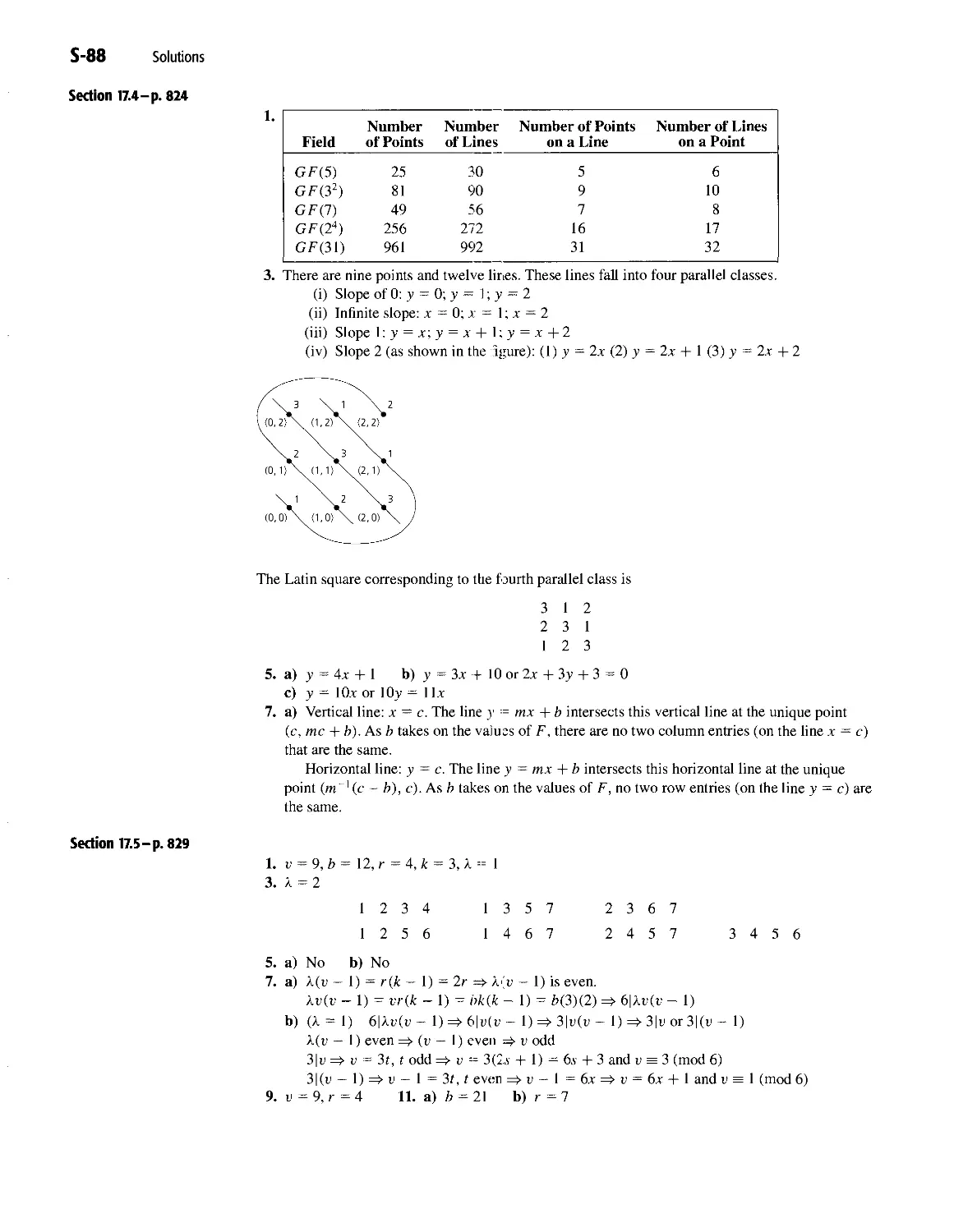
CO BINATO»IAL
AT E ATICS An Applied Introduction
T «■> ^* til
v1 1 f ^ ' 1
Ralph P. Grimaldi Fifth Edition

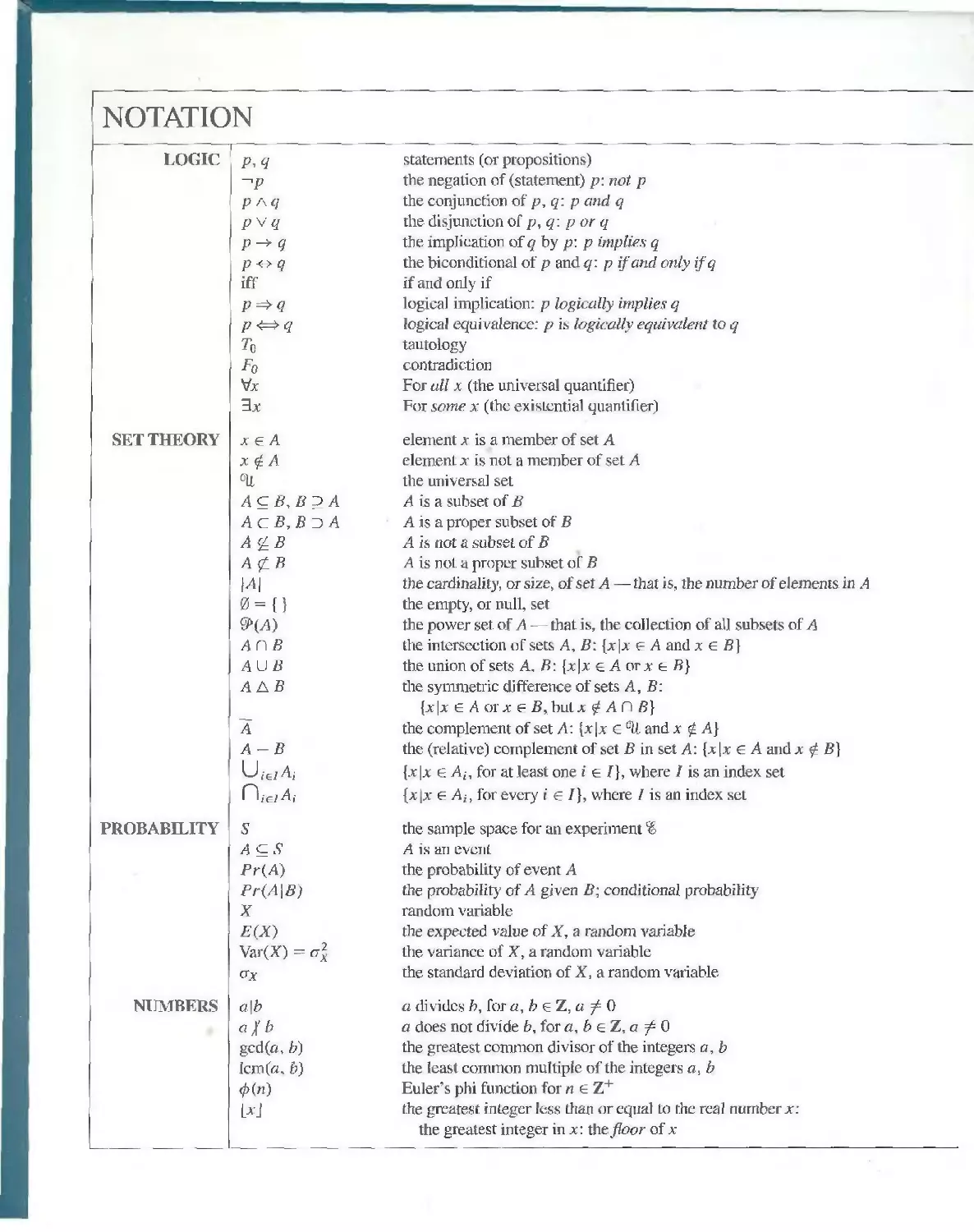
NOTATION
LOGIC
SET THEORY
PROBABILITY
NUMBERS
p,q
^p
pAq
pvq
p^-q
p -o- q
iff
p^-q
p<^>q
To
^0
Vjc
3x
x e A
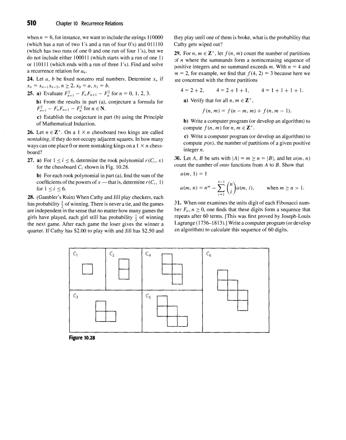
.x £ A
°U
Acg.gDA
AcB,BDA
A£5
A££
1-41
0 = n
9>(.A)
AflB
AUB
AAB
A
A-fl
U,e/Ay
n,e/A,-
S
ACS
Pr(A)
Pr(A\B)
X
E(X)
Var(X) = a\
<?x
a\b
alb
gcd(c, b)
Icm(fl. b)
<P(n)
LxJ
statements (or propositions)
the negation of (statement) p: not p
the conjunction of p, q: p and q
the disjunction of p, q: p or q
the implication of q by p: p implies q
the biconditional of p and q: p if and only ifq
if and only if
logical implication: p logically implies q
logical equivalence: p is logically equivalent to q
tautology
contradiction
For all x (the universal quantifier)
For some x (the existential quantifier)
element x is a member of set A
element x is not a member of set A
the universal set
A is a subset of B
A is a proper subset of B
A is not a subset of B
A is not a proper subset of B
the cardinality, or size, of set A — that is, the number of elements in A
the empty, or null, set
the power set of A — that is, the collection of all subsets of A
the intersection of sets A, B: [x\x e A and x e B}
the union of sets A, B: [x\x e A or x e B]
the symmetric difference of sets A, B:
{x\x e A or x e B, but x $ A n B]
the complement of set A: {x\x G % and jc ^ A}
the (relative) complement of set B in set A: {jc \x e A and x £ B]
[x \x G A;, for at least one i e /}, where / is an index set
{x\x e A,, for every i e I}, where / is an index set
the sample space for an experiment %
A is an event
the probability of event A
the probability of A given B; conditional probability
random variable
the expected value of X, a random variable
the variance of X, a random variable
the standard deviation of X, a random variable
a divides b, for a, b <E Z, a f 0
a does not divide b, for a, b e Z, a ^ 0
the greatest common divisor of the integers a, b
the least common multiple of the integers a, b
Euler's phi function for n G Z+
the greatest integer less than or equal to the real number x:
the greatest integer in x: the floor of jc

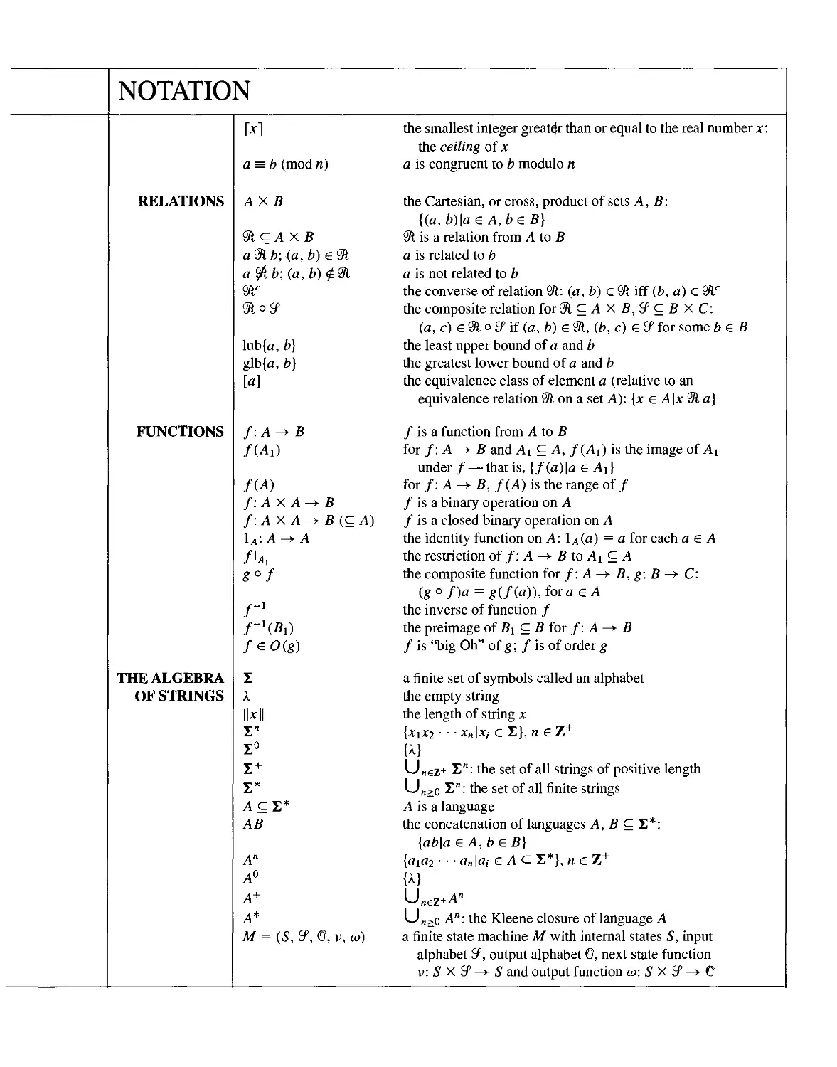
NOTATION
RELATIONS
FUNCTIONS
THE ALGEBRA
OF STRINGS
M
a = b (mod n)
AX B
9lc A X B
a<3lb;(a,b)e<3l
a$,b;(a,b)<£<3t
m,c
9lo^
lub{a, b)
glb{a, b]
[a]
f-.A^B
/(Ai)
f{A)
f:AXA^>-B
/: A X A-> B(c A)
lA: A^A
/u,
8°f
r1
rl{B,)
f G O(g)
T
A.
Ik II
E"
E°
T+
T*
ACE*
AB
A"
A0
A+
A*
M = (S, if, €, v, co)
the smallest integer greater than or equal to the real number x:
the ceiling of x
a is congruent to b modulo n
the Cartesian, or cross, product of sets A, B:
{(a, b)\a e A, b e B}
91 is a relation from A to B
a is related to b
a is not related to b
the converse of relation 91: (a, b) e 91 iff (£, a) e 9lc
the composite relation for 91 c A X B, if c £ X C:
(a, c) e 91 o ^ if (a, b) e 91, (fc, c) e if for some kB
the least upper bound of a and b
the greatest lower bound of a and b
the equivalence class of element a (relative to an
equivalence relation 91 on a set A): {x e A\x 91 a]
f is a function from A to B
for /: A ->■ B and Ai c A, /(Ai) is the image of Ai
under / — that is, {f(a)\a e A\}
for /: A ->■ B, /(A) is the range of /
/ is a binary operation on A
/ is a closed binary operation on A
the identity function on A: l,t(a) = a for each a e A
the restriction of /: A —>■ B to Ai c A
the composite function for f: A—> B, g: B —>■ C:
(g°/)a = g(/(a)),foraeA
the inverse of function /
the preimage of B\ c B for /: A ->■ B
f is "big Oh" of g; /is of order g
a finite set of symbols called an alphabet
the empty string
the length of string x
\x\X2 ■ ■ ■ xn\xi e E}, n e Z+
{k}
U„ez+ E": the set of all strings of positive length
U„>o E": the set of all finite strings
A is a language
the concatenation of languages A, B c T,*:
{ab\a eA,beB]
{axa2 • • -a„|a,- e A c E*}, n eZ+
W
Un6Z+A"
U„>o A": the Kleene closure of language A
a finite state machine M with internal states S, input
alphabet ^, output alphabet 0, next state function
v: S X if -► S and output function w: 5 X ^ -► ©

DISCRETE
AND
COMBINATORIAL
MATHEMATICS
An Applied Introduction
FIFTH EDITION
RALPH P. GRIMALDI
Rose-Hulman Institute of Technology
PEARSON
Addison
Wesley
Boston San Francisco New York
London Toronto Sydney Tokyo Singapore Madrid
Mexico City Munich Paris Cape Town Hong Kong Montreal

Publisher: Greg Tobin
Senior Acquisitions Editor: William Hoffman
Assistant Editor: RoseAnne Johnson
Executive Marketing Manager: Yolanda Cossio
Senior Marketing Manager: Pamela Laskey
Marketing Assistant: Heather Peck
Managing Editor: Karen Guardino
Senior Production Supervisor: Peggy McMahon
Senior Manufacturing Buyer: Hugh Crawford
Composition and Technical Art Rendering: Techsetters, Inc.
Production Services: Barbara Pendergast
Design Supervisor: Barbara T. Atkinson
Cover Designer: Dennis Schaefer
Photo Research and Design Specifications: Beth Anderson
Cover Illustration: George V. Kelvin
Photographs of Blaise Pascal, Aristotle, Lord Hen rand Arthur William Russell, Euclid,
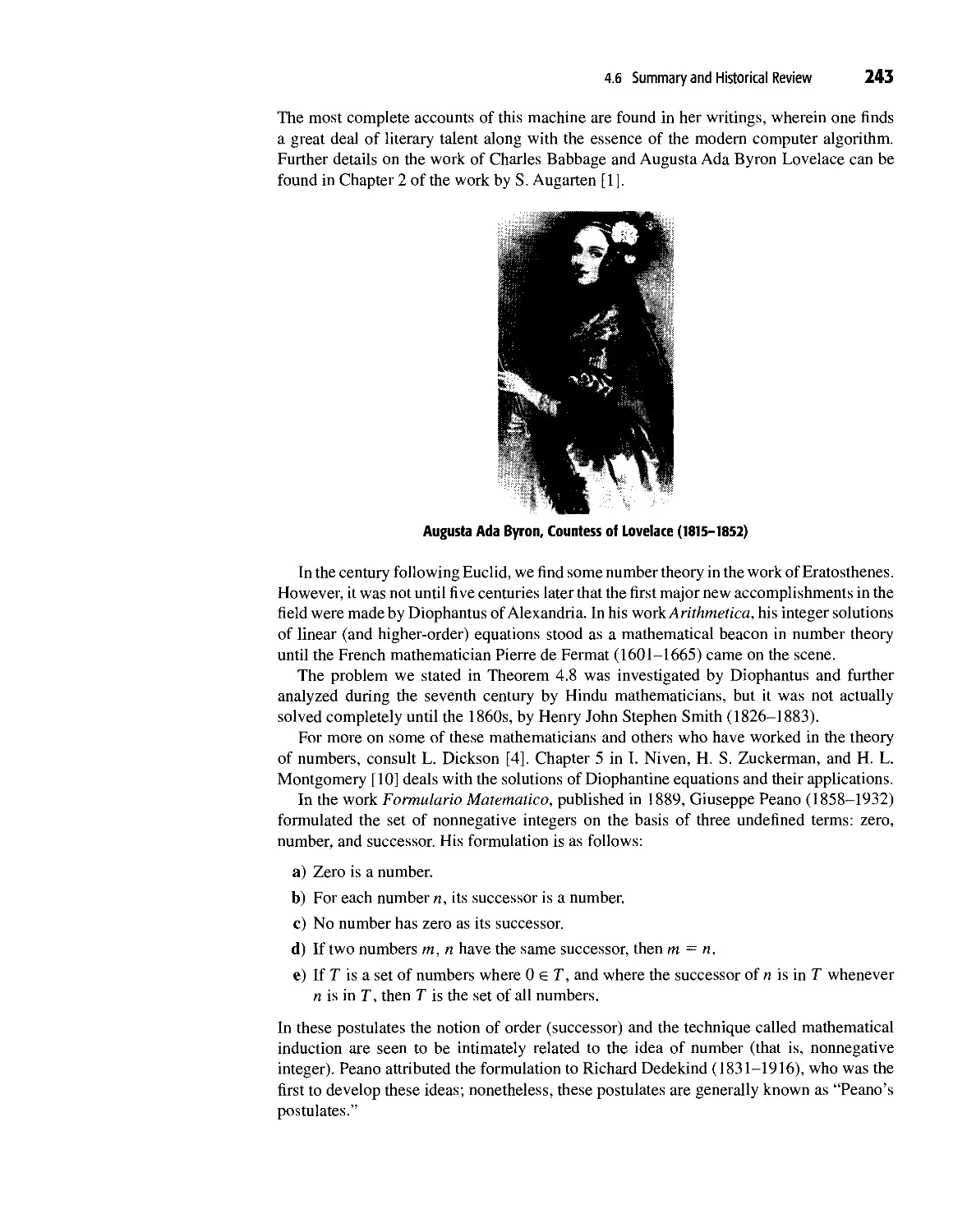
Augusta Ada Byron (Countess of Lovelace), Gottfried Wilhelm Leibniz, Carl Friedrich Gauss,
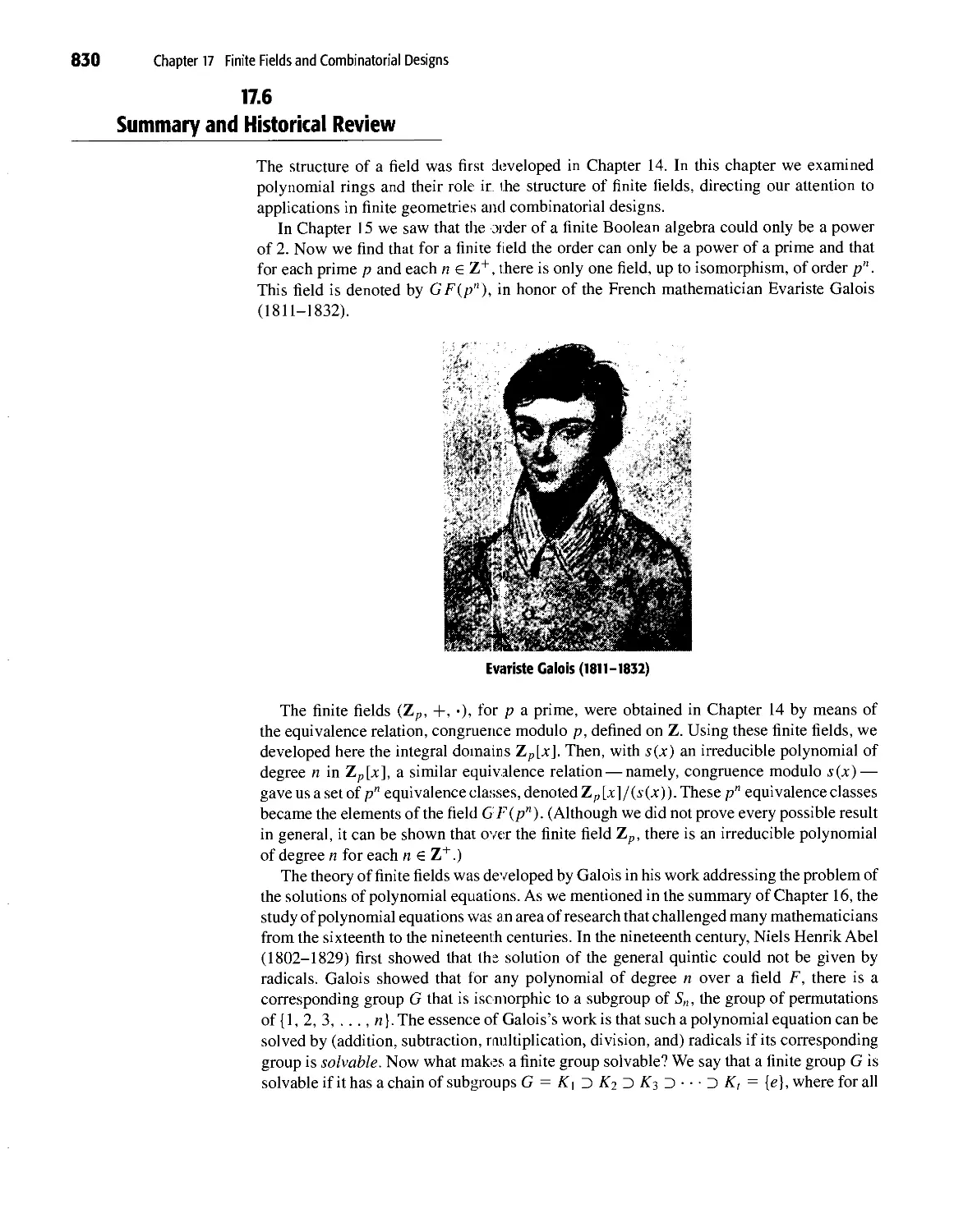
Leonhard Euler, Arthur Cayley, Pierre de Fermat, Niels Henrik Abel, and Evariste Galois
are reproduced courtesy of the Bettman Archive (Corbis). Photographs of George Boole,
Peter Gustav Lejeune Dirichlet, David Hilbeit, Giuseppe Peano, James Joseph Sylvester,
Sophie Germain, and Emmy Noether are reproduced courtesy of Historical Pictures/Stock
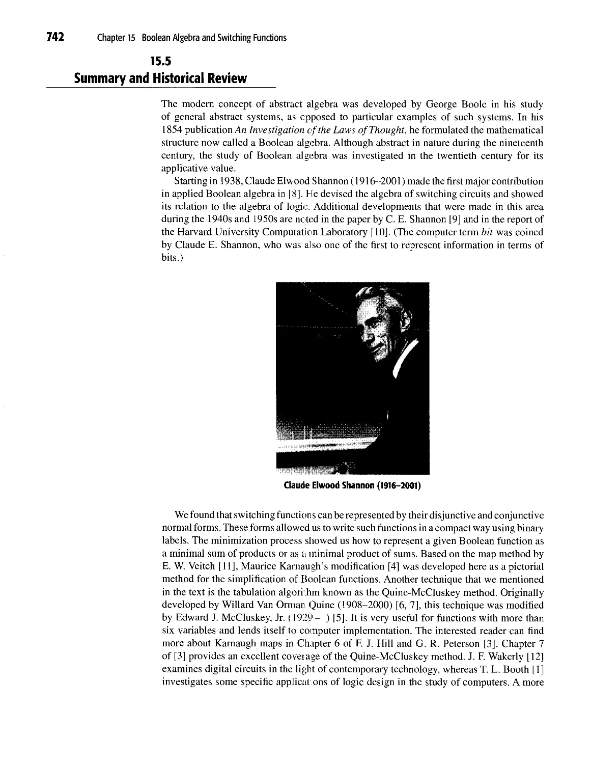
Montage. The photograph of Claude Elwood Shannon is reproduced courtesy of the MIT
Museum. The photograph of Edsger W. Dijkstra is. reproduced courtesy of the University of
Texas at Austin. The photographs of Andrew John Wiles and Rear Admiral Grace Murray
Hopper are reproduced courtesy of APAVide World. The photographs of Georg Cantor,
Alan Mathison Turing, William Rowan Hamilton, and Leonardo Fibonacci are reproduced
courtesy of The Granger Collection. The photograph of Paul Erdos is reproduced courtesy
of Christopher Barker. The photographs of Andrei Nikolayevich Kolmogorov, Thomas
Bayes, and Al-Khowarizmi are reproduced cour :esy of the St. Andrews University Mac-
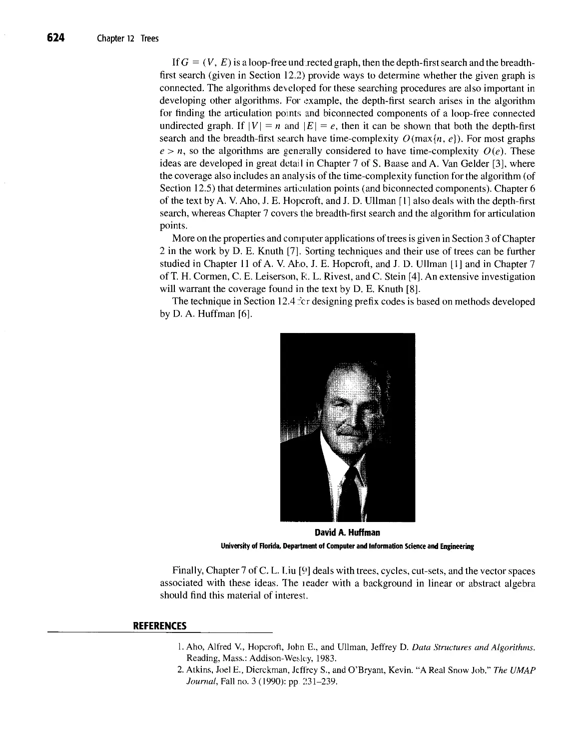
Tutor Archive. The photograph of David A. Huffman is reproduced courtesy of Manuel
Enrique Bermudez of the Department of Computer and Information Science and
Engineering at the University of Florida. The photograph of Joseph P. Kruskal is reproduced
courtesy of Leiden University.
Library of Congress Cataloging-in-l>iiblication Data
Grimaldi, Ralph P.
A review of discrete and combinatorial mathematics / by Ralph P. Grimaldi.-5th ed.
p. cm.
Includes index.
Rev. ed of: Discrete and combinatorial mathematics, cl999.
ISBN 0-201-72634-3
1. Mathematics. 2. Computer science-Mathe natics. 3. Combinatorial analysis. I.
Grimaldi, Ralph P. Discrete and combinatorial mathematics. II. Title.
QA39.2.G748 2003
510-dc21
2002038383
ISBN 0-201-72634-3
Copyright © 2004 Pearson Education, Inc. All rights reserved. No part of this publication
may be reproduced, stored in a retrieval system, cr transmitted in any form or by any means
electronic, mechanical, photocopying, recording, or otherwise, without the prior written
permission of the publisher. Printed in the United States of America.
123456789 10 — CRW — 0504030202

Alia memoria
di mia madre
e mio padre
con affetto e stima

It has been more than twenty years since September 2, 1982, when I signed the contract
to develop what turned into the first edition of this present textbook. At that time the
idea of further editions never crossed my mind. Consequently, I continue to find myself
simultaneously very humbled and very pleased with the way this textbook has been received
by so many instructors and especially students. The first four editions of this textbook have
found their way into many colleges and universities here in the United States. They have
also been used in other nations such as Australia, Canada, England, Ireland, Japan, Mexico,
the Netherlands, Scotland, Singapore, South Africa, and Sweden. I can only hope that this
fifth edition will continue to enlighten and challenge all those who wish to learn about some
of the many facets of the fascinating area of mathematics called discrete mathematics.
The technological advances of the last four decades have resulted in many changes
in the undergraduate curriculum. These changes have fostered the development of many
single-semester and multiple-semester courses where some of the following are introduced:
1. Discrete methods that stress the finite nature inherent in many problems and structures;
2. Combinatorics — the algebra of enumeration, or counting, with its fascinating
interrelations with so many finite structures;
3. Graph theory with its applications and interrelations with areas such as data structures
and methods of optimization; and
4. Finite algebraic structures that arise in conjunction with disciplines such as coding
theory, methods of enumeration, gating networks, and combinatorial designs.
A primary reason for studying the material in any or all of these four major topics is the
abundance of applications one finds in the study of computer science — especially in the
areas of data structures, the theory of computer languages, and the analysis of algorithms.
In addition, there are also applications in engineering and the physical and life sciences, as
well as in statistics and the social sciences. Consequently, the subject matter of discrete and
combinatorial mathematics provides valuable material for students in many majors — not
just for those majoring in mathematics or computer science.
The major purpose of this new edition is to continue to provide an introductory survey
in both discrete and combinatorial mathematics. The coverage is intended for the beginning
student, so there are a great number of examples with detailed explanations. (The examples
are numbered separately and a thick line is used to denote the end of each example.) In
addition, wherever proofs are given, they too are presented with sufficient detail (with the
novice in mind).
V

The text strives to accomplish the following objectives:
1. To introduce the student at the sophomore-junior level, if not earlier, to the topics and
techniques of discrete methods and combinatorial reasoning. Problems in counting, or
enumeration, require a careful analysis of structure (for example, whether or not order
and repetition are relevant) and logical possibilities. There may even be a question of
existence for some situations. Following such a careful analysis, we often find that the
solution of a problem requires simple techniques for counting the possible outcomes that
evolve from the breakdown of the given problem into smaller subproblems.
2. To introduce a wide variety of applications. In this regard, whenever data structures
(from computer science) or structures from abstract algebra are required, only the basic
theory needed for the application is developed. Furthermore, the solutions of some
applications lend themselves to iterative procedures that lead to specific algorithms. The
algorithmic approach to the solution of problems is fundamental in discrete
mathematics, and this approach reinforces the close ties between this discipline and the area of
computer science.
3. To develop the mathematical maturity of the student through the study of an area that
is so different from the traditional coverage in calculus and differential equations. Here,
for example, there is the opportunity to establish results by counting a certain collection
of objects in more than one way. This provides what are called combinatorial identities;
it also introduces a novel proof technique. In this edition the nature of proof, along with
what constitutes a valid argument, is developed in Chapter 2, in conjunction with the
laws of logic and rules of inference. The coverage is extensive, keeping the student
(with minimal background) in mind. [For the reader with a logic course (or something
comparable) in his or her background, this material can be skipped over with little or
no difficulty.] Proofs by mathematical induction (along with recursive definitions) are
introduced in Chapter 4 and then used throughout the subsequent chapters.
With regard to theorems and their proofs, in many instances an attempt has been made
to motivate theorems from observations on specific examples. In addition, whenever a
finite situation provides a result that is not true for the infinite case, this situation is
singled out for attention. Proofs that are extremely long and/or rather special in nature
are omitted. However, for the very small number of proofs that are omitted, references are
supplied for the reader interested in seeing the validation of these results. (The amount
of emphasis placed on proofs will depend on the goals of the individual instructor and
on those of his or her student audience.)
4. To present an adequate survey of topics for the computer science student who will be
taking more advanced courses in areas such as data structures, the theory of computer
languages, and the analysis of algorithms. The coverage here on groups, rings, fields,
and Boolean algebras will also provide an applied introduction for mathematics majors
who wish to continue their study of abstract algebra.
The prerequisites for using this book are primarily a sound background in high school
mathematics and an interest in attacking and solving a variety of problems. No particular
programming ability is assumed. Program segments and procedures are given in
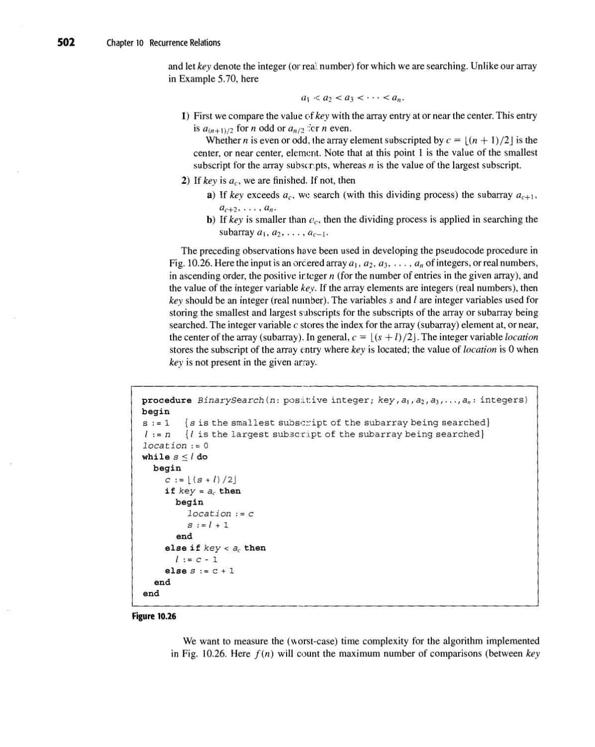
pseudocode, and these are designed and explained in order to reinforce particular examples. With
regard to calculus, we shall mention later in this preface its extent in Chapters 9 and 10.
My primary motivation for writing the first four editions of this book has been the
encouragement I had received over the years from my students and colleagues, as well as from
the students and instructors who used the first four editions of the textbook at many different
colleges and universities. Those four editions reflected both my interests and concerns and

Preface VII
those of my students, as well as the recommendations of the Committee on the
Undergraduate Program in Mathematics and of the Association of Computing Machinery. This fifth
edition continues along the same lines, reflecting the suggestions and recommendations
made by the instructors and especially the students who have used or are using the fourth
edition.
Features
Following are brief descriptions of some of the major features of this newest edition. These
are designed to assist the reader (student or otherwise) in learning the fundamentals of
discrete and combinatorial mathematics.
Emphasis on algorithms and applications. Algorithms and applications in many areas
are presented throughout the text. For example:
1. Chapter 1 includes several instances where the introductory topics on enumeration
are needed — one example, in particular, addresses the issue of over-counting.
2. Section 7 of Chapter 5 provides an introduction to computational complexity. This
material is then used in Section 8 of this chapter in order to analyze the running times of
some elementary pseudocode procedures.
3. The material in Chapter 6 covers languages and finite state machines. This introduces
the reader to an important area in computer science — the theory of computer languages.
4. Chapters 7 and 12 include discussions on the applications and algorithms dealing with
topological sorting and the searching techniques known as the depth-first search and the
breadth-first search.
5. In Chapter 10 we find the topic of recurrence relations. The coverage here includes
applications on (a) the bubble sort, (b) binary search, (c) the Fibonacci numbers,
(d) the Koch snowflake, (e) Hasse diagrams, (f) the data structure called the stack,
(g) binary trees, and (h) tilings.
6. Chapter 16 introduces the fundamental properties of the algebraic structure called
the group. The coverage here shows how this structure is used in the study of algebraic
coding theory and in counting problems that require Polya's method of enumeration.
Detailed explanations. Whether it is an example or the proof of a theorem,
explanations are designed to be careful and thorough. The presentation is primarily focused on
improving understanding on the part of the reader who is seeing this type of material for
the first time.
Exercises. The role of the exercises in any mathematics text is a crucial one. The amount
of time spent on the exercises greatly influences the pace of the course. Depending on
the interest and mathematical background of the student audience, an instructor should
find that the class time spent on discussing exercises will vary.
There are over 1900 exercises in the 17 chapters. Those that appear at the end of each
section generally follow the order in which the section material is developed. These
exercises are designed to (a) review the basic concepts in the section; (b) tie together
ideas presented in earlier sections of the chapter; and (c) introduce additional concepts
that are related to the material in the section. Some exercises call for the development
of an algorithm, or the writing of a computer program, often to solve a certain instance
of a general problem. These usually require only a minimal amount of programming
experience.

Viii Preface
Each chapter concludes with a set of supplementary exercises. These provide further
review of the ideas presented in the chapter, and also use material developed in earlier
chapters.
Solutions are provided at the back of the text for almost all parts of all the odd-
numbered exercises.
Chapter summaries. The last numbered section in each chapter provides a summary
and historical review of the major ideas covered in that chapter. This is intended to give
the reader an overview of the contents of the chapter and provide information for further
study and applications. Such further study can be readily assisted by the list of references
that is supplied.
In particular, the summaries at the ends of Chapters 1,5, and 9 include tables on the
enumeration formulas developed within each of these chapters. Sometimes these tables
include results from earlier chapters in order to make comparisons and to show how the
new results extend the prior ones.
Organization
The areas of discrete and combinatorial mathematics are somewhat new to the undergraduate
curriculum, so there are several options as to which topics should be covered in these courses.
Each instructor and each student rr ay have different interests. Consequently, the coverage
here is fairly broad, as a survey course mandates. Yet there will always be further topics that
some readers may feel should be included. Furthermore, there will also be some differences
of opinion with regard to the order in which some topics are presented in this text.
The nature and importance of the algorithmic approach to problem solving is stressed
throughout the text. Ideas and approaches on problem solving are further strengthened by
the interrelations between enumeration and structure, two other major topics that provide
unifying threads for the material developed in the book.
The material is subdivided into four major areas. The first seven chapters form the
underlying core of the book and present the fundamentals of discrete mathematics. The
coverage here provides enough material for a one-quarter or one-semester course in discrete
mathematics. The material in Chapter 2 can be reviewed by those with a background in logic.
For those interested in developing and writing proofs, this material should be examined
very carefully. A second course —Dne that emphasizes combinatorics — should include
Chapters 8,9, and 10 (and, time permitting, sections 1,2,3,10,11, and 12 of Chapter 16). In
Chapter 9 some results from calculus are used; namely, fundamentals on differentiation and
partial fraction decompositions. However, for those who wish to skip this chapter, sections
1,2, 3, 6, and 7 of Chapter 10 can still be covered. A course that emphasizes the theory and
applications of finite graphs can be developed from Chapters 11,12, and 13. These chapters
form the third major subdivision of the text. For a course in applied algebra, Chapters
14, 15, 16, and 17 (the fourth, and final, subdivision) deal with the algebraic structures —
group, ring, Boolean algebra, and field — and include applications on cryptology, switching
functions, algebraic coding theory, and combinatorial designs. Finally, a course on the role
of discrete structures in computer science can be developed from the material in Chapters
11, 12, 13, 15, and sections 1-9 of Chapter 16. For here we find applications on switching
functions, the RSA cryptosystem, and algebraic coding theory, as well as an introduction
to graph theory and trees, and their role in optimization.
Other possible courses can be developed by considering the following chapter
dependencies.

Preface IX
Chapter Dependence on Prior Chapters
1 No dependence
2 No dependence (Hence an instructor can start a course in discrete
mathematics with either the study of logic or an introduction to enumeration.)
3 1,2
4 1,2,3
5 1,2,3,4
6 1,2,3,5 (Minor dependence in Section 6.1 on Sections 4.1, 4.2)
7 1, 2, 3, 5, 6 (Minor dependence in Section 7.2 on Sections 4.1,4.2)
8 1,3 (Minor dependence in Example 8.6 on Section 5.3)
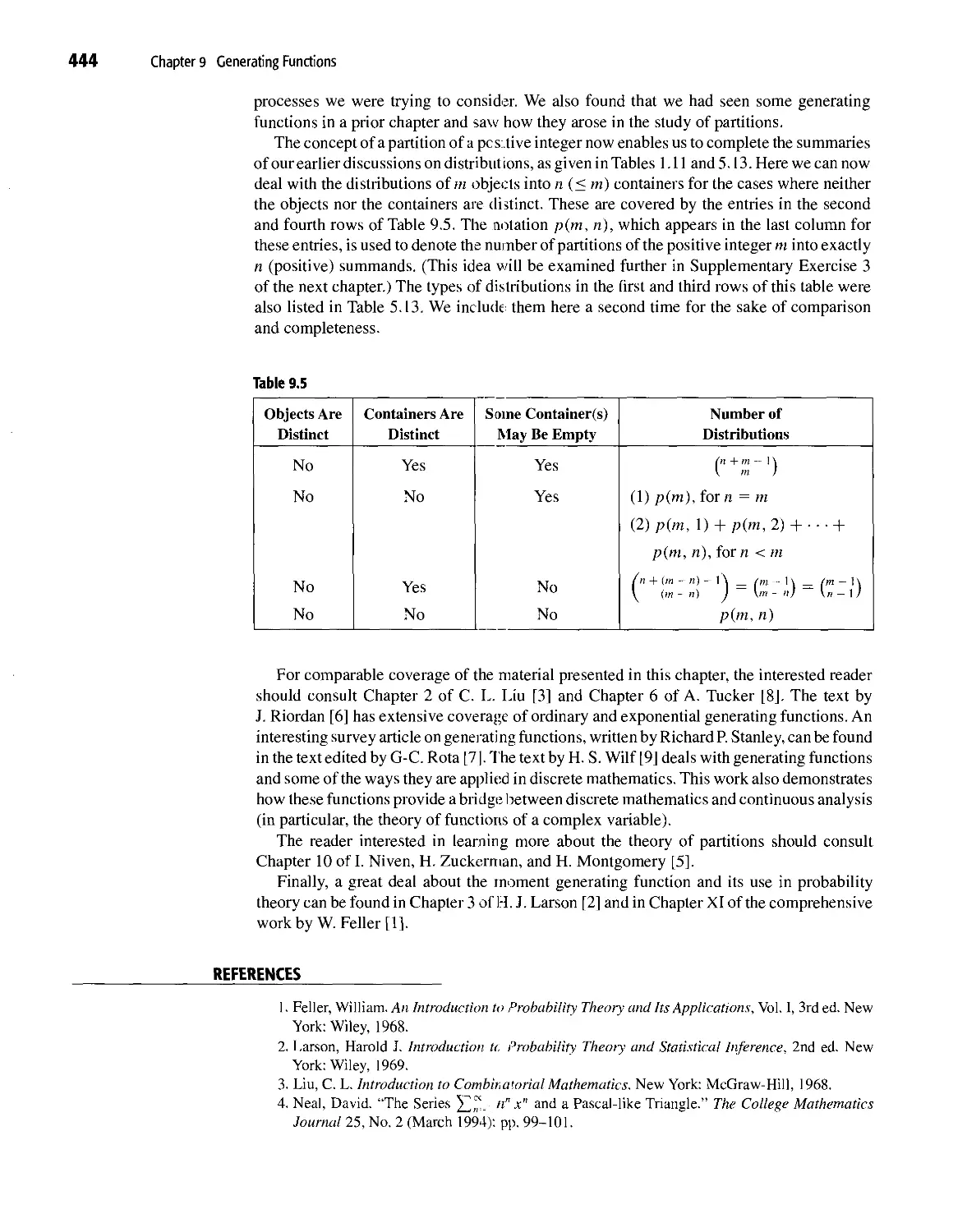
9 1,3
10 1,3,4, 5, 9 (Minor dependence in Example 10.33 on Section 7.3)
11 1,2,3,4,5 (Although some graph-theoretic ideas are mentioned in Chapters
5,6,7,8, and 10, the material in this chapter is developed with no dependence
on the graph-theoretic material given in these earlier results.)
12 1,2,3,4,5,11
13 3,5,11,12
14 2,3,4,5,7 (The Euler phi function (0) is used in Section 14.3. This function
is derived in Example 8.8 of Section 8.1 but the result can be used here in
Chapter 14 without covering Chapter 8.)
15 2,3,5,7
16 1,2,3,4,5,7
17 2,3,4,5,7,14
In addition, the index has been very carefully developed in order to make the text even
more flexible. Terms are presented with primary listings and several secondary listings.
Also there is a great deal of cross referencing. This is designed to help the instructor who
may want to change the order of presentation and deviate from the straight and narrow.
Changes in the Fifth Edition
The changes here in the fifth edition of Discrete and Combinatorial Mathematics reflect
the observations and recommendations of students and instructors who have used earlier
editions of the text. As with the first four editions, the tone and purpose of the text remain
intact. The author's goal is still the same: to provide within these pages a sound, readable,
and understandable introduction to the foundations of discrete and combinatorial
mathematics— for the beginning student or reader. Among the changes one will find in this fifth
edition we mention the following:
• The examples in Section 4 of Chapter 1 now include material on runs, a concept that
arises in the study of statistics — in particular, in the area of quality control.
• Exercise 13 for Section 3 of Chapter 2 develops the rule of inference known as
resolution, a rule that serves as the basis for many computer programs designed to automate
a reasoning system.
• The earlier editions of this text included a section that introduced the notion of
probability. This section has now been expanded and three additional optional sections have
been added for those who wish to further examine some of the introductory ideas
associated with discrete probability — in particular, the axioms of probability, conditional
probability, independence, Bayes' Theorem, and discrete random variables.

X Preface
• The coverage on partial orders and total orders in Section 3 of Chapter 7 now includes
an optional example where the Catalan numbers arise in this context.
• The introductory material in Section 1 of Chapter 8 has been rewritten to provide
a more readable transition between the coverage on counting and Venn diagrams in
Section 3 of Chapter 3 and the more general technique known as the Principle of Inclusion
and Exclusion.
• One of the fascinating features of discrete and combinatorial mathematics is the
variety of ways a given problem can be solved. In the fourth edition (in Chapters 1 and 3)
the reader learned, in two different contexts, that a positive integer n had 2"_1
compositions— that is, there are 2"~] ways to write n as an ordered sum of positive-integer
summands. This result is now established in three other ways: (i) by the Principle of
Mathematical Induction in Chapter 4; (ii) using generating functions in Chapter 9; and
(iii) by solving a recurrence relation in Chapter 10.
• For those who want even more on discrete probability, Section 2 of Chapter 9 includes
an example that deals with the geometric random variable.
• Section 2 of Chapter 10 now includes a discussion of the work by Gabriel Lame in
estimating the number of divisions used in the Euclidean algorithm to find the greatest
common divisor of two positive integers.
• The Master theorem (of importance in the analysis of algorithms) is introduced and
developed in an exercise for Section 6 of Chapter 10.
• The material on transport networks (in Section 3 of Chapter 13) has been updated and
now incorporates the Edmonds-Ktirp algorithm in the procedure originally developed by
Lester Ford and Delbert Fulkerson.
• The coverage on modular arithmetic in Section 3 of Chapter 14 now includes
applications dealing with the linear congruential pseudorandom number generator, private-key
cryptosy stems, and modular exponentiation. Further, in Section 4 of Chapter 14, the
material dealing with the Chinese Remainder Theorem, which was only stated in previous
editions, now includes a proof of this result as well as an example dealing with how it is
applied.
• Section 4 of Chapter 16 is new arid optional. The material here provides an introduction
to the RSApublic-key cryptosystern and shows how one can apply some of the theoretical
results developed in prior sections of the text.
• As with the second, third, and fourth editions, a great deal of effort has been applied
in updating the summary and historical review at the end of each chapter. Consequently,
new references and/or new editions are provided where appropriate.
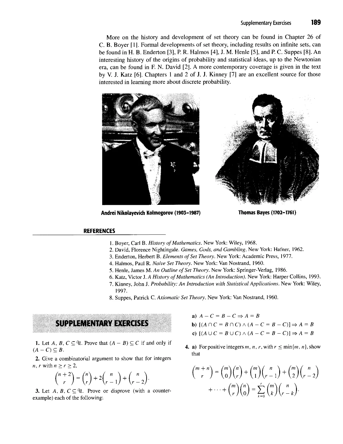
• For this fifth edition, the following pictures and photographs have been added to the
summary and historical review of certain chapters: a picture of Thomas Bayes and a
photograph of Andrei Nikolayevich Kolmogorov in Chapter 3; a picture of Al-Khowarizmi
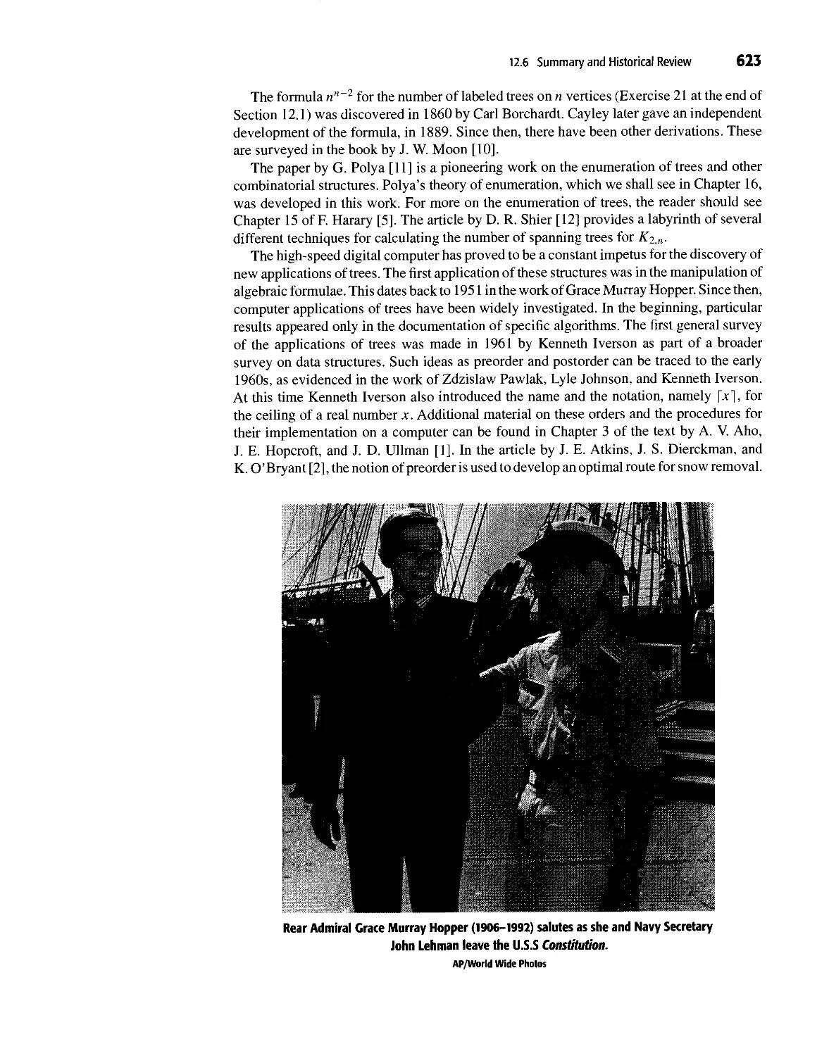
in Chapter 4; a photograph of Bavid A. Huffman in Chapter 12; and a photograph of
Joseph B. Kruskal in Chapter 13
Ancillaries
• There is an Instructor's Solutions Manual that is available, from the publisher, for
those instructors who adopt the textbook for their classes. It contains the solutions and/or
answers for all of the exercises within the 17 chapters and the three appendices of this
textbook.

Preface XI
• There is also a Student's Solutions Manual that is available separately. It contains the
solutions and/or answers for all of the odd-numbered exercises in the textbook. In some
cases more than one solution is presented.
• The following Web site provides additional resources for learning more about discrete
and combinatorial mathematics. In addition it also provides a way for readers to contact
the author with comments, suggestions, or possible errors they have found.
www.aw.com/grimaldi
Acknowledgments
If space permitted, I should like to mention each of the students who provided help and
encouragement when I was writing the five editions of this book. Their suggestions helped
to remove many mistakes and ambiguities, thus improving the exposition. Most helpful
in this category were Paul Griffith, Meredith Vannauker, Paul Barloon, Byron Bishop,
Lee Beckham, Brett Hunsaker, Tom Vanderlaan, Michael Bryan, John Breitenbach, Dan
Johnson, Brian Wilson, Allen Schneider, John Dowell, Charles Wilson, Richard Nichols,
Charles Brads, Jonathan Atkins, Kenneth Schmidt, Donald Stanton, Mark Stremler, Stephen
Smalley, Anthony Hinrichs, Kevin O'Bryant, and Nathan Terpstra.
I thank Larry Alldredge, Claude Anderson, David Rader, Matt Hopkins, John Rickert, and
Martin Rivers for their comments on the computer science material, and Barry Farbrother,
Paul Hogan, Dennis Lewis, Charles Kyker, Keith Hoover, Matthew Saltzman, and Jerome
Wagner for their enlightening remarks on some of the applications.
I gratefully acknowledge the persistent enthusiasm and encouragement of the staff at
Addison-Wesley (both past and present), especially Wayne Yuhasz, Thomas Taylor, Michael
Payne, Charles Glaser, Mary Crittendon, Herb Merritt, Maria Szmauz, Adeline Ruggles,
Stephanie Botvin, Jack Casteel, Jennifer Wall, Joanne Sousa Foster, Karen Guardino, Peggy
McMahon, Deborah Schneider, Laurie Rosatone, Carolyn Lee-Davis, and Jennifer Al-
banese. William Hoffman, and especially RoseAnne Johnson and Barbara Pendergast,
deserve the most recognition for their outstanding contributions to this fifth edition. The efforts
put forth by Steven Finch in proofreading the text and that of Paul Lorczak who checked
the accuracy of the answers to the exercises are also greatly appreciated.
I am also indebted to my colleagues John Kinney, Robert Lopez, Allen Broughton,
Gary Sherman, George Berzsenyi, and especially Alfred Schmidt, for their interest and
encouragement throughout the writing of this and/or earlier editions.
Thanks and appreciation are due the following reviewers of the first, second, third, fourth,
and/or fifth editions.
Norma E. Abel Digital Equipment Corporation
Larry Alldredge Qualcomm, Inc.
Charles Anderson University of Colorado, Denver
Claude W. Anderson III Rose-Hulman Institute of Technology
David Arnold Baylor University
V. K. Balakrishnan University of Maine at Orono
Robert Barnhill University of Utah
Dale Bedgood East Texas State University
Jerry Beehler Tri-State University
Katalin Bencsath Manhattan College
Allan Bishop Western Illinois University
Monte Boisen Virginia Polytechnic Institute

Samuel Councilman
Robert Crawford
Ellen Cunningham, SP
Carl DeVito
Vladimir Drobot
John Dye
Carl Eckberg
Michael Falk
Marvin Freedman
Robert Geitz
James A. Glasenapp
Gary Gordon
Harvey Greenberg
Laxmi Gupta
Eleanor O. Hare
James Harper
David S. Hart
Maryann Hastings
W. Mack Hill
Stephen Hirtle
Arthur Hobbs
Dean Hoffman
Richard litis
David P. Jacobs
Robert Jajcay
Akihiro Kanamori
John Konvalina
Rochelle Leibowitz
James T. Lewis
Y-Hsin Liu
Joseph Malkevitch
Brian Martensen
Hugh Montgomery
Thomas Morley
Richard Orr
Edwin P. Oxford
John Rausen
Martin Rivers
Gabriel Robins
Chris Rodger
James H. Schmerl
Paul S. Schnare
Leo Schneider
Debra Diny Scott
Gary E. Stevens
Dalton Tarwater
Jeff Tecosky-Feldman
W. L. Terwilliger
Donald Thompson
California State University at Long Beach
Western Kentucky University
Saint Mary-of-the-Woods College
Naval Postgraduate School
San Jose State University
California State University at Northridge
San Diego State University
Northern Arizona University
Boston University
Oberlin College
Rochester Institute of Technology
Lafayette College
University of Colorado, Denver
Rochester Institute of Technology
Clemson University
Central Washington University
Rochester Institute of Technology
Marymount College
Worcester State College
University of Pittsburgh
Texas A&M University
Auburn University
Willamette University
Ciemson University
Indiana State University
Boston University
University of Nebraska at Omaha
Wheaton College
University of Rhode Island
University of Nebraska at Omaha
York College (CUNY)
The University of Texas at Austin
University of Michigan
Georgia Institute of Technology
Rochester Institute of Technology
Baylor University
New Jersey Institute of Technology
Lexmark International, Inc.
University of Virginia
Auburn University
University of Connecticut
Eastern Kentucky University
John Carroll University
University of Wisconsin at Green Bay
Hanwick College
Texas Tech University
Harvard University
Bowling Green State University
Pepperdine University

Preface xiii
Thomas Upson Rochester Institute of Technology
W. D. Wallis Southern Illinois University
Larry West Virginia Commonwealth University
Yixin Zhang University of Nebraska at Omaha
Special thanks are due to Douglas Shier of Clemson University for the outstanding work
he did in reviewing the manuscripts of all five editions. Thanks are also due to Joan Shier
for letting Doug review the fourth and fifth editions.
The translation for the dedication is due to Dr. Yvonne Panaro of Northern Virginia
Community College. Thank you, Yvonne, and thank you, Patter (Patricia Wickes Thurston),
for your role in obtaining the translation.
A text of this length requires the use of many references. The members of the library staff
of Rose-Hulman Institute of Technology were always available when books and articles
were needed, so it is only fitting to express one's appreciation for the efforts of John Robson,
Sondra Nelson, Dong Chao, Jan Jerrell, and especially Amy Harshbargerand Margaret Ying.
In addition, Keith Hoover and Raymond Bland are thanked for rescuing the author from
the perils of many hardware problems.
The last, and surely the most important, note of thanks belongs once again to the ever-
patient and encouraging now-retired secretary of the Rose-Hulman mathematics
department — Mrs. Mary Lou McCullough. Thank you for the fifth time, Mary Lou, for all of
your work!
Alas, the remaining errors, ambiguities, and misleading comments are once again the
sole responsibility of the author.
R.P.G.
Terre Haute, Indiana

Contents
PART 1
Fundamentals of Discrete Mathematics 1
1 Fundamental Principles of Counting 3
1.1 The Rules of Sum and Product 3
1.2 Permutations 6
1.3 Combinations: The Binomial Theorem 14
1.4 Combinations with Repetition 26
1.5 The Catalan Numbers (Optional) 36
1.6 Summary and Historical Review 41
2 Fundamentals of Logic 47
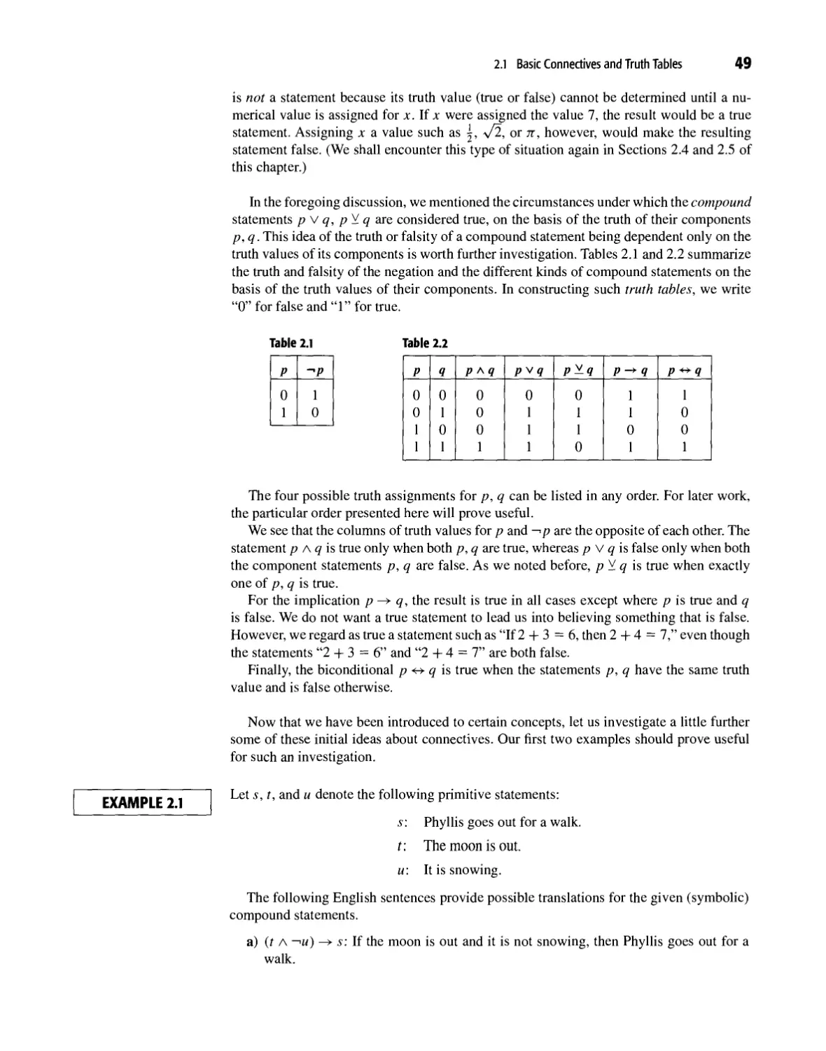
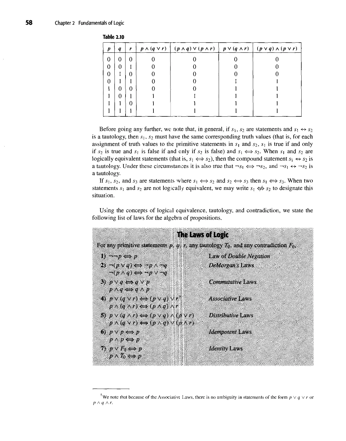
2.1 Basic Connectives and Truth Tables 47
2.2 Logical Equivalence: The Laws of Logic 55
2.3 Logical Implication: Rules of Inference 67
2.4 The Use of Quantifiers 86
2.5 Quantifiers, Definitions, and the Proofs of Theorems 103
2.6 Summary and Historical Review 117
3 Set Theory 123
3.1 Sets and Subsets 123
3.2 Set Operations and the Laws of Set Theory 136
3.3 Counting and Venn Diagrams 148
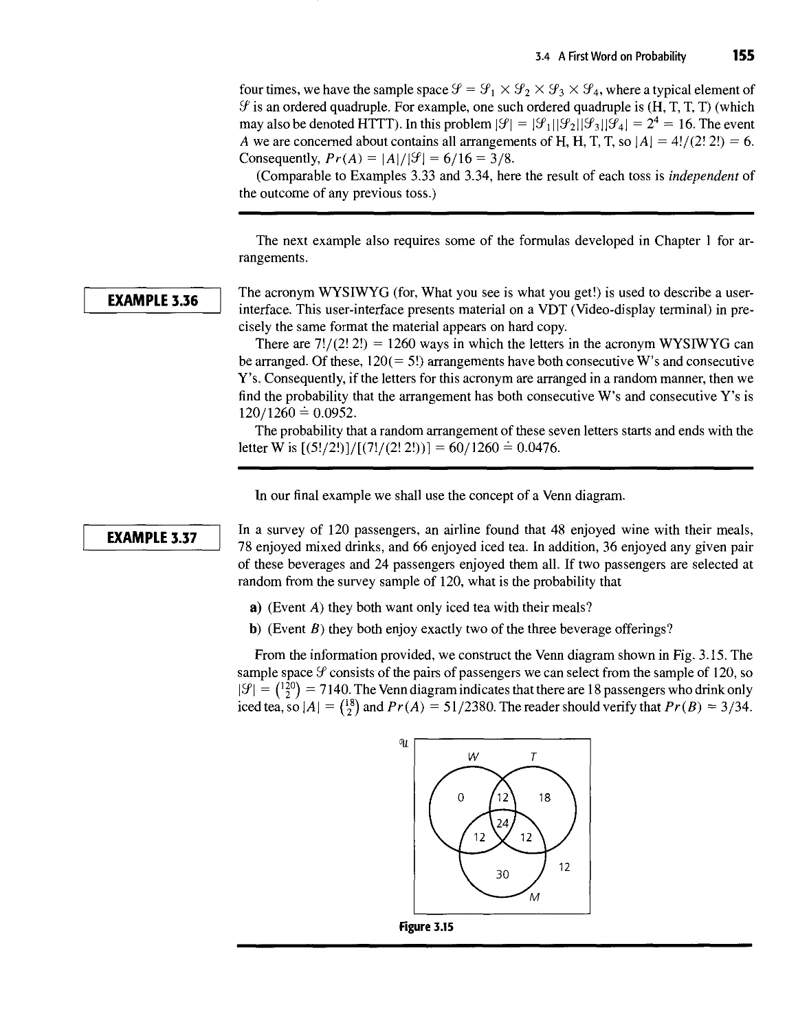
3.4 A First Word on Probability 150
3.5 The Axioms of Probability (Optional) 157
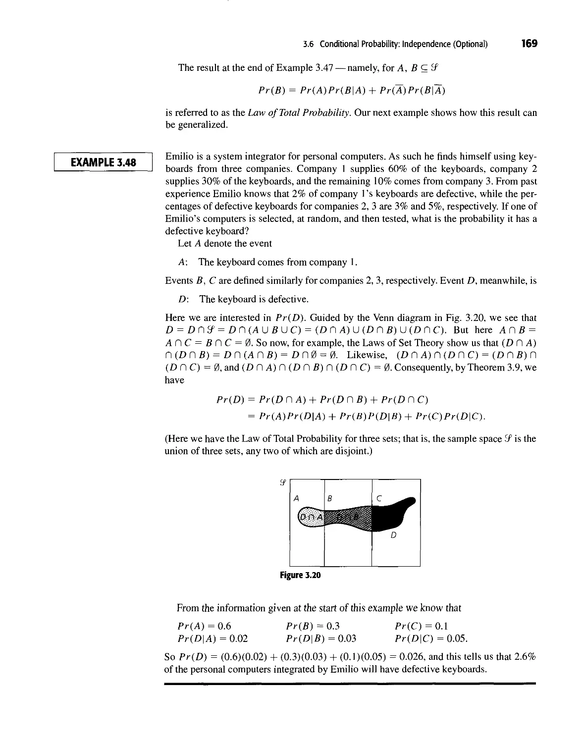
3.6 Conditional Probability: Independence (Optional) 166
3.7 Discrete Random Variables (Optional) 175
3.8 Summary and Historical Review 186
XV

XVJ Contents
4 Properties of the Integers: Mathematical Induction 193
4.1 The Well-Ordering Principle: Mathematical Induction 193
4.2 Recursive Definitions 210
4.3 The Division Algorithm: Prime Numbers 221
4.4 The Greatest Common Divisor: The Euclidean Algorithm 231
4.5 The Fundamental Theorem of Arithmetic 237
4.6 Summary and Historical Review 242
5 Relations and Functions 247
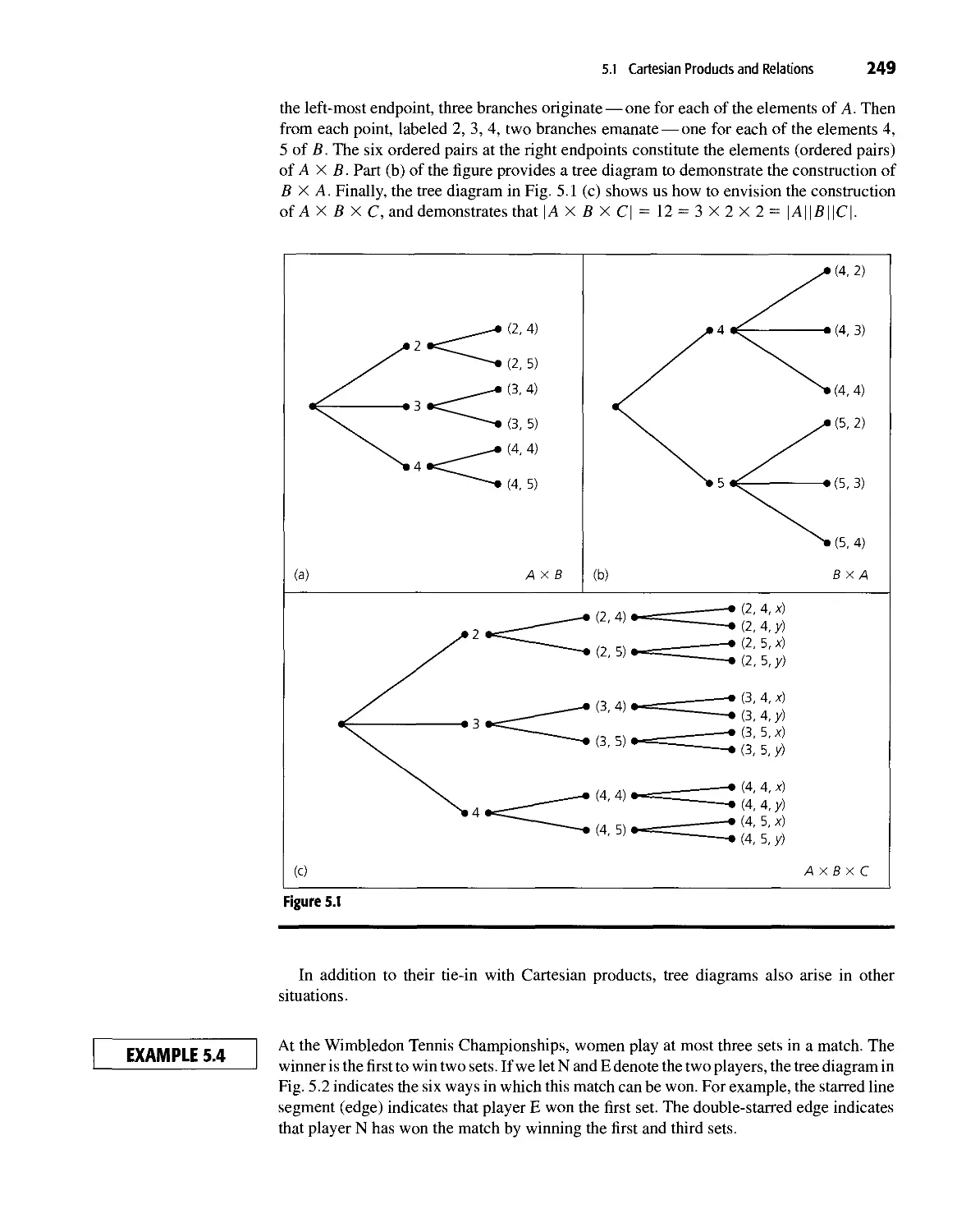
5.1 Cartesian Products and Relations 248
5.2 Functions: Plain and One-to-One 252
5.3 Onto Functions: Stirling Numbers of the Second Kind 260
5.4 Special Functions 267
5.5 The Pigeonhole Principle 273
5.6 Function Composition and Inverse Functions 278
5.7 Computational Complexity 289
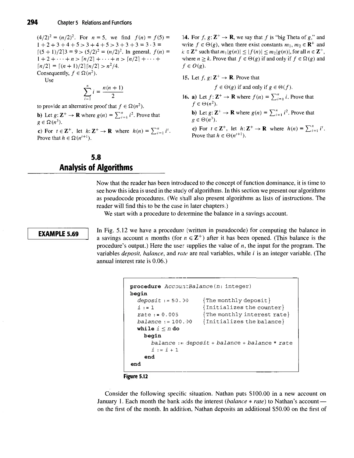
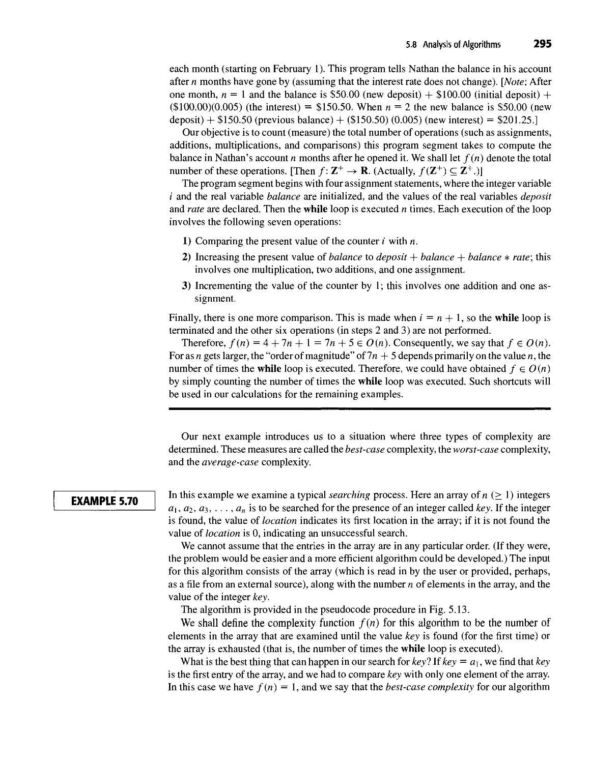
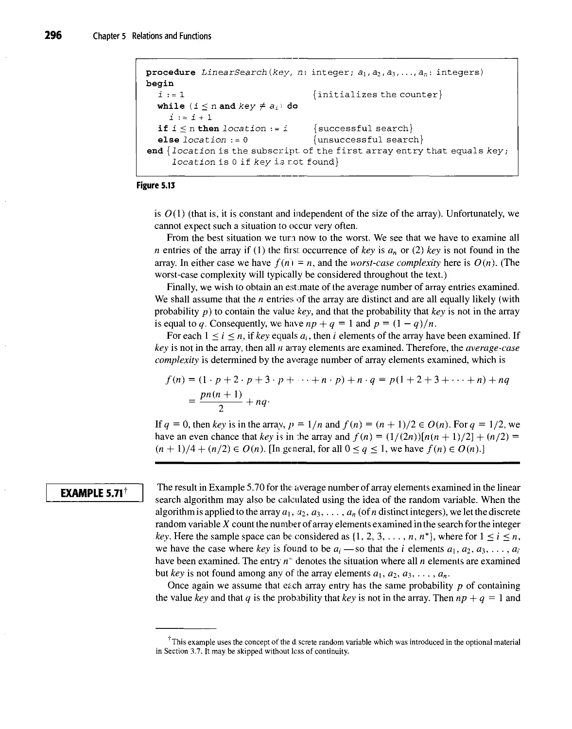
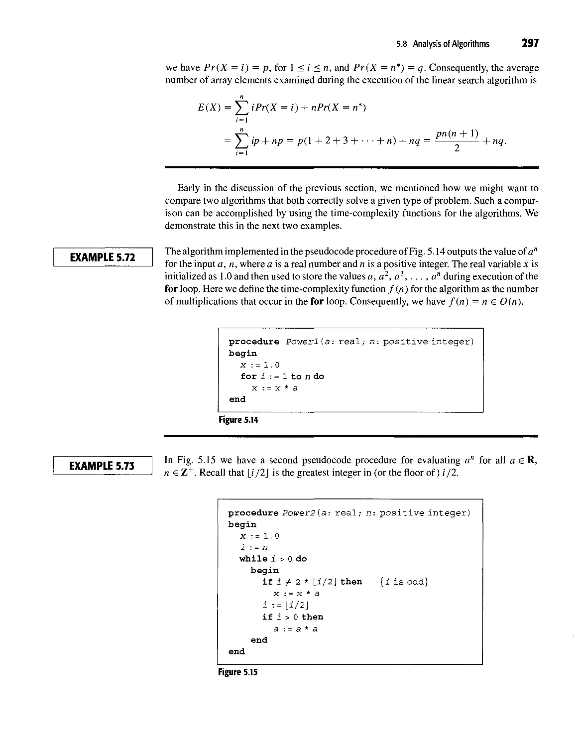
5.8 Analysis of Algorithms 294
5.9 Summary and Historical Review 302
6 Languages: Finite State Machines 309
6.1 Language: The Set Theory of Strings 309
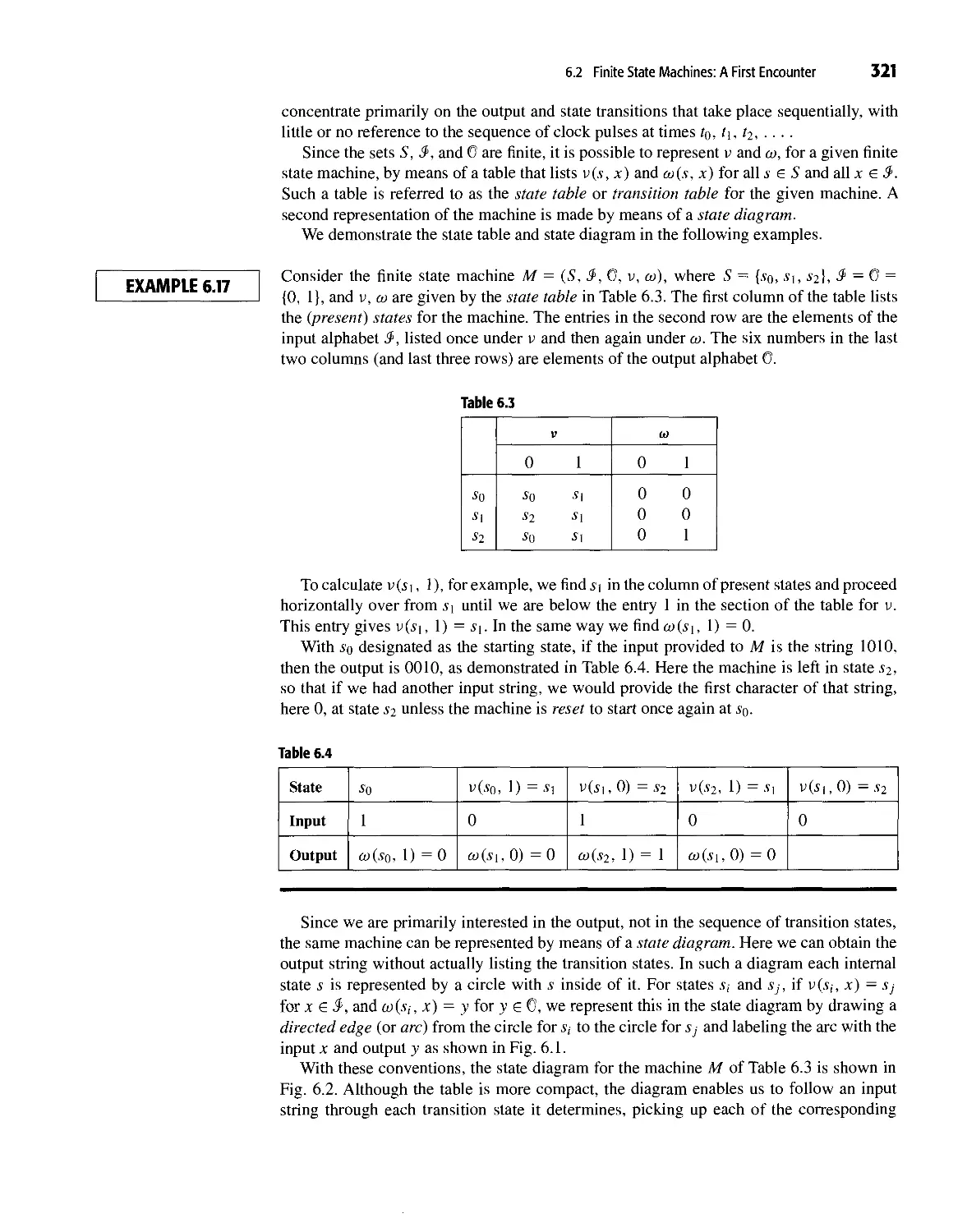
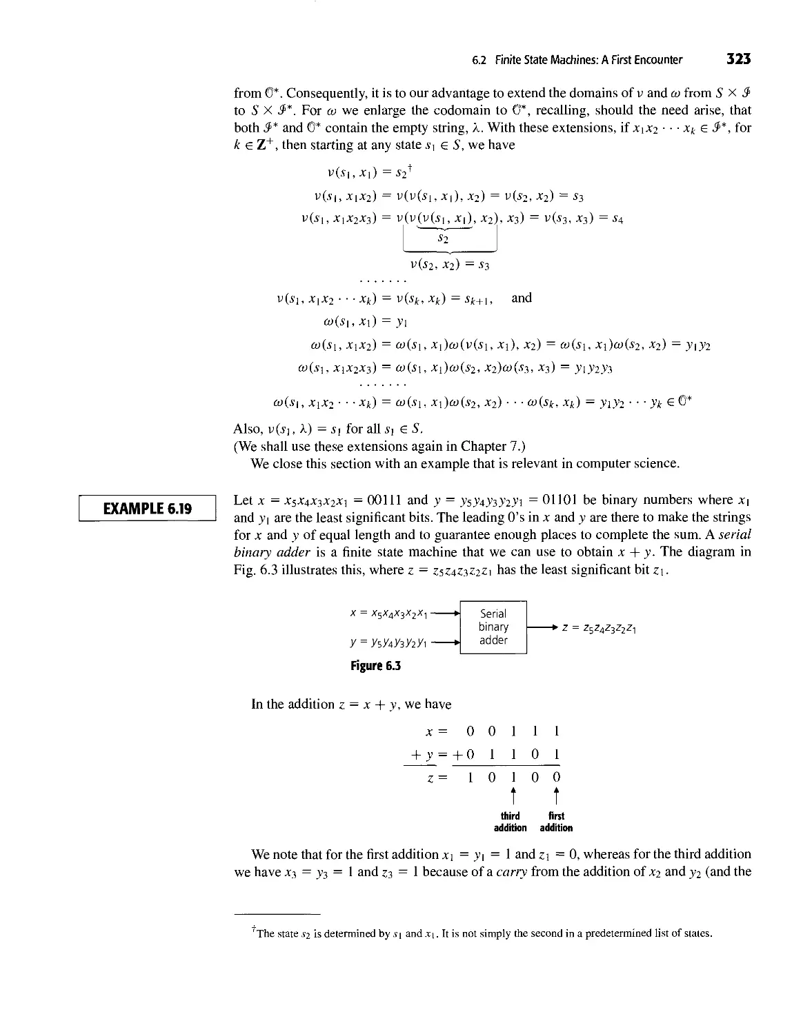
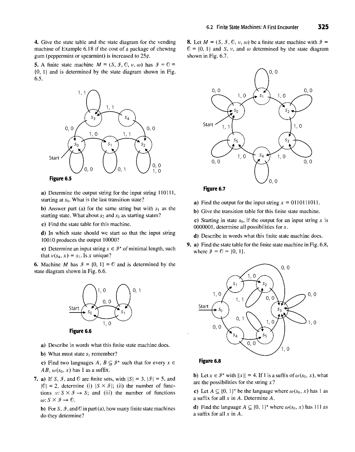
6.2 Finite State Machines: A Frst Encounter 319
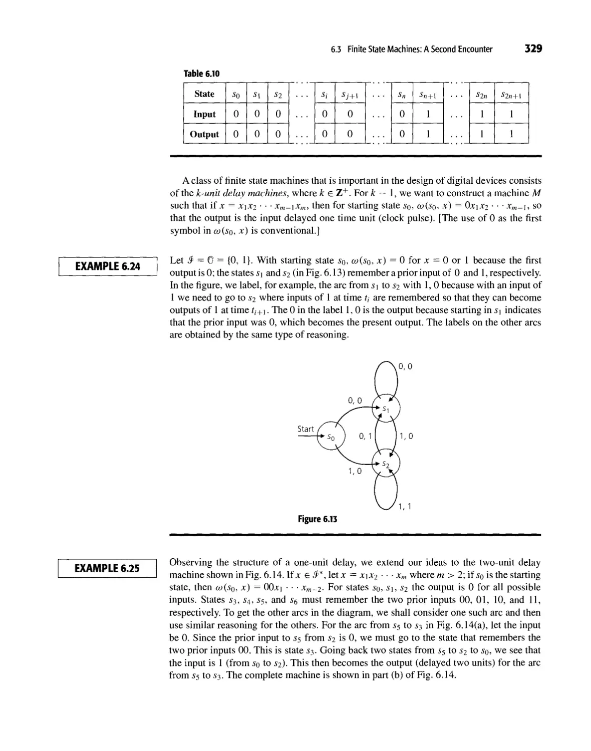
6.3 Finite State Machines: A Second Encounter 326
6.4 Summary and Historical Review 332
7 Relations: The Second Time Around 337
7.1 Relations Revisited: Proper ies of Relations 337
7.2 Computer Recognition: Zero- One Matrices and Directed Graphs 344
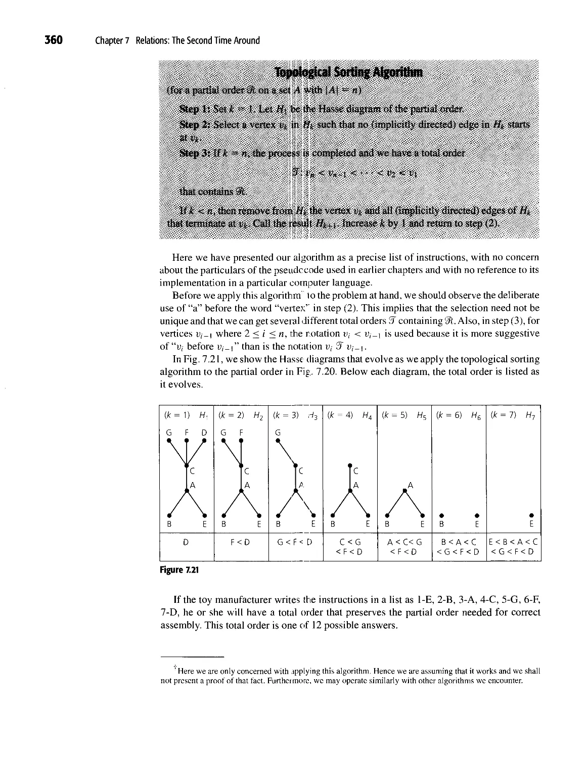
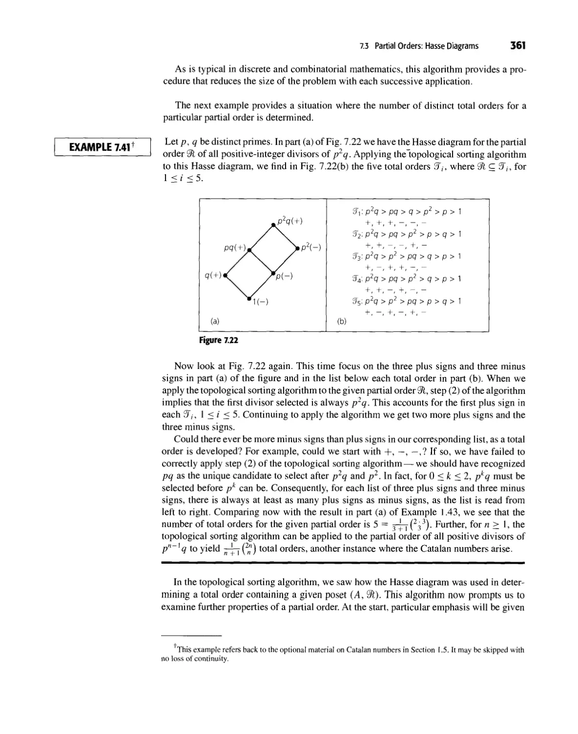
7.3 Partial Orders: Hasse Diagrams 356
7.4 Equivalence Relations and Partitions 366
7.5 Finite State Machines: The Minimization Process 371
7.6 Summary and Historical Review 376
PART 2
Further Topics in Enumeration 383
8 The Principle of Inclusion and Exclusion 385
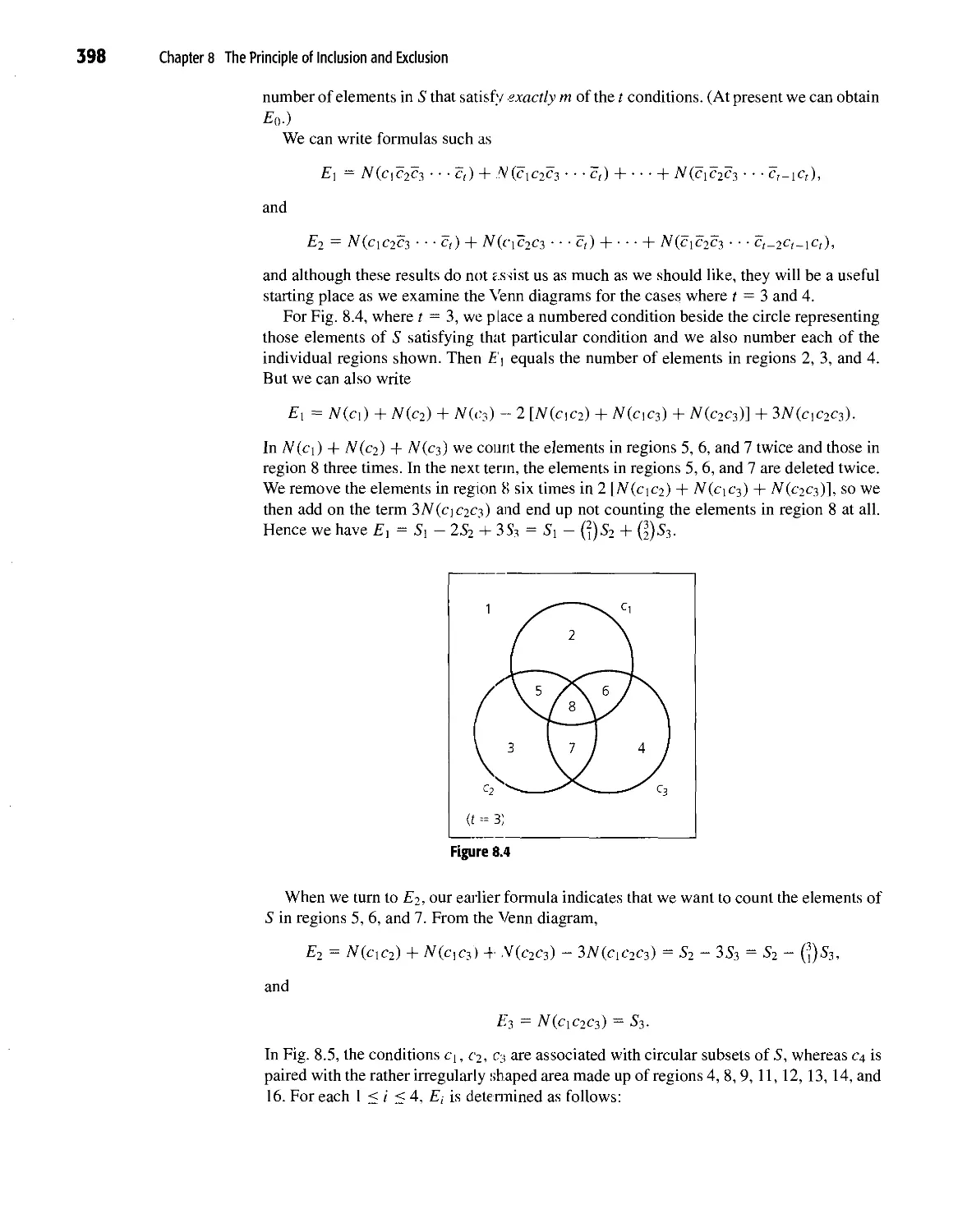
8.1 The Principle of Inclusion aid Exclusion 385
8.2 Generalizations of the Principle 397
8.3 Derangements: Nothing Is in Its Right Place 402
8.4 Rook Polynomials 404
8.5 Arrangements with Forbidden Positions 406
8.6 Summary and Historical Review 411

Contents XVii
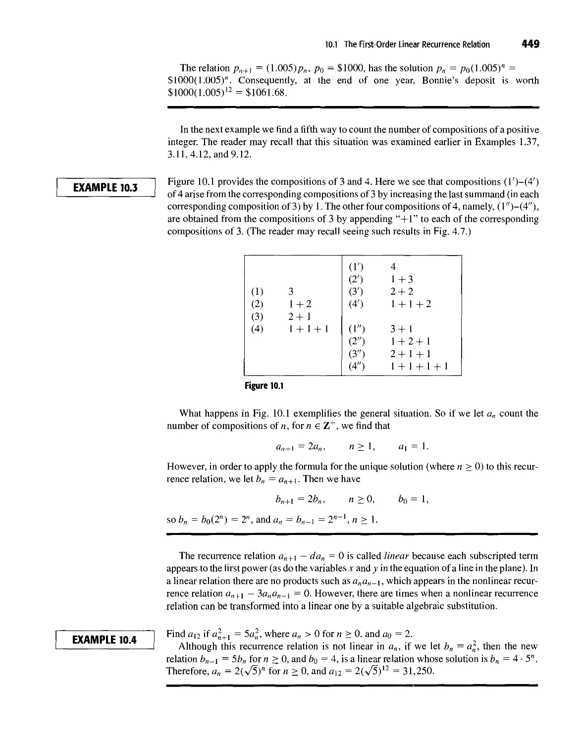
9
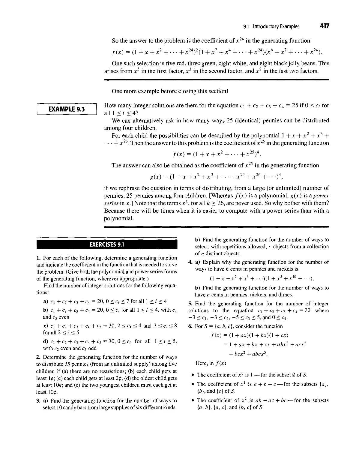
9.1
9.2
9.3
9.4
9.5
9.6
10
10.1
10.2
10.3
10.4
10.5
10.6
10.6
PART 3
Graph Theory and Applications 511
11 An Introduction to Graph Theory 513
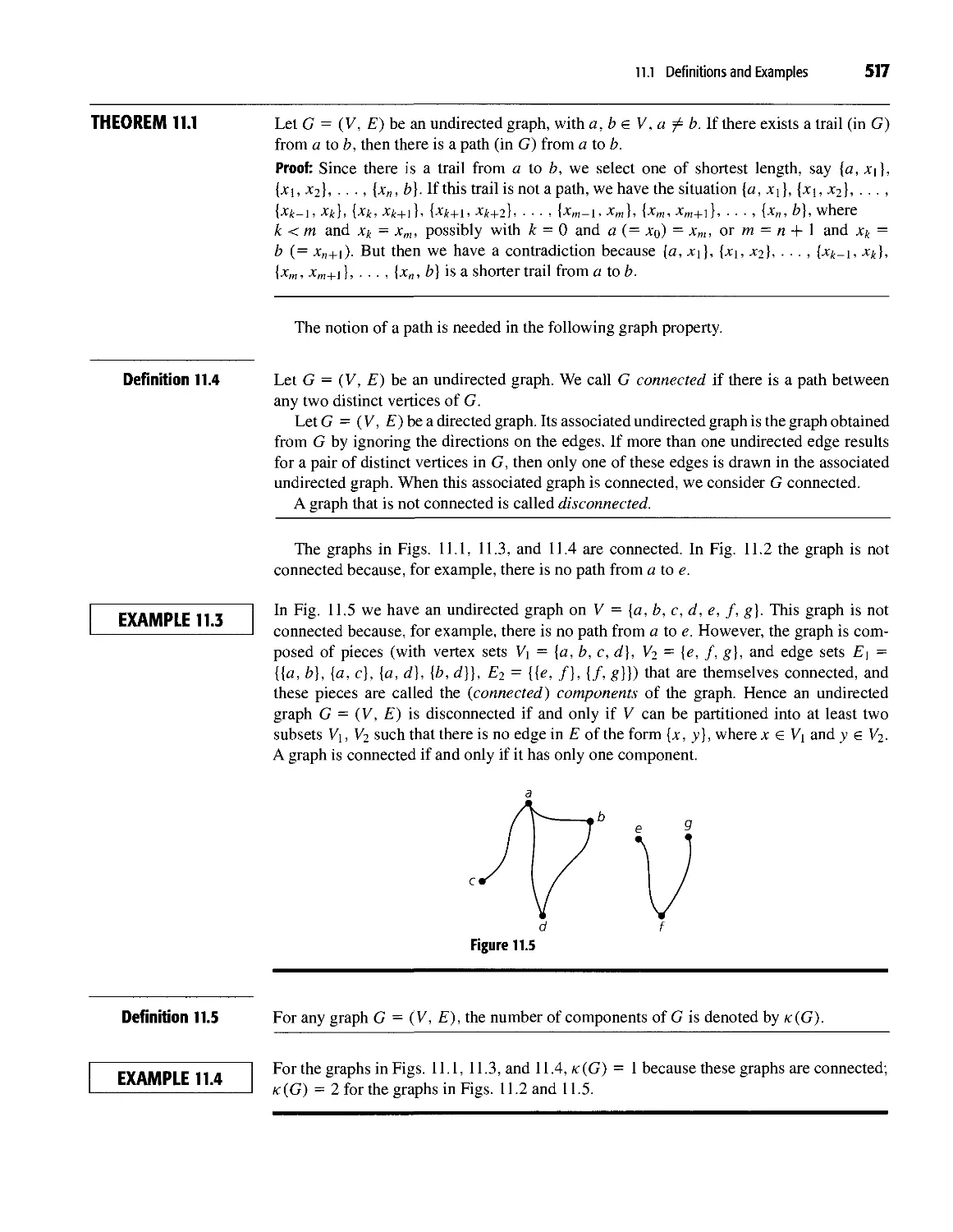
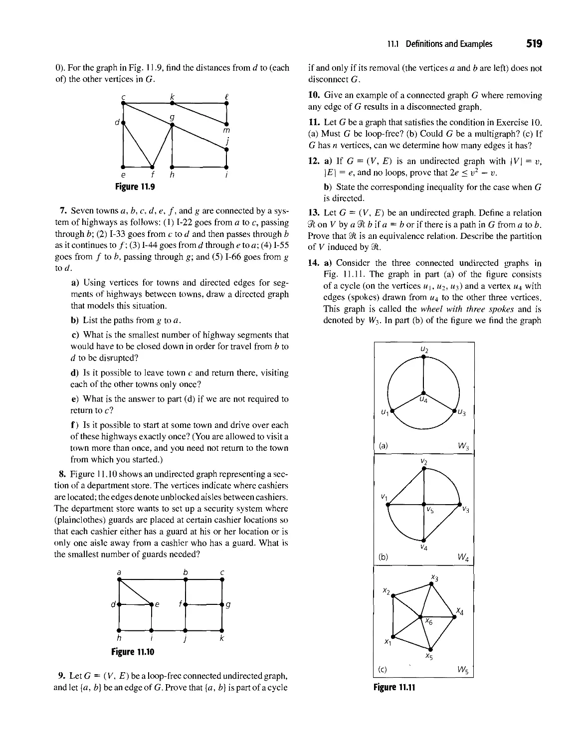
11.1 Definitions and Examples 513
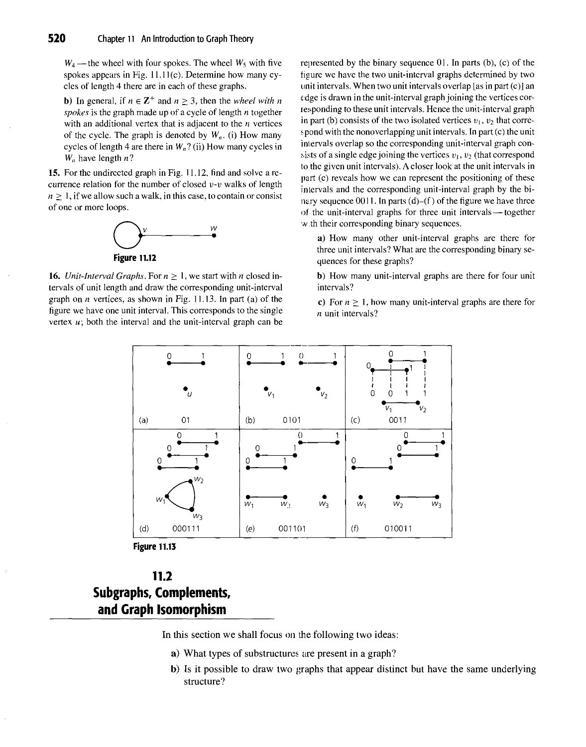
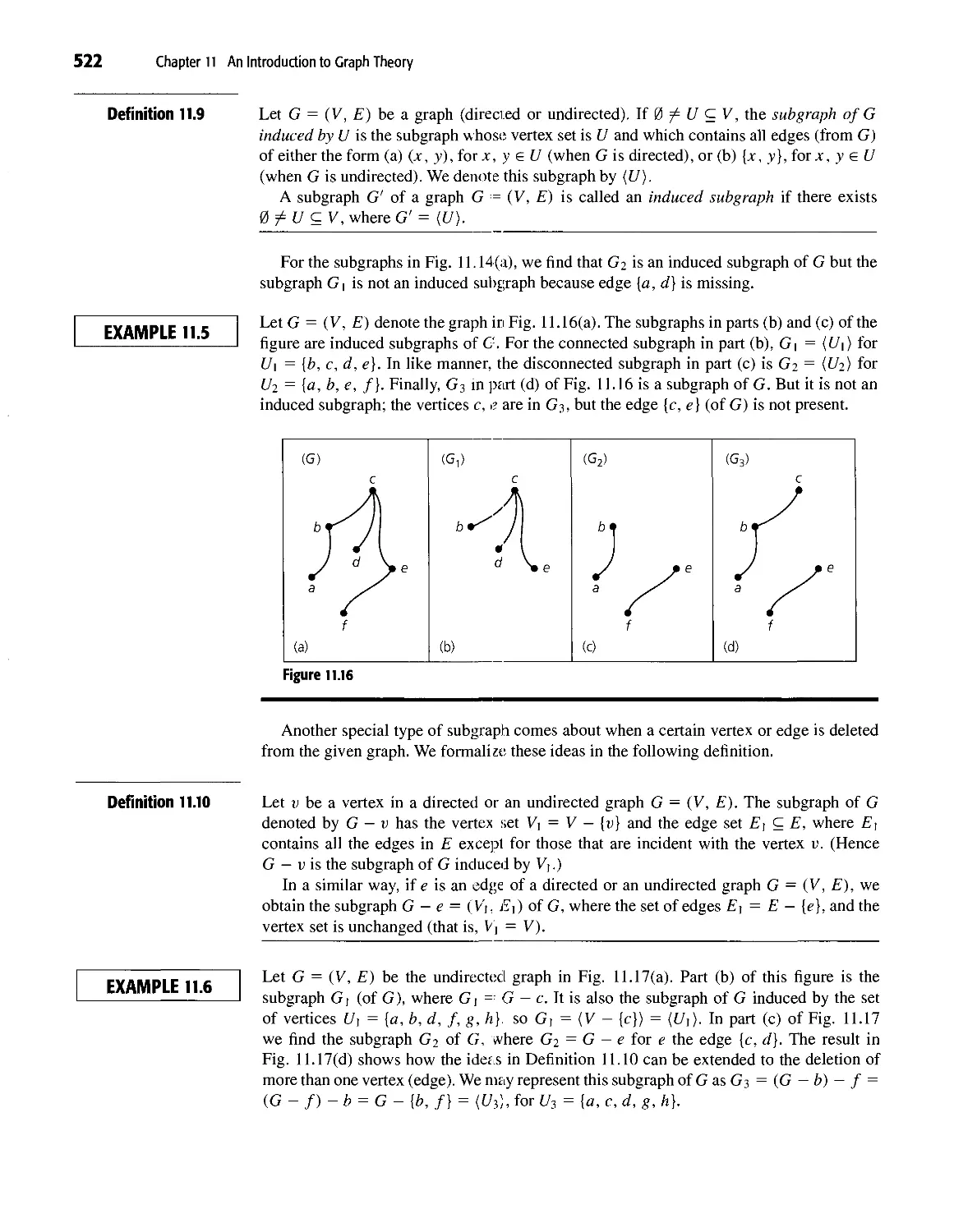
11.2 Subgraphs, Complements, and Graph Isomorphism 520
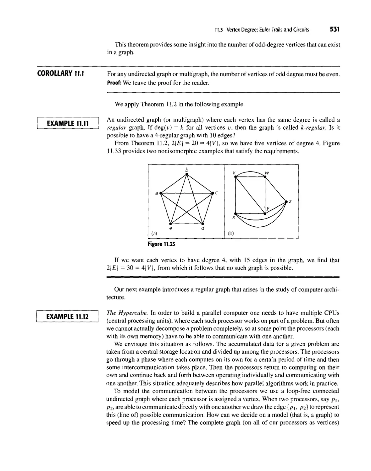
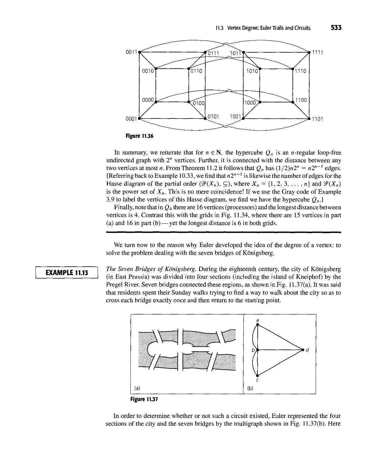
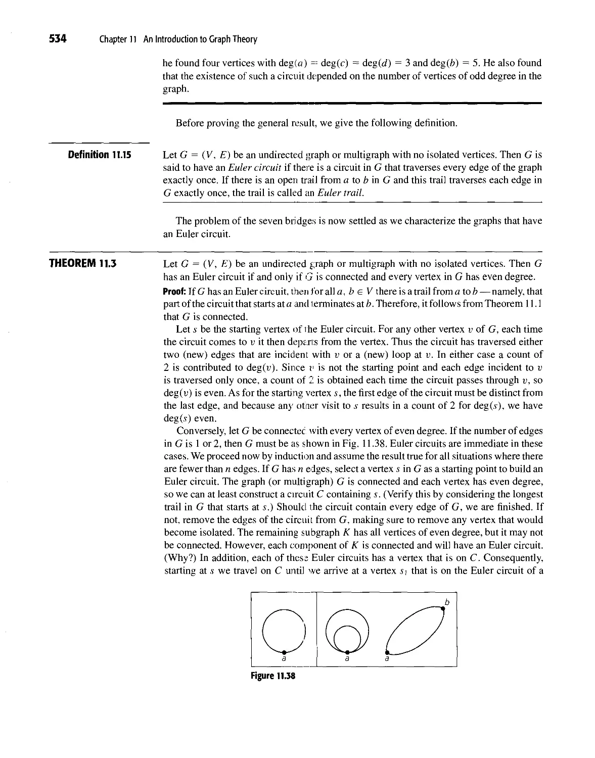
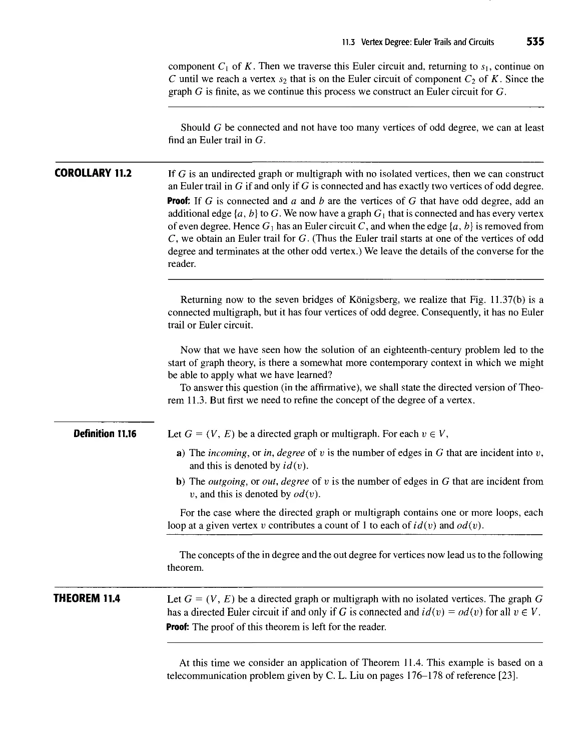
11.3 Vertex Degree: Euler Trails and Circuits 530
11.4 Planar Graphs 540
11.5 Hamilton Paths and Cycles 556
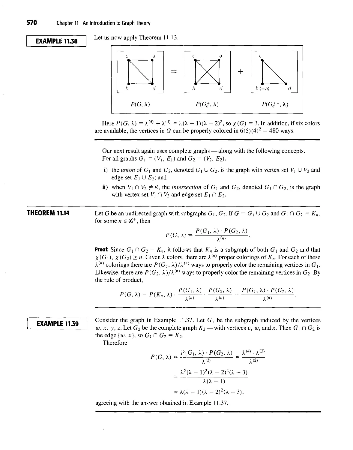
11.6 Graph Coloring and Chromatic Polynomials 564
11.7 Summary and Historical Review 573
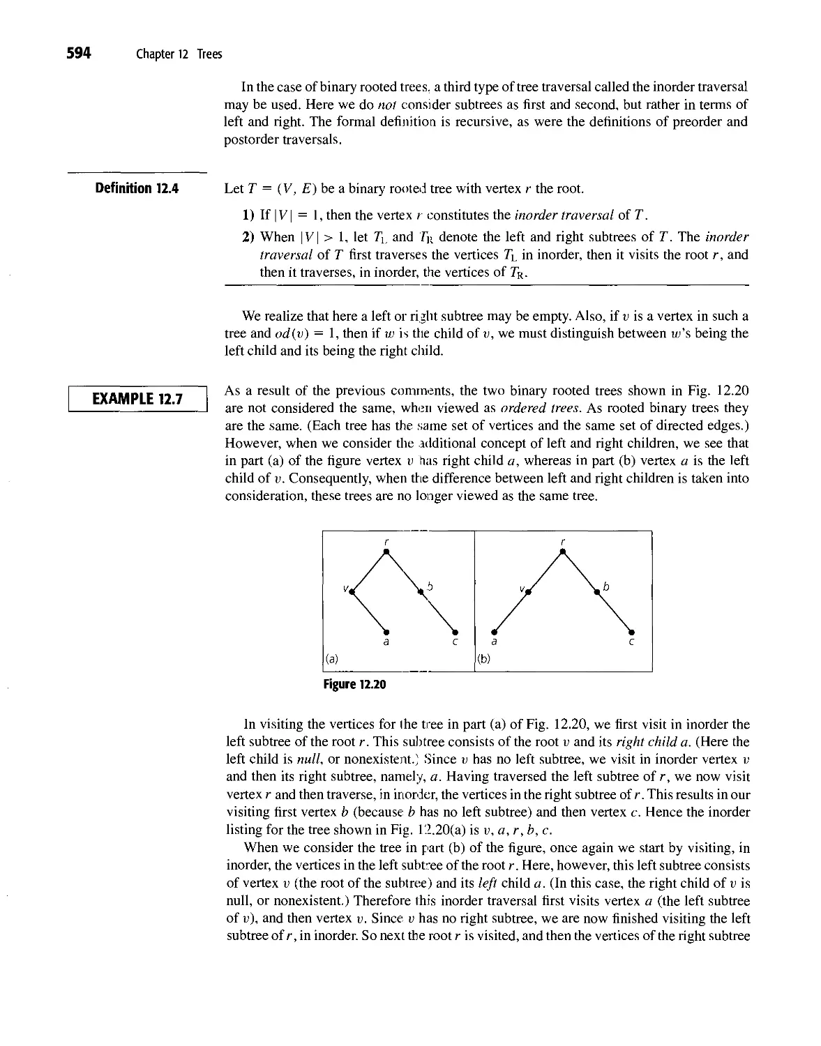
12 Trees 581
12.1 Definitions, Properties, and Examples 581
12.2 Rooted Trees 587
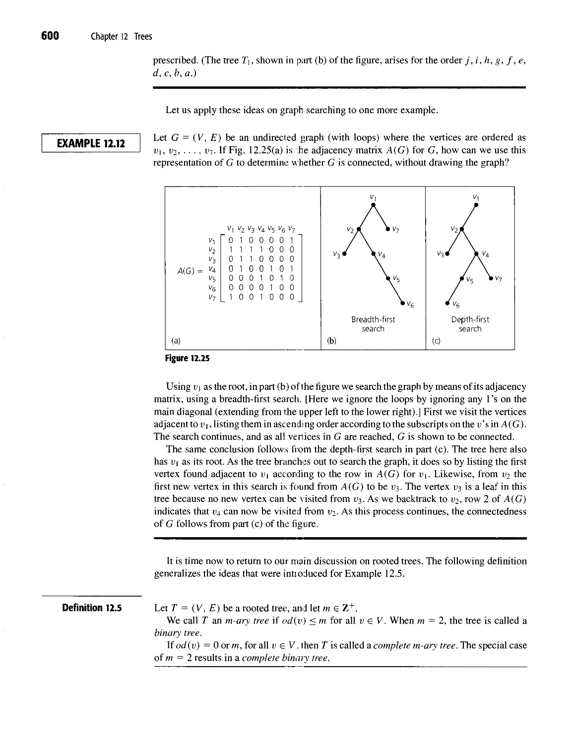
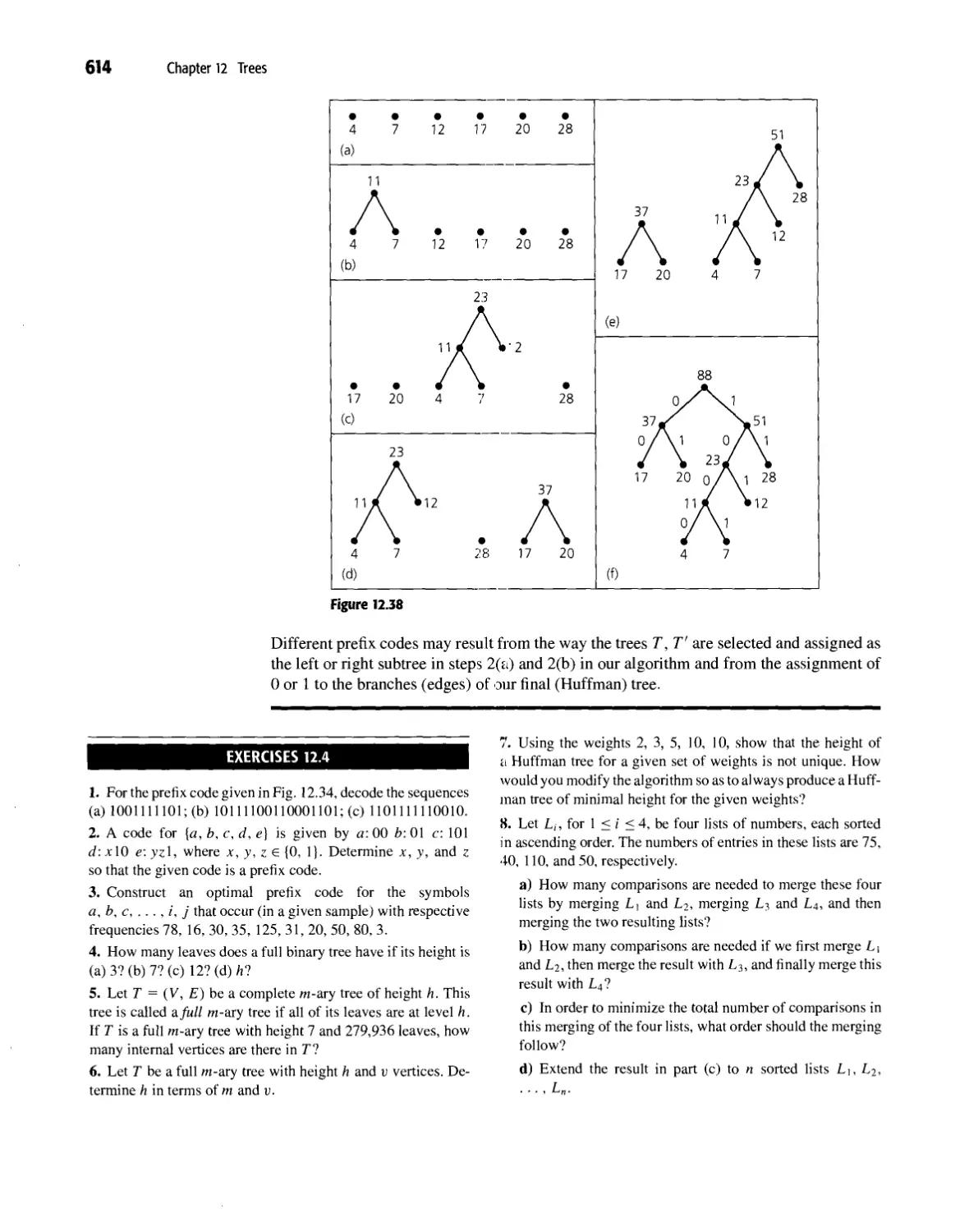
12.3 Trees and Sorting 605
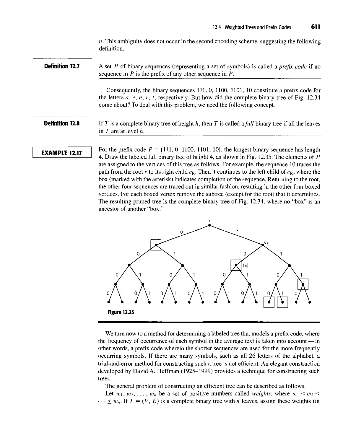
12.4 Weighted Trees and Prefix Codes 609
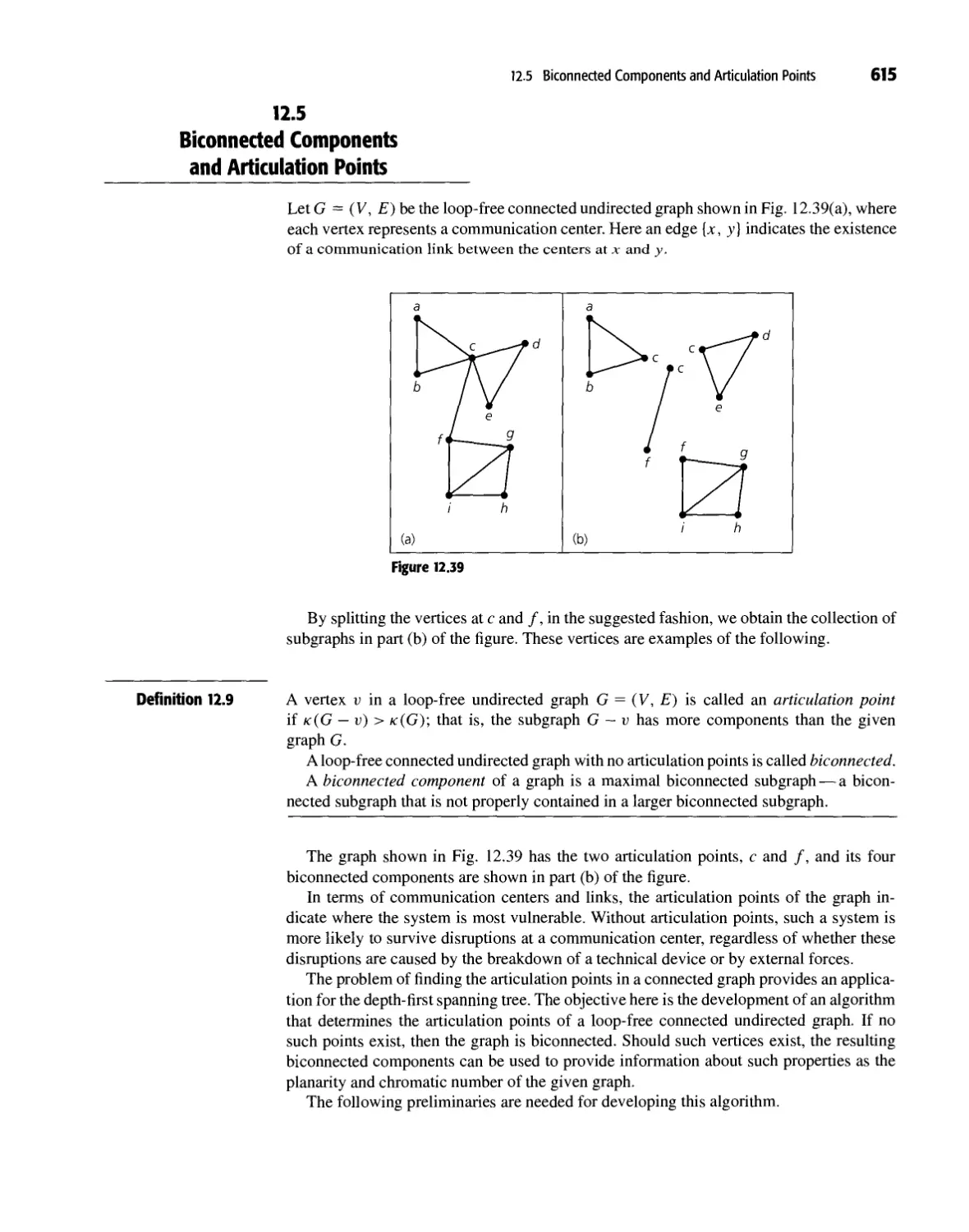
12.5 Biconnected Components and Articulation Points 615
12.6 Summary and Historical Review 622
13 Optimization and Matching 631
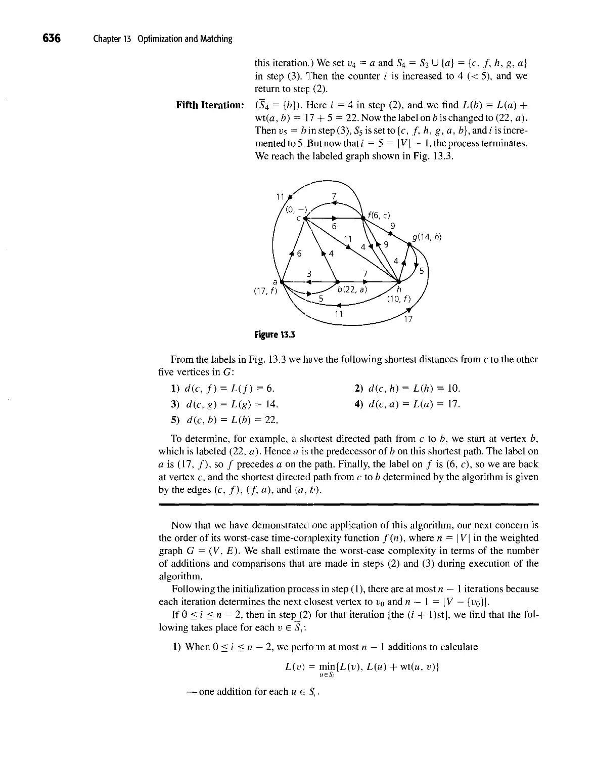
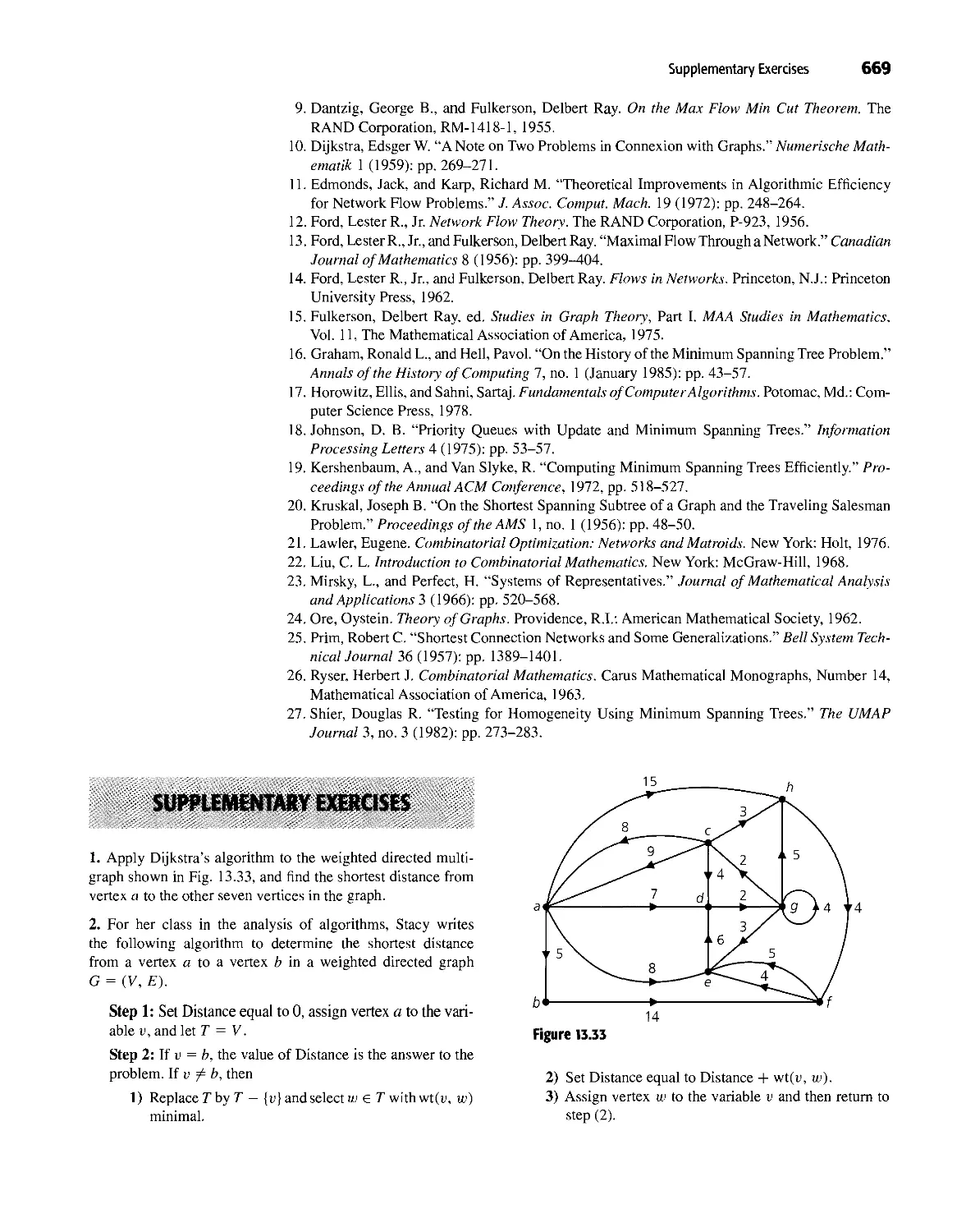
13.1 Dijkstra's Shortest-Path Algorithm 631
13.2 Minimal Spanning Trees: The Algorithms of Kruskal and Prim 638
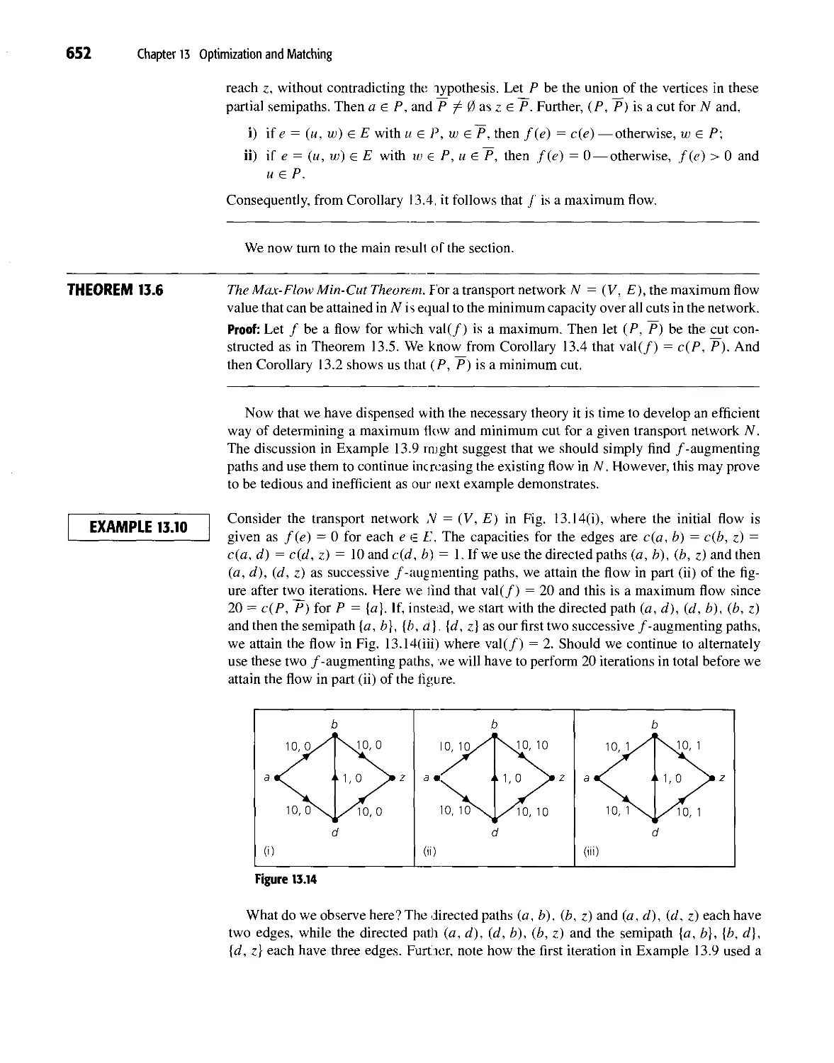
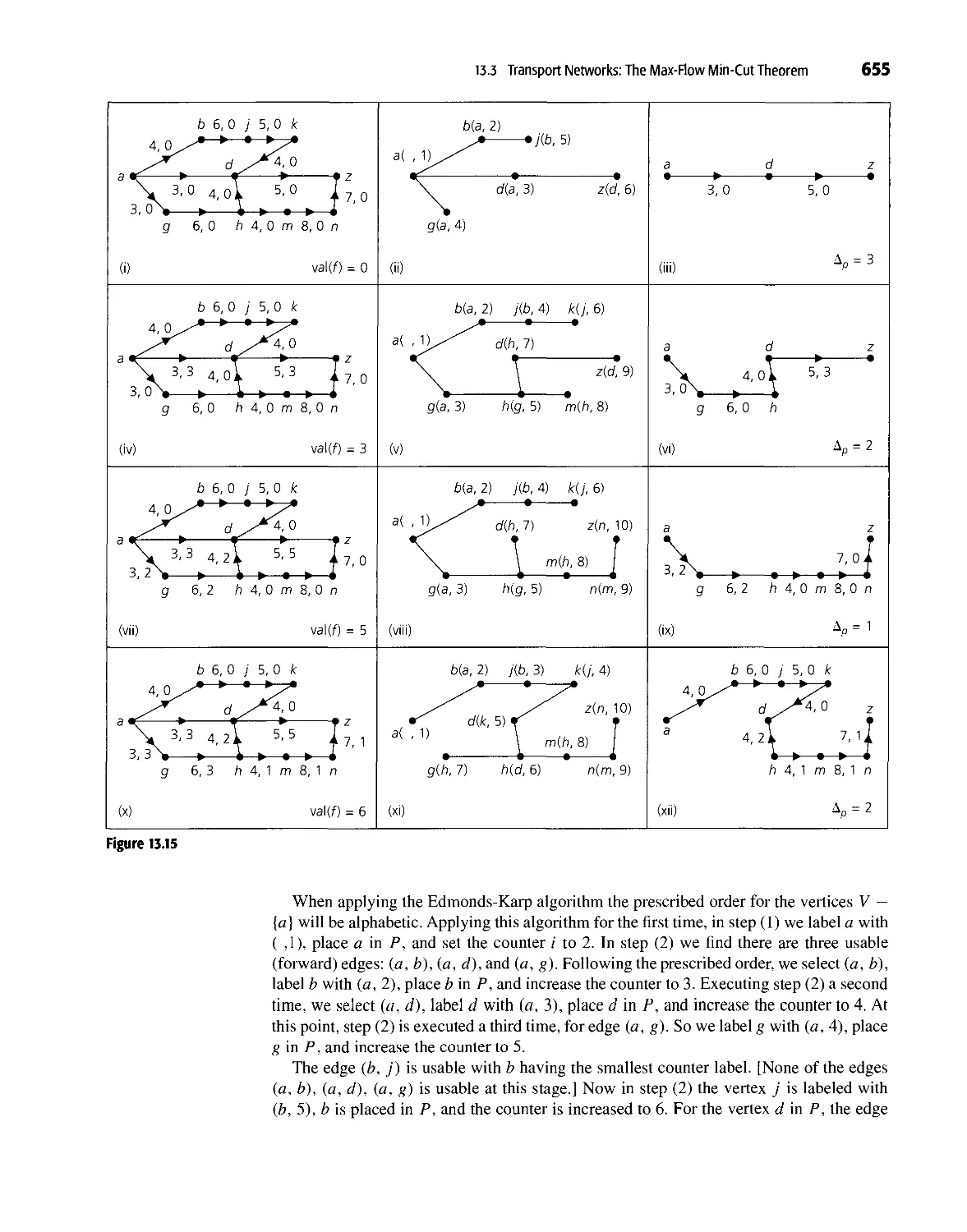
13.3 Transport Networks: The Max-Flow Min-Cut Theorem 644
13.4 Matching Theory 659
13.5 Summary and Historical Review 667
Generating Functions 415
Introductory Examples 415
Definition and Examples: Calculational Techniques 418
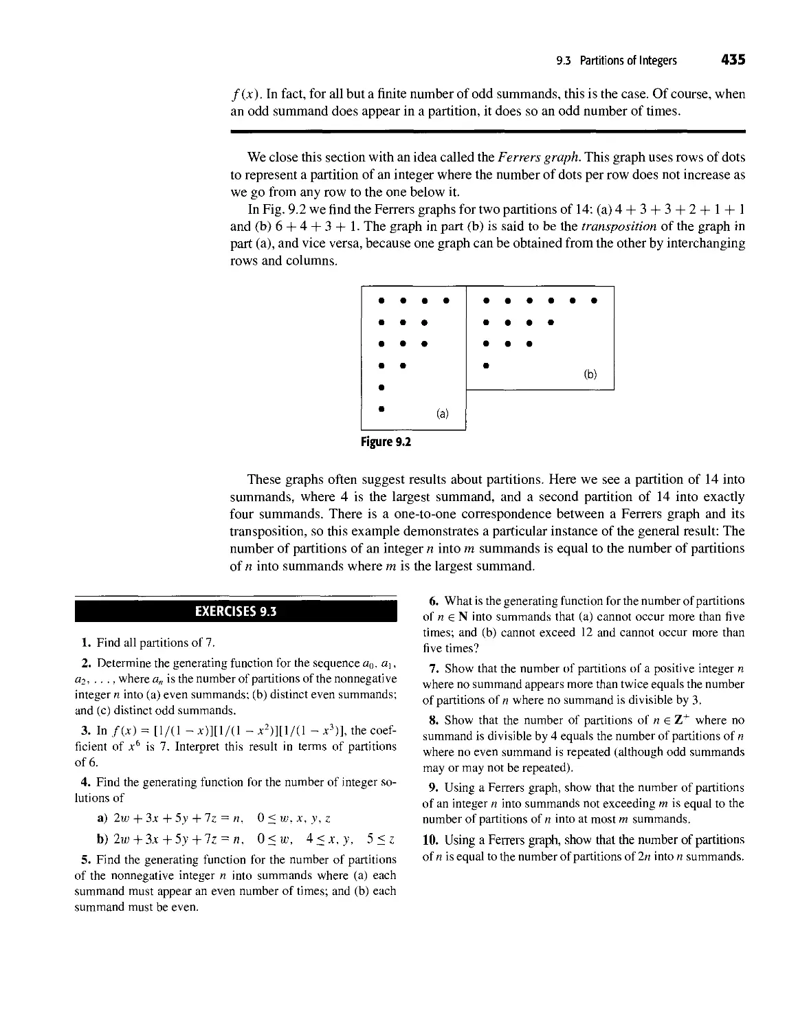
Partitions of Integers 432
The Exponential Generating Function 436
The Summation Operator 440
Summary and Historical Review 442
Recurrence Relations 447
The First-Order Linear Recurrence Relation 447
The Second-Order Linear Homogeneous Recurrence Relation with Constant
Coefficients 456
The Nonhomogeneous Recurrence Relation 470
The Method of Generating Functions 482
A Special Kind of Nonlinear Recurrence Relation (Optional) 487
Divide-and-Conquer Algorithms (Optional) 496
Summary and Historical Review 505

XViil Contents
PART 4
Modern Applied Algebra 671
14 Rings and Modular Arithmetic 673
14.1 The Ring Structure: Definition and Examples 673
14.2 Ring Properties and Substructures 679
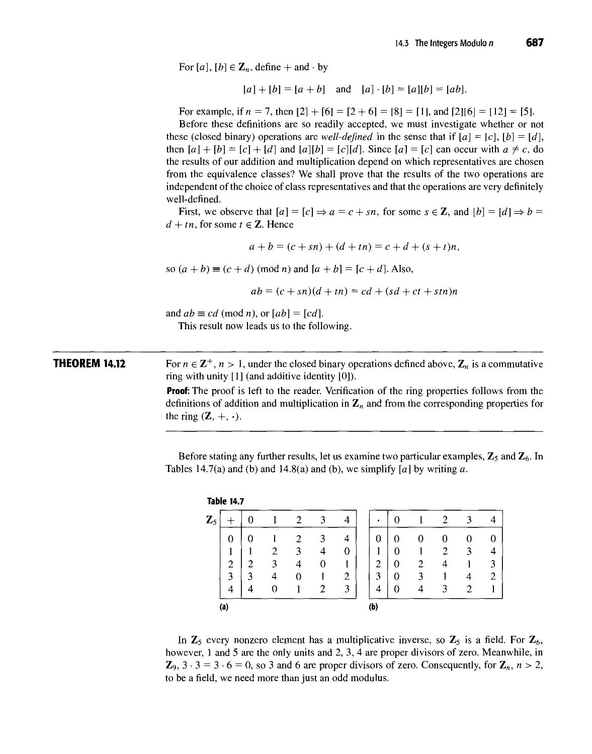
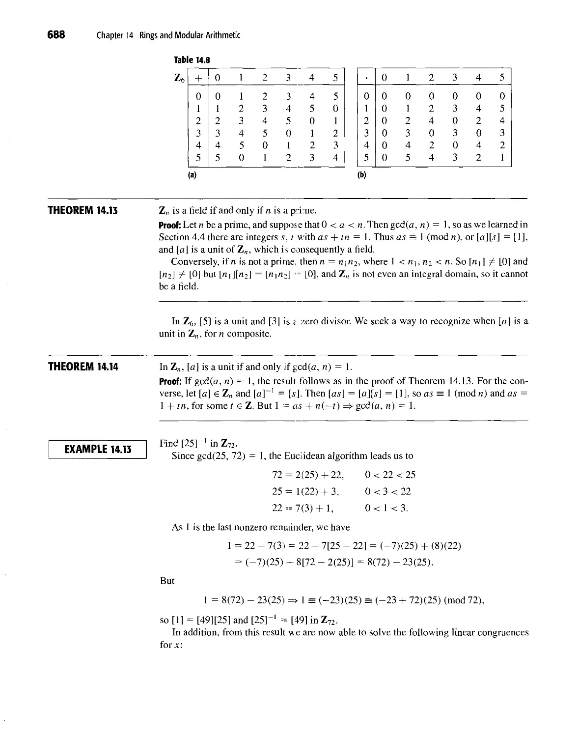
14.3 The Integers Modulo n 686
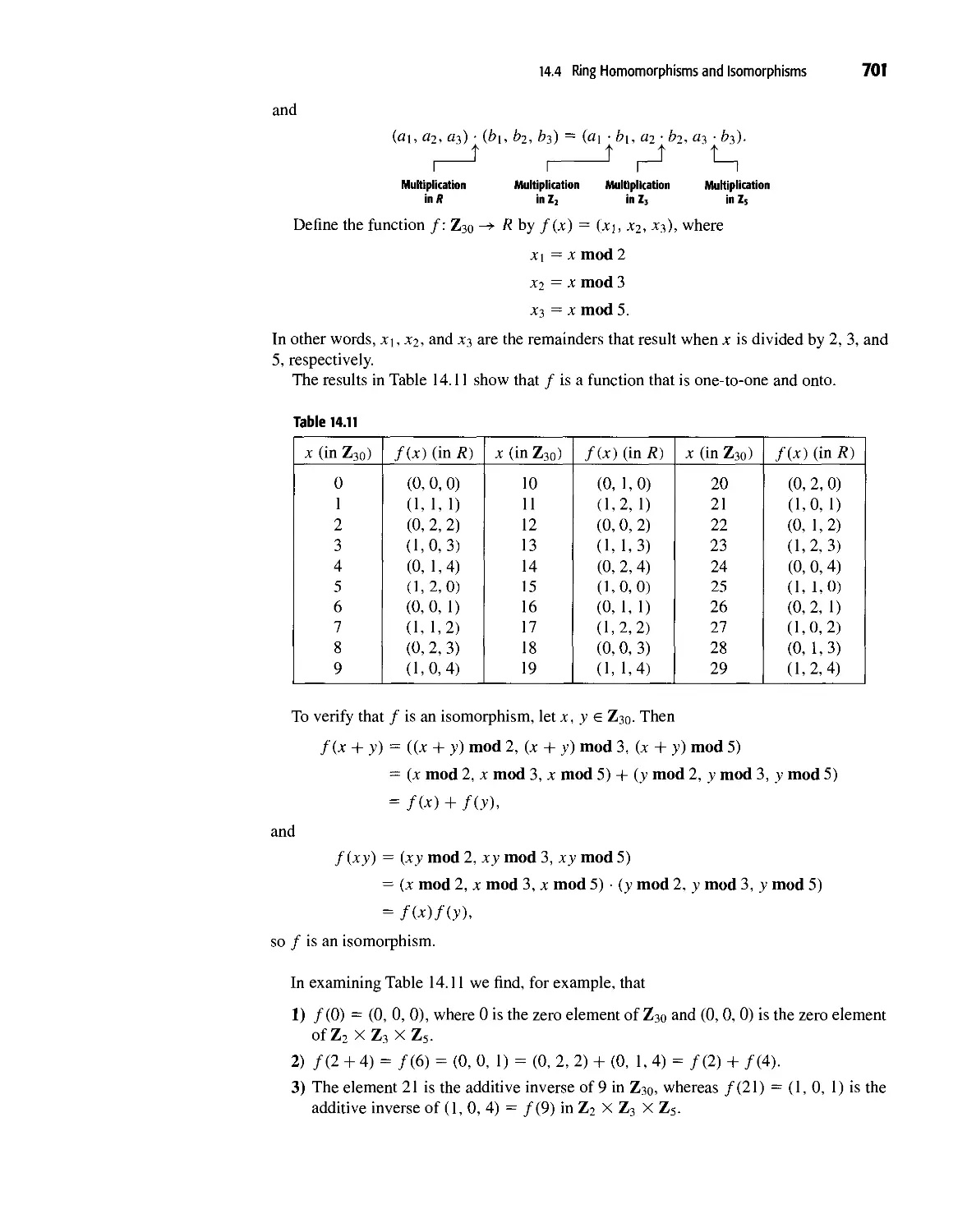
14.4 Ring Homomorphisms and Isomorphisms 697
14.5 Summary and Historical Review 705
15 Boolean Algebra and Switching Functions 711
15.1 Switching Functions: Disjunctive and Conjunctive Normal Forms 711
15.2 Gating Networks: Minimal Sums of Products: Karnaugh Maps 719
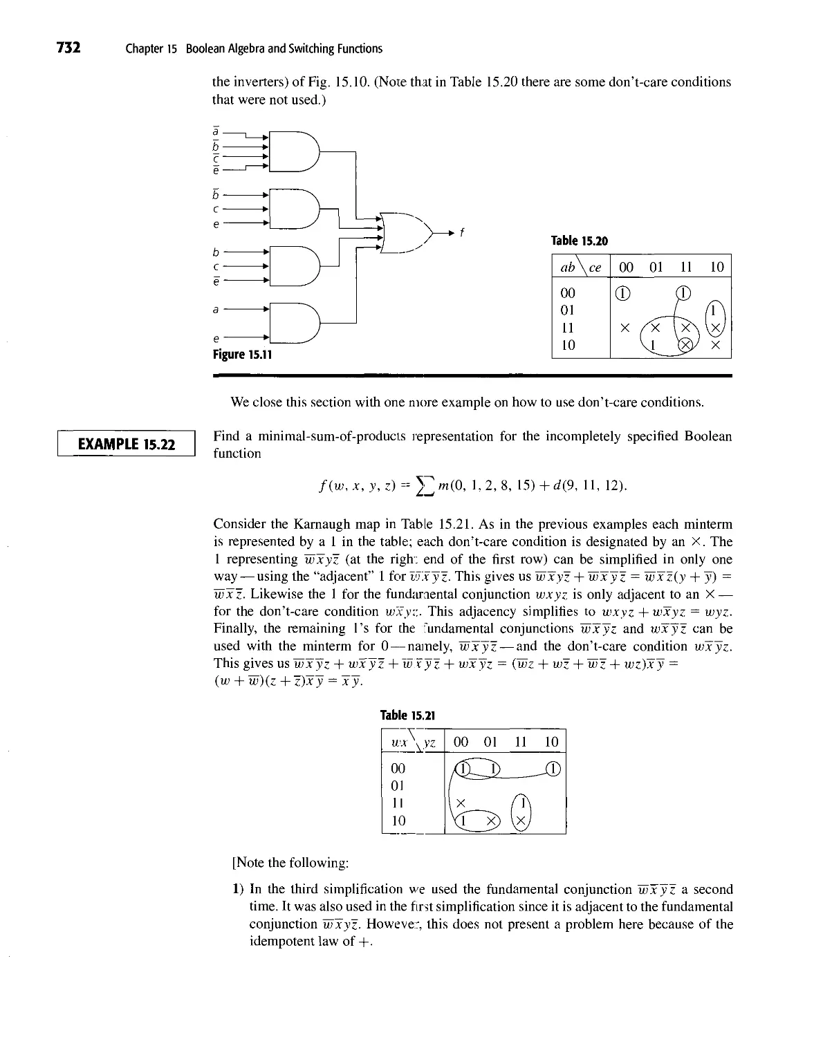
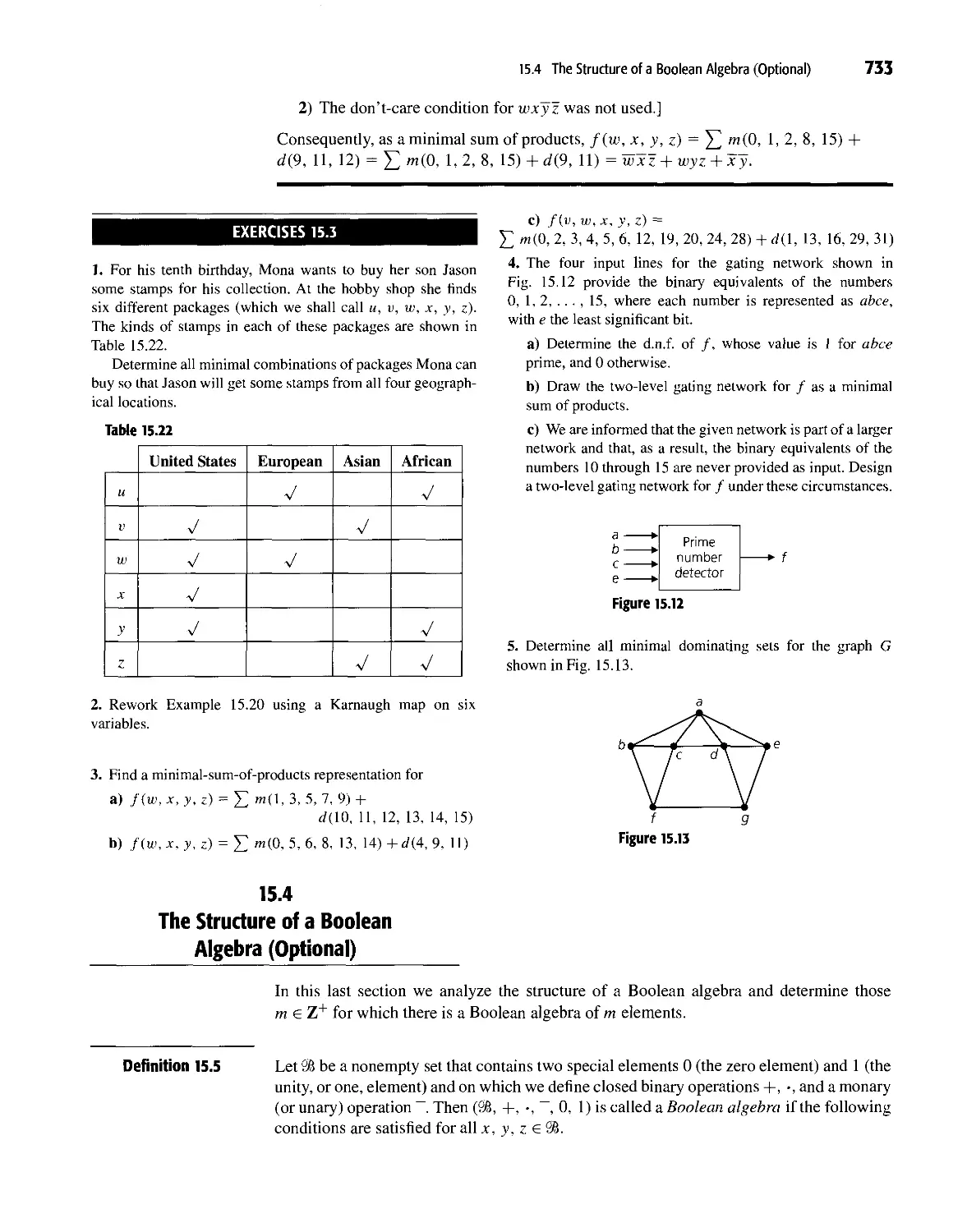
15.3 Further Applications: Don't-Care Conditions 729
15.4 The Structure of a Boolean Algebra (Optional) 733
15.5 Summary and Historical Review 742
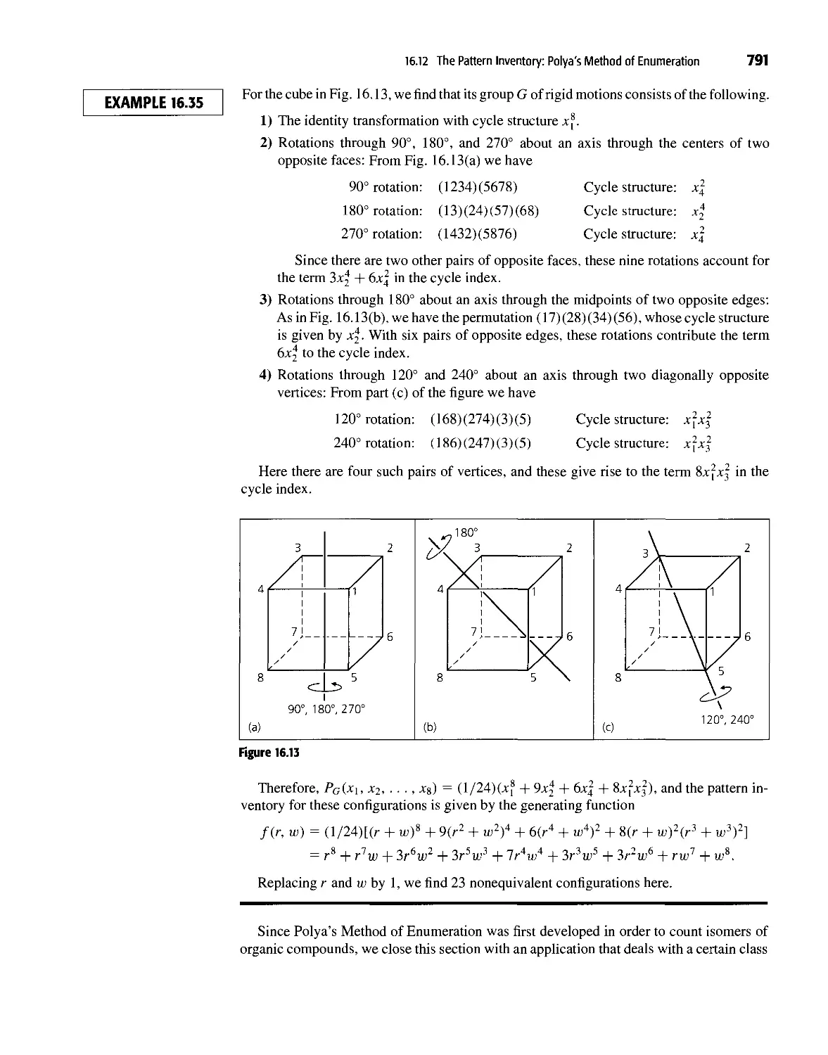
16 Groups, Coding Theory, and Polya's Method of Enumeration 745
16.1 Definition, Examples, and Elementary Properties 745
16.2 Homomorphisms, Isomorphisms, and Cyclic Groups 752
16.3 Cosets and Lagrange's Theorem 757
16.4 The RSA Cryptosystem (Optional) 759
16.5 Elements of Coding Theory 761
16.6 The Hamming Metric 766
16.7 The Parity-Check and Generator Matrices 769
16.8 Group Codes: Decoding with Coset Leaders 773
16.9 Hamming Matrices 777
16.10 Counting and Equivalence: Bumside's Theorem 779
16.11 The Cycle Index 785
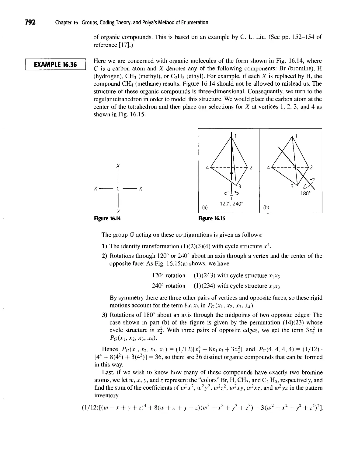
16.12 The Pattern Inventory: Polya's Method of Enumeration 789
16.13 Summary and Historical Review 794
17 Finite Fields and Combinatorial Designs 799
17.1 Polynomial Rings 799
17.2 Irreducible Polynomials: Finite Fields 806
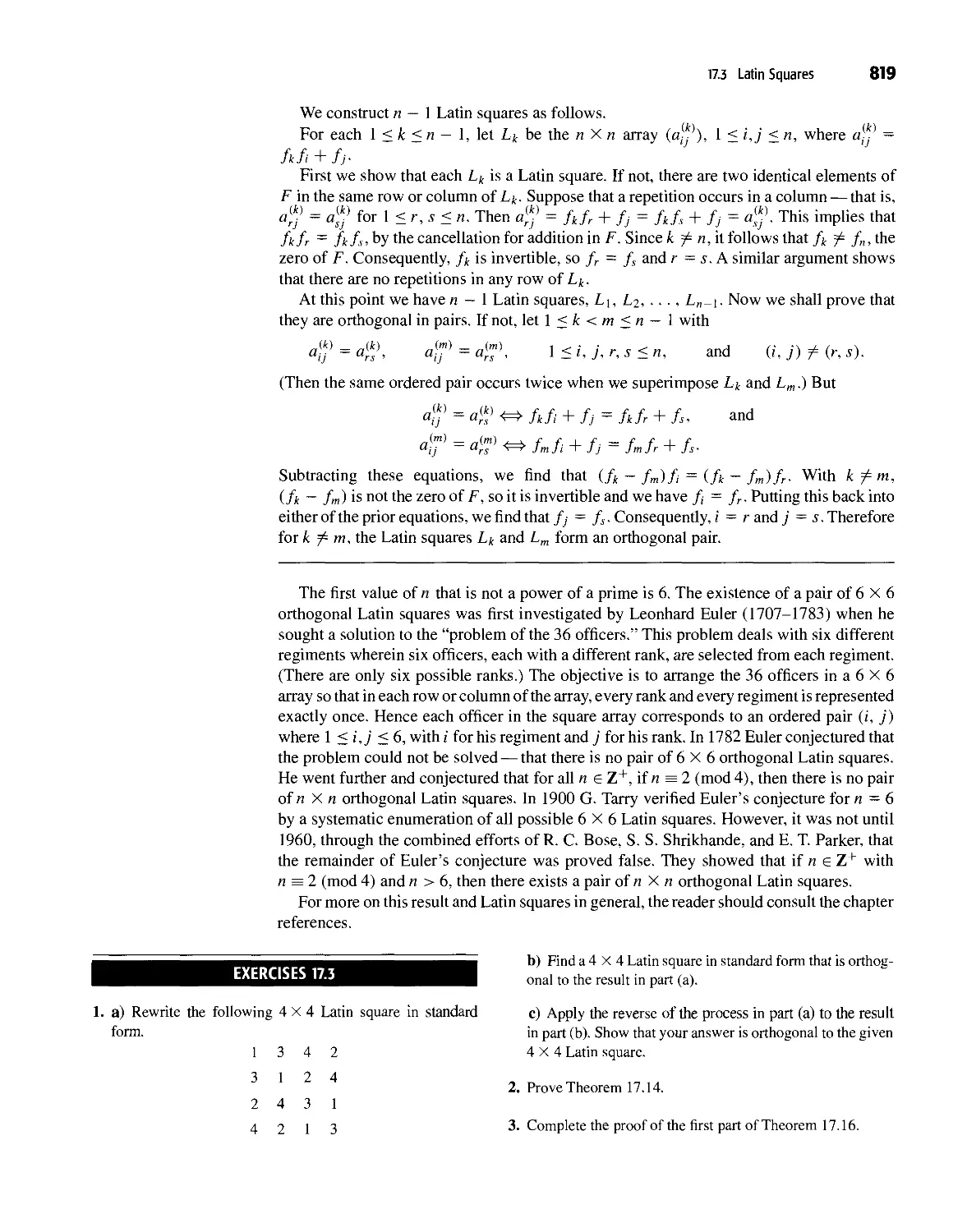
17.3 Latin Squares 815
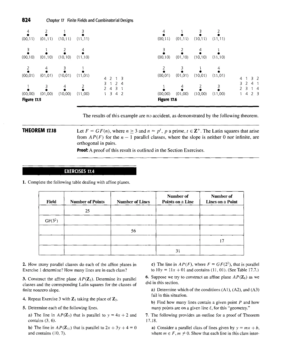
17.4 Finite Geometries and Affine Planes 820
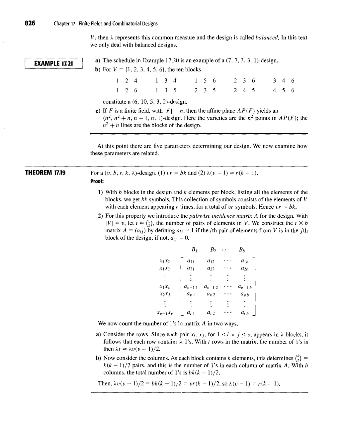
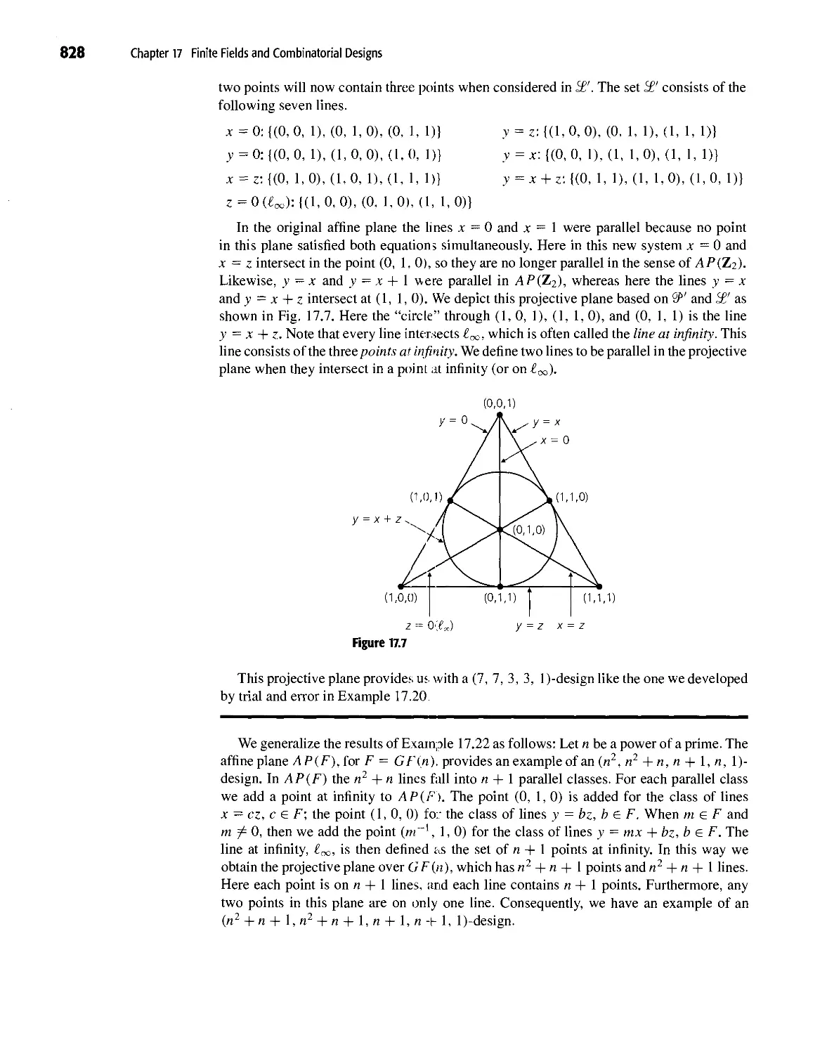
17.5 Block Designs and Projective Planes 825
17.6 Summary and Historical Review 830
Appendix 1 Exponential and Logarithmic Functions A-l
Appendix 2 Matrices, Matrix Operations, and Determinants A-ll
Appendix 3 Countable and Uncountable Sets A-23

Contents xix
Solutions S-1
Index 1-1

PART
1
FUNDAMENTALS
OF DISCRETE
MATHEMATICS

1
Fundamental
Principles of
Counting
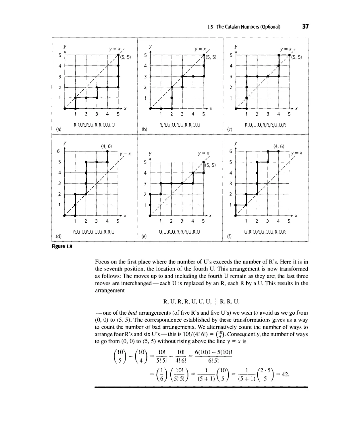
Enumeration, or counting, may strike one as an obvious process that a student learns
when first studying arithmetic. But then, it seems, very little attention is paid to further
development in counting as the student turns to "more difficult" areas in mathematics, such
as algebra, geometry, trigonometry, and calculus. Consequently, this first chapter should
provide some warning about the seriousness and difficulty of "mere" counting.
Enumeration does not end with arithmetic. It also has applications in such areas as coding
theory, probability and statistics, and in the analysis of algorithms. Later chapters will offer
some specific examples of these applications.
As we enter this fascinating field of mathematics, we shall come upon many problems that
are very simple to state but somewhat "sticky" to solve. Thus, be sure to learn and understand
the basic formulas — but do not rely on them too heavily. For without an analysis of each
problem, a mere knowledge of formulas is next to useless. Instead, welcome the challenge
to solve unusual problems or those that are different from problems you have encountered
in the past. Seek solutions based on your own scrutiny, regardless of whether it reproduces
what the author provides. There are often several ways to solve a given problem.
1.1
The Rules of Sum and Product
Our study of discrete and combinatorial mathematics begins with two basic principles of
counting: the rules of sum and product. The statements and initial applications of these
rules appear quite simple. In analyzing more complicated problems, one is often able to
break down such problems into parts that can be solved using these basic principles. We
want to develop the ability to "decompose" such problems and piece together our partial
solutions in order to arrive at the final answer. A good way to do this is to analyze and solve
many diverse enumeration problems, taking note of the principles being used. This is the
approach we shall follow here.
Our first principle of counting can be stated as follows:
The Rule Of Sum: If a first tusk can be performed in m ways, while a second task can
be performed in w ways, and the two tasks cannot be performed simultaneously, then
performing either task can be accomplished in any one of m + n ways.
3

4 Chapter 1 Fundamental Principles of Counting
Note that when we say that a partic ular occurrence, such as a first task, can come about in m
ways, these m ways are assumed to be distinct, unless a statement is made to the contrary.
This will be true throughout the entire text.
EXAMPLE 1.1
A college library has 40 textbooks on sociology and 50 textbooks dealing with anthropology.
By the rule of sum, a student at this college can select among 40 + 50 = 90 textbooks in
order to learn more about one or the other of these two subjects.
EXAMPLE 1.2
The rule can be extended beyond two tasks as long as no pair of tasks can occur
simultaneously. For instance, a computer science instructor who has, say, seven different introductory
books each on C++, Java, and Perl can recommend any one of these 21 books to a student
who is interested in learning a first programming language.
EXAMPLE 1.3
The computer science instructor of Example 1.2 has two colleagues. One of these
colleagues has three textbooks on the analysis of algorithms, and the other has five such
textbooks. If n denotes the maximum number of different books on this topic that this
instructor can borrow from them, Ihen 5 < n < 8, for here both colleagues may own copies
of the same textbook(s).
The following example introduces our second principle of counting.
EXAMPLE 1.4
In trying to reach a decision on plant expansion, an administrator assigns 12 of her employees
to two committees. Committee A consists of five members and is to investigate possible
favorable results from such an expansion. The other seven employees, committee B, will
scrutinize possible unfavorable repercussions. Should the administrator decide to speak to
just one committee member befors making her decision, then by the rule of sum there are
12 employees she can call upon fcr input. However, to be a bit more unbiased, she decides
to speak with a member of committee A on Monday, and then with a member of committee
B on Tuesday, before reaching a decision. Using the following principle, we find that she
can select two such employees to speak with in 5 X 7 = 35 ways.
The Rule of Product: if a procedure can be broken down into first and second stages,
and if there are m possible outcomes for the first stage and if, for each of these outcomes,
there are n possible outcomes for tlte second stage, then the total procedure can be carried
out. in the designated order, in mn ways.
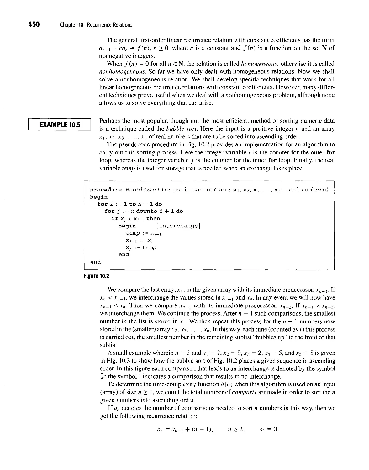
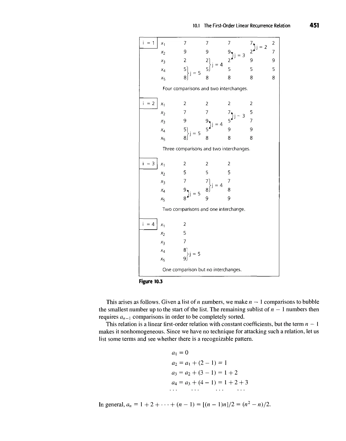
EXAMPLE 1.5
The drama club of Central University is holding tryouts for a spring play. With six men and
eight women auditioning for the leading male and female roles, by the rule of product the
director can cast his leading couple in 6 X 8 = 48 ways.
EXAMPLE 1.6
Here various extensions of the rule are illustrated by considering the manufacture of license
plates consisting of two letters followed by four digits.

1.1 The Rules of Sum and Product 5
a) If no letter or digit can be repeated, there are 26X25X10X9X8X7 =
3,276,000 different possible plates.
b) With repetitions of letters and digits allowed, 26X26X10X10X10X10 =
6,760,000 different license plates are possible.
c) If repetitions are allowed, as in part (b), how many of the plates have only vowels (A,
E, I, O, U) and even digits? (0 is an even integer.)
EXAMPLE 1.7
In order to store data, a computer's main memory contains a large collection of circuits, each
of which is capable of storing a bit — that is, one of the binary digits 0 or 1. These storage
circuits are arranged in units called (memory) cells. To identify the cells in a computer's
main memory, each is assigned a unique name called its address. For some computers,
such as embedded microcontrollers (as found in the ignition system for an automobile), an
address is represented by an ordered list of eight bits, collectively referred to as a byte. Using
the rule of product, there are 2X2X2X2X2X2X2X2 = 28 = 256 such bytes. So
we have 256 addresses that may be used for cells where certain information may be stored.
A kitchen appliance, such as a microwave oven, incorporates an embedded
microcontroller. These "small computers" (such as the PICmicro microcontroller) contain thousands
of memory cells and use two-byte addresses to identify these cells in their main memory.
Such addresses are made up of two consecutive bytes, or 16 consecutive bits. Thus there
are 256 X 256 = 28 X 28 = 216 = 65,536 available addresses that could be used to
identify cells in the main memory. Other computers use addressing systems of four bytes. This
32-bit architecture is presently used in the Pentiumt processor, where there are as many
as 28 X 28 X 28 X 28 = 232 = 4,294,967,296 addresses for use in identifying the cells in
main memory. When a programmer deals with the UltraSPARC* or Itanium8 processors, he
or she considers memory cells with eight-byte addresses. Each of these addresses comprises
8 X 8 = 64 bits, and there are 264 = 18,446,744,073,709,551,616 possible addresses for
this architecture. (Of course, not all of these possibilities are actually used.)
EXAMPLE 1.8
At times it is necessary to combine several different counting principles in the solution of
one problem. Here we find that the rules of both sum and product are needed to attain the
answer.
At the AWL corporation Mrs. Foster operates the Quick Snack Coffee Shop. The menu
at her shop is limited: six kinds of muffins, eight kinds of sandwiches, and five beverages
(hot coffee, hot tea, iced tea, cola, and orange juice). Ms. Dodd, an editor at AWL, sends
her assistant Carl to the shop to get her lunch — either a muffin and a hot beverage or a
sandwich and a cold beverage.
By the rule of product, there are 6 X 2 = 12 ways in which Carl can purchase a muffin and
hot beverage. A second application of this rule shows that there are 8 X 3 = 24 possibilities
for a sandwich and cold beverage. So by the rule of sum, there are 12 + 24 = 36 ways in
which Carl can purchase Ms. Dodd's lunch.
Pentium (R) is a registered trademark of the Intel Corporation.
The UltraSPARC processor is manufactured by Sun (R) Microsystems, Inc.
8 Itanium (TM) is a trademark of the Intel Corporation.

6 Chapter 1 Fundamental Principles of Counting
1.2
Permutations
Continuing to examine applications of the rule of product, we turn now to counting linear
arrangements of objects. These arrangements are often called permutations when the objects
are distinct. We shall develop some systematic methods for dealing with linear arrangements,
starting with a typical example.
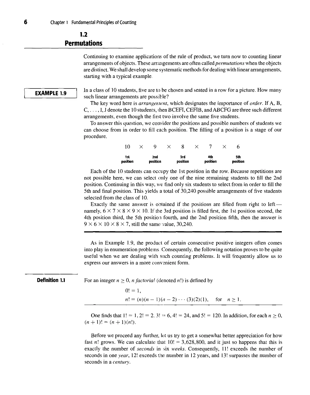
~ I In a class of 10 students, five are to be chosen and seated in a row for a picture. How many
I such linear arrangements are possible?
The key word here is arrangement, which designates the importance of order. If A, B,
C,..., I, J denote the 10 students, then BCEFI, CEFIB, and ABCFG are three such different
arrangements, even though the first two involve the same five students.
To answer this question, we consider the positions and possible numbers of students we
can choose from in order to fill each position. The filling of a position is a stage of our
procedure.
10 X 9X8X7X6
1st 2nd 3rd 4th 5th
position position position position position
Each of the 10 students can occupy the 1st position in the row. Because repetitions are
not possible here, we can select only one of the nine remaining students to fill the 2nd
position. Continuing in this way, we find only six students to select from in order to fill the
5th and final position. This yields a total of 30,240 possible arrangements of five students
selected from the class of 10.
Exactly the same answer is obtained if the positions are filled from right to left —
namely, 6 X 7 X 8 X 9 X 10. If the 3rd position is filled first, the 1st position second, the
4th position third, the 5th position fourth, and the 2nd position fifth, then the answer is
9X6X10X8X7, still the same value, 30,240.
As in Example 1.9, the product of certain consecutive positive integers often comes
into play in enumeration problems Consequently, the following notation proves to be quite
useful when we are dealing with such counting problems. It will frequently allow us to
express our answers in a more convenient form.
Definition 1.1 For an integer n > 0, n factorial (denoted «!) is defined by
0! = 1,
«!=(«)(«- l)(n- 2) ••• (3)(2)(1), for n>\.
One finds that 1! = 1, 2! = 2, 3! == 6, 4! = 24, and 5! = 120. In addition, for each n > 0,
(« + l)! = (« + l)(«!).
Before we proceed any further, let us try to get a somewhat better appreciation for how
fast «! grows. We can calculate that 10! = 3,628,800, and it just so happens that this is
exactly the number of seconds in six weeks. Consequently, 11! exceeds the number of
seconds in one year, 12! exceeds the number in 12 years, and 13! surpasses the number of
seconds in a century.

1.2 Permutations 7
If we make use of the factorial notation, the answer in Example 1.9 can be expressed in
the following more compact form:
10X9X8X7X6= 10X9X8X7X6X
5X4X3X2X1 _ 10!
5X4X3X2X1 ~ "IT'
Definition 1.2
Given a collection of n distinct objects, any (linear) arrangement of these objects is called
a permutation of the collection.
Starting with the letters a, b, c, there are six ways to arrange, or permute, all of the letters:
abc, acb, bac, bca, cab, cba. If we are interested in arranging only two of the letters at a
time, there are six such size-2 permutations: ab, ba, ac, ca, be, cb.
Jf there are n distinct objects and r is an integer, with 1 < r < n, then by the rule of
product, the number of permutations of size r for the n objects is
P(n,r) = n X (n - 1) X (n-2) X • • • X (n - r + 1)
1st
position
2nd
position
3rd
position
= (n)(/t - \){n - 2) ■ ■ ■ (n - r + 1) X
rth
position
(n - r)(n - r - 1) ■ ■ ■ (3)(2)(1)
(n - r)(n - r - 1) • ■ • (3)(2)(1)
n!
(« - r)\
Forr = 0, P(n,0) = 1 =«!/(«- 0)!, so P(n, r) = nl/(n - r)\ holds for all 0 < r < n.
A special case of this result is Example 1.9, where n = 10, r = 5, and P{\0, 5) = 30,240.
When permuting all of the n objects in the collection, we have r = n and find that P(n, n) =
n!/0! = n\.
Note, for example, that if n > 2, then P(n, 2) = n\/(n — 2)! = n(n — 1). When n > 3
one finds that P(n, n - 3) = n\/[n - (n - 3)]! = n!/3! = («)(« - l)(n - 2) • • ■ (5)(4).
The number of permutations of size r, where 0 < r < n, from a collection of n objects,
is P(n, r) = «!/(« — r)!. (Remember that P{n, r) counts (linear) arrangements in which
the objects cannot be repeated.) However, if repetitions are allowed, then by the rule of
product there are nr possible arrangements, with r > 0.
EXAMPLE 1.10
The number of permutations of the letters in the word COMPUTER is 8!. If only five of the
letters are used, the number of permutations (of size 5) is P(8, 5) = 8!/(8 — 5)! = 8!/3! =
6720. If repetitions of letters are allowed, the number of possible 12-letter sequences is
812 = 6.872 X 1010.+
EXAMPLE 1.11
Unlike Example 1.10, the number of (linear) arrangements of the four letters in BALL is
12, not 4! (= 24). The reason is that we do not have four distinct letters to arrange. To get
the 12 arrangements, we can list them as in Table 1.1(a).
'The symbol "=" is read "is approximately equal to."

8 Chapter 1 Fundamental Principles of Counting
Table 1.1
A B
A L
A L
B A
B L
B L
L A
L A
L B
L B
L L
L L
L
B
L
L
A
L
B
L
A
L
A
B
L
L
B
L
L
A
L
B
L
A
B
A
A
A
A
B
B
B
Li
U
u
u
u
u
B
Li
Li
A
Li
Li
A
A
B
B
L2
L2
Li
B
L2
L,
A
U
B
u
A
u
A
B
L2
U
B
u
u
A
u
B
L2
A
B
A
A
A
A
B
B
B
u
L2
L2
U
U
L2
B
u
u
A
u
u
A
A
B
B
Li
L,
U
B
L,
U
A
U
B
Li
A
Li
A
B
Li
Li
B
Li
Li
A
Li
B
L,
A
B
A
(a) (b)
If the two L's are distinguished as Li, L2, then we can use our previous ideas on
permutations of distinct objects; with the four distinct symbols B, A, Li, L2, we have 4! = 24
permutations. These are listed in Table 1.1 (b). Table 1.1 reveals that for each arrangement
in which the L's are indistinguishable there corresponds a. pair of permutations with distinct
L's. Consequently,
2 X (Number of arrangements of the letters B, A, L, L)
=: (Number of permutations of the symbols B, A, L|, L2),
and the answer to the original problem of finding all the arrangements of the four letters in
BALLis4!/2= 12.
Using the idea developed in Example 1.11, we now consider the arrangements of all nine
letters in DATABASES.
There are 3! = 6 arrangements with the A's distinguished for each arrangement in
which the As are not distinguished. For example, DA|TA2BA3SES, DA|TA3BA2SES,
DA2TA, BA3SES, DA2TA3BA, SES. DA3TA, BA2SES, and DA3TA2BA, SES all correspond
to DATABASES, when we remove the subscripts on the As. In addition, to the
arrangement DA|TA2BA3SES there corresponds the pair of permutations DA|TA2BA3S|ES2 and
DAiTA2BA3S2ES(, when the S's are distinguished. Consequently,
(2!)(3!)(Number of arrangements of the letters in DATABASES)
= (Number of pei mutations of the symbols D, Ai,T, A2, B, A3, Si, E, S2),
so the number of arrangements of the nine letters in DATABASES is 9!/(2! 3!) = 30,240.
Before stating a general principle for arrangements with repeated symbols, note that in our
prior two examples we solved a new type of problem by relating it to previous enumeration
principles. This practice is common in mathematics in general, and often occurs in the
derivations of discrete and combinatorial formulas.

1.2 Permutations 9
If there aren objects with n i indistinguishable objects of a first type, n i indistinguishable
objects of a second type and nr indistinguishable objects of an rlh type, where
u objects.
+ nr = h, then there are ■
n i'/!,>. ■ • ■ "/■
- (linear) arrangements of the given
EXAMPLE 1.13
The MASSAS AUGA is a brown and white venomous snake indigenous to North America.
Arranging all of the letters in MASSASAUGA, we find that there are
10!
4! 3! 1! 1! 1!
possible arrangements. Among these are
7!
= 25,200
= 840
3! 1! 1! 1! 1!
in which all four A's are together. To get this last result, we considered all arrangements of
the seven symbols AAAA (one symbol), S, S, S, M, U, G.
EXAMPLE 1.14
Determine the number of (staircase) paths in the xy-plane from (2, 1) to (7, 4), where each
such path is made up of individual steps going one unit to the right (R) or one unit upward
(U). The blue lines in Fig. 1.1 show two of these paths.
J
4
3
2
1
/
■
4
i—
_J
; e
r
> i
—i
3 /
-» X
(a) R,U,R,R,U,R,R,U
J
4
3
2
1
/
1
L
3 4 E
|
Zi
i
p
3
f
-► X
1
(b) U,R,R,R,U,U,R,R
Figure 1.1
Beneath each path in Fig. 1.1 we have listed the individual steps. For example, in part
(a) the list R, U, R, R, U, R, R, U indicates that starting at the point (2, 1), we first move
one unit to the right [to (3, 1)], then one unit upward [to (3, 2)], followed by two units to
the right [to (5, 2)], and so on, until we reach the point (7, 4). The path consists of five R's
for moves to the right and three U's for moves upward.
The path in part (b) of the figure is also made up of five R's and three U's. In general,
the overall trip from (2, 1) to (7, 4) requires 7-2 = 5 horizontal moves to the right and
4—1 = 3 vertical moves upward. Consequently, each path corresponds to a list of five
R's and three U's, and the solution for the number of paths emerges as the number of
arrangements of the five R's and three U's, which is 8!/(5! 3!) = 56.

10 Chapter 1 Fundamental Principles of Counting
EXAMPLE 1.15
We now do something a bit more abstract and prove that if n and k are positive integers with
n = 2k, then n\/2k is an integer. Because our argument relies on counting, it is an example
of a combinatorial proof.
Consider the n symbols x\, .\\, x>, jt2, ...,**, je*. The number of ways in which we can
arrange all of these n = 2k symbols is an integer that equals
n\
2! 2!- --2!
k factors of 2!
n\
2k
Finally, we will apply what has been developed so far to a situation in which the
arrangements are no longer linear.
EXAMPLE 1.16
If six people, designated as A, B,.. ., F, are seated about a round table, how many different
circular arrangements are possible, if arrangements are considered the same when one can
be obtained from the other by rotation? [In Fig. 1.2, arrangements (a) and (b) are considered
identical, whereas (b), (c), and (d) are three distinct arrangements.]
Y
K
(a)
A
^ ^s
F
\
X
U_
Ev
(b)
C
*-—
E
^
X
Y
K
(0
A
^ .
F
^
X
Y
K
(d)
D
■^ .
B
"Y
X
Figure 1.2
We shall try to relate this problem to previous ones we have already encountered.
Consider Figs. 1.2(a) and (b). Starting at the top of the circle and moving clockwise, we list
the distinct linear arrangements ABEFCD and CDABEF, which correspond to the same
circular arrangement. In addition to these two, four other linear arrangements — BEFCDA,
DABEFC, EFCDAB, and FCDABE — are found to correspond to the same circular
arrangement as in (a) or (b). So inasmuch as each circular arrangement corresponds to six
linear arrangements, we have 6 X (Number of circular arrangements of A, B, ... , F) =
(Number of linear arrangements of A, B,..., F) = 6!.
Consequently, there are 6!/6 = .5! = 120 arrangements of A, B,. . ., F around the circular
table.
EXAMPLE 1.17
Suppose now that the six people of Example 1.16 are three married couples and that A, B,
and C are the females. We want to arrange the six people around the table so that the sexes
alternate. (Once again, arrangements are considered identical if one can be obtained from
the other by rotation.)
Before we solve this problem, let us solve Example 1.16 by an alternative method,
which will assist us in solving our piresent problem. If we place A at the table as shown in
Fig. 1.3(a), five locations (clockwise from A) remain to be filled. Using B, C,..., F to fill

1.2 Permutations
11
Y
\
(a)
A
' \
3
M3/
X
(b)
A
S" ^N
M2
\ M1
A
Figure 1.3
these five positions is the problem of permuting B, C, ... , F in a linear manner, and this
can be done in 5! = 120 ways.
To solve the new problem of alternating the sexes, consider the method shown in
Fig. 1.3(b). A (a female) is placed as before. The next position, clockwise from A, is marked
Ml (Male 1) and can be filled in three ways. Continuing clockwise from A, position F2
(Female 2) can be filled in two ways. Proceeding in this manner, by the rule of product,
there are 3X2X2X1X1 = 12 ways in which these six people can be arranged with no
two men or women seated next to each other.
EXERCISES 1.1 AND 1.2
1. During a local campaign, eight Republican and five
Democratic candidates are nominated for president of the school
board.
a) If the president is to be one of these candidates, how
many possibilities are there for the eventual winner?
b) How many possibilities exist for a pair of candidates
(one from each party) to oppose each other for the eventual
election?
c) Which counting principle is used in part (a)? in
part (b)?
2. Answer part (c) of Example 1.6.
3. Buick automobiles come in four models, 12 colors, three
engine sizes, and two transmission types, (a) How many distinct
Buicks can be manufactured? (b) If one of the available colors
is blue, how many different blue Buicks can be manufactured?
4. The board of directors of a pharmaceutical corporation has
10 members. An upcoming stockholders' meeting is scheduled
to approve a new slate of company officers (chosen from the 10
board members).
a) How many different slates consisting of a president, vice
president, secretary, and treasurer can the board present to
the stockholders for their approval?
b) Three members of the board of directors are physicians.
How many slates from part (a) have (i) a physician
nominated for the presidency? (ii) exactly one physician
appearing on the slate? (iii) at least one physician appearing on
the slate?
5. While on a Saturday shopping spree Jennifer and Tiffany
witnessed two men driving away from the front of a jewelry
shop, just before a burglar alarm started to sound. Although
everything happened rather quickly, when the two young ladies
were questioned they were able to give the police the following
information about the license plate (which consisted of two
letters followed by four digits) on the get-away car. Tiffany was
sure that the second letter on the plate was either an O or a Q and
the last digit was either a 3 or an 8. Jennifer told the investigator
that the first letter on the plate was either a C or a G and that the
first digit was definitely a 7. How many different license plates
will the police have to check out?
6. To raise money for a new municipal pool, the chamber of
commerce in a certain city sponsors a race. Each participant pays
a $5 entrance fee and has a chance to win one of the different-
sized trophies that are to be awarded to the first eight runners
who finish.
a) If 30 people enter the race, in how many ways will it be
possible to award the trophies?
b) If Roberta and Candice are two participants in the race,
in how many ways can the trophies be awarded with these
two runners among the top three?
7. A certain "Burger Joint" advertises that a customer can have
his or her hamburger with or without any or all of the
following: catsup, mustard, mayonnaise, lettuce, tomato, onion,
pickle, cheese, or mushrooms. How many different kinds of
hamburger orders are possible?

12 Chapter 1 Fundamental Principles of Counting
8. Matthew works as a computer operator at a small
university. One evening he finds that 12 computer programs have been
submitted earlier that day for batch processing. In how many
ways can Matthew order the processing of these programs if
(a) there are no restrictions? (b) he considers four of the
programs higher in priority than the other eight and wants to process
those four first? (c) he first separates the programs into four of
top priority, five of lesser priority, and three of least priority,
and he wishes to process the 12 programs in such a way that the
top-priority programs are processed first and the three programs
of least priority are processed last?
9. Patter's Pastry Parlor offers eight different kinds of pastry
and six different kinds of muffins. In addition to bakery items
one can purchase small, medium, or large containers of the
following beverages: coffee (black, with cream, with sugar, or with
cream and sugar), tea (plain, with cream, with sugar, with cream
and sugar, with lemon, or with lemon and sugar), hot cocoa, and
orange juice. When Carol comes to Patter's, in how many ways
can she order
a) one bakery item and one medium-sized beverage for
herself?
b) one bakery item and one container of coffee for herself
and one muffin and one container of tea for her boss, Ms.
Didio?
c) one piece of pastry and one container of tea for herself,
one muffin and a container of orange juice for Ms. Didio,
and one bakery item and one container of coffee for each
of her two assistants, Mr. Talbot and Mrs. Gillis?
10. Pamela has 15 different books. In how many ways can she
place her books on two shelves so that there is at least one book
on each shelf? (Consider the books in each arrangement to be
stacked one next to the other, with the first book on each shelf
at the left of the shelf.)
11. Three small towns, designated by A, B, and C, are
interconnected by a system of two-way roads, as shown in Fig. 1.4.
R9
Figure 1.4
a) In how many ways can Linda travel from town A to
town C?
b) How many different round trips can Linda travel from
town A to town C and back to town A?
c) How many of the round trips in part (b) are such that
the return trip (from town C to town A) is at least partially
different from the route Linda takes from town A to town
C? (For example, if Linda travels from town A to town C
along roads Ri and R6, then on her return she might take
roads R6 and R3, or roads R7 and R2, or road R9, among
other possibilities, but she does not travel on roads Rf,
and Ri.)
12. List all the permutations for the letters a, c, t.
13. a) How many permutations are there for the eight letters
a, c, f, g, i, t, w, x?
b) Consider the permutations in part (a). How many start
with the letter t? How many start with the letter t and end
with the letter c?
14. Evaluate each of the following.
a) P(7, 2) b) P(8, 4) c) P(10, 7) d) P(12, 3)
15. In how many ways can the symbols a, b, c, d, e, e, e, e, e
it. arranged so that no e is adjacent to another e?
Id. An alphabet of 40 symbols is used for transmitting messages
,n a communication system. How many distinct messages (lists
of symbols) of 25 symbols can the transmitter generate if sym-
doIs can be repeated in the message? How many if 10 of the
40 symbols can appear only as the first and/or last symbols of
:he message, the other 30 symbols can appear anywhere, and
repetitions of all symbols are allowed?
17. In the Internet each network interface of a computer is
assigned one, or more, Internet addresses. The nature of these
Internet addresses is dependent on network size. For the
Internet Standard regarding reserved network numbers (STD 2),
each address is a 32-bit string which falls into one of the
following three classes: (1) A class A address, used for the largest
networks, begins with a 0 which is then followed by a seven-bit
network number, and then a 24-bit local address. However, one
is restricted from using the network numbers of all 0's or all
l's and the local addresses of all 0's or all l's. (2) The class
B address is meant for an intermediate-sized network. This
address starts with the two-bit string 10, which is followed by a
14-bit network number and then a 16-bit local address. But the
local addresses of all 0's or all l's are not permitted. (3) Class C
addresses are used for the smallest networks. These addresses
consist of the three-bit string 110, followed by a 21 -bit network
number, and then an eight-bit local address. Once again the local
addresses of all 0's or all 1 's are excluded. How many different
addresses of each class are available on the Internet, for this
Internet Standard?
18. Morgan is considering the purchase of a low-end computer
system. After some careful investigating, she finds that there are
seven basic systems (each consisting of a monitor, CPU,
keyboard, and mouse) that meet her requirements. Furthermore, she

1.2 Permutations 13
also plans to buy one of four modems, one of three CD ROM
drives, and one of six printers. (Here each peripheral device of
a given type, such as the modem, is compatible with all seven
basic systems.) In how many ways can Morgan configure her
low-end computer system?
19. A computer science professor has seven different
programming books on a bookshelf. Three of the books deal with C++,
the other four with Java. In how many ways can the professor
arrange these books on the shelf (a) if there are no restrictions?
(b) if the languages should alternate? (c) if all the C++ books
must be next to each other? (d) if all the C++ books must be
next to each other and all the Java books must be next to each
other?
20. Over the Internet, data are transmitted in structured blocks
of bits called datagrams.
a) In how many ways can the letters in DATAGRAM be
arranged?
b) For the arrangements of part (a), how many have all
three As together?
21. a) How many arrangements are there of all the letters in
SOCIOLOGICAL?
b) In how many of the arrangements in part (a) are A and
G adjacent?
c) In how many of the arrangements in part (a) are all the
vowels adjacent?
22. How many positive integers n can we form using the digits
3, 4, 4, 5, 5, 6, 7 if we want n to exceed 5,000,000?
23. Twelve clay targets (identical in shape) are arranged in four
hanging columns, as shown in Fig. 1.5. There are four red
targets in the first column, three white ones in the second column,
two green targets in the third column, and three blue ones in
the fourth column. To join her college drill team, Deborah must
break all 12 of these targets (using her pistol and only 12
bullets) and in so doing must always break the existing target at
the bottom of a column. Under these conditions, in how many
different orders can Deborah shoot down (and break) the 12
targets?
24. Show that for all integers n,r >0, if n + 1 > r, then
P(n + l,r) = (—— )P(n,r).
\n + 1 - r /
25. Find the value(s) of n in each of the following:
(a) P(n, 2) = 90, (b) P(n, 3) = 3P(n, 2), and
(c) 2P(n, 2) + 50 = P(2n,2).
26. How many different paths in the xv-plane are there from
(0, 0) to (7, 7) if a path proceeds one step at a time by
going either one space to the right (R) or one space upward (U)?
How many such paths are there from (2, 7) to (9, 14)? Can any
general statement be made that incorporates these two results?
27. a) How many distinct paths are there from (— 1, 2, 0) to
(1, 3, 7) in Euclidean three-space if each move is one of
the following types?
(H): (x, y, z) -> (x + 1, v, z);
(V):(x,y,z)-*(x,y + l,z);
(A): (x, y, z) -> (x, y,z+\)
b) How many such paths are there from (1,0,5) to
(8, 1,7)?
c) Generalize the results in parts (a) and (b).
28. a) Determine the value of the integer variable counter
after execution of the following program segment. (Here i,
j, and k are integer variables.)
counter : = 0
for i := 1 to 12 do
counter := counter +1
for j := 5 to 10 do
counter : = counter + 2
for k := 15 down to 8 do
counter := counter + 3
b) Which counting principle is at play in part (a)?
29. Consider the following program segment where i, j, and k
are integer variables.
for i := 1 to 12 do
for j := 5 to 10 do
for k .- = 15 down to 8 do
print (i - j)*k
a) How many times is the print statement executed?
b) Which counting principle is used in part (a)?
30. A sequence of letters of the form abcba, where the
expression is unchanged upon reversing order, is an example of a
palindrome (of five letters), (a) If a letter may appear more than
twice, how many palindromes of five letters are there? of six
letters? (b) Repeat part (a) under the condition that no letter
appears more than twice.

14
Chapter 1 Fundamental Principles of Counting
H
C
A
B
E
D
(0
F
C
G
B
H
A
Figure 1.6
31. Determine the number of six-digit integers (no leading
zeros) in which (a) no digit may be repeated; (b) digits may be
repeated. Answer parts (a) and (b) with the extra condition that
the six-digit integer is (i) even; (ii) divisible by 5; (iii) divisible
by 4.
32. a) Provide a combinatorial argument to show that if n and
k are positive integers with n = 3k, then n!/(3!)* is an
integer.
b) Generalize the result of part (a).
33. a) In how many possible ways could a student answer a
10-question true-false test?
b) In how many ways can the student answer the test in
part (a) if it is possible to leave a question unanswered in
order to avoid an extra penalty for a wrong answer?
34. How many distinct four-digit integers can one make from
the digits 1,3,3, 7, 7, and 8?
35. a) In how many ways can seven people be arranged about
a circular table?
b) If two of the people insist on sitting next to each other,
how many arrangements are possible?
36. a) In how many ways can eight people, denoted A,
B, .. . , H be seated about the square table shown in Fig.
1.6, where Figs. 1.6(a) and 1.6(b) are considered the same
but are distinct from Fig. 1.6(c)?
b) If two of the eight people, say A and B, do not get along
well, how many different seatings are possible with A and
B not sitting next to each other?
37. Sixteen people are to be seated at two circular tables, one
of which seats 10 while the other seats six. How many different
seating arrangements are possible?
38. A committee of 15 — nine women and six men —is to be
seated at a circular table (with 15 seats). In how many ways can
the seats be assigned so that no two men are seated next to each
other?
.39. Write a computer program (or develop an algorithm)
:o determine whether there is a three-digit integer
abc (= 100a + 106 + c) where abc = a! + b\ + d.
1.3
Combinations: The Binomial Theorem
The standard deck of playing cards consists of 52 cards comprising four suits: clubs,
diamonds, hearts, and spades. Etch suit has 13 cards: ace, 2, 3, ... , 9, 10, jack, queen,
king. If we are asked to draw three cards from a standard deck, in succession and without
replacement, then by the rule of product there are
52!
52 X 51 X50= — = P(52, 3)
possibilities, one of which is AH (ace of hearts), 9C (nine of clubs), KD (king of
diamonds). If instead we simply select three cards at one time from the deck so that the order
of selection of the cards is no longer important, then the six permutations AH-9C-KD,
AH-KD-9C, 9C-AH-KD, 9C--KD-AH, KD-9C-AH, and KD-AH-9C all correspond to
just one (unordered) selection. Consequently, each selection, or combination, of three cards,
with no reference to order, corresponds to 3! permutations of three cards. In equation form

1.3 Combinations: The Binomial Theorem 15
this translates into
(3!) X (Number of selections of size 3 from a deck of 52)
= Number of permutations of size 3 for the 52 cards
52!
= P(52, 3) = —.
49!
Consequently, three cards can be drawn, without replacement, from a standard deck in
52!/(3!49!) = 22,100 ways.
If we star! with n distinct objects, each selection, or combinutum, of #■ of these objects,
with no reference to order, corresponds to r\ permutations of size /■ from the n objects.
Thus the number of combinations of size r from a collection of size // is
P(n, r) /i!
Cin.r) ~
#■!(#? — r)!
0
n.
In addition to C(n, r) the symbol (") is also frequently used. Both C(n,r) and (") are
sometimes read "n choose r." Note that for all n > 0, C(n, 0) = C(n, n) = 1. Further, for
all n > 1, C(n, 1) = C(n, n - 1) = n. When 0 < n < r, then C(n, r) = (?) = 0.
A word to the wise! When dealing with any counting problem, we should ask ourselves
about the importance of order in the problem. When order is relevant, we think in terms
of permutations and arrangements and the rule of product. When order is not relevant,
combinations could play a key role in solving the problem.
EXAMPLE 1.18
A hostess is having a dinner party for some members of her charity committee. Because
of the size of her home, she can invite only 11 of the 20 committee members. Order is not
important, so she can invite "the lucky 11" in C(20, 11) = (2°) = 20!/(ll! 9!) = 167,960
ways. However, once the 11 arrive, how she arranges them around her rectangular dining
table is an arrangement problem. Unfortunately, no part of the theory of combinations and
permutations can help our hostess deal with "the offended nine" who were not invited.
EXAMPLE 1.19
Lynn and Patti decide to buy a PowerBall ticket. To win the grand prize for PowerBall
one must match five numbers selected from 1 to 49 inclusive and then must also match
the powerball, an integer from 1 to 42 inclusive. Lynn selects the five numbers (between
1 and 49 inclusive). This she can do in (459) ways (since matching does not involve order).
Meanwhile Patti selects the powerball — here there are (4,2) possibilities. Consequently, by
the rule of product, Lynn and Patti can select the six numbers for their PowerBall ticket in
(49)(42) = 80,089,128 ways.
EXAMPLE 1.20
a) A student taking a history examination is directed to answer any seven of 10 essay
questions. There is no concern about order here, so the student can answer the
examination in
10!
773!
10X9X8
3X2X1
120 ways.

16 Chapter 1 Fundamental Principles of Counting
b) If the student must answer three questions from the first five and four questions from
the last five, three questions can be selected from the first five in (3) = 10 ways, and
the other four questions can be selected in (4) = 5 ways. Hence, by the rule of product,
the student can complete the examination in (3) (4) = 10 X 5 = 50 ways.
c) Finally, should the directions on this examination indicate that the student must answer
seven of the 10 questions where at least three are selected from the first five, then there
are three cases to consider:
i) The student answers three; of the first five questions and four of the last five: By
the rule of product this can happen in (3) (4) = 10X5 = 50 ways, as in part (b).
ii) Four of the first five questions and three of the last five questions are selected by
the student: This can come about in (4) (3) = 5 X 10 = 50 ways — again by the
rule of product.
iii) The student decides to answer all five of the first five questions and two of the
last five: The rule of product tells us that this last case can occur in (5) (2) =
1X10=10 ways.
Combining the results for cases (i), (ii), and (iii), by the rule of sum we find that the
student can make (^)Q + Q(^) + QQ = 50 + 50 + 10 = 110 selections of seven (out
of 10) questions where each selection includes at least three of the first five questions.
EXAMPLE 1.21
a) At Rydell High School, the gym teacher must select nine girls from the junior and
senior classes for a volleyball] team. If there are 28 juniors and 25 seniors, she can
make the selection in (593) = 4,431,613,550 ways.
b) If two juniors and one senior are the best spikers and must be on the team, then the
rest of the team can be chosen in (56°) = 15,890,700 ways.
c) For a certain tournament the team must comprise four juniors and five seniors. The
teacher can select the four juniors in (248) ways. For each of these selections she has
(255) ways to choose the five seniors. Consequently, by the rule of product, she can
select her team in (248)(255) = 1,087,836,750 ways for this particular tournament.
Some problems can be treated from the viewpoint of either arrangements or
combinations, depending on how one analyzes the situation. The following example demonstrates
this.
EXAMPLE 1.22
The gym teacher of Example 1.21 must make up four volleyball teams of nine girls each
from the 36 freshman girls in her P.E. class. In how many ways can she select these four
teams? Call the teams A, B, C. and D.
a) To form team A, she can sebct any nine girls from the 36 enrolled in (396) ways. For
team B the selection process yields (29) possibilities. This leaves (98) and (9) possible
ways to select teams C and D. respectively. So by the rule of product, the four teams
can be chosen in
36\/27\/l
36!
9! 27!
36!
27!
18!
3i qi
)!9!9!9!
9118!,
= 2.145 X 1019ways
9!
9T0!

1.3 Combinations: The Binomial Theorem 17
b) For an alternative solution, consider the 36 students lined up as follows:
EXAMPLE 1.23
1st 2nd 3rd
student student student
35th 36th
student student
To select the four teams, we must distribute nine A's, nine B's, nine C's, and nine D's in
the 36 spaces. The number of ways in which this can be done is the number of arrangements
of 36 letters comprising nine each of A, B, C, and D. This is now the familiar problem of
arrangements of nondistinct objects, and the answer is
36! . '
, as in part (a).
Q! Q! Q! Q! r v '
Our next example points out how some problems require the concepts of both
arrangements and combinations for their solutions.
The number of arrangements of the letters in TALLAHASSEE is
11!
831,600.
3! 2! 2! 2! 1! 1!
How many of these arrangements have no adjacent A's?
When we disregard the A's, there are
8!
5040
2! 2! 2! 1! 1!
ways to arrange the remaining letters. One of these 5040 ways is shown in the following
figure, where the arrows indicate nine possible locations for the three A's.
E E S T L L S H
Three of these locations can be selected in (') = 84 ways, and because this is also possible
for all the other 5039 arrangements of E, E, S, T, L, L, S, H, by the rule of product there
are 5040 X 84 = 423,360 arrangements of the letters in TALLAHASSEE with no
consecutive A's.
Before proceeding we need to introduce a concise way of writing the sum of a list of
n + 1 terms like am, am+\, am+2, .. ., am+n, where m and n are integers and n > 0. This
notation is called the Sigma notation because it involves the capital Greek letter S; we use
it to represent a summation by writing
m+n
dm + am+\ + Qm+2 + ' ' ' + am+n =
i=m
Here, the letter i is called the index of the summation, and this index accounts for all
integers starting with the lower limit m and continuing on up to (and including) the upper
limit m+n.
We may use this notation as follows.
7 7
1) 2_\ at = fl3 + a4 + as + a6 + «7 = /J aj, for there is nothing special about the
letter/.
7 = 3

EXAMPLE 1.24
18 Chapter 1 Fundamental Principles of Counting
4 4
2) J2 [1 = I2 + 22 + 32 + 42 == 30 = ^] k2, because 02 = 0.
i=l *=0
100 101
3) J2 i3 = ll3 + 123 + 133 + • • • + 1003 = J2U ~ !)3 = J2(k + D3-
i = ll j=\2 * = 10
10 10
4) J2 2i = 2(?) + 2(8) + 2(-') + 2(10) = 68 = 2(34) = 2(7 + 8 + 9 + 10) = 2 ^ i.
99
i = 7
3 4 _2
5) ^a,=«3 = ^a,_i = Y>+|.
i=7
i=4
i = 2
6) 2, a = a+a + a + a + a = 5a.
Furthermore, using this summation notation, we see that one can express the answer to
part (c) of Example 1.20 as
5
»(»©£ "/5V5
EQ^hg^x;
5 \/5
We shall find use for this new notation in the following example and in many other places
throughout the remainder of this Dook.
In the studies of algebraic coding theory and the theory of computer languages, we consider
certain arrangements, called strings, made up from a prescribed alphabet of symbols. If the
prescribed alphabet consists of the symbols 0, 1, and 2, for example, then 01, 11, 21, 12,
and 20 are five of the nine strings of length 2. Among the 27 strings of length 3 are 000,
012,202, and 110.
In general, if n is any positive integer, then by the rule of product there are 3" strings of
length n for the alphabet 0,1, and 2. If* = X|*2*3 • • • x„ is one ofthese strings, we define the
weight of x, denoted wt(x), by wt(x) = x\ + X2 + x?, + ■ ■ ■ + xn. For example, wt( 12) = 3
and wt(22) = 4 for the case where n = 2; wt(101) = 2, wt(210) = 3, and wt(222) = 6 for
n = 3.
Among the 310 strings of length 10, we wish to determine how many have even weight.
Such a string has even weight precisely when the number of l's in the string is even.
There are six different cases to consider. If the string x contains no 1 's, then each of the
10 locations in x can be filled with either 0 or 2, and by the rule of product there are 210 such
strings. When the string contains two l's, the locations for these two l's can be selected in
('20) ways. Once these two locations have been specified, there are 28 ways to place either 0
or 2 in the other eight positions. Hence there are (2°)28 strings of even weight that contain
two l's. The numbers of strings for the other four cases are given in Table 1.2.
Table 1.2
Number of 1 's Number of Strings
4
6
(\°)26
(,5°)24
Number of 1 's Number of Strings
10
(,8°)22
(18)

1.3 Combinations: The Binomial Theorem 19
Consequently, by the rule of sum, the number of strings of length 10 that have even
weight is 2«° + ('°)2» + (!°)2« + C6°)24 + (^ + Q = £*_„ Q^io-*
Often we must be careful of overcounting — a situation that seems to arise in what
may appear to be rather easy enumeration problems. The next example demonstrates how
overcounting may come about.
EXAMPLE 1.25
a) Suppose that Ellen draws five cards from a standard deck of 52 cards. In how many
ways can her selection result in a hand with no clubs ? Here we are interested in counting
all five-card selections such as
i) ace of hearts, three of spades, four of spades, six of diamonds, and the jack of
diamonds.
ii) five of spades, seven of spades, ten of spades, seven of diamonds, and the king of
diamonds.
iii) two of diamonds, three of diamonds, six of diamonds, ten of diamonds, and the
jack of diamonds.
If we examine this more closely we see that Ellen is restricted to selecting her five
cards from the 39 cards in the deck that are not clubs. Consequently, she can make her
selection in (359) ways.
b) Now suppose we want to count the number of Ellen's five-card selections that contain
at least one club. These are precisely the selections that were not counted in part (a).
And since there are (552) possible five-card hands in total, we find that
2,598,960 - 575,757 = 2,023,203
of all five-card hands contain at least one club.
c) Can we obtain the result in part (b) in another way? For example, since Ellen wants to
have at least one club in the five-card hand, let her first select a club. This she can do in
C,3) ways. And now she doesn't care what comes up for the other four cards. So after
she eliminates the one club chosen from her standard deck, she can then select the
other four cards in (54') ways. Therefore, by the rule of product, we count the number
of selections here as
13 X 249,900 = 3,248,700.
Something here is definitely wrong! This answer is larger than that in part (b) by more
than one million hands. Did we make a mistake in part (b)? Or is something wrong
with our present reasoning?
For example, suppose that Ellen first selects
and then selects
the three of clubs
the five of clubs,
king of clubs,
seven of hearts, and
jack of spades.

20 Chapter 1 Fundamental Principles of Counting
If, however, she first selects
the five of clubs
and then selects
the three of clubs,
king of clubs,
seven of hearts, and
jack of spades,
is her selection here really different from the prior selection we mentioned?
Unfortunately, no! And the case where she first selects
the king of clubs
and then follows this by selecting
the three of clubs,
five of clubs,
seven of hearts, and
jack of spades
is not different from the other two selections mentioned earlier.
Consequently, this approach is wrong because we are overcounting — by
considering like selections as if they were distinct.
d) But is there any other way to arrive at the answer in part (b)? Yes! Since the five-card
hands must each contain at least one club, there are five cases to consider. These are
given in Table 1.3. From the results in Table 1.3 we see, for example, that there are
('23) (339) five-card hands that contain exactly two clubs. If we are interested in having
exactly three clubs in the hand, then the results in the table indicate that there are
('33)(329) such hands.
Table 1.3
Number
of Clubs
1
2
3
4
5
Number of V
to Select T
Number of (
(?)
(?)
(?)
(?)
(?)
ays
is
ubs
Number of
Cards That
Are Not Clubs
4
3
2
1
0
Number of Ways
to Select This
Number of Nonclubs
(?)
(f)
(?)
(?)
(?)

1.3 Combinations: The Binomial Theorem 21
Since no two of the cases in Table 1.3 have any five-card hand in common, the number
of hands that Ellen can select with at least one club is
(XXXKXKi)(?MX)
= (13)(82,251) + (78)(9139) + (286)(741) + (715)(39) + (1287)(1)
= 2,023,203.
We shall close this section with three results related to the concept of combinations.
First we note that for integers n, r, with n > r > 0, (") = („" r). This can be established
algebraically from the formula for ("), but we prefer to observe that when dealing with
a selection of size r from a collection of n distinct objects, the selection process leaves
behind n — r objects. Consequently, (") = („ " r) affirms the existence of a correspondence
between the selections of Size r (objects chosen) and the selections of size n — r (objects
left behind). An example of this correspondence is shown in Table 1.4, where n = 5, r = 2,
and the distinct objects are 1, 2, 3, 4, and 5. This type of correspondence will be more
formally defined in Chapter 5 and used in other counting situations.
Table 1.4
Selections of Size r = 2
(Objects Chosen)
1. 1,2 6. 2,4
2. 1,3 7. 2,5
3. 1,4 8. 3,4
4. 1,5 9. 3,5
5. 2,3 10. 4,5
Selections of Size n — r = 3
(Objects Left Behind)
1. 3,4,5 6. 1,3,5
2. 2,4,5 7. 1,3,4
3. 2,3,5 8. 1,2,5
4. 2,3,4 9. 1,2,4
5. 1,4,5 10. 1,2,3
Our second result is a theorem from our past experience in algebra.
THEOREM 1.1 The Binomial Theorem. If x and y are variables and n is a positive integer, then
Before considering the general proof, we examine a special case. If n = 4, the coefficient
of x2y2 in the expansion of the product
(x + y) (x + y) (x + y) (x + y)
1st 2nd 3rd 4th
factor factor factor factor

22 Chapter 1 Fundamental Principles of Counting
is the number of ways in which we can select two x's from the four x's, one of which is
available in each factor. (Although the x's are the same in appearance, we distinguish them
as the x in the first factor, the x in :he second factor, ... , and the x in the fourth factor.
Also, we note that when we select two x's, we use two factors, leaving us with two other
factors from which we can select the two y's that are needed.) For example, among the
possibilities, we can select (1) x from the first two factors and y from the last two or (2) x
from the first and third factors and y from the second and fourth. Table 1.5 summarizes the
six possible selections.
Table 1.5
(1)
(2)
(3)
(4)
(5)
(6)
ed for x
,2
,3
,4
,3
,4
,4
Factors Selected for y
(1)
(2)
(3)
(4)
(5)
(6)
3,4
2,4
2,3
1,4
1,3
1,2
Consequently, the coefficient of x 2y2 in the expansion of (x + y)4 is (2) = 6, the number
of ways to select two distinct objects from a collection of four distinct objects.
Now we turn to the proof of the general case.
Proof: In the expansion of the product
(x + y) (x + y) (x + y) • • • (x + y)
1st
factor
2nd
factor
3rd
factor
nth
factor
the coefficient of xky"~k, where 0 < k < n, is the number of different ways in which we
can select k x's [and consequently (« — k) y's] from the n available factors. (One way, for
example, is to choose x from the first k factors and y from the last n — k factors.) The total
number of such selections of size /: from a collection of size n is C(n, k) = ("k), and from
this the binomial theorem follows.
In view of this theorem, ("k) is often referred to as a binomial coefficient. Notice that it
is also possible to express the result of Theorem 1.1 as
—§U)
*v
EXAMPLE 1.26
a) From the binomial theorem it follows that the coefficient of x5y2 in the expansion of
(x + y)7is(7) = (7)=21.
b) To obtain the coefficient of a5b2 in the expansion of (2a — 3b)7, replace 2a by x and
—3b by y. From the binomial theorem the coefficient of x5y2 in (x + y)7 is Q, and
(7)x5y2 = (7)(2a)5(-36)2 = Q(2)5(-3)2a5b2 = 6048a5*2.

1.3 Combinations: The Binomial Theorem 23
COROLLARY 1.1
For each integer n > 0,
a)("o) + (i) + (2) + -'- + (")=2",and
W (8) - (") + (5) + (-D"Cl) = o.
Proof: Part (a) follows from the binomial theorem when we set x = y = 1. When x
and y = 1, part (b) results.
Our third and final result generalizes the binomial theorem and is called the multinomial
theorem.
THEOREM 1.2
For positive integers n, t, the coefficient of x^'x^x"3 ■ • • x"' in the expansion of
{x\ + x2 +xs H Yxtf is
n\
i! n-it nil • • • h.I
n\\ nil ny. ■ ■ ■ nt\
where each n, is an integer with 0 < n, < n, for all 1 < i < t, and nx + nj + H3 + • • • +
nt = n.
Proof: As in the proof of the binomial theorem, the coefficient of x^'x^x^ ■ ■ ■ x"' is the
number of ways we can select x\ from n \ of the n factors, X2 from «2 of the n — n\ remaining
factors, x-i from n3 of the n — n\ — M2 now remaining factors, . . . , and xt from n, of the
last n — n\ — ni — n-i, — ■ • ■ — nt-\ = n, remaining factors. This can be carried out, as in
part (a) of Example 1.22, in
n — n\ — nj — nj — ■ • ■ — n,_\
n,
n \/n — n\\(n — n\ — nj
ynj\ n2 )\ n3
ways. We leave to the reader the details of showing that this product is equal to
n\
n\\ n2\ nj,\ • • • ntl'
which is also written as
(
\n\, «2, «3» • • •» nt
and is called a multinomial coefficient. (When t = 2 this reduces to a binomial coefficient.)
EXAMPLE 1.27
a) In the expansion of (x + y + z)1 it follows from the multinomial theorem that the
coefficient of x2y2z3 is (223) = 2!2!3! = ^^' whi\e the coefficient of xyz5 is (, \ 5) =
42 and that of x V is (3 j 4) = 3^ = 35.
b) Suppose we need to know the coefficient of a2b2c2d5 in the expansion of
(a + 2b — 3c + 2d + 5)16. If we replace a by v, 2b by w, —3c by x, 2d by y, and
5 by z, then we can apply the multinomial theorem to (v + w + x + y + z)16
and determine the coefficient of v2wix2y5zA as (2,3%a) = 302,702,400. But
(2,3,265,4)(«)2(2^)3(-3c)2(2d)5(5)4 = (2i31265,4)(l)2(2)3(-3)i(2)5(5)4(a2^c2rf5) =
435,891,456,000,000 a2b3c2d5.

24
Chapter 1 Fundamental Principles of Counting
EXERCISES 1.3
1. Calculate (f) and check your answer by listing all the
selections of size 2 that can be made from the letters a, b, c, d, e,
and f.
2. Facing a four-hour bus trip back to college, Diane decides to
take along five magazines from the 12 that her sister Ann Marie
has recently acquired. In how many ways can Diane make her
selection?
3. Evaluate each of the following.
a)C(10,4) b) (>72) c) C(14, 12) d) ($
4. In the Braille system a symbol, such as a lowercase letter,
punctuation mark, suffix, and so on, is given by raising at least
one of the dots in the six-dot arrangement shown in part (a) of
Fig. 1.7. (The six Braille positions are labeled in this part of
the figure.) For example, in part (b) of the figure the dots in
positions 1 and 4 are raised and this six-dot arrangement
represents the letter c. In parts (c) and (d) of the figure we have the
representations for the letters m and t, respectively. The definite
article "the" is shown in part (e) of the figure, while part (f)
contains the form for the suffix "ow." Finally, the semicolon,
;, is given by the six-dot arrangement in part (g), where the dots
at positions 2 and 3 are raised.
1 • -A
2- -5
3- -6
(a)
• •
• •
• •
(e) "the"
• •
• •
•
(b) "c"
• •
• •
• •
(f) "ow"
• •
•
• •
(c) "m"
•
• •
• •
(g) ";"
• •
• •
• •
(d) -t"
Figure 1.7
a) How many different symbols can we represent in the
Braille system?
b) How many symbols have exactly three raised dots?
c) How many symbols have an even number of raised dots?
a) How many permutations of size 3 can one produce with
the letters m, r, a, f, and t?
b) List all the combinations of size 3 that result for the
letters m, r, a, f, and t.
6. If n is a positive integer and n > 1, prove that (j) + (" 2 ')
is a perfect square.
7. A committee of 12 is to be selected from 10 men and 10
women. In how many ways can the selection be carried out if
(a) there are no restrictions? (b) there must be six men and six
women? (c) there must be an even number of women? (d) there
must be more women than men? (e) there must be at least eight
rren?
8. In how many ways can a gambler draw five cards from a
standard deck and get (a) a flush (five cards of the same suit)?
(b) four aces? (c) four of a kind? (d) three aces and two jacks?
(e) three aces and a pair? (f) a full house (three of a kind and a
pair)? (g) three of a kind? (h) two pairs?
9. How many bytes contain (a) exactly two l's; (b) exactly
four l's; (c) exactly six l's; (d) at least six l's?
It). How many ways are there to pick a five-person basketball
team from 12 possible players? How many selections include
the weakest and the strongest players?
13. A student is to answer seven out of 10 questions on an
examination. In how many ways can he make his selection if (a) there
are no restrictions? (b) he must answer the first two questions?
Jc) he must answer at least four of the first six questions?
12. In how many ways can 12 different books be distributed
among four children so that (a) each child gets three books?
;b) the two oldest children get four books each and the two
youngest get two books each?
13. How many arrangements of the letters in MISSISSIPPI
lave no consecutive S's?
14. A gym coach must select 11 seniors to play on a football
i:eam. If he can make his selection in 12,376 ways, how many
seniors are eligible to play?
15. a) Fifteen points, no three of which are collinear, are given
on a plane. How many lines do they determine?
b) Twenty-five points, no four of which are coplanar, are
given in space. How many triangles do they determine?
How many planes? How many tetrahedra (pyramidlike
solids with four triangular faces)?
Determine the value of each of the following summations.
6 2 10
a)£(;2 + l) b) £(j3-l) c) £[! + (-!)']
36.
«=i
2«
J = -2
d) ^(-1)*, where n is an odd positive integer
6
e) £i(-l)'
117. Express each of the following using the summation (or
Sigma) notation. In parts (a), (d), and (e), n denotes a positive
integer.
Ill 1
a) —I 1 1 1 ,
2! 3! 4! n\
n>2

1.3 Combinations: The Binomial Theorem 25
b) 1+4 + 9+16 + 25 + 36 + 49
3 - 23 + 33 - 43 + 53 - 63 + 73
c)
«.)i+4
n n +
+
e) n
+ (-!)"
n + 1
2!
2«
(2«J!
n + 2 +
. n + 2
+
■ +
n + 1
4!
In
n + 3
6!
+ ■
18. For the strings of length 10 in Example 1.24, how many
have (a) four 0's, three l's, and three 2's; (b) at least eight l's;
(c) weight 4?
19. Consider the collection of all strings of length 10 made up
from the alphabet 0, 1,2, and 3. How many of these strings
have weight 3? How many have weight 4? How many have
even weight?
20. In the three parts of Fig. 1.8, eight points are equally spaced
and marked on the circumference of a given circle.
Figure 1.8
a) For parts (a) and (b) of Fig. 1.8 we have two different
(though congruent) triangles. These two triangles
(distinguished by their vertices) result from two selections of size
3 from the vertices A, B, C, D, E, F, G, H. How many
different (whether congruent or not) triangles can we inscribe
in the circle in this way?
b) How many different quadrilaterals can we inscribe in the
circle, using the marked vertices? [One such quadrilateral
appears in part (c) of Fig. 1.8.]
c) How many different polygons of three or more sides can
we inscribe in the given circle by using three or more of the
marked vertices?
21. How many triangles are determined by the vertices of a
regular polygon of n sides? How many if no side of the polygon
is to be a side of any triangle?
22. a) In the complete expansion of (a + b + c + d) ■
(e + f + g + h)(u + v + w+x + y + z) one obtains the
sum of terms such as agw, cfx, and dgv. How many such
terms appear in this complete expansion?
b) Which of the following terms do not appear in the
complete expansion from part (a)?
i) afx ii) bvx Hi) chz
iv) cgw v) egu vi) dfz
23. Determine the coefficient of x9y3 in the expansions of
(a) (x + y)n, (b) (x + 2y)n, and (c) (2x - 3y)n.
24. Complete the details in the proof of the multinomial
theorem.
25. Determine the coefficient of
a) xyz2 in (x + y + z)4
b) xyz2 in (w + x + y + z)4
c) xyz2 in (2x - y - z)4
d) xyz'2 in (x - 2y + 3Z"1)4
e) wix2yz2 in (2w — x + 3y — 2z)8
26. Find the coefficient of w2x2y2z2 in the expansion of
(a) (w+x + y + z + \)'0, (b) (2w - x + 3y + z - 2)12, and
(c) (v + w - 2x + y + 5z + 3)12.
27. Determine the sum of all the coefficients in the
expansions of
a) (x+y)3 b) (x + y)10
d) (w + x+y + z)5
e) (2s - 3? + 5m + 6v - \\w + 3x + 2y)m
28. For any positive integer n determine
29. Show that for all positive integers m and n,
(m + n\ (m + n
= (m+ 1) , ,
m J \m + 1
30. With n a positive integer, evaluate the sum
c) (x+y+zV
•>E—^~
+ 21 +22
+ 2*
+ • • • + 2"
31. For x a real number and n a positive integer, show that
a) 1 = (1 +x)n
+ [2U2(\+xy-2-.
b) 1 = (2 + x)n
+ (2)(x + l)2(2 + x)"-2
x'(l +x)"~'
+ (-ir ir-
(* + l) (2+*)"-'
+ (-!)"(
(* + !)"

26
Chapter 1 Fundamental Principles of Counting
c) 2" = (2 + x)" - , )x'(2 + x
+ Q \x2(2 + x)"-2 -••• + (-1)" r)x"
32. Determine x if £;5£() (f )8' = xm).
33. a) If ciq, at, a2, a->, is a list of four real numbers, what is
b) Given a list — an, a\, a2, . .. , a„ —of n + 1 real
numbers, where n is a positive integer, determine
c) Determine the value of X!/=°i (nrj — 7~+\)-
34. a) Write a computer program (or develop an algorithm)
that lists all selections of size 2 from the objects 1,2,3, 4,
5,6.
b) Repeat part (a) for selections of size 3.
1.4
Combinations with Repetition
EXAMPLE 1.28
When repetitions are allowed, we have seen that for n distinct objects an arrangement of
size r of these objects can be obtained in nr ways, for an integer r > 0. We now turn to
the comparable problem for combinations and once again obtain a related problem whose
solution follows from our previous enumeration principles.
On their way home from track practice, seven high school freshmen stop at a restaurant,
where each of them has one of the following: a cheeseburger, a hot dog, a taco, or a fish
sandwich. How many different purchases are possible (from the viewpoint of the restaurant)?
Let c, h, t, and f represent cheeseburger, hot dog, taco, and fish sandwich, respectively.
Here we are concerned with how many of each item are purchased, not with the order
in which they are purchased, so the problem is one of selections, or combinations, with
repetition.
In Table 1.6 we list some possible purchases in column (a) and another means of
representing each purchase in column (b).
Table 1.6
1.
2.
3.
4.
5.
6.
7.
c, c, h. h, t, t, f
c, c, c. c, h, t, f
c, c, c. c, c, c, f
h, t, t, f, f, f, f
t, t, t, t, t f, f
t, t, t, t, t. t, t
f, f, f, f, f, f, f
1.
2.
3.
4.
5.
6.
7.
X X X X X X X
X X X X | X | X | X
X X X X X X | | | X
| X | X X | X X X X
| | X X X X X | X X
| | X X X X X X X |
| | | X X X X X X X
(a)
(b)
For a purchase in column (b) of Table 1.6 we realize that each x to the left of the first bar
(|) represents a c, each x between the first and second bars represents an h, the x's between
the second and third bars stand for t's, and each x to the right of the third bar stands for
an f. The third purchase, for example, has three consecutive bars because no one bought
a hot dog or taco; the bar at the start of the fourth purchase indicates that there were no
cheeseburgers in that purchase.
Once again a correspondence lias been established between two collections of objects,
where we know how to count the number in one collection. For the representations in

1.4 Combinations with Repetition 27
column (b) of Table 1.6, we are enumerating all arrangements of 10 symbols consisting
of seven x's and three |'s, so by our correspondence the number of different purchases for
column (a) is
10!
7!~3!
In this example we note that the seven x's (one for each freshman) correspond to the size
of the selection and that the three bars are needed to separate the 3 + 1 = 4 possible food
items that can be chosen.
When we wish lo select, with repetition, r of n distinct objects, wc lind (as in Table 1.6)
that we are considering all arrangements of r x's and n — I |'s and that their number is
(;» + r - D! _ hi + /■ - 1\
r!(#i - IV. ~ \ r )'
Consequently, the number of combinations of/? objects taken r ai a time, with repetition.
is C(n -rr- l.r).
(In Example 1.28, n = 4, r = 7, so it is possible for r to exceed n when repetitions are
allowed.)
EXAMPLE 1.29
A donut shop offers 20 kinds of donuts. Assuming that there are at least a dozen of each kind
when we enter the shop, we can select a dozen donuts in C (20 + 12 — 1, 12) = C(31, 12) =
141,120,525 ways. (Here« = 20, r = 12.)
EXAMPLE 1.30
President Helen has four vice presidents: (1) Betty, (2) Goldie, (3) Mary Lou, and (4) Mona.
She wishes to distribute among them $ 1000 in Christmas bonus checks, where each check
will be written for a multiple of $100.
a) Allowing the situation in which one or more of the vice presidents get nothing,
President Helen is making a selection of size 10 (one for each unit of $100) from
a collection of size 4 (four vice presidents), with repetition. This can be done in
C(4 + 10 - 1, 10) = C(13, 10) = 286 ways.
b) If there are to be no hard feelings, each vice president should receive at least $ 100. With
this restriction, President Helen is now faced with making a selection of size 6 (the
remaining six units of $100) from the same collection of size 4, and the choices now
number C(4 + 6 - 1, 6) = C(9, 6) = 84. [For example, here the selection 2, 3, 3, 4,
4, 4 is interpreted as follows: Betty does not get anything extra — for there is no 1 in
the selection. The one 2 in the selection indicates that Goldie gets an additional $100.
Mary Lou receives an additional $200 ($100 for each of the two 3's in the selection).
Due to the three 4's, Mona's bonus check will total $100 + 3($100) = $400.]

28
Chapter 1 Fundamental Principles of Counting
c) If each vice president must gel at least $100 and Mona, as executive vice president,
gets at least $500, then the number of ways President Helen can distribute the bonus
checks is
C(3 + 2 - 1, 2) + C(3 + 1 - 1, 1) + C(3 + 0 - 1, 0) =
Mona gets Mona gets Mona gets
exactly $500 exactly $600 exactly $700
= 10 =
= C(4 + 2-l,2)
Using the
technique in part (b)
Having worked examples utilizing combinations with repetition, we now consider two
examples involving other counting principles as well.
EXAMPLE 1.31
In how many ways can we distribute seven bananas and six oranges among four children
so that each child receives at least one banana?
After giving each child one banana, consider the number of ways the remaining three
bananas can be distributed among these four children. Table 1.7 shows four of the
distributions we are considering here. For example, the second distribution in part (a) of
Table 1.7 — namely, 1,3, 3 — indicates that we have given the first child (designated by 1)
one additional banana and the third child (designated by 3) two additional bananas. The
corresponding arrangement in part (b) of Table 1.7 represents this distribution in terms of
three b's and three bars. These six symbols — three of one type (the b's) and three others of a
second type (the bars) —can be arranged in 6!/(3! 3!) = C(6, 3) = C(4 + 3 - 1, 3) = 20
ways. [Here n = 4, r = 3.] Consequently, there are 20 ways in which we can distribute
the three additional bananas among these four children. Table 1.8 provides the
comparable situation for distributing the six oranges. In this case we are arranging nine
symbols— six of one type (the o's) and three of a second type (the bars). So now we learn
that the number of ways we can distribute the six oranges among these four children is
9!/(6!3!) = C(9, 6) = C(4 + 6- 1,6) = 84 ways. [Here n = 4,r = 6.] Therefore, by the
rule of product, there are 20 X 84 = 1680 ways to distribute the fruit under the stated
conditions.
Table 1.7
1) 1,2,3
2) 1,3,3
3) 3,4,4
4) 4, 4, 4
1) b\b\b\
2) b\\bb\
3) \\b\bb
4) \\\bbb
(a)
(b)
Table 1.8
1) 1,2,2,3,3,4
2) 1,2,2,4,4,4
3) 2, 2, 2, 3, 3, 3
4) 4, 4, 4, 4, 4, 4
1)
2)
3)
4)
o\oo\oo\o
o \o o \|ooo
\ooo\ooo\
| | \o o o o o o
(a)
(b)
EXAMPLE 1.32
A message is made up of 12 different symbols and is to be transmitted through a
communication channel. In addition to the 12 symbols, the transmitter will also send a total
of 45 (blank) spaces between the symbols, with at least three spaces between each pair of
consecutive symbols. In how man)' ways can the transmitter send such a message?
There are 12! ways to arrange the 12 different symbols, and for each of these arrangements
there are 11 positions between the 12 symbols. Because there must be at least three spaces
between successive symbols, we use up 33 of the 45 spaces and must now locate the
remaining 12 spaces. This is now a selection, with repetition, of size 12 (the spaces) from a
collection of size 11 (the locations), and this can be accomplished in C(ll + 12 — 1, 12) =
646,646 ways.

1.4 Combinations with Repetition 29
Consequently, by the rule of product the transmitter can send such messages with the
required spacing in (12!)(^) = 3.097 X 1014 ways.
EXAMPLE 1.33
In the next example an idea is introduced that appears to have more to do with number
theory than with combinations or arrangements. Nonetheless, the solution of this example
will turn out to be equivalent to counting combinations with repetitions.
Determine all integer solutions to the equation
x\ + X2 + xt, + X4 = 7, where x, > 0 for all 1 < / < 4.
One solution of the equation is x\ = 3, xi = 3, xt, = 0, xa, = 1. (This is different from a
solution such as x\ = \,X2 = 0,X3 = 3,X4 = 3, even though the same four integers are being
used.) A possible interpretation for the solution x\ = 3,jt2 = 3,x3 = 0,x4 = 1 isthatweare
distributing seven pennies (identical objects) among four children (distinct containers), and
here we have given three pennies to each of the first two children, nothing to the third child,
and the last penny to the fourth child. Continuing with this interpretation, we see that each
nonnegative integer solution of the equation corresponds to a selection, with repetition, of
size 7 (the identical pennies) from a collection of size 4 (the distinct children), so there are
C(4 + 7 - 1, 7) = 120 solutions.
At this point it is crucial that we recognize the equivalence of the following:
a) The number of integer solutions of (he equation
A| + A'2 + ■ • ■ -i- A„ = /\ Xt > 0. K / < //.
b) The number of selections, with repetition, of size /• from a collection of size n.
c) The number of ways /■ identical objects can be distributed among /; distinct
containers.
EXAMPLE 1.34
In terms of distributions, part (c) is valid only when the r objects being distributed are
identical and the n containers are distinct. When both the r objects and the n containers
are distinct, we can select any of the n containers for each one of the objects and get nr
distributions by the rule of product.
When the objects are distinct but the containers are identical, we shall solve the problem
using the Stirling numbers of the second kind (Chapter 5). For the final case, in which both
objects and containers are identical, the theory of partitions of integers (Chapter 9) will
provide some necessary results.
In how many ways can one distribute 10 (identical) white marbles among six distinct
containers?
Solving this problem is equivalent to finding the number of nonnegative integer solutions
to the equation x\ + X2 + ■ ■ ■ + *6 = 10- That number is the number of selections of size 10,
with repetition, from a collection of size 6. Hence the answer is C(6 + 10 — 1, 10) = 3003.
We now examine two other examples related to the theme of this section.

30 Chapter 1 Fundamental Principles of Counting
EXAMPLE 1.35
From Example 1.34 we know that there are 3003 nonnegative integer solutions to the
equation x\ + x2 + • • • + x$ = 10 How many such solutions are there to the inequality
x\+x2 + -- - + x6< 10?
One approach that may seem feasible in dealing with this inequality is to determine
the number of such solutions to X\ + x2 + ■ ■ ■ + xb = k, where k is an integer and 0 <
k < 9. Although feasible now, the technique becomes unrealistic if 10 is replaced by a
somewhat larger number, say 100. In Example 3.12 of Chapter 3, however, we shall
establish a combinatorial identity that will help us obtain an alternative solution to the problem
by using this approach.
For the present we transform the, problem by noting the correspondence between the
nonnegative integer solutions of
x\ + x2 ■
and the integer solutions of
x\ + x2 ■
■ x6 + x-i == 10,
x6 <
0<x,,
10
1 < i £ 6,
0 < Xt.
(1)
(2)
The number of solutions of Eq (2) is the same as the number of nonnegative integer
solutions of y\ + y2 + • • • + }><; + >7 = 9, where y, = x-, for 1 < i < 6, and y-j = x-j — 1.
ThisisC(7 + 9- 1,9) = 5005.
Our next result takes us back to the binomial and multinomial expansions.
EXAMPLE 1.36
In the binomial expansion for (x + y)", each term is of the form ^)xky"~k, so the total
number of terms in the expansion is the number of nonnegative integer solutions of n\ +
n2 = n (n\ is the exponent for x, n2 the exponent for y). This number is C(2 +n — 1, ri) =
n + l.
Perhaps it seems that we have used a rather long-winded argument to get this result.
Many of us would probably be willing to believe the result on the basis of our experiences
in expanding (x + y)n for various small values of n.
Although experience is worthwhile in pattern recognition, it is not always enough to find
a general principle. Here it would prove of little value if we wanted to know how many
terms there are in the expansion of (w + x + y + z)10.
Each distinct term here is of the form (K nwn K4)w",x"2/'3z"4, where 0 < n, for
1 < i < 4, and n\ + n2 + «3 + n4 == 10. This last equation can be solved in C(4 + 10 — 1,
10) = 286 ways, so there are 286 terms in the expansion of (w + x + y + z)10.
And now once again the binomial expansion will come into play, as we find ourselves
using part (a) of Corollary 1.1
EXAMPLE 1.37
a) Let us determine all the different ways in which we can write the number 4 as a sum
of positive integers, where the order of the summands is considered relevant. These
representations are called the compositions of 4 and may be listed as follows:
1)4
2) 3+1
3) 1+3
4) 2 + 2
5) 2 + 1 + 1
6) 1+2+1
7) 1 + 1+2
8) 1 + 1 + 1

1.4 Combinations with Repetition 31
Here we include the sum consisting of only one summand — namely, 4. We find that
for the number 4 there are eight compositions in total. (If we do not care about the order
of the summands, then the representations in (2) and (3) are no longer considered to be
different—nor are the representations in (5), (6), and (7). Under these circumstances
we find that there are five partitions for the number 4 — namely, 4; 3 + 1; 2 + 2;
2+ 1 + 1; and 1 + 1 + 1 + 1. We shall learn more about partitions of positive integers
in Section 9.3.)
b) Now suppose that we wish to count the number of compositions for the number 7.
Here we do not want to list all of the possibilities —which include 7; 6 + 1; 1+6;
5 + 2; 1+2 +4; 2 + 4+1; and 3+1+2+1. To count all of these compositions,
let us consider the number of possible summands.
i) For one summand there is only one composition — namely, 7.
ii) If there are two (positive) summands, we want to count the number of integer
solutions for
W\ + u>2 = 7, where w\, u>2 > 0.
This is equal to the number of integer solutions for
x\ + X2 = 5, where x\, xj > 0.
The number of such solutions is (2 + 5 ~ ') = (!)•
iii) Continuing with our next case, we examine the compositions with three (positive)
summands. So now we want to count the number of positive integer solutions for
y\ + >'2 + yi = 7.
This is equal to the number of nonnegative integer solutions for
Z\ +Z2+ Z3 = 4,
and that number is (3 + \ ~ ') = (£).
We summarize cases (i), (ii), and (iii), and the other four cases in Table 1.9, where we
recall for case (i) that 1 = (g).
Table 1.9
n = The Number of Summands
in a Composition of 7
(i) n=\
(ii) n = 2
(iii) n = 3
(iv) n = 4
(v) n = 5
(vi) n = 6
(vii) n =1
The Number of Compositions
of 7 with n Summands
(i) (9
(ii) (!)
(iii) (4)
(iv) (!)
(v) (!)
(vi) (!)
(vii) (!)

32 Chapter 1 Fundamental Principles of Counting
Consequently, the results from the right-hand side of our table tell us that the (total)
number of compositions of 7 is
£
£ = 0
From part (a) of Corollary 1.1 this reduces to 26.
In general, one finds that for each positive integer m, there are ^"Jq ("
compositions.
-\m — \
EXAMPLE 1.38
EXAMPLE 1.39
From Example 1.37 we know the.t there are 212_l = 211 = 2048 compositions of 12. If
our interest is in those compositions where each summand is even, then we consider, for
instance, compositions such as
2(1+2 + 3)
2(4 +1+1)
2 + 8
■2-
6
2(1
2(3-
■4 +
■3).
1)
In each of these four examples, the parenthesized expression is a composition of 6. This
observation indicates that the number of compositions of 12, where each summand is even,
equals the number of (all) compositions of 6, which is 26_1 = 25 = 32.
Our next two examples provide applications from the area of computer science.
Furthermore, the second example will lead to an important summation formula that we shall use
in many later chapters.
Consider the following program segment, where i, j, and k are integer variables.
for i := 1 to 2 0 do
for j := 1 to i do
for k : = 1 to j do
print (i * j + k)
How many times is the print statement executed in this program segment?
Among the possible choices for i, j, and k (in the order (-first, y-second, A-third) that
will lead to execution of the print statement, we list (1) 1, 1, 1; (2) 2, 1, 1; (3) 15, 10, 1;
and (4) 15, 10, 7. We note that i = 10, j = 12, k = 5 is not one of the selections to be
considered, because j = 12 > 10 = i; this violates the condition set forth in the second
for loop. Each of the above four selections where the print statement is executed satisfies
the condition 1 < k < j < i < 20. In fact, any selection a, b, c (a < b < c) of size 3, with
repetitions allowed, from the list I, 2, 3, .. ., 20 results in one of the correct selections:
here, k = a, j = b,i = c. Consequently the print statement is executed
^20 + 3- 1\ _ /^
1540 times.
If there had been r (> 1) for loops instead of three, the print statement would have been
executed (20+rr _ ') times.
EXAMPLE 1.40
Here we use a program segment tc derive a summation formula. In this program segment,
the variables i, j, n, and counter are integer variables. Furthermore, we assume that the
value of n has been set prior to this segment.

1.4 Combinations with Repetition 33
counter -. = 0
for i : = 1 to n do
for j : = 1 to i do
counter := counter
From the results in Example 1.39, after this segment is executed the value of (the variable)
counter will be (" + \ ~ ') = (" \ '). (This is also the number of times that the statement
(*)
counter
counter
is executed.)
This result can also be obtained as follows: When i : = 1, then j varies from 1 to 1 and
(*) is executed once; when i is assigned the value 2, then j varies from 1 to 2 and (*) is
executed twice; j varies from 1 to 3 when i is assigned the value 3, and (*) is executed three
times; in general, for 1 < k < n, when i := k, then j varies from 1 to A: and (*) is executed
k times. In total, the variable counter is incremented [and the statement (*) is executed]
1 + 2 + 3 H Yn times.
Consequently,
J2 i = 1 + 2 + 3 ■
n+ 1
2
n(n + 1)
The derivation of this summation formula, obtained by counting the same result in two
different ways, constitutes a combinatorial proof.
EXAMPLE 1.41
Our last example for this section introduces the idea of a run, a notion that arises in
statistics — in particular, in the detecting of trends in a statistical process.
The counter at Patti and Terri's Bar has 15 bar stools. Upon entering the bar Darrell finds
the stools occupied as follows:
OOEOOOOEEEOOOEO,
where O indicates an occupied stool and E an empty one. (Here we are not concerned with
the occupants of the stools, just whether or not a stool is occupied.) In this case we say that
the occupancy of the 15 stools determines seven runs, as shown:
00 E 0000 EEE 000 E O .
Run Run Run Run Run Run Run
In general, a run is a consecutive list of identical entries that are preceded and followed by
different entries or no entries at all.
A second way in which five E's and 10 O's can be arranged to provide seven runs is
EOOOEEOOEOOOOOE.
We want to find the total number of ways five E's and 10 O's can determine seven runs.
If the first run starts with an E, then there must be four runs of E's and three runs of O's.
Consequently, the last run must end with an E.
Let x\ count the number of E's in the first run, X2 the number of O's in the second run,
JC3 the number of E's in the third run,. . . , and xj the number of E's in the seventh run. We
want to find the number of integer solutions for
" Xt, + X5 + X-i
X\, Xt,, X5, Xj > 0
(3)

34 Chapter l Fundamental Principles of Counting
and
X2 + X4 + Xf, = 10, X2, X4, X6 > 0. (4)
The number of integer solutions for Eq. (3) equals the number of integer solutions for
y\ + yi + ys + yn = 1, y\, y3, ys, yi > 0.
This number is (4+ ]" ') = ({) == 4. Similarly, for Eq. (4), the number of solutions is
(3 + y_ ') = (^) = 36. Consequently, by the rule of product there are 4 • 36 = 144
arrangements of five E's and 10 O's that determine seven runs, the first run starting with E.
The seven runs may also have Ihe first run starting with an O and the last run ending
with an O. So now let w 1 count the number of O's in the first run, W2 the number of E's in
the second run, W3 the number of O's; in the third run,. . . , and wj the number of O's in the
seventh run. Here we want the number of integer solutions for
and
W\ + W3 + WJ5 H- Wj = 10, W\, W3, W5, Wj > 0
tt>2 + tt>4 + Wf, = 5, U)2, W4, W(, > 0.
Arguing as above, we find that the number of ways to arrange five E's and 10 O's, resulting
in seven runs where the first run starts with an O, is (4 + 66 ~ ') (3 + \ ~ ') = Q @) = 504.
Consequently, by the rule of sum, the five E's and 10 O's can be arranged in 144 + 504 =
648 ways to produce seven runs.
EXERCISES 1.4
1. In how many ways can 10 (identical) dimes be distributed
among five children if (a) there are no restrictions? (b) each
child gets at least one dime? (c) the oldest child gets at least two
dimes?
2. In how many ways can 15 (identical) candy bars be
distributed among five children so that the youngest gets only one
or two of them?
3. Determine how many ways 20 coins can be selected from
four large containers filled with pennies, nickels, dimes, and
quarters. (Each container is filled with only one type of coin.)
4. A certain ice cream store has 31 flavors of ice cream
available. In how many ways can we order a dozen ice cream cones
if (a) we do not want the same flavor more than once? (b) a
flavor may be ordered as many as 12 times? (c) a flavor may be
ordered no more than 11 times?
5. a) In how many ways can we select five coins from a
collection of 10 consisting of one penny, one nickel, one dime,
one quarter, one half-dollar, and five (identical) Susan B.
Anthony dollars?
b) In how many ways can we select n objects from a
collection of size In that consists of n distinct and n identical
objects?
6. Answer Example 1.32, where the 12 symbols being
transmitted are four As, four B's, and four C's.
7. Determine the number of integer solutions of
x\ + x2 + x3 + x4 = 32,
b) x,■ > 0, 1 < i < 4
where
a)
c)
d)
Xi
X\
Xi
>o,
,x2>
>8,
1
5,
1
<
<
1 <4
*3> x4
1 <4
>
7
e)
Xi >
-2, 1 < i < 4
f) x\, X2, X3 > 0, 0 < x4 < 25
8. In how many ways can a teacher distribute eight chocolate
doriuts and seven jelly donuts among three student helpers if
each helper wants at least one donut of each kind?
9. Columba has two dozen each of n different colored beads.
If she can select 20 beads (with repetitions of colors allowed)
in 230,230 ways, what is the value of n?
10. In how many ways can Lisa toss 100 (identical) dice so that
al least three of each type of face will be showing?
11. Two «-digit integers (leading zeros allowed) are considered
equivalent if one is a rearrangement of the other. (For example,
1:1033, 20331, and 01332 are considered equivalent five-digit
integers.) (a) How many five-digit integers are not equivalent?
(b) If the digits 1, 3, and 7 can appear at most once, how many
nonequivalent five-digit integers are there?

1.4 Combinations with Repetition 35
12. Determine the number of integer solutions for
X| + x2 + x3 + x4 + x5 < 40,
where
a) x,■ > 0, 1 < i < 5
b) x, > -3, 1 < i < 5
13. In how many ways can we distribute eight identical white
balls into four distinct containers so that (a) no container is
left empty? (b) the fourth container has an odd number of balls
in it?
14. a) Find the coefficient of v2w4xz in the expansion of
(iv + 2w + x + y + zf.
b) How many distinct terms arise in the expansion in
part (a)?
15. In how many ways can Beth place 24 different books on
four shelves so that there is at least one book on each shelf? (For
any of these arrangements consider the books on each shelf to
be placed one next to the other, with the first book at the left of
the shelf.)
16. For which positive integer n will the equations
(1) X[ + x2 + x3 + • • • + x]9 = n, and
(2) yt + y2 + yi H h ym = n
have the same number of positive integer solutions?
17. How many ways are there to place 12 marbles of the same
size in five distinct jars if (a) the marbles are all black? (b) each
marble is a different color?
18. a) How many nonnegative integer solutions are there
to the pair of equations x\ + x2 + x3 + • • • + x7 = 37,
x, + x2 + x-i = 6?
b) How many solutions in part (a) have xu x2, x3 > 0?
19. How many times is the print statement executed for the
following program segment? (Here, i, j, k, and m are integer
variables.)
for i := 1 to 2 0 do
for j : = 1 to i do
for k : = 1 to j do
for m : = 1 to k do
print (i * j) + (k * m)
20. In the following program segment, i, j, k, and counter are
integer variables. Determine the value that the variable counter
will have after the segment is executed.
counter -. = 10
for i -. = 1 to 15 do
for j : = i to 15 do
for k : = j to 15 do
counter -. = counter + 1
21. Find the value of sum after the given program segment is
executed. (Here i, j, k, increment, and sum are integer
variables.)
increment : = 0
sum : = 0
for i := 1 to 10 do
for j : = 1 to i do
for k : = 1 to j do
begin
increment ■. = increment + 1
sum : = sum + increment
end
22. Consider the following program segment, where i, j, k, n,
and counter are integer variables and the value of n (a positive
integer) is set prior to this segment.
counter : = 0
for i : = 1 to n do
for j -. = 1 to i do
for k : = 1 to j do
counter : = counter+ 1
We shall determine, in two different ways, the number of times
the statement
counter := counter+ 1
is executed. (This is also the value of counter after execution
of the program segment.) From the result in Example 1.39, we
know that the statement is executed (" + 3~') = ("t2) times.
For a fixed value of i, the for loops involving j and k result
in (' \') executions of the counter increment statement.
Consequently, (n^2) = X!?=i ('t')-Use this result to obtain a
summation formula for
l2 + 22 + 32 + --.+«2 = X>'2.
23. a) Given positive integers m, n with m> n, show that the
number of ways to distribute m identical objects into n
distinct containers with no container left empty is
C(m - 1, m - n) = C(m - 1, n — 1).
b) Show that the number of distributions in part (a) where
each container holds at least r objects (m > nr) is
C(m- 1 + (1 - r)n,n - 1).
24. Write a computer program (or develop an algorithm) to list
the integer solutions for
a) X, +x2 +x3 = 10, 0<x,, 1<('<3
b) X, + x2 + x3 + x4 = 4, -2 < xt, 1 < i < 4
25. Consider the 219 compositions of 20. (a) How many have
each summand even? (b) How many have each summand a
multiple of 4?
26. Let «, m, k be positive integers with n = mk. How many
compositions of n have each summand a multiple of kl
27. Frannie tosses a coin 12 times and gets five heads and seven
tails. In how many ways can these tosses result in (a) two runs
of heads and one run of tails; (b) three runs; (c) four runs;

36 Chapter 1 Fundamental Principles of Counting
(d) five runs; (e) six runs; and (f) equal numbers of runs of
heads and runs of tails?
28. a) For n > 4, consider the strings made up of n bits — that
is, a total of n O's and l's. In particular, consider those
strings where there are (exactly) two occurrences of 01.
For example, if n = 6 we want to include strings such as
OlOOlOand 100101, but not 101111 orOlOlOl. How many
such strings are there?
b) For n > 6, how many strings of n O's and l's contain
(exactly) three occurrences of 01 ?
c) Provide a combinatorial proof for the following:
For n > 1,
1\ (n + \\ (("J1)' "Odd
3 J+"'+i(;;:;), "even.
2" =
1.5
The Catalan Numbers (Optional)
EXAMPLE 1.42
In this section a very prominent sequence of numbers is introduced. This sequence arises in
a wide variety of combinatorial situations. We'll begin by examining one specific instance
where it is found.
Let us start at the point (0, 0) in the xy-plane and consider two kinds of moves:
R-. (x, y) -* (* + 1, y) U: (x, y) -*(x,y + 1).
We want to know how we can move from (0, 0) to (5, 5) using such moves — one unit to
the right or one unit up. So we'll need five R's and five U's. At this point we have a situation
like that in Example 1.14, so we know there are 10!/(5! 5!) = (j0) such paths. But now
we'll add a twist! In going from (0, 0) to (5, 5) one may touch but never rise above the line
y = x. Consequently, we want to include paths such as those shown in parts (a) and (b) of
Fig. 1.9 but not the path shown in part (c).
The first thing that is evident is that each such arrangement of five R's and five U's must
start with an R (and end with a L). Then as we move across this type of arrangement —
going from left to right — the number of R's at any point must equal or exceed the number
of U's. Note how this happens in parts (a) and (b) of Fig. 1.9 but not in part (c). Now we
can solve the problem at hand if we can count the paths [like the one in part (c)] that go
from (0, 0) to (5, 5) but rise above the line y = x. Look again at the path in part (c) of
Fig. 1.9. Where does the situation there break down for the first time? After all, we start
with the requisite R — then follow it by a U. So far, so good! But then there is a second U
and, at this (first) time, the number of U's exceeds the number of R's.
Now let us consider the follow :ng transformation:
R, U, U, ] U, R, R, R, U, U, R -w- R, U, U, • R, U, U, U, R, R, U.
What have we done here? For the path on the left-hand side of the transformation, we
located the first move (the second U) where the path rose above the line y = x. The moves
up to and including this move (the second U) remain as is, but the moves that follow are
interchanged — each U is replaced by an R and each R by a U. The result is the path on
the right-hand side of the transformation — an arrangement of four R's and six U's, as seen
in part (d) of Fig. 1.9. Part (e) of that figure provides another path to be avoided; part (f)
shows what happens when this path is transformed by the method described above. Now
suppose we start with an arrangement of six U's and four R's, say
R, U, R, R, U, U, U, U, U, R.

1.5 The Catalan Numbers (Optional) 37
J
5
4
3
2
1
(a)
J
6
5
4
3
2
1
(d)
f—
/
/
/
/
/
/
/
/
/
/
/
/
/
/
/
X /
/
'(5, 5)
12 3 4 5
R,U,R,R,U,R,R,U,U,U
[ (4,6)
/
/
/
/
/
/
/
/
/
/
/
/
/
/
/
/
y = x
12 3 4 5
R,U,U,R,U,U,U,R,R,U
J
5
4
3
2
1
(b)
L_ y=
/
/
/
/
/
/
/
/
/
/
/
X /
/
(5, 5)
12 3 4 5
R,R,U,U,R,U,R(R,U,U
5
4
3
2 <
1 i
(e)
/
/
/
/
/
/
>
/
/
/
/
= X
/
/
(5,5)
12 3 4 5
U,U,R,U,R,R,R,U,R,U
J
5
4
3
2
1
(0
6
5
4
3
2
1 i
(f)
' J^
/
/
/
/
/
/
/
/
/
/
/
/
/
/
X /
/
'(5, 5)
12 3 4 5
R,U,U,U,R,R,R,U,U,R
\ (4,6)
1 /
/
/
/
/
/
/
/
/
/
/
/
/
/
/
/
y = x
/
/
■
12 3 4 5
U,R,U,R,U,U,U,R,U,R
Figure 1.9
Focus on the first place where the number of U's exceeds the number of R's. Here it is in
the seventh position, the location of the fourth U. This arrangement is now transformed
as follows: The moves up to and including the fourth U remain as they are; the last three
moves are interchanged — each U is replaced by an R, each R by a U. This results in the
arrangement
R, U, R, R, U, U, U, | R,R, U.
— one of the bad arrangements (of five R's and five U's) we wish to avoid as we go from
(0, 0) to (5, 5). The correspondence established by these transformations gives us a way
to count the number of bad arrangements. We alternatively count the number of ways to
arrange four R's and six U's — this is 10!/(4! 6!) = ('^). Consequently, the number of ways
to go from (0, 0) to (5, 5) without rising above the line y = x is
10! 10!
~5\5\ ~ 4!~6!
6/ \5!5!
6(10)1-5(10)!
6!~5!
1 /10
" (5+DV5.
1 /2-5
(5 + nv 5
= 42.

38 Chapter 1 Fundamental Principles of Counting
The above result generalizes as follows. For any integer n > 0, the number of paths
(made up of n R's and n U's) gcing from (0, 0) to (n, n), without rising above the line
y = x, is
n
In \ _ 1 /2n\
n — 1/ n + 1 \ n / '
n > 1,
1.
The numbers foo, fci, ^2. • • •are called the Catalan numbers, after the Belgian mathematician
Eugene Charles Catalan (1814--1894), who used them in determining the number of ways to
parenthesize the product x\x2x^xa ■ • ■ x„. For instance, the five (= H) ways to parenthesize
x\X2Xt,xa are:
(((x 1X^X^X4) ((Xl(x2X3})x.i) ((XlX2)(X3X4)) (X\ ((JC2JC3)JC4)) Ul (x2(XiX4))).
The first seven Catalan numbers are b§ = \,b\ = l,b2 =2,H = 5, H = 14, £5 = 42, and
b6 = 132.
EXAMPLE 1.43
Here are some other situations where the Catalan numbers arise. Some of these examples
are very much like the result in Example 1.42. A change in vocabulary is often the only
difference.
a) In how many ways can one arrange three l's and three — l's so that all six partial
sums (starting with the first summand) are nonnegative? There are five (= b-$) such
arrangements:
1, 1, 1, -1, -1, -1
1, 1, -1, -1, 1, -1
1, 1, -1, 1,-1, -1
1, -1, 1, 1, -1, -1
1,-1, 1, -1, 1, -1
In general, for n > 0, one: can arrange n 1 's and n —l's, with all In partial sums
nonnegative, in bn ways.
b) Given four l's and four O's, there are 14 (= b4) ways to list these eight symbols so
that in each list the number of O's never exceeds the number of l's (as a list is read
from left to right). The following shows these 14 lists:
10101010
10101100
101100(0
10110100
10111000
11001010
11001100
11010010
11010100
11011000
11100010
11100100
11101000
11110000
For n > 0, there are b„ such lists of n l's and n O's.
c) Table T.T0
(((ab)c)d)
((a(bc))d)
((ab)(cd))
(a((bc)d))
(a(b(cd)))
(((abc
((a(bc
«ab(c
(a«bc
(a (b(c
111000
110100
110010
101100
101010
Consider the first column in Table 1.10. Here we find five ways to parenthesize the
product abed. The first of these is (((ab)c)d). Reading left to right, we list the three
occurrences of the left parenthesis "(" and the letters a, b, c — maintaining the order
in which these six symbols occur. This results in (((abc, the first expression in col-

1.5 The Catalan Numbers (Optional) 39
umn 2 of Table 1.10. Likewise, ((a(bc))d) in column 1 corresponds to ((a(bc in
column 2 — and so on, for the other three entries in each of columns 1 and 2. Now one
can also go backward, from column 2 to column 1. Take an expression in column 2
and append "t/)" to the right end. For instance, ((ab(c becomes ((ab(cd). Reading
this new expression from left to right, we now insert a right parenthesis ")" whenever
a product of two results arises. So, for example, ((ab(cd) becomes
«ab)(cd))
For the For the
product of product of
a and b (ab) and (cd)
The correspondence between the entries in columns 2 and 3 is more immediate.
For an entry in column 2 replace each "(" by a "1" and each letter by a "0". Reversing
this process, we replace each "1" by a "(", the first 0 by a, the second by b, and the
third by c. This takes us from the entries in column 3 to those in column 2.
Now consider the correspondence between columns 1 and 3. (This correspondence
arises from the correspondence between columns 1 and 2 and the one between columns
2 and 3.) It shows us that the number of ways to parenthesize the product abed equals
the number of ways to list three 1 's and three 0's so that, as such a list is read from left
to right, the number of l's always equals or exceeds the number of 0's. The number
of ways here is 5 (= £3).
In general, one can parenthesize the product *i*2*3 • • ■ x„ in bn-\ ways.
d) Let us arrange the integers 1, 2, 3, 4, 5, 6 in two rows of three so that (1) the integers
increase in value as each row is read, from left to right, and (2) in any column the
smaller integer is on top. For example, one way to do this is
1 2 4
3 5 6
Now consider three l's and three 0's. Arrange these six symbols in a list so that
the l's are in positions 1, 2, 4 (the top row) and the 0's are in positions 3, 5, 6 (the
bottom row). The result is 110100. Reversing the process, start with another list, say
101100 (where the number of 0's never exceeds the number of l's, as the list is read
from left to right). The l's are in positions 1, 3, 4 and the 0's are in positions 2, 5, 6.
This corresponds to the arrangement
1 3 4
2 5 6
which satisfies conditions (1) and (2), as stated above. From this correspondence we
learn that the number of ways to arrange 1, 2, 3, 4, 5, 6, so that conditions (1) and (2)
are satisfied, is the number of ways to arrange three l's and three 0's in a list so that
as the six symbols are read, from left to right, the number of 0's never exceeds the
number of 1 's. Consequently, one can arrange 1,2, 3,4,5,6 and satisfy conditions (1)
and (2) in fo3 (= 5) ways.
In closing let us mention that the Catalan numbers will come up in other sections — in
particular, Section 5 of Chapter 10. Further examples can be found in reference [3] by
M. Gardner. For even more results about these numbers one should consult the references
for Chapter 10.

40
Chapter 1 Fundamental Principles of Counting
EXERCISES 1.5
1. Verify that for each integer n >
(2n\ ( 2n
1
n ) \n — 1/ n + 1
2. Determine the value of bj, b%, b9, and b10.
3. a) In how many ways can one travel in the xy-plane from
(0, 0)to(3, 3) using the moves R: (x, y) -> (x + 1, >>)and
U: (x, y) —> (x, y + 1), if the path taken may touch but
never fall below the line y = xl In how many ways from
(0, 0) to (4, 4)?
b) Generalize the results in part (a).
c) What can one say about the first and last moves of the
paths in parts (a) and (b)?
4. Consider the moves
R: (x, y)-> (x + 1, y) and U: (x, y) -> {x, y + 1),
as in Example 1.42. In how many ways can one go
a) from (0, 0) to (6, 6) and not rise above the line y = xl
b) from (2, 1) to (7, 6) and not rise above the line y =
x- 1?
c) from (3, 8) to (10, 15) and not rise above the line
y = x+51
5. Find the other three ways to arrange 1, 2, 3, 4, 5, 6 in two
rows of three so that the conditions in part (d) of Example 1.43
are satisfied.
6. There are b4 (= 14) ways to arrange 1, 2, 3, ... , 8 in two
rows of four so that (1) the integers increase in value as each
row is read, from leftto right, and (2) in any column the smaller
integer is on top. Find, as in part (d) of Example 1.43,
a) the arrangements that correspond to each of the
following.
i) 10110010 ii) 11001010 iii) 11101000
b) the lists of four 1 's and four 0's that correspond to each
of these arrangements of 1, 2, 3,. .. , 8.
i) 1 3 4 5 ii) 1 2 3 7 iii) 12 4 5
2678 4568 3678
7. In how many ways can one parenthesize the product
abcdefl
8. There are 132 ways in which one can parenthesize the
product abodefg.
a) Determine, as in part (c) of Example 1.43, the list of five
1 's and five 0's that corresponds to each of the following,
i) {{{ab)c){d{ef)))
ii) (a(b(c(d(ef)))))
iii) {{{{ab){cd))e)f)
b) Find, as in Example 1.43, the way to parenthesize
abcdef that corresponds to each given list of five l's and
five 0's.
i) 1110010100
ii) 1100110010
iii) 1011100100
9. Consider drawing n semicircles on and above a horizontal
line, with no two semicircles intersecting. In parts (a) and (b)
of Fig. 1.10 we find the two ways this can be done for n = 2;
the results for n = 3 are shown in parts (c)-(g).
r^r~\
(a)
^
(0
r^ fr\
(e)
^
(b)
r^r^r^
(d)
AA
(f)
fr^ r\
(g)
Figure 1.10
i) How many different drawings are there for four
semicircles?
ii) How many for any n > 0? Explain why.
II). a) In how many ways can one go from (0, 0) to (7, 3) if
the only moves permitted are R: {x, y) —> (x + 1, y) and
U: (x, y) -> (jc, y + 1), and the number of U's may never
exceed the number of R's along the path taken?
b) Let m, n be positive integers with m > n. Answer the
question posed in part (a), upon replacing 7 by m and 3
by n.
11. Twelve patrons, six each with a $5 bill and the other six
e£.cti with a $10 bill, are the first to arrive at a movie theater,
where the price of admission is five dollars. In how many ways
can these 12 individuals (all loners) line up so that the number
with a $5 bill is never exceeded by the number with a $10 bill
(and, as a result, the ticket seller is always able to make any
necessary change from the bills taken in from the first 11 of
these 12 patrons)?

1.6 Summary and Historical Review 41
1.6
Summary and Historical Review
In this first chapter we introduced the fundamentals for counting combinations,
permutations, and arrangements in a large variety of problems. The breakdown of problems into
components requiring the same or different formulas for their solutions provided a key
insight into the areas of discrete and combinatorial mathematics. This is somewhat similar
to the top-down approach for developing algorithms in a structured programming
language. Here one develops the algorithm for the solution of a difficult problem by first
considering major subproblems that need to be solved. These subproblems are then further
refined — subdivided into more easily workable programming tasks. Each level of
refinement improves on the clarity, precision, and thoroughness of the algorithm until it is readily
translatable into the code of the programming language.
Table 1.11 summarizes the major counting formulas we have developed so far. Here
we are dealing with a collection of n distinct objects. The formulas count the number of
ways to select, or order, with or without repetitions, r of these n objects. The summaries of
Chapters 5 and 9 include other such charts that evolve as we extend our investigations into
other counting methods.
Table T.TT
Order Is
Relevant
Yes
Yes
No
No
Repetitions
Are Allowed
No
Yes
No
Yes
Type of Result
Permutation
Arrangement
Combination
Combination
with repetition
Formula
P(n, r) =n\/(n - r)\,
0 < r < n
nr, n, r > 0
C(n,r) = nl/[r\(n-r)\]= (),
0 <r <n
Location
in Text
Page 7
Page 7
Page 15
Page 27
As we continue to investigate further principles of enumeration, as well as discrete
mathematical structures for applications in coding theory, enumeration, optimization, and
sorting schemes in computer science, we shall rely on the fundamental ideas introduced in
this chapter.
The notion of permutation can be found in the Hebrew work Sefer Yetzirah (The Book of
Creation), a manuscript written by a mystic sometime between 200 and 600. However, even
earlier, it is of interest to note that a result of Xenocrates of Chalcedon (396-314 B.C.) may
possibly contain "the first attempt on record to solve a difficult problem in permutations
and combinations." For further details consult page 319 of the text by T. L. Heath [4],
as well as page 113 of the article by N. L. Biggs [1], a valuable source on the history
of enumeration. The first textbook dealing with some of the material we discussed in this
chapter was Ars Conjectandi by the Swiss mathematician Jakob Bernoulli (1654-1705). The
text was published posthumously in 1713 and contained a reprint of the first formal treatise

Chapter l Fundamental Principles of Counting
on probability. This treatise had been written in 1657 by Christiaan Huygens (1629-1695),
the Dutch physicist, mathematician, and astronomer who discovered the rings of Saturn.
The binomial theorem for n -- 2 appears in the work of Euclid (300 B.C.), but it was not
until the sixteenth century that the term "binomial coefficient" was actually introduced by
Michel Stifel (1486-1567). In his Arithmetic a Integra (1544) he gives the binomial
coefficients up to the order of n = 17. Blaise Pascal (1623-1662), in his research on probability,
published in the 1650s a treatise dealing with the relationships among binomial coefficients,
combinations, and polynomials. These results were used by Jakob Bernoulli in proving the
general form of the binomial theorem in a manner analogous to that presented in this
chapter. Actual use of the symbol (j.) did not begin until the nineteenth century, when it was
used by Andreas von Ettinghausen (1796-1878).
Blaise Pascal (1623-1662)
It was not until the twentieth c;ntury, however, that the advent of the computer made
possible the systematic analysis of processes and algorithms used to generate permutations
and combinations. We shall examine one such algorithm in Section 10.1.
The first comprehensive textbook dealing with topics in combinations and permutations
was written by W. A. Whitworlh [10]. Also dealing with the material of this chapter are
Chapter 2 of D. I. Cohen [2], Chapter 1 of C. L. Liu [5], Chapter 2 of F. S. Roberts [6],
Chapter 4 of K. H. Rosen [7], Chapter 1 of H. J. Ryser [8], and Chapter 5 of A. Tucker [9],
REFERENCES
1. Biggs, Norman L. "The Roots of Combinatorics." Historia Mathematica 6 (1979): pp. 109-
136.
2. Cohen, Daniel I. A. Basic Techniques of Combinatorial Theory. New York: Wiley, 1978.
3. Gardner, Martin. "Mathematical Games, Catalan Numbers: An Integer Sequence that
Materializes in Unexpected Places." Scientific American 234, no. 6 (June 1976): pp. 120-125.
4. Heath, Thomas Little. A History of Greek Mathematics, vol. 1. Reprint of the 1921 edition.
New York; Dover Publications, 1981.
5. Liu, C. L. Introduction to Combinatorial Mathematics. New York: McGraw-Hill, 1968.
6. Roberts, Fred S. Applied Combinatorics. Englewood Cliffs, N.J.: Prentice-Hall, 1984.
7. Rosen, Kenneth H. Discrete Mathematics and Its Applications, 5th ed. New York: McGraw-
Hill, 2003.
8. Ryser, H. J. Combinatorial Mathematics. Published by the Mathematical Association of
America. New York: Wiley, 1963.

Supplementary Exercises 43
9, Tucker, Alan, Applied Combinatorics, 4th ed. New York: Wiley, 2002,
10, Whitworth, W, A, Choice and Chance. Reprint of the 1901 edition. New York: Hafner, 1965,
SUPPLEMENTARY EXERCISES
1. In the manufacture of a certain type of automobile, four
kinds of major defects and seven kinds of minor defects can
occur. For those situations in which defects do occur, in how
many ways can there be twice as many minor defects as there
are major ones?
2. A machine has nine different dials, each with five settings
labeled 0, 1,2, 3, and 4.
a) In how many ways can all the dials on the machine be
set?
b) If the nine dials are arranged in a line at the top of the
machine, how many of the machine settings have no two
adjacent dials with the same setting?
3. Twelve points are placed on the circumference of a circle
and all the chords connecting these points are drawn. What is
the largest number of points of intersection for these chords?
4. A choir director must select six hymns for a Sunday church
service. She has three hymn books, each containing 25 hymns
(there are 75 different hymns in all). In how many ways can
she select the hymns if she wishes to select (a) two hymns from
each book? (b) at least one hymn from each book?
5. How many ways are there to place 25 different flags on
10 numbered flagpoles if the order of the flags on a flagpole is
(a) not relevant? (b) relevant? (c) relevant and every flagpole
flies at least one flag?
6. A penny is tossed 60 times yielding 45 heads and 15 tails.
In how many ways could this have happened so that there were
no consecutive tails?
7. There are 12 men at a dance, (a) In how many ways can
eight of them be selected to form a cleanup crew? (b) How
many ways are there to pair off eight women at the dance with
eight of these 12 men?
8. In how many ways can the letters in WONDERING be
arranged with exactly two consecutive vowels?
9. Dustin has a set of 180 distinct blocks. Each of these blocks
is made of either wood or plastic and comes in one of three sizes
(small, medium, large), five colors (red, white, blue, yellow,
green), and six shapes (triangular, square, rectangular,
hexagonal, octagonal, circular). How many of the blocks in this set
differ from
a) the small red wooden square block in exactly one way?
(For example, the small red plastic square block is one such
block.)
b) the large blue plastic hexagonal block in exactly two
ways? (For example, the small red plastic hexagonal block
is one such block.)
10. Mr, and Mrs, Richardson want to name their new daughter
so that her initials (first, middle, and last) will be in alphabetical
order with no repeated initial. How many such triples of initials
can occur under these circumstances?
11. In how many ways can the 11 identical horses on a carousel
be painted so that three are brown, three are white, and five are
black?
12. In how many ways can a teacher distribute 12 different
science books among 16 students if (a) no student gets more than
one book? (b) the oldest student gets two books but no other
student gets more than one book?
13. Four numbers are selected from the following list of
numbers: —5, —4, —3, —2, — 1, 1, 2, 3,4. (a) In how many ways can
the selections be made so that the product of the four numbers
is positive and (i) the numbers are distinct? (ii) each number
may be selected as many as four times? (iii) each number may
be selected at most three times? (b) Answer part (a) with the
product of the four numbers negative.
14. Waterbury Hall, a university residence hall for men, is
operated under the supervision of Mr. Kelly. The residence has
three floors, each of which is divided into four sections. This
coming fall Mr. Kelly will have 12 resident assistants (one for
each of the 12 sections). Among these 12 assistants are the four
senior assistants — Mr. DiRocco, Mr. Fairbanks, Mr. Hyland,
and Mr. Thornhill. (The other eight assistants will be new this
fall and are designated as junior assistants.) In how many ways
can Mr. Kelly assign his 12 assistants if
a) there are no restrictions?
b) Mr. DiRocco and Mr. Fairbanks must both be assigned
to the first floor?
c) Mr. Hyland and Mr. Thornhill must be assigned to
different floors?
15. a) How many of the 9000 four-digit integers 1000, 1001,
1002, . .., 9998, 9999 have four distinct digits that are
either increasing (as in 1347 and 6789) or decreasing (as in
6421 and 8653)?
b) How many of the 9000 four-digit integers 1000, 1001,
1002,. .. , 9998, 9999 have four digits that are either non-
decreasing (as in 1347, 1226, and 7778) or nonincreasing
(as in 6421, 6622, and 9888)?
16. a) Find the coefficient of x2yz2 in the expansion of
[(x/2) + y-3z]5.

44 Chapter 1 Fundamental Principles of Counting
b) How many distinct terms are there in the complete
expansion of
V + y - 3z
c) What is the sum of all coefficients in the complete
expansion?
17. a) In how many ways can 10 people, denoted A, B, .. .,
I, J, be seated about the rectangular table shown in
Fig. 1.11, where Figs. 1.11(a) and 1.11(b) are considered
the same but are considered different from Fig. 1.11 (c)?
b) In how many of the arrangements of part (a) are A and B
seated on longer sides of the table across from each other?
18. a) Determine the number of nonnegative integer solutions
to the pair of equations
x1+x2+x1 = 6, x\ + x2 + • ■ ■ + Xs = 15,
x,>0, 1<('<5.
b) Answer part (a) with the pair of equations replaced by
the pair of inequalities
X\ + x2 + x3 < 6,
x, > 0,
X] + X2 + ■
\<i <5.
+ *5 < 15,
19. For any given set in a tennis tournament, opponent A can
beat opponent B in seven different ways. (At 6-6 they play a
tie breaker.) The first opponent to win three sets wins the
tournament, (a) In how many ways can scores be recorded with
A winning in five sets? (b) In how many ways can scores be
recorded with the tournament requiring at least four sets?
20. Given n distinct objects, determine in how many ways r of
these objects can be arranged in a circle, where arrangements
are considered the same if one can be obtained from the other
by rotation.
21. For every positive integer n, show that
ohGMIK
n\ (n\ ln\
+ (3 + 5 +
22. a) In how many ways can the letters in UNUSUAL be
arranged?
b) For the arrangements in part (a), how many have all
three U's together?
c) How many of the arrangements in part (a) have no
consecutive U's?
23. Francesca has 20 different books but the shelf in her
dormitory residence will hold only 12 of them.
a) In how many ways can Francesca line up 12 of these
books on her bookshelf?
b) How many of the arrangements in part (a) include
Francesca's three books on tennis?
24. Determine the value of the integer variable counter after
execution of the following program segment. (Here i, j, k, I,
in, and n are integer variables. The variables r, s, and t are
also integer variables; their values — where r > 1, s > 5, and
j > 7 — have been set prior to this segment.)
counter : = 10
for i : = 1 to 12 do
for j : = 1 to r do
counter := counter + 2
for k : = 5 to s do
for 1 : = 3 to k do
counter := counter + 4
for m := 3 to 12 do
counter -.= counter + 6
for n -. = t downto 7 do
counter := counter + 8
25. a) Find the number of ways to write 17 as a sum of 1 's and
2's if order is relevant.
b) Answer part (a) for 18 in place of 17.
c) Generalize the results in parts (a) and (b) for n odd and
for n even.
Figure 1.11

Supplementary Exercises 45
26. a) In how many ways can 17 be written as a sum of 2's
and 3's if the order of the summands is (i) not relevant?
(ii) relevant?
b) Answer part (a) for 18 in place of 17.
27. a) If n and r are positive integers with n>r, how many
solutions are there to
X\ + x2 + ■ ■ ■ + xr = n,
where each x, is a positive integer, for 1 < i < r?
b) In how many ways can a positive integer n be written
as a sum of r positive integer summands (1 < r < n) if the
order of the summands is relevant?
28. a) In how many ways can one travel in the x>>-plane from
(1, 2) to (5, 9) if each move is one of the following types:
(R): (x, >■) -► (x + 1, y); (U): (x, y) -► (x, y + 1)?
b) Answer part (a) if a third (diagonal) move
(D):(jc,y)-»>(jc + l,y + l)
is also possible.
29. a) In how many ways can a particle move in the xy-plane
from the origin to the point (7, 4) if the moves that are
allowed are of the form:
(R): (x, y) -► (x + 1, y); (U): (x, y) -► (x, y + 1)?
b) How many of the paths in part (a) do not use the path
from (2, 2) to (3, 2) to (4, 2) to (4, 3) shown in Fig. 1.12?
c) Answer parts (a) and (b) if a third type of move
(P);(x,y)^(x+l,y+l)
is also allowed.
4
3
2
1
12 3 4 5 6 7
Figure 1.12
30. Due to their outstanding academic records, Donna and
Katalin are the finalists for the outstanding physics student (in
their college graduating class). A committee of 14 faculty
members will each select one of the candidates to be the winner and
place his or her choice (checked off on a ballot) into the
ballot box. Suppose that Katalin receives nine votes and Donna
receives five. In how many ways can the ballots be selected,
one at a time, from the ballot box so that there are always more
votes in favor of Katalin? [This is a special case of a general
problem called, appropriately, the ballot problem. This problem
was solved by Joseph Louis Francois Bertrand (1822-1900).]
31. Consider the 8 X 5 grid shown in Fig. 1.13. How many
different rectangles (with integer-coordinate corners) does this
grid contain? [For example, there is a rectangle (square) with
corners (1, 1), (2, 1), (2, 2), (1, 2), a second rectangle with
corners (3, 2), (4, 2), (4, 4), (3, 4), and a third with corners (5, 0),
(7, 0), (7, 3) (5, 3).]
5 <»-
ii • • • • • • • •
it <i (> • <i ii ii ii ii
ii ii ii f ii ii it ii ii
ii ii—-ii • -ii ih—it-—-ii ii
ip ii ii i ii ii it—ii ii
• • • 1 1 » i I •—►
12 3 4 5 6 7 8
Figure 1.13
32. As head of quality control, Silvia examined 15 motors, one
at a time, and found six defective (D) motors and nine in good
(G) working condition. If she listed each finding (of D or G)
after examining each individual motor, in how many ways could
Silvia's list start with a run of three G's and have six runs in
total?
33. In order to graduate on schedule, Hunter must take (and
pass) four mathematics electives during his final six quarters. If
he may select these electives from a list of 12 (that are offered
every quarter) and he does not want to take more than one of
these electives in any given quarter, in how many ways can he
select and schedule these four electives?
34. In how many ways can a family of four (mother, father,
and two children) be seated at a round table, with eight other
people, so that the parents are seated next to each other and
there is one child on a side of each parent? (Two seatings are
considered the same if one can be rotated to look like the other.)

2
Fundamentals
of Logic
In the first chapter we derived a summation formula in Example 1.40 (Section 1.4). We
obtained this formula by counting the same collection of objects (the statements that were
executed in a certain program segment) in two different ways and then equating the results.
Consequently, we say that the formula was established by a combinatorial proof. This is
one of many different techniques for arriving at a proof.
In this chapter we take a close look at what constitutes a valid argument and a more
conventional proof. When a mathematician wishes to provide a proof for a given situation,
he or she must use a system of logic. This is also true when a computer scientist develops
the algorithms needed for a program or system of programs. The logic of mathematics is
applied to decide whether one statement follows from, or is a logical consequence of, one
or more other statements.
Some of the rules that govern this process are described in this chapter. We shall use these
rules in proofs (provided in the text and required in the exercises) throughout subsequent
chapters. However, at no time can we hope to arrive at a point at which we can apply the
rules in an automatic fashion. As in applying the counting ideas discussed in Chapter 1,
we should always analyze and seek to understand the situation given. This often calls for
attributes we cannot learn in a book, such as insight and creativity. Merely trying to apply
formulas or invoke rules will not get us very far either in proving results (such as theorems)
or in doing enumeration problems.
2.1
Basic Connectives and Truth Tables
In the development of any mathematical theory, assertions are made in the form of
sentences. Such verbal or written assertions, called statements (orpropositions), are declarative
sentences that are either true or false — but not both. For example, the following are
statements, and we use the lowercase letters of the alphabet (such as p, q, and r) to represent
these statements.
p: Combinatorics is a required course for sophomores.
q: Margaret Mitchell wrote Gone with the Wind,
r: 2 + 3 = 5.
47

48 Chapter 2 Fundamentals of Logic
On the other hand, we do not regard sentences such as the exclamation
"What a beautiful evening!"
or the command
"Gel up and do your exercises."
as statements since they do not have truth values (true or false).
The preceding statements represented by the letters p, q, and r are considered to be
primitive statements, for there is really no way to break them down into anything simpler.
New statements can be obtained from existing ones in two ways.
1) Transform a given statement p into the statement —<p, which denotes its negation and
is read "Not p."
For the statement p above, ->p is the statement "Combinatorics is not a required
course for sophomores." (We do not consider the negation of a primitive statement
to be a primitive statement.)
2) Combine two or more statements into a compound statement, using the following
logical connectives.
a) Conjunction: The conjunction of the statements p, q is denoted by p A q, which
is read "/? and q." In our example the compound statement p A q is read
"Combinatorics is a required course for sophomores, and Margaret Mitchell wrote Gone
with the Wind"
b) Disjunction: The expression pVq denotes the disjunction of the statements p, q
and is read "p orq." Hence "Combinatorics is a required course for sophomores,
or Margaret Mitchell wrote Gone with the Wind" is the verbal translation for
p V q, when p, q are as above. We use the word "or" in the inclusive sense here.
Consequently, p V q is i;me if one or the other of p, q is true or if both of the
statements p, q are true. In English we sometimes write "and/or" to point this out.
The exclusive "or" is denoted by p Y q. The compound statement p Y q is true if
one or the other of p, q is true but not both of the statements p, q are true. One
way to express pVq for the example here is "Combinatorics is a required course
for sophomores, or Margaret Mitchell wrote Gone with the Wind, but not both."
c) Implication: We say that "p implies q" and write p —> q to designate the statement,
which is the implication of q by p. Alternatively, we can also say
(i) "If p, then q." (ii) "p is sufficient for q."
(iii) "p is a sufficient condition for q." (iv) "q is necessary for p."
(v) "q is a necessary condition for p." (vi) "p only if q."
A verbal translation of p -+ q for our example is "If combinatorics is a required
course for sophomores, then Margaret Mitchell wrote Gone with the Wind." The
statement p is called the hypothesis of the implication; q is called the
conclusion. When statements are combined in this manner, there need not be any causal
relationship between the statements for the implication to be true.
d) Biconditional: Last, the biconditional of two statements p, q, is denoted by p 4» q,
which is read "p if and only if q," or "p is necessary and sufficient for q." For
our p, q, "Combinatorics is a required course for sophomores if and only if
Margaret Mitchell wrote Gone with the Wind" conveys the meaning of p 4» q.
We sometimes abbreviate "p if and only if q" as "p iff q."
Throughout our discussion on logic we must realize that a sentence such as
"The, number x is an integer."

2.1 Basic Connectives and Truth Tables 49
is not a statement because its truth value (true or false) cannot be determined until a
numerical value is assigned for x. If x were assigned the value 7, the result would be a true
statement. Assigning x a value such as j, >/2, or n, however, would make the resulting
statement false. (We shall encounter this type of situation again in Sections 2.4 and 2.5 of
this chapter.)
In the foregoing discussion, we mentioned the circumstances under which the compound
statements pVq, pYq are considered true, on the basis of the truth of their components
p, q. This idea of the truth or falsity of a compound statement being dependent only on the
truth values of its components is worth further investigation. Tables 2.1 and 2.2 summarize
the truth and falsity of the negation and the different kinds of compound statements on the
basis of the truth values of their components. In constructing such truth tables, we write
"0" for false and "1" for true.
Table 2.1 Table 2.2
p
0
1
-p
1
0
p
0
0
1
1
q
0
l
0
1
pKq
0
0
0
1
pwq
0
1
1
1
pVq
0
1
1
0
p-* q
1
1
0
1
p++q
1
0
0
1
The four possible truth assignments for p, q can be listed in any order. For later work,
the particular order presented here will prove useful.
We see that the columns of truth values for p and —<p are the opposite of each other. The
statement p A q is true only when both p, q are true, whereas p V q is false only when both
the component statements p, q are false. As we noted before, p Y q is true when exactly
one of p, q is true.
For the implication p —>■ q, the result is true in all cases except where p is true and q
is false. We do not want a true statement to lead us into believing something that is false.
However, we regard as true a statement such as "If 2 + 3 = 6, then 2 + 4 = 7," even though
the statements "2 + 3 = 6" and "2 + 4 = 7" are both false.
Finally, the biconditional p -o- q is true when the statements p, q have the same truth
value and is false otherwise.
Now that we have been introduced to certain concepts, let us investigate a little further
some of these initial ideas about connectives. Our first two examples should prove useful
for such an investigation.
Let s, t, and u denote the following primitive statements:
s: Phyllis goes out for a walk.
t: The moon is out.
u: It is snowing.
The following English sentences provide possible translations for the given (symbolic)
compound statements.
a) (t A ->w) —>■ s: If the moon is out and it is not snowing, then Phyllis goes out for a
walk.

Chapter 2 Fundamentals of Logic
b) t —>■ (-<u —> s): If the moon is out, then if it is not snowing Phyllis goes out for a
walk. [So ->w —>■ j is understood to mean (->w) —>■ 5 as opposed to ->(w —>■ 5).]
c) ->(* 4> (w v ?)): It is not the case that Phyllis goes out for a walk if and only if it is
snowing or the moon is out
Now we will work in reverse order and examine the logical (or symbolic) notation for
three given English sentences:
d) "Phyllis will go out walking if and only if the moon is out." Here the words "if
and only if" indicate that we are dealing with a biconditional. In symbolic form this
becomes s +±t.
e) "If it is snowing and the moon is not out, then Phyllis will not go out for a walk."
This compound statement is an implication where the hypothesis is also a compound
statement. One may express this statement in symbolic form as (u A —>t) —>■ ->*.
f) "It is snowing but Phyllis will still go out for a walk." Now we come across a new
connective — namely, but. In our study of logic we shall follow the convention that
the connectives but and and convey the same meaning. Consequently, this sentence
may be represented as u As.
Now let us return to the results in Table 2.2, particularly the sixth column. For if this is
one's first encounter with the trath table for the implication p —> q, then it may be somewhat
difficult to accept the stated entries — especially the results in the first two rows (where p has
the truth value 0). The following example should help make these truth value assignments
easier to grasp.
Consider the following scenario It is almost the week before Christmas and Penny will be
attending several parties that week. Ever conscious of her weight, she plans not to weigh
herself until the day after Christnas. Considering what those parties may do to her waistline
by then, she makes the following resolution for the December 26 outcome: "If I weigh more
than 120 pounds, then I shall enroll in an exercise class."
Here we let p and q denote the (primitive) statements
p: I weigh more than 120 pounds.
q: I shall enroll in an exercise class.
Then Penny's statement (implication) is given by p —> q.
We shall consider the truth values of this particular example of p —> q for the rows of
Table 2.2. Consider first the easier cases in rows 4 and 3.
• Row 4: p and q both have the truth value 1. On December 26 Penny finds that she
weighs more than 120 pounds and promptly enrolls in an exercise class, just as she said
she would. Here we consider p —>■ q to be true and assign it the truth value 1.
• Row 3: p has the truth value 1, q has the truth value 0. Now that December 26 has
arrived, Penny finds her weig;ht to be over 120 pounds, but she makes no attempt to enroll
in an exercise class. In this case we feel that Penny has broken her resolution — in other
words, the implication p ■-» q is false (and has the truth value 0).
The cases in rows 1 and 2 may not immediately agree with our intuition, but the example
should make these results a little easier to accept.

2.1 Basic Connectives and Truth Tables 51
• Row 1: p and q both have the truth value 0. Here Penny finds that on December 26
her weight is 120 pounds or less and she does not enroll in an exercise class. She has not
violated her resolution; we take her statement p —>■ q to be true and assign it the truth
value 1.
• Row 2: p has the truth value 0, q has the truth value 1. This last case finds Penny
weighing 120 pounds or less on December 26 but still enrolling in an exercise class.
Perhaps her weight is 119 or 120 pounds and she feels this is still too high. Or maybe
she wants to join an exercise class because she thinks it will be good for her health. No
matter what the reason, she has not gone against her resolution p —>■ q. Once again, we
accept this compound statement as true, assigning it the truth value 1.
Our next example discusses a related notion: the decision (or selection) structure in
computer programming.
EXAMPLE 2.3
In computer science the if-then and if-then-else decision structures arise (in various
formats) in high-level programming languages such as Java and C++. The hypothesis p is often
a relational expression such as x > 2. This expression then becomes a (logical) statement
that has the truth value 0 or 1, depending on the value of the variable x at that point in
the program. The conclusion q is usually an "executable statement." (So q is not one of
the logical statements that we have been discussing.) When dealing with "if p then q," in
this context, the computer executes q only on the condition that p is true. For p false, the
computer goes to the next instruction in the program sequence. For the decision structure
"if p then q else r" q is executed when p is true and r is executed when p is false.
Before continuing, a word of caution: Be careful when using the symbols —> and 4» . The
implication and the biconditional are not the same, as evidenced by the last two columns
of Table 2.2.
In our everyday language, however, we often find situations where an implication is used
when the intention actually calls for a biconditional. For example, consider the following
implications that a certain parent might direct to his or her child.
s —>■ t: If you do your homework, then you will get to watch the baseball game.
t —>■ s: You will get to watch the baseball game only if you do your homework.
• Case 1: The implication s —>■ t. When the parent says to the child, "If you do your
homework, then you will get to watch the baseball game," he or she is trying a positive
approach by emphasizing the enjoyment in watching the baseball game.
• Case 2: The implication t —> s. Here we find the negative approach and the parent who
warns the child in saying, "You will get to watch the baseball game only if you do your
homework." This parent places the emphasis on the punishment (lack of enjoyment) to
be incurred.
In either case, the parent probably wants his or her implication — be it s —>■ t or t —>■ s —
to be understood as the biconditional s 4» t. For in case 1 the parent wants to hint at the
punishment while promising the enjoyment; in case 2, where the punishment has been
used (perhaps, to threaten), if the child does in fact do the homework, then that child will
definitely be given the opportunity to enjoy watching the baseball game.

52 Chapter 2 Fundamentals of Logic
In scientific writing one must make every effort to be unambiguous—when an
implication is given, it ordinarily cannot, and should not, be interpreted as a biconditional.
Definitions are a notable exception, which we shall discuss in Section 2.5.
Before we continue let us take a step back. When we summarized the material that
gave us Tables 2.1 and 2.2, we may not have stressed enough that the results were for any
statements p, q —no? just primitive statements p, q. Examples 2.4 through 2.6 should help
to reinforce this.
EXAMPLE 2.4
Let us examine the truth table for the compound statement "Margaret Mitchell wrote Gone
with the Wind, and if 2 + 3 7^ 5, then combinatorics is a required course for sophomores."
In symbolic notation this statement is written as q A (->r —> p), where p, q, and r represent
the primitive statements introduced at the start of this section. The last column of Table 2.3
contains the truth values for this result. We obtained these truth values by using the fact
that the conjunction of any two statements is true if and only if both statements are true.
This is what we said earlier in Table 2.2, and now one of our statements — namely, the
implication ->r —>■ p—is definitely a compound statement, not a primitive one. Columns
4, 5, and 6 in this table show how we build the truth table up by considering smaller parts
of the compound statement and by using the results from Tables 2.1 and 2.2.
Table 2.3
P
0
0
0
0
1
1
1
1
q
0
0
1
1
0
0
1
1
r
0
1
0
1
0
1
0
1
->r
1
0
1
0
1
0
1
0
->r -*■ p
0
1
0
1
1
1
1
1
q A (-r ->■ p)
0
0
0
1
0
0
1
1
EXAMPLE 2.5
In Table 2.4 we develop the truth tables for the compound statements p V (q A r)
(column 5) and (pvq)Ar (column 7).
Table 2.4
P
0
0
0
0
1
1
1
1
q
0
0
1
1
0
0
1
1
r
0
1
0
1
0
1
0
1
q A r
0
0
0
1
0
0
0
1
P v (q A r)
0
0
0
pvq
(pvq)Ar
0
0
0
1
0
1
0
1

2.1 Basic Connectives and Truth Tables 53
Because the truth values in columns 5 and 7 differ (in rows 5 and 7), we must avoid
writing a compound statement such as p V q A r. Without parentheses to indicate which of
the connectives V and A should be applied first, we have no idea whether we are dealing
with p v (q a r) or (p v q) a r.
Our last example for this section illustrates two special types of statements.
The results in columns 4 and 7 of Table 2.5 reveal that the statement p —>■ (p V q) is true and
that the statement p A (->/? A q) is false for all truth value assignments for the component
statements p, q.
Table 2.5
p
0
0
1
1
q
0
l
0
1
pwq
0
1
1
1
P ~* (P v q)
1
1
1
1
-P
1
1
0
0
-•pAq
0
1
0
0
p A (-.p A q)
0
0
0
0
Definition 2.1 A compound statement is called a tautology if it is true for all truth value assignments for
its component statements. If a compound statement is false for all such assignments, then
it is called a contradiction.
Throughout this chapter we shall use the symbol Tq to denote any tautology and the
symbol Fo to denote any contradiction.
We can use the ideas of tautology and implication to describe what we mean by a valid
argument. This will be of primary interest to us in Section 2.3, and it will help us develop
needed skills for proving mathematical theorems. In general, an argument starts with a list
of given statements called premises and a statement called the conclusion of the argument.
We examine these premises, say p\, p2, P3, . .., p„, and try to show that the conclusion
q follows logically from these given statements — that is, we try to show that if each of
P\, P2, ^3. • • ■ , Pn is a true statement, then the statement q is also true. To do so one way
is to examine the implication
(p\ A p2 A p3 A ■ ■ ■ A pn)f -* q,
wherethehypothesisistheconjunctionofthenpremises.Ifanyoneof/7], pj, P3, .. ., pn is
false, then no matter what truth value q has, the implication (pi A p2 A p^, A ■ ■ ■ A pn) —>■ q
is true. Consequently, if we start with the premises p\, pz, Pi, ■ • ■ , Pn —each with truth
value 1 — and find that under these circumstances q also has the value 1, then the implication
(P\ A p2 A p3 A ■ ■ ■ A pn) -» q
is a tautology and we have a valid argument.
'At this point we have dealt only with the conjunction of two statements, so we must point out that the
conjunction pi A p2 A p3 A ■ ■ ■ A p„ of n statements is true if and only if each p,, 1 < i < n, is true. We shall
deal with this generalized conjunction in detail in Example 4.16 of Section 4.2.

54 Chapter 2 Fundamentals of Logic
EXERCISES 2.1
1. Determine whether each of the following sentences is a
statement.
a) In 2003 George W. Bush was the president of the United
States.
b) x + 3 is a positive integer.
c) Fifteen is an even number.
d) If Jennifer is late for the party, then her cousin Zachary
will be quite angry.
e) What time is it?
f) As of June 30, 2003, Christine Marie Evert had won the
French Open a record seven times.
2. Identify the primitive statements in Exercise 1.
3. Let p, q be primitive statements for which the implication
p —* q is false. Determine the truth values for each of the
following.
a) p A q b) ->p v q c) q -+ p &) ->q->-<p
4. Let p,q, r, s denote the following statements:
p: I finish writing my computer program before lunch.
q: I shall play tennis in the afternoon.
r: The sun is shining.
s: The humidity is low.
Write the following in symbolic form.
a) If the sun is shining, I shall play tennis this afternoon.
b) Finishing the writing of my computer program before
lunch is necessary for my playing tennis this afternoon.
c) Low humidity and sunshine are sufficient for me to play
tennis this afternoon.
5. Let p, q, r denote the following statements about a
particular triangle ABC.
p: Triangle ABC is isosceles.
q: Triangle ABC is equilateral.
r: Triangle ABC is equiangular.
Translate each of the following into an English sentence.
a) q -> p b) --p -> --<7
c) q o- r d) p A ->q
e) r -> p
6. Determine the truth value of each of the following
implications.
a) If 3+ 4= 12, then 3+ 2 = 6.
b) If 3 + 3 = 6, then 3 + 4 = 9.
c) If Thomas Jefferson was the third president of the United
States, then 2 + 3 = 5.
a) --(p v -*q) -> --p
c) (P -> q) -> r
e) [p A (p -+ q)] -+ q
g) q *+ (-p V ^q)
h) [(p-► 9) A (?-►/-)]-
b) p -> (<? -
d) (p -> 9) "
f) (PA<?)-
* (P -> O
>r)
+ (<?
► P
7. Rewrite each of the following statements as an implication
in the if-then form.
a) Practicing her serve daily is a sufficient condition for
Darci to have a good chance of winning the tennis
tournament.
b) Fix my air conditioner or I won't pay the rent.
c) Mary will be allowed on Larry's motorcycle only if she
wears her helmet.
8. Construct a truth table for each of the following compound
si.a:ements, where p, q, r denote primitive statements.
P)
9. Which of the compound statements in Exercise 8 are
Uutologies?
10. Verify that [p -> (q -> r)] -> [(p -> q) -> (p -> r)] is a
tautology.
11. a) How many rows are needed for the truth table of the
compound statement (p v —^q) o- [(-.r as)-> t], where
p, q, r, s, and t are primitive statements?
b) Let pi, p2, . .. , p„ denote n primitive statements. Let
p be a compound statement that contains at least one
occurrence each of p,, for 1 < / < n — and p contains no
other primitive statement. How many rows are needed to
construct the truth table for p?
12. Determine all truth value assignments, if any, for the prim-
it: ve statements p, q, r, s, t that make each of the following
compound statements false.
a) [(p A,q)Ar]^ (s v t)
b) [p A (q a r)] -> (s V f)
13. If statement q has the truth value 1, determine all truth value
assignments for the primitive statements, p, r, and s for which
the truth value of the statement
(q -> [(-.p V r) A -.«]) A [--s -> (--r A q)]
is 1.
14. At the start of a program (written in pseudocode) the
integer variable n is assigned the value 7. Determine the value of
n after each of the following successive statements is
encountered during the execution of this program. [Here the value of
n following the execution of the statement in part (a) becomes
the value of n for the statement in part (b), and so on, through
the statement in part (d). For positive integers a, b, [a/b\
returns the integer part of the quotient— forexample, |_6/2J = 3,
|j/2J = 3, L2/5J = 0, and |_8/3J = 2.]
a) if n > 5 then n : = n + 2

2.2 Logical Equivalence: The Laws of Logic 55
b) if ( (n + 2 = 8) or (n - 3 = 6) ) then
n := 2 * n + 1
c) if ( (n - 3 = 16) and (|_n/6J =1)) then
n : = n + 3
d) if (U/ 21) and (n - 7 = 15) ) then
n := n - 4
15. The integer variables m and « are assigned the values 3
and 8, respectively, during the execution of a program (written
in pseudocode). Each of the following successive statements is
then encountered during program execution. [Here the values
ofm,n following the execution of the statement in part (a)
become the values ofm,n for the statement in part (b), and so on,
through the statement in part (e).] What are the values of w, n
after each of these statements is encountered?
a) if n - m = 5 then n : = n - 2
b) if ( (2 * m = n) and (|_n/4j = 1) ) then
n := 4 * m - 3
c) if ( (n < 8) or (|_m/2j= 2) ) then n : = 2 * m
else m : = 2 * n
d) if ( (m < 20) and (Ln/6J = 1) ) then
m : = m - n - 5
e) if ( (n = 2 * m) or (|_n/2 J = 5) ) then
m : = m + 2
16. In the following program segment i, j, m, and n are integer
variables. The values of m and n are supplied by the user earlier
in the execution of the total program.
for i : = 1 to m do
for j : = 1 to n do
if i ^ j then
print i + j
How many times is the print statement in the segment
executed when (a) m = 10, n = 10; (b) m = 20, n = 20; (c) m =
10, n =20; (d) m = 20, n = 10?
17. After baking a pie for the two nieces and two nephews who
are visiting her. Aunt Nellie leaves the pie on her kitchen
table to cool. Then she drives to the mall to close her boutique
for the day. Upon her return she finds that someone has eaten
one-quarter of the pie. Since no one was in her house that day —
except for the four visitors —Aunt Nellie questions each niece
and nephew about who ate the piece of pie. The four "suspects"
tell her the following:
Charles: Kelly ate the piece of pie.
Dawn: I did not eat the piece of pie.
Kelly: Tyler ate the pie.
Tyler: Kelly lied when she said I ate the pie.
If only one of these four statements is true and only one of
the four committed this heinous crime, who is the vile culprit
that Aunt Nellie will have to punish severely?
2.2
Logical Equivalence: The Laws of Logic
In all areas of mathematics we need to know when the entities we are studying are equal or
essentially the same. For example, in arithmetic and algebra we know that two nonzero real
numbers are equal when they have the same magnitude and algebraic sign. Hence, for two
nonzero real numbers x, y, we have x = y if \x\ = \y\ and xy > 0, and conversely (that is,
if x = y, then \x\ = \y\ and xy > 0). When we deal with triangles in geometry, the notion
of congruence arises. Here triangle ABC and triangle DEF are congruent if, for instance,
they have equal corresponding sides — that is, the length of side AB = the length of side
D E, the length of side B C = the length of side E F, and the length of side C A = the length
of side FD.
Our study of logic is often referred to as the algebra of propositions (as opposed to the
algebra of real numbers). In this algebra we shall use the truth tables of the statements,
or propositions, to develop an idea of when two such entities are essentially the same. We
begin with an example.
EXAMPLE 2.7
For primitive statements p and q, Table 2.6 provides the truth tables for the compound
statements —>p V q and p —> q. Here we see that the corresponding truth tables for the two
statements —•p v q and p —>■ q are exactly the same.

56 Chapter 2 Fundamentals of Logic
Table 2.6
p
0
0
1
1
q
0
l
0
1
-p
1
1
0
0
-Pv9
1
1
0
1
p-+q
1
1
0
1
This situation leads us to the following idea.
Definition 2.2 Two statements s\, sj are said to be logically equivalent, and we write s\ <J=> si, when the
statement s\ is true (respectively, false) if and only if the statement sj is true (respectively,
false).
Note that when s\ <*=>• si tne statements s\ and si provide the same truth tables because
s\, s'2 have the same truth values for all choices of truth values for their primitive
components.
As a result of this concept we see that we can express the connective for the implication (of
primitive statements) in terms of negation and disjunction — that is, (p —>■ q) <=>• ->p V q.
In the same manner, from the result in Table 2.7 we have (p 4» q) <=>• (p —>■ q) A (q —>■ p),
and this helps validate the use of the term biconditional. Using the logical equivalence from
Table 2.6, we find that we can also write (p 4» q) <J=> (->/? v q) a {—<q v p). Consequently,
if we so choose, we can eliminate ;he connectives —> and <-> from compound statements.
Table 2.7
p
0
0
1
1
q
0
1
0
1
p-+ q
1
1
0
1
F-» P
1
0
1
1
(P -> 9) A (9 -+ p)
1
0
0
1
p++q
— 0 0 —
Examining Table 2.8, we find that negation, along with the connectives A and v, are all
we need to replace the exclusive or connective, v. in fact, we may even eliminate either A
or v. However, for the related applications we want to study later in the text, we shall need
both A and v as well as negation.
Table 2.8
p
0
0
1
1
q
0
1
0
1
pVq
0
1
1
0
pvq
0
1
1
1
pAq
0
0
0
1
-(p Aq)
0 — — —
(p vq) A-(p Aq)
0 — — 0

2.2 Logical Equivalence: The Laws of Logic 57
EXAMPLE 2.8
We now use the idea of logical equivalence to examine some of the important properties
that hold for the algebra of propositions.
For all real numbers a, b, we know that — (a + b) = (—a) + (—b). Is there a comparable
result for primitive statements p, ql
In Table 2.9 we have constructed the truth tables for the statements —>(p A q), —>p V —•q,
—>(p V q), and —<p A -<q, where p, q are primitive statements. Columns 4 and 7 reveal
that —<(p A q) <=>• —>p v -<q; columns 9 and 10 reveal that —<(p V q) <J=> —<p A —<q. These
results are known as DeMorgan 's Laws. They are similar to the familiar law for real numbers,
-(a + b) = (-a) + (-b),
already noted, which shows the negative of a sum to be equal to the sum of the
negatives. Here, however, a crucial difference emerges: The negation of the conjunction of two
primitive statements p, q results in the disjunction of their negations —>p, —•q, whereas
the negation of the disjunction of these same statements p, q is logically equivalent to the
conjunction of their negations —>p, —>q.
Table 2.9
P
0
0
1
1
1
0
1
0
1
pAq
0
0
0
1
-(.P A?)
1
1
1
0
-p
1
1
0
0
-9
1
0
1
0
->p V -<q
1
1
1
0
pvq
0
1
1
1
-(/>V0)
1
0
0
0
->p A -<q
1
0
0
0
Although p, q were primitive statements in the preceding example we shall soon learn
that DeMorgan's Laws hold for any two arbitrary statements.
In the arithmetic of real numbers, the operations of addition and multiplication are both
involved in the principle called the Distributive Law of Multiplication over Addition: For
all real numbers a, b, c,
aX (b + c) = (aXb) + (aX c).
The next example shows that there is a similar law for primitive statements. There is also
a second related law (for primitive statements) that has no counterpart in the arithmetic of
real numbers.
EXAMPLE 2.9
Table 2.10 contains the truth tables for the statements p A (q V r), (p A q) V (p A r),
pV(qA r), and (p V q) A (p V r). From the table it follows that for all primitive
statements p, q, andr,
p A(qVr) ^>(p Aq)V(p Ar)
p V (q A r) <^ (p V q) A (p V r)
The Distributive Law of a over v
The Distributive Law of v over A
The second distributive law has no counterpart in the arithmetic of real numbers. That
is, it is not true for all real numbers a, b, and c that the following holds: a + (b X c) =
(a + b) X (a + c). For a = 2, b = 3, and c = 5, for instance, a + (b X c) = 17 but
(a + b) X {a + c) = 35.

2 Fundamentals of Logic
Table 2.10
p
0
0
0
0
1
1
1
1
g
0
0
1
1
0
0
1
1
r
0
1
0
1
0
1
0
1
P A (q V r)
0
0
0
0
0
1
1
1
(pAq) v(pAr)
0
0
0
0
0
1
1
1
P V (q A r)
0
0
0
1
1
1
1
1
(p V q) A (p V r)
0
0
0
1
1
1
1
1
Before going any further, we note that, in general, if s\, sj are statements and s\ -o- s2
is a tautology, then s\, ^ must have the same corresponding truth values (that is, for each
assignment of truth values to the primitive statements in st and S2, si is true if and only
if s2 is true and s\ is false if and only if S2 is false) and s\ <*=>• S2- When .vi and ^2 are
logically equivalent statements (that is, s\ -£=> S2), then the compound statement s\ -o- S2 is
a tautology. Under these circumstances it is also true that —<s\ <=>• _,i2> and ""^i **■ ""^ is
a tautology.
If s\, s2, and S3 are statements where s\ <=>• .v2 and 52 <*=>• ^3 then st <J=> j3. When two
statements s\ and s2 are not logically equivalent, we may write s\ <& si to designate this
situation.
Using the concepts of logical equivalence, tautology, and contradiction, we state the
following list of laws for the algebra of propositions.
The Laws of Logic
For any primitive statements p, q, r. any tautology 7"(i. and any contradiction Fa,
1) -.-./>«=> p
2) -■(/> v q) <=> -7; A ->q
->{p Aq) «=*■ ->/? V ->q
3) p \ q <=$ q V />
p A q •?=> q A p
4) p v (9 v r)t*(pvi/) v r'
p A {q A r) <=> (/' A q) a r
5) p v [q A /•) «=> (p V«/) A (p V r)
p A (q v /•)<=*■ (y? A </) v (/> ,\r)
6) /; V p <=> p
p a />■*=> p
7) /? v /•;, <?=> p
/I A 7|| <F=> p
Law of Double Negation
DeMorgan s Laws
Commutative Laws
Associative Laws
Distributive Laws
Idempotent Laws
Identity Laws
We note that because of the Associative Laws, there is no ambiguity in statements of the form p v q v r or
p A q Ar.

2.2 Logical Equivalence: The Laws of Logic 59
8) pv ->p <=> To Inverse Laws
p a -<p «=> F0
9) p v 7o <=* 7"o Domination Laws
/j a F() <=> F0
10) /? v (/> a <y) <=» p Absorption Laws
/? A (/; V q) <=> p
We now turn our attention to proving all of these properties. In so doing we realize that
we could simply construct the truth tables and compare the results for the corresponding
truth values in each case — as we did in Examples 2.8 and 2.9. However, before we start
writing, let us take one more look at this list of 19 laws, which, aside from the Law of
Double Negation, fall naturally into pairs. This pairing idea will help us after we examine
the following concept.
Definition 2.3 Let s be a statement. If s contains no logical connectives other than A and v, then the dual
of s, denoted sd, is the statement obtained from s by replacing each occurrence of A and v
by v and A, respectively, and each occurrence of 7q and F0 by Fq and Tq, respectively.
If p is any primitive statement, then pd is the same as p — that is, the dual of a primitive
statement is simply the same primitive statement. And (-<p)d is the same as —>p. The
statements p v —>p and p A —>p are duals of each other whenever p is primitive — and so
are the statements pv To and p a F0.
Given the primitive statements p,q, r and the compound statement
s: (p A ->q) v (r A 7b),
we find that the dual of s is
sd: (p v -.q) a (r v F0).
(Note that ->q is unchanged as we go from s to sd.)
We now state and use a theorem without proving it. However, in Chapter 15 we shall
justify the result that appears here.
THEOREM 2.1 The Principle of Duality. Let s and / be statements that contain no logical connectives other
than A and v. If s «=*> /, then sd «=*> td.
As a result, laws 2 through 10 in our list can be established by proving one of the laws
in each pair and then invoking this principle.
We also find that it is possible to derive many other logical equivalences. For example,
if q, r, s are primitive statements, the results in columns 5 and 7 of Table 2.11 show us that
(rAj)-*^ ->(r A s) V q
or that [(r As)->^]^ [->{r A s) v q] is a tautology. However, instead of always
constructing more (and, unfortunately, larger) truth tables it might be a good idea to recall from
Example 2.7 that for primitive statements p, q, the compound statement
(/?->■ q)<r> (-ipvq)

60
Chapter 2 Fundamentals of Logic
Table 2.11
g
0
0
0
0
1
1
1
1
r
0
0
1
1
0
0
1
1
5
0
1
0
1
0
1
0
1
r as
0
0
0
1
0
0
0
1
(r as)-* q
1
1
1
0
1
1
1
1
-(/• a s)
1
1
1
0
1
1
1
0
->(r As)Vq
0
EXAMPLE 2.10
is a tautology. If we were to replace each occurrence of this primitive statement p by the
compound statement r As, then we would obtain the earlier tautology
[(r A s) -* q]*> [-(r A s) V q].
What has happened here illustrates the first of the following two substitution rules:
1) Suppose that the compound statement P is a tautology. If p is a primitive statement
that appears in P and we replace each occurrence of p by the same statement q, then
the resulting compound statement P\ is also a tautology.
2) Let Pbea compound statement where p is an arbitrary statement that appears in
P, and let q be a statement such that q «=^ p. Suppose that in P we replace one or
more occurrences of p by q. Then this replacement yields the compound statement
P\. Under these circumstances P\ «=>■ P.
These rules are further illustrated in the following two examples.
a) From the first of DeMorgan's Laws we know that for all primitive statements p, q,
the compound statement
P: ^(pvq)^(^p A^q)
is a tautology. When we replace each occurrence of p by r a s, it follows from the
first substitution rule that
P\\ -i[(,r A s) V q] <-* [-i(r A s) A-iq]
is also a tautology. Extending this result one step further, we may replace each
occurrence of q by / —>■ u. The same substitution rule now yields the tautology
Pi- -'[(r As) V (t ->■ u)] -o-[-"(r As) A ->(t ->■ u)],
and hence, by the remarks following shortly after Example 2.9, the logical equivalence
->[(r Aj)V(i-^ u)] <=$■ [->(r As) A ->(/ ->■ u)\
b) For primitive statements p, q, we learn from the last column of Table 2.12 that the
compound statement [p A (p ■-*• q)] —>■ g is a tautology. Consequently, if r, s, t, u are
any statements, then by the first substitution rule we obtain the new tautology
[(r ->■ s) A [i r ->■ 5) ->■ (-"/ v m)]] ->■ (-./ v m)
when we replace each occurrence of p by r —>■ 5 and each occurrence of <? by -■/ v u.

2.2 Logical Equivalence: The Laws of Logic
61
Table 2.12
P
0
0
1
1
g
0
l
0
l
p^q
1
1
0
1
p A (p ->• q)
0
0
0
1
[p A (p ->• q)] ->• 9
1
1
1
1
EXAMPLE 2.11
a) For an application of the second substitution rule, let P denote the compound statement
(p —»■ q) —»■ r. Because (p —>■ g) <$=»■ ->p v g (as shown in Example 2.7 and Table 2.6),
if fi denotes the compound statement (->p v q) —>■ r, then />i «=^ />. (We also find
that [(p —>■ g) —>■ r] -o- [(->p v g) —>■ r] is a tautology.)
b) Now let P represent the compound statement (actually a tautology) p —»■ (p v q).
Since -,_,p <=> p, the compound statement P]\ p-+ (-•-•p vg) is derived from f
by replacing on/y //ie second occurrence (but rao/ the first occurrence) of p by -,_,p.
The second substitution rule still implies that Pi <=> P. [Note that P2: -•-•p —»■
(-"-■p v #), derived by replacing both occurrences of p by -"-"p, is also logically
equivalent to P.]
EXAMPLE 2.12
Our next example demonstrates how we can use the idea of logical equivalence together
with the laws of logic and the substitution rules.
Negate and simplify the compound statement (p v q) —>■ r.
We organize our explanation as follows:
1) (p v q) —>• r «=^ ->(p v q)v r [by the first substitution rule because
(s —w) •**■ (-"5 v /) is a tautology for primitive statements s, t].
2) Negating the statements in step (1), we have -•[(p v q) —>■ r] «=^ -"[-"(p v g) v r].
3) From the first of DeMorgan's Laws and the first substitution rule,
-"[-■(/> v«)vr]<=)> -.-■ (p v 9) a -.r.
4) The Law of Double Negation and the second substitution rule now gives us
-■-■(p v q) a -.r «=*> (p v #) A -r.
From steps (1) through (4) we have ->[(p v #) —>■ r] «=^ (p\f q) A ->r.
When we wanted to write the negation of an implication, as in Example 2.12, we found
that the concept of logical equivalence played a key role — in conjunction with the laws of
logic and the substitution rules. This idea is important enough to warrant a second look.
EXAMPLE 2.13
Let p, q denote the primitive statements
p: Joan goes to Lake George. q: Mary pays for Joan's shopping spree,
and consider the implication
p —»■ q: If Joan goes to Lake George, then Mary will pay for Joan's shopping spree.

Chapter 2 Fundamentals of Logic
Here we want to write the negaton of p —>■ q in a way other than simply ->(p -+ q). We
want to avoid writing the negation as "It is not the case that if Joan goes to Lake George,
then Mary will pay for Joan's shopping spree."
To accomplish this we consider the following. Since p —>■ q «=^ ->p v q, it follows that
->(p —»■ q) <$=$> -,(_,p v#). ThenbyDeMorgan'sLaw wehave-•(-•p v q) «=^ -,_,p a -■#,
and from the Law of Double Negation and the second substitution rule it follows that
-•-•p A —>q «=^ p A -*q. Consequently,
-,(p -^q)^=> ->(->p vq)^=> -.-■ p A^q^ p A^q,
and we may write the negation of p ->■ q in this case as
->(p —»■ #): Joan gees to Lake George, but Mary does not
pay for Joan's shopping spree.
(Note: The negation of an if-then statement does not begin with the word if. It is not another
implication)
EXAMPLE 2.14
In Definition 2.3 the dual sd of a statement s was defined only for statements involving
negation and the basic connectives a and v. How does one determine the dual of a statement
such as s: p —>■ q, where p, q are primitive?
Because (p —»■ q) 4=> -•p v </, ^ is logically equivalent to the statement (->/? v #)d,
which is ->p Aq.
The implication p —>■ g and certain statements related to it are now examined in the
following example.
EXAMPLE 2.15
Table 2.13 gives the truth tables for the statements p —>■ q, -q —>■ ->p, q -+ p, and
->p —>■ -■#. The third and fourth columns of the table reveal that
(p ~» 9) <^> (-.9
^)-
Table 2.13
p
0
0
1
1
g
0
l
0
1
p^q
1
1
0
1
^q^^p
1
1
0
1
?-*■ P
1
0
1
1
-p^-q
1
0
1
1
The statement —>q —>■ ->p is called the contrapositive of the implication p —>■ q. Columns
5 and 6 of the table show that
(q -» p) «=*> (-p -* -^).
The statement </ —>■ p is called the converse of p —>■ g; —>p
p-+ q. We also see from Table 2.13 that
-■</ is called the inverse of
(p^q)^(q^ p) and (-.p -* ->q) <& (-.q -+ -.p).
Consequently, we must keep the implication and its converse straight. The fact that a certain
implication p —>■ g is true (in particular, as in row 2 of the table) does not require that the

2.2 Logical Equivalence: The Laws of Logic
63
EXAMPLE 2.16
converse q —>■ p also be true. However, it does necessitate the truth of the contrapositive
-•q -* -■/?.
Let us consider a specific example where p, q represent the statements
p: Jeff is concerned about his cholesterol (HDL and LDL) levels.
q: Jeff walks at least two miles three times a week.
Then we obtain
• (The implication: p —>■ q). If Jeff is concerned about his cholesterol levels, then he
will walk at least two miles three times a week.
• (The contrapositive: -<q —>■ -'p). If Jeff does not walk at least two miles three times a
week, then he is not concerned about his cholesterol levels.
• (The converse: q —>■ p). If Jeff walks at least two miles three times a week, then he is
concerned about his cholesterol levels.
• (The inverse: -■/?—»■ ~^q) ■ If Jeff is not concerned about his cholesterol levels, then he
will not walk at least two miles three times a week.
If p is true and q is false, then the implication p —>■ q and the contrapositive ->q —>■ ->p
are false, while the converse q —»■ p and the inverse ->p —»■ ->q are true. For the case where
p is false and q is true, the implication p —>■ </ and the contrapositive -^ —>■ —>p are now
true, while the converse q —>■ p and the inverse -■/? —>■ -^ are false. When /?, q are both true
or both false, then the implication is true, as are the contrapositive, converse, and inverse.
We turn now to two examples involving the simplification of compound statements. For
simplicity, we shall list the major laws of logic being used, but we shall not mention any
applications of our two substitution rules.
For primitive statements p, q, is there any simpler way to express the compound statement
(p v q) a -"(-"/? a q) —that is, can we find a simpler statement that is logically equivalent
to the one given?
Here one finds that
(p V q) a -.(-■/? A q)
<=>(PVq)A (-.-■/? V -<q)
<=*> (p V q) A (p V -.q)
<=>(PV(«A ->q)
<=> pv F0
^p
Consequently, we see that
Reasons
DeMorgan's Law
Law of Double Negation
Distributive Law of v over a
Inverse Law
Identity Law
(pvq) A ->(->p A q) ^ p,
so we can express the given compound statement by the simpler logically equivalent
statement p.
EXAMPLE 2.17
Consider the compound statement
H(?v?)Ar]v-.?],

Chapter 2 Fundamentals of Logic
where p,q,rare primitive statements. This statement contains four occurrences of primitive
statements, three negation symbols, and three connectives.
From the laws of logic it follows that
-•[-•l(pVq)Ar]v->q]
«=*• ->-■[(/? V q) Ar]A -"-"#
«=*> [(p v q) a r] A q
«=*> (p V q) A (r A q)
«=*• (P v 4) A (q A r)
<=$> [(p V q) A q] A r
<=>q Ar
Reasons
DeMorgan's Law
Law of Double Negation
Associative Law of a
Commutative Law of a
Associative Law of a
Absorption Law (as well as the
Commutative Laws for a and v)
Consequently, the original statement
-■[-'[(/> Vtf) Ar] v->q]
is logically equivalent to the much simpler statement
q Ar,
where we find only two primitive statements, no negation symbols, and only one connective.
Note further that from Example 2.7 we have
#v«)Ar
^1
-[->[(pVq)Ar]v->q],
so it follows that
-[[(p V q) A r] -+ ->q] <=*> q A r.
EXAMPLE 2.18
We close this section with an application on how the ideas in Examples 2.16 and 2.17 can
be used in simplifying switching networks.
A switching network is made up o:? wires and switches connecting two terminals T\ and
72. In such a network, each switch is either open (0), so that no current flows through it, or
closed (1), so that current does flow through it.
In Fig. 2.1(a) we have a network with one switch. Each of parts (b) and (c) contains two
(independent) switches.
• H •
(a)
•--
(b)
1 P 1
— q
T2
• p q •
(0
Figure 2.1
For the network in part (b), current flows from T\ to 72 if either of the switches p, q is
closed. We call this a. parallel network and represent it by p v q. The network in part (c)

2.2 Logical Equivalence: The Laws of Logic 65
requires that each of the switches p, q be closed in order for current to flow from T\ to T2.
Here the switches are in series; this network is represented by p a q.
The switches in a network need not act independently of each other. Consider the network
shown in Fig. 2.2(a). Here the switches labeled / and -■/ are not independent. We have
coupled these two switches so that / is open (closed) if and only if -■/ is simultaneously
closed (open). The same is true for the switches at q, —>q. (Also, for example, the three
switches labeled p are not independent.)
h
(a)
1 P
1 P
p 1
h
h
(b)
— f —
— -<? —
T2
Figure 2.2
This network is represented by the statement (p v q v r) A (p v / v -iq) a
(p v ->t v r). Using the laws of logic, we may simplify this statement as follows.
(p v q v r) a (/> v / V ->q) A {p v -•/ v r)
<=>•/> V [(q V r) A (r V ->q) A <"->/ V /■)|
*=*pv|^v /•) a (-■/ v /•) a (r v -v/)|
<=*■/» v |((<y A ~>t) v r) A (/ V -.(/)|
<=> p V |(U/ A -i/) V r) A (-!-■/ V -><y>|
<=> /> V (((</ A ->M v r) A ->(--/ A q)\
s=> /> V !->(-■» A q) A ((-■/ A </) v r)|
•«=> /» v K^t-1' A t/) A (-■/ a </)) v (-.(-■; a (/) a r)\
<=*pv|F(1V (-■(-'f a q) a r)\
<=* /'V !(-■(-'/ Af/)) Af|
■fc* /> V \r A ->(-■/ A </)J
<=> /) V [r A (/ v ->q)\
Reasons
Distributive Law of v
over a
Commutative Law of a
Distributive Law of v
over a
Law of Double Negation
DeMorgan's Law
Commutative Law of a
(twice.)
Distributive Law of" a
over v
->s a s «=*■ Fa, for any
statement .v
/•"o is the identity for V
Commutative Law of A
DeMorgan's Law and
the Utw of Double
Negation
Hence (p v q v r) A (p v t v -<q) A (p v ->r v r) <^> p v [r A (t v -19)], and the
network shown in Fig. 2.2(b) is equivalent to the original network in the sense that current

66 Chapter 2 Fundamentals of Logic
flows from T\ to T2 in network (a) exactly when it does so in network (b). But network (b)
has only four switches, five fewer than network (a).
EXERCISES 2.2
1. Let p, q, r denote primitive statements.
a) Use truth tables to verily the following logical
equivalences.
i) p->(?Ar)«(p-»?)A(p-»r)
ii) [(p v q) -* r] <i=> [(p -+r)/\(q^> r)]
Hi) [p^(?vr)]«hr-»(p^?)]
b) Use the substitution rules to show that
[p^(?v r)] «=> [(p A -.4) -> r].
2. Verify the first Absorption Law by means of a truth table.
3. Use the substitution rules to verify that each of the
following is a tautology. (Here p, q, and r are primitive statements.)
a) [p v (q a r)] V -.[p v (q a r)]
b) Up V q) -> r] 4+ [-t -> -.(p v «?)]
4. For primitive statements p, q, r, and 5, simplify the
compound statement
Hl(p A q) A r] v [(p A 9) A -r]] v -<?] -> s.
5. Negate and express each of the following statements in
smooth English.
a) Kelsey will get a good education if she puts her studies
before her interest in cheerleading.
b) Norma is doing her homework, and Karen is practicing
her piano lessons.
c) If Harold passes his C++ course and finishes his data
structures project, then he will graduate at the end of the
semester.
6. Negate each of the following and simplify the resulting
statement.
a) p a (q v r) a (->/> v -iqv r)
b) (pA?)-» r
c) p ->■ (-'q a r)
d) pv qv (->p A^Ar)
7. a) If p, q are primitive statements, prove that
(-p V q) A (p A (p A q)) <=>(pA q).
b) Write the dual of the logical equivalence in part (a).
8. Write the dual for (a) q —> p, (b) p —>■ (q A r), (c) p •«->■ q,
and (d) p Y q, where p, q, and r are primitive statements.
9. Write the converse, inverse, and contrapositive of each of
the following implications. For each implication, determine its
truth value as well as the truth values of its corresponding
converse, inverse, and contrapositive.
a) If 0 + 0 = 0, then 1 + 1 = 1.
b) If — 1 <3and3 + 7= 10, then sin (^f) ■■
-1.
10. Determine whether each of the following is true or false.
Here p, q are arbitrary statements.
a) An equivalent way to express the converse of "p is
sufficient for q" is "p is necessary for q."
b) An equivalent way to express the inverse of "p is
necessary for q" is "—>q is sufficient for ->p."
c) An equivalent way to express the contrapositive of
"p is necessary for q" is "—<q is necessary for —<p."
11. Let p, q, and r denote primitive statements. Find a form of
the contrapositive of p —► (q —> r) with (a) only one occurrence
of the connective ->; (b) no occurrences of the connective —►.
12. Show that for primitive statements p, q,
pV?0[(pA^)v (-.p A q)] <=> -(p -o- q).
13. Verify that [(p +» 9) A (q +» r) A (r -o- p)] <=>
[(» —>• (?) A (<jr —>• r) A (r —>• p)], for primitive statements p,
q, and r.
14. For primitive statements p, g,
a) verify that p —>[<?—>• (p a 9)] is a tautology.
b) verify that (p v q) —> [q —>■ q] is a tautology by using
the result from part (a) along with the substitution rules and
the laws of logic.
c) is (p v q) —> [q —> (p A q)} a tautology?
15. Define the connective "Nand" or "Not . . . and . . ." by
(p \ q) <=> -i(p a q), for any statements p, q. Represent the
following using only this connective.
a) -ip b) p v q c) p A q
&) p-> q e) p**q
16. The connective "Nor" or "Not ... or ..." is defined for
any statements p, q by (p 4- <?) <=> -l(p V (7). Represent the
statements in parts (a) through (e) of Exercise 15, using only
this connective.
17. For any statements p, q, prove that
a) -(p lq)<^> ("•/> t "-<?)
b) -.(p f <?) <^> (-p I -<?)
18. Give the reasons for each step in the following
simplifications of compound statements.
a) [(/> vg)A(pv ^q)] v <? Reasons
<=>[pV(? A-?)] V?
<!=> (p v F0) v <?

2.3 Logical Implication: Rules of Inference
67
tt
| P
(a)
'T —
—<r —
— q —
-^q -
~*
•—
7"i
(b)
I P
p q
p-r-f —
^2
Figure 2.3
b) (p->q) A [-iq A (r V -<?)]
<^=> (p -> <?) A -<?
<=>(-J)V?)A^
<!=>-? A (->/) V <?)
<^=> (-4 A -./>) V (-.4 A 9)
<^=> (-^ A -./>) V F0
•<=>-># A ->/>
Reasons 19. Provide the steps and reasons, as in Exercise 18, to establish
the following logical equivalences.
a) pv[pA(pv?)]Op
b) pv qV (->p A -<q A r) <=> pv qv r
C) [(-•/> V-?)->(f)A?Ar)]«pA9
20. Simplify each of the networks shown in Fig. 2.3.
2.3
Logical Implication: Rules of Inference
At the end of Section 2.1 we mentioned the notion of a valid argument. Now we will begin
a formal study of what we shall mean by an argument and when such an argument is valid.
This in turn will help us when we investigate how to prove theorems throughout the text.
We start by considering the general form of an argument, one we wish to show is valid.
So let us consider the implication
(pi A p2 A pi A ■ ■ ■ Ap„)^ q.
Here n is a positive integer, the statements p\, pi, pi, ..., pn are called the premises
of the argument, and the statement q is the conclusion for the argument.
The preceding argument is called va/i<i if whenever each of the premises/?], pi, p?,, . . . ,
pn is true, then the conclusion q is likewise true. [Note that if any one of
Pi, Pi, Pi, ■ ■ ■, pn is false, then the hypothesis p\ A P2 A p^ A ■ ■ ■ A p„ is false and the
implication (p\ A P2 A p$ A ■ ■ ■ A pn) —*■ q is automatically true, regardless of the truth
value of q.] Consequently, one way to establish the validity of a given argument is to show
that the statement (p\ A P2 A p$ A ■ ■ ■ A p„) —*■ q is a tautology.
The following examples illustrate this particular approach.
EXAMPLE 2.19
Let p, q,r denote the primitive statements given as
p: Roger studies.
q: Roger plays racketball.
r: Roger passes discrete mathematics.

68
Chapter 2 Fundamentals of Logic
Now let p\, P2, P3 denote the premises
p\: If Roger studies, then he will pass discrete mathematics.
P2 '■ If Roger doesr.'i: play racketball, then he'll study.
py. Roger failed discrete mathematics.
We want to determine whether the argument
(Pi AftAR)^?
is valid. To do so, we rewrite p], P2, P3 as
P\\ p-?r p2: ^q^-p py- -r
and examine the truth table for the implication
[(/? -> r) A (-<q -+ p) A -t] -+ q
given in Table 2.14. Because the final column in Table 2.14 contains all 1 's, the implication
is a tautology. Hence we can say that (p\ a^a pi) —*■ q is a valid argument.
Table 2.14
p
0
0
0
0
1
1
1
1
q
0
0
1
1
0
0
1
1
r
0
1
0
1
0
1
0
1
P\
p^-r
1
1
1
1
0
1
0
1
1
-4
Pi
--►/?
o
o
Pi
->r
1
0
1
0
1
0
1
0
(/?! A pi A p3) ->■ q
l(p ->■ r) A (-.? ->■ p) A -./•] ->■ ^
EXAMPLE 2.20
Let us now consider the truth table: n Table 2.15. The results in the last column of this table
show that for any primitive statements p, r, and s, the implication
[p A ((p Ar)-> s)] -+ (r -► s)
Table 2.15
Pi
p
0
0
0
0
1
1
1
1
r
0
0
1
1
0
0
1
1
s
0
1
0
1
0
1
0
1
p a r
0
0
0
0
0
0
1
1
Pi
(P at)
1
1
1
1
1
1
0
1
->• s
q
r -*■ s
1
1
0
1
1
1
0
1
(p\ a pi)-* q
[(p A ((/? Af)-> S)] -*.(/•-►«)

2.3 Logical Implication: Rules of Inference 69
is a tautology. Consequently, for premises
Pi- P Pi- (pAr)^-s
and conclusion q: (r —*■ s), we know that (pi A P2) —*■ q is a valid argument, and we may
say that the truth of the conclusion q is deduced or inferred from the truth of the premises
Pi, Pi-
The idea presented in the preceding two examples leads to the following.
Definition 2.4 If p, q are arbitrary statements such that p —*■ q is a tautology, then we say that p logically
implies q and we write p =>■ q to denote this situation.
When p, q are statements and p=> q, the implication p —>• q is a tautology and we
refer to p —*■ q as a logical implication. Note that we can avoid dealing with the idea of a
tautology here by saying that p => q (that is, p logically implies q) if q is true whenever p
is true.
In Example 2.6 we found that for primitive statements p, q, the implication p —>• (/? V g)
is a tautology. In this case, therefore, we can say that p logically implies p v q and write
p =$. (p V q). Furthermore, because of the first substitution rule, we also find that p =>■
(p V q) for any statements p, q —that is, p —*■ (p V q) is a tautology for any statements
p, q, whether or not they are primitive statements.
Let p, q be arbitrary statements.
1) If p ■<=>• q, then the statement p -o- q is a tautology, so the statements /?, g have the
same (corresponding) truth values. Under these conditions the statements p —*■ q,
q —*■ p are tautologies, and we have p=> q and q =>■ p.
2) Conversely, suppose that p => q and q ^ p. The logical implication p ^ q tells us
that we never have statement p with the truth value 1 and statement q with the truth
value 0. But could we have q with the truth value 1 and p with the truth value 0?
If this occurred, we could not have the logical implication q —*■ p. Therefore, when
p => q and q =$■ p, the statements p, q have the same (corresponding) truth values
and p ■<=>• q.
Finally, the notation p j$- q is used to indicate that p —*■ q is not a tautology — so the given
implication (namely, p —>• q) is not a logical implication.
From the results in Example 2.8 (Table 2.9) and the first substitution rule, we know that for
statements p, q,
^(pAq)^^^pV^q.
Consequently,
->(p Aq)^> (-■/? V ->q) and (->p V ->q) =^ ->(p A q)
for all statements p, q. Alternatively, because each of the implications
-•(pAq)^-(-'pV-'q) and (->p V -<q) ->• -.(/? A <?)
is a tautology, we may also write
[-.(p A?)^ (-.p V -.g)] <^ 70 and [(-■/? V ^q) -+ ^{p A q)} <^> T0.

70 Chapter 2 Fundamentals of Logic
Returning now to our study of techniques for establishing the validity of an argument, we
must take a careful look at the size of Tables 2.14 and 2.15. Each table has eight rows. For
Table 2.14 we were able to express the three premises p\, p2, and p$, and the conclusion
q, in terms of the three primitive statements p, q, and r. A similar situation arose for the
argument we analyzed in Table 2.15, where we had only two premises. But if we were
confronted, for example, with establishing whether
lip ->r)A(r->s)A((v ->s) A (-* V«)A ->u] ->• ->p
is a logical implication (or presents a valid argument), the needed table would require
25 = 32 rows. As the number of premises gets larger and our truth tables grow to 64, 128,
256, or more rows, this first technique for establishing the validity of an argument rapidly
loses its appeal.
Furthermore, looking at Table 2.14 once again, we realize that in order to establish
whether
[(p -> r) A (-><? -+ p) A ->r] -+ q
is a valid argument, we need to consider only those rows of the table where each of the three
premises p —*■ r,—^q —>• p, and-^r has the truth value 1. (Remember that if the hypothesis —
consisting of the conjunction of all of the premises — is false, then the implication is true
regardless of the truth value of the conclusion.) This happens only in the third row, so a
good deal of Table 2.14 is not really necessary. (It is not always the case that only one row
has all of the premises true. Note that in Table 2.15 we would be concerned with the results
in rows 5, 6, and 8.)
Consequently, what these observations are telling us is that we can possibly eliminate a
great deal of the effort put into constructing the truth tables in Table 2.14 and Table 2.15. And
since we want to avoid even larger tables, we are persuaded to develop a list of techniques
called rules of inference that will help us as follows:
1) Using these techniques will enable us to consider only the cases wherein all the
premises are true. Hence we consider the conclusion only for those rows of a truth
table wherein each premise has the truth value 1 —and we do not construct the truth
table.
2) The rules of inference are fundamental in the development of a step-by-step validation
of how the conclusion q logically follows from the premises p\, pi_, Pt,, . . . , pn in
an implication of the form
(P\ A p2 A p3 A ■ ■ ■ A pn) -+q.
Such a development will establish the validity of the given argument, for it will show
how the truth of the conclusion can be deduced from the truth of the premises.
Each rule of inference arises from a logical implication. In some cases, the logical
implication is stated without proof. (However, several of these proofs will be dealt with in
the Section Exercises.)
Many rules of inference arise in the study of logic. We concentrate on those that we need
to help us validate the arguments that arise in our study of logic. These rules will also help
us later when we turn to methods for proving theorems throughout the remainder of the
text. Table 2.19 (on p. 78) summarizes the rules we shall now start to investigate.

2.3 Logical Implication: Rules of Inference 71
EXAMPLE 2.22
For a first example we consider the rule of inference called Modus Ponens, or the Rule of
Detachment. {Modus Ponens comes from Latin and may be translated as "the method of
affirming.") In symbolic form this rule is expressed by the logical implication
[p A{p^ q)]^ q,
which is verified in Table 2.16, where we find that the fourth row is the only one where both
of the premises p and p —>• q (and the conclusion q) are true.
Table 2.16
P
0
0
1
1
q
0
l
0
l
p^-q
1
1
0
1
pA{p^-q)
0
0
0
1
[P A {p -► q)] -► q
1
1
1
1
The actual rule will be written in the tabular form
P
p^-q
:.q
where the three dots (.'.) stand for the word "therefore," indicating that q is the conclusion
for the premises p and p —>• q, which appear above the horizontal line.
This rule arises when we argue that;/ (1) p is true, and (2) p —*■ q is true (or p =>■ q),
then the conclusion q must also be true. (After all, if q were false and p were true, then we
could not have p —>• q true.)
The following valid arguments show us how to apply the Rule of Detachment.
a) 1) Lydia wins a ten-million-dollar lottery. p
2) If Lydia wins a ten-million-dollar lottery, then Kay will quit her job. p —*■ q
3) Therefore Kay will quit her job. ;. q
b) 1) If Allison vacations in Paris, then she will have to win a scholarship. p —*■ q
2) Allison is vacationing in Paris. p
3) Therefore Allison won a scholarship. :.q
Before closing the discussion on our first rule of inference let us make one final
observation. The two examples in (a) and (b) might suggest that the valid argument
[p A {p —>• q)] —*■ q is appropriate only for primitive statements p, q. However,
since [p A {p —*■ q)] —*■ q is a tautology for primitive statements p, q, it follows from the
first substitution rule that (all occurrences of) p or q may be replaced by compound
statements — and the resulting implication will also be a tautology. Consequently, if r, s, t, and
u are primitive statements, then
rVs
{rvs)
(->r a u)
.'. —>t A U
is a valid argument, by the Rule of Detachment—just as [(rVs)A[(rVs)
(—>t A u)]] —>• (-•? A u) is a tautology.

72 Chapter 2 Fundamentals of Logic
EXAMPLE 2.23
A similar situation — in which we can apply the first substitution rule — occurs for each
of the rules of inference we shall study. However, we shall not mention this so explicitly
with these other rules of inference.
A second rule of inference is given by the logical implication
[(p-^q)A(q^- r)]-> (p^-r),
where p, q, and r are any statements. In tabular form it is written
p^q
q^r
p^r
This rule, which is referred to as the Law of the Syllogism, arises in many arguments. For
example, we may use it as follows:
1) If the integer 35244 is divisible by 396, then the integer 35244 is
divisible by 66. p —*■ q
2) If the integer 35244 is divisible by 66, then the integer 35244 is
divisible by 3. q —*■ r
3) Therefore, if the integer 35244 is divisible by 396, then the integer
35244 is divisible by 3. ,'.p—*-r
The next example involves a slightly longer argument that uses the rules of inference
developed in Examples 2.22 and 2.23. In fact, we find here that there may be more than one
way to establish the validity of an argument.
EXAMPLE 2.24
Consider the following argument.
1) Rita is baking a cake.
2) If Rita is baking a cake, then she is not practicing her flute.
3) If Rita is not practicing her flute, then her father will not buy her a car.
4) Therefore Rita's father will not buy her a car.
Concentrating on the forms of the statements in the preceding argument, we may write
the argument as
P (*)
p^-^q
-■g->- T
.'. —>r
Now we need no longer worry about what the statements actually stand for. Our objective
is to use the two rules of inference lhat we have studied so far in order to deduce the truth
of the statement —>r from the truth cf the three premises p, p —*■ -<q, and -<q —*■ —>r.

2.3 Logical Implication: Rules of Inference 73
EXAMPLE 2.25
We establish the validity of the argument as follows:
Steps Reasons
1) p —*■ —•q Premise
2) -<q —>• —>r Premise
3) p —*■ —>r This follows from steps (1) and (2) and the Law of the Syllogism
4) p Premise
5) .'. —>r This follows from steps (4) and (3) and the Rule of Detachment
Before continuing with a third rule of inference we shall show that the argument presented
at (*) can be validated in a second way. Here our "reasons" will be shortened to the form
we shall use for the rest of the section. However, we shall always list whatever is needed
to demonstrate how each step in an argument comes about, or follows, from prior steps.
A second way to validate the argument follows.
Steps
1) P
2) p^-^q
3) -</
4) -.tf -+ -T
5) .-.-r
Reasons
Premise
Premise
Steps (1) and (2) and the Rule of Detachment
Premise
Steps (3) and (4) and the Rule of Detachment
The rule of inference called Modus Tollens is given by
P~>
-•I
'■-•P
This follows from the logical implication [(p —*■ q) A —<q] —*■ ->p. Modus Tollens comes
from Latin and can be translated as "method of denying." This is appropriate because we
deny the conclusion, q, so as to prove —>p. (Note that we can also obtain this rule from the
one for Modus Ponens by using the fact that p —>• q ■<=>• —>q —>• —<p)
The following exemplifies the use of Modus Tollens is making a valid inference:
1) If Connie is elected president of Phi Delta sorority, then Helen will
pledge that sorority. p —>• q
2) Helen did not pledge Phi Delta sorority. —<q
3) Therefore Connie was not elected president of Phi Delta sorority. .-. —>p
And now we shall use Modus Tollens to show that the following argument is valid (for
primitive statements p, r, s, t, and u).
p^-r
r —*■ s
t V -15
^tVU
—<u
■.-•p
Both Modus Tollens and the Law of the Syllogism come into play, along with the logical
equivalence we developed in Example 2.7.

Chapter 2 Fundamentals of Logic
Steps Reasons
1) p —*■ r, r —*■ s Premises
2) p —*■ s Step (I) and the Law of the Syllogism
3) t V ->s Premise
4) -15 v r Step (3) and the Commutative Law of v
5) s ->• t Step (4) and the fact that -ijvt<^s->f
6) p —*■ t Steps (2) and (5) and the Law of the Syllogism
7) -itvu Premise
8) t ->• u Step (7) and the fact that -*t v u ^ t ^> u
9) p —*■ u Steps (6) and (8) and the Law of the Syllogism
10) -<u Premise
11) .■.-■/? Steps (9) and (10) and Modus Tollens
Before continuing with another rule of inference let us summarize what we have just
accomplished (and not accomplished). The preceding argument shows that
[(/? ->• r) A (r --> ,?) A (t V -<s) A (->r V«)A -<u] =>■ ->p.
We have not used the laws of logic:, as in Section 2.2, to express the statement
(p ->• r) A (r -> s)A((V -15) A (->r V«)A-iu
as a simpler logically equivalent statement. Note that
[(p -4r)A(r->s)A((V -<s) A (->/ Vu)a ->m] <^4> ->p.
For when p has the truth value 0 and u has the truth value 1, the truth value of —<p is 1 while
that of ->u and (p ->• r) A (r ->• 5) A (f V -*) A (->r V w) A ->m is 0.
Let us once more examine a tabular form for each of the two related rules of inference,
Modus Ponens and Modus Tollens.
Modus Ponens: p —>• q Modus Tollens: p —*■ q
p ^q
:.q :.-~p
The reason we wish to do this i s that there are other tabular forms that may arise — and
these are similar in appearance but present invalid arguments — where each of the premises
is true but the conclusion is false.
a) Consider the following argument:
1) If Margaret Thatcher is the president of the United States, then
she is at least 35 years old. p —*■ q
2) Margaret Thatcher is at least 35 years old. q
3) Therefore Margaret Thatcher is the president of the United States. .'. p
Here we find that [(p —*■ q) a q] —*■ p is not a tautology. For if we consider the truth
value assignments p: 0 and q: 1, then each of the premises p —*■ q and q is true
while the conclusion p is false. This invalid argument results from the fallacy
(error in reasoning) where we try to argue by the converse — that is, while
[(p —>• q) A p] =>■ q, it is not the case that [(p —*■ q) A q] =>■ p.

2.3 Logical Implication: Rules of Inference 75
EXAMPLE 2.26
EXAMPLE 2.27
b) A second argument where the conclusion doesn't necessarily follow from the premises
may be given by:
1) If 2 + 3 = 6, then 2 + 4 = 6. p^q
2) 2 + 3^6. ^p
3) Therefore 2 + 4^6. .-. -q
In this case we find that [(p —>• q) A —>p] —>• —>q is not a tautology. Once again
the truth value assignments p: 0 and q: 1 show us that the premises p -*■ q and -•p
can both be true while the conclusion —>q is false. The fallacy behind this invalid
argument arises from our attempt to argue by the inverse — for although
[(p —*■ q) A -iq] =>■ —>p, it does not follow that [(p —*■ q) A —<p] =>■ —>q.
Before proceeding further we now mention a rather simple but important rule of
inference.
The following rule of inference arises from the observation that if p, q are true statements,
then p A q is a true statement.
Now suppose that statements p, q occur in the development of an argument. These
statements may be (given) premises or results that are derived from premises and/or from
results developed earlier in the argument. Then under these circumstances the two statements
p, q can be combined into their conjunction p A q, and this new statement can be used in
later steps as the argument continues.
We call this rule the Rule of Conjunction and write it in tabular form as
P
1
:.pAq
As we proceed further with our study of rules of inference, we find another fairly simple
but important rule.
The following rule of inference — one we may feel just illustrates good old common sense—
is called the Rule of Disjunctive Syllogism. This rule comes about from the logical
implication
[(pVq) A^p]^q,
which we can derive from Modus Ponens by observing that pVq ■<=> -<p —*■ q.
In tabular form we write
pVq
^P
This rule of inference arises when there are exactly two possibilities to consider and we are
able to eliminate one of them as being true. Then the other possibility has to be true. The
following illustrates one such application of this rule.
1) Bart's wallet is in his back pocket or it is on his desk. p v q
2) Bart's wallet is not in his back pocket. —>p
3) Therefore Bart's wallet is on his desk. :.q

76 Chapter 2 Fundamentals of Logic
EXAMPLE 2.28
At this point we have examined five rules of inference. But before we try to validate any
more arguments like the one (with 11 steps) in Example 2.25, we shall look at one more
of these rules. This one underlies a method of proof that is sometimes confused with the
contrapositive method (or proof) given in Modus ToUens. The confusion arises because
both methods involve the negation of a statement. However, we will soon realize that these
are two distinct methods. (Toward the end of Section 2.5 we shall compare and contrast
these two methods once again.)
Let p denote an arbitrary statement, and F$ a contradiction. The results in column 5 of Table
2.17 show that the implication (->p —»• F0) —>• p is a tautology, and this provides us with
the rule of inference called the Rule of Contradiction. In tabular form this rule is written as
Table
P
1
0
2.17
-P
0
1
Fq
0
0
-p-
0
(-p -+ F„) -+ p
This rule tells us that if p is a statetr ent and ->p —*■ Fb is true, then ->p must be false because
Fq is false. So then we have p true.
The Rule of Contradiction is the basis of a method for establishing the validity of an
argument — namely, the method of Proof by Contradiction, or Reductio adAbsurdum. The
idea behind the method of Proof by Contradiction is to establish a statement (namely, the
conclusion of an argument) by showing that, if this statement were false, then we would
be able to deduce an impossible consequence. The use of this method arises in certain
arguments which we shall now describe.
In general, when we want to establish the validity of the argument
(P\ A p2 A ■ • • A p„) -+ q,
we can establish the validity of ihe logically equivalent argument
(P\ A pi A ■ ■ ■ A p„ A ->q) -+ Fq.
[This follows from the tautology in column 7 of Table 2.18 and the first substitution rule —
where we replace the primitive statement p by the statement (p\ A p2 A ■ ■ • A p„)^.]
Table
P
0
0
1
1
2.18
1
0
1
0
1
F„
0
0
0
0
pA^q
0
0
1
0
(PA-
q)^FQ
1
1
0
1
p^q
1
1
0
1
(P ->■ 9) ** [(P A -q) ->■ F0]
1
1
1
1
In Section 4.2 we shall provide the reason why we know that for any statements p\, P2 Pn< and q, it
follows that (p\ A pi A ■ ■ • A p„) a —<q <$=* p\ A pi A • ■ ■ A pn A -•(jr.

2.3 Logical Implication: Rules of Inference 77
EXAMPLE 2.29
When we apply the method of Proof by Contradiction, we first assume that what we are
trying to validate (or prove) is actually false. Then we use this assumption as an additional
premise in order to produce a contradiction (or impossible situation) of the form s A —>s, for
some statement s. Once we have derived this contradiction we may then conclude that the
statement we were given was in fact true — and this validates the argument (or completes
the proof).
We shall turn to the method of Proof by Contradiction when it is (or appears to be) easier
to use —>q in conjunctionwithihepremises p\, P2, ■ ■ ■ , p„ in order to deduce a contradiction
than it is to deduce the conclusion q directly from the premises p\, p2, . .. , p„. The method
of Proof by Contradiction will be used in some of the later examples for this section —
namely, Examples 2.32 and 2.35. We shall also find it frequently reappearing in other
chapters in the text.
Now that we have examined six rules of inference, we summarize these rules and
introduce several others in Table 2.19 (on the following page).
The next five examples will present valid arguments. In so doing, these examples will
show us how to apply the rules listed in Table 2.19 in conjunction with other results, such
as the laws of logic.
Our first example demonstrates the validity of the argument
p^r
^p^-q
q^-s
.'. —•r
Steps Reasons
1) p —*■ r Premise
2) —>r —*■ —>p Step (1) and p —*■ r ■<=>• ->r —*■ —>p
3) —>p —*■ q Premise
4) —>r —*■ q Steps (2) and (3) and the Law of the Syllogism
5) q —*■ s Premise
6) :.->r-*-s Steps (4) and (5) and the Law of the Syllogism
A second way to validate the given argument proceeds as follows.
Steps
1) P^r
2) q^s
3) ^p^-q
pvq
4)
5)
6)
r V s
. T
Reasons
Premise
Premise
Premise
Step (3) and (->p ->• q) <^> (->->p V q) -^ (pV q), where the
second logical equivalence follows by the Law of Double Negation
Steps (1), (2), and (4) and the Rule of the Constructive Dilemma
Step (5) and (rvs)« (-^^r v s) <^> (->r ->• s), where the Law of
Double Negation is used in the first logical equivalence
The next example is somewhat more involved.

78 Chapter 2 Fundamentals of Logic
Table 2.19
Rule of Inference
1)
2)
3)
4)
5)
6)
7)
8)
9)
10)
11)
12)
P
p^q
■ q
p^q
q^r
\p^r
p^-q
^q
■.-7?
p
q
■.pAq
pvq
^P
■ q
■ P
pAq
■ P
P
■.pvq
pAq
p^> (q^-r)
p^r
q^r
\(pvq)^r
p^q
r —*■ s
pV r
\q Vs
p^q
r —>• s
-■q V -<s
■ -ip V -T
Related Logical Implication
[p A (p ^ q)] -* q
[(p ^q)A(q^ r)] -» (p ->■ r)
[(p->- q) a->#]-► -<p
[(pVq) A^p]^q
(->p -+ F0) -+ p
(p A<?)^ p
?^pv^
[(p Aq) A[p^ (q^r)]]^r
[(p -+ r) A (q -+ r)] -> [(p V 4) -
[(p -+ <?) A (r ->■ s) A (p V r)] -+
[(p -+ 4) A (r -+ s) A (^q v -*)]
-*r]
(«vj)
-+ (--p v -.r)
Name of Rule
Rule of Detachment
(Modus Ponens)
Law of the Syllogism
Modus Tollens
Rule of Conjunction
Rule of Disjunctive
Syllogism
Rule of
Contradiction
Rule of Conjunctive
Simplification
Rule of Disjunctive
Amplification
Rule of Conditional
Proof
Rule for Proof
by Cases
Rule of the
Constructive
Dilemma
Rule of the
Destructive
Dilemma
EXAMPLE 2.30
Establish the validity of the argument
p^q
->r v (->r v u)
p At
.'. u

2.3 Logical Implication: Rules of Inference 79
Steps
1)
2)
3)
4)
5)
6)
7)
8)
9)
10)
11)
12)
p^q
^->(rAs)
p —>■ (r A ,?)
p At
P
r As
r
->r v (-.f v u)
->(r At)v u
t
r At
.'. u
Reasons
Premise
Premise
Steps (1) and (2) and the Law of the Syllogism
Premise
Step (4) and the Rule of Conjunctive Simplification
Steps (5) and (3) and the Rule of Detachment
Step (6) and the Rule of Conjunctive Simplification
Premise
Step (8), the Associative Law of v, and DeMorgan's Laws
Step (4) and the Rule of Conjunctive Simplification
Steps (7) and (10) and the Rule of Conjunction
Steps (9) and (11), the Law of Double Negation, and the
Rule of Disjunctive Syllogism
EXAMPLE 2.31
This example will provide a way to show that the following argument is valid.
If the band could not play rock music or the refreshments were not delivered
on time, then the New Year's party would have been canceled and Alicia would
have been angry. If the party were canceled, then refunds would have had to be
made. No refunds were made.
Therefore the band could play rock music.
First we convert the given argument into symbolic form by using the following statement
assignments:
p: The band could play rock music.
q: The refreshments were delivered on time.
r: The New Year's party was canceled.
s: Alicia was angry.
t: Refunds had to be made.
The argument above now becomes
(-/? v ^q) ^ (r as)
r ->• t
We can establish the validity of this argument as follows.
Steps
1)
2)
3)
4)
5)
6)
7)
8)
r ->• t
->r
—>r
->r V ->s
-•(r As)
(-p V -q) -
-^(-p V ^q)
pAq
(r As)
9)
Reasons
Premise
Premise
Steps (1) and (2) and Modus Tollens
Step (3) and the Rule of Disjunctive Amplification
Step (4) and DeMorgan's Laws
Premise
Steps (6) and (5) and Modus Tollens
Step (7), DeMorgan's Laws, and the Law of Double
Negation
Step (8) and the Rule of Conjunctive Simplification

80
Chapter 2 Fundamentals of Logic
EXAMPLE 2.32
In this instance we shall use the method of Proof by Contradiction. Consider the argument
^p±*q
q^r
—>r
■ ■P
To establish the validity for this argument, we assume the negation —<p of the conclusion p
as another premise. The objective now is to use these four premises to derive a contradiction
Fq. Our derivation follows.
Steps
1) -<p4+q
2) (^p^q)A(q
3) -^p^q
4) q^r
5) -p -► r
6) -p
7) r
8) -r
9) r A -r(<^> F0)
10) :.P
Reasons
Premise
-p) Step (1) and (-.p ^ 4) <=>■ [(-.p -+ 4) A (q -+ -.p)]
Step (2) and the Rule of Conjunctive Simplification
Premise
Steps (3) and (4) and the Law of the Syllogism
Premise (the one assumed)
Steps (5) and (6) and the Rule of Detachment
Premise
Steps (7) and (8) and the Rule of Conjunction
Steps (6) and (9) and the method of Proof by
Contradiction
If we examine further what has happened here, we find that
[(-■p <-> q) A (q ->• r) A ->r A ->p] =>■ F0.
This requires the truth value of |(->p -o- q) A (q —>• r) A —>r A —<p] to be 0. Because
—>p -o- q, q —*■ r, and —>r are the given premises, each of these statements has the truth
value 1. Consequently, for [(->p <+ q) A (q —>• r) A —>r A —>p] to have the truth value 0, the
statement ->p must have the truth \ alue 0. Therefore p has the truth value 1, and the
conclusion p of the argument is true.
Before we consider our next example, we need to examine columns 5 and 7 of Table
2.20. These identical columns tell us that for primitive statements p, q, and r,
[p -> (q -+ r)] <=>■ [(p A q) -+ r].
Using the first substitution rule, let us replace each occurrence of p by the compound
statement (pi A p2 A ■ • ■ A pn). Then we obtain the new result
[(pi A p2 A ■ ■ • A p„) --> {q -+ r)] <^> [(pi A p2 A • ■ ■ A p„ A q)1 -+ r].
In Section 4.2 we shall present a formal proof of why
(Pi A />2 A • ■ ■ A />„) A If <=>• pi A />2 A ■ • ■ A p„ A <?.

2.3 Logical Implication: Rules of Inference
81
Table 2.20
P
0
0
0
0
1
1
1
1
1
0
0
1
1
0
0
1
1
r
0
1
0
1
0
1
0
1
pAq
0
0
0
0
0
0
1
1
(P A?)-)-r
1
1
1
1
1
1
0
1
q->-r
1
1
0
l
l
l
0
l
p ->■ (q ->■ r)
0
1
This result tells us that if we wish to establish the validity of the argument (*) we may be
able to do so by establishing the validity of the corresponding argument (**).
(*)
Pi
Pi
/**\
P\
Pi
Pn
Pn
, r
After all, suppose we want to show that g —>• r has the truth value 1, when each of
Pi, P2, ■ ■ ■, pn does. If the truth value for q is 0, then there is nothing left to do, since
the truth value for q —>• r is 1. Hence the real problem is to show that q —*■ r has truth
value 1, when each of p\, p2, ■ ■ ■, pn, and q does — that is, we need to show that when
P\, pi, ■ ■ ■, pn, q each have truth value 1, then the truth value of r is 1.
We demonstrate this principle in the next example.
EXAMPLE 2.33
In order to establish the validity of the argument
(*)
u —*■ r
(r A s) ->• (p V t)
q —*■ (u As)
:.q^ p
we consider the corresponding argument
u —*■ r
0 A s) ->• (p V t)
q —*■ (u A s)
■ ■P
[Note that q is the hypothesis of the conclusion q —*■ p for argument (*) and that it becomes
another premise for argument (**) where the conclusion is p.]

82
Chapter 2 Fundamentals of Logic
To validate the argument (**) v/e proceed as follows.
Steps
1) q
2) q —>• (u A s)
3) u A s
4) h
5) u —>• r
6) r
7) j
8)rAj
9) (r A s) -► (p V t)
10) pvt
11) -*
12) ..p
Reasons
Premise
Premise
Steps (1) and (2) and the Rule of Detachment
.Step (3) and the Rule of Conjunctive Simplification
Premise
Steps (4) and (5) and the Rule of Detachment
Step (3) and the Rule of Conjunctive Simplification
Steps (6) and (7) and the Rule of Conjunction
Premise
Steps (8) and (9) and the Rule of Detachment
Premise
Steps (10) and (11) and the Rule of Disjunctive Syllogism
We now know that for argument (**)
[(u -+ r) A [(r A s) -> (p V t)] A [q
and for argument (*) it follows that
[(u -+ r) A [(r AJ)^(?V r)] A [4 -
(m aj)] A-<t Aq]=> p,
(u As)] A~>t] =*■(#-► p).
Examples 2.29 through 2.33 have given us some idea of how to establish the validity
of an argument. Following Example 2.25 we discussed two situations indicating when an
argument is invalid — namely, when we try to argue by the converse or the inverse. So now
it is time for us to learn a little men; about how to determine when an argument is invalid.
Given an argument
Pi
Pi
P2
EXAMPLE 2.34
Pn
we say that the argument is invalid if it is possible for each of the premises p\, p2, P2, . ..,
p„ to be true (with truth value 1), while the conclusion q is false (with truth value 0).
The next example illustrates an indirect method whereby we may be able to show that
an argument we feel is invalid (perhaps because we cannot find a way to show that it is
valid) actually is invalid.
Consider the primitive statements p, q, r, s, and t and the argument
P
pvq
q ->• (r ->• s)
t ->• r
. —>s
->t
To show that this is an invalid argument, we need one assignment of truth values for each
of the statements p, q,r, s, and t such that the conclusion —>s—*—>tis false (has the truth
value 0) while the four premises are all true (have the truth value 1). The only time the

2.3 Logical Implication: Rules of Inference 83
conclusion ->s —► ->t is false is when ->s is true and ->t is false. This implies that the truth
value for s is 0 and that the truth value for t is 1.
Because p is one of the premises, its truth value must be 1. For the premise p v q to
have the truth value 1, q may be either true (1) or false (0). So let us consider the premise
t —*■ r where we know that t is true. If t —*■ r is to be true, then r must be true (have the
truth value 1). Now with r true (1) and s false (0), it follows that r -*■ s is false (0), and that
the truth value of the premise q —*■ (r —*■ s) will be 1 only when q is false (0).
Consequently, under the truth value assignments
p: 1 q: 0 r: 1 s: 0 t: 1,
the four premises
p pV q q -*■ (r -*■ s) t -*■ r
all have the truth value 1, while the conclusion
->s ->• ->t
has the truth value 0. In this case we have shown the given argument to be invalid.
The truth value assignments p: l,q:0,r: l,s:0, and t: 1 of Example 2.34 provide one
case that disproves what we thought might have been a valid argument. We should now
start to realize that in trying to show that an implication of the form
(P\ A p2 A p3 A • • • A pn) -+ q
presents a valid argument, we need to consider all cases where the premises p\, p2, pi, ...,
pn are true. [Each such case is an assignment of truth values for the primitive statements
(that make up the premises) where p\, p2, p?,, ..., p„ are true.] In order to do so — namely,
to cover the cases without writing out the truth table — we have been using the rules of
inference together with the laws of logic and other logical equivalences. To cover all the
necessary cases, we cannot use one specific example (or case) as a means of establishing
the validity of the argument (for all possible cases). However, whenever we wish to show
that an implication (of the preceding form) is not a tautology, all we need to find is one
case for which the implication is false — that is, one case in which all the premises are true
but the conclusion is false. This one case provides a counterexample for the argument and
shows it to be invalid.
Let us consider a second example wherein we try the indirect approach of Example 2.34.
What can we say about the validity or invalidity of the following argument? Here p,q,r,
and s denote primitive statements.)
p^q
q^s
r ->• -is
_2P^r_
■'■-•P
Can the conclusion -ip be false while the four premises are all true? The conclusion —ip
is false when p has the truth value 1. So for the premise p —*■ q to be true, the truth value
of q must be 1. From the truth of the premise q —*■ s, the truth of q forces the truth of
s. Consequently, at this point we have statements p, q, and s all with the truth value 1.

84 Chapter 2 Fundamentals of Logic
Continuing with the premise r —*■ —•,<:, we find that because s has the truth value 1, the truth
value of r must be 0. Hence r is false. But with —>p false and the premise —>p Y r true, we
also have r true. Therefore we find that p =>■ (—>r A r).
We have failed in our attempt to find a counterexample to the validity of the given
argument. However, this failure has shown us that the given argument is valid—and the
validity follows by using the method of Proof by Contradiction.
This introduction to the rules o:f inference has been far from exhaustive. Several of the
books cited among the references listed near the end of this chapter offer additional material
for the reader who wishes to pursue this topic further. In Section 2.5 we shall apply the ideas
developed in this section to statements of a more mathematical nature. For we shall want to
learn how to develop a proof for a theorem. And then in Chapter 4 another very important
proof technique called mathematical induction will be added to our arsenal of weapons for
proving mathematical theorems. First, however, the reader should carefully complete the
exercises for this section.
EXERCISES 2.3
1. The following are three valid arguments. Establish the
validity of each by means of a truth table. In each case, determine
which rows of the table are crucial for assessing the validity of
the argument and which rows can be ignored.
a) [pA(p^q)Ar]^ [(p V q) -> r]
b) [[(p A q) -> r] A -.g A (p -> -.r)] -> (-.p V -.g)
c) [[pv(q Vr)] A-.$]-> (pvr)
2. Use truth tables to verify that each of the following is a
logical implication.
. r)]_> (p _> r)
-+^p
r)]^ [(pvq)-yr]
3. Verify that each of the following is a logical implication by
showing that it is impossible for the conclusion to have the truth
value 0 while the hypothesis has the truth value 1.
a) (pAq)^p
a) [(p -> q) a (q ->
b) l(p->q) A^q]
c) [(p v q) a -.p] -
d) [(p -+ r) A (q ->
b) p^(pvq)
c) [(pv?)A-p]->?
d) [(p -> ?) A (r -> j) A (p V r)] -(-(^vs)
e) [(P -> q) a (r -> j) a (-.g v -.j)] -> (-.p v -.r)
4. For each of the following pairs of statements, use Modus
Ponens or Modus Tollens to fill in the blank line so that a valid
argument is presented.
a) If Janice has trouble starting her car, then her daughter
Angela will check Janice's spark plugs.
Janice had trouble starting her car.
b) If Brady solved the first problem correctly, then the
answer he obtained is 137.
Brady's answer to the first problem is not 137.
c) If this is a repeat-until loop, then the body of this loop
is executed at least once.
.'. The body of the loop is executed at least once.
d) If Tim plays basketball in the afternoon, then he will not
watch television in the evening.
.'. Tim didn't play basketball in the afternoon.
5. Consider each of the following arguments. If the argument
is valid, identify the rule of inference that establishes its validity.
If not, indicate whether the error is due to an attempt to argue
by the converse or by the inverse.
a) Andrea can program in C++, and she can program in
Java.
Therefore Andrea can program in C++.
b) A sufficient condition for Bubbles to win the golf
tournament is that her opponent Meg not sink a birdie on the
last hole.
Bubbles won the golf tournament.
Therefore Bubbles' opponent Meg did not sink a birdie on
the last hole.
c) If Ron's computer program is correct, then he'll be able
to complete his computer science assignment in at most two
hours.
It takes Ron over two hours to complete his computer
science assignment.
Therefore Ron's computer program is not correct.
d) Eileen's car keys are in her purse, or they are on the
kitchen table.

2.3 Logical Implication: Rules of Inference 85
Eileen's car keys are not on the kitchen table.
Therefore Eileen's car keys are in her purse.
e) If interest rates fall, then the stock market will rise.
Interest rates are not falling.
Therefore the stock market will not rise.
6. For primitive statements p, q, and r, let P denote the
statement
[p A (q a r)] V -.[p V (q A r)],
while />, denotes the statement
[pA(qvr)]V^[pV(qVr)].
a) Use the rules of inference to show that
q A r => q V r.
b) Is it true that P=> P,?
7. Give the reason(s) for each step needed to show that the
following argument is valid.
[pA(j)^9)A(sVr)A(r-> -.g)] ->(svt)
Steps Reasons
1) P
2) p^ q
3) 9
4) r ->■ ^q
5) 9->-r
6) -v
7) sVr
8) s
9) .-.j v?
8. Give the reasons for the steps verifying the following
argument.
(^pVq)^r
c->(sV()
-•S A ->M
-■« —> —>t
.'. P
Steps
Reasons
1)
2)
3)
4)
5)
6)
7)
8)
9)
10)
11)
12)
13)
14)
15)
—•S A -■«
-■«
—•u. -
-•t
—•s
-> -■?
->S A ->t
r —>
-(*
(SVI)
v0-»-
(-■.v a ->r) -
—<r
(-P
-T -
-■r -
pA
.'. P
vg)->
■*-(-/>
■> (p A-
^9
->r
► -r
r
<Vq)
-q)
9. a) Give the reasons
argument
[(p-> tf) a (-.r
Steps
1) -(-?-► 5)
2) -.^ a --j
3) -j
4) -r v s
5) -r
6) P^q
7) -^
8) -p
9) p vr
10) r
11) ->r A r
12) /.^->5
for the steps given to validate the
■ V s) A (p Vr)]
Reasons
b) Give a direct proof for the result in
c) Give a direct proof for the result in
10. Establish the validity of the following ;
a) [(p a --q) Ar]^
b) [p a (p ^ q) a (-
c) p^q
^q
-T
.-.-■(pvr)
e) p^> (q^-r)
^q^ ^p
P
.'.r
g) p^ (q^-r)
pv s
t^-q
—•s
[(pAr) V?]
-><? V r)]^>- r
d) p-
r —j
r
.'•-■P
f) pA
P-
r —j
h) p V
^P
-T
• '•9
-+ (-<? -> 5).
part (a).
Example 2.32.
arguments.
>q
■^q
q
> (r a q)
•(sv)
q
Vr
11. Show that each of the following arguments is invalid by
providing a counterexample — that is, an assignment of truth
values for the given primitive statements p, q, r, and s such
that all premises are true (have the truth value 1) while the
conclusion is false (has the truth value 0).
a) [(p A -.q) A[p^(q^ r)]] -> -r
b) [[(p A q) -> r] A (-.g vr)Hp
c) p<*q d) p
<? —> r p ^>- r
r V -ij p —> (<? V -t)
-•j —> <? —•qy-'S

86 Chapter 2 Fundamentals of Logic
12. Write each of the following arguments in symbolic form.
Then establish the validity of the argument or give a
counterexample to show that it is invalid.
a) If Rochelle gets the supervisor's position and works
hard, then she'll get a raise. If she gets the raise, then she'll
buy a new car. She has not purchased a new car. Therefore
either Rochelle did not get the supervisor's position or she
did not work hard.
b) If Dominic goes to the racetrack, then Helen will be mad.
If Ralph plays cards all night, then Carmela will be mad. If
either Helen or Carmela gets mad, then Veronica (their
attorney) will be notified. Veronica has not heard from either
of these two clients. Consequently, Dominic didn't make it
to the racetrack and Ralph didn't play cards all night.
c) If there is a chance of rain or her red headband is missing,
then Lois will not mow her lawn. Whenever the
temperature is over 80°F, there is no chance for rain. Today the
temperature is 85°F and Lois is wearing her red headband.
Therefore (sometime today) Lois will mow her lawn.
13. a) Given primitive statements p, q, r, show that the
implication
[(pV?)A(-.pVf)]-> (?Vr)
is a tautology.
b) The tautology in part (a) provides the rule of inference
known as resolution, where the conclusion (q v r) is called
the resolvent. This rule was proposed in 1965 by I. A.
Robinson and is the basis of many computer programs designed
to automate a reasoning system.
In applying resolution each premise (in the
hypothesis) and the conclusion are written as clauses. A clause is
a primitive statement or its negation, or it is the
disjunction of terms each of which is a primitive statement or the
negation of such a statement. Hence the given rule has the
clauses (p V q) and (->p v r) as premises and the clause
(q Vr)as its conclusion (or, resolvent). Should we have the
premise ->(p a q), we replace this by the logically equiva-
lentclause->p v ->q, by the first of DeMorgan's Laws. The
premise ->(p v q) can be replaced by the two clauses ->p,
-•q. This is due to the second DeMorgan Law and the Rule
of Conjunctive Simplification. For the premise p v (q a r),
we apply the Distributive Law of v over a and the Rule
of Conjunctive Simplification to arrive at either of the two
clauses p v q, p v r. Finally, the premise p —> q becomes
the clause ->p v q.
Establish the validity of the following arguments, using
resolution (along with the rules of inference and the laws
of logic).
(i) pv(q Ar) (ii)
(iii) pvq (iv)
pv (q Ar)
p^s
:.rv s
pvq
p^r
r —> s
:.q vs
->p V s
->t V (.v A r)
-•q V r
p V q v t
p
-■p V q V r
(v)
.'/Vs
c) Write the following argument in symbolic form, then
use resolution (along with the rules of inference and the
laws of logic) to establish its validity
lonathan does not have his driver's license or his new
car is out of gas. lonathan has his driver's license or he does
not like to drive his new car. lonathan's new car is not out
of gas or he does not like to drive his new car. Therefore,
lonathan does not like to drive his new car.
2.4
The Use of Quantifiers
In Section 2.1, we mentioned how sentences that involve a variable, such as x, need not
be statements. For example, the sentence "The number x + 2 is an even integer" is not
necessarily true or false unless we know what value is substituted for x. If we restrict our
choices to integers, then when x is replaced by —5, — 1, or 3, for instance, the resulting
statement is false. In fact, it is false whenever x is replaced by an odd integer. When an
even integer is substituted for x, hcwever, the resulting statement is true.
We refer to the sentence "The number x + 2 is an even integer" as an open statement,
which we formally define as follows.
Definition 2.5 A declarative sentence is an open statement if
1) it contains one or more variables, and

2.4 The Use of Quantifiers 87
2) it is not a statement, but
3) it becomes a statement when the variables in it are replaced by certain allowable
choices.
When we examine the sentence "The number x + 2 is an even integer" in light of
this definition, we find it is an open statement that contains the single variable x. With
regard to the third element of the definition, in our earlier discussion we restricted the
"certain allowable choices" to integers. These allowable choices constitute what is called
the universe or universe of discourse for the open statement. The universe comprises the
choices we wish to consider or allow for the variable(s) in the open statement. (The universe
is an example of a set, a concept we shall examine in some detail in the next chapter.)
In dealing with open statements, we use the following notation:
The open statement "The number x + 2 is an even integer" is denoted by p(x) [or q(x),
r(x), etc.]. Then —<p(x) may be read "The number x + 2 is not an even integer."
We shall use q(x, y) to represent an open statement that contains two variables. For
example, consider
q(x, y); The numbers y + 2, x — y, and x + 2y are even integers.
In the case of q(x, y), there is more than one occurrence of each of the variables x, y. It is
understood that when we replace one of the x's by a choice from our universe, we replace
the other x by the same choice. Likewise, when a substitution (from the universe) is made
for one occurrence of y, that same substitution is made for all other occurrences of the
variable y.
With p(x) and q(x, y) as above, and the universe still stipulating the integers as our only
allowable choices, we get the following results when we make some replacements for the
variables x, y.
p(5): The number 7(= 5 + 2) is an even integer. (FALSE)
—>p(J): The number 9 is not an even integer. (TRUE)
q(4, 2): The numbers 4, 2, and 8 are even integers. (TRUE)
We also note, for example, that q(5, 2) and q(4, 7) are both false statements, whereas
-"#(5, 2) and ->q(4, 7) are true.
Consequently, we see that for both p(x) and q(x, y), as already given, some substitutions
result in true statements and others in false statements. Therefore we can make the following
true statements.
1) For some x, p(x).
2) For some x, y, q(x, y).
Note that in this situation, the statements "For some x, ->p(x)" and "For some x, y,
-<q(x, y)" are also true. [Since the statements "For some x, p(x)" and "For somex, ->p(x)"
are both true, we realize that the second statement is not the negation of the first—even
though the open statement ->p(x) is the negation of the open statement p(x). And a similar
result is true for the statements involving q(x, y) and ->q(x, y).]
The phrases "For some x" and "For some x, y" are said to quantify the open statements
p(x) and q(x, y), respectively. Many postulates, definitions, and theorems in mathematics
involve statements that are quantified open statements. These result from the two types of
quantifiers, which are called the existential and the universal quantifiers.

88 Chapter 2 Fundamentals of Logic
EXAMPLE 2.36
Statement (1) uses the existential quantifier "For some x," which can also be expressed
as "For at least one x" or "There exists an x such that." This quantifier is written in symbolic
form as 3x. Hence the statement "For some x, p(x)" becomes 3x p(x), in symbolic form.
Statement (2) becomes 3x 3y q(x, y) in symbolic form. The notation 3x,y can be used
to abbreviate 3x 3y q(x, y) to 3x,y q(x, y).
The universal quantifier is denoted by Vx and is read "For all x," "For any x," "For each
x," or "For every x." "For all x, y,'' "For any x, y," "For every x, y" or "For all x and y"
is denoted by Vx Vy, which can be abbreviated to Vx,y.
Taking p(x) as defined earlier and using the universal quantifier, we can change the open
statement p(x) into the (quantified) statement Vx p(x), a false statement.
If we consider the open statement r(x): "2x is an even integer" with the same universe
(of all integers), then the (quantified) statement Vx r(x) is a true statement. When we say
that Vx r (x) is true, we mean that no matter which integer (from our universe) is substituted
for x in r(x), the resulting statement is true. Also note that the statement 3x r(x) is a true
statement, whereas Vx -r(x) and 3x -r(x) are both false.
The variable x in each of open statements p(x) and r(x) is called a free variable (of
the open statement). As x varies over the universe for an open statement, the truth value
of the statement (that results upon the replacement of each occurrence of x) may vary.
For instance, in the case of p(x), we found p(5) to be false — while p(6) turns out to be
a true statement. The open statement r(x), however, becomes a true statement for every
replacement (for x) taken from the universe of all integers. In contrast to the open statement
p(x) the statement 3x p(x) has i. fixed truth value — namely, true. And in the symbolic
representation 3x p(x) the variable x is said to be a bound variable — it is bound by the
existential quantifier 3. This is also the case for the statements Vx r (x) and Vx ->r (x), where
in each case the variable x is bound by the universal quantifier V
For the open statement q(x, y) we have two free variables, each of which is bound by
the quantifier 3 in either of the statements 3x 3y q(x, y) or 3x,y q(x, y).
The following example shows how these new ideas about quantifiers can be used in
conjunction with the logical connectives.
Here the universe comprises all real numbers. The open statements p(x), q(x), r(x), and
s(x) are given by
p(x):
q(x)\
x>0
x2 > 0
r(x):
s(x):
x' - 3x - 4 :
c2 - 3 > 0.
0
Then the following statements .ire true.
1) 3x lp(x) Ar(x)]
This follows because the real number 4, for example, is a member of the universe and is
such that both of the statements /?(4) and r(4) are true.
2) Vx[p(x)->q(.x)]
If we replace x in p(x) by a negative real number a, then p(a) is false, but p(a) —> q(a)
is true regardless of the truth value of q(a). Replacing x in p(x) by a nonnegative real
number b, we find that p(b) and q(b) are both true, as is p(b) —>• q(b). Consequently,
p(x) —> q(x) is true for all replacements x taken from the universe of all real numbers, and
the (quantified) statement Vx [p(x) —>• q(x)] is true.
This statement may be translated into any of the following:
a) For every real number x, if x > 0, then x2 > 0.

2.4 The Use of Quantifiers 89
b) Every nonnegative real number has a nonnegative square.
c) The square of any nonnegative real number is a nonnegative real number.
d) All nonnegative real numbers have nonnegative squares.
Also, the statement 3x [p(x) —>• q(x)] is true.
The next statements we examine are false.
1') Vx lq(x) -* s(x)]
We want to show that the statement is false, so we need exhibit only one counterexample —
that is, one value of x for which q(x) —> s(x) is false — rather than prove something
for all x as we did for statement (2). Replacing x by 1, we find that q(l) is true and
s(l) is false. Therefore ^(1) —^ 5(1) is false, and consequently the (quantified) statement
Vx \q(x) —>• s(x)] is false. [Note that x = 1 does not produce the only counterexample:
Every real number a between —V3 and V3 will make q(a) true and s(a) false.]
2') Mx[r(x)v s(x)]
Here there are many values forx, such as 1, ^, — |, and 0, that produce counterexamples.
Upon changing quantifiers, however, we find that the statement 3x [r (x) v s(x)] is true.
3') Vx [r(x) -* p(x)]
The real number —1 is a solution of the equation x2 — 3x — 4 = 0, so r(— 1) is true while
p(—l) is false. Therefore the choice of —1 provides the unique counterexample we need
to show that this (quantified) statement is false.
Statement (3') may be translated into either of the following:
a) For every real number x, if x2 — 3x — 4 = 0, then x > 0.
b) For every real number x, if x is a solution of the equation x2 — 3x — 4 = 0, then
x >0.
Now we make the following observations. Let p(x) denote any open statement (in the
variable x) with a prescribed nonempty universe (that is, the universe contains at least one
member). Then if Vx p(x) is true, so is 3x p(x), or
Vx p(x) =>■ 3x p(x).
When we write Vx p(x) =>■ 3x p(x) we are saying that the implication Vx p(x) —>
3x p(x) is a logical implication — that is, 3x p(x) is true whenever Vx p(x) is true. Also,
we realize that the hypothesis of this implication is the quantified statement Vx p(x), and
the conclusion is 3x p(x), another quantified statement. On the other hand, it does not
follow that if 3x p(x) is true, then Vx p(x) must be true. Hence 3x p(x) does not logically
imply Vx p(x), in general.
Our next example brings out the fact that the quantification of an open statement may
not be as explicit as we might prefer.
a) Let us consider the universe of all real numbers and examine the sentences:
1) If a number is rational, then it is a real number.
2) If x is rational, then x is real.

Chapter 2 Fundamentals of Logic
We should agree that these sentences convey the same information. But we should
also question whether the sentences are statements or open statements. In the case
of sentence (2) we at least hctve the presence of the variable x. But neither sentence
contains an expression such as "For all," or "For every," or "For each." Our one and
only clue to indicate that we are dealing with universally quantified statements here is
the presence of the indefinite article "a" in the first sentence. In situations like these
the use of the universal quantifier is implicit as opposed to explicit.
If we let p(x), q(x) be the open statements
p(x): x is a rational number q{x): x is a real number,
then we must recognize the fact that both of the given sentences are somewhat informal
ways of expressing the quantified statement
Vx [p(x) -> q(x)}.
b) For the universe of all triangles in the plane, the sentence
"An equilateral triangle has three angles of 60°, and conversely."
provides another instance of implicit quantification. Here the indefinite article "An" is
the only indication that we might be able to express this sentence as a statement with
a universal quantifier. If the op2n statements
e(t): Triangle t is equilateral.
a(t): Triangle t has three angles of 60°.
are defined for this universe, then the given sentence can be written in the explicit
quantified form
Vf[c(0«*a(0].
c) In the typical trigonometry textbook one often comes across the trigonometric identity
sin x + cos2 x = 1.
This identify contains no explicit quantification, and the reader must understand or be
told that it is defined for all real numbers x. When the universe of all real numbers is
specified (or at least understood), then the identity can be expressed by the (explicitly)
quantified statement
\'x [sin2 x + cos2 x = 1].
d) Finally, consider the universe of all positive integers and the sentence
"The integer 41 is equal to the sum of two perfect squares."
Here we have one more example where the quantification is implicit — but this
time the quantification is existential. We may express the result here in a more formal
(and symbolic) manner as
:3m 3« [41 = m2 + n2].
The next example demonstrates that the truth value of a quantified statement may depend
on the universe prescribed.

2.4 The Use of Quantifiers 91
EXAMPLE 2.38
Consider the open statement p(x): x2 > 1.
1) If the universe consists of all positive integers, then the quantified statement Vx p(x)
is true.
2) For the universe of all positive real numbers, however, the same quantified
statement Vx p(x) is false. The positive real number 1/2 provides one of many possible
counterexamples.
Yet for either universe, the quantified statement 3x p(x) is true.
EXAMPLE 2.39
One use of quantifiers in a computer science setting is illustrated in the following
example.
In the following program segment, n is an integer variable and the variable A is an array
A[l], A[2], ..., A [20] of 20 integer values.
for n := 1 to 2 0 do
A[n] : = n * n - n
The following statements about the array A can be represented in quantified form, where
the universe consists of all integers from 1 to 20, inclusive.
1) Every entry in the array is nonnegative:
Vn(A[n] >0).
2) There exist two consecutive entries in A where the larger entry is twice the smaller:
3n(A[n + l] = 2A[n]).
3) The entries in the array are sorted in (strictly) ascending order:
Vn [(1 < n < 19) -+ (A[n] < A[n + 1])].
Our last statement requires the use of two integer variables m, n.
4) The entries in the array are distinct:
Vm Vn [(m ^ n) —*■ (A[m] f A[n])], or
Vm, n [(m <«)—»• (A[m] f A[n])].
Before continuing, we summarize and somewhat extend, in Table 2.21, what we have
learned about quantifiers.
The results in Table 2.21 may appear to involve only one open statement. However, we
should realize that the open statement p(x) in the table may stand for a conjunction of open
statements, such as q(x) A r(x), or an implication of open statements, such as s(x) —>• t{x).
If, for example, we want to know when the statement 3x [s(x) —> t(x)] is true, then we
look at the table for 3x p(x) and use the information provided there. The table tells us that
3x [s(x) ->• ?(x)]istruewhen^(a) ->• t(a) is true for some (at least one) a in the prescribed
universe.
We will look further into quantified statements involving more than one open statement.
Before doing so, however, we need to examine the following definition. This definition is
comparable to Definitions 2.2 and 2.4 where we defined the ideas of logically equivalent
statements and logical implication. It settles the same types of questions for open statements.

92 Chapter 2 Fundamentals of Logic
Table 2.21
Statement
3x p(x)
Vx p(x)
3x ->p(x)
Vx ->p(x)
When Is It True?
For some (at least one) a in
the universe, p(a) is true.
For every replacement a from
the universe, p(a) is true.
For at least one choice a in
the universe, p(a) is false, so
its negation ->p(a) is true.
For every replacement a from
the universe, p(a) is false and
its negation ->p(ci) is true.
When Is It False?
For every a in the universe,
p(a) is false.
There is at least one replacement
a from the universe for which
p(a) is false.
For every replacement a in the
universe, p(a) is true.
There is at least one replacement
a from the universe for which
—,p(a) is false and p(a) is true.
Definition 2.6 Let p(x), q(x) be open statements defined for a given universe.
The open statements p(x) and q(x) are called (logically) equivalent, and we write
Vx ip(x) -^ q(x)] when the biconditional p(a) +» q(a) is true for each replacement a
from the universe (that is, p(a) <==> q(a) for each a in the universe). If the implication
p(a) —> q(a) is true for each a in the universe (that is, p(a) =>■ q(a) for each a in the
universe), then we write Vx [p(x) :=£■ q(x)] and say that p(x) logically implies q(x).
For the universe of all triangles in the plane, let p(x), q(x) denote the open statements
p(x): x is equiangular q(x): x is equilateral.
Then for every particular triangle a (a replacement for x) we know that p(a) +» q (a) is true
(that is, p(a) -^ q(a), for every trangle in the plane). Consequently, Vx [p(x) «=^ q(x)].
Observe that here and, in general, Vx [p(x) •*=*■ g(x)] if and only if Vx [p(x) =>■ g(x)]
and Vx [g(x) =>■ p(x)].
We also realize that a definition similar to Definition 2.6 can be given for two open
statements that involve two or more variables.
Now we take another look at the logical equivalence of statements (not open
statements) as we examine the converse, inverse, and contrapositive of a statement of the form
Vx [p(x) ^ q(x)].
Definition 2.7 For open statements p(x), q(x) — defined for a prescribed universe — and the universally
quantified statement Vx [p(x) —;► q(x)], we define:
1) The contrapositive of Vx \p(x) —>• g(x)] to be Vx [-^(x) —>• -<p(x)].
2) The converse of Vx [p(x) —>• ^(x)] to be Vx [g(x) —>• p(x)].
3) The inverse of Vx [p(x) -> q(x)] to be Vx [-'p(x) —> -^(x)].
The following two examples illustrate Definition 2.7.

2.4 The Use of Quantifiers
93
EXAMPLE 2.40
For the universe of all quadrilaterals in the plane let s (x) and e(x) denote the open statements
s(x): x is a square e(x): x is equilateral.
a) The statement
Vx [s(x) —> e(x)]
is a true statement and is logically equivalent to its contrapositive
Vx [->e(x) —>• ->s(x)]
because [s(a) —>• e(a)] -^ [->e(a) —>• -'s(a)] for each replacement a. Hence
Vx [s(x) -* e(x)] <^> Vx [-*(*) -* -*(*)].
b) The statement
Vx [e(x) —>• s(x)]
is a false statement and is the converse of the true statement
Vx [s(x) —>• e(x)].
The false statement
Vx [-•six) —> ->e(x)]
is the inverse of the given statement Vx [s(x) —> e(x)].
Since [e(a) —>• s(a)] •*=*■ [-'s(a) -*• _,e(a)] for each specific quadrilateral a, we
find that the converse and inverse are logically equivalent — that is,
Vx [e(x) -> s(x)] <^> Vx [~<s(x) -> -<e(x)].
EXAMPLE 2.41
Here p(x) and q(x) are the open statements
p(x): |x|>3
and the universe consists of all real numbers.
g(x): x > 3
a) The statement Vx [p(x) —>• ^(x)] is a false statement. For example, if x = —5, then
p(—5) is true while q(—5) is false. Consequently, p(—5) —>• g(—5) is false, and so
is Vx [p(x) -+q(x)].
b) We can express the converse of the given statement [in part (a)] as follows:
Every real number greater than 3 has magnitude
(or, absolute value) greater than 3.
In symbolic form this true statement is written Vx [g(x) —>• p(x)].
c) The inverse of the given statement is also a true statement. In symbolic form we have
Vx [-'p(x) —*■ -'q(x)], which can be expressed in words by
If the magnitude of a real number is less than or equal to 3,
then the number itself is less than or equal to 3.
And this is logically equivalent to the (converse) statement given in part (b).
d) Here the contrapositive of the statement in part (a) is given by Vx [-^(x) —>• -ip(x)].
This false statement is logically equivalent to Vx [p(x) —> q(x)] and can be expressed

94
Chapter 2 Fundamentals of Logic
as follows:
If a real number is less than or equal to 3, then so is its magnitude,
e) Together with p(x) and q(x) as above, consider the open statement
r(x): x < —3,
which is also defined for the universe of all real numbers. The following four
statements are all true:
Statement: Vx [p(x) —» (r(x) v q(x))]
Contrapositive: Vx [~,(r(x) v q{x)) —>• -*p(x)]
Converse: Vx [(r(x) V q(x)) —>• p(x)]
Inverse: Vx [->/?(*) —>• _,(r(x) V q(x))]
In this case (because the statement and its converse are both true) we find that the
statement Vx [p(x) -<-»■ (r(x) V q(x))] is true.
EXAMPLE 2.42
Now we use the results of Table 2.21 once again as we examine the next example.
Here the universe consists of all the integers, and the open statements r(x), s(x) are
given by
r(x): 2x + 1
s(x):
9.
We see that the statement 3x [r (x) A s (x)] is false because there is no one integer a such
that 2a + 1 = 5 and a2 = 9. However, there is an integer b (= 2) such that 2b + 1 = 5,
and there is a second integer c (:= 3 or —3) such that c2 = 9. Therefore the statement
3x r(x) A 3x s(x) is true. Consequently, the existential quantifier 3x does not distribute
over the logical connective A. This one counterexample is enough to show that
3x [r(x) A s(x)] ^ [3x r(x) A 3x s(x)],
where ^4> is read "is not logically equivalent to." It also demonstrates that
[3x r(x) A 3x s(x)] #> 3x [r(x) A s(x)],
where ^> is read "does not logically imply." So the statement
[3x r(x) A 3x s(x)] —>• 3x [r(x) A s(x)]
is not a tautology.
What, however, can we say about the converse of a quantified statement of this form?
At this point we present a general argument for any (arbitrary) open statements p(x), q(x)
and any (arbitrary) prescribed universe.
Examining the statement
3x [p(x) A g(x)] —>• [3x p(x) A 3x g(x)],
we find that when the hypothesis Eh: [p(x) A #(x)] is true, there is at least one element c
in the universe for which the statement p(c) A q(c) is true. By the Rule of Conjunctive
Simplification (see Section 2.3), [/?(<•) A q(c)] =>■ p(c). From the truth of p(c) we have the
true statement 3x p(x). Similarly we obtain 3x q(x), another true statement. So 3x p(x) A

2.4 The Use of Quantifiers 95
3x q{x) is a true statement. Since 3x p(x) A 3x q{x) is true whenever 3x [p(x) a q(x)]
is true, it follows that
3x [p(x) A q(x)] =>■ [3x p(x) A 3x q(x)].
Arguments similar to the one for Example 2.42 provide the logical equivalences and
logical implications listed in Table 2.22. In addition to those listed in Table 2.22 many other
logical equivalences and logical implications can be derived.
Table 2.22 Logical Equivalences and Logical Implications for Quantified Statements in One
Variable
For
i prescribed
universe anc
3x
3x
Vx
[Vj
[p(x) A
lp(x) v
[p(x) A
■ p(x) v
any open statements p(x),q(x) in the variable x:
q(x)] =>■ [3x p(x) A 3x q(x)]
q(x)] «=>• [3x p(x) V 3x q(x)]
q(x)] «=>• [Vx p(x) A Vx q(x)]
Vx q(x)] => Vx [p(x) Vq(x)]
Our next example lists several of these and demonstrates how two of them are verified.
EXAMPLE 2.43
Let p(x), q(x), and r(x) denote open statements for a given universe. We find the following
logical equivalences. (Many more are also possible.)
1) Vx [p(x) A (q(x) A r(x))] «=>• Vx [(p(x) A q(x)) A r(x)]
To show that this statement is a logical equivalence we proceed as follows:
For each a in the universe, consider the statements p(a) A (q(a) A r{a)) and
(p(a) A q(a)) A r{a). By the Associative Law for A, we have
p(a) A (q(a) A r(a)) -^ (p(a) A q(a)) A r(a).
Consequently, for the open statements p(x) A (q(x) A r(x)) and
(p(x) A q(x)) A r(x), it follows that
Vx [p(x) A (q(x) A r(x))] «=>• Vx [(p(x) Aq(x)) A r(x)].
2) 3x [p(x) -+ q(x)] <^ 3x [^p(x) V q(x)]
For each c in the universe, it follows from Example 2.7 that
[p(c) -* q{c)} <=> [^p(c) V q(c)].
Therefore the statement 3x [p(x) —>• q(x)] is true (respectively, false) if and only if
the statement 3x [-<p(x) v q(x)] is true (respectively, false), so
3x [p(x) ->■ q(x)] <^> 3x [^p(x) v q(x)].
3) Other logical equivalences that we shall often find useful include the following.
a) Vx -i-ipix) -^ Vx p(x)
b) Vx ~-[p(x) A q(x)] «=>• Vx [-■/?(*) V ->q(x)]
c) Vx ~-[p(x) V q(x)] «=>• Vx [-■/?(*) A ->q(x)]

Chapter 2 Fundamentals of Logic
4) The results for the logical equivalences in 3(a), (b), and (c) remain valid when all of
the universal quantifiers are replaced by existential quantifiers.
The results of Tables 2.21 and 2.22 and Examples 2.42 and 2.43 will now help us with
a very important concept. How do we negate quantified statements that involve a single
variable?
Consider the statement Vx p(x). Its negation — namely, ->[Vx p(x)]—can be stated
as "It is not the case that for all x, p(x) holds." This is not a very useful remark, so we
consider —>[Vx p(x)] further. When —>[Vx p(x)] is true, then Vx p(x) is false, and so for
some replacement a from the universe ->p(a) is true and 3x ->p(x) is true. Conversely,
whenever the statement 3x ->p(x) is true we know that ->p(b) is true for some member b of
the universe. Hence Vx p(x) is false and -"[Vx p(x)] is true. So the statement -"[Vx p(x)]
is true if and only if the statement 3x -<p(x) is true. (Similar considerations also tell us that
-■[Vx p(x)] is false if and only if z\x -'p(x) is false.)
These observations lead to the following rule for negating the statement Vx p(x):
--[Vx p(x)] «=>• 3x ->p(x).
In a similar way, Table 2.21 shows as that the statement 3x p(x) is true (false) precisely
when the statement Vx -<p(x) is lalse (true). This observation then motivates a rule for
negating the statement 3x p(x).
-•[3x p(x)] «=>• Vx ->p(x).
These two rules for negation, and two others that follow from them, are given in Table 2.23
for convenient reference.
Table 2.23 Rules for Negating Statements with One
Quantifier
-■[Vx p(x)] <=> 3x ->p(x)
-■[3x p(x)_ -!=>• Vx ->p(x)
-■[Vx ->p{x)'\ <=^ 3x ->->p(x) •*=*■ 3x p(x)
-■[3*--^(jOI-^V*->->/?(*) <^>Vx p(x)
We use the rules for negating quantified statements in the following example.
Here we find the negation of two statements, where the universe comprises all of the integers.
1) Let p(x) and q(x) be given by
p(x): x \i odd q(x): x2 — 1 is even.
The statement "If x is odd, then x2 — 1 is even" can be symbolized as
Vx [p(x) —> q(x)]. (This is a true statement.)
The negation of this statement is determined as follows:
-[Vx (p(x) -»- q(x))] <=> 3x [-(/?(x) -► q(x))]
<^> 3x [-"(->p(x) V q(x))] <^> 3x [->->p(x) A ->q(x)]
<F*3x[p(x) \^q(x)]
In words, the negation says, "There exists an integer x such that x is odd and
x2 — 1 is odd (that is, not even)." (This statement is false.)

2.4 The Use of Quantifiers 97
2) As in Example 2.42, let r(x) and s(x) be the open statements
EXAMPLE 2.45
r(x): 2x + 1 = 5
s(x):
9.
The quantified statement 3x [r(x) A .s(x)] is false because it asserts the existence
of at least one integer a such that 2a + 1 = 5 (a = 2) and a2 = 9 (a = 3 or —3).
Consequently, its negation
-.[Bx (r(x) a .j(x))] «=>• Vx [-(r(x) aj(jc))] «=>• Vx [-r(x) V -.s(x)]
is true. This negation may be given in words as "For every integer x, 2x + 1 f1 5 or
x2 f 9."
Because a mathematical statement may involve more than one quantifier, we continue
this section by offering some examples and making some observations on these types of
statements.
Here we have two real variables x, y, so the universe consists of all real numbers. The
commutative law for the addition of real numbers may be expressed by
Vx Vy (x + y = y + x).
This statement may also be given as
Vy Vx (x + y = y+x).
Likewise, in the case of the multiplication of real numbers, we may write
Vx Vy (xy = yx) or Vy Vx (xy = yx).
These two examples suggest the following general result. If p(x, y) is an open statement
in the two variables x, y (with either a prescribed universe for both x and y or one prescribed
universe for x and a second for y), then the statements Vx Vy p(x, y) and Vy Vx /?(x, y)
are logically equivalent—that is, the statement Vx Vy p(x, y) is true (respectively, false)
if and only if the statement Vy Vx p(x, y) is true (respectively, false). Hence
Vx Vy p(x, y) -^ Vy Vx /?(x, y).
EXAMPLE 2.46
When dealing with the associative law for the addition of real numbers, we find that for all
real numbers x, y, and z,
x + (y + z) = (x + y) + z.
Using universal quantifiers (with the universe of all real numbers), we may express this by
Vx Vy Vz [x + (y + z) = (x + y) + z] or Vy Vx Vz [x + (y + z) = (x + y) + z].
In fact, there are 3! = 6 ways to order these three universal quantifiers, and all six of these
quantified statements are logically equivalent to one another.
This is actually true for all open statements p(x, y, z), and to shorten the notation, one
may write, for example,
Vx, y, z p(x, y, z) <^> Vy, x, z p(x, y, z) <^> Vx, z, y p(x, y, z),
describing the logical equivalence for three of the six statements.

98
Chapter 2 Fundamentals of Logic
EXAMPLE 2.47
EXAMPLE 2.48
In Examples 2.45 and 2.46 we encountered quantified statements with two and three
bound variables — each such variable bound by a universal quantifier. Our next example
examines a situation in which then', are two bound variables — and this time each of these
variables is bound by an existential quantifier.
For the universe of all integers, consider the true statement "There exist integers x, y such
that x + y = 6." We may represent this in symbolic form by
3x 3y (x + y = 6).
If we let p(x, y) denote the open statement "x + y = 6," then an equivalent statement can
be given by 3y 3x p(x, y).
In general, for any open statement p(x, y) and universe(s) prescribed for the
variables x, y,
3x 3y p{x, y) <^> 3y 3x p(x, y).
Similar results follow for statements involving three or more such quantifiers.
When a statement involves both existential and universal quantifiers, however, we must
be careful about the order in which the quantifiers are written. Example 2.48 illustrates this
case.
We restrict ourselves here to the universe of all integers and let p(x, y) denote the open
statement "x + y = 17."
1) The statement
Vx 3y p(x, y)
says that "For every integer x. there exists an integer y such that x + y = 17." (We
read the quantifiers from left to right.)
This statement is true; once we select any x, the integer y = 17 — x does exist
and x + y = x + (17 — x) = 17. But we realize that each value of x gives rise to a
different value of y.
2) Now consider the statement
3y Vx p(x, y).
This statement is read "There exists an integer y so that for all integers x, x + y =
17." This statement is false. Once an integer y is selected, the only value that x can
have (and still satisfy x + y := 17) is 17 — y.
If the statement 3y V.v p(x, y) were true, then every integer (x) would equal
17 — y (for some one fixed y). This says, in effect, that all integers are equal!
Consequently, the statements Vx 3y p(x, y) and 3y Vx p(x, y) are generally not
logically equivalent.
Translating mathematical statements — be they postulates, definitions, or theorems —
into symbolic form can be helpful lor two important reasons.
1) Doing so forces us to be very careful and precise about the meanings of statements,
the meanings of phrases such as "For all x" and "There exists an x," and the order in
which such phrases appear.

2.4 The Use of Quantifiers 99
EXAMPLE 2.49
2) After we translate a mathematical statement into symbolic form, the rules we have
learned should then apply when we want to determine such related statements as the
negation or, if appropriate, the contrapositive, converse, or inverse.
Our last two examples illustrate this, and in so doing, extend the results in Table 2.23.
Let p(x, y), q(x, y), and r(x, y) represent three open statements, with replacements for
the variables x, y chosen from some prescribed universe(s). What is the negation of the
following statement?
We find that
Vx 3y [(p(x, y) A q(x, y)) -> r(x, y)]
-■[Vx 3y [(p(x, y) A q(x, y)) -* r(x, y)]]
<^ 3x [^3y [(p(x, y) A q(x, y)) -+ r(x, y)]]
«=>• 3x Vy ->[(/?(*, y) A q(x, y)) -* r(x, y)]
^ 3x Vy -.[-■[/?(*, y) Aq(x, y)] V r(x, y)]
«=>• 3x Vy [-•-•[p(x, y) A q(x, y)] A ->r(x, y)]
«=>• 3x Vy [(p(x, y) A q(x, y)) A ->r(x, y)].
Now suppose that we are trying to establish the validity of an argument (or a mathematical
theorem) for which
Vx 3y [(p(x, y) A q(x, y)) -* r(x, y)]
is the conclusion. Should we want to try to prove the result by the method of Proof by
Contradiction, we would assume as an additional premise the negation of this conclusion.
Consequently, our additional premise would be the statement
3x Vy [(p(x, y) A q(x, y)) A ->r(x, y)].
Finally, we consider how to negate the definition of limit, a fundamental concept in
calculus.
EXAMPLE 2.50
In calculus, one studies the properties of real-valued functions of a real variable. (Functions
will be examined in Chapter 5 of this text.) Among these properties is the existence of limits,
and one finds the following definition: Let / be an open interval containing the real number
a and suppose the function / is defined throughout /, except possibly at a. We say that /
has the limit L as x approaches a, and write lim^^a f(x) = L, if (and only if) for every
e > 0 there exists a 8 > 0 so that, for all x in 7,(0 < \x — a\ < S) —>■ (\f(x) — L\ < e).This
can be expressed in symbolic form as
lim f(x) = L <!=!> Ve > 0 35 > 0 Vx [(0 < \x - a\ < S) -+ (\f(x) - L\ < e)].
The concept of an open interval is defined at the end of Section 3.1.

100
Chapter 2 Fundamentals of Logic
[Here the universe comprises the real numbers in the open interval /, except possibly a.
Also, the quantifiers Ve > 0 and 3S > 0 now contain some restrictive information.] Then,
to negate this definition, we do the following (in which certain steps have been combined):
lim f(x) f L
x—>a
<^ -.[Ve > 0 38 > 0 Vx [(0 < \x - a\ < 8) -+ (\f{x) - L\ < e)]]
<=$ 3e > 0 V.5 > 0 3x -.[(0 <\x-a\<8)^ (\f(x) - L\ < e)]
^ 3e > 0 V5 > 0 3a- -.[-.(0 < \x - a\ < 8) v (\f(x) - L\ < e)]
<=$ 3e > 0 V.5 > 0 3x I -.-i(0 < \x - a\ < 8) A -(|/(x) - L\ < e)]
^ 3e > 0 V5 > 0 3x (0 < \x - a\ < 8) A (\f(x) -L\>e)]
Translating into words, we fine, that limx^a f(x) f L if (and only if) there exists a
positive (real) number e such that for every positive (real) number 5, there is an x in / such
thatO < \x — a] < 5 (that is, x f a and its distance from a is less than 5) but \f(x) — L\ > e
[that is, the value of f(x) differs from L by at least e].
EXERCISES 2.4
1. Let p(x), q(x) denote the following open statements.
p(x): x<3 q(x): x + 1 is odd
If the universe consists of all integers, what are the truth values
of the following statements?
a) q(l) b) -p(3) c)p(l)vq(l)
d) p(3) A q(A) e) -(p(-4) v q(-3))
f) -nP(_4)A-9(-3)
2. Let p(x), q(x) be defined as in Exercise 1. Let r(x) be the
open statement "x > 0." Once again the universe comprises all
integers.
a) Determine the truth values of the following statements.
i) p(3)v[<7(3)v-r(3)]
ii) P(2)-► [?(2)-► r(2)]
HI) [p(2)A?(2)]->r(2)
iv) p(0)^[-?(-l)*>r(l)]
b) Determine all values of x for which
[p(x) A q(x)] A r(x) results in a true statement.
3. Let p(x) be the open statement "x2 = 2x" where the
universe comprises all integers. Determine whether each of
the following statements is true or false.
a) p(0) b) p(l) c) p(2)
d) p(-2) e) 3x p(x) f) Vx p(x)
4. Consider the universe of all polygons with three or four
sides, and define the following open statements for this
universe.
a(x): all interior angles of x are equal
e(x): x is an equilateral triangle
h(x): all sides of x are equal
i(x): x is an isosceles triangle
p(x): x has an interior angle that exceeds 180°
q(x): x is a quadrilateral
r(x): x is a rectangle
s(x): x is a square
?(x): x is a triangle
Translate each of the following statements into an English
sentence, and determine whether the statement is true or false.
a) Vx [q(x) v t(x)} b) Vx [/(x) -► e(x)]
c) 3x [?(x) a p(x)] d) Vx [(a(x) A ?(x)) ++ e(x)]
e) 3x [^(x) a -t(x)] f) 3x [r(x) A ->s(x)]
g) Vx [/!(x) ^ e(x)] h) Vx [?(x) ^ -p(jc)]
i) Vx[i(x)^(a(x) a/j(x))]
j) Vx[;(x)^(a(x)^/!(x))]
5. Professor Carlson's class in mechanics is comprised of 29
students of which exactly
1) three physics majors are juniors;
2) two electrical engineering majors are juniors;
3) four mathematics majors are juniors;
4) twelve physics majors are seniors;
5) four electrical engineering majors are seniors;
6) two electrical engineering majors are graduate students;
and
7) two mathematics majors are graduate students.
Consider the following open statements.
c(x): Student x is in the class (that is,
Professor Carlson's mechanics class
as already described).

2.4 The Use of Quantifiers 101
j(x): Student x is a junior.
s(x): Student x is a senior.
g(x): Student x is a graduate student.
p(x): Student x is a physics major.
e(x): Student x is an electrical engineering major.
m(x): Student x is a mathematics major.
Write each of the following statements in terms of quantifiers
and the open statements c(x), j(x),s(x), g(x), p(x), e(x), and
mix), and determine whether the given statement is true or false.
Here the universe comprises all of the 12,500 students enrolled
at the university where Professor Carlson teaches. Furthermore,
at this university each student has only one major.
a) There is a mathematics major in the class who is a junior.
b) There is a senior in the class who is not a mathematics
major.
c) Every student in the class is majoring in mathematics or
physics.
d) No graduate student in the class is a physics major.
e) Every senior in the class is majoring in either physics or
electrical engineering.
6. Let p(x, >•), q(x, y) denote the following open statements.
p(x,y): x2>y q(x,y): x + 2<y
If the universe for each of x, y consists of all real numbers,
determine the truth value for each of the following statements.
a) p(2, 4) b) q(l, ji)
c) p(-3, 8) A q(\, 3) d) p (I, I) v -^(-2, -3)
e) p(2, 2)->q(l, 1) f) p(l, 2) *> -^(1, 2)
7. For the universe of all integers, let p(x), q(x), r{x), s(x),
and t(x) be the following open statements.
p(x): x > 0
q(x): x is even
r(x); x is a perfect square
s(x): x is (exactly) divisible by 4
t(x): x is (exactly) divisible by 5
a) Write the following statements in symbolic form.
i) At least one integer is even,
ii) There exists a positive integer that is even,
iii) If x is even, then x is not divisible by 5.
iv) No even integer is divisible by 5.
v) There exists an even integer divisible by 5.
vi) If x is even and x is a perfect square, then x is
divisible by 4.
b) Determine whether each of the six statements in
part (a) is true or false. For each false statement, provide a
counterexample.
c) Express each of the following symbolic representations
in words.
i) Vx [r(x) -* p(x)] ii) \/x[s(x)^-q(x)]
iii) Vx [s(x) -h> ->t(x)] iv) 3x [s(x) A -r(x)]
d) Provide a counterexample for each false statement in
part (c).
8. Let p(x), q(x), and r(x) denote the following open
statements.
p(x): x2-8x+15 = 0
q(x): x is odd
r(x): x > 0
For the universe of all integers, determine the truth or falsity of
each of the following statements. If a statement is false, give a
counterexample.
a) Vx [p(x) -> q(x)] b) Vx [q(x) -* p(x)]
c) 3x [p(x) -* q(x)] d) 3x [q(x) -* p(x)]
e) 3x [r(x) -* p(x)] f) Vx l^q(x) -* ->p(x)]
g) 3x [p(x) -* (q(x) A r(x))]
h) Vx[(p(x)v?(x))^r(x)]
9. Let p(x), q(x), and r(x) be the following open statements.
p(x): x2 - 7x + 10 = 0
q(x): x2 - 2x - 3 = 0
r(x): x < 0
a) Determine the truth or falsity of the following
statements, where the universe is all integers. If a statement is
false, provide a counterexample or explanation.
i) Vx [p(x) -► -r(x)] ii) Vx [q(x) -+ r(x)]
iii) 3x [q(x) -► r(x)] iv) 3x [p(x) ^ r(x)]
b) Find the answers to part (a) when the universe consists
of all positive integers.
c) Find the answers to part (a) when the universe contains
only the integers 2 and 5.
10. For the following program segment, m and n are integer
variables. The variable A is a two-dimensional array A[l, 1],
A[l, 2], . . . , A[l, 20], . . . , A[10, 1], . . . , A[10, 20], with 10
rows (indexed from 1 to 10) and 20 columns (indexed from 1
to 20).
for m := 1 to 10 do
for n := 1 to 2 0 do
A [m,n] : = m + 3 * n
Write the following statements in symbolic form. (The universe
for the variable m contains only the integers from 1 to 10
inclusive; for n the universe consists of the integers from 1 to 20
inclusive.)
a) All entries of A are positive.
b) All entries of A are positive and less than or equal to 70.
c) Some of the entries of A exceed 60.

102 Chapter 2 Fundamentals of Logic
d) The entries in each row of A are sorted into (strictly)
ascending order.
e) The entries in each column of A are sorted into (strictly)
ascending order.
f) The entries in the first three rows of A are distinct.
11. Identify the bound variables and the free variables in each
of the following expressions (or statements). In both cases the
universe comprises all real numbers.
a) Vy 3z [cos(x + y) = sin(z - x)]
b) 3x 3y [x2 - y2 = z]
12. a) Let p(x, y) denote the open statement "x divides y,"
where the universe for each of the variables x, y comprises
all integers. (In this context "divides" means "exactly
divides" or "divides evenly.") Determine the truth value of
each of the following statements; if a quantified statement
is false, provide an explanation or a counterexample.
i) p(3,7) ii) p(3,27)
iii) Vy p(1, >■) iv) Vx p(x, 0)
v) Vx p(x, x) vi) V>' 3x p(x, y)
vii) 3y Vx p(x, y)
viii) Vx Vy [(p(x, y) A p(y, x)) -+(x = y)]
b) Determine which of the eight statements in part (a) will
change in truth value if the universe for each of the variables
x, y were restricted to just the positive integers.
c) Determine the truth value of each of the following
statements. If the statement is false, provide an explanation or
a counterexample. [The universe for each of x, y is as in
part (b).]
i) Vx By p(x, y) ii) Vy 3x p(x, y)
iii) 3xVyp(x, y) iv) 3y Vx p(x, y)
13. Suppose that p(x, y) is an open statement where the
universe for each of x, y consists of only three integers: 2, 3, 5.
Then the quantified statement 3y p(2, y) is logically
equivalent to p(2, 2) v p(2, 3) v p(2, 5). The quantified statement
3x Vy p(x, y) is logically equivalent to [p(2, 2) A p(2, 3) A
p(2, 5)] v [P(3, 2) A p(3, 3) A p(3, 5)] v [p(5, 2) A p(5, 3)
A p(5, 5)]. Use conjunctions and/or disjunctions to express the
following statements without quantifiers.
a) Vx p(x, 3) b) 3x 3y p(x, y) c) Vy 3x p(x, y)
14. Let p(n), q(n) represent the open statements
p(n): n is odd q(n): n2 is odd
for the universe of all integers. Which of the following
statements are logically equivalent to each other?
a) If the square of an integer is odd, then the integer is odd.
b) Vn [p(n) is necessary for<7(n]
c) The square of an odd integer is odd.
d) There are some integers whose squares are odd.
e) Given an integer whose square is odd, that integer is
likewise odd.
f) Vn [-p(x) -* -^q(n)]
g) Vn [p(n) is sufficient for q(n)]
15. For each of the following pairs of statements determine
whether the proposed negation is correct. If correct, determine
which is true: the original statement or the proposed negation.
If the proposed negation is wrong, write a correct version of the
negation and then determine whether the original statement or
your corrected version of the negation is true.
a) Statement: For all real numbers x, y, if x2 > y2, then
x > y.
Proposed negation: There exist real numbers x, y such that
x2 > y2 but x < y.
b) Statement: There exist real numbers x, y such that x and
y are rational but x + y is irrational.
Proposed negation: For all real numbers x, y, if x + y is
rational, then each of x, y is rational.
c) Statement: For all real numbers x, if x is not 0, then x
has a multiplicative inverse.
Proposed negation: There exists a nonzero real number that
does not have a multiplicative inverse.
d) Statement: There exist odd integers whose product is
odd.
Proposed negation: The product of any two odd integers is
odd.
16. Write the negation of each of the following statements as
an English sentence — without symbolic notation. (Here the
universe consists of all the students at the university where
Professor Lenhart teaches.)
a) Every student in Professor Lenhart's C++ class is
majoring in computer science or mathematics.
b) At least one student in Professor Lenhart's C++ class is
a history major.
17. Write the negation of each of the following true statements.
For parts (a) and (b) the universe consists of all integers; for
parts (c) and (d) the universe comprises all real numbers.
a) For all integers n, if n is not (exactly) divisible by 2,
then n is odd.
b) If k, m, n are any integers where k — m and m — n are
odd, then k — n is even.
c) If x is a real number where x2 > 16, then x < —4 or
x > 4.
d) For all real numbers x, if |x — 3| < 7, then—4 < x < 10.
18. Negate and simplify each of the following.
a) 3x [p(x) v q(x)] b) Vx [p(x) A -<y(x)]
c) Vx [/>(*)-► q(x)]
d) 3x[(p(x)v^(x))^r(x)]
19. For each of the following statements state the converse,
inverse, and contrapositive. Also determine the truth value for
each given statement, as well as the truth values for its converse,

2.5 Quantifiers, Definitions, and the Proofs of Theorems 103
inverse, and contrapositive. (Here "divides" means "exactly
divides.")
a) [The universe comprises all positive integers.]
If m > n, thenm2 > n2.
b) [The universe comprises all integers.]
If a > b, then a2 > b2.
c) [The universe comprises all integers.]
If m divides n and n divides p, then m divides p.
d) [The universe consists of all real numbers.]
Vx [(x > 3) -* (x2 > 9)]
e) [The universe consists of all real numbers.]
For all real numbers x, if x2 + Ax — 21 > 0, then x > 3 or
x < -7.
20. Rewrite each of the following statements in the if-then form.
Then write the converse, inverse, and contrapositive of your
implication. For each result in parts (a) and (c) give the truth value
for the implication and the truth values for its converse, inverse,
and contrapositive. [In part (a) "divisibility" requires a
remainder of 0.]
a) [The universe comprises all positive integers.]
Divisibility by 21 is a sufficient condition for divisibility
by 7.
b) [The universe comprises all snakes presently slithering
about the jungles of Asia.]
Being a cobra is a sufficient condition for a snake to be
dangerous.
c) [The universe consists of all complex numbers.]
For every complex number z, z being real is necessary for
z2 to be real.
21. For the following statements the universe comprises all
nonzero integers. Determine the truth value of each statement.
a) 3x 3y [xy =1] b) 3x Vy [xy = 1]
c) Vx 3 y [xy = 1]
d) 3x 3y [(2x + y = 5) A (x - 3v = -8)]
e) 3x 3y [(3x - y = 7) A (2x + Ay = 3)]
22. Answer Exercise 21 for the universe of all nonzero real
numbers.
23. In the arithmetic of real numbers, there is a real
number, namely 0, called the identity of addition because a + 0 =
0 + a = a for every real number a. This may be expressed in
symbolic form by
3z Va [a + z = z + a = a].
(We agree that the universe comprises all real numbers.)
a) In conjunction with the existence of an additive
identity is the existence of additive inverses. Write a quantified
statement that expresses "Every real number has an
additive inverse." (Do not use the minus sign anywhere in your
statement.)
b) Write a quantified statement dealing with the existence
of a multiplicative identity for the arithmetic of real
numbers.
c) Write a quantified statement covering the existence of
multiplicative inverses for the nonzero real numbers. (Do
not use the exponent — 1 anywhere in your statement.)
d) Do the results in parts (b) and (c) change in any way
when the universe is restricted to the integers?
24. Consider the quantified statement Vx 3v [x + y =
17],Determine whether this statement is true or false for each of the
following universes: (a) the integers; (b) the positive integers;
(c) the integers for x, the positive integers for y; (d) the positive
integers for x, the integers for y.
25. Let the universe for the variables in the following
statements consist of all real numbers. In each case negate and
simplify the given statement.
a) Vx Vy [(x > y) ->■ (x - y > 0)]
b) Vx Vy [(x < y) ->■ 3z (x < z < y)]
c) VxVj[(|x| = |y|)^(v=±x)]
26. In calculus the definition of the limit L of a sequence of
real numbers r\, r2, r3, . . . can be given as
lim r„ = L
if (and only if) for every e > 0 there exists a positive integer k
so that for all integers n, if n > k then \rn — L\ < e.
In symbolic form this can be expressed as
lim r„ = L <^=> Ve > 0 3k > 0 Vn [(n >k)^\rn- L\< e].
n-*OQ
Express lim rn f" L in symbolic form.
2.5
Quantifiers, Definitions, and the Proofs
of Theorems
In this section we shall combine some of the ideas we have already studied in the prior two
sections. Although Section 2.3 introduced rules and methods for establishing the validity
of an argument, unfortunately the arguments presented there seemed to have little to do
with anything mathematical. [The rare exceptions are in Example 2.23 and the erroneous

104 Chapter 2 Fundamentals of Logic
EXAMPLE 2.51
argument in part (b) of the material preceding Example 2.26.] Most of the arguments dealt
with certain individuals and predicaments they were either in or about to face.
But now that we have learned sortie of the properties of quantifiers and quantified
statements, we are better equipped to handle arguments that will help us to prove mathematical
theorems. Before dealing with theorems, however, we shall consider how mathematical
definitions are traditionally presented in scientific writing.
Following Example 2.3 in Section 2.1, the discussion concerned how an implication
might be used in place of a biconditional in everyday conversation. But in scientific writing,
it was noted, we should avoid any and all situations where an ambiguous interpretation
might come about — in particular, an implication should not be used when a biconditional
is intended. However, there is one major exception to that rule and it concerns the way that
mathematical definitions are tradirionally presented in mathematics textbooks and other
scientific literature. Example 2.51 demonstrates this exception.
a) Let us start with the universe of all quadrilaterals in the plane and try to identify those
that are called rectangles.
One person might say that
"If a quadrilateral is a rectangle then it has four equal angles."
Another individual might identify these special quadrilaterals by observing that
"If a quadrilateral has four equal angles, then it is a rectangle."
(Here both people are making implicitly quantified statements, where the quantifier is
universal.)
Given the open statements
p(x): x is a rectangle q(x): x has four equal angles,
we can express what the first person says as
Vx [p(x) ^ q(x)],
while for the second person we; would write
Vx [q(x) -* p(x)].
So which of the preceding (quantified) statements identifies or defines a rectangle?
Perhaps we feel that they both do. But how can that be, since one statement is the
converse of the other and, in general, the converse of an implication is not logically
equivalent to the implication.
Here the reader must consider what is intended — not just what each of the two
people has said, or the symbolic expressions we have written to represent these
statements. In this situation each person is using an implication with the meaning of a
biconditional. They are both intending (though not stating)
Vx [p(x) oq(x)],
— that is, each is really telling us that
"A quadrilateral is a rectangle if and only if it has four equal angles."
b) Within the universe of all integers we can distinguish the even integers by means of a
certain property and so we may define them as follows:
For every integer n we call n even if it is divisible by 2.

2.5 Quantifiers, Definitions, and the Proofs of Theorems 105
(By the expression "divisible by 2" we mean "exactly divisible by 2"
is no remainder upon division of the dividend n by the divisor 2.)
If we consider the open statements
-that is, there
p(n): n is an even integer q(n): n is divisible by 2,
then it appears that the preceding definition may be written symbolically as
V« [q(n)-> p(n)].
After all, the given quantified statement (in the preceding definition) is an implication.
However, the situation here is similar to that given in part (a). What appears to be
stated is not what is intended. The intention is for the reader to interpret the given
definition as
Vn [q(n) -<-» p(n)],
that is,
"For every integer n, we call n even if and only if n is divisible by 2."
(Note that the open statement "« is divisible by 2" can also be expressed by the open
statement "n = Ik, for some integer k." Don't be misled here by the presence of
the quantifier "for some integer k" — for the expression 3k [n = 2k] is still an open
statement because n remains a free variable.)
EXAMPLE 2.52
So now we see how quantifiers may enter into the way we state mathematical
definitions— and that the traditional way in which such a definition appears is as an implication.
But beware and remember: It is only in definitions that an implication can be (mis)read and
correctly interpreted as a biconditional.
Note how we defined the limit concept in Example 2.50. There we wrote "if (and only
if)" since we wanted to let the reader know our intention. Now we are free to replace "if
(and only if)" by simply "if."
Having settled our discussion on the nature of mathematical definitions, we continue
now with an investigation of arguments involving quantified statements.
Suppose that we start with the universe that comprises only the 13 integers 2, 4, 6, 8, ... ,
24, 26. Then we can establish the statement:
For all n (meaning n = 2, 4, 6, . . ., 26),
we can write n as the sum of at most three perfect squares.
The results in Table 2.24 provide a case-by-case verification showing the given
(quantified) statement to be true. (We might call this statement a theorem.)
Table 2.24
2=1 + 1
4 = 4
6=4+1+1
8 = 4 + 4
10 = 9+1
12 = 4 + 4 + 4
14 = 9+4+ 1
16= 16
18= 16+1 + 1
20= 16 + 4
22 = 9 + 9 + 4
24= 16 + 4 + 4
26 = 25 + 1

106
Chapter 2 Fundamentals of Logic
This exhaustive listing is an example of a proof using the technique we call, rather
appropriately, the method of exhaustion. This method is reasonable when we are dealing
with a fairly small universe. If we are confronted with a situation in which the universe
is larger but within the range of a computer that is available to us, then we might write a
program to check all of the individual cases.
(Note that for certain cases in Table 2.24 more than one answer may be possible. For
example, we could have written 18 = 9 + 9 and 26 = 16 + 9 + 1. But this is all right. We
were told that each positive even integer less than or equal to 26 could be written as the
sum of one, two, or three perfect squares. We were not told that each such representation
had to be unique, so more than one possibility could occur. What we had to check in each
case was that there was at least one possibility.)
In the previous example we mentioned the word theorem. We also found this term used in
Chapter 1 —for example, in results like the binomial theorem and the multinomial theorem
where we were introduced to certa n types of enumeration problems. Without getting overly
technical, we shall consider theorems to be statements of mathematical interest, statements
that are known to be true. Sometimes the term theorem is used only to describe major
results that have many and varied consequences. Certain of these consequences that follow
rather immediately from a theorem are termed corollaries (as in the case of Corollary 1.1
in Section 1.3). In this text, however, we shall not be so particular in our use of the word
theorem.
Example 2.52 is a nice starting point to examine the proof of a quantified statement.
Unfortunately, a great number of mathematical statements and theorems often deal with
universes that do not lend themselves to the method of exhaustion. When faced with
establishing or proving a result for all integers, for example, or for all real numbers, then we
cannot use a case-by-case method like the one in Example 2.52. So what can we do?
We start by considering the following rule.
The Rule Of Universal Specification: If an open statement becomes true for all
replacements by the members in a given universe, then that open statement is true for
each specific individual member in that universe. (A bit more symbolically — if p{x)
is an open statement for a given universe, and if V* p(x) is true, then p(a) is true for
each a in the universe.)
This rule indicates that the truth of an open statement in one particular instance follows
(as a special case) from the more general (for the entire universe) truth of that universally
quantified open statement. The following examples will show us how to apply this idea.
a) For the universe of all people, consider the open statements
m(x): x is a mathematics professor c(x): x has studied calculus.
Now consider the following argument.
All mathematics professors have studied calculus.
Leona is a mathematics professor.
Therefore Leona has studied calculus.

2.5 Quantifiers, Definitions, and the Proofs of Theorems 107
If we let / represent this particular woman (in our universe) named Leona, then we
can rewrite this argument in symbolic form as
Vx [m(x) —*■ c(x)]
mil)
:.c{l)
Here the two statements above the line are the premises of the argument, and the
statement c(l) below the line is its conclusion. This is comparable to what we saw in
Section 2.3, except now we have a premise that is a universally quantified statement.
As was the case in Section 2.3, the premises are all assumed to be true and we must
try to establish that the conclusion is also true under these circumstances. Now, to
establish the validity of the given argument, we proceed as follows.
Steps Reasons
1) Vx [m(x) —>• c(x)] Premise
2) mil) Premise
3) m(l) —*■ c(l) Step (1) and the Rule of Universal Specification
4) :.c(l) Steps (2) and (3) and the Rule of Detachment
Note that the statements in steps (2) and (3) are not quantified statements. They are
the types of statements we studied earlier in the chapter. In particular, we can apply
the rules of inference we learned in Section 2.3 to these two statements to deduce the
conclusion in step (4).
We see here that the Rule of Universal Specification enables us to take a universally
quantified premise and deduce from it an ordinary statement (that is, one that is not
quantified). This (ordinary) statement — namely, m(l) —*■ c(l)—is one specific true
instance of the universally quantified true premise Vx [m(x) —>• c(x)].
b) For an example of a more mathematical nature let us consider the universe of all
triangles in the plane in conjunction with the open statements
pit)
git)
rit)
t has two sides of equal length.
/ is an isosceles triangle.
t has two angles of equal measure.
Let us also focus our attention on one specific triangle with no two angles of equal
measure. This triangle will be called triangle XYZ and will be designated by c. Then
we find that the argument
In triangle XYZ there is no pair of angles of equal
measure. ~,r(c)
If a triangle has two sides of equal length, then it is
isosceles. V? [pit) —>• qit)]
If a triangle is isosceles, then it has two angles of equal
measure. V? [qit) —>• rit)]
Therefore triangle XYZ has no two sides of equal length. .\ —•pic)
is a valid one — as evidenced by the following.

Chapter 2 Fundamentals of Logic
Steps Reasons
1) Vt[p{t)->-q(t)] Premise
2) p(c) —*■ q(c) Step (1) and the Rule of Universal Specification
3) V? [q(t) -* r(t)] Premise
4) q(c) —*■ r(c) Step (3) and the Rule of Universal Specification
5) pic) —*■ r(c) Steps (2) and (4) and the Law of the Syllogism
6) —,r(c) Premise
7) :.->p(c) Steps (5) and (6) and Modus Tollens
Once again we see how the Rule of Universal Specification helps us. Here it has
taken the universally quantified statements at steps (1) and (3) and has provided us
with the (ordinary) statements at steps (2) and (4), respectively. Then at this point we
were able to apply the rules of inference we learned in Section 2.3 (namely, the Law
of the Syllogism and Modus Tollens) to derive the conclusion -•pic) in step (7).
c) Now for one last argument to drive the point home! Here we'll consider the universe
to be made up of the entire student body at a particular college. One specific student,
Mary Gusberti, will be designated by m.
For this universe and the open statements
jix): x i> a junior six): x is a senior
pix): x is enrolled in a physical education class
we consider the argument:
No junior or senior is enrolled in a physical education class.
Mary Gusberti is enrolled in a physical education class.
Therefore Mary Gusberti is not a senior.
In symbolic form this argument becomes
\'x[ijix)vsix))^^pix)]
PJm)
.". —>sim)
Now the following steps (and reasons) establish the validity of this argument.
Steps Reasons
1) Vx Hjix) v six)) -> -<pix)] Premise
2) pirn) Premise
3) ijim) v sim)) —*■ -•pirn) Step (1) and the Rule of Universal
Specification
4) pirn) ->• -'ijim) v sim)) Step (3), iq ->• t) -<=>■ (-.? ->• ->q), and the
Law of Double Negation
5) pirn) —*■ i—'jim) A —s(m)) Step (4) and DeMorgan's Law
6) —>j (m) A —*sim) Steps (2) and (5) and the Rule of
Detachment (or Modus Ponens)
7) .•.-•sim) Step (6) and the Rule of Conjunctive
Simplification
In Example 2.53 we have had our first opportunity to apply the Rule of Universal
Specification. Using the rule in conjunction with Modus Ponens (or the Rule of Detachment) and

2.5 Quantifiers, Definitions, and the Proofs of Theorems 109
Modus Tollens, we are able to state the following corresponding analogs, each of which
involves a universally quantified premise. In either case we consider a fixed universe that
includes a specific member c and make use of the open statements p(x), q(x) defined for
this universe.
These
rules of
between
when
Let
letc
£is91
two^
valid arguments are presented here for the same reason we presented them for the
inference — Modus Ponens and Modus Tollens — in Section 2.3 (in the discussion
Examples 2.25 and 2.26). We want to examine some possible errors that may arise
results in (1) and (2) are not used correctly.
us start with the universe of all polygons in the plane. Within this universe we shall
denote one specific polygon — the quadrilateral EFGH, where the measure of angle
D. For the open statements
tliei
the foil 3wing argument is invalid.
d')
d")
angle o:'
and the
the
(1)
Vx [p(x)
p(c)
■q(x)]
(2)
Vx [p(x)
-q(c)
q(x)]
:.q(c)
.^P(c)
p(x): x is a square
q(x): x has four sides,
All squares have four sides.
Quadrilateral EFGH has four sides.
Therefore quadrilateral EFGH is a square.
In symbolic form this argument translates into
Vx [p(x)
q(x)]
q(c)
p(c)
Unfortunately, although the premises are true, the conclusion is false. (For a square has no
measure 91°.) We admit that there might be some confusion between this argument
valid one in (1) above. For when we apply the Rule of Universal Specification to
quantified premise in (1"), in this instance we arrive at the invalid argument
P(c)
q(c)
q(c)
■ :p(c)
And hei e, as in Section 2.3, the error in reasoning lies in our attempt to argue by the converse.
A second invalid argument — from the misuse of argument (2) above — can also be
given, is shown in the following.
(2') All squares have four sides.
Quadrilateral EFGH is not a square.
Therefore quadrilateral EFGH does not have four sides.
Translating (2') into symbolic form results in
(2") Vx[p(x)^q(x)]
-P(c)
■ :^q(c)

Chapter 2 Fundamentals of Logic
This time the Rule of Universal Specification leads us to
p(c) -* q(c)
where the fallacy arises because we are trying to argue by the inverse.
And now let us look back at the three parts of Example 2.53. Although the arguments
presented there involved premises that were universally quantified statements, there was
never any instance where a universally quantified statement appeared in the conclusion. We
now want to remedy this situatiori, since many theorems in mathematics have the form of
a universally quantified statement. To do so we need the following considerations.
Start with a given universe and the open statement p(x). To establish the truth of the
statement Vx p(x), we must establish the truth of p(c) for each member c in the given
universe. But if the universe has many members or, for example, contains all the positive
integers, then this exhaustive, if not exhausting, task of validating the truth of each p(c)
becomes difficult, if not impossible. To get around this situation we shall prove that p(c)
is true — but now we do it for the case where c denotes a specific but arbitrarily chosen
member from the prescribed universe.
Should the preceding open statement p(x) have the form q(x) —*■ r(x), for open
statements q(x) and r (x), then we shall assume the truth of q(c) as an additional premise and try
to deduce the truth of r (c) — by using definitions, axioms, previously proven theorems, and
the logical principles we have studied. For when q(c) is false, the implication q(c) —>• r(c)
is true, regardless of the truth value of r(c).
The reason that the element c must be arbitrary (or generic) is to make sure that what
we do and prove about c is applic able for all the other elements in the universe. If we are
dealing with the universe of all integers, for example, we cannot choose c in an arbitrary
manner by selecting c as 4, or by selecting c as an even integer. In general, we cannot
make any assumptions about our choice for c unless these assumptions are valid for all the
other elements of the universe. The word generic is applied to the element c here because it
indicates that our choice (for c) must share all of the common characteristics of the elements
for the given universe.
The principle we have described in the preceding three paragraphs is named and
summarized as follows.
The Rule of Universal Generalization: if an open statement p(x) is proved to be
true when x is replaced by any arbitrarily chosen element c from our universe, then the
universally quantified statement Vx p{x) is true. Furthermore, the rule extends beyond
a single variable. So if, for example, we have an open statement q(x, v) that is proved
to be true when x and y are replaced by arbitrarily chosen elements from the same
universe, or their own respective universes, then the universally quantified statement
Vx Vy q(x, v) [or, Vx,y q(x, y)] is true. Similar results hold for the cases of three or
more variables.
Before we demonstrate the use of this rule in any examples, we wish to look back at
part (1) of Example 2.43 in Section 2.4. It turns out that the explanation given there to
establish that
Vx [p(x) A (q(x) A r(x))] «=>• Vx [(p(x) A q(x)) A r(x)]

2.5 Quantifiers, Definitions, and the Proofs of Theorems 111
EXAMPLE 2.54
anticipated what we have now described in detail as the Rules of Universal Specification
and Universal Generalization.
Now we'll turn to an example which is strictly symbolic. This example provides an
opportunity to apply the Rule of Universal Generalization.
Let p(x),q(x), and r(x) be open statements that are defined for a given universe. We show
that the argument
Vx [p(x)
Vx [q(x) ■
■ q(x)]
r(x)]
.-.Vx [p(x) -+r(x)]
is valid by considering the following.
Reasons
Premise
Step (1) and the Rule of Universal Specification
Premise
Step (3) and the Rule of Universal Specification
Steps (2) and (4) and the Law of the Syllogism
Step (5) and the Rule of Universal Generalization
Here the element c introduced in steps (2) and (4) is the same specific but arbitrarily
chosen element from the universe. Since this element c has no special or distinguishing
properties but does share all of the common features of every other element in this universe,
we can use the Rule of Universal Generalization to go from step (5) to step (6).
And so at last we have dealt with a valid argument where a universally quantified
statement appears as the conclusion, as well as among the premises.
Steps
1)
2)
3)
4)
5)
6)
Vx [(p(x) -*
p(c) -* q(c)
Vx [q(x) —► r
q(c)^r(c)
p(c) -* r(c)
.-.Vx [p(x)~,
q(x)]
(*)]
► r(*)]
EXAMPLE 2.55
The question that now may be at the back of the reader's mind is one of practicality.
Namely, when would we ever need to use the argument that we validated in Example 2.54?
We may find that we have already used it (perhaps, unknowingly) in earlier algebra and
geometry courses, as we demonstrate in the following example.
a) For the universe of all real numbers, consider the open statements
p{x): 3x - 7 = 20 q(x): 3x = 27 r(x):
9.
The following solution of an algebraic equation parallels the valid argument from
Example 2.54.
1) If 3x - 7 = 20, then 3x = 27. Vx [p(x) -* q(x)]
2) If 3x = 27, then x = 9. Vx [q(x) -> r(x)]
3) Therefore, if 3x - 7 = 20, then x = 9. .-. Vx [p(x) -* r(x)]
b) When we dealt with the universe of all quadrilaterals in plane geometry, we may have
found ourselves relating something like this:
"Since every square is a rectangle, and every rectangle
is a parallelogram, it follows that every square is a parallelogram."
In this case we are using the argument in Example 2.54 for the open statements
p(x): x is a square q(x): x is a rectangle r(x): x is a parallelogram.

112 Chapter 2 Fundamentals of Logic
Now we continue with one more argument to validate.
EXAMPLE 2.56
The steps and reasons needed to establish the validity of the argument
Vx \~_p(x) V q(x)]
Vx [(->/?(*) Aq(x))
r(*)]
.Vx hr(x)->/)(x)]
are given as follows. [Here the element c is in the universe assigned for the argument. Also,
since the conclusion is a universally quantified implication, we can assume ->r(c) as an
additional premise — as was mentioned earlier when the Rule of Universal Generalization
was first introduced.!
Steps
1) Vx[p(x)vq(x)]
2) p(c)Vq(c)
3) Vr[(-p(x) A ?(*))-►/■.»]
4) [-.p(c) A#(c)]->-r(c)
5) -r(c)->•-.[-./7(c) Aq(c\]
6) ^r{c) -* [/7(c) V -</(<•)]
7) -r(c)
8) /7(c)v^(c)
9) [p(c)v9(c)]A[p(c)v-^(c)]
10) p(c) v fe(c) A-9(c)]
ID P(c)
12) .-.Vr [-/■(*)-»p(x)]
Reasons
Premise
Step (1) and the Rule of Universal
Specification
Premise
Step (3) and the Rule of Universal
Specification
Step (4) and 5 ->• t «=>• ->t ->• ->s
Step (5), DeMorgan's Law, and the Law of
Double Negation
Premise (assumed)
Steps (7) and (6) and Modus Ponens
Steps (2) and (8) and the Rule of Conjunction
Step (9) and the Distributive Law of v over A
Step (10), q(c) A ->q(c) «=>• F0, and
p(c) Vfo«> p(c)
Steps (7) and (11) and the Rule of Universal
Generalization
Before going on we want to point out a convention that the reader may not like but
will have to get used to. It concerns our coverage of the Rules of Universal Specification
and Universal Generalization. In the first case we started with the statement Vx p(x) and
then dealt with p(c) for some specific element c in our universe. For the Rule of Universal
Generalization we obtained the truth of Vx p(x) from that of p(c), where c was arbitrarily
selected from the universe. Unfortunately, we'll often find ourselves using the letter x
instead of c to denote the element — but as long as we understand what is happening we
shall soon find the convention easy enough to work with.
The results of Example 2.54 and especially Example 2.56 lead us to believe that we can
use universally quantified statements and the rules of inference — including the Rules of
Universal Specification and Universal Generalization — to formalize and prove a variety of
arguments and, hopefully, theorems. When we do so it appears that the validation of some
rather short arguments requires quite a number of steps, because we have been very
meticulous and included all the steps ar d reasons — we left little, if anything, to the imagination.
The reader should rest assured that when we start to prove mathematical theorems, we shall
present the proofs in the more conventional paragraph style. We shall no longer mention

2.5 Quantifiers, Definitions, and the Proofs of Theorems 113
each and every application of the laws of logic and the other tautologies or the rules of
inference. On occasion we may single out a certain rule of inference, but our attention will
be primarily directed to the use of definitions, mathematical axioms and principles (other
than those we have found in our study of logic), and other (earlier) theorems we have been
able to prove. Why then have we been learning all of this material on validating arguments?
Because it will provide us with a framework to fall back on whenever we doubt whether
a given attempt at a proof really does the job. If in doubt, we have our study of logic to
supply us with a somewhat mechanical but strictly objective means to help us decide.
And now we present paragraph-style proofs for some results about the integers. (These
results may be considered rather obvious to us — in fact, we may find we have already
seen and used some of them. But they provide an excellent setting for writing some simple
proofs.) The proofs we shall presently introduce use the following ideas, which we now
formally define. [The first idea was mentioned earlier in part (b) of Example 2.51.]
Definition 2.8 Let n be an integer. We call n even if n is divisible by 2 — that is, if there exists an integer
r so that n = 2r. If n is not even, then we call n odd and find for this case that there exists
an integer 5 where n = 2s + 1.
THEOREM 2.2 For all integers k and /, if k, I are both odd, then k + I is even.
Proof: In this proof we shall number the steps so that we may refer to them for some later
remarks. After this we shall no longer number the steps.
1) Since k and / are odd, we may write k = la + 1 and / = 2b + 1, for some integers
a, b. This is due to Definition 2.8.
2) Then
k + I = (2a + 1) + (2b + 1) = 2(a + b + 1),
by virtue of the Commutative and Associative Laws of Addition and the Distributive
Law of Multiplication over Addition — all of which hold for integers.
3) Since a, b are integers, a + b+l=cisan integer; with k + I = 2c, it follows from
Definition 2.8 that k + I is even.
Remarks
1) In step (1) of the preceding proof k and / were chosen in an arbitrary manner, so we
know by the Rule of Universal Generalization that the result obtained is true for all
odd integers.
2) Although we may not realize it, we are using the Rule of Universal Specification
(twice) in step (1). The first argument implicit in this step reads as follows.
i) If n is an odd integer, then n = 2r + 1 for some integer r.
ii) The integer A; is a specific (but arbitrarily chosen) odd integer.
iii) Therefore we may write k = 2a + 1 for some (specific) integer a.
3) In step (1) we do not have k = 2a + 1 and / = 2a + 1. Since k, I are arbitrarily
chosen, it may be the case that k = I — and when this happens we have 2a + 1 =
k = I = 2b + 1, from which it follows that a = b. [Since k may not equal /, it follows

114 Chapter 2 Fundamentals of Logic
that (k — l)/2 = a may not equal b = (I — l)/2. Thus we should use the different
variables a and b.]
Before we proceed with another theorem — written in the more conventional manner —
let us examine the following.
Consider the following statement for the universe of integers.
If n is an integer, then n2 = n — or, Vn [n2 = n\.
Now for n = 0 it is true that n' = ()2 = 0 = n. And if n = 1, it is also true that n2 = l2 =
1 = n. However, we cannot conclude n2 = n for every integer n. The Rule of Universal
Generalization does not apply hen:, for we cannot consider the choice of 0 (or 1) as an
arbitrarily chosen integer. If n ■= 2, we have n2 = 4 ^ 2 = n, and this one counterexample
is enough to tell us that the given statement is false. However, either replacement — namely,
n = 0 or n — 1 — is enough to establish the truth of the statement:
For some integer n, n2 = n —or, 3n [n2 = n].
We close — at last—with three results to demonstrate how we shall write proofs
throughout the remainder of the text.
THEOREM 2.3 For all integers k and /, if k and / aire both odd, then their product kl is also odd.
Proof: Since k and / are both odd. we may write k = 2a + 1 and / = 2b + 1, for some
integers a and b — because of Definition 2.8. Then the product kl = (2a + l)(2b + 1) =
Aab + 2a + 2b + 1 = 2(2ab + a + b) + 1, where 2ab + a + b is an integer. Therefore, by
Definition 2.8 once again, it follows that kl is odd.
The preceding proof is an example of a direct proof. In our next example we shall prove
a result in three ways: first by a direct argument (or proof), then by the contrapositive
method, and finally by the method of proof by contradiction. [For the (method of) proof
by contradiction we put in some extra details, since this is our first opportunity to use this
technique.] The reader should not assume, however, that every theorem can be so readily
proved in a variety of ways.
THEOREM 2.4 If m is an even integer, then m + 1 is odd.
Proof:
1) Since m is even, we have m = 2a for some integer a. Then m+l = 2a + l =
2a + 6 + 1 = 2(a + 3) + 1. Since a + 3 is an integer, we know that m + 7 is odd.
2) Suppose that m +1 is not odd, hence even. Then m +1 = 2b for some integer b
and m=2b — l = 2b — %-\-\= 2(b - 4) + 1, where b - 4 is an integer. Hence
m is odd. [The result fo lows because the statements Vw [p(m) -*■ q(m)] and
\/m[-<q(m) -*■ -•p(m)] are logically equivalent.]

2.5 Quantifiers, Definitions, and the Proofs of Theorems 115
3) Now assume that m is even and that m + 7 is also even. (This assumption is the
negation of what we want to prove.) Then m + 7 even implies that m +1 = 2c for
some integer c. And, consequently, m = 2c — 1 = 2c — 8+1= 2(c — 4) + 1 with
c — 4 an integer, so m is odd. Now we have our contradiction. We started with m even
and deduced m odd — an impossible situation, since no integer can be both even and
odd. How did we arrive at this dilemma? Simple — we made a mistake! This mistake
is the false assumption — namely, m + 1 is even — that we wanted to believe at the
start of the proof. Since the assumption is false, its negation is true, and so we now
have m +1 odd.
The second and third proofs for Theorem 2.4 appear to be somewhat similar. This is
because the contradiction we derived in the third proof arises from the hypothesis of the
theorem and its negation. We shall see as we progress (as early as the next chapter) that a
contradiction may also be obtained by deriving the negation of a known fact — a fact that
is not the hypothesis of the theorem we are attempting to prove. For now, however, let us
think about this similarity a little more. Suppose we start with the open statements p{m)
and q (m) — for a prescribed universe — and consider a theorem of the form \/m [p{m) —>
q(m)]. If we try to prove this result by the contrapositive method, then we shall actually
prove the logically equivalent statement Vw [-^q{m) —> -^p{m)]. To do so we assume the
truth of -^q(m) (for any specific but arbitrarily chosen m in the universe) and show that
this leads to the truth of -*p{m). On the other hand, if we wish to prove the theorem
\/m [p(m) -*■ q(m)] by the method of proof by contradiction, then we assume that the
statement Vw [p(m) -*■ q(m)] is false. This amounts to the fact that p(m) -*■ q(m) is false
for at least one replacement for m from the universe — that is, there is some element m
in the universe for which p(m) is true and q{m) is false [or -*q{m) is true]. We then use
the truth of p{m) and —>q (m) to derive a contradiction. [In the third proof of Theorem 2.4
we obtained p{m) a -<p(m).] These two methods can be compared symbolically in the
following — where m is specific but arbitrarily chosen for the method of contraposition.
Assumption Result Derived
Contraposition ->q(m) —<p(m)
Contradiction p(m) and -^q{m) Fq
In general, when we are able to establish a theorem by either a direct proof or an indirect
proof, the direct approach is less cumbersome than an indirect approach. (This certainly
appears to be the case for the three proofs presented for Theorem 2.4.) When we do not
have any prescribed directions given for attempting the proof of a certain theorem, we might
start with a direct approach. If we succeed, then all is well. If not, then we might consider
trying to find a counterexample to what we thought was a theorem. Should our search for
a counterexample fail, then we might consider an indirect approach. We might prove the
contrapositive of the theorem, or obtain a contradiction, as we did in the third proof of
Theorem 2.4, by assuming the truth of the hypothesis and the truth of the negation of the
conclusion (for some element m in the universe) in the given theorem.
We close this section with one more indirect proof by the method of contraposition.
THEOREM 2.5 For all positive real numbers x and y, if the product xy exceeds 25, then x > 5 or y > 5.
Proof: Consider the negation of the conclusion — that is, suppose that 0 < x < 5 and 0 <
y < 5. Under these circumstances we find that 0 = 0 • 0 < x ■ y < 5 • 5 = 25, so the product

116 Chapter 2 Fundamentals of Logic
xy does not exceed 25. (This indirect method of proof now establishes the given statement,
since we know that an implication is logically equivalent to its contrapositive.)
EXERCISES 2.5
1. In Example 2.52 why did we stop at 26 and not at 28?
2. In Example 2.52 why didn't we include the odd integers
between 2 and 26?
3. Use the method of exhaustion to show that every even
integer between 30 and 58 (including 30 and 58) can be written
as a sum of at most three perfect squares.
4. Let n be a positive integer greater than 1. We call n prime
if the only positive integers that (exactly) divide n are 1 and
n itself. For example, the first seven primes are 2, 3, 5, 7, 11,
13, and 17. (We shall learn more about primes in Chapter 4.)
Use the method of exhaustion to show that every integer in the
universe 4, 6, 8, ..., 36, 38 can be written as the sum of two
primes.
5. For each of the following (universes and) pairs of
statements, use the Rule of Universal Specification, in conjunction
with Modus Ponens and Modus Tollens, in order to fill in the
blank line so that a valid argument results.
a) [The universe comprises all real numbers.]
All integers are rational numbers.
The real number n is not a rational number.
b) [The universe comprises the present population of the
United States.]
All librarians know the Library of Congress Classification
System.
.". Margaret knows the Library of Congress Classification
System.
c) [The same universe as in part (b).]
Sondra is an administrative director.
.". Sondra knows how to delegate authority.
d) [The universe consists of all quadrilaterals in the plane.]
All rectangles are equiangular.
.". Quadrilateral MNPQ is not a rectangle.
6. Determine which of the following arguments are valid and
which are invalid. Provide an explanation for each answer. (Let
the universe consist of all people presently residing in the United
States.)
a) All mail carriers carry a can of mace.
Mrs. Bacon is a mail carrier.
Therefore Mrs. Bacon carries a can of mace.
b) All law-abiding citizens pay their taxes.
Mr. Pelosi pays his taxes.
Therefore Mr. Pelosi is a law-abiding citizen.
c) All people who are concerned about the environment
recycle their plastic containers.
Margarita is not concerned about the environment.
Therefore Margarita does not recycle her plastic containers.
7. For a prescribed universe and any open statements p(x),
q (x) in the variable x, prove that
a) 3x [p(x) v q(x)] «=> 3x p(x) v 3x q(x)
b) Vx [p(x) A q(x)] •£=> Vx p(x) A Vx q(x)
8. a) Letp(x),<7(x)beopenstatementsinthevariablex,with
a given universe. Prove that
\/x p(x) v \/x q(x) =*> \/x [p(x) v q(x)].
[That is, prove that when the statement Vx p(x) v \/x q(x)
is true, then the statement \/x [p(x) v q(x)] is true.]
b) Find a counterexample for the converse in part (a). That
is, find open statements p(x), q(x) and a universe such that
Vx [p(x) v q(x)] is true, while Vx p(x) v Vx q(x) is false.
9. Provide the reasons for the steps verifying the following
argument. (Here a denotes a specific but arbitrarily chosen
element from the given universe.)
Vx[p(x)^(q(x)Ar(x))]
\/x [p(x) A s(x)]
.■. Vx [r(x) A s(x)]
Steps Reasons
1) V* [/»(*)-►($(*) A r(*))]
2) Vx [p(x) As(x)]
3) p(a)^(q(a)Ar(a))
4) p(a)As(a)
5) p(a)
6) q(a) A r(a)
7) r(a)
8) s(a)
9) r(o)Aj(a)
10) ;.Vx[r(x)As(x)]
10. Provide the missing reasons for the steps verifying the
following argument:
Vx[p(x)vq(x)]
3x ->p(x)
Vx [-•qix) v r{x)]
Vx [s(x) —>• -t(jc)]
.•. 3x -'s(x)

2.6 Summary and Historical Review 117
Steps
1) Vx[p(x)vq(x)]
2) 3*-/»(*)
3) -p(a)
Reasons
Premise
Premise
Step (2) and the definition of
the truth for 3x ^p(x). [Here
a is an element (replacement)
from the universe for which
-•p(x) is true.] The reason for
this step is also referred to as
the Rule of Existential
Specification.
4) p(a)vq(a)
5) q(a)
6) toh?(j)VrW]
7) ^q(a)Vr(a)
8) q(a)^r(a)
9) r(a)
10) V* [■$(.*)-►-./•(*)]
11) s(a) -+ -r(a)
12) r(a)-s- -w(a)
13) -vs(a)
14) .\3x^s(x)
Step (13) and the definition
of the truth for 3x -•six). The
reason for this step is also
referred to as the Rule of
Existential Generalization.
11. Write the following argument in symbolic form. Then either
verify the validity of the argument or explain why it is invalid.
[Assume here that the universe comprises all adults (18 or over)
who are presently residing in the city of Las Cruces (in New
Mexico). Two of these individuals are Roxe and Imogene.]
All credit union employees must know COBOL. All credit
union employees who write loan applications must know
Excel.'' Roxe works for the credit union, but she doesn't know
Excel. Imogene knows Excel but doesn't know COBOL.
Therefore Roxe doesn't write loan applications and Imogene doesn't
work for the credit union.
12. Give a direct proof (as in Theorem 2.3) for each of the
following.
a) For all integers k and l,iik, I are both even, then k +1
is even.
b) For all integers k and /, if k, I are both even, then kl is
even.
13. For each of the following statements provide an indirect
proof [as in part (2) of Theorem 2.4] by stating and proving the
contrapositive of the given statement.
a) For all integers k and /, if kl is odd, then k, I are both
odd.
b) For all integers k and /, if k +1 is even, then k and / are
both even or both odd.
14. Prove that for every integer n, if n is odd, then n2 is odd.
15. Provide a proof by contradiction for the following: For
every integer n, if n2 is odd, then n is odd.
16. Prove that for every integer n, n2 is even if and only if n is
even.
17. Prove the following result in three ways (as in Theorem
2.4): If n is an odd integer, then n + 11 is even.
18. Let m, n be two positive integers. Prove that if m, n are
perfect squares, then the product mn is also a perfect square.
19. Prove or disprove: If m, n are positive integers and m, n
are perfect squares, then m + n is a perfect square.
20. Prove or disprove: There exist positive integers m, n,
where m, n, and m + n are all perfect squares.
21. Prove that for all real numbers x and v, if x + v > 100, then
x > 50 or y > 50.
22. Prove that for every integer n, An + 7 is odd.
23. Let n be an integer. Prove that n is odd if and only if In + 8
is odd.
24. Let n be an integer. Prove that n is even if and only if
31n + 12 is even.
2.6
Summary and Historical Review
This second chapter has introduced some of the fundamentals of logic — in particular, some
of the rules of inference and methods of proof necessary for establishing mathematical
theorems.
The first systematic study of logical reasoning is found in the work of the Greek
philosopher Aristotle (384-322 B.C.). In his treatises on logic Aristotle presented a collection of
principles for deductive reasoning. These principles were designed to provide a foundation
The Excel spreadsheet is a product of Microsoft, Inc.

Chapter 2 Fundamentals of Logic
for the study of all branches of knov/ledge. In a modified form, this type of logic was taught
up to and throughout the Middle Ages.
Aristotle (384-322 B.C.)
The German mathematician Gottfried Wilhelm Leibniz (1646-1716) is often considered
the first scholar who seriously pursued the development of symbolic logic as a universal
scientific language. This he professed in his essay DeArte Combinatorial published in 1666.
His research in the area of symbolic logic, carried out from 1679 to 1690, gave considerable
impetus to the creation of this mathematical discipline.
Following the work by Leibniz, little change took place until the nineteenth century, when
the English mathematician George Boole (1815-1864) created a system of mathematical
logic that he introduced in 1847 in the pamphlet The Mathematical Analysis of Logic,
Being an Essay Towards a Calculus of Deductive Reasoning. In the same year, Boole's
countryman Augustus DeMorgan (1806-1871) published Formal Logic; or, the Calculus
of Inference, Necessary and Probable. In some ways this treatise extended Boole's work
George Boole (1815-1864)

2.6 Summary and Historical Review 119
considerably. Then, in 1854, Boole detailed his ideas and further research in the notable
work An Investigation in the Laws of Thought, on Which Are Founded the Mathematical
Theories of Logic and Probability, The American logician Charles Sanders Peirce (1839-
1914), who was also an engineer and philosopher, introduced the formal concept of the
quantifier into the study of symbolic logic.
The concepts formulated by Boole were thoroughly examined in the work of another
German scholar, Ernst Schroder (1841-1902). These results are known collectively as Vor-
lesungen iiber die Algebra der Logik; they were published in the period from 1890 to
1895.
Further developments in the area saw an even more modern approach evolve in the work
of the German logician Gottlieb Frege (1848-1925) between 1879 and 1903. This work
significantly influenced the monumental Principia Mathematica (1910-1913) by England's
Alfred North Whitehead (1861-1947) and Bertrand Russell (1872-1970). Here what was
begun by Boole was finally brought to fruition. Thanks to this remarkable effort and the work
of other twentieth-century mathematicians and logicians, in particular the comprehensive
Grundlagen der Mathematik (1934-1939) of David Hilbert (1862-1943) and Paul Bernays
(1888-1977), the more polished techniques of contemporary mathematical logic are now
available.
Several sections of this chapter stressed the importance of proof. In mathematics a proof
bestows authority on what might otherwise be dismissed as mere opinion. Proof embodies
the power and majesty of pure reason. But even more than that, it suggests new mathematical
ideas. Our concept of proof goes hand in hand with the notion of^theorem — a mathematical
statement the truth of which has been confirmed by means of a logical argument, namely, a
proof. For those who feel they can ignore the importance of logic and the rules of inference,
we submit the following words of wisdom spoken by Achilles in Lewis Carroll's What the
Tortoise Said to Achilles: "Then Logic would take you by the throat, and force you to do
it!"
Comparable coverage of the material presented in this chapter can be found in Chapters
2 and 11 of the text by K. A. Ross and C. R. B. Wright [11]. The first two chapters of the
text by S. S. Epp [3] provide many examples and some computer science applications for
those who wish to see more on logic and proof at a very readable introductory level. The
text by H. Delong [2] provides an historical survey of mathematical logic, together with an
examination of the nature of its results and the philosophical consequences of these results.
This is also the case with the texts by H. Eves and C. V. Newsom [4], R. R. Stoll [13], and
R. L. Wilder [14], wherein the relationships among logic, proof, and set theory (the topic
of our next chapter) are examined in their roles in the foundations of mathematics.
For more on resolution (introduced in Exercise 13 of Section 2.3) and automated
reasoning, the reader should examine the texts by J. H. Gallier [6] and M. R. Genesereth and
N.J. Nilsson[7].
The text by E. Mendelson [9] provides an interesting intermediate introduction for those
readers who wish to pursue additional topics in mathematical logic. A somewhat more
advanced treatment is given in the work of S. C. Kleene [8]. Accounts of other work in
mathematical logic are presented in the compendium edited by J. Barwise [1].
The objective of the works by D. Fendel and D. Resek [5] and R. P. Morash [10] is to
prepare the student with a calculus background for the more theoretical mathematics found
in abstract algebra and real analysis. Each of these texts provides an excellent introduction
to the basic methods of proof. The unique text by D. Solow [12] is devoted entirely to
introducing the reader who has a background in high school mathematics to the primary
techniques used in writing mathematical proofs.

120 Chapter 2 Fundamentals of Logic
REFERENCES
1. Barwise, Jon (editor). Handbook of Mathematical Logic. Amsterdam: North Holland, 1977.
2. Delong, Howard. A Profile of Mathematical Logic. Reading, Mass.: Addison-Wesley, 1970.
3. Epp, Susanna S. Discrete Mathematics with Applications, 2nd ed. Boston, Mass.: PWS
Publishing Co., 1995.
4. Eves, Howard, and Newsom, Carroll V. An Introduction to the Foundations and Fundamental
Concepts of Mathematics, rev. ed. New York: Holt, 1965.
5. Fendel, Daniel, and Resek, E'iane. Foundations of Higher Mathematics. Reading, Mass.:
Addison-Wesley, 1990.
6. Gallier, Jean H. Logic for Computer Science. New York: Harper & Row, 1986.
7. Genesereth, Michael R., and Nilsson, Nils J. Logical Foundations of Artificial Intelligence.
Los Altos, Calif: Morgan Kaufmann, 1987.
8. Kleene, Stephen C. Mathematical Logic. New York: Wiley, 1967.
9. Mendelson, Elliott. Introduction to Mathematical Logic, 3rd ed. Monterey, Calif.: Wadsworth
and Brooks/Cole, 1987.
10. Morash, Ronald P. Bridge to Abstract Mathematics: Mathematical Proof and Structures. New
York: Random House/Birkhaii;>er, 1987.
11. Ross, Kenneth A., and Wright, Charles R. B. Discrete Mathematics, 4th ed. Upper Saddle
River, N.J.: Prentice-Hall, 1999.
12. Solow, Daniel. How to Read and Do Proofs, 3rd ed. New York: Wiley, 2001.
13. Stoll, Robert R. Set Theory and Logic. San Francisco: Freeman, 1963.
14. Wilder, Raymond L. Introduction to the Foundations of Mathematics, 2nd ed. New York:
Wiley, 1965.
SUPPLEMENTARY EXERCISES
1. Construct the truth table for
^[(«Ar)->-(sVr)].
2. a) Construct the truth table for
(p -> q) A (-p ->■ r).
b) Translate the statement in part (a) into words such that
the word "not" does not appear in the translation.
3. Let p, q, and r denote primitive statements. Prove or
disprove (provide a counterexample for) each of the following.
a) [p ■«• (q ■«• r)] <=> [(p •*» q) •*» r]
b) [p -> (q -+ r)] <=> [(p -> q) -> r]
4. Express the negation of the statement p «-»• q in terms of
the connectives a and v.
5. Write the following statement as an implication in two
ways, each in the if-then form: Either Kay lyn practices her piano
lessons or she will not go to the movies.
6. Letp, q, r denote primitive statements. Write the converse,
inverse, and contrapositive of
a)p->(?Ar) b) (p v q) ->■ r
7. a) For primitive statements p, q, find the dual of the
statement (--p A ->g) v (T0 a p) v p.
b) Use the laws of logic to show that your result from
part (a) is logically equivalent to p a -•q.
8. Let p, q, r, and s be primitive statements. Write the dual
of each of the following compound statements.
a) (p v -.<?) a (t v s)
b) P -* (q A "■'■ A s)
c) [(p V T0) A (<? V F0)] V [r A s A T0]
9. For each of the following, fill in the blank with the word
converse, inverse, or contrapositive so that the result is a true
statement.
a) The converse of the inverse of p —> q is the
of P -+ q-
b) The converse of the inverse of p —> q is the
of q^ P-
c) The inverse of the converse of p —> q is the
oip^-q.
d) The inverse of the converse of p —> q is the
of q^ P-
e) The inverse of the contrapositive of p —> q is the
ofp^^.
10. Establish the validity of the argument
[(p -*q)A [(q Ar)->s]Ar]->(p-> s).

Supplementary Exercises 121
11. Prove or disprove each of the following, where p, q, and r
are any statements.
a) [(/> v q) y r] <-$. [p y (q y r)]
b) [p v (q -> r)] *=> Up Yq)^(pY r)]
12. Write the following argument in symbolic form. Then
either establish the validity of the argument or provide a
counterexample to show that it is invalid.
If it is cool this Friday, then Craig will wear his
suede jacket if the pockets are mended. The
forecast for Friday calls for cool weather, but the
pockets have not been mended. Therefore Craig won't
be wearing his suede jacket this Friday.
13. Consider the open statement
p(x, y): y — x = y +x2
where the universe for each of the variables x, y comprises all
integers. Determine the truth value for each of the following
statements.
a) p(0, 0)
c) p(0, 1)
e) 3y p(\,y)
g) 3y Vx p(x, y)
b) p(l,1)
d) Vy p(0, y)
f) Vx 3>> p(x, y)
h) Vy 3x p(x, y)
14. Determine whether each of the following statements is true
or false. If false, provide a counterexample. The universe
comprises all integers.
a) Vx 3y 3z (x = ly + 5z)
b) Vx 3y 3z (x = Ay + 6z)
15. Suppose two opposite corner squares are removed from an
8X8 chessboard — as in part (a) of Fig. 2.4. Can the remaining
62 squares be covered by 31 dominos (rectangles consisting of
two adjacent squares — one white and the other blue, as shown
in the figure)? (When a domino is placed on the chessboard, a
square of a given color need not be placed on a square of the
same color.)
r
(a)
...•'■'■ ■..,."'"'■ ■..■. ;" '
(b)
Figure 2.4
16. In part (b) of Fig. 2.4 we have an 8 X 8 chessboard where
two squares (one blue and one white) have been removed from
each of two opposite corners. Can the remaining 60 squares be
covered by 15 T-shaped figures (of three white squares and one
blue one, or three blue squares and one white one — as shown
in the figure)? [The reader may wish to verify that a 4 X 4
chessboard (of all 16 squares) can be covered by four of the
T-shaped figures. Then it follows that an 8 X 8 chessboard (of
all 64 squares) can be covered by 16 of the T-shaped figures.]

3
Set Theory
Underlying the mathematics we study in algebra, geometry, combinatorics,
probability, and almost every other area of contemporary mathematics is the notion of a set.
Very often this concept provides an underlying structure for a concise formulation of the
mathematical topic being investigated. Consequently, many books on mathematics have
an introductory chapter on set theory or mention in an appendix those parts of the theory
that are needed in the text. Here it may appear that, in opening the book with a chapter
on fundamentals of counting, we have neglected set theory. Actually we have relied on
intuition; each time the word collection appeared in Chapter 1, we were dealing with a set.
Also, in Sections 2.4 and 2.5, the notion of a set (if not the term itself) was invoked when
we dealt with the universe (of discourse) for an open statement.
Trying to define a set is rather difficult and often results in the circular use of such
synonyms as "class," "collection," and "aggregate." When we first began the study of
geometry, we used our intuition to grasp the ideas of point, line, and incidence. Then we
started to define new terms and prove theorems, relying on these intuitive notions along
with certain axioms and postulates. In our study of set theory, intuition is invoked once
again, this time for the comparable ideas of element, set, and membership.
We shall find that the ideas we developed in Chapter 2 on logic are closely tied to set
theory. Furthermore, many of the proofs we shall study in this chapter draw on the ideas
developed in Chapter 2.
3.1
Sets and Subsets
We have a "gut feeling" that a set should be a well-defined collection of objects. These
objects are called elements and are said to be members of the set.
The adjective well-defined implies that for any element we care to consider, we are able
to determine whether it is in the set under scrutiny. Consequently, we avoid dealing with
sets that depend on opinion, such as the set of outstanding major league pitchers for the
1990s.
We use capital letters, such as A, B, C, .. ., to represent sets and lowercase letters to
represent elements. For a set A we write x e A if x is an element of A; y £ A indicates that
y is not a member of A.
~ I A set can be designated by listing its elements within set braces. For example, if A is the set
— 1 consisting of the first five positive integers, then we write A = {1, 2, 3, 4, 5}. Here 2 e A
but 6 i A.
123

124 Chapter 3 Set Theory
Another standard notation for tiis set provides us with A = [x\x is an integer and 1 <
x < 5}. Here the vertical line | within the set braces is read "such that." The symbols {x \ ...}
are read "the set of all x such that. . .." The properties following | help us determine the
elements of the set that is being described.
Beware! The notation {x\l < x < 5} is not an adequate description of the set A unless
we have agreed in advance that the elements we are considering are integers. When such an
agreement is adopted, we say that v/e are specifying a universe, or universe of discourse,
which is usually denoted by °U. We then select only elements from °U to form our sets. In this
particular problem, if °U denotes the set of all integers or the set of all positive integers, then
{jc 11 < x < 5} adequately describes. A. If °U is the set of all real numbers, then {x | 1 < x < 5}
would contain all of the real numbers between 1 and 5 inclusive; if °U consists of only even
integers, then the only members of {jc 11 < x < 5} would be 2 and 4.
For °U = {1, 2, 3, ...}, the set of positive integers, we consider the following sets. At the
same time we introduce various notations one may use to describe such sets.
a) A = {1,4,9, . ..,64,81} = {x2\x e % x2 < 100} = {x2\x e^Ax2 < 100}
b) B = {1, 4, 9, 16} = {y2\y e H, y2 < 20} = {y2\y e °U, y2 < 23}
= {y2\yeaU,Ay2 < 16}.
c) C = {2, 4, 6, 8, . ..} = {2k\k g °tt}.
Sets A and B are examples of finite sets, whereas C is an infinite set. When dealing with
sets like A or C, we can either describe the sets in terms of properties the elements must
satisfy or list enough elements to indicate what is, we hope, an obvious pattern. For any
finite set A, \A\ denotes the number of elements in A and is referred to as the cardinality,
or size, of A. In this example we find that \A\ = 9 and \B\ =4.
Here the sets B and A are such that every element of B is also an element of A. This
important relationship occurs throughout set theory and its applications, and it leads to the
following definition.
Definition 3.1 If C, D are sets from a universe °ll, we say that C is a subset of D and write C c D, or
D 2 C, if every element of C is an element of D. If, in addition, D contains an element that
is not in C, then C is called a proper subset of D, and this is denoted by C C D or D D C.
Note that for all sets C, D from a universe °U, if C c D, then
Vjc [x eC^x e D],
and if Vjc [x e C => x e £>], then C c D.
Here the universal quantifier Vx indicates that we should have to consider every element
x in the prescribed universe °U. However, for each replacement c (from °U) where the
statement c e C is false, we know that the implication c eC -> c e D is true, regardless of
the truth value of the statement c e D. Consequently, we actually need to consider only those
replacements c' (from °U) where the statement c' e C is true. If for each such d we find that
the statement d e D is also true, then we know that Vt [x e C =>■ x e D] or, equivalently,
CCZ).
Also, we find that for all subsets C, D of °ll,
CCD=)>CCD,

3.1 Sets and Subsets 125
EXAMPLE 3.3
and when C, D are finite,
CC£>=>|C|<|£>|, and C c D=HC| < |£>|.
However, for °U = {1, 2, 3, 4, 5}, C = {1, 2}, and Z) = {1, 2}, we see that C is a subset of
D (that is, C c £>), but it is not a proper subset of D (or, C (jt D). So, in general, we do not
find that C c Z) =>• C c £>.
In an early version of ANSI (American National Standards Institute) FORTRAN, no
distinction was made between uppercase and lowercase letters, and a variable name consisted of a
single letter followed by at most five characters (letters or digits). If °U denotes the set of all
such variable names, then by the rules of sum and product, |°U| = 26 + 26(36) + 26(36)2 +
• ■ • +26(36)5 = 26£f=036'' = 1,617,038,306. Thus, °U is large, but still finite. An integer
variable in this programming language had to start with one of the letters I, J, K, L, M, N.
So if A denotes the subset of all integer variables in this early version of ANSI FORTRAN,
then | A| = 6 + 6(36) + 6(36)2 + • • • + 6(36)5 = 6 £?=0 36' = 373,162,686.
EXAMPLE 3.4
The subset concept may now be used to develop the idea of set equality. First we consider
the following example.
For the universe °U = {1, 2, 3, 4, 5}, consider the set A = {1, 2}. If B = {x\x2 e °U}, then
the members of B are 1, 2. Here A and B contain the same elements — and no other
element(s) — leading us to feel that the sets A and B are equal.
However, it is also true here that Ac. B and B c A, and we prefer to formally define
the idea of set equality by using these subset relations.
Definition 3.2
For a given universe °U, the sets C and D (taken from °U) are said to be equal, and we write
C = D, when C c D and D c C.
From these ideas on set equality, we find that neither order nor repetition is relevant for a
general set. Consequently, we find, for example, that {1, 2, 3} = {3, 1, 2} = {2, 2, 1, 3} =
{1,2, 1,3, 1}.
Now that we have defined the concepts of subset and set equality, we shall use the
quantifiers of Section 2.4 to examine the negations of these ideas.
For a given universe °U, let A, B be sets taken from °U. Then we may write
Ac.B<=$Vx[xeA^xeB].
From the (quantified) definition of Ac. B, we find that
A<^B (that is, A is not a subset of B)
<=$ ->Vje [x e A=>x e B]
<=$ 3x ->[* e A=>x e B]
<=$ 3x ->[->(* e A) v x e B]
<=$ 3x [x e A a ->(* e B)]
■<=)• 3x [x e A a x £ B].

126 Chapter 3 Set Theory
Hence A <£. B if there is at least on; element x in the universe where x is a member of A
but x is not a member of B.
In a similar way, because A = B ■<=)• A c. B A B c. A, then
A 7* fl <£=> -.(A cBaBca)^ -.(A c B) v -.(B CA){4A^vB^A.
Therefore two sets A and Z? are net equal if and only if (1) there exists at least one element
x in °U where x e A but jc^Bor (2) there exists at least one element j> in °U where yeB
and y £ A — or perhaps both (1) and (2) occur.
We also note that for any sets C, D c % (that is, C c % and D c qj,),
Now that we have introduced the; four ideas of set membership, set equality, subset, and
proper subset, we shall consider one more example to see what these concepts tell us, as
well as what they do not tell us. Following this example, the proof of our first theorem for
this chapter will be fairly straightforward — because it readily follows from some of these
ideas.
Let°U = {1, 2, 3, 4, 5, 6, x, y, {1. 2}, {1, 2, 3}, {1, 2, 3, 4}} (wherex, y are the 24th, 25th
lowercase letters of the alphabet and do not represent anything else, such as 3,5, or {1,2}).
Then|°U| = 11.
a) If A = {1, 2, 3, 4}, then \A\ ■■= 4 and here we have
i) A c OU; ii) A c °U; in) Ae°U,;
iv) {A} c °U; v) {A} c °U; but vi) {A} i °ll.
b) Now letB = {5, 6, x, y, A} = {5,6, x,y, {1, 2, 3, 4}}.Then |B| = 5, not 8. And now
we find that
i) AeB; ii) {A} c B; and iii) {A} c B.
But
iv) {A)iB;
v) A ^ B (that is, A is not a subset of B); and
vi) A (£B (that is, A is not a proper subset of B).
THEOREM 3.1 Let A, B, C c °U.
a) If A c B and B c C, then A c C. b) If A c B and BcC, then A c C.
c) If A c B and B c C, then A c C. d) If A c B and B cC, then A c C.
Before we prove this theorem we want to recall a comment we made back in Section 2.5. It
concerns our coverage of the Rules of Universal Specification and Universal Generalization
and appears after Example 2.56. For now it is appropriate in this new area on set theory.
When we want to prove, for example, that x e A^- x eC,we shall start by considering any
fixed but arbitrarily chosen element x in °U — but we shall want this element x to be such
that "x e A" is a true statement (not an open statement). Then we must show that this same
fixed but arbitrarily chosen element x is also in C. The proofs we present are consequently
referred to as element arguments. Al ways remember that in these proofs x represents a fixed
but arbitrarily chosen element of A — and though x is generic (since it is not a specifically
named element in A), it does reman the same throughout each proof.

3.1 Sets and Subsets 127
Proof: We shall prove parts (a) and (b) and leave the remaining parts for the exercises.
a) To prove that A c C, we need to verify that for all x e °ll, if x e A then x e C. We start
with an element x from A. Since A cfi,ie Aimpliesx e ZJ. Then with Z? cC.jteB
implies x e C.Sox e A implies x e C (by the Law of the Syllogism — Rule 2 in Table
2.19 — since x e A, x e B, and x e C are statements), and A c C.
b) Since A c B, if x e A then x e B. With B c C, it then follows that x e C, so A c C.
However, A c Z? =?> there exists an element b e B such that b $ A. Because B c C,
b e B ^ b eC. Thus A c C and there exists an element b eC with b $ A, so
AcC.
Our next example involves several subset relations.
Let°U = {1, 2, 3, 4, 5} with A = {1, 2, 3}, B = {3, 4}, and C = {1, 2, 3, 4}. Then the
following subset relations hold:
a) A c C b) A c C
c) Z? c C d) A c A
e) B<£ A
f) A cjt A (that is, A is not a proper subset of A)
The sets A, B are just two of the subsets of C. We are interested in determining how
many subsets C has in total. Before answering, however, we need to introduce the set with
no members.
Definition 3.3 The null set, or empty set, is the (unique) set containing no elements. It is denoted by 0 or { }.
We note that |0| = 0 but {0} f= 0. Also, 0 ^ {0} because {0} is a set with one element,
namely, the null set.
The empty set satisfies the following property given in Theorem 3.2. To establish this
property we use the method of proof by contradiction (or reductio adabsurdum). Following
the proof of Theorem 2.4 (in Section 2.5), we said that in establishing a theorem by this
method, we assumed the negation of the result and arrived at a contradiction. In our prior
work (as found in Example 2.32 and the third proof of Theorem 2.4), we arrived at a
contradiction of the form r A —>roi p(m) A —>p(m), respectively — where —>r was a premise
in Example 2.32 and p(m) a specific instance of the hypothesis in Theorem 2.4. In proving
Theorem 3.2 things are now a little different. This time we shall find ourselves denying (or
contradicting) an earlier result we have accepted as true, namely, the definition of the null
set.
THEOREM 3.2 For any universe °ll, let AC«ll, Then 0 c A, and if A f 0, then 0 c A.
Proof: If the first result is not true, then 0 ^ A, so there is an element x from the universe
with x e 0 but x $ A. But x e 0 is impossible. So we reject the assumption 0 ^ A and find
that 0 c A. In addition, if A f 0, then there is an element a e A (and a £ 0), so 0 c A.

128 Chapter 3 Set Theory
EXAMPLE 3.7
Returning now to Example 3.6 we determine the number of subsets of the set C = {1, 2,
3, 4}. In constructing a subset of C, we have, for each member x of C, two distinct choices:
Either include it in the subset or exclude it. Consequently, there are 2X2X2X2 choices,
resulting in 24 = 16 subsets of C. These include the empty set 0 and the set C itself. Should
we need the number of subsets of two elements from C, the result is the number of ways
two objects can be selected from a set of four objects, namely, C(4, 2) or (2). As a result,
the total number of subsets of C, 24, is also the sum ($) + (4) + (4) + (3) + (4), where the
first summand is for the empty set the second summand for the four singleton subsets, the
third summand for the six subsets of size 2, and so on. So 24 = X^=o CD-
Definition 3.4
If A is a set from universe °ll, the power set of A, denoted SP(A),t is the collection (or set)
of all subsets of A.
EXAMPLE 3.8
For the set C of Example 3.7, 3>(C) = {0, {1}, {2}, {3}, {4}, {1, 2}, {1, 3}, {1, 4}, {2, 3},
{2, 4}, {3, 4}, {1, 2, 3}, {1, 2, 4}, (1, 3, 4}, {2, 3, 4}, C}.
For any finite set A with jA| = n > {). we find that .4 has 2" subsets and (hat |:;A(A)| = 2".
For any 0 < k < n. there are (J) subsets of size k. Counting the subsets of A according
to the number. Jt, of elements in a subset, we have the combinatorial identity
(:)+«) + (?)+■ ■■ + (;)
zi
.„(;) = 2". farn>0.
This identity was established earlier in Corollary 1.1 (a). The presentation here is another
example of a combinatorial proof because the identity is established by counting the same
collection of objects (subsets of A) in two different ways.
A systematic way to represent the; subsets of a given nonempty set can be accomplished
by using a coding scheme known as a Gray code. This is demonstrated in our next example.
EXAMPLE 3.9
Consider the binary strings (of 0"s and 1' s) in Fig. 3.1. In particular, examine the first column
of the strings in part (b). How did this column come about? First we see 0, then 1 — as in
part (a) of the figure. Then we see 1 followed by 0 — the reverse order (from bottom to top)
of the two binary strings in part (a). Once we obtain the first column for the binary strings
in part (b), we then list two 0's followed by two 1 's.
Continuing with the strings in part (c) of the figure, now we concentrate on the first two
columns. The first four entries (binary strings of length 2) are precisely the four strings
in part (b). The last four entries (again, binary strings of length 2) are likewise the binary
strings in part (b) — now in reverse order (from bottom to top). For these eight strings of
length 2, we append 0 to the right of the first four and 1 to the right of the last four.
For each Gray code in parts (a), (b), (c) of the figure, as we go from one binary string (in
a column) to the next binary string; (in that column), there is exactly one bit that changes.
For instance, in part (b), in going from 10 to 11, we find one change (from 0 to 1) in the
second position. Furthermore, for the third and fourth strings in part (c), as we go from
In some computer science textbooks the reader may find the notation 2A used for &(A).

3.1 Sets and Subsets 129
(a)
0
1
1
0
(b)
0
1
0
0
1
1
0
M
0
M
\x.y)
(y)
(0
00
1 0
1 1
0 1
0 1
1 1
1 0
00
0
0
0
0
1
1
1
1
0
M
Ix.y]
{y\
[y,z\
\x, y, z\
\x,z\
\z\
(d)
000 *n
100 \
110 '
010
011
111 \
101 /
001 -/
000
010
011
001
101
111
110
100
(e)
000
001
101
100
110
010
011
111
(f)
Figure 3.1
110 to 010, there is exactly one change — from 1 to 0 in the first position. The fourth and
fifth strings have the one change from 0 to 1 — this time in the third position. Also notice
how the first and last strings for each code differ in the last position. Part (d) of the figure
demonstrates this for the strings of length 3.
This technique, for constructing a Gray code for the strings of length 2 from those of
length 1 and the strings of length 3 from those of length 2, is an example of a recursive
construction. (This idea will be examined in more detail in Section 4.2.)
When we examine each Gray code in parts (a), (b), (c) of Fig. 3.1, we see a listing of
subsets to the right of each of these codes. For example, in part (b), if we start with the set
A = {x, y] and keep the order of the elements fixed,+ then we can list the subsets of A in
terms of binary strings of length 2. We write 0 for an element when it is not in the subset and
1 when it is. Hence the subset {x) is encoded as 10 because the "first" element x (of ordered
set A) is in the subset, while the "second" element y (of ordered set A) is not present — as
the 0, in 10, indicates. For part (c), the (ordered) set B = {x, y, z] has its eight subsets listed
next to the elements of the Gray code. As we go from one subset to the next (in a given
column), we see that there is exactly one change in the makeup of the subset. For instance,
in going from {x, y] (110) to {y} (010), exactly one element is deleted — as indicated by
the change from 1 to 0 in the first positions of 110 and 010. Likewise, as we go from {z}
(001) to 0 (000), exactly one element is deleted — the change from 1 to 0, in the third bits
of 001 and 000, indicates this. Examining the change from {y, z] (011) to {x, y, z] (HI),
we see that one new element is added — here it is x. The change from 0 to 1 as we go from
011 to 111 takes this into account.
Note that the first four subsets in part (c) are the four subsets in part (b). Further, the last
four subsets in part (c) come about from the same four subsets in part (b) — this time in
reverse order and with the element z included in each subset.
The recursive construction given here shows how we can continue to develop Gray codes
for binary strings of longer length. When this coding scheme was introduced —just prior
to the start of this example— we spoke of it as a Gray code, not as the Gray code. Other
Gray codes are possible. The code in part (e) of Fig. 3.1 provides a second Gray code for
the eight binary strings of length 3. Furthermore, if we no longer require the first and last
entries in a code to differ in only one position, then the code in part (f) of Fig. 3.1 would
also serve as a Gray code for the eight binary strings of length 3.
'Originally we considered the elements of a set as unordered, so we are making an exception here. In textbooks
dealing with data structures, such ordered sets are often referred to as lists and one finds, for instance, the ordered
set [x, y, z] denoted by [x, y, z] or {x, y, z).

T30 Chapter 3 Set Theory
EXAMPLE 3.10
The ability to count certain, or all, subsets of a given set provides a second approach for
the solution of two of our earlier examples.
In Example 1.14, we counted the number of (staircase) paths in the xy-plane from (2, 1) to
(7, 4) where each such path is made up of individual steps going one unit to the right (R)
or one unit upward (U). Figure 3.2 is the same as Fig. 1.1, where two of the possible paths
are indicated.
4 1
f
(a)
2 3 4 5 6 7
R,U,R,R,U,R,R,U
4 '' 1 1 1 1 . ] •
3
2 . 1
1 It
1 1 1 1 1 1 L» x
12 3 4 5 6 7
(b) U,R,R,R,U,U,R,R
Figure 3.2
The path in Fig. 3.2(a) has its three upward (U) moves located in positions 2, 5, and 8
of the list at the bottom of the figure. Consequently, this path determines the three-element
subset {2, 5, 8) of the set {1, 2, 3, ..., 8). In Fig. 3.2(b) the path determines the three-
element subset {1, 5, 6). Conversely, if we start, for example, with the subset {1, 3, 7) of
{1, 2, 3, . . . , 8), then the path that determines this subset is given by U, R, U, R, R, R,
U, R.
Consequently, the number of paths sought here equals the number of subsets A of
/8\ 8!
{1, 2, 3,..., 8), where \A\ = 3. There are = —— = 56 such paths (and subsets),
as we found in Example 1.14.
If we had considered the moves R to the right, instead of the upward moves U, we would
have found the answer to be the number of subsets B of {1, 2, 3, ... , 8), where \B\ = 5.
There are
K5J 5! 3!
for the result developed in Table 1.4.)
56 such subsets. (The idea presented here was examined earlier
EXAMPLE 3.11
In part (b) of Example 1.37 of Seclion 1.4 we learned that there are 26 compositions for the
integer 7 — that is, there are 26 ways to write 7 as a sum of one or more positive integers,
where the order of the summands is relevant. The result we obtained there used the binomial
theorem in conjunction with the answers for seven cases that were summarized in Table 1.9.
Now we shall obtain this result in a somewhat different and easier way.
First consider the following composition of 7:
1
+
1st plus
sign
1
+
2nd plus
sign
+ 1+1
+
5th plus
sign
1
+
6th plus
sign
1
Here we have seven summands. each of which is 1, and six plus signs.

3.1 Sets and Subsets
131
For the set {1, 2, 3, 4, 5, 6) there are 26 subsets. But what does this have to do with the
compositions of 7?
Consider a subset of {1, 2, 3, 4, 5, 6),say{l, 4, 6). Now form the following composition
of 7:
(1 + 1) + 1 + (1 + 1) + (1 + 1)
1st plus 4th plus 6th plus
sign sign sign
Here the subset {1,4,6) indicates that we should place parentheses around the 1 's on either
side of the first, fourth, and sixth plus signs. This results in the composition
2+1+2 + 2.
If the same way we find that the subset {1, 2, 5, 6) indicates the use of the first, second,
fifth, and sixth plus signs, giving us
(1 + 1 + 1)
1st plus 2nd plus
+ 1 +
sign
sign
(1 + 1 + D
ir i
5th plus 6th plus
sign sign
or the composition 3 + 1 +3.
Going in reverse we see that the composition 1 + 1+5 comes from
1 + 1 + (1 + 1 + 1 + 1 + 1)
and is determined by the subset {3, 4, 5, 6) of {1, 2, 3, 4, 5, 6). In Table 3.1 we have listed
six compositions of 7 along with the corresponding subset of {1, 2, 3, 4, 5, 6) that
determines each of them.
Table 3.1
Composition of 7
(i)
(ii)
(iii)
(iv)
(v)
(vi)
1+1+1+1+1+1+1
1+2+1+1+1+1
1+1+3+1+1
2 + 3+2
4 + 3
7
D2termining Subset of {1, 2, 3, 4, 5, 6}
(i) 0
(ii) (2)
(iii) (3,4)
(iv) {1,3,4,6)
(v) (1,2,3,5,6)
(vi) {1,2,3,4,5,6)
The examples we have obtained here indicate a correspondence between the
compositions of 7 and the subsets of {1, 2, 3, 4, 5, 6). Consequently, once again we find that there
are 26 compositions of 7. In fact, for each positive integer m, there are 2m_1 compositions
of m.
Out next example yields another important combinatorial identity.
EXAMPLE 3.12
For integers n, r with n>r> 1,
n+ 1
r
n\ In
r, + \r-X

T32 Chapter 3 Set Theory
Although this result can be established algebraically from the definition of (") as
n\/{r\{n — r)!), we use a combinatorial approach. Let A = {x, a\, a.2, . .. , a„] and
consider all subsets of A that contain r elements. There are (" |') such subsets. Each of these
falls into exactly one of the following two cases: those subsets that contain the element x
and those that do not. To obtain a subset C of A, where x e C and \C\ = r, place x inC and
then select r — 1 of the elements a\,a.2, . . . ,an. This can be done in (r " ,) ways. For the
other case we want a subset B of A with \B\ = r and x £ B. So we select r elements from
among a\, a2, . . . , a„, which we can do in (") ways. It then follows by the rule of sum that
cr) = (;) + u.)-
Before we proceed any further let us reconsider the result of Example 3.12, but this time
we shall do it in light of what we learned in Example 3.10.
Once again we let n, r be positive integers where n > r > 1. Then (" |') counts the
number of (staircase) paths in the xy-plane from (0, 0) to (n + 1 — r, r), where, as in
Example 3.10, each such path has
(n + 1) — r horizontal moves of the form (x, y) —► (x + 1, y), and
r vertical moves of the form (x, y) —► (x, y + 1).
The last edge in each of these (stiiircase) paths terminates at the point (n + 1 — r, r) and
starts at either (i) the point {n — r,r) or (ii) the point (n + 1— r, r — 1).
In case (i) we have the last edge horizontal, namely, (n — r, r) —► (n + 1 — r, r); the
number of (staircase) paths from (0, 0) to (n — r, r) is ((" ~rr>+ r) = (£). For case (ii) the
last edge is vertical, namely, (n ■+■". - r, r — 1) —► (n + 1 — r, r); the number of (staircase)
paths from (0, 0) to (n + 1 - r, r - 1) is ((" + ' ~rrl\{r ~ ") = (r " l). Since these two cases
exhaust all possibilities and have nothing in common, it follows that
CVHH-i)-
EXAMPLE 3.13
We now investigate how the identity of Example 3.12 can help us solve Example 1.35,
where we sought the number of nonnegative integer solutions of the inequality x\ + X2 +
\-x6 < 10.
For each integer k, 0 < k < 9, the number of solutions to x\ + X2 + ■ ■ ■ + x^ = k is
6 + k- \\ _ ji + k
c *
10 is
5
) = C X k) ■ S°tne number of nonnegative integer solutions to x\ + X2 + ■ ■ ■ + x^ <
+
+
+
+ •

3.1 Sets and Subsets 133
EXAMPLE 3.14
In Fig. 3.3 we find a part of the useful and interesting array of numbers called Pascal's
triangle
(n = Q)
(n= 1)
(n = 2)
(n = 3)
(n = 4)
(n = 5)
Figure 3.3
Note that in this partial listing the two triangles shown satisfy the condition that the
binomial coefficient at the bottom of the inverted triangle is the sum of the other two terms
in the triangle. This result follows from the identity in Example 3.12.
When we replace each of the binomial coefficients by its numerical value, the Pascal
triangle appears as shown in Fig. 3.4.
(n = 0)
(n = D
(n = 2)
(n = 3)
(n = 4)
(n = 5)
Figure 3.4
There are certain sets of numbers that appear frequently throughout the text.
Consequently, we close this section by assigning them the following designations.
a) Z = the set of integers = (0, 1.-1.2, -2, 3. -3 }
b) N = the set of nonnegative integers or natural numbers ={0.1.2.3,...)
c) Z~ = the set of positive integers = {1. 2. 3. ...} = |.v e Z | .v > 0)
d) Q = the set of rational numbers = \afb \a. he Z, b f 0}
e) QH = the set of positive rational numbers = {r e Q | r > 0]
f) Q* = the set of nonzero rational numbers
g) R = the set of real numbers

134 Chapter 3 Set Theory
h) R"^ = the set of positive real numbers
i) R* = the set of nonzero tal numbers
j) C = the set of complex numbers = [x + yi \ x. y e R. i2 = — 1)
k) C = the set of nonzero < (implex numbers
I) For each h€Z\ Z„ = :'(.'. 1.2 n - I}
m) For real numbers a. b with a < b. [a. h] = {x e R j a < a■ < /;).
Ui. b) - {.v eR|a<.f < b). \u. b) - |.r e R I a < x < b),
(<v. b\ = {x € R | « < a ;£ /»}. The I'trst set is called a closed interval, the second
set an open interval, and the other two sets luilf-open intervals.
EXERCISES 3.1
1. Which of the following sets are equal?
a) (1,2,3)
c) {3, 1,2,3)
2. Let A = {1, (1)
are true?
a) 1 eA
0 U)CA
e) (2) 6 A
g) {{2)1 c A
b) {3,2, 1,3)
d) (1,2,2,3)
(2)). Which of the following statements
b) {1)6 A
d) {{1)1 c A
f) (2) c A
h) {{2)) c A
3. For A = {1, 2, (2)), which of the eight statements in
Exercise 2 are true?
4. Which of the following statements are true?
a) 060 b)0C0 c) 0 c 0
d) 0 6 (0) e) 0 C (0) f) 0 c (0)
5. Determine all of the elements in each of the following sets.
a) {1 +(-l)"|neN)
b) {n + (l/n)|n 6 {1,2, 3,5,7))
c) {n3+n2|ne{0, 1,2,3,4))
6. Consider the following six subsets of Z.
A = {2m+l|meZ) B = {2n + 3|neZ)
C = {2p-3\peZ} D = {3r + l|reZ)
E = {3s+2\s eZ} F = {3t -2\t€Z}
Which of the following statements are true and which are false?
a)A = fi b)A = C c)fi = C
d) D = E e) D = F f) E = F
7. Let A, B be sets from a universe °U. (a) Write a
quantified statement to express the proper subset relation Ac B.
(b) Negate the result in part (a) to determine when A <£B.
8. For A = {1, 2, 3, 4, 5, 6, 7), determine the number of
a) subsets of A
b) nonempty subsets of A
c) proper subsets of A
d) nonempty proper subsets of A
e) subsets of A containing three elements
f) subsets of A containing 1, 2
g) subsets of A containing five elements, including 1, 2
h) subsets of A with an even number of elements
1) subsets of A with an odd number of elements
9. a) If a set A has 63 proper subsets, what is | A|?
b) If a set B has 64 subsets of odd cardinality, what is |fi|?
c) Generalize the result of part (b)
10. Which of the following sets are nonempty?
a) {x|xeN, 2x + 7 = 3)
b) {x e Z | 3x + 5 = 9)
c) {x\x eQ,x2 +4 = 6}
d) {x e R | x2 + 4 = 6)
e) [x 6 R | x2 + 3x + 3 = 0)
f) {x\xeC, x2+3x + 3 = 0)
LI. When she is about to leave a restaurant counter, Mrs.
Alba nese sees that she has one penny, one nickel, one dime, one
quarter, and one half-dollar. In how many ways can she leave
some (at least one) of her coins for a tip if (a) there are no
restrictions? (b) she wants to have some change left? (c) she wants
lo leave at least 10 cents?
12. Let A = {1,2,3,4,5,7,8, 10, 11, 14, 17, 18).
a) How many subsets of A contain six elements?
b) How many six-element subsets of A contain four even
integers and two odd integers?
c) How many subsets of A contain only odd integers?
13. Let 5 = {1, 2, 3, ... , 29, 30). How many subsets A of S
satisfy (a) \A\ = 5? (b) \A\ =5 and the smallest element in A
is 5? (c) | A| = 5 and the smallest element in A is less than 5?
14. a) How many subsets of {1, 2, 3, .. . , 11) contain at least
one even integer?

3.1 Sets and Subsets 135
b) How many subsets of {1, 2, 3, .. ., 12} contain at least
one even integer?
c) Generalize the results of parts (a) and (b).
15. Give an example of three sets W, X, Y such that W e X
and X e Y but W i Y.
16. Write the next three rows for the Pascal triangle shown in
Fig. 3.4
17. Complete the proof of Theorem 3.1.
18. For sets A, B, C c °U, prove or disprove (with a
counterexample), the following: If A c B, B <£ C, then A<£C.
19. In part (i) of Fig. 3.5 we have the first six rows of Pascal's
triangle, where a hexagon centered at 4 appears in the last three
rows. If we consider the six numbers (around 4) at the vertices of
this hexagon, we find that the two alternating triples — namely,
3, 1, 10 and 1,5, 6 —satisfy 3- 1 • 10 = 30 = 1 • 5 • 6. Part (ii)
of the figure contains rows 4 through 7 of Pascal's triangle. Here
we find a hexagon centered at 10, and the alternating triples
at the vertices — in this case, 4, 10, 15 and 6, 20, 5 — satisfy
4- 10- 15 = 600 = 6-20-5.
a) Conjecture the general result suggested by these two
examples.
b) Verify the conjecture in part (a).
1
1
1 2
1 3
1 4 <e>
1 5 10
(i)
1 3
4 6
1 < 5 10
1 t- 15 20
(ii)
1
1
4
10
3 1
\ 4
10 \ 5
/ I'j
V
=/•
1
1
6 1
Figure 3.5
20. a) Among the strictly increasing sequences of integers that
start with 1 and end with 7 are:
i) 1,7 ii) 1,3,4,7 Hi) 1,2,4,5,6,7
How many such strictly increasing sequences of integers
start with 1 and end with 7?
b) How many strictly increasing sequences of integers start
with 3 and end with 9?
c) How many strictly increasing sequences of integers start
with 1 and end with 37? How many start with 62 and end
with 98?
d) Generalize the results in parts (a) through (c).
21. One quarter of the five-element subsets of {1, 2, 3, .. ., n)
contain the element 7. Determine n (> 5).
22. For a given universe °U, let A c °U where A is finite
with \9{A)\ = n. If B C % how many subsets does B have,
if (a) B = A U {x}, where x e °U - A? (b) B = A U [x, y],
where x, y e °U - A? (c) B = A U {xj, x2, .. ., xk], where
xj, x2, ■ ■ ■, xk e °U — A?
23. Determine which row of Pascal's triangle contains three
consecutive entries that are in the ratio 1:2:3.
24. Use the recursive technique of Example 3.9 to develop a
Gray code for the 16 binary strings of length 4. Then list each
of the 16 subsets of the ordered set {w, x, y, z] next to its
corresponding binary string.
25. Suppose that A contains the elements v, w, x, y, z and no
others. If a given Gray code for the 32 subsets of A encodes the
ordered set {t>, w} as 01100 and the ordered set {x, y} as 10001,
write A as the corresponding ordered set.
26. For positive integers n, r show that
/n + r+l\ (n + r\ (n + r-\\
+cn+(";')+0
27. In the original abstract set theory formulated by Georg
Cantor (1845-1918), a set was defined as "any collection into a
whole of definite and separate objects of our intuition or our
thought." Unfortunately, in 1901, this definition led Bertrand
Russell (1872-1970) to the discovery of a contradiction—a
result now known as Russell's paradox — and this struck at the
very heart of the theory of sets. (But since then several ways
have been found to define the basic ideas of set theory so that
this contradiction no longer comes about.)
Russell's paradox arises when we concern ourselves with
whether a set can be an element of itself. For example, the set

136 Chapter 3 Set Theory
of all positive integers is not a positive integer—or Z+ ^ Z+.
But the set of all abstractions is an abstraction.
Now in order to develop the paradox let S be the set of
all sets A that are not members of themselves — that is, S =
{A|A is a set a A ^ A).
a) Show that if 5 6 5, then SiS.
b) Show that if S $ S, then SeS.
The results in parts (a) and (b) show us that we must avoid
trying to define sets like S. To do so we must restrict the types
of elements that can be members of a set. (More about this is
mentioned in the Summary and Historical Review in Section
3.8.)
28. Let A = {1,2,3, ...,39,40).
a) Write a computer program (or develop an algorithm) to
generate a random six-element subset of A.
b) For B = {2,3,5,7, 11, 13, 17, 19,23,29,31,37),
write a computer program (or develop an algorithm) to
generate a random six-element subset of A and then determine
whether it is a subset of B.
29. Let A = {1, 2, 3, . .. , 7). Write a computer program (or
develop an algorithm) that lists all the subsets B of A, where
\B\=4.
'M. Write a computer program (or develop an algorithm) that
lists all the subsets of {1, 2, 3, ..., n), where 1 < n < 10. (The
value of n should be supplied during program execution.)
3.2
Set Operations and the Laws of Set Theory
Definition 3.5
After learning how to count, a student usually faces methods for combining counting
numbers. First this is accomplished through addition. Usually the student's world of arithmetic
revolves about the set Z+ (or a subset of Z+ that can be spoken and written about, as well
as punched out on a hand-held calculator) wherein the addition of two elements from Z+
results in a third element of Z+, called the sum. Hence the student can concentrate on
addition without having to enlarge his or her arithmetic world beyond Z+. This is also true for
the operation of multiplication.
The addition and multiplication of positive integers are said to be closed binary
operations on Z+. For example, when we compute a + b, for a, b e Z+, there are two
operands, namely, a and b. Hencs the operation is called binary. And since a + b e Z+
when a, b e Z+, we say that the binary operation of addition (on Z+) is closed. The binary
operation of (nonzero) division, however, is not closed for Z+ — we find, for example, that
1/2 (= 1 -=- 2) £ Z+, even though 1. 2 e Z+. Yet this operation is closed when we consider
the set Q+ instead of the set Z+.
We now introduce the following binary operations for sets.
For A, B, c °U we define the following:
a) A U B (the union of A and B) = {x\x e A v x e B}.
b) A D B (the intersection of A and B) = {x\x e A Ax e B}.
c) A A B (the symmetric difference of A and B) = [x\(x e A \/ x e B) a x £ A P\ B} =
{x\x e A U B Ax ^ AOy9}.
Note that if A, B c °U, then A U B, A n B, A A B c °U. Consequently, U, D, and A are
closed binary operations on SPf^i), and we may also say that &(%) is closed under these
(binary) operations.
EXAMPLE 3.15
With°U = {1, 2, 3, ..., 9, 10}, A =-- {1, 2, 3, 4, 5}, B = {3, 4, 5, 6, 7},andC = {7, 8, 9},
we have:
a) AOB = {3,4,5}
b) AUB = {1,2,3,4,5,6,7}

3.2 Set Operations and the Laws of Set Theory 137
c) B D C = {7}
e) A AS = {1, 2,6,7}
g) A AC = {1,2, 3,4,5,7, 8,9}
In Example 3.15 we see thar AdfiCAcAUB. This result is not special for just this
example but is true in general. The result follows because
xeAnB=>(xeAAxeB)=>xeA
(by the Rule of Conjunctive Simplification — Rule 7 of Table 2.19), and
xeA=^(x€Avx€fl)=^xeAufl
(where the first logical implication is a result of the Rule of Disjunctive Amplification —
Rule 8 of Table 2.19).
Motivated by parts (d), (f), and (g) of Example 3.15, we introduce the following general
ideas.
Definition 3.6 Let S, T c °U. The sets 5 and T are called disjoint, or mutually disjoint, when 5 D T = 0.
THEOREM 3.3 If S, T c % then 5 and T are disjoint if and only if SUT = SAT.
Proof: We start with S, T disjoint. (To prove that 5 U T = S A T we use Definition 3.2.
In particular, we shall provide two element arguments, one for each inclusion.) Consider
each x in °U. If x e 5 U T, then x e S or x eT (or perhaps both). But with 5 and T
disjoint, x £ S CiT so x e S AT. Consequently, because x e S U T implies x e S AT,
we have 5 U T c 5 A T. For the opposite inclusion, if y e S A T, then y e S or y e T.
(But y i S D T; we don't actually use this here.) So y e S U T. Therefore S AT 'C SLIT.
And now that we have SUT^SATmdSAT^SUT, it follows from Definition 3.2
that S AT = SLIT.
We prove the converse by the method of proof by contradiction. To do so we consider
any S, T c °U and keep the hypothesis (that is, that SLIT = S AT) asis, but we assume
the negation of the conclusion (that is, we assume that 5 and T are not disjoint). So if
5 D T f 0, let x € S n T. Then x e 5 and x e 7\ so x e 5 U T and
xeS AT(= SUT).
But when xeSUTandxeSnr, then
x i S A T.
From this contradiction — namely, x ^S AT /\x <£S AT — we realize that our original
assumption was incorrect. Consequently, we have S and T disjoint.
In proving the first part of Theorem 3.3 we showed that if S, T are any sets, then
SATCSUT. The disjointness of S and T was needed only for the opposite inclusion.
After mastering the skill of addition, one usually comes next to subtraction. Here the set
N causes some difficulty. For example, N contains 2 and 5 but 2 — 5 = —3, and — 3 £ N.
Therefore the binary operation of subtraction is not closed for N, although it is closed for
d) A D C = 0
f) AUC = {1,2, 3,4, 5,7, 8,9}

138 Chapter 3 Set Theory
the superset Z of N. So for Z we can introduce the unary, or monary, operation of negation
where we take the "minus" or "negative" of a number such as 3, getting -3.
We now introduce a comparabl; unary operation for sets.
Definition 3.7 For a set A c °U, the complement of A, denoted0!/, - A, or A, is given by {x|x e °U Ax £ A}.
EXAMPLE 3.16
Forthe sets of Example 3.15, A = |6, 7, 8, 9, 10}, B = {1,2,8, 9, 10}, and C = {1,2,3,
4, 5, 6, 10}.
Definition 3.8
For every universe °U and every set A c °U, we find that A c °U. Therefore S^C5!/,) is
closed under the unary operation defined by the complement.
The following concept is related to the concept of the complement.
For A, B C °U, the (relative) complement of A in B, denoted B - A, is given by
{x|x e £ ax £ A}.
EXAMPLE 3.17
For the sets of Example 3.15 we have:
a)B-A = {6, 7} b)A-fl = {l,2} c) A - C = A
d)C-A = C e: A- A = 0 f) °U - A = A
In order to motivate our next theorem, we first consider the following.
EXAMPLE 3.18
For°U = R, let A = [1, 2] and B --= [1, 3). Then we find that
a) A = {x|l <x<2}c{x|l <x <3} = B
b) AUB = {x|l <x<3} = B
c) AOB = {x|l <x <2} = A
d) ~B = (-oo, 1) U [3, +oo) c (-oo, 1) U (2, +oo) = A
This next theorem now shows us that the four results in Example 3.18 are related in
general. In order to prove this theorem we again make use of Definition 3.2, as we discover
the interplay between the notions of subset, union, intersection, and complement.
THEOREM 3.4
For any universe °U and any sets A, B c °U, the following statements are equivalent:
a)Acfl b)AUB = B
c)AOfl = A d)BCA
Proof: In order to prove the theorem, we prove that (a) =>■ (b), (b) =>■ (c), (c) =>■ (d), and
(d) => (a). (The reason this suffices to prove this theorem is based on the idea presented in
Exercise 13 at the end of Section 2.2.)

3.2 Set Operations and the Laws of Set Theory 139
i) (a)=^(b) IfA, B are any sets, thenB c A U B (as mentioned after Example 3.15).
For the opposite inclusion, if x e A U B, then x e A or x e B, but since A c B, in
either case we have xeB.SoAUBCB and, since we now have both inclusions,
it follows (once again from Definition 3.2) that ALI B = B.
ii) (b) =>■ (c) Given sets A, B, we always have A 5 A D B (as mentioned after
Example 3.15). For the opposite inclusion, let y e A. With AU B = B, y e A=s> y e
A U B =>■ y e B (since A U B = B) =>■ >< e A n B, so A c A n B and we conclude
that A = A n B. _
Hi) (c) =>■ (d) We know that zeB => z<£ B. Now if z e A D B, then z e B, since
A n B c B. The contradiction — namely, z £ B A z e B — tells us that z £ A D B.
Therefore, z g A because A n B = A. But z £ A =>■ z e A, so B c A.
iv) ((!)=>■ (a)_ Last, weA^w^A. If w^B, then w e B. With B c A it then follows
that w e A. This time we get the contradiction id £ A A w e A, and this tells us that
we B. Hence A c B.
With a bit of theorem proving under our belts, we now introduce some of the major laws
that govern set theory. These bear a marked resemblance to the laws of logic given in Section
2.2. In many instances these set theoretic laws are similar to the arithmetic properties of the
real numbers, where "U" plays the role of "+" and "D" the role of "X." However, there are
several differences.
The Laws of Set Theory
For any sets A, B, and C taken from a universe °li
1) A — A Law of Double Complement
2) AU B = A n B DeMorgan 's Laws
ADB=AUfi
3)AUB = BUA Commutative Laws
ADB = BDA
4) A U (B U C) = (A U B) U C Associative Laws
An(BnC) = (ADB)nc
5) A U (B n C) = (A U B) D (A U C) Distributive Laws
A n (B u C) = (A n B) u (A n C)
6) A U A = A Idempotent Laws
An A = A
7) A U 0 = A Identity Laws
An°u = a
8) A U A = °U Inverse Laws
AnA = 0
9) A U °U = °U Domination Laws
AO0 = 0
10) A U (A n B) = A Absorption Laws
A n (A U B) = A

140 Chapter 3 Set Theory
All these laws can be establishsd by element arguments, as in the first part of the proof
of Theorem 3.3. We demonstrate this by establishing the first of DeMorgan's Laws and the
second Distributive Law, that of intersection over union.
Proof: Let x e °IL Then
x e AUB =}x gAU B
=$■ x £ A and x £ B
=$■ x e A and x e B
=>ie!nB,
soAUBC/inB.To establish trie opposite inclusion, we check to see that the converse of
each logical implication is also a logical implication (that is, that each logical implication
is, in fact, a logical equivalence). As a result we find that
x e A n B =» x e A and x e B
=> x £ A and x £ B
=$>x <£AUB
=$>x e AUB .
Therefore A n B c A U B. Consequently, with A U B c A D B and A n B c A U B, it
follows from Definition 3.2 that A~u"# = A n B.
In our second proof, we shall establish both subset relations simultaneously by using the
logical equivalence (•<=>■) as opposed to the logical implications (=> and 4=).
Proof: For each x e %
* e A n (B U C) ^ (* e A) and (* e B U C)
<==$ (x e A) and (xeBorxeC)
^ (x e A and x e B) or (x e A and x eC)
<=3> (x e A n B) or (a: e A n C)
^==> * e(AnB)U(AnC).
As we have equivalent statements throughout, we have established both subset relations
simultaneously, so A n (B U C) == (A n B) U (A n C). (The equivalence of the third and
fourth statements follows from the comparable principle in the laws of logic — namely, the
Distributive Law of conjunction over disjunction.)
The reader undoubtedly expects the pairing of the laws in items 2 through 10 to have
some importance. As with the laws of logic, these pairs of statements are called duals. One
statement can be obtained from the other by replacing all occurrences of U by n and vice
versa, and all occurrences of °K. by d and vice versa.
This leads us to the following formal idea.
Definition 3.9 Let s be a (general) statement dealing with the equality of two set expressions. Each such
expression may involve one or more occurrences of sets (such as A, A, B, B, etc.), one or
more occurrences of 0 and °lt, and only the set operation symbols fl and U. The dual of s,
denoted sd, is obtained from s by replacing (1) each occurrence of 0 and °lt (in s) by °ll and
0, respectively; and (2) each occurrence of n and U (in s) by U and n, respectively.

3.2 Set Operations and the Laws of Set Theory 141
As in Section 2.2, we shall state and use the following theorem. We shall prove a more
general result in Chapter 15.
THEOREM 3.5 The Principle of Duality. Let s denote a theorem dealing with the equality of two set
expressions (involving only the set operations fl and U as described in Definition 3.9). Then
sd, the dual of s, is also a theorem.
Using this principle cuts our work down considerably. For each pair of laws in items
2 through 10, one need prove only one of the statements and then invoke this principle to
obtain the other statement in the pair.
We must be careful about applying Theorem 3.5. This result cannot be applied to
particular situations but only to results (theorems) about sets in general. For example, let
us consider the particular situation where °lt = {1, 2, 3, 4, 5} and A = {1, 2, 3, 4}, B =
{1, 2, 3, 5}, C = {1, 2}, and D = {1, 3}. Under these circumstances
AD B = {1,2,3} = CUD.
However, we cannot infer that s: AD B = C U D => sd: AU B = C n D. For here
AU B = {1,2, 3,4, 5], whereas C P\ D = {1}. The reason why Theorem 3.5 is not
applicable here is that although AP\B = CUD in this particular example, it is not true in
general (that is, for any sets A, B, C, and D taken from a universe °U).
Inasmuch as Definition 3.9 and Theorem 3.5 do not mention anything about subsets, can
we find a dual for the statement KB (where A, B c °lt)?
Here we get an opportunity to use some of the results in Theorem 3.4. We can deal with
the statement Acfiby using the equivalent statement AU B = B.
The dual of A U B = B gives us A n B = B. But A n B = B <^ B c A. Consequently,
the dual of the statement A c B is the statement B c. A. (We could also have obtained this
result by using Kfi^Aflfi^A.)
When we consider the relations that may exist among the sets that are involved in a
set-equality or subset statement, we can investigate the situation graphically.
Named in honor of the English logician John Venn (1834—1923), a Venn diagram is
constructed as follows: °ll is depicted as the interior of a rectangle, while subsets of °ll
are represented by the interiors of circles and other closed curves. Figure 3.6 shows four
Venn diagrams. The (blue) shaded region in Fig. 3.6(a) represents the set A, whereas A is
represented by the unshaded area. The shaded region in Fig. 3.6(b) comprises A U B; the
set A n B is represented by the shaded region in Fig. 3.6(c). The Venn diagram for A — B
is given in part (d) of this figure.
In Fig. 3.7 Venn diagrams are used to establish the second of DeMorgan's Laws. Figure
3.7(a) has everything except Aflfi shaded, so the shaded portion represents A C\ B. We
now develop a Venn diagram to depict AU B.ln Fig. 3.7(b), A is the shaded region (outside
the circle representing set A). Likewise, B is the shaded region shown in Fig. 3.7(c). When
the results from Fig. 3.7(b) and Fig. 3.7(c) are put together, we get the Venn diagram for
their union in Fig. 3.7(d). Since the shaded region in part (d) is the same as that in part (a),
it follows that ADB = AUB.

142
Chapter 3 Set Theory
(a)
(b)
(0
Figure 3.6
(d)
(a)
(b)
(c)
Figure 3.7
(d)
We further illustrate the use oflhese diagrams by showing that for any sets A, B,C ^a\l,
(Aufl)nc = (AnB)uc.
Instead of shading regions, another approach that also uses Venn diagrams numbers the
regions as shown in Fig. 3.8 where, for example, region 3 is A n B n C and region 7 is
A n B n C. Each region is a set of the form Si n S2 n S3, where S\ is replaced by A or
A, S2 by B or B, and S3 by C or C. Consequently, by the rule of product, there are eight
possible regions.
Consulting Fig. 3.8, we see that A U B comprises regions 2,3, 5,6,7, 8 and that regions
4, 6, 7, 8 make up set C. Therefore (A U B) n C comprises the regions common toAUfi

3.2 Set Operations and the Laws of Set Theory 143
Figure 3.8
and C: namely, regions 6, 7, 8. Consequently, (A U B) n C is made up of regions 1, 2, 3,4,
5. The set A consists of regions 1,3,4,6, while regions 1, 2,4,7 make up B. Consequently,
A n B comprises regions 1 and 4. Since regions 4, 6, 7, 8 comprise C, the set C is made
up of regions 1, 2, 3, 5. Taking the union of A n B with C, we then finish with regions 1,
2, 3, 4, 5, as we did for (AUB)fl C.
One more technique for establishing set equalities is the membership table. (This method
is akin to using the truth table introduced in Section 2.1.)
We observe that for sets A, B c °U, an element x e °U satisfies exactly one of the
following four situations:
a) x £ A, x £ B b) x £ A, x e B.
c) x e A,x <£ B d) x e A, x e B.
When x is an element of a given set, we write a 1 in the column representing that set in
the membership table; when x is not in the set, we enter a 0. Table 3.2 gives the membership
tables for A n B, A U B, A in this notation. Here, for example, the third row in part (a) of
the table tells us that when an element x e °U is in set A but not in B, then it is not in A n B
but it is in A UB.
Table 3.2
A
0
0
1
1
B
0
1
0
1
Ar\B
0
0
0
1
AUB
0
1
1
1
A
0
1
A
1
0
(a) (b)
These binary operations on 0 and 1 are the same as in ordinary arithmetic (relative to •
and +) except that 1 U 1 = 1.
Using membership tables, we can establish the equality of two sets by comparing their
respective columns in the table. Table 3.3 demonstrates this for the Distributive Law of
union over intersection. We see here how each of the eight rows corresponds with exactly
one of the eight regions in the Venn diagram of Fig. 3.8. For example, row 1 corresponds
with region 1: A n B D C; and row 6 corresponds with region 1: AD B DC.

144
Chapter 3 Set Theory
Table 3.3
EXAMPLE 3.20
A
0
0
0
0
1
1
1
1
B
0
0
1
1
0
0
1
1
c
0
1
0
1
0
1
0
1
fine
0
0
0
1
0
0
0
1
A u (B n C)
0
0
0
AUB
0
0
AUC
0
1
0
(AUB)n(AU C)
0
0
0
Since these columns are identical, we conclude
that A u (B n C) = (A u B) n (A u C).
Before we continue let us make two points. (1) A Venn diagram is simply a graphical
representation of a membership table. (2) The use of Venn diagrams and/or membership
tables may be appealing, especially to the reader who presently does not appreciate writing
proofs. However, neither one of these techniques specifies the logic and reasoning displayed
in the element arguments we presented, for instance, to prove that for any A, B, C ^a\l,
AUB = AC\B, and A n (B U C) = (A D B) U (A n C).
We feel that Venn diagrams may help us to understand certain mathematical situations
— but when the number of sets involved exceeds three, the diagram could be difficult to
draw.
In summary, let us agree that the element argument (especially with its detailed
explanations) is more rigorous than these two techniques and is the preferred method for proving
results in set theory.
Now that we have the laws of set theory, what can we do with them? The following
examples will demonstrate how the laws are used to simplify a complicated set expression
or to derive new set equalities. (When more than one law is used in a given step, we list the
principal law as the reason.)
Simplify the expression (AUB)flCUB.
(AUB)flCUB
= ((AUB)nqnB
= ((A u B) n C) n b
= (A u B) n (c n B)
= (A u B) n (B n C)
= puB)nfl]nc
= fine
Reasons
DeMorgan's Law
Law of Double Complement
Associative Law of Intersection
Commutative Law of Intersection
Associative Law of Intersection
Absorption Law
The reader should note the similarity between the steps and reasons in this example and
those for simplifying the statement
^-•[(p V q) A r] V ->q]

to the statement
in Example 2.17.
3.2 Set Operations and the Laws of Set Theory 145
q A r
EXAMPLE 3.21
Express A - B in terms of U and .
From the definition of relative complement, A
Therefore,
B = {x\x eAAx<£B} = ADB.
A-B = ADB
= AUB
= AUB
Reasons
DeMorgan's Law
Law of Double Complement
EXAMPLE 3.22
From the observation made in Example 3.21, we have A A B =
{x\x e A U B A x <£ A n B} = (A U B) - (A n B) = (A U B) n (Anfl), so
A A B = (A U B) n (A n B)
(AUB) LI (ADB)
(A U B) U (A 0 B)
(A n B) U (A U B)
(AnB)U(AflB) _
[(A n B) u A] n [{A n B) u bj_ _
[(A U A) nj.B U A)] nJ_(A UB)n(BU B)]
[°u n (B u A)] nj(A u B) n °U]
(B U A) n (A U B)
(A U B) n (A U B)
(AUB)n(AnB)
A AB
(AUB)n(AUB)
(A u_^) n (AnB)
A AB
Reasons
DeMorgan's Law
Law of Double Complement
Commutative Law of U
DeMorgan's Law
Distributive Law of U over n
Distributive Law of U over PI
Inverse Law
Identity Law
Commutative Law of U
DeMorgan's Law
Commutative Law of n
DeMorgan's Law
In closing this section we extend the set operations of U and n beyond three sets.
Definition 3.10
Let / be a nonempty set and °U a universe. For each i e I let A, c °U. Then / is called an
index set (or set of indices), and each i e I is called an index.
Under these conditions,
U A, = {x\x e A, for at least one re/}
16/
(1 A, = [x\x e A; for every i e 1}
and

146 Chapter 3 Set Theory
We can rephrase Definition 3.10 by using quantifiers:
x e U A, <^ 3i e I (x e A,) x e H A,-^ Vr e /(x e A,)
Then x ^ U,e/A, <^=>- -■ [3i e l(x zi A,)] <^> Vr e /(x ^ A,); that is, x £ U,e/Aj if and
only if x ^ A,- for every index r e I. Similarly, x ^ n,e/A; -<=4- -■ [Vr e /(x e A,)] ^=>-
3r e /(x ^ A,); that is, x ^ n,e/A, if and only if x ^ A, for a? Zea,st one index r e /.
If the index set / is the set Z4, we can write
00
U A; = Aj U A2U--- == U A,-,
PI A;
ieZ+
A! n a2 n
riA,
EXAMPLE 3.23
Let / = {3, 4, 5, 6, 7}, and for each i e / let A,- = {1, 2, 3, ..., r} c °U = Z+. Then
U,-e/A,- = U/.3A,
{1, 2, 3, ..., 7} = A7, whereas n,e/A, = {1, 2, 3} = A3.
EXAMPLE 3.24
Let °U = R and / = R+. If for each r e R+, Ar = [-r, r], then Ure/Ar = R and
nreIAr = {0}.
When dealing with generalized unions and intersections, membership tables and Venn
diagrams are unfortunately next to useless, but the rigorous element approach, as
demonstrated in the first part of the proof of Theorem 3.3, is still available.
THEOREM 3.6
GeneralizedDeMorgan's Laws. Lei / be an index set where for each r e /, A,- c °U. Then
a) U A,- = H A,
16/ !€/
b) n a, = u a,
ie/ ie/
Proof: We shall prove Theorem 3.6(a) and leave the proof of part (b) for the reader. For each
x e °U, x e U,e/A,- •<=>• x £ U,e, A,- <=>• x ^ A,, for all i e / •<=>• x e A;, for all r e / •<=>•
xen,-e/A,-.
EXERCISES 3.2
1. For °U = {1,2, 3, ...,9, 10} let A = {1, 2, 3, 4, 5),
B = {1,2, 4,8), C = {1,2, 3,5, 7), and D = {2, 4, 6, 8).
Determine each of the following:
a) (AUB)flC
c) CUD
e) (AUB)-C
g) (B - C) - D
i) (AUB)-(Cn D)
b)AU(BnC)
d)Cno
f) AU(B-C)
h) B - (C - D)
2. If A = [0, 3], B = [2, 7), with °U = R, determine each of
the following:
a) A n B b)AUB
c) A d) A A B
e) A- B f) B - A
.3. a) Determine the sets A, B where A — B - {1, 3, 7, 11),
B - A = {2, 6, 8), and A n B = {4, 9).
b) Determine the sets C, D where C — D = {1, 2, 4),
D - C = {7, 8), and C U D = {1, 2, 4, 5, 7, 8, 9).
4. Let A, B,C,D,£CZ be defined as follows:
A = {2n\n e Z) — that is, A is the set of all (integer)
multiples of 2;
B = {3n|neZ); C = {4n\n e Z);
D = {6n\n e Z); and £ = {8n|n e Z).
a) Which of the following statements are true and which
are false?
i) ECCCA
iii) BCD
v) DC A
ii) A c C c £
iv) D c B
vi) D c A

3.2 Set Operations and the Laws of Set Theory 147
b) Determine each of the following sets.
i) C n E ii) B U D iii) A n B
i\) Bn D v) A vi) A n £
5. Determine which of the following statements are true and
which are false.
a) Z+ c Q+ b)Z+cQ
c) Q+ c R d) R+ c Q
e) Q+ n R+ = Q+ f) Z+ U R+ = R+
g) R+ n C = R+ h)CUR = R
i)Q*nz = z
6. Prove each of the following results without using Venn
diagrams or membership tables. (Assume a universe °U.)
a) If A c B and C c D, then A n C c B n D and
AUCC BU D.
b) A c B if and only if A n B = 0.
c) A c B if and only if AUB = °U.
7. Prove or disprove each of the following:
a) For sets A, B, Cc% AnC = BnC=»A = B.
b) For sets A, B, Cc», AUC = BUC=»A = B.
c) For sets A, B, C C %
[(A n C = B n C) A (A U C = B U C)] =» A = B.
d) For sets, A, B, Cc«ll, AAC=BAC=>A = B.
8. Using Venn diagrams, investigate the truth or falsity of each
of the following, for sets A, B, C c °U.
a) A A (B n C) = (A A B) n (A A C)
b) A - (B U C) = (A - B) n (A - C)
c) A A (B A C) = (A A B) A C
9. If A = {a, £>, d], B = {d, x, y},andC = {x, z),howmany
proper subsets are there for the set (A n B) U C? How many
forthesetAn(BUC)?
10. For a given universal set °U, each subset A of °U satisfies
the idempotent laws of union and intersection, (a) Are there any
real numbers that satisfy an idempotent property for addition?
(That is, can we find any real number(s) x such that x + x = xl)
(b) Answer part (a) upon replacing addition by multiplication.
11. Write the dual statement for each of the following set-
theoretic results.
a) °U = (A n B) U (A n B) U (A n B) U (A n B)
b) A = A n (A U B)
c) A U B = (A n B) U (A n B) U (A n B)
d) A = (A U B) n (A U 0)
12. Let A, B c °U. Use the equivalence A c B <!=>> An B = A
to show that the dual statement of A c B is the statement B c A.
13. Prove or disprove each of the following for sets A, B c °U.
a) g>(AUB) = g>(A)U9>(B)
b) GP(AnB) = 9>(A)n9>(B)
14. Use membership tables to establish each of the following:
a) AHB = AUB
c) A U (A n B) = A
b) A U A = A
d) (A n B) u (A n C) = (A n B) u (A n o
15. a) How many rows are needed to construct the membership
table for A n (B U C) l~l (D U ~E U F)?
b) How many rows are needed to construct the
membership table for a set made up from the sets A\, A2, .. ., A„,
using n, U, and ?
c) Given the membership tables for two sets A, B, how
can the relation A c B be recognized?
d) Use membership tables to determine whether or not
(A n B) U (BHC) DAUB.
16. Provide the justifications (selected from the laws of set
theory) for the steps that are needed to simplify the set
(A n B) u [B n ((c ncjufcn D))],
where A, B, C,Dcl
Steps Reasons
(A n B) u [B n ((c n D) u (C n D))]
= (a n b) u [b n (C n (d u d))]
= (AnB)u[Bn(cn°U)]
= (A n B) u (B n c)
= (B n A) u (B n c)
= b n (A u Q
17. Using the laws of set theory, simplify each of the following:
a) A n (B - A)
b) (A n B) u (A n b n c n D) u (A n B)
c) (A - B) U (A n B)
d) A U B U (A n B n C)
18. For each n e Z+ let A„ = {1, 2, 3, . . ., n - 1, n). (Here
°U = Z+ and the index set / = Z+.) Determine
7 11 m m
U A„, D A„, U A„, and Pi A„,
n=l n=l «=1 n=l
where m is a fixed positive integer.
19. Let °U = R and let / = Z+. For each n e Z+ let A„ =
[—2n, 3n]. Determine each of the following:
a) A3 b) A4
c) A3 - A4 d) A3 A A4
e) U AH
n-\
f) Ha„
n=l
g) U A„
neZ+
h) Pi A„
n = l
20. Provide the details for the proof of Theorem 3.6(b).

148 Chapter 3 Set Theory
3.3
Counting and Venn Diagrams
With all of the theoretical work and theorem proving we did in the last section, now is a
good time to examine some additional counting problems.
For sets A, B from a finite universe °U, the following Venn diagrams will help us obtain
counting formulas for |A| and \A U B\ in terms of |°lt|, |A|, \B\, and \A n B\.
As Fig. 3.9 demonstrates, A UA = °Uand A n A = 0, so by the rule of sum, \A\ + \A\ =
|°U| or \A\ = |°U| — |A|. The sets A, B, in Fig. 3.10, have empty intersection, so here the
rule of sum leads usto|AUfi| = |A| + |fi| and necessitates that A, B be finite but does
not require any condition on the cardinality of °U.
Figure 3.9
Figure 3.10
Turning to the case where A, B are not disjoint, we motivate the formula for \A U B\
with the following example.
EXAMPLE 3.25
In a class of 50 college freshmen, 30 are studying C++, 25 are studying Java, and 10 are
studying both languages. How many freshmen are studying either computer language?
We let °U be the class of 50 freshmen, A the subset of those students studying C++, and
B the subset of those studying Java. To answer the question, we need \A U B\. In Fig. 3.11
the numbers in the regions are obtained from the given information: \A\ = 30, \B\ = 25,
\A n B\ = 10. Consequently, \A U B\ = 45 f 55 = 30 + 25 = \A\ + \B\, because \A\ +
\B\ counts the students in A n B Iwice. To remedy this overcount, we subtract \A n B\
from|A| + |fi| to obtain the correct formula: |AUB| = \A\ + \B\ - |Anfl|.
°u
5 A_^
(
20
V
(10)
B
15 J
Figure 3.11
II' A and B arc finite sots, then A U B\ = \A\ + \B\ - \A fi B\. Consequently, finite
sets A and B are (mutually) disjoint if and only if |A U li\ = \A\ + \B\.
In addition, when :V is linite, from DcMorgan's Law we have \A Ci B\ = \A U B\ =
l-IJj - \A Li B\ = |--*L| - |A| - |»| + \A n B\.

EXAMPLE 3.26
3.3 Counting and Venn Diagrams
This situation extends to three sets, as the following example illustrates.
149
An AND gate in an ASIC (Application Specific Integrated Circuit) has two inputs: Ii, I2,
and one output: O. (See Fig. 3.12). Such an AND gate can have any or all of the following
defects:
Di: The input Ii is stuck at 0.
D2: The input I2 is stuck at 0.
D3: The output O is stuck at 1.
Figure 3.12
Figure 3.13
Forasampleof 100 such gates we let A, B, and C be the subsets (of these 100gates)hav-
ing defects D,, D2, and D3, respectively. With \A\ = 23, |B| = 26, \C\ = 30, \A n B\ =
7, \A n C\ = 8, \B n C\ = 10, and \A (~) B n C\ = 3, how many gates in the sample have
at least one of the defects Di, D2, D3?
Working backward from \AP\ B P\C\ = 3 to |A| = 23, we label the regions as shown in
Fig. 3.13 and find that \AU BUC\ = \A\ + \B\ + \C\ - \A H B\ - \A n C\ - \B H C\ +
IA n B n C\ = 23 + 26 + 30 - 7 - 8 - 10 + 3 = 57. Thus the sample contains 57 AND
gates with at least one of the defects and 100 - 57 = 43 AND gates with no defect.
If A, B, C are finite sets, then \A U B U C\ = \A\ + \B\ + \C\ - \A n B\ - \A n C\ -
\Bf\C\ + \AnBC\C\.
From tiie formula for | A U B_U Cj and DeMorgan's Law, we find that if the universe
% is finite, then |A n B n C\ = |A U B U C\ = \% - (A U B U C\ = \%\ - \A\ -
\b\ - |C| + \a n B\ + \a n c\ + \b n c\ - \a n b n c\.
EXAMPLE 3.27
We close this section with a problem that uses this last result.
A student visits an arcade each day after school and plays one game of either Laser Man,
Millipede, or Space Conquerors. In how many ways can he play one game each day so that
he plays each of the three types at least once during a given school week?
Here there is a slight twist. The set °ll consists of all arrangements of size 5 taken from
the set of three games, with repetitions allowed. The set A represents the subset of all
sequences of five games played during the week without playing Laser Man. The sets B
and C are defined similarly, leaving out Millipede and Space Conquerors, respectively.
The enumeration techniques of Chapter 1 give |°U| = 35, \A\ = \B\ = \C\ = 25, \A n B\ =

150 Chapter 3 Set Theory
| A n C_\ =J_B n C\ = l5 = 1 and | A n S n C| = 0, so by the preceding formula there are
| A n B n C\ = 35 - 3 ■ 25 + 3 l5 — 0 = 150 ways the student can select his daily games
during a school week and play each type of game at least once.
This example can be expressed in an equivalent distribution form, since we are seeking
the number of ways to distribute five distinct objects (Monday, Tuesday,..., Friday) among
three distinct containers (the computer games) with no container left empty. More will be
said about this in Chapter 5.
EXERCISES 3.3
1. During freshman orientation at a small liberal arts college,
two showings of the latest James Bond movie were presented.
Among the 600 freshmen, 80 attended the first showing and 125
attended the second showing, while 450 didn't make it to either
showing. How many of the 600 freshmen attended twice?
2. A manufacturer of 2000 automobile batteries is concerned
about defective terminals and defective plates. If 1920 of her
batteries have neither defect, 60 have defective plates, and 20
have both defects, how many batteries have defective terminals?
3. A binary string of length 12 is made up of 12 bits (that is,
12 symbols, each of which is a 0 or a 1). How many such strings
either start with three 1 's or end in four 0's?
4. Determine \A U B U C\ when \A\ = 50, |B| = 500, and
\C\ =5000,if(a)AC£CC;(b)An£ = AnC = BHC =
0;and(c) |An£| = |AnC| = |BnC| = 3 and
lAnsnci = i.
5. How many permutations of the digits 0, 1, 2, ..., 9 either
start with a 3 or end with a 7?
6. A professor has two dozen introductory textbooks on
computer science and is concerned about their coverage of the topics
(A) compilers, (B) data structures, and (C) operating systems.
"he following data are the numbers of books that contain
material on these topics:
|fi| = 13 |C| = 13
|AnC|=3 |BnC|=6
|A| = 8
\Ar\B\ =5
|An£nc|
(a i How many of the textbooks include material on exactly one
of these topics? (b) How many do not deal with any of the
topics? (c) How many have no material on compilers?
7. How many permutations of the 26 different letters of the
alphabet contain (a) either the pattern "OUT" or the pattern
"DIG"? (b) neither the pattern "MAN" nor the pattern "ANT"?
8. A six-character variable name in a certain version of ANSI
FORTRAN starts with a letter of the alphabet. Each of the other
five characters can be either a letter or a digit. (Repetitions are
allowed.) How many six-character variable names contain the
pattern "FUN" or the pattern "TIP"?
9. How many arrangements of the letters in
MISCELLANEOUS have no pair of consecutive identical letters?
10. How many arrangements of the letters in CHEMIST have
H before E, or E before T, or T before M? (Here "before" means
anywhere before, not just immediately before.)
3.4
A First Word on Probability
When one performs an experiment such as tossing a single fair coin, rolling a single fair
die, or selecting two students at random from a class of 20 to work on a project, a set of all
possible outcomes for each situation is called a sample space. Consequently, {H, T} serves
as a sample space for the first experiment mentioned and {1, 2, 3, 4, 5, 6} is a sample space
for the roll of a single fair die. Moreover, {{a,-, a7}| 1 < i < 20, 1 < j < 20, i f- j} can be
used for the last experiment, with a, denoting the i'th student, for each 1 < i < 20.
In dealing with the sample space ~f = {1, 2, 3, 4, 5, 6} for the roll of a single fair die, we
feel that each of the six possible outcomes has the same, or equal, likelihood of occurrence.
Using this assumption of equal likelihood, we shall start our study of probability theory with
a definition for probability that was first given by the French mathematician Pierre-Simon
de Laplace (1749-1827) in his Analytic Theory of Probability.

3.4 A First Word on Probability 151
Under the assumption of equal likelihood, let U be the sample space for an experiment
*&. Each subset A of if, including the empty subset, is called an event. Each element of
'/ determines an outcome, so if |!/| = n and a e if. .4 c .'/, then
Pr({a)) = The probability that [a] ion a) occurs = ^ = ;. and
/V(/t) = 77j? probability that A occurs = !£ = —.
\Noie: We often write Pr(a) for Pr((«}).J
We demonstrate these ideas in the following four examples.
EXAMPLE 3.28
When Daphne tosses a fair coin, what is the probability she gets a head? Here the sample
space if = {H, T} with A = {H} and we find that
Pr(A)
1
m
EXAMPLE 3.29
If Dillon rolls a fair die, what is the probability he gets (a) a 5 or a 6, (b) an even number?
For either part the sample space if = {1, 2, 3, 4, 5, 6}. In part (a) we have event A = {5, 6}
and Pr(A) = |^| = | = |. For part (b) we consider event B = {2, 4, 6} and find that
pr(B) = 1*1 = 2 = I
rr\D> \y\ 6 2-
Furthermore we also notice here that
i) PrW) = |||
5 = 1 — after all, the occurrence of the event if is a certainty; and
ii) Pr{A) = Pr{{\, 2, 3, 4}) = ^ = \ = \ = 1 - ± = 1 - Pr(A).
EXAMPLE 3.30
There are 20 students enrolled in Mrs. Arnold's fourth-grade class. Hence, if she wants to
select two of her students, at random, to take care of the class rabbit, she may make her
selection in (22°) = 190 ways, so \if \ = 190.
Now suppose that Kyle and Kody are two of the 20 students in the class and we let A
be the event that Kyle is one of the students selected and B be the event that the selection
includes Kody. Consequently, upon choosing the students, at random, the probability that
Mrs. Arnold selects
a) both Kyle and Kody is Pr{A C\B) = (j)/^0) = 1/190;
b) neither Kyle nor Kody is Pr{A n ~B) = (28)/(220) = 153/190;
c) Kyle but not Kody is Pr{A nfi) = (|) (^/(f) = 18/190 = 9/95.
EXAMPLE 3.31
Consider drawing five cards from a standard deck of 52 cards. This can be done in (552) =
2,598,960 ways. Now suppose that Tanya draws five cards, at random, from a standard
deck. What is the probability she gets (a) three aces and two jacks; (b) three aces and a pair;
(c) a full house (that is, three of one kind and a pair)?

152 Chapter 3 Set Theory
In all three cases we have \if\ == 2,598,960.
a) There are (3) = 4 ways in which one can select three aces and (2) = 6 ways in which
two jacks may be selected. Consequently, if A is the event where Tanya draws three
aces and two jacks, then \A\ = (*)(*) = 4 • 6 = 24 and Pr(A) = 24/2,598,960 =
0.000009234.
b) Once again there are (3) = 4 ways to select the aces, and there are (2) = 6 ways to
select a pair of deuces, or a pair of threes,..., or a pair of tens, or a pair of jacks,...,
or a pair of kings. So the pair can be selected in (]j2) (2) = 12 • 6 = 72 ways. If B is
the event where three aces and a pair are drawn, then Pr(B) = (4 • 72)/2,598,960 =
0.000110814.
c) From part (b) we know there are 4 • 72 = 288 full houses with three aces. Likewise,
there are 288 full houses with three deuces, 288 with three threes, ..., and 288 with
three kings. So the probability that Tanya draws a full house is (V) (3) (\2) (2)/(¥) =
3744/2,598,960 = 0.001440576.
If these three probabilities appear on the slim side, consider the chances of Tanya drawing a
royal flush — that is, the ten, jack, queen, king, and ace of one given suit. For this five-card
hand the probability is only 4/(552) = 4/2,598,960 = 0.000001539.
To study some additional sample spaces we need to introduce the idea of the ordered
pair. This arises in the following stnicture.
Definition 3.11
For sets A, B, the Cartesian product, or cross product, of A and B is denoted by A X B
and equals {(a, b)\a e A, b e B}.
We call the elements of A X B ordered pairs. For {a, b), (c, d) e A X B, we have
(a, b) = (c, d) if and only if a = c and b = d.f
EXAMPLE 3.32
If A = {1,2, 3} and B = {x, y], then A X B = {(1, x), (1, y), (2, x), (2, y), (3, x),
(3, y)} while B X A = {(x, 1), (x, 2), (x, 3), (y, 1), (y, 2), (y, 3)}. Here (1, x) e A X B
but (1, x) i B X A, although (x, 1) e B X A. So A X B f B X A, but \A X B\ = 6 =
2-3 = |A||fi| = \B\\A\ = \BXA\.
Now let us see how the Cartesian product can arise in a probability problem.
EXAMPLE 3.33
Suppose Concetta rolls two fair dice. This experiment can be decomposed as follows. Let % \
be the experiment where the first die is rolled — with sample space if 1 = {1, 2, 3, 4, 5, 6}.
Likewise we let %2 account for the second die rolled — also with sample space if 2 =
{1, 2, 3, 4, 5, 6}. (To keep the two dice distinct we can imagine the first die rolled with the
left hand and the second with the right. Or we can have the first die colored red and the
More about ordered pairs and the Cartesian product is given in Section 5.1.

3.4 A First Word on Probability
153
second green — in order to distinguish them.) Consequently, when Concetta rolls these dice
the sample space
<f = y, X &>2 = {(1, 1), (1, 2), (1, 3), (1, 4), (1, 5), (1, 6), (2, 1), (2, 2), (2, 3), (2, 4),
(2, 5), (2, 6), (3, 1), (3, 2), (3, 3), (3, 4), (3, 5), (3, 6), (4, 1), (4, 2),
(4, 3), (4, 4), (4, 5), (4, 6), (5, 1), (5, 2), (5, 3), (5, 4), (5, 5), (5, 6),
(6, 1), (6, 2), (6, 3), (6, 4), (6, 5), (6, 6)}
= {(x,y)|x,y=l,2,3,4,5,6}.
Now consider the following events:
A: Concetta rolls a 6 (that is, the top faces of the dice sum to 6);
B: The sum of the dice is at least 7;
C: Concetta rolls an even sum; and
D: The sum of the dice is 6 or less.
a) Here
i) A = {(1, 5), (2, 4), (3, 3), (4, 2), (5, 1)} with Pr(A) = \A\/\V\ = 5/36;
ii) B = {(1, 6), (2, 5), (3, 4), (4, 3), (5, 2), (6, 1), (2, 6), (3, 5), (4, 4),
(5, 3), (6, 2), (3, 6), (4, 5), (5, 4), (6, 3), (4, 6), (5, 5), (6, 4), (5, 6),
(6, 5), (6, 6)} = {(x, y)\x, y = 1,2,3, 4, 5,6; x + y > 7} with
Pr(B) = \B\/\V\ = 21/36 = 7/12;
iii) C = {(1, 1), (1, 3), (2, 2), (3, 1), (1, 5), (2, 4), (3, 3), (4, 2), (5, 1),
(2, 6), (3, 5), (4, 4), (5, 3), (6, 2), (4, 6), (5, 5), (6, 4), (6, 6)} with
Pr(C) = |C|/|Sf| = 18/36 = 1/2; and
iv) D = {(1, 1), (1, 2), (2, 1), (1, 3), (2, 2), (3, 1), (1, 4), (2, 3), (3, 2), (4, 1),
(1, 5), (2, 4), (3, 3), (4, 2), (5, 1)} with Pr(D) = \D\/\if\ = 15/36 = 5/12.
b) We notice the following:
i) AV B = {(x, y)\x, y = 1,2,3,4, 5,6; x + y > 6}, so \A U B\ = 26 and
Pr(A U B) = \A U B\I\V\ = | = | + | = Pr(A) + Pr(B);
ii) C U D = {(1, 1), (1, 2), (2, 1), (1, 3), (2, 2), (3, 1), (1, 4), (2, 3), (3, 2),
(4, 1), (1, 5), (2, 4), (3, 3), (4, 2), (5, 1), (2, 6), (3, 5), (4, 4), (5, 3),
(6, 2), (4, 6), (5, 5), (6, 4), (6, 6)} so \C U D\ = 24 and Pr{C U £>) =
|CU£>|/|Sf| =24/36 = 2/3.
Here, however,
Pr(C U £>) = 24/36 f 33/36 = 18/36 + 15/36 = Pr(C) + Pr(D), although
Pr(C U £>) = 24/36 = 18/36 + 15/36 - 9/36 = Pr(C) + Pr(D) - P(C n £>).
The result here and that in part (i) [of (b)] mirror the ideas we saw earlier in the formulas
following Example 3.25.
iii) Finally, Pr(B) = Pr(D) = 15/36 = 1 - 21/36 = 1 - Pr(B).
Let us consider a second example where the Cartesian product is used. This time we'll
also learn about another important structure.
EXAMPLE 3.34
An experiment % is conducted as follows: A single die is rolled and its outcome noted, and
then a coin is flipped and its outcome noted. Determine a sample space if for %,

154
Chapter 3 Set Theory
Lefg] denote the first part of experiment^, and let if\ — {1, 2, 3, 4, 5, 6} be a sample
space for %\. Likewise let if 2 — {H, T} be a sample space for %2, the second part of the
experiment. Then if = if 1 X if 2 is a sample space for %.
This sample space can be represented pictorially with a tree diagram that exhibits all
the possible outcomes of experiment %. In Fig. 3.14 we have such a tree diagram, which
proceeds from left to right. From the left-most endpoint, six branches originate for the six
outcomes of the first stage of the experiment %. From each point, numbered 1, 2, ..., 6,
two branches indicate the subsequent outcomes for tossing the coin. The 12 ordered pairs
at the right endpoints constitute the sample space if.
(1,H)
(5.T)
(6. H)
(6,T)
Figure 3.14
Now for this experiment % consider the events
A: A head appears when the coin is tossed.
B: A3 appears when the die is rolled.
Then A = {(1, H), (2, H), (3, H) (4, H), (5, H), (6, H)} and B = {(3, H), (3, T)}. So
Pr(A) = \A\/\if\ = 6/12 = 1/2, Pr{B) = \B\/\if\ = 2/12 = 1/6, and
7 6 2 1
P(A\JB)
12 12 H' 12 12
Pr(A) + Pr(B) - Pr(A n B).
Before we continue let us look back at Examples 3.33 and 3.34. We may not realize
it, but we have been making a certain assumption. In Example 3.33 we assumed that the
outcome for the first die had no influence on the outcome for the second die. Likewise, in
Example 3.34 we assumed that the outcome for the die had no bearing on the outcome for
the coin. This concept of independence will be examined more closely in Section 3.6.
In our next example we extend the idea of the Cartesian (or, cross) product to more than
two sets.
EXAMPLE 3.35
If Charles tosses a fair coin four times, what is the probability that he gets two heads and
two tails?
Here the sample space for the first toss is if\ = {H, T}. Likewise, forthe second, third, and
fourth tosses, we have if 2 = ifi = i?4 = {H, T}. So, for this experiment of tossing a fair coin

3.4 A First Word on Probability 155
four times, we have the sample space if = if\ Xif2X if?, XifA, where a typical element of
if is an ordered quadruple. For example, one such ordered quadruple is (H, T, T, T) (which
may also be denoted HTTT). In this problem \if \ = I^H^II^II^tl = 24 = 16. The event
A we are concerned about contains all arrangements of H, H, T, T, so \A\ — 41/(21 2!) = 6.
Consequently, Pr(A) = \A\/\if\ = 6/16 = 3/8.
(Comparable to Examples 3.33 and 3.34, here the result of each toss is independent of
the outcome of any previous toss.)
The next example also requires some of the formulas developed in Chapter 1 for
arrangements.
EXAMPLE 3.36
The acronym WYSIWYG (for, What you see is what you get!) is used to describe a user-
interface. This user-interface presents material on a VDT (Video-display terminal) in
precisely the same format the material appears on hard copy.
There are 7!/(2! 2!) = 1260 ways in which the letters in the acronym WYSIWYG can
be arranged. Of these, 120(= 5!) arrangements have both consecutive W's and consecutive
Y's. Consequently, if the letters for this acronym are arranged in a random manner, then we
find the probability that the arrangement has both consecutive W's and consecutive Y's is
120/1260 = 0.0952.
The probability that a random arrangement of these seven letters starts and ends with the
letter Wis [(5!/2!)]/[(7!/(2! 2!))] = 60/1260 = 0.0476.
EXAMPLE 3.37
In our final example we shall use the concept of a Venn diagram.
In a survey of 120 passengers, an airline found that 48 enjoyed wine with their meals,
78 enjoyed mixed drinks, and 66 enjoyed iced tea. In addition, 36 enjoyed any given pair
of these beverages and 24 passengers enjoyed them all. If two passengers are selected at
random from the survey sample of 120, what is the probability that
a) (Event A) they both want only iced tea with their meals?
b) (Event B) they both enjoy exactly two of the three beverage offerings?
From the information provided, we construct the Venn diagram shown in Fig. 3.15. The
sample space if consists of the pairs of passengers we can select from the sample of 120, so
\if\ = i^f) — 7140. The Venn diagram indicates that there are 18 passengers who drink only
iced tea, so \A\ = (^) and Pr(A) = 51/2380. The reader should verify that Pr(B) = 3/34.
°u
w
1 °
V /12
( \
124/
30
T
18 \
12 \ y
J 12
Figure 3.15

156 Chapter 3 Set Theory
EXERCISES 3.4
1. The sample space for an experiment is if = [a, b, c,
d, e, f, g, h], where each outcome is equally likely. If event
A = (a, b, c] and event B = [a, c, e, g), determine (a) Pr(A)\
(b) Pr(B); (c) Pr(AnB); (d) Pr(AU B); (e) Pr(A);
(f) Pr(A U B)\ and (g) Pr(A n ~B).
2. Joshua draws two ping-pong balls from a bowl of twenty
ping-pong balls numbered 1 to 20. Provide a sample space for
this experiment if
a) the first ball drawn is replaced before the second ball is
drawn.
b) the first ball drawn is not replaced before the second ball
is drawn.
3. A sample space if (for an experiment %) contains 25 equally
likely outcomes. If an event A (for this experiment %) is such
that Pr(A) = 0.24, how many outcomes are there in A?
4. A sample space if (for an experiment %) contains n equally
likely outcomes. If an event A (for this experiment %) contains
7 of these outcomes and Pr(A) = 0.14, what is n?
5. The Tuesday night dance club is made up of six married
couples and two of these twelve members must be chosen to
find a dance hall for an upcoming fund raiser, (a) If the two
members are selected at random, what is the probability they
are both women? (b) If Joan and Douglas are one of the couples
in the club, what is the probability at least one of them is among
the two who are chosen?
6. If two integers are selected, at random and without
replacement, from {1, 2, 3, .. ., 99, 100), what is the probability the
integers are consecutive?
7. Two integers are selected, at random and without
replacement, from{l, 2, 3 99, 100). What is the probability their
sum is even?
8. If three integers are selected, at random and without
replacement, from (1, 2, 3, ..., 99, 100), what is the probability
their sum is even?
9. Jerry tosses a fair coin six times. What is the probability
he gets (a) all heads; (b) one head; (c) two heads; (d) an even
number of heads; and (e) at least four heads?
10. Twenty-five slips of paper, numbered 1, 2, 3 25, are
placed in a box. If Amy draws six of these slips, without
replacement, what is the probability that (a) the second smallest
number drawn is 5? (b) the fourth largest number drawn is 15?
(<;) the second smallest number drawn is 5 and the fourth largest
number drawn is 15?
11. Darci rolls a fair die three times. What is the probability that
(a) her second and third rolls are both larger than her first roll?
(b) the result of her second roll is greater than that of her first
roll and the result of her third roll is greater than the second?
12. In selecting a new server for its computing center, a
college examines 15 different models, paying attention to the
following considerations: (A) cartridge tape drive, (B) DVD
Burner, and (C) SCSI RAID Array (a type of failure-tolerant
disk-storage device). The numbers of servers with any or all of
these features are as follows: |A| = |fl| = \C\ = 6, \A n B\ =
\SnC\ = 1, |AnC| = 2, |AnflnC| = 0. (a) How many of
the models have exactly one of the features being considered?
(b) How many have none of the features? (c) If a model is
selected at random, what is the probability that it has exactly two
of i;hese features?
13. At the Gamma Kappa Phi sorority the 15 sisters who are
seniors line up in a random manner for a graduation picture. Two
of these sisters are Columba and Piret. What is the probability
that this graduation picture will find (a) Piret at the center
position in the line? (b) Piret and Columba standing next to each
other? (c) exactly five sisters standing between Columba and
Pirst?
14. The freshman class of a private engineering college has
300 students. It is known that 180 can program in Java, 120 in
"Visual BASIC1", 30 in C++, 12 in Java and C++, 18 in Visual
BASIC and C++, 12 in Java and Visual BASIC, and 6 in all
three languages.
a) A student is selected at random. What is the probability
that she can program in exactly two languages?
b) Two students are selected at random. What is the
probability that they can (i) both program in Java? (ii) both
program only in Java?
15. An integer is selected at random from 3 through 17
inclusive. If A is the event that a number divisible by 3 is chosen
and B is the event that the number exceeds 10, determine
Fr(A), Pr(B), Pr(A n B), and Pr{A U B). How is
Fr(A U B) related to Pr(A), Pr(B), and Pr{A n B)1
16. a) If the letters in the acronym WYSIWYG are arranged in
a random manner, what is the probability the arrangement
starts and ends with the same letter?
b) What is the probability that a randomly generated
arrangement of the letters in WYSIWYG has no pair of
consecutive identical letters?
Visual BASIC is a trademark of the Microsoft Corporation.

3.5 The Axioms of Probability (Optional) 157
3.5
The Axioms of Probability (Optional)
EXAMPLE 3.38
In Section 3.4 our typical experiment had a sample space where each outcome had the same
likelihood, or probability, of occurrence. If this does not happen, what do we do? Let us
start by considering the following examples.
Suppose Trudy tosses a single coin but it is not fair — for instance, suppose this coin is loaded
to come up heads twice as often as it comes up tails. Here the sample space if = {H, T},
as in Example 3.28, but unlike that example where PrQi)^ = Pr(T), in this situation
we have Pr(H) ^ Pr(T). With H, T as the only outcomes, we have 1 = Pr(if) =
Pr({H] U {T}) = Pr(U) + Pr(T). Since Pr(U) = 2Pr(T), it follows that 1 =
Pr(H) + Pr(T) = 2Pr(T) + Pr(T), so Pr(7) = 1/3 and Pr(H) = 2/3.
EXAMPLE 3.39
A warehouse contains 10 motors, three of which are defective (D). The other seven are
in good (G) working condition. A first inspector enters the warehouse and selects (and
inspects)one of the motors.Forthis experimental, we have the sample spaced] = {D, G}
where Pr (D) = 3/10 and Pr(G) = 7/10. The next day a second inspector enters this same
warehouse and selects (and inspects) a motor. For this second experiment—call it %2 — we
likewise have if 2 — {D, G}. But how do we define Pr (D), Pr (G) in this case? The answer
depends on whether the first motor selected remained in the warehouse, or was removed.
3
10/
7\
10
(a)
nj~^^ 10 9 \2)j\2! 90
\ TO "9 =llJllj/l2J = 90
v J^-""* TO " 9 =iljilj/i2) = 90
G^—* 7 6 (AIC10) 42
| 10 9 {2)1 \2) 90
Without Replacement
3
10/
7\
10
(b)
3
10
7
10
3
10,
7
10
D 3 3 _ 9
■^ 10 10 100
--^ 3 . 7 _ 21
10 ' 10 100
2 7 3-21
-"^ 10 ' 10 100
-^7 7 _ 49
10 ' 10 100
With Replacement
Figure 3.16
The tree diagrams in Fig. 3.16 deal with the two possibilities. For part (a) of the figure
consider, for example, the case where the first motor selected is defective (D), with
probability 3/10, and then the second motor selected is also defective (D). Since motors are
not replaced here, when selecting the second motor the inspector is dealing with nine
motors— two defective (D) and seven in good (G) working condition. Hence the probability
of selecting a defective motor here is 2/9, not 3/10. So this situation, as shown by the top
branching, has probability ^ • | = (2)/(2°) = |j = 13- The comparable case in part (b) of
the figure has probability -j^
_3^
10
9
100-
Recall that when an event consists of a single outcome — say a, we may abbreviate Pr([a\) as Pr(a).

158 Chapter 3 Set Theory
When selecting two motors, either with or without replacement, the sample space is
if = {DD, DG, GD, GG}where,forinstance,DGisusedtoabbreviate(D, G). Yet in neither
situation do the outcomes have the same likelihood of occurrence. If the selections are done
without replacement [as in Fig. 3.16(a)], then Pr(DD) = ^, Pr(DG) = |±, Pr(GD) =
|, Pr(GG) = |, with | + f0 + | + |§ = 1 = P(if). When the first motor is replaced
[as in Fig. 3.16(b)], we have Pr(DD) = -^, Pr(DG) = ^, Pr(GD) = ^, Pr(GG) =
iL with -i-4--2L-L._2L + i2.==l = PrfSPI
100' Wlm 100 + 100 + 100 ^ 100 l rryo).
From this point on we'll deal exclusively with the case where the two selections are
made without replacement. Consider the following events:
A
B
C
E
Here
One (that is exactly one) motor is defective: {DG, GD};
At least one motor is defective: {DG, GD, DD);
Both motors are defective: (DD);
Both motors are in good working condition: {GG}.
21 21 7 21 21 6 8
Pr(A) = — + —=: —, Pr(B) = — + — + — = —,
v ' 90 90 15 90 90 90 15
6 1 42 7
PriC) = — = —. Pr(E) = — = —.
v 90 15 ; 90 15
Further, (i) ~B = E and Pr(B) = Pr(E) = ^ = 1 - £ = 1 - Pr(B); and (ii) A U C = B
with A n C = 0, so Pr(A UC) = Pr(B) = ^ = B + T5 = Pr^ + ^(C).
What we did in the latter part of Example 3.39 now motivates our next observation. This
observation extends our earlier results in Section 3.4 where each outcome of the sample
space had the same likelihood, or probability, of occurring.
Let if be the sample space for an experiment %. Each element a e if is called an outcome,
or elementary event, and we let Pr({a}) = Pr(a) denote the probability that this outcome
occurs. Each nonempty subset A of if is still called an event. If event A = {a\, a2..., a„},
where a,- is an outcome, for all 1 < i < n, then Pr(A) = £^=i Pr(ai)- {Note: When A = 0
we assign Pr(A) = 0, a result we shall actually establish later in this section.)
However, before we get to our axioms of probability, there is a point that needs to be
clarified. We know that when a fair die is rolled, the sample space if = [I, 2, 3, 4, 5, 6),
where each outcome has the same likelihood, or probability, of occurrence — namely, 1/6.
However, if this die is rolled six times we should not expect to see one occurrence of each
of the possible outcomes 1, 2, ..., 6. Should this die be rolled 60 times we want each roll
(after the first) to be unaffected by any previous roll — that is, each roll (after the first) is
to be independent of any previous roll. Further, we cannot expect each of the six possible
outcomes to occur ten times. In fact, if the 1 comes up 20 times and this die is then rolled
60 more times we cannot expect to see 1 come up 20 times again. So what can we expect?
If, in rolling this fair die n times, the outcome of 1 occurs m times, then as n grows larger
we expect the relative frequency mjn to approach 1/6.
So far this discussion has dealt with a sample space where each outcome has the same
likelihood, or probability, of occurrence. However, theideais still appropriate if we consider
any sample space — for example, the sample space of Example 3.38. Equally important is
how one can use the idea of relative frequency in modeling an experiment. For suppose we
have a coin that we believe to be biased — perhaps because it is heavier than other similar

3.5 The Axioms of Probability (Optional) 159
coins that we have weighed. In tossing this coin the sample space is if = {H, T}, but how
can we determine Pr(H), Pr(T)7 We might toss the coin n times, assuming the outcome
of each toss (after the first) is not affected by any previous outcome. If H comes up m
times, then we can assign Pr(H) = m/n and Pr(T) = (n — m)/n = 1 — (m/n), where the
accuracy of these assigned probabilities improves as n grows larger.
Having addressed the issue of probabilities as relative frequencies, now it is time to
focus on the topic of this section — namely, the axioms of probability. One should find these
axioms rather intuitive, especially when we look back at some of the results in Example
3.29 and part (b) of Example 3.33. The axioms were first introduced in 1933 by Andrei
Kolmogorov and they apply to the case when the sample space if is finite.
The Axioms of Probability
Let if be the sample space for an experiment %. If A, B are any events — that is,
0 c A, B c if (so we now allow the empty set to be an event), then
1) Pr(A)>0
2) Pr(if) = 1
3) if A, B are disjoint (or, mutually disjoint) then Pr(A US) = Pr(A) + Pr(B)?
Using these axioms we shall now establish a number of applicable results.
THEOREM 3.7
The Rule of Complement. Let if be the sample space for an experiment %. If A is an event
(that is, A c if), then
Pr(A) = 1 - Pr(A).
Proof: We know that if = A U A with A n A = 0. So from axioms (2) and (3) it follows that
1 = Pr(if) = Pr(A U A) = Pr(A) + Pr(A), and Pr(A) = 1 - Pr(A).
EXAMPLE 3.40
Note that when A = 0 in Theorem 3.7 we have 1 = Pr(if) = Pr(A) = 1 - Pr(A), so
Pr(0) = Pr(A) = 0, in agreement with our earlier assignment.
The result of Theorem 3.7 can help cut down on our calculations in solving certain
probability problems. This is demonstrated in the next two examples.
Suppose the letters in the word PROBABILITY are arranged in a random manner.
Determine Pr(A) for the event
A: The arrangement begins with one letter and ends in a different letter.
'Although our major concern in this chapter (if not the entire text) deals with if finite, when if is infinite
Kolmogorov provided the fourth axiom:
4) if A\, Ai, A3, .. . are events (taken from if) and A; n A;- = 0 for all 1 < i < j, then
/ oc \ 00
Pr I IU A„l = £Pr(A„).

160
Chapter 3 Set Theory
We consider four cases:
1) Start with the situation where neither B nor I appears at the start or finish. There
are seven remaining (distinct) letters. Any one of them can be used at the start of
the arrangement and there are six choices then for the last letter. For the nine letters
in between there are jry arrangements. So for this case there are (7)(2Fj?)(6) =
3,810,240 possibilities.'
2) Now suppose that B is used as the first or last letter (but not in both positions) and I
only appears among the nine hitters in the center. With one B so placed there are seven
other (distinct) letters that can be used at the opposite end of the arrangement. The
nine remaining letters in between can be arranged in || ways, so this case accounts
for (2) (7)| = 2,540,160 arrangements.
3) If we use one of the l's and none of the B's to start or end an arrangement, then there
are again 2,540,160 arrangements, as we had in case (2).
4) Finally, if one of B, I is used at the start and the other letter at the end, we can arrange
the remaining nine letters in between in 9! ways. So here we have the final 2(9!) =
725,760 arrangements.
Here \if\ = ^
9,979,200, so Pr(A)
9,6)6,320 _ 53
9,979,200 55 •
This result took quite a lot of calculations. So instead of the event A let us consider the
event A — that is, the event where the arrangement begins and ends with the same letter.
How many such arrangements are :here? Say we use the letter B at the start and finish of the
arrangement. Then the other nine letters in between can be arranged in |f ways. If I is used
in place of B another || arrangements result. So \A\
9!and/MA)=aT^ = £.
With much less effort Theorem 3.7 shows us that Pr{A) = 1 — Pr(A)
- 13
55-
EXAMPLE 3.41
Due to an intense preseason workout schedule, Coach Davis has honed her volleyball
team into a major contender. Consequently, the probability her team will win any given
tournament is 0.7, regardless of any previous win or loss. Suppose the team is slated to play
eight tournaments.
a) The probability the women will win all eight tournaments is (0.7)8 = 0.057648. Could
they possibly lose all eight tournaments? Yes, with probability (0.3)8 = 0.000066.
b) What is the probability the team wins exactly five of the eight tournaments? One way
this can happen is if the team v/ins the first and second tournaments, loses the next three,
and then wins the last three. We represent this by WWLLLWWW. The probability for
this outcome is (0.7)2(0.3)3(0.7)3 = (0.7)5(0.3)3. Another possibility that results in
five tournament wins can be represented by WWLLWWLW. The probability here is
(0.7)2(0.3)2(0.7)2(0.3)(0.7) = (0.7)5(0.3)3. At this point we see that the probability
Coach Davis's team wins five of the eight tournaments is
(The number of arrangements of five W's and three L's) X (0.7)5 (0.3)3.
From the material in Sections 1.2 and 1.3, especially Example 1.22, we know that there
are -^ = (f) ways to arrange five W's and three L's. Consequently, the probability
the team wins five tournaments is
I).
7)5(0.3)3 =0.254122.

3.5 The Axioms of Probability (Optional) 161
c) Finally, what is the probability the team wins at least one tournament? Let us not do
here what we did in Example 3.40. If we let A be the given event, then Pr(A) =
£f=i (;)(0.7)'(0.3)8"'. But Pr(A) is more readily determined as 1 - Pr(A), where
Pr(A) = the probability the team loses all eight tournaments = (0.3)8 = 0.000066
[as in part (a)]. Consequently, Pr(A) = 1 - (0.3)8 = 0.999934.
Before we go on we want to examine the structure of the answer at the end of part (b)
of Example 3.41. Each tournament in the example results in either a win (success) or
loss (failure). Further, after the first tournament, the outcome of each later tournament is
independent of the outcome of any previous tournament. Such a two-outcome occurrence
is called a Bernoulli trial. If there are n such trials and each trial has probability p of
success and probability q (= 1 — p) of failure, then the probability that there are (exactly)
k successes among these n trials is
kn-k
p <t
0<k<n.
(We shall come upon this idea again in Section 16.5 when we study the application of
Abelian groups in coding theory.)
Returning now to the axioms of probability, we know from axiom (3) that, for A, B c if,
if A ("1 B = 0 then Pr(A U B) = Pr{A) + Pr(B). But what can we say if A n B f 0?
Figure 3.17
For the Venn diagram in Fig. 3.17 the interior of the rectangle represents the universe —
here the sample space if. The shaded region in the diagram denotes the event A — B =
A ("1 ~B. Further,
i) the events AHBandfi are disjoint, since (An~B) (~) B = An(B (~) B) = A(~)0 =
0; and
ii) (A n Z?) U B = (A U B) n (B U B) = (A U B) C\ if = A U B.
From these two observations and axiom (3) it follows that
(*) Pr(AUB) = Pr((An~B)UB) = Pr(A nl?) + Pr{B).
Next note that A = A n if = A n (B U Z?) = (A ("1 B) U (A ("1 Z?) where (A n B) ("1
(A n Z?) = (A n A) n (Z? n Z?) = A n 0 = 0. So once again axiom (3) gives us
/**\
Pr(A) = Pr(A n B) + Pr(A ("1 B), or
Pr(A n Z?) = Pr(A) - Pr(A D B).
The results in Eqs. (*) and (**) now establish the following.

162 Chapter 3 Set Theory
THEOREM 3.8
EXAMPLE 3.42
The Additive Rule. If if is the sample space for an experiment %, and A, B c if, then
Pr(A U B) = Pr(A n B~) + P(B) = Pr{A) + Pr(B) - Pr(A D B).
At this point we use the result in Theorem 3.8 in the following two examples.
Yosi selects a card from a well-shufiled standard deck. What is the probability his card is a
club or a card whose face value is between 3 and 7 inclusive?
Start by defining the events A, B as follows:
A: The card drawn is a club.
B: The face value of the card drawn is between 3 and 7 inclusive.
The answer to the problem is Pr(A U B).
Here Pr(A) = 13/52 and Pr(B) = 20/52. Also Pr(A flfi)= 5/52 —for the 3 of
clubs, 4 of clubs,. .., and 7 of clubs. Consequently, by Theorem 3.8, we have
13 20 5 28 7
Pr{A UB) = Pr{A) + Pr{B) - Pr(A nfi) = ^ + ^"^ = ^ = ^-
EXAMPLE 3.43
Diane inspects 120 cast aluminum rods and classifies the diameter and surface finish of
each rod as adequate or superior. Her findings are summarized in Table 3.4.
Table 3.4
Surface
Finish
adequate
superior
Diameter
adequate superior
10
12
18
80
Define the events A, B as, follows:
A: The diameter of the rod is classified as superior.
B: The surface finish of the rod is classified as superior.
Then
Pr(A) = (18 + 80)/120 = 98/120 = 49/60 = 0.816667
Pr(B) = (12+ 80)/120 = 92/120 = 23/30 = 0.766667
Pr(A DB) = 80/120 = 2/3 = 0.666667.
By Theorem 3.8
Pr(A UB) = Pr{A) + Pr{B) - Pr{A n B)
80 110 11
98 92
120 + 120
120 120 12
0.916667.
So 110 [= 110.40 = (0.92)(120)] of these 120 rods have either a superior diameter or a
superior surface finish, or perhaps both.

3.5 The Axioms of Probability (Optional)
163
In addition,
Pr(A) = the probability the diameter of the rod is classified as adequate =
m = l - il = l - Pr^>and
Pr{B) = the probability the surface finish of the rod is classified as adequate
(10+12)
120
(10+18)
120
Using DeMorgan's Laws we also find that Pr{A Ufi) = Pr{A C\ B) = \ - Pr{A n B)
1
, and Pr(A n B) = Pr(A U B) = 1 - Pr(A Ufl) = l
12
12-
Now we want to extend the result of Theorem 3.8 to more than two events. The following
theorem deals with three events and suggests the pattern for four or more.
THEOREM 3.9
Let if be the sample space for an experiment %. For events A, B, C c if,
Pr(Al) BUC) =
Pr{A) + Pr{B) + Pr{C) - Pr(A n B) - Pr(A n C) - Pr(B n C) + Pr(A nflflC).
Proof: The Laws of Set Theory from Section 3.2 validate what follows:
Pr{A U B U C) = Pr((A UB)UC) = Pr{A UB) + Pr(C) - Pr((A U B) n C)
= Pr(A) + /V(fi) - Pr(A nfl) + ^(C) - /V((A flC)U(Bn C))
= /V(A) + /V(fi) + Pr{C) - Pr{A n B)
- [Pr(A n C) + Pr(B DC) - Pr((A n C) n (B n C))]
= Pr(A) + /V(fl) + fr(C) - Pr{A n B)
- Pr(A nC)- ZV(£ n C) + Pr(A nfiflC).
EXAMPLE 3.44
Note that the last equality follows because (A n C) n (B n C) = A n B n C by the
Associative, Commutative, and Idempotent Laws of Intersection. Also note the
similarity between the formula for Pr(Al) B U C) and that for \A U B U C\ (given prior to
Example 3.27).
Further, we see that the formula for Pr(A UBUC) involves 7 (= 23 — 1) summands.
For four events we would have 15 (= 24 — 1) summands: (i) 4 = (J) summands — one
for each single event; (ii) 6 = (j) summands — one for each pair of events; (iii) 4 = (3)
summands — one for each triple of events; and (iv) 1 = Q summand for all four of
the events. When dealing with n events, A\, A2, ■ ■ ■, A„, where n > 2, the formula for
Pr(Ai U A2 U • • • U A„) has a total of £"=I (") = E"=o CO ~ (0) = 2" ~ l summands,
by Corollary 1.1. For 1 < r < n, there are (") summands — one for each way we can select
r of the n events. Each of these summands is preceded by a plus sign, for r odd, or a minus
sign, for r even.
We'll see more formulas like the one in Theorem 3.9 in Section 8.1. For now let us apply
the result of this theorem in the following example.
The game of Roulette is played by initially spinning a small white ball on a circular wheel that
is divided into 38 sections of equal area. These sections are labeled 00, 0, 1, 2, 3, ..., 36.

164 Chapter 3 Set Theory
As the wheel slows down, the number of the section where the ball comes to rest is the
outcome for that one play of the game.
The numbers on the wheel are colored as follows.
Green:
Red:
Black:
00
1
19
2
20
0
3
21
4
22
5
23
6
24
7
25
8
26
9 12
27 30
10 11
28 29
14
32
13
31
16
34
15
33
18
36
17
35
A player may place bets in various ways, such as (i) odd, even (here 00 and 0 are considered
neither even nor odd); (ii) low (1-18), high (19-36); or (iii) red, black.
Gary enjoys Roulette and decides to place bets according to the events.
A: The outcome is low. B: The outcome is red. C: The outcome is odd.
Whatistheprobability Gary wins at least one of his bets— that is, what is Pr(A U B U C)?
Here Pr(A) = Pr{B) = Pr(C) = 18/38, Pr(A flfi) = Pr(A n C) = 9/38,
Pr(B n C) = 10/38, Pr(A r\Bi~)C) = 5/38, and by Theorem 3.9
18 18 18 9 9 10 5 31
Pr(A UBUC) = 1 1 1 = —
38 38 38 38 38 38 38 38
0.815789.
In closing this section we need lo make one more point. The examples we've seen here
and in the previous section have all dealt with finite sample spaces. Yet it is possible to have
situations where a sample space is infinite. For instance, suppose a man takes a driver's test
until he passes it. If he passes the lest on his first try, we write P for this outcome. Should
he need three attempts to pass the test, then we write FFP to denote the first and second
failures followed by his passing of the test. Hence the sample space may be given here as
if = {P, FP, FFP, FFFP,. . .}, an example of a countably infinite'' set.
When dealing with sample spaces that are finite or countably infinite, we call the sample
space discrete. The coverage here in Chapter 3 deals strictly with discrete sample spaces
that are finite. However, in Section 9.2, we'll consider an example where the sample space
is countably infinite.
Finally, suppose an experiment calls for a technician to record the temperature, in degrees
Fahrenheit, of a heated iron rod. Theoretically, the sample space here could comprise an
open interval of real numbers — for instance, if = {t | 180°F < t < 190°F}. Here the sample
space is again infinite, but this time it is uncountably* infinite. In this case the sample space
is called continuous and now one needs calculus to solve the related probability problems.
We will not pursue this here but v/ill direct the interested reader to the chapter references —
especially, the text by J. J. Kinney [7].
EXERCISES 3.5
1. Let if be the sample space for an experiment % and
let A, B be events from if, where Pr(A) = 0.4, Pr{B) =
0.3, and Pr(A n S) = 0.2. Determine Pr(A), Pr(B),
Pr(A U S), Pr(A U S), Pr(A n S), Pr(A n S),
Pr(A US), and Pr(A US).
2. Ashley tosses a fair coin eight times. What is the probability
she gets (a) six heads; (b) at least six heads; (c) two heads; and
(d) at most two heads?
The interested reader can find more on countable sets in Appendix 3.
More on uncountable sets can be found in Appendix 3.

3.5 The Axioms of Probability (Optional) 165
3. Ten ping-pong balls labeled 1 to 10 are placed in a box.
Two of these balls are then drawn, in succession and without
replacement, from the box.
a) Find the sample space for this experiment.
b) Find the probability that the label on the second ball
drawn is smaller than the label on the first.
c) Find the probability that the label on one ball is even
while the label on the other is odd.
4. Russell draws one card from a standard deck. If A, B, C
denote the events
The card is a spade.
The card is red.
The card is a picture card (that is, a jack, queen, or king).
Find Pr(A U B U C).
5. Let if be the sample space for an experiment %. If A, B are
disjoint events from if with Pr{A) = 0.3 and Pr{A U B) =
0.7, what is Pr(B)?
6. If if is the sample space for an experiment % and A, B <^if,
how is Pr(A A B) related to Pr(A), Pr(B), and Pr(A n S)?
[Note: Pr(A A B) is the probability that exactly one of the
events A, B occurs.]
7. A die is loaded so that the probability a given number turns
up is proportional to that number. So, for example, the
outcome 4 is twice as likely as the outcome 2, and the outcome 3
is three times as likely as that of 1. If this die is rolled, what is
the probability the outcome is (a) 5 or 6; (b) even; (c) odd?
8. Suppose we have two dice—each loaded as described in
the previous exercise. If these dice are rolled, what is the
probability the outcome is (a) 10; (b) at least 10; (c) a double?
9. Juan tosses a fair coin five times. What is the probability
the number of heads always exceeds the number of tails as each
outcome is observed?
10. Three types of foam are tested to see if they meet
specifications. Table 3.5 summarizes the results for the 125 samples
tested.
Table 3.5
Foam
Type
1
2
3
Specifications Are Met
No Yes
5 60
7 30
8 15
Let A, B denote the events
A: The sample has foam type 1.
B: The sample meets specifications.
Determine Pr(A), Pr(B), Pr(A n S), Pr(A U B), Pr(A),
Pr{B), Pr(AU~B), Pr{AC\ B), Pr(A A B).
11. Consider the game of Roulette as described in Example
3.44.
a) If the game is played once, what is the probability the
outcome is (i) high or odd; (ii) low or black?
b) If the game is played twice, what is the probability
(i) both outcomes are black; (ii) one outcome is red and
the other green?
12. Let if be the sample space for an experiment % and
let A, fig if. If Pr(A) = Pr(B), Pr(A n B) = 1/5, and
Pr(A U B) = 1/5,determine Pr(A U S), Pr(A), Pr(A - S),
Pr(A A B).
13. The following data give the age and gender of 14 science
professors at a small junior college.
25 M 39 F 27 F 53 M 36 F 37 F 30 M
29 F 32 M 31 M 38 F 26 M 24 F 40 F
One professor will be chosen at random to represent the
faculty on the board of trustees. What is the probability that the
professor chosen is a man or over 35?
14. The nine members of a coed intramural volleyball team are
to be randomly selected from nine college men and ten college
women. To be classified as coed the team must include at least
one player of each gender. What is the probability the selected
team includes more women than men?
15. While traveling through Pennsylvania, Ann decides to buy
a lottery ticket for which she selects seven integers from 1 to
80 inclusive. The state lottery commission then selects 11 of
these 80 integers. If Ann's selection matches seven of these 11
integers she is a winner. What is the probability Ann is a winner?
16. Let S be the sample space for an experiment % and let
A, B C.if with ACS. Prove that Pr(A) < Pr(B).
17. Let if be the sample space for an experiment %, and
let A, B c if. If Pr{A) = 0.7 and Pr(B) = 0.5, prove that
Pr{AC\B) >0.2.

166 Chapter 3 Set Theory
3.6
Conditional Probability: Independence
(Optional)
EXAMPLE 3.45
Throughout Sections 3.4 and 3.5 — especially prior to and at the end of Example 3.35, as
well as in and after Example 3.41 — we mentioned the idea of the independence of outcomes.
There we questioned whether the occurrence of a certain outcome might somehow affect the
occurrence of another outcome. In this section we extend this idea from a single outcome to
an event and make it more mathematically precise. To do so we proceed with the following.
Vincent rolls a pair of fair dice. The sample space if for this experiment is shown in Fig. 3.18,
along with the events
A: The sum (on the faces) is at least 9.
B: A double is rolled.
if = 1(0, D, X ■ :• •■ 3), (1,4), (1,5), (1,6),
(2, 1)X(2, i),\.-' .-!
\
(6, 1), (6 .' v"'(6.3), «6,4i, '6,
Figure 3.18
10 _ _5_
36 IS
Pr(B) = 4 = L and Pr(A C\ B) = Pr(B HA)=| =
36
We see that Pr(A)
But now, instead of just askmg about the probability of the occurrence of event B, we
go one step further. Here we want to determine the probability of the occurrence of event
B given the condition that event A has occurred. This conditional probability is denoted by
Pr(B\A) and may be determined as follows.
The occurrence of event A reduces the sample space from the 36 equally-likely ordered
pairs in if to the 10 equally-likely ordered pairs in A. Among the ordered pairs in A,
two are also doubles — namely, (5, .5) and (6,6). Consequently, the probability of B given
A = Pr(B\A) =
— j^, and we notice that
(2/36)
(10/36)
Pr(B 0 A)
Pr(A)
Before we suggest the result at the end of Example 3.45 as a general formula, let us
consider a second example — one where the outcomes are not equally likely.
EXAMPLE 3.46
Lindsay has a coin that is biased with Pr(H) = | and Pr(T) = |. She tosses this coin
three times, where the result of each toss is independent of any preceding result. The eight
possible outcomes in the sample space have the following probabilities:

3.6 Conditional Probability: Independence (Optional) 167
Pr(HHH) = (if = £
/V(HHT) = Pr(HTH) = /V(THH) = (f)£ (|) =
Pr(HTT) = Pr(THT) = Pr(TTH) = (§) (±)
3) 27
2 = 2,
27
Pr(TYT) = (|)J = £.
[Note that the sum of these probabilities is J, + 3 (^) + 3 (^) + ^ = 8+122+6+1 = 1.]
Consider the events
A: The first toss results in a head [so A = {HTT, HTH, HHT, HHH} and
/>r(A) = £+2(£) + £ = if].
B: The number of heads is even [so B = {TTT, HHT, HTH, THH} and
/,r(B) = ^+3(±)=i2].
Furthermore, A n B = {HTH, HHT} and Pr(B n A) = Pr(A flB)=| + ^=|.
To determine the conditional probability of 5 given A — that is, Pr (B | A) — we'll make
A our new sample space and redefine the probability of the four outcomes in A as follows:
Pr'mTTi = Pr<HTT> = (2/27> = I Pr'mTtn = Pr<HTH) = <4/27> = 2
/-a (Tin; pr(/1) (ig/27) 9 ' V^im; Pr{A) (18/27) 9
p.'muT\ _ Pr(HHT) (4/27) 2 pjfflm = Pr(HHH) = (8/27) 4
rr(nnl) pr(A) (18/27) 9 ^r(,ooo; pr(A) (is/27) 9
[We see that /V(HTT) + /V(HTH) + /V(HHT) + /V(HHH) = I + | + | + | = l.]
Among the four outcomes in A, two of them satisfy the condition given in event B —
namely, HTH and HHT, the outcomes in B n A. Consequently, Pr(B\A) = Pr'(HTH) +
D//HHT) =2i2 = 4 = _8__ 8/27 _ Pr(BflA)
rr \nnij 9T, 9 lg lg/27 Pr(A) ■
Motivated by the final result in each of the last two examples, we now summarize the
underlying general procedure. We want a formula for Pr (B | A), the conditional probability
of the occurrence of event B given the occurrence of event A. Further, this formula should
help us avoid unnecessary calculations such as those in Example 3.46, where we recalculated
the probability of each outcome in A.
Now once we know that the event A has occurred, the sample space if shrinks to the
outcomes in A. If we divide the probability of each outcome in A by Pr(A), as in Example
3.46, the sum of these new probabilities sums to 1, so A can serve as the new sample
space. Further, suppose e\, e2 are two outcomes in if with Pr(e2) = kPr(e\), where k is
a constant. If e\, e2 € A, then within the new sample space A the probability of e\ is still k
times that of 62-
To calculate Pr(B\A) we now consider those outcomes in event A that are in event B.
This gives us the outcomes in event B C\ A and leads us to the following.
If if is the sample space for an experiment & and A. li c .7. then
PriBHA)
tine conditional probability of B given A — PriB\A) — — .
solongas/V(A) ?{).
Further,
Pr(B n A) = Pr(A D B) = Pr(A)Pr{B\A),

168
Chapter 3 Set Theory
and upon changing the roles of A and B we have
Pr(A n B) = Pr(B C\ A) = Pr{B)Pr(A\B).
The result
Pr(A)Pr(B\A) = Pr(A D B) = Pr{B)Pr(A\B)
is often called the multiplicative rule.
Without realizing it, we actually used the multiplicative rule in Example 3.39 — in the
case where the motors were not replaced after inspection. The first part of our next example
now reinforces how we use this rile.
EXAMPLE 3.47
A cooler contains seven cans of cola and three cans of root beer. Without looking at the
contents, Gustavo reaches in and withdraws one can for his friend Jody. Then he reaches in
again to get a can for himself.
Let A, B denote the events
A: The first selection is a can of cola.
B: The second selection is a can of cola.
a) Using the multiplicative rule. the probability that Gustavo chooses two cans of cola is
L) (-) = -•
10/ \9/ 15
Pr(ADB) ---- Pr(A)Pr(B\A)
[Here Pr(B\A) = 6/9 because after the first can of cola is removed, the cooler then
contains six cans of cola and three of root beer.]
b) The multiplicative rule and the additive rule (of Theorem 3.8) tell us that the probability
Gustavo selects two cans of cola or two cans of root beer is
Pr(ADB) + Pr(ADB)
P(A)P(B\A)
10,
Pr(A)Pr(B\A)
L) (-) = -•
10/ \9/ 15
c) Finally, let us determine Pr(B). To do so we develop a new formula with the help of
the Venn diagram (for a sample space if and events A, B) in Fig. 3.19. From the
figure (and the laws of set theory) we^see that B = B D if = B n (A U A) = (B D A) U
(B n A), where (B n A) n (B n A) = B n (A n A) = B n 0 = 0.
Pr(B) =-- Fr(B D A) + Pr(B D A)
== Pr(A)Pr(B\A) + Pr(A)Pr(B\A)
~ lloj U/+ vToJ v9) ~ 90 ~ To'
A
(
>v_._
B
B ~\A
A
REJ*v
^P
Figure 3.19

3.6 Conditional Probability: Independence (Optional) 169
EXAMPLE 3.48
The result at the end of Example 3.47 — namely, for A, ficjf
Pr(B) = Pr{A)Pr{B\A) + Pr(A)Pr(B\A)
is referred to as the Law of Total Probability. Our next example shows how this result can
be generalized.
Emilio is a system integrator for personal computers. As such he finds himself using
keyboards from three companies. Company 1 supplies 60% of the keyboards, company 2
supplies 30% of the keyboards, and the remaining 10% comes from company 3. From past
experience Emilio knows that 2% of company l's keyboards are defective, while the
percentages of defective keyboards for companies 2, 3 are 3% and 5%, respectively. If one of
Emilio's computers is selected, at random, and then tested, what is the probability it has a
defective keyboard?
Let A denote the event
A: The keyboard comes from company 1.
Events B, C are denned similarly for companies 2, 3, respectively. Event D, meanwhile, is
D: The keyboard is defective.
Here we are interested in Pr(D). Guided by the Venn diagram in Fig. 3.20, we see that
D = D n SP = D n (A U B U C) = (D n A) U (D n B) U (D n C). But here A n B =
AnC = Z?nC = 0. So now, for example, the Laws of Set Theory show us that (D n A)
n (D n fi) = D n (A n fi) = D n 0 = 0. Likewise, (D n A) n (D n C) = (D n B) n
(D n C) = 0, and (D n A) n (D n B) n (D n C) = 0. Consequently, by Theorem 3.9, we
have
Pr(D) = Pr(D n A) + Pr(D n fi) + Pr(Z) n C)
= /V(A)/V(D|A) + Pr(B)P(D\B) + Pr(C)Pr(D\C).
(Here we have the Law of Total Probability for three sets; that is, the sample space if is the
union of three sets, any two of which are disjoint.)
A
(pr-.A
B
on ft
c ^^^
D
Figure 3.20
From the information given at the start of this example we know that
Pr(A) = 0.6
Pr{D\A) = 0.02
Pr(B) = 0.3
Pr(D\B) = 0.03
Pr(C) = 0.1
Pr(D\C) =0.05.
So Pr(D) = (0.6)(0.02) + (0.3)(0.03) + (0.1)(0.05) = 0.026, and this tells us that 2.6%
of the personal computers integrated by Emilio will have defective keyboards.

170 Chapter 3 Set Theory
EXAMPLE 3.49
The next example takes us back to the situation in Example 3.48 and introduces us to
Bayes'Theorem. As with the Law of Total Probability, the situation here likewise
generalizes— that is, when appropriate, Bayes' Theorem may be applied to any sample space if
that is decomposed into two or more events that are disjoint in pairs.
Referring back to the information in the preceding example, now we ask the question "If
one of Emilio's personal computers is found to have a defective keyboard, what is the
probability that keyboard came from company 3?"
Using the notation in Example 3.48 we see that here the given condition is D and that
we want to find Pr(C\D).
Pr(C\D)
Pr(Cr)D)
Pr(D)
Pr(C)Pr(D\C)
Pr{A)Pr(D\A)
(0.1)(0.05)
(0.6)(0.02) + (0.3)(0.03) + (0.1)(0.05) 0.026
Pr{B)Pr{D\B)
_ 0.005 _ 5
26
Pr(C)Pr(D\C)
0.192308.
[Before leaving this example let us observe a small point. Since we have a choice on how
to rewrite the numerator of ^7775^-, do we know we've made the correct choice? Yes!
The other choice, namely, Pr(C h D) = Pr(D)Pr(C\D), would tell us that Pr(C\D) =
Pricno) = priD)Pric\D) = Pr{C\D), a correct but not very useful result.]
Having dealt with the Law of Total Probability and Bayes' Theorem, it is now time to
settle the issue of independence. In our work on conditional probability we learned earlier
that for events A, B, taken from a sample space if, Pr(A C\ B) = Pr(A)Pr(B\A). Should
the occurrence of event A have no effect on that of B, we have Pr(B\A) — Pr(B) — and
so event B is independent of event A. These considerations now guide us to the following.
Definition 3.12
Given a sample space if with events A, B c if, we call A, B independent when
Pr(ADB) = Pr(A)Pr{B).
ForA, B c if, the general situation has Pr(B)Pr(A\B) = Pr(B n A) = Pr(A n B) =
Pr(A)Pr{B\A). Using this and the result in Definition 3.12 we now have three ways to
decide when A, B are independent
1) Pr(AC\B) = Pr(A)Pr(B);
2) Pr(A\B) = Pr(A);or
3) Pr(B\A) = Pr(B).
We also realize that A is indepenc.ent of B if and only if B is independent of A.
Our next example uses the preceding discussion to decide whether two events are
independent.
EXAMPLE 3.50
Suppose Arantxa tosses a fair coin three times. Here the sample space if = {HHH, HHT,
HTH, THH, HTT, THT, TTH, TTT), where each outcome has probability ±.
Consider the events
A: The first toss is H: A = {HHH, HHT, HTH, HTT) and Pr(A) =
B: The second toss is H: B = {HHH, HHT, THH, THT) and Pr(B)
2'

3.6 Conditional Probability: Independence (Optional)
171
C: There are at least two H's: C = {HHT, HTH, THH, HHH} and Pr(C)
2'
a) A n B = {HHH, HHT}, so Pr(A n B) = \ = (\) ({) = Pr(A)Pr(B).
Consequently, the events A, B are independent.
b) A n C = {HHH, HHT, HTH}, so P(A n C) = f f (±) (±) = /MA)Pr(C).
Therefore, the events A, C are no? independent.
C) Likewise, /V(fl nC) = \f(\) (\) = Pr(B)Pr(C) so B, C are also no?
independent.
d) The event B~ = {TTT, TTH, HTT, HTH} and Pr{B) = \. Further A D~B = {HTH,
HTT} with Pr(An~B) = \ = (j) (5) = Pr(A)Pr(B). So not only are the events
A, B independent but the events A, B are also independent.
The first part of the following theorem shows us that what has happened here in parts
(a) and (d) is not an isolated instance.
THEOREM 3.10
Let A, B be events taken from a sample space if. If A, B are independent, then (a) A, B
are independent; (b) A, B are independent; and (c) A, B are independent.
Proof: [We shall prove part (a) and leave the proofs of parts (b), (c) for the Section Exercises.]
Since A = A n if = A n (B U fi) = (A n B) U (A n ~B) and (A_n B) n (A n fi) =
An(finfi) = A n 0 = 0, we have Pr(A) = Pr(A n fi) + Pr(A n fi).With A, fi
independent, it follows that Pr(A C\ B) = Pr(A)Pr(B). The last two equations imply that
Pr(A n ~B) = Pr(A) - Pr(A D B) = Pr(A) - Pr(A)Pr(B) = Pr{A)[\ - Pr(B)] =
Pr(A)Pr(B). Consequently, from Definition 3.12 we know that A, B are independent.
Our next example will help motivate the idea of independence for three events.
EXAMPLE 3.51
Tino and Monica each roll a fair die. If we let x denote the result of Tino's roll and y that of
Monica's, then once again if = {(x, y)\ 1 < x, y < 6}. Now consider the events A, B, C:
Tino rolls a 1, 2, or 6.
Monica rolls a 3,4, 5, or 6.
The sum of Tino's and Monica's rolls is 7.
Here Pr(A)
_18
36
Pr(B)
24
36
|, and Pr{C)
_6_
36
\. Further,
A n B = {(a, b)\a e {1, 2, 6}, b e {3, 4, 5, 6}}, so \A n B\
55 = 3 = (5) (f) = Pr(A)Pr(B), so A, fi are independent;
3 _ 1 _ (\
12 and Pr(ADB)
A n C = {(1,6), (2, 5), (6, 1)} and Pr(A n C) = | = ^ = (I) (I) = Pr(A)Pr(C),
making A, C independent;
fi n C = {(4, 3), (3, 4), (2, 5), (1, 6)} and Pr(B n C) = ^ = i = (f) ({) =
Pr(B)Pr(C), so fi, C are also independent.
Finally,
An
Pr(A)Pr(B)Pr(C).
A n fi n C = {(1, 6), (2, 5)} and /V(A n fi D C) = ^ = ^ = (i) (f) (i)
What has happened in Example 3.51 leads us to the following.

172 Chapter 3 Set Theory
Definition 3.13 For a sample space if and events A, B, C c if, we say that A, B, C are independent if
1) Pr(A n fi) = Pr(A)Pr(B);
2) Pr(APlC) = /V(A)/V(C);
3) Pr(fi n C) = Pr(B)Pr(C)\ and
4) Pr(A n fi n C) = Pr{A)Pr(B)Pr(C).
Looking back now at Example 3.51 we see that there we verified the independence of the
events A, B, C. But did we do too much? In particular, do we really need condition (4) in
Definition 3.13? Perhaps we may feel that the first three conditions are enough to insure the
fourth condition. But, perhaps, they are not enough. The next example will help us settle
this issue.
EXAMPLE 3.52
Adira tosses a fair coin four times. So in this case the sample space if =
\x\X2X^Xi\X[ e {H, T}, 1 <i < 4}.
Let A, B, C c y be the events:
A: Adira's first toss is a tail (T);
B: Adira's last toss is a tail (T); and
C: The four tosses yield two heads and two tails.
For these events we find that Pr(A) = -^ = 5, Pr(B) = -^ = \, and Pr(C) = jg© =
A = 1
16 8'
In addition,
Pr(A n B) = ± = i = (i) (I) = Pr(A)Pr(B),
Pr(A nC)=| = (I) (|) = Pr(A)Pr(C), and
Pr(B f1C)4 = (I) (|) = Pr(B)Pr(C).
However, ADBDC = {THHT] and /V(A nBnC) = ^ = | ^ = (|) (|) (|) =
Pr{A)Pr{B)Pr{C). So while the three events in Example 3.51 are independent, the three
events in this example are (mutually) independent in pairs—but not independent.
In closing this section we provide a summary of the probability rules and laws we have
learned in this and the preceding section.
Summary of Probability Rules and Laws
1) The Rule of Complement. Pr(A) = 1 - Pr{/\)
2) The Additive Rule: Pr(A U B) = Pr(A) + Pr(li) - Pr(A P. B).
When A, B are disjoint. Pr(A U B) - />/■(.A) + Pr(B).
PriAHB)
3) Conditional Probability: Pr(A\B) - . Pr(B) /()
Pr(li)
4) Multiplicative Rule: Pr[A)Pr(B\A) = Pr{A P. B) - AV<tf)/V(A|fl).
When A. S are independent, PriA n B) ^ Pr[A)Pr(B).

3.6 Conditional Probability: Independence (Optional) 173
5) The Law of Total Probability: Pr[.B) - Pr(A)Pr(B\A) + Pr(A)Pr(B\A)
6) The Uiw of Total Probability (Extended Version): If A\, .4; A„ C .7, where
« > 3. Aj n M, = 0 for all I <i < j <n. and .7' = U)',, A,-, then for any event B,
Pr(B) = PrM,)/»r(»|A,) + - ■ ■-r /'rM„WJ/-< fl|.4„) - ]T /VM^/Vi/J^,).
i-i
7) Bayes'Theorem: Pr(A\B) =
/VM n 0)
/V(/i) /VM)/V(/?|A) + /V(/\)f r(/»|/\)
8) Bayes' Theorem (Extended Version): If .4|. .4^ /!„ c :/, where n > 3.
/4, O y4j = tf for all 1 </<./' < n. and -i — \J\^A-,. then for any event B. and
each 1 <k <n.
Pr(Ak\B) =
Pr(Akr\B)
Pr(Ak)Pr(B\Ak)
Pr(B) Pr(A])Pr{B\A]) + ■■■+ Pr(An)Pr(B\A„)
= Pn\k)Pr(B\Ak)
£? , PnA^PnmA.Y
EXERCISES 3.6
1. Recall that in a standard deck of 52 cards there are 12
picture cards — four each of jacks, queens, and kings. Kevin draws
one card from the deck. Find the probability his card is a king
if we know that the card drawn is an ace or a picture card.
2. Let A, B be events taken from a sample space if.
If Pr(A) = 0.6, Pr(B) = 0.4, and Pr(A U B) = 0.7, find
Pr{A\B) and Pr(A\B).
3. If Coach Mollet works his football team throughout August,
then the probability the team will be the division champion is
0.75. The probability the coach will work his team throughout
August is 0.80. What is the probability Coach Mollet works his
team throughout August and the team finishes as the division
champion?
4. The 420 freshmen at an engineering college take either
calculus or discrete mathematics (but not both). Further, both
courses are offered providing either an introduction to a CAS
(computer algebra system) or using such a system extensively
throughout the course. The results in Table 3.6 summarize how
the 420 freshmen are distributed.
Table 5.6
Calculus
Discrete Mathematics
CAS CAS
(Introduction) (Extensive
Coverage)
170
80
120
50
a) If Sandrine is taking calculus, what is the probability
her class is only being introduced to the use of a CAS?
b) Derek's class is making extensive use of the CAS. What
is the probability Derek is taking discrete mathematics?
5. Let if be the sample space for an experiment % and let A, B
be events from if. If A, B are independent, prove that
Pr(A U B) = Pr(A) + Pr(A)Pr(B)
= Pr(B) + Pr(B)Pr(A).
6. Ceilia tosses a fair coin five times. What is the
probability she gets three heads, if the first toss results in (a) a head;
(b) a tail?
7. One bag contains 15 identical (in shape) coins — nine of
silver and six of gold. A second bag contains 16 more of these
coins — six silver and 10 gold. Bruno reaches in and selects one
coin from the first bag and then places it in the second bag. Then
Madeleine selects one coin from this second bag.
a) What is the probability Madeleine selected a gold coin?
b) If Madeleine's coin is gold, what is the probability
Bruno had selected a gold coin?
8. A coin is loaded so that Pr(H)
Todd tosses this coin twice.
Let A, B be the events
2/3 and Pr(T) = 1/3.
The first toss isatail.
B: Both tosses are the same.
Are A, B independent?
9. Suppose that A, B are independent with Pr{A U B) = 0.6
and Pr{A) = 0.3. Find Pr{B).
10. Alice tosses a fair coin seven times. Find the probability
she gets four heads given that (a) her first toss is a head; (b) her
first and last tosses are heads.

174 Chapter 3 Set Theory
11. Paulo tosses a fair coin five times. If A, B denote the events
A: Paulo gets an odd number of tails.
B: Paulo's first toss is a tail.
are A, B independent?
12. The probability that a certain mechanical component fails
when first used is 0.05. If the component does not fail
immediately, the probability it will function correctly for at least one
year is 0.98. What is the probability that a new component
functions correctly for at least one year?
13. Paul has two coolers. The first contains eight cans of cola
and three cans of lemonade. The second cooler contains five
cans of cola and seven cans of lemonade. Paul randomly
selects one can from the first cooler and puts it into the second
cooler. Five minutes later Betty randomly selects two cans from
the second cooler. If both of Betty's selections are cans of cola,
what is the probability Paul initially selected a can of lemonade?
14. Let if be the sample space for an experiment % and let
A, B, C Qif. If events A, B are independent, events A, C
are disjoint, and events B, C are independent, find Pr(B) if
Pr(A) = 0.2, Pr(C) = 0.4, and Pr(A U B U C) = 0.8.
15. An electronic system is made up of two components
connected in parallel. Consequently, the system fails only when
both of the components fail. The probability the first component
fails is 0.05 and, when this happens, the probability the second
component fails is 0.02. What is the probability the electronic
system fails?
16. Gayla has a bag of 19 marbles of the same size. Nine of
these marbles are red, six blue, and four white. She randomly
selects three of the marbles, without replacement, from the bag.
What is the probability Gayla has withdrawn more red than
white marbles?
17. Let A, B, C be independent events taken from a sample
space if. If Pr(A) = 1/8, Pr(B) = 1/4, and Pr(A U B U C)
= 1/2, find Pr(C).
18. A company involved in the integration of personal
computers gets its graphics cards from three sources. The first source
provides 20% of the cards, the second source 35%, and the third
source 45%. Past experience has shown that 5% of the cards
from the first source are found to be defective, while those from
the second and third sources are found to be defective 3% and
2%, respectively, of the time.
a) What percentage of the company's graphics cards are
defective?
b) If a graphics card is selected and found to be defective,
what is the probability it was provided by the third source?
19. Gustavo tosses a fair coin twice. For this experiment
consider the following events:
A: The first toss is a head.
B: The second toss is a tail.
C: The tosses result in one head and one tail.
Are the events A, B, and C independent?
20. Three missiles are fired at an enemy arsenal. The
probabilities the individual missiles will hit the arsenal are 0.75, 0.85,
and 0.9. Find the probability that at least two of the missiles hit
the arsenal.
21. Dustin and Jennifer each toss three fair coins. What is the
probability (a) each of them gets the same number of heads?
(b) Dustin gets more heads than Jennifer? (c) Jennifer gets more
leads than Dustin?
22. Tiffany and four of her cousins play the game of "odd person
out" to determine who will rake up the leaves at their
grandmother Mary Lou's home. Each cousin tosses a fair coin. If the
outcome for one cousin is different from that of the other four,
then this cousin has to rake the leaves. What is the probability
that a "lucky" cousin is determined after the coins are flipped
only once?
23. Ninety percent of new airport-security personnel have had
prior training in weapon detection. During their first month on
the job, personnel without prior training fail to detect a weapon
3% of the time, while those with prior training fail only 0.5%
of the time. What is the probability a new airport-security
employee, who fails to detect a weapon during the first month on
the job, has had prior training in weapon detection?
24. The binary string 101101, where the string is unchanged
upon reversing order, is called a palindrome (of length 6).
Suppose a binary string of length 6 is randomly generated, with 0,
1 equally likely for each of the six positions in the string. What
is the probability the string is a palindrome if the first and sixth
bits (a) are both 1; (b) are the same?
25. In defining the notion of independence for three events
we found (in Definition 3.13) that we had to check four
conditions. If there are four events, say E\, E2, £3, £4, then we
have to check 11 conditions — six of the form Pr(Et n £y) =
Pr(Ei)Pr(Ej), 1 <i<jS 4; four of the form Pr(E; n
Ej n Ek) = Pr(Ei)Pr(Ej)Pr(Ek), 1 <i < j < k < 4; and
/V(£, n £2 n £3 n £4) = Pr(El)Pr{E2)Pr(Ei)Pr(E4).
(a) How many conditions need to be checked for the
independence of five events? (b) How many for n events, where n > 2?
26. Let A, B be events taken from a sample space if. If Pr (A n
B) = 0.1 andfV(AnS) = 0.3, what is Pr(A A B\AU S)?
27. Urn 1 contains 14 envelopes (of the same size) — six each
contain $1 and the other eight each contain $5. Urn 2 contains
eight envelopes (of the same size as those in urn 1) — three
each contain $1 and the other five each contain $5. Three
envelopes are randomly selected from urn 1 and transferred to urn
2. If Carmen now draws one envelope from urn 2, what is the
probability her selection contains $1?
28. Let A, B be events taken from a sample space if (with
Pr(A) > 0 and Pr{B) > 0). If Pr(B\A) < Pr(B), prove that
Pr(A\B) < Pr(A).

3.7 Discrete Random Variables (Optional) 175
29. Let A, B be events taken from a sample space if. If
Pr(A) = 0.5, Pr(B) = 0.3, and Pr(A\B) + Pr(B\A) = 0.8,
what is Pr(AC\B)l
30. Let if be the sample space for an experiment %, with events
A, BQif. If Pr(A\B) = Pr(A A S) = 0.5 and Pr(A U S)
= 0.7, determine Pr(A) and Pr(B).
3.7
Discrete Random Variables (Optional)
EXAMPLE 3.53
In this section we introduce a fundamental idea in the study of probability and statistics —
namely, the random variable. Since we are dealing exclusively with discrete sample spaces,
we shall deal only with discrete random variables. Consequently, whenever the term
random variable arises, it is understood that it is a discrete random variable — that is, a random
variable defined for a discrete sample space. [Those interested in continuous random
variables should consult the chapter references. Chapter 3 of the text by John J. Kinney [7] is
an excellent starting point.]
We introduce the concept of a random variable in an informal way. The following
example will help us do this.
If Keshia tosses a fair coin four times, the sample space for this random experiment may
be given as
if = {HHHH,
HHHT, HHTH, HTHH, THHH,
HHTT, HTHT, HTTH, THHT, THTH, TTHH,
HTTT, THTT, TTHT, TTTH,
TTTT).
Now, for each of the 16 strings of H's and T's in if, we define the random variable X as
follows:
For JC1JC2JC3JC4 g if, X(x\X2X->,x\) counts the number of H's that appear among the four
components x\, xi, x^, X4. Consequently,
X(HHHH) = 4,
X(HHHT) = X(HHTH) = X(HTHH) = X(THHH) = 3,
X(HHTT) = X(HTHT) = X(HTTH) = X(THHT) = X(THTH) = X(TTHH) = 2,
X(HTTT) = X(THTT) = X(TTHT) = X(TTTH) = 1, and
X(TTTT) =0.
We see that X associatest each of the 16 strings of H's and T's in if with one of the
nonnegative integers in {0, 1, 2, 3, 4} (asubset of R).This allows us to think of an outcome
in if in terms of a real number. Further, suppose we are interested in the event
A: the four tosses result in two H's and two T's.
'This association by X between the strings in if and the nonnegative integers 0, 1, 2, 3, 4 is an example of
a function — an idea to be covered in detail in Chapter 5. In general, a random variable is a function from the
sample space if of an experiment % to R, the set of real numbers. The domain of any random variable X is if and
the codomain is always R. The range in this case is (0, 1, 2, 3, 4). (The concepts of domain, codomain, and range
are formally defined in Section 5.2.)

176 Chapter 3 Set Theory
In our earlier work we might have described this event by writing
A = {HHTT, HTHT, HTTH, THHT, THTH, TTHH).
Now we can summarize the six outcomes in this event by writing A =
{x\X2Xt,xa,\X(x\X2Xt,xa,) = 2), and this may be abbreviated to A = {x\X2Xi,x^\X = 2). Also,
we express Pr(A), in terms of the random variable X, as Pr(X = 2). So here we have
Pr(A) = Pr(X = 2) = 6/16 = 3/8. Similarly, it follows that Pr(X = 4) = 1/16 since
there is only one outcome for this case — namely, HHHH.
The following provides what we call the probability distribution for this particular
random variable X.
X
0
1
2
3
4
Pr(X=x)
1/16
4/16= 1/4
6/16 = 3/8
4/16= 1/4
1/16
Observe how £^=0 Pr(X ~ ■*) == 1 in agreement with axiom (2) of Section 3.5. Also, it
is understood that Pr(X =*) = () for x f 0, 1, 2, 3, 4.
Let us now reinforce what we have learned by considering a second example.
EXAMPLE 3.54
Suppose Giorgio rolls a pair of fair dice. This experiment was examined earlier — for
instance, in Examples 3.33 and 3.45. The sample space here comprises 36 ordered pairs
and may be expressed as if = \(x, y)|l <x < 6, 1 <y<6).
We define the random variable X, for each ordered pair (x, y) in if, by X((x, y)) =
x + y, the sum of the numbers that appear on the (tops of) two fair dice. Then X takes on
the following values:
X((l, 1)) = 2
X((1,2)) = X((2, 1)) = 3
X((1,3)) = X((2, 2)) = X((3, 1))=4
X((l, 4)) = X((2, 3)) = X((3, 2)) = X((4, 1)) = 5
X((l, 5)) = X((2, 4)) = X((3, 3)) = X((4, 2)) = X((5, 1)) = 6
X((l, 6)) = X((2, 5)) = X((3, 4)) = X((4, 3)) = X((5, 2)) = X((6, 1)) = 7
X((2, 6)) = X((3, 5)) = X((4, 4)) = X((5, 3)) = X((6, 2)) = 8
X((3, 6)) = X((4, 5)) = X((5, 4)) = X((6, 3)) = 9
X((4, 6)) = X((5, 5)) = X((6,4)) = 10
X((5,6)) = X((6,5)) = 11
X((6, 6)) = 12
The probability distribution for X is as follows:
Pr(X = 2) = 1/36 Pr(X = 6) = 5/36
/V(X = 3)=2/36 Pr(X = 7) = 6/36
Pr(X=4) = 3/36 Pr(X = 8) = 5/36
Pr(X = 5) = 4/36 Pr(X = 9) = 4/36
Pr(X = 10) = 3/36
/V(X= 11) = 2/36
Pr(X = 12) = 1/36

3.7 Discrete Random Variables (Optional) 177
This can be abbreviated somewhat by
f x- 1
Pr(X = x) =
36 '
12 - (x - 1)
36 '
x = 2, 3, 4, 5, 6, 7
jc = 8, 9, 10, 11, 12.
Note that J^]x2=2 Pr(X = x) = 1.
Having finished with describing X and its probability distribution, now let us consider
the events:
B: Giorgio rolls an 8 — that is, the sum of the two dice is 8.
C: Giorgio rolls at least a 10.
The event B = {(2, 6), (3, 5), (4, 4), (5, 3), (6, 2)} and Pr(B) = Pr(X = 8) = 5/36.
Meanwhile C = {(4, 6), (5, 5), (6, 4), (5, 6), (6, 5), (6, 6)} and Pr(C) = 6/36 = 3/36
+ 2/36 + 1/36 = Pr(X = 10) + Pr(X = 11) + Pr(X = 12) = Pr(l0 < X < 12) =
£i2=,o Pr(X = x) = £x>10 Pr(X = x).
The preceding two examples have shown us how a random variable may be described by
its probability distribution. Now we shall see how a random variable can be characterized
by means of two measures — its expected value, a measure of central tendency, and its
variance, a measure of dispersion.
When a fair coin is tossed 10 times, our intuition may suggest that we expect to get
five heads and five tails. Yet we know that we could actually see 10 heads, although the
probability for this outcome is only (j^Q) = TIS4 ^ 0-000977, while the probability
for five heads and five tails is substantially higher as (5°)(2) (2) = jm ^ 0.246094.
Similarly, we may want to know how many times we might expect to see a 6 when a fair
die is rolled 50 times. To deal with such concerns we introduce the following idea.
Definition 3.14 Let X be a random variable defined for the outcomes in a sample space if. The mean, or
expected value, of X is
E(X) = J2X' Pr(X =x)'
X
where the sum is taken over all the values x determined by the random variable XK
The following example deals with E(X) in several different situations.
One finds the terms mean (value) and expectation also used to describe E(X), as well as the alternate notation
fj.x ■ Further, although our discussion deals solely with finite sample spaces, the above formula is valid for countably
infinite sample spaces, so long as the infinite sum converges.

178
EXAMPLE 3.55
Chapter 3 Set Theory
a) If a fair coin is tossed once and X counts the number of heads that appear, then
^={H, T), X(H) = 1, X(T) = 0,
l
PriX = 0) = Pr(X=l) = -,
and £W:=£V,pr(x = j:)=o.i +1-1 = 1.
x = 0
Note that E(X) is neither 0 nor 1.
b) If one fair die is rolled, then if = {1, 2, 3, 4, 5, 6). Further, for each 1 < i < 6, we
have X(i) = i and Pr(X = 0 = 1/6. So here
-A 111111
E(X) = V jc • Pr(X ==x)=l--+2--+3--+4--+5--+6--
•i ' () () h fs h h
X=\
(1+2 + .
6
+ 6)
6
21
~6~
Note, once again, that E(X) is not among the values determined by the random
variable X,
c) Suppose now we have a locded die, where the probability of rolling the number i
is proportional to i. As in part (b), Sf = {1, 2, 3, 4, 5, 6} and X(i) = i for 1 < i < 6.
However, here, if p is the probability of rolling 1, then ip is the probability of
rolling i, for each of the other five outcomes i, where 2 < i < 6. From axiom (2),
1 = £f=1 ip = p(\ + 2 -) h 6) = 21/?, so /? = 1/21 and Pr(X = i) = i/21,
1 < i < 6. Consequently,
£W = f;x.Fr(A=x) = l.l+2.A + ...+6.A
_ 1+4 + 9+16 + 25+36 _ 91 _ 13
21 2\ ~ T'
d) Consider the random variable X in Example 3.53, where a fair coin was tossed four
times. Then here
E(X) = J2x- Pr(X = x)
x=0
14 6 4 1
0- — + 1 ■ — +2- — +3- — +4- —
16 16 16 16 16
0 + 4+12+ 12 + 4
16
= 2.
In this case E(X) is found i:o be among the values determined by the random
variable X.
e) Finally, for Example 3.54, where Giorgio rolled a pair of fair dice, we find that
E(X) = 2-~ +3- —+■
36 36
252
+ 7'36+:
36
+"- + 11-| + 12-i
Before continuing let us recall from Section 3.5 that a Bernoulli trial is an experiment
with exactly two outcomes — success, with probability p, and failure, with probability
q = 1 — p. When such an experiment is performed n times, and the outcome of any one

3.7 Discrete Random Variables (Optional) 179
trial is independent of the outcomes of any previous trials, then the probability that there
are (exactly) k successes among the n trials is (l)pkq"~k, 0 < k < n.
Now if we consider the sample space of all 2" possibilities for the n outcomes of these
n Bernoulli trials, then we can define the random variable X, where X counts the number
of successes among the n trials. Under these circumstances X is called a binomial random
variable and
Pr(X = x) ■= (H \pxqn~x, x = 0, 1, 2, . . . , n.
This probability distribution is called the binomial probability distribution and it is
completely determined by the values of n and p. Further, it is precisely the type of probability
distribution that occurs in Example 3.53, where we regard an H as a success and find that
—-i-GKD'G)4 "**-»-HOG)'G'
1 /4\ /lV /1\3 1 /4\ /1 \4 /1
Pr(Jf=1) = 4 = WUJ \V Pr(X = 4)=16 V4/V2/ V2
3 /4\ /1\2 /l
Pr(X = 2) = -=,„,.„ , . „
\2) \2J \2
The five previous results can be summarized by
4\ /lV /lx4_Jr
Pr{X=x)=yx)\2) {2) • -=o'1""4-
But why should we be bringing all of this up here in the discussion on the expected value of
a random variable? At this point notice that in part (d) of Example 3.55 we found E(X) = 2,
where X is the binomial random variable described above. For this binomial random variable
Zwehaven = 4 and/? = l/2.Isitjustacoincidenceherethat£'(X) = 2 = (4) (1/2) = npl
Suppose we were to roll a fair die 12 times and ask for the number of times we expect to
see a 5 come up. Here the binomial random variable X would count the number of times a 5
is rolled among the 12 rolls. Our intuition might suggest the answer is 2 = (12) (1 /6) = np.
But is this once again E(X) for this binomial random variable XI Instead of verifying this
result directly — by using the formula in Definition 3.14, we shall obtain the result from
the following theorem.
THEOREM 3.11 Let X be the binomial random variable that counts the number of successes, each with
probability p, among n Bernoulli trials. Then E(X) = np.
Proof: From Definition 3.14 we have
n n / \
E(X) = Y^xPr(X = x) = J2x(n)pX4n~X'
x = 0 x=0 \XS
where q = 1 — p. Since x(")pxq"~x = 0 when x = 0, it follows that
E(X) = J2x(n)pxq«-* = £ x Hl pxq«-*
V- «■' x „-x V- ("-D! x-i n-x
= > p q = np > p q
fr\ (x -!)!(«- x)V H y f^ (x - l)l(n - x)\y H

180 Chapter 3 Set Theory
!«/'E...r..(wJM^pv-(y+l)
%y\[n--{y+ I)]!'
upon substituting y = x — 1,
and realizing that >> varies from 0 to
n — \ when jc varies from 1 to n
n- 1
«/>E(" - 'W^'^ = «/>(/>+<?)
n-\
by the binomial theorem
y=0
np, since p + q = 1.
As a result of Theorem 3.11 we now know that upon rolling a fair die 12 times the
number of 5's we expect to see is (12)( 1 /6) = 2, as our intuition suggested earlier. Better still,
should we roll this fair die 1200 times and let the random variable Y count the
number of 5's that appear, then Y is a binomial random variable with n = 1200, p = 1/6, and
Pr(Y = y) = (]2™)(zY(z)]m~y , >' = 0, 1, 2, ..., 1200. Further, instead of trying to
determine E(Y) by actually calculating £}2i>00 y(l^0)(g)>'(i)l20°~>". we obtain E(Y) =
np = (1200)(1/6) = 200, quite readily from Theorem 3.11.
Definition 3.15
Having dealt with the concept of the mean, or expected value, of a random variable X,
we turn now to the variance of X — a measure of how widely the values determined by
X are dispersed or spread out. If X is the random variable defined on the sample space
ifx = {a, b, c], where X(a) = -1. X(b) = 0, X(c) = 1, and Pr(X = x) = 1/3, for x =
— 1,0, 1, then E(X) = 0. But then if Y is the random variable defined on the sample
space ifY = [r, s, t, u, v}, where Y(r) = -4, Y(s) = -2, Y(t) = 0, Y(u) = 2, Y(v) = 4,
and/V(y = y) = 1/5, for y = -4, -2, 0, 2, 4, we get the same mean — thatis,£'(y) - 0.
However, although E(X) = £'(!'), we can see that the values determined by Y are more
spread out about the mean of 0 than the values determined by X. To measure this notion of
dispersion we introduce the following.
Let if be the sample space for an experiment % and let X be a random variable defined on
the outcomes in if. Suppose further that E(X) is the mean, or expected value, of X. Then
the variance of X, denoted a\, or Var(X), is defined by
a\ = Var(X) = E(X - £(X))2 = ]T(a: - £(X))2 • Pr(X = x),
EXAMPLE 3.56
where the sum is taken over all the values of x determined by the random variable X.
The standard deviation of X, denoted ax, is defined by
ax = VVar(X).
Now let us apply Definition 3.15 in the following.
Let X be the random variable defined on the outcomes of the sample space if = {a, b, c, d],
with X(a) = 1, X(b) = 3, X(<:) = 4, and X(d) = 6.
Suppose the probability distribution for X is
x Pr(X = x)
1
3
4
6
1/5
2/5
1/5
1/5.

3.7 Discrete Random Variables (Optional) 181
Then
1 2 1 1 17
E(X) = l- + 3-+4-+6- = —
5 5 5 5 5
and
Var(X) = E(X - E(X))2
= E(^-f)2 Pr(X=x)
■wm+w®
+ K)2G)+K)2G)
=(f)G)+(5)G)+(s)G)+(f)
/330\/l\ 66
" \~25j \5j ~ 25'
/66~ 1
so ox = VVar(X) = J ^- = ^ V66 = 1.624808.
G)
Our next result provides a second way by which we can compute Var(X).
THEOREM 3.12 If X is a random variable defined on the outcomes of a sample space if, then
Var(X) = E(X2) - [E(X)f.
Proof: From Definition 3.15 we know that
Var(X) = E(X - E(X))2 = J^(x ~ £W)2 ' Pr(x = *)■
X
Expanding within the summation we have
Var(X) = ^(jc2 - 2xE(X) + [£(X)]2) • Pr(X = x)
X
= J2 x2Pr(X = x) - 2E(X) J2 x ■ Pr(x = x)
X X
+ [E(X)]2 ^2 Pr(x = *)> because E(X) is a constant
X
= E(X)2 - 2E(X)E(X) + [£(X)]2, because ]T x ' Pr(x = *) = E(X)
X
and J2 Pr(x = *) = 1
= £(X2) - [£(X)]2.
Let us check the result for Var(X) in Example 3.56 by using Theorem 3.12.

182 Chapter 3 Set Theory
EXAMPLE 3.57
The information in Example 3.56 provides the following:
X
1
3
4
6
X2
1
9
16
36
Pr{X = x)
1/5
2/5
1/5
1/5
So E(X2) = Y,x x2Pr(X = x) = (1) (I) + (9) (f) + (16) (I) + (36) Q) = ^.
Earlier in Example 3.56 we learned that £(X) = 17/5. Consequently, from Theorem
E(X2) - [E(X)]2 = H _ (^Z)2 = (±) (355 - 289) = §§, as we
3.12 we have Var(X)
found earlier.
We'll use the formula of Theorem 3.12 a second time in the following.
EXAMPLE 3.58
In Example 3.53 we studied the random variable X, which counted the number of heads
that result when a fair coin is tossed four times. Soon thereafter we learned that X was
a binomial random variable with n = 4, p = 1/2, q = 1 — p = 1/2, and Pr(X = x) =
G) ({T ({)4~X , * = 0, 1, 2, 3. 4. Further, in part (d) of Example 3.55 we found that
E(X) = 2 (= np, as we learned later in Theorem 3.11). To compute Var(X) we use the
formula in Theorem 3.12, but first v/e consider the following.
x
0
1
2
3
4
x
0
1
4
9
16
Pr(X =*)
1/16
4/16
6/16
4/16
1/16
Using these results we find that E(X2) = J^4x=0x2Pr(X =x)=0-± + l-±+4--^ +
+ 16
_!_
16
80 _
5. So Var(X) = E(XZ) - [E(X)]Z = 5 - (2)z
16 ' ^ 16
i=4G)G) =
«/?<?, a result that is true in general. Further, for this random variable, the standard deviation
ax = 1.
As we mentioned, the preceding example contains an instance of a more general result.
We state that result now in our next theorem and outline a proof for this theorem in the
Section Exercises.
THEOREM 3.13
Let X be the binomial random variable that counts the number of successes, each with
probability p, among n independent Bernoulli trials. Then Var(X) = npq and ax = -s/npq,
where q = 1 — p.
As a result of Theorems 3.11 and 3.13 we now find that our next example requires little
calculation.
EXAMPLE 3.59
Due to top-notch recruiting, Coach Jenkins' baseball team has probability 0.85 of winning
each of the 12 baseball games it will play during the spring semester. (Here the outcome of
each game is independent of the outcome of any previous game.)

3.7 Discrete Random Variables (Optional)
183
Let X be the random variable that counts the number of games Coach Jenkins'
team wins during the spring semester. Then Pr(X = x) = (1X2)(0.85)J:(0.15)12_JC,
x = 0, 1, 2, . .. , 12. Further, with n = 12 and p = 0.85, we readily see that
E(X) = X^io *(';*)(°-85)*(°-15)12~* = np = 12(0.85) = 10.2 and Var(X) =
£Ji0(* - 10.2)2(^2)(0.85r(0.15)12^ = Y.?^x2(^)(0.^Y(0,\5)n~x - (10.2)2 =
npq = (12)(0.85)(0.15) = 1.53.
EXAMPLE 3.60
A word of warning! The preceding example shows how easy it is to compute E(X)
and Var(X) for a binomial random variable X, once we know the values of n and p. But
remember, the formulas in Theorems 3.11 and 3.13 are valid only when the random variable
X is binomial.
Before we introduce the last idea for this section we shall consider an example in order
to motivate and illustrate the idea.
Referring back to Example 3.59, at this point we want to determine a lower bound for
the probability that the random variable X is within k standard deviations ax of the mean
E(X), for k = 2, 3. When k = 2 we find that Pr{E(X) - 2ax < X < E(X) + 2ax) =
Pr(\X — E(X)\ < 2ox). From the calculations in Example 3.59 we know that E(X) =
10.2 and Var(X) = 1.53, so ax = VL53 = 1.236932. Consequently, Pr(\X - E(X)\ <
lax) = Pr(l0.2 - 2(1.236932) < X < 10.2 + 2(1.236932)) = /V(7.726136 < X <
12.673864) = Pr(X = 8) + Pr(X = 9) + •• ■ + Pr(X = 12) =
Ei=8 C2)(0.85)*(0.15)12-* = 0.068284 + 0.171976 + 0.292358 + 0.301218 +
0.142242 = 0.976078.
Likewise, for k = 3,
Pr(X = 7) + Pr(X = 8)
0.142242 = 0.995358.
But where is this lower bound that we mentioned at the start of our discussion? Looking
at the results for k = 2, 3 once more, we see that Pr(\X - E(X)\ < 2ax) = 0.976078 >
I = 1 - £ and Pr{\X - E(X)\ < 3ax) = 0.995358 > f = 1 - £. So
Pr(\X-E(X)\<kax)>l--z, for/t = 2, 3.
kl
Further, although this lower bound is on the crude side, our next result will show that it is
true for any positive real number k. In addition, the result is true for any random variable
X, not just a binomial random variable like the one we have used here.
Pr(\X - E(X)\ < 3ax) = Fr(6.489204 < X < 13.910796) =
• + Pr(X = 12) = 0.019280 + 0.068284 + • ■ ■ +
THEOREM 3.14
Chebyshev's Inequality. Let if be the sample space for an experiment % and let X be a
random variable defined on the outcomes in if. If E(X) is the mean of X and ax its
standard deviation, then for any k > 0,
Pr{E{X) -kax<X< E{X) + kax) = Pr(\X - E{X)\ < kax) > 1 - 77.
kL
[Here, as in Example 3.60, X accounts for those x values where x = X{s) for some s eif
and|x- E(X)\ <kaX-]
Proof: The proof presented here is for X discrete.^ However, the result is also true for
continuous random variables.
'The proof presented here is valid for the case where the sample space is countably infinite, so long as all the
summations converge.

184
Chapter 3 Set Theory
Let A, B be the following subsets of R.
A = {jc||jc - E(X)\ > kax} B = {jc||jc - E(X)\ < kax}
(Note that A, B are not necessarily events for they need not be subsets of if- They are
subsets of the set of real numbers determined by the random variable X.)
We know that
Var(X) = a\ = Y^(x ~ E(X))2Pr(X = x)
X
= Y^(x - E(X))2Pr(X =x) + Y^(x - E(X))2Pr(X = x)
xeA lefi
> Y^(x - E(X))2Pr(X = x), as ^(x - E(X))2Pr(X = x)>0.
xeA
xeB
For x e A, \x — E(X)\ > kax ar|d so it follows that here \x — E(X)\ > kax- Since
(x - E(X))2 =\x - E(X)\2 we now have
o\ > Y^ \x ~ E(X)\2Pr(X =x)> k2a\ ^ Pr(X = x), and
xeA xeA
°x > k2(Jx J2 Pr(x = •<■) => °\ > k2axPr(\X - E(X)\ > kax)
k2
>Pr{\X-E{X)\>kax)
k2
<-Pr(\X-E(X)\>kax)
l-^<l- Pr(\X-E(X)\>kax)
I - -p < PrQX - E{X)\ <k<rx).
EXAMPLE 3.61
Our last example for this section shows how one might apply Chebyshev's Inequality.
Angelica is selling boxes of candy for her choir's Christmas fund raiser. The pieces of candy
are packed into each box so that the: mean number of pieces is 125 with a standard deviation
of 5 pieces. To find a lower bound cm the probability that a box of Angelica's candy contains
between 118 and 132 pieces we proceed as follows.
Here the random variable X counts the number of pieces of candy in a box, with E (X) =
125 and ax = 5. Applying Chebyshev's Inequality we have
Pr(118 < X < 132) = Pr(118 - 125 < X - 125 < 132 - 125)
= Pr(~l < X - 125 < 7) = Pr(\X - 125| < 7)
Pr[\X-E(X)\<[-)ax)>\
(I)2
1 -
25 _ 24
49 ~ 49'
Consequently, the probability that a box of Angelica's candy contains between 118 and
132 pieces is at least 24/49 = 0.^-89796. (Note here that the value of k in Chebyshev's
Inequality is 7/5, which is not an integer.)

3.7 Discrete Random Variables (Optional) 185
EXERCISES 3.7
1. Let X be a random variable with the following probability
distribution.
X
Pr(X = x)
0
1
8
1
1
4
2
1
4
3
1
4
4
1
8
Determine (a) Pr(X = 3); (b) Pr(X <4); (c) Pr(X > 0);
(d) Pr(l < X < 3); (e) Pr(X = 2\X < 3); and
(f) Pr(X< lorX = 4).
2. The probability distribution for a random variable X
is given by Pr(X = x) = (3x + l)/22, x = 0, 1, 2, 3.
Determine (a) Pr(X=3); (b)Pr(X < 1); (c) Pr(l<X<3);
(d) Pr(X > -2); and (e) Pr(X = l\X < 2).
3. A shipment of 120 graphics cards contains 10 that are
defective. Serena selects five of these cards, without replacement, and
inspects them to see which, if any, are defective. If the random
variable X counts the number of defective graphics cards in
Serena's selection, determine (a) Pr(X = x), x = 0, 1, 2, . .., 5;
(b) Pr(X = 4); (c) Pr(X > 4); and (d) Pr(X = l\X < 2).
4. Connie tosses a fair coin three times. If X = X, — X2,
where X\ counts the number of heads that result and X2 counts
the number of tails that result, determine (a) the probability
distributions for X], X2, and X; and (b) the means E(Xt), E(X2),
and E(X).
5. Let X be the random variable where Pr(X = x) = 1/6
for x = 1, 2, 3, .. ., 6. (Here X is a uniform discrete
random variable.) Determine (a) Pr(X > 3); (b) Pr(2 < X < 5);
(c) Pr(X = 4\X > 3); (d) E(X); and (e) Var(X).
6. A computer dealer finds that the number of laptop
computers her dealership sells each day is a random variable X where
the probability distribution for X is given by
-, x = 1,2,3,4,5
Pr(X = x) =
0,
otherwise,
Pr(X = x) =
where c is a constant. Determine (a) the value of c;
(b) Pr(X>3); (c) Pr(X = 4\X > 3); (d) E(X); and
(e) Var(X).
7. A random variable X has probability distribution given by
c(6-x), jc = 1,2, 3, 4, 5
0, otherwise,
where c is a constant. Determine (a) the value of c;
(b) Pr(X < 2); (c) E(X); and (d) Var(X).
8. Wayne tosses an unfair coin — one that is biased so that a
head is three times as likely to occur as a tail. How many heads
should Wayne expect to see if he tosses the coin 100 times?
9. Suppose that X is a binomial random variable where
Pr(X =x) = (?)/>*(1 - p)"-\ x = 0, 1, 2, . . . , n. If
E(X) = 70 and Var(X) = 45.5, determine n, p.
10. A carnival game invites a player to select one card from a
standard deck of 52 cards. If the card is a seven or a jack the
player is given five dollars. For a king or an ace the player is
given eight dollars. The other 36 cards result in the player
losing. How much should one be willing to pay to play this game so
that it is fair—that is, so that the expected value of the player's
net winnings is 0?
11. The route that Jackie follows to school each day includes
eight stoplights. When she reaches each stoplight, the
probability that the stoplight is red is 0.25 and it is assumed that the
stoplights are spaced far enough apart so as to operate
independently. If the random variable X counts the number of red
stoplights Jackie encounters one particular day on her ride to school,
determine (a) Pr(X = 0); (b) Pr(X = 3); (c) Pr(X > 6);
(d) Pr(X > 6\X > 4); (e) E(X); and (f) Var(X).
12. Suppose that a random variable X has mean E(X) = 17
and variance Var(X) = 9, but its probability distribution is
unknown. Use Chebyshev's Inequality to estimate a lower
bound for (a) Pr(ll < X < 23); (b) Pr(l0 < X < 24); and
(c) Pr(8 < X < 26).
13. Suppose that a random variable X has mean E(X) = 15
and variance Var(X) = 4, but its probability distribution is
unknown. Use Chebyshev's Inequality to find the value of the
constant c where Pr(\X - 15| < c) > 0.96.
14. Fred rolls a fair die 20 times. If X is the random variable
that counts the number of 6's that come up during the 20 rolls,
determine E(X) and Wai(X).
15. A carton contains 20 computer chips, four of which are
defective. Isaac tests these chips — one at a time and without
replacement— until he either finds a defective chip or has tested
three chips. If the random variable X counts the number of
chips Isaac tests, find (a) the probability distribution for X;
(b) Pr(X<2); (c) Pr(X = l\X<2); (d) E(X); and
(e) Var(X).
16. Suppose that X is a random variable defined on a sample
space if and that a, b are constants. Show that (a) E (a X + b) =
aE(x) + b and (b) Var(aX + b) = a2Var(X).
17. Let X be a binomial random variable with Pr(X = x) =
(")pxq"~x, x = 0, 1, 2, . . . , n, where n (> 2) is the number of
Bernoulli trials, p is the probability of success for each trial,
and q = 1 — p.
a) Show that E(X(X - 1)) = n2p2
np
b) Using the fact that E(X(X - 1)) = E(X2 - X) =
E(X2) - E(X) and that E(X) = np, show that Var(X) =
npq.
18. In alpha testing a new software package, a software
engineer finds that the number of defects per 100 lines of code is a
random variable X with probability distribution:
X
Pr(X = x)
1
0.4
2
0.3
3
0.2
4
0.1

186 Chapter 3 Set Theory
Find (a) Pr(X > 1); (b) Pr(X = 3\X > 2); (c) E(X); and
(d)Var(X).
19. In Mario Puzo's novel The Godfather, at the wedding
reception for his daughter Constanzia, Don Vito Corleone discusses
with his godson Johnny Fontane how he will deal with the movie
mogul Jack Woltz. And in this context he speaks the famous line
"I'll make him an offer he can't refuse."
If we let the random variable X count the number of letters
and apostrophes in a randomly selected word (from the above
quotation) and we assume that each of the eight words has the
same probability of being selected, determine (a) the probability
distribution for X; (b) E{X)\ and (c) Var(X).
20. An assembly comprises three electrical components that
operate independently. The probabilities that these components
function according to specifications are 0.95, 0.9, and 0.88. If
the random variable X counts the number of components that
function according to specifications, determine (a) the
probability distribution for X; (b) Pr(X > 2\X > 1); (c) E(X); and
(d)Var(X).
21. An urn contains five chips numbered 1,2,3,4, and 5. When
two chips are drawn (without replacement) from the urn, the
random variable X records the higher value. Find E (X) and ax ■
3.8
Summary and Historical Review
In this chapter we introduced some of the fundamentals of set theory, together with certain
relationships to enumeration problems and probability theory.
The algebra of set theory evolved during the nineteenth and early twentieth centuries.
In England, George Peacock (1791-1858) was a pioneer in mathematical reforms and was
among the first, in his Treatise on A Igebra, to revolutionize the entire conception of algebra
and arithmetic. His ideas were further developed by Duncan Gregory (1813-1844), William
Rowan Hamilton (1805-1865), and Augustus DeMorgan (1806-1871), who attempted to
remove ambiguity from elementary algebra and cast it in the strict postulational form.
Not until 1854, however, when Boole published his Investigation of the Laws of Thought,
was an algebra dealing with sets and logic formalized and the work of Peacock and his
contemporaries extended.
The presentation here is primarily concerned with finite sets. However, the investigation
of infinite sets and their cardinalities, has occupied the minds of many mathematicians and
philosophers. (More about this can be found in Appendix 3. However, the reader may
want to learn more about functions; — as presented in Chapter 5 —before looking into the
material in this appendix.) The intuitive approach to set theory was taken until the time of
the Russian-born mathematician Cleorg Cantor (1845-1918), who defined a set, in 1895,
in a way comparable to the "gut feeling" we mentioned at the start of Section 3.1. His
definition, however, was one of the obstacles he was never able to entirely remove from his
theory of sets.
In the 1870s, when Cantor was researching trigonometric series and series of real
numbers, he needed a device to compare the sizes of infinite sets of numbers. His treatment of
the infinite as an actuality, on the sarae level as the finite, was quite revolutionary. Some of
his work was rejected because it proved to be much more abstract than what many
mathematicians of his time were accustomed to. However, his work won wide enough acceptance
so that by 1890 the theory of sets, both finite and infinite, was considered a branch of
mathematics in its own right.
By the turn of the century the theory was widely accepted, but in 1901 the paradox
now known as Russell's paradox (which was discussed in Exercise 27 of Section 3.1)
showed that set theory, as originally proposed, was internally inconsistent. The difficulty
seemed to be in the unrestricted waj' in which sets could be defined; the idea of a set's being a

3.8 Summary and Historical Review 187
Georg Cantor (1845-1918)
Reproduced courtesy of The Granger Collection, New York
member of itself was considered particularly suspect. In their work Principia Mathematica,
the British mathematicians Lord Bertrand Arthur William Russell (1872-1970) and Alfred
North Whitehead (1861-1947) developed a hierarchy in the theory of sets known as the
theory of types. This axiomatic set theory, among other twentieth-century formulations,
avoided the Russell paradox. In addition to his work in mathematics, Lord Russell wrote
books dealing with philosophy, physics, and his political views. His remarkable literary
talent was recognized in 1950 when he was awarded the Nobel prize for literature.
Lord Bertrand Arthur William Russell (1872-1970)
The discovery of Russell's paradox — even though it could be remedied — had a
profound impact on the mathematical community, for many began to wonder if other
contradictions were still lurking. Then in 1931 the Austrian-born mathematician (and logician)
Kurt Godel (1906-1978) formulated that "under a specified consistency condition, any

Chapter 3 Set Theory
sufficiently strong formal axiomatic system must contain a proposition such that neither it
nor its negation is provable and thai: any consistency proof for the system must use ideas and
methods beyond those of the system itself." And unfortunately, from this we learn that we
cannot establish — in a mathematically rigorous manner — that there are no contradictions
in mathematics. Yet despite "Godel's. proof," mathematical research continues on — in fact,
to the point where the amount of research since 1931 has surpassed that in any other period
in history.
The use of the set membership symbol e (a stylized form of the Greek letter epsilon)
was introduced in 1889 by the Italian mathematician Giuseppe Peano (1858-1932). The
symbol "e" is an abbreviation for the Greek word "ecru" meaning "is."
The Venn diagrams of Section 3.2 were introduced by the English logician John Venn
(1834-1923) in 1881. In his book Symbolic Logic, Venn clarified ideas previously
developed by his countryman George Boole (1815-1864). Furthermore, Venn contributed to the
development of probability theory — as described in the widely read textbook he wrote on
this subject. The Gray code, which we used in Section 3.1 to store the subsets of a finite set
as binary strings, was developed in the 1940s by Frank Gray at the AT&T Bell
Laboratories. Originally, such codes were used to minimize the effect of errors in the transmission
of digital signals.
If we wish to summarize the importance of the role of set theory in the development of
twentieth-century mathematics, the following quote attributed to the German mathematician
David Hilbert (1862-1943) is worth pondering: "No one shall expel us from the paradise
which Cantor has created for us."
In Section 3.1 we mentioned the array of numbers known as Pascal's triangle. We could
have introduced this array in Chapter 1 with the binomial theorem, but we waited until we
had some combinatorial identities that we needed to verify how the triangle is constructed.
The array appears in the work of the Chinese algebraist Chu Shi-kie (1303), but its first
appearance in Europe was not until the sixteenth century, on the title page of a book by
Petrus Apianus (1495-1552). NiccoloTartaglia (1499-1559) used the triangle in computing
powers of (x + y). Because of his work on the properties and applications of this triangle,
the array has been named in honor of the French mathematician Blaise Pascal (1623-1662).
Although probability theory originated with games of chance and enumeration problems,
we included it here because set theory has evolved as the exact medium needed to state
and solve problems in this important contemporary area of applied mathematics. In the
decade following 1660, probability entered European thought as a way of understanding
stable frequencies in random processes. Ideas, which exemplify this consideration, were put
forth by Blaise Pascal, and these led to the first systematic treatise on probability, written in
1657 by Christian Huygens (1629-1695). In 1812 Pierre-Simon de Laplace (1749-1827)
collected all the ideas developed on probability theory at that time — starting with the
definition in which each individual outcome is equally likely — and published them in his
Analytic Theory of Probability. Among other ideas, this text includes the Central Limit
Theorem — a fundamental result ai: the heart of hypothesis testing (in statistics). Along
with Pierre-Simon de Laplace, Thomas Bayes (1702-1761) also showed how to determine
probabilities by examining certain empirical data. Bayes' Theorem honors the name of this
English Presbyterian minister and mathematician. Chebyshev's Inequality (of Section 3.7)
is named for the Russian mathematician Pafnuty Lvovich Chebyshev (1821-1894), who
may be better remembered for his work in number theory and interest in mechanics. Finally,
the axiomatic approach to probability was first given in 1933 by the Russian
mathematician Andrei Nikolayevich Kolmogorov (1903-1987) in his monograph Grundbegrijfe der
Wahrscheinlichkeitsrechnung (Foundations of the Theory of Probability).

Supplementary Exercises 189
More on the history and development of set theory can be found in Chapter 26 of
C. B. Boyer [1]. Formal developments of set theory, including results on infinite sets, can
be found in H. B. Enderton [3], P. R. Halmos [4], J. M. Henle [5], and P. C. Suppes [8]. An
interesting history of the origins of probability and statistical ideas, up to the Newtonian
era, can be found in F N. David [2]. A more contemporary coverage is given in the text
by V. J. Katz [6]. Chapters 1 and 2 of J. J. Kinney [7] are an excellent source for those
interested in learning more about discrete probability.
Andrei Nikolayevich Kolmogorov (1903-1987)
Thomas Bayes (1702-1761)
REFERENCES
1. Boyer, Carl B. History of Mathematics. New York: Wiley, 1968.
2. David, Florence Nightingale. Games, Gods, and Gambling. New York: Hafner, 1962.
3. Enderton, Herbert B. Elements of Set Theory. New York: Academic Press, 1977.
4. Halmos, Paul R. Naive Set Theory. New York: Van Nostrand, 1960.
5. Henle, James M. An Outline of Set Theory. New York: Springer-Verlag, 1986.
6. Katz, Victor J. A History of Mathematics (An Introduction). New York: Harper Collins, 1993.
7. Kinney, John J. Probability: An Introduction with Statistical Applications. New York: Wiley,
1997.
8. Suppes, Patrick C. Axiomatic Set Theory. New York: Van Nostrand, 1960.
SUPPLEMENTARY EXERCISES
1. Let A, B, C c <%. Prove that (A - B) c C if and only if
(A - C) c B.
2. Give a combinatorial argument to show that for integers
n, r with n > r > 2,
C:KK-K-0-
3. Let A, B, C c <%. Prove or disprove (with a
counterexample) each of the following:
a) A-C = B -C^A = B
b) [(A n C = B n C) A (A - C = B - C)] => A = B
c) [(A U C = B U C) A (A - C = B - C)] => A = B
4. a) Forpositiveintegersm, n, r, withr < min{m, n], show
that
m + n
r
XMX",+G%-2
+ —h
.-£
m \ / n i
k)\r-k)

190 Chapter 3 Set Theory
b) For n a positive integer, show that
o-w-
5. a) In how many ways can a teacher divide a group of seven
students into two teams each containing at least one
student? two students?
b) Answer part (a) upon replacing seven with a positive
integer n > 4.
6. Determine whether each of the following statements is true
or false. For each false statement, give a counterexample.
a) If A and B are infinite sets, then A n B is infinite.
b) If B is infinite and ACS, then A is infinite.
c) If A c B with B finite, then A is finite.
d) If A c B with A finite, then B is finite.
7. A set A has 128 subsets of even cardinality, (a) How many
subsets of A have odd cardinality? (b) What is | A |?
8. Let A = {1,2, 3, ..., 15}.
a) How many subsets of A contain all of the odd integers
in A?
b) How many subsets of A contain exactly three odd
integers?
c) How many eight-element subsets of A contain exactly
three odd integers?
d) Write a computer program (or develop an algorithm) to
generate a random eight-element subset of A and have it
print out how many of the eight elements are odd.
9. Let A, B, C c <%. Prove that
(AnS)UC = A n (5 UC) if and only ifCc A.
10. Let % be a given universe with A, B Q% |A n B| = 3,
|AU5| = 8, and |°U | = 12.
a) How many subsets Cell satisfy A n B c C c
A U 5? How many of these subsets C contain an even
number of elements?
b) How many subsets D c <% satisfy AUfiCDC
A U 5? How many of these subsets D contain an even
number of elements?
11. Let °U = R and let the index set / = Q+. For each q € Q+,
let Aq = [0, 2q] and Bq = (0, 3q]. Determine
a) A7/3 b) A3 A B4
o u Aq d) n s,
12. For a universe °U and sets A, BclJ, prove that
a)AAB = BAA b) A AA=sll
c) A A "U = A
d) A A 0 = A, so 0 is the identity for A, as well as for U
13. Consider the membership table (Table 3.7). If we are given
the condition that ACS, then we need consider only those
rows of the table for which this is true — rows 1, 2, and 4, as
indicated by the arrows. For these rows, the columns for B and
A U B are exactly the same, so this membership table shows
that AC5=>AU5 = 5.
Table 3.7
~*■
A
0
0
1
1
B
0
1
0
1
AUB
0
1
1
1
Use membership tables to verify each of the following:
a) AC5=>An5 = A
b) [(A n B = A) A (5 U C = C)] => A U B U C = C
c) ccscA=>(An"s)U(snc) = Anc
d) A A B = C^A A C = B and B A C = A
14. State the dual of each theorem in Exercise 13. (Here you
will want to use the result of Example 3.19 in conjunction with
Theorem 3.5.)
15. a) Determine the number of linear arrangements of m l's
and r 0's with no adjacent l's. (State any needed
condition^) form, r.)
b) If °U = {1, 2, 3, ... , «}, how many sets A c0^ are such
that \A\ = k with A containing no consecutive integers?
[State any needed condition(s) for n, k.]
16. If the letters in the word BOOLEAN are arranged at
random, what is the probability that the two O's remain together in
ths arrangement?
17. At a high school science fair, 34 students received awards
for scientific projects. Fourteen awards were given for projects
in biology, 13 in chemistry, and 21 in physics. If three students
received awards in all three subject areas, how many received
awards for exactly (a) one subject area? (b) two subject areas?
18. Fifty students, each with 75^, visited the arcade of Example
3.27. Seventeen of the students played each of the three
computer games, and 37 of them played at least two of them. No
student played any other game at the arcade, nor did any student
play a given game more than once. Each game costs 25jzfto play,
and the total proceeds from the student visit were $24.25. How
many of these students preferred to watch and played none of
the games?
19. In how many ways can 15 laboratory assistants be assigned
to work on one, two, or three different experiments so that each
experiment has at least one person spending some time on it?
2(1. Professor Diane gave her chemistry class a test consisting
of three questions. There are 21 students in her class, and
every student answered at least one question. Five students did
not answer the first question, seven failed to answer the second
question, and six did not answer the third question. If nine stu-

Supplementary Exercises 191
dents answered all three questions, how many answered exactly
one question?
21. Let °U be a given universe with A, B c % A n 5 = 0,
|A| = 12, and |fl| = 10. If seven elements are selected from
A U 5, what is the probability the selection contains four
elements from A and three from 5?
22. For a finite set A of integers, let a (A) denote the sum of
the elements of A. Then if 11 is a finite universe taken from
Z+, E4€g.(nu)Or(A) denotes the sum of all elements of all
subsets of 11. Determine E^gn^a (^) f°r
a) "II = {1,2, 3} b) "II = {1,2, 3, 4}
c) 11 = {1, 2, 3, 4, 5} d) 11 = {1, 2, 3, .. ., n)
e) 11 = {fli, a2, a-i, .. ., a„), where
J = fli + fl2 + «3 + • • • + an
23. a) In chess, the king can move one position in any
direction. Assuming that the king is moved only in a forward
manner (one position up, to the right, or diagonally
northeast), along how many different paths can a king be moved
from the lower-left corner position to the upper-right corner
position on the standard 8X8 chessboard?
b) For the paths in part (a), what is the probability that a
path contains (i) exactly two diagonal moves? (ii) exactly
two diagonal moves that are consecutive? (iii) an even
number of diagonal moves?
24. Let A, B c R, where A = {x\x2 -lx = -12} and B =
[x\x2 - x = 6). Determine A U B and A n B.
25. Let A, B c R, where A = {x\x2 -lx< -12} and B =
{x\x2 - x < 6}. Determine A U B and A n B.
26. Four torpedoes, whose probabilities of destroying an
enemy ship are 0.75, 0.80, 0.85, and 0.90, are fired at such a
vessel. Assuming the torpedoes operate independently, what is
the probability the enemy ship is destroyed?
27. Travis tosses a fair coin twice. Then he tosses a biased coin,
one where the probability of a head is 3/4, four times. What is
the probability Travis's six tosses result in five heads and one
tail?
28. Let if be the sample space for an experiment %, with events
A, B c if. Prove that
Pr(A) + Pr(B) - 1
Pr(A\B) > ——-- — .
1 ' - Pr(B)
29 ,et A, 5, C be independent events taken from a sample
s uce if. Prove that the events A and B U C are independent.
30. What is the minimum number of times we must toss a fair
coin so that the probability that we get at least two heads is at
least 0.95?
31. Alarge jet aircraft has two wheels per landing gear for added
safety. The tires are rated so that even with a "hard landing" the
probability of any single tire blowing out is only 0.10. (a) What
is the probability that a landing gear (with two tires) will survive
even a hard landing with at least one good tire? (b) In order for
the plane to land safely, all three landing gears (the nose and
both wing landing gears) must have at least one good tire. What
is the probability that the jet will be able to land safely even on
a hard landing?
32. Let if be the sample space for an experiment % and let
A, B be events —that is, A, B c if. Prove that Pr(A n B) >
Pr(A) + Pr(B) — 1. (This result is known as Bonferroni's
Inequality.)
33. The exit door at the end of a hallway is open half of the time.
On a table by the entrance to this hallway is a box containing 10
keys, but only one of these keys opens the exit door at the end
of the hallway. Upon entering the hallway Mario selects two of
the keys from the box. What is the probability she will be able
to leave the hallway via the exit door, without returning to the
box for more keys?
34. Dustin tosses a fair coin eight times. Given that his first and
last outcomes are the same, what is the probability he tossed
five heads and three tails?
35. The probability Coach Sears' basketball team wins any
given game is 0.8, regardless of any prior win or loss. If her
team plays five games, what is the probability it wins more
games than it loses?
36. Suppose that the number of boxes of cereal packaged each
day at a certain packaging plant is a random variable — call it
X — with£(X) = 20,000 boxes and Var(X) = 40,000 boxes2.
Use Chebyshev's Inequality to find a lower bound on the
probability that the plant will package between 19,000 and 21,000
boxes of cereal on a particular day.
37. Find the probability of getting one head (exactly) two times
when three fair coins are tossed four times.
38. Devon has a bag containing 22 poker chips — eight red,
eight white, and six blue. Aileen reaches in and withdraws
three of the chips, without replacement. Find the probability
that Aileen has selected (a) no blue chips; (b) one chip of each
color; or (c) at least two red chips.
39. Let X be a random variable with probability distribution
fc(x2 + 4), x=0, 1,2, 3,4
Pr(X=x)= I
I 0, otherwise,
where c is a constant. Determine (a) the value of c;
(b) Pr{X>\)\ (c) Pr(X = 3|X > 2); (d) E(X); and
(e) Var(X).
40. A dozen urns each contain four red marbles and seven green
ones. (All 132 marbles are of the same size.) If a dozen students
each select a different urn and then draw (with replacement)
five marbles, what is the probability that at least one student
draws at least one red marble?
41. Maureen draws five cards from a standard deck: the 6 of
diamonds, 7 of diamonds, 8 of diamonds, jack of hearts, and king
of spades. She discards the jack and king and then draws two
cards from the remaining 47. What is the probability Maureen

192 Chapter 3 Set Theory
finishes with (a) a straight flush; (b) a flush (but not a straight
flush); and (c) a straight (but not a straight flush)?
42. In the game of pinochle the deck consists of 48 cards — two
each of the 9, 10, jack, queen, king, and ace for each of the four
suits. There are four players and each is dealt 12 cards. What is
the probability a given player is dealt four kings (one of each
suit), four queens (one of each suit), and four other cards none
of which is a king or queen? (Such a hand is referred to as a
bare roundhouse.)
43. A grab bag contains one chip with the number 1, two chips
each with the number 2, three chips each with the number
3, .. ., and n chips each with the number n, where n e Z+.
All chips are of the same size, those numbered 1 to m are red,
and those numbered m + 1 to n are blue, where m e Z+ and
m <n. If Casey draws one chip, what is the probability it is the
chip with 1 on it, given that the chip is red?
44. A fair die is rolled three times and the random variable X
i eeords the number of different outcomes that result. For
example, if two 5's and one 4 are rolled, then X records two
different outcomes. Determine (a) the probability distribution for X;
(b)£(X);and(c)Var(X).
45. When a coin is tossed three times, for the outcome HHT
we say that two runs have occurred — namely, HH and T. Like-
wise, for the outcome THT we find three runs: T, H, and T.
(The notion of a run was first introduced in Example 1.41.)
Now suppose a biased coin, with Pr(H) = 3/4, is tossed three
times and the random variable X counts the number of runs
that result. Determine (a) the probability distribution for X;
(b)£(X);and(c)ffx.

4
Properties of
the Integers:
Mathematical
Induction
Having known about the integers since our first encounters with arithmetic, in this chapter
we examine a special property exhibited by the subset of positive integers. This property
will enable us to establish certain mathematical formulas and theorems by using a technique
called mathematical induction. This method of proof will play a key role in many of the
results we shall obtain in the later chapters of this text. Furthermore, this chapter will provide
us with an introduction to five sets of numbers that are very important in the study of discrete
mathematics and combinatorics — namely, the triangular numbers, the harmonic numbers,
the Fibonacci numbers, the Lucas numbers, and the Eulerian numbers.
When x, y e Z, we know that x + y, xy, x — y e Z. Thus we say that the set Z is
closed under (the binary operations of) addition, multiplication, and subtraction. Turning
to division, however, we find, for example, that 2, 3 e Z but that the rational number | is
not a member of Z. So the set Z of all integers is not closed under the binary operation
of nonzero division. To cope with this situation, we shall introduce a somewhat restricted
form of division for Z and shall concentrate on special elements of Z+ called primes. These
primes turn out to be the "building blocks" of the integers, and they provide our first example
of a representation theorem — in this case the Fundamental Theorem of Arithmetic.
4.1
The Well-Ordering Principle:
Mathematical Induction
Given any two distinct integers x, y, we know that we must have either x < y or y < x.
However, this is also true if, instead of being integers, x and y are rational numbers or real
numbers. What makes Z special in this situation?
Suppose we try to express the subset Z+ of Z, using the inequality symbols > and >.
We find that we can define the set of positive elements of Z as
Z+ = {x e Z\x > 0} = {x e Z\x > 1}.
193

194 Chapter 4 Properties of the Integers: Mathematical Induction
When we try to do likewise for the rational and real numbers, however, we find that
Q+ = [x e Q\x > 0} and R+ = [x e R\x > 0},
but we cannot represent Q+ or R+ using > as we did for Z+.
The set Z+ is different from the sets Q+ and R+ in that every nonempty subset X of
Z+ contains an integer a such that a < x, for all x e X — that is, X contains a least (or
smallest) element. This is not so for either Q+ or R+. The sets themselves do not contain least
elements. There is no smallest postive rational number or smallest positive real number. If
q is a positive rational number, then since 0 < q/2 < q, we would have the smaller positive
rational number q/2.
These observations lead us to the following property of the set Z+ C Z.
The Well-Ordering Principle: Every nonempty subset of IT contains a smallest
clement. (We often express this by saying that 'IT is well ordered.)
This principle serves to distinguish Z+ from Q+ and R+. But does it lead anywhere that
is mathematically interesting or useful? The answer is a resounding "Yes!" It is the basis
of a proof technique known as mathematical induction. This technique will often help us to
prove a general mathematical statement involving positive integers when certain instances
of that statement suggest a general pattern.
We now establish the basis for this induction technique.
THEOREM 4.1 The Principle of Mathematical Induction. Let S(n) denote an open mathematical statement
(or set of such open statements) ttiat involves one or more occurrences of the variable rc,
which represents a positive integer.
a) If 5(1) is true; and
b) If whenever S(k) is true (for some particular, but arbitrarily chosen, k e Z+), then
S(k + 1) is true;
then S(n) is true for all n e Z+.
Proof: Let S(n) be such an open statement satisfying conditions (a) and (b), and let F =
{t e Z+ \S(t) is false}. We wish to prove that F = 0, so to obtain a contradiction we assume
that F f1 0. Then by the Well-Ordering Principle, F has a least element m. Since S(\)
is true, it follows that m f= 1, so m > 1, and consequently m — 1 e Z+. With m — 1 ^ F,
we have S(m — 1) true. So by condition (b) it follows that S((m — 1) + 1) = S(m) is true,
contradicting m e F. This contradiction arose from the assumption that F f= 0.
Consequently, F = 0.
We have now seen how the Well-Ordering Principle is used in the proof of the Principle of
Mathematical Induction. It is also true that the Principle of Mathematical Induction is useful
if one wants to prove the Well-Ordering Principle. However, we shall not concern ourselves
with that fact right now. In this section our major goal will center on understanding and
using the Principle of Mathematical Induction. (But in the exercises for Section 4.2 we shall
examine how the Principle of Mathematical Induction is used to prove the Well-Ordering
Principle.)

4.1 The Well-Ordering Principle: Mathematical Induction 195
In the statement of Theorem 4.1 the condition in part (a) is referred to as the basis step,
while that in part (b) is called the inductive step.
The choice of 1 in the first condition of Theorem 4.1 is not mandatory. All that is needed
is for the open statement S(n) to be true for some first element no e Z so that the induction
process has a starting place. We need the truth of S(no) for our basis step. The integer no
could be 5 just as well as 1. It could even be zero or negative because the set Z+ in union
with {0} or any finite set of negative integers is well ordered. (When we do an induction
proof and start with no < 0, we are considering the set of all consecutive negative integers
> «o m union with {0} and Z+.)
Under these circumstances, we may express the Principle of Mathematical Induction,
using quantifiers, as
[S(n0) A [V& > n0 [S(k) => S(k + 1)]]] => Vn > n0 S(n).
We may get a somewhat better understanding of why this method of proof is valid by
using our intuition in conjunction with the situation presented in Fig. 4.1.
MM
n0 n0 + 1 n0 + 2 n0 + 3
(a)
1 k k+ 1
(b)
/I I I
n0 n0 + 1 n0 + 2 n0 + 3
(c)
Figure 4.1
In part (a) of the figure we see the first four of an infinite (ordered) arrangement of
dominos, each standing on end. The spacing between any two consecutive dominos is
always the same, and it is such that if any one domino (say the £th) is pushed over to
the right, then it will knock over the next ((k + l)st) domino. This process is suggested
in Fig. 4.1(b). Our intuition leads us to feel that this process will continue, the (k + l)st
domino toppling and knocking over (to the right) the (k + 2)nd domino, and so on. Part (c)
of the figure indicates how the truth of S(no) provides the push (to the right) to the first
domino (at no). This provides the basis step and sets the process in motion. The truth of S(k)

196 Chapter 4 Properties of the Integers: Mathematical Induction
forcing the truth of S(k + 1) gives us the inductive step and continues the toppling process.
We then infer the fact that S(n) is true for all n > no as we imagine all the successive
dominos toppling (to the right.)
We shall now demonstrate several results that call for the use of Theorem 4.1.
EXAMPLE 4.1
For all n e Z+, £"=l i = 1 + 2 + 3 + • • • + /
Proof: For n = 1 the open statement
n
S(n): J2{ =1+2 + 3 +
npi+l)
2 '
n(n+ 1)
becomes 5(1): £• = , « = 1 = (1)(1 + l)/2. So 5(1) is true and we have our basis step —
and a starting point from which to begin the induction. Assuming the result true for n = k
(for some k e Z+), we want to establish our inductive step by showing how the truth of
S(k) "forces" us to accept the truth of S(k + 1). [The assumption of the truth of S(k) is our
induction hypothesis.] To establish the truth of S(k + 1), we need to show that
Ar-Hl
(*+!)(*+ 2)
We proceed as follows.
k+]
J2 ' = 1 + 2 + • •
+ * + (*+!)= (£i J+(*+!)
k(k+ 1)
+ (*+!),
v' = l
for we are assuming the truth of S(k). But
*(*+1),„,.n Hk + l) 2(k+l) (k+l)(k + 2)
h (k + 1) == 1 = ,
2 2 2 2
establishing the inductive step | condition (b)] of the theorem.
Consequently, by the Principle of Mathematical Induction, S(n) is true for all n e Z+.
Now that we have obtained the summation formula for X!; = l ' m two waYs (see
Example 1.40), we shall digress from our main topic and consider two examples that use this
summation formula.
EXAMPLE 4.2
A wheel of fortune has the numbers, from 1 to 36 painted on it in a random manner. Show
that regardless of how the numbers are situated, there are three consecutive (on the wheel)
numbers whose total is 55 or more.
Let X\ be any number on the wheel. Counting clockwise from X\, label the other numbers
X2, x$, . . ., X36-For the result to be false, we must have X] + X2 + xt, < 55, X2 + xo, + X4 <
55, .. ., X34 + X35 + X36 < 55, X3;; + X36 + X] < 55, and X36 + x\ + X2 < 55. In these 36
inequalities, each of the terms X], x>, . .. , X36 appears (exactly) three times, so each of the
integers 1, 2, . .., 36 appears (exactly) three times. Adding all 36 inequalities, we find that
3 £?=i xt = 3 £?£, i < 36(55) == 1980. But ^ti i = (36)(37)/2 = 666, and this gives
us the contradiction that 1998 = 3(666) < 1980.
EXAMPLE 4.3
Among the 900 three-digit integers, (from 100 to 999) those such as 131, 222, 303, 717,
848, and 969, where the integer is the same whether it is read from left to right or from

4.1 The Well-Ordering Principle: Mathematical Induction 197
right to left, are called palindromes. Without actually determining all of these three-digit
palindromes, we would like to determine their sum.
The typical palindrome under study here has the form aba = 100a + 10b + a =
101a + 10b, where 1 < a < 9 and 0 < b < 9. With nine choices for a and ten for b,
it follows from the rule of product that there are 90 such three-digit palindromes. Their
sum is
9/9 \ 9 9 99
J2 I ^ aba I = ^ ^ aba = J^ £(101a + 10/>)
a=\ \b=0
a = \ b=0
9
= 1 b=0
9
= £
a = l
10(101a)+10 ^2b
*=o
10(9 • 10)
1010a + —^-—-
9
10(101a)+ 10^/?
= £
a = \
9
J](1010a+450)
*=i
a = l
= 1010 Y2a +9(450)
1010(9- 10)
+ 4050 = 49,500.
EXAMPLE 4.4
The next summation formula takes us from first powers to squares.
Prove that for each n e Z+,
v^ .2 = h(h+1)(2h + 1)
U 6
Proof: Here we are dealing with the open statement
S(n): ^i = .
i = i
Basis Step: We start with the statement S(l) and find that
XV = i2
1(1 + 1)(2(1) + 1)
so 5(1) is true.
Inductive Step: Now we assume the truth of S(k), for some (particular) k e Z+ —that
is, we assume that
£'2
k{k+\)(2k+\)
i=i
is a true statement (when n is replaced by k). From this assumption we want to deduce the
truth of
k + l
S(k+l): J2i2
/=i
(*+l)((fc+l)+l)(2(*+l) + l)
(k+l)(k + 2)(2k + 3)

198
Chapter 4 Properties of the Integers: Mathematical Induction
EXAMPLE 4.5
Using the induction hypothesis S(k), we find that
k+l k
J2 i2 = I2 + 22 + • • • + k2 + (k + l)2 = J2 i2 + (k + I)2
k(k + l)(2k + 1)
+ (k + iy
= (*+!)
k(2k+l)
6
+ (*+!)
= (*+!)
2k2 + 7k + 6
(k+l)(k + 2)(2k + 3)
and the general result follows by trie Principle of Mathematical Induction.
The formulas from Examples 4.1 and 4.4 prove handy in deriving our next result.
Figure 4.2 provides the first four entries of the sequence of triangular numbers. We see
that ?i = 1, t2 = 3, ?3 = 6, t4 = II), and, in general, t,■ = 1 + 2 -\ \-i =i(i + l)/2,
for each i e Z+. For a fixed n e Z+ we want a formula for the sum of the first n triangular
numbers — that is, t\ + ?2 + • ■ ■ + t„ = Y^1=\ li- When n = 2 we have t\ + t2 = 4. For
n = 3 the sum is 10. Considering n fixed (but arbitrary) we find that
/=i i=i ~ i=i i=i i=i
1=1
i
2
n(n + l)(2n + 1)
2f=i
n(n + 1)
/ = i
n(n + 1)
2n + 1 1'
12 +4
n(n + l)(n + 2)
Consequently, if we wish to know the sum of the first 100 triangular numbers, we have
100(101)(102)
h +12 +
+ 'ioo
171,700.
U = 1
Figure 4.2
t, = 1
2
tz, = 1 + 2 +
3
3 • 4
2
r4 =1+2 + 3+4
4-5
2
10^
Before we present any more results, let us note how we started the proofs in Examples 4.1
and 4.4. In both cases we simply replaced the variable n by 1 and verified the truth of some
rather easy equalities. Considering how the inductive step in each of these proofs was

4.1 The Well-Ordering Principle: Mathematical Induction 199
definitely more complicated to establish, we might question the need for bothering with
these basis steps. So let us examine the following example.
EXAMPLE 4.6
If n e Z+, establish the validity of the open statement
n
S(n): ^\' = l + 2 + 3H Yn
n2 + n + 2
This time we shall go directly to the inductive step. Assuming the truth of the statement
S(k): J^i = l + 2 + 3 + ---+k
k2 + k + 2
;=1
for some (particular) k e Z+, we want to infer the truth of the statement
k+l
S(k+l): £i = l + 2 + 3 + --- + * + (*+l)
k2 + 3k + 4
(k+l)2 + (k+l) + 2
; = i
As we did previously, we use the induction hypothesis and calculate as follows:
k+l / k \
J2 i = 1 + 2 + 3 + • • • + k + (k + 1) = I J2 »' I + (* + !)
/=1 k2 + k + 2 ^' = 1 '
= j + <*+*)
k2 + k + 2 2k+ 2 k2 + 3k + 4
Hence, for each k e Z+, it follows that S(k) => S(k +1). But before we decide to accept
the statement V n S (n) as a true statement, let us reconsider Example 4.1. From that example
we learned that Y11= i ' = n(n + l)/2,foralln e Z+. Therefore, we can use these two results
(from Example 4.1 and the one already "established" here) to conclude that for all n e Z+,
n(n + 1)
£■
n2 + n + 2
which implies that n(n + 1) = n2 + n + 2 and 0 = 2. (Something is wrong somewhere!)
Ifn = l,then£,- = i 1 = l,but (n2 + n + 2)/2 = (1 + 1 + 2)/2 = 2. So 5(1) is not true.
But we may feel that this result just indicates that we have the wrong starting point. Perhaps
S(n) is true for all n > 7, or all n > 137. Using the preceding argument, however, we know
that for any starting point no € Z+, if S(nrj) were true, then
nl + riQ + 2
£\' = l+2 + 3 + --- +
no-
/ = i
From the result in Example 4.1 we have X^=i ' = no("o + l)/2, so it follows once again
that 0 = 2, and we have no possible starting point.
This example should indicate to the reader the need to establish the basis step — no
matter how easy it may be to verify it.

200 Chapter 4 Properties of the Integers: Mathematical Induction
Now consider the following pseudocode procedures. The procedure in Fig. 4.3 uses a for
loop to accumulate the sum of the squares. The second procedure (Fig. 4.4) demonstrates
how the result of Example 4.4 can be used in place of such a loop. In both procedures the input
is a positive integer n and the output is 5Z"=i i1 ■ However, whereas the pseudocode within
the for loop of the procedure in Fig 4.3 entails a total of n additions and n multiplications
(not to mention the n — 1 additions for incrementing the counter variable i), the procedure
in Fig. 4.4 requires only two additions, three multiplications, and one (integer) division.
And this total number of additions., multiplications, and (integer) divisions is still 6 as the
value of n increases. Consequently, the procedure in Fig. 4.4 is considered more efficient.
(This idea of a more efficient procedure will be examined further in Sections 5.7 and 5.8.)
procedure SumCfSquaresl (n: positive integer)
begin
sum : = 0
for i : = 1 to n do
,■2
sum : = sum + i'
end
Figure 4.3
EXAMPLE 4.7
procedure SumCfSquares2 (n: positive integer)
begin
sum : = n * (n+1) * (2*n + l)/6
end
Figure 4.4
Looking back at our first two applications of mathematical induction (in Examples 4.1
and 4.4), we might wonder whether this principle applies only to the verification of known
summation formulas. The next seven examples show that mathematical induction is a vital
tool in many other circumstances as. well.
Let us consider the sums of consecutive odd positive integers.
1) 1 = 1 (= l2)
2) 1+3 =4 (=22)
3) 1+3 + 5 =9 (=32)
4)1+3+5 + 7 =16 (=42)
From these first four cases we conjecture the following result: The sum of the first n
consecutive odd positive integers is n2; that is, for all n e Z+,
S(n): J^(2i - 1) = n2.
i=]
Now that we have developed what we feel is a true summation formula, we use the
Principle of Mathematical Induction to verify its truth for all n > 1.

4.1 The Well-Ordering Principle: Mathematical Induction
201
From the preceding calculations, we see that 5(1) is true [as are 5(2), 5(3), and 5(4)],
and so we have our basis step. For the inductive step we assume the truth of S(k) for some
k (> 1) and have
J^(2i - 1) = k2.
i = ]
We now deduce the truth of S(k + 1): £?+,'(22 - 1) = (k + l)2. Since we have assumed
the truth of S(k), our induction hypothesis, we may now write
k+\
53(2i - 1) = J3(2i - 1) + [2(k + 1) - 1] = k2 + [2(k + 1) - 1]
i = i
k2 + 2k+l ={k + \)2.
Consequently, the result S(n) is true for all n > 1, by the Principle of Mathematical
Induction.
Now it is time to investigate some results that are not summation formulas.
EXAMPLE 4.8
In Table 4.1, we have listed in adjacent columns the values of An and n2 — 7 for the positive
integers n, where 1 < n < 8. From the table, we see that (n2 — 7) < An for n = 1, 2, 3, 4, 5;
but when n = 6, 7, 8, we have An < (n2 — 7). These last three observations lead us to
conjecture: For all n > 6, An < (n2 — 1).
Table 4.1
n
1
2
3
4
4h
4
8
12
16
n2-7
-6
-3
2
9
n
5
6
7
8
4n
20
24
28
32
n2-7
18
29
42
57
Once again, the Principle of Mathematical Induction is the proof technique we need to
verify our conjecture. Let 5(n) denote the open statement: An < (n2 — 7). Then Table 4.1
confirms that 5(6) is true [as are 5(7) and 5(8)], and we have our basis step. (At last we
have an example wherein the starting point is an integer no f1 1-)
In this example, the induction hypothesis is S(k): Ak < (k2 — 7), where k eZ+ and
k > 6. In order to establish the inductive step, we need to obtain the truth of S(k + 1) from
that of S(k). That is, from Ak < (k2 - 7) we must conclude that A(k + 1) < [(k + l)2 - 7].
Here are the necessary steps:
Ak < (k2 - 7) => Ak + A < (k2 - 7) + 4 < (k2 - 7) + (2k + 1)
(because for k > 6, we find 2k + 1 > 13 > 4), and
Ak + A < (k2 - 1) + (2k + 1) => A(k +\)<(k2 + 2k+\)-l=(k+ l)2 - 7.
Therefore, by the Principle of Mathematical Induction, S(n) is true for all n > 6.

202
Chapter 4 Properties of the Integers: Mathematical Induction
EXAMPLE 4.9
Among the many interesting sequsnces of numbers encountered in discrete mathematics
and combinatorics, one finds the harmonic numbers H\, H2, H3, . .. , where
//, = 1
H2 = l + -
1 1
Ht>= 1 + - + -,
2 3
and, in general, Hn = 1 + ~ + \ -\- ■ ■ ■ + -, for each n e Z+.
The following property of the harmonic numbers provides one more opportunity for us
to apply the Principle of Mathematical Induction.
n
For all n il Z+, £] Hj = (n + \)Hn - n.
7 = 1
Proof: As we have done in the earlier examples (that is, Examples 4.1, 4.4, and 4.7), we
verify the basis step at n = 1 for the open statement S (n): X!/=i Hj = (n + l)Hn — n.This
result follows readily from
1
J2 Hj = H\ = 1 = 2 • 1 - 1 = (1 + 1)//, - 1.
j=i
To verify the inductive step, we assume the truth of S(k), that is,
t
y_jHj = {k+\)Hk-k.
j =
This assumption then leads us to the following:
k+\ k
J2Hj = H hj + H^ = [(-k +l)Hk ~k] + Hk+i
i=l J = ' =(k+l)Hk-k + Hk+]
= (k+ l)[Hk+] - {\/{k + 1))] - * + Hk+l
= (k + 2)Hk+] -l-k
= (k + 2)Hk+l-(k+l).
Consequently, we now know from the Principle of Mathematical Induction that S(n) is true
for all positive integers n.
EXAMPLE 4.10
For all n > 0 let A„ c R, where A„ \ = 2" and the elements of An are listed in ascending
order. If r e R, prove that in order to determine whether r e A„ (by the procedure developed
below), we must compare r with no more than n + 1 elements in An.
When n = 0, Ao = {a} and only one comparison is needed. So the result is true for
n = 0 (and we have our basis step). For n = 1, A\ = {a\, a2} with a\ < a2. In order to
determine whether r e A1, at most two comparisons must be made. Hence the result follows
when n = 1. Now if n = 2, we write A2 = {&i, b2, c\, c2) = B\ U C\, where b\ <b2<
C\ <c2, B] = [b\, b2}, and C\ = [c\, c2}. Comparing r with b2, we determine which of
the two possibilities — (i) r e B\, or (ii) r eC\ —can occur. Since \B\ \ = \C\ \ = 2, either
one of the two possibilities requires at most two more comparisons (from the prior case

4.1 The Well-Ordering Principle: Mathematical Induction 203
where n = 1). Consequently, we can determine whether r e A 2 by making no more than
2 + 1 = n + 1 comparisons.
We now argue in general. Assume the result true for some k > 0 and consider the case for
Ak+U where \Ak+\ \ = 2k+]. In order to establish our inductive step, let Ak+l = Bk U Ck,
where \Bk\ = \Ck\ = 2k, and the elements of Bk, Ck are in ascending order with the largest
element x in Bk smaller than the least element in Ck. Let r e R. To determine whether
r e Ak+i, we consider whether r e Bk or r e Ck.
a) First we compare r and x. (One comparison)
b) If r <x, then because \Bk\ = 2k, it follows by the induction hypothesis that we can
determine whether r e Bk by making no more than k + 1 additional comparisons.
c) If r > x, we do likewise with the elements in Ck. We make at most k + 1 additional
comparisons to see whether r e Ck.
In any event, at most (k + 1) + 1 comparisons are made.
The general result now follows by the Principle of Mathematical Induction.
EXAMPLE4.il
One of our first concerns when we evaluate the quality of a computer program is whether
the program does what it is supposed to do. Just as we cannot prove a theorem by checking
specific cases, so we cannot establish the correctness of a program simply by testing various
sets of data. (Furthermore, doing this would be quite difficult if our program were to become
a part of a larger software package wherein, perhaps, a data set is internally generated.) Since
software development places a great deal of emphasis on structured programming, this has
brought about the need for program verification. Here the programmer or the programming
team must prove that the program being developed is correct regardless of the data set
supplied. The effort invested at this stage considerably reduces the time that must be spent
in debugging the program (or software package). One of the methods that can play a major
role in such program verification is mathematical induction. Let us see how.
The pseudocode program segment shown in Fig. 4.5 is supposed to produce the answer
x(y") for real variables x, y with n a nonnegative integer. (The values for these three
variables are assigned earlier in the program.) We shall verify the correctness of this program
segment by mathematical induction for the open statement.
S(n): For all x, y e R, if the program reaches the top of the while loop with n e N, after
the loop is bypassed (for n = 0) or the two loop instructions are executed n (> 0) times,
then the value of the real variable answer is x(y").
while n
begin
x :
n ■■ ■-
end
answer
f 0 do
= x * y
= n - 1
: = X
Figure 4.5
The flowchart for this program segment is shown in Fig. 4.6. Referring to it will help us
as we develop our proof.

204 Chapter 4 Properties of the Integers: Mathematical InductiDn
("start )
Initialize the
real variables
x, y and the
nonnegative
integer variable n
The top of
the while loop.
The program continues
with the next executable
statement following the
assignment statement for
the real variable answer.
First consider 5(0), the stateine m. for the case where n = 0. Here the program reaches the
top of the while loop, but since n == 0, it follows the No branch in the flowchart and assigns
the value x = x(l) = x(y°) to the real variable answer. Consequently, the statement 5(0)
is true and the basis step of our induction argument is established.
Now we assume the truth of S(k), for some nonnegative integer k. This provides us with
the induction hypothesis.
S(k): For all x, y eR, if the program reaches the top of the while loop with k eN, after
the loop is bypassed (for k = 0) or the two loop instructions are executed k (> 0) times,
then the value of the real variable answer is x(yk).
Continuing with the inductive step of the proof, when dealing with the statement
S(k + 1), we note that because k +- 1 > 1, the program will not simply follow the No
branch and bypass the instructions in the while loop. Those two instructions (in the while
loop) will be executed at least once.. When the program reaches the top of the while loop for
the first time, n = k + 1 > 0, so the loop instructions are executed and the program returns
to the top of the while loop where now we find that
• The value of y is unchanged.
• The value of x is x\ = x(y]) == xy.
• The value of n is (k + 1) — 1 := k.
But now, by our induction hypothesis (applied to the real numbers X\, y), we know that
after the while loop for x\, y and n = A: is bypassed (for k = 0) or the two loop instructions
are executed k (> 0) times, then the value assigned to the real variable answer is
xl(yk) = (xy)(yk)=x(yk+l).
So by the Principle of Mathematical Induction, S(n) is true for all n > 0 and the
correctness of the program segment is established.
No
answer: = x
Figure 4.6

4.1 The Well-Ordering Principle: Mathematical Induction 205
EXAMPLE 4.12
Recall (from Examples 1.37 and 3.11) that for a given n e Z+, a composition of n is an
ordered sum of positive-integer summands summing to n. In Fig. 4.7 we find the
compositions of 1, 2, 3, and 4. We see that
= 21 = 22 ' compositions, 3 has 4 = 22 =
1 compositions; and
a) 1 has 1 = 2° = 21 ' composition, 2 has 2
23~' compositions, and 4 has 8 = 23 = 24
b) the eight compositions of 4 arise from the four compositions of 3 in two ways:
(i) Compositions (l')-(4') result by increasing the last summand (in each
corresponding composition of 3) by 1; (ii) Each of compositions (l")-(4") is obtained by
appending "+1" to the corresponding composition of 3.
(« = 1)
(« = 2)
(« = 3)
1
2
1 + 1
(1)
(2)
(3)
(4)
3
1+2
2+1
1 + 1 + 1
(n = 4) (1')
(2')
(3')
(4')
d")
(2")
(3")
(4")
4
1+3
2 + 2
1 + 1+2
3 + 1
1+2+1
2+1 + 1
1+1+1+1
Figure 4.7
The observations in part (a) suggest that for all n e Z+, S(n): n has 2n~~l compositions.
The result [in part (a)] for n = 1 provides our basis step, 5(1). So now let us assume the
result true for some (fixed) k e Z+ —namely, S(k): k has 2k~l compositions. At this point
consider S(k + 1). One can develop the compositions of k + 1 from those of k as in part
(b) above (where k = 3). For k > 1, we find that the compositions of k + 1 fall into two
distinct cases:
1) The compositions of k + 1, where the last summand is an integer t > 1: Here this
last summand t is replaced by t — 1, and this type of replacement provides a
correspondence between all of the compositions of k and all those compositions of k + 1,
where the last summand exceeds 1.
2) The compositions of k + 1, where the last summand is 1: In this case we delete
"+1" from the right side of this type of composition of k + 1. Once again we get
a correspondence between all the compositions of k and all those compositions of
k+l, where the last summand is 1.
Therefore, the number of compositions of k + 1 is twice the number for k.
Consequently, it follows from the induction hypothesis that the number of compositions of
k + 1 is 2(2i_l) = 2k. The Principle of Mathematical Induction now tells us that for
all n e Z+, S(n): n has 2"_1 compositions (as we learned earlier in Examples 1.37
and 3.11).
EXAMPLE 4.13
We learn from the equation 14 = 3 + 3 + 8 that we can express 14 using only 3's and 8's
as summands. But what may prove to be surprising is that for all n > 14,
S(n): n can be written as a sum of 3's and/or 8's (with no regard to order).

206 Chapter 4 Properties of the Integers: Mathematical Induction
As we start to verify S(n) for all n > 14, we realize that the given introductory sentence
shows us that the basis step 5(14) is true. For the inductive step we assume the truth of
S(k) for some k e Z+, where k > 14, and then consider what can happen for S(k + 1). If
there is at least one 8 in the sum (of 3's and/or 8's) that equals k, then we can replace this 8
by three 3's and obtain k + 1 as a sum of 3's and/or 8's. But suppose that no 8 appears as a
summand of k. Then the only summand used is a 3, and, since k > 14, we must have at least
five 3's as summands. And now if we replace five of these 3's by two 8's, we obtain the
sum k + 1, where the only summands are 3 's and/or 8's. Consequently, we have shown how
S(k) =>• S(k + 1) and so the result follows for all n > 14 by the Principle of Mathematical
Induction.
Now that we have seen several applications of the Principle of Mathematical Induction,
we shall close this section by introducing another form of mathematical induction. This
second form is sometimes referred to as the Alternative Form of the Principle of Mathematical
Induction or the Principle of Strong Mathematical Induction.
Once again we shall consider a statement of the form Vn >n0 S(n), where no e Z+,and
we shall establish both a basis step and an inductive step. However, this time the basis step
may require proving more than just the first case — where n = n$. And in the inductive step
we shall assume the truth of all the statements S(no), S(no + 1), ..., S(k — 1), and S(k),
in order to establish the truth of the statement S(k +1). We formally present this second
Principle of Mathematical Induction in the following theorem.
THEOREM 4.2 The Principle of Mathematical Induction—Alternative Form. Let S(n) denote an open
mathematical statement (or set of such open statements) that involves one or more
occurrences of the variable n, which represents a positive integer. Also let no, ni e Z+ with
n0 <n{.
a) If 5(«o), 5(«o + 1). 5(«o + 2), ... , S(n\ — 1), and S(«i) are true; and
b) If whenever 5(«o). S(«o f 1), .. •, S(k — 1), and S(k) are true for some (particular
but arbitrarily chosen) k e Z+. where k>n\, then the statement S(k + 1) is also true;
then S(n) is true for all n > hq.
As in Theorem 4.1, condition (a) is called the basis step and condition (b) is called the
inductive step.
The proof of Theorem 4.2 is similar to that of Theorem 4.1 and will be requested in the
Section Exercises. We shall also learn in the exercises for Section 4.2 that the two forms
of mathematical induction (given in Theorems 4.1 and 4.2) are equivalent, for each can be
shown to be a valid proof technique when we assume the truth of the other.
Before we give any examples where Theorem 4.2 is applied, let us mention, as we did
for Theorem 4.1, that «o need not actually be a positive integer — it may, in reality, be 0 or
even possibly a negative integer. And now that we have taken care of that point once again,
let us see how we might apply this new proof technique.
Our first example should be familiar. We shall simply apply Theorem 4.2 in order to
obtain the result in Example 4.13 in a second way.

4.1 The Well-Ordering Principle: Mathematical Induction 207
EXAMPLE 4.14
The following calculations indicate that it is possible to write (without regard to order) the
integers 14, 15, 16 using only 3's and/or 8's as summands:
14 = 3 + 3 + 8 15 = 3 + 3 + 3 + 3 + 3 16=8 + 8
On the basis of these three results, we make the conjecture
For every n eZ+ where n > 14,
S(n): n can be written as a sum of 3's and/or 8's.
Proof: It is apparent that the statements 5(14), 5(15), and 5(16) are true — and this
establishes our basis step. (Here «o = 14 and «i = 16.)
For the inductive step we assume the truth of the statements
5(14), 5(15), ...,S(k~2),S(k- 1), and S(k)
for some k e Z+, where k > 16. [The assumption of the truth of these (k — 14) + 1
statements constitutes our induction hypothesis.] And now if n = k + l,then« > 11 andk + 1 =
(k - 2) + 3. But since I4<k-2<k, from the truth of S(k - 2) we know that (k - 2)
can be written as a sum of 3's and/or 8's; so (k + 1) = (k — 2) + 3 can also be written in
this form. Consequently, S(n) is true for all n > 14 by the alternative form of the Principle
of Mathematical Induction.
EXAMPLE 4.15
In Example 4.14 we saw how the truth of S(k + 1) was deduced by using the truth of the
one prior result S(k — 2). Our last example presents a situation wherein the truth of more
than one prior result is needed.
Let us consider the integer sequence ao, a\, a2, a3, ..., where
ao = 1) 0i = 2, «2 = 3, and
an = a„-\ + a„_2 + fln-3. f°r au n eZ+ where n > 3.
(Then, for instance, we find that a3 = a2 + fli + ^o = 3 + 2 + 1 = 6; a^ = «3 + «2 + ^i =
6 + 3 + 2= ll;anda5 =a4 + a3 + a2 = 11 +6 + 3 = 20.)
We claim that the entries in this sequence are such that an < 3" for all n e N — that is,
VneN 5'(m), where 5'(«) is the open statement: an < 3".
For the basis step, we observe that
i) fl0 = 1 = 3° < 3°;
ii) ax = 2<3 = 3';and
Hi) a2 = 3 < 9 = 32.
Consequently, we know that 5'(0), 5'(1), and 5'(2) are true statements.
So now we turn our attention to the inductive step where we assume the truth of the
statements 5'(0), 5'(1), 5'(2), ..., S'(k - 1), S'(k), for some k e Z+ where k > 2. For
the case where n = k + 1 > 3 we see that
a^+i = ak + dk-\ + cik-2
<3k + 3*-i + 3*-2
< 3* + 3* + 3* =3(3*) = 3*+1,
so [S'(k - 2) A S'(k - 1) A S'(k)] => S'(k + 1).

208 Chapter 4 Properties of the Integers: Mathematical Induction
Therefore it follows from the alternative form of the Principle of Mathematical Induction
that an < 3" for all n e N.
Before we close this section, let us take a second look at the preceding two results. In
both Example 4.14 and Example 4.15 we established the basis step by verifying the truth
of three statements: 5(14), 5(15), and 5(16) in Example 4.14; and, S'(0), S'(l), and S'(2)
in Example 4.15. However, to obtain the truth of S(k + 1) in Example 4.14, we actually
used only one of the (k — 14) + 1 statements in the induction hypothesis — namely, the
statement S(k — 2). For Example 4.15 we used three of the k + 1 statements in the induction
hypothesis — in this case, the statements S'(k — 2), S'(k — 1), and S'(k).
EXERCISES 4.1
1. Prove each of the following for all n > 1 by the Principle
of Mathematical Induction.
> -iTT i n(2n — l)(2n + 1)
a) l2 + 32 + 52 + • • • + (2n - l)2 = ^——
b) 1 • 3 + 2 • 4 + 3 • 5 + • • • + n(n + 2) =
n(n + l)(2w + 7)
o y -^— = —
I
;=i ' \; = 1
2. Establish each of the following for all n > 1 by the Principle
of Mathematical Induction.
n n-1
a) y 2'-' = y 2'' = 2" - 1
1=1 1=0
n
b) ]T\-(2'') = 2+(w- 1)2"+1
i=i
n
c) ^(/)(/!) = (n+l)!-l
i = ]
3. a) Note how Y.U '3 + (« + D3 = E"-o(' + D3 =
m"=o(!'3 + 3*'2 + 3/ + 1). Use this result to obtain a
formula for yi=l i2. (Compare with the formula given in
Example 4.4.)
b) Use the idea presented in part (a) to find a formula
for X!"=i *3 ar,d one f°r Yl"i=i '4- [Compare the result for
£]"=i i3 with the formula in part (d) of Exercise 1 for this
section.]
4. A wheel of fortune has the integers from 1 to 25 placed on it
in a random manner. Show that regardless of how the numbers
are positioned on the wheel, there are three adjacent numbers
whose sum is at least 39.
5. Consider the following program segment (written in
pseudocode):
for i := 1 to 12 3 do
for j : = 1 to i do
print i * j
a) How many times is the print statement of the third line
executed?
b) Replace i in the second line by i2, and answer the
question in part (a).
(5. a) For the four-digit integers (from 1000 to 9999) how
many are palindromes and what is their sum?
b) Write a computer program to check the answer for the
sum in part (a).
7. A lumberjack has An 4- 110 logs in apileconsistingofn
layers. Each layer has two more logs than the layer directly above
it If the top layer has six logs, how many layers are there?
8. Determine the positive integer n for which
In n
E*=y<
'). Evaluate each of the following:
a)E3:
b)E32
10. Determine X!,'™] ?" where t, denotes the i'th triangular
number, for 51 <i < 100.
11. a) Derive a formula for £]"=1 t2i, where t2l denotes the 1i th
triangular number for 1 < i < n.
b) Determine X!,1™ hi-
c) Write a computer program to check the result in part (b).
12. a) Prove that (cos 6 + i sin 6)2 = cos 29 + i sin 29,
where i e C and i2 = — 1.
b) Using induction, prove that for all n e Z+,
(cos 9 + i sin 9)" = cos n9 + i sin n9.
(This result is known as DeMoivre's Theorem.)
c) Verify that 1 + i = V2(cos 45° -I- i sin 45°), and
compute (1 + /)100.
1.3. a) Consider an 8 X 8 chessboard. It contains sixty-four
1 X 1 squares and one 8X8 square. How many 2X2

4.1 The Well-Ordering Principle: Mathematical Induction 209
squares does it contain? How many 3x3 squares? How
many squares in total?
b) Now consider an n X n chessboard for some fixed
n e Z+. For 1 < k < n, how many k X k squares are
contained in this chessboard? How many squares in total?
14. Prove that for all n e Z+, n > 3 => 2" < n\
15. Prove that for all n e Z+, n > 4 => n2 < 2".
16. a) For n = 3 let X3 = {1,2, 3). Now consider the sum
■?3
11111 1
+ ^ + X + T^r + T—7 + T-7 +
2 3 1-2 1-3 2-3 1-2-3
= E -•
where p,i denotes the product of all elements in a nonempty
subset A of X3. Note that the sum is taken over all the
nonempty subsets of X3. Evaluate this sum.
b) Repeat the calculation in part (a) for s2 (where n = 2 and
X2 = {l,2))and54(wheren = 4andAr4 = (1,2,3,4)).
c) Conjecture the general result suggested by the
calculations from parts (a) and (b). Prove your conjecture using
the Principle of Mathematical Induction.
17. For n e Z+, let Hn denote the nth harmonic number (as
defined in Example 4.9).
a) For all n e N prove that 1 + (§) < H2„.
b) Prove that for all n e Z+,
E^ =
y-i
n(n+ 1)
Hn+\ —
n(n + 1)
18. Consider the following four equations:
1) 1 = 1
2) 2 + 3 + 4=1+8
3) 5 + 6 + 7 + 8 + 9 = 8 +27
4) 10+11 + 12+13+14+15 + 16 = 27 + 64
Conjecture the general formula suggested by these four
equations, and prove your conjecture.
19. For n e Z+, let S(n) be the open statement
(n + (l/2))2
£' =
Show that the truth of S(k) implies the truth of S(k + 1) for all
k e Z+. Is S(n) true for all n e Z+?
20. Let 5j and S2 be two sets where \S\ | = m, \S2\ = r, for
m, r e Z+, and the elements in each of S\, S2 are in
ascending order. It can be shown that the elements in S[ and S2 can be
merged into ascending order by making no more than m + r — 1
comparisons. (See Lemma 12.1.) Use this result to establish the
following.
For n > 0, let 5 be a set with 151 = 2". Prove that the number
of comparisons needed to place the elements of S in ascending
order is bounded above by n ■ 2".
21. During the execution of a certain program segment (written
in pseudocode), the user assigns to the integer variables x and n
any (possibly different) positive integers. The segment shown in
Fig. 4.8 immediately follows these assignments. If the program
reaches the top of the while loop, state and prove (by
mathematical induction) what the value assigned to answer will be
after the two loop instructions are executed n (> 0) times.
while 23
begin
X :
n :
end
answer
f 0 do
= x * n
= n - 1
: = X
Figure 4.8
22. In the program segment shown in Fig. 4.9, x, y, and answer
are real variables, and n is an integer variable. Prior to
execution of this while loop, the user supplies real values for* and y
and a nonnegative integer value for n. Prove (by mathematical
induction) that for all x, y e R, if the program reaches the top
of the while loop with n e N, after the loop is bypassed (for
n = 0) or the two loop instructions are executed n (> 0) times,
then the value assigned to answer is x + ny.
while 23
begin
X :
n :
end
answer
f o do
= x + y
= n - 1
: = X
Figure 4.9
23. a) Let n e Z+, where n f^ 1, 3. Prove that n can be
expressed as a sum of 2's and/or 5's.
b) For all n e Z+ show that if n > 24, then n can be written
as a sum of 5's and/or 7's.
24. A sequence of numbers a\, a2, a3, ... is defined by
a\ = 1 a2 = 2 an = a„-i + an-2, n > 3.
a) Determine the values of a3, 04, a5, a^, and a7.
b) Prove that for all n > 1, an < (7/4)".
25. For a fixed n e Z+, let X be the random variable where
Pr(X = x) = i, x = 1, 2, 3, ..., n. (Here X is called a
uniform discrete random variable.) Determine E(X) and Var(X).
26. Let a0 be a fixed constant and, for n > 1, let an =
En-1 in - \\
,=0 \ i )aia(n-\)-h
a) Show that a, = a\ and that a2 = 2a\.
b) Determine a3 and a4 in terms of a0.

210 Chapter 4 Properties of the Integers: Mathematical Induction
c) Conjecture a formula for an in terms of a0 when n > 0. 28. a) Of the 25 ' = 24 = 16 compositions of 5, determine
Prove your conjecture using the Principle of Mathematical how many start with (i) 1; (ii) 2; (iii) 3; (iv) 4; and (v) 5.
Induction. b) Provide a combinatorial proof for the result in part (a)
27. Verify Theorem 4.2. of Exercise 2.
4.2
Recursive Definitions
Let us start this section by considering the integer sequence bo, b\, b2, bi, . . . , where
bn = In for all «eN. Here we find that bo = 2Q = Q,bx = 2 • 1 = 2, b2 = 2 • 2 = 4, and
&3 = 2 ■ 3 = 6. If, for instance, we need to determine b^, we simply calculate b^ = 2 • 6 =
12 — without the need to calculate the value of bn for any other «eN. We can perform
such calculations because we have an explicit formula — namely, bn = 2m —that tells us
how bn is determined from n (alone).
In Example 4.15 of the preceding section, however, we considered the integer sequence
ao, o.\, a2, a-i, ..., where
a0 = 1, «i =2, «2 = 3, and
an = a„_i + <2„_2 + a«-3, for all «eZ+ where rc > 3.
Here we do not have an explicit formula that defines each an in terms of n for all n e N.
If we want the value of a^,, for example, we need to know the values of a$, a^, and a^.
And these values (of as, a^, and a{] require that we also know the values of a2, a.\, and a§.
Unlike the rather easy situation where we determined ^6 = 2-6= 12, in order to calculate
fl6, here we might find ourselves writing
fl6 = 05 + «4 — at,
= (a4 + a-i + a2) + (a3 + a2 + fl|) + (a2 + a\ + a0)
= [(a3 +a2+a.\) + (a2 + a\ + a0) + a2]
+ [(a2 + a\ — a0) +a2 + a\] + (a2 + ai + a0)
= [[(a2 + a\ + flo) +a2 + a{\ + (a2 + ax + a0) + a2]
+ [(a2 + ci\ — a0) + a2+ a\\ + (a2 + a\ + a0)
= [[(3 + 2 + 1) + 3 + 2] + (3 + 2 + 1) + 3]
+ [(3 + 2+ 1) +3 + 2]+ (3+ 2+1)
= 37.
Or, in a somewhat easier manner, we could have gone in the opposite direction with these
considerations:
a-i ■■
«4 :
a5 ■■
a6
= a2 + a i + ao
= a3 + a2 + a\
= 114 + «3 + a2
= df, + «4 + fl3
=3+2+1=6
= 6 + 3 + 2= 11
= 11+6 + 3 = 20
= 20+11+6 = 37.
No matter how we arrive at 06, we realize that the two integer sequences — bo, b\, b2,
bi, .. ., and a0» a\, a2, ai, ... — are more than just numerically different. The integers
bo, b\, b2, bi, ..., can be very readily listed as 0, 2, 4, 6, ..., and for any n e N we have

4.2 Recursive Definitions 211
the explicit formula bn = 2n. On the other hand, we might find it rather difficult (if not
impossible) to determine such an explicit formula for the integers ao, a\, a2, a3,
What is happening here for a sequence of integers can also occur for other mathematical
concepts — such as sets and binary operations [as well as functions (in Chapter 5), languages
(in Chapter 6), and relations (in Chapter 7)]. Sometimes it is difficult to define a mathematical
concept in an explicit manner. But, as for the sequence do, a\, a2, a3, ..., we may be able
to define what we need in terms of similar prior results. (We shall examine what we mean by
this in several examples in this section.) When we do so we say that the concept is defined
recursively, using the method, or process, of recursion. In this way we obtain the concept
we are interested in studying — by means of a recursive definition. Hence, although we do
not have an explicit formula here for the sequence ao, a.\, a2, fl3> • ■ •» we do have a way of
defining the integers a„, for n e N, by recursion. The assignments
ao = 1, ai = 2, a2 — 3
provide a base for the recursion.
The equation
a„ = a„-\ +a„-2 + a«-3, for n e Z+ where n > 3, (*)
provides the recursive process; it indicates how to obtain new entries in the sequence from
those prior results we already know (or can calculate). [Note: The integers computed from
Eq. (*) may also be computed from the equation an+3 = an+2 + an+\ + a„, for n e N.]
We now use the concept of the recursive definition to settle something that was mentioned
in three footnotes in Sections 2.1 and 2.3. After studying Section 2.2 we knew (from the
laws of logic) that for any statements p\, p2, and p3, we had
P\ A (p2 A p3) <^ (p\ A pi) A p3,
and, consequently, we could write p\ A p2 A p3 without any chance of ambiguity. This is
because the truth value for the conjunction of three statements does not depend on the way
parentheses might be introduced to direct the order of forming the conjunctions of pairs
of (given or resultant) statements. But we were concerned about what meaning we should
attach to an expression such as p\ A p2 A p3 A p4. The following example now settles that
issue.
The logical connective A was defined (in Section 2.1) for only two statements at a time.
How, then, does one deal with an expression such as p\ A p2 A p3 A /?4, where p\, p2, p3,
and P4 are statements? In order to answer this question we introduce the following
recursive definition, wherein the concept at a certain [(« + l)st] stage is developed from the
comparable concept at an earlier [nth] stage.
Given any statements p\, p2, ..., pn, p„+\, we define
1) the conjunction of p\, p2 by px A p2 (as we did in Section 2.1), and
2) the conjunction of px, p2, ..., pn, pn+x, for n > 2, by
P\ A p2 A • • • A p„ A /?„+, <^> (p\ A p2 A • • • A pn) A pn+].

Chapter 4 Properties of the Integers: Mathematical Induction
[The result in (1) establishes the base for the recursion, while the logical equivalence in (2)
is used to provide the recursive process. Note that the statement on the right-hand side of
the logical equivalence in (2) is the conjunction of two statements: p„+] and the previously
determined statement (ft A ft A • • • A pn).]
Therefore, we define the conjunction of p\, p2, ft, Pa by
P\ A p2 A ft A ft <^=>- (ft AftA ft) A ft.
Then, by the associative law of A, we find that
(ft A p2 A p3) A ft <^ [(p\ A pi) A p3] A ft
«=>• iP\ A p2) A (ft A ft)
«=>• P\ A [P2 A (p3 A ft)]
«=>• Pi A [(ft A ft) A ft]
«=>-/>l A (ft Aft Aft).
These logical equivalences show that the truth value for the conjunction of four statements
is also independent of the way parentheses might be introduced to indicate how to associate
the given statements.
Using the above definition, we now extend our results to the following "Generalized
Associative Law for A."
Let «eZ+ where n > 3, and let r e Z+ with 1 < r < n. Then
S(n): For any statements ft,ft,..., Pr, pr+\, ■ ■ ■, pn,
(P\ A p2 A • • • A pr) A (ft+ A • • • A pn) «=>• ft A p2 A • • • A pr A ft+1 A • • • A pn.
Proof: The truth of the statement S(3) follows from the associative law for A — and this
establishes the basis step for our inductive proof. For the inductive step we assume that
S(k) is true for some k > 3 and all 1 < r < k. That is, we assume the truth of
S(k): (p\ A p2 A • • • A pr) A (/?,+, A • • • A pk)
<^ P\ A P2 A • • • A pr A pr+\ A • • • A pk.
Then we show that S(k) =>• S(k+ 1). When we consider k + 1 statements, then we must
account for all 1 < r < k + 1.
1) Ifr = k, then
(/), A ft A • ■ • A pt) Aft+, <^/7| Aft A • • • Apk Aft+1,
from our recursive definition.
2) For 1 < r < k, we have
(ft A ft A • • • A pr) A (ft+ A • • • A ft A ft+i)
<=> (ft A ft A • • • A ft) A [(ft+1 A • • • A ft) A ft+1]
<=> [(ft A ft A • • • A ft) A (ft+1 A • • • A ft)] A ft+1
<^> (ft A ft A • • • A ft A ft+1 A • • • A ft) A ft+1
<^> ft A ft A • • • A ft A ft+| A • • • A ft A ft+!.

4.2 Recursive Definitions 213
So it follows by the Principle of Mathematical Induction (Theorem 4.1) that the open
statement S(n) is true for all n eZ+ where n > 3.
Our next example provides us with a second opportunity to generalize an associative
law — but this time we shall deal with sets instead of statements.
EXAMPLE 4.17
In Definition 3.10 we extended the binary operations of U and n to an arbitrary (finite or
infinite) number of subsets from a given universe °lt. However, these definitions do not rely
on the binary nature of the operations involved, and they do not provide a systematic way
of determining the union or intersection of any finite number of sets.
To overcome this difficulty, we consider the sets Ai, A2, . .., A„, A„+i, where A,- c°lt
for all 1 < i < n + 1, and we define their union recursively as follows:
1) The union of Aj, A2 is A] U A2. (This is the base for our recursive definition.)
2) The union of A!, A2, . .., A„, An+\, forn > 2, is given by
A, U A2 U • • • U A„ U A„+1 = (A, U A2 U • • • U A„) U A„+1,
where the set on the right-hand side of the set equality is the union of two sets,
namely, A\ U A2 U • • • U A„ and An+\. (Here we have the recursive process needed
to complete our recursive definition.)
From this definition we obtain the following "Generalized Associative Law for U." If
n, r e Z+ with n > 3 and 1 < r < n, then
S(n): (A, U A2 U • • -U Ar) U (Ar+1 U
•UA„)
= A, U A2U<
UArU Ar+\ U • • • U A„
where A, c °lt for all 1 < (' < n.
Proof: The truth of S(n) for n = 3 follows from the associative law of U, thereby providing
the basis step needed for this inductive proof. Assuming the truth of S(k) for some k eZ+,
where k > 3 and 1 < r < k, we shall now establish our inductive step by showing that
S(k) => S(k + 1). When dealing with^ + 1 (> 4) sets we need to consider all 1 < r < k + 1.
We find that
1) Forr = kwehave
(A, U A2 U • • • U Ak) U Ak+X = A, U A2 U • • • U Ak U Ak+].
This follows from the given recursive definition.
2)lfl<r<k, then
(A, U A2 U • • • U Ar) U (Ar+] U • • • U Ak U Ak+X)
= (A, U A2 U • • • U Ar) U [(Ar+1 U • • • U Ak) U Ak+]]
= [(A, U A2 U • • • U Ar) U (Ar+1 U • • • U Ak)] U Ak+]
= (A, U A2 U • • • U Ar U Ar+1 U • • • U Ak) U Ak+X
= A, U A2 U • • • U Ar U Ar+] U • • • U Ak U Ak+].

214 Chapter 4 Properties of the Integers: Mathematical Induction
So it follows by the Principle of Mathematical Induction that S(n) is true for all integers
n >3.
Similar to the result in Example 4.17, the intersection of then + 1 sets A], A2, ..., An,
An+) (each taken from the same universe °lt) is defined recursively by:
1) The intersection of Ax, A2 is A\ n A2.
2) For n>2, the intersection of A\, A2, ..., A„, An+\ is given by
a, n a2 n • • • n a„ n a„+, = (A, n a2 n • • • n a„) n a„+,,
the intersection of the two sets Ai n A2 n • • • n A„ and A„+i.
We find that the recursive definitions for the union and intersection of any finite number of
sets provide the means by which we can extend the DeMorgan Laws of Set Theory. We shall
establish (by using mathematical induction) one of these extensions in the next example
and request a proof of the other ex tension in the Section Exercises.
Let n e Z+ where n > 2, and let A\, A2, ..., A„ £ °U for each 1 < i < n. Then
A, n A2TT~ -n a„ = a, u a2 u • • • u a„.
Proof: The basis step of this proof is given for n = 2. It follows from the fact that A\ n A2 =
Ai U A2 —by the second of DeMorgan's Laws (listed in the Laws of Set Theory in
Section 3.2).
Assuming the truth of the result for some k, where k > 2, we have
Aj n A27T~- -n Ak = a\ u a2 u- • -ult.
And when we consider fc + 1 (> 3) sets, the induction hypothesis is used to obtain the third
set equality in the following:
Ai n a2 n • • • rfA^n Ak+\ = (Ai n a2 n • • • n Ak) n am
= {Axf\A2r\---~A~) U A~k+X = (Ax U A2 U • • • U ~Ak) U A*+1
= A, U A2U- ■•UAi U A*+i.
This then establishes the inducti\'e step in our proof and so we obtain this generalized
DeMorgan Law for all n > 2 by the Principle of Mathematical Induction.
Now that we have seen the two recursive definitions (in Examples 4.16 and 4.17), as
we continue to investigate situations where this type of definition arises, we shall generally
refrain from labeling the base and recursive parts. Likewise, we may not always designate
the basis and inductive steps in a proof by mathematical induction.
As we look back at Examples 4.16 and 4.17, the recursive definitions in these two
examples should seem similar to us. For if we interchange the statement /?, with the set A,,
for all 1 < i < n + 1, and if we interchange each occurrence of A with U and replace <*=>•
with =, then we can obtain the recursive definition in Example 4.17 from the one given in
Example 4.16.
In a similar way one can recursively define the sum and product of n real numbers,
where n eZ+ and n > 2. Then we can obtain (by the Principle of Mathematical Induction)
generalized associative laws for the addition and multiplication of real numbers. (In the

4.2 Recursive Definitions 215
Section Exercises the reader will be requested to do this.) We want to be aware of such
generalized associative laws because we have been using them and will continue to use them.
The reader may be surprised to learn that we have already used the generalized associative
law of addition. In each of Examples 4.1 and 4.4, for instance, the generalized associative
law of addition was used to establish the inductive step (in the proof by mathematical
induction). Furthermore, now that we are more aware of it, the generalized associative law
of addition can be used (usually, in an implicit manner) in recursive definitions — for now
there will be no chance for ambiguity if one wants to add four or more summands. For
example, we could define the sequence of harmonic numbers Hx, H2, H3, ..., by
1) //, = l;and
2)Forn>l,H„+i =Hn + (^).
Turning from addition to multiplication, we may use the generalized associative law of
multiplication to provide a recursive definition of «!. In this case we write
1) 0!= l;and
2) Forrc>0, (n + 1)! = (n + l)(«!).
(This was suggested in the paragraph following Definition 1.1 in Section 1.2.) Also, the
integer sequence bo, b\, b2, b3, ..., given explicitly (at the start of this section) by the
formula bn = 2m, n e N, can now be defined recursively by
1) b0 = 0; and
2) Forn > 0, bn+x = bn + 2.
When we investigate the sequences in our next two examples, we shall once again find
recursive definitions. In addition we shall establish results where the generalized associative
law of addition will be used — although in an implicit manner.
In Section 4.1 we introduced the sequence of rational numbers called the harmonic numbers.
Now we introduce an integer sequence that is prominent in combinatorics and graph theory
(and that we shall study further in Chapters 10, 11, and 12). The Fibonacci numbers may
be defined recursively by
1) F0 = 0, F = Uand
2) F„ = F„_, + Fn-2, for n e Z+ with n > 2.
Hence, from the recursive part of this definition, it follows that
F2 = F + F0 = 1 + 0 = 1 FA = F3 + F2 = 2 + 1 = 3
F3 = F2 + F, = 1 + 1 = 2 F5 = FA + F3 = 3 + 2 = 5.
We also find that F6 = 8, F7 = 13, F8 = 21, Fg = 34, Fw = 55, Fu = 89, and Fn = 144.
The recursive definition of the Fibonacci numbers can be used (in conjunction with the
Principle of Mathematical Induction) to establish many of the interesting properties that
these numbers exhibit. We investigate one of these properties now.
Let us consider the following five results that deal with sums of squares of the Fibonacci
numbers.
1) F02 + F,2 = 02 + l2 = 1 = 1 X 1
2) F2 + F2 + F22 = 02 + l2 + l2 = 2 = 1 X 2
3) F02 + F2 + F22 + F2 = 02 + l2 + l2 + 22 = 6 = 2 X 3

216
Chapter 4 Properties of the Integers: Mathematical Induction
EXAMPLE 4.20
4) F2 + F,2 + F2 + F2 + F42 = 02 + l2 + l2 + 22 + 32 = 15 = 3 X 5
5) F2 + F2 + F\ + F2 + Fl + F2 = 02 + l2 + l2 + 22 + 32 + 52 = 40 ;
From what is suggested in these calculations, we conjecture that
5X8
V«€:Z+^F2 = F„XF„+1.
F,2 = 1 X 1
-shows us that the
Proof: For n = 1, the result in Eq. (1) — namely, F0
conjecture is true in this first case.
Assuming the truth of the conjecture for some k> 1, we obtain the induction hypothesis:
J~2F? = FkXFk+].
■=o
Turning now to the case where n = k + 1 (> 2) we find that
k + \ k
E F> = E F> + F*+' = (F* X F*+l} + F*+> = F*+' X (Fk
Fk+\) — Fk+\ X Fk+2-
Hence the truth of the case for n = k + 1 follows from the case for n = k. So the given
conjecture is true for all n e Z" by the Principle of Mathematical Induction. (The reader
may wish to note that the prior calculation uses the generalized associative law of addition.
Furthermore we employ the recursive definition of the Fibonacci numbers; it allows us to
replace Fk + Fk+A by Fk+2.)
Closely related to the Fibonacci numbers is the sequence known as the Lucas numbers. This
sequence is defined recursively by
1) L0 = 2, Li = l;and
2) Ln = L„_i + L„_2, for n e Z+ with n > 2.
The first eight Lucas numbers an; given in Table 4.2
Table 4.2
n
L„
0
2
1
1
2
3
3
4
4
7
5
11
6
18
7
29
Although they are not as prominent as the Fibonacci numbers, the Lucas numbers also
possess many interesting properties. One of the interrelations between the Fibonacci and
Lucas numbers is illustrated in the fact that
\/n ~Z+ Ln = F„_i +F„+|.
Proof: Here we need to consider what happens when n = 1 and n = 2. We find that
L, = 1 = 0 + 1 = F0 + F2 = F,_, + F,+i, and
L2 = 3 = 1 + 2 = F, + F3 = F2_i + F2+1,
so the result is true in these first two cases.

4.2 Recursive Definitions 217
Next we assume that Ln = F„_i + Fn+\ for the integers n = 1, 2, 3, ..., fc —
where k >2, and then we consider the Lucas number Z^+i. It turns out that
Lk+i — Lk + Lk_\ — (Fk-\ + Fk+\) + {Fk-2 + Fk)
= (Fk-\ + Fk-i) + (Fk+i + Fk) = Fk + Fk+2 = F(k+\)-\
(*)
(*+!)+!•
Therefore, it follows from the alternative form of the Principle of Mathematical Induction
thatL„ = F„-\ + Fn+\ foralln e Z+. [The reader should observe how we used the recursive
definitions for both the Fibonacci numbers and the Lucas numbers in the calculations at
(*)•]
EXAMPLE 4.21
In Section 1.3 we introduced the binomial coefficients (") for n, r e N, where n>r>
0. Corollary 1.1 in that section revealed that £"=0 (?) = £"=0 C{n, r) = 2", the total
number of subsets for a set of size n. With the help of the result in Example 3.12 we can
now define these binomial coefficients recursively by
n+ 1
r
= 1,
= 0,
n
r- 1
r > n,
n>r>Q,
= 0, r < 0.
At this time we present a second set of numbers, each of which is also dependent on two
integers. For m, k e N, the Eulerian numbers amtk are defined recursively by
am,k = (m - k)am-itk-\ + (k + l)a„,
a0,o = 1. am,k = 0, k >m,
-i,t. 0 <k <m - 1,
amk =0, k < 0.
(*)
(In Exercise 18 of the Section Exercises we shall examine a situation that shows how this
recursive definition may arise.) The values for am<k, where 1 < m < 5 and 0 < k < m — 1,
are given as follows:
(m = 1)
(m = 2)
(m = 3)
(m = 4)
(m = 5)
11
11
26
66
26
Row Sum
1 = 1!
2 = 2!
6 = 3!
24 = 4!
120 = 5!
These results suggest that for a fixed m e Z+, £"=0 am,t = w!, the number of permutations
of m objects taken m at a time. We see that the result is true for 1 < m < 5. Assuming the
result true for some fixed m (> 1), upon using the recursive definition at (*), we find that
y, am+u = 2^ [(m + 1 - k)am,k-\ + (k + l)am,*]
= [(m + l)am,_i + am,o] + [wam>0 + 2am,i] -
+ [3am,m-3 + (m - l)am,m_2] + [2a
+ [Om.m-1 +(m+ l)flm,m].
[(m - l)am,i
" m^m,m-\\
■ 3a,
m,2\

218
Chapter 4 Properties of the Integers: Mathematical Induction
Since am _i = 0 = am ,„ we can write
^2,am+\,k - [am,o + man,o] + [2amj + (m - l)am,i]
*=o
+ [(m - l)am,m_2 + 2am>m_2] + [mam,m-\ +
ffi-1
= (m + 1) V am^ = (m + l)m! = (m + 1)!
k = 3
Consequently, the result is true for all m > 1 — by the Principle of Mathematical Induction.
(We'll see the Eulerian numbers again in Section 9.2.)
In closing this section we shall introduce the idea of a recursively defined set X. Here we
start with an initial collection of elements that are in X — and this provides the base of the
recursion. Then we provide a rule or list of rules that tell us how to find new elements in
X from other elements already known to be in X. This rule (or list of rules) constitutes the
recursive process. But now (and ths part is new) we are also given an implicit restriction —
that is, a statement to the effect that no element can be found in the set X except for those
that were given in the initial collection or those that were formed using the prescribed rule(s)
provided in the recursive process.
We demonstrate the ideas giver here in the following example.
EXAMPLE 4.22
Define the set X recursively by
1) leX; and
2) For each a e X, a + 2 e X.
Then we claim that X consists (precisely) of all positive odd integers.
Proof: If we let Y denote the set of all positive odd integers — that is, Y = {2m + 1 \n e N) —
then we want to show that Y = X. This means, as we learned in Section 3.1, that we must
verify both Y c X and X c Y.
In order to establish that FCJ(,we must prove that every positive odd integer is in X.
This will be accomplished through the Principle of Mathematical Induction. We start by
considering the open statement
S(n): 2n + \eX,
which is defined for the universe N The basis step — that is, S(0)—is true here because
1 = 2(0) + 1 e X by part (1) of the recursive definition of X. For the inductive step we
assume the truth of S(k) for some k > 0; this tells us 2k + 1 is an element in X. With
2k + 1 e X it then follows by part (2) of the recursive definition of X that (2k + 1) + 2 =
(2k + 2) + 1 = 2(k + 1) + 1 e X, so 5(fc + 1) is also true. Consequently, S(n) is true (by
the Principle of Mathematical Induction) for all n e N and we have Y c X.
For the proof of the opposite inclusion (namely, X c Y) we use the recursive
definition of X. First we consider part (1) of the definition. Since 1 (= 2 • 0 + 1) is a positive
odd integer, we have 1 e Y. To complete the proof, we must verify that any integer in X
that results from part (2) of the recursive definition is also in Y. This is done by
showing that a + 2 e Y whenever the element a in X is also an element in Y. For if a e Y,
then a = 2r + 1, where r e N — this by the definition of a positive odd integer. Thus

4.2 Recursive Definitions 219
a + 2 = (2r + 1) + 2 = (2r + 2) + 1 = 2(r + 1) + 1, where r + 1 e N (actually, Z+),
and so a + 2 is a positive odd integer. This places a + 2 in Y and now shows that X C.Y.
From the preceding two inclusions — that is, Y c XandX c y—it follows that X = Y.
EXERCISES 4.2
1. The integer sequence a\, a2, a3, . .. , defined explicitly by
the formula a„ = 5n for n e Z+, can also be defined recursively
by
1) ai = 5; and
2) a„+1 = a„ +5, forn > 1.
For the integer sequence bi, b2, b3, ..., where bn =
n(n + 2) for all n e Z+, we can also provide the recursive
definition:
1)' fc, = 3; and
2)' fc„+i = bn + 2w + 3, for n > 1.
Give a recursive definition for each of the following integer
sequences a, c2, c3, ..., where for all n e Z+ we have
a) c = In b) c = 7"
c) c„ = 3n + 7 d) c„ = 7
e)c„=«2 f)c = 2-(-l)"
2. a) Give a recursive definition for the disjunction of
statements pi, P2,..., Pn, Pn+U n > 1.
b) Show that if n, r e Z+, with n > 3 and 1 < r < n, then
(pi v p2 v • • • v pr) v (pr+l v • ■ • v p„)
^?1Vp2V-.-Vp,V pr+i V • ■ • V p„.
3. Use the result of Example 4.16 to prove that if p, qi, <?2>
... , qn are statements and n > 2, then
P V (qi! A 92 A • • • A q„)
0(pV?i)A(/)V?2)A---A(pV q„).
4. For n e Z+, n > 2, prove that for any statements pi, p2,
■■■-Pn,
a) -.(pi V p2 V • • • V p„) <f=* -•pi a -.p2 A • • • A -p„.
b) -.(pi A p2 A • • • A p„) •<=» -.pi V --P2 V • • • V -p„.
5. a) Give a recursive definition for the intersection of the
sets At, A2, ..., A„, A„+i C°U, n > 1.
b) Use the result in part (a) to show that for all n, r e Z+
with n > 3 and 1 < r < n,
(Ai n A2 n • • • n Ar) n (A,+1 n • • • n A„)
= Ai n A2 n • • • n A, n Ar+1 n • • • n A„.
6. For n > 2 and any sets Aj, A2, ..., A„ c °U, prove that
7. Use the result of Example 4.17 to show that if sets
A, Bu B2, ..., B„ c <m and n > 2, then
A 0 (Bi U B2 U • • • U B„)
= (A n so u (A n b2) u • • • u (A n b„).
8. a) Develop a recursive definition for the addition of n real
numbers x\, x2, ..., x„, where n > 2.
b) For all real numbers and*3, the associative law of
addition states that X\ + (x2 + x3) = (xi + x2) + x3. Prove
that if n, r e Z+, where n > 3 and 1 < r < n, then
(Xl + X2 H h Xr) + (Xr + l H h Xn)
= Xi + X2 + • ■ • + Xr + Xr+i + • • • + X„.
9. a) Develop a recursive definition for the multiplication of
n real numbers x„, where n > 2.
b) For all real numbers xi, x2, and x3, the associative law
of multiplication states that Xi(x2X3) = (xix2)x3. Prove that
if n, r e Z+, where n > 3 and 1 < r < n, then
^X]X2 • • • Xf^Xf-i-i • • • Xn) — X[X2 ' ' ■ XrXi-^.[ ■ • • Xn.
10. For all x e R,
x,
ifx>0
ifx<0
and
— |x|<x<|x|. Consequently, \x + y\2 = (x + y)2 = x2 +
2xy + y2<x2 + 2\x\\y\ + y2 = \x\2 + 2\x\\y\ + \y\2 =
(\x\ + \y\)2, and \x + y\2 < (\x\ + \y\)2 =► \x + y\ <
Ixl + lyl, forallx, y e R.
Prove that if n e Z+, n > 2, and X\, X2, . .
, x„ e R, then
• + |x„|.
.., recursively
Ai U A2 U • • • U A„ = A] n A2 n • • • n A„.
\Xi +X2-\ h X„ I < \Xi I + \X2 I + • •
11. Define the integer sequence ao, ai, a2. a3,
by
1) a0 = 1, at = 1, a2 = 1; and
2) For n > 3, a„ = a„_] + a„_3.
Prove that an+2 > (V2)" for all n > 0.
12. For n > 0 let F„ denote the nth Fibonacci number. Prove
that
n
F0 + F\ + F2 + ■ ■ ■ + F„ = J2 Fi = Fn+2 - 1.
1=0
13. Prove that for any positive integer n,
Fj-i _ , _ fjH
2' 2"
EFi-i _ , Fn+2
7<

220 Chapter 4 Properties of the Integers: Mathematical Induction
14. As in Example 4.20 let L0, L\, L2, ... denote the Lucas
numbers, where (1) L0 = 2, L\ = 1; and (2) L„+2 = Ln+l +
L„, for n > 0. When n > 1, prove that
L\ + L\ + L\ + --- + Ll = L„Ln+l - 2.
15. If n e N, prove that 5Fll+2 = L„+4 — L„.
16. Give a recursive definition for the set of all
a) positive even integers
b) nonnegative even integers
17. One of the most common uses for the recursive definition
of sets is to define the well-formed formulae in various
mathematical systems. For example, in the study of logic we can
define the well-formed formulae as follows:
1) Each primitive statement p, the tautology T0, and the
contradiction F$ are well-formed formulae; and
2) If p, q are well-formed formulae, then so are
i) (-p) ii) (p v q) Hi) (p a q)
iv) (p -* q) v) (p -o- q)
Using this recursive definition, we find that for the primitive
statements p, q, r, the compound statement ((p a (-•q)) —*■
(r v T0)) is a well-formed formula. We can derive this well-
formed formula as follows:
Steps
1) p, q, r, T0
2) (-?)
3) (p a (-?))
4) (r V 7b)
5) ((P A (-</)) -
* (r V 7b))
Reasons
Part (1) of the definition
Step (1) and part (2i)
of the definition
Steps (1) and (2) and part (2iii)
of the definition
Step (1) and part (2ii)
of the definition
Steps (3) and (4) and part (2iv)
of the definition
For the primitive statements p, q, r, and s, provide derivations
showing that each of the following is a well-formed formula.
a) ((p V q) -* (7b A (-nr)))
b) (((-/»)«>«)->(r A (j VF„)))
18. Consider the permutations of 1, 2, 3, 4. The permutation
1432, for instance, is said to have one ascent — namely, 14
(since 1 < 4). This same permutation also has two descents —
namely, 43 (since 4 > 3) and 32 (since 3 > 2). The permutation
1423, on the other hand, has two ascents, at 14 and 23 — and
the one descent 42.
a) How many permutations of 1, 2, 3 have k ascents, for
k = Q, 1,2?
b) How many permutations of 1, 2, 3, 4 have k ascents, for
k = 0, 1, 2, 3?
c) If a permutation of 1,2, 3, 4, 5, 6, 7 has four ascents,
how many descents does it have?
d) Suppose a permutation of 1, 2, 3, ..., m has k ascents,
for 0 < k < m — 1. How many descents does the
permutation have?
e) Consider the permutation p = 12436587. This
permutation of 1, 2, 3, ..., 8 has four ascents. In how many of
the nine locations (at the start, end, or between two
numbers) in p can we place 9 so that the result is a permutation
of 1, 2, 3, ... , 8, 9 with (i) four ascents; (ii) five ascents?
f) Let 7tm,k denote the number of permutations of 1, 2, 3,
..., m with k ascents. Note how 774,2 = 11 = 2(4) +
3(1) = (4 - 2)7T3,i + (2 + 1)77-3,2. How is jt„,,k related to
"m-u-i and7rm_u?
19. a) For keZ+ verify that k2 = (*) + (* + ').
b) Fix n in Z+. Since the result in part (a) is true for all
k = 1, 2, 3, ..., n, summing the n equations
'i\ a>
2j + \2
H2R;
we have EU k2 = LU ®+LU (kV) = ("£') +
("J2)- [Tne last equality follows from Exercise 26 for
Section 3.1 because £Li (*) = (2) + (!) + (2) + • • • +
("2)=0+a) + G) + --- + („"_2) = ("„^) = ("V) and
£L,er) = ©+G)+©+---+("n = a)+
G)+a)+---+e-!) = ("^) = ("t2)-show to
n +
3
+
n+2\ n(n+ l)(2w + 1)
3 J 6
c) For keZ+ verify that k3 = (*) + 4(k + ') + (* +2).
d) Use part (c) and the results from Exercise 26 for Section
3.1 to show that
e) Find a, b, c, d e Z+ so that for any k e Z+, k4 =
a(D+b(kr)+cr42)+dr,%
20. a) For n > 2, if p\, p2, p3, ..., pn, pn+] are statements,
prove that
[(Pi -► Pi) a (Pi ->■ Pi) a • • • a (pn ->■ p„+])]
=> [(P\ A p2 A Pi A • • • A pn) ->■ p„+] ].
b) Prove that Theorem 4.2 implies Theorem 4.1.
c) Use Theorem 4.1 to establish the following: If 0 f
S c Z+, so that n e S for some n e Z+, then S contains a
least element.
d) Show that Theorem 4.1 implies Theorem 4.2.

4.3 The Division Algorithm: Prime Numbers 221
4.3
The Division Algorithm: Prime Numbers
Although the set Z is not closed under nonzero division, in many instances one integer
(exactly) divides another. For example, 2 divides 6 and 7 divides 21. Here the division is
exact and there is no remainder. Thus 2 dividing 6 implies the existence of a quotient —
namely, 3 — such that 6 = 2-3. We formalize this idea as follows.
Definition 4.1
If a, b eZ and b f- 0, we say that b divides a, and we write b\a, if there is an integer n such
that a = bn. When this occurs we say that b is a divisor of a, or a is a multiple of b.
With this definition we are able to speak of division inside of Z without going to Q.
Furthermore, when ab = 0 for a, b e Z, then either a = 0 or b = 0, and we say that Z has
no proper divisors of 0. This property enables us to cancel as in 2x = 2y =>■ x = y, for
x, y e Z, because 2x = 2y =>• 2(x ~ y) = 0 =>• 2 = 0 or x - y = 0 =>• jt = y. (Note that at
no time did we mention multiplying both sides of the equation 2x = 2y by ^. The number
| is outside the system Z.)
We now summarize some properties of this division operation. Whenever we divide by
an integer a, we assume that a ^ 0.
THEOREM 4.3
For all a, b, c e Z
a) l|aanda|0. b) [(a\b) A (b\a)] =>• a = ±b.
c) [(a|fc) A (b\c)] =>a\c. d) a|£=>a|fo for all x e Z.
e) If x = y + z, for some x, y, z e Z, and a divides two of the three integers x, y, andz,
then a divides the remaining integer.
f) [(a\b) A (a\c)] =>■ a\(bx + cy), for all x, y e Z. (The expression bx + cy is called a
linear combination of b, c.)
g) For I <i <n, let c, e Z. If a divides each c,, then a|(ciJti + C2X2 + ■ ■ ■ + cnx„),
where Xj e Z for all 1 < ;' < n.
Proof: We prove part (f) and leave the remaining parts for the reader.
If a\b and a\c, then b = am and c = an, for some m, n £ Z. So fo + cy = (am)x +
(an)y = a(mx + ny) (by the Associative Law of Multiplication and the Distributive Law
of Multiplication overAddition — since the elements in Z satisfy both of these laws). Since
bx + cy = a(mx + ny), with mx + ny e Z, it follows that a\(bx + cy).
We find part (g) of the theorem useful when we consider the following question.
EXAMPLE 4.23
Do there exist integers x, y, z (positive, negative, or zero) so that 6x + 9y + 15z = 107?
Suppose that such integers did exist. Then since 3|6, 3|9, and 3| 15, it would follow from
part (g) of Theorem 4.3 that 3 is a divisor of 6x +9y + \5z and, consequently, 3 is a divisor
of 107 — but this is not so. Hence there do not exist such integers x, y, z.
Several parts of Theorem 4.3 help us in the following

222 Chapter 4 Properties of the Integers: Mathematical Induction
Let a, b e Z so that 2a + 3b is a multiple of 17. (For example, we could have a = 1 and
b = 1 —and a = 4, b = 3 also works.) Prove that 17 divides 9a + 5b.
Proof: We observe that 17|(2a + 3b) =>• 17|(-4)(2a + 3b), by part (d) of Theorem 4.3.
Also, since 17|17, it follows from part (f) of the theorem that 17|(17a + lib). Hence,
17|[(17a + lib) + (-4)(2a + 3b)], by part (e) of the theorem. Consequently, as [(17a +
\lb) + (-A)(2a + 3b)] = [(17 - 8)a + (17 - 12)b] = 9a + 5fc, we have I7\(9a + 5b).
Using this binary operation of integer division we find ourselves in the area of
mathematics called number theory, which examines the properties of integers and other sets of
numbers. Once considered an area cf strictly pure (abstract) mathematics, number theory is
now an essential applicable tool —sspecially, in dealing with computer and Internet
security. But for now, as we continue to examine the set Z+ further, we notice that for all n £ Z+
where n > 1, the integer n has at .east two positive divisors, namely, 1 and n itself. Some
integers, such as 2, 3, 5, 7, 11, 13, and 17 have exactly two positive divisors. These
integers are called primes. All other positive integers (greater than 1 and not prime) are called
composite. An immediate conneclion between prime and composite integers is expressed
in the following lemma.
LEMMA 4.1 If n e Z+ and n is composite, then ihere is a prime p such that p\n.
Proof: If not, let S be the set of all composite integers that have no prime divisor(s). If S ^ 0,
then by the Well-Ordering Principle, S has a least element m. But if m is composite, then
m = m\m2, where m\, m2 e Zf with 1 <m\ <m and 1 < m2 < m. Since m\ £ S, m\ is
prime or divisible by a prime—so, ihere exists a prime/? such that p\m\. Since m = m\m2,
it now follows from part (d) of Theorem 4.3 that p\m, and so S = 0.
Now why did we call the preceding result a lemma instead of a theorem? After all, it had
to be proved like all other theorems in the book so far. The reason is that although a lemma
is itself a theorem, its major role is to help prove other theorems.
In listing the primes we are inclined to believe that there are infinitely many such
numbers. We now verify that this is tme.
THEOREM 4.4 (Euclid) There are infinitely many primes.
Proof: If not, let p\, p2, ..., Pkbe the finite list of all primes, and let B = p\p2 ■ ■ ■ pk + 1.
Since B > p, for all 1 < i < k, B cannot be a prime. Hence B is composite. So by Lemma
4.1 there is a prime pj, where 1 < j < k and Pj\B. Since pj\B and Pj\piP2 • • • Pk, by
Theorem 4.3(e) it follows that p,-|l. This contradiction arises from the assumption that
there are only finitely many primes the result follows.
Yes, this is the same Euclid from the fourth century B.C. whose Elements, written on 13
parchment scrolls, included the first organized coverage of the geometry we studied in high
school. One finds, however, that these 13 books are also concerned with number theory. In
particular, Books VII, VIII, and IX dwell on this topic. The preceding theorem (with proof)
is found in Book IX.

4.3 The Division Algorithm: Prime Numbers 223
We turn now to the major idea of this section. This result enables us to deal with nonzero
division in Z when that division is not exact.
THEOREM 4.5 The Division Algorithm. If a, b e Z, with b > 0, then there exist unique q, r e Z with
a = qb + r, 0 < r < b.
Proof: If b\a the result follows with r = 0, so consider the case where b / a (that is, b does
not divide a).
Let S = {a - tb\t e Z, a - tb > 0). If a > 0 and t = 0, then a e S and S f 0. For a <
0, let t = a - 1. Then a - tb = a - (a - \)b = a(\ - b) + b, with (1 - b) < 0, because
b>\.So a — tb >Q and 5^0. Hence, for any a e Z, S is a nonempty subset of Z+. By
the Well-Ordering Principle, S has a least element r, where 0 < r = a — qb, for some
q e Z. Ifr = b,thena = (q + \)bandb\a,contradictingb/ a. If r > b, thenr = £ + c, for
some c e Z+, and a — #& = r = & + c => c = a — (q + \)b e S, contradicting r being the
least element of S. Hence, r < b.
This now establishes a quotient q and remainder r, where 0 < r < b, for the theorem. But
are there other ^'s and r's that also work? If so, let^i, qi, r\, ri e Z with a = q\b + r\, for
0 < r\ < b, and a = ^ + r2, for 0 < r2 < b. Then q\b + r\ = q2b + r2 => b\q\ — q2\ =
\r2 — rx | < fe, becauseO <r\,r2<b. \fq\ f- q2, we have the contradiction Z%! — q2\ < b.
Hence q\ = q2, r\ = r2, and the quotient and remainder are unique.
As we mentioned in the preceding proof, when a, b e Z with b > 0, then there exists a
unique quotient q and a unique remainder r where a = qb + r, with 0 < r < b.
Furthermore, under these circumstances, the integer b is called the divisor while a is termed the
dividend.
a) When a = 170 and b = 11 in the division algorithm, we find that 170 = 15 • 11 + 5,
where 0 < 5 < 11. So when 170 is divided by 11, the quotient is 15 and the remainder
is 5.
b) If the dividend is 98 and the divisor is 7, then we find that 98 = 14 • 7. So in this case
the quotient is 14 and the remainder is 0, and 7 (exactly) divides 98.
c) For the case of a = -45 and b = 8 we have -45 = (-6)8 + 3, where 0 < 3 < 8.
Consequently, the quotient is —6 and the remainder is 3 when the dividend is —45 and
the divisor is 8.
d) Let a, beZ+.
1) If a = qb for some q e Z+, then —a = (-q)b. So, in this case, when —a (< 0) is
divided by b (> 0) the quotient is —q (< 0) and the remainder is 0.
2) If a = qb + r for some q e N and 0 < r < b, then —a = (-q)b — r =
(-q)b — b + b — r = (—q — \)b + (b — r). For this case, when —a (< 0) is
divided by b (> 0) the quotient is — q — 1 (< 0) and the remainder is b — r,
where 0 < b — r < b.
Despite the proof of Theorem 4.5 and the results in Example 4.25, we really do not have
any systematic way to calculate the quotient q and remainder r when we divide an integer a
(the dividend) by the positive integer b (the divisor). The proof of Theorem 4.5 guarantees
the existence of such integers q and r, but the proof is not constructive. It does not appear to
tell us how to actually calculate q and r, and it does not mention anything about the ability
to use multiplication tables or perform long division. To remedy this situation we provide

224 Chapter 4 Properties of the Integers: Mathematical Induction
the procedure (written in pseudocode) in Fig. 4.10. Our next example illustrates the idea
presented in part of this procedure.
procedure IntegerDivision (a, b: integers)
begin
if a = 0 then
begin
quotient: : = 0
remainder : = 0
end
else
begin
r : = abs (a) {the absolute value of a}
g := 0
while r > b do
begin
r := r - b
q : = g + 1
end
if a > 0 then
begin
quozient : = q
remainder : = r
end
else if r = 0 then
begin
quozient : = -q
remainder : = 0
end
else
begin
quotient : = -g - 1
remainder : = b - r
end
end
end
Figure 4.T0
EXAMPLE 4.26
Just as the multiplication of positive integers may be viewed as repeated addition, so too
can we view (integer) division as repeated subtraction. We see that subtraction does play a
role in the definition of the set S in (he proof of Theorem 4.5.
When calculating 4 ■ 7, for example, we can think in terms of repeated addition and write
2
3
4
7 =
7 =
7 =
= 7 + 7 =
= (2+1)
= (3+1)
14
•7 =
7 =
2
3
7+1
7+1
7 =
7 =
= (7 + 7) + 7 =
= 14 + 7 = 21
= ((7+ 7)+7)+7 =
= 21 +7
28.
If, on the other hand, we wish to divide 37 by 8, then we should think of the quotient q as the
number of 8's contained in 37. When each one of these 8's is removed (that is, subtracted)

4.3 The Division Algorithm: Prime Numbers 225
and no other 8 can be removed without giving us a negative result, then the integer that is
left (remaining) is the remainder r. So we can calculate q and r by thinking in terms of
repeated subtraction as follows:
29 - 8 = (37 -
21-8 = ((37-8)-
3 = (((37 - 8) - 8) -
37 - 8 = 29 >
-8)-8 = 37-2-8 = 21 >
-8)-8 = 37-3-8= 13 >
-8)-8 = 37-4-8 = 5<8
13
The last line shows that four 8's can be subtracted from 37 before we obtain a nonnegative
result — namely, 5 — that is smaller than 8. Therefore, in this example we have q = 4 and
r = 5.
EXAMPLE 4.27
Using the division algorithm, we consider some results on representing integers in bases
other than 10.
Write 6137 in the octal system (base 8). Here we seek nonnegative integers r$, r\, r2,
rk, with 0 < rk < 8, such that 6137 = (rk ■ ■ ■ r2r\r0)s.
With6137 = r0 + r, • 8 + r2 ■ 82 + ■ • • + rk ■ 8* = r0 + 8(r, + r2 ■ 8 + ■ • • + rk ■!
ro is the remainder obtained in the division algorithm when 6137 is divided by 8.
Consequently, since 6137 = 1 + 8 • 767, we have r0 = 1 and 767 = r\ + r2 ■ 8 + •
P*-lN
3k-l
rk -a""' =r\ +8(r2 + r3 • 8 + • •
767 is divided by 8) and 95 = r2 -
find r2 = 7, r3 = 3, r\ = 1, and r,
rk ■ %k~2). This yields r\ = 1 (the remainder when
■ rj ■ 8 + • • • + rk ■ 8k~2. Continuing in this manner, we
= 0 for all / > 5, so
6137= 1 • 84 + 3 • 83
7 ■ 82 + 7 • 8 + 1 = (13771)8
We can arrange the successive divisions by 8 as follows:
Remainders
8 16137
[767
8 [95
8 In
8L
0
Kro)
7(r,)
7(r2)
3(r3)
Kr4)
EXAMPLE 4.28
In the field of computer science, the binary number system (base 2) is very important.
Here the only symbols that one may use are the bits 0 and 1. In Table 4.3 we have listed the
binary representations of the (base-10) integers from 0 to 15. Here we have included leading
zeros and find that we need four bits because of the leading 1 in the representations for the
integers from 8 to 15. With five bits we can continue up to 31 (= 32 — 1 = 25 — 1); six bits
are necessary to proceed to 63 (= 64 — 1 = 26 — 1). In general, if x e Z and 0 < x < 2",
for n e Z+, then we can write x in base 2 by using n bits. Leading zeros appear when
0 < x < 2"_1 - 1, and for 2"_1 < x < 2" - 1 the first (most significant) bit is 1.
Information is generally stored in machines in units of eight bits called bytes, so for
machines with memory cells of one byte we can store in a single cell any one of the binary

Chapter 4 Properties of the Integers: Mathematical Induction
Table 4.3
Base 10
0
1
2
3
4
5
6
7
0
0
0
0
0
0
0
0
Base 2
0 0 0
0 0 1
0 1 0
0 1 1
1 0 0
1 0 1
1 1 0
1 1 1
Base 10
8
9
10
11
12
13
14
15
Base 2
10 0 0
10 0 1
10 10
10 11
110 0
110 1
1110
1111
equivalents of the integers from 0 to 28 — 1 = 255. For a machine with two-byte cells, any
one of the integers from 0 to 216 — 1 = 65,535 can be stored in binary form in each cell. A
machine with four-byte cells would take us up to 232 — 1 = 4,294,967,295.
When a human deals with long sequences of 0's and l's, the job soon becomes very
tedious and the chance for error increases with the tedium. Consequently, it is common
(especially in the study of machine and assembly languages) to represent such long sequences
of bits in another notation. One such notation is the hexadecimal (base-\6) notation. Here
there are 16 symbols, and because we have only 10 symbols in the standard base-10 system,
we introduce the following six additional symbols:
A (Alfa) C (Charlie) E (Echo)
B (Bravo) D (Delta) F (Foxtrot)
In Table 4.4 the integers from 0 to 15 are given in terms of both the binary and the
hexadecimal number systems.
Table 4.4
Base 10
0
1
2
3
4
5
6
7
Base 2
0 0 0 0
0 0 0 1
0 0 10
0 0 11
0 10 0
0 10 1
0 110
0 111
Base 16
0
1
2
3
4
5
6
7
Base 10
8
9
10
11
12
13
14
15
Base 2
10 0 0
10 0 1
10 10
10 11
1100
110 1
1110
1111
Base 16
8
9
A
B
C
D
E
F
To convert from base 10 to base 16, we follow a procedure like the one outlined in Example
4.27. Here we are interested in the remainders upon successive divisions by 16. Therefore,
if we want to represent the (base-10) integer 13,874,945 in the hexadecimal system, we do
the following calculations:

4.3 The Division Algorithm: Prime Numbers 227
13,874,945
16 867,184
16 54,199
16 3,387
16 \2\\
16 |i3
0
Remainders
1 (r0)
0 (r,)
7 (r2)
11 (=B) (r3)
3 (r4)
13 (=D) (r5)
Consequently, 13,874,945 = (D3B701)i6.
There is, however, an easier approach for converting between base 2 and base 16. For
example, if we want to convert the binary (one-byte) integer 01001101 to its base-16
counterpart, we break the number into blocks of four bits:
0100
4
1101
D
We then convert each block of four bits to its base-16 representation (as shown in Table 4.4),
and we have (01001101)2 = (4D)16. If we start with the (two-byte) number (A13F)16 and
want to convert in the other direction, we replace each hexadecimal symbol by its (four-bit)
binary equivalent (also as shown in Table 4.4):
A
KM0
1
oooT
3
0011
F
ill?
This results in (A13F)16 = (1010000100111111)2.
EXAMPLE 4.29
We need negative integers in order to perform the binary operation of subtraction in terms of
addition [that is, (a — b) = a + (—b)]. When we are dealing with the binary representation
of integers, we can use a popular method that enables us to perform addition, subtraction,
multiplication, and (integer) division: the two's complement method. The method's
popularity rests on its implementation by only two electronic circuits — one to invert and the
second to add.
In Table 4.5 the integers from —8 to 7 are represented by the four-bit patterns shown.
The nonnegative integers are represented as they were in Tables 4.3 and 4.4. To obtain the
results for — 8 < n < — 1, first consider the binary representation of \n\, the absolute value
of n. Then do the following:
1) Replace each 0(1) in the binary representation of \n\ by 1(0); this result is called the
one's complement of (the given representation of) \n\.
2) Add 1 (= 0001 in this case) to the result in step (1). This result is called the two's
complement of n.
For example, to obtain the two's complement (representation) of —6, we proceed as
follows.

228 Chapter 4 Properties of the Integers: Mathematical Induction
1) Start with the binary
representation of 6.
2) Interchange the O's and l's; ihis
result is the one's complement of 0110.
3) Add 1 to the prior result.
6
I
0110
1001
1001
0001 = 1010
We can also obtain the four-bit patterns for the values — 8 < n < — 1 by using the four-
bit patterns for the integers from 0 to 7 and complementing (interchanging O's and l's) these
patterns as shown by four such pairs of patterns in Table 4.5. Note in Table 4.5 that the
four-bit patterns for the nonnegative integers start with 0, whereas 1 is the first bit for the
negative integers in the table.
Table 4.5
Two's Complement Notation
Value Represented Four-Bit Pattern
6
5
4
3
1
]
0
-1
_■)
-3
-4
-5
-6
-7
-8
0
0
0
0
0
0
0
0
1
1
1
1
0
0
0
0
1
1
1
1
0
0
0
0
1
1
0
0
1
1
0
0
1
1
0
0
1
1
0
0
1 <•-
0
1 -r-
0
1
0 *-
0
1 *-
0
1
0 +-
1
0 *-
EXAMPLE 4.30
How do we perform the subtraction 33 — 15 in base 2, using the two's complement method
with patterns of eight bits (= one byte)?
We want to determine 33 - 15 ==33 + (-15). We find that 33 = (00100001)2,and 15 =
(00001111>2- Therefore we represent -15 by
11110000 + 00000001 = 11110001.
The addition of integers represented in two's complement notation is the same as ordinary
binary addition, except that all results must have the same size bit patterns. This means that
when two integers are added by ihe two's complement method, any extra bit that results on
the left of the answer (by a final carry) must be discarded. We illustrate this in the following
calculations.

4.3 The Division Algorithm: Prime Numbers 229
33 00100001
_V5 * + 11110001
i «- 100010010
Answer = (OOOlOOlOh = 18
This bit is
discarded. t This bit indicates that
the answer is nonnegative.
To find 15 - 33 we use 15 = (00001111)2 and 33 = (00100001)2. Then, to calculate
15 -33 as 15+ (-33), we represent -33 by 11011110 + 00000001 = 11011111. This
gives us the results
In order to get the
1) Take the one's
complement.
2) Add 1 to the
prior result.
Since (00010010)2 =
15 00001111
-33 ' + 11011111
11101110
T This bit indicates that
the answer is negative.
positive form of the answer, we proceed as follows:
11101110
I
00010001
4
00010010
18, the answer is —18.
One problem we have avoided in the two preceding calculations involves the size of the
integers that we can represent by eight-bit patterns. No matter what size patterns we use,
the size of the integers that can be represented is limited. When we exceed this size, an
overflow error results. For example, if we are working with eight-bit patterns and try to add
117 and 88, we obtain
117 01110101
+ 88 * +01011000
11001101
T This bit indicates that
the answer is negative.
This result shows how we can detect an overflow error when adding two numbers. Here
an overflow error is indicated: The sum of the eight-bit patterns for two positive integers
has resulted in the eight-bit pattern for a negative integer. Similarly, when the addition of
(the eight-bit patterns of) two negative integers results in the eight-bit pattern of a positive
integer, an overflow error is detected.
To see why the procedure in Example 4.30 works in general, let x, y e Z+ with x > y.
Let 2"~' < x < 2". Then the binary representation for x is made up of n bits (with the
leading bit 1). The binary representation for 2" consists of n + 1 bits: a leading bit 1 followed
by n 0's. The binary representation for 2" — 1 consists of n Vs.
When we subtract y from 2" — 1, we have
(2" — 1) — v = 11 ... 1 —v, the one's complement of v.
ill's

230
Chapter 4 Properties of the Integers: Mathematical Induction
Then (2" — 1) — y + 1 gives us the two's complement of —y, and
x-y =JC + [(2"-l)-y+l]-2",
where the final term, —2", results in the removal of the extra bit that arises on the left of the
answer.
EXAMPLE 4.31
We close this section with one final result on composite integers.
If n e Z+ and n is composite, then there exists a prime p such that p\n and p < Jn.
Proof: Since n is composite, we can write n = ni«2> where 1 < n\ < n and 1 < m < n.
We claim that one of the integers ni,ri2 must be less than or equal to Jn. If not, then
n\ > Jn and «2 > *Jn give us (he contradiction n = ni«2 > (Jn)(Jn) = n. Without loss
of generality, we shall assume thai n\ < Jn. \fn\ is prime, the result follows. If n\ is not
prime, then by Lemma 4.1 there exists a prime p <n\ where p\n\. So p\n and p < Jn.
EXERCISES 4.3
1. Verify the remaining parts of Theorem 4.3.
2. Let a,b,c,deZ+. Prove that (a) [(a\b) A (c\d)] =>•
ac\bd\ (b) a\b =$■ ac\bc\ and (c) ac\bc => a\b.
3. If p, q are primes, prove that p\q if and only if p = q.
4. If a, b, c eZ+ and a\bc, does it follow that a\b oro|c?
5. For all integers a, £>, and c, prove that if a / be, then a K b
and a / c.
6. Let n e Z+ where n > 2. Prove that if ai, a2> ■ ■ ■ > «»>
£>!, £>2, . .., £>„ € Z+ and a,-|fc,- for all l</<n, then
(ai«2 ■ • • an~)\(bxb2 • • • b„).
7. a) Find three positive integers a, b, c such that
3l\(5a + 7b+ lie).
b) If a,b,ceZ and 31|(5a + lb + lie), prove that
31|(21a + 17b + 9c).
8. Agrocery store runs a weekly contest to promote sales. Each
customer who purchases more than $20 worth of groceries
receives a game card with 12 numbers on it; if any of these
numbers sum to exactly 500, then that customer receives a $500
shopping spree (at the grocery store). After purchasing $22.83
worth of groceries at this store, Eleanor receives her game card
on which are printed the following 12 numbers: 144, 336, 30,
66, 138, 162, 318, 54, 84, 288, 126, and 456. Has Eleanor won
a $500 shopping spree?
9. Let a, b e Z+. If b\a and b\(a + 2), prove that b = 1 or
b = 2.
10. If n e Z+, and n is odd, prove that 8|(n2 - 1).
11. If a, b e Z+, and both are odd, prove that 2\(a2 + b1) but
4jV+b2).
12. Determine the quotient q and remainder r for each of the
following, where a is the dividend and b is the divisor.
a) a = 23, b = l b) a = —115, b = 12
c)a=0, b = 42 d)a = 434, b = 31
13. If n e N, prove that 3|(7" - 4").
14. Write each of the following (base-10) integers in base 2,
base 4, and base 8.
a) 137 b) 6243 c) 12,345
15. Write each of the following (base-10) integers in base 2 and
base 16.
a) 22 b) 527 c) 1234 d) 6923
16. Convert each of the following hexadecimal numbers to base
2 and base 10.
a) A7 b) 4C2 c) 1C2B d) A2DFE
17. Convert each of the following binary numbers to base 10
and base 16.
a) 11001110 b) 00110001
c) 11110000 d) 01010111
18. For what base do we find that 251 + 445 = 1026?
19. Find all n e Z+ where n divides 5n + 18.
20. Write each of the following integers in two's complement
representation. Here the results are eight-bit patterns.
a) 15 b) -15 c) 100
d) -65 e) 127 f) -128
21. If a machine stores integers by the two's complement
nethod, what are the largest and smallest integers that it can
store if it uses bit patterns of (a) 4 bits? (b) 8 bits? (c) 16 bits?
;d)32bits?(e)2"bits,nsZ+?
22. In each of the following problems, we are using four-bit
patterns for the two's complement representations of the
integers from —8 to 7. Solve each problem (if possible), and then
convert the results to base 10 to check your answers. Watch for
any overflow errors.
a) 0101 b) 1101
+ 0001 +1110

4.4 The Greatest Common Divisor: The Euclidean Algorithm 231
c) 0111
+ 1000
d) 1101
+ 1010
23. If a, x, y e Z, and a f 0, prove that ax = ay => x = y.
24. Write a computer program (or develop an algorithm) to
convert a positive integer in base 10 to base b, where 2 < b < 9.
25. The Division Algorithm can be generalized as follows:
For a, b e Z, b f 0, there exist unique q, r e Z with a =
qb + r, O < r < \b\. Using Theorem 4.5, verify this generalized
form of the algorithm for b < 0.
26. Write a computer program (or develop an algorithm) to
convert a positive integer in base 10 to base 16.
27. For n e Z+, write a computer program (or develop an
algorithm) that lists all positive divisors of n.
28. Define the set X C Z+ recursively as follows:
1) 3 e X; and
2) lfa,beX,thena+beX.
Prove that X = {3k\k e Z+}, the set of all positive integers
divisible by 3.
29. Letn e Z+ withn = r* • 10* + • • • + r2 ■ 102 +r, • 10 + ro
(the base-10 representation of n). Prove that
a) 2|w if and only if 2|r0
b) 4|nifandonlyif4|(r, • 10 + r0)
c) 8|nifandonlyif8|(r2' 102 + r, • 10 + r0)
State a general theorem suggested by these results.
4.4
The Greatest Common Divisor:
The Euclidean Algorithm
Definition 4.2
EXAMPLE 4.32
Definition 4.3
Continuing with the division operation developed in Section 4.3, we turn our attention to
the divisors of a pair of integers.
For a, b eZ,a positive integer c is said to be a common divisor of a and b if c\a and c\b.
The common divisors of 42 and 70 are 1, 2, 7, and 14, and 14 is the greatest of the common
divisors.
Let a, b e Z, where either a f1 0 or b f" 0. Then c e Z+ is called a greatest common divisor
of a, b if
a) c\a and c\b (that is, c is a common divisor of a, b), and
b) for any common divisor d of a and b, we have d\c.
The result in Example 4.32 satisfies these conditions. That is, 14 divides both 42 and 70,
and any common divisor of 42 and 70—namely, 1,2,7, and 14 — divides 14. However, this
example deals with two small integers. What would we do with two integers each having
20 digits? We consider the following questions.
1) Given a, b e Z, where at least one of a, b is not 0, does a greatest common divisor
of a and b always exist? If so, how does one find such an integer?
2) How many greatest common divisors can a pair of integers have?
In dealing with these questions, we concentrate on a, b G Z+.
THEOREM 4.6
For all a, b € Z+, there exists a unique c € Z+ that is the greatest common divisor of a, b.
Proof: Given a, b e Z+, let S = [as + bt\s, t eZ,as + bt > 0}. Since S f 0, by the Well-
Ordering Principle S has a least element c. We claim that c is a greatest common divisor of
a, b.

232 Chapter 4 Properties of the Integers: Mathematical Induction
Since c e S, c = ax + by, for some x, y e Z. Consequently, if d e Z and rf|a and d|b,
then by Theorem 4.3(f) d|(ax + by), so d|c.
If c / a, we can use the division algorithm to write a = qc + r, with q, r e Z+ and 0 <
r < c.Thenr = a — qc = a — q(ax + by) = (1 — qx)a + (—qy)b,sor e S,contradicting
the choice of c as the least element of S. Consequently, c\a, and by a similar argument, c\b.
Hence all a, b e Z+ have a greatest common divisor. If c\, C2 both satisfy the two
conditions of Definition 4,3, then with c\ as a greatest common divisor, and C2 as a common
divisor, it follows that C2\c\. Reversing roles, we find that c\ \ci, and so we conclude from
Theorem 4.3(b) that c\ = c2 because c\, c2 e Z+.
We now know that for all a,kZ+, the greatest common divisor ofa,b exists — and it
is unique. This number will be denoted by gcd(a, b). Here gcd(a, b) = gcd(b, a); and for
each a e Z, if a ^ 0, then gcd(a, 0) = |a|. Also when a, b e Z+, we have gcd(—a, b) =
gcd(a, —b) = gcd(-a, -fc) = gcd(a, b). Finally, gcd(0, 0) is not defined and is of no
interest to us.
From Theorem 4.6 we see that not only does gcd(a, b) exist but that gcd(a, b) is also
the smallest positive integer we can write as a linear combination of a and b. However,
we must realize that if a, b, c e Z+ and c = ax + by for some x, y e Z, then we do not
necessarily know that c is gcd(a, b) —unless we somehow also know that c is the smallest
positive integer that can be wrilten us such a linear combination of a and b.
Finally, integers a and b are called relatively prime when gcd(a, b) = 1 —that is, when
there exist x, y eZ with ax + by =- 1.
EXAMPLE 4.33
Since gcd(42, 70) = 14, we can f nd x, y e Z with 42x + 70y = 14, or 3x + 5y = 1. By
inspection,* = 2, y = -1 is a solution; 3(2) + 5 (-1) = 1. But for k e Z, 1 = 3(2 - 5k) +
5(-l +3fc), so 14 = 42(2 -5A)-i-70(-l + 3k), and the solutions for x, y are not unique.
In general, if gcd(a, b) = d, then gcd((a/cf), (b/d)) = 1. (Verify this!) If (a/d)xQ +
(b/d)y0 = 1, then 1 = (a/d)(xo - (b/d)k) + (b/d)(y0 + (a/d)k), for each k e Z. So d =
a(xo — (b/d)k) + £>()>o + (a/d)k), yielding infinitely many solutions to ax + by = d.
The preceding example and the prior observations work well enough when a, b are
fairly small. But how does one find gcd(a, b) for some arbitrary a, b e Z+? If a\b, then
gcd(a, b) = a; and if b\a, then gcd(a, b) = b — otherwise, we turn to the following result,
which we owe to Euclid.
THEOREM 4.7
Euclidean Algorithm. Let a, b e Z+. Set ro = a and r\ = b and apply the division algorithm
n times as follows:
ro = #in + r2,
r\ = 42>"2 + r3,
ri = q-iTT, + r4,
0 < r2 < ri
0 < r3 < r2
0 < r4 < r-i
ri = tfi+if;-! + ri+2, 0 < r,-+2 < r/+1
»"n-l = Qnrr,-
Then r„, the last nonzero remainder, equals gcd(a, b).

4.4 The Greatest Common Divisor: The Euclidean Algorithm 233
Proof: To verify that rn = gcd(a, b), we establish the two conditions of Definition 4.3.
Start with the first division process listed (where r0 = a and r\ = b). If c\ro and c\r{,
then as r0 = q\r\ + r2, it follows that c|r2. Next [(c|ri) A (c|r2)] => c|r3, because r\ =
^2r2 + r2- Continuing down through the division processes, we get to where c|r„_2 and
c|r„_i. From the next-to-last equation, we conclude that c\rn, and this verifies condition
(b) of Definition 4.3.
To establish condition (a) we go in reverse order. From the last equation, r„|r„_i, and
so r„|r„_2, because r„_2 = q>„_ir„_i + rn. Continuing up through the equations, we get to
where rn\r^ and rn\ri, so r„|r2. Then [(r„|r3) A (r„|r2)] => r„|r! (that is, rn\b), and finally
[(r„\r2) A (r„|r!)] =>r„|r0, (that is, rn\a). Hence r„ = gcd(a, b).
We have now used the word algorithm in describing the statements set forth in Theorems
4.5 and 4.7. This term will recur frequently throughout other chapters of this text, so it may
be a good idea to consider just what it connotes.
First and foremost, an algorithm is a list of precise instructions designed to solve a
particular type of problem — not just one special case. In general, we expect all of our
algorithms to receive input and provide the needed result(s) as output. Also, an algorithm
should provide the same result whenever we repeat the value(s) for the input. This happens
when the list of instructions is such that each intermediate result that comes about from the
execution of each instruction is unique, depending on only the (initial) input and on any
results that may have been derived at any preceding instructions. In order to accomplish
this any possible vagueness must be eliminated from the algorithm; the instructions must
be described in a simple yet unambiguous manner, a manner that can be executed by a
machine. Finally, our algorithms cannot go on indefinitely. They must terminate after the
execution of & finite number of instructions.
In Theorem 4.7 we are confronted with the determination of the greatest common divisor
of any two positive integers. Hence this algorithm receives the two positive integers a, b
as its input and generates their greatest common divisor as the output.
The use of the word algorithm in Theorem 4.5 is based on tradition. As stated, it does not
provide the precise instructions we need to determine the output we want. (We mentioned
this fact prior to Example 4.26.) To eliminate this shortcoming of Theorem 4.5, however,
we set forth the instructions in the pseudocode procedure of Fig. 4.10.
We now apply the Euclidean algorithm in the following five examples.
Find the greatest common divisor of 250 and 111, and express the result as a linear
combination of these integers.
250 = 2(111)+ 28, 0 < 28 < 111
111 = 3(28)+ 27, 0<27<28
28 = 1(27)+1, 0 < 1 < 27
27 = 27(1)+ 0.
So 1 is the last nonzero remainder. Therefore gcd(250, 111) = 1, and 250 and 111 are
relatively prime. Working backward from the third equation, we have 1 = 28 — 1 (27) =
28- 1[111 -3(28)] = (—1)(111) + 4(28) = (-1)(111)+4[250 - 2(111)] = 4(250)-
9(111) = 250(4)+ 111(-9), a linear combination of 250 and 111.
This expression of 1 as a linear combination of 250 and 111 is not unique, for 1 =
250[4- 111&] + lll[-9 + 250&],forany£eZ.

234 Chapter 4 Properties of the Integers: Mathematical Induction
We also have
gcd(-250, 111) = gcd(250, -111) = gcd(-250, -111) = gcd(250, 111) = 1.
Our next example is somewhat more general, as it concerns the greatest common divisor
for an infinite number of pairs of integers.
EXAMPLE 4.35
For any n e Z+, prove that the integers 8n + 3 and 5n + 2 are relatively prime.
When n = 1 we find that gcd(8rc + 3, 5n + 2) = gcd(ll, 7) = 1.
For n > 2 we have 8n + 3 > 5r< + 2, and as in the previous example, we may write
8n + 3 = l(5n-f 2) + (3n + 1),
5n + 2= l(3n+ l) + (2n+ 1),
3n+ 1 = l(2n+ l) + n,
2n+ 1 = 2(n) + 1,
n = n(l)+0.
0<3n+l<5n+2
0 < 2n + 1 < 3n + 1
0 < n < 2n + 1
0< 1 <n
Consequently, the last nonzero remainder is 1, so gcd(8n + 3, 5n + 2) = 1 for all n > 1.
But we could also have arrived at this conclusion if we had noticed that
(8n + 3)(-5) + (5n + 2)(8) = -15 + 16 = 1.
And since 1 is expressed as a linear combination of 8n + 3 and 5n + 2, and no smaller
positive integer can have this property, it follows that the greatest common divisor of
8n + 3 and 5n + 2 is 1, for any positive integer n.
EXAMPLE 4.36
At this point we shall use the Euclidean algorithm to develop a procedure (in pseudocode)
that will find gcd(a, b) for all a, b e Z+. The procedure in Fig. 4.11 employs the binary
operation mod, where for x, y 6 Z+, x mod y = the remainder after x is divided by y. For
example, 7 mod 3 is 1, and 18 mod 5 is 3. (We shall deal with "the arithmetic of remainders"
in more detail in Chapter 14.)
procedure gcd (a, b : positive integers)
begin
r := a mod b
d := b
while r > 0 do
begin
c := d
d := r
r := cmod d
end
end {gcd (a, b) is d, the last nonzero remainder}
Figure 4.11
Meanwhile, if we call this procedure for a = 168 and b = 456, the procedure first
assigns r the value 168 mod 456 -= 168 and d the value 456. Since r > 0 the code in the
while loop is executed (for the first time) and we obtain the following: c = 456, d = 168,

4.4 The Greatest Common Divisor: The Euclidean Algorithm 235
r = 456 mod 168 = 120. We then find that the code in the while loop is executed three
more times with the following results:
(2nd pass): c = 168, d = 120, r = 168 mod 120 = 48
(3rd pass): c = 120, d = 48, r = 120 mod 48 = 24
(4th pass): c = 48, d = 24, r = 48 mod 24 = 0.
Since r is now 0, the procedure tells us that gcd(a, b)
value of d (the last nonzero remainder).
gcd(168, 456) = 24, the final
EXAMPLE 4.37
Griffin has two unmarked containers. One container holds 17 ounces and the other holds
55 ounces. Explain how Griffin can use his two containers to measure exactly one ounce.
From the Euclidean algorithm we find that
55 = 3(17)+4,
17 = 4(4) + 1,
0<4< 17
0 < 1 < 4.
Therefore 1 = 17 - 4(4) = 17 - 4[55 - 3(17)] = 13(17) - 4(55). Consequently, Griffin
must fill his smaller (17-ounce) container 13 times and empty the contents (for the first 12
times) into the larger container. (Griffin empties the larger container whenever it is full.)
Before he fills the smaller container for the thirteenth time, Griffin has 12(17) — 3(55) =
204— 165 = 39 ounces of water in the larger (55-ounce) container. After he fills the smaller
container for the thirteenth time, he will empty 16 (= 55 — 39) ounces from this container,
filling the larger container. Exactly one ounce will be left in the smaller container.
EXAMPLE 4.38
Assisting students in programming classes, Brian finds that on the average he can help a
student debug a Java program in six minutes, but it takes 10 minutes to debug a program
written in C++. If he works continuously for 104 minutes and doesn't waste any time, how
many programs can he debug in each language?
Here we seek integers x, y > 0, where 6x + lOy = 104, or 3x + 5y = 52. As
gcd(3, 5) = 1, we can write 1 = 3(2) + 5(-1), so 52 = 3(104) + 5(-52) = 3(104 - 5k)
+ 5(-52 + 3k), k e Z. In order to obtain 0 < x = 104 - 5k and 0 < y = -52 + 3k, we
must have (52/3) < k < (104/5). So k = 18, 19, 20 and there are three possible solutions:
a) (k = 18): x = 14, y = 2
c) (k = 20): x = 4, y = 8
b) (jfc = 19): x = 9, y = 5
The equation in Example 4.38 is an example of a Diophantine equation: a linear
equation requiring integer solutions. This type of equation was first investigated by the Greek
algebraist Diophantus, who lived in the third century A.D.
Having solved one such equation, we seek to discover when a Diophantine equation has
a solution. The proof is left to the reader.
THEOREM 4.8
If a, b, c e Z+, the Diophantine equation ax + by = c has an integer solution x = xq, y =
y0 if and only if gcd(a, b) divides c.
We close this section with a concept that is related to the greatest common divisor.

236 Chapter 4 Properties of the Integers: Mathematical Induction
Definition 4.4
EXAMPLE 4.39
For a, b, c e Z+, c is called a common multiple of a, b if c is a multiple of both a and
b. Furthermore, c is the least common multiple of a, b if it is the smallest of all positive
integers that are common multiples of a, b. We denote c by lcm(a, b).
If a, b e Z+, then the product ab is a common multiple of both a and b. Consequently,
the set of all (positive) common multiples of a, b is nonempty. So it follows from the
Well-Ordering Principle that the lcm(a, b) does exist.
a) Since 12 = 3-4 and no other smaller positive integer is a multiple of both 3 and 4, we
have lcm(3, 4) = 12 = lcm(4, 3). However, lcm(6, 15) f 90 —for although 90 is a
multiple of both 6 and 15, there is a smaller multiple, namely, 30. And since no other
common multiple of 6 and 1.') is smaller than 30, it follows that lcm(6, 15) = 30.
b) For all n e Z+, we find that lcm(l, n) = lcm(n, 1) = n.
c) When a, n e Z+, we have lcm a, na) = na. [This statement is a generalization of part
(b). The earlier statement follows from this one when a = 1.]
d) If a, m,n eZ+ withm <«, thenlcm(am, a") = a". [Andgcd(am, a") = am.]
THEOREM 4.9
Let a, b, c e Z+, with c = lcm(«, b). If d is a common multiple of a and b, then c\d.
Proof: If not, then because of the division algorithm we can write d = qc + r, where
0 < r < c. Since c = lcm(a, b), it follows that c = ma for some m e Z+. Also, d = na for
some n e Z+, because d is a multiple of a. Consequently, na = qma + r =>■ (n — qm)a =
r > 0, and r is a multiple of a. In a similar way r is seen to be a multiple of b, so r is a
common multiple of a, b. But with 0 < r < c, we contradict the claim that c is the least
common multiple of a, b. Hence c\d.
Our last result for this section ties together the concepts of the greatest common divisor
and the least common multiple. Fu rttiermore, it provides us with a way to calculate lcm(a, b)
for all a, b e Z+. The proof of this result is left to the reader.
THEOREM 4.10
For all a, b e Z+, ab = lcm(a, b) ■ gcd(a, b).
EXAMPLE 4.40
By virtue of Theorem 4.10 we have the following:
a) For all a, b e Z+, if a, b are relatively prime, then lcm(a, b) = ab.
b) The computations in Example 4.36 establish the fact that gcd(168, 456) = 24. As a
result we find that
lcm(168, 456)
(168)(456)
24
= 3,192.
EXERCISES 4.4
1. For each of the following pairs a,beZ+, determine
gcd(a, b) and express it as a linear combination of a, b.
a) 231, 1820 b) 1369,2597 c) 2689,4001
I. For a, b e Z+ and s, tsZ, what can we say about
;:d(a, b) if
a) as + bt = 2?
c) as + bt = 4?
b) as + bt = 3?
d) as + bt = 6?

4.5 The Fundamental Theorem of Arithmetic 237
3. For a, b e Z+ and d = gcd(a, b), prove that
4. For a, b, n S Z+, prove that gcd(na, nb) = n gcd(a, b).
5. Let a, b, c e Z+ with c = gcd(a, b). Prove that c2
divides a£>.
6. LetneZ+.
a) Prove that gcd(n, n + 2) = 1 or 2.
b) What possible values can gcd(n, n + 3) have? What
about gcd(n, n + 4)?
c) If k e Z+, what can we say about gcd(n, n + k)l
7. For a, b, c, d eZ+, prove that if d = a + be, then
gcd(£>, d) = gcd(a, b).
8. Let a, b, c e Z+ with gcd(a, £>) = 1. If a\c and £>|c, prove
that ab\c. Does the result hold if gcd(a, b) f= 1?
9. Let a, b eZ, where at least one of a, i> is nonzero.
a) Using quantifiers, restate the definition for c =
gcd(a, b), where c S Z+.
b) Use the result in part (a) in order to decide when
c f gcd(a, b) for some c eZ+.
10. If a, b are relatively prime and a > b, prove that
gcd(a — b, a + b) = 1 or 2.
11. Leta, b, c e Z+ withgcd(a, b) = I.If a\bc, prove that a \c.
\2. Let a, b e Z+ where a > b. Prove that gcd(a, b) =
gcd(a — b, b).
13. Prove that for any n e Z+, gcd(5n + 3, In + 4) = 1.
14. An executive buys $2490 worth of presents for the children
of her employees. For each girl she gets an art kit costing $33;
each boy receives a set of tools costing $29. How many presents
of each type did she buy?
15. After a weekend at the Mohegan Sun Casino, Gary finds
that he has won $1020 — in $20 and $50 chips. If he has more
$50 chips than $20 chips, how many chips of each denomination
could he possibly have?
16. Let a, b eZ+. Prove that there exist c, d e Z+ such that
cd = a andgcd(c, d) = b if and only if b2\a.
17. Determine those values of c e Z+, 10 < c < 20, for which
the Diophantine equation 84x + 990y = c has no solution.
Determine the solutions for the remaining values of c.
18. Verify Theorems 4.8 and 4.10.
19. If a, be Z+ with a = 630, gcd(a, b) = 105, and
lcm(a, b) = 242, 550, what is bl
20. For each pair a, b in Exercise 1, find 1cm(a, b).
21. For each n e Z+, what are gcd(n, n + 1) and
lcm(n, n + 1)?
22. Prove that lcm(na, nb) = n lcm(a, b) for all n, a, b e Z+.
4.5
The Fundamental Theorem of Arithmetic
In this section we extend Lemma 4.1 and show that for each n e Z+, n > 1, either n is
prime or n can be written as a product of primes, where the representation is unique up to
order. This result, known as the Fundamental Theorem of Arithmetic, can be found in an
equivalent form in Book IX of Euclid's Elements.
The following two lemmas will help us accomplish our goal.
LEMMA 4.2
If a, b e Z+ and p is prime, then p\ab => p\a or p\b.
Proof: If p\a, then we are finished. If not, then because p is prime, it follows that gcd(p, a) —
1, and so there exist integers x, y with px + ay = 1. Then b = p(bx) + (ab)y, where p\p
and p\ab. So it follows from parts (d) and (e) of Theorem 4.3 that p\b.
LEMMA 4.3
Let a, e Z+ for all 1 < ;' < n. If p is prime and p\a\a2
Proof: We leave the proof of this result to the reader.
• an, then p\at for some 1 < i <n.
Using Lemma 4.2 we now have another opportunity to establish a result by the method
of proof by contradiction.

238 Chapter 4 Properties of the Integers: Mathematical Induction
EXAMPLE 4.41
We want to show that ~/2 is irrational.
If not, we can write ~J2 = a/b, where a, b e Z+ and gcd(a, b) = 1. Then \[2 = a/b =>
2 = a2/b2 => 2b2 = a2 => 2|a2 => 2|a. (Why?) Also, 2|a => a = 2c for some c e Z+, so
2^2 = a2 = (2c)2 = 4c2 and b2 = 2c2. But then 2\b2 => 2|fc. Since 2 divides both a and
b, it follows that gcd(a, b) > 2 — but this contradicts the earlier claim that gcd(a, b) =
1. [Note: The preceding proof for the irrationality of ~/2 was known to Aristotle (384-
322 B.C.) and is similar to that given in Book X of Euclid's Elements]
Before we turn to the main result for this section, let us point out that the integer 2 in
the preceding example is not that special. The reader will be asked to show in the Section
Exercises that in fact ^fp is irrational for every prime p. Now that we have mentioned this
fact, it is time to present the Fundamental Theorem of Arithmetic.
THE0REM4.il
Every integer n > 1 can be wrilteri as a product of primes uniquely, up to the order of the
primes. (Here a single prime is considered a product of one factor.)
Proof: The proof consists of two parts: The first part covers the existence of a prime
factorization, and the second part deals with its uniqueness.
If the first part is not true, let m > 1 be the smallest integer not expressible as a product
of primes. Since m is not a prime, we are able to write m = m\rri2, where 1 < ni] < m,
1 < ni2 <m. But then ni], ni2 can be written as products of primes, because they are less
than m. Consequently, with m -- ni\m2 we can obtain a prime factorization of m.
In order to establish the uniqueness of a prime factorization, we shall use the alternative
form of the Principle of Mathematical Induction (Theorem 4.2). For the integer 2, we have
a unique prime factorization, and assuming uniqueness of representation for 3, 4, 5, ... ,
n — 1, we suppose that n = p\ pi2 ■ ■ ■ pskk = q['q'22 • • • q'rr, where each pi, 1 < i < k, and
each qj, 1 < j < r, is a prime. Also p\ < p2 < • ■ • < Pk, and q] < q2 < • • • < qr, and
si > 0 for all 1 < i < k, ts > 0 for all 1 < j < r.
Sincepi|n, wehavepil^j'^j2 • • q'r' -By Lemma 4.3, P\\qj for some 1 <j <r. Because
p\ and qj are primes, we have pi = qj. In fact j = 1, for otherwise q\ \n =>■ qi = pe for
some 1 < e < k and p\ < pe = q\ < qj = p\. With p\ = q\, we find that n\ = n/pi =
Pi Pi
plk = q[] [q'22 ■ ■ ■ q'r'■ Since n\ < n, by the induction hypothesis it follows
that k = r, pt = qt for 1 < ;' < k, s{ - 1 = t\ - 1 (so s\ = t\), and st — tt for 2 <i <k.
Hence the prime factorization of n is unique.
This result is now used in the following five examples.
EXAMPLE 4.42
For the integer 980,220 we can determine the prime factorization as follows:
980,220 = 21(490,110) =-- 22(245,055) = 2231(81,685) = 223151(16,337)
= 22315'171(961) = 22-3-5- 17 • 312
EXAMPLE 4.43
Suppose that n e Z+ and that
(*) 10 • 9 • 8 • 7 • 6 • 5 • 4 3 • 2 • n = 21 • 20 • 19 • 18 • 17 • 16 • 15 • 14.
Since 17 is a prime factor of the integer on the right-hand side of Eq. (*) it must also
be a factor for the left-hand side (by the uniqueness part of the Fundamental Theorem of

4.5 The Fundamental Theorem of Arithmetic 239
EXAMPLE 4.44
Arithmetic). But 17 does not divide any of the factors 10,9, 8,..., 3 or 2, so it follows that
\l\n. (A similar argument shows us that 19|n).
For n e Z+, we want to count the number of positive divisors of n. For example, the number
2 has two positive divisors: 1 and itself. Likewise, 1 and 3 are the only positive divisors of
3. In the case of 4, we find the three positive divisors 1, 2, and 4.
To determine the result for each n e Z+, n > 1, we use Theorem 4.11 and write n =
pV pe22 ■ • • pik, where for each 1 < i < k, pi is a prime and e, > 0. If m\n, then m =
Jt
P\ P2
ber of positive divisors of n is
pk\ where 0 < /,• < e, for all 1 < i < k. So by the rule of product, the num-
(ei + \){e2 + 1) • • • (ek + 1).
For example, since 29,338,848,000 = 2835537311, we find that 29,338,848,000 has
(8 + 1)(5 + 1)(3 + 1)(3 + 1)(1 + 1) = (9) (6) (4) (4) (2) = 1728 positive divisors.
Should we want to know how many of these 1728 divisors are multiples of 360 = 23325,
then we must realize that we want to count the integers of the form 2'13'25'37'4 ll'5 where
3<?i <8,
2 < h < 5,
1 < h < 3,
0 < u < 3,
and
0<(5<1.
Consequently, the number of positive divisors of 29,338,848,000 that are divisible by
360 is
[(8 - 3) + 1][(5 - 2) + 1][(3 - 1) + 1][(3 - 0) + 1][(1 - 0) + 1]
= (6)(4)(3)(4)(2) = 576.
To determine how many of the 1728 positive divisors of 29,338,848,000 are perfect
squares, we need to consider all divisors of the form 2Sl 3i25'S37-!4 IV5, where each of s\, s2, s^,
54, 55 is an even nonnegative integer. Consequently, here we have
5 choices for s\ —namely, 0, 2,4, 6, 8;
3 choices for s2 — namely, 0, 2, 4;
2 choices for each of 53, 54 — namely, 0, 2; and
1 choice for 55 — namely, 0.
It then follows that the number of positive divisors of 29,338,848,000 that are perfect
squares is (5)(3)(2)(2)(1) = 60.
For our next example we shall need the multiplicative counterpart of the Sigma-notation
(for addition) that we first observed in Section 1.3. Here we use the capital Greek letter n
for the Pi-notation.
We can use the Pi-notation to express the product X1X2X3X4X5X6, for example, as Ylt= 1 xt ■
In general, one can express the product of the n — m + 1 terms xm, xm+\, xm+2, ..., xn,
where m, n e Z and m < n, as Yli=m xi- As with the Sigma-notation the letter i is called
the index of the product, and here this index accounts for all n - m + 1 integers starting
with the lower limit m and continuing on up to (and including) the upper limit n.
This notation is demonstrated in the following:
i) n/=3 x,
31
= X3X4X5X6X7 = ri;=3 xh smce there is nothing special about the letter i;
3 • 4 • 5 • 6 = 6!/2!;

240
Chapter 4 Properties of the Integers: Mathematical Induction
EXAMPLE 4.45
3) n"=m ' = m(m + \){m + 2) ■ --(n- l)(n) = n\/(m - 1)!, for all m, n e Z+ with
m <n; and
4) 1 1,=7 xi = X-]X%X<)X\qX\\ '= [ [j=0 Xq+j = [ [j=0 X\\-j.
J<
lfm,ne Z+, let m = p\] pc22 ■ ■ ■ p'i' and n = p\] p2 ■ ■ ■ Pi', with each /?,• prime and 0 < e,
and 0 < fi for all 1 < i < f. Then if a, = min{e,, /)}, the minimum (or smaller) of e, and
fi,andbj = max{e,, /;}, the maximum (or larger) of e, and/;,for all 1 <i <f,we have
gcd(m, n) = p?p? ■ ■ ■ pf =-- II P? and lcm(m, n) = p\>pf ■ ■ ■ ph< = \\ p?>.
For example, let m = 491,891,400 = 23335272ll' 132 and let n = 1,138,845,708 =
223271112133171. Then with p = 2, p2 = 3, p3 = 5, p4 = 7, p5 = 11, p6 = 13, and
pi = 17, we find a\ = 2, a2 = 2, a? = 0 (the exponent of 5 in the prime factorization of n
must be 0, because 5 does not appear in the prime factorization), a$ = 1, a$ = 1, a^, = 2,
and a7 = 0. So
gcd(m, n) ---- 22325°7111113217° = 468,468.
We also have
lcm(m, n) = 2J3,f;272ll213J171 = 1,195,787,993,400.
Our final result for this section ties together the Fundamental Theorem of Arithmetic
with the fact that any two consecutive integers are relatively prime (as observed in Exercise
21 for Section 4.4).
EXAMPLE 4.46
Here we seek an answer to the following question. Can we find three consecutive
positive integers whose product is a perfect square — that is, do there exist m, n e Z+ with
m(m + l)(m +2) = n2?
Suppose that such positive integers m, n do exist. We recall that gcd(m, m + 1) = 1 =
gcd(m + 1, m + 2), so for any prims/?, if p\(m + 1), then/?/ m and/>/(m + 2).
Furthermore, if p | (m + 1), it follows that p \n2. And since n2 is a perfect square, by the Fundamental
Theorem of Arithmetic, we find thai the exponents on p in the prime factorizations of both
m + 1 and n2 must be the same even integer. This is true for each prime divisor of m + 1,
so m + 1 is a perfect square. With n2 and m + 1 both being perfect squares, we conclude
that the product m (m + 2) is also a perfect square. However, the product m (m + 2) is such
that m2 < m2 + 2m = m(m + 2) < m2 + 2m + 1 = (m + l)2. Consequently, we find that
m (m +2) is wedged between two consecutive perfect squares — and is not equal to either
of them. So m (m + 2) cannot be a perfect square, and there are no three consecutive positive
integers whose product is a perfect square.
EXERCISES 4.5
1. Write each of the following integers as a product of primes
pV Pi1 ■' ' Pkk' where 0 < n; for all 1 < i < k
and pi < p2 < ■ ■ ■ < pk.
a) 148,500 b) 7,114,800 c) 7,882,875
2. Determine the greatest common divisor and the least
common multiple for each pair of integers in the preceding exercise.
3. Let t e Z+ and p\, p-i, p3,
Pi be distinct primes. If
m eZ+ has prime factorization p\] p^p^ ■ ■ ■ pe,', what is the
prime factorization of (a) m2? (b) m3?
4. Verify Lemma 4.3.
5. Prove that Jp is irrational for any prime p.
6. The change machine at Cheryll's laundromat contains
n quarters, 2n nickels, and An dimes, where n e Z+. Find
all values of n so that these coins total k dollars, where
keZ+.

4.5 The Fundamental Theorem of Arithmetic 241
7. Find the number of positive divisors for each integer in
Exercise 1.
8. a) How many positive divisors are there for
n = 21439587101131353710?
b) For the divisors in part (a), how many are
i) divisible by 233457112372?
ii) divisible by 1,166,400,000?
Hi) perfect squares?
iv) perfect squares that are divisible by 223452112?
v) perfect cubes?
vi) perfect cubes that are multiples of
210395275112132372?
vii) perfect squares and perfect cubes?
9. Letm,neZ+withmn = 24345371ll3131.Iflcm(m,n) =
2233527> 112131, what is gcd(m, n)?
10. Extend the results in Example 4.45 and find the greatest
common divisor and least common multiple for the three
integers in Exercise 1.
11. How many positive integers n divide 100137n +
248396544?
12. Let a e Z+. Find the smallest value of a for which 2a is a
perfect square and 3a is a perfect cube.
13. a) Let a e Z+. Prove or disprove: (i) If 10|a2, then 10|a;
and(ii)If 4|a2, then4|a.
b) Generalize the true result(s) in part (a).
14. Let a, b, c e {0, 1, 2,. .. , 9} with at least one of a, b, c
nonzero. Prove that the six-digit integer abcabc is divisible by
at least three distinct primes.
15. Determine the smallest perfect square that is divisible by 7!
16. For all n e Z+, prove that n is a perfect square if and only
if n has an odd number of positive divisors.
17. Find the smallest positive integer n for which the product
1260 X n is a perfect cube.
18. Two hundred coins numbered 1 to 200 are put in a row
across the top of a cafeteria table. Two hundred students are
assigned numbers (from 1 to 200) and are asked to turn over
certain coins. The student assigned number 1 is supposed to turn
over all the coins. The student assigned number 2 is supposed to
turn over every other coin, starting with the second coin. In
general, the student assigned the number n, for each 1 < n < 200,
is supposed to turn over every nth coin, starting with the nth
coin.
a) How many times will the 200th coin be turned over?
b) Will any other coin(s) be turned over as many times as
the 200th coin?
c) Will any coin be turned over more times than the 200th
coin?
19. How many different products can one obtain by multiplying
any two (distinct) integers in the set
a) {4, 8, 16, 32}? b) {4, 8, 16, 32, 64}?
c) (4, 8, 9, 16, 27, 32, 64, 81, 243}?
d) {4, 8, 9, 16, 25, 27, 32, 64, 81, 125, 243, 625, 729,
3125}?
e) [p2, p3, p4, p5, p6, q2, o3, o4, o5, o6, r2, r3, r4, r5},
where p, q, and r are distinct primes?
20. Write a computer program (or develop an algorithm) to find
the prime factorization of an integer n > 1.
21. In triangle ABC the length of side BC is 293. If the length
of side AB is a perfect square, the length of side AC is a power
of 2, and the length of side AC is twice the length of side AB,
determine the perimeter of the triangle.
22. Express each of the following in simplest form.
10
a) JIM)'
; = l
2n+!
b) 11 (-0'', where we Z+
; = 1
on
(i + l)(/+2)
d)n
/4 (i - D(0
2n
i=n 2n — i + 1
, where n e Z4
23. a) Let n = 88,200. In how many ways can one factor n as
ab where l<a<n,l<b<n, and gcd(a, b) = 1. (Note:
Here order is not relevant. So, for example, a = 8, b =
11,025, and a = 11,025, b = 8 result in the same unordered
factorization.)
b) Answer part (a) for n = 970,200.
c) Generalize the results in parts (a) and (b).
24. Use the Pi-notation to write each of the following.
a) (l2 + 1)(22 + 2)(32 + 3)(42 + 4)(52 + 5)
b) (1 + x)(l + x2)(l + x3)(l + x4)(l + x5)
c) (1 +x)(l + x3)(l + x5)(l + x7)(l +x9)(l +xu)
25. Prove that if n e Z+ and n > 2, then
n + 1
*K)=
2n
26. When does a positive integer n have exactly
a) two positive divisors? b) three positive divisors?
c) four positive divisors? d) five positive divisors?
27. Let n e Z+. We say that n is a perfect integer if 2n
equals the sum of all the positive divisors of n. For example,
since 2(6) = 12= 1+2 + 3 + 6, it follows that 6 is a perfect
integer.
a) Verify that 28 and 496 are perfect integers.
b) If m e Z+ and2m - 1 is prime, prove that 2m-1(2m - 1)
is a perfect integer. [You may find the result from part (a)
of Exercise 2 for Section 4.1 useful here.]

242 Chapter 4 Properties of the Integers: Mathematical Induction
4.6
Summary and Historical Review
According to the Prussian mathematician Leopold Kronecker (1823-1891), "God made the
integers, all the rest is the work of man .... All results of the profoundest mathematical
investigation must ultimately be expressible in the simple form of properties of the integers."
In the spirit of this quotation, we find in this chapter how the handiwork of the Almighty
has been further developed by men and women over the last 24 centuries.
Starting in the fourth century B.C. we find in Euclid's Elements not only the geometry of
our high school experience but also the fundamental ideas of number theory. Propositions
1 and 2 of Euclid's Book VII include an example of an algorithm to determine the greatest
common divisor of two positive integers by using an efficient technique to solve, in & finite
number of steps, a specific type of problem.
The term algorithm, like its predecessor algorism, was unknown to Euclid. In fact, this
term did not enter the vocabulary of most people until the late 1950s when the computer
revolution began to make its impact on society. The word comes from the name of the
famous Islamic mathematician, astronomer, and textbook writer Abu Ja'far Mohammed
ibn Musa al-Khowarizmi (c. 780-850). The last part of his name, al-Khowarizmi, which is
translated as "a man from the town of Khowarizm," gave rise to the term algorism. The word
algebra comes from al-jabr, which is contained in the title of al-Khowarizmi's textbook
Kitab al-jabr w 'al muquabala. Translated into Latin during the thirteenth century, this book
had a profound impact on the mathematics developed during the European Renaissance.
Euclid (c. 400 b.c.) Al-Khowarizmi (c. 780-850)
As mentioned in Section 4.4, our use of the word algorithm connotes a precise step-by-
step method for solving a problem in a finite number of steps. The first person credited with
developing the concept of a computer algorithm was Augusta Ada Byron (1815-1852),
the Countess of Lovelace. The only child of the famous poet Lord Byron and Annabella
Millbanke, Augusta Ada was raised by a mother who encouraged her intellectual talents.
Trained in mathematics by the likes of Augustus DeMorgan (1806-1871), she continued
her studies by assisting the gifted English mathematician Charles Babbage (1792-1871) in
the development of his design for an early computing machine — the "Analytical Engine."

4.6 Summary and Historical Review 243
The most complete accounts of this machine are found in her writings, wherein one finds
a great deal of literary talent along with the essence of the modern computer algorithm.
Further details on the work of Charles Babbage and Augusta Ada Byron Lovelace can be
found in Chapter 2 of the work by S. Augarten [1].
Augusta Ada Byron, Countess of Lovelace (1815-1852)
In the century following Euclid, we find some number theory in the work of Eratosthenes.
However, it was not until five centuries later that the first major new accomplishments in the
field were made by Diophantus of Alexandria. In his work Arithmetica, his integer solutions
of linear (and higher-order) equations stood as a mathematical beacon in number theory
until the French mathematician Pierre de Fermat (1601-1665) came on the scene.
The problem we stated in Theorem 4.8 was investigated by Diophantus and further
analyzed during the seventh century by Hindu mathematicians, but it was not actually
solved completely until the 1860s, by Henry John Stephen Smith (1826-1883).
For more on some of these mathematicians and others who have worked in the theory
of numbers, consult L. Dickson [4]. Chapter 5 in I. Niven, H. S. Zuckerman, and H. L.
Montgomery [10] deals with the solutions of Diophantine equations and their applications.
In the work Formulario Matematico, published in 1889, Giuseppe Peano (1858-1932)
formulated the set of nonnegative integers on the basis of three undefined terms: zero,
number, and successor. His formulation is as follows:
a) Zero is a number.
b) For each number n, its successor is a number.
c) No number has zero as its successor.
d) If two numbers m, n have the same successor, then m = n.
e) If T is a set of numbers where 0 e T, and where the successor of n is in T whenever
n is in T, then T is the set of all numbers.
In these postulates the notion of order (successor) and the technique called mathematical
induction are seen to be intimately related to the idea of number (that is, nonnegative
integer). Peano attributed the formulation to Richard Dedekind (1831-1916), who was the
first to develop these ideas; nonetheless, these postulates are generally known as "Peano's
postulates."

244 Chapter 4 Properties of the Integers: Mathematical Induction
The first European to apply the Principle of Mathematical Induction in proofs was the
Venetian scientist Francisco Maurocylus (1491-1575). His book, Arithmeticorum Libri
Duo (published in 1575), contains a proof, by mathematical induction, that the sum of
the first n positive odd integers is n2. In the next century, Pierre de Fermat made further
improvements on the technique in his work involving "the method of infinite descent."
Blaise Pascal (c. 1653), in proving such combinatorial results as C(n, k)/C(n, k + 1) =
(k + l)/(n — k), 0 <k <n — 1. used induction and referred to the technique as the work
of Maurocylus. The actual term mathematical induction was not used, however, until the
nineteenth century when it appeared in the work of Augustus DeMorgan (1806-1871). In
1838 he described the process with great care and gave it the name mathematical induction.
(An interesting survey on this topic is found in the article by W. H. Bussey [2].)
The text by B. K. Youse [13] illustrates many varied applications of the Principle of
Mathematical Induction in algebra geometry, and trigonometry. For more on the relevance
of this method of proof to the problems of programming and the development of algorithms,
the text by M. Wand [12] (especially Chapter 2) provides ample background and examples.
More on the theory of numbers can be found in the texts by G. H. Hardy and E. M.
Wright [5], W. J. LeVeque [7, 8], and I. Niven, H. S. Zuckerman, and H. L. Montgomery
[10]. At a level comparable to that of this chapter, Chapter 3 of V. H. Larney [6] provides an
enjoyable introduction to this material. The text by K.H. Rosen [11] integrates applications
in cryptography and computer science in its development of the subject. The journal article
by M. J. Collison [3] examines the history of the Fundamental Theorem of Arithmetic. The
articles in [9] recount some interesting developments in number theory.
REFERENCES
1. Augarten, Stan. BIT by BIT, An Illustrated History of Computers. New York: Ticknor & Fields,
1984.
2. Bussey, W. H. "Origins of Mathematical Induction." American Mathematical Monthly 24
(1917): pp. 199-207.
3. Collison, Mary Joan. "The Unique Factorization Theorem: From Euclid to Gauss."
Mathematics Magazine 53 (1980): pp. 96-100.
4. Dickson, L. History of the Theory of Numbers. Washington, D.C.: Carnegie Institution of
Washington, 1919. Reprinted by Chelsea, in New York, in 1950.
5. Hardy, Godfrey Harold, and Wright, Edward Maitland.Arc Introduction to the Theory of
Numbers, 5th ed. Oxford: Oxford University Press, 1979.
6. Larney, Violet Hachmeister. Abstract Algebra: A First Course. Boston: Prindle, Weber &
Schmidt, 1975.
7. LeVeque, William J. Elemeniwy Theory of Numbers. Reading, Mass.: Addison-Wesley, 1962.
8. LeVeque, William J. Topics in Number Theory, Vols. I and II. Reading, Mass.: Addison-Wesley,
1956.
9. LeVeque, William J., ed. Studies in Number Theory. MAA Studies in Mathematics, Vol. 6.
Englewood Cliffs, N.J.: Prentice-Hall, 1969. Published by the Mathematical Association of
America.
10. Niven, Ivan, Zuckerman, Herbsrt S., and Montgomery, Hugh L. An Introduction to the Theory
of Numbers, 5th ed. New York: Wiley, 1991.
11. Rosen, Kenneth H. Elementary Number Theory, 4th ed. Reading, Mass.: Addison-Wesley,
2000.
12. Wand, Mitchell. Induction, Recursion, and Programming. New York: Elsevier North Holland,
1980.
13. Youse, Bevan K. Mathematical Induction. Englewood Cliffs, N.J.: Prentice-Hall, 1964.

Supplementary Exercises 245
SUPPLEMENTARY EXERCISES
1. Let a, d be fixed integers. Determine a summation
formula for a + (a + d) + (a + 2d) H h (a + (n - \)d), for
n e Z+. Verify your result by mathematical induction.
2. In the following pseudocode program segment the variables
n and sum are integer variables. Following the execution of this
program segment, which value of n is printed?
n := 3
sum ■. = 0
while sum < 10 , 000 do
begin
n := n + 7
sum : = sum + n
end
print n
3. Consider the following five equations.
1) 1 = 1
2) 1-4=-(1+2)
3) 1-4 + 9 = 1 + 2 + 3
4) 1-4 + 9-16 = -(1+2 +3+ 4)
5) 1-4 + 9-16+ 25 =1+2 + 3 + 4+5
Conjecture the general formula suggested by these five
equations, and prove your conjecture.
4. For n e Z+, prove each of the following by mathematical
induction:
a) 5|(«5-«) b) 6|(«3 + 5«)
5. For all n e Z+, let S(n) be the open statement: n2 + n + 41
is prime.
a) Verify that S(n) is true for all 1 < n < 9.
b) Does the truth of S(k) imply that of S(k + 1) for all
&eZ+?
6. For n e Z+ define the sum s„ by the formula
_ 1 2 3 (n- 1) «
*"~2! + 3! + 4!+'" + ~^T~ + (^TT)!'
a) Verify that s\ = |, 52 = f» and s3 = ||.
b) Compute J4, s5, and sg.
c) On the basis of your results in parts (a) and (b),
conjecture a formula for the sum of the terms in s„.
d) Verify your conjecture in part (c) for all n 6 Z+ by the
Principle of Mathematical Induction.
7. For all n 6 Z, n > 0, prove that
a) 22n+1 + 1 is divisible by 3.
b) n3 + (n + l)3 + (n + 2)3 is divisible by 9.
8. Let n e Z+ where n is odd and n is not divisible by 5. Prove
that there is a power of n whose units digit is 1.
9. Find the digits x, y, z where (xyz)g = (zyx)e-
10. If n e Z+, how many possible values are there for
gcd(«, n + 3000)?
11. If n e Z+ and « > 2, prove that 2" < (2„") < 4".
12. If n e Z+, prove that 57 divides 7"+2 + 82n+1.
13. For all n 6 Z+, show that if « > 64, then « can be written
as a sum of 5's and/or 17's.
14. Determine all a, b 6 Z such that f + ^ = ^.
15. Given r e Z+, write r = r0 + n • 10 + r2 ■ 102 H h
r„ ■ 10", where 0 < r,■ < 9 for 0 < (' < n - 1, and 0 < r„ < 9.
a) Prove that 9\r if and only if 9|(r„ + r„-\ + • • • + r2 +
r\ + >"o).
b) Prove that 3|r if and only if 3\(r„ + r„_] + • • • + r2 +
n + r0).
c) If t = 137486x225, where x is a single digit, determine
the value(s) of x such that 3|f. Which values of x make t
divisible by 9?
16. Frances spends $6.20 on candy for prizes in a contest. If a
10-ounce box of this candy costs $.50 and a 3-ounce box costs
$.20, how many boxes of each size did she purchase?
17. a) How many positive integers can we express as a product
of nine primes (repetitions allowed and order not relevant)
where the primes may be chosen from {2, 3, 5, 7, 11}?
b) How many of the positive integers in part (a) have at
least one occurrence of each of the five primes?
18. Find the product of all (positive) divisors of (a) 1000;
(b) 5000; (c) 7000; (d) 9000; (e) pmq", where p, q are
distinct primes and m, n 6 Z+; and (f) pmq"rk, where p, q, r are
distinct primes and m,n,teZ+.
19. a) Ten students enter a locker room that contains 10
lockers. The first student opens all the lockers. The second
student changes the status (from closed to open, or vice versa)
of every other locker, starting with the second locker. The
third student then changes the status of every third locker,
starting at the third locker. In general, for 1 < k < 10, the
kth student changes the status of every kth locker, starting
with the kth locker. After the tenth student has gone through
the lockers, which lockers are left open?
b) Answer part (a) if 10 is replaced by n 6 Z+, n > 2.
20. Let A = {a\, a2, 03, a4, as} C Z+. Prove that A contains a
nonempty subset S where the sum of the elements in 5 is a
multiple of 5. (Here it is possible to have a sum consisting of only
one summand.)
21. Consider the set {1, 2, 3). Here we may write {1, 2, 3) =
{1,2)U{3), where 1+2 = 3. For the set {1,2,3,4) we
find that {1,2,3,4) = {1, 4) U {2, 3), where 1 +4 = 2 + 3.

246 Chapter 4 Properties of the Integers: Mathematical Induction
However, things change when we examine the set
{1, 2, 3, 4, 5). In this case, if C C {1, 2, 3, 4, 5} and we let
sc denote the sum of the elements in C, then we find that there
is no way to write {1, 2, 3, 4, 5) = A U 8, with A f) B = 0 and
a) For which n e Z+, n > 3, can we write {1, 2, 3
n] = AU B, with A n 8 = 0 and s^ = sB? (As above, j^
and sB denote the sums of the elements in A and B,
respectively.)
b) Let n e Z+ with « > 3. If we can write {1, 2, 3, .. . ,
n} = All B with A n B = 0 and ,?4 = sfl, describe how
such sets A and B can be determined.
22. Determine those integers n for which ^p and ^j^ are
also integers.
23. Let a, beZ+.
a) Prove that if a2\b2 then a\b.
b) Is it true that if a2\b3 then a\b1
24. Let n be a fixed positive integer that satisfies the property:
For all a, b e Z+, M n\ab then «|a or «|fr. Prove that « = 1 or
n is prime.
25. Suppose that a, b, k e Z+ and that fc is not a power of 2.
a) Prove that if ak + bk f= 2, then ak + bk is composite.
b) If n e Z+ and n is not a power of 2, prove that if 2" + 1
is prime, then n is prime.
For the next three exercises, recall that H„, F„, and L„ denote
the «th harmonic, Fibonacci, and Lucas numbers, respectively.
26. Prove that for all n e N, H2» < 1 + n.
27. Prove that Fn < (5/3)" for all n e N.
28. For n e N, prove that
n
La + L\ + L2 + ■ ■ ■ + L„ = J2 U■■ = L„+2 - 1.
i-O
29. a) For the five-digit integers (from 10000 to 99999) how
many are palindromes and what is their sum?
b) Write a computer program to check the answer for the
sum in part (a).
30. Let a, b be odd with a > b. Prove that gcd(a, b) =
gCd(2=M).
31. Let n 6 Z+ with u the units digit of n. Prove that 7|« if and
onlyif7|(==f-2K).
32. Let m, n 6 Z+ with 19m + 90+ 8n = 1998. Determine
m, n so that (a) n is minimal; (b) m is minimal.
33. Catrina selects three integers from {0, 1, 2, 3, 4, 5, 6, 7, 8,
9) and then forms the six possible three-digit integers (leading
zero allowed) they determine. For instance, for the selection 1,
3, and 7, she would form the integers 137, 173,317,371,713,
and 731. Prove that no matter which three integers she initially
selects, it is not possible for all six of the resulting three-digit
integers to be prime.
34. Consider the three-row and four-column table shown in
Fig. 4.12. Show that it is possible to place eight of the nine
integers 2, 3, 4, 7, 10, 11, 12, 13, 15 in the remaining eight cells
cf the table so that the average of the integers in each row is the
same integer and the average of the integers in each column is
tie same integer. Specify which of the nine integers given can-
r ot be used and show how the other eight integers are placed in
t ne table.
1
5
14
9
Figure 4.12
35. Allen writes the consecutive integers 1, 2, 3, .. ., n on a
blackboard. Then Barbara erases one of these integers. If the
average of the remaining integers is 35 -j^, what is n and what
integer was erased?
36. Leslie selects a random integer between 1 and 100
(inclusive). Find the probability her selection is divisible by (a) 2 or
3;(b)2, 3, or 5.
M. Let m = P^ p"i p7p'a an(^ " = p{' Pi Pii Ps > wnere Pi.
P2> P3> P4> />5 are distinct primes, and ej, ei, e^, e$, ft, fi, /?,
fs e Z+. How many common divisors are there for m, nl

5
Relations and
Functions
In this chapter we extend the set theory of Chapter 3 to include the concepts of relation
and function. Algebra, trigonometry, and calculus all involve functions. Here, however,
we shall study functions from a set-theoretic approach that includes finite functions, and
we shall introduce some new counting ideas in the study. Furthermore, we shall examine
the concept of function complexity and its role in the study of the analysis of algorithms.
We take a path along which we shall find the answers to the following (closely related)
six problems:
1) The Defense Department has seven different contracts that deal with a high-security
project. Four companies can manufacture the distinct parts called for in each contract,
and in order to maximize the security of the overall project, it is best to have all four
companies working on some part. In how many ways can the contracts be awarded
so that every company is involved?
2) How many seven-symbol quaternary (0, 1,2, 3) sequences have at least one
occurrence of each of the symbols 0, 1,2, and 3?
3) An m X n zero-one matrix is a matrix A with m rows and n columns, such that in
row i, for all 1 < i <m, and column j, for all 1 < j < n, the entry a,7 that appears is
either 0 or 1. How many 7X4 zero-one matrices have exactly one 1 in each row and
at least one 1 in each column? (The zero-one matrix is a data structure that arises in
computer science. We shall learn more about it in later chapters.)
4) Seven (unrelated) people enter the lobby of a building which has four additional
floors, and they all get on an elevator. What is the probability that the elevator must
stop at every floor in order to let passengers off?
5) For positive integers m, n with m < n, prove that
U \n~k'
6) For every positive integer n, verify that
U \n~k'
Do you recognize the connection among the first four problems? The first three are the
same problem in different settings. However, it is not obvious that the last two problems
are related or that there is a connection between them and the first four. These identities,
however, will be established using the same counting technique that we develop to solve
the first four problems.
247

248 Chapter 5 Relations and Functions
5.1
Cartesian Products and Relations
We start with an idea that was introduced earlier in Definition 3.11. However, we repeat the
definition now in order to make the: presentation here independent of this prior encounter.
Definition 5.1
For sets A, B the Cartesian product, or cross product, of A and B is denoted by A X B and
equals {(a, b)\a e A, b e B}.
We say that the elements of A X B are ordered pairs. For (a, b), (c, d) € A X B, we
have (a, b) = (c, d) if and only if a = c and b = d.
If A, B are finite, it follows from the rule of product that \A X B\ = \A\ ■ \B\. Although
we generally will not have A X B = B X A, we will have |AXB| = |BXA|.
Here A c °U,i and B c °U,2, and we may find that the universes are different — that is,
°lli f" °ll2- Also, even if A, B c °U. it is not necessary that A X B c °U, so unlike the cases
for union and intersection, here (.?'('ill.) is not necessarily closed under this binary operation.
We can extend the definition of (he Cartesian product, or cross product, to more than two
sets. Letn e Z+, n > 3. For sets A,. A2, . . ., A„, the (n-fold)product of A|, A2, .. . , A„
is denoted by A] X A2 X • • • X A, and equals {(at, a2, . .. , a„)|a,- € A,, 1 < i < n}^ The
elements of A1 X A2 X • • • X A„ are called ordered n-tuples, although we generally use the
term triple in place of 3-tuple. As with ordered pairs, if (a,, a2, . . . , a„), (b\, b2, . .. , &„) e
A, X A2 X • • • X A„, then (ai, a2, . . . , a„) = (b\, b2
all 1 < i < n.
bn) if and only if at = bv for
EXAMPLE 5.1
Let A = {2, 3, 4}, B = {4, 5}. Then
a) A X B = {(2, 4), (2, 5), (3, 4), (3, 5), (4, 4), (4, 5)}.
b) B X A = {(4, 2), (4, 3), (4, 4), (5, 2), (5, 3), (5, 4)}.
c) B2 = BXB = {(4, 4), (4, 5), (5, 4), (5, 5)}.
d)B3 = BXBXB = {(a, b. c)\a, b, c € B}; for instance, (4, 5, 5) e B3.
EXAMPLE 5.2
The set R X R = {(x, y) \x, y e R} is recognized as the real plane of coordinate geometry
and two-dimensional calculus. The subset R+ X R+ is the interior of the first quadrant
of this plane. Likewise R3 represents Euclidean three-space, where the three-dimensional
interior of any sphere (of positive radius), two-dimensional planes, and one-dimensional
lines are subsets of importance.
EXAMPLE 5.3
Once again let A = {2, 3, 4} and B = {4, 5}, as in Example 5.1, and let C = {x, y}. The
construction of the Cartesian prod act AX B can be represented pictorially with the aid of
a tree diagram, as in part (a) of Fig. 5.1. This diagram proceeds from left to right. From
When dealing with the Cartesian product of three or more sets, we must be careful about the lack
of associativity. In the case of three set;, for example, there is a difference between any two of the sets
A\ X A2X A3, (A\ X A2) X A3, and A\ X (A2 X A3) because their respective elements are ordered triples
(a\, ai, as), and the distinct ordered pair; ((a\, 02), ^3) and (a\, (02, 03)). Although such differences are
important in certain instances, we shall not co icentrate on them here and shall always use the nonparenthesized form
A\ X A2 X A-}. This will also be our convention when dealing with the Cartesian product of four or more sets.

5.1 Cartesian Products and Relations 249
the left-most endpoint, three branches originate — one for each of the elements of A. Then
from each point, labeled 2, 3, 4, two branches emanate — one for each of the elements 4,
5 of B. The six ordered pairs at the right endpoints constitute the elements (ordered pairs)
of A X B. Part (b) of the figure provides a tree diagram to demonstrate the construction of
B X A. Finally, the tree diagram in Fig. 5.1 (c) shows us how to envision the construction
of A X B X C, and demonstrates that | A X B X C| = 12 = 3X2X2= |A||B||C|.
Figure 5.1
In addition to their tie-in with Cartesian products, tree diagrams also arise in other
situations.
At the Wimbledon Tennis Championships, women play at most three sets in a match. The
winner is the first to win two sets. If we let N and E denote the two players, the tree diagram in
Fig. 5.2 indicates the six ways in which this match can be won. For example, the starred line
segment (edge) indicates that player E won the first set. The double-starred edge indicates
that player N has won the match by winning the first and third sets.

250 Chapter 5 Relations and Functions
First set
Figure 5.2
Second set
Third set
(when needed)
Definition 5.2
Tree diagrams are examples of a general structure called a tree. Trees and graphs are
important structures that arise in computer science and optimization theory. These will be
investigated in later chapters.
For the cross product of two sets, we find the subsets of this structure of great interest.
For sets A, B, any subset of A X B is called a {binary) relation from A to B. Any subset
of A X A is called a {binary) relation on A.
EXAMPLE 5.5
Since we will primarily deal wifh binary relations, for us the word "relation" will mean
binary relation, unless something otherwise is specified.
With A, B as in Example 5.1, the following are some of the relations from A to B.
a) 0 b) {(2, 4)}
c) {(2, 4), (2, 5)} d) {(2, 4), (3, 4), (4, 4)}
e) {(2, 4), (3, 4), (4, 5)} f) A X B
Since \A X B\ = 6, it follows from Definition 5.2 that there are 26 possible relations
from A to B (for there are 26 possible subsets of A X B).
For finite sets A. li with |A| = m and \B\ — n, there are 2m" relations from A to B.
including the empty relation as well as the relation A X B itself.
There are also 2nm( = 2mn) relations from B to A, one of which is also 0 and another
of which is B x A. The reason we get the same number of relations from B to A as we
have from A to B is that any relation M\ from 6 to A can be obtained from a unique
relation vfl; from .A to B by simply reversing the components of each ordered pair in
$: (and vice versa).
EXAMPLE 5.6
For B = {1, 2}, let A = 9>(fl) = 0, {1}, {2}, {1, 2}}. The following is an example of a
relation on A: 2ft = {(0, 0), (0, {1}), (0, {2}), (0, {1, 2}), ({1}, {1}), ({1}, {1, 2}),
({2}, {2}), ({2}, {1, 2}), ({1, 2}, (1, 2})}.Wecansaythattherelation2ftisthes«feerretoi'on
where (C, D) e 2ft if and only if C, D c B and C c D.

5.1 Cartesian Products and Relations 251
EXAMPLE 5.7
With A = Z+, we may define a relation 2ft on set A as {(x, y)\x < y}. This is the familiar
"is less than or equal to" relation for the set of positive integers. It can be represented
graphically as the set of points, with positive integer components, located on or above the
line y = x in the Euclidean plane, as partially shown in Fig. 5.3. Here we cannot list the
entire relation as we did in Example 5.6, but we note, for example, that (7, 7), (7, 11) e 2ft,
but(8, 2) i 2ft. The fact that (7, 11) e 2ft can also be denoted by 7 2ft 11; (8, 2) ^ 2ft becomes
8^2. Here 7 2ft 11 and 8 ^k 2 are examples of the infix notation for a relation.
y ■
4
3
2
1
- • •
— • •
/ i i
A 1 2
Figure 5.3
• «r
I I
3 4
EXAMPLE 5.8
Our last example helps us to review the idea of a recursively defined set.
Let 2ft be the subset of N X N where 2ft = {(m, n)\n = 7m}. Consequently, among the
ordered pairs in 2ft one finds (0, 0), (1, 7), (11, 77), and (15, 105). This relation 2ft on N
can also be given recursively by
1) (0, 0) e 2ft; and
2) If (s, t) e 2ft, then (s + 1, t + 7) e 2ft.
We use the recursive definition to show that the ordered pair (3, 21) (from N X N) is in
2ft. Our derivation is as follows: From part (1) of the recursive definition we start with
(0, 0) e 2ft. Then part (2) of the definition gives us
i) (0, 0)e2ft=»(0+l,0 + 7) = (l,7)e2ft;
ii) (1, 7) e 2ft =» (1 + 1, 7 + 7) = (2, 14) e 2ft; and
iii) (2, 14) e 2ft =» (2 + 1, 14 + 7) = (3, 21) e 2ft.
We close this section with these final observations.
1) ForanysetA, A X 0 = 0. (If A X0 f 0, let (a, b) eA X0.Thena eAand£e0.
Impossible!) Likewise, 0 X A = 0.
2) The Cartesian product and the binary operations of union and intersection are
interrelated in the following theorem.
THEOREM 5.1
For any sets A, B, CCl:
a) A x (B n C) = (A x B) n (A x c)
b) A X (B U C) = (A X B) U (A X C)

252 Chapter 5 Relations and Functions
c) (A n B) x c = (A x C) n (iS x c)
d) (A U B) X C = (A X C) U (-5 X C)
Proof: We prove part (a) and leave the other parts for the reader. We use the same concept of
set equality (as in Definition 3.2 of Section 3.1) even though the elements here are ordered
pairs. For all a, b e °li, (a, b) e A X (B n C) <=> a e A and ieBnC^aGA and
fceB,C«aeA,kBand«eA,i)eC^(a,i))eAXBand(fl,fc)eAXC«
(a, fc) e (A X B) n (A X C).
EXERCISES 5.T
1. If A = {1,2,3,4},
determine A X B; B X
(A XC)U(B XC).
B = {2, 5},andC = {3, 4, 7},
A; AU(BXC); (A U B) XC;
2. If A = {1, 2, 3}, and B = {2, 4, 5}, give examples of
(a) three nonempty relations from A to B; (b) three nonempty
relations on A.
3. For A, B as in Exercise 2, determine the following:
(a) |A X B\; (b) the number of relations from A to B; (c) the
number of relations on A; (d) the number of relations from A
to B that contain (1,2) and (1, 5); (e) the number of relations
from A to B that contain exactly five ordered pairs; and (f) the
number of relations on A that contain at least seven elements.
4. For which sets A, B is it true that A X B = B X Al
5. Let A, B, C, D be nonempty sets.
a) Prove that A X B c C X D if and only if A c C and
BCD.
b) What happens to the result in part (a) if any of the sets
A, B,C, D is empty?
6. The men's final at Wimbledon is won by the first player to
win three sets of the five-set match. Let C and M denote the
players. Draw a tree diagram to show all the ways in which the
match can be decided.
7. a) If A = {1, 2, 3, 4, 5} and B = {w, x, y, z), how many
elements are there in 9>(A X B)?
b) Generalize the result in part (a).
8. Logic chips are taken from a container, tested individually,
and labeled defective or good. The testing process is continued
u ntil either two defective chips are found or five chips are tested
in total. Using a tree diagram, exhibit a sample space for this
process.
9. Complete the proof of Theorem 5.1.
10. A rumor is spread as follows. The originator calls two
people. Each of these people phones three friends, each of whom in
tun calls five associates. If no one receives more than one call,
aid no one calls the originator, how many people now know the
rumor? How many phone calls were made?
11. For A, B, C C % prove that
AX(B -C) = (AX B)-(AX C).
12. Let A, B be sets with \B\ = 3. If there are 4096 relations
from A to B, what is |A|?
13. Let 2ft c N X N where (m, rc) e 2ft if (and only if) n =
5m + 2. (a) Give a recursive definition for 2ft. (b) Use the
recursive definition from part (a) to show that (4, 22) 6 2ft.
14. a) Give a recursive definition for the relation 2ft c
Z+ X Z+ where (m, n) e 2ft if (and only if) m > n.
b) From the definition in part (a) verify that (5, 2) and
(4, 4) are in 2ft.
5.2
Functions: Plain and One-to-One
In this section we concentrate on a special kind of relation called a function. One finds
functions in many different settings throughout mathematics and computer science. As for
general relations, they will reappear in Chapter 7, where we shall examine them much more
thoroughly.
Definition 5.3
For nonempty sets A, B, a function, or mapping, f from A to B, denoted /: A -> B, is a
relation from A to 6 in which eveiy element of A appears exactly once as the first
component of an ordered pair in the relation.

5.2 Functions: Plain and One-to-One 253
EXAMPLE 5.9
We often write f(a) = b when (a, b) is an ordered pair in the function /. For (a, b) e /,
b is called the image of a under /, whereas a is apreimage of b. In addition, the definition
suggests that / is a method for associating with each a e A the unique element f(a) =
b e B. Consequently, (a, b), (a, c) e f implies b = c.
For A = {1, 2, 3} and B = {w, x, y, z], f = {(1, w), (2, x), (3, x)} is a function, and
consequently a relation, from A to B. 2ft, = {(1, w), (2,x)}and2ft2 = {(1, w), (2, w), (2, x),
(3, z)} are relations, but not functions, from A to 5. (Why?)
Definition 5.4
For the function /: A —> B, A is called the domain of / and B the codomain of /. The
subset of B consisting of those elements that appear as second components in the ordered
pairs of / is called the range of / and is also denoted by f(A) because it is the set of
images (of the elements of A) under /.
In Example 5.9, the domain of f = {1,2, 3}, the codomain of f = {w, x, y, z], and the
range of / = f(A) = {w,x}.
A pictorial representation of these ideas appears in Fig. 5.4. This diagram suggests that a
may be regarded as an input that is transformed by / into the corresponding output, f(a).
In this context, a C++ compiler can be thought of as a function that transforms a source
program (the input) into its corresponding object program (the output).
EXAMPLE 5.10
Many interesting functions arise in computer science.
a) A common function encountered is the greatest integer function, or floor function.
This function /: R -> Z, is given by
f(x) = |_xj = the greatest integer less than or equal to x.
Consequently, f(x)=x,ifxeZ\ and, when x e R — Z, f(x) is the integer to the
immediate left of x on the real number line.
For this function we find that
1) L3.8J = 3, L3J = 3, L-3.8J = -4, L-3J = -3;
2) L7.1+8.2J = L15.3J = 15 =7 + 8= |7.1J + L8.2J;and
3) |7.7 + 8.4J = L16.1J = 16 ^ 15 =7 + 8= |7.7J + L8.4J.

254
Chapter 5 Relations and Functions
b) A second function — one relal ed to the floor function in part (a) — is the ceiling
function. This function g: R -> Z is defined by
g(x) = pel = tilt; least integer greater than or equal to x.
Sog(x) = x whenx e Z,butwhenx e R — Z,theng(x) is the integerto the immediate
right of x on the real number line. In dealing with the ceiling function one finds that
1) p31 = 3, p3.011 = P3.71 == 4 = T41, [-31 = -3, r—3.011 = T-3.71 = -3;
2) T3.6 + 4.51 = T8.ll =9== 4 + 5= [3.61 + [4.51; and
3) [3.3 + 4.21 = [7.51 =87-9=4 + 5= [3.31 + [4.21.
c) The function trunc (for truncation) is another integer-valued function defined on R.
This function deletes the fractional part of a real number. For example, trunc(3.78)
= 3, trunc(5) = 5, trunc(-7.22) = -7. Note that trunc(3.78) = L3.78J = 3 while
trunc(-3.78) = [-3.781 := "3.
d) In storing a matrix in a one-dimensional array, many computer languages use the row
major implementation. Here, if A = (ajj)mxn is an m X n matrix, the first row of A is
stored in locations 1, 2, 3, ..., n of the array if we start with a\\ in location 1. The entry
d2i is then found in position n + 1, while entry 034 occupies position 2n + 4 in the array.
In order to determine the location of an entry a,-7 from A, where 1 <i <m,\ < j <n,
one defines the access function/ from the entries of A to the positions 1, 2, 3, . . ., mn
of the array. A formula for the access function here is f{a-,j) = (i — \)n + j.
an
an
0-\n
a2\
a22
aM
dij
&mn
1 2
n n + 1 n + 2 ■ ■ • 2,i 2n + 1 ■ • • (i — \)n + j ■ ■ ■ (m — \)n + n (= mn)
EXAMPLE 5.II
We may use the floor and ceiling functions in parts (a) and (b), respectively, of Example
5.10 to restate some of the ideas we examined in Chapter 4.
a) When studying the division algorithm, we learned that for all a, b e Z, where b > 0,
it was possible to find unique q, r e Z with a = qb + r and 0 < r < b. Now we may
add that q = [f J and r = a - [f J b.
b) In Example 4.44 we found thai: the positive integer
29,338,848,000 = 2835537311
has
60
(5)(3)(2)(2)(1)
"(8+1)"
2
["(5 + 1)1
2
["(3 + 1)1
2
[(3 + 1)1
2
["(1 + D1
2
positive divisors that are perfect squares. In general, if n e Z+ with n > 1, we know
that we can write
n = p\,P?
••Pi
where k eZ+, pi is prime for all 1 < i < k, p, f^ pj for all 1 < i < j < k, and e, e Z+
for all 1 < i < k. This is due to the Fundamental Theorem of Arithmetic. Then if
r e Z+, we find that the number of positive divisors of n that are perfect rth powers
e, + l
k r
isn
k k
. When r == 1 we get \\ [e, + 11 = \\ (e,■ + 1), which is the number
1 = 1 ; = 1
of positive divisors of n.

5.2 Functions: Plain and One-to-One 255
EXAMPLE 5.12
In Sections 4.1 and 4.2 we were introduced to the concept of a sequence in conjunction
with our study of recursive definitions. We should now realize that a sequence of real
numbers n, r2, r-*,, . .. can be thought of as a function /: Z+ —> R where f(n) = r„, for all
n e Z+. Likewise, an integer sequence a0> «i, 02, • •. can be denned by means of a function
g: N —> Z where g(n) = an, for all n e N.
In Example 5.9 there are 212 = 4096 relations from A to B. We have examined one
function among these relations, and now we wish to count the total number of functions
from A to B.
For the general case, lei A, # be nonempty sets with \A\ — in. \li\ = n. Consequently,
if A = \u\, az. «3 a,„\ and B = {/>]. /jj, /».* />„). then a typical function
/: A —* B can be described by {(«]. .vi), (<(2- *:>, («.*, .v<) («„,, .v,„)}. We can
select any of the n elements of B for x\ and then do the same for .vi. (We can
select any element of R for a-; so that the same element of A? may be selected for both .V|
and a>.) We continue this selection process until one of the n elements of B is finally
selected for xm. In this way. using the rule of product, there are n'" - \B\A' functions
from A to B.
Therefore, for A, B in Example 5.9, there are 43 = |5||A| = 64 functions from A to B,
and 34 = |A||B| = 81 functions from B to A. In general, we do not expect |A||B| to equal
|5|'A|. Unlike the situation for relations, we cannot always obtain a function from 5 to A
by simply interchanging the components in the ordered pairs of a function from A to 5 (or
vice versa).
Now that we have the concept of a function as a special type of relation, we turn our
attention to a special type of function.
Definition 5.5
A function /: A —>■ B is called one-to-one, or injective, if each element of B appears at
most once as the image of an element of A.
If /: A —>■ 5 is one-to-one, with A, B finite, we must have \A\ < \B\. For arbitrary sets
A, B, f:A—> B is one-to-one if and only if for all a i, fl2 e A, f{a\) = f{ai) =>- a\ = fl2-
EXAMPLE 5.13
Consider the function/: R —>■ R where/(x) = 3x + 7 for all x e R. Then for allxi, x2 e R,
we find that
/(*i) = /fe) =>- 3xi + 7 = 3x2 + 7 => 3xi = 3x2 => x\ = X2,
so the given function / is one-to-one.
On the other hand, suppose that g: R —>■ R is the function defined by g(x) = x4 — x for
each real number x. Then
S(0) = (0)4 - 0 = 0 and g(l) = (l)4 - (1) = 1 - 1 = 0.
Consequently, g is not one-to-one, since g(0) = g(l)but0 ^ 1—that is, g is not one-to-one
because there exist real numbers x\, X2 where g{x\) = gte) ^ x\ = jc2.

EXAMPLE 5.14
256 Chapter 5 Relations and Functions
Let A = {1, 2, 3} and B = {1, 2, 3, 4, 5}. The function
/=={(!.!), (2, 3), (3, 4)}
is a one-to-one function from A to B;
g -- {(1, 1), (2, 3), (3, 3)}
is a function from A to B, but it fails to be one-to-one because g(2) = g(3) but 2 f 3.
For A, B in Example 5.14 there are 215 relations from A to 5 and 53 of these are functions
from A to 5. The next question we want to answer is how many functions f:A—> 5 are
one-to-one. Again we argue for general finite sets.
With A "■- [ci). «j. ti\ {!„,}. B = {/>!. />?, In />„}, and m < n. a one-to-one
function /: A --» B has the form \(a\. x\). («;■ -V;h (</;,. X}) Uim. x,„)). where
there are n clioiees for .V| (that is, any clement of B). n — 1 choices for .v; (that is.
any element of B except the one chosen for x\). n — 1 choices for .v.i. and so on.
finishing with ii - (»i — I) ~ n — m ■>.■ 1 clioiees for x,„. By the rule of product, the number
of one-to-one functions from A to B is
1.1
nin - 1 )(n - 2) ■ ■ • (h - m + I) =
in -m)\
- P(n.m) = P\\B\. )A\).
Consequently, for A, B in Example 5.14, there are 5 • 4 • 3 = 60 one-to-one functions
f-.A^B.
Definition 5.6
If/: A-> Band A, C A, then
f(A]) = {b e B\b = f(a), for some a e A]
and f(A\) is called the image of A\ under f.
EXAMPLE 5.15
For A = {1, 2, 3, 4, 5} and B = {w, x, y, z], let /: A -► B be given by / = {(1, w),
(2, x), (3, x), (4, y), (5, y)}.Then for A, = {1}, A2 = {1, 2}, A3 = {1, 2, 3}, A4 = {2, 3},
and A5 = {2, 3, 4, 5}, we find the following corresponding images under /:
/(A,) = {f(a)\a e A,} = {/(a> e {1}} = {f(a)\a = 1} = {/(l)} = {u>};
/(A2) = {/(fl)|a e A2} = {/(a;|fl e {1, 2}} = {f(a)\a = 1 or 2}
= {/(1),/(2)} = {u>,*}:
/(A3) = {/(l), /(2), /(3)} = {«;, x}, and/(A3) = /(A2) because /(2) =x = /(3);
/(A4) = {x};and/(A5) = {x,y}.
EXAMPLE 5.16
a) Let g: R -» R be given by g(x) = x2. Then g(K) = the range of g = [0, +oo). The
image of Z under g is g(Z) = {0, 1, 4, 9, 16, . . .}, and for A\ = [-2, 1] we get
g(A,) = [0,4].

5.2 Functions: Plain and One-to-One 257
b) Let h: Z X Z -* Z where h(x, y) = 2x + 3y. The domain of h is Z X Z, not Z,
and the codomain is Z. We find, for example, that n(0, 0) = 2(0) + 3(0) = 0 and
n(-3, 7) = 2(-3) + 3(7) = 15. In addition, n(2, -1) = 2(2) + 3(-l) = 1, and for
each n e Z, h(2n, —n) = 2(2n) + 3(—n) = 4n — 3n = n. Consequently, n(Z X Z)
= the range of h = Z. For A, = {(0, n)\n e Z+} = {0} X Z+ c Z X Z, the image
of A, under n is n(A,) = {3,6,9, .. .} = {3n\n eZ+}.
Our next result deals with the interplay between the images of subsets (of the domain)
under a function / and the set operations of union and intersection.
THEOREM 5.2
Let f-.A^-B, with A,, A2 C A. Then
a) f(Al U A2) = /(A,) U f(A2); b) /(A, n A2) c /(A,) n f(A2);
c) /(A| n A2) = f(A\) n /(A2) when / is one-to-one.
Proof: We prove part (b) and leave the remaining parts for the reader.
For each beB.be f(A\ n A2) =3- b = f(a), for some a e A\ n A2 =>• [ft = /(a)
for some a e A|] and [ft = f(a) for some a e A2] =>b e f(A\) and ft e /(A2) =>•
ft e /(A,) n /(A2), so /(A, n A2) c /(A,) n f(A2).
Definition 5.7
If /: A -^ B and A, C A, then /|Al: A,
/Ia, (a) = /(a) for all a e A].
B is called the restriction of f to A\ if
Definition 5.8
Let A] £ A and /: A] -
an extension of f to A.
B. If g: A ->■ B and g(a) = f(a) for alia e A], then we call g
EXAMPLE 5.17
ForA = {1,2, 3,4, 5},let/: A ^ R be defined by / = {(1, 10), (2, 13), (3, 16), (4, 19),
(5, 22)}. Let g: Q -► R where g(#) = 3<? + 7 for all ^ e Q. Finally, let h: R -^ R with
/i(r) = 3r + 7 for all r e R. Then
i) g is an extension of / (from A) to Q;
ii) / is fne restriction of g (from Q) to A;
iii) n is an extension of / (from A) to R;
iv) / is the restriction of h (from R) to A;
v) h is an extension of g (from Q) to R; and
vi) g is the restriction of h (from R) to Q.
EXAMPLE 5.18
Let A = {w, x, y, z}, B = {1, 2, 3, 4, 5}, and A, =
be represented by the diagrams in Fig. 5.5. Then g :
Ai to A. We note that for the given function g: A\
from Ai to A.
{w, y, z}. Let /: A -► B, g: A, -► B
f\ a, and / is an extension of g from
->• B, there are five ways to extend g

258 Chapter 5 Relations and Functions
f:A-
g:A^
• 2
• 2
Figure 5.5
• 3
EXERCISES 5.2
1. Determine whether or not each of the following relations is
a function. If a relation is a function, find its range.
a) {(jc, y)\x, y e Z, y = x2 + 7}, a relation from Z to Z
b) {(jc, y)\x, yeR, y2 = x}, a relation from R to R
c) {(x, y)\x, y e R, y = 3jc + 1}, a relation from R to R
d) {(jc, y)\x, y € Q, x2 + y2 = 1}, a relation from Q to Q
e) 91 is a relation from A to B where |A| =5, \B\ =6, and
|9l| =6.
2. Does the formula /(jc) = 1/(jc2 — 2) define a function
/: R -+ R? A function /: Z -+ R?
3. Let A = {1, 2, 3, 4} and B = {jc, y, z}. (a) List five
functions from A to B. (b) How many functions /: A —>■ B are there?
(c) How many functions f: A —>■ B are one-to-one? (d) How
many functions g: B —>■ A are there? (e) How many functions
g: B —>■ A are one-to-one? (f) How many functions f: A —>■ B
satisfy /(l) = jc? (g) How many functions /: A —>■ B satisfy
/(I) = /(2) = jc? (h) How many functions /: A ->■ B satisfy
/(l)=jcand/(2) = y?
a) Determine
i) Aflfi
4. If there are 2187 functions f:A-
is |A|?
B and \B\ = 3, what
5. Let A, B, C C R2 where A = {(jc, y)\y = 2x + 1}, B =
{(■*> jv)l jv = 3-^}. and C = {(jc, v)|jc — y = 7}. Determine each
of the following:
a) A n B b) B n C
c) A U C d) B U C
6. Let A, B, C C Z2 where A = {(jc, y)|y
{(jc, y)|y = 3x},andC = {(jc, v)|jc - y = 1}.
ii) B n C
iv) B U C
■■ 2x + 1}, B =
iii) AUC
b) How are the answers for (i)-(iv) affected if A, B, C c
Z+ X Z+?
7.. Determine each of the following:
a) 12.3-1.6J b) L2.3J- L1-6J c) T3.41 L6.2J
d) L3.4JT6.21 e) \_2tz\ f) 2^1
8. Determine whether each of the following statements is true
cr false. If the statement is false, provide a counterexample.
a) [a] = \a~\ for all a e Z.
b) LaJ = \a] for all a e R.
c) LaJ = T«l - 1 for all a € R - Z.
d) - [al = r-al for all a € R.
9. Find all real numbers jc such that
a) 7|_jcJ = L7jcJ b) |_7jcJ =7
c) Ljc + 7J = x + 7 d) U + 7J = UJ + 7
10. Determine all jc e R such that UJ + L* + 5J = L2jcJ .
11. a) Find all real numbers x where [3jc] = 3 M.
b) Let n e Z+ where n > 1. Determine all x e R such that
fnjcl = n fjcl.
12. For n,keZ+, prove that rn/Jtl = L(« - O/^J + 1-
13. a) Let a e R+ where a > 1. Prove that (i) [ T«l A*J = 1;
and(ii) TLaJ /al = 1-
b) If a e R+ and 0 < a < 1, which result(s) in part (a) is
(are) true?
14. Let a\, 02, 03, . .. be the integer sequence defined
recursively by

5.2 Functions: Plain and One-to-One 259
1) a.\ = 1; and
2) For all n € Z+ where n > 2, a„ = 2a^„/2j •
a) Determine an for all 2 < « < 8.
b) Prove that an<n for all n eZ+.
15. For each of the following functions, determine whether it
is one-to-one and determine its range.
16
a) /
b) /
c) /
d) /
e) /
f) /
Let/
Z-
Q
z-
R
[-;
[0,
:R
■» Z, /(x) = 2x + 1
-> Q, /(x) = 2x + 1
-+Z, /(x)=x3-x
-> R, /(jc) = ex
t/2, jt/2] —>■ R, f(x) = sin x
jt] —► R, /(x) = sin x
—>■ R where /(x) = x2. Deter
Determine /(A) for the
following subsets A taken from the domain R.
a) A = {2, 3} b) A = {-3, -2, 2, 3}
c) A = (-3, 3) d) A = (-3, 2]
e) A = [-7, 2] f) A = (-4, -3] U [5, 6]
17. Let A = {1, 2, 3, 4, 5}, B = {u>, x, y. z), A, = {2, 3, 5}
c A, and g: A\ —> B. In how many ways can g be extended
to a function /: A —>■ B?
18. Give an example of a function /: A ->■ B and A,, A2CA
for which /(Ai n A2) 7^ f{A\) n /(A2). [Thus the inclusion
in Theorem 5.2(b) may be proper.]
19. Prove parts (a) and (c) of Theorem 5.2.
20. If A = {1, 2, 3, 4, 5} and there are 6720 injective functions
/: A->- B, what is |B|?
21. Let /: A -> B, where A = XUY with X n Y = 0. If /|x
and f\Y are one-to-one, does it follow that / is one-to-one?
22. For n e Z+ define X„ = {1, 2, 3, . . ., n}. Given m, « e
Z+, /: Xm —>■ Xn is called monotone increasing if for all/, / €
A'm, 1 < / < y < m => /(/) < /(J), (a) How many monotone
increasing functions are there with domain X7 and codomain
X51 (b) Answer part (a) for the domain X6 and codomain Xg.
(c) Generalize the results in parts (a) and (b). (d) Determine
the number of monotone increasing functions /: X[0 —>■ X&
where /(4) = 4. (e) How many monotone increasing functions
/: X-i ->■ Xn satisfy /(5) = 9? (f) Generalize the results in
parts (d) and (e).
23. Determine the access function /(a,;), as described in
Example 5.10(d), for a matrix A = (a,j)mx„, where (a) m = 12,
n = 12; (b) m = 7, n = 10; (c) m = 10, n = 1.
24. For the access function developed in Example 5.10(d),
the matrix A = (a,-;-)mX„ was stored in a one-dimensional
array using the row major implementation. It is also
possible to store this matrix using the column major
implementation, where each entry a,i, 1 </ <m, in the first column
of A is stored in locations 1, 2, 3, .. ., m, respectively, of
the array, when a\\ is stored in location 1. Then the entries
fl/2, 1 5 ' < m, of the second column of A are stored in
locations m + 1, m + 2, m + 3, . . . , 2m, respectively, of the array,
and so on, Find a formula for the access function g(atj) under
these conditions.
25. a) Let A be an m X n matrix that is to be stored (in a
contiguous manner) in a one-dimensional array of r entries.
Find a formula for the access function if au is to be stored
in location k (> 1) of the array [as opposed to location 1 as
in Example 5.10(d)] and we use (i) the row major
implementation; (ii) the column major implementation.
b) State any conditions involving m, n, r, and k that must
be satisfied in order for the results in part (a) to be valid.
26. The following exercise provides a combinatorial proof for
a summation formula we have seen in four earlier results:
(1) Exercise 22 in Section 1.4; (2) Example 4.4; (3) Exercise 3
in Section 4.1; and (4) Exercise 19 in Section 4.2.
Let A = {a, b, c), B = {1, 2, 3, ...,«,« + 1), and 5 =
{/: A -> B\f(a) < /(c) and f(b) < f(c)}.
a) If 5, = {f:A^ B\f € S and /(c) = 2), what is |S, |?
b) If52 = {/:A^B|/e5and/(c) = 3), what is |52|?
c) For 1 < / < n, let St ={f:A^ B\f € S and /(c) =
/+ 1}. What is |S; I?
d) Letr, = {/: A^ B\f € S and /(a) = f(b)}. Explain
why |r,| = ("+').
e) Letr2 = {f:A^ B\f e Sand f (a) < f(b)}andT3 =
{/: A -> B\f e S and /(a) > f(b)}. Explain why \T2\ =
m\ = ("?).
f) What can we conclude about the sets
Si U 52 U S3 U • • • U 5„ and Tv U T2 U T3?
g) Use the results from parts (c), (d), (e), and (f) to verify
that
^,2_ n(n+V)(2n + i)
hl " 6
27. One version of Ackermann 's function A(m,n) is defined
recursively for m, n e N by
A(0,n) =n + l,n>0;
A(m, 0) = A(m — 1, 1), m > 0; and
A(m, n) = A(m — 1, A(m, n — 1)), m, n > 0.
[Such functions were defined in the 1920s by the German
mathematician and logician Wilhelm Ackermann (1896-1962), who
was a student of David Hilbert (1862-1943). These functions
play an important role in computer science — in the theory of
recursive functions and in the analysis of algorithms that involve
the union of sets.]
a) Calculate A (1, 3) and A (2, 3).
b) Prove that A(l, n) = n + 2 for all n € N.

260 Chapter 5 Relations and Functions
c) For all n e N show that A(2, n) = 3 + In.
d) Verify that A(3, n) = 2"+3 - 3 for all n e N.
28. Given sets A, B, we define a partial function f with
domain A and codomain B as a function from A' to B, where 0 f-
A' c A. [Here/(x) is not defined for x e A — A'.] For example,
/: R* -> R, where /(x) = 1 /x, is a partial function on R since
/(0) is not defined. On the finite side, {(1, x), (2, x), (3, y)} is
a partial function for domain A = {1, 2, 3, 4, 5} and codomain
B = {io,x, y,z}. Furthermore, a computer program may be
ttiought of as a partial function. The program's input is the
input for the partial function and the program's output is the
output of the function. Should the program fail to terminate, or
terminate abnormally (perhaps, because of an attempt to divide
by 0), then the partial function is considered to be undefined
for that input, (a) For A = {1, 2, 3, 4, 5}, B = {w, x, y, z),
hew many partial functions have domain A and codomain Bl
lb) Let A, B be sets where \A\ = m > 0, \B\ = n > 0. How
many partial functions have domain A and codomain B?
5.3
Onto Functions: Stirling Numbers
of the Second Kind
The results we develop in this section will provide the answers to the first five problems
stated at the beginning of this chapter. We find that the onto function is the key to all of the
answers.
Definition 5.9
A function /: A —► B is called onto, or surjective, if f(A) = B —that is, if for all b e B
there is at least one a e A with f(a) = b.
EXAMPLE 5.19
The function /: R —»• Rdefinedby f(x) = x3 is an onto function. For here we find that if r
is any real number in the codomain of /, then the real number^/r is in the domain of / and
fiy/r) = (\/r~)3 — r. Hence the codomain of / = R = the range of /, and the function /
is onto.
The function,*?: R —*■ R, where #(je) = x1 for each real number x, is not an onto function.
In this case no negative real number appears in the range of g. For example, for —9 to be
in the range of g, we would have to be able to find a real number r with g(r) = r2 = —9.
Unfortunately, r2 = — 9 => r — 3/ or r = —3i, where 3/, —3/ e C, but 3/, —3/ £ R. So here
the range of g = g(R) = [0, +oc) c R, and the function g is not onto. Note, however, that
the function h: R —>■ [0, +oo) defined by h(x)
= x2 is an onto function.
EXAMPLE 5.20
Consider the function /: Z — 2, where f(x) = 3x + 1 for each x eZ. Here the range of
/ = {..., —8, —5, —2, 1, 4, 7, ...} c Z, so / is not an onto function. If we examine the
situation here a little more closely, we find that the integer 8, for example, is not in the range
of / even though the equation
3x + 1 = 8
can be easily solved — giving us x = 7/3. But that is the problem, for the rational number
7/3 is not an integer — so there is no x in the domain Z with f(x) = 8.
On the other hand, each of the functions
1) 8'- Q ->■ Q, where g(x) = 3x + 1 for x e Q; and
2) h: R -»• R, where h(x) ■= :<x + 1 for x e R

5.3 Onto Functions: Stirling Numbers of the Second Kind 261
is an onto function. Furthermore, 3x\ + 1 = 3^2 + 1 => 3;t| = 3^2 => x\ = x2, regardless
of whether x\ and X2 are integers, rational numbers, or real numbers. Consequently, all three
of the functions /, g, and h are one-to-one.
EXAMPLE 5.21
If A = {1,2, 3, 4} and B = {x, y, z}, then
/i={(l,z),(2,y),(3,jc),(4,y)} and f2 = {(l,x), (2, x), (3, y), (4, z)}
are both functions from A onto B. However, the function g = {(1, x), (2, x), (3, y), (4, y)}
is not onto, because g(A) = {x, y} c B.
If A, B are finite sets, then for an onto function f: A—* B to possibly exist we must have
\A\ > |B|. Considering the development in the first two sections of this chapter, the reader
undoubtedly feels it is time once again to use the rule of product and count the number
of onto functions /: A —>• B where \A\ = m>n = \B\. Unfortunately, the rule of product
proves inadequate here. We shall obtain the needed result for some specific examples and
then conjecture a general formula. In Chapter 8 we shall establish the conjecture using the
Principle of Inclusion and Exclusion.
EXAMPLE 5.22
If A = {x, y, z} and B = {1, 2}, then all functions /: A —► B are onto except f\ = {(x, 1),
(y, 1), (z, 1)}, and f2 = {(x, 2), (y, 2), (z, 2)}, the constant functions. So there are
|B||A| - 2 = 23 - 2 = 6 onto functions from A to B.
In general, if \A\ = m > 2 and \B\ = 2, then there are 2m — 2 onto functions from A to
B. (Does this formula tell us anything when m = 1?)
EXAMPLE 5.23
For A = {w, x, y, z} and B = {1, 2, 3}, there are 34 functions from A to B. Considering
subsets of B of size 2, there are 24 functions from A to {1,2}, 24 functions from A to
{2, 3}, and 24 functions from A to {1, 3}. So we have 3(24) = (?)24 functions from A to
B that are definitely not onto. However, before we acknowledge 34 — (l)24 as the final
answer, we must realize that not all of these (^)24 functions are distinct. For when we
consider all the functions from A to {1,2}, we are removing, among these, the function
{(w, 2), (x, 2), (y, 2), (z, 2)}.Then, considering the functions from A to {2, 3},we remove
the same function: {(w, 2), (x, 2), (y, 2), (z, 2)}. Consequently, in the result 34 — (2)24,
we have twice removed each of the constant functions f: A —*■ B, where f(A) is one
of the sets {1}, {2}, or {3}. Adjusting our present result for this, we find that there are
34 - g)24 + 3 = (|)34 — g)24 + (?) I4 = 36 onto functions from A to B.
Keeping B = {1, 2, 3), forany set A with | A\ = m > 3, there are Q)3m - (f)2m + (?) lm
functions from A onto B. (What result does this formula yield when m = 1 ? when m = 2?)
The last two examples suggest a pattern that we now state, without proof, as our general
formula.

262 Chapter 5 Relations and Functions
For finite sets A, B with \A\ = m and \B\ = n, there are
(:>H:>-'>H">-2)";;"
onto functions from A to B.
EXAMPLE 5.24
Let A = {1, 2, 3, 4, 5, 6, 7} and i? = {uj, x, y, z}. Applying the general formula with
in =1 and n = 4, we find that there are
O-G>+0J'-9"-§<-<->-«'
= T^( -1 )* I I (4 - A:)7 = 8400 functions from A onto B.
h(, ' \4-*/
The result in Example 5.24 is also the answer to the first three questions proposed at the
start of this chapter. Once we remove the unnecessary vocabulary, we recognize that in all
three cases we want to distribute seven different objects into four distinct containers with
no container left empty. We can do this in terms of onto functions.
For Problem 4 we have a sample space if consisting of the 47 = 16,384 ways in which
seven people can each select one of the four floors. (Note that 47 is also the total number
of functions f.A^-B where \A\ =7, \B\ =4.) The event that we are concerned with
contains 8400 of those selections, so the probability that the elevator must stop at every
floor is 8400/16384 = 0.5127, sligntly more than half of the time.
Finally, for Problem 5, since X]a=o(~~ l)*G-/t)(n ~~ ^m 's me numt>er of onto functions
/: A —> fi for |A| = in, \B\ = n, ::cr the case where in < n there are no such functions and
the summation is 0.
Problem 6 will be addressed in Section 5.6.
Before going on to anything new, however, we consider one more problem.
EXAMPLE 5.25
At the CH Company, Joan, the supervisor, has a secretary, Teresa, and three other
administrative assistants. If seven accounts must be processed, in how many ways can Joan assign
the accounts so that each assistant works on at least one account and Teresa's work includes
the most expensive account?
First and foremost, the answer is not 8400 as in Example 5.24. Here we must consider
two disjoint subcases and then apply the rule of sum.
a) If Teresa, the secretary, works only on the most expensive account, then the other
six accounts can be distributed among the three administrative assistants in
£jt=o(-l)* G-JO -&)'' =: -540 ways. (540 = the number of onto functions
/: A-> fiwith|A| =6, B\ ==3.)

5.3 Onto Functions: Stirling Numbers of the Second Kind 263
EXAMPLE 5.26
b) If Teresa does more than just the most expensive account, the assignments can be made
in Ylk=o(-l)k(4-k)(4 - k)6 = 1560 wavs- (1560 = the number of onto functions
g:C-> Dwith|C| =6, \D\ = 4.)
Consequently, the assignments can be given under the prescribed conditions in 540 +
1560 = 2100 ways. [We mentioned earlier that the answer would not be 8400, but it is
(l/4)(8400) = (l/|fi|)(8400), where 8400 is the number of onto functions f-.A^-B,
with \A\ = 7 and \B\ =4. This is no coincidence, as we shall learn when we discuss
Theorem 5.3.]
We now continue our discussion with the distribution of distinct objects into containers
with none left empty, but now the containers become identical.
If A = {a, b, c, d] and B = {1, 2, 3}, then there are 36 onto functions from A to B or,
equivalently, 36 ways to distribute four distinct objects into three distinguishable containers,
with no container empty (and no regard for the location of objects in a given container).
Among these 36 distributions we find the following collection of six (one of six such possible
collections of six):
1) {a,b}i
3) {ch
5) {dh
{ch {dh
{a,b}2 {dh
{a, b}2 {c}3
2) {a, bh
4) {ch
6) {dh
{dh {ch
{dh {a,bh
{ch {a, bh,
where, for example, the notation {ch means that c is in the second container. Now if
we no longer distinguish the containers, these 6 = 3! distributions become identical, so
there are 36/(3!) = 6 ways to distribute the distinct objects a, b, c, d among three identical
containers, leaving no container empty.
Form > n there are ]C*=o(—^(n-tK" ~ k)m ways to distribute m distinct objects into
n numbered (but otherwise identical) containers with no container left empty. Removing
the numbers on the containers, so that they are now identical in appearance, we find
that one distribution into these n (nonempty) identical containers corresponds with n\
such distributions into the numbered containers. So the number of ways in which it is
possible to distribute the m distinct objects into n identical containers, with no container
left empty, is
«!£j \n-k)
This will be denoted by S{m, n) and is called a Stirling number of the second kind.
We note that for |A| = m >n — \B\, there are n\ • S(m, n) onto functions from A
XqB.
Table 5.1 lists some Stirling numbers of the second kind.
EXAMPLE 5.27
For m > n, X^=i ^(m>') 's me number of possible ways to distribute m distinct objects
into n identical containers with empty containers allowed. From the fourth row of Table 5.1

264 Chapter 5 Relations and Functions
Table 5.1
1
2
3
4
5
6
7
8
1 2 3
1 1
1 3 1
1 7 6
1 15 25
1 31 90
1 63 301
1 127 966
S(m, n)
4 5
1
10 1
65 15
350 140
1701 1050
6
1
21
266
7
1
28
8
1
we see that there are 1 + 7 + 6 == 14 ways to distribute the objects a, b, c, d among three
identical containers, with some container(s) possibly empty.
We continue now with the derivation of an identity involving Stirling numbers of the
second kind. The proof is combinatorial in nature.
THEOREM 5.3
Let m, n be positive integers with 1 < n < m. Then
S(m + 1, n) = S(m, n — 1) + nS(m, n).
Proof: Let A = {a1( a2. • • •. am, am+{}. Then S(m + 1, n) counts the number of ways in
which the objects of A can be distributed among n identical containers, with no container
left empty.
There are S(m, n — 1) ways of distributing a\, ci2, ■ ■., am among n — 1 identical
containers, with none left empty. Then, placing am+\ in the remaining empty container results
in S(m, n — 1) of the distributions counted in S(m + 1, n) — namely, those distributions
where am+\ is in a container by itself. Alternatively, distributing ay, a2, ... ,am among the
n identical containers with none left empty, we have S(m, n) distributions. Now, however,
for each of these S(m, n) distributions the n containers become distinguished by their
contents. Selecting one of the n distinct containers for am+l, we have nS(m, n) distributions
of the total S(m + 1, n) — namely, those where am+\ is in the same container as another
object from A. The result then follows by the rule of sum.
To illustrate Theorem 5.3 consider the triangle shown in Table 5.1. Here the largest
number corresponds with S(m + 1, n), for m = 7 and n = 3, and we see that S(l + 1,3) =
966 = 63 + 3(301) = S(7, 2) + 35(7, 3). The identity in Theorem 5.3 can be used to
extend Table 5.1 if necessary.
If we multiply the result in Theorem 5.3 by (n — 1)! we have
[n\S(m + 1. n)] = [(n - l)\S(m, n - 1)] + [n\S(m, n)]

5.3 Onto Functions: Stirling Numbers of the Second Kind 265
This new form of the equation tells us something about numbers of onto functions. If
A = [a], ci2, . . . , am, am+[] and B = {b\, bi, ■ ■ ■ , bn-\, bn\ with m > n — 1, then
1\
- I (The number of onto functions h: A —> B)
n)
= (The number of onto functions f: A — {am+\} —> B — {bn})
+ (The number of onto functions g: A — {am+\}
Thus the relationship at the end of Example 5.25 is not just a coincidence.
B).
EXAMPLE 5.28
We close this section with an application that deals with a counting problem in which the
Stirling numbers of the second kind are used in conjunction with the Fundamental Theorem
of Arithmetic.
Consider the positive integer 30,030 =2X3X5X7X11X13. Among the unordered
factorizations of this number one finds
i) 30 X 1001 = (2 X 3 X 5)(7 X 11 X 13)
ii) 110 X 273 = (2 X 5 X 11)(3 X 7 X 13)
iii) 2310 X 13 = (2 X 3 X 5 X 7 X 11)(13)
iv) 14 X 33 X 65 = (2 X 7)(3 X 11)(5 X 13)
v) 22 X 35 X 39 = (2 X 11)(5 X 7)(3 X 13)
The results given in (i), (ii), and (iii) demonstrate three of the ways to distribute the six
distinct objects 2,3,5,7,11,13 into two identical containers with no container left empty. So
these first three examples are three of the S(6, 2) = 31 unordered two-factor factorizations
of 30,030 — that is, there are S(6, 2) ways to factor 30,030 as mn where m, n e Z+ for
1 < m, n < 30,030 and where order is not relevant. Likewise, the results in (iv) and (v) are
two of the S(6, 3) = 90 unordered ways to factor 30,030 into three integer factors, each
greater than 1. If we want at least two factors (greater than 1) in each of these unordered
factorizations, then we find that there are ^Zf=2 S(6, i) = 202 such factorizations. If we
want to include the one-factor factorization 30,030 — where we distribute the six distinct
objects 2,3,5,7,11,13 into one (identical) container — then we have 203 such factorizations
in total.
EXERCISES 5.3
1. Give an example of finite sets A and B with | A|, \B\ > 4
and a function f: A —>■ B such that (a) / is neither one-to-one
nor onto; (b) / is one-to-one but not onto; (c) / is onto but not
one-to-one; (d) / is onto and one-to-one.
2. For each of the following functions /: Z ->• Z, determine
whether the function is one-to-one and whether it is onto. If the
function is not onto, determine the range /(Z).
a) fix) = x+l b) fix) = 2x - 3
c) fix) = -x+5
e) fix)=x2+x
d) f{x) = x2
f) fix) = x3
3. For each of the following functions g: R —>• R, determine
whether the function is one-to-one and whether it is onto. If the
function is not onto, determine the range g(R).
n)gix)=x+l b)gix) = 2x-3
c) gix) = -x + 5 d) gix) = x2
e)gix)=x2+x f) gix) = x3
4. Let A = (1, 2, 3, 4} and B = (1, 2, 3, 4, 5, 6}. (a) How
many functions are there from A to B? How many of these
are one-to-one? How many are onto? (b) How many functions
are there from B to Al How many of these are onto? How many
are one-to-one?
5. Verify that T,l=o(-l'>k{n-k)(n - *)m = 0 for « = 5 and
m = 2, 3, 4.

266 Chapters Relations and Functions
6. a) Verify that 57 = £f=i (?)(i!)S(7, i).
b) Provide a combinatorial argument to prove that for all
m, n € Z+,
m" = Y1 (m)(.^)S(.n,i).
7. a) Let A = {1, 2, 3, 4, 5, 6, 7} and B = [v, w, x, y, z}.
Determine the number of functions f: A —>■ B where (i)
f(A) = {v, x};(ii) |/(A)| = 2;(hi) f(A) = {w, x, y};(iv)
|/(A)| = 3; (v) f(A) = [v, x, y, z}; and (vi) |/(A)| = 4.
b) Let A, B be sets with | A\ = m>n = \B\.lfke Z+with
1 <k <n, how many functions /: A —>• B are such that
|/(A)|=fc?
8. A chemist who has five assistants is engaged in a research
project that calls for nine compounds that must be synthesized.
In how many ways can the chemist assign these syntheses to the
five assistants so that each is working on at least one synthesis?
9. Use the fact that every polynomial equation having real-
number coefficients and odd degree has a real root in
order to show that the function /: R —>■ R, defined by f(x) =
x5 — 2x2 + x, is an onto function. Is / one-to-one?
10. Suppose we have seven different colored balls and four
containers numbered I, II, III, and IV. (a) In how many ways
can we distribute the balls so that no container is left empty?
(b) In this collection of seven colored balls, one of them is
blue. In how many ways can we distribute the balls so that no
container is empty and the blue ball is in container II? (c) If
we remove the numbers from the containers so that we can no
longer distinguish them, in how many ways can we distribute
the seven colored balls among the four identical containers, with
some container(s) possibly empty?
11. Determine the next two rows (m =9, 10) of Table 5.1 for
the Stirling numbers S(m, n), where 1 < n < m.
12. a) In how many way scan 31,100,905 be factored into three
factors, each greater than 1, if the order of the factors is not
relevant?
b) Answer part (a), assuming the order of the three factors
is relevant.
c) In how many ways can one factor 31,100,905 into two
or more factors where each factor is greater than 1 and no
regard is paid to the order of the factors?
d) Answer part (c), assuming the order of the factors is to
be taken into consideration.
13. a) How many two-factor unordered factorizations, where
each factor is greater than 1, are there for 156,009?
b) In how many ways can 156,009 be factored into two
or more factors, each greater than 1, with no regard to the
order of the factors?
c) Let pi, P2, P3, . . . , p„ be n distinct primes. In how
many ways can one factor the product J }, = 1 p, into two
or more factors, each greater than 1, where the order of the
factors is not relevant?
14. Write a computer program (or develop an algorithm) to
compute the Stirling numbers S(m, n) when 1 < m < 12 and
1 < n < m.
15. A lock has n buttons labeled 1, 2, ...,«. To open this lock
we press each of the n buttons exactly once. If no two or more
buttons may be pressed simultaneously, then there are n\ ways
to do this. However, if one may press two or more buttons
simultaneously, then there are more than n\ ways to press all of
the buttons. For instance, if n = 3 there are six ways to press
the buttons one at a time. But if one may also press two or more
battons simultaneously, then we find 13 cases — namely,
(1) 1,2,3 (2) 1,3,2 (3) 2, 1,3
(4) 2,3, 1 (5) 3, 1,2 (6) 3,2, 1
(7) (1,2}, 3 (8) 3, (1,2} (9) (1,3}, 2
(10) 2, (1,3} (11) (2,3}, 1 (12) 1, (2,3}
(13) {1,2,3}.
[Here, for example, case (12) indicates that one presses button
1 first and then buttons 2, 3 (together) second.] (a) How many
ways are there to press the buttons when n = 4? n = 5? How
many for n in general? (b) Suppose a lock has 15 buttons. To
open this lock one must press 12 different buttons (one at a time,
or simultaneously in sets of two or more). In how many ways
can this be done?
16. At St. Xavier High School ten candidates C\, C2, ..., Cl0,
run for senior class president.
a) How many outcomes are possible where (i) there are no
ties (that is, no two, or more, candidates receive the same
number of votes? (ii) ties are permitted? [Here we may
have an outcome such as (C2, C3, C7}, [C[, C4, C9, Cl0},
(C5}, (C6, C8}, where C2, Ci, C7 tie for first place,
C], C4, C9, C10 tie for fourth place, C5 is in eighth place,
and C6, C8 are tied for ninth place.] (iii) three candidates
tie for first place (and other ties are permitted)?
b) How many of the outcomes in section (iii) of part (a)
have C3 as one of the first-place candidates?
c) How many outcomes have C3 in first place (alone, or
tied with others)?
17. Form, n, r € Z+withm > rn,\et.Sr(m, n) denote the
number of ways to distribute m distinct objects among n identical
containers where each container receives at least r of the
objects. Verify that
( m \
Sr(m + 1, n) = nSr(m, n) + I \Sr(m + 1 — r, n — 1).
18. We use s(m, n) to denote the number of ways to seat m
people at n circular tables with at least one person at each table.
The arrangements at any one table are not distinguished if one
can be rotated into another (as in Example 1.16). The ordering
of the tables is not taken into account. For instance, the arrange-

5.4 Special Functions
267
ments in parts (a), (b), (c) of Fig. 5.6 are considered the same;
those in parts (a), (d), (e) are distinct (in pairs).
The numbers s(m, n) are referred to as the Stirling numbers
of the first kind.
a) If n > m, what is s(m, «)?
b) Form > 1, what are s(m, m) and s(m, 1)?
c) Determine s(m,m — 1) for m > 2.
d) Show that for m > 3,
s(m, m — 2) = I — I m(m — \){m — 2)(3m — 1).
19. As in the previous exercise, j (m, n) denotes a Stirling
number of the first kind.
a) For m > n > 1 prove that
s(m, n) = (m — l)s(m — 1, n) + s(m — 1, n — 1).
b) Verify that for m > 2,
' 1
s(m, 2) = (m- 1)! V -
. i
5.4
Special Functions
(c)
(d)
Figure 5.6
In Section 2 of Chapter 3 we mentioned that addition is a closed binary operation on the
set Z+, whereas D is a closed binary operation on 9i(ali,) for any given universe °\L. We also
noted in that section that "taking the minus" of an integer is a unary operation on Z. Now it
is time to make these notions of (closed) binary and unary operations more precise in terms
of functions.
Definition 5.10
For any nonempty sets A, B, any function /: A X A —> B is called a binary operation on
A. If B c A, then the binary operation is said to be closed (on A). (When B c A we may
also say that A is closed under f.)
Definition 5.11
A function g: A —> A is called a unary, or monary, operation on A.
EXAMPLE 5.29
a) The function /:ZXZ^Z, defined by f(a, b) — a — b, is a closed binary operation
onZ.
b) Ifg: Z+ X Z+ —> Z is the function where g (a, b) = a — b, then g is a binary operation
on Z+, but it is not closed. For example, we find that 3,7 6 Z+, but g(3, 7) = 3 — 7 =
-4 i Z+.
c) The function h: R+ -> R+ defined by h(a) = \ja is a unary operation on R+.

268 Chapter 5 Relations and Functions
EXAMPLE 5.30
Let °U be a universe, and let A, B c %. (a) If /: g>(°U) X S?(°lt) -> S?(°lt) is defined by
f(A,B) = AUB, then / is a closed binary operation on 2P(°U). (b) The function
g: 9>(°ll) -> 9>(°ll) defined by ,e(A) = A is a unary operation on 2P(°U).
Definition 5.12
Let /: A X A —>■ B; that is, / is a binary operation on A.
a) / is said to be commutative if f(a, b) = f(b, a) for all (a, b) 6 A X A.
b) When ficA (that is, when / is closed), / is said to be associative if for all a, b, c e
A,f(f(a,b),c) = f(a,f(b,c)).
EXAMPLE 5.31
The binary operation of Example 5.30 is commutative and associative, whereas the binary
operation in part (a) of Example 5.29 is neither.
EXAMPLE 5.32
a) Define the closed binary operation /: Z X Z -> Z by f(a, b) = a + b — 3ab. Since
both the addition and the multiplication of integers are commutative binary operations,
it follows that
f(a, b) — a -\-b — 3ab = b + a — 3ba = f(b, a),
so / is commutative.
To determine whether / is associative, consider a, b, c e Z. Then
f(a, b) = a + b - 3ab and
whereas
f(b,c) = b-
/(/( a, b), c) = f(a, b)+c- 3f(a, b)c
= (a + b — 3ab) + c — 3 (a + b — 3ab)c
= a + b + c — 3ab — 3ac — 3bc + 9abc,
c — 3bc and f(a, f(b, c)) = a + f(b, c) - 3af(b, c)
= a + (b + c- 3bc) - 3a(b + c- 3bc)
= a + b + c — 3ab — 3ac — 3bc + 9abc.
Since f(f(a, b), c) = f(a, f(b, c)) for all a, b, c e Z, the closed binary operation
/ is associative as well as commutative.
b) Consider the closed binary operation fcZXZ^Z, where h(a, b) = a\b\. Then
h(3, -2) = 3|- 2| = 3(2) == 6, but h(-2, 3) = -2|3| = -6. Consequently, h is not
commutative. However, with regard to the associative property, if a, b, c e Z, we find
that
h(h(a. b), c) = h(a, b)\c\ = a\b\\c\ and
h(a, h(b. r)) = a\h(b, c)\ = a\b\c\\ = a\b\\c\,
so the closed binary operation h is associative.
EXAMPLE 5.33
If A = [a, b, c, d},fhen \A X A\ - 16. Consequently, there are 416 functions f:AXA^>-
A; that is, there are 416 closed binary operations on A.
To determine the number of commutative closed binary operations g on A, we realize
that there are four choices foreachoffheassignmentsg(a, a), g(b, b), g(c, c),andg(d, d).

5.4 Special Functions 269
We are then left with the 42 - 4 = 16 - 4 = 12 other ordered pairs (in A X A) of the form
(x, y), x f^ y. These 12 ordered pairs must be considered in sets of two in order to insure
commutativity. For example, we need g (a, b) = g(b,a) and may select any one of the four
elements of A for g(a, b). But then this choice must also be assigned to g(b, a). Therefore,
since there are four choices for each of these 12/2 = 6 sets of two ordered pairs, we find
that the number of commutative closed binary operations g on A is 44 • 46 = 410.
Definition 5.13
Let /:AXA—»5bea binary operation on A. An element x e A is called an identity (or
identity element) for / if f(a, x) = f(x, a) = a, for all a e A.
EXAMPLE 5.34
a) Consider the (closed) binary operation /:ZXZ->Z, where f(a, b) = a + b. Here
the integer 0 is an identity since f(a, 0)=a + 0 = 0 + a = f(0, a) = a, for each
integer a.
b) We find that there is no identity for the function in part (a) of Example 5.29. For if /
had an identity x, then for any a eZ, f(a, x) = a^- a — x = a => x = 0. But then
f(x, a) = f(0, a) = 0 — a yt= a, unless a = 0.
c) Let A = {1, 2, 3, 4, 5, 6, 7}, and let g: A X A -> A be the (closed) binary operation
denned by g(a, b) = min{a, b]—that is, the minimum (or smaller) of a, b. This
binary operation is commutative and associative, and for any a 6 A we have g(a, 7) =
min{a, 7} = a = min{7, a] = g(7, a). So 7 is an identity element for g.
In parts (a) and (c) of Example 5.34 we examined two (closed) binary operations, each
of which has an identity. Part (b) of that example showed that such an operation need not
have an identity element. Could a binary operation have more than one identity? We find
that the answer is no when we consider the following theorem.
THEOREM 5.4
Let f: A X A —>■ B be a binary operation. If / has an identity, then that identity is unique.
Proof: If / has more than one identity, let x\, xi e A with
f(a, x\) = a = f(x\, a), forallaeA, and
f(a, X2) = a = f(x2, a), for all a e A.
Consider xx as an element of A and X2 as an identity. Then f(x\, X2) = x\. Now reverse
the roles of xx and X2 — that is, consider x2 as an element of A and X\ as an identity. We
find that f(x\, X2) = x<i. Consequently, x\ = x2, and / has at most one identity.
Now that we have settled the issue of the uniqueness of the identity element, let us see
how this type of element enters into one more enumeration problem.
EXAMPLE 5.35
If A = {x, a, b, c, d], how many closed binary operations on A have x as the identity?
Let f: A X A^- A with f(x, y) = y = f(y, x) for all y e A. Then we may represent
/ by a table as in Table 5.2. Here the nine values, where x is the first component — as in
(x, c), or the second component — as in (d, x), are determined by the fact that x is the
identity element. Each of the 16 remaining (vacant) entries in Table 5.2 can be filled with
any one of the five elements in A.

270 Chapter 5 Relations and Functions
Table 5.2
s_
x
a
b
c
d
X
X
a
b
c
d
a
a
-
b
b
-
c
c
-
d
d
-
Hence there are 5 '6 closed binary operations on A where x is the identity. Of these 510 =
54 • 5(4 ~A)/1 are commutative. We: also realize that there are 516 closed binary operations
on A where b is the identity. So thsre are 517 = (^)516 = (f)552-[2(5)",] = (^)5(5"1)2 closed
binary operations on A that have an identity, and of these 5" = (])510 = (^)545(4 "4)/2 are
commutative.
Having seen several examples of functions (in Examples 5.16(b), 5.29, 5.30, 5.32, 5.33,
5.34, and 5.35) where the domain is a cross product of sets, we now investigate functions
where the domain is a subset of a cross product.
Definition 5.14
For sets A and B, if D c A X B, then tta: D —> A, defined by nA(a, b) = a, is called the
projection on the first coordinate The function nB: D —> B, defined by nB(a, b) = b, is
called the projection on the second coordinate.
We note that if D = A X B then tta and ttb are both onto.
EXAMPLE 5.36
If A = {w,x,y}and5 = {1, 2, 3, 4}, let D = {(x, 1), (x,2), (x,3), (y, 1), (y, 4)}. Then
the projection nA: D —> A satisfies nA(x, 1) = nA(x, 2) = nA(x, 3) = x, and nA(y, 1) =
7iA(y, 4) = y. Since nA(D) = {x. y] C A, this function is not onto.
For ttb: D^B we find that :rB(x, 1) = nB(y, 1) = 1, ttb(x, 2) = 2, ttb(x, 3) = 3,
and JTB(y, 4) = 4, so nB(D) -■ B and this projection is an onto function.
EXAMPLE 5.37
Let A = B = R and consider ths set D c A X B where D = {(x, y)\y = x2}. Then D
represents the subset of the Euclidean plane that contains the points on the parabola y = x2.
Among the infinite number of points in D we find the point (3, 9). Here 71a (3, 9) = 3,
the*-coordinate of (3, 9), whereas 7Tb(3, 9) = 9, the y-coordinate of the point.
For this example, nA (D) = R = A, so nA is onto. (The projection tta is also one-to-one.)
However, nB{D) = [0, +oo) c R, so ttb is not onto. [Nor is it one-to-one — for example,
7rB(2,4)=4 = 7rB(-2,4).]
We now extend the notion of projection as follows. Let A {, At, ..., A„ be sets, and
{/[, i-2. • • • » im] ^ {1, 2, .. . , n\ with i\ < i2 < ■ ■ ■ < im and m < n. If D c A\ X A2 X
• • • X An =X"=l Ai, then the function jt: D -> A;, X Ah X • • • X Aim defined by
it (a \ ,a2, . .. ,an) = (a,,, a,2, .. . a,m) is the projection of D on the i[th, i2th, .. . , imth
coordinates. The elements of D are called (ordered) n-tuples; an element in tz(D) is an
(ordered) m-tuple.

5.4 Special Functions 271
These projections arise in a natural way in the study of relational data bases, a standard
technique for organizing and describing large quantities of data by modern large-scale
computing systems. In situations like credit card transactions, not only must existing data
be organized but new data must be inserted, as when credit cards are processed for new
cardholders. When bills on existing accounts are paid, or when new purchases are made on
these accounts, data must be updated. Another example arises when records are searched
for special considerations, as when a college admissions office searches educational records
seeking, for its mailing lists, high school students who have demonstrated certain levels of
mathematical achievement.
The following example demonstrates the use of projections in a method for organizing
and describing data on a somewhat smaller scale.
EXAMPLE 5.38
At a certain university the following sets are related for purposes of registration:
A\ — the set of course numbers for courses offered in mathematics.
A2 = the set of course titles offered in mathematics.
A3 = the set of mathematics faculty.
A4 = the set of letters of the alphabet.
Consider the table, or relation^ DCA| X A 2 X A3 X A4 given in Table 5.3.
Table 5.3
Course Number
MA111
MA 111
MA 112
MA 112
MA 112
MA 113
Course Title
Calculus I
Calculus I
Calculus II
Calculus II
Calculus II
Calculus III
Professor
P. Z. Chinn
V. Larney
J. Kinney
A. Schmidt
R. Mines
J. Kinney
Section Letter
A
B
A
B
C
A
The sets A\, A2, A3, A4 are called the domains of the relational data base, and table D
is said to have degree 4. Each element of D is often called a list.
The projection of D on A\ X A3 X A4 is shown in Table 5.4. Table 5.5 shows the results
for the projection of DonAj X A2.
Table 5.4
Table 5.5
Course Number
MA111
MA 111
MA 112
MA 112
MA 112
MA 113
Professor
P. Z. Chinn
V. Larney
J. Kinney
A. Schmidt
R. Mines
J. Kinney
Section Letter
A
B
A
B
C
A
Course Number
MA 111
MA 112
MA 113
Course Title
Calculus I
Calculus II
Calculus III
Here the relation D is not binary. In fact, D is a quaternary relation.

272 Chapter 5 Relations and Functions
Tables 5.4 and 5.5 are another way of representing the same data that appear in
Table 5.3. Given Tables 5.4 and 5.5, one can recapture Table 5.3.
The theory of relational data bases is concerned with representing data in different ways
and with the operations, such as projections, needed for such representations. The computer
implementation of such techniques is also considered. More on this topic is mentioned in
the exercises and chapter references.
EXERCISES 5.4
1. For A = [a, b, c}, let /: A X A ->• A be the closed binary
operation given in Table 5.6. Give an example to show that /
is not associative.
Table 5.6
/
a
b
c
a b c
b a c
a c b
c b a
2. Let /: R X R ->• Z be the closed binary operation defined
by fia, b) = \a + b~\. (a) Is / commutative? (b) Is /
associative? (c) Does / have an identity element?
3. Each of the following functions /: Z X Z ->• Z is a closed
binary operation on Z. Determine in each case whether / is
commutative and/or associative.
a) fix, y) = x + y - xy
b) f(x, y) = max)*, >>}, the maximum (or larger) of x, y
c) fix, y) = xy
d) fix, y)=x + y-3
4. Which of the closed binary operations in Exercise 3 have
an identity?
5. Let |A|=5. (a) What is |AXA|? (b) How many
functions/: A X A —>• A are there? (c) How many closed
binary operations are there on A? (d) How many of these closed
binary operations are commutative?
6. Let A = [x, a, b, c, d}.
a) How many closed binary operations / on A satisfy
fia, b) = c?
b) How many of the functions / in part (a) have x as an
identity?
c) How many of the functions / in part (a) have an
identity?
d) How many of the functions / in part (c) are
commutative?
7. Let /: Z+ X Z+ ->• Z+ be the closed binary operation
defined by fia,b) = gcd(a, b). (a) Is / commutative? (b) Is /
associative? (c) Does / have an identity element?
8. Let A = [2, 4, 8, 16, 32}, and consider the closed binary
operation /: A X A ->• A where fia, b) = gcd(a, b). Does /
Y.ave an identity element?
9. For distinct primes p, q let A = [pmqn\0 < m < 31,
(':£«< 37}. (a) What is |A|? (b) If /: A X A -* A is the
closed binary operation defined by fia, b) = gcd(a, b), does
f have an identity element?
10. State a result that generalizes the ideas presented in the
previous two exercises.
11. For 0 f A C Z+, let /, g: A X A ->■ A be the closed
binary operations defined by fia, b) = min{a, b] and gia, b) =
max{a, b}. Does / have an identity element? Does g?
12. Let A = B = R. Determine TtAiD) and 7Tfl(£>) for each of
the following sets DUXi
a) D = lix, y)\x = y2}
b) D = [ix, y)\y = sin x}
c) D = Hx,y)\x2 + y2 = l}
13. Let Ah 1 < i < 5, be the domains for a table D c. At X
A, X A-i X A4 X A5, where A, = (U, V, W, X, Y, Z} (used as
code names for different cereals in a test), and A2 = A3 = At, =
A., = Z+. The table D is given as Table 5.7.
a) What is the degree of the table?
b) Find the projection of D on A3 X A\ X As.
c) A domain of a table is called a primary key for the table
if its value uniquely identifies each list of D. Determine the
primary key(s) for this table.
14. Let At, 1 < i < 5, be the domains for a table D c. At X
A2 X A-i X A4 X A5, where Ax = (1,2} (used to identify the
daily vitamin capsule produced by two pharmaceutical
companies), A2 = (A, D, E}, and A3 = A4 = A5 = Z+. The table D
is given as Table 5.8.
a) What is the degree of the table?
b) What is the projection of D on At X A21 on A3 X
A4 XA57
c) This table has no primary key. (See Exercise 13.) We
can, however, define a composite primary key as the cross
product of a minimal number of domains of the table, whose
components, taken collectively, uniquely identify each list
of D. Determine some composite primary keys for this
table.

5.5 The Pigeonhole Principle 273
Table 5.7
Code Name
of Cereal
U
V
w
X
Y
z
Grams of
Sugar per
1-oz Serving
1
7
12
0
3
2
%ofRDAaof
Vitamin A per
1-oz Serving
25
25
25
60
25
25
%ofRDAof
Vitamin C per
1-oz Serving
25
2
2
40
40
40
% ofRDAof
Protein per
1-oz Serving
6
4
4
20
10
10
"RDA = recommended daily allowance
Table 5.8
Vitamin
Capsule
1
1
1
2
2
2
Vitamin Present
in Capsule
A
D
E
A
D
E
Amount of Vitamin
in Capsule in IU"
10,000
400
30
4,000
400
15
Dosage:
Capsules / Day
No. of Capsules
per Bottle
100
100
100
250
250
250
aIU = international units
5.5
The Pigeonhole Principle
A change of pace is in order as we introduce an interesting distribution principle. This
principle may seem to have nothing in common with what we have been doing so far, but
it will prove to be helpful nonetheless.
In mathematics one sometimes finds that an almost obvious idea, when applied in a
rather subtle manner, is the key needed to solve a troublesome problem. On the list of such
obvious ideas many would undoubtedly place the following rule, known as the pigeonhole
principle.
The Pigeonhole Principle: u m pigeons occupy // pigeonholes and m > n. then ul
least one pigeonhole has two or more pigeons roosting in it.
One situation for 6 (= m) pigeons and 4 (= n) pigeonholes (actually birdhouses) is shown
in Fig. 5.7. The general result readily follows by the method of proof by contradiction. If
the result is not true, then each pigeonhole has at most one pigeon roosting in it — for a
total of at most n (< m) pigeons. (Somewhere we have lost at least m — n pigeons!)
But now what can pigeons roosting in pigeonholes have to do with mathematics —
discrete, combinatorial, or otherwise? Actually, this principle can be applied in various
problems in which we seek to establish whether a certain situation can actually occur. We

274 Chapter 5 Relations and Functions
j
" 11
i)
■ \
Figure 5.7
illustrate this principle in the following examples and shall find it useful in Section 5.6 and
at other points in the text.
EXAMPLE 5.39
An office employs 13 file clerks, so at least two of them must have birthdays during the
same month. Here we have 13 pigeons (the file clerks) and 12 pigeonholes (the months of
the year).
Here is a second rather immediate application of our principle.
EXAMPLE 5.40
Larry returns from the laundromat with 12 pairs of socks (each pair a different color) in a
laundry bag. Drawing the socks from the bag randomly, he'll have to draw at most 13 of
them to get a matched pair.
EXAMPLE 5.41
From this point on, application of the pigeonhole principle may be more subtle.
Wilma operates a computer with a magnetic tape drive. One day she is given a tape that
contains 500,000 "words" of four or fewer lowercase letters. (Consecutive words on the
tape are separated by a blank character.) Can it be that the 500,000 words are all distinct?
From the rules of sum and product, the total number of different possible words, using
four or fewer letters, is
264 + 263 + 262 + 26 = 475,254.
With these 475,254 words as the pigeonholes, and the 500,000 words on the tape as the
pigeons, it follows that at least one word is repeated on the tape.
EXAMPLE 5.42
Let S c Z+, where |5| = 37. Then S contains two elements that have the same remainder
upon division by 36.
Here the pigeons are the 37 positive integers in S. We know from the division algorithm
(of Theorem 4.5) that when any positive integer n is divided by 36, there exists a unique
quotient q and unique remainder r, where
n = 36q + r, 0 < r < 36.
The 36 possible values of r constitute the pigeonholes, and the result is now established by
the pigeonhole principle.

5.5 The Pigeonhole Principle 275
EXAMPLE 5.43
Prove that if 101 integers are selected from the set S = {1, 2, 3, ..., 200}, then there are
two integers such that one divides the other.
For each x e S, we may write x = 2ky, with k > 0, and gcd(2, y) = 1. (This result
follows from the Fundamental Theorem of Arithmetic.) Then y must be odd, so y e
T = {1, 3, 5, ..., 199}, where \T\ = 100. Since 101 integers are selected from S, by the
pigeonhole principle there are two distinct integers of the form a = 2my, b = 2"y for
some (the same) y e T. If m < n, then a\b; otherwise, we have m > n and then b\a.
EXAMPLE 5.44
Any subset of size 6 from the set S = {1, 2, 3, . .., 9} must contain two elements whose
sum is 10.
Here the pigeons constitute a six-element subset of {1, 2, 3, ..., 9}, and the
pigeonholes are the subsets {1, 9}, {2, 8}, {3, 7}, {4, 6}, {5}. When the six pigeons go to their
respective pigeonholes, they must fill at least one of the two-element subsets whose members
sum to 10.
EXAMPLE 5.45
Triangle ACE is equilateral with AC = 1. If five points are selected from the interior of
the triangle, there are at least two whose distance apart is less than 1 /2.
For the triangle in Fig. 5.8, the four smaller triangles are congruent equilateral triangles
and AB = 1/2. We break up the interior of triangle ACE into the following four regions,
which are mutually disjoint in pairs:
A F
Figure 5.8
R i: the interior of triangle BCD together with the points on the segment B D, excluding
B and D.
7?2•' the interior of triangle ABF.
Ry. the interior of triangle BDF together with the points on the segments BF
and DF, excluding B, D, and F.
Ry. the interior of triangle FDE.
Now we apply the pigeonhole principle. Five points in the interior of triangle ACE must
be such that at least two of them are in one of the four regions R;, 1 <i < 4, where any two
points are separated by a distance less than 1 /2.
EXAMPLE 5.46
Let S be a set of six positive integers whose maximum is at most 14. Show that the sums
of the elements in all the nonempty subsets of S cannot all be distinct.
For each nonempty subset A of S, the sum of the elements in A, denoted s&, satisfies
1 < sA < 9 + 10 + • • • + 14 = 69, and there are 26 - 1 = 63 nonempty subsets of S. We

276 Chapter 5 Relations and Functions
should like to draw the conclusion from the pigeonhole principle by letting the possible
sums, from 1 to 69, be the pigeonholes, with the 63 nonempty subsets of S as the pigeons,
but then we have too few pigeons.
So instead of considering all nonempty subsets of S, we cut back to those nonempty
subsets A of S where \A\ < 5. Then for each such subset A it follows that 1 < sA < 10 +
11 + • • • + 14 = 60. There are 62 nonempty subsets A of S with \A\ < 5 —namely, all the
subsets of S except for 0 and the set S itself. With 62 pigeons (the nonempty subsets A of
S where \A\ < 5) and 60 pigeonholes (the possible sums sA), it follows by the pigeonhole
principle that the elements of at least two of these 62 subsets must yield the same sum.
EXAMPLE 5.47
Let m e Z+ with m odd. Prove that there exists a positive integer n such that m divides
2" - 1.
Consider the m + 1 positive integers 21 - 1, 22 - 1, 23 - 1, . . . , 2m - 1, 2m+l - 1.
By the pigeonhole principle and the division algorithm there exist s, t e Z+ with 1 <
s < t < m + 1, where 2s — 1 and 2' — 1 have the same remainder upon division by m.
Hence 2s - 1 = q,m +r and2' - 1 = q2m + r, for qu q2 e N, and (2' - 1) - (2V - 1) =
(q2m + r) — (q\tn +r),so2' — T = (q2 — q\)m. But2' — 2s = 2S(2'~'S — 1); and since m
is odd, wehavegcd(2s, m) = 1. Hence m|(2'~v — 1), and the result follows with n = t — s.
EXAMPLE 5.48
While on a four-week vacation. Herbert will play at least one set of tennis each day, but he
won't play more than 40 sets total during this time. Prove that no matter how he distributes
his sets during the four weeks, there is a span of consecutive days during which he will play
exactly 15 sets.
For 1 < / < 28, let xt be the total number of sets Herbert will play from the start of
the vacation to the end of the f'th day. Then 1 < x\ < x2 < ■ • ■ < x2& < 40, and x\ + 15 <
• • • < Jt28 + 15 < 55. We now have the 28 distinct numbers x\, x2, .. . , x2& and the 28
distinct numbers X\ + 15, x2 + 15, . . . , x2$ + 15. These 56 numbers can take on only 55
different values, so at least two cf them must be equal, and we conclude that there exist
1 < j < (' < 28 with Xj = Xj + 15. Hence, from the start of day j + 1 to the end of day i,
Herbert will play exactly 15 sets, of tennis.
Our last example for this section deals with a classic result that was first discovered in
1935 by Paul Erdos and George Szekeres.
EXAMPLE 5.49
Let us start by considering two particular examples:
1) Note how the sequence 6,5, 8, 3,7 (of length 5) contains the decreasing subsequence
6, 5, 3 (of length 3).
2) Now note how the sequence 11, 8, 7, 1, 9, 6, 5, 10, 3, 12 (of length 10) contains the
increasing subsequence 8, 9, 10, 12 (of length 4).
These two instances demonstrate the general result: For each n e Z+, a sequence of n2 + 1
distinct real numbers contains a decreasing or increasing subsequence of length n + 1.
To verify this claim let a\, a2, . . , a„2+1 be a sequence of n2 + 1 distinct real numbers.
For 1 < k < n2 + 1, let
Xk = the maximum length of a decreasing subsequence that ends with a^, and
yk = the maximum length of an increasing subsequence that ends with a^.

5.5 The Pigeonhole Principle 277
For instance, our second particular example would provide
fell 234567 8 9 10
ak 11 8 7 1 9 6 5 10 3 12
xk 1234245261
yk 11112 2 2 3 2 4
If, in general, there is no decreasing or increasing subsequence of length n + 1, then 1 <
xk < n and 1 < yk < n for all 1 < k < n2 + 1. Consequently, there are at most n2 distinct
ordered pairs (xk, yk). But we have n2 + 1 ordered pairs (xk, yk), since 1 < k < n2 + 1. So
the pigeonhole principle implies that there are two identical ordered pairs (x,, y{), (xj, yj),
where i f= j — say;' < j. Now the real numbers a\, aj, . . . , <v+i are distinct, so if a, < a,
then j; < yj, while if aj < a, then Xj > x,. In either case we no longer have (x,, yi) =
(xj, yj). This contradiction tells us that xk = n + 1 or yk = n + 1 for some n + 1 < k <
n2 + 1; the result then follows.
For an interesting application of this result, consider n2 + 1 sumo wrestlers facing
forward and standing shoulder to shoulder. (Here no two wrestlers have the same weight.) We
can select n + 1 of these wrestlers to take one step forward so that, as they are scanned from
left to right, their successive weights either decrease or increase.
1. In Example 5.40, what plays the roles of the pigeons and
of the pigeonholes?
2. Show that if eight people are in a room, at least two of them
have birthdays that occur on the same day of the week.
3. An auditorium has a seating capacity of 800. How many
seats must be occupied to guarantee that at least two people
seated in the auditorium have the same first and last initials?
4. Let S = (3, 7, 11, 15, 19, ... , 95, 99, 103}. How many
elements must we select from S to insure that there will be
at least two whose sum is 110?
5. a) Prove that if 151 integers are selected from (1, 2, 3,
.. ., 300}, then the selection must include two integers x, y
where x\y or y\x.
b) Write a statement that generalizes the results of part (a)
and Example 5.43.
6. Prove that if we select 101 integers from the set S =
(1, 2, 3, .. ., 200}, there exist m, n in the selection where
gcd(m, n) = 1.
7. a) Show that if any 14 integers are selected from the set
S = (1, 2, 3, . .. , 25}, there are at least two whose sum
is 26.
b) Write a statement that generalizes the results of part (a)
and Example 5.44.
8. a) If S c Z+ and |5| > 3, prove that there exist distinct
x, y € S where x + y is even.
b) Let SgZ+XZ+. Find the minimal value of |5|
that guarantees the existence of distinct ordered pairs
(jti, x-t), (>'i, y2) € S such that x\ + y\ andx2 + yi are both
even.
c) Extending the ideas in parts (a) and (b), consider S c
Z+ X Z+ X Z+. What size must |5| be to guarantee the
existence of distinct ordered triples (x\, x2, x3), (y\, y2, yi) €
S where x\ + y\, x2 + y2, and x3 + y3 are all even?
d) Generalize the results of parts (a), (b), and (c).
e) A point P(x, y) in the Cartesian plane is called
a lattice point if x, y € Z. Given distinct lattice
points Pi(xi, yi), P2(x2, y2), . .. , P„(x„, y„), determine
the smallest value of n that guarantees the existence of
Pi(xt, y^, Pj(xj, y^, 1 <i < j < n, such that the
midpoint of the line segment connecting P, fe, J;) and
Pj(xj, yj) is also a lattice point.
9. a) If 11 integers are selected from (1, 2, 3, ... , 100},
prove that there are at least two, say x and y, such that
0 < |V^- V^l < J-
b) Write a statement that generalizes the result of part (a).
10. Let triangle ABC be equilateral, with AB = 1. Show that
if we select 10 points in the interior of this triangle, there must
be at least two whose distance apart is less than 1/3.
11. Let A BCD be a square with AB = 1. Show that if we
select five points in the interior of this square, there are at least
two whose distance apart is less than 1/V2.
12. Let A c (1, 2, 3, ... , 25} where \A\=9. For any subset
B of A let sB denote the sum of the elements in B. Prove that

278 Chapter 5 Relations and Functions
there are distinct subsets C, D of A such that \C\ = \D\ = 5
and sc = sD.
13. Let S be a set of five positive integers the maximum of
which is at most 9. Prove that the sums of the elements in all
the nonempty subsets of S cannot all be distinct.
14. During the first six weeks of his senior year in college,
Brace sends out at least one resume each day but no more than
60 resumes in total. Show that there is a period of consecutive
days during which he sends out exactly 23 resumes.
15. Let S CZ+ with \S\ = 7. For 0 f A c S, let sA denote the
sum of the elements in A. If m is the maximum element in 5,
find the possible values of m so that there will exist distinct
subsets B, C of S with sB = sc.
16. Let k € Z+. Prove that there exists a positive integer n such
that k\n and the only digits in n are 0's and 3's.
17. a) Find a sequence of four distinct real numbers with no
decreasing or increasing subsequence of length 3.
b) Find a sequence of nine distinct real numbers with no
decreasing or increasing subsequence of length 4.
c) Generalize the results in parts (a) and (b).
d) What do the preceding parts of this exercise tell us about
Example 5.49?
18. The 50 members of Nardine's aerobics class line up to get
their equipment. Assuming that no two of these people have the
same height, show that eight of them (as the line is equipped
from first to last) have successive heights that either decrease
or increase.
19. For k, n € Z+, prove that if kn + 1 pigeons occupy n
pigeonholes, then at least one pigeonhole has k + 1 or more
pigeons roosting in it.
20. How many times must we roll a single die in order to get
the same score (a) at least twice? (b) at least three times? (c) at
least n times, for n > 4?
21. a) Let S C Z+. What is the smallest value for 151 that
guarantees the existence of two elements x, y € S where x and
y have the same remainder upon division by 1000?
b) What is the smallest value of n such that whenever S c
Z+ and 151 = n, then there exist three elements x, y, z € 5
where all three have the same remainder upon division by
1000?
c) Write a statement that generalizes the results of parts (a)
and (b) and Example 5.42.
22. For m, n € Z+, prove that if m pigeons occupy n
pigeonholes, then at least one pigeonhole has \_(m — \)/n\ + lormore
pigeons roosting in it.
23. Let pt, p2, .. ., p„ € Z+. Prove that if p\ + pi + • • • +
;>„—« + 1 pigeons occupy n pigeonholes, then either the first
pigeonhole has p\ or more pigeons roosting in it, or the second
pigeonhole has p2 or more pigeons roosting in it, ... , or the
/rfh pigeonhole has p„ or more pigeons roosting in it.
24. Given 8 Perl books, 17 Visual B ASIC+ books, 6 Java books,
12 SQL books, and 20 C++ books, how many of these books
must we select to insure that we havelO books dealing with the
same computer language?
5.6
Function Composition
and Inverse Functions
When computing with the elements of Z, we find that the (closed binary) operation of
addition provides a method for combining two integers, say a and b, into a third integer,
namely a + b. Furthermore, for each integer c there is a second integer d where c + d =
d + c = 0, and we call d the additive: inverse of c. (It is also true that c is the additive inverse
ofd.)
Turning to the elements of R and the (closed binary) operation of multiplication, we
have a method for combining any r, s eR into their product rs. And here, for each t e R,
if t i= 0, then there is a real nuinb;r u such that ut = tu = 1. The real number u is called
the multiplicative inverse of t. (The real number t is also the multiplicative inverse of u.)
In this section we first study a method for combining two functions into a single function.
Then we develop the concept of the inverse (of a function) for functions with certain
properties. To accomplish these objectives, we need the following preliminary ideas.
Visual BASIC is a trademark of the Microsoft Corporation.

5.6 Function Composition and Inverse Functions 279
Having examined functions that are one-to-one and those that are onto, we turn now to
functions with both of these properties.
Definition 5.15
If /: A —? B, then / is said to be bijective, or to be a one-to-one correspondence, if / is
both one-to-one and onto.
EXAMPLE 5.50
If A = {1,2, 3, 4} and B = {w, x, y, z], then / = {(1, w), (2, x), (3, y), (4, z)} is a one-
to-one correspondence from A (on)to B, and g = {(w, 1), (x, 2), (y, 3), (z, 4)} is a one-
to-one correspondence from B (on)to A.
It should be pointed out that whenever the term correspondence was used in Chapter 1
and in Examples 3.11 and 4.12, the adjective one-to-one was implied though never stated.
For any nonempty set A there is always a very simple but important one-to-one
correspondence, as seen in the following definition.
Definition 5.16
The function \A: A
for A.
A, defined by 1 a (a) = a for all a e A, is called the identity function
Definition 5.17
If /, g: A
a e A.
B, we say that / and g are equal and write / = g, if f(a) = g(a) for all
EXAMPLE 5.51
A common pitfall in dealing with the equality of functions occurs when / and g are
functions with a common domain A and f(a) = g(a) for all a e A. It may not be the case
that f = g. The pitfall results from not paying attention to the codomains of the functions.
Let f:Z^-Z,g:Z^-Q where f(x) = x = g(x), for all x e Z. Then /, g share the
common domain Z, have the same range Z, and act the same on every element of Z. Yet
f f1 g\ Here / is a one-to-one correspondence, whereas g is one-to-one but not onto; so
the codomains do make a difference.
EXAMPLE 5.52
Consider the functions /, g: R —>■ Z defined as follows:
fix)
x,
IW + i.
ifxeZ
ifxeR-Z
g(x) = [x~\, for all x e R
If x e Z, then f(x) = x = M = g(*).
For x 6 R — Z, write x = n + r where neZ and 0 < r < 1. (For example, if x = 2.3,
we write 2.3 = 2 + 0.3, with n = 2 and r = 0.3; for x = -7.3 we have -7.3 = -8 + 0.7,
with n = -8 and r = 0.7.) Then
f(x) = [xj + 1 = n + 1 = M = *(*).
Consequently, even though the functions /, g are defined by different formulas, we
realize that they are the same function — because they have the same domain and codomain
and fix) = gix) for all x in the domain R.

280 Chapter 5 Relations and Functions
Definition 5.18
Now that we have dispensed with the necessary preliminaries, it is time to examine an
operation for combining two appropriate functions.
If /: A —>■ B and g: B —>■ C, we define the composite function, which is denoted
go f:A^ C,by (go f)(a) = g(f(a)), for each a e A.
EXAMPLE 5.53
Let A = {1,2, 3,4), B = {a,b,c}, and C = {w,x,y, z} with /: A -* B and g: B -* C
given by / = {(1, a), (2, a), (3, b), (4, c)} and g = {(a, x), (b, y), (c, z)}. For each
element of A we find:
(g o /)(1) = g(/(l)) = g(«) = x (go /)(3) = g(/(3)) = g(i) = j>
(g o /)(2) = g(/(2)) = g(«) = x (go /)(4) = g(f(4)) = g(c) = z
So
go/ = ;(U),(2>x),(3j),(4,Z)).
Note: The composition / o g is no; defined.
EXAMPLE 5.54
Let/:R^R,
R
R be defined by f(x) = x% g(x) = x + 5. Then
(go/)(*) = *(/(*)) = *(*') =^+5
whereas
(/ o g)(x) = f(g(x)) ---- f(x + 5) = (x + 5)2 = x2 ■
lOx+25.
Herego/:R^ Rand/o g: R -+ R, but (g o /)(1) = 6^36 = (/ og)(l), so even
though both composites fog and go/ can be formed, we do not have / o g = g o f.
Consequently, the composition of functions is not, in general, a commutative operation.
The definition and examples for composite functions required that the codomain of / =
domain ofg. If range of / c domain ofg, this will actually be enough to yield the composite
function g o f: A ^- C. Also, for any /: A —>■ B, we observe that f o \A = f = \B o f.
An important recurring idea in mathematics is the investigation of whether combining
two entities with a common property yields a result with this property. For example, if A
and B are finite sets, then AC\ B and A U B are also finite. However, for infinite sets A and
B, we have A U B infinite but A C B could be finite.
For the composition of functions we have the following result.
THEOREM 5.5
Let/: A-> B andg: B -> C.
a) If / and g are one-to-one, then g o f is one-to-one.
b) If / and g are onto, then g o f is onto.
Proof:
a) To prove that g o f: A —* C is one-to-one, let ai,a2&A with (g o f)(a\) =
(gof)(a2). Then (g o /)(«,) = (g o f)(a2) => g(f(ax)) = g(f(a2)) => /(a,) =
f(a2), because g is one-to-one. Also, f(a\) = /(a2) => a\ = a2> because / is one-
to-one. Consequently, g o f is one-to-one.

5.6 Function Composition and Inverse Functions 281
b) For g o f: A —>■ C, let z e C. Since g is onto, there exists y e B with g(y) = z. With
/ onto and y e B, there exists x e A with f(x) = y. Hence z = g(y) = g(f(x)) =
(g o f)(x), so the range of g o f = C = the codomain of g o /, and g o f is onto.
Although function composition is not commutative, if /: A —>■ B, g: B —>■ C, and ft:
C ^>- D, what can we say about the functions (ft o g) o f and ft o (g o /)? Specifically, is
(h o g) o f = h o (g o /)? That is, is function composition associative?
Before considering the general result, let us first investigate a particular example.
EXAMPLE 5.55
5) =
Let /, g, ft: R -* R, where /(*) = x2, g(x) = x + 5, and h(x) = Vx2 + 2.
Then ((h o g) o f)(x) = (hog)(f(x)) = (h o g)(x2) = h(g(x2)) = ft(x2
V(x2 + 5)2 + 2 = V*4 + 10x2 + 27.
On the other hand, we see that (h o (g o f))(x) = h((g o f)(x)) = h(g(f(x))) =
h(g(x2)) = h(x2 + 5) = V(x2 + 5)2 + 2 = Vx4 + 10x2 + 27, as above.
So in this particular example, (h o g) o f and ft o (g o f) are two functions with the
same domain and codomain, and for all x e R, ((ft o g) o /)(x) = Vx4 + 10x2 + 27 =
(ho (go /))(*)• Consequently, (h o g) o f = h o (g o f).
We now find that the result in Example 5.55 is true in general.
THEOREM 5.6
If /: A -> fl, g: B -^ C, and h: C ^ D, then (ho g) o f = ho (go f).
Proof: Since the two functions have the same domain, A, and codomain, D, the result
will follow by showing that for every x e A, ((ft o g) o f)(x) = (ft o (g o /))(x). (See the
diagram shown in Fig. 5.9.)
<g°f)
Figure 5.9
Using the definition of the composite function we know that for each x € A it takes two
steps to determine (g o f)(x). First we find /(x), the image of x under /. This is an element
of B. Then we apply the function g to the element f(x) to determine g(f(x)), the image
of f(x) under g. This results in an element of C. At this point we apply the function ft
to the element g(f(x)) to determine h(g(f(x))) = h((g o f)(x)) = (ft o (g o /))(*). This
result is an element of D. Similarly, starting once again with x in A, we have f(x) in B,

282
Chapter 5 Relations and Functions
and now we apply the composite function h o g to f(x). This gives us ((h o g) o f)(x) =
(hog)(f(x))=h(g(f(x))).
Since((/i o g) o f)(x) = h(g(f(x))) = (h o (g o /))(x),foreachx in A, it now follows
that
(hog)o f = ho(go f).
Consequently, the composition of functions is an associative operation.
Definition 5.19
EXAMPLE 5.56
By virtue of the associative property for function composition, we can write h o g o f,
(ho g) o f or h o (g o f) without any problem of ambiguity. In addition, this property
enables us to define powers of functions, where appropriate.
If /: A -* A we define /' = /, arid for n e Z+, /'
fn + \ —
f°(fn).
This definition is another example; wherein the result is defined recursively. With f"+i =
f ° if"), we see the dependence of fn+] on a previous power, namely, /".
WithA = {1, 2, 3, 4}and/: A -+ Adefinedby/ = {(1, 2), (2, 2), (3, 1), (4, 3)},wehave
/2 = /o/ = {(l,2),(2,2),(3,2), (4, 1)} and f = f o f2 = f o / o / = {(1, 2),
(2, 2), (3, 2), (4, 2)}. (What are f\ /5?)
We now come to the last new idea for this section: the existence of the invertible function
and some of its properties.
Definition 5.20
For sets A, B, if 2ft is a relation from A to B, then the converse of 2ft, denoted 2ftc, is the
relation from B to A defined by 2ftc = {(b, a)\(a, b) e 2ft}.
EXAMPLE 5.57
To get 2ftc from 2ft, we simply interchange the components of each ordered pair in
2ft. So if A = {1, 2, 3, 4}, B = {w. x, y], and 2ft = {(1, w), (2, w), (3, x)}, then 2ftc =
{(w, 1), (w, 2), (x, 3)}, a relation from B to A.
Since a function is a relation we can also form the converse of a function. For the
same preceding sets A, B, let /: A —> B where / = {(1, w), (2, x), (3, y), (4, x)}. Then
fc = {(w, 1), (x, 2), (y, 3), (x, 4)}, a relation, but not a function, from B to A. We wish to
investigate when the converse of a function yields a function, but before getting too abstract
let us consider the following example.
For A = {1, 2, 3} and B = {vu,x, y}, let f:A->B be given by / = {(1, w), (2, x),
(3, y)}. Then /c = {(w, 1), (x, 2), (j, 3)} is a function from B to A, and we observe that
/co/ = lAand/o/c=lB.
This finite example leads us to the following definition.
Definition 5.21
If /: A —>■ B, then / is said to be invertible if there is a function g: B —>■ A such that
go/ = lAand/og = 1B.

5.6 Function Composition and Inverse Functions 283
Note that the function g in Definition 5.21 is also invertible.
EXAMPLE 5.58
Let /, g: R -* R be defined by f(x) = 2x + 5, g(x) = (l/2)(x - 5). Then (g o f)(x)
g(f{x)) = g(2x + 5) = (1/2) [(2x + 5) - 5] = x, and (/ o g)(x) = f(g(x)) =
/((l/2)(x - 5)) = 2 [(l/2)(x - 5)] + 5 = x, so / o g = 1R and g o / = 1R.
Consequently, / and g are both invertible functions.
Having seen some examples of invertible functions, we now wish to show that the
function g of Definition 5.21 is unique. Then we shall find the means to identify an invertible
function.
THEOREM 5.7
If a function /: A —>■ B is invertible and a function g: B —>■ A satisfies g o f = lA and
f ° g = lfl> then this function g is unique.
Proof: If g is not unique, then there is another function h: B —>■ A with h o f = 1A and
f oh = \B. Consequently, h=holB=ho(fog) = (hof)og= \A o g = g.
As a result of this theorem we shall call the function g the inverse of / and shall adopt
the notation g = f~x. Theorem 5.7 also implies that f~x = fc.
We also see that whenever / is an invertible function, so is the function f~l, and
(/_1)_1 = /> again by the uniqueness in Theorem 5.7. But we still do not know what
conditions on / insure that / is invertible.
Before stating our next theorem we note that the invertible functions of Examples 5.57
and 5.58 are all bijective. Consequently, these examples provide some motivation for the
following result.
THEOREM 5.8
A function /: A —>■ B is invertible if and only if it is one-to-one and onto.
Proof: Assuming that /: A —>■ B is invertible, we have a unique function g: B —>■ A with
go/=lA,/og= lB.lfaua2 eA with/(ai) = f (a2), then g(f (a i)) = g(f(a2)), or
(g o f)(a\) = {go f)(a2).W\\hg o f = \A it follows that a i = a2, so / is one-to-one. For
the onto property, let b e B.Thengib) e A,sowecantalkabout/(g(fe)).Since/ o g = \B,
we have b = lB(b) = (/ o g)(b) = f(g(b)), so / is onto.
Conversely, suppose /: A —>■ B is bijective. Since / is onto, for each b e B there is an
a e A with f(a) = b. Consequently, we define the function g: B —>■ A by g(b) = a, where
/(a) = b. This definition yields a unique function. The only problem that could arise is if
g(b) = a\ f" a2 = g(fc) because /(ai) = b = f(a2). However, this situation cannot arise
because / is one-to-one. Our definition of g is such that g o f = 1A and fog = lfl,sowe
find that / is invertible, with g = f~x.
EXAMPLE 5.59
From Theorem 5.8 it follows that the function f: R—> R defined by f\(x) = xz is not
invertible (it is neither one-to-one nor onto), but fa. [0, +oo)
fax) = x2 is invertible with f2\x) = -Jx.
[0, +oo) defined by
The next result combines the ideas of function composition and inverse functions. The
proof is left to the reader.

284 Chapter 5 Relations and Functions
THEOREM 5.9
If /:A-> B,g:B
(8 of)-1 =f~]
C are inveitible functions, then g o f: A ^- C is invertible and
°8
EXAMPLE 5.60
Having seen some examples of 1'unctions and their inverses, one might wonder whether
there is an algebraic method to determine the inverse of an invertible function. If the
function is finite, we simply interchange: the components of the given ordered pairs. But what if
the function is defined by a formula, as in Example 5.59? Fortunately, the algebraic
manipulations prove to be little more than a careful analysis of "interchanging the components of
the ordered pairs." This is demonstrated in the following examples.
For m, b e R, m ^ 0, the function /: R —»■ R defined by / = {(x, y)\y = mx
invertible function, because it is ore-to-one and onto.
To get f~x we note that
/_1 = {(x, y)\y = mx + b}c = {{y, x)\y = mx + b)
= {(x, y)\x = my + b} = {(x, y)\y = (l/m)(x - b)}.
b] is an
This is where we rename the variables
(replacing x by y and y by x) in order to
change the components of the ordered pairs of f.
So /: R -> R is defined by f(x) = mx + b, and /_1: R ■
(l/m)(x-b).
R is defined by / ' (x) =
EXAMPLE 5.61
Let /: R^- R+ be defined by f{x) = ex, where e = 2.7183, the base for the natural
logarithm. From the graph in Fig. 5.10 we see that / is one-to-one and onto, so f~] :
R+ ->■ R does exist and/"1 = {(x. y)\y = ex}c = {(x, y)\x = ey] = {(x, y)\y = lnx},so
/"1(x)=lnx.
Figure 5.10
We should note that what happens in Fig. 5.10 happens in general. That is, the graphs
of / and f~] are symmetric about the line y = x. For example, the line segment
connecting the points (1, e) and (e, 1) would be bisected by the line y = x. This is true for any
corresponding pair of points (x, f(x)) and (f(x), /"' (/(*))).

5.6 Function Composition and Inverse Functions 285
This example also yields the following formulas:
x = lR(x) = (/-' o f)(x) = h\(ex), for all x e R.
x = lR+(x) = (fof-l)(x) = eXnx, forallx>0.
Even when a function f: A
following sense.
B is not invertible, we find use for the symbol / ' in the
Definition 5.22
EXAMPLE 5.62
If /: A-> BandBi c B, then /-' (B,) = {x e A\f(x) e Bx}. The set f~](B\) is called
the preimage of B\ under f.
Be careful! We are now using the symbol f~x in two different ways. Although we have
the concept of a preimage for any function, not every function has an inverse function.
Consequently, we cannot assume the existence of an inverse for a function / just because
we find the symbol f~x being used. A little caution is needed here.
Let A = {1, 2, 3, 4, 5, 6} and B = {6, 7, 8, 9, 10}. If f:A->B with / = {(1, 7), (2, 7),
(3, 8), (4, 6), (5, 9), (6, 9)}, then the following results are obtained.
a) For Bj = {6, 8} c B, we have f-\Bx) = {3, 4}, since /(3) = 8 and /(4) = 6, and
for any a e A, f(a) £ B\ unless a = 3 or a = 4. Here we also note that \f~x (B\)\ =
2=|B,|.
b) In the case of B2 = {7, 8} c B, since/(l) = /(2) = 7 and /(3) = 8, we find that the
preimage of B2 under/ is {1, 2, 3}. And here \f~i(B2)\ = 3 > 2 = IB2I.
c) Now consider the subset B3 = {8, 9} of B. For this case it follows that /"' (B3) =
{3, 5, 6} because /(3) = 8 and /(5) = /(6) = 9. Also we find that I/-1 (B3)| =3 >
2 = |B3|.
d) IfB4 = {8, 9, 10} c B, then with/(3) = 8and/(5) = /(6) = 9, we have /_1(B4) =
{3, 5, 6}. So /_1(B4) = f~l(B3) even though B4 D B3. This result follows because
there is no element a in the domain A where f(a) = 10 — that is,/~'({10}) = 0.
e) Finally, when B5 = {8, 10} we find that /_1(B5) = {3} since /(3) = 8 and, as in
part (d),/-1 ({10}) =0. In this case I/"1 (B5) I = 1 <2= |B5|.
Whenever /: A —>■ B, then for each kBwe shall write / '(£) instead of / '({&}).
For the function in Example 5.62, we find that
-l/"7\ —
l,-r>\ —
r'(6) = {4} r'(7) = {l,2} /-(8) = {3} r'(9) = {5,6} /-'(10)
EXAMPLE 5.63
Let /: R -> R be defined by
/W =
3x — 5,
-3x+l,
x >0
x<0.
a) Determine /(0), /(l), /(-l), /(5/3), and /(-5/3).
b) Find /"'(0), /"' (1), /"' (-1), /"' (3), /"' (-3), and /"' (-6).
c) What are /"' ([-5, 5]) and /"' ([-6, 5])?

286 Chapter 5 Relations and Functions
/(5/3) = 3(5/3) -5=0
/(-5/3) = -3(-5/3) +1=6
a) /(0) = -3(0) + 1 = 1
/(l) = 3(l)-5 = -2
/(-l) = -3(-l) + l=4
b) /-' (0) = {x e R\f(x) e {0}} = {x e R\f(x) = 0}
= {x e R\x > 0 and 3x - 5 = 0} U [x e R\x < 0 and - 3x + 1 = 0}
= {x e R\x > 0 and x = 5/3} U {x e R\x < 0 and x = 1/3}
= {5/3}U0 = {5/3}
[Note how the horizontal line y = 0 — that is, the x-axis — intersects the graph in
Fig. 5.11 only at the point (5/3, 0).]
y= 1
1 = 1]
Figure 5.11
f~\\) = {x e R|/Cv) 6 {1}} = {x e R|/(x) = 1}
= {x e R|x > 0 and 3x - 5 = 1} U {x e R|x < 0 and - 3x
= {x e R|x > 0 and x = 2} U {x e R|x < 0 and x = 0}
= {2} U {0} = {(), 2}
[Here we note how the ciashed line y = 1 intersects the graph in Fig. 5.11 at the
points (0, 1) and (2, 1).]
/"'(-I) ={xeR|x>0and3x-5 = -1} U {x e R\ x < 0 and - 3x + 1 = -1}
= {x e R|x > 0 and x = 4/3} U {x e R|x < 0 and x = 2/3}
= {4/3} U 0 = {4/3}
r1 (3) =={-2/3, 8/3} /-i(_3) = {2/3}
/_1 (-6) = {x e R|x > 0 and 3x - 5 = -6} U {x e R| x < 0 and - 3x + 1 = -6}
= {x eR|x >0andx = -1/3} U [x e R\x < Oandx = 7/3}
=0U0=0
c) /"' ([-5, 5]) = {x\fix) €= [-5, 5]} = {x| - 5 < f(x) < 5}.
(Case 1) x > 0 : -5 < 3x - 5 < 5
0 < 3x < 10
0 < x < 10/3 — so we use 0 < x < 10/3.

5.6 Function Composition and Inverse Functions 287
(Case 2) x < 0 :
-5 < -3x + 1 < 5
-6< -3x <4
2 > x > -4/3 — here we use -4/3 < x < 0.
Hence /-'([-5, 5]) = {x\ - 4/3 < x < 0 or 0 < x < 10/3} = [-4/3, 10/3].
Since there are no points (x, y) on the graph (in Fig. 5.11) where y < —5, it follows
from our prior calculations that /"' ([-6, 5]) = /"' ([-5, 5]) = [-4/3, 10/3]. ■
EXAMPLE 5.64
a) Let /: Z -* Rbe defined by f(x) = x2 + 5. Table 5.9 lists /_1 (B) for various subsets
B of the codomain R.
b) Ifg:R^- R is defined by g(x) = x2 + 5, the results in Table 5.10 show how a change
in domain (from Z to R) affects the preimages (in Table 5.9).
Table 5.9
B
{6}
[6,7]
[6, 10]
[-4, 5)
[-4, 5]
[5, +oo)
f~\B)
{-1,1}
{-1,1}
{-2,-1,1,2}
0
{0}
Z
Table 5.10
B
{6}
[6,7]
[6, 10]
[-4, 5)
[-4, 5]
[5, +oo)
g-HB)
{-1,1}
[-V2, -1]U[1, V2]
[-V5,-1]U[1, V5]
0
{0}
R
The concept of a preimage appears in conjunction with the set operations of
intersection, union, and complementation in our next result. The reader should note the difference
between part (a) of this theorem and part (b) of Theorem 5.2.
THEOREM 5.10
If f: A^ B and Bu B2Q B,then(a) f~l(Bx n B2) = f~x{Bx) C\ f-x{B2);
(b) /"'(B, U B2) = f~\Bx) U f-\B2); and (c) /"'(BO = /"'(B,).
Proof: We prove part (b) and leave parts (a) and (c) for the reader.
Fora e A, a e f '
f~\Bi) or a e f~\B2) ** a e f
{Bx U B2) <!=> f(a) eB,Ufi2<^> f(a) e Bx or f(a) e B2 <i=^ a e
\Bx)VJf-\B2).
Using the notation of the preimage, we see that a function f: A
and only if \f~x (b)\ < 1 for each beB.
B is one-to-one if
Discrete mathematics is primarily concerned with finite sets, and the last result of this
section demonstrates how the property of finiteness can yield results that fail to be true in
general. In addition, it provides an application of the pigeonhole principle.
THEOREM 5.11
Let /: A —>■ B for finite sets A and B, where \A\ = \B\. Then the following statements are
equivalent: (a) / is one-to-one; (b) / is onto; and (c) / is invertible.
Proof: We have already shown in Theorem 5.8 that (c) => (a) and (b), and that together (a),
(b) => (c). Consequently, this theorem will follow when we show that for these conditions

288 Chapter 5 Relations and Functions
on A, B, (a) •<=>• (b). Assuming (b), if / is not one-to-one, then there are elements a\, a2 €
A, with ax f a2, but f(a\) = f(a2). Then \A\ > \f(A)\ = \B\, contradicting |A| = \B\.
Conversely, if /is not onto, then |/(A)| < |B|.With|A| = \B\ wehave|A| > |/(A)|,and
it follows from the pigeonhole principle that / is not one-to-one.
Using Theorem 5.11 we now verify the combinatorial identity introduced in Problem 6
at the start of this chapter. For if n eZ+ and \A\ = \B\ = n, there are n\ one-to-one
functions from A to B and X^=0(—1)k(n-k)(n ~ k)n onto functions from A to B. The
equality n\ = YHk=o(~ ^k(n-k)(n " k)" is then the numerical equivalent of parts (a) and
(b) of Theorem 5.11. [This is also the reason why the diagonal elements S{n, n), 1 < n < 8,
shown in Table 5.1 all equal 1.]
EXERCISES 5.6
1. a) For A = {1, 2, 3, 4, .. ., 7}, how many bijective
functions /: A -> A satisfy /(l) f 1?
b) Answer part (a) where A = {x|x e Z+, 1 < x < n], for
some fixed n e Z+.
2. a) For A = (—2, 7] c R define the functions
/,g:A^Rby
2x2-8
2x — 4 and g(x)
x +2
/(*)■
Verify that f — g.
b) Is the result in part (a) affected if we change A to
[-7, 2)?
3. Let /, g: R -> R, where gO) = 1 - x + x2 and /(*) =
ax + b. If (g o /)(x) = 9x2 — 9x + 3, determine a, fr.
4. Letg:N^ N be defined by g(«) = In.VL A = {1, 2, 3, 4}
and /: A -> N is given by / = {(1, 2), (2, 3), (3, 5), (4, 7)},
find go f.
5. If °U is a given universe with (fixed) S, T c °U, define
g: 2P(°U) -> 2P(°U) by g(A) = T n (S U A) for A c °U. Prove
thatg2 = g.
6. Let/, g: R^- Rwhere/O) = ax +frandgO) = ex +d
for all x e R, with a, b, c, d real constants. What relationship(s)
must be satisfied by a, fr, c, dif (/ o g)(x) = (g o /)(x) for all
xeR?
: Z —> Z be defined by /(x)
7. Let /, g,
g(x) = 3x,
1,
h(x)
0,
1,
x even
x odd.
'■°g, f °(g°h),
1,1 1,500
Determine (a) / o g, g o /, g o /
(/og)o/t;(b)/2,/3,g2,g3,,
8. Let /: A -> B, g: B -^ C. Prove that (a) if g o /: A -^ C
is onto, then g is onto; and (b) if g o /: A ->■ C is one-to-one,
then / is one-to-one.
9. a) Find the inverse of the function /: R —> R+ defined by
fix) = e2x+5.
b) Show that / o /"' = 1R+ and/"1 o / = 1R.
10. For each of the following functions /: R —> R, determine
whether / is invertible, and, if so, determine /"'.
a) / = {(x,y)|2x+3y = 7}
b) f = {(Xty)\ax+by = c,b?0}
c) / = {(x,y)|y = x3}
d) / = {(x,y)|y=x4+x}
1.1. Prove Theorem 5.9.
12. If A = {1, 2, 3, 4, 5, 6, 7}, B = {2, 4, 6, 8, 10, 12}, and
f:A^B where / = {(1, 2), (2, 6), (3, 6), (4, 8), (5, 6),
(6, 8), (7, 12)}, determine the preimage of B\ under / in
each of the following cases.
a) fli = {2} b) B,
c) B, = {6, 8} d) B,
e) B, = {6, 8, 10, 12} f) B,
3. Let /: R -> R be defined by
= {6}
= {6, 8, 10}
= {10, 12}
/(*)
x+7, x<0
-2x + 5, 0 < x < 3
x - 1, 3 <x
a) Find /-'(-10), /-'(0), /"'(4), /"'(6), /-'(7), and
/"'(8).
b) Determine the preimage under / for each of the
intervals (i) [-5, -1]; (ii) [-5, 0]; (iii) [-2, 4]; (iv) (5, 10);
and (v) [11, 17).
14. Let /: R -> R be defined by fix) = x2. For each of the
following subsets B of R, find /'(B).
a) B = {0, 1} b) B = {-1,0, 1}
c) B = [0, 1] d) B = [0, 1)
e) B = [0, 4] f) B = (0, 1] U (4, 9)

5.7 Computational Complexity 289
15. Let A = {1, 2, 3, 4, 5} and B = {6, 7, 8, 9, 10, 11, 12}.
How many functions /: A —> B are such that /"' ({6, 7, 8}) =
{1,2}?
16. Let /:R-> R be defined by f{x) = [_x\, the greatest
integer in x. Find f'l(B) for each of the following subsets B
of R
a) B = {0, 1} b) £ = {-1,0, 1}
c) B = [0, 1) d) B = [0, 2)
e)£ = [-l,2] f) B = [-1,0)U(1,3]
17. Let /, g: Z+ -> Z+ where for all x e Z+, /(*) = * + 1
and g(x) = max{l, x — 1}, the maximum of 1 andx — 1.
a) What is the range of /?
b) Is / an onto function?
c) Is the function / one-to-one?
d) What is the range of g?
e) Is g an onto function?
f) Is the function g one-to-one?
g) Show that g o / = lz+.
h) Determine (/ o g)(x) for x = 2, 3, 4, 7, 12, and 25.
i) Do the answers for parts (b), (g), and (h) contradict the
result in Theorem 5.8?
18. Let /, g, h denote the following closed binary operations
on 2P(Z+). For A, B C Z+, /(A, B) = A n B, g(A, B) =
AUB,h(A,B) = AAB.
a) Are any of the functions one-to-one?
b) Are any of /, g, and h onto functions?
5.7
Computational Complexity
In Section 4.4 we introduced the concept of an algorithm, following the examples set forth
by the division algorithm (of Section 4.3) and the Euclidean algorithm (of Section 4.4). At
that time we were concerned with certain properties of a general algorithm:
• The precision of the individual step-by-step instructions
• The input provided to the algorithm, and the output the algorithm then provides
• The ability of the algorithm to solve a certain type of problem, not just specific instances
of the problem
• The uniqueness of the intermediate and final results, based on the input
The material in Sections 5.7 and 5.8 may be skipped at this point. It will not be used very much until Chapter
10. The only place where this material appears before Chapter 10 is in Example 7.13, but that example can be
omitted without any loss of continuity.
c) Is any one of the given functions invertible?
d) Are any of the following sets infinite?
(1) /_1(0) (2) g-'(0)
(3) /T>(0) (4) /"'({I})
(5) g-\{2}) (6) /t-'({3})
(V) /-'({4,7}) (8) g-'({8, 12})
(9) h-l({5,9})
e) Determine the number of elements in each of the finite
sets in part (d).
19. Prove parts (a) and (c) of Theorem 5.10.
20. a) Give an example of a function /: Z —> Z where (i) / is
one-to-one but not onto; and (ii) / is onto but not one-to-
one.
b) Do the examples in part (a) contradict Theorem 5.11 ?
21. Let /: Z -> N be defined by
2x-l, ifx>0
-2x, for x < 0.
a) Prove that / is one-to-one and onto.
b) Determine /"'.
22. If \A\ = \B\ = 5, how many functions /: A —> B are
invertible?
23. Let /, g, h, k: N -> N where f(n) = 3n, g(n) = |n/3J,
h(n) = l(n + 1)/3J, and k(n) = [in + 2)/3J, for each n e N.
(a) For each n e N what are (g o /)(«), (h o /)(«), and
(k o /)(«)? (b) Do the results in part (a) contradict
Theorem 5.7?
/(*)

290 Chapter 5 Relations and Functions
• The finite nature of the algorithm in that it terminates after the execution of a finite
number of instructions
When an algorithm correctly solves a certain type of problem and satisfies these five
conditions, then we may find ourselves examining it further in the following ways.
1) Can we somehow measure how long it takes the algorithm to solve a problem of a
certain size? Whether we can may very well depend, for example, on the compiler
being used, so we want to develop a measure that doesn't actually depend on such
considerations as compilers, execution speeds, or other characteristics of a given
computer.
For example, if we wart to compute a" for a e R and n e Z+, is there some
"function of n" that can describe how fast a given algorithm for such exponentiation
accomplishes this?
2) Suppose we can answer questions such as the one set forth at the start of item 1. Then
if we have two (or more) algorithms that solve a given problem, is there perhaps a
way to determine whether one algorithm is "better" than another?
In particular, suppose we consider the problem of determining whether a certain real
number x is present in the list of n real numbers a\, 02, ■ • ■ , an. Here we have a problem
of size n.
If there is an algorithm that solves this problem, how long does it take to do so? To
measure this we seek a function f(n), called the time-complexity function^ of the algorithm.
We expect (both here and in general) that the value of f(n) will increase as n increases.
Also, our major concern in dealing with any algorithm is how the algorithm performs for
large values of n.
In order to study what has now been described in a somewhat informal manner, we need
to introduce the following fundamental idea.
Definition 5.23 Let /, g: Z+ -> R. We say that g dominates f (or / is dominated by g) if there exist
constants m e R+ and k e Z+ such that \f(n)\ < m\g(n)\ for all n e Z+, where n > k.
Note that as we consider the values of f(l), g(l), f(2), g(2), ..., there is a point
(namely, k) after which the size of f(n) is bounded above by a positive multiple (m) of
the size of g(n). Also, when g dominates /, then \f(n)/g(n)\ < m [that is, the size of the
quotient f(n)/g(n) is bounded by m], for those n e Z+ where n > k and g(n) ^ 0.
When / is dominated by g we say that / is of order (at most) g and we use what is
called "big-Oh" notation to designate this. We write / e 0(g), where 0(g) is read "order
g" or "big-Oh of g." As suggested by the notation "/ e 0(g)" 0(g) represents the set of
all functions with domain Z+ and codomain R that are dominated by g. These ideas are
demonstrated in the following examples.
Let /, g: Z+ —>■ R be given by f(n) = 5n, g(n) = n2, for n e Z+. If we compute f(n)
and g(n) for 1 < n < 4, we find that /(l) = 5, g(l) = 1; f(2) = 10, g(2) = 4; /(3) =
'We could also study the space-complexity function of an algorithm, which we need when we attempt to
measure the amount of memory required for the execution of an algorithm on a problem of size n, In this text,
however, we limit our study to the time-complexity function.

5.7 Computational Complexity 291
15, g(3) = 9; and /(4) = 20, g(4) = 16. However, n > 5 => «2 > 5«, and we have
|/(n)| = 5n <n2 = \g(n)\. So with m = 1 and & = 5, we find that for n > k, \f(n)\ <
m\g(n)\. Consequently, g dominates / and / e 0(g). [Note that \f(n)/g(n)\ is bounded
by 1 for all n > 5.]
We also realize that for all n e Z+, \f(n)\ = 5« < 5«2 = 5\g(n)\. So the dominance of /
by g is shown here with k = 1 and m = 5. This is enough to demonstrate that the constants
k and m of Definition 5.23 need not be unique.
Furthermore, we can generalize this result if we now consider functions f\, g\. Z+ ->■ R
defined by /i («) = an, gi («) = bn2, where a, £ are nonzero real numbers. For if m e R+
with m\b\ > \a\, then for all n > l(= k), \f\(n)\ = \an\ = \a\n <m\b\n <m\b\n2 =
m\bn2\ = m|gi(n)|, and so f\ e 0(g\).
EXAMPLE 5.66
In Example 5.65 we observed that / e 0(g). Taking a second look at the functions /
and g, we now want to show that g £ 0(f).
Once again let /, g: Z+ —>■ R be defined by f(n) = 5«, g(n) = n2, for n e Z+.
If g e 0(/), then in terms of quantifiers, we would have
3m e R+ Bit e Z+ Vn e Z+ [(« >*:)=*• |g(n)| < m|/(n)|].
Consequently, to show that g £ 0(f), we need to verify that
Vm e R+ Vifc e Z+ 3n e Z+ [(n > fe) A (|g(n)| > m\f(n)\)].
To accomplish this, we first should realize that m and k are arbitrary, so we have no control
over their values. The only number over which we have control is the positive integer n
that we select. Now no matter what the values of m and k happen to be, we can select
n e Z+ such that n > max{5m, k}. Then n > k (actually n > k) and n > 5m => n2 > 5mn,
so \g(n)\ = n2 > 5mn = m\5n\ = m\f(n)\ and g £ 0(f).
For those who prefer the method of proof by contradiction, we present a second approach.
If g e 0(f), then we would have
n2 = \g(n)\ < m\f(n)\ = mn
for all n >k, where k is some fixed positive integer and m is a (real) constant. But then
from n2 < mn we deduce that n <m. This is impossible because n(e Z+) is a variable that
can increase without bound while m is still a constant.
EXAMPLE 5.67
a) Let /, g: Z+ -> R with f(n) = 5n2
\5n2 + 3n + l\=5n2+3n + l<5n2 -
- 3« -
3«2
1 and g(n) = n2. Then \f(n)\ =
■ n2 = 9n2 = 9\g(n)\. Hence for all
n > 1 (= k), \f(n)\ < m\g(n)\ for any m>9, and / e 0(g). We can also write
f e 0(n2) in this case.
In addition, \g(n) \ = n2 <5n2 <5n2 +3n + 1 = \f(n)\ for all n > l.So|g(n)| <
m|/(n)| for any m > 1 and all n > k > 1. Consequently g e 0(/). [In fact, 0(g) =
0(f); that is, any function from Z+ to R that is dominated by one of /, g is also
dominated by the other. We shall examine this result for the general case in the Section
Exercises.]

292 Chapter 5 Relations and Functions
EXAMPLE 5.68
b) Now consider /, g: Z+ ->■ R v/ith f(n) = 3«3 + In2 - 4n + 2 and g(n) = n3. Here
we have \f(n)\ = |3n3 + 7/!2 - An +2| < |3«3| + \ln2\ + \ - An\ + \2\ < 3«3 +
7«3 + 4«3 + 2«3 = 16«3 = 16|g(n)|, for all n > 1. So with m = 16 and k = 1, we
find that / is dominated by g, and / e 0(g), or / e 0(«3).
Since In - 4 > 0 for all « > 1, we can write «3 < 3«3 < 3«3 + {In - 4)n + 2
whenever n > l.Then \g(n)\ < \f(n)\ for all n > l,andg e 0(f). [As in part (a), we
also have 0(f) = 0(g) =: C'(«3) in this case.]
We generalize the results of Exampl
function where f(n) = a,n' + at-\n'
at,a0eR, a, f 0, t e N. Then
In
\f(n)\ =
<
=
<
=
Definition 5.23, let
\atn' + at..\n
\a,n'\ + |a,_i
\a,\n' + \at-\
\a,\n' + a,_i
(|a,| + |c,..i|
m = \a,\ + \a
i 5.67 as
-'+■■■
'-'+■■
n'-]\ +
In'"1 +
\n' + ■■
follows. Let /: Z+ —>■ R be the polynomial
+ ci2n2 + a\n + ao, for at, at-\, . . . , ci2,
■ + ci2n2 + a\n + aol
■ ■ • + |a2n2| + \a\n\ + \a0\
• • • + \a2\n2 + \a\\n + \a0\
■ + \a2\n' + \a\\n' + \a0\n'
+ --- + |a2| + |ail +|aol)«'.
r-il + -
■ + \a2\ + \a\\ + \a0\ and k = 1,
and let
g: Z+ —> R be given by g(n) -= r;' Then \f(n)\ < m\g(n)\ for all n > k, so / is
dominated by g, or / e 0(n').
It is also true that geO(f) and that 0(f) = 0(g) = O(n').
This generalization provides ths following special results on summations.
a) Let /: Z+ -+ R be given by f in) = 1 + 2 + 3 -\ Yn. Then (from Examples 1.40
and 4.1) f(n) = Q) (n)(n + 1) = (i) n2 + (i) n, so / e 0(n2).
b) Ifg:Z+-^Rwithg(n) = 1" + 22 + 32 + • • • + n2 = (i) (n)(n + l)(2n + 1) (from
Example 4.4), then g(n) == (j)n3 + (\) n2 + Q) n and g e 0(n3).
c) If r e Z+, and h: Z+ ->■ R is defined by /i(n) = ^"=1 i', then /i(n) = 1' + 2' +
3' H 1- n' < n< + n' + n' + \-n' = n(n') = nt+x so h e 0(n'+1).
Now that we have examined several examples of function dominance, we shall close this
section with two final observations. In the next section we shall apply the idea of function
dominance in the analysis of algorithms.
1) When dealing with the concept of function dominance, we seek the best (or tightest)
bound in the following sense. Suppose that /, g, h: Z+ ->• R, where / e 0(g) and
g e 0(h). Then we also have / e 0(h). (A proof for this is requested in the Section
Exercises.) If h £ 0(g), however, the statement / e 0(g) provides a "better" bound
on \f(n)\ than the statement / e 0(h). For example, if f(n) = 5, g(n) = 5n, and
h(n) = n2, for all n e Z+, then / e 0(g), g e 0(h), and / e 0(/j), but h i 0(g).
Therefore, we are provided v/ith more information by the statement f e 0(g) than
by the statement / e 0(h).
2) Certain orders, such as 0(n) and 0(n2), often occur when we deal with function
dominance. Therefore they have come to be designated by special names. Some of
the most important of these orders are listed in Table 5.11.

5.7 Computational Complexity
293
Table 5.11
Big-Oh Form
0(1)
0(\og2n)
0(n)
0(n log2 ri)
0(n2)
0(«3)
0(nm),m = 0, 1, 2, 3, ...
0(c"), c > 1
0(n\)
Name
Constant
Logarithmic
Linear
n log2 n
Quadratic
Cubic
Polynomial
Exponential
Factorial
EXERCISES 5.7
1. Use the results of Table 5.11 to determine the best "big-Oh"
form for each of the following functions /: Z+ —> R.
a)/(n) = 3n+7 b) f(n) = 3 + sin(l/n)
c) f(n) = ni -5n2 +25n - 165
d) f(n) = 5n2 + 3n log2 n
e) f(n) = n2 + (n-\f
njn + DJn+2)
f) fM = r~T^
in +3)
g) f(n) = 2+4 + 6 + - -- + 2n
2. Let/, g: Z+ —> R,where/(«) = « andg(«) = n + (l/«),
for « e Z+. Use Definition 5.23 to show that / e 0(g) and
g e 0(/).
3. In each of the following, / g: Z+ —> R. Use Definition 5.23
to show that g dominates /.
a) /(«)= 100 log2 »,*(») = (£)»
b) /(«) = 2", g(«) = 22" - 1000
c) fin) = 3n2, gin) = 2" +2n
4. Let /, g: Z+ -> R be defined by fin) = n + 100, gin) =
n2. Use Definition 5.23 to show that / e 0(g) but g g 0(/).
5. Let /, g:Z+^-R, where fin) = n2 + n and gin) =
(j) n3, for n € Z+. Use Definition 5.23 to show that / e Oig)
but g£ 0(f).
(Hint:
6. Let / g: Z+ —> R be defined as follows:
fin)
n, for « odd
1, for n even
Verify that f $ Oig) and g £ Oif)
gin)
1,
for n odd
for « even
7. Let / g: Z+ ->■ R where /(«) = « and g(«) = log2 n, for
n e Z+. Show that g e 0(/) but / i Oig).
lim
log2«
= +oo.
This requires the use of calculus.)
8. Let/, g, h: Z+ -> Rwhere/ e 0(g) andg e 0(A).Prove
that /€ 0(A).
9. If g: Z+ ->■ R and c e R, we define the function eg:
Z+ —> R by (cg)(«) = cigin)), for each « e Z+. Prove that
if /, g: Z+ -^ R with / e Oig), then / e Oicg) for all c e R,
c^O.
10. a) Prove that / e 0(f) for all /: Z+ -> R.
b) Let /, g: Z+ -> R. If / e 0(g) and g e 0(/), prove
that 0(f) = 0(g). That is, prove that for all h: Z+ -> R,
if A is dominated by /, then A is dominated by g, and
conversely.
c) If /, g: Z+ -> R, prove that if 0(/) = 0(g), then / e
0(g) and geO(/).
11. The following is analogous to the "big-Oh" notation
introduced in conjunction with Definition 5.23.
For /, g: Z+ —> R we say that / is of order at least g if there
exist constants M e R+and£ e Z+ such that \f(n)\ > M\g(n)\
for all n e Z+, where n > k. In this case we write/ e Q(g) and
say that / is "big Omega of g." So Q(g) represents the set of
all functions with domain Z+ and codomain R that dominate g.
Suppose that / g, h: Z+ —> R, where f(n) = 5n2 + 3«,
g(n) = n2, h(n) = n, for all n e Z+. Prove that (a) / e &(g);
(b) g e Q(f); (c) / e Q(h); and (d) h £ Q(f)— that is, A is
not "big Omega of /."
12. Let /, g: Z+ -> R. Prove that / e £l(g) if and only if
geO(f).
13. a) Let /: Z+ -^ R where f(n) = J]"=l i. When n = 4,
for example, we have /(«) = /(4) = l+2 + 3+4>
2 + 3+4>2 + 2 + 2 = 3-2= f(4+ 1)/2"|2 = 6 >

294 Chapters Relations and Functions
(4/2)2 = («/2)2. For n = 5, we find f(n) = /(5) =
l+2+3+4+5>3+4+5>3+3+3=3-3=
r(5 + D/213 = 9 > (5/2)2 = («/2)2. In general, f(n) =
1 + 2 H + n > \n/l\ -\ + n > \n/2] H +
r«/21 = l(n + l)/2]\n/2]>n2/4.
Consequently, / e Q(n2).
Use
n(n + 1)
£<' =
to provide an alternative proof that / e Q(n2).
b) Let g: Z+ -> R where g(«) = £"=1 '2- Prove tnat
geQ(rc3).
c) For f e Z+, let /i: Z+ -> R where /i(n) = £"=1 ''■
Prove that A e Q(«'+1).
14. For /, g: Z+ —> R, we say that / is "big Theta of g," and
wjite / e 0(g), when there exist constants m\, m2 e R+ and
;;€Z+suchthatmi|g(«)| < \f(n)\ < m2\g(n)\, for all n e Z+,
wliere n >k. Prove that f e®(g) if and only if / e Q (g) and
/ € 0(g).
15. Let /, g: Z+ -^ R. Prove that
/ e0(g) if and only if g € ©(/).
16. a) Let /: Z+ -^ R where /(n) = £"=i '■ Prove that
/€0(n2).
b) Letg:Z+-
g€0(«3).
c) For f e Z+
R where g(«) = J]''=] i2. Prove that
let h: Z+ -^ R where A(n) = J]"=i ''
Prove that h e ®(n'+1).
5.8
Analysis of Algorithms
Now that the reader has been introduced to the concept of function dominance, it is time to
see how this idea is used in the study of algorithms. In this section we present our algorithms
as pseudocode procedures. (We shall also present algorithms as lists of instructions. The
reader will find this to be the case in later chapters.)
We start with a procedure to determine the balance in a savings account.
EXAMPLE 5.69
In Fig. 5.12 we have a procedure (written in pseudocode) for computing the balance in
a savings account n months (for n e Z+) after it has been opened. (This balance is the
procedure's output.) Here the user supplies the value of n, the input for the program. The
variables deposit, balance, and rate are real variables, while i is an integer variable. (The
annual interest rate is 0.06.)
procedure Accou.i^Balance(n: integer)
begin
deposit : = 5 0. DO {The monthly deposit}
i :=1 {Initializes the counter}
rate := 0.005 {The monthly interest rate}
balance : =100.00 {initializes the balance}
while i < n do
begin
balance :- deposit + balance +balance * rate
2 := 2 + 1
end
end
Figure 5.12
Consider the following specific situation. Nathan puts $100.00 in a new account on
January 1. Each month the bank adds the interest (balance * rate) to Nathan's account —
on the first of the month. In addition, Nathan deposits an additional $50.00 on the first of

5.8 Analysis of Algorithms 295
each month (starting on February 1). This program tells Nathan the balance in his account
after n months have gone by (assuming that the interest rate does not change). [Note: After
one month, n = 1 and the balance is $50.00 (new deposit) + $100.00 (initial deposit) +
($100.00)(0.005) (the interest) = $150.50. When n = 2 the new balance is $50.00 (new
deposit) + $150.50 (previous balance) + ($150.50) (0.005) (new interest) = $201.25.]
Our objective is to count (measure) the total number of operations (such as assignments,
additions, multiplications, and comparisons) this program segment takes to compute the
balance in Nathan's account n months after he opened it. We shall let fin) denote the total
number of these operations. [Then /: Z+ -+ R. (Actually, /(Z+) c Z+.)]
The program segment begins with four assignment statements, where the integer variable
i and the real variable balance are initialized, and the values of the real variables deposit
and rate are declared. Then the while loop is executed n times. Each execution of the loop
involves the following seven operations:
1) Comparing the present value of the counter i with n.
2) Increasing the present value of balance to deposit + balance + balance * rate; this
involves one multiplication, two additions, and one assignment.
3) Incrementing the value of the counter by 1; this involves one addition and one
assignment.
Finally, there is one more comparison. This is made when i = n + 1, so the while loop is
terminated and the other six operations (in steps 2 and 3) are not performed.
Therefore, f(n) = 4 + 7«+l=7« + 5e 0(n). Consequently, we say that / e 0(n).
For as n gets larger, the "order of magnitude" of In + 5 depends primarily on the value n, the
number of times the while loop is executed. Therefore, we could have obtained f e 0{n)
by simply counting the number of times the while loop was executed. Such shortcuts will
be used in our calculations for the remaining examples.
Our next example introduces us to a situation where three types of complexity are
determined. These measures are called the best-case complexity, the worst-case complexity,
and the average-case complexity.
In this example we examine a typical searching process. Here an array of n (> 1) integers
a\, ai, a$, ..., a„ is to be searched for the presence of an integer called key. If the integer
is found, the value of location indicates its first location in the array; if it is not found the
value of location is 0, indicating an unsuccessful search.
We cannot assume that the entries in the array are in any particular order. (If they were,
the problem would be easier and a more efficient algorithm could be developed.) The input
for this algorithm consists of the array (which is read in by the user or provided, perhaps,
as a file from an external source), along with the number n of elements in the array, and the
value of the integer key.
The algorithm is provided in the pseudocode procedure in Fig. 5.13.
We shall define the complexity function fin) for this algorithm to be the number of
elements in the array that are examined until the value key is found (for the first time) or
the array is exhausted (that is, the number of times the while loop is executed).
What is the best thing that can happen in our search for key! If key = a\, we find that key
is the first entry of the array, and we had to compare key with only one element of the array.
In this case we have fin) = 1, and we say that the best-case complexity for our algorithm

296
Chapter 5 Relations and Functions
procedure LinearSearch{key,
begin
i := 1
while (i < n and key f a± i do
2 := 2 + 1
if i < n then location := i
else location := 0
n: integer; ai, a2,a^,. . .,an : integers)
{initializes the counter}
{successful search}
{unsuccessful search}
end {location is the subscript, of the first array entry that equals key;
location is 0 if key is rot found}
Figure 5.13
is 0(1) (that is, it is constant and independent of the size of the array). Unfortunately, we
cannot expect such a situation to occur very often.
From the best situation we tun now to the worst. We see that we have to examine all
n entries of the array if (1) the first occurrence of key is an or (2) key is not found in the
array. In either case we have f(n) = n, and the worst-case complexity here is 0(n). (The
worst-case complexity will typically be considered throughout the text.)
Finally, we wish to obtain an estimate of the average number of array entries examined.
We shall assume that the n entries of the array are distinct and are all equally likely (with
probability p) to contain the value key, and that the probability that key is not in the array
is equal to q. Consequently, we have np + q = 1 and p = (1 — q)/n.
For each 1 < i < n, if key equals a,, then i elements of the array have been examined. If
key is not in the array, then all n aiTay elements are examined. Therefore, the average-case
complexity is determined by the average number of array elements examined, which is
f(n) = (l-p
_ pn(n
2 ■ p
1)
■ 3 • p +
■ n ■ p) + n ■ q = p{\ + 2 + 3 ■
■ n) + nq
nq-
lfq= 0, then key is in the array, p = l/n and/(«) = (n + l)/2 e O(n). Forq = 1/2, we
have an even chance that key is in the array and f(n) = (l/(2n))[n(n + l)/2] + (n/2) =
(n + l)/4 + (n/2) e 0(n). [In general, for all 0 < q < 1, we have f(n) e 0(n).]
EXAMPLE 5.71
The result in Example 5.70 for the average number of array elements examined in the linear
search algorithm may also be calculated using the idea of the random variable. When the
algorithm is applied to the array ci\, .32, a-$,... ,an (ofn distinct integers), we let the discrete
random variable X count the number of array elements examined in the search for the integer
key. Here the sample space can be considered as {1, 2, 3, .. ., n, n*}, where for 1 < i < n,
we have the case where key is found to be a, —so that the i elements a\, ai, a$, ..., a,-
have been examined. The entry ri' denotes the situation where all n elements are examined
but key is not found among any of the array elements a\, ai, a^, . . . , an.
Once again we assume that es.ch array entry has the same probability p of containing
the value key and that q is the probability that key is not in the array. Then np + q = 1 and
This example uses the concept of the discrete random variable which was introduced in the optional material
in Section 3.7. It may be skipped without loss of continuity.

5.8 Analysis of Algorithms
297
we have Pr(X = i) = p, for 1 < i < n, and Pr(X = n*) = q. Consequently, the average
number of array elements examined during the execution of the linear search algorithm is
E(X) = J2 iPr(X = i) + nPr(X = «*)
i = i
•^ ■ „ „ „ x pn(n + l)
= > ip + np = p{\ + 2 + 3 + ---+n)+nq = \- nq.
Early in the discussion of the previous section, we mentioned how we might want to
compare two algorithms that both correctly solve a given type of problem. Such a
comparison can be accomplished by using the time-complexity functions for the algorithms. We
demonstrate this in the next two examples.
EXAMPLE 5.72
The algorithm implemented in the pseudocode procedure of Fig. 5.14 outputs the value of a™
for the input a, n, where a is a real number and n is a positive integer. The real variable x is
initialized as 1.0 and then used to store the values a, a2, a3, ..., a" during execution of the
for loop. Here we define the time-complexity function / (n) for the algorithm as the number
of multiplications that occur in the for loop. Consequently, we have f(n) = n e 0(n).
procedure Power1(a:
begin
X := 1.0
for i : = 1 to n do
X : = X * a
end
real; n-. positive integer)
Figure 5.14
EXAMPLE 5.73
In Fig. 5.15 we have a second pseudocode procedure for evaluating a" for all a € R,
n e Z+. Recall that [i/2j is the greatest integer in (or the floor of) i/2.
procedure Power2(a: real; n
begin
X := 1-0
i : = n
while i > 0 do
begin
if i f 2 * [i/2\ then
x : = x * a
2 := U/2J
if i > 0 then
a ■. = a * a
end
end
positive integer)
{i is odd}
Figure 5.15

5 Relations and Functions
For this procedure the real variable x is initialized as 1.0 and then used to store the
appropriate powers of a until it contains the value of a". The results shown in Fig. 5.16
demonstrate what is happening to x (and a) for the cases where n = 1 and 8. The numbers 1,
2,3, and 4 indicate the first, second, third, and fourth times the statements in the while loop
(in particular, the statement i := I.//2J) are executed. If n = 7, then because 22 < 7 < 23,
we have 2 < log2 7 < 3. Here the while loop is executed three times and
3== Llog27J + l<log27+l,
where |_log2 7 J denotes the greatest integer in log2 7, which is 2. Also, when n
number of times the while loop is executed is
8, the
4= Llog28J + l =log28+l,
since log2 8 = 3.
n= 7
x := 1.0
i := 7
!x ■-= x * a \x = a}
i := 3
a -.= a* a
!x := x * a \x = a3}
i := 1
a : = a * a
x : = x * a
\x=a1}
i := 0
[x = a7 = a ■ a2 ■ a4]
n = 8
x := 1.0
i := 8
i := 4
a := a * a
i := 2
a := a * a
i := 1
a -.= a* a
x := x * a
i := 0
[x= (((a)
{x=as}
2)2)2]
Figure 5.16
We shall define the time-complexity function g(n) for (the implementation of) this
exponentiation algorithm as the number of times the while loop is executed. This is
also the number of times the statement i := \i/2\ is executed. (Here we assume that
the time interval for the computation of each \i/2\ is independent of the magnitude
of i.) On the basis of the foregoing two observations, we want to establish that for all
n>l, g(n) < log2 /i + le 0(log2 n). We shall establish this by the Principle of
Mathematical Induction (the alternative form — Theorem 4.2) on the value of n.
When n = 1, we see in Fig. 5.15 that i is odd, x is assigned the value of a = a1, and
a1 is determined after only 1 = log2 1 + 1 execution of the while loop. So g(l) = 1 <
log2 1 + 1.
Now assume that for all 1 < n < k, g(n) < log2 n + 1. Then for n = k + 1
k+ 1
first pass through the while loop the value of i is changed to
1
< k, by the induction hypothesis we shall execute the while loop g
during the
Since 1 <
k+l
more times, where g
k+ 1
2
j < l°g2
k+l
2

5.8 Analysis of Algorithms 299
Therefore
!og2
k+l
< 1
log2
k+ 1
= 1 + [log2(* + 1) - log2 2 + 1] = log2(k + 1) + 1.
For the time-complexity function of Example 5.72, we found that f(n) e O(n). Here we
have g{n) e 0(log2 n). It can be verified that g is dominated by / but / is not dominated
by g. Therefore, for large n, this second algorithm is considered more efficient than the first
algorithm (of Example 5.72). (However, note how much easier the pseudocode in Fig. 5.14
is than that of the procedure in Fig. 5.15.)
In closing this section, we shall summarize what we have learned by making the following
observations.
1) The results we established in Examples 5.69, 5.70, 5.72, and 5.73 are useful when
we are dealing with moderate to large values of n. For small values of n, such
considerations about time-complexity functions have little purpose.
2) Suppose that algorithms A\ and A2 have time-complexity functions f(n) and g(n),
respectively, where f(n) e 0(n) and g(n) e 0(n2). We must be cautious here. We
might expect an algorithm with linear complexity to be "perhaps more efficient" than
one with quadratic complexity. But we really need more information. If f(n) = lOOOn
and g(n) = n2, then algorithm A2 is fine until the problem size n exceeds 1000. If
the problem size is such that we never exceed 1000, then algorithm A 2 is the better
choice. However, as we mentioned in observation 1, as n grows larger, the algorithm
of linear complexity becomes the better alternative.
3) In Fig. 5.17 we have graphed a log-linear plot for the functions associated with some
of the orders given in Table 5.11. [Here we have replaced the (discrete) integer variable
n by the (continuous) real variable «.] This should help us to develop some feeling
for their relative growth rates (especially for large values of n).
m
128
64
32
16
8
4
2
1
_
•
/ f(n)
/ -'"'
/£—
S/ .■■'■'
' /■ 1 1 1 1
2 4 6 8
= 2"
m
—
= n2
f(n) = n \og2n
1 1
10 12
Figure 5.17

300 Chapter 5 Relations and Functions
The data in Table 5.12 provide estimates of the running times of algorithms for certain
orders of complexity. Here we have the problem sizes n = 2, 16, and 64, and we assume
that the computer can perform one operation every 10~6 second = 1 microsecond (on
the average). The entries in the table then estimate the running times in microseconds.
For example, when the problem size is 16 and the order of complexity is n log2 n, then
the running time is a very brief 16 log2 16 = 16 • 4 = 64 microseconds; for the order of
complexity 2", the running time is 6.5 X 104 microseconds = 0.065 seconds. Since both of
these time intervals are so short, it is difficult for a human to observe much of a difference
in execution times. Results appear to be instantaneous in either case.
Table 5.12
Problem size n
2
16
64
Order of Complexity
log2«
1
4
6
n
2
16
64
n log2 n n1 2"
2 4 4
64 256 6.5 X 104
384 4096 1.84 X 1019
n\
2
2.1 X 1013
>1089
However, such estimates can grow rather rapidly. For instance, suppose we run a program
for which the input is an array A of n different integers. The results from this program are
generated in two parts:
1) First the program implements an algorithm that determines the subsets of A of
size 1. There are n such subsets.
2) Then a second algorithm is implemented to determine all the subsets of A. There are
2" such subsets.
Let us assume that we have a computer that can determine each subset of A in a
microsecond. For the case where \A\ =64, the first part of the output is executed almost
instantaneously — in approximately 64 microseconds. For the second part, however, Table
5.12 indicates that the amount of time needed to determine all the subsets of A will be about
1.84 X 1019 microseconds. We cannot be too content with this result, however, since
1.84 X 1019 microseconds = 2.14 X 108 days = 5845 centuries.
EXERCISES 5.8
1. In each of the following pseudocode program segments,
the integer variables i, j, n, and sum are declared earlier in the
program. The value of n (a positive integer) is supplied by the
user prior to execution of the segment. In each case we define
the time-complexity function f(n) to be the number of times
the statement sum := sum + 1 is executed. Determine the best
"big-Oh" form for /.
a) begin
sum : = 0
for i : = 1 to n do
for j : = 1 to n do
sum : = sum + 1
end
b) begin
sum : = 0
for i : = 1 to n do
for j : = 1 to n * n do
sum : = sum + 1
end
c) begin
sum : = 0 ;
for i : = 1 to n do
for j : = i to n do
sum : = sum + 1
end
d) begin
sum : = 0
i : = n

5.8 Analysis of Algorithms 301
while i > 0 do
begin
sum : = sum + 1
i :=li/2\
end
end
e) begin
sum : = 0
for i : = 1 to n do
begin
j := n
while j > 0 do
begin
sum ■. = sum + 1
J == LJ/2J
end
end
end
2. The following pseudocode procedure implements an
algorithm for determining the maximum value in an array
a\, a2, a}, ..., a„ of integers. Here n > 2 and the entries in
the array need not be distinct.
procedure Maximum {n: integer;
ai, a2 , a3,..., a„: integers)
begin
max : = a\
for i : = 2 to n do
if a; > max then
max •. = at
end
a) If the worst-case complexity function f(n) for this
segment is determined by the number of times the comparison
a, > max is executed, find the appropriate "blg-Oh" form
for/.
b) What can we say about the best-case and average-case
complexities for this Implementation?
3. a) Write a computer program (or develop an algorithm) to
locate the first occurrence of the maximum value in an array
ai,a2,a3,... ,a„ of integers. (Here n s Z+ and the entries
in the array need not be distinct.)
b) Determine the worst-case complexity function for the
implementation developed in part (a).
4. a) Write a computer program (or develop an algorithm) to
determine the minimum and maximum values in an array
a\, at, ai,..., an of integers. (Here n € Z+ with n > 2,
and the entries in the array need not be distinct.)
b) Determine the worst-case complexity function for the
implementation developed in part (a).
5. The following pseudocode procedure can be used to
evaluate the polynomial
8 - 10* + lx2 - 2x3 + 3x4 + \2xs,
when x is replaced by an arbitrary (but fixed) real number r.
For this particular instance, n = 5 and oq = 8, <ji = —10,
«2 = 7, 03 = —2, 04 = 3, and as = 12.
procedure PolynomialEvaluationl
{n: nonnegative integer;
r, ao, ai, a2,..., a„: real)
begin
product : = 1. 0
value : = ao
for i : = 1 to n do
begin
product : = product * r
value : = value + a, * product
end
end
a) How many additions take place in the evaluation of
the given polynomial? (Do not include the n — 1 additions
needed to increment the loop variable i.) How many
multiplications?
b) Answer the questions in part (a) for the general
polynomial
ao + 0[X + atx2 + 03X3 + • • ■ + a„-\x"~l +anx",
where ao, a\, a2, a^, ..., a„_i, a„ are real numbers and n
is a positive integer.
6. We first note how the polynomial in the previous exercise
can be written in the nested multiplication method:
8 + x(-10 + x(7 + x(-2 + x(3+ 12*)))).
Using this representation, the following pseudocode procedure
(implementing Horner's method) can be used to evaluate the
given polynomial.
procedure PolynomialEvaluation2
{n: nonnegative integer;
r, ao, a\, a2 ,. ■., a„: real)
begin
value : = a„
for j : = n - 1 down to 0 do
-value := aj + r * value
end
Answer the questions in parts (a) and (b) of Exercise 5 for the
new procedure given here.
7. Let a\, a2, 03, ... be the integer sequence defined
recursively by
1) a\ = 0; and
2) For n > 1, a„ = 1 + aL„/2j.
Prove that a„ = |_log2 n\ for all n e Z+.

302 Chapter 5 Relations and Functions
suppose the probability that key has the value a{ isi/[n(n + 1)],
foi 1 < i < n. Under these circumstances, what is the average
number of array elements examined?
11. a) Write a computer program (or develop an algorithm)
to determine the location of the first entry in an array
oi, a2, a3, . . ., a„ of integers that repeats a previous
entry in the array.
b) Determine the worst-case complexity for the
implementation developed in part (a).
12. a) Write a computer program (or develop an algorithm)
to determine the location of the first entry a, in an array
a\, 02, 03, ... , a„ of integers, where a, < a,_i.
b) Determine the worst-case complexity for the
implementation developed in part (a).
5.9
Summary and Historical Review
In this chapter we developed the Junction concept, which is of great importance in all areas
of mathematics. Although we were primarily concerned with finite functions, the definition
applies equally well to infinite sets and includes the functions of trigonometry and calculus.
However, we did emphasize the role of a finite function when we transformed a finite set
into a finite set. In this setting, computer output (that terminates) can be thought of as a
function of computer input, and a compiler can be regarded as a function that transforms a
(source) program into a set of machine-language instructions (object program).
The actual word function, in its Latin form, was introduced in 1694 by Gottfried Wil-
helm Leibniz (1646-1716) to denote a quantity associated with a curve (such as the slope
of the curve or the coordinates of a point of the curve). By 1718, under the direction of
Johann Bernoulli (1667-1748), a function was regarded as an algebraic expression made
up of constants and a variable. Equations or formulas involving constants and variables
Gottfried Wilhelm Leibniz (1646-1716)
8. Let a\, az, ai, ... be the integer sequence defined
recursively by
1) a\ = 0; and
2) Forn > 1, a„ = 1 +a^„/2].
Find an explicit formula for an and prove that your formula is
correct.
9. Suppose the probability that the integer key is in the array
a\, ci2, 03, . .. ,an (of n distinct integers) is 3/4 and that each
array element has the same probability of containing this value.
If the linear search algorithm of Example 5.70 is applied to this
array and value of key, what is the average number of array
elements that are examined?
10. When the linear search algorithm is applied to the array
a\, ci2, fl3, ... , a„ (of n distinct integers) for the integer key,

5.9 Summary and Historical Review 303
came later with Leonhard Euler (1707-1783). His is the definition of "function" generally
found in high school mathematics. Also, in about 1734, we find in the work of Euler and
Alexis Clairaut (1713-1765) the notation f(x), which is still in use today.
Euler's idea remained intact until the time of Jean Baptiste Joseph Fourier (1768-1830),
who found the need for a more general type of function in his investigation of trigonometric
series. In 1837, Peter Gustav Lejeune Dirichlet (1805-1859) set down a more rigorous
formulation of the concepts of variable, function, and the correspondence between the
independent variable x and the dependent variable y, when y = f(x). Dirichlet's work
emphasized the relationship between two sets of numbers and did not call for the existence
of a formula or expression connecting the two sets. With the developments in set theory
during the nineteenth and twentieth centuries came the generalization of the function as a
particular type of relation.
Peter Gustav Lejeune Dirichlet (1805-1859)
In addition to his fundamental work on the definition of a function, Dirichlet was also
quite active in applied mathematics and in number theory, where he found need for, and
was the first to formally state, the pigeonhole principle. Consequently, this principle is
sometimes referred to as the Dirichlet drawer principle or the Dirichlet box principle.
The nineteenth and twentieth centuries saw the use of the special function, one-to-one
correspondence, in the study of the infinite. In about 1888, Richard Dedekind (1831-1916)
defined an infinite set as one that can be placed into a one-to-one correspondence with a
proper subset of itself. [Galileo (1564-1642) had observed this for the set Z+.] Two infinite
sets that could be placed in a one-to-one correspondence with each other were said to have
the same transfinite cardinal number. In a series of articles, Georg Cantor (1845-1918)
developed the idea of levels of infinity and showed that |Z| = |Q| but |Z| < |R|. A set A
with \A\ = |Z| is called countable, or denumerable, and we write |Z| = Ko as Cantor did,
using the Hebrew letter aleph, with the subscripted 0, to denote the first level of infinity. To
show that |Z| < |R|, or that the real numbers were uncountable, Cantor devised a technique
now referred to as the Cantor diagonal method. (More about the theory of countable and
uncountable sets can be found in Appendix 3.)
The Stirling numbers of the second kind (in Section 5.3) are named in honor of James
Stirling (1692-1770), a pioneer in the development of generating functions, a topic we
will investigate later in the text. These numbers appear in his work Methodus Differentialis,
published in London in 1730. Stirling was an associate of Sir Isaac Newton (1642-1727) and

304 Chapter 5 Relations and Functions
was using the Maclaurin series in his work 25 years before Colin Maclaurin (1698-1746).
However, although his name is net attached to this series, it appears in the approximation
known as Stirling's formula: n\ == {2tin)^2e~nn", which, as justice would have it, was
actually developed by Abraham DeMoivre (1667-1754).
Using the counting principles ceveloped in Section 5.3, the results in Table 5.13 extend
the ideas that were summarized in Table 1.11. Here we count the number of ways it is
possible to distribute m objects into n containers, under the conditions prescribed in the
first three columns of the table. (The cases wherein neither the objects nor the containers
are distinct will be covered in Chapter 9.)
Table 5.13
Objects
Are
Distinct
Yes
Yes
Yes
Yes
No
No
Containers
Are
Distinct
Yes
Yes
No
No
Yes
Yes
Some
Container(s)
May B;e Empty
Yes
No
Yes
No
Yes
No
Number
of
Distributions
nm
n\ S(m, n)
S(m, 1) + S(m, 2)-\ h S(m, n)
S(m, n)
In + m — 1 \
\ m )
f n + (m — n) — 1 \ ( m — 1 \
y (m — n) J ym — n J
\n-\)
Finally, the "big-Oh" notation of Section 5.7 was introduced by Paul Gustav Heinrich
Bachmann (1837-1920) in his book Analytische Zahlentheorie, an important work on
number theory, published in 1892. This notation has become prominent in approximation theory,
in such areas as numerical analysis and the analysis of algorithms. In general, the notation
/ e 0(g) denotes that we do not know the function / explicitly but do know an upper
bound on its order of magnitude. The "big-Oh" symbol is sometimes referred to as the
Landau symbol, in honor of Edmund Landau (1877-1938), who used this notation throughout
his work.
Further properties of the Stirling numbers of the second kind are given in Chapter 4
of D. I. A. Cohen [3] and in Chapter 6 of the text by R. L. Graham, D. E. Knuth, and
O. Patashnik [7]. The article by D. J. Velleman and G S. Call [11] provides a very interesting
introduction to the Stirling numbers of the second kind — as well as the Eulerian numbers
introduced in Example 4.21. For more on infinite sets and the work of Georg Cantor,
consult Chapter 8 of H. Eves and C. V. Newsom [6] or Chapter IV of R. L. Wilder [12].
The presentation in the book by .1. W. Dauben [5] covers the controversy surrounding set
theory at the turn of the century and shows how certain aspects of Cantor's personal life
played such an integral part in his understanding and defense of set theory.
More examples that demonstrate how to apply the pigeonhole principle are given in
the articles by K. R. Rebman [9] and A. Soifer and E. Lozansky [10]. Further results and

Supplementary Exercises 305
extensions on problems arising from the principle are covered in the article by D. S. Clark
and J. T. Lewis [2]. During the twentieth century a great deal of research has been
devoted to generalizations of the pigeonhole principle, culminating in the subject of Ramsey
theory, named for Frank Plumpton Ramsey (1903-1930). An interesting introduction to
Ramsey theory can be found in Chapter 5 of D. I. A. Cohen [3]. The text by R. L. Graham,
B. L. Rothschild, and J. H. Spencer [8] provides further worthwhile information.
Extensive coverage on the topic of relational data bases can be found in the work of
C. J. Date [4]. Finally, the text by S. Baase and A. Van Gelder [1] is an excellent place to
continue the study of the analysis of algorithms.
REFERENCES
1. Baase, Sara, and Van Gelder, Allen. Computer Algorithms: Introduction to Design & Analysis,
3rd ed. Reading, Mass.: Addison-Wesley, 2000.
2. Clark, Dean S., and Lewis, James T. "Herbert and the Hungarian Mathematician: Avoiding
Certain Subsequence Sums." The College Mathematics Journal 21 (March 1990): pp. 100-
104.
3. Cohen, Daniel I. A. Basic Techniques of Combinatorial Theory. New York: Wiley, 1978.
4. Date, C. J. An Introduction to Database Systems, 7th ed. Boston, Mass.: Addison-Wesley,
2002.
5. Dauben, Joseph Warren. Georg Cantor: His Mathematics and Philosophy of the Infinite.
Lawrenceville, N. J.: Princeton University Press, 1990.
6. Eves, Howard, and Newsom, Carroll V. An Introduction to the Foundations and Fundamental
Concepts of Mathematics, rev. ed. New York: Holt, 1965.
7. Graham, Ronald L., Knuth, Donald E., and Patashnik, Oren. Concrete Mathematics, 2nd ed.
Reading, Mass.: Addison-Wesley, 1994.
8. Graham, Ronald L., Rothschild, Bruce L., and Spencer, Joel H. Ramsey Theory, 2nd ed. New
York: Wiley, 1980.
9. Rebman, Kenneth R. "The Pigeonhole Principle (What it is, how it works, and how it applies
to map coloring)." The Two-Year College Mathematics Journal, vol. 10, no. 1 (January 1979):
pp. 3-13.
10. Soifer, Alexander, and Lozansky, Edward, "Pigeons in Every Pigeonhole." Quantum (January
1990): pp. 25-26, 32.
11. Velleman, Daniel J., and Call, Gregory S. "Permutations and Combination Locks."
Mathematics Magazine 68 (October 1995): pp. 243-253.
12. Wilder, Raymond L. Introduction to the Foundations of Mathematics, 2nd ed. New York:
Wiley, 1965.
SUPPLEMENTARY EXERCISES
1. Let A, B C <=U. Prove that
a) (A X B) n (B X A) = (A n B) X (A n B); and
b) (A X B) U (B X A) C (A U B) X (A U B).
2. Determine whether each of the following statements is true
or false. For each false statement give a counterexample.
a) If /: A -+ B and {a, b), {a, c) e f, then b = c.
b) If /: A —>• B is a one-to-one correspondence and A, B
are finite, then A = B.
c) If /: A —>• B is one-to-one, then / is invertible.
d) If /: A —>• B is invertible, then / is one-to-one.
e) If /: A —>• B is one-to-one and g, h: B —>■ C with
g o f = h o f, then g = h.
f) If f:A^B and A,,A2CA, then f(AlC\A2) =
/(A,)D/(A2).
g) If /: A -* B and S,, B2 C B, then f-'(Bt n B2) =
f-l(Bl)C\f-\B2).

306 Chapter 5 Relations and Functions
3. Let /:R^R where f(ab)=af(b) + bf(a), for all
a,beR. (a) What is /(l)? (b) What is /(0)? (c) If n e Z+,
a e R, prove that f(a") = na"~' f(a).
4. Let A,«CN with 1 < |A| < |S|. If there are 262,144
relations from A to B, determine all possibilities for |A| and \B\.
5. If %, % are universal sets with A, B C %, and C, D C
%, prove that (AnB)X(CnO) = (AXC)n(«X £>).
6. Let A = (1, 2, 3, 4, 5} and B = (1, 2, 3, 4, 5, 6}. How
many one-to-one functions f: A —>■ B satisfy (a) /(l) = 3?
(b)/(l) = 3,/(2) = 6?
7. Determine all real numbers x for which
x2 - UJ = 1/2.
8. Let Sft c Z+ X Z+ be the relation given by the following
recursive definition.
1) (1, Demand
2) For all (a, b)e 91, the three ordered pairs (a + l,b),
(a + 1, b + 1), and (a + 1, b + 2) are also in <3i.
Prove that 2a > b for all (a, fc) e 91.
9. Let a, b denote fixed real numbers and suppose that /:
R -+ R is defined by f(x) = a(x + b) - b, x e R. (a)
Determine f2(x) and P(x). (b) Conjecture a formula for f(x),
where « e Z+. Now establish the validity of your conjecture.
10. Let A,, A and B be sets with {1, 2, 3, 4, 5} = A, c A,
B = [s, t, u, v, w, x], and /: At —>■ B. If / can be extended
to A in 216 ways, what is |A|?
11. Let A = {1, 2, 3, 4, 5} and S = {t, u, v, w, x, y, z}. (a) If
a function /: A —>• B is randomly generated, what is the
probability that it is one-to-one? (b) Write a computer program (or
develop an algorithm) to generate random functions /: A —>• B
and have the program print out how many functions it generates
until it generates one that is one-to-one.
12. Let S be a set of seven positive integers the maximum of
which is at most 24. Prove that the sums of the elements in all
the nonempty subsets of S cannot be distinct.
13. In a ten-day period Ms. Rosatone typed 84 letters to
different clients. She typed 12 of these letters on the first day, seven
on the second day, and three on the ninth day, and she finished
the last eight on the tenth day. Show that for a period of three
consecutive days Ms. Rosatone typed at least 25 letters.
14. If {xi, x2, ■ ■ ■ , x-]} C Z+, show that for some i f1 j, either
Xi + Xj or xi — Xj is divisible by 10.
15. Let n eZ+, n odd. If i{, i2, ■ ■ ■, i„ is a permutation of the
integers 1, 2, . . . , n, prove that (1 — ;'i)(2 — i2) ■ ■ ■ (n — i„) is
an even integer. (Which counting principle is at work here?)
16. With both of their parents working, Thomas, Stuart, and
Craig must handle ten weekly chores among themselves, (a) In
how many ways can they divide up the work so that everyone
is responsible for at least one chore? (b) In how many ways can
this chores be assigned if Thomas, as the eldest, must mow the
lawn (one of the ten weekly chores) and no one is allowed to
be idle?
:17. Let n € N, n > 2. Show that S(rt, 2) = 2""1 - 1.
:18. Mrs. Blasi has five sons (Michael, Rick, David, Kenneth,
and Donald) who enjoy reading books about sports. With
Christinas approaching, she visits a bookstore where she finds 12
different books on sports.
a) In how many ways can she select nine of these books?
b) Having made her purchase, in how many ways can she
distribute the books among her sons so that each of them
gets at least one book?
c) Two of the nine books Mrs. Blasi purchased deal with
basketball, Donald's favorite sport. In how many ways can
she distribute the books among her sons so that Donald gets
at least the two books on basketball?
19. Let m, n e Z+ with rt >m. (a) In how many ways can
one distribute n distinct objects among m different
containers with no container left empty? (b) In the expansion of
Oi + x2 + ■ ■ ■ + xm)", what is the sum of all the
multinomial coefficients ( ,„2".„.„„,)where«i + n2 + ■ ■ ■ +nm = nand
•i, > 0 for all 1 < ; <ra?
20. If n e Z+ with n > 4, verify that S(rt, n - 2) = (5) + 3(j).
21. If /: A -► A, prove that for all m,n€ Z+, /'" o /" =
f o fm. (First let m = 1 and induct on n. Then induct on m.
This technique is known as double induction.)
22. Let f:X^-Y, and for each i e /, let At C X. Prove that
a) / (Ui6/ Ai) = Ui6/ /(A,).
b) /(ni£/A,)cni£//(A,).
c) / (n/e/ Ai) = nie, /(A,), for / one-to-one.
23. Given a nonempty set A, let f: A ^ A and g: A ^ A
where
f(a) = g(f(f(a))) and g(a) = f(g(f(a)))
for all a in A. Prove that / = g.
24. Let A be a set with \A\ = n.
a) How many closed binary operations are there on A?
b) A closed ternary (3-ary) operation on A is a function
f: A X A X A ^ A. How many closed ternary operations
are there on A?
c) A closed £-ary operation on A is a function /: A| X
A2 X • • • X Ak -► A,whereA, = A,foralll < ; <£.How
many closed £-ary operations are there on A?
d) A closed £-ary operation for A is called commutative if
f(a,,a2, . . . , ak) = /(w(a,), n(a2), . . . , n(ak)),
where a\, a2, . . . , ak e A (repetitions allowed), and

Supplementary Exercises 307
71 (a\), 7T(a2), . ■ ■ , n(ak) is any rearrangement of
a\,d2, . . . , at- How many of the closed fc-ary operations
on A are commutative?
25. a) Let S = {2, 16, 128, 1024, 8192, 65536}. If four
numbers are selected from S, prove that two of them must have
the product 131072.
b) Generalize the result in part (a).
26. If °lt is a universe and A c °U, we define the characteristic
function of A by Xa '■ "^ —* (0, 1}, where
1, xeA
0,
c) Determine it 2, n 3, it " (n > 2),
o<7-' =
XaU)
For sets A, B C "IX, prove each of the following:
a) Xaos = Xa • Xa. where (xa • Xb)(x) = XaU) ■ Xb(x)
b) Xaus = Xa + Xb - Xahb
c) Xa = 1 - Xa, where (1 - Xa)(x) = \(x) - Xa(*) =
1 - XaO)
(For "IX finite, placing the elements of "IX in a fixed order
results in a one-to-one correspondence between subsets A of "IX
and the arrays of 0's and 1 's obtained as the images of "IX under
Xa • These arrays can then be used for the computer storage and
manipulation of certain subsets of "IX.)
27. With A = [x, y, z}, let f,g:A-*A be given by / =
{(*, y), (y, z), (z, x)}, g = {(x, y), (y, x), (z, z)}. Determine
each of the following: / o g, g o /,/"', g_1, (g o /)"',
/"'og-'.andg-'o/-1.
28. a) If /: R -+ R is defined by f(x) = 5x + 3, find /"' (8).
R, where g(x) = \x2 + 3x + 11, findg-'(l).
->■ R, given by
h(x)
b) Ifg.-R^-
c) Forh:R-
x +2
find /j"1 (4).
29. If A = {1, 2, 3, ..., 10}, how many functions /: A -+ A
(simultaneously) satisfy /"'({l, 2, 3}) = 0,/"'({4, 5}) =
{1,3, 7}, and/-1 ({8, 10}) = {8, 10}?
30. Let /: A -»• A be an invertible function. For « e Z+ prove
that (/")"' = (/-')"• [This result can be used to define /"" as
either (/T1 or (/-1)".]
31. In certain programming languages, the functions pred and
succ (for predecessor and successor, respectively) are functions
from Z to Z where pred(x) = tt(x) = x — 1 and succ(x) =
a(x) = x + 1.
a) Determine (u o o)(x), (o o jt)(x).
b) Determine jr2, ^3, w"(n > 2), ct2, ct3, ct"(« > 2).
ct "(«>2), where, for example, a 2 =
(a o a)~l = (a2)~l. (See Supplementary Exercise 30.)
32. For n eZ+, define r: Z+ -^- Z+ by x{n) = the number of
positive-integer divisors of n.
a) Let n = p\x pe22peJ .. . p[k, where pu p2, p3, ... , pk
are distinct primes and e, is a positive integer for all
1 <i <k. WhatisT(rc)?
b) Determine the three smallest values of n e Z+ for which
r(n) = k, where k = 2, 3, 4, 5, 6.
c) For all k e Z+, k > 1, prove that t~' (fe) is infinite.
d) If a, b e Z+ with gcd(a, b) = 1, prove that x{ab) =
T(a)T(fc).
33. a) How many subsets A = {a, b, c, d\ c Z+, where
a, b, c, d > 1, satisfy the property a • b • c • d =
2 • 3 • 5•7 • 11• 13 • 17 • 19?
b) How many subsets A = {at, a2, ■ ■ ■ , am] Q Z+,
where a,- > 1, 1 < i < m, satisfy the property j |, = 1 a, =
11 j=i Pj, where the pj, 1 5 j <n, are distinct primes and
n > ml
34. Give an example of a function/: Z+ -^ R where/ e 0(1)
and / is one-to-one. (Hence / is not constant.)
35. Let / g: Z+ -+ R where
fin)
2,
for n even
for n odd
g(n) =
3,
4,
for n even
for « odd
Prove or disprove each of the following: (a) f e O(g); and
(b)geO(f).
36. For / g: Z+ -> R we define / + g: Z+ -^ R by
(/ + g)(«) = f(n) + g(n), for n e Z+. [A^ofe: The plus sign
in / + g is for the addition of the functions / and g, while
the plus sign in /(«) + g(n) is for the addition of the real
numbers f(n) andg(«).]
a) Let /,, g,: Z+ -+ R with / e 0(/,) and g e 0(g,). If
f\(n)> 0, g, (n) > 0, for all n e Z+, prove that (/ + g) e
0(/,+g,).
b) If the conditions /, (n) > 0, g, (n) > 0, for all n e Z+,
are not satisfied, as in part (a), provide a counterexample to
show that
/ € 0(/,), g € 0(gl) 5^ (/ + g) € 0(/, + g,).
37. Let a, * € R+, with a, b > 1. Let / g: Z+ -► R be
defined by f(n) = loga n,g(n) = log,,«. Prove that f e 0(g)
and g € O(f). [Hence 0(loga n) = 0(\ogb n).]

6
Languages: Finite
State Machines
in this era of computers and telecommunications, we find ourselves confronted every day
with input-output situations. For example, in purchasing a package of chewing gum from
a vending machine, we input some coins and then press a button to get our expected output,
the package of chewing gum we desire. The first coin that we input sets the machine in
motion. Although we usually don't care about what happens inside the machine (unless
some kind of breakdown occurs and we suffer a loss), we should realize that somehow the
machine is keeping track of the coins we insert, until the correct total has been inserted.
Only then, and not before, does the vending machine output the desired package of chewing
gum. Consequently, for the vendor to make the expected profit per package of chewing gum,
the machine must internally remember, as each coin is inserted, what sum of money has
been deposited.
Acomputer is another example of an input-output device. Here the input is generally some
type of information, and the output is the result obtained after processing this information.
How the input is processed depends on the internal workings of the computer; it must
have the ability to remember past information as it works on the information it is currently
processing.
Using the concepts we developed earlier on sets and functions, in this chapter we shall
investigate an abstract model called afinite state machine, or sequential circuit. Such circuits
are one of two basic types of control circuits found in digital computers. (The other type is
a combinational circuit or gating network, which is examined in Chapter 15.) They are also
found in other systems such as our vending machine, as well as in the controls for elevators
and in traffic-light systems.
As the name indicates, a finite state machine has a finite number of internal states where
the machine remembers certain information when it is in a particular state. However, before
getting into this concept we need some set-theoretic material in order to talk about what
constitutes valid input for such a machine.
6.1
Language: The Set Theory of Strings
Sequences of symbols, or characters, play a key role in the processing of information by a
computer. Inasmuch as computer programs are representable in terms of finite sequences
of characters, some algebraic way is needed for handling such finite sequences, or strings.
Throughout this section we use E to denote a nonempty finite set of symbols, collectively
called an alphabet. For example, we may have E = {0, 1} or E = [a, b, c, d, e}.
309

310 Chapter 6 Languages: Finite State Machines
Definition 6.1
In any alphabet E, we do not list elements that can be formed from other elements
of E by juxtaposition (that is, if a, b e E, then the string ab is the juxtaposition of the
symbols a and b). As a result of this convention, alphabets such as E = {0, 1, 2, 11, 12}
and E = {a,b, c, ba, aa] are not considered. (In addition, this convention will help us later
in Definition 6.5, when we talk about the length of a string.)
Using an alphabet E as the starti tig place, we can construct strings from the symbols of
E in a systematic manner by using ihe following idea.
If E is an alphabet and n e Z+, we define the powers of E recursively as follows:
1) E1 = E;and
2) E"+l = [xy\x e E, y e £"], where xy denotes the juxtaposition of x and y.
EXAMPLE 6.1
Let E be an alphabet.
If n = 2, then E2 = [xy\x, y e: E}. For instance, with E = {0, 1} we find E2 =
{00,01, 10, 11}.
Whenn = 3, the elements of E3 have the formal), where u e Eandu e E2. But since we
know the form of the elements in E2, we may also regard the strings in E3 as sequences of the
form uxy, where u, x, y e E. As an example for this case, suppose that E = [a, b, c, d, e}.
Then E3 would contain 53 = 125 three-symbol strings — among them aaa, acb, ace, cdd,
and eda.
In general, for all n e Z+ we find that | E" | = | E |" because we are dealing with
arrangements (of size n) where we are allowed to repeat any of the | E | objects.
Now that we have examined E1 for n e Z+, we shall look into one more power of E.
Definition 6.2
For an alphabet E we define E° = [X], where X denotes the empty string — that is, the
string consisting of no symbols taken from E.
Definition 6.3
The symbol X is never an element in our alphabet E, and we should not mistake it for
the blank (space) that is found in many alphabets.
However, although X £ E,wedohave0 c E, so we need to be cautious here. We observe
that (1) IX} <£ E since X i E; and (2) {X\ f 0 because |{A}| = \ f0= |0|.
In order to speak collectively about the sets E°, E1, E2, . . . , we introduce the following
notation for unions of such sets.
If E is an alphabet, then
a) E+ = U~ , E" = U„eZ+ S<!;
and
b) E* = U~ 0 E".
We see that the only difference between the sets E+ and E* is the presence of the element
X because X e E" only when n = 0. Also E* = E+ U E°.
In addition to using the term string, we shall also refer to the elements of E+ or E* as
words and sometimes as sentences. For E = {0, 1, 2}, we find such words as 0, 01, 102,
and 1112 in both E+ and E*.
Finally, we note that even though the sets E+ and E* are infinite, the elements of these
sets are finite strings of symbols.

6.1 Language: The Set Theory of Strings 311
For E = {0, 1} the set E* consists of all finite strings of O's and l's together with the
empty string. For n reasonably small, we could actually list all strings in E".
If E = {0, 0, 1, 2, . .., 9, +, -, X, /, (,)}, where 0 denotes the blank (or space), it is
harder to describe E* and, for n > 2, there are too many strings to list in E". Here in E*
we find familiar arithmetic expressions such as (7 + 5)/(2 X (3 — 10)) as well as gibberish
suchas+)((7/X +3/(.
We are now confronted with a familiar situation. As with statements (Chapter 2), sets
(Chapter 3), and functions (Chapter 5), once again we need to be able to decide when two
objects under study — in this case strings — are to be considered the same. We investigate
this issue next.
Definition 6.4 If w\, n>2 e E+, then we may write w\ = x\X2 ■ ■ ■ xm and W2 = yiyi • ■ ■ y„, form, n e Z+,
andxj, X2, . . . , xm, yi, y2, . . ., yn e T,. We say that the strings wx and W2 are equal, and
we write w\ = u>2, if m = n, and x, = )>, for all 1 < i < m.
It follows from this definition that two strings in E+ are equal only when each is formed
from the same number of symbols from E and the corresponding symbols in the two strings
match identically.
The number of symbols in a string is also needed to define another property.
Definition 6.5 Let w = x\x2 ■ ■ ■ xn e E+, where x, e E for each 1 < i < n. We define the length of w,
which is denoted by ||w\\, as the value n. For the case of X, we have ||A.|| = 0.
As a result of Definition 6.5, we find that for any alphabet E, if w e E* and ||w|| > 1,
then w € E+, and conversely. Also, for all y € E*, \\y\\ = 1 if and only if y € E. Should
E contain the symbol fi (for the blank), it is still the case that ||/3|| = 1.
If we use a particular alphabet, say E = {0, 1, 2}, and examine the elements x = 01, y =
212, and z = 01212 (in E*), we find that
||z|| = ||01212||=5 = 2 + 3= ||01|| + ||212|| = ||x|| + ||y||.
In order to continue our study of the properties of strings and alphabets, we need to
extend the idea of juxtaposition a little further.
Definition 6.6 Let x, y e E+ with x = x\X2 • • • xm and y = y\yi • • • yn, so that each x,, for 1 < i < m,
and each yj, for 1 < j < n, is in E. The concatenation of x and y, which we write as xy,
is the string X\X2 ■ ■ ■ xmy\y2 ■ ■ ■ yn-
The concatenation of x and XisxX = X\X2 ■ ■ ■ xmX = X\X2 ■ ■ • xm = x, and the
concatenation of X and x is Xx = Xx\X2 ■ ■ ■ xm = x\X2 ■ ■ ■ xm = x. Finally, the concatenation of X
and X is XX = X.
Here we have defined a closed binary operation on E* (and E+). This operation is
associative but not commutative (unless |E| = 1), and since xX = Xx = x for all x e E*,
the element X e E* is the identity for the operation of concatenation. The ideas embodied

312 Chapter 6 Languages: Finite State Machines
in the last two definitions (the length of a string and the operation of concatenation) are
interrelated in the result
lky|| = 11*11+ ILy||, fbrallx.yeE*,
from which we obtain the special case
\\x\\ = \\x\\+0=\\x\\ + \\X\\ = \\xk\\(=\\Xx\\).
Finally, for each z € E, we have ||.;|| = ||zA.|| = ||A.z|| = 1, whereas \\zz\\ = 2.
The closed binary operation of concatenation now leads us to another recursive definition.
Earlier we looked at powers of an alphabet E. Now we examine powers of strings.
Definition 6.7
For each x e E*, we define the powers of x by x°
. .., where n e N.
X,x]
2 3 _ 2
■A, ^ ~X ~X ~X » Jv -A, -A, •
EXAMPLE 6.3
This definition is another illustration of how a mathematical entity is given in a
recursive manner: The mathematical entity we presently seek is derived from previously derived
entities. The definition provides a way for us to deal with the n-fold concatenation [an
(n + l)st power] of a string as the concatenation of the string with its (n — l)-fold
concatenation (an nth power). In so doing, the definition includes the special case where the string
is just one symbol.
If E = {0, 1} and x = 01, then x° = X, x1 = 01, x2 = 0101, and x3 = 010101. For all
n > 0, x" consists of a string of n O's and n l's where the first symbol is 0 and the
symbols alternate. Here \\xz
4 = :
^3 II _
6 = 311* II, and, for all neN, |lxn|| =rc||x||
Definition 6.8
We are just about ready to tackle the major theme of this section, the concept of a
language. Before we do so, however, we need to inquire about three other ideas. These
ideas involve special subsections of strings.
If x, y e E* and w = xy, then the string x is called a prefix of w, and if y f1 X, then x is
said to be a proper prefix. Similarly, the string y is called a suffix of w; it is a proper suffix
when x f X.
EXAMPLE 6.4
Let E = {a, b, c], and consider the string w = abbcc. Then each of the strings X, a, ab,
abb, abbe, and abbcc is a prefix of w, and except for abbcc itself, each is a proper prefix.
On the other hand, each of the strings X, c, cc, bec, bbec, and abbcc is a suffix of w, where
the first five strings are proper suffixes.
In general, for an alphabet E, if n e Z+ and x, e E, for all 1 <; < n, then each of
X, x\, x\X2, X]X2Xt,, . . ., andxi^ri • • • xn is a prefix of the string x = X\X2Xj, ■ ■ ■ xn. And
X, x„, xn-\xn, xn-2Xn-\xn, and x\X2Xi ■ ■ ■ xn are all suffixes of x. So x has n + 1
prefixes, n of which are proper — and the situation is the same for suffixes.
EXAMPLE 6.5
If ||x || =5, \\y || = 4, and w = xy, then w has x as a proper prefix and y as a proper suffix.
In all, w has nine proper prefixes and nine proper suffixes because X is both a proper prefix
and a proper suffix for every string in E+. Here xy is both a prefix and a suffix, but in
neither case is it proper.

EXAMPLE 6.6
6.1 Language: The Set Theory of Strings 313
For a given alphabet E, let w, a, b, c, d e E*. If w = ab = cd, then
1) a is a prefix of c, or c is a prefix of a; and
2) b is a suffix of d, or rf is a suffix of b.
Definition 6.9 If x, y, z e E* and w = xyz, then )> is called a substring of w. When at least one of x and
z is different from X (so that )> is different from w), we call y a proper substring.
EXAMPLE 6.7
For E = {0, 1}, let w = 00101110 e E*. We find the following substrings in w:
1) 1011: This arises in only one way — when w = xyz, with x = 00, y = 1011, and
z= 10.
2) 10: This example comes about in two ways:
a) w = xyz where x = 00, )> = 10, and z = 1110; and
b) w = xyz for x =001011,)'= 10, and z = X.
In case (b) the substring is also a (proper) suffix of w.
Now that we are familiar with the necessary definitions, it is time to think about the
concept of language. When we consider the standard alphabet, including the blank, many
strings such as qxio, the wxxy red atzl, and aeytl do not represent words or parts of sentences
that appear in the English language, even though they are elements of E*. Consequently, in
order to consider only those words and expressions that make sense in the English language,
we concentrate on a subset of E*. This leads us to the following generalization.
Definition 6.10
For a given alphabet E, any subset of E* is called a language over E. This includes the
subset 0, which we call the empty language.
EXAMPLE 6.8
With E = {0, 1}, the sets A = {0, 01, 001} and B = {0, 01, 001, 0001, .. .} are examples
of languages over E.
EXAMPLE 6.9
With E the alphabet of 26 letters, 10 digits, and the special symbols used in a given
implementation of C++, the collection of executable programs for that implementation constitutes
a language. In the same situation, each executable program could be considered a language,
as could a particular set of such programs.
Since languages are sets, we can form the union, intersection, and symmetric difference
of two languages. However, for the work here, an extension of the closed binary operation
defined (in Definition 6.6) for strings is more useful.
Definition 6.11
For an alphabet E and languages A, B c E*, the concatenation of A and B, denoted AB,
is \ab\a e A, b e B}.

314 Chapter 6 Languages: Finite State Machines
EXAMPLE 6.10
We might compare concatenation with the cross product. We shall see that just as
AXB^BXA in general, we also have AB f^ BA in general. For A, B finite we did
have |A X B\ = \B X A\, but here \AB\ f^ \BA\ is possible for finite languages.
Let E = {x, y, z), and let A, B be the finite languages A = {x, xy, z), B = {X, y). Then
AB — {x, xy, z, xyy, zy) and BA -= {x, xy, z, yx, yxy, yz), so
1) \AB\ = 5 f6= |BA|;and
2) \AB\ = 5^6 = 3-2= \A\ B\.
The differences arise because there are two ways to represent xy: (1) xy for x e A, y e B
and (2) xyX where xy e A and A <= B. [The concept of uniqueness of representation is
something we cannot take for granted. Although it does not hold here, it is a key to the
success of many mathematical ideas. We saw this, for example, in the Fundamental Theorem
of Arithmetic (Theorem 4.11).]
The preceding example suggests that for finite languages A and B, \AB\ < |A||B|.This
can be shown to be true in general.
The following theorem deals with some of the properties satisfied by the concatenation
of languages.
THEOREM 6.1
For an alphabet E, let A, B, C c: I*. Then
a) A{X) = {X}A = A
c) A(BUC) = ABU AC
e) A(BnC)C ABC\AC
b) (AB)C = A(BC)
d) (BUC)A = BAUCA
f) (BHC)A CBAHCA
Proof: We prove parts (d) and (f) and leave the other parts for the reader.
(d) Since we are trying to prove that two sets are equal, once again we use the idea of
set equality that we first found n Definition 3.2. Starting with x in E* we find that
x e (B U C)A =>■ x = yz for y e B J Candz e A =>■ (x = yzfory e B, z e A) or(x = yz
for y e C, z e A) =^ x e BA or x e CA ^x e BA U CA, so (B U C)A cfiAU CA.
Conversely, it follows that x e BA J CA =$> x e BA or x e CA =$> (x = &ai where & e B
and «] e A) or (x = cai where c 6 C and «2 e A). Assume x = &«i for ^ e B, «] e A.
Since B c B U C, we have x = bt*.\, where b e B (J C and «i e A. Then x e (B U C)A, so
BA U CA C(gu C)A. (The argument is similar if x = cci2.) With both inclusions
established, it follows that (B U C)A = BA U CA.
(f) For x e E*, we see that x e (B n C)A =j> x = yz where y e B DC and zeA=)>
(x = yzfory e B and zeA) and Jx = yzfory eC and z e A) =$> x e BA andx e CA =j>
x e BA n CA, so (B n C)A c BA n CA.
With E = {x, y, z), let B -= {x, xx, y], C = {y, xy), and A = {)>, yy}. Then xyy e
BA n CA, but xyy £ (B n C)A. Consequently, (B n C)A C BA n CA for these
particular languages.
Comparable to the concepts of
arbitrary language A c E*.
E*, E+, the following definitions are given for an

6.1 Language: The Set Theory of Strings 315
Definition 6.12 For a given language A c E* we can construct other languages as follows:
a) A0 = {X}, A1 = A, and for all n eZ+,An+> = {ab\a e A, b e A"}.
b) A+ = U„£z+ A", the positive closure of A.
c) A* = A+ U {A}. The language A* is called the Kleene closure of A, in honor of the
American logician Stephen Cole Kleene (1909-1994).
EXAMPLE6.il
IfE = {x,y, z}andA = {x}, then (1) A0
{x" |« > 1}; and (4) A* = {x" |« > 0}.
{X}; (2) A" = {x"}, for each « e N; (3) AH
EXAMPLE 6.12
Let E = [x, y).
a) If A = {xx, xy, yx, yy} = E2, then A* is the language of all strings w in E* where
the length of w is even.
b) With A as in part (a) and B = {x, y], the language BA* contains all the strings in E*
of odd length. In this case we also find that BA* = A*B and that E* = A* U BA*.
c) The language {x}{x, y}* (the concatenation of the languages {x} and [x, y}*) contains
every string in E* for which x is a prefix. The language {x}{x, y}+ (the concatenation
of the languages {x} and (x;y}+) contains every string in E+ for which x is a proper
prefix.
The language containing all strings in E* for which yy is a suffix can be defined
by {x, y}*{yy}.
Every string in the language {x, y}*{xxy}{x, y}* has xxy as a substring.
d) Each string in the language {x}*{)>}* consists of a finite number (possibly zero) of
x's followed by a finite number (also possibly zero) of y's. And although {x}*{)>}* c
[x, y}*, the string w = xyx isinfx, y}* but not in {x}* {)>}*. Hence {x}*{)>}* C [x, y}*.
EXAMPLE 6.13
In the algebra of real numbers, if a, b e R and a, b > 0, then a2 = b2 =>■ a = b. However,
in the case of languages, if E = {x, y], A = {X, x, x3, x4, . . .} = {x"\n > 0} — {x2} and
B = {xn\n > 0}, then A2 = B2{= B), but A f B. (Note: We never have X e E, but it is
possible to have X e A c E*.)
We continue this section with a lemma and a second theorem that deal with the properties
of languages.
LEMMA 6.1
Let E be an alphabet, with languages A, B c EMf A c B, then for all /ieZ+,A"Cfl".
Proof: Since AI=KB = J)1, it follows that the result is true in the case for n = 1.
Assuming the truth for n = k,we have Kfi^A^cfi*. Now consider a string x from
A*+1.Frompart(a)ofDefinition6.12weknowthatx = xjx^.wherexj e A, x^ e A*.If A c
B then Ak c Bk (by the induction hypothesis), and we have x\ e B, x^ e Bk. Consequently,
x = x\xk e BBk = Bk+i and Ak+1 c Bk+1. By the Principle of Mathematical Induction, it
now follows that if A c B, then for all n e Z+, A" c B".

316 Chapter 6 Languages: Finite State Machines
THEOREM 6.2
EXAMPLE 6.14
Note: Lemma 6.1 does not establish that AH
part of our next theorem.
c B+ or that A* c B*. These results are
For an alphabet E and languages A, B c E*,
a) A c AB*
c) AC84A+CS+
e) AA* = A*A = A+
g) (A U B)* = (A* U B*)* = (A*B*)*
b) A c B*A
d) A c B => A*
f) A*A* = A* =
c B*
= (A*)* = (A*)H
= 0*+)*
Proof: We provide the proofs for parts (c) and (g).
(c)Let A c B andx e A+.Then.c e A+ =$> x e A", for somen e Z+. From Lemma 6.1
it then follows that x e B" c B+, and we have shown that A+ c B+.
(g) [(A U B)* = (A* U B*)*]. We know that A c A*, B c B* =>• (A U B) c (A* U B*)
=>(AU B)* c (A* U B*)* [by part (d)]. Conversely, we also see that A, B c A U B =>•
A*, B* c (A U B)* [by part (d)] =»■ (A* U B*) c (A U B)* =>• (A* U B*)* c (A U B)* [by
parts (d) and (f)]. From both inclusions it follows that (A U B)* = (A* U B*)*.
[(A* U B*)* = (A*B*)*]. First we find that A*, B* c A*B*[by parts (a) and (b)] =>>
(A* U B*) c A*B* => (A* U B*)* c (A*B*)* [by part (d)]. Conversely, if xy e A*B*
where x e A* and ye B*, then x, y e A* U B*, so xy e (A* U B*)*, and A*B* c
(A* U B*)*. Using parts (d) and (f) again, (A*B*)* c (A* U B*)*, and so the result
follows.
As we close this first section we further examine the idea of a recursively defined set
(given in Section 4.2), as demonstrated in the following three examples.
For the alphabet E = {0, 1} consider the language A c E* where each word in A contains
exactly one occurrence of the symbol 0. Then A is an infinite set, and among the words in
A one finds 0, 01, 10, 01111, 11110111, and 11111111110. There are also infinitely many
words in E* that are not in A —such as, 1, 11, 00, 000, 010, and 011111111110. We can
define this language A recursively as follows:
1) Our base step tells us that 0 t A; and
2) For the recursive process we want to include in A the words Ix and x 1, for each word
x e A.
Using this definition, the following discussion shows us that the word 1011 is in A.
From part (1) of our definition, we know that 0 e A. Then by applying part (2) of our
definition — three times — we find:
i) 01 e A, because Oe A;
ii) 011 e A, because 01 e A; and
iii) Since 011 e A, we have 1011 e A.
EXAMPLE 6.15
For E = {(,)} — the alphabet containing the left and right parentheses — we want to
consider the language ACE* consisting of those nonempty strings of parentheses that are
grammatically correct for algebraic expressions. Hence we find, for example, the three
strings (( )), ((( ) ( ))), and ()(){) in this language, but we do not find strings such as
(()(),()) ((). or )()(())). We see that if a string x(f X) is to be in A, then

6.1 Language: The Set Theory of Strings 317
i) we must have the same number of left parentheses in x as there are right parentheses;
and
ii) the number of left parentheses must (always) be greater than or equal to the number
of right parentheses, as we examine each of the parentheses in x — reading them
consecutively from left to right.
The language A may be given recursively as follows:
1) ()isin A; and
2) For all x, y e A we have (i) xy e A and (ii) (x) e A.
[As we mentioned prior to Example 4.22, we also have an implicit restriction here — that
no string of parentheses is in A unless it can be derived through steps (1) and (2) above.]
Using this recursive definition, the following shows us how to establish that the string
(()()) in E* is in the language A.
Steps
1) OisinA.
2) (X)isinA.
3) (()()) is in A.
Reasons
Part (1) of the recursive definition
Step (1) and part (2i) of the definition
Step (2) and part (2ii) of the definition
EXAMPLE 6.16
Given an alphabet E, consider the string x = x\x2X3 • ■ ■ xn-\x„ in E* where x, e E for
each 1 < i <n and n e Z+. The reversal of x, denoted xR, is the string obtained from
x by reading the symbols (in x) from right to left — that is, xR = xnxn-\ • • • x^xix\. For
example, if E = {0, 1} and x = 01101, then xR = 10110 and for w = 101101 we find
wR = 101101 = w. In general, we can define the reversal of a string (from E*) recursively
as follows:
1) XR = X; and
2) For each n eN.ifx e E"+1, then we can write x = zy where z e Eandy e E"—and
here we define xR = (zy)R = (yR)z.
Using this recursive definition we shallnow prove thatif Eis an alphabet andxj, X2 e E*,
then (X]X2)R = x^xf.
Proof: Here the proof is by mathematical induction — on the value of \\x\ \\. If \\x\ \\ = 0, then
x\ = X and {x\X2)R — {Xx2)R = xR = xRX = xRXR = xRxR because XR = X from part (1)
of the recursive definition. Consequently, the result is true in this first case and this establishes
the basis step. For the inductive step we shall assume the result is true for all y, X2 e E*
where ||;y|| = Morsome£ e N. Now consider what happens for x\, xo e E* wherexj = zy\,
with ||z|| = 1 and \\y\ || = k. Here we find that {X]X2)R = (zy\x2)R = (y\X2)Rz [from part
(2) of the recursive definition] = xRyRz (from the induction hypothesis) = xR(zy\)R [again
by part (2) of the recursive definition] = xRxf. Therefore the result is true for all xj, x2 € E*
by the Principle of Mathematical Induction.
EXERCISES 6.1
1. Let S = [a, b, c, d, e}. (a) What is |S2|? |S3|? (b) How
many strings in S* have length at most 5?
2. For S = {w, x, y, z\ determine the number of strings in
S* of length 5 (a) that start with w; (b) with precisely two w's;
(c) with no n>'s; (d) with an even number of it>'s.
3. Ifxe E*and||x3|| = 36, what is ||x||?

318 Chapter 6 Languages: Finite State Machines
4. Let £ = {/3, x, y, z} where /3 denotes a blank, so x/J ^ x,
PP f P, and xfiy f^ xy but xAy = x>\ Compute each of the
following:
a) IIA.H b) HA.A.H c) ||l||
d) \\ffl\ e) ||/i3|| f) |U^y||
g) IIAH h) ||A'°||
5. Let S = {u, w, x, y, z] and A = Un=! E". How many
strings in A have xy as a proper prefix?
6. Let S be an alphabet. Let x, e S for 1 < ( < 100 (where
Xj f Xj for all 1 < i < j < 100). How many nonempty
substrings are there for the string s = xxx2 • - ■ xioo?
7. For the alphabet S = {0, 1}, let A, B, C c E* be the
following languages:
A = {0, 1,00, 11,000, 111,0000, 1111},
B = {we E*|2<|M|},
C = {we E*|2> |M|}.
Determine the following subsets (languages) of E*.
a) A n B b) A - B c) AAB
A) ADC e) B U C f) (ITTC)
8. Let A = {10, 11}, B = {00, 1} be languages for the
alphabet E = {0, 1}. Determine each of the following: (a) AB\
(b) BA\ (c) A3; (d) B2.
9. If A, B, C, and D are languages over S, prove that
(a) (A c B a C c £>) => AC c B£>; and (b) A0 = 0A = 0.
10. For S = {x, y, z}, let A, B c E* be given by A = {xy}
and B = {X, x}. Determine (a) AB\ (b) BA; (c) B3; (d) B+;
(e) A*.
11. Given an alphabet S, is there a language ACS* where
A* = A?
12. For S = {0, 1} determine whether the string 00010 is in
each of the following languages (taken from £*).
a) {0, 1}* b) {000, 101}{10, HI
c) {ooMonio} d) {ooonino}
e) {00}*{10}* f) {0}*{1}*{0}*
13. For S = {0, 1} describe the strings in A* for each of the
following languages A c S*.
a) {01} b) {000}
c) {0,010} d) {1, 10}
14. For S = {0, 1} determine all possible languages A, B c
E* where AB = {01, 000, 0101, 0111, 01000, 010111}.
15. Given a nonempty language A c S*, prove that if A2 = A,
then X e A.
16. For a given alphabet S, let a e S —with a fixed. Define
the functions pa, sa, r. S* -»■ S* and the functiond: S+ -+ S*
as follows:
i) The prefix (by a) function: pa(x) = ax, x e S*.
ii) The suffix (by a) function: sa(x) = xa, x e S*.
iii) The reversal function: r(X) = X; for x e S+, if x =
xj^2 • • • x„_jx„, where x,- e S for all 1 < i < n, then
r(x) = x„x„_| • • • x2X| = xR (as defined in Example
6.16).
iv) The front deletion function: for x e S+, if x =
X|X2x3 • • • x„, then d(x) = x2x3 • • • x„.
a) Which of these four functions is (or are) one-to-one?
b) Determine which of these four functions is (or are) onto.
If a function is not onto, determine its range.
c) Are any of these four functions invertible? If so,
determine their inverse functions.
d) Suppose that S = {a, e, ;', o, u}. How many words x in
S4 satisfy r(x) = x? How many in S5? How many in S",
where neN?
e) For x e S*, determine
(d o pa)(x) and (r o d o r o sa)(x).
f) If E = {a, e, i, o, u] and B = [ae, ai, ao, oo, eio,
eiouu] c E*, findr-'(B), p~\B), s~\B), and \d~\B)\.
17. If A{f 0) is a language and A2 = A, prove that A = A*.
18. Provide the proofs for the remaining parts of Theorems 6.1
and 6.2.
19. Prove that for all finite languages A,BCS*,|AB|<
A||B|.
2(1. For S = {x, y], use finite languages from S* (as in
Example 6.12), together with set operations, to describe the set
of strings in S* that (a) contain exactly one occurrence of x;
(b) contain exactly two occurrences of x; (c) begin with x;
(d.) end in yxy; (e) begin with x or end in yxy or both;
(f) begin with x or end in yxy but not both.
21. For S = {0, 1}, let A c S* be the language defined
recursively as follows:
1) The symbols 0,1 are both in A — this is the base for our
definition; and
2) For each word x in A, the word Ox 1 is also in A — this
constitutes the recursive process.
a) Find four different words — two of length 3 and two of
length 5 — in A.
b) Use the given recursive definition to show that 0001111
is in A.
c) Explain why 00001111 is not in A.
22. Provide a recursive definition for each of the following
languages ACS* where S = {0, 1}.
a) x e A if (and only if) the number of 0's in x is even.
b) x e A if (and only if) all of the l's in x precede all of
the 0's.
23. Use the recursive definition given in Example 6.15 to verify
that each of the following strings is in the language A of that
example.

6.2 Finite State Machines: A First Encounter 319
a) (())() b) (())()() c) ()(()())
24. For an alphabet S a string x in S* is called & palindrome
if x = xR — that is, x is equal to its reversal. If A c S* where
A = {x e Y,*\x = xR], how can we define the language A
recursively?
25. ForS = {0, l},letA c E*, where A = {00, 1}. How many
strings in A* have length 3? length 4? length 5? length 6?
26. For S = {0, 1}, let A c E*, where A = {00, 111}. How
many strings in A* have length 19?
6.2
Finite State Machines: A First Encounter
We return now to the vending machine mentioned at the start of this chapter and analyze it
in the following circumstance.
At a metropolitan office, a vending machine dispenses two flavors of chewing gum (each
flavor in a package of five pieces): peppermint (P) and spearmint (S). The cost of a package
of either flavor is 200. The machine accepts nickels, dimes, and quarters and returns the
necessary change. One day Mary Jo decides she'd like a package of peppermint-flavored
chewing gum. She goes to the vending machine, inserts two nickels and a dime, in that order,
and presses the white button, denoted W. Out comes her package of peppermint-flavored
chewing gum. (To get a package of spearmint-flavored chewing gum one presses the black
button, denoted B.)
What Mary Jo has done, in making her purchase, can be represented as shown in Table 6.1,
where to is the initial time, when she inserts her first nickel, and t\, tj, h, t\ are later moments
in time, with t\ < ?2 < h < k-
Table 6.1
State
Input
Output
h
(1) *o
(2) 50
(3) Nothing
h
(4) Sl (50)
(5) 50
(6) Nothing
h
(7) 52 (100)
(8) 100
(9) Nothing
h
(10) 53(2O0)
(11) W
(12) P
U
(13) s0
The numbers (1), (2) (12), (13) in this table indicate the order of events in the purchase of Mary Jo's
package of peppermint chewing gum. For each input at time/,, 0 < (' < 3,thereisa//tarfm£acorresponding
output and then a change in state. The new state at time tj+\ depends on both the input and the (present)
state at time t-,.
The machine is in a state of readiness at state so- It waits for a customer to start inserting
coins that will total 200 or more and then press a button to get a package of chewing gum.
If at any time the total of the coins inserted exceeds 200, the machine provides the needed
change (before the customer presses the button to get the package of chewing gum).
At time to Mary Jo provides the machine with her first input, 50. She receives nothing
at this time, but at the later time t\ the machine is in state s\, where it remembers her total
of 50 and waits for her second input (of 50 at time ?i). The machine again (at time t\)
provides no output, but at the next time, ?2> it is in state S2, remembering a total of 100 =
50 (remembered at state s\) + 50 (inserted at time t\). Providing her dime (at time ?2) as
27. For S = {0, 1}, let A, B c E*, where A is the language of
all strings in S* of even length, while B is the language of all
strings in S* of odd length. Give a recursive definition for each
of the languages A, B.
28. LetS = {a, b, c}. Determine the smallest number of words
one must select from S4 to guarantee that at least two of the
words start and end with the same letter.

320 Chapter 6 Languages: Finite State Machines
the next input to the machine, Mary Jo does not receive a package of chewing gum at this
time because the machine doesn't "know" which flavor Mary Jo prefers, but it does "know"
now fe) that she has inserted the necessary total of 200 = 100 (remembered at state s^) +
100 (inserted at time t{). At last Mary Jo presses the white button, and at time h the machine
dispenses the output (her package of peppermint chewing gum) and then returns, at time tt,,
to the starting state so, just in time for Mary Jo's friend Rizzo to deposit a quarter, receive
her nickel change, press the black button, and obtain the package of spearmint chewing
gum she desires. The purchase made by Rizzo is analyzed in Table 6.2.
Table 6.2
State
Input
Output
(1) '
(2) :
(3) .'
k
■50
i change
h
(4) *3 (200)
(5) B
(6) S
h
(7) s0
What has happened in the case of this vending machine can be abstracted to help in the
analysis of certain aspects of digital computers and telephone communication systems.
The major features of such a machine are as follows:
1) The machine can be in only one of finitely many states at a given time. These states
are called the internal states of the machine, and at a given time the total memory
available to the machine is the knowledge of which internal state it is in at that
moment.
2) The machine will accept as input only a finite number of symbols, which collectively
are referred to as the input alphabet 3. In the vending machine example, the input
alphabet is {nickel, dime, quarter, W, B), each item of which is recognized by each
internal state.
3) An output and a next state are determined by each combination of inputs and internal
states. The finite set of all possible outputs constitutes the output alphabet 0 for the
machine.
4) We assume that the sequential processings of the machine are synchronized by
separate and distinct clock pulses and that the machine operates in a deterministic manner,
where the output is completely determined by the total input provided and the starting
state of the machine.
These observations lead us to the following definition.
Definition 6.13 A finite state machine is a five-tuple M = (S, 3, 0, v, co), where S = the set of internal
states for M; 3 = the input alphabet for M; © = the output alphabet for M; v. S X 3 —>■ S
is the next state function; and co: S X 3 —► 0 is the output function.
Using the notation of this definition, if the machine is in state s at time f, and we input
x at this time, then the output at lime f, is co(s, x). This output is followed by a transition
of the machine at time f,-+i to the next internal state given by v(s, x).
We assume that when a finite state machine receives its first input, we are at time to = 0
and the machine is in a designated starting state denoted by s$. Our development will

6.2 Finite State Machines: A First Encounter 321
concentrate primarily on the output and state transitions that take place sequentially, with
little or no reference to the sequence of clock pulses at times to, t\, t2, • ■ • •
Since the sets S, 3, and 0 are finite, it is possible to represent v and a>, for a given finite
state machine, by means of a table that lists v(s, x) and a>(s, x) for all s e S and all x e 3.
Such a table is referred to as the state table or transition table for the given machine. A
second representation of the machine is made by means of a state diagram.
We demonstrate the state table and state diagram in the following examples.
Consider the finite state machine M = (S, 3, €, v, co), where S = {so, *i, s2), 3 = € =
{0, 1}, and v, co are given by the state table in Table 6.3. The first column of the table lists
the {present) states for the machine. The entries in the second row are the elements of the
input alphabet 3, listed once under v and then again under co. The six numbers in the last
two columns (and last three rows) are elements of the output alphabet 0.
Table 6.3
so
S\
S2
V
0 1
so st
S2 Si
So Si
00
0 1
0 0
0 0
0 1
Tocalculate v(si, 1), for example, we find^i in the column of present states and proceed
horizontally over from si until we are below the entry 1 in the section of the table for v.
This entry gives v(si, 1) = si. In the same way we find co(si, 1) = 0.
With so designated as the starting state, if the input provided to M is the string 1010,
then the output is 0010, as demonstrated in Table 6.4. Here the machine is left in state s2,
so that if we had another input string, we would provide the first character of that string,
here 0, at state s2 unless the machine is reset to start once again at sq.
Table 6.4
State
Input
Output
so
1
co(s0, 1)=0
v(so, 1) = si
0
co(si,0) =0
v(si,0) = s2
1
co(s2, 1) = 1
v(s2, 1) = *l
0
w (*i,0) =0
v(.si,0) = s2
0
Since we are primarily interested in the output, not in the sequence of transition states,
the same machine can be represented by means of a state diagram. Here we can obtain the
output string without actually listing the transition states. In such a diagram each internal
state s is represented by a circle with s inside of it. For states s, and Sj, if v(sj, x) = Sj
for xel, and o>(sj, x) — y for y e 0, we represent this in the state diagram by drawing a
directed edge (or arc) from the circle for s, to the circle for Sj and labeling the arc with the
input x and output y as shown in Fig. 6.1.
With these conventions, the state diagram for the machine M of Table 6.3 is shown in
Fig. 6.2. Although the table is more compact, the diagram enables us to follow an input
string through each transition state it determines, picking up each of the corresponding

322
Chapter 6 Languages: Finite State Machines
x, V
Figure 6.1
output symbols before each transition. Here if the input string is 00110101, then starting at
state so, the first input of 0 yields an output of 0 and returns us to so- The next input of 0
yields the same result, but for the third input, 1, the output is 0 and we are now in state s\.
Continuing in this manner, we arrive at the output string 00000101 and finish in state s\.
(We note that the input string 00110101 is an element of $*, the Kleene closure of 3, and
that the output string is in €*, the Kleene closure of €.)
Starting at sq, what is the output string for the input string 1100101101 ?
Figure 6.2
EXAMPLE 6.18
For the vending machine described earlier in this section, we have the state table, Table 6.5,
with
1) S = {s0, si, ,?2, S3, s4}, where at state st, for each 0 < k < 4, the machine remembers
retaining 5 k cents.
2) 3 = {50, 100, 250, B, W}, where B denotes the black button one presses for a
package of spearmint-flavored chewing gum and W the white button for a package of
peppermint-flavored chewing gum.
3) € = {n (nothing), P (peppermint chewing gum), S (spearmint chewing gum), 50,
100, 150, 200, 250).
Table 6.5
so
S\
S2
S3
.v4
V
50
S\
S2
S?i
S4
s4
100
*2
S3
.94
S4
S4
25<t
s4
s4
s4
s4
s4
B
*0
S\
S2
S3
so
W
so
S\
S2
S3
so
CO
50
n
n
n
n
50
100
n
n
n
50
100
250
50
100
150
200
250
B
n
n
n
n
S
W
n
n
n
n
P
As we observed in the discussion just prior to Example 6.18, for a general finite state
machine M = (S, §, C, v, a>), the input can be realized as an element of J1*, with the output

6.2 Finite State Machines: A First Encounter 323
from €*. Consequently, it is to our advantage to extend the domains of v and on from S x 3
to S X 3*. For oj we enlarge the codomain to €*, recalling, should the need arise, that
both 3* and ©* contain the empty string, X. With these extensions, \ix\x2 ■ ■ ■ xk e $*, for
k e Z+, then starting at any state s\ e 5, we have
v(suxi) =S2+
vCsi,*i*2) = v(vCsi,*i),*2) = v(s2,x2) = s3
v(si,xix2x3) = v(v(v(si,xi), x2), x3) = v(s3, x3) = s4
s2
v(s2, x2) = s3
v(si, x{x2 ■ ■ ■ xk) = v(sk, xk) = sk+u and
co(suxi) = yi
co(su x\x2) = a>(s\,x\)co(v(si, x\), x2) = co(su x\)a)(s2, x2) = y\y2
co(s\, x\x2x3) = co{s\, x\)to{s2, x2)ca(s3, x3) = yiy2y3
oj(s1,x1x2 ■ ■ -xk) = oj(su xi)ca(s2,x2) ■ ■ -coisicXk) = y\y2 ■ ■ -yke€
Also, v(jj, X) = si for all S} e S.
(We shall use these extensions again in Chapter 7.)
We close this section with an example that is relevant in computer science.
EXAMPLE 6.19
Let x = x5X4x3x2x\ = 00111 and y = yiy^y3y2y\ = 01101 be binary numbers where x\
and y\ are the least significant bits. The leading 0's in x and y are there to make the strings
for x and y of equal length and to guarantee enough places to complete the sum. A serial
binary adder is a finite state machine that we can use to obtain x + y. The diagram in
Fig. 6.3 illustrates this, where z = zsZ4Z3z2Z\ has the least significant bit z\.
X — Xc^X^X^X-^X^ ►
y = 757473/2/1 —►
Figure 6.3
Serial
binary
adder
► z =
the addition z = x + y, we have
x= 0 0 1 1 1
+ y = l
-0 1 1
0 1
Z5Z4Z3Z2Zi
1 0 1
0 0
t
third first
addition addition
We note that for the first addition x\ = y\ = 1 and z\ = 0, whereas for the third addition
we have x3 = y3= \ and z3 = 1 because of a carry from the addition of x2 and y2 (and the
'The state S2 is determined by si and x\. It is not simply the second in a predetermined list of states.

324 Chapter 6 Languages: Finite State Machines
carry from xi + y\). Consequently, each output depends on the sum of two inputs and the
ability to remember a carry of 0 or 1, which is crucial when the carry is 1.
The serial binary adder is modeled by a finite state machine M = (S, $, €, v, w) as
follows. The set S = {s0, si),where s,indicates a carry of;'; 3f = {00,01, 10, 11),so there
is a pair of inputs, depending on whether we are seeking 0 + 0, 0 + 1, 1 + 0, or 1 + 1,
respectively; and € = {0, 1). The functions v, w are given in the state table (Table 6.6) and
the state diagram (Fig. 6.4).
Table 6.6
•so
Sl
V
00
■so
■so
01
■so
Sl
10
■so
Sl
11
■Sl
■Sl
w
00
0
1
01
1
0
10
1
0
11
0
1
In Table 6.6 we find, for exarrple, that v(s\, 01) = si and (o(s\, 01) = 0, because si
indicates a carry of 1 from the addition of the previous bits. The 01 input indicates that we
are adding 0 and 1 (and carrying a 1). Hence the sum is 10 and a>(si, 01) = 0 for the 0 in
10. The carry is again remembered in s\ = v(s\, 01).
From the state diagram (Fig. 6.4) we see that the starting state must be so because there
is no carry prior to the addition of the least significant bits.
The state diagrams in Figs. 6.2 and 6.4 are examples of labeled directed graphs. We
shall see more about graph theory throughout the text, for it has applications not only in
computer science and electrical engineering but also in coding theory (prefix codes) and
optimization (transport networks).
EXERCISES 6.2
1. Using the finite state machine of Example 6.17, find the
output for each of the following input strings x € $*, and determine
the last internal state in the transition process. (Assume that we
always start at sq.)
a) x = 1010101 b) x = 1001001 c) x = 101001000
2. For the finite state machine of Example 6.17, an input string
x, starting at state s0, produces the output string 00101.
Determine x.
3. Let M = (S, 3, 0, v, co) be a finite state machine where
S = {sQ, si, s2, s3], 3> = {a, b, c}, 0 = {0, 1}, and v, co are
determined by Table 6.7.
Table 6.7
■so
■Sl
Sl
Si
V
a
so
Sl
Sl
S2
b
S3
Sl
Sl
S3
c
S2
S3
S3
so
CO
a
0
0
1
1
b
1
0
1
0
c
1
1
0
1
a) Starting at s0, what is the output for the input string
abbcccl
b) Draw the state diagram for this finite state machine.

6.2 Finite State Machines: A First Encounter 325
4. Give the state table and the state diagram for the vending
machine of Example 6.18 if the cost of a package of chewing
gum (peppermint or spearmint) is increased to 250.
5. A finite state machine M = (S, 3>, ©, v, cd) has 3> = 0 =
{0, 1} and is determined by the state diagram shown in Fig.
6.5.
Start
Figure 6.5
a) Determine the output string for the input string 110111,
starting at sQ. What is the last transition state?
b) Answer part (a) for the same string but with S[ as the
starting state. What about i2 and i3 as starting states?
c) Find the state table for this machine.
d) In which state should we start so that the input string
10010 produces the output 10000?
e) Determine an input string* e $* of minimal length, such
that v(i4, x) = S[. Is x unique?
6. Machine M has 3> = {0, 1} = € and is determined by the
state diagram shown in Fig. 6.6.
0, 1
1,0
Figure 6.6
a) Describe in words what this finite state machine does.
b) What must state .si remember?
c) Find two languages A, Sc|* such that for every x e
AB, a>(sa, x) has 1 as a suffix.
7. a) If S, 3>, and 0 are finite sets, with |5| = 3, \3>\ = 5, and
|0| = 2, determine (i) |5 X 3>\; (ii) the number of
functions v: S X 3 -> S; and (iii) the number of functions
b) For S, 3>, and € in part (a), how many finite state machines
do they determine?
8. Let M = (S, 3>, 0, v, aS) be a finite state machine with 3 =
0 = {0, 1} and S, v, and u> determined by the state diagram
shown in Fig. 6.7.
Start
Figure 6.7
a) Find the output for the input string x =0110111011.
b) Give the transition table for this finite state machine.
c) Starting in state s0, if the output for an input string x is
0000001, determine all possibilities for*.
d) Describe in words what this finite state machine does.
9. a) Find the state table for the finite state machine in Fig. 6.8,
where 3> =0 = {0, 1}.
0,0
1,0
Figure 6.8
b) Let* e 3>* with ||jc|| = 4. If 1 isasuffixof a)(sQ, x), what
are the possibilities for the string xl
c) Let A c {0, 1 }* be the language where a>(s0, x) has 1 as
a suffix for all x in A. Determine A.
d) Find the language A c {0, 1 }* where co{s0, x) has 111 as
a suffix for all x in A.

326 Chapter 6 Languages: Finite State Machines
6.3
Finite State Machines: A Second Encounter
Having seen some examples of finite state machines, we turn to the study of some additional
machines that are relevant to the design of computer hardware. One important type of
machine is the sequence recognizer.
EXAMPLE 6.20
Here, 3 = € = {0, 1}, and we want to construct a machine that recognizes each occurrence
of the sequence 111 as it is encountered in an input string x e 3>*. For example, if x =
1110101111, then the corresponding output should be 0010000011, where a 1 in the ;'th
position of the output indicates that a 1 can be found in positions ;', i — \, and i —2oix.
Here overlapping of sequences of 111 can occur, so some characters in the input string can
be thought of as characters in mon; than one triple of l's.
Letting s0 denote the starting state, we realize that we must have a state to remember
1 (the possible start of 111) and a. state to remember 11. In addition, any time our input
symbol is 0, we go back to s0 and start the search for three successive l's over again.
In Fig. 6.9, s\ remembers a single 1, and s^ remembers the string 11. If s2 is reached,
then a third "1" indicates the occurrence of the triple in the input string, and the output 1
recognizes this occurrence. But this third "1" also means that we have the first two l's of
another possible triple coming up in the string (as happens in 11101011 "1" 1). So after
recognizing the occurrence of 111 with an output of 1, we return to state S2 to remember
the two inputs of 1 "1".
0, 0
1,1
Figure 6.9
If we are concerned with recognizing all strings that end in 111, then for each x e $*,
the machine will recognize such a sequence with final output 1. This machine is then a
recognizer of the language A = (0, 1 }*{111}-
Another finite state machine that recognizes the same triple 111 is shown in Fig. 6.10.
The finite state machines represented by the state diagrams in Figs. 6.9 and 6.10 perform
0,0
Start
Figure 6.10
0,0
1,1

6.3 Finite State Machines: A Second Encounter 327
EXAMPLE 6.21
the same task and are said to be equivalent. The state diagram in Fig. 6.10 has one more
state than that in Fig. 6.9, but at this stage we are not overly concerned with getting a finite
state machine with a minimal number of states. In Chapter 7 we shall develop a technique to
take a given finite state machine M and find one that is equivalent to it and has the smallest
number of internal states needed.
The next example is a bit more selective.
Now we want to not only recognize the occurrence of 111 but we want to recognize only
those occurrences that end in a position that is a multiple of three. Consequently, with 3 =
0 = {0, l},ifx e,?*, where x = 1110111, then we want ca(s0x) = 0010000, not 0010001.
In addition, for x e$*, where x = 111100111, the output co(s0, x) is to be 001000001, not
001100001, for here, because of length considerations, overlapping of sequences of 111 is
not allowed.
Again we start at so (Fig. 6.11), but now s\ must remember a first 1 only if it occurs in x
in position 1, 4, 7, .... If the input at sq is 0, we cannot simply return to sq as in Example
6.20. We must remember that this 0 is theirs? of three symbols of no interest. Hence from
so we go to S3 and then to 54, processing any triple of the form Oyz where 0 occurs in x in
position 3k + 1, k > 0. The same type of situation happens at si if the input is 0. Finally, at
sj the sequence 111 is recognized with an output of 1, if it occurs. The machine then returns
to sq to input the next symbol of the input string.
Start
1,0
Figure 6.11
EXAMPLE 6.22
Figure 6.12 shows the state diagrams for finite state machines that will recognize the
occurrence of the sequence 0101 in an input string x e 3>*, where 3> = 0 = {0, 1}. The machine
in Fig. 6.12(a) recognizes with an output of 1 each occurrence of 0101 in an input string,
regardless of where it occurs. In Fig. 6.12(b) the machine recognizes with an output of 1 only
those prefixes of x whose length is a multiple of four and that end in 0101. (Hence no
overlapping is allowed here.) Consequently, for x = 01010100101, w(s0, x) = 00010100001
for (a), whereas for (b), w(s0, x) = 00010000000.
Now that we have examined some finite state machines that serve as sequence
recognizers, it is only fair to consider a set of sequences that cannot be recognized by a finite state
machine. This example gives us another opportunity to apply the pigeonhole principle.
EXAMPLE 6.23
Let 3 = 0 = {0, 1}. Can we construct a finite state machine that recognizes precisely those
strings in the language A = {01, 0011, 000111, .. .} = {0'' 1* \i e Z+}? If we can, then if s0

328 Chapter 6 Languages: Finite State Machines
Figure 6.12
denotes the starting state, we shall expect a>(sa, 01) = 01, co(so, 0011) = 0011, and, in
general, co (sq , 0' 1') = 0' 1', for all i eZ+. [Note: Here, for example, we want co (s0, 0011) =
0011, where the first 1 in the output is for recognition of the substring 01 and the second 1
is for recognition of the string 0011.]
Suppose that there is a finite state machine M = (S, 3, 0, v, co) that can recognize
precisely those strings in A. Let s^ e S, where s0 is the starting state, and let \S\ = n > 1.
Now consider the string 0"+11"+1 in 1 he language A. If our machine Mis to operate correctly,
then we want co(s0, 0"+11"+1) = ()"+' 1"+1. Therefore, we see in Table 6.8 how this finite
state machine will process the n — 1 0's, starting at the state so, then continuing at the n
states^] = v(sa, 0), s2 = v(su 0), ..., ands„ = v(sn_u 0).Since \S\ = n, by applying the
pigeonhole principle to the n + 1 states so, s\, s2, ■ ■ ■, s„-i, s„, we realize that there are
two states st and Sj where i < j but Sj = sj.
Table 6.8
State
Input
Output
so
0
0
•Sl
0
0
■52
0
0
■5«-l
0
0
Sn
0
0
Sn+\
1
1
Sin
1
1
Sln+\
1
1
Now in Table 6.9 we see how the removal of the j — i columns — for states si+i,
Sj —results in Table 6.10. This table shows us that the finite state machine M recognizes
the string x = 0<"+1)"(y"l) 1"+1, where n + 1 - (j - i) < n + 1. Unfortunately x i A, so
M recognizes a string that it is not supposed to recognize. This demonstrates that we cannot
construct a finite state machine that recognizes precisely those strings in the language
A = {O'l'li eZ+}.
Table 6.9
State
Input
Output
•so
0
0
•Sl
0
0
Si
0
0
Si
0
0
si+\
o
1
0
Sin
1
1
Sln+\
1
1
Sn
0
0
sn+\
1
1
Sj
0
0
sj+\
0
0

6.3 Finite State Machines: A Second Encounter
329
Table 6.10
State
Input
Output
so
0
0
S\
0
0
S2
0
0
Si
0
0
Sj+\
0
0
Sn
0
0
Sn+\
1
1
S2n
1
1
S2n+\
1
1
A class of finite state machines that is important in the design of digital devices consists
of the k-unit delay machines, where k eZ+. For k = 1, we want to construct a machine M
such that if x = x\X2 ■ ■ ■ xm-\xm, then for starting state sq, co(s0, x) = Oxixa • ■ ■ xm-\, so
that the output is the input delayed one time unit (clock pulse). [The use of 0 as the first
symbol in co(sq, x) is conventional.]
EXAMPLE 6.24
Let 3> = 0 = {0, 1}. With starting state sq, co(sq, x) = 0 for x = 0 or 1 because the first
output is 0; the states s\ and S2 (in Fig. 6.13) remember a prior input of 0 and 1, respectively.
In the figure, we label, for example, the arc from s\ to S2 with 1,0 because with an input of
1 we need to go to s2 where inputs of 1 at time t, are remembered so that they can become
outputs of 1 at time ti+\. The 0 in the label 1, 0 is the output because starting in s\ indicates
that the prior input was 0, which becomes the present output. The labels on the other arcs
are obtained by the same type of reasoning.
Figure 6.13
1,0
EXAMPLE 6.25
Observing the structure of a one-unit delay, we extend our ideas to the two-unit delay
machine shown in Fig. 6.14. If x e$*,letx = x\X2 ■ ■ • xm wherem > 2; if sq is the starting
state, then co(s0, x) = 00xi • ■ ■ xm~i- For states so, s\, S2 the output is 0 for all possible
inputs. States St,, 54, 55, and s^ must remember the two prior inputs 00, 01, 10, and 11,
respectively. To get the other arcs in the diagram, we shall consider one such arc and then
use similar reasoning for the others. For the arc from s5 to st, in Fig. 6.14(a), let the input
be 0. Since the prior input to 55 from S2 is 0, we must go to the state that remembers the
two prior inputs 00. This is state 53. Going back two states from s5 to s2 to sq, we see that
the input is 1 (from sq to ^2)- This then becomes the output (delayed two units) for the arc
from 55 to S3. The complete machine is shown in part (b) of Fig. 6.14.

330
Chapter 6 Languages: Finite State Machines
Figure 6.14
We turn now to some additional properties that arise in the study of finite state machines.
The machine in Fig. 6.15 will be used for examples of the terms defined.
Definition 6.14
Let M = (S, 3>, 0, v, co) be a finite state machine.
a) For s^ Sj e S, Sj is said to be reachable from s, if s, = s, or if there is an input string
x € 3+ such that v(s-,, x) — Sj. (In Fig. 6.15, state St, is reachable from so, s\, S2, and
S3 but not from 54, 55, s6, or 57. No state is reachable from st, except 53 itself.)
b) Astates e S is saidtobc transient if v(s, x) = sfor;
is no x e 3>+ with v(s, x) — -
state.)
»^»« n l,v», *> » ™rx £ •$* implies* = X; that is, there
?. (For the machine in Fig. 6.15, S2 is the only transient
1,0
Herei
= 10, II
Figure 6.15

6.3 Finite State Machines: A Second Encounter 331
c) A state s e Sis called a sink, or sink state, if v(s, x) = s, for all x e 3*. (S3 is the only
sink in Fig. 6.15.)
d) Let S\ CS,j,c 3. If V] = v|5|X^,: Si X 3\ ->• S (that is, the restriction of v to
Si X 3\ c S X 3) has its range within Si, then with &>i = co^xa,, Mx = (Si, $1, 0,
vi, a>i) is called a submachine of M. (With Si = {54, 55, 56- sq\, and 3\ = {0, 1}, we
get a submachine M\ of the machine M in Fig. 6.15.)
e) A machine is said to be strongly connected if for any states s,, Sj e S, Sj is reachable
from Sj. (The machine in Fig. 6.15 is not strongly connected, but the submachine M\
in part (d) has this property.)
We close this section with a concept that uses a tree diagram.
Definition 6.15
For a finite state machine M, let s,, Sj be two distinct states in S. An input string x e 3+ is
called a transfer (or transition) sequence from 5,- to sy- if
a) v(s,-, x) = Sj, and
b) y e 3>+ with v(s,-, y) = Sj =>• IMI > II* II-
There can be more than one such (shortest) sequence for two states s-,, sj.
EXAMPLE 6.26
Find a transfer sequence from state sq to state sj for the finite state machine M given by the
state table in Table 6.11, where 3 = 0 = {0, 1}.
Table 6.11
•so
Sl
Si
S3
s4
S5
S6
V
0
S6
S5
Sl
s4
S2
S3
S3
1
•Sl
so
S2
so
Jl
S5
S6
0)
0
0
0
0
0
0
1
1
1
Figure 6.16
In constructing the tree diagram of Fig. 6.16, we start at state j0 and find those states
that can be reached from sq by using strings of length 1. Here we find s\ and ,$6. Then we
do the same thing with si and s^, finding, as a result, those states reachable from sq with
input strings of length 2. Continuing to expand the tree from left to right, we get to a vertex
labeled with the desired state, s2- Each time we reach a vertex labeled with a state used
previously, we terminate that part of the expansion because we cannot reach any new states.
After we arrive at the state we want, we backtrack to sq and use the state table to label the
branches, as shown in Fig. 6.16. Hence, forx = 0000, v(sq, x) = s2 with co(sq, x) = 0100.
(Here x is unique.)

332
Chapter 6 Languages: Finite State Machines
EXERCISES 6.3
1. Let J = 0 = {0, 1}. (a) Construct a state diagram for a
finite state machine that recognizes each occurrence of 0000 in
a string x e 3>*. (Here overlapping is allowed.) (b) Construct
a state diagram for a finite state machine that recognizes each
string x e 9* that ends in 0000 and has length 4k, k e Z+. (Here
overlapping is not permitted.)
2. Answer Exercise 1 for each of the sequences 0110 and 1010.
3. Construct a state diagram for a finite state machine with
3 = 0 = {0, 1} that recognizes all strings in the language
{o, inoo}u{o, inn}.
4. For J> = 0 = {0, 1} a string x e $* is saidtohave even parity
if it contains an even number of 1 's. Construct a state diagram
for a finite state machine that recognizes all nonempty strings
of even parity.
5. Table 6.12 defines v and <w for a finite state machine M where
3 = 0 = {0, 1}.
a) Draw the state diagram for M.
b) Determine the output for the following input sequences,
starting at s0 in each case: (i) x = 111; (ii) x = 1010;
(iii) jc = 00011.
Table 6.12
•so
•Si
p
0
•so
•so
1
•Si
•Si
O)
0 1
0 0
1 1
c) Describe in words what machine M does.
d) How is this machine related to that shown in Fig. 6.13?
6. Show that it is not possible to construct a finite state
machine that recognizes precisely those sequences in the
language A = {0?V\i, j e Z+, i > j}. (Here the alphabet for A
isS = {0, 1}.)
7. For each of the machines in Table 6.13, determine the
transient states, sink states, submachines (where 3>\ = {0, 1}), and
strongly connected submachines (where $\ = {0, 1}).
8. Determine a transfer sequence from state s2 to state s5 in
finite state machine (c) of Exercise 7. Is your sequence unique?
Table 6.13
•so
•Si
Si
S3
s4
S5
P
0
•S4
•S4
•S3
Si
S4
Si
1
Si
Si
•S5
S5
s4
S3
O)
0 1
0 0
0 1
0 0
1 0
1 1
0 1
•so
•Sl
Sl
•S3
•S4
P
0 1
•so si
•SO Sl
•Sl Si
so Si
•S4 S4
O)
0
1
0
0
0
1
1
0
1
0
0
1
•so
•Sl
Sl
•S3
•S4
•S5
•S6
P
0
•Sl
•so
Sl
S6
•S5
•S3
•S6
1
Sl
Sl
•S3
•S4
•S5
•S4
•S6
O)
0 1
0 1
1 1
1 1
0 0
1 0
1 0
0 0
(a)
(b)
(c)
6.4
Summary and Historical Review
In this chapter we have been introduced to the theory of languages and to a discrete structure
called afinite state machine. Using our prior development of elementary set theory and finite
functions, we were able to combine some abstract notions and to model digital devices
such as sequence recognizers and delays. Comparable coverage of this material appears in

6.4 Summary and Historical Review 333
Chapter 1 of L. L. Dornhoff and F E. Hohn [3] and in Chapter 2 of D. F Stanat and D. F
McAllister [15].
The finite state machine we developed is based on the model put forth in 1955 by G H.
Mealy in [11] and is consequently referred to as the "Mealy machine." The model is based
on earlier concepts found in the work of D. A. Huffman [8] and E. F Moore [13]. For further
reading on the pioneering work dealing with various aspects and applications of the finite
state machine, consult the material edited by E. F. Moore [14]. Additional information
on the actual synthesis of such machines and on related hardware considerations, along
with an extensive coverage of many related ideas, can be found in Chapters 9-15 of
Z. Kohavi [9].
For more on languages and their relation to finite state machines, one should look into
the UMAP module by W. J. Barnier [1], Chapter 8 of J. L. Gersting [4], and Chapters 7
and 8 of A. Gill [5]. A comprehensive coverage of these (and related) topics is given in the
texts by J. G Brookshear [2], J. E. Hopcroft and J. D. Ullman [7], H. R. Lewis and C. H.
Papadimitriou [10], M. Minsky [12], and D. Wood [16].
Alan Mathison Turing (1912-1954)
Reproduced courtesy of The Granger Collection, New York
One may be surprised to learn that the basic ideas of automata theory were developed to
solve rather theoretical questions in the foundations of mathematics — as posed in 1900 by
the German mathematician David Hilbert (1862-1943). In 1935 the English mathematician
and logician Alan Mathison Turing (1912-1954) became interested in Hilbert's decision
problem, which asked if there could be a general method one could apply to a given
statement in order to determine if that statement were true. Turing's approach to the solution of
this problem led him to develop what is now known as a Turing machine, the most general
model for a computing machine. By using this model, he was able to establish very
profound theoretical results about how computers should have to operate — before any such
machines were actually built. During World War II Turing worked for the Foreign Office at
Bletchley Park, where he did extensive work on the cryptanalysis of Nazi ciphers. His
efforts contributed to the breaking of the mechanical cipher machine Enigma, a breakthrough
that helped to bring about the defeat of the Third Reich. Following the war (and up to the
time of his death), Turing's interest in the ability of machines to think led him to play a
major role in the development of actual (not just theoretical) computers. For more on the
life of this interesting scholar one should look into the biography by A. Hodges [6].

334 Chapter 6 Languages: Finite State Machines
REFERENCES
1. Barnier, William J. "Finite-State Machines as Recognizers" (UMAP Module 671). The UMAP
Journal 7, no. 3 (1986): pp. 209-232.
2. Brookshear, J. Glenn. Theory of Computation: Formal Languages, Automata, and Complexity.
Reading, Mass.: Benjamin/Cuinmings, 1989.
3. Dornhoff, Larry L., and Hohn, Franz E. Applied Modern Algebra. New York: Macmillan, 1978.
4. Gersting, Judith L. Mathematical Structuresfor Computer Science, 5th ed. New York: Freeman,
2003.
5. Gill, Arthur. Applied Algebra for the Computer Sciences, Prentice-Hall Series in Automatic
Computation. Englewood Clifl's. N.J.: Prentice-Hall, 1976.
6. Hodges, Andrew. Alan Turing: The Enigma. New York: Simon and Schuster, 1983.
7. Hopcroft, John E., and Ullman, Jeffrey D. Introduction to Automata Theory, Languages, and
Computation. Reading, Mass.: Addison-Wesley, 1979.
8. Huffman, D. A. "The Synthesis of Sequential Switching Circuits." Journal of the Franklin
Institute 257 (March 1954): pp 161-190, (April 1954): pp. 275-303. Reprinted in Moore
[14].
9. Kohavi, Zvi. Switching and Finite Automata Theory, 2nd ed. New York: McGraw-Hill, 1978.
10. Lewis, Harry R., and Papadimitriou, Christos H. Elements of the Theory of Computation, 2nd
ed. Englewood Cliffs, N.J.: Prentice-Hall, 1997.
11. Mealy, G H. "A Method for Synthesizing Sequential Circuits." Bell System Technical Journal
34 (September 1955): pp. 1045-1079.
12. Minsky, Marvin. Computation. Finite and Infinite Machines. Englewood Cliffs, N.J.: Prentice-
Hall, 1967.
13. Moore, E. F. "Gedanken-experiments on Sequential Machines." Automata Studies, Annals of
Mathematical Studies, no. 34: pp. 129-153. Princeton, N.J.: Princeton University Press, 1956.
14. Moore, E. F, ed., Sequential Machines: Selected Papers. Reading, Mass.: Addison-Wesley,
1964.
15. Stanat, Donald F, and McAllister, David F Discrete Mathematics in Computer Science.
Englewood Cliffs, N.J.: Prentice-Hall, 1977.
16. Wood, Derick. Theory of Computation. New York: Wiley, 1987.
SUPPLEMENTARY EXERCISES
1. Let E| = {id, x, y} and E2 = {x, y, z} be alphabets.
If A, = {x'yJ\i, j e Z+, j > i > 1}, A2 = {w'yJ\i, j e Z+,
i > J > 1}, A3 = [w'x'y'z'V, j € Z+, j > i > 1}, and A4 =
\z' (wz)'w'\i, j e Z+, i > 1, j > 1], determine whether each
of the following statements is true or false.
a) A\ is a language over E|.
b) A2 is a language over E2.
c) A3 is a language over Sj U E2.
d) A\ is a language over E] n E2.
e) A4 is a language over Sj A E2.
f) A| U A2 is a language over Ej.
2. For languages A, B c E*, does A* c B* =4> A c Bl
3. Give an example of a language A over an alphabet E, where
(A2)* f (A*)2.
4. For E = {0, 1} consider the languages A, B,C c E*
where A = {01, 11), B = (01, 11, 111}, and C = {01, 11,
1 111}, (a) How are A* and B* related? (b) How about A* and
C*?
:5. Let M be the finite state machine shown in Fig. 6.17. For
states sh sj, where 0 < i, j < 2, let 0,j denote the set of all
nonempty output strings that M can produce as it goes from state
.$,■ to states,-. Iff = 2, j = 0, for example, 020 = {0}{1,00}*.
Find 002, 022, 0„, Ooo, and 010.
Figure 6.17

Supplementary Exercises 335
6. Let M be the finite state machine in Fig. 6.18.
Figure 6.18
a) Find the state table for this machine.
b) Explain what this machine does.
c) How many distinct input strings x are there such that
||;t|| = 8 and v(s0, x) = s0? How many are there with
11*11 = 12?
7. Let M = (S, 3>, 0, v, w) be a finite state machine with
\S\ =n, and let Oe^.
a) Show that for the input string 0000 . .. , the output is
eventually periodic.
b) What is the maximum number of 0's we can input before
the periodic output starts?
c) What is the length of the maximum period that can
occur?
8. For$ = 0 = {0, 1}, let M be the finite state machine given
in Table 6.14. If the starting state for M is not s\, find an
input string x (of smallest length) such that v(s;, x) = s\, for all
( = 2, 3, 4. (Hence x gets the machine M to state st regardless
of the starting state.)
Table 6.14
■$1
Sl
■$3
■$4
V
0 1
■$4 S3
Si 54
■$1 S2
S\ S4
ft)
0 1
0 0
0 1
1 0
1 1
9. Let $ = 0 = {0, 1}. Construct a state diagram for a finite
state machine that reverses (from 0 to 1 or from 1 to 0) the
symbols appearing in the 4th, in the 8th, in the 12th, ...,
positions of an input string x e 3>+. For example, if s0 is the starting
state, then a>(s0, 0000) = 0001, co(s0, 000111) = 000011, and
w(s0, 000000111) = 000100101.
10. With 3 = 0 = {0, 1}, let M be the finite state machine given
in Table 6.15. Here s0 is the starting state. Let Acj+ where
x e A if and only if the last symbol in iv(s0, x) is 1. [There may
be more than one 1 in the output string cu(s0, x).] Construct a
finite state machine wherein the last symbol of the output string
is 1 for all y e $+ - A.
Table 6.15
so
■$1
■$2
■$3
V
0 1
•Sl S2
Si Sf
Sl S3
s\ so
ft)
0 1
1 0
0 1
0 1
1 0
11. Let 3 = 0 = {0, 1} for the two finite state machines M,
and M2, given in Tables 6.16 and 6.17, respectively. The
starting state for M\ is s0, whereas s3 is the starting state for M2.
Table 6.16 Table 6.17
■$0
■$1
■$2
Vl
0 1
■$0 Sl
■$1 .$2
S2 S0
&)[
0 1
1 0
0 0
0 1
■$3
■$4
l>2
0 1
53 S4
54 S3
<t>2
0 1
1 1
1 0
We connect these machines as shown in Fig. 6.19. Here
each output symbol from M\ becomes an input symbol for
M2. For example, if we input 0 to M\, then w\ (s0, 0) = 1 and
vi (s0, 0) = s0. As a result, we then input 1 (= u>\ (s0, 0)) to M2
to get 0)2(^3, 1) = 1 and ^fc, 1) = -V
My
M2
Figure 6.19
We construct a machine M = (S, 3, 0, v, a>) that represents
this connection of Mt and M2 as follows:
3 = €= {0, 1}.
S = S\ X 52, where 5, is the set of internal
states for M,, for;' = 1,2.
v:SX$^S, where
v((s, t), x) = (vi(s, x), v2(t, w\(s, x))), fors € Si, ? € S2,
andx e 3.

336 Chapter 6 Languages: Finite State Machines
u)\ S X 3 -» 0, where
co((s, t), x) = tu2(t, ct)\(s, x)), fors e S\,t € S2, and x e $.
a) Find a state table for machine M.
b) Determine the output string for the input string 1101.
After this string is processed, in which state do we find
(i) machine M{1 (ii) machine M2?
12. Although the state diagram seems more convenient than
the state table when we are dealing with a finite state machine
M = (S, $, 0, v, <o), as the input strings get longer and the sizes
of S, .9, and 0 increase, the state table proves useful when
simulating the machine on a computer. The block form of the table
suggests the use of a matrix or two-dimensional array for
storing v, tu. Use this observation to write a program (or develop
an algorithm) that will simulate the machine in Table 6.18.
Table 6.18
■S'l
■$2
■$3
V
0 1
52 Sf
■$3 Sf
53 Si
It)
0 1
0 0
0 0
1 1

7
Relations: The
Second Time Around
In Chapter 5 we introduced the concept of a (binary) relation. Returning to relations in this
chapter, we shall emphasize the study of relations on a set A —that is, subsets of A X A.
Within the theory of languages and finite state machines from Chapter 6, we find many
examples of relations on a set A, where A represents a set of strings from a given alphabet
or a set of internal states from a finite state machine. Various properties of relations are
developed, along with ways to represent finite relations for computer manipulation. Directed
graphs reappear as a way to represent such relations. Finally, two types of relations on a set
A are especially important: equivalence relations and partial orders. Equivalence relations,
in particular, arise in many areas of mathematics. For the present we shall use an equivalence
relation on the set of internal states in a finite state machine M in order to find a machine
M\, with as few internal states as possible, that performs whatever tasks M is capable of
performing. The procedure is known as the minimization process.
7.1
Relations Revisited:
Properties of Relations
We start by recalling some fundamental ideas considered earlier.
Definition 7.1
For sets A, B, any subset of A X B is called a (binary) relation from A to B. Any subset
of A X A is called a (binary) relation on A.
As mentioned in the sentence following Definition 5.2, our primary concern is with
binary relations. Consequently, for us the word "relation" will once again mean binary
relation, unless something otherwise is specified.
EXAMPLE 7.1
a) Define the relation 2ft on the set Z by a Sft b, or (a, b) € <3i, if a < b. This subset of
Z X Z is the ordinary "less than or equal to" relation on the set Z, and it can also be
defined on Q or R, but not on C.
b) Let n e Z+. For x, y e Z, the modulo n relation Sft is defined by x Sft y if x — y is a
multiple of n. With n = 7, we find, for instance, that 9 912, -3 91 11, (14, 0) e 3i, but
3 tfl 7 (that is, 3 is not related to 7).
337

338 Chapter 7 Relations: The Second Time Around
c) For the universe °K, = {1, 2, .3, 4, 5, 6, 7} consider the (fixed) set C c °K, where
C = {1, 2, 3, 6}. Define the relation 2ft on <3>(°\L) by A 2ft fl when A n C = B n C.
Then the sets {1, 2,4, 5}and{l, 2, 5, 7} are related since {1, 2, 4, 5} n C = {1, 2} =
{1, 2, 5, 7} n C. Likewise we find that X — {4, 5} and F = {7} are so related because
XDC = 0 = r n C. However, the sets 5 = {1, 2, 3,4, 5}andT = {1, 2,3, 6, 7} are
no? related — that is, S$,T — since S n C = {1,2,3} f {1, 2,3,6} = TC\C.
EXAMPLE 7.2
Let E be an alphabet, with language A c E*. For x, v e A, define x 2ft v if x is a prefix
of j. Other relations can be defined on A by replacing "prefix" with either "suffix" or
"substring."
EXAMPLE 7.3
Consider a finite state machine M ~ (S, 3>, 0, v, ft)).
a) For ii, S2 e S, define s\ 2ft .$2 if v(s\, x) = 52. f°r some xei. Relation 2ft establishes
the first level of reachability.
b) The relation for the second level of reachability can also be given for S. Here s\ 2ft ,s2 if
v(ii, X1X2) = S2,iorsomex\X: e 52. This can be extended to higher levels if the need
arises. For the general reachability relation we have v(s\, v) = £2. for some yei*.
c) Given si, .$2 G S the relation of 1-equivalence, which is denoted by s\ E\ S2 and is
read "^i is 1-equivalent to S2", is defined when w(s\, x) = co(s2, x) for all x e $.
Consequently, si Ei ^2 indicates that if machine M starts in either state s\ or i2. the
output is the same for each element of 3>. This idea can be extended to states being
k-equivalent, where we write s\ Ek s2 if co(s\, y) = co(s2, y), for all y e 3k. Here the
same output string is obtained for each input string in 3>k if we start at either Sj or .$2-
If two states are ^-equivalent for all k e Z+, then they are called equivalent. We
shall look further into this idea later in the chapter.
We now start to examine some of the properties a relation can satisfy.
Definition 7.2
EXAMPLE 7.4
A relation 2ft on a set A is called reflexive if for all x e A, (x, x) e 2ft.
To say that a relation 2ft is reflexive simply means that each element x of A is related
to itself. All the relations in Examples 7.1 and 7.2 are reflexive. The general reachability
relation in Example 7.3(b) and all of the relations mentioned in part (c) of that example
are also reflexive. [What goes wrong with the relations for the first and second levels of
reachability given in parts (a) and (b) of Example 7.3?]
For A = {1, 2, 3, 4}, a relation 2ft c A X A will be reflexive if and only if 2ft ^ {(1, 1),
(2,2), (3,3), (4, 4)}. Consequently. 2ft, = {(1, 1), (2,2), (3, 3)} is not a reflexive relation
on A, whereas 2ft2 = {(x, y)|x, y (.1 A,x < y] is reflexive on A.
EXAMPLE 7.5
Given a finite set A with |A| = n, we have \A X A\ = n2, so there are 2" relations on A.
How many of these are reflexive?
If A = {ai, a2, . .. , a„], a relation 2ft on A is reflexive if and only if {(a,, a,)]l <i <
n\ c gft. Considering the other n1 — n ordered pairs in A X A [those of the form (a,, a,),

7.1 Relations Revisited: Properties of Relations 339
where i f1 j for 1 < i,j < rc] as we construct a reflexive relation 2ft on A, we either include
or exclude each of these ordered pairs, so by the rule of product there are 2(n ~n) reflexive
relations on A.
Definition 7.3
Relation 2ft on set A is called symmetric if (x, y) e 2ft =>■ (y, x) e 2ft, for all x, y e A.
EXAMPLE 7.6
With A = {1,2, 3}, we have:
a) 2fti = {(1, 2), (2, 1), (1, 3), (3, 1)}, a symmetric, but not reflexive, relation on A;
b) 2ft2 = {(1, 1), (2, 2), (3, 3), (2, 3)}, a reflexive, but not symmetric, relation on A;
c) 2ft3 = {(1, 1), (2, 2), (3, 3)} and 2ft4 = {(1, 1), (2, 2), (3, 3), (2, 3), (3, 2)}, two
relations on A that are both reflexive and symmetric; and
d) 2ft5 = {(1, 1), (2, 3), (3, 3)}, a relation on A that is neither reflexive nor symmetric.
To count the symmetric relations on A = {a\, a2, ..., a„], we write A X A as
A\ U A2, where Ai = {(a,-, a,)|l < / < rc} and A2 = {(a,, a;)|l < /,y < rc, i f- j}, so that
every ordered pair in A X A is in exactly one of A\, A2. For A2, |A2| = |AXA| — |Ai| =
rc2 — n = n(n — 1), an even integer. The set A2 contains (l/2)(rc2 — rc) subsets Sy of the
form {{a;,Oj), (aj, a,-)} where 1 < / < j < n. In constructing a symmetric relation 2ft on A,
for each ordered pair in Ai we have our usual choice of exclusion or inclusion. For each of
the (l/2)(rc2 — rc) subsets S,-7-(1 <i < j < rc) taken from A2 we have the same two choices.
So by the rule of product there are 2" ■ 2(1/2)("2_n) = 2(1/2)("2+"> symmetric relations on A.
In counting those relations on A that are both reflexive and symmetric, we have only
one choice for each ordered pair in Ai. So we have 2(1//2)(" _n) relations on A that are both
reflexive and symmetric.
Definition 7.4
For a set A, a relation 2ft on A is called transitive if, for all x, y, z e A, (x, j), (y, z) e 2ft
=>■ (x, z) e 2ft. (So if x "is related to" y, and y "is related to" z, we want x "related to" z,
with j playing the role of "intermediary.")
EXAMPLE 7.7
All the relations in Examples 7.1 and 7.2 are transitive, as are the relations in
Example 7.3(c).
EXAMPLE 7.8
Define the relation 2ft on the set Z+ by a 2ft b if a (exactly) divides b — that is, b = ca for
some c e Z+. Now if x 2ft v and y 2ft z, do we have x 2ft z? We know that x 2ft j =>■ y = sx
for some s eZ+ and j 2ft z => z = ty where t e Z+. Consequently, z = ty = ?(.sx) = (ts)x
for ?5 e Z+, so x 2ft z and 2ft is transitive. In addition, 2ft is reflexive, but not symmetric,
because, for example, 2 Sft 6 but 6 $ 2.
EXAMPLE 7.9
Consider the relation 2ft on the set Z where we define a 2ft b when a& > 0. For all integers
x we have xx = x2 > 0, so x 2ft x and 2ft is reflexive. Also, if x, y e Z and x 2ft j, then
x2ft;y=>x;y>0=>vx>0=>;y2ftx,

340 Chapter 7 Relations: The Second Time Around
so the relation 2ft is symmetric as well. However, here we find that (3, 0), (0, —7) e 2ft—
since (3)(0) > 0 and (0)(-7) > 0 —but (3, -7) £ 2ft because (3)(-7) < 0. Consequently,
this relation is not transitive.
EXAMPLE 7.10
If A = {1, 2, 3, 4), then 2ft, = {(1, 1), (2, 3), (3, 4), (2, 4)} is a transitive relation on A,
whereas 2ft2 = {(1, 3), (3, 2)} is not transitive because (1, 3), (3, 2) e 2ft2 but (1, 2) £ 2ft2.
At this point the reader is probably ready to start counting the number of transitive
relations on a finite set. But this is not possible here. For unlike the cases dealing with the
reflexive and symmetric properties, there is no known general formula for the total number
of transitive relations on a finite set. However, at a later point in this chapter we shall have
the necessary ideas to count the relations 2ft on a finite set, where 2ft is (simultaneously)
reflexive, symmetric, and transitive.
For now we consider one last property for relations.
Definition 7.5
Given a relation 2ft on a set A, 2ft is called antisymmetric if for all a, b e A, (a'Sib and
b 2ft a) =>■ a = b. (Here the only way we can have both a "related to" b and b "related to"
a is if a and b are one and the same element from A.)
EXAMPLE7.il
For a given universe °U, define the relation 2ft on 2?(°K,) by (A, B) e 2ft if A c B, for
A, B c °IL So 2ft is the subset relation of Chapter 3 and if A 2ft B and B 2ft A, then we have
Ac. B and B c A, which gives us A = B. Consequently, this relation is antisymmetric, as
well as reflexive and transitive, but it is not symmetric.
Before we are led astray into thinking that "not symmetric" is synonymous with
"antisymmetric", let us consider the following.
EXAMPLE 7.12
ForA = {1,2, 3}, the relation 2ft on A given by 2ft = {(1,2), (2, 1), (2, 3)} is not symmetric
because (3, 2) £ 2ft, and it is not antisymmetric because (1, 2), (2, 1) e 2ft but 1 f 2. The
relation 2fti = {(1, 1), (2, 2)} is both symmetric and antisymmetric.
How many relations on A are antisymmetric? Writing
A X A = {(1, 1), (2, 2), (3, 3)} U {(1, 2), (2, 1), (1, 3), (3, 1), (2, 3), (3, 2)},
we make two observations as we try to construct an antisymmetric relation 2ft on A.
1) Each element (x, x) e A X A. can be either included or excluded with no concern
about whether or not 2ft is antisymmetric.
2) For an element of the form (x, y), x f= y, we must consider both (x, y) and (y, x)
and we note that for 2ft to remain antisymmetric we have three alternatives: (a) place
(x, y) in 2ft; (b) place (y, x) in 2ft; or (c) place neither (x, y) nor (y, x) in 2ft. [What
happens if we place both (x. v) and (y, x) in 2ft?]

7.1 Relations Revisited: Properties of Relations 341
So by the rule of product, the number of antisymmetric relations on A is (23)(33) =
(23)(3(32_3)/2). If \A\ = n > 0, then there are (2")(3("2-")/2) antisymmetric relations on A.
EXAMPLE 7.13
For our next example we return to the concept of function dominance, which we first
defined in Section 5.7.
Let SF denote the set of all functions with domain Z+ and codomain R; that is, 9 =
{/I/: Z+ -> R}. For /, g ef, define the relation 2ft on 9 by / 2ft g if / is dominated by g
(or / e 0(g)). Then 2ft is reflexive and transitive.
If /, g: Z+ —>■ R are defined by f(n) = n and g(n) = n + 5, then / 2ft g and g 2ft / but
/ ^ g, so 2ft is no? antisymmetric. In addition, if /*: Z+ —>■ R is given by h(n) = n2, then
(/, h), (g, h) e 2ft, but neither (h, f) nor (h, g) is in 2ft. Consequently, the relation 2ft is
also not symmetric.
Definition 7.6
At this point we have seen the four major properties that arise in the study of relations.
Before closing this section we define two more notions, each of which involves three of
these four properties.
A relation 2ft on a set A is called a partial order, or a partial ordering relation, if 2ft is
reflexive, antisymmetric, and transitive.
EXAMPLE 7.14
The relation in Example 7.1(a) is a partial order, but the relation in part (b) of that example
is not because it is not antisymmetric. All the relations of Example 7.2 are partial orders, as
is the subset relation of Example 7.11.
EXAMPLE 7.15
X2ftj:
j2ftx
y
Our next example provides us with the opportunity to relate this new idea of a partial
order with results we studied in Chapters 1 and 4.
We start with the set A = {1, 2, 3, 4, 6, 12}—the set of positive integer divisors of 12 —
and define the relation 2ft on A by x 2ft y if x (exactly) divides y. As in Example 7.8 we
find that 2ft is reflexive and transitive. In addition, if x, y e A and we have both x 2ft y and
y 2ft x, then
ax, for some a e Z+, and
by, for some b e Z+.
= a(by) = (ab)y, and since y i= 0, we have ab = 1.
b = 1, so y = x and 2ft is antisymmetric — hence it
defines a partial order for the set A.
Now suppose we wish to know how many ordered pairs occur in this relation 2ft. We
may simply list the ordered pairs from AX A that comprise 2ft:
2ft = {(1, 1), (1, 2), (1, 3), (1, 4), (1, 6), (1, 12), (2, 2), (2, 4), (2, 6),
(2, 12), (3, 3), (3, 6), (3, 12), (4, 4), (4, 12), (6, 6), (6, 12), (12, 12)}
In this way we learn that there are 18 ordered pairs in the relation. But if we then wanted to
consider the same type of partial order for the set of positive integer divisors of 1800, we
should definitely be discouraged by this method of simply listing all the ordered pairs. So
Consequently, it follows that y = ax
Because a, b e Z+, ab = 1 =>■ a = b

342
Chapter 7 Relations: The Second Time Around
let us examine the relation 2ft a little closer. By the Fundamental Theorem of Arithmetic we
may write 12 = 22 • 3 and then realize that if (c, d) e 2ft, then
c ■=?." -3" and d = 2p-3\
where m, n, p,q e N with 0 < m < p <2 and 0 <n <q < I.
When we consider the fact that 0 < m < p < 2, we find that each possibility for m, p
is simply a selection of size 2 from a set of size 3 — namely, the set {0, 1,2} — where
repetitions are allowed. (In any such selection, if there is a smaller nonnegative integer,
then it is assigned to m.) In Chapter 1 we learned that such a selection can be made in
(3 + 2 ~ ') = (2) = ^ ways. And, in like manner, n and q can be selected in (2 + \ ~ ') = (2) =
3 ways. So by the rule of product There should be (6)(3) = 18 ordered pairs in 2ft — as we
found earlier by actually listing all of them.
Now suppose we examine a similar situation, the set of positive integer divisors of
1800 = 23 -32 -52. Here we are dealing with (3+ 1)(2+1)(2+ 1) = (4)(3)(3) =36divi-
sors, and a typical ordered pair for this partial order (given by division) looks like (2r ■ 3s • 5',
2" ■ 3" ■ 5W), where r, s, t7 u, v, iv e N with 0 <r <u <3,0 <s <v <2, and 0<t <
w < 2. So the number of ordered pairs in the relation is
(A + 2 - 1\ (3 + 2 - 1\ (3 + 2 - 1\ /5\ /4\ /4\
2 )( 2 ){ 2 ) = (2)(2)Q = <'0,«6„6,-360.
and we definitely should not want to have to list all of the ordered pairs in the relation in
order to obtain this result.
In general, for n e Z+ with n > 1, use the Fundamental Theorem of Arithmetic to write
n ~ P\ Pi~P33 ' '' Pk> where k e Z , p\ < P2 < P3 < ■ ■ < Pk, and Pi is prime and e, e
Z+ for each 1 < / < k. Then n has n?=i(e< + 1) positive integer divisors. And when we
consider the same type of partial order for this set (of positive integer divisors of n), we
find that the number of ordered pairs in the relation is
k
n
(«-,■ + !)+2
2
k
= n
et + 2
In closing this section we introduce the equivalence relation — a concept that is very
important in the study of mathematics.
Definition 7.7
An equivalence relation 91 on a set A is a relation that is reflexive, symmetric, and
transitive.
EXAMPLE 7.16
a) The relation in Example 7.1 (b) and all the relations in Example 7.3(c) are equivalence
relations.
b) If A = {1,2, 3}, then
91, ={(1, 1), (2, 2), (3, 3)},
Sft2 = {(1, 1), (2, 2), (2, 3), (3, 2), (3, 3)},
Sft3 = {(1, 1), (1, 3), (2, 2), (3, 1), (3, 3)}, and
Sft4 = {(1, 1), (1, 2), (1, 3), (2, 1), (2, 2), (2, 3), (3, 1), (3, 2), (3, 3)} = A X A
are all equivalence relations on A.
c) For a given finite set A, A X A is the largest equivalence relation on A, and if A =
{a\,d2, . . . ,a„], then the equality relation 2ft = {(a;, a;)]l <i <n] is the smallest
equivalence relation on A.

7.) Relations Revisited: Properties of Relations 343
d) Let A = {1, 2, 3, 4, 5, 6, 7), fi = {x, y, z), and /: A -► 5 be the onto function
/ = {(1, x), (2, Z), (3, x), (4, y), (5, z), (6, j), (7, x)}.
Define the relation 2ft on A by a 2ft b if f{a) = f(b). Then, for instance, we find
here that 12ft 1, 1 2ft 3, 22ft 5, 32ft 1, and 4 916.
ForeachaeA, f(a) = f(a) because /is a function — so a 2ft a, and 2ft is
reflexive. Now suppose that a, b e A and a9kb. Then a9kb =>■ /(a) = /(&) =>■ f(b) =
f(a) =>■ b9ha, so 2ft is symmetric. Finally, if a, &, c e A with a 2ft & and b 2ft c,
then f(a) = /(&) and /(&) = /(c). Consequently, /(a) = /(c), and we see that
(a 9k b A b 9k c) ^ a 9k c. So 2ft is transitive. Since 2ft is reflexive, symmetric, and
transitive, it is an equivalence relation.
Here2ft - {(1, 1), (1, 3), (1, 7), (2, 2), (2, 5), (3, 1), (3, 3), (3, 7), (4, 4), (4, 6),
(5, 2), (5, 5), (6, 4), (6, 6), (7, 1), (7, 3), (7, 7)}.
e) If 2ft is a relation on a set A, then 2ft is both an equivalence relation and a partial order
on A if and only if 2ft is the equality relation on A.
1. If A = {1, 2, 3, 4}, give an example of a relation 2ft on A
that is
a) reflexive and symmetric, but not transitive
b) reflexive and transitive, but not symmetric
c) symmetric and transitive, but not reflexive
2. For relation (b) in Example 7.1, determine five values of x
for which (jc, 5) e 2ft.
3. For the relation 2ft in Example 7.13, let /: Z+ ->• R where
f(n) -n.
a) Find three elements f\, f2, fi e 9 such that ft 2ft / and
/2ft/, for all 1 </<3.
b) Find three elements g,, g2, gi e 9 such that gt 2ft / but
f$.gi, for all 1 </<3.
4. a) Rephrase the definitions for the reflexive, symmetric,
transitive, and antisymmetric properties of a relation 2ft (on
a set A), using quantifiers.
b) Use the results of part (a) to specify when a relation 2ft
(on a set A) is (i) not reflexive; (ii) not symmetric; (iii) not
transitive; and (iv) not antisymmetric.
5. For each of the following relations, determine whether the
relation is reflexive, symmetric, antisymmetric, or transitive.
a) Sft c Z+ X Z+ where a 2ft b if a \b (read "a divides b,"
as defined in Section 4.3).
b) 2ft is the relation on Z where a 'Si b if a\b.
c) For a given universe °ll and a fixed subset C of "IX, define
2ft on 9>(0U) as follows: For A, B C °1X we have A 2ft B if
Anc = Bnc.
d) On the set A of all lines in R2, define the relation 2ft for
two lines li, l2 by &i 2ft ^2 if £1 is perpendicular to t2.
e) 2ft is the relation on Z where x 2ft y if x + y is odd.
f) 2ft is the relation on Z where x 2ft >' if x — y is even.
g) Let T be the set of all triangles in R2. Define 2ft on T by
t\ 2ft t2 if t\ and f2 have an angle of the same measure.
h) 2ft is the relation on Z X Z where (a, fo)2ft(c, d)\ia < c.
[Note: 2ft C (Z X Z) X (Z X Z).]
6. Which relations in Exercise 5 are partial orders? Which are
equivalence relations?
7. Let 2fti, 2ft2 be relations on a set A. (a) Prove or disprove
that 2fti, 2ft2 reflexive =^> 2ft, n 2ft2 reflexive, (b) Answer part (a)
when each occurrence of "reflexive" is replaced by (i)
symmetric; (ii) antisymmetric; and (iii) transitive.
8. Answer Exercise 7, replacing each occurrence of n by U.
9. For each of the following statements about relations on a
set A, where |A| = n, determine whether the statement is true
or false. If it is false, give a counterexample.
a) If 2ft is a relation on A and |2ft| > n, then 2ft is reflexive.
b) If 2ft 1, 2ft2 are relations on A and 2ft2 2 2ft,, then 2ft,
reflexive (symmetric, antisymmetric, transitive) =>■ 2ft2
reflexive (symmetric, antisymmetric, transitive).
c) If 2ft,, 2ft2 are relations on A and 2ft2 2 2ft,, then 2ft2
reflexive (symmetric, antisymmetric, transitive) =>■ 2ft,
reflexive (symmetric, antisymmetric, transitive).
d) If 2ft is an equivalence relation on A, then n < |2ft| £ n2.
10. If A = {w, x, y, z}, determine the number of relations on
A that are (a) reflexive; (b) symmetric; (c) reflexive and
symmetric; (d) reflexive and contain (x, y); (e) symmetric and
contain (x, y); (f) antisymmetric; (g) antisymmetric and contain
(x, y); (h) symmetric and antisymmetric; and (i) reflexive,
symmetric, and antisymmetric.
11. Let neZ+ with n > 1, and let A be the set of positive
integer divisors of n. Define the relation 2ft on A by x 2ft y if x

344 Chapter 7 Relations: The Second Time Around
(exactly) divides y. Determine how many ordered pairs are in
the relation 91 when n is (a) 10; (b) 20; (c) 40; (d) 200; (e) 210;
and(f) 13860.
12. Suppose that pt, p2, pi are distinct primes and that n, k e
Z+ with n — p\p\p\- Let A be the set of positive integer
divisors of n and define the relation 91 on A by x 91 y if x (exactly)
divides y. If there are 5880 ordered pairs in 91, determine k
and|A|.'
13. What is wrong with the following argument?
Let A be a set with 91 a relation on A. If 91 is symmetric and
transitive, then 91 is reflexive.
Proof: Let (x, y) e 91. By the symmetric property, (y, x) e
9!.. Then with (x, y), (y, x) e 91, it follows by the transitive
property that (x, x) e 9t Consequently, 91 is reflexive.
14. Let A be a set with \A\ — n, and let 91 be a relation on
A that is antisymmetric. What is the maximum value for |9l|?
How many antisymmetric relations can have this size?
15. Let A be a set with \A\ = n, and let 91 be an equivalence
relation on A with |9l| = r. Why is r — n always even?
16. A relation 9t on a set A is called irreflexive if for all a e
A, {a, a) i<ih.
a) Give an example of a relation 91 on Z where 91 is
irreflexive and transitive but not symmetric.
b) Let 91 be a nonempty relation on a set A. Prove that if 91
satisfies any two of the following properties — irreflexive,
symmetric, and transitive — then it cannot satisfy the third.
c) If | A | = n > 1, how many different relations on A are
irreflexive? How many are neither reflexive nor irreflexive?
17, Let A = {1, 2, 3, 4, 5, 6, 7}. How many symmetric rela-
t ons on A contain exactly (a) four ordered pairs? (b) five
ordered pairs? (c) seven ordered pairs? (d) eight ordered pairs?
18. a) Let f.A^B, where \A\ =25, B = {x, y, z}, and
\r\x)\= 10, |/-'(y)| = 10, |/-'(z)| = 5. If we define
the relation 91 on A by a 91 b if a, b e A and f(a) = f(b),
how many ordered pairs are there in the relation 91?
b) For n, n\, n2, n-s, «4 e Z+, let /: A ->• B, where
\A\ =n,B = {w, x, y, z}, \f~](w)\ = n„ |/-'(jc)| = n2,
\f~l(y)\ = n3, l/"'(z)l = «4,and«, + n2 + n3 + n4 = n.
If we define the relation 91 on A by a 91 b if a, b e A
and /(a) = f(b), how many ordered pairs are there in the
relation 91?
7.2
Computer Recognition: Zero-One Matrices
and Directed Graphs
Since our interest in relations is focused on those for finite sets, we are concerned with ways
of representing such relations so that the properties of Section 7.1 can be easily verified. For
this reason we now develop the necessary tools: relation composition, zero-one matrices,
and directed graphs.
In a manner analogous to the composition of functions, relations can be combined in the
following circumstances.
Definition 7.8
If A, B, and C are sets with 91] c A X B and S^2 <= B X C, then the composite relation
8ft 1 o 2/I2 is a relation from A to C defined by 2fti o 9l2 = {(*, z)l* € A, z e C, and there
exists j e fi with (x, j) e 8ft 1, (y, j) e Sft2}-
Beware! The composition of two relations is written in an order opposite to that for
function composition. We shall see why in Example 7.21.
EXAMPLE 7.17
Let A = {1, 2, 3, 4}, B = {w, x, y,.;}, and C = {5, 6, 7}. Consider Sft, = {(1, x), (2, x),
(3, y), (3, z)}, a relation from A to B, and Sft2 = {O, 5), (x, 6)}, a relation from B to
C. Then Sft, oSft2 = {(1,6), (2, 6)] is a relation from A to C. If Sft3 = {(w, 5), (w, 6)} is
another relation from B to C, then ?t\ o Sft3 = 0.

7.2 Computer Recognition: Zero-One Matrices and Directed Graphs 345
EXAMPLE 7.18
Let A be the set of employees at a computing center, while B denotes a set of high-level
programming languages, and C is a set of projects {p\, /?2, . .., p&] for which managers
must make work assignments using the people in A. Consider 2ft, c A X B, where an
ordered pair of the form (L. Alldredge, Java) indicates that employee L. Alldredge is proficient
in Java (and perhaps other programming languages). The relation 2ft 2 <= B X C consists of
ordered pairs such as (Java, pi), indicating that Java is considered an essential language
needed by anyone who works on project /?2. In the composite relation 2ft, o 2ft 2 we find
(L. Alldredge, pi). If no other ordered pair in Sft2 has p2 as its second component, we know
that if L. Alldredge was assigned to P2 it was solely on the basis of his proficiency in Java.
(Here 8ft.i o 2ft 2 has been used to set up a matching process between employees and projects
on the basis of employee knowledge of specific programming languages.)
Comparable to the associative law for function composition, the following result holds
for relations.
THEOREM 7.1
Let A, B, C, and D be sets with 2ft, c A X B, 2ft2 c B X C, and 2ft3 c C X D. Then
2ft, o (2ft2 o 2ft3) = (2ft, o 2ft2) o 2ft3.
Proof: Since both 2ft, o (2ft2 o2ft3) and (2ft, oSft2) °2ft3 are relations from A to D, there
is some reason to believe they are equal. If (a, d) e2ft, o (2ft2 o2ft3), then there is an
element b e B with (a,b)e 2ft, and (b, d) e (2ft2 o 2ft3). Also, (b, d) e (2ft2 o 2ft3) =>•
(b, c)e2ft2 and (c, <i)e2ft3 for some ceC. Then (a,b)e<3l1 and (b, c)e2ft2=^
(a, c) e 2ft, o 2ft2. Finally, (a, c) e 2ft, o 2ft2 and (c, d) e 2ft3 =>• (a, rf) e (2ft, o 2ft2) o 2ft3,
and 2ft, o (2ft2 o2ft3) c (gft, o2ft2) o2ft3. The opposite inclusion follows by similar
reasoning.
As a result of this theorem no ambiguity arises when we write 2ft, o 2ft2 o 2ft3 for either
of the relations in Theorem 7.1. In addition, we can now define the powers of a relation Sft
on a set.
Definition 7.9
Given a set A and a relation 2ft on A, we define the powers of Sft recursively by (a) Sft1 = Sft;
and (b) for n e Z+, 2ft"+l = 2ft o 2ft".
Note that for n e Z, Sft" is a relation on A.
EXAMPLE 7.19
If A = {1, 2, 3, 4}and2ft = {(1, 2), (1, 3), (2, 4), (3, 2)},thenSft2 = {(1, 4), (1, 2), (3, 4)},
Sft3 = {(1,4)}, and for n > 4, 2ft" =0.
As the set A and the relation 2ft on A grow larger, calculations such as those in Example
7.19 become tedious. To avoid this tedium, the tool we need is the computer, once a way
can be found to tell the machine about the set A and the relation Sft on A.
Definition 7.10
An m X n zero-one matrix E = (e;7 )mX« is a rectangular array of numbers arranged in m
rows and n columns, where each e,7, for 1 < i <m and 1 < j <n, denotes the entry in the
ith row andy'th column of E, and each such entry is 0 or 1. [We can also write (0, 1 )-matrix
for this type of matrix.]

346 Chapter 7 Relations: The Second Time Around
EXAMPLE 7.20
EXAMPLE 7.21
The matrix
1
0
1
0
1
0
0
0
0
1
1
0
is a 3 X 4 (0, l)-matrix where, for example, en = 1, C23 = 0, and e^
In working with these matrices, we use the standard operations of matrix addition and
multiplication with the stipulation that 1 + 1 = 1. (Hence the addition is called Boolean.)
Consider the sets A, B, and C and the relations 8ft 1, 8ft 2 of Example 7.17. With the orders
of the elements in A, B, and C fixed as in that example, we define the relation matrices for
8fti,Sft2 as follows:
(w) (x) (v) (z)
(1)
1) = (2)
(3)
(4)
0
0
0
0
1
1
0
0
0
0
]
0
0
0
1
0
(w)
M(Sft2) = (x)
00
(z)
(5)
1
0
0
0
(6)
0
1
0
0
(7)
0
0
0
0
In constructing Af (8ft,), we are dealing with a relation from A to B, so the elements of A
are used to mark the rows of M(Sft,) and the elements of B designate the columns. Then to
denote, for example, that (2, x) e 8ft,, we place a 1 in the row marked (2) and the column
marked (x). Each 0 in this matnx indicates an ordered pair in A X B that is missing from
8ft,. For example, since (3, w) g 2*',, there is a 0 for the entry in row (3) and column (w)
of the matrix Af (8ft,). The same process is used to obtain Af (8ft2).
Multiplying these matrices/ we find that
Af(Sft,) • Af(Sft2)
0 10 0
0 10 0
0 0 11
0 0 0 0
1 0 0
0 1 0
0 0 0
0 0 0
(1)
(2)
(3)
(4)
(5)
0
0
0
0
(6)
1
1
0
0
(7)
0
0
0
0
Af(Sft, oSft2),
where the rows of the 4X3 matrix A/(Sft, o Sft2) are marked by the elements of A while its
columns are marked by the elements of C. In general we have: If Sfti is a relation from A
to B and Sft2 is a relation from B to C, then Af(8ft,) • M(2ft2) = Af(Sft, o 8ft2). That is, the
product of the relation matrices for Sft,, 8ft2, in that order, equals the relation matrix of the
composite relation 8ft, o 8/I2. (This is why the composition of two relations was written in
the order specified in Definition 7.8.1
The reader will be asked to prove the general result of Example 7.21, along with some
results from our next example, in Exercises 11 and 12 at the end of this section.
Further properties of relation matrices are exhibited in the following example.
'The reader who is not familiar with matrix multiplication or simply wishes a brief review should consult
Appendix 2.

7.2 Computer Recognition: Zero-One Matrices and Directed Graphs 347
EXAMPLE 7.22
Let A = {1, 2, 3, 4} and 2ft = {(1, 2), (1, 3), (2, 4), (3, 2)}, as in Example 7.19. Keeping
the order of the elements in A fixed, we define the relation matrix for 2ft as follows: Af (2ft)
is the 4 X 4 (0, l)-matrix whose entries m,y, for 1 < i,j < 4, are given by
In this case we find that
1,
o,
=
if(/,j)e2ft
otherwise.
"0 110"
0 0 0 1
0 10 0
0 0 0 0
M(Sft)
Now how can this be of any use? If we compute (A/(2ft))2 using the convention that
1 + 1 = 1, then we find that
(M(2ft))2
0 10 1
0 0 0 0
0 0 0 1
0 0 0 0
which happens to be the relation matrix for 2ft o 91 = 2ft2. (Check Example 7.19.)
Furthermore,
(M(2ft))4
0 0 0 0
0 0 0 0
0 0 0 0
0 0 0 0
which is also the relation matrix for the relation 2ft4 — that is, (M(2ft))4 = M(2ft4). Also,
recall that 2ft4 = 0, as we learned in Example 7.19.
What has happened here carries over to the general situation. We now state some results
about relation matrices and their use in studying relations.
Let A be a set with \A\ - u and .-ft ii relation on A. If ,W(;!ft) is the relation matrix for
.-ft. then
a) M{?H) = 0 (the matrix of all O's) if'aiid only if :A = <A
b) M(M) -~ 1 (the matrix of all l"s) if and only if;* - A X A
c) MMm) = |A/<.-«>r. form e Z*
Using the (0, l)-matrix for a relation, we now turn to the recognition of the
reflexive, symmetric, antisymmetric, and transitive properties. To accomplish this we need the
concepts introduced in the following three definitions.
Definition 7.11
Let E = (eij)mxn, F = (fij)mxn be two m X n (0, l)-matrices. We say that Eprecedes, or
is less than, F, and we write E < F, if e,-7- < f,j, for all 1 < i < m, I < j <n.

348 Chapter 7 Relations: The Second Time Around
EXAMPLE 7.23
1 0 1"
0 0 1
and F =
Tl 0 1
0 1 1
With E =
(0, l)-matrices G for which E <G.
, we have E < F. In fact, there are eight
Definition 7.12
For n e Z+, /„ = (&n)nxn is the n X n (0, l)-matrix where
&U =
if (' = j,
Definition 7.13
Let A — (aij)mxn be a (0, l)-matrix. The transpose of A, written Atr, is the matrix (a*j)n>
where a*( = atj, for all 1 < j < n, 1 < i < m.
EXAMPLE 7.24
For A =
0
0
1
1
0
1
, we find that Aa ==
0 0 1
1 0 1
As this example demonstrates, the ith row (column) of A equals the jth column (row)
of Aa. This indicates a method we can use in order to obtain the matrix Au from the
matrix A.
THEOREM 7.2
Given a set A with \A\
Then
n and a relation 91 on A, let M denote the relation matrix for 91.
a) 91 is reflexive if and only if /,, < M.
b) 91 is symmetric if and only if M = Mtr.
c) 91 is transitive if and only if M • M - M2 < M.
d) 91 is antisymmetric if and only if M n Mtr < /„. (The matrix M n Mtr is formed
by operating on corresponding entries in M and Mtr according to the rules 0 fl 0 =
On 1 = 1 n0 = 0andl n 1 == 1—that is, the usual multiplication for 0's and/or l's.)
Proof: The results follow from the definitions of the relation properties and the (0, l)-matrix.
We demonstrate this for part (c), using the elements of A to designate the rows and columns
in M, as in Examples 7.21 and 7.22.
Let M2 < M. If (x, >), (y, z) e l3l, then there are l's in row (x), column (y) and in
row (y), column (z) of M. Consequently, in row (x), column (z) of M2 there is a 1. This 1
must also occur in row (x), column (z) of M because M2 < M. Hence (x, z) e 91 and 91 is
transitive.
Conversely, if 91 is transitive and M is the relation matrix for 91, let sxz be the entry in
row (x) and column (z) of M2, with sxz = 1. For sxz to equal 1 in M2, there must exist at
least one y e A where mxy = myz = 1 in M. This happens only if x 91 y and y*3lz. With
91 transitive, it then follows that x 91 z. So mxz = 1 and M2 < M.
The proofs of the remaining pans are left to the reader.
The relation matrix is a useful tool for the computer recognition of certain properties
of relations. Storing information as described here, this matrix is an example of a data

7.2 Computer Recognition: Zero-One Matrices and Directed Graphs 349
structure. Also of interest is how the relation matrix is used in the study of graph theory+
and how graph theory is used in the recognition of certain properties of relations.
At this point we shall introduce some fundamental concepts in graph theory. Often these
concepts will be given within examples and not in terms of formal definitions. In Chapter 11,
however, the presentation will not assume what is given here and will be more rigorous and
comprehensive.
Definition 7.14
Let V be a finite nonempty set. A directed graph (or digraph) G on V is made up of the
elements of V, called the vertices or nodes of G, and a subset E, of V X V, that contains
the (directed) edges, or arcs, of G. The set V is called the vertex set of G, and the set E is
called the edge set. We then write G = (V, E) to denote the graph.
If a, b e V and (a, b) e £*, then there is an edge from a to b. Vertex a is called the
origin or source of the edge, with b the terminus, or terminating vertex, and we say that b
is adjacent from a and that a is adjacent to b. In addition, if a f"b, then (a, b) f" (b, a). An
edge of the form (a, a) is called a loop (at a).
EXAMPLE 7.25
For V = {1, 2, 3, 4, 5}, the diagram in Fig. 7.1 is a directed graph G on V with edge set
{(1, 1), (1, 2), (1,4), (3, 2)}. Vertex 5 is a part of this graph even though it is not the origin
or terminus of an edge. It is referred to as an isolated vertex. As we see here, edges need
not be straight line segments, and there is no concern about the length of an edge.
Figure 7.2
When we develop a flowchart to study a computer program or algorithm, we deal with
a special type of directed graph where the shapes of the vertices may be important in the
analysis of the algorithm. Road maps are directed graphs, where the cities and towns are
represented by vertices and the highways linking any two localities are given by edges. In
road maps, an edge is often directed in both directions. Consequently, if G is a directed
graph anda, b e V,witha ^ b, and both {a, b), (b, a) e E, then the single undirected edge
{a, b} = {b, a} in Fig. 7.2(b) is used to represent the two directed edges shown in Fig. 7.2(a).
In this case, a and b are called adjacent vertices. (Directions may also be disregarded for
loops.)
Since the terminology of graph theory is not standardized, the reader may find some differences between
definitions given here and in other texts.
*In this chapter we allow only one edge from a to b. Situations where multiple edges occur are called
multigraphs. These are discussed in Chapter 11.

350 Chapter 7 Relations: The Second Time Around
Directed graphs play an important role in many situations in computer science. The
following example demonstrates one of these.
EXAMPLE 7.26
Computer programs can be processed more rapidly when certain statements in the program
are executed concurrently. But in order to accomplish this we must be aware of the
dependence of some statements on earlier statements in the program. For we cannot execute
a statement that needs results from other statements — statements that have not yet been
executed.
In Fig. 7.3(a) we have eight assignment statements that constitute the beginning of
a computer program. We represent these statements by the eight corresponding vertices
si, s2, S3, . .., «8 in part (b) of the figure, where a directed edge such as («i, s$) indicates
that statement s$ cannot be executed until statement s\ has been executed. The resulting
directed graph is called the precedence graph for the given lines of the computer program.
Note how this graph indicates, for example, that statement sj cannot be executed until after
each of the statements su s2, s^, and S4 has been executed. Also, we see how a statement such
as s\ must be executed before it is possible to execute any of the statements s2, «4, s$, sj, or
Si. In general, if a vertex (statement) s is adjacent from m other vertices (and no others), then
the corresponding statements for these m vertices must be executed before statement s can
be executed. Similarly, should a vsrtex (statement) s be adjacent to n other vertices, then
each of the corresponding statements for these vertices requires the execution of statement
s before it can be executed. Finally, from the precedence graph we see that the statements
si, S3, and S(, can be processed concurrently. Following this, the statements s2, s^, and s%
can be executed at the same time, and then the statements s5 and sj. (Or we could process
statements s2 and s4 concurrently, and then the statements s$, s7, and s8.)
&1>
(s2>
(S3>
(s4)
(s5)
(s6)
(57)
(s8)
(a)
b := 3
c
a
d
e
f
e
9
= b + 2
= 1
= a * b + 5
= d- 1
= 7
= c + d
= b*f
Figure 7.3
Now we want to consider how relations and directed graphs are interrelated. For a start,
given a set A and a relation 91 on A, we can construct a directed graph G with vertex set A
and edge set E c A X A, where (a, b) e E if a, b e A and a<3ib. This is demonstrated in
the following example.
EXAMPLE 7.27
For A = {1, 2, 3, 4}, let 91 = {(1, 1), (1, 2), (2, 3), (3, 2), (3, 3), (3, 4), (4, 2)} be arela-
tion on A. The directed graph associated with 91 is shown in Fig. 7.4(a), where the undirected
edge {2, 3}(= {3, 2}) is used in place of the pair of distinct directed edges (2, 3) and (3, 2).
If the directions in Fig. 7.4(a) are ignored, we get the associated undirected graph shown in

7.2 Computer Recognition: Zero-One Matrices and Directed Graphs 351
part (b) of the figure. Here we see that the graph is connected in the sense that for any two
vertices x, y, with x f" y, there is apath starting at x and ending at y. Such a path consists
of a. finite sequence of undirected edges, so the edges {1, 2}, {2, 4} provide a path from 1 to
4, and the edges {3, 4}, {4, 2}, and {2, 1} provide a path from 3 to 1. The sequence of edges
{3, 4}, {4, 2}, and {2, 3} provides a path from 3 to 3. Such a closed path is called a cycle.
This is an example of an undirected cycle of length 3, because it has three edges in it.
(a)
(b)
t
(c)
L
(d)
Figure 7.4
When we are dealing with paths (in both directed and undirected graphs), no vertex
may be repeated. Therefore, the sequence of edges {a, b], {b, e}, {e, /}, {/, b}, {b, d] in
Fig. 7.4(c) is not considered to be a path (from a to d) because we pass through the vertex b
more than once. In the case of cycles, the path starts and terminates at the same vertex and has
at least three edges. In Fig. 7.4(d) the sequence of edges (b, f), (f, e), (e, d), (d, c), (c, b)
provides a directed cycle of length 5. The six edges (b, f), (f, e), (e, b), (b, d), (d, c),
(c, b) do not yield a directed cycle in the figure because of the repetition of vertex b. If their
directions are ignored, the corresponding six edges, in part (c) of the figure, likewise pass
through vertex b more than once. Consequently, these edges are not considered to form a
cycle for the undirected graph in Fig. 7.4(c).
Now since we require a cycle to have length at least 3, we shall not consider loops to be
cycles. We also note that loops have no bearing on graph connectivity.
We choose to define the next idea formally because of its relevance to what we did earlier
in Section 6.3.
Definition 7.15
A directed graph G on V is called strongly connected if for all x, y e V, where x ^ y,
there is a path (in G) of directed edges from x to y — that is, either the directed edge (x, y)
is in G or, for some n e Z+ and distinct vertices V), i>2, ..., v„ e V, the directed edges
(x, V\), (v\, t>2), . . ., (vn, y) are in G.
It is in this sense that we talked about strongly connected machines in Chapter 6. The
graph in Fig. 7.4(a) is connected but not strongly connected. For example, there is no
directed path from 3 to 1. In Fig. 7.5 the directed graph on V = {1, 2, 3, 4} is strongly
connected and loop-free. This is also true of the directed graph in Fig. 7.4(d).

352 Chapter 7 Relations: The Second Time Around
Figure 7.6
EXAMPLE 7.28
For A = {1, 2, 3, 4}, consider the relations 2ft, = {(1, 1), (1, 2), (2, 1), (2, 2), (3, 3),
(3, 4), (4, 3), (4, 4)}andSft2 = {(2, 4), (2, 3), (3, 2), (3, 3), (3, 4)}. As Fig. 7.6illustrates,
the graphs of these relations are disconnected. However, each graph is the union of two
connected pieces called the components of the graph. For 2ft i the graph is made up of two
strongly connected components. For 2ft2, one component consists of an isolated vertex, and
the other component is connected but not strongly connected.
EXAMPLE 7.29
The graphs in Fig. 7.7 are examples of undirected graphs that are loop-free and have an
edge for every pair of distinct vertices. These graphs illustrate the complete graphs on n
vertices which are denoted by A'„. In Fig. 7.7 we have examples of the complete graphs on
three, four, and five vertices, respectively. The complete graph K2 consists of two vertices
x, y and an edge connecting them, whereas the complete graph K\ consists of one vertex
and no edges because loops are not allowed.
Figure 7.7
In this drawing of K$ two edges cross, namely, (3, 5} and (1, 4}. However, there is
no point of intersection creating a new vertex. If we try to avoid the crossing of edges by
drawing the graph differently, we "in into the same problem all over again. This difficulty
will be examined in Chapter 11 when we deal with the planarity of graphs.
A digraph G on a vertex set V gives rise to a relation 2ft on V where x 2ft y if (x, y) is an
edge in G. Consequently, there is a (0, l)-matrix for G, and since this relation matrix comes
about from the adjacencies of pairs of vertices, it is referred to as the adjacency matrix for
G as well as the relation matrix for di.

7.2 Computer Recognition: Zero-One Matrices and Directed Graphs 353
EXAMPLE 7.30
At this point we tie together the properties of relations and the structure of directed
graphs.
If A = {1, 2, 3} and Sft = {(1, 1), (1, 2), (2, 2), (3, 3), (3, 1)}, then 2ft is a reflexive
antisymmetric relation on A, but it is neither symmetric nor transitive. The directed graph
associated with 2ft consists of five edges. Three of these edges are loops that result from the
reflexive property of 2ft. (See Fig. 7.8.) In general, if 2ft is a relation on a finite set A, then
2ft is reflexive if and only if its directed graph contains a loop at each vertex (element of A).
EXAMPLE 7.31
The relation 2ft = {(1, 1), (1, 2), (2, 1), (2, 3), (3, 2)} is symmetric on A = {1, 2, 3}, but
it is not reflexive, antisymmetric, or transitive. The directed graph for 2ft is found in
Fig. 7.9. In general, a relation 2ft on a finite set A is symmetric if and only if its directed
graph may be drawn so that it contains only loops and undirected edges.
EXAMPLE 7.32
For A = {1,2, 3}, consider 2ft = {(1, 1), (1,2), (2,3), (1, 3)}. The directed graph for 2ft is
shown in Fig. 7.10. Here 2ft is transitive and antisymmetric but not reflexive or symmetric.
The directed graph indicates that a relation on a set A is transitive if and only if it satisfies
the following: For all x, y e A, if there is a (directed) path from x to y in the associated
graph, then there is an edge (x, y) also. [Here (1,2), (2, 3) is a (directed) path from 1 to 3,
and we also have the edge (1,3) for transitivity.] Notice that the directed graph in Fig. 7.3
of Example 7.26 also has this property.
The relation 2ft is antisymmetric because there are no ordered pairs in 2ft of the form
(jc, y) and (y, x) with x f" y. To use the directed graph of Fig. 7.10 to characterize
antisymmetry, we observe that for any two vertices x, y, with x ^ y, the graph contains at most
one of the edges (x, y) or (y, x). Hence there are no undirected edges aside from loops.
Figure 7.8
Figure 7.9
Figure 7.10
Our final example deals with equivalence relations.
EXAMPLE 7.33
For A = {1, 2, 3, 4, 5}, the following are equivalence relations on A:
2ft, = {(1, 1), (1, 2), (2, 1), (2, 2), (3, 3), (3, 4), (4, 3), (4, 4), (5, 5)},
2ft2 = {(1, 1), (1, 2), (1, 3), (2, 1), (2, 2), (2, 3), (3, 1), (3, 2), (3, 3),
(4, 4), (4, 5), (5,4), (5,5)}.
Their associated graphs are shown in Fig. 7.11. If we ignore the loops in each graph, we
find the graph decomposed into components such as K\, K2, and K^. In general, a relation
on a finite set A is an equivalence relation if and only if its associated graph is one complete

354 Chapter 7 Relations: The Second Time Around
graph augmented by loops at every vertex or consists of the disjoint union of complete
graphs augmented by loops at ever}' vertex.
Figure 7.11
Or
2/1,
-O
Q
3
V
Q-~p
9i2
EXERCISES 7.2
1. For A = {1, 2, 3, 4}, let 2ft and if be the relations on A
defined by 2ft = {(1,2), (1,3), (2,4), (4,4)}andSP= {(1, 1),
(1,2), (1,3), (2,3), (2, 4)}. Find 2ft oSP, 9>o2ft, 2ft2, 2ft3, 9>2,
and 9*.
2. If 2ft is a reflexive relation on a set A, prove that 2ft2 is also
reflexive on A.
3. Provide a proof for the opposite inclusion in Theorem 7.1.
4. Let A = {1, 2, 3}, B = {w, x, y, z}, and C = {4, 5, 6}.
Define the relations tiCAX£,a2CBXC, and 2ft3 c
BXC, where 2ftj = {(1, w), (3, w), (2, x), (1, y)}, 2ft2 =
{(u>, 5), (x,6), (>>, 4), (;y,6)}, and 2ft3 = {(w, 4), (u>, 5),
(;y, 5)}. (a) Determine 2ft, o (2ft2 U 2ft3) and (2ft,o2ft2)U
(2ftj o 2ft3). (b) Determine 2ft, o (2ft2 n 2ft3) and (2ft, o 2ft2) n
(2ft, o2ft3).
5. Let A = {1, 2}, B = {m, n, p}, and C = {3, 4}. Define the
relations 2ft, c A X B, 2ft2 c B X C, and 2ft3 c B X C by
2ft, = {(1, m), (1, n), (1, p)}, 2ft2 = {(m, 3), (m, 4), (p, 4)},
and2ft3 = {(m, 3), (m, 4), (p, 3)}. Determine 2ft, o (2ft2 n2ft3)
and (2ft, o 2ft2) fl (2ft, o 2ft3).
6. For sets A, B, and C, consider relations 2ft, c A X B,
2ft2 c B X C, and 2ft3 c B X C. Prove that (a) 2ft, o (2ft2 U 2ft3)
= (2ft, o 2ft2) U (2ft, o 2ft3); and (b) 2ft, o (2ft2 n 2ft3) c
(2ft, o2ft2)n(2ft, o2ft3).
7. For a relation 2ft on a set A, define 2ft° = {(a, a)\a € A}.
If \A\ = n, prove that there exist s,(eN with 0 <s < t < 2"
such that 2fts = 2ft'.
8. With A = {1,2, 3, 4}, let 2ft = {(1, 1), (1, 2), (2, 3),
(3, 3), (3, 4), (4, 4)} be a relation on A. Find two relations if,
J on A where SP^3"but2ftoSP = 2fto3" = {(1, 1), (1,2),
(1,4)}.
9. How many 6 X 6 (0, l)-matrices A are there with A = Atr?
how many (0, l)-matrices F
10 11
10. If E = 0 0 0 1
10 0 0
satisfy E < Fl How many (0, l)-matrices G satisfy G < El
11. Consider the sets A = {a^, a2, . .. , am}, B = {£>,, b2, ■ ■ ■ ,
b„], and C = {c,, c2,..., cp}, where the elements in each set
remain fixed in the order given here. Let 2ft, be a relation from
.4 to B, and let 2ft2 be a relation from B to C. The relation matrix
for2ft, is M (2ft,), where; = 1, 2. The rows and columns of these
mitrices are indexed by the elements from the appropriate sets
.4, B, and C according to the orders already prescribed. The
mltrix for 2ft, o 2ft2 is the m X p matrix M(2ft, o 2ft2), where
I he elements of A (in the order given) index the rows and the
elements of C (also in the order given) index the columns.
Show that for all 1 < i < m and 1 < j < p, the entries in the
ith row and j'th column of M(2ft,) • M(2ft2) and Af(91, o2ft2)
are equal. [Hence Af (2ft,) • M(2ft2) = Af (2ft, o 2ft2).]
12. Let A be a set with \A\ = n, and consider the order for
Ihe listing of its elements as fixed. For 2ft c A X A, let M(2ft)
denote the corresponding relation matrix.
a) Prove that M (2ft) = 0(then X n matrix of all 0's) if and
only if 2ft = 0.
b) Prove that M (2ft) = l(then X rcmatrixofall l's)ifand
only if 2ft = A X A.
c) Use the result of Exercise 11, along with the
Principle of Mathematical Induction, to prove that A/(2ftm) =
[A/(2ft)]m,forallmeZ+.
:13. Provide the proofs for Theorem 7.2(a), (b), and (d).
14. Use Theorem 7.2 to write a computer program (or to
develop an algorithm) for the recognition of equivalence relations
on a finite set.
15:. a) Draw the digraph G, = (V,, £,) where V, = {a, b, c,
d, e, f} and £, = {(a, b), {a, d), (b, c), (b, e), (d, b),
(d, e), (e, c), (e, /), (/, d)}.

7.2 Computer Recognition: Zero-One Matrices and Directed Graphs 355
b) Draw the undirected graph G2 = (V2, £2) where V2 =
{s, t, u, v, 10, x, y, z} and E2 = {{s, t}, {s, «}, {s, x},
{?, «}, {t, w}, {u, w}, {u, x}, {v, w}, {v, x], {d, y], {w, z},
{x,y}}.
16. For the directed graph G = (V, E) in Fig. 7.12, classify
each of the following statements as true or false.
a) Vertex c is the origin of two edges in G.
b) Vertex g is adjacent to vertex h.
c) There is a directed path in G from d to b.
d) There are two directed cycles in G.
Figure 7.12
17. For A = {a, b, c, d, e, /}, each graph, or digraph, in
Fig. 7.13 represents a relation 2ft on A. Determine the rela-
(iv)
tion 2ft c A X A in each case, as well as its associated relation
matrix Af (91).
18. For A = {v, w, x, y, z), each of the following is the (0, 1)-
matrix for a relation 2ft on A. Here the rows (from top to
bottom) and the columns (from left to right) are indexed in the
order v, w, x, y, z. Determine the relation 2ft C A X A in each
case, and draw the directed graph G associated with 2ft.
^01100
10 111
a) M(2ft) =
b) M(2ft) =
0
0
_0
ro
1
1
1
0
0
0
0
1
0
1
0
0
0
0
0
1
1
0
0
1
0
0
0
1
0
0
0
1
1
1
0
0
0
1
1
0
19. For A = {1,2, 3, 4}, let 2ft = {(1, 1), (1,2), (2,3), (3,3),
(3, 4)} be a relation on A. Draw the directed graph G on A that
is associated with 2ft. Do likewise for 2ft2, 2ft3, and 2ft4.
20. a) Let G = (V, £) be the directed graph where V =
{1, 2, 3, 4, 5, 6, 7} and E = {(1, j)\\ <i <j < 7}.
1) How many edges are there for this graph?
il) Four of the directed paths in G from 1 to 7 may be
given as:
1) (1,7);
2) (1, 3), (3, 5), (5, 6), (6, 7);
3) (1,2), (2,3), (3, 7); and
4) (1,4), (4,7).
How many directed paths (in total) exist in G from
1 to 7?
b) Now let n e Z+ where n > 2, and consider the
directed graph G = (V, E) with V = {1, 2, 3, .. . , n] and
E = W,j)\\<i <j <n}.
i) Determine \E\.
ii) How many directed paths exist in G from 1 to nl
iii) If a, b e Z+ with 1 <a < b <n, how many
directed paths exist in G from a to bl
(The reader may wish to refer back to Exercise 20 in
Section 3.1.)
21. Let \A\ = 5. (a) How many directed graphs can one
construct on A? (b) How many of the graphs in part (a) are actually
undirected?
22. For \A\ = 5, how many relations 2ft on A are there? How
many of these relations are symmetric?
23. a) Keeping the order of the elements fixed as 1, 2, 3, 4, 5,
determine the (0, 1) relation matrix for each of the
equivalence relations in Example 7.33.
b) Do the results of part (a) lead to any generalization?
Figure 7.13

356 Chapter 7 Relations: The Second Time Around
24. How many (undirected) edges are there in the complete
graphs Kb, K7, and K„, where n e Z+?
25. Draw a precedence graph for the following segment found
at the start of a computer program:
(s,)
(s2)
(s3)
(s4)
(s5)
(s5)
(s7)
a : =
b ::
a : =
c : =
a : =
b -.:
c ::
d :
1
2
a + 3
b
2 * a ■
a * c
7
c + 2
26. a) Let 2ft be the relation on A = {1, 2, 3, 4, 5, 6, 7}, where
the directed graph associated with 2ft consists of the two
components, each a directed cycle, shown in Fig. 7.14. Find
4 3
Figure 7.14
the smallest integer n > 1, such that Sft" = 2ft. What is the
smallest value of n > 1 for which the graph of Sft"
contains some loops? Does it ever happen that the graph of Sft"
consists of only loops?
b) Answer the same questions from part (a) for the
relation 2ft on A = {1, 2, 3, ..., 9, 10}, if the directed graph
associated with 2ft is as shown in Fig. 7.15.
Figure 7.15
c) Do the results in parts (a) and (b) indicate anything in
general?
27. If the complete graph K„ has 703 edges, how many vertices
does it have?
7.3
Partial Orders: Hasse Diagrams
If you ask children to recite the numbers they know, you'll hear a uniform response of
"1, 2, 3, .. . ." Without paying attention to it, they list these numbers in increasing order.
In this section we take a closer loo < at this idea of order, something we may have taken for
granted. We start with some observations about the sets N, Z, Q, R, and C.
The set N is closed under the binary operations of (ordinary) addition and multiplication,
but if we seek an answer to the equation x + 5 = 2, we find that no element of N provides
a solution. So we enlarge N to Z, where we can perform subtraction as well as addition and
multiplication. However, we soon run into trouble trying to solve the equation 2x + 3 = 4.
Enlarging to Q, we can perform nonzero division in addition to the other operations. Yet
this soon proves to be inadequate; the equation x2 — 2 = 0 necessitates the introduction
of the real but irrational numbers ± \fl. Even after we expand from Q to R, more trouble
arises when we try to solve xl + 1 = 0. Finally we arrive at C, the complex numbers,
where any polynomial equation of the form c„x" + c„^\x"~l + • • • + cj.x2 + c\x + co = 0,
where c, e C for 0 < i <n,n>0 and cn f" 0, can be solved. (This result is known as the
Fundamental Theorem of Algebra, [ts proof requires material on functions of a complex
variable, so no proof is given hen;.) As we kept building up from N to C, gaining more
ability to solve polynomial equations, something was lost when we went from R to C. In
R, given numbers rt, rz, with ;•) -^ n, we know that either r\ < r2 or r2 < r\. However,
in C we have (2 + /) f" (1 +2i), but what meaning can we attach to a statement such

7.3 Partial Orders: Hasse Diagrams 357
EXAMPLE 7.34
as "(2 + (') < (1 + 20"? We have lost the ability to "order" the elements in this number
system!
As we start to take a closer look at the notion of order we proceed as in Section 7.1
and let A be a set with 91 a relation on A. The pair (A, 91) is called a partially ordered
set, or poset, if relation 91 on A is a partial order, or a partial ordering relation (as given in
Definition 7.6). If A is called a poset, we understand that there is a partial order 91 on A
that makes A into this poset. Examples 7.1(a), 7.2, 7.11, and 7.15 are posets.
Let A be the set of courses offered at a college. Define the relation 91 on A by x 91 y if x, y
are the same course or if x is a prerequisite for y. Then 91 makes A into a poset.
EXAMPLE 7.35
Define 91 on A = {1, 2, 3, 4} by x 91 y if x\y — that is, x (exactly) divides y. Then 91 =
{(1, 1), (2, 2), (3, 3), (4, 4), (1, 2), (1, 3), (1, 4), (2, 4)} is a partial order, and (A, 91) is
a poset. (This is similar to what we learned in Example 7.15.)
EXAMPLE 7.36
In the construction of a house certain jobs, such as digging the foundation, must be performed
before other phases of the construction can be undertaken. If A is a set of tasks that must
be performed in building a house, we can define a relation 91 on A by x 91 y if x, y denote
the same task or if task x must be performed before the start of task y. In this way we
place an order on the elements of A, making it into a poset that is sometimes referred to
as a PERT (Program Evaluation and Review Technique) network. (Such networks came
into play during the 1950s in order to handle the complexities that arose in organizing the
many individual activities required for the completion of projects on a very large scale. This
technique was actually developed and first used by the U.S. Navy in order to coordinate the
many projects that were necessary for the building of the Polaris submarine.)
Consider the diagrams given in Fig. 7.16. If part (a) were part of the directed graph
associated with a relation 91, then because (1, 2), (2, 1) e 91 with 1 ^ 2, 91 could not be
antisymmetric. For part (b), if the diagram were part of the graph of a transitive relation 91,
then (1, 2), (2, 3) e 91 => (1, 3) e 91. Since (3, 1) e 91 and 1 f 3, 91 is not antisymmetric,
so it cannot be a partial order.
Figure 7.16
From these observations, if we are given a relation 91 on a set A, and we let G be the
directed graph associated with 91, then we find that:
i) If G contains a pair of edges of the form (a, b), (b, a), for a, b e A with a y*= b, or

358
Chapter 7 Relations: The Second Time Around
ii) If 91 is transitive and G contains a directed cycle (of length greater than or equal to
three),
then the relation 91 cannot be antisymmetric, so (A, 91) fails to be a partial order.
EXAMPLE 7.37
Consider the directed graph for the partial order in Example 7.35. Figure 7.17(a) is the
graphical representation of 91. In part (b) of the figure, we have a somewhat simpler
diagram, which is called the Hasse diagram for 91.
c
D
V
(a)
Figure 7.17
When we know that a relation 31 is a partial order on a set A, we can eliminate the loops
at the vertices of its directed graph. Since 91 is also transitive, having the edges (1, 2) and
(2, 4) is enough to insure the existence of edge (1,4), so we need not include that edge. In
this way we obtain the diagram ir. Fig. 7.17(b), where we have not lost the directions on
the edges — the directions are assumed to go from the bottom to the top.
In general, if Jl is a partial order on a finite set A, we construct a Hasse diagram for
.'ft on A h\ drawing a line segment from x up to y, if .r, v e ,\ with x J\ y and, most
important, if there is no other clement r. t A such that .i .1) z and r .ft y. (So there is
nothing "in between"" .v and y.) If we adopt the convention of reading the diagram from
bottom to top. then it is not necessary to direct any edges.
EXAMPLE 7.38
InFig.7.18wehavetheHassediagramsforthefollowingfourposets.(a)WithaU, = {1, 2, 3}
and A = S0^), 91 is the subset relation on A. (b) Here 91 is the "(exactly) divides" relation
(a)
Figure 7.18
4
j 2
1 1
:b)
• • • •
2 3 5 7
(c)
2 3 5 7 11
(d)

7.3 Partial Orders: Hasse Diagrams 359
applied to A = {1, 2, 4, 8}. (c) and (d) Here the same relation as in part (b) is applied to
{2, 3, 5, 7} in part (c) and to {2, 3, 5, 6, 7, 11, 12, 35, 385} in part (d). In part (c) we note
that a Hasse diagram can have all isolated vertices; it can also have two (or more) connected
pieces, as shown in part (d).
Let A = {1, 2, 3, 4, 5}. The relation 91 on A, defined by x 91 y if x < y, is a partial order.
This makes A into a poset that we can denote by (A, <). If B = {1, 2, 4} c A, then the set
(B X fl)nSft= {(1, 1), (2,2), (4,4), (1,2), (1,4), (2, 4)} is a partial order on 5.
In general if 91 is a partial order on A, then for each subset B of A, (Z? X Z?) n 91 makes
Z? into a poset where the partial order on B is induced from 91.
We turn now to a special type of partial order.
If (A, 91) is a poset, we say that A is totally ordered (or, linearly ordered) if for all x, y e A
either jc 91 y or y 91 x. In this case 91 is called a tofa/ order (or, a linear order).
a) On the set N, the relation 91 defined by x 91 y if jc < y is a total order.
b) The subset relation applied to A = S^C3!/,), where °U = {1, 2, 3}, is a partial, but not
total, order: {1, 2}, {1, 3} e A but we have neither {1, 2} c {1, 3} norjl, 3} c {1, 2}.
c) The Hasse diagram in part (b) of Fig. 7.18 shows a total order. In Fig. 7.19(a) we have
the directed graph for this total order — alongside its Hasse diagram in part (b).
8
4
2
1
(a) ^-^ | (b)
Figure 7.19
Could these notions of partial and total order ever arise in an industrial problem?
Say a toy manufacturer is about to market a new product and must include a set of
instructions for its assembly. In order to assemble the new toy, there are seven tasks, denoted
A, B, C, .. . , G, that one must perform in the partial order given by the Hasse diagram of
Fig. 7.20. Here we see, for example, that all of the tasks B, A, and E must be completed
before we can work on task C. Since the set of instructions is to consist of a listing of these
tasks, numbered 1, 2, 3, .. ., 7, how can the manufacturer write the listing and make sure
that the partial order of the Hasse diagram is maintained?
What we are really asking for here is whether we can take the partial order 91, given by
the Hasse diagram, and find a total order 9" on these tasks for which 91 c 2T. The answer is
yes, and the technique that we need is known as topological sorting.
/ 1
/ 4,
\{6
\. j
L \
2
J
i
i
i
i

7 Relations: The Second Time Around
Topological Sorting Algorithm
(for a partial order \-ft on a set A with \A\ = n)
Step 1: Sol k — 1. Lcl H\ be the Hasse diagram of the partial order.
Step 2: Select a vertex vi in W*. such Ihut no (implicitly directed) edge in //* stare
at i't.
Step 3: If A — n, the process is completed and we have a total order
.?: v„ < t'„ i < ••• < t": < i'i
that contains A.
If A' <. h. then remove from Wj the \ertex i.-j and all (implicitly directed) edges of Hk
that terminate at i\. Call the result //* (i. Increase A. by 1 and return to step (2).
Here we have presented our algorithm as a precise list of instructions, with no concern
about the particulars of the pseudocode used in earlier chapters and with no reference to its
implementation in a particular computer language.
Before we apply this algorithm to the problem at hand, we should observe the deliberate
use of "a" before the word "vertex'' in step (2). This implies that the selection need not be
unique and that we can get several different total orders 9" containing 2ft. Also, in step (3), for
vertices i>,_i where 2 < i <n, the rotation i>, < i>,_i is used because it is more suggestive
of "u,- before i>,--i" than is the notation u,- 9" i;,_,.
In Fig. 7.21, we show the Hasse diagrams that evolve as we apply the topological sorting
algorithm to the partial order in Fig. 7.20. Below each diagram, the total order is listed as
it evolves.
(*=1) H,
G F D
N
/
Y
A
B E
D
(k = 2) H2
G F
N
/
i
A
B E
F<D
(k=3) H3
G
\
j
t
C
A
\
B E
G < F < [)
(k = 4) H4
i
)
[c
A
\
B E
C<G
< F< D
(k=5) Hs
A
A
B E
A<C< G
< F<D
(k=6) H6
• •
B E
B< A<C
<G<F<D
(k = l) H7
•
E
E< B<A<C
<G<F<D
Figure 7.21
If the toy manufacturer writes the instructions in a list as 1-E, 2-B, 3-A, 4-C, 5-G, 6-F,
7-D, he or she will have a total order that preserves the partial order needed for correct
assembly. This total order is one of 12 possible answers.
Here we are only concerned with applying this algorithm. Hence we are assuming that it works and we shall
not present a proof of that fact. Furthermore, we may operate similarly with other algorithms we encounter.

7.3 Partial Orders: Hasse Diagrams 361
As is typical in discrete and combinatorial mathematics, this algorithm provides a
procedure that reduces the size of the problem with each successive application.
The next example provides a situation where the number of distinct total orders for a
particular partial order is determined.
EXAMPLE 7.41
Let p, q be distinct primes. In part (a) of Fig. 7.22 we have the Hasse diagram for the partial
order 91 of all positive-integer divisors of p2q. Applying thelopological sorting algorithm
to this Hasse diagram, we find in Fig. 7.22(b) the five total orders 2T,, where 91 c 9",-, for
1 < i < 5.
pq(+)
q(+)\
(a)
"u-
,p2q(+)
\p2(-)
Yp(-)
2T,: p2q >pq>q>p2>p> 1
+ , +, +, -, -, -
?f2'. P2Q >pq>p2>p>q>1
+ , +, -, -, +, ~
3~3: p2q >p2>pq>q>p>1
+ , ~, +, +, ~, -
94: p2q >pq>p2>q>p>\
+ , +, ~, +, -, ~
2T5: p2q >p2>pq>p>q> 1
+ . -, +, -, +, -
(b)
Figure 7.22
Now look at Fig. 7.22 again. This time focus on the three plus signs and three minus
signs in part (a) of the figure and in the list below each total order in part (b). When we
apply the topological sorting algorithm to the given partial order 91, step (2) of the algorithm
implies that the first divisor selected is always p2q. This accounts for the first plus sign in
each ST,-, 1 < i < 5. Continuing to apply the algorithm we get two more plus signs and the
three minus signs.
Could there ever be more minus signs than plus signs in our corresponding list, as a total
order is developed? For example, could we start with +, —, —,? If so, we have failed to
correctly apply step (2) of the topological sorting algorithm — we should have recognized
pq as the unique candidate to select after p2q and p2. In fact, for 0 < k < 2, pkq must be
selected before pk can be. Consequently, for each list of three plus signs and three minus
signs, there is always at least as many plus signs as minus signs, as the list is read from
left to right. Comparing now with the result in part (a) of Example 1.43, we see that the
number of total orders for the given partial order is 5 = j-1—p (233). Further, for n > 1, the
topological sorting algorithm can be applied to the partial order of all positive divisors of
pn~lq to yield ^77 (2„") total orders, another instance where the Catalan numbers arise.
In the topological sorting algorithm, we saw how the Hasse diagram was used in
determining a total order containing a given poset (A, 2ft). This algorithm now prompts us to
examine further properties of a partial order. At the start, particular emphasis will be given
This example refers back to the optional material on Catalan numbers in Section 1.5. It may be skipped with
no loss of continuity.

362 Chapter 7 Relations: The Second Time Around
to a vertex like the vertex u* in step (2) of the algorithm. The special property exhibited by
such a vertex is now considered in the following.
Definition 7.17
If (A, 91) is a poset, then an element x e A is called a maximal element of A if for all
aeA,a^=x^x^ia.An element y e A is called a minimal element of A if whenever
kA and b f y, then btfiy.
If we use the contrapositive of the first statement in Definition 7.17, then we can state
that x(e A) is a maximal element if for each a e A, x<3la=$ x = a. In a similar manner,
y e A is a minimal element if for each b e A, b<3ly=$ b = y.
EXAMPLE 7.42
Let "11 = {1,2, 3} and A = 9>(C10
a) Let 91 be the subset relation on A. Then °U is maximal and 0 is minimal for the poset
b) For B, the collection of proper subsets of {1, 2, 3}, let 91 be the subset relation on B.
In the poset (5, C), the sets 1,2), {1, 3), and {2, 3} are all maximal elements; 0 is
still the only minimal element.
EXAMPLE 7.43
With *3l the "less than or equal to ' relation on the set Z, we find that (Z, <) is a poset with
neither a maximal nor a minimal element. The poset (N, <), however, has minimal element
0 but no maximal element.
EXAMPLE 7.44
When we look back at the partial orders in parts (b), (c), and (d) of Example 7.38, the
following observations come to light.
1) The partial order in part (b) has the unique maximal element 8 and the unique minimal
element 1.
2) Each of the four elements — 2,3,5, and 7 —is both a maximal element and a minimal
element for the poset in part (c) of Example 7.38.
3) In part (d) the elements 12 and 385 are both maximal. Each of the elements 2, 3, 5,
7, and 11 is a minimal element for this partial order.
Are there any conditions indicating when a poset must have a maximal or minimal
element?
THEOREM 7.3
If (A, 91) is a poset and A is finite, then A has both a maximal and a minimal element.
Proof: Letai e A.Ifthereisnoelementa e A wherea f1 a\ andai 9la,thena| is maximal.
Otherwise there is an element «2 e A wither f" a\ andai 91 aa. If no element a e A, a f= ai,
satisfies a-i 91 a, then a2 is maximal. Otherwise we can find a^ e A so that a^ f1 ai, aj, f1 a\
(Why?) while a\*3la2 and ai 9i a$. Continuing in this manner, since A is finite, we get to
an element an e A with an <$ a for all a e A where a f^ an, so an is maximal.
The proof for a minimal element follows in a similar way.

7.3 Partial Orders: Hasse Diagrams 363
Returning now to the topological sorting algorithm, we see that in each iteration of
step (2) of the algorithm, we are selecting a maximal element from the original poset (A, 91),
or a poset of the form (B, '31') where 0 f B c A and 91' = (B X B) n 91. At least one such
element exists (in each iteration) by virtue of Theorem 7.3. Then in the second part of
step (3), if jc is the maximal element selected [in step (2)], we remove from the present
poset all elements of the form (a, x). This results in a smaller poset.
We turn now to the study of some additional concepts involving posets.
Definition 7.18
If (A, 91) is a poset, then an element x e A is called a least element if x 91 a for all a e A.
Element y e A is called a greatest element if a Sft y for all a e A.
EXAMPLE 7.45
Let °ll = {1, 2, 3}, and let 91 be the subset relation.
a) With A = ^("It), the poset (A, c) has 0 as a least element and °U as a greatest element.
b) For 6 = the collection of nonempty subsets of flU, the poset (6, c) has °U as a greatest
element. There is no least element here, but there are three minimal elements.
EXAMPLE 7.46
For the partial orders in Example 7.38, we find that
1) The partial order in part (b) has a greatest element 8 and a least element 1.
2) There is no greatest element or least element for the poset in part (c).
3) No greatest element or least element exists for the partial order in part (d).
We have seen that it is possible for a poset to have several maximal and minimal elements.
What about least and greatest elements?
THEOREM 7.4
If the poset (A, 91) has a greatest (least) element, then that element is unique.
Proof: Suppose that x, y e A and that both are greatest elements. Since x is a greatest
element, y 91 x. Likewise, x 91 y because y is a greatest element. As 91 is antisymmetric, it
follows that* = y.
The proof for the least element is similar.
Definition 7.19
Let (A, 91) be a poset with B c A. An element x e A is called a lower bound of B if x 91 b
for all b e B. Likewise, an element y e A is called an upper bound of B if b 91 y for all
beB.
An element x' e A is called a greatest lower bound (gib) of B if it is a lower bound of B
and if for all other lower bounds x" of B we have x" 91 *'. Similarly y' e A is a /easf w/?/?er
bownd (lub) of 6 if it is an upper bound of B and if y' 91 /' for all other upper bounds y"
ofB.
EXAMPLE 7.47
Let °U = {1, 2, 3, 4}, with A = ^("It), and let 91 be the subset relation on A. If B =
{{1}, {2}, {1, 2}}, then {1, 2}, {1, 2, 3}, {1, 2, 4}, and {1, 2, 3, 4} are all upper bounds for

364 Chapter 7 Relations: The Second Time Around
B (in (A, 91)), whereas (1,2) is a least upper bound (and is in B). Meanwhile, a greatest
lower bound for B is 0, which is not in B.
EXAMPLE 7.48
Let 91 be the "less than or equal to' relation for the poset (A, 91).
a) If A = R and B = [0, 1], then B has gib 0 and lub 1. Note that 0, 1 e B. For C =
(0, 1], C has gib 0 and lub 1, and 1 e C but 0 i C.
b) Keeping A = R, let B = {q s Q|<?2 < 2). Then B has V2 as a lub and — V2 as a gib,
and neither of these real numbers is in 6.
c) Now let A = Q, with B as in part (b). Here B has no lub or gib.
THEOREM 7.5
These examples lead us to the allowing result.
If (A, 91) is a poset and B c A, then B has at most one lub (gib).
Proof: We leave the proof to the reader.
Definition 7.20
We close this section with one last ordered structure.
The poset (A, 91) is called a lartice if for all jc, y e A the elements lub{;t, y) and glb{jc, y)
both exist in A.
EXAMPLE 7.49
For A = N and*, y e N, defines 9t y by x < y. Then lub{;t, y) = max{*, y), glb{*, y)
min{.x, y), and (N, <) is a lattice.
EXAMPLE 7.50
For the poset in Example 7.45(a), if S, T c °U, with lub{,S, 7) = 5 U 7 and glb{,S, 7)
5ni, then (2P(°U), C) is a lattice.
EXAMPLE 7.51
Consider the poset in Example 7.218(d). Here we find, for example, that
lub{2, 3) = 6, lub{3, 6) = 6. lab{5, 7) = 35, lub{7, 11) = 385, lubfll, 35) = 385,
and
glb{3, 6) = 3, glb{2, 12) = 2, glb{35, 385) = 35.
However, even though lub{2, 3} exists, there is no gib for the elements 2 and 3. In
addition, we are also lacking (among; other considerations) glb{5, 7), glbfll, 35), glb{3, 35),
and lub{3, 35). Consequently, this partial order is not a lattice.
EXERCISES 7.3
1. Draw the Hasse diagram for the poset (2?(°U), C), where
°U = {1, 2,3,4}.
2. Let A = {1,2, 3,6,9, 18}, and define 91 on A by x 31 y if
x\y. Draw the Hasse diagram for the poset (A, 2ft).
3. Let (A, 91,), (B, 9l2) be two posets. On A X B, define
relation 91 by (a, b) 91 (x, y) if a 911 x and b 9l2 y. Prove that
■3ft is a partial order.
4. If 911, 9l2 in Exercise 3 are total orders, is 9i a total order?
fi. Topological^ sort the Hasse diagram in part (a) of
Example 7.38.

7.3 Partial Orders: Hasse Diagrams 365
6. For A = {a, b, c, d, e], the Hasse diagram for the poset
(A, 2ft) is shown in Fig. 7.23. (a) Determine the relation
matrix for 2ft. (b) Construct the directed graph G (on A) that is
associated with 2ft. (c) Topologically sort the poset (A, 2ft).
7. The directed graph G for a relation 91 on set A = (1, 2, 3, 4}
is shown in Fig. 7.24. (a) Verify that (A, 2ft) is a poset and
find its Hasse diagram, (b) Topologically sort (A, 2ft). (c) How
many more directed edges are needed in Fig. 7.24 to extend
(A, 2ft) to a total order?
a *—
Figure 7.23 F'8ure 7M
8. Prove that if a poset (A, 2ft) has a least element, it is unique.
9. Prove Theorem 7.5.
10. Give an example of a poset with four maximal elements but
no greatest element.
11. If (A, 2ft) is a poset but not a total order, and 0 f- B c A,
does it follow that (B X B) D 2ft makes B into a poset but not
a total order?
12. If 2ft is a relation on A, and G is the associated directed
graph, how can one recognize from G that (A, 2ft) is a total
order?
13. If G is the directed graph for a relation 2ft on A, with
|A| = «,and(A, 2ft) is a total order, how many edges (including
loops) are there in G?
14. Let M(2ft) be the relation matrix for relation 2ft on A, with
|A| = n. If (A, 2ft) is a total order, how many l's appear in
M(Sft)?
15. a) Describe the structure of the Hasse diagram for a totally
ordered poset (A, 2ft), where |A| = n > 1.
b) For a set A where |A| = n > 1, how many relations on
A are total orders?
16. a) For A = [a\, a2, ..., a„}, let (A, 2ft) be a poset. If
M(2ft) is the corresponding relation matrix, how can we
recognize a maximal or minimal element of the poset from
M(2ft)?
b) How can one recognize the existence of a greatest or
least element in (A, 2ft) from the relation matrix M(2ft)?
17. Let°tt = (1, 2, 3, 4}, with A = 2P(°U), and let 2ft be the
subset relation on A. For each of the following subsets B (of A),
determine the lub and gib of B.
a) B = {{1}, {2}}
b) B = {{1},{2}, {3}, {1,2}}
c) B = {0,{1},{2}, {1,2}}
d) B = {{1}, {1,2}, {1,3}, {1,2, 3}}
e) B = {{1}, {2},{3},{1,2},{1,3},{2,3}}
18. Let °a = { 1, 2, 3, 4, 5, 6, 7}, with A = 9>(°U), and let <3i be
the subset relation on A. For B = {{1}, {2}, {2, 3}} C A,
determine each of the following.
a) The number of upper bounds of B that contain (i) three
elements of °U; (ii) four elements of °U; (iii) five elements
of°U
b) The number of upper bounds that exist for B
c) The lub for B
d) The number of lower bounds that exist for B
e) The gib for B
19. Define the relation 2ft on the set Z by a Sft b if a — b is a
nonnegative even integer. Verify that 2ft defines a partial order
for Z. Is this partial order a total order?
20. For X = {0, 1}, let A = X X X. Define the relation 2ft
on A by (a, b) 2ft (c, d) if (i) a < c; or (ii) a = c and b <d.
(a) Prove that 2ft is a partial order for A. (b) Determine all
minimal and maximal elements for this partial order, (c) Is there
a least element? Is there a greatest element? (d) Is this partial
order a total order?
21. Let X = {0, 1, 2} and A = X X X. Define the relation 2ft
on A as in Exercise 20. Answer the same questions posed in
Exercise 20 for this relation 2ft and set A.
22. For n € Z+, let X = {0, 1, 2, ...,«- 1, n] and A =
XXX. Define the relation 2ft on A as in Exercise 20.
Remember that each element in this total order 2ft is an ordered pair
whose components are themselves ordered pairs. How many
such elements are there in 2ft?
23. Let (A, 2ft) be a poset. Prove or disprove each of the
following statements.
a) If (A, 2ft) is a lattice, then it is a total order.
b) If (A, 2ft) is a total order, then it is a lattice.
24. If (A, 2ft) is a lattice, with A finite, prove that (A, 2ft) has a
greatest element and a least element.
25. For A = {a, b, c, d, e, v, w, x, y, z], consider the poset
(A, 2ft) whose Hasse diagram is shown in Fig. 7.25. Find
a) g\b{b, c) b) g\b{b, w}
c) glb{e, x} d) lub{c, b]
e) lub{d, x} f) lub{c, e\
g) lub{a, v}

366 Chapter 7 Relations: The Second Time Around
Is (A, 2ft) a lattice? Is there a maximal element? a minimal
element? a greatest element? a least element?
Figure 7.25
26. Given partial orders (A, 2ft) and (B, J/3), a function /:
A —>■ B is called order-preserving if for all x, y e A, x 2ft y =>
f(x)iff(y). How many such order-preserving functions are
there for each of the following, where 9ft, £f both denote < (the
usual "less than or equal to" relation)?
a) A = {1,2, 3, 4}, B = {1, 2};
b) A = {1, ...,«},«> 1, B = {1,2};
c) A = {ai, a2, . . ., a„} C Z+, « > 1,
ai < a2 < • • • < a„, fi = {1, 2};
d) A = {1,2}, fi = {l,2, 3,4};
e) A = {1, 2}, B = {1, . .., «}, « > 1; and
f) A = {1, 2}, B = {*!, 62, • • •, bn] C Z+, n > 1,
^! < 62 < • • • < **•
27. Let p, q, r, s be four distinct primes and m, n,k, I € Z+.
How many edges are there in the Hasse diagram of all
positive divisors of (a) p3; (b)pm; (c) p3q2; (d) pmqn; (e) piq2r*\
(f) p'Vr*; (g) piq2r\1\ and (h) pmqnrksil
28. Find the number of ways to totally order the partial order
of all positive-integer divisors of (a) 24; (b) 75; and (c) 1701.
29. Let p, q be distinct primes and k € Z+. If there are 429
ways to totally order the partial order of positive-integer
divisors of pkq, how many positive-integer divisors are there for
this partial order?
3(1. For m, n e Z+, let A be the set of all m X n (0, l)-matrices.
Prove that the "precedes" relation of Definition 7.11 makes A
: nto a poset.
7.4
Equivalence Relations and Partitions
As we noted earlier in Definition 7.7, a relation 91 on a set A is an equivalence relation
if it is reflexive, symmetric, and transitive. For any set A f1 0, the relation of equality is
an equivalence relation on A, where two elements of A are related if they are identical;
equality thus establishes the property of "sameness" among the elements of A.
If we consider the relation ?A on Z defined by x 91 y if x — y is a multiple of 2, then 91
is an equivalence relation on Z where all even integers are related, as are all odd integers.
Here, for example, we do not have 4 = 8, but we do have 4 918, for we no longer care
about the size of a number but are: concerned with only two properties: "evenness" and
"oddness." This relation splits Z into two subsets consisting of the odd and even integers:
Z = {.. ., -3, -1, 1, 3, . ..} U {. . ., -4, -2, 0, 2, 4, .. .}. This splitting up of Z is an
example of a partition, a concept closely related to the equivalence relation. In this section
we investigate this relationship and see how it helps us count the number of equivalence
relations on a finite set.
Definition 7.21 Given a set A and index set /, let 0 f A,- c A for each / e /. Then {A, },e/ is ^partition of
A if
a) A = U A, and b) A, n A, = 0, for all i, j e I where / f j.
Each subset A, is called a cell or block of the partition.
EXAMPLE 7.52
If A = {1, 2, 3, ..., 10}, then each of the following determines a partition of A:
a) A, = {1, 2, 3, 4, 5}, A2 == {5. 7, 8, 9, 10}

b) A{ = {1,2, 3}, A2 = {4,6,7,9}, A3
c) At = {/, / + 5}, 1 < i < 5
7.4 Equivalence Relations and Partitions
= {5, 8, 10}
367
In these three examples we note how each element of A belongs to exactly one cell in each
partition.
EXAMPLE 7.53
Let A = R and, for each i e Z, let A, = [/, i + 1). Then {A,},ez is a partition of R.
Now just how do partitions come into play with equivalence relations?
Definition 7.22
Let 91 be an equivalence relation on a set A. For each x e A, the equivalence class of x,
denoted [x], is defined by [x] = {y e A\y 91*}.
EXAMPLE 7.54
Define the relation 91 on Z by x 91 y if 4\{x — y). Since 91 is reflexive, symmetric, and
transitive, it is an equivalence relation and we find that
[0] = {..., -8, -4, 0, 4, 8, 12, .
[1] = {...,-7,-3, 1,5,9, 13, .
[2] = {..., -6, -2, 2, 6, 10, 14,
[3] = {..., -5, -1,3,7, 11, 15, .
{4k\keZ}
{4k + l\keZ]
= {4k + 2\k e Z}
= {4k + 3\keZ}.
But what about [«], where n is an integer other than 0, 1, 2, or 3? For example, what
is [6]? We claim that [6] = [2] and to prove this we use Definition 3.2 (for the equality of
sets) as follows. If x e [6], then from Definition 7.22 we know that x 916. Here this means
that 4 divides (x — 6), so x — 6 = 4k for some k e Z. But then x — 6 = 4k=> x — 2 =
4(k + 1) =» 4 divides (x - 2)=$ x*3l2=$ x e [2], so [6] c [2]. For the opposite inclusion
start with an element y in [2]. Then ye[2]=».y9l2=»4 divides (y - 2) =» y - 2 = 41 for
some / e Z =» y - 6 = 4(1 - 1), where / - 1 e Z =» 4 divides y-6=».y9t6=».ye [6],
so [2] C [6]. From the two inclusions it now follows that [6] = [2], as claimed.
Further, we also find, for example, that [2] = [-2] = [-6], [51] = [3], and [17] = [1].
Most important, {[0], [1], [2], [3]} provides a partition of Z.
[Note: Here the index set for the partition is implicit. If, for instance, we let A0 = [0],
A, = [1], A2 = [2], and A3 = [3], then one possible index set / (as in Definition 7.21) is
{0, 1, 2, 3}. When a collection of sets is called a partition (of a given set) but no index set
is specified, the reader should realize that the situation is like the one given here — where
the index set is implicit.]
EXAMPLE 7.55
Define the relation 91 on the set Z by a 91 b if a2 = b (or, a =±b). For all a e Z, we have
a2 = a2 — so a 91 a and Sft is reflexive. Should a, b e Z with a<3lb, then a2 = b2 and it
follows that b2 = a2, or b91 a. Consequently, relation 91 is symmetric. Finally, suppose
that a, b, c e Z with a 91 b and b 91 c. Then a2 = b2 and b2 = c2, so a2 = c2 and a 91 c.
This makes the given relation transitive. Having established the three needed properties,
we now know that 91 is an equivalence relation.
What can we say about the corresponding partition of Z?

368
Chapter 7 Relations: The Second Time Around
Here one finds that [0] = {0}, [1] = [-1] = {-1, 1}, [2] = [-2] = {-2, 2}, and, in
general, for each n e Z+, [n] = [—n] = {— n, n\. Furthermore, we have the partition
Z = U [n] = U [n] = |0} U ( U {-«, n\) = {0} U ( U {-«, n] ) .
n=0 neN \n=l / \neZ+ /
These examples lead us to the following general situation.
THEOREM 7.6
If 91 is an equivalence relation on a set A, and x, y e A, then (a) * e [*]; (b) * 91 y if and
only if [a:J = [y]; and (c) [x] = [y\or [x] n [y] = 0.
Proof:
a) This result follows from the reflexive property of 91.
b) The proof here is somewhat reminiscent of what was done in Example 7.54.
If x 91 y, let w e [x]. Theme 9t*and because91 is transitive, w 91 y.Hencew e [y]
and [x] c [j]. With 91 symmetric, x 91 y =» y. 91 a. So if ? e [>>], then ? 91 y- and by
the transitive property, t 2llx. Hence t e [x] and [y] c [a:]. Consequently, [x] = [y].
Conversely, let [x] = [ y ]. Since x e [x] by part (a), then x e [y] or x 9ft y.
c) This property tells us that two equivalence classes can be related in only one of two
possible ways. Either they are identical or they are disjoint.
We assume that \x\ f^ \y] and show how it then follows that [x] fl [y] = 0. If
[x] n [>•] f 0, then let v e A with v e [x] and u e [>•]• Then u 91 x, v 91 >>, and, since
91 is symmetric, x<3lv. Now {x<3lv and u 91 y) =» a 91 y, by the transitive property.
Also x 91 _y =» [a] = [y] by ]3art (b). This contradicts the assumption that [x] f= [y],
so we reject the supposition that [x] fl [y] f1 0, and the result follows.
EXAMPLE 7.56
Note that if 91 is an equivalence relation on A, then by parts (a) and (c) of Theorem 7.6
the distinct equivalence classes determined by 2ft provide us with a partition of A.
a) If A = {1,2, 3, 4, 5} and 2ft = {(1, 1), (2, 2), (2, 3), (3, 2), (3, 3), (4, 4), (4, 5),
(5,4), (5, 5)}, then 91 is an equivalence relation on A. Here [1] = {1}, [2] = {2, 3} =
[3], [4] = {4, 5} = [5], and A = [1] U [2] U [4] with [1] n [2] = 0, [1] n [4] = 0, and
[2] n [4] = 0. So {[1], [2], [4]} determines a partition of A.
b) Consider part (d) of Example 'U6 once again. We have A = {1, 2, 3, 4, 5, 6, 7}, B =
{x, y, z], and /: A —> B is the onto function
/ = {(1, a), (2, z), (3, a), (4, .y), (5, z), (6, >-), (7, x)}.
The relation 91 defined on A oy a'Sib if f (a) = f(b) was shown to be an equivalence
relation. Here
f-
f-
f-
'(a) = {1,3,7} = [1](=[3]
'0') = {4,6} = [4](=[6]),
'(;;) = {2, 5} = [2] (=[5]).
= [7])
and
With A = [1]U[4]U[2] = ,/'-'(A)U/-|(3;)U/-|(z),weseethat
{/-1(a), /~'(y), f~\z)} determines a partition of A.
In fact, for any nonempty sets A, B, if /: A —>■ fi is an onto function, then A
U/,gfi f~[(b) and {/~'(A)|fe e fi} provides us with a partition of A.

7.4 Equivalence Relations and Partitions 369
EXAMPLE 7.57
In the programming language C++ a nonexecutable specification statement called the union
construct allows two or more variables in a given program to refer to the same memory
location.
For example, within a program the statements
{
EXAMPLE 7.58
mt a;
int c;
int p;
int up;
int down;
inform the C++ compiler that the integer variables a, c, and p will share one memory
location while the integer variables up and down will share another. Here the set of all
program variables is partitioned by the equivalence relation 91, where v\ 91 V2 if V[ and V2
are program variables that share the same memory location.
Having seen examples of how an equivalence relation induces a partition of a set, we now
gobackward. If an equivalence relation 91 on A = {1, 2, 3, 4, 5, 6, 7} induces the partition
A = {1,2}U{3}U{4, 5,7}U{6}, what is 91?
Consider thecell {1, 2} ofthe partition. This subset implies that [1] = {1, 2} = [2], and so
(1, 1), (2, 2), (1, 2), (2, 1) e 91. (The first two ordered pairs are necessary for the reflexive
property of 91; the others preserve symmetry.)
In like manner, the cell {4, 5, 7} implies that under 91, [4] = [5] = [7] = {4, 5, 7} and
that, as an equivalence relation, 91 must contain {4, 5, 7} X {4, 5, 7}. In fact,
and
91 = ({1, 2} X {1, 2}) U ({3} X {3}) U ({4, 5, 7} X {4, 5, 7}) U ({6} X {6}),
15.
The results in Examples 7.54, 7.55, 7.56, and 7.58 lead us to the following.
THEOREM 7.7
If A is a set, then
a) any equivalence relation 91 on A induces a partition of A, and
b) any partition of A gives rise to an equivalence relation 91 on A.
Proof: Part (a) follows from parts (a) and (c) of Theorem 7.6. For part (b), given a partition
{A; }i€i of A, define relation 91 on A by x 91 y, if x and y are in the same cell ofthe partition.
We leave to the reader the details of verifying that 91 is an equivalence relation.
On the basis of this theorem and the examples we have examined, we state the next
result. A proof for it is outlined in Exercise 16 at the end ofthe section.

370 Chapter 7 Relations: The Second Time Around
THEOREM 7.8
EXAMPLE 7.59
For any set A, there is a one-to-one correspondence between the set of equivalence relations
on A and the set of partitions of A
We are primarily concerned with using this result for finite sets.
a) If A = {1, 2, 3, 4, 5, 6}, how many relations on A are equivalence relations?
We solve this problem by counting the partitions of A, realizing that a partition
of A is a distribution of the (distinct) elements of A into identical containers, with
no container left empty. From Section 5.3 we know, for example, that there are
S(6, 2) partitions of A into two identical nonempty containers. Using the Stirling
numbers of the second kind, as the number of containers varies from 1 to 6, we have
£^f=i S(6, i) = 203 different partitions of A. Consequently, there are 203 equivalence
relations on A.
b) How many of the equivalence relations in part (a) satisfy 1, 2 e [4]?
Identifying 1, 2, and 4 as tat: "same" element under these equivalence relations, we
count as in part (a) for the set B = {1, 3, 5, 6} and find that there are Y.Ui 5(4'') = I5
equivalence relations on A for which [1] = [2] = [4].
We close by noting that if A is a finite set with \A\ = n, then for all n < r < n2, there is
an equivalence relation 91 on A with |9l| = r if and only if there exist n\, «2> •••,«* e Z+
with J^*=] «,■ = n and 5Zf=] n? =: r-
EXERCISES 7.4
1. Determine whether each of the following collections of sets
is a partition for the given set A. If the collection is not a
partition, explain why it fails to be.
a) A = (1, 2, 3, 4, 5, 6, 7, 8}; A, = {4, 5, 6},
A2 = {1, 8}, A3 = {2, 3, 7}.
b) A = [a, b, c, d, e, /, g, h}\ A\ = {d, e],
A2 = [a, c, d), A3 = {/, h], A4 = {b, g}.
2. Let A = (1, 2, 3, 4, 5, 6, 7, 8}. In how many ways can we
partition A as A1 U A2 U A3 with
a) l,2eA,, 3, 4eA2, and 5, 6, 7 e A3?
b) l,2eA,, 3,4eA2, 5, 6 e A3, and |A,| = 3?
c) l,2eA,, 3, 4e A2, and 5, 6eA3?
3. If A = (1, 2, 3, 4, 5} and 2ft is the equivalence relation
on A that induces the partition A = (1, 2} U (3, 4} U {5}, what
is 91?
4. ForA = (1, 2, 3, 4, 5, 6},2ft = {(1, 1), (1, 2), (2, 1), (2, 2),
(3, 3), (4, 4), (4, 5), (5, 4), (5, 5), (6, 6)} is an equivalence
relation on A. (a) What are [1], [2], and [3] under this equivalence
relation? (b) What partition of A does 2ft induce?
5. If A = A, UA2UA3, where A, ={1,2}, A2 = {2,3,4},
and A3 = {5}, define relation 2ft on A by x 2ft y if x and y are in
the same subset A,, for 1 < / < 3. Is gft an equivalence relation?
6. ForA = R2, define 2ft on A by (xu y,) 2ft (x2, y2) if
x = x2.
a) Verify that 2ft is an equivalence relation on A.
b) Describe geometrically the equivalence classes and
partition of A induced by 2ft.
7. LetA = {1,2,3,4,5} X {1, 2, 3, 4, 5}, and define 2ft on A
by (xi,yi)2ft (x2, y2) if x, + y, = x2 + y2.
a) Verify that 2ft is an equivalence relation on A.
b) Determine the equivalence classes [(1, 3)], [(2, 4)], and
[(1, !)]•
c) Determine the partition of A induced by 2ft.
8. If A = {1,2, 3, 4, 5, 6, 7}, define 2ft on A by (x, y) e 2ft if
x — y is a multiple of 3.
a) Show that 2ft is an equivalence relation on A.
b) Determine the equivalence classes and partition of A
induced by 2ft.
9. ForA = {(-4, -20), (-3, -9), (-2, -4), (-1, -11),
(-1, -3), (1, 2), (1, 5), (2, 10), (2, 14), (3, 6), (4, 8), (4, 12)},
define the relation 2ft on A by (a, b) 2ft (c, d) if ad = be.
a) Verify that 2ft is an equivalence relation on A.
b) Find the equivalence classes [(2, 14)], [(—3, —9)], and
[(4, 8)].

7.5 Finite State Machines: The Minimization Process 371
c) How many cells are there in the partition of A induced
by 91?
10. Let A be a nonempty set and fix the set B, where BCA.
Define the relation 9t on 9(A) by X <3l Y, for X, Y c A, if
B n x = B n y.
a) Verify that 91 is an equivalence relation on 'S'(A).
b) If A = {1, 2, 3} and B = {1, 2}, find the partition of
<3>(A) induced by 91.
c) IfA = {l,2, 3, 4, 5} and B = {1, 2, 3}, find [X] if X =
{1,3,5}.
d) For A = (1, 2, 3, 4, 5} and B = (1, 2, 3}, how many
equivalence classes are in the partition induced by 91?
11. How many of the equivalence relations on A —
{a, b, c, d, e, /} have (a) exactly two equivalence classes of
size 3? (b) exactly one equivalence class of size 3? (c) one
equivalence class of size 4? (d) at least one equivalence class
with three or more elements?
12. Let A = [v, w, x, y, z}. Determine the number of relations
on A that are (a) reflexive and symmetric; (b) equivalence
relations; (c) reflexive and symmetric but not transitive; (d)
equivalence relations that determine exactly two equivalence
classes; (e) equivalence relations where w e [x]; (f)
equivalence relations where v, w e [x]; (g) equivalence relations
where w e [x] and y e [z]; and (h) equivalence relations where
we[x],y e[z], and [x] f [z].
13. If \A\ = 30 and the equivalence relation 91 on A partitions
A into (disjoint) equivalence classes A\, A2, and A3, where
|A,| = |A2| = |A3|,whatis|9l|?
14. Let A = {1, 2, 3,4, 5, 6, 7}. For each of the following
values of r, determine an equivalence relation 91 on A with |9l| =
r, or explain why no such relation exists, (a) r = 6; (b) r = 7;
(c) r = 8; (d) r = 9; (e) r = 11; (f) r = 22; (g) r = 23;
(h)r = 30;(i)r =31.
15. Provide the details for the proof of part (b) of
Theorem 7.7.
16. For any set A f 0, let P(A) denote the set of all partitions
of A, and let E(A) denote the set of all equivalence relations
on A. Define the function /: E(A) -+ P(A) as follows: If 91
is an equivalence relation on A, then /(9l) is the partition of
A induced by 91. Prove that / is one-to-one and onto, thus
establishing Theorem 7.8.
17. Let f:A^B. If {Bu B2, B3, ■
B, prove that {/-'(fi,)! 1 <i <n, f
of A.
■ , B„) is a partition of
\Bt) f 0} is a partition
7.5
Finite State Machines:
The Minimization Process
In Section 6.3 we encountered two finite state machines that performed the same task but
had different numbers of internal states. (See Figs. 6.9 and 6.10.) The machine with the
larger number of internal states contains redundant states — states that can be eliminated
because other states will perform their functions. Since minimization of the number of
states in a machine reduces its complexity and cost, we seek a process for transforming a
given machine into one that has no redundant internal states. This process is known as the
minimization process, and its development relies on the concepts of equivalence relation
and partition.
Starting with a given finite state machine M = (S, 3>, €, v, co), we define the relation
Ei on S by s\ E\ s2 if co(s\, x) = co(s2, x), for all xel This relation E] is an equivalence
relation on S, and it partitions S into subsets such that two states are in the same subset if
they produce the same output for each x e 3. Here the states s\, S2 are called 1-equivalent.
For each k e Z+, we say that the states s\, 52 me k-equivalent if co(S[, x) = co(s2, x) for
all x e $k. Here co is the extension of the given output function to5X^*. The relation of k-
equivalence is also an equivalence relation on S; it partitions S into subsets of k-equivalent
states. We write s\ E^ S2 to denote that s\ and S2 are ^-equivalent.
Finally, if s\, S2 e S and s-\, S2 are A;-equivalent for all A: > 1, then we call si and S2
equivalent and write s\ E S2- When this happens, we find that if we keep s\ in our machine,
then S2 will be redundant and can be removed. Hence our objective is to determine the
partition of S induced by E and to select one state for each equivalence class. Then we shall
have a minimal realization of the given machine.

372 Chapter 7 Relations: The Second Time Around
To accomplish this, let us start with the following observations.
a) If two states in a machine are not 2-equivalent, could they possibly be 3-equivalent?
(or ^-equivalent, for k > 4?)
The answer is no. If s\, a2 e S and s\ %2 s2 (that is, aj and a2 are not 2-equivalent),
then there is at least one string xy e 32 such that co(s\, xy) = v\v2 ^ w\u>2 =
co(s2, xy), where v\, v2, w\, v>2 e 0. So with regard to E3, we find that aj $3 a2
because for any z e $, co(s\, xyz.) = i>i v2vj, f" w\ w2wj, = co(s2, xyz).
In general, to find states that are (k + 1)-equivalent, we look at states that are
A;-equivalent.
b) Now suppose that s\, s2 e S and s\ E2s2. We wish to determine whether s\ E3 a2.
That is, does co(s\, x\x2x3) = co(s2, x\x2xj,) for all strings x\x2x^ e 331
Consider what happens. First we get co(s\, x\) = co(s2, x\), because s\ E2 s2 =» s\ E\ s2.
Then there is a transition to the states v(ai,am) and v(a2,jm)- Consequently,
co(s\, X\x2xx) = co(s2, x\X2X-$) if co(v(s\, X\), X2X3) = co(v(s2, x\), x2xi) [that is,
ifv(si,xi)E2v(s2,xi)].
In general, for ai, s2, n S, where ai E^ s2, we find that ai E^+i s2 if (and only if)
v(s\, x) Ek v(s2, x) for all x 6 $.
With these observations to guide us, we now present an algorithm for the minimization of
a finite state machine M.
Step t: Set k ■— 1. We determine the states that arc 1-equivalent by examining the
rows in the state table for M. For am. a2 e S it follows that .vj Ei a2 when .si, .v2 have
the same output rows.
Let ft he the partition of S induced by E|.
Step 2: Having determined ft, we obtain ft_i by noting that if am E{ .v;. then
A" 1 E^i 1 $2 when i'(.V|. x)Ek i'(a2, x) for all .rel We have .?i E; .v2 if aj. a1; are
in the same cell of ihe partition ft. Likewise, r(\|. .v> Ej r(A2. .1) for each x e .1'.
if l'Uj. .v) and v(sj,. .v) are in the same cell of the partition Pk. In this way ft, 1 is
obtained from ft.
Step 3: If ft n = ft, the process is complete. We select one state from each equi\ -
alence class and these states yield a minimal realization of M.
If ft ; 1 ? ft, we increase k by I and return to step t2).
We illustrate the algorithm in the following example.
EXAMPLE 7.60
With J> = 0 = {0, 1}, let M be given by the state table shown in Table 7.1. Looking at the
output rows, we see that 53 and A4 are 1-equivalent, as are s2, 55, and 56- Here E\ partitions
S as follows:
ft: {am}, {s2, a5, a6}, {a3, a4}.
For each s e S and each k eZ~, s E^ a, so as we continue this process to determine ft, we
shall not concern ourselves with equivalence classes of only one state.
Since A3 E] a4, there is a chance that we could have A3 E2 A4. Here vfe, 0) = s2,
v(a4, 0) = A5 withA2 Ei A5,andi>(s3, 1) = a4, v(a"4, 1) = A3 withA4 Ei A3. Hence v(A3, x) E\
v(A4, x), for all x e J>, and A3 E2 A4. Similarly, v(s2, 0) = A5, v(s$, 0) = a2 with A5 Ei a2,
and v(a2, 1) = a2, vfe, 1) = as with a2 Ei A5. Thus a2 E2 a5. Finally, v(as, 0) = a2 and

7.5 Finite State Machines: The Minimization Process 373
v(i6. 0) = 5], but 52 & 5], so 55 E2 56- (Why don't we investigate the possibility of
52 E2 56?) Equivalence relation E2 partitions S as follows:
Pi- {si}, {52,55}, {53,54}, {56}.
Since P2 f1 P\, we continue the process to get Pi. In determining whether 52 E3 55, we
see that v(s2, 0) = 55, v(ss, 0) = 52, and 55 E2 52. Also, v(s2, 1) = ^2> v(ss, 1) = S5, and
52 E2 55. With v(s2, x) E2 v(s5, x) for all x e 3, we have 52 E3 55. For 53, 54, (v(j3, 0) = 52)
E2 (55 = v(*4, 0)) and (v(si, 1) = 54) E2 (53 = v(54, 1)), so 53 E3 54 and E3 induces the
partition P3: {51}, {52, 55}, {53, 54}, {56}
Table 7.1
S]
S2
S3
54
^5
^6
V
0 1
54 53
^5 S2
52 54
^5 S3
Si ^5
5] 56
a>
0 1
0 1
1 0
0 0
0 0
1 0
1 0
Now Pi = P2 so the process is completed, as indicated in step (3) of the algorithm. We
find that 55 and 54 may be regarded as redundant states. Removing them from the table, and
replacing all further occurrences of them by 52 and 53, respectively, we arrive at Table 7.2.
This is a minimal machine that performs the same tasks as the machine given in Table 7.1.
If we do not want states that skip a subscript, we can always relabel the states in this
minimal machine. Here we would have si, 52, 53, 54 (= 56), but this 54 is not the same 54
we started with in Table 7.1.
You may be wondering how we knew that we could stop the process when Pi = P2. For
after all, couldn't it happen that perhaps Pa, f Pi, or that P4 = Pi but P5 f P4? To prove
that this never occurs, we define the following idea.
Definition 7.23 If P\, P2 are partitions of a set A, then P2 is called a refinement of P\, and we write P2 < P\,
if every cell of P2 is contained in a cell of P\. When P2 < P\ and P2 f1 P\ we write P2 < P\.
This occurs when at least one cell in P2 is properly contained in a cell in P\.
In the minimization process of Example 7.60, we had Pi = P2< P\. Whenever we
apply the algorithm, as we get Pk+\ from P^, we always find that Pk+\ < Pk, because
(k + 1)-equivalence implies ^-equivalence. So each successive partition refines the
preceding partition.
THEOREM 7.9 In applying the minimization process, if k > 1 and Pk and Pk+X are partitions with Pk+l =
Pk, then Pr+i = Pr for all r > k + 1.
Proof: If not, let r (> k + 1) be the smallest subscript such that Pr+\ f1 Pr. Then Pr+\ < Pr,
so there exist si, s2 e S with 51 Er s2 butS] E^+i 52. But5i Er s2 =>■ v(s\, x) Er_i v(s2, x),
Table 7.2
S]
s2
Si
S6
V
0 1
Si 53
52 52
^2 S3
S\ 56
a>
0 1
0 1
1 0
0 0
1 0

374 Chapter 7 Relations: The Second Time Around
for all x 6 $, and with Pr = P,-\, we then find that v(s\, x) Er v(s2, x), for all xsJ,so
5i Er+i 52- Consequently, Pr
■+i
:= D
We close this section with the following related idea. Let M be a finite state machine
with s\, 52 e S, and si, $2 not equivalent. If 5] E"i S2> men these states produce different
output rows in the state table for M. In this case it is easy to find an x e 3 such that
co(si, x) 7* co(s2, x), and this distinguishes these nonequivalent states. Otherwise, s\ and
52 produce the same output rows in the table but there is a smallest integer k > 1 such that
s\ Eks2h\x\.s\ %k+\ 52-Now ifwe are to distinguish these states, we need to find a strings =
x\X2 ■ ■ ■ xkxk+i 6 $k+x such that -jo(s\, x) ^ co(s2, x), even though co(si, x\X2 ■ ■ ■ xk) =
co(s2, x\X2 ■ ■ ■ xk). Such a string x is called a distinguishing string for the states s\ and S2-
There may be more than one such siring, but each has the same (minimal) length k + 1.
Before we try to find a distinguishing string for two nonequivalent states in a specific
finite state machine, let us examine the major idea at play here. So suppose that s\, S2 & S
and that for some (fixed) k e Z~ we have si Ek 52 but s\ $k+l S2- What can we conclude?
We find that
si %k+l s2 ^Bxie3 [v(.vi, xi) %k v(s2, xi)]
=>■ 3xi e 3 3x2 e S> [v(v(su xr), x2) E"t_i v(v(s2, x\), x2)],
or 3xi 6 S> 3x2 e $' b>(s\, xix2) E"t_i v(s2, x\x2)]
=>> 3xu X2, X3 6 3' \v(si, XxX2Xt,) %k_2 V(S2, XlX2X3)]
=>■...
=>3xi,X2, . . ., Xi e$ [V(S\,X]_X2 ■ ■ •*,•) Uk+l-i V(S2, X\X2 ■ ■ ■ Xj)]
=>■...
=>3X\,X2, . . . , Xk 6 3 [V(su X\X2 ■ ■ ■ Xk) E"i V(S2, XXX2 ■ ■ ■ Xk)].
This last statement about the states v(s\, x\X2 ■ ■ ■ xk), v(s2, x\X2 ■ ■ ■ xk) not being
1-equivalent implies that we can find xk+\ e 3 where
&)(v(Ji, XiX2 ■ ■ ■ Xk), Xk+i) f 0)(V(S2, X\X2 ■ ■ -Xk), Xk+i). (1)
That is, these single output symbols from 0 are different.
The result denoted by Eq. (1) also implies that
to(S\, X) = 0)(Su X\X2 ■ ■ ■ XkXk+i) f 0)(S2, X\X2 ■ ■ ■ XkXk+\) = C0(S2, X).
In this case we have two output strings of length k + 1 that agree for the first k symbols
and differ in the (k + l)st symbol
We shall use the preceding observations, together with the partitions P\, P2, . . . , Pk,
Pk+\ of the minimization process, in order to deal with the following example.
EXAMPLE 7.61
From Example 7.60 we have the partitions shown below. Here 52 Ei s^, but 52 %2 s6- So we
seek an input string x of length 2 such that co(s2, x) f1 co(s^, x).
1) We start at P2, where for 5>, s6, we find that v(s2, 0) = 55 and v(s^, 0) = s\ are in
different cells of Pi —that is,
s5 = v(s2,0) E", v(s6, 0) =si.

7.5 Finite State Machines: The Minimization Process
375
[The input 0 and output 1 (for w(s2, 0) = 1 = co(s^, 0)) provide the labels for the
arrows going from the cells of P2 to those of P\.]
P2: {•$,}, {s2, s5], {s3,s4}, {s6}
o, i\ ^-^^oTi
P\- {s\)As2,s?,,s§\AsVsa,l
0,0
0,1
2) Working with s\ and 55 in the partition P\ we see that
co(v(s2, 0), 0) = co(s5, 0) = 1 f 0 = o)(su 0) = m(v(s6, 0), 0).
3) Hence x = 00 is a minimal distinguishing string for s2 and 56 because co(s2, 00) =
11 f 10 = w(j6, 00).
EXAMPLE 7.62
Applying the minimization process to the machine given by the state table in part (a) of
Table 7.3, we obtain the partitions in part (b) of the table. (Here P4 = P3.) We find that the
states 5] and 54 are 2-equivalent but not 3-equivalent. To construct a minimal distinguishing
string for these two states, we proceed as follows:
1) Since s\ $3 s4, we use partitions P3 and P2 to find x\ e $ (namely, x\ = 1) so that
(v(s\, 1) = s2) #2(s5 = v(s4, 1)).
2) Thenv(i,, 1) ti v(s4, 1) =>■ 3x2 e i(herex2 = l)with(v(ji, 1), 1) t\ (v(s4, 1), 1),
orv(si, 11) %\ v(s4, 11). We used the partitions P2 and Pi to obtain^ = 1.
3) Now we use the partition P\ where we find that for X3 = 1 6 $,
w(v(si, 11), 1) = 0 f 1 = co(v(s4, 11), 1) or
w(ji, 111) = 100 f 101 = co(s4, 111).
In part (b) of Table 7.3, we see how we arrived at the minimal distinguishing string
x = 111 for these states. (Also note how this part of the table indicates that 11 is a minimal
distinguishing string for the states s2 and 55, which are 1-equivalent but not 2-equivalent.)
Table 7.3
s\
S2
S3
54
^5
(a)
0 1
54 52
^5 S2
54 52
S3 S5
S2 S3
0 1
0 1
0 0
0 1
0 1
0 0
P3: {s^,s3}, {s2}, {s4}, {s5}
P2: {s^s3,s4}, {s2}, \s5]
P{. {5!,53,54}, {S2,S5}
1, ll I 1,0
"(b)

376 Chapter 7 Relations: The Second Time Around
A great deal more can be done with finite state machines. Among other omissions, we
have avoided offering any rigorous explanation or proof of why the minimization process
works. The interested reader should consult the chapter references for more on this topic.
EXERCISES 7.5
1. Apply the minimization process to each machine in Table 7.4.
Table 7.4
S\
■S2
■S3
54
■?5
V
0
54
■$3
S]
■Si
■S3
1
S\
■S3
54
■S3
■?3
a>
0 1
0 1
1 0
1 0
0 1
1 0
(a)
■Vl
■S2
■$3
54
■$5
■S6
V
0
■S6
■S5
■$6
54
■$2
54
1
■S3
54
■S2
■$3
54
■S6
a>
0 1
0 0
0 1
1 1
1 0
0 1
0 0
(b)
S\
■$2
S3
54
■$5
■$6
■S7
V
0
■$6
.$3
■$2
■$7
■$6
■$5
54
1
■$3
S\
54
54
Si
S2
■Si
a>
0 1
0 0
0 0
0 0
0 0
0 0
1 0
0 0
2. For the machine in Table 7.4(c), find a (minimal)
distinguishing string for each given pair of states: (a) s\, s*,; (b) j2. s3\
(c) s5,s7.
Z. Let M be the finite state machine given in the state diagram
shown in Fig. 7.26.
a) Minimize machine M.
b) Find a (minimal) distinguishing string for each given pair
of states: (i) s3, s6; (ii) s3, j4; and (iii) st, s2.
1, 0
Figure 7.26
(c)
7.6
Summary and Historical Review
Once again the relation concept surfaces. In Chapter 5 this idea was introduced as a
generalization of the function. Here in Chapter 7 we concentrated on relations and the special
properties: reflexive, symmetric, antisymmetric, and transitive. As a result we focused on
two special kinds of relations: panial orders and equivalence relations.

7.6 Summary and Historical Review 377
A relation 91 on a set A is a partial order, making A into a poset, if 91 is reflexive,
antisymmetric, and transitive. Such a relation generalizes the familiar "less than or equal
to" relation on the real numbers. Try to imagine calculus, or even elementary algebra,
without it! Or take a simple computer program and see what happens if the program is
entered into the computer haphazardly, permuting the order of the statements. Order is
with us wherever we turn. We have grown so accustomed to it that we sometimes take it
for granted. The origins of the subject of partially ordered sets (and lattices) came about
during the nineteenth century in the work of George Boole (1815-1864), Richard Dedekind
(1831-1916), Charles Sanders Peirce (1839-1914), and Ernst Schroder (1841-1902). The
work of Garrett Birkhoff (1911-1996) in the 1930s, however, is where the initial work on
partially ordered sets and lattices was developed to the point where these areas emerged as
subjects in their own right.
For a finite poset, the Hasse diagram, a special type of directed graph, provides a pictorial
representation of the order defined by the poset; it also proves useful when a total order,
including the given partial order, is needed. These diagrams are named for the German
number theorist Helmut Hasse (1898-1979). He introduced them in his textbook Hohere
Algebra (published in 1926) as an aid in the study of the solutions of polynomial equations.
The method we employed to derive a total order from a partial order is called topological
sorting and it is used in the solution of PERT (Program Evaluation and Review Technique)
networks. As mentioned earlier, this method was developed and first used by the U.S. Navy.
Although the equivalence relation differs from the partial order in only one property,
it is quite different in structure and application. We make no attempt to trace the origin
of the equivalence relation, but the ideas behind the reflexive, symmetric, and transitive
properties can be found in / Principii di Geometria (1889), the work of the Italian
mathematician Giuseppe Peano (1858-1932). The work of Carl Friedrich Gauss (1777-1855) on
congruence, which he developed in the 1790s, also utilizes these ideas in spirit, if not in
name.
Giuseppe Peano (1858-1932) Carl Friedrich Gauss (1777-1855)
Basically, an equivalence relation 91 on a set A generalizes equality; it induces a
characteristic of "sameness" among the elements of A. This "sameness" notion then causes the
set A to be partitioned into subsets called equivalence classes. Conversely, we find that a
partition of a set A induces an equivalence relation on A. The partition of a set arises in
many places in mathematics and computer science. In computer science many searching

378 Chapter 7 Relations: The Second Time Around
algorithms rely on a technique that: successively reduces the size of a given set A that is
being searched. By partitioning A iito smaller and smaller subsets, we apply the searching
procedure in a more efficient manner. Each successive partition refines its predecessor, the
key needed, for example, in the minimization process for finite state machines.
Throughout the chapter we emphasized the interplay between relations, directed graphs,
and (0, l)-matrices. These matrices provide a rectangular array of information about a
relation, or graph, and prove useful in certain calculations. Storing information like this, in
rectangular arrays and in consecutive memory locations, has been practiced in computer
science since the late 1940s and earl}' 1950s. For more on the historical background of such
considerations, consult pages 456-462 of D. E. Knuth [3]. Another way to store information
about a graph is the adjacency list representation. (See Supplementary Exercise 11.) In the
study of data structures, linked lists and doubly linked lists are prominent in implementing
such a representation. For more on this, consult the text by A. V. Aho, J. E. Hopcroft, and
J. D. Ullman[l].
With regard to graph theory, we are in an area of mathematics that dates back to 1736
when the Swiss mathematician Leonhard Euler (1707-1783) solved the problem of the
seven bridges of Konigsberg. Since then, much more has evolved in this area, especially in
conjunction with data structures in computer science.
For similar coverage of some of the topics in this chapter, see Chapter 3 of D. F. Stanat
and D. F. McAllister [6]. An interesting presentation of the "Equivalence Problem" can be
found on pages 353-355 of D. E. Knuth [3] for those wanting more information on the role
of the computer in conjunction wilh the concept of the equivalence relation.
The early work on the development of the minimization process can be found in the
paper by E. F. Moore [5], which builds upon prior ideas of D. A. Huffman [2]. Chapter 10
of Z. Kohavi [4] covers the minimization process for different types of finite state machines
and includes some hardware considerations in their design.
REFERENCES
1. Aho, Alfred V., Hopcroft, John IL, and Ullman, Jeffrey D. Data Structures and Algorithms.
Reading, Mass.: Addison-Wesley, 1983.
2. Huffman, David A. "The Synthesis of Sequential Switching Circuits." Journal of the Franklin
Institute 257, no. 3; pp. 161-190; no. 4; pp. 275-303, 1954.
3. Knuth, Donald E. The Art of Computer Programming, 2nd ed., Volume 1, Fundamental
Algorithms. Reading, Mass.: Addison-Wesley, 1973.
4. Kohavi, Zvi. Switching and Finite Automata Theory, 2nd ed. New York: McGraw-Hill, 1978.
5. Moore, E. F. "Gedanken-experiments on Sequential Machines." Automata Studies, Annals of
Mathematical Studies, no. 34: pp 129-153. Princeton, N.J.: Princeton University Press, 1956.
6. Stanat, Donald F., and McAllister, David F. Discrete Mathematics in Computer Science. Engle-
wood Cliffs, N.J.: Prentice-Hall, 1977.
SUPPLEMENTARY EXERCISES
b) l) 3ft,- is reflexive on A if and only if each 3ft; is reflex-
ive on A.
1. Let A be a set and / an index set where, for each i e /, % 2- Repeat Exercise 1 with "reflexive" replaced by (i) symmet-
is a relation on A. Prove or disprove each of the following. ^c; (") antisymmetric; (iii) transitive.
a) U % is reflexive on A if and only if each Sft, is reflex- 3 For a set A> let ^ and ^ be symmetric reiations on A. If
ive on A. 91, o Sft2 c Sft2 o Sft,, prove that Sft, o Sft2 = Sft2oSft,.

Supplementary Exercises 379
4. For each of the following relations on the set specified,
determine whether the relation is reflexive, symmetric,
antisymmetric, or transitive. Also determine whether it is a partial
order or an equivalence relation, and, if the latter, describe the
partition induced by the relation.
a) 2ft is the relation on Q where a 2ft b if \a — b\ < 1.
b) Let T be the set of all triangles in the plane. For
t\, t2 € T, define t\ 2ft t2 if t\, t2 have the same area.
c) For T as in part (b), define 2ft by t\ 2ft t2 if at least two
sides of t\ are contained within the perimeter of t2.
d) Let A = {1, 2, 3, 4, 5, 6, 7}. Define 2ft on A by x 2ft y
ifxy > 10.
5. For sets A, B, and C with relations 2fti c A X B and
2ft2 c B X C, prove or disprove that (2fti o 2ft2)c = 2ft^ o 2ftJ.
6. For a set A, let C = [P/\Pi is a partition of A}. Define
relation 2ft on C by />■ 2ft Pj if />■ < Pj — that is, Pt is a refinement
of Pj.
a) Verify that 2ft is a partial order on C.
b) For A = {1, 2, 3, 4, 5}, let P,, 1 < (' < 4, be the
following partitions: />,: {1, 2}, {3, 4, 5}; P2: {1, 2}, {3, 4}, {5};
Py. {1}, {2}, {3, 4, 5}; P4: {1, 2}, {3}, {4}, {5}. Draw the
Hasse diagram for C = {Pj 11 < i < 4}, where C is partially
ordered by refinement.
7. Give an example of a poset with 5 minimal (maximal)
elements but no least (greatest) element.
8. Let A = {1,2,3,4,5,6} X {1, 2, 3, 4, 5, 6}. Define 2ft on
A by (xi, yi) <3i (x2, y2), if x^yi = x2y2.
a) Verify that 2ft is an equivalence relation on A.
b) Determine the equivalence classes [(1, 1)], [(2, 2)],
[(3, 2)], and [(4, 3)].
9. If the complete graph K„ has 45 edges, what is nl
10. Let^ = {/:Z+ -> R} — that is, SF is the set of all functions
with domain Z+ and codomain R.
a) Define the relation 2ft on 2F by g 2ft h, for g, h e SF, if
g is dominated by /i and /i is dominated by g — that is,
g € &(h). (See Exercises 14, 15 for Section 5.7.) Prove
that 2ft is an equivalence relation on SF.
b) For / € SF, let [/] denote the equivalence class of /
for the relation 2ft of part (a). Let SF' be the set of
equivalence classes induced by 2ft. Define the relation if on SF' by
[g] if [h], for [g], [h] € 9', if g is dominated by ft. Verify
that if is a partial order.
c) For 91 in part (a), let /,/i,/2€? with /,, f2 e [/].
If /, + /2: Z+ -». R is defined by (/, + /2)(«) = /, («) +
/2(n), for n € Z+, prove or disprove that fi + f2e [/].
11. We have seen that the adjacency matrix can be used to
represent a graph. However, this method proves to be rather
inefficient when there are many O's (that is, few edges) present. A
better method uses the adjacency list representation, which is
made up of an adjacency list for each vertex v and an index list.
For the graph shown in Fig. 7.27, the representation is given by
the two lists in Table 7.5.
Figure 7.27
Table 7.5
Adjacency List
1
2
3
4
5
6
7
8
9
10
1
2
3
6
1
6
3
5
2
7
Index List
1
2
3
4
5
6
7
8
1
4
5
7
9
9
11
11
For each vertex v in the graph, we list, preferably in
numerical order, each vertex w that is adjacent from v. Hence for 1,
we list 1, 2, 3 as the first three adjacencies in our adjacency list.
Next to 2 in the index list we place a 4, which tells us where
to start looking in the adjacency list for the adjacencies from 2.
Since there is a 5 to the right of 3 in the index list, we know
that the only adjacency from 2 is 6. Likewise, the 7 to the right
of 4 in the index list directs us to the seventh entry in the
adjacency list — namely, 3 — and we find that vertex 4 is adjacent
to vertices 3 (the seventh vertex in the adjacency list) and 5 (the
eighth vertex in the adjacency list). We stop at vertex 5 because
of the 9 to the right of vertex 5 in the index list. The 9's in the
index list next to 5 and 6 indicate that no vertex is adjacent from
vertex 5. In a similar way, the 11 's next to 7 and 8 in the index
list tell us that vertex 7 is not adjacent to any vertex in the given
directed graph.
In general, this method provides an easy way to determine
the vertices adjacent from a vertex v. They are listed in the
positions index(u), index(u) + 1, . . . , index(u + 1) — 1 of the
adjacency list.
Finally, the last pair of entries in the index list — namely, 8
and 11 — is a "phantom" that indicates where the adjacency list
would pick up from;/ there were an eighth vertex in the graph.
Represent each of the graphs in Fig. 7.28 in this manner.

380
Chapter 7 Relations: The Second Time Around
Figure 7.28
12. The adjacency list representation of a directed graph G is
given by the lists in Table 7.6. Construct G from this
representation.
Table 7.6
Table 7.7
Adjacency List
1
2
3
4
5
6
7
8
9
2
3
6
3
3
4
5
3
6
Index List
1
2
3
4
5
6
7
8
1
4
5
5
8
10
10
10
13. Let G be an undirected graph with vertex set V. Define the
relation 2ft on V by i; 2ft w if i; = w or if there is a path from v
to w (or from id to i; since G is undirected), (a) Prove that 2ft
is an equivalence relation on V. (b) What can we say about the
associated partition?
14. a) ForthefinitestatemachinegiveninTable7.7,determine
a minimal machine that is equivalent to it.
b) Find a minimal string that distinguishes states j4 and sb.
15. At the computer center Maria is faced with running 10
computer programs which, because of priorities, are restricted by
the following conditions: (a) 10 > 8, 3; (b) 8 > 7; (c) 7 > 5;
(d) 3 > 9, 6; (e) 6 > 4, 1; (f) 9 > 4, 5; (g) 4, 5, 1 > 2; where,
for example, 10 > 8, 3 means that program number 10 must be
run before programs 8 and 3. Determine an order for running
these programs so that the priorities are satisfied.
16. a) Draw the Hasse diagram for the set of positive
integer divisors of (i) 2; (ii) 4; (iii) 6; (iv) 8; (v) 12; (vi) 16;
(vii) 24; (viii) 30; (ix) 32.
■Sl
■S2
■S3
■S4
■S5
■S6
■S7
■S8
V
0
■S7
■S7
■S7
■S2
■S3
S4
■S3
■S7
1
■S6
■S7
■S2
■S3
■S7
■Sl
■S5
■S3
(O
0
1
0
1
0
0
0
1
0
1
0
0
0
0
0
0
0
0
b) For all 2 < n < 35, show that the Hasse diagram for the
set of positive-integer divisors of n looks like one of the
nine diagrams in part (a). (Ignore the numbers at the
vertices and concentrate on the structure given by the vertices
and edges.) What happens for n = 36?
c) For n e Z+, r(n) = the number of positive-integer
divisors of n. (See Supplementary Exercise 32 in Chapter 5.)
Let m, n € Z+ and S, T be the sets of all positive-integer
divisors of m, n, respectively. The results of parts (a) and
(b) imply that if the Hasse diagrams of S, T are structurally
the same, then r(m) = r(n). But is the converse true?
d) Show that each Hasse diagram in part (a) is a lattice if we
define glb{x, y} = gcd(x, y) and lub{x, y} = lcm(x, y).
17. Let U denote the set of all points in and on the unit square
shown in Fig. 7.29. That is, U = {(x, y)|0 < x < 1, 0 < y < 1}.
Define the relation 2ft on U by (a, b) 2ft (c, d) if (1) (a, b) =
(c. d),or(2)b = d and a = Oandc = l,or(3)£> = <ianda = 1
and c = 0.
a) Verify that 2ft is an equivalence relation on U.

Supplementary Exercises 381
\U, u' ■
u
(0,0)
1' VI, 1/
(1,0)
Figure 7.29
b) List the ordered pairs in the equivalence classes
[(0.3, 0.7)], [(0.5, 0)], [(0.4, 1)], [(0, 0.6)], [(1, 0.2)]. For
0 <a < 1,0 < b < 1, how many ordered pairs are in
l(a, b)]l
c) If we "glue together" the ordered pairs in each
equivalence class, what type of surface comes about?
18. a) For°lt = {1, 2, 3}, let A = 3>(°U). Define the relation 2ft
on A by B 2ft C if B c C. How many ordered pairs are there
in the relation 2ft?
b) Answer part (a) for °U = {1, 2, 3, 4}.
c) Generalize the results of parts (a) and (b).
19. Forn € Z+,let°U = [1, 2, 3, ..., n\. Define the relation 2ft
on 2P(°U) by A 2ft B if A <£ B and B <£ A. How many ordered
pairs are there in this relation?
20. Let A be a finite nonempty set with B c A (B fixed), and
\A\ = n,\B\=m. Define the relation 2ft on 2?(A) by X 2ft F,
for X, Y c A, if X n B = Y n B. Then 2ft is an equivalence
relation, as verified in Exercise 10 of Section 7.4. (a) How many
equivalence classes are in the partition of 2?(A) induced by 2ft?
(b) How many subsets of A are in each equivalence class of the
partition induced by 2ft?
21. For A f 0, let (A, 2ft) be a poset, and let 0 f B c A such
that 2ft' = (B X B) n 2ft. If (B, 2ft') is totally ordered, we call
(B, 2ft') a chain in (A, 2ft). In the case where B is finite, we may
order the elements of B by /?, 2ft' b2 2ft' b3 2ft' ■ ■ ■ 2ft' 6„_ i 2ft' bn
and say that the chain has length n. A chain (of length n)
is called maximal if there is no element a e A where a ^
{/?,, /?2, 63, ■ ■ ■, bn] and a 2ft/?,, b„ 2ft a, or 6, 2fta2ft/?,+i, for
some 1 < i < n - 1.
a) Find two chains of length 3 for the poset given by the
Hasse diagram in Fig. 7.20. Find a maximal chain for this
poset. How many such maximal chains does it have?
b) For the poset given by the Hasse diagram in Fig. 7.18(d),
find two maximal chains of different lengths. What is the
length of a longest (maximal) chain for this poset?
c) Let °U = [1, 2, 3, 4} and A = 2?(°U). For the poset
(A, C), find two maximal chains. How many such maximal
chains are there for this poset?
d) If °U = {1, 2, 3, .. ., n], how many maximal chains are
there in the poset (2?(°U), c)?
22. For 0 f C c A, let (C, 2ft') be a maximal chain in the poset
(A, 2ft), where f = (CXC)fl 2ft. If the elements of C are
ordered as c\ 2ft' c2 2ft' ■ ■ ■ 2ft' c„, prove that c\ is a minimal
element in (A, 2ft) and that c„ is maximal in (A, 2ft).
23. Let (A, 2ft) be a poset in which the length of a longest
(maximal) chain is n > 2. Let M be the set of all maximal
elements in (A, 2ft), and let B = A - M. If 2ft' = (B X B) n2ft,
prove that the length of a longest chain in (B, 2ft') is n - 1.
24. Let (A, 2ft) be a poset, and let 0 f C c A. If (CxC)n
2ft = 0, then for all distinct x, y € C we have x $1 y and y $1 x.
The elements of C are said to form an antichain in the poset
(A, 2ft).
a) Find an antichain with three elements for the poset given
in the Hasse diagram of Fig. 7.18(d). Determine a largest
antichain containing the element 6. Determine a largest
antichain for this poset.
b) If °U = [1, 2, 3, 4}, let A = 2?(°U). Find two different
antichains for the poset (A, c). How many elements occur
in a largest antichain for this poset?
c) Prove that in any poset (A, 2ft), the set of all maximal
elements and the set of all minimal elements are antichains.
25. Let (A, 2ft) be a poset in which the length of a longest chain
is n. Use mathematical induction to prove that the elements of
A can be partitioned into n antichains C\, C2, . .. , C„ (where
C; nCj =0, for 1 <i < j <n).
26. a) In how many ways can one totally order the partial order
of positive-integer divisors of 96?
b) How many of the total orders in part (a) start with
96 > 32?
c) How many of the total orders in part (a) end with 3 > 1 ?
d) How many of the total orders in part (a) start with
96 > 32 and end with 3 > 1 ?
e) How many of the total orders in part (a) start with
96 > 48 > 32 > 16?
27. Let n be a fixed positive integer and let A„ = {0, 1,
... , n] c N. (a) How many edges are there in the Hasse
diagram for the total order (A„, <), where "<" is the ordinary
"less than or equal to" relation? (b) In how many ways can the
edges in the Hasse diagram of part (a) be partitioned so that the
edges in each cell (of the partition) provide a path (of one or
more edges)? (c) In how many ways can the edges in the Hasse
diagram for (Ai2, <) be partitioned so that the edges in each
cell (of the partition) provide a path (of one or more edges) and
one of the cells is {(3, 4), (4, 5), (5, 6), (6, 7)}?

PART
2
FURTHER
TOPICS IN
ENUMERATION

8
The Principle
of Inclusion
and Exclusion
We now return to the topic of enumeration as we investigate the Principle of Inclusion
and Exclusion. Extending the ideas in the counting problems on Venn diagrams in
Chapter 3, this principle will assist us in establishing the formula we conjectured in Section
5.3 for the number of onto functions /: A —>■ /?, where A, B are finite (nonempty) sets.
Other applications of this principle will demonstrate its versatile nature in combinatorial
mathematics.
8.1
The Principle of Inclusion and Exclusion
In this section we develop some notation for stating this new counting principle. Then
we establish the principle by a combinatorial argument. Following this, a wide range of
examples demonstrate how this principle may be applied.
We shall motivate the Principle of Inclusion and Exclusion with a series of three
examples, the first two of which will be reminiscent of the work we did with counting and Venn
diagrams in Section 3.3.
EXAMPLE 8.1
Let S represent the set of 100 students enrolled in the freshman engineering program at
Central College. Then \S\ = 100. Now let c\, C2 denote the following conditions (or properties)
satisfied by some of the elements of S:
c\\ A student at Central College is among the 100 students in the freshman engineering
program and is enrolled in Freshman Composition.
C2: A student at Central College is among the 100 students in the freshman engineering
program and is enrolled in Introduction to Economics.
Suppose that 35 of these 100 students are enrolled in Freshman Composition and that
30 of them are enrolled in Introduction to Economics. We shall denote this by
yV(c,)=35 and N(c2) = 30.
If nine of these 100 students are enrolled in both Freshman Composition and Introduction
to Economics then we write N(c\C2) = 9.
385

Chapter 8 The Principle of Inclusion and Exclusion
Further, of these 100 students, there are 100 — 35 = 65 who are not taking Freshman
Composition. Denoting \S\ by N, we can designate this by writing N(c\) = N — N(c\).
In a similar way we designate that there are N(c2) = N — N(c2) = 100 — 30 = 70 of
these students who are not taking Introduction to Economics. The number who are taking
Freshman Composition and who are not taking Introduction to Economics is N{c{c2) =
N(c\) — N(c\c2) = 35 — 9 = 26. Likewise, of these 100 students, there are N(c\c2) =
N(c2) — N(c\C2) = 30 — 9 = 21 who are enrolled in Introduction to Economics but not in
Freshman Composition. Of particular interest are those students (from among these 100
freshmen) who are taking neither Freshman Composition nor Introduction to Economics —
that is, they are not taking Freshman Composition and they are also not taking Introduction
to Economics. Their number is N(c\c2). And since N(c\) = N(c\c2) + N(c\C2), we learn
that N(c{c2) = N(c\) - N(c^c2) = 65 - 21 = 44.
The preceding observations also demonstrate that
yV(c,c2) = N(cx) - N(cxc2) ---- [N - N(ci)] - [N(c2) - N(C]c2)]
= N - yV(c,) - N(c2) + N{c\c2) = N - [N(ci) + N(c2)] + N(cxc2)
= 100 - [35 + 30] f 9 = 44, as we saw above.
From the Venn diagram in Fig. 8.1, we see that if N{c\) denotes the number of elements
of S in the left-hand circle and N{c2) denotes the number in the right-hand circle, then
N(c\c2) is the number of these elements from S in the overlap, while N(c\c2) counts those
elements of S that are outside the union of these two circles. Consequently, we see once
again — this time from the figure — that
N(c,c2) = .V - [N(Cl) + N(c2)] + yV(c,c2),
where the last term is added on because it was eliminated twice in the term [N(c\) + N(c2)].
(Also, at this point, the reader may wish to look back at the second formula following
Example 3.25 to find the same .result presented with a different notation.)
A/(C!C2)
N(c^c2)
Figure 8.1
[Before we advance to our next example where we will introduce a third condition, let us
note that N(c]C2) is not the same as NiTT^ci). For N{^ci) = N - N(c\c2) = 100 - 9 =
91, in this example, while N(c:\Ci) = 44, as we learned earlier. However, N(c\ or c2) =
N(wi) = 91 = 65 +70 -44 = Ar(c,) + N(c2) - ^(c,c2).]
We start with the same 100 students as in Example 8.1 and the same conditions c\, c2, but
now we consider a third condition, given as follows:
C3: A student at Central College is among the 100 students in the freshman engineering
program and is enrolled in Fundamentals of Computer Programming.

8.1 The Principle of Inclusion and Exclusion 387
It is still the case that N(c\) = 35, N{c2) = 30, and N(c\C2) = 9, but now we are also given
that N(c3) = 30, N(cic3) = 11, N(c2c3) = 10, and N(c\c2c3) = 5 (that is, there are five
of these 100 freshmen who are taking Freshman Composition, Introduction to Economics,
and Fundamentals of Computer Programming). Looking to Fig. 8.2, we learn that
W(cic2c3) = N- [N(Ci) + N(c2) + N(c3)] + [N(cxc2) + N(cxc3) + N(c2c3)]
- N(cic2c3).
So here we have N(cic2c3) = 100 - [35 + 30 + 30] + [9 + 11 + 10] - 5 = 30. That is,
out of these 100 students there are 30 who are not enrolled in any of the courses:
(i) Freshman Composition; (ii) Introduction to Economics; or (iii) Fundamentals of
Computer Programming.
[We also learn here that N(c3) = 70 = 100 - 30 = N - N(c3), N(c\c3) = 46 = 100 -
[35 +30] + 11 = N - [N(c{) + N(c3)] + yV(c,c3), and TV(c2c3) = 50 = 100 - [30 + 30]
+ 10 = N — [N(c2) + N(c3)] + N (c2c3). Furthermore, we note the similarity here with the
result for | A n B n C| given in the second formula following Example 3.26.]
W(ClC2C3) /
( W(c2)
Mq)
I
/V(c
/)
2C3)
N{c,c2c3)
N(c3) J
Figure 8.2
EXAMPLE 8.3
Based on the results in the previous two examples we may now feel that for a given finite
set S (with \S\ = N) and four conditions c\, c2, c3, C4 we should have
yV(c,c2c3c4) = N- [N(c0 + N(c2) + N(c3) + N(c4)]
+ [N(cic2) + N(ac3) + N(cxcA) + N(c2c3) + N(c2c4)
- [N(cxc2c3) + A'(c1c2c4) + N(c{c3cA) + N(c2c3c4)]
+ N(c\c2c3c4).
(*)
yv(C3C4)]
To show that this is the case we consider an arbitrary element x from S and show that it is
counted the same number of times on both sides of the above equation.
0) If x satisfies none of the four conditions, then it is counted once on the left side of
Eq. (*) [in N(c\c2c3C4)], and once on the right side of Eq. (*) [in N].
1) If x satisfies only one of the conditions, say ci, then it is not counted at all on the left
side of Eq. (*). But on the right side of Eq. (*), x is counted once in N and once in
N(c\), for a total of 1 - 1 = 0 times.

388 Chapter 8 The Principle of Inclusion and Exclusion
2) Now suppose that x satisiies conditions c2, c4 but does not satisfy conditions c\, c3.
Once again x is not counted on the left side of Eq. (*). For the right side of Eq. (*),
x is counted once in N, once: in each of N{c2) and N(c4), and then once in N(c2C4),
totaling 1 - [1 + l] + 1 = 1 - (2) + (2) = 0 times.
3) Continuing with the case for three conditions, we'll suppose here that x satisfies
conditions c\, c2, and c4, but not c3. As in the previous two cases, x is not counted
on the left side of Eq. (H:). On the right side of Eq. (*), x is counted once in N,
once in each of N(c\), N(c2), and N(c4), once in each of N(c\C2), N(c\c4), and
N(c2C4), and, finally, once in N(c\C2C4). So on the right side of Eq. (*), x is counted
1 - [1 + 1 + 1] + [1 + 1 + 1| - 1 = 1 - (]) + (I) - (I) = 0 times, in total.
4) Finally, if x satisfies all four of the conditions c\, c2, c3, c4, then once again it is not
counted on the left side of Eq. (*). On the right side of Eq. (*), x is counted once for
each ofthe 16termson the right side of this equation — foratotalof 1 — [1 + 1 + 1 +
1] + [1 + 1 + 1 + 1 + 1 + ].] - [1 + 1 + 1 + 1] + 1 = 1 - (j) + (2) - ® + G) =
0 times.
Consequently, from these: preceding five cases we have shown that the two sides
of Eq. (*) count the same elements from S, and this provides a combinatorial proof
for the formula for N(c\C2C3c4).
So now we shall reconsider the situation in Example 8.2 and introduce a fourth condition
as follows:
c4: A student at Central College; is among the 100 students in the freshman engineering
program and is enrolled in Introduction to Design.
We already know that N(c{) = 35, N(c2) = 30, N(c3) = 30, N(c\c2) = 9, N(cxct,) = 11,
N(c2c3) = 10, and A?(c1c2c3) == 5. If N(c4) = 41, N{cxc4) = 13, N(c2c4) = 14, A^(c3c4)
= 10, N(c\c2C4) = 6, N(c\CiC4) = 6, N(c2Ct,ca) = 6, and A?(cic2C3C4) = 4, then, using
the equation we derived above, it follows that N(c\C2~cic4) = 100 — [35 + 30 + 30 + 41]
+ [9+11 + 13 + 10+14+10] -[5+ 6 + 6 + 6]+4= 100- 136 + 67-23+4 =
12. Thus, of the 100 students in the freshman engineering program at Central College,
there are 12 who are not taking any of the four courses: Freshman Composition,
Introduction to Economics, Fundamentals of Computer Programming, or Introduction to
Design.
If we are interested in the number (from these 100 students) who are taking
Freshman Composition, but none of the other three courses, then we should want to compute
N(c\C2C3Ca)- To do so we start by observing that
N(C2C3C4) '-= N(ciC2C3C4) + N(CiC2C3C4),
which can be established by an argument similar to the one above for N(c\C2^^ca)- This
then leads us to
N(c{c2Ct~C4) = N(C2CiC4) - N(CiC2C3C4).
Using the result in Example 8.2 we find that
N(c2c3c4) = N~ [N(c2) + N(c3) + N(c4)] + [N(c2c3) + N(c2c4) + N(c3c4)]
- N(c2c3c4)
= 100 - [30 + 30 + 41] + [10 + 14 + 10] - 6 = 27, and
N(c\C2Ct,~c4) = NIC2C3C4) - N(c{c2C3ca) = 27 - 12 = 15.

8.1 The Principle of Inclusion and Exclusion 389
So there are 15 students in this set of 100 who are taking Freshman Composition, but none
of the other courses: Introduction to Economics, Fundamentals of Computer Programming,
or Introduction to Design.
Further, we also observe that
yV(cic2c3c4) = N(c2C]C4) - N(cic2c3c4)
= {N- [N(c2) + N(a) + N(c4)] + [N(c2c3) + N(c2c4) + N(c3c4)]
- N(c2c3c4)} -{N- [N(ci) + N(c2) + N(c3) + N(c4)]
+ [N(cic2) + N(ciCi) + A^(c,c4) + N{c2c3) + N{c2c4) + N(c3c4)]
- [N(c\c2c3) + N(c\c2c4) + N{c\Ct,c4) + N(c2c3c4)] + N(c\c2c3c4)), or
N(cic2CiC4) = yV(c,) - [N(cxc2) + N(cic3) + N(ctc4)]
+ [N(c\c2c3) + N(c\c2c4) + A?(c1c3c4)] - N(cxc2c3c4).
So here N(C]c2c3c4) = 35 - [9 + 11 + 13] + [5 + 6 + 6] - 4 = 35 - 33 + 17 - 4 = 15,
as we found above.
Having seen the results in Examples 8.1, 8.2, and 8.3, now it is time for us to generalize
these results and establish the Principle of Inclusion and Exclusion. To do so we once again
let S be a set with \S\ = N, and we let c\, c2, ..., c, be a collection of t conditions or
properties — each of which may be satisfied by some of the elements of S. Some elements
of S may satisfy more than one of the conditions, whereas others may not satisfy any of
them. For all 1 <i <t, N(ci) will denote the number of elements in S that satisfy condition
c,. (Elements of S are counted here when they satisfy only condition c-,, as well as when
they satisfy c, and other conditions cj, for j ^ ;'.) For all ;', j e {1, 2, 3, ..., t} where
; f1 j, N(cjCj) will denote the number of elements in S that satisfy both of the conditions
c,, Cj, and perhaps some others. [N(cj Cj) does not count the elements of S that satisfy only
Ci, Cj.] Continuing, if I <i, j, k <t are three distinct integers, then N(CjCjCk) denotes the
number of elements in S satisfying, perhaps among others, each of the conditions q, cy,
and q.
For each I <i <t, N(cj) = N — N(q) denotes the number of elements in S that do
not satisfy condition q. If 1 < ;', j < t with ;' ^ j, N(ci~Cj) = the number of elements in S
that do not satisfy either of the conditions q or q. [This is not the same as N(cjCj), as we
observed at the end of Example 8.1.]
With the necessary preliminaries now in hand we state the following theorem.
THEOREM 8.1 The Principle of Inclusion and Exclusion. Consider a set S, with \S\ = N, and
conditions q, 1 < i < t, each of which may be satisfied by some of the elements of S. The
number of elements of S that satisfy none of the conditions q, 1 <i<t, is denoted by
TV = N(c]C2Ci • ■ • q) where
TV = N - [N(Cl) + N(c2) + N(c3) + ■■■ + N(ct)] (1)
+ [N(c]C2) + yV(c,c3) + ■ • • + N(dct) + N(c2Ci) + ■■■ + yV(q_,q)]
- [N(cic2c3) + N{c{c2c4) H h N(cic2ct) + N(c\c3c4) H
+ N(qc3q) + ■ • ■ + 7V(q_2q-iq)] + ■ • • + (-l)'yV(qc2c3 ■ • • q),

390 Chapter 8 The Principle of Inclusion and Exclusion
or
N = N- JJ N(a)+ JJ N^ci)~ E N(c,CjCk) + ■ ■ ■ (2)
\<i<t l<i<j<t \<i<j<k<t
+ (-l)'W(c,C20 ••■<:,).
Proof: Although this result can be established by applying the Principle of Mathematical
Induction to the number t of conditions, we shall give a combinatorial proof. The argument
will be reminiscent of the ideas we saw in Example 8.3 in establishing the formula for
N(ciC2Ct,C4).
For each x e S we show that x contributes the same count, either 0 or 1, to each side of
Eq. (2). _
If x satisfies none of the conditions, then x is counted once in N and once in N, but not
in any of the other terms in Eq. (2). Consequently, x contributes a count of 1 to each side
of the equation.
The other possibility is that x satisfies exactly r of the conditions where 1 < r < t. In
this case x contributes nothing to 77. But on the right-hand side of Eq. (2), x is counted
(1) One time in N.
(2) r times in YJ N(c,). (Once for each of the r conditions.)
(3) I J times in YJ N(ciCj)- (Once for each pair of conditions selected from
the r conditions it satisfies.)
(4) r) times in JJ N(ciCjck). (Why?)
vV \<i<j<k<t
(r + 1) I 1 = 1 time in ^> Ar(c,,c,2 • • ■ c,r), where the summation is taken over all
selections of size r from the t conditions.
Consequently, on the right-har.d side of Eq. (2), x is counted
1 - r + Q " (3) + ' ' ■ + (_1)r (r) = [1 + ("°r = °r = ° times'
by the binomial theorem. Therefore, the two sides of Eq. (2) count the same elements from
S, and the equality is verified.
An immediate corollary of this principle is given as follows:
COROLLARY 8.1 Under the hypotheses of The ;orem 8.1, the number of elements in S that satisfy at least one
of the conditions c,, where 1 < i < t, is given by N(c\ or ca or ... or ct) = N — N.
Before solving some examples, we examine some further notation for simplifying the
statement of Theorem 8.1.

8.1 The Principle of Inclusion and Exclusion 391
We write
So = N,
Si =[N(ci) + N(c2) + ---+N(c,)],
S2 = [N(c]C2) + NiCid) + ■■■ + N(cict) + N(c2c3) + ■■■+ N(c,-ic)],
and, in general,
Sk = ^W(cflc!-2 ■■■cik),l<k<t,
where the summation is taken over all selections of size k from the collection of t conditions.
Hence S^ has Q summands in it.
Using this notation we can rewrite the result in Eq. (2) as
yv = s0 - Si + s2 - s3 + ■ ■ ■ + (-i)'s,.
Now let us look at how this principle is used to solve certain enumeration problems.
EXAMPLE 8.4
Determine the number of positive integers n where 1 < n < 100 and n is not divisible by
2, 3, or 5.
Here S = {1, 2, 3, ..., 100} and N = 100. For neS,n satisfies
a) condition c\ if n is divisible by 2,
b) condition c2 if n is divisible by 3, and
c) condition C3 if n is divisible by 5.
Then the answer to this problem is Af (C1C2C3).
As in Section 5.2 we use the notation \r\ to denote the greatest integer less than or equal
to r, for any real number r. This function proves to be helpful in this problem as we find
that
N(C]) = L100/2J = 50 [since the 50 (= U00/2J) positive integers 2, 4, 6, 8, ..., 96,
98 (= 2 • 49), 100 (= 2 ■ 50) are divisible by 2];
N(c2) = L100/3J = L33 1/3J = 33 [since the 33 (= L100/3J) positive integers 3, 6, 9,
12, ..., 96 (= 3 ■ 32), 99 (= 3 • 33) are divisible by 3];
yV(c3) = L100/5J = 20;
N{c\c2) = I.100/6J = 16 [since there are 16 ('= L100/6J) elements in 5 that are divisible
by both 2 and 3 — hence divisible by lcm(2, 3) = 2 • 3 = 6];
N(c\c3)= L100/10J = 10;
N(c2c3)= L100/15J =6; and
N(c]c2c3)= L100/30J =3.
Applying the Principle of Inclusion and Exclusion, we find that
N(c\c2c3) = S0-Si+S2-S3 = N- [A/(c,) + N(c2) + N(c3)]
+ [N(c\c2) + N(C]c3) + N(c2c3)] - N(c\c2c3)
= 100 - [50 + 33 + 20] + [16 + 10 + 6] - 3 = 26.

392 Chapter 8 The Principle of Inclusion and Exclusion
(These 26 numbers are 1, 7, 11, 13, 17, 19, 23, 29, 31, 37,41,43,47,49, 53, 59, 61,67,71,
73, 77,79, 83, 89, 91, and 97.)
EXAMPLE 8.5
In Chapter 1 we found the number of nonnegative integer solutions to the equation
x\ + X2 + xi + X4 = 18. We now answer the same question with the extra restriction that
xi < 7, for all 1 < ; < 4.
Here S is the set of solutions of x\ + X2 + x3 + x<\ = 18, with 0 < xt for all 1 < i < 4.
So\S\ = N = So = C+\l^)--0.
We say that a solution x\, X2, je.j, x\ satisfies condition c,, where 1 < ;' < 4, if Xj > 7 (or
Xi > 8). The answer to the problem is then N(c\C2C->,ca).
Here by symmetry N(c\) = Nfa) = N(co) = N(c^). To compute N(c\), we consider
the integer solutions for X\ + X2 + £3 + X4 = 10, with each xt > 0 for all 1 < ;' < 4. Then
we add 8 to the value of x\ and get the solutions of x\ + X2 + xt, + X4 = 18 that satisfy
condition c,. Hence N(c,-) = (4+ \°~ ') = (\l), for each 1 < i < 4, and 5, = (1)(\l).
Likewise, N{c\ C2) is the number of integer solutions of xi + X2 + X3 + X4 = 2, where
x, > 0 for all 1 < 1 < 4. So N(n c,_) = {A + \~') = G), and S2 = (f)(1)-
Since NiCjCjCk) = 0 for every selection of three conditions, and N'(C1C2C3C4) = 0, we
have
A?(c]c2C3C4) = So - Si + S2 - S3 + 54 =
0 + 0 = 246.
So of the 1330 nonnegative integer solutions of x\
satisfy x-, < 1 for each 1 < 1 < 4.
■ X2 + x-i + X4 = 18, only 246 of them
Our next example establishes the formula conjectured in Section 5.3 for counting onto
functions.
EXAMPLE 8.6
For finite sets A, B, where \A\ == m >n = \B\, let A = [a], 02, . . ., am\, B = {b\, &2,
..., bn), and S = the set of all functions f:A^B. Then N = SQ = \S\ = nm.
For all 1 < ;' < n, let c, denote the condition on S where a function /: A —>■ B satisfies
c, if &, is no? in the range of /. (Note the difference between c, here and c, in Examples
8.4 and 8.5.) Then N(cj) is the number of functions in S that have &, in their range, and
N(c\C2 ■ ■ ■ ~cn) counts the number of onto functions /: A —>■ B.
For all 1 < i < n, N(cj) = (n — l)m, because each element of B, except b-„ can be used
as the second component of an ordered pair for a function /: A —>■ B, whose range does not
include b,■. Likewise, for all 1 <i < j <n, there are (n — 2)m functions f.A^-B whose
range contains neither bj nor bj. From these observations we have S\ = [N(c]) + N(c2) +
■■■ + N(cn)] = n(n - \)m = (l)(n - l)m,and52 = [N(C]c2) + N(ctc3) + ■■■ + N{cxcn)
+ N{c2c?,) + ■ ■ ■ + N{c2cn) + ■ ■ ■ + A^(c„_ic„)] = (f)(n -2)m. In general, for each
1 <k<n,
Sk= Yl N(ci]ch---cik) = r)(n-k)m.
1</i<<2< ■■■<it<n '
It then follows by the Principle of Inclusion and Exclusion that the number of onto

8.1 The Principle of Inclusion and Exclusion
393
functions from A to B is
N(cic2Ci ■ ■ ■ cn) - So - Si + S2 - S3
(n ~ D"
-(-l)nSn
n2h~2r-(nun-3r
+ ... + (_!)«(„_ „)m = £(-l)'("Vn -
£(-l)'( " .)(n-0m.
0"
Before we finish discussing this example, let us note that
i (-iy(B>-
0"
can also be evaluated even if m < n. Furthermore, for m <n, the expression
yV(ciC2c3 • ■ -c„)
still counts the number of functions /: A —>■ /?, where |A| = m, |B| = n, and each element
of B is in the range of /. But now this number is 0.
For example, suppose that m = 3 < 7 = n. Then N(c]C2C?, ■ ■ ■ cj) counts the number of
onto functions /: A —>■ B for \A\ = 3 and \B\ =7. We know this number is 0, and we also
find that
1=0
£(-i)'(7l,)(7 - o3 = G)73 - (76)63 + ©53 - G)43 + ©a3 - ©23 + G)i3 - C)o3
= 343 - 1512 + 2625 - 2240 + 945 - 168 + 7 - 0 = 0.
Hence, for all m, n € Z+, if m < n, then
T (-l)'Y " .Vn-i)m=0.
EXAMPLE 8.7
We now solve a problem similar to those in Chapter 3 that dealt with Venn diagrams.
In how many ways can the 26 letters of the alphabet be permuted so that none of the patterns
car, dog, pun, or byte occurs?
Let S denote the set of all permutations of the 26 letters. Then \S\ = 26! For each
1 < ; < 4, a permutation in S is said to satisfy condition c, if the permutation contains the
pattern car, dog, pun, or byte, respectively.
In order to compute N(c\), for example, we count the number of ways the 24 symbols car,
b, d, e, f, . .. , p, q, s, t, . . . , x, y, z can be permuted. So N(c\) = 24!, and in a similar
way we obtain
N(c2) = N(c3) = 24!, while N(c4) = 23!
For N(c\ c2) we deal with the 22 symbols car, dog, b, e, f,h,i, .. . ,m, n, p, q, s, t, . .. ,
x, y, z, which can be permuted in 22! ways. Hence N(c\c2) = 22!, and comparable
calculations give
yv(cic3) = yv(c2c3) = 22!,
N(ciC4) =21!, if A.

394 Chapter 8 The Principle of Inclusion and Exclusion
Furthermore,
N(c]C2c3) = 20!
N(ciCjc4) = 19!, 1 < i < j < 3,
N(c\c2C3C4) = 17!
So the number of permutations in S that contain none of the given patterns is
yV(cic2c3c4) = 26! - [3(24!) + 23!] + [3(22!) + 3(21!)] - [20! + 3(19!)] + 17!
EXAMPLE 8.8
Our next example deals with a number theory problem.
For n € Z+, n > 2, let 0(h) be the number of positive integers m, where 1 < m < n and
gcd(m, n) = 1 —that is, m, n are relatively prime. This function is known as Euler's phi
function, and it arises in several situations in abstract algebra involving enumeration. We find
that 0(2) = 1, 0(3) = 2, 0(4) == 2, 0(5) = 4, and 0(6) = 2. For each prime p, <p(p) =
p —\. We would like to derive a formula for 0(h) that is related to n so that we need not
make a case-by-case comparison for each m, 1 <m < n, against the integer n.
The derivation of our formula will use the Principle of Inclusion and Exclusion as in
Example 8.4. We proceed as follows: Forn > 2, use the Fundamental Theorem of Arithmetic
to write n = p*''p^2 ■ ■ ■ pet', where p\, pi, ■ ■ ■ , pt are distinct primes and e, > 1, for all
1 < i < t. We consider the case where t = 4. This will be enough to demonstrate the general
idea.
With S = {1, 2, 3, ..., n], we have N = S0 = \S\= n, and for each 1 < ;' < 4 we say
that k e S satisfies condition c,- if k is divisible by /?,-. For 1 < k < n, gcd(k, n) = 1 if & is
not divisible by any of the primes ;?,, where 1 < i < 4. Hence 0(h) = N(c\C2c{ca)-
For each 1 < ; < 4, we have N (c,•) = n/pi; N(cjCj) = n/(pipj), for all 1 < ; < j < 4.
Also, N(cjCjCe) = n/(ptpjpe), for all 1 < ;' < y < £ < 4, and jV(cic2C3C4) =
H/(/>l/>2/>3/>4)-S0
0(rc) = So - Si + S2 — S;\ + S4
= n
n
P\
n
n
/'4
n
n
n
n
P\P2 P\P3
n
PiP-i]
P\PlP3
1
P\
1 -
P2P3P4J P\P2PlP\
-LWJ- + -'
Pa/
1
P\Pl P\P3
Pi PA
P\PlPl
n
P2P3P4/ P\PiPt,Pa\
lP\ PIP': P4 - (P2PlPA + P\ P3P4 + Pi P2P4 + P\ PlPi)
PIP2P3P4
+ (P3P4 + P2P4 + P2Pl + P\P4 + P\P3 + PlP2)
- (P4 + P3 + P2 + P\) + 1]
[(/»|-1)(P2-1)(P3-1)(P4-1)]
PIP2P3P4
>1 - 1 p?~\ P3 - 1 P4 - 1
P\
P2
P3
P4 J
=„n(i_i
<=i V Pi

8.1 The Principle of Inclusion and Exclusion
395
In general, <f>(n) = n ilp|«(l — (\lP))i where the product is taken over all primes p
dividing n. When n = p,a prime, cf>(n) = 4>(p) = p [1 — (1/p)] = P — 1, as we observed
earlier. If n = 23,100, for example, we find that
0(23,100) = 4>(22 -3 -52 -7- 11)
= (23,100X1 - (1/2))(1 - (1/3))(1 - (1/5))(1 - (1/7))(1 - (1/11))
= 4800.
EXAMPLE 8.9
The Euler phi function has many interesting properties. We shall investigate some of
them in the exercises for this section and in the Supplementary Exercises.
The next example provides another encounter with the circular arrangements introduced
in Chapter 1.
Six married couples are to be seated at a circular table. In how many ways can they arrange
themselves so that no wife sits next to her husband? (Here, as in Example 1.16, two seating
arrangements are considered the same if one is a rotation of the other.)
For 1 < i < 6, we let c, denote the condition where a seating arrangement has couple i
seated next to each other.
To determine N(ci), for instance, we consider arranging 11 distinct objects — namely,
couple 1 (considered as one object) and the other 10 people. Eleven distinct objects can be
arranged around a circular table in (11 — 1)! = 10! ways. However, here N(ci) = 2(10!),
where the 2 takes into account whether the wife in couple 1 is seated to the left or right of
her husband. Similarly, 7V(c,) = 2(10!), for 2 < ; < 6, and Si = (?)2(10!).
Continuing, let us now compute Af(c,cy), for 1 < i < j < 6. Here we are arranging 10
distinct objects — couple i (considered as one object), couple j (likewise considered as one
object), and the other eight people. Ten distinct objects can be arranged around a circular
table in (10 — 1)! = 9! ways. So here N(ciCj) = 22(9!) because there are two ways for the
wife in couple i to be seated next to her husband, and two ways for the wife in couple j to
be seated next to her husband. Consequently, Sj = (2)22(9!).
Similar reasoning shows us that
yV(C,C2C3) = 23(8!), S3 = (3)23(8!) N(c{c2c,c,) = 24(7!), SA = (£)24(7!)
tf(c,c2c3C4C5) = 25(6!), 55 = g)25(6!) N(Clc2cic4c5c6) = 26(5!), S6 = (|?)26(5!).
With So (the total number of arrangements of the 12 people) = (12 — 1)! = 11!, we find
that the number of arrangements where no couple is seated side by side is
Nic^ ■ • • c6) = X}(-1)''S,- = ^(-1)''(6V'(11 - 0!
i=0 (=0 ^
= 39,916,800 - 43,545,600 + 21,772,800 - 6,451,200
+ 1,209,600 - 138,240 + 7680
= 12,771,840.
EXAMPLE 8.10
Our final example recalls some of the graph theory we studied in Chapter 7.
In a certain area of the countryside are five villages. An engineer is to devise a system of
two-way roads so that after the system is completed, no village will be isolated. In how
many ways can he do this?

396 Chapter 8 The Principle of Inclusion and Exclusion
Calling the villages a, b, c,d, md e, we seek the number of loop-free undirected graphs
on these vertices, where no vertex is isolated. Consequently, we want to count situations
such as those illustrated in parts (a) and (b) of Fig. 8.3, but not situations such as those
shown in parts (c) and (d).
(a)
(b)
(0
(d)
Figure 8.3
Let S be the set of loop-free undirected graphs G on V = {a, b, c, d, e}. Then TV =
So = \S\ = 210 because there are (:'{) = 10 possible two-way roads for these five villages,
and each road can be either included or excluded.
For each 1 < / < 5, let c, be the: condition that a system of these roads isolates village
a, b, c, d, and e, respectively. Then the answer to the problem is N(c{c2C3CACi)-
For condition c\ village a is isolated, so we consider the six edges (roads) {b, c], {b, d],
{b, e], {c, d], {c, e], {d, e}. With two choices for each edge — namely, put the edge in the
graph or leave the edge out — we find that N(c\) = 26. Then by symmetry N(cj) = 26 for
all 2 < i < 5, so S, = (^)26.
When villages a and b are to be isolated, each of the edges {c, d], {d, e], {c, e] may be put
in or left out of our graph. This results in 23 possibilities, so N(c\C2) = 23, and 52 = (2)23.
Similar arguments tell us that N(c\C2Cs) = 21 and 53 = (3)2'; N(c\C2Ct,c<[) = 2° and
S4 = Q)2°; and N(c\c2c3cAci) = 2° and S5 = (i)2°.
Consequently,
Ar(c,c2C3C4C5) = 2"' - (5)26 + ©23 - ©21 + ©2° - ©2° = 768.
EXERCISES 8.1
1. Let 5 be a finite set with |5| = N and let c\, c2, c3, c4 be
four conditions, each of which may be satisfied by one or more
of the elements of 5. Prove that iV(c2C3C4) = N(c^c^ca) +
iV(C|C2c3c4).
2. Establish the Principle of Inclusion and Exclusion by
applying the Principle of Mathematical Induction to the number t
of conditions.
3. Of the 100 students in Example 8.3, how many are taking
(a) Fundamentals of Computer Programming but none of the
other three courses; (b) Fundamentals of Computer
Programming and Introduction to Economics but neither of the other
two courses?
4. Annually, the 65 members of the maintenance staff
sponsor a "Christmas in July" picnic for the 400 summer employees
at their company. For these 65 people, 21 bring hot dogs, 35
bring fried chicken, 28 bring salads, 32 bring desserts, 13 bring
hot dogs and fried chicken, 10 bring hot dogs and salads, 9
bring hot dogs and desserts, 12 bring fried chicken and
salads, 17 bring fried chicken and desserts, 14 bring salads and
desserts, 4 bring hot dogs, fried chicken, and salads, 6 bring hot
dogs, fried chicken, and desserts, 5 bring hot dogs, salads, and
desserts, 7 bring fried chicken, salads, and desserts, and 2 bring
all four food items. Those (of the 65) who do not bring any of
these four food items are responsible for setting up and cleaning
up for the picnic. How many of the 65 maintenance staff will
(a) help to set up and clean up for the picnic? (b) bring only hot
dogs? (c) bring exactly one food item?

8.2 Generalizations of the Principle 397
5. Determine the number of positive integers^, 1 <n < 2000,
that are
a) not divisible by 2, 3, or 5
b) not divisible by 2, 3, 5, or 7
c) not divisible by 2, 3, or 5, but are divisible by 7
6. Determine how many integer solutions there are to
x\ + x2 + x} + x4 = 19, if
a) 0 < Xj for all 1 < i < 4
b) 0 < x,: < 8 for all 1 < i < 4
c) 0 < x, < 5, 0 < x2 5 6, 3 < x3 < 7, 3 < x4 < 8
7. In how many ways can one arrange all of the letters in the
word INFORMATION so that no pair of consecutive letters
occurs more than once? [Here we want to count arrangements such
as IINNOOFRMTA and FORTMAIINON but not INFORIN-
MOTA (where "IN" occurs twice) or NORTFNOIAMI (where
"NO" occurs twice).]
8. Determine the number of integer solutions to x\ + x2 +
x3 + jc4 = 19 where -5 < xt < 10 for all 1 < i < 4.
9. Determine the number of positive integers x where x <
9,999,999 and the sum of the digits in x equals 31.
10. Professor Bailey has just completed writing the final
examination for his course in advanced engineering mathematics.
This examination has 12 questions, whose total value is to be
200 points. In how many ways can Professor Bailey assign the
200 points if each question must count for at least 10, but not
more than 25, points and the point value for each question is to
be a multiple of 5?
11. At Flo's Flower Shop, Flo wants to arrange 15 different
plants on five shelves for a window display. In how many ways
can she arrange them so that each shelf has at least one, but no
more than four, plants?
12. In how many ways can Troy select nine marbles from a bag
of twelve (identical except for color), where three are red, three
blue, three white, and three green?
13. Find the number of permutations of a, b, c, ..., x, y, z, in
which none of the patterns spin, game, path, or net occurs.
14. Answer the question in Example 8.10 for the case of six
villages.
15. If eight distinct dice are rolled, what is the probability that
all six numbers appear?
16. How many social security numbers (nine-digit sequences)
have each of the digits 1,3, and 7 appearing at least once?
17. In how many ways can three x's, three y's, and three z's be
arranged so that no consecutive triple of the same letter appears?
18. Frostburg township sponsors four Boy Scout troops, each
with 20 boys. If the head scoutmaster selects 50 of these boys to
represent this township at the state jamboree, what is the
probability that his selection will include at least one boy from each
of the four troops?
19. If Zachary rolls a fair die five times, what is the probability
that the sum of his five rolls is 20?
20. At a 12-week conference in mathematics, Sharon met seven
of her friends from college. During the conference she met each
friend at lunch 35 times, every pair of them 16 times, every trio
eight times, every foursome four times, each set of five twice,
and each set of six once, but never all seven at once. If she had
lunch every day during the 84 days of the conference, did she
ever have lunch alone?
21. Compute 4>(n) for n equal to (a) 51; (b) 420; (c) 12300.
22. Compute 4>{n) for n equal to (a) 5186; (b) 5187; (c) 5188.
23. Let n e Z+. (a) Determine 0(2"). (b) Determine 4>{2np),
where p is an odd prime.
24. For which n e Z+ is 4>{n) odd?
25. How many positive integers n less than 6000 (a) satisfy
gcd(«, 6000) = 1? (b) share a common prime divisor with
6000?
26. If m,rceZ+, prove that (p(nm) = n"-[(p(n).
27. Find three values for n e Z+ where 4>{n) = 16.
28. For which positive integers n is 4>(n) a power of 2?
29. For which positive integers n does 4 divide <f>(n)2
30. At an upcoming family reunion, five families — each
consisting of a husband, wife, and one child—are to be seated
around a circular table. In how many ways can these 15 people
be arranged around the table so that no family is seated all
together? (Here, as in Example 8.9, two seating arrangements
are considered the same if one is a rotation of the other.)
8.2
Generalizations of the Principle
Consider a set S with |5| = TV, and conditions c\, C2, ■. ■, ct satisfied by some of the
elements of S. In Section 8.1 we saw how the Principle of Inclusion and Exclusion provides
a way to determine N(c\C2 • • • ct), the number of elements in S that satisfy none of the t
conditions. If m e Z+ and 1 < m < t, we now want to determine Em, which denotes the

Chapter 8 The Principle of Inclusion and Exclusion
number of elements in S that satisfy exactly m of the t conditions. (At present we can obtain
Eq.)
We can write formulas such as
Ei = N{cxc2c3 •••?,) + N(cic2c3 ■ ■ ■ c,) H h N(cic2c3 ■ ■ ■ c,-\ct),
and
E2 - N(cic2C3 •••?,) + N{c{c2C3 ■ ■ ■ ct) H h N{cic2c3 ■ ■ • cr_2cr_icr),
and although these results do not E.ssist us as much as we should like, they will be a useful
starting place as we examine the Venn diagrams for the cases where t — 3 and 4.
For Fig. 8.4, where t = 3, we place a numbered condition beside the circle representing
those elements of S satisfying that particular condition and we also number each of the
individual regions shown. Then E\ equals the number of elements in regions 2, 3, and 4.
But we can also write
E{ = N(ci) + N(c2) + ;V(<:3) - 2 [N(cic2) + N(cic3) + N(c2c2)] + 3N(Clc2c2).
In N(ci) -f N(c2) -f Nfe) we count the elements in regions 5, 6, and 7 twice and those in
region 8 three times. In the next term, the elements in regions 5, 6, and 7 are deleted twice.
We remove the elements in region 8 six times in 2 [N(c\c2) 4- N(c\Ci) 4- N(c2ci)], so we
then add on the term 3N(c]C2c^) and end up not counting the elements in region 8 at all.
Hence we have Et = Si - 2S2 + 3S3 = Si - (])S2 + Q)S3.
Figure 8.4
When we turn to E2, our earlier formula indicates that we want to count the elements of
S in regions 5, 6, and 7. From the Venn diagram,
E2 = N(cic2) + N(cic3) + .V(c2c3) - 3N(cic2c2) = S2 - 3S3 = S2 - Q)S3,
and
E3 = N(cic2c3) = S3.
In Fig. 8.5, the conditions ci, c2, c-j are associated with circular subsets of S, whereas ct, is
paired with the rather irregularly shaped area made up of regions 4, 8,9,11,12,13,14, and
16. For each 1 < i < 4, £,• is determined as follows:

8.2 Generalizations of the Principle 399
Ex [regions 2, 3, 4, 5]:
Ex = [N(d) + N(c2) + N(c3) + N(c4)]
- 2 [N(cxc2) + N(Clc3) + N(cxc4) + N(c2c3) + N(c2c4) + N(c3c4)]
+ 3 [N(cxc2c3) + N{cxc2c4) + N{c{c3c4) + N(c2c3c4)]
- AN{cxc2c3c4)
= Si - 2S2 + 3S3 - 4S4 = Si - (?)S2 + (l)S3 - g)S4.
Note: Taking an element in region 3, we find that it is counted once in E\ and once in Si
[in N(c3)]. Taking an element in region 6, we find that it is not counted in E\; it is counted
twice in Si [in both N(c2) and ./V(c3)] but removed twice in 2S2 [for it is counted once in S2
in N(c2c3)], so overall it is not counted. The reader should now consider an element from
region 12 and one from region 16 and show that each contributes a count of 0 to both sides
of the formula for E\.
Figure 8.5
E2 [regions 6-11]:
From Fig. 8.5, E2 = S2 — 3S3 + 6S4 = S2 — (^)S3 + (2)^4. For details on this formula
we examine the results in Table 8.1, where next to each summand of S2, S3, and S4 we
list the regions whose elements are counted in determining that particular summand. In
calculating S2 — 3 S3 + 6S4 we find the elements in regions 6-11, which are precisely those
that are to be counted for E2.
Table 8.1
s2
N{c\c2):l, 13, 15, 16
N(cic3): 10, 14, 15, 16
7V(cic4): 11, 13, 14, 16
7V(c2C3):6, 12, 15, 16
7V(c2C4): 8, 12, 13, 16
7V(c3C4):9, 12, 14, 16
S3
N(cxc2c3): 15, 16
N(c]C2c4): 13, 16
7V(cic3C4): 14, 16
7V(c2C3C4): 12, 16
S4
N{c\c2c3c4): 16

400 Chapter 8 The Principle of Inclusion and Exclusion
THEOREM 8.2
Finally, the elements for £3 are found in regions 12-15, and £3 = S3 — 4S4 = S3
(t)^; the elements for £4 are those in region 16, and £4 — S4.
These results suggest the following theorem.
Under the hypotheses ofTheoremS.l, for each 1 < m < t, the number of elements in Sthat
satisfy exactly m of the conditions c\, C2, ■ ■ ■, c, is given by
F = <?
+ 1\ (m +
1 J^+l + ( 2
->m+2
(-1)'
st.
(1)
(If m = 0, we obtain Theorem 8.1.)
Proof: Arguing as in Theorem 8.1, let x e S and consider the following three cases.
a) When x satisfies fewer than m conditions, it contributes a count of 0 to each of the
terms Em, Sm, Sm+], . . . . St, so it is not counted on either side of the equation.
b) When x satisfies exactly m oi'the conditions, it is counted once in Em and once in Sm,
but not in Sm+\, . .. , St. Consequently, it is included once in the count for either side
of the equation.
c) Suppose x satisfies r of the conditions, where m < r <t. Then x contributes nothing
to Em. Yet it is counted (,^,) times in Sm, (mr+]) times in Sm+i, .. . , and (£) times in
Sr, but 0 times for any term beyond Sr. So on the right-hand side of the equation, x is
counted (;„) - cnu.)+n2)(mr+2) -■■■+(-i)r-mum)«times-
For 0 < k < r — m,
m + k
k
m + k
(m + k)l
k\ m\
(m + k)\(r — m — k)\
1 r!
(r — m)\
r\
m\ k\{r — m — k)\ m\(r — m)\ k\(r — m — k)\
r\ (r — m^
Kmj \ k
Consequently, on the right-hand side of Eq. (1), x is counted
r \lr —m\ I r \/r — m
m)\ 0 )"\m)\ 1
r
m
r
r \ ir — m
m)\ 2
(-1/
r \ I r — m
r -in
0
r — m
1
r — m
2
(-Dr
m) \r — m
r — m
r — m
m
[1 - 11
r — m
•0 = 0 times,
and the formula is verified.
Based on this result, if Lm denotes the number of elements of S (under the hypotheses of
Theorem 8.1) that satisfy at least m of the t conditions, then we have the following formula.
COROLLARY 8.2
Lm - Sm - (mm_ ,)5m+i + (2_ x)Sm+2 h (-1)' m(m_ ,)5r.
Proof: A proof is outlined in the exercises at the end of this section.

8.2 Generalizations of the Principle 401
When m = 1, the result in Corollary 8.2 becomes
L, = 5l-(o)52 + (o)53"--- + (-irlCo>
= S, -S2 + S3 + (_i)'-is,.
Comparing this with the result in Theorem 8.1, we find that
L, =N -~N = |S|-/V.
This result is not much of a surprise, because an element x of S is counted in L i if it satisfies
at least one of the conditions c\, c2, c3, ..., c, — that is, if x e S and x is not counted in
N = N(c\C2Cj, ■ ■ -Ct).
Looking back to Example 8.10, we shall find the numbers of systems of two-way roads so
that exactly (£2) and at least (L2) two of the villages remain isolated.
The previously calculated results for this example show
£2 = S2 - Q)S3 + ($)S4 - (l)S5 = 80 - 3(20) + 6(5) - 10(1) = 40,
L2 = 52 - (])S2 + (?)£♦ - (1)S5 = 80 - 2(20) + 3(5) - 4(1) = 51.
1. For the situation in Examples 8.10 and 8.11 compute £, for
0 < i < 5 and show that £jL0 E,■ = N = \S\.
2. a) In how many ways can the letters in ARRANGEMENT
be arranged so that there are exactly two pairs of consecutive
identical letters? at least two pairs of consecutive identical
letters?
b) Answer part (a), replacing two with three.
3. In how many ways can one arrange the letters in
CORRESPONDENTS so that (a) there is no pair of consecutive
identical letters? (b) there are exactly two pairs of consecutive
identical letters? (c) there are at least three pairs of
consecutive identical letters?
4. Let A = {1, 2, 3, ..., 10}, and B = {1,2,3, ..., 7}. How
many functions /: A —>• B satisfy |/(A)| = 4? How many have
1/04)15 4?
5. In how many ways can one distribute ten distinct prizes
among four students with exactly two students getting nothing?
How many ways have at least two students getting nothing?
6. Zelma is having a luncheon for herself and nine of the women
in her tennis league. On the morning of the luncheon she places
name cards at the ten places at her table and then leaves to run a
last-minute errand. Her husband, Herbert, comes home from his
morning tennis match and unfortunately leaves the back door
open. A gust of wind scatters the ten name cards. In how many
ways can Herbert replace the ten cards at the places at the
table so that exactly four of the ten women will be seated where
Zelma had wanted them? In how many ways will at least four
of them be seated where they were supposed to be?
7. If 13 cards are dealt from a standard deck of 52, what is
the probability that these 13 cards include (a) at least one card
from each suit? (b) exactly one void (for example, no clubs)?
(c) exactly two voids?
8. The following provides an outline for proving Corollary 8.2.
Fill in the needed details.
a) First note that E, = L, = S,.
b) What is E,-\, and how are L, and L,_i related?
c) Show that L,_, = 5,_, - ('tZ]2)S,.
d) For all 1 < m < t — 1, how are Lm, Lm+], and Em
related?
e) Using the results in steps (a) through (d), establish the
corollary by a backward type of induction.

402
Chapter 8 The Principle of Inclusion and Exclusion
8.3
Derangements: Nothing
Is in Its Right Place
EXAMPLE 8.12
In elementary calculus the Maclaurin series for the exponential function is given by
2 1
X X3
e ={+x+v. + v.
£
n = 0
SO
^—> »' 2! 3!
n =0
To five places, e~[ = 0.36788 and 1 - 1 + (1/2!) - (1/3!)
-(1/7!) =0.36786.
Consequently, for all k e Z+, il'/fc > 7, then ^]^=0((-l)")/rt! is a very good approximation
toe"1.
We find these ideas helpful in working some of the following examples.
While at the racetrack, Ralph bets on each of the ten horses in a race to come in according
to how they are favored. In how many ways can they reach the finish line so that he loses
all of his bets?
Removing the words horses End racetrack from the problem, we really want to know
in how many ways we can arrange the numbers 1, 2, 3, . . . , 10 so that 1 is not in first
place (its natural position), 2 is not in second place (its natural position), ... , and 10 is
not in tenth place (its natural position). These arrangements are called the derangements of
1, 2, 3, ..., 10.
The Principle of Inclusion arid Exclusion provides the key to calculating the number
of derangements. For each 1 < i < 10, an arrangement of 1, 2, 3, ..., 10 is said to satisfy
condition c, if integer;' is in the i tli place. We obtain the number of derangements, denoted
by dio, as follows:
dm = Ndc{c2c3 ■ ■ • cio) = 10! - (*?)9\ + ('2°)8! - (!3°)7! + • • • + Q0!
= 10![1 - (T)(9!/10!) -h ('2°)(8!/10!) - (13°)(7!/10!) + • ■ • + Q(0!/10!)]
= 10![1 - 1 + (1/2!) - (1/3!) + ■ • • + (1/10!)] = (lO!)^"1).
The sample space here consists of the 10! ways the horses can finish. So the probability
that Ralph will lose every bet is approximately (10!)(e~')/(10!) = e_1. This probability
remains (more or less) the same if the number of horses in the race is 11, 12, .... On the
other hand, for n horses, where n > 10, the probability that our gambler wins at least one
of his bets is approximately 1 - <•"' = 0.63212.
EXAMPLE 8.13
The number of derangements of 1,2, 3, 4 is
rf4 = 4![1 - 1+(1/2!) - (1/3!) + (1/4!)]
= 4![(l/2!) - (1/3!) + (1/4!)] = (4)(3) - 4 ■
These nine derangements are

8.3 Derangements: Nothing Is in Its Right Place 403
2143 3142 4123
2341 3412 4312
2413 3421 4321.
Among the 24 — 9 = 15 permutations of 1,2,3,4 that are not derangements one finds 1234,
2314, 3241, 1342, 2431, and 2314.
Peggy has seven books to review for the C-H Company, so she hires seven people to review
them. She wants two reviews per book, so the first week she gives each person one book
to read and then redistributes the books at the start of the second week. In how many ways
can she make these two distributions so that she gets two reviews (by different people) of
each book?
She can distribute the books in 7! ways the first week. Numbering both the books and the
reviewers (for the first week) as 1, 2, . . ., 7, for the second distribution she must arrange
these numbers so that none of them is in its natural position. This she can do in d-] ways.
By the rule of product, she can make the two distributions in (7\)dj = (7!)2(e_1) ways.
1. In how many ways can the integers 1, 2, 3, ..., 10 be
arranged in a line so that no even integer is in its natural position?
2. a) List all the derangements of 1, 2, 3, 4, 5 where the first
three numbers are 1, 2, and 3, in some order.
b) List all the derangements of 1, 2, 3, 4, 5, 6 where the
first three numbers are 1, 2, and 3, in some order.
3. How many derangements are there for 1, 2, 3, 4, 5?
4. How many permutations of 1,2, 3, 4, 5, 6, 7 are not
derangements?
5. a) Let A = {1, 2, 3, . .. , 7}. A function /: A -»• A is said
to have a fixed point if for some x e A, f(x) = x. How
many one-to-one functions /: A —>• A have at least one
fixed point?
b) In how many ways can we devise a secret code by
assigning to each letter of the alphabet a different letter to
represent it?
6. How many derangements of 1, 2, 3, 4, 5, 6, 7, 8 start with
(a) 1, 2, 3, and 4, in some order? (b) 5, 6, 7, and 8, in some
order?
7. For the positive integers 1, 2, 3, .. ., n — \, n, there are
11,660 derangements where 1, 2, 3, 4, and 5 appear in the first
five positions. What is the value of nP.
8. Four applicants for a job are to be interviewed for 30
minutes each: 15 minutes with each of supervisors Nancy and
Yolanda. (The interviews are in separate rooms, and
interviewing starts at 9:00 a.m.) (a) In how many ways can these
interviews be scheduled during a one-hour period? (b) One
applicant, named Josephine, arrives at 9:00 A.M. What is the
probability that she will have her two interviews one after the
other? (c) Regina, another applicant, arrives at 9:00 a.m. and
hopes to be finished in time to leave by 9:50 a.m. for another
appointment. What is the probability that Regina will be able
to leave on time?
9. In how many ways can Mrs. Ford distribute ten distinct
books to her ten children (one book to each child) and then
collect and redistribute the books so that each child has the
opportunity to peruse two different books?
10. a) When n balls, numbered 1, 2, 3, . .., n are taken in
succession from a container, a rencontre occurs if the rath ball
withdrawn is numbered ra, for some 1 < ra < n. Find the
probability of getting (i) no rencontres; (ii) (exactly) one
rencontre, (iii) at least one rencontre; and (iv) r rencontres,
where 1 < ;- < n.
b) Approximate the answers to the questions in part (a).
11. Ten women attend a business luncheon. Each woman
checks her coat and attache case. Upon leaving, each woman is
given a coat and case at random, (a) In how many ways can the
coats and cases be distributed so that no woman gets either of
her possessions? (b) In how many ways can they be distributed
so that no woman gets back both of her possessions?
12. Ms. Pezzulo teaches geometry and then biology to a class
of 12 advanced students in a classroom that has only 12 desks.
In how many ways can she assign the students to these desks so
that (a) no student is seated at the same desk for both classes?
(b) there are exactly six students each of whom occupies the
same desk for both classes?
13. Give a combinatorial argument to verify that for all n sZ+,
"!=0*+G)*+0*+■ ■ ■+0*=§ (*)*■
(For each 1 < k S n, dk = the number of derangements of 1,
2, 3, . .., k\ d0 = 1.)

404 Chapter 8 The Principle of Inclusion and Exclusion
14. a) In how many ways can the integers 1, 2, 3, . .., n be
arranged in a line so that none of the patterns 12, 23,
34, . . . , (n — \)n occurs?
b) Show that the result in part (a) equals dn^\ + d„.
(dn = the number of derangements of 1, 2, 3, ..., n.)
15. Answer part (a) of Exercise 14 if the numbers are arranged
in a circle, and, as we count clockwise about the circle, none of
the patterns 12, 23, 34, . . . , (n - \)n, n\ occurs.
L6. What is the probability that the gambler in Example 8.12
wins (a) (exactly) five of his bets? (b) at least five of his bets?
8.4
Rook Polynomials
3 2_ I
4
5 6
Figure 8.6
Figure 8.7
Consider the six-square "chessboard" shown in Fig. 8.6 (Note: The shaded squares are not
part of the chessboard.). In chess a piece called a rook or castle is allowed at one turn to
be moved horizontally or vertically over as many unoccupied spaces as one wishes. Here
a rook in square 3 of the figure co aid be moved in one turn to squares 1, 2, or 4. A rook at
square 5 could be moved to square 6 or square 2 (even though there is no square between
squares 5 and 2).
For k e Z+ we want to determine: the number of ways in which k rooks can be placed on
the unshaded squares of this chessboard so that no two of them can take each other — that
is, no two of them are in the same row or column of the chessboard. This number is denoted
by r/t, or by ^(C) if we wish to stress that we are working on a particular chessboard C.
For any chessboard, r\ is the number of squares on the board. Here r\ = 6. Two nontaking
rooks can be placed at the following pairs of positions: {1,4}, {1,5}, {2,4}, {2,6}, {3,5},
{3, 6}, {4, 5), and {4, 6}, so n =: 8. Continuing, we find that r$ = 2, using the locations
{1,4, 5} and {2,4,6}; r* = 0, for k > 4.
With ro = 1, the rook polynomial, r(C, x), for the chessboard in Fig. 8.6 is defined as
r(C, x) — 1 + 6x + 8.r2 + 2x3. For each & > 0, the coefficient of xk is the number of ways
we can place k nontaking rooks on chessboard C.
What we have done here (using a case-by-case analysis) soon proves tedious. As the size
of the board increases, we have to consider cases wherein numbers such as n, and r$ are
nonzero. Consequently, we shall now make some observations that will allow us to make
use of small boards and somehow break up a large board into smaller subboards.
The chessboard C in Fig. 8.7 is made up of 11 unshaded squares. We note that C consists
of a 2 X 2 subboard C\ located i:i the upper left corner and a seven-square subboard C2
located in the lower right corner. These subboards are disjoint because they have no squares
in the same row or column of C.
Calculating as we did for our first chessboard, here we find
r(Cj, x) = 1 + Ax + 2x2, r(C2, x) = 1 + Ix + 10x2 + 2x\
r(C, x) = 1 + llx + 40.r! + 56x3 + 28x4 + Ax5 = r(C,, x) ■ r(C2, x).
Hencer(C, x) = r(C], x) ■ r(Ci, x). But did this occur by luck or is something
happening here that we should examine more closely? For example, to obtain r3 for C, we need to
know in how many ways three nontaking rooks can be placed on board C. These fall into
three cases:
a) All three rooks are on subboard C2 (and none is on C\): (2)(1) = 2 ways.
b) Two rooks are on subboard C> and one is on Cy. (10)(4) = 40 ways.
c) One rook is on subboard C2 and two are on C\\ (7)(2) = 14 ways.

8.4 Rook Polynomials 405
Consequently, three nontaking rooks can be placed on board C in (2)(1) + (10)(4) +
(7)(2) = 56 ways. Here we see that 56 arises just as the coefficient of x3 does in the product
r(C\,x) -r(C2,x).
In general, if C is a chessboard made up afpainvise disjoint subboards Ci, C\ C„.
then r{C. x) = r(G, x)r(Ci. x) ■ ■ ■ r(C„. x).
The last result for this section demonstrates the type of principle we have seen in other
results in combinatorial and discrete mathematics: Given a large chessboard, break it into
smaller subboards whose rook polynomials can be determined by inspection.
(*)
(a) (b) (c)
Figure 8.8
Consider chessboard C in Fig. 8.8(a). For k > 1, suppose we wish to place k
nontaking rooks on C. For each square of C, such as the one designated by (*), there are two
possibilities to examine.
a) Place one rook on the designated square. Then we remove, as possible locations for the
other k — 1 rooks, all other squares of C in the same row or column as the designated
square. We use Cs to denote the remaining smaller subboard [seen in Fig. 8.8(b)].
b) We do not use the designated square at all. The k rooks are placed on the subboard Ce
[C with the one designated square eliminated —as shown in Fig. 8.8(c)].
Since these two cases are all-inclusive and mutually disjoint,
n(C) = rk_\{Cs)+rk{Ce).
From this we see that
rk(C)xk = rt-KC,)** + rk(Ce)xk. (1)
If n is the number of squares in the chessboard (here n is 8), then Eq. (1) is valid for all
I <k <n, and we write
n n n
J2 rk{C)xk = J^ rk-l(Cs)xk + £ rk(Ce)xk. (2)
k=l k=\ k=\
For Eq. (2) we realize that the summations may stop before k = n. We have seen cases, as
in Fig. 8.6, where r„ and some prior rk 's are 0. The summations start at k = 1, for otherwise
we could find ourselves with the term r_i(Cs)x0 in the first summand on the right-hand
side of Eq. (2).

406 Chapter 8 The Principle of Inclusion and Exclusion
Equation (2) may be rewritten as
n n n
J2 n(C)xk = x J2 rk-i(Cs)xk-] + J2 rk(Ce)xk
(3)
k=\
k = )
k = )
or
1 + J2 rk(C)xi = x ■ r(C- x) + Y. rk(Ce)xk + 1,
k=\
k = \
from which it follows that
r(C, x) = x ■ r{Cs, x) + r{Ce, x).
(4)
We now use this final equation to determine the rook polynomial for the chessboard
shown in part (a) of Fig. 8.8. Eiach time the idea in Eq. (4) is used, we mark the special
square we are using with (*). Parentheses are placed about each chessboard to denote the
rook polynomial of the board.
(*)
\
+
(*)
\
(*)
/J
= x2
2x
I n\
\i_i_i/
x2(l + 2x) + 2x(l + 4x + 2x2) + x(l +3x+ x2)
(*)
/
X
\
\
L-'/
/J
= 3x + \2x2 + Ix7, ^- x{\ + 2x) + (1 + Ax + 2x2) = 1 + 8x + 16x2 + 7x3.
8.5
Arrangements with Forbidden Positions
The rook polynomials of the previous section seem interesting on their own. Now we shall
find them useful in solving the following problems.
EXAMPLE 8.15
In making seating arrangements for their son's wedding reception, Grace and Nick are
down to four relatives, denoted R,, for 1 < i < 4, who do not get along with one another.
There is a single open seat at each of the five tables T,, where 1 < j < 5. Because of family
differences,
a) Ri will not sit at T] or T2.
c) R3 will not sit at T3 or T4.
b) R2 will not sit at T2.
d) R4 will not sit at T4 or T5.

8.5 Arrangements with Forbidden Positions 407
This situation is represented in Fig. 8.9. The number of ways we can seat these four
people at four different tables, and satisfy conditions (a) through (d), is the number of ways
four nontaking rooks can be placed on the chessboard made up of the unshaded squares.
However, since there are only seven shaded squares, as opposed to thirteen unshaded ones,
it would be easier to work with the shaded chessboard.
T, T T T
Ri | [ | | |
R2
R3
R4
Figure 8.9
We start with the conditions that are required for us to apply the Principle of Inclusion and
Exclusion: For each 1 < ;' < 4, let c, be the condition where a seating assignment of these
four people (at different tables) is made with relative R, in a forbidden (shaded) position.
As usual, |5| denotes the total number of ways we can place the four relatives, one to a
table. Then | S] = N = S0 = 5!
To determine S\ we consider each of the following:
• N(ci) = 4! + 4!, for there are 4! ways to seat R2, R3, and R4 if Ri is in forbidden
position Ti and another 4! ways if Ri is at table T2, his or her other forbidden position.
• N(c2) = 4!, for after placing R2 at forbidden table T2, we must place Ri, R3, and R4
at Ti, T3, T4, and T5, one person to a table.
• N(ci) = 4! + 4!, one summand for R3 being in forbidden position T3, and the other
summand for R3 being in the forbidden position T4.
• N (c4) = 4! + 4!, each of the two summands arising when R4 is placed at each of the
two forbidden positions T4 and T5.
Hence Si = 7(4!).
Turning to S2 we have these considerations:
• N(ac2) = 3!, because after we place Ri at Ti and R2 at T2, there are three tables
(T3, T4, and T5) where R3 and R4 can be seated.
• N(c\c?,) = 3! + 3! + 3! + 3!, because there are four cases where Ri and R3 are located
at forbidden positions:
i) Ri at T,; R3 at T3 ii) R, at T2; R3 at T3
iii) R, at T,; R3 at T4 iv) R, at T2; R3 at T4.
In a similar manner we find that A?(c,c4) = 4(3!), A?(c2c3) = 2(3!), N(c2c4) = 2(3!),
and A^(c3c4) = 3(3!). Consequently, S2 = 16(3!).
Before continuing, we make a few observations about S] and S2. For S\ we have
7(4!) = 7(5 — 1)!, where 7 is the number of shaded squares in Fig. 8.9. Also, S2 = 16(3!) =
16(5 — 2)!, where 16 is the number of ways two nontaking rooks can be placed on the
shaded chessboard.
In general, for all 0 < ;' < 4, Si = r,(5 — i)\, where r, is the number of ways in which it
is possible to place i nontaking rooks on the shaded chessboard shown in Fig. 8.9.

408
Chapter 8 The Principle of Inclusion and Exclusion
Consequently, to expedite the solution of this problem, we turn to r(C,x), the rook
polynomial of this shaded chessboard. Using the decomposition of C into the disjoint
subboards in the upper left and lov/er right corners, we find that
r(C, x) = (1 + 3x + x2)(l + Ax + 3x2) = 1 + Ix + 16x2 + 13x3 + 3x4,
so
W(c,c2C3?4) = So - S, + S2 - S3 + S4 = 5! - 7(4!) + 16(3!) - 13(2!) + 3(1!)
= £(-l),'rI-(5-0! = 25.
!=0
Grace and Nick can breathe a sigh of relief. There are 25 ways in which they can seat
these last four relatives at the reception and avoid any squabbling.
The next example demonstrates how a bit of rearranging of our chessboard can help in
our calculations.
EXAMPLE 8.16
We have a pair of dice; one is red, ihe other green. We roll these dice six times. What is the
probability that we obtain all six values on both the red die and the green die if we know
that the ordered pairs (1, 2), (2, 1), (2, 5), (3, 4), (4, 1), (4, 5), and (6, 6) did not occur?
[Here an ordered pair (a, b) indicates a on the red die and b on the green.]
Recognizing this problem as one dealing with permutations and forbidden positions,
we construct the chessboard shown in Fig. 8.10(a), where the row labels represent the
outcome on the red die, the column labels the outcome on the green die, and the shaded
squares constitute the forbidden positions. In this figure the shaded squares are scattered.
Relabeling the rows and columns, we can redraw the chessboard as shown in Fig. 8.10(b),
where we have taken shaded squares in the same row (or column) of the board shown in
part (a) and made them adjacent. In Fig. 8.10(b), the chessboard C (of seven shaded squares)
is the union of four pairwise disjoint subboards, and so
.,5
r(C,x) = (1+4*
2x2)(l -f x)3= 1
7jc+17jc2 + 19jc3
10x4 + 2x3
1
2
3
4
5
6
(a)
1 2
3
4
C
6
1
2
4
3
5
6
(b)
1 5
3
4
2
6
Figure 8.10
For each 1 < ; < 6, define c, as Ihe condition where, having rolled the dice six times,
we find that all six values occur or both the red die and the green die, but i on the red die

8.5 Arrangements with Forbidden Positions
409
EXAMPLE 8.17
is paired with one of the forbidden numbers on the green die. [Note that N(cs) = 0.] Then
the number of (ordered) sequences of the six rolls of the dice for the event we are interested
in is
6 6
(6!)yV(cic2c3C4?5c6) = (6!) J^-D'S = (6!) £(-l)'>,(6 - /)!
i=0 i=0
= 6![6! - 7(5!) + 17(4!) - 19(3!) + 10(2!) - 2(1!) + 0(0!)]
= 6![192] = 138,240.
Since the sample space consists of all sequences of six ordered pairs selected with
repetition from the 29 unshaded squares of the chessboard, the probability of this event is
138,240/(29)6 = 0.00023.
Our last example provides a unifying idea for what we have done in this section.
LetA = {1, 2, 3, 4}andS = [u, v, if, x, y, z}. How many one-to-one functions/: A —> B
satisfy none of the following conditions:
c\\ /(l) = u or v C2'-f(2) — w cy. f (3) = w orx C4: /(4) = x, y, or z
As in our two prior examples, we construct a chessboard, as shown in Fig. 8.11. Here
we are really interested in the chessboard C made up of the eight shaded squares (which
comprise two disjoint subboards). Now
r(C, x) = (1 + 2x)(l + 6x + 9x2 + 2x3) = 1 + 8x + 2Lc2 + 20x3 + 4x4.
So
N(c\c2ct,ca) = So - S\ + S2 - S3 + S4
= (6!/2!) - 8(5!/2!) +21(4!/2!) - 20(3!/2!) +4(2!/2!)
^(-l),>/(6-0!/2! = 76
1=0
and there are 76 one-to-one functions /: A —> B where none of the conditions c\, cj, C3,
C4 is satisfied.
1
2
3
4
u
V
w
X
y
z
Figure 8.11
Even more so, look back at N(c\ C2C3C4) in Example 8.15. Disregarding the vocabulary of
the "relatives" and "tables," we realize that we are counting the number of one-to-one
functions g: [R], R2, R3, R4} —> {Ti, T2, T3, T4, T5} where none of the conditions C], c2, C3, Q
is satisfied. (The situation is similar for N(C1C2C3C4C5C6) in Example 8.16.)

410
Chapter 8 The Principle of Inclusion and Exclusion
Finally, for A = {1, 2, 3, 4, 5, 6, 7, 8}, suppose we want to count the number of
one-to-one functions h: A —> A where h(i) f" i for all i e A. Here the rook polynomial
would be
r(c,,:=a+x)* = ±Q
and we find that the number of such one-to-one functions h is
V.
l,7, + l2j6!-l3»5! +
1-1 + i-i
2! 3!
1
= ds, the number of derangements of 1, 2, 3,
0!
EXERCISES 8.4 AND 8.5
1. Verify directly the rook polynomials for (a) the unshaded
chessboards in Figs. 8.7 and 8.8(a), and (b) the shaded
chessboards in Figs. 8.9 and 8.10(b).
2. Construct or describe a smallest (least number of squares)
chessboard for which r10 f 0.
3. a) Find the rook polynomial for the standard 8X8
chessboard.
b) Answer part (a) with 8 replaced by n, for n e Z+.
4. Find the rook polynomials for the shaded chessboards in
Fig. 8.12.
Q:
m
Q:
Figure 8.12
5. a) Find the rook polynomials for the shaded chessboards
in Fig. 8.13.
b) Generalize the chessboard (and rook polynomial) for
Fig. 8.13(i).
6. a) Let C be a chessboard that has m rows and n columns,
with m <n (for a total of mn squares). For 0 < k < m, in
how many ways can we arrange k (identical) nontaking
rooks on C?
b) For the chessboard C in part (a), determine the rook
polynomial r(C, x).
7. Professor Ruth has five graders to correct programs in her
courses in Java, C++, SQL, Perl, and VHDL. Graders Jeanne
(i)
(
ii)
(ii)
(
"
I
v)
Figure 8.13
and Charles both dislike SQL, Sandra wants to avoid C++ and
VHDL. Paul detests Java and C++, and Todd refuses to work
in SQL and Perl. In how many ways can Professor Ruth assign
each grader to correct programs in one language, cover all five
'anguages, and keep everyone content?
8. Why do we have 6! in the term (6!)/V(cic2 • • • c6) for the
solution of Example 8.16?
9. Five professors named Al, Violet, Lynn, Jack, and Mary Lou
are to be assigned to teach one class each from among
calculus I, calculus II, calculus III, statistics, and combinatorics. Al
will not teach calculus II or combinatorics, Lynn cannot stand
statistics, Violet and Mary Lou both refuse to teach calculus I
or calculus III, and Jack detests calculus II.
a) In how many ways can the head of the mathematics
department assign each of these professors one of these five
courses and still keep peace in the department?
b) For the assignments in part (a), what is the probability
that Violet will get to teach combinatorics?

8.6 Summary and Historical Review 411
10. A pair of dice, one red and the other green, is rolled six
times. We know that the ordered pairs (1, 1), (1, 5), (2, 4),
(3, 6), (4, 2), (4, 4), (5, 1), and (5, 5) did not come up. What is
the probability that every value came up on both the red die
and the green one?
11. A computer dating service wants to match each of four
women with one of six men. According to the information these
applicants provided when they joined the service, we can draw
the following conclusions.
• Woman 1 would not be compatible with man 1, 3, or 6.
8.6
Summary and Historical Review
In the first and third chapters of this text we were concerned with enumeration problems
in which we had to be careful of situations wherein arrangements or selections were
overcounted. This situation became even more involved in Chapter 5 when we tried to count
the number of onto functions for two finite sets.
With Venn diagrams to lead the way, in this chapter we obtained a pattern called the
Principle of Inclusion and Exclusion. Using this principle, we restated each problem in terms
of conditions and subsets. Using enumeration formulas on permutations and combinations
that were developed earlier, we solved some simpler subproblems and let the principle
manage our concern about overcounting. As a result, we were able to solve a variety of
problems, some dealing with number theory and one with graph theory. We also proved the
formula conjectured earlier in Section 5.3 for the number of onto functions for two finite
sets.
This principle has an interesting history, being found in different manuscripts under such
names as the "Sieve Method" or the "Principle of Cross Classification." A set-theoretic
version of the principle, which concerned itself with set unions and intersections, is found
in Doctrine of Chances (1718), a text on probability theory by Abraham DeMoivre (1667-
1754). Somewhat earlier, in 1708, Pierre Remond de Montmort (1678-1719) used the idea
behind the principle in his solution of the problem generally known as le probleme des
rencontres (matches). (In this old French card game the 52 cards in a first deck are arranged
face up in a row — perhaps on a table. Then the 52 cards of a second deck are dealt, with
one new card being placed on each of the 52 cards previously arranged on the table top.
The score for the game is determined by counting the resulting matches, where both the
suit and the face value for each of the two cards must match.)
Credit for the way we developed and dealt with the Principle of Inclusion and Exclusion
belongs to James Joseph Sylvester (1814-1897). (This colorful English-born
mathematician also made major contributions in the theory of equations; the theory of matrices and
determinants; and invariant theory, which he founded with Arthur Cayley (1821-1895).
In addition Sylvester founded the American Journal of Mathematics, the first American
journal established for mathematical research.) The importance of the inclusion-exclusion
technique was not generally appreciated, however, until somewhat later, when the
publication Choice and Chance by W. A. Whitworth [10] made mathematicians more aware of its
potential and use.
• Woman 2 would not be compatible with man 2 or 4.
• Woman 3 would not be compatible with man 3 or 6.
• Woman 4 would not be compatible with man 4 or 5.
In how many ways can the service successfully match each
of the four women with a compatible partner?
12. For A = (1, 2, 3, 4, 5} and B = {u, v, w, x, y, z),
determine the number of one-to-one functions /: A —> B where
/(l) f v, to; /(2) f ii, w- /(3) f x; and /(4) f v, x, y.

412 Chapter 8 The Principle of Inclusion and Exclusion
James Joseph Sylvester (1814-1897)
For more on the application of this principle, examine Chapter 4 of C. L. Liu [4], Chapter
2 of H. J. Ryser [8], or Chapter 8 of A. Tucker [9]. More number-theoretic results related
to the principle, including the Mobius inversion formula, can be found in Chapter 2 of
M. Hall [1], Chapter X of C. L. Liu [5], and Chapter 16 of G. H. Hardy and E. M. Wright
[3]. An extension of this formula is given in the article by G. C. Rota [7].
The article by D. Hanson, K. Seyffarth, and J. H. Weston [2] provides an interesting
generalization of the derangement problem discussed in Section 8.3. The ideas behind
the rook polynomials and their applications were developed in the late 1930s and
during the 1940s and 1950s. Additional material on this topic is found in Chapters 7 and 8 of
J. Riordan [6].
REFERENCES
1. Hall, Marshall, Jr. Combinatorial Theory. Waltham, Mass.: Blaisdell, 1967.
2. Hanson, Denis, Seyffarth, Karen, and Weston, J. Harley. "Matchings, Derangements,
Rencontres." Mathematics Magazine 56, no. 4 (September 1983): pp. 224-229.
3. Hardy, Godfrey Harold, and Wright, Edward Maitland. An Introduction to the Theory of
Numbers, 5th ed. Oxford: Oxford University Press, 1979.
4. Liu, C. L. Introduction to Combinatorial Mathematics. New York: McGraw-Hill, 1968.
5. Liu, C. L. Topics in Combinatorial Mathematics. Mathematical Association of
America, 1972.
6. Riordan, John. An Introduction to Combinatorial Analysis. Princeton, N.J.: Princeton
University Press, 1980. (Originally published in 1958 by John Wiley & Sons.)
7. Rota, Gian Carlo. "On the Foundations of Combinatorial Theory, I. Theory of Mobius
Functions." Zeitschriftfiir Wahrscheinlichkeits Theorie 2 (1964): pp. 340-368.
8. Ryser, Herbert J. Combinatorial Mathematics. Carus Mathematical Monograph, No. 14.
Published by the Mathematical Association of America, distributed by John Wiley & Sons,
New York, 1963.
9. Tucker, Alan. Applied Combinatorics, 4th ed. New York: Wiley, 2002.
10. Whitworth, William Allen. Choice and Chance. Originally published at Cambridge in 1867.
Reprint of the 5th ed. (1901), Hafner, New York, 1965.

Supplementary Exercises 413
SUPPLEMENTARY EXERCISES
1. Determine how many n e Z+ satisfy n < 500 and are not
divisible by 2, 3, 5,6, 8, or 10.
2. How many integers n are such that 0 < n < 1,000,000 and
the sum of the digits in n is less than or equal to 37?
3. At next week's church bazaar, Joseph and his cousin Jeffrey
must arrange six baseballs, six footballs, six soccer balls, and
six volleyballs on the four shelves in the sports booth sponsored
by their Boy Scout troop. In how many ways can they do this
so that there are at least two, but no more than seven, balls on
each shelf? (Here all six balls for any one of the four sports are
identical in appearance.)
4. Find the number of positive integers n where 1 <n < 1000
and n is not a perfect square, cube, or fourth power.
5. In how many ways can we arrange the integers 1, 2, 3,
. .., 8 in a line so that there are no occurrences of the patterns
12,23, ...,78,81?
6. a) If we have k different colors available, in how many
ways can we paint the walls of a pentagonal room if
adjacent walls are to be painted with different colors?
b) What is the smallest value of k for which such a coloring
is possible?
7. Ten students take a physics test in a certain room. When
the test is over the students take a break and then return to the
room to discuss their answers to the test questions. If there are
14 chairs in this room, in how many ways can the students seat
themselves after the break so that no one is in the same chair
he, or she, occupied during the test?
8. Using the result of Theorem 8.2, prove that the number of
ways we can place s different objects in n distinct containers
with m containers each containing exactly r of the objects is
(-\)mn\s\ yy (-l)'(n~iy-ir
m\ fr^ (;' - m)\(n - i)\(s - ;>)!(r!)' '
e
A
abed
(a)
Figure 8.14
9. If an arrangement of the letters in SURREPTITIOUS is
selected at random, what is the probability that it contains
(a) (exactly) three pairs of consecutive identical letters? (b) at
most three pairs of consecutive identical letters?
10. In how many ways can four w's, four x's, four y's, and four
z's be arranged so that there is no consecutive quadruple of the
same letter?
11. a) Given n distinct objects, in how many ways can we
select r of these objects so that each selection includes some
particular m of the n objects? (Here m < r < n.)
b) Using the Principle of Inclusion and Exclusion, prove
that f or m < r < n,
(:::)-§<-<)(";')■
12. a) Let A e Z+. If we have A different colors available, in
how many ways can we color the vertices of the graph
shown in Fig. 8.14(a) so that no adjacent vertices share the
same color? This result in X is called the chromatic
polynomial of the graph, and the smallest value of A for which the
value of this polynomial is positive is called the chromatic
number of the graph. What is the chromatic number of this
graph? (We shall pursue this idea further in Chapter 11.)
b) If there are six colors available, in how many ways can
the rooms R,, 1 < / < 5, shown in Fig. 8.14(b) be painted
so that rooms with a common doorway, Dy, 1 < j < 5, are
painted with different colors?
13. Find the number of ways to arrange the letters in LAPTOP
so that none of the letters L, A, T, O is in its original position
and the letter P is not in the third or sixth position.
14. For n e Z+ prove that if 0(«)=« — 1 then n is prime.
15. Let D]8 denote the set of positive divisors of 18. For d e
DK let Sd = {n\0 < n < 18 and gcd(«, 18) = d}. (a) Show
that the collection Sd, d e D^, provides a partition of {1, 2,
3, 4, ..., 17, 18). (b) Note that |S,| = 6 = 0(18) and \S2\ =
6 = <p(9). For each d e DK, express |5</| in terms of Euler's
phi function.
R,
— D2-
D, R3
R2
-p
D4
-D3 —
R4 D5
R5
(b)

414 Chapter 8 The Principle of Inclusion and Exclusion
16. For m e Z+ let Dm = [d e Z+\d divides m). For d e Dm
let Sd = {«|0 < n <m and gcd(n, m) = d\. (a) Show that the
collection Sd, d € Dm, provides a partition of {1, 2, 3, 4, ...,
m — 1, m}. (b) Determine |Srf| for each d e Dm.
17. If n e Z+, prove that (a) 4>{2n) = 2<p(n) when « is even;
and (b) <p(2n) = 4>(n) when « is odd.
18. Let a, b, c eZ+ with c = gcd(a, b). Prove that
4>(ab)4>(c) = 4>{a)4>(b)c.
19. Caitlyn has 48 different books: 12 each in mathematics,
chemistry, physics, and computer science. These books are
arranged on four shelves in her office with all books on any one
subject on its own shelf. When her office is cleaned, the 48
books are taken down and then replaced on the shelves — once
again with all 12 books on any one subject on its own shelf.
In how many ways can this be done so that (a) no subject is
on its original shelf? (b) one subject is on its original shelf?
{c) no subject is on its original shelf and no book is in its orig-
nal position? [For example, the book originally in the third
(from the left) position on the first shelf must not be replaced
on the first shelf and must not be in the third (from the left)
position on the shelf where it is placed.]

__?
Generating
Functions
In this chapter and the next, we continue our study of enumeration, introducing at this time
the important concept of the generating function.
The problem of making selections, with repetitions allowed, was studied in Chapter 1.
There we sought, for example, the number of integer solutions to the equation c\ + C2 +
C3 + C4 = 25 where c, > 0 for all 1 < i < 4. With the Principle of Inclusion and Exclusion,
in Chapter 8, we were able to solve a more restricted version of the problem, such as
c\ + Q + C3 + C4 = 25 with 0 < c, < 10 for all 1 < i < 4. If, in addition, we wanted C2 to
be even and C3 to be a multiple of 3, we could apply the results of Chapters 1 and 8 to
several subcases.
The power of the generating function rests upon its ability not only to solve the kinds of
problems we have considered so far but also to aid us in new situations where additional
restrictions may be involved.
9.1
Introductory Examples
Instead of denning a generating function at this point, we shall examine some examples
that motivate the idea.
,. _ I While shopping one Saturday, Mildred buys 12 oranges for her children, Grace, Mary, and
" I Frank. In how many ways can she distribute the oranges so that Grace gets at least four,
and Mary and Frank get at least two, but Frank gets no more than five? Table 9.1 lists
Table 9.1
G
4
4
4
4
5
5
5
5
M
3
4
5
6
2
3
4
5
F
5
4
3
2
5
4
3
2
G
6
6
6
7
7
8
M
2
3
4
2
3
2
F
4
3
2
3
2
2
415

Chapter 9 Generating Functions
all the possible distributions. We see that we have all the integer solutions to the equation
c\ + C2 + C3 = 12 where 4 < c\, 2 < C2, and 2 < C3 < 5.
Considering the first two cases ;.n this table, we find the solutions 4 + 3 + 5= 12 and 4 +
4 + 4 = 12. Now where in our prior algebraic experiences did anything like this happen?
When multiplying polynomials we add the powers of the variable, and here, when we
multiply the three polynomials.
(x4 + x5 + x6 + x7 + x&)(x2 + x3 + x4 + x5 + x6)(x2 + x3 + x4 + x5),
two of the ways to obtain x12 are us follows:
1) From the product x4x3x5. where x4 is taken from (x4 + x5 +x6 +x7 +x8), x3 from
(x2 + x3 + x4 + x5 + x6), and x5 from (x2 + x3 + x4 + x5).
2) From the product x4x4x4, where the first x4 is found in the first polynomial, the
second x4 in the second polynomial, and the third x4 in the third polynomial.
Examining the product
(x4 + x5 + x6 + x7 + x8)(x2 + x3 + x4 + x5 + x6)(x2 + x3 + x4 + x5)
more closely, we realize that we obtain the product x'xyx* for every triple (/, j, k) that
appears in Table 9.1. Consequently, the coefficient of x12 in
f{x) = (x4 + x5 + x6 + x7 + x8)(x2 + x3 + x4 + x5 + x6)(x2 + x3 + x4 + x5)
counts the number of distributions — namely, 14 — that we seek. The function f(x) is
called a generating function for the distributions.
But where did the factors in thi? product come from?
The factor x4 + x5 + x6 + x7 + x8, for example, indicates that we can give Grace 4 or
5 or 6 or 7 or 8 of the oranges. Once again we make use of the interplay between the exclusive
or and ordinary addition. The coefficient of each power of x is 1 because, considering the
oranges as identical objects, there is only one way to give Grace four oranges, one way
to give her five oranges, and so on. Since Mary and Frank must each receive at least two
oranges, the other terms (x2 + x3 + x4 + x5 + x6) and (x2 + x3 + x4 + x5) start with x2,
and for Frank we stop at x5 so tha: he doesn't receive more than five oranges. (Why does
the term for Mary stop at x6?)
Most of us are reasonably convinced now that the coefficient of x12 in f(x) yields the
answer. Some, however, may be a bit skeptical about this new idea. U seems that we could
list the cases in Table 9.1 faster than we could multiply out the three factors in f(x) or
calculate the coefficient x12 in fix). At present that may seem true. But as we progress to
problems with more unknowns and larger quantities to distribute, the generating function
will more than demonstrate its wor:b. (The reader may realize that the rook polynomials of
Chapter 8 are examples of generating functions.) For now we consider two more examples.
If there is an unlimited number (or at least 24 of each color) of red, green, white, and black
jelly beans, in how many ways can Douglas select 24 of these candies so that he has an
even number of white beans and at least six black ones?
The polynomials associated with the jelly bean colors are as follows:
• red (green): 1 + x + x2 + • • • + x24, where the leading 1 is for lx°, because one
possibility for the red (and green) jelly beans is that none of that color is selected
• white: (1 + x2 + x4 + x6 H h x24)
• black: (x6 + x7 + xs H h x24)

9.1 Introductory Examples
417
So the answer to the problem is the coefficient ofx24 in the generating function
/(x) = (l+x+x2
-x24)2(l
■x24)(x6
■x24).
One such selection is five red, three green, eight white, and eight black jelly beans. This
arises from x5 in the first factor, x3 in the second factor, and x8 in the last two factors.
EXAMPLE 9.3
One more example before closing this section!
How many integer solutions are there for the equation c\ + C2 + c^ + ca, = 25 if 0 < c, for
all 1 < i < 4?
We can alternatively ask in how many ways 25 (identical) pennies can be distributed
among four children.
For each child the possibilities can be described by the polynomial 1 + x + x2 + x3 +
• • • +x25. Then the answer to this problem is the coefficient ofx25 in the generating function
/(x) = (l+x+x2 + ---+x25)4.
The answer can also be obtained as the coefficient ofx25 in the generating function
g(x) = (1 +x +x2 +x3 + • • • +x25 +x26 + • • -)\
if we rephrase the question in terms of distributing, from a large (or unlimited) number of
pennies, 25 pennies among four children. [Whereas f(x) is a polynomial, g(x) is apower
series in x.] Note that the terms xk, for all k > 26, are never used. So why bother with them?
Because there will be times when it is easier to compute with a power series than with a
polynomial.
EXERCISES 9.1
1. For each of the following, determine a generating function
and indicate the coefficient in the function that is needed to solve
the problem. (Give both the polynomial and power series forms
of the generating function, wherever appropriate.)
Find the number of integer solutions for the following
equations:
a) ci + c2 + c3 + c4 = 20, 0 < c,■ < 7 for all 1 < / < 4
b) ci + c2 + c3 + c4 = 20, 0 < Ci for all 1 < ; < 4, with c2
and c3 even
c) ci + c2 + c3 + c4 + c5 = 30, 2 < ci < 4 and 3 < ct < 8
for all 2 < / < 5
d) ci + c2 + c3 + c4 + c5 = 30, 0 < ci for all 1 < ; < 5,
with c2 even and c3 odd
2. Determine the generating function for the number of ways
to distribute 35 pennies (from an unlimited supply) among five
children if (a) there are no restrictions; (b) each child gets at
least 1 <t; (c) each child gets at least 20; (d) the oldest child gets
at least 100; and (e) the two youngest children must each get at
least 100.
3. a) Find the generating function for the number of ways to
select 10 candy bars from large supplies of six different kinds.
b) Find the generating function for the number of ways to
select, with repetitions allowed, r objects from a collection
of n distinct objects.
4. a) Explain why the generating function for the number of
ways to have n cents in pennies and nickels is
(l+x + x2 + x3 + ---)(l+x5 + x10+ •••)•
b) Find the generating function for the number of ways to
have n cents in pennies, nickels, and dimes.
5. Find the generating function for the number of integer
solutions to the equation ci + c2 + c3 + c4 = 20 where
-3 <ci, -3 <c2, -5 <c3 <5, and0<c4.
6. For S = {a, b, c}, consider the function
/(x) = (l+ax)(l+fcc)(l+cx)
= 1 + ax + bx + ex + abx2 + acx2
+ bcx2 + abcx2.
Here, in /(x)
• The coefficient ofx0 is 1 —for the subset 0 of S.
• The coefficient of x1 is a + b + c — for the subsets {a},
{b}, and {c} of S.
• The coefficient of x2 is ab + ac + be — for the subsets
{a,b}, {a,c}, and {b,c} of S.

418 Chapter 9 Generating Functions
• The coefficient of x3 is abc — for the subset [a, b, c] = S.
Consequently, f(x) is the generating function for the
subsets of S. For when we calculate /(1), we obtain a sum wherein
each of the eight summands corresponds with a subset of S;
the summand 1 corresponds with 0. [If we go one step further
and set a = b = c = 1 in f(x), then /(l) = 8, the number of
subsets of S.]
a) Give the generating function for the subsets of
S = {a, b, c, . . ., r, s, t\.
b) Answer part (a) for selections wherein each element can
be rejected or selected as many as three times.
9.2
Definition and Examples:
Calculational Techniques
Definition 9.1
In this section we shall examine a number of formulas and examples dealing with power
series. These will be used to obtain the coefficients of particular terms in a generating
function.
We start with the following concept.
Let ao, a.\, «2> • • • be a sequence of real numbers. The function
fix) = a<) + a\x + «2* + • • • = Y ajx'
is called the generating function i'or the given sequence.
Where could this idea have come from?
EXAMPLE 9.4
For any n e Z+,
so (1 +x)n is the generating function for the sequence
x.
EXAMPLE 9.5
a) For n e Z+,
So
(1 -x"+l) = (t - x)(l + x + x2 + x2 + ■ ■ ■ + x").
1 - X , 2
= l+x + x2 -\ \-x",
1 — x
and (1 — x"+1)/(l — x) is the generating function for the sequence 1, 1, 1,
0, 0, ..., where the first n + I terms are 1.
.,1,0,

9.2 Definition and Examples: Calculational Techniques 419
b) Extending the idea in part (a), we find that
1 = (1 -jc)(1 + x+x2+x2 +x4 + •••),
so
1
1 -x
is the generating function for the sequence 1,1,1,1,.... [Note that 1/(1 — x) — 1 +
x + x2 + x3 + • • • is valid for all real x where \x\ < 1; it is for this set of values that
the geometric series 1 + x + x2 + x3 + • • • converges. In our work with generating
functions we shall be primarily concerned with the coefficients of the powers of x.
However, later in Example 9.18, we shall use this and two other related series to
evaluate infinite sums for values within the set of values for which each such infinite
series converges.]
c) With
taking
Conse
1 -x
; the derivative yields
d 1
dx 1 — x
quently,
d
dx
dx
= 1+.
*r' =
X + X
x+x2 +.
= (-l)(l-
+ x3 + -
x3 +
-x)-
••) =
1=0
2( »- l
( 1} (1-
1 + 2x + 3x2
x)2
+ 4x3
1
(l-*)2
is the generating function for the sequence 1, 2, 3, 4, ..., while
= 0 + Ix + 2x2 + 3x3 + 4x4 H
a-x)2
is the generating function for the sequence 0, 1, 2, 3, ....
d) Continuing from part (c),
d x d 1 ->
= —(0 + x+2x2+3x3 H ),
or
Hence,
dx (l — x)2 dx
x+ l
2^2 , ,2 1
(1-x)3
1 + 2zx + 3zxz + 4zx
1
generates 1 , 22, 3 , ..., and
generates 02, l2, 22, 32
(1-X)3
x(x + 1)
(1-x)3

420 Chapter 9 Generating Functions
e) Now let us take one more look at the results in parts (b), (c), (d) — along with some
extensions. But this time we have a change in the notation:
Mx) = 7-- = l
1 - ;c
■x+x2 + x3
/lW=-VJc/0(x)=a^
= 0 + x + 2x2 + 3x3 H
d x2 + x
= 02 + l2x + 22x2 + 32x3 + •
a x3 + 4x2 + x
h(x) = X T2(x) — :
J ' dxJ ' (1-x)4
= ()3 + 13X + 23X2 + 33X
4 ' llx3 + llx2
a x
f4(x) = x--fi(x) = -j
ax (1 — xy
= rv*
04 -f l4x + 24x2 + 34x
4^.3
Now look at the output for the Maple code in Fig. 9.1. Here we find the numerators for
fo(x), f\{x), ..., f4(x), along with those for fs(x) and fe(x) [where the denominators
are (1 — x)6 and (1 — x)1, respectively]. The coefficients for these numerators are exactly
the Eulerian numbers we introduced in Example 4.21. We choose not to pursue this here,
but the interested reader, who wants to examine this connection further, should look into
reference [4].
> f||0(x) := l/(l-x);
fOOc) :=-
1
l-x
> for i from 1 to 6 do
> f||i(x) := simplify(x*diff(f||(i-l) (x),x)):
> print(sort(expand((-1)A(i+l)*numer(f||i(x)))));
> od:
2 ,
X +X
x +4x +x
x4+ llx3 + llx2 + x
x + 26 x4 + 66 x + 26 x2 +x
x +57 x +302x4 + 302x3 + 57 x2 + x
Figure 9.1

9.2 Definition and Examples: Calculational Techniques 421
EXAMPLE 9.6
a) Rewriting the result in part (b) of Example 9.5, we have
= 1 + y + y2 + yi + ■ ■
l-y
Upon substituting 2x for y, we then learn that
1
1 -2x
= 1 + (2x) + (2x)2 + (2xY
= 1 + 2x
■22x2-
3^3
2Jx
so 1/(1 — 2x) is the generating function for the sequence 1 (= 2°), 2 (= 21), 22,
23, ... .In fact, for each a e R, it follows that 1/(1 - ax) = 1 + (ax) + (ax)2 + (ax)2
+ • • • = 1 + ax + a2x2 + a3x3 + • • • , so 1/(1 — ax) is the generating function for
the sequence 1 (= a0),a (= a'), a2, a3, .... [Here we want 0° = 1 for the case where
a = 0.]
b) Again, from part (b) of Example 9.5, we know that the generating function for the
sequence 1, 1, 1, 1, ... is f(x) = 1/(1 — x). Therefore the function
>(x) = f(x) -x
2 _
1
— X
l-x
is the generating function for the sequence 1, 1,0, 1, 1, 1, ..
1
while the function
hix) = fix) + 2x3 =
3 _
l-X
2x3
generates the sequence 1, 1, 1,3, 1, 1, ....
c) Finally, can we use the results of Example 9.5 to find a generating function for the
sequence 0, 2, 6, 12, 20, 30, 42, ... ?
Here we observe that
a0 = 0 = 02 + 0,
a2 = 6 = 22 + 2,
aA = 20 = 42 + 4, .
ai =2= 12+ 1,
a3 = 12 = 32+3,
In general, we have an = n2 + n, for each n > 0.
Using the results from parts (c) and (d) of Example 9.5, we now find that
xix + 1) x
(1-X)3 +(1-X)2
xix+ l)+x(l -x) _ 2x
(l-x)3 (l-x)3
is the generating function for the given sequence. (The solution here depends upon
our ability to recognize each an as the sum of n2 and n. If we do not see this, we may
be unable to answer the given question. Consequently, in Example 10.6 of the next
chapter, we shall examine another technique to help us recognize the formula for an.)
For each n e Z+, the binomial theorem tells us that (1 + x)n = (g) + (l)x + g)x2 +
• • • + (Jj)jc" . We want to extend this idea to cases where (a) n < 0 and (b) n is not necessarily
an integer.

422 Chapter 9 Generating Functions
With n. r e Z! and n > r •> 0, we have
n(n - I){n -2)- ••(//-/•+ 1)
\r/ r!(H-?-)!
r\
If /i e R. we use
n(« - J)(h - 2) ■ • ■ [n - r + \)
r\
as the definition of (").
Then, for example, if n e Z+, we have
1)
(~n\ _ <-")'-" - lH-n -2)- ■ •(-« -r ■
(-1)'(»)(« + l)(n + 2) ■ ■ • (« + /•- 1)
(-I)'(h +■ r- 1)!
(/; - l)!r!
Finally, for each real number «. we detinc (">) = I
= 1—1»'
m
EXAMPLE 9.7
For « e Z+, the Maclaurin series expansion for (1 + x) " is given by
(l+x)-" = 1 + (-n).c + (-«)(-« - l)x2/2!
+ (-«)(-« - l)(-n - 2)x3/3! + • • •
" (-w)(-w - l)(-w - 2) • • • (-w - r + 1) -r
> + Ei;
r=0 V
Hence (1 +x)'n = ("0") + ("j")* + ("2")x2 + • • • = £~0 (~?)xr. This generalizes the
binomial theorem of Chapter 1 and shows us that (1 + x)~" is the generating function
for the sequence (~0n), (","), (7), (""), ....
EXAMPLE 9.8
Find the coefficient of x5 in (1 — 2x) 7.
With y = —2x, use the result in Example 9.7 to write (1 - 2x)~7 = (1 + y)"7
E~o {~r)yr = E^o {~r)(-2x)r. Consequently, the coefficient of x5 is ("57)(-2)5
C-l)5(7 + |-1)(-32) = (32)(V) = 14,784.
EXAMPLE 9.9
For each real number n, the Maclaurin series expansion for (1 +x)n is
l+nx+n(n- \)x2/2\ + n(n - l)(n - 2)x3/3! H
CO
«(« - l)(n-2)- •• (n-r + 1) r
x .
r=l

9.2 Definition and Examples: Calculational Techniques
423
Therefore,
(1 + 3,)-/3 = ! + f (-l/3)(-4/3)(-7/3)...((-3, + 2)/3)(3;cr
r=l
~ (_l)(_4)(-7)-..(-3r + 2) r
= 1 + L ? x '
r = \
and (1 + 3x)~l/3 generates the sequence 1, -1, (-l)(-4)/2!, (-l)(-4)(-7)/3!,
(-l)(-4)(-7)---(-3r + 2)/r!, ....
EXAMPLE 9.10
Determine the coefficient of x15 in f(x) = (x2 + x3 + x4 + ■ ■ -)4
Since (x
) = xz(l +x+xz
•) = xz/(l — x), the coefficient of
x15 in f{x) is the coefficient of x15 in (x2/(l — x))4 — x8/(l — x)4. Hence the coefficient
sought is that of x1 in (1 - x)~4, namely, ("74)(-l)7 = (-l)7(4 + v"')(-!)7 = (7°) = 12°-
In general, for n e Z+, the coefficient of x" in f(x) is 0, when 0 < n < 7. For all n > 8,
the coefficient of x" in f(x) is the coefficient of xn~8 in (1 — x)~4, which is (Mr_4g) •
(-i)"-8 = G:58)-
EXAMPLE 9.11
Before continuing, we collect the identities shown in Table 9.2 (on page 424) for future
reference.
The next two examples show how generating functions can be applied to derive some
of our earlier results.
In how many ways can we select, with repetitions allowed, r objects from n distinct objects?
For each of the n distinct objects, the geometric series 1 + x + x2 + x3 + ■ ■ • represents
the possible choices for that object (namely none, one, two,. ..). Considering all of the n
distinct objects, the generating function is
f(x) = (l+x+x2 + x3 + ■■■)",
and the required answer is the coefficient of xr in f(x). Now from identities 5 and 8 in
Table 9.2 we have
(l+x+x2+x3+ ■■■)" =
so the coefficient of xr is
the result we found in Chapter 1.
1
1 ^Ef"+i-V
\-x) (l-x)" ^\ (
n + r — 1
EXAMPLE 9.12
Once again we consider the problem of counting the compositions of a positive integer
n —this time using generating functions.
Start with
1
■x2+x3+x4

424 Chapter 9 Generating Functions
Table 9.2
For ail m. n e Z!
1) (l+.v)" =
2) (1 + ax)n -
3) (l+.v'")" =
« t R.
(5) + 0 + (-{
= (»}+('.' )«v +
= IS) + (?)-<"' +
4) (1 -.vB+,)/(l -.v> = 1 +
5) 1/(1 -T) =
6) 1/(1 -ax)
7) 1/(1 + x)"
8) 1/(1 -.vl"
ir/u> = i:,V
/'U) = E/M.^-r
<* ^
= 1 + .v + x: +
).v2 + ■ ■ • + (:;).vn
(l)(rx2 + ■ ■ ■ + (;)«".r"
(«).r>. + ... + («),.«"-
x + .v: + h x"
*'+■■■ = e;v
- 1 + (ax) + Ui.v)2 + \axV + • ■ ■
= £,%><<" >; =
= 1 +ax+tr.
=■(";;') + (,")-•
= i + (-n("-
= ^,.i-D'i
= U") + (7)<
- i + <-i>("--
~ Z^i-D ( i
,-A'..i}(.r) = E
= L,\«'-V
l2 + l,V + ...
+ C:V- + --
!-').v + (-1)-(",;-1)a
-;■'),'
-,v) + (7)(-.v)2 + .--
-vV
: ■■')(-.¥) +(-I);(sl ;■
)■<'
2 + -
')("
x:„ />,.v\ and /n.v) = f(x)mx).
, where lor all A- > 0.
- a,A +a]bt. i
+ h«i-i/'l +«t/»ii -
A)- + -.-
then
i,fti../.
where, for example, the coefficient of x4 is 1, for the one-summand composition of 4 —
namely, 4. To obtain the number of compositions of n where there are two summands,
we need the coefficient of x" in (x + x2 + x3 + x4 + • • -)2 = [*/(l — x)]2 = x2/(l — x)2.
Here, for instance, we obtain x4 in (x + x2 + x3 + x4 + • • )2 from the products x' • x3,
x2 x2, and x3 x1. So the coefficient of x4 in x2/(l — x)2 is 3—for the three two-
summand compositions 1 + 3, 2 + 2, and 3 + 1 (of 4). Continuing with the three-summand
compositions we now examine (x +x2 +x3 +x4 + • • -)3 = [jc/(1 — x)]3 = x3/(l — x)3.
Once again we look at the ways x4 comes about — namely, from the products x1 • x' • x2,
x1 x2 • x1, x2 ■ x1 x1. So here the coefficient of x4 is 3, which accounts for the
compositions 1 + 1+2, 1 + 2 + 1, and 2 + 1 + 1 (of 4). Finally, the coefficient of x4 in (x + x2 +
x3 +x4 + • • -)4 = [jc/(1 — x)]4 == x4/(l — x)4 is 1 —for the one four-summand
composition 1 + 1 + 1 + 1 (of 4).
The results in the previous paragraph tell us that the coefficient of x4 in J2t= i [*/(! ~ *)]'
is 1+3 + 3+1=8 (= 23), the number of compositions of 4. In fact, this is also the
coefficient of x4 in Y1T=AX/^ ~ ;-)]'- Generalizing the situation we find that the number
of compositions of a positive integer n is the coefficient of x" in the generating function

9.2 Definition and Examples: Calculational Techniques 425
f(x) = £~i[*/(l -x)]'. Butifwesety =x/(l - x), it then follows that
= x/{\ - 2x) = x[l + (2x) + (2x)2 + (2x)3 +
= 2°x + 2lx2 + 2V + 23x4 + • • • .
1-fe)
1 -x
1— x— x
l-x
So the number of compositions of a positive integer n is the coefficient of xn in f(x) — and
this is 2"_1 (as we found earlier in Examples 1.37, 3.11, and 4.12.)
EXAMPLE 9.13
Before we look at any specific compositions, let us start by examining identity 4 in Table
9.2. When x is replaced by 2 in this identity, the result tells us that for all n e Z+, 1 +
2 + 22 + ■ • • + 2" = (1 - 2"+1)/(l - 2) = 2"+1 - 1. [This result was also established by
the Principle of Mathematical Induction — in part (a) of Exercise 2 for Section 4.1.] All
well and good — but where would one ever use such a formula? In Table 9.3 we find the
special compositions of 6 and 7 that read the same left to right as right to left. These are the
£a/mdrome.sof6and7.Wefindthatfor7therearel + (1 +2 + 4) = 1 + (1 +21 +22) =
1 + (23 — 1) = 23 palindromes. There is one palindrome with one summand — namely, 7.
There is also one palindrome where the center summand is 5 and where we place the one
composition of 1 on either side of this summand.
Table 9.3
1)
2)
3)
4)
5)
6)
7)
8)
6
1+4+1
2 + 2 + 2
1+1+2+1+1
3 + 3
1+2+2+1
2+1+1+2
1+1+1+1+1+1
(1)
(1)
(2)
(4)
1)
2)
3)
4)
5)
6)
7)
8)
7
1+5+1
2 + 3 + 2
1+1+3+1+1
3+1 + 3
1+2+1+2+1
2+1+1+1+2
1+1+1+1+1+1+1
(1)
(1)
(2)
(4)
For the center summand 3 we place one of the two compositions of 2 on the right (of 3)
and then match it on the left, with the same composition, in reverse order. This procedure
provides the third and fourth palindromes of 7 in the table. Finally, when the center summand
is 1, we put a given composition of 3 on the right of this 1 and match it on the left with the
same composition, in reverse order. There are 23_1 = 4 compositions of 3, so this procedure
results in the last four palindromes of 7 in the table.
The situation is similar for the palindromes of 6 except for the case where, instead of 0
as the center summand, a plus sign appears in the center. Here we obtain the last 23_1 =4
palindromes of 6 in the table—one for each composition of 3. Summarizing for n = 6 we
have
i) Center summand 6
ii) Center summand 4
iii) Center summand 2
iv) Plus sign at the center
1 palindrome
1 (= 2I_1) palindrome
2 (= 22_1) palindromes
4 (= 23_1) palindromes

426 Chapter 9 Generating Functions
So there are 1 + (1 + 21 + 22) == 1 + (23 - 1) = 23 palindromes for 6.
Now we look at the general situation. For n = 1 there is one palindrome. If n = 2k + 1,
for k e Z+, then there is one palindrome with center summand n. For 1 < t < k, there
are 2'_l palindromes of n with center summand n — 2t. (One palindrome for each of the
2'_l compositions of t.) Hence i:he total number of palindromes of n is 1 + (1 + 21 +
22 + • • • + 2k~l) = 1 + (2* - 1) = 2k = 2(""l)/2. Now consider n even, say n = 2k, for
ieZ+. Here there is also one palindrome with center summand n and, for I <s <k — 1,
there are 2s_1 palindromes of « with center summand n — 2s. (One palindrome for each
of the 2,v_1 compositions of 5.) lr addition, there are 2*~' palindromes where a plus sign
is at the center. (One palindrome for each of the 2*_1 compositions of k.) In total, n has
1 + (1 + 21 + 22 + ■ • • + 2*"2 + 2'-1) = 1 + (2* - 1) = 2* = 2"/2 palindromes.
The preceding results can be simplified. Observe that for n e Z+, n has 21""/2-1
palindromes.
Having dealt with composition > (once again) and palindromes, we continue at this point
with some additional examples dealing with generating functions.
EXAMPLE 9.14
In how many ways can a police captain distribute 24 rifle shells to four police officers so
that each officer gets at least three shells, but not more than eight?
The choices for the number of s.hells each officer receives are given by x3 + x4 + ■ • • +
x8. There are four officers, so the resulting generating function is
f(x) ==(x3+x4 + --- + x8)4.
.24:
We seek the coefficient ofx24 in/(x). With (x3 +x4H hx8)4 = x12(l +x
• + x5)4 = xl2((l — x6)/(l — x) )4, the answer is the coefficient of x12 in (1 -
x6)4
(1 -X)-4 = [1 - (4),6 + (4)x.2 ._ (4)x.B +X24] [(-4} + (-4)(_x) + (-4)(_x)2 + . . ^
which is [(724)(-l)12 - (l)(-64)(-D6 + (42)("04)] = [(j52) - (4)Q + (4)] = 125.
EXAMPLE 9.15
Verify that for all n e Z+, (2«) = V"=0 (?) .
Since (1 +x)2" = [(1 +x)"]2, by comparison of coefficients (of like powers of x),
the coefficient of x" in (1 +x)2n, which is (2H"), must equal the coefficient of x" in
[(g) + (l)x + ©x2 + • • • + («)x'l2, and this is («)(«) + (»)(„»,) + («)(/2) + • • • +
(^)(S). With ("r) = (nn_r), for all 0 < r < n, the result follows.
EXAMPLE 9.16
Determine the coefficient of x8 in -.
(.c-3)(x-2)2
Since l/(x - a) = (-l/a)(l/;i - (x/a))) = (-l/a)[l + (x/a) + (x/a)2 + ■
any a ^ 0, we could solve this problem by finding the coefficient of x8 in
l/[(x - 3)(x - 2)2] expressed as i-l/3)[l + (x/3) + (x/3)2 + • • -](l/4) [("2) -
(-2)(-x/2) + (-22)(-x/2)2 + ---].
An alternative technique uses the partial fraction decomposition:
1 A B C
(x-3)(x -~2~)2 ~ x-3 + x-2 + (x - 2)2'
This decomposition implies that
•] for
1 = A(x - 2)2 + B(x - 2)(x - 3) + C(x - 3),

9.2 Definition and Examples: Calculational Techniques
427
or
0-x2+0-x + l = l = (A + B)x2 + (-4A -5B + C)x + (4A + 6B- 3C).
By comparing coefficients (for x2, x, and 1, respectively), we find that A + B = 0,
-4A - 5B + C = 0, and 4A + 6B - 3C = 1. Solving these equations yields A = 1, B =
-1, and C = -1. Hence
1 _ 1 1_ 1
(x-3)(x -2)2 ~ x-3 ~ x -2 ~ (x - 2)2
1\ 1 /1\ 1
3 / 1 - (x/3) \2) 1 - (x/2)
-1
3 ; z^ \ 3
-1_
T
o
/ (=0
4/(1- (x/2))2
2\ /-x
2 M 2
2V i /^8 _
The coefficient of x8 is (—l/3)(l/3)8 + (l/2)(l/2)8 + (-1/4)(_82)(—1/2)
[(l/3)9 + 7(l/2)10].
EXAMPLE 9.T7
Use generating functions to determine how many four-element subsets of S = {1, 2, 3, ...,
15} contain no consecutive integers.
a) Consider one such subset (say {1, 3, 7, 10}), and write 1 < 1 < 3 < 7 < 10 < 15. We
see that this set of inequalities determines the differences 1 — 1 = 0, 3 — 1=2, 7 —
3 = 4, 10 — 7 = 3, and 15 — 10 = 5, and these differences sum to 14. Considering
another such subset — say {2, 5, 11, 15}, we write 1 < 2 < 5 < 11 < 15 < 15; these
inequalities yield the differences 1, 3, 6, 4, and 0, which also sum to 14.
Turning things around, we find that the nonnegative integers 0,2, 3,2, and 7 sum to
14 and they are the differences that arise from the inequalities 1<1<3<6<8<15
(for the subset {1,3, 6, 8}).
These examples suggest a one-to-one correspondence between the four-element
subsets to be counted and the integer solutions to c\ + C2 + c^ + c\ + c$ = 14 where
0 < ci, C5, and 2 < C2, C3, c\. {Note: Here q, C3, a, > 2 guarantee that there are no
consecutive integers in the subset.) The answer is the coefficient of xu in
f{x) = (1 +x+x2 +x3
■)(x2 + x3
•)3(1 +x+x2 +x3 + ■■ •)
x6(l
xY
This then is the coefficient of x8 in (1 -x)~5, which is ("85)(-l)8 = (5 + 8~') =
Cs2) = 495.
b) Another way to look at the problem is as follows.
For the subset {1, 3, 7, 10}, we examine the strict inequalities 0 < 1 < 3 < 7 <
10 < 16 and consider how many integers there are strictly between each successive
pair of these numbers. Here we get 0, 1,3, 2, and 5: 0 because there is no integer
between 0 and 1,1 for the integer 2 between 1 and 3, 3 for the integers 4,5,6 between
3 and 7, and so on. These five integers sum to 11. When we do the same thing for the
subset {2, 5, 11, 15}, the strict inequalities 0 <2<5<11<15< 16 yield the results
1, 2, 5, 3, andO, which also sum to 11.

428
Chapter 9 Generating Functions
On the other hand, we find that the nonnegative integers 0, 1,2, 1, and 7 add up to
11 and they arise as the numbers of distinct integers between the integers in the five
successive strict inequalities 0<1<3<6<8<16. These correspond to the subset
{1,3,6,8}.
These results suggest a one-to-one correspondence between the desired subsets
and the integer solutions to b\ + b2 + bi + ba, + b$ = 11, where 0 < b\, b$ and 1 <
i>2, b^, b4. (Note: In this cass, b\, £2, bj, > 1 guarantee that there are no consecutive
integers in the subset.) The number of these solutions is the coefficient of 1" in
g(x) = (1 + x + x:
= jc3(1 - x)":
■)(x
•)3(1
■x2 + ---)
The answer is (85) (— 1 )8 = 495, as above. (The reader may now wish to look back
at Supplementary Exercise 15 in Chapter 3.)
EXAMPLE 9.18
Our next example takes us back to the optional material in Chapter 3 where we first
encountered the idea of the sample space. But now that we know about generating functions
we will be able to deal with a sample space that is discrete but not finite — that is, a countably
infinitef sample space.
a) Suppose that Brianna takes an actuarial examination until she passes it. Further,
suppose the probability that Brianna passes the examination on any given attempt is 0.8
and that the result of each attempt, after the first, is independent of any previous
attempt. If we let P denote "pass" and F denote "fail", for any given attempt, then here our
sample space may be expressed as if = {P, FP, FFP, FFFP, ...}, where, for example,
Pr (FFP) — the probability Brianna fails the exam twice before she passes it — is given
by (0.2)2(0.8). In addition, th; sum of the probabilities for the outcomes in if is (0.8) +
(0.2)(0.8) + (0.2)2(0.8) + (().2)3(0.8) + • • ■ = £~0(0.2)<(0.8) = (0.8) £~0(0.2)<
= (0.8) (t _'02) = (0.8) (q!j) = 1, as it should be—for according to the second axiom
of probability (in Section 3.5) we expect Pr(if) = 1. [Note that £~o(0-2)' = y^
follows from the result in part (b) of Example 9.5. The given geometric series
converges to x _'02 because |0.2| < 1.]
b) Now suppose we want to know the probability Brianna passes the exam on an even-
numbered attempt. That is, we want Pr{A) where A is the event {FP, FFFP, ...}.
At this point let us introduce the discrete random variable Y where Y counts the
number of attempts up to and including the one where Brianna passes the exam. Then the
probability distribution for Y is given by Pr(Y = y) = (0.2)>_1(0.8), y > l.SoPr(A)
can be determined as follows: Pr(A) = J2T=\ Pr(Y = 20 = £~i(0-2)2'-'(0-8) =
(0.8) YT=x(0.2)2i-1 = 0.8[(0.2) + (0.2)3 + (0.2)5 + •••] = (0.8)(0.2)[1 + (0.2)2 +
(0.2)4 + •••] = (0.8X0.2)—-^ = (a|^°-2) = \. And once again we have used the
result in part (b) of Example 9.5, this time withx = (0.2)2, where |(0.2)2| = |0.04| < 1.
The reader can learn more about countably infinite sets from the material in Appendix 3.
■•"This example uses material from the optional sections of Chapter 3. It may be skipped without any loss of
continuity.

9.2 Definition and Examples: Calculational Techniques 429
c) Continuing with Y, now we'd like to find E(Y), the number of times Brianna expects
to take the actuarial exam before she passes it. To determine E{Y) we'll start with
the formula 1/(1 — t) = 1 + t + t2 + ?3 + • • • and go one step further. Taking the
derivative of both sides, we find [as in Example 9.5(c)] that
(-l)(l-r)-2(-D
1
d
(l-O2 dt
1
1 -t
1 + It + 3t2 + 4?3
where this series likewise convergesf for \t\ < 1. Therefore,
00 00
E(Y) = £ yPr(Y = y) = £ y{0.2)>-\0.%)
v=l
(0.8) Y^ yiOiy-1 = (0.8)[1 + 2(0.2) + 3(0.2)2 + 4(0.2)3 + • • ■]
y = l
(0.8)-
1
(0.8)-
1
-L=* = 1.25.
0.8 4
(1 -0.2)2 ' (0.8)2
So Brianna expects to take the exam 1.25 times before she passes it.
d) Finally, to determine Var(7) we first want to find E(Y2). To do so we first multiply
the result in part (c) by t and find [as in Example 9.5(c)] that
t
t + 2tz + 3?J
■At"
(l-O2
Differentiating both sides of this equation now gives us
(1 - ?)2(1) - r(2)(l - r)(-l) = 1+* = d_
dt
(l-O2
(l-O4 (l-O3
= l2 + 22t + 32t2 + 42?3
and this series is also convergent* for \t\ < 1. So now we have
E(Y2) = Y y2Pr(Y = y) = J^ y2(0.2)>-l(0.8)
y=\ _v=l
oo
= (0.8) J2 y2(0.2)^_l = (0.8)[12 + 22(0.2) + 32(0.2)2 + 42(0.2)3 + • • •]
= (0.8)
1+0.2
(1 -0.2)3
1.2
15
(0.8)2
Using the Ratio Test from calculus, one finds that
(n + \)tn
lim
nf-
\t\
n + \ ( \\
lim = |f| lim 1 + -
n^oo n n^oo \ n )
|f|(D=|f|.
When t = ± 1, lim„^oo ntn ' f- 0, so the series does not converge for t = ± 1. Consequently, this infinite series
converges for \t\ < 1.
*Once again we use the Ratio Test from calculus. Here
lim
(n + l)2r"
|f|
lim i!i±!2!=kilim(1+iy
kidr = ki.
When t = ± 1, lim„^oo n2t" ' f- 0, so the series does not converge for t = ± 1. Consequently, this infinite series
converges for |r| < 1.

430 Chapter 9 Generating Functions
Consequently,
Var(Y) = E(Y2) - [E(Y)]2
15
30 - 25 _ 5
16 16'
EXAMPLE 9.19
The preceding example introduced us to a new discrete random variable — namely, the
geometric random variable. In this situation we perform a Bernoulli trial until we are
successful (for the first time). As with the binomial random variable the outcome of each
trial, after the first, is independent of the outcome for any previous trial. Further, the
probability of success for each Bernoulli trial is p, and the probability of failure is q = 1 — p.
If we let the random variable Y count the number of trials until we are finally successful,
then Y is a discrete random variable with probability distribution given by
Pr(Y = y) = q
H,
y = 1,2,3,
E(Y)
-.1'
In addition, we find that
-• and Var(7) =
P P*
The following example uses the last identity in Table 9.2. (This identity was used earlier in
Examples 9.14 and 9.15 — but rather implicitly.)
Let f(x) = x/(l — x)2. This is the generating function for the sequence ao, a\, 02, ... ,
where ak = k for all k 6 N. The function g(x) = x(x + 1)/(1 — x)3 generates the sequence
bo, b\, b2, ..., for bk = k2, k e N.
The function h(x) = f(x)g(x) consequently gives us a^bo + (cto^i + aibo)x +
(cto^2 + a\bi + a2bo)x2 + • • •, so h(x) is the generating function for the sequence Co, c\,
C2, ■ ■., where for each k e N,
b2 +ak_\b\ +akb0.
ck = a0bk +axbk„
, for example, we find that
co = 0
c, =0
c2 = 0
c3 = 0
-- a2bk.
C2 = 0
12+1
22+l
32+l
_2H \-ak-2
02=0
l2 + 2-02= 1
22 + 2- l2 + 3
02 = 6
i)2. (We shall simplify this summation formula in the
and, in general, ck = YHl=o '(^
Section Exercises.)
Whenever a sequence cq, c\, q, ... arises from two generating functions f(x) [for
ao, a\, «2, ■ ■ .] andg(;t) \iovbo- b\, b2, ■ ■ .], as in this example, the sequence Co, c\,C2, ■ ■ ■
is called the convolution of the sequences a0, a\, a-i, ■ ■. and bo, b\,b2, ■ ■ ■ ■
EXAMPLE 9.20
Our last example provides one more instance of the convolution of sequences.
For f(x)= 1/(1 -x) = l+x+x:
x7, + ■ ■ ■, we find that
and g(x) = 1/(1 +x) = 1 - x + x2
f(x)g(x) = 1/[(1 — jc)C1 +x)] = 1/(1 -x2) = 1 +x2 + x4+x6

9.2 Definition and Examples: Calculational Techniques
431
Consequently, the sequence 1, 0, 1, 0, 1, 0, ... is the convolution of the sequences 1, 1, 1,
1, 1, 1, .. .and 1, -1, 1, -1, 1, -1, ... .
EXERCISES 9.2
1. Find generating functions for the following sequences.
[For example, in the case of the sequence 0, 1, 3, 9, 27, ... ,
the answer required is x/(l — 3x), not X!^o 3'x'+1 or simply
0 + x + 3x2+9x3H .]
a) a©,®,...,®
b) (?), 2©, 3®, ..., 8(|)
c) 1, -1, 1, -1, 1, -1, ...
d) 0, 0, 0, 6, -6, 6, -6, 6, ...
e) 1,0, 1,0, 1,0, 1, ...
f) 0,0, l,a,a2,a3 afO
2. Determine the sequence generated by each of the following
generating functions.
a) f{x) = (2x - 3)3 b) fix) = x4/(l - x)
c) fix) = x3/(l -x2) d) fix) = 1/(1+3*)
e) /(x) = l/(3-x)
f) fix) = 1/(1 -x) + 3x7- 11
3. In each of the following, the function fix) is the generating
function for the sequence a0, au a2, ■ .., whereas the sequence
bo, b\, b2, . .. is generated by the function gix). Express gix)
in terms of fix).
a) bi = 3
b„ = a„, n € N, n ^ 3
b) bi = 3
by =7
b„ = a„, n e N, n f" 3, 7
c> *, = 1
*3 = 3
bn = 2an, n eN, n ^ 1,3
d) fc, = l
*3 = 3
i7 =7
i„ =2a„ +5,«eN, n f 1,3,7
4. Determine the constant (that is, the coefficient of x°) in
(3x2 - (2/x))15.
5. a) Find the coefficient of x1 in
(l+x+x2+x3 + ---)15.
b) Find the coefficient of x1 in
(1 + x + x2+x3+ ••■)" for «eZ+.
6. Find the coefficient of x50 in (x7 + x8 + x9 H )6.
7. Find the coefficient of x20 in (x2 + x3 +x4 +x5 +x6)5.
8. For « e Z+, find in (1 + x + x2)(l + x)" the coefficient of
(a) x7; (b) x8; and (c) xr for 0 < r < « + 2, r e Z.
9. Find the coefficient of x15 in each of the following.
a) x3(l -2x)10
b) (x3-5x)/(l -x)3
c) ii+x)4/il-x)4
10. In how many ways can two dozen identical robots be
assigned to four assembly lines with (a) at least three robots
assigned to each line? (b) at least three, but no more than nine,
robots assigned to each line?
11. In how many ways can 3000 identical envelopes be divided,
in packages of 25, among four student groups so that each group
gets at least 150, but not more than 1000, of the envelopes?
12. Two cases of soft drinks, 24 bottles of one type and 24 of
another, are distributed among five surveyors who are conducting
taste tests. In how many ways can the 48 bottles be distributed
so that each surveyor gets (a) at least two bottles of each type?
(b) at least two bottles of one particular type and at least three
of the other?
13. If a fair die is rolled 12 times, what is the probability that
the sum of the rolls is 30?
14. Carol is collecting money from her cousins to have a party
for her aunt. If eight of the cousins promise to give $2, S3, $4,
or $5 each, and two others each give $5 or $10, what is the
probability that Carol will collect exactly $40?
15. In how many ways can Traci select n marbles from a large
supply of blue, red, and yellow marbles (all of the same size) if
the selection must include an even number of blue ones?
16. How can Mary split up 12 hamburgers and 16 hot dogs
among her sons Richard, Peter, Christopher, and James in such
a way that James gets at least one hamburger and three hot dogs,
and each of his brothers gets at least two hamburgers but at most
five hot dogs?
17. Verify that (1
■ x4 — x5 — x6) 'is the
generating function for the number of ways the sum «, where « e N,
can be obtained when a single die is rolled an arbitrary number
of times.
18. Show that (1 — 4x)"1/2 generates the sequence (2„"), n e N.
19. a) If a computer generates a random composition of 8,
what is the probability the composition is a palindrome?
b) Answer the question in part (a) after replacing 8 by n, a
fixed positive integer.
20. a) How many palindromes of 11 start with 1 ? with 2? with
3? with 4?

432 Chapter 9 Generating Functions
b) How many palindromes of 12 start with 1 ? with 2? with
3? with 4?
21. Let n be a (fixed) positive integer, with n > 2. If 1 < t <
L«/2J, how many palindromes of « start with tl
22. Let n e Z+, « odd. Can a palindrome of « have an even
number of summands?
23. Let neZ+,n even. How many palindromes of n have an
even number of summands? How many have an odd number of
summands?
24. Determine the number of palindromes of n, where all
summands are even, for (a) n = 10; (b) n = 12; and (c) n even.
25. Shay rolls a fair die until she gets a 6. If the random
variable Y counts the number of times Shay rolls the die until she
gets her first 6, determine (a) the probability distribution for F;
(b)£(F); and (c) or.
26. Referring back to the preceding exercise, what is the
probability Shay rolls her first 6 on an even-numbered roll?
27. Leroy has a biased coin where fV(H) = \ and Pr(T) = j.
Assuming that each toss, after the first, is independent of any
previous outcome, if Leroy tosses the coin until he gets a tail,
what is the probability he tosses it an odd number of times?
28. If Y is a geometric random variable with E(Y) = |,
determine (a) Pr{Y = 3); (b) Pr(F>3); (c) Pr(Y > 5);
(d) Pr(Y > 5\Y > 3); (e) Pr(Y > 6\Y > 4); and (f) aY.
29. Consider part (a) of Example 9.17.
a) Determine the differences for the inequalities that
result from the subset {3, 6, 8, 15) of S, and verify that those
differences add to the correct sum.
b) Find the subset of S that determines the differences 2,
2, 3, 7, and 0.
c) Find the subset of S that determines the differences
a, b, c, d, and e, where 0 < a, e, and 2 < b, c, d.
30. In how many ways can we select seven nonconsecutive
ntegers from {1,2, 3, . ..,50}?
31. Use the following summation formulas to simplify the
expression for Ck in Example 9.19:
Z-' = Z' =
k(k+ 1)
i=0
k
E^E'2 =
k(k+ l)(2jfc+ 1)
and
El* = Ei3 =
k2(k + \f
i=0 i=l
32. a) Find the first four terms co, c\, c2, and c3 of the
convolutions for each of the following pairs of sequences,
i) an = 1, b„ = 1, for all n e N
ii) an = \,bn = 2",forall«eN
iii) ao = a\ = a2 = a3 = 1; a„ = 0, n e N,
n fO, 1,2,3; bn = l,forall«eN
b) Find a general formula for c„ in each of the results of
part (a).
23. Find a formula for the convolution of each of the following
pairs of sequences.
a) a„ = 1, 0 < n < 4, an = 0, for all n > 5;
b„ = «, for all n € N
b) an = (-!)",*„ = (-1)", foralln €N
9.3
Partitions of Integers
In number theory, we are confronted with partitioning a positive integer n into positive
summands and seeking the number of such partitions, without regard to order. This number
is denoted by p(n). For example,
p(l)=l: 1
p(2) = 2: 2=1 + 1
p(3) = 3: 3 = 2+1 = 1 + 1 + 1
^(4) = 5: 4 = 3+1=2 + 2 = 2-
p(5) =7: 5 = 4+1=3 + 2 = 3-
= 2+1 + 1 + 1 = 1-
1 = 1 + 1
1 =2
1 + 1-
We should like to obtain p{n) for a given n without having to list all the partitions. We
need a tool to keep track of the numbers of l's, 2's, ..., «'s that are used as summands
for n.

9.3 Partitions of Integers 433
If n e Z+, the number of 1 's we can use is 0 or 1 or 2 or... . The power series 1 + x +
x2 + x3 + x4 + ■ ■ ■ keeps account of this for us. In like manner, 1 + x2 + x4 + x6 + ■ ■ ■
keeps track of the number of 2's in the partition of n, while 1 + x3 + x6 + x9 + ■ ■ ■
accounts for the number of 3's. Therefore, in order to determine p(lO), for instance,
we want the coefficient of x10 in f(x) = (1 + x + x2 + x3 + ■ ■ 0(1 + x2 + x4 + x6 +
,3
•)d
■+xm)(l+x2
■x4 +
cio.
•)•••(! +x>" +x
20
•) or in g(x) = (1 + x + x1 + xs
+ xw)(l+xi
-*").•• (1
u).
We prefer to work with f(x), because it can be written in the more compact form
/(*) =
1
1
1
1
10
n
i
(1 - x) (1 - x2) (1 - x3) (1-x10) ,="=1 (1 — Jc')
If this product is extended beyond i = 10, we get P(x) — Y\i=\ [1/(1 — x')], which
generates the sequence /?(0), p(l), p(2), p(3), ..., where we define p(0) = 1.
Unfortunately, it is impossible to actually calculate the infinite number of terms in the
product P(x). If we consider only IX = i[l/(l — *')] f°r some fixed r, then the coefficient
of x" here is the number of partitions of n into summands that do not exceed r.
Despite the difficulty in calculating p(n) from P(x) for large values of n, the idea of the
generating function will be useful in studying certain kinds of partitions.
EXAMPLE 9.21
Find the generating function for the number of ways an advertising agent can purchase n
minutes (n e Z+) of air time if time slots for commercials come in blocks of 30, 60, or 120
seconds.
Let 30 seconds represent one time unit. Then the answer is the number of integer solutions
to the equation a + 2b + Ac = 2rt with 0 <a, b, c.
The associated generating function is
f(x) = (1 + x + x2 + ■ ■ -)(1 + x2 + x4 + ■ ■ -)(1 + x4 + x8 + • • 0
1 1 1
1 — X 1 — X2 1 — X
4'
and the coefficient of x2n is the number of partitions of 2n into 1 's, 2's, and 4's, the answer
to the problem.
EXAMPLE 9.22
Find the generating function for Pd(n), the number of partitions of a positive integer n into
distinct summands.
Before we start, let us consider the 11 partitions of 6:
1) 1 + 1 + 1 + 1 + 1 + 1 2) 1 + 1 + 1 + 1+2
3 4) 1 + 1+4
2 6) 1 + 5
8) 2 + 2 + 2
10) 3 + 3
3)
5)
7)
9)
11)
1 + 1 + 1
1 + 1+2
1+2 + 3
2 + 4
6
Partitions (6), (7), (9), and (11) have distinct summands, so Pd(6) = 4.

434 Chapter 9 Generating Functions
In calculating Pd(n), for each /; e Z+ there are two choices: Either k is not used as one
of the summands of n, or it is. This can be accounted for by the polynomial 1
consequently, the generating function for these partitions is
Pd(x) = (I + x)(l
x2){\
c3)...= ]1 (l+A
For each n e Z+, pd(n) is the coefficient of x" in (1 -
define Pd(0) = 1.] When n = 6, the coefficient of x6 in (1
■x)(l
-x)(l
+ x2)
(1-
(1
and
■x")
- x
[We
6) is 4.
EXAMPLE 9.23
Considering the partitions in Example 9.22, we see that there are four partitions of 6 into odd
summands: namely, (1), (3), (6), and (10). We also have /?</(6) = 4. Is this a coincidence?
Let p„ (n) denote the number of partitions of n into odd summands, when n > 1. We define
po(0) = 1. The generating function for the sequence po(0), p„(l), /?0(2), ... is given by
P„(x) = (l+x+x2+xi + ■
(1
+ •••)
•)d
1
0(1
' + ...).
1 — JC 1-X3 1
Now because
1 H-jc
\-xl
1 + x-
r2'
we have
Pdix)
(1
1 -
-x)(l+x2)(l+x3)(l+x4)
l-x l-x- 1
X" 1
"^3 T
1 -X 1
= Poix).
From the equality of the generating functions, Pd(n) = p0{n), for all n > 0.
EXAMPLE 9.24
Once again we shall permit only odd summands, but in this example each such (odd)
summand must occur an odd number of times — or not at all. Here, for example, there is
one such partition of the integer I — namely, 1 — but there are no such partitions of the
integer 2. For the integer 3 we have two of these partitions: 3 and 1 + 1 + 1. When we
examine the possibilities for the integer 4, we find the one partition 3 + 1.
The generating function for the partitions described here is given by
fix) = (1
•)(l+x3
y^ JC(2t+i)(2i4-i) I
1=0 /
The generating function is not given by
0(1
„25
+•••)■
(X
•)U'3 +
•)(*s
.25
+ •••)
(*)
If it were, then the product could not contain any terms where x would appear to a finite
power. The situation given by equation (*) would occur if we were to believe that every
odd positive integer must appear as a summand at least once. And in such a "partition" the
number of summands and the sum itself would both be infinite. Consequently, whether or
not it is stated, we must realize that each odd summand may not appear at all — and this
condition is accounted for by the ('first) summand, 1 = x°, that appears in each factor of

9.3 Partitions of Integers 435
f(x). In fact, for all but a finite number of odd summands, this is the case. Of course, when
an odd summand does appear in a partition, it does so an odd number of times.
We close this section with an idea called the Ferrers graph. This graph uses rows of dots
to represent a partition of an integer where the number of dots per row does not increase as
we go from any row to the one below it.
In Fig. 9.2 we find the Ferrers graphs for two partitions of 14: (a) 4 + 3 + 3 + 2 + 1 + 1
and (b) 6 + 4 + 3 + 1. The graph in part (b) is said to be the transposition of the graph in
part (a), and vice versa, because one graph can be obtained from the other by interchanging
rows and columns.
• • •
• • •
• •
•
(a)
• • • •
• • •
(b)
Figure 9.2
These graphs often suggest results about partitions. Here we see a partition of 14 into
summands, where 4 is the largest summand, and a second partition of 14 into exactly
four summands. There is a one-to-one correspondence between a Ferrers graph and its
transposition, so this example demonstrates a particular instance of the general result: The
number of partitions of an integer n into m summands is equal to the number of partitions
of n into summands where m is the largest summand.
EXERCISES 9.3
1. Find all partitions of 7.
2. Determine the generating function for the sequence a0, a\,
a2, .. ., where a„ is the number of partitions of the nonnegative
integer n into (a) even summands; (b) distinct even summands;
and (c) distinct odd summands.
3. In/(x) = [1/(1 -x)][l/(l -x2)][l/(l - x3)], the
coefficient of x6 is 7. Interpret this result in terms of partitions
of 6.
4. Find the generating function for the number of integer
solutions of
a) 2w + 3x + 5y + lz = «, 0 < w, x, y, z
b) 2w+3x+5y + lz = n, 0<w, 4<x,y, 5<z
5. Find the generating function for the number of partitions
of the nonnegative integer n into summands where (a) each
summand must appear an even number of times; and (b) each
summand must be even.
6. What is the generating function for the number of partitions
of n € N into summands that (a) cannot occur more than five
times; and (b) cannot exceed 12 and cannot occur more than
five times?
7. Show that the number of partitions of a positive integer n
where no summand appears more than twice equals the number
of partitions of n where no summand is divisible by 3.
8. Show that the number of partitions of n e Z+ where no
summand is divisible by 4 equals the number of partitions of n
where no even summand is repeated (although odd summands
may or may not be repeated).
9. Using a Ferrers graph, show that the number of partitions
of an integer n into summands not exceeding m is equal to the
number of partitions of n into at most m summands.
10. Using a Ferrers graph, show that the number of partitions
of n is equal to the number of partitions of 2n into n summands.

436 Chapter 9 Generating Functions
9.4
The Exponential Generating Function
Definition 9.2
The type of generating function we have been dealing with is often referred to as the ordinary
generating function for a given sequence. This function arose in selection problems, where
order was not relevant. However, turning now to problems of arrangement, where order is
crucial, we seek a comparable tool. To find such a tool, we return to the binomial theorem.
For each n e Z+, (1 + x)n = ("0\ + (l)x + ft)x2 + ■■■ + (nn)xn, so (1 + x)n is the
(ordinary) generating function for the sequence (q), ("), (2), ..., (jj), 0, 0, ... .Whendealing
with this idea in Chapter 1, we also wrote (") = C(n, r) when we wanted to emphasize that
(") represented the number of combinations of n objects taken r at a time, with 0 < r < n.
Consequently, (1 + x)n generates the sequence C(n, 0), C(n, 1), C(n, 2), .. ., C(n, n),
0, 0, ... .
Now for all 0 < r < n,
C(n, r) =
n\
P(n,r),
r\(n — r)\ \r\ /
where P(n, r) denotes the number of permutations of n objects taken r at a time. So
(1 + x)n = C(n, 0) + C(n, \)x + C(n, 2)x2 + C(n, 3)x3 + ■■■ + C(n, n)x"
= P(n, 0) + P(n, l)x + P(n, 2)— + P(n, 3)-
x2 x3 , x"
P(n,n)-
n\
Hence, if in (1 + x)" we conside'r the coefficient of xr/r\, with 0 < r < n, we obtain
P(n, r). On the basis of this observation, we have the following definition.
For a sequence ao, a\, 02, a^, . . . of real numbers,
x2 x3
f(x) = a0 + a\x +«2— +«3 —
Ea<7T>
(=0
is called the exponential generating function for the given sequence.
EXAMPLE 9.25
Examining the Maclaurin series expansion for ex, we find
1+"+2[ +
x
x^
~4\
OO J
so ex is the exponential generating function for the sequence 1,1,1,.... (The function ex
is the ordinary generating function for the sequence 1, 1, 1/2!, 1/3!, 1/4!, . .. .)
Our next example shows how this idea can help us count certain types of arrangements.
EXAMPLE 9.26
In how many ways can four of the letters in ENGINE be arranged?
In Table 9.4 we list the possible selections of size 4 from the letters E, N, G, I, N, E,
along with the number of arrangements those four letters determine.
We now obtain the answer by means of an exponential generating function. For the
letter E we use [1 + x + (x2/2!)] because there are 0, 1, or 2 E's to arrange. Note that
the coefficient of x2/2\ is 1, the number of distinct ways to arrange (only) two E's. In like

9.4 The Exponential Generating Function
437
Table 9.4
E E N N
E E G N
E E I N
E E G I
4!/(2!2!)
4!/2!
41/21
4!/2!
E G N N
E I N N
G I N N
E I G N
4!/2!
4!/2!
4!/2!
4!
EXAMPLE 9.27
manner, we have [ 1 +x + (x2/2!)] for the arrangements of 0,1, or 2 N's. The arrangements
for each of the letters G and I are represented by (1 + x).
Consequently, we find here that the exponential generating function is
/(*) = [1
■x + (x2/2\)f(l+x)2,
and we claim that the required answer is the coefficient of x4/4! in f(x).
In order to motivate our claim, let us consider two of the eight ways in which the term
xA/4\ arises in the expansion of
f(x) = [1 + x + U2/2!)][l + x + 0t2/2!)](l + jc)C1 + x).
1) From the product (jt2/2!)U2/2!)(l)(l), where (x2/2l) is taken from each of the
first two factors (namely, [1 + x + (x2/2l)]) and 1 is taken from each of the last two
factors [namely, (1 + x)]. Then U2/2!)(x2/2!)(l)(l) = x4/{2\ 2!) = (4!/(2! 2!)) •
(x4/4\), and the coefficient of x4/4\ is 4!/(2! 2!)—the number of ways one can
arrange the four letters E, E, N, N.
2) From the product (x2/2l)(l)(x)(x), where (x2/2!) is taken from the first factor
(namely, [1 + x + (x2/2\)]), 1 is taken from the second factor (again, [1 + x +
(x2/2\)]), and x is taken from each of the last two factors [namely, (1 + x)]. Here
(x2/2l)(l)(x)(x) = x4/2\ = (4!/2!)(x4/4!), so the coefficient of xA/4\ is 4!/2!— the
number of ways the four letters E, E, G, I can be arranged.
In the complete expansion of fix), the term involving x4 [and, consequently, x4/4l] is
x
2V2\
x"
~2\
x"
27"
4!
2!~2!
x"
~2\
x
" 2T
4!
2!
x"
~2\
x^
~2\
■4!
where the coefficient of x4/4\ is the answer (102 arrangements) produced by the eight
results in the table.
Consider the Maclaurin series expansions of ex and e x.
2 3 4 2
X X X x , X
Adding these series together, we find that
«" + '""-2(l + 5T + 5? + -)-
or
ex + e~x x2 x4
— 1 1 1 1
2 l ' 2! ' 4! ' '
x3 x4
3! + 4!

438 Chapter 9 Generating Functions
Subtracting e~x from ex yields
EXAMPLE 9.28
eK — e
3! 5!
+ •
These results now help us in the following.
A ship carries 48 flags, 12 each of the colors red, white, blue, and black. Twelve of these
flags are placed on a vertical pole in order to communicate a signal to other ships.
a) How many of these signals use an even number of blue flags and an odd number of
black flags?
The exponential generating function
fix) = 1
X
~1\
r: +
3!
x
~2\
x
X
xJ
considers all such signals made up of n flags, where n > 1. The last two factors in
f(x) restrict the signals to an even number of blue flags and an odd number of black
flags, respectively.
Since
f(x) = (ex)
x\2
-){■
T i^)(e
2*\/"„2*
-2x
1
) = T(«'-D
-ig^-)-G)g^
the coefficient of x]2/12! in fix) yields (l/4)(412) = 4" signals made up of 12 flags
with an even number of blue flags and an odd number of black flags.
b) How many of the signals havs at least three white flags or no white flags at all? In this
situation we use the exponential generating function
g(x)= [l+x
x
~2\
3!
+
x
X
4!"
l+x +
2!
x
3!"
e — x —
-E
(4Xy
xe
x2e3x
Here the factor (1 + ^ + j, + ■ ■ ■) = ex - x — |f in g(x) restricts the signals to
those that contain three or more of the 12 white flags, or none at all. The answer for
the number of signals sought tere is the coefficient of xn/12! in g(x). As we consider
each summand (involving an infinite summation), we find:
(4xY
ȣ
- Here we have the term
(4-t)'- _
12!
412(f5T), so the coefficient of xl2/12!
;=o
is412;

9.4 The Exponential Generating Function
439
Ox)'
"> x 2- -
- Now we see that in order to get x12 /12! we need to consider the
termx[(3x)u/ll!] = 3l\xl2/U\) = (12)(3u)(;t12/12!), and here the coefficient
ofx12/12!is(12)(3u);and
Ox)1
iii) (x2/2)l^^)-Forthis
last summand we observe that
U2/2)[(3x)10/10!] = (1/2)(310)UI2/10!) = (1/2)(12)(11)(310)UI2/12!),
where this time the coefficient of x12/12! is (1/2)(12)(11)(310).
Consequently, the number of 12 flag signals with at least three white flags, or none at
all, is
12(3") - (1/2)(12)(11)(3IU) = 10,754,218
EXAMPLE 9.29
Our final example is reminiscent of past results.
A company hires 11 new employees, each of whom is to be assigned to one of four
subdivisions. Each subdivision will get at least one new employee. In how many ways can these
assignments be made?
Calling the subdivisions A, B, C, and D, we can equivalently count the number of 11-
letter sequences in which there is at least one occurrence of each of the letters A, B, C, and
D. The exponential generating function for these arrangements is
4
fix)
x2
—
2!
+
x3
3!
+
x4
4!
iex
l)4 = e4x
4e
3x
6e
2x
4ex
1.
The answer then is the coefficient of x "/11! in f(x):
4" - 4(3") + 6(2n) - 4(1") = ^(-1)'' ( . )(4 " '
This form of the answer should bring to mind some of the enumeration problems in
Chapter 5. Once the vocabulary is set aside, we are counting the number of onto functions
g:X-± Y where |X| = 11, |K| =4.
EXERCISES 9.4
1. Find the exponential generating function for each of the
following sequences.
a) 1, -1, 1, -1, 1, -1, ...
b) 1,2, 22, 23,24, ...
c) 1, -a, a2, -a?, a4, . .. , aeR
d) \,a2,a\a6, ..., a eR
e) a, a3, a5, a1, . .. , a e R
f) 0, 1,2(2),3(22),4(23), ...
2. Determine the sequence generated by each of the following
exponential generating functions.
3e2
a) f(x) = 3eix
b) f(x)= 6e5x
c) f(x) = ex + x2
d) f(x) = e2x - 3x3 + 5x2 + Ix
e) f(x) = 1/0-x)
f) f(x) = 3/0 -2x)+e*
3. In each of the following, the function f(x) is the
exponential generating function for the sequence cto, a\, ai, ...,
whereas the function g(x) is the exponential generating
function for the sequence bo, b\, bi, ... . Express g(x) in terms of
fix) if
a) b} = 3
b„ = a„, n e N, n f1 3

440
Chapter 9 Generating Functions
b) a„ = 5",«eN
b3 = -\
b„ = a„, n € N, n f= 3
c) i, = 2
i2 = 4
b„ = 2«„, w. €N, n ?M, 2
d) />, = 2
i2 = 4
i3 = 8
b„ = 2a„ +3, n € N, n ^ 1, 2, 3
4. a) For the ship in Example 9.28, how many signals use at
least one flag of each color? (Solve this with an exponential
generating function.)
b) Restate part (a) in an alternative way that uses the
concept of an onto function.
c) How many signals are there in Example 9.28, where the
total number of blue and black flags is even?
5. Find the exponential generating function for the sequence
0!, 1!, 2!, 3!,
6. a) Find the exponential generating function for the number
of ways to arrange n letters, n > 0, selected from each of
the following words.
i) HAWAII
ii) MISSISSIPPI
iii) ISOMORPHISM
b) For section (ii) of part (a), what is the exponential
generating function if the arrangement must contain at least two
Fs?
1. Say the company in Example 9.29 hires 25 new
employee?. Give the exponential generating function for the number
of ways to assign these people to the four subdivisions so that
each subdivision receives at least 3, but no more than 10, new
people.
8. Given the sequences a0, ci\, a2, ■ ■. and b0, b,, b2, ■ ■.,
v/ith exponential generating functions fix), g{x), respectively,
show that if h(x) = f{x)g(x), then h(x) is the exponential
generating function of the sequence cq, c\ , c2, ..., where c„ =
)^"=0 (")a,i„_,, for each n > 0.
9.. If a 20-digit ternary (0, 1, 2) sequence is randomly
generated, what is the probability that: (a) It has an even number of
l's? (b) It has an even number of l's and an even number of
2's? (c) It has an odd number of 0's? (d) The total number of 0's
and l's is odd? (e) The total number of 0's and l's is even?
10. How many 20-digit quaternary (0, 1, 2, 3) sequences are
there where: (a) There is at least one 2 and an odd number of
0's? (b) No symbol occurs exactly twice? (c) No symbol occurs
exactly three times? (d) There are exactly two 3's ornone at all?
9.5
The Summation Operator
This final section introduces a technique that helps us go from the (ordinary)
generating function for the sequence ao, a\, a2, ... to the generating function for the sequence
aQ, a0 + a\, a0 + ci\ + a2, ■ ■ ■ ■
For f(x) = a<) + a\x + aix2 -f- a-.x^ + ■ ■ ■ , consider the function f(x)/(\ — x).
fix)
fix)
1
1
= [«o + a\x + ci2X2 + a3x^ + • • -][1 + x + x2 + xl
«o + (ao + a\)x + ia0 + a\ + a2)x2 + (aQ + a\ + a2 + a^x3 +
so/(x)/(l — x) generates the sequence of sums ao, cio + ci\,cio + a.\ + 02, «o + «i +a2 +
«3, . ... This is why we refer to 1/(1 — x) as the summation operator. Furthermore we see
that the sequence ao, «o + a\, ao + c<\ + a2, ao + a\ + a2 + «3, ... is the convolution of
the sequence ao, a\, a2, ... and the sequence bo, b\, b2, ... , where bn = 1 for all n e N.
We find this technique handy in the following examples.
EXAMPLE 9.30
a) We know from part (b) of Example 9.5 that 1/(1 — x) is the generating function
for the sequence 1,1,1,.... Consequently, upon applying the summation operator,
1/(1 —x), we see that (1/(1 — .t))(l/(l — x)) is the generating function for the
sequence 1,1 + 1,1 + 1 + 1,... —that is, 1/(1 — x)2 is the generating function for
the sequence 1, 2, 3, ..., as we found in part (c) of Example 9.5.

9.5 The Summation Operator 441
b) Now let us start with the polynomial x + x2, the generating function for the
sequence 0, 1, 1, 0, 0, 0, .... Applying the summation operator, we have
(* + *2)(1/(1 — *)) = (x + *2)/(l — x), the generating function for the sequence
0, 0+1,0+1 + 1,0+1 + 1+0, ..., —that is, the sequence 0, 1, 2, 2, A
second application of the summation operator tells us that (* + *2)/(l — x)2 is the
generating function for the sequence 0, 0+1,0+1 + 2, 0+1+2 + 2, ..., —
that is, the sequence 0, 1, 3, 5, .... A final application of the summation operator
tells us that (* + x2)/(l — *)3 is the generating function for the sequence 0,
0+1,0+1 + 3, 0+1+3 + 5, ..., —that is, the sequence 0, 1, 4, 9, This
suggests that, for n > 1, YH=\^ — 1) = «2- To verify this suggestion, we look at
the coefficient of xn in (x + *2)/(l - jc)3 = x(\ - *)~3 + x2(l -*)~3.The
coefficient of*" in (1 — jc) [which is the coefficient of*" in jc(1 — x) ]
n- 1
(-1)
(i-i
(-!)"-
3 + (n - 1) - 1
n
1
(-D
«-i _
1
:(«+!)(«)•
The coefficient of *"
^ („132)(-D""2 = (
quently, for n > 1, J^l
2 in (1 -
-l)-2(3
x) 3 [which is the coefficient of *" in *2(1 — x) 3]
+ <"n~2~ ')(-l)"-2 = („" 2) = 1(")(" " D- Conse-
the coefficient of x" in (x + *2)/(l — x)3 =
1)
_.. i(2*
\(n + 1)(«) + \{n)(n - 1) = \{n)[{n + 1) + (« — 1)] = n2, as we learned earlier
in Example 4.7, using the Principle of Mathematical Induction.
Our last example provides us with a method for deriving some of the summation
formulas we encountered in earlier chapters.
EXAMPLE 9.31
Find a formula to express 02 + l2 + 22
Wl
(-D(i-*r2(-D =
n2 as a function of n
2 j
As in Section 9.2, we start with g(x) = 1/(1 - x) = 1 + x + x
1 dg(x)
d-x)2
dx
= 1
so*/(l — x)2 is the generating function for 0, 1, 2, 3, 4,
find that
• •. Then
2x + 3jc2 + 4jc3 H ,
... Repeating this technique, we
dx
dg(x)
dx
x{\ +x)
(l-*)3
2V + ¥x
2„3
so x(l + x)/(l — x)3 generates 02, l2, 22, 32, .... As a consequence of our earlier
observations about the summation operator, we find that
x(l +x) 1 _ x(l +x)
(1 -jc)3 (1 -x) ~ (1 -x)A
is the generating function for 02, 02 + l2, 02 + l2 + 22, 02 + l2 + 22 + 32, ....
Hence the coefficient of*" in [x{\ + *)]/(l — x)4 is X^=o '2- ^ut tne coefficient of*" in
[*(1 + *)]/(! — *)4 can also be calculated as follows:
*(1 +*) , .
7i-^=(*+*2)(l-*)- =
(* + x2)
-4
(-*) +
-4
(-xf +

442
Chapter 9 Generating Functions
so the coefficient of x" is
^V^' + C-V11,
4 + (n - 1) - 1
= (-D"
'n + 2\ (n+l\ (« + 2)! (n + 1)!
„_2/4+(«-2)-l
l(-i)B-, + (-i)',-"( :' ")(-d
n — 1 / V « — 2
«-2
« - 1/ V«-2y 3!(n-l)! 3!(n-2)!
= -[(« + 2)(« + 1)(«) + (« + 1)(«)(« - 1)]
6
1 «(« + l)(2«+l)
= -(«)(« + 1)[(« + 2} + (« - 1)] = -i '- '-.
o o
EXERCISES 9.5
1. Find the generating function for the sequences (a) 1, 2, 3, 3,
3, ...; (b) 1, 2, 3, 4, 4, 4, ...; (c) 1, 4, 7, 10, 13, ....
2. a) Find the generating function for the sequences (i)0, 1,0,
0,0, ...;(ii)0, 1, 1, 1, 1, ...;(iii)0, 1,2, 3,4, ...;
(iv)0, 1,3, 6, 10, ....
b) Use result (iv) from part (a) to find a formula for Y^l=\ k-
3. Continue the development of the ideas set forth in Example
9.31 and derive the formula £"=o'3 = [n(n + l)/2]2.
4. If/U) = Y1Tm> anXn, what is the generating function for the
sequence^. a0 + ci\, ci\ + a2, a2 + 03,... ? What is the
generating function for the sequence a0, a0 + a\, ao + «i + a2, a\ +
ai + a3, a2 + «3 + "4, • • • ? What is the generating function for
the sequence f, 'f + |, J + \ + f, a. + a + a ... ?
5. Let f(x) be the generating function for the sequence a0, a,,
a i,.... For what sequence is (1 — x) / (x) the generating func-
tion?
6. Let f(x) = YlT=o a'x' w'm /O = YlT=o ai> a fin'te
number. Verify that the quotient [fix) — f{\)]/(x — 1) is the
generating function for the sequence s0, su s2, ■ ■ ■, where sn =
7,. Findthegeneratingfunctionforthesequencea0, a\, a2, ...,
wherea„ = ^"=0(l/j'!), n € N.
8. a) Find the generating function for the sequence 0, 1,3, 6,
10, 15, ... (where 1, 3, 6, 10, 15, ... are the triangular
numbers of Example 4.5).
b) For n & Z+, determine a formula for the sum of the first
a triangular numbers.
9.6
Summary and Historical Review
In the early thirteenth century the Italian mathematician Leonardo of Pisa (c. 1175-1250),
in his Liber Abaci, introduced the European world to the Hindu-Arabic notation for
numerals and algorithms for arithmelic. In this text he also originated the study of the
sequence 0, 1, 1, 2, 3, 5, 8, 13, 21, ..., which can be given recursively by Fo = 0, Ft = 1,
and F„+2 = F„+] + F„, n > 0. Since Leonardo was the son of Bonaccio, the sequence has
come to be called the Fibonacci numbers. (Filius Bonaccii is the Latin form for "son of
Bonaccio.")
If we consider the formula
1
1
v^
-V5"
«>0,
we find Fo = 0, F\ = 1, F^ = 1, Ft = 2, F4 = 3, ..,. Yes, this formula determines each
Fibonacci number as a function of n. (Here we have the solution for the recursive Fibonacci
relation. We shall learn more about this in the next chapter,) This formula was not derived,

9.6 Summary and Historical Review 443
however, until 1718, when Abraham DeMoivre (1667-1754) obtained the result from the
generating function
Extending the existing techniques of the generating function, Leonhard Euler (1707—
1783) advanced the study of the partitions of integers in his 1748 two-volume opus, Intro-
ductio in Analysin Infinitorum. With
111 t^ 1
1 — x 1 — x1 1 — Xs i=i 1 — x'
we have the generating function for p(0), p(l), p(2), ... , where p(n) is the number of
partitions of n into positive summands and p(0) is denned to be 1.
Leonhard Euler (1707-1783)
In the latter part of the eighteenth century, further developments on generating functions
arose in conjunction with ideas in probability theory, especially with what is now called the
"moment generating function." These related notions were presented in their first complete
treatment by the great scholar Pierre-Simon de Laplace (1749-1827) in his 1812 publication
Theorie Analytique des Probabilites.
Finally, we mention Norman Macleod Ferrers (1829-1903), after whom the diagram we
called the Ferrers graph is named.
For us the study of the ordinary and exponential generating functions provided a powerful
technique that unified ideas found in Chapters 1, 5, and 8. Extending our prior experience
with polynomials to power series, and extending the binomial theorem to (1 + x)n for
the cases where n need not be positive or even an integer, we found the necessary tools
to compute the coefficients in these generating functions. This was more than worth the
effort because the algebraic calculations we performed took into account all of the selection
/(*) =
1
71

444 Chapter 9 Generating Functions
processes we were trying to consider. We also found that we had seen some generating
functions in a prior chapter and saw how they arose in the study of partitions.
The concept of a partition of a pes: tive integer now enables us to complete the summaries
of our earlier discussions on distributions, as given in Tables 1.11 and 5.13. Here we can now
deal with the distributions of m objects into n (< m) containers for the cases where neither
the objects nor the containers are distinct. These are covered by the entries in the second
and fourth rows of Table 9.5. The notation p(m, n), which appears in the last column for
these entries, is used to denote the number of partitions of the positive integer m into exactly
n (positive) summands. (This idea will be examined further in Supplementary Exercise 3
of the next chapter.) The types of distributions in the first and third rows of this table were
also listed in Table 5.13. We include: them here a second time for the sake of comparison
and completeness.
Table 9.5
Objects Are
Distinct
No
No
No
No
Containers Are
Distinct
Yes
No
Yes
No
ne Container(s)
lay Be Empty
Yes
Yes
No
No
Number of
Distributions
rr1)
(1) p(m), for n = m
(2) p{m, \) + p{m,!) + ■■■ +
p(m, n), for n < m
tn + (m -n) - l\ _ (m - \\ _ tm - 1\
y (m -n) J \m - n) \n-\)
p(m, n)
For comparable coverage of the material presented in this chapter, the interested reader
should consult Chapter 2 of C. L. Liu [3] and Chapter 6 of A. Tucker [8]. The text by
J. Riordan [6] has extensive coverage of ordinary and exponential generating functions. An
interesting survey article on generating functions, written by Richard P. Stanley, can be found
in the text edited by G-C. Rota [71. The text by H. S. Wilf [9] deals with generating functions
and some of the ways they are applied in discrete mathematics. This work also demonstrates
how these functions provide a bridge between discrete mathematics and continuous analysis
(in particular, the theory of functions of a complex variable).
The reader interested in learning more about the theory of partitions should consult
Chapter 10 of I. Niven, H. Zuckerman, and H. Montgomery [5].
Finally, a great deal about the moment generating function and its use in probability
theory can be found in Chapter 3 of H. J. Larson [2] and in Chapter XI of the comprehensive
work by W. Feller [1].
REFERENCES
1. Feller, William. An Introduction to Probability Theory and Its Applications, Vol. I, 3rded. New
York: Wiley, 1968.
2. Larson, Harold J. Introduction tc Probability Theory and Statistical Inference, 2nd ed. New
York: Wiley, 1969.
3. Liu, C. L. Introduction to Combinatorial Mathematics. New York: McGraw-Hill, 1968.
4. Neal, David. "The Series Y^*= "" x" ar,d a Pascal-like Triangle." The College Mathematics
Journal 25, No. 2 (March 1994): pp. 99-101.

Supplementary Exercises 445
5. Niven, Ivan, Zuckerman, Herbert, and Montgomery, Hugh. An Introduction to the Theory of
Numbers, 5th ed. New York: Wiley, 1991.
6. Riordan, John. An Introduction to Combinatorial Analysis. Princeton, N.J.: Princeton University
Press, 1980. (Originally published in 1958 by John Wiley & Sons.)
7. Rota, Gian-Carlo, ed. Studies in Combinatorics, Studies in Mathematics, Vol. 17. Washington,
D.C.: The Mathematical Association of America, 1978.
8. Tucker, Alan. Applied Combinatorics, 4th ed. New York: Wiley, 2002.
9. Wilf, Herbert S. Generatingfunctionology, 2nd ed. San Diego, Calif.: Academic Press, 1994.
SUPPLEMENTARY EXERCISES
1. Find the generating function for each of the following
sequences.
a) 7, 8, 9, 10,...
b) I, a, a2, a3, a4, ..., aeR
c) 1, (1+a), (1+fl)2, (1 + a)3, ..., aeR
d) 2, 1 + a, 1 +a2, l + a3, ..., aeR
2. Find the coefficient of x83 in
/(x) = (x5+x8+x11+x14+x17)10.
3. Sergeant Bueti must distribute 40 bullets (20 for rifles and
20 for handguns) among four police officers so that each officer
gets at least two, but no more than seven, bullets of each type.
In how many ways can he do this?
4. Find a generating function for the number of ways to
partition a positive integer n into positive-integer summands, where
each summand appears an odd number of times or not at all.
5. For n e Z+, show that the number of partitions of n in
which no even summand is repeated (an odd summand may or
may not be repeated) is the same as the number of partitions of
n where no summand occurs more than three times.
6. How many 10-digit telephone numbers use only the digits
1, 3, 5 and 7, with each digit appearing at least twice or not at
all?
7. a) For what sequence of numbers is g(x) = (1 — 2x)_5/2
the exponential generating function?
b) Find a and b so that (1 — ax)b is the exponential
generating function for the sequence 1,7, 7 ■ 11, 7 ■ 11 • 15, . ...
8. For integers n, k > 0 let
• Pi be the number of partitions of n.
• P2 be the number of partitions of 2n + k, where n + k is
the greatest summand.
• Pj be the number of partitions of 2n + k into precisely
n + k summands.
Using the concept of the Ferrers graph, prove that P| = P2
and P2 = Pi, thus concluding that the number of partitions of
2n + k into precisely n + k summands is the same for all k.
9. Simplify the following sum where n € Z+: (") + 2(![) +
3(3) + • • • +«("). (Hint: You may wish to start with the
binomial theorem.)
10. Determine the generating function for the number of
partitions of n e N where 1 occurs at most once, 2 occurs at most
twice, 3 at most thrice, and, in general, k occurs at most k times,
for every k €Z+.
11. In a rural area 12 mailboxes are located at a general store.
a) If a newscarrier has 20 identical fliers, in how many
ways can she distribute the fliers so that each mailbox gets
at least one flier?
b) If the mailboxes are in two rows of six each, what is
the probability that a distribution from part (a) will have 10
fliers distributed to the top six boxes and 10 to the bottom
six?
12. Let S be a set containing n distinct objects. Verify that
ex /(\ — x)k is the exponential generating function for the
number of ways to choose m of the objects in S, for 0 < m <n, and
distribute these objects among k distinct containers, with the
order of the objects in any container relevant for the
distribution.
13. a) For a, d e R, find the generating function for the
sequence a, a + d, a + 2d, a + 3d, ....
b) For n eZ+, use the result from part (a) to find a formula
for the sum of the first n terms of the arithmetic progression
a, a + d, a + 2d, a + 3d, ....
14. a) For the alphabet E = {0, 1}, let an count the number
of strings of length n in E*—that is, for n e N, an =
|E"|. Determine the generating function for the sequence
a0, au a2,
b) Answer the question posed in part (a) when |E| = k,
a fixed positive integer.
15. Let /(x) = a0 + a\X + a2x2 + a^x3 + . . ., the generating
function for the sequence a0, a\, a2, a^, .... Now let n e Z+,
n fixed.
a) Find the generating function for the sequence 0, 0, 0,
... 0, oq, ci\, a2, 03, .. ., where there are n leading zeros.
b) Find the generating function for the sequence a„, a„+i,
a„+2, ....
16. Suppose that X is a discrete random variable with
probability distribution given by

446 Chapter 9 Generating Functions
Pr(X =x) =
k{^)\ x=0, 1,2, 3,
0,
otherwise,
where k is a constant. Determine (a) the value of k;
(b) Pr (X = 3), Pr (X < 3), Pr (X > 3), Pr (X > 2); and
(c) Pr (X > 4|X > 2), Pr (X > 104|X > 102).
17. Suppose that F is a geometric random variable where the
probability of success for each Bernoulli trial is p. If m, n € Z+
withra > n, determine Pr (Y > m\Y > n).
18. A test car is driven a fixed distance of n miles along a straight
highway. (Here n € Z+.) The car travels at one mile per hour
for the first mile, two miles per hour for the second mile, four
miles per hour for the third mile, . .. , and 2"_1 miles per hour
for the nth mile.
a) What is the car's average velocity for the first four miles?
b) For a given value of n, what is the car's average velocity
for the first n miles?
c) Find the smallest value of n for which the car's average
velocity for the first n miles exceeds 10 miles per hour.

10
Recurrence
Relations
In earlier sections of the text we saw some recursive definitions and constructions. In
Definitions 5.19, 6.7, 6.12, and 7.9, we obtained concepts at level n + 1 (orofsizen + 1)
from comparable concepts at level n (or of size «), after establishing the concept at a
first value of n, such as 0 or 1. When we dealt with the Fibonacci and Lucas numbers in
Section 4.2, the results at level n + 1 turned out to depend on those at levels n and n — 1;
and for each of these sequences of integers the basis consisted of the first two integers
(of the sequence). Now we shall find ourselves in a somewhat similar situation. We shall
investigate functions a(n), preferably written as an (for n > 0), where an depends on some
of the prior terms a„_i, a„-2, • ■ ■ , a{, a0. This study of what are called either recurrence
relations or difference equations is the discrete counterpart to ideas applied in ordinary
differential equations.
Our development will not employ any ideas from differential equations but will start
with the notion of a geometric progression. As further ideas are developed, we shall see
some of the many applications that make this topic so important.
10.1
The First-Order Linear
Recurrence Relation
A geometric progression is an infinite sequence of numbers, such as 5, 15, 45, 135,
where the division of each term, other than the first, by its immediate predecessor is a
constant, called the common ratio. For our sequence this common ratio is 3: 15 = 3(5), 45 =
3(15), and soon. If a$, o.\, «2, ■ ■ ■ is a geometric progression, thenai/ao = «2/ai = ■ • ■ =
an+)/an = ■ ■ • = r, the common ratio. In our particular geometric progression we have
an+\ = 3a„, n > 0.
The recurrence relation a„+i = 3an, n > 0, does not define a unique geometric
progression. The sequence 7, 21, 63, 189, . . . also satisfies the relation. To pinpoint a particular
sequence described by an+] = 3an, we need to know one of the terms of that sequence.
Hence
an+\ = 3a„, n > 0, «o = 5,
uniquely defines the sequence 5, 15, 45, .. ., whereas
an+\ = 3an, n > 0, a\ = 21,
identifies 7, 21, 63, . . . as the geometric progression under study.
447

448
Chapter 10 Recurrence Relations
The equation a„+\ = 3an, n > 0 is a recurrence relation because the value of an+\ (the
present consideration) is dependent on a„ (a prior consideration). Since an+\ depends only
on its immediate predecessor, the relation is said to be of first order. In particular, this
is & first-order linear homogeneous recurrence relation with constant coefficients. (We'll
say more about these ideas later.) The general form of such an equation can be written
an+\ = dan, n > 0, where d is a constant.
Values such as «o or «|, given in addition to the recurrence relations, are called boundary
conditions. The expression a0 = A where A is a constant, is also referred to as an initial
condition. Our examples show the importance of the boundary condition in determining the
unique solution.
Let us return now to the recurrence relation
a,,+] == 3a„, n > 0, ao = 5.
The first four terms of this sequence are
a0 == 5,
a\ -"= 2flo = 3(5),
eh "■= 2'fli = 3(3«o) ~ 3 (5),
a3 == 2o2 = 3(32(5)) = 33(5)
and
These results suggest that for each n > 0, an = 5(3"). This is the unique solution of the
given recurrence relation. In this solution, the value of an is a function of n and there is no
longer any dependence on prior terms of the sequence, once we define uq. To compute «io,
for example, we simply calculate 5(3l0) = 295,245; there is no need to start at a0 and build
up to ag in order to obtain aio-
From this example we are directed to the following. (This result can be established by
the Principle of Mathematical Induction.)
The unique solution of the recurrence relation
un.,\=daH. where h>0. d is a constant, and ci{,~-A.
i.< given by
./, --= Ad". «>0.
EXAMPLE 10.1
Thus the solution an = Ad", n > 0, defines a discrete function whose domain is the set
N of all nonnegative integers.
Solve the recurrence relation a„ = '!an-\, where n > 1 and ai = 98.
This is just an alternative form of the relation a„+\ = lan for n > 0 and a2 = 98. Hence
the solution has the form a„ = ao(V). Since a2 = 98 = a0(72), it follows that a0 = 2, and
a„ = 2(7"), n > 0, is the unique solution.
EXAMPLE 10.2
A bank pays 6% (annual) interest on savings, compounding the interest monthly. If Bonnie
deposits $1000 on the first day of May, how much will this deposit be worth a year later?
The annual interest rate is 6%, so the monthly rate is 6%/12 = 0.5% = 0.005. For
0 < n < 12, let pn denote the value of Bonnie's deposit at the end of n months. Then
p„+\ = p„ +0.005/?„, where 0.005p„ is the interest earned on p„ during month n + 1,
for 0 < n < 11, and p0 = $1000.

10.1 The First-Order Linear Recurrence Relation 449
The relation p„+l = (1.005)/?„, p0 = $1000, has the solution pn = p0(l.005)n =
$1000(1.005)". Consequently, at the end of one year, Bonnie's deposit is worth
$1000(1.005)12 = $1061.68.
In the next example we find a fifth way to count the number of compositions of a positive
integer. The reader may recall that this situation was examined earlier in Examples 1.37,
3.11,4.12, and 9.12.
EXAMPLE 10.3
Figure 10.1 provides the compositions of 3 and 4. Here we see that compositions (l')-(4')
of 4 arise from the corresponding compositions of 3 by increasing the last summand (in each
corresponding composition of 3) by 1. The other four compositions of 4, namely, (1 ")-(4"),
are obtained from the compositions of 3 by appending "+1" to each of the corresponding
compositions of 3. (The reader may recall seeing such results in Fig. 4.7.)
(1)
(2)
(3)
(4)
3
1+2
2+1
1 + 1 + 1
d')
(2')
(3')
(4')
d")
(2")
(3")
(4")
4
1+3
2 + 2
1 + 1+2
3+1
1+2+1
2+1 + 1
1+1+1+1
Figure 10.1
What happens in Fig. 10.1 exemplifies the general situation. So if we let an count the
number of compositions of n, forn e Z+, we find that
an+\ = 2a„, n > 1, a\ = 1.
However, in order to apply the formula for the unique solution (where n > 0) to this
recurrence relation, we let bn = an+\. Then we have
b„+i =2b„, n>0, b0= 1,
sobn = b0(2n) =2n,mdan =bn-\ =2n~\n > 1.
The recurrence relation an+\ — dan = 0 is called linear because each subscripted term
appears to the first power (as do the variables x and y in the equation of a line in the plane). In
a linear relation there are no products such as anan-\, which appears in the nonlinear
recurrence relation a„+1 — 3a„a„_i = 0. However, there are times when a nonlinear recurrence
relation can be transformed into a linear one by a suitable algebraic substitution.
EXAMPLE 10.4
Find an if a2+1 = 5a2n, where a„ > 0 for n > 0, and ao = 2.
Although this recurrence relation is not linear in an, if we let b„ = a\, then the new
relation bn+\ = 5b„ for n > 0, and bo = 4, is a linear relation whose solution is b„ =4-5".
Therefore, an = 2(V5)n for n > 0, and aX2 = 2(V5)12 = 31,250.

450 Chapter 10 Recurrence Relations
The general first-order linear recurrence relation with constant coefficients has the form
an+\ + can = f(n), n > 0, where c is a constant and f(n) is a function on the set N of
nonnegative integers.
When f(n) = 0 for all n e N, the relation is called homogeneous; otherwise it is called
nonhomogeneous. So far we have- only dealt with homogeneous relations. Now we shall
solve a nonhomogeneous relation. We shall develop specific techniques that work for all
linear homogeneous recurrence relations with constant coefficients. However, many
different techniques prove useful when we deal with a nonhomogeneous problem, although none
allows us to solve everything that can arise.
EXAMPLE 10.5
Perhaps the most popular, though not the most efficient, method of sorting numeric data
is a technique called the bubble sort. Here the input is a positive integer n and an array
x\, X2, *3, • • •, xn of real numbers that are to be sorted into ascending order.
The pseudocode procedure in Fig. 10.2 provides an implementation for an algorithm to
carry out this sorting process. Here: the integer variable i is the counter for the outer for
loop, whereas the integer variable j is the counter for the inner for loop. Finally, the real
variable temp is used for storage fiat is needed when an exchange takes place.
procedure BubbleSort (n: positive integer; X[,X2,x3,
begin
for i : = 1 to n — 1 do
for j := n downto i + 1 do
if xj < x,_i then
begin {interchange}
temp : = Xj_i
. ., x„ : real numbers)
temp
end
end
Figure 10.2
We compare the last entry, x„, in the given array with its immediate predecessor, x„_ i. If
xn <jc„.|,we interchange the values stored in xn-\ and x„. In any event we will now have
xn-\ < x„. Then we compare xn-\ with its immediate predecessor, x„-2- If x„-\ < x„-2,
we interchange them. We continue the process. After n — 1 such comparisons, the smallest
number in the list is stored in .vi. We then repeat this process for the n — 1 numbers now
stored in the (smaller) arrays, x$, ..., x„. In this way, each time (counted by/) this process
is carried out, the smallest number in the remaining sublist "bubbles up" to the front of that
sublist.
A small example wherein n -= i and x\ = 7, X2 = 9, xj, = 2, xt, = 5, and x$ = 8 is given
in Fig. 10.3 to show how the bubble sort of Fig. 10.2 places a given sequence in ascending
order. In this figure each comparison that leads to an interchange is denoted by the symbol
I); the symbol} indicates a comparison that results in no interchange.
To determine the time-complexity function h(n) when this algorithm is used on an input
(array) of size n > 1, we count the total number of comparisons made in order to sort the n
given numbers into ascending order.
If a„ denotes the number of comparisons needed to sort n numbers in this way, then we
get the following recurrence relation:
a„ = a„-) + (n - 1),
n >2,
ai =0.

10.1 The First-Order Linear Recurrence Relation
451
i = 1
i = 2
i = 3
i =4
*1 7 7 7 7»._
x2 9 9 9.. = 3 2JJ
x, 2 2] 2^ 9
x4 5 5j 5 5
M = 5
x5 8j 8 8 8
Four comparisons and two interchanges.
x, 2 2 2 2
V 3 5
9 V=4 5 ?
x4 5] 5*1 9 9
H = 5
x5 8j 8 8 8
Three comparisons and two interchanges.
x, 2 2 2
x2 5 5 5
x3 7 71 7
j = 4
*4 9*. _ 8j 8
x5 8^J 9 9
Two comparisons and one interchange.
x, 2
x2 5
x3 7
x5 9j
One comparison but no interchanges.
2
2
7
9
5
8
Figure 10.3
This arises as follows. Given a list of n numbers, we make n — 1 comparisons to bubble
the smallest number up to the start of the list. The remaining sublist of n — 1 numbers then
requires an-\ comparisons in order to be completely sorted.
This relation is a linear first-order relation with constant coefficients, but the term n — 1
makes it nonhomogeneous. Since we have no technique for attacking such a relation, let us
list some terms and see whether there is a recognizable pattern.
fl! =0
a2 = ax + (2 - 1) = 1
a3 = a2 + (3 - 1) = 1
an = A3 + (4 - 1) = 1
In general, an = 1 + 2
■ + (n - 1) = [(n - l)n]/2 = (n2 - n)/2.

452 Chapter 10 Recurrence Relations
As a result, the bubble sort determines the time-complexity function h: Z+ —>• R given
by h(n) = o„ = (n2 — n)/2. [Here /((Z+) C N.] Consequently, as a measure of the running
time for the algorithm, we write h e 0(n2). Hence the bubble sort is said to require 0(n2)
comparisons.
EXAMPLE 10.6
In part (c) of Example 9.6 we sought the generating function for the sequence 0, 2, 6, 12,
20, 30, 42, ..., and the solution rested upon our ability to recognize that a„ = n2 +n for
each n e N. If we fail to see this, perhaps we can examine the given sequence and determine
whether there is some other pattern that will help us.
Here oo = 0, ot = 2, ai = 6, a:, = 12, 04 = 20, 05 = 30, a^ = 42, and
a\
Cll
-o0 = 2
-a, = 4
a-i — ai = 6
O4 — flj = 8
fl5 — 04 = 10
06 — O5 = 12.
These calculations suggest the recurrence relation
o„.. 1 -= 2n,
n > 1,
a0 = 0.
To solve this relation, we proceed in a slightly different manner from the method we used
in Example 10.5. Consider the following n equations:
O] — 00 = 2
«2 — CL\ = 4
03 — 02 = 6
a« -o„_i = In.
When we add these equations, the sum for the left-hand side will contain o, and —o, for all
\ <i <n — 1. So we obtain
o„ - o0 = 2 + 4 + 6 H h 2n = 2(1 + 2 + 3 H h n)
= 2[n(«+ ])/2] =n2 + n.
Since o0 = 0, it follows that a,, = n2 +n for all n 6 N, as we found earlier in part (c) of
Example 9.6.
At this point we shall examine a recurrence relation with a variable coefficient.
EXAMPLE 10.7
Solve the relation a„ = n ■ a„-\, where n > 1 and o0 = 1.
Writing the first five terms defi led by the relation, we have
a0 = 1
a\ = 1 • Oq = 1
O)
Oj
2-0, =2- 1
1 ■ a2 = 3 • 2 • 1
o4 = 4 • o3 = 4 • 3 • 2 • 1
Therefore, o„ = n\ and the solution is the discrete function a„, which counts the number
of permutations of n objects, n > 0.

10.1 The First-Order Linear Recurrence Relation 453
While on the subject of permutations, we shall examine a recursive algorithm for
generating the permutations of {1, 2, 3, ..., n - 1, n] from those for {1, 2, 3, ..., n - l}.t
There is only one permutation of {1}. Examining the permutations of {1, 2},
1 2
2 1
we see that after writing the permutation 1 twice, we intertwine the number 2 about 1 to get
the permutations listed. Writing each of these two permutations three times, we intertwine
the number 3 and obtain
1 2 3
1 3 2
3 1 2
3 2 1
2 3 1
2 1 3
We see here that the first permutation is 123 and that we obtain each of the next two
permutations from its immediate predecessor by interchanging two numbers: 3 and the
integer to its left. When 3 reaches the left side of the permutation, we examine the remaining
numbers and permute them according to the list of permutations we generated for {1, 2}.
(This makes the procedure recursive.) After that we interchange 3 with the integer on its
right until 3 is on the right side of the permutation. We note that if we interchange 1 and 2
in the last permutation, we get 123, the first permutation listed.
Continuing for S = {1, 2, 3, 4}, we first list each of the six permutations of {1, 2, 3} four
times. Starting with the permutation 1234, we intertwine the 4 throughout the remaining
23 permutations as indicated in Table 10.1 (on page 454). The only new idea here develops
as follows. When progressing from permutation (5) to (6) to (7) to (8), we interchange 4
with the integer to its right. At permutation (8), where 4 has reached the right side, we
obtain permutation (9) by keeping the location of 4 fixed and replacing the permutation
132 by 312 from the list of permutations of {1, 2, 3}. After that we continue as for the first
eight permutations until we reach permutation (16), where 4 is again on the right. We then
permute 321 to obtain 231 and continue intertwining 4 until all 24 permutations have been
generated. Once again, if 1 and 2 are interchanged in the last permutation, we obtain the
first permutation in our list.
The chapter references provide more information on recursive procedures for generating
permutations and combinations.
We shall close this first section by returning to an earlier idea — the greatest common
divisor of two positive integers.
Recursive methods are fundamental in the areas of discrete mathematics and the analysis
of algorithms. Such methods arise when we want to solve a given problem by breaking it
down, or referring it, to smaller similar problems. In many programming languages this can
be implemented by the use of recursive functions and procedures, which are permitted to
invoke themselves. This example will provide one such procedure.
'The material from here to the end of this section is a digression that uses the idea of recursion. It does not
deal with methods for solving recurrence relations and may be omitted with no loss of continuity.

454
Chapter 10 Recurrence Relations
Table 10.1
(1)
(2)
(3)
(4) 4
(5) 4
(6)
(7)
(8)
(9)
(10)
(11)
(15)
(16)
(17)
(22)
(23)
(24)
3
3
2
2
2
2
4
4
4
4
2
2
2
2
3
3
3
3
1
1
1
2
2
3
1
1
1
4
4
4
4
4
3
3
3
3
2
2
2
2
2
2
2
1
1
1
3
3
3
4
4
4
4
4
4
In computing gcd(333, 84) we obtain the following calculations when we use the
Euclidean algorithm (presented in Suction 4.4).
333 =3(84)+ 81 0 < 81 < 84
84= 1(81)+ 3 0 < 3 < 81
81 =27(3)+0.
(1)
(2)
(3)
Since 3 is the last nonzero remainder, the Euclidean algorithm tells us that
gcd(333, 84) = 3. However, if we use only the calculations in Eqs. (2) and (3), then we find
that gcd(84, 81) = 3. And Eq. (3) alone implies that gcd(81, 3) = 3 because 3 divides 81.
Consequently,
gcd(333, 84) = gcd(84, 81) = gcd(81, 3) = 3,
where the integers involved in the successive calculations get smaller as we go from Eq. (1)
to Eq. (2) to Eq. (3).
We also observe that
and
84 mod 81.
81 =333 mod 84
Therefore it follows that
gcd(333, 84) = gcd(84, 333 mod 84) = gcd(333 mod 84, 84 mod (333 mod 84)).
These results suggest the following recursive method for computing gcd(a, b), where
a,beZ+.
Say we have the input a, b e Z+.
Step 1: If b\a (or a mod b = 0), then gcd(a, b) = b.
Step 2: If b / a, then perforin the following tasks in the order specified,
i) Set a = b.

10.1 The First-Order Linear Recurrence Relation 455
ii) Set b = a mod b, where the value of a for this assignment is the old value
of a.
iii) Return to step(l).
These ideas are used in the pseudocode procedure in Fig. 10.4. (The reader may wish to
compare this procedure with the one given in Fig. 4.11.)
procedure gcd2 (a, b
begin
i f a mod b
gcd = b
else gcd =
end
= 0 then
gcd2(b,
positive
a mod b)
integers)
Figure 10.4
EXERCISES 10.1
1. Find a recurrence relation, with initial condition, that
uniquely determines each of the following geometric
progressions.
a) 2, 10, 50, 250, .. .
b) 6, -18,54, -162, ...
c) 7, 14/5, 28/25, 56/125, . ..
2. Find the unique solution for each of the following
recurrence relations.
a) a„+i — l.5a„ =0, n > 0
b) 4a„ - 5a„_, =0, n > 1
c) 3a„+i — 4a„ = 0, n > 0, a\ = 5
d) 2a„ - 3a„_, = 0, n > 1, a4 = 81
3. If a„, n > 0, is the unique solution of the recurrence
relation a„+, - da„ = 0, and a3 = 153/49, a5 = 1377/2401, what
isd?
4. Thenumberofbacteriainacultureis 1000 (approximately),
and this number increases 250% every two hours. Use a
recurrence relation to determine the number of bacteria present after
one day.
5. If Laura invests $100 at 6% interest compounded quarterly,
how many months must she wait for her money to double? (She
cannot withdraw the money before the quarter is up.)
6. Paul invested the stock profits he received 15 years ago in
an account that paid 8% interest compounded quarterly. If his
account now has $7218.27 in it, what was his initial investment?
7. Let X|, x2, ■. ., x20 be a list of distinct real numbers to be
sorted by the bubble-sort technique of Example 10.5. (a) After
how many comparisons will the 10 smallest numbers of the
original list be arranged in ascending order? (b) How many more
comparisons are needed to finish this sorting job?
8. For the implementation of the bubble sort given in Fig. 10.2,
the outer for loop is executed n — 1 times. This occurs
regardless of whether any interchanges take place during the
execution of the inner for loop. Consequently, for ;' = k, where
1 < k < n — 2, if the execution of the inner for loop results
in no interchanges, then the list is in ascending order. So
the execution of the outer for loop for k + 1 < ;' < n — 1 is not
needed.
a) For the situation described here, how many unnecessary
comparisons are made if the execution of the inner for loop
for i = k (1 < k < n — 2) results in no interchanges?
b) Write an improved version of the bubble sort shown in
Fig. 10.2. (Your result should eliminate the unnecessary
comparisons discussed at the start of this exercise.)
c) Using the number of comparisons as a measure of
its running time, determine the best-case and the worst-
case time complexities for the algorithm implemented in
part (b).
9. Say the permutations of {1, 2, 3, 4, 5} are generated by
the procedure developed after Example 10.7. (a) What is the
last permutation in the list? (b) What two permutations precede
25134? (c) What three permutations follow 25134?
10. Forn > 1, a permutation pi, p2, pi, ■ ■ ■, p„ of the integers
1, 2, 3, . .. , n is called orderly if, for each ;' = 1, 2, 3, . . .,
n — 1, there exists a j > ;' such that \pj — pt\ = 1. [If n = 2, the
permutations 1, 2 and 2, 1 are both orderly. When n = 3 we find
that 3, 1, 2 is an orderly permutation, while 2, 3, 1 is not. (Why
not?)] (a) Listall the orderly permutations for 1, 2, 3. (b) List all
the orderly permutations for 1, 2, 3, 4. (c) If px, p2, p3, pn, ps
is an orderly permutation of 1, 2, 3, 4, 5, what value(s) can p\
be? (d) For n > 1, let a„ count the number of orderly
permutations for 1, 2, 3, .. ., n. Find and solve a recurrence relation
for a„.

456 Chapter 10 Recurrence Relations
10.2
The Second-Order Linear
Homogeneous Recurrence
Relation with Constant Coefficients
Let k eZ+ and C0 {f 0), C\, C->, ..., C* (f 0) be real numbers. If a„, for n > 0, is a
discrete function, then
C0an + C\an-\ + C2an-2 H (- Qa„_t = /(n), n > fc,
is a linear recurrence relation (with constant coefficients) of order k. When f(n) = 0 for
all n > 0, the relation is called homogeneous; otherwise, it is called nonhomogeneous.
In this section we shall concentrate on the homogeneous relation of order two:
Coa„ + C 6!„_i + C2an-2 = 0, n > 2.
On the basis of our work in Section 10.1, we seek a solution of the form an = cr", where
c f 0 and r f 0.
Substituting a„ = cr" into Co a, + C\a„-\ + C2an-2 = 0, we obtain
C0cr" -f- Cicrn~l + C2crn-2 = 0.
With c, r f" 0, this becomes Cor-! + Cir + C2 = 0, a quadratic equation which is called
the characteristic equation. The roots r\, r2 of this equation determine the following three
cases: (a) r\, r2 are distinct real numbers; (b) r\, r? form a complex conjugate pair; or
(c) r\, r2 are real, but r\ = r2. In all cases, r\ and r2 are called the characteristic roots.
Case (A): (Distinct Real Roots)
PYAMDIP in a I Solve the recurrence relation a„ + «„_i — 6an_2 = 0, where n > 2 and ao = — 1, a\ =8.
' 1 If an = cr" with c, r ^ 0, we obtain cr" + crn~l — 6crn~2 = 0 from which the
characteristic equation r2 + r — 6 = 0 follows:
0 = r2 + r-6 = (r + 3)(r - 2) => r = 2, -3.
Since we have two distinct real roots, an = 2" and an = (-3)" are both solutions [as are
b{2n) and d(—3)", for arbitrary constants b, d]. They are linearly independent solutions
because one is not a multiple of the other; that is, there is no real constant k such that
(-3)" = k{2") for all n e N.+ We write a„ = c,(2") + c2(-3)" for the general solution,
where cx, c2 are arbitrary constants
With ao = — 1 and a\ = 8, cj and c2 are determined as follows:
-l=a0=:ci(20)+c2(-3)° = c1+c2
8 = a, == d(2l) + c2(-3)' = 2ci - 3c2.
Solving this system of equations, one finds c\ = 1, c2 = —2. Therefore, a„ = 2" — 2(—3)",
n > 0, is the unique solution of the given recurrence relation.
The reader should realize that to determine the unique solution of a second-order linear
homogeneous recurrence relation w tth constant coefficients one needs two initial conditions
We can also call the solutions a„ = 2" and a„ = (-3)" linearly independent when the following condition
is satisfied: For fci, k2 e R, if/ti(2") + k2(-3)" = 0 for all n e N, then k\ = k2 = 0.

10.2 The Second-Order Linear Homogeneous Recurrence Relation with Constant Coefficients
457
EXAMPLE 10.10
(values) — that is, the value of a„ for two values of n, very often n = 0 and n = 1, or n = 1
and n = 2.
An interesting second-order homogeneous recurrence relation is the Fibonacci relation.
(This was mentioned earlier in Sections 4.2 and 9.6.)
Solve the recurrence relation F„+2 = F„+\ + F„, where n > 0 and F0 = 0, F\ = 1.
As in the previous example, let Fn = crn, for c, r f1 0, n > 0. Upon substitution we get
cr«+2 = cr"+> -)_ cr« xhis gives the characteristic equation r2 — r — 1 = 0. The
characteristic roots are r = (1 ± \/5)/2, so the general solution is
To solve for ci, C2, we use the given initial values and write 0 = Fo = c\ + C2, 1
F, =c,[(l +V5)/2] +c2[(l - V5)/2]. Since -ct = c2, we have 2 = c,(l+V5)
C! (1 — V5) and ci = 1/V5- The general solution is given by
Fn
V5
1+V5
V5^
n >0.
When dealing with the Fibonacci numbers one often finds the assignments a = (1 + V5)/2
and ft = (I — V5)/2, where a is known as the golden ratio. As a result, we find that
r.--#*-?>
n>0.
[This representation is referred to as the Binetform for Fn, as it was first published in 1843
by Jacques Philippe Marie Binet (1786-1856).]
EXAMPLE 10.11
For n > 0, let S = {1, 2, 3, . . . , n] (when n = 0, S = 0), and let a„ denote the number
of subsets of S that contain no consecutive integers. Find and solve a recurrence relation
for a„.
For 0 < n < 4, we have ao = 1, a\ = 2, <22 = 3, a?, = 5, and a^ = 8. [For example,
<23 = 5 because 5 = {1, 2, 3} has 0, {1}, {2}, {3}, and {1, 3} as subsets with no consecutive
integers (and no other such subsets).] These first five terms are reminiscent of the Fibonacci
sequence. But do things change as we continue?
Let n > 2 and S = {1, 2, 3, . . . , n — 2, n — 1, n). If A C S and A is to be counted in
an, there are two possibilities:
a) n e A: When this happens (n — 1) ^ A, and A — {n} would be counted in a„_2-
b) n ^ A: For this case A would be counted in an-\.
These two cases are exhaustive and mutually disjoint, so we conclude that an = an-\ +
a„_2, where n > 2 and ao = 1, a\ = 2, is the recurrence relation for the problem. Now we
could solve for a„, but if we notice that an = Fn+2,n > 0, then the result of Example 10.10
implies that
a„ =
1
71
'l+y/5'
n+2
Vs'
n+2
n>0.

458
Chapter 10 Recurrence Relations
EXAMPLE 10.12
Suppose we have a 2 X n chessboard, for n e Z+. The case for n =4 is shown in part (a) of
Fig. 10.5. We wish to cover such a chessboard using 2X1 (vertical) dominoes, which can
also be used as 1 X 2 (horizontal) dominoes. Such dominoes (or tiles) are shown in part (b)
of Fig. 10.5.
(a)
(t
Figure 10.5
For n e Z+ we let bn count the number of ways we can cover (or tile) a 2 X n chessboard
using our 2 X 1 and 1 X 2 dominoes. Here b\ = 1, for a 2 X 1 chessboard necessitates one
2 X 1 (vertical) domino. A2 X 2 chessboard can be covered in two ways — using two 2 X 1
(vertical) dominoes or two 1 X 2 (horizontal) dominoes, as shown in part (c) of the figure.
Hence b2 = 2.Forn > 3,considei the last (nth) column of a2 X n chessboard. This column
can be covered in two ways.
i) By one 2X1 (vertical) dcmino: Here the remaining 2 X (n — 1) subboard can be
covered in bn_\ ways.
ii) By the right squares of two 1X2 (horizontal) dominoes placed one above the other:
Now the remaining 2 X (n — 2) subboard can be covered in bn~2 ways.
Since these two ways have nothing in common and deal with all possibilities, we may write
b„ = b„_\ +bn-
n>3,
1,
b2 = 2.
We find that bn = Fn+\, so here is another situation where the Fibonacci numbers arise. The
result from Example 10.10 gives us b„ = (1/V5)[((1 + v/5)/2)"+l - ((1 - V5)/2)"+'],
n > 1.
EXAMPLE 10.13
At this point we examine an interesting application where the number a = (1 + \/5)/2
plays a major role. This application deals with Gabriel Lame's work in estimating the
number of divisions used in the Euclidean algorithm to find gcd(a, b), where a, b e Z+ with
a > b > 2. To find this estimate we need the following property of the Fibonacci numbers,
which can be established by the alternative form of the Principle of Mathematical Induction.
(A proof is requested in the Section Exercises.)
Property: For n > 3, Fn > a""2.
Addressing the problem at hand — namely, estimating the number of divisions when
the Euclidean algorithm is used to find gcd(a, b) — we recall the following steps from
Theorem 4.7.

10.2 The Second-Order Linear Homogeneous Recurrence Relation with Constant Coefficients 459
Letting r0 = a and rx = b, we have
ro = qxrx + r2, 0 < r2 < rx
n=q2r2 + n, 0<r3<r2
r2 = <?3r3 + r4, 0 < r4 < r3
r„_2 = qn-\rn-\ +rn, 0 < r„ < r„_i
r„_! = <7„r„.
So r„, the last nonzero remainder, is gcd(a, b).
From the subscripts on r we see that n divisions have been performed in determining
r„ = gcd(a, b). In addition, qi > 1, for all 1 < i < n — 1, and qn>2 because rn < rn-\.
Examining the n nonzero remainders r„, r„-\, r„_2, ..., r2, and rx (= b), we learn that
rn > 0, so rn > 1 = F2.
[(?« > 2) A (r„ > 1)] =>• r„_! = qnrn > 2 • 1 = 2 = F3
r„_2 = qn-\rn-\ + rn > 1 • r„_t + r„ > F3 + F2 = F4
>-2 = <73>"3 + r4 > 1 • r3 + r4 > F„_! + F„_2 = F„
b = rx= q2r2 + r3 > 1 • r2 + r3 > F„ + F„_t = F„+1.
Therefore, if rc divisions are performed by the Euclidean algorithm to determine gcd(a, b),
with a > b > 2, then b > Fn+X. So by virtue of the property introduced earlier, we may write
b > a("+1)_2 = a"~l = [(1 + v/5)/2]"_1. Consequently, we find now that
M — 1
&>«""' =^log10&>log10(a"~l) = (n - l)log10a> ——,
since log10 a = log10[(l + V5)/2] = 0.208988 > 0.2 = ^.
At this point suppose that 10*-1 < b < 10*, so that the decimal (base 10) representation
of b has k digits. Then
, n — \
fc = log1010*>log io b >—-—, and n<5A:+l.
With n, k e Z+ we have n<5£+l=>-n< 5A:, and this last inequality now completes a
proof for the following.
Lame's Theorem: Let a, b e Z+ with a >b >2. Then the number of divisions needed, in
the Euclidean algorithm, to determine gcd(a, b) is at most 5 times the number of decimal
digits in b.
Before closing this example, we learn one more fact from Lame's Theorem. Since b > 2,
it follows that log10 b > log10 2, so 5 log10 b > 5 log10 2 = log10 25 = log|0 32 > 1. From
above we know that n — 1 < 5 log10 b, so
n < 1 + 5 log,,, & < 5 logi0 & + 5 log10 b = 10 log10 &
and n e O(log|0 b). [Hence, the number of divisions needed, in the Euclidean algorithm,
to determine gcd(a, b), for a, b e Z+ with a > b > 2, is O(log10 b) —that is, on the order
of the number of decimal digits in b.]

460 Chapter 10 Recurrence Relations
Returning to the theme of the section we now examine a recurrence relation in a computer
science application.
EXAMPLE 10.14
In many programming languages one may consider those legal arithmetic expressions,
without parentheses, that are made up of the digits 0, 1, 2, . . . , 9 and the binary operation
symbols +,*,/. For example, 3 + 4 and 2 + 3 * 5 are legal arithmetic expressions; 8 + * 9
is not. Here 2 + 3*5= 17, since there is a hierarchy of operations: Multiplication and
division are performed before addition. Operations at the same level are performed in their
order of appearance as the expression is scanned from left to right.
For n e Z+, let a„ be the number of these (legal) arithmetic expressions that are made
up of n symbols. Then a\ = 10, since the arithmetic expressions of one symbol are the 10
digits. Next a2 = 100. This accounts for the expressions 00, 01, ... , 09, 10, 11, ... , 99.
(There are no unnecessary leading plus signs.) When n > 3, we consider two cases in order
to derive a recurrence relation for an:
1) If x is an arithmetic expression of n — 1 symbols, the last symbol must be a digit.
Adding one more digit to the right of x, we get 10a„_i arithmetic expressions of n
symbols where the last two symbols are digits.
2) Now let y be an arithmetic expression of n — 2 symbols. To obtain an arithmetic
expression with n symbols (that is not counted in case 1), we adjoin to the right of y one
of the 29 two-symbol expressions +1, .. . , +9, +0, *1, . . ., *9, *0, /l, .. ., /9.
From these two cases we have a„ = 10a„_i + 29a„_2, where n > 3 and a\ = 10, a2 =
100. Here the characteristic roots are 5±3V6 and the solution is a„ = (5/(3^6)) •
[(5 + 3V6)" - (5 - 3V6)"] for n > 1. (Verify this result.)
Another way to complete the solution of this problem is to use the recurrence relation
a„ = 10a„_i + 29a„_2, with m =- 100 and a\ = 10, to calculate a value for a0 — namely,
ao ~ (a2 — 10ai)/29 = 0. The solution for the recurrence relation
10a„-i +29an.-2,
n>2,
ao = 0,
a,
10
(5/(3v/6))[(5 + 3V6)" - (5 - 3^6)"], n > 0.
A second method for counting p>alindromes arises in our next example.
EXAMPLE 10.15
In Fig. 10.6 we find the palindromes of 3, 4, 5, and 6 — that is, the compositions of 3,4, 5,
and 6 that read the same left to rigtK as right to left. (We saw this concept earlier in Example
9.13.) Consider first the palindromes of 3 and 5. To build the palindromes of 5 from those
of 3 we do the following:
i) Add 1 to the first and last summands in a palindrome of 3. This is how we get
palindromes (1') and (2') for 5 from the respective palindromes (1) and (2) for
3. [Note: When we have a one summand palindrome n we get the one summand
palindrome n +2. That is how we build palindrome (1') for 5 from palindrome (1)
for 3.]
ii) Append " 1 +" to the start anc:"+1" to the end of each palindrome of 3. This technique
generates the palindromes (1") and (2") for 5 from the respective palindromes (1)
and (2) for 3.

10.2 The Second-Order Linear Homogeneous Recurrence Relation with Constant Coefficients 461
(1) 3
(2) 1 + 1 + 1
d')
(2')
d")
(2")
5
2+1+2
1+3 + 1
1+1+1+1+1
(1)
(2)
(3)
(4)
4
1+2+1
2 + 2
1+1+1+1
(10
(2')
(3')
(4')
(1")
(2")
(3")
(4")
6
2 + 2 + 2
3 + 3
2+1+1+2
1+4+1
1+1+2+1+1
1+2+2+1
1+1+1+1+1+1
Figure 10.6
The situation is similar for building the palindromes of 6 from those of 4.
The preceding observations lead us to the following. For n eZ+, let pn count the number
of palindromes of n. Then
pn=2pn-2, n>3, p\ = \, Pi = 2.
Substituting p„ = cr", for c, r ^ 0, n > 1, into this recurrence relation, the resulting
characteristic equation is r2 — 2 = 0. The characteristic roots are r = ± -J2, so p„ = c\ (V2)n +
c2(-v/2)".From
l=p1=c1(V2)+c2(-V2)
2 = p2 = Cl(V2)2 + c2(-V2)2
we find that c, = (j + ^),c2 = (j - ^),so
Unfortunately, this does not look like the result found in Example 9.13. After all, that answer
contained no radical terms. However, suppose we consider n even, say n = 2k. Then
^G^^G-^)2'-2'^'2
For n odd, say n = 2k — 1, k e Z+, we leave it for the reader to show that pn = 2k~l =
2(«-l)/2_
The preceding results can be expressed by pn = 2^"^2J, n > 1, as we found in Example
9.13.
The recurrence relation for the next example will be set up in two ways. In the first part
we shall see how auxiliary variables may be helpful.
EXAMPLE 10.16
Find a recurrence relation for the number of binary sequences of length n that have no
consecutive O's.

462
Chapter 10 Recurrence Relations
a) For n > 1, let an be the number of such sequences of length n. Let a^ count those
that end in 0, and a{nl) those that end in 1. Then a„ = a^0) + a(nl).
We derive a recurrence relation for an, n > 1, by computing a\ = 2 and then
considering each sequence x of length n — 1 (> 0) where x contains no consecutive 0's.
(i)
If x ends in 1, then we can append a 0 or a 1 to it, giving us 2an_x of the sequences
counted by an. If the sequence x ends in 0, then only 1 can be appended, resulting in
an_x sequences counted by an. Since these two cases exhaust all possibilities and have
nothing in common, we have
a,
(i)
71-1
2 • a
;
The nth position
can be 0 or 1.
\
The nth position
can only be 1.
If we consider any sequence y counted in an_2 we find that the sequence y 1 is counted
in an_x. Likewise, if the sequence zl is counted in an_,, then z is counted in a„-2.
Consequently, an_2 = a„„', and
(i) i r (i) i (0) i (i) , ,
Therefore the recurrence relation for this problem is an = an-\ + an_2, where n > 3
and a\ = 2, a2 = 3. (We leave the details of the solution for the reader.)
b) Alternatively, if n > 1 and an counts the number of binary sequences with no
consecutive 0's, then a\=2 and a2 = 3, and for n > 3 we consider the binary sequences
counted by an. There are two possibilities for these sequences:
(Case 1: The nth symbol is 1) Here we find that the preceding n — 1 symbols form
a binary sequence with no consecutive 0's. There are a„_i such sequences.
(Case 2: The nth symbol is 0) Here each such sequence actually ends in 10 and the
first n — 2 symbols provide a binary sequence with no consecutive 0's. In this case
there are a„_2 such sequences.
Since these two cases cover all the possibilities and have no such sequence in common,
we may write
an — a„-\ + cin-2,
as we found in part (a).
n>3, a\ = 2,
ai
In both part (a) and part (b) wo can use the recurrence relation and a\ = 2, a2 = 3 to
go back and determine a value for ao — namely, ao = a2 — a\ =3 — 2= 1. Then we can
solve the recurrence relation
-1 +fln-2>
n>2,
a0 = 1,
a\ = 2.
EXAMPLE 10.17
Before going any further we want to be sure that the reader understands why a general
argument is needed when we develop our recurrence relations. When we are proving a
theorem we do not draw any general conclusions from a few (or even, perhaps, many)
particular instances. The same is true here. The following example should serve to drive
this point home.
We start with n identical pennies and let an count the number of ways we can arrange these
pennies — contiguous in each row where each penny above the bottom row touches two
pennies in the row below it. (In these arrangements we are not concerned with whether any

10.2 The Second-Order Linear Homogeneous Recurrence Relation with Constant Coefficients
463
given penny is heads up or heads down.) In Fig. 10.7 we have the possible arrangements
for 1 < n < 6. From this it follows that
a\ = 1, ci2 = \, a-i = 2, a\ = 3, a$ = 5, and ag = 8.
Consequently, these results might suggest that, in general, an = Fn, the nth Fibonacci
number. Unfortunately, we have been led astray, as one finds, for example, that
a-, = 12 f 13 = F7, as = 18 f 21 = Fs, and a9 = 26 f 34 = F9.
(The arrangements in this example were studied by F. C. Auluck in reference [2].)
(/">= 1)
>. *' * s
(n = 2)
(n = 3)
i I
/-■>■-/-
(n = 4)
(n = 5)
(n = 6)
Figure 10.7
The last two examples for case (A) show us how to extend the results for second-order
recurrence relations to those of higher order.
EXAMPLE 10.18
Solve the recurrence relation
2aM+3 = an+2 + 2an+\ - a„, n > 0, a0 = 0, a\ = 1, a2 = 2.
Letting an = crn fore, r f" Oandn > 0, we obtain the characteristic equation 2r3 — r2 —
2r + 1 = 0 = (2r — l)(r — l)(r + 1). The characteristic roots are 1/2, 1, and —1, so the
solution is an = c\{\)n + c2(-l)n + c3(l/2)n = c, + c2(-l)" + c3(l/2)n. [The solutions
1, (—!)", and (1/2)" are called linearly independent because it is impossible to express

464 Chapter 10 Recurrence Relations
any one of them as a linear combination of the other two.+] From 0 = ao, 1 = a\, and 2 =
a2, we derive c, = 5/2, c2 = 1/6, c3 = -8/3. Consequently, an = (5/2) + (l/6)(-l)n +
(-8/3)(l/2)", n>0.
EXAMPLE 10.19
For n > 1 we want to tile a 2 X n cnessboard using the two types of tiles shown in part (a)
of Fig. 10.8. Letting an count the lumber of such tilings, we find that a \ = 1, since we can
tile a 2 X 1 chessboard (of one column) in only one way — using two 1 X 1 square tiles.
Part (b) of the figure shows us that a2 = 5. Finally, for the 2 X 3 chessboard there are 11
possible tilings: (i) one that uses six 1 X 1 square tiles; (ii) eight that use three 1 X 1 square
tiles and one of the larger tiles; and (iii) two that use two of the larger tiles. When n > 4 we
consider the nth column of the 2 X n chessboard. There are three cases to examine."
1) the nth column is covered by two 1 X 1 square tiles — this case provides a„_i tilings;
2) the (« — l)st and nth columns are tiled with one 1 X 1 square tile and one larger
tile — this case accounts for 4a„_2 tilings; and
3) the (n — 2)nd, (n — l)st, and nth columns are tiled with two of the larger tiles — this
results in 2a„_3 tilings.
(a)
□
(b)
Figure 10.8
These three cases cover all possibilities and no two of the cases have anything in common,
so
an = an-\ + 4a„_2 + 2an..3, n>4, a\ = \, a2 = 5, a3 = 11.
The characteristic equation x3 — .c': — Ax — 2 = 0 can be written as
(x + l)(x2 — 2x — 2) = 0, so the characteristic roots are — 1, 1 + V3, and 1 — V3.
Consequently, an = c\ (-1)" + c2(l + V3)n + c3(l - V3)n, n > 1. From 1 = a, = -c, +
c2(l + V3) + c3(l - \/3), 5 = «j2 = c, + c2(l + V3)2 + c3(l - V3)2, and 11 = a3 =
-c\ + c2(\ + V3)3 + c3(l - V^)-', we have c\ = 1, c2 = 1/V3, and c3 = -1/V3. So
a„ = (-l)n + (l/V3)ll+V3)tt + (-l/V3)(l -V3)M, n> 1.
Case (B): (Complex Roots)
Before getting into the case of co nplex roots, we recall DeMoivre's Theorem:
(cos 6 + i sin 9)" = cos n6 + i sin n6, n > 0.
[This is part (b) of Exercise 12 of Section 4.1.]
t
Alternatively, the solutions 1, (-1)', and (1/2)" are linearly independent, because if k\, ki, kj, are real
numbers, and k\(\) + k2(-\)n +k3(\/2)" = 0 for all n eN.thenjti = k2 = h =0.

10.2 The Second-Order Linear Homogeneous Recurrence Relation with Constant Coefficients 465
If z = x + iy e C, z f" 0, we can write z = r(cos 9 + i sin 6), where r = -Jx2 + y2 and
(y/x) = tan 6, for x f 0. If x = 0, then for y > 0,
z = yi = yi sin(7r/2) = y(cos(jt/2) + i sin(7r/2)),
and for y < 0,
z = 3"' = M' sin(37r/2) = |;y|(cos(37r/2) + / sin(37r/2)).
In all cases, zn = r"(cos n6 + i sin n6), for « > 0, by DeMoivre's Theorem.
EXAMPLE 10.20
Determine (1 + V3')10-
Figure 10.9 shows a geometric way to represent the complex number 1 + V3 i as the
point
(1, V3) in the jcy-plane. Here r = V\2 + (V3)2 = 2, and 6 = tt/3.
Figure 10.9
So 1 + V3 i = 2(cos(tt/3) + i sin(7r/3)), and
(1 + V3 (")10 = 210(cos(107r/3) + i sin(10;r/3)) = 210(cos(47r/3) + i sin(47r/3))
= 2l0((-l/2) - (V3/2)0 = (-29)(1 + V3 i).
We'll use such results in the following examples.
EXAMPLE 10.21
Solve the recurrence relation an = 2(an~\ — an^2), where n > 2 and ao = 1, a\ = 2.
Letting a„ = cr", for c, r ^ 0, we obtain the characteristic equation r2 — 2r + 2 =
0, whose roots are 1 +/. Consequently, the general solution has the form c\(l + i)n +
C2O — i)n, where c\ and C2 presently denote arbitrary complex constants. [As in case (A),
there are two independent solutions: (1 + if and (1 — i)".]
1 + i = V2(cos(7r/4) + i sin(7r/4))
and
1 - i = ^(cos(-7r/4) + i sin(-7r/4)) = ^(cos(7r/4) - i sin(7r/4)).

466 Chapter 10 Recurrence Relations
This yields
aB=c,(l+i)"+c2(l-i)"
= ci[V2(cos(tt/4) + i sin(7r/4))]" + c2[v/2(cos(-7r/4) + i sin(-7r/4))]"
= ci(V2)"(cos(n7r/4) + i s:in(w7r/4)) + c2(v/2)"(cos(-n7r/4) + i sin(-w7r/4))
= ci(v/2)"(cos(n7r/4) + i sin(w7r/4)) + c2(v/2)"(cos(hjt/4) - i sin(n7r/4))
= (V2)n[k, cos(n7r/4) + k2 sin(w7r/4)],
where k\= c\+ c2 and £2 = (a — c2)i.
1 = ao = [^i cos 0 + £2 sin 0] = kx
2 = ax = V2[l ■ cos(.7r/4) + k2 sin(7r/4)], or 2 = 1 + k2, and k2 = 1.
The solution for the given initial conditions is then given by
an = (\/2)"[cos(n7r/4) + sin(n7r/4)], n > 0.
[Note: This solution contains no complex numbers. A small point may bother the reader here.
How did we start with c\, c2 complex and end up with k\ = c\ + c2 and £2 = (ci ~ ci)i
real? This happens if c\, c2 are complex conjugates.]
Let us now examine an application from linear algebra.
EXAMPLE 10.22
For b e R+, consider the n X n determinant1' Dn given by
b b 0 0 0
b b b 0 0
0 b b b 0
0 0 b b b
0 0 0 0 0
0 0 0 0 0
0 0 0 0 0
0 0 0 0 0
0 0 0 0 0
0 0 0 0 0
0 0 0 0 0
0 0 0 0 0
b b b 0 0
0 b b b 0
0 0 b b b
0 0 0 b b
Find the value of Dn as a function of n.
Let an,n>l, denote the value of the n X n determinant Dn. Then
a\ = \b\=b and a2
0 (and a-i
b b 0
b b b
0 b b
TThe expansion of determinants is d: scussed in Appendix 2.

10.2 The Second-Order Linear Homogeneous Recurrence Relation with Constant Coefficients
467
Expanding Dn by its first row, we have D„
b b 0 0
b b b 0
0 b b b
0 0 0 0
0 0 0 0
0 0 0 0
0
0
0
b
0
0
0
0
0
b
b
0
0
0
0
b
b
b
0
0
0
0
b
b
-b
b
0
0
0
0
0
b
b
b
0
0
0
0
b
b
0
0
0
0 •■
0 ■•
b ■■
0 ••
0 ■ ■
0 ■•
0
0
0
b
0
0
0
0
0
b
b
0
0
0
0
b
b
b
0
0
0
0
b
b
(This is 0„-,.)
When we expand the second determinant by its first column, we find that Dn = bDn^\ —
(b)(b)Dn~2 = bDn^\ — b2D„^2- This translates into the relation a„ = ba„^\ — b2a„~2, for
n > 3, fl| = b, ci2 = 0.
If we let an = crn for c, r f- 0 and n > 1, the characteristic equation produces the roots
M(l/2)±iV3/2].
Hence
an = c,[fc((l/2) + iV3/2)]B + c2[b((l/2) - iy/3/2)]"
= fo"[c,(cos(7r/3) + i sin(7r/3))" + c2(cos(tt/3) - i sin(7r/3))"]
= bn[k\ cos(h7t/3) + £2 sin(«7r/3)].
b = ax= b[kx cos(tt/3) + k2 sin(7r/3)], so 1 = £,(1/2) +k2(V3/2), or kx + V3 k2 = 2.
0 = a2 = b2[k] cos(27r/3) + Jt2sin(27r/3)], soO = (Jt0(-l/2) + k2(V3/2), or
jfc, = V3£2.
Hence k\ = l,k2 = 1/V3 and the value of £)„ is
fo"[cos(n7r/3) + (1/V3) sin(/i7r/3)].
EXAMPLE 10.23
Case (C): (Repeated Real Roots)
Solve the recurrence relation an+2 = 4a„+\ — 4a„, where n > 0 and ao = 1. a\ =3.
As in the other two cases, we let a„ = crn, where c, r f= 0 and rc > 0. Then the
characteristic equation is r2 — Ar + 4 = 0 and the characteristic roots are both r = 2. (So r = 2 is
called "a root of multiplicity 2.") Unfortunately, we now lack two independent solutions: 2"
and 2" are definitely multiples of each other. We need one more independent solution. Let
us try g(n)2n where g(n) is not a constant. Substituting this into the given relation yields
in+2
g(n + 2)2"^=4g(n + l)2>
n + \
4g(n)2"
or
g(n+2) = 2g(n+l)-g(n).
(1)
One finds that g(n) = n satisfies Eq. (1).T So n2n is a second independent solution. (It is
independent because it is impossible to have n2n = k2" for all n > 0 if k is a constant.)
Actually, the general solution is g(n) — an +b, for arbitrary constants a, b, with a ^ 0. Here we chose a — 1
and b — 0 to make g(n) as simple as possible.

468 Chapter 10 Recurrence Relations
The general solution is of the form an = C\ (2") + C2«(2"). With a0
a„ = 2" + (l/2)w(2") = 2" + «(2"-'), n > 0.
l,fli =3 we find
In general, if G)«„ + C'i«„ ..| ■+- G«„. : + •■• + CV'n --*- = 0, with C„ (p 0). C"i. CY
.... C't (^ 0) real constants, and /■ a characteristic root of multiplicity m. where
2 < m < k, then the part of the general solution that involves the root r has the form
A()r" -*- A{nr" + /Ayr/-" + ■■■ + A,,,..,/!'"-'/•"
where /In, A\. A2,
= (,\l) + A)H + A2ir + '
Am.. i are arbitrary constants.
■ + Am.,»m- ')/•"
EXAMPLE 10.24
Our last example involves a lifJe probability.
If a first case of measles is recorded in a certain school system, let pn denote the probability
that at least one case is reported during the nth week after the first recorded case. School
records provide evidence that pn == pn-\ — (0.25)p„_2, where n > 2. Since p0 = 0 and
P\ = 1, if the first case (of a new outbreak) is recorded on Monday, March 3, 2003, when
did the probability for the occurrence of a new case decrease to less than 0.01 for the first
time?
With/?„ = crn fore, r f- 0, the characteristic equation for the recurrence relation is r2 —
r + (1/4) = 0 = (r - (1/2))2. The general solution has the form pn = (c, + c2n)( 1/2)",
n > 0. For p0 = 0, p\ = 1, we gel c\ = 0, c2 = 2, so pn = n2~n+l,n > 0.
The first integer n for which pn < 0.01 is 12. Hence, it was not until the week of May
19, 2003, that the probability of another new case occurring was less than 0.01.
EXERCISES 10.2
1. Solve the following recurrence relations. (No final answer
should involve complex numbers.)
a) a„ = 5a„_i + 6a„_2, w > 2, ao = 1, a\ = 3
b) 2a„+2 — 1 la„+i + 5a„ =0, n > 0, a0 = 2, at = —8
c) a„+2 + a„ = 0, n > 0, a0 = 0, ai = 3
d) a„ — 6a„_i + 9a„_2 = 0, n > 2, ao = 5, ai = 12
e) a„ + 2a„_i + 2a„_2 = 0, n > 2, ao = 1, ai = 3
2. a) Verify the final solutions in Examples 10.14 and 10.23.
b) Solve the recurrence relation in Example 10.16.
3. If aa = 0, a i = 1, a2 = 4, and a3 = 37 satisfy the
recurrence relation a„+2 + ban+i + ca„ = 0, where n > 0 and 6, c
are constants, determine fc, c and solve for a„.
4. Find and solve a recurrence relation for the number of ways
to park motorcycles and compact cars in a row of n spaces if
each cycle requires one space and each compact needs two. (All
cycles are identical in appearance, as are the cars, and we want
to use up all the n spaces.)
:5. Answer the question posed in Exercise 4 if (a) the
motorcycles come in two distinct models; (b) the compact cars come
in three different colors; and (c) the motorcycles come in two
d stinct models and the compact cars come in three different
colors.
6. Answer the questions posed in Exercise 5 if empty spaces
are allowed.
7. In Exercise 12 of Section 4.2 we learned that F0 + F\ +
F2 + ■ ■ ■ + F„ = J]1=0 F; = F„+2 — 1. This is one of many
such properties of the Fibonacci numbers that were discovered
by the French mathematician Francois Lucas (1842-1891).
Although we established the result by the Principle of
Mathematical Induction, we see that it is easy to develop this formula by
adding the system of n + 1 equations
F() = F2 — F\
F\ = Ft, — F2
F„-\ — F„+l ■
F„ — Fn+2 ■
Fn
F„+\-

10.2 The Second-Order Linear Homogeneous Recurrence Relation with Constant Coefficients 469
Develop formulas for each of the following sums, and then
check the general result by the Principle of Mathematical
Induction.
a) F, + F3 + F5 + • • • + F2„_i, where n e Z+
b) F0 + F2 + F4 H h F2„, where n e Z+
8. a) Prove that
(This limit has come to be known as the golden ratio and is
often designated by a, as we mentioned in Example 10.10.)
b) Consider a regular pentagon ABCDE inscribed in a
circle, as shown in Fig. 10.10.
i) Use the law of sines and the double angle formula
for the sine to show that AC/ AX = 2 cos 36°.
ii) As cos 18° = sin 72°
= 4 sin 18° cos 18°(1 - 2 sin2 18°) (Why?), show
that sin 18° is a root of the polynomial
equation 8jc3 - Ax + 1 = 0, and deduce that sin 18° =
(V5-l)/4.
c) Verify that AC/AX = (1 + V3)/2.
9. For n > 0, let a„ count the number of ways a sequence
of l's and 2's will sum to n. For example, a3 = 3 because
(1) 1,1, 1; (2) 1,2; and (3) 2,1 sum to 3. Find and solve a
recurrence relation fora„.
10. ForE = (0, 1}, let Ac E*, where A = (00, l}.Forn > 1,
let a„ count the number of strings in A* of length n. Find and
solve a recurrence relation for a„. (The reader may wish to refer
to Exercise 25 for Section 6.1.)
11. a) For n > 1, let an count the number of binary strings of
length n, where there are no consecutive 1 's. Find and solve
a recurrence relation for a„.
b) For n > 1, let bn count the number of binary strings of
length n, where there are no consecutive l's and the first
and last bit of the string are not both 1. Find and solve a
recurrence relation for b„.
12. Suppose that poker chips come in four colors — red, white,
green, and blue. Find and solve a recurrence relation for the
number of ways to stack n of these poker chips so that there are
no consecutive blue chips.
13. An alphabet E consists of the four numeric characters 1,
2, 3, 4, and the seven alphabetic characters a, b, c, d, e, f, g.
Find and solve a recurrence relation for the number of words of
length n (in E*), where there are no consecutive (identical or
distinct) alphabetic characters.
14. An alphabet E consists of seven numeric characters and
k alphabetic characters. For n > 0, a„ counts the number of
strings (in E*) of length n that contain no consecutive
(identical or distinct) alphabetic characters. If a„+2 = la„+l + 63a„,
n > 0, what is the value of kl
15. Solve the recurrence relation a„+2 = an+la„,n > 0, a^ = 1,
a\ = 2.
16. For n > 1, let a„ be the number of ways to write n as an
ordered sum of positive integers, where each summand is at least
2. (For example, a$ = 3 because here we may represent 5 by 5,
by 2 + 3, and by 3 + 2.) Find and solve a recurrence relation
for a„.
17. a) For a fixed nonnegative integer n, how many
compositions of n + 3 have no 1 as a summand?
b) For the compositions in part (a), how many start with
(i) 2; (ii) 3; (iii) k, where 2 < k < n + 1?
c) How many of the compositions in part (a) start with
n + 2 or n + 3?
d) How are the results in parts (a)-(c) related to the formula
derived at the start of Exercise 7?
18. Determine the points of intersection of the parabola y =
x2 — 1 and the line y = x.
19. Find the points of intersection of the hyperbola y — 1 + -
and the line y = x.
20. a) For a = (1 + V5)/2, show that a2 = a + 1.
b) Ifn e Z+, prove that a" = aF„ + F„_i.
21. Let F„ denote the nth Fibonacci number, for n > 0, and
let a = (1 + S)/2. For n > 3, prove that (a) F„ > a"'2 and
(b)F„ <«"-'.
22. a) For n e Z+, let a„ count the number of palindromes of
In. Then a„+l = 2a„, n > 1, a{ = 2. Solve this first-order
recurrence relation for a„.
b) For n e Z+, let bn count the number of palindromes of
2n — 1. Set up and solve a first-order recurrence relation
for b„.
(You may want to compare your solutions here with those given
in Examples 9.13 and 10.15.)
23. Consider ternary strings — that is, strings where 0, 1, 2 are
the only symbols used. For n > 1, let a„ count the number of
ternary strings of length n where there are no consecutive 1 's
and no consecutive 2's. Find and solve a recurrence relation
for a„.

470 Chapter 10 Recurrence Relations
24. For n > 1, let a„ count the number of ways to tile a 2 X n
chessboard using horizontal (1X2) dominoes [which can also
be used as vertical (2X1) dominoes] and square (2 X 2) tiles.
Find and solve a recurrence relation for a„.
25. In how many ways can one tile a 2 X 10 chessboard using
dominoes and square tiles (as in Exercise 24) if the dominoes
come in four colors and the square tiles come in five colors?
26. LetE = (0, l}andA = (0,01, 11} c E*.Forn> l,leta„
count the number of strings in A* of length n. Find and solve a
recurrence relation for a„.
27. LetE = (0, l}andA = (0,01,011, 111} c E*.Forn > 1,
let a„ count the number of strings in A* of length n. Find and
solve a recurrence relation for a„.
28. Let E = {0, 1} and A = {0,01,011,0111, 1111} CE'.
For n > 1, let a„ count the number of strings in A* of length n.
Find and solve a recurrence relation for a„.
29. A particle moves horizontally to the right. For n e Z+, the
distance the particle travels in the (n + l)st second is equal to
twice the distance it travels during the nth second. If x„, n > 0,
denotes the position of the particle at the start of the (n + l)st
second, find and solve a recurrence relation for x„, where x0 = 1
and X\ = 5.
10.3
The Nonhomogeneous
Recurrence Relation
We now turn to the recurrence relations
a„ +Clan-i = fin), n > 1, (1)
an + C\an..\ +C2a„-2 = fin), n>2, (2)
where C\ and Cj are constants, C\ ^ 0 in Eq. (1), Cj f- 0, and f(n) is not identically 0.
Although there is no general method for solving all nonhomogeneous relations, for certain
functions f(n) we shall find a successful technique.
We start with the special case for Eq. (1), when C\ = —1. For the nonhomogeneous
relation a„ - a„_i = /(«), we have
a\ = a0 + /(l)
fl2 = fli+/(2)=ac + /(l) + /(2)
«3 = «2 + /(3) = ac + /(l) + /(2) + /(3)
n
an = a„_i + fin) = a0 + /(l) + • • • + fin) = a0 + ^ /(«)•
i = i
We can solve this type of relation in terms of n, if we can find a suitable summation
formula for Y^i = \ /(*')•
30. For n > 1, let Dn be the following n X n determinant.
2
1
0
0
0
0
1
2
1
0
0
0
0
1
2
0
0
0
0
0
1
0
0
0
0 ••
0 ••
0 •■
0 ••
0 ••
0 ••
0
0
0
1
0
0
0
0
0
2
1
0
0
0
0
1
2
1
0
0
0
0
1
2
Find and solve a recurrence relation for the value of D„.
M. Solve the recurrence relation a2n+2 — 5aj+l + Aa2n = 0,
where n > 0 and a0 = 4, at = 13.
32. Determine the constants b and c if a„ = c\ + c2(7"), n > 0,
is the general solution of the relation a„+2 + ba„+[ + ca„ =
0, n > 0.
33. Prove that any two consecutive Fibonacci numbers are
relatively prime.
34. Write a computer program (or develop an algorithm) to
determine whether a given nonnegative integer is a Fibonacci
number.

10.3 The Nonhomogeneous Recurrence Relation
471
EXAMPLE 10.25
Solve the recurrence relation an — an_\ = 3n2, where n > 1 and «o = 7.
Here f(n) = 3n2, so the unique solution is
n n .
a„=a0 + J2 /(0 = 7 + 3 £] /2 = 7 + -(«)(« + 1)(2« + 1).
i = i
i = i
EXAMPLE 10.26
When a formula for the summation is not known, the following procedure will handle
Eq. (1) for certain functions /(«), regardless of the value of C\ {f 0). It also works for
the second-order nonhomogeneous relation in Eq. (2) — again, for certain functions f(n).
Known as the method of undetermined coefficients, it relies on the associated homogeneous
relation obtained when f(n) is replaced by 0.
For either of Eq. (1) or Eq. (2), we let a^ denote the general solution of the associated
homogeneous relation, and we let a„ be a solution of the given nonhomogeneous relation.
>)
„(/>)
The term an is called a particular solution. Then an = a{n J + a„ is the general solution
,(/>)
(/>)
of the given relation. To determine an we use the form of f(n) to suggest a form for a„
Solve the recurrence relation a„ — 3an-\ = 5(7"), where n > 1 and ao = 2.
The solution ofthe associated homogeneous relation is a^h} = c(3"). Since f(n) = 5(7"),
we seek a particular solution a/ of the form A (7"). As a„ is to be a solution of the
given nonhomogeneous relation, we place a(np) = A(7") into the given relation and find
that A(7") - 3A(7""1) = 5(7"), n > 1. Dividing by T~\ we find that 7A - 3A = 5(7), so
A = 35/4, and a^ = (35/4)7" = (5/4)7"+l, n > 0. The general solution is an = c(3") +
(5/4)7"+1.With2 = a0 = c + (5/4)(7),itfollowsthatc = -27/4anda„ = (5/4)(7"+l)-
(l/4)(3"+3),«>0.
EXAMPLE 10.27
Solve the recurrence relation an — 3an-\ = 5(3"), where n > 1 and ao = 2.
As in Example 10.26, a^ = c(3"), but here a(nh) and f(n) are not linearly independent.
As a result we consider a particular solution a„p of the form Bn{3n). (What happens if we
substitute a{np) = B(3n) into the given relation?)
Substituting a„ = Bn3n into the given relation yields
B«(3")-3B(«-1)(3"_I) = 5(3"), or Bn - B(n - 1) = 5, so B = 5.
Hence a„ = a(nh} + a„ = (c + 5n)3", n > 0. With ao = 2, the unique solution is an =
(2 + 5«)(3"),«>0.
From the two preceding examples we generalize as follows.
Consider the nonhomogeneous firsi-order relation
a„ +C\ti„. i ~ At".
where k is a constant and »eZ". It"/" is not a solution ofthe associated homogeneous
relation
a„ +C,ei„..i --(),
then «,','" ~ A»", where .4 is a constant. When r" is a solution ofthe associated
homogeneous relation, then «,'/" — linr". for tf a constant.

472
Chapter 10 Recurrence Relations
Now consider the case of the nonhomogeneous second-order relation
where k is a constant. Here we tind that
a) ci'„'" ~ Ar'.UvA a constant, if r" is not a solution ofthe associated homogeneous
relation:
b) a)!" —■ Bur", where li is a constant, if tj,'/" ■= c\r" + <\>/-", where r\ ^ r: and
c) a],'"' - Ctrr". for C a constant, when a'J" - (c\ + C2ti)r".
EXAMPLE 10.28
The Towers of Hanoi. Consider n circular disks (having different diameters) with holes in
their centers. These disks can be stacked on any of the pegs shown in Fig. 10.11. In the
figure, n = 5 and the disks are stacked on peg 1 with no disk resting upon a smaller one.
The objective is to transfer the disks one at a time so that we end up with the original stack
on peg 3. Each of pegs 1, 2, and 3 may be used as a temporary location for any disk(s), but
at no time are we allowed to have a larger disk on top of a smaller one on any peg. What is
the minimum number of moves needed to do this for n disks?
Figure TO.TT
For n > 0, let a„ count the minimum number of moves it takes to transfer n disks from
peg 1 to peg 3 in the manner described. Then, for n + 1 disks we can do the following:
a) Transfer the top n disks from peg 1 to peg 2 according to the directions that are given.
This takes at least an moves.
b) Transfer the largest disk from peg 1 to peg 3. This takes one move.
c) Finally, transfer the n disks on peg 2 onto the largest disk, now on peg 3 — once again
following the specified directions. This also requires at least a„ moves.
Consequently, at this point we know that an+\ is no more than 2a„ + 1 —that is, an+] <
2an + 1. But could there be a method where we actually have an+\ < 2a„ + 1? Alas, no!
For at some point the largest disk if lie one at the bottom of the original stack — on peg 1)
must be moved to peg 3. This move requires that peg 3 has no disks on it. So this largest
disk may only be moved to peg 3 alter the n smaller disks have moved to peg 2 [where they
are stacked in increasing size from the smallest (on the top) to the largest (on the bottom)].
Getting these n smaller disks moved, accordingly, requires at least a„ moves. The largest

10.3 The Nonhomogeneous Recurrence Relation 473
disk must be moved at least once to get it to peg 3. Then, to get the n smaller disks on top
of the largest disk (all on peg 3), according to the requirements, requires at least an more
steps. So an+\ >an + l+an= 2an + 1.
With 2an + 1 <an+\ < lan + 1, we now obtain the relation a„+\ = 2an + 1, where n >
0 and «o = 0.
Fora„+i - 2an = 1, we know that a(nh) = c(2"). Since f(n) = 1 = (1)" is not a solution
of an+\ — 2an = 0, we set a„p = A(l)" = A and find from the given relation that A =
2A + 1, so A = -1 and an = c(2") - 1. From a0 = 0 = c - 1 it then follows that c = 1,
soa„ = 2" - \,n > 0.
EXAMPLE 10.29
The next example arises from the mathematics of finance.
Pauline takes out a loan of S dollars that is to be paid back in T periods of time. If r is the
interest rate per period for the loan, what (constant) payment P must she make at the end
of each period?
We let an denote the amount still owed on the loan at the end of the nth period (following
the nth payment). Then at the end of the (n + l)st period, the amount Pauline still owes on
her loan is an (the amount she owed at the end of the nth period) + ran (the interest that
accrued during the (n + l)st period) — P (the payment she made at the end of the (n + l)st
period). This gives us the recurrence relation
an+\ = an+ ran - P,
0<n<T - 1,
,(p) _
a0 = S,
aj = 0.
For this relation a^h) = c(\ + r)n, while a)?' = A since no constant is a solution of the
associated homogeneous relation. With a/ = A we find A — (1 + r)A = — P, so A =
P/r. From a0 = S, we obtain a„ = (S - (P/r))(l + r)n + (P/r), 0<n<T.
Since 0 = aT = (S - (P/r))(\ + r)T + (P/r), it follows that
(P/r) = ((P/r)-S)(\ +r)T and P = (Sr)[\ - (1 + rrT]~].
We now consider a problem in the analysis of algorithms.
EXAMPLE 10.30
For n > 1, let S be a set containing 2" real numbers.
The following procedure is used to determine the maximum and minimum elements of
S. We wish to determine the number of comparisons made between pairs of elements in S
during the execution of this procedure.
lfan denotes the number of needed comparisons, then a i = l.Whenn = 2, |5| = 22 = 4,
so S = {x\, X2, }'\, yi) = S\ U S2 where S\ = {x\, X2), S2 = {y\, yi}- Sinceaj = 1,it takes
one comparison to determine the maximum and minimum elements in each of S\, Si-
Comparing the minimum elements of S\ and 52 and then their maximum elements, we
learn the maximum and minimum elements in S and find that «2 = 4 = 2a 1 + 2. In general,
if \S\ = 2"+l, we write S = S\U S2 where |5i| = |52| = 2". To determine the maximum
and minimum elements in each of Si and S2 requires an comparisons. Comparing the
maximum (minimum) elements of Si and S2 requires one more comparison; consequently,
an+\ = 2an + 2, n > 1.
Herea^' = c(2")anda„ = A, a constant. Substituting a„p into the relation, we find that
A = 2A + 2, or A = -2. So a„ = c2" - 2, and with ax = 1 = 2c - 2, we obtain c = 3/2.
Therefore an = (3/2) (2") - 2.

474
Chapter 10 Recurrence Relations
A note of caution! The existence of this procedure, which requires (3/2)(2") — 2
comparisons, does not exclude the possibility that we could achieve the same results via another
remarkably clever method that requires fewer comparisons.
An example on counting certain strings of length 10, for the quaternary alphabet £
{0, 1, 2, 3}, provides a slight twist to what we've been doing so far.
EXAMPLE 10.31
For the alphabet £ = {0, 1, 2, 3}, there are 410 = 1,048,576 strings of length 10 (in £10,
or £*). Now we want to know how many of these more than 1 million strings contain an
even number of l's.
Instead of being so specific about the length of the strings, we will start by letting a„
count those strings among the 4" strings in £" where there are an even number of l's. To
determine how the strings counted by a„, for n > 2, are related to those counted by an-\,
consider the nth symbol of one of these strings of length n (where there is an even number
of l's). Two cases arise:
1) The nth symbol is 0, 2, or 3: Here the preceding n — 1 symbols provide one of the
strings counted by a„-\. So :his case provides 3a„_i of the strings counted by a„.
2) The nth symbol is 1: In this case, there must be an odd number of 1 's among the first
n — 1 symbols. There are 4""'1 strings of length n — 1 and we want to avoid those
that have an even number of l's — there are 4""1 — a„_i such strings. Consequently,
this second case gives us 4"'"1 — a„_i of the strings counted by a„.
These two cases are exhaustive and mutually disjoint, so we may write
= 3a
i„_i +(4"""' -a„_i) = 2a„_
+ 4
n-l
Here a\ = 3 (for the strings 0, 2, and 3). We find that a{nh)
Upon substituting a„ into the above relation we have A(4"~')
n >2.
c(2") and anp)
A(4"-').
2A(4"~2)+4"
so
a\ = 2c + 2 it
there are 29 +
AA = 2A + 4 and A = 2. Hence, an = c(2n) + 2(4""'), n > 2. From 3 =
follows that c = 1/2, so an = 2"~l + 2(4""'), n > 1.
When n = 10, we learn that of the 410 = 1,048,576 strings in £10
2(49) = 524,800 that contain an even number of l's.
Before continuing we realize that the answer here for a„ can be checked by using the
exponential generating function f(x)
developed in Section 9.4 we have
Y^«=o a"^i (where «o = !)■ From the techniques
fix)
l+X+2i +
e + e
e*x +
E
(4*)"
„2*
1 + -~T +
?'
+
r.
4!
+
(lx)n
l+X+2i + '
1+*+2! +
Here an = the coefficient of ^ in f(x) = ({) 4" + ({) 2" = 2"~' + 2(4""'), as above.

10.3 The Nonhomogeneous Recurrence Relation 475
EXAMPLE 10.32
In 1904, the Swedish mathematician Helge von Koch (1870-1924) created the intriguing
curve now known as the Koch "snowflake" curve. The construction of this curve starts with
an equilateral triangle, as shown in part (a) of Fig. 10.12, where the triangle has side 1,
perimeter 3, and area V3/4. (Recall that an equilateral triangle of side .? has perimeter 3.?
and area s2\/3/4.) The triangle is then transformed into the Star of David in Fig. 10.12(b)
by removing the middle one-third of each side (of the original equilateral triangle) and
attaching a new equilateral triangle whose side has length 1/3. So as we go from part (a)
to part (b) in the figure, each side of length 1 is transformed into 4 sides of length 1/3,
and we get a 12-sided polygon of area (n/3/4) + (3)(V3/4)(l/3)2 = x/3/3. Continuing
the process, we transform the figure of part (b) into that of part (c) by removing the middle
one-third of each of the 12 sides in the Star of David and attaching an equilateral
triangle of side l/9(= (1/3)2). Now we have [in Fig. 10.12(c)] a 42 (3)-sided polygon whose
area is
(V3/3) + (4)(3)(V3/4)[(l/3)2]2 = 10^3/27.
Figure T0.T2
For n > 0, let an denote the area of the polygon P„ obtained from the original equilateral
triangle after we apply n transformations of the type described above [the first from Pq
in Fig. 10.12(a) to P\ in Fig. 10.12(b) and the second from P, in Fig. 10.12(b) to P2 in
Fig. 10.12(c)]. As we go from Pn (with 4"(3) sides) to Pn+X (with 4"+1(3) sides), we find
that
*n+\
aa + (4"(3))(V3/4)(l/3"+1)2 = aa + (l/(4V3))(4/9)«
because in transforming P„ into Pn+\ we remove the middle one-third of each of the 4" (3)
sides of P„ and attach an equilateral triangle of side (l/3"+l).
The homogeneous part of the solution for this first-order nonhomogeneous recurrence
relation is a^ = A(\)n = A. Since (4/9)" is not a solution of the associated homoge-
(p)
neous relation, the particular solution is given by a„ = B(4/9)", where B is a constant.
Substituting this into the recurrence relation an+\
B = (-9/5)(l/(4v/3)). Consequently,
an + (l/(4v/3))(4/9)", we find that
a„ = A + (-9/5)(l/(4V3))(4/9)« = A - (l/(5V3))(4/9)"-', n > 0.
Since V3/4 = a0 = A - (l/(5v/3))(4/9)-', it follows that A = 6/(5^3) and
an = (6/(5^3)) - (l/(5V3))(4/9)"-1 = (l/(5>/3))[6 - (4/9)""'], n > 0.

476
Chapter 10 Recurrence Relations
[As n grows larger, we find that (4/9)"-1 tends to 0 and an approaches 6/(5\/3) • We can also
obtain this value by continuing the calculations we had before we introduced our recurrence
relation, thus noting that this limiting area is also given by
(V3/4) + (V3/4)(3)(l/3)2 + <V3/4)(4)(3)(l/32)2 + (V3/4)(42)(3)(l/33)2 + • ■ •
CO 00
= (V3/4) + (V3/4)(3) J] 4"(l/3"+1)2 = (V3/4) + (1/(4^3)) £(4/9)"
1---0
«=o
= (V3/4) + (1/(W3))[1/(1 - (4/9))] = (V3/4) + (l/(4>/3))(9/5) = 6/(5^3),
by using the result for the sum of a geometric series from part (b) of Example 9.5.]
EXAMPLE 10.33
For n > 1, let Xn = {1, 2, 3, ..., n); S?(A"„) denotes the power set of Xn. We want to
determine an, the number of edges, in the Hasse diagram for the partial order (2P(X„), c).
Here a\ = 1 and «2 = 4, and from Fig. 10.13 it follows that
«3 = 2«2 + 22.
--{1,2,3}
__->{2,3}
Figure T0.T3
This is because the Hasse diagram for (S?(X3), c) contains the a2 edges in the Hasse
diagram for (S?(X2), c) as well as the «2 edges in the Hasse diagram for the partial order
({{3}, {1, 3}, {2, 3}, {1, 2, 3}}, c). [Note the identical structure shared by the partial
orders (9>({1, 2}), c)and({{3}, {1, 3[, {2,3}, {1,2,3}}, c).] In addition, there are 22 other
(dashed) edges — one for each subset of {1, 2}. Now for n > 1, consider the Hasse diagrams
for the partial orders (2?(X„), c) and ({T U {n + 1}\T e 2?(X„)}, c). For each S e 2?(X„),
draw an edge from S in (2?(Xn), C) to S U {n + 1} in ({T U {n + 1}\T e<3>(Xn)}, c). The
result is the Hasse diagram for (f?(X„+i), c). From the construction we see that
an+\ = 2an +2",
n>\,
a\
1.
The solution to this recurrence relation, with the given condition a\ = 1, is an = n2" ',
n>\.
Each of our next two examples deals with a second-order relation.
EXAMPLE 10.34
Solve the recurrence relation
an+2 - 4an+] + 3an = -200,
n >0,
a0 = 3000,
ax = 3300.

10.3 The Nonhomogeneous Recurrence Relation 477
Hereof5 = c,(3") + c2(l") = ci(3")+c2. Since/(n) = -200 = -200(1") is a solution
of the associated homogeneous relation, here a/ = An for some constant A. This leads
us to
A(n + 2) - 4A(n + 1) + 3 An = -200,
so
2A = -200,
100.
Hence a„ = c,(3") +c2 + lOOn. With a0 = 3000 and a, =3300, we have a„
100(3")+2900+ 100n,n > 0.
Before proceeding any further, a point needs to be made about the role of technology in
solving recurrence relations. When a computer algebra system is available, we are spared
much of the drudgery of computation. Consequently, all our effort can be directed to
analyzing the situation at hand and setting up the recurrence relation with its initial condition(s).
Once this is done our job is just about finished. A line or two of code will often do the trick!
For example, the Maple code in Fig. 10.14 shows how one can readily solve the recurrence
relations of Examples 10.33 and 10.34.
> rsolve({a(n+l)=2*a(n)+2An,a(l)=l},a(n)) ;
> simplify(%);
2" n 1 ,
- — +- + - 2"
2 U 2y
2 n
> rsolve({a(n+2)=4*a(n+l)+3*a(n)=-200,a(0)=3000,a(l)=3300},a(n));
100 3" + 2900 + 100 n
Figure T0.T4
EXAMPLE 10.35
In part (a) of Fig. 10.15 we have an iterative algorithm (written as a pseudocode procedure)
for computing the nth Fibonacci number, for n > 0. Here the input is a nonnegative integer
n and the output is the Fibonacci number F„. The variables i,fib, last, next_to_last, and
temp are integer variables. In this algorithm we calculate Fn (in this case for n > 0) by first
assigning or computing all of the previous values F0, Ft, F2, ..., Fn^\. Here the number
of additions needed to determine Fn is 0 for n = 0, 1 and n — 1 (within the for loop) for
n>2.
Part (b) of Fig. 10.15 provides a pseudocode procedure to implement a recursive
algorithm for calculating Fn for n e N. Here the variable^ is likewise an integer variable. For
this procedure we wish to determine an, the number of additions performed in computing
Fn, n > 0. We find that ao = 0, a \ =0, and from the shaded line in the procedure — namely,
fib := FibNum2(n - 1) + FibNum2(n - 2)
we obtain the nonhomogeneous recurrence relation
(*)
:+l,
n >2,
where the summand of 1 is due to the addition in Eq. (*).

478
Chapter 10 Recurrence Relations
procedure FibNuml (n: nonnegative integer)
begin
if n = 0 then
fib := 0
else if n = 1 then
fib : = 1
else
begin
last :== 1
next^to_last -.= 0
for i : = 2 to n do
begin
temp ■. = last
last -.= last + next_to_last
next_to_last -.= temp
end
fib := last
end
end
(a)
procedure 'fibllum2 (n: nonnegative integer)
begin
if n = 0 then
fib : = 0
else if n = 1 then
fib ■. = 1
else
fib := FibNum2(n - I) + FiJbi\7Um2(ji - 2)
end (b)
Figure T0.T5
Here we find that a(nh) = c, (--,--)" + c1(l=^)n and that a(„p) = A, a constant. Upon
substituting anp into the nonhomcigeneous recurrence relation we find that
A = A + A + 1,
so A = -1 anda„ = ci(±^)" + r2(^)" - 1.
Since a0 = 0 and a\ = 0 it follows that
/l+V5\ /l-V5\
c, + c2 = 1 and c, —-— + c2 —-— 1 = 1.
From these equations we learn thc.t c\ = (1 + v/5)/(2v/5), c2 = (\/5 - l)/(2\/5).
Therefore,
1 + V5\ /1 +V5N
2V5 jr"2 .
i-Vs\ /i - V5N
V5\ 2'
\ H + l
I V5\ 2
2V5 / \ 2
-1.
1

10.3 The Nonhomogeneous Recurrence Relation
479
As n gets larger [(1 - \/5)/2]"+1 approaches 0 since |(1 - \/5)/2| < 1, and an =
(1/V5)[(1 + V5)/2f+1 = ((1 + V5)/(2V5))((1 + V5)/2)".
Consequently, we can see that, as the value of n increases, the first procedure requires
far less computation than the second one does.
We now summarize and extend the solution techniques already discussed in Examples
10.26 through 10.35.
Given a linear nonhomogeneous recurrence relation (with constant coefficients) of the
formCoan + Cia„_i + C2an-2 + • • • + Cjfl„_t = f(n), where Co f" OandQ ^ 0,leta^A)
denote the homogeneous part of the solution an.
1) If f(n) is a constant multiple of one of the forms in the first column of Table 10.2
and is not a solution of the associated homogeneous relation, then a„ has the form
shown in the second column of Table 10.2. (Here A, B, Ao, A\, A2, ■ • ■, At-\, At
are constants determined by substituting a„ into the given relation; t,r, and 0 are
also constants.)
Table T0.2
c, a constant
n
n2
n',t€Z+
rn,r eR
sin 9n
cos 6n
n'r"
rn sin On
rn cos On
a<p)
A, a constant
A\tt + A0
A2n2 + A\tt + A0
A,n' + A,_in'-] + ■ • • + Axn + A0
Arn
A sin On + B cos On
A sin 6n + B cos On
rn(Atn< + At^n'-1 + ■ ■ ■ + Axn + A0)
Ar" sin On + Br" cos On
Arn sin On + Br" cos On
2) When f(n) comprises a sum of constant multiples of terms such as those in the
first column of the table for item (1), and none of these terms is a solution of the
associated homogeneous relation, then a„ is made up of the sum of the corresponding
terms in the column headed by a(np . For example, if f(n) = n2 + 3 sin 2« and no
summand of f(n) is a solution of the associated homogeneous relation, then
(A2n2 + A,« + A0) + (A sin In + B cos In).
3) Things get trickier if a summand f\ (n) of f(n) is a solution of the associated
homogeneous relation. This happens, for example, when f(n) contains summands such as
crn or (c\ + c2n)rn and r is a characteristic root. If f\ (n) causes this problem, we
multiply the trial solution (a„p ) i corresponding to f\ (n) by the smallest power of n,
say ns, for which no summand ofnsfi (n) is a solution of the associated homogeneous
AP)
(P)
relation. Then ns (a„ ) i is the corresponding part of an .
In order to check some of our preceding remarks on particular solutions for
nonhomogeneous recurrence relations, the next application provides us with a situation that can be
solved in more than one way.

480 Chapter 10 Recurrence Relations
EXAMPLE 10.36
For n > 2, suppose that there are n people at a party and that each of these people shakes
hands (exactly one time) with all of the other people there (and no one shakes hands with
himself or herself). If an counts the total number of handshakes, then
-i = an +n,
n>2,
a2
1,
(3)
because when the (« + l)st person arrives, he or she will shake hands with the n other
people who have already arrived.
According to the results in Table 10.2, we might think that the trial (particular) solution
for Eq. (3) is A.\n + Ao, for constants Ao and A\. But here the associated homogeneous
relation is an+\ = an, or an+\ — an = 0, for which a^h) = c(l") = c, where c denotes an
arbitrary constant. Therefore, the summand Ao (in A\n + Ao) is a solution of the associated
homogeneous relation. Consequently, the third remark (given with Table 10.2) tells us that
we must multiply A\ti + Aq by the smallest power of n for which we no longer have any
constant summand. This is accomplished by multiplying A\n + Ao by n1, and so we find
here that
u{np) = Am2 + A0n.
When we substitute this result into Eq. (3) we have
Ax(n + l)2 + A0(n + 1) = A,«2 + A0n + n,
or Am2 + (2Ai + A0)n + (Ax + A0) = Am2 + (A0 + \)n.
By comparing the coefficients on like powers of n we find that
in2): Ai=A,;
(«): 2A,+A0 = A0+l;and
(«°): A,+A0=0.
>> - (l/2)«2
1). Since ci2 = 1, it follows from 1 = a2
(-l/2)« anda„ =a<*»
c + (l/2)(2)(l) that
1 "I" /i0
Consequently, A\ = 1/2 and Ao == —1/2, so a„F
a^ =c + (l/2)(n)(n
c = 0, anda„ = (l/2)(n)(n - 1), forn>2.
We can also obtain this result by considering the n people in the room and realizing that
each possible handshake corresponds with a selection of size 2 from this set of size n — and
there are (j) = (n!)/(2!(n - 2)!) == (l/2)(n)(n - 1) such selections. [Or we can consider
the n people as vertices of an undirected graph (with no loops) where an edge corresponds
with a handshake. Our answer is then the number of edges in the complete graph Kn, and
there are (j) = (1/2)(«)(«- 1) such edges.]
Our last example further demonstrates how we may use the results in Table 10.2.
EXAMPLE 10.37
a) Consider the nonhomogeneous recurrence relation
an+2 - 1.0a„+i + 2la„ = fin).
Here the homogeneous part of the solution is
Jh)
ci(3")+c2(7"),
n >0.
for arbitrary constants C\, c2.
In Table 10.3 we list the form for the particular solution for certain choices of fin).
Here the values of the 11 constants A,, for 0 < / < 10, are determined by substituting
a„ into the given nonhomogeneous recurrence relation.

10.3 The Nonhomogeneous Recurrence Relation
481
Table T0.3
/(»)
5
3«2-2
7(11")
31(r"),r ^3,7
6(3")
2(3") - 8(9")
4(3") + 3(7")
A0
A3«2 + A2n + A]
A4(ll")
A5(r")
A6«3"
A7«3" + A8(9")
A9«3" + AwnT
b) The homogeneous component of the solution for
an+4an~]+4an~2 = f(n), n>2,
is
,(A)
c1(-2)"+c2«(-2)",
where ci, c2 denote arbitrary constants. Consequently,
1) if f(n) = 5(-2)", then a{np) = A«2(-2)";
2) if /(n) = 7«(-2)", then a{np) = «2(-2)"(A,« + A0); and
3) if/(n) = -ll«2(-2)",then^p) = n2(-2)n(B2n2 + Bxn + B0).
(Here, the constants A, Aq, A\, Bq, B\, and B2 are determined by substituting a„
into the given nonhomogeneous recurrence relation.)
(p)
EXERCISES 10.3
1. Solve each of the following recurrence relations.
a) an+\ — a„ = 2n + 3, n > 0, a0 = 1
b) a„+i — an = 3«2 — n, « > 0, «o = 3
c) a„+i — 2a„ =5, « > 0, a0 = 1
d) an+] — 2an =2", n > 0, «o = 1
2. Use a recurrence relation to derive the formula for ^, ^o *2 ■
3. a) Let « lines be drawn in the plane such that each line
intersects every other line but no three lines are ever
coincident. For n > 0, let an count the number of regions into
which the plane is separated by the n lines. Find and solve
a recurrence relation for a„.
b) For the situation in part (a), let bn count the number
of infinite regions that result. Find and solve a recurrence
relation for b„.
4. On the first day of a new year, Joseph deposits $1000 in
an account that pays 6% interest compounded monthly. At the
beginning of each month he adds $200 to his account. If he
continues to do this for the next four years (so that he makes
47 additional deposits of $200), how much will his account be
worth exactly four years after he opened it?
5. Solve the following recurrence relations.
a) an+2 + 3a„+i + 2a„ = 3", n> 0, a0 = 0, a\ = 1
b) an+2 + Aan+\ + Aan = 7', n > 0, a0 = 1, a\ = 2
6. Solve the recurrence relation an+2 - 6a„+i + 9a„ =
3(2")+ 7(3"), where «> 0 and a0 = l,«i =4.
7. Find the general solution for the recurrence relation
a„+3 — 3a„+2 + 3a„+i — a„ = 3 + 5«, n > 0.
8. Determine the number of «-digit quaternary (0, 1, 2, 3)
sequences in which there is never a 3 anywhere to the right
ofaO.
9. Meredith borrows $2500, at 12% compounded monthly, to
buy a computer. If the loan is to be paid back over two years,
what is his monthly payment?
10. The general solution of the recurrence relation a„+2 +
b\an+\ + bian = b^,n + b$,n> 0, with b, constant for 1 < i <
4, is cj 2" + c23" + n - 1. Find bt for each 1 < i < 4.
11. Solve the following recurrence relations.
a) a2n+2 -5a2n+l + 6a2 =7n, n > 0, a0 = «i = 1
b) a\ — 2a„_i =0, n > 1, a0 = 2 (Let b„ = log2 a„,
«>0.)
12. Let S = {0, 1, 2, 3). For « > 1, let an count the number of
strings in E" containing an odd number of 1 's. Find and solve
a recurrence relation for a„.

482 Chapter 10 Recurrence Relations
^^m
(n = D
(n = 2)
Figure T0.T6
<8>
(n = 3)
do
•y«T*
• t»t«t#
(n = 4)
13. a) For the binary string 001110, there are three runs: 00,
111, and 0. Meanwhile, the string 000111 has only two
runs: 000 and 111; while the string 010101 determines the
six runs: 0, 1,0, 1,0, 1. For n = 1, we consider two binary
strings, namely, 0 and 1 — these two strings (of length 1)
determine a total of two runs. There are four binary strings
of length n = 2 and these strings determine 1 (for 00) + 2
(for 01) + 2 (for 10) + 1 (for 11) = 6 runs. Find and solve
a recurrence relation for tn, the total number of runs
determined by the 2" binary strings of length n, where n > 1.
b) Answer the question posed in part (a) for quaternary
strings of lengths.(Here the alphabet comprises 0, 1, 2, 3.)
c) Generalize the results of parts (a) and (b).
14. a) For n > 1, the «th triangular number t„ is defined by
t„ = \+2+--- + n = n(n + l)/2. Find and solve a
recurrence relation for sn, n > 1, where sn= t\ + t2 + ■ ■ ■ +
?„, the sum of the first n triangular numbers. [The reader
may wish to compare the result obtained here with the
formula given in Example 4.5 or with the result requested in
part (b) of Exercise 8 of Section 9.5.]
b) In an organic laboratory, Kelsey synthesizes a
crystalline structure that is made up of 10,000,000 triangular
layers of atoms. The first layer of the structure has one
atom, the second layer has three atoms, and, in general, the
«th layer has 1 + 2 + •■■ + « = tn atoms. (Consider each
layer, other than the last, as if it were placed upon the spaces
that result among the neighboring atoms of the succeeding
layer. See Fig. 10.16.) (i) How many atoms are there in
one of these crystalline structures? (ii) How many atoms
are packed (strictly) between the 10,000th and 100,000th
layer?
15. Write a computer program (or develop an algorithm) to
>olve the problem of the Towers of Hanoi. For n e Z+, the
program should provide the necessary steps for transferring the n
disks from peg 1 to peg 3 under the restrictions specified in
Example 10.28.
10.4
The Method of Generating Functions
With all the different cases we had to consider for the nonhomogeneous linear recurrence
relation, we now get some assistance from the generating function. This technique will find
both the homogeneous and the particular solutions for an, and it will incorporate the given
initial conditions as well. Furthermore, we'll be able to do even more with this method.
We demonstrate the method in the following examples.
EXAMPLE 10.38
Solve the relation an — 3a„_i == n, n > 1, a^ = 1.
This relation represents an infinite set of equations:
(r:. = 1) a\- 3a0 = 1
(r: =2) «2 — 3ai = 2

10.4 The Method of Generating Functions 483
Multiplying the first of these equations by x, the second by x2, and so on, we obtain
(n = 1) dijc1 — 3aox] = lx]
(n = 2) CI2X2 — 3a\X2 = 2x2
Adding this second set of equations, we find that
00 00 00
J2anxn -3^a„_,jc" = ^«Jc". (1)
«=l n — \ n = \
We want to solve for an in terms of n. To accomplish this, let /(jc) = J2T=o anx" ^e
the (ordinary) generating function for the sequence ao,a\,a2 .. .. Then Eq. (1) can be
rewritten as
00 00 / 00 \
(f(x) - a0) -3x^2 an_xxn~x = £ nxn = £ nx" . (2)
n = l n = l \ n=0 /
Since J2n=\ an~\xn~x = J2T=o anx" ~ /(*) and ao = 1>tne left-hand side of Eq. (2)
becomes (/(jc) — 1) - 3jc/(jc).
Before we can proceed, we need the generating function for the sequence 0, 1, 2, 3, ....
Recall from part (c) of Example 9.5 that
x + 2x2 + 3x3 H , so
d-x)2
(fix) - 1) - 3xf(x) = it X ,, and f(x)
(1 — jc)2 ' J (1 — 3jc) (1 — jc)2(1 — 3jc) '
Using a partial fraction decomposition, we find that
x ABC
(1 — jc)2(1 — 3jc) (1 — jc) (1 — jc)2 (1 — 3jc)'
or
x = A(\ - jc)(1 - 3x) + B(l - 3x) + C(\ - xf.
From the following assignments for jc, we get
(*=1): l = B(-2), B = ~\-
i
(jc = 0): 0=A + B + C, A = -{B + C) = --.
Therefore,
f(x)=^+tiq+pi»+jw
\-3x (1 — jc) (1 — jc)2 (1-3jc)
(7/4) (-1/4) (-1/2)
(1-3*) (1-*) (l-x)2'
We find an by determining the coefficient of jc" in each of the three summands.

484 Chapter 10 Recurrence Relations
a) (7/4)/(1-3jc) = (7/4)[1/(1-3*)]
= (7/4)[1 + (3a:) + (3x)2 + (3jc)3 + •••], and the coefficient of
xn is (7/4)3".
b) (-l/4)/(l -x) = (—1/4)[1 -f- jc + jc2 H ], and the coefficient of xn here is
(-1/4).
c) (_i/2)/(1-jc)2 = (-1/2)(1-jc)-2
= (-1/2) [("*) + (?)(-*) + (?)(-*)* + (^)(-x)3 + • • •]
and the coefficient of x" is given by (-l/2)(-2)(-l)« = (-l/2)(-l)"(2 + ^-') •
(-l)" = (-l/2)(«+l).
Therefore an = (7/4)3" - (l/2)n - (3/4), n > 0. (Note that there is no special concern
here with a(np). Also, the same answer is obtained by using the techniques of Section 10.3.)
In our next example we extend what we learned in Example 10.38 to a second-order
relation. This time we present the solution within a list of instructions one can follow in
order to apply the generating-function method.
EXAMPLE 10.39
Consider the recurrence relation
an+2 - 5an+\ + 6an =■ 2, n > 0, a0 = 3, ax = 7.
1) We first multiply this given relation by xn+1 because n + 2 is the largest subscript
that appears. This gives us
an+2x"+2 - 5an+lxn+2 + 6a„xn+2 = 2x"+2.
2) Then we sum all of the equations represented by the result in step (1) and obtain
£ an+2x»+2 - f, £ an+]x»+2 + 6 £ anx"+2 = 2 £ x»+2.
n=0
n=0
« = 0
n=0
3) In order to have each of the subscripts on a match the corresponding exponent on x,
we rewrite the equation in step (2) as
OO 00 00 00
J^ a„+2xn+2 - 5x Y an+]xn+l + 6x2 J^ anx" = 2jc2 J^ xn.
n=0
n=0
n=0
n=0
Here we also rewrite the power series on the right-hand side of the equation in a form
that will permit us to use what we learned in Section 2 of Chapter 9.
4) Let f(x) = Xl«=o anx>l '3e ^e generating function for the solution. The equation in
step (3) now takes the form
or
(f(x) - aQ - c\x) - 5x(f(x) - a0) + 6x2f(x)
(f{x) - 3 - Ix) - 5x(f(x) - 3) + 6x2f(x)
2x2
1 — jc*
2a2
1 -x

5) Solving for f(x) we have
(1 - 5jc + 6jcz)/(jc) =3-8.*
10.4 The Method of Generating Functions 485
2x2 3-llx + 10x2
from which it follows that
3-llx + 10x2
fix)
l-x l-x
(3 — 5jc)(1 -2x) 3-5x
(\ - 5x + 6x2)(l - x) (1 -3x)(l -2x)(1 - x) (1 - 3jc)(1 - x)'
A partial-fraction decomposition (by hand, or via a computer algebra system)
gives us
/(*) =
1
1-3* l-x
Consequently, an = 2(3") + 1, n > 0.
2^(3*)"+^*".
n=0
n=0
EXAMPLE 10.40
We consider a third example, which has a familiar result.
Let n e N. For r > 0, let a(n,r) = the number of ways we can select, with repetitions
allowed, r objects from a set of n distinct objects.
Forn > 1, let {£>], &2, ■ • ■, bn} be the set of these objects, and consider object b\. Exactly
one of two things can happen.
a) The object b\ is never selected. Hence the r objects are selected from {bt, . .., bn).
This we can do in a(n — 1, r) ways.
b) The object b\ is selected at least once. Then we must select r — \ objects from
{b\, bi, ■ ■ ■, bn], so we can continue to select b\ in addition to the one selection
of it we've already made. There are a(n, r — 1) ways to accomplish this.
Thena(«, r) = a(n — 1, r) + a(n, r — 1) because these two cases cover all possibilities
and are mutually disjoint.
Let /„ = J2r=o ain> r)xr be tne generating function for the sequence a(n, 0), a(n, 1),
a(n, 2), . . . . [Here /„ is an abbreviation for /„(*).] From a(n, r) = a(n — 1, r) +
a(n, r — 1), where n > 1 and r > 1, it follows that
a(n, r)xr = a{n — 1, r)xr + a(n, r — l)xr and
OO OO 00
y a(n, r)xr = \\ ain — 1, r)xr + \\ ain> r ~ l)xr.
/■ = ] r=l r~\
Realizing that a(n, 0) = 1 for n > 0 and a(0, r) = 0 for r > 0, we write
DO
/„ — a(n, 0) = /„_i — a(n — 1, 0) + x YJ ain, r — l)xr~],
so /„ - 1 = /„_i - 1 + xfn. Therefore, /„ - xf„ = /„_i, or /„ = /„-i/(l - x).
If n = 5, for example, then
U 1 /3 /3 /2 f
h
(l-x) (l-x) (l-x) (l-x)2 (l-x)3 (l-x)4
h 1
(l-x)5 (l-x)5'
since /0 = a(0, 0) + a(0, l)x + a(0, 2)x2
1 +0 + 0-

486 Chapter 10 Recurrence Relations
In general,/„ = 1/(1 - jc)" = 11 - x) ", so a(n, r) is the coefficient of jcrin(l - x) ",
which is (-")(- \y = ("+;-')■
[Here we dealt with a recurrence relation for a(n, r), a discrete function of the two
(integer) variables n, r > 0.]
Our last example shows how generating functions may be used to solve a system of
recurrence relations.
EXAMPLE 10.41
This example provides an approxirr.ate model for the propagation of high- and low-energy
neutrons as they strike the nuclei of fissionable material (such as uranium) and are absorbed.
Here we deal with a fast reactor w'lere there is no moderator (such as water). (In reality,
all the neutrons have fairly high eiergy and there are not just two energy levels. There is a
continuous spectrum of energy levels, and these neutrons at the upper end of the spectrum
are called the high-energy neutrons The higher-energy neutrons tend to produce more new
neutrons than the lower-energy ones.)
Consider the reactor at time 0 and suppose one high-energy neutron is injected into the
system. During each time interval thereafter (about 1 microsecond, or 10~6 second) the
following events occur.
a) When a high-energy neutron interacts with a nucleus (of fissionable material), upon
absorption this results (one microsecond later) in two new high-energy neutrons and
one low-energy one.
b) For interactions involving a low-energy neutron, only one neutron of each energy level
is produced.
Assuming that all free neutrons interact with nuclei one microsecond after their creation,
find functions of n such that
an = the number of high-energy neutrons,
bn = the namber of low-energy neutrons,
in the reactor after n microseconds, n > 0.
Here we have qq = 1, b0 = 0 arid the system of recurrence relations
an+\ = 2an + bn
K+\ = an + b„.
(3)
(4)
Let f(x) = £]„=()£/!-*", g(x) = ^n=obnx" be the generating functions for the
sequences {an\n > 0}, {bn\n > ()}, respectively. From Eqs. (3) and (4), when n > 0
an¥[xn+x =2anxn+] + bnxn+]
bn+]xn+] =anxn+] +bnx
Summing Eq. (3)' over all n > 0, we have
n+\
n = 0
In similar fashion, Eq. (4)' yields
DO
.71 + 1
n=0
X 2_] anXn + X V" bnXn.
(3)'
(4)'
(3)"
(4)"
«=o
n = 0

10.5 A Special Kind of Nonlinear Recurrence Relation (Optional) 487
Introducing the generating functions at this point, we get
f(x)-ao = 2xf(x)+xg(x) (3)"
g(x) -b0 = xf(x) + xg(x), (4)"
a system of equations relating the generating functions. Solving this system, we find that
l-x /5 + V5\ / 1 \ . /5- V5N
fix)
g(x)
jc2 — 3jc + 1 V 10 )\y-x) ' V 10 J\S-x
x /-5-3V5\/ 1 \ . /-S + Sy^W 1
and
3jc + 1
10
y -x
10
S-x
where
Consequently,
3 + V5 e 3-V5
y = —z—> $ = —z—•
1=l^v^"'+^v^r" ,„<,
10
10
^.r'-^v^yy-'+^v^r1. »>».
10
10
EXERCISES 10.4
1. Solve the following recurrence relations by the method of
generating functions.
a) an+x - an = 3", n > 0, a0 = 1
b) an+\ — an — n2, n > 0, a0 = 1
c) a„+2 - 3a„+, + 2a„ = 0, w > 0, a0 = 1, a, = 6
d) a„+2 - 2a„+1 + a„ = 2", w > 0, a0 = 1, aj = 2
2. For n distinct objects, let a(n, r) denote the number of ways
we can select, without repetition, r of the n objects when
0 < r < n. Here a(n, r) = 0 when r > n. Use the recurrence
relation a(n, r) = a(n — 1, r — 1) + a(n — 1, r), where n > 1
and r > 1, to show that /(x) = (1 +x)n generates a(n, r),
r >0.
3. Solve the following systems of recurrence relations.
a) a„+i = -2a„ - 4fc„
fc»+i = 4a„ + 6fc„
w > 0, a0 = 1, b0 = 0
b) a„+i = 2a„ - fc„ + 2
fc»+i = -a» + 2fc„ - 1
w > 0, a0 = 0, b0 = \
10.5
A Special Kind of Nonlinear
Recurrence Relation (Optional)
Thus far our study of recurrence relations has dealt with linear relations with constant
coefficients. The study of nonlinear recurrence relations and of relations with variable
coefficients is not a topic we shall pursue except for one special nonlinear relation that
lends itself to the method of generating functions.
We shall develop the method in a counting problem on data structures. Before
doing so, however, we first observe that if f(x) = ^N(iii' is the generating function
for ao, a\, ci2,
then [/(*)] generates aoao, aofli + aiflo, aoai + a\a\ +CI2CI0,

488 Chapter 10 Recurrence Relations
aoan + a\a„-\ +a2««-2 + ■ ■ • + a,,-\a\ + anciQ,
ao, ci\, a2, • ■ •» with itself.
the convolution of the sequence
EXAMPLE 10.42
In Sections 3.4 and 5.1, we encountered the idea of a tree diagram. In general, a tree is
an undirected graph that is connected and has no loops or cycles. Here we examine rooted
binary trees.
In Fig. 10.17 we see two such trees, where the circled vertex denotes the root. These trees
are called binary because from each vertex there are at most two edges (called branches)
descending (since a rooted tree is a directed graph) from that vertex.
In particular, these rooted binary trees are ordered in the sense that a left branch
descending from a vertex is considered different from a right branch descending from that vertex.
For the case of three vertices, the live possible ordered rooted binary trees are shown in
Fig. 10.18. (If no attention were paid to order, then the last four rooted trees would be the
same structure.)
Figure 10.17
A
o
Figure 10.18
(2)
(3)
(4)
(5)
Our objective is to count, for n > 0, the number bn of rooted ordered binary trees on n
vertices. Assuming that we know the values of b; for 0 < / < n, in order to obtain bn+\ we
select one vertex as the root and note, as in Fig. 10.19, that the substructures descending on
the left and right of the root are smaller (rooted ordered binary) trees whose total number of
vertices is n. These smaller trees are called subtrees of the given tree. Among these possible
subtrees is the empty subtree, of which there is only 1 (= bo).
Left
;ibtree
Figure 10.19
Right
subtree
Now consider how the n vertices in these two subtrees can be divided up.

10.5 A Special Kind of Nonlinear Recurrence Relation (Optional) 489
(1) 0 vertices on the left, n vertices on the right. This results in b$bn overall
substructures to be counted in bn+\.
(2) 1 vertex on the left, n — 1 vertices on the right, yielding b\bn_\ rooted ordered
binary trees on n + 1 vertices.
(j + 1) i vertices on the left, n — / on the right, for a count of &,■&„_, toward bn+\
(n + 1) n vertices on the left and none on the right, contributing bnbo of the trees.
Hence, for all n > 0,
bn+i = bQb„ +b]bn-] +b2bn-2 H h&n-i&i + b„b0,
and
^ b„+1xn+] = J^(b0bn + bibn-i + ■■■+ *„_,*, + bnb0)xn+1.
(1)
rc = 0
n = 0
Now let fix) = J2T=o b„xn be the generating function for bo, b], b2, . . . . We rewrite
Eq. (1) as
00
(f(x) -b0)=x J^(b0bn + *,*„_, + • • • + b„b0)x" = x[f(x)]2.
This brings us to the quadratic [in f(x)]
x[f(x)]2-f(x) + l=0, so f(x) = [l±y/l-4x]/(2x).
But VI7^ = (1 - 4jc)i/2 = ('^) + ('(2)(-4jc) + ('f)(-4;c)2 + • • • , where the
coefficient of x", n > 1, is
1/2
(-4)" =
l/2)((l/2) - l)((l/2) - 2) • • • ((1/2) - n + 1)
n!
(-4)"
-D"
(l/2)(l/2)(3/2) • • • ((2n - 3)/2)
n\
(-4)"
■l)2n(l)(3)---(2n-3)
-l)2"(n!)(l)(3) ■ ■ ■ (2« - 3)(2n - 1)
(n!)(n!)(2n - 1)
-1)(2)(4) ■ • • (2«)(1)(3) • • • (2h - 1) = (-1) /2n
(2n - 1) V n
{In - \)(n\)(n\)
In /(*) we select the negative radical; otherwise, we would have negative values for the
b„'s. Then
/(*) =
1
2x
1 -
'-E
1
«=i
(2n - 1) \n
In
and b„, the coefficient of x" in fix), is half the coefficient of x"+] in
fr!(2»-i)V»^

490
Chapter 10 Recurrence Relations
So
b„ = -
2
1
2(«+l)- 1
](2<:
+ i)
f i
(2n)\
(« + !)!(«!)
1 (In
(n + \) l n
The numbers bn are called the Catalan numbers — the same sequence of numbers we
encountered in Section 1.5. As we mentioned earlier (following Example 1.42), these numbers
are named after the Belgian mathematician Eugene Charles Catalan (1814-1894), who used
them in determining the number of ways to parenthesize the expression * 1*2*3 • • • x„. The
first nine Catalan numbers are bo == \,b\ = 1, &2 = 2, b^ = 5, bi, = 14, b5 = 42, bb = 132,
b7 = 429, and b% = 1430.
EXAMPLE 10.43
We continue now with a second application of the Catalan numbers. This is based on an
example given by Shimon Even. (See page 86 of reference [6].)
An important data structure that arises in computer science is the stack. This structure allows
the storage of data items according to the following restrictions.
1) All insertions take place at one end of the structure. This is called the top of the stack,
and the insertion process is referred to as the push procedure.
2) All deletions from the (norempty) stack also take place from the top. We call the
deletion process the pop procedure.
Since the last item inserted in this structure is the first item that can then be popped out
of it, the stack is often referred to as a "last-in-first-out" (LIFO) structure.
Intuitive models for this data structure include a pile of poker chips on a table, a stack
of trays in a cafeteria, and the discard pile used in playing certain card games. In all three
of these cases, we can only (1) insert a new entry at the top of the pile or stack or (2) take
(delete) the entry at the top of the (nonempty) pile or stack.
Here we shall use this data structure, with its push and pop procedures, to help us permute
the (ordered) list 1, 2, 3, . . . , n, for n e Z+. The diagram in Fig. 10.20 shows how each
integer of the input 1, 2, 3, .. ., n must be pushed onto the top of the stack in the order
given. However, we may pop an entry from the top of the (nonempty) stack at any time.
But once an entry is popped from the stack, it may not be returned to either the top of the
stack or the input left to be pushed onto the stack. The process continues until no entry is
left in the stack. Thus the ordered sequence of elements popped from the stack determines
a permutation of 1, 2, 3, . .. , «.
Output
1,2,3,
, n Input
Stack
Figure 10.20

10.5 A Special Kind of Nonlinear Recurrence Relation (Optional) 491
If n = 1, our input list consists of only the integer 1. We insert 1 at the top of the (empty)
stack and then pop it out. This results in the permutation 1.
For n = 2, there are two permutations possible for 1, 2, and we can get both of them
using the stack.
1) To get 1, 2 we place 1 at the top of the (empty) stack and then pop it. Then 2 is placed
at the top of the (empty) stack and it is popped.
2) The permutation 2,1 is obtained when 1 is placed at the top of the (empty) stack and
2 is then pushed onto the top of this (nonempty) stack. Upon popping first 2 from the
top of the stack, and then 1, we obtain 2, 1.
Turning to the case where n = 3, we find that we can obtain only five of the 3! = 6
possible permutations of 1, 2, 3 in this situation. For example, the permutation 2, 3, 1
results when we take the following steps.
• Place 1 at the top of the (empty) stack.
• Push 2 onto the top of the stack (on top of 1).
• Pop 2 from the stack.
• Push 3 onto the top of the stack (on top of 1).
• Pop 3 from the stack.
• Pop 1 from the stack, leaving it empty.
The reason we fail to obtain all six permutations of 1, 2, 3 is that we cannot generate
the permutation 3, 1, 2 using the stack. For in order to have 3 in the first position of the
permutation, we must build the stack by first pushing 1 onto the (empty) stack, then pushing
2 onto the top of the stack (on top of 1), and finally pushing 3 onto the stack (on top of 2).
After 3 is popped from the top of the stack, we get 3 as the first number in our permutation.
But with 2 now at the top of the stack, we cannot pop 1 until after 2 has been popped, so
the permutation 3, 1, 2 cannot be generated.
Whenrc = 4,there are 14 permutations of the (ordered) list 1,2,3,4 that can be generated
by the stack method. We list them in the four columns of Table 10.4 according to the
location of 1 in the permutation.
Table 10.4
1,2,3,4
1,2,4,3
1,3,2,4
1,3,4,2
1,4,3,2
2,1,3,4
2,1,4,3
2,3, 1,4
3,2,1,4
2, 3, 4, 1
2, 4, 3, 1
3, 2, 4, 1
3, 4, 2, 1
4,3,2, 1
1) There are five permutations with 1 in the first position, because after 1 is pushed onto
and popped from the stack, there are five ways to permute 2, 3, 4 using the stack.
2) When 1 is in the second position, 2 must be in the first position. This is because we
pushed 1 onto the (empty) stack, then pushed 2 on top of it and then popped 2 and
then 1. There are two permutations in column 2, because 3,4 can be permuted in two
ways on the stack.

492 Chapter 10 Recurrence Relations
3) For column 3 we have 1 in position three. We note that the only numbers that can
precede it are 2 and 3, which can be permuted on the stack (with 1 on the bottom) in
two ways. Then 1 is popped, and we push 4 onto the (empty) stack and then pop it.
4) In the last column we obtain five permutations: After we push 1 onto the top of the
(empty) stack, there are five ways to permute 2, 3, 4 using the stack (with 1 on the
bottom). Then 1 is popped from the stack to complete the permutation.
On the basis of these observations, for 1 < / < 4, let a, count the number of ways to
permute the integers 1, 2, 3, .. ., / (or any list of / consecutive integers) using the stack.
Also, we define a$ = 1 since there is only one way to permute nothing, using the stack.
Then
a\ == OQa-s + ci\ci2 + aia\ + a^cio,
where
a) Each summand ajCik satisfies j + k = 3.
b) The subscript j tells us that there are j integers to the left of 1 in the permutation — in
particular, for j > 1, these are the integers from 2 to j + 1, inclusive.
c) The subscript k indicates that there are k integers to the right of 1 in the permutation —
for k > 1, these are the integers from 4 — (k — 1) to 4.
This permutation problem can now be generalized to any n e N, so that
an+\ = cioan + a 6„-i + fl2fl«-2 + • • • + a«-ifli + a«flo,
with a0 = 1- From the result in Example 10.42 we know that
Now let us make one final observation about the permutations in Table 10.4. Consider,
for example, the permutation 3, 2, 4, 1. How did this permutation come about? First 1 is
pushed onto the empty stack. This is then followed by pushing 2 on top of 1 and then
pushing 3 on top of 2. Now 3 is popped from the top of the stack, leaving 2 and 1; then 2
is popped from the top of the stack, leaving just 1. At this point 4 is pushed on top of 1 and
then popped, leaving 1 on the stack. Finally, 1 is popped from the (top of the) stack, leaving
the stack empty. So the permutation 3, 2, 4, 1 comes about from the following sequence of
four pushes and four pops:
push, push, push, pop, pop, push, pop, pop.
Now replace each "push" with a" 1" and each "pop" with a "0". The result is the sequence
1 1 10 0 10 0.
Similarly, the permutation 1, 3. 4, 2 is determined by the sequence
push, pop, push, push, pop, push, pop, pop
and this corresponds with the sequence
10 110 10 0.
In fact, each permutation in Table 10.4 gives rise to a sequence of four l's and four O's.
But there are 8!/(4! 4!) = 70 ways to list four 1 's and four O's. Do these 14 sequences have
some special property? Yes! As we go from left to right in each of these sequences, the

10.5 A Special Kind of Nonlinear Recurrence Relation (Optional) 493
number of l's (pushes) is never exceeded by the number of O's (pops) [just like in part (b)
of Example 1.43 — another situation counted by the Catalan numbers].
EXAMPLE 10.44
Our last example for this section is comparable to Example 10.17. Once again we see
that we must guard against trying to obtain a general result without a general argument — no
matter what a few special cases might suggest.
Here we start with n distinct objects and, for n > 1, we distribute them among at most n
identical containers, but we do not allow more than three objects in any container, and we
are not concerned about how the objects are arranged within any one container. We let an
count the number of these distributions, and from Fig. 10.21 we see that
ao = 1. a\ = 1, ai = 2, <23 = 5, and a^ — 14.
It appears that we might have the first five terms in the sequence of Catalan numbers.
Unfortunately, the pattern breaks down and we find, for example, that
a^ = 46 f^ 42 (the sixth Catalan number) and
<26 = 166 f^ 132 (the seventh Catalan number).
(The distributions in this example were studied by F. L. Miksa, L. Moser, and M. Wyman
in reference [22].)
Figure 10.21
(n = 0)
(n =
4)
C
B
A
A
A
(n= D
D
C
D
B
D
B
A
C
A
B
A
(n = 2)
D
D
C
A
C
B
B
A
B
B
D
C
B
C
A
D
A
C
B
A
(n = 3)
B
A
B
D
C
D
C
B
A
C
A
C
A
D
B
C
C
A
B
D
D
A
B
A
C
B
B
A
C
A
A
B
B
C
A
B
C
D
C
D
Other examples that involve the Catalan numbers can be found in the chapter references.
EXERCISES 10.5
1. For the rooted ordered binary trees of Example 10.42,
calculate £>4 and draw all of these four-vertex structures.
2. Verify that for all n > 0,
H—
2\2n + \
l)\n + l) \n + l)\n)'
3. Show that for all n > 2,
''In — 1\ (In
n
(« + 1)
4. Which of the following permutations of 1, 2, 3, 4, 5, 6, 7,
can be obtained using the stack (of Example 10.43)?
a) 4, 2, 3, 1, 5, 6, 7, 8 b) 5, 4, 3, 6, 2, 1, 8, 7
c) 4, 5, 3, 2, 1, 8, 6, 7 d) 3, 4, 2, 1, 7, 6, 8, 5

494 Chapter 10 Recurrence Relations
5. Suppose that the integers 1, 2, 3, 4, 5, 6, 7, 8 are permuted
using the stack (of Example 10.43). (a) How many permutations
are possible? (b) How many permutations have 1 in position 4
and 5 in position 8? (c) How many permutations have 1 in
position 6? (d) How many permutations start with 321?
6. This exercise deals with a problem that was first proposed
by Leonard Euler. The problem examines a given convex
polygon of n (> 3) sides — that is, a polygon of n sides that satisfies
the property: For all points P\, P2 within the interior of the
polygon, the line segment joining P\ and Pi also lies within
the interior of the polygon. Given a convex polygon of n sides,
Euler wanted to count the number of ways the interior of the
polygon could be triangulated (subdivided into triangles) by
drawing diagonals that do not intersect.
For a convex polygon of n > 3 sides, let t„ count the
number of ways the interior of the polygon can be triangulated by
drawing nonintersecting diagonals.
a) Define t2 = 1 and verify that
?n+l — hU + htn-\ + ' ' ' + tn-\H + !nh-
b) Express t„ as a function of n.
7. In Fig. 10.22 we have two of the five ways in which we can
triangulate the interior of a convex pentagon with no
intersecting diagonals. Here we have labeled four of the sides — with
the letters a, b, c, d — as well as the five vertices. In part (i)
we use the labels on sides a and b to give us the label ab on
the diagonal connecting vertices 2 and 4. This is because this
diagonal (labeled ab), together with the sides a and b, provides
us with one of the interior triangles for this triangulation of
the convex pentagon. Then the diagonal ab and the side c give
rise to the label (ab)c on the diagonal determined by vertices
Figure 10.22
2 and 5 — and the sides labeled ab, c and (ab)c provide a
second interior triangle for this triangulation. Continuing in this
way, we label the base edge connecting vertices 1 and 2 with
[(ab)c)d — one of the five ways we can introduce parentheses
:.n order to obtain the three products (of two numbers at a time)
needed to compute abed. The triangulation in part (ii) of the
figure corresponds with the parenthesized product (ab)(cd).
a) Determine the parenthesized product involving a, b, c,
d for the other three triangulations of the convex pentagon.
b) Find the parenthesized product for each of the
triangulated convex hexagons in parts (iii) and (iv) of Fig. 10.22
[From part (a) we learn that there are five ways to parenthesize
the expression abed (and five ways to triangulate a convex
pentagon). Part (b) shows us two of the 14 ways one can introduce
parentheses for the expression abode (and triangulate a convex
hexagon). In general, there are -~—x (2n") ways to parenthesize the
expression XiX2x3 ■ ■ ■ x„_ix„x„+1. It was in solving this
problem that Eugene Charles Catalan discovered the sequence that
now bears his name.]
8. For n > 0,
H^)(2;)
is the wth Catalan number,
a) Show that for all n > 0,
b) Use the result of part (a) to write a computer program
(or develop an algorithm) that calculates the first 15 Catalan
numbers.
9. Forw > 0, evenly distribute 2w points on the circumference
of a circle, and label these points cyclically with the integers
I, 2, 3, ..., 2w. Let a„ be the number of ways in which these
In points can be paired off as n chords where no two chords
intersect. (The case for n = 3 is shown in Fig. 10.23.) Find and
solve a recurrence relation for a„, n > 0.
10. For n e N, consider all paths from (0, 0) to (2w, 0)
using the moves N: (x, y) -> (x + 1, y + 1) and S: (x, y) ->
(x + 1, y — 1), where any such path can never fall below the
x-axis. The five paths (generally called mountain ranges) for
n = 3 are shown in Fig. 10.24. How many mountain ranges are
there for each n e N? (Verify your claim!)
II. Forw eZ+,let/: {1,2, .. ., w}-> {1, 2, ..., w), where/
is monotone increasing [that is, 1 < i < j < n => /(;') < f(j)]
and /(;') > i for all \ <i <n. (a) Determine the five
monotone increasing functions /: {1, 2, 3) —> {1, 2, 3), where
f(i) > i for all 1 < i < 3. (b) Use the graphs of the
functions from part (a) to set up a one-to-one
correspondence with the paths from (0, 0) to (3, 3) using the moves
R: (x, y) -> (x + 1, y), U: (x, y) -> (x, y + 1), where each
such path never falls below the line y = x. (The reader may

10.5 A Special Kind of Nonlinear Recurrence Relation (Optional)
495
Figure 10.23
,/W\ .
12 3 4 5 6
,/\ i i i t\
'12 3 4 5 6
3 -
'12 3 4 5 6
3 -
' 1 2 3 4 5 6
1 2 3 4 5 6
Figure 10.24
wish to check Exercise 3 for Section 1.5.) (c) If the paths in
part (b) are rotated clockwise through 45°, what results do we
find? (d) How many monotone increasing functions / have
domain and codomain equal to {1, 2, 3, . .. , n], for n € Z+, and
satisfy f(i)> i for all 1 < i < nl
12. For n e Z+, let g: {1, 2, .. ., n] -> {1, 2, ..., n\, where
g(i) <' for all 1 < i < n. (a) Determine the five
functions g: {1, 2, 3} -> {1, 2, 3} where g(i) < i for all 1 < / < 3.
(b) Set up a one-to-one correspondence between the functions
in part (a) here and those in part (a) of the previous
exercise. [You want a one-to-one correspondence that will
generalize when you examine the functions /, g: [1, 2, ■ ■ ■ , n] —>
{1,2, ... ,n],n €Z+, where/(/) > i andg(i') < /for all 1 < i
<n.] (c) How many functions g have domain and codomain
equal to {1, 2, 3, . . . , n], for n e Z+, and satisfy g(i) < i for
all 1 <l <w?
13. For n e N, consider the arrangements of pennies built on a
contiguous row of n pennies. Each penny that is not in the
bottom row (of n pennies) rests upon the two pennies below it, and
there is no concern about whether heads or tails appears. The
situation for n = 3 is shown in Fig. 10.25. How many such
arrangements are there for a contiguous row of n pennies, n € N?
14. For n € N, let sn count the number of ways one can travel
from (0, 0) to (n, n) using the moves R: (x, y) —> (x + 1, y),
U: (x, y) -y (x, y + 1),D: (x, y) -> (x + 1, y + 1),where the
path can never rise above the line y = x. (a) Determine s2.
(b) How is s2 related to the Catalan numbers b0, b],b2l (c) How
is 53 related to b0, b\, b2, £>3? What is st<1 (d) For n e N, how
is s„ related to b0, b\, b2, ■. ■, b„? (The numbers *0, ■s'i , *2. • • •
are known as the Schroder numbers.)
15. A one-to-one function /: {1, 2, 3, . . . , n] -> {1, 2, 3,
. .. , n] is often called a permutation. Such a permutation is
termed a rise/fall permutation when /(l) < /(2),/(2) > /(3),
/(3) < /(4), .. .. For example, if rc = 4 the five permutations
1324 (where /(l) = 1, /(2) = 3, /(3) = 2, /(4) = 4), 1423,
2314, 2413, and 3412 are the rise/fall permutations (for 1, 2,
3, 4). This we denote by writing £4 = 5, where, in general, E„
counts the number of rise/fall permutations for 1, 2, 3, ..., n.
The numbers E0, E\, E2, £3, . . . are called the Euler numbers
(not to be confused with the Eulerian numbers in Example 4.21).
We define E0 = 1 and find that £, = 1, E2 = 1.
a) Find the rise/fall permutations for 1, 2, 3. What is £3?
b) Find the rise/fall permutations for 1, 2, 3, 4, 5. What
is£5?
c) Explain why in each rise/fall permutation of 1,2,
3, ... n, we find n at position 2/ for some 1 < / < [n/2},
if n > 1.
f
St/->."'-
Figure 10.25

496 Chapter 10 Recurrence Relations
d) For n > 2, show that
L«/2J , _|N^
E„ = Y, U- _ j J£2i-i£«-2/, E0 = Et = 1.
e) Where do we find 1 in a rise/fall permutation of
1,2, 3, ...,n?
f) Forrc > 1, show that
L(n-D/2J
e r
2j
E2iEn-2i-], Eo — 1.
g) Prove that for rc > 2,
;=o
£,£„-,-
h) Use the result in part (g) to find Eb and E7.
i) Find the Maclaurin series expansion for f(x) = sec x +
tanx. Conjecture (no proof required) the sequence for
which this is the exponential generating function.
10.6
Divide-and-Conquer
Algorithms (Optional)
One of the most important and widely applicable types of efficient algorithms is based on
a divide-and-conquer approach. Here the strategy, in general, is to solve a given problem
of size n (n e Z+) by
1) Solving the problem for a small value of n directly (this provides an initial condition
for the resulting recurrence relation).
2) Breaking the general problem of size n into a smaller problems of the same type
and (approximately) the same size — either \n/b~\ or \n/b\? where a, b e Z+ with
1 < a < n and 1 < b < n.
Then we solve the a smaller problems and use their solutions to construct a solution for the
original problem of size n. We shall be especially interested in cases where n is a power of
b, and b = 2.
We shall study those divide- and- conquer algorithms where
1) The time to solve the initial problem of size n = 1 is a constant c > 0, and
2) The time to break the given problem of size n into a smaller (similar) problems,
together with the time to combine the solutions of these smaller problems to get a
solution for the given problem, is h(n), a function of n.
Our concern here will actually be with the time-complexity function f(n) for these
algorithms. Consequently, we shall use the notation f(n) here, instead of the subscripted
notation an that we used in the earlier sections of this chapter.
The conditions that have now been stated lead to the following recurrence relation.
/(l) = c,
f(n)=af(n/b)+h(n), forn=bk, k>\.
We note that the domain of / is {1, b, b2, b3, ...} = {bl \i e N} c Z+.
The material in this section may be skipped with no loss of continuity. It will be used in Section 12.3
to determine the time-complexity function for the merge sort algorithm. However, the result there will also be
obtained for a special case of the merge sort by another method that does not use the material developed in this
section.
''Foreach* 6 R, recall that \x~\ denotes the ceiling of x and [atJ Ihefloor of x, orgreatest integer inx, where
a) UJ = M = x, for x 6 Z.
b) UJ = the integer directly to the left of x, for x e R - Z.
c) r*l = the integer directly to i:h<: right of x, for x e R — Z.

10.6 Divide-and-Conquer Algorithms (Optional) 497
In our first result, the solution of this recurrence relation is derived for the case where
h(n) is the constant c.
THEOREM 10.1 Let a, b, c e Z+ with b > 2, and let /: Z+ -> R. If
/(I) = c, and
f(n)=af(n/b)+c, for n=bk, k>l,
then for all n = \,b, b2, b3,
1) fin) = c(logh n + 1), when a = 1, and
c(an]°z»a - 1)
2) fin) = — -, when a > 2.
a — 1
Proof: For k > 1 and n = bk, we write the following system of k equations. [Starting with
the second equation, we obtain each of these equations from its immediate predecessor by
(i) replacing each occurrence of n in the prior equation by n/b and (ii) multiplying the
resulting equation in (i) by a.]
f{n) = af(n/b) + c
af(n/b) =a2f(n/b2)+ac
a2f(n/b2) = a*f(n/b3) + a2c
ak-2f{n/bk-2) = ak-lf(n/bk-l)+ak-2c
ak-]f(n/bk~]) =akf(n/bk)+ak-]c
We see that each of the terms a f(n/b), a2 f(n/b2), ..., ak~] f(n/bk~]) occurs one time as
a summand on both the left-hand and right-hand sides of these equations. Therefore, upon
adding both sides of the k equations and canceling these common summands, we obtain
f{n) = akf(n/bk) + [c + ac + a2c + ■ ■ ■ + ak-]c].
Since n = bk and /(l) = c, we have
fin) = akfi\) + c[l + a + a2 + ■ ■ ■ + ak~]]
2 ,
= c[\ + a + a
1) If a = l,then/(n) = c(k + l).Butn = bk ^>loghn = k,sof(n) = c(logbn+ 1),
forne{b'\ieN}.
cil-ak+]) ciak+] - 1)
2) When a > 2, then fin) = — = — -, from identity 4 of Table 9.2.
1 — a a — 1
Now n = bk «=> log^, n = k, so
ak = al°ih" = iblogl>a)log>>n = (hl°ii>n)l°iba = n]°Sba^
and
cianl°z»a - 1)
(a - 1)

498 Chapter 10 Recurrence Relations
EXAMPLE 10.45
a) Let /: Z+ -> R, where
/(l) = 3, and
/(n) = /(n/2) + 3,
for n
=- o*
keZ+.
So by part (1) of Theorem 10.1, with c = 3, b = 2, and a = 1, it follows that
/(n) = 3(log2 n + 1) for n e {1, 2, 4, 8, 16, ...}.
b) Suppose that g: Z+ —>• R witli
g(l) = 7, and
g(«)=4g(*/3) + 7, forn = 3*,
keZ+.
Then with c = 7,b = 3, and a = 4, part (2) of Theorem 10.1 implies that g(«)
(7/3)(4«'°«34- 1), whence: {l, 3,9, 27,81, ...}.
c) Finally, consider h: Z+ —► R., where
fc(l) = 5. and
h(n) =lh(r/l)+5,
forn
keTS
Once again we use part (2) of Theorem 10.1, this time with a = b = 1 and c = 5.
Here we learn that h(n) = (5/6)(7«'°^7 - 1) = (5/6)(7n - 1) for n e {1, 7, 49,
343, ...}.
Considering Theorem 10.1, we must unfortunately realize that although we know about
/ for n e {1, b, b2, ...}, we cannoi: say anything about the value of / for the integers in
Z+ — {1, b, b2, ...}. So at this time we are unable to deal with the concept of / as a time-
complexity function. To overcome this, we now generalize Definition 5.23, wherein the
idea of function dominance was first introduced.
Definition 10.1
Let /, g: Z+ —>• R with S an infinite subset of Z+. We say that g dominates/on S (or / is
dominatedbyg on S) if there exist constants m e R+ andfc e Z+ such that \f(n)\ < m\g(n)\
for all n e S, where n > tc.
Under these conditions we alsc say that f e O(g) on S.
EXAMPLE 10.46
Let /: Z4
Then f e O(n) on S] and / e 0(nl) on S2. However, we cannot conclude that / e O(n).
R be defined so that
f(n)=n.
fin) = n2,
fornefl, 3,5,7, .
forn e {2, 4, 6, 8,
..} = Si,
■ ■} = S2
EXAMPLE 10.47
From Example 10.45, it now follows from Definition 10.1 that
a) /eO(log2«)on{2':|/teNj b) g e 0(nl0^4) on {3*|jfc e N}
c) he 0(n) on {7*|JfceN}.

10.6 Divide-and-Conquer Algorithms (Optional) 499
Using Definition 10.1, we now consider the following corollaries for Theorem 10.1. The
first is a generalization of the first two results given in Example 10.47.
COROLLARY 10.1 Let a, b, c e Z+ with b > 2, and let /: Z+ -> R. If
/(D = c, and
f(n) =af(n/b)+c, tor n=bk, k>\,
then
1) / e 0(\ogb n) on {bk\k e N}, when a = 1, and
2) /e 0(«logfcfl)on{M|£eN},whena>2.
Proof: This proof is left as an exercise for the reader.
This second corollary changes the equal signs of Theorem 10.1 to inequalities. As a
result, the codomain of / must be restricted from R to R+ U {0}.
COROLLARY 10.2 For a,b,ce Z+ with b > 2, let /: Z+ -* R+ U {0}. If
/(l)<c, and
f(n)<af(n/b) + c, for n=bk, k>\,
then for all n = 1, b, b2, b3, .. .,
1) / e 0(logb n), when a = 1, and
2) /e O^108*"), when a > 2.
Proof: Consider the function g: Z+ -> R+ U {0}, where
g(l) = c, and
g(«) = ag(n/b) +c, forn e {1, ^, ^2, ...}.
By Corollary 10.1,
g e 0(logfc «) on {bk\k e N}, when a = 1, and
geO(«log»fl) on {M|JfceN}, when a > 2.
We claim that /(n) < g(n) for all« e {1, b, b2, ...}. To prove our claim, we induct on k
where n = bk. Ifk = 0, thenn = b° = 1 and/(l) < c = g(l) — so the result is true for this
first case. Assuming the result is true for some t eN,wehave/(«) = f(b') < g(b') = g(n),
for n = b'. Then for & = f + 1 and n = bk = &r+l, we find that
f{n) = f(b,+ l) < af(b'+x/b) + c = af(b<) + c < flg(i') + c = g(bt+]) = g(n).
Therefore, it follows by the Principle of Mathematical Induction that f(n) < g(n) for all
n e {1, b, b2, ...}. Consequently, / e O(g) on {M|^ e N}, and the corollary follows
because of our earlier statement about g.
Up to this point, our study of divide-and-conquer algorithms has been predominantly
theoretical. It is high time we gave an example in which these ideas can be applied. The
following result will confirm one of our earlier examples.

500 Chapter 10 Recurrence Relations
EXAMPLE 10.48
For n = 1, 2, 4, 8, 16, ..., let f(n) count the number of comparisons needed to find the
maximum and minimum elements in a set S C R, where \S\ = n and the procedure in
Example 10.30 is used.
If n = 1, then the maximum and minimum elements are the same element. Therefore,
no comparisons are necessary and /(l) = 0.
If n > 1, then n = 2k for some k ti Z+, and we partition S as S] U S2 where \S]\ = | S21 =
n/2 = 2k~l. It takes f(n/2) comparisons to find the maximum M, and the minimum m, for
each set S,, i = 1,2. For n > 4. knowing m\, M|, m2, and M2, we then compare m\ with
m2 and M\ and M2 to determine the: minimum and maximum elements in S. Therefore,
f(n) = 2/(n/2i + 1,
f(n) = 2f(n/Z\ + 2,
when n = 2, and
when n = 4, 8, 16, ....
Unfortunately, these results do not provide the hypotheses of Theorem 10.1. However,
if we change our equations into the inequalities
/(D<2
f(n)<2f{n/2) + 2,
forn = 2k,
k> 1,
Definition 10.2
then by Corollary 10.2 the time-complexity function f(n), measured by the number of
comparisons made in this recursive procedure, satisfies / e 0(n]ogl 2) = O(n), for all n =
1,2, 4, 8, ....
We can examine the relationship between this example and Example 10.30 even further.
From that earlier result, we know that if | S\ = n = 2k,k > 1, then the number of comparisons
f(n) we need (in the given procedure) to find the maximum and minimum elements in S is
(3/2)(2':) — 2. (Note: Our statement here replaces the variable n of Example 10.30 by the
variable £.)
Since n = 2k, we find that we can now write
/(1)=0
f{n) = f(2k) = (3/2)(2':) - 2 = (3/2)n - 2, for n = 2, 4, 8, 16, . . ..
Hence / e 0(n) for n e {2k\k <e N}, just as we obtained above using Corollary 10.2.
All of our results have required that n = bk, for some k e N, so it is only natural to ask
whether we can do anything in the case where n is allowed to be an arbitrary positive integer.
To find out, we introduce the following idea.
Afunction /: Z+ —>• R+ U {0} is called monotone increasing if for all m, n e Z+, m <n=>
f(m)<f(n).
This permits us to consider results for all «eZ+ —under certain circumstances.
THEOREM 10.2 Let /: Z+ -> R+ U {0} be monotone increasing, and let g: Z+ -> R. For kZ4
suppose that / e O(g) for all n e S = {bk\k e N}. Under these conditions,
a) If g e 0(log«), then / e <9(log«).
b) If g e 0(n logn), then / e 0(n log«).
c) Ifge 0(/O, then/G 0(nr'\, for r e R+ U {0}.
>2,

10.6 Divide-and-Conquer Algorithms (Optional) 501
Proof: We shall prove part (a) and leave parts (b) and (c) for the Section Exercises. Before
starting, we should note that the base for the logarithms in parts (a) and (b) is any positive
real number greater than 1.
Since / e O(g) on S, and g e 0(\og n), we at least have / e 0(\og n) on S. Therefore,
by Definition 10.1, there exist constants m e R+ and s eZ+ such that fin) — \f(n)\ <
m\ log n\ = m log n for all n e S, n > s. We need to find a constant M e R+ such that
f(n) < M log n for all n >s, not just those n e S.
First let us agree to choose s large enough so that log s > 1. Now let n e Z+, where
n > s but n <£ S. Then there exists k e Z+ such that s <bk < n < M+'. Since / is monotone
increasing and positive,
fin) < fibk+]) < m \og{bk+]) = m[\og(bk) + log b]
= m \og(bk) +mlogb
< m \og(bk) +mlogb log(6':)
= m(l+logb)log(bk)
< m(l + log ^) log n.
So with M = m(l + log ^) we find that for all n e Z+ — S, if n > s then /(«) < M log «.
Hence fin) < M log n for a// « e Z+, where n > j, and / e 0(\og n).
We shall now use the result of Theorem 10.2 in determining the time-complexity function
f(n) for a searching algorithm known as binary search.
In Example 5.70 we analyzed an algorithm wherein an array a\, ai, a^, ..., an of
integers was searched for the presence of a particular integer called key. At that time the array
entries were not given in any particular order, so we simply compared the value of key with
those of the array elements aj, a-i, a?,, ..., an. This would not be very efficient, however,
if we knew that a\ < a2 < «3 < • • • < ««■ (After all, one does not search a telephone book
for the telephone number of a particular person by starting at page 1 and examining every
name in succession. The alphabetical ordering of the last names is used to speed up the
searching process.) Let us look at a particular example.
Consider the array a\, 02, a?,, . .., a-i of integers, where aj = 2, ai = 4, ^3 = 5, aa, = 7,
as = 10, a(, = 17, and a-i — 20, and let key = 9. We search this array as follows:
1) Compare key with the entry at the center of the array; here it is a4 = 7. Since key >
aa,, we now concentrate on the remaining elements in the subarray a5, a,(,, aj.
2) Now compare key with the center element a^. Since key = 9 < 17 = a^, we now turn
to the subarray (of a5, a&, a-i) that consists of those elements smaller than a&. Here
this is only the element a$.
3) Comparing key with a$, we find that key f as, so key is not present in the given array
a\, a2, A3, . . ., a-;.
From the results of Example 10.49, we make the following observations for a general
(ordered) array of integers (or real numbers). Let a\, ai, aj,, ..., an denote the given array,

502 Chapter 10 Recurrence Relations
and let key denote the integer (or real number) for which we are searching. Unlike our array
in Example 5.70, here
<2\ < Cl2 < #3 < • • • < Cln.
1) First we compare the value of key with the array entry at or near the center. This entry
is a(n+\)/2 for n odd or an/2 ::cr n even.
Whether n is even or odd, ihe array element subscripted by c = \_(n + 1)/2J is the
center, or near center, element. Note that at this point 1 is the value of the smallest
subscript for the array subscripts, whereas n is the value of the largest subscript.
2) If key is ac, we are finished. If not, then
a) If key exceeds ac, we search (with this dividing process) the subarray ac+\,
ac+2, • .., a„.
b) If key is smaller than ac, then the dividing process is applied in searching the
subarray a\, ci2, ..., ac-i-
The preceding observations have been used in developing the pseudocode procedure in
Fig. 10.26. Here the input is an ordered array aj, at, a-j, .. ., an ofintegers, or real numbers,
in ascending order, the positive integer n (for the number of entries in the given array), and
the value of the integer variable key. If the array elements are integers (real numbers), then
key should be an integer (real number). The variables s and / are integer variables used for
storing the smallest and largest subscripts for the subscripts of the array or subarray being
searched. The integer variable c stores the index for the array (subarray) element at, or near,
the center of the array (subarray). In general, c = \_(s + Z)/2J. The integer variable location
stores the subscript of the array entry where key is located; the value of location is 0 when
key is not present in the given array.
procedure BinarySearch{n: positive integer; key,at, ai, a3,...,a„ : integers)
begin
s := 1 {s is the smallest subscript of the subarray being searched}
I := n {I is the largest subscript of the subarray being searched}
location : - 0
while s < I do
begin
C := L(S + 0/2J
if key = ac then
begin
location : = c
s :=l + 1
end
else if key < ac then
I := C - 1
else s : = c + 1
end
end
Figure 10.26
We want to measure the (worst-case) time complexity for the algorithm implemented
in Fig. 10.26. Here f(n) will count the maximum number of comparisons (between key

10.6 Divide-and-Conquer Algorithms (Optional) 503
and ac) needed to determine whether the given number key appears in the ordered array
a\, ci2, A3, . . . , an.
• For n = 1, key is compared to a.\ and f{\) = 1.
• When n = 2, in the worst case key is compared to a\ and then to a-i, so f{2) = 2.
• In the case of n = 3, /(3) = 2 (in the worst case).
• When n = 4, the worst case occurs when &e_y is first compared to a2 and then a binary
search of aj,, a^ follows. Searching aj,, a^ requires (in the worst case) f(2) comparisons.
So /(4) = 1 + /(2) = 3.
At this point we see that /(l) < /(2) < /(3) < /(4), and we conjecture that / is a
monotone increasing function. To verify this, we shall use the Principle of
Mathematical Induction in its alternative form. Here we assume that for all /, j e {1, 2, 3, ..., n],
i < j =$■ /(/) < f(j). Now consider the integer n + 1. We have two cases to examine.
1) n + 1 is odd: Here we write n = 2k and « + 1 = 2k + 1, for some k e Z+. In the
worst case, f(n + 1) = f(2k + 1) = 1 + fik), where 1 counts the comparison of
key with a*+i, and f(k) counts the (maximum) number of comparisons needed in a
binary search of the subarray ai, a-i, ..., a* or the subarray a^+2, a,t+3, . • •, a^t+i •
Now /(n) = /(2ik) = 1 + max{/0fc - 1), f(k)}. Since Jt - 1, k < n, by the
induction hypothesis we have f(k — 1) < f(k), so f(n) = 1 + f(k) = f(n + 1).
2) n + 1 is even: At this time we have n + 1 = 2r, for some r 6 Z+, and in the worst
case, f(n + 1) = 1 + max{/(r — 1), f(r)} = 1 + f(r), by the induction hypothesis.
Therefore,
f{n) = f(2r - 1) = 1 + f(r - 1) < 1 + /(r) = f(n + 1).
Consequently, the function / is monotone increasing.
Now it is time to determine the worst-case time complexity for the binary search
algorithm, using the function f(n). Since
/(D = 1, and
f(n) = f(n/2) + 1, forn = 2*, k > 1,
it follows from Theorem 10.1 (with a = 1, b = 2, and c = 1) that
f(n) = \og2n + 1, and /eO(log2n) forn e {1, 2, 4, 8, ...}.
But with / monotone increasing, from Theorem 10.2 it now follows that/ e 0(log2 n) (for
all « e Z+). Consequently, binary search is an 0(log2 n) algorithm, whereas the searching
algorithm of Example 5.70 is 0{n). Therefore, as the value of n increases, binary search
is the more efficient algorithm — but then it requires the additional condition that the array
be ordered.
This section has introduced some of the basic ideas in the study of divide-and-conquer
algorithms. It also extends the material first introduced on computational complexity and
the analysis of algorithms in Sections 5.7 and 5.8.
The Section Exercises include some extensions of the results developed in this section.
The reader who wants to pursue this topic further should find the chapter references both
helpful and interesting.

504 Chapter 10 Recurrence Relations
EXERCISES 10.6
1. In each of the following, /: Z+ —> R. Solve for f(n)
relative to the given set S, and determine the appropriate "big-Oh"
form for / on S.
a) /(1) = 5
/(«) = 4/(w/3) + 5, n = 3, 9, 21,...
S = {3''|/€N}
b) /(l) = 7
/(«) = /(w/5) + 7, w = 5, 25, 125, ...
S = {5''|i€N}
2. Let a, fc, c € Z+ with 6 > 2, and let d e N. Prove that the
solution for the recurrence relation
f(n) = af(n/b) + c, w = bk, k>\
satisfies
a) f(n)=d + c log,, w, for w = bk, k € N, when a = 1.
b) /(«) = dwlo«"a + (c/(a - l))[w'°8»a - 1], for n = M,
teN, when a > 2.
3. Determine the appropriate "big-Oh" forms for / on
{bk\k e N} in parts (a) and (b) of Exercise 2.
4. In each of the following, /: Z+ —> R. Solve for /(n)
relative to the given set S, and determine the appropriate "big-Oh"
form for / on S.
a) /(1) = 0
/(«) = 2/(n/5) +3, w = 5, 25, 125, ...
S = {5'|/eN}
b) /(1) = 1
f(n) = /(w/2) + 2, w = 2, 4, 8, ...
S = {2'|/eN}
5. Consider a tennis tournament for w players, where n = 2k,
k & Z+. In the first round w/2 matches are played, and the w/2
winners advance to round 2, where w/4 matches are played.
This halving process continues until a winner is determined.
a) For w = 2\ k e Z+, let f(n) count the total number of
matches played in the tournament. Find and solve a
recurrence relation for /(«) of the form
/(I) = d
f(n) = a/(w/2) + c, w = 2, 4, 8, . . . ,
where a, c, and d are constants.
b) Show that your answer in part (a) also solves the
recurrence relation
fW=d
f(n) = /(w/2) + (w/2), w = 2, 4, 8, ....
6. Complete the proofs for Corollary 10.1 and parts (b) and
(c) of Theorem 10.2.
7. What is the best-case time-complexity function for binary
search?
8. a) Modify the procedure in Example 10.48 as follows: For
any XcR, where |S| = w, partition S as Si U S2, where
\S\ | = |S21, for« even, and |St| = 1 4- |S21, forw odd. Show
that if /(w) counts the number of comparisons needed (in
this procedure) to find the maximum and minimum
elements of S, then / is a monotone increasing function.
b) What is the appropriate "big-Oh" form for the function
/ of part (a)?
9. In Corollary 10.2 we were concerned with finding the
appropriate "big-Oh" form for a function /: Z+ ->• R+ U {0}
where
/(l)<c, forceZ+
fin) < af(n/b) + c,
for a,beZ+ with b>2, and w = bk, keZ+.
Here the constant c in the second inequality is interpreted as
the amount of time needed to break down the given problem
of size w into a smaller (similar) problems of size n/b and to
combine the a solutions of these smaller problems in order to
gel a solution for the original problem of size w. Now we shall
examine a situation wherein this amount of time is no longer
constant but depends on w.
a) Let a,b,ce Z+, with b>2. Let /: Z+ ->• R+ U {0} be
a monotone increasing function, where
fW<c
f(n)<af(n/b) + cn, for n = bk, keZ+.
Use an argument similar to the one given (for equalities)
in Theorem 10.1 to show that for all w = \,b, b2, b3,
k
f(n) <cn'Y_l(alb)'.
i=0
b) Use the result of part (a) to show that f e 0(n log w),
where a = b. (The base for the log function here is any real
number greater than 1.)
c) When a f^ b, show that part (a) implies that
c
/(»)<
(ak+' -bk+').
d) From part (c), prove that (i) / e 0(n), when a < b; and
(ii) / € 0(wlos»"), when a > b. [Note: The "big-Oh" form
for /here and in part (b) is for/ on Z+, not just [bk\k e N}.]
10. In this exercise we briefly introduce the Master Theorem.
(For more on this result, including a proof, we refer the reader
to pip. 73-84 of reference [5] by T. H. Cormen, C. E. Leiserson,
R. L. Rivest, and C. Stein.)
Consider the recurrence relation
/(1)=1,
/(w) = af(n/b) + h(n),
where w e Z+, w > 1, a e Z+, a < n, and b € R+, 1 < b < n.
The function h accounts for the time (or cost) of dividing the
giv;n problem of size w into a smaller (similar) problems of
size; approximately n/b and then combining the results from

10.7 Summary and Historical Review 505
the a smaller problems. Further, there exists teZ+ such that
h(n) > 0 for all n > k. (Since n/b need not be an integer, the
recurrence relation is not properly defined. To get around this
we need to replace n/b by either [n/b\ orfn/b]. But as this
does not affect the outcome of the result, for large values of n,
we shall not concern ourselves with such details.)
Under the above hypothesis we find the following [where 0
(big theta) and Q (big omega) are as given in Exercises 11-16
for Section 5.7]:
i) If h e 0(n]°zi>"-e), for some fixed e > 0, then / e
ii) If h e ®(nloe»"), then / e 0(wlog»" log2 «); and
iii) If /i££2(nlo8»"+i) for some fixed e > 0, and if
a h(n/b) < c h{n), for some fixed c, where 0 < c < 1,
and for all sufficiently large n, then / e ®{h).
In all three cases, the function h is compared with ntoSb"
and, roughly speaking, the Master Theorem then determines the
complexity of the solution f(n) as the larger of the two
functions in cases (i) and (iii), while in case (ii) we find the added
factor log2 n. However, it is important to realize that there are
some recurrence relations of this type that do not fall under any
of these three cases.
For now we consider the following, where /(l) = 1 for all
three examples.
10.7
Summary and Historical Review
In this chapter the recurrence relation has emerged as another tool for solving combinatorial
problems. In these problems we analyze a given situation and then express the result an in
terms of the results for certain smaller nonnegative integers. Once the recurrence relation
is determined, we can solve for any value of an (within reason). When we have access
to a computer, such relations are particularly valuable, especially if they cannot be solved
explicitly.
The study of recurrence relations can be traced back to the Fibonacci relation F„+2 =
F„+\ + Fn, n > 0, Fo = 0, F\ — 1, which was given by Leonardo of Pisa (c. 1175-1250) in
1202. In his Liber Abaci, he deals with a problem concerning the number of pairs of rabbits
that result in one year if one starts with a single pair that produces another pair at the end
of each month. Each new pair starts to breed similarly one month after its birth, and we
assume that no rabbits die during the given year. Hence, at the end of the first month there
are two pairs of rabbits; three pairs after two months; five pairs after three months; and so
on. [As mentioned in the summary of Chapter 9, Abraham DeMoivre (1667-1754) obtained
this result by the method of generating functions in 1718.] This same sequence appears in
the work of the German mathematician Johannes Kepler (1571—1630), who used it in his
studies on how the leaves of a plant or flower are arranged about its stem. In 1844 the
French mathematician Gabriel Lame (1795-1870) used the sequence in his analysis of the
efficiency of the Euclidean algorithm. Later, Francois Edouard Anatole Lucas (1842-1891),
who popularized the Towers of Hanoi puzzle, derived many properties of this sequence and
was the first to call these numbers the Fibonacci sequence.
1) f(n) = 16/(n/4) + n
Here a = 16, b = 4, n,0^a = n'og*lf> = n2, and h(n) = n.
So he 0(wlog416_e) with e = 1. Consequently, h falls
under the hypothesis for case (i) and it follows that/ e ®{n2).
2) f(n) = /(3n/4) + 5
Now we have a = 1, b = 4/3, n'°e>>" = wlog4/3' = n" = 1,
and h (n) =5. Consequently, he® (n10^1') and from case
(ii) we learn that / e ®(nXa%^ ' log2 n) = 0(log2 n).
3) f(n) = 7/(w/8) + wlog2w
For this recurrence relation we have a = 7, b = 8,
Mlog),a = Mlog87 = M0.9365 and h{jl) = n jog2 n So he
ft(wlogs7+€), where e = 0.064 > 0. Further, for all
sufficiently large n, a h(n/b) = 7(w/8) log2(w/8) =
(7/8)w[log2 n - log2 8] < (7/8)w log2 n = c h(n), for
0 < c = 7/8 < 1. Thus, h satisfies the hypotheses for case
(iii) and we have f e ®(n log2 n).
Use the Master Theorem to determine the complexity of /
in each of the following, where /(l) = 1:
a) f(n) = 9/(n/3) + n b) f(n) = 2/(n/2) + 1
c) f{n) = /(2n/3) + 1 d) f(n) = 2/(n/3) + n
e) f(n) = 4fin/2) + n2

506 Chapter 10 Recurrence Relations
Leonardo Fibonacci (c. 1175-1250)
Reproduced courtesy of The Granger Collection, New York
For an elementary coverage of examples and properties for the Fibonacci numbers one
should examine the book by T. H. Gcirland [10]. Even more can be learned from the texts by
V. E. Hoggatt, Jr. [14] and S. Vajda [29]. The UMAP article by R.V. Jean [16] gives many
applications of this sequence. Chapter 8 of the mathematical exposition by R. Honsberger
[15] provides an interesting account of the Fibonacci numbers and of the related sequence
called the Lucas numbers. The text by R. L. Graham, D. E. Knuth, and O. Patashnik [12]
also includes many interesting examples and properties of both the Fibonacci numbers
and the Catalan numbers. More counterexamples for the Fibonacci and Catalan numbers,
like those found in Examples 10.17 and 10.44, respectively, can be found in the article by
R. K. Guy [13]. Additional material on the role of the golden ratio in such areas as geometry,
probability, and fractals is given iri the book by H. Walser [30]. The book by T. Koshy [19]
provides a definitive history and extensive analysis of the Fibonacci and Lucas numbers,
together with a wide variety of applications, examples, and exercises.
Comparable coverage of the material presented in this chapter can be found in Chapter 3
of C. L. Liu [21]. For more on the theoretical development of linear recurrence relations
with constant coefficients, examine Chapter 9 of N. Finizio and G Ladas [8].
Applications in probability theory dealing with recurrent events, random walks, and ruin
problems can be found in Chapters XIII and XIV of the classic text by W. Feller [7]. The
UMAP module by D. R. Sherbert [24] introduces difference equations and includes an
application in economics known as the Cobweb Theorem. The text by S. Goldberg [11] has
more on applications in the social sciences.
Recursive techniques in the generation of permutations and combinations are developed
in Chapter 4 of R. A. Brualdi [3]. The algorithm presented in Section 10.1 for the
permutations of {1, 2, 3, ..., n} first appeared in the work of H. D. Steinhaus [27] and is often
referred to as the adjacent mark ordering algorithm. This result was rediscovered later,
independently by H. F. Trotter [281 and S. M. Johnson [17]. Efficient sorting methods for
permutations and other combinatorial structures are analyzed in the text by D. E. Knuth
[18]. The work of E. M. Reingold, J. Nievergelt, and N. Deo [23] also deals with such
algorithms.
For those who enjoyed the rooted ordered binary trees in Section 10.5, Chapter 3 of
A. V Aho, J. E. Hopcroft, and J. D. Ullman [1] should prove interesting. The basis for the

References 507
example on stacks is given on page 86 of the text by S. Even [6]. The article by M. Gardner [9]
provides other examples where the Catalan numbers arise. Computational considerations in
determining Catalan numbers are examined in the article by D. M. Campbell [4]. Much more
about the Catalan numbers can be found in the text by R. P. Stanley [26] — in particular, 66
situations, where these numbers arise, are provided on pp. 219-229.
Finally, the coverage on divide-and-conquer algorithms in Section 10.6 is modeled after
D. F. Stanat and D. F. McAllister's presentation in Section 5.3 of [25]. Chapter 10 of the
text by A. V. Aho, J. E. Hopcroft, and J. D. Ullman [1] provides some further information
on this topic. An application of this method in a matrix multiplication algorithm appears in
Chapter 10 of the text by C. L. Liu [20]. Additional coverage and a proof for the Master
Theorem are given in Chapter 4 of the text by T. H. Cormen, C. E. Leiserson, R. L. Rivest,
and C. Stein [5].
REFERENCES
1. Aho, Alfred V., Hopcroft, John E., and Ullman, Jeffery D. Data Structures and Algorithms.
Reading, Mass.: Addison-Wesley, 1983.
2. Auluck, F. C. "On Some New Types of Partitions Associated with Generalized Ferrers Graphs."
Proceedings of the Cambridge Philosophical Society Al (1951): pp. 679-685.
3. Brualdi, Richard A. Introductory Combinatorics, 3rd ed. Upper Saddle River, N.J.: Prentice-
Hall, 1999.
4. Campbell, Douglas M. "The Computation of Catalan Numbers." Mathematics Magazine 57,
no. 4 (September 1984): pp. 195-208.
5. Cormen, Thomas H., Leiserson, Charles E., Rivest, Ronald L., and Stein, Clifford. Introduction
to Algorithms, 2nd ed. Boston, Mass.: McGraw-Hill, 2001.
6. Even, Shimon. Graph Algorithms. Rockville, Md.: Computer Science Press, 1979.
7. Feller, William. An Introduction to Probability Theory and Its Applications, Vol. I, 3rd ed.
New York: Wiley, 1968.
8. Finizio, N., and Ladas, G. An Introduction to Differential Equations. Belmont, Calif.:
Wadsworth Publishing Company, 1982.
9. Gardner, Martin. "Mathematical Games, Catalan Numbers: An Integer Sequence that
Materializes in Unexpected Places." Scientific American 234, no. 6 (June 1976): pp. 120-125.
10. Garland, Trudi Hammel. Fascinating Fibonaccis. Palo Alto, Calif.: Dale Seymour
Publications, 1987.
11. Goldberg, Samuel. Introduction to Difference Equations. New York: Wiley, 1958.
12. Graham, Ronald Lewis, Knuth, Donald Ervin, and Patashnik, Oren. Concrete Mathematics,
2nd ed. Reading, Mass.: Addison-Wesley, 1994.
13. Guy, Richard K. "The Second Strong Law of Small Numbers." Mathematics Magazine 63,
no. 1 (February 1990): pp. 3-20.
14. Hoggatt, Verner E., Jr. Fibonacci and Lucas Numbers. Boston, Mass.; Houghton Mifflin, 1969.
15. Honsberger, Ross. Mathematical Gems III (The Dolciani Mathematical Expositions, Number
Nine). Washington, D.C.: The Mathematical Association of America, 1985.
16. Jean, Roger V. "The Fibonacci Sequence." The UMAP Journal 5, no. 1 (1984): pp. 23-47.
17. Johnson, Selmer M. "Generation of Permutations by Adjacent Transposition." Mathematics
of Computation 17 (1963): pp. 282-285.
18. Knuth, Donald E. The Art of Computer Programming/Volume 3 Sorting and Searching.
Reading, Mass: Addison-Wesley, 1973.
19. Koshy, Thomas. Fibonacci and Lucas Numbers with Applications. New York: Wiley, 2001.
20. Liu, C. L. Elements of Discrete Mathematics, 2nd ed. New York: McGraw-Hill, 1985.
21. Liu, C. L. Introduction to Combinatorial Mathematics. New York: McGraw-Hill, 1968.
22. Miksa, F. L., Moser, L., and Wyman, M. "Restricted Partitions of Finite Sets." Canadian
Mathematics Bulletin 1 (1958): pp. 87-96.

508 Chapter 10 Recurrence Relations
23. Reingold, E. M., Nievergelt. J., and Deo, N. Combinatorial Algorithms: Theory and Practice.
Englewood Cliffs, N.J.: Prentice-Hall, 1977.
24. Sherbert, Donald R. Difference Equations with Applications, UMAP Module 322. Cambridge,
Mass.: Birkhauser Boston, 1980.
25. Stanat, Donald R, and McAllister, David F. Discrete Mathematics in Computer Science.
Englewood Cliffs, N.J.: Prentice-Hall, 1977.
26. Stanley, Richard P. Enumerathe Combinatorics, Vol. 2. New York: Cambridge University
Press, 1999.
27. Steinhaus, Hugo D. One Hundred Problems in Elementary Mathematics. New York: Basic
Books, 1964.
28. Trotter, H. F. "ACM Algorithm 115—Permutations." Communications of the ACM 5 (1962):
pp. 434-435.
29. Vajda, S. Fibonacci & Lucas Numbers, and the Golden Section. New York: Halsted Press (a
division of John Wiley & Sons), 1989.
30. Walser, Hans. The Golden Section. Washington, D.C.: The Mathematical Association of
America, 2001.
SUPPLEMENTARY EXERCISES
1. For n e Z+ and n > k + 1 > 1, verify algebraically the
recursion formula
/ n \ ( n — ks
k + \
2. a) For n > 0, let B„ denote the number of partitions of
{1, 2, 3, ...,«). Set B0 = 1 for the partitions of 0. Verify
that for all n > 0,
[The numbers S,, f > 0, are referred to as the Bell numbers
after Eric Temple Bell (1883-1960).]
b) How are the Bell numbers related to the Stirling
numbers of the second kind?
3. Let n, k eZ*, and define p(n, k) to be the number of
partitions of n into exactly k (positive-integer) summands. Prove
that p(n, k) = p(n - 1, k - 1) + p(n - k, k).
4. For n > 1, let a„ count the number of ways to write n as
an ordered sum of odd positive integers. (For example, a4 =
3 since 4 = 3 + 1 = 1+3 = 1 + 1-1-1-1-1.) Find and solve a
recurrence relation for a„.
5. Let A =
0
a) Compute A2, A*, and A4.
b) Conjecture a general formula for A", n e Z+, and
establish your conjecture by the Principle of Mathematical
Induction.
6. Let M
a) Compute M2, M3, and M4.
b) Conjecture a general formula for M", n e Z+, and
establish your conjecture by the Principle of Mathematical
Induction.
7. Determine the points of intersection of the parabola y =
xl - 1 and the hyperbola y = 1 + i.
3. Let a = (1 + V5)/2 and p = (1 - V5)/2.
a) Verify that a2 = a + 1 and fi2 = fi + 1.
b) Prove that for all n > 0, £j=0 (l)Fk = F2„.
c) Show that a3 = 1 + 2a and ^ = 1 + 2/3.
d) Prove that for all n > 0, "£Uo (*)2*F* = F3,.-
9. a) For a = (1 + V5)/2, verify that a2 + 1 = 2 + a and
(2 +a)2
5a2.
b) Show that for p = (1
(2 + y8)2 = 5jS2.
c) If n, to e N prove that
V5)/2, p2 + 1 = 2 + ,6 and
= 5"F2,
10. Renu wants to sell her laptop for $4000. Narmada offers to
buy it for $3000. Renu then splits the difference and asks for
$3500. Narmada likewise splits the difference and makes a new
offer of $3250. (a) If the women continue this process (of
asking prices and counteroffers), what will Narmada be willing to
pay on her 5th offer? 10th offer? klh offer, k > 1? (b) If the
women continue this process (providing many, many new
asking prices and counteroffers), what price will they approach?
(c; Suppose that Narmada was willing to buy the laptop for
$3200. What should she have offered to pay Renu the first time?
11, Parts (a) and (b) of Fig. 10.27 provide the Hasse diagrams
for two partial orders referred to as the fences 2F5, 2F6 [on 5, 6
(distinct) elements, respectively]. If, for instance, 2ft denotes the

Supplementary Exercises 509
partial order for the fence 8F5, then a\ $1 a2, a?, "31 a2, ai <3l a4,
and as 91 a4. For each such fence 3%,, n > 1, we follow the
convention that an element with an odd subscript is minimal
and one with an even subscript is maximal. Let (jl, 2), <)
denote the partial order where < denotes the usual "less than or
equal to" relation. As in Exercise 26 of Section 7.3, a
function /: S^,, —> {1,2} is called order-preserving when for all
x, y e 3%,, x 91 y => f(x) < /(y). Let c„ count the number of
such order-preserving functions. Find and solve a recurrence
relation for c„.
32 a4
AA
/V\
a1 a3 a5
(a) S5
b2 b4 b6
AA/
/VV
b, b3 b5
(b) Se
Figure 10.27
12. For «>0, let m = [(« + 1)/2J. Prove that F„+2 =
S!T=o (" ~ * +' )■ (You may want to look back at Examples 9.17
and 10.11.)
13. a) For n e Z+, determine the number of ways one can tile
a 1 X/i chessboard using 1 X 1 white (square) tiles and
1 X 2 blue (rectangular) tiles.
b) How many of the tilings in part (a) use (i) no blue tiles;
(ii) exactly one blue tile; (iii) exactly two blue tiles; (iv)
exactly three blue tiles; and (v) exactly k blue tiles, where
0<k< [«/2J?
c) How are the results in parts (a) and (b) related?
14. Letc = Jl+V/l + Vl + vTT7^. How is c2 related to
c? What is the value of c?
15. For n e Z+, d„ denotes the number of derangements of
(1, 2, 3, ...,«), as discussed in Section 8.3.
a) If n > 2, show that d„ satisfies the recurrence relation
d„ = (n- l)(rf„-i +d„_2), d2 =1, d, = 0.
b) How can we define d0 so that the result in part (a) is
valid for n > 2?
c) Rewrite the result in part (a) as
d„ -nd„-i = -04-i - (n - IK-2L
How can d„ — ndn-\ be expressed in terms of d„-2, d„-i?
d) Show that d„ - nd„-, = (-1)".
e) Let f(x) = ^2^LQ(d„x")/n\. After multiplying both
sides of the equation in part (d) by x"/nl and summing
for n>2, verify that f(x) = (e x)/(l - x). Hence
Till (-1)""
dn=n\ 1-- + --- + h ■'—-^- .
[_ 1! 2! 3! n\
16. For n > 0, draw n ovals in the plane so that each oval
intersects each of the others in exactly two points and no three
ovals are coincident. If a„ denotes the number of regions in the
plane that results from these n ovals, find and solve a recurrence
relation for a„.
17. For n > 0, let us toss a coin 2n times.
a) If a„ is the number of sequences of 2n tosses where n
heads and n tails occur, find a„ in terms of n.
b) Find constants r, s, and t so that (r + sx)' = f(x) =
Eo° n
„=0 anx ■
c) Let b„ denote the number of sequences of 2n tosses
where the numbers of heads and tails are equal for the first
time only after all In tosses have been made. (For example,
if n = 3, then HHHTTT and HHTHTT are counted in b„,
but HTHHTT and HHTTHT are not.)
Define b0 = 0 and show that for all n > 1,
a„ = a0b„ +a]b„-] + ■ ■ ■ + a„^ib, + a„bQ.
d) Letg(x) = £r=o £»■*"■ show that Six) = 1 - \/f(x),
and then solve for b„, 11 > 1.
18. For a = (1 + V5)/2 and /3 = (1 - V5)/2, show that
££0 Pk = -P = a - 1 and that £~ „ |/3|* = a2.
19. Let a, b, c be fixed real numbers with ab = 1 and let
/: R X R —>■ R be the binary operation, where f(x,y)=a +
bxy + c(x + y). Determine the value(s) of c for which / will
be associative.
20. a) For a = (1 + V5)/2 and 0 = (1 - V5)/2, verify that
a2 - or2 = a - 0 = fi~2 - ft2.
b) Prove that F2„ = F2+l -F2^,n>\.
c) For n> 1, let T be an isosceles trapezoid with bases of
length F„-t and F„+\, and sides of length F„. Prove that the
area of T is (V3/4)F2„. [Note that, when n = 1, the
trapezoid degenerates into a triangle. However, the formula is
still correct.]
21. Let if be the sample space for an experiment %. If A, B are
events from 3' with AU B = if, A D B = VS, Pr(A) = p, and
Pr(B) = /j2, determine p.
22. De'Jzaun and Sandra toss a loaded coin, where Pr(H) =
p > 0. The first to obtain a head is the winner. Sandra goes first
but, if she tosses a tail, then De'Jzaun gets two chances. If he
tosses two tails, then Sandra again tosses the coin and, if her
toss is a tail, then De'Jzaun again goes twice (if his first toss is
a tail). This continues until someone tosses a head. What value
of p makes this a fair game (that is, a game where both Sandra
and De'Jzaun have probability | of winning)?
23. For« > 1, let a„ count the number of binary strings of length
n, where there is no run of l's of odd length. Consequently,

510 Chapter 10 Recurrence Relations
when n = 6, for instance, we want to include the strings 110000
(which has a run of two l's and a run of four 0's) and 011110
(which has two runs of one 0 and one run of four 1 's), but we
do not include either 100011 (which starts with a run of one 1)
or 110111 (which ends with a run of three l's). Find and solve
a recurrence relation for a„.
24. Let a, b be fixed nonzero real numbers. Determine xn if
Xn = Xn—\Xn—2> ft ^ 2, -^0 ~ d> ■%] = b.
25. a) Evaluate F„2+1 - F„F„+] - Fj for/i = 0, 1, 2, 3.
b) From the results in part (a), conjecture a formula for
F„+l - FnF„ + l
- F} for n e N.
c) Establish the conjecture in part (b) using the Principle
of Mathematical Induction.
26. Let n e Z+. On a 1 X n chessboard two kings are called
nontaking, if they do not occupy adjacent squares. In how many
ways can one place 0 or more nontaking kings on a 1 X n
chessboard?
27. a) For 1 < i < 6, determine the rook polynomial r(Ct, x)
for the chessboard C, shown in Fig. 10.28.
b) For each rook polynomial in part (a), find the sum of the
coefficients of the powers of x — that i s, determi ne r (C,, 1)
for 1 < i < 6.
28. (Gambler's Ruin) When Cathy and Jill play checkers, each
has probability i of winning. There is nevera tie, and the games
are independent in the sense that no matter how many games the
girls have played, each girl still has probability ^ of winning
the next game. After each game the loser gives the winner a
quarter. If Cathy has $2.00 to play with and Jill has $2.50 and
they play until one of them is broke, what is the probability that
Cathy gets wiped out?
29. For n, m e Z+, let f(n, m) count the number of partitions
of n where the summands form a nonincreasing sequence of
positive integers and no summand exceeds m. With n = 4 and
m = 2, for example, we find that /(4, 2) = 3 because here we
ire concerned with the three partitions
4 = 2 + 2,
4 = 2+1 + 1,
4=1+1+1+
a) Verify that for all n, m e Z+,
f(n, m) = f(n — m, m) + f(n, m — 1).
b) Write a computer program (or develop an algorithm) to
compute f(n, m) for n, m e Z+.
c) Write a computer program (or develop an algorithm) to
compute p(n), the number of partitions of a given positive
integers.
M. Let A, B be sets with \A\ = m>n = \B\, and let a(m, n)
count the number of onto functions from A to B. Show that
a(m, 1) = 1
a(m, n) = nm — YJ I . \a(m, i), when m >n > 1.
31. When one examines the units digit of each Fibonacci
number F„, n > 0, one finds that these digits form a sequence that
repeats after 60 terms. [This was first proved by Joseph-Louis
Lagrange (1736-1813).] Write a computer program (or develop
an algorithm) to calculate this sequence of 60 digits.
n
Q
c3
c4 —
C5 1
—1
—J
n
Q
Figure 10.28

PART
5
GRAPH
THEORY AND
APPLICATIONS

11
An Introduction
to Graph Theory
With this chapter we start to develop another major topic of this text. Unlike other areas
in mathematics, the theory of graphs has a definite starting place, a paper published
in 1736 by the Swiss mathematician Leonhard Euler (1707-1783). The main idea behind
this work grew out of a now-popular problem known as the seven bridges of Konigsberg.
We shall examine the solution of this problem, from which Euler developed some of the
fundamental concepts for the theory of graphs.
Unlike the continuous graphs of early algebra courses, the graphs we examine here are
finite in structure and can be used to analyze relationships and applications in many
different settings. We have seen some examples of applications of graph theory in earlier
chapters (3,5-8, and 10). However, the development here is independent of these prior
discussions.
11.1
Definitions and Examples
When we use a road map, we are often concerned with seeing how to get from one town
to another by means of the roads indicated on the map. Consequently, we are dealing with
two distinct sets of objects: towns and roads. As we have seen many times before, such sets
of objects can be used to define a relation. If V denotes the set of towns and E the set of
roads, we can define a relation 91 on V by a 91 b if we can travel from a to b using only the
roads in E. If the roads in E that take us from a to b are all two-way roads, then we also
have b'3ia. Should all the roads under consideration be two-way, we have a symmetric
relation.
One way to represent a relation is by listing the ordered pairs that are its elements.
Here, however, it is more convenient to use a picture, as shown in Fig. 11.1. This figure
demonstrates the possible ways of traveling among six towns using the eight roads indicated.
It shows that there is at least one set of roads connecting any two towns (identical or distinct).
This pictorial representation is a lot easier to work with than the 36 ordered pairs of the
relation 91.
At the same time, Fig. 11.1 would be appropriate for representing six communication
centers, with the eight "roads" interpreted as communication links. If each link provides
two-way communication, we should be quite concerned about the vulnerability of center a
to such hazards as equipment breakdown or enemy attack. Without center a, neither b nor
c can communicate with any of d, e, or /.
From these observations we consider the following concepts.
513

514 Chapter 11 An Introduction to Graph Theory
Figure 11.1
Figure 11.2
Definition 11.1
Let V be a finite nonempty set, and let E c V X V. The pair (V, E) is then called a directed
graph (on V), or digraph^ (on V). where V is the set of vertices, or nodes, and £ is its set
of (directed) edges or arcs. We wiite G = (V, E) to denote such a graph.
When there is no concern about the direction of any edge, we still write G = (V, E). But
now E is a set of unordered pairs of elements taken from V, and G is called an undirected
graph.
Whether G = (V, E) is directed or undirected, we often call V the vertex set of G and
E the edge set of G.
Figure 11.2 provides an example of a directed graph on V = {a, b, c, d, e] with E =
{(a, a), (a, b), (a, d), (b, c)}. The direction of an edge is indicated by placing a directed
arrow on the edge, as shown here. For any edge, such as (b, c), we say that the edge is
incident with the vertices b, c; b is said to be adjacent to c, whereas c is adjacent from b.
In addition, vertex b is called the ongin, or source, of the edge (b, c), and vertex c is the
terminus, or terminating vertex. The edge (a, a) is an example of a loop, and the vertex e
that has no incident edges is called an isolated vertex.
An undirected graph is shown in Fig. 11.3(a). This graph is a more compact way of
describing the directed graph given in Fig. 11.3(b). In an undirected graph, there are
undirected edges such as {a, b},{b, c},a, c},{c, d} in Fig. 11.3(a). An edge such as {a, b] stands
for {(a, b), (b, a)}. Although (a, b) = (b, a) only when a = b, we do have {a, b] = {b, a]
Figure 11.3
Since the terminology of graph theory is not standard, the reader may find some differences between terms
used here and in other texts.

11.1 Definitions and Examples 515
for any a, b. We can write {a, a} to denote a loop in an undirected graph, but {a, a] is
considered the same as {a, a).
In general, if a graph G is not specified as directed or undirected, it is assumed to be
undirected. When it contains no loops it is called loop-free.
In the next two definitions we shall not concern ourselves with any loops that may be
present in the undirected graph G.
Definition 11.2 Let x, y be (not necessarily distinct) vertices in an undirected graph G = (V, E). An x-y
walk in G is a (loop-free) finite alternating sequence
x = xq, e\, x\, e2, x2, e3, .. . , e„_i, x„_i, e„, xn = y
of vertices and edges from G, starting at vertex x and ending at vertex y and involving the
n edges et = {x,-i, x,•}, where 1 <i<n.
The length of this walk is n, the number of edges in the walk. (When n = 0, there are no
edges, x = y, and the walk is called trivial. These walks are not considered very much in
our work.)
Any x-y walk where x = y (and n > 1) is called a closed walk. Otherwise the walk is
called open.
Note that a walk may repeat both vertices and edges.
For the graph in Fig. 11.4 we find, for example, the following three open walks. We can list
the edges only or the vertices only (if the other is clearly implied).
1) {a, b], {b, d], {d, c], {c, e], {e, d], {d, b}: This is an a-b walk of length 6 in which
we find the vertices d and b repeated, as well as the edge {b, d] (= {d, b\).
2) b—>c—>d—>e—>c—>f: Here we have a b-f walk where the length is 5 and the
vertex c is repeated, but no edge appears more than once.
3) {/, c], {c, e], {e, d], {d, a): In this case the given f-a walk has length 4 with no
repetition of either vertices or edges.
Figure 11.4
Since the graph of Fig. 11.4 is undirected, the a-b walk in part (1) is also a b-a walk
(we read the edges, if necessary, as {b, d), {d, e], {e, c], {c, d], {d, b], and {b, a}). Similar
remarks hold for the walks in parts (2) and (3).
Finally, the edges {b, c], {c, d], and {d, b) provide a b-b (closed) walk. These edges
(ordered appropriately) also define (closed) c-c and d-d walks.

516 Chapter 11 An Introduction to Graph Theory
Definition 11.3
Now let us examine special types of walks.
Consider any x-y walk in an undirected graph G = (V, E).
a) If no edge in the x-y walk is repeated, then the walk is called an x-y trail. A closed
x-x trail is called a circuit.
b) If no vertex of the x-y walk occurs more than once, then the walk is called an x-y
path. When x = y, the term cycle is used to describe such a closed path.
Convention: In dealing with circuits, we shall always understand the presence of at least
one edge. When there is only one edge, then the circuit is a loop (and the graph is no longer
loop-free). Circuits with two edges arise in multigraphs, a concept we shall define shortly.
The term cycle will always imply the presence of at least three distinct edges (from the
graph).
EXAMPLE 11.2
a) The b-f walk in part (2) of Example 11.1 is a b-f trail, but it is not a b-f path because
of the repetition of vertex c. However, the f-a walk in part (3) of that example is both
an f-a trail (of length 4) and an f-a path (of length 4).
b) In Fig. 11.4, the edges {a, />}, {b, d], {d, c], {c, e], {e, d}, and {d, a) provide an a-a
circuit. The vertex d is repeated, so the edges do not give us an a-a cycle.
c) The edges {a, b], {b, c), {c, d), and {d, a) provide an a-a cycle (of length 4) in
Fig. 11.4. When ordered appropriately these same edges may also define a b-b, c-c, or
d-d cycle. Each of these cycles is also a circuit.
For a directed graph we shall use the adjective directed, as in, for example, directed
walks, directed paths, and directed cycles.
Before continuing, we summarize (in Table 11.1) for future reference the results of
Definitions 11.2 and 11.3. Each occurrence of "Yes" in the first two columns here should
be interpreted as "Yes, possibly." Table 11.1 reflects the fact that a path is a trail, which in
turn is an open walk. Furthermore, every cycle is a circuit, and every circuit (with at least
two edges) is a closed walk.
Table 11.1
Repeated Vertex
(Vertices)
Yes
Yes
Yes
Yes
No
No
Repeated
Edge(s)
Yes
Yes
No
No
No
No
Open
Yes
Yes
Yes
Closed
Yes
Yes
Yes
Name
Walk (open)
Walk (closed)
Trail
Circuit
Path
Cycle
Considering how many concepts we have introduced, it is time to prove a first result in
this new theory.

11.1 Definitions and Examples 517
THEOREM 11.1
Let G = (V, E) be an undirected graph, with a, b e V,a ^ b. If there exists a trail (in G)
from a to b, then there is a path (in G) from a to b.
Proof: Since there is a trail from a to b, we select one of shortest length, say {a, x\},
{x\, x2\, .. ., {x„, b\. If this trail is not a path, we have the situation {a, x\\, {x\, x2}, . .. ,
{xk-u xk), {xk, xk+l}, {xk+i, xk+2}, . . . , {xm-i,xm}, {xm, xm+]], . . . , {x„, b}, where
k < m and xk = xm, possibly with k = 0 and a (= xq) = xm, or m = n + 1 and xk =
b (= xn+\). But then we have a contradiction because {a, xi], {jq, ^2}, . . . , {xk_i, xk},
£} is a shorter trail from a to b.
The notion of a path is needed in the following graph property.
Definition 11.4
Let G = (V, E) be an undirected graph. We call G connected if there is a path between
any two distinct vertices of G.
LetG = (V, E) be a directed graph. Its associated undirected graph is the graph obtained
from G by ignoring the directions on the edges. If more than one undirected edge results
for a pair of distinct vertices in G, then only one of these edges is drawn in the associated
undirected graph. When this associated graph is connected, we consider G connected.
A graph that is not connected is called disconnected.
The graphs in Figs. 11.1, 11.3, and 11.4 are connected. In Fig. 11.2 the graph is not
connected because, for example, there is no path from a to e.
EXAMPLE 11.3
In Fig. 11.5 we have an undirected graph on V = {a, b, c, d, e, /, g}. This graph is not
connected because, for example, there is no path from a to e. However, the graph is
composed of pieces (with vertex sets V\ = {a, b, c, d}, V2 = {e, f, g], and edge sets E\ =
{{a, b), {a, c), {a, d), {b, d}}, E2 = {{e, /}, {/, g}}) that are themselves connected, and
these pieces are called the (connected) components of the graph. Hence an undirected
graph G = (V', E) is disconnected if and only if V can be partitioned into at least two
subsets V\, V2 such that there is no edge in E of the form {x, y], where x e V\ and _y e V2.
A graph is connected if and only if it has only one component.
Figure 11.5
Definition 11.5
For any graph G = (V, E), the number of components of G is denoted by k(G).
EXAMPLE 11.4
For the graphs in Figs. 11.1, 11.3, and 11.4, /t: (G) = 1 because these graphs are connected;
k(G) = 2 for the graphs in Figs. 11.2 and 11.5.

518 Chapter 11 An Introduction to Graph Theory
Before closing this first section, we extend our concept of a graph. Thus far we have
allowed at most one edge between two vertices; we now consider an extension.
Definition 11.6
Let V be a finite nonempty set. We say that the pair (V, E) determines a multigraph G with
vertex set V and edge set E^ if, for some x, y e V, there are two or more edges in E of the
form (a) (x, y) (for a directed multigraph), or (b) {x, y] (for an undirected multigraph). In
either case, we write G = (V, E) to designate the multigraph, just as we did for graphs.
Figure 11.6 shows an example of a directed multigraph. There are three edges from a to
b, so we say that the edge {a, b) has multiplicity 3. The edges (b, c) and (d, e) both have
multiplicity 2. Also, the edge (e, i) and either one of the edges (d, e) form a (directed)
circuit of length 2 in the multigraph.
b
Figure 11.6
We shall need the idea of a multigraph later in the chapter when we solve the problem
of the seven bridges of Konigsberg. (Note: Whenever we are dealing with a multigraph G,
we shall state explicitly that G is a multigraph.)
EXERCISES 11.1
1. List three situations, different from those in this section,
where a graph could prove useful.
2. For the graph in Fig. 11.7, determine (a) a walk from b to
d that is not a trail; (b) a b-d trail that is not a path; (c) a path
from b to d\ (d) a closed walk from b to b that is not a circuit;
(e) a circuit from b to b that is not a cycle; and (f) a cycle from
btob.
Figure 11.7
3. For the graph in Fig. 11.7, how many paths are there from
* to/?
4. For n > 2, let G = (V, E) be the loop-free undirected
graph, where V is the set of binary n-tuples (of O's and l's)
and E = {{v, w}\v, w e V and v, w differ in (exactly) two
positions}. Find/c(G).
5. Let G = (V, E) be the undirected graph in Fig. 11.8. How
many paths are there in G from a to hi How many of these
paths have length 5?
c d
Figure 11.8
6. If a, b are distinct vertices in a connected undirected graph
G, the distance from a to b is defined to be the length of a
shortest path from a to b (when a = b the distance is defined to be
'We now allow a set to have repeated e lements in order to account for multiple edges. We realize that this is a
change from the way we dealt with sets in Chapter 3. To overcome this the term multiset is often used to describe
E in this case.

11.1 Definitions and Examples 519
0). For the graph in Fig. 11.9, find the distances from d to (each
of) the other vertices in G.
e f h /
Figure 11.9
7. Seven towns a, b, c, d, e, /, and g are connected by a
system of highways as follows: (1) 1-22 goes from a to c, passing
through b; (2) 1-33 goes from c to d and then passes through b
as it continues to /; (3) 1-44 goes from d through e to a; (4) 1-55
goes from / to b, passing through g; and (5) 1-66 goes from g
tod.
a) Using vertices for towns and directed edges for
segments of highways between towns, draw a directed graph
that models this situation.
b) List the paths from g to a.
c) What is the smallest number of highway segments that
would have to be closed down in order for travel from b to
d to be disrupted?
d) Is it possible to leave town c and return there, visiting
each of the other towns only once?
e) What is the answer to part (d) if we are not required to
return to c?
f) Is it possible to start at some town and drive over each
of these highways exactly once? (You are allowed to visit a
town more than once, and you need not return to the town
from which you started.)
8. Figure 11.10 shows an undirected graph representing a
section of a department store. The vertices indicate where cashiers
are located; the edges denote unblocked aisles between cashiers.
The department store wants to set up a security system where
(plainclothes) guards are placed at certain cashier locations so
that each cashier either has a guard at his or her location or is
only one aisle away from a cashier who has a guard. What is
the smallest number of guards needed?
a
d<
i
X
1 1
le
i
b c
f<
—<
i 1
i 1
h i j k
Figure 11.10
9. LetG = (V, E) be a loop-free connected undirected graph,
and let (a, b] be an edge of G. Prove that (a, b) is part of a cycle
if and only if its removal (the vertices a and b are left) does not
disconnect G.
10. Give an example of a connected graph G where removing
any edge of G results in a disconnected graph.
11. Let G be a graph that satisfies the condition in Exercise 10.
(a) Must G be loop-free? (b) Could G be a multigraph? (c) If
G has n vertices, can we determine how many edges it has?
12. a) If G = (V, E) is an undirected graph with \V\ = v,
\E\ = e, and no loops, prove that 2e <v2 — v.
b) State the corresponding inequality for the case when G
is directed.
13. Let G = (V, E) be an undirected graph. Define a relation
2ft on V by a 2ft b if a = b or if there is a path in G from a to b.
Prove that 2ft is an equivalence relation. Describe the partition
of V induced by 2ft.
14. a) Consider the three connected undirected graphs in
Fig. 11.11. The graph in part (a) of the figure consists
of a cycle (on the vertices W|, u2, u3) and a vertex w4 with
edges (spokes) drawn from u4 to the other three vertices.
This graph is called the wheel with three spokes and is
denoted by W3. In part (b) of the figure we find the graph
Figure 11.11

520 Chapter 11 An Introduction to Graph Theory
W4 —the wheel with four spokes. The wheel W5 with five
spokes appears in Fig. 11.11(c). Determine how many
cycles of length 4 there are in each of these graphs.
b) In general, if n e Z+ and n > 3, then the wheel with n
spokes is the graph made up of a cycle of length n together
with an additional vertex that is adjacent to the n vertices
of the cycle. The graph is denoted by W„. (i) How many
cycles of length 4 are there in W„ ? (ii) How many cycles in
W„ have length n ?
15. For the undirected graph in Fig. 11.12, find and solve a
recurrence relation for the number of closed v-v walks of length
n > l,if we allow such a walk, in this case, to contain or consist
of one or more loops.
O
Figure 11.12
16. Unit-Interval Graphs. For n > 1, we start with n closed
intervals of unit length and draw the corresponding unit-interval
graph on n vertices, as shown in Fig. 11.13. In part (a) of the
figure we have one unit interval. This corresponds to the single
vertex u; both the interval and the unit-interval graph can be
represented by the binary sequence 01. In parts (b), (c) of the
figure we have the two unit-interval graphs determined by two
unit intervals. When two unit intervals overlap Las in part (c)] an
edge is drawn in the unit-interval graph joining the vertices
corresponding to these unit intervals. Hence the unit-interval graph
in part (b) consists of the two isolated vertices D|, y2 that
correspond with the nonoverlapping unit intervals. In part (c) the unit
intervals overlap so the corresponding unit-interval graph
consists of a single edge joining the vertices vi, V2 (that correspond
to the given unit intervals). A closer look at the unit intervals in
part (c) reveals how we can represent the positioning of these
intervals and the corresponding unit-interval graph by the
binary sequence 0011. In parts (d)-(f) of the figure we have three
of the unit-interval graphs for three unit intervals — together
with their corresponding binary sequences.
a) How many other unit-interval graphs are there for
three unit intervals? What are the corresponding binary
sequences for these graphs?
b) How many unit-interval graphs are there for four unit
intervals?
c) For n > 1, how many unit-interval graphs are there for
n unit intervals?
0 1
• •
(a) 01
0 1
• •
0 1
0 1
w3
(d) 000111
Figure 11.13
0 10 1
"1 v2
(b) 0101
0
0
(e)
001101
0.
1
t
1 1 1
1 1 1
0 0 1
(O
(f)
"1
0011
"2
010011
11.2
Subgraphs, Complements,
and Graph Isomorphism
In this section we shall focus on the following two ideas:
a) What types of substructures are present in a graph?
b) Is it possible to draw two graphs that appear distinct but have the same underlying
structure?

11.2 Subgraphs, Complements, and Graph Isomorphism 521
To answer the question in part (a) we introduce the following definition.
Definition 11.7 IfG = (V, E) is a graph (directed or undirected), then G i = (V\, E i) is called a subgraph
of G if 0 f= V\ c V and E\ c £, where each edge in £i is incident with vertices in V\.
Figure 11.14(a) provides us with an undirected graph G and two of its subgraphs, G i and
Gi- The vertices a, b are isolated in subgraph G\. Part (b) of the figure provides a directed
example. Here vertex w is isolated in the subgraph G'.
(G)
(G,)
(G2)
b b b
a c \e a c \e
\1/ ' 1 /
V 1 /
d d d
(a)
f
(b)
(G)
s
^ i r V
11 •
u /v
w
(G')
s
A
/\
/ \
f V
•
w
Figure 11.14
Certain special types of subgraphs arise as follows:
Definition 11.8 Given a (directed or undirected) graph G = (V, £'),letGi = (Vu Et) be a subgraph of G.
If Vi = V, then G\ is called a spanning subgraph of G.
In part (a) of Fig. 11.14 neither G\ nor G2 is a spanning subgraph of G. The subgraphs
G3 and G4 — shown in part (a) of Fig. 11.15 — are both spanning subgraphs of G. The
directed graph G' in part (b) of Fig. 11.14 is a subgraph, but not a spanning subgraph, of
the directed graph G given in that part of the figure. In part (b) of Fig. 11.15 the directed
graphs G" and G"' are two of the 24 = 16 possible spanning subgraphs.
(G3)
(G4)
b
\
\
a c \e a
N
(a) C
•
1
b
c \e
• •
d
J
4
t
(b)
(G
)\
/■
i
i
V
■■) (G'")
s
f A
■ A
/
\ m 4 •
7/1/ t U
V W
\
\
1/
Figure 11.15

522 Chapter 11 An Introduction to Graph Theory
Definition 11.9 Let G = (V, E) be a graph (directed or undirected). If 0 f U c V, the subgraph of G
induced by U is the subgraph whose vertex set is U and which contains all edges (from G)
of either the form (a) (x, y), for x, yet/ (when G is directed), or (b) {x, y}, for x, y e U
(when G is undirected). We denote this subgraph by {£/).
A subgraph G' of a graph G = (V, E) is called an induced subgraph if there exists
0 f U c y, where G' = <£/).
EXAMPLE 11.5
For the subgraphs in Fig. 11.14(a), we find that Gi is an induced subgraph of G but the
subgraph G \ is not an induced subgraph because edge {a, d] is missing.
Let G = (V, E) denote the graph in Fig. 11.16(a). The subgraphs in parts (b) and (c) of the
figure are induced subgraphs of G. For the connected subgraph in part (b), G \ = (U\) for
U\ = {b, c, d, e). In like manner, the disconnected subgraph in part (c) is Gi = (U2) for
f/2 = ia, b, e, f). Finally, G3 in part (d) of Fig. 11.16 is a subgraph of G. But it is not an
induced subgraph; the vertices c, e are in G3, but the edge {c, e] (of G) is not present.
(G)
(G,
b*S
(b)
Figure 11.16
(G2
(G,
Definition 11.10
Another special type of subgraph comes about when a certain vertex or edge is deleted
from the given graph. We formalize these ideas in the following definition.
Let v be a vertex in a directed or an undirected graph G = (V, E). The subgraph of G
denoted by G — v has the vertex set V\ = V — {v} and the edge set E] c E, where E\
contains all the edges in E except for those that are incident with the vertex v. (Hence
G — v is the subgraph of G induced by V].)
In a similar way, if e is an edge of a directed or an undirected graph G = (V, E), we
obtain the subgraph G — e = (\\, E\) of G, where the set of edges E] = E — {e}, and the
vertex set is unchanged (that is, V) = V).
EXAMPLE 11.6
Let G = (V, E) be the undirected graph in Fig. 11.17(a). Part (b) of this figure is the
subgraph G] (of G), where Gi, =: G — c. It is also the subgraph of G induced by the set
of vertices £/, = {a, b, d, f, g, h}. so G, = (V - {c}) = {£/,). In part (c) of Fig. 11.17
we find the subgraph G2 of G, where G2 = G — e for e the edge {c, d}. The result in
Fig. 11.17(d) shows how the ideas in Definition 11.10 can be extended to the deletion of
more than one vertex (edge). We may represent this subgraph of G as G3 = (G — b) — f =
(G-f)-b = G-{b,f} = (Ui), for U3 = {a, c, d, g, h}.

11.2 Subgraphs, Complements, and Graph Isomorphism 523
(G,)
b*
(b)
(G2)
(0
f
(G,
(d)
Figure 11.17
Definition 11.11
The idea of a subgraph gives us a way to develop the complement of an undirected
loop-free graph. Before doing so, however, we define a type of graph that is maximal in
size for a given number of vertices.
Let V be a set of n vertices. The complete graph on V, denoted Kn, is a loop-free undirected
graph, where for all a, b e V, a ^ b, there is an edge [a, b).
Figure 11.18 provides the complete graphs Kn, for 1 < n < 4. We shall realize, when we
examine the idea of graph isomorphism, that these are the only possible complete graphs
for the given number of vertices.
a
•
a
\
(K2)
\
b
a
A
c
(K3)
b
c
j if
(K4)
c /
Figure 11.18
Definition 11.12
In determining the complement of a set in Chapter 3, we needed to know the universal
set under consideration. The complete graph plays a role similar to a universal set.
Let G be a loop-free undirected graph on n vertices. The complement of G, denoted G, is
the subgraph of Kn consisting of the n vertices in G and all edges that are not in G. (If
G = Kn, G is a graph consisting of n vertices and no edges. Such a graph is called a null
graph.)
Figure 11.19(a) shows an undirected graph on four vertices. Its complement is shown in
part (b) of the figure. In the complement, vertex a is isolated.
Once again we have reached a point where many new ideas have been defined. To
demonstrate why some of these ideas are important, we apply them now to the solution of
an interesting puzzle.

524
Chapter 11 An Introduction to Graph Theory
i ah
\
di \c
(a)
a* i
Ha i
[h
(b)
Figure 11.19
EXAMPLE 11.7
Instant Insanity. The game of Instant Insanity is played with four cubes. Each of the six
faces on a cube is painted with one cf the colors red (R), white (W), blue (B), or yellow (Y).
The object of the game is to place the cubes in a column of four such that all four (different)
colors appear on each of the four sides of the column.
Consider the cubes in Fig. 11.20 and number them as shown. (These cubes are only one
example of this game. Many others exist.) First we shall estimate the number of
arrangements that are possible here. If we wish to place cube 1 at the bottom of the column, there
are at most three different ways in which we can do this. In Fig. 11.20 cube 1 is unfolded,
and we see that it makes no difference whether we place the red face on the table or the
opposite white face on the table. We are concerned only with the other four faces at the
base of our column. With three pairs of opposite faces there will be at most three ways
to place the first cube for the base of the column. Now consider cube 2. Although some
colors are repeated, no pair of opposite faces has the same color. Hence we have six ways
to place the second cube on top of the first. We can then rotate the second cube without
changing either the face on the top of the first cube or the face on the bottom of the second
cube. With four possible rotations we may place the second cube on top of the first in as
many as 24 different ways. Continuing the argument, we find that there can be as many as
(3)(24)(24)(24) = 41,472 possibilities to consider. And there may not even be a solution!
W
(1)
R
(3)
Y
R
B
R
B
W
Y
Y
W
B
B
R
B
v
W
(2)
W
W
R
W
B
(4)
Y
Y
Figure 11.20
Figure 11.21
In solving this puzzle we realize that it is difficult to keep track of (1) colors on opposite
faces of cubes and (2) columns of colors. A graph (actually a labeled multigraph) helps us
to visualize the situation. In Fig. 11.21 we have a graph on four vertices R, W, B, and Y.
As we consider each cube, we examine its three pairs of opposite faces. For example, cube

11.2 Subgraphs, Complements, and Graph Isomorphism 525
1 has a pair of opposite faces painted yellow and blue, so we draw an edge connecting Y
and B and label it 1 (for cube 1). The other two edges in the figure that are labeled with 1
account for the pairs of opposite faces that are white and yellow, and red and white. Doing
likewise for the other cubes, we arrive at the graph in the figure. A loop, such as the one at
B, with label 3, indicates a pair of opposite faces with the same color (for cube 3).
In the graph we see a total of 12 edges falling into four sets of 3, according to the labels
for the cubes. At each vertex the number of edges incident to (or from) the vertex counts
the number of faces on the four cubes that have that color. (We count a loop twice.) Hence
Fig. 11.21 tells us that for our four cubes we have five red faces, seven white ones, six blue
ones, and six that are yellow.
With the four cubes stacked in a column, we examine two opposite sides of the column.
This arrangement gives us four edges in the graph of Fig. 11.21, where each label appears
once. Since each color is to appear only once on a side of the column, each color must
appear twice as an endpoint of these four edges. If we can accomplish the same result for
the other two sides of the column, we have solved the puzzle. In Fig. 11.22(a) we see that
each side in one pair of opposite sides of our column has the four colors if the cubes are
arranged according to the information provided by the subgraph shown there. However, to
accomplish this for the other two sides of the column also, we need a second such subgraph
that doesn't use any edge in part (a). In this case a second such subgraph does exist, as
shown in part (b) of the figure.
4(
(a)
R
Y
3
1
W
B
2
R
3
rs
(b)
1
2
W
4
^B
Figure 11.22
Figure 11.23 shows how to arrange the cubes as indicated by the subgraphs in Fig. 11.22.
w
(1)
Y
B
R
Y
(2)
B
W
B
R
(3)
W
R
Y
B
(4)
R
Y
W
Figure 11.23
In general, for any four cubes we construct a labeled multigraph and try to find two
subgraphs where (1) each subgraph contains all four vertices, and four edges, one for each
label; (2) in each subgraph, each vertex is incident with exactly two edges (a loop is counted
twice); and (3) no (labeled) edge of the labeled multigraph appears in both subgraphs.
Now we turn to the second question posed at the start of the section.

526 Chapter 11 An Introduction to Graph Theory
Parts (a) and (b) of Fig. 11.24 show two undirected graphs on four vertices. Since straight
edges and curved edges are considered the same here, each graph represents six adjacent
pairs of vertices. In fact, we probably feel that these graphs are both examples of the graph
K4. We make this feeling mathematically rigorous in the following definition.
(0
(d)
Figure 11.24
Definition 11.13
Let G] = (V], E]) and Gi = (V2, £2) be two undirected graphs. A function /: V\ —> V2
is called a graph isomorphism if (a) / is one-to-one and onto, and (b) for all a, b e V\,
[a, b) e E\ if and only if {f(a), fib)} e £2- When such a function exists, G\ and G^ are
called isomorphic graphs.
The vertex correspondence of a graph isomorphism preserves adjacencies. Since which
pairs of vertices are adjacent and which are not is the only essential property of an undirected
graph, in this way the structure of the graphs is preserved.
For the graphs in parts (a) and (b) of Fig. 11.24 the function / defined by
f(a)
w,
f(b)
He) = y,
fid) = z
provides an isomorphism. [In fact, any one-to-one correspondence between {a, b, c, d] and
[w, x, y, z] will be an isomorphism because both of the given graphs are complete graphs.
This would also be true if each of the given graphs had only four isolated vertices (and no
edges).] Consequently, as far as (graph) structure is concerned, these graphs are considered
the same — each is (isomorphic to) the complete graph K4.
For the graphs in parts (c) and (d) of Fig. 11.24 we need to be a little more careful. The
function g defined by
g(m) = r,
g{ri) = s,
g(p)
?(<?)
is one-to-one and onto (for the given vertex sets). However, although {m, q} is an edge in the
graph of part (c), {gim), g(q)} = {r, u] is not an edge in the graph of part (d). Consequently,
the function g does not define a graph isomorphism. To maintain the correspondence of
edges, we consider the one-to-one onto function h where
h(m) = s, h{n) = r, h(p) = u, h(q)=t.
In this case we have the edge correspondences
[m, n) -o- [h(m), h(n)} = [s, r], {n, q] -o- {h(n), h(q)} = {r, t],
[m, p} <+ {h(m), h(p)} =■■ {s, u], [p, q] <+ {h(p), h(q)} = [u, t],
{m, q) -o- [h(m), h{q)\ = {s, t],

11.2 Subgraphs, Complements, and Graph Isomorphism 527
so h is a graph isomorphism. [We also notice how, for example, the cycle m —*■ n —*■ q —► m
corresponds with the cycle 5 (= him)) —> r (= hin)) —*■ t (= hiq)) —*■ s (= him)).]
Finally, since the graph in part (a) of Fig. 11.24 has six edges and that in part (c) has
only five edges, these two graphs cannot be isomorphic.
Now let us examine the idea of graph isomorphism in a more difficult situation.
EXAMPLE 11.8
In Fig. 11.25 we have two graphs, each on ten vertices. Unlike the graphs in Fig. 11.24, it
is not immediately apparent whether or not these graphs are isomorphic.
Figure 11.25
One finds that the correspondence given by
a —*■ q
b —> v
c —»• u
d-*■ y
e —*■ r
/-► w
g^ X
h -»• t
1 -*■ z
J -+s
preserves all adjacencies. For example, {/, h] is an edge in graph (a) with [w, t] the
corresponding edge in graph (b). But how did we come up with the correspondence? The
following discussion provides some clues.
We note that because an isomorphism preserves adjacencies, it preserves graph
substructures such as paths and cycles. In graph (a) the edges [a, /}, {/, i], [i, d], [d, e],
and [e, a] constitute a cycle of length 5. Hence we must preserve this as we try to find an
isomorphism. One possibility for the corresponding edges in graph (b) is [q, w], [w, z],
{z, y], [y, r], and [r, q], which also provides a cycle of length 5. (A second possible
choice is given by the edges in the cycle y —> r —> s —> t —> u —> y.) In addition,
starting at vertex a in graph (a), we find a path that will "visit" each vertex only once. We
express this path bya—>-/—>-/i—>-c—>-b—>■£—>■ 7—>■£—>■</—>■/. For the graphs to be
isomorphic there must be a corresponding path in graph (b). Here the path described by
g—>-w—>-r—>■«—>-d—>-x—>-.?—>-r—>-v—>-zisthe counterpart.
These are some of the ideas we can use to try to develop an isomorphism and
determine whether two graphs are isomorphic. Other considerations will be discussed
throughout the chapter. However, there is no simple, foolproof method — especially when we are
confronted with larger graphs G\ = (Vj, £1) and G2 = (V2, E2), where | Vi | = IV2I and
|£il = |£2|.
We close this section with one more example involving graph isomorphism.

528 Chapter 11 An Introduction to Graph Theory
EXAMPLE 11.9
Each of the two graphs in Fig. 11.26 has six vertices and nine edges. Therefore it is
reasonable to ask whether they are isomorphic.
In graph (a), vertex a is adjacent to two other vertices of the graph. Consequently, if
we try to construct an isomorphism between these graphs, we should associate vertex a
with a comparable vertex in graph (b), say vertex u. A similar situation exists for vertex d
and either vertex x or vertex z. But no matter which of the vertices x or z we use, there
remains one vertex in graph (b) that is adjacent to two other vertices. And there is no other
such vertex in graph (a) to continue our one-to-one structure preserving correspondence.
Consequently, these graphs are not isomorphic.
Furthermore, in graph (b) it is pos sible to start at any vertex and find a circuit that includes
every edge of the graph. For example, if we start at vertex u, the circuit u —*■ w —*■ v —>■
v—>-w—>-z—>-v—>-x—>-i)—>■;< exhibits this property. This does not happen in graph (a)
where the only trails that include each edge start at either b or / and then terminate at / or
b, respectively.
Figure 11.26
EXERCISES 11.2
1. Let G be the undirected graph in Fig. 11.27(a).
a) How many connected subgraphs of G have four vertices
and include a cycle?
b) Describe the subgraph G{ (of G) in part (b) of the
figure first, as an induced subgraph and second, in terms of
deleting a vertex of G.
c) Describe the subgraph G2 (of G) in part (c) of the figure
first, as an induced subgraph and second, in terms of the
deletion of vertices of G.
d) Draw the subgraph of G induced by the set of vertices
U = {b,c,d,f,i,j}.
e) For the graph G, let the edge e = [c, /}. Draw the
subgraph G — e.
a) Let G = (V, E) be an undirected graph, with G\ =
(Vi, E\) a subgraph of G. Under what condition(s) is G\
not an induced subgraph of G?
b) For the graph G in Fig. 11.27(a), find a subgraph that is
not an induced subgraph.
a) How many spanning subgraphs are there for the graph
Gin Fig. 11.27(a)?
Figure 11.27

1.2 Subgraphs, Complements, and Graph Isomorphism
529
Figure 11.28
b) How many connected spanning subgraphs are there in
part (a)?
c) How many of the spanning subgraphs in part (a) have
vertex a as an isolated vertex?
4. If G = (V, E) is an undirected graph, how many spanning
subgraphs of G are also induced subgraphs?
5. Let G = (V, E) be an undirected graph, where | V | > 2. If
every induced subgraph of G is connected, can we identify the
graph G?
6. Find all (loop-free) nonisomorphic undirected graphs with
four vertices. How many of these graphs are connected?
7. Each of the labeled multigraphs in Fig. 11.28 arises in the
analysis of a set of four blocks for the game of Instant Insanity.
In each case determine a solution to the puzzle, if possible.
8. a) How many paths of length 4 are there in the complete
graph A"7? (Remember that a path such as vt —> v2 —>
i>3 —> i>4 —*■ t'5 is considered to be the same as the path
V5 -> V4^ Vi -> V2 -> Ui.)
b) Let m, n e Z+ with m < n. How many paths of length
m are there in the complete graph A"„?
9. For each pair of graphs in Fig. 11.29, determine whether or
not the graphs are isomorphic.
10. Let G be an undirected (loop-free) graph with v vertices
and e edges. How many edges are there in G?
11. a) If G i, G2 are (loop-free) undirected graphs, prove that
Gi, G2 are isomorphic if and only if G\, G2 are
isomorphic.
b) Determine whether the graphs in Fig. 11.30 are
isomorphic.
12. a) Let G be an undirected graph with n vertices. If G is
isomorphic to its own complement G, how many edges must
G have? (Such a graph is called self-complementary.)
b) Find an example of a self-complementary graph on four
vertices and one on five vertices.
c) If G is a self-complementary graph on n vertices, where
n > 1, prove that n = 4k or n = 4k + 1, for some k e Z+.
13. Let G be a cycle on n vertices. Prove that G is self-
complementary if and only if n = 5.
Figure 11.29
a s
z
c y
h.
9lC
t
Kb
d
Figure 11.30
14. a) Find a graph G where both G and G are connected.
b) If G is a graph on n vertices, for n > 2, and G is not
connected, prove that G is connected.

530 Chapter 11 An Introduction to Graph Theory
15. a) Extend Definition 11.13 to directed graphs.
b) Determine whether the directed graphs in Fig. 11.31 are
isomorphic.
16. a) How many subgraphs H = (V, E) of K6 satisfy \V\ =
3? (If two subgraphs are isomorphic but have different
vertex sets, consider them distinct.)
b) How many subgraphs H = (V, E) of Kb satisfy
| V| =4?
c) How many subgraphs does K6 have?
d) For n > 3, how many subgraphs does K„ have?
17. Let v, w be two vertices in K„, n > 3. How many walks of
length 3 are there from utoro?
Figure 11.31
11.3
Vertex Degree: Euler Trails and Circuits
In Example 11.9 the number of edges incident with a vertex was used to show that two
undirected graphs were not isomorphic. We now find this idea even more helpful.
Definition 11.14
Let G be an undirected graph or multi graph. For each vertex v of G, the degree ofv, written
deg(u), is the number of edges in G that are incident with v. Here a loop at a vertex v is
considered as two incident edges for v.
EXAMPLE 11.10
For the graph in Fig. 11.32, cleg(fo) = deg(d) = deg(/) = deg(g) = 2, deg(c) = 4,
deg(e) = 0, and deg(/j) = 1. For vertex a we have deg(a) = 3 because we count a loop
twice. Since h has degree 1, it is called a pendant vertex.
Using the idea of vertex degres, we have the following result.
THEOREM 11.2
If G = (V, E) is an undirected graph or multigraph, then Y^v<=v deg(v) = 2\E\.
Proof: As we consider each edge [a, b) in graph G, we find that the edge contributes a count
of 1 to each of deg(a), dcg(b). and consequently a count of 2 to ^veV deg(u). Thus 2\E\
accounts for degO), for all v eV, and Y^vev deg(v) = 2\E\.

11.3 Vertex Degree: Euler Trails and Circuits
531
Thi s theorem provi des some i nsi ght i nto the number of odd-degree verti ces that can exi st
in a graph.
COROLLARY 11.1
For any undirected graph or multi graph, the number of vertices of odd degree must be even.
Proof: We leave the proof for the reader.
EXAMPLE 11.11
We apply Theorem 11.2 in the following example.
An undirected graph (or multi graph) where each vertex has the same degree is called a
regular graph. If deg(u) = k for all vertices v, then the graph is called k-regular. Is it
possible to have a 4-regular graph with 10 edges?
From Theorem 11.2, 2\E\ = 20 = 4| V\, so we have five vertices of degree 4. Figure
11.33 provides two nonisomorphic examples that satisfy the requirements.
w
e d
(a)
V
X
(b)
w
Figure 11.33
If we want each vertex to have degree 4, with 15 edges in the graph, we find that
2\E\ = 30 = 4| V\, from which it follows that no such graph is possible.
Our next example introduces a regular graph that arises in the study of computer
architecture.
EXAMPLE 11.12
The Hypercube. In order to build a parallel computer one needs to have multiple CPUs
(central processing units), where each such processor works on part of a problem. But often
we cannot actually decompose a problem completely, so at some point the processors (each
with its own memory) have to be able to communicate with one another.
We envisage this situation as follows. The accumulated data for a given problem are
taken from a central storage location and divided up among the processors. The processors
go through a phase where each computes on its own for a certain period of time and then
some intercommunication takes place. Then the processors return to computing on their
own and continue back and forth between operating individually and communicating with
one another. This situation adequately describes how parallel algorithms work in practice.
To model the communication between the processors we use a loop-free connected
undirected graph where each processor is assigned a vertex. When two processors, say p\,
P2, are able to communicate directly with one another we draw the edge [p\, pi\ to represent
this (line of) possible communication. How can we decide on a model (that is, a graph) to
speed up the processing time? The complete graph (on all of our processors as vertices)

An Introduction to Graph Theory
would be ideal — but prohibitively expensive because of all the necessary connections. On
the other hand, one can connect n processors along a path with n — 1 edges or on a cycle
with n edges. Another possible model is a grid (or, mesh) graph, examples of which are
shown in Fig. 11.34.
Pi
Pi
P3
P%
P5
t 1 > 11 • 1»
Pe Pi Ps If'9
» 11 1 > 4 1»
P10
P12 P13
(a) Two-by-four grid
Pis
Pi
P2
P3
P4
1 It II It
Ps Pe P?
P9 P10 P11
1 1) 1) It
Ps
P12
Pl3 P14 P15 P16
(b) Three-by-three grid
Figure 11.34
But in these last three models the distances (as measured by the number of edges in
the shortest paths) between pairs of processors get longer and longer as the number of
processors increases. A compromise that weighs the number of edges (direct connections)
against the distance between pairs of vertices (processors) is embodied in the regular graph
called the hypercube.
For neN, the n-dimensional hypercube (or n-cube) is denoted by Q„. It is a loop-free
connected undirected graph with V vertices. For n > 1, these vertices are labeled by the
2" n-bit sequences representing 0, 1, 2, ..., 2" — 1. For instance, Q3 has eight vertices —
labeled 000, 001, 010, 011, 100, 101, 110, and 111. Two vertices v{, v2 of Qn are joined
by the edge {v\, v2) when the binary labels for v\, v2 differ in exactly one position. Then
for any vertices u, w in Q„ there is a shortest path of length d, when d is the number of
positions where the binary labels for u, w differ. [This insures that Q„ is connected.]
Figure 11.35 shows Q„ forn = 0, 1, 2, 3. In general, for n > 0, Qn+\ can be constructed
recursively from two copies of Q„ as follows. Prefix the vertex labels of one copy of Q„
with 0 (call the result <2o,«) and those of the other copy with 1 (call this result Q \ .„). For x in
Qo,« and> in Q\n draw the edge [x, y) if the (newly prefixed) binary labels for x, v differ
only in the first (newly prefixed) position. The case for n = 3(son + 1 = 4) is demonstrated
in Fig. 11.36. The blue edges are the new edges described above for constructing Q4 from
two copies of Q3.
0o
Figure 11.35
01
co
011
v010 110-
^
000 100N
001 101
03

11.3 Vertex Degree: Euler Trails and Circuits 533
Figure 11.36
In summary, we reiterate that for n e N, the hypercube Q„ is an n-regular loop-free
undirected graph with 2" vertices. Further, it is connected with the distance between any
two vertices at most n. From Theorem 11.2 it follows that Q„ has (l/2)n2" = n2n~l edges.
[Referring back to Example 10.33, we find that n2n~' is likewise the number of edges for the
Hasse diagram of the partial order (2P(X„), c), where X„ = {l,2,3,...,n} and 2P(X„)
is the power set of Xn. This is no mere coincidence! If we use the Gray code of Example
3.9 to label the vertices of this Hasse diagram, we find we have the hypercube Q„.]
Fi nally, note that i n Qa there are 16 vertices (processors) and the longest distance between
vertices is 4. Contrast this with the grids in Fig. 11.34, where there are 15 vertices in part
(a) and 16 in part (b) — yet the longest distance is 6 in both grids.
We turn now to the reason why Euler developed the idea of the degree of a vertex: to
solve the problem dealing with the seven bridges of Konigsberg.
The Seven Bridges of Konigsberg. During the eighteenth century, the city of Konigsberg
(in East Prussia) was divided into four sections (including the island of Kneiphof) by the
Pregel River. Seven bridges connected these regions, as shown in Fig. 11.37(a). It was said
that residents spent their Sunday walks trying to find a way to walk about the city so as to
cross each bridge exactly once and then return to the starting point.
Figure 11.37
In order to determine whether or not such a circuit existed, Euler represented the four
sections of the city and the seven bridges by the multigraph shown in Fig. 11.37(b). Here

534 Chapter 11 An Introduction to Graph Theory
he found four vertices with deg(a) == deg(c) = deg(d) = 3 and deg(b) = 5. He also found
that the existence of such a circuit depended on the number of vertices of odd degree in the
graph.
Definition 11.15
Before proving the general result, we give the following definition.
Let G = (V, E) be an undirected graph or multigraph with no isolated vertices. Then G is
said to have an Euler circuit if there is a circuit in G that traverses every edge of the graph
exactly once. If there is an open trail from a to b in G and this trail traverses each edge in
G exactly once, the trail is called an Euler trail.
The problem of the seven bridges is now settled as we characterize the graphs that have
an Euler circuit.
THEOREM 11.3
Let G = (V, E) be an undirected graph or multigraph with no isolated vertices. Then G
has an Euler circuit if and only if G is connected and every vertex in G has even degree.
Proof: If G has an Euler circuit, then for all a, b e V there is a trail from a to b — namely,that
part of the circuit that starts at a and terminates at b. Therefore, it follows from Theorem 11.1
that G is connected.
Let s be the starting vertex of the Euler circuit. For any other vertex i; of G, each time
the circuit comes to i; it then departs from the vertex. Thus the circuit has traversed either
two (new) edges that are incident with i; or a (new) loop at v. In either case a count of
2 is contributed to deg(u). Since v is not the starting point and each edge incident to i;
is traversed only once, a count of 2 is obtained each time the circuit passes through v, so
deg(u) is even. As for the starting vertex s, the first edge of the circuit must be distinct from
the last edge, and because any of tier visit to s results in a count of 2 for degCv), we have
deg(s) even.
Conversely, let G be connectec with every vertex of even degree. If the number of edges
in G is 1 or 2, then G must be as shown in Fig. 11.38. Euler circuits are immediate in these
cases. We proceed now by induction and assume the result true for all situations where there
are fewer than n edges. If G has n edges, select a vertex s in G as a starting point to build an
Euler circuit. The graph (or multigraph) G is connected and each vertex has even degree,
so we can at least construct a circuit C containing s. (Verify this by considering the longest
trail in G that starts at s.) Should the circuit contain every edge of G, we are finished. If
not, remove the edges of the circuit from G, making sure to remove any vertex that would
become isolated. The remaining subgraph K has all vertices of even degree, but it may not
be connected. However, each component of K is connected and will have an Euler circuit.
(Why?) In addition, each of thess Euler circuits has a vertex that is on C. Consequently,
starting at s we travel on C until we arrive at a vertex s\ that is on the Euler circuit of a
Figure 11.38

11.3 Vertex Degree: Euler Trails and Circuits 535
component C\ of K. Then we traverse this Euler circuit and, returning to s\, continue on
C until we reach a vertex S2 that is on the Euler circuit of component C2 of K. Since the
graph G is finite, as we continue this process we construct an Euler circuit for G.
Should G be connected and not have too many vertices of odd degree, we can at least
find an Euler trail in G.
COROLLARY 11.2 ifG is an undirected graph or multigraph with no isolated vertices, then we can construct
an Euler trail in G if and only if G is connected and has exactly two vertices of odd degree.
Proof: If G is connected and a and b are the vertices of G that have odd degree, add an
additional edge {a, b] to G. We now have a graph G\ that is connected and has every vertex
of even degree. Hence G\ has an Euler circuit C, and when the edge {a, b] is removed from
C, we obtain an Euler trail for G. (Thus the Euler trail starts at one of the vertices of odd
degree and terminates at the other odd vertex.) We leave the details of the converse for the
reader.
Returning now to the seven bridges of Konigsberg, we realize that Fig. 11.37(b) is a
connected multigraph, but it has four vertices of odd degree. Consequently, it has no Euler
trail or Euler circuit.
Now that we have seen how the solution of an eighteenth-century problem led to the
start of graph theory, is there a somewhat more contemporary context in which we might
be able to apply what we have learned?
To answer this question (in the affirmative), we shall state the directed version of
Theorem 11.3. But first we need to refine the concept of the degree of a vertex.
Definition 11.16 Let G = (V, E) be a directed graph or multigraph. For each v eV,
a) The incoming, or in, degree of 1; is the number of edges in G that are incident into v,
and this is denoted by id(v).
b) The outgoing, or out, degree of 1; is the number of edges in G that are incident from
v, and this is denoted by od(v).
For the case where the directed graph or multigraph contains one or more loops, each
loop at a given vertex 1; contributes a count of 1 to each of id(v) and odiy).
The concepts of the in degree and the out degree for vertices now lead us to the following
theorem.
THEOREM 11.4 Let G = (V, E) be a directed graph or multigraph with no isolated vertices. The graph G
has a directed Euler circuit if and only if G is connected and id(v) = od(v) for all v e V.
Proof: The proof of this theorem is left for the reader.
At this time we consider an application of Theorem 11.4. This example is based on a
telecommunication problem given by C. L. Liu on pages 176-178 of reference [23].

536 Chapter 11 An Introduction to Graph Theory
EXAMPLE 11.14
In Fig. 11.39(a) we have the surface of a rotating drum that is divided into eight sectors of
equal area. In part (b) of the figure we have placed conducting (shaded sectors and inner
circle) and nonconducting (unshaded sectors) material on the drum. When the three terminals
(shown in the figure) make contact with the three designated sectors, the nonconducting
material results in no flow of current and a 1 appears on the display of a digital device.
For the sectors with the conducting material, a flow of current takes place and a 0 appears
on the display in each case. If the drum were rotated 45 degrees (clockwise), the screen
would read 110 (from top to bottom). So we can obtain at least two (namely, 100 and 110)
of the eight binary representations from 000 (for 0) to 111 (for 7). But can we represent all
eight of them as the drum continues to rotate? And could we extend the problem to the 16
four-bit binary representations from 0000 through 1111, and perhaps generalize the results
even further?
(a)
(b)
/-T^
hCj
^ x^EP"
\«e
1
0
Figure 11.39
To answer the question for the' problem in the figure, we construct a directed graph
G = (V, E),where V = {00, 01, 10, ll}and£isconstructedasfollows:If£i£2, b2b3 e V,
draw the edge (b \b2, £2^3) This results in the directed graph of Fig. 11.40(a), where \E\ = 8.
We see that this graph is connected and that for all v e V, id(v) = odiy). Consequently,
by Theorem 11.4, it has a directed E uler circuit. One such circuit is given by
100 000 001 010 101 011 111
,10 >00 >00 >01 > 10 >01 > 11 > 11
c
D
no
Here the label on each edge e = (a, c), as shown in part (b) of Fig. 11.40, is the three-bit
sequence xix2x3, where a = x\x2 and c = *2*3- Since the vertices of G are the four distinct
two-bit sequences 00,01,10, and 11, the labels on the eight edges of G determine the eight
distinct three-bit sequences. Also, any two consecutive edge labels in the Euler circuit are
of the form y\y2y3 and y2yi,yn.
Starting with the edge label 100, in order to get the next label, 000, we concatenate the
last bit in 000, namely 0, to the string 100. The resulting string 1000 then provides 100
(1000) and 000 (1000). The next edge label is 001, so we concatenate the 1 (the last bit in
001) to our present string 1000 and get 10001, which provides the three distinct three-bit
sequences 100 (10001), 000 (10001), and 001 (10001). Continuing in this way, we arrive at
the eight-bit sequence 10001011 (where the last 1 is wrapped around), and these eight bits
are then arranged in the sectors of the rotating drum as in Fig. 11.41. It is from this figure
that the result in Fig. 11.39(b) is obtained. And as the drum in Fig. 11.39(b) rotates, all of
the eight three-bit sequences 100, 110, 111, 011, 101, 010, 001, and 000 are obtained.

11.3 Vertex Degree: Euler Trails and Circuits 537
01 /^
(a)
/V°
V/il
\ 10
01
(b)
001 *
01 N
000
/v°
f ,„,\ioo
101 \
mo_Jv10
I Vl10
111
Start
Figure 11.40
Figure 11.41
In closing this section, we wish to call the reader's attention to reference [24] by Anthony
Ralston. This article is a good source for more ideas and generalizations related to the
problem discussed in Example 11.14.
EXERCISES 11.3
1. Determine | V | for the following graphs or multigraphs G.
a) G has nine edges and all vertices have degree 3.
b) G is regular with 15 edges.
c) G has 10 edges with two vertices of degree 4 and all
others of degree 3.
2. If G = (V, E) is a connected graph with \E\ = 17 and
deg(ii) > 3 for all «eV, what is the maximum value for | V|?
3. Let G = (V, E) be a connected undirected graph.
a) What is the largest possible value for |V| if \E\ = 19
and deg(i>) > 4 for all v e V?
b) Draw a graph to demonstrate each possible case in
part (a).
4. a) LetG = (V, E) be a loop-free undirected graph, where
IVI = 6 and deg(i>) = 2 for all v e V, Up to isomorphism
how many such graphs G are there?
b) Answer part (a) for |V| =7.
c) Let G\ = (Vj, £1) be a loop-free undirected 3-regular
graph with | Vj | = 6. Up to isomorphism how many such
graphs Gi are there?
d) Answer part (c) for | Vi | =7 and Gi 4-regular.
e) Generalize the results in parts (c) and (d).
5. Let Gi = (Vi, £1) and G2 = (V2, E2) be the loop-free
undirected connected graphs in Fig. 11.42.
a) Determine |V,|, |£i|, |V2|, and \E2\.
c
3 i
^^^^£^
df\
I^^T^
J
G, = (V,, £,)
_
>
jie
0
h
'
^
^
/ ^
/
G2 = (V2, E2)
7
Vw
A
r-
Figure 11.42
b) Find the degree of each vertex in Vt. Do likewise for
each vertex in V2.
c) Are the graphs Gi and G2 isomorphic?
6. Let V = {a, b, c, d, e, /}. Draw three nonisomorphic
loop-free undirected graphs Gt = (V, £1), G2 = (V, E2), and

538 Chapter 11 An Introduction to Graph Theory
Gj, = (V, £3), where, in all three graphs, we have deg(a) = 3,
deg(i) = deg(c) = 2, and deg(rf) = deg(e) = deg(/) = 1.
7. a) How many different paths of length 2 are there in the
undirected graph G in Fig. 11.43?
b) Let G = (V, E) be a loop-free undirected graph, where
V = {vi, i>2, . .., v„] and deg(i>;) = d,, for all 1 < i < n.
How many different paths of length 2 are there in G?
Figure 11.43
8. a) Find the number of edges in Qs.
b) Find the maximum distance between pairs of vertices
in Qs. Give an example of one such pair that achieves this
distance.
c) Find the length of a longest path in (?8.
9. a) What is the dimension of the hypercube with 524,288
edges?
b) How many vertices are there for a hypercube with
4,980,736 edges?
10. For n e Z+, how many distinct (though isomorphic) paths
of length 2 are there in the n-dimensional hypercube Qnl
11. Let n e Z+, with n > 9. Prove that if the edges of K„ can
be partitioned into subgraphs isomorphic to cycles of length
4 (where any two such cycles share no common edge), then
n = %k + 1 for some k e Z+.
12. a) For n > 2, let V denote the vertices in Q„. For 1 < k <
I < n, define the relation 2ft on V as follows: If w, x e V,
then w 2ft x if w and x have the same bit (0, or 1) in position
k and the same bit (0, or 1) in position I of their binary
labels. [For example, if n = 7and/t = 3,1 = 6, then 1100010
2ft 0000011.] Show that 2ft is an equivalence relation. How
many blocks are there for this equivalence relation? How
many vertices are there in each block? Describe the
subgraph of Q„ induced by the vertices in each block.
b) Generalize the results of part (a).
13. If G is an undirected graph with n vertices and e edges, let
5 = min„ey{deg(iO} and let A = max„eV{deg(i;)}. Prove that
S < 2(e/n) < A.
14. Let G = (V, E), H = (V, £") be undirected graphs with
/: V —>■ V establishing an isomorphism between the graphs,
(a) Prove that /~': V —>■ V is also an isomorphism for G and
H. (b) If a e V, prove that deg(a) (in G) = deg(/(a)) (in H).
15. For all k € Z+ where k > 2, prove that there exists a loop-
free connected undirected graph G = (V, E), where | V | = 2k
and deg(i;) = 3 for all v 6 V.
16. Prove that for each n 6 Z+ there exists a loop-free
connected undirected graph G = (V, E), where | V| =2n and
which has two vertices of degree i for every 1 < i < n.
17. Complete the proofs of Corollaries 11.1 and 11.2.
18. Let k be a fixed positive integer and let G = (V, E) be
a loop-free undirected graph, where deg(i>) > k for all v 6 V.
Prove that G contains a path of length k.
19. a) Explain why it is not possible to draw a loop-free
connected undirected graph with eight vertices, where the
degrees of the vertices are 1, 1, 1, 2, 3, 4, 5, and 7.
b) Give an example of a loop-free connected undirected
multigraph with eight vertices, where the degrees of the
vertices are 1, 1, 1, 2, 3, 4, 5, and 7.
20. a) Find an Euler circuit for the graph in Fig. 11.44.
b) If the edge {d, e] is removed from this graph, find an
Euler trail for the resulting subgraph.
21. Determine the value(s) of n for which the complete graph
Kn has an Euler circuit. For which n does K„ have an Euler trail
but not an Euler circuit?
22. For the graph in Fig. 11.37(b), what is the smallest number
of bridges that must be removed so that the resulting subgraph
has an Euler trail but not an Euler circuit? Which bridge(s)
should we remove?
23. When visiting a chamber of horrors, Paul and David try to
figure out whether they can travel through the seven rooms and
surrounding corridor of the attraction without passing through
any door more than once. If they must start from the starred
position in the corridor shown in Fig. 11.45, can they accomplish
their goal?
24. Let G = (V, E) be a directed graph, where \V\ = n and
\E\ = e. What are the values for £^ veV id{v) and J^vev od{v)l
25. a) Find the maximum length of a trail in
i) K6 ii) Ks
iii) K]0 iv) K2„,n e Z+

11.3 Vertex Degree: Euler Trails and Circuits 539
Figure 11.45
b) Find the maximum length of a circuit in
i) K6 ii) Kg
Hi) A'm iv) K2n, n e Z+
26. a) Let G = (V, E) be a directed graph or multigraph with
no isolated vertices. Prove that G has a directed Euler
circuit if and only if G is connected and od{v) = id{v) for all
b) A directed graph is called strongly connected if there
is a directed path from a to b for all vertices a, b, where
a f b. Prove that if a directed graph has a directed Euler
circuit, then it is strongly connected. Is the converse true?
27. Let G be a directed graph on n vertices. If the
associated undirected graph for G is K„, prove that Y^ veV [od(v)]2 =
E^vUdiv)]2.
28. If G = (V, E) is a directed graph or multigraph with no
isolated vertices, prove that G has a directed Euler trail if and only
if (i) G is connected; (ii) od(v) = id(v) for all but two vertices
x, y in V; and (iii) od(x) = id(x) + 1, id(y) = od(y) + 1.
29. Let V = {000, 001, 010, .. ., 110, 111}. For each four-bit
sequence b\b2b3bn draw an edge from the element b\b2b3 to
the element b2b^bn in V. (a) Draw the graph G = (V, E) as
described, (b) Find a directed Euler circuit for G. (c) Equally
space eight 0's and eight 1 's around the edge of a rotating
(clockwise) drum so that these 16 bits form a circular sequence where
the (consecutive) subsequences of length 4 provide the binary
representations of 0, 1,2,..., 14, 15 in some order.
30. Carolyn and Richard attended a party with three other
married couples. At this party a good deal of handshaking took
place, but (1) no one shook hands with her or his spouse; (2) no
one shook hands with herself or himself; and (3) no one shook
hands with anyone more than once. Before leaving the party,
Carolyn asked the other seven people how many hands she or
he had shaken. She received a different answer from each of the
seven. How many times did Carolyn shake hands at this party?
How many times did Richard?
31. LetG = (V, E) be a loop-free connected undirected graph
with 1V1 > 2. Prove that G contains two vertices v, w, where
deg(u) = deg(iti).
32. If G = (V, E) is an undirected graph with \V\ = n and
\E\ = k, the following matrices are used to represent G.
Let V = {v\, i>2, .. ., v„}. Define the adjacency matrix A =
{<iij)nxn where a,-,- = 1 if {vt, Vj] e E, otherwise atj = 0.
If E = {e\, e2, ... , ek], the incidence matrix I is the n X k
matrix (btj)„xk where btj = 1 if vt is a vertex on the edge ej,
otherwise b/j = 0.
a) Find the adjacency and incidence matrices associated
with the graph in Fig. 11.46.
b) Calculating A2 and using the Boolean operations where
0 + 0 = 0,0+1 = 1+0=1 + 1 = l,and0-0 = 0-l =
1-0 = 0, 1-1 = 1, prove that the entry in row (' and
column j of A2 is 1 if and only if there is a walk of length 2
between the ;th and jfh vertices of V.
c) If we calculate A2 using ordinary addition and
multiplication, what do the entries in the matrix reveal about G?
d) What is the column sum for each column of A? Why?
e) What is the column sum for each column of /? Why?
Figure 11.46
33. Determine whether or not the loop-free undirected graphs
with the following adjacency matrices are isomorphic.
a)
b)
0 0
0 0
_1 1
"0 1
1 0
0 1
1 1
1
1
0_
,
0 1"
1 1
0 1
1
0_
0
1
1 0
1 0
'
"0
1
1
1
r
0
0_
1 1 1
0 1 0
1 0 1
0
1 0
0
0
1
1
1
1
0
1
0
1
1
0
0
11
0
0
0
'
"0 10 1"
10 10
0 10 1
1 0 1 0_
34. Determine whether or not the loop-free undirected graphs
with the following incidence matrices are isomorphic.
a)
b)
1 0
0 1
b i
"1 0
1 1
0 1
0 0
1"
1
0_
,
.
1 1"
0 0
1 0
0 1
0 1
1 1
1 0
'
"1
1
0
0
1"
0
1_
0 0 1
1 0 0
1 1 0
0 1 1

540 Chapter 11 An Introduction to Graph Theory
c)
"1 0 0 0 f
0 110 1
0 10 10
10 110
"1 10 0 0'
0 110 1
0 0 0 11
10 110
35. There are 15 people at a party. Is it possible for each of
these people to shake hands with (exactly) three others?
36. Consider the two-by-four grid in Fig. 11.34. Assign the
partial Gray code A = {00, 01, 11} to the three horizontal levels:
top (00), middle (01), and bottom (11). Now assign the
partial Gray code B = {000, 001, 011, 010, 110} to the five
vertical levels: left, or first (000), second (001), third (011), fourth
(010), and right, or fifth (110). Use the elements of A X B to
label the 15 processors of this grid; for example, p\ is labeled
(00,000), p2 is labeled (00, 001), p8 is labeled (01, 011), p,4 is
labeled (11, 010), and p,5 is labeled (11, 110). Show that the
two-by-four grid is isomorphic to a subgraph of the hypercube
Qi. (Thus we can consider the two-by-four grid to be embedded
in the hypercube Q5.)
37. Prove that the three-by-three grid of Fig. 11.34 is
isomorphic to a subgraph of the hypercube (?4-
11.4
Planar Graphs
On a road map the lines indicating the roads and highways usually intersect only at junctions
or towns. But sometimes roads seem to intersect when one road is located above another,
as in the case of an overpass. In this case the two roads are at different levels, or planes.
This type of situation leads us to the following definition.
Definition 11.17
A graph (or multigraph) G is called planar if G can be drawn in the plane with its edges
intersecting only at vertices of G. Such a drawing of G is called an embedding of G in the
plane.
EXAMPLE 11.15
The graphs in Fig. 11.47 are planar. The first is a 3-regular graph, because each vertex has
degree 3; it is planar because no edges intersect except at the vertices. In graph (b) it appears
that we have a nonplanar graph; the edges {x, z} and {w, y] overlap at a point other than a
vertex. However, we can redraw this graph as shown in part (c) of the figure. Consequently,
Ki, is planar.
Figure 11.47
EXAMPLE 11.16
Just as Ka, is planar, so are the graphs K\, A^, and K3.
An attempt to embed K5 in the plane is shown in Fig. 11.48. If K5 were planar, then any
embedding would have to contain the pentagon in part (a) of the figure. Since a complete
graph contains an edge for every pair of distinct vertices, we add edge {a, c] as shown in
part (b). This edge is contained entirely within the interior of the pentagon in part (a). (We
could have drawn the edge in the exterior region determined by the pentagon. The reader
will be asked in the exercises to show that the same conclusion arises in this case.) Moving

11.4 Planar Graphs 541
Figure 11.48
to part (c), we add in the edges {a, d], {c, e},and {b, e). Now we consider the vertices b and
d. We need the edge {b, d) in order to have ^5. Vertex d is inside the region formed by the
cycle edges {a, c), {c, e], and {e, a], whereas b is outside the region. Thus in drawing the
edge [b, d}, we must intersect one of the existing edges at least once, as shown by the dotted
edges in part (d). Consequently, K5 is nonplanar. (Since this proof appeals to a diagram, it
definitely lacks rigor. However, later in the section we shall prove that K$ is nonplanar by
another method.)
Before we can characterize all nonplanar graphs we need to examine another class of
graphs.
Definition 11.18 A graph G = (V, E) is called bipartite if V = Vi U V2 with V\ D V2 = 0, and every edge
of G is of the form {a, b} with a e V\ and b e V2. If each vertex in V\ is joined with every
vertex in V2, we have a complete bipartite graph. In this case, if |Vi| = m, \ V2\ = «, the
graph is denoted by Km.„.
Figure 11.49 indicates how we may partition the vertices of the hypercubes Q\, Q2, Q3 to
demonstrate that these graphs are bipartite. In general, for each n > 1, partition the vertices
of Qn as Vi U V2, where V\ consists of all vertices whose binary labels have an even number
of l's, while V2 consists of those whose binary labels have an odd number of l's. Could
there exist an edge {x, y] in Q„ where x, y e V\ ? Recall that edges in Q„ connect vertices
that differ in exactly one of the n positions in their binary labels. Suppose that the binary
labels of x, y differ only in position /, for some \ <i <n. Then the total number of l's
in the binary labels for x, y is 2 • [the number of l's in x (or y) in all positions other than
position /] + 1, an odd total. But with x, y 6 V\, their binary labels each contain an even
number of l's — so the total number of l's in these binary labels is even! This contradiction
tells us that there is no edge {x, y] in Q„ where x, ye V\.A similar argument can be given

542 Chapter 11 An Introduction to Graph Theory
to rule out the possibility of an edge {u, w], where w, w e V2. Consequently, Qn is bipartite
for all n > 1.
V, = {0}
V2 = {1}
(0,)
01
11
—•
00
10
- '00,
-•01,
(Q2)
11}
10}
011
111
v010 110,
'000 100
001
101
V, = {000,011, 101, 110}
V2 = {001,010, 100, 111}
(03)
Figure 11.49
Figure 11.50 shows two bipartite graphs. The graph in part (a) satisfies the definition
for V\ = {a, b] and V2 = {c, d, e\. If we add the edges {b, d] and {b, c], the result is
the complete bipartite graph K23, which is planar. Graph (b) of the figure is £3,3. Let
V] = {h\, hi, h-i} and V2 = {«], k;>, M3}, and interpret V] as a set of houses and V2 as a set
of utilities. Then ^33 is called the utility graph. Can we hook up each of the houses with
each of the utilities and avoid having overlapping utility lines? In Fig. 11.50(b) it appears
that this is not possible and that ^33 is nonplanar. (Once again we deduce the nonplanarity
of a graph from a diagram. However, we shall verify that AT3i3 is nonplanar by another
method, later in Example 11.21 of this section.)
(a)
.*<:
+ d
*e
(b)
^7)
u
TX_j^2
\ ' \
\ '
V\ "V^
h
"v u
3
3 J 1
Figure 11.50
We shall see that when we art; dealing with nonplanar graphs, either K$ or K3,3 will be
the source of the problem. Before stating the general result, however, we need to develop
one final new idea.
Definition 11.19
Let G = (V, E) be a loop-free undirected graph, where E f= 0. An elementary subdivision
of G results when an edge e = {it, w] is removed from G and then the edges {«, v], {v, w]
are added to G — e, where v <$. V.
The loop-free undirected graphs G\ = (V], £]) and G2 = (V2, £2) are called homeo-
morphic if they are isomorphic or if they can both be obtained from the same loop-free
undirected graph H by a sequence of elementary subdivisions.

11.4 Planar Graphs 543
EXAMPLE 11.18
a) Let G = (V, E) be a loop-free undirected graph with |£| > 1. If G is obtained from
G by an elementary subdivision, then the graph G' = (V, E') satisfies | V \ = | V \ + 1
and|£'| = |£| + 1.
b) Consider the graphs G, Gi, G2, and G3 in Fig. 11.51. Here G\ is obtained from G
by means of one elementary subdivision: Delete edge {a, b] from G and then add
the edges {a, w) and {w, b). The graph G2 is obtained from G by two elementary
subdivisions. Hence G\ and G2 are homeomorphic. Also, G3 can be obtained from G
by four elementary subdivisions, so G3 is homeomorphic to both G\ and Gi.
Figure 11.51
However, we cannot obtain G\ from G2 (or G2 from Gi) by a sequence of
elementary subdivisions. Furthermore, the graph G3 can be obtained from either G\ or G2
by a sequence of elementary subdivisions: six (such sequences of three elementary
subdivisions) for G\ and two for G2. But neither G\ nor G2 can be obtained from G3
by a sequence of elementary subdivisions.
One may think of homeomorphic graphs as being isomorphic except, possibly, for
vertices of degree 2. In particular, if two graphs are homeomorphic, they are either both planar
or they are both nonplanar.
These preliminaries lead us to the following result.
THEOREM 11.5
Kuratowski's Theorem. A graph is nonplanar if and only if it contains a subgraph that is
homeomorphic to either K5 or AT3 3.
Proof: (This theorem was first proved by the Polish mathematician Kasimir Kuratowski in
1930.) If a graph G has a subgraph homeomorphic to either K$ or AT3 3, it is clear that G
is nonplanar. The converse of this theorem, however, is much more difficult to prove. ^A
proof can be found in Chapter 8 of C. L. Liu [23] or Chapter 6 of D. B. West [32].)
We demonstrate the use of Kuratowski's Theorem in the following example.
EXAMPLE 11.19
a) Figure 11.52(a) is a familiar graph called the Petersen graph. Part (b) of the figure
provides a subgraph of the Petersen graph that is homeomorphic to Kxi- (Figure 11.53
shows how the subgraph is obtained from ^3.3 by a sequence of four elementary
subdivisions.) Hence the Petersen graph is nonplanar.
b) In part (a) of Fig. 11.54 we find the 3-regular graph G, which is isomorphic to the 3-
dimensional hypercube Q3. The 4-regular complement of G is shown in Fig. 11.54(b),
where the edges {a, g] and {d, /} suggest that G may be nonplanar. Figure 11.54(c)

544 Chapter 11 An Introduction to Graph Theory
depicts a subgraph H of G that: is homeomorphic to K$, so by Kuratowski's Theorem
it follows that G is nonplanar.
Figure 11.52
Figure 11.53
(a)
3 I
i c
G(03)
D
c
(b)
i (
i
G(03)
a
e g
(0 H
Figure 11.54
When a graph or multigraph is planar and connected, we find the following relation,
which was discovered by Euler. For this relation we need to be able to count the number
of regions determined by a planar connected graph or multigraph — the number (of these
regions) being defined only when we have a planar embedding of the graph. For instance,
the planar embedding of A"4 in part (a) of Fig. 11.55 demonstrates how this depiction of K4
determines four regions in the plant;: three of finite area — namely, R[, R2, and R3 — and

11.4 Planar Graphs 545
the infinite region R4. When we look at Fig. 11.55(b) we might think that here K4 determines
five regions, but this depiction does not present a planar embedding of K4. So the result in
Fig. 11.55(a) is the only one we actually want to deal with here.
a
d
(a)
«i
«2
\
«3
J
C
R4
a
d
\/
/\
b
c
(b)
Figure 11.55
THEOREM 11.6 LetG = (V, E) be aconnected planar graph or multigraph wi th |V| = u and | £ | = e.Letr
be the number of regions in the plane determined by a planar embedding (or, depiction) of
G; one of these regions has infinite area and is called the infinite region. Then v — e + r = 2.
Proof: The proof is by induction on e. If e = 0 or 1, then G is isomorphic to one of the graphs in
Fig. 11.56. The graph in part (a) has t; = l,e = 0, andr = l;so, v — e + r = 1—0+1 =2.
For graph (b), v = l,e = l,andr = 2. Graph (c) has v = 2,e = l,andr = 1. In both cases,
v — e + r = 2.
•
a
(a)
/-—x
C )
(b) b
rd
(
<A
Figure 11.56
Now let k e N and assume that the result is true for every connected planar graph or
multigraph with e edges, where 0 < e < k. If G = (V, E) is a connected planar graph or
multigraph with v vertices, r regions, and e = k + 1 edges, let a, b eV with {a, b\ e E.
Consider the subgraph H of G obtained by deleting the edge [a, b\ from G. (If G is a
multigraph and [a, b] is one of a set of edges between a and b, then we remove it only
once.) Consequently, we may write H = G — {a, b} or G = H + {a, b\. We consider the
following two cases, depending on whether H is connected or disconnected.
Case 1: The results in parts (a), (b), (c), and (d) of Fig. 11.57 show us how a graph G may be
obtained from a connected graph H when the (new) loop {a, a] is drawn as in parts (a) and
(b) or when the (new) edge {a, b\ joins two distinct vertices in H as in parts (c) and (d). In all
of these situations, H has v vertices, k edges, and r — 1 regions because one of the regions
for H is split into two regions for G. The induction hypothesis applied to graph H tells us
that v — k + (r — 1) = 2, and from this it follows that 2 = v — (k+1) + r = v — e + r.
So Euler's Theorem is true for G in this case.

546 Chapter 11 An Introduction to Graph Theory
(a)
(b) "~"''
(e)
Figure 11.57
(c)
(f)
(d)
>
Case 2: Now we consider the case where G — {a, b} = H is a disconnected graph [as
demonstrated in Fig. 11.57(e) and (f)]. Here H has v vertices, k edges, and r regions. Also,
H has two components H\ and H:, where //, has t>, vertices, e, edges, and r,- regions,
for ( = 1,2. [Part (e) of Fig. 11.57 indicates that one component could consist of just
an isolated vertex.] Furthermore, v\ + v2 = v, e\ + e2 = k (= e — 1), and r\ + r2 = r + 1
because each of Hi and H2 determines an infinite region. When we apply the induction
hypothesis to each of H\ and Hi we learn that
v\ — e\ + )'i = 2 and V2 — ei + r2 = 2.
Consequently, (vi + v{) — (e\ + «'2) + (n + rj) = v — (e — 1) + (r + 1) = 4, and from
this it follows that v — e + r = 2, :hus establishing Euler's Theorem for G in this case.
The following corollary for Theorem 11.6 provides two inequalities relating the number
of edges in a loop-free connected planar graph G with (1) the number of regions determined
by a planar embedding of G; and (2) the number of vertices in G. Before we examine this
corollary, however, let us look at the following helpful idea. For each region R in a planar
embedding of a (planar) graph ormultigraph, the degree ofR, denoted deg(R), is the number
of edges traversed in a (shortest) dosed walk about (the edges in) the boundary of R. If
G = (V, E) is the graph of Fig. 11 58(a), then this planar embedding of G has four regions
where
deg(7?,) = 5, deg(tf2) = 3, deg(7?3) = 3, deg(R4) = 7.
[Here deg(7?4) = 7, as determined by the closed walk: a—>-b^-g^-h—>-g^-f—>-d—>-
a.] Part (b) of the figure shows a second planar embedding of G — again with four regions —
and here
deg(R5) = 4, deg(/i'6) = 3, deg(R7) = 5, deg(7?8) = 6.
[The closed walk b^g—>h—*g-^>f—>-b gives us deg(7?7) = 5.)]
Weseethat]T?=1 deg (/?,-) = 18 --= ]Tf=5 deg (/?,-) = 2 • 9 = 2\E\. This is true in general
because each edge of the planar embedding is either part of the boundary of two regions
[like {b, c] in parts (a) and (b)] or occurs twice in the closed walk about the edges in the
boundary for one region [like {g, h] in parts (a) and (b)].

11.4 Planar Graphs
547
le
a b
\ «2 /
C
«1
d
\ «4
«3 \o
/^ h
t
(a)
Figure 11.58
tus
consider the following.
i
c
(b
-. c
y/ R6 \l
«5
/
D
«7
f
«8
^>»9
COROLLARY 11.3
Let G = (V, E) be a loop-free connected planar graph with |V| = v, \E\ = e > 2, and r
regions. Then 3r < 2e and e < 3v — 6.
Proof: Since G is loop-free and is not a multigraph, the boundary of each region
(including the infinite region) contains at least three edges — hence, each region has degree > 3.
Consequently, 2e = 2\E| = the sum of the degrees of the r regions determined by G and
2e > 3r. From Euler's Theorem, 2 = v — e + r < v — e + (2/3)e = v — (l/3)e, so
6 < 3v — e, or e < 3v — 6.
EXAMPLE 11.20
We now consider what this corollary does and does not imply. If G = (V, E) is a loop-
free connected graph with |£| > 2, then if e > 3v — 6, it follows that G is not planar.
However, if e < 3v — 6, we cannot conclude that G is planar.
The graph A"5 is loop-free and connected with ten edges and five vertices. Consequently,
3v — 6 = 15 — 6 = 9 < 10 = e. Therefore, by Corollary 11.3, we find that A"5 isnonplanar.
EXAMPLE 11.21
The graph ^33 is loop-free and connected with nine edges and six vertices. Here 3v — 6 =
18 — 6= 12 > 9 = e. It would be a mistake to conclude from this that ^3,3 is planar. It
would be the mistake of arguing by the converse.
However, ^33 is nonplanar. If K"33 were planar, then since each region in the graph is
bounded by at least four edges, we have 4r < 2e. (We found a similar situation in the proof of
Corollary 11.3.) From Euler's Theorem, v — e + r = 2, orr = e — t; + 2 = 9 — 6 + 2 = 5,
so 20 = 4r < 2e = 18. From this contradiction we have ^3,3 being nonplanar.
EXAMPLE 11.22
We use Euler's Theorem to characterize the Platonic solids. [For these solids all faces are
congruent and all (interior) solid angles are equal.] In Fig. 11.59 we have two of these
solids. Part (a) of the figure shows the regular tetrahedron, which has four faces, each an
equilateral triangle. Concentrating on the edges of the tetrahedron, we focus on its underlying
framework. As we view this framework from a point directly above the center of one of the
faces, we picture the planar representation in part (b). This planar graph determines four
regions (corresponding to the four faces); three regions meet at each of the four vertices.
Part (c) of the figure provides another Platonic solid, the cube. Its associated planar graph
is given in part (d). In this graph there are six regions with three regions meeting at each
vertex.

Chapter 11 An Introduction to Graph Theory
(b)
Figure 11.59
On the basis of our observations for the regular tetrahedron and the cube, we shall
determine the other Platonic solids by means of their associated planar graphs. In these
graphsG = (V, Zs)wehavet> =- \V\\e = \E\\r = the number of planar regions determined
by G; m = the number of edges ::n the boundary of each region; and n = the number of
regions that meet at each vertex. Thus the constants m,n>3. Since each edge is used in the
boundary of two regions and there are r regions, each with m edges, it follows that 2e = mr.
Counting the endpoints of the edges, we get 2e. But all these endpoints can also be counted
by considering what happens at each vertex. Since n regions meet at each vertex, n edges
meet there, so there are n endpoints of edges to count at each of the v vertices. This totals
nv endpoints of edges, so 2e = ni. From Euler's Theorem we have
0<2 = v
2e 2e
fr = e-\
n m
With e, m, n > 0, we find that
2m — mn + 2n > 0 =>• mn ■
=>• mn — 2m - 2n + 4 < 4
Since m, n > 3, we have (m — 2), (n — 2) e Z
1) (m — 2) = (n — 2) = 1; m == n = 3
2) (m - 2) = 2, (n - 2) = 1; m = 4, n = 3
3) (m - 2) = 1, (« - 2) = 2; m = 3, n = 4
4) (m - 2) = 3, (« - 2) = 1; m = 5, « = 3
5) (m - 2) = 1, (n - 2) = 3; w = 3, n = 5
2m — mn + 2«
m«
2m — 2« < 0
> (m - 2)(« - 2) < 4.
and there are only five cases to consider:
(The regular tetrahedron)
(The cube)
(The octahedron)
(The dodecahedron)
(The icosahedron)
The planar graphs for cases 3-5 are shown in Fig. 11.60.
Octahedron
Dodecahedron
Icosahedron
Figure 11.60

11.4 Planar Graphs 549
The last idea we shall discuss for planar graphs is the notion of a dual graph. This
concept is also valid for planar graphs with loops and for planar multigraphs. To construct
a dual (relative to a particular embedding) for a planar graph or multigraph G with V =
{a, b, c, d, e, /}, place a point (vertex) inside each region, including the infinite region,
determined by the graph, as in Fig. 11.61(a). For each edge shared by two regions, draw
an edge connecting the vertices inside these regions. For an edge that is traversed twice in
the closed walk about the edges of one region, draw a loop at the vertex for this region.
In Fig. 11.61(b), Gd is a dual for the graph G = (V, E). From this example we make the
following observations:
1) An edge in G corresponds with an edge in Gd, and conversely.
2) A vertex of degree 2 in G yields a pair of edges in Gd that connect the same two
vertices. Hence Gd may be a multigraph. (Here vertex e provides the edges {a, e},
{e, /} in G that brought about the two edges connecting v and z in Gd.)
3) Given a loop in G, if the interior of the (finite area) region determined by the loop
contains no other vertex or edge of G, then the loop yields a pendant vertex in Gd.
(It is also true that a pendant vertex in G yields a loop in Gd.)
4) The degree of a vertex in Gd is the number of edges in the boundary of the closed
walk about the region in G that contains that vertex.
Figure 11.61
(Why is Gd called a dual of G instead of the dual of G? The Section Exercises will show
that it is possible to have isomorphic graphs G\ and Gj with respective duals Gd, Gf that
are not isomorphic.)
In order to examine further the relationship between a graph G and a dual Gd of G, we
introduce the following idea. [Here we recall (from Definition 11.5) that k(G) counts the
number of components of G.]
Definition 11.20 Let G = (V, E) be an undirected graph or multigraph. A subset E' of E is called a cut-set
of G if by removing the edges (but not the vertices) in E' from G, we have k(G) < k(G'),
where G' = (V, E — E')\ but when we remove (from E) any proper subset E" of E', we
have k(G) = k(G"), for G" = (V, E - £"').

550 Chapter 11 An Introduction to Graph Theory
EXAMPLE 11.23
For a given connected graph, a cui-set is a minimal disconnecting set of edges. In the graph
in Fig. 11.62(a), note that each of the sets {{a, b], {a, c}}, {{a, b], {c, d}}, {{<?, h], {/, h],
{g, h}},and {{d, /}} is a cut-set. For the graph in part (b) of the figure, the edge set {{«, p],
{r, p], {r, s}} is a cut-set. Note that the edges in this cut-set are not all incident to some
single vertex. Here the cut-set separates the vertices m, n, r from the vertices p, s, t. The
edge set {{s, t}} is also a cut-set for this graph — the removal of the edge {s, t] from this
connected graph results in a subgraph with two components, one of which is the isolated
vertex t.
Figure 11.62
Whenever a cut-set for a connected graph consists of only one edge, that edge is called
a bridge for the graph. For the graph in Fig. 11.62(a), the edge {d, /} is the only bridge;
the edge {s, t] is the only bridge in part (b) of the figure.
We return now to the graphs in Fig. 11.61, redrawing them as shown in Fig. 11.63 in
order to emphasize the correspondence between their edges.
Figure 11.63
Here the edges in G are labeled 1, 2, . .., 10. The numbering scheme for Gd is obtained
as follows: The edge labeled 4*, for example, connects the vertices w and z in Gd. We drew
this edge because edge 4 in G was a common edge of the regions containing these vertices.
Likewise, edge 7 is common to the region containing x and the infinite region containing
v. Hence we label the edge in Gd that connects x and v with 7*.
In graph G the set of edges labeled 6, 7, 8 constitutes a cycle. What about the edges
labeled 6*, 7*, 8* in Gd1 If they are removed from Gd, then vertex x becomes isolated
and Gd is disconnected. Since we cannot disconnect Gd by removing any proper subset

11.4 Planar Graphs 551
of {6*, 7*, 8*}, these edges form a cut-set in Gd. In similar fashion, edges 2, 4, 10 form a
cut-set in G, whereas in Gd the edges 2*, 4*, 10* yield a cycle.
We also have the two-edge cut-set {3, 10} in G, and we find that the edges 3*, 10* provide
a two-edge circuit in Gd. Another observation: The one-edge cut set {1*} in Gd comes about
from edge 1, a loop in G.
In general, there is a one-to-one correspondence between the following sets of edges in
a planar graph G and a dual Gd of G.
1) Cycles (cut-sets) of n (> 3) edges in G correspond with cut-sets (cycles) of n edges
inG^.
2) A loop in G corresponds with a one-edge cut-set in G"'.
3) A one-edge cut-set in G corresponds with a loop in Gd.
4) A two-edge cut-set in G corresponds with a two-edge circuit in Gd.
5) If G is a planar multigraph, then each two-edge circuit in G determines a two-edge
cut-set of Gd.
All these theoretical observations are interesting, but let us stop here and see how we
might apply the idea of a dual.
EXAMPLE 11.24
If we consider the five finite regions in Fig. 11.64(a) as countries on a map, and we construct
the subgraph (because we do not use the infinite region) of a dual as shown in part (b), then
we find the following relationship.
Suppose we are confronted with the "mapmaker's problem" whereby we want to color
the five regions of the map in part (a) so that two countries that share a common border are
colored with different colors. This type of coloring can be translated into the dual notion of
coloring the vertices in part (b) so that adjacent vertices are colored with different colors.
(Such coloring problems will be examined further in Section 11.6.)
Figure 11.64
The final result for this section provides us with an application for an electrical network.
This material is based on Example 8.6 on pp. 227-230 of the text by C. L. Liu [23].
EXAMPLE 11.25
In Fig. 11.65 we see an electrical network with nine contacts (switches) that control the
excitation of a light. We want to construct a dual network where a second light will go on
(off) whenever the light in our given network is off (on).
The contacts (switches) are of two types: normally open (as shown in Fig. 11.65) and
normally closed. We use a and a' as in Fig. 11.66 to represent the normally open and
normally closed contacts, respectively.

552 Chapter 11 An Introduction to Graph Theory
Figure 11.65
Figure 11.66
In Fig. 11.67(a) a one-terminal-pair-graph represents the network in Fig. 11.65. Here
the special pair of vertices is labeled 1 and 2. These vertices are called the terminals of the
graph. Also each edge is labeled according to its corresponding contact in Fig. 11.65.
(a)
(c)
Figure 11.67
A one-terminal-pair-graph G is called a planar-one-terminal-pair-graph if G is planar,
and the resulting graph is also planar when an edge connecting the terminals is added to G.
Figure 11.67(b) shows this situation. Constructing a dual of part (b), we obtain the graph in
part (c) of the figure. Removal of the dotted edge results in the terminals 1*, 2* for this dual,
which is a one-terminal-pair-graph. This graph provides the dual network in Fig. 11.67(d).
We make two observations in closing.
1) When the contacts at a, b, c are closed in the original network (Fig. 11.65), the light
is on. In Fig. 11.67(b) the edges a, b, c, j form a cycle that includes the terminals.

11.4 Planar Graphs 553
In part (c) of the figure, the edges a*, b*, c*, j* form a cut-set disconnecting the
terminals 1*, 2*. Finally, with a', b', c' open in part (d) of the figure, no current gets
past the first level of contacts (switches) and the light is off.
2) In like manner, the edges c, d, e, g, j form a cut-set that separates the terminals in
Fig. 11.67(b). (When the contacts at c, d, e, g are open in Fig. 11.65, the light is off.)
Figure 11.67(c) shows how c*, d*, e*, g*, j* form a cycle that includes 1*, 2*. If c',
d', e', g' are closed in part (d), current flows through the dual network and the light
is on.
EXERCISES 11.4
1. Verify that the conclusion in Example 11.16 is unchanged
if Fig. 11.48(b) has edge {a, c] drawn in the exterior of the
pentagon.
2. Show that when any edge is removed from K5, the resulting
subgraph is planar. Is this true for the graph A"3 3?
3. a) How many vertices and how many edges are there in
the complete bipartite graphs A"4 7> A"7iU, and Km „, where
m,n, eZ+?
b) If the graph Kmil2 has 72 edges, what is m?
4. Prove that any subgraph of a bipartite graph is bipartite.
5. For each graph in Fig. 11.68 determine whether or not the
graph is bipartite.
6. Let n e Z+ with n > 4. How many subgraphs of Kn are
isomorphic to the complete bipartite graph Kt 3?
7. Let m, n e Z+ with m > n > 2. (a) Determine how many
distinct cycles of length 4 there are in Kmn. (b) How many
different paths of length 2 are there in Kmnl (c) How many
different paths of length 3 are there in Km „?
8. What is the length of a longest path in each of the following
graphs?
a) A-,,4 b) tf3,7 c) K1A2
d) Km „, where m, n € Z+ with m < n.
9. How many paths of longest length are there in each of the
followinggraphs?(RememberthatapathsuchasDi —>■ v2—>■ v3
is considered to be the same as the path 1)3 —► d2 —► D|.)
a) ATi,4 b) KX7 c) K1A2
d) Km„, where m, n € Z+ with m < n.
10. Can a bipartite graph contain a cycle of odd length? Explain.
11. LetG = (V, E) be a loop-free connected graph with \V \ =
v.lf\E\ > (v/2)1, prove that G cannot be bipartite.
12. a) Find all the nonisomorphic complete bipartite graphs
G = (V, E), where I V| =6.
b) How many nonisomorphic complete bipartite graphs
G = (V, E) satisfy |V| = n > 2?
13. a) Let X = {1, 2, 3, 4, 5}. Construct the loop-free
undirected graph G = (V, E) as follows:
• (V): Let each two-element subset of X represent a
vertex in G.
• (E): If Vi, v2 € V correspond to subsets {a, b] and
{c, d}, respectively, of X, then draw the edge {di, v2]
inGif{a,6}n{c, d] = 0.
b) To what graph is G isomorphic?
14. Determine which of the graphs in Fig. 11.69 are planar. If
a graph is planar, redraw it with no edges overlapping. If it is
nonplanar, find a subgraph homeomorphic to either K5 or #33.
15. Let m, n € Z+ with m <n. Under what condition(s) on
m, n will every edge in Kmn be in exactly one of two isomorphic
subgraphs of Km „?
Figure 11.68

554
Chapter 11 An Introduction to Graph Theory
a b c d
(d)
(f)
Figure 11.69
16. Prove that the Petersen graph is isomorphic to the graph in
Fig. 11.70
Figure 11.70
17. Determine the number of vertices, the number of edges, and
the number of regions foreach of the planar graphs in Fig. 11.71.
Then show that your answers satisfy Euler's Theorem for
connected planar graphs.
(a
)
(b)
Figure 11.71
18. Let G = (V, E) be an undirected connected loop-free
graph. Suppose further that G is planar and determines 53
regions. If, for some planar embedding of G, each region has at
least five edges in its boundary, prove that | V | > 82.
19. Let G = (V, E) be a loop-free connected 4-regular planar
graph. If |£| = 16, how many regions are there in a planar de-
Diction of G?
20. Suppose that G = (V, E) is a loop-free planar graph with
\'\ = v, \E\ = e,and(c(G) = the number of components of G.
'a) State and prove an extension of Euler's Theorem for such
a graph, (b) Prove that Corollary 11.3 remains valid if G is
loop-free and planar but not connected.
21. Prove that every loop-free connected planar graph has a
vertex v with deg(u) < 6.
22. a) Let G = (V, E) be a loop-free connected graph with
| V \ > 11. Prove that either G or its complement G must be
nonplanar.
b) The result in part (a) is actually true for | V | > 9, but the
prooffor|V| =9, 10, is much harder. Find a
counterexample to part (a) for | V | = 8.
13. a) Let k eZ+, k>3.1fG = (V, £) is a connected planar
graph with | V| = v, \E\ = e, and each cycle of length at
least k, prove that e < (^) (v — 2).
b) What is the minimal cycle length in ^3.3?
c) Use parts (a) and (b) to conclude that AT3 3 is nonplanar.
d) Use part (a) to prove that the Petersen graph is
nonplanar.
24. a) Find a dual graph for each of the two planar graphs and
the one planar multigraph in Fig. 11.72.

11.4 Planar Graphs
555
Figure 11.72
b) Does the dual for the multigraph in part (c) have any
pendant vertices? If not, does this contradict the third
observation made prior to Definition 11.20?
25. a) Find duals for the planar graphs that correspond with
the five Platonic solids.
b) Find the dual of the graph Wn, the wheel with n spokes
(as defined in Exercise 14 of Section 11.1).
26. a) Show that the graphs in Fig. 11.73 are isomorphic.
b) Draw a dual for each graph.
c) Show that the duals obtained in part (b) are not
isomorphic.
d) Two graphs G and H are called 2-isomorphic if one can
be obtained from the other by applying either or both of the
following procedures a finite number of times.
a b
(a
e
/ w
A
y z
(b)
Figure 11.73
1) In Fig. 11.74 we split a vertex, namely r, of G and
obtain the graph H, which is disconnected.
2) In Fig. 11.75 we obtain graph (d) from graph (a) by
i) first splitting the two distinct vertices j and
q — disconnecting the graph,
ii) then reflecting one subgraph about the
horizontal axis, and
iii) then identifying vertex j(q) in one subgraph
with vertex q(j) in the other subgraph.
Prove that the dual graphs obtained in part (c) are 2-
isomorphic.
e) For the cut-set {{a, b}, {c, b}, [d, b}} in part (a) of
Fig. 11.73, find the corresponding cycle in its dual. In the
Figure 11.75

556 Chapter 11 An Introduction to Graph Theory
dual of the graph in Fig. 11.73(b), find the cut-set that
corresponds with the cycle {w, z}, {z, x), [x, y), [y, w) in the
given graph.
27. Find the dual network for the electrical network shown in
Fig. 11.76.
28. Let G = (V, E) be a loop-free connected planar graph. If
G is isomorphic to its dual and \V\ = n, what is \E\1
29. Let G i, G2 be two loop-free connected undirected graphs.
If G\, G2 are homeomorphic, prove that (a) G|, G2 have the
same number of vertices of odd degree; (b) G \ has an Euler
trail if and only if G2 has an Euler trail; and (c) G1 has an Euler
circuit if and only if G2 has an Euler circuit.
11.5
Hamilton Paths and Cycles
In 1859 the Irish mathematician Sir William Rowan Hamilton (1805-1865) developed a
game that he sold to a Dublin toy manufacturer. The game consisted of a wooden regular
dodecahedron with the 20 corner points (vertices) labeled with the names of prominent
cities. The objective of the game was to find a cycle along the edges of the solid so that each
city was on the cycle (exactly once). Figure 11.77 is the planar graph for this Platonic solid;
such a cycle is designated by the darkened edges. This illustration leads us to the following
definition.
Figure 11.77
Definition 11.21 If G = (V, E) is a graph or multigraph with | V\ > 3, we say that G has a Hamilton cycle
if there is a cycle in G that contains every vertex in V. A Hamilton path is a path (and not
a cycle) in G that contains each vertex.
Given a graph with a Hamilton cycle, we find that the deletion of any edge in the cycle
results in a Hamilton path. It is possible, however, for a graph to have a Hamilton path
without having a Hamilton cycle.
It may seem that the existence of a Hamilton cycle (path) and the existence of an Euler
circuit (trail) for a graph are similar problems. The Hamilton cycle (path) is designed to
visit each vertex in a graph only once; the Euler circuit (trail) traverses the graph so that
each edge is traveled exactly once. Unfortunately, there is no helpful connection between
the two ideas, and unlike the situation for Euler circuits (trails), there do not exist necessary
Figure 11.76

11.5 Hamilton Paths and Cycles 557
EXAMPLE 11.26
and sufficient conditions on a graph G that guarantee the existence of a Hamilton cycle
(path). If a graph has a Hamilton cycle, then it will at least be connected. Many theorems
exist that establish either necessary or sufficient conditions for a connected graph to have a
Hamilton cycle or path. We shall investigate several of these results later. When confronted
with particular graphs, however, we shall often resort to trial and error, with a few helpful
observations.
Referring back to the hypercubes in Fig. 11.35 we find in Q2 the cycle
00 —> 10 —> 11 —> 01 —> 00
and in Q3 the cycle
000 —► 100 -
110
010-
011
111
101
001
000.
Hence Qi and Q3 have Hamilton cycles (and paths). In fact, for all n > 2, we find that Qn
has a Hamilton cycle. (The reader is asked to establish this in the Section Exercises.) [Note,
in addition, that the listings: 00, 10, 11, 01 and 000, 100, 110, 010, 011, 111, 101, 001 are
examples of Gray codes (which were introduced in Example 3.9).]
EXAMPLE 11.27
If G is the graph in Fig. 11.78, the edges {a, b], [b, c), {c, /}, {/, e], [e, d], [d, g], [g, h],
[h, i} yield a Hamilton path for G. But does G have a Hamilton cycle?
g h i
Figure 11.78
Since G has nine vertices, if there is a Hamilton cycle in G it must contain nine edges.
Let us start at vertex b and try to build a Hamilton cycle. Because of the symmetry in the
graph, it doesn't matter whether we go from b to c or to a. We'll go to c. At c we can go
either to / or to i. Using symmetry again, we go to /. Then we delete edge [c, i} from
further consideration because we cannot return to vertex c. In order to include vertex i in
our cycle, we must now go from / to i (to h to g). With edges [c, /} and {/, i] in the
cycle, we cannot have edge [e, /} in the cycle. [Otherwise, in the cycle we would have
deg(/) > 2.] But then once we get to e we are stuck. Hence there is no Hamilton cycle for
the graph.
Example 11.27 indicates a few helpful hints for trying to find a Hamilton cycle in a graph
G = (V, E).
1) If G has a Hamilton cycle, then for all v eV, deg(i>) > 2.
2) If a e V and deg(a) = 2, then the two edges incident with vertex a must appear in
every Hamilton cycle for G.

558
Chapter 11 An Introduction to Graph Theory
3) If a 6 V and deg(a) > 2, then as we try to build a Hamilton cycle, once we pass
through vertex a, any unused edges incident with a are deleted from further
consideration.
4) In building a Hamilton cycle for G, we cannot obtain a cycle for a subgraph of G
unless it contains all the vertices of G.
Our next example provides an interesting technique for showing that a special type of
graph has no Hamilton path.
EXAMPLE 11.28
In Fig. 11.79(a) we have a connected graph G, and we wish to know whether G contains
a Hamilton path. Part (b) of the figure provides the same graph with a set of labels x, y.
This labeling is accomplished as Jollows: First we label vertex a with the letter x. Those
vertices adjacent to a (namely, b, c, and d) are then labeled with the letter y. Then we label
the unlabeled vertices adjacent to />, c, or d with x. This results in the label x on the vertices
e, g, and i. Finally, we label the unlabeled vertices adjacent to e, g, or i with the label y. At
this point, all the vertices in G are labeled. Now, since \V\ = 10, if G is to have a Hamilton
path there must be an alternating sequence of five x's and five y's. Only four vertices are
labeled with x, so this is impossible. Hence G has no Hamilton path (or cycle).
Figure 11.79
But why does this argument work here? In part (c) of Fig. 11.79 we have redrawn the
given graph, and we see that it is bipartite. From Exercise 10 in the previous section we
know that a bipartite graph cannot have a cycle of odd length. It is also true that if a graph
has no cycle of odd length, then it is bipartite. (The proof is requested of the reader in
Exercise 9 of this section.) Consequently, whenever a connected graph has no odd cycle
(and is bipartite), the method described above may be helpful in determining when the graph
does not have a Hamilton path. (Exercise 10 in this section examines this idea further.)
Our next example provides an application that calls for Hamilton cycles in a complete
graph.
EXAMPLE 11.29
At Professor Alfred's science cainp, 17 students have lunch together each day at a circular
table. They are trying to get to kr ow one another better, so they make an effort to sit next to
two different colleagues each afternoon. For how many afternoons can they do this? How
can they arrange themselves on these occasions?
To solve this problem we consider the graph Kn, where n > 3 and is odd. This graph
has n vertices (one for each student) and (2) = n(n — l)/2 edges. A Hamilton cycle in K„

11.5 Hamilton Paths and Cycles 559
corresponds to a seating arrangement. Each of these cycles has n edges, so we can have at
most (l/n)^) = (n — l)/2 Hamilton cycles with no two having an edge in common.
Consider the circle in Fig. 11.80 and the subgraph of Kn consisting of the n vertices and
the n edges {1, 2}, {2, 3}, .. ., [n — 1, n}, [n, 1}. Keep the vertices on the circumference
fixed and rotate this Hamilton cycle clockwise through the angle [l/(n - 1)](2jt). This
gives us the Hamilton cycle (Fig. 11.81) made up of edges {1, 3}, {3, 5}, {5, 2}, {2, 7}, . ..,
{n, n — 3}, [n — 3, n — 1}, {n — 1, 1}. This Hamilton cycle has no edge in common with
the first cycle. When n > 7 and we continue to rotate the cycle in Fig. 11.80 in this way
through angles [k/(n — l)](2;r), where 2 < k < (n — 3)/2, we obtain a total of (n — l)/2
Hamilton cycles, no two of which have an edge in common.
Figure 11.80 Figure 11.81
Therefore the 17 students at the science camp can dine for [(17 — l)/2] = 8 days before
some student will have to sit next to another student for a second time. Using Fig. 11.80
with n = 17, we can obtain eight such possible arrangements.
We turn now to some further results on Hamilton paths and cycles. Our first result was
established in 1934 by L. Redei.
THEOREM 11.7 Let K* be a complete directed graph — that is, K* has n vertices and for each distinct pair
x, y of vertices, exactly one of the edges (x, y) or (y, x) is in K*. Such a graph (called a
tournament) always contains a (directed) Hamilton path.
Proof: Let m>2 with pm a path containing the m — 1 edges (uj, V2), (i>2, ^3), ■ • •,
(um_i, vm). \im = n, we're finished. If not, let v be a vertex that doesn't appear in pm.
If (u, D|) is an edge in K*, we can extend pm by adjoining this edge. If not, then (vt, v)
must be an edge. Now suppose that (d, D2) is in the graph. Then we have the larger path:
(dj, d), (d, D2), (V2, V3), ..., (vm-i, vm). If (u, V2) is not an edge in K*, then (V2, v) must
be. As we continue this process there are only two possibilities: (a) For some 1 < k < m — 1
the edges (vk, v), (v, Vk+\) are in K* and we replace (v^, 1^+1) with this pair of edges; or
(b) (vm, v) is in K* and we add this edge to pm. Either case results in a path pm+\ that
includes m + 1 vertices and has m edges. This process can be repeated until we have such
a path pn on n vertices.
In a round-robin tournament each player plays every other player exactly once. We want to
somehow rank the players according to the results of the tournament. Since we could have
players a, b, and c where a beats b and b beats c, but c beats a, it is not always possible
to have a ranking where a player in a certain position has beaten all of the opponents in

560 Chapter 11 An Introduction to Graph Theory
later positions. Representing the players by vertices, construct a directed graph G on these
vertices by drawing edge (x, y) il"x beats y. Then by Theorem 11.7, it is possible to list the
players such that each has beaten the next player on the list.
THEOREM 11.8 LetG = (V, E) be a loop-free graph with |V| = n > 2. If deg(x) + deg(y) > n - 1 for all
x, y e V, x f= y, then G has a Hamilton path.
Proof: First we prove that G is connected. If not, let C\, C2 be two components of G and
let x, y e V with x a vertex in Cj and y a vertex in C2. Let C,- have n, vertices,; = 1, 2.
Then deg(x) < Mj — 1, deg(y) <n.2 — l, and deg(x) + deg(y) < {n\ + M2) — 2<n — 2,
contradicting the condition given in the theorem. Consequently, G is connected.
Now we build a Hamilton path for G. For m > 2, let pm be the path [i>], V2}, {V2, U3},
. . . , [vm-\, vm) of length m — 1. (We relabel vertices if necessary.) Such a path exists,
because for m = 2 all that is needed is one edge. If V\ is adjacent to any vertex v other
than i>2, V3, ... , vm, we add the edge {v, V\] to pm to get pm+\. The same type of
procedure is carried out if vm is adjacent to a vertex other than Uj, vi, .. . , vm_\. If we
are able to enlarge pm to p„ in this way, we get a Hamilton path. Otherwise the path
pm: [V], V2}, . . •, [vm~], vm} has Dj, vm adjacent only to vertices in pm, andm < n. When
this happens we claim that G contains a cycle on these vertices. If dj and vm are
adjacent, then the cycle is [vt, D2I, {i>2, V3}, . . . , [vm-\, vm\, {vm, v\). If V\ and vm are not
adjacent, then v\ is adjacent to a subset S of the vertices in {i>2, V3, . . . , vm~\}. If there
is a vertex u, e 5 such that d„, is adjacent to i>,_\, then we can get the cycle by adding
[V], v,}, [v,-\, vm\ to pm and deleting [vt-\, v,} as shown in Fig. 11.82. If not, let |5| =
k < m — 1. Then deg(i>!) = k and deg(um) < irn — 1) — k, and we have the contradiction
deg(i)]) +deg(um) < m — 1 < « ■- 1. Hence there is a cycle connecting v\, V2, . . . , vm.
Figure 11.82 Figure 11.83
Now consider a vertex v e V that is not found on this cycle. The graph G is connected,
so there is a path from v to a first vertex vr in the cycle, as shown in Fig. 11.83(a). Removing
the edge {iy~\, vr}{ov[v\, u,}ifr =; t), we get the path (longer than the original pm) shown
in Fig. 11.83(b). Repeating this process (applied to pm) for the path in Fig. 11.83(b), we
continue to increase the length of the path until it includes every vertex of G.

11.5 Hamilton Paths and Cycles 561
COROLLARY 11.4 Let G = (V, E) be a loop-free graph with n (> 2) vertices. If deg(u) > (n - l)/2 for all
v e V, then G has a Hamilton path.
Proof: The proof is left as an exercise for the reader.
Our last theorem for this section provides a sufficient condition for the existence of a
Hamilton cycle in a loop-free graph. This was first proved by Oystein Ore in 1960.
THEOREM 11.9 LetG = (V, E) be a loop-free undirected graph with | V| = n > 3. If deg(x) + deg(y) >n
for all nonadjacent x, y e V, then G contains a Hamilton cycle.
Proof: Assume that G does not contain a Hamilton cycle. We add edges to G until we arrive
at a subgraph H of Kn, where H has no Hamilton cycle, but, for any edge e (of K„) not in
H, H + e does have a Hamilton cycle.
Since H f" K„, there are vertices a, b e V, where {a, b] is not an edge of H but H +
{a, b) has a Hamilton cycle C. The graph H has no such cycle, so th; edge [a, b) is a part
of cycle C. Let us list the vertices of H (and G) on cycle C as follows:
aci (= t;,) -+ b (= v2) -^ v3 -^ v4 -^ > tvi -^ vn -.
For each 3 < / < n, if the edge [b, i>,} is in the graph H, then we claim that the edge [a, d,■ _ j}
cannot be an edge of H. For if both of these edges are in H, for some 3 < i < n, then we
get the Hamilton cycle
£b^>vi^>vl+] -> >v„_] ->£;„-> a-> tv, -> u,-_2 -> ■■■ t^-^^
for the graph // (which has no Hamilton cycle). Therefore, for each 3 < ; < n, at most one
of the edges [b, i>,}, {a, Vj~\} is in H. Consequently,
degH(a) + degH(b) < n,
where deg//(n) denotes the degree of vertex v in graph H. For all i> e V, deg//(n) >
degG(u) = deg(u), so we have nonadjacent (in G) vertices a, b, where
deg(a) +deg(£) < n.
This contradicts the hypothesis that deg(x) + deg(y) > n for all nonadjacent x, y e V,
so we reject our assumption and find that G contains a Hamilton cycle.
Now we shall obtain the following two results from Theorem 11.9. Each will give us a
sufficient condition for a loop-free undirected graph G = (V, E) to have a Hamilton cycle.
The first result is similar to Corollary 11.4 and is concerned with the degree of each vertex
v in V. The second result examines the size of the edge set E.
COROLLARY 11.5 If G = (V, E) is a loop-free undirected graph with | V\ = n > 3, and if deg(i;) > n/2 for
all v e V, then G has a Hamilton cycle.
Proof: We shall leave the proof of this result for the Section Exercises.

562 Chapter 11 An Introduction to Graph Theory
COROLLARY 11.6 If G = (V, E) is a loop-free undirected graph with | V| = n > 3, and if \E\ > (" 2 ') + 2,
then G has a Hamilton cycle.
Proof: Let a, b e V, where {a, b} it E. [Since a, b are nonadjacent, we want to show that
deg(a) + deg(^) > «.] Remove the following from the graph G: (i) all edges of the form
{a, x], where x e V; (ii) all edges of the form {y, b], where y e V; and (iii) the vertices a
andb.LetH = (V, E') denote the resulting subgraph. Then | E | = \E'\ +deg(a) +deg(&)
because [a,b\ £ E.
Since | V'\ = n — 2, H is a subgraph of the complete graph K„^2, so \E'\ < (" ;>2)-
Consequently, (" 2 ') + 2 < \E\ ■= | E'\ + deg(a) + deg(^) < (" :, 2) + deg(a) + deg(6),
and we find that
deg(«)+deg(^)>("~ ]\+2-("~2\
= ( i) (n - l)(n - 2) + 2 - Q) (n - 2)(n - 3)
= (i)(n-2)[(n-l)-(n-3)] + 2
= (■-)(«- 2)(2) + 2 = (n - 2) + 2 = n.
Therefore it follows from Theorem 11.9 that the given graph G has a Hamilton cycle.
A problem that is related to the search for Hamilton cycles in a graph is the traveling
salesman problem. (An article dea ing with this problem was published by Thomas P. Kirk-
man in 1855.) Here a traveling salesperson leaves his or her home and must visit certain
locations before returning. The objective is to find an order in which to visit the locations
that is most efficient (perhaps in terms of total distance traveled or total cost). The problem
can be modeled with a labeled (edges have distances or costs associated with them) graph
where the most efficient Hamilton cycle is sought.
The references by R. Bellman. K. L. Cooke, and J. A. Lockett [7]; M. Bellmore and
G.L.Nemhauser[8];E.A.Elsayed[15];E.A.ElsayedandR.G.Stern[16];andL.R.Foulds
[17] should prove interesting to the reader who wants to learn more about this important
optimization problem. Also, the text edited by E. L. Lawler, J. K. Lenstra, A. H. G. Rinnooy
Kan, and D. B. Shmoys [22] presents 12 papers on various facets of this problem.
Even more on the traveling salesman problem and its applications can be found in the
handbooks edited by M. O. Ball, T. L. Magnanti, C. L. Monma, and G. L. Nemhauser — in
particular, the articles by R. K. Aiuja, T. L. Magnanti, J. B. Orlin, and M. R. Reddy [2],
and by M. Jiinger, G. Reinelt, and CJ. Rinaldi [21].
1. Give an example of a connected graph that has (a) Neither
an Euler circuit nor a Hamilton cycle, (b) An Euler circuit but
no Hamilton cycle, (c) A Hamilton cycle but no Euler circuit,
(d) Both a Hamilton cycle and an Euler circuit.
2. Characterize the type of graph in which an Euler trail
(circuit) is also a Hamilton path (cycle).
3. Find a Hamilton cycle, if one exists, for each of the graphs
or multigraphs in Fig. 11.84. If the graph has no Hamilton cycle,
determine whether it has a Hamilton path.
4. a) Show that the Petersen graph [Fig. 11.52(a)] has no
Hamilton cycle but that it has a Hamilton path.
b) Show that if any vertex (and the edges incident to it) is
removed from the Petersen graph, then the resulting
subgraph has a Hamilton cycle.

11.5 Hamilton Paths and Cycles 563
(d)
a b c d e
1 II II II 1
f g h i
i ii ii n i
k I m n o
(e)
a b c d e
f g
h i
k 1 m n
i ii ii ii i
i • • 1 1
p q r s t
(f)
Figure 11.84
5. Consider the graphs in parts (d) and (e) of Fig. 11.84. Is it
possible to remove one vertex from each of these graphs so that
each of the resulting subgraphs has a Hamilton cycle?
6. If n > 3, how many different Hamilton cycles are there in
the wheel graph W„ ? (The graph W„ was defined in Exercise 14
of Section 11.1.)
7. a) Forn > 3, how many different Hamilton cycles are there
in the complete graph Kn ?
b) How many edge-disjoint Hamilton cycles are there in
c) Nineteen students in a nursery school play a game each
day where they hold hands to form a circle. For how many
days can they do this with no student holding hands with
the same playmate twice?
8. a) For n e Z+, n > 2, show that the number of distinct
Hamilton cycles in the graph Knn is (1/2)(n — l)!n!
b) How many different Hamilton paths are there for K„„,
n> 1?
9. LetG = (V, E) be a loop-free undirected graph. Prove that
if G contains no cycle of odd length, then G is bipartite.
10. a) Let G = (V, E) be a connected bipartite undirected
graph with V partitioned as V\ U V2. Prove that if |V\\ f^
IV21, then G cannot have a Hamilton cycle.
b) Prove that if the graph G in part (a) has a Hamilton path,
then |V,|- |V2| =±1-
c) Give an example of a connected bipartite undirected
graph G = (V, E), where V is partitioned as Vt U V2 and
I V| | = | V21 - 1, but G has no Hamilton path.
11. a) Determine all nonisomorphic tournaments with three
vertices.
b) Find all of the nonisomorphic tournaments with four
vertices. List the in degree and the out degree for each
vertex, in each of these tournaments.
12. Prove that for n>2, the hypercube Q„ has a Hamilton
cycle.
13. Let T = (V, E) be a tournament with v e V of maximum
out degree. If w e V and w f^ v, prove that either (u, iv) e E or
there is a vertex y in V where y f1 v, to, and (v, y), (y, w) 6 E.
(Such a vertex v is called a king for the tournament.)
14. Find a counterexample to the converse of Theorem 11.8.
15. Give an example of a loop-free connected undirected multi-
graph G = (V, E) such that | V\ = n and deg(x) + deg(y) >
n — 1 for all x, y 6 V, but G has no Hamilton path.
16. Prove Corollaries 11.4 and 11.5.
17. Give an example to show that the converse of Corollary 11.5
need not be true.
18. Helen and Dominic invite 10 friends to dinner. In this group
of 12 people everyone knows at least 6 others. Prove that the
12 can be seated around a circular table in such a way that each
person is acquainted with the persons sitting on either side.
19. Let G = (V, E) be a loop-free undirected graph that is 6-
regular. Prove that if \V\ = 11, then G contains a Hamilton
cycle.
20. Let G = (V, E) be a loop-free undirected n-regular graph
with | V\ >2n + 2. Prove that G (the complement of G) has a
Hamilton cycle.

564 Chapter 11 An Introduction to Graph Theory
21. For n > 3, let C„ denote the undirected cycle on n
vertices. The graph C„, the complement of C„, is often called the
cocycle on n vertices. Prove that for n > 5 the cocycle C„ has
a Hamilton cycle.
22. Let n e Z+ with n > 4, and let the vertex set V for the
complete graph K„-\ be (i>i, v2, i>3, .. ., i>„-i). Now construct the
loop-free undirected graph G„ = (V', £) from AT„ i as follows:
V = V U {u},and £consistsof all the edges in ST„_i exceptfor
the edge {vt, ii2}, which is replaced by the pair of edges (i>i, v}
and {v, v2}.
a) Determine deg(x) + deg(y) for all nonadjacent vertices
x and y in V.
b) Does G„ have a Hamilton cycle?
c) How large is the edge set El
d) Do the results in parts (b) and (c) contradict
Corollary 11.6?
23. For neZ+ where n > 4, let V = {i>i, i>2, v3, ... , i>„_[}
be the vertex set for the complete graph AT„_|. Construct the
loop-free undirected graph H„ = (V, E) from ST„_i as follows:
V = V U {i>}, and £ consists of all the edges in Kn_x together
with the new edge [v, V[}.
a) Show that H„ has a Hamilton path but no Hamilton
cycle.
b) How large is the edge set El
24. Let n = 2k fork 6 Z+. We use the n k-b\t sequences (of O's
and 1 's) to represent 1, 2, 3, .. ., n, so that for two
consecutive integers j, i + 1, the corresponding k-b\t sequences differ
in exactly one component. This representation is called a Gray
code (comparable to what we saw in Example 3.9).
a) For k = 3, use a graph model with V = (000, 001,
010,..., 111} to find such a code for 1,2,3 ,8.
How is this related to the concept of a Hamilton path?
b) Answer part (a) for k = 4.
25. If G = (V, E) is an undirected graph, a subset / of V is
called independent if no two vertices in / are adjacent. An
independent set / is called maximal if no vertex v can be added
to / with / U ju} independent. The independence number of G,
denoted fi(G), is the size of a largest independent set in G.
a) For each graph in Fig. 11.85 find two maximal
independent sets with different sizes.
b) Find /3(G) for each graph in part (a).
c) Determine fi(G) for each of the following graphs:
(i) Kh3; (ii) K2y, (iii) KX2; (iv) K4A; (v) K4_6;
(vi) Kmjl, m,n e Z+.
d) Let / be an independent set in G = (V, E). What type
of subgraph does / induce in G?
(0
b
/T\
d
—ic
/
i
(ii)
V
' \
V
~7^
J ^
w
\
)'
Figure 11.85
26. Let G = (V, E) be an undirected graph with subset / of
V an independent set. For each a e I and each Hamilton
cycle C for G, there will be deg(a) - 2 edges in E that are
incdent with a and not in C. Therefore there are at least
X],,E/[deg(a) - 2] = £a6/ deg(a) - 2|/| edges in £ that do
not appear in C.
a) Why are these X!as; deg(a) — 2|/| edges distinct?
b) Letu = \V\,e = \E\. Prove that if
^deg(a) + 2|/|
< i1,
(16/
then G has no Hamilton cycle.
c) Select a suitable independent set / and use part (b) to
show that the graph in Fig. 11.86 (known as the Herschel
graph) has no Hamilton cycle.
Figure 11.86
11.6
Graph Coloring
and Chromatic Polynomials
At the J. & J. Chemical Company, Jeannette is in charge of the storage of chemical
compounds in the company warehouse. Since certain types of compounds (such as acids and
bases) should not be kept in the same vicinity, she decides to have her partner Jack par-

11.6 Graph Coloring and Chromatic Polynomials 565
tition the warehouse into separate storage areas so that incompatible chemical reagents
can be stored in separate compartments. How can she determine the number of storage
compartments that Jack will have to build?
Ifthis company sells 25 chemical compounds, let jcj, C2, .. ., C25} = V, a set of vertices.
For all 1 < i < j < 25, we draw the edge {c,, c,-} if c, and Cj must be stored in separate
compartments. This gives us an undirected graph G = (V, E).
We now introduce the following concept.
Definition 11.22 If G = (V, E) is an undirected graph, a proper coloring of G occurs when we color the
vertices of G so that if [a, b] is an edge in G, then a and b are colored with different colors.
(Hence adjacent vertices have different colors.) The minimum number of colors needed to
properly color G is called the chromatic number of G and is written x(G).
Returning to assist Jeannette at the warehouse, we find that the number of storage
compartments Jack must build is equal to x(G) for the graph we constructed on V =
[c], C2, . .. , C25}. But how do we compute x(G)? Before we present any work on how to
determine the chromatic number of a graph, we turn to the following related idea.
In Example 11.24 we mentioned the connection between coloring the regions in a planar
map (with neighboring regions having different colors) and properly coloring the vertices
in an associated graph. Determining the smallest number of colors needed to color planar
maps in this way has been a problem of interest for over a century.
In about 1850, Francis Guthrie (1831-1899) became interested in the general problem
after showing how to color the counties on a map of England with only four colors. Shortly
thereafter, he showed the "Four-color Problem" to his younger brother Frederick (1833—
1866), who was then a student of Augustus DeMorgan (1806-1871). DeMorgan
communicated the problem (in 1852) to William Hamilton (1805-1865). The problem did not interest
Hamilton and lay dormant for about 25 years. Then, in 1878, the scientific community was
made aware of the problem through an announcement by Arthur Cayley (1821-1895) at a
meeting of the London Mathematical Society. In 1879 Cayley stated the problem in the first
volume of the Proceedings of the Royal Geographical Society. Shortly thereafter, the British
barrister (and keen amateur mathematician) Sir Alfred Kempe (1849-1922) devised a proof
that remained unquestioned for over a decade. In 1890, however, the British mathematician
Percy John Heawood (1861-1955) found a mistake in Kempe's work.
The problem remained unsolved until 1976, when it was finally settled by Kenneth
Appel and Wolfgang Haken. Their proof employs a very intricate computer analysis of
1936 (reducible) configurations.
Although only four colors are needed to properly color the regions in a planar map, we
need more than four colors to properly color the vertices of some nonplanar graphs.
We start with some small examples. Then we shall find a way to determine x(G) from
smaller subgraphs of G—in certain situations. [In general, computing x(G) is a very
difficult problem.] We shall also obtain what is called the chromatic polynomial for G and
see how it can be used in computing x (G).
For the graph G in Fig. 11.87, we start at vertex a and next to each vertex write the number
of a color needed to properly color the vertices of G that have been considered up to that
point. Going to vertex b, the 2 indicates the need for a second color because vertices a
and b are adjacent. Proceeding alphabetically to /, we find that two colors are needed to

566
Chapter 11 An Introduction to Graph Theory
properly color {a, b, c,d,e,f}. For vertex g a third color is needed; this third color can
also be used for vertex h because [g, h\ is not an edge in G. Thus this sequential coloring
(labeling) method gives us a proper coloring for G, so x(G) < 3. Since #3 is a subgraph
of G [for example, the subgraph iaduced by a, b and g is (isomorphic to) K3], we have
X(G)>3,soX(G) = 3.
d,l
Figure 11.87
EXAMPLE 11.32
a) For all n > 1, x(Kn) = "•
b) The chromatic number of the Herschel graph (Fig. 11.86) is 2.
c) If G is the Petersen graph [see; Fig. 11.52 (a)], then x (G) = 3.
EXAMPLE 11.33
Let G be the graph shown in Fig. 11.88. For U = [b, f, h, i\, the induced subgraph (U)
of G is isomorphic to K4, so x(G) > x(%4) ~ 4- Therefore, if we can determine a way to
properly color the vertices of G with four colors, then we shall know that x (G) = 4. One
way to accomplish this is to color the vertices e, f, g blue; the vertices b, j red; the vertices
c, h white; and the vertices a, d, ':. green.
a I
%
i'
d
K
h i
Figure 11.88
We turn now to a method for determining x(G). Our coverage follows the development
in the survey article [25] by R. C. Read.
Let G be an undirected graph, and let X be the number of colors that we have available
for properly coloring the vertices of G. Our objective is to find a polynomial function
P(G, k), in the variable A., called the chromatic polynomial of G, that will tell us in how
many different ways we can propsrly color the vertices of G, using at most A. colors.
Throughout this discussion, the vertices in an undirected graph G = (V, E) are
distinguished by labels. Consequently, two proper colorings of such a graph will be considered
different in the following sense: A proper coloring (of the vertices of G) that uses at most A
colors is afunction /, with domain V andcodomain {1, 2, 3, ..., A}, where f(u) f" f(v),

11.6 Graph Coloring and Chromatic Polynomials 567
for adjacent vertices u, v e V. Proper colorings are then different in the same way that these
functions are different.
EXAMPLE 11.34
a) If G = (V, E) with | V| = n and E = 0, then G consists of n isolated points, and by
the rule of product, P(G, X) = X".
b) If G = Kn, then at least n colors must be available for us to color G properly. Here,
by the rule of product, P(G, X) = X(X - l)(X - 2) • • • (X - n + 1), which we
denote by A'"'. For X < n, P(G, X) = 0 and there are no ways to properly color K„.
P(G, X) > 0 for the first time when X = n = / (G).
c) For each path in Fig. 11.89, we consider the number of choices (of the X colors) at
each successive vertex. Proceeding alphabetically, we find that P{G\, X) = X(X — l)3
and P(G2, X) = X(X - l)4. Since P(GU 1) = 0 = P(G2, 1), but P(GU 2) = 2 =
P(G2, 2), it follows that /(Gi) = /(G2) = 2. If five colors are available we can
properly color Gj in 5(4)3 = 320 ways; G2 can be so colored in 5(4)4 = 1280 ways.
d, \ - 1
c, X- 1
(6,)
a, x
,X- 1
a, X
e, X- 1
d, X - 1 c, X - 1
(G2)
Figure 11.89
In general, if G is a path on n vertices, then P(G, >.) = X{X — 1)
»-i
d) If G is made up of components G\, G2, ■ ■ ■, G^, then again by the rule of product, it
follows that P(G, X) = P(GU X) ■ P(G2, X) ■ ■ ■ P(Gk, X).
As a result of Example 11.34(d), we shall concentrate on connected graphs. In many
instances in discrete mathematics, methods have been employed to solve problems in large
cases by breaking these down into two or more smaller cases. Once again we use this method
of attack. To do so, we need the following ideas and notation.
Let G -= (V, E) be an undirected graph. For e = {a, b] e E, let Ge denote the subgraph
of G obtained by deleting e from G, without removing vertices a and b; that is, Ge = G — e
as defined in Section 11.2. From Ge a second subgraph of G is obtained by coalescing (or,
identifying) the vertices a and b. This second subgraph is denoted by G'e.
EXAMPLE 11.35
Figure 11.90 shows Ge and G'e for graph G with the edge e as specified. Note how the
coalescing of a and b in G'e results in the coalescing of the two pairs of edges [d, b], {d, a]
and {a, c], [b, c].

568
Chapter 11 An Introduction to Graph Theory
a c
•H •
• -^»
d t
G
Figure 11.90
a c a(=b) c
ii • • •
ii • •
d b d
Ge G'e
Using these special subgraphs, we turn now to the main result.
THEOREM 11.10
Decomposition Theorem for Chromatic Polynomials. If G = (V, E) is a connected graph
and e e E, then
P(Ge,k) = P(G,X) + P(G'e,X).
Proof: Let e = [a, b). The number of ways to properly color the vertices in Ge with (at
most) X colors is P(Ge, X). Those colorings where a and b have different colors are proper
colorings of G. The colorings of Ge that are not proper colorings of G occur when a and
b have the same color. But each of these colorings corresponds with a proper coloring for
G'e. This partition of the P(Ge, A) proper colorings of Ge into two disjoint subsets results
in the formula P(Ge, A) = P(G, A) + P(G'e, A).
When calculating chromatic polynomials, we shall place brackets about a graph to
indicate its chromatic polynomial.
EXAMPLE 11.36
The following calculations yield P (G, A) for G a cycle of length 4.
a
c
P(G, X)
b
e
d
—
a
c
b
d
P(Ge, X)
—
a
c
M=d)
^(g; x)
From Example 11.34(c) it follows that P(Ge, A) = A(A - l)3. With G'e = K3 we have
P(G'e,X) = A<3). Therefore,
P(G, A) = A(A - l)3 - A(A - 1)(A - 2) = A(A - 1)[(A - l)2 - (A - 2)]
= A(A - 1)[A2 - 3A + 3] = A4 - 4A3 + 6A2 - 3A.
Since P(G, 1) = 0 while P(G, 2) = 2 > 0, we know that / (G) = 2.

EXAMPLE 11.37
11.6 Graph Coloring and Chromatic Polynomials 569
Here we find a second application of Theorem 11.10.
= (\)(XW) - 2A.W = (X - 2)X^ = X(X - 1)(X - 2)2(X - 3)
For the disconnected graph
with the components K\, K4
For each 1 < X < 3, P{G, X) = 0,but P(G, X) > 0 for all X > 4. Consequently, the given
graph has chromatic number 4.
The chromatic polynomials given in Examples 11.36 and 11.37 suggest the following
results.
THEOREM 11.11
For each graph G, the constant term in P(G, X) is 0.
Proof: For each graph G, x(G) > 0 because V ^ 0. If P(G, X) has constant term a, then
P(G, 0) = a ^ 0. This implies that there are a ways to color G properly with 0 colors, a
contradiction.
THEOREM 11.12
Let G = (V, E) with \E\ > 0. Then the sum of the coefficients in P(G, X) is 0.
Proof: Since \E\ > 1, we have /(G) > 2, so we cannot properly color G with only one color.
Consequently, P(G, 1) = 0 = the sum of the coefficients in P(G, X).
Since the chromatic polynomial of a complete graph is easy to determine, an alternative
method for finding P (G, X) can be obtained. Theorem 11.10 reduced the problem to smaller
graphs. Here we add edges to a given graph until we reach complete graphs.
THEOREM 11.13
Let G = (V, E), with a, b eV but {a, b} = e £ E. We write Gj for the graph we obtain
from G by adding the edge e = [a, b}. Coalescing the vertices a and b in G gives us the
subgraph G++ of G. Under these circumstances P(G, X) = P(G+, X) + P(G++, X).
Proof: This result follows as in Theorem 11.10 because P(G+ X) = P(G, X) - P(Gt+, X).

570
EXAMPLE 11.38
Chapter 11 An Introduction to Graph Theory
Let us now apply Theorem 11.13.
+
P(G, X)
P(Ge+, X)
Here P(G, k) = k{4) + k0) = k(k - l)(k - 2)2, so / (G) = 3. In addition, if six colors
are available, the vertices in G can be properly colored in 6(5) (4)2 = 480 ways.
Our next result again uses complete graphs — along with the following concepts.
For all graphs Gt = (Vt, E\) and G2 = (V2, £2).
i) the union of G\ and G2, denoted G\ U G2, is the graph with vertex set V\ U V2 and
edge set £j U £2; and
ii) when V\ n V2 f" 0, the intersection of G\ and G2, denoted G\ n G2, is the graph
with vertex set V\ n V2 and edge set £1 n £2.
THEOREM 11.14
EXAMPLE 11.39
Let G be an undirected graph with subgraphs Gi,G2. IfG = G1UG2 and G\ n G2 = Kn,
for some n e Z+, then
P(G, A) =
P(Guk)-P(G2,k)
A.W
Proof: Since G\ n G2 = K„, it follows that #„ is a subgraph of both G\ and G2 and that
/ (Gi), / (G2) > «. Given k colors, there are k(n) proper colorings of K„. For each of these
k{n) colorings there are P(G\, A)/a<") ways to properly color the remaining vertices in G\.
Likewise, there are P(G2, k)/k<n) ways to properly color the remaining vertices in G2- By
the rule of product,
P(GuW P{G2,k) P(GuV- P(G2,k)
P(G,k) = P{Kn,k)
\w
Id)
xw
Consider the graph in Example 11.37. Let G\ be the subgraph induced by the vertices
w, x, y, z. Let G2 be the complete graph #3 —with vertices u, w, and x. Then G\ n G2 is
the edge {w, x], so G\ n G2 = K2.
Therefore
P(Guk)-P(G2,k) k^ ■ k^
p{g, k) W) ^r~
_ k2(k- i)2q-2)2q-3)
A.(A. - 1)
= A.(A-l)(A.-2)2(A.-3),
agreeing with the answer obtained in Example 11.37.

11.6 Graph Coloring and Chromatic Polynomials 571
Much more can be said about chromatic polynomials — in particular, there are many
unanswered questions. For example, no one has found a set of conditions that indicate
whether a given polynomial in X is the chromatic polynomial for some graph. More about
this topic is introduced in the article by R. C. Read [25].
EXERCISES 11.6
1. A pet-shop owner receives a shipment of tropical fish.
Among the different species in the shipment are certain pairs
where one species feeds on the other. These pairs must
consequently be kept in different aquaria. Model this problem as a
graph-coloring problem, and tell how to determine the smallest
number of aquaria needed to preserve all the fish in the
shipment.
2. As the chair for church committees, Mrs. Blasi is faced with
scheduling the meeting times for 15 committees. Each
committee meets for one hour each week. Two committees having a
common member must be scheduled at different times. Model
this problem as a graph-coloring problem, and tell how to
determine the least number of meeting times Mrs. Blasi has to
consider for scheduling the 15 committee meetings.
3. a) At the J. & J. Chemical Company, Jeannette has received
three shipments that contain a total of seven different
chemicals. Furthermore, the nature of these chemicals is such
that for all 1 < i < 5, chemical i cannot be stored in the
same storage compartment as chemical / + 1 or chemical
i + 2. Determine the smallest number of separate storage
compartments that Jeannette will need to safely store these
seven chemicals.
b) Suppose that in addition to the conditions in part (a),
the following four pairs of these same seven chemicals also
require separate storage compartments: 1 and 4, 2 and 5, 2
and 6, and 3 and 6. What is the smallest number of storage
compartments that Jeannette now needs to safely store the
seven chemicals?
4. Give an example of an undirected graph G = (V, E), where
X (G) = 3 but no subgraph of G is isomorphic to K3.
5. a) Determine P(G, X) for G = Kt 3.
b) For« e Z+, what is the chromatic polynomial for A"|„?
What is its chromatic number?
a) Consider the graph K23 shown in Fig. 11.91, and let
X e Z+ denote the number of colors available to properly
color the vertices of K23, (i) How many proper colorings
of K2j have vertices a, b colored the same? (ii) How many
proper colorings of K2,i have vertices a, b colored with
different colors?
b) What is the chromatic polynomial for A"2,3? What is
X(*2.3)?
c) For« e Z+, what is the chromatic polynomial for K2m1
Whatis/(/f2.n)?
Figure 11.91
7. Find the chromatic number of the following graphs.
a) The complete bipartite graphs Km„.
b) A cycle on n vertices, n > 3.
c) The graphs in Figs. 11.59(d), 11.62(a), and 11,85.
d) The«-cube Qn, n > 1.
8. If G is a loop-free undirected graph with at least one edge,
prove that G is bipartite if an only if / (G) = 2.
9. a) Determine the chromatic polynomials for the graphs in
Fig. 11.92
b) Find x (G) for each graph,
c) If five colors are available, in how many ways can the
vertices of each graph be properly colored?
Figure 11.92

572 Chapter 11 An Introduction to Graph Theory
10. a) Determine whether the graphs in Fig. 11.93 are
isomorphic.
b) Find P(G, X) for each graph.
c) Comment on the results found in parts (a) and (b).
Figure 11.93
11. For n > 3, let G„ - (V, E) be the undirected graph
obtained from the complete graph K„ upon deletion of one edge.
Determine P(G„, X) and x(G„).
12. Consider the complete graph K„ for n > 3. Color r of the
vertices in Kn red and the remaining n — r (= g) vertices green.
For any two vertices v, w in K„ color the edge {v, w] (1) red if
v, w are both red; (2) green if v, w are both green; or (3) blue
if d, w have different colors. Assume that r > g.
a) Show that for r = 6 and g = 3 (and n = 9) the total
number of red and green edges in K9 equals the number of
blue edges in K9.
b) Show that the total number of red and green edges in
K„ equals the number of blue edges in K„ if and only if
n = r + g, where g, r are consecutive triangular numbers,
[The triangular numbers are defined recursively by fi =
1, f„+i =t„ + (n + 1), n > 1; so t„ = n(n + l)/2. Hence
r, = U2 = 3,r3 =6, ....1
13. Let G = (V, E) be the undirected connected "ladder
graph" shown in Fig. 11.94.
a) Determine |V| and \E\.
b) Prove that P(G,X) = X(X - \)(X2 - 3X + 3)"^'.
14. Let G be a loop-free undirected graph, where A =
max„£v{deg(u)}. (a) Prove that /(G) < A + 1. (b) Find two
types of graphs G, where / (G) = A + 1.
M "7 *;
T T T
ii i ii
*n-1
—•
7i 72 73
Figure 11.94
yn-i yn
] 5. For n > 3, let C„ denote the cycle of length n.
a) What is P(C3, A)?
b) If n > 4, show that
P(C„,X)= P(Pn.uX)- P(C„^,X),
where P„^ t denotes the path of length n - 1.
c) Verify that P{P„.UX) = X(X - l)'-1, for all n > 2.
d) Establish the relations
P(C„, X)-(X- \)" = (X- I)""1 - /»(C„_,, X),
D"
n > 4,
n > 5.
P(Cn,X)-{X--\Y = P(Cn.2,X)-(X
e) Prove that for all n > 3,
p(c,„x) = (x- ir + (-i),!(x-i).
16. For« > 3, recall that the wheel graph, W„, is obtained from
a cycle of length « by placing a new vertex within the cycle and
adding edges (spokes) from this new vertex to each vertex of
the cycle.
a) What relationship is there between / (C„) and / (W„)?
b) Use part (e) of Exercise 15 to show that
P(W„, X) = X(X - 2)" + (- \)"X(X - 2).
c) i) If we have k different colors available, in how many
ways can we paint the walls and ceiling of a
pentagonal room if adjacent walls, and any wall and the
ceiling, are to be painted with different colors?
ii) What is the smallest value of k for which such a
coloring is possible?
17. Let G = (V, E) be a loop-free undirected graph with
chromatic polynomial P(G, X) and |V| = n. Use Theorem 11.13 to
prove that P(G, X) has degree n and leading coefficient 1 (that
is, the coefficient of X" is 1).
18. Let G = (V, E) be a loop-free undirected graph.
a) For each such graph, where | V\ < 3, find P(G, X) and
show that in it the terms contain consecutive powers of X.
Also show that the coefficients of these consecutive powers
alternate in sign.
b) Now consider G = (V, E), where | V\ = n > 4 and
\E\ = k. Prove by mathematical induction that the terms
in P(G, X) contain consecutive powers of X and that the
coefficients of these consecutive powers alternate in sign.
[For the induction hypothesis, assume that the result is

11.7 Summary and Historical Review 573
true for all loop-free undirected graphs G = (V, E), where
either (i) \V\=n- lor(ii)|V| = n, but \E\ =k-\.]
c) Prove that if \V\ = n, then the coefficient of A."-1 in
P(G, A.) is the negative of \E\.
19. Let G = (V, E) be a loop-free undirected graph. We call G
color-critical if / (G) > x (G — v) for all v e V.
a) Explain why cycles with an odd number of vertices are
color-critical while cycles with an even number of vertices
are not color-critical.
11.7
Summary and Historical Review
Unlike other areas in mathematics, graph theory traces its beginnings to a definite time
and place: the problem of the seven bridges of Konigsberg, which was solved in 1736 by
Leonhard Euler (1707-1783). And in 1752 we find Euler's Theorem for planar graphs. (This
result was originally presented in terms of polyhedra.) However, after these developments,
little was accomplished in this area for almost a century.
Then, in 1847, Gustav Kirchhoff (1824-1887) examined a special type of graph called
a tree. (A tree is a loop-free undirected graph that is connected but contains no cycles.)
Kirchhoff used this concept in applications dealing with electrical networks in his extension
of Ohm's laws for electrical flow. Ten years later Arthur Cay ley (1821-1895) developed
this same type of graph in order to count the distinct isomers of the saturated hydrocarbons
CnH2n+2,n eZ+.
This period also saw two other major ideas come to light. The four-color conjecture was
first investigated by Francis Guthrie (1831-1899) in about 1850. In Section 11.6 we related
some of the history of this problem, which was solved via an intricate computer analysis in
1976 by Kenneth Appel and Wolfgang Haken.
The second major idea was the Hamilton cycle. This cycle is named for Sir William
Rowan Hamilton (1805-1865), who used the idea in 1859 for an intriguing puzzle that used
the edges on a regular dodecahedron. A solution to this puzzle is not very difficult to find,
but mathematicians still search for necessary and sufficient conditions to characterize those
undirected graphs that possess a Hamilton path or cycle.
Following these developments, we find little activity until after 1920. The
characterization of planar graphs was solved by the Polish mathematician Kasimir Kuratowski (1896-
1980) in 1930. In 1936 we find the publication of the first book on graph theory, written
by the Hungarian mathematician Denes Konig (1884-1944), a prominent researcher in the
field. Since then there has been a great deal of activity in the area, the computer providing
assistance in the last five decades. Among the many contemporary researchers (not
mentioned in the chapter references) in this and related fields one finds the names Claude Berge,
V. Chvatal, Paul Erdos, Laszlo Lovasz, W. T. Tutte, and Hassler Whitney.
Comparable coverage of the material presented in this chapter is contained in Chapters
6, 8, and 9 of C. L. Liu [23]. More advanced work is found in the works by J. A. Bondy
and U. S. R. Murty [10], N. Hartsfield and G. Ringel [20], and D. B. West [32]. The book
by F. Buckley and F. Harary [11] revises the classic work of F. Harary [18] and brings the
reader up to date on the topics covered in the original 1969 work. The text by G. Chartrand
and L. Lesniak [12] provides a more algorithmic approach in its presentation. A proof of
b) For« € Z+, n > 2, which of the complete graph K„ are
color-critical?
c) Prove that a color-critical graph must be connected,
d) Prove that if G is color-critical with x(G) = k, then
deg(i;) >k — 1 for all v e V.

574 Chapter 11 An Introduction to Graph Theory
William Rowan Hamilton (1805-1865) Paul Erdos (1913-1996)
Reproduced courtesy of The Granger Collection, New York Reproduced courtesy of Christopher Barker
Kuratowski's Theorem appears in Chapter 8 of C, L, Liu [23] and Chapter 6 of D, B, West
[32]. The article by G. Chartrand and R. J, Wilson [13] develops many important concepts in
graph theory by focusing on one particular graph — the Petersen graph. This graph (which
we mentioned in Section 11.4) is named for the Danish mathematician Julius Peter Christian
Petersen (1839-1910), who discussed the graph in a paper in 1898,
Applications of graph theory in electrical networks can be found in S, Seshu and M, B.
Reed [30], In the text by N, Deo [14], applications in coding theory, electrical networks,
operations research, computer programming, and chemistry occupy Chapters 12-15, The text
by F. S, Roberts [26] applies the methods of graph theory to the social sciences. Applications
of graph theory in chemistry are given in the article by D, H, Rouvray [29].
More on chromatic polynomials can be found in the survey article by R, C. Read [25],
The role of Polya's theory1 in graphical enumeration is examined in Chapter 10 of N. Deo
[14], A thorough coverage of this topic is found in the text by F, Harary and E, M, Palmer
[19].
Additional coverage on the historical development of graph theory is given in N, Biggs,
E. K, Lloyd, and R, J, Wilson [9].
Many applications in graph theory involve large graphs that require the computationally
intensive talents of a computer in conjunction with the ingenuity of mathematical methods.
Chapter 11 of N. Deo [14] presents computer algorithms dealing with several of the graph-
theoretic properties we have studied here. Along the same line, the text by A. V. Aho, J. E.
Hopcroft, and J. D. Ullman [1] provides even more for the reader interested in computer
science.
As mentioned at the end of Section 11.5, the traveling salesman problem is closely related
to the search for a Hamilton cycle in a graph. This is a graph-theoretic problem of interest
in both operations research and computer science. The article by M. Bellmore and G. L.
We shall introduce the basic ideas behind this method of enumeration in Chapter 16.

References 575
Nemhauser [8] provides a good introductory survey of results on this problem. The text
by R. Bellman, K. L. Cooke, and J. A. Lockett [7] includes an algorithmic treatment of
this problem along with other graph problems. A number of heuristics for obtaining an
approximate solution to the problem are given in Chapter 4 of the text by L. R. Foulds [17].
The text edited by E. L. Lawler, J. K. Lenstra, A. H. G. Rinnooy Kan, and D. B. Shmoys
[22] contains 12 papers dealing with various aspects of this problem, including historical
considerations as well as some results on computational complexity. Applications, where a
robot visits different locations in an automated warehouse in order to fill a given order, are
examined in the articles by E. A. Elsayed [15] and by E. A. Elsayed and R. G. Stern [16].
The solution of the four-color problem can be examined further by starting with the
paper by K. Appel and W. Haken [3]. The problem, together with its history and solution, is
examined in the text by D. Barnette [6] and in the Scientific American article by K. Appel
and W. Haken [4]. The proof uses a computer analysis to handle a large number of cases; the
article by T. Tymoczko [31] examines the role of such techniques in pure mathematics. In
[5] K. Appel and W. Haken further examine their proof in the light of the computer analysis
that was used. The articles by N. Robertson, D. P. Sanders, P. D. Seymour, and R. Thomas
[27, 28] provide a simplified proof. In 1997 their computer code was made available on the
Internet. This code could prove the four-color problem on a desktop workstation in roughly
three hours.
Finally, the article by A. Ralston [24] demonstrates some of the connections among
coding theory, combinatorics, graph theory, and computer science.
REFERENCES
1. Aho, Alfred V., Hopcroft, John E., and Ullman, Jeffrey D. Data Structures and Algorithms.
Reading, Mass.: Addison-Wesley, 1983.
2. Ahuja, Ravindra K., Magnanti, Thomas L., Orlin, James B., and Reddy, M. R.'Applications
of Network Optimization." In M. O. Ball, Thomas L. Magnanti, C. L. Monma, and G. L.
Nemhauser, eds., Handbooks in Operations Research and Management Science, Vol. 7,
Network Models. Amsterdam, Holland: Elsevier, 1995, pp. 1-83.
3. Appel, Kenneth, and Haken, Wolfgang. "Every Planar Map Is Four Colorable." Bulletin of the
American Mathematical Society 82 (1976): pp. 711-712.
4. Appel, Kenneth, and Haken, Wolfgang.'The Solution of the Four-Color-Map Problem. "
Scientific American 237 (October 1977): pp. 108-121.
5. Appel, Kenneth, and Haken, Wolfgang.'The Four Color Proof Suffices." Mathematical
Intelligencer 8, no. 1 (1986): pp. 10-20.
6. Barnette, David. Map Coloring, Polyhedra, and the Four-Color Problem. Washington, D.C.:
The Mathematical Association of America, 1983.
7. Bellman, R., Cooke, K. L., and Lockett, J. A. Algorithms, Graphs, and Computers. New York:
Academic Press, 1970.
8. Bellmore, M., and Nemhauser, G. L.'The Traveling Salesman Problem: A Survey." Operations
Research 16 (1968): pp. 538-558.
9. Biggs, N., Lloyd, E. K., and Wilson, R. J. Graph Theory (1736-1936). Oxford, England:
Clarendon Press, 1976.
10. Bondy, J. A., and Murty, U. S. R. Graph Theory with Applications. New York: Elsevier North-
Holland, 1976.
11. Buckley, Fred, and Harary, Frank. Distance in Graphs. Reading, Mass.: Addison-Wesley, 1990.
12. Chartrand, Gary, and Lesniak, Linda. Graphs and Digraphs, 3rd ed. Boca Raton, Fla.: CRC
Press, 1996.
13. Chartrand, Gary, and Wilson, Robin J."The Petersen Graph." In Frank Harary and John S.
Maybee, eds., Graphs and Applications. New York: Wiley, 1985.

576 Chapter 11 An Introduction to Graph Theory
14. Deo, Narsingh. Graph Theory with Applications to Engineering and Computer Science. En-
glewood Cliffs, N. J.: Prentice-Hall, 1974.
15. Elsayed, E. A."Algorithms for Optimal Material Handling in Automatic Warehousing
Systems." Int. J. Prod. Res. 19 (198 I): pp. 525-535.
16. Elsayed, E. A., and Stern, R. G.'Computerized Algorithms for Order Processing in Automated
Warehousing Systems." Int. J. Prod. Res. 21 (1983): pp. 579-586.
17. Foulds, L. R. Combinatorial Optimization for Undergraduates. New York: Springer-Verlag,
1984.
18. Harary, Frank. Graph Theory. Reading, Mass.: Addison-Wesley, 1969.
19. Harary, Frank, and Palmer, Edgar M. Graphical Enumeration. New York: Academic Press,
1973.
20. Hartsfield, Nora, and Ringel, Gerhard. Pearls in Graph Theory: A Comprehensive Introduction.
Boston, Mass.: Harcourt/Academic Press, 1994.
21. Jiinger, M., Reinelt, G., and Rinaldi, G.'The Traveling Salesman Problem." In M. O. Ball,
Thomas L. Magnanti, C. L. Morima, and G. L. Nemhauser, eds., Handbooks in Operations
Research and Management Science, Vol. 7, Network Models. Amsterdam, Holland: Elsevier,
1995, pp. 225-330.
22. Lawler, E. L., Lenstra, J. K., Rinvvooy Kan, A. H. G., and Shmoys, D. B., eds. The Traveling
Salesman Problem. New York: Wiley, 1986.
23. Liu, C. L. Introduction to Combinatorial Mathematics. New York: McGraw-Hill, 1968.
24. Ralston, Anthony. "De Bruijn Sequences—A Model Example of the Interaction of Discrete
Mathematics and Computer Science." Mathematics Magazine 55, no. 3 (May 1982): pp. 131-
143.
25. Read, R. C."An Introduction to Chromatic Polynomials." Journal of Combinatorial Theory 4
(1968): pp. 52-71.
26. Roberts, Fred S. Discrete Mathematical Models. Englewood Cliffs, N. J.: Prentice-Hall, 1976.
27. Robertson, N., Sanders, D. P., Seymour, P. D., and Thomas, R. "Efficiently Four-coloring
Planar Graphs." Proceedings of the 28th ACM Symposium on the Theory of Computation.
ACM Press (1996): pp. 571-57;;.
28. Robertson, N., Sanders, D. P.. Seymour, P. D., and Thomas, R. "The Four-color Theorem."
Journal of Combinatorial Theory Series B 70 (1997): pp. 166-183.
29. Rouvray, Dennis H. "Predicting Chemistry from Topology." Scientific American 255, no. 3
(September 1986): pp. 40-47.
30. Seshu, S., and Reed, M. B. Linear Graphs and Electrical Networks. Reading, Mass.: Addison-
Wesley, 1961.
31. Tymoczko, Thomas. "Computers, Proofs and Mathematicians: A Philosophical Investigation
of the Four-Color Proof." Mathematics Magazine 53, no. 3 (May 1980): pp. 131-138.
32. West, Douglas B. Introduction to Graph Theory, 2nd ed. Upper Saddle River, N.J.: Prentice-
Hall, 2001.
SUPPLEMENTARY EXERCISES
1. Let G be a loop-free undirected graph on n vertices. If G
has 56 edges and G has 80 edges, what is nl
2. Determine the number of cycles of length 4 in the hyper-
cube Q„.
3. a) If the edges of K6 are painted either red or blue, prove
that there is a red triangle or a blue triangle that is a
subgraph.
b) Prove that in any group of six people there must be three
who are total strangers to one another or three who are
mutual friends.
4. a) Let G = (V, E) be a loop-free undirected graph. Recall
that G is called self-complementary if G and G are
isomorphic. If G is self-complementary (i) determine |£| if
| V ] = n; (ii) prove that G is connected.
b) Let n e Z+, where n = 4fc (fee Z+) or n = 4fe + 1
(k e N). Prove that there exists a self-complementary graph
G = (V, E), where |V| =n.

Supplementary Exercises 577
5. a) Show that the graphs Gt and G2, in Fig. 11.95, are
isomorphic.
b) How many different isomorphisms /: G\ —> G2 are
possible here?
1 ;
4 \
(G,)
> 3
5 6
t
Zl
y
;
1 V
1 W
(G2)
Figure 11.95
6. Are any of the planar graphs for the five Platonic solids
bipartite?
7. a) How many paths of length 5 are there in the
complete bipartite graph K317 (Remember that a path such
as ui —> v2 —> U3 —> 114 —> 115 —> V(, is considered to be the
same as the path u6 —> u5 —> u4 —> u3 —> v2 —> i>i.)
b) How many paths of length 4 are there in K->,.7?
c) Let m,n, p e Z+ with 2m < n and \ < p < 1m. How
many paths of length p are there in the complete bipartite
graph ATm,„?
8. LetX = (1, 2, 3, ..., «}, whererc > 2. Construct the loop-
free undirected graph G = (V, E) as follows:
• (V): Each two-element subset of X determines a vertex
of G.
• (E): If ui, v2 e V correspond to subsets {a, b] and (c, d},
respectively, of X, draw the edge (ui, v2} in G when
(a, fc} n {c, d] = 0.
a) Show that G is an isolated vertex when n = 2 and that
G is disconnected for n = 3, 4.
b) Show that for « > 5, G is connected. (In fact, for all
v\, u2 e V, either (ui, u2} e £ or there is a path of length 2
connecting ui and v2.)
c) Prove that G is nonplanar for n > 5.
d) Prove that for n > 8, G has a Hamilton cycle.
9. If G = (V, E) is an undirected graph, a subset AT of V is
called a covering of G if for every edge {a, b} of G either a or
& is in K. The set ^ is a minimal covering if K — [x] fails to
cover G for each x e K. The number of vertices in a smallest
covering is called the covering number of G.
a) Prove that if / c V, then / is an independent set in G if
and only if V — I is a covering of G.
b) Verify that | V | is the sum of the independence number
of G (as defined in Exercise 25 for Section 11.5) and its
covering number.
10. If G = (V, E) is an undirected graph, a subset D of V is
called a dominating set if for all v e V, either v e D or v is
adjacent to a vertex in D. If D is a dominating set and no proper
subset of D has this property, then D is called minimal. The size
of any smallest dominating set in G is denoted by y(G) and is
called the domination number of G.
a) If G has no isolated vertices, prove that if D is a minimal
dominating set, then V — D is a dominating set.
b) If / c y is independent, prove that / is a dominating
set if and only if / is maximal independent.
c) Show that y(G)<0(G), and that \V\ < 0(G)x(G).
[Here /3(G) is the independence number of G — first given
in Exercise 25 of Section 11.5.]
11. Let G = (y, E) be the undirected connected "ladder
graph" shown in Fig. 11.94. For n > 0, let an denote the number
of ways one can select n of the edges in G so that no two edges
share a common vertex. Find and solve a recurrence relation
for a„.
12. Consider the four comb graphs in parts (i), (ii), (iii), and
(iv) of Fig. 11.96. These graphs have 1 tooth, 2 teeth, 3 teeth,
and n teeth, respectively. For n > 1, let o„ count the number of
independent subsets in {*i, x2, .. ., xn, y\, y2, ..., v„}. Find
and solve a recurrence relation for a„.
*1
y\
(i)
*2
y\ yi
(ii)
x2 x3
(iii)
Yi Yi
x2 x3
*n-1 *n
II
Y\ Yi y3
Yn-\ Yn
(iv)
Figure 11.96
13. Consider the four graphs in parts (i), (ii), (iii), and (iv) of
Fig. 11.97. If an counts the number of independent subsets of
{xi, x2, .. ., xn, y\, y2 v„}, where n > 1, find and solve a
recurrence relation for an.

578
Chapter 11 An Introduction to Graph Theory
Yi
(i)
x, x2
Y\ yi
(»)
x\ *2 x3
x1 x2 x3
yi y2 y3
yn-1 Yn
(iv)
Figure 11.97
14. For n > 1, let an = ("), the number of edges In K„, and let
a0 = 0. Find the generating function f(x) = J^7=o anXn■
15. For the graph G in Fig. 11.98, answer the following
questions.
a) Whatarey(G),/3(G), and x(G)?
b) Does G have an Euler circuit or a Hamilton cycle?
c) Is G bipartite? Is it planar?
Figure 11.98
16. a) Suppose that the complete bipartite graph K„,,n
contains 16 edges and satisfies m <n. Determine m, n so that
Kmn possesses (i) an Euler circuit but not a Hamilton cycle;
(ii) both a Hamilton cycle and an Euler circuit.
b) Generalize the results of part (a).
17. If G = (V, E) is an undirected graph, any subgraph of G
that is a complete graph is called a clique in G. The number of
vertices in a largest clique in G is called the clique number for
G and is denoted by w(G).
a) How are x(G) and w(G) related?
b) Is there any relationship between w(G) and /3(G)?
18. If G = (V, E) is an undirected loop-free graph, the line
graph of G, denoted L(G), is a graph with the set E as vertices,
where we join two vertices e\, ei in L(G) if and only if e\, e2
are adjacent edges in G.
a) Find L(G) for each of the graphs in Fig. 11.99.
b) Assuming that |V| = n and |£| = e, show that L{G)
has e vertices and (1/2) J^veV deg(u)[deg(u) - 1] =
[(1/2) £ueV,[deg(.0]2] - e = £„eV, (def>) edges.
a
(a)
d
cl
b
Y
z
\^u
w
(b)
X
Figure 11.99
c) Prove that if G has an Euler circuit, then L(G) has both
an Euler circuit and a Hamilton cycle.
d) If G = K4, examine L(G) to show that the converse of
part (c) is false.
e) Prove that if G has a Hamilton cycle, then so does L(G).
f) Examine L(G) for the graph in Fig. 11.99(b) to show
that the converse of part (e) is false.
g) Verify that L(G) is nonplanarforG = AT5andG = AT33.
h) Give an example of a graph G, where G is planar but
L(G) is not.
19. Explain why each of the following polynomials in X cannot
be a chromatic polynomial.
a) A4 - 5A3 + IX2 - 6X + 3
b) 3A3 - 4X2 + X
c) X4 - 3A3 + 5A2 - 4X
20. a) For all x, y e Z+, prove that xly — xy7, is even.
b) Let V = (1, 2, 3, ..., 8, 9}. Construct the loop-free
undirected graph G = (V, E) as follows: For m, n e V,
m t4 n, draw the edge (m, n} in G if 5 divides m + n or
m — «.
c) Given any three distinct positive integers, prove that
there are two of these, say x and y, where 10 divides
x3y —xy3.
21. a) For n > 1, let P„_i denote the path made up of n
vertices and n — 1 edges. Let a„ be the number of independent
subsets of vertices in P„-\. (The empty subset is
considered one of these independent subsets.) Find and solve a
recurrence relation for an.

b) Determine the number of independent subsets (of
vertices) in each of the graphs Gt, G2, and G3,of Fig. 11.100.
c) For each of the graphs Hu H2, and Hj, of Fig. 11.101,
find the number of independent subsets of vertices.
d) Let G = (V, E) be a loop-free undirected graph with
V = [u], u2, ... , vr} and where there are m independent
subsets of vertices. The graph G' = (V, E') is constructed
from G as follows: V = V (J [xu x2, ..., xs], with no xt
in V, for all 1 <i <s\ and E' = £U {{;<•,, Vj}\\ <i <s,
1 < j < r}. How many subsets of V are independent?
5<^
(G,)
i1
i2
i3
u
(G2)
'1
'2
'4
I5
" + 1V
(G3)
»1
'2
• n - 1
>n
Figure 11.100
Supplementary Exercises 579
Figure 11.101
22. Suppose that G = (V, E) is a loop-free undirected graph.
If G is 5-regular and | V | = 10, prove that G is nonplanar.

12
Trees
Continuing our study of graph theory, we shall now focus on a special type of graph called
a tree. First used in 1847 by Gustav Kirchhoff (1824-1887) in his work on electrical
networks, trees were later redeveloped and named by Arthur Cayley (1821-1895). In 1857
Cay ley used these special graphs in order to enumerate the different isomers of the saturated
hydrocarbons C„H2«+2, n e Z+.
With the advent of digital computers, many new applications were found for trees. Special
types of trees are prominent in the study of data structures, sorting, and coding theory, and
in the solution of certain optimization problems.
12.1
Definitions, Properties, and Examples
Definition 12.1 Let G = (V, E) be a loop-free undirected graph. The graph G is called a tree1 if G is
connected and contains no cycles.
In Fig. 12.1 the graph G\ is a tree, but the graph Gj is not a tree because it contains the
cycle {a, b}, [b, c], (c, a}. The graph G3 is not connected, so it cannot be a tree. However,
each component of G3 is a tree, and in this case we call G3 a forest.
Figure 12.1
As in the case of graphs, the terminology in the study of trees is not standard and the reader may find some
differences from one textbook to another.
581

582 Chapters Trees
When a graph is a tree we write: T instead of G to emphasize this structure.
In Fig. 12.1 we see that G\ is a subgraph of Gz where G\ contains all the vertices of Gz
and G\ is a tree. In this situation G\ is a spanning tree for Gz- Hence a spanning tree for
a connected graph is a spanning subgraph that is also a tree. We may think of a spanning
tree as providing minimal connectivity for the graph and as a minimal skeletal framework
holding the vertices together. The graph G3 provides a spanning forest for the graph Gz-
We now examine some properties of trees.
THEOREM 12.1
If a, b are distinct vertices in a tree T = (V, E), then there is a unique path that connects
these vertices.
Proof: Since T is connected, there is at least one path in T that connects a and b. If there
were more, then from two such paths some of the edges would form a cycle. But T has no
cycles.
THEOREM 12.2
If G = (V, E) is an undirected graph, then G is connected if and only if G has a spanning
tree.
Proof: If G has a spanning tree T, tien for every pair a, b of distinct vertices in V a subset of
the edges in T provides a (unique) path between a and b, and so G is connected. Conversely,
if G is connected and G is not a tree, remove all loops from G. If the resulting subgraph G\
is not a tree, then G\ must contain a cycle C\. Remove an edge e\ from C\ and let Gz =
G\ — e\. If Gz contains no cycle;;, then Gz is a spanning tree for G because G2 contains
all the vertices in G, is loop-free, and is connected. If Gz does contain a cycle — say, Cz —
then remove an edge ez from Cz and consider the subgraph G3 = Gz — ez = G\ — {e\, ez\-
Once again, if G3 contains no cycles, then we have a spanning tree for G. Otherwise we
continue this procedure a finite number of additional times until we arrive at a spanning
subgraph of G that is loop-free and connected and contains no cycles (and, consequently,
is a spanning tree for G).
Figure 12.2 shows three nonisomorphic trees that exist for five vertices. Although they
are not isomorphic, they all have the same number of edges, namely, four. This leads us to
the following general result.
(T3)
Figure 12.2
THEOREM 12.3
In every tree T = (V, E), | V| == \E\ + 1.
Proof: The proof is obtained by applying the alternative form of the Principle of
Mathematical Induction to \E\. If \E\ =- 0, then the tree consists of a single isolated vertex, as in

12.1 Definitions, Properties, and Examples
583
Fig. 12.3(a). Here |V| = 1 = |E| + 1. Parts (b) and (c) of the figure verify the result for the
cases where \E\ = 1 or 2.
•
(a)
(b)
>
(0
Figure 12.3
Figure 12.4
Assume the theorem is true for every tree that contains at most k edges, where k > 0.
Now consider a tree T = (V, E), as in Fig. 12.4, where |£| = k + 1. [The dotted edge(s)
indicates that some of the tree doesn't appear in the figure.] If, for instance, the edge with
endpoints y,z is removed from T, we obtain two subtrees7T\ = (V\, £1)andr2 = (V2, E2),
where |V| = |Vil + \V2\ and |Ei| + \E2\ + 1 = \E\. (One of these subtrees could
consist of just a single vertex if, for example, the edge with endpoints w, x were removed.)
Since 0 <\E\\<k and 0 <\E2\ <k, it follows, by the induction hypothesis, that
IE/1 + 1 = |V,-|,fori = 1,2.Consequently, |V| = |V(| + |V2| = (|£,| + 1) + (|£2| + 1) =
(|£i | + |£2| + 1) + 1 = |E| + 1, and the theorem follows by the alternative form of the
Principle of Mathematical Induction.
As we examine the trees in Fig. 12.2 we also see that each tree has at least two pendant
vertices — that is, vertices of degree 1. This is also true in general.
THEOREM 12.4
For every tree T = (V, E), if | V\ > 2, then T has at least two pendant vertices.
Proof: Let | V | = n > 2. From Theorem 12.3 we know that | E | = n — 1, so by Theorem 11.2
it follows that 2(n — 1) = 2|£| = J^V€V deg(i>). Since T is connected, we have deg(i>) > 1
for all i> e V. If there are k pendant vertices in 7\ then each of the other n — k vertices has
degree at least 2 and
2(«- 1) = 2|E| = £] deg(i;) > fc + 2(h - fc).
veV
From this we see that [2(« -\)>k + 2{n- k)] => [(2« -2)>(k + 2n- 2k)] =*■
[—2 > —k] =f- [k > 2], and the result is consequently established.
EXAMPLE 12.1
In Fig. 12.5 we have two trees, each with 14 vertices (labeled with C's and H's) and 13
edges. Each vertex has degree 4 (C, carbon atom) or degree 1 (H, hydrogen atom). Part (b) of
the figure has a carbon atom (C) at the center of the tree. This carbon atom is adjacent to four
vertices, three of which have degree 4. There is no vertex (C atom) in part (a) that possesses
this property, so the two trees are not isomorphic. They serve as models for the two chemical

584 Chapter 12 Trees
EXAMPLE 12.2
isomers that correspond with the saturated1^ hydrocarbon C4H10. Part (a) represents n-butane
(formerly called butane); part (b) represents 2-methyl propane (formerly called isobutane).
H
H — C
H — C
H — C
H — C
H
(a)
H H
C
H
H H
C — H
H
(b)
Figure T2.5
A second result from chemistry is given in the following example.
If a saturated hydrocarbon [in parti cular, an acyclic (no cycles), single-bond hydrocarbon —
called an alkane] has n carbon atoms, show that it has 2« + 2 hydrogen atoms.
Considering the saturated hydrocarbon as a tree T = (V, E), let k equal the number of
pendant vertices, or hydrogen atoms, in the tree. Then with a total of n + k vertices, where
each of the n carbon atoms has degree 4, we find that
4« + fc = ]Tdeg(i;) = 2|£| = 2(\V\ - 1) = 2(« + k - 1),
veV
and
An + k --= 2(« + k - 1) =» k = In + 2.
THEOREM 12.5
We close this section with a theorem that provides several different ways to characterize
trees.
The following statements are equivalent for a loop-free undirected graph G = (V, E).
a) G is a tree.
b) G is connected, but the remo val of any edge from G disconnects G into two subgraphs
that are trees.
c) G contains no cycles, and | V'| = \E\ + 1.
d) G is connected, and |V| = \E\ + 1.
'The adjective saturated is used here lo indicate that for the number of carbon atoms present in the molecule,
we have the maximum number of hydrogen atoms.

12.1 Definitions, Properties, and Examples 585
e) G contains no cycles, and if a, b e V with {a,b} £ E, then the graph obtained by
adding edge {a, b] to G has precisely one cycle.
Proof: We shall prove that (a) =» (b), (b) =» (c), and (c) =» (d), leaving to the reader the
proofs for (d) =» (e) and (e) =» (a).
[(a) =» (b)]: If G is a tree, then G is connected. So let e = [a, b] be any edge of G.
Then if G — e is connected, there are at least two paths in G from a to b. But this
contradicts Theorem 12.1. Hence G — e is disconnected and so the vertices in G — e
may be partitioned into two subsets: (1) vertex a and those vertices that can be reached
from a by a path inG — e; and (2) vertex b and those vertices that can be reached from
b by a path in G — e. These two connected components are trees because a loop or cycle
in either component would also be in G.
[(b) => (c)]: If G contains a cycle, then let e = {a, b] be an edge of the cycle. But
then G — e is connected, contradicting the hypothesis in part (b). So G contains no
cycles, and since G is a loop-free connected undirected graph, we know that G is a tree.
Consequently, it follows from Theorem 12.3 that | V\ = \E\ + 1.
[(c) =» (d)]: Let k{G) = r and let G\,G2, ... ,Gr be the components of G. For 1 <
i < r, select a vertex t;; e G; and add the r — 1 edges {v\, V2}, {V2, v?,},..., {vr-\, vr]
to G to form the graph G' = (V, E'), which is a tree. Since G' is a tree, we know that
|V| = |£'| + lbecauseofTheoreml2.3.Butfrompart(c), |V| = |£| + l,so|£| = \E'\
and r - 1 = 0. With r = 1, it follows that G is connected.
1. a) Draw the graphs of all nonisomorphic trees on six
vertices.
b) How many isomers does hexane (C6Hi4) have?
2. Let T, = (V,, £,), T2 = (V2, E2) be two trees where
|£,| = 17and|V2| = 2|V,|. Determine |V,|, \V2\, and \E2\.
3. a) Let F\ = (V\, E\) be a forest of seven trees where
I £11 =40. What is Ml?
b) If F2 = (V2, £2) is a forest with |V2| = 62 and |E2| =
51, how many trees determine F2?
4. IfG = (V, £) is a forest with I V| = v, \E\ = e,and(c
components (trees), what relationship exists among v, e, and k?
5. What kind of trees have exactly two pendant vertices?
6. a) Verify that all trees are planar.
b) Derive Theorem 12.3 from part (a) and Euler's Theorem
for planar graphs.
7. Give an example of an undirected graph G = (V, E) where
I V| = \E\ + 1 but G is not a tree.
8. a) If a tree has four vertices of degree 2, one vertex of
degree 3, two of degree 4, and one of degree 5, how many
pendant vertices does it have?
b) If a tree T = (V, E) has v2 vertices of degree 2, t?3
vertices of degree 3, .. ., and vm vertices of degree m, what
are|V|and|£|?
9. If G = (V, E) is a loop-free undirected graph, prove that
G is a tree if there is a unique path between any two vertices
ofG.
10. The connected undirected graph G = (V, E) has 30 edges.
What is the maximum value that | V | can have?
11. LetT = (V, E) be a tree with | V\ =n> 2. How many
distinct paths are there (as subgraphs) in Tl
12. Let G = (V, E) be a loop-free connected undirected
graph where V = {t>i, v2, t>3, . . ., v„}, n > 2, deg(vi) = 1, and
deg(t>j) > 2 for 2 < i < n. Prove that G must have a cycle.
13. Find two nonisomorphic spanning trees for the complete
bipartite graph K23. How many nonisomorphic spanning trees
are there for K2.3I
14. For n e Z+, how many nonisomorphic spanning trees are
there for K2,n1
15. Determine the number of nonidentical (though some may
be isomorphic) spanning trees that exist for each of the graphs
shown in Fig. 12.6.
16. For each graph in Fig. 12.7, determine how many
nonidentical (though some may be isomorphic) spanning trees exist.

586
Chapter 12 Trees
CI
d<
(1)
bi
ci
(2)
b
e
g.
%—U
^j* e
d
a
f
g
h
h
k
,k
\j
k 1
yAi
Figure T2.6
Figure T2.7
17. Let T = (V, E) be a tree where | V\ = n. Suppose that for
each v e.V, deg(t>) = 1 or deg(v) > m, where m is a fixed
positive integer and m > 2.
a) What is the smallest value possible for n?
b) Prove that T has at least m pendant vertices.
18. Suppose that T = (V, E) is a tree with \V\ = 1000. What
i 5 the sum of the degrees of all the vertices in Tl
19. LetG = (V, E) be a loop-free connected undirected graph.
Let H be a subgraph of G. The complement of H in G is the
suDgraph of G made up of those edges in G that are not in H
(along with the vertices incident to these edges).
a) If T is a spanning tree of G, prove that the complement
of T in G does not contain a cut-set of G.
b) If C is a cut-set of G, prove that the complement of C
in G does not contain a spanning tree of G.
20. Complete the proof of Theorem 12.5.
21. A labeled tree is one wherein the vertices are labeled. If the
Iree has n vertices, then {1, 2, 3, .. ., n] is used as the set of
labels. We find that two trees that are isomorphic without labels
may become nonisomorphic when labeled. In Fig. ] 2.8, the first
two trees are isomorphic as labeled trees. The third tree is iso-
norphic to the other two if we ignore the labels; as a labeled
:ree, however, it is not isomorphic to either of the other two.
Figure 12.8
The number of nonisomorphic trees with n labeled
vertices can be counted by setting up a one-to-one
correspondence between these trees and the n"~2 sequences (with
repetitions allowed) x\, x2, ■ ■., x„_2 whose entries are taken from
(1, 2, 3, . .., n\. If T is one such labeled tree, we use the
following algorithm to find its corresponding sequence — called
the Priifer code for the tree. (Here T has at least one edge.)

12.2 Rooted Trees 587
Step 1: Set the counter /to 1.
Step 2: Set T(i) = T.
Step 3: Since a tree has at least two pendant vertices, select
the pendant vertex in T(i) with the smallest label y,-. Now
remove the edge {x,, y,} from T(i) and use x; for the ith
component of the sequence.
Step 4: If i = n — 2, we have the sequence corresponding
to the given labeled tree 7(1). If / f- n — 2, increase i by 1,
set T(i) equal to the resulting subtree obtained in step (3),
and return to step (3).
a) Find the six-digit sequence (Priifer code) for trees (i)
and (iii) in Fig. 12.8.
b) If v is a vertex in T, show that the number of times the
label on v appears in the Priifer code x\, x2, .. ., x„_2 is
deg(f) - 1.
c) Reconstruct the labeled tree on eight vertices that is
associated with the Priifer code 2, 6, 5, 5,5,5.
d) Develop an algorithm for reconstructing a tree from a
given Priifer code x\, x2, .. ., x„_2.
22. Let n e Z+, n > 3. If v is a vertex in Kn, how many of the
n"~2 spanning trees of K„ have v as a pendant vertex?
12.2
Rooted Trees
We turn now to directed trees. We find a variety of applications for a special type of directed
tree called a rooted tree.
Definition 12.2 If G is a directed graph, then G is called a directed tree if the undirected graph associated
with G is a tree. When G is a directed tree, G is called a rooted tree if there is a unique
vertex r, called the root, in G with the in degree of r = id{r) = 0, and for all other vertices
v, the in degree of v = id(v) = 1.
The tree in part (a) of Fig. 12.10 is directed but not rooted; the tree in part (b) is rooted
with root r.
a b
\ T
\ •
\
f s
i
yC
h i
(a)
r
r\
A\
u* \v \w \x
(b) yt^z
Figure T2.T0
23. Characterize the trees whose Priifer codes
a) contain only one integer, or
b) have distinct integers in all positions.
24. Show that the number of labeled trees with n vertices, k
of which are pendant vertices, is (l)(n — k)\S(n — 2, n — k) =
(n\/k\)S(n — 2, n — k), where S(n — 2, n — k) is a Stirling
number of the second kind. (This result was first established
in 1959 by A. Renyi.)
25. LetG = (V, E) be the undirected graph in Fig. 12.9.Show
that the edge set E can be partitioned as Ei U E2 so that the
subgraphs G] = (V, Ei), G2 = (V, E2) are isomorphic spanning
trees of G.
Figure 12.9

588 Chapter 12 Trees
We draw rooted trees as in Fig. 12.10(b) but with the directions understood as going
from the upper level to the lower level, so that the arrows aren't needed. In a rooted tree,
a vertex with out degree 0 is called a leaf (or terminal vertex.) Vertices u, v, x, y, z are
leaves in Fig. 12.10(b). All other vertices are called branch nodes (or internal vertices).
Consider the vertex s in this rooted tree [Fig. 12.10(b)]. The path from the root, r, to 5 is
of length 2, so we say that s is at level 2 in the tree, or that s has level number 2. Similarly, x
is at level 3, whereas y has level number 4. We call 5 a child of n, and we call n the parent
of s. Vertices w, y, and z are considered descendants of s, n, and r, while s, n, and r are
called ancestors of w, y, and z. In general, if v\ and V2 are vertices in a rooted tree and v\
has the smaller level number, then v\ is an ancestor of V2 (or t;2 is a descendant of v\) if
there is a (directed) path from i'| to V2. Two vertices with a common parent are referred to
as siblings. Such is the case for veitices q and s, whose common parent is vertex n. Finally,
if v\ is any vertex of the tree, the subtree at v\ is the subgraph induced by the root v\ and
all of its descendants (there may be none).
EXAMPLE 12.3
In Fig. 12.11(a) a rooted tree is used to represent the table of contents of a three-chapter
(CI, C2, C3) book. Vertices with level number 2 are for sections within a chapter; those
at level 3 represent subsections within a section. Part (b) of the figure displays the natural
order for the table of contents of this book.
Book
C1 C2 C3
S1.1 SI.2 S3.1 S3.2 S3.3
S3.2.1 S3.2.2
(a)
Figure T2.TT
Book
C1
S1.1
S1.2
C2
C3
S3.1
53.2
53.2.1
53.2.2
53.3
(b)
The tree in Fig. 12.11(a) suggests an order for the vertices if we examine the subtrees
at C1, C2, and CI from left to right. (This order will recur again in this section, in a more
general context.) We now consider a second example that provides such an order.
EXAMPLE 12.4
In the tree T shown in Fig. 12.12, the edges (or branches, as they are often called) leaving
each internal vertex are ordered from left to right. Hence T is called an ordered rooted tree.

12.2 Rooted Trees 589
1.2
1.1
1.3
1.4
3.1
3.2
1.2.1 1.2.2
,1.2.3
2.2.1
1.2.3.1 1.2.3.2
Figure 12.12
We label the vertices for this tree by the following algorithm.
Step 1: First assign the root the label (or aildwss) 0.
Step2: Next assign the positive integers 1, 2, 3. ... to the vertices at level I. going
from left to right.
Step J: Now lei v be an internal vertex at level n > 1. and let 11, t': i>t denote
the children of i> (going from left to right). If a is the label assigned to vertex v.
assign the labels ti.l. ei.2 a.k to the children t.'i. v: i!*. respectively.
Consequently, each vertex in T, other than the root, has a label of the form
a\M2.a3 an if and only if that vertex has level numbern. This is known as the universal
address system.
This system provides a way to order all vertices in T. If u and v are two vertices
in T with addresses b and c, respectively, we define b < c if (a) b = a\.a2 am and
c = a\.a2 am.am+\ a„, with m < n; or (b) b = a\.U2 am.x\ y and
c = a\.a2 am.x2 z, where Xi, X2 e Z+ and xj < X2-
For the tree under consideration, this ordering yields
0
1
1.1 —
i—M.2
1.2.1
1.2.2 —
i—> 1.2.3
1.2.3.1
1.2.3.2 —
i—M.3
1.4
2 —
[—>2.1
2.2
2.2.1 —
r->3
3.1
3.2
Since this resembles the alphabetical ordering in a dictionary, the order is called the
lexicographic, or dictionary, order.
EXAMPLE 12.5
We now consider an application of a rooted tree in the study of computer science.
a) A rooted tree is a binary rooted tree if for each vertex v, od(v) =0, l,or2 — that is,
if v has at most two children. If od(v) = 0 or 2 for all v eV, then the rooted tree is
called a complete binary tree. Such a tree can represent a binary operation, as in parts

(a) and (b) of Fig. 12.13. To avoid confusion when dealing with a noncommutative
operation o, we label the root as o and require the result to be a o b, where a is the left
child, and b the right child, of the root.
./
(a)
+ • (a + b)
/ \
' \
a*
(b)
-nia-
-b)
\b
Figure 12.13.
b) In Fig. 12.14 we extend the ideas presented in Fig. 12.13 in order to construct the
binary rooted tree for the algebraic expression
i;(7-fl)/5)*((fl+fc)t3),
A
7 a
(a)
7 a
(b)
A
a b
(0
a b
(d:
7 a a b
(e)
Figure 12.14
where * denotes multiplication and t denotes exponentiation. Here we construct this
tree, as shown in part (e) of the figure, from the bottom up. First, a subtree for the
expression 7 — a is constructed in part (a) of Fig. 12.14. This is then incorporated (as
the left subtree for /) in the binary rooted tree for the expression (7 — a)/5 in Fig.
12.14 (b). Then, in a similar w ay, the binary rooted trees in parts (c) and (d) of the figure
are constructed for the expressions a + b and (a + b) \ 3, respectively. Finally, the
two subtrees in parts (b) anc (d) are used as the left and right subtrees, respectively, for
* and give us the binary rooted tree [in Fig. 12.14(e)] for ((7 — a)/5) * {{a +b) \ 3).
The same ideas are used in Fig. 12.15, where we find the binary rooted trees for the
algebraic expressions
(a - (3/b)) + 5 [in part (a)] and a - (3/(b + 5)) [in part (b)].
c) In evaluating t + (uv)/(w -\-x — yz) in certain procedural languages, we write the
expression in the form t + (u * v)/(w + x — y \ z). When the computer evaluates
this expression, it performs the binary operations (within each parenthesized part)
according to a hierarchy of operations whereby exponentiation precedes multiplication

12.2 Rooted Trees
591
Figure 12.15
t + (u * v) / (w + x - y t z)
I II I I I
© ©© ®@©
Figure 12.16
and division, which in turn precede addition and subtraction. In Fig. 12.16 we number
the operations in the order in which they are performed by the computer. For the
computer to evaluate this expression, it must somehow scan the expression in order
to perform the operations in the order specified.
Instead of scanning back and forth continuously, however, the machine converts
the expression into a notation that is independent of parentheses. This is known as
Polish notation, in honor of the Polish (actually Ukrainian) logician Jan Lukasiewicz
(1878-1956). Here the infix notation a o b for a binary operation o becomes o ab, the
prefix (or Polish) notation. The advantage is that the expression in Fig. 12.16 can be
rewritten without parentheses as
+ t/ * uv + w — x f yz,
where the evaluation proceeds from right to left. When a binary operation is
encountered, it is performed on the two operands to its right. The result is then treated as one
of the operands for the next binary operation encountered as we continue to the left.
For instance, given the assignments t = 4, u = 2, v = 3, w = 1, x = 9, y = 2, z = 3,
the following steps take place in the evaluation of the expression
; — x f yz.
1) + 4 / .
2) + 4 / »
3) + 4 / »
4) + 4 / j
5) +4 /_
6
6)^4J
4~ni
*2 3+ 1-
^2 3 + 1-
9
^2 3 + 1 1
k 2 3 2
I * 3 = 6
62
/ 2 = 3
= 7
+1/ * uv
9f2 3
2t3 = 8
9 8
-8=1
= 2
So the value of the given expression for the preceding assignments is 7.
The use of Polish notation is important for the compilation of computer programs and
can be obtained by representing a given expression by a rooted tree, as shown in Fig. 12.17.
Here each variable (or constant) is used to label a leaf of the tree. Each internal vertex is

592 Chapter 12 Trees
labeled by a binary operation whose left and right operands are the left and right subtrees
it determines. Starting at the root, as we transverse the tree from top to bottom and left to
right, as shown in Fig. 12.17, we lind the Polish notation by writing down the labels of the
vertices in the order in which the)' are visited.
Figure 12.17
The last two examples illustrate the importance of order. Several methods exist for
systematically ordering the vertices in a tree. Two of the most prevalent in the study of data
structures are the preorder and postorder. These are defined recursively in the following
definition.
Definition 12.3 Let T = (V, E) be a rooted tree with root r. If T has no other vertices, then the root by itself
constitutes the preorder and postorder traversals of T. If | V | > 1, let T\, T2, T3, . .. , Tk
denote the subtrees of T as we go from left to right (as in Fig. 12.18).
h h T3 Tk
Figure 12.18
a) The preorder traversal of T first visits r and then traverses the vertices of T\ in
preorder, then the vertices of T2 in preorder, and so on until the vertices of 7* are
traversed in preorder.
b) The postorder traversal of T traverses in postorder the vertices of the subtrees T\,
T2, ..., 7). and then visits ihe root.

12.2 Rooted Trees 593
We demonstrate these ideas in the following example.
EXAMPLE 12.6
Consider the rooted tree shown in Fig. 12.19.
11 12 13
Figure 12.19
15 16 17
a) Preorder: After visiting vertex 1 we visit the subtree T\ rooted at vertex 2. After
visiting vertex 2 we proceed to the subtree rooted at vertex 5, and after visiting vertex
5 we go to the subtree rooted at vertex 11. This subtree has no other vertices, so we
visit vertex 11 and then return to vertex 5 from which we visit, in succession, vertices
12, 13, and 14. Following this we backtrack (14 to 5 to 2 to 1) to the root and then
visit the vertices in the subtree T2 in the preorder 3, 6, 7. Finally, after returning to the
root for the last time, we traverse the subtree T3 in the preorder 4, 8, 9, 10, 15, 16, 17.
Hence the preorder listing of the vertices in this tree is 1, 2, 5, 11, 12, 13, 14, 3, 6, 7,
4,8,9, 10, 15, 16, 17.
In this ordering we start at the root and build a path as far as we can. At each level
we go to the leftmost vertex (not previously visited) at the next level, until we reach a
leaf I. Then we backtrack to the parent p of this leaf £ and visit £'s sibling 5 (and the
subtree that 5 determines) directly on its right. If no such sibling 5 exists, we backtrack
to the grandparent g of the leaf I and visit, if it exists, a vertex u that is the sibling of
p directly to its right in the tree. Continuing in this manner, we eventually visit (the
first time each one is encountered) all of the vertices in the tree.
The vertices in Figs. 12.11(a), 12.12, and 12.17 are visited in preorder. The preorder
traversal for the tree in Fig. 12.11(a) provides the ordering in Fig. 12.11(b). The
lexicographic order in Example 12.4 arises from the preorder traversal of the tree in
Fig. 12.12.
b) Postorder: For the postorder traversal of a tree, we start at the root r and build the
longest path, going to the leftmost child of each internal vertex whenever we can. When
we arrive at a leaf £ we visit this vertex and then backtrack to its parent p. However,
we do not visit p until after all of its descendants are visited. The next vertex we visit is
found by applying the same procedure at p that was originally applied at r in obtaining
I — except that now we first go from p to the sibling of I directly to the right (of €)■
And at no time is any vertex visited more than once or before any of its descendants.
For the tree given in Fig. 12.19, the postorder traversal starts with a postorder
traversal of the subtree T\ rooted at vertex 2. This yields the listing 11, 12, 13, 14, 5,
2. We proceed to the subtree T2, and the postorder listing continues with 6, 7, 3. Then
for T3 we find 8, 9,15, 16, 17,10,4 as the postorder listing. Finally, vertex 1 is visited.
Consequently, for this tree, the postorder traversal visits the vertices in the order 11,
12, 13, 14, 5, 2, 6, 7, 3, 8, 9, 15, 16, 17, 10, 4, 1.

594 Chapter 12 Trees
In the case of binary rooted trees, a third type of tree traversal called the inorder traversal
may be used. Here we do not consider subtrees as first and second, but rather in terms of
left and right. The formal definition is recursive, as were the definitions of preorder and
postorder traversals.
Definition 12.4
Let T = (V, E) be a binary rooted tree with vertex r the root.
1) If | V | = 1, then the vertex r constitutes the inorder traversal of T.
2) When |V| > 1, let TL and rR denote the left and right subtrees of T. The inorder
traversal of T first traverses the vertices TL in inorder, then it visits the root r, and
then it traverses, in inorder, the vertices of Tr.
We realize that here a left or right subtree may be empty. Also, if v is a vertex in such a
tree and od(v) = 1, then if w is the child of v, we must distinguish between w's being the
left child and its being the right child.
EXAMPLE 12.7
As a result of the previous comments, the two binary rooted trees shown in Fig. 12.20
are not considered the same, when viewed as ordered trees. As rooted binary trees they
are the same. (Each tree has the same set of vertices and the same set of directed edges.)
However, when we consider the additional concept of left and right children, we see that
in part (a) of the figure vertex v has right child a, whereas in part (b) vertex a is the left
child of v. Consequently, when the difference between left and right children is taken into
consideration, these trees are no longer viewed as the same tree.
Figure 12.20
In visiting the vertices for ihe tree in part (a) of Fig. 12.20, we first visit in inorder the
left subtree of the root r. This subtree consists of the root v and its right child a. (Here the
left child is null, or nonexistent." .Since v has no left subtree, we visit in inorder vertex v
and then its right subtree, namely, a. Having traversed the left subtree of r, we now visit
vertex r and then traverse, in inorder, the vertices in the right subtree of r. This results in our
visiting first vertex b (because b has no left subtree) and then vertex c. Hence the inorder
listing for the tree shown in Fig. 12.20(a) is v, a, r, b, c.
When we consider the tree in part (b) of the figure, once again we start by visiting, in
inorder, the vertices in the left subtree of the root r. Here, however, this left subtree consists
of vertex v (the root of the subtree) and its left child a. (In this case, the right child of v is
null, or nonexistent.) Therefore this inorder traversal first visits vertex a (the left subtree
of v), and then vertex v. Since v has no right subtree, we are now finished visiting the left
subtree of r, in inorder. So next the root r is visited, and then the vertices of the right subtree

12.2 Rooted Trees 595
of r are traversed, in inorder. This results in the inorder listing a, v, r, b, c for the tree shown
in Fig. 12.20(b).
We should note, however, that for the preorder traversal in this particular example? the
same result is obtained for both trees:
Preorder listing: r, v, a, b,c.
Likewise, this particular example is such that the postorder traversal for either tree gives us
the following:
Postorder listing: a, v, c, b, r.
It is only for the inorder traversal, with its distinctions between left and right children and
between left and right subtrees, that a difference occurs. For the trees in parts (a) and (b) of
Fig. 12.20 we found the respective inorder listings to be
(a) v, a, r, b, c and (b) a, v, r, b, c.
EXAMPLE 12.8
If we apply the inorder traversal to the binary rooted tree shown in Fig. 12.21, we find that
the inorder listing for the vertices is p, j, q, f, c, k, g, a, d, r, b, h, s, m, e, i, t, n, u.
p q
Figure 12.21
EXAMPLE 12.9
Our next example shows how the preorder traversal can be used in a counting problem
dealing with binary trees.
For n > 0, consider the complete binary trees on 2« + 1 vertices. The cases for 0 < n < 3
are shown in Fig. 12.22. Here we distinguish left from right. So, for example, the two
'A note of caution! If we interchange the order of the two existing children (of a certain parent) in a binary
rooted tree, then a change results in the preorder, postorder, and inorder traversals. If one child is "null," however,
then only the inorder traversal changes.
*■
This example uses material developed in the optional Sections 1.5 and 10.5. It may be omitted with no loss
of continuity.

596 Chapters Trees
complete binary trees for n = 2 are considered distinct. [If we do not distinguish left from
right, these trees are (isomorphic and) no longer counted as two different trees.]
(n = 0)
• r
r
(n= 1)
A
r, a, b
L, R
(n = 3)
A A
A A A
/\/\ J\d
c d e f A
eJ \f
r, a, c, d, b, e, f r, a, c, e, f, d, b
I, L, R, R, L, R L, L, L, R, R, R
(n = 2)
A A
aA A
r, a, b, c, d r, a, c, d, b
L, R, L, R L, L, R, R
A A A
a/ \b ad Yb ad \b
cd \d cd \d c/ \d
ed \f ed \f ed \f
r, a, c, d, e, f, b r, a, b, c, d, e, f r, a, b, c, e, f, d
L, L, R, L, R, R L, R, L, R, L, R L, R, L, L, R, R
Figure 12.22
Below each tree in the figure we list the vertices for a preorder traversal. In addition, for
1 < n < 3, we find a list of n L's and n R's under each preorder traversal. These lists are
determined as follows. The first tree for n = 2, for instance, has the list L, R, L, R because,
after visiting the root r, we go to the left (L) subtree rooted at a and visit vertex a. Then we
backtrack to r and go to the right (R) subtree rooted at b. After visiting vertex b we go to
the left (L) subtree of b rooted at c and visit vertex c. Then, lastly, we backtrack to b and
go to its right (R) subtree to visit vertex d. This generates the list L, R, L, R and the other
seven lists of L's and R's are obtained in the same way.
Since we are traversing these trees in preorder, each list starts with an L. There is an
equal number of L's and R's in each list because the trees are complete binary trees. Finally,
the number of R's never exceeds the number of L's as a given list is read from left to right —
again, because we have a preorder traversal. Should we replace each L by a 1 and each R
by a —1, for the five trees for n -■ 3, we find ourselves back in part (a) of Example 1.43,
where we have one of our early examples of the Catalan numbers. Hence, for n > 0, we
see that the number of complete binary trees on 2n + 1 vertices is ~-j (2n"), the nth Catalan
number. [Note that if we prune the five trees for n = 3 by removing the four leaves for each
tree, we obtain the five rooted ordered binary trees in Fig. 10.18.]
The notion of preorder now arises in the following procedure for finding a spanning tree
for a connected graph.
Let G = (V, E) be a loop-free connected undirected graph with r e V. Starting from r,
we construct a path in G that is as long as possible. If this path includes every vertex in V,
then the path is a spanning tree T for G and we are finished. If not, let x and y be the last
two vertices visited along this path, with y the last vertex. We then return, or backtrack, to
the vertex x and construct a second path in G that is as long as possible, starts at x, and

12.2 Rooted Trees 597
doesn't include any vertex already visited. If no such path exists, backtrack to the parent
p of x and see how far it is possible to branch off from p, building a path (that is as long
as possible and has no previously visited vertices) to a new vertex yx (which will be a
new leaf for T). Should all edges from the vertex p lead to vertices already encountered,
backtrack one level higher and continue the process. Since the graph is finite and connected,
this technique, which is called backtracking, or depth-first search, eventually determines a
spanning tree T for G, where r is regarded as the root of T. Using T, we then order the
vertices of G in a preorder listing.
The depth-first search serves as a framework around which many algorithms can be
designed to test for certain graph properties. One such algorithm will be examined in detail
in Section 12.5.
One way to help implement the depth-first search in a computer program is to assign a
fixed order to the vertices of the given graph G = (V, E). Then if there are two or more
vertices adjacent to a vertex v and none of these vertices has already been visited, we shall
know exactly which vertex to visit first. This order now helps us to develop the foregoing
description of the depth-first search as an algorithm.
Let G = (V, E) be a loop-free connected undirected graph where | V\ = n and the
vertices are ordered as v\, v2, i>3, ..., v„. To find the rooted ordered depth-first spanning tree
for the prescribed order, we apply the following algorithm, wherein the variable v is used
to store the vertex presently being examined.
Depth-First Search Algorithm
Step I: Assign i'i to the variable r and initialize T as the tree consisting of just
this one vertex. (The vertex i'i will be the rooi of the spanning tree that develops.)
Visit i'|.
Step 2: Select the smallest subscript /, for 2 < /' < n. such that {r. i>,} e E and v,
has nol already been visited.
If no such subscript is found, then go to step (3). Otherwise, perform the
following: (1) Attach the edge [v. i',| to the tree 7 and visit j.7: (2) Assign v, to r: and
(3) Return to step (2).
Step 3: If v = H|. the tree '/' is the (rooted ordered) spanning tree for the order
specified.
Step 4: I-or i! f v\. backtrack from r to its parent u in 7. Then assign 11 10 ?■ and
return to step (2).
EXAMPLE 12.10
We now apply this algorithm to the graph G = (V, E) shown in Fig. 12.23(a). Here the
order for the vertices is alphabetic: a, b, c, d, e, f, g, h, i, j.
First we assign the vertex a to the variable 1; and initialize T as just the vertex a (the
root). We visit vertex a. Then, going to step (2), we find that the vertex b is the first vertex
w such that {a, w] € E and w has not been visited earlier. So we attach edge {a, b] to T
and visit b, assign b to v, and then return to step (2).
At 1; = b we find that the first vertex (not visited earlier) that provides an edge for the
spanning tree is d. Consequently, the edge {b, d] is attached to T and d is visited, then d is
assigned to v, and we again return to step (2).

598 Chapters Trees
Figure 12.23
This time, however, there is no new vertex that we can obtain from d, because vertices
a and b have already been visited. So we go to step (3). But here the value of i; is d, not a,
and we go to step (4). Now we backtrack from d, assigning the vertex b to v, and then we
return to step (2). At this time we add the edge {b, e) to T and visit e.
Continuing the process, we attach the edge {e, /} (and visit /) and then the edge {e, h)
(and visit h). But now the vertex h has been assigned to v, and we must backtrack from
h to e to b to a. When v is assigned the vertex a this (second) time, the new edge {a, c]
is obtained and vertex c is visited. Then we proceed to attach the edges [c, g], [g, /}, and
{g, j) (visiting the vertices g, i, and j, respectively). At this point all of the vertices in G
have been visited, and we backtrack from j to g to c to a. With v = a once again we return
to step (2) and from there to step (3), where the process terminates.
The resulting tree T = (V, £]) is shown in part (b) of Fig. 12.23. Part (c) of the figure
shows the tree T that results for the vertex ordering: j, i, h, g, f, e, d, c, b, a.
A second method for searching the vertices of a loop-free connected undirected graph is
the breadth-first search. Here we designate one vertex as the root and fan out to all vertices
adjacent to the root. From each child of the root we then fan out to those vertices (not
previously visited) that are adjacent to one of these children. As we continue this process,
we never list a vertex twice, so no cycle is constructed, and with G finite the process
eventually terminates.
We actually used this technique earlier in Example 11.28 of Section 11.5.
A certain data structure proves useful in developing an algorithm for this second searching
method. A queue is an ordered list wherein items are inserted at one end (called the rear) of
the list and deleted at the other end (called the front). The first item inserted in the queue is
the first item that can be taken out of it. Consequently, a queue is referred to as a "first-in,
first-out," or FIFO, structure.
As in the depth-first search, we again assign an order to the vertices of our graph.
We start with a loop-free connected undirected graph G = (V, E), where |V| = « and
the vertices are ordered as v\, in, i>j, ..., v„. The following algorithm generates the (rooted
ordered) breadth-first spanning tree T of G for the given order.
Breadth-First Search Algorithm
Step 1: Insert vertex V\ at the iear of the (initiall) empty) queue Q and initialize T
as the tree made up of this one vertex i| (the root of the final version of T). Visit v;.

12.2 Rooted Trees 599
Step 2: While the queue Q is not empty, delete the vertex »■ from the front of Q.
Now examine the vertices i1, (for 2 < i < n) that are adjacent to r — in the specified
order. If v, has not been visited, perform the following: (1) Insert r, at the rear of
Q\ (2) Attach the edge {i\ v,} to T; and (3) Visit vertex r,. [If we examine all of
the vertices previously in the queue Q and obtain no new edges, then the tree T
(generated to this point) is the (rooted ordered) spanning tree for the given order. |
We shall employ the graph of Fig. 12.23(a) with the prescribed order a, b, c, d, e, f, g, h,
i, j to illustrate the use of the algorithm for the breadth-first search.
Start with vertex a. Insert a at the rear of (the presently empty) queue Q, initialize T as
this one vertex (the root of the resulting tree), and visit vertex a.
In step (2) we now delete a from (the front of) Q and examine the vertices adjacent to
a — namely, the vertices b, c, d. (These vertices have not been previously visited.) This
results in our (i) inserting vertex b at the rear of Q, attaching the edge {a, b} to T, and
visiting vertex b; (ii) inserting vertex c at the rear of Q (after b), attaching the edge {a, c}
to T, and visiting vertex c; and (iii) inserting vertex d at the rear of Q (after c), attaching
the edge {a, d] to T, and visiting vertex d.
Since the queue Q is not empty, we execute step (2) again. Upon deleting vertex b from
the front of Q, we now find that the only vertex adjacent to b (that has not been previously
visited) is e. So we insert vertex e at the rear of Q (after d), attach the edge {b, e] to T,
and visit vertex e. Continuing with vertex c we obtain the new (unvisited) vertex g. So we
insert vertex g at the rear of Q (after e), attach the edge {c, g} to T, and visit vertex g.
And now we delete vertex d from the front of Q. But at this point there are no unvisited
vertices adjacent to d, so we then delete vertex e from the front of Q. This vertex leads
to the following: inserting vertex / at the rear of Q (after g), attaching the edge [e, f] to
T, and visiting vertex /. This is followed by: inserting vertex h at the rear of Q (after /),
attaching edge {e, h} to T, and visiting vertex h. Continuing with vertex g, we insert vertex
/ at the rear of Q (after h), attach edge {g, i} to T, and visit vertex i, and then we insert
vertex j at the rear of Q (after i), attach edge {g, j) to T, and visit vertex j.
Once again we return to the beginning of step (2). But now when we delete (from the
front of Q) and examine each of the vertices /, h, i, and j (in this order), we find no
unvisited vertices for any of these four vertices. Consequently, the queue Q now remains
empty and the tree T in Fig. 12.24(a) is the breadth-first spanning tree for G, for the order
A
3
AA
f hi j
(a) T
\
,A,
(b) r,
Figure 12.24

600
Chapter 12 Trees
prescribed. (The tree T\, shown in part (b) of the figure, arises for the order j,i,h,g, f,e,
d, c, b, a.)
Let us apply these ideas on graph searching to one more example.
EXAMPLE 12.12
Let G = (V, E) be an undirected graph (with loops) where the vertices are ordered as
ui, i>2, • • •, t>7- If Fig. 12.25(a) is :he adjacency matrix A(G) for G, how can we use this
representation of G to determine whether G is connected, without drawing the graph?
I/, V2 V3 l/4 1/5 l/g V7
A(G)
'1
'?
'?
'4
's
'fi
'7
0 10 0 0 0 1
11110 0 0
0 1 10 0 0 0
0 10 0 10 1
0 0 0 10 10
0 0 0 0 10 0
10 0 10 0 0
(a)
Breadth-first
search
(b)
Depth-first
search
(c)
Figure 12.25
Using v\ as the root, in part (b) of the figure we search the graph by means of its adjacency
matrix, using a breadth-first search. [Here we ignore the loops by ignoring any 1 's on the
main diagonal (extending from the upper left to the lower right).] First we visit the vertices
adjacent to V], listing them in ascending order according to the subscripts on the v's in A(G).
The search continues, and as all vertices in G are reached, G is shown to be connected.
The same conclusion follows from the depth-first search in part (c). The tree here also
has v\ as its root. As the tree branches out to search the graph, it does so by listing the first
vertex found adjacent to v\ according to the row in A(G) for v\. Likewise, from V2 the
first new vertex in this search is found from A(G) to be 1)3. The vertex 1)3 is a leaf in this
tree because no new vertex can be visited from 1)3. As we backtrack to V2, row 2 of A(G)
indicates that 1)4 can now be visited from vj. As this process continues, the connectedness
of G follows from part (c) of the figure.
It is time now to return to our main discussion on rooted trees. The following definition
generalizes the ideas that were introduced for Example 12.5.
Definition 12.5
Let T = (V, E) be a rooted tree, and let m e Z+.
We call T an m-ary tree if od(v) < in for all v e V. When m = 2, the tree is called a
binary tree.
If od{v) = 0 or m, for all v e V, Ihen T is called a complete m-ary tree. The special case
of m = 2 results in a complete binary tree.

12.2 Rooted Trees 601
In a complete m-ary tree, each internal vertex has exactly m children. (Each leaf of this
tree still has no children.)
Some properties of these trees are considered in the following theorem.
THEOREM 12.6
Let T = (V, E) be a complete m-ary tree with |V| = n. If T has
nal vertices, then (a) n = mi + 1; (b) £ = (m - 1)/ + 1; and (c) i -
(n — l)/m.
Proof: This proof is left for the Section Exercises.
leaves and / inter-
(£-l)/(m-l) =
EXAMPLE 12.13
The Wimbledon tennis championship is a single-elimination tournament wherein a player
(or doubles team) is eliminated after a single loss. If 27 women compete in the singles
championship, how many matches must be played to determine the number-one female
player?
Consider the tree shown in Fig. 12.26. With 27 women competing, there are 27 leaves in
this complete binary tree, so from Theorem 12.6(c) the number of internal vertices (which
is the number of matches) is i = (£ - l)/(m - 1) = (27 - l)/(2 - 1) = 26.
The
champion
The ,-
finals |
The
semifinals
The
quarterfinals
Figure 12.26
EXAMPLE 12.14
A classroom contains 25 microcomputers that must be connected to a wall socket that has
four outlets. Connections are made by using extension cords that have four outlets each.
What is the least number of cords needed to get these computers set up for class use?
The wall socket is considered the root of a complete m-ary tree for m = 4. The
microcomputers are the leaves of this tree, so £ = 25. Each internal vertex, except the root,
corresponds with an extension cord. So by part (c) of Theorem 12.6, there are (£ - l)/(m - 1) =
(25 — l)/(4 — 1) = 8 internal vertices. Hence we need 8 — 1 (where the 1 is subtracted for
the root) = 7 extension cords.
Definition 12.6
If T — (V, E) is a rooted tree and h is the largest level number achieved by a leaf of T,
then T is said to have height h. A rooted tree T of height h is said to be balanced if the
level number of every leaf in T is h — 1 or h.

602 Chapter 12 Trees
The rooted tree shown in Fig. 12.19 is a balanced tree of height 3. Tree T in Fig. 12.23(c)
has height 7 but is not balanced. (Why?)
The tree for the tournament in Example 12.13 must be balanced so that the tournament
will be as fair as possible. If it is not balanced, some competitor will receive more than one
bye (an opportunity to advance wilhout playing a match).
Before stating our next theorem, let us recall that for all x e R, |_xj denotes the greatest
integer in x, or floor of x, whereas \x~\ designates the ceiling of x.
THEOREM 12.7 Let T = (V, E) be a complete m-nry tree of height h with £ leaves. Then £ <mk and
h>\Yogmt\.
Proof: The proof that £ <mh will be established by induction on h. When h = 1, T is a tree
with a root and m children. In this case £ = m = mh, and the result is true. Assume the result
true for all trees of height < h, anc consider a tree T with height h and £ leaves. (The level
numbers that are possible for these leaves are 1, 2, ..., h, with at least m of the leaves at
level h.) The £ leaves of T are also the £ leaves (total) for the m subtrees 7;, 1 < i < m, of
T rooted at each of the children of the root. For 1 < i < m, let £, be the number of leaves in
subtree 7}. (In the case where leaf and root coincide, I,■ — 1. But since m > 1 and h — 1 > 0,
we have mh~x > 1 = £,.) By the induction hypothesis, £, < mkiTi) < mh"\ where /z(7})
denotes the height of the subtree 7}, and so £ = l\ + £2 + • • • + £m < m(mh~x) = mh.
With £ < mk, we find that logm £ < logm(mh) = /z, and since h e Z+, it follows that
h>flogml].
COROLLARY 12.1 Let T be a balanced complete w-;iry tree with £ leaves. Then the height of T is [~logOT £].
Proof: This proof is left as an exercise.
We close this section with an application that uses a complete ternary (m = 3) tree.
Decision Trees. There are eight coins (identical in appearance) and a pan balance. If exactly
one of these coins is counterfeit and heavier than the other seven, find the counterfeit coin.
Let the coins be labeled 1, 2, 3, ..., 8. In using the pan balance to compare sets of coins
there are three outcomes to consider: (a) the two sides balance to indicate that the coins in
the two pans are not counterfeit; (b) the left pan of the balance goes down, indicating that
the counterfeit coin is in the left pan; or (c) the right pan goes down, indicating that it holds
the counterfeit coin.
In Fig. 12.27(a), we search for the counterfeit coin by first balancing coins 1, 2, 3, 4
against 5, 6,7, 8. If the balance tips to the right, we follow the right branch from the root to
then analyze coins 5, 6 against 7, 8. If the balance tips to the left, we test coins 1, 2 against
3, 4. At each successive level, we have half as many coins to test, so at level 3 (after three
weighings) the heavier counterfeil coin has been identified.
The tree in part (b) of the figure finds the heavier coin in two weighings. The first weighing
balances coins 1,2,3 against 6,7, S. Three possible outcomes can occur: (i) the balance tips
to the right, indicating that the heavier coin is 6,7, or 8, and we follow the right branch from
the root; (ii) the balance tips to the left and we follow the left branch to find which of 1, 2,
3 is the heavier; or (iii) the pans balance and we follow the center branch to find which of
4, 5 is heavier. At each internal vertex the label indicates which coins are being compared.

12.2 Rooted Trees 603
11,2,3,4)- 15,6,7,8)
■r^TI, 21-13, 41 ^XI5, 61-17, 8)
/l)-|2)\|3)-|4) /5)-(6)\(7)-(8)
ID 12) (3) |4) (51 16) 17) 18)
Binary decision tree
(a) (Height = 3)
11,2,31-
i
rlD-i3) j
-16,7,8)
M4)-|5)^J
M61-I8I
A\ /i\ /i\
ID (2) 13) (4) 0 (5) 16) 17) (8)
Ternary decision tree
(b) (Height = 2)
Figure 12.27
Unlike part (a), a conclusion may be deduced in part (b) when a coin is not included in a
weighing. Finally, when comparing coins 4 and 5, because equality cannot take place we
label the center leaf with 0.
In this particular problem, we claim that the height of the complete ternary tree used must
be at least 2. With eight coins involved, the tree will have at least eight leaves. Consequently,
with £ > 8, it follows from Theorem 12.7 that h > [~log3 £] > [~log3 81 = 2, so at least two
weighing are needed. If n coins are involved, the complete ternary tree will have £ leaves
where l>n, and its height h satisfies h > [log3 «].
EXERCISES 12.2
1. Answer the following questions for the tree shown in
Fig. 12.28.
k p q s
Figure 12.28
a) Which vertices are the leaves?
b) Which vertex is the root?
c) Which vertex is the parent of g?
d) Which vertices are the descendants of c?
e) Which vertices are the siblings of si
f) What is the level number of vertex /?
g) Which vertices have level number 4?
2. Let T = (V, E) be a binary tree. In Fig. 12.29 we find the
subtree of T rooted at vertex p. (The dashed line coming into
vertex p indicates that there is more to the tree T than what
appears in the figure.) If the level number for vertex u is 37,
(a) what are the level numbers for vertices p, s, t, v, w, x, y,
and z? (b) how many ancestors does vertex u have? (c) how
many ancestors does vertex y have?
Figure 12.29
3. a) Write the expression (w + x
notation, using a rooted tree.
y)l(n * z3) in Polish

604 Chapter 12 Trees
b) What is the value of the expression (in Polish notation)
/ f a - be + d * ef,if a = c = d = e = 2, b = f = 41
4. Let T = (V, E) be a rooted tree ordered by a universal
address system, (a) If vertex v in T has address 2.1.3.6, whatis the
smallest number of siblings that v must have? (b) For the vertex
v in part (a), find the address of its parent, (c) How many
ancestors does the vertex v in part (a) have? (d) With the presence
of v in T, what other addresses must there be in the system?
5. For the tree shown in Fig. 12.30, list the vertices
according to a preorder traversal, an inorder traversal, and a postorder
traversal.
v, v2 t>3 t>4 i>5 i>6 v-, t)8
Figure 12.30
6. List the vertices in the tree shown in Fig. 12.31 when they
are visited in a preorder traversal and in a postorder traversal.
11 12 13
14 15 16 17
Figure 12.31
7. a) Find the depth-first spanning tree for the graph
shown in Fig. 11.72(a) if the order of the vertices is
given as (i) a, b, c, d, e, f, g, h; (ii) h, g, f, e, d, c, b, a;
(iii) a, b, c, d, h, g, /, e.
b) Repeat part (a) for the graph shown in Fig. 11.85(i).
8. Find the breadth-first spanning trees for the graphs and
prescribed orders given in Exercise 7.
9. LetG = (V, E) be an undirected graph with adjacency
matrix A(G) as shown here.
Vl
v2
V3
l)4
l>5
l>6
D7
D8
" 0
1
0
0
0
0
1
0
1
1
0
1
1
0
1
0
0
0
0
1
0
1
0
1
0
1
1
0
0
0
0
0
0
1
0
0
0
0
1
0
0
0
1
0
0
1
0
0
1
1
0
0
1
0
0
0
0
0
1
0
0
0
0
0
Use a breadth-first search based on A (C) to determine whether
G is connected.
10. a) Let T = (V, E) be abinary tree. If |V| = n, what is the
maximum height that T can attain?
b) If T = (V, E) is a complete binary tree and |V| = n,
what is the maximum height that T can reach in this case?
11. Prove Theorem 12.6 and Corollary 12.1.
12. With m, n, i, t as in Theorem 12.6, prove that
a) n = (ml - l)/(m - 1). b) (. = [(m - \)n + \]/m.
13. a) A complete ternary (or 3-ary) tree T = (V, E) has 34
internal vertices. How many edges does T have? How
many leaves?
b) How many internal vertices does a complete 5-ary tree
with 817 leaves have?
14.. The complete binary tree T = (V, E) has V = {a, b, c,
..,(', j, k}. The postorder listing of V yields d, e, b, h, i,
f, j, k, g, c, a. From this information draw T if (a) the height
of T is 3; (b) the height of the left subtree of T is 3.
15., For m > 3, a complete m-ary tree can be transformed into a
complete binary tree by applying the idea shown in Fig. 12.32.
a) Use this technique to transform the complete ternary
decision tree shown in Fig. 12.27(b).
b) If T is a complete quaternary tree of height 3, what is
the maximum height that T can have after it is transformed
into a complete binary tree? What is the minimum height?
c) Answer part (b) if T is a complete m-ary tree of
height h-
Figure 12.32

12.3 Trees and Sorting 605
16. a) At a men's singles tennis tournament, each of 25 players
brings a can of tennis balls. When a match is played, one
can of balls is opened and used, then kept by the loser. The
winner takes the unopened can on to his next match. How
many cans of tennis balls will be opened during this
tournament? How many matches are played in the tournament?
b) In how many matches did the tournament champion
play?
17. What is the maximum number of internal vertices that a
complete quaternary tree of height 8 can have? What is the
number for a complete m-ary tree of height /;?
18. On the first Sunday of 2003 Rizzo and Frenchie start a chain
letter, each of them sending five letters (to ten different friends
between them). Each person receiving the letter is to send five
copies to five new people on the Sunday following the letter's
arrival. After the first seven Sundays have passed, what is the
total number of chain letters that have been mailed? How many
were mailed on the last three Sundays?
19. Use a complete ternary decision tree to repeat Example
12.15 for a set of 12 coins, exactly one of which is heavier (and
counterfeit).
20. Let T = (V, E) be a balanced complete m-ary tree of
height h > 2. If T has I leaves and bh_\ internal vertices at
level h — 1, explain why I = mh~[ + (m — \)bh_\.
21. Consider the complete binary trees on 31 vertices. (Here
we distinguish left from right as in Example 12.9.) How many
of these trees have 11 vertices in the left subtree of the root?
How many have 21 vertices in the right subtree of the root?
22. For n > 0, let a„ count the number of complete binary trees
on 2n + 1 vertices. (Here we distinguish left from right as in
Example 12.9.)Howisa„+i related to a0, a\, a2, ■ ■ ■, ««-!> ««?
12.3
Trees and Sorting
In Example 10.5, the bubble sort was introduced. There we found that the number of
comparisons needed to sort a list of n items is n(n — l)/2. Consequently, this algorithm
determines a function h: Z+ —*■ R defined by h(n) = n(n — l)/2. This is the (worst-case)
time-complexity function for the algorithm, and we often express this by writing h e 0(n2).
Consequently, the bubble sort is said to require 0(n2) comparisons. We interpret this to
mean that for large n, the number of comparisons is bounded above by en2, where c is a
constant that is generally not specified because it depends on such factors as the compiler
and the computer that are used.
In this section we shall study a second method for sorting a given list of n items into
ascending order. The method is called the merge sort, and we shall find that the order of
its worst-case time-complexity function is 0(n log2 n). This will be accomplished in the
following manner:
1) First we shall measure the number of comparisons needed when n is a power of 2.
Our method will employ a pair of balanced complete binary trees.
23. Consider the following algorithm where the input i s a rooted
tree with root r.
Step 1: Push r onto the (empty) stack
Step 2: While the stack is not empty
Pop the vertex at the top of
the stack and record its label
Push the children — going from
right to left—of this vertex
onto the stack
(The stack data structure was explained in Example 10.43).
What is the output when this algorithm is applied to (a) the
tree in Fig. 12.19? (b) any rooted tree?
24. Consider the following algorithm where the input is a rooted
tree with root r.
Step 1: Push r onto the (empty) stack
Step 2: While the stack is not empty
If the entry at the top of the stack is
not marked
Then mark it and push its
children — right to left — onto
the stack
Else
Pop the vertex at the top of the
stack and record its label
What is the output when the algorithm is applied to (a) the tree
in Fig. 12.19? (b) any rooted tree?

Chapter 12 Trees
2) Then we shall cover the case for general n by using the optional material on divide -
and-conquer algorithms in Section 10.6.
For the case where n is an arbit rary positive integer, we start by considering the following
procedure.
Given a list of n items to sort into ascending order, the merge sort recursively splits the
given list and all subsequent sublists in half (or as close as possible to half) until each sublist
contains a single element. Then the procedure merges these sublists in ascending order until
the original n items have been so sorted. The splitting and merging processes can best be
described by a pair of balanced complete binary trees, as in the next example.
EXAMPLE 12.16
Merge Sort. Using the merge sort, Fig. 12.33 sorts the list 6, 2, 7, 3, 4, 9, 5, 1, 8. The tree
at the top of the figure shows how the process first splits the given list into sublists of size
1. The merging process is then outlined by the tree at the bottom of the figure.
6,2, 7, 3, 4- 9, 5, 1,1
6, 2, 7 - 3, 4
9, 5 - 1,
6, 2-7 3-4 9-5 1 - :
6-2 73
A
6 2
6 2
V
2, 6 7 3
4 9
5 1
4 9
5 1
2,6,7 3,4 5,9 1,
\ /
2, 3,4,6,7
1, 5, 8, 9
1,2,3,4,5,6,7,8,9
Figure 12.33
To compare the merge sort to vie bubble sort, we want to determine its (worst-case)
time-complexity function. The following lemma will be needed for this task.
LEMMA 12.1
Let Lj and L2 be two sorted lists oi'ascending numbers, where L, contains n, elements, for
i = 1,2. Then L1 and L2 can be merged into one ascending list L using at most n \ + «2 — 1
comparisons.
Proof:To merge L\, L2 into list L, we perform the following algorithm.

12.3 Trees and Sorting 607
Step 1: Set L equal to the empty list VI.
Step 2: Compare the first elements in /. i. Z,j. Remove the smaller of the two from
the list it is in and place il at the end of /..
Step 3: For the present lists I.\. L2 (one change is made in one of these lists each
time step (2) is executed], there are two considerations.
a) If either of L \, Li is empty, then the other list is concatenated to the end
of L. This completes the merging process.
b) If not, return to step (2).
Each comparison of a number from L\ with one from Li results in the placement of an
element at the end of list L, so there cannot be more than n\ + 112 comparisons. When one
of the lists L\ or L2 becomes empty no further comparisons are needed, so the maximum
number of comparisons needed is n \ + n-i — 1.
To determine the (worst-case) time-complexity function of the merge sort, consider a
list of n elements. For the moment, we do not treat the general problem, assuming here
that n = 2h.i In the splitting process, the list of 2h elements is first split into two sublists of
size 2h~]. (These are the level 1 vertices in the tree representing the splitting process.) As
the process continues, each successive list of size 2h~k, h > k, is at level k and splits into
two sublists of size (\/2)(2h~k) = 2h~k~i. At level h the sublists each contain 2h~h = 1
element.
Reversing the process, we first merge the n = 2h leaves into 2h~l ordered sublists of
size 2. These sublists are at level h — 1 and require (l/2)(2/z) = 2h~l comparisons (one per
pair). As this merging process continues, at each of the 2k vertices at level k, 1 < k < h,
there is a sublist of size 2h~k, obtained from merging the two sublists of size 2h~k~l at
its children (on level k + 1). From Lemma 12.1, this merging requires at most 2h~k~l +
2h~k~l — 1 = 2h~k — 1 comparisons. When the children of the root are reached, there are
two sublists of size 2h~x (at level 1). To merge these sublists into the final list requires at
most 2h~x + 2h~x - 1 = 2h - 1 comparisons.
Consequently, for 1 < k < h, at level k there are 2k~] pairs of vertices. At each of these
vertices is a sublist of size 2h~k, so it takes at most 2h~k+l — 1 comparisons to merge each
pair of sublists. With 2k~] pairs of vertices at level k, the total number of comparisons at
level k is at most 2k~] (2h~k+l — 1). When we sum over all levels k, where 1 < k < h, we
find that the total number of comparisons is at most
h h-\ h-\ h-\
J22k-\2h-k+] - l) = J22k(2h~k- V = ^2h -^2k = h ■ 2h - {2h - 1).
k=\ k=0 k=0 k=0
With n — 2h, we have h — log2 n and
h ■ 2h - (2h - 1) = n log2 n - (n ~ 1) = n log2 n - n + 1,
The result obtained here for n = 2h,h e N, is actually true for all n e Z+. However, the derivation for general
n requires the optional material in Section 10.6. That is why this counting argument is included here — for the
benefit of those readers who did not cover Section 10.6.

608 Chapter 12 Trees
where n log2 n is the dominating term for large n. Thus the (worst-case) time-complexity
function for this sorting procedure is g(n) = n log, n — n + 1 and g e 0(n log, n), for
n — 2h, h e Z+. Hence the number of comparisons needed to merge sort a list of n items
is bounded above by dn log2 n for some constant d, and for all n > no, where no is some
particular (large) positive integer.
To show that the order of the merge sort is 0(n log2 n) for all n e Z+, our second
approach will use the result of Exercise 9 from Section 10.6. We state that now:
Let a, b, c e Z+, with b > 2. If g: Z+ —>■ R+ U {0} is a monotone increasing function,
where
gW<c,
g(n) <ag(n/b) + en, for n - bh, h e Z+,
then for the case where a = £>, we have g e (9(rc log n), for a// rc e Z+. (The base for the
log function may be any real number greater than 1. Here we shall use the base 2.)
Before we can apply this result to the merge sort, we wish to formulate this sorting
process (illustrated in Fig. 12.33) as a precise algorithm. To do so, we call the procedure
outlined in Lemma 12.1 the "merge"' algorithm. Then we shall write "merge (L\, L2)" in
order to represent the application of that procedure to the lists L\,Li, which are in ascending
order.
The algorithm for merge sort is a recursive procedure because it may invoke itself. Here
the input is an array (called List) o~.n items, such as real numbers.
The MergeSort Algorithm
Step 1: If « = I, then List is already sorted and the process terminates. If« > l.then
go to step (2).
Step 2: (Divide the array and sort the subarrays.) Perform the following:
1) Assign m the value _«/2J.
2) Assign to List I the subarray
Listf 1 J. List[2| Listf/w].
3) Assign to List 2 the subarray
Listfw -t- I], l.ist|/« + 2| List[/i].
4) Apply MergeSort to List I (of size m) and to List 2 (of size n - in).
Step 3: Merge (List 1. List 2).
The function g: Z+ —>■ R U {0} will measure the (worst-case) time-complexity for this
algorithm by counting the maximum number of comparisons needed to merge sort an array
of n items. Forn = 2h, h e Z+, we have
g{n) = 2g(,n/2) + [(n/2) + (n/2) - 1] .
The term 2g(n/2) results from step (2) of the MergeSort algorithm, and the summand
[(n/2) + (n/2) — 1] follows from step (3) of the algorithm and Lemma 12.1.

12.4 Weighted Trees and Prefix Codes 609
With g(l) = 0, the preceding equation provides the inequalities
S(D=0<1,
g(n) = 2g(n/2) + (n - 1) < 2g(n/2) +n, forn = 2h, h e Z+.
We also observe that g(l) = 0, g(2) = 1, g(3) = 3, and g(4) = 5, so g(l) < g(2) <
g(3) 5 g(4). Consequently, it appears that g may be a monotone increasing function. The
proof that it is monotone increasing is similar to that given for the time-complexity function
of binary search. This follows Example 10.49 in Section 10.6, so we leave the details
showing that g is monotone increasing to the Section Exercises.
Now with a = b = 2 and c = 1, the result stated earlier implies that g e 0(n log2 ri) for
all n e Z+.
Although n log2 n <n2 for all n e Z+, it does not follow that because the bubble sort is
0(n2) and the merge sort is 0(n log2 n), the merge sort is more efficient than the bubble sort
for all n e Z+. The bubble sort requires less programming effort and generally takes less
time than the merge sort for small values of n (depending on factors such as the programming
language, the compiler, and the computer). However, as n increases, the ratio of the worst-
case running times, as measured by (cn2)/(dn log2 n) = (c/d)(n/log2 ri), gets arbitrarily
large. Consequently, as the input list increases in size, the 0(n2) algorithm (bubble sort)
takes significantly more time than the 0(n log2 ri) algorithm (merge sort).
For more on sorting algorithms and their time-complexity functions, the reader should
examine [1], [3], [4], [7], and [8] in the chapter references.
EXERCISES 12.3
1. a) Give an example of two lists L\, L2, each of which is in
ascending order and contains five elements, and where nine
comparisons are needed to merge L\, L2 by the algorithm
given in Lemma 12.1.
b) Let m, n e Z+ with m < n. Give an example of two lists
L\, L2, each of which is in ascending order, where Lx has
m elements, Li has n elements, and m + n — 1
comparisons are needed to merge L\, L2 by the algorithm given in
Lemma 12.1.
2. Apply the merge sort to each of the following lists. Draw the
splitting and merging trees for each application of the procedure.
a) -1,0,2, -2,3,6,-3,5, 1,4
b) -1,7,4, 11,5,-8, 15,-3,-2,6, 10,3
3. Related to the merge sort is a somewhat more efficient
procedure called the quick sort. Here we start with a list
L: oi, a2, . . . , an, and use ax as a pivot to develop two
sublists Lx and L2 as follows. For i > 1, if a, < a,, place a;
at the end of the first list being developed (this is L\ at the end
of the process); otherwise, place at at the end of the second
list Li.
After all at,i > 1, have been processed, place a\ at the end
of the first list. Now apply quick sort recursively to each of the
lists L\ and Li to obtain sublists Lu, L{2, L2{, and L22.
Continue the process until each of the resulting sublists contains one
element. The sublists are then ordered, and their concatenation
gives the ordering sought for the original list L.
Apply quick sort to each list in Exercise 2.
4. Prove that the function g used in the second method to
analyze the (worst-case) time-complexity of the merge sort is
monotone increasing.
12.4
Weighted Trees and Prefix Codes
Among the topics to which discrete mathematics is applied, coding theory is one wherein
different finite structures play a major role. These structures enable us to represent and
transmit information that is coded in terms of the symbols in a given alphabet. For instance,
the way we most often code, or represent, characters internally in a computer is by means
of strings of fixed length, using the symbols 0 and 1.

610 Chapter 12 Trees
The codes developed in this section, however, will use strings of different lengths. Why a
person should want to develop such a coding scheme and how the scheme can be constructed
will be our major concerns in this section.
Suppose we wish to develop a way to represent the letters of the alphabet using strings
of 0's and 1 's. Since there are 26 letters, we should be able to encode these symbols in terms
of sequences of five bits, given that 24 < 26 < 25. However, in the English (or any other)
language, not all letters occur with the same frequency. Consequently, it would be more
efficient to use binary sequences cf different lengths, with the most frequently occurring
letters (such as e, i, t) represented by the shortest possible sequences. For example, consider
S = {a, e, n, r, t}, a subset of the alphabet. Represent the elements of S by the binary
sequences
a: 01
e:0 n: 101
r: 10
t: 1.
If the message "ata" is to be transmitted, the binary sequence 01101 is sent. Unfortunately,
this sequence is also transmitted fcr the messages "etn", "atet", and "an".
Consider a second encoding scheme, one given by
a: 111
:0
n: 1100
r: 1101
t: 10.
Here the message "ata" is represented by the sequence 11110111 and there are no other
possibilities to confuse the situation. What's more, the labeled complete binary tree shown
in Fig. 12.34 can be used to decode the sequence 11110111. Starting at the root, traverse the
edge labeled 1 to the right child (o~ the root). Continuing along the next two edges labeled
with 1, we arrive at the leaf labeled a. Hence the unique path from the root to the vertex
at a is unambiguously determined by the first three l's in the sequence 11110111. After
we return to the root, the next two symbols in the sequence — namely, 10 — determine the
unique path along the edge from the root to its right child, followed by the edge from that
child to its left child. This terminates at the vertex labeled t. Again returning to the root,
the final three bits of the sequence determine the letter a for a second time. Hence the tree
"decodes" 11110111 as ata.
a: 111
n: 1103
Figure 12.34
r: 1101
Why did the second encoding scheme work out so readily when the first led to
ambiguities? In the first scheme, r is represented as 10 and n as 101. If we encounter the symbols
10, how can we determine whether the symbols represent r or the first two symbols of 101,
which represent nl The problem is that the sequence for r is a prefix of the sequence for

12.4 Weighted Trees and Prefix Codes 611
n. This ambiguity does not occur in the second encoding scheme, suggesting the following
definition.
Definition 12.7 A set P of binary sequences (representing a set of symbols) is called a prefix code if no
sequence in P is the prefix of any other sequence in P.
Consequently, the binary sequences 111, 0, 1100, 1101, 10 constitute a prefix code for
the letters a, e, n, r, t, respectively. But how did the complete binary tree of Fig. 12.34
come about? To deal with this problem, we need the following concept.
Definition 12.8 If T is a complete binary tree of height h, then T is called a full binary tree if all the leaves
in T are at level h.
For the prefix code P = {111, 0, 1100, 1101, 10}, the longest binary sequence has length
4. Draw the labeled full binary tree of height 4, as shown in Fig. 12.35. The elements of P
are assigned to the vertices of this tree as follows. For example, the sequence 10 traces the
path from the root r to its right child cr. Then it continues to the left child of cr, where the
box (marked with the asterisk) indicates completion of the sequence. Returning to the root,
the other four sequences are traced out in similar fashion, resulting in the other four boxed
vertices. For each boxed vertex remove the subtree (except for the root) that it determines.
The resulting pruned tree is the complete binary tree of Fig. 12.34, where no "box" is an
ancestor of another "box."
Figure 12.35
We turn now to a method for determining a labeled tree that models a prefix code, where
the frequency of occurrence of each symbol in the average text is taken into account — in
other words, a prefix code wherein the shorter sequences are used for the more frequently
occurring symbols. If there are many symbols, such as all 26 letters of the alphabet, a
trial-and-error method for constructing such a tree is not efficient. An elegant construction
developed by David A. Huffman (1925-1999) provides a technique for constructing such
trees.
The general problem of constructing an efficient tree can be described as follows.
Let u>\, u>2, ■ ■. , w„ be a set of positive numbers called weights, where w\ < wi <
■ ■ ■ < wn. If T = (V, E) is a complete binary tree with n leaves, assign these weights (in

Chapter 12 Trees
any one-to-one manner) to the n leaves. The result is called a complete binary tree for the
weightsu>\, u>2, ■ ■ ■ , wn.Theweiphtofthetree,denoted VK(r),isdefinedas^Z; = i w,£(«;,)
where, for each 1 < i < n, l(u.\) is the level number of the leaf assigned the weight w,.
The objective is to assign the weights so that W(T) is as small as possible. A complete
binary tree T for these weights is said to be an optimal tree if W(T') < W(T) for any other
complete binary tree T for the weights.
Figure 12.36 shows two complete binary trees for the weights 3, 5, 6, and 9. For tree T\,
W(T{) = Y,f=\ w,(-{wt) = (3 + 9 + 5 + 6) • 2 = 46 because each leaf has level number 2.
In the case of T2, W(T2) = 3 • 3 + 5 • 3 + 6 • 2 + 9 • 1 = 45, which we shall find is optimal.
A
A!
3 9 5
(h)
\
6
A
3 5
(Td
Figure 12.36 Figure 12.37
The major idea behind Huffman's construction is that in order to obtain an optimal tree
T for the n weights W\, w2, u>3, . . . , wn, one considers an optimal tree T for the n — 1
weights W\ + u>2, wt,, . . . , wn. (It cannot be assumed that W\ + w2 < wt,.) In particular,
the tree T is transformed into T by replacing the leaf v having weight W\ + w2 by a tree
rooted at v of height 1 with left chi Id of weight w \ and right child of weight w2. To illustrate,
if the tree T2 in Fig. 12.36 is opt.mal for the four weights 1 + 2, 5, 6, 9, then the tree in
Fig. 12.37 will be optimal for the five weights 1, 2, 5, 6, 9.
We need the following lemma to establish these claims.
LEMMA 12.2 If T is an optimal tree for the n weights W\ < w2 < ■ ■ ■ < wn, then there exists an optimal
tree T in which the leaves of weights w\ and w2 are siblings at the maximal level (in T').
Proof: Let v be an internal vertex of T where the level number of v is maximal for all
internal vertices. Let wx and wy be the weights assigned to the children x, y of vertex
v, with wx < wv. By the choice of vertex d, l(wx) = t(wy) > l(w\), l(w2). Consider the
case of w \ < wx. (If w | = wx, the n w \ and wx can be interchanged and we would consider
the case of w2 < wy. Applying the following proof to this case, we would find that wy and
w2 can be interchanged.)
Ifl(wx) > l(w\),letl(wx) — i'-(w\) + y',forsomey e Z+.Thenu)|£(«;|) + wxl(wx) =
W\l(W\) + Wx[l(W\) + j] = W[t(W\) + Wxj + Wxl(W\) > W\l(W\) + W\j +
wx£(W[) = wxl(wx) + wxl(w\). So W(T) = w\l(w\) + wx£(wx) + X^U ui,-€(«;,•) >
W[l(wx) +wxl(w\) + Ylif\ x W;((wi). Consequently, by interchanging the locations of
the weights w\ and wx, we obtain a tree of smaller weight. But this contradicts the choice
of T as an optimal tree. Therefore l(wx) = l(w\) = l(wy). In a similar manner, it can be
shown that l(wy) = l(w2), so i{wx) = l(wy) = l(w\) = l(w2). Interchanging the
locations of the pair w\, wx, and the pair w2, wy, we obtain an optimal tree 7", where w\, w2
are siblings.

12.4 Weighted Trees and Prefix Codes 613
From this lemma we see that smaller weights will appear at the higher levels (and thus
have higher level numbers) in an optimal tree.
THEOREM 12.8 Let T be an optimal tree for the weights w\ + wi, w^, . .. , w„, where w\ <W2<w^<
■ ■ ■ < wn. At the leaf with weight w\ + u>2 place a (complete) binary tree of height 1 and
assign the weights w\, u>2 to the children (leaves) of this former leaf. The new binary tree
T\ so constructed is then optimal for the weights w\, u>2, wj,, . . . , wn.
Proof: Let T2 be an optimal tree for the weights w\, W2, ■ ■ ■ , wn, where the leaves for
weights w\, u>2 are siblings. Remove the leaves of weights W\,W2 and assign the weight
w\ + u)2 to their parent (now a leaf). This complete binary tree is denoted T-$ and W(T2) =
W(T3) + wi + w2. Also, W(TX) = W(T) + wx + w2. Since T is optimal, W(T) < W(T3).
If W(T) < W(Ti), then W(T\) < W(T2), contradicting the choice of T2 as optimal. Hence
W(T) = W(T3) and, consequently, W(T{) = W(T2). So T, is optimal for the weights
VU[, W2, . . . , Wn.
Remark. The preceding proof started with an optimal tree T2 whose existence rests on the
fact that there is only a finite number of ways in which we can assign n weights to a complete
binary tree with n leaves. Consequently, with a finite number of assignments there is at least
one where W(T) is minimal. But finite numbers can be large. This proof establishes the
existence of an optimal tree for a set of weights and develops a way for constructing such
a tree. To construct such a (Huffman) tree we consider the following algorithm.
Given Ihe n (> 2) weights u;j, u'2 v;„, proceed as follows:
Stop 1: Assign the given weights, one e;ich to a set S of n isolated vertices. |Eaeh
vertex is the root of a complete binary tree (of height 0) with a weight assigned
to it.]
Step 2: While \S\ > 1 perform the following:
a) Find two trees T. 7" in S with the smallest two root weights v:. ?/■',
respectively.
b) Create the new (complete binary) tree 7"* with root weight w* =
w + w' and having 7', T as its left and right subtrees, respectively.
c) Place T in S and delete T and 7". [Where |5| = 1. the one complete
binary tree in 5 is a Huffman tree.]
We now use this algorithm in the following example.
Construct an optimal prefix code for the symbols a, o, q, u, y, z that occur (in a given
sample) with frequencies 20, 28, 4, 17, 12, 7, respectively.
Figure 12.38 shows the construction that follows Huffman's procedure. In part (b)
weights 4 and 7 are combined so that we then consider the construction for the weights 11,
12, 17, 20, 28. At each step [in parts (c)-(f) of Fig. 12.38] we create a tree with subtrees
rooted at the two smallest weights. These two smallest weights belong to vertices each of
which is originally either isolated (a tree with just a root) or the root of a tree obtained
earlier in the construction. From the last result, a prefix code is determined as
a: 01 o:ll q: 1000 «:00 y: 101 z: 1001.

614
Chapter 12 Trees
4 7 12 17 20 28
(a)
11
17 20
(0
A . . . .
4 7 12 17 20 28
(b)
28
37
A
17 20
37
A
17 20 4 7
(e)
(f)
Figure 12.38
Different prefix codes may result from the way the trees T, T are selected and assigned as
the left or right subtree in steps 2(a) and 2(b) in our algorithm and from the assignment of
0 or 1 to the branches (edges) of our final (Huffman) tree.
EXERCISES 12.4
1. For the prefix code given in Fig. 12.34, decode the sequences
(a) 1001111101; (b) 10111100110001101; (c) 1101111110010.
2. A code for {a, b, c, d, e) is given by a: 00 b: 01 c: 101
d: xlO e: yz\, where x, y, z 6 {0, 1). Determine x, y, and z
so that the given code is a prefix code.
3. Construct an optimal prefix code for the symbols
a, b, c, . . . , /, j that occur (in a given sample) with respective
frequencies 78, 16, 30, 35, 125, 31, 20, 50, 80, 3.
4. How many leaves does a full binary tree have if its height is
(a) 3? (b) 7? (c) 12? (d) hi
5. Let T = (V, E) be a complete m-ary tree of height h. This
tree is called a. full m-ary tree if all of its leaves are at level h.
If T is a full m-ary tree with height 7 and 279,936 leaves, how
many internal vertices are there in Tl
6. Let T be a full m-ary tree with height h and v vertices.
Determine h in terms of m and u.
7. Using the weights 2, 3, 5, 10, 10, show that the height of
a Huffman tree for a given set of weights is not unique. How
would you modify the algorithm so as to always produce a
Huffman tree of minimal height for the given weights?
8. Let Li, for 1 < i < 4, be four lists of numbers, each sorted
in ascending order. The numbers of entries in these lists are 75,
40, 110, and 50, respectively.
a) How many comparisons are needed to merge these four
lists by merging L, and L2, merging L3 and L4, and then
merging the two resulting lists?
b) How many comparisons are needed if we first merge L\
and Z-2, then merge the result with L3, and finally merge this
result with L4?
c) In order to minimize the total number of comparisons in
this merging of the four lists, what order should the merging
follow?
d) Extend the result in part (c) to n sorted lists Lt, L2,
...,L„.

12.5 Biconnected Components and Articulation Points 615
12.5
Biconnected Components
and Articulation Points
LetG = (V, E) be the loop-free connected undirected graph shown in Fig. 12.39(a), where
each vertex represents a communication center. Here an edge {x, y] indicates the existence
of a communication link between the centers at x and y.
a
b
f<
(a)
\c -d
1 e
*—-—-.1
h
*d
a
>.,
b 1
(b)
/
/
f '
c5
F
\T
V
e
9
h
Figure 12.39
By splitting the vertices at c and /, in the suggested fashion, we obtain the collection of
subgraphs in part (b) of the figure. These vertices are examples of the following.
Definition 12.9 A vertex v in a loop-free undirected graph G = (V, E) is called an articulation point
if k(G — v) > k(G); that is, the subgraph G — v has more components than the given
graph G.
A loop-free connected undirected graph with no articulation points is called biconnected.
A biconnected component of a graph is a maximal biconnected subgraph — a
biconnected subgraph that is not properly contained in a larger biconnected subgraph.
The graph shown in Fig. 12.39 has the two articulation points, c and /, and its four
biconnected components are shown in part (b) of the figure.
In terms of communication centers and links, the articulation points of the graph
indicate where the system is most vulnerable. Without articulation points, such a system is
more likely to survive disruptions at a communication center, regardless of whether these
disruptions are caused by the breakdown of a technical device or by external forces.
The problem of finding the articulation points in a connected graph provides an
application for the depth-first spanning tree. The objective here is the development of an algorithm
that determines the articulation points of a loop-free connected undirected graph. If no
such points exist, then the graph is biconnected. Should such vertices exist, the resulting
biconnected components can be used to provide information about such properties as the
planarity and chromatic number of the given graph.
The following preliminaries are needed for developing this algorithm.

616 Chapter 12 Trees
Returning to Fig. 12.39(a), we see that there are four paths from a to e — namely,
(1) a —>■ c —>■ e; (2) a —>• c —>• d -» e; (3) a —>• £> —>• c —>■ e; and (4) a —>• £> —>• c —>• d —>• e.
Now what do these four paths have in common? They all pass through the vertex c, one of
the articulation points of G. This observation now motivates our first preliminary result.
LEMMA 12.3 Let G = (V, E) be a loop-free connected undirected graph with zeV. The vertex z is an
articulation point of G if and only if there exist distinct x, y e V with x f" z, y f" z, and
such that every path in G connecting x and y contains the vertex z-
Proof: This result follows from Definition 12.9. A proof is requested of the reader in the
Section Exercises.
Our next lemma provides an important and useful property of the depth-first spanning
tree.
LEMMA 12.4 Let G = (V, E) be a loop-free connected undirected graph with T = (V, E') a depth-first
spanning tree of G. If {a, b] e E but {a, b] £ E', then a is either an ancestor or a descendant
of bin the tree T.
Proof: From the depth-first spanning tree T, we obtain a preorder listing for the vertices in
V. For all v e V, let dfi(u) denote the depth-first index of vertex v — that is, the position
of v in the preorder listing. Assume that dfi(a) < dfi(^). Consequently, a is encountered
before b in the preorder traversal of T, so a cannot be a descendant of b. If, in addition,
vertex a is not an ancestor of b, then b is not in the subtree Ta of T rooted at a. But when we
backtrack (through Ta) to a, we find that because {a, b] e E, it should have been possible
for the depth-first search to go from a to b and to use the edge {a, b] in T. This contradiction
shows that b is in Ta, so a is an ancestor of b.
If G = (V, E) is a loop-free connected undirected graph, let T = (V, £") be a depth-first
spanning tree for G, as shown in Fig. 12.40. By Lemma 12.4, the dotted edge {a, b], which
is not part of T, indicates an edge that could exist in G. Such an edge is called a back edge
(relative to T), and here a is an ancestor of b. [Here dfi(a) = 3, whereas dfi(^) = 6.] The
dotted edge [b, d) in the figure cannot exist in G, also because of Lemma 12.4. Thus all
edges of G are either edges in T or back edges (relative to T).
Figure 12.40

12.5 Biconnected Components and Articulation Points 617
Our next example provides further insight into the relationship between the articulation
points of a graph G and a depth-first spanning tree of G.
In part (1) of Fig. 12.41 we have a loop-free connected undirected graph G = (V, E),
Applying Lemma 12.3 to vertex a, for example, we find that the only path in G from b
to i passes through a. In the case of vertex d, we apply the same lemma and consider the
vertices a and h. Now we find that although there are four paths from a to h, all four pass
through vertex d. Consequently, vertices a and d are two of the articulation points in G.
The vertex h is the only other articulation point. Can you find two vertices in G for which
all connecting paths (for these vertices) in G pass through hi
Figure 12.41
Applying the depth-first search algorithm, with the vertices of G ordered alphabetically,
in part (2) of Fig. 12.41, we find the depth-first spanning tree T = (V, E') for G, where
a has been chosen as the root. The parenthesized integer next to each vertex indicates the
order in which that vertex is visited during the prescribed depth-first search. Part (3) of the
figure incorporates the three back edges (relative to T, in G) that are missing from part (2).
For the tree T', the root a, which is an articulation point in G, has more than one child.
The articulation point d has a child — namely, g — with no back edge from g or any of its
descendants (h and j) to an ancestor of d [as we see in part (3) of Fig. 12.41]. The same is
true for the articulation point h. Its child j has (no children and) no back edge to an ancestor
of A.
In part (4) of the figure, T" = (V, E") is the depth-first spanning tree for the vertices
ordered alphabetically once again, but this time vertex g has been chosen as the root. As
in part (2) of the figure, the parenthesized integer next to each vertex indicates the order in
which that vertex is visited during this depth-first search. The three back edges (relative to
T", in G) that are missing from T" are shown in part (5) of the figure.
The root g of T" has only one child and g is not an articulation point in G. Further, for
each of the articulation points there is at least one child with no back edge from that child
or one of its descendants to an ancestor of the articulation point. To be more specific, from
part (5) of Fig. 12.41 we find that for the articulation point a we may use any of the children
b, c or i, but not /; for d that child is a; and for h the child is j.
The observations made in Example 12.19 now lead us to the following.

618 Chapter 12 Trees
LEMMA 12.5 Let G = (V, E) be a loop-free connected undirected graph with T = (V, £") a depth-first
spanning tree of G. If r is the root of T, then r is an articulation point of G if and only if r
has at least two children in T.
Proof: If r has only one child — say, c — then all the other vertices of G are descendants of
c (and r) in T. So if x, y are two distinct vertices of T, neither of which is r, then in the
subtree Tc, rooted at c, there is a path from x to y. Since r is not a vertex in Tc, r is not
on this path. Consequently, r is not in articulation point in G — by virtue of Lemma 12.3.
Conversely, let r be the root of the depth-first spanning tree T and let c\, C2 be children of
r. Let x be a vertex in TC[, the sub.ree of T rooted at c\. Similarly, let y be a vertex in TC2,
the subtree of T rooted at c^.. Could there be a path from x to y in G that avoids r? If so,
there is an edge [v\, U2} in G with i>i in TCl and i>2 in 7C2. But this contradicts Lemma 12.4.
Our final preliminary result settles the issue of when a vertex, that is not the root of a
depth-first spanning tree, is an articulation point of a graph.
LEMMA 12.6 Let G = (V, E) be a loop-free connected undirected graph with T = (V, E') a depth-first
spanning tree for G. Let r be the root of T and let v 6 V, 1; f- r. Then 1; is an articulation
point of G if and only if there exists a child c of v with no back edge (relative to T, in G)
from a vertex in 7C, the subtree roo:ed at c, to an ancestor of v.
Proof: Suppose that vertex v has ;i child c such that there is no back edge (relative to T,
in G) from a vertex in Tc to an ancestor of v. Then every path (in G) from r to c passes
through v. From Lemma 12.3 it then follows that v is an articulation point of G.
To establish the converse, let the nonroot vertex v of T satisfy the following: For each
child c of v there is a back edge (relative to T, in G) from a vertex in 7C, the subtree rooted
at c, to an ancestor of v. Now let x, y e V with x ^ v, y f- v. We consider the following
three possibilities:
1) If neither x nor y is a descendant of u, as in part (1) of Fig. 12.42, delete from T the
subtree Tv rooted at v. The resulting subtree (of T) contains x, y and a path from x
to y that does not pass through v, so v is not an articulation point of G.
Figure 12.42

12.5 Biconnected Components and Articulation Points 619
2) If one of x, y — say, x — is a descendant of v but y is not, then x is a child of v or a
descendant of a child c of v [as in part (2) of Fig. 12.42]. From the hypothesis there
is a back edge (relative to T, in G) from some z s Tc to an ancestor w of v. Since
x, z e 7C, there is a path pi from x to z (that does not pass through v). Then, as neither
w nor y is a descendant of v, from part (1) there is a path p2 from w to y that does
not pass through v. The edges in p\, p2 together with the edge {z, w] provide a path
from x to y that does not pass through v — and once again, v is not an articulation
point.
3) Finally, suppose that both x, y are descendants of v, as in part (3) of Fig. 12.42. Here
c\, C2 are children of v — perhaps, with c\ = C2 — and x is a vertex in TCi, the subtree
rooted at c\, while y is a vertex in TCl, the subtree rooted at C2- From the hypothesis,
there exist back edges {d\, a\] and {cfe, a2] (relative to T, in G), where di, d2 are
descendants of v and ai, 02 are ancestors of v. Further, there is a path px from x to
c?i in 7C, and a path P2 from y to d2 in 7^. As neither a\ nor 02 is a descendant of u,
from part (1) we have a path p (in 7) from ai to 02. where p avoids v. Now we can
do the following: (i) Go from x to d\ using path p\; (ii) Go from d\ to ai on the edge
{d\,a\}\ (iii) Continue to a2 using path p; (iv) Go from a2 tocfe on the edge (02, ^2};
and (v) Finish at y using the path P2 from c^ to y. This provides a path from x to y
that avoids v so u is not an articulation point of G and this completes the proof.
Using the results from the preceding four lemmas, we once again start with a loop-free
connected undirected graph G = (V, E) with depth-first spanning tree T. For v e V, where
v is not the root of T, we let TViC be the subtree consisting of edge {v, c] (c a child of v)
together with the tree Tc rooted at c. If there is no back edge from a descendant of v in
Tvc to an ancestor of v (and v has at least one ancestor — the root of T), then the splitting
of vertex v results in the separation of TViC from G, and v is an articulation point. If no
other articulation points of G occur in TViC, then the addition to TViC of all other edges in G
determined by the vertices in Tv<c (the subgraph of G induced by the vertices in TViC) results
in a biconnected component of G. A root has no ancestors, and it is an articulation point if
and only if it has more than one child.
The depth-first spanning tree preorders the vertices of G. For x e V let dfi(x) denote the
depth-first index of x in that preorder. If y is a descendant of x, then dfi(x) < dfi(.y). For y
an ancestor of x, dfi(x) > dfi(.y). Define low(x) = min{dfi(.y)|.y is adjacent in G to either
x or a descendant of x}. If z is the parent of x (in T), then there are two possibilities to
consider:
1) low(x) = dfi(z): In this case Tx, the subtree rooted at x, contains no vertex that is
adjacent to an ancestor of z by means of a back edge of T. Hence z is an articulation
point of G. If Tx contains no articulation points, then Tx together with edge {z, x]
spans a biconnected component of G (that is, the subgraph of G induced by vertex
z and the vertices in Tx is a biconnected component of G). Now remove Tx and the
edge {z, x] from T, and apply this idea to the remaining subtree of T.
2) low(x) < dfi(z): Here there is a descendant of z in Tx that is joined [by a back edge
(relative to T, in G)] to an ancestor of z-
To deal in an efficient manner with these ideas, we develop the following algorithm.
Let G = (' V, E) be a loop-free connected undirected graph.

620 Chapter 12 Trees
EXAMPLE 12.20
Step 1: Find the depth-first spanning tree T for G according to a prescribed order.
Let x\. .*: v„ be the vertices of G preordered by T. Then dli(.vy) — j for all
• <j 5".
Step 2: Start with x„ and continue back to x„ -i, .v„~: ,v*. .r;, x\, determining
lo\v(^j). for j = n. n — I. « - 2 3. 2, 1. recursively, as follows:
a) low'(.Vj) = min{dti(7)|; is adjacent in G to x,}.
bl If £■], c; r,, die the children of .v,, then low(.v;) = mi»(low\.Y,).
low(f|). low(f:) Iow(<„,)|.[NoprobIe7nariseshere.forthever-
tices are examined in the reverse order to the given preorder.
Consequently, iff is a child of p. then lovv(r) is determined before low(/.>.).]
Step 3: Let Wj be the parent of a , in T. If Iow(_v,) — dli( w,), then w, is an articulation
point of G, unless ti-, is the root of T and u>, has no chi Id in T other than x,. Moreover,
in either situation the subtree rooted at .*, together with the edge {i/.1,. a;} is part of
a biconnected component of G.
We apply this algorithm to the graph G = (V, E) shown in part (i) of Fig. 12.43.
(i)
G = (V, E)
i>(1,1)/ >e(1,1) f>(2,1)/ >e(4, 1)
c(1,D
a(4, D
c(3, 1
a(5, 1)
(iii)
(iv)
Figure 12.43
In part (ii) of the figure we have the depth-first spanning tree T = (V, £") for G with
d as the root. (Here the order followed for the vertices of G is alphabetic.) Next to each
vertex v of T [in part (ii)] is the dli( i>). These labels tell us the order in which the vertices
of G are first visited.
For step (2) of the algorithm we go in the reverse order from the depth-first search
and start with vertex ft( = xg). .Since [g, ft) e E and ft is not adjacent to any other vertex
of G we have low'(ft) = dfi(g) [= dfiQt7)] = 7. Further, as ft has no children, it follows
that low(ft) = low'(ft) = 7. This accounts for the label (7, 7) [= (low'(ft), low(ft))] next

12.5 Biconnected Components and Articulation Points 621
to h in part (iii) of Fig. 12.43. Continuing next with g, and then /, we obtain the labels
(6, 6) for g, and (1, 1) for /, since low'(g) = low(g) = 6 and low'(/) = low(/) = 1.
Since {a, e], {a, f}eE with dfi(e) = 4 and dfi(/) = 6, for vertex a we have low'(a) =
min{4, 6} = 4. Then we find that low(a) = min{4, low(/)} = min{4, 1} = 1. Hence the
label (4, 1) for vertex a. Continuing back through e, c, b, and d, we obtain the labels
(low'(*,-), lowQt,-)) for i = 4, 3, 2, 1. Consequently, by applying step (2) of the algorithm
we arrive at the tree in Fig. 12.43 (iii).
In part (iv) of Fig. 12.43 the ordered pair next to each vertex i> is (dfi(i>), low(i>)).
Applying step (3) of the algorithm to the tree in part (iv), at this point we go in reverse
order once again. First we deal with vertex h (= x%). Since g is the parent of h (in T) and
low(/i) = 7 = dfi(g), g is an articulation point of G and the edge {h, g} is a biconnected
component of G. Deleting the subtree rooted at g from T, we continue with vertex g
(= x-]). Here / is the parent of g (in the tree T - h) and low(g) = 6 = dfi(/), so / is
another articulation point — with edge {g, /} the corresponding biconnected component.
Continuing now with the tree (T — h) — g, as we go from / to a to e, and then from c
to b, we find no new articulation points among the four vertices a, e, c, and b. Since vertex
d is the root of T and d has two children — namely, the vertices b and e, it then follows
from Lemma 12.5 that d is an articulation point of G. The vertices d, e, a, f induce the
biconnected component consisting ofthe tree edges {/, a], {a, e], {e, d) and the back edges
(relative to T, in G) {/, e) and {/, d). Finally, the cycle induced (in G) by the vertices b, c
and d provides the fourth biconnected component.
Part (v) of Fig. 12.43 shows the three articulation points g, f, and d, and the four
biconnected components of G.
EXERCISES 12.5
1. Find the articulation points and biconnected components
for the graph shown in Fig. 12.44.
Figure 12.44
2. Prove Lemma 12.3.
3. Let T = (V, E) be a tree with |V\ = n > 3.
a) What are the smallest and the largest numbers of
articulation points that T can have? Describe the trees for each
of these cases.
b) How many biconnected components does T have in
each of the cases in part (a)?
4. a) Let T = (V, E) be a tree. If v e V, prove that v is an
articulation point of T if and only if deg(u) > 1.
b) Let G = (V, E) be a loop-free connected undirected
graph with \E\ > 1. Prove that G has at least two vertices
that are not articulation points.
5. If B\, B2, . .., Bk are the biconnected components of a
loop-free connected undirected graph G, how is x(G) related
to x(Bi), 1 < / <kl [Recall that /(G) denotes the chromatic
number of G, as defined in Section 11.6.]
6. Let G = (V, E) be a loop-free connected undirected graph
with biconnected components fl|, B2, .. ., flg. For 1 < i < 8,
the number of distinct spanning trees for fl, is nt. How many
distinct spanning trees exist for G?
7. Let G = (V, E) be a loop-free connected undirected graph
with | V\ > 3. If G has no articulation points, prove that G has
no pendant vertices.
8. For the loop-free connected undirected graph G in
Fig. 12.43(i), order the vertices alphabetically.
a) Determine the depth-first spanning tree T for G with e
as the root.
b) Apply the algorithm developed in this section to the tree
T in part (a) to find the articulation points and biconnected
components of G.
9. Answer the questions posed in the previous exercise but
this time order the vertices as h, g, f, e, d, c, b, a and let c be
the root of T.

622 Chapter 12 Trees
10. Let G = (V, E) be a loop-free connected undirected graph,
where V = {a, b, c, . .., h, i, j}. Ordering the vertices
alphabetically, the depth-first spanning tree T for G — with a as the
root — is given in Fig. 12.45(i). In part (ii) of the figure the
ordered pair next to each vertex v provides (low'(u), low(u)).
Determine the articulation points and the spanning trees for the
biconnected components of G.
a(1)
Xe(2)
b®/ \h(9)
m)/ /gm
c(5)/ \/(8)
d(6T ^'(7)
(i)
a(2, 1)
/v1,1)
b(2,2)/V(1i1)
f(3, 2)/ /g(9i 9)
c(4, 4)/ \/(2_ 2)
/ V(4, 4)
d(5,5)
(ii)
Figure 12.45
12.6
Summary and Historical Review
11. In step (2) of the algorithm for articulation points, is it really
necessary to compute low(xi) and lowfe)?
12. Let G = (V, E) be a loop-free connected undirected graph
wilh v e V.
a) Prove that G — v = G - v.
b) If v is an articulation point of G, prove that v cannot be
an articulation point of G.
13. If G = (V, E) is a loop-free undirected graph, we call G
color-critical if x(G — v) < x(G)forallu e V. (We examined
such graphs earlier, in Exercise 19 of Section 11.6.) Prove that
a color-critical graph has no articulation points.
14. Does the result in Lemma 12.4 remain true if T = (V, E')
is a breadth-first spanning tree for G = (V, £)?
The structure now called a tree first appeared in 1847 in the work of Gustav Kirchhoff
(1824-1887) on electrical networks. The concept also appeared at this time in Geometrie
die Lage, by Karl von Staudt (1798-1867). In 1857 trees were rediscovered by Arthur
Cayley (1821-1895), who was unaware of these earlier developments. The first to call the
structure a "tree," Cayley used it in applications dealing with chemical isomers. He also
investigated the enumeration of certain classes of trees. In his first work on trees, Cayley
enumerated unlabeled rooted trees. This was then followed by the enumeration of unlabeled
ordered trees. Two of Cayley's contemporaries who also studied trees were Carl Borchardt
(1817-1880) and Marie Ennemond Jordan (1838-1922).
Arthur Cayley (1821-1895)

12.6 Summary and Historical Review 623
The formula n"~2 for the number of labeled trees on n vertices (Exercise 21 at the end of
Section 12.1) was discovered in 1860 by Carl Borchardt. Cay ley later gave an independent
development of the formula, in 1889. Since then, there have been other derivations. These
are surveyed in the book by J. W. Moon [10].
The paper by G. Polya [11] is a pioneering work on the enumeration of trees and other
combinatorial structures. Polya's theory of enumeration, which we shall see in Chapter 16,
was developed in this work. For more on the enumeration of trees, the reader should see
Chapter 15 of F. Harary [5]. The article by D. R. Shier [12] provides a labyrinth of several
different techniques for calculating the number of spanning trees for K2,„.
The high-speed digital computer has proved to be a constant impetus for the discovery of
new applications of trees. The first application of these structures was in the manipulation of
algebraic formulae. This dates back to 1951 in the work of Grace Murray Hopper. Since then,
computer applications of trees have been widely investigated. In the beginning, particular
results appeared only in the documentation of specific algorithms. The first general survey
of the applications of trees was made in 1961 by Kenneth Iverson as part of a broader
survey on data structures. Such ideas as preorder and postorder can be traced to the early
1960s, as evidenced in the work of Zdzislaw Pawlak, Lyle Johnson, and Kenneth Iverson.
At this time Kenneth Iverson also introduced the name and the notation, namely [x~\, for
the ceiling of a real number x. Additional material on these orders and the procedures for
their implementation on a computer can be found in Chapter 3 of the text by A. V. Aho,
J. E. Hopcroft, and J. D. Ullman [1]. In the article by J. E. Atkins, J. S. Dierckman, and
K. O' Bryant [2], the notion of preorder is used to develop an optimal route for snow removal.
Rear Admiral Grace Murray Hopper (1906-1992) salutes as she and Navy Secretary
John Lehman leave the U.S.S Constitution.
AP/World Wide Photos

Chapter 12 Trees
IfG = (V, E) is a loop-free undirected graph, then the depth-first search and the breadth-
first search (given in Section 12.2) provide ways to determine whether the given graph is
connected. The algorithms developed for these searching procedures are also important in
developing other algorithms. For example, the depth-first search arises in the algorithm
for finding the articulation points and biconnected components of a loop-free connected
undirected graph. If | V| = n and |£| = e, then it can be shown that both the depth-first
search and the breadth-first search have time-complexity 0(max{n, e}). For most graphs
e > n, so the algorithms are generally considered to have time-complexity O(e). These
ideas are developed in great detail in Chapter 7 of S. Baase and A. Van Gelder [3], where
the coverage also includes an analysis of the time-complexity function for the algorithm (of
Section 12.5) that determines articulation points (and biconnected components). Chapter 6
of the text by A. V. Aho, J. E. Hopcroft, and J. D. Ullman [ 1 ] also deals with the depth-first
search, whereas Chapter 7 covers the breadth-first search and the algorithm for articulation
points.
More on the properties and computer applications of trees is given in Section 3 of Chapter
2 in the work by D. E. Knuth [7]. Sorting techniques and their use of trees can be further
studied in Chapter 11 of A. V. Aho, J. E. Hopcroft, and J. D. Ullman [1] and in Chapter 7
of T. H. Cormen, C. E. Leiserson, R. L. Rivest, and C. Stein [4]. An extensive investigation
will warrant the coverage found in the text by D. E. Knuth [8].
The technique in Section 12.4 :xr designing prefix codes is based on methods developed
by D.A.Huffman [6].
David A. Huffman
University of Florida, Department of Computer and Information Science and Engineering
Finally, Chapter 7 of C. L. Liu [9] deals with trees, cycles, cut-sets, and the vector spaces
associated with these ideas. The reader with a background in linear or abstract algebra
should find this material of interest.
REFERENCES
1. Aho, Alfred V., Hopcroft, John E., and Ullman, Jeffrey D. Data Structures and Algorithms.
Reading, Mass.: Addison-Wesley, 1983.
2. Atkins, Joel E., Dierckman, Jeffrey S., and O'Bryant, Kevin. "A Real Snow Job." The UMAP
Journal, Fall no. 3 (1990): pp 231-239.

Supplementary Exercises 625
3. Baase, Sara, and Van Gelder, Allen. Computer Algorithms: Introduction to Design and Analysis,
3rd ed. Reading, Mass.: Addison-Wesley, 2000.
4. Cormen, Thomas H., Leiserson, Charles E., Rivest, RonaldL., and Stein, Clifford. Introduction
to Algorithms, 2nd ed. Boston, Mass.: McGraw-Hill, 2001.
5. Harary, Frank. Graph Theory. Reading, Mass.: Addison-Wesley, 1969.
6. Huffman, David A. "A Method for the Construction of Minimum Redundancy Codes."
Proceedings of the IRE 40 (1952): pp. 1098-1101.
7. Knuth, Donald E. The Art of Computer Programming, Vol. 1,2nd ed. Reading, Mass.: Addison-
Wesley, 1973.
8. Knuth, Donald E. The Art of Computer Programming, Vol. 3. Reading, Mass.: Addison-Wesley,
1973.
9. Liu, C. L. Introduction to Combinatorial Mathematics. New York: McGraw-Hill, 1968.
10. Moon, John Wesley. Counting Labelled Trees. Canadian Mathematical Congress, Montreal,
Canada, 1970.
11. Polya, George. "Kombinatorische Anzahlbestimmungen fiir Gruppen, Graphen und Chemis-
che Verbindungen." Acta Mathematica 68 (1937): pp. 145-234.
12. Shier, Douglas R. "Spanning Trees: Let Me Count the Ways." Mathematics Magazine 73
(2000): pp. 376-381.
SUPPLEMENTARY EXERCISES
1. LetG = (V, E) be a loop-free undirected graph with | V\ =
n. Prove that G is a tree if and only if P(G, X) = X(X - l)""1.
2. A telephone communication system is set up at a company
where 125 executives are employed. The system is initialized
by the president, who calls her four vice presidents. Each vice
president then calls four other executives, some of whom in turn
call four others, and so on. (Each executive who does make a
call will actually make four calls.)
a) How many calls are made in reaching all 125
executives?
b) How many executives, aside from the president, are
required to make calls?
3. Let T be a complete binary tree with the vertices of T
ordered by a preorder traversal. This traversal assigns the label
1 to all internal vertices of T and the label 0 to each leaf. The
sequence of 0's and 1 's that results from the preorder traversal
of T is called the tree's characteristic sequence.
a) Find the characteristic sequence for the complete binary
tree shown in Fig. 12.17.
b) Determine the complete binary trees for the
characteristic sequences
i) 1011001010100 and
ii) 1011110000101011000.
c) What are the last two symbols in the characteristic
sequence for all complete binary trees? Why?
4. For k € Z+, let n = 2k, and consider the list L: a\, a2,
a-i, . . . , a„. To sort L in ascending order, first compare the
entries a, anda,+(„/2), for each 1 < i < n/2. For the resulting 2*~'
ordered pairs, merge sort the ith and (i + («/4))-th ordered
pairs, for each 1 < i < n/4. Now do a merge sort on the ith
and (i + (n/8))-th ordered quadruples, for each 1 < i < n/8.
Continue the process until the elements of L are in ascending
order.
a) Apply this sorting procedure to the list
L: 11,3,4,6, -5,7,35,
-2, 1,23,9, 15, 18,2, -10,5.
b) lfn = 2k, how many comparisons at most does this
procedure require?
5. Let G = (V, E) be a loop-free undirected graph. If
deg(u) > 2 for all v e V, prove that G contains a cycle.
6. Let T = (V, E) be a rooted tree with root r. Define the
relation 2ft on V by x 2ft y, for x, y € V, if x = y or if x is on the
path from r to y. Prove that 2ft is a partial order.
7. Let T = {V, E) be a tree with V = [vuv2, . . . , vn], for
n > 2. Prove that the number of pendant vertices in T is equal
to
2+ J2 (deg(i>,)-2).
deg(D,-)>3
8. LetG = (V, E) be a loop-free undirected graph. Define the
relation 2ft, on E as follows: If e\, e2 € E, then e\ 91 e2 if ei = e2
or if e i and e2 are edges of a cycle C in G.
a) Verify that 2ft is an equivalence relation on E.
b) Describe the partition of E induced by 2ft.

626
Chapter 12 Trees
a t
i
(a)
[A
f
G
e
a
i\
*v
(b)
b
"^
N
£
G2
Figure 12.46
9. If G = (V, £) is a loop-free connected undirected graph
and a, b e V, then we define the distance from a to b (or from
fc to a), denoted <i(a, b), as the length of a shortest path (in G)
connecting a and fc. (This is the number of edges in a shortest
path connecting a and b and is 0 when a = b.)
For any loop-free connected undirected graph G = (V, E),
the square of G, denoted G2, is the graph with vertex set V
(the same as G) and edge set defined as follows: For distinct
a, b € V, {a, b} is an edge in G2 if d{a, b) < 2 (in G). In parts
(a) and (b) of Fig. 12.46, we have a graph G and its square.
a) Find the square of the graph in part (c) of the figure.
b) Find G2 if G is the graph Kt 3.
c) If G is the graph K\„, for n > 4, how many edges are
added to G in order to construct G2?
d) For any loop-free connected undirected graph G, prove
that G2 has no articulation points.
10. a) Let T = (V, E) be a complete 6-ary tree of height 8.
If T is balanced, but not full, determine the minimum and
maximum values for | V\.
b) Answer part (a) if T = (V, E) is a complete ra-ary tree
of height /j .
11. The rooted Fibonacci trees Tn,n > 1, are defined
recursively as follows:
1) T] is the rooted tree consisting of only the root;
2) T2 is the same as 7*, — it too is a rooted tree that consists
of a single vertex; and
3) For n > 3, T„ is the rooted binary tree with 7*„_i as its
left subtree and T„^2 as its right subtree.
The first six rooted Fibonacci trees are shown in Fig. 12.47:
a) For n > 1, let l„ count the number of leaves in T„. Find
and solve a recurrence relation for l„.
b) Let i„ count the number of internal vertices for the
tree 7*„, where n > 1. Find and solve a recurrence relation
for ('„.
c) Determine a formula for i>„, the total number of vertices
in T„, where n > 1.
12. a) The graph in part (a) of Fig. 12.48 has exactly one
spanning tree—namely, the graph itself. The graph in
Fig. 12.48(b) has four nonidentical, though isomorphic,
spanning trees. In part (c) of the figure we find three of
the nonidentical spanning trees for the graph in part (d).
Note that T2 and T^ are isomorphic, but T\ is not
isomorphic to T2 (or T3). How many nonidentical spanning trees
exist for the graph in Fig. 12.48(d)?
b) In Fig. 12.48(e) we generalize the graphs in parts (a),
(b), and (d) of the figure. For each n € Z+, the graph G„ is
K2,n-
If t„ counts the number of nonidentical spanning trees
for G„, find and solve a recurrence relation for tn.
13. Let G = (V, E) be the undirected connected "ladder
Jiaph" shown in Fig. 12.49. Forn > 0, let an count the number
of spanning trees of G, whereas b„ counts the number of these
spanning trees that contain the edge {x\, V|}.
a) Explain why an = a„_, + b„.
b) Find an equation that expresses bn in terms of a„_i and
bn-\-
•
•
T2
,A
y\
A
Figure 12.47

(a)
(d)
1« f 2»3 1 « f2»3 1
(c) 7"i
Supplementary Exercises 627
(e)
Figure 12.48
c) Use the results in parts (a) and (b) to set up and solve a
recurrence relation for a„.
X1 x2 X3
II f
•^n-l ^n
/1 /2 /3
Figure 12.49
/n-1 Yn
14. Let r = (V, £) be a tree where | V\ = v and |£| = e. The
tree T is called graceful if it is possible to assign the labels
(1, 2, 3, . . . , ii} to the vertices of T in such a manner that the
induced edge labeling — where each edge {(', j} is assigned the
label \i — j\, for ;', j e (1, 2, 3, ... , v], i f" j —results in the
e edges being labeled by 1, 2, 3, . . . , e.
a) Prove that every path on n vertices, n > 2, is graceful.
b) For n € Z+, n > 2, show that K\,„ is graceful.
c) If T = (V, E) is a tree with 4 < | V| < 6, show that T is
graceful. (It has been conjectured that every tree is
graceful.)
15. For an undirected graph G = (V, E) a subset of / of V is
called independent when no two vertices in / are adjacent. If,
in addition, / U {x} is not independent for each x € V — /, then
we say that 7 is a maximal independent set (of vertices).
The two graphs in Fig. 12.50 are examples of special kinds
of trees called caterpillars. In general, a tree T = (V, E) is a
caterpillar when there is a (maximal) path p such that, for all
v € V, either v is on the path p or v is adjacent to a vertex on
the path p. This path p is called the spine of the caterpillar.
a) How many maximal independent sets of vertices are
there for each of the caterpillars in parts (i) and (ii) of
Fig. 12.50?
b) Forn € Z+,withn > 3, let an count the number of
maximal independent sets in a caterpillar T whose spine contains
n vertices. Find and solve a recurrence relation for an. [The
reader may wish to reexamine part (a) of Supplementary
Exercise 21 in Chapter 11.]
Figure 12.50
16. In part (i) of Fig. 12.51 we find a graceful labeling of the
caterpillar shown in part (i) of Fig. 12.50. Find a graceful
labeling for the caterpillars in part (ii) of Figs. 12.50 and 12.51.

628 Chapter 12 Trees
Figure 12.51
17. Develop an algorithm to gracefully label the vertices of a
caterpillar with at least two edges.
18. Consider the caterpillar in part (i) of Fig. 12.50. If we label
each edge of the spine with a 1 and each of the other edges
with a 0, the caterpillar can be represented by a binary string.
Here that binary string is 10001001 where the first 1 is for the
first (left-most) edge of the spine, the next three 0's are for the
(nonspine) edges at i>2, the second 1 is for edge [v2, v^}, the two
0's are for the (nonspine) leaves at v3, and the final 1 accounts
for the third (right-most) edge of the spine.
We also note that the reversal of the binary string
10001001—namely, 10010001—corresponds with a second
caterpillar that is isomorphic to the one in part (i) of Fig. 12.50.
a) Find the binary strings for each of the caterpillars in
part (ii) of Figs. 12.50 and 12.51.
b) Can a caterpillar have a binary string of all 1 's?
c) Can the binary string for a caterpillar have only two l's?
d) Draw all the nonisomorphic caterpillars on five vertices.
For each caterpillar determine its binary string. How many
of these binary strings are palindromes?
e) Answer the question posed in part (d) upon replacing
"five" by "six."
f) For n > 3, prove that the number of nonisomorphic
caterpillars on n vertices is (l/2)(2"~3 + 2r("-3)/21) =
2„-4 + 2L(«-4)/2j = 2"~4 + 2L"/2J-2. (This was first
established in 1973 by F. Harary and A. J. Schwenk.)
1.9. For n > 0, we want to count the number of ordered rooted
trees on n + 1 vertices. The five trees in Fig. 12.52(a) cover the
case forn = 3.
[Note: Although the two trees in Fig. 12.52(b) are distinct as
binary rooted trees, as ordered rooted trees they are considered
the same tree and each is accounted for by the fourth tree in
Fig. 12.52(a).]
a) Performing a postorder traversal of each tree in
Fig. 12.52(a), we traverse each edge twice — once going
down and once coming back up. When we traverse an
edge going down, we shall write "1" and when we traverse
one coming back up, we shall write "— 1." Hence the post-
order traversal for the first tree in Fig. 12.52(a) generates
the list 1, 1, 1,-1, -1, -1. The list 1, 1,-1, -1, 1,-1
arises for the second tree in part (a) of the figure. Find the
corresponding lists for the other three trees in Fig. 12.52(a).
b) Determine the ordered rooted trees on five vertices that
generate the lists: (i) 1, -1, 1, 1, -1, 1, -1, -l;(ii) 1, 1,
-1,-1, 1, 1,-1,-1; and (iii) 1,-1, 1,-1, 1, 1,-1,-1.
How many such trees are there on five vertices?
c) For n > 0, how many ordered rooted trees are there for
n + 1 vertices?
20. For n > 1, let tn count the number of spanning trees for the
fan on n + 1 vertices. The fan forn = 4 is shown in Fig. 12.53.
a) Show that t„+\ = tn + J] "=0 tt, where n > 1 and t0 = 1.
b) For n > 2, show that tn+l = 3t„ — t„^\.
c) Solve the recurrence relation in part (b) and show that
forn > \,t„ = F2n, the 2nth Fibonacci number.
Figure 12.53
21. a) Consider the subgraph of G (in Fig. 12.54) induced by
the vertices a,b,c,d. This graph is called a kite. How many
nonidentical (though some may be isomorphic) spanning
trees are there for this kite?
Figure 12.52

Supplementary Exercises 629
b) How many nonidentical (though some may be
isomorphic) spanning trees of G do not contain the edge {c, h}l
c) How many nonidentical (though some may be
isomorphic) spanning trees of G contain all four of the edges {e, h},
{g,k),{hp),md{d,o)l
d) How many nonidentical (though some may be
isomorphic) spanning trees exist for G'l
e) We generalize the graph G as follows. For n > 2, start
with a cycle on the 2n vertices v\, v2, . ■ ■, v2„-], v2n.
Replace each of the n edges {i>i,i>2}, {113,114},...,
[v2n-1 - V2n} with a (labeled) kite so that the resulting graph
is 3-regular. (The case for n = 4 appears in Fig. 12.54.)
How many nonidentical (though some may be isomorphic)
spanning trees are there for this graph?

15
Optimization
and Matching
Using the structures of trees and graphs, the final chapter for this part of the text
introduces techniques that arise in the area of mathematics called operations research.
These optimization techniques can be applied to graphs and multigraphs that have a
positive real number (in Sections 13.1 and 13.2) or a nonnegative integer (in Section 13.3),
called a weight, associated with each edge of the graph or multigraph. These numbers relate
information such as the distance between the vertices that are the endpoints of the edge, or
perhaps the amount of material that can be shipped from one vertex to another along an edge
that represents a highway or air route. With the graphs providing the framework, the
optimization methods are developed in an algorithmic manner to facilitate their implementation
on a computer. Among the problems we analyze are the determinations of.
1) The shortest distance between a designated vertex v0 and each of the other vertices
in a loop-free connected directed graph.
2) A spanning tree for a given graph or multigraph, where the sum of the weights of the
edges in the tree is minimal.
3) The maximum amount of material that can be transported from a starting point (the
source) to a terminating point (the sink), where the weight of an edge indicates its
capacity for handling the material being transported.
13.1
Dijkstra's Shortest-Path Algorithm
We start with a loop-free connected directed graph G = (V, E). Now to each edge e = (a, b)
of this graph, we assign a positive real number called the weight of e. This is denoted by
wt(e), or wt(a, b). If x, y e V but (x, y) $. E, we define wt(x, y) = oo.
For each e = (a, b) € E, wt(e) may represent (1) the length of a road from a to b, (2) the
time it takes to travel on this road from a to b, or (3) the cost of traveling from a to b on
this road.
Whenever such a graph G = (V, E) is given with the weight assignments described
here, the graph is referred to as a weighted graph.
:YAMDIF I ^n ^'£' ^"^ me we'ghted graph G = (V, E) represents travel routes between certain pairs
- - 1 of cities. Here the weight of each edge (x, y) indicates the approximate flying time for a
direct flight from city x to city y.
631

Chapter 13 Optimization and Matching
Figure 13.1
In this directed graph there are situations where wt(x, y) f" wt(j, x) for certain edges
(x, y) and (y, x) in G. For example, wt(c, /) = 6 f" 7 = wt(/, c). Perhaps this is due to
tailwinds. As a plane flies from c to /, the plane may be assisted by tailwinds that, in turn,
slow it down when it is flying in the opposite direction (from / to c).
We see that c, g € V but (c. g), (g, c) $. E, so wt(g, c) = wt(c, g) = oo. This is also
true for other pairs of vertices. On the other hand, for certain pairs of vertices such as a, /,
we have wt(a, /) = oo whereas w:(/, a) = 11, a finite number.
Our objective in this section has two parts. Given a weighted graph G = (V, E), for
each e = (jc, y) € E, we shall interpret wt(e) as the length of a direct route (whether by
automobile, plane, or boat) from ;: to y. For a, b e V, suppose that v\, V2, ■ ■ ■ , vn e V
and that the edges (a, vt), (vi. V2), ■ ■ ■, (v„, b) provide a directed path (in G) from a
to b. The length of this path is defined as wt(a, v\) + wt(t>i, vi) + • • • + wt(t>„, b). We
write d(a, b) for the (shortest) distance from a to b — that is, the length of a shortest
directed path (in G) from a to b if no such path exists (in G) from a to b, then we define
d(a, b) = 00. And for all a e V, d(a, a) = 0. Consequently, we have the distance function
d: V X V -+ R+ U {0, 00}.
Now fix Do e V. Then for all v £ V, we shall determine
1) d(vo, v); and
2) a directed path from v0 to v [of length d(v0, v)] if d(v0, v) is finite.
To accomplish these objectives, we shall introduce a version of the algorithm that was
developed by Edsger Wybe Dijkstrg (1930-2002) in 1959. This procedure is an example of
a greedy algorithm, for what we do to obtain the best result locally (for vertices "close" to
uo) turns out to be the best result globally (for all vertices of the graph).
Before we state the algorithm, we wish to examine some properties of the distance
function d. These properties will help us understand why the algorithm works.
With v0 e V fixed (as it was earlier), let S C V with v0 e S, and S = V - S. Then we
define the distance from vq to S by
d(V), S) = min{d(vo, v)}.
veS
Whend(vo, S) < oo,thend(t>o, S) i sdie length of a shortest directed path from vq to a vertex
in S. In this case there will exist at least one vertex vm+\ in S with d(vo, S) = d(vo, vm+\).

13.1 Dijkstra's Shortest-Path Algorithm 633
Here P: (vq, t>i), (v\, V2), ■ ■ ■ , (vm-i, vm), (vm, vm+\) is a shortest directed path (in G)
from vq to vm+). So, at this point, we claim that
1) vo, v\, v2, ..., vm e S; and
2) P': (vo, V[), (vi, V2), ■. ■, (Vk-i, Vk) is a shortest directed path (in G) from vo to v^,
for each 1 < k < m.
(The proofs for these two results are requested in the first exercise at the end of this section.)
From these observations it follows that
d(vo, S) = mm{d(v0, u) + wt(w, w)},
where the minimum is evaluated over all u e S, w € S. If a minimum occurs for u — x and
w = y, then
d(v0, y) = d(v0, x) + wt(x, y)
is the (shortest) distance from vq to y.
The formula for d(vo, S) is the cornerstone of the algorithm. We start with the set
So — {vo) and then determine
d(vo, S0) = min {d(vo, u) + wt(w, w)}.
U € So
w e So
This gives us d(v0, So) = min!il6jo{wt(i;o, w)}sinceSo = {vo} andd(v0, vq) = O.Ifui e So
and d(vo, So) = wt(i;o» Vi), then we enlarge S0 to S[ = So U {vi} and determine
d(vo, Sj) = min {d(vo, u) + wt(«, w)}.
u € S\
w e Si
This leads us to a vertex U2 in S] with d(vo, SO = c?(i;o, ^2)- Continuing the process, if
St = {vq, vi, i)2, ..., u;} has been determined and u,-+] e S, with c?(uo, ty+i) = ^(^o, S,),
then we enlarge S, to S,+1 = S, U {u,-+i}. We stop when we reach S„-\ =0 (where n = | V |)
or when g?(uo, S,) = 00 for some 0 < / < n — 2.
Throughout this process, various labels will be placed on each vertex v e V, The final
set of labels appearing on the vertices will have the form (L(v), u), where L(v) = d(va, v),
the distance from vo to v, and u is the vertex (if one exists) that precedes v along a shortest
path from vq to u. That is, (u, v) is the last edge in a directed path from Do to v, and this
path determines d(vo, v). At first we label vo with (0, —) and all of the other vertices v
with the label (00, —). As we apply the algorithm, the label on each v ^ vo will change
(sometimes more than once) from (00, —) to the final label (L(v), u) = (d(v0, v), u), unless
d(vo, v) = 00.
Now that these preliminaries are behind us, it is time to formally state the algorithm.
Let G = (V, E) be a weighted graph, with | V \ = n. To find the shortest distance from a
fixed vertex vq to all other vertices in G, as well as a shortest directed path for each of these
vertices, we apply the following algorithm.
Dijkstra's Shortest-Path Algorithm
Step 1: Set the counter 1 := 0 and S» — {i>o}. Label ro with (.0. —) and each r =* r(l
with (oc. -).
If n - 1. then V = J vt)\ and the problem is solved.
If n > I. continue to step (2).

634 Chapter 13 Optimization and Matching
Step 2: For each v e S, replace, when possible, the label on v by the new label
(Z.(ri. v) where
Ur)
min{/Ui), Lku) + wt(u, v)\.
icei',
and v is a vertex in S, that produces the minimum Hv). [When a replacement does
take place, it is due to the fact that we can go from i'o to r and travel a shorter distance
bv going along a path that includes the edge (v. v).}
Step 3: If everj' vertex in S, (for some 0 < i < n — 2) has the label (oc. —), then the
labeled graph contains the information we are seeking.
If not. then there is at least one vertex r e 5, that is not labeled by (">c. —), and
we perforin the following task*.:
J) Select a vertex v, m where L(v,i i) is a minimum (for all such r).
There may be more than one such vertex, in which case we are free to
choose among the possible candidates. The vertex r,-h is an element
of S, that is closest to vq.
2) Assign Si U{rlf]) to Si+i.
3) Increase the counter /by 1.
If / = n — 1. the labeled graph contains the information we want.
If / < « — I, return to step (2).
We now apply this algorithm in the following example.
EXAMPLE 13.2
Apply Dijkstra's algorithm to the weighted graph G = (V, E) shown in Fig. 13.1 in order
to find the shortest distance from vertex c (= v$) to each of the other five vertices in G.
Initialization:
First Iteration:
Second Iteration:
whereas
(«' = 0). Set So = {c}. Label c with (0, —) and all other vertices
in G with (oo, —).
(So = {a, b, f, g, h}). Here i = 0 in step (2) and we find, for
example, that
L(a) = min{L(a), L(c) + wt(c, a)}
= min{oo, 0 + oo} = oo,
L(/) = min{L(/),L(c) + wt(c,/)}
= min{oo, 0 + 6} = 6.
Similar calculations yield L(b) = L(g) = oo and L(h) = 11. So
we label the vertex / with (6, c) and the vertex h with (11, c). The
other vertices in So remain labeled by (oo, —). [See Fig. 13.2(a).]
In step (3) we see that / is the vertex v\ in So closest to vo, so we
assign to S\ the set So U {/} = {c, /} and increase the counter ('
to 1. Since j = 1 < 5 (= 6 — 1), we return to step (2).
(S\ = {a, b, g, h}). Now (' = 1 in step (2), and for each v e S\
we set
L(v)
min{L(i;), L(u) + wt(«, i;)}.
ueSi

13.1 Dijkstra's Shortest-Path Algorithm 635
Figure 13.2
This yields
L(a) = min{L(a), L(c) + wt(c, a), L(f) + wt(/, a)}
= min{oo, 0 + oo, 6 + 11} = 17,
so vertex a is labeled (17, /). In a similar manner, we find
L(b) = min{oo, 0 + oo, 6 + oo} = oo,
L(g) = min{oo, 0 + oo, 6 + 9} = 15,
L{h) = min{ll,0+ 11,6 + 4} = 10.
[These results provide the labeling in Fig. 13.2(b).] In step (3) we
find that the vertex v2 is h because h e S\ and L(h) is a minimum.
Then S2 is assigned S\ U {h} = {c, /, h], the counter is increased
to 2, and since 2 < 5, the algorithm directs us back to step (2).
Third Iteration: (52 = {a, b, g}). With (' = 2 in step (2) the following are now
computed:
L(a) = min{L(a), L(u) + wt(«, a)}
ueS2
= min{17, O + oo, 6+ 11, 10+ 11} = 17
(so the label on a is not changed);
L(b) = minfoo, 0 + 00, 6 + 00, 10 + 00} = 00
(so the label on b remains 00); and
L(g) = min{15, 0 + 00, 6 + 9, 10 + 4} = 14 < 15,
so the label on g is changed to (14, h) because 14 = L(h) +
wt(/z, g). Among the vertices in 52, g is the closest to Do since
L{g) is a minimum. In step (3), vertex v$ is defined as g and
53 = 52 U {g} = {c, f, h, g}. Then the counter (' is increased to
3 < 5, and we return to step (2).
Fourth Iteration: (53 = {a, b}). With (' = 3, the following are determined in step
(2): L{a) = 17; L{b) = 00. (Thus no labels are changed during

636 Chapter 13 Optimization and Matching
this iteration.) We set v$ = a and S4 = S3 U {a} = {c, f, h, g, a]
in step (3). Then the counter (' is increased to 4 (< 5), and we
return to step (2).
Fifth Iteration: (54 = {b}). Here i = 4 in step (2), and we find Lib) = Lid) +
wt(a, b) == 17 + 5 = 22. Now the label on b is changed to (22, a).
Then vs = b in step (3), S5 is set to {c, /, h, g,a, b], and i is
incremented to 5 But now that i = 5 = \V \ — 1, the process terminates.
We reach the labeled graph shown in Fig. 13.3.
Figure 13.3
From the labels in Fig. 13.3 we have the following shortest distances from c to the other
five vertices in G:
1) die, f) = Lif) = 6. 2) die, h) = Lih) = 10.
3) die, 8) = Ug) = 14. 4) die, a) = L(a) = 17.
5) die, b) = Lib) = 22.
To determine, for example, a shortest directed path from c to b, we start at vertex b,
which is labeled (22, a). Hence a is the predecessor of b on this shortest path. The label on
a is (17, /), so / precedes a on the path. Finally, the label on / is (6, c), so we are back
at vertex c, and the shortest directed path from c to b determined by the algorithm is given
by the edges (c, /), (/, a), and (a, b).
Now that we have demonstrated one application of this algorithm, our next concern is
the order of its worst-case time-coraplexity function fin), where n = | V| in the weighted
graph G = (V, E). We shall estimate the worst-case complexity in terms of the number
of additions and comparisons that are made in steps (2) and (3) during execution of the
algorithm.
Following the initialization process in step (1), there are at most n — 1 iterations because
each iteration determines the neKt closest vertex to vq and n — 1 = \V — {foil-
If 0 < i < n - 2, then in step (2) for that iteration [the (j + l)st], we find that the
following takes place for each v e S,:
1) When 0 <('<« — 2, we perform at most n — 1 additions to calculate
L(v) = min{L(u), Liu) + wt(«, 1;)}
— one addition for each u e S,.

13.1 Dijkstra's Shortest-Path Algorithm 637
2) We compare the present value of L(v) with each of the (possibly infinite) numbers
L(v) + wt(«, v) —one for each u e 5,-, where|5, | < n — 1 —in order to determine
the updated value of L (v). This requires at most n — 1 comparisons. Therefore, before
we get to step (3) we have performed at most 2(n — 1) steps for each v e Si — a total
of at most 2(« — l)2 steps for all v e Si.
Continuing to step (3), we now must select the minimum from among at most
n — 1 numbers L(v), where v e Si. This requires n — 2 additional comparisons — in
the worst case.
Consequently, each iteration needs no more than 2(n — l)2 + (n — 2) steps in all.
It is possible to have as many as n — 1 iterations, so it follows that
f(n) <(n- l)[2(n - l)2 + (n - 2)] e 0(«3).
We shall close this section with some observations that can be used to improve the worst-
case time-complexity of this algorithm. First we should observe that for 0 < (' < n — 2, the
((' + l)st iteration of our present algorithm generated the (i + l)st closest vertex to i>o- This
was the vertex Vj+\. In our example we found v\ = /, i>2 = h, v?, = g, V4 = a, and v$ = b.
Second, note how much duplication we had when computing L(v). This is seen quite
readily in the second and third iterations of Example 13.2. We should like to cut back on
such unnecessary calculations, so let us try a slightly different approach to our shortest-
path problem. Once again we start with a weighted graph G = (V, E) with |V| = n and
vq e V. We shall now let vt denote the (th closest vertex to v0, where 0 <i<n — 1, 5, =
[vo, v\, .. ., Vi}, and St = V — Sj. At the start we assign to each 1; e V the number L0(v)
as follows:
^o(uo) = 0 because d(vo, vq) = 0 and
L0(v) = 00, for 1; ^ vq.
Then for (' > 0 and v e 5;, we define
Li+X(v) = min{L,-(i;), L;0;) + wt(u;, v)},
where V[ is a vertex for which L; (u,) is minimal: a vertex that is /th closest to vq. We find
that
L,-+i(i;) = min {d(v0, Vj) + wt(Vj, v)}.
Now let us see what happens at each of the (at most) n — 1 iterations when we employ
the definition of Ll+\{v) that uses the vertex v-t.
For each v e 5, we need only one addition [namely, L,(d,) + wt(i>,, v)] and one
comparison [between L{(v) and L,-(u,) + wt(u,, 1;)] in order to compute Li+\(v). Since there are at
most n — 1 vertices in 5,-, this necessitates at most 2(n — 1) steps to obtain L,+| (v) for all
v e St. Finding the minimum of {L,-+i(i;)|i; € 5,} requires at most n — 2 comparisons, so
at each iteration we can obtain vi+i — a vertex 1; e 5, where Li+\ (v) is a minimum — in at
most 2(n — 1) + (n — 2) = 3n — 4 steps. We perform at most n — 1 iterations, so we find
for this version of Dijkstra's algorithm, that the worst-case time-complexity is 0(n2).
In order to find a shortest path from vq to each 1; e V, v ^ v0, we see that whenever
Li+\ (v) < Li(v), for any 0 <i <n — 2, we need to keep track of the vertex y e St for
which Li+i (v) = d(v0, y) + wt(y, v).
Other implementations of Dijkstra's algorithm use a data structure called a heap. For a
weighted graph G = (V, E), where |V| = n and |£| = m, we find, for example, that the
binary heap implementation of this algorithm has worst-case time-complexity 0(m log2 n).
(This, and much more, is discussed on pp. 108-122 of the text by R. K. Ahuja, T. L. Magnanti,

638 Chapter 13 Optimization and Matching
and J. B. Orlin [2], The reader can also find more about various kinds of heaps on pp. 773-
787 of this text. Another source for the implementation and running-time of Dijkstra's
algorithm is Section 24.3 (pp. 595-601) of the text by T. H. Cormen, C. E. Leiserson, R. L.
Rivest, andC. Stein [7].)
EXERCISES 13.1
1. Let G = (V, E) be a weighted graph, where for each edge
e = (a, b) in E, wt(a, b) equals the distance from a to b along
edge e. If (a, b) £ E, then wt(a, b) = oo.
Fix v0 e V and let S C V, with v0 e S. Then for S =
V — S we define d(v0, S) = mmv€^{d(v0, v)}. If vm+i e S
and d(v0, S) = d(v0, vm+i), then P: (v0, vi), Oi, v2), ■■ ■,
(vm-i, v„), (vm, vm+i) is a shortest directed path (in G) from
u0to vm+i. Prove that
a) v0, vuvi,..., vm-\, vm e S.
b) P'\ (v0, Vi), (vi, V2), ■ ■ ■, (Vk-i, Vic) is a shortest
directed path (in G) from v0 to vk, for each 1 < k < m.
2. a) Apply Dijkstra's algorithm to the weighted graph G =
(V, E) in Fig. 13.4, and determine the shortest distance
from vertex a to each of the other six vertices in G. Here
wt(e) = wt(x, y) = wt(y, x) for each edge e = {x, y} in E.
b) Determine a shortest path from vertex a to each of the
vertices c, /, and i.
3. a) Apply Dijkstra's algorithm to the graph shown in
Fig. 13.1 and determine the shortest distance from vertex
a to each of the other vertices in the graph.
b) Find a shortest path from vertex a to each of the vertices
/, g, and/j.
Figure 13.4
4. Use the ideas developed at the end of the section to con-
fiim the result obtained in (a) Example 13.2; and (b) part (a) of
Exercise 2.
5. Prove or disprove the following for a weighted graph
G = (V, E), where V = {v0, V\, v2, ■ .. , v„] and e\ e E with
wt(ei) < wt(e) for all e e E, e ^ et. If Dijkstra's algorithm is
applied to G, and the shortest distance d(v0, u,) is computed
for each vertex vt, 1 < i < n, then there exists a vertex vj, for
some 1 < j < n, where the edge e-, is used in the shortest path
from vo to Vj.
13.2
Minimal Spanning Trees:
The Algorithms of Kruskal and Prim
A loosely coupled computer network is to be set up for a system of seven computers. The
graph G in Fig. 13.5 models the situation. The computers are represented by the vertices
in the graph; the edges represent transmission lines that are being considered for linking
certain pairs of computers. Associated with each edge e in G is a positive real number wt(e),
the weight of e. Here the weight of an edge indicates the projected cost for constructing that
particular transmission line. The objective is to link all the computers while minimizing
the total cost of construction. To do so requires a spanning tree T, where the sum of the
weights of the edges in T is minim al. The construction of such an optimal spanning tree can
be accomplished by using the algorithms that were developed by Joseph Bernard Kruskal
(1928- ) and Robert Clay Prim (1921- ).
Like Dijkstra's algorithm, these algorithms are greedy; when each is used, at each step
of the process an optimal (here minimal) choice is made from the remaining available data.
Once again, if what appears to be the best choice locally (for example, for a vertex c and

13.2 Minimal Spanning Trees: The Algorithms of Kruskal and Prim 639
the vertices near c) turns out to be the best choice globally (for all vertices of the graph),
then the greedy algorithm will lead to an optimal solution.
We first consider Kruskal's algorithm. This algorithm is given as follows.
Let G = (V, E) be a loop-free undirected connected graph, where |V| = n and each
edge e is assigned a positive real number wt(e). To find an optimal (minimal) spanning tree
for G, apply the following algorithm.
Kruskal's Algorithm
Step I: Set the counter i = i and selecl an edge c\ in <J, where wt(e\) is as small as
possible.
Step 2: For I < / < n — 2. if edges e\, t'2 e, have been selected, then select
edge e,-., i from the remaining edges in G so thai (a) \v!(<?, + j) is as small as possible
and (b) the subgraph of G determined by the edges c\. c; <»,. e, 11 (and the
vertices they are incident with) contains no cycles.
Step 3: Replace / by / + 1.
If i — h — I. the subgraph of G determined by edges e\,e^ e„..\ is
connected with n vertices and n — 1 edges, and is an optimal spanning tree for G.
If i < n - 1. return to step (2).
Before establishing the validity of the algorithm, we consider the following example.
EXAMPLE 13.3
Apply Kruskal's algorithm to the graph shown in Fig. 13.5.
Initialization:
First Iteration:
Second Iteration:
Third Iteration:
(i = 1). Since there is a unique edge — namely, {e, g} — of
smallest weight 1, start with T = {{e, g}}. (T starts as a tree with one
edge, and after each iteration it grows into a larger tree or forest.
After the last iteration the subgraph T is an optimal spanning tree
for the given graph G.)
Among the remaining edges in G, three have the next smallest
weight 2. Select {d, /}, which satisfies the conditions in step (2).
Now T is the forest {{e, g), {d, /}}, and i is increased to 2. With
i = 2 < 6, return to step (2).
Two remaining edges have weight 2. Select {d, e}. Now T is the
tree {{e, g}, {d, /}, {d, e}}, and ;' increases to 3. But because
3 < 6, the algorithm directs us back to step (2).
Among the edges of G that are not in 7, edge {/, g} has
minimal weight 2. However, if this edge is added to T, the result
contains a cycle, which destroys the tree structure being sought.
Consequently, the edges {c, e}, {c, g}, and {d, g} are
considered. Edge {d, g} brings about a cycle, but either {c, e\ or {c, g\
satisfies the conditions in step (2). Select {c, e). T grows to
{{<?, g}, {d, /}, {d, e), {c, e}} and / is increased to 4. Returning
to step (2), we find that the fourth and fifth iterations provide the
following.

640 Chapter 13 Optimization and Matching
Fourth Iteration: T — {{e, g], {d, /}, {d, e], {c, e], {b, e}}; i increases to 5.
Fifth Iteration: T = {\e, g), {d, /}, {d, e], {c, e], {b, e), {a, b}}. The counter i
now becomes 6 = (number of vertices in G) — 1. So T is an
optimal tree for graph G and has weight 1+2+2+3+4+
5 = 17.
Figure 13.6 shows this spanning tree of minimal weight.
Example 13.3 demonstrates that Kruskal's algorithm does generate a spanning tree.
This follows from parts (a) and (c.) of Theorem 12.5 since the resulting subgraph has n
(= |V|) vertices and n — 1 edges and is connected. In general, if G = (V, E) is a loop-
free weighted connected undirected graph and T is the subgraph of G that is generated by
Kruskal's algorithm, then T has no cycles. Furthermore, T is a spanning subgraph of G.
For if v e V and v is not in T, then we can add an edge e of G to T where e is incident
with v — and the resulting subgraph of G still contains no cycles. Finally, T is connected.
Otherwise T has at least two components, say T\ and T2, and since G is connected we
could add to T an edge {x, y} from G where x is in T\ and y is in Ti — and no cycle would
be present in this subgraph. Consequently, the subgraph T of G is a connected spanning
subgraph of G with no cycles (or loops), so T is a spanning tree of G.
The algorithm is greedy; it selects from the remaining edges an edge of minimal weight
that doesn't create a cycle. The following result guarantees that the spanning tree obtained
is optimal.
THEOREM 13.1 Let G = (V, E) be a loop-free weighted connected undirected graph. Any spanning tree
for G that is obtained by Kruskal's algorithm is optimal.
Proof: Let \V\ = n, and let T be a spanning tree for G obtained by Kruskal's algorithm. The
edges in T are labeled e\, e2, . ■ , e„-\, according to the order in which they are generated
by the algorithm. For each optimal tree T of G, define d(T) = k if k is the smallest positive
integer such that T and T both contain et, e%, . . . , et-\, but e^ <£ T.
Let T\ be an optimal tree for whicti d(T\) = r is maximal. If r — n, then T = T\ and the
result follows. Otherwise, r < n — 1 and adding edge e, (of T) to T\ produces the cycle C,
where there exists an edge e'r of C :hat is in T\ but not in T.
Start with tree T\. Adding er to T and deleting e'r, we obtain a connected graph with n
vertices and n — 1 edges. This graph is a spanning tree, T2. The weights of T\ and T% satisfy
wt(72) = wt(7|) + wt(e,) - wt(^).
Following the selection of e\, e2, . . . , er-i in Kruskal's algorithm, the edge er is chosen
so that wt(er) is minimal and no cycle results when er is added to the subgraph H of G
determined by e\, e2> ■ • ■, er_i. Since e'r produces no cycle when added to the subgraph
H, by the minimality of wt(er) it follows that wt(^) > wt(er). Hence wt(er) - wt(e^) < 0,
so wt(72) < wt(7i). But with T\ optimal, we must have wt(72) = wt(7i), so T2 is optimal.
The tree T2 is optimal and has the edges e\, e2, . .. , er~\, er in common with T, so
d(T2) > r + 1 > r = d(T\), contradicting the choice of T\. Consequently, T\ = T and the
tree T produced by Kruskal's algorithm is optimal.
We measure the worst-case time-complexity for Kruskal's algorithm by making the
following observations. Given aloop-'rce weighted connected undirected graph G = (V, E),
Figure 13.6

13.2 Minimal Spanning Trees: The Algorithms of Kruskal and Prim 641
where | V\ = n and \E\ = m > 2, we can use the merge sort of Section 12.3 to list (and
relabel, if necessary) the edges in E as e\, ei, ■ ■ ■ , em, where wt(ei) < wt(e2) <■■■ < wt(em).
The number of comparisons needed to do this is 0(m log2 m). Then once we have the edges
of G listed in this order (of nondecreasing weights), step (2) of the algorithm is carried out
at most m — 1 times — once for each of the edges e2, ^3, ..., em.
For each edge e,-, 2 < ;' < m, we must determine whether e, causes the formation of a
cycle in the tree, or forest, that we have developed (after considering the edges e\, e2, . ■.,
e,_i). This can be done for each edge in a constant [that is, O(l)] amount of time, if we
use additional data structures, such as the component flag data structure. Unfortunately, the
updating of this data structure cannot be performed in a constant amount of time. However,
it does turn out that all of the work needed for cycle detection can be carried out in at most
0(n log2 n) steps.1
Consequently, we shall define the worst-case time-complexity function /, for m > 2, as
the sum of the following:
1) The total number of comparisons needed to sort the edges of G into nondecreasing
order, and
2) The total number of steps that are carried out in step (2) in order to detect the formation
of a cycle.
Unless G is a tree, it follows that \V\ — n <m = \E\ because G is connected. As a result,
n log2 n <m log2 m and / e 0(m log2 m).
A measure in terms of n, the number of vertices in G, can also be given. Here n — 1 < m
because the graph is connected, and m < (2) = (l/2)(«)(« — 1), the number of edges in
K„. Consequently m log2 m < n2 log2 n2 = In2 log2 n, and we can express the worst-case
time-complexity of Kruskal's algorithm as 0(n2 log2 «), although this is less precise than
0(m log2 m).
A second technique for constructing an optimal tree was developed by Robert Clay Prim.
In this greedy algorithm, the vertices in the graph are partitioned into two sets: processed
and not processed. At first only one vertex is in the set P of processed vertices, and all
other vertices are in the set Af of vertices to be processed. Each iteration of the algorithm
increases the set P by one vertex while the size of set Af decreases by one. The algorithm
is summarized as follows.
Let G = (V, E) be a loop-free weighted connected undirected graph. To obtain an
optimal tree T for G, apply the following procedure.
Prim's Algorithm
Step 1: Set the counter i = 1 and place an arbitrary vertex i'i e V into set P. Define
N = V -{i>,} and T = 0.
Step 2: For ]</<«- 1. where |V| = n, let P = {V|, v2 i',}, T = {eu e2,
....£',_i}. and N = V — P. Add to T a shortest edge (an edge of minimal weight)
in G that connects a vertex x in P with a vertex y (- x>n.\) in N. Place v in P and
delete it from N.
'For more on the analysis of the segment dealing with cycle detection, we refer the reader to Chapter 8 of the
text by S. Baase and A. Van Gelder [3] and to Chapter 4 of the text by E. Horowitz and S. Sahni [17].

642 Chapter 13 Optimization and Matching
Step 3: hicvca.'se the counter bv 3.
If; =■- h. the subgraphot (i determinedby theedgest \, t>i.
with n vertices and w — i edge* and is an optimal tree for G.
If i <n. return to step (3).
i<; tuniiocK'd
EXAMPLE 13.4
We use this algorithm to find an optimal tree for the graph in Fig. 13.5.
Prim's algorithm generates an optimal tree as follows.
Initialization: i = \\ P ---- {a}; N = [b, c, d, e, f, g}; 7 = 0.
First Iteration: T = {{a, />}}; P = [a, b}; N = [c, d, e, f, g}; i = 2.
Second Iteration: T = {{a, b), {b, e}}\ P = {a, b, e}\ N = [c, d, f, g}\ i = 3.
Third Iteration: T = [{a, b), [b, e), [e, g}}; P = [a, b, e, g};
N = {c, d, /}; i = 4.
Fourth Iteration: T = {{a, b), [b, e), [e, g), [d, e}}\ P = [a, b, e, g, d}\
N = [c, /}: i = 5.
Fifth Iteration: T = {{a, b}, [b, e), [e, g], [d, e}, {/, g}}; P = {a, b, e, g, d, /};
N = [c): i = 6.
Sixth Iteration: T = {{a, b}, {b, e), [e, g], [d, e), {/, g], [c, g}}\
P = [a, b, e, g, d, f,c} = V; N = 0; / = 7 = \V\. Hence T is
an optimal spanning tree of weight 17 for G, as seen in Fig. 13.7.
Note that the minimal spanning tree obtained here differs from that in Fig. 13.6. So this
type of spanning tree need not be unique.
We shall only state the following theorem, which establishes the validity of Prim's
algorithm. The proof is left for the reader.
THEOREM 13.2
Let G = (V, E) be a loop-free weighted connected undirected graph. Any spanning tree
for G that is obtained by Prim's algorithm is optimal.
Note that at each iteration Prim's algorithm always grows a tree. Some iteration(s) of
Kruskal's algorithm may grow a forest (which is not a tree). Also observe that Prim's
algorithm can be started at any vertex in the graph.
We conclude this section with a few words and references about the worst-case time-
complexity for Prim's algorithm. When the algorithm is applied to a loop-free weighted
connected undirected graph G — (V, E), where \V\ = n and |£| = m, the typical
implementations require O (n2) steps. (T.ii s can be found in Chapter 7 of A. V. Aho, J. E. Hopcroft,
and J. D. Ullman [1]; in Chapter 8 of S. Baase and A. Van Gelder [3]; and in Chapter 4
of E. Horowitz and S. Sahni [17].) Other implementations of the algorithm have improved
the situation so that it requires 0(m log2 ri) steps. (This is discussed in the articles by R. L.
Graham and P. Hell [16]; by D. B. Johnson [18]; and by A. Kershenbaum and R. Van Slyke
[19].) The worst-case time-complexities for various heap implementations are discussed in

13.2 Minimal Spanning Trees: The Algorithms of Kruskal and Prim 643
Section 13.5 of R. V. Ahuja, T. L. Magnanti, and J. B. Orlin [2] and Section 23.2 of T. H.
Cormen, C. E. Leiserson, R. L. Rivest, and C. Stein [7].
EXERCISES 13.2
1. Apply Kruskal's and Prim's algorithms to determine
mal spanning trees for the graph shown in Fig. 13.8.
mim-
3 ^^ 3 ^\ 3
dfc; =»■♦*: = ^f
3 ~*\. 1 ^\ 3
11
9
Figure 13.8
2. Let G = W4, the wheel on four spokes. Assign the weights
1, 1, 2, 2, 3, 3,4, 4 to the edges of G so that (a) G has a unique
minimal spanning tree; (b) G has more than one minimal
spanning tree.
3. Let G = (V, E) be a loop-free weighted connected
undirected graph with T = (V, E'), a minimal spanning tree for G.
For d, we V, is the path from v to w in T a path of minimum
weight in G?
4. Table 13.1 provides information on the distance (in miles)
between pairs of cities in the state of Indiana.
A system of highways connecting these seven cities is to be
constructed. Determine which highways should be constructed
so that the cost of construction is minimal. (Assume that the
cost of construction of a mile of highway is the same between
every pair of cities.)
5. a) Answer Exercise 4 under the additional requirement that
the system includes a highway directly linking Evansville
and Indianapolis.
b) If there must be a direct link between Fort Wayne and
Gary in addition to the one connecting Evansville and
Indianapolis, find the minimum number of miles of highway
that must be constructed.
6. Let G = (V, E) be a loop-free weighted connected
undirected graph. For n e Z , let {ei, e2,
e„} be a set of edges
(from E) that includes no cycle in G. Modify Kruskal's
algorithm in order to obtain a spanning tree of G that is
minimal among all the spanning trees of G that include the edges
ei, e2, . . . , e„.
7. a) Modify Kruskal's algorithm to determine an optimal
tree of maximal weight.
b) Interpret the information of Exercise 4 in terms of the
number of calls that can be placed between pairs of cities
via the adoption of certain new telephone transmission
lines. (Cities that are not directly linked must
communicate through one or more intermediate cities.) How can the
seven cities be minimally connected and allow a maximum
number of calls to be placed?
8. Prove Theorem 13.2.
9. Let G = (V, E) be a loop-free weighted connected
undirected graph, where for each pair of distinct edges e\, ei e E,
wt(ej) ^ wt(e2). Prove that G has only one minimal spanning
tree.
Table 13.1
Evansville
Fort Wayne
Gary
Indianapolis
South Bend
Terre Haute
Bloomington
119
174
198
51
198
58
Evansville
—
290
277
168
303
113
Fort
Wayne
—
—
132
121
79
201
Gary
—
—
—
153
58
164
Indianapolis
—
—
—
—
140
71
South
Bend
—
—
—
—
—
1%

644 Chapter 13 Optimization and Matching
13.3
Transport Networks:
The Max-Flow Min-Cut Theorem
This section provides an application for weighted directed graphs to the flow of a commodity
from a source to a prescribed destination. Such commodities may be gallons of oil that flow
through pipelines or numbers of telephone calls transmitted in a communication system.
In modeling such situations, we interpret the weight of an edge in the directed graph as a
capacity that places an upper limit on, for example, the amount of oil that can flow through
a certain part of a system of pipelines. These ideas are expressed formally in the following
definition.
Definition 13.1
Let A' = (V, E) be a loop-free connected directed graph. Then A' is called a network, or
transport network, if the following conditions are satisfied:
a) There exists a unique vertex a 6 V with id(a), the in degree of a, equal to 0. This
vertex a is called the source.
b) There is a unique vertex z>~ V, called the sink, where od(z), the out degree of z,
equals 0.
c) The graph N is weighted, so there is a function from E to the set of nonnegative integers
that assigns to each edge e =- (v, w) e E a capacity, denoted by c(e) = c(v, w).
EXAMPLE 13.5
The graph in Fig. 13.9 is a transport network. Here vertex a is the source, the sink is at
vertex z, and capacities are shown beside each edge. Since c(a, b) + c(a, g) = 5 + 7 =
12, the amount of the commodity being transported from a to z cannot exceed 12. With
c(d, z) + c(h, z) = 5 + 6 = II, the amount is further restricted to be no greater than 11.
To determine the maximum amount that can be transported from a to z, we must consider
the capacities of all edges in the network.
Figure 13.9
The following definition is introduced to assist us in solving this problem.
Definition 13.2
If N = (V, E) is a transport network, a function / from E to the nonnegative integers is
called a. flow for N if
a) f(e) < c(e) for each edge e e E; and
b) for each v e V, other than the source a or the sink z, ^2weV f(w> v) =
Xluiev /("> w)- (If there is no edge (v, w), then f(v, w) = 0.)

13.3 Transport Networks: The Max-Flow Min-Cut Theorem 645
EXAMPLE 13.6
The first property specifies that the amount of material transported along a given edge
cannot exceed the capacity of that edge. Property (b) enforces a conservation condition:
The amount of material flowing into a vertex v must equal the amount that flows out from
this vertex. This is so for all vertices except the source and the sink.
For the networks in Fig. 13.10, the label x, y on each edge e is determined so that x = c(e)
and y is the value assigned for a possible flow /. The label on each edge e satisfies f(e) <
c(e). In part (a) of the figure, the "flow" into vertex g is 5, but the "flow" out from that
vertex is 2 + 2 = 4. Hence the function / is not a flow in this case. The function / for part
(b) does satisfy both properties, so it is a flow for the given network.
a «
(a)
b 4, 1 of
5'3/
\5. 2
(^ "5, 2 \6, 4 -2, 1 ^
7, 5\,
/b, 5
9 5,2 h
» z
a «C
(b)
b 4,2 d
5,3/>
\5, 4
^ -5, 2X6, 3 -2,2 ^
7, 5\,
Sb. 4
9 5,3 h
• z
Figure 13.10
Definition 13.3
Let / be a flow for a transport network N = (V, E).
a) An edge e of the network is called saturated if f(e) = c(e). When f(e) < c(e), the
edge is called unsaturated.
b) If a is the source of N, then val(/) = JZuev f(a, v) is called the value of the flow.
EXAMPLE 13.7
For the network in Fig. 13.10(b), only the edge (h, d) is saturated. All other edges are
unsaturated. The value of the flow in this network is
val(/) = J^ /(«. ") = /(«- b) + /(«. S) = 3 + 5 = 8.
veV
But is there another flow f\ such that val(/i) > 8? The determination of a maximal flow
(a flow that achieves the greatest possible value) is the objective of the remainder of this
section. To accomplish this, we observe that in the network of Fig. 13.10(b),
J2 f(a, v) = 3+5 = 8 = 4 + 4 = f(d, z) + f(h, z) = J2 /(". z)-
vsV
veV
Consequently, the total flow leaving the source a equals the total flow into the sink z.
The last remark in Example 13.7 seems like a reasonable circumstance, but will it occur
in general? To prove the result for every network, we need the following special type of
cut-set.
Definition 13.4
If N = (V, E) is a transport network and C is a cut-set for the undirected graph associated
with N, then C is called a cut, or an a-z cut, if the removal of the edges in C from the
network results in the separation of a and z.

646 Chapter 13 Optimization and Matching
EXAMPLE 13.8
Each of the dotted curves in Fig. 13.11 indicates a cut for the given network. The cut C\
consists of the undirected edges \a, g), {b, d}, {b, g), and {b, h). This cut partitions the
vertices of the network into the two sets P = {a, b) and its complement P = [d, g, h, z),
so Cj is denoted as (P, P). The capacity of a cut, denoted c(P, P), is defined by
c(P, P)= Yj c(-v> w)'
V€ P
weT
the sum of the capacities of all edges (v, w), where v e P and w e P. In this example,
c(P, P) = c(a, g) + c(b, d) + c(b. h) = 7 + 4 + 6 = 17. [Considering the directed edges
(from P to ~P) in the cut C\ = (P, P) —namely, (a, g), (b, d), (b, /i) — we find that the
removal of these edges does not result in a subgraph with two components. However, the
removal of these three edges eliminates all possible directed paths from a to z and no proper
subset of {{a, g), (b, d), (b, h)} has this separating property.]
Figure 13.11
The cut C2 induces the vertex partition Q = {a, b, g}, Q = {d, h, z} and has capacity
c(Q, G) = c(b, d) + c(b, h) + c(g, h) = 4 + 6 + 5 = 15.
A third cut of interest is the one that induces the vertex partition S = {a, b, d, g, h),
S = {z}. (What are the edges in this cut?) Its capacity is 11.
Using the idea of the capacity of a cut, this next result provides an upper bound for the
value of a flow in a network.
THEOREM 13.3
Let / be a flow in a network N == (V, £).IfC = (P, P)isany cut in N, then val(/) cannot
exceed c(P, P).
Proof: Let vertex a be the source in N and vertex z the sink. Since id{a) = 0, it follows that
for all w e V, f(w, a) = 0. Consequently,
val(/) = Y, /(«. v) = Y /(«. ") " J2 f(w' a)-
veV
By property (b) in the definition of a flow, for all x e P, x f" a, ^veV f(x, v) —
T,wsv /o.*) = 0.

13.3 Transport Networks: The Max-Flow Min-Cut Theorem 647
Adding the results in the above equations yields
val(/)
X€ P
vsV
J2 f(a, w) - £ f(w, a)
v € V w e V
P X£P
V wsV
J2 fix, v)+J2 f(x, v)
£
16 P
x f- a
£ f(x,v)- £ f(w,x)
vsV
weV
iff
HEP
iff
J2 f(w,x)+ J^ fiw.x)
x € P
W€ P
Iff
w <=7
Since
^2 fix, v) and ^2 /(w. x)
x e P
v<= P
X € P
weP
are summed over the same set of all ordered pairs in P X P, these summations are equal.
Consequently,
val(/) = J^ fix, v) - J2 fiw' x^-
X <= P_
v e P
X € P
For all x, w e V, f(w, x) > 0, so
Y^ fiw' x)>0 and val(/) < J] f(x, v) < ^ c(x, v) = c(P, ~P).
X€ P_
W(=~P
xeP_
lie P
iff
v<= P
From Theorem 13.3 we find that in a network N, the value for any flow is less than or
equal to the capacity of any cut in that network. Hence the value of the maximum flow cannot
exceed the minimum capacity over all cuts in a network. For the network in Fig. 13.11, it
can be shown that the cut consisting of edges (d, z) and (h, z) has minimum capacity 11.
Consequently, the maximum flow / for the network satisfies val(/) < 11. It will turn out
that the value of the maximum flow is 11. How to construct such a flow and why its value
equals the minimum capacity among all cuts will be dealt with in this section.
However, before we deal with this construction, let us note that in the proof of
Theorem 13.3, the value of a flow is given by
val(/) = J2 fix, v) - J2 /(«". x),
iff
V £~P
x e P_
w e~P
where (P, P) is any cut in N. Therefore, once a flow is constructed in a network, then for
any cut (P, P) in the network, the value of the flow equals the sum of the flows in the
edges directed from the vertices in P to those in P minus the sum of the flows in the edges
directed from the vertices in P to those in P.
This observation leads to the following result.

648 Chapter 13 Optimization and Matching
COROLLARY 13.1 If / is a flow in a transport network N = (V, E), then the value of the flow from the source
a is equal to the value of the flow into the sink z.
Proof: Let P = {a), P = V - {a}, and Q = V - {z), Q = {z}. From the above observation,
J2 fix, v) - J2 /(«. *) = va«/) = L fb>< ") - L /(«"' >)•
x € P x <= P y £ Q y eQ
ii e P w e P v e Q u> e Q
With P = {a}and;'fif(a) = 0, we find that ^2xeP w<£p f(w, x) = ^2mej f(w, a) = 0. Sim-
ilarly.for Q = {z)andofif(z) = 0, it follows that Y,y€Q,w€Q f(w, y) = £jeG f(z, y) = 0.
Consequently,
J2 fix, v) = J2 fia- ") = val(/) = £ f(y, v) = J^ /(?. z),
x<=P_ veT yeQ y e 2
v € P ve~Q
and this establishes the corollary.
Additional properties of flow s and cuts in a network are given in the following corollaries.
COROLLARY 13.2 Let /be a flow in a transport network N = (V, E) and let (P, P)_be a cut, where val(/) =
c(P, P). Then / is a maximum flow for the network N and (P, P) is a minimum cut [that
is, (P, P) has minimum capacity in N].
Proof: If /i is any flow in N, then from Theorem 13.3 it follows that
val<y,)<c(P,P) = val(/),
so / is a maximum flow. Likewise, for any cut (Q, Q) in N we have
tCP,70 = val(/)<c(g,g),
so (P, P) is a minimum cut — again, by Theorem 13.3.
COROLLARY 13.3 If / is a maximum flow in a transport network N = (V, E) and (P, P) is a minimum cut,
thenval(/) <c(P, P).
Proof: The proof of this corollary is requested in the Section Exercises.
COROLLARY 13.4 For a transport_network N = (V, E), let / be a flow in N and let (P, P) be a cut. Then
val(/) = c(P, P) if and only if
a) f(e) — c(e) for each edge e ■= (x, y), where x e P and y e P, and
t>) f(e) — 0 for each edge e =- (v. w), where v e P and w e P.

13.3 Transport Networks: The Max-Flow Min-Cut Theorem 649
Furthermore, under these circumstances, / is a maximum flow and (P, P) is a minimum
cut.
Proof: The proof of this corollary is requested in the Section Exercises.
We turn now to the main results of the section — namely, (1) developing an efficient
algorithm to solve the Maximum Flow-Minimum Cut (Max-Flow Min-Cut) problem, and
(2) establishing the Max-Flow Min-Cut Theorem. The algorithm we introduce was initially
presented in the work of Lester R. Ford, Jr., and Delbert Ray Fulkerson. Basically, it is
designed to increase the flow in a transport network N iteratively, until no further increase
is possible.
In order to motivate the concepts we shall need here, we start by considering the following
example.
Let N = (V, E) be the transport network shown in part (i) of Fig. 13.12. Examining the
edges (b, z) and (g, z), we see that the value of the flow is 6 + 2 = 8. But neither of
these two edges is saturated, nor is any other edge in N, so we shall try to increase the
present flow. To do so, consider a directed path from a to z — for example, the path p
made up of the edges (a, b) and (b, z) [as in part (ii) of the figure]. For this path we
define Ap = mineep{c(e) - f(e)} = min{8 - 4, 8 - 6} = min{4, 2} = 2. This tells us that
the flow in each of these two edges can be increased by 2, with the conservation of flow still
maintained. The resulting network, in part (iii) of the figure, now has flow value 8 + 2 = 10.
b
8,4*^/^X48, 5
a<^ M, 1 \5' U*z
6, W V V5 2
0) d^g
b
8, 4*^X48. 6
ar »z
(ii)
b
8, 6^7X^8,8
a"^A. A1\'^*Z
6,W V V52
oh) d6'3g
6, 4 >•—►—r5,2
r\ d 6' 3 9
(iv)
b
8, SX/VX8' 8
3 "-C A, 1 V' L^* z
6, 6» » > 5 4
(v) d6'5g
b
8X/\
• ► ^5,4
, ., d 6,5 g
(vi)
b
8, 7*^/^X48,8
a<T Ao\5'^>z
6, W V V5 5
(vn)
Figure 13.12
So far, so good. Now let us try to increase the flow again. This time we use the
directed path p[ from a to z as shown in part (iv) of Fig. 13.12. This path comprises the
edges (a, d), (d, g), and (g, z) and here Api = min^, {c(e) — f(e)} = min{6 - 4, 6 - 3,
5 — 2} = min{2, 3, 3} = 2. The resulting network, with the adjustment API = 2, is shown
in Fig. 13.12(v) and it has flow value 12.
Now, at this point, any possible directed a-z path in N [of Fig. 13.12(v)] must use either
edge(a, J)oredge(^, z), both of which are saturated — thatis,c(e) = /(e). Consequently,
it may seem that the current flow of 12 is the maximum flow possible.
If, however, we disregard the directions on the edges of the network, it is possible to find
other paths from a to z. Consider one such path — the path P2 shown in part (vi) of the figure.
This undirected path comprises the edges {a, b], {b, d], {d, g}, and {g, z\. Here we define

650 Chapter 13 Optimization and Matching
AP2 = minee/,2{Ae}, where Ae == cie) — f(e) for the forward edges (a, b), (d, g), (g, z),
and Ae = f(e) for the backward edge going from b to d [the opposite of the direction for
edge (d, b) in N]. So APl = min[{8 - 6, 6 - 5, 5 - 4} U {1}] = 1. This increase of one
unit of flow is added to the flow for each of the three forward edges and subtracted from
the flow for the one backward edge. The resulting final network appears in part (vii) of
Fig. 13.12, where we see that by decreasing the flow from d to b by one unit (of flow) we
have been able to redirect this one unit from d to g and then from g to z. So now the flow
value for N is 12 + 1 = 13 and this is the maximum flow value possible — for the edges
(b, z) and (g, z) are saturated.
What has taken place in Example 13.9 now leads us to the following.
Definition 13.5 Let N = (V, E) be a transport network and let
a = v0, e.\, vx, e2, v2, . ■ ■ , u„-i, e„, vn = z
be an alternating sequence of vertices and edges, where the edges are taken from the
undirected graph associated with N. This sequence is called a semipath."'
For 2 < i <n — 1, if e, = (v,~\, Vj) —that is, et is the directed edge in N from ii,_i to
Vj —thene, is called & forward edge. In the case where 2 < j < n — lande,- = (vj, u,-i) —
that is, (Vj~\, Vj) is the actual directed edge in /V — then ej is called a backward edge.
When all of the edges in a semipath are forward edges (in N), then we have a directed
path from a to z in N. It is only when there is at least one backward edge (from N) that the
path in the associated undirected graph is a semipath.
Our next idea takes the notion of the semipath one step further.
Definition 13.6 Let / be a flow in a transport network N = (V, E). An j'-augmenting path p is a semipath
(from a to z) where for each edge s on p we have
f(e) < c(e), for e a forward edge
f(e) > 0, for e a backward edge.
From Definition 13.6 we see that along an /-augmenting path p the flow on a forward
edge can be increased, for no such forward edge is saturated. [Note that here we could
have f(e) = 0.] For each backward edge the flow is positive, so it can be decreased (and
redirected elsewhere). The maximum possible increase or decrease is given in terms of Ae,
the tolerance on an edge e, as we learn in the following.
Definition 13.7 Let p be an /-augmenting path in a transport network N = (V, E). For each edge e on the
semipath p,
_ ( c(e) — f(e), for e a forward edge
e | f(e), for e a backward edge.
The quantity Ae is often called the tolerance on edge e.
Some authors use the term chain or quasi-path in place of semipath.

13.3 Transport Networks: The Max-Flow Min-Cut Theorem 651
Note that in Definition 13.7 we have Ac > 0 for each edge e on p. Further, we find that
Ap = minee/,{ Ae} is the maximum increase (for the forward edges) and maximum decrease
(for the backward edges) that we can have and still maintain the conservation condition in
part (b) of Definition 13.2.
Our next result formally establishes what was described in Definition 13.7 and the
paragraph that followed.
THEOREM 13.4
Let / be a flow in a transport network N
N with Ap = min(,e/,{A(,}. Define f\\E-
fx(e)
fie) + Ap,
fie) - Ap,
fie),
- (V, E) and let p be an /-augmenting path in
Nby
e e p, e a forward edge
e e p, e a backward edge
e e E, e £ p.
p-
Then f\ is a flow in N with val(/i) = val(/) + A
Proof: From the definition of Ap we have 0 < f\ (e) < c(e), for each e e E. So f\ satisfies
condition (a) of Definition 13.2. To establish condition (b) of Definition 13.2 for /), we only
need to consider those v eV where v is on the semipath p and v ^ a, z. So let {v,, v] and
{v, V{+2} be the two edges in p that are incident with v. When we consider the net change
at v, we see in the four cases of Fig. 13.13 that this change is 0. Consequently, f\ satisfies
condition (b) and is a flow.
AP *p
V; V Vj+2
The Ap additional
units of flow that come
into v along {vh v) are
counterbalanced by
the Ap units that leave
v along (v, vj+2).
ap "ap
Vj V Vj+2
The Ap additional
units of flow that come
into v along (v,, v) are
counterbalanced by
the Ap units from vi+2
that are redirected
away from v.
"ap "*p
V; V Vj+2
The Ap units of flow
redirected from v, into v
are counterbalanced by
the Ap units from vi+2
that are redirected
away from v.
"ap *p
Vj V Vi+2
The Ap units of flow
redirected from v, into v
are counterbalanced by
the Ap units that leave
v along (v, vM).
Figure 13.13
To determine val(/i) we consider e\ = (uo, ui) = (a, vi), the first edge on the
/-augmenting path p. Then e\ is adjacent from the source a and it follows from part (b) of
Definition 13.3 that val(/i) = £ueV /,(a, v) = £„eV_{Ul) f\(a, v) + /,(a, v\) =
Y,vev-{v,} fia- v) + fia- ui) + Ap= Y,V€V f(a> v) + Ap = val(/) + Ap.
The result of Theorem 13.4 now helps us in characterizing a maximum flow in a transport
network.
THEOREM 13.5
Let N = (V, E) be a transport network with flow /. The flow / is a maximum flow in N
if and only if there exists no /-augmenting path in N.
Proof: If / is a maximum flow in A', then it follows from Theorem 13.4 that there is no
/-augmenting path in N.
Conversely, if there is no /-augmenting path in Af, consider the set of all partial semipaths
in A' that start at a. We call each of these edge sets a partial semipath because it cannot

652 Chapter 13 Optimization and Matching
reach z, without contradicting the tiypothesis. Let P be the union of the vertices in these
partial semipaths. Then a e P, and P ^ 0 as z e P. Further, (P, P) is a cut for N and,
i) if e = (u, w) e E with u e P, w e P, then f(e) = c(e) —otherwise, w e P;
ii) if e = (u, w) e E with id e P, u e P, then f(e) = 0— otherwise, f(e) > 0 and
u e P.
Consequently, from Corollary 13.4, it follows that / is a maximum flow.
We now turn to the main result of the section.
THEOREM 13.6 The Max-Flow Min-Cut Theorem. For a transport network N = (V, E), the maximum flow
value that can be attained in A' is equal to the minimum capacity over all cuts in the network.
Proof: Let / be a flow for which val(/) is a maximum. Then let (P, P) be the cut
constructed as in Theorem 13.5. We know from Corollary 13.4 that val(/) = c(P, P). And
then Corollary 13.2 shows us that (P, P) is a minimum cut.
Now that we have dispensed with the necessary theory it is time to develop an efficient
way of determining a maximum flow and minimum cut for a given transport network A'.
The discussion in Example 13.9 rmght suggest that we should simply find /-augmenting
paths and use them to continue increasing the existing flow in A'. However, this may prove
to be tedious and inefficient as our next example demonstrates.
Consider the transport network N = (V, E) in Fig. 13.14(i), where the initial flow is
given as f(e) = 0 for each e e E. The capacities for the edges are c(a, b) = c(b, z) =
c(a, d) =c(d,z) = \0 and c(d, b) = 1. If we use the directed paths (a, b), (b, z) and then
(a, d), (d, z) as successive /-augmenting paths, we attain the flow in part (ii) of the
figure after two iterations. Here we lind that val(/) = 20 and this is a maximum flow since
20 = c{P, ~P) for P = {a}. If, instead, we start with the directed path (a, d), (d, b), (b, z)
and then the semipath {a, b}, {b, d] {d, z] as our first two successive /-augmenting paths,
we attain the flow in Fig. 13.14(iii) where val(/) = 2. Should we continue to alternately
use these two /-augmenting paths, we will have to perform 20 iterations in total before we
attain the flow in part (ii) of the figure.
Figure 13.14
What do we observe here? The directed paths (a, b), (b, z) and (a, d), (d, z) each have
two edges, while the directed path (a, d), (d, b), (b, z) and the semipath {a, b}, {b, d},
[d, z] each have three edges. Furtier, note how the first iteration in Example 13.9 used a

13.3 Transport Networks: The Max-Flow Min-Cut Theorem 653
directed path with two edges, the second iteration a directed path with three edges, and the
third iteration a semipath of four edges.
The observations made in Example 13.10 suggest that for each iteration it is more
efficient to use an /-augmenting path with the least number of edges. This idea was used
by Jack Edmonds and Richard M. Karp in the development of an algorithm to find such
/-augmenting paths. Their approach uses a breadth-first search and, as in Prim's algorithm,
the vertex set V is partitioned as PUP, where P accounts for the processed vertices.
However, before we can deal with this algorithm we need one additional idea.
Definition 13.8 Let N = (V, E) be a transport network with flow /. Start to construct a breadth-first
spanning tree T for N (as an undirected graph) using the source a as the root, and a prescribed
order for the other vertices in V. While the sink z is not a vertex in T, let e = {v, w] be the
newest edge appended in the construction of T, with v in the present tree and w the new
vertex. The edge e is called usable if
e = (v, w) with /(<?) < c(e), or
e = (w, v) with /(e) > 0.
Now we are ready to deal with the following algorithm. Here the input is a transport
network N = (V, E) with flow /. The output is an /-augmenting path p, with a
minimum number of edges, if one exists; otherwise, the output is a minimum cut (P, P) with
c(P, ~P) = val(/).
The Edmonds-Karp Algorithm
Step 1: Place the source a into set /' (thus initializing the set of processed vertices.)
Assign the label ( . 1) to a and set the counter / = 2.
Step 2: While the sink ; is not in P
If there is a usable edge in N
Let e - [v. w\ be usable with labeled vertex v ha\ing
ihe smallest counter assignment
If )/• is unlabeled
Label w with (v. i)
Place m! in P
Increase the counter i by I.
Else
Return the minimum cut (/'. /').
Step 3: If ; is in P. start with .- and backtrack to a using the first component of the
vertex labels. (This provides an /'-augmenting path p with the smallest number of
edges.)
At this point we have finally arrived at the algorithm for determining a maximum flow
and minimum cut for a transport network TV* = (V, E). The original version of this algorithm
was developed by Lester R. Ford, Jr., and Delbert Ray Fulkerson. Here we shall incorporate
the previous algorithm by Jack Edmonds and Richard M. Karp in order to improve the
efficiency of the original algorithm.

654 Chapter 13 Optimization and Matching
As with the preceding algorithm, the input is again a transport network N
output is a maximum flow and minimum cut for N.
(V, £).The
The Ford-Fulkerson Algorithm
Step 1: Dciinc the initial flow / on the edges of N by fie) = 0 for each e e £.
Step 2: Repeat
Apph the Edmonds-Karp algorithm to determine
an /-augmenting path p.
Let Ap = miiic^A,}.
For each e e p
If e is a forward edge
fie) := f(e) + AP
Else (e is a backward edge)
/(£■):=/«-)-A;>
Until no /-augmenting path p can be found in N.
Return the maximum flow /.
Step 3: Return the minimum cut (P. P) (from the last application of the Edmonds-
Karp algorithm, where no fuititer /-augmenting path could be constructed).
Before demonstrating the use cf the Ford-Fulkerson and Edmonds-Karp algorithms we
state one last corollary and some related comments. The proof of the corollary is left as an
exercise.
COROLLARY 13.5
Let N = (V, E) be a transport network where for each e e E, c(e) is a positive integer.
Then there is a maximum flow / for N, where /(e) is a nonnegative integer for each
edge e.
The definition of transport network and flow (in a transport network) may be modified to
allow nonnegative real-valued capacity and flow functions. If the capacities in a transport
network are rational numbers, then the Ford-Fulkerson algorithm will terminate and attain
a maximum flow and minimum ;ut. When some capacities are irrational, however, the
original algorithm developed by L. R. Ford, Jr., and D. R. Fulkerson may not terminate
correctly. Furthermore, Ford and Fulkerson [14] showed that their algorithm could result
in a flow — but that the flow need not be a maximum flow. When irrational capacities do
arise, the modification given by Edmonds and Karp [11] terminates and attains a maximum
flow. Further, the Edmonds-Karp algorithm can be implemented so that its worst-case
time-complexity is 0(nm2), where n = \V\, m = \E\, for N = (V, E). (For more on the
time-complexity of this algorithm one should examine Section 6.5 of Ahuja, Magnanti, and
Orlin [2] and Chapter 26 of Cormen, Leiserson, Rivest, and Stein [7].)
EXAMPLE 13.11
Use the Ford-Fulkerson and Edmonds-Karp algorithms to find a maximum flow for the
transport network in Fig. 13.15(t)
In the transport network N := (V, E) [of Fig. 13.15(i)], each edge is labeled with a pair
of nonnegative integers x, y, where x is the capacity of the edge and y = 0 indicates an
initial flow. This follows from step (1) of the Ford-Fulkerson algorithm.

13.3 Transport Networks: The Max-Flow Min-Cut Theorem 655
4,0
6 6,0/5,0 1;
->—•—►-
4,0
3,0
" f * Tz
.0 4,o\ 5,0 I?i0
—» *—►—•—►—i
g 6, 0 h 4,0 m 8,0 n
(i) val(f) = 0
b(a, 2)
a( ,1)
+ j(b, 5)
z(d, 6)
g(a, 4)
(ii)
adz
• ► • ► •
3,0
5,0
(iii)
AP = 3
6 6,0/5,0 1;
>—•—+—*
4,0
4,oI ^3 T
*■ •—►—•—►—i
a( ,1)
7,0
b(a, 2) j(b, 4) k(j, 6)
• •
d(h, 7)
T 4d9)
3, 0N
g 6, 0 h 4,0 m 8,0 n
(iv) val(f) = 3
g(a, 3) 6(g, 5) m(h, 8)
^5
of z
■* •
5, 3
g 6,0 h
(v)
(vi)
Ap = 2
4, 0
6 6,0/5,0 1;
-►—•—►-
d ^4.0
6(a, 2) j(b, 4) /c(/, 6)
• •
a< ■ ^^ d(h,l) z(n, 10)
3,3
3,2
* *—►—•—►—*
\ m(h 8) /
g 6, 2 h 4,0 m 8,0 n
(vii) val(f) = 5
g(a, 3) 6(g, 5) n(m, 9)
a z
3,2\ ^ . > . > I
g 6, 2 6 4, 0 m 8, 0 n
(viii)
(ix)
Ap=1
4,0
6 6,0/5,0 1;
-►—•—►-
b(a, 2) j(b, 3) k(j, 4)
z(n, 10)
3,3
3,3
4,2 k ^ T
♦ »—►—•—►—i
7, 1
a( , 1)
6 6,0/5,0 1:
-►—•—►-
^uf
g 6, 3 h 4, 1 m 8, 1 n
(x) val(f) = 6
g(6, 7) 6(of, 6) n(m, 9)
(xi)
(xii)
AP = 2
Figure 13.15
When applying the Edmonds-Karp algorithm the prescribed order for the vertices V —
{a} will be alphabetic. Applying this algorithm for the first time, in step (1) we label a with
( ,1), place a in P, and set the counter i to 2. In step (2) we find there are three usable
(forward) edges: (a, b), {a, d), and (a, g). Following the prescribed order, we select (a, b),
label b with (a, 2), place bin P, and increase the counter to 3. Executing step (2) a second
time, we select (a, d), label d with {a, 3), place d in P, and increase the counter to 4. At
this point, step (2) is executed a third time, for edge (a, g). So we label g with (a, 4), place
g in P, and increase the counter to 5.
The edge {b, j) is usable with b having the smallest counter label. [None of the edges
(a, b), (a, d), (a, g) is usable at this stage.] Now in step (2) the vertex j is labeled with
(b, 5), b is placed in P, and the counter is increased to 6. For the vertex d in P, the edge

656
Chapter 13 Optimization and Matching
(k, d) is not usable because the flow in this edge is 0. The next application of step (2),
consequently, results in the label (d, 6) on z, places z in P, and increases the counter to
7. But with z in P we are finished with step (2), and so we arrive at the partial breadth-
first spanning tree (for the undirected graph associated with N) rooted at a — as shown
in Fig. 13.15(H). Backtracking in step (3) of the Edmonds-Karp algorithm now provides
the /-augmenting path p: (a, d), (d, z), where Ap = min{3 — 0, 5 — 0} = 3, as shown in
Fig. 13.15(iii).
At this point, we go to step (2) of the Ford-Fulkerson algorithm and increase the flow
on (a, d) from 0 to 3 and that on (J, z) from 0 to 3. The result is the transport network in
Fig. 13.15(iv), where val(/) = 3.
We now return to the Edmonds- Karp algorithm to determine the next /-augmenting path.
The resulting partial breadth-first spanning tree for this is shown in part (v) of the figure.
The corresponding /-augmenting path p in Fig. 13.15(vi) has tolerance Ap = min{3 — 0,
6 — 0, 4 — 0, 5 — 3} = 2. Step (2) of the Ford-Fulkerson algorithm then provides the
network in Fig. 13.15(vii), where val(/) = 3 + Ap = 5. The next (similar) iteration takes us
from this transport network to the one in Fig. 13.15(x), where the flow is now 6. When the
Edmonds-Karp algorithm is invoked at this stage, the resulting breadth-first spanning tree is
shown in Fig. 13.15(xi). In this application of the algorithm, after we label d with (k, 5), we
next label h because we now have the usable (back) edge (h, d) — for the flow from h to d
is 2 (> 0). Backtracking from z to a in the tree in part (xi) results in the /-augmenting path
p in part (xii) with Ap = min{4 - 0, 6 - 0, 5 - 0, 4 - 0, 2, 4 - 1, 8 - 1, 7 - 1} = 2.
This now brings us to the transport network in Fig. 13.16(i), where val(/) = 8. If we
try to apply the Edmonds-Karp algorithm to find the next /-augmenting path, we obtain
the partial breadth-first spanning tree in Fig. 13.16(H). At this point, P = {a, b, j, k, d] so
z ^ P, and there are no other usable edges. Consequently, the last line of step (2) provides the
minimum cut {P, P), where P := {g, h, m, n, z], as shown in Fig. 13.16(iii). Further, from
the edges that are crossed by the dotted curve, we have val(/) = /((a, g)) + f((d, z)) —
f((h,d)) = 3 + 5-0 = & = c(P, ~P).
b 6, 2 j 5, 2 k
*■—•—►-
^4, 2
(i)
* f—► rz
:'3 4,ol 5,5 i7i.
—► *—►—•—►—i
g 6, 3 h 4, 3 m 8, 3 n
val(f):
Ma, 2) j(b,3)
k(j, 4)
a( , 1)
(ii)
d(k, 5)
P = {a,b,j,k,d]
b 6, 2 j 5, 2 k
>—•—►-
^4,2
"■*■ y>" *■ rz
!'_3__.''U,0 5,5 J7i3
► *—>—•—►—*
g 6, 3 h 4,3 m 8,3 n
(iii) (P. P)
Figure 13.16
We close this section with three examples that are modeled with the concept of the
transport network. After setting up the models, the final solution of each example is left to
the Section Exercises.
EXAMPLE 13.12
Computer chips are manufactured (in units of a thousand) at three companies, c\, C2, and
ct,. These chips are then distributed to two computer manufacturers, m\ and »i2, through
the "transport network" in Fig. 13.17(a), where there are the three sources — c\, ci, and
ct, —and the two sinks, m\ and m;. Company c\ can produce up to 15 units, company C2
up to 20 units, and company C3 up to 25 units. If each manufacturer needs 25 units, how

13.3 Transport Networks: The Max-Flow Min-Cut Theorem 657
many units should each company produce so that together they can meet the demand of
each manufacturer or at least supply them with as many units as the network will allow?
q <
i. 20
15
^»^ fa ^<
15" \o^>
q<
<U.5
<T ^ 15
15 -> 15 Z>
<-A
<Tl5
^r^ d >^
^ 10
15
q
i^IO
"20 1Jp="
h
<^" i
"10 15 >>
>"5
10
(a)
Figure 13.17
In order to model this example with a transport network, we introduce a source a and a
sink z, as shown in Fig. 13.17(b). The manufacturing capabilities of the three companies
are then used to define capacities for the edges (a, c\), (a, c2), and (a, c3). For the edges
(m i, z) and (m2, z) the demands are used as capacities. To answer the question posed here,
one applies the Edmonds-Karp and Ford-Fulkerson algorithms to this network to find the
value of a maximum flow.
EXAMPLE 13.13
The transport network shown in Fig. 13.18(a) has an added restriction, for now there are
capacities assigned to vertices other than the source and sink. Such a capacity places an
upper limit on the amount of the commodity in question that may pass through a given
vertex. Part (b) of the figure shows how to redraw the network in order to obtain one where
the Edmonds-Karp and Ford-Fulkerson algorithms can be applied. For each vertex v other
than a or z, split v into vertices V\ and v2. Draw an edge from v\ to v2 and label it with
the capacity originally assigned to v. An edge of the form (v, w), where v ^ a, w ^ z,
then becomes the edge (v2, w\), maintaining the capacity of (v, w). Edges of the form
(a, v) become (a, v\) with capacity c(a, v). An edge such as (w, z) is replaced by the edge
(w2, z), with capacity c(w, z).
(a)
6(15) 10 d(15)
g(20) 15 /)(10)
6,15 fa, 10 dASd-
(b)
g,20g2 15/1,10 h2
Figure 13.18
The maximum flow for the given network is now determined by applying the Edmonds-
Karp and Ford-Fulkerson algorithms to the network shown in Fig. 13.18(b).
EXAMPLE 13.14
During the practice of war games, messengers must deliver information from headquarters
(vertex a) to a field command station (vertex z)- Since certain roads may be blocked or

658 Chapter 13 Optimization and Matching
destroyed, how many messengers should be sent out so that each travels along a path that
has no edge in common with any other path taken?
Since the distances between vertices are not relevant here, the graph shown in Fig. 13.19
has no capacities assigned to its edges. The problem here is to determine the maximum
number of edge-disjoint paths from a to z- Assigning each edge a capacity of 1 converts the
problem into a maximum-flow problem, where the number of edge-disjoint paths (from a
to z) equals the value of a maximum flow for the network.
Figure 13.19
EXERCISES 13.3
a) For the network shown in Fig. 13.20, let the capacity of
each edge be 10. If each edge e in the figure is labeled by a
function /, as shown, determine the values of.?, t, w, x, and
v so that / is a flow in the network.
b) What is the value of this flow?
c) Find three cuts (P, P) in this network that have
capacity 30.
Figure 13.20
2. Prove Corollaries 13.3 and 13.4.
3. Find a maximum flow and the corresponding minimum cut
for each transport network shown in Fig. 13.21.
4. Apply the Edmonds-Karp and Ford-Fulkerson algorithms to
find a maximum flow in Examples 13.12, 13.13, and 13.14.
5. Prove Corollary 13.5.
(a)
h 6 /
12 k
Figure 13.21
6. In each of the following "transport networks" two
companies, C\ and c2, produce a certain product that is used by two
manufacturers, m i and ni2- For the network shown in part (a) of
Fig. 13.22, company c\ can produce 8 units and company c2 can
produce 7 units; manufacturer m { requires 7 units and
manufacturer m2 needs 6 units. In the network shown in Fig. 13.22(b),
each company can produce 7 units and each manufacturer needs
6 units. In which situation(s) can the producers meet the
manufacturers' demands?

13.4 Matching Theory 659
fa
c2 «<^~ i i 3 J^» m2
(a) 9
fa 4 of
^ b^^
c *C 5 ^* 6
(b) '" 3 *
^>m,
^>m2
7. Find a maximum flow for the network shown in Fig. 13.23.
The capacities on the undirected edges indicate that the
capacity is the same in either direction. [However, for an undirected
edge a flow can go in only one direction at a time as opposed to
the situation for vertices b, g in Fig. 13.18(a).]
Figure 13.23
Figure 13.22
13.4
Matching Theory
Figure 13.24
The Villa school district must hire four teachers to teach classes in the following subjects:
mathematics (si), computer science (52), chemistry (S3), physics (54), and biology (55). Four
candidates who are interested in teaching in this district are Miss Carelli (ci), Mr. Ritter
(C2), Ms. Camille (C3), and Mrs. Lewis (C4). Miss Carelli is certified in mathematics and
computer science; Mr. Ritter in mathematics and physics; Ms. Camille in biology; and Mrs.
Lewis in chemistry, physics, and computer science. If the district hires all four candidates,
can each teacher be assigned to teach a (different) subject in which he or she is certified?
This problem is an example of a general situation called the assignment problem. Using
the Principle of Inclusion and Exclusion in conjunction with the rook polynomial (see
Sections 8.4 and 8.5), one can determine in how many ways, if any, the four teachers may
be assigned so that each teaches a different subject for which he or she is qualified. However,
these techniques do not provide a means of setting up any of these assignments. In Fig. 13.24
the problem is modeled by means of a bipartite graph G = (V, E), where V is partitioned
as X U Y with X = {c{, cj, C3, C4} and Y = {s\, S2, s^, S4, 55}, and the edges of G represent
the qualifications for the individual teachers. The edges {c{, S2}, {cj, 54}, {03, s$], {C4, S3}
demonstrate such an assignment of X into Y.
To examine this idea further, the following concepts are introduced.
Definition 13.9
Let G = (V, E) be a bipartite graph with V partitioned as X U Y. (Each edge of E has the
form {x, y] with x e X and y e Y'.)
a) A matching in G is a subset of E such that no two edges share a common vertex in X
orY.

660 Chapter 13 Optimization and Matching
b) A complete matching of X into Y is a matching in G such that every x e X is the
endpoint of an edge.
In terms of functions, a matching is a function that establishes a one-to-one
correspondence between a subset of X and a subset of y. When the matching is complete, a one-to-one
function from X into Y is defined. The example in Fig. 13.24 contains such a function and
a complete matching.
For a bipartite graph G = (V, E) with V partitioned as X U Y, a complete matching of
X into y requires | X \ < | y |. If | X | is large, then the construction of such a matching cannot
be accomplished just by observat: on or trial and error. The following theorem, due to the
English mathematician Philip Hall (1935), provides a necessary and sufficient condition for
the existence of such a matching. The proof of the theorem, however, is not that given by
Hall. A constructive proof that uses the material developed on transport networks is given.
THEOREM 13.7
Let G = (V, E) be bipartite with V partitioned as X U Y. A complete matching of X into
y exists if and only if for every subset A of X, \A\ < |/?(A)|, where R(A) is the subset of
y consisting of those vertices each of which is adjacent to at least one vertex in A.
Before proving the theorem, we illustrate its use in the following example.
EXAMPLE 13.15
a) The bipartite graph shown in Fig. 13.25(a) has no complete matching. Any attempt
to construct such a matching must include {x\, y\] and either {x2, yi] or {x^, y^}.
If {xi, y?,} is included, there is no match for je3. Likewise, if {xi, yi] is included,
we are not able to match jc2. If A = {xi, x2, X?,} c X, then R(A) = {ylt y3). With
\A\ = 3 > 2 = |/?(A)|, it follows from Theorem 13.7 that no complete matching can
exist.
Table 13.2
Figure 13.25
A
0
{*ll
{x2}
tel
{x4}
{X\, X2]
{x\,x3}
{xux4}
{X2, Xi\
{x2, x4]
{Xi, XA\
{X\,X2, Xi)
{X\, X2, Xi,}
{X\, X3, Xa]
{X2,Xi,XA\
X
R(A)
0
{yi, yi, y?,}
{yi}
{yi, yi, ys)
{y4, ys)
{yi. yi, yi)
{yi-, yi, yi, yA\
Y
{yi, y^ ys)
{yi, yA, ys\
{yi, yi, yA, ys\
{yi, yi, yi, ys\
Y
Y
{yi, yi, yA, ys\
y
|A|
0
l
l
l
l
2
2
2
2
2
2
3
3
3
3
4
\R(A)\
0
3
1
3
2
3
4
5
3
3
4
4
5
5
4
5

13.4 Matching Theory 661
b) For the graph in part (b) of the figure, consider the exhaustive listing in Table 13.2.
Assuming the validity of Theorem 13.7, this listing indicates that the graph contains a
complete matching.
We turn now to a proof of the theorem.
Proof: With V partitioned as X U Y, let X = {xu x2, .. . , xm] and Y = {yu y2, . .. , y„}.
Construct a transport network TV that extends graph G by introducing two new vertices a
(the source) and z (the sink). For each vertex x-t, 1 < i < m, draw edge (a, jc,); for each
vertex yj, 1 < j < n, draw edge (yj, z). Each new edge is given a capacity of 1. Let M be
any positive integer that exceeds |X|. Assign each edge in G the capacity M. The original
graph G and its associated network N appear as shown in Fig. 13.26. It follows that a
complete matching exists in G if and only if there is a maximum flow in TV that uses all
edges (a,Xj), 1 <i <m. Then the value of such a maximum flow is m = \X\.
Figure 13.26
We shall prove that there is a complete matching in G by showing that c(P, P) > \X\
for each cut (P, P) in N. So if (P, P) is an arbitrary cut in the transport network N, let us
define A = X n P and B = Y n P.Then A c X where we shall write A = {x\, x2, ■ ■ ■, x,■}
for some 0 < i < m. (The elements of X are relabeled, if necessary, so that the subscripts
on the elements of A are consecutive. When i = 0, A = 0.) Now P consists of the source
a together with the vertices in A and the set B c Y, as shown in Fig. 13.27(a). (Elements
of Y are also relabeled if necessary.) In addition, P = (X — A) U (Y — B) U {z}. If there is
an edge {x, y] with x e A and y e (Y — B), then the capacity of that edge is a summand in
c(P, P) and c(P, P) > M > \X\. Should no such edge exist, then c(P, P) is determined
by the capacities of (1) the edges from the source a to the vertices in X — A and (2)
the edges from the vertices in B to the sink z- Since each of these edges has capacity
l,c(P, ~P) = \X -A\ + \B\ = \X\ - |A| + |fl|. With B^R(A), we have \B\>\R(A)\,
and since \R(A)\ > \A\, it follows that \B\ > \A\. Consequently, c(P, P) = \X\ + (\B\ -
IA |) > |X|. Therefore, since every cut in network N has capacity at least |X| and the cut
({a}, V — {a}) achieves a capacity of |X|, by Theorem 13.6 any maximum flow for N has

662 Chapter 13 Optimization and Matching
value \X\. Such a flow will result in exactly \X\ edges from X to Y having flow 1, and this
flow provides a complete matching of X into Y.
Figure 13.27
Conversely, suppose that there exists a subset A of X where \A\ > \R(A)\. Let (P, P)
be the cut shown for the network in FigM3.27(b), with P = {a} U A U R(A) and T =
(X - A) U (Y - R(A)) U {z}. Then c(P, P) is determined by (1) the edges from the source
a to the vertices in X — A and (2) the edges from the vertices in R(A) to the sink z.
Hence c(P, T) = \X - A\ + \R(A)\ = \X\ - (\A\ - \R(A)\) < |X|, since \A\> \R(A)\.
The network has a cut of capacity less than |X|, so once again by Theorem 13.6 it follows
that any maximum flow in the network has value smaller than |X|. Therefore there is no
complete matching from X into Y for the given bipartite graph G.
EXAMPLE 13.16
Five students, si, S2, si, s$, and s:-,, are members of three committees, c\, cj, and ct,. The
bipartite graph shown in Fig. 13.28(a) indicates the committee memberships. Each
committee is to select a student representative to meet with the school president. Can a selection
be made in such a way that each committee has a distinct representative?
Figure 13.28

13.4 Matching Theory 663
Although this problem is small enough to solve by inspection, we use the ideas developed
in Section 13.3. Figure 13.28(b) provides the network for the given bipartite graph. Here
we consider the vertices, other than the source a, ordered as c\, ci, a, s\, S2, 53, S4, 55, z.
In Fig. 13.29(a), the Edmonds-Karp algorithm is applied for the first time and provides the
/-augmenting path p: (a, c\), (ci, 53), (53, z) with Ap = 1. Applying the Ford-Fulkerson
algorithm results in the network in part (b) of the figure, and this network indicates the
edge (c|, 53) as the start for a possible complete matching. [Many edge labels are omitted
in parts (b) and (c) of the figure in order to simplify the diagrams. Every unlabeled edge
that starts at a or terminates at z should have the label 1, 0 to indicate a capacity of 1 and
a flow of 0; all other unlabeled edges should bear the label M, 0.] The next application of
these two algorithms provides the /-augmenting path (a, C2), (C2, si), (s\, z) and the edge
(C2, S]) to extend the matching. Finally, the last application of the Edmonds-Karp and Ford-
Fulkerson algorithms gives us the /-augmenting path (a, C3), (C3, S2), fe, z) and the final
edge — namely, (C3, S2)—for the complete matching. This is indicated by the maximum
flow in part (c) of Fig. 13.29.
Figure 13.29
This example is a particular instance of a problem studied by Philip Hall. He considered a
collection of sets A \, A2, ■ ■ ■, An, where the elements a\, ci2, .. . , an were called a system
of distinct representatives for the collection if (a) a, e A,, for all 1 < i < n; and (b) a, f aj,
whenever 1 <i < j < n. Rewording Theorem 13.7 in this context, we find that the collection
A\, A2, .. ., An has a system of distinct representatives if and only if, for all 1 < i < n, the
union of any i of the sets A\, A2, ■ ■ ■, A„ contains at least i elements.
Although the condition in Theorem 13.7 may be very tedious to check, the following
corollary provides a sufficient condition for the existence of a complete matching.
COROLLARY 13.6 Let G = (V, E) be a bipartite graph with V partitioned as X U Y. There is a complete
matching of X into Y if, for some k e Z+, deg(.x;) > k > deg(y) for all vertices x e X and
yeY.
Proof: This proof is left for the Section Exercises.

664 Chapter 13 Optimization and Matching
EXAMPLE 13.17
a) Corollary 13.6 is applicable to the graph shown in Fig. 13.28(a). Here the appropriate
value of k is 2.
b) There are 50 students (25 females and 25 males) in the senior class at Bell High School.
If each female in the class is appreciated by exactly five of the males, and each male
enjoys the company of exactly five of the females in the class, then it is possible for each
male to go to the class party with a female he likes and each female will attend with a
male who likes her. (As a result of problems of this type, the condition in Theorem 13.7
has often been referred to in tie literature as Hall's Marriage Condition.)
For problems such as the one in Example 13.15(a), where a complete matching does not
exist, the following type of matching is often of interest.
Definition 13.10
If G = (V, E) is a bipartite graph with V partitioned as X U Y, a maximal matching in G
is one that matches as many vertices in X as possible with the vertices in Y.
To investigate the existence and construction of a maximal matching, the following new
idea is presented.
Definition 13.11
Let G — (V, E) be a bipartite graph, where V is partitioned as X U Y. If A c X, then
8(A) = \A\ — |/?(A)| is called the deficiency of A. The deficiency of graph G, denoted
<5(G),isgivenby<5(G) =max{<?(A)|A c X}.
For 0 c X, we have 7?(0) = 0, so 3(0) = 0 and 8(G) > 0. If 8(G) > 0, there is a subset
AofXwith|A| - \R(A)\ >0,so|A| > \R(A)\ and from Theorem 13.7 we know that there
is no complete matching of X into Y.
EXAMPLE 13.18
The graph in Fig. 13.30(a) has no complete matching. [See Example 13.15(a).] For A =
{x\, x2, xi], we find that R(A) -- {yi, y$} and 8(A) = 3 - 2 = 1. As a result of this subset
A we find that 8(G) = 1. Removing one of the vertices from A (and the edges incident
with it), we obtain the subgraph shown in part (b) of the figure. This (bipartite) subgraph
contains a complete matching frorr X\ = {xj, *3, xa\ into Y. The edges {xj, y\], {x^, ^3),
and {X4, ^4} indicate one such matching that is also a maximal matching of X into Y.
Figure 13.30

13.4 Matching Theory 665
The ideas developed in Example 13.18 lead to the following theorem.
THEOREM 13.8 Let G = (V, E) be bipartite with V partitioned as X U Y. The maximum number of vertices
in X that can be matched with those in Y is |X| - 8(G).
Proof: We provide a constructive proof, using transport networks as in the proof of
Theorem 13.7. As in Figure 13.26, let N be the network associated with the bipartite graph
G. The result will follow when we show that (a) the capacity of every cut (P, P) in TV is
greater than or equal to |X| - 8(G), and (b) there exists a cut with capacity |X| - 8(G).
Let (P, P) be a cut in N, where P is made up of the source a, the vertices in A =
P n X c X, and the vertices in B = P n Y c Y. [See Fig. 13.27(a).] As in the proof of
Theorem 13.7, the subsets A, B may be 0.
1) If edge (x, y) is in N with x e A and y e Y — B, then c(x, y) is a summand in
c(P, ~P). Since c(x, y) = M > |X|, it follows that c(P, ~P) > |X| > |X| - 8(G).
2) Ifno such edge as in (1) exists, then c(P, P) is determined by the |X — A| edges from
a to X — A and the | B | edges from B to z. Since each of these edges has capacity 1, we
find that c(P,~P) = \X - A\ + \B\ = \X\ - \A\ + | B \. No edge connects a vertex in
A with a vertex in Y - B, so R(A) c Ba.nd\R(A)\ < \B\. Consequently, c(P, P) =
(|X| - |A|) + \B\ > (\X\ - \A\) + \R(A)\ = |X| - (|A| - \R(A)\) = \X\ - 8(A) >
\X\-S(G).
Therefore, in either case, c(P, P)>\X\ — 8(G) for every cut (P, P) in N.
To complete the proof, we must establish the existence of a cut with capacity |X| — 8(G).
Since 8(G) = max{<S(A)|A c X}, we can select a subset A of X with 8(G) = 8(A).
Examining Fig. 13.27(b), we let P = {a} U A U R(A). Then ~P = (X - A) U (Y - R(A)) U
{z}. There is no edge between the vertices in A and those in Y — R(A), so c(P, P) =
\X-A\ + \R(A)\ = |X| - (|A| - \R(A)\) = |X| - 8(A) = |X| - 8(G).
We close this section with an example that deals with these concepts.
Let G = (V, E) be bipartite with V partitioned as X U Y. For each x e X, deg(jc) > 4 and,
for each .y e Y,deg(y) < 5.If |X| < 15, find an upper bound (as small as possible) for 8(G).
Let0 f A cXandlet£i c E, where EX = {{a,b}\a eA,be R(A)}. Since deg(a) >
4 for all a e A, |£,| >4|A|. With deg(b) <5 for all b e R(A), |£,| <5|/?(A)|. Hence
4|A| <5|/?(A)|andS(A) = \A\ - \R(A)\ < \A\ - (4/5)|A| = (1/5)|A|. Since A c X, we
have|A| < 15,so5(A) < (1/5)(15) = 3.Consequently,8(G) = max{<5(A)|A c X) < 3,so
there exists a maximal matching M of X into 7 such that \M\ > \X\ - 3.
1. For the graph shown in Fig. 13.24, if four edges are selected
at random, what is the probability that they provide a complete
matching of X into y?
2. Cathy is liked by Albert, Joseph, and Robert; Janice by
Joseph and Dennis; Theresa by Albert and Joseph; Nettie by
Dennis, Joseph, and Frank; and Karen by Albert, Joseph, and
Robert, (a) Set up a bipartite graph to model the matching
problem where each man is paired with a woman he likes, (b) Draw
the associated network for the graph in part (a) and determine
a maximum flow for this network. What complete matching
does this determine? (c) Is there a complete matching that pairs
Janice with Dennis and Nettie with Frank? (d) Is it possible to
determine two complete matchings where each man is paired
with two different women?
3. At Rydell High School the senior class is represented on six
school committees by Annemarie (A), Gary (G), Jill (J),
Kenneth (K), Michael (M), Norma (N), Paul (P), and Rosemary
(R). The senior members of these committees are {A, G, J, P},

666 Chapter 13 Optimization and Matching
(G, J, K, R},{A, M, N, P}, {A, G, M, N, P}, (A, G, K, N, R},
and {G, K, N, R}. (a) The student government calls a meeting
that requires the presence of exactly one senior member from
each committee. Find a selection that maximizes the number of
seniors involved, (b) Before the meeting, the finances of each
committee are to be reviewed by a senior who is not on that
committee. Can this be accomplished so that six different seniors
are involved in this review process? If so, how?
4. Let G = (V, E) be a bipartite graph with V partitioned as
X U Y, whereX = {x\, x2, . . . , xm}andY = {yt, y2, ■ . ■ , y,,}-
How many complete matchings of X into Y are there if
a) m = 2, n = 4, and G = #,„.„?
b) m = 4, n = 4, and G = K,„,,P.
c) m = 5,n = 9, andG = K,„,„?
d) m <n andG = K,„,„7
5. If G = (V, E) is an undirected graph, a spanning subgraph
W of G in which each vertex has degree 1 is called a one-factor
(ox perfect matching) for G.
a) If G has a one-factor, prove that | V | is even.
b) Does the Petersen graph have a one-factor? (The
Petersen graph was first introduced in Example 11.19.)
c) In Fig. 13.31 we find the graph K4 in part (a), while part
(b) provides the three possible one-factors for K4. How
many one-factors are there for the graph Kbl
d) For n e Z+, let a„ count the number of one-factors that
exist for the graph K2„. Find and solve a recurrence relation
for a„.
6. Prove Corollary 13.6.
7. Fritz is in charge of assigning students to part-time jobs at
the college where he works. He has 25 student applications, and
there are 25 different part-time jobs available on the campus.
Each applicant is qualified for at least four of the jobs, but each
job can be performed by at most four of the applicants. Can
Fritz assign all the students to jobs for which they are qualified?
Explain.
8. For each of the following collections of sets, determine, if
possible, a system of distinct representatives. If no such system
exists, explain why.
a) A, =(2, 3,4}, A2 = {3,4], A3 = {]}, A4 = {2, 3}
b) A, = A2 = A3 = {2, 4, 5}, A4 = A5 = {1, 2, 3, 4, 5}
c) A, = (1, 2}, A2 = (2, 3, 4}, A3 = (2, 3}, A4 = {1, 3},
As = (2. 4}
9. a) Determine all systems of distinct representatives for the
collection of sets A, = {1, 2}, A2 = {2, 3}, A3 = {3, 4},
A4 = {4, 1}.
b) Given the collection of sets A i = {1,2}, A2 =
{2, 3}, . . . , An = [n, 1}, determine how many different
systems of distinct representatives exist for the collection.
1.0. Let A\, A2, .. ., A„ be a collection of sets, where A\ =
A: = ■ ■ ■ = A„ and |A,-| = k > 0 for all 1 < i < n. (a) Prove
that the given collection has a system of distinct
representatives if and only if n < k. (b) When n <k, how many different
systems exist for the collection?
11. LetG = (V, E) be a bipartite graph, where V is partitioned
as X U Y. If deg(x) > 4 for all x e X and deg(j) < 5 for all
v £ Y, prove that if |X| < 10 then 8(G) < 2.
12. Let G = (V, E) be bipartite with V partitioned asXUX.
For all x e X, deg(x) > 3, and for all y e Y, deg(>>) < 7. If
|A | < 50, find an upper bound (that is as small as possible) on
o(G).
-13'. a) Let G = (V, E) be the bipartite graph shown in
Fig. 13.32, with V partitioned as X U Y. Determine 8(G)
and a maximal matching of X into Y.
Figure 13.32
b) For any bipartite graph G = (V, E), with V partitioned
as X U Y, if fi(G) denotes the independence number of G,
show that |y| = P(G) — 8(G). (The independence number
Figure 13.31

13.5 Summary and Historical Review 667
of an undirected graph is defined in Exercise 25 for
Section 11.5.)
c) Determine a largest maximal independent set of vertices
for the graphs shown in Fig. 13.30(a) and Fig. 13.32.
13.5
Summary and Historical Review
This chapter has provided us with a sample of the ways in which graph theory enters into an
area of mathematics called operations research. Each topic was presented in an algorithmic
manner that can be used in the computer implementation needed for solving each type of
problem. Comparable coverage of this material can be found in Chapters 10 and 11 of the
text by C. L. Liu [22]. Chapters 4 and 5 of E. Lawler [21] offer an extensive coverage of
many other developments on networks and matching. This text provides a wide variety of
applications and includes references for additional reading.
In Section 13.1 we examined a shortest-path algorithm for weighted graphs. The full
development of the algorithm is given in the article by E. W. Dijkstra [10].
Edsger W. Dijkstra (1930-2002) Joseph B. Kruskal (1928- )
Section 13.2 provided two techniques for finding a minimal spanning tree in a weighted
loop-free connected undirected graph. These techniques were developed in the late 1950s
by J. B. Kruskal [20] and R. C. Prim [25]. Actually, however, methods for constructing
minimal spanning trees can be traced back to 1926, to the work of Otakar Boruvka
dealing with the construction of an electric power network. Even before this (1909-1911) the
anthropologist Jan Czekanowski, in his work on various classification schemes, was very
close to recognizing the minimal spanning tree problem and to providing a greedy algorithm
for its solution. The survey paper by R. L. Graham and P. Hell [16] mentions the
contributions made by Boruvka and Czekanowski and gives more information on the history and
applications of this structure.
The computer implementation of all the techniques given in the first two sections can be
found in Chapters 6 and 7 of A. V. Aho, J. E. Hopcroft, and J. D. Ullman [1]; in Chapter 8
of S. Baase and A. Van Gelder [3]; in Chapters 23 and 24 of T. H. Cormen, C. E. Leiserson,
14. For n>2, prove that the hypercube Qn has at least 2<2" )
perfect matchings (as defined above in Exercise 5).

668 Chapter 13 Optimization and Matching
R. L. Rivest, and C. Stein [7]; and in Chapter 4 of E. Horowitz and S. Sahni [17]. These
references also discuss the efficiency and speed of these algorithms. Sections 4.5^1.9 of
the text by R. K. Ahuja, T. L. Magnanti, and J. B. Orlin [2] provide more on different
implementations of Dijkstra's algorithm, along with discussions on their features and worst-
case time-complexities. Six applications of the algorithm are described in Section 4.2 of
this text. As we mentioned at the end of Section 13.2, the articles by R. L. Graham and
P. Hell [ 16], by D. B. Johnson [ 18], and by A. Kershenbaum and R. Van Slyke [ 19] discuss
other implementations of Prim's algorithm. An interesting application of the concept of the
minimal spanning tree in a physical science setting is provided in the article by D. R. Shier
[27]. Other applications are discussed in Section 13.2 of R. K. Ahuja, T. L. Magnanti, and
J. B. Orlin [2].
As we noted in Section 13.3, problems dealing with the allocation of resources or the
shipment of goods can be modeled by means of transport networks. The fundamental work
by G. B. Dantzig, L. R. Ford, and D. R. Fulkerson can be found in their pioneering articles
[8, 9, 12, 13]. The classic text by L. R. Ford and D. R. Fulkerson [14] provides excellent
coverage of this topic. In addition, the reader may wish to examine Chapter 6 of R. K.
Ahuja, T. L. Magnanti, and J. B. Orlin [2], Chapter 8 of the text by C. Berge [4], Chapter
7 of the book by R. G. Busacker and T. L. Saaty [6], or Chapter 26 of T. H. Cormen, C.
E. Leiserson, R. L. Rivest and C. Stein [7]. Chapter 10 in C. L. Liu [22] includes coverage
on an extension to networks wherein the flow in each edge is restricted by a lower as well
as an upper capacity. For more applications the reader should examine the article by D. R.
Fulkerson on pages 139-171 of [15]. Section 6.2 of R. K. Ahuja, T. L. Magnanti, and J. B.
Orlin [2] contains six additional applications.
The last topic discussed here dealt with matching in a bipartite graph. The theory behind
this was first developed by Philip Hall in 1935, but here the ideas on transport networks were
used to provide an algorithm for a solution. Chapter 7 of the text by O. Ore [24] provides a
very readable introduction to this topic, along with some applications. For more on systems
of representatives, the reader should examine Chapter 5 of the monograph by H. J. Ryser
[26]. A second method for finding a maximal matching in a bipartite graph is called the
Hungarian method. This is given in Chapter 5 of the text by J. A. Bondy and U. S. R. Murty
[5] and in Chapter 10 of the book by C. Berge [4]. In addition to its application in solving
the assignment problem, matching theory has many interesting combinatorial implications.
One may learn more about these ir the survey article by L. Mirsky and H. Perfect [23].
REFERENCES
1. Aho, Alfred V., Hopcroft, John E., and Ullman, Jeffrey D. Data Structures and Algorithms.
Reading, Mass.: Addison-Wesley, 1983.
2. Ahuja, Ravindra K., Magnanti, Thomas L., and Orlin, James B. Network Flows. Englewood
Cliffs, N.J.: Prentice Hall, 1993.
3. Baase, Sara, and Van Gelder, Allen. Computer Algorithms, Introduction to Design and Analysis,
3rd ed. Reading Mass.: Addison- Wesley, 2000.
4. Berge, Claude. The Theory of Graphs and Its Applications. New York: Wiley, 1962.
5. Bondy, J. A., and Murty, U. S. R. Graph Theory with Applications. New York: Elsevier North
Holland, 1976.
6. Busacker, Robert G., and Saaty, Thomas L. Finite Graphs and Networks. New York: McGraw-
Hill, 1965.
7. Cormen, Thomas H., Leiserson, Claries E., Rivest, Ronald L., and Stein, Clifford. Introduction
to Algorithms, 2nd ed. New York: McGraw-Hill, 2001.
8. Dantzig, George B., and Fulkerson, Delbert Ray. Computation of Maximal Flows in Networks.
The RAND Corporation, P-677, 1955.

Supplementary Exercises 669
9. Dantzig, George B., and Fulkerson, Delbert Ray. On the Max Flow Min Cut Theorem. The
RAND Corporation, RM-1418-1, 1955.
10. Dijkstra, Edsger W. "A Note on Two Problems in Connexion with Graphs." Numerische Math-
ematik 1 (1959): pp. 269-271.
11. Edmonds, Jack, and Karp, Richard M. "Theoretical Improvements in Algorithmic Efficiency
for Network Flow Problems." J. Assoc. Comput. Mach. 19 (1972): pp. 248-264.
12. Ford, Lester R., Jr. Network Flow Theory. The RAND Corporation, P-923, 1956.
13. Ford, Lester R., Jr., and Fulkerson, Delbert Ray. "Maximal Flow Through a Network." Canadian
Journal of Mathematics 8 (1956): pp. 399-404.
14. Ford, Lester R., Jr., and Fulkerson, Delbert Ray. Flows in Networks. Princeton, N.J.: Princeton
University Press, 1962.
15. Fulkerson, Delbert Ray, ed. Studies in Graph Theory, Part I. MAA Studies in Mathematics,
Vol. 11, The Mathematical Association of America, 1975.
16. Graham, Ronald L., and Hell, Pavol. "On the History of the Minimum Spanning Tree Problem."
Annals of the History of Computing 7, no. 1 (January 1985): pp. 43-57.
17. Horowitz, Ellis, and Sahni, Sartaj. Fundamentals of Computer Algorithms. Potomac, Md.:
Computer Science Press, 1978.
18. Johnson, D. B. "Priority Queues with Update and Minimum Spanning Trees." Information
Processing Letters 4 (1975): pp. 53-57.
19. Kershenbaum, A., and Van Slyke, R. "Computing Minimum Spanning Trees Efficiently."
Proceedings of the Annual ACM Conference, 1972, pp. 518-527.
20. Kruskal, Joseph B. "On the Shortest Spanning Subtree of a Graph and the Traveling Salesman
Problem." Proceedings oftheAMS 1, no. 1 (1956): pp. 48-50.
21. Lawler, Eugene. Combinatorial Optimization: Networks and Matroids. New York: Holt, 1976.
22. Liu, C. L. Introduction to Combinatorial Mathematics. New York: McGraw-Hill, 1968.
23. Mirsky, L., and Perfect, H. "Systems of Representatives." Journal of Mathematical Analysis
and Applications 3 (1966): pp. 520-568.
24. Ore, Oystein. Theory of Graphs. Providence, R.I.: American Mathematical Society, 1962.
25. Prim, Robert C. "Shortest Connection Networks and Some Generalizations." Bell System
Technical Journal 36 (1957): pp. 1389-1401.
26. Ryser, Herbert J. Combinatorial Mathematics. Cams Mathematical Monographs, Number 14,
Mathematical Association of America, 1963.
27. Shier, Douglas R. "Testing for Homogeneity Using Minimum Spanning Trees." The UMAP
Journal 3, no. 3 (1982): pp. 273-283.
SUPPLEMENTARY EXERCISES
1. Apply Dijkstra's algorithm to the weighted directed multi-
graph shown in Fig. 13.33, and find the shortest distance from
vertex a to the other seven vertices in the graph.
2. For her class in the analysis of algorithms, Stacy writes
the following algorithm to determine the shortest distance
from a vertex a to a vertex b in a weighted directed graph
G = (V, E).
Step 1: Set Distance equal to 0, assign vertex a to the
variable ii, and let T = V.
Step 2: If v = b, the value of Distance is the answer to the
problem. If v f b, then
1) ReplaceTby T — {v\ and select w e Twifhwt(i>, w)
minimal.
14
Figure 13.33
2) Set Distance equal to Distance + wt(i>, w).
3) Assign vertex w to the variable v and then return to
step (2).

670 Chapter 13 Optimization and Matching
Is Stacy's algorithm correct? If so, prove it. If not, provide
a counterexample.
3. a) LetG = (V, E) be a loop-free weighted connected
undirected graph. If e\ e E with wt(e[) < wt(e) for all other
edges e e E, prove that edge ef is part of every minimal
spanning tree for G.
b) With G as in part (a), suppose that there are edges
e\, e2 e E with wt(e,) < wt(e2) < wt(e) for all other edges
e e E. Prove or disprove: Edge e2 is part of every minimal
spanning tree for G.
4. a) LetG = (V, E) be a loop-free weighted connected
undirected graph where each edge e of G is part of a cycle. Prove
that if ei e E with wt(ei) > wt(e) for all other edges e e E,
then no spanning tree for G that contains ef can be minimal.
b) With G as in part (a), suppose that et, e2 e E with
wt(ei) > wt(e2) > wt(e) for all other edges e e E. Prove or
disprove: Edge e2 is not part of any minimal spanning tree
forG.
5. Using the concept of flow in a transport network, construct
a directed multigraph G = (V, E), with V = {u, v, w, x, y)
and id(u) = 1, od(u) = 3; id{v) = 3, od(v) = 3; id(w) = 3,
od(w) = 4; id(x) = 5, od(x) = 4; and id(y) = 4, od(y) = 2.
6. A set of words {qs, tq, ut, pqr, srt] is to be transmitted
using a binary code for each letter, (a) Show that it is possible to
select one letter from each word as a system of distinct
representatives for these words, (b) If a letter is selected at random
from each of the five words, what is the probability that the
selection is a system of distinct representatives for the words?
7. For neZ+ and for each 1 < i < n, let A,■ = {1, 2,
3, .. . , n] — {i}. How many different systems of distinct
representatives exist for the collection Ah A2, A3, . .. , Anl
8. This exercise outlines a proof of the Birkhoff-von Neumann
Theorem.
a) For neZ+,annXn matrix is called a permutation
matrix if there is exactly one 1 in each row and column, and all
other entries are 0. How many 5X5 permutation matrices
are there? How many n X nl
b) An n X n matrix B is called doubly stochastic if btj > 0
for all \ <i <n, 1 < j <n, and the sum of the entries in
each row or column is
B =
1. If
"0.2
0.4
0.4
0.1
0.5
0.4
0.7
0.1
0.2
verify that B is doubly stochastic.
c) Find four positive real numbers C], c2, c3, and c4, and four
permutation matrices Pi, P2, P3, and P4, such that ci + c2 +
c3 + c4 = 1 and B = cf Pf + c2P2 + c3P3 + C4P4.
d) Part (c) is a special case of the Birkhoff-von Neumann
Theorem: If B is an n X n doubly stochastic matrix, then
there exist positive real numbers C], c2, .. ., ck and
permutation matrices Py, P2, .. ., Pk such that JZ?=i c> = 1
and £*=ic'-p<' = B. To prove this result, proceed as
follows: Construct a bipartite graph G = (V, E) with V
partitioned as X U Y, where X = {xu x2, .. . , x„) and Y =
[yi, y2, . . . , y„}. The vertex x,, for all 1 < 1 < n,
corresponds with the;' th row of B; the vertex yj, for all 1 < j <n,
corresponds with the y'th column of B. The edges of G are of
the form {x,, yj} if and only if b,j > 0. We claim that there
is a complete matching of X into Y.
If not, there is a subset A of X with \A\>\R(A)\. That
is, there is a set of r rows of B having positive entries in s
columns and r > s. What is the sum of these r rows of B?
Yet the sum of these same entries, when added column by
column, is less than or equal to s. (Why?) Consequently, we
have a contradiction.
As a result of the complete matching of X into Y', there
are n positive entries in B that occur so that no two are in
the same row or column. (Why?) If ci is the smallest of
these entries, then we may write B = c\P\ + B\, where Pt
is an n X n permutation matrix wherein the 1 's are located
according to the positive entries in B that came about from
the complete matching. What are the sums of the entries in
the rows and columns of Bi?
e) How is the proof completed?
9. Let G = (V, E) be a bipartite graph with V partitioned as
X U Y. If E' c E, and E' determines a complete matching of
X into Y, what property do the vertices determined by E in
the line graph L(G) have? [The line graph L(G) for a loop-free
undirected graph G is defined in Supplementary Exercise 18 of
Chapter 11.]

4
MODERN APPLIED
ALGEBRA

14
Rings and Modular
Arithmetic
In this fourth and final part of the text, the emphasis will be on structure again as we
begin the investigation of sets of elements that are closed under two binary operations.
The concepts of structure and enumeration often reinforce each other. Here we will see this
occur as ideas seen in Chapters 1, 4, 5, and 8 come to the forefront again.
When we examined the set Z in Chapter 4, it was in conjunction with the closed binary
operations of addition and multiplication. In this chapter we emphasize these operations by
writing (Z, +, •), instead of just Z. Patterned after some of the properties of (Z, +, •), the
algebraic structure called a ring will be defined. Without knowing it, we have been dealing
with rings in many mathematical settings. Now we shall be concerned with finite rings that
arise in number theory and computer science applications. Of particular interest in the study
of computer science is the hashing function, which we find provides a means of identifying
records stored in a table.
14.1
The Ring Structure:
Definition and Examples
We start by defining the ring structure, realizing as we do that most abstract definitions, like
theorems, come about from a study of many examples where one recognizes the common
idea or ideas present in what may seem to be a collection of unrelated objects.
Definition 14.1 Let R be a nonempty set on which we have two closed binary operations, denoted by +
and • (which may be quite different from the ordinary addition and multiplication to which
we are accustomed). Then (R, +, •) is a ring if for all a, b, c e R, the following conditions
are satisfied:
a) a + b = b + a
b) a + (b + c) = (a + b) + c
c) There exists z& R such that
a+z = z + a = a for every a e R.
d) For each a e R there is an element
b e R with a + b = b + a = z-
e) a ■ (b ■ c) = (a ■ b) ■ c
Commutative Law of +
Associative Law of +
Existence of an identity for +
Existence of inverses under +
Associative Law of •
673

674 Chapter 14 Rings and Modular Arithmetic
f) a-(b + c)=a-b + a-c
(b + c)-a=b-a+c-a
Distributive Laws of • over +
Since the closed binary operations of + (ring addition) and • (ring multiplication) are
both associative, no ambiguity will arise if we write a + b + c for either (a + b) + c or
a + (b + c), or a ■ b ■ c for either (a ■ b) ■ c or a ■ (b ■ c). When dealing with the (closed)
binary operation of ring multiplication, we shall often write ab for a ■ b. In addition, we
can extend the associative laws (given in the definition of a ring) as we did in Exercises 8
and 9 of Section 4.2. Using mathematical induction, it can be verified that for all r, n € Z+,
with n > 3 and 1 < r < n,
(a\ + a2 + ■ ■ ■ + ar) + (ar+l + ■ ■ + an) = a\ + a2 + ■ ■ ■ + ar + ar+l + ■ ■ ■ + an,
and
(<2i<22 • • • ar)(ar-i ■ ■ ■ a„) = a\a2 ■ ■ ■ arQr+\
■an,
whereai, a2, ■ ■ ■, ar, ar+], . . . , a„ are elements of agivenring (R, +, •)• In a
corresponding way, the distributive laws generalize as follows:
a{b\ + b2 + ■ ■ ■ + b„) = ab\ + ab2 + ■ ■ ■ + ab„,
{b\ + b2 + ■ ■ ■ + b„)a = b\a + b2a + ■ ■ ■ + b„a,
for arbitrary ring elements a, b\, b2, . . . , b„ and all n e Z+ where n > 3.
In the next section we shall learn that the additive identity (or zero element) is unique,
as is the additive inverse of each ring element. For now, let us consider some examples of
rings.
EXAMPLE 14.1
Under the (closed) binary operations of ordinary addition and multiplication, we find that
Z, Q, R, and C are rings. In all of these rings the additive identity z is the integer 0, and
the additive inverse of each number x is the familiar —x.
EXAMPLE 14.2
Let M2(Z) denote the set of all 2x2 matrices with integer entries. [The sets M2(Q),
M2(R), and M2(C) are defined similarly.] In M2(Z) two matrices are equal if their
corresponding entries are equal in Z.
Here we define + and • by
a b
c d
+
e f
e h
a+e b + f
c + g d + h
a b
c d
ae + bg af + bh
ce + dg cf + dh
Under these (closed) binary operations, M2(Z) is a ring. Here z
inverse of
0 0
0 0
and the additive
a b
c d
—a —b
-c -d
A few things happen here, however, that do not occur in the rings of Example 14.1. For
example,
"1 2"
1 1
"3 7"
1 0
:=
"5 7"
4 7
f
"10 13"
1 2
=
"3 7"
1 0
"1 2"
1 1

14.1 The Ring Structure: Definition and Examples 675
shows that multiplication need not be commutative in a ring. That is why there are two
distributive laws. Also,
1
-1
even though neither
1
-1
-1
1
nor
II TO 0
0 0
is the additive identity. Hence a ring may
contain what are called proper divisors of zero — that is, nonzero elements whose product
is the zero element of the ring.
We extend our study of the ring structure in the following.
Definition 14.2
Let (R, +, •) be a ring.
a) If ab = ba for all a, b e R, then R is called a commutative ring.
b) The ring R is said to have no proper divisors of zero if for alia, b e R,ab = z=f- a = z
orb = z.
c) If an element u e R is such that u ^ z and au = ua = a for all a e R, we call u a
unity, or multiplicative identity, of R. Here R is called a ring with unity.
It follows from part (c) of Definition 14.2 that whenever we have a ring R with unity,
then R contains at least two elements. Furthermore, if a ring has a unity we shall learn in
the next section that it is unique.
The rings in Example 14.1 are all commutative rings whose unity is the integer 1. None of
these rings has any proper divisors of zero. Meanwhile, the ring M2(Z) is a noncommutative
. This ring does contain proper divisors of zero.
ring whose unity is the matrix
0 1
Also, whenever we want to verify that a particular structure (R, +, •) is a ring, we can
start by showing that R is closed under both binary operations. Then we can continue and
verify conditions (a)-(e) of Definition 14.1. Before we try to establish the distributive laws,
however, we might want to first determine if the multiplication operation is commutative.
Should we find this operation to be commutative, then we need only establish one of the
distributive laws (for the other will follow automatically). Further, if we are able to verify
all of the preceding conditions, then we'll know that (R, +, •) is not just a ring, but a
commutative ring.
Now let us study another example as we further investigate the ideas set down in
Definitions 14.1 and 14.2.
EXAMPLE 14.3
Consider the set Z together with the binary operations of © and O, which are denned by
x@y=x+y— 1, x © y = x + y — xy.
Consequently, here we find, for instance, that 3©7=3+7—1=9 and 307 = 3 + 7-
3-7 = -11.
Since ordinary addition, subtraction, and multiplication are closed binary operations for
Z, these new binary operations — namely, © and O — are also closed for Z. In fact, we
shall find that (Z, ©, O) is a ring.

Chapter 14 Rings and Modular Arithmetic
a) In order to verify that (Z, ©, Q) is a ring we must establish the six conditions given in
Definition 14.1. We shall examine three of these conditions and leave the other three
for the Section Exercises.
1) First, since ordinary addition is a commutative binary operation for Z, we find that
for all x, y e Z,
x®y = x + y—l=y+x — l=y®x.
So the binary operation © is also commutative for Z.
2) When we examine condition (c) we realize that we need to find an integer z such
that a © z = z © a = a, foi every a in Z. Therefore, we must solve the equation
a + z — 1 = a, which leads us to z = 1. Hence the nonzero integer 1 is the zero
element (or additive identity) for ©.
3) What about additive inverses? At this point if we are given an (arbitrary) integer
a, we want to know if there is an integer b such that a®b = b(Ba = z- From
part (2) above and the definition of © this says that the integer b must satisfy
a + b — 1 = 1, and it folic ws that b = 2 — a. So, for instance, the additive inverse
of 7 is 2 - 7 = -5 and the additive inverse for -42 is 2 - (-42) = 44. After all,
in the case of 7 we find that 7 © (-5) = 7 + (-5) -1=7-5-1 = 1, where 1
is the additive identity. [Note: Since we showed in part (1) that © is commutative,
we also know that (-5) © 7 = 1.]
b) Furthermore, the ring (Z. ©, O) also possesses the additional properties given in
Definition 14.2. In particular this ring has a unity (that is, a multiplicative identity). To
determine the unity, let a be ;my integer and consider the element u (^ z = 1) where
a O u = u O a = a.
Since a Q u = a -\- u — au, v/esolvea + u — au = a to find that u(\ — a) = 0. Since
a is arbitrary, this must hold even when a f" 1. Consequently, the integer u = 0 is the
unity for the ring (Z, ©, O).
After these examples of infinite rings, we turn now to rings with finitely many elements.
Let °U = {1, 2} and R = S?(°U). Define + and • on the elements of R by
A + B = A A B = {jc|jc € A or x e B, but not both}
A ■ B = A n B =-- the intersection of sets A, B c °lt.
We form Tables 14.1(a) and (b) for these operations.
From results in Chapter 3, one finds that R satisfies conditions (a), (b), (e), and (f) of
Definition 14.1 for these (closed) binary operations of "addition" and "multiplication." The
table for "addition" shows that 0 is the additive identity. For each x e R, the additive inverse
of x is x itself. The multiplication table is symmetric about the diagonal from the upper left
to the lower right, so the operation described by the table is commutative. The table also
indicates that R has unity °IL So R is a finite commutative ring with unity. The elements
{1}, {2} provide an example of proper divisors of zero.

14.1 The Ring Structure: Definition and Examples
677
Table T4.T
+ (A)
0
{1}
{2}
°U
0
0
{1}
{2}
°U
{1}
{1}
0
°H
{2}
{2}
{2}
°U
0
{1}
°n
°u
{2}
{1}
0
(a)
•(H)
0
{1}
{2}
°U
0
0
0
0
0
{1}
0
{1}
0
{1}
{2}
0
0
{2}
{2}
°H
0
{1}
{2}
°U
(b)
EXAMPLE 14.5
For R = {a, b, c, d, e} we define + and • by Tables 14.2(a) and (b).
Table T4.2
+
a
b
c
d
e
a
a
b
c
d
e
b
b
c
d
e
a
c
c
d
e
a
b
d
d
e
a
b
c
e
e
a
b
c
d
•
a
b
c
d
e
a
a
a
a
a
a
b
a
b
c
d
e
c
a
c
e
b
d
d
a
d
b
e
c
e
a
e
d
c
b
(a)
(b)
Although we do not verify them here, the 125 equalities needed to establish each of
the associative laws and the distributive laws all hold, so (R, +, •) turns out to be a finite
commutative ring with unity, and it has no proper divisors of zero. The element a is the zero
(that is, the additive identity) of R, whereas b is the unity. Here every nonzero element x has a
multiplicative inverse y, where xy = yx = b, the unity. Elements c and d are multiplicative
inverses of each other; b is its own inverse, as is e.
We now consider the concept of a multiplicative inverse for a ring element in general.
Definition 14.3
Let R be a ring with unity u.lia e R and there exists b e R such that ab = ba = u, then
b is called a multiplicative inverse of a and a is called a unit of R. (The element b is also a
unit of R.)
In Section 14.2 we shall see that if a ring element does have a multiplicative inverse,
then it has only one such inverse. In the meantime, we'll examine two special kinds of ring
structures.
Definition 14.4
Let R be a commutative ring with unity. Then
a) R is called an integral domain if R has no proper divisors of zero.
b) R is called afield if every nonzero element of R is a unit.

678 Chapter 14 Rings and Modular Arithmetic
The ring (Z, +, •) is an integral domain but not a field, while Q, R, C, under ordinary
addition and multiplication, are both integral domains and fields. The ring in Example 14.5
is both an integral domain and a lie-Id.
It follows from part (c) of Definition 14.2 that if R is an integral domain or a field, then
\R\>2.
EXAMPLE 14.6
For our last ring of this section we let R = {s, t, v, w, x, y} and + and • are given by
Tables 14.3(a) and(b).
Table T4.3
+
s
t
V
w
X
y
s
s
t
V
w
X
y
t
t
V
w
X
y
s
V
V
w
X
y
s
t
w
w
X
y
s
t
V
X
X
y
V
I
V
V)
y
s
t
V
w
X
•
s
t
V
w
X
y
s
s
s
s
s
s
s
t
s
t
V
w
X
y
V
s
V
X
s
V
X
w
s
w
s
w
s
w
X
s
X
V
s
X
V
y
s
y
X
w
V
t
(a)
(b)
From these tables we see that (R, +, •) is a commutative ring with unity, but it is neither
an integral domain nor a field. The element t is the unity, and t and y are the units of R.
We also note that vv = vy, and even though i; is not the zero element of R, we cannot
cancel and say that i; = y. So a ge-neral ring does not satisfy the cancellation law of
multiplication that we may sometimes take for granted. We shall look at this idea again in the
next section.
EXERCISES 14.1
1. Find the additive inverse for each element in the rings of
Examples 14.5 and 14.6.
2. Determine whether or not each of the following sets of
numbers is a ring under ordinary addition and multiplication.
a) R = the set of positive integers and zero
b) R = [kn\n e Z, k a fixed positive integer)
c) R = {a+bV2\a,beZ}
d) R = {a + b-Jl + c^3 | a e Z, b, c e Q)
3. Let (R, +, •) be a ring with a, b, c, d elements of R. State
the conditions (from the definition of a ring) that are needed to
prove each of the following results.
a) (a + b) + c = b + (c + a)
b) d + a(b + c) = ab + (d + ac)
c) c(d + b) + ab = (a + c)b + cd
d) a(bc) + (ab)d = (ab)(d+c)
4. For the set R in Example 14.4, keep A ■ B = A n B, but
define A + B = A U B. Is (R, U, 0) a ring?
5. Consider the set Z together with the binary operations ffi
and 0 given in Example 14.3. (a) Verify the associative laws
ror © and 0 and the distributive laws in order to complete the
work started in part (a) of Example 14.3. [This now establishes
that (Z, ffi, O) is a ring.] (b) Is this ring commutative? (c) In
oiirt (b) of Example 14.3 we showed that 0 is the unity for
[7j, ffi, 0). What are the units for this ring? (d) Is this ring an
ntegral domain? a field?
<i. Define the binary operations ffi and © on Z by x ffi y =
x + y — 7, xQy~x-\-y — 3xy, for all .x, y e Z. Explain why
(Z, ffi, 0) is not a ring.
7. Let k, m be fixed integers. Find all values for k, m for
which (Z, ffi, 0) is a ring under the binary operations x ffi y =
x+y — k, xQy = x+y — mxy, where x, y eZ.
8. Tables 14.4(a) and (b) make (R, +, •) into a ring, where
R = {s, t, x, y). (a) What is the zero for this ring? (b) What is
the additive inverse of each element? (c) What is t(s +.xy)?
(d) Is R a commutative ring? (e) Does R have a unity? (f) Find
a pair of zero divisors.
9. Define addition and multiplication, denoted by ffi and 0,
respectively, on the set Q as follows. For a, b eQ, a@b =

14.2 Ring Properties and Substructures 679
Table T4.4
+
s
t
X
y
s
y
X
s
t
t
X
y
t
s
X
s
t
X
y
y
t
s
y
X
s t x y
s y y x x
t y y x x
X X X X X
y x x x x
(a)
(b)
a+b + 7,aQb = a + b + {ab/1). (a) Prove that (Q, ffl, 0)
is a ring, (b) Is this ring commutative? (c) Does the ring have a
unity? What about units? (d) Is this ring an integral domain? a
field?
10. Let (Q, ©, 0) denote the field where © and 0 are
defined by
a®b = a + b — k, aQb = a+b + (ab/m),
for fixed elements k, m {f= 0) of Q. Determine the value for k
and the value for m in each of the following.
a) The zero element for the field is 3.
b) The additive inverse of the element 6 is —9.
c) The multiplicative inverse of 2 is 1/8.
11. Let R = {a + bi\a, b e Z, i2 - -1), with addition and
multiplication defined by (a + bi) + (c + di) = (a + c) +
(b + d)i and (a 4- bi){c + di) = {ac — bd) + {be + ad)i,
respectively, (a) Verify that R is an integral domain, (b)
Determine all units in R.
12. a) Determine the multiplicative inverse of the matrix
"l 2]
in the ring M2(Z)— that is, find a, b, c, d so that
3 7
14.2
Ring Properties and Substructures
a b
c d
=
a b
c d
1 2
3 7
=
1 0
0 1
b) Show that
unit in M2 (Z).
a b
c d
is a unit in the ring M2(Q) but not a
is a unit of this
13. If " ", e Af2(R), prove that
ring if and only if ad - be f= 0.
14. Give an example of a ring with eight elements. How about
one with 16 elements? Generalize.
15. For R - [s, t, x, y), define + and •, making R into a ring,
by Table 14.5(a) for + and by the partial table for • in Table
14.5(b).
Table T4.5
+
s
t
X
y
s
s
t
X
y
t
t
s
y
X
X
X
y
s
t
y
y
X
t
s
•
s
t
X
y
s
s
s
s
s
t
s
t
t
1
X
s
7
7
s
y
s
7
y
7
(a) (b)
a) Using the associative and distributive laws, determine
the entries for the missing spaces in the multiplication table.
b) Is this ring commutative?
c) Does it have a unity? How about units?
d) Is the ring an integral domain or a field?
In each ring of Section 14.1 we were concerned with the zero element of the ring and the
additive inverse of each ring element. It is time now to show, along with other properties,
that these elements are truly unique.
THEOREM 14.1
In any ring (R, +, •),
a) the zero element z is unique, and
b) the additive inverse of each ring element is unique.
Proof:
a) If R has more than one additive identity, let zi, Z2 denote two such elements. Then
Z[ = Z\ + Z2 = Zl-
r x
Since z2 is an Since i\ is an
additive identity additive identity

680 Chapter 14 Rings and Modular Arithmetic
THEOREM 14.2
b) For a e R, suppose there art; two elements b, c e R where a + b = b + a = z and
a + c = c + a = z. Then b =z b + z = b + (a + c) = (b + a) + c = z + c = c. (The
reader should supply the condition that establishes each equality.)
As a result of the uniqueness in part (b), from this point on we shall denote the additive
inverse of a e R by —a. Further, we may now speak of subtraction in the ring, where we
understand that a — b = a + (—b).
From Theorem 14.1(b) we also obtain the following for any ring R.
The Cancellation Laws of Addition. For all a, b, c e R,
a) a + b = a + c=?b = c, and
b)b + a=c + a=^b = c.
Proof:
a) Since a e R, it follows that —a e R and we have
a + b = a+c=> (-a) + (a + b) = (~a) + (a + c)
=> [(-a) + a] + b = [(-a) + a] + c
=$-z + b = z + c=>b = c.
b) We leave this similar proof for the reader.
Note that when we examine the addition table for a finite ring we find that each element
of the ring occurs exactly one time in each row and column of the table. This is a direct
consequence of Theorem 14.2 — where part (a) handles the rows and part (b) the columns.
THEOREM 14.3
For any ring (R, +, •) and any a € R,we have az = za = z.
Proof: If a e R, then az = a{z — z) because z + z = z. Hence z + az = az = az + az.
(Why?) Using the cancellation law of addition, we have z = az.
The proof that za = z is done similarly.
The reader may feel that the result of Theorem 14.3 is obvious. But we are not dealing
with just Z or Q or M2(Z). Our objective is to show that any ring satisfies such a result,
and to get the result we may only use the conditions in the definition of a ring and whatever
properties we've derived for arbitrary rings up to this point.
The uniqueness of additive inverses [from part (b) of Theorem 14.1] now implies the
following result.
THEOREM 14.4
Given a ring (R, +, •), for all «, b e R,
a) —(—a) = a,
b) a(-b) = (-a)b = -(ab), and
c) (-a)(-b) = ab.

14.2 Ring Properties and Substructures 681
Proof:
a) By the convention stated after Theorem 14.1, —(—a) denotes the additive inverse of
—a. Since (—a) + a = z, a is also an additive inverse for —a. Consequently, by the
uniqueness of such inverses, —(—a) = a.
b) We shall prove that a(—b) = —(ab) and shall leave the other part for the reader.
We know that —(ab) denotes the additive inverse of ab. However, ab + a(—b) =
a[b + (—b)] = az = z, by Theorem 14.3, so by the uniqueness of additive inverses,
a(-b) = -(ab).
c) Here we establish an idea we have used in algebra since our first encounter with signed
numbers. "Minus times minus does indeed equal plus," and the proof follows from the
properties and definition of a ring. From part (b) we have (—a)(—b) = — [a(—b)\ =
— [—(ab)], and the result then follows from part (a).
For the operation of multiplication one also finds the following, which is comparable to
Theorem 14.1.
THEOREM 14.5 For a ring (R, +, •),
a) if R has a unity, then it is unique, and
b) if R has a unity, and x is a unit of R, then the multiplicative inverse of x is unique.
Proof: The proofs of these results are left to the reader.
As a result of this theorem, when (R, +, •) is a ring with unity, we shall denote the unity
by u. Furthermore, in such a ring the multiplicative inverse of each unit x will be denoted
by x~x. Also, one may now restate the definition of a field as a commutative ring F with
unity, such that for all x e F, x f1 z =/• x~' e F.
With this notion to assist us, we examine some further properties and relations between
fields and integral domains.
THEOREM 14.6 Let (R, +, •) be a commutative ring with unity. Then R is an integral domain if and only if,
for all a, b, c e R where a f1 z, ab = ac =?■ b = c. (Hence, a commutative ring with unity
that satisfies the cancellation law of multiplication is an integral domain.)
Proof: If R is an integral domain and x, y € R, then xy = z =/• x = z or y = z- Now if
ab = ac, then ab — ac = a(b — c) = z, and because a f1 z, it follows that b — c = z or
b = c. Conversely, if R is commutative with unity and R satisfies multiplicative
cancellation, then let a, b e R with ab = z. If a = z, we are finished. If not, as az = z, we can write
ab = az and conclude that b = z. So there are no proper divisors of zero and R is an integral
domain.
Before going on, let us realize that the cancellation law of multiplication does not imply
the existence of multiplicative inverses. The integral domain (Z, +, •) satisfies
multiplicative cancellation, but it contains only two elements — namely, 1 and —1 —that are units.
Hence, an integral domain need not be a field. But what about a field? Is it necessarily an
integral domain?

682 Chapter 14 Rings and Modular Arithmetic
THEOREM 14.7
If (F, +, •) is a field, then it is an integral domain.
Proof: Let a, b e F with ab = z. If a = z, we are finished. If not, a has a multiplicative
inverse a-1 because F is a field. Then
ab
\ab)
{a a)b = a z=>-ub = z^-b = z-
Hence F has no proper divisors of zero and is an integral domain.
In Chapter 5 we found that functions /: A —► A could be one-to-one (or onto) without
being onto (or one-to-one). However, if A were finite, such a function / was one-to-one if
and only if it was onto. (See Theorem 5.11.) The same situation occurs with finite integral
domains. An integral domain need not be a field, but when it is finite we find that this
structure is a field.
THEOREM 14.8 A finite integral domain (D, +. •) is a field.
Proof: Since £> is finite, we may list the elements of Das {d\, di, ..., dn}.Ford e D, where
d ^z,we have dD = \dd\, dd_i, . .. , ddn} c D because D is closed under multiplication.
Now \D\ = n and dD c D, so if we could show that dD contains n elements, we would
have dD = D. If \dD\ < n, then ddt = ddj, for some 1 < ; < j < n. But since D is an
integral domain and d ^ z, we have dt = dj, when they are supposed to be distinct. So
dD = D and for some 1 < k < n, ddk = u, the unity of D. Then ddk = u =>■ d is a unit of
D, and since d was chosen arbitrarily, it follows that (D, +, ■) is a field.
From the proof of Theorem 14.8 we also realize that when we are dealing with the
nonzero elements of a finite field, the multiplication table for these elements is such that each
element of the field occurs exactl) once in each of the rows and columns.
In the next section we shall look at finite fields that are useful in discrete mathematics.
Before closing this section, however, let us examine some special subsets of a ring.
When we were dealing with finite state machines in Chapter 6, we saw instances where
subsets of the set of internal states g;ave rise to machines on their own (when the next state
and output functions of the original machines were suitably restricted). These were called
submachines. Since closed binary operations are special kinds of functions, we encounter
a similar idea in the following definition.
Definition 14.5
For a ring (R, +, •), a nonempty subset S of R is called a subring of R if (S, +, •) — that
is, S under the addition and multiplication of R, restricted to S — is a ring.
EXAMPLE 14.7
For every ring R, the subsets {;:) and R are always subrings of R.
EXAMPLE 14.8
a) The set of all even integers is a subring of (Z, +, •)• In fact, for each n e Z+, «Z =
{nx\x e Z} is a subring of (Z, +, •)•
b) (Z, +, •) is a subring of (Q, +, •), which is a subring of (R, +, •), which is a subring
of(C,+, •).

EXAMPLE 14.9
14.2 Ring Properties and Substructures 683
In Example 14.6, the subsets S = {s, w} and T = {s, v, x] are subrings of R.
The next result characterizes those subsets of a ring that are subrings.
THEOREM 14.9 Given a ring (R, +, •), a nonempty subset S of R is a subring of R if and only if
1) for alia, b e S, we have a + b,ab e S (that is, S is closed under the binary operations
of addition and multiplication defined on R), and
2) for all a e S, we have —a e S.
Proof: If (S, +, •) is a subring of R, then in its own right it satisfies all the conditions of a
ring. Hence it satisfies conditions 1 and 2 of the theorem. Conversely, let S be a nonempty
subset of R that satisfies conditions 1 and 2. Conditions (a), (b), (e), and (f) of the definition
of a ring are inherited by the elements of S, because they are also elements of R. Thus, all
we need to verify here is that S has an additive identity. Now S ^ 0, so there is an element
a e S, and by condition 2, —a e S. Then by condition 1, z = a + (—a) e S.
EXAMPLE 14.10
Consider the ring (Z, ©, ©) that we examined in Example 14.3 and Exercise 5 of Section
14.1. Here we have x®y=x + y — 1 and xOy=x+y— xy. Now consider the subset
S = {..., —5, —3, — 1, 1, 3, 5, ...} of all odd integers. Since, for example, 3 and 5 are in
S but the ordinary sum 3+5 = 8^5, this set S is not a subring of (Z, +, •). However,
3©5 = 3+5— 1 = 7 € 5. In fact, for all a, b e S we have a®b = a+b— 1, where
a + b is even, and a + b — 1 is odd — so a © b e S. Also, aQb = a+b — ab, where
a + b is even and ab is odd — so a O b e S. Finally, —a [the additive inverse of a in the
ring (Z, ©, ©)] is equal to 2 — a, which is odd whenever a is odd. Consequently, if a e S
then —a e S, and it follows from Theorem 14.9 that S is a subring of (Z, ©, O).
Note that (Z+, +, •) satisfies condition 1 in Theorem 14.9, but not condition 2, so it is
not a subring of (Z, +, •)•
The result in Theorem 14.9 can also be given as follows.
THEOREM 14.10
For any ring (R, +, •), if 0 f S c R,
a) then (S, +, •) is a subring of R if and only if for alia, b e S, we have a — b e S and
abeS;
b) and if S is finite, then (S, +, •) is a subring of R if and only if for all a, b e S, we have
a + b,ab e S. (Once again, additional help comes from a finiteness condition.)
Proof: These proofs we leave for the reader.
EXAMPLE 14.11
The next example demonstrates how one might use the first part of the preceding theorem.
Let us consider the ring R = M2(Z) and the subset
S =
x x + y
x + y x
x, y eZ

684
Chapter 14 Rings and Modular Arithmetic
of R. When x = y = 0 it follows that
0 0
0 0
e S, and S f1 0. So now we examine any two
elements of S — namely, two matrices of the form
and
x x + y
x + y x
V V + W
V + W V
where x, y, v, w e Z. We find that
x x + y
x + y x
v v ~ w
V + W V
x — v (x — v) + (y — w)
(x — v) + (y — w) x — v
so S is closed under subtraction. Turning to multiplication we have
x x + y
x + y x
v v ■+- w
v + w v
xv + (x + y)(v + w) x(v + w) + (x + y)v
(x + y)v +x(v + w) (.x-\-y)(v + w) + xv
xv + xv + yv + xw + yw xv + xw + xv + yv
xv + yv + xv + xw xv + yv + xw + yw + xv
xv + xv + yv + xw — yw (xv + xv + yv + xw + yw) + (—yw)
(xv + xv + yv + xw + yw) + (—yw) xv + xv + yv + xw + yw
so .S is also closed under multiplication.
Appealing now to part (a) of Theorem 14.10, one finds that S is a subring of R.
Definition 14.6
We shall now single out an important type of subring.
A nonempty subset / of a ring R is called an ideal of R if for all a, b e / and all r e R, we
have (a) a — b e / and (b) ar, ra 6 /.
An ideal is a subring, but the converse does not necessarily hold: (Z, +, •) is a sub-
ring of (Q, +, •) but not an ideal because, for example, (1/2)9 ^ Z for (1/2) e Q, 9 e Z.
Meanwhile, all the subrings in Example 14.8(a) are ideals of (Z, +, •)•
Looking back to Example 14.10 we see that if a e S, x e Z, then aQx=a+x — ax
(= x Qa), and if x is even (because the case for x odd has already been covered within
Example 14.10), then a + x is odd and ax is even, making a + x — ax odd. Consequently,
for all a e S and all x e Z, a © x and x 0 a are in S, so S is an ideal of the ring (Z, ©, 0).
EXERCISES 14.2
1. Complete the proofs of Theorems 14.2, 14.4, 14.5, and
14.10.
2. If a, b, and c are any elements in a ring (R, +, •), prove
that (a) a(b - c) = ab — (ac) = ab - ac and (b) (b — c)a =
ba — (ca) = ba — ca.
3. a) If R is a ring with unity and a, b are units of R, prove
that ab is a unit of R and that (ab)~l = b~la~K
b) For the ring M2(Z), find A"1, B[, (AB)~\ (BA)"1,
and B~lA-] if
A =
B =
5 2
2 1
4. Prove that a unit in a ring R cannot be a proper divisor of
zero.
5. If a is a unit in ring R, prove that —a is also a unit in R.
6. a) Verify that the subsets 5 = {s, w} and T = {s, v, x}
are subrings of the ring R in Example 14.6. (The binary
operations for the elements of 5, T are those given in
Table 14.3.)

14.2 Ring Properties and Substructures 685
5 =
jeZ
b) Are the subrings in part (a) ideals of R?
7. Let 5 and T be subrings of a ring R. Prove that 5 n T is a
subring of R.
8. Let R = Af2(Z) and let 5 be the subset of R where
x x — y
_x-y y
Prove that 5 is a subring of R.
9. Let (R, +, •) be a ring. If 5, Tx, and T2 are subrings of R,
and 5 c T, U T2, prove that 5 c T, or 5 c T2.
10. a) Let (/?, +, •) be a finite commutative ring with unity u.
If r e /? and r is not the zero element of R, prove that r is
either a unit or a proper divisor of zero.
b) Does the result in part (a) remain valid when R is
infinite?
11. a) For R = M2(Z), prove that
0"
0
5 =
a e Z
is a subring of R.
b) What is the unity of R?
c) Does 5 have a unity?
d) Does 5 have any properties that R does not have?
e) Is 5 an ideal of R?
12. Let 5 and T be the following subsets of the ring/? = M2(Z):
0"
c
5 =
a, b, c e Z
T =
,b,c,deZ)
2a 2b
2c 2d
a) Verify that 5 is a subring of R. Is it an ideal?
b) Verify that T is a subring of R. Is it an ideal?
13. Let (R, +, •) be a commutative ring, and let z denote the
zero element of R. For a fixed element a e R, define N(a) =
[r e R\ra = z\- Prove that N(a) is an ideal of R.
14. Let R be a commutative ring with unity u, and let / be an
ideal of R. (a) If u e /, prove that I = R. (b) If/ contains a unit
of R, prove that I = R.
15. If /? is a field, how many ideals does R have?
16. Let (R, +, •) be the (finite) commutative ring with unity
given by Tables 14.6(a) and (b).
Table T4.6
+
z
u
a
b
z
z
u
a
b
u
u
z
b
a
a
a
b
z
u
b
b
a
u
z
•
z
u
a
b
z
z
z
z
z
u
z
u
a
b
a
z
a
b
u
b
z
b
u
a
a) Verify that R is a field.
b) Find a subring of R that is not an ideal.
c) Let x and y be unknowns. Solve the following system
of linear equations in R: bx + y = u; x + by = z.
17. Let R be a commutative ring with unity u.
a) For any (fixed) a e R, prove that aR = [ar\r e /JJisan
ideal of R.
b) If the only ideals of R are [z] and R, prove that R is a
field.
18. Let (5, +, •) and (T, +', •') be two rings. For R = S X T,
define addition "©" and multiplication "©" by
(.?,, h) ® (s2, t2) = (s, + s2, h +' h),
(s\,ti)Q(s2,t2) = (.sl-s2,tl-'t2).
a) Prove that under these closed binary operations, R is a
ring.
b) If both 5 and T are commutative, prove that R is
commutative.
c) If 5 has unity us and T has unity uT, what is the unity
of/??
d) If 5 and T are fields, is R also a field?
19. Let (/?, +, •) be a ring with unity u, and \R\ = 8. On
R4 = RXRXRXR, define + and • as suggested by
Exercise 18. In the ring R4, (a) how many elements have exactly two
nonzero components? (b) how many elements have all nonzero
components? (c) is there a unity? (d) how many units are there
if R has four units?
20. Let (R, +, •) be a ring, with a e R. Define Qa = z, la = a,
and in + \)a = na + a, for all n e Z+. (Here we are
multiplying elements of R by elements of Z, so we have yet another
operation that is different from the multiplications in either of
Z or R.) For n > 0, we define (-n)a = n(—a), so, for
example, (-3)a = 3(-a) = 2(-a) + (-a) = [(-a) + (-a)] +
(-a) = [-(a + a)] + (-a) = -[(a + a) + a] =
— [2a +a] = —(3a).
For all a, b e R, and all m, n e Z, prove that
a) ma + na = (m + rc)a b) m(na) = (mn)a
c) n(a + b) = na + nb d) rc(ab) = (na)fc = a(nfc)
e) (ma)(nb) = (mn)(ab) = (na)(mb)
21. a) For ring (/?, +, •) and each a e /?, we define a' = a,
and a"+l = a"a, for all n e Z+. Prove that for all m, rc
e Z+, (am)(an) = am+n and (am)« = amn.
b) Can you suggest how we might define a0 or a~n, n
e Z+, including any necessary conditions that R must
satisfy for these definitions to make sense?
(a)
(b)

686 Chapter 14 Rings and Modular Arithmetic
14.3
The Integers Modulo n
Definition 14.7
Enough abstraction for a while! We shall now concentrate on the construction and use of
special finite rings and fields.
Let n e Z+, n > 1. For a, b e Z. we say that a is congruent to b modulo n, and we write
a = b (mod n), if n\(a — b), or, equivalently, a = b + kn for some k e Z.
EXAMPLE 14.12
i) We find that 17 = 2 (mod 5), since 17-2=15 = 3(5), or 17 = 2 + 3(5).
ii) As -7 + 49 = -7 - (-49) = 42 = 7(6) [or, -7 = -49 + 7(6)], we have
-7 = -49 (mod 6).
Hi) Since 11 - (-5) = 16 == 2(8) [or, 11 = -5 + 2(8)],itfollowsthat 11 = -5 (mod 8).
Before we examine our first theorem, let us make three observations about this new
concept of congruence modulo n. Here, as above, we have a, b, n e Z, with n > 1.
i) Using the division algorithm, we can write a = q\n + r\ and b = q2n + r2, with
0 < r\ < n, 0 < r2 < n. So a — b = (q\ — q2)n + (r\ — r2). Then, if a = b (mod n),
it follows that n | (a — b), and, consequently, n \ (r\ — r2). But with 0 < \r\ — r2\ <n,
we now find that r\ = r2.
Hence, if a = b (mod n), then a, b have the same remainder upon division by n.
ii) The converse ofthe result in (i) is also true. That is, if a = q\n + r\ andfe = q2n + r2,
with r\ = r2, then a — b = (q-\ — q2)n and a = b (mod n).
iii) Although a = b =» a = b (mod n), we cannot expect a = b (mod n)=$ a = b.
However, if a =b (modn) andc, b e [0, 1, 2, . . . , n — 1}, then a = b.
THEOREM 14.11
Congruence modulo n is an equivalence relation on Z.
Proof: The proof is left for the reader.
Since an equivalence relation on a set induces a partition of that set, for n > 2, congruence
modulo n partitions Z into the n equivalence classes
[0] = {. ..
[!] = {••
[2] = {. .
, — 2m, —n, 0, n, 2n, . . .} = [0 + nx\x e Z}
, -2n+ 1, -n + 1, 1, n + 1, 2n + 1, . . .} = [1 +nx\xeZ
, -In + 2, -n + 2, 2, n + 2, 2n + 2, . . .} = [2 + nx\x e Z
[n - 1] = {... ,-n- 1, -1, n - 1, 2n - 1, 3n - 1, . . .}
= {(«- \) + nx\x <-:Z}.
For all t e Z, by the division algorithm (of Section 4.3) we can write t = qn + r, where
0 < r < n, so t e [r], or [t] = [r]. We use the notation Z„ to denote {[0], [1], [2], . . . ,
[n — 1]}. (When there is no danger of ambiguity, we often replace [a] by a and write
Z„ = [0, 1, 2, ...,« — 1}.) Our objective now is to define closed binary operations of
addition and multiplication on the set Z„ of equivalence classes so that we obtain a ring.

14.3 The Integers Modulo n 687
For [a], [b] e Z„, define + and • by
[a] + [b] = [a+b] and [a] ■ [b] = [a][b] = [ab].
For example, if n =7, then [2] + [6] = [2 + 6] = [8] = [1], and [2][6] = [12] = [5].
Before these definitions are so readily accepted, we must investigate whether or not
these (closed binary) operations are well-defined in the sense that if [a] = [c], [b] = [d],
then [a] + [b] = [c] + [d] and [a][b] = [c][d]. Since [a] = [c] can occur with a f c, do
the results of our addition and multiplication depend on which representatives are chosen
from the equivalence classes? We shall prove that the results of the two operations are
independent of the choice of class representatives and that the operations are very definitely
well-defined.
First, we observe that [a] = [c] =» a = c + sn, for some s eZ, and [b] = [d]=>b =
d + tn, for some t € Z. Hence
a + b = (c + sn) + (d + tn) = c + d + (s + t)n,
so (a + b) = (c + d) (mod n) and [a + b] = [c + d]. Also,
ab = (c + sn){d + tn) = cd + (sd + ct + stn)n
and ab = cd (mod n), or [ab] = [cd].
This result now leads us to the following.
THEOREM 14.12 For n e Z+, n > 1, under the closed binary operations defined above, Z„ is a commutative
ring with unity [1] (and additive identity [0]).
Proof: The proof is left to the reader. Verification of the ring properties follows from the
definitions of addition and multiplication in Z„ and from the corresponding properties for
the ring (Z, +, •)•
Before stating any further results, let us examine two particular examples, Z5 and Z(,. In
Tables 14.7(a) and (b) and 14.8(a) and (b), we simplify [a] by writing a.
Table 14.7
+
0
1
2
3
4
0
0
1
2
3
4
1
1
2
3
4
0
2
2
3
4
0
1
3
3
4
0
1
2
4
4
0
1
2
3
•
0
1
2
3
4
0
0
0
0
0
0
1
0
1
2
3
4
2
0
2
4
1
3
3
0
3
1
4
2
4
0
4
3
2
1
(a) (b)
In Z5 every nonzero element has a multiplicative inverse, so Z5 is a field. For Z6,
however, 1 and 5 are the only units and 2, 3, 4 are proper divisors of zero. Meanwhile, in
Z9, 3 • 3 = 3 • 6 = 0, so 3 and 6 are proper divisors of zero. Consequently, for Z„, n > 2,
to be a field, we need more than just an odd modulus.

688 Chapter 14 Rings and Modular Arithmetic
Table 14.8
+
0
1
2
3
4
5
0
0
1
2
3
4
5
1
1
2
3
4
5
0
2
2
3
4
5
0
1
3
3
4
5
0
1
2
4
4
5
0
1
2
3
5
5
0
1
2
3
4
•
0
1
2
3
4
5
0
0
0
0
0
0
0
1
0
1
2
3
4
5
2
0
2
4
0
2
4
3
0
3
0
3
0
3
4
0
4
2
0
4
2
5
0
5
4
3
2
1
(a)
(b)
THEOREM 14.13
Z„ is a field if and only if « is a pri me.
Proof: Let n be a prime, and suppose that 0 < a < «. Then gcd(a, n) = 1, so as we learned in
Section 4.4 there are integers s, t with as + tn = 1. Thus as = 1 (mod n), or [a][s] = [I],
and [a] is a unit of Z„, which is consequently a field.
Conversely, if n is not a prime, then n = n\n2, where 1 < n\, m < n. So [«i] ^ [0] and
[ni\ f1 [0] but [«i][«2] = [«i«:z] := [0], and Z„ is not even an integral domain, so it cannot
be a field.
In Z6, [5] is a unit and [3] is e. zero divisor. We seek a way to recognize when [a] is a
unit in Z„, for n composite.
THEOREM 14.14
In Z„, [a] is a unit if and only if gcd(a, n) = 1.
Proof: If gcd(a, n) = 1, the result follows as in the proof of Theorem 14.13. For the
converse, let [a] e Z„ and [a]-1 = [s]. Then [as] = [a][s] = [1], so as = 1 (mod n) and as =
1 + tn, for some t 6 Z. But 1 := as + n(—t) =» gcd(a, n) = 1.
EXAMPLE 14.13
Find [25]"' in Z72.
Since gcd(25, 72) = 1, the Euclidean algorithm leads us to
72 == 2(25) +22, 0 < 22 < 25
25= 1(22)+ 3, 0<3<22
22 = 7(3) + l, 0 < 1 < 3.
As 1 is the last nonzero remainder, we have
1 = 22 - 7(3) = 22 - 7[25 - 22] = (-7)(25) + (8)(22)
= (-7)(25) + 8[72 - 2(25)] = 8(72) - 23(25).
But
1 = 8(72) - 23(25) => 1 = (-23)(25) = (-23 + 72)(25) (mod72),
so [1] = [49][25] and [25]"' == [49] in Z72.
In addition, from this result we are now able to solve the following linear congruences
forx:

14.3 The Integers Modulo n 689
1) If 25x = 1 (mod 72), then x = 49 (mod 72).
2) If 25x = 3 (mod 72), then x = 49 • 3 (mod 72) = 3 (mod 72).
Now [25] is a unit in Z72, but is there any way of knowing how many units this ring
has? From Theorem 14.14, if 1 < a < 72, then [a]-1 exists if and only if gcd(a, 72) = 1.
Consequently, the number of units in Z72 is the number of integers a, such that 1 < a < 72
and gcd(a, 72) = 1. Using Euler's phi function (Example 8.8), we find that this is
0(72) = 0(2J3Z) = (72)[1 - (1/2)][1 - (1/3)] = (72)(1/2)(2/3) = 24.
In general, for any h eZi,« > 1, there are 4>(n) units and// — 1 — $(//) proper ilmsors
of zero in Z„.
EXAMPLE 14.14
Before we continue with some examples where congruence plays a role, we want to look
back at the binary operation mod that was introduced earlier in Examples 4.36 and 10.8. In
those examples we considered x, y e Z+ and defined x mod y as the remainder obtained
when we divide x by y. At this point we shall extend this concept to include the case where
x < 0. Hence, for x e Z and y e Z+, x mod y is the remainder that results upon division of
x by y.
But, now, how is mod related to the mod of Definition 14.7? Here we find that if
a, b, n e Z, withrc > 1, then a = b (mod «) if and only if a modrc = b mod n. (This follows
from the observations we made prior to Theorem 14.11.)
And now the time has arrived for some additional examples.
Randomly generated numbers arise in many applications. In particular, they are often used
for the computer simulation of experiments that are too expensive, too dangerous, or just
plain impossible to conduct in the real world.
The idea of using a computer to generate random numbers was first developed by John
von Neumann (1903-1957) in 1946. However, although these numbers may appear to be
random, they are not — hence the title pseudorandom numbers.
Proposed in 1949 by Derrick H. Lehmer (1905-1991), the most commonly used
technique for generating such pseudorandom numbers employs the notion of congruence. For
the linear congruential generator, one starts with the four integers: the multiplier a, the
increment c, the modulus m, and the seed xq, where
2 <a < m, 0 < c < m,
and
0 < x0 < m.
These nonnegative integers are used to generate a sequence of pseudorandom numbers,
X], X2, X3, . . . , recursively, by
xn+i = (axn + c) mod m.
So 0 < x„+i < m, for n > 0. For example, if a = 3, c = 2, m = ll, andxo = 1, then
x\ = (axo + c) modffl = [3(1) + 2] mod 11=5, soxi = 5.
Similarly, X2 = (axi + c) mod m = [3(5) + 2] mod 11 = 17 mod 11 = 6, so X2 = 6.

690
Chapter 14 Rings and Modular Arithmetic
Continuing in this manner, one inds that Ar3 = 9, x4 = 7, and x$ = 1, the seed.
Consequently, this linear congruential generator produces five distinct integers before repeating.
The sequence of pseudorandom numbers thus obtained is 1, 5, 6, 9, 7, 1, 5, 6, ... .
Witha = 3,c = 5,m = 12,and;:o = 6, we first learn that X\ = [3(6) +5] mod 12 = 11,
so x\ = 11. Next, x2 = [3(11) + 5] mod 12 = 38 mod 12 = 2, so x2 = 2. Further
computation yields xi = 11. This time the linear congruential generator yields only three
distinct integers before repeating. The sequence of pseudorandom numbers generated here is
6, 11,2, 11,2, 11,2, . . ., where the seed is not repeated.
In practice large values for a and m are used — especially for critical simulations. For
a = 16,807 (=75),c = 0,m = 2,147,483,647 (= 231 - 1, a prime), and x0 = 1, one
obtains a sequence of 2,147,483,647 pseudorandom numbers before a repeated integer
appears.
EXAMPLE 14.15
a) Whether it's youngsters using decoder rings or military leaders sending battle plans
to troops, throughout history, various people have wanted to keep certain information
unintelligible, should it fall into the wrong hands.
As early as the first century h.c, the Roman general Gaius Julius Caesar (100 B.c-
44 B.C.) used a cipher shift to make the contents of certain messages understandable
only for those he intended the messages to reach. To describe this early form of cryp-
tosystem — often termed the Caesar cipher — we shall make certain conventions to
simplify the presentation. First, we shall write the original message, the plaintext,
using only lowercase letters, with no punctuation or spaces. Then to encrypt the
plaintext, each lowercase letter, from a to w, is shifted to the letter three places forward in
the alphabet, and the last three letters — namely, x,y, and z — are shifted to the first
three letters, respectively. We use the uppercase letters for the resulting ciphertext.
Consequently, a is encrypted as D, b as E, c as F, . . . , j as M, . . . , m as P, . . ., y
as B, and z as C.
If Caesar wanted to inform a senator in Rome of a recent victory, he might have
sent the message "I came, I se.w, I conquered." Encryption of this message takes place
as follows:
Plaintext i came, i s a w i c o n q u e r e d
Ciphertext LFDPHLVDZLFRQTXHUHG
Upon receiving the ciphertext, as long as this senator knows the size and direction
of the shift, he can reverse the process. Decryption then results by replacing each
uppercase letter, from D to Z, in the ciphertext by the lowercase letter three places
back in the alphabet, and A by x, B by y, and C by z. After decrypting, one then
inserts the appropriate spaces and punctuation in the plaintext. (Note that by removing
spaces in the plaintext, the resulting absence of spaces in the ciphertext helps make
the message more unintelligible. If one does not know the size and direction of the
shift for decryption, the presence of spaces may suggest certain information about the
structure of the original message.)
b) The idea of Caesar's cipher can be generalized and modeled mathematically by using
the concept of congruence. Start by assigning each of the 26 letters of the plaintext a
nonnegative integer as shown:
abed
0 12 3
k I m n
10 11 12 13
w x y z
22 23 24 25

14.3 The Integers Modulo n 691
The 26 letters for the ciphertext are assigned the same integers — that is, A is assigned
0, B is assigned 1, ..., Y is assigned 24, and Z is assigned 25.
Now select a nonnegative integer k, where 0 < k < 25. For instance, Caesar chose
k = 3. This integer k is called the key and helps us define the encrypting function
E: Z26 —*■ Z26 as follows. Given a letter ofthe plaintext, let 0 be the nonnegative integer
to which it corresponds. Then E{6) = (0 + k) mod 26 and this result determines the
corresponding ciphertext letter for the plaintext letter assigned the nonnegative integer
0. To decrypt we apply the inverse function D: Z26 —*■ Z26 where we write D{9) =
(0 — k) mod 26. Replacing each nonnegative integer with its corresponding plaintext
letter, one captures the plaintext version of the original message.
If we do not know the key, a trial-and-error approach can be used. There are 26
possibilities — one for each of the 26 possible values of k. A more efficient method of
attack takes into account the most frequently occurring letters in the alphabet and the
most frequently occurring letters in the ciphertext. In the English language, the letter
e occurs most often, with t, a, o and i the next four most frequently occurring letters.
Now if a parent receives the ciphertext ZLUKTVYLTVULF
from a college student, and does not know the key, what can the parent do? Since
the most frequently occurring letter in the ciphertext is L, the parent can
correspond e with L under the encryption. This suggests that E: Z26 —*■ Z26 be defined
by E{8) = (8 + 7) mod 26, since L is seven places after e in the alphabet. So here the
key, k, is 7 and the decryption function is D: Z26 -*■ Z26 with D{8) = (8 - 7) mod 26.
Decoding the ciphertext message received by the parent can be analyzed as follows:
(1) ZLUKTVYLTVULF
(2) 25 11 20 10 19 21 24 11 19 21 20 11 5
(3) 18 4 13 3 12 14 17 4 12 14 13 4 24
(4) s endmoremoney
Here (1) provides the given (encrypted) ciphertext. In (2) each ciphertext letter is
replaced by the nonnegative integer assigned to it. Upon applying the decryption function
D, the results in (2) provide the assignments in (3). Replacing each nonnegative integer
in (3) by its corresponding plaintext letter yields the original message
"Send more money."
c) The security of the shift cipher in part (b) can be slightly enhanced by means of
the affine cipher. The letters of the plaintext and ciphertext are assigned nonnegative
integers, as in part (b). Here, however, the encryption function E is given by E(8) =
(a8 + k) mod 26, where 0 < a, k < 25, and gcd(a, 26) = 1.
If 0i, 82 6 Z26, then £(0i) = E{82) =» (or0i + k) mod 26 = (a02 + k) mod 26 =»
a0i mod 26 = a82 mod 26 =>■ 0i = 02, by Theorem 14.14. So E is one-to-one.
Further, E is also onto and invertible, by Theorem 5.11, because Z26 is finite.
Let us consider a specific example. Suppose a = 11 and k = 7. Then the encryption of
the plaintext letter g proceeds as follows:
i) g is assigned the nonnegative integer 6;
ii) applying E, we have £(6) = (11 • 6 + 7) mod 26 = 73 mod 26 = 21; and
iii) the nonnegative integer 21 determines the ciphertext letter V.

692 Chapter 14 Rings and Modular Arithmetic
[So using this affine cipher, where E(6) = (119 + 7) mod 26, the plaintext letter g is
encrypted as the ciphertext letter V.]
Now suppose we have the following ciphertext for a message encrypted by an affine
cipher:
QYYFGCULBLKYZVOSTCOYPURGCULYZYWKYOSTCOYL
With no knowledge of a or k, one might have to examine as many as [(/>(26)](26) =
[26 (l - \) (1 - ±)] (26) = [26 (|) (j|)] (26) = (12)(26) = 312 cases for the key a, k.
However, let's say that by some means — perhaps by considering the frequencies of
occurrence for the letters in the plaintext and ciphertext — we deduce two correspondences.
Specifically, we know that e and Y correspond, as do t and R. In addition, the nonnegative
integers 4 and 19 are the replacements for the plaintext letters e and t, respectively, while
24 and 17 are the respective replacements for Y and R, in the ciphertext, so the encryption
function £ is determined as follows:
1) The correspondence of e(4) and 7(24) tells us that £(4) = (4a + k) mod 26 = 24.
2) The correspondence of ?(19) aid fl(17) tells us that £(19) = (19a + k) mod 26 = 17.
Consequently, £(19) - £(4) = [(19a + k) - (4a + k)] mod 26 = 15a mod 26 =
(17 - 24) mod 26 = -7 mod 26 = 19. Since 15 • 7 = 105 = 1 + 104 = 1 + 4(26), we
have 15-7=1 mod 26, so 15"' ■■= 1 (in Z26). Then 15a = 19 mod 26 =>■
a = 15-1 • 19 mod 26 = 7- 19 mod 26= 133 mod 26 = 3, as 133 = 3 + 5(26).
With a = 3 mod 26 it now follows from (1) that k = (24 — 4a) mod 26 =
(24 - 12) mod 26 = 12. [Or, from (2), *: = (17 - 19a) mod 26 = (17 - 57) mod 26 =
-40 mod 26= 12.]
Consequently, £: Z26 —*■ Z26 15 defined by E(6) = (36 + 12) mod 26 and the
decryption function D: Z26 -* Z26 is given by D(6) = (96 + 22) mod 26, since £~'(6») =
3~' (6 - 12) mod 26 = 9(6 - 12) mod 26 = (96 - 108) mod 26 = (96 + 22) mod 26.
This function D is used in the following to obtain the results in row 3 from the
nonnegative integers (that replace the ciphertext letters) in row 2.
(1) Ciphertext Q Y Y F
(2) 16 24 24 5
(3) 10 4 4 15
(4) Plaintext keep
(1) Ciphertext PURGCULYZYWKYOSTCOYL
(2) 15 20 17 6 2 20 11 24 25 24 22 10 24 14 18 19 2 14 24 11
(3) 1 20 19 24 14 20 17 4 13 4 12 8 4 18 2 11 14 18 4 17
(4) Plaintext butyourenemiescloser
Here, for example, the ciphertext letter Q is replaced by the nonnegative integer 16.
Applying the decryption function D to 16 we have D(16) = (9 ■ 16 + 22) mod 26 =
166 mod 26 = 10, and 10 is the nonnegative integer that corresponds to the plaintext
letter k.
The decrypted message now reveals the sage advice given by Don Vito Corleone (of
Mario Puzo's The Godfather) to his youngest son, Michael — namely, "Keep your friends
close but your enemies closer.''
G C U
6 2 20
24 14 20
y 'J u
L B
11 1
17 5
r f
L K Y
11 10 24
17 8 4
r i e
Z
25
13
n
V
21
3
d
O
14
18
s
S T C
18 19 2
2 11 14
c I 0
O
14
18
s
Y
24
4
e

14.3 The Integers Modulo n 693
EXAMPLE 14.16
The security of each of the cryptosystems in Example 14.15 depends on the key [k = 3
in part (a), k in part (b), and a, k in part (c)]. For such private key cryptosystems, the
two people wishing to use the system need to securely exchange the key. Should any
unauthorized person discover the key, then that person could readily encrypt or decrypt
messages.
Our next example deals with modular exponentiation.
In the study of cryptology+ one often needs to perform modular exponentiation to compute
a result such as be mod n, where b, e, and n are large integers. To demonstrate this — on
a somewhat smaller scale — let us determine 5143 mod 222. We realize that it is rather
inefficient to actually compute 5143 (a very large integer) and then find the remainder
upon dividing the result (for 5143) by 222. A more efficient approach starts with the binary
representation for the exponent — here, 143. With
143 = 1(128) + 0(64) + 0(32) + 0(16) + 1(8)
= 1 (27) + 0(26) + 0(25) + 0(24) + 1 (23) 4
= (10001111)2,
1-1(4)-
1(22)-
1(2) i
K21)
KD
-1(2°)
we compute 5143 mod 222 by using the binary representation (of 143) in reverse order —
that is, going from the right to the left. The pseudocode procedure in Fig. 14.1 provides
the necessary steps for this computation. Here the input is an integer b, the positive integer
n (the modulus), and the binary representation (amam^\ ■ ■ ■ aia\a^2 for the exponent e,
another positive integer. The output x equals be mod n.
procedure
begin
X : = 1
power : =
for i = 0
begin
if a
ModularExponentiation(b:
n, e = (
b mod n
to m do
i = 1 then x : =
power : = {power *
end
end
3«a,-r • ■a2a1a0
integer;
)2: positive
- (x * power) mod n
power) mod n
int
egers)
Figure 14.1
For our example, b = 5, e = 143 = (10001111)2 = («7«6tf5 • • • «2«i«o)2 [so m = 7],
and n = 222. The results in Table 14.9 show us the steps that are followed in the execution
of the for loop. This is after the initial assignments are made: x is 1 and power is b mod n —
that is, 5 mod 222 = 5.
Following the execution of this procedure, the last entry in the column for x tells us that
5143 mod 222 is 89.
'For more on cryptology (and related topics), the reader should find the references by T. H. Barr [3], P. Garrett
[6], and W. Trappe and L. C. Washington [13] of interest.

694
Chapter 14 Rings and Modular Arithmetic
Table 14.9
i
0
1
2
3
4
5
6
7
at
1
1
1
1
0
0
0
1
X
1*5 = 5
5* 25 mod 222= 125
125* 181 mod 222 = 203
203* 127 mod 222 = 29
29
29
29
29 * 49 mod 222 = 89
power
52 (= 25) mod 222 = 25
252 (= 625) mod 222 = 181
1812(= 32761) mod 222= 127
1272(= 16129) mod 222= 145
1452 (= 21025) mod 222 = 157
1572(=24649)mod222 = 7
72 (= 49) mod 222 = 49
492(= 2401) mod 222= 181
The next example provides an application of modular congruence in information
retrieval.
EXAMPLE 14.17
When searching a table of records siored in a computer, each record is assigned a memory
location or address in the computer's memory. The record itself is often made up of fields
(this has nothing to do with ring stiuctures). For instance, a college registrar keeps a record
on each student, with the record containing information on the student's social security
number, name, and major, for a total of three fields.
In searching for a particular student's record, we can use his or her social security number
as the key to the record because it uniquely identifies that record. As a result, we develop a
function from the set of keys to the set of addresses in the table.
If the college is small enough, we may find that the first four digits of the social security
number are enough for identification. We develop a hashing (or scattering) function h from
the set of keys (still social security numbers) to the set of addresses, determined now by the
first four digits of the key. For example, /z(081-37-6495) identifies the record at the address
associated with 0813. In this way we can store the table using at most 10,000 addresses.
All is well as long as h is one-to-one. Should a second student have social security number
081-39-0207, then h would no longer uniquely identify a student's record. When this
happens, a collision is said to occur. Since increasing the size of the stored table often results in
more unused storage, we must balance the cost of this storage against the cost of handling
such collisions. Techniques for resolving collisions have been devised. They depend on the
data structures (such as vectors or linear linked lists) that are used to store the records.
Different kinds of hashing functions that have been developed include the following.
a) The division method: Here we restrict the number of addresses we want to use to
a fixed integer n. For any key k (a positive integer), we define h(k) = r, where r =
k mod n —that is, r = k (mod n) and 0 < r < n.
b) Often implemented is the folding method, where the key is split into parts and the
parts are added together to give /z(key). For example, /z(081-37-6495) = 081 + 37 +
6495 = 6613 utilizes folding, and if we want only three-digit addresses, suppressing
the first digit 6, we can have /!(081-37-6495) = 613.
The importance of choosing a pertinent hashing function cannot be emphasized enough
as we try to improve efficiency in terms of greater speed and less unused storage.

14.3 The Integers Modulo n 695
Using the modular concept, we can develop a hashing function h, using the same keys
as above, where
/z(XiX2X3-X4X5-X6X7X8X9) = y\yiy-$,
with
yi = Of] + x2 + JC3) mod 5
yi = (X4 +X5) mod 3
>3 = C*6 + X7 + x8 + x9) mod 7.
Here, for example, h(081-37-6495) = 413.
Our last example for this section provides one more encounter with the Catalan numbers
(of Sections 1.5 and 10.5).
In how many ways can we select three elements a, b, c from {0, 1, 2, 3}, if repetitions
are allowed and we want a + b + c = 0 (mod 4)? The selections are listed in column 1 of
Table 14.10. (Here each selection sums to 0,4, or 8, and order is not relevant. For instance,
a = 0, b = 1, c = 3 is considered the same selection as a = 1, b = 0, c = 3.) We see that
there are five such selections and we recall that 5 = (jW) (233)> the third Catalan number.
Furthermore, by adding 1 to each entry of the selection 0, 0, 0 (in row 1 and column 1) we
obtain the selection 1,1,1 (in row 1 and column 2). Likewise, the selection 2, 3,1 (in row 2
and column 3) arises by adding 2 to each entry of the selection 0, 1, 3 (in row 2 and column
1) and reducing each sum modulo 4. Similar computations provide the other 13 selections
in columns 2, 3, 4.
Table 14.10
Sum Is 0 (mod 4)
0,0,0
0, 1,3
0,2,2
1, 1,2
2,3,3
Sum Is 3 (mod 4)
1, 1, 1
1,2,0
1,3,3
2,2,3
3,0,0
Sum Is 2 (mod 4)
2,2,2
2,3, 1
2,0,0
3,3,0
0, 1, 1
Sum Is 1 (mod 4)
3,3,3
3,0,2
3, 1, 1
0,0, 1
1,2,2
To generalize this result, we count the number of selections xj, x2, . .., x„,from{0, 1, 2,
3, ..., «}, where repetitions are allowed and x\ + xi + ■ ■ ■ + x„ = 0 (mod n + 1). From
Section 1.4 we know there are ('"+ 1)n+" ~') = (2„") ways to select n objects from n + 1
distinct objects, with repetitions allowed. Let Sel„ denote the set of these (2„") selections.
(The 20 selections in Table 14.10 illustrate Se/3.) Define the relation 91 on Seln by s\ 91 s2,
if the sum of the entries in selection s\ is the same, modulo n + 1, as the sum of the entries
in selection s2- Then 91 is an equivalence relation, so Seln can be partitioned into n + 1
equivalence classes (one for each of the selection sums 0, 1,2,..., n—taken modulo
n + I). [Note: We get all n + 1 possible selection sums, for if 0 < k\ <n,0<k2<n, and
nk\ = nki (mod n + 1), then £1 s k2 (mod n + 1). This is due to Theorem 14.14 since
gcd(n, n + 1) = 1. With jfci, k2 e {0, 1, ..., n] it then follows that k\ = k2.]
For 0 < s < n, let Selsn denote the selections that sum to s, modulo n + 1. When
l<s<n, write s = nk (for k = n~1s). Define f:Sel®^>-Selsn as follows. For

696 Chapter 14 Rings and Modular Arithmetic
[x\, xi, ..., x„} 6 Sel®, f({x\, X'z, ..., x„}) = [x\ + k, xi + k, ..., x„ + k}, where
Xj + k is reduced modulo n + l. Now consider [yt, yi, .. ., y„} e Selsn and define
g: Sel*n -». Sell ^ gilVu yi, ■ ■ ■ , V,}) = {?i + (« + 1 - *), yi + (n + 1 - *), . . . ,
y„ + (n+l - k)}. One finds that g = f ~' so | Sefn \ = \ Sell I = •' ' = I Seln I • Consequently,
each equivalence class has the sains size, namely, (~p[) (2„")> the nth Catalan number.
EXERCISES 14.3
1. a) Determine whether each of the following pairs of
integers is congruent modulo 8.
i) 62,118 ii) -43,-237 iii)-90, 230
b) Determine whether each of the following pairs of
integers is congruent modulo 9.
i) 76,243 ii) -137,700 iii) -56,-1199
2. For each of the following determine the value(s) of the
integer n > 1 for which the given congruence is true.
a) 28 = 6 (mod n) b) 68 = 37 (mod n)
c) 301 = 233 (mod n) d) 49 = 2 (mod n)
3. List four elements in each of the following equivalence
classes.
a)[l]inZ7 b) [2]inZn c)[10]inZ17
4. Prove that if a, b, c,n eZ with a, n > 0, and
b = c (mod n), then ab = ac (mod an).
5. Let a, b, m, n e Z with m, n > 0. Prove that
if a = b (modn) and m\n, then a = b (modm).
6. Let m, n e Z+ with gcd(m, n) = 1 and let a, b eZ.
Prove that a = b (mod m) and a = b (mod n) if and only if
a = b (modmn),
7. Provide a counterexample to show that the result in the
preceding exercise is false if gcd(m, n) > 1.
8. Prove that for all integers n exactly one of n. In — 1, and
2n + 1 is divisible by 3.
9. If n e Z+ and n > 2 prove that
£<■ =
0 (modn),
'i (mod n),
« odd
n even.
10. Complete the proofs of Theorems 14.11 and 14.12.
11. Define relation 91 on Z+ by a 91 b, if r(a) = x(b), where
r(a) = the number of positive (integer) divisors of a. For
example, 2 9i 3 and 4 91 25 but 5 $ 9.
a) Verify that 91 is an equivalence relation on Z+.
b) For the equivalence classes [a] and [b] induced by '31,
define operations of addition and multiplication by [a] +
[b] = [a + b] and [a][b] = [ab]. Are these operations well-
defined [that is, does a 31 c, b 31 d => (a + b) 31 (c + d),
(ab) 3i (cd)Y>
12. Find the multiplicative inverse of each element in Zn, Z13,
and Zi7.
13. Find [«rl in Zi009 for (a) a = 17, (b) a = 100, and
(c) a = 111.
14. a) Find all subrings of Z!2, Zi8, and Z24.
b) Construct the Hasse diagram for each of these
collections of subrings, where the partial order arises from set
inclusion. Compare these diagrams with those for the set
of positive divisors of n (n = 12; 18; 24), where the partial
order now comes from the divisibility relation.
c) FindtheformulaforthenumberofsubringsinZ„,n > 1.
15. How many units and how many (proper) zero divisors are
therein(a)Z,7?(b)Z„7?(c)Z„17?
16. Prove that in any list of n consecutive integers, one of the
integers is divisible by n.
17. If three distinct integers are randomly selected from the set
{1, 2, 3, ..., 1000}, what is the probability that their sum is
div sible by 3?
18. a) For c, d,n,m e Z, with n > 1 and m > 0, prove that
if c = d (modn), then mc = md (mod n) and cm=dm
(modn).
b) If x„x„_! ■ ■ ■ X\x0 = x„ ■ 10" + ■ ■ ■ + X[ ■ 10 + x0
denotes an (n + 1)-digit integer, then prove that
xnx„^\ ■ ■ ■ xix0 = xn + *„_! + ■ • ■ + x\ + x0 (mod 9).
19. a) Prove that for all n e N, 10" =(-1)" (mod 11).
b) Consider the result for mod 9 in part (b) of Exercise 18.
State and prove a comparable result for mod 11.
2(1. For p a prime determine all elements a e Zp where a2 = a.
21. For a, b, n e Z+ and n > 1, prove that a = b (mod n) =>
gcd(a, n) = gcd(b, n).
22. a) Show that for all [a] e Z7, if [a] f [0], then
W6 = [l].
b) Let n eZ+ with gcd(«, 7) = 1. Prove that
7|(n6-l).
23'. Use the Caesar cipher to encrypt the plaintext: "All Gaul is
divided into three parts."
24. The ciphertext FTQIMKIQIQDQ was encrypted us-
in j the encryption function E: Z26 -* Z26 where E(0) =
(8 + k) mod 26. Considering the frequencies of occurrence for
the letters in the ciphertext, determine (a) the key k for this

14.4 Ring Homomorphisms and Isomorphisms 697
cipher shift; (b) the decryption function D; and (c) the original
(plaintext) message.
25. Determine the total number of affine ciphers for an alphabet
of (a) 24 letters; (b) 25 letters; (c) 27 letters; and (d) 30 letters.
26. The ciphertext
RWJWQTOOMYHKUXGOEMYP
was encrypted with an affine cipher. Given that the plaintext
letters e, t are encrypted as the ciphertext letters W, X,
respectively, determine (a) the encryption function E; (b) the
decryption function D; and (c) the original (plaintext) message.
27. (a) How many distinct terms does the linear congruential
generator with a = 5, c = 3, m = 19, and x0 = 10, produce?
(b) What is the sequence of pseudorandom members generated?
28. Given the modulus m and the two seeds x0, xL, with 0 <
xq, x\ < m, a sequence of pseudorandom numbers can be
generated recursively from xn = (x„_i + xn^2) mod m, n > 2. This
generator is called the Fibonacci generator.
Find the first ten pseudorandom numbers generated when
m = 37 and xq = 1, x\ = 28.
29. Let x„.
(ax„ + c) mod m, where 2 < a < m, 0 < c <
m, 0 < x0 < m, 0 < xn+[ < m, and n > 0. Prove that
xn = (a"x0 + c[(a" - l)/(a — 1)]) modm, 0 < x„ < m.
30. Consider the linear congruential generator with a = 7,
c = 4, and m = 9. If x4 = 1, determine the seed x0.
31. Prove that the sum of the cubes of three consecutive integers
is divisible by 9.
32. Determine the last digit in 355.
33. For m, n, r e Z+, let p(m, n, r) count the number of
partitions of m into at most n (positive) summands each no larger
than r. Evaluate Y^k=o P(k(n + 1), n, n), n e Z+.
34. Given a ring (R, +, •), an element r e R is called idempo-
tent whenr2 = r. If n e Z+ withn > 2, prove that if k e Z„ and
k is idempotent, then n — k + 1 is idempotent.
35. For the hashing function at the end of Example 14.17, find
(a) /i(123-04-2275); (b) a social security number n such that
h(n) = 413, thus causing a collision with the number 081-37-
6495 of the example.
36. Write a computer program (or develop an algorithm) that
implements the hashing function of Exercise 35.
37. The parking lot for a local restaurant has 41 parking spaces,
numbered consecutively from 0 to 40. Upon driving into this
lot, a patron is assigned a parking space by the parking
attendant who uses the hashing function h(k) = k mod 41, where
k is the integer obtained from the last three digits on the
patron's license plate. Further, to avoid a collision (where an
occupied space might be assigned), when such a situation arises,
the patron is directed to park in the next (consecutive) available
space — where 0 is assumed to follow 40.
a) Suppose that eight automobiles arrive as the restaurant
opens. If the last three digits in the license plates for these
eight patrons (in their order of arrival) are
206, 807, 137, 444, 617, 330, 465, 905,
respectively, which spaces are assigned to the drivers of
these eight automobiles by the parking attendant?
b) Following the arrival of the eight patrons in part (a), and
before any of the eight could leave, a ninth patron arrives
with a license plate where the last three digits are OOx. If
this patron is assigned to space 5, what is (are) the possible
value(s) of x?
38. Solve the following linear congruences for x.
a) 3x =7 (mod 31) b) 5x = 8 (mod 37)
c) 6x = 97(modl25)
14.4
Ring Homomorphisms and Isomorphisms
In this final section we shall examine functions (between rings) that obey special properties
which depend on the closed binary operations in the rings.
EXAMPLE 14.19
Consider the rings (Z, +, •) and (Z&, +, ■), where addition and multiplication in Z& are as
defined in Section 14.3.
Define /: Z -* Z6 by f(x) = [x]. For example, /(l) = [1] = [7] = /(7) and /(2) =
/(8) = /(2 + 6k) = [2], for all keZ. (So / is onto though not one-to-one.)
For2, 3eZ,/(2) = [2],/(3) = [3] and we have/(2 + 3) =/(5) = [5] = [2] + [3] =
/(2) + /(3), and /(2 • 3) = /(6) = [0] = [2][3] = /(2) • /(3).

698 Chapter 14 Rings and Modular Arithmetic
In fact, for all x, y e Z,
and
fix + y) = [x + y] = [x] + [y] = f(x) + f(y),
t t
Addition in Z Addition in Z6
fix ■ y) == [xy] = [x][y] = fix) ■ fiy).
t t
Multiplication in Z Multiplication in Zs
Definition 14.8
This example suggests the following definition.
Let (/?, +, -) and (5, ©, O) be rings. A function /: R
if for all a, b 6 R,
S is called a ring homomorphism
a) fia+b) = fia)®fib),aad
b) fia ■ b) = fia) © fib).
When the function / is onto we say that S is a homomorphic image of R.
This function is said to preserve the ring operations for the following reasons: Consider
fia + b) = fia) © fib). Adding a, b in R first and then finding the image (under /) in
S of this sum, we get the same result as when we first determine the images (under /) in
S of a, b, and then add these images in S. (Hence we have the function operation and the
additive operations commuting with each other.) Similar remarks can be made about the
multiplicative operations in the rings.
For the rings Z4 and Zg, define the. function/: Z4 -»■ Zgby/([a]) = [a]2 (= [a2]).Then
for all [a], [b] 6 Z4, we have
fila][b]) = fi[ab])
t
Multiplication in Z4
abY = i[a][b]y = [aVlb]1 = f i[a]) f i[b]).
t
Multiplication in Z8
Definition 14.9
Consequently, this function / preserves the multiplicative operations in the rings. However,
for[l], [2] e Z4, we find that/([l] - [2]) = /([3]) = [3]2 = [1], while/([l]) + /([2]) =
[l]2 + [2]2 = [1] + [4] = [5] if [ 1] in Z8). So / does not preserve the additive operations
in the rings — hence, / is not a ring homomorphism.
The function g: Z4 ->■ Z8, defined by gi[a]) = 3[a], preserves the additive operations,
but not the multiplicative operations, in the rings.
Let /: (7?, +, •) —>■ (5, ©, O) be a ring homomorphism. If / is one-to-one and onto, then
/ is called a ring isomorphism and we say that R and S are isomorphic rings.
We can think of isomorphic ring;; arising when the "same" ring is dealt with in two
different languages. The function / then provides a dictionary for unambiguously translating
from one language into the other.
The terms"homomorphism'? and "isomorphism" come from the Greek, where morphe
refers to shape or structure, homo means similar, and iso means identical or same. Hence
homomorphic rings (that is, rings where one is a homomorphic image of the other) may

14.4 Ring Homomorphisms and Isomorphisms 699
be thought of as similar in structure, while isomorphic rings are (abstractly) replicas of the
same structure.
In Definition 11.13 we defined the concept of graph isomorphism. There we called the
undirected graphs G\ = (V\, E\) and G2 = (V2, E2) isomorphic when we could find a
function /: V\ -»■ V2 such that
a) / is one-to-one and onto, and
b) {a,b}eEi if and only if {/(a), f(b)} e E2.
In light of our statements about ring isomorphisms, another way to think about condition (b)
here is in terms of the function / preserving the structures of the undirected graphs G\ and
G2. When I Vi I = | V21, it is not difficult to find a function /: V\ -»■ V2 that is one-to-one and
onto. However, for a given set V of vertices, what determines the structure of an undirected
graph G = (V, E) is its set of edges (where the vertex adjacencies are defined). Therefore
a one-to-one correspondence /: V\ —> V2 is a graph isomorphism when it preserves the
structures of Gi and G2 by preserving these vertex adjacencies.
EXAMPLE 14.20
For the ring R in Example 14.5 and the ring Z5, the function /: R —> Z5 given by
/(fl) = [0], f(b) = [l], f(c) = [2], f(d) = [3], /(e) = [4]
provides us with a ring isomorphism.
For example, f(c + d) = f(a) = [0] = [2] + [3] = /(c) + f(d), while f(be) = /(e)
= [4] = [1][4] = f(b)f(e). (In the absence of other methods and theorems, there are 25
such equalities that must be verified for the preservation of each of the binary operations.)
Inasmuch as there are 5! = 120 one-to-one functions from R onto Z5, is there any
assistance we can call upon in attempting to determine when one of these functions is an
isomorphism? Suggested by Example 14.20, the following theorem provides ways of at
least starting to determine when functions between rings can be homomorphisms and
isomorphisms. [Parts (c) and (d) of this theorem rely on the results of Exercises 20 and 21 in
Section 14.2.]
THEOREM 14.15
If /: (R, +, •) ->■ (S, ©, O) is a ring homomorphism, then
a) I(zr) = zs, where zr, Zs are the zero elements of R, S, respectively;
b) f(-a) = -/(a), for all a e R;
c) f(na) = nf(a), for all a e R, n e Z;
d) f(an) = [f(a)]n, for all a e R, ne Z+; and
e) if A is a subring of R, it follows that /(A) is a subring of S.
Proof:
a) zs 0 f(zR) = f(zR) = f(zR + zR) = f(zR) 0 f(zR). (Why?) So by the
cancellation law of addition in S, we have /(zr) = zs-
b) Zs — /(zr) = f(a + (—a)) = f(a) © /(—a). Since additive inverses inSare unique
and /(—a) is an additive inverse of f(a), it follows that /(-a) = -/(a).

700
Chapter 14 Rings and Modular Arithmetic
c) If n = 0, then f(na) = /(Zr) = Zs = nf(a). The result is also true for n = 1, so
we assume the truth for n — k (> 1). Proceeding by mathematical induction, we
examine the case where n == k + 1. By the results of Exercise 20 of Section 14.2,
we get f((k + l)a) = f(ka + a) = f(ka) © f(a) = kf(a) © f(a) (Why?) =
(k + \)(f(a)) (Why?). (Note: There are three different kinds of addition here.)
When n > 0, f(—na) = -nf{a). This follows from our prior proof by
induction, part (b) of this proof, and part (b) of Theorem 14.1, because f(—na) + f(na) =
/(n(-a)) + find) = nf(-a) + nf(a) = n[f(-a) + f(a)] = n[-f(a) + f(a)] =
nzs = zs- Hence the result follows for all n e Z.
d) We leave this result for the reader to prove.
e) Since A f 0, /(A) f 0. If .t, y 6 /(A), then x = f(a), y = f(b) for some a, b e A.
Then x®y = /(a) © /(fc) - /(a + fc), and x © v = /(a) © f(b) = /(afc), with
fl + d,(il)6A (Why?), so * © )\ x © v 6 /(A). Also, if * 6 /(A) then * = /(a) for
some a e A. So we have f(—a) = —/(<?) = — x, and because —aeA (Why?), we
have —x e /(A). Therefore /(A) is a subring of S.
When the homomorphism is onto, we obtain the following theorem.
THEOREM 14.16
If /: (R, +, •) —)■ (S, ©, ©) is a ring homomorphism from R onto S, where \S\ > 1, then
a) if R has unity uR, then /(mr) is the unity of S;
b) if R has unity mr and a is a unit in R, then f(a) is a unit in S and /(a-1) = [f(a)]~];
c) if R is commutative, then S is commutative; and
d) if / is an ideal of R, then /(/) is an ideal of S.
Proof: We shall prove part (d) and leave the other parts to the reader. Since / is a subring of
R, it follows that /(/) is a subring of S by part (e) of Theorem 14.15. To verify that /(/)
is an ideal, let x e /(/) and s e S. Then x = f(a) and s = f(r), for some a 6 /,r e R. So
s Ox = f(r) © f(a) = f(ra), withra e /, and we have s O x 6 /(/). Similarly, x Q s 6
/(/), so/(/) is an ideal of 5.
These theorems reinforce the way in which homomorphisms and isomorphisms preserve
structure. But can we find any use for these functions, aside from using them to prove more
theorems? To help answer this, we stirt by considering the following example.
EXAMPLE 14.21
Extending the idea developed in Exercise 18ofSection 14.2, let/? be the ring Z2 X Z3 X Z5.
Then \R\ = yL2\ ■ IZ3I • |Zs| = 30, arid the operations of addition and multiplication are
defined in R as follows:
For all (a\, 02, a^), (b\, b2, b<) <= R where a\, b\ e Z2, a2, b2 € Z3, and 03, b-i e Z5,
(aua2, a3) + (bu b2, 63) = (a{ + bu a2 + b2, a3 + fc3)
t t t t
Addition Addition Addition Addition
in R in Z2 in Z, in Z*

14.4 Ring Homomorphisms and Isomorphisms 701
and
(au a2, a3) ■ (bu b2, h) = (a\ ■ b\, a2 ■ b2, a3 ■ b3).
^ I * ^ ^
Multiplication Multiplication Multiplication Multiplication
in R in Z2 in Z3 in Z5
Define the function /: Z30 -»■ R by f(x) = (x\, x2,x3), where
x\ = x mod 2
x2= x mod 3
x3 = x mod 5.
In other words, x\,x2, and x3 are the remainders that result when x is divided by 2, 3, and
5, respectively.
The results in Table 14.11 show that / is a function that is one-to-one and onto.
Table 14.11
x (in Z30)
0
1
2
3
4
5
6
7
8
9
/(*) (in R)
(0, 0, 0)
(1,1,1)
(0, 2, 2)
(1,0,3)
(0,1,4)
(1,2,0)
(0, 0, 1)
(1,1,2)
(0, 2, 3)
(1,0,4)
x (in Z30)
10
11
12
13
14
15
16
17
18
19
fix) (in R)
(0,1,0)
(1,2,1)
(0, 0, 2)
(1,1,3)
(0, 2, 4)
(1,0,0)
(0, 1, 1)
(1,2,2)
(0, 0, 3)
(1,1,4)
x (in Z30)
20
21
22
23
24
25
26
27
28
29
fix) (in R)
(0, 2, 0)
(1,0,1)
(0,1,2)
(1,2,3)
(0, 0, 4)
(1,1,0)
(0, 2, 1)
(1,0,2)
(0,1,3)
(1,2,4)
To verify that / is an isomorphism, let x, y e Z30. Then
fix + y) = ((x + y) mod 2, (x + y) mod 3, (x + y) mod 5)
= (x mod 2, x mod 3, x mod 5) + (y mod 2, y mod 3, y mod 5)
= /(*) + f(y),
and
/(^y) = (xy mod 2, *y mod 3, xy mod 5)
= (x mod 2, * mod 3, x mod 5) • (y mod 2, y mod 3, y mod 5)
= fix)fiy),
so / is an isomorphism.
In examining Table 14.11 we find, for example, that
1) /(0) = (0, 0, 0), where 0 is the zero element of Z30 and (0, 0, 0) is the zero element
ofZ2 XZ3 XZ5.
2) /(2 + 4) = /(6) = (0, 0, 1) = (0, 2, 2) + (0, 1, 4) = /(2) + /(4).
3) The element 21 is the additive inverse of 9 in Z30, whereas /(21) = (1, 0, 1) is the
additive inverse of (1, 0, 4) = /(9) in Z2 X Z3 X Z5.

702 Chapter 14 Rings and Modular Arithmetic
4) {0,5, 10, 15, 20, 25}isasubiingofZ30with{(0, 0, 0)(= /(0)),(1, 2, 0) (=/(5)),
(0, 1, 0) (= /(10)), (1, 0. 0) (= /(15)), (0, 2, 0) (= /(20)), (1, 1, 0) (= /(25))}
the corresponding subring in Z2 X Z3 X Z5.
But what else can we do with this isomorphism between Z30 and Z2 X Z3 X Z5?
Suppose, for example, that we need to calculate 28 ■ 17 in Z30. We can transfer the problem to
Z2 X Z3 X Z5 and compute /(28) ■ /(17) = (0, 1, 3) ■ (1, 2, 2), where the moduli
2, 3, and 5 are smaller than 30 and easier to work with. Since (0, 1, 3) • (1, 2, 2) =
(0- 1, 1 -2, 3-2) = (0,2, 1) and/-•((), 2, 1) = 26, it follows that 28 ■ 17 (inZ30) is 26.
In Example 14.21 we see that if we are given an element (x\, X2, *3) in Z2 X Z3 X Z5,
then we can use Table 14.11 to find ;he unique element* in Z3o so that f(x) = (x\, X2, X3).
But what would we do if we did not have such a table — especially, if we found
ourselves working with larger rings, such as Z32736 and Z31 X Z32 X Z33, and the isomorphism
8' Z32736 ->■ Z31 X Z32 X Z33 where g(x) = (x mod 31, x mod 32, x mod 33) for x e
Z32736? The following result provides a technique for determining the unique preimage for
a given element of the codomain for such an isomorphism g.
THEOREM 14.17 The Chinese Remainder Theorem. Let mi, W2, . .. , m^ e Z+ — {1} with k > 2, and with
gcd(m,, mj) = 1 for all 1 < / < j < k. Then the system of k congruences
x = ai (mod mi)
x = a2 (modm2)
x = at (mod mk)
has a simultaneous solution. Further, any two such solutions of the system are congruent
modulo mim2 ■ ■ ■ m^.
Proof: We start by showing how to construct a simultaneous solution of the system of k
congruences.
Let m = mim2 ■ ■ ■ m^ and, for 1 < j < k, let Mj = m/mj. [So, for example, M\ =
ra2W3ra4 ■ ■ ■ rrik andM2 = mim^m^ ■ ■ ■ m^.] We find that for all 1 < j < k,gcd(mj, Mj) =
1. If not, then for some (fixed) j, with 1 < j < k, there exists a prime p such that p\mj
and p\Mj. But from Lemma 4.3 it follows that if p\Mj then p\mt for some 1 < / < k,
where / f= j. Consequently, we find that p\mj and p\mt for / f= j, and this contradicts
gcd(m;, mj) = 1.
For each 1 < j < k,gcd(mj, M.) = 1. Consequently, from Theorem 14.14 we know that
Mj is a unit in Zm . So there exists Xj eZmj such that MjXj = 1 (mod ms■). Now consider
the sum
x = aiMiXi + a2.M2.x2 + • ■ • + a^MfrXk.
We claim that x is a simultaneous solution of the system of k congruences. Note that for
1 < j < k and 1 < / < k, if / f j then M, = 0 (mod mj) because my \M,■. Hence M,*, =
0 (mod mj). Since MjXj = 1 (mod my) we find that
x := ajMjXj = aj (mod mj),
for each 1 < j < k.

14.4 Ring Homomorphisms and Isomorphisms 703
Now suppose that x, y are both simultaneous solutions of the system of k
congruences. Then x = y (mod nij) for all 1 < j < k. Consider the prime factorization of m =
m\m2 ■ ■ ■ m^. Let p be a prime such that p'\m but p'+l j( m, for some t e Z+. Since
gcd(m;, nij) = 1 for all 1 < / < j < k, it follows that/?' \rrij for one (and only one) modulus
m j. Consequently, we see that p'\(x — y), and so it follows from the Fundamental Theorem
of Arithmetic that m\(x — y), or x = y (mod m).
Now let us see how one can apply the Chinese Remainder Theorem.
In Marjorie's fourth-grade arithmetic class, three students — namely, Megan, Avery, and
Elizabeth — enjoy doing long-division problems (without a calculator). So Marjorie selects
a positive integer n and asks for the remainder upon division by three different divisors.
Upon dividing by 31 Megan learns that the remainder is 14. Avery divides n by 32 and finds
the remainder is 16. Meanwhile, Elizabeth obtains the remainder of 18 when she divides n
by 33. What is the smallest value of n that Marjorie could have selected?
Here we seek a simultaneous solution for the three congruences
x= 14 (mod 31), x= 16 (mod 32), x= 18 (mod 33).
So a\ = 14, a2 = 16, a3 = 18, m\ = 31, m2 = 32, m^ = 33, and m = mim2w3 = 32736.
Further, M\ = m/mx = 1056, M2 = m/m2 = 1023, and M3 = m/m3 = 992. Using the
Euclidean algorithm (when necessary), as in Example 14.13, we learn that
[Xl] = [M!]"1 = [1056]"1 = [34(31) + 2]"1 = [2]"1 = [16] inZm, = Z3i,
[x2] = [M,]-1 = [1023]"1 = [31(32) +31]"1 = [31]"1 = [31] in Zm = Z32, and
[*3] = [M3]-' = [992]"1 = [30(33) + 2]"1 = [2]"1 = [17] in Zm = Z33.
Hence,
x = (14)(1056)(16) + (16)(1023)(31) + (18)(992)(17) (mod 32736)
= 1047504 (mod 32736)
= 31(32736) + 32688 (mod 32736)
= 32688 (mod 32736).
So the (smallest) positive integer n that Marjorie could have selected is 32688.
(As a check we find that 32688= 1054(31) + 14= 1021(32)+ 16 = 990(33) + 18, so
x satisfies the given system of three congruences and is the smallest positive integer that
does so.)
Now if we look back at the isomorphism g: Z32736 ->■ Z3i X Z32 X Z33 (that we
mentioned prior to stating the Chinese Remainder Theorem) we see that for the codomain
element (14, 16, 18) in Z31 X Z32 X Z33, the element 32688 in the domain Z32736 is the
(unique) preimage. That is, g(32688) = (14, 16, 18) and for any other integer}', if g(y) =
(14, 16, 18), then y = 32688 (mod 32736) —so 32688 is the only solution in {0, 1, 2, 3,
..., 32735).

704 Chapter 14 Rings and Modular Arithmetic
The isomorphisms / (of Example 14.21) and g (of Example 14.22) are special cases of a
more general result1' that we shall now state. If n = m«2 • • ■ «*> where n, > 1 for all 1 < i <
k and gcd(«;, nj) = 1 for all 1 < / < j < k, then the rings Z„ and Z„, X Z„2 X • ■ ■ X Z„t
are isomorphic. In particular, we know from the Fundamental Theorem of Arithmetic that
for each n e Z+ — {1}, we can factor n as p\' p1^2 ■ ■ ■ pet', where p\, p2, . .., pt are t distinct
primes, r > 1, and e\, e2, ..., e, € Z+. It then follows that the rings Z„ and Zm, X Zm2 X
■ ■ • X Zm, are isomorphic for mi =- pex', m2 = pe22, . . ., m, = pet'.
As a result of this isomorphism, arithmetic involving large integers (that exceed the word
size of a given computer) can be performed using the smaller different moduli. Further,
the computation for these smaller moduli can be carried out in parallel — thus, reducing
computation time. [For more on the Chinese Remainder Theorem in conjunction with
applications of residue arithmetic in computers, we direct the interested reader to pages
146-149 of the text by K. H. Rosen [12], pages 344-359 of the text by J. P. Tremblay and
R. Manohar [14], as well as the text by D. E. Knuth [8].
EXERCISES 14.4
1. If R is the ring of Example 14.6, construct an isomorphism
f:R^Z6.
2. Complete the proofs of Theorems 14.15 and 14.16.
3. If R, S, and T are rings and f:R^-S, g: S -> T are
ring homomorphisms, prove that the composite function g o f:
R —> T is a ring homomorphism.
'a 0
4. If S =
0
aeR
then S is a ring under matrix
addition and multiplication. Prove that R is isomorphic to S.
5. a) Let (R, +, ■) and (S, ©, 0) be rings with zero elements
Zr and zs, respectively. If /: R —>■ S is a ring
homomorphism, let K = {a e R\f(a) = zs}- Prove that K is an ideal
of R. (K is called the kernel of the homomorphism /.)
b) Find the kernel of the homomorphism in Example 14.19.
c) Let /, (R, +, •), and (5, 0, O) be as in part (a). Prove
that / is one-to-one if and only if the kernel of / is {zr}.
6. Use the information in Table 14.11 to compute each of the
following in Z30.
a) (13)(23) + 18 b) (11)(21)-20
c) (13 + 19)(27) d) (13)(29) + (24)(8)
7. a) Construct a table (as in Example 14.21) for the
isomorphism /: Z2o —>■ Z4 X Z5.
b) Use the table from part (a) to compute the following
in Z2o-
i) (17)(19) + (12)(14)
ii) (18)(11)-(9)(15)
8. Let n, r, s e Z+ with n, r, s > 2, n = rs, and gcd(r, s) =
1. If /: Z„ —>■ Zr X Zs is a ring isomorphism with f(a) =
(1,0) and f(b) = (0, 1), prove that if (m, t)eZrX Zs, then
/~'(m, t) = ma + tb (modn).
9. a) How many units are there in the ring Z8?
b) How many units are there in the ring Z2 X Z2 X Z2?
c) Are Z8 and Z2 X Z2 X Z2 isomorphic rings?
10. a) How many units are there in Z15? How many in
Z3 x Z5?
b) Are Z15 and Z3 X Z5 isomorphic?
11. Are Z4 and the ring in Example 14.4 isomorphic?
12. If /: R —> S is a ring homomorphism and J is an ideal of
S, prove that /"' (J) = {a e R\f(a) e J] is an ideal of R.
13. Find a simultaneous solution for the system of two
congruences:
x = 5 (mod 8)
x= 73 (mod 81).
14. A band of 17 pirates captures a treasure chest full of
(identical) gold coins. When the coins are divided up into equal
numbers, three coins remain. One pirate accuses the distributor of
miscounting and kills him in a duel. As a result, the second
tine the coins are distributed, in equal numbers, among the 16
surviving pirates, there are 10 coins remaining. An argument
erupts and leads to gun play, resulting in the demise of another
pirate. Now when the coins are divided up, in 15 equal piles,
there are no remaining coins. What is the smallest number of
coins that could have been in the chest?
15. Find a simultaneous solution for the system of four con-
grjences:
x = 1 (mod 2)
x = 2 (mod 3)
x = 3 (mod 5)
x =5 (mod 7).
In some textbooks this result is referred to as the Chinese Remainder Theorem.

14.5 Summary and Historical Review 705
14.5
Summary and Historical Review
Emphasizing structure induced by two closed binary operations, this chapter has introduced
us to the mathematical system called a ring. Throughout the development of mathematics,
the ring of integers has played a key role. In the branch of mathematics called number
theory, we examine the basic properties of (Z, +, •), as well as the finite rings (Z„, +, •)•
The matrix rings provide familiar examples of noncommutative rings.
This chapter contains the development of an abstract theory. On the basis of the definition
of a ring, we established principles of elementary algebra that we have been using since
our early encounters with arithmetic, signed numbers, and the manipulation of unknowns.
The reader may have found some of the proofs tedious, as we justified all the steps in the
derivations. Faced with the challenge of trying to prove a result in abstract mathematics,
one should follow the advice given by the Roman rhetorician Marcus Fabius Quintilianus
(first century a.d), when he said, "One should not aim at being possible to understand (or
follow), but at being impossible to be misunderstood."
A famous problem in number theory, known as Fermat's Last Theorem, claims that
the equation x" + y" = z", n e Z+, n > 1, has no solutions in Z+ when n > 2. In 1637
the French mathematician Pierre de Fermat (1601-1665) wrote that he had proved this
result but that the proof was too long to be included in the margin of his manuscript.
Many renowned mathematicians of the eighteenth and nineteenth centuries tried to prove
this result — among them Leonhard Euler (1707-1783), Peter Gustav Lejeune Dirichlet
(1805-1859), Carl Friedrich Gauss (1777-1855), Sophie Germain (1776-1831), Adrien-
MarieLegendre (1752-1833), Niels Henrik Abel (1802-1829), GabrielLame (1795-1870),
and Leopold Kronecker (1823-1891). Although unsuccessful, attempts to resolve Fermat's
claim did result in new mathematical ideas and theories. The twentieth century also produced
scholars who expended tremendous efforts on this problem. One such scholar was born in
Cambridge, England, in 1953. There, at the age of 10, he went to the public library in his
town and looked into a book on mathematics. As he read about Fermat's Last Theorem,
it seemed so simple — and he wanted to prove it. In the 1970s Andrew Wiles went to
Cambridge University, and after he finished his degree, he became a research student there,

Chapter 14 Rings and Modular Arithmetic
working in number theory—in an area called Iwasawa theory. For at this time Fermat's
Last Theorem was not in fashior. When Wiles completed his doctorate, he moved to the
United States, to a position at Princeton University. In the 1980s his enthusiasm for his
childhood dream was rekindled and he spent close to seven years working alone — locked
up in his attic office. He finally confided in his colleague Nick Katz — in January 1993. Then
in June 1993 Professor Wiles returned to Cambridge to deliver a series of three lectures
at a number-theory conference. The last lecture ended in grand applause, accompanied by
flashing cameras and reporters' questions. It appeared that he had solved Fermat's Last
Theorem. Unfortunately, when his 200-page write-up was peer-reviewed, by experts such
as Nick Katz, problems started to arise, and a hole in the proof caused everything to collapse
like a house of cards. The fall of ;. 993 found Wiles back at Princeton — now crestfallen,
angry, and humiliated. But then, after renewed effort, on September 19, 1994, he took one
last look at his proposed proof. The next morning he wrote up a new proof, as everything
fell into place. This time no one could find any flaws. The May 1995 issue of the journal
Annals of Mathematics contains the original Cambridge paper by Andrew Wiles and the
correction by Wiles and his friend and former student Richard Taylor. At last Fermat's Last
Theorem was laid to rest. (Although Wiles gets much of the praise, other mathematicians
deserve accolades as well — among them, Kenneth Ribet, Barry Mazur, Goro Shimura,
Yutaka Taniyama, Gerhard Frey, Matthias Flach, and Richard Taylor.) For more on the
history and development of the proof of this famous theorem, the reader is directed to the
very readable account given by A. D. Aczel [1].
Andrew John Wiles (1953- )
AP/Wide World Photos
In trying to prove Fermat's Last Theorem, the German mathematician Ernst Kummer
(1810-1893) developed the foundations for the concept of the ideal. This concept was later
formulated, named, and utilized by his countryman Richard Dedekind (1831-1916) in his
research on what are now called Dedekind domains. Use of the term "ring," however, seems
to be attributable to the German mathematician David Hilbert (1862-1943).
Ring homomorphisms and their interplay with ideals were extensively developed by
the German mathematician Emmy Noether (1882-1935). This great genius received little
remuneration, financial or otherwise, from the governing bodies of her native land because

14.5 Summary and Historical Review 707
of the sexual bias that was prevalent in the universities at that time. Emmy Noether's talents
were nonetheless recognized by her colleagues, and she was eulogized in the New York
Times on May 3, 1935, by Albert Einstein (1879-1955), who acknowledged the influence
and importance of her work for the development of relativity theory. In addition to enduring
sexual bias, as a Jew she was forced to flee her homeland in 1933, when the Nazis came to
power. She spent the last two years of her life guiding young mathematicians in the United
States. For more on the life of this fascinating person, examine the biography by A. Dick
[4] and the article by C. Kimberling [7].
The special rings called fields arise in the rational, real, and complex number systems.
But we also saw some interesting finite fields. These structures will be examined again
in Chapter 17 in connection with combinatorial designs. The field theory developed by
the French genius Evariste Galois (1811-1832) answered questions about the solutions
of polynomial equations of degree > 4. These questions had baffled mathematicians for
centuries, and his ideas, now known as Galois theory, still comprise one of the most
elegant mathematical theories ever developed. More on Galois theory appears in the text by
O. Zariski and P. Samuel [16].
Emmy Noether (1882-1935)
For supplemental reading on ring theory at the introductory level, the interested reader
should examine Chapters 12-18 of J. A. Gallian [5], Chapter 6 of V. H. Larney [9], and
Chapters 6, 7, and 12 of N. H. McCoy and T. R. Berger [10]. A somewhat more advanced
coverage can be found in Chapter 4 of the text by E. A. Walker [15].
The development of modular congruence, along with many related ideas, we owe
primarily to Carl Friedrich Gauss. Problems involving systems of congruences date back to the
late first century where they appear in the work of the Greek mathematician Nicomachus
of Gerasa. Systems of two congruences can also be found in the writings of the seventh-
century mathematician Brahmagupta (born in 1598 in northwestern India). However, it was
not until 1247 that we find the publication of a general method for solving systems of linear
congruences. In his Shushu jiuzhang (Mathematical Treatise in Nine Sections), the method
now called the Chinese Remainder Theorem is presented by the Chinese mathematician
Qin Jiushao (c. 1202-1261). Born in the province of Sichuan during the time of Genghis
Khan, this remarkable mathematical talent was also an accomplished architect, musician,
and poet, as well as being quite the sportsman — in archery, fencing, and horsemanship.

708 Chapter 14 Rings and Modular Arithmetic
More on the solution of congruences and the Chinese Remainder Theorem can be found in
the texts by I. Niven, H. S. Zuckemian, and H. L. Montgomery [11] and K. H. Rosen [12].
As mentioned earlier (in the footnote in Example 14.16), more on the history,
development, and applications of cryptology can be found in the texts by T. H. Barr [3], P. Garrett
[6], and W. Trappe and L. C. Washington [13].
Finally, the topic of hashing, cr scattering, can be further investigated in Chapter 2 of
J. P. Tremblay and R. Manohar [14]. Chapter 4 of A. V. Aho, J. E. Hopcroft, and J. D.
Ullman [2] includes a discussion on the efficiency of hashing functions and a probabilistic
investigation of the collision problem that arises for these functions.
REFERENCES
1. Aczel, Amir D. Fermat's Last Theorem: Unlocking the Secret of an Ancient Mathematical
Problem. New York: Four Walls Bight Windows, 1996.
2. Aho, Alfred V., Hopcroft, John H., and Ullman, Jeffrey D. Data Structures and Algorithms.
Reading, Mass.: Addison-Wesley. 1983.
3. Barr, Thomas H. Invitation to Cryptology. Upper Saddle River, N.J.: Prentice-Hall, 2002.
4. Dick, Auguste. Emmy Noether (1882-1935), trans. Heidi Blocher. Boston: Birkhauser-Boston,
1981.
5. Gallian, Joseph A. Contemporary Abstract Algebra, 5th ed. Boston: Houghton Mifflin, 2002.
6. Garrett, Paul. Making, Breaking Codes: An Introduction to Cryptology. Upper Saddle River,
N.J.: Prentice-Hall, 2001.
7. Kimberling, Clark. "Emmy Noettier, Greatest Woman Mathematician." Mathematics Teacher
(March 1982): pp. 246-249.
8. Knuth, Donald Ervin. The Art of Computer Programming, 3rd ed., Volume 2, Semi-Numerical
Algorithms. Reading, Mass.: Acdison-Wesley, 1997.
9. Larney, Violet Hachmeister. Abstract Algebra: A First Course. Boston: Prindle, Weber &
Schmidt, 1975.
10. McCoy, Neal H., and Berger, Thomas R. Algebra: Groups, Rings and Other Topics. Boston:
Allyn and Bacon, 1977.
11. Niven, Ivan, Zuckerman, Herbert S., and Montgomery, Hugh L. An Introduction to the Theory
of Numbers, 5th ed. New York: Wiley, 1991.
12. Rosen, Kenneth H. Elementary Number Theory, 4th ed. Reading, Mass.: Addison-Wesley, 1999.
13. Trappe, Wade, and Washington, Lawrence C. Introduction to Cryptography with Coding Theory.
Upper Saddle River, N.J.: Prentice-Hall, 2002.
14. Tremblay, Jean-Paul, and Manohar, R. Discrete Mathematical Structures with Applications
to Computer Science. New York: McGraw-Hill, 1975.
15. Walker, Elbert A. Introduction to Abstract Algebra. New York: Random House/Birkhauser,
1987.
16. Zariski, Oscar, and Samuel, Pierre. Commutative Algebra, Vol. I. Princeton, N.J.: Van Nostrand,
1958.
SUPPLEMENTARY EXERCISES
1. Determine whether each of the following statements is true
or false. For each false statement give a counterexample.
a) \i(R, +, •) is a ring, and 0 f S c R with S closed under
+ and •, then S is a subring of R.
b) If (R, +, •) is a ring with unity, and S is a subring of R,
then S has a unity.
c) If (R, +, •) is a ring with unity uR, and S is a subring
of R with unity Ms, then uR = us.
d) Every field is an integral domain.
e) Every subring of a field is a field.
f) A field can have only two subrings.
g) Every finite field has a prime number of elements.
h) The field (Q, +, •) has an infinite number of subrings.
1. Prove that a ring R is commutative if and only if
(a + bf = a2 + lab + b2, for all a, b e R.

Supplementary Exercises 709
3. A ring R is called Boolean if a2 = a for all a e R. If R is
Boolean, prove that (a) a + a = la = z, for all a e R; and (b) R
is commutative.
4. With C the field of complex numbers and S the ring of
a b~
2X2 real matrices of the form
a
define /: C —* Sby
for a + bi e C. Prove that / is a ring
f(a + bi) --
isomorphism.
5. If (R, +, •) is a ring, prove that C = {r e R\ar = ra, for
all a e R] is a subring of R. (The subring C is called the center
of/?.)
6. Given a finite field F, let M2(F) denote the set of all
2X2 matrices with entries from F. As in Example 14.2,
(M2(F), +, •) becomes a noncommutative ring with unity.
a) Determine the number of elements in M2(F) if F is
i) Z2 ii) Z3 iii) Zp, /? a prime
b) As in Exercise 13 of Section 14.1, A =
A/2(Zp) is a unit if and only if ad — be f z. This occurs if
the first row of A does not contain all zeros (that is, z's) and
the second row is not a multiple (by an element of Zp) of
the first. Use this observation to determine the number of
units in
i) Af2(Z2) ii) Af2(Z3) iii) M2(ZP), p a prime
7. Given an integral domain (Z), +, •) with zero element z,
let a, b e D with ab f z. (a) If a3 = b3 and a5 = b5, prove that
a = b. (b) Let m, n e Z+ with gcd(m, n) = 1. If a"' = 6m and
a" = b", prove that a = b.
8. Let A = R+. Define ffi and O on A by o © b = ofo, the
ordinary product of a, b; and a Q b = olog2 *.
a) Verify that (A, ffi, ©) is a commutative ring with unity.
b) Is this ring an integral domain or field?
9. Let R be a ring with ideals A and B. Define A + B =
[a + b\a e A, b e B). Prove that A + B is an ideal of /?. (For
any ring R, the ideals of /? form a poset under set
inclusion. If A and B are ideals of /?, with glbjA, B) = A n B and
lub{A, fi} = A + fi, the poset is a lattice.)
10. a) If p is a prime, prove that p divides (Q, for all 0 <
k < p.
b) lfa,beZ, prove that (a + b)p =ap +bp (mod p).
11. Given n positive integers x\, x2, . .. , x„, not
necessarily distinct, prove that either n\(x\ + x2 + ■ ■ ■ + xt),
for some 1 < i < n, or there exist 1 < / < j < n such that
n\{xi+\ -\ VXj-i +xj).
12. Consider the ring (Z3, ©, ©) where addition and
multiplication are defined by (a, b, c) ffi (d, e, f) = (a +d, b + e,
c + f) and (a, b, c) © (d, e, f) = (ad, be, cf). (Here, for
example, a + d and ad are computed by using the standard binary
operations of addition and multiplication in Z.) Let S be the
subset of Z3 where S = {(a, b, c)\a = b + c). Prove that S is not
a subring of (Z3, ffi, ©).
13. a) In how many ways can one select two positive
integers m, n, not necessarily distinct, so that 1 < m < 100,
1 < n < 100 and the last digit of 7m + 3" is 8?
b) Answer part (a) for the case where 1 < m < 125, 1 <
n < 125.
c) If one randomly selects m, n [as in part (a)], what is the
probability that 2 is now the last digit of 7'" +3"?
14. Let neZ4" with n>\.
a) If n = 2k where k is an odd integer, prove that
&3 = k (mod «).
b) If n = 4k for some k eZ+, prove that
(2k)2 = 0(modn).
c) Prove that
(f(modft)
I 0 (mod «),
E'3-
for n even with | odd,
otherwise.
15. Suppose that a, b, c e Z and 5\(a2 + b2 + c2). Prove that
5\a or 5\b or 5|c.
16. Write a computer program (or develop an algorithm) that
reverses the order of the digits in a given positive integer. For
example, the input 1374 should result in the output 4731.
17. Suppose that a, b, k e Z+ with a — b = p\l pc22 ■ ■ ■ pf, for
P\, p2, . . . , Pk prime and e\, e2, . . . , ek e Z+. For how many
values of n (> 1) is a = b (mod n) true?
18. As the co-chairs of the Homecoming Parade Committee,
Jerina and Noor must organize the freshmen for a pregame
presentation. When they arrange these students in rows of 8,
there are three students remaining. When rows of 11 are tried,
four students remain. Finally, rows of 15 leave five students
remaining. So the co-chairs use the rows of 15 and place the
remaining five students at the center (in positions 6-10) of the
first row. What is the smallest number of freshmen Jerina and
Noor are trying to organize?

15
Boolean Algebra
and Switching
Functions
A gain we encounter an algebraic system in which the structure depends primarily on two
■ •closed binary operations. Unlike the situation for rings, in dealing with Boolean algebras
we shall stress applications more than the abstract nature of the system. Nonetheless, we
shall carefully examine the structure of a Boolean algebra, and in our study we shall find
results that are quite different from those for rings. Among other things, a finite Boolean
algebra must have 2" elements, for some n e Z+. Yet we know of at least one ring for each
m e Z+, m > 1 —namely, the ring (Zm, +, •)•
In 1854 the English mathematician George Boole published his monumental work
An Investigation of the Laws of Thought. Within this work Boole created a system of
mathematical logic that he developed in terms of what is now called a Boolean algebra.
In 1938 Claude Elwood Shannon developed the algebra of switching functions and
showed how its structure was related to the ideas established by Boole. As a result of this
work, an example of abstract mathematics in the nineteenth century became an applied
mathematical discipline in the twentieth century.
15.1
Switching Functions: Disjunctive
and Conjunctive Normal Forms
An electric switch can be turned on (allowing the flow of current) or off (preventing the flow
of current). Similarly, in a transistor, current is either passing (conducting) or not passing
(nonconducting). These are two examples of two-state devices. (In Section 2.2 we saw how
the electric switch was related to the two-valued logic.)
In order to investigate such two-state devices, we abstract these notions of "true" and
"false," "on" and "off," as follows.
Let B = {0, 1}. We define addition, multiplication, and complements for the elements
offlby
a) 0 + 0-0: 0 + 1-1+0=1 + 1-1.
b) 0.0-0=1.0-0.1; 1-1 = 1.
c) 0=1; 7 = 0.
711

712 Chapter 15 Boolean Algebra and Switching Functions
EXAMPLE 15.1
A variable x is called a Boolean, variable if x takes on only values in B. Consequently,
x + x = x and x2 = x ■ x = xx == x for every Boolean variable x.
If x, y are Boolean variables, then
1) x + y = 0 if and only if x = y = 0, and
2) xy = 1 if and only if x = y := 1.
If n € Z+, B" = {(*>,, fo2, • • • > Wlfci € {0, 1), 1 <!<«). A function /: B" -± B is
called a Boolean, or switching, function of n variables. The n variables are emphasized
by writing f{x\, X2, ■ ■ ■ , x„), where each *,-, for 1 < / < n, is a Boolean variable.
Let/: fi3 —>■ B,where f(x, y, z) == xjy + z^ (We write x>> for x • y.) This Boolean function
is determined by evaluating / for each of the eight possible assignments to the variables x,
y, z, as Table 15.1 demonstrates.
Table 15.1
X
0
0
0
0
1
1
1
1
)'
0
0
1
1
0
0
1
1
z
0
0
1
0
1
0
1
xy
0
0
0
0
0
0
1
1
fix
y, z) = xy + z
0
1
0
1
0
1
1
1
Definition 15.1
For n € Z+, n>2, let /, g: B" ■-¥■ B be two Boolean functions of the n Boolean
variables X], X2, ■ ■ ■ , xn. We say that / and g are equal and write / = g if the columns for
/, g [in their respective (function) tables] are exactly the same. [The tables show that
f(b\, 1)2, . . . , bn) = g{b\, &2- • • ■ . bn) for each of the 2" possible assignments of either 0
or 1 to each of the n Boolean variables x\, X2, ■ ■ ■ , xn.]
Definition 15.2
If /: B" —>■ B, then the complement of /, denoted /, is the Boolean function defined on
B"by
f(b,,b2....,b„) = f(bl,b2,...,bn).
If g: B" —>■ B, we define / + g, f ■ g: B" —>■ B, the sum and product of /, g,
respectively, by
(/ + g)(b],b2, ..., b„) = /(*!, b2,..., bn) + g(blt b2,..., bn)
and
(/ • gKbu b2, ..., bn) = fibx, b2, . . . , bn) ■ g(bu b2, . . . , bn).
When dealing with Boolean variables; multiplication is performed before addition. Hence xy + z represents
(xy) + z,notx(y + z).

15.1 Switching Functions: Disjunctive and Conjunctive Normal Forms
713
Ten laws — important consequences of these definitions — are summarized in
Table 15.2.
Table 15.2
1)
2)
3)
4>
5)
6)
7)
8)
/ = /
fs = f + K
f + ft = g + f
fg = gf
/+(.f + /7)-(/+i'
figll) = (/.If)*
l + ft
/(«+*) = fg + fh
./" + / = /
/ + o - ./•
/ • 1 = /
/ + / = 1
// = «
9) / + 1 = 1
/•0 = 0
10)
/ + fg = /
/</+£> = /
X = X
x + y = a y
Ay = x + y
-v + y = y + .v
xv = y.v
.v + (y + ;) = (x +
x(yz) := (xy)z
x +yz ^ (.v + y)u
.i-<y + c) =--.vy+.vc
.V + .V = A"
A.V = A"
.V + 0 = A
.V • 1 = .V
X+X = l
XX - 0
JT+1 = 1
A • 0 = 0
x + xy = a
x(x + y) = x
y) + z
+ z)
Law of the Double
Complement
DeMorgan s Laws
Commutative
Laws
Associative Laws
Distributive Laws
hiempoteni Laws
Identity Laws
Inverse Laws
Dominance Laws
Absorption Laws
As with the laws of logic (in Chapter 2) and the laws of set theory (in Chapter 3), the
properties shown in Table 15.2 are satisfied by all Boolean functions /, g, h: B" -> B and
by all Boolean variables x, y, z. (We write fg for / • g.)
The symbol 0 denotes the constant Boolean function whose value is always 0, and 1 is
the function whose only value is 1. (Note: 0,1 ^ B.)
Once again the idea of duality appears in properties 2-10. If s stands for a theorem about
the equality of Boolean functions, then sd, the dual of s, is obtained by replacing in s all
occurrences of + (•) by • (+) and all occurrences of 0 (1) by 1 (0). By the principle of
duality (which we shall examine in Section 15.4) the statement sd is also a theorem. The
same is true for a theorem dealing with the equality of Boolean variables, except here it is
the Boolean values 0 and 1 that are replaced, not the constant functions 0 and 1.
The principle of duality is handy for establishing property 5 of Table 15.2 for Boolean
functions and Boolean variables.
EXAMPLE 15.2
The Distributive Law of + over •. The last two columns of Table 15.3 show that / +
gh = (f + g)(f + h). We also see that x + yz = (x + y)(x + z) is a special case of this
property for the situation where /, g, h: B3 -> B, with f(x, y, z) — x, g(x, y, z) = y, and
h(x, y, z) — z- Hence no additional tables are needed to establish this property for Boolean
variables.

15 Boolean Algebra and Switching Functions
Table 15.3
/
0
0
0
0
1
1
1
1
g
0
0
1
1
0
0
1
1
h
0
1
0
1
0
1
0
1
gh
0
0
0
1
0
0
0
1
\f + g
0
0
1
1
1
1
1
1
f+h
0
1
0
f + gh
0
0
0
(f + g)(f + h)
0
0
0
By the principle of duality, we obtain f(g + h) = fg + fh.
a) To establish the first absorption property for Boolean variables, instead of relying on
table construction we argue as follows:
x + xy = x\ + xy
= x{\+y)
= x\
Reasons
Identity Law
Distributive Law of • over +
Dominance Law (and Commutative Law of +)
Identity Law
This result indicates that some of our laws can be derived from others. The question
then is which properties we must establish with tables so that we can derive the other
properties as we did here. We shall consider this later in Section 15.4 when we study
the structure of a Boolean algebra.
In the meantime, let us demonstrate how the results of Table 15.2 can be used to
simplify another Boolean expression.
b) Simplify the expression wx -\-~xz + (y + z), where w, x, y, and z are Boolean
variables.
wx + Hz + (y + z) = vox + (x + z) + (y + ~z)
= wx + (x + z) + (y + z)
= [(wx+x) + z] + (y + z)
= (x + z) + (y + z)
= x + (z + z) + y
= x + z + y
Reasons
DeMorgan's Law
Law of the Double Complement
Associative Law of +
Absorption Law (and the
Commutative Laws of + and •)
Commutative and
Associative Laws of +
Idempotent Law of +
Up to this point we have repeated for Boolean functions what we did in Chapter 2 for
statements. When given a Boolean function (in algebraic terms), we construct its table
of values. Now we consider the reverse process: Given a table of values, we shall find a
Boolean function (described in algebraic terms) for which it is the correct table.

15.1 Switching Functions: Disjunctive and Conjunctive Normal Forms 715
EXAMPLE 15.4
Given three Boolean variables x,y,z, find formulas for functions /, g, h: B3 -> B for the
columns specified in Table 15.4.
For the column under / we want a result that has the value 1 only in the case where
x — y = 0 and z = 1. The function fix, y, z) = ~x"yz is one such function. In the same
way, g(x, y, z) = x~yz yields the value 1 forx = 1, y = z = 0, and is 0 in all other cases.
As each of / and g has the value 1 in only one case and these cases are distinct from
each other, their sum f + g has the value 1 in exactly these two cases. So h(x, y, z) —
f(x, y, z) + g(x, y, z) = 'xjz+xjz has the column of values given under h.
Table 15.4
X
0
0
0
0
1
1
1
1
y
0
0
l
i
0
0
i
l
z
0
1
0
1
0
1
0
1
/
0
1
0
0
0
0
0
0
g
0
0
0
0
1
0
0
0
h
0
1
0
0
1
0
0
0
Definition 15.3
This example leads us to the following definition.
For all n e Z+, if / is a Boolean function on the n variables x\, X2, ■ ■ ■, x„, we call
a) each term x,- or its complement x,, for 1 < i < n, a literal;
b) a term of the form yiy2 ■ ■ ■ y„, where each y, = x, or x,, for 1 < i < n, & fundamental
conjunction; and
c) a representation of / as a sum of fundamental conjunctions a disjunctive normal
form (d.n.f.) of/.
Although no formal proof is given here, the following examples suggest that each
f;Bn-*B,ff: 0, has a unique (up to the order of fundamental conjunctions)
representation as a d.n.f.
EXAMPLE 15.5
Find the d.n.f. for /: B3 -*■ B, where fix, y, z) = xy + ~x~z.
From Table 15.5, we see that the column for / contains four l's. They indicate the
four fundamental conjunctions needed in the d.n.f. of /, so fix, y, z) = ~x~yz + ~xyz +
xyz + xyz-
Another way to solve this problem is to take each product term appearing in / — namely,
xy and ~xz — and somehow involve whichever variables are missing. Using the
properties of these variables, we have xy + xz = xyiz + z) +~xiy +7)z(Why?) = xyz + xyz +
~xyz +x"yz-

15 Boolean Algebra and Switching Functions
Table 15.5
X
0
0
0
0
1
1
1
1
y
0
0
i
l
0
0
i
i
z
0
1
0
1
0
1
0
1
xy
0
0
0
0
0
0
1
1
xz
0
1
0
1
0
0
0
0
/
0
1
0
1
0
0
1
1
Find the d.n.f. for g(w, x, y, z) == wxy + wyz + xy.
We examine each term, as follows:
a) wx~y = wx~y(z + z) = wxyz + wx~y z
b) wyz = w(x + ~x)y~z = wxy'z + xvxyz
c) xy = (w + W)xy(z + z) ="- wxyz + wxyl + wxyz + wxyl
It follows from the idempolent property of + that the d.n.f. of g is
g(w, x, y, z) — wxjz ■+■ wx~yz + wxyz + wxyl + wxyz + wxyz + wxyl.
Consider the first three columns in Table 15.6. If we agree to list the Boolean variables
in alphabetical order, we see that the values for x, y, z in any row determine a binary label.
These binary labels for 0, 1, 2, . . . , 7 arise for rows 1, 2, . .. , 8, respectively, as shown in
columns 4 and 5 of Table 15.6. [We note, for instance, that the first row has row number 1
but binary label 000 (= 0). Likewise, the seventh row — where x = l,y = l,z = 0 — has
row number 7 but binary label 110 (= 6).] As a result, the d.n.f. of a nonzero Boolean
function can be expressed more compactly. For instance, the function / in Example 15.5
can be given by / = ^ m(l, 3, 6, 7), where m indicates the minterms (that is, fundamental
conjunctions — each here on three literals) at rows 2,4,7,8, with the respective binary labels
1, 3, 6, 7. The word minterm is used here to emphasize that the fundamental conjunction
has the value 1 a minimal number of times — namely, one time — without being identically
0. For example, m(l) denotes the minterm for the row with binary label 001 (= 1) where
Table 15.6
0
0
0
0
1
1
1
1
0
0
1
1
0
0
1
1
z
0
1
0
1
0
1
0
1
Binary Label
000 (= 0)
001 (= 1)
010 (=2)
011 (=3)
100 (= 4)
101 (= 5)
110 (=6)
111 (=7)
Row Number
1
2
3
4
5
6
7
8

15.1 Switching Functions: Disjunctive and Conjunctive Normal Forms 717
15.7
/
0
1
0
1
1
1
0
1
15.8
x = y = 0 and z = 1; this corresponds with the fundamental conjunction x~yz, which has
the value 1 for exactly one assignment (where x = y = 0 and z = 1).
Lacking a table, we can still represent the d.n.f. of the function g of Example 15.6, for
instance, as a sum ofminterms. For each fundamental conjunction c\ C2C3C4, where c\ = w
or w, ..., c\ = z or z, we replace each c,, 1 < i < 4, by 0 if c, is a complemented variable,
and by 1 otherwise. In this way the binary label associated with that fundamental
conjunction is obtained. As a sum of minterms, we find that g = ^ m(6, 7, 10, 12, 13, 14, 15).
Dual to the disjunctive normal form is the conjunctive normal form, which we discuss
before closing this section.
Let /: B3 -> B be given by Table 15.7. A term of the form c\ + ci + C3, where c\ = x
or ~x, C2 = y or y, and C3 = z or z, is called a fundamental disjunction. The fundamental
disjunction x + y + z has value 1 in all cases except where the value for each of x, y, z is
0. Similarly, x +~y + z has value 1 except when x = z = 0 and y = 1. Since each of these
fundamental disjunctions has the value 0 in only one case, and these cases do not occur
simultaneously, the product (x + y + z) (x + ~y + z) has the value 0 in precisely the two
cases just given. Continuing in this manner, we may represent the function / as
f = {x + y + z){x + y + z)(x + y + z)
and we call this the conjunctive normal form (c.n.f.) for /.
Since the fundamental disjunction x + y + z has the value 1 a maximum number of
times (without being identically 1), it is called a maxterm, especially when we use a binary
row label to represent it. Using the binary labels to index the rows of the table, we may
write / = n M(0, 2, 6), a product ofmaxterms.
Such a representation exists for each / ^ 1, and it is unique up to the order of the
fundamental disjunctions (or maxterms).
Let g: B4 -> B, where g(w, x, y, z) — (w + x + y)(x + y + z)(w + y). To obtain the
c.n.f. for g, we rewrite each disjunction in the product as follows:
a) w+x+y = w+x+y + 0=:w+x + y + zz
= (w + x + y + z)(w + x + y + z)
b) x + J + z = ww +x +y + z = (w +x + y + z)(w+x + y + z)
c) w + y = w + xx~ + J = (w + x +J)(w + x +J)
= (w + x + J + zz) (w + ~x + ~y + zz)
= (w +x +y + z)(w +x + y + z)(w +1 + y + z)(w + J + y + z)
Consequently, using the idempotent law of-, wehaveg(u>, x, y, z) = (w + x + y + z) •
(w +x +y + z)(w +x + y + z)(w + x +y + z)(w +x +~y + z)(w + J + y + z) •
(w +x~ + y + z).
To obtain g as a product of maxterms, we associate with each fundamental disjunction
d\ + di + di+ d\ the binary number bfob^ba,, where b\ = 0 if d\ = w; b\ = 1 if d\ =
w; ...; b4 = 0 if dA = z\ bA = 1 if d4 = z. As a result, g = \\ M(0, 1, 2, 3, 6, 7, 10).
Our last example in this section reviews what we have learned about the ways to represent
a nonconstant Boolean function / (that is, / ^ 0 and / ^ 1).

718
EXAMPLE 15.9
Chapter 15 Boolean Algebra and Switching Functions
If h(w, x, y, z) — wx + wy + xyz. then we may rewrite each summand in h as follows:
i) wx = wx(y + ~y)(z + z) =: -Joxyz + wxyz + wx~yz + wx~yz
ii) wy = w(x + x~)y(z + z) =■ 'wxyz + wxyz + w'xyz + w'xyz
iii) ~xyz = (w + wjxyz = vSxyz + w'xyz
Using the idempotent law of +. we find that the d.n.f. for h is
wxyz + wxyz + wxyz + wxyz + wxyz + wxyl + w'xyz + wxyz + w'xyz-
Considering each fundamental conjunction in the d.n.f. for h, we obtain the following
binary labels and minterm numbers:
wxyz: 1111 (= 15)
wxyz: 1110 (=14)
wxyz: HOI (= 13)
wxyz: 1100 (=12)
wxyz: 0111 (= 7)
wxyz: 0110 (=6)
wxyz: 0011 (=3)
wxyz: 0010 (= 2)
wxyz: 1011 (=11)
8 = 1000:
9 = 1001:
0= 1010:
w + x + y + z
w + x + y +1
w + x + y + z
So we may write h = ^ m(2. 3, 6, 7, 11, 12, 13, 14, 15). And from this representation
using minterms we have h = Y\ M(0, 1, 4, 5, 8, 9, 10), a product of maxterms.
Finally, we take the binary label for each maxterm and determine its corresponding
fundamental disjunction:
0 = 0000: w+x+y + z
1 = 0001: w+x+y + z
4 = 0100: w + x+y + z
5 = 0101: w + x+y+z
This tells us that the c.n.f. for h is
(w +x +y +z)(w + x + y + z)(w +x + y + z)(w + x + y + z) •
(w + x + y + z){w +x +y + z) (w + x +~y + z).
Hence,
wxyz + wxyl + wxjz + wx'yz + wxyz + wxyz + w'xyz + wxyz + w'xyz =
Y, m(2, 3, 6, 7, 11, 12, 13, 14, 15) = ]J M(0, 1, 4, 5, 8, 9, 10) =
(w+x + y + z)(w +x + y + z)(w +x + y + z)(w + x + y + z) •
(w + x + y +z)(w + x +y + z) (w + x + y + z).
EXERCISES 15.1
1. Find the value of each of the following Boolean expressions
if the values of the Boolean variables w,x, y, and z are 1, 1, 0,
and 0, respectively.
a) ~xy + xy b) w + xy c) wx + y + yz
d) (wx + yz) + wy + (w + y)(x + y)
2. Let w, x, and y be Boolean variables where the value of x
is 1. For each of the following Boolean expressions, determine,
if possible, the value of the expression. If you cannot determine
the value of the expression, then find the number of
assignments of values for w and y that will result in the value 1 for
the expression.
a) x + xy + w b) xy + w
c) xy + xw d) xy + w
3. a) How many rows are needed to construct the (function)
table for a Boolean function of n variables?
b) How many different Boolean functions of n variables
are there?
4. a) Find the fundamental conjunction made up from the
variables w, x, y, z, or their complements, where the value
of the conjunction is 1 precisely when

15.2 Gating Networks: Minimal Sums of Products: Karnaugh Maps 719
i) w = x = 0, y = z = \.
ii) w = 0, x = 1, y = 1, z = 0.
iii) w = 0, x = y = z = 1.
iv) w = x = y = z = 0.
b) Answer part (a) this time for fundamental disjunctions,
instead of fundamental conjunctions, where the value of
each fundamental disjunction is 0 precisely for the stated
values of w, x, y, z.
5. Suppose that f:B3^B is denned by
11. Simplify the following Boolean expressions.
a) xy + (x +y)z+y
f(x,y,z) = (x+y) + (xz).
a) Determine the d.n.f. and c.n.f. for /.
b) Write / as a sum of minterms and as a product of max-
terms (utilizing binary labels).
6. Let g: B4 -* B be denned by
g(w, x, y, z) = (wz +xyz)(x +xyz).
a) Find the d.n.f. and c.n.f. for g.
b) Write g as a sum of minterms and as a product of max-
terms (utilizing binary labels).
7. Let F6 denote the set of all Boolean functions /: B6 —>■ B.
(a) What is | F6|? (b) How many fundamental conjunctions
(disjunctions) are there in F6? (c) How many minterms (maxterms)
are there in F6?
8. Let /: B4 —>■ B. Find the disjunctive normal form for / if
a) /~'(1) = {0101 (that is, w = 0, x = 1, y = 0, z = 1),
0110, 1000, 1011}.
b) /-1(0) = {0000, 0001, 0010, 0100, 1000, 1001, 0110}.
9. Let B" —>■ B. If the d.n.f. of / has m fundamental
conjunctions and its c.n.f. has k fundamental disjunctions, how are m,
n, and k related?
10. If x, y, and z are Boolean variables and x + y + z = xyz,
prove that x, y, z all have the same value.
b) x + y + (x + y + z)
c) yz + wx +z + [wz(xy + wz)]
12. Find the values of the Boolean variables w, x, y, z that
satisfy the following system of simultaneous (Boolean) equations.
x + xy = 0 xy = xz xy + x z + zw — zw
13. a) For/, g, h: B" -+ B, provejhat fg + Jh + gh =
fg + fh and that fg + fg + fg + fg = 1.
b) State the dual of each result in part (a).
14. Let /, g: B" -»■ B. Define the relation "<" on F„, the set of
all Boolean functions of n variables, by / < g if the value of g
is 1 at least whenever the value of / is 1.
a) Prove that this relation is a partial order on F„.
b) Prove that fg < / and / < / + g.
c) For n = 2, draw the Hasse diagram for the 16 functions
in Fi. Where are the minterms and maxterms located in the
diagram? Compare this diagram with that for the power set
of {a, b, c, d} partially ordered under the subset relation.
15. Define the closed binary operation © (Exclusive Or) on F„,
the set of all Boolean functions on n variables, by / © g =
fg + Jg, where f,g:B»^B.
a) Determine /©/,/©/,/'© 1, and / © 0.
b) Prove or disprove each of the following.
i) /©g = o=>/ = g
ii) /©(g©_/0 =_{f®g)®h
iii) f®g = f®g
iv) f®gh = (f®g)(f®h)
v) f(g®h) =_fg ®fh
vi) (/ © g) = / © g = / © g
vii) f®g = f ®h=>g = h
15.2
Gating Networks: Minimal Sums
of Products: Karnaugh Maps
The switching functions of Section 15.1 present an interesting mathematical theory. Their
importance lies in their implementation by means of logic gates (devices in a digital
computer that perform specified tasks in the processing of data). The electrical and mechanical
components of such gates depend on the state of the art; we shall not concern ourselves
here with questions relating to hardware.
Figure 15.1 contains the logic gates for negation (complement), conjunction, and
disjunction in parts (a), (b), and (c), respectively. Since the Boolean operations of + and • are
associative, we may have more than two inputs for an AND gate or an OR gate.
Figure 15.2 shows the logic, or gating, network for the expression (u> +x)(y + xz).
Symbols on a line to the left of a gate (or inverter) are inputs. When they are on line

720
Chapter 15 Boolean Algebra and Switching Functions
x^
(a) Inverter
—►• x
>-*
>
(b) AND gate
—*• xy
;^>
(c) OR gate
—►• x + y
Figure 15.1
*■ (w + x)(y + xz)
Figure 15.2
segments to the right of a gate, they are outputs. We have split the input line for x, so that
x may serve as input for both an AND gate and an inverter.
The exercises will provide practice in drawing the logic network for a Boolean expression
and in going from the network to the expression. Meanwhile certain features of these
networks need to be emphasized.
1) An input line may be split to provide that input to more than one gate.
2) Input and output lines come together only at gates.
3) There is no doubling back; that is, the output from a gate g cannot be used as an input
for the same gate g or for any gate (directly or indirectly) leading into g.
4) We assume that the output of a gating network is an instantaneous function of the
present inputs. There is no time dependence and we attach no importance to prior
inputs, as we do with finite state machines.
With these ideas in mind, let us analyze the computer addition of binary numbers.
EXAMPLE 15.10
When we add two bits (binary digits.), the result consists of a sum s and a carry c. In three of
four cases the carry is 0, so we shall concentrate on the computation of 1 + 1. Examining
parts (b) and (c) of Table 15.8, we consider the sum s and the carry c as Boolean functions
of the variables x and y. Then c = xy and s=x~y+x~y = x(By = (x + y)(xy). (Recall
that © denotes exclusive OR.)
Table 15.8
0
0
1
1
Binary Sum
0 + 0
0+1
1+0
1 + 1
0
1
1
10
X
0
0
1
1
y
0
l
0
i
Sum
0
1
1
0
(a)
(b)
X
0
0
1
1
y
0
l
0
i
Carry
0
0
0
1
(c)
Figure 15.3 is a gating network with two outputs. It is referred to as a multiple output
network. This device, called a half-adder, implements the results in parts (b) and (c) of

15.2 Gating Networks: Minimal Sums of Products: Karnaugh Maps 721
x + y
xy
—•—►
s = (x + y)(xy)
xy
c = xy
The half-adder
Figure 15.3
Table 15.8. Using two half-adders and an OR gate, we construct the full-adder shown in
Fig. 15.4(a). If x = x„x„_i . . . X2\X\x§ and y = ynyn-\ ■ ■ ■ y2y\yo> consider the process of
adding the bits xt and _y, in finding the sum x + y. Here c,-_i is the carry from the addition
of xi-\ and _y,_i (and a possible carry c,-_2). The input c,-_i, together with the inputs x, and
yi, produce the sum Sj and the carry c,- as shown in the figure. Finally, in Fig. 15.4(b) two
full-adders and a half-adder are combined to produce the sum of the two binary numbers
X2X\Xq and y2y\yo, whose sum is C2S2S\So-
S = X; ® Vi
Xj ►
HA.
H.A.
Si = S: (?) Q 1
c,-i(x,©y,)
c/ = x,y, ) V"*
►/ ^ c =
X:V: + C: , (X; fP) v!\
(a) The fi
ill-add
er
x0 —►
y0—+
H.A.
co
—►
x:
F.A.
* Ju
* J1
Cl
(b)
F.A.
—*-s2
—*-c2
Figure 15.4
EXAMPLE 15.11
The next example introduces the main theme of this section — the minimal-sum-of-
products representation of a Boolean function.
Find a gating network for the Boolean function
f(w,x,y,z) = J]m(4, 5,7, 8, 9, 11).
Consider the order of the variables as w, x, y, z. We can determine the d.n.f. of /
by writing each minterm number in binary notation and then finding its corresponding
fundamental conjunction. For example, (a) 5 = 0101, indicating the fundamental
conjunction wxjz; and (b) 7 = 0111, indicating wxyz- Continuing in this way, we have
f(w, x, y, z) = wxyz + wxyz + wxy~z + wx~yz + wxyz + wx~yz.
Using properties of Boolean variables, we find that
/ = wxz(y + y) + wxy(z + z) + wxyz + wxy~z
= wxz + wx~y + wxyz + wxjz = wx(z + yJ) + wx(y + yz)
= wx(z + ~y) + wx~(y + z) (Why?) = wx(y + z) + wx~(y + z),
so

722 Chapter 15 Boolean Algebra and Switching Functions
a) f(w, x, y, z) = wxz + wxy + wx~y + wxz; or
b) f(w, x, y, z) = wx(y + ::) + wx(y + z).
In Example 15.11, the result
f(w, x, y, z) = wxz + wx~y + wx~y + wxz
is often referred to as a mimmal-sum-of-products representation for the function
f(w, x, y, z) = Yl w(4, 5, 7, 8, 9. 11). We see that this representation is a sum of four
products — where each product is made up of three literals. When we call such a
representation minimal we mean two things:
1) Any possible further modification will result in a representation that is not a sum of
such products; and
2) If / can be represented in a second way as a sum of products (of literals), then we
will have at least four product terms — each with at least three literals.
[Note: A minimal sum of products for a given Boolean function / (^ 0) need not be
unique — as we shall find in Example 15.15.]
In this text our discussion of this idea will be somewhat informal. We shall not attempt to
prove that each nonzero Boolean function has such a minimal-sum-of-products
representation. Instead we shall assume the existence of this representation and simply continue our
study of how to obtain such a result.
From this point on we shall consider an input of the form u; as an exact input, which has
not passed through any gates, instead of regarding it as the result obtained from inputting
w and passing it through an inverter.
In Fig. 15.5(a), we have a gating network implementing the d.n.f. of the function /
in Example 15.11. Part (b) of the figure is the gating network for / as a minimal sum of
products. Figure 15.5(c) has a gating network for / = wx(y + z) + wx(y + z).
The network in part (c) has only four logic gates, whereas that in part (b) has five such
devices. Consequently, we may feel that the network in part (c) is better with regard to
minimizing cost because each extra gate increases the cost of production. However, even
though there are fewer inputs and fewer gates for the implementation in part (c), some of
the inputs (namely, ~y~ and z) must pass through three levels of gating before providing the
output /. For the minimal sum of products in part (b), there are only two levels of gating. In
the study of gating networks, outputs are considered instantaneous functions of the input.
In practice, however, each level of gating adds a delay in the development of the function
/. For high-speed digital equipment we want to minimize delay, so we opt for more speed
at the price of increased manufacturing cost.
It is this need to maximize speed that makes us want to represent a Boolean function
as a minimal sum of products. In order to accomplish this for functions of not more than
six variables, we use a pictorial method called the Karnaugh map, developed in 1953 by
Maurice Karnaugh (1924 - ). Karnaugh maps always produce forms with at most two levels
of gating, and we shall find that the d.n.f. of a Boolean function is a major key behind this
technique.
In simplifying the d.n.f. of / in Example 15.11, we combined the two
fundamental conjunctions Wx'yz and uJxyz into the product term wxz because Wx'yz + wxyz =
wxz(~y + y) = wxz(\) = 'wxz. This indicates that if two fundamental conjunctions differ
in exactly one literal, then they car! be combined into a product term with that literal missing.

15.2 Gating Networks: Minimal Sums of Products: Karnaugh Maps 723
W 1_>.
y *
z —I—*
y—►
Z '""*'
y—►
z —I—*■
X ►
y—►
z —I—*■
W !_►
> "
z —I—*■
w—1_»
z —I—*■
(a)
(c)
^\ wxyz
J
■~v —
\ wxyz
1
J
~-\
\ wxyz
———
J
^\ wxyz
_f—
\ wxyz
J
*/
"\ wxyz
J
v *X
y *
z *L
-\
\
^
L<
;v
el 1
\
,
-J
~-\
\ ,
/ '
\
f(w, x, y, z)
^
)
i
\
)
Level 2
w-
x -
z -
w-
x -
y -
w-
x -
y -
w-
X -
z -
\ wxz
J
\ wxy
J
^\ wxy
)
,v
*/
\ WXZ
*i-
■-"
J
(b)
wx(y + z)
wx(y
t]
*l
-v
~)—► f(w, x, y, z)
y
+ z)
Lev
el 3
N
'Kw,
x, y, z)
Figure 15.5
Table 15.9
w\x
0
1
0
1
1
(a) wx
w\x
0
1
0
c
1
1
(b) w + x
For g: B4 ->• B, where g(w, x, y, z) = wxyz + wxyz + wxyz + wxyz, each
fundamental conjunction (except the first) differs from its predecessor in exactly one literal. Here
we can simplify g as g = wxy(z + z) + wxy(z + z) = wx~y + wxy = wx(y + y) = wx.
We could have also written
g = wx(yz + yz + yz + yz) = wx(y + y)(z +z) = wx.
The key to this reduction process is the recognition of pairs (quadruples,. . . , 2"-tuples)
of fundamental conjunctions where any two adjacent terms differ in exactly one literal. If
h: B4 ->• B, and the d.n.f. of h has 12 terms, can we move these terms around to recognize
the best reductions? The Karnaugh map organizes these terms for us.
We start with the case of two variables, w and x. Table 15.9 shows the Karnaugh maps
for the functions f(w, x) = wx and g(w, x) = w + x. (The O's are suppressed in the tables
for these maps.)
In part (a), the 1 interior to the table indicates the fundamental conjunction wx. This
occurs in the row for w = 1 and the column for x = 1, the one case when wx = 1. In

724
Chapter 15 Boolean Algebra and Switching Functions
part (b), there are three l's in the (able. The top 1 is for wx, which has the value 1 exactly
when w = 0, x = 1. The bottom wo l's are for wx and wx, as we read the bottom row
from left to right.
Table 15.9(b) represents the d.r.f. wx + wx + wx. As a result of their adjacency in
the bottom row, the table indicates that wx and wx differ in only one literal and can be
combined to yield w. By the ideripotent law of addition (which is so crucial in working
with Karnaugh maps), we can use the same fundamental conjunction wx a second time
in this reduction process. The adjacency in the second column of the table indicates the
combining of wx and wx to get x. (In the x column all possibilities for w — namely,
w and w — appear. This is a way to recognize x as the result for that column.) Thus
Table 15.9(b) illustrates that wx + wx + wx = wx + wx + wx + wx = (wx + wx) +
(wx + wx) = w(x + x) + (w -f w)x = w(\) + (l)x = w + x.
EXAMPLE 15.12
We now consider three Boolean variables w, x, y. In Table 15.10, the first new idea we
encounter is in the column headings for xy. These are not the same as the headings we had
for the rows in the function tables. We see here, in going from left to right, that 00 differs
from 01 in exactly one place, 01 differs from 11 in exactly one place, 11 differs from 10 in
exactly one place, and, upon wrapping around, 10 differs from 00 in exactly one place.
Table 15.10
\
w \xy
0
1
00 01 11 10
tJ 7
If f(w, x, y) = Y, m(0, 2, 4, 7), then because 0 = 000(wxy), 2 = 010(uLry), 4 =
IQQ(wxy), and 7 = lll(uay), we can represent these terms by placing l's as shown in
Table 15.10. The 1 for wxy is not adjacent to any other 1 in the table, so it is isolated; we
shall have wxy as one of the summands in the minimal sum of products representing /. The
1 for wxy (at the right end of the first row) is not isolated, for once again we consider the
table as wrapping around, making this 1 adjacent to the 1 for wxy (at the left end of the first
row). These combine (under addition) to give us wxy + wx~y = w~y(x +~x) = wy(l) =
TUy. Finally, the l's in the column for x = y = 0 indicate a reduction of wxy + w~x~y to
(w + w)~xy = (l)xy = xy. Hence, as a minimal sum of products, / = wxy + uJy + x~y.
EXAMPLE 15.13
From the respective parts of Tabic 15.11 we have
a) f(w, x, y) = J2 m(0, 2, 4, 6) = £ ra(0, 4) + J2 m(2> 6) = (™xy + w^y) +
(wxy + wxy) = (w + w)x'y + (w + w)xy = (l)xy + (l)xy = xy + xy =
(x + x)y = (1)7 =y, the only variable whose value does not change when the
four terms designated by the l's are considered. [The value of y is 0 here, so
f(w, x, y) = y.]
b) f(w, x, y) = Y1, m(Q, 1, 2, 3) = wxy + wxy + wxy + wxy = w(xy + xy +
xy +xy) = w(x +x)(y ■}- y) = uJ( 1)(1) = w.
c) f(w,x,y) = £m(l,2, 3, 5,6, 7) = ^ m(l, 3, 5, 7) + £ m(2, 3, 6, 7) = y +x.

15.2 Gating Networks: Minimal Sums of Products: Karnaugh Maps
725
Table 15.11
w \xy
(a)
00 01 11 10
(b)
w\xy
0
1
00
(f"
01
1
11
1
10
~J)
w \xy
00 01 11 10
(c)
EXAMPLE 15.14
Advancing to four variables, we consider the following example.
Find a minimal-sum-of-products representation for the function
f(w, x, y,z) = J2 m(0, 1, 2, 3, 8, 9, 10).
The Karnaugh map for / in Table 15.12 combines the 1 's in the four (adjacent) corners to
give the term vux~ yz + uJxyz + wx yz + wxyz = x~ I(wy + wy + w~y + wy) = x"z. The
four I's in the top row combine to give wx. (Using only the middle two I's, we do not
make use of all the available adjacencies and get the term wxz, which has one more literal
than wx.) Finally, the 1 in the row (w = 1, x = 0) and the column (y = 0, z = 1) can be
combined with the 1 on its left, and these can then be combined with the first two 1 's in
the top row to give wxy"z + wxyz + wxy~z + wxyz = xy. Hence, as a minimal sum of
products, f(w, x, y, z) = xz + wx + xy.
Table 15.12
wx\yz
00
01
11
10
00
(£f>-
(!>-
01
"T-
^i__
n
~T^
10
SP>
-<t>
EXAMPLE 15.15
The map for f(w, x, y, z) = ^ m(9, 10, 11, 12, 13) appears in Table 15.13. The only
1 in the table that has not been combined with another term is adjacent to a 1 on its right (this
combination yields wxz) and to a 1 above it (this combination yields wyz). Consequently,
we can represent / as a minimal sum of products in two ways: wxy + wxy + wxz and
wxy + wx~y + wyz. This type of representation, then, is not unique. However, we should
Table 15.13
wx\yz
00
01
11
10
00 01 11 10

726
Chapter 15 Boolean Algebra and Switching Functions
observe that the same number of product terms and the same total number of literals appear
in each case.
EXAMPLE 15.16
There is a right way and there is a wrong way to use a Karnaugh map.
Let f(w, x, y,z) = Y, m(3> 4> 5> 7> 9> 13> 14> 15)- In Table 15.14(a) we combine a
block of four I's into the term xz. But when we account for the other four I's, we do what
is shown in part (b). So the result in part (b) will yield / as a sum of four terms (each with
three literals), whereas the method suggested in part (a) adds the extra (unneeded) term xz.
Table 15.14
wx\yz
00
01
11
10
00
1
01
n
kl
1
(a)
11 10_
1
1
wx\yz
00
01
11
10
00
<r
01
D
ll)
w
11
p\
1
Ci
10
t>
(b)
EXAMPLE 15.17
The following suggestions on the use of Karnaugh maps are based on what we have done
so far. We state them now so that they may be used for larger maps.
1) Start by combining those terms in the table where there is at most one possibility for
simplification.
2) Check the four corners of a I able. They may contain adjacent I's even though the I's
appear isolated.
3) In all simplifications, try to cbtain the largest possible block of adjacent 1 's in order to
get a minimal product term. (Recall that 1 's can be used more than once, if necessary,
because of the idempotent law of +.)
4) If there is a choice in simplifying an entry in the table, try to use adjacent I's that
have not been used in any prior simplification.
If f(v, w, x, y,z) = J2 m(l- 5- 10< H. 14> 15> 18, 26, 27, 30, 31), we construct two
4X4 tables, one for v = 0, the other for v = 1. (See Table 15.15.)
Table 15.15
wx\yz
00
01
11
10
00
01 11
ft
w
(L
10
1\
_\X
wx\yz
00
01
11
10
00
01
11
A
\1___
10
(I)
N
_0
(v = 0)
(v=l)
Following the order of the variables, we write, for example, 5 = 00101 in order to
indicate the need for a 1 in the second row and second column of the table for v = 0. The other
five I's in the table where v = 0 are for the minterms for 1,10, 11, 14, 15. The minterms for

15.2 Gating Networks: Minimal Sums of Products: Karnaugh Maps 727
18, 26, 27, 30, 31 are represented by the five 1 's in the table where v = 1. After filling in all
the 1 's, we see that the 1 in the first row, fourth column of the table for v = 1 can be combined
with another term in only one way — with vwxyz — yielding the product vxyz. This is also
true for the two 1 's in the second column of the (v = 0) table. These give the product vwyz.
The block of eight 1 's yields wy, and we have f(v, w, x, y, z) = wy + vw~yz + vxyz~.
Afunction/of the six variables?, v, w,x, y, and z requires four tables — oneforeachof
the cases (a) t = 0, v = 0; (b) t = 0, v = 1; (c) t = 1, v = 1; and (d) t = 1, v = 0. Beyond
six variables, this method becomes overly complicated. Another procedure, the Quine-
McCluskey Method, can be used. For a large number of variables the method is tedious to
perform by hand, but it is a systematic procedure suitable for computer implementation,
particularly for computers possessing some type of "binary compare" command. (More
about this technique is given in Chapter 7 of Reference [3].)
EXAMPLE 15.18
We close this section with an example involving the dual concept — namely, a minimal
product of sums.
Forg(w, x, y, z) = Yl M{\, 5, 7, 9, 10, 13, 14, 15), this time we place aO in each of the
positions for the binary equivalents of the maxterms listed. This yields the results shown in
Table 15.16 (where the l's are suppressed).
Table 15.16
wx\yz
00
01
11
10
00 01
M
Pi
w.
W
n
0\
oy
10
/b\
w
The 0 in the lower right-hand corner can only be combined with the 0 above it, and
so we have (W + x +J + z)(w +x +y + z) = (w + y + z) + xx = (uJ + 7 + z)+0 =
w + y + z. The block of four 0's (for the maxterms for 5, 7, 13, 15) simplifies to x + z,
whereas the four 0's (for the maxterms for 1, 5, 9, 13) in the second column yield y + z- So
g(w, x, y, z) = (w + y + z)(x + z)(y + z), a minimal product of sums.
EXERCISES 15.2
1. Using inverters, AND gates, and OR gates, construct the
gates shown in Fig. 15.6.
2. Using only NAND+ gates (see Fig. 15.6), construct the
inverter, AND gate, and OR gate.
3. Answer Exercise 2, replacing NAND by NOR.
4. Using inverters, AND gates, and OR gates, construct
gating networks for
a) f(x, y, z) = xz + yz + x
b) g(x, y, z) = (x + z)(y + z)x
c) h(x, y, z) = (xy ®yz)
The NAND gate is constructed in a very simple manner from transistors — both in the old-fashioned
technology of semiconductors as well as in the more recent techniques of silicon chip fabrication. Furthermore, most of
the gating networks that represent what is actually happening inside of today's computers contain large numbers
of these NAND gates.

728
Chapter 15 Boolean Algebra and Switching Functions
xyZry-fuy)
f(x,y) = x©y
EXCLUSIVE-OR gate
x—►
V-*- g(x, y)
g(x,y) = xy
NAND gate
Jo-*-h(x,y)
h{x, y) = x + y
NOR gate
Figure 15.6
Figure 15.8
5. For the network in Fig. 15.7, express / as a function of
io, x, y, z.
6. Implement the half-adder of Fig. 15.3 using only (a) NAND
gates; (b) NOR gates.
7. For each of the networks in Fig. 15.8 express the output in
terms of the Boolean variables x, y or their complements. Then
use the expression for the output to simplify the given network.
8. For each of the following Boolean functions /', design a
two-level gating network for / as a minimal sum of products.
a) /: B} —y B, where f(x, y, z) = 1 if and only if exactly
two of the variables have the value 1.
b) /: B4 —y B, where f(w, x, y, z) = 1 if and only if an
odd number of variables have the value 1.
9. Find a minimal-sum-of-products representation for
a) /(io,jc,y) = £>(l,2,5,6)
b) /(io,x, y) = fl«(H 1.4, 5)
c) /(io, x, y, z) = £ m(0, 2, 5, 7, 8, 10, 13, 15)
d) f(w,x,y,z) = £ w(5, 6, 8, 11, 12, 13, 14, 15)
e) /(io, x, y, z) = £ m(7, 9, 10, 11, 14, 15)
f) f(v, io, x, y, z.) =
£ m(l, 2, 3, 4, 10, 17, 18, 19, 22, 23, 27, 28, 30, 31)
10. Obtain a minimal-product-of-sums representation for
f(w,x, y,z) = Yi M(0, 1,2,4,5, 10, 12, 13, 14).
11. Let /: B" —* B be a function of the Boolean variables
X[ x2, ■ ■ ■ , xn. Determine n if the number of l's needed to
express x\ in the Karnaugh map for / is (a) 2; (b) 4; (c) 8;
(d) 2*, for k e Z+ with 1 < k < n - 1.
12. If g: B1 -^ B is a Boolean function of the Boolean
variables X], how many 1 's are needed in the Karnaugh
nap of g in order to represent the product term (a) x\; (b) x\ xi;
{Z) X\X2Xi\ (d) JC1X3X5X7?
13. In each of the following, /: B4 —* B, where the Boolean
variables (in order) are 10, x, y, and z. Determine |/-1(0)| and
I f~{(\)\ if, as a minimal sum of products, / reduces to
a) x b) wy c) loyz
d) x + y e) xy + z f) xyz + w
Figure 15.7

15.3 Further Applications: Don't-Care Conditions 729
15.3
Further Applications:
Don't-Care Conditions
Our objective now is to use the ideas we have developed in the first two sections in a variety
of applications.
F ._ ._ 1 As head of the church bazaar, Paula has volunteered to leave her automobile dealership
1 early one evening in order to bake a cake that will be sold at the bazaar. Members of the
bazaar committee volunteer to donate the needed ingredients as shown in Table 15.17.
Table 15.17
Sue
Dorothy
Bettie
Theresa
Ruthanne
Flour
X
X
Milk
X
X
X
Butter
X
X
X
Pecans
X
X
Eggs
X
Paula sends her daughter Amy to pick up the ingredients. Write a Boolean expression to
help Paula determine which (minimal) sets of volunteers she should consider so that Amy
can collect all of the necessary ingredients.
Let s, d, b, t, and r denote five Boolean variables corresponding, respectively, to the
women listed in the first column of the table. To get the flour, Amy must visit Sue or Bettie.
In Boolean terminology, we can say that flour determines the sum s + b. This term will be
part of a product of sums. For the other ingredients, the following sums denote the choices.
milk: b + t + r butter: s + d + r pecans: d + r eggs: t
To answer the question posed here, we seek a minimal sum of products for the function
f(s, d, b, t, r) = (s + b)(b + t + r)(s + d + r)(d + r)t. The answer can be obtained by
multiplying everything out and then simplifying the result, or by using a Karnaugh map.
This time we'll use the map (in Table 15.18).
Table 15.18
db\tr
00
01
11
10
00
0
0
0
0
01
0
0
0
0
11
0
1
1
0
10
0
0
1
0
db\tr
00
01
11
10
00
0
0
0
0
01
0
0
0
0
11
1
1
1
1
10
0
0
1
1
(s = 0) (5=1)
We are starting with / as a product (not minimal) of sums. Consequently, we first fill in
the 0's of the table as follows: Here s + b, for example, is represented by the eight 0's in
the first and fourth rows of the table for s = 0 — these are the eight assignments for s, d, b,

730 Chapter 15 Boolean Algebra and Switching Functions
t, r where s + b has the value 0; for t we need the 16 0's in the first two columns of both
tables. After filling in the 0's for the other three sums in the product, we then place a 1 in
the nine remaining spaces and arrive at the table shown. Now we need a minimal sum of
products for the nine 1 's in the table. We find the result is srt + sdt + brt + dbt. (Verify
this.) Therefore, Amy can be sent to collect the ingredients in one of four ways. She may
call upon Sue, Ruthanne, and Theresa — or, perhaps, Dorothy, Bettie, and Theresa — or she
may follow through with one of her other two options.
In our next application, we examine a certain property of graphs. This property was
introduced earlier in Supplementary Exercise 10 of Chapter 11. The development here,
however, does not rely on that prior presentation.
Definition 15.4
Let G = (V, E) denote a graph (undirected) with vertex set V and edge set E. A subset D
of V is called a dominating set for G if for every v e V, either v e D or v is adjacent to a
vertex in D.
For the graph shown in Fig. 15.9, the sets {a, d), {a, c, e) and {b, d, e, f) are examples
of dominating sets. The set {a. c, e) is a minimal dominating set, for if any of the three
vertices a, c, or e is removed, the remaining two no longer dominate the graph. The set
{a, d) is also minimal, but {b, c/, e, f) is not because {b, d, e) already dominates G.
Figure 15.9
EXAMPLE 15.20
For the graph shown in Fig. 15.9, let the vertices represent cities and the edges highways.
We wish to build hospitals in some of these cities so that each city either has a hospital or
is adjacent to a city that does. In how many ways can this be accomplished by building a
minimal number of hospitals in es.ch case?
To answer this question, we need the minimal dominating sets for G. Consider vertex
a. To guarantee that a will satisfy our objective, we must build a hospital in a, or b, or d,
or / (since b, d, and / are all adjacent to a). Hence we have the term a + b + d + f. For
b to satisfy our objective, we generate the term a + b + c + d. Continuing with the other
four locations, we find that the answer is then a minimal-sum-of-products representation for
the Boolean function g(a, b, c. d, e, /) = (a + b + d + f)(a + b + c + d)(b + c + d) ■
(a + b + c + d + e)(d + e + f)(a + e + f). Using the properties of Boolean variables,
we have
H = (a + b + d+ f)ih + r+d)-
(J + f + />(«■+ e+ ,f)
= \(a + f)c + (b + d)][da +■ (i- -r /)|
Absorption Law
Distributive Law of + over •,
and the Commutative Law of +

15.3 Further Applications: Don't-Care Conditions 731
■■ [ac + fc + b + d][da +e + /]
: acda + ace + acf + fcda + fee + fcf
+ bda + be + bf + dda + de + df
■■ are + {acf + aedf + cef + cf)
+ (at:d 4- abd + ad) + be + hf
+ de + df
ace + cf + ad + be + bf + de + df
Distributive Law of • over 4-
Distributive Law of • over +
Commutative and Associative
Laws of + and -. and the
Idempotent Law of •
Absorption Law
Consequently, in six of the cases the objective can be achieved by building only two
hospitals. If a and c have the largest populations and we want to locate hospitals in each of
these cities, then we would also have to construct a hospital at e.
EXAMPLE 15.21
The next application we shall examine introduces the notion of "don't-care" conditions.
The four input lines for the gating network shown in Fig. 15.10 provide the binary
equivalents of the digits 0, 1, 2, .. . , 9, with each number represented as abce (e is least
significant). Construct a gating network with two levels of gating such that the output function /
equals 1 for the input that represents the digits 0, 3, 6, 9 (that is, / detects digits divisible
by 3).
Table 15.19
h
^
Multiple
of three
detector
Figure 15.10
a
0
0
0
0
0
0
0
0
b
0
0
0
0
1
1
1
1
c
0
0
1
1
0
0
1
1
e
0
1
0
1
0
1
0
1
/
1
0
0
1
0
0
1
0
a
1
1
1
1
1
1
1
1
b
0
0
0
0
1
1
1
1
c
0
0
1
1
0
0
1
1
e
0
1
0
1
0
1
0
1
/
0
1
X
X
X
X
X
X
Before concluding that / = 0 for the other 12 cases, we examine Table 15.19, where an
"X" appears for the value of / in the last six cases. These input combinations do not occur
(because of certain external constraints), so we don't care what the value of / is in these
situations. For such occurrences, the outputs are referred to as unspecified and / is called
incompletely specified. Therefore, we write f = Yl m(0> 3. 6, 9) + d(l0, 11, 12, 13,
14, 15), where d(l0, 11, 12, 13, 14, 15) denotes the six don't-care conditions for the rows
with the binary labels for 10, 11, 12, 13, 14, 15. When seeking a minimal-sum-of-products
representation for /, we can use any or all of these don't-care conditions in the simplification
process.
From the Karnaugh map in Table 15.20, we write / as a minimal sum of products,
obtaining
/ = abce + bee + bee + ae.
The first summand in / is for recognition of 0; bee provides recognition for 3 because
it stands for 0011 (abce), since 1011 (abce) does not occur. Likewise bee is needed to
recognize 6, whereas ae takes care of 9. Figure 15.11 provides the interior details (minus

732
Chapter 15 Boolean Algebra and Switching Functions
the inverters) of Fig. 15.10. (Note that in Table 15.20 there are some don't-care conditions
that were not used.)
Table 15.20
Figure 15.11
ab\ce
00
01
11
10
00
®
X
01
/x
VJ^_
11
CD
TxSn\
^y
10
(l)
w
X
EXAMPLE 15.22
We close this section with one more example on how to use don't-care conditions.
Find a minimal-sum-of-products lepresentation for the incompletely specified Boolean
function
f(w,x,y,z) =-- ^m(0, 1,2,8, 15)+cf(9, 11, 12).
Consider the Karnaugh map in Table 15.21. As in the previous examples each minterm
is represented by a 1 in the table; each don't-care condition is designated by an X. The
1 representing Wxyz (at the righ: end of the first row) can be simplified in only one
way — using the "adjacent" 1 for Ivxjz. This gives us WJyz + WJ~yz = WJz(y + ~y) =
wx~z. Likewise the 1 for the fundamental conjunction wxyz is only adjacent to an X —
for the don't-care condition wxyz. This adjacency simplifies to wxyz + w~xyz = wyz.
Finally, the remaining l's for the fundamental conjunctions Wx"yz and wJ~yz can be
used with the minterm for 0 — namely, wx~~yz — and the don't-care condition wJJz.
This gives us WJ~yz + wx~yz + Wxyz + wl~yz = (Wz + wz + wz + wz)~x^y =
(w + W)(z + ~z)~xj = x"y.
Table 15.21
wx\yz
00
01
11
10
00
/&-
\ x
yl__
01
71)
><)
11 10
,-J®
(l]
^J
[Note the following:
1) In the third simplification we used the fundamental conjunction Wx"yz a second
time. It was also used in the first simplification since it is adjacent to the fundamental
conjunction W~xyz. However, this does not present a problem here because of the
idempotent law of +.

15.4 The Structure of a Boolean Algebra (Optional)
733
2) The don't-care condition for wxyz was not used.]
Consequently, as a minimal sum of products, f(w, x, y, z) = Yl m(0> 1> 2, 8, 15)
d(9, 11, 12) = £m(0, 1,2,8, l5) + d(9, 11) = wxz + wyz + xy.
EXERCISES 15.3
1. For his tenth birthday, Mona wants to buy her son Jason
some stamps for his collection. At the hobby shop she finds
six different packages (which we shall call u, v, w, x, y, z).
The kinds of stamps in each of these packages are shown in
Table 15.22.
Determine all minimal combinations of packages Mona can
buy so that Jason will get some stamps from all four
geographical locations.
Table 15.22
u
V
w
X
y
z
United States
V
■J
V
V
European
V
V
Asian
V
V
African
V
V
V
c) f(v, w,x, y, z) =
£ m(0, 2, 3, 4, 5, 6, 12, 19, 20, 24, 28) + d(\, 13, 16, 29, 31)
4. The four input lines for the gating network shown in
Fig. 15.12 provide the binary equivalents of the numbers
0, 1, 2, ... , 15, where each number is represented as abce,
with e the least significant bit.
a) Determine the d.n.f. of /, whose value is 1 for abce
prime, and 0 otherwise.
b) Draw the two-level gating network for / as a minimal
sum of products.
c) We are informed that the given network is part of a larger
network and that, as a result, the binary equivalents of the
numbers 10 through 15 are never provided as input. Design
a two-level gating network for / under these circumstances.
h
,
'
Prime
number
detector
Figure 15.12
5. Determine all minimal dominating sets for the graph G
shown in Fig. 15.13.
2. Rework Example 15.20 using a Karnaugh map on six
variables.
3. Find a minimal-sum-of-products representation for
a) f(w, x, y,z) = Y, m(x> 3' 5> 7> 9) +
d(l0, 11, 12, 13, 14, 15)
b) f(w, x, y,z) = T, OT(°> 5' 6- 8' !3, 14) +d(4, 9, 11)
f 9
Figure 15.13
15.4
The Structure of a Boolean
Algebra (Optional)
In this last section we analyze the structure of a Boolean algebra and determine those
m e Z+ for which there is a Boolean algebra of m elements.
Definition 15.5
Let 28 be a nonempty set that contains two special elements 0 (the zero element) and 1 (the
unity, or one, element) and on which we define closed binary operations +, •, and a monary
(or unary) operation ~. Then (28, +, •, ~~, 0, 1) is called a Boolean algebra if the following
conditions are satisfied for all x, y, z € 28.

734 Chapter 15 Boolean Algebra and Switching Functions
a) x +y = y +x
b) x(y + z) = xy +xz
c) x + 0 = x
d) x + x = 1
e) 0;M
a)' xy = yx
b)' x +yz = (x +y)(x + z)
c)' x 1 = x ■ 1 = x
d)' xx~ = x ■ ~x = 0
Commutative Laws
Distributive Laws
Identity Laws
Inverse Laws
EXAMPLE 15.23
As seen in Definition 15.5, we often write xy for x ■ y. When the operations and identity
elements are known, we write 'M instead of (28, +, ■, —, 0, 1).
From our past experience we have the following examples.
If °K, is a (finite) set, then 28 = 9>\stl) is a Boolean algebra where for A, B c °U, we have
A + B = AU B, AB = AC\ B, A ■■= the complement of A (in °ll), and where 0 is the zero
element and °U is the unity.
EXAMPLE 15.24
For n € Z+, F„ = {/: B" —► B}, the set of Boolean functions on n Boolean variables, is a
Boolean algebra where +, •, and ~ are as defined in Definition 15.2, and where the zero
element is the constant function 0, while the constant function 1 is the one element.
EXAMPLE 15.25
Let us now examine a new type of Boolean algebra.
Let 28 be the set of all positive integer divisors of 30: 28 = {1, 2, 3, 5, 6, 10, 15, 30}. For
all x, y e 28, define x + y = lcm(x, y); xy = gcd(x, y); and 1 = 30/*. Then with 1 as
the zero element and 30 as the unity element, one can verify that (28, +, •, ~~, 1, 30) is a
Boolean algebra. We shall establish one of the distributive laws for this Boolean algebra
and leave the other conditions for the reader to check.
For the first distributive law we want to show that
gcd(x, lcm(3>, z)) = lcm(gcd(x, y), gcd(x, z)),
for all x, y, z € 28. In order to do 30 we write
x=2k]3k25k\ y = 2m'3m25m\ and
z = 2"'3"25"\
where 0 < &,-, m,, n, < 1 for all 1 < / < 3.
Then \cm(y, z) = 25l3525s-\ where s,■= max{m,-, n{\, for all 1 < i < 3, and so
gcd(x, lcm(y, z)) = 2''3'25'\ where tt = min{^,, max{m,, n,-}}, for all 1 < / < 3. Also,
gcd(;t, y) = 2"l3"25"3, whereut =: ninfc, m,},when 1 < i < 3,andgcd(x, z) = 2l,|3"251'3
with Vj = min{ki, n,-} for all 1 < i < 3. So lcm(gcd(;t, y), gcd(x, z)) = 2U"3U'25U'3, where
u), = maxfM,, Vj}, for all 1 < / < 3.
Therefore, for each i e {1, 2, 3}, 10, = max{t<,, d,} = max{min{^,, m,}, min{^,, n,}},
and r, = min{&,, max{m,, n,}}. To verify the result, we need to show that 10, = f,- for all
1 < i < 3. If ^, = 0, then w, = 0 == f,. If ^, = 1, then 10, = max{m,, n,} = r,. This exhausts
all possibilities, so w, = f,- for 1 < i < 3 and
gcd(x, lcm(3>, z)) = lcm(gcd(x, y), gcd(x, z)).
If we analyze this result further, we find that 30 can be replaced by any number m =
P\P2P3, where p\, P2, Pi are distinct primes. In fact, the result follows for the set of all
divisors of p\ P2 • • • p„, a product of n distinct primes. (Note that such a product is square-
free; that is, there is no k € Z+, k > 1, with k2 dividing it.)

15.4 The Structure of a Boolean Algebra (Optional) 735
EXAMPLE 15.26
A word about the propositional calculus. If p, q are two primitive propositions, we may
feel that the collection of all propositions obtained from p, q, using v, a, and ->, should be
a Boolean algebra. After all, just look at the laws of logic and the way they compare with
the comparable results for set theory and Boolean functions. There is one main difference.
In our study of logic we found, for example, that p A q <£=> q a p, not that p A q = q A p.
To get around this we define a relation 91 on the set S of all propositions so obtained from
p, q, where s\ 9152 if ^i 4=> s2. Then 91 is an equivalence relation on S and partitions S, in
this case, into 16 equivalence classes. If we define +, ■, and-on these equivalence classes
by [s\] + [S2] = [si v S2], [s\][s2] = [s\ As2], and [s\] = [-^i], and if we recognize (T0]
as the one element and [Fq] as the zero element, then we get a Boolean algebra.
THEOREM 15.1
In the definition of a Boolean algebra, there are nine conditions. Yet in the lists of
properties we examined for set theory, logic, and Boolean functions, we listed 19 properties.
And there were even more! Undoubtedly, there is a way to get the remaining properties,
and others not listed among the 19, from the ones given in the definition.
The Idempotent Laws. For all x € 9J, a Boolean algebra, (i) x + x = x; and (ii) xx = x.
Proof: (To the right of each equality appearing in this proof, we list the letter of the
condition from Definition 15.5 that justifies it.)
i) x = x + 0
= x + xx~
= (x +x)(x + x~)
= (x+x)-l
= X + X
c)
d)'
b)'
d)
c)'
ii)
x = x ■ 1
= x (x + T)
= XX + X X~
= xx+0
= XX
c)'
d)
b)
d)'
c)
In proving this theorem we can obtain the proof of part (ii) from that of part (i) by
changing all occurrences of + to ■, and vice versa, and all occurrences of 0 to 1, and vice
versa. Also, the justifications for the corresponding steps constitute a pair of conditions in
Definition 15.5. As in the past, these pairs are said to be duals of each other; condition (e)
is called self-dual. This now leads us to the following result.
THEOREM 15.2 The Principle of Duality. If s is a theorem about a Boolean algebra, and s can be proved
from the conditions in Definition 15.5 and properties derived from these same conditions,
then its dual sd is likewise a theorem.
Proof: Let s be such a theorem. Dualizing all the steps and reasons in the proof of s (as in
the proof of Theorem 15.1), we obtain a proof for sd.
We now list some further properties for a Boolean algebra. We shall prove some of these
properties and leave the remaining proofs for the reader.
THEOREM 15.3
For every Boolean algebra 28, if x, y, z € 9), then
a) x ■ 0 = 0 a)' x + 1 = 1 Dominance Laws
b) x(x + y) = x b)' x + xy = x Absorption Laws

736
Chapter 15 Boolean Algebra and Switching Functions
c) [xy = xz and xy = xz] => y = z
c)' [x + y = x + z and ~x + y ■= J + z] => y = z
d) x(yz) = (xy)z d)' x + (y + z) = (x + y) + z
e) [x + y = 1 and xy = 0] => ) = J
f) f = x
Cancellation Laws
Associative Laws
Uniqueness of Complements
(Inverses)
Law of the Double
Complement
DeMorgan's Laws
-x)z = 1 • z = z. (Verify
g) xy = x + y g)' x + y = x y
h) 0 = 1 h)' Y = 0
i) x~y = 0 if and only if i)' x + ~y = 1 if and only if
xy = x x + y = x
Proof:
a) x ■ 0 = 0 + x ■ 0, by Definition 15.5(c), (a)
= x ■ x + x ■ 0, by Definition 15.5(d)'
= x-(x+0), by Definition 15.5(b)
= x -x~, by Definition 15.5(c)
= 0, by Definition 15.5(d)'
a)' This follows from part (a) by the Principle of Duality.
c) Here y = 1 • y = (x + x)y =-■ xy +x~y=xz + xz = (x
all equalities.)
c)' This is the dual of part (c).
d) To establish this result, we use result (c)' and arrive at the conclusion by showing
that x + [x{yz)] = x + [{xy)z] and x + [x(yz)] = x + [{xy)z]. Using the
absorption law, we find that x + [x(yz)] — x. Likewisex + [U;y)z] = [x + (xy)](x + z) =
x(x +z) = x.Then 1+ \x{yz)] = (x + x)(x + yz) = 1 • (x + yz) = x + yz,
whereas x + [(xy)z] = (x + xy)(x + z) = ((x + x)(x + y))(x + z) =
(1 • (x + y))(x + z) = {J + y)(x + z) = x + yz. (Verify all equalities.)
The result now follows by the cancellation law in part (c)'.
d)' Fortunately, this is the dual of part (d).
e) We find here that x=J + 0zzJ + xy = (x + x)(x + y) = 1 ■ (x + y) =
(x + y) ■ 1 = (x + y)(x + )) = Jx + y = 0 + y = y. (Verify all equalities.)
We note that statement (e) is self-dual. Statement (f) is a corollary of (e) because
Jc and x are both complements (inverses) of ~x.
g) This result will follow from part (e) if we can show that x + y is a complement
of xy.
xy + (x + y) = (xy + x) + y = (x + x)(y + x) + y
=■ I • (y + x) + y = (y + y) + x = 1 +
x = 1.
Also, xy(x + y) = (xy'x) + (xyy) = ((xx)y) + (x(yy)) = 0 • y + x ■ 0 =
0 + 0 = 0.
Consequently, J + ~y is a complement of xy, and by uniqueness of complements,
it follows that Jy = x +~y.
Enough proving for a while! Now we are going to investigate how to impose an order on
the elements of a Boolean algebra. In fact, we shall want a partial order, and for this reason
we turn now to the Hasse diagram.

15.4 The Structure of a Boolean Algebra (Optional) 737
Let us start by considering the Hasse diagrams for the following two Boolean algebras.
a) (9>(°ll), U, n, ~, 0, °U), where °U = {1, 2, 3}, and the partial order is induced by the
subset relation.
b) (SP, +, ■, ~, 1, 30), where £f = {1, 2, 3, 5, 6, 10, 15, 30}, x + y = lcm(.*, y), xy =
gcd(x, y), and J = 30/*. Hence the zero element is the divisor 1 and the one element
is the divisor 30. The relation 91 on if, defined by x 91 y if x divides y, makes if into
a poset.
Figure 15.14 shows the Hasse diagrams for these two Boolean algebras. Ignoring the
labels at the vertices in each diagram, we see that the underlying structures are the same.
This suggests how we should define the concept of isomorphism for Boolean algebras.
These examples also suggest two other ideas.
1) Can we partially order any finite Boolean algebra?
2) Looking at Fig. 15.14(a), we see that the nonzero elements just above 0 are such
that every element other than 0 can be obtained as a Boolean sum of these three. For
example, {1, 3} = {1} U {3}and{l, 2, 3} = {1} U {2} U {3}. For part (b), the numbers
2, 3, and 5 are such that every divisor other than 1 is realized as the Boolean sum of
these three. For example, 6 = lcm(2, 3) and 30 = lcm(2, lcm(3, 5)) = lcm(2, 3, 5).
We now start to deal formally with these suggestions.
When dealing with sets in Chapter 3 we related the operations of U, n, and ~~ to the
subset relation by the equivalence of the statements: (a) A C B;(b) A Pi B = A;(c)A U B = B;
and (d) B C. A, where A, B C °U. We now use parts (a) and (b) in an attempt to partially
order any Boolean algebra 28.
If x, y e 28, define x < y if xy = x.
Hence we define a new concept — namely, "<" — in terms of notions we have in 28 —
namely, • and the notion of equality. We can make up definitions! But does this one lead us
anywhere?
THEOREM 15.4 The relation "<", just defined, is a partial order.
Proof: Since xx = x for all x € 28, we have x < x and the relation is reflexive. To establish
antisymmetry, suppose that x, y € 28 with x < y and y < x. Then xy = x and yx = y. By
the commutative property, xy = yx, so x = y. Finally, if x < y and y < z, then xy = x and
yz = y, so x = xy = x(yz) = (xy)z = xz, and with x = xz, we have x < z, so the relation
is transitive.
Now we can partially order any Boolean algebra, and we note that for all x in a Boolean
algebra, 0 < x and x < 1. (Why?) Before going on, however, let us consider the Boolean
algebra consisting of the divisors of 30. How do we apply Theorem 15.4 in this example?
Here the partial order is given by x < y if xy = x. Since xy is gcd(x, y), if gcd(x, y) = x,
then x divides y. But this was precisely the partial order we had on this Boolean algebra
when we started.
11,2]
{1}<
(a)
6
2
(b)
1,2,3} =°U
0
f }
*!>
3}
{2,3}
{3}
/
= 0
30
i'
V
^
S>
V
.15
»5
V
1
Figure 15.14
Definition 15.6

738 Chapter 15 Boolean Algebra and Switching Functions
Armed with this concept of partial order, we return to the observations we made earlier
about the elements in the Hasse diagrams of Fig. 15.14.
Let 0 denote the zero element of a Boolean algebra 28. An element x e 28, x f1 0, is called
an atom of 28 if for all y € 28, y < x• => y = 0 or y = x.
a) For the Boolean algebra of all subsets of °U = {1, 2, 3}, the atoms are {1}, {2}, and {3}.
b) When we are dealing with the positive integer divisors of 30, the atoms of this
Boolean algebra are 2, 3, and 5.
c) The atoms in the Boolean algebra Fn = {/: B" —► B] are the minterms (or
fundamental conjunctions).
The atoms of a finite Boolean algebra satisfy the following properties.
THEOREM 15.5 a) If x is an atom in a Boolean algebra 28, then for all y e 28, xy = 0 or xy = x.
b) If x\,X2 are atoms of 28 and.x} f X2, thenx\x2 = 0.
Proof:
a) For all x, y € 28, xy < x, because (xy)x = x(yx) = x(xy) = (xx)y = xy. For x an
atom, xy < x => xy = 0 or xy = x.
b) This follows from part (a) Tie reader should supply the details.
THEOREM 15.6 If x\, X2, ■ ■ ■, x„ are all the atoms in a finite Boolean algebra 28 and x e 28 with xxt = 0
for all 1 < i < n, then x = 0.
Proof: If x f 0, let S = {y e 28 | 0 < y < x). (0 < y denotes 0 < y and 0 f y.) With xeS,
we have 5^0. Since S is finite, we can find an element z in 28 where 0 < z < x and no
element of 28 is between 0 and z- Then z is an atom and 0 = xz = z > 0. This possibility
has led us to a contradiction, so we cannot have x f 0; that is, x = 0.
This leads us to the following result on representation.
THEOREM 15.7 Given a finite Boolean algebra 28 with atoms x\, X2, ■ ■ ■, x„, each x e 28, x ^ 0, can be
written as a sum of atoms uniquely, up to order.
Proof: Since x f 0, by Theorem 15.6, S = {xj\xxi f 0} f 0. Let S = {*,-,, xi2, ..., xh},
and y = x-l{ + xh + ■ ■ ■ + xh. Then xy = x(xit + xh + ■ ■ ■ + xit) = xxit + xxl2 + • • • +
xx-,k = Xj{ + xJ2 + ■ ■ ■ + Xjt, by Theorem 15.5(a). So xy = y.
Now consider (jcy)*,- for each^l <i<n.lfxj<£ S, then xx, = 0, and (xJ)xj = 0. For
xi € S, we have (xy)xt = xxi(xh + x,2 + ■ ■ ■ + xik) = xxi{Jjl'xi2 ■ ■ ■ *,-,) = x{x{xj){z),
where z is the product of the complements of all elements in S — {xj}. As xpCj = 0, it
follows that (xy)Xj = 0. So (xy)x: = 0 for all *,-, where I <i <n. By Theorem 15.6,
we have xj = 0.
With xy = y and xy = 0, it follows that x = x ■ 1 = x(y + y) = xy + xy = xy + 0 =
y = Xj, + Xj2 + ■ ■ ■ + Xjk, a sum of atoms.
Definition 15.7
EXAMPLE 15.27

15.4 The Structure of a Boolean Algebra (Optional) 739
To show that this representation for x is unique, up to order, suppose x = Xj,
xh +
+ x
k-
If Xj, does not appear as a summand in x,, + x,.
xik, then Xj, = Xjt
xh =
-*/,) = 0
■■+xik,
Xjt. So I < k. By the same reasoning, we get k < £ and find the represen-
xj{{Xji + xJ2 + ■ ■ ■ + Xj,) [by Theorem 15.5(b)] = xj,x = Xj,(*,-, + x-n + ■
[again, by Theorem 15.5(b)]. Hence Xj, must appear as a summand in x„ + *,-.
as must x,,,
tations identical, except for order.
From this result we see that if Sfi is a finite Boolean algebra with atoms x\, X2, ... , xn,
fheneachx e Sfi can be uniquely written as J^l=i c,^/, with each c, e {0, 1} (and because Sfi
is closed under +, each such linear combination of atoms is in Sfi). If c, = 0, this indiciiies
that Xj is not in the representation of x\ c, = 1 indicates that it is. Consequently, each x € Sfi
is associated with a unique n-tuple (c\,C2, .. ■ ,c„), and there are 2" such n-tuples.
Therefore we have proved the following result.
THEOREM 15.8
If SB is a finite Boolean algebra with n atoms, then
= 2".
There is one final question to resolve. If n e Z+, how many different Boolean algebras
of size 2" are there? Looking at the Hasse diagrams in Fig. 15.14, we see two different
pictures. But if we ignore the labels on the vertices, the underlying structures emerge as
exactly the same. Hence these two Boolean algebras are said to be abstractly identical or
isomorphic.
Definition 15.8
Suppose (SB,, +, •, ~, 0, 1) and (2S2, +, •,'
called isomorphic if there is a function /:'
and for all x\, y\ e SSi,
a) f(xi+yi) = f(xi) + f(yi)
t t
(in 29,) (ina2)
b) f(.xl-yi) = f(.xl)-f(yl)
t t
(in a,) (inSj)
, 0, 1) are Boolean algebras. Then 2&i, 2S2 are
li —> S^2 such that / is one-to-one and onto,
c) f(x\) = f(x\) [In f(x\) we take the complement in S8|, while for f(x\) the
complement is taken in 2^2-]
Such a function / preserves the operations of the algebraic structures.
EXAMPLE 15.28
For the two Boolean algebras in Fig. 15.14, define / by
/:0->l /:{2}^3 /:{l,2}->6
/:{1}^2 /:{3}->5 /:{1,3}->10
Note the following:
a) The zero elements correspond under /, as do the unity elements.
b) /({!} U {2}) = /({l, 2}) = 6 = lcm(2, 3) = lcm(/({l}), /({2}))
/:{2,3}^15
/:{1,2, 3}->30

740 Chapter 15 Boolean Algebra and Switching Functions
c) /({l, 2} n {2, 3}) = /({2}) = 3 = gcd(6, 15) = gcd(/({l, 2}), /({2, 3}))
d) /({2}) = /({l, 3)) = 10 = 30/3 = 3 = 702)7
e) The image of each atom ([1), (2), (3)) is an atom (2, 3, 5, respectively).
This function is an isomorphism. Once we establish a correspondence between the
respective zero elements and between the respective atoms, the remaining correspondences
are determined from these by Theorem 15.7 and the preservation of the operations under /.
From this example we have our final result.
THEOREM 15.9 Every finite Boolean algebra 28 is isomorphic to a Boolean algebra of sets.
Proof: Since 28 is finite, 28 has n atoms xt, 1 <i <n, and |28| = 2". Let °U = {1, 2, . .., n\
and 9^(°lt) be the Boolean algebra of subsets of °U.
We define /: 25 —» 2P(°U) as follows. For each x e 28, it follows from Theorem 15.7 that
we can write x = J^"i=\ c>x>> where each ci is 0 or 1. [Here c, € [0, 1} (= B) and for each
atom a in 28, Cia = 0 (the zero element in 28) if c, = 0, while Cja = a when c, = 1.] Then
we define
fix) = {i 11 < / < n and c, = 1}.
[For example, (1) /(0) = 0; (2) /(*,■) = {/} for each atom *,, where \<i<n;
(3) /(jci + jc2) = [1, 2); and (4) f(x2+x4+x1) = [2, 4, 7}.] Now consider jt, y e 28,
with x = ^f=1 CjXj and )> = ^''= , diXj, where c,, 4 e [0, 1} for all \ < i <n.
First we find that x + y = Y.! "= i s;^i>where 5, = c, + d; for each 1 < / < n. (Remember
that here 1 + 1 = 1.) Consequently,
f(x + y) = {(' 11 < / < n and .?,■ = 1}
= {': I1 -. > - n and (c, = 1 or dt = 1)}
= {('11 < i < n and c, = 1} U {/11 < / < n and dt = 1}
= f(x)Uf{y).
Theorem 15.5(b) tells us that
n
x ■ y = ^tiXt,
i = i
where f, = c,d, for all 1 <i<n. and so, in a similar way, we get
f(x ■ y) = {/11 < ;' < n and tt = 1}
= {'U < i :: « and (c, = 1 andd, = 1)}
= {('|1 < (' <n and c, = 1} fl {/|1 < / <n andd, = 1}
= /Wn/W.
To complete the proof that f is an isomorphism, we should first observe that if x =
^"=l c,x,-, then x = X!;'=i ^i-**- This follows from Theorems 15.3(e) and 15.5(b) because
n n n n
^ CiXi + ]T ?,X; = ^(C, + C,)x; = ^ Xj = 1
1 = 1 '=--1 i = \ i = l

15.4 The Structure of a Boolean Algebra (Optional)
(Why is this true? See Exercise 15 for this section.) and
In \ / n \ n n
I ^ CiXi J I X ^ixi J = X Ci^iXi = X °Xi = °-
741
i = i
Now we find that
f(x) = [i\\ <i <n and c,
= {'|1 < i < n andc,
= {'1 <i<n and c,-
= 1}
= 0}
= 1}
= fix),
so the function / preserves the operations in the Boolean algebras Sfi and S^0)!).
We leave to the reader the details showing that / is one-to-one and onto.
EXERCISES 15.4
1. Verify the second distributive law and the identity and
inverse laws for Example 15.25.
2. Complete the proof of Theorem 15.3.
3. Let 2S be the set of positive integer divisors of 210, and
define +, •, and ~ for 26 by x + y = lcm(x, y), x ■ y = xy =
gcd(x, y), and x = 210/x. Determine each of the following:
a) 30 + 5 ■ 7 b) (30 + 5) ■ (30 + 7)
c) (14+15) d) 21(2+ T0)
e) (2+ 3)+ 5 f) (6 + 35)(7+10)
4. For a Boolean algebra 26 the relation "<" on 26, defined
by x < y if xy = x, was shown to be a partial order. Prove
that: (a) if x < y then x + y = y; and (b) if x < y then J < ~x.
5. Let (26, +, ■
ordered by <.
a) If w e <3i
b) Ifxe26
c) If y, z e
6. Let (26, +, ■
, , 0, 1) be a Boolean algebra that is partially
and w < 0, prove that w = 0.
and 1 < x, prove that x = 1.
28 with y < z and y < z, prove that y = 0.
, ~~, 0, 1) be a Boolean algebra that is partially
ordered by <. If ui, x, y, z 6 26 with uj < x and y < z, prove
that (a) uiy < xy; and (b) uj + y < x + z.
7. If 26 is a Boolean algebra, partially ordered by <, and
x, y e'Si, what is the dual of the statement "x < y"7
8. Let F„ = {/: Bn ->• B} be the Boolean algebra of all
Boolean functions on n Boolean variables. How many atoms
does Fn have?
9. Verify Theorem 15.5(b).
10. If 26 is a Boolean algebra, prove that the zero element and
the one element of 26 are unique.
11. Let /: 261 ^- 262 be an isomorphism of Boolean algebras.
Prove each of the following:
a)/(0) = 0. b)/(l)=l.
c) If x, y e 261 with* < y, then in $S2, fix) < fiy).
d) If x is an atom of 261, then f(x) is an atom in 9i2-
12. Let 261 be the Boolean algebra of all positive integer
divisors of 2310, with 262 the Boolean algebra of all subsets of
{a, b, c, d, e}.
a) Define /: 26, -► 262 so that /(2) = {a}, /(3) = {b),
/(5) = {c}, /(7) = {d), f(ll) = {e}. For / to be an
isomorphism, what must the images of 35, 110, 210, and
330 be?
b) How many different isomorphisms can one define
between 26, and 262?
13. a) If 26,, 262 are Boolean algebras and /: 261 ->• 262 is
one-to-one, onto, and such that f(x + y) = f(x) + f(y)
and f(x) = f(x), for all x, y e 26i, prove that / is an
isomorphism.
b) State and prove another result comparable to that in
part (a). (What principle is used here?)
14. Prove that the function / in Theorem 15.9 is one-to-one
and onto.
15. Let 26 be a finite Boolean algebra with the n atoms x\,
x2,..., xn. (So |95| = 2".) Prove that
1 = X\ + X2 + • • ■ + X„.

742 Chapter 15 Boolean Algebra and Switching Functions
15.5
Summary and Historical Review
The modern concept of abstract algebra was developed by George Boole in his study
of general abstract systems, as opposed to particular examples of such systems. In his
1854 publication An Investigation of the Laws of Thought, he formulated the mathematical
structure now called a Boolean algebra. Although abstract in nature during the nineteenth
century, the study of Boolean algebra was investigated in the twentieth century for its
applicative value.
Starting in 1938, Claude Elwood Shannon (1916-2001) made the first major contribution
in applied Boolean algebra in [8]. He devised the algebra of switching circuits and showed
its relation to the algebra of logic. Additional developments that were made in this area
during the 1940s and 1950s are noted in the paper by C. E. Shannon [9] and in the report of
the Harvard University Computaticm Laboratory [10]. (The computer term bit was coined
by Claude E. Shannon, who was also one of the first to represent information in terms of
bits.)
Claude Elwood Shannon (1916-2001)
We found that switching functions can be represented by their disjunctive and conjunctive
normal forms. These forms allowed us to write such functions in a compact way using binary
labels. The minimization process showed us how to represent a given Boolean function as
a minimal sum of products or as a minimal product of sums. Based on the map method by
E. W. Veitch [11], Maurice Karnaugh's modification [4] was developed here as a pictorial
method for the simplification of Boolean functions. Another technique that we mentioned
in the text is the tabulation algorithm known as the Quine-McCluskey method. Originally
developed by Willard Van Ormar Quine (1908-2000) [6, 7], this technique was modified
by Edward J. McCluskey, Jr. (1929- ) [5]. It is very useful for functions with more than
six variables and lends itself to computer implementation. The interested reader can find
more about Karnaugh maps in Chapter 6 of F. J. Hill and G. R. Peterson [3]. Chapter 7
of [3] provides an excellent coverage of the Quine-McCluskey method. J. F. Wakerly [12]
examines digital circuits in the light of contemporary technology, whereas T. L. Booth [1]
investigates some specific applications of logic design in the study of computers. A more

Supplementary Exercises 743
advanced coverage of the applications given in this chapter (along with many other related
concepts) is given in the text by K. G. Gopolan [2].
Although the major part of this chapter was applied in nature, Section 15.4 found us
investigating the structure of a Boolean algebra. Unlike commutative rings with unity,
which come in all possible sizes, we found that a Boolean algebra can contain only 2"
elements, where n € Z+. Uniqueness of representation appeared as we found the atoms
of a Boolean algebra used to build the rest of the algebra (except for the zero element).
The Boolean algebra of sets that we studied in Chapter 3 was found to represent all finite
Boolean algebras in the sense that a finite Boolean algebra with n atoms is isomorphic to
the Boolean algebra of all subsets of {1, 2, 3, . . . , n).
REFERENCES
1. Booth, Taylor L. Digital Networks and Computer Systems, 2nd ed. New York: Wiley, 1978.
2. Gopolan, K. Gopal. Introduction to Digital Microelectronic Circuits. Chicago: Irwin, 1996.
3. Hill, Frederick J., and Peterson, Gerald R. Introduction to Switching Theory and Logical
- Design, 3rd ed. New York: Wiley, 1981.
4. Karnaugh, Maurice. "The Map Method for Synthesis of Combinational Logic Circuits."
Transactions oftheAIEE, part I, vol. 72, no. 9 (1953): pp. 593-599.
5. McCluskey, Edward J., Jr. "Minimization of Boolean Functions." Bell System Technical
Journal 35, no. 6 (November 1956): pp. 1417-1444.
6. Quine, Willard V. "The Problem of Simplifying Truth Functions." American Mathematical
Monthly 59, no. 8 (October 1952): pp. 521-531.
7. Quine, Willard V. "A Way to Simplify Truth Functions." American Mathematical Monthly 62,
no. 9 (November 1955): pp. 627-631.
8. Shannon, Claude E. "A Symbolic Analysis of Relay and Switching Circuits." Transactions of
theAlEE, vol. 57 (1938): pp: 713-723.
9. Shannon, Claude E. "The Synthesis of Two-terminal Switching Circuits." Bell System Tech-
nicalJournal, vol. 28 (1949): pp. 59-98.
10. Staff of the Computation Laboratory. Synthesis of Electronic Computing and Control Circuits,
Annals 27. Cambridge, Mass.: Harvard University Press, 1951.
11. Veitch, E. W. "A Chart Method for Simplifying Truth Functions." Proceedings of the ACM.
Pittsburgh, Penn. (May 1952): pp. 127-133.
12. Wakerly, John F. Digital Design: Principles and Practices, 2nd ed. Englewood Cliffs, N.J.:
Prentice-Hall, 1994.
SUPPLEMENTARY EXERCISES
1. Let n > 2. If xt is a Boolean variable for all 1 < i < n,
prove that
a) (xi + x2 + ■ ■ ■ + x„) = ~x{x2 ■ ■ ■ x„
b) (x,X2 ■ ■ ■ Xn) = ~X\ + J2 + ■ ■ ■ + ~Xn
2. Let /, g: B5 —>• B be Boolean functions, where / =
£ m(l, 2, 4, 7, x) and g = £ m(0, 1, 2, 3, y, z, 16, 25). If
/ < 8, what are x, y, z?
3. Eileen is having a party and finds herself confronted with
decisions about inviting five of her friends.
a) If she invites Margaret, she must also invite Joan.
b) If Kathleen is invited, Nettie and Margaret must also be
invited.
c) She can invite Cathy or Joan, but definitely not both of
them.
d) Neither Cathy nor Nettie will show up if the other is not
invited.
e) Either Kathleen or Nettie or both must be invited.
Determine which subsets of these five friends Eileen can
invite to her party and still satisfy conditions (a) through (e).
4. Let /, g: B4 -+ B. where / = £ m(2, 4, 6, 8), and
g = £ «i(l,2, 3,4, 5, 6, 7, 8, 9, 11, 13, 15). Find a function
h:B4^ B such that/ = gh.
5. Let SS be a Boolean algebra that is partially ordered by <. If
x, y, z e (3i, prove that x + y< z if and only if x < zandy < z.

744 Chapter 15 Boolean Algebra and Switching Functions
6. State and prove the dual of the result in Exercise 5.
7. Let 28 be a Boolean algebra that is partially ordered by <.
For all x, y e Si prove that
a) x < y if and only if x + y = 1; and
b) x < y if and only if xy = 0.
8. Let x, y be elements in the Boolean algebra Si. Prove that
x = y if and only if x~y + xy = 0.
9. Use a Karnaugh map to find a minimal-sum-of products
representation for
a) /(io, x, y,z) = Y, m(°. 1, 2, 3, 6, 7, 14, 15)
b) g(v,w,x,y,z) = Yl M(l,2, 4, 6, 9, 10, 11, 14, 17,
18, 19,20,22,25,26,27,30)
10. The four input lines for the network in Fig. 15.15 provide
the binary equivalents of the numbers 0, 1, 2, .. ., 15, where
each number is represented as abce, with e the least significant
bit.
Power
of two
detector
Figure 15.15
a) Find the d.n.f. of g, whose value is 1 exactly when abce
is the binary equivalent of 1, 2, 4, or 8.
b) Draw the two-level gating network for g as a minimal
sum of products.
c) If this network is part of a larger network and,
consequently, the binary equivalents of the numbers 10 through
15 never occur as inputs, design a two-level gating network
for g in this case.
11. For n Boolean variables there are 22 Boolean functions,
each of which can be represented by a function table.
a) A Boolean function / on the n variables xj, x2, . .. , x„
is called self-dual if
f(xux2, ...,*„) = f(xux2, . . . ,xn).
How many Boolean functions on n variables are self-dual?
b) Let /: B3 ->■ B. Then / is called symmetric if
f(x, y, z) = f(x, z, y) = f(y, x, z)
= f(y, z, x) = f(z, x, y) = /(z, y, x).
So the value of / is unchanged when we rearrange the three
columns of values listed under x, y, and z in the table for
/. How many such functions are there on three Boolean
variables? How many are there on n Boolean variables?
12. Let 361 be the Boolean algebra of all positive integer
divisors of 30030, and let £82 be the Boolean algebra of all subsets
of {u, v, w, x, y, z}- How many isomorphisms /: SSi —>• SS2
satisfy /(2) = {«.} and /(6) = [u, u}?
13. For (a) n = 60, and (b) n = 120, explain why the
positive integer divisors of n do not yield a Boolean algebra. (Here
x + y = lcm(x, >'). xy = gcd(x, >'), x = n/x, 1 is the zero
element, and n is the one element.)
14. Let a, b, c € 95, a Boolean algebra. Prove that ab + c =
a(b + c) if and only if c < a.

16
Groups, Coding
Theory, and Polya's
Method of
Enumeration
In our study of algebraic structures we examine properties shared by particular
mathematical systems. Then we generalize our findings in order to study the underlying structure
common to these particular examples.
In Chapter 14 we did this with the ring structure, which depended on two closed binary
operations. Now we turn to a structure involving one closed binary operation. This structure
is called a group.
Our study of groups will examine many ideas comparable to those for rings. However,
here we shall dwell primarily on those aspects of the structure that are needed for applications
in cryptology, coding theory, and a counting method developed by George Polya.
16.1
Definition, Examples,
and Elementary Properties
Definition 16.1 If G is a nonempty set and o is a binary operation on G, then (G, o) is called a group if the
following conditions are satisfied.
1) For all a, b e G, a o b e G. (Closure of G under o)
2) For all a, b, c e G, a o (b o c) = {a o b) o c. (The Associative Property)
3) There exists e e G with a o e = e o a = a, for all a e G. (The Existence of an
Identity)
4) For each a e G there is an element b e G such that aob = boa = e. (Existence of
Inverses)
Furthermore, if a ob = boaforalla,beG, then G is called a commutative, or abelian,
group. The adjective abelian honors the Norwegian mathematician Niels Henrik Abel
(1802-1829).
745

746 Chapter 16 Groups, Coding Theory, and Polya's Method of Enumeration
EXAMPLE 16.1
We realize that the first condition in Definition 16.1 could have been omitted if we simply
required the binary operation for G to be a closed binary operation.
Following Definition 14.1 (for a ring) we mentioned how the associative laws for the
closed binary operations of + (ring addition) and • (ring multiplication) could be extended
by mathematical induction. The same type of situation arises for groups. If (G, o) is any
group, and r, n e Z+ with n > 3 and 1 <r<n, then
(a\ o c(2 o • • • o ar) o (arj.\ o • ■ ■ o a„) = a\ o ai o • • ■ o ar o ar+\ o ■ • • o a„,
where a\, ai, . . . , ar, ar+], . . . , a„ are all elements from G.
Under ordinary addition, each of Z. Q, R, C is an abelian group. None of these is a group
under multiplication because 0 has no multiplicative inverse. However, Q*, R*, and C*
(the nonzero elements of Q, R, and C, respectively) are abelian groups under ordinary
multiplication.
If (R, +, •) is a ring, then (R, +) is an abelian group; the nonzero elements of afield
(F, +, •) form the abelian group (F*, •)•
EXAMPLE 16.2
For n e Z+, n> 1, we find that (Z„, +) is an abelian group. When p is a prime, (Z*, •) is
an abelian group. Tables 16.1 and 16.2 demonstrate this for n = 6 and p = 7, respectively.
(Recall that in Z„ we often write a for [a] = {a + kn\k e Z}. The same notation is used
inz;.)
Table 16.1
Table 16.2
+
0
1
2
3
4
5
0
0
1
2
3
4
5
1
1
2
3
4
5
0
2
2
3
4
5
0
1
3
3
4
5
0
1
2
4
4
5
0
1
2
3
5
5
0
1
2
3
4
•
1
2
3
4
5
6
1
1
2
3
4
5
6
2
2
4
6
1
3
5
3
3
6
2
5
1
4
4
4
1
5
2
6
3
5
5
3
1
6
4
2
6
6
5
4
3
2
1
Definition 16.2
For every group G the number of elements in G is called the order of G and this is denoted
by \G\. When the number of elements in a group is not finite we say that G has infinite
order.
EXAMPLE 16.3
For all n e Z+, |(Z„, +)| = n, while |(Z* -)\ = p - 1 for each prime/?.
EXAMPLE 16.4
Let us start with the ring (Z9, +, -) and consider the subset Ug = {a e Zg| a is a unit
inZ9) = {aeZ9|Gr'exists) = {1, 2, 4, 5, 7, 8) = {aeZ+\l <a < 8andgcd(a, 9) = 1).
The results in Table 16.3 show us that Ug is closed under the multiplication for the ring
(Z9, +, •) — namely, multiplication modulo 9. Furthermore, we also see that 1 is the
identity element and that each element has an inverse (in 1V9). For instance, 5 is the inverse for
2, and 7 is the inverse for 4. Finally, since every ring is associative under the operation

16.1 Definition, Examples, and Elementary Properties 747
of (ring) multiplication, it follows that a ■ (b ■ c) = {a ■ b) ■ c for all a, b, c e U9.
Consequently, (Ug, •) is a group of order 6 — in fact, it is an abelian group of order 6.
Table 16.3
.
1
2
4
5
7
8
1
1
2
4
5
7
8
2
2
4
8
1
5
7
4
4
8
7
2
1
5
5
5
1
2
7
8
4
7
7
5
1
8
4
2
8
8
7
5
4
2
1
In general, for each n e Z+, where « > 1, if Un = {a e (Z„, +, -)l a is a unit} =
{a e Z+|l <a <« — 1 and gcd(a, n) = 1}, then (£/„, •) is an abelian group under the
(closed) binary operation of multiplication modulo n. The group (£/„, •) is called the group
of units for the ring (Z„, +, •) and it has order <j){n), where 0 denotes the Euler phi function
of Section 8.1.
From here on the group operation will be written multiplicatively, unless it is given
otherwise. So a o b now becomes ab.
The following theorem provides several properties shared by all groups.
THEOREM 16.1 For every group G,
a) the identity of G is unique.
b) the inverse of each element of G is unique.
c) if a, b, c e G and ab = ac, then b = c. (Left-cancellation property)
d) if a, b, c e G and ba = ca, then b = c. (Right-cancellation property)
Proof:
a) If e\, e2 are both identities in G, then e\ = e\ e2 = ^2- (Justify each equality.)
b) Let a e G and suppose that b, c are both inverses of a. Then b = be = b{ac) =
(ba)c = ec = c. (Justify each equality.)
The proofs of properties (c) and (d) are left for the reader. (It is because of these properties
that we find each group element appearing exactly once in each row and each column of
the table for a finite group.)
On the basis of the result in Theorem 16.1 (b) the unique inverse of a will be designated
by a-1. When the group is written additively, —a is used to denote the (additive) inverse
of a.
As in the case of multiplication in a ring, we have powers of elements in a group. We
define a0 = e, a1 = a, a2 = a ■ a, and in general an+l = an ■ a, for all n e N. Since each
group element has an inverse, for n e Z+, we define a~n = (a-1)". Then a" is defined for
all n e Z, and it can be shown that for all m, n e Z, am ■ a" = am+" and (am)" = amn.

748 Chapter 16 Groups, Coding Theory, and Polya's Method erf Enumeration
If the group operation is addition, then multiples replace powers and for all m, n e Z,
and all a e G, we find that
ma
- na = (m + n)a
m(na) = (mn)a.
In this case the identity is written as 0, rather than e. And here, for all a e G, we have
0a = 0, where the "0" in front of a is the integer 0 (in Z) while the "0" on the right side of
the equation is the identity 0 (in G). [So these two "0" 's are different.]
For an abelian group G we also iind that for all n e Zand all a, b e G, (1) (ab)n = a"b",
when G is written multiplicatively; and (2) n(a
is used for G.
b) = na + nb, when the additive notation
EXAMPLE 16.5
We now take a look at a special subset of a group.
Let G = (Z6, +). If H = {0, 2, ^}, then H is a nonempty subset of G. Table 16.4 shows
that (H, +) is also a group under the binary operation of G.
Table 16.4
+
0
2
4
0
0
2
4
2
2
4
0
4
4
0
2
This situation motivates the following definition.
Definition 16.3
Let G be a group and 0 ^ H c_ G. If // is a group under the binary operation of G, then
we call H a subgroup of G.
EXAMPLE 16.6
a) Every group G has {e} and G as subgroups. These are the trivial subgroups of G. All
others are termed nontrivial, or proper.
b) In addition to // = {0, 2, 4], the subset K = {0, 3} is also a (proper) subgroup of
G = (Z6) +).
c) Each of the nonempty subset s {1, 8} and {1, 4, 7} is a subgroup of (t/g, •).
d) The group (Z, +) is a subgroup of (Q, +), which is a subgroup of (R, +). Yet Z*
under multiplication is not a subgroup of (Q*, •)• (Why not?)
For a group G and 0 ^ H c G, the following tells us when // is a subgroup of G.
THEOREM 16.2
If H is a nonempty subset of a group G, then H is a subgroup of G if and only if (a) for all
a, b e H,ab e //, and (b) for all a e H, a~x e //.
Proof: If H is a subgroup of G, then by Definition 16.3 H is a group under the same binary
operation. Hence it satisfies all the group conditions, including the two mentioned here.
Conversely, let 0 ^ H C G with H satisfying conditions (a) and (b). For all a, b, c e H,
(ab)c = a(bc) in G, so (ab)c = a(£>c) in H. (We say that H "inherits" the associative

16.1 Definition, Examples, and Elementary Properties 749
property from G.) Finally, as H ^ 0, let a e H. By condition (b), a ' e H and by condition
(a), aa~x = e e H, so H contains the identity element and is a group.
A finiteness condition modifies the situation.
THEOREM 16.3 If G is a group and 0/ffCG, with H finite, then H is a subgroup of G if and only if H
is closed under the binary operation of G.
Proof: As in the proof of Theorem 16.2, if H is a subgroup of G, then H is closed under
the binary operation of G. Conversely, let H be a finite nonempty subset of G that is so
closed. If a e H, then aH = \ah\h e H} c H because of the closure condition. By left-
cancellation in G, ah\ = ah2 => h\ = h2, so \aH\ = \H\.W\thaH c H and \aH\ = \H\,
it follows from H being finite that a// = H. As a e H, there exists foe// with ab = a.
But (in G) ab = a = ae, so b = e and // contains the identity. Since e e H = aH, there
is an element c e H such that ac = e. Then (ca)2 = (ca)(ca) = (c(ac))a = (ce)a = ca =
(ca)e, so ca
of G.
e, and c = a e H. Consequently, by Theorem 16.2, H is a subgroup
The finiteness condition in Theorem 16.3 is crucial. Both Z+ and N are nonempty closed
subsets of the group (Z, +), yet neither has the additive inverses needed for the group
structure.
The next example provides a nonabelian group.
EXAMPLE 16.7
Consider the first equilateral triangle shown in Fig. 16.1(a). When we rotate this triangle
counterclockwise (within its plane) through 120° about an axis perpendicular to its plane
and passing through its center C, we obtain the second triangle shown in Fig. 16.1(a).
As a result, the vertex originally labeled 1 in Fig. 16.1(a) is now in the position that was
originally labeled 3. Likewise, 2 is now in the position originally occupied by 1, and 3
has moved to where 2 was. This can be described by the function it\: {1, 2, 3} —>■ {1, 2, 3},
where 7Ti(l) = 3, Jt\{2) = 1, 7Ti(3) = 2. A more compact notation, (-j 2 \), where we
write Jt\{i) below i for each 1 < i < 3, emphasizes that jt\ is a permutation of {1, 2, 3}.
If 7T2 denotes the counterclockwise rotation through 240°, then Jt2 = Q \ ])■ For the
identity jr0 — that is, the rotation through «(360°) for n eZ — we write ito = (] \ 3).
These rotations are called rigid motions of the triangle. They are two-dimensional motions
that keep the center C fixed and preserve the shape of the triangle. Hence the triangle looks
the same as when we started, except for a possible rearrangement of the labels on some of
its vertices.
(a)
Figure 16.1

750 Chapter 16 Groups, Coding Theory, and Polya's Method of Enumeration
In addition to these rotations, the triangle can be reflected along an axis passing through
a vertex and the midpoint of the opposite side. For the diagonal axis that bisects the base
angle on the right, the reflection gives the result in Fig. 16.1(b). This we represent by
ri = (2 \ !)■ A similar reflection about the axis bisecting the left base angle yields the
permutation r2 = (] \ 2)- When the triangle is reflected about its vertical axis, we have
r3 = (3 j '])• Each r,, for 1 < i < 3, is a three-dimensional rigid motion.
Let G = {ito, 7T\, tx2, r\, r2, r3), the set of rigid motions (in space) of the equilateral
triangle. We make G into a group by defining the rigid motion ctfi, for a, fi e G, as that
motion obtained by applying iirst a and then following up with /J. Hence, for example,
it\r\ = r-$. We can see this geometrically, but it will be handy to consider the permutations
as follows: n\r\ = (3 2 32)(\ \ 3), where, for example, 7Ti(l) = 3 and n(3) = 3 and
we write 1 —1-> 3 —]-> 3. So 1 >■ 3 in the product 7i\ r\. (Note that the order in which we
write the product Jt\ r\ here is the opposite of the order for their composite function as defined
in Section 5.6. The notation of Section 5.6 occurs in analysis, whereas in algebra there is a
tendency to employ this opposite order.) Also, since 2 —> 1 —U- 2 and 3 —> 2 —> 1, it
follows that n\r\ = (3 \ 3) ~ ?3
Table 16.5 verifies that under this binary operation G is closed, with identity ttq. Also
7Tf' = n2,7r2-1 = n\, and every other element is its own inverse. Since the elements of
G are actually functions, the assocative property follows from Theorem 5.6 (although in
reverse order).
Table 16.5
.
7TQ
K\
TZ2
r\
ri
r-i
7TQ
3Tij
71'i
Til
r\
l"2
r3
Tt\
TZ\
IX 2
JZq
ri
r-i
r\
m
Tt2
7*0
Tt\
ri
r\
ri
r\
r\
ri
ri
7T0
7X2
Tt\
ri
ri
r\
ri
Tt\
7T0
7T2
ri
ri
r2
r\
7*2
7t]
TtO
We computed 7t\r\ as r3, but from Table 16.5 we see that r\Tt\ = r2. With 7t\r\ = r3 ^
r2 = r\7t\, it follows that G is nonabelian.
This group can also be obtained as the group of all permutations of the set {1, 2, 3} under
the binary operation of function composition. It is denoted by S3 (the symmetric group on
three symbols).
EXAMPLE 16.8
The symmetric group S4 consists of the 24 permutations of {1, 2, 3, 4}. Here ttq =
(j 22 I I) is the identity. If a = (2 \ \ % 0 = (' \ \ J), then a? =
(1 3 4 2) but Pa = (1 2 1 ;')'so 54 is nonabelian. Also, ^ = (2 \ \ I) and
a2 = 7Tq = /J3. Within S4 there is a subgroup of order 8 that represents the group of rigid
VI i 4 2) ""' I V
a2 = 7t0 = /S3. Within S4
motions for a square
We turn now to a construction for making larger groups out of smaller ones.

16.1 Definition, Examples, and Elementary Properties 751
THEOREM 16.4 Let (G, o) and (H, *) be groups. Define the binary operation • on G X H by (gu A,) •
(82, ^2) = (gi ° 82, h] * A2). Then (G X //, •) is a group and is called the direct product
of G and//.
Proof: The verification of the group properties for (G X H, • ) is left to the reader.
EXAMPLE 16.9
Consider the groups (Z2, +), (Z3, +). On G = Z2 X Z3, define (a1; M • (a2, ^2) =
(a] + a2, foi + fr2). Then G is a group of order 6 where the identity is (0, 0), and the
inverse, for example, of the element (1, 2) is (1, 1).
EXERCISES 16.1
1. For each of the following sets, determine whether or not the
set is a group under the stated binary operation. If so, determine
its identity and the inverse of each of its elements. If it is not a
group, state the condition(s) of the definition that it violates.
a) {—1,1} under multiplication
b) (—1, 1} under addition
c) {—1, 0, 1} under addition
d) j I0n\n e Z} under addition
e) The set of all one-to-one functions g: A ->■ A, where
A = {1, 2, 3, 4}, under function composition
f) [a/2"\a, neZ,n>0} under addition
2. Prove parts (c) and (d) of Theorem 16.1.
3. Why is the set Z not a group under subtraction?
4. LetG = {q e Q\q f1 -1}. Define the binary operation o on
Gbyxoy = x + y + xy. Prove that (G, o) isanabeliangroup.
5. Define the binary operation o on Z by 1 o 31 = x + y + \.
Verify that (Z, o) is an abelian group.
6. Let S = R* X R. Define the binary operation o on S
by (u, v) o (x. y) = (ux, vx + y). Prove that (S, o) is a non-
abelian group.
7. Find the elements in the groups U20 and U24 — the groups
of units for the rings (Z2o, +, •) and (Z24, +, ■), respectively.
8. For any group G prove that G is abelian if and only if
(abf = a2b2 for all a, b € G.
9. If G is a group, prove that for all a, b e G,
a) (a~[)'1 =a b) (ab)'[ = b'[a'[
10. Prove that a group G is abelian if and only iffor all a, b e G,
(ab)-[ =a'[b'[.
11. Find all subgroups in each of the following groups.
a)(Z,2,+) b)(Z*,-) c) 53
12. a) How many rigid motions (in two or three dimensions)
are there for a square?
b) Make a group table for these rigid motions like the one
in Table 16.5 for the equilateral triangle. What is the
identity for this group? Describe the inverse of each element
geometrically.
13. a) How many rigid motions (in two or three dimensions)
are there for a regular pentagon? Describe them
geometrically.
b) Answer part (a) for a regular «-gon, n > 3.
14. In the group Ss, let
12 3 4
.2153
4, a"1, p~\ (aP)~\ (,8a)-
2 3 4 5
^23145
Determine a/J, /Ja, a3,
and 0 =
5^
4;
', and
15. If G is a group, let H = [a e G\ag = ga for all g e G}.
Prove that H is a subgroup of G. (The subgroup H is called the
center of G.)
16. Let &> be the complex number (1/V2)(1 + /).
a) Show that &>8 = 1 but of f 1 for n e Z+, 1 < n < 7.
b) Verify that (&>"|h e Z+, 1 < « < 8} is an abelian group
under multiplication.
17. a) Prove Theorem 16.4.
b) Extending the idea developed in Theorem 16.4 and
Example 16.9 to the group Z6 X Z6 X Z6 = X\, answer
the following.
i) What is the order of this group?
ii) Find a subgroup of Z36 of order 6, one of order 12,
and one of order 36.
iii) Determine the inverse of each of the elements
(2, 3, 4), (4, 0, 2), (5, 1,2).
18. a) If H, K are subgroups of a group G, prove that H n K
is also a subgroup of G.
b) Give an example of a group G with subgroups H, K
such that H U K is not a subgroup of G.
19. a) Find all x in (Z*, •) such that x = x'1.
b) Find all x in (Z* , •) such thatx = x~[.
c) Let p be a prime. Findallx in(Z*, -)suchthatx = x~l.

752 Chapter 16 Groups, Coding Theory, and Polya's Method oi Enumeration
d) Prove that (p — 1)! = — 1 (mod p), for p a prime. [This
result is known as Wilson's Theorem, although it was only
conjectured by John Wilson (1741-1793). The first proof
was given in 1770 by Joseph Louis Lagrange (1736-1813).]
.2(1. a) Find x in (Ug, ■) where x f 1, x f 7 but x = x~l.
b) Findx in (Uk,, ■) wherex -f \,x f 15 butx = x~\
c) Let k e Z+, k > 3. Find x in (U2t, •) where x f
xf2k - lbutx =x~l.
16.2
Homomorphisms, Isomorphisms,
and Cyclic Groups
EXAMPLE 16.10
We turn our attention once again to functions that preserve structure.
Let G = (Z, +) and H = (Z4, +). Define /: G -+ H by
/(.*) = lx] = {x+4k\k€Z).
For all x, y e G,
fix + y) ---- \x + y] = [x] + [y] = f(x) + f(y),
t t
The operation in C The operation in H
where the second equality follows from the way the addition of equivalence classes was
developed in Section 14.3. Consequently, here / preserves the group operations and is an
example of a special type of function that we shall now define.
Definition 16.4
If (G, o) and (H, *) are groups and f:G—>H, then / is called a group homomorphism if
for all a,beG, f(a ob) = f(a) * f(b).
When we know that the given structures are groups, the function / is simply called a
homomorphism.
Some properties of homomorphisms are given in the following theorem.
THEOREM 16.5
Let (G, o), (H, *) be groups with respective identities eg, e^. If /: G —> H is a
homomorphism, then
a) f(eG) = eH. b) f{a~x) = [/(a)]"1 for all a e G.
c) f(an) = [f(a)]n for all a € G and all neZ.
d) f(S) is a subgroup of H for each subgroup S of G.
Proof:
a) eH * f(eG) = /(<?g) := f(eG ° eG) = f(eG) * f(eG), so by right-cancellation
[Theorem 16.1(d)], it follows that f(eG)=eH-
b) & c) The proofs of these parts are left for the reader.

16.2 Homomorphisms, Isomorphisms, and Cyclic Groups 753
d) If S is a subgroup of G, then S f 0, so f(S) f 0. Let x, y e f(S). Then x =
f(a), y = f(b), for some a, b e S. Since S is a subgroup of G, it follows
that aobeS, so x *y = f(a)* f(b) = f(aob) e f(S). Finally, x~l =
[/(a)]-1 = f(a~l) e f(S) because a-1 e 5 when a e S. Consequently, by
Theorem 16.2, f(S) is a subgroup of H.
Definition 16.5
If /: (G, o) —> (//, *) is a homomorphism, we call / an isomorphism if it is one-to-one
and onto. In this case G, H are said to be isomorphic groups.
EXAMPLE 16.11
Let/: (R+, •) —> (R, +) where/(.x) = log i0(x). This function is both one-to-one and onto.
(Verify these properties.) For all a, b e R+, f(ab) = logw(ab) = log10 a + log10 Z? =
/(a) +f(b). Therefore, / is an isomorphism and the group of positive real numbers under
multiplication is abstractly the same as the group of all real numbers under addition. Here
the function / translates a problem in the multiplication of real numbers (a somewhat
difficult problem without a calculator) into a problem dealing with the addition of real numbers
(an easier arithmetic consideration). This was a major reason behind the use of logarithms
before the advent of calculators.
EXAMPLE 16.12
Let G be the group of complex numbers {1, —1, i, —i] under multiplication. Table 16.6
shows the multiplication table for this group. With H = (Z4, +), consider /: G —> H
defined by
/d) = [0] /(-D = [2] /(0 = [1] /(-0 = [3].
Then /((«)(-0) = /(I) = [0] = [1] + P] = /(«) + /(-«), and /((-l)(-f)) = f(i)
= [1] = [2] +[3] = /(-l)+/(-»).
Although we have not checked all possible cases, the function is an isomorphism. Note
that the image under / of the subgroup {1, — 1} of G is {[0], [2]}, a subgroup of H.
Table 16.6
.
1
-1
i
—1
1
1
-1
i
—1
-1
-1
1
—i
1
i
i
—i
-1
1
—i
—i
i
1
-1
Let us take a closer look at this group G. Here i1 = i, i2 — — 1, i3 = —/, and ;4 = 1,
so every element of G is a power of i, and we say that i generates G. This is denoted by
G = (/). (It is also true that G = (-/). Verify this.)
The last part of the preceding example leads us to the following definition.
Definition 16.6
A group G is called cyclic if there is an element x e G such that for each a e G,a - x" for
some n e Z.

754 Chapter 16 Groups, Coding Theory, and Polya's Method of Enumeration
EXAMPLE 16.13
a) The group H — (Z4, +) is cyclic. Here the operation is addition, so we have multiples
instead of powers. We find that both [1] and [3] generate H. For the case of [3], we
have 1 • [3] = [3], 2 • [3] 1 == [3] + [3]) = [2], 3 • [3] = [1], and 4 • [3] = [0]. Hence
H = ([3]) = ([1]).
b) Consider the multiplicative group C/9 = {1, 2, 4, 5, 7, 8) that we examined in
Example 16.4. Here we find that 2' = 2, 22 = 4, 23 = 8, 24 = 7, 25 = 5, 26 = 1, so CA> is
a cyclic group of order 6 and Ug = (2). It is also true that C/9 = (5) because 51 = 5,
52 = 7,53 = 8,54 = 4, 55 :=2,56 = 1.
The concept of a cyclic group leads to a related idea. Given a group G, if a e G consider
the set S — {ak\k e Z). From Theorem 16.2 it follows that S is a subgroup of G. This
subgroup is called the subgroup generated by a and is designated by {a). In Example 16.12
(i) = (-/) = G; also, (-1) = {-1 1) and (1) = {1). For part (a) of Example 16.13 we
consider multiples instead of powers and find that H = ([1]) = ([3]), ([2]) = {[0], [2]},
and ([0]) = {[0]}. When we examine the group C/9 in part (b) of that example we see that
I/, = (2) (or ([2])) = (5), (4) == {I, 4, 7) = (7), (8) = {1, 8), and (!) = {!}.
Definition 16.7
If G is a group and a e G, the order of a, denoted o(a), is | (a) \. (If | (a) | is infinite, we say
that a has infinite order.)
In Example 16.12, o(l) = 1. o(- 1) = 2, whereas both i and —i have order 4.
Let us take a second look at the idea of order for the case where |(a)| is finite. When
I (a) I = 1 then a = e because a ~ a' 6 {a) and e = a0 e (a). If | (a) | is finite but a ^ e, then
(a) = {am\m e Z) is finite, so {a, a2, a3, . . .} = {a'"\m e Z+) is also finite. Consequently,
there exist 5, t e Z+, where 1 < s < t and a" = a' —from which it follows that a'~s = e,
with t — s e Z+. Since e e {a'"\m t Z+), let n be the smallest positive integer such that
n-\an(=e)}.
, a" (= e)}\ = n. Otherwise, we have a" =
a" = e. We claim that (a) = {a, a . tc', . . .
First we observe that \{a, a1, a3, . .., a
a" for positive integers u, v where 1 <u < v <n, and then av~u — e with 0 < i> — u <
n. This, however, contradicts the minimality of n. So now we know that |(a)| > n. But
for each k e Z, it follows from the division algorithm that k = qn + r, where 0 < r < n,
and so ak = aqn+r = {anf{ar) =■■ {ei)(ar) = ar e {a, a2
an-\an <-
(=e = a0)).
Therefore, {a) = {a, a , cr,
,11-1
a" (— e) )and we can also define c(a) as the smallest
positive integer n for which a" =- e. This alternative definition for the order of a group
element (of finite order) proves to tie of value in the following theorem.
THEOREM 16.6 Let a e G with c(a) = n. If k e Z and a* = e, then n|fc.
Proof: By the division algorithm (again), we have k — qn + r, for 0 < r < n, and so it
follows that e = ak = aqn+r = (an)q(ar) = (eq)(ar) = ar. If 0 < r < n, we contradict the
definition of n as c(a). Hence /• = 0 and k — qn.
We now examine some further results on cyclic groups. The next example helps us to
motivate part (b) of Theorem 16.7.
EXAMPLE 16.14
It is known from part (b) of Example 16.13 that C/9 = {1, 2, 4, 5, 7, 8) = (2). We use this
fact to define the function /: C/9 --» (Z6, +) as follows:

16.2 Homomorphisms, Isomorphisms, and Cyclic Groups
755
THEOREM 16.7
EXAMPLE 16.15
/(I) = [0] /(2) = [1]
/(5) = /(25) = [5] /(7) = /(24) = [4]
/(4) = P]
/(8) = /(23) = [3].
So, in general, for each a e C/9 we write a = 2*, for some 0 < fc < 5, and have f(a) —
f(2k) — [k]. This function /is one-to-one and onto and we find, for example, that/ (2 • 5) =
/(I) = [0] = [1] + [5] = /(2) + /(5), and /(7 • 8) = /(2) = [1] = [4] + [3] = /(7) +
/(8).
In general, for a, b in £/9 we may write a — 2m and b = 2", where 0 < m < 5 and
0 < n < 5. It then follows that
f(a ■ b) = /(2m • 2") = f(2m+n) = [m+n] = [m] + [n] = f(a) + f(b).
Consequently, the function / is an isomorphism and the groups U9 and (Z&, +) are
isomorphic.
[Note how the function / links the generators of the two cyclic groups. Also note that
the function g: U9 ^ (Z^, +) where
S(D = [0] S(5) = [1] g{D = g(52) = [2]
g(8) = g(53) = [3] g(4) = g(54) = [4] g(2) = g(55) = [5]
is another isomorphism between these two cyclic groups.]
Let G be a cyclic group.
a) If \G\ is infinite, then G is isomorphic to (Z, +).
b) If \G\ = n, where « > 1, then G is isomorphic to (Z„, +).
Proof:
a) For G = (a) = {a*|A: e Z), let /: G -> Z be defined by /(a*) = ik. (Could we have
ak — a' with k i= t1\i so, / would not be a function.) For am, a" e G, /(am • a") =
f(am+n) — m + n = f(am) + /(a"),so/isahomomorphism. We leave to the reader
the verification that / is one-to-one and onto.
b) If G = (a) — {a, a2, . . . , a"-1, a" = e), then the function f:G^Zn defined by
f{ak) — [k] is an isomorphism. (Verify this.)
If G = (g), G is abelian because gm ■ gn = gm+" = g"+m = g" ■ gm for all m, n e Z. The
converse, however, is false. The group // of Table 16.7 is abelian, and o(e) = 1, o(a) =
c(fe) = c(c) = 2. Since no element of // has order 4, // cannot be cyclic. (The group H is
the smallest noncyclic group and is known as the Klein Four group.)
Table 16.7
.
e
a
b
c
e
e
a
b
c
a
a
e
c
b
b
b
c
e
a
c
c
b
a
e
Our last result concerns the structure of subgroups in a cyclic group.

756 Chapter 16 Groups, Coding Theory, and Polya's Method of Enumeration
THEOREM 16.8 Every subgroup of a cyclic group is cyclic.
Proof: Let G = {a). If H is a subgroup of G, each element of H has the form ak, for some
k e Z.For H ^ {e}, let t be the small est positive integer such that a' e //.(How do we know
such an integer t exists?) We claim that H = {a'). Since a' e H, by the closure property
for the subgroup H, {a') c H. For the opposite inclusion, let b e H, with b = as', for some
s e Z. By the division algorithm, s — qt + r, where q, r e Z and 0 < r < t. Consequently,
as - aqt+r andsoar = a~q'as = \a')~qb. H is a subgroup of G, so a' e H => (a')~<? e //.
Then with (a'yq, b e //, it follows that ar = (a'Yqb e H. But ifareH with r > 0, then
we contradict the minimality of r. Hence r = 0 and b = aqt = (a')q e (a1), so // = (a'), a
cyclic group.
EXERCISES 16.2
Prove parts (b) and (c) of Theorem 16.5.
0
1
2. Let A =
-1 0_
a) Determine A2, A3, and A4.
b) Verify that (A, A2, A3, A4} is an abelian group under
ordinary matrix multiplication.
c) Prove that the group in part (b) is isomorphic to the
group shown in Table 16.6.
3. If G = (Z6, +), H = (Z3, +), and AT = (Z2, +), find an
isomorphism for the groups H X K and G.
4. Let /: G —> // be a group homomorphism onto //. If G is
abelian, prove that H is abelian.
5. Let (Z X Z, ©) be the abelian group where (a, b) ©
(c, d) = (a + c, b + d) — here a + c and b + d are computed
using ordinary addition in Z — and let (G, +) be an
additive group. If /: Z X Z ->• G is a group homomorphism where
/(l, 3) = gi and /(3, 7) = g2, express /(4, 6) in terms of gi
and g2.
6. Let /: (Z XZ,8)-» (Z, +) be the function defined by
f(x, y) = x — y. [Here (Z X Z, ©) is the same group as in
Exercise 5, and (Z, +) is the group of integers under ordinary
addition.]
a) Prove that / is a homomorphism onto Z.
b) Determine all (a, b) e Z X Z with f(a, b) = 0.
c) Find/"1 (7).
d) If E = {2n|n€Z}, what is/-'(£)?
7. Find the order of each element in the group of rigid motions
of (a) the equilateral triangle; and (b) the square.
8. In S5 find an element of order n, for all 2 < n < 5. Also de-
:ermine the (cyclic) subgroup of 5S that each of these elements
generates.
9. a) Find all the elements of order 10 in (Z40, +).
b) Let G = (a) be a cyclic group of order 40. Which
elements of G have order 10?
10. a) Determine U\n, the group of units for the ring
(Z14,+, ■)•
b) Show that U\n is cyclic and find all of its generators.
11. Verify that (Z* ■) is cyclic for the primes 5, 7, and 11.
12. For a group G, prove that the function f:G—>G defined
by f(a) = a~' is an isomorphism if and only if G is abelian.
IS. If /: G -> H, g: H —> K are homomorphisms, prove that
the composite function g o /: G —> A-, where (g o f)(x) =
g(/(jc)), is a homomorphism.
14. For u> = (1/V2)(1 + ;'), let G be the multiplicative group
{ojn\neZ+, 1 <«<8}.
a) Show that G is cyclic and find each element x e G such
that (jc) = G.
b) Prove that G is isomorphic to the group (Z8, +).
15. a) Find all generators of the cyclic groups (Z12, +),
(Z16, +), and (Z24, +)•
b) Let G = (a) witho(a) = «. Prove that ak, k e Z+,
generates G if and only if k and n are relatively prime.
c) If G is a cyclic group of order n, how many distinct
generators does it have?
16. Let f:G—>Hbea group homomorphism. If a e G with
c(a) = «, and e(f(a)) = & (in //), prove that k\n.

16.3 Cosets and Lagrange's Theorem 757
16.3
Cosets and Lagrange's Theorem
Definition 16.8
In the last two sections, for all finite groups G and subgroups H of G, we had \H\ dividing
\G\. In this section we'll see that this was not mere chance but is true in general. To prove
this we need one new idea.
If H is a subgroup of G, then for each a eG, the set aH = {ah\h e H] is called a left coset
of H in G. The set Ha = {ha\h e H) is a right coset of H in G.
EXAMPLE 16.16
If the operation in G is addition, we write a + H in place of aH, where a + H =
{a+h\h eH}.
When the term coset is used in this chapter, it will refer to a left coset. For abelian groups
there is no need to distinguish between left and right cosets. However, at the end of the next
example we'll see that this is not the case for nonabelian groups.
If G is the group of Example 16.7 and// = {no, n\, n2\, the coset rtH — {r\jr0, rtn\, rtn2]
— ki, r2, r3}. Likewise we have r2H = r-$H = {r\, r2, r3}, whereas n^H = it\H =
it2H = //.
We see that \aH\ = \H\ for each a e G and that G = H U r\ H is a partition of G.
For the subgroup K = {n0, r\}, we find r2K - {r2, Jt2} and r3K = {r3, jt\}. Again a
partition of G arises: G = K Li r2K Li r3K. (Note: Kr2 = {TtQr2, r\r2) = {r2, it\] f" r2K.)
EXAMPLE 16.17
For G = (Z12, +) and H = {[0], [4], [8]}, we find that
[0] + H = {[0], [4], [8]} = [4] + H = [8] + H = //
[1] + // = {[1], [5], [9]} = [5] + // = [9] + H
[2] + H = {[2], [6], [10]} = [6] + // = [10] + //
[3] + H = {[3], [7], [11]} = [7] + // = [11] + H,
and H U ([1] + //) U ([2] + //) U ([3] + //) is a partition of G.
These examples now prepare us for the following results.
LEMMA 16.1
If H is a subgroup of the finite group G, then for all a, b e G, (a) | a H \ - \H\; and (b) either
aH = bH or aH C\bH = 0.
Proof:
a) Since aH = {ah\h e //}, it follows that \aH\ < \H\. If \aH\ < \H\, we have ah, =
ahi with hi, hj distinct elements of H. By left-cancellation in G we then get the
contradiction ht = hj, so \aH\ = \H\.
b) If aH n bH ^ 0, let c = ah\ = bh2, for some h\, h2 e H. If x e aH, then x = ah
forsome/z e //,andsox = (bh2h~[])h — b(h2h^xh) e bH,mdaH c &//. Similarly,
y e /?// => y = M3, for some A3 e // => y = (ahxh^)^ = a(h\h2^h3) e aH, so
bH c a//. Therefore a// and /?// are either disjoint or identical.

758 Chapter 16 Groups, Coding Theory, and Polya's Method of Enumeration
We observe that if g e G, then g e gH because e e H. Also, by part (b) of Lemma 16.1,
G can be partitioned into mutually disjoint cosets.
At this point we are ready to prove the main result of this section.
THEOREM 16.9 Lagrange's Theorem. If G is a finite group of order n with H a subgroup of order m, then
m divides n.
Proof: If H = G the result follows. Otherwise m < n and there exists an element a e G — H.
Since a $H, it follows that aH f H,soaHHH = 0.IfG = aH U //.then \G\ = \aH\ +
\H\ = 2|//| and the theorem follows. If not, there is an element b e G - (H U aH), with
bH n H = 0 = bH n aH and \bH\ = \H\. If G = £// U a// U //, we have |G| = 3|//|.
Otherwise we're back to an element c e G with c £ bH U aH U H. The group G is finite,
so this process terminates and we find that G — a\H \Ja2H U ■ • • Ua^H. Therefore, |G| =
fc|//| and m divides n.
An alternative method for proving this theorem is given in Exercise 12 for this section.
We close with the statements of two corollaries. Their proofs are requested in the Section
Exercises.
COROLLARY 16.1 If G is a finite group and a e G, then c(a) divides \G\.
COROLLARY 16.2 Every group of prime order is cyclic.
1. Let G = 54. (a) For a = ( 2 3 4 t ), find the
subgroup H = (a), (b) Determine the left cosets of H in G.
2. Answer Exercise 1 for the case where a is replaced by
£= ( 2 3 1 4 )•
3. If y = ( 2 j 4 3 eS4, how many cosets does (y)
determine?
4. For G = (Z24, +), find the cosets determined by the
subgroup H = ([3]). Do likewise for the subgroup K = ([4]).
5. Let G be a group with subgroups H and K. If \G\ = 660,
I AT I = 66, and K c // C G, what are the possible values for
|//|?
6. Let /? be a ring with unity u. Prove that the units of R form
a group under the multiplication of the ring.
7. Let G = 54, the symmetric group on four symbols, and let
H be the subset of G where
J/1234\/1234\/1234\/1234Y
{^1 2 3 4,1^2 1 4 3,1^3 4 1 2,1^4 3 2 lj "
a) Construct a table to show that H is an abelian subgroup
ofG.
b) How many left cosets of H are there in G?
c) Consider the group (Z2 X Z2, ©) where (a,b)®
(c, d) = (a + c, b + d) — and the sums a + c, b + d are
computed using addition modulo 2. Prove that H is
isomorphic to this group.
8. If G is a group of order n and a e G, prove that a" = e.
9. Let p be a prime, (a) If G has order 2p, prove that every
proper subgroup of G is cyclic, (b) If G has order p2, prove that
G has a subgroup of order p.
10. Prove Corollaries 16.1 and 16.2.
11. Let H and K be subgroups of a group G, where e is the
identity of G.
a) Prove that if | H \ = 10and|A:| = 21,then H n AT = {e}.
b) If \H\ = m and |AT| = «,withgcd(m, n) = Lprovethat
HHK = {e}.
12. The following provides an alternative way to establish
Lagrange's Theorem. Let G be a group of order n, and let H
be a subgroup of G of order m.
a) Define the relation 9t on G as follows: If a, b e G, then
a 91 b if a~'b e //. Prove that 91 is an equivalence relation
onG.
b) For a, b e G, prove that a 9lbif and only if aH = bH.

16.4 The RSA Cryptosystem (Optional) 759
c) If a e G, prove that [a], the equivalence class of a under
2ft, satisfies [a] = aH.
d) For each a e G, prove that \aH\ = \H\.
e) Now establish the conclusion of Lagrange's Theorem,
namely that \H\ divides \G\.
13. a) Fermat's Theorem. If p is a prime, prove that ap = a
(mod p) for each a e Z. [How is this related to Exercise
22(a) of Section 14.3?]
b) Euler's Theorem. For each n e Z+, « > 1, and each
a e Z, prove that if gcd(a, n) — 1, then a*'"' == l(modrc).
c) How are the theorems in parts (a) and (b) related?
d) Is there any connection between these two theorems and
the results in Exercises 6 and 8?
16.4
The RSA Cryptosystem (Optional)
This section provides us with an opportunity to use some of the theoretical ideas we
encountered in Sections 14.3 and 16.3 in a more contemporary application.
In Example 14.15 of Section 14.3 we introduced two private-key cryptosystems: the
cipher shift and the affine cipher. For an alphabet of m characters, the encryption function
E: Z„, -> Zm, for the cipher-shift cryptosystem, is given by E(9) — (9 + k) mod m, where
9, k e Zm, for k (j= 0) fixed. (Using k = 0 would not alter any of the characters in a
message.) Consequently, there are m — \ possibilities to examine in an attempt to discover the
value of the key k. Further, once we know the value of k, we also know the decryption
function D: Zm —*■ Zm,forZ)($) — {0 — k) mod in. In the case of the affine-cipher cryptosystem
(also with an alphabet of m characters) the encryption function E: Zm —> Zm is now given
by E(9) = (a9 + k) mod m, where 9, a, k e Zm, for fixed a, k, with a invertible in Zm [or,
equivalently, with gcd(a, m) = 1]. Here the decryption function D: Zm -> Zm is given by
D(9) = [a-1 (9 — k)] mod m. Without prior knowledge of the key (a, k), now one would
have to check mcp(m) possibilities to discover the appropriate values of a and k for this
private-key cryptosystem.
The security of either of the above cryptosystems depends on having the key [be it k or
(a, k)] known only to the sender and the recipient of the messages.
The RSA cryptosystem is an example of a public-key cryptosystem. This cryptosystem
was developed in the 1970s (and patented in 1983) by Ronald Rivest (1948- ), Adi Shamir
(1952- ), and Leonard Adleman (1945- ). (Taking the first letter from the surname of each
of these three men provides the adjective RSA.)
We shall describe how this cryptosystem works and provide an example for encryption
and decryption. In so doing, we shall find ourselves using some of the results from Sections
14.3 and 16.3.
EXAMPLE 16.18
As with the two private-key cryptosystems, once again we have an alphabet of m characters.
We start with two distinct primes p, q.ln practice, these should be large primes — each
with 100 or more digits. (However, for our example we shall use much smaller primes.)
After selecting the primes p, q, we then consider the integers n — pq and r — (p — 1) •
(q — 1) = 4>{p)4>{q) = 4>{pq) — 4>(n), and, at this point, we choose an invertible element
e in Zr = (Z0(„)).
[Here, if the element e is chosen at random, then the only time we fail to obtain an
invertible element is when the element chosen is a multiple of p (there are q possibilities) or
a multiple of q (there are p possibilities). In this count of p + q elements we have accounted
for pq twice, so there are only p + q — 1 possibilities for failure. Hence, the probability for

760 Chapter 16 Groups, Coding Theory, and Polya's Method of Enumeration
failure is (p + q - l)/(pq) - (l/q) + (1/ p) - (l/(pq)), a very small number if p and q
each have 100 or more digits.]
For instance, consider p = 61, q = 127, with n = (61)(127) = 7747 and r = 0(61) •
0(127) = (60)(126) = 7560. Now suppose we select e as 17.
Consider the following message that we wish to encrypt.
INVEST IN BONDS
Using the same plaintext assignments as in part (b) of Example 14.15, here we would replace
the letter "I" by 08 (not merely 8). Then we replace "N" by 13. This provides us with the
first block of four digits — namely, 0813 — for the first two letters "IN". The assignment
for the complete message is as follows [where we have appended the letter "X" to the right
end, in order for the final block to have two letters (or, four digits)]:
INVESTINBONDSX
08 13 21 04 18 19 08 13 01 14 13 03 18 23
We now encrypt each block B of four digits by the encryption function E, where E(B) =
Be mod n. (This modular exponentiation can be carried out efficiently by using the
procedure in Example 14.16.) So here the domain of E is the concatenation of Z26 with itself,
and we find that
081317 mod 7747 = 2169 2104'7 mod 7747 = 0628 1819'7 mod 7747 = 5540
0813l7mod7747 = 2169 011417 mod 7747 = 6560 1303l7 mod 7747 = 6401
182317 mod 7747 = 4829.
Consequently, the recipient of the e icrypted assignment (for the given plaintext message)
receives the ciphertext
2169 0628 5540 2169 6560 6401 4829.
Now the question is: "How does the recipient decrypt the ciphertext received?"
Since e is a unit in Zr (= X^n)), we can use the Euclidean algorithm (as in Example
14.13) to compute e"1 = d. Then we define the decryption function D, where D(C) =
Cd modn, for a block C of four d: gits. Since e~x — d, it follows that ed = 1 mod0(«) —
that is, ed mod <f>(n) — 1. Therefore, ed = k<p(n) + 1, for some k eZ. Now recall the
argument given earlier for the probability that a randomly selected element e from Z„ is
invertible (or a unit in Z„). For any block B of four digits, we consider B as an element of
Z„ —in fact, we consider B as a unit in Z„. Since the units in the ring (Z„, +, •) form a
group of order <p (n) under multiplication, it follows from the result in Exercise 8 of Section
16.3 that Bed = B^(»)+1 = {BMn-)kBx = B (mod «), or Bed modn = B. [This is also a
consequence of Euler's Theorem, as stated in part (b) of Exercise 13 in Section 16.3.]
Applying the result from the previous paragraph in our example we have p = 61, q =
127, n = pq = 7747, r = </>(n) = (p - l)(q - 1) = (60)(126) = 7560, and e = 17. From
the Euclidean algorithm we calculate d = e~] =3113. Now we find, for instance, that
21693"3 mod 7747 = 0813 and that 06283"3 mod 7747 = 2104. Continuing, the recipient
determines the numeric assignmert for the original plaintext and then the plaintext.
Now what makes the RSAcryptosystem more secure than the private-key cryptosystems
we studied? First, we should relate that the RSA cryptosystem is not a private-key cryp-
tosystem. This system is an example of a public-key cryptosystem, where the key («, e) is
made public. So it seems that all one needs to do to decrypt the encrypted assignment is

16.5 Elements of Coding Theory 761
to determine d = e~] in Zr (= Z$(n)). Now it is time to realize that by knowing n we do
not immediately know r. For to be able to determine r — (p — l)(q — 1), we need to know
p, q, the prime factors of n. And this is what makes this system so much more secure than
the other cryptosystems we mentioned. Determining the primes p, q, when they are 100
or more digits long, is not a feasible problem. However, as computer power continues to
improve, to keep the RSA cryptosystem secure, one may need to redefine the key using
primes with more and more digits.
In closing, we show how the problem of factoring the modulus n as pq is related to the
problem of determining r — {p — X)(q — 1). We start by observing that
p + q = pq - (p - i)(q - 1) + 1 = n - </>(n) + 1 = n - r + 1,
while
p-q = y/(p - q)2 = y/(p - q)2 + Apq - Apq = y/(p + q)2 - Apq
= y/(p + q)2 -An = j(n-r + l)2 - An.
Then, from these two equations, we learn that
p = (l/2)[(p + q) + (p- q)] = (l/2)[(n - r + 1) + y/(n-r + l)2 - An]
and
q = (l/2)[(p + q)-(p- q)] = (l/2)[(n - r + 1) - V(« - r + l)2 - An].
Consequently, when we know n and r, then we can readily determine the primes p, q such
that n = pq.
3. Determine the plaintext for the RSA ciphertext 1418 1436
2370 1102 1805 0250, if e = 11 and n = 2501.
4. Determine the plaintext for the RSA ciphertext 0986 3029
1134 1105 1232 2281 2967 0272 1818 2398 1153, if
e= 17and« = 3053.
5. Find the primes p, q if n = pq = 121,361 and <p(n) =
120,432.
6. Find the primes p, q if n = pq = 5,446,367 and <p(n) =
5,441,640.
16.5
Elements of Coding Theory
In this and the next four sections we introduce an area of applied mathematics called
algebraic coding theory. This theory was inspired by the fundamental paper of Claude
Shannon (1948) along with results by Marcel Golay (1949) and Richard Hamming (1950).
Since that time it has become an area of great interest where algebraic structures, probability,
and combinatorics all play a role.
Our coverage will be held to an introductory level as we seek to model the transmission
of information represented by strings of the signals 0 and 1.
In digital communications, when information is transmitted in the form of strings of 0's
and l's, certain problems arise. As a result of "noise" in the channel, when a certain signal
is transmitted a different signal may be received, thus causing the receiver to make a wrong
EXERCISES 16.4
The use of a computer algebra system is strongly
recommended for the first four exercises.
1. Determine the ciphertext for the plaintext INVEST IN
STOCKS, when using RSA encryption with e = 7 and n =
2573.
2. Determine the ciphertext for the plaintext ORDER A PIZZA,
when using RSA encryption with e = 5 and n = 1459.

762 Chapter 16 Groups, Coding Theory, and Polya's Method of Enumeration
decision. Hence we want to develop techniques to help us detect, and perhaps even correct,
transmission errors. However, we can only improve the chances of correct transmission;
there are no guarantees.
Our model uses a binary symmetric channel, as shown in Fig. 16.2. The adjective binary
appears because an individual signal is represented by one of the bits 0 or 1. When a
transmitter sends the signal 0 or 1 in such a channel, associated with either signal is a
(constant) probability p for incorrect transmission. When that probability p is the same for
both signals, the channel is called symmetric. Here, for example, we have probability p of
sending 0 and having 1 received. The probability of sending signal 0 and having it received
correctly is then 1 — p. All possibilities are illustrated in Fig. 16.2.
Transmitted
signal
Received
p signal
1 1 -p
The Binary Symmetric Channel
Figure 16.2
EXAMPLE 16.19
Consider the string c = 10110. We regard c as an element of the group Zj, formed from
the direct product of five copies of (Z2, +). To shorten notation we write 10110 instead of
(1,0, 1, 1,0). When sending each bit (individual signal) of c through the binary symmetric
channel, we assume that the probability of incorrect transmission is p = 0.05, so that the
probability of transmitting c with nc errors is (0.95)5 = 0.77.
Here, and throughout our discussion of coding theory, we assume that the transmission of
each signal does not depend in any way on the transmissions of prior signals. Consequently,
the probability of the occurrence of all of these independent events (in their prescribed
order) is given by the product of their individual probabilities.
What is the probability that the party receiving the five-bit message receives the string
r = 00110 — that is, the original message with an error in the first position? The probability
of incorrect transmission for the first bit is 0.05, so with the assumption of independent
events, (0.05)(0.95)4 == 0.041 is the probability of sending c = 10110 and receiving r =
00110. With e = 10000, we can write c + e = r and interpret r as the result of the sum of
the original message c and the particular error pattern e
— 1 = 1 in Z2, we also have c + r - e and r + e = c.
In transmitting c = 10110, the probability of receiving r = 00100 is
10000. Since c, r, e e l\ and
(0.05)(0.95)2(0.05)(0.95) = 0.002,
so this multiple error is not very likely to occur.
Finally if we transmit c = 101II), what is the probability that r differs from c in exactly
two places? To answer this we sum the probabilities for each error pattern consisting of two
l's and three 0's. Each such pattern has probability 0.002. There are (*) such patterns, so

16.5 Elements of Coding Theory 763
the probability of two errors in transmission is given by
(0.05)2(0.95)3 =0.021.
These results lead us to the following theorem.
THEOREM 16.10
Let c G Z". For the transmission of c through a binary symmetric channel with probability
p of incorrect transmission,
a) the probability of receiving r = c + e, where e is a. particular error pattern consisting
of Jt l'sand(« - jfc) 0's, is pk(\ - p)n~k.
b) the probability that (exactly) k errors are made in the transmission is
(l)pk(l-p)n-k-'
In Example 16.19, the probability of making at most one error in the transmission of
c = 10110 is (0.95)5 + (5)(0.05)(0.95)4 = 0.977. Thus the chance for multiple errors in
transmission will be considered negligible throughout the discussion in this chapter. Such
an assumption is valid when p is small. In actuality, a binary symmetric channel is considered
"good" when p < 10~5. However, no matter what else we stipulate, we always want p <
1/2.
To improve the accuracy of transmission in a binary symmetric channel, certain types
of coding schemes can be used where extra bits are provided.
For m, n eZ+,letn > m. Consider 0 ^ ffCZ™. The set W consists of the messages to
be transmitted. To each w e W are appended n — m extra bits to form the code word c, where
cgZJ. This process is called encoding and is represented by the function E: W —> Z!|.
Then E(w) = c and E(W) = C C Zj. Since the function E simply appends extra bits
to the (distinct) messages, the encoding process is one-to-one. Upon transmission, c is
received as T(c), where T(c) e Zj. Unfortunately, T is not a function because T(c) may be
different at different transmission times (for the noise in the channel changes with time). (See
Fig. 16.3.)
Message w
(an element
ofZT)
Figure 16.3
Associated code
word c = E(w) (an
element of Zi)
The received
word 7(c) (an
element of 2")
Binary symmetric channel
The decoded
result (an
element of 27)
Upon receiving T(c), we want to apply a decoding function D: Z" —> Z™ to remove the
extra bits and, we hope, obtain the original message w. Ideally D oT o E should be the
identity function on W, with D: C —>- W. Since this cannot be expected, we seek functions
E and D such that there is a high probability of correctly decoding the received word T(c)
and recapturing the original message w. In addition, we want the ratio m/n to be as large
as possible so that an excessive number of bits are not appended to w in getting the code
This is the binomial probability distribution that was developed in (optional) Sections 3.5 and 3.7.

764
Chapter 16 Groups, Coding Theory, and Polya's Method of Enumeration
EXAMPLE 16.20
word c = E(w). This ratio m/n measures the efficiency of our scheme and is called the rate
of the code. Finally, the functions E and D should be more than theoretical results; they
must be practical in the sense that they can be implemented electronically.
In such a scheme, the functions E and D are called the encoding and decoding functions,
respectively, of an (n, m) block code.
We illustrate these ideas in the following two examples.
8. Let W
■ W&W9, where wg
Zj. For each w
W\W2 ■ ■ ■ U>8 G
5Zf=] Wi, with the addi-
Considerthe (m + \,m) block code form
W, define £: Z\ -> Z92 by E(w) =■■ wxw2 ■
tion performed modulo 2. For example, £(11001101) = 110011011, and £(00110011) =
001100110.
For all w e Z|, E(w) contains an even number of l's. So for w = 11010110 and E(w) =
110101101, if we receive T(c) = T(E(w)) as 100101101, from the odd number of l's in
T(c) we know that a mistake has occurred in transmission. Hence we are able to detect
single errors in transmission. But we seem to have no way to correct such errors.
The probability of sending the code word 110101101 and making at most one error in
transmission is
0-/')9 + O(i-/»8.
All nine bits are
correctly transmitted
One bit is changed in
transmission and an error is detected.
For p = 0.001 this gives (0.999)l> f (^)(0.001)(0.999)8 = 0.99996417.
If we detect an error and we an: able to relay a signal back to the transmitter to repeat
the transmission of the code word, and continue this process until the received word has an
even number of 1 's, then the probabil ity of sending the code word 110101101 and receiving
the correct transmission is approximately 0.99996393^
Should an even positive number of errors occur in transmission, T (c) is unfortunately
accepted as the correct code word and we interpret its first eight components as the original
message. This scheme is called the: <m + l,m) parity-check code and is appropriate only
when multiple errors are not likely to occur.
If we send the message 11010110 through the channel, we have probability (0.999)8 =
0.99202794 of correct transmission. By using this parity-check code, we increase our
chances of getting the correct message to (approximately) 0.99996393. However, an extra
signal is sent (and perhaps additional transmissions are needed) and the rate of the code has
decreased from 1 to 8/9.
But suppose that instead of sending eight bits we sent 160 bits, in successive strings of
length 8. The chances of receiving the correct message without any coding scheme would be
'For p = 0.001 the probability that an odd number of errors occurs in the transmission of the code word
110101101 is
Podd = (i')(0.999)8(0.001) + («)(0.999)"(0.001)3 + g)(0.999)4(0.001)5 + (f)(0.999)2(0.001)7 + ©(0.001)9
= 0.008928251 + 0.000000083 + 0.000000000 + 0.000000000 + 0.000000000 = 0.008928334.
With q = the probability of the correct transmission of 110101101 = (0.999)9, the probability that this code word
is transmitted and correctly received under ihese conditions (of retransmission) is then given by
i + Podd • q + (pm) q + (PonYq
: ?/0 - Poii) = 0.99996393 (to eight decimal places).

16.5 Elements of Coding Theory 765
(0.999)160 = 0.85207557. With the parity-check method we send 180 bits, but the chances
for correct transmission now increase to (0.999964)20 = 0.99928025.
The (3m, m) triple repetition code is one where we can both detect and correct single errors
in transmission. With m = 8 and W = Zj, we define E: Z\ —> Zj4by E(w\W2 ■ ■ ■ w7wg) =
W\U>2 ■ ■ ■ W%W\W2 ■ ■ ■ Wg,W\U>2 ■ • • W%.
Hence if w = 10110111, then c = E(w) = 101101111011011110110111.
The decoding function D: Zj4 —► Z\\ is carried out by the majority rule. For example, if
T(c) = 101001110011011110110110, then we have three errors occurring in positions 4,
9, and 24. We decode T(c), by examining the first, ninth, and seventeenth positions to see
which signal appears more times. Here it is 1 (which occurs twice), so we decode the first
entry in the decoded message as 1. Continuing with the entries in the second, tenth, and
eighteenth positions, the result for the second entry of the decoded message is 0 (which
occurs all three times). As we proceed, we recapture the correct message, 10110111.
Although we have more than one transmission error here, all is well unless two (or more)
errors occur with the second error eight or sixteen spaces after the first — that is, if two (or
more) incorrect transmissions occur for the same bit of the original message.
Now how does this scheme compare with the other methods we have? With p =
0.001, the probability of correctly decoding a single bit is (0.999)3 + Q(0.001)(0.999)2 =
0.99999700. So the probability of receiving and correctly decoding the eight-bit message
is (0.99999700)8 = 0.99997600, just slightly better than the result from the parity-check
method (where we may have to retransmit, thus increasing the overall transmission time).
Here we transmit 24 signals for this message, so our rate is now 1/3. For this increased
accuracy and the ability to detect and now correct single errors (which we could not do in
any previous schemes), we may pay with an increase in transmission time. But we do not
waste time with retransmissions.
1. Let C be a set of code words, where C c Zj. In each of the
following, two of e (error pattern), r (received word) and c (code
word) are given, with r = c + e. Determine the third term.
a) c= 1010110, r = 1011111
b) c= 1010110, e =0101101
c) e = 0101111, r = 0000111
2. A binary symmetric channel has probability p = 0.05 of
incorrect transmission. If the code word c = 011011101 is
transmitted, what is the probability that (a) we receive r =
011111101? (b) we receiver = 111011100? (c) a single error
occurs? (d) a double error occurs? (e) a triple error occurs?
(f) three errors occur, no two of them consecutive?
3. Let E: Z2 —>■ Z;J be the encoding function for the (9,3) triple
repetition code.
a) If D: Z92 ->• 7?2 is the corresponding decoding function,
apply D to decode the received words (i) 111101100;
(ii) 000100011; (iii) 010011111.
b) Find three different received words r for which D(r) =
000.
c) For each w e Z|, what is |£>~'(i(;)|?
4. The (5m, m) five-times repetition code has encoding
function E: Z™ ->• Z'"1, where E{w) = wwwww. Decoding with
D: Z52m —>■ Z2 is accomplished by the majority rule. (Here we
are able to correct single and double errors made in
transmission.)
a) With p = 0.05, what is the probability for the
transmission and correct decoding of the signal 0?
b) Answer part (a) for the message 110 in place of the
signal 0.
c) For m = 2, decode the received word
r =0111001001.
d) If m = 2, find three received words r where D(r) = 00.
e) For m = 2 and D: Z[2° ->■ Z\, what is ID"1 (w)\ for each
iueZ^?

766 Chapter 16 Groups, Coding Theory, and Polya's Method of Enumeration
16.6
The Hamming Metric
In this section we develop the general principles for discussing the error-detecting and
error-correcting capabilities of a coding scheme. These ideas were developed by Richard
Wesley Hamming (1915-1998).
We start by considering a code C c Z2, where c\ =0111, c2 = 1111 eC. Now both
the transmitter and the receiver know the elements of C. So if the transmitter sends c\
but the person receiving the code v/ord receives T(c\) as 1111, then he or she feels that
ci was transmitted and makes whatever decision (a wrong one) c2 implies. Consequently,
although only one transmission eiror was made, the results could be unpleasant. Why is
this? Unfortunately we have two code words that are almost the same. They are rather close
to each other, for they differ in only one component.
We describe this notion of closeness more precisely as follows.
Definition 16.9
For each element x = x\X2 • • • x„ €■ Z", where n G Z+, the weight of x, denoted wt(x), is the
numberof components x, of x, for 1 <i <n, where x, = 1. If y G Z", the distance between
x and y, denoted d(x, y), is the number of components where x, f1 y,-, for \ <i <n.
EXAMPLE 16.22
For« = 5, let* = 01001 and y = 11101. Then wt(x) = 2, wt(y) = 4, and d(x, y) = 2. In
addition, x + y = 10100, so wtix f y) = 2. Is it just by chance that d(x, y) = wt(x + y)?
For each 1 < i < 5, x, + y,- contributes a count of 1 to wt(x + y) <^> x, ^ y, <^> x,, y,
contribute a count of 1 to d(x, y). [This is actually true for all n e Z+, so wt(x + y) =
d(x, y) for all x, y eZJJ
When x, y G 7T2, we write dix, y) = ^"=i d(xi, y,) where,
for each 1 < i < r,, d(xh y,)
0 if x, = y;
1 ifx,- f y,.
LEMMA 16.2
For all x, y e Zn2, wt(x + y) < wt(x) + wt(y).
Proof: We prove this lemma by examining, for each 1 < i < n, the components x,, y,,x, + y,,
of x, y, x + y, respectively. Only one situation would cause this inequality to be false: if
x, + y,■ = 1 while x, = 0 and >, =: 0, for some 1 <i <n. But this never occurs because
x, + y,■ = 1 implies that exactly one of x, and y, is 1.
In Example 16.22 we found that
wt(x+y) = wt(10100) = 2 <2+ 4= wt(01001) + wt(11101) = wt(x) + wt(y).
THEOREM 16.11
The distance function d defined or Z'2' X Z2' satisfies the following for all x, y, z G Z2.
a) d(x, y) > 0 b) d{x, y) = 0 <^> x = y
c) t/(x, y) = </(y, x) d) d(x, z) < d(x, y) + d(y, z)

16.6 The Hamming Metric 767
Proof: We leave the first three parts for the reader and prove part (d).
In Zn2, y + y = 0, so d(x, z) = wt(x + z) = wt(x + (y + y) + z) = wt((x + y) +
(y + z)) < wt(x + y) + wt(y + z), by Lemma 16.2. With wt(x + y) = d(x, y) and
wt(y + z) = d(y, z), the result follows. (This property is generally called the Triangle
Inequality.)
When a function satisfies the four properties listed in Theorem 16.11, it is called a
distance function or metric, and we call (Zj, d) a metric space. Hence d (as given above)
is often referred to as the Hamming metric. This metric is used in the following.
For n, k G Z+ and x g Z", the sphere of radius k centered at x is defined as S(x, k) =
{yeZn2\d(x,y)<k}.
For n = 3 and x = 110 g Z^, S(x, 1) = (110, 010, 100, 111} and S(x, 2) = (110, 010,
100, 111,000, 101,011).
With these preliminaries in hand we turn now to the two major results of this section.
THEOREM 16.12 Let E: W —>■ C be an encoding function with the set of messages ffcZJ and the set of
code words E(W) = C c Z", where m < n. If our objective is error detection, then for
k G Z+, we can detect all transmission errors of weight < k if and only if the minimum
distance between code words is at least k + 1.
Proof: The set C is known to both the transmitter and the receiver, so if w g W is the
message and c = E(w) is transmitted, let c ^ T(c) = r. If the minimum distance between
code words is at least k + 1, then the transmission of c can result in as many as k errors
and r will not be listed in C. Hence we can detect all errors e where wt(e) < k. Conversely,
let c\, C2 be code words with d{c\, C2) < k + 1. Then C2 = c\ + e where wt(e) < k. If we
send c\ and T(c\) = C2, then we would feel that C2 had been sent, thus failing to detect an
error of weight < k.
What can we say about error-correcting capability?
THEOREM 16.13 Let E, W, and C be as in Theorem 16.12. If our objective is error correction, then for
k g Z+, we can construct a decoding function D: Z" —> W that corrects all transmission
errors of weight < k if and only if the minimum distance between code words is at least
2k + 1.
Proof: For c G C, consider S(c, k) = [x g Tr2\d(c, x) < k}. Define D: 7I[ -+ W as follows.
If r G Z" and r G 5(c, &) for some code word c, then D(r) = w where £(w) = c. [Here
c is the (unique) code word nearest to r.] If r 0 5(c, k) for any c G C, then we
define D(r) = wo, where wo is some arbitrary message that remains fixed once it is
chosen. The only problem we could face here is that D might not be a function. This will
happen if there is an element r in Zj with r in both S{c\, k) and S(c2, k) for distinct
code words c\, C2- But r G S(c\, k) =$-d(c\, r) < k, and r G S(c2, k) =$■ d(c2, r) < k, so
d(c\, C2) < d(ci, r) + d(r, ci) < k + k < 2k + 1. Consequently, if the minimum distance
between code words is at least 2k + I, then D is a function, and it will decode all possible
Definition 16.10
EXAMPLE 16.23

768 Chapter 16 Groups, Coding Theory, and Polya's Method of Enumeration
received words, correcting any transmission error of weight < k. Conversely, if c\, ci 6 C
and d(c\, c{) < 2k, then C2 can be obtained from c\ by making at most 2k changes. Starting
at code word c\ we make approximately half (exactly, \d(c\, ca)/2J) of these changes.
This brings us to r = C\ + e\ with wt(ej) < k. Continuing from r, we make the remaining
changes to get to C2 and find r + <?2 = ci with wt(e2) < &• But then r = C2 + ^2- Now with
cj + g| = r = C2 + e2 and wt(<2]), wt(e2) < k, how can one decide on the code word from
which r arises? This ambiguity results in a possible error of weight < k that cannot be
corrected.
With W = Z\ let £: W -+ l\ be given by
£(00) =000000 £(101=101010 £(01) = 010101 £(11) = 111111.
Then the minimum distance between code words is 3, so we can correct all single errors.
With
5(000000, 1) = {x e Z\M(000000, x) < 1}
= (000000, 100000, 010000, 001000, 000100, 000010, 000001),
the decoding function D: Z\ ~> w ?ives DM = °° for a11 x G 5(000000, 1).
Similarly,
5(010101, 1) = {x &Z\\d(0\()m, x) < 1}
= {010101, 113101, 000101, 011101, 010001, 010111, 010100),
and here D(x) = 01 for each x e .5(010101, 1). At this point our definition of D accounts
for 14of the elements in Zj. Continuing to define Dfor the 14elementsin SX101010, 1) and
5(111111, 1) there remain 36 other elements to account for. We define D(x) =00 (or any
other message) for these 36 other elements and have a decoding function that will correct
single errors.
Beware! There is a subtle point that needs to be made about Theorems 16.12 and 16.13.
For example, if the minimum distance between code words is 2k + 1 one may feel that
we can detect all errors of weight < 2k and correct all errors of weight < k. This is not
necessarily true. That is, error detection and error correction need not take place at the same
time and at the maximum levels. To see this, reconsider the (6, 2)-triple repetition code of
Example 16.24. Here the encoding function £: W(= X\) —>• Zj is given by £(101102) =
w\ W2W\ W2W\ u>2 and the code comprises the four elements of Zj in the range of £. Since
the minimum distance between any two elements of l\ is 1, it follows that the minimum
distance between code words is 3 (as observed earlier in Example 16.24).
Now suppose that our major objective is error correction and that r = 100000 [^ £(W)]
is received. We see that (/(000000, r) = 1, (/(101010, r) = 2, d(010101, r) = 4, and
t/(llllll,r) = 5. Consequently, we should choose to decode r as 000000, the unique
code word nearest to r. Unfortunate 1}/, suppose that the actual message were 10 (with
corresponding code word 101010), but we received r = 100000. Upon correcting r as 000000,
we should then decode 000000 to get the incorrect message 00. And, in so doing, we have
failed to detect an error of weight 2.
In this type of situation one can develop a scheme where a mixed strategy is used. Here
both error correction and error detection may be carried out at some levels.

16.7 The Parity-Check and Generator Matrices 769
For t G N, if the received word is r and there is a unique code word c\ such that
d(c\, r) <t, then we decode r as c\. (Note: The case where r = c\ is covered when t = 0.)
If there exists a second code word cj, such that d(ci, r) = d(c\, r), or if d(c, r) > t for all
code words c, then an error is declared (and retransmission is generally requested). Using
this scheme, if the minimum distance between code words is at least 2t + s + 1, for s e N,
then we can correct all errors of weight < t and detect all errors with weights between
t + 1 and t + s, inclusive.
When using this scheme for the (6, 2)-triple repetition code, our options include:
1) t = 0; s = 2: Here we can detect all errors of weight < 2 but we have no error-
correction capability.
2) t = l;s = 0: Single errors are corrected here but there is no error-detecting capability.
If we use the (10, 2)-five-times repetition code, then the minimum distance is 5. Applying
the above scheme in this case, our options now include:
1) t = 0; s = 4: Here we can detect all errors of weight < 4 but we have no error-
correction capability.
2) t = 1; s = 2: Now single errors are corrected and we can also detect all errors e,
where 2 < wt(e) < 3.
3) t = 2; s = 0: All errors of weight < 2 are corrected but there is no error-detecting
capability.
[For more on this, the interested reader should examine Chapter 4 of the text by S. Roman
[24].]
16.7
The Parity-Check and Generator Matrices
In this section we introduce an example where the encoding and decoding functions are
given by matrices over Z2. One of these matrices will help us to locate the nearest code
word for a given received word. This will be especially helpful as the set C of code words
grows larger.
EXAMPLE 16.25
Let
^10 0 110'
0 10 0 11
0 0 110 1
be a 3 X 6 matrix over Z2. The first three columns of G form the 3 X 3 identity matrix 73.
Letting A denote the matrix formed from the last three columns of G, we write G = [h\A]
to denote its structure. The (partitioned) matrix G is called a. generator matrix.
We use G to define an encoding function E: Z| —> Z% as follows. For w e Z|, E(w) =
wG is the element in X\ obtained by multiplying w, considered as a three-dimensional row
vector, by the matrix G on its right. Unlike the results on matrix multiplication in Chapter 7,
in the calculations here we have 1 + 1=0, not 1 + 1 = 1.
(Even if the set W of messages is not all of Z\, we'll assume that all of l\ is encoded
and that the transmitter and receiver will both know the real messages of importance and
their corresponding code words.)

770 Chapter 16 Groups, Coding Theory, and Polya's Method of Enumeration
We find here, for example, that
£(110) = (110)G = [110]
and
£(010) = (010)G = [010]
1
0
0
"1
0
0
0
1
0
0
1
0
0
0
1
0
0
1
1
0
1
1
0
1
1
1
0
1
1
0
0
1
1
0
1
1
[110101]
[010011].
Note that £(110) can be obtained by adding the first two rows of G, whereas £(010) is
simply the second row of G.
The set of code words obtained by this method is
C = (000000, 100110,010011. 001101, 110101, 101011,011110, 111000} CZ^,
and one can recapture the corresponding message by simply dropping the last three
components of the code word. In addition, the minimum distance between code words is 3, so
we can detect errors of weight < 2 or correct single errors. (We shall assume that multiple
errors are rare and concentrate on error correction.)
For all w = w\102W3 G 7?2, E(w) = 101102W3104105106 g 7j\. Since
1
0
0
0
1
0
0
0
1
1
0
1
1
1
0
0
1
1
= [W\W;iW3(W\ + Wt,)(W\ + W2)(W2 + UJ3)],
we have 104 = 101+103,105 = w\ + W2,W(, = W2 + W3, and these equations are called the
parity-check equations. Since vj, <l Z2 for each 1 < i < 6, it follows that 10, = — w, and so
the equations can be rewritten as
W] + IO3 + IO4
W\ + Wl + W5
Wl + IO3 + W(,
0
0
0.
Thus we find that
1
0
1
1 0
0 I
0 0
0"
0
1
10]
102
103
104
w5
_W(,_
H ■ (£(w))lr
where (£(io))tr denotes the transpose of E(w). Consequently, if r = r\r2
can identify r as a code word if arid only if
r6 G Zj, we
H
Writing H = [fi|/3], we notice that if the rows and columns of B are interchanged, then
we get A. Hence B = Atr.

16.7 The Parity-Check and Generator Matrices 771
From the theory developed earlier on error correction, because the minimum distance
between the code words of this example is 3, we should be able to develop a decoding
function that corrects single errors.
Suppose we receive r = 110110. We want to find the code word c that is the nearest
neighbor of r. If there is a long list of code words against which to check r, we would be
better off to first examine H ■ rlr, which is called the syndrome of r. Here
Hr«
10 110 0
110 0 10
0 110 0 1
~r
i
(i
i
i
0
=
r°i
i
i
l -1
so r is not a code word. Hence we at least detect an error. Looking back at the list of
code words, we see that (/(100110, r) = 1. For all other c e C, d(r, c) > 2. Writing r =
c + e = 100110 + 010000, we find that the transmission error (of weight 1) occurs in the
second component of r. Is it just a coincidence that the syndrome H ■ ra produced the
second column of HI If not, then we can use this result in order to realize that if a single
transmission error occurred, it took place at the second component. Changing the second
component of r, we get c; the message w comprises the first three components of c.
Let r = c + e, where c is a code word and e is an error pattern of weight 1. Suppose that
1 is in the ith component of e, where 1 < i < 6. Then
H ra = H • (c + ef = H ■ (ctr + etr) = H ■ ctr + H ■ eu.
With c a code word, it follows that H ■ cu = 0, so H ■ ru = H ■ eu = ith column of matrix
H. Thus c and r differ only in the z'th component, and we can determine c by simply
changing the ith component of r.
Since we are primarily concerned with transmissions where multiple errors are rare, this
technique is of definite value. If we ask for more, however, we find ourselves expecting too
much.
Suppose that we receive r = 000111. Computing the syndrome
Hra =
10 1 10 0
110 0 10
0 110 0 1
we obtain a result that is not one of the columns of H. Yet H ■ rtr can be obtained as
the sum of two columns from H. If H ■ rtr came from the first and sixth columns of H,
correcting these components in r results in the code word 100110. If we sum the third and
fifth columns of H to get this syndrome, upon changing the third and fifth components of
r we get a second code word, 001101. So we cannot expect H to correct multiple errors.
This is no surprise since the minimum distance between code words is 3.
We summarize the results of Example 16.25 for the general situation. For m,n eZ+
with m < n, the encoding function E: Z™ -> Z" is given by an m X n matrix G over Z2.
This matrix G is called the generator matrix for the code and has the form [Im\ A], where

772 Chapter 16 Groups, Coding Theory, and Polya's Method ol Enumeration
A is an m X (n — m) matrix. Here E(w) = wG for each message w G Z™, and the code
C = E(Z™)cZ"2.
The associated parity-check matrix H is an (n - m) X n matrix of the form [Atr| /„_m].
This matrix can also be used to define the encoding function E, because if w — w\Wi ■ ■ ■ wm
G Z™, then E(w) = W\u>2 ■ ■ ■ w,„wm+\ ■ ■ ■ wn, where wm+\, . .., w„ can be determined
from the set ofn-m (parity-check) equations that arise from H ■ (E(w))tv = 0, the column
vector of n - m 0's.
This unique parity-check matrix H also provides a decoding scheme that corrects single
errors in transmission if:
a) H does not contain a column ofO's. (Iftheith column of H hadallO'sand H ■ ra = 0
for a received word r, we couldn't decide whether r was a code word or a received
word whose (th component was incorrectly transmitted. We do not want to compare
r with all code words when C is large.)
b) No two columns of H are the same. (If the ('th and y'th columns of H are the same and
H ■ rtt equals this repeated calumn, how would we decide which component of r to
change?)
When H satisfies these two conditions, we get the following decoding algorithm. For
each r G Z!J, if T(c) = r, then:
1) With H ■ rtr = 0, we feel that the transmission was correct and that r is the code word
that was transmitted. The decoded message then consists of the first m components
of r.
2) With H ■ r" equal to the i th column of H, we feel that there has been a single error
in transmission and change :he ith component of r in order to get the code word c.
Here the first m components of c yield the original message.
3) If neither case 1 nor case 2 occurs, we feel that there has been more than one
transmission error and we cannot provide a reliable way to decode in this situation.
We close with one final comment on the matrix H. If we start with a parity-check matrix
H = [B\In-m] and use it, as described above, to define the function E, then we obtain
the same set of code words that is generated by the unique associated generator matrix
G = [Im\Ba].
1. For Example 16.24, list the elements in 5(101010, 1) and
5(111111, 1).
2. Decode each of the following received words for
Example 16.24.
a) 110101 b) 101011
c) 001111 d) 110000
3. a) IfxeZf, determine | S(x, 1)|, \S(x, 2)|, \S(x, 3)|.
b) For«, keZ+ with 1 < k < n, if x e Tl2, what is
|S(jc,*)|?
4, Let E: Z\ -> Zf be an encoding function where the
minimum distance between code words is 9. What is the largest
val ue of k such that we can detect errors of weight < k? If we
v/ish to correct errors of weight < n, what is the maximum value
foin?
5. For each of the following encoding functions, find the
minimum distance between the code words. Discuss the error-
delecting and error-correcting capabilities of each code.
a) E: Z22 -► Z{
00^00001 01 ^ 01010
10 ^ 10100 11 —^ 11111
b) E: Z\ -y Z]2°
00 -► 0000000000 01 -► 0000011111
10-► 1111100000 11 -► 1111111111

16.8 Group Codes: Decoding with Coset Leaders 773
c) E: Z\
000^
010^
100^
110->
d) E:Z\
000^
010^
100^
110->
-► 76
000111
010010
100100
110001
->■ 78
-> L,2
00011111
01010101
10001101
11000100
001 -y
Oil -+
101 -+
111 -+
001
on
101
111
001001
011100
101010
111000
-►00111010
^ 01110000
-+ 10101000
-+ 11100011
6. a) Use the parity-check matrix H of Example 16.25 to
decode the following received words.
i) 111101 ii) 110101
in) 001111 iv) 100100
v) 110001 vi) 111111
vii) 111100 viii) 010100
b) Are all the results in part (a) uniquely determined?
7. The encoding function E: X\ —>■ Tj\ is given by the
generator matrix
~1 0 1 1 0~
0 10 11
a) Determine all code words. What can we say about the
error-detection capability of this code? What about its error-
correction capability?
b) Find the associated parity-check matrix H.
c) Use H to decode each of the following received words.
i) 11011 ii) 10101 iii) 11010
iv) 00111 v) 11101 vi) 00110
8. Define the encoding function E: Z
parity-check matrix
"10 11
H
l\ by means of the
1
0 0 1
10 10 0
a) Determine all code words.
b) Does this code correct all single errors in transmission?
9. Find the generator and parity-check matrices for the (9, 8)
single parity-check coding scheme of Example 16.20.
10. a) Show that the 1 X 9 matrix G = [1 1 1 ... 1 ] is the
generator matrix for the (9, 1) nine-times repetition code.
b) What is the associated parity-check matrix H in this
case?
11. For an («, m) code C with generator matrix G = [Im\A]
and parity-check matrix H = [Atr|/n-m], the («, n — m) code
Cd with generator matrix [/„_m|Atr] and parity-check matrix
[A|/m] is called the dual code of C. Show that the codes in each
of Exercises 9 and 10 constitute a pair of dual codes.
12. Given n e Z+, let the set M{n, k) c Z" contain the
maximum number of code words of length n, where the minimum
distance between code words is 2k + 1. Prove that
2" 2"
< \M(n, k)\ <
£,2io(7)-' "-E?=o(7)'
(The upper bound on \M{n, k)\ is called the Hamming bound;
the lower bound is referred to as the Gilbert bound.)
16.8
Group Codes:
Decoding with Coset Leaders
Definition 16.11
Now that we've examined some introductory material on coding theory, it is time to see
how the group structure enters the picture.
Let E: Z™ -> Z", for n > m, be an encoding function. The code C = £(Z™) is called a
group code if C is a subgroup of Z".
Recall the encoding function E: T\ -> Z* (of Example 16.24) where
£(00) = 000000 £(10) = 101010 £(01) = 010101 £(11)
111111.
Here 7?2 and T\ are groups under componentwise addition modulo 2; the subset C =
E(Z\) = (000000, 101010, 010101, 111111} is a subgroup of Z\, and an example of a
group code. (Note that C contains 000000, the zero element of Z\.)
In general when the code words form a group, we find that it is easier to compute the
minimum distance between code words.

774 Chapter 16 Groups, Coding Theory, and Polya's Method of Enumeration
THEOREM 16.14 In a group code, the minimum distance between distinct code words is the minimum of the
weights of the nonzero elements of the code.
Proof: Let a, b, c e C where a f b, d(a, b) is minimum, and c is nonzero with minimum
weight. By closure in the group C, a + b is a code word. Since d(a, b) = wt(a + b), by
the choice of c we have d(a, b) > wt(c). Also, wt(c) = d(c, 0), where 0 is a code word
because C is a group. Then d(c, 0) > d(a, b) by the choice of a, b, so wt(c) > d(a, b).
Consequently, d(a, b) = wt(c).
If C is a set of code words and \C\ = 1024, we have to compute (l0224) = 523,776
distances to find the minimum distance between code words. But if we can recognize that
C possesses a group structure, we need only compute the weights of the 1023 nonzero
elements of C.
Is there some way to guarantee that the code words form a group? By Theorem 16.5(d),
the homomorphic image of a subgroup is a subgroup, so if E: Z"1 -> Zn2 is a group homo-
morphism, then C = £(Z™) will be a subgroup of Z\. Our next result will use this fact to
show that the codes we obtain when using a generator matrix G or a parity-check matrix H
are group codes. Furthermore, the proof of this result reconfirms the observation we made
(at the end of the previous section) about the code that arises from a generator matrix G or
its associated parity-check matrix H.
THEOREM 16.15 Let E: 1™ -» 1\ be an encoding function given by a generator matrix G or the associated
parity-check matrix H. Then C = E(L™) is a group code.
Proof: We establish these results by proving that the function E arising from G or H is a
group homomorphism.
If x, y G Z™, then E(x + y) == (x + y)G = xG + yG = E(x) + E(y). Hence £ is a
homomorphism and C = E(Z"') is a group code [by virtue of part (d) of Theorem 16.5].
For the case of H, if x is a message, then E(x) = x\x-i ■ - • xmxm+\ ■ ■ ■ xn, where x =
x\X2 • • ■ Jtffl G Z™ and H ■ (£(*))" = 0. In particular, E(x) is uniquely determined by
these two properties. If y is also a message, then x + y is likewise, and E(x + y) has
(x\ + y\), (X2 + yi), ■ ■ ■, (x„, -f yM) as its first m components, as does E(x) + E(y).
Further, H ■ (E(x) + E(y))tt = H ■ (E(x)tr + E(y)tr) = H ■ E(x)tr + H ■ E(y)u = 0 + 0 =
0. Since E(x + y) is the unique element of Z" with (x\ + y\), {X2 + yi), ■ ■ ■ ■, (xm + ym)
as its first m components and with H ■ (E(x + y))tr = 0, it follows that E(x + y) =
E(x) + E(y). So £ is a group homomorphism and, consequently, C = (c e Zj| H ■ ctr
= 0} is a group code.
Now we use the group structure of C, together with its cosets in Zj, to develop a scheme
for decoding. Our example uses trie code developed in Example 16.25, but the procedure
applies for every group code.
We develop a table for decoding as follows.
1) First list in a row the elements of the group code C, starting with the identity.
000000 100110 010011 001101 110101 101011 011110 111000.
2) Next select an element x of 'L\ (L\, in general) where x does not appear anywhere
in the table developed so far and has minimum weight. Then list the elements of the

16.8 Group Codes: Decoding with Coset Leaders 775
coset x + C, with x + c directly below c for each c e C. For x = 100000 we have
000000 100110 010011 001101 110101 101011 011110 111000
100000 000110 110011 101101 010101 001011 111110 011000.
3) Repeat step (2) until the cosets provide a partition of Z* (Zj, in general). This results
in the decoding table shown in Table 16.8.
4) Once the decoding table is constructed, for each received word r we find the column
containing r and use the first three components of the code word c at the top of the
column to decode r.
Table 16.8 Decoding Table for the Code of Example 16.25
000000
100000
010000
001000
000100
000010
000001
010100
100110
000110
110110
101110
100010
100100
100111
110010
010011
110011
000011
011011
010111
010001
010010
000111
001101
101101
011101
000101
001001
001111
001100
011001
110101
010101
100101
111101
110001
110111
110100
100001
101011
001011
111011
100011
101111
101001
101010
111111
011110
111110
001110
010110
011010
011100
011111
001010
111000
011000
101000
110000
111100
111010
111001
101100
From the table we find that the code words for the received words
H = 101001 r2= 111010 r3= 001001 r4= 111011
are
c, = 101011 c2= 111000 c3 =001101 c4= 101011,
respectively. From these results the respective messages are
u>i = 101 u>2=Hl w3=001 w4 = 101.
The entries in the first column of Table 16.8 are called the coset leaders. For the first
seven rows, the coset leaders are the same in all tables, with some permutations of rows
possible. However, for the last row, either 100001 or 001010 could have been used in place
of 010100 because they also have minimum weight 2. So the table need not be unique.
[As a result, not all double errors can be corrected because there may not be a unique code
word at a minimum distance for each r in the last coset (the one with coset leader 010100).
For example, r =001010 has three closest code words (at distance 2) — namely, 000000,
101011, and 011110.]
How do the coset leaders really help us? It seems that the code words in the first row are
what we used to decode r\,ri,r-$, and r4 above.
Consider the received words r\ = 101001 and r2 = 111010 in the sixth row, where the
coset leader is x = 000010. Computing syndromes, we find that
H • (n)tr
0
1
0
H ■ (r2)tr = H ■ xtt.
This is not just a coincidence.

776 Chapter 16 Groups, Coding Theory, and Polya's Method of Enumeration
THEOREM 16.16
Let C c Zj be a group code for a parity-check matrix H, and let rx, r-i g Z£. For the table
ofcosetsof CinZj,ri and r2 are in the same coset of C if and only if H ■ (rj)tr = H ■ (>2)tr.
Proof: If n and r2 are in the same coset, then r\ = x + c\ and r^ — x + ci, where x is
the coset leader, and c\ and ci are the code words at the tops of the respective columns
for n and r2. Then H ■ (r{)lr == H ■ (x + c,)tr = H ■ xtr + H
H ■ xtr + 0 = H ■ xtt
because c\ is a code word. Likewise, H ■ (>2)tr = H ■ xa, so r\,ri have the same syndrome.
Conversely, H ■ (r\ )tr = H ■ (r;: )tr =» // • (r i + r2)tr = 0 =>■ r \ + r^ is a code word c. Hence
ri + f2 = c's0 ri — r2+ c and ;-i €: r2 + C. Since r2 G r2 + C, we have rx, r2 in the same
coset.
In decoding received words, when Table 16.8 is used we must search through 64
elements to find a given received word. For C c Z\2 there are 4096 strings, each with 12 bits.
Such a searching process is tedious, so perhaps we should be thinking about having a
computer do the searching. Presently it appears that this means storing the entire table:
6 X 64 = 384 bits of storage for Table 16.8; 12 X 4096 = 49,152 bits for C c Z\2. We
should like to improve this situation. Before things get better, however, they'll look worse
as we enlarge Table 16.8, as shown in Table 16.9. This new table includes to the left of the
coset leaders (the transposes of) the syndromes for each row.
Table 16.9 Decoding Table 16.8 with Syndromes
000 000000
110 100000
011 010000
101 001000
100 000100
010 000010
001 000001
111 010100
100110
000110
110110
101110
100010
100100
100111
110010
01001
11001
00001
01101
01011
01000
010010
0001
001101
101101
011101
000101
001001
001111
) 001100
011001
110101
010101
100101
111101
110001
110111
110100
100001
101011
001011
111011
100011
101111
101001
101010
111111
011110
111110
001110
010110
011010
011100
011111
001010
111000
011000
101000
110000
111100
111010
111001
101100
Now we can decode a receivec. word r by the following procedure.
1) Compute the syndrome H ■ rlr.
2) Find the coset leader x to the right of H ■ rtt.
3) Add x to r to get c. (The code word c that we are seeking at the top of the column
containing r satisfies c + x =~- r, or c = x + r.)
Consequently, all that is needed from Table 16.9 are the first two columns, which will
require (3) (8) + (6) (8) = 72 storage bits. With 18 more storage bits for H we can store
what we need for this decoding process, called decoding by coset leaders, in 90 storage
bits, as opposed to the original estimate of 384 bits.
Applying this procedure to r =■ 110110, we find the syndrome
H
Since 011 is to the left of the coset leader x = 010000, the code word c = x +r
010000 + 110110 = 100110, frori which we recapture the original message, 100.

16.9 Hamming Matrices 777
The code here is a group code where the minimum weight of the nonzero code words
is 3, so we expected to be able to find a decoding scheme that corrected single errors. Here
this is accomplished because the error patterns of weight 1 are all coset leaders. We cannot
correct all double errors; only one error pattern of weight 2 is a coset leader. All error
patterns of weight 1 or 2 would have to be coset leaders before our decoding scheme could
correct both single and double errors in transmission.
Unlike the situation in Example 16.25, where syndromes were also used for decoding,
things here are a bit different. Once we have a complete table listing all of the cosets of C in
Z*, the process of decoding by coset leaders will give us an answer for all received words,
not just for those that are code words or have syndromes that appear among the columns of
the parity-check matrix H. However, we do realize that there is still a problem here because
the last row of our table is not unique. Nonetheless, as our last result will affirm, this method
provides a decoding scheme that is as good as any other.
THEOREM 16.17
When we are decoding by coset leaders, if r e Zj is a received word and r is decoded as
the code word c* (which we then decode to recapture the message), then d(c*, r) < d(c, r)
for all code words c.
Proof: Let x be the coset leader for the coset containing r. Then r = c* + x, or r + c* = x,
so d(c*, r) = wt(r + c*) = wt(*). If c is any code word, then d(c, r) = wt(c + r), and
we have c + r = c + (c* + x) = (c + c*) + x. Since C is a group code, it follows that
c + c* e C and so c + r is in the coset x + C. Among the elements in the coset x + C, the
coset leader x is chosen to have minimum weight, so wt(c + r) > wt(x). Consequently,
d(c*, r) = wt(;t) < wt(c + r) = d(c, r).
16.9
Hamming Matrices
We found the parity-check matrix H helpful in correcting single errors in transmission
when (a) H had no column of O's and (b) no two columns of H were the same. For the
matrix
H
110 110 0'
10 110 10
0 1110 0 1
we find that H satisfies these two conditions and that for the number of rows (r = 3) in H
we have the maximum number of columns possible. If an additional column is added, H
will no longer be useful for correcting single errors.
The generator matrix G associated with H is
10 0 0 110'
0 10 0 10 1
0 0 10 0 11
0 0 0 1111
Consequently we have a (7, 4) group code. The encoding function E: Zj -> Z72 encodes
four-bit messages into seven-bit code words. We realize that because H is determined by
three parity-check equations, we have now maximized the number of bits we can have in

778
Chapter 16 Groups, Coding Theory, and Polya's Method of Enumeration
EXAMPLE 16.27
the messages (under our present coding scheme). In addition, the columns of H, read from
top to bottom, are the binary equivalents of the integers from 1 to 7.
In general, if we start with r parity-check equations, then the parity-check matrix H
can have as many as 2r - 1 columns and still be used to correct single errors. Under these
circumstances H = [B\ Ir], where B is an r X (2r - 1 - r) matrix, and G = [Im\ Ba] with
m = 2r - 1 - r. The parity-check matrix H associated with a (2r - 1, 2r — 1 — r) group
code in this way is called a Hamming matrix, and the code is referred to as a Hamming
code.
If r = 4, then 2r - 1 = 15 and 2' - 1 — r = 11. The one (up to a permutation of the
columns) possible Hamming matrix H for r = 4 is
11111110 0 0 0 10 0 0"
111100011100100
110011011010010
101010110110001
Once again, the columns of H contain the binary equivalents of the integers from 1 to 15
(=24-l).
This matrix H is the parity-check matrix of a Hamming (15, 11) code whose rate is
11/15.
With regard to the rate ofthese Hamming codes, for all r > 2,theratem/« of suchacode
is given by m/n = (2r - 1 - r)/('2r — 1) = 1 - [r/(2r — 1)]. As r increases, r/(2r — 1)
goes to 0 and the rate approaches 1.
We close our discussion on coding theory with one final observation. In Section 16.7 we
presented G (and H) in what is called the systematic form. Other arrangements of the rows
and columns of these matrices are also possible, and these yield equivalent codes. (More
on this can be found in the text by L. L. Dornhoff and F. E. Hohn [4].) We mention this here
because it is often common practice to list the columns in a Hamming matrix of r rows so
that the binary representations of :he integers from 1 to 2r — 1 appear as the columns of H
are read from left to right. For the Hamming (7, 4) code, the matrix H mentioned at the
start of this section would take the (equivalent) form
H,
0 0 0 1111
0 110 0 11
10 10 10 1
Here the identity appears in the iirst, second, and fourth columns instead of in the last three.
Consequently, we would use these components for the parity checks and find that if we send
the message w = w\ W2W3 W4, then the corresponding code word E(w) is c\ C2W\c^W2W3 W4,
where
C\ '-= W\ + U>2 + W4
Cl '■= W\ + W3 + W4
Ci := U>2 + W3 + W4,
so that Hx ■ (E(w))u = 0.
In particular, if we send the message w = W]W2W^u>4 = 1010, the corresponding code
word would be E(w) = c = C1QW1C3W2W3W4 = C1C2IC3OIO, where c\ = w\ + u>2 +

16.10 Counting and Equivalence: Burnside's Theorem 779
u>4 = 1 + 0 + 0 = 1, C2 = W] + Wt, + w4 = 1 + 1 + 0 = 0, and cj, = w2 + wj, + w4 =
0+1+0= l.Thenc= 1011010 and Hx ■ (E(w))tr = Hx ■ (£(1010))tr =
H - (1011010)tr = 0. (Verify this!) So if c= 1011010 is sent but r = 1001010 is received,
we have H{ ■ ra = H{ • (1001010)tr = (01 l)tr. (Verify this as well!) Since Oil is the binary
representation for 3 we know that the error is in position 3 — and this time we did not have
to examine the columns of H\. So using a parity-check matrix of the form H{ simplifies
syndrome decoding. In general, for c = c\c-iwxct, wjWt, 104, let r = c + e, where e is an error
pattern of weight 1. And suppose that the 1 in e is in position i, where 1 < i < 7. Then the
syndrome H\ • rtr provides the binary representation for i and we can determine c without
examining the columns of H\. From the third, fifth, sixth, and seventh components of c we
can then recapture the original message w.
EXERCISES 16.8 and 16.9
1. Let E: Z* —>■ Z[22 be the encoding function for a code C. How
many calculations are needed to find the minimum distance
between code words? How many calculations are needed if E is
a group homomorphism?
2. a) Use Table 16.9 to decode the following received words.
000011 100011 111110 100001
001100 011110 001111 111100
b) Do any of the results in part (a) change if a different set
of coset leaders is used?
3. a) Construct a decoding table (with syndromes) for the
group code given by the generator matrix
"10 110"
0 1 0 1 1
b) Use the table from part (a) to decode the following
received words.
11110 11101 11011 10100
10011 10101 11111 01100
c) Does this code correct single errors in transmission?
4. Let
"110 110 0"
#=1011010
0 1 1 1 0 0 1_
be the parity-check matrix for a Hamming (7, 4) code.
G =
a) Encode the following messages:
1000 1100 1011 1110 1001 1111.
b) Decode the following received words:
1100001 1110111 0010001 0011100.
c) Construct a decoding table consisting of the syndromes
and coset leaders for this code.
d) Use the result in part (c) to decode the received words
given in part (b).
5. a) What are the dimensions of the generator matrix for the
Hamming (63, 57) code? What are the dimensions for the
associated parity-check matrix HI
b) What is the rate of this code?
6. Compare the rates of the Hamming (7, 4) code and the
(3, 1) triple-repetition code.
7. a) Let p = 0.01 be the probability of incorrect transmission
for a binary symmetric channel. If the message 1011 is sent
via the Hamming (7, 4) code, what is the probability of
correct decoding?
b) Answer part (a) for a 20-bit message sent in five blocks
of length 4.
16.10
Counting and Equivalence:
Burnside's Theorem
In this section and the next two we shall develop a counting technique known as Polya's
Method of Enumeration. Our development will not be very rigorous. Often we shall only
state the general results of the theory as seen in the solution of a specific problem. Our first
encounter with the type of problem to which this counting technique applies is presented
in the following example.

780 Chapter 16 Groups, Coding Theory, and Polya's Method or Enumeration
EXAMPLE 16.28
We have a set of sticks, all of the same length and color, and a second set of round plastic
disks. Each disk contains two holes, as shown in Fig. 16.4, into which the sticks can be
inserted in order to form different shapes, such as a square. (See Fig. 16.5.) If each disk is
either red or white, how many distinct squares can we form?
Figure 16.4
c€(1)
Q
c€(2)
c€(3)
c€(4)
c€(5)
c€(6)
Figure 16.5
If the square is considered stationary, then the four disks are located at four distinct
locations; a red or white disk is used at each location. Thus there are 24 = 16 different
configurations, as shown in Fig, 16.5, where a dark circle indicates a red disk. The
configurations have been split into six a asses, cl(l), cl(2),..., cl(6), according to the number
and relative location of the red disks.
Now suppose that the square is not fixed but can be moved about in space. Unless the
vertices (disks) are marked somehow, certain configurations in Fig. 16.5 are indistinguishable
when we move them about.
To place these notions in a more mathematical setting, we use the nonabelian group
of three-dimensional rigid motions of a square to define an equivalence relation on the
configurations in Fig. 16.5. Since this group will be used throughout this section and the
next two sections, we now give a detailed description of its elements.
In Fig. 16.6 we have the group G = [no, tt\, 7i2, tti, ru ri, r-*,, ra] for the rigid
motions of the square in part (a), where we have labeled the vertices with 1,2,3, and 4. Parts (b)
through (i) of the figure show how each element of G is applied. We have expressed each
group element as a permutation of {1, 2, 3, 4} and in a new form called aproduct of disjoint
cycles. For example, in part (b) we find jz\ = (1234). The cycle (1234) indicates that if we
start with the square in part (a), after applying ii\, we find that 1 has moved to the position
originally occupied by 2, 2 to that of 3, 3 to that of 4, and 4 to that of 1. In general, if xy
appears in a cycle, then x moves to the position originally occupied by y. Also, for a cycle
where x and y appear as (x ... y), y moves to the position originally occupied by x when the
motion described by this cycle is applied. Note that (1234) = (2341) = (3412) = (4123).
We say that each of these cycles tias length 4, the number of elements in the cycle. In the
case of r\ in part (f) of the figure, starting with 1 we find that r\ sends 1 to 4, so we have

16.10 Counting and Equivalence: Burnside's Theorem 781
1
4
2
3
Starting position of
the square
(a)
2
1
0
3
4
Clockwise rotation
through 270°
"3 = (^g> = (1432)
(d)
2
3
i
i
i
i
i
i
1
4
Reflection in the vertical
r2 = (1234) = (12)(34)
(g)
4
3
.~\
1
2
Clockwise rotation
through 90°
^=(]f^) = (1234)
(b)
1
4
0
2
3
Clockwise rotation
through 360°
7r0 = (]2|4) = (1)(2)(3)(4)
(e)
3
4
/
/
/
y
/
/
/
/
2
1
Reflection in the diagonal
through vertices 2 and 4
r3 = (3214) = (13)(2)(4)
(h)
3
2
0
4
1
Clockwise rotation
through 180°
^ = (1234) = (13)(24)
(0
4
---
1
—-
3
---
2
Reflection in the horizontal
^, = (4^) = d4)(23)
(f)
\
1
2
\
X
\
\
\
4
3
\
Reflection in the diagonal
through vertices 1 and 3
r4=(]^4) = (i)(24)(3)
(i)
Figure 16.6
(14 . . .) as the start of our first cycle in this decomposition of r\. However, here rx sends
4 to 1, so we have completed a portion — namely, (14) — of the complete decomposition.
We then select a vertex that has not yet appeared —for example, vertex 2. Since r\ sends
2 to 3 and 3, in turn, to 2, we get a second cycle (23). This exhausts all vertices and so
(14)(23) = r\, where the cycles (14) and (23) have no vertex in common. Here (14)(23) =
(23)(14) = (23)(41) = (32)(41) all provide a representation of r\ as a product of disjoint
cycles, each of length 2. Last, for the group element r^ = (13) (2) (4), the cycle (2) indicates
that 2 is fixed, or invariant, under the permutation r?,. When the number of vertices involved
is known, the permutation rj, may also be written as r^ = (13), where the missing elements
are understood to be fixed. However, we shall write all of the cycles in our decompositions,
for this will be useful later in our discussion.
Before continuing with the main discussion concerning the disks and sticks, let us
examine some further results on disjoint cycles.
In the group $6 ofall permutations of {1, 2, 3, 4, 5, 6}, letjr = I 9 , I.
As a product of disjoint cycles,
n = (123)(4)(56) = (56)(4)(123) = (4)(231)(65).

782 Chapter 16 Groups, Coding Theory, and Polya's Method of Enumeration
Ifae56,witha = ^2 4 5 j 6 3 J, then
(\ 2 3 4 5 6\/l 2 3 4 5 6
a= (124)056) = (2 4 3 } 5 6j(1 2 5 4 6 3
so each cycle can be thought of as an element of $6.
Finally, if a = (124) (3) (56) and /3 = (13) (245) (6) are elements of S6, then
afi = (124)(3)(56)(13)(245)(6) = (143)(256),
whereas
Pa = (13) (245) (6) (124) (3) (56) = (132) (465).
Returning to the 16 configurations, or colorings, in Fig. 16.5, we now examine how
each element in the group G, in Fig. 16.6, acts upon these configurations. For example,
/ 1 2 3 4 \
:ri = I I permutes the numbers {1, 2, 3, 4} according to a 90° clockwise
rotation for the square in Fig. 16.6(a), yielding the result in Fig. 16.6(b). How does such
a rotation act on S = {C\, C2. ■ ■ ■ , C^}, our set of colorings? We use n* to distinguish
between the 90° clockwise rotation for {1, 2, 3, 4} and the same rotation when applied to
S = {C\, C2, . .. , C,6}. We find that
C\ C2 C3 C4 Cs C(, C-j C% C9 Cm C]i C\2 C"i3 C14 C15 C
16
yC\ C3 C4 Cs Ci C-i C% C9 C(, C\\ C10 C13 C14 C\s C\i C
As a product of disjoint cycles,
We note that under the action of :tf, no configuration is changed into one that is in another
class.
As a second example, consider the reflection r^ in Fig. 16.6(h). The action of this rigid
motion on S is given by
* _ Z^1 ^2 Cl C4 ^S ('6 C-j Ci C<) C|0 C\\ C\2 C13 C14 C(5 Cj6
\C\ C2 C5 C4 C3 C-i C(, Cg Ci C10 C"n C14 C13 C\2 C]s Cj6
= (C,)(C2)(C3C5)(C4}(C6C7)(CgC9)(C,o)(C11)(C,2C,4)(C|3)(C,5)(C,6).
Once again, no configuration is taken by r* into one that is outside the class that it was in
originally.
Using the idea of the group G acting on the set S, we define a relation 2ft on S as follows.
For colorings C,, Cj e S, when: 1 < i, j < 16, we write C, 2ft Cj if there is a permutation
a e G such that <7*(C,) = C;. That is, as a* acts on the 16 configurations in S, C, is
transformed into Cj. This relation 2ft is an equivalence relation, as we now verify.
a) (Reflexive Property) For all C, e 5, where 1 <i < 16, it follows that C, 2ft C, because
G contains the identity permutation. [7r^(C,-) = C, for all 1 <i £ 16.]
b) (Symmetric Property) If C, 2ft C,- for C(, C, e 5, then a*{C;) = C,-, for some a e G.
G is a group, so a-1 e G, and we find that (ct*)-' = (<7-1)*. (Verify this for two
choices of a e G.) Hence C, = (ct_i)*(C;), and C; 2ft C,.

16.10 Counting and Equivalence: Burnside's Theorem 783
c) (Transitive Property) Let Q, Ch Ck e S with C, 2ft Cj and Cj 2ft Ck. Then Cj =
<7*(C,) and Ck — x*(Cj), for some a, x e G. By closure in G, or e G, and we find
that (or)* = ct*t*, where a is applied first in or and a* first in ct*t*. (Verify this for
two specific permutations a, x e G.) Then Ck = (ax)*(Cj) and 2ft is transitive. [The
reader may have noticed that Q = x*(Cj) = t*(ct*(C,)) and felt that we should have
written (ax)* — x*a*. Once again, there has been a change in the notation for the
composite function as we first defined it in Chapter 5. Here we write a*x* for {ax)*,
and a* is applied first.]
Since 2ft is an equivalence relation on S, 2ft partitions S into equivalence classes, which
are precisely the classes cl(\), cl(2),..., cl(6) of Fig. 16.5. Consequently, there are six
nonequivalent configurations under the group action. So among the original 16 colorings
only 6 are really distinct.
What has happened in this example generalizes as follows. With S a set of configurations,
let G be a group (of permutations) that acts on S. If the relation 2ft is defined on S by x 2ft y
if n*(x) = y, for some ireG, then 2ft is an equivalence relation.
With only red and white disks to connect the sticks, the answer to this example could
have been determined from the results in Fig. 16.5. However, we developed quite a bit of
mathematical overkill to answer the question. Referring to S as the set of 2-colorings of
the vertices of a square, we start to wonder about the role of 2 and seek the number of
nonequivalent configurations if the disks come in three or more colors.
In addition, we might notice that the function f(r, w) = r4 + r3w + 2r2w2 + rw3 + w4
is the generating function (of two variables) for the number of nonequivalent
configurations from S. Here the coefficient of r'w4~', for 0 < i < 4, yields the number of distinct
2-colorings that have i red disks and (4 — i) white ones. The coefficient of r2w2 is 2
because of the two equivalence classes cl(3) and c£(4). Finally, /(l, 1) = 6, the number of
equivalence classes. This generating function /(r, w) is called the pattern inventory for the
configurations. We shall examine it in more detail in the next two sections.
For now we record an extended version of our present results in the following theorem.
(A proof of this result is given on pages 136-137 of C. L. Liu [17].)
THEOREM 16.18 Burnside's Theorem. Let S be a set of configurations on which a finite group G of
permutations acts. The number of equivalence classes into which S is partitioned by the action of
G is then given by
— V fin*),
where if(n*) is the number of configurations in S fixed under it*.
To better accept the validity of this theorem, we first examine two examples where we
already know the answers.
In Example 16.28 we find that ir(n*) = 2 because only C\ and C\(, are fixed, or invariant,
under n*. Forr^ e G, however, ijr(r*) = 8 because C\, C2, Q, Cjo, C\\, C13, C]5,andCi6
remain fixed under this group action. In like manner ir(jt*) = 4, \jr(n*) = 2, ^(tTq) = 16,

784
Chapter 16 Groups, Coding Theory, and Polya's Method of Enumeration
ir(rf) = ir(r*) = 4, and f(r*) = 8. With \G\ = 8, Burnside's Theorem implies that the
number of equivalence classes, or nonequivalent configurations, is
(1/8)(16 + 2 + 4 + 2 + 4 + 4 + 8 + 8) = (l/8)(48) = 6,
the original answer.
EXAMPLE 16.30
In how many ways can six people be arranged around a circular table if two arrangements
are considered equivalent when o ne can be obtained from the other by means of a clockwise
rotation through / • 60°, for 0 < i < 5?
Here the six distinct people ar; to be placed in six chairs located at a table, as shown in
Fig. 16.7. Our permutation group G consists of the clockwise rotations 7T, through i ■ 60°,
where 0 < i < 5. Here reflections are not meaningful. The situation is two-dimensional, for
we can rotate the circle (represeriting the table) only in the plane; the circle never lifts off
the plane. The total number of possible configurations is 6! We find that ^(ttq) = 6! and
that if(n*) = 0, for 1 < i < 5. (It's impossible to move different people and simultaneously
have them stay in a fixed location.)
Consequently, the total number of nonequivalent seating arrangements is
(7^)E^,CT*) = Q)(6! + 0 + 0 + 0 + 0 + 0) = 5!'
as we found in Example 1.16 of Chapter 1.
EXAMPLE 16.31
4 3
Figure 16.8
We now examine a situation v/here the power of this theorem is made apparent.
In how many ways can the vertices of a square be 3-colored, if the square can be moved
about in three dimensions?
Now we have the sticks of Example 16.28, along with red, white, and blue disks.
Considering the group in Fig. 16.6, we find the following:
if(n*) = 34, because the identity fixes all 81 configurations in the set S of possible
configurations.
if(n*) = if(n*) = 3, for each of it*, it* leaves invariant only those configurations with
all vertices the same color.
if{yt*) = 9, for it* can fix only those configurations where the opposite (diagonally)
vertices have the same color. Consider a square like the one shown in Fig. 16.8. There
are three choices for placing a colored disk at vertex 1 and then one choice for matching
it at vertex 3. Likewise, there are three choices for colors at vertex 2 and then one for
vertex 4. Consequently, there are nine configurations invariant under tz*.
\jr(r*) = if(r*) = 9. In the ce.sc of r*, for the square shown in Fig. 16.8 we have three
choices for coloring each of trie vertices 1 and 2, and then we must match the color of
vertex 4 with the color of vertex 1, and the color of vertex 3 with that of vertex 2.
Finally, \jr(r*) = i[r(r%) = 27 Forr*, we have nine choices for coloring the two vertices
at 2 and 4, and three choices for vertex 1. Then there is only one choice for vertex 3
because we must match the color of vertex 1.
By Burnside's Theorem, the number of nonequivalent configurations is
(l/8)(34 + 3 + 32 + 3 + 32 + 32 + 33 + 33) = 21.

16.11 The Cycle Index 785
EXERCISES 16.10
1. Consider the configurations shown
a) Determine n*, n*,
b) Verify that Of'
c) Verify that (jr,ri
2. Express each of the
of disjoint cycles.
-G
'-G
-G
-G
)* =
)* =
r2.
= (*
= *
and
,*)"
*r*
following
2
4
2
6
2
3
2
2
3
6
3
5
3
1
3
7
4
7
4
2
4
7
4
1
r4*.
in Fig. 16.5.
' and (i
-3-1)* = (r3*r1.
and (n^r*)* = n*r*.
slements of S7 as a product
5
1
5
1
5
5
5
3
6
5
6
7
6
4
6
6
D
I)
I)
I)
3. a) Determine the order of each of the elements in
Exercise 2.
b) State a general result about the order of an element in
Sn in terms of the lengths of the cycles in its decomposition
as a product of disjoint cycles.
4. a) Determinethenumberofdistinctwaysonecancolorthe
vertices of an equilateral triangle using the colors red and
white, if the triangle is free to move in three dimensions.
b) Answer part (a) if the color blue is also available.
5. Answer the questions in Exercise 4 for a regular pentagon.
6. a) How many distinct ways are there to paint the edges of
a square with three different colors?
b) Answer part (a) for the edges of a regular pentagon.
7. We make a child's bracelet by symmetrically placing four
beads about a circular wire. The colors of the beads are red,
white, blue, and green, and there are at least four beads of each
color, (a) How many distinct bracelets can we make in this
way, if the bracelets can be rotated but not reflected? (b) Answer
part (a) if the bracelets can be rotated and reflected.
8. A baton is painted with three cylindrical bands of color (not
necessarily distinct), with each band of the same length.
a) How many distinct paintings can be made if there are
three colors of paint available? How many for four colors?
b) Answer part (a) for batons with four cylindrical bands.
c) Answer part (a) for batons with n cylindrical bands.
d) Answer parts (a) and (b) if adjacent cylindrical bands
are to have different colors.
9. In how many ways can we 2-color the vertices of the
configurations shown in Fig. 16.9 if they are free to move in (a) two
dimensions? (b) three dimensions?
Figure 16.9
10. A pyramid has a square base and four faces that are
equilateral triangles. If we can move the pyramid about (in three
dimensions), how many nonequivalent ways are there to paint
its five faces if we have paint of four different colors? How
many if the color of the base must be different from the color(s)
of the triangular faces?
11. a) In how many ways can we paint the cells of a 3 X 3
chessboard using red and blue paint? (The back of the
chessboard is black.)
b) In how many ways can we construct a 3 X 3 chess-
boardbyjoining (with paste) the edges of nine 1 X 1 plastic
squares that are transparent and tinted red or blue? (There
are nine squares of each color available.)
12. Answer Exercise 11 for a 4 X 4 chessboard. [Replace each
"nine" in part (b) with "sixteen."]
13. In how many ways can we paint the seven (identical) horses
on a carousel using black, brown, and white paint?
14. a) Let S be a set of configurations and G a group of
permutations that acts on S. If x e S, prove that {n e G\n*(x) =
x] is a subgroup of G (called the stabilizer of x).
b) Determine the respective stabilizer subgroups in part (a)
for each of the configurations C7 and Cls in Fig. 16.5.
16.11
The Cycle Index
In applying Burnside's Theorem we have been faced with computing \jr(n*) f°r eacn
n e G, where G is a permutation group acting on a set S of configurations. As the number
of available colors increases and the configurations get more complex, such computations
can get a bit involved. In addition, it seems that if we can determine the number of 2-
colorings for a set S of configurations, we should be able to use some of the work in this
case to determine the number of 3-colorings, 4-colorings, and so on. We shall now find

Chapter 16 Groups, Coding Theory, and Polya's Method of llnumeration
some assistance as we return to the solution of Example 16.28. This time more attention
will be paid to the representation of each permutation it e G as a product of disjoint cycles.
Our results are summarized in Table 16.10.
Table 16.10
Rigid Motions n
(Elements of G)
7T() = (1)(2)(3)(4)
7T| = (1234)
7T2 = (13)(24)
7T3 = (1432)
n = (14)(23)
r2 = (12)(34)
r3 = (13)(2)(4)
r4 = (l)(24)(3)
Configurations
in S that Are
Invariant under jt*
24: All configurations
in S
2: C\, C|6
2 : C\, C|0, C||, C|6
2: C|, C|6
2 : C|, C7, C9, C|j
2 : C\, C(,, Cg, C](,
2 : C|, C2, C4, C10,
C||, Cl2, C15, C|6
2 : C|, C3, C5, C10,
C|| , C|2, C14, Ci6
Cycle
Structure

Representation
of n
A
Xa,
r2
Xa
x\
4
x2x]
xix]
Inventory of Configurations that Are
Invariant under n*
(r + w)4 = r4 + 4/-3uj + 6r2w2 + 4rio3 + w4
4 1 4 4 1 4
r + w = r + w
(r2 + w2)2 = r4 + 2r2w2 + w4
4 1 4 4 1 4
r + w = r + w
(r2 + w2)2 = r4 + 2r2w2 + w4
(r2 + w2)2 =r4 + 2r2w2 + w4
(r2 + w2)(r + w)2 = r4 + 2r3io + 2r2w2 + 2rwi + w4
(r2 + w2)(r + w)2 = r4 + 2r3io + 2r2w2 + 2rio3 + w4
^gC*i, *2, *3, ^4) = Complete
5 '-""i + 2^4 + 3x2 + 2*2*1) Inventory
= Sr4 + Sr3w + \6r2w2 + Srw3 + Sw4
For 7r0, the identity of G, we write no = (1)(2)(3)(4), a product of four disjoint cycles.
We shall represent this cycle structure algebraically by x\, where x\ indicates a cycle of
length 1. The term x\ is called the cycle structure representation of ttq. Here we interpret
"disjoint" as "independent," in the sense that whatever color is used to paint the vertices in
one cycle has no bearing on the choice of color for the vertices in another cycle. As long
as all the vertices in a given cycle have the same color, we shall find configurations that
are invariant under jTq . (Admittedly, this seems like mathematical overkill again, inasmuch
as ttq fixes all 2-colorings of the square.) In addition, since we can paint the vertices in
each cycle either red or white, we have 24 configurations, and we find that (r + w)4 =
r4 + 4r3u> + 6r2w2 + 4rw3 + v)4 generates these 16 configurations. For example, from
the term 6r2w2 we find that there are: six configurations with two red and two white vertices,
as found in classes c£(3) and cl(A) of Fig. 16.5.
Turning to it\, we find it\ = (1234), a cycle of length 4. This cycle structure is represented
by X4, and here there are only two invariant configurations. The fact that the cycle structure
for jt\ has only one cycle tells us that for a configuration to be invariant under it*, every
vertex in this cycle must be painted the same color. With two colors to choose from, there
are only two possible configurations, C\ and C\(,. In this case the term r4 + w4 generates
these configurations.
Continuing with r\, we have r\ = (14)(23), a product of two disjoint cycles of length
2; the term x\ represents this cycle structure. For a configuration to be invariant under r*,
the vertices at 2 and 3 must be the same color; that is, we have two choices for coloring the

16.11 The Cycle Index 787
vertices in (23). We also have two choices for coloring the vertices in (14). Consequently, we
get 22 invariant configurations: C\(r4), Cn(r2w2), Cg(r2w2), and C16(u;4). [(r2 + u>2)2 =
r4 + 2r2w2 + w\]
Finally, in the case of r3 = (13) (2)(4), we find that X2X2 indicates its decomposition into
one cycle of length 2 and two of length 1. The vertices at 1 and 3 must be painted the same
color if the configuration is to be invariant under r*. With three cycles and two choices
of color for each cycle, we find 23 invariant configurations. They are Ci(r4), C2(r3w),
C4(r3u;), C\o{r2w2), C\\{r2w2), Cu(rw3), Cis(rw3), and C\e{wA). These configurations
are generated by (r2 + w2)(r + w)2, for when we consider the cycle (13) we have two
choices: both vertices red (r2) or both vertices white (w2). This gives us r2 + w2. For
each single vertex in the two cycles of length 1, r + w provides the choices for each cycle,
(r + w)2 the choices for the two. By the independence of choice of colors as we go from
one cycle to another, (r2 + w2){r + w)2 generates the 23 configurations that are invariant
under r*.
Similar arguments provide the information in Table 16.10 for the permutations Jt2, Tt-},,
r2, and ra,-
At this point we see that what determines the number of configurations that are invariant
under it*, for n e G, depends on the cycle structure of it. Within each cycle the same color
must be used, but that color can be selected from the two or more choices made available.
For n, we had two cycles (of length 2) and 22 configurations. If three colors had been
available, the number of invariant configurations would have been 32. For m colors, the
number is m2. Adding these terms for all the cycle structures that arise gives X^eG VK^*)-
We now wish to place more emphasis on cycle structures, so we define the cycle index,
Pc, for the group G (of permutations) as
Pg(X\,X2,X3,X4)
tt\ E (cyc1.
e structure representation of it).
1Z€C
In this example,
Pg{X\, X2, Xt„ X4) = (l/8)(x/ + 2X4 + 3*2 + 2X2X2).
When each occurrence of x\, x2, X3, x\ is replaced by 2, we find that the number of non-
equivalent 2-colorings is equal to
PG(2, 2, 2, 2) = (l/8)(24 + 2(2) + 3(22) + 2(2)(22)) = 6.
We summarize our present findings in the following result.
THEOREM 16.19
Let S be a set of configurations that are acted upon by a permutation group G. [G is a
subgroup of Sn, the group of all permutations of {1, 2, 3, ..., «}, and the cycle index
Pc{x\, X2, xt,, ... , x„) of G is
(1/|G|) YJ (cycle structure representation of 7r).]
7Z€C
The number of nonequivalent m-colorings of S is then Pc{m, m, m, ..., m).
We close this section with an example that uses this theorem.
EXAMPLE 16.32
In how many distinct ways can we 4-color the vertices of a regular hexagon that is free to
move in space?

788 Chapter 16 Groups, Coding Theory, and Polya's Method of Enumeration
For a regular hexagon there are twelve rigid motions: (a) the six clockwise rotations
through 0°, 60°, 120°, 180°, 240° and 300°; (b) the three reflections in diagonals through
opposite vertices; and (c) the three reflections about lines passing through the midpoints of
opposite edges.
(1)
(2)
(3)
(4)
(5)
(6)
(1)(2)(3)(4)(5)(6)
(123456)
(135K246)
(14)(25)(36)
(153K264)
(165432)
*f
*6
*i
*1
*l
*6
6
'5
1
/^ ^\2
^\ /^
4
(7) (1)(26)(35)(4)
(8) (13) (46) (2) (5)
(9) (15)(24)(3)(6)
(10) (12)(36)(45)
(11) (14)(23)(56)
(12) (16)(25)(34)
*\*\
x]x\
*?*i
*\
*\
*\
Figure 16.10
In Fig. 16.10 we have listed each group element as a product of disjoint cycles, together
with its cycle structure representation. Here
Pc(xux2, x-i, x4, x5, x5) = (l/12)(xf + 2x6 + 2*3 + 4x\ + 3jcfjcf),
and there are
/>G(4, 4, 4, 4, 4, 4) = (1/12}(46 + 2(4) + 2(42) + 4(43) + 3(42)(42)) = 430
nonequivalent 4-colorings of a regular hexagon. (Note: Even though neither x\ nor x^ occurs
in a cycle structure representation, we may list these variables among the arguments of Pq •)
EXERCISES16.11
1. In how many ways can we 5-color the vertices of a square
that is free to move in (a) two dimensions? (b) three dimensions?
2. Answer Exercise 1 for a regular pentagon.
3. Find the number of nonequivalent 4-colorings of the vertices
in the configurations shown in Fig. 16.11 when they are free to
move in (a) two dimensions; (b) three dimensions.
AIM
Figure 16.11
4. a) In how many ways can we 3-color the vertices of a regular
hexagon that is free to move in space?
b) Give a combinatorial argument to show that for all m e
Z+, (m6 + 2m + 2m2 + 4mi + 3m4) is divisible by 12.
5. a) In how many ways can we 5-color the vertices of a regular
hexagon that is free to move in two dimensions?
b) Answer part (a) if the hexagon is free to move in three
dimensions.
c) Find two 5-colorings that are equivalent for case (b) but
distinct for case (a).
6. In how many distinct ways can we 3-color the edges in the
configurations shown in Fig. 16.11 if they are free to move in
(a) two dimensions; (b) three dimensions?
7. a) In how many distinct ways can we 3-color the edges of a
square that is free to move in three dimensions?
b) In how many distinct ways can we 3-color both the
vertices and the edges of such a square?
c) For a square that can move in three dimensions, let k,
m, and n denote the number of distinct ways in which we
can 3-color its vertices (alone), its edges (alone), and both
its vertices and edges, respectively. Does n = kml (Give a
geometric explanation.)

16.12 The Pattern Inventory: Polya's Method of Enumeration 789
16.12
The Pattern Inventory:
Polya's Method of Enumeration
In this final section we return to Example 16.28 and its continued analysis in Section 16.11.
At this time we introduce the pattern inventory and how it is derived from the cycle index.
For 7To e G, every configuration in S is invariant. The cycle structure (representation)
for 7To is given by x4, where for each cycle of length 1 we have a choice of coloring the
vertex in that cycle red (r) or white (w). Using + to represent exclusive or, we write r + w
to denote the two choices for that vertex (cycle of length 1). With four such cycles, (r + w)4
generates the patterns of the 16 configurations.
In the case of it\ = (1234), x\ denotes the cycle structure, and here all four vertices must
be the same color for the configuration to remain fixed under it*. Consequently, we have
all four vertices red or all four vertices white, and we express this algebraically by r4 + w4.
At this point we notice that for each of the permutations we have considered, the number
of factors in the expression used to generate the patterns fixed under a certain permutation
equals the number of factors in the cycle structure (representation) of that permutation. Is
this just a coincidence?
Continue now with n = (14)(23), whose cycle structure is x\. For the cycle (14) we
must color both of the vertices 1 and 4 either red or white. These choices are represented by
r2 + w2. Since there are two such cycles of length 2, we find that (r2 + w2)2 will generate
the patterns of the configurations in S fixed under r*. Once again the number of factors in
the cycle structure equals the number of factors in the corresponding term used to generate
the patterns.
Last, for ri, = (13)(2)(4), the cycle structure is X2X2 = x2x2- For each of the cycles (2)
and (4), r + w represents the choices for each of these vertices, so that (r + w)2 accounts
for all four colorings of the pair. The cycle (13) indicates that vertices 1 and 3 must have
the same color; r2 + w2 accounts for the two possibilities. Therefore, (r + w)2(r2 + w2)
generates the patterns of the configurations in S fixed under r*, and we find three factors in
both the cycle structure and the product (r + w)2(r2 + w2). But even more comes to light
here.
Looking at the terms in the cycle structures, we see that, for 1 < i < n, the factor x, in
the cycle structure corresponds with the term r' + w' in the expression used to generate the
patterns.
Continuing with the cycle structures for it2, itj,, r2, and r^, we find that the pattern
inventory can be obtained by replacing each x, in Pg(x[, xi, xj, x\) with r' + w', for
1 < i < 4. Consequently,
Pair + w,r2 + w2, r3 + w3, r4 + w4) = r4 + r3w + 2r2w2 + rio3 + w4.
(This result is (l/8)-th of the complete inventory listed in Table 16.10.)
If we had three colors (red, white, and blue), the replacement for x, would be r' + w' +
b', where 1 < i <4.
We generalize these observations in the following theorem.
THEOREM 16.20 Polya 's Method of Enumeration. Let S be a set of configurations that are acted upon by a
permutation group G, where G is a subgroup of Sn and G has cycle index Pc{x\, x-i, . .., x„).

790 Chapter 16 Groups, Coding Theory, and Polya's Method of Enumeration
Then the pattern inventory of nonequivalent m-colorings of S is given by
/ m m m \
where c\,C2, ... ,cm denote the m colors that are available.
One important point should be rsiterated here before applying Theorem 16.20 — namely,
the pattern inventory is another example of a generating function. Having made that point,
we now apply this theorem in the following examples.
EXAMPLE 16.33
A child's bracelet is formed by placing three beads — red, white, and blue — on a circular
piece of wire. Bracelets are considered equivalent if one can be obtained from the other by
a (planar) rotation. Find the patten inventory for these bracelets.
Here G is the group of rotations of an equilateral triangle, so G = {(1)(2)(3), (123),
(132)}, where 1, 2, 3 denote the vertices of the triangle. Then Pc{x\, X2, xt) = (1/3) •
(x3 + 2x3),andthepatterninventoryisgivenby (l/3)[(r + w + b)3 + 2(r3 + w3 + b3)] =
(l/3)[3r3 + 3r2w + 3r2b + 3rw2 + 6rwb + 3rb2 + 3w3 + 3w2b + 3wb2 + 3b3] =
r-" + r2w-
as follows:
r2b
■ rw + 2rwb + rb
w
wb + b . We interpret this result
Figure 16.12
1) For each summand, other than 2rwb, the coefficient is 1 because there is only one
(distinct) bracelet of that type. That is, there is one bracelet with three red beads (for
r3), one with two red beads and one white bead (for r2w), and so on for the other
seven summands with coefficient 1.
2) The summand 2rwb has coefficient 2 because there are two nonequivalent bracelets
with one red, one white, and one blue bead — as shown in Fig. 16.12.
If the bracelets can also be reflected, then G becomes {(1)(2)(3), (123), (132), (1)(23),
(2)(13), (3)(12)}, and the pattern inventory here is the same as the one above, with one
exception. Here we have rwb, instead of 2rwb, because the nonequivalent (for rotations)
patterns in Fig. 16.12 become equivalent when reflections are allowed.
EXAMPLE 16.34
Consider the 3-colorings of the configurations in Example 16.28. If the three colors are red,
white, and blue, how many noneqaivalent configurations have exactly two red vertices?
Given that Pc{x\, X2, x^, x\) =-■ (1/8)(X[ + 2x4
3x2 ■
of the coefficients of r2w2, r2b2, and r2wb in (l/8)[(r
3(r2
2x2^), the answer is the sum
w
w + bf + 2(r4 + w4 + b4) +
b2)2 + 2{r2 + w2 + bl){r + w + b)2].
In (r + w + b)4, we find the term 6r2w2 + 6r2b2 + \2r2wb. For 3(r2 + w2 + b2)2,
we are interested in the term 6r2w2 + 6r2b2, whereas 4r2w2 + Ar2b2 + Ar2bw arises in
2(r2
b2)(r-
b)2.
Then (1/8) [6r2w2 + 6r2b2 + \2r2wb + 6r2w2 + 6r2b2 + Ar2w2 + Ar2b2 + Ar2bw] =
2r2b2 + 2r2bw, the inventory of the six nonequivalent configurations that contain
2,.,2
2r
exactly two red vertices.
Our next example deals with the pattern inventory for the 2-colorings of the vertices of
a cube. (The colors are red and white.)

16.12 The Pattern Inventory: Polya's Method of Enumeration 791
EXAMPLE 16.35
Cycle structure: x2
Cycle structure: x4
Cycle structure: x\
For the cube in Fig. 16.13, we find that its group G of rigid motions consists of the following.
1) The identity transformation with cycle structure x*.
2) Rotations through 90°, 180°, and 270° about an axis through the centers of two
opposite faces: From Fig. 16.13(a) we have
90° rotation: (1234)(5678)
180° rotation: (13)(24)(57)(68)
270° rotation: (1432)(5876)
Since there are two other pairs of opposite faces, these nine rotations account for
the term 3x% + bx\ in the cycle index.
3) Rotations through 180° about an axis through the midpoints of two opposite edges:
As in Fig. 16.13(b), we have the permutation (17)(28)(34) (56), whose cycle structure
is given by x\. With six pairs of opposite edges, these rotations contribute the term
6*2 to the cycle index.
4) Rotations through 120° and 240° about an axis through two diagonally opposite
vertices: From part (c) of the figure we have
120° rotation: (168)(274)(3)(5)
240° rotation: (186)(247)(3)(5) Cycle structure:
Cycle structure: x\x2
3
2x2
Here there are four such pairs of vertices, and these give rise to the term %x\x\ in the
cycle index.
90°, 180°, 270°
(a)
,180'
(b)
(c)
120°, 240°
Figure 16.13
Therefore, Pg(x\, x2, ■ ■ ■ , x%) = (1/24)(.xf + 9x4 + 6x2 + 8x2x|), and the pattern
inventory for these configurations is given by the generating function
f(r, w) = (l/24)[(r + w)s + 9(r2 + w2)4 + 6(r4 + w4)2 + 8(r + w)2(r3 + w3)2]
= r8 + r7w + 3r6w2 + 3r5w3 + lr4w4 + 3r3w5 + 3r2w6 + rw1 + w8.
Replacing r and w by 1, we find 23 nonequivalent configurations here.
Since Polya's Method of Enumeration was first developed in order to count isomers of
organic compounds, we close this section with an application that deals with a certain class

792 Chapter 16 Groups, Coding Theory, and Polya's Method of Enumeration
of organic compounds. This is based on an example by C. L. Liu. (See pp. 152-154 of
reference [17].)
EXAMPLE 16.36
Here we are concerned with organic molecules of the form shown in Fig. 16.14, where
C is a carbon atom and X denotes any of the following components: Br (bromine), H
(hydrogen), CH3 (methyl), or C2H5 (ethyl). For example, if each X is replaced by H, the
compound CH4 (methane) results. Figure 16.14 should not be allowed to mislead us. The
structure of these organic compounds is three-dimensional. Consequently, we turn to the
regular tetrahedron in order to model this structure. We would place the carbon atom at the
center of the tetrahedron and then place our selections for X at vertices 1, 2, 3, and 4 as
shown in Fig. 16.15.
x
Figure 16.14
Figure 16.15
The group G acting on these configurations is given as follows:
1) The identity transformation (1)(2)(3)(4) with cycle structure x\.
2) Rotations through 120° or 24(1° about an axis through a vertex and the center of the
opposite face: As Fig. 16.15(a) shows, we have
120° rotation: (1)(243) with cycle structure xjx3
240° rotation: (1)(234) with cycle structure x\xt,
By symmetry there are three other pairs of vertices and opposite faces, so these rigid
motions account for the term 8x1X3 in Pg(x\, X2, X3, X4).
3) Rotations of 180° about an axis through the midpoints of two opposite edges: The
case shown in part (b) of the figure is given by the permutation (14)(23) whose
cycle structure is x\. With three pairs of opposite edges, we get the term 3x| in
PG(xl,x2, x3,x4).
Hence PG(xu x2, x3, x4) = (l/12)[xf + 8x[X3 + 3x22] and PG(4, 4, 4, 4) = (1/12) •
[44 + 8(42) + 3(42)] = 36, so there are 36 distinct organic compounds that can be formed
in this way.
Last, if we wish to know how many of these compounds have exactly two bromine
atoms, we let w, x, y, and z represent the "colors" Br, H, CH3, and C2 H5, respectively, and
find the sum of the coefficients of vrx2, w2y2, w2z2, w2xy, w2xz, and w2yz in the pattern
inventory
(l/12)[(iu + x + y + z)4 + 8(w + x + y + z)(w3 + x3 + y3 + z3) + 3(w2 + x2 + y2 + z2)2].

16.12 The Pattern Inventory: Polya's Method of Enumeration 793
For (w + x + y + z)4 the relevant term is 6w2x2 + 6w2y2 + 6w2z2 + \2w2xy
+ I2w2xz + \2w2yz- The middle summand of the pattern inventory does not give rise
to any of the desired configurations, whereas in 3(w2 + x2 + y2 + z2)2 we find 6w2x2 +
6w2y2 +6w2z2.
Consequently that part of the pattern inventory for the compounds containing exactly
two bromine atoms is
2.2
(\/\2)[\2w2x
■ \2w2y2 + \2w2z2 + \2w2xy + \2w2xz + \2w2yz]
and there are six such organic compounds.
EXERCISES 16.12
1
a) Find the pattern inventory for the 2-colorings of the edges
of a square that is free to move in (i) two dimensions; (ii) three
dimensions. (Let the colors be red and white.)
b) Answer part (a) for 3-colorings, where the colors are red,
white, and blue.
2. If a regular pentagon is free to move in space and we can
color its vertices with red, white, and blue paint, how many
nonequivalent configurations have exactly three red vertices?
How many have two red, one white, and two blue vertices?
3. Suppose that in Example 16.35 we 2-color the faces of the
cube, which is free to move in space.
a) How many distinct 2-colorings are there for this
situation?
b) If the available colors are red and white, determine the
pattern inventory.
c) How many nonequivalent colorings have three red and
three white faces?
4. For the organic compounds in Example 16.36, how many
have at least one bromine atom? How many have exactly three
hydrogen atoms?
5. Find the pattern inventories for the 2-colorings of the
vertices in the configurations in Fig. 16.11, when they are free to
move in space. (Let the colors be green and gold.)
6. a) In how many ways can the seven (identical) horses on
a carousel be painted with black, brown, and white paint in
such a way that there are three black, two brown, and two
white horses?
b) In how many ways would there be equal numbers of black
and brown horses?
c) Give a combinatorial argument to verify that for all
n e Z+, n1 + 6n is divisible by 7.
7. a) In how many ways can we paint the eight squares of a
2X4 chessboard, using the colors red and white? (The back
of the chessboard is black cardboard.)
b) Find the pattern inventory for the colorings in part (a).
c) How many of the colorings in part (a) have four red and
four white squares? How many have six red and two white
squares?
8. a) In how many ways can we 2-color the eight regions of
the pinwheel shown in Fig. 16.16, using the colors black and
gold, if the back of each region remains grey?
b) Answer part (a) for the possible 3-colorings, using black,
gold, and blue paints to color the regions.
c) For the colorings in part (b), how many have four black,
two gold, and two blue regions?
Figure 16.16
9. Letm, n e Z+ withn > 3. How many distinct summands
appear in the pattern inventory for the m-colorings of the vertices
of a regular polygon of n sides?

794 Chapter 16 Groups, Coding Theory, and Polya's Method of Enumeration
16.13
Summary and Historical Review
Although the notion of a group of transformations evolved gradually in the study of
geometry, the major thrust in the development of the group concept came from the study of
polynomial equations.
Methods for solving quadratic equations were known to the ancient Greeks. Then in
the sixteenth century, advances were made toward solving cubic and quartic polynomial
equations where the coefficients were rational numbers. Continuing with polynomials of
fifth and higher degree, both Leonhard Euler (1707-1783) and Joseph-Louis Lagrange
(1736-1813) attempted to solve the general quintic. Lagrange realized there had to be
a connection between the degree n of a polynomial equation and the permutation group
S„. However, it was Niels Henrik Abel (1802-1829) who finally proved that it was not
possible to find a formula for solving the general quintic using only addition, subtraction,
multiplication, division, and rool extraction. During this same period, the existence of a
necessary and sufficient condition for when a polynomial of degree n > 5 with rational
coefficients can be solved by radicals was investigated and solved by the illustrious French
mathematician Evariste Galois (1811-1832). Since the work of Galois utilizes the structures
of both groups and fields, we shall say more about him in the summary of Chapter 17.
Niels Henrik Abel (1802-1829)
Examining pages 278-280 of J. Stillwell [28], one finds that the group concept, and
in fact the actual word "group," first appears in Galois' work Memoire sur les conditions
de resolubilite des equations par radicaux, published in 1831. Associativity, the group
identity, and inverses were consequences of Galois' assumptions, for he only dealt with
a group of permutations of a finite set and his definition of a group required only the
closure property. It was Arthur Cayley (1821-1895) (in 1854, in his paper On the Theory
of Groups, as Depending on the Symbolic Equation 6" = 1) who first found the need to
state the associative property for group elements. The first actual mention of inverses in the
definition of a group occurs in the 1883 article Gruppentheoretischen Studien II by Walther
Franz Anton von Dyck (1856-1934).

16.13 Summary and Historical Review 795
The concept of the coset, which we introduced in Section 16.3, was also developed by
Evariste Galois (in 1832). The actual term was coined (in 1910) by George Abram Miller
(1863-1951).
Following the accomplishments of Galois, group theory affected many areas of
mathematics. During the late nineteenth century, for example, the German mathematician Felix
Klein (1849-1929), in what has come to be known as the Erlanger Programm, attempted
to codify all existing geometries according to the group of transformations under which the
properties of the geometry were invariant.
Many other mathematicians, such as Augustin-Louis Cauchy (1789-1857), Arthur Cay-
ley (1821-1895), Ludwig Sylow (1832-1918), Richard Dedekind (1831-1916), and
Leopold Kronecker (1823-1891), contributed to the further development of certain types
of groups. However, it was not until 1900 that lists of defining conditions were given for
the general abstract group.
During the twentieth century a great deal of research took place in the attempt to analyze
the structure of finite groups. For finite abelian groups, it is known that any such group is
isomorphic to a direct product of cyclic groups of prime power order. However, the case
of the finite nonabelian groups has turned out to be considerably more complex. Starting
with the work of Galois, one finds particular attention paid to a special type of subgroup
called a normal subgroup. For any group G, a subgroup H (of G) is called normal if,
for all g € G and all h e H, we have ghg~] e H. In an abelian group every subgroup is
normal, but this is not the case for nonabelian groups. In every group G, both {e} and G are
normal subgroups, but if G has no other normal subgroups it is called simple. During the
past six decades mathematicians have sought and determined all the finite simple groups
and examined their role in the structure of all finite groups. Among the prime movers in the
classification of the finite simple groups are Professors Walter Feit, John Thompson, Daniel
Gorenstein, Michael Aschbacher, and Robert Griess, Jr. For more on the history and impact
of this monumental work we refer the reader to the articles by J. A. Gallian [5], A. Gardiner
[7], M. Gardner [9], R. Silvestri [27], and, especially, the one by D. Gorenstein [13].
There are many texts one can turn to for further study in the theory of groups. At the
introductory level, the texts by J. A. Gallian [6] and V. H. Larney [16] provide further
coverage beyond the introduction given in this chapter. The text by I. N. Herstein [15] is an
excellent source and includes material on Galois theory.
More on the RSApublic-key cryptosystem of Section 16.4 can be found in the references
by T H. Barr [2], P. Garrett [10], and W. Trappe and L. C. Washington [31], An early
description of the system is given in the article by M. Gardner [8], where a message is
encrypted using, as the modulus n, the product of a 64-digit prime and a 65-digit prime.
The article by G. Taubes [30] relates the effort set forth by Arjen Lenstra, Paul Leyland,
Michael Graff, and Derek Atkins, along with 600 volunteers, in factoring n.
The beginnings of algebraic coding theory can be traced to 1941, when Claude Elwood
Shannon began his investigations of problems in communications. These problems were
prompted by the needs of the war effort. His research resulted in many new ideas and
principles that were later published in 1948 in the journal article [26]. As a result of this
work, Shannon is acknowledged as the founder of information theory. After this publication,
results by M. J. E. Golay [11] and R. W. Hamming [14] soon followed, giving further impetus
to research in this area. The 1478 references listed in the bibliography at the end of Volume
II of the texts by F. J. Mac Williams and N. J. A. Sloane [18] should convey some idea of
the activity in this area between 1950 and 1975.

796 Chapter 16 Groups, Coding Theory, and Polya's Method of Enumeration
Our coverage of coding theory followed the development in Chapter 5 of the text
by L. L. Dornhoff and F. E. Hohn [4], The texts by E. F. Assmus, Jr., and J. D. Key
[1], S. W. Golomb, R. A. Scholtz, and R. E. Peile [12], V. Pless [20], and S. Roman [24]
provide a nice coverage of topics at a fairly intermediate level. More advanced work in
coding can be found in the books by F. J. Mac Williams and N. J. A. Sloane [18], S. Roman
[25], and A. P. Street and W. D. Wallis [29], An interesting application on the use of the
pigeonhole principle in coding theory is given in Chapter XI of [29].
In Sections 10,11, and 12 of trie chapter, we came upon an enumeration technique whose
development is attributed to the Hungarian mathematician George Polya (1887-1985). His
article [21 ] provided the fundamental techniques for counting equivalence classes of
chemical isomers, graphs, and trees. (To some extent, the ideas in this work were anticipated by
J. H. Redfield [23].) Since then these techniques have been found invaluable for counting
problems in such areas as the electronic realizations of Boolean functions. Polya's
fundamental theorem was first generalized in the article by N. G. DeBruijn [3], and other
extensions of these ideas can be found in the literature. The article by R. C. Read [22]
relates the profound influence that Polya's Theorem has had on developments in
combinatorial analysis. (The issue of the journal that contains this article also includes several other
articles dealing with the life and work of George Polya.)
Our coverage of this topic follows the presentation given in the article by A. Tucker
[32]. A more rigorous presentation of this method can be found in Chapter 5 of the text by
C.L.Liu [17],
In dealing with Burnside's Theorem we have another instance of an inaccurate attribution.
As we learn in the article by P. M. Neumann [19], the result appears in a paper by Georg
Frobenius (1848-1917) that was published in 1887, as well as in some of Cauchy's work
from 1845.
REFERENCES
1. Assmus, E. F, Jr., and Key, J. D. Designs and Their Codes. New York: Cambridge University
Press, 1992.
2. Barr, Thomas H. Invitation to Cryptology. Upper Saddle River, N. J.: Prentice-Hall, 2002.
3. DeBruijn, Nicolaas Govert. "Polya's Theory of Counting." Chapter 5 in Applied Combinatorial
Mathematics, ed. by Edwin F. Btickenbach. New York: Wiley, 1964.
4. Dornhoff, Larry L., and Hohn, Franz E. Applied Modern Algebra. New York: Macmillan, 1978.
5. Gallian, Joseph A. "The Search lor Finite Simple Groups." Mathematics Magazine 49, 1976,
pp. 163-179.
6. Gallian, Joseph A. Contemporary Abstract Algebra, 5th ed. Boston, Mass.: Houghton Mifflin,
2002.
7. Gardiner, Anthony. "Groups of Monsters." New Scientist, April 5, 1979, p. 34.
8. Gardner, Martin. "A New Kind of Cipher That Would Take Millions of Years to Break."
Scientific American (August 1977): pp. 120-124.
9. Gardner, Martin. "The Capture of the Monster. A Mathematical Group with a Ridiculous
Number of Elements." Scientific American 242 (6), 1980, pp. 20-32.
10. Garrett, Paul. Making, Breaking Codes: An Introduction to Cryptology. Upper Saddle River,
N. J.: Prentice-Hall, 2001.
11. Golay, Marcel J. E. "Notes on Digital Coding." Proceedings of the IRE 37, 1949, p. 657.
12. Golomb, Solomon W., Scholtz, Robert A., and Peile, Robert E. Basic Concepts in Information
Theory and Coding. New York: Plenum, 1994.
13. Gorenstein, Daniel. "The Enormous Theorem." Scientific American 253 (6), 1985, pp. 104-
115.
14. Hamming, Richard Wesley. "Error Detecting and Error Correcting Codes." Bell System
Technical Journal 29, 1950, pp. 147-160.

Supplementary Exercises 797
15. Herstein, Israel Nathan. Topics in Algebra, 2nd ed. Lexington, Mass.: Xerox College
Publishing, 1975.
16. Larney, Violet H. Abstract Algebra: A First Course. Boston: Prindle, Weber & Schmidt, 1975.
17. Liu, C. L. Introduction to Combinatorial Mathematics. New York: McGraw-Hill, 1968.
18. MacWilliams, F. Jessie, and Sloane, Neil J. A. The Theory of Error-Correcting Codes, Volumes
I and II. Amsterdam: North-Holland, 1977.
19. Neumann, Peter M. "A Lemma That Is Not Burnside's." The Mathematical Scientist, Vol. 4,
1979, pp. 133-141.
20. Pless, Vera. Introduction to the Theory of Error-Correcting Codes, 2nd ed. New York: Wiley,
1989.
21. Polya, George. "Kombinatorische Anzahlbestimmungen fiir Gruppen, Graphen und Chemishe
Verbindungen." Acta Mathematica 68, 1937, pp. 145-254.
22. Read, R. C. "Polya's Theorem and Its Progeny." Mathematics Magazine 60, 1987, pp. 275-282.
23. Redfield, J. Howard. "The Theory of Group Reduced Distributions." American Journal of
Mathematics 49, 1927, pp. 433^55.
24. Roman, Steven. Introduction to Coding and Information Theory. New York: Springer-Verlag,
1997.
25. Roman, Steven. Coding and Information Theory. New York: Springer-Verlag, 1992.
26. Shannon, Claude E. "The Mathematical Theory of Communication." Bell System Technical
Journal 27, 1948, pp. 379^23, 623-656. Reprinted in C. E. Shannon and W. Weaver, The
Mathematical Theory of Communication (Urbana: University of Illinois Press, 1949).
27. Silvestri, Richard. "Simple Groups of Finite Order." Archive for the History of Exact Sciences
20, 1979, pp. 313-356.
28. Stillwell, John. Mathematics and Its History. New York: Springer-Verlag, 1989.
29. Street, Anne Penfold, and Wallis, W. D. Combinatorial Theory: An Introduction. Winnipeg,
Canada: The Charles Babbage Research Center, 1977.
30. Taubes, G. "Small Army of Code-breakers Conquers a 129-digit Giant." Science 264, 1994,
pp. 776-777.
31,Trappe, Wade, and Washington, Lawrence C. Introduction to Cryptography with Coding
Theory. Upper Saddle River, N. J.: Prentice-Hall, 2002.
32. Tucker, Alan. "Polya's Enumeration Formula by Example." Mathematics Magazine 47, 1974,
pp. 248-256.
SUPPLEMENTARY EXERCISES
1. Let/:G^- f/beagrouphomomorphismwithewtheiden-
tity in H. Prove that
a) K = [x e C\f(x) = eH\ is a subgroup of G. (K is
called the kernel of the homomorphism.)
b) if g e C andx e K, then gxg~l e K.
2. If G, H, and K are groups and G = H X K, prove that G
contains subgroups that are isomorphic to H and K.
3. Let G be a group where a2 = e for all a e G. Prove that G
is abelian.
4. If G is a group of even order, prove that there is an element
a e G with a f e and a = a-1.
5. Let f:G^ H be a group homomorphism onto H. If G is
a cyclic group, prove that H is also cyclic.
6. a) Consider the group (Z2 X Z2, ©) where,fora, b, c,d e
Z2, (a, b) © (c, d) = (a + c, b + d)—the sums a+c
and b + d are computed using addition modulo 2. What
is the value of (1, 0) © (0, 1) © (1, 1) in this group?
b) Now consider the group (Z2 X Z2 X Z2, ©) where
(a, b, c) © (d, e, f) = (a+d,b + e,c + f). (Here the
sums a +d, b + e, c + f are computed using addition
modulo 2.) What do we obtain when we add the seven
nonzero (or nonidentity) elements of this group?
c) State and prove a generalization that includes the results
in parts (a) and (b).
7. Let (G, o) be a group where
xoaoy=boaoc=$xoy=boc,
for all a, b, c, x, y e G. Prove that (G, o) is an abelian group.
8. For k,neZ+ with n > k > 1, let Q(n, k) count the
number of permutations n e S„ where any representation of n, as
a product of disjoint cycles, contains no cycle of length greater
than k. Verify that
fi(H + l,t) = ^C?)(l!)G(H-l,*).
,=0 V/

798 Chapter 16 Groups, Coding Theory, and Polya's Method of Enumeration
9. For k,n € Z+ where n > 2 and 1 < k < n, let P(n, k)
denote the number of permutations n e Sn that have k cycles. [For
example, (1)(23) is counted in P(3, 2), (12)(34) is counted in
P(4, 2), and (1)(23)(4) is counted in P(4, 3).]
a) Verify that P(n + 1, k) = P(n, k - 1) + nP(n, k).
b) Determine YJl~\ p(n> k)-
10. Forn > 1, if a, x e S„, define the distance d(a, x) between
a and t by
d{a, t) = max{|<r(() -t(()I|1 <i <n}.
a) Prove that the following properties hold for d.
i) d(a, t) > 0 for all <r, t e 5„
ii) d(a, t) = 0 if and only if a = x
iii) d(a, x) = d(x, a) for all a, x e Sn
iv) d(p, x) <d(p, a) +d(a, x), for all p, a, x e Sn
b) Let € denote the identity element of S„ (that is, e(i) = i
for all 1 < i < m). If 7T e S„ and d(n, e) < 1, what can we
say about n(n)l
c) For M > 1 let a„ count the number of permutations n in
5„, whered(jr, e) < 1. Find and solve a recurrence relation
for a„.
!ll. Wilson's Theorem [in part (d) of Exercise 19 of Section
!.6.1] tells us that (p - 1)! = -1 (mod p), for p a prime.
a) Is the converse of this theorem true or false — that is,
if n e Z+ and n > 2, does (n — 1)! = — 1 (modn) => n is
prime?
b) For p an odd prime, prove that
2(p-3)\ = -\ (mod/7).
12. In how many ways can Nicole paint the eight regions of the
square shown in Fig. 16.17 if
a) five colors are available?
b) she actually uses exactly four of the five available
colors?
Figure 16.17

17
Finite Fields and
Combinatorial
Designs
It is time now to recall the ring structure of Chapter 14 as we examine rings of polynomials
and their role in the construction of finite fields. We know that for every prime p, (Zp, +, •)
is a finite field, but here we shall find other finite fields. Just as the order of a finite Boolean
algebra is restricted to powers of 2, for finite fields the possible orders are p", where p is
a prime and n e Z+. Applications of these finite fields will include a discussion of such
combinatorial designs as Latin squares. Finally, we shall investigate the structure of a finite
geometry and discover how these geometries and combinatorial designs are interrelated.
17.1
Polynomial Rings
We recall that a ring (R, +, •) consists of a nonempty set R, where (R, +) is an abelian
group, (R, •) is closed under the associative operation •, and the two operations are related
by the distributive laws: a(b + c) = ab + ac and (b + c)a = ba + ca, for all a, b, c e R.
(We write ab for a ■ b.)
In order to introduce the formal concept of a polynomial with coefficients in R we let x
denote an indeterminate — that is, a formal symbol that is not an element of the ring R. We
then use this symbol x to define the following.
Definition 17.1 Given a ring (R, +, •), an expression of the form f(x) = anx" + an_ix"^1 + ■ ■ ■ + a\x' +
aox°, where a, e R for all 0 < / < n, is called a polynomial in the indeterminate x with
coefficients from R.
If an is not the zero element of R, then an is called the leading coefficient of f(x) and we
say that f(x) has degree n. Hence the degree of a polynomial is the highest power of a: that
occurs in a summand of the polynomial. The term aox0 is called the constant, or constant
term, of f(x).
lfg(x) = bmxm +bm-\xm~x + ■ • • +b\xx + box0 is also a polynomial in x over/?, then
f(x) = g(x) if m = n and a, = bt for all 0 < i < n.
Finally, we use the notation R[x] to represent the set of all polynomials in the
indeterminate x with coefficients from R.
799

800
Chapter 17 Finite Fields and Combinatorial Designs
EXAMPLE 17.1
a) Over the ring R = (Z6, +, •), the expression 5x2 + 3x{ — 2x° is a polynomial of
degree 2, with leading coefficient 5 and constant term — 2x°. As before, here we are
using a to denote [a] in Z(,. This polynomial may also be written as 5x2 + 3x{ + 4x°
since [4] = [—2] in Z(,.
b) If z is the zero element of ring R, then the zero polynomial zx° = z is also the zero
element of R [x ] and is said to have no degree and no leading coefficient. A polynomial
over R that is the zero element or is of degree 0 is called a constant polynomial. For
example, the polynomial 5.c° over Z7 has degree 0 and leading coefficient 5 and is a
constant polynomial.
For a ring of coefficients (R, +, •), let
f(x) = anx" +a„-\x"~l
gix) = bmxm + bm-]X'"-
■ a\x'
-OqX"
?\X
%x"
where a,-, bf e R for all 0 < / < n, 0 < j < m. We introduce (closed binary) operations of
addition and multiplication for these polynomials in order to obtain a new ring.
Assume that n > m. We define
f(x) + g(x) = J^(ai+bi)xi,
(1)
where b, = z for / > m, and
f(x)g(x) = (anbn)x"+m + (a„bm.x +an.ibm)x"+m-i
+ ■ ■ + (a i*o + aobi)xl + (a0b0)x°.
(2)
In the definition of f(x) + g(x), tie coefficient (a,- + *,),foreach0 < / < n, is obtained
from the addition of elements in #. For f(x)g(x), the coefficient of x' is YHk=oat-kbk,
where all additions and multiplications occur within R, and 0 < t < n +m. Here is one
such example to demonstrate the types of calculations that are involved.
Let f(x) = 4x3
Z$[x]. Here
and
- 2x2 + 3xl
a3 = 4,
\x and gix) = 3x2 +x + 2x° be polynomials from
= 2,
a\ = 3,
a0
b2 ='- 3,
1,
*o = 2.
For all n > 4 we find that a„ = 0. When m > 3 we have *OT = 0. Using the definitions in
Eqs. (1) and (2), where the addition and multiplication of the coefficients are now performed
modulo 5, we obtain
fix) + gix) = (4 + C)jc3 + (2 + 3)x2 + (3 + l)*1 + (1 + 2)x°
= 4x3 + Ox2 + 4x] + 3x° = 4x3 + 4xy + 3x°
and
fix) gix) = [y^as-kh
\k=0
X! aA-kh I X4 + I ^
az-kbk
\k = 0
\k = 0
y^a2-kbk \x2 +\Y^a
\-k"k
\k=0
\k = 0
E
\k=0
ay-kbk

17.1 Polynomial Rings
(0-2 + 0-1+4-3+2-0 + 3-0+1- 0)x5
+ (0-2 + 4-l+2-3 + 3-0+l- 0)x4
+ (4-2 + 2-l+3-3+l- 0)x3
+ (2-2 + 3-1 + 1 • 3)a;2 + (3 ■ 2 + 1- I)*1 +(1 -2)x°
2x5 + Ox4 + 4x3 + 0x2 + 2xl + 2x° = 2x5 + 4x3 + 2xl +
801
2xv
The closed binary operations defined in Eqs. (1) and (2) were designed to give us the
following result.
THEOREM 17.1
If R is a ring, then under the operations of addition and multiplication given in Eqs. (1) and
(2), (/?[*], +, •) is a ring, called the polynomial ring, or ring of polynomials, over R.
Proof:The ring properties for R[x] hinge upon those of R. Consequently, we shall prove the
associative law of multiplication here, as an example, and shall then leave the proofs of the
other properties to the reader. Let h(x) = YLl=o ckXk, with f(x), gix) as defined earlier.
A typical summand in (f(x)g(x))h(x) has the form Ax', where 0 < t < (m + n) + p and
A is the sum of all products of the form (aibj)ck, with 0 < / < n, 0 < j < m, 0 < k < p,
and i + j +k = t. In f(x)(g(x)h(x)) the coefficient of x' is the sum of all products of
the form aiibjCk), again with 0<i<n,0<j<m,0<k<p, and / + j + k = t. Since
R is associative under multiplication, (aibj)ck = ai(bjCk) for each of these terms, and
so the coefficient of x' in (f(x)g(x))h(x) is the same as it is in f(x)(g(x)h(x)). Hence
(f(x)g(x))h(x) = f(x)(g(x)h(x)).
COROLLARY 17.1
Let R[x] be a polynomial ring.
a) If R is commutative, then R[x] is commutative.
b) If R is a ring with unity, then R[x] is a ring with unity.
c) R[x] is an integral domain if and only if R is an integral domain.
Proof: The proof of this corollary is left for the reader.
From this point on, we shall write x instead of*1. If R has unity u, we define x° = u,
and for all r e R we write «° as r.
EXAMPLE 17.2
Let f{x), gix) e Z8[x] with fix) = Ax2 + 1 and gix) = 2x + 3. Then fix) has degree 2
and gix) has degree 1. From our past experiences with polynomials, we expect the degree
of fix)gix) to be 3, the sum of the degrees of fix) and gix). Here, however, fix)gix) =
iAx1 + l)(2x + 3) = Sx3 + 12a:2 + 2x + 3 = 4x2 + 2x + 3 because [8] = [0] in Z8. So
degree fix) gix) = 2 < 3 = degree fix) + degree gix).
The cause of the phenomenon in Example 17.2 is the existence of proper divisors of zero
in the ring Z8. This observation leads us to the following theorem.

802 Chapter 17 Finite Fields and Combinatorial Designs
THEOREM 17.2
Let (R, +, •) be a commutative ring with unity u. Then R is an integral domain if and only
if for all f(x), g(x) e R[x], if neither f(x) nor g(x) is the zero polynomial, then
degree fix) gix) = degree f(x)+ degree gix).
Proof: Let f(x) = Y11=q a*x\ ?(-0 = 5ZJ=o b)X>, with a„ == z, b,„ == z. If R is an integral
domain, then a„bm == z, so degree fix)g(x) = n + m = degree fix) + degree gix).
Conversely, if R is not an integral domain, let a, b e R with a j= z,b =*= z, but a& = z. The
polynomials /(*) = ax + u, gix) =-- bx + u each have degree 1, but f(x)g(x) = (a + b)x + u
and degree fix) gix) < 1 < 2 == degree f(x) + degree g(x).
Before we can proceed we need to recall an idea that was introduced in Section 14.2 — in
Exercise 21. If R is a ring with unity u andr e R, we define r° = u,r] = r, andr"+l = rnr
for all n e Z+. [From these definitions one can show, for example, that for all m, n e Z+,
(rm)(r") = rm+" and (rm)" = ;•"".] So now we continue as follows.
Let R be a ring with unity u and let f(x) = a„x" + ■ • ■ + a\x + ciq e R[x]. If r e R,
then f(r) = a„r" + ■ • ■+ a\r + liq e R. We are especially interested in those values of r
for which f(r) = z, and this interest leads us to the following concept.
Definition 17.2
Let R be a ring with unity u and let f(x) e R[x], with degree f(x) > 1. If r e R and
f(r) = z, then r is called a roof of the polynomial fix).
EXAMPLE 17.3
a) If f(x) = x2 ~ 2 e R[x\, then f(x) has ~Jl and — \/2 as roots because (V2)2 - 2 =
0 = (—~J2)2 — 2. In addition, we can write f(x) = (x — -Jl)(x + -j2), with
x — \/2, x + ~Jl e R[x). However, if we regard f(x) as an element of Q[x], then
f(x) has no roots because -</2 and — V2 are irrational numbers. Consequently, the
existence of roots for a polynomial is dependent on the underlying ring of coefficients.
b) For f(x) =
/(0)
/(I)
/(2)
;2 + 3x + 2 e Z6U], we find that
(0)2+3(0)+2 = 2 /(3)
(l)2 + 3(1) +2 = 6 = 0 /(4)
(2)2+ 3(2)+2= 12 = 0 /(5)
(3)2
(4)2
(5)2
+ 3(3)+2 =
+ 3(4)+ 2 =
+ 3(5)+ 2 =
= 20 =
= 30 =
= 42 =
= 2
= 0
= 0
Consequently, fix) has fcur roots: 1, 2, 4, and 5. This is more than we expected. In
our prior experiences, a polynomial of degree 2 had at most two roots.
Definition 17.3
In this chapter we shall be primarily concerned with polynomial rings F[x], where F
is a field (and F[x] is an integral domain). Consequently, we shall not dwell any further
on situations where degree f(x)gix) < degree fix) + degree gix). In addition, unless it
is stated otherwise, we shall denote the zero element of a field by 0 and use 1 to denote its
unity.
As a result of Example 17.3(b), we shall now develop the concepts needed to find out
when a polynomial of degree n has at most n roots.
Let F be a field. For fix),,?(;:) e F[x], where fix) is not the zero polynomial, we call
fix) a divisor (or factor) of g(;:) if there exists hix) e F[x] with fix)hix) = gix). In this
situation we also say that fix) divides gix) and that gix) is a multiple of fix).

17.1 Polynomial Rings
803
EXAMPLE 17.4
This leads to the division algorithm for polynomials. Before proving the general result,
however, we shall examine two particular examples.
Early in algebra we were taught how to perform the long division of polynomials with
real coefficients. Given two polynomials f(x), g(x) with degree f(x)< degree g(x), we
organized our work in the form
qi(x) + q2(x)-\ \-q,(x) (= q(x))
ftojgto
f(x)qi(x)
g(x) - f(x)qi(x)
r(x)
where we continued to divide until we found either
r(x) = 0 or degree r(x) < degree f(x).
It then followed that g(x) = q(x)f(x) + r(x).
For example, if f(x) = x — 3 andg(x) = 7a3 — 2x2 + 5x — 2, then/ (x), g(x) eQ[x]
(or R[x], or C[x]), and we find
lx2 + \9x +62 (=q(x))
x - 3 ) 7a3 - 2x2
lx3 - 2\x2
5x- 2
19a2 + 5x - 2
19a2 - 51x
62a: - 2
62* - 186
184 (=/•(*))
Checking these results, we have
q(x)f(x) + r(x) = (lx2 + \9x + 62)(a: - 3) + 184 = 7a3 - 2x2 + 5x - 2 = g(x).
EXAMPLE 17.5
The technique illustrated in Example 17.4 also applies when the coefficients of our
polynomials are taken from a. finite field.
If f(x) = 3x2 +4x + 2 and g(x) = 6x4 + 4a3 + 5x2 + 3x + 1 are polynomials in
Z7[x], then the process of long division provides the following calculations:
2x2+ .
6 (=q(x))
3x2 +Ax + 2
)6x4
6x4
■4a3
v3
5x2
4x2
3x + 1
3x3 + x2 + 3x + 1
3a3 + 4a2 + 2a
4a2
4a2
A
3a
5a+3 (=r(x))

804 Chapter 17 Finite Fields and Combinatorial Designs
Performing all arithmetic in Z7, we find (as in Example 17.4) that
q(x)f(x) + r(x) --= (2x2 +x+ 6)(3a:2 + 4x + 2) + (5x + 3)
== bxA + 4x3 + 5x2 + 3x + 1 = g(x)
We turn now to the general situation.
THEOREM 17.3 Division Algorithm. Let f(x), g(x) e F[x] with f(x) not the zero polynomial. There exist
unique polynomials q(x), r(x) e F[x] such that g(x) = q(x)f(x) + r(x), where r(x) = 0
or degree r(x) < degree f(x).
Proof: Let S = {g(x) - t(x)f(x)\i(x) e F[x]}.
If 0 e S, then 0 = g(x) - t(x)f(x) for some t(x) e F[x]. Then with q(x) = t(x) and
r(x) = 0, we have g(x) = q(x)f{x) + r(x).
If 0 ^ S, consider the degrees of the elements of S, and let r(x) = g(x) — q(x)f(x)
be an element in S of minimum cegree. Since r(x) ^ 0, the result follows if degree r(x)
< degree f(x). If not, let
r(x) = anx" + an-.\x"~A + • • ■ + ci2X2 + a\x + a0, an ^ 0,
f{x) = bmxm + bm-\xn-x +■■■ + b2x2 + bxx + bih bm f 0,
with n >m. Define
h(x) = r(x) - [anb~{xn~m]f(x) = (an - a„bm{bm)x" + (a„_, - a^bm-^"^
+ 1- (an_m - anbra{b0)x"~m + an-m_yxn-m-x -\ \-a\x +a0.
Then h(x) has degree less than n, the degree of r(x). More important, h(x) =
[g(x) - q(x)f(x)] - [anb-lx"'m]f(x) = g(x) - [q(x) + anbmxx"-m]f(x), so h(x) e S
and this contradicts the choice of r(x) as having minimum degree. Consequently, degree
r(x) < degree f(x) and we have i±ie existence part of the theorem.
For uniqueness, let g(x) = q\ (x)f(x) + r\(x) = q2(x)f(x) + r2(x) where r\(x) = 0
or degree r\(x) < degree /(x), and ^(je) = 0 or degree r2(x) < degree f(x). Then
[qi(x) - q\(x)]f(x) = r\(x) - r-Ax), and if qi(x) - q\(x) f 0, then degree ([q2(x) -
q\(x)]f(x)) > degree f(x), whereas r\{x) — r2(x) = 0 or degree [r\(x) — r2(x)] <
maxfdegree r\(x), degree r2(.«)]< degree f(x). Consequently, q\(x) = q2(x), and
n(x) = r2(x).
The division algorithm provides the following results on roots and factors.
THEOREM 17.4 The Remainder Theorem. For f(x) E F[x] anda e F, the remainderin the division of f(x)
by x — a is f(a).
Proof: From the division algorithm, f(x) = q(x)(x — a) + r(x), with r(x) = 0 or degree
r(x) < degree (x — a) = 1. Hence r(x) = r is an element of F. Substituting a for x, we
find f(a) = q(a)(a — a) + r —- 0 + r = r.
THEOREM 17.5 The Factor Theorem. If f(x) e F[x] and a e F, then x — a is a factor of f(x) if and only
if a is a root of f(x).
Proof: If x — aisafactorof/(x),then/(x) = q(x)(x —a). With f(a) = q(a)(a — a) = 0,
it follows that a is a root of f(x). Conversely, suppose that a is a root of f(x). By the

17.1 Polynomial Rings 805
division algorithm, f(x) = q(x)(x — a) + r, where r e F. Since f(a) = 0 we have r = 0,
so f(x) = q(x)(x — a), and* — a is a factor of /CO-
EXAMPLE 17.6
a) Let f{x) = x1 - 6x5 + 4xA
follows that when f(x) is divided by x
/(2) = 27 - 6(25) + 4(24) - 22
If we were to divide f(x)byx
3x - 7 e Q[jc]. From the remainder theorem it
2, the remainder is
■3(2)-7 = -5.
b) Ifg(jc)
= x5
1, then the remainder would be /(— 1) = —2.
3x4 + x3, + x2 +2x + 2 e Z5[x] is divided by x — 1, then the
remainder here is g(l) = 1+3+1 + 1+2 + 2 = 0 (in Z5). Consequently, x — 1 divides
g(x), and by the factor theorem,
g(x) = q(x)(x — 1) (where degree q(x) = 4).
Using the results of Theorems 17.4 and 17.5, we now establish the last major idea for
this section.
THEOREM 17.6
If f(x) e F[x] has degree n > 1, then f(x) has at most n roots in F.
Proof: The proof is by mathematical induction on the degree of f(x). If f(x) has degree
1, then f(x) = ax + b, for a, b e F, a f 0. With f(-a~]b) = 0, f(x) has at least one
root in F. If Cj and c2 are both roots, then f(c\) = ac\ + b = 0 = ac2 + £ = /(c2). By
cancellation in a ring, ac\ + b = ac2 + b ^> ac\ = ac2. Since F is a field and a ^= 0, we
have aci = ac2 =$► Cj = c2, so /(x) has only one root in F.
Now assume the result of the theorem is true for all polynomials of degree k (> 1) in
F[x]. Consider a polynomial f(x) of degree £ + 1. If f(x) has no roots in F, the theorem
follows. Otherwise, let r e F with f(r) = 0. By the factor theorem, f(x) = (x — r)g(x)
where g(x) has degree k. Consequently, by the induction hypothesis, g(x) has at most k
roots in F, and f(x), in turn, has at most k + 1 roots in F.
EXAMPLE 17.7
a) Let f(x) = x2 — 6x + 9 e R[*]. Then /(x) has at most two roots in R — namely,
the roots 3, 3. So here we say that 3 is a root of multiplicity 2. In addition f(x) =
(x — 3)(x — 3), a factorization into two first-degree, or linear, factors.
b) For g(x) = x2 + 4 e R[je], g(x) has no real roots, but Theorem 17.6 is not
contradicted. (Why?) In C[x], g(x) has the roots 2i, —2i and can be factored as g(x) =
(x -2i)(x + 2i).
c) If h(x) = x2 + 2x + 6 e Z7[x], then /i(2) = 0, h(3) = 0 and these are the only roots.
Also, h(x) = (x-2)(x-3)=x2-5x+6 = x2+2x + 6, because [-5] = [2]
in Z7.
d) As we saw in Example 17.3(b), the polynomial x2 + 3x + 2 has four roots. This is
not a contradiction to Theorem 17.6 because Z6 is not a field. Also, x2 + 3x + 2 =
(* + 1)(* + 2) = (* + 4)(* + 5), two distinct factorizations.
We close with one final remark, without proof, on the idea of factorization in F[x].
If f(x) e F[x] has degree n, and ru r2, .. . , rn are the roots of f(x) in F (where it is

806 Chapter 17 Finite Fields and Combinatorial Designs
possible for a root to be repeated — that is, r, = rj for some 1 < / < j < «), then f(x) =
a„(x — r\)(x — r2) ■ ■ ■ (x — r„), where a„ is the leading coefficient of f(x). This
representation of f(x) is unique up to the order of the first-degree factors.
EXERCISES 17.1
1. Let fix), gix) e Z7[x] where fix) = 2x4 + 2x3 + 3x2 +
x +4 and g(x) = 3x3 + 5x2 +6x + 1. Determine fix) +
gix), f(x) - g(x), and f(x)g(x).
2. Determine all of the polynomials of degree 2 in Z2[x].
3. How many polynomials are there of degree 2 in Zn[x]?
How many have degree 3? degree 4? degree n, for n e N?
4. a) Find two nonzero polynomials fix), gix) in Z\2[x]
where /(x)g(x) = 0.
b) Find polynomials h(x), k(x) e Z12[x] such that degree
h(x) = 5, degree k(x) = 2, and degree h(x)k(x) — 3.
5. Complete the proofs of Theorem 17.1 and Corollary 17.1.
6. For each of the following pairs fix), gix), find q(x),
r(x) so that g(x) = q(x)f(x) +r(x), where r(x) = 0 or
degree r(x) < degree f(x).
a)/W,sW£QW, fix) = x4 - 5x3 + 7x, g(x) =
x5 — 2x2 + 5x — 3
b) /(jc), g(x) e Z2[x], f(x) = x2 + \, g(x) = x4 + x3 +
X2 +X + 1
c) f(x), g(x) e Z5[x], f{x) =x2 + 3x + \,g(x) =x4 +
2xl +x +4
7. a) If f(x) = x4 — 16, find its roots and factorization in
QM-
b) Answer part (a) for fix) e R[x].
c) Answer part (a) for f(x) e C[x].
d) Answer parts (a), (b), and (c) for f(x) = x4 — 25.
8. a) Find all roots of f(x) = x2 + 4x if f(x) e Z,2[x].
b) Find four distinct linear polynomials g(x), h(x), s(x),
t(x) e Zl2[x] so that f(x) = g(x)h(x) = s(x)t(x).
c) Do the results in part (b) contradict the statements made
in the paragraph following Example 17.7?
9. In each of the following, find the remainder when f(x) is
divided by g(x).
a) fix), gix) e Q[x], fix) = x8 + 7x5 - 4x4 + 3x3 +
5x2 - 4, gix) = x - 3
b) fix),gix)eZ2[x], fix) = xm + x90 + xm + x50
+
\,gix) = x - 1
c) fix),gix)eZn[x], fix) =3x5 -&x4+x3 -x2 +
Ax - 7, gix) = x + 9
10. For each of the following polynomials fix) e Z7[x],
determine all of the roots in Z7 and then write fix) as a product
of first-degree polynomials.
a) fix) = x3 + 5x2 + 2x + 6
b) fix) = x1 - x
11. How many units are there in the ring Z5[x]? How many in
Z7[jc]? How many in Zp[x], p a prime?
12. Given a field F, let fix) e F[x] where fix) = a„x" +
a„_ix'!~' + ■ ■ ■ + a2x2 + a\x + a0. Prove that x — 1 is a
factor of fix) if and only if
a„ + a„-i + • • • + a2 + a\ + a0 = 0.
13. Let R, S be rings, and let g: R ->• 5 be a ring homomor-
phism. Prove that the function G: R[x] ->• 5[x] defined by
\i=o / i=o
is a ring homomorphism.
14. If i? is an integral domain, prove that if fix) is a unit in
R[x], then /(x) is a constant and is a unit in R.
15. Verify that fix) = 2x + 1 is a unit in Z4[x]. Does this
contradict the result of Exercise 14?
16. Forn eZ+,n > 2, let fix) e Z„[x]. Prove that if a, beZ
and a =b (mod n), then /(a) = fib) (mod n).
17. If F is a field, let S c F[x] where /(x) = a„x"+
t!„-ix"~' + ■ ■ ■ + <22-*2 + #ix + #0 £ 5 if and only if a„ +
un-\ + ■ ■ ■ + a2 + a\ + a0 = 0. Prove that 5 is an ideal of F[x].
18. Let (/?, +, •) be a ring. If / is an ideal of R, prove that
I[x], the set of all polynomials in the indeterminate x with
coefficients in /, is an ideal in R[x].
17.2
Irreducible Polynomials: Finite Fields
We now wish to construct finite fields other than those of the type (Zp, +, •), where p is a
prime. The construction will use the following special polynomials.

17.2 Irreducible Polynomials: Finite Fields 807
Definition 17.4 Let f(x) e F[x], with F a field and degree f(x) > 2. We call f(x) reducible (over F) if
there exist g(x), h(x) e F[x], where f(x) = g(x)h(x) and each of g(x), h(x) has degree
> 1. If f(x) is not reducible it is called irreducible, or prime.
Theorem 17.7 contains some useful observations about irreducible polynomials.
THEOREM 17.7
For polynomials in F[x],
a) every nonzero polynomial of degree < 1 is irreducible.
b) if f(x) e F[x] with degree f(x) = 2 or 3, then f(x) is reducible if and only if f(x)
has a root in the field F.
Proof: The proof is left for the reader.
EXAMPLE 17.8
a) The polynomial x2 + 1 is irreducible in Q[x] and R[x], but in C[x] we find x2 + 1 =
(x +i)(x - i).
b) Let f(x) = x4 + 2x2 + 1 e R[x]. Although f(x) has no real roots, it is reducible
because (x2 + l)2 = x4 + 2x2 + 1. Hence part (b) of Theorem 17.7 is not applicable
for polynomials of degree > 3.
c) In Z2[x], f(x) = xi + x2 + x + 1 is reducible because /(l) = 0. But g(x) = xi +
x + 1 is irreducible because g(0) = g(l) = 1.
d) Let h(x) =x4 +X3, +x2+x + l e Z2[x]. Is h(x) reducible in Z2[x]7 Since h(0) =
h(\) = l,h(x) has no first-degree factors, but perhaps we can find a, b, c, d e Z2 such
that (x2 + ax + b)(x2 + ex + d) = x4 + x3, + x2 + x + 1.
By expanding (x2 + ax + b)(x2 + ex + d) and comparing coefficients of like
powers of x, we find a + c = 1, ac + b + d = 1, ad + be = 1, and bd = 1. With
bd = 1, it follows that b = 1 and d=\, soac + b + d=l=$-ac=l^>a = c =
\=>a + c = 0. This contradicts a + c=\. Consequently, h(x) is irreducible
in Z2[x].
All of the polynomials in Example 17.8 share a common property, which we shall now
define.
Definition 17.5
A polynomial f(x) e F[x] is called monic if its leading coefficient is 1, the unity of F.
Some of our next results (up to and including the discussion in Example 17.11) awaken
memories of Chapters 4 and 14.
Definition 17.6
If f(x), g(x) e F[x], then h(x) e F[x] is a greatest common divisor of f(x) and g(x)
a) if h(x) divides each of f(x) and g(x), and
b) if k(x) e F[x] and k(x) divides both f(x), g(x), then k(x) divides h(x).

808 Chapter 17 Finite Fields and Combinatorial Designs
THEOREM 17.8
We now state the following results on the existence and uniqueness of what we shall
call the greatest common divisor, v/hich we shall abbreviate as gcd. Furthermore, there is a
method for finding this gcd that is called the Euclidean algorithm for polynomials. A proof
for the first result is outlined in the Section Exercises.
Let f(x), g(x) e F[x], with at least one of f(x), g(x) not the zero polynomial. Then each
polynomial of minimum degree that can be written as a linear combination of f(x) and
g(x)— that is, intheform.?(;n/u) + t (x)g(x), for s(x), t(x) e F[x]—will be a greatest
common divisor of f(x), g(x). If we require a gcd to be monic, then it will be unique.
THEOREM 17.9
Euclidean Algorithm for Polynomials. Let f(x), g(x) e F[x] with degree f(x) < degree
g(x) and f(x) ^ 0. Applying the division algorithm, we write
g(x) = q(x)f(x) + r(x), degree r(x) < degree f(x)
f(x) = q\(x)r(x) + r\ (x), degree r\(x) < degree r(x)
r(x) = qi(x)r\(x) + r2(x), degree r2(x) < degree rx(x)
Definition 17.7
rk_2(x) = qk(x)rk_\(x) + rk(x),
rk_i(x) = qk+\ (x)rk(x) + rk+l (x),
degree rk(x) < degree rk_\(x)
n+\(x) =0.
Then rk (x), the last nonzero remainder, is a greatest common divisor of / (x), g (x), and is
a constant multiple of the monic greatest common divisor of / (x), g (x). [Multiplying rk (x)
by the inverse of its leading coefficient allows us to obtain the unique monic polynomial
we call the greatest common divisor.]
If f(x), g(x) e F[x] and theii gcd is 1, then f(x) and g(x) are called relatively prime.
The last results we need to construct our new finite fields provide the analog of a
construction we developed in Section 14.3.
THEOREM 17.10
Let s(x) e F(x), s(x) f 0. Define relation 2ft on F[x] by f(x) 91 g(x) if f(x) - g(x) =
t(x)s(x), for some t(x) e F[x] —that is, s(x) divides f(x) — g(x). Then 91 is an
equivalence relation on F[x].
Proof: The verification of the reflexive, symmetric, and transitive properties of 91 is left for
the reader.
EXAMPLE 17.9
When the situation in Theorem 17.10 occurs, we say that f(x) is congruent to g(x)
modulo s(x) and write f(x) = g(x) (mod s(x)). The relation 91 is referred to as congruence
modulo s(x).
Let us examine the equivalence classes for one such relation.
— ,2
Let s(x) = x2 + x + \ e Z2[x]. Then
a) [0]
= Tv-2
■X + l] = {0, X2 +*+ 1, X3 +X2 +X, (X + 1)(X2 +X + 1), . .
{t(x)(x2 + x+l)\t(x)eZ2[x]}

17.2 Irreducible Polynomials: Finite Fields 809
[l,x2+x,x(x2+x + 1) + 1, (x+ l)(x2+x + 1) + 1, . . .}
{t(x)(x2+x + l) + l\t(x)eZ2[x]}
{x,x2+ \,x(x2 +x + 1) +x, (x + l)(x2 +x + l)+x, .. .}
{t(x)(x2+x + 1) + jc|f(jc) eZ2[x]}
1] = {x + l,x2,x(x2+x + l) + (x+ 1), (x+ l)(x2 + x + 1)
+ (x + 1), ...} = [t(x)(x2 + x + 1) + (x + \)\t(x) e Z2[x]}
Are these all of the equivalence classes? If f(x) e Z2[x], then by the division
algorithm f(x) = q(x)s(x) + r(x), where r(x) = 0 or degree r(x) < degree s(x). Since
f(x) - r(x) = q(x)s(x), it follows that f(x) = r(x)(mods(x)), so f(x)e[r(x)].
Consequently, to determine all the equivalence classes, we consider the possibilities for
r(x). Here r(x) = 0 or degree r(x) < 2, so r(x) = ax + b, where a, b e Z2. With only
two choices for each of a, b, there are four possible choices for r(x): 0, 1, x, x + 1.
We now place a ring structure on the equivalence classes of Example 17.9. Recalling
how this was accomplished in Chapter 14 for Z„, we define addition by [f(x)] + [g(x)] =
[f(x) + g(x)]. Since degree (f(x) + g(x)) < maxfdegree /(x), degree g(x)}, we can find
the equivalence class for [f(x) + g(x)] without too much trouble. Here, for example,
[x] + [x + 1] = [x + (x + 1)] = [2x + 1] = [1] because 2 = 0 in Z2.
In defining the multiplication of these equivalence classes, we run into a little more
difficulty. For instance, what is [x][x] in Example 17.9? If, in general, we define [/(x)][g(x)] =
[f(x)g(x)], it is possible that degree f(x)g(x) > degree s(x), so we may not readily
find [f(x)g(x)] in the list of equivalence classes. However, if degree f(x)g(x) > degree
s(x), then using the division algorithm, we can write f(x)g(x) = q(x)s(x) + r(x), where
r(x) = 0 or degree r(x) < degree s(x). With f(x)g(x) = q(x)s(x) + r(x), it follows that
f(x)g(x) = r(x) (mod s(x)), and we define [f(x)g(x)] = [r(x)], where [r(x)] does occur
in the list of equivalence classes.
From these observations we construct Tables 17.1 and 17.2 for the addition and
multiplication, respectively, of {[0], [1], [x], [x + 1]}. (In these tables we write a for [a].)
Table 17.1 Table 17.2
+
0
1
X
x + 1
0
0
1
X
x + 1
1
1
0
x + 1
X
X
X
X + 1
0
1
X + 1
X + 1
X
1
0
•
0
1
X
X + 1
0
0
0
0
0
1
0
1
X
x + 1
x
0
X
X + 1
1
X + l
0
X + 1
1
X
From the multiplication table (Table 17.2), we find that these equivalence classes form
not only a ring but also a field, where [1]~' = [1], [x]_l = [x + 1], and [x + 1]~' = [x].
This field of order 4 is denoted by Z2[x]/(x2 + x + 1), and we observe that it contains (an
isomorphic copy of) the subfield Z2. [In general, a subring (R, +, •) of a field (F, +, •)
is called a subfield when (R, +, •) is a field.] In addition, for the nonzero elements of this
field we find that [x]1 = [x], [x]2 = [x + 1], [x]3 = [1], so we have acyclic group of order
3. But the nonzero elements of any field form a group under multiplication, and any group
of order 3 is cyclic, so why bother with this observation? In general, the nonzero elements
of any finite field form a cyclic group under multiplication. (A proof for this can be found
in Chapter 12 of reference [10].)
b) [1] =
c) [x] =
d) [x +

810 Chapter 17 Finite Fields and Combinatorial Designs
The preceding construction is summarized in the following theorem. An outline of the
proof is given in the Section Exercises.
THEOREM 17.11 Let s(x) be a nonzero polynomial :n F[x].
a) The equivalence classes of F [x] for the relation of congruence modulo s(x) form a
commutative ring with unity under the closed binary operations
[fix)] + [g(x)] = [fix) + g(x)], [f(x)][g(x)] = [f(x)g(x)] = [#■(*)],
where r(x) is the remainder obtained upon dividing f(x)g(x) by six). This ring is
denoted by F[x]/(s(x)).
b) If s(x) is irreducible in F[x ], then F[x]/(s(x)) is a field.
c) If \F\ = q and degree s(x) == n, then F[x]/(s(x)) contains q" elements.
Before we continue we wish to emphasize that for s(x) irreducible in F[x] the
elements in the field F[x]/(^(x)) are not simply polynomials (in x). But how can this be,
considering the presence of the symbol x in each of the elements [x] and [x + 1] in the field
Z2[x]/(x2 +x + l)ofExample 17 9? In order to make our point more apparent we consider
an infinite example that is somewhal familiar to us.
Here we let F = (R, +, ■), the field of real numbers, and we consider the irreducible
polynomial.?^) = x2 + 1 in R[x]. From part (b) of Theorem 17.11 we learn that R[x]/(s(x)) =
R[x]/(x2+ 1) is a field.
For all f(x) e R[x] it follows by the division algorithm that
fix) = <?(x)(x2 + 1) + r(x), where r(x) = 0 orO < deg r(x) < 1.
Therefore,
R[x]/(x2 + 1) = {[a + bx]\a, b e R},
where it can be shown that [a + bx] = [a] + [bx] = [a] + [b][x].
Among the (infinitely many) elements of R[x]/(x2 + 1) are the following:
1) [1] = {1 +?(x)(x2 + l)\t(x) <eR[x]}, where we find the elements x2+2 and 3x3 +
3x + 1 (fromR[x]);
2) [r] = {r + ?(x)(x2 + l)|?(x) G R[x]}, where r is any (fixed) real number;
3) [-1] = {-1+?(x)(x2 + l)|nx) eR[x]}, where we find the polynomial -1+
(l)(x2 +1) = x2 —so, [x][x] = [x2] = [-1]; and
4) [V2x - 3] = {(V2x - 3) + t(x)(x2 + l)\t(x) e R[x]}.
Now let us consider the field (C, 1, •) of complex numbers and the correspondence
/t:R[x]/(x2 + l)^C,
where h(\a + bx]) = a + bi.
For all [a +bx], [c +dx] e R[x]/(x2 + 1), we have [a + bx] = [c + dx] <=>
(a + bx) - (c + dx) = tix)ix2 + 1}, for some t(x) e R[x] <=^ (a - c) + (b - d)x =
?(x)(x2 + 1). If tix) is not the zero polynomial, then we have (a — c) + ib — d)x, a
polynomial of degree less than 2, equal to ?(x)(x2 + 1), a polynomial of degree at least 2.
Consequently, tix) = 0, so a + bx -■= c + dx and a = c, b = d. This guarantees that the

17.2 Irreducible Polynomials: Finite Fields 811
correspondence given by h is actually a function. In fact, h is an isomorphism of fields.
(See Exercise 24 in the exercises at the end of this section.) To establish that h preserves
the operation of multiplication, for example, we observe that
h([a + bx][c + dx]) — h([ac + adx + bcx + bdx2])
= h([ac + (ad + bc)x] + [bd][x2])
= h([ac + (ad + bc)x] + [bd][-\])
= h([ac - bd) + (ad + bc)x})
= (ac — bd) + (ad + bc)i = (a + bi)(c + di)
= h([a + bx])h([c + dx]).
Since R[x]/(x2 + 1) is isomorphic to C, the correspondence /j([x]) = i makes us think
of [x] as a number in R[x]/(x2 + 1) and not as a polynomial in x (in R[x]). The number
[x] represents an equivalence class of polynomials in R[x], and this number [x] behaves
like the complex number i in the field (C, +, •)■ We should also note that for each real
number r, h([r]) = r, and {[r]\r e R} is a subfield of R[x]/(x2 + 1), which is isomorphic
to the subfield R of C.
Finally, if we identify the field R[x]/(x2 + 1) with the field (C, +, ■), we can summarize
what has happened above as follows: We started with the irreducible polynomial s(x) =
x2 + 1 in R[x], which had no root in the field (R, +, •)■ We then enlarged (R, +, •) to
(C, +, •) and in C we found the root i (and the root —i) for s(x), which can now be
factored as (x + i)(x — (') in C[x].
Since our major concern in the chapter is with finite fields, we now examine another
example of a finite field that arises by virtue of Theorem 17.11.
EXAMPLE 17.11
In Z3[x] the polynomial s(x) = x2 + x + 2 is irreducible because s(Q) = 2, s(\) = 1, and
5(2) = 2. Consequently, Z3[x]/(.?(x)) is a field containing all equivalence classes of the
form [ax + b], where a, b e Z3. These arise from the possible remainders when a
polynomial f(x) e Z3[x] is divided by s(x). The nine equivalence classes are [0], [1], [2], [x],
[x + 1], [x + 2], [2x], [2x + 1], and [2x + 2].
Instead of constructing a complete multiplication table, we examine four sample
multiplications and then make two observations.
a) [2x][x] = [2x2] = [2x2 + 0] = [2x2 + (x2 + x + 2)] = [3x2 + x + 2] = [x + 2]
because 3 = 0 in Z3.
2] = [x2 + 2 + 2(x2 + x + 2)] = [2x].
b) [x + l][x + 2] = [x2 + 3x + 2] = [j
c) [2x + 2]2 = [4x2 + 8x + 4] = [x2 + 2x + 1] = [(-x - 2) + (2x + 1)] since x2 =
(-x - 2) (modsOc)). Consequently, [2x + 2]2 = [x - 1] = [x + 2].
d) Often we write the equivalence classes without brackets and concentrate on the
coefficients of the powers of x. For example, 11 is written for [x + 1] and 21 represents
[2x + 1]. Consequently, (21) ■ (12) = [2x + l][x + 2] = [2x2 + 5x + 2] =
[2x2 + 2x + 2] = [2(-x - 2) + 2x + 2] = [-4 + 2] = [-2] = [1], so (21)"1 = (12).
e) We also observe that
[x]1 = [x]
[x]2 = [2x + 1]
[x]3 = [2x + 2]
M4 = [2]
M5 = [2x]
[x]6 = [x + 2]
[x]7 = [x + 1]
M8 = [1]

812
Chapter 17 Finite Fields and Combinatorial Designs
Therefore the nonzero elements of Zj[x]/(s(x)) form a cyclic group under
multiplication.
f) Finally, when we consider the equivalence classes [0], [1], [2], we realize that they
provide us with a subfield of Xt,[x]/(s(x))— a subfield we identify with the field
(Z3, +, •)•
In Example 17.9 (and in the discussion that follows it) and in Example 17.11, we
constructed finite fields of orders 4 (== 22) and 9 (= 32), respectively. Now we shall close this
section as we investigate other possibilities for the order of a finite field. To accomplish this
we need the following idea.
Definition 17.8
Let (R, +, •) be a ring. If there is a least positive integer n such that nr = z (the zero of
R) for all r g R, then we say that R has characteristic n and write char(7?) = n. When no
such integer exists, R is said to have characteristic 0.
EXAMPLE 17.12
a) The ring (Z3, +, •) has characteristic 3; (Z4, +, •) has characteristic 4; in general,
(Z„, +, •) has characteristic n.
b) The rings (Z, +, •) and (Q, +, •) both have characteristic 0.
c) A ring can be infinite and still have positive characteristic. For example, Z3[x] is an
infinite ring but it has characteristic 3.
d) The ring in Example 17.9 has characteristic 2. In Example 17.11 the characteristic of
the ring is 3. Unlike the examples in part (a), the order of a finite ring can be different
from its characteristic.
Examples 17.9 and 17.11, however, are more than just rings. They are fields with
prime characteristic. Could this property be true for all finite fields?
THEOREM 17.12
Let (F, +, •) be a field. If char(F^ > 0, then char(F) must be prime,
Proof: In this proof we write the unily of F as u so that it is distinct from the positive integer 1,
Letchar(F) = n > 0. Ifrc is not prime, we write n = mk, where m, k e Z+ and 1 < m < n,
1 < k < n. By the definition of characteristic, nu — z, the zero of F. Hence (mk)u = z- But
(mk)(u) = (u + u
u) -= (m
■ u) (u
+ w) = (mu)(ku).
mk summands
m summands
k summands
With F a field, (mu)(ku) = z => (mu) = z or (ku) = z. Assume without loss of generality
that ku = z. Then for each r e F, kr = k(ur) = (ku)r = zr — z, contradicting the choice
of n as the characteristic of F. Consequently, char(F) is prime.
(The proof of Theorem 17.12 actually requires that F only be an integral domain.)
If F is a finite field and m = \F\, then ma = z for all a e F because (F, +) is an additive
group of order m, (See Exercise 8 of Section 16.3.) Consequently, F has positive
characteristic and by Theorem 17,12 this characteristic is prime. This leads us to the following
theorem.

17.2 Irreducible Polynomials: Finite Fields 813
THEOREM 17.13 A finite field F has order p', where p is a prime and t e Z+.
Proof: Since F is a finite field, let char(F) = p, a prime, and let u denote the unity and z the
zero element. Then So = {u, 2w, 3w, . . ., pu = z} is a set of p distinct elements in F. If
not, mu = nu for \ <m < n < p and (rc — m)u = z, with 0 < rc — m < p. So for all x e F
we now find that (n — m)x = (n — m)(ux) = [(« — m)u]x — zx = z, and this contradicts
char(F) = p. If F = 5o, then |F| = /?' and the result follows. If not, let a e F — So. Then
S\ = {ma + rcw|0 < m, « < /?} is a subset of F with |5i| < p2- If |5i| < p2, then mja +
n\u = m2fl + nju, withO < m\, m.2, n\, ri2 < P and at least one of mi — m2, «2 ~~ ni 7^ 0.
Should mi -m2 = 0, then (mi — ni2)a = z = («2 — «i)w, with 0 < |«2 — «il < p.
Consequently, for all x e F, |«2 — nil* = |«2 — n\\(ux) = (|«2 — n\\u)x = zx = z with 0 <
l«2 — n\ | < /? = char(F), another contradiction. If n\ — m = 0, then (mi — mz)a = z with
0 < |mi — m2| < p. Since F is a field and a ^ z we know that cr1 e F, so |mi — m2|w =
|mi — m2|aa_1 = za~x = z with 0 < |mi — m2| < p — yet another contradiction. Hence
neither m\ — mj nor n\ — nj is 0. Therefore, (mi — mi)a = {nj — n\)u ^ z. Choose
k e Z+ such that 0 < k < p and k(m\ — mi) = 1 (mod p). Then a = k(m\ — mj)a =
k(ri2 — n\)u, and a e So, one more contradiction. Hence |5]| = p2, and if F = S] the
theorem is proved. If not, continue this process with an element b e F — S\. Then S2 =
{lb + ma + nu\Q < £, m, n < p} will have order p3. (Prove this.) Since F is finite, we
reach a point where F = S,-\ for some t e Z+, and |F| = |5r-i | = p'.
As a result of this theorem there can be no finite fields with orders such as 6,10, 12, 14,
15,.... In addition, for each prime p and each t e Z+, there is really only one field of order
p'. Any two finite fields of the same order are isomorphic. These fields were discovered
by the French mathematician Evariste Galois (1811-1832) in his work on the nonexistence
of formulas for solving general polynomial equations of degree > 5 over Q. As a result, a
finite field of order p' is denoted by GF(p'), where the letters GF stand for Galois field.
1. Determine whether or not each of the following
polynomials is irreducible over the given fields. If it is reducible, provide
a factorization into irreducible factors.
a) x2 + 3x - 1 over Q, R, C
b) x4 - 2 over Q, R, C
c) x2 + x + 1 over Z3, Z5, Z7
d) x4 + x3 + 1 over Z2
e) xy + 3x2 — x + 1 over Z5
2. Give an example of a polynomial f(x) e R[x] where f(x)
has degree 6, is reducible, but has no real roots.
3. Determine all polynomials f(x) e Z2[x] such that 1 <
degree f(x) < 3 and f(x) is irreducible (over Z2).
4. Let /(*) = (2x2 + l)(5x3 - 5x + 3)(4x - 3) e Z7[x].
Write /(x) as the product of a unit and three monic
polynomials.
5. How many monic polynomials in Z7[x] have degree 5?
6. Prove Theorem 17.7.
7. An outline for a proof of Theorem 17.8 follows.
a) Let S = ls(x)f(x) + t(x)g(x)\s(x), t(x) e F[x]}.
Select an element m(x) of minimum degree in S. (Recall that
the zero polynomial has no degree, so it is not selected.)
Can we guarantee that m(x) is monic?
b) Show that if h{x) e F[x] and h(x) divides both f(x)
and g(x), then h(x) divides m(x).
c) Show that m(x) divides f(x). If not, use the
division algorithm and write f(x) = q{x)m{x) + r(x), where
r(x) t^ 0 and degree r(x) < degree m(x). Then show that
r(x) G S and obtain a contradiction.
d) Repeat the argument in part (c) to show that m(x)
divides g(x).
8. Prove Theorems 17.9 and 17.10.
9. Use the Euclidean algorithm for polynomials to find the gcd
of each pair of polynomials, over the designated field F. Then
write the gcd as s(x)f(x) + t(x)g{x), where s(x), t(x) e F[x].
a) f(x) = x2 + x - 2, g(x) = x5 - x4 + x3 + x2 -
x — 1 in Q[x]
b) f(x) = x4 + x3 + 1, g(x) = x2 + x + 1 in Z2[x]

814 Chapter 17 Finite Fields and Combinatorial Designs
c) f(x) = x4 + 2x2 + 2x + 2, g(x) = 2x3 + 2x2 +
x + 1 in Z3[x]
10. If F is any field, let /(x), g(x) e F[x]. If f(x), g(x) are
relatively prime, prove that there is no element a G F with
f(a) = 0 and g(a) = 0.
11. Let /(x), g(x) G R[x] with f(x) = x3 + 2x2 + ax - b,
g(x) = x1 + x2 — bx + a. Determine values for a, b so that
the gcd of f(x), g(x) is a polynomial of degree 2.
12. For Example 17.9, determine which equivalence class
contains each of the following:
a) x4+x3 +x + 1
b) x3 + x2 + 1
c) x4 + x3 + x2 + 1
13. An outline for the proof of Theorem 17.11 follows.
a) Prove that the operations defined in part (a) of
Theorem 17.11 are well-defined by showing that if f(x) =
f[(x) (mods(x)) and g(x) = g\(x) (mods(x)), then
f(x) + g(x) = fl(x) + gl(x) (mod.s(x))and/(x)g(x) =
f](x)g\(x) (mods(x)).
b) Verify the ring properties for the equivalence classes in
F[x]/(s(x)).
c) Let f(x) G F[x], with f(x) f 0 and degree f(x) <
degree s(x). If s(x) is irreducible in F[x], why does it follow
that 1 is the gcd of f(x) and .s (x)?
d) Use part (c) to prove that if s(x) is irreducible in F[x],
then F[x]/(s(x)) is a field.
e) If \F\ = g and degree s(x) = n, determine the order of
F[x]/(s(x)).
14. a) Show that j (x) = x2 + 1 is reducible in Z2[x].
b) Find the equivalence classes for the ring Z2[x]/(.s(x)).
c) Is Z2[x]/(.s(x)) an integral domain?
15. For the field in Example 17.11, find each of the following:
a) [x + 2][2x + 2] + [x+ 1]
b) [2x + l]2[x + 2]
c) (22)-' = [2x + 2]-'
16. Let.s(x) = x4 + x3 + 1 eZ2[x].
a) Prove that s(x) is irreducible.
b) What is the order of the field Z2[x]/(.s(x))?
c) Find [x2 + x + 1]_1 in Z2[x]/(.s(x)). (Hint: Find a, b,
c, d G Z2 so that [x2 + x + l][ax3 + bx2 + ex + d]
= [1].)
d) Determine [x3 + x + l][x2 + 1] in Z2[x]/(.s(x)).
17. For p a prime, let .s(x) be irreducible of degree n in Zp[x].
a) How many elements are there in the field Zp[x]/(.s(x))?
b) How many elements in Zp[x]/(.s(x)) generate the
multiplicative group of nonzero elements of this field?
18. Give the characteristic for each of the following rings:
a) Z„ b) Z,,[x] c) Q[x]
d) Z[V5] = {a + b-/5\a, b G Z}, under the binary
operations of ordinary addition and multiplication of real
numbers.
19. In each of the following rings, the operations are compo-
lentwise addition and multiplication, as in Exercise 18 of
Section 14.2. Determine the characteristic in each case.
a) Z2 X Z3 b) Z3 X Z4 c) Z4 X Z6
d) Zm X Z„, for m, n G Z+, m, n > 2
e)ZjXZ
2(1. For Theorem 17.13, prove that |S2| = p3.
21. Find the orders n for all fields GF(n), where 100 <
•i < 150.
22. Construct a finite field of 25 elements.
23. Construct a finite field of 27 elements.
24. a) Prove that the function h in Example 17.10 is one-to-
one and onto and preserves the operation of addition.
b) Let (F, +, •) and (K, ©, O) be two fields. If g: F ->• K
is a ring isomorphism and a is a nonzero element of F (that
is, a is a unit in F), prove that g(a~l) = [g(a)]~].
(Consequently, this function g establishes an isomorphism of
fields. In particular, the function h of Example 17.10 is
such a function.)
25. a) Let Q[V2] = {a + bV2\a, b G Q}. Prove that
(Q[V2], +, •) is a subring of the field (R, +, •)■ (Here the
binary operations in R and Q[V2] are those of ordinary
addition and multiplication of real numbers.)
b) Prove that Q[V2] is a field and that Q[x]/(x2 - 2) is
isomorphic to Q["/2].
26. Let p be a prime, (a) How many monic quadratic (degree
21 polynomials x2 + bx + c in Zp[x] can we factor into linear
factors in Zp[x]? (For example, if p = 5, then the polynomial
xl + 2x + 2 in Z5 [x] would be one of the quadratic polynomials
for which we should account, under these conditions.) (b) How
rr.any quadratic polynomials ax2 + bx + c in Zp[x] can we
factor into linear factors in Zp[x]? (c) How many monic quadratic
polynomials x2 + bx + c in Zp[x] are irreducible over Zp?
(cl) How many quadratic polynomials ax2 + bx + c in Zp[x]
are irreducible over Z„?

17.3 Latin Squares 815
17.3
Latin Squares
EXAMPLE 17.13
Our first application for this chapter deals with the structure called a Latin square. Such
configurations arise in the study of combinatorial designs and play a role in statistics — in
the design of experiments. We introduce the structure in the following example.
A petroleum corporation is interested in testing four types of gasoline additives to determine
their effects on mileage. To do so, a research team designs an experiment wherein four
different automobiles, denoted A, B, C, and D, are run on a fixed track in a laboratory. Each
run uses the same prescribed amount of fuel with one of the additives present. To see how
each additive affects each type of auto, the team follows the schedule in Table 17.3, where
the additives are numbered 1,2,3, and 4. This schedule provides a way to test each additive
thoroughly in each type of auto. If one additive produces the best results in all four types,
the experiment will reveal its superior capability.
The same corporation is also interested in testing four other additives developed for
cleaning engines. A similar schedule for these tests is shown in Table 17.4, where these
engine-cleaning additives are also denoted as 1, 2, 3, and 4.
Table 17.3
Table 17.4
Auto
A
B
C
D
Day
Mon
1
2
3
4
T\ies Wed
2 3
1 4
4 1
3 2
Thurs
4
3
2
1
Auto
A
B
C
D
Day
Mon
1
3
4
2
T\ies Wed
2 3
4 1
3 2
1 4
Thurs
4
2
1
3
Furthermore, the research team is interested in the combined effect of both types of
additives. It requires 16 days to test the 16 possible pairs of additives (one for improved
mileage, the other for cleaning engines) in every automobile. If the results are needed in
four days, the research team must design the schedules so that every pair is tested once by
some auto. There are 16 ordered pairs in {1, 2, 3, 4} X {1, 2, 3, 4}, so this can be done in
the allotted time if the schedules in Tables 17.3 and 17.4 are superimposed to obtain the
schedule in Table 17.5. Here, for example, the entry (4, 3) indicates that on Tuesday, auto
C is used to test the combined effect of the fourth additive for improved mileage and the
third additive for maintaining a clean engine.
Table 17.5
Auto
A
B
C
D
Day
Mon
(1,1)
(2, 3)
(3,4)
(4,2)
T\ies
(2,2)
(1,4)
(4,3)
(3,1)
Wed
(3,3)
(4,1)
(1,2)
(2,4)
Thurs
(4,4)
(3,2)
(2,1)
(1,3)

816 Chapter 17 Finite Fields and Combinatorial Designs
What has happened here leads us to the following concepts.
Definition 17.9
An n X n Latin square is a square array of symbols, usually 1, 2, 3,
symbol appears exactly once in each row and each column of the array.
, n, where each
EXAMPLE 17.14
a) Tables 17.3 and 17.4 are examples of 4 X 4 Latin squares.
b) For all n > 2, we can obtain an n X n Latin square from the table of the group (Z„, +)
if we replace the occurrences of 0 by the value of n.
Definition 17.10
From the two Latin squares in Example 17.13 we were able to produce all of the ordered
pairs in S X S, for S = {1, 2, 3, 4}. We now question whether or not we can do this for
n X n Latin squares in general.
Let L\ = {ciij), L2 = (bij) be twc n X n Latin squares, where 1 < i,j < n and each a-tj,
bjj e {1, 2, 3, ..., n}. If the n2 ordered pairs (a^, bij), 1 < i,j < n, are distinct, then L\,
L2 are called a pair of orthogonal Latin squares.
EXAMPLE 17.15
Table 17.6
1 2
4 3
2 1
3 4
3
2
4
1
4
1
3
2
a) There is no pair of 2 X 2 orthogonal Latin squares because the only possibilities are
Lx: and L2:
b) In the 3 X 3 case we find the orthogonal pair
1
L,
2 3
3 1
1 2
and
2
1
1
3
2
1
2
2
1
3
3
2
1
c) The two 4X4 Latin squares in Example 17.13 form an orthogonal pair. The 4X4
Latin square shown in Table 17.6 is orthogonal to each of the Latin squares in that
example.
We could continue listing some larger Latin squares, but we've seen enough of them at
this point to ask the following questions:
1) Is there any n > 2 for which there is no pair of orthogonal n X n Latin squares? If
so, what is the smallest such nl
2) For n > 1, what can we say about the number ofnXn Latin squares that can be
constructed so that each pair of them is orthogonal?
3) Is there a method to assist us in constructing a pair of orthogonal n X n Latin squares
for certain values of n > 2?
Before we can examine these questions, we need to standardize some of our results.
Definition 17.11
If L is an n X n Latin square, then L is said to be in standard form if its first row is
12 3 ■■■ n.

17.3 Latin Squares 817
EXAMPLE 17.16
Except for the Latin square Lj in Example 17.15(a), all the Latin squares we've seen in
this section are in standard form. If a Latin square is not in standard form, it can be put in
that form by interchanging some of the symbols.
The 5X5 Latin square shown in (a) is not in standard form. If, however, we replace each
occurrence of 4 with 1, each occurrence of 5 with 4, and each occurrence of 1 with 5, then
the result is the (standard) 5X5 Latin square shown in (b).
4
1
3
2
5
2
3
4
5
1
3
5
2
1
4
(a)
5
4
1
3
2
1
2
5
4
3
1
5
3
2
4
2
3
1
4
5
3
4
2
5
1
(b)
4
1
5
3
2
5
2
4
1
3
It is often convenient to deal with Latin squares in standard form. But will this affect our
results on orthogonal pairs in any way?
THEOREM 17.14
Let L\, Lj be an orthogonal pair of n X n Latin squares. If L\, Lj are standardized as
L*, Lj,thenLf,
., , i^2, kiui j^j , L* are orthogonal.
Proof: The proof of this result is left for the reader.
These ideas are needed for the main results of this section.
THEOREM 17.15
In n e Z+, n > 2, then the largest possible number ofnX« Latin squares that are
orthogonal in pairs is n — 1.
Proof: Let L\, L2» ■ • •, Lk be k distinct n X n Latin squares that are in standard form and
orthogonal in pairs. We write a\- to denote the entry in the «'th row and 7'th column of
Lm, where I <i,j < n, 1 < m < k. Since these Latin squares are in standard form, we
have a
(m)
11
1, a$ = 2, . .. , and aXn
(m)
(m)
n for all 1 < m < k. Now consider a2l , for all
1 < m < k. These entries in the second row and first column are below af, = 1. Thus
ai\ 7^ 1> f°r a^ 1 < w < fc, or the configuration is not a Latin square. Further, if there
exists 1 < I < m < k with a2l = a2"{ , then the pair L^, Lm cannot be an orthogonal pair.
(Why not?) Consequently, there are at best n — 1 choices for the ^21 entries in any of our
n X n Latin squares, and the result follows from this observation.
EXAMPLE 17.17
This theorem places an upper bound on the number of n X n Latin squares that are
orthogonal in pairs. We shall find that for certain values of n, this upper bound can be
attained. In addition, our next theorem provides a method for constructing these Latin
squares, though initially not in standard form. The construction uses the structure of a finite
field. Before proving this theorem for the general situation, however, we shall examine one
special case.
Let F = {fi\\ < i < 5} = Z5 with /, = 1, f2 = 2, f3 = 3, /4 = 4, and f5 = 5, the zero
ofZ5.

818 Chapter 17 Finite Fields and Combinatorial Designs
For 1 < k < 4, let Lk be the 5X5 array (ajf), where 1 < i,j < 5 and
a(!? = fkfi + fj.
Whenfc = 1, we construct L \ == (a^) as follows. Here a!1' = f\f + fj = f■ + fj, for
1 < «',y < 5. With i = 1, the first row of L\ is calculated as follows:
a\\] = /i + /i = 2 fl£ = /, + /2 = 3 aft = /, + /3 = 4
a}? = /i + /4 = 5 a™ = /, + /5 = 1
The entries in the second row of L \ are computed when i = 2. Here we find
<$ = h + h = 3 4' = h + h = 4 c% = fi + ft = 5
<$ = f2 + A=l a% = f2 + f5=2
Continuing these calculations, we obtain the Latin square L\ as
2 3 4 5 1
3 4 5 12
4 5 12 3
5 12 3 4
12 3 4 5
For k = 2, the entries of L2 are given by the formula a], = fif + fj = 2f + fj- To
obtain the first row of L2, we set i equal to 1 and compute
«|? = 2/, + /, = 3 a{22> = 2/, + /2 = 4 a® = If + h = 5
^ = 2/, + /4 = 1 a{? = 2/, + /s = 2
When «' is set equal to 2, the entries in the second row of L2 are calculated as follows:
<$ = 2/2 + /1 = 5 a® = 2/2 + /2 = 1 ag' = 2/2 + h = 2
«24 = 2/2 + /4 = 3 a® = 2/2 + /s = 4
Similar calculations for i = 3, 4, and 5 result in the Latin square L2 given by
3 4 5 12
5 12 3 4
2 3 4 5 1
4 5 12 3
12 3 4 5
It is straightforward to check lhat the two Latin squares L\ and L2 are orthogonal. In
Exercise 5 (at the end of this section) the reader will be asked to calculate L3 and L4. Our
next result will verify that the four arrays L\, L2, £3, and L\ are Latin squares and that they
are orthogonal in pairs.
THEOREM 17.16 Letrc eZ+,n > 2. If pis a prime and n = p',fort e Z+, then there are n — 1 Latin squares
that are n X n and orthogonal in pairs.
Proof: Let F = GF(p'), the Galois field of order p' = n. Consider F = {f, f2, ... , /„},
where f is the unity and /„ is the zero element.

17.3 Latin Squares 819
We construct n — 1 Latin squares as follows.
For each 1 < k < n — 1, let Lk be the n X n array (at■■ ), 1 < i,7 < n, where aj =
/*/< + /,■•
First we show that each Lk is a Latin square. If not, there are two identical elements of
F in the same row or column of Lk. Suppose that a repetition occurs in a column — that is,
-«
(*)'
a:/. This implies that
a?) = a% for 1 < r,s < n. Then a% = /t/r + /,- = fkfs + f,
fkfr — fkfs, by the cancellation for addition in F. Since k ^ n, it follows that /t ^ /„, the
zero of F. Consequently, fk is invertible, so fr = fs and r = s. A similar argument shows
that there are no repetitions in any row of Lk.
At this point we have n — 1 Latin squares, L\, L2, .. ■, L„-\. Now we shall prove that
they are orthogonal in pairs. If not, letl<fc<m<« — 1 with
a(k) = a(k)
ulj urs '
(«) = (m)
1 < ', J, r,s<n, and («', 7) t6 (r, 5).
(Then the same ordered pair occurs twice when we superimpose Lk and Lm.) But
4k) <=> A/; + // = /t/r + /„ and
)<=> fmfi+fj =fmfr + fs.
Subtracting these equations, we find that (fk — fm)f = (fk — fm)fr- With k ^ m,
(fk — fm) is not the zero of F, so it is invertible and we have f = fr. Putting this back into
either of the prior equations, we find that/, = f,. Consequently, i = rand j = 5. Therefore
for k j^ m, the Latin squares Lk and Lm form an orthogonal pair.
(k)
Jm)
The first value of n that is not a power of a prime is 6. The existence of a pair of 6 X 6
orthogonal Latin squares was first investigated by Leonhard Euler (1707-1783) when he
sought a solution to the "problem of the 36 officers." This problem deals with six different
regiments wherein six officers, each with a different rank, are selected from each regiment.
(There are only six possible ranks.) The objective is to arrange the 36 officers in a 6 X 6
array so that in each row or column of the array, every rank and every regiment is represented
exactly once. Hence each officer in the square array corresponds to an ordered pair (i, j)
where 1 < ij < 6, with /' for his regiment and j for his rank. In 1782 Euler conjectured that
the problem could not be solved — that there is no pair of 6 X 6 orthogonal Latin squares.
He went further and conjectured that for all n e Z+, if n = 2 (mod 4), then there is no pair
of«Xfl orthogonal Latin squares. In 1900 G. Tarry verified Euler's conjecture for n — 6
by a systematic enumeration of all possible 6X6 Latin squares. However, it was not until
1960, through the combined efforts of R. C. Bose, S. S. Shrikhande, and E. T. Parker, that
the remainder of Euler's conjecture was proved false. They showed that if n e Z+ with
n = 2 (mod 4) and n > 6, then there exists a pair ofnX/i orthogonal Latin squares.
For more on this result and Latin squares in general, the reader should consult the chapter
references.
EXERCISES 17.3
1. a) Rewrite the following 4X4 Latin square in standard
form.
1
3
2
4
3
1
4
?
4
2
3
1
2
4
1
3
b) Find a 4 X 4 Latin square in standard form that is
orthogonal to the result in part (a).
c) Apply the reverse of the process in part (a) to the result
in part (b). Show that your answer is orthogonal to the given
4X4 Latin square.
2. Prove Theorem 17.14.
3. Complete the proof of the first part of Theorem 17.16.

820 Chapter 17 Finite Fields and Combinatorial Designs
4. The three 4X4 Latin squares in Tables 17.3, 17.4, and 17.6
are orthogonal in pairs. Can you find another 4X4 Latin square
that is orthogonal to each of these three?
5. Complete the calculations in Example 17.17 in order to
obtain the two 5X5 Latin squares Ly and L4. Rewrite each Latin
square L;, for 1 < i < 4, in standard form.
6. Find three 7X7 Latin squares that are orthogonal in pairs.
Rewrite these results in standard form.
7. Extend the experiment in Example 17.13 so that the research
team needs three 4X4 Latin squares that are orthogonal in
pairs.
17.4
Finite Geometries and Affine Planes
In the Euclidean geometry of the real plane, we find that (a) two distinct points determine a
unique line and (b) if £ is a line in the plane, and P a point not on t, then there is a unique line
I' that contains P and is parallel to I. During the eighteenth and nineteenth centuries, non-
Euclidean geometries were developed when alternatives to condition (b) were investigated.
Yet all of these geometries contained infinitely many points and lines. The notion of a finite
geometry did not appear until the end of the nineteenth century in the work of Gino Fano
(Giornale di Matematiche, 1892).
How can we construct such a geometry? To do so, we return to the more familiar
Euclidean geometry. In order to describe points and lines in this plane algebraically, we
introduced a set of coordinate axes and identified each point P by an ordered pair (c, d) of real
numbers. This description set up a one-to-one correspondence between the points in the
plane and the set R X R. By using the idea of slope, we could uniquely represent each line
in this plane by either (1) x = a, where the slope is infinite, or (2) y = mx + b, where m is
the slope; a, m, and b are real numbers. We also found that two distinct lines are parallel if
and only if they have the same slope. When their slopes are distinct, the lines intersect in a
unique point.
Instead of using real numbers a,b, c, d, m for the point (c, d) and the lines x = a,
y = mx + b, we now turn to a comparable finite structure, the finite field. Our objective is
to construct what is called a (finite) affine plane.
Definition 17.12 Let 2? be a finite set of points, and let i£ be a set of subsets of 9\ called lines. A {finite)
affine plane on the sets 2P and '£ is a finite structure satisfying the following conditions.
Al) Two distinct points of ty are (simultaneously) in only one element of i£; that is, they
are on only one line.
A2) For each I e $£,, and each P e 2? with P £ £, there exists a unique element £' e X
where Pet' and I, I' have no point in common.
A3) There are four points in 2?. no three of which are collinear (that is, no three of these
four points are in any one of the subsets I e SE).
The reason for condition (A3) is to avoid uninteresting situations like the one shown in
Fig. 17.1. If only conditions (Al) and (A2) were considered, then this system would be an
affine plane.
8. A Latin square L is called self-orthogonal if L and its
transpose L" form an orthogonal pair.
a) Show that there is no 3 X 3 self-orthogonal Latin square.
b) Give an example of a 4 X 4 Latin square that is self-
orthogonal.
c) If L = (a,,) is an n X n self-orthogonal Latin square,
prove that the elements a,,, for 1 < i < n, must all be
distinct.
Figure 17.1

17.4 Finite Geometries and Affine Planes 821
We return now to our construction. Let F = GF(n), where n = p' for some prime p and
t e Z+. In constructing our affine plane, denoted by AP(F), we let 2P = {(c, d)\c, d e F}.
Thus we have n2 points.
How many lines should we have for the set i£?
The lines fall into two categories. For a line of infinite slope the equation is x = a, where
a e F. Thus we have n such "vertical lines." The other lines are given algebraically by
y = mx + b, where m, b e F. With n choices for each of m and b, it follows that there are
n2 lines that are not "vertical." Hence |££| = n2 + n.
Before we verify that AP(F), with 2P and i£ as constructed, is an affine plane, we make
two other observations.
First, for each line £ e i£, if £ is given by x = a, then there are n choices for y on
£ = {(a, y)\y e F}. Thus £ contains exactly n points. If £ is given by y = mx + b, for
m, b e F, then for each choice of x we have y uniquely determined, and again £ consists
of n points.
Now consider any point (c, d) e 2P. This point is on the line x = c. Furthermore, on each
line y = mx + b of finite slope m, d — mc uniquely determines b. With n choices for m, we
see that the point (c, d) is on the n lines of the form y = mx + (d — mc). Overall, (c, d) is
on n + 1 lines.
Thus far in our construction of AP(F) we have a set 2? of points and a set !£ of lines
where (a) 12?! = n2; (b) |i£| = n2 + n; (c) each £ e !£ contains n points; and (d) each point
in SP is on exactly n + 1 lines. We shall now prove that AP(F) satisfies the three conditions
to be an affine plane.
Al) Let (c, d), (e, f) e 2?. Using the two-point formula for the equation of a line, we
have
(e - c)(y - d) = (/ - d)(x - c) (1)
as a line on which we find both (c, d) and (e, /). Each of these points is on n + 1
lines. Could there be a second line containing both of them?
The point (c, d) is on the line x = c. If (e, f) is also on this line, then e =
c, but f ^ d because the points are distinct. With e = c, Eq. (1) reduces to 0 =
(/ — d)(x — c), or x = c because / — d f1 0, and so we do not have a second line.
With c ^ e, if (c, d), (e, f) are on a second line of the form y = mx + b,
then d = mc + b,f = me + b,and(f — d) = m(e — c). Our coefficients are taken
from a field and e ^ c, som = (/ — d)(e — c)~] andb = d — mc = d — (f — d) ■
(e — c)~xc. Consequently, this second line containing (c, d) and (e, /) is
y = (f- d)(e - c)~]x + {d-(f- d)(e - c)~]c]
or, because multiplication in F is commutative, (e — c)(y — d) = (f — d)(x — c),
which is Eq. (1). Thus two points from 2? are on only one line, and condition (Al)
is satisfied.
A2) To verify this condition, consider the point P and the line £ as shown in Fig. 17.2.
Since there are n points on any line, let Pj, P2, . .., P„ be the points of £. (These
are the only points on £, although the figure might suggest others.) The point P is
not on £, so P and P, determine a unique line £,, for each 1 <i <n. We showed
earlier that each point is on n + 1 lines, so now there is one additional line £' with
P on £' and with £' not intersecting £.
A3) The last condition uses the field F. Since \F\ > 2, there is the unity 1 and the
zero element 0 in F. Considering the points (0, 0), (1, 0), (0, 1), (1, 1), if line £

822 Chapter 17 Finite Fields and Combinatorial Designs
contains any three of these points, then two of the points have the form (c, c), (c, d).
Consequently the equation lor £ is given by x = c, which is not satisfied by either
(d, c) or (d, d). Hence no three of these points are collinear.
We have now shown the following.
THEOREM 17.17
If F is a finite field, then the system based on the set 2? of points and the set i£ of lines, as
described above, is an affine plane denoted by AP(F).
Some particular examples will indicate a connection between these finite geometries, or
affine planes, and the Latin squares of the previous section.
EXAMPLE 17.18
For F = (Z2, +, •). we nave n = ^1 = 2. The affine plane in Fig. 17.3 has n2 = 4 points
and n2 + n = 6 lines. For example, the line £4 = {(1, 0), (1, 1)}, and £4 contains no other
points that the figure might suggest. Furthermore, £5 and £(, are parallel lines in this finite
geometry because they do not inlersect.
EXAMPLE 17.19
Let/7 = GF(22) — the field of Ex ample 17.9. Recall the notation of Example 17.11(d) and
write F = {00, 01, 10, 11}, with addition and multiplication given by Table 17.7. We use
this field to construct a finite geometry with n2 = 16 points and n2 + n = 20 lines. The 20
lines can be partitioned into five parallel classes of four lines each.
Class 1: Here we have the lines of infinite slope. These four "vertical" lines are given
by the equations x = 00, x = 01, x = 10, and x = 11.
Class 2: For the "horizontal" class, or class of slope 0, we have the four lines y = 00,
y = 0l,y = 10, andy = 11.

17.4 Finite Geometries and Affine Planes 823
Table 17.7
+
00
01
10
11
00
00
01
10
11
01
01
00
11
10
10
10
11
00
01
11
11
10
01
00
•
00
01
10
11
00
00
00
00
00
01
00
01
10
11
10
00
10
11
01
11
00
11
01
10
Class 3: The lines with slope 01 are those whose equations are y = 0\x + 00, y =
01* + 01, y = 01* + 10, and y = 0lx+ll.
Class 4: This class consists of the lines with equations y = lOx + 00, y = lOx + 01,
y = 10*+ 10, andy = 10* + 11.
Class 5: The last class contains the four lines given by y = 1 \x + 00, y = \\x + 01,
y = llx+ 10, and y = llx + 11.
Since each line in AP(F) contains four points and each parallel class contains four lines,
we shall see now how three of these parallel classes partition the 16 points of AP(F).
(00,11) (01,11) (10,11) (11,11)
Figure 17.4
For the class with m = 01, there are four lines: (1) y = 0\x + 00; (2) y = Olx + 01;
(3) y = Olx + 10; and (4) y = Olx + 11. Above each point in AP(F) we write the number
corresponding to the line it is on. (See Fig. 17.4.) This configuration can be given by the
following Latin square:
4 3 2 1
3 4 12
2 14 3
12 3 4
If we repeat this process for classes 4 and 5, we get the partitions shown in Figs. 17.5
and 17.6, respectively. In each class the lines are listed, for the given slope, in the same
order as for Fig. 17.4. Within each figure is the corresponding Latin square.
These figures give us three 4X4 Latin squares that are orthogonal in pairs.

824
Chapter 17 Finite Fields and Combinatorial Designs
4 2 13
• • • •
(00,11) (01,11) (10,11) (11,11)
3 12 4
• • • •
(00,10) (01,10) (10,10) (11,10)
2 4 3 1
• • • •
(00,01) (01,01) (10,01) (11,01)
13 4 2
• • • •
(00,00) (01,00) (10,00) (11,00)
Figure 17.5
4 2 13
3 12 4
2 4 3 1
13 4 2
4 13 2
• • • •
(00,11) (01,11) (10,11) (11,11)
3 2 4 1
• • • •
(00,10) (01,10) (10,10) (11,10)
2 3 14
• • • •
(00,01) (01,01) (10,01) (11,01)
14 2 3
• • • •
(00,00) (01,00) (10,00) (11,00)
Figure 17.6
4 13 2
3 2 4 1
2 3 14
14 2 3
THEOREM 17.18
The results of this example are no accident, as demonstrated by the following theorem.
Let F = GF(n), where n > 3 and n = p', p a prime, t e Z+. The Latin squares that arise
from AP(F) for the n — 1 parallel classes, where the slope is neither 0 nor infinite, are
orthogonal in pairs.
Proof: A proof of this result is outlined in the Section Exercises.
EXERCISES 17.4
1. Complete the following table dealing with affine planes.
Field
GF(32)
Number of Points
25
Number of Lines
56
2. How many parallel classes do each of the affine planes in
Exercise 1 determine? How many lines are in each class?
3. Construct the affine plane AP(Z3). Determine its parallel
classes and the corresponding Latin squares for the classes of
finite nonzero slope.
4. Repeat Exercise 3 with Z5 taking the place of Z3.
5. Determine each of the following lines.
a) The line in AP(Z7) that is parallel to y = 4x + 2 and
contains (3, 6).
b) The line in AP(Z,,) that is parallel to 2x + 3y + 4 = 0
and contains (10, 7).
Number of
Points on a Line
31
Number of
Lines on a Point
17
c) The line in AP(F), where F = GF(22), that is parallel
to \0y = Ux +01 and contains (11, 01). (See Table 17.7.)
6. Suppose we try to construct an affine plane AP(Zs) as we
did in this section.
a) Determine which of the conditions (Al), (A2), and (A3)
fail in this situation.
b) Find how many lines contain a given point P and how
many points are on a given line I, for this "geometry."
7. The following provides an outline for a proof of Theorem
17.18.
a) Consider a parallel class of lines given by y = mx + b,
where m e F,m f=Q. Show that each line in this class inter-

17.5 Block Designs and Projective Planes 825
sects each "vertical" line and each "horizontal" line in
exactly one point of AP(F). Thus the configuration obtained
by labeling the points of AP(F), as in Figs. 17.4, 17.5, and
17.6, is a Latin square.
b) To show that the Latin squares corresponding to two
different classes, other than the classes of slope 0 or infinite
slope, are orthogonal, assume that an ordered pair (j, j)
appears more than once when one square is superimposed upon
the other. How does this lead to a contradiction?
17.5
Block Designs and Projective Planes
EXAMPLE 17.20
In this final section, we examine a type of combinatorial design and see how it is related to
the structure of a finite geometry. The following example will illustrate this design.
Dick (d) and his wife Mary (m) go to New York City with their five children — Richard (r),
Peter (/?), Christopher (c), Brian (b), and Julie (j). While staying in the city they receive
three passes each day, for a week, to visit the Empire State Building. Can we make up a
schedule for this family so that everyone gets to visit this attraction the same number of
times?
The following schedule is one possibility.
1) b, c, d
5) c, p, r
2) b, j, r
6) d, j, p
3) b, m, p
7) d, m, r
4) c, j, m
Here the result was obtained by trial and error. For a problem of this size such a technique
is feasible. However, in general, a more effective strategy is needed. Furthermore, in asking
for a certain schedule, we may be asking for something that doesn't exist. In this problem,
for example, each pair of family members is together on only one visit. If the family had
received four passes each day, we would not be able to construct a schedule that maintained
this property.
Definition 17.13
The situation in this example generalizes as follows.
Let V be a set with v elements. A collection {B\, B2, ..., By] of subsets of V is called a
balanced incomplete block design, or (v, b, r, k, X)-design, if the following conditions are
satisfied:
a) For each 1 < i < b, the subset Bt contains k elements, where k is a fixed constant and
k < v.
b) Each element x e V is in r (5 b) of the subsets fi,, 1 < i < b.
c) Every pair 1,31 of elements of V appears together in X (< b) of the subsets fi,,
1 < i < b.
The elements of V are often called varieties because of the early applications in the design
of experiments that dealt with tests on fertilizers and plants. The b subsets B\, B2,..., B/,
of V are called blocks, where each block contains k varieties. The number r is referred to as
the replication number of the design. Finally, X is termed the covalency for the design. This
parameter makes the design balanced in the following sense. For general block designs we
have a number Xxy for each pair x, y e V; if Xxy is the same for all pairs of elements from

826 Chapter 17 Finite Fields and Combinatorial Designs
EXAMPLE 17.21
V, then X represents this common raeasure and the design is called balanced. In this text
we only deal with balanced designs.
a) The schedule in Example 17.20 is an example of a (7, 7, 3, 3, l)-design.
b) For V = {1, 2, 3, 4, 5, 6}, the ten blocks
124 134 156 236 346
126 13 5 235 245 456
constitute a (6, 10, 5, 3, 2)-dcsign.
c) If F is a finite field, with \F\ = n, then the affine plane AP(F) yields an
(n2, n2 + n, n + 1, n, l)-design. Here the varieties are the n2 points in AP(F); the
n2 + n lines are the blocks of the design.
THEOREM 17.19
At this point there are five parameters determining our design. We now examine how
these parameters are related.
For a (v, b, r, k, A)-design, (1) vr
Proof:
M and (2) Mi;- 1) = r(k - 1).
1) With b blocks in the design £.nd k elements per block, listing all the elements of the
blocks, we get bk symbols. This collection of symbols consists of the elements of V
with each element appearing r times, for a total of vr symbols. Hence vr = bk.
2) For this property we introduce the pairwise incidence matrix A for the design. With
\V| = v, let t = (j), the number of pairs of elements in V. We construct the t X b
matrix A = (a,,) by defining a,j = 1 if the ith pair of elements from V is in the jth
block of the design; if not, «, = 0.
fi.
B2
Bh
-!•*'«
•*1*2
X\X?
X\XV
X2X3
a\\
a2\
®v-\ 1
av\
an
an
av-\2 ■
aV2
a\b
aib
• av_\ b
avb
atX
at2
atb
We now count the number of 1 's in matrix A in two ways.
a) Consider the rows. Since each pair *,-, Xj, for \ <i < j <v, appears in X blocks, it
follows that each row contains a l's. With t rows in the matrix, the number of l's is
then Xt = Xv{v - l)/2.
b) Now consider the columns. As each block contains k elements, this determines Q =
k(k — l)/2 pairs, and this is the number of l's in each column of matrix A. With b
columns, the total number of l's is bk(k — l)/2.
Then, Xv(v - l)/2 = bk(k - 1 )/2 = vr(k - l)/2, so X(v - 1) = r(k - 1).

17.5 Block Designs and Projective Planes 827
As we mentioned earlier, when n is a power of a prime, an (n2, n2 + n, n + 1, n, 1)-
design can be obtained from the affine plane AP(F), where F = GF(n). Here the points
are the varieties and the lines are the blocks. We shall now introduce a construction that
enlarges A P (F) to what is called a finite projective plane. From this projective plane we can
construct an (n2 + n + 1, n2 + n + 1, n + 1, n + 1, l)-design. First let us see how these
two kinds of planes compare.
Definition 17.14
If 2P' is a finite set of points and ££' a set of lines, each of which is a nonempty subset of
SP', then the (finite) plane based on 2P' and !£' is called a projective plane if the following
conditions are satisfied.
PI) Two distinct points of SP' are on only one line.
P2) Any two lines from ££' intersect in a unique point.
P3) There are four points in W, no three of which are collinear.
The difference between the affine and projective planes lies in the condition dealing with
the existence of parallel lines. Here the parallel lines of the affine plane based on 2? and !£
will intersect when the given system is enlarged to the projective plane based on 2?' and X.
The construction proceeds as follows.
EXAMPLE 17.22
Start with an affine plane AP(F) where F = GF(n). For each point (x, y) e 2?, rewrite
the point as (x, y, 1). We then think of the points as ordered triples (x, y, z) where z = 1.
Rewrite the equations of the lines x = c and y = mx + b in AP(F) as x = cz and y =
mx + bz, where z = 1. We still have our original affine plane AP(F), but with a change of
notation.
Add the set of points {(1, 0, 0)} U {(x, 1, 0)\x e F] to 2? to get the set °f. Then |SP'| =
n2 + n + 1. Let £&> be the subset of 2?' consisting of these new points. This new line can be
given by the equation z = 0, with the stipulation that we never have x = y = z = 0. Hence
(0, 0, 0) i (3".
Now let us examine these ideas for the affine plane AP{Z,2). Here 2? = {(0, 0), (1, 0),
(0, 1), (1, 1)}, so
2?' = {(0, 0, 1), (1, 0, 1), (0, 1, 1), (1, 1, 1)} U {(1, 0, 0), (0, 1, 0), (1, 1, 0)}.
The six lines in i£ were originally
x = 0: {(0, 0), (0, 1)}
* = 1:{(1,0), (1, 1)}
We rewrite these as
;y = 0:{(0,0),(l,0)}
y = l:{(0, l),(l, 1)}
y=jc:{(0>0),(l,l)}
y=x+l:{(0, 1), (1,0)}
0
y=0
y=x
y = x + z
and add a new line t^ defined by z = 0. These constitute the set i£' of lines for our projective
plane. And now at this point we consider z as a variable. Consequently, the line x = z
consists of the points (0, 1,0), (1,0, l),and(l, 1, 1). In fact, each line of !£ that contained

828
Chapter 17 Finite Fields and Combinatorial Designs
two points will now contain three points when considered in !£'. The set !£' consists of the
following seven lines.
x=0:{(0,0, 1), (0, 1,0), (0, 1, 1)}
y = 0: {(0,0,1), (1,0,0), (1,0, 1)}
x = z:{(0, 1,0), (1,0,1), (1,1, 1)}
z = 0 (€«,): {(1,0,0), (0, 1,0), (1, 1,
y = z:{(l,0,0), (0, 1,1), (1,1,1)}
y=x:{(0,0, 1), (1, 1,0), (1,1,1)}
y = x + z: {(0, 1, 1), (1, 1,0), (1,0, 1)}
0)}
In the original affine plane the lines x = 0 and x = 1 were parallel because no point
in this plane satisfied both equations simultaneously. Here in this new system x = 0 and
x = z intersect in the point (0, 1, 0), so they are no longer parallel in the sense of AP(Z2).
Likewise, y = x and y = x + 1 were parallel in AP^Li), whereas here the lines y = x
and y = x + z intersect at (1, 1, 0). We depict this projective plane based on 2?' and i£' as
shown in Fig. 17.7. Here the "circle" through (1, 0, 1), (1,1, 0), and (0, 1, 1) is the line
y = x + z. Note that every line intersects £x, which is often called the line at infinity. This
line consists of the three points at infinity. We define two lines to be parallel in the projective
plane when they intersect in a point at infinity (or on £<»).
y = x + z
(1,1,1)
2 = 0(C)
y = z x = z
Figure 17.7
This projective plane provides us, with a (7, 7, 3, 3, l)-design like the one we developed
by trial and error in Example 17.20.
We generalize the results of Example 17.22 as follows: Let n be a power of a prime. The
affine plane AP(F), for F = GF(n). provides an example of an (n2, n2 + n, n + 1, n, 1)-
design. In AP(F) the n2 + n lines fall into n + 1 parallel classes. For each parallel class
we add a point at infinity to AP(F). The point (0, 1,0) is added for the class of lines
x = cz, c e F; the point (1,0, ()) for the class of lines y = bz, b e F. When m e F and
m 7^ 0, then we add the point (m"\ 1, 0) for the class of lines y = mx + bz, b e F. The
line at infinity, lx, is then defined as the set of n + 1 points at infinity. In this way we
obtain the projective plane over GF(n), which has n2 + n + 1 points and n2 + n + 1 lines.
Here each point is on n + 1 lines, and each line contains n + 1 points. Furthermore, any
two points in this plane are on only one line. Consequently, we have an example of an
(n2 + n + 1, n2 + n + 1, n + 1, n + 1, l)-design.

17.5 Block Designs and Projective Planes 829
EXERCISES 17.5
1. Let V = {1, 2, .. ., 9}. Determine the values of v, b, r, k,
and X for the design given by the following blocks.
126 147 234 279 378
135 189 258 369 459
2. Find an example of a (4, 4, 3, 3, X)-design.
3. Find an example of a (7, 7, 4, 4, X)-design.
4. Complete the following table so that the parameters v, b,
r, k, X in any row may be possible for a balanced incomplete
block design.
b) 9>' = {(x,y,z)\x,y,zeR} =
i£' is the set of all lines in R3.
R3
468
567
11
4
9
10
13
b
12
30
r
9
4
10
k
3
3
4
X
2
2
3
5. Is it possible to have a (v, b, r, k, X)-design where
(a) b = 28, r = 4, k = 3? (b) v = 17, r = 8, k = 5?
6. Given a (v, b, r, k, X)-design with b = v, prove that if v is
even, then X is even.
7. A (i>, b, r, k, X)-design is called a triple system if k = 3.
When & = 3 and X = 1, we call the design a Steiner triple
system.
a) Prove that in every triple system, X(v — 1) is even and
Xv(v — 1) is divisible by 6.
b) Prove that in every Steiner triple system, v is congruent
to 1 or 3 modulo 6.
8. Verify that the following blocks constitute a Steiner triple
system on nine varieties.
128 147 234 279 389 468
135 169 256 367 459 578
9. In a Steiner triple system with b = \2, find the values of v
and r.
10. In each of the following, 9*' is a set of points and i£' a set
of lines, each of which is a nonempty subset of 9*'. Which of
the conditions (PI), (P2), and (P3) of Definition 17.14 hold for
the given <3" and Tl
a) 9' = {a, b, c]
T = {{a, b], {a, c], {b, c}}
c) 9' is the set of all lines in R3 that pass through (0, 0, 0).
i£' is the set of all planes in R3 that pass through
(0, 0, 0).
11. Bowling teams of five students each are formed from a class
of 15 college freshmen. Each of the students bowls on the same
number of teams; each pair of students bowls together on two
teams, (a) How many teams are there in all? (b) On how many
different teams does each student bowl?
12. Mrs. Mackey gave her computer science class a list of 28
problems and directed each student to write algorithms for the
solutions of exactly seven of these problems. If each student did
as instructed and if for each pair of problems there was exactly
one pair of students who wrote algorithms to solve them, how
many students did Mrs. Mackey have in her class?
13. Consider a (i>, b, r, k, X)-design on the set V of varieties,
where | V| = v > 2. Ifx, y e V, how many blocks in the design
contain either x or yl
14. In a programming class Professor Madge has a total of n
students, and she wants to assign teams of m students to each
of p computer projects. If each student must be assigned to the
same number of projects, (a) in how many projects will each
individual student be involved? (b) in how many projects will
each pair of students be involved?
15. a) If a projective plane has six lines through every point,
how many points does this projective plane have in all?
b) If there are 57 points in a projective plane, how many
points lie on each line of the plane?
16. In constructing the projective plane from AP(Z2) in
Example 17.22, why didn't we want to include the point (0, 0, 0)
in the set 9"}
17. Determine the values of v, b, r, k, and X for the balanced
incomplete block design associated with the projective plane
that arises from AP(F) for the following choices of F: (a) Z5
(b) Z7 (c) GF(8).
18. a) List the points and lines in AP(Z^). How many
parallel classes are there for this finite geometry? What are the
parameters for the associated balanced incomplete block
design?
b) List the points and lines for the projective plane that
arises from AP(Z3). Determine the points on l^,, and use
them to determine the "parallel" classes for this geometry.
What are the parameters for the associated balanced
incomplete block design?

830 Chapter 17 Finite Fields and Combinatorial Designs
17.6
Summary and Historical Review
The structure of a field was first developed in Chapter 14. In this chapter we examined
polynomial rings and their role ir the structure of finite fields, directing our attention to
applications in finite geometries and combinatorial designs.
In Chapter 15 we saw that the order of a finite Boolean algebra could only be a power
of 2. Now we find that for a finite field the order can only be a power of a prime and that
for each prime p and each n € Z+, there is only one field, up to isomorphism, of order p".
This field is denoted by GF(p"), in honor of the French mathematician Evariste Galois
(1811-1832).
Evariste Galois (1811-1832)
The finite fields (Zp, +, •)» f°r P a prime, were obtained in Chapter 14 by means of
the equivalence relation, congruence modulo p, denned on Z. Using these finite fields, we
developed here the integral domains Zp[x]. Then, with s(x) an irreducible polynomial of
degree n in Zp[x], a similar equivalence relation — namely, congruence modulo s(x) —
gave us a set of p" equivalence classes, denoted Zp [x]/(s(x)). These pn equivalence classes
became the elements of the field GF(pn). (Although we did not prove every possible result
in general, it can be shown that over the finite field Zp, there is an irreducible polynomial
of degree n for each n € Z+.)
The theory of finite fields was developed by Galois in his work addressing the problem of
the solutions of polynomial equations. As we mentioned in the summary of Chapter 16, the
study of polynomial equations was an area of research that challenged many mathematicians
from the sixteenth to the nineteenth centuries. In the nineteenth century, Niels Henrik Abel
(1802-1829) first showed that \hs solution of the general quintic could not be given by
radicals. Galois showed that for any polynomial of degree n over a field F, there is a
corresponding group G that is isomorphic to a subgroup of Sn, the group of permutations
of {1, 2, 3, ..., n}. The essence of Galois's work is that such a polynomial equation can be
solved by (addition, subtraction, multiplication, division, and) radicals if its corresponding
group is solvable. Now what makes a finite group solvable? We say that a finite group G is
solvable if it has a chain of subgroups G = K, d K2 D K3 d • • ■ d K, = {e}, where for all

References 831
2 < i < t, Kj is a normal subgroup of A^,_i (that is, xyx~] e Kt for all y € Kj and for all
x € A",-i), and the quotient group A";_i//Q is abelian. One finds that all subgroups of 5,,
for 1 < i < 4, are solvable, but for n > 5 there are subgroups of Sn that are not solvable.
Though it seems that Galois theory is concerned predominantly with groups, there is
a great deal more on the theory of fields that we have not mentioned. As a consequence
of Galois's work, the areas of field theory and finite group theory became topics of great
mathematical interest.
For more on Galois theory, the reader will find Chapter 6 of the text by V. H. Larney
[8] and Chapter 12 in the book by N. H. McCoy and T. R. Berger [10] good places to start.
Chapter 5 of I. N. Herstein [6] has more on the topic, while a detailed presentation can be
found in the text by S. Roman [11] and the classic work by O. Zariski and P. Samuel [17].
Appendix E in the text by V. H. Larney [8] includes an interesting short account of the life of
Galois; more on his life can be found in the somewhat fictional account by L. Infeld [7]. The
article by T. Rothman [12] provides a more contemporary discussion of the inaccuracies
and myths surrounding the life, and especially the death, of Galois. The biographical notes
on pages 287-291 of the text by J. Stillwell [14] relate more on the life and work of this
great genius.
The Latin squares, combinatorial designs, and finite geometries of the later sections of the
chapter showed us how the finite field structure entered into problems of design. Dating back
to the time of Leonhard Euler (1707-1783) and the problem of the "36 officers," the study
of orthogonal Latin squares has been developed considerably since 1900, and especially
since 1960 with the work of R. C. Bose, S. S. Shrikhande, and E. T. Parker. Chapter 7 of
the monograph by H. J. Ryser [13] provides the details of their accomplishments. The text
by C. L. Liu [9] includes ideas from coding theory in its discussion of Latin squares.
The study of finite geometries can be traced back to the work of Gino Fano, who, in
1892, considered a finite three-dimensional geometry consisting of 15 points, 35 lines, and
15 planes. However, it was not until 1906 that these geometries gained any notice, when
O. Veblen and W. Bussey began their study of finite projective geometries. For more on this
topic, the reader should find the texts by A. A. Albert and R. Sandler [1] and H. L. Dorwart
[4] very interesting. The text by P. Dombowski [3] provides an extensive coverage for those
seeking something more advanced.
Finally, the notion of designs was first studied by statisticians in the area called the design
of experiments. Through the research of R. A. Fisher and his followers, this area has come to
play an important role in the modern theory of statistical analysis. In our development, we
examined conditions under which a (v, b, r, k, A.)-design could exist and how such designs
were related to affine planes and finite projective planes. The text by M. Hall, Jr. [5] provides
more on this topic, as does the work by A. P. Street and W. D. Wallis [15]. Chapter XIII of
reference [15] includes material relating to designs and coding theory. A rather thorough
coverage of the topic of designs is given in the work by W. D. Wallis [16], and the text
edited by J. H. Dinitz and D. R. Stinson [2] provides the reader with a collection of more
work in this area.
REFERENCES
1. Albert, A. Adrian, and Sandler, R. An Introduction to Finite Projective Planes. New York:
Holt, 1968.
2. Dinitz, Jeffrey H., and Stinson, Douglas R., eds. Contemporary Design Theory. New York:
Wiley, 1992.
3. Dombowski, Peter. Finite Geometries. New York: Springer-Verlag, 1968.

832 Chapter 17 Finite Fields and Combinatorial Designs
4. Dorwart, Harold L. The Geometry of Incidence. Englewood Cliffs, N.J.: Prentice-Hall, 1966.
5. Hall, Marshall, Jr. Combinatorial Theory. Waltham, Mass.: Blaisdell, 1967.
6. Herstein, Israel Nathan. Topics in Algebra, 2nd ed. Lexington, Mass.: Xerox College
Publishing, 1975.
7. Infeld, Leopold. Whom the Gods Love. New York: McGraw-Hill, 1948.
8. Larney, Violet H. Abstract Algebra: A First Course. Boston: Prindle, Weber & Schmidt, 1975.
9. Liu, C. L. Topics in Combinatorial Mathematics. Mathematical Association of America, 1972.
10. McCoy, Neal H., and Berger. Thomas R. Algebra: Groups, Rings, and Other Topics. Boston:
Allyn and Bacon, 1977.
11. Roman, Steven. Field Theory. New York: Springer-Verlag, 1995.
12. Rothman, Tony. "Genius and Biographers: The Fictionalization of Evariste Galois." The
American Mathematical Montnly 89, no. 2 (1982): pp. 84-106.
13. Ryser, Herbert J. Combinatorial Mathematics. Carus Mathematical Monographs, Number 14,
Mathematical Association of America, 1963.
14. Stillwell, John. Mathematics and Its History. New York: Springer-Verlag, 1989.
15. Street, Anne Penfold, and Wallis, W. D. Combinatorial Theory: An Introduction. Winnipeg,
Canada: The Charles Babbage Research Center, 1977.
16. Wallis, W. D. Combinatorial Designs. New York: Marcel Dekker, Inc., 1988.
17. Zariski, Oscar, and Samuel, Perre. Commutative Algebra, Vol. I. New York: Van Nostrand,
1958.
SUPPLEMENTARY EXERCISES
1. Determine n if over GF(n) there are 6561 monic
polynomials of degree 5 with no constant term.
2. a) Let f(x) = a„x" H h a,x + aQ e Z[x]. If r/s e Q,
withgcdO, s) = land f (r/s) = 0, prove that s \a„ and r\a0.
b) Find the rational roots, if any exist, of the following
polynomials over Q. Factor f(x) in Q[x].
i) f(x) = 2x3 + 3x2 - 2x - 3
ii) f(x) = x4 + x3 - x2 - 2x - 2
c) Show that the polynomial f(x) = xm - x50 + x20 +
x3 + 1 has no rational root.
3. a) For how many integers n, where 1 < n < 1000, can we
factor f(x)=x2+x — n into the product of two first
degree factors in Z[x]?
b) Answer part (a) for f(x) = x2 + 2x — n.
c) Answer part (a) for f(x) = x2 + 5x — n.
d) Let g(x) = x2 + kx - n e Z[x], for 1 < n < 1000.
Find the smallest positive integer k so that g(x) cannot
be factored into two first degree factors in Z[x] for all
1 < n < 1000.
4. Verify that the polynomial f(x) = x4 + x3 + x + 1 is
reducible over every field F (finite or infinite).
5. If p is a prime, prove that in Zp[x],
xp — x = | } (x — a).
aeZ„
(>. For any field F, let f(x) = x" + a„-\x"~x + • • ■ + atx +
3o € F[x].lfr\, r2, . . . , r„ are the roots of/(x), and r, e F for
all 1 < i < n, prove that
a) -a„_i = r, +r2-\ rr„.
b) (-l)"fl0 = nr2---r„.
7. Four of the seven blocks in a (7, 7, 3, 3, l)-design are
(1,3,7), (1,5,6), (2, 6, 7), and (3, 4, 6). Determine the other
three blocks.
8. Find the values of b and r for a Steiner triple system where
u = 63.
9. a) If a projective plane has 73 points, how many points lie
on each line?
b) If each line in a projective plane passes through 10
points, how many lines are there in the projective plane?
10. A projective plane is coordinatized with the elements of a
field F. If this plane contains 91 lines, what are \F\ andchar(F)?
11. Let V = [x\, x2, . ■., xv) be the set of varieties and
[B\, B2, ■ ■ ■, Bb] the collection of blocks for a (v, b, r, k, X)-
dcsign. We define the incidence matrix A for the design by
... , | 1, if X-, e B;
A = K-W, where fl/, = [a otherw.^
a) How many l's are there in each row and column of A?
b) Let Jmxn be the m X n matrix where every entry is 1.
For y„x„ we write J„. Prove that for the incidence matrix
A, A- Jh= r ■ JvXh and Jv ■ A = k ■ JvXh.

Supplementary Exercises 833
c) Show that
A- Au ■
r X X
X r X
X X r
XXX
= (r-X)Iv+XJv,
where /„ is the v X 11 (multiplicative) identity.
d) Prove that
det(A ■ Alr) = (r - k)"-l[r + (v - \)X] = (r - X)1'
12. Given a (it, b, r, k, A)-design based on the v varieties of
V, replace each of the blocks B,, for 1 < i < b, by its
complement B,■ = V — Bj. Then the collection [B\, B2, . . . , Bh]
provides the blocks for a (v, b, r', k', X')-design, also based on
the set V.
a) Find this corresponding complementary (v, b, r', k',
X')-designforthedesign given inExercise 1 of Section 17.5.
b) In general, how are the parameters r', k', X' of the
complementary design related to the parameters v, b, r, k, X of
the original design?
'rk.

Appendix 1
Exponential and
Logarithmic
Functions
Definition Al.l
Throughout the study of mathematics and computer science, one confronts exponential and
logarithmic functions. The function concept is introduced in Section 5.2, and in part (d) of Exercise
15 for that section we find the function /: R —> R, where f(x) = ex forieR. This is an example
of an exponential function. Then in Example 5.61 we come across the function /: R —> R+, where
f(x) = ex —this time in conjunction with a logarithmic function, denoted In x, where x e R+. Later,
in Example 5.73 of this same chapter, another logarithmic function — namely, log2 n, for n eZ+ —
appears in the analysis of an algorithm. And since these types of functions occur in later chapters as
well, we now provide this appendix as a review of some of the fundamental properties of these two
kinds of functions.
Let us start with the idea of positive integer exponents. For instance, we know that the expression
37 indicates the multiplication of seven 3's — that is,
37 = 3-3-3-3-3-3-3 = 2187.
In this example, the number 3 is called the base of 37; the number 7 is the exponent, or power.
Generally, when the exponent is a positive integer, the base — call it b — can be any real number
(including 0). In dealing with an exponent that is a negative integer, we use the following definition.
For every nonzero real number b and every n e Z+, we have b " = 1 /b".
EXAMPLE Al.l
From Definition Al.l we see that
a) 3"7 = 1/37 = 1/2187 b) (1/2)"6 = l/(l/2)6 = 1/(1/64) = 64
c) (-3/5)"5 = l/(-3/5)5 = l/(-243/3125) = -3125/243
Finally, when our exponent is the integer 0 we define b° = 1, for any nonzero^ real number b.
The preceding ideas can be summarized in the following, where we use the idea of a recursive
definition (introduced in Section 2 of Chapter 4) in the first part:
For all 6 eR,
The expression 0° is called an indeterminate form since its value may be different in different situations. This
idea is studied in calculus and is covered in conjunction with L'Hospital's Rule.
A-1

A-2 Appendix 1 Exponential and Logarithmic Functions
1) b1 =b,andbn = b ■ b"~], for n e Z+ where n > 1;
2) if b f 0 and n e Z+, then b~" =■■ \/b"; and
3) h'b fO, then 6° = 1.
In order to proceed from integer exponents to those that are rational numbers, we recall from
earlier work in algebra that if q e 'L¥, where q > 1, and b is any nonnegative real number, then the
expression bxlq denotes rtegfhrootof b. Hence bxiq is the real number a where a* = b. For example,
32
1/5
: 2 because 25 = 32, and (1/8)1/3 = 1/2 because (1/2)3 = 1/8.
But when we are confronted with the equations 22 = 4 and (—2)2 = 4, we must ask ourselves what we
shall mean here by 41/2. The convention that is followed names the positive root as the one represented
by4'/2,so41/2 = 2, not-2 or ±2. Likewise, 9I/2 =3, 161/2 = 4, and for all r e R, (r2)1/2 = |r|,the
absolute value of r, not just plain r Also, though 24 = (—2)4 = (2i)4 = (—2;')4 = 16, when the
expression 16l/4 is encountered it denoies the positive fourth root, namely, 2.
When b is a negative real number and q is an odd positive integer, our earlier definition of bxlq
continues to make sense. We find, for example, that (—8)l/3 = —2 since (—2)3 = —8 and no other
cube of a real number results in -8 However, for the case where q = 2, the expression (—4)l/2
denotes a complex number that is not real — and so we shall avoid such situations here.
Finally, without getting into a detailed discussion on the development of irrational numbers, we
shall agree that real, but irrational, numbers such as 2I/2 = ~J2 and (—5)l/3 = -v^—5 do exist and, in
general, for q e Z+ and reR, the following real numbers also exist:
J/9
Z[r, forr>0
Mi
ifr, for r < 0 and q odd.
And now that we have settled this issue of exponents (or powers) of the form 1 /q, where q is a
positive integer greater than 1, we pass to the following definition.
Definition Al.2
Let b e R and let p,qeZ+. Then
1) bp/q = (b,/q)pJoTb>0;
2) b-p'i = {bxlq)-p = l/[(bu,-y_JoTb>0\
3) b"/q = (b"")", for 6 < 0 and q odd; and
4) b-p/" = (b,/qrp = \/[(b"'-)p _, fori <0 and q odd.
EXAMPLE Al.2
This definition is illustrated in the following example.
a) (8)2/3 = 82/-3 = (81/3)2 = 22 = 4 I = 641/3 = (82)1/3)
b) (81T3/4= (81'/4r3 = 3"3 == 1/33 = 1/27 (= (3"1)3 = [(811/4)-']3 = t(81)-|/4]3)
c) (-1/32)3/5 = [(-1/32)'/5!3 == (-1/2)3 = -1/8
d) (-1024)
-2/5
[(-1024)l/5r2= (-4)-2 = l/(-4)2= 1/16 (= l/(-1024)2/5).
The last result observed in part (a) of the preceding example suggests the following, which is true
in general:
bP'i =--{b")V, b>0, p,qeZ+.
The other parts of Definition A1.2 can also be extended as
b-plq = (b-")1'" = (l/b")"" = {\/bpli), b>0, p,qe Z+.
bp'i = (b")"", b < 0, p, q e Z+, q odd.
b-Pli = (b-")"i = (l/b")1'" = (\/bp/"),b<0, p,qe Z+,q odd.

Appendix 1 Exponential and Logarithmic Functions A-3
EXAMPLE A1.3
Using 2 as o
2 3 = 1/8
and that
Using 2 as our base, we know from Definitions A1.1 and A1.2 that
1/4,
1/2, 2°= 1, 21 =2, 22 = 4, 23 =8
2-3/2 = (2i/2)-3 = (v^)"3 = (1/V^)3 = 1/(272) = 0.3535534
23/2 = (x/2)3 = 2v^ = 2.8284271(= (23)l/2 = V^).
However, how do we deal with something like where now an irrational power confronts us?
Using the fact that \/3 = 1.7320508 .. ., we can evaluate the successive rational powers:
21 =2
2i.7( = 2i7/io = (217)1/10 = 131072'/i0) = 3.2490096
21'73 = 3.3172782
21-732 = 3.3218801
2I7320 = 3.3218801
2i.73205 i 33219952
With the assistance of a hand-held calculator or a computer one finds that to seven decimal places
2^3 is given as 3.3219971. If we want to be more precise, we can say that the real number 2^ is the
limit of the sequence 21, 21-7, 21'73, 21732, 217320, 2173205, .... (One studies such ideas in calculus and
introductory analysis.)
In a similar way one deals with the expression br, where b e R+ and r e R.
Using the results we have now learned about exponents, we state the following properties — but
we do not prove any of them.
THEOREM Al.l
The Properties of Exponents. For all a, b e R+ and all x, y e R,
1) (bx)(by) = bx -b> = bx+>,
2) (bx)/(b>) =bx/b> =bx->\
3) (bx)y = bx>' = b>'x = (b>)x, and
4) (ab)x = (ax)(bx) = ax ■ bx.
EXAMPLE A1.4
The properties in Theorem Al.l are illustrated in the following.
1) 35/2 • 33/2 = 3l<5/2)+(3/2)] = 38/2 = 34 = g [
2) (7'/5)/(7ll/5) = 7l(l/5)-(ll/5)] = 7-IO/5 = 7-2 = \pl = 1/49
3) [(v^-Y = (V^)6 = (2'/2)6 = 2(|/2)6 = 23 = 8
4) (3V5)4 = 34(V5)4 = (81)(25) = 2025
We have now finished with the preliminaries needed to define an exponential function.
Definition Al.3
For a fixed positive real number b, the function /: R —> R+ defined by f(x) = bx is called the
exponential function for base b. [Sometimes we denote bx by exp,,(x).]

A-4 Appendix 1 Exponential and Logarithmic Functions
EXAMPLE Al.5
a) In Fig. Al. 1 we find the graphs of four functions:
/r.R-
/3:R-
*R+,
>R,
Mx) = x2
h(x) =xi
/2-.R-
/4.-R-
+ R+,
+ R+,
fi(x) = 2
Mx) = 3
The functions f\ and fa are polynomial functions—not exponential functions. Hence, when
we examine the exponential functions fi and /4 we realize that there is a distinct difference
between the expressions x1 (for f\) and 2X (for /•;), and between the expressions x3 (for /3) and
3X (for /4). The exponential functions fi and /4 are such that
1) /2OO > 0and/4(x) > 0,forallx e R — in particular, /2(x) > 1 and/4(x) > l,forallx > 0,
while 0 < fo{x) < 1 and 0 < f4(x) < 1, for all x < 0.
2) for all x, y e R, x < y => /21'x) < fiiy) [and /4(x) < /4(y)]. (This is true for every
exponential function where the base b > 1. That is, when b > 1 and x < y, then bx < by.)
3) if 11, w e R and /2(i>) = fii'v), then i> = w. [This property is also true whenever we are
dealing with an exponential function f(x) = bx, for b > 1. So for i>, w e R and b > 1,
bv =bw^v = w.]
f5(x)
Figure Al.l
Figure Al.2
b) The graph of the function /5:R-^-R+, defined by f5(x) = (l/2)jr = 2~x, is given in Fig. Al.2.
This graph demonstrates the following properties, which are true for all exponential functions
/: R -> R+, where f(x) = b' tor 0 < b < 1.
1) Here /5(x) > 0 for all x e R — but now we find fs(x) > 1 for x < 0 and /s(x) < 1 when
x>0.
2) If x, y e R with* < y, then /•«(*) > My).
3) For ijgR, if f5(x) = f5(y), then x = y.

Appendix l Exponential and Logarithmic Functions A-5
c) When one speaks of the exponential function the reference is to the function /: R —> R+, where
f(x) = ex for the irrational number e = 2.71828. This function is shown as f6 in Fig. A1.3,
where we have used the approximations e2 = 7.38906 and e3 == 20.08554. The function /7 (also
in Fig. A 1.3) is the exponential function where fi(x) = e~x.
Figure A1.3
EXAMPLE A1.6
From property (3) in parts (a) and (b) of Example A 1.5 we learned that for all b e R+ and all
x, y e R, if b ^ 1 and bx = by then x = y. This observation helps us to solve the following
exponential equation.
For which real number(s) n is it true that (1/2)"6"2 = (l/8)-<l0"+4)/3?
This equation can be written as 26"2 = 8(10"+4)/3 because (1/2)-6"2 = [(1/2)"1]6"2 = 26"2 and
n IQ\-(Wn+4)/3 -_ [(l/8)-|](l0"+4>/3 = g(IOn+4)/3_ ■pnen
26"2 = s(ion+4>/3 _v 26"2 = (-23)<10"+4)/3 =\ 26"2 = 2<l0"+4) =>
-4=>3«2 = 5« + 2=>
■l)(n-2) = 0=>n = -1/3 or n =2.
(1/8)
6n2 = \0n
3n2 — 5n — 2 = (3n -
Definition Al.4
Now that we have examined the exponential function, we shall turn our attention to a second type
of function that goes hand-in-hand with the exponential function. This is the logarithm or logarithmic
function. However, before we introduce this function, we shall review some of the fundamental
properties of logarithms. First we consider the precise relationship between exponents and logarithms,
as described in the following definition.
Let b denote a fixed positive real number other than 1. If x e R+, we write logA x to designate the
logarithm ofx to the base b (or the logarithm to the base b ofx), which is the (unique) real number
y that satisfies by = x.
This idea can be restated as follows: log,, x is the exponent (or power) to which we raise the base
b in order to obtain x. Hence,
y = log^ x if and only if x = by.
EXAMPLE A1.7
The following results are obtained from the preceding definition:
a) Since 23 = 8, we have log2 8 = 3.
b) One finds that log3( 1/81) = -4 because 3"4 = l/(34) =1/81.

A-6 Appendix 1 Exponential and Logarithmic Functions
c) For all b e R+, where b ^ 1, it follows that
i) log,, b = 1 because b' = b,
ii) log,, b2 = 2 because b2 = b2, and
Hi) \ogb(\/b) = -1 because b-1 = \/b.
d) Since V7" = 7I/2, it follows that \og7 Jl = 1/2.
EXAMPLE A1.8
Suppose that b, x e R+ where b is fixed and different from 1. If log,, x = 6, what is log^ x ?
We know that log,, x = 6 ■<=> b6 = i, so i = (b2)3. And x = (b2)3 ■<=> logft2 x = 3. (In a similar
manner one also finds that log63X =: 2 and logA6 x = 1.)
In conjunction with properties (1), (2), and (3) for exponents, as found in Theorem A 1.1, the
following properties correspond for logarithms.
THEOREM A1.2
Let b,r, s e R+ where b is fixed and ether than 1. Then
1) log^rs) = log,, r + log,, s,
2) \ogh(r/s) = log,, r - log,, s, anc
3) logfc(rs) = s log,, r.
Proof: We shall prove part (1) and request a proof for part (2) in the exercises at the end of this
appendix. For part (3) we shall only request (in the exercises) the proof for the case where s is a
nonzero integer—but we shall accept (without proof) and use the general statement given here.
Suppose that x = log,, r and y = log,, s. Then, because x = log,, r <
by = s, it follows from part (1) of Theorem Al.l that rs = (bx)(by)
\ogh(rs) = x + y, we have shown that
>bx =
bx+y.
r and y = log,, s
Since rs = bx+y
log„(r,f)
- y = l°g(, r + log,, s.
EXAMPLE A1.9
In our next example we find how the three results in Theorem A 1.2 can be used to calculate
logarithms.
Before the advent of computers and hand-held calculators, logarithms were used to assist in calculating
products, quotients, and powers and in extracting roots. Very often the base for these logarithms was 10
and tables of these numbers were available for working with logarithms. [Logarithms were invented
by the Scottish mathematician John N.ipier (1550-1617). Navigators and astronomers used them in
the seventeenth century to reduce the time it took to perform multiplication and division.]
For example, since log10 10 = 1 and log10 100 = 2, one finds that 1 < log10 31 < 2. In fact,
log10 31 = 1.4914. Likewise, we have 2 < log,0 137 = 2.1367 < 3. From Theorem A 1.2 it then fol-
+ log10 137 = 1.4914 + 2.1367 = 3.6281,
2.1367- 1.4914 = 0.6453, and
3) log,„ ^T37 = log,„ 137'/3 = (l/3)log10 137 = (1/3)(2.1367) = 0.7122.
vs that
1) logK
2) logK
4247 = log
(137/31) =
io(31
logio
137)
137 —
="- °Sio :
log,„31
In calculus we find use for logarithms to the base e = 2.71828, and these so-called natural
logarithms are usually denoted by ln:c, for x e R+. When dealing with the analysis of algorithms in
computer science, logarithms to the base 2 often prove to be useful. But this does not mean we need
to be overly concerned about dealing with logarithms in several different bases. Many hand-held
calculators provide logarithms to the base 10 and the base e. And we'll find in our next result that if
we can obtain logarithms in one base, we can use these to obtain logarithms in any other base.

Appendix l Exponential and Logarithmic Functions A-7
THEOREM A1.3
The Base-Changing Formula. Let a, b e R+ where neither a nor b is 1. For all x e R+
log,*
tog,,*
log, a
Proof: Let c = log, x and t/= logfl x. Then bc = x = ad and log,, x = log,, ad = d log,, a
(loga x)(logfc a). Consequently, log0 x = log,, x/ log, a.
EXAMPLE ALIO
From a table or hand-held calculator one finds that loge 2 = In 2 = 0.6931 and loge 10 = In 10 :
2.3026. Therefore, by virtue of Theorem A 1.3, log2 10 = In 10/ln 2 = 2.3026/0.6931 = 3.3222.
EXAMPLEA1.il
A special formula results from Theorem A1.3 when x = b. In this case we find that
log, b _ 1
log* b ■■
log, a log,, a '
Having reviewed the necessary preliminaries, it is time to define the logarithmic function.
Definition A 1.5
Let b f 1 be a fixed positive real number. The function g: R+ —> R defined by g(x) = log,, x is called
the logarithmic function to the base b.
EXAMPLE A1.12
a) Consider the logarithmic functions
gi:R+->-R, £i(x) = log2x g2:R+->-R, g2(x)=\og3x.
Figure A1.4
The graphs of these functions are shown in Fig. A1.4. These functions are such that
1) g\ (x) > 0 and gi{x) > 0 for all x > 1, and g\ (x) < 0 and gi(x) < 0 for all x < 1. (This is
true for every logarithmic function log, x where b > 1.)
2) for all x, y e R+, x < y =>• gi(x) < g\(y) [and gi(x) < g2(y)]- (Again this is true for all
logarithmic functions log, x where b > 1.)
3) if «, i> e R+ and g\ (u) = g[ (it), then u = v. (In fact, for b > 1, we have log,, u = log, i> =>
u = v because w = log,, u •<=> u = bw, and w = log,, v ■<=> v = bw.)
b) The graph in Fig. A1.5 is for the function g3: R+ —>• R defined by g-$(x) = logu/2) x. This graph
illustrates the following properties, which are true for those logarithmic functions log,, x where
0<b< 1.

Appendix 1 Exponential and Logarithmic Functions
(1,0) I-
(8, -3)
1) Here g3 (x) > 0 for all x < 1, while g3 (x) < 0 for all x > 1.
2) For all x, y e R+, if x < v then gi(x) > gi(y).
3) If u, v e R+ and g3(u) = gi(v), then u = v. [The proof here is the same as that given in
section (3) of part (a).]
c) In part (a) of Fig. A 1.6 we ha\e the graphs of the functions /: R —> R+, where f(x) = 2',
and g: R+ -> R, where g(x) ~ log, x. These graphs are symmetric (to each other) in the line
y = x —that is, if one were to to d the figure along the line y = x, then the graphs of / and g
would coincide. Here we also observe how the points on one graph correspond with the points
on the other. For instance, the point (2, 4) on the graph of / corresponds with the point (4, 2)
on the graph of g. In general, each point (jc, 2X) on the graph of / corresponds with the point
(2x,x (= log2 2X)) on the graph afg, and (x, log2 x) on the graph of g corresponds with (log2 x,
x (= 2l082 *)) on the graph of /.
y = x
2 4 6 8
[(1/2, -1)
y = x
(8, -3)
Figure AT.6
d) The graphs of the functions
h:R^R+, h{x)
(1/2)'
k: R+ -> R, k(x) = log(
1/2)-
are shown in part (b) of Fig. A 1.6. As in part (c) of this example these functions are also
symmetric in the line y = x. Hers each point (x, (1/2)') on the graph of h corresponds with
the point ((1/2)', x (= log(, ,2)(l/2)')) on the graph of k, and (x, log(1/2) x) on the graph of A:
corresponds with (log(, ,2) x, x (= (l/2)log(|/2)x)) on the graph of h. (These two graphs intersect
on the line y = x where x = 0.6412.)
e) The reader may now want to examine, or reexamine, the graphs of the functions y = ex and
y = In x shown in Fig. 5.10 of Section 5.6. In that section, the relationship of symmetry of

Appendix 1 Exponential and Logarithmic Functions A-9
functions in the line y = x [mentioned above in parts (c) and (d)] is studied in conjunction with
the ideas of function composition and the inverse of a function.
EXERCISES A.1
1. Write each of the following in exponential form, for
x, y eR+.
a) /^ b) ^8LFV
2. Evaluate each of the following,
a) 125~4/3 b) 0.0272'3
c) 5^8xV5
c) (4/3)(l/8)-2/3
3. Determine each of the following.
73/5
a) (53/4)(513/4) b)
718/5
c) (5'/2)(20"2)
4. In each of the following find the real number(s) x for which
the equation is valid.
a) 53j2 = 55x+2 b) 4X-' = (\/2)4"-[
c) (\/25)[-x = (1/125)*
5. Write each of the following exponential equations as a
logarithmic equation.
a) 27 = 128 b) 125l/3 = 5
c) 1(T4= 1/10,000 d) 2° = b
6. Find each of the following logarithms.
a) log10 100
c) log2 2048
e) log4 8
8) log 15 1
b) logl0(l/1000)
d) log2(l/64)
f) log8 2
h) log27 9
Solve for x in each of the following.
a) log, 243 = 5 b) log3 x = -3
8. Prove part (2) of Theorem Al. 2.
9. Let b, r e R+ where b is fixed and different from 1.
a) For all n e Z+, prove that logA r" = n logA r.
b) Prove that logA r~" = (~n) logA r for all n € Z+.
10. Approximate each of the following on the basis that (to four
decimal places) log2 5 = 2.3219 and log2 7 = 2.8074.
a) log2 10 b) log2 100
c) log2(7/5) d) log2 175
11. Given that (to four decimal places) In 2 = 0.6931, In 3 =
1.0986, and In 5 = 1.6094, approximate each of the following.
a) log2 3 b) log5 2 c) 1°§3 5
12. Determine the value of x in each of the following.
a) logl0 2 + log10 5 = log10 x
b) log4 3 + log4 x = log4 7 - log4 5
13. Solve for x in each of the following.
a) logl0x + logl06= 1
b) In x — In (x — 1) = In 3
c) log3(x2 + Ax + 4) - log3(2x - 5) = 2
14. Determine the value of x if
log
(l/3)[log2 3 - log2 5] + (2/3) log2 6 + log2 17.
15. Let i be a fixed positive real number other than 1. If
a,ce R+, prove that a,ogi>c = c,0^a.
c) logl0 1000 = x
d) logt 32 = 5/2

Appendix 2
Matrices, Matrix
Operations,
and Determinants
Starting in Chapter 7, and then in several subsequent chapters, certain kinds of matrices have
been introduced. Historically, these mathematical structures were developed and studied in the
nineteenth century by the English mathematician Arthur Cayley (1821-1895) and his (English-born)
American coworker James Joseph Sylvester (1814-1897). Introduced in 1858, Cayley's work in
matrix algebra provides another instance where research in abstract mathematics later proved to be
of importance in many applied areas — for example, in quantum theory in physics and data analysis
in psychology and sociology.
For those readers who may not have studied anything about matrices in earlier coursework or who
simply wish to review the matrix algebra we use in this text, the material in this appendix should
prove to be helpful. (We shall not prove all of the results in general here but state many of them in
conjunction with a given example. For a more rigorous development the reader should consult one
of the references at the end of this appendix.)
First and foremost, we start with the following.
Definition A2.T
Form, n eZ+ anm X n matrix is a rectangular array of mn numbers arranged in m (horizontal) rows
and n (vertical) columns.
An mX n matrix A is denoted by A = (a,/)mxn. where 1 <i <m and 1 < j < n, and the number
aVl is called the (i, j)-entry (that is, the entry that appears in the ith row and _/th column of A). An
m X 1 matrix is often called a column matrix (or column vector); alXn matrix is referred to as a
row matrix (or row vector). When m = n the matrix is called square.
EXAMPLE A2.1
Let A = (a,7)3X2 =
and C
1/2
0
V2
1 2
0 3 , B = (&,-,-)2x4 =
-5 4_
Here A is a 3 X 2 matrix where an = 1, a^ = 2, 021 = 0, a22 = 3, ait = —5, and a32 = 4. The
matrix B has two rows and four columns, where, for instance, one finds the entries b^ = 0 and
£>24 = 7. In the 2 X 2 square matrix C we see that the entries in a matrix may be rational numbers and
even irrational numbers.
(Note: Although the entries in a matrix may even be complex numbers, in this appendix we shall
deal only with matrices where each entry is a real number.)
As with other mathematical structures, once the structure is defined one needs to decide when two
such structures are the same. The method for that decision is now addressed.
A-11

A-12 Appendix 2 Matrices, Matrix Operations, and Determinants
Definition A2.2 Let A = (a;;)mxn and B = (bij)myn be wo m X n matrices. We say that A and B are equal, and we
write A = B, when a,j = b,j for all 1 < i <m and all 1 <j< «.
EXAMPLE A2.2
In Definition A2.2 we learned that two matrices are equal when they have the same number of rows
and the same number of columns and when their corresponding entries are equal. As a result, if
w 2 0
0 3 x
and B =
-7 y 0
0 z 4
then for A and B to be equal we must have w = —7, x = 4,y = 2,z = 3.
Thinking back to our first encounters with arithmetic, after we learned how to count, we then
started to combine integers by using iiddition, and then multiplication. Along the same lines we now
consider how we may combine matrices.
Definition A2.3
If A = (aij)mx„ and B = (bij)mXn are two m X n matrices, their sum, denoted A + B, is the m X n
matrix C = (c,7)mX„, where c,7 = a,7 + £»,j, for all 1 < i < m, 1 < j < n.
From Definition A2.3 we see that we can only add two matrices of the same size (where they
have the same number of rows and tie same number of columns). Furthermore, the addition of two
matrices is carried out by adding iheir corresponding entries.
EXAMPLE A2.3
Consider the matrices
A =
1 3 4
2 0 6
1 1 3
2-16
3 1 7
4 2 2
and C
3 -4
-7 6
Here we find that A + B
have B + A
In fact, we also
1+2 3 + (-l) 4 + 61 [3 2 10
2 + 3 0+1 6 + 7 = 51 13
__ 1+4 1+2 3 + 2 5 3 5
3 2 10_
5 1 13
5 3 5
For any two m X n matrices E and F,E + F = F + E. Hence the addition of matrices is an
example of a commutative (binary) operation.
We cannot determine either of the ;ums A + C or B + C because each of A, B has three columns
while C has only two. However, we can find the sum
which illustrates the following general result.
C + C =
1 -1
3 -4
-7 6
In the last part of Example A2.3, we see that we could have obtained the result C + C by simply
multiplying each entry of C by the number 2. This leads us to the general idea we now state as follows.
Definition A2.4
If A = (ajj)mx„ and r e R, the scalar product rA is the m X n matrix where the (;', j)-entry is ra,j,
for all 1 < i < m, 1 < j < n.

Appendix 2 Matrices, Matrix Operations, and Determinants A-13
EXAMPLE A2.4
a) If A
1 6
0 -1
3A
b) For A
6
-1
4
-3
3(A + B) = 3
then
4"
-3
and B
4
-3
3- 1
30
-16 6
-5 0 4
3A + 3B.
3-6
3-(-D
3-4
3 • (-3)
-2
-5
-2
-5
3
5
0
1
0
1
18
0
2"
7_
2"
7
18 "
12
, we
\
)
18 12
> -3 -9
-6 0 6"
15 3 21
and
-6 0 6
15 3 21
c) The result in part (b) may be generalized as follows: For any two m X n matrices E, F and any
r e R, r(E + F) = rE + rF. This principle is called the Distributive Law of Scalar
Multiplication over Matrix Addition.
EXAMPLE A2.5
a) Let A = (0,7)3x2 represent an arbitrary 3X2 matrix, and let Z
"0
0
0
0"
0
0
. Then
A + Z
an
a2|
031
"12
a22
"32
0 0
0 0
0 0
au +0 a]2 + 0
a2i +0 a22 + 0
a3i +0 a32 + 0 _
au
a2i
a3.
=
"0 0"
0 0
0 0
a12
a22
"32
We say that Z is the additive identity (or zero element) for all 3 X 2 matrices.
"1 1 1 [ -1 -1 "
b) When A = 2-3 and B = -2 3 , it follows that
_ -4 5 J |_ 4 -5 _
~l+(-l) l+(-l)
A + B= 2+(-2) (-3)+ 3
_(-4) + 4 5+ (-5)
Consequently, we call B = (— 1)A the additive inverse of A, and also write B
Hopefully, what we have done so far has proved to be somewhat interesting. But what makes the
study of matrices truly interesting and useful is the operation of matrix multiplication. If one tries
to define this operation like the componentwise operation of matrix addition, the result is of little
interest. Instead, matrix multiplication rests upon a row-and-column multiplication and summation
where, for example,
[«i «2 a}]
by
b2
~ a\b\ + aibi + 03/73 = 2, aibi-
Hence, in one particular case, we have
2
[-1 4 3]
(-!)• 2 + 4- 1 +3-7= -2 + 4 + 21 =23.

A-14 Appendix 2 Matrices, Matrix Operations, and Determinants
In general, if a = (a,)i<<<„ is a 1 X n row vector and b = (*;)i<(<„ is an n X 1 column vector,
then ab = J]"=1 a, A,-. This result, which is a real number, is called the scalar product of the vectors
(or matrices) a and b. This idea is the '«;y we need for the following definition.
Definition A2.5
Given the matrices A = (a,y)mxn :ind B = (bjk)nxp, the (matrix) product AB is the matrix C ■
(Cik)mxp, where
cik = a(i6i* + 0(2*2* + •••+■ ainbnk = 2J aii*i*, for all 1 < i < m, 1 < & <
Hence the entry c;k in the ith row and fclh column of the m X p matrix C is obtained from the scalar
product of the ith row (vector) of A and the jth column (vector) of B.
The following demonstrates the result given by Definition A2.5.
AB
au an
#21 #22
un an
1»l dm2
c
C]\ en
Cl\ C22
C;\ (■;;>
Cm] Cm2
a2„
a,n
bu bn
bi\ b22
■■■ cn ■
■ ■ ■ c2k ■
■ ■ ■ CiHj ■
Cmk
c\p
■ c2p
(■ip
Cmp _
Ait
b2,
hnt
b\p
b2p
EXAMPLE A2.6
a) Consider the matrices A — (^1^)2x3
Then AB = C = (c,k)2x3 =
1 2 1
3 0 4
and B = (bik)3x3 =
1 2 7
1 3 3
0 1 1
C|| C]2 C]3
C; 1 C22 c23
where
cn = 1- 1 +2-
•0 = 3
c12 = l-2 + 2-3+l-l=9
C,3 :
7 + 2-3-
14
C21 = 3 • 1 + 0 • 1 + 4 • 0 = 3
1 2 1
3 0 4
1 2 1
3 0 4
1 2 1
3 0 4
1 2 1
3 0 4
1 2 7
1 3 3
0 1 1
1 2 7
1 3 3
0 1 1
1 2 7
1 3 3
0 1 1
1 2 7
1 3 3
0 1 1

Appendix 2 Matrices, Matrix Operations, and Determinants
A-15
c22 = 3 • 2 + 0 • 3 + 4 • 1 = 10
c23 = 3 • 7 + 0 • 3 + 4 • 1 = 25
1 2
3 0
" 1 2
3 0
1
4
1 "
4
r 1
1
|_o
" 1
1
0
2 7 1
3 3
1 I
2 7"
3 3
1 1
Consequently,
AB = C
3 9 14
3 10 25
b) With A and B as in part (a) let us try to form the matrix product BA =
1 2 7
1 3 3
0 1 1
To find the entry in the first row and first column of BA we want to form the scalar product
1 2 1
3 0 4
[1 2 7]
1 • 1 + 2 • 3 + 7 • "?"
Unfortunately, we do not have enough entries in the first column of A, and so we cannot form
either this scalar product or the matrix product BA.
Now we may find ourselves wondering why we could form the product AB but couldn't
form the product BA. Considering the product BA once again, we see that the difficulty hinges
on the fact that the first column of A did not have the same number of entries as the first row
of B. The number of entries in the first row of B is 3, which is the number of columns in B.
The number of entries in the first column of A is 2, which is the number of rows in A. These
observations lead us to the following general result.
If C is an m X n matrix and D is a p X q matrix, then the product CD can be formed when
n = p — that is, when the number of columns in C (the first matrix) equals the number of rows
in D (the second matrix). And when n = p the resulting product CD has m rows and q columns.
Let us examine matrix multiplication a little further.
EXAMPLE A2.7
a) If A
" 1
1
1
2"
3
1
and B =
then AB =
1 6
1 8
1 4
while BA =
Consequently, even though it is possible to form both matrix products AB and BA, we do not
have AB = BA. In fact, these products are not even of the same size.
b) ForA =
-1
1
1
-1
1
1
one finds that AS =
and B =
So here AB and BA are of the same size, but AB ^ BA.
c) Finally, consider the matrices
and BA
A =
1 3
-1 5
Here we find that
AB =
1 1 3
4-15
2
0
-3
2
0
3
1
1
-1
1
1
-1
and
-7 -1
-7 -2
and
1 -1
1 -1

A-16 Appendix 2 Matrices, Matrix Operations, and Determinants
(AB)C =
while
7 -1
7 -2
1 2
3 -4
-10
-13
3 -4
3 "
5
5
3
-6
"5 0"
3 -4
-6 -2
=
0"
-4
-2 _
" -10
-13
an
-10"
-6
BC
A(BC)
Hence, (Afi)C = A(BC).
In general, if m, n, p, q 6 Z"h and A = (a,j)mXn, B = (bjk)„Xl„ and C = (ckl)pXq, then
(Afi)C = A(fiC),
so matrix multiplication is associative (when it can be performed).
EXAMPLE A2.8
From the results in parts (a) and (t) of Example A2.7 we learn two important facts:
1) The operation of matrix multiplication is not commutative in general.
2) It is possible to find two nonzerc matrices C = (Cjj)mXH(Cjj ^Oforsomel <i <m,\ <j<n)
and D = {djk)nXp, (dlk ^ 0 foi some 1 < j < n, 1 < k S p), where CD = Z = (0)mXp.
In short, matrix multiplication does not necessarily behave like the multiplication of real numbers.
Now that we've made some compar sons between matrix multiplication and the multiplication of
real numbers, let us pursue a few mors.
a) When we consider square matrices — in particular, 2x2 matrices — we learn that
a b
c d
'I 0"
0 1
=
" 1 0 "
0 1
a b
c d
=
a b
c d
Consequently, the matrix I2 ~
1 0
0 1
is called the multiplicative identity for all 2 X 2
matrices. In general, for a fixed positive integer n > 1, the matrix
h = (Sj)„x.„ where <5,7 = I Q'
ifi = j
is the multiplicative identity for all n X n matrices.
b) Returning to the real numbers le: us recall that for each x e R, if x ^0, then there exists y e R
where xy = yx = 1. This real njinber y is termed the multiplicative inverse of x and is often
designated by x~x.
We would like to know if there is a similar situation for square matrices—and we shall
concentrate on 2 X 2 matrices.
If A
where a, b, c, rf are fixed real numbers, can we find a matrix B =
w x
y z
so that AB = BA = I21 (Here in. x, y, z are unknown real numbers and our objective is to
determine the values of these four numbers in terms of the given real numbers a, b, c, d.)
Forming the product AS we find that
AB
a
c
b
d
w
y
X
z
aw + by ax + bz,
cw + dy ex + dz

Appendix 2 Matrices, Matrix Operations, and Determinants A-17
For AS to equal h — that is, for
aw + by
cw + dy
ax + bz
ex + dz
1
0
0
1
— it follows from the definition of equality of matrices that
(1) aw + by = l (3) ax + bz = 0
(2) cw + dy = 0 (4) cx+dz=l.
Focusing on Eqs. (1) and (2), if we multiply Eq. (1) by d and Eq. (2) by b, we find that
(1)' adw+bdy = d (2)' bew + bdy = 0.
Subtracting Eq. (2)' from Eq. (1)', we learn that adw — bew = (ad ~ bc)w = d, so
w = d/(ad — be), if ad — be ^ 0. Similar calculations yield x = ~b/(ad — be), y =
—c/(ad — be), z = a/(ad — be), and these formulas are also valid as long as ad — be f1 0.
[Note: (1) The real number ad — be is called the determinant of the matrix A. (2) Although
we determined the values for w, x, y, and z from the equation AB = I2, it can be shown that
the same solutions result when we deal with the equation BA = h.]
c) Using the results in part (b), let
Then with ad - be = 1 • 1 - 2 • 0 = 1 (f 0), it follows that w = 1/1
y = -0/1 =0,z = 1/1 = l.and
1, x
-2/1
" 1 -2"
0 1
=
" 1 0"
0 1
=
" 1 -2 "
0 1
Under these circumstances we write A~
d) Consider the matrix A,
Here we find that A 7
"3 1 "
l "i
"3 1 "
1 2
,\
vecan
, where the determinant of A
-i
sa
ytha
2/5 -1/5"
.-1/5 3/5 _
tifA =
a b
. c d .
= 1/5
,then A
= 3-2- 1 ■ 1 =5 (^0).
2 -:
-l :
i
det(A)
d -b
-c a
when det(A) = determinant of A = ad — be ^ 0.
" 1 2
3 6
f) For the matrix At
one finds that the determinant of A2 = 1 • 6 — 2 • 3 = 0, so in
this case there is no multiplicative inverse — that is, A2' does not exist.
At this point we have developed some fundamental ideas about matrices, and the reader may be
wondering how one might use these mathematical structures. Therefore we return one more time to
the real numbers and some of the ideas we encountered in elementary algebra.
When the equation 2x = 3 is solved the following list of equations may be written:
2x = 3
(I) (2x) = (I) (3)
[(i)2]* = 3/2
1 -x = 3/2
(1)
(2)
(3)
(4)
x = 3/2 (5)

A-18 Appendix 2 Matrices, Matrix Operations, and Determinants
And in solving this equation the real number 1/2 (= 2~'), introduced in Eq. (2), is what we need to
"get the unknown, x, by itself" as. we progress through steps (3) and (4) and get to step (5). So. in
general, if we start with the fixed real numbers a, b, where a ^ 0, then the equation ax = b has the
Now let us consider the system of linear equations:
which can be represented in matrix form as
3x + y =
x + 2y-
n as
3 1 "
1 2 _
X
_ y _
= 3
= 7,
" 3
7
(*)
[This way of representing a system of' linear equations is helpful in understanding the reason behind
the definition of matrix multiplication For the left-hand side of each equation at (*) is the scalar
product of a row from the matrix
3 1
1 2
with the column matrix
X =
and
If we let
then we are seeking a solution for the (matrix) equation AX = B. Could the solution here be X =
A~[ B, considering that it was x = a~]n for the earlier equation ax = b?
Since the determinant of A = 3 • 2 — 1 • 1 =5^0, from part (e) of Example A2.8 we know that
Then we find that
(1/5)
2 -1
-1 3
2/5 -1/5
-1/5 3/5
"3 1 "
1 2
X
_ y _
=
" 3 "
7
(1)'
2/5
-1/5
-1/5
3/5
(
"3 1 '
1 2
X
_ y .
)-
2/5
-1/5
-1/5
3/5
(2)'
2/5 -1/5
-1/5 3/5
"3 1 '
1 2
)
X
_ y _
=
"-1/5"
18/5 _
(3)'
" 1 0"
0 1
X
. y.
=
"-1/5"
. 18/5
(4)'
-1/5
18/5
From Definition A2.2 it then follows from the solution
x = -1/5 and ^= 18/5.
In general, if A
an
an
an
a22
and B ■
b2
X = A-'B =
-1/5
18/5
(5)'
that
with an, <3|2, «2i, a22, bi, b2 e R and det(A)
aii#22 — ai2#2i f" 0, then the solution of the system of linear equations,
a,,* +a]2y = bi
a2[x +a22y = b2,

Appendix 2 Matrices, Matrix Operations, and Determinants A-19
is given by
X --
A'lB
1
det(A)
a22
-a2]
-an
an
b2
(l/det(A))(a22*i -012*2)
(l/det(A))(-a21/?, + aub2)
Furthermore, although we cannot prove our next result, the following is true for n e Z+, n > 2.
If A = (ajj)nx„ is a real matrix (which has a multliplicative inverse), and B = (£>,)]<,<„, X =
(Xi)\<i<„ are n X 1 column matrices (like those defined earlier for n = 2), then the resulting system
of linear equations
has the solution
AX = B
X = A-'B.
Now although we shall not deal with the inverses of any matrices larger than 2 X 2, we close this
appendix with some further results on larger determinants.
a b
We already know that for A
is generally denoted by
the following idea.
a b
c d
, , the determinant of A = det(A) = ad ~ be. The det(A)
c d
In order to deal with the determinants of larger matrices we need
Definition A2.6
Let A = (aij)nxn with n > 3. For all 1 < i < n and 1 < j < n, the minor associated with a,; is the
(n ~ 1) X (n ~ 1) determinant obtained from matrix A after we delete the (th row and 7'th column
of A.
EXAMPLE A2.9
a) For A
1
3
-1
0 2
4 6
3 7
we find that
1) the minor associated with 0 is obtained from A by deleting its first row and second column:
2) for <323 = 6 the minor is
b) Given the 4 X 4 matrix
0
4
3
«31
an
an
leads us to
=
1 0
-1 3
3 6
-1 7
the minor associated with 3 is the 3 X 3 determinant
1 2 0
3 7 8
4 -3 -2
6 9 4
determinant
2 0 6
-3 -2 5
9 4 0
6
-1
5
0
'
and
obtained from the matrix B by deleting the second row and first column of B (and replacing
the matrix brackets by the vertical bars for determinants).

A-20 Appendix 2 Matrices, Matrix Operations, and Determinants
Given a matrix A = (a;,)3X3, for all 1 < i < 3, 1 < j < 3, we shall let M,-,- denote the minor
associated with a^. Then
det(A)
au al2 ar:
CL2\ ^22 ®2:
a?,] a?,2 ay.
an(-\)wMn+an(-\y+2Mn + an(~\)]+iMv.
a22
"32
^23
"33
- al2
a2\
"31
^23
^33
+ ^13
a2\ a22
and we say that we are evaluating det(A) by using an expansion by minors.
In this way we reduce the problen to 2 X 2 determinants that we know how to evaluate. Let us
examine a particular example.
EXAMPLE A2.10
a)
2 4-7
3 8 2
5 6 0
2(-D'
8 2
6 0
+ 4(-l),+2
3 2
5 0
+ (-7)(-l),+3
3 8
5 6
2(8 ■ 0 - 2 ■ 61 - 4(3 ■ 0 - 2 ■ 5) - 7(3 ■ 6 - 8 ■ 5)
= 2(-12) -4(- 10)-7(-22) = 170.
[Note: In this expansion by minors we find a sum that uses each entry a\j, for 1 < j < 3, in the
first row of the determinant, and each such entry is multiplied by two terms:
1) (—1)1+-\ where the exponent 1 + j is the sum of the row number and column number for
a-[j\ and
2) its associated minor M\j.]
b) The reader may be wondering what is so special about the first row of a determinant. For suppose
we expand the determinant in ptin: (a) by the third column. The resulting expansion is
£fl(3(-l)i+3Mi3 = (-7)(-l)
1+3
3 8
5 6
+ 2(-l):
2+3
2 4
5 6
+ 0(-l)3+3
2 4
3 8
= (-7)0! ■ 6 - 8 ■ 5) - 2(2 ■ 6 - 4 ■ 5) + 0(2 ■ 8 - 4 ■ 3)
= (-7)(-22) - 2(-8) = 170.
c) What has happened in parts (a) and (b) is not just a mere conicidence. In general, for any 3X3
matrix A, the determinant of A can be evaluated by expanding along any one (fixed) row or
down any one (fixed) column. And this method extends to larger square matrices—that is, for
n e Z+ where n > 4, an n X n deteminant can be expanded, along any one of its n rows or
down any one of its n columns, into n summands each of which involves an (n — 1) X (n ~ 1)
determinant.
If A = (a,y)„xn, where n > 3, then
n
det(A) = £a,7(-l)''+'M,7
n
[expansion across the (fixed) ith row]
[expansion down the (fixed) 7'fh column].
d) From part (c) we now realize that if A = (a,j)„x„ for any n > 3, then if A has a row or column
where every entry is 0, it follows that the determinant of A is 0.

Appendix 2 Matrices, Matrix Operations, and Determinants A-21
REFERENCES
The ideas presented in this appendix (and its corresponding exercises) should provide a sufficient
background for what is needed in the way of matrices and determinants in this text. For the reader
who would like to learn more about this area of mathematics, any one of the following should serve
as a good starting point.
1. Anton, Howard, and Rorres, Chris. Elementary Linear Algebra with Applications. New York:
Wiley, 1987.
2. Lay, David C. Linear Algebra and Its Applications, 3rd ed. Boston Mass.: Addison-Wesley,
2003.
3. Strang, Gilbert. Linear Algebra and Its Applications, 3rd ed. San Diego, Calif.: Harcourt Brace
Jovanovich, 1988.
EXERCISES A.2
1. Let A =
"0 1 2'
5 4-3
a) A+B
c) B + C
e) 2A
B
2 4
and C
Find each of the following.
b) (A + B) + C
d) A + (B + C)
f) 2A+3B
g)2C + 3C h) 5C(= (2 + 3)C)
i) IB - AC (= IB + (-4)C)
j) A + 2B-3C
k) 2(3B) 1) (2-3)B
Solve for a, b, c, d if
0
3
3
a b
c d
+ 4
1 -2
-3 -2_
= 2
1
5
3. Perform the following matrix multiplications
a) [ 1 3 7 ]
" -2"
0
2
b)
c)
d)
e)
f)
1 1 -
-1
2-2 3
4 0-5
10 0"
0 1 0
0 0 3 _
10 0"
0 0 3
0 1 0
a
d
_ 8
a
d
8
3 0
4
-10 6
7 7 2
b c '
e f
h i _
b c '
e f
h i
4. Let A
-1
1
0
B =
and C =
0
-2
Show that (a) AB + AC = A(B + C);
and (b) BA + CA = (B + C)A.
[In general, if A is an m X n matrix and B, C are n X p
matrices, then AB + AC = A(B + C). For n X p matrices B, C
and a p X q matrix A, it follows that BA + CA = (B + C)A.
These two results are called the Distributive Laws for Matrix
Multiplication over Matrix Addition.]
5. Find the multiplicative inverse of each of the following
matrices if the multiplicative inverse exists.
a)
c)
b)
d)
"0 1 "
1 0
7 -
-2
-3 "
1
6. Solve each of the following matrix equations for the 2 X 2
matrix A.
a)
b)
2 3
3 5
7. If A --
following.
a) A-'
d) (AB)
A =
3 2
and B
b) B-1
e) fi-'
determine the
c) AB
8. Evaluate the following 2X2 determinants:
a)
c)
5
15
b)
d)
5 10
3 4
5 10
15 20
9. Solve the following systems of linear equations by using
matrices:

A-22 Appendix 2 Matrices, Matrix Operations, and Determinants
a) 3x -2y
4x ~3y
b) 5x + 3y
3x~2y
35
2
10. Let
a, b, c, d
e R with
of each of the following.
a)
c)
3a 3b
c d
a b
3c 3d
a b
c d
= 7. Deter
b)
d)
3a b
3c d
3a 3b
3c 3d
11. Let A be a 2 X 2 matrix with det(A) = 31. What is
det(2A)?Whatisdet(5A)?
12. Expand each of the following determinants across the
specified row as well as down the specified column.
a)
b)
0
row 2 and column 3
row 1 and column 2
13. Expand each of the following determinants across any row
or down any column.
a)
b)
c)
14. a) Evaluate each of the following 3X3 determinants.
i) 1 1
iii)
2 4
3 -1
2 4
ii)
iv)
d
e
f
d e f
a b c
a b c
b) State a general result suggested by the answers in
part (a).
15. a) Evaluate each of the following 3X3 determinants.
2
i)
ii)
iii)
0
2
5
0
10
5
0
10
b) Let a, b, c, d, e, f, g, h, i € R. If
evaluate
i)
ii)
17,
3a
3d
3g
b
e
h
c
f
i
3a b 1c
9d 3e 6/
3g h 2/
iii)
la
3d
5g
16. Let A = (a,7)„:
2b 2c
3e 3/
5h 5i
<„ and B
(bjj)„xn be two matrices. When
the matrix product AS is formed, as defined in Definition A2.5,
how many multiplications (of entries) are performed? How
many additions (of entry-products) are performed?

Appendix 3
Countable and
Uncountable Sets
In Example 3.2 of Section 3.1 we informally mention the ideas of what we feel are a finite set and
an infinite set. This final appendix will deal with these issues in a more rigorous manner and will
help us attach some meaning to |A| (the size, or cardinality, of a set A) when A is an infinite set. To
develop these notions more precisely let us recall the following concept that was first introduced in
Section 5.6.
Definition A3.1
For any nonempty sets A, B the function /: A —>• B is called a one-to-one correspojidence if / is
both one-to-one and onto.
EXAMPLE A3.1
Let A = Z+ and B = 2Z+ = {2k\k e Z+} = (2, 4, 6,
f(x) = 2x, is a one-to-one correspondence:
The function /: A —>• B, defined by
1) Forai, a2 e A, we have f(at) = f(a2) => 2a\ = 2a2 => ai = a2, so / is one-to-one.
2) If b e B, then b = 2a for some (unique) a e A, and f(a) = 2a = b, making / onto.
The result in Example A3.1 now leads us to consider the following.
Definition A3.2
If A, B are two nonempty sets, we say that A has the same size, or cardinality, as B and we write
A ~ B, if there exists a one-to-one correspondence /: A -*■ B.
From Example A3.1 we see that Z+ has the same size as 2Z+, even though it seems that 2Z+ has
fewer elements than Z+ —after all, we do know that 2Z+C Z+.
If we define g: B ->■ A (for B = 2Z+ and A = Z+) by g(2k) = k, then
1) g{2k\) = g(2k2) => fci = k2 => 2k[ = 2k2, establishing that g is one-to-one; and
2) for each k e A, we have 2k e B with g(2k) = k, so g is also an onto function.
Consequently, g is a one-to-one correspondence and B ~ A.
So at least in the case of A = Z+ and B = 2Z+ we find that A ~ B and B ~ A (even though
B C A). But, in reality, what has happened in this one situation holds true in general. For the function
g just defined is actually the function /"' for / in Example A3.1. And we learned in Theorem 5.8
that a function is invertible if and only if it is both one-to-one and onto. Consequently, whenever there
are two nonempty sets A, B with A ~ B then it follows from Theorem 5.8 that B ~ A, so we can say
that A and B have the same cardinality and denote this by |A| = |B|. {Note: It does not necessarily
follow that A = B.)
Let us consider another example.
A-23

A-24 Appendix 3 Countable and Uncountable Sets
EXAMPLE A3.2
For B = 2Z+ = {2k\k e Z+) and C = 3Z+ = [3k\k e Z+), the function h: B -► C denned by
h(2k) — 3k establishes a one-to-one cojTespondence between B and C. Therefore we have B ~ C
(andC ~ B, and \B\ = \C\). Furthennore, using the function /: A —>• B that was defined in Example
A3.1, where A = Z+, by virtue of Theorem 5.5 we know that h o /: A —>• C is also a one-to-one
correspondence. So A ~ C (and C ~ A, and \A\ = \C\).
What we have learned up to this point can be summarized as part of the following result.
THEOREM A3.1
For all nonempty sets A, B, C,
a) A ~ A;
b) if A ~ B, then B ~ A; and
c) if A ~ B and B ~ C, then A -~ C.
Proof:
a) Given any nonempty set A, it fol.ows that A ~ A because the identity function \A: A —>• A is a
one-to-one correspondence.
b) If A ~ B, then there exists a one-io-one correspondence f: A ^- B. But then /~': B —>• A is
also a one-to-one correspondence and we have B ^ A.
c) When A ~ B and B ~ C there exist one-to-one correspondences f: A ^f B and g: B —>• C.
Since g o /: A —>• C is also a one-io-one correspondence, it follows that A~ C.
We shall now use the ideas developed so far in order to define what we shall mean by a finite set
and by an infinite set.
Definition A3.3
Any set A is called & finite set if A == 0 or if A ~ {1, 2, 3, . . . , n] for some n e Z+. When A = 0 we
say that A has no elements and write |.4| = 0. In the latter case A is said to have n elements and we
write \A\ = n. When a set A is not 1ini:e then it is called infinite.
Definition A3.4
From this definition we see that if A is a nonempty finite set then there is a one-to-one
correspondence g: {1, 2, 3, . .., n\ —>• A for some n e Z+. This function g provides a listing of the elements of
A as g (1), g (2), .. ., g (n) — a listing where we can count (or account for) a first element, a second
element, .. ., and so on, up to an nth (last) element.
Also when A is an infinite set we see that there is no n e Z+ for which we can find a one-to-
one correspondence /: A —>• (1, 2, 3, . ., n}. But if A, B are both infinite sets, can we conclude
automatically that \A\ = |B| —that is, that there is a one-to-one correspondence between A and B?
This is the question we shall answer, in the negative, as we continue our discussion. For now we
introduce the following concept.
A set A is called countable (or denumberable) if (1) A is finite or (2) A
We have seen that 2Z+ ~ Z+ and 3Z+ ~ Z+, and since Z+ ~ Z+, it follows that the sets Z+, 2Z+,
and 3Z+ are all countable sets. In fact, lor all k e Z, k f 0, the function /: Z+ ->• kZ+, defined by
f(x) = kx, is a one-to-one correspondence so kZ+ is countable (and \kZ+\ = |Z+|). Consequently,
the set of all negative integers — that is., (— 1)Z+ — is a countable set.
Furthermore, whenever A is infinite and A ~ Z+, we also have Z+ ~ A, so there is a one-to-one
correspondence /: Z+ ->• A which provides a listing of the elements of A—namely, /(l), /(2),
/(3), ... —and in this way we can count (but never finish counting) the elements in A.

Appendix 3 Countable and Uncountable Sets A-25
EXAMPLE A3.3
Finally, as noted above, whenever A ~ Z+ we have Z+ ~ A. Consequently, a given set A can be
shown to be countably infinite (that is, both infinite and countable) by finding either a one-to-one
correspondence /: A —>• Z+ or a one-to-one correspondence g: Z+ —*■ A.
Since Z+, (-1)Z+, and {0} are all countable, is Z = Z+ U (-1)Z+ U {0} countable?
Consider the function /: Z+ ->• Z defined by
x/2,
-(x - D/2,
for x even
for x odd.
Here we find, for example, that
/(4) =4/2 = 2
and
/(3) = -(3 - l)/2 = -2/2 = -1.
We claim that / is a one-to-one correspondence where /(2Z+) = Z+ and /(Z+ — 2Z+) =
(-1)Z+ U {0}. For suppose that a,beZ+ with /(a) = /(/>).
1) If a, b are both even, then f(a) = f(b) => a/2 = b/2 => a = b.
2) If a, b are both odd, then f(a) = f(b) => -(a - l)/2 = -(/>- l)/2 => a - 1 = b - 1 =>
a = /?.
3) If a is even and 6 odd, then f(a) = f(b) => a/2 = -(6 - l)/2 => a = -6 + 1 => a - 1 =
—/?, with a — 1 > 1 and —b < 0. Hence this case cannot occur—nor can the case where a is
odd and b even.
Consequently, the function / is at least one-to-one.
Furthermore, for all y e Z,
1) if> =0, then/(l) = 0;
2) if >> > 0, then 2y e Z+ and f(2y) = 2y/2 = y; and
3) if y < 0, then -2y + 1 e Z+ and /(-2>> + 1) = -[(-2>> + 1) - l]/2 = -(-2y)/2 = y.
So / is also an onto function and /: Z+ —>• Z is a one-to-one correspondence. Hence Z is countable.
Although all of our examples of countably infinite sets have been subsets of Z, other countably
infinite sets are possible.
EXAMPLE A3.4
Let A = (1, 1/2, 1/3, 1/4, . ..} = {\/n\n e Z+}. The function /: Z+ -► A defined by f(n) = \/n
establishes a one-to-one correspondence between Z+ and A. Hence |Z+| = |A| and A is countable.
Definition A3.5
In order to take our development on countable sets one step further we now introduce the following
definition.
For n e Z+, a.finite sequence of n terms is a function / whose domain is (1, 2, 3,
Such a
sequence is usually written as an ordered set (xi, x2, x3, . .., x„}, where x, = f(i) for all 1 < i < n.
An infinite sequence is a function g having Z+ as its domain. This type of sequence is generally
denoted by the ordered set (x,},6Z+ or [X], x2, x3, . ..}, where x, = g(i) for all (' e Z+.
EXAMPLE A3.5
a) The set (1, 1/2, 1/4, 1/8, 1/16} can be thought of as a finite sequence — given by the function
/: A ->■ Q+ where A = (1, 2, 3, 4, 5} and /(«) = 2~"+l.
b) The set A in Example A3. 4 can also be expressed as (l/«}„6z+ —an infinite sequence given
by the function g: Z+ —>• Q+, where g(n) = \/n for each n e Z+.

A-26 Appendix 3 Countable and Uncountable Sets
c) The terms in a sequence need noi: be distinct. For instance, let /: Z+ —>• Z, where xn = f(n) =
(—l)"+l, for each positive integer/i. Then {x„}„6z+ = [x\, x2, x$, x4, x5, .. .} = {1, — 1, 1, — 1
1, . . .}, but the range of / is only rhe two-element set (1, —1}.
Our next result ties together the concepts introduced in Definitions A3.4 and A3.5.
THEOREM A3.2
If A is a nonempty countable set, then A can be written as a sequence of distinct elements.
Proof: There are two cases to consider.
1) If A is finite, then A ~ (1, 2, 3, .. n] (and (1, 2, 3, ...,«} ~ A) for some n e Z+. Hence
there is a one-to-one correspondence /: {1, 2, 3, ... , n} —>• A.
Define a, = /((') for each 1 < i < n. Then, since / is one-to-one and onto,
{a], a2, 03, . .. , a,,} is a sequence of the n distinct elements of A.
2) For A infinite there is a one-lo-one correspondence g: Z+ —>• A.
Define a, = g(i) for all i s 2,+. Since g is one-to-one, the elements of the infinite sequence
{ai, a2, a3, . . .} are distinct; {at, a2, a3, . . .} = A because g is onto.
Before moving forward let us retrace some of our steps and recall that Z+ is countable as are the
subsets 2Z+ and 3Z+ (of Z+). This suggests that perhaps every subset of a countable set is itself
countable. To deal with this possibility we introduce the next two ideas.
Definition A3.6
EXAMPLE A3.6
1) The infinite sequence [a\, ui, *, . . .} = {ai};6z+ is a subsequence of Z+ = (1, 2, 3, . . .}
if for all i e Z+, a, e Z+ and a, < ai+\.
2) Let (x„}„6z+ and {y„}nGz+ be two infinite sequences. We say that {y„}„Gz+ is a subsequence of
{x„}nez+ if there exists a subsequence {ak}kGz+ of Z+ where for each k e Z+ we have y^ = xat.
a) (1, 3, 5, 7, .. .} is a subsequence of Z+, as is (1, 2, 4, 7, 11, 16, . ..}. The first subsequence can
be given by the function/: Z+ —»• Z+ where a„ = f(n) = 2n — 1. The second subsequence can
be generated recursively by
1) c, =h(\) = 1; and
2) c„+i = h(n + 1) = h{n) + n ■= c„ +n, forn > 1.
b) Let (x„}„gZ+ and {y„}nGz+ be twc sequences where for each n e Z+, x„ = /(«) = (—1)" +
(1/n) and yn = g(n) = 1 + (1/(2/0). So {x„}„6Z+ = (0, 3/2, -2/3, 5/4, -4/5, 7/6, -6/7,
9/8, . ..}—and [yn}„Gz+ = (3/2, 5/4, 7/6, 9/8, .. .} —and yn = x2n for all n e Z+. For the
subsequence {ak}kGz+ (of Z+) where a* = 2k for each fc e Z+, we find that y„ = x2n = x„„ for
each n e Z+ — and this shows, us ttiat {y„}„Gz+ is a subsequence of (x„}„6Z+-
c) For « € Z+ let x„ = 1/n and lei .>>„ = l/(3«). Then (x„}„6Z+ = (1, 1/2, 1/3, 1/4, 1/5, 1/6,
1/7, .. .} and{>>„}„6z+ = {1/3, 1/6, 1/9, . ..}. Now considerthe subsequence [ak}kGZ+ (of Z+)
where a* = 3k for each k e Z". Then for all n e Z+, yn = l/(3«) = x3„ = xa„, so {y„}„Gz+ is a
subsequence of {x„}nGZ+-
And now we turn to the following result for countable sets and their subsets.
THEOREM A3.3
If S is an infinite countable set and A c: S, then A is countable.
Proof: If A is finite, then from Definition A3.4 we know that A is countable. So assume from this
point on that A is infinite. Since S is countable, we can invoke Theorem A3.2 in order to list the

Appendix 3 Countable and Uncountable Sets A-27
elements of 5 as an infinite sequence of distinct terms — so we write S = {slt s2, s3, . ..}. Now define
a subsequence (a„}„ez+ of Z+ as follows:
a\ = min{«|« e Z+, ands„ e A]
a2 = min{« \n eZ+, n > a\ and s„ e A}
a3 = min{« \n eZ+, n > a2 and s„ e A}
In general, once a\, a2, a3, . .. , a, have been selected, we define a,+\ = min{«|« e Z+, n > a,
and j„ e A}. Consider the "function" F: Z+ —>• A given by F(«) = san. If m, « € Z+, we find that
m = n => am = a„ => sBm = s„„ => F(m) = F(«), so there is no doubt that F is a function. To
complete the proof that A is countable we need to show that F is a one-to-one correspondence.
Supposethatm, n e Z+ with F{m) = F(n). Then F(m) = F(n) => sam — san => am = a„ because
the elements of the sequences = {si, s2, s3, .. .} are distinct. Furthermore, am = a„ => m = ^because
the elements in the subsequence (a„)„6z+ of Z+ are also distinct. Consequently, this function F is
one-to-one.
Now let b e A. Since A C S = [s\, s2, s3 . . .} we can write b = sm for some m e Z+. If m — a\
then F(l) = sai = sm = b. If m f" a\, then since a\ < a2 < a3 < ■ ■ ■, there is a smallest r e Z+ such
thatar_i <m <ar. From the definition of the subsequence (a„}„6z+ we know that a,. = min{?|? e Z+,
t > ar_\ and i, e A} —and since m > ar_\ and im e A, we have ar < m. Now ar <m and m < ar =>
ar = m, and so F(r) = i0r = sm = b. Consequently, the function F is also onto.
From Theorem A3.3 we deduce that a given infinite set T is countable if and only if T has the
same cardinality as a subset of Z+. So if there is a one-to-one function f:T^-Z+ (not necessarily
a one-to-one correspondence), then this is enough to tell us that T is countable—for T ~ f(T) (or
\T\ = \f(T)\) and f(T) is countable.
Up to this point every infinite set we have examined has turned out to be countable. Could it be
that all infinite sets are countable — and that for all infinite sets A, B we have |A| = |fi|? The next
result settles this issue.
THEOREM A3.4 The set (0, 1] = {x\x e R and 0 < x < 1} is not a countable set.
Proof: If (0, 1] were countable, then (by Theorem A3.2) we could write this set as a sequence of
distinct terms: (0, 1] = [r\, r2, r3, . ..}. To avoid two representations we agree to write real numbers
in (0, 1 ] such as 0.5 as 0.499 ... — so no element in (0, 1 ] is represented by a decimal expansion that
terminates. Writing such decimal expansions for r,, r2, r$, . .., we get
n = 0.aua12a13a]4 ■ ■ •
r2 = 0.021^22023024 ' ' '
r3 = 0.a31a32a33a34 ■ ■ ■
r„ = Q.an\an2an3anA ■ ■ ■
where au e (0, 1, 2, 3, ... , 8, 9} for all ij e Z+.
Now consider the real number r = §.b\b2bi ■ ■ •, where for each k eZ+,
\ 3, ifaw t^3
°k J 7, ifa«=3.
Then r e (0, 1), but for every k e Z+ we have r f" rk — so r g {r\, r2, r3, r4, . . .}. This contradicts
our assumption that (0, 1] = [r\, r2, r3, r4, . . .}.

A-28 Appendix 3 Countable and Uncountable Sets
The technique employed in this proof (of Theorem A3.4) is generally known as Cantor's Diagonal
Construction in honor of the (Russian-born) German mathematician Georg Cantor (1845-1918), who
introduced the idea in December of 1873.
When a set is not countable it is termed uncountable. So (0, 1] is uncountable. When a set A is
uncountablethen(l)Z+ and A do not have the same size, or cardinality, soZ+ t6 A and the cardinality
of A is greater than that of Z+ —that is, |A| > |Z+|, even though both A and Z+ are infinite sets.
The following corollary provides another example of an uncountable set.
COROLLARY A3.1
The set R (of all real numbers) is an uncountable set.
Proof: If R were countable, then by Theorem A3.3 the subset (0, 1] of R would be countable.
Before continuing with anything new let us say a few more words about this notion of an
uncountable set.
1) First and foremost we realize that Corollary A3.1 is a special case of the general result: For all
sets A, B, if A is uncountable and A C B, then B is uncountable.
2) Unlike the result in Theorem A3.3 we do not find in general that nonempty subsets of
uncountable sets are uncountable. We may even have an infinite subset A of an uncountable set B
where A is countable—for instance, let A = Z and B = R.
3) Following Theorem A3.3 we remarked that whenever we had a set A and could find a one-to-
one function f: A —>■ Z+, then trie set A had to be countable. We cannot reverse the roles of
A and Z+ for the function /. If :here is a one-to-one function g: Z+ —>• A, the set A could be
uncountable. Just consider g: 2'4 -*■ R where g(x) = x for each x e Z+.
4) Consider the points in the ('artesian plane on the unit circle x2 + (y
this setS = {(x, y)\x, y e Rant*2 + (y - l)2
l)2 = 1. How large is
that is, is S countable or uncountable?
In Fig. A3.1 we have aumt circle (in the plane) centered at C(0, 1). This circle is tangent to
the real number line (or x-axis) at the point where x = 0. The point P, on the circumference,
has coordinates (0, 2).
Let (x, y) be any point on ;he circumference of the unit circle, other than the point P(0, 2).
For example, point Q is one such point, and R is another. Draw the line determined by P and
Q. This line intersects the jr-axis at Q'. Likewise the line determined by P and R intersects the
x-axis at R'. Conversely, consider the points on the x-axis — except for the point where x = 0.
Two such points are 7" and U' The line through P and 7" intersects the unit circle at T. Point U
is the point of intersection (on S) determined by the line through P and U'. Finally, correspond

Appendix 3 Countable and Uncountable Sets A-29
P with P' (on the x-axis where x = 0). In this way we obtain a one-to-one correspondence
between the elements of S and the set R. Hence \S\ = |R|, so S is another uncountable set.
Summarizing what we now know about |Z| and |R|—namely, that |Z| < |R|—we now want
to determine whether |Q| = |Z| or |Q| = |R| or, perhaps, |Z| < |Q| < |R|. In accomplishing this we
shall prove something more general; to do so we start with the following.
THEOREM A3.5 The set Z+ X Z+ is countable.
Proof: Define the function /: Z+XZ+-» Z+ by f(a, b) = 2°3*. The result will follow if we can
show that / is one-to-one. For (m, n), (u, v)eZ+ X Z+, f(m, n) = f(u, v) => 2m3" = 2"3" =>
m = u, n = v, by the Fundamental Theorem of Arithmetic. Consequently, / is one-to-one and
Z+ X Z+ is countable.
Before any statements can be made about the size, or cardinality, of Q, we first need to consider
the subset Q n (0, 1] = [s\s e Q and 0 < j < 1} of Q.
The set Q n (0, 1] is countable.
Proof: First we must agree that each s in Q n (0, 1] will be written in the (unique) form p/q, where
p, q e Z+ and have no common divisor other than 1. Now define /: Q Ci (0, 1] —>• Z+ X Z+ by
fip/q) = (p, q), and let K = range /.For p/q, u/v e Q n (0, 1], we find that f(p/q) = f(u/v) =>
(p, q) = («, v) => p = u and q = v => p/q = u/v, so / is a one-to-one function. Consequently,
Q n (0, 1] ~ K, a subset of the countable set Z+ X Z+. From Theorem A3.3 it now follows that the
set Q n (0, 1] is countable.
As we continue in our efforts to determine |Q| we shall need the next two definitions and theorem.
Let 3» be any collection of sets from a universe °lt. The union of all the sets in 3», written U^ej A,
is defined as [x\x e °lt and x e A, for some A e 3»}.
When 3» is a countable collection—that is, 3» = {At, A2, Ay, . ..} — we may write U^6si A =
U,7=1 An = U„6Z+A„.
In each of the following the universe °lt is R.
a) For each n e Z+ let A„ = [n — 1, n). Then, for example, A\ = [0, 1), A2 = [1, 2), and A3 =
[2,3).ForSP = {A,,A2,A3, ...} = {A,\i e Z+} we find that 0 AG» A = U^l, A„
= U„6Z+ An = [0, +00).
b) Given any q e Q+ let Aq = (q - 1/2, q + 1/2). Here, for instance, Al/2 = (0, 1), A4 =
(7/2, 9/2), and A,,/3 = (19/6, 25/6). If 9 = \Aq\q e Q+}, then UAg9 A = UqGQ+Aq =
(-l/2,+oo).
Let 9" be a collection of sets each taken from a universe °U. The collection 3» is called a disjoint
collection if for all A, B in 3% when A f B then A n B = 0.
When we reexamine the two collections in Example A3.7 we find that the collection in
part (a) is the only disjoint collection.
THEOREM A3.6
Definition A3.7
EXAMPLE A3.7
Definition A3.8
EXAMPLE A3.8

A-50 Appendix 3 Countable and Uncountable Sets
The concepts of a countable set and a disjoint collection of sets now come together in our next
result.
THEOREM A3.7 Let 9 be a countable disjoint collection of sets, each of which is countable. Then U ^<§ A is also a
countable set.
Proof: Since 9 is a countable disjoint collection, we may write 9 = [A\, A2, A3, . . .}, where
A, n Aj = 0 for all i,j e Z+, when i ^ j. Furthermore, for each n e Z+, A„ is countable and can
be expressed as {an\, a„2, a„3, ■. ■}, a sequence of distinct terms. In order to show that UAej A is
countable, consider each x e UA,& A.
Since U^es A = U„=1A„, wehavex e An for some (fixed) n e Z+, and this n is unique because
9 is a disjoint collection. In addition, x a A„ => x = ank for some k e Z+ (where k is fixed and unique).
Now define/: UA6g; A —>■ Z+ X Z+ by f(x) = f(ank) = (n,k). From Theorem A3.5 we know that
Z+ X Z+ is countable, so the range oi f is countable. Consequently, the result will be established
once we show that / is one-to-one. This readily follows, for if x = ank, y = apq e <JAg» A with
fix) = /(>>), then f(ank) = f(aM) =;> («, k) = (p, q) => n = p, k = q => a„k = ap<l => x = y.
Note that the proof of Theorem A3.7 is valid if 9 is finite (and 00 is replaced by l^l) or if one or
more of the sets A,-,;' e Z+, is finite.
As a result of Theorem A3.7 we car now deal with the cardinality of Q.
THEOREM A3.8 The set Q (of all rational numbers) is countable.
Proof: We start by recalling that A() == Q n (0, 1] is countable—from Theorem A3.6. Now for each
nonzero integer«, let A„ = Q n («, n + 1] and define/„: A„ —>■ A0by f„(q) = q — n.Then f„(q[) =
fniqi) =>qi — n = q2 — n =>i?i == qi, so /„ is one-to-one. Consequently, A„ ~ f„{An) c A0,andby
Theorem A3.3 we have A„ countable. In addition, for all m, n e Z, m f= n => Am n A„ = 0. From
Example A3.3 we know that Z is countable, so 9 = {A0, At, A-\, A2, A_2, ...} is a countable
disjoint collection of countable sets. Therefore, by virtue ofTheoremA3.7, itfollows that UA69; A =
U„6Z An = Q is countable.
So now we know that Z+, Z, and Q are all infinite and Z+ ~ Z ~ Q while R is infinite and
R t6 Z+. Recall that any infinite set A, where A ~ Z+, is said to be countably infinite — and we shall
now denote the cardinality of such a set A by writing |A| = H0, using the Hebrew letter aleph, with
the subscripted 0, to designate the first level of infinity. The cardinality of R is greater than H0 and is
usually denoted by c, for the continuum.
In our next theorem we shall improve upon the result in Theorem A3.7. The following lemma
helps with the improvement.
LEMMA A3.1 LetSF = {Au At, A3, . ..} be any countable collection of sets (from a universe<3U). Let <g = \BX, B2,
fi3,...} be the countable collection o::" sets where B\ = A x and Bn = A„ — U k=, Ak for n > 2. Then
UOO I IOO
k=l Ak = Ut=1 Bk.
Proof: First we establish that the countable collection ^ is disjoint. To do so we must show that for
all i, j e Z+, where i f j, we have B n Bj = 0. If not, let i < j with B,- n Bj f 0. For x e B, n B}
we find that x e Bj = Aj — Ut= j Ak => x <£ A,, because 1 < i < j — 1. But it also happens that
x e Bj = A,- Ut=] Ak => x e A; because A; - Ut=] Ak c A,. (Note: Ut=] Ak = 0 when i = 1.)

Appendix 3 Countable and Uncountable Sets A-31
The contradiction—x t£ A,- and x e A, — tells us that B, n Bj = 0 for all i,j e Z+, where *' f j. So
^ is a disjoint countable collection of sets.
UOO I IOO I |O0
k=i Ak = Uk=] Bk—startwithx e Uk=l A^.Thenx 6 A„
for some « e Z+, and let m denote the smallest such n. If m = 1, then x e Ai =fi|C U^j Bk. If
Urn—] j ioo
_ „ _ . „. k=] Ak = Bm c Ut=1 B*. In either
UOO I I OO I IOO I IOO
k=j Bk and Ut=1 A* c Ut=] Bj.. For the opposite inclusion we find that y e {-> k=\ Bk =>
y e Bn, for some (unique) « e Z+ =3. y e An, for this same n e Z+, because B\ = Ax and B, = A; -
Ut=1 At c A,-,foralh' > 2.Then>> e A„ =» y e U;(.=] A*, so Ut=1 fi* c U;(.=1 Ak. Consequently,
UOO I I OO
As in the case of Theorem A3.7, the proof of Lemma A3.1 is valid if 9 is finite (and oo is then replaced
by l^l).
From Lemma A3.1 we learn that the hypothesis of Theorem A3.7 can be weakened—the countable
collection 9 need not be disjoint. This is formally established as follows.
THEOREM A3.9 The union of any countable collection of countable sets is countable.
Proof: If 9 = [A\, A2, A3, . ..} is a countable collection of countable sets, construct the countable
collection^ = {B\, B2, B3, .. .} as in Lemma A3.1. For each k e Z+, Bk c Ak, so by Theorem A3.3
each Bk is countable. Lemma A3.1 tells us that Ut=1 Ak = U^, Bk, and from Theorem A3.7 we
know that Ut=1 Bk is countable. Hence UA6s A = Ut=] Ak is countable.
Once again, should 9 be finite, the proof of Theorem A3.9 remains valid (upon replacing each
occurrence of oo by 1^1).
Following Theorem A3.8 we mentioned that | Z+1 = ^oand|R| = c, where K0 < c. Although there
is still a great deal more that can be said about infinite sets, we shall close this appendix by showing
that these are not the only infinite cardinal numbers. In fact, there are infinitely many infinite cardinal
numbers.
THEOREM A3.10 If A is any set, then \A\ < \9(A)\.
Proof: If A = 0, then \A\ = 0 and \9(A)\ = |S7>(0)| = |{0}| = 1, so the result is true in this case. If
A f= 0, let /: A —>• 9(A) be defined by f(a) = {a} for each a e A. The function / is a one-to-one
function and it follows that | A| = |/(A)| < |2P(A)|.Toshow that \A\ f W(A)\ we must prove that no
function g: A -> 2P(A) can be onto. So let g: A -> 9(A) and consider B = {a\a e A and a £ g(a)}.
Remember that g(a) c: A and that B c A. With B e 9(A), if g is to be an onto function there must
exist a' e A such that g(a') = B. Now do we have a' e g(a') or a' ^ g(a')l Exactly one of these two
results must be true.
If a' € g(a') = B, then from the definition of B we have a' £ g(a') — and the contradiction:
a' e g(a') and a' g g(a'). On the other hand, when a' £ g(a') then a' e B — but B = g(a'). Once
again we get the same contradiction.
Therefore, there is no a' e A with g(a') = B, so g cannot be onto, and hence \A\ < \9(A)\.
As a consequence of Theorem A3.10 we find that there is no largest infinite cardinal number. For
if A is any infinite set, then \A\ < \9(A)\ < \9(9(A))\ < ■ ■ ■. However, there is a smallest infinite
cardinal number. As we mentioned earlier, this is Kq.

A-32 Appendix 3 Countable and Uncountable Sets
REFERENCES
Since there is still more that can be said about countable and uncountable sets, the interested reader
may want to examine one of the folio wing for further information.
1. Enderton, Herbert B. Elements of Set Theory. New York: Academic Press, 1977.
2. Halmos, Paul R. Naive Set Theory. New York: Van Nostrand, 1960.
3. Henle, James M. An Outline of Set Theory. New York: Springer-Verlag, 1986.
EXERCISES A.3
1. Determine whether each of the following statements is true
or false. For parts (d)-(g) provide a counterexample if the
statement is false.
a) The set Q+ is countable.
b) The set R+ is countable.
c) There is a one-to-one correspondence between the sets N
and2Z = {2k\k e Z).
d) If A, B are countable sets, then A U B is countable.
e) If A, B are uncountable sets, then A n B is uncountable.
f) If A, B are countable sets, then A — B is countable.
g) If A, B are uncountable sets, then A — B is uncountable.
2. a) Let A = {n2\n e Z+}. Find a one-to-one correspondence
between Z+ and A.
b) Find a one-to-one correspondence between Z+ and
{2,6, 10, 14, ...}.
3. Let A, B be sets with A uncountable. If A c B, prove that
B is uncountable.
4. Let I = {r e R\r is irrational} = R — Q. Is / countable or
jncountable? Prove your assertion.
5. If S, T are infinite and countable, prove that S X T is
countable.
6. Prove that Z+X Z+X Z+= {(a, b, c)\a, b, c eZ+) is
countable.
7. Prove that the set of all real solutions of the quadratic
equations ax2 + bx + c = 0, where a, b. c e Z, a ^ 0, is a
countable set.
8. Determine a one-to-one correspondence between the open
nterval (0, 1) and the open intervals (a) (0, 3); (b) (2, 7); and
>'c) (a, b), where a, b e R and a < b.

Solutions
Chapter 1
Fundamental Principles of Counting
Sections 1.1
and 1.2-p. 11
Section 1.3-p. 24
1. a) 13 b) 40 c) The rule of sum in part (a); the rule of product in part (b)
3. a) 288 b) 24
5. 2 X 2 X 1 X 10 X 10 X 2 = 800 different license plates
7.2" 9. a) (14)(12) = 168 b) (14)(12)(6)(18) = 18,144 c) 73,156,608
11. a) 12 + 2=14 b) 14X14=196 c)182
13. a) P(8, 8) = 8! b) 7! 6! 15. 4! = 24
17. Class A: (27 - 2)(224 - 2) = 2,113,928,964
Class B: 214(216 - 2) = 1,073,709,056
Class C: 212(28 - 2) = 1,040,384
19. a) 7! = 5040 b) (4!)(3!) = 144 c) (5!)(3!) = 720 d) 288
21. a) 12!/(3!2!2!2!) b) 2[ll!/(3! 2! 2!2!)] c) [7!/(2! 2!)][6!/(3! 2!)]
23. 12!/(4!3!2!3!) = 277,200 25. a) n = 10 b) n = 5 c) n = 5
27. a) (10!)/(2! 7!) = 360 b) 360
c) Let x, y, and z be any real numbers and let m, n, and p be any nonnegative integers.
The number of paths from (x, y, z) to (x + m, y + n, z + p), as described in part (a), is
(m + n + p)\/(m\ n\ p\).
29.
31.
33.
37.
a) 576 b) The rule of product
a) 9x9x8x7x6x5= 136,080 b) 9 x 105
(i) (a) 68,880 (b) 450,000
(ii) (a) 28,560 (b) 180,000
(iii) (a) 33,600 (b) 225,000
a) 210 b) 310 35. a) 6! b) 2(5!) =240
(Jg)9! 5! = 348,713,164,800
I- ©
de,
3. a)
c)
5. a)
b)
7. a)
d)
9. a)
11. a)
13
a, f, t
f, m, t
a, m, r
f,r, t
a, m, t
m, r, t
b) fflffl =44,100 c) EMnW2,)G°)
e) E^0%^)
15. a)
17. a)
19- (\°)
2^0
= 6!/(2! 4!) = 15. The selections of size 2 are ab, ac, ad, ae, af, be, bd, be, bf, cd, ce, cf,
df, and ef.
C(10, 4) = 10!/(4! 6!) = 210 b) (>72) = 12!/(7! 5!) = 792
C(14, 12) = 91 d) (\50) = 3003
P(5, 3) = 60
a, f, m a, f, r
a, r, t f, m, r
($ = 125,970
(f) = 28 b) 70 c) Q) = 28 d) 37
120 b) 56 c) 100
7!
477!,
(•|) = 105 b) (f) = 2300; (235); (25) = 12,650
E*% I c) Ej^-iv-'y3 = EL.(-D*+1*3
+ (,.°)(?) + (1i°)=220 n + (12°) + (,l°)© + (\0)G)
(E?-oG?))
7350
d) EU
i + 1
n + ;
705
S-l

S-2 Solutions
Section 1.4-p. 34
21- (") (3) ~n-n(n-4-),n >4
23. a) C,2) b) (>92)(23) c) (',J).;29)(-3)3
25. a) (,.?.2)=12 b) 12 C) (,j2)(2)(-l)(-l)2 = -24
d) -216 e) (12812)(2a)(-l)2(3)(-2)2 = 161,280
27. a) 23 b) 210 cj 310 d) 45 e) 410
(m f n)\ (m + «)!
/m+n\ (m + n)\
29. «I = «
m / m!«!
= (m+ 1)-
= (m + 1)-
m!(«-l)! (m+ l)(m!)(« - 1)!
(m+n)! , , /m + n
= (m + 1)
1)! Vm+1
(m + l)!(r
31. Consider the expansions of (a) | ({ + x) — x]"; (b) [(2 + x) — (x + 1)]"; and
(c) [(2 + jc) - jc]\
33. a) a3 — a0 b) a„ — a(l c)
-25
51
1. a) (JJ) b) (?) c) (>2)
7. a) (3f) b) (II) c) ('-)
3- ©
d) 1 e
) (40.
5. a) 25 b) 2"
43^ f> ©-a)
9. « = 7
11. a) (I?) b) (n)+3('4») + 3© + (28
15. (g)(24!) 17. a) (
1 [for « = ('!)]
b) 512
13- a) Q b)£?=0(»:£)
19. (243) 21. 24,310 = E;=,
23. a) Place one of the m identical objects into each of the n distinct containers. This leaves m — n
identical objects to be placed into the n distinct containers, resulting in
(" + (::;,-,) = te:,;) = (::ri distributions.
25. a) 29 b) 24
27. a) (2 + 3-')=4 b) 10 c) 48 d) (3 + t~')(2 + ^') + (3 + ''')(2 + ^') = 96
e) 180 f) 420
Section 1.5 -p. 40
2«
(2«)!
(2«)!
(2«)!(«+l) (2n)\n
nj \n-\J n\n\ (n - \)\(n + 1)! (« + l)!«! n\(n + 1)!
(2n)![(n+1)-«1 1 (2n)! / 1 \ (2n\
1.
(«+l)!«! («+r),j.'«! \« +
3. a) 5 (=/>3); 14 (=/>4)
/ 1 /2«\\
b) For n > 0 there are £>„ I == 1 ) ) such paths from (0, 0) to («, ri).
\ (n+l)\nJJ
c) For n > 0 the first move is II and the last is R.
5. Using the results in the third column of Table 1.10 we have:
111000
123
456
110010
125
346
101010
1 35
246
7. There are b5(= 42) ways.
9. (i) When n = 4 there are 14 (= bn) such diagrams.
(ii) For each n > 0, there are b,. different drawings of n semicircles on and above a horizontal
line, with no two semicircles intersecting. Consider, for instance, the diagram in part (f) of
Fig. 1.10. Going from left to right, write 1 the first time you encounter a semicircle and write 0
the second time that semicircle is encountered. Here we get the list 110100. The list 110010
corresponds with the drawing : n part (g). This correspondence shows that the number of such
drawings for n semicircles is the; same as the number of lists of n l's and n O's where, as the list
is read from left to right, the number of O's never exceeds the number of 1 's.
11. I -I I 2 l(6!)(6!) = ( \- ) (12!) = 68,428,800
Supplementary
Exercises-p. 43
1. (?)(27) + G)G) + (!)G)
3. Select any four of these twelve points (on the circumference). As seen in the figure, these points
determine a pair of chords that intersect. Consequently, the largest number of points of

intersection for all possible chords is ('42) = 495.
Solutions S-3
5. a) 102s b) (10)(ll)(12)-.-(34) = 341/9! c)(25!)(294)
7. a) C(12, 8) b) P(12, 8) 9. a) 12 b) 49
11. (l/ll)[ll!/(5!3!3!)]
13. a) (i) Q + ® (<) + (t) (ii) («) + (f)(i) + © (iii) g) + («)(!) + 0-9
W (0 (f)(5) + (l)(f) Cn) and (iii) (?)(f) + G)(f)
15. a) 2(94) + (») = 343 b) [2('42) - 9] + [(',2) - 1] = 1200
17. a) (5)(9!) b) (3)(8!)
19. a) ©75 b) 2[©74 + (4)75]
21. 0 = (1 + (-1))" = (») - (',') + (»)-(») + ...+ (-D-d), so
(«) + (-) + (;) + ... = (.) + (-) + («) + ...
23. a) P(20, 12) = 20!/8! b) ('97)(12!)
25. a) (?) + (<°) + • ■ ■ + (\!) + (!?) = Et=o (,++A) b) ELo (T)
c) « = 2*+1,*>0: £*=„(* + !£'')
« = 2A,A>l:n=o(^i)
27. a) (^'r„;»-') = (rj) = (;;})
b)E^l(":;) = ("o') + ("7') + --- + a,:!) = 2"-1
29. a) ll!/(7!4!) b) [ll!/(7! 4!)] - [4!/(2! 2!)][4!/(3! 1!)]
c) [ll!/(7! 4!)] + [10!/(6! 3! 1!)] + [9!/(5! 2! 2!)] + [8!/(4! 1! 3!)] + [7!/(3! 4!)] [in part (a)]
{[ll!/(7! 4!)] + [10!/(6! 3! 1!)] + [9!/(5! 2! 2!)] + [8!/(4! 1! 3!)] + [7!/(3! 4!)])
- [{[4!/(2! 2!)] + [3!/(l! 1! 1!)] + [2!/2!]} X {[4!/(3! 1!)] + [3!/(2! 1!)]}]
[in part (b)]
31. (l)$) = 540 33. (5)(12)(11)(10)(9) = 178,200
Chapter 2
Fundamentals of Logic
Section 2.1 -p. 54 1. The sentences in parts (a), (c), (d), and (f) are statements. The other two sentences are not.
3. a) 0 b) 0 c) 1 d) 0
5. a) If triangle ABC is equilateral, then it is isosceles.
b) If triangle ABC is not isosceles, then it is not equilateral.
d) Triangle ABC is isosceles, but it is not equilateral.
7. a) If Darci practices her serve daily then she will have a good chance of winning the tennis
tournament.
b) If you do not fix my air conditioner, then I shall not pay the rent.
c) If Mary is to be allowed on Larry's motorcycle, then she must wear her helmet.
9. Statements (a), (e), (f), and (h) are tautologies.
11. a) 25 = 32 b) 2" 13. p: 0; r: 0; s: 0
15. a) m = 3, n = 6 b) m = 3, n = 9 c) m = 18, n = 9 d) m = 4, n = 9
e) m = 4, n = 9
17. Dawn

S-4 Solutions
Section 2.2-p. 66
1. a) (i)
p
0
0
0
0
1
1
1
1
9
0
0
1
1
0
0
1
1
r
0
1
0
1
0
1
0
1
q Ar
0
0
0
1
0
0
0
1
p
-■*• (9 A r)
1
1
1
1
0
0
0
1
p^-q
1
1
1
1
0
0
1
1
p^-r
1
1
1
1
0
1
0
1
(/»-»• q) A (/» -»• r)
1
1
1
1
0
0
0
1
(iii)
p
0
0
0
0
1
1
1
1
9
0
0
1
1
0
0
1
1
r
0
1
0
1
0
1
0
1
qVr
0
1
1
1
0
1
1
1
b) [p^(?vr)]ohr->(p
<=S> [-"• -> (-P v q)]
> -► (qVr)
0
-»?)]
p^-q
1
1
1
1
0
0
1
1
-r ->• (p ->• 9)
1
1
1
1
0
1
1
1
From part (iii) of part (a)
<=>[-.(-.pv<?)-*•-■-*•]
<=>[(-— p/>"
<=S> [(P A -.(/)
->r]
By the 2nd Substitution Rule,
and (/> -* q) <=>• (-•/> v g)
By the 1st Substitution Rule,
and (s -> 0 <=^> (--f -> --j) for any
primitive statements s, t
By DeMorgan's Law, Double Negation,
and the 2nd Substitution Rule
By Double Negation and the
2nd Substitution Rule
3. a) For any primitive statement s, v v -w •<=> T0. Replace each occurrence of s by p v (q A /-),
and the result follows by the 1st Substitution Rule.
b) For any primitive statements s. t, we have (s —*■ t) <=^> (-if —> -ij). Replace each
occurrence of s by p v (7, and each occurrence of f by r, and the result is a consequence of the
1 st Substitution Rule.
5. a) Kelsey placed her studies before her interest in cheerleading, but she (still) did not get a
good education.
b) Norma is not doing her mathematics homework or Karen is not practicing her piano lesson.
c) Harold did pass his C++ course and he did finish his data structures project, but he did not
graduate at the end of the semes :er.
7. a)
p
0
0
1
1
9
0
1
0
1
(-p V q) A (p A (p A q))
0
0
0
1
pAq
0
0
0
1
b) (-.p A q) V (p V (p V q)) «-■ pvq
9. a) If 0 + 0 = 0, then 1 + 1 = 1. (FALSE)
Contrapositive: If 1 + 1 f 1, then 0 + 0^0. (FALSE)
Converse: If 1 + 1 = 1, then 0-^0 = 0. (TRUE)
Inverse: If 0 + 0 f 0, then 1 + 1^1. (TRUE)

Solutions S-5
b) If -1 < 3 and 3 + 7 = 10, then sin (^) = - 1. (TRUE)
Converse: If sin (^) = -1, then -1 < 3 and 3 + 7 = 10. (TRUE)
Inverse: If -1 > 3 or 3 + 7 f 10, then sin (^) f -1. (TRUE)
Contrapositive: If sin (^) ^ _i; then -1 > 3 or3 + 7 ^ 10. (TRUE)
11. a) (q -> r) V -■p b) (-■<? V r) V ->p
13.
/>
0
0
0
0
1
1
1
1
9
0
0
1
1
0
0
1
1
r
0
1
0
1
0
1
0
1
[(/> -H- q) A (q -H- r) A (r «-► /?)]
1
0
0
0
0
0
0
1
l(P -»• 9) A (? -»- r) A (r -»• p)]
1
0
0
0
0
0
0
1
15. a) (p f p) b) (p f p) f (q f <?) c) (p f <?) f (p f (?) d) p f ((? f 9)
e) (/- f j) f (r f s), where r stands for p f ((? f q) and j for (? f (p f p)
17.
/>
0
0
1
1
9
0
1
0
1
-(P 1 9)
0
1
1
1
(-P \ -9)
0
1
1
1
-(P t 9)
0
0
0
1
(-/> 1 -9)
0
0
0
1
19. a) pv[pA(pV(?)]
C) [(-.p V -(?) -+ (p A q A r)]
<=> ->(-.p V -■(?) V (p A q A r)
<=> (-.-.p A -.-■(?) v (p A q A r)
<=> (p A (?) v (p a q A r)
Reasons
Absorption Law
Idempotent Law of v
Reasons
s -> f •<=> --j v f
DeMorgan's Laws
Law of Double Negation
Absorption Law
Section 2.3-p. 84
1. a)
P
0
0
0
0
1
1
1
1
9
0
0
1
1
0
0
1
1
r
0
1
0
1
0
1
0
1
/>-»-9
1
1
1
1
0
0
1
1
(pvq)
0
0
(pvq)^-r
1
1
0
1
0
1
0
1
The validity of the argument follows from the results in the last row. (The first seven rows may
be ignored.)

c)
p
0
0
0
0
1
1
1
1
9
0
0
1
1
0
0
1
1
r
0
1
0
1
0
1
0
1
q v r
0
1
1
1
0
1
1
1
p v \q v r)
0
1
1
1
1
1
1
1
-9
1
1
0
0
1
1
0
0
pVr
0
1
0
1
1
1
1
1
The results in rows 2, 5, and 6 establish the validity of the given argument. (The results in the
other five rows of the table may be disregarded.)
3. a) If p has the truth value 0, then so does p a q.
b) When p v q has the truth value 0, then the truth value of p (and that of q) is 0.
c) If q has truth value 0, then the iruth value of [(p v q) a ->p] is 0, regardless of the truth
value of p.
d) The statement q v s has truth value 0 only when each of q, s has truth value 0. Then
(p —> q) has truth value 1 when p has truth value 0; (r —> s) has truth value 1 when r has truth
value 0. But then (p v r) must have truth value 0, not 1.
5. a) Rule of Conjunctive Simplification
b) Invalid— attempt to argue by the converse
c) Modus Tollens
d) Rule of Disjunctive Syllogism
e) Invalid — attempt to argue by the inverse
7. 1) and 2) Premise
3) Steps (1) and (2) and the Rule of Detachment
Premise
Step (4) and (r -> -<q) <=>• (-<-<q -> -r) <=S> (q -> -r)
Steps (3) and (5) and tie Rule of Detachment
Premise
Steps (6) and (7) and the Rule of Disjunctive Syllogism
Step (8) and the Rule of Disjunctive Amplification
4)
5)
6)
7)
8)
9)
9. a)
1)
2)
3)
4)
5)
6)
7)
8)
9)
10)
ID
12)
b) 1)
2)
3)
4)
5)
6)
7)
8)
Premise (The Negation of the Conclusion)
Step (1) and ->(-<q -> s) <=:> -■(-■-'(? vs)«. ->{q vj)<4-.^a-
Step (2) and the Rule of Conjunctive Simplification
Premise
Steps (3) and (4) and the Rule of Disjunctive Syllogism
Premise
Step (2) and the Rule of Conjunctive Simplification
Steps (6) and (7) and Modus Tollens
Premise
Steps (8) and (9) and the Rule of Disjunctive Syllogism
Steps (5) and (10) and the Rule of Conjunction
Step (11) and the Method of Proof by Contradiction
p —*■ q Premise
-•q -> -•p Step (1) and [p -> q) <=>• (->q -> ->p)
p v r Premise
-•p -> r Step (3) and (p v r) <=:> (->p -> r)
-•q —*■ r Steps (2) ar d (4) and the Law of the Syllogism
—>rvs Premise
r —> s Step (6) and \->r v s) •<=> (r —*■ s)
.'. -<q —*■ s Steps (5) and (7) and the Law of the Syllogism

Solutions S-7
. a) p: 1 q: 0 r:\
b) p:0 q:0 r:0or 1
p:0 <?: 1 r: 1
c) p, <?, r: 1 s:0
d) p, q, r:\ s:0
13. a)
p
0
0
0
0
1
1
1
1
9
0
0
1
1
0
0
1
I
r
0
1
0
1
0
1
0
1
pVq
0
0
->pv r
1
1
1
1
0
1
0
1
(pvq)A (-p v r)
0
0
1
1
0
1
0
1
q v r
0
1
1
1
0
1
1
1
[(p vq)A (-p v /•)] ->(i;vr)
From the last column of the truth table it follows that [(p v q) A (-<p v r)] —*■ (q v r) is a
tautology.
b) (i) Steps
1) pv(qAr)
2) (pv?)A(pv r)
3) pvr
4) p^ j
5) -i/)Vj
6) .-.rvj
(iii) Steps
1) pv?
2) p^r
3) -pvr
4) [(pvg)A(--pvr)]
5) <? v r
6) r^s
7) -r v s
8) [(rv?)A(-rvs)]
9) .-.?vs
(iv) Steps
1) -ipvqvr
2) q v (-.p v r)
3) -?
4) -■<? v (--p v r)
Reasons
Premise
Step (1) and the Distributive Law of v over a
Step (2) and the Rule of Conjunctive Simplification
Premise
Step (4), p^s<=j.-.pvj
Steps (3), (5), the Rule of Conjunction, and Resolution
Reasons
Premise
Premise
Step (2), ^rO-.pVr
Steps (1), (3), and the Rule of Conjunction
Step (4) and Resolution
Premise
Step (6), r -> s <=S> ->r v s
Steps (5), (7), the Commutative Law of v, and the Rule of
Conjunction
Step (8) and Resolution
Reasons
Premise
Step (1) and the Commutative and
Associative Laws of v
Premise
Step (3) and the Rule of Disjunctive
5) [[<? v (-.p v r)] a [-<? v (-.p v r)]]
6) (-pvr)
7) -r
8) -rv-.p
9) [(r v-.p) A (-r v-.p)]
10) .-.-p
Amplification
Steps (2), (4), and the Rule of Conjunction
Step (5), Resolution, and the Idempotent
Law of A
Premise
Step (7) and the Rule of Disjunctive
Amplification
Steps (6), (8), the Commutative Law of v,
and the Rule of Conjunction
Step (9), Resolution, and the Idempotent
Law of v

S-8 Solutions
c) Consider the following assignments.
p: Jonathan has his driver's license.
q: Jonathan's new car is out of gas.
r: Jonathan likes to drive nis new car.
Then the given argument can be written in symbolic form as
Steps
1) -^pvq
2) p v ->r
3) (pv-r)A(-
4) ->r v q
5) q v ->r
6) ->q v ->r
7) (qV^r)A(-
8) -rv-r
9) .-.-/•
-.pv
■^V
9)
-/-)
-pvq
pV-T
-<q v-t
.'. -T
Reasons
Premise
Premise
Steps (2), (1), and the Rule of Conjunction
Step (3) and Resolution
Step (4) and the Commutative Law of v
Premise
Steps (5), (6), and the Rule of Conjunction
Step (7) and Resolution
Step (8) and the Idempotent Law of v
Section 2.4-p. 100 1. a) False b) False c) False d) True e) False f) False
3. Statements (a), (c), and (e) are tins, and statements (b), (d), and (f) are false.
5. a) 3x [m(x) a c(x) a j(x)] True
b) 3x [x(x) a c(x) a -vh(jc)| True
c) Vx \c(x) -> (m(x) Y p(x))] False
d) Vx [(g(x) A c(x)) -> -'p(x)], or True
Vx [(p(x) A c(x)) -» --i'(.c)], or
Vx|(g(x)Ap(x))^-<'(x)]
e) Vx [(t-(x) a s(x)) -» (p(.r) y e(x))J True
7. a) (i) 3x<?(x)
(ii) 3x[p(x) Aq(x)]
(iii) Vx[q(x)-+^t(x)]
(iv) Vx[?(x)^-fU)|
(v) 3x[9(x)A/(x)J
(vi) Vx[(g(x)Ar(x))->A(.0]
b) Statements (i), (ii), (v), and i vi) are true. Statements (iii) and (iv) are false; x = 10 provides
a counterexample for either statement.
c) (i) If x is a perfect square, then x > 0.
(ii) If x is divisible by 4, then x is even.
(iii) If x is divisible by 4, then x is not divisible by 5.
(iv) There exists an integer that is divisible by 4, but it is not a perfect square.
== 20.
Consider x = 3.
d) (i) Let x =
a) (i) True
(iii) True
c) (i) True
(iii) True
0. (iii) 1
(ii) False
(iv) True
(ii) True
(iv) False
For x = 2 or 5, the truth value of p(x) is 1
while that of r(x) is 0.
11. a) In this case the variable x is free, while the variables y, z are bound.
b) Here the variables x, y are bound; the variable z is free.
13. a) p(2, 3) a p(3, 3) a p(5. 3)
b) [p(2, 2) v p(2, 3) v p(2, 5)] v [p(3, 2) v p(3, 3) v p(3, 5)] v [p(5, 2) v p(5, 3) v p(5, 5)]

Solutions S-9
15. a) The proposed negation is correct and is a true statement.
b) The proposed negation is wrong. A correct version of the negation is: For all rational
numbers x, y, the sum x + y is rational. This correct version of the negation is a true statement.
d) The proposed negation is wrong. A correct version of the negation is: For all integers x, y, if
x, y are both odd, then xy is even. The (original) statement is true.
17. a) There exists an integer n such that n is not divisible by 2 but n is even (that is, not odd).
b) There exist integers k, m, n such that k — m and m — n are odd, and k — n is odd.
d) There exists a real number x such that \x - 3| < 7 and either x < -4 or x > 10.
19. a) Statement: For all positive integers m, n,ifm> n, then m2 > n2. (TRUE)
Converse: For all positive integers m, n, if m2 > n2, then m > n. (TRUE)
Inverse: For all positive integers m, n, if m < n, then m2 < n2. (TRUE)
Contrapositive: For all positive integers m, n, if m2 < n2, then m <n. (TRUE)
b) Statement: For all integers a, b,ifa> b, then a2 > b2. (FALSE — let a = 1 and b = —2.)
Converse: For all integers a, b, if a2 > b2, then a > b. (FALSE — let a = — 5 and b = 3.)
Inverse: For all integers a, b,ifa< b, then a2 < b2. (FALSE — let a = — 5 and b = 3.)
Contrapositive: For all integers a, b, if a2 < b2, then a < b. (FALSE — let a = 1 and
b = -2.)
c) Statement: For all integers m, n, and p, if m divides n and « divides p, then m divides p.
(TRUE)
Converse: For all integers m and p, if m divides p, then for each integer n it follows that m
divides n and n divides p. (FALSE — let m = 1, n = 2, and p = 3.)
Inverse: For all integers m, n, and p, if m does not divide k or k does not divide p, then m
does not divide p. (FALSE — let m = 1, n = 2, and p = 3.)
Contrapositive: For all integers m and p, if m does not divide p, then for each integer n it
follows that m does not divide n or n does not divide p. (TRUE)
e) Statement: Vx [(x2 + Ax - 21 > 0) -+ [(x > 3) v (x < -7)]] (TRUE)
Converse: Vx [[(x > 3) v (x < -7)] -+ (x2 + 4x - 21 > 0)] (TRUE)
Inverse: Vx [(x2 + 4x - 21 < 0) -+ [(x < 3) A (x > -7)]], or Vx [(x2 + 4x - 21 < 0) -+
(-7<x<3)](TRUE)
Contrapositive: Vx [[(x < 3) A (x > -7)] -+ (x2 + 4x - 21 < 0)], or Vx [(-7 < x < 3) ^
(x2 + 4x-21 <0)](TRUE)
21. a) True b) False c) False d) True e) False
23. a) Va 3b [a + b = b + a = 0] b) 3« Va [a« = ua = a] c) Va ^ 0 3b [ab = ba = 1]
d) The statement in part (b) remains true, but the statement in part (c) is no longer true for this
new universe.
25. a) 3x 3 v [(x > y) a (x - y < 0)] b) 3x 3y [(x < >•) a Vz [x > z v z > y]]
Section 2.5-p. 116 1. Although we may write 28 = 25 + 1 + 1 + 1 = 16 + 4 + 4 + 4, there is no way to express 28
as the sum of at most three perfect squares.
30 =
32 =
34 =
36 =
38 =
= 25+4+1
= 16 + 16
= 25+9
36
= 36+1 + 1
40 =
42 =
44 =
46 =
48 =
= 36 + 4
= 25 + 16+1
= 36 + 4 + 4
= 36 + 9+1
= 16 + 16 + 16
50 =
52 =
54 =
56 =
58 =
= 25 + 25
= 36+16
= 25+25 + 4
= 36+16 + 4
= 49 + 9
5. a) The real number n is not an integer.
c) All administrative directors know how to delegate authority.
d) Quadrilateral MNPQ is not equiangular.
7. a) When the statement 3x [p(x) v a(x)] is true, there is at least one element c in the
prescribed universe where p(c) v q(c) is true. Hence at least one of the statements p(c), q(c)
has the truth value 1, so at least one of the statements 3x p(x) and 3x q(x) is true. Therefore, it
follows that 3x p(x) v 3x q(x) is true, and 3x [p(x) v g(x)] => 3x p(x) v 3x q(x).
Conversely, if 3x p(x) v 3x q(x) is true, then at least one of p(a), q(b) has the truth value 1,

for some a, b in the prescribed universe. Assume without loss of generality that it is p(a). Then
p(a) v q(d) has truth value 1 so 3x [p(x) v q(x)] is a true statement, and
3x p(x) v 3x q(x) => 3x [p(x) v g(x)].
b) First consider when the statement Vx [p(x) A q(x)] is true. This occurs when p(a) A q(a) is
true for each a in the prescribed universe. Then p(a) is true [as is q(a)] for all a in the universe,
so the statements Vx p(x) and Vx q(x) are true. Therefore, the statement Vx p(x) A Vx q(x) is
true and Vx [p(x) a g(x)] => Vx p(x) a Vx g(x). Conversely, suppose that Vx p(x) a Vx q(x)
is a true statement. Then Vx p(x), Vx q(x) are both true. So now let c be any element in the
prescribed universe. Then p(c), 0(c), and p(c) a q(c) are all true. And since c was chosen
arbitrarily, it follows that the statement Vx [p(x) A q(x)] is true, and
Vx p(x) A Vx q(x) => Vx [p(.x') A q(x)].
9. 1) Premise
2) Premise
3) Step (1) and the Rule of Universal Specification
4) Step (2) and the Rule of Universal Specification
5) Step (4) and the Rule of Conjunctive Simplification
6) Steps (5) and (3) and Modus. Ponens
7) Step (6) and the Rule of Conjunctive Simplification
8) Step (4) and the Rule of Conjunctive Simplification
9) Steps (7) and (8) and the Rule of Conjunction
10) Step (9) and the Rule of Universal Generalization
11. Consider the open statements
iv (x): x works for the credit union
l(x): x writes loan applications
c(x): x knows COBOL
q(x): x knows Excel
and let r represent Roxe and i represent Imogene.
In symbolic form the given argument is as follows:
Vx [w(x) —*■ c(x)]
Vx [(w(x) A £(x)) -+ q(x)]
w(r) A -'q(r)
q(i) A-.c(Q
:.^£(r) A -iw(i)
The steps (and reasons) needed to verify this argument can now be presented.
Steps Reasons
1) Vx [w(x) —*■ c(x)] Premise
2) q(i) A -'c(i) Premise
3) -'c(i) Step (2) and the Rule of Conjunctive Simplification
4) w(i) —> c(i) Step (1) and the Rule of Universal Specification
5) -<w(i) Steps (3) and (4) and Modus Tollens
6) Vx [O(x) A £(x)) -> q(x)] Premise
7) w(r)A-<q(r) Premise
8) -'q(r) Step (7) and the Rule of Conjunctive Simplification
9) (w(r) a £(r)) -> q(r) Step (6) and the Rule of Universal Specification
10) -.(u;(r) Al(r)) Steps (8) and (9) and Modus Tollens
11) w(r) Step (7) and the Rule of Conjunctive Simplification
12) -.«;(/-) v -i£(r) Step (10) and DeMorgan's Law
13) -^(r) Steps (11) and (12) and the Rule of Disjunctive
Syllogism
14) :.-i£(r) a ->w(i) Steps (13) and (5) and the Rule of Conjunction

Solutions S-ll
13. a) Contrapositive: For all integers k and I, \ik, I are not both odd, then kl is not odd — OR,
For all integers k and I, if at least one of k, I is even, then kl is even.
Proof: Let us assume (without loss of generality) that k is even. Then k = 2c for some
integer c — because of Definition 2.8. Then kl = (2c)£ = 2(d), by the associative law of
multiplication for integers — and cl is an integer. Consequently, kl is even — once again, by
Definition 2.8. (Note that this result does not require anything about the integer I.)
15. Proof: Assume that for some integer n, n2 is odd while n is not odd. Then n is even and we may
write n = 2a, for some integer a —by Definition 2.8. Consequently, n2 = (2a)2 = (2a)(2a) =
(2 • 2) (a • a), by the commutative and associative laws of multiplication for integers. Hence, we
may write n2 = 2(2a2), with 2a2 an integer—and this means that n2 is even. Thus we have
arrived at a contradiction, since we now have n2 both odd (at the start) and even. This
contradiction came about from the false assumption that n is not odd. Therefore, for every
integer n, it follows that n2 odd => n odd,
17. Proof:
(1) Since n is odd, we have n = 2a + 1 for some integer a. Then n + 11 = (2a + 1) + 11 =
2a + 12 = 2(a + 6), where a + 6 is an integer. So by Definition 2.8 it follows that
m + 11 is even.
(2) If n + 11 is not even, then it is odd and we have n + 11 = 2b + 1, for some integer b. So
n = (2b + 1) — 11 = 2b — 10 = 2(b — 5), where b — 5 is an integer, and it follows from
Definition 2.8 that n is even — that is, not odd.
(3) In this case we stay with the hypothesis — that n is odd — and also assume that n + 11 is
not even — hence, odd. So we may write n + 11 = 2b + 1, for some integer b. This then
implies that n = 2(b — 5), for the integer b — 5. So by Definition 2.8 it follows that n is
even. But with n both even (as shown) and odd (as in the hypothesis), we have arrived at
a contradiction. So our assumption was wrong, and it now follows that n + 11 is even for
every odd integer n.
19. This result is not true, in general. For example, m = 4 = 22 and n = 1 = l2 are two positive
integers that are perfect squares, but m+« = 22 + l2 = 5is not a perfect square.
21. Proof:
We shall prove the given result by establishing the truth of its (logically equivalent)
contrapositive.
Let us consider the negation of the conclusion — that is, x < 50 and y < 50. Then with
x < 50 and y < 50 it follows that x + y < 50 + 50 = 100, and we have the negation of the
hypothesis. The given result now follows by this indirect method of proof (by the
contrapositive).
23. Proof: If n is odd, then n = 2k + 1 for some (particular) integer k. Then In + 8 = 7(2& + 1) +
8 = 14k + 7 + 8 = lAk + 15 = Uk + 14 + 1 = 2(7k + 7) + 1. It then follows from Definition
2.8 that In + 8 is odd.
To establish the converse, suppose that n is not odd. Then n is even, so we can write n = 2t,
for some (particular) integer t. But then 7k + 8 = 7(2/) + 8 = 14/ + 8 = 2(7/ + 4), so it
follows from Definition 2.8 that In + 8 is even — that is, In + 8 is not odd. Consequently, the
converse follows by contraposition.
Supplementary
Exercises-p. 120
1.
p
0
0
0
0
0
0
0
0
q
0
0
0
0
1
1
1
1
r
0
0
1
1
0
0
1
1
s
0
1
0
1
0
1
0
1
q A r
0
0
0
0
0
0
1
1
->(s v r)
1
0
0
0
1
0
0
0
t
[(q Ar)^ -(s v /•)]
1
1
1
1
1
1
0
0
p **■ t
0
0
0
0
0
0
1
1

p
q
0
0
0
0
1
1
1
1
r
0
0
1
1
0
0
1
1
s
0
1
0
1
0
1
0
1
q A r
0
0
0
0
0
0
1
1
-(*
->(s v r)
[(q Ar)-> -(s v /•)]
3. a)
p
0
0
0
0
1
1
1
1
q
0
0
1
1
0
0
1
1
r
0
1
0
1
0
1
0
1
q -trr- r
1
0
0
1
1
0
0
1
p*-
(? ■**■»•)
0
1
1
0
1
0
0
1
(p+*q)
1
1
0
0
0
0
1
1
(p «-► q) «-► r
0
1
1
0
1
0
0
1
It follows from the results in columns 5 and 7 that [p -o- (q -o- r)] <=> [(p -o- q) -o- r],
b) The truth value assignments p: 0; q: 0; r: 0 result in the truth value 1 for [p —*■ (q —*■ r)] and
the truth value 0 for [(p —> q) —>■ r ]. Consequently, these statements are not logically equivalent.
(1) If Kaylyn does not practice her piano lessons, then she cannot go to the movies.
(2) If Kaylyn is to go to the movies, then she will have to practice her piano lessons.
a)
b)
9. a)
11. a)
(-.p v-g) a(F0 v p) ,\p
(-■p V -.<?) A (F0 V p) A p
<=> (-.p V -g) A (p A p)
<=> (->p V-.g) A p
<=>pA(-pV-g)
<=> (p A -.p) V (p A -g)
<=> F0 V (p A -<?)
<=> p A ->q
contrapositive b) inverse
F0 v p <=> p
Idempotent Law of a
Commutative Law of a
Distributive Law of A over v
p A -.p <=> F(,
F() is the identity for v.
c) contrapositive d) inverse
e) converse
p
0
0
0
0
1
1
1
1
q
0
0
1
1
0
0
1
1
r
0
1
0
1
0
1
0
1
P^q
0
0
1
1
1
1
0
0
(p.±q))Lr
0
1
1
0
1
0
0
1
q Xr
0
1
1
0
0
1
1
0
pX(9yr)
0
l
i
0
1
0
0
1
:q-0;
It follows from the results in columns 5 and 7 that [(p y.q)Yr] <=> [p v (q v r)]
b) The given statements are not ogically equivalent. The truth value assignments p: 1;
r: 0 provide a counterexample.
13. a) True b) False c) True d) True e) False f) False g) False h) True
15. Suppose that the 62 squares in this 8 X 8 chessboard (with two opposite missing corners) can be
covered with 31 dominos. The chessboard contains 30 blue squares and 32 white ones. Each

Solutions S-13
domino covers one blue and one white square — for a total of 31 blue squares and 31 white ones.
This contradiction tells us that we cannot cover this 62-square chessboard with the 31 dominos.
Chapter 3
Set Theory
Section 3.1-p. 134
15
17,
1. They are all the same set.
3. Parts (b) and (d) are false; the remaining parts are true.
5. a) {0,2} b) {2, 2i,3i,5i,7i} c) {0,2,12,36,80}
7. a) Vx [x e A -+ x e B] a 3x [x e B a x <£. A]
b) 3x [x e A A x <£ B] V Vx [x <£ B V x e A]
OR, 3x [x e A A x <£ B] v Vx [x e B -> x e A]
9. a) \A\ = 6 b) \B\ = 7 c) If B has 2" subsets of odd cardinality, then |B| = n + 1.
11. a) 31 b) 30 c) 28 13. a) (») b) (245) c) (») + (») + (*) + (*)
Let W = {1}, X = {{1}, 2}, and F = {X, 3}.
c) If x e A, then ACB=>xeB,andBcC=>xeC. Hence A c C. Since B c C, there
exists y e C with y £ B. Also, A C B and y £ B => y £ A. Consequently, A C C and y e C
with y ^ A => A C C.
d) Since A C B, it follows that A C B. The result then follows from part (c).
19. a) For n, k eZ+ with n > k + \, consider the hexagon centered at (£). This has the form
U-l) '*) U + l)
en (z:o
where the two alternating triples -
("!'). CtJ). G-.) —satisfy (21
b) For n, it e Z+ with n > k + 1,
-namely,^:}), G»j))(iCr) ™d
i)u + i)( * ) = ( k )U + i)u-i)-
n
\J\k + \
' in - 1)!
k\(n- 1 -k)\
n + 1
k
(n-lV.
(k- \)\(n-k)\
(n + 1)!
(it + l)!(n-it)!
L(fc + 1)!(« ■
nl
(k- l)\(n-k+l)\
(n + 1)!
*!(« +• 1 -it)!.
n + 1
it+1
n
k- 1
21. n = 20
23. The fifth, sixth, and seventh entries in the row for n = 14 provide the unique solution.
25. As an ordered set, A = {x, v, w, z, y}.
27. a) If S e S, then since S = [A\A <£ A] we have S <£ S.
b) If S i S, then by the definition of S it follows that S e S.
Section 3.2-p. 146
1.
3.
5.
a) {1,2,3
f) {1,2,3
a) A = {1
b) C = {1
a) True
f) True
5} b) A c) and d) °lt - {2}
4, 5, 8} g) 0 h) {2, 4, 8}
3,4,7,9,11} B = {2, 4, 6, 8, 9}
2,4,5,9} D = {5,7, 8,9}
b) True c) True d) False
g) True h) False i) False
= {1,2, 3}, A = {1}, B = {2},andC
e) {4,8}
i) {1,3,4,5,!
e) True
a) Let °U = {1, 2, 3}, A = {1}, B = {2}, and C = {3}. Then AflC = BnC = 0 but AfB.
b) For°U = {1,2}, A = {1}, B = {2}, and C = % we have A U C = B U C but A ^ B. [From
parts (a) and (b) we see that we do not have cancellation laws for n or U. This differs from what
we know about R, where for a, b, c eft (i) ab = ac and a f1 0 => b = c; and (ii) a + b =
a + c => b = c]
c) xeA=>xeAUC=>xeBUC.SoxeBorxeC. IfxeB, then we are finished. If
x e C, then xeAnC = BnC and x e B. In either case, x e B so A C B. Likewise,

S-14 Solutions
yeB=>yeBUC = AUC, so yeA or ye C. If ye C, then yeBnC = AnC. In either
case, y e A and B c A. Hence A = B.
d) Let x e A. Consider two cases: (l)xeC=>x^AAC=>x^BAC=>xeB.
(2)x^C=>xeAAC=>xeBAC=>xeB (because x & C). In either case, x e B, so
A C B. In a similar way it follows that B C A and A = B.
9,7:1 _ _ _
11. a) 0 = (AUB)n(AUB)rwA"lJB_)n(AUB) b) A = AU(AHB)
c) A n B = (A U B) n (A U B") fl (A U B) d) A = (A n B) U (A n °U)
13. a) Let°lt = {1,2,3}, A= {1}. and B = {2}. Then {1, 2} e 9(A U B) but
{1,2}£9>(A)U9>(B).
b) X e 27>(A n B)<=> Z c A n B -<=> Z c A and Z C B <=> Z e 27>(A) and
Z e 9(B) <=> Z e 27>(A) n 9(B), so 27>(A n B) = 9(A) n 27>(B).
15. a) 26 b) 2"
c) In the membership table, A ^ B if the columns for A, B are such that whenever a 1 occurs
in the column for A, there is a corresponding 1 in the column for B.
d) ' " " aub (Ane)u(enc)
l
l
0
0
1
1
1
1
17. a) A n (B - A) = A n (fin A) = B_n (A n A) = B n 0 = 0
b) [(A r^B) U (A n B n C n D); U (A n B) = (A n B) U (A n B) by the Absorption Law
= (A U A) n B = % n_B = B _
d) AUBU(AnBn C) = (A n i?2.u [(AnB)n C]^_=
pnfi)u(AnB)]n[(AnB) jq = pnfi)uc] = aubuc
19. a) [-6, 9] c) 0 e) A7 g) R
A
0
0
0
0
1
1
1
1
B
0
0
1
1
0
0
1
1
c
0
1
0
1
0
1
0
1
Section 3.3-p. 150
1. 55 3. 29 + 28 - 25 = 736 5. 9! + 9! - 8! = 685,440
7. a) 24! + 24! - 22! b) 26! - [24! + 24! - 23!]
9. [13!/(2!)3]-3[12!/(2!)2] + 3(ll!/2!)- 10!
Section 3.4-p. 156
1. a) 3/8 b) 1/2 c) 1/4 d) 5/8 e) 5/8 f) 7/8 g) 1/8
3. 6 5. a) (D/i1?) = 5/22 b) 7/22 7. 49/99
9. a) 1/64 b) 3/32 c) 15/64 d) 1/2 e) 11/32
13. a) $ = 15 b) 2/15 c) 3/35
15. Pr(A) = 1/3, Pr(B) = 7/15, PMA n B) = 2/15, Pr(A U B)
1/3 + 7/15-2/15 = Pr(A) + Pr(B) - Pr(ADB)
11. a) 55/216 b) 5/54
= 2/3; Pr(A U B) = 2/3 =
Section 3.5-p. 164
1. Pr(A) = 0.6; Pr(B) = 0.7^_P;'(A U B) =_0.5; Pr(A U B) = 0.5; Pr(A n B) = 0.2;
Pr(J n B) = 0.1; Pr(A U B) = 0.9; Pr(A U B) = 0.8
3. a) S = {(x,y)\x,ye{\,2, 3 ,10},x^y} b) 1/2 c) 5/9
5. 0.4 7. a) 11/21 b) 12/21 c) 9/21 9. 3/16
11. a) (i) 27/38 (ii) 27/38 b) (i) 81/361 (ii) 18/361
13. 11/14 15. (V)/(870) =330/3,176,716,400

Solutions S-15
17. Since A U B c if, it follows from the result of the preceding exercise that
Pr(A U B) < PrOP) = 1. So 1 > Pr(A U B) = Pr(A) + Pr(B) - Pr(A n B), and
Pr(A n B) > Pr(A) + Pr(B) - 1 = 0.7 + 0.5 - 1 = 0.2.
Section 3.6-p. 173
1. 1/4 3. (0.80X0.75) = 0.60
5. In general, Pr(A U B) = Pr(A) + Pr(B) - Pr(A n B). Since A, B are independent,
Pr(A n B) = Pr(A)Pr(B). So
Section 3.7-p. 185
Pr(A U B) = Pr(A) + Pr(B) - Pr(A)Pr(B) = Pr(A) + [1 - Pr(A)]Pr(B)
= Pr(A) + Pr(A)Pr(B).
The proof for Pr(B) + Pr(B)Pr(A) is similar.
7. a) 52/85 b) 11/26 9. 3/7
11. Pr(A n B) = 1/4 = (l/2)(l/2) = Pr(A)Pr(B), so the events A, B are independent.
13.1/5 15. (0.05) (0.02) =0.001 17.5/21
19. Any two of the events are independent. However, Pr(A n B n C) = 1/4 ^ 1/8 =
(l/2)(l/2)(l/2) = Pr(A)Pr(B)Pr(C), so the events A, B, C are not independent.
21. a) 5/16 b) 11/32 c) 11/32 23. 0.6
25. a) 25 - Q - Q = 26 b) 2" - (J) - (',') = 2" - (n + 1) 27. 30/77 29. 0.15
1. a) 1/4 b) 1 c) 7/8 d) 3/4 e) 2/7 f) 1/2
C°)Gno.)
3. a) Pr(X = x) =
0?)
x = 0, 1,2,3,4,5.
(i0W110\
b) Pr(X = 4) = X4'l ' ; = 275/2,268,786
V 5 )
c) 139/1,134,393 d) 2675/8796
5. a) 2/3 b) 2/3 c) 1/4 d) 7/2 e) 35/12
7. a) c = 1/15 b) 3/5 c) 7/3 d) 14/9 9. n = 200, p = 0.35
11. a) (0.75)8 = 0.100113 b) (|)(0.25)3(0.75)5 = 0.207642
c) £*=6 («)(0.25)^(0.75)^ = 0.004227
d) 0.037139 (approximately) e) 2 f) 1.5
13. c = 10 15. a) Pr(X = 1) = 1/5; Pr(X = 2) = 16/95; Pr(X = 3) = 12/19
b) 7/19 c) 19/35 d) 231/95 = 2.431579 e) 5824/9025 = 0.645319
n n
17. a) E(X(X - 1)) = 52 x<-x ~ l)Pr(x = x) = ^x(x - l)Pr(X = x)
=t^-ity«"-x=t
x\(n — x)
■x(x - l)p*q"
= E
(x -2)\(n -x)!
pv_* = /»(»-1) E... (!L,2)! ....p'-V"
(*-2)!(n-jc)!
(«-2)!
= p2n(n - 1) Y^ ——— pyqn'{y+2\ substituting x - 2 = y,
= p2k(« -1) y —^—^—py-2)--v
= p2«(» - l)(p + q)"~2, by the Binomial Theorem
= p2n(n - 1)(1)""2 = p2n(n - 1) = n2p2 - np2
b) Var(X) = £(X)2 - [E(X)f = [E(X(X - 1)) + E(X)] - [E(X)\2 =
[(n2p2 - np2) + np] — (np)2 = n2p2 - np2 + np - n2p2 = np — np2 = np(l — p) = npq.

S-16 Solutions
19. a) Pr(X = 2) = 1/4; Pr(X == 3> == 1/8; Pr(X = 4) = 1/4; Pr(X = 5) = 1/4;
Pr(X=6) = \/% b) 31/8 c) 119/64
21. £(X) = 4; ax = 1
Supplementary
Exercises-p. 189
1. Suppose that (A - B) C C and x e A - C. Then x e A but x <£ C. If x <£ B, then
[x e A a x ^ B] => x e (A — B) c C. So now we have x ^ C and x eC. This contradiction
gives us x e B, so (A — C) c S.
Conversely, if (A - C) C B, let )>eA-B. Then y e A but y £ B. If y $ C, then
[y e A a y £ C] => y e (A - (7) c B. This contradiction — that is, y £ B and y e B — yields
yeC, so (A-B)cc.
3. a) The sets °lt = {1, 2, 3}, A = {I, 2}, B = {1}, and C = {2} provide a counterexample.
b) a = a n °u = a n (C u c) = (A n o u (A n c) = (A n o u (A - o
= (B n c) u (B - o = (B n c) u (B n c) = b n (c u C) = b n % = b
5. a) 126 (if teams wear different uniforms); 63 (if teams are not distinguishable)
112 (if teams wear different uniforms); 56 (if teams are not distinguishable)
b) 2" - 2; (l/2)(2" - 2). 2" - 2 - 2k; (l/2)(2" - 2 - 2k).
7. a) 128 b) \A\ = 8
9. Suppose that (A n B) U C = A n (B U C) and that x e C. Then
x e C => x e (A n B) U C => x e A n (B U C) c A, so x e A, and C c A.
Conversely, suppose that C C A.
(1) If y e (A n B) U C, then y s A n B or y e C.
(i) y e A n B => y e IA ~) B) U (A n C) => y e A n (B U C).
(ii) jeC4)>eA, because C c A. Also, y e C => y e B U C. So y e A n (B U C).
In either case (i) or case (ii), we have y e A n (B U C), so (A n B) U C c A n (B U C).
(2) Now let z e A n (B U C). Then z e A n (B U C) = (A n B) U (A n C) C (A n B) U C,
since A n C C C.
From parts (1) and (2) it follows that (A n B) U C = A n (B U C).
0, 14/3] b) {0} U (6, 12] c) [0, +oo) d) 0
11. a)
13. a)
B
Since A C B, consider only rows 1,
2, and 4. For these rows, A n B = A.
0
A
0
0
0
0
1
1
1
1
B
0
0
1
1
0
0
1
1
c
0
1
0
1
0
1
0
1
AnB
0
0
0
1
(A n B) u (B n C) A n c
0
0
1
0
1
1
1
0
0
0
0
0
1
0
1
0
For C C B C A, consider only
rows 1, 5, 7, and 8. Here
(AnB)u(Bnc) = Anc.

Solutions S-17
d)
A
0
0
0
0
1
1
1
1
B
0
0
1
1
0
0
1
1
c
0
1
0
1
0
1
0
1
AAB A AC BAC
15. a) (■
17. a) 23
> + r
(m<r + l) b) ("-* + ')
b) 8 19. 715 -3(315) + 3
0
1
1
0
0
1
1
0
(2k<n + l)
2i. c^w)
When A A B = C, we consider
rows 1, 4, 6, and 7. In these cases,
A AC = Band B AC = A.
0.3483
23.
a\ V8 (2i\(i + s\ -'V* (' + 8)!
A> Li=0(i !(&-i! l^i=0 i\il(S-:)\
*) « ('62)('24)/[E?=oC)Gt!)] (H) CDC^/ELoe/X^D]
("i) [Cs6) + Ca2)('24) + G)('42) + G)('a°) + (g)(1)] / [E?=o GO^J)]
25. A U B = [-2, 4], A n B = {3} 27. 135/512 = 0.263672
29. Pr(A n (B U C)) = Pr((A n B) U (A n C)) =
Pr(A n B) + Pr(A n C) - Pr((A n B) n (A n C)). Since A, B, C are independent and
(A n B) n (A n C) = (A n A) n (B n C) = A n B n C, Pr(A n (B U C)) = Pr(A)Pr(B) +
Pr(A)Pr(C) - Pr(A)Pr(B)Pr(C) = Pr(A)[Pr(B) + Pr(C) - Pr(B)Pr(C)] =
Pr(A)[Pr(B) + Pr(C) - Pr(B n C)] = Pr(A)Pr(B U C), so A and B U C are independent.
31. a) 0.99 b) (0.99)3 = 0.970299 33. 3/5
35. (=)(0.8)3(0.2)2 + (5)(0.8)4(0.2) + ©(0.8)5 = 0.94208
37.675/2048 39. a) c = 1/50 b) 0.82 c) 13/41 d) 2.8 e) 1.64
41.a)3/(?) b)[('2")-3]/C27)
43. 2/[m(m + 1)]
45. a) Pr(X = 1) = 7/16; Pr(X = 2) = 3/8; Pr(X = 3) = 3/16
b) 7/4 c) ax = 3/4
0 [3(f)(4)-3]/(427)
Chapter 4
Properties of the Integers: Mathematical Induction
Section 4.1-p. 208
b) Since 1 ■ 3 = (l)(2)(9)/6, the result is true for n = 1. Assume the result is true for n =
k (> 1): 1 ■ 3 + 2 ■ 4 + 3 ■ 5 H +k(k + 2)=k(k + l)(2k + 7)/6. Then consider the case
for n = k + 1: [1 • 3 + 2 ■ 4 + ■ ■ ■ + k(k + 2)] + (k + l)(k + 3) = [k(k + I)(2k + 7)/6] +
(*: + 1)(£ + 3) = [(k + l)/6][ifc(2ifc + 7) + 6 (it + 3)] = (k + l)(2it2 + 13* + 18)/6 =
(it + l)(k + 2)(2k + 9)/6. Hence the result follows for all n e Z+ by the Principle of
Mathematical Induction.
c) S(n):
Y-
^-f i(i
(i + 1) n + 1
5(1): Y
1
1
1
i(i + \) 1(2)
Assume S(k):
k 1
E —
1 + 1
it
E
1
1=1
(j +1) * +1
so 5(1) is true.
. Consider S(k + 1).
i(i + l)
* i
E —
*-! id 4
4--
1
(J4-D (k + l)(k + 2)
[k(k + 2) + l]/[(k + l)(k + 2)]
+ ■
1
(^4-1) (*4-l)(it4-2)
= (* + !)/(*+ 2),

so S(k) => S(k + 1) and the result follows for all n e Z+ by the Principle of Mathematical
Induction.
3. a) From E?=, i3 + in + l)3 = E^O"3 + 3/2 + 3i + 1) = E?=. «"3 + 3 LU «2 +
3 H?=i '" + XZT=o 1' we nave (w + ^)3 = ^ 1^=1 2"2 + ^ 5Zi = i *" + (« + 1). Consequently,
n
3 52 J2 = (n3 + 3k2 + 3k + 1) - 3[(n)(n + l)/2] - n - 1
, = 1 = «3 + (3/2)k2 + (1/2)k
= (l/2)[2n3+3n2+n] = (1/2)k(2k2 + 3k + 1)
= (1/2)k(k + 1)(2k + l), so
E"=i i2 = (1/6)k(k + 1)(2k + 1) (as shown in Example 4.4).
b) From £■=, i4 + (k + l)4 = y;=0(j + l)4 = ^;=0(/4 +4i3 +6/2 +4i + 1) =
E;=, i4 +4 E?=i ;3 +6 E" = , '2+4Em '■ + E?=o L it follows that („ + l)4 =
4 E;=. *3 + 6 E"=, *2 + 4 E?=, - + E';=o 1. Consequently,
n
4 ^ *'3 = (« + I)4 - 6[n(» + l)(2n + l)/6] - 4[n(n + l)/2] - (n + 1)
; = 1 = k4 + 4n3 + 6k2 +- 4k + 1 - (2k3 + 3k2 + k) - (2k2 + 2k) - (k + 1)
= k4 + 2k3+«2=:k2(k2+2k + 1) = k2(k + 1)2.
So E!'=i '3 = (1/4)k2(k + l)2 [as shown in part (d) of Exercise 1 for this section].
From E"=i <5 + (» + I)5 = E"=o(* + D5 = E"=o('5 + 5;" + 10<3 + 10'2 + 5j + 1) =
E^+SE^ + lOl^ + lOEL^+SE^ + E^wehave
5 E"=i i4 = (« + I)5 - (10/4)k2(k + l)2 - (10/6)k(k + 1)(2k + 1) - (5/2)k(k + 1) -
(k+ 1).So
11
5 52 i4 = «5 +5k4 + 10k3 + 10k2 +5k + 1 - (5/2)k4
;=1 - 5k3 - (5/2m2 - (10/3)k3 - 5k2 - (5/3)k - (5/2)k2 - (5/2)k - k - 1
= k5 + (5/2)k4 -+ (5/3)k3 - (1/6)k.
Consequently, E"=i ;" = (1/30>(k + 1)(6k3 + 9k2 +k - 1).
5. a) 7626 b) 627,874 7. n = 10 9. a) 506 b) 12,144
ii. a) e;=, h, = e?=i eiKf±ii = e;=. ^+0=2 e?=, ;2+e?=. * =
2[(k)(k + 1)(2k + l)/6] + [/■/(« + l)/2] = [k(k + 1)(2k + l)/3] + [k(k + l)/2] =
k(k + l)^ + {] = n(n + 1)[^] = k(k + 1)(4k + 5)/6.
b) Ei'™ '2i = 100(101)(405)/6 ==681,750.
c) begin
sum : = 0
for i := 1 to 10 0 do
sum := sum + (2 * i. ' * (2 * i + 1) /2
print sum
end
13. a) There are 49 (= 72) 2 X 2 squares and 36 (= 62) 3 X 3 squares. In total there are
l2 + 22 + 32 + • • • + 82 = (8)(£ + 1)(2 • 8 + l)/6 = (8)(9)(17)/6 = 204 squares.
b) For each 1 < k < n the n X n chessboard contains (n — A: + l)2 A: X A: squares. In total there
are l2 + 22 + 32 H I-k2 = n(n + l)(2n + l)/6 squares.
15. For k = 5, 25 = 32 > 25 = 51. Assume the result for n = k (> 5): 2k > k2. For k > 3,
k(k-2)> l,ork2 > 2k + 1 2* > A:2 => 2* + 2* > A:2 + A:2 => 2*+' > A:2 + A:2 > A:2 + (2k + 1)
= (k + l)2. Hence the result is fue for n > 5 by the Principle of Mathematical Induction.

Solutions S-19
17. b) Starting with n = lwe find that
l
J^JHj = ff, = 1 = [(2)(l)/2](3/2) - [(2)(l)/4] = [(2)(l)/2]ff2 - [(2)(l)/4].
Assuming the truth of the given (open) statement for n = &, we have
*
J2 jHj = [(k + l)(k)/2]Hk+l - [(* + l)(*)/4].
For n = k + 1 we now find that
*+i *
Y^jHj^^jHj + ik+DH^
= [(* + l)(*)/2]ffi+i - [(* + l)(*)/4] + (* + \)HM
= (k + 1)[1 + (k/2)]Hk+l - [(k + l)(*)/4]
= (* + 1)[1 + (k/2)][Hk+2 - (l/(* + 2))] - [(* + l)(*)/4]
= [(* + 2)(k + l)/2\Hk+2 - i(k + l)(k + 2)]/[2(k + 2)] - [(* + l)(*)/4]
= [(* + 2)(k + l)/2]Hk+2 - [(l/4)[2(* + 1) + k(k + 1)]]
= [(* + 2)(k + l)/2]Hk+2 - [(k + 2)(k + l)/4].
Consequently, by the Principle of Mathematical Induction, it follows that the given (open)
statement is true for all n e Z+.
19. Assume S(k). For S(k + 1), we find that £*ij i = ([k + (l/2)]2/2) + (k + 1) =
(k2+k + (1/4) +2k + 2)/2 = [(k + l)2 + (k+l) + (l/4)]/2 = [(* + 1) + (l/2)]2/2. So
S(k) => S(^ + 1). However, we have no first value of k where S(k) is true: for all
k> l,£.- = i i = W(A: + l)/2and(A:)(A: + l)/2 = [A: + (l/2)]2/2=>0= 1/4.
21. Let S(n) denote the following (open) statement: For x, n e Z+, if the program reaches the top
of the while loop, after the two loop instructions are executed n (> 0) times, then the value of
the integer variable answer is x(n\).
First consider S(l), the statement for the case where n — 1. Here the program (if it reaches
the top of the while loop) will result in one execution of the while loop: x will be assigned the
value x ■ 1 = x(l!), and the value of n will be decreased to 0. With the value of n equal to 0, the
loop is not processed again and the value of the variable answer is x(l!). Hence S(\) is true.
Now assume the truth for n = k (> 1): For x, k e Z+, if the program reaches the top of the
while loop, then upon exiting the loop, the value of the variable answer is x(k\). To establish
the truth of S(k + 1), if the program reaches the top of the while loop, then the following occur
during the first execution:
The value assigned to the variable x is x(k + 1).
The value of n is decreased to (k + 1) — 1 = k.
But then we can apply the induction hypothesis to the integers x(k + 1) and k, and upon exiting
the while loop for these values, the value of the variable answer is (x(k + 1))(&!) = x(k + 1)!
Consequently, S(n) is true for all n > 1, and we have verified the correctness of this program
segment by using the Principle of Mathematical Induction.
23. b) 24 = 5 + 5 + 7 + 7 25 = 5 + 5 + 5 + 5+5 26 = 5+7 + 7 + 7
27 = 5+5 + 5 + 5+7 28 = 7 + 7 + 7 + 7
Hence the result is true for all 24 < n < 28. Assume the result true for 24, 25, 26, 27, 28, . . ., k,
and consider n = k + 1. Since k + 1 > 29, we may write k + 1 = [(k + 1) — 5] + 5 =
(k — 4) + 5, where k — 4 can be expressed as a sum of 5's and 7's. Hence k + 1 can be
expressed as such a sum and the result follows for all n > 24 by the alternative form of the
Principle of Mathematical Induction.

S-20
Solutions
25. £ro,£,W-,,-£,(I)-(i) £>-(!)
««-E','"<'-"-E*'G)-G)i;*,-(i)
n(n + 1)
n +
n(n + l)(2n + 1)
(n + l)(2n + 1)
, , (/* + l)(2n + 1) (n + l)2
Var(Z) = E(X2) - [E(X)Y = ^ -
= (« + !)
4n + 2 - (3n + 3)
(n + l)(n- 1)
12
= (« + 1)
n2-l
"2« + 1
6
n + 1"
4
12
27. Let T = {neZ+\n>n0 and S(n) is false }. Since S(n0), S(n0 + 1), S(n0 + 2), . . . , S(n,) are
true, we know that no, n0 + 1, no — 2, . . . , n\ <£ T. If T ^ 0, then T has a least element r,
because T c Z+. However, since A'(no), S(n0 + 1), . .. , S(r - 1) are true, it follows that S(r)
is true. Hence T = 0 and the result follows.
Section 4.2-p. 219
1. a) C\ = 7; c„+i = c„ +7, forn > 1. b) c\ = 7; c„+i = 7c„, forn > 1.
c) C] = 10; c„+i = c„ +3, forn 2; 1. d) c, = 7; c„+, = c„, forn > 1.
3. Let T(n) denote the following statement: For n e Z+, n > 2, and the statements
p, <7i, ?2, • • • , <ft,
p V (qt A q2 A ■ ■ ■ A qn) <=^ (p V q,) A (p V q2) A ■ ■ ■ A (p V qn).
The statement 7"(2) is true by virtue of the Distributive Law of V over A. Assuming T(k), for
some k > 2, we now examine the situation for the statements p, qt, q2, . . . , (ft, qk+\■ We find
that pV (qt Aq2A- ■ ■ Aqk A qk+l)
<=^PV [(</, A <?2 A • • • A (ft) A qM]
<=^ [p V (q, A (?2 A • • • A <?*)] A (p V (ft+1)
<=>[(pV?,)A(pVft)A-..A(pV <ft)] A (p V (ft+1 )
<4(pV fl,) A (p V q2) A ■ ■ ■ A (p V qk) A (p V qk+]).
It then follows by the Principle of Mathematical Induction that the statement T(n) is true for all
n > 2.
5. a) (i) The intersection of A\, A- is A| n A2.
(ii) The intersection of A\, A:;, . . . , A„, A„+1 is given by A\ C\ A2 C\ ■ ■ ■ C\ An C\ An+\ =
(A, n A2 n • • • fl A„) n A„+,, the intersection of the two sets A] fl A2 fl • • • n A„ and A„+].
b) Let S(n) denote the given (open) statement. Then the truth of S(3) follows from the
Associative Law of n. Assuming S(k) true for some k > 3, consider the case for k + 1 sets.
(1) If r = lc, then
(At n a2 n • • • i At) n At+, = A, n A2 n • • • n Ak n Ak+U
from the recursive definition given in part (a).
(2) For 1 < r < k, we have
(A, n A2r •
= (A, n A2n-
= [(Ai C\A2 n-
= (A! n A2n •
= A, n a2 n- •
■nAr)n(Ar+1n-
■nAr)n[(Ar+1n
•nAr)n(Ar+1n
■ n Ar n Ar+i n • • •
■ ■ n Ak n Ak+I)
■■nAk)r\Ak+l]
■■nAk)]r\Ak+l
C\Ak)C\Ak+i
n Ar n Ar+1 n • ••n a* n a*+],
and by the Principle of Mathematical Induction, S(n) is true for all n > 3 and all 1 < r < n.

Solutions S-21
7. For n = 2, the truth of the result A n (B, U B2) = (A n B,) U (A D B2) follows by virtue of the
Distributive Law of n over U. Assuming the result for n = k, let us examine the case for the sets
A, B,, B2, . . . , Bk, BM. We have A n (B{ U B2 U • • • U Bk U BM) = AH [(B, U B2 U • • •
U Bk) U Bt+1] = [(A n (B, U B2 U ■ • • U Bk)] U(An BM) = [(A n B,) U (A n B2) U • • • U
(A n B*)] U (A n Bt+1) = (A n B,) U (A n B2) U • • • U (A n flt) U (A n Bt+1). So the result
is true for all n > 2, by the Principle of Mathematical Induction.
9. a) (i) For n = 2, the expression jqx2 denotes the ordinary product of the real numbers x\ and x2.
(ii) Let n eZ+ with n > 2. For the real numbers define
X\X2 ■ ■ ■ XnXn+i = \X\X2 ■ ■ ■ Xn)Xn+\,
the product of the two real numbers x\x2 ■ ■ ■ xn and xn+t.
b) The result holds for n = 3 by the Associative Law of Multiplication (for real numbers). So
X] (x2Xi) = (X]X2)x3, and there is no ambiguity in writing xtx2x3. Assuming the result true for
some k > 3 and all 1 < r < k, let us examine the case for k + 1 (> 4) real numbers. We find that
(1) if r = k, then (xtx2 ■ ■ ■ xk)xk+l = xtx2 ■ ■ ■ xkxk+l by the recursive definition given in part
(a); and (2) if 1 < r < k, then (x,x2 ■ ■ ■ xr)(xr+1 ■ ■ ■ xkxk+i) = (x\X2 ■ ■ ■ xr)((xr+l ■ ■ ■ xk)xk+1)
= ((X\X2 ■ ■ ■ Xr)(xr+i ■ • ■ Xk))xk+y = (X\X2 ■ ■ ■ XrXr+] ■ ■ ■ Xk)xk+I = X]X2 ■ ■ ■ XrXr+\ ■ ■ ■ XkXk+\,
so the result is true for all n > 3 and all 1 < r < n, by the Principle of Mathematical Induction.
11. Proof (By the Alternative Form of the Principle of Mathematical Induction): For n = 0, 1, 2 we
have
(n = 0) a0+2 = a2 = 1 > (V2)°;
(n = 1) a\+2 = an, = a2 + a0 = 2 > V2 = (-v/2)1; and
(n = 2) a2+2 =a4=a3+ai=2 + l=3>2= (V2)2.
Therefore, the result is true for these first three cases, and this gives us the basis step for the
proof.
Next, for some k > 2, we assume the result true for all n = 0, 1, 2, .. ., k. When n = k + 1
we find that
fl(*+i)+2 = ak+3 = ak+2+ak > (V2)k + (V2)k~2 = [(V2)2 + 1](V2)*-2
= l(-/2)k-2 = (3/2)(2)(V2)*-2 = (3/2XV2)* > (V2)*+l,
because (3/2) = 1.5 > ~J2 (= 1.414). This provides the inductive step for the proof.
From the basis and inductive steps it now follows by the alternative form of the Principle of
Mathematical Induction that an+2 > (V2)" for all n e N.
13. Proof (By Mathematical Induction):
Basis Step: When n = 1 we find that
£ ^i = Fo/2 = 0 = 1 - (2/2) = 1 - ^ = 1 - ^±i,
so the result holds in the first case.
Inductive Step: Assuming the given (open) statement true for n = &, we have
£f=1 %i = 1 - ^p. When n = k + 1, we find that
k+\
Fi-\ v-^ F-t . Fk , Fk-
Efi-i _ v-i fj-\ rk _ ^ rk+2 rk
2' ■*—-1 2' 2*+' 2k 2k+1
/=1 (-1
= 1 + (l/2M)[Fk - 2Fk+2] = 1 + (l/2'+1)[(F, - Fk+2) - Fk+2]
= 1 + (l/2t+1)[-Fi+1 - Fi+2] = 1 - (l/2t+1)(Fi+1 + Fi+2) = 1 - (Fk+i/2k+').
From the basis and inductive steps it follows from the Principle of Mathematical Induction that
Vn € Z+ 52(F,-_,/2'') = 1 - (F„+2/2").

S-22 Solutions
15. Proof (By the Alternative Form of the Principle of Mathematical Induction): The result holds
for n = 0 and n = 1 because
(n = 0) 5F0+2 = 5F2 = 5(1) = 5=7-2 = L4 - L0 = L0+4 - L0; and
(n = 1) 5Fl+2 = 5Ft, = 5(2) = 10 = 11 - 1 = L5 - U = i-i+4 - £i-
This establishes the basis step for the proof.
Next we assume the induction hypothesis — that is, for some k (> 1), 5F„+2 = L„+4 — L„
for all n = 0, 1, 2, . . . , k - 1, k. It then follows that for n = k + 1,
5^(*+i)+2 = 5F(.+3 = 5(7^^2 + ^t+i) = 5(Ft+2 + F(t_o+2) = 5Fk+2 + 5Fik-\)+2
= (Lk+A — Li) + (L(t_u+4 - Z.*-i) = (i*+4 — Lk) + (Lk+3 - Lk-\)
= (Lk+4 + i(+3.' ~ (i* + i-t-l) = Lk+5 - Lk+\ = L(k+\)+4 - Lk+\,
where we have used the recursive definitions of the Fibonacci numbers and the Lucas numbers
to establish the second and eighth equalities.
In then follows by the alternative form of the Principle of Mathematical Induction that
VrceN 5F„+2 = L„+4 - L„.
17. a) Steps Reasons
1) p, q, r, T0 Part (1) of the definition
2) (pvq) Step (1) and part (2-ii) of the definition
3) (->r) Step (1) part (2-i) of the definition
4) (r0 A (-v)) Steps (1) and (3) and part (2-iii) of the definition
5) ((p vq)^ (To A (-v))) Steps (2) and (4) and part (2-iv) of the definition
19. a) {2) + {ktl) = [k(k- l)/2] + [tk + l)k/2] = (k2 - k + k2 + k)/2 = k2.
c) (*) +4(* + ') + (* + 2) = [k{k - l)(k - 2)/6] +4[(k + l)(k)(k - l)/6] + [(* + 2) •
(k + l)(k)/6\ = (k/6)[(k- l)(fc-2)+4(A:+ \)(k- 1) + (k +2)(k + 1)] = (k/6)[6k2] = k\
e) ik4 = a) + ii(iv)+n(*4f2)-i-(*:3)
In general, k' = ^J.='o ai.r(k I')' w'lere thea,./s are the Eulerian numbers of Example 4.21
(The given summation formula is kiown as Worpitzky's identity.)
Section 4.3-p. 230
1. e) If a\x and a\y, then x = ac and y = ad for some c, d € Z. So z = x — y = a(c - d), and
a\z. The proofs for the other cases c.re similar,
g) Follows from part (f) by the Principle of Mathematical Induction.
3. Since q is prime, its only positive divisors are 1 and q. With p a prime, it follows that p > 1.
Hence p\q => p = q.
5. Proof (By the Contrapositive): Si.ppose that a \b or a \c. If a \b, then ak = b for some k e Z. But
ak = b =>• (ak)c = a(kc) = be => c\bc. A similar result is obtained if a\c.
7. a) Let a = 1, b = 5, c = 2. Another example is a = b = 5, c = 3.
b) Proof: 3\\(5a+lb+ lie) ==> 31|(10a + 146 + 22c). Also, 31|(31a + 316 + 31c), so
31|[(31a+316 + 31c)- (10a + 146 + 22c)]. Hence 31|(21a + 176 + 9c).
9. [6|aand6|(a+2)l=>6|[ax4 (a - 2)y] for all x, y € Z. Let x = ~\,y= 1. Then Z> > 0 and
6|2, so 6 = 1 or 2.
11. Let a = 2m + 1 and 6 = 2n + 1, for some m, n € N. Then a2 + b2 = A(m2 + m + n2 + n) + 2,
so2|(a2+62)but4/(a2+62).
13. For n = 0 we have 7" - 4" = 7° -- 4° = 1 - 1 = 0, and 3|0. So the result is true for this first
case. Assuming the truth for n — k i > 0), we have 3|(7* — 4*). Turning to the case for
n = k + 1, we find that 7*+l - 4*"1 = 7(7*) - 4(4*) = (3 + 4)(7*) - 4(4*) = 3(7*) +
4(7* - 4*). Since 3|3 and 3|(7* - 4*) (by the induction hypothesis), it follows from part (f) of
Theorem 4.3 that 3|[3(7*) + 4(7* - 4*)], that is, 3|(7*+l - 4*+l). It now follows by the
Principle of Mathematical Induction that 31 (7" - 4") for all n e N.

Solutions S-23
Section 4.4-p. 236
15. Base 10
a) 22
b) 527
c) 1234
d) 6923
17. Base 2
a) 11001110
b) 00110001
c) 11110000
d) 01010111
Base 2 Base 16
10110 16
1000001111 20F
10011010010 4D2
1101100001011 1B0B
Base 10 Base 16 19. n = 1, 2, 3, 6, 9, 18
206 CE
49 31
240 F0
87 57
21. Largest Integer Smallest Integer
a) 7 = 23 - :
b) 127 = 27 -
c) 215 - 1
d) 231 - 1
e) 2"_1 - 1
23. ax = ay =>• ax
then b = 0 or c
29. a) Since 2| 10'
1 -8 = -(23)
-1 -128 = -(27)
-(215)
-(231)
_(2«-i)
— ay = 0 => a(x — y) = 0. In the system of integers, if b, c € Z and be = 0.
= 0. Since a(x — y) = 0 and a f" 0, it follows that (x — v) = 0 and x = y.
for all; e Z+, 2\n if and only if 2|r0.
b) Follows from the fact that 4| 10' for / > 2.
c) Follows from the fact that 8| 10' for; > 3. In general,
2'+'|nifandonlyif2'+l|(r, • 10' + • • • + r, • 10 + r0).
1. a) gcd(1820, 231) = 7 = 1820(8) + 231 (-63)
b) gcd(2597, 1369) = 1 = 2597(534) + 1369(-1013)
c) gcd(4001, 2689) = 1 = 4001 (-1117) + 2689(1662)
3. gcd(a, b) = d => d = ax + by, for some ijeZ
gcd(a, b) = d => aid, bid e Z
1 = (a/d)x + (b/d)y =*■ gcd(a/d, b/d) = 1.
5. Proof: Since c = gcd(a, £>) we have a = ex, b = cy for some x, v e Z+. So a£> = (cx)(cy) =
c2(xy), and c2 divides ab.
7. Let gcd(a, b) = h and gcd(£>, d) = g.
gcd(a, b) = h^ [h\a and h\b] =>■ /j|(a • 1 +6c) =>/i|d.
[/!|iand/!|rf]=>/!|g.
gcd(6, d) = g=>[g|6andg|d]=> g|(d- 1 +i(-c)) => g|a.
[g|£>, g|a, and h = gcd(a, £>)] => g|/j. A|g, g|/i, with g, h € Z+ => g = A.
9. a) If c e Z+, then c = gcd(a, b) if (and only if)
(1) c\a and c|£>; and
(2)VdeZ [(d|a)A(d|6)]=>d|c.
b) If c e Z+, then c f gcd(a, 6) if (and only if)
(1) c j( a or c/ £>; or
(2) 3d e Z [(d|a) A (d|6) A (d/ c)].
11. gcd(a, £>) = 1 => ax + £>y = 1, for some x, v e Z. Then acx + icv = c. a\acx, a\bcy (because
a\bc) =>a|c.
13. We find that for any n e Z+, (5n + 3)(7) + (In + 4)(-5) = (35n + 21) - (35n + 20) = 1.
Consequently, it follows that gcd(5n + 3, In + 4) = 1, or 5n + 3 and 7n + 4 are relatively
prime.
15. One $20 and 20 $50 chips; six $20 and 18 $50 chips; eleven $20 and 16 $50 chips.
17. There is no solution for c ^ 12, 18. For c = 12, the solutions are x = 118 — 165k, y = —10 +
\4k, k e Z. Fore = 18, the solutions arex = 177 - 165k, v = -15 + 14k, keZ.
19. b = 40,425 21. gcd(n, n + 1) = 1; lcm(n, n + 1) = n(n + 1)

1. a) 22 • 33 • 53 • 11 b) 24 • 3 -5: -72 • ll2 c) 32 • 53 • 72 • 11 • 13
. a) m2 = pt [p2 2p3 ■ ■ ■ p, b.l m1 = pi p2 >3 3 • ■ • p, '
5. (The proof is similar to that given in Example 4.41.) If not, we have J~p = alb, where
a, b e Z+ and gcd(a, b) = 1. Then Jp = a/b =>• p = a2/b2 =>• pb2 = a2 => p|a2 => p\a (by
Lemma 4.2). Since p\a we know that a = pk for some & e Z+, and pb2 = a2 = (pk)2 = p2k2,
orb2 = pk2. Hence p\b2 and so p|fc. But if p\a and p|£>, then gcd(a, b) > p > 1 —
contradicting our earlier claim thai: gcd(a, b) = 1.
7. a) 96 b) 270 c) 144 9.660 11. There are 252 possible values for n.
13. a) Proof: (i) Since 10|a2 we have 5|a2 and 2|a2. Then by Lemma 4.2 it follows that 5\a and
1\a. So a = 5b for some b € Z . Panther, since 2|5£> we have 2|5 or 2\b (by Lemma 4.2).
Consequently, a = 5b = 5(2c) =: 10c, and 10 divides a.
(ii) This result is false — let a '-- 2.
b) We can generalize section (i) of part (a) by replacing 10 by an integer n of the form
P\ Pi ■ ■ ■ Pi, a product of; distinct pirimes. (So n is a square-free integer — that is, no square
greater than 1 divides n.)
15. 176,400 17. n = 2 ■ 3 • 52 • 7! = 7350
19. a) 5 b) 7 c) 32 d) 7 + 7 + 5 + 25 + 20 + 20 = 84 e) 84
21. 1061 (=512 + 256 + 293)
23. a) From the Fundamental Theorem of Arithmetic 88,200 = 23 • 32 • 52 • 72. Consider the set
F = {23, 32, 52, 72}. Each subset of F determines a factorization ab where gcd(a, b) = 1.
There are 24 subsets — hence, 24 factorizations. Since order is not relevant, this number (of
factorizations) reduces to (l/2)24 = 23. And since 1 < a < n, 1 < b < n, we remove the case
for the empty subset of F (or the subset F itself). This yields 23 - 1 such factorizations.
b) Here n = 23 • 32 • 52 • 72 • 11 anc. there are 24 — 1 such factorizations.
c) Suppose that n = p"1 p^2 • • • p"^, where pt, P2, ■ ■ ■, Pk are k distinct primes and
ri\, n2, ■ ■ ■ ,nk > 1. The number of unordered factorizations of n as ab, where
1 < a < n, 1 < b < n, and gcd(o, b\ = 1, is 2*~' — 1.
25. Proof: (By Mathematical Induction): For n = 2 we find that
n7=2 (1 - -i) = (1 - jr) = (1 - :'f) = 3/4 = (2 + l)/(2 • 2), so the result is true in this first
case, and this establishes the basis step for our inductive proof. Next we assume the result true
for some k e Z+ where k > 2. This gives us j |i=2 (l — t) = (^ + l)/(2&). When we consider
the case for n = k + 1, we obtain :he inductive step for we find that
n('-J)-(fi('-*))('-
= [(k + l)/,[2k)l
k2+2k
(k+\)2
1
(* + D2
1+1
2k
(fr+D2-
(*+D2
(2k)(k + \)
= (k + 2)/(2(* + D) = ((* + 1) + l)/(2(* + 1)).
The result now follows for all pos.tive integers n > 2 by the Principle of Mathematical
Induction.
27. a) The positive divisors of 28 are 1, 2, 4, 7, 14, and 28, and 1 + 2 + 4 + 7 + 14 + 28 = 56 =
2(28), so 28 is a perfect integer. The positive divisors of 496 are 1,2,4,8, 16,31,62, 124,248,
and 496, and 1 + 2 + 4 + 8 + 16 + 31 + 62 + 124 + 248 + 496 = 992 = 2(496), so 496 is a
perfect integer.
b) It follows from the Fundamental Theorem of Arithmetic that the divisors of 2m-'(2m — 1),
for 2'" - 1 prime, are 1, 2, 22, 2:\ . .., 2"-\ and (2m - 1), 2(2'" - 1), 22(2m - 1),
23(2'" - 1), ...,and2m-1(2M - 1). These divisors sum to [1 + 2 + 22 + 23 H +2"-'] +
(2m - 1)[1 +2 + 22+23 + --- + 2m-'] = (2m - l) + (2m - l)(2m - 1) =
(2m - 1)[1 + (2m - 1)] = 2'"(2m - 1) = 2[2'"~'(2m - 1)], so2m-'(2m - 1) is a perfect integer.

Solutions S-25
Supplementary
Exercises-p. 245 1. a + (a + d) + (a + 2d) H + (a + (n - l)d) = na + [(n - l)nd]/2. For n = 1, a =
a + 0, and the result is true in this case. Assuming that
J2 la + U - Dd] = ka + [(k - l)kd]/2,
we have
k+\
Y\a + (' ~ D^] = (ka + l(k - \)kd]/2) + (a + kd) = (k + \)a + [k(k + l)d]/2,
i=[
so the result follows for all n € Z+ by the Principle of Mathematical Induction.
3. Conjecture: £;=1(-l)m!2 = (-1)"+' £"=i i, for all n € Z+.
Proof (By the Principle of Mathematical Induction): If n = 1 the conjecture provides
E;=,(-l)''+1i2 = (-l),+l(l)2= 1 = (-l)l+1(l) = (-D1+1E,1=i i, which is a true
statement. And this establishes the basis step of the proof. To confirm the inductive step, we
shall assume the truth of the result
£(-1)1 + 1/2 = (_!)*+'£,
/=i /=i
for some k > 1. When n = k + 1 we find that
*+i / * \ k
Y^i-iy+U2 = ^(-i)'+1;2 + (-i)(*+l)+l(* +1)2 = (-1)*+' Y, i + (~Vk+2(k + D2
i=l \i=l / i = l
= (-l)k+,(k)(k + l)/2 + (-1)*+2(A: + l)2 = (-1)*+2[(A: + l)2 - (k)(k + l)/2]
= (-1)*+2(1/2)[2(A: + 1)2-A:(A: + 1)] = (-1)*+2(1/2)[2A:2 + Ak + 2 - k2 - k]
= (-1)*+2(1/2)[A:2 + 3k + 2] = (-1)*+2(1/2)(A: + l)(k + 2)
k+\
= (-d*+2E;>
1=1
so the truth of the result at n = k implies the truth at n = k + 1 — and we have the inductive
step. It then follows by the Principle of Mathematical Induction that
X>i)'+i*2 = (-i)"+lX>
forallneZ+.
5. a) n n2 + n + 41 n n2 + n + 41 n n2 + n + 41
1 43 4 61 7 97
2 47 5 71 8 113
3 53 6 83 9 131
b) For n = 39, n2 + n + 41 = 1601, a prime. But for n = 40, n2 + n + 41 = (41)2, so
S(39) #■ S(40).
7. a) For n = 0, 22"+1 + 1 = 2 + 1 = 3, so the result is true in this first case. Assuming that 3
divides 22*+1 + 1 for n = k (> 0) € N, consider the case of n = k + 1. Since 22<*+,)+1 + 1 =
22i+3 + j = 4(22*+l) + 1 = 4(22*+l + 1) - 3, and 3 divides both 22*+l + 1 and 3, it follows
that 3 divides 22<*+1)+1 + 1. Consequently, the result is true for n = k + 1 whenever it is true for
n = k. So by the Principle of Mathematical Induction, the result follows for all n € N.
9. x = y = z = 0 and x = 2, >>=5,z = 5

11. For n = 2we find that 22 = 4 < 6 =: (2) < 16 = 42, so the (open) statement is true in this first
case. Assuming the result true for n = k > 2 —that is, 2* < (2/) < 4*, we now consider what
happens for n = k + 1. Here we find that
2(* + l)\ (2k + 2\ '(2k + 2)(2k + l)'
k + l J \k + \ J _ (* + l)(* + l)
>2[(2k + \)/(k + 1)]2*>2*+I,
2k\ = 2[(2k + D/(k + mP
since (2k + \)/(k + 1) = [(k + 1) - k]/(k + 1) > 1. In addition, [(k + 1) + k]/(k + 1) < 2, so
(2/+i2) = 2[(2k + \)/(k + l)](f) < (2)(2)(2/) < 4*+'. Consequently, the result is true for all
n > 2, by the Principle of Mathematical Induction.
13. First we observe that the result is true for all n eZ+ where 64 < n < 68. This follows from the
calculations
64 = 2(17)+ 6(5) 65=13(5) 66 = 3(17) + 3(5)
67= 1(17)+ I0(:5) 68 = 4(17)
Now assume the result is true for iill n where 68 < n < k, and consider the integer k+l. Then
k + 1 = (k — 4) + 5, and since 64 < k — 4 < k, we can write k — 4 = a(17) + b(5) for some
a, b € N. Consequently, k+l ■= a (17) + (b + 1)(5), and the result follows for all n > 64, by
the alternative form of the Principle of Mathematical Induction.
15. a) r = ro + n ■ 10 + r2 • 102 + • • • + r„ ■ 10"
= r0 + r1(9)+r1 + r2(99) - r2 + . . . + r„ (99...9)+r„
n 9's
= [9r, + 99r2 + • • . + (99 • • 9)r„] + (r0 + r, + r2 + • • • + r„).
Hence 9\r if and only if 9|(r0 + ■ r\ + r2 + • • • + r„).
c) 3|/ for x = 1 or 4 or 7; 9|/ for x = 7.
17- a) ('i) b) («)
19. a) 1, 4, 9 b) 1, 4, 9, 16, ... , k, where k is the largest square less than or equal to n.
21. a) ForallneZ+,n>3, 1+2 + 3H +n = n(n + l)/2. If {1, 2, 3, . . . , n] = A U B with
.s.4 = 5B, then 2sa = «(« + l)/2, cr 4i-.4 = n(n + 1). Since 4|n(n + 1) and gcd(n, n + 1) = 1,
then either 4|n or 4|(n + 1).
b) Here we are verifying the converse of our result in part (a),
(i) If 4|n, we write n = 4k. Here we have
{1,2, 3, ...,*, Ac+ 1, ...,3k, 3k + I, ...,4k] = A U B where A = {1,2,3, ...,*,
3*+ 1,3*+ 2, ...,4£- l,4*}andB = {Ac + l,Ac + 2, . . . , 2/c, 2/c + 1,3*- 1,3*},
with sA = (1 + 2 + 3 + • ■ • + k) + [(3k + 1) + (3* + 2) + • • • + (3* + *)] =
[k(k + l)/2] + k(3k) + [k(k + l)/2] = k(k + 1) + 3*2 = 4*2 + k, and
sb = l(k + 1) + (* + 2) + ••• + (* + *)] + [(2* + 1) + (2k + 2) + • • • + (2k + k)]
= k(k) + [k(k + l)/2] + kilk) + [k(k + l)/2] = 3*2 + k(k + 1) = 4*2 + k.
(ii) Now we consider the case v/here n + 1 = 4k. Then n = 4k — 1 and we have
{1,2, 3, ...,k- l,k , 3k-I, 3k, ...,4k-2,4k-1} = AUB,with
A = [I, 2, 3, ...,*- 1, 3k, 3k + 1, . .. , 4k - 1} and
B = {k,k + I, ... ,2k - I. 2k,2k + \, .. . ,3k - 1}. Here we find
sA = [1 + 2 + 3 + • • • + (* - 1)] + [3* + (3* + 1) + • • • + (3* + (k - 1))] =
[(* - l)(*)/2] + k(3k) + [(* - l)(*)/2] = 3k2 +k2-k = 4k2 - k, and
sB = [k + (k + 1) + ... + (* + (* - 1))] + [2k + (2k + 1) + • • • + (2k + (k- 1))]
= k2 + [(k - l)(*)/2] + k(2k) + [(k - l)(k)/2] = 3*2 + (k- l)k = 4*2 - *.
23. a) The result is true for a = 1, so consider a > 1. From the Fundamental Theorem of Arithmetic
we can write a = p\[ p22 • • • p*', where p\, p2, . .. , p, are t distinct primes and e, > 0, for all
l<i<t. Since a2\b2 it follows that pf' \b2 for all 1 < i < t. So b2 = p\h p2/2 ■ ■ ■ p2f'c2,
where /, > e-, for all I <i <t, anc. b - p{[ p{2 ■ ■ ■ pf'c = a(p{[~'[ p(2'"2 ■ ■ ■ ps,'~")c, where
ft — ei > 0 for all I <i <t. Consequently, a\b.
b) This result is not necessarily true! Let a = 8 and b = 4. Then a2 (= 64) divides b3, (= 64),
but a does not divide b.

Solutions S-27
25. a) Recall that
a3+63 = (a+b)(a2 -ab+b2)
a5 +b5 = (a + b)(a4 - a3b + a2b2 - ab3 + b4)
a" +b" = (a+bKaP-1 - a"-2b + ■ ■ ■ + b>-1)
p
= (a+&)£V-'(-&)''"',
i=l
for p an odd prime.
Since k is not a power of 2 we write k = r • p, where p is an odd prime and r > 1. Then
ak +bk = (ary + (brY = (ar+//)£f=1a'(p-')(-//)<i-1), so a* + Mis composite.
b) Here n is not a power of 2. If, in addition, n is not prime, then n = r ■ p where p is an odd
prime. Then 2" + 1 = 2" + 1" = 2'" + V" = (2r + V) £f_, 2r<"-')(-lr)<'~1) =
(2r + 1) £f=1(-l)'-12'<''-''),so2" + 1 is composite —not prime.
27. Proof: For n = 0 we find that F0 = 0 < 1 = (5/3)°, and for n = 1 we have F, = 1 < (5/3) =
(5/3)'. Consequently, the given property is true in these first two cases (and this provides the
basis step of the proof).
Assuming that this property is true for n = 0, 1, 2, . . . , k — 1, k, where k > 1, we now
examine what happens at n = k + 1. Here we find that
Fk+I =Fk + F*_i 5 (5/3)* + (5/3)*-1 = (5/3)*-'[(5/3) + 1] = (5/3)*-'(8/3)
= (5/3)*-' (24/9) < (5/3)*-'(25/9) = (5/3)*-' (5/3)2 = (5/3)*+1.
It then follows from the alternative form of the Principle of Mathematical Induction that
F„ S (5/3)" for all neN.
29. a) There are 9 • 10 • 10 = 900 such palindromes and their sum is
£2=i E'-o El, abcba = ZU £*'=„ £c%d0001a + lOlQfe + 100c) =
£«=i £'=0[10(10001a + 10106) + 100(9 • 10/2)] =
Ea=i £Lo(10001Oa + 101006 + 4500) = ^=1[10(100010a) + 10100(9 • 10/2) +
10(4500)] = 1000100 Y,Ui a + 9(454500) + 9(45000) = 1000100(9 • 10/2) +
4090500 + 405000 = 49,500,000.
b) begin
sum := 0
for a := 1 to 9 do
for b := 0 to 9 do
for c := 0 to 9 do
sum := sum + 10001 *a + 1010*jb + 100*c
print sum
end
31. Proof: Suppose that l\n. We see that l\n =>• 7|(/i - 21«) => 7|[(n - «) - 20m] =>•
7|[10(!iIif)-20«]=>7|[10(^ -2«)]=>7|(2=f - 2«), by Lemma 4.2 since gcd(7, 10) = 1.
[Note: ^ € Z+ since the units digit of n — u is 0.] Conversely, if 7|(!i^ — 2m), then since
^ -2« = "-^ wefindthat7|(^=|^)=>7- 10 -x = n - 21m, for some x € Z+. Since 7|7
and 7|21, it then follows that l\n —by part (e) of Theorem 4.3.
33. If Catrina's selection includes any of 0, 2, 4, 6, 8, then at least two of the resulting three-digit
integers will have an even unit's digit, and be even — hence, not prime. Should her selection
include 5, then two of the resulting three-digit integers will have 5 as their unit's digit; these
three-digit integers are then divisible by 5 and so, they are not prime. Consequently, to
complete the proof we need to consider the four selections of size 3 that Catrina can make from
{1, 3, 7, 9}. The following provides the selections — each with a three-digit integer that is not
prime.
1) {1,3, 7}: 713 = 23-31
2) {1,3, 9}: 913= 11 -83

S-28 Solutions
3) {1, 7, 9}: 917 = 7 • 131 4) {3, 7, 9}: 793 =13-61
35. Let x denote the integer Barbara srased. The sum of the integers 1, 2, 3, .. ., x — 1, x + 1,
x + 2, . . . , n is [n(n + l)/2] - ;:, so [[n(n + l)/2] - x]/(n - 1) = 35-^. Consequently,
[n(n + \)/2\-x = (35^)(n- I) = (602/17) (n - 1). Since [«(« + l)/2] - x € Z+, it
follows that (602/17)(n - 1) € Z+. Therefore, from Lemma 4.2, we find that 17|(n - 1)
because 17 / 602. For n = 1, 18, 35, 52 we have:
n x = [«(« + l)/2] - (602/17)(n - 1)
1 1
18 -431
35 -574
52 -428
When n = 69, we find that x --= 7 [and (£?£,( - 7)/68 = 602/17 = 35^].
For n = 69 + 17&, k > 1, we have
x = [(69 + l7Jk)(70+ 17&)/2] - (602/17)[68 + 17*]
= 7 + <*/2)[1159 + 289*]
= [7 + (1159*/2)] + (289/t2)/2 > n.
Hence the answer is unique: namely, n = 69 and x = 7.
37. (1 +m!)(l + m2)(l + m3), where m, = min{e;, /,} for 1 < i < 3.
Chapter 5
Relations and Functions
Section 5.1-p. 252
\. AXB = {(1, 2), (2, 2), (3, 2), (4, 2), (1, 5), (2, 5), (3, 5), (4, 5)}
B X A = {(2, 1), (2, 2), (2, 3). (2, 4), (5, 1), (5, 2), (5, 3), (5, 4)}
A U (B X C) = {1, 2, 3, 4, (2, 3), (2, 4), (2, 7), (5, 3), (5, 4), (5, 7)}
(A U B) X C = {(1, 3), (2, 3), (3, 3), (4, 3), (5, 3), (1, 4), (2, 4), (3, 4), (4, 4), (5, 4),
(1, 7), (2, 7). l'3, 7), (4, 7), (5, 7)} = (A X C) U (B X C)
3. a) 9 b) 2" c) 2" d) 2" e) (?) f) (?) + Q + (»)
5. a) Assume that A X B C C X D and let a e A and teB. Then (a, b) e A X B, and since
A X B c C X D, we have (a. b)e.C X D. But (a, Z>) € C X D =>• a e C and JeD. Hence,
a € A =>• a € C, so A C C, and fc t B =>• Z> e D, so B C £>.
Conversely, suppose that ACC and B c. D, and that (x, >>) e A X B. Then
(x, y) e A X B =>• x € A and y e 5 =>• x e C (since A C C) and >> e D (since BCD)
=>• (x, >>) € C X D. Consequently, AXficCXD.
b) Even if any of the sets A, B, C, D is empty, we still find that
[(A C C) A (B C £>)] => [A X B C C X £>].
However, the converse need not hold. For example, let A = 0, B = {1, 2}, C = {1, 2}, and
D = {1}. Then A X B = 0 — if not, there exists an ordered pair (x, y) in A X B, and this
means that the empty set A contains an element x. And soAXB = 0CCX D —but
B = {l,2}g{l} = D.
7. a) 220 b) If |A| = m, |B| = n, form, neN, then there are 2m" elements in 2P(A X B).
9. c) (x, >>) € (A n B) X C <^=> x (= A n B and y e C <=3~ (x e A and ieB)andyeCo
(x € A and jeC) and (x e B and jeC)<=>(ij)6AXC and (x, y) e B x C <=>
(x, >>) € (A X C) n (B X C)
11. (x, >>) € A X (B - C) <^=> x g A and y e B - C <^=> x e A and (y e B and >> £ C) <^=>
(x € A and >> e B) and (x e A and ^C)<4(ij)eAXfi and (i,^/1XC<=>
(x, >>) € (A X B) - (A X C)
13. a) (1) (0, 2) € 2ft; and
(2) If (a, Z>) € 2ft, then (a 4- I, Z> + 5) e 2ft

Solutions S-29
b) From part (1) of the definition we have (0, 2) e 2ft. By part (2) of the definition we then find
that
(i) (0, 2) e 2ft => (0 + 1, 2+ 5) = (1,7) €91;
(ii) (l,7)e2ft=>(l +1,7 + 5) = (2, 12) e 2ft;
(iii) (2, 12)e2ft=>(2+ 1, 12 + 5) = (3, 17) e2ft;and
(iv) (3, 17) € 2ft =>• (3 + 1, 17 + 5) = (4, 22) e 2ft.
Section 5.2-p. 258
1. a) Function; range = (7, 8, 11, 16, 23, . . .} b) Relation, not a function
c) Function; range = R d) and e) Relation, not a function
3. a) (1) {(1, x), (2, x), (3, x), (4, x)) (2) {(1, y), (2, y), (3, y), (4, y)}
(3) \(\,z), (2,z), (3,z), (4,Z)} (4) {(1, x), (2, y), (3, x), (4, y)}
(5) {(l,x), (2, y),Q,z), (4,x)}
b) 34 c) 0 d) 43 e) 24 f) 33 g) 32 h) 32
5. a) {(1,3)} b) {(-7/2,-21/2)}
c) {(-8,-15)} d) R2- {(-7/2, -21/2)} = {{x,y)\xf -7/2 or yf -21/2}
7. a) L2.3 - 1.6J = L0.7J = 0 b) L2.3J - L1.6J = 2 - 1 = 1
c) T3.41 L6.2J = 4 • 6 = 24 d) L3.4J \(>2~\ =3-7 = 21
e) Y2ti\ =6 f) 2\n~\ = 8
9. a) • • • U [-1, -6/7) U [0, 1/7) U [1, 8/7) U [2, 15/7) U • • •
b) [1,8/7) c) Z d) R
11. a) • • • U (-7/3, -2] U (-4/3, -1] U (-1/3, 0] U (2/3, 1] U (5/3, 2] U • • • =
UmeZ(m - 1/3, m]
b) • • • U ((-2n - l)/n, -2] U ((-n - l)/n, -1] U (-1/n, 0] U ((n - l)/n, 1] U
((2n - l)/n, 2] U • • • = UmeZ(m - 1/n, m]
13. a) Proo/ (i): If a € Z+, then r^l = a and Lfal/aJ = LI J = 1- If a £ Z+, write a = n+c,
where neZ+ and 0 < c < 1. Then [a"|/a = (n + l)/(n + c) = 1 + (1 - c)/(n + c), where
0< (1 -c)/(n + c) < 1. Hence LM/aJ = LI +(1 -c)/(n + c)J = 1.
b) Consider a = 0.1. Then
(i) LTal/aJ = L0/0.1J = L10J = 10 f 1; and
(ii) \Ya\la\ = [0/0.11=0^ 1.
In fact (ii) is false for all 0 < a < 1, since |"LaJ/al = 0 for all such values of a. In the case of
(i), when 0 < a < 0.5, it follows that \a~\/a > 2 and LTal/aJ > 2 f 1. However, for
0.5 < a < 1, \d]/a = \/a where 1 < \/a < 2, and so LM/aJ = 1 for 0.5 < a < 1.
15. a) One-to-one; the range is the set of all odd integers.
b) One-to-one; the range is Q.
c) Not one-to-one; the range is {0, ± 6, + 24, + 60, . . .} = [n7, — n\n e Z}.
d) One-to-one; the range is (0, +oo).
e) One-to-one; the range is [—1, 1].
f) Not one-to-one; the range is [0, 1].
17. 42
19. a) f(At U A2) = {ye B\y = f(x), x e A, U A2] = {y e B\y = fix), x e A, orx e A2] =
[y e B\y = fix), xeAl}U{yeB\y = fix), x e A2] = fiAt) U /(A2)
c) From part (b), /(A, n A2) C /(A,) n /(A2). Conversely, y e /(A,) n f(A2) ^y =
fix\) = fix2), for x\ € A\, x2 € A2 =>• y = fix\) and x\ = x2 (because / is injective)
=> y e fiAt n A2). So / injective => /(A, n A2) = /(A,) n /(A2).
21. No. Let A = {1,2},X = {1}, Y = [2},B = {3}.For/ = {(1,3), (2, 3)} we have f\x, f\r
one-to-one, but / is not one-to-one.
23. a) /(ay) = 12(« - 1) + 7 b) /(ay) = 10(« - 1) + j c) /(a,v) = 7(« - 1) + j
25. a) (i) /(ay) = n(/ - 1) + (* - 1) + j (ii) g(«,7) = m{j - 1) + (* - 1) + /
b) k + imn - 1) < r
27. a) A(l, 3) = A(0, A(l, 2)) = A(l, 2) + 1 = A(0, A(l, 1)) + 1 = [A(l, 1) + 1] + 1 =
A(l, 1) +2 = A(0, A(l, 0)) +2 = [A(l, 0) + 1] + 2 = A(l, 0) + 3 = A(0, 1) + 3 =
(l + l)+3 = 5

S-30
Solutions
A (2, 3) = A(l, AC2. 2))
A(2, 2) = A(l, A(2. ]))
A(2, 1) = A(l, A(2. 0)) = A(l, A(l, 1))
A(l, 1) = A(0, All. 0)) = A(l, 0) + 1 = A(0, 1) + 1 = (1 + 1) + 1 = 3
A(2, 1) = A(l, 3) = A(0, A(l, 2)) = A(l, 2) + 1 = A(0, A(l, 1)) + 1
= [A(1, l) + l; +1 =5
A(2, 2) = A(l,5) = A(0, A(l, 4)) = A(l, 4) + 1 = A(0, A(l, 3)) + 1 = A(l,3)+2
= A(0, A(l,2)) + 2 == A(l,2) + 3 = A(0, A(l, 1)) + 3 = A(l, 1)+4 = 7
A(2, 3) = A(l, 7) = A(0, A(], 6)) = A(l, 6) + 1 = A(0, A(l, 5)) + 1
= A(0,7) + l = (7+ 1) + 1 =9
b) Since A(l, 0) = A(0, 1) = 2 = 0 + 2, the result holds for the case where n = 0. Assuming the
truth of the (open) statement for some, k (> 0), we have A(l, k) = k + 2. Then we find that
A(l,k+l) = A(0, A(l, k)) = A(l,k) + 1 = (k + 2) + 1 = (k + 1) + 2, so the truth at n = k
implies the truth at n = k + 1. Consequently, A(l, n) = n + 2 for all n e N by the Principle of
Mathematical Induction.
Section 5.3-p. 265
1. a) A = {1, 2, 3, 4}, B = {v, w, x. y, z), f = {(1, v), (2, v), (3, tt>), (4, x)}
b) A, B as in (a), / = {(1, v), (2, x), (3, z), (4, y)}
c) A = {1, 2, 3, 4, 5}, B = {w, x, y, z}, f = {(1, w), (2, w), (3, x), (4, y), (5, z)\
d) A = {1, 2, 3, 4}, B = {u>, x, y. z), f = {(1, w), (2, x), (3, y), (4, z))
3. a), b), c), and f) are one-to-one and onto.
d) Neither one-to-one nor onto; :'ange = [0, +oo)
e) Neither one-to-one nor onto; :'ange = [— j, +oo)
5. (For the case n = 5, m = 3):
±rV->-^-{-i)0Q
'03 = (-D°( gW (-1)1 Q43 + (-1)2Q33
+ (-l)J
v + i-iy
+ (-iy
{2J \lj \0J
= 125 - 5(64) + 10(27) - 10(8) +5 = 0
(iii) 3!S(7, 3)
(vi) 0)[4!S(7, 4)]
7. a) (i) 2!S(7, 2) (ii) (52)[2!S(7, 2)]
(iv) (53)[3!S(7, 3)] (v) 4!S(7, 4)
b) (l)[k\S(m,k)]
9. For each r e R there is at least one a e R such that a5 — 2a2 + a — r = 0, because the
polynomial x5 — 2x2 + x — r has odd degree and real coefficients. Consequently, / is onto.
However, /(0) = 0 = /(l), so / is not one-to-one.
11.
9
10
1
8
10
1 255 3025 7770 6951 2646 462 36 1
1 511 9330 34105 42525 22827 5880 750 45
1
13. a) Since 156,009 = 3 X 7 X 17 X 19 X 23, it follows that there are S(5, 2) = 15 two-factor
unordered factorizations of 156,009, where each factor is greater than 1.
b> E?=2 5(5, 0= 15 + 25+10+1 =51 c) £"=2 S(n, i)

Solutions S-31
15. a) n = 4 : Y.U «'!S(4, 0; n = 5 : £*=1 «!S(5, «)
In general, the answer is 5Z"=1 i !S(«, i)-
b) (il) £,'£, '-!S(12, 0.
17. Let ai, a2, . .. , am, x denote the m + 1 distinct objects. Then Sr(m + 1, n) counts the number
of ways these objects can be distributed among n identical containers so that each container
receives at least r of the objects.
Each of these distributions falls into exactly one of two categories:
(1) The element x is in a container with r or more other objects: Here we start with Sr(m, n)
distributions of a\, a2, . . . , am into n identical containers — each container receiving at least r
of the objects. Now we have n distinct containers — distinguished by their contents.
Consequently, there are n choices for locating the object x. As a result, this category provides
nSr(m, n) of the distributions.
(2) The element x is in a container with r — 1 of the other objects: These other r — 1 objects can
be chosen in (rm,) ways, and then these objects — along withx— can be placed in one of then
containers. The remaining m + 1 — r distinct objects can then be distributed among the n — \
identical containers — where each container receives at least r of the objects — in
Sr(m + 1 — r, n — 1) ways. Hence this category provides the remaining
(r-i)Sr(m + 1 — r, n — 1) distributions.
19. a) We know that s(m, n) counts the number of ways we can place m people — call them
Pi, Pi, ■ ■ ■ , Pm —around n circular tables, with at least one occupant at each table. These
arrangements fall into two disjoint sets: (1) The arrangements where p\ is alone: There are
s(m — 1, n — 1) such arrangements; and (2) The arrangements where p\ shares a table with at
least one of the other m — 1 people: There are s(m — 1, n) ways where p2, pi, ■ ■ ■ , pm can be
seated around the n tables so that every table is occupied. Each such arrangement determines a
total of m — 1 locations (at all the n tables) where p\ can now be seated — this for a total of
(m — l)s(m — \,n) arrangements. Consequently, s(m, n) = (m — X)s(m — 1, n) +
s(m — 1, n — 1), for m > n > 1.
Section 5.4-p. 272
1. Here we find, for example, that f(f(a, b), c) = f(a, c) = c, while f(a, f(b, c)) =
f(a, b) = a, so / is not associative.
3. a), b), and d) are commutative and associative; c) is neither commutative nor associative.
5. a) 25 b) 525 c) 525 d) 510
7. a) Yes b) Yes c) No 9. a) 1216 b) pilq31
11. By the Well-Ordering Principle, A has a least element and this same element is the identity for
g. If A is finite, then A will have a largest element, and this same element will be the identity
for /. If A is infinite, then / cannot have an identity.
13. a) 5 b) Aj, AA A5 c) A,, A2
25 25 6
25 2 4
60 40 20
25 40 10
Section 5.5-p. 277
1. The pigeons are the socks; the pigeonholes are the colors. 3. 262 + 1 = 677
5. a) For each x e {1, 2, 3, . .. , 300} write x = 2" • m, where n > 0 and gcd(2, m) = 1. There
are 150 possibilities for m: 1, 3, 5, ... , 299. When we select 151 numbers from
{1, 2, 3, ..., 300}, there must be two numbers of the form x = 2s • m, y = 2' ■ m. If x < y,
then x\y\ otherwise y < x and y\x.
b) If n + 1 integers are selected from the set {1, 2, 3, .. ., 2n}, then there must be two integers
x, y in the selection where x\y or y\x.
7. a) Here the pigeons are the integers 1, 2, 3, ... , 25 and the pigeonholes are the 13 sets
{1, 25}, {2, 24}, ..., {11, 15}, {12, 14}, {13}. In selecting 14 integers, we get the elements in at
least one two-element subset, and these sum to 26.

S-32 Solutions
b) If 5 = {1, 2, 3, ..., 2n + 1}, for n a positive integer, then any subset of size n + 2 from 5
must contain two elements that sum to In + 2.
9. a) For each t e {1, 2, 3, . .. , 100}, we find that 1 < V7 < 10. When we select 11 elements
from {1, 2, 3, ... , 100} there must be two — say, x and y —where |_V*J = ly/yi so that
o<W*-jy\<i.
b) Letn e Z+. If n + 1 elements are selected from {1, 2, 3, ... , n2}, then there exist
two — say, x and y— where 0 < \+fx - ^/y\ < 1.
11. Divide the interior of the square into four smaller congruent squares as shown in the figure.
Each smaller square has diagonal length 1/V2. Let region Rt be the interior of square AEKH
together with the points on segment EK, excluding point E. Region R2 is the interior of square
EBFK together with the points on segment FK, excluding points F and K. Regions R3 and R4
are defined in a similar way. Then if five points are chosen in the interior of square ABCD, at
least two are in Rt for some 1 < i < 4, and these points are within 1/V2 (units) of each other.
13. Consider the subsets A of 5 where 1 < |A| < 3. Since |5| = 5, there are (f) + (f) + (I) = 25
such subsets A. Let sa denote the sum of the elements in A. Then 1 < sA < 7 + 8 + 9 = 24. So
by the pigeonhole principle, there are two subsets of 5 whose elements yield the same sum.
15. For (0 f)T c 5, we have 1 < sT < m + (m - 1) H h (m - 6) = 1m - 21. The set 5 has
27 — 1 = 128 — 1 = 127 nonempty subsets. So by the pigeonhole principle we need to have
127 > 1m -21 or 148 > 7m. Hence 7 < m < 21.
17. a) 2, 4, 1, 3 b) 3, 6, 9, 2, 5, 8, 1,4, 7
c) For n > 2, there exists a sequence of n2 distinct real numbers with no decreasing or
increasing subsequence of length n + 1. For example, consider n, 2n, 3n, . . . , (n — l)n,
n2, (n- 1), (2n- 1), . . . , (n2 - 1), (n - 2), (2n - 2), . . . , (n2 - 2), . . . , 1, (n + 1),
(2n+ 1), ...,(n- l)n + 1.
d) The result in Example 5.49 (foi n > 2) is best possible — in the sense that we cannot reduce
the length of the sequence from i2 + 1 to n2 and still obtain the desired subsequence of length
n + 1.
19. Proof: If not, each pigeonhole contains at most k pigeons — for a total of at most kn pigeons.
But we have kn + 1 pigeons. So we have a contradiction and the result then follows.
21. a) 1001 b) 2001
c) Let n, k e Z+. The smallest value for |5| (where 5 C Z+) so that there exist n elements
x\, X2, ■ ■., x„ e 5 where all n of these integers have the same remainder upon division by k is
k{n- 1)+ 1.
23. Proof: If not, then the number oi pigeons roosting in the first pigeonhole is x{ < p{ — 1, the
number of pigeons roosting in the second pigeonhole is x2 < P2 — 1, • • • , and the number
roosting in the nth pigeonhole is x„ < p„ — I. Hence the total number of pigeons is
x, + x2 + ■ ■ ■ + x„ = (pi - 1) ■+- (/?2 - 1) H h (p„ - 1) = P\ + Pi H V p„-n<
P\ + Pi + • • • + Pn ~ w + 1> the number of pigeons we started with. The result now follows
because of this contradiction.
Section 5.6-p. 288
1. a) 7! - 6! = 4320 b) n! - (r,
3. a = 3, b = -I: a = -3, b = 2
1)! = (n- l)(n- 1)!

Solutions S-33
5. g2(A) = g(T n (5 U A)) = T n (5 U [T n (5 U A)])
= T n [(5 U T) n (5 U (5 U A))] = T n [(5 U T) n (5 U A)]
= [T n (5 U T)] n (5 U A) = T n (5 U A) = g(A)
7. a) (/ o g)(x) = 3x - 1; (g o /)(x) = 3(x - 1);
(go/j)(x) =
0, x even;
3, x odd
(hog)(x) =
(fo(goh))(x) = f((goh)(x)) =
((fog)oh)(x) =
0, x even;
1, x odd
— 1, x even;
2, x odd
— 1, x even
2, x odd
(/ o g)(0), x even _
(/og)(l), xodd
b) /2(x) = /(/(*)) = x - 2; /3(x) = x - 3; g2(x) = 9x; g3(x) = 27x; h2 = /j3 = /i500 = /j.
9. a) /"'(x) = (l/2)(lnx-5)
b) ForxeR"1",
(/ O /-')(*) = /((l/2)(ln X - 5)) = e2«l/2)(lnx-5))+5 = glnx-5+5 = glnx = %^
For x € R,
(/"' o /)(x) = /-'(e2^5) = (l/2)[ln(e2t+5) - 5] = (l/2)[2x + 5 - 5] = x.
11. /, g invertible => each of /, g is both one-to-one and onto => g o / is one-to-one and onto
=>§o/ invertible. Since (g o /) o (/"' o g"1) = lc and (/"' o g"1) o (g o /) = 1A, it
follows that /"' o g_1 is an inverse of g o /. By uniqueness of inverses, we have
/-' og"1 = (go/)"1.
13. a) /-'(-10) = {-17} /-'(0) = {-7,5/2}
/-'(4) = {-3, 1/2,5} /-'(6) = {-l,7}
/-'(7) = {0, 8} /"'(8) = {9}
b) (i) [-12, -8] (ii) [-12, -7] U [5/2, 3)
(iii) [-9, -3] U [1/2, 5] (iv) (-2, 0] U (6, 11)
(v) [12, 18)
J L_»x

S-34 Solutions
15. 32 • 43 = 576 functions
17. a) The range of/ = {2, 3, 4, . ..| =Z+-{1}.
b) Since 1 is not in the range of /, the function is not onto.
c) For all x, y e Z+, f(x) = /(>) =>x+1=j+1=>x = j, so/is one-to-one.
d) The range of g is Z+. e) S: nee g(Z+) = Z+, the codomain of g, this function is onto.
f) Here g(l) = 1 = g(2), and 1 f- 2, so g is not one-to-one.
g) Forallx € Z+, (g o f)(x) = g(f(x)) = g(x + 1) = max{l, (x + 1) - 1} =
maxjl, x) — x, since x e Z+. Herics g o f — lz+.
h) (/og)(2) = /(max{l,l}) = /(l)= 1 + 1=2
(/ o g)(3) = /(max{l, 2}) == /(2) = 2+1=3
(/ o g)(4) = /(max{l, 3}) == /(3) =3+1=4
(/ ° 8)0) = /(max{l, 6}) == /(6) = 6+1=7
(/ o g)(12) = /(max{l, 11}) = /(l 1) = 11 + 1 = 12
(/og)(25) = /(max{l,24}) = /(24) = 24+l =25
i) No, because the functions /, g are not inverses of each other. The calculations in part (h)
may suggest that / o g = lz+, since (/ o g)(x) = x forx > 2. But we also find that
(/ ° g)(D = /(max{l, 0}) =/■() = 2, so (/ o g)(l) f 1, and, consequently, / o g ^ lz+.
19. a) ae f-l(B{ ("1 B2) <=> /(a) e B, n B2 <=> /(a) € Bi and/(a) e B2 <^> a e /"'(Bi)and
ae/-'(B2)^ae/-1(B,n/"'(B2)
c) a e f-'(Bi) <f^ f(a) € b;<=> f(a) $ B, <^ a $ /"'(B,) <^ a € /"'(B,)
21. a) Suppose that xi, x2 € Z and f(x\) = /(x2). Then either /(xi), /(x2) are both even or they
are both odd. If they are both even, then f(x\) = /(x2) => —2x! = —2x2 => X! = x2.
Otherwise, /(xi), /(x2) are both odd and f(x\) = /(x2) => 2xi — 1 = 2x2 — 1 => 2xi =
2x2 => Consequently, the function / is one-to-one.
To prove that / is an onto function, let n € N. If n is even, then (—w/2) e Z and (—n/2) < 0,
and /(—n/2) = —2(—n/2) = «. For the case where n is odd we find that (n + l)/2 e Z and
(n + l)/2 > 0, and /((n + l)/2) = 2[(n + l)/2] - 1 = (n + 1) - 1 = n. Hence / is onto.
b) /-':N->-Z, where
f-l<r\ - (l)(x+1)' x= 1,3,5,7, ...
7 { ' -x/2, x = 0, 2, 4, 6, .. .
23. a) For all n e N, (g o /)(«) - (n o /)(«) = (A: o /)(«) = n.
b) The results in part (a) do not contradict Theorem 5.7. For although
g o f = h o / = k o / = 1N, we note that
'(i) (/og)(l) = /(Ll/3j)= /(0) = 3-0 = 0^ l,so/og^lN;
(ii) (/o/j)(l) = /(L2/3J) = /(0) = 3-0 = 0^ I, so f oh f 1N; and
(iii) (/ o jfc)(l) = /(L3/3J) = /(l) = 3 • 1 = 3 ^ 1, so / o k f 1N.
Consequently, none of g, /j, and ^ is the inverse of /. (After all, since / is not onto, it is not
invertible.)
Section 5.7-p. 293
1. a)/eO(n) b)/eO(l) c)/eO(n3) d) / e 0(n2)
e) / € 0(n3) f) / € 0(n2) g) / e 0(n2)
3. a) For all n e Z+, 0 < log2 n < n. So let k = 1 and m = 200 in Definition 5.23. Then
|/(n)| = 100 log2 n = 200 (I log2 n) < 200 (I/i) = 200|g(n)|, so / e O(g).
b) Forn = 6, 2" = 64 < 3096 = 4096 - 1000 = 212 - 1000 = 22" - 1000. Assuming that
2* < 22* - 1000 for n = k > 6, we find that 2 < 22 => 2(2*) < 22(22* - 1000) < 2222* - 1000,
or 2*+1 < 22<*+1) - 1000, so /(«) <: gin) for all n > 6. Therefore, with k = 6 and m = 1 in
Definition 5.23, we find that forn > k, \f(n)\ < m|g(n)| and f e O(g).
5. To show that / e O(g), let k ~ 1 and m = 4 in Definition 5.23. Then for all n > it, |/(n)| =
n2 + n < n2 + n2 = 2n2 < 2n3 := 4((\/2)n3) = 4|g(n)|, and / is dominated by g. To show that
g ^ O(f), we follow the idea giv;n in Example 5.66, namely, that
Mm e R+ VA: e Zh 3n e Z+ [(n > k) a (|g(n)| > m|/(n)|)].

Solutions S-35
Section 5.8-p. 300
So no matter what the values of m and k are, choose n > max {Am, k}. Then
\g(n)\ = Q) n3 > (|) (Am)n2 = m(2n2) > m(n2 + n) = m|/(n)|, so g ^ 0(/). Alternatively,
ifge 0(/),then3meR+ 3ieZ+ VneZ+ |(|) w3| < m|n2 +w|, or (|) n2 < m(n + 1).
Then "" < m => 0 < 7- < ""., < m => 7 < m, a contradiction since n is variable and m
2(n+l) — 4n 2(«+l) — 4 —
constant.
7. For all n > 1, log2 n < n, so with fc = 1 and m = 1 in Definition 5.23, we have \g(n)\ =
log2 n <n = m ■ n = m|/(n)|. Hence g e 0(/). To show that / ^ 0(g), we first observe that
lim„^oc \^— = +oo. (This can be established by using L'Hospital's Rule from the calculus.)
Since lim^^, -^—^ = +oo, we find that for every m e R+ and k e Z+, there in an n e Z+ such
that -^— > m, or \f(n)\ = n> m log2 n = m|g(n)|. Hence / ^ 0(g).
9. Since / e 0(g), there exists m e R+, keZ+ such that |/(n)| < m|g(n)| for all n>k. But then
l/(n)l < [m/k|]|cg(n)| for all n >k,sof€ 0(cg).
11. a) For all n > 1, f(n) = 5n2 + 3n > n2 = g(n). So with M = 1 and £ = 1, we have
\f(n)\ > M\g(n)\ for all n > k and it follows that / e Q(g).
c) For all n > 1, /(n) = 5n2 + 3n > n = /j(n). With M = 1 and k = 1, we have |/(n)| >
M|/j(n)| for all n > £ and so / e Q(/j).
d) Suppose that h e Q(f). If so, there exist M e R+ and k e Z+ with n = |/i(n)| >
M|/(n)| = M(5n2+3n)foralln>LThenO<M<n/(5n2+3n) =
l/(5n + 3). But how can M be a positive constant while l/(5n + 3) approaches 0 as n
(a variable) gets larger? From this contradiction it follows that h <£ Q(f).
13. a) For n > 1, /(n) = £"=i i = n(n + l)/2 = (n2/2) + (w/2) > (n2/2). With it = 1 and
M = 1/2, we have \f(n)\ > M|n2| for all n > it. Hence / e Q(n2).
b) £"=, i2 = l2 + 22 + • • • + n2 > Tn/212 + • • • + n2 > \n/2]2 + ■■■+ \n/l\2 =
\(n + 1)/21 Tn/212 > n3/8. With it = 1 and M = 1/8, we have |g(n)| > M|n3| for all n>k.
Hence g e Q(n3).
Alternatively, forn > 1, g(n) = £"=1 i2 = n(n + l)(2n + l)/6 = (2n3 + 3n2 + n)/6 >
n3/6. Withit = 1 andM = 1/6, we find that \g(n)\ > M|n3| for all n > it — so g e Q(n3).
c) E°=i i' = 1' + 2' + ■ • ■ + n' > \n/l\' + •••+«'> rn/21' + • • • + \n/l\' =
T(n + 1)/21 rw/21' > (n/2)'+1.With^= 1 and M = (1/2)'+', we have |/j(n)| > M|n'+'| for
all n > it. Hence h e Q(n'+I).
15. Proof: f e 0(g) => / € Q(g) and f e O(g) (from Exercise 14 of this section) => g € 0(/)
and g e Q(/) (from Exercise 12 of this section) => g e ©(/).
1. a) / € 0(n2) b) / € 0(n3) c) / e 0(n2) d) / € 0(log2 n)
e) f eO(n log2n)
5. a) Here there are five additions and 10 multiplications.
b) For the general case there are n additions and 2n multiplications.
7. For n = 1, we find that ai = 0 = LOJ = |_log2 1J, so the result is true in this first case. Now
assume the result true for all n = 1,2,3, ..., k, where k > 1, and consider the cases for
n = k+ 1.
(i) n = k + 1 = 2m, where m e Z+: Here a„ = 1 + a[n/2j = 1 + a2m-\ =
1 + |_log2 2'"-'J = 1 + (m - 1) = m = [log2 2mJ = Llog2 nj; and
(ii) n = k+\=2m+r, where m eZ+ and 0 < r < 2m: Here 2m < n < 2m+x, so we have
(1)2"-' <(n/2)<2m;
(2) 2"-1 = L2m-'J < L«/2J < L2mJ = 2m; and
(3) m - 1 = log2 2"*-1 < log2[n/2J < log2 2m = m.
Consequently, |_log2L"/2JJ = m — 1 anda„ = 1 + aL„/2J = 1 + |_log2L"/2JJ =
1 + (m — 1) = m = Llog2 nJ. Therefore it follows from the alternative form of the Principle of
Mathematical Induction that a„ = |_log2 n\ for all n e Z+.
9. (5/8)n + (3/8)

S-36 Solutions
11. a) procedure LocateRepeat (n -. positive integer;
a\, a21 a3,. .., a„ -. integers)
begin
location -. = 0
i := 2
while j < n and locat ion = 0 do
begin
3 ■■= 1
while j < i and location = 0 do
if ay = a; then location := i
else j ■. = j + 1
i := i + 1
end
end {location is the subscript of the first array entry that
repeats a previous array entry; location is 0 if the array
contains n distinct integers . }
b) 0(n2)
Supplementary
Exercises-p. 305 1. a) If either A or B is 0, then AXB=0=AnB and the result is true. For A, B nonempty we
find that:
(x, y) e (A X B) n (B X A) => (.c, y) e AX B and (x, y) € B X A => (x e A and y € B) and
(x e B and j e A) => x e A n B and j e A n B => (x, y) e (A n B) X (A n B); and
(x, j) € (A n B) X (A n B) => (x ie A and x e B) and (y € A and y € B) => (x, y) € A X. B
and (ij)€»XA4 (x, y) e (A X B) n (B X A).
Consequently, (A X B) n (B X A) = (A n B) X (A n B).
b) If either A or B is 0, then A X it = 0 = B X A and the result follows. If not, let
(x, y) e (A X B) U (B X A). Then
(x, j) € (A X B) U (B X A) => (x, j) € A X B or (x, j) € (B X A) => (x e A and y e B) or
(x € B and j e A) =>(x € A or x € B) and (y e A or v € B) => x, j € A U B =>
(x, j) € (A U B) X (A U B).
3. a) /(l) = /(l . l) = 1 . /(l) + 1 /(l), so /(l) = 0. b) /(0) = 0
c) Proo/ (by Mathematical Induction): When a = 0 the result is true, so consider a f 0. For
n = 1,/(a") =/(a) = 1 • a0 •/(a) = na"_1/(a), so the result follows in this first case, and
this establishes our basis step. Assume the result true for n = k (> 1) — that is,
f(ak) = kak-' f(a). For n = k+\ we have f(ak+') = f(a ■ ak) = af(ak) + ak f(a) =
akak-lf(a)+akf(a) = kakf(a) ~akf{a) = (k + l)akf(a). Consequently, the truth of the
result for n = k + 1 follows from the truth of the result for n = k. So by the Principle of
Mathematical Induction the result is true for all n e Z+.
5. (x, y) e (A n B) X (C n D) <=> x € A n B, j € C n £> <=> (x € A, j € C) and
(x € B, j € O) <=> (x, y) e A X C and (x, j) e B X D <=> (x, j) e (A X C) ("1 (B X D)
7. x= 1/V2andx = V3/2
9. b) Conjecture: For n e Z+, /' (x I = a"(x + b) - b. Proof (by Mathematical Induction): The
formula is true for n = 1 — by the definition of / (x). Hence we have our basis step. Assume the
formula true forn = k (> 1) — th.it is, /*(x) = ak(x + b) — b. Now consider n = k + 1. We
find that/*+'(x) = f(fk{x)) = f(ak(x + b) - b) = a[(ak(x + b) - b) + b] - b =
ak+,(x + b) - b. Since the truth of the formula at n = k implies the truth of the formula at
n = k + 1, it follows that the formula is valid for all n e Z+ — by the Principle of Mathematical
Induction.
11. a) (7!)/[2(75)]
13. For 1 < (' < 10, let x, be the number of letters typed on day ('. Then
x\ + x2 + x3 + • ■ • + x8 + x9 + xio = 84, or x3 + • • • + x8 = 54. Suppose that

Solutions S-37
x\ + x2 + x3 < 25, x2 + x3 + x4 < 25, . .. , x8 + x9 + xu) < 25. Then
xi + 2x2 + 3(x3 + • • • + jc8) + 2x9 + xw < 8(25) = 200, or 3(x3 + • • • + x8) < 160.
Consequently, we obtain the contradiction 54 = x3 + ■ ■ ■ + x8 < ^p =53^.
15. For | [k=l (k — ik) to be odd, (k — ik) must be odd for all 1 < k < n; that is, one of k, ik must be
even and the other odd. Since n is odd, n = 2m + 1 and in the list 1, 2, .. ., n there are m even
integers and m + 1 odd integers. Let 1, 3, 5, . .., n, be the pigeons and i\, i3, /5, . .. , i„ the
pigeonholes. At most m of the pigeonholes can be even integers, so (k — ik) must be even for at
least one k = 1, 3, 5, . . . , n. Consequently, [ [k=l(k — ik) is even.
17. Let the n distinct objects be x\, x2, ■ ■ ■ , x„. Place xn in a container. Now there are two distinct
containers. For each of x\, x2, ■ ■ ■, x„_i there are two choices, and this gives 2"_1 distributions.
Among these there is one where x\, x2, . . ., x„_i are in the container with x„, so we remove
this distribution and find S(n, 2) = 2"_1 - 1.
19. a) and b) m\S(n, m)
21. Fix m = 1. For n = 1 the result is true. Assume f ° fk = fk o f and consider / o fk+l.
f o /*+' = / o (/ o /*) = / o (/* o /) = (/ o /*) o / = /*+' o /. Hence / o /" = /» o /
for all n e Z+. Now assume that for some t > 1, /' o /" = /" o /'. Then
/'+' o /" = (/ o /') o /" = / o (/' o /") = / o (/" o /') = (/ o /») o /' =
(/" o /) o /' = /" o (/ o /') = /" o /'+', so fm o /" = /" o fm for all m, n € Z+.
23. Proof: Let a e A. Then /(a) = g(/(/(a))) = /(g(/(/(/(a))))) = f(g o p(a)). From
f(a) = *(/(/(«))) we have f2(a) = (/ o f)(a) = /(g(/(/(a)))). So /(a) =
f{g o f{a)) = /(g(/(/(/(a))))) = /2(/(a)) = /2(g(/2(a))) = /(/(g(/(/(a))))) =
/(g(/(a))) = g(a). Consequently, / = g.
25. a) Note that 2 = 2', 16 = 2\ 128 = 27, 1024 = 2'°, 8192 = 2'\ and 65536 = 216. Consider
the exponents on 2. If four numbers are selected from {1, 4, 7, 10, 13, 16}, there is at least one
pair whose sum is 17. Hence if four numbers are selected from S, there are two numbers whose
product is 217 = 131072.
b) Let a, b, c,d,ne Z+. Let 5 = {b\ ba+d, ba+2d, . . ., ba+ni1}. If \\\ + 1 numbers are
selected from 5 then there are at least two of them whose product is b2a+"d'.
27. / o g = {(x, z), (y, y), (z, x)); gof = {(x, x), (y, z), (z, y)}; /"' = {(*, z), (y, x), (z, y)\;
g-> = {(x, y), (J, x), (z, z)}; (g o /)-' = {(x, x), (j, z), (z, y)} = /"' o g"1;
g-'o/"1 ={(x,z), (j,j), (z,x)}.
29. 23 • 22 • 35 = 7776 functions
31. a) (n oct)(x) = (ct o n)(x) = x b) n"(x) = x ~ n; ct"(x) = x + n (n > 2)
c) n~"{x) = x +n; o~"(x) = x — n (n > 2)
33. a) 5(8, 4) b) S(n, m)
35. a) Letm = 1 and k = 1. Then for all n >k, \f(n)\ <2<3 < |g(n)| = m|g(n)|,so/ e O(g).
37. First note that if loga n = r, then n = ar and log,, n = log^a'') = r log,, a = (log,, a)(loga n).
Now let m = (log,, a) and fc = 1. Then for all n>k, \g(n)\ = log,, n = (log,, a)(loga n) =
m\f(n)\, so g e O(f). Finally, with m = (log^a)-1 = loga b andk = 1, we find that for all
n>k, \f(n)\ = loga n = (loga b)(\ogh n) = m\g(n)\. Hence / e O(g).
Chapter 6
Languages: Finite State Machines
Section 6.1-p. 317 1. a) 25; 125 b) 3906 3. 12 5. 780
7. a) {00, 11,000, 111,0000, 1111} b) {0, 1}
c) E*-{X, 00, 11,000, 111,0000, 1111} d) {0, 1,00, 11}
e) E* f) E*-{0, 1,00, 11} = {A., 01, 10} U [w\\\w\\ > 3}
9. a) x € AC => x = ac, for some a e A, c € C => x e BD, since A c B, C c D.
b) If A0 f 0, let x € A0. x € A0 => x = jz, for some j e A, z € 0. But z € 0 is impossible.
Hence A0 = 0. [In like manner, 0A = 0.]
11. For any alphabet E, let B c E. Then, if A = B*, it follows from part (f) of Theorem 6.2 that
A* = (B*)* = B* = A.

S-38
Solutions
15,
17.
19
21
13. a) Here A* consists of all strings x of even length where if x f X, then x starts with 0 and ends
with 1, and the symbols (0 and 1) alternate.
b) In this case A* contains precisely those strings made up of 3n 0's, for n e N.
c) Here a string x e A* if (and oily if)
(i) x is a string of n 0's, for n e N; or
(ii) x is a string that starts and ends with 0, and has at least one 1 and at least two 0's
between any two 1 's.
Let E be an alphabet with 0 f- A C E*. If |A| = 1 and x e A, then xx = x since A2 = A. But
||jcjc|| =2||jc|| = ||x|| => ||x|| =-Q=>x = X. If |A| > 1, let x e A where ||jc|| > 0 but ||jc|| is
minimal. Then x € A2 => x = >'z, for j, z e A. Since ||x|| = ||j|| + ||z||, if \\y\\, \\z\\ > 0, then
one of y, z is in A with length smaller than ||jc||. Consequently, one of \\y\\ or \\z\\ is 0, sol e A.
If A = A2, then it follows by the Principle of Mathematical Induction that A = A" for all
n e Z+. Hence A = A+. By Exercise 15, A = A2 => X € A. Hence A = A*.
By Definition 6.11, AB = {ab\a E A, b e B], and since it is possible to have ai£>i = a2b2 with
au a2 € A,at f a2,andbl, b2 e B, b\ f b2, it follows that \AB\ < \A X B\ - \A\\B\.
a) The words 001 and 011 have ength 3 and are in A. The words 00011 and 00111 have length
5 and they are also in A.
b) From step (1) we know that 1 € A. Then by applying step (2) three times we get
(i) 1 eA=>011 e A;
(ii) 011 e A => 00111 e A; and
(iii) 00111 e A => 0001111 e A.
c) If 00001111 were in A, then f rem step (2) we see that this word would have to be generated
from 000111 (in A). Likewise. 0C0111 in A => 0011 is in A => 01 is in A. However, there are no
words in A of length 2 — in fact, there are no words of even length in A.
Reasons
Part (1) of the recursive definition
Step (1) and part (2-ii) of the definition
Steps (I) and (2) and part (2-i) of the definition
Reasons
Part (1) of the recursive definition
Step (I) and part (2-ii) of the definition
Steps 11) and (2) and part (2-i) of the definition
Steps 11) and (3) and part (2-i) of the definition
Length 4: Q + (?) + (2) = 5
Length 5: (•>) + (]) + (I) = 8 Length 6: (^) + (?) + @) + (3) = 13 [Here the summand
(f,) counts the strings where there are no 0's; the summand (?) counts the strings where we
arrange the symbols 1, 1, 1, 1, 00; the summand (2) is for the arrangements of 1, 1, 00, 00; and
the summand (,) counts the arrangements of 00, 00, 00.1
A: (1) XeA
(2) If a € A, thenOaO, Oal, laO, la 1 e A.
B: (1) 0, leB.
(2) If a eB, then OaO, Oal, laO, lal eB.
23. a)
b)
25.
Steps
1) () is in A.
2) (()) is in A.
3) (())() is in A.
Steps
1) () is in A.
2)(())isinA.
3) (())() is in A.
4) (())()() is in A.
Length 3: © + (?)= 3
27.
Section 6.2-p. 324
1. a) 0010101; «i b) 0000000; s{ c) 001000000; s0
3. a) 010110 b) a0
,sy La, 1 ( 16,0

Solutions S-39
5. a) 010000; s2
b) (.J,) 100000; s2
(s2) 000000; s2
fo) 110010; s2
c)
d) si e) x = 101 (unique)
7. a) (i) 15 (ii) 315 (iii) 215
9. a)
so
Si
S2
Si
s4
S5
V
0
54
■S3
•*3
■S3
^5
^5
1
S]
S2
S2
Si
Si
Si
CO
0 1
0 0
0 0
0 1
0 0
0 0
1 0
b) 615
so
S\
S2
Si
s4
V
0
so
S]
S2
so
S2
1
S\
S2
S2
Si
Si
CO
0 1
0 0
1 1
0 0
0 1
0 1
b) There are only two possibilities: x = 1111 or x = 0000.
c) A = {111}{1}*U{000}{0}*
d) Here A = {111 11}{1}* U {00000}{0}\
Section 6.3-p. 332
1. a)
b)
3.
b) (i)011 (ii)0101 (iii) 00001
c) The machine outputs a 0 followed by the first n — 1 symbols of the n symbol input string x.
Hence the machine is a unit delay.
d) This machine performs the same tasks as the one in Fig. 6.13 (but has only two states).
a) The transient states are s0» ■Si- State j4 is a sink state. {s\, s2, j3, S4, s5), {S4}, and {s2, 53, s5}
(with the corresponding restrictions on the given function v) constitute submachines. The
strongly connected submachines are {54} and {s2, S3, 55}.
b) States s2, S3 are transient. The only sink state is s4. The set {so, S[, S3, S4} provides the states
for a submachine; {j0, Ji} and {^4} provide strongly connected submachines.

-40 Solutions
Exercises-p. 334
A* = [k, x,x2
1. a) True b) False c) True d) True e) True f) True
3. Let x e E and A = {x}. Then A2 ---- {xx} and (A1)* = [k, x2, x\ . . .}
and (A*)2 = A", so (A2)* f (A*)2.
5. 002 = {1,00}*{0} 022 = {0}{1,00}*{0} C„=0
Ooo = {1, 00}* - {k} 010 == 11}{1, 00}* U {10}{1, 00}*
7. a) By the pigeonhole principle t'it:re is a first state s that is encountered twice. Let y be the
output string that resulted since 5 was first encountered, until we reach this state a second time.
Then from that point on the output is yyy ....
b) n c) n
11. a)
Oo, s3)
(so, s4)
(Si,
(Si,
S3)
s4)
(S2, S3)
(S2, S4)
0
1
(s0, s4)
(so, S3)
(Si, S3)
(si, s4)
(S2, S3)
O2, s4)
(si,sj
(s2, s:,)
(4'2, S.)
(so, s,)
(so, s:.)
0 1
b) <w((so, s3), 1101) = 1111; M, is in state so, and Mi is in state s4.
Chapter 7
Relations: The Second Time Around
Section 7.1-p. 343
1. a) {(1, 1), (2, 2), (3, 3), (4, 4), (1, 2), (2, 1), (2, 3), (3, 2)}
b) {(1, 1), (2, 2), (3, 3), (4, 4), (:., 2)} c) {(1, 1), (2, 2), (1, 2), (2, 1)}
3. a) Let /,, /2, /,ef with /,(«) == n + 1, /2(n) = 5n, and /3(n) = 4n + \/n.
b) Letgi, g2, g? € 3* with g,(») == 3, g2(n) = l/n, and g3(n) = sin n.
5. a) Reflexive, antisymmetric, transitive b) Transitive
c) Reflexive, symmetric, transitive d) Symmetric e) Symmetric
f) Reflexive, symmetric, transitive g) Reflexive, symmetric h) Reflexive, transitive
7. a) For all x e A, (x,x) e Sfti, Sft2, so (x, x) e 2ft, n2ft2 and Sfti nSft2 is reflexive.
b) (i) (x,_y) e», n2ft2=Mx, >)e2ft1,Sft2=> (j, *)e2ft1,2ft2=M.y,x) e2ft, n 2ft2 and
Sfti fl Sft2 is symmetric,
(ii) (x, y), (y, x) € Sfti ("1 Sft:> => (x, j), (j, x) € Sfti, Sft2. By the antisymmetry of 2ft,
(or 2ft2), x = y and Sfti 0 (.ift2 is antisymmetric,
(iii) (x, j), (y, z) e2ft, n2ft; ==> (x, y), (y, z) eSfti,2ft2=> (x, z) € 91,, 2ft 2 (transitive
property) => (x, z) e 911 n 2ft2, so Sfti n Sft2 is transitive.
9. a) False: let A = {1, 2} and SI == [(1, 2), (2, 1)}.
b) (i) Reflexive: true
(ii) Symmetric: false. Lei .4 - {1,2}, 2ft, = {(1, 1)}, and2ft2 = {(1, 1), (1,2)}.
(iii) Antisymmetric and transitive: false. Let A — {1, 2}, Sfti = {(1, 2)}, and
Sft2 = {(l,2), (2, 1)}.
d) True.
ii.a)e+r')rn = ©G)=9 »»18 c)me+n = (i)©=3°
d) 60 e) 81 f) 972

Solutions S-41
13. There may exist an element a € A such that for all b e A, neither (a, b) nor (b, a) is in 2ft.
15. r — n counts the elements in 2ft of the form (a, b), a f= b. Since 2ft is symmetric, r — n is even.
17- a) © ft) + © (Y) + © V) w © ft1) + G) ft1) + G) (22')
^ooo+cmo+Gmo+oe;)
Section 7.2-p. 354
1. 2ft o^= {(1,3), (l,4)};£Po2ft = {(1,2), (1,3), (1,4), (2,4)};
2ft2 = 2ft3 = {(1, 4), (2, 4), (4, 4)}; 9*2 = 9*3 = {(1, 1), (1, 2), (1, 3), (1,4)}
3. (a, d) € (2ft, o 2ft2) o 2ft3 => (a, c) e 2ft, o 2ft2, (c, d) e 2ft3 for some c e C => (a, b) e 2ft,,
(6, c) e 2ft2, (c, d) € 2ft3 for some b e B, c e C => (a, b) e 2ft,, (6, d) e 2ft2 o 2ft3 =^
(a, d) € 2ft, o (2ft2 o 2ft3), and (2ft, o 2ft2) o 2ft3 c 2ft, o (2ft2 o 2ft3)
5. 2ft, o(2ft2n2ft3) = 2ft, o{(m,3), (m, 4)} = {(1,3), (1,4)}
(2ft, o2ft2) n (2ft, o2ft3) = {(1, 3), (1, 4)} n {(1, 3), (1, 4)} = {(1, 3), (1, 4)}
7. This follows by the pigeonhole principle. Here the pigeons are the 2"' + 1 integers between 0
2 2
and 2" , inclusive, and the pigeonholes are the 2" relations on A.
9. 221
11. Consider the entry in the i'th row and jth column of M(2ft, o 2ft2). If this entry is a 1, then there
exists bke B where 1 < k < n and (a-,, bk) e 2ft,, (bk, Cj) e 2ft2. Consequently, the entry in the
;'th row and kth column of M(2ft,) is 1, and the entry in the kth row and jth column of M(2ft2)
is 1. This results in a 1 in the i'th row and jth column in the product M(2ft,) • M(2ft2).
Should the entry in row ;' and column j of M(2ft, o 2ft2) be 0, then for each bk, where
1 <k <n, either (a,, bk) £ 2ft, or (bk, cj) £ 2ft2. This means that in the matrices M(2ft,),
M(2ft2), if the entry in the i'th row and kth column of M(2ft,) is 1, then the entry in the kth row
and jth column of M(2ft2) is 0. Hence the entry in the ;'th row and jth column of
M(2ft,)-M(2ft2)isO.
13. d) Let sjy be the entry in row (x) and column (y) of M. Then syx appears in row (x) and
column (y) of Mtr. 2ft is antisymmetric <^=> (sxy = syx = 1 => x = y) <^=> M V\ Mtr < /„.
17. (i) 2ft = {(a, b), (b, a), (a, e), (e, a), (b, c), (c, b), (b, d), (d, b), (b, e), (e, b), (d, e),
(e, d), (d, f), (/, d)} :
M(2ft) =
(a)
(b)
-- (c)
(d)
(e)
(/)
(a)
" 0
1
0
0
1
0
(*)
1
0
1
1
1
0
(c)
0
1
0
0
0
0
(d)
0
1
0
0
1
1
to
1
1
0
1
0
0
(/)
0
0
0
1
0
0
For part (ii) the rows and columns of the relation matrix are indexed as in part (i).
(ii) 2ft = {(a, b), (b, e), (d, b), (d, c), (e, /)}:
0
0
0
0
0
0
1
0
0
1
0
0
0
0
0
1
0
0
0
0
0
0
0
0
0
1
0
0
0
0
0
0
0
0
1
0

S-42 Solutions
19- 31
Sft3 and 2ft4
b) 215
1 1 0
1 1 0
0 0 1
0 0 1
0 0 0
0
0
1
1
0
0"
0
0
0
1
2ft2:
" 1
1
1
0
0
1
1
1
0
0
1
1
1
0
0
0
0
0
1
1
0
0
0
1
1
21. a) 22:
23. a)
b) Given an equivalence relalior 91 on a finite set A, list the elements of A so that elements in
the same cell of the partition (see Section 7.4) are adjacent. The resulting relation matrix will
then have square blocks of 1 's ;ilong the diagonal (from upper left to lower right).
25. (j,)
fe)
(Si)
(S4)
(*)
(*>)
Csv)
(s8)
= 1
:=2
:=a + 3
:=b
:= 2*a-
:= a * c
:=7
:= c + 2
27.
38
Section 7.3-p. 364
(3.41
For all a e A, b e B, we have a c3l\ a and b 2ft2 b, so (a, b) 2ft (a, b) and 2ft is reflexive.
(a, b) 2ft (c, d), (c, d) 2ft (a, b) =» at, c, c 2ft, a and 6 2ft2 d, d<3l2 b => a = c, * = d =>
(a, *) = (c, d), so 2ft is antisymmetric, (a, 6) 2ft (c, d), (c, d) 2ft (e, f) => a 2ft, c, c 2ft, e and
6 2ft2 d, d 2ft2 / => a 2ft, e, 6 2ft 2 / => (a, *) 2ft (e, /), and this implies that 2ft is transitive.
0 < {1} < {2} < {3} < {1, 2} < {1, 3} < {2, 3} < {1, 2, 3} (There are other possibilities.)
a) 4 b)3<2<]<4 or 3<1<2<4 c) 2
9. Let x, y both be least upper bounds. Then x 2ft y, since y is an upper bound and x is a least
upper bound. Likewise, y 2ft.«. 2ft antisymmetric => x = y. (The proof for the gib is similar.)
11. Let°tt = {1, 2}, A = 2P(°U),and let 2ft be the inclusion relation. Then (A, 2ft) is a poset but not a
total order. Let B = (0, (1}}. Then (B X B) n 2ft is a total order.
13. n + (J)

Solutions S-43
15. a) The n elements of A are arranged along a vertical line. For if A = [a\, a2, ..., a„} where
ax 3l a2 3l a3 31 ■ ■ ■ 3la„, then the diagram can be drawn as follows:
b) n\
17. lub gib lub gib lub gib lub gib lub gib
a) (1,2} 0 b) (1,2,3} 0 c)(l,2} 0 d) (1,2,3} (1} e) (1,2,3} 0
19. For each a e Z it follows that a3l a because a — a = 0, an even nonnegative integer. Hence 31
is reflexive. If a, b, c € Z with a 3l b and b3lc, then
a — b = 2m, for some m e N
b — c = 2n, for some neN,
and a — c = (a — b) + (b — c) = 2(m + n), where m + n e N. Therefore, a3lc and 91 is
transitive. Finally, suppose that a 31 b and b3l a for some a, b eZ. Then a — £ and b — a are
both nonnegative integers. Since this can only occur for a — b = b — a = 0, we find that
[a 91 b A £ 31 a] => a = £, so Sft is antisymmetric.
Consequently, the relation 91 is a partial order for Z. But it is not a total order. For example,
2, 3 e Z and we have neither 2 91 3 nor 3 31 2, because neither — 1 nor 1, respectively, is a
nonnegative even integer.
21. b) & c) Here the least element (and only minimal element) is (0, 0). The element (2, 2) is the
greatest element (and the only maximal element).
d) (0, 0) 91 (0, 1) 31 (0, 2) 31 (1, 0) 3i (1, 1) 3i (1, 2) 3i (2, 0) 3i (2, 1) 3i (2, 2)
23. a) False. Let °U = (1, 2}, A = 9>(°tt), and let 91 be the inclusion relation. Then (A, 31) is a
lattice where for all 5, T e A, lub(5, T} = 5 U 7 and glb(5, r} = 5 n 7\ However, (1} and
(2} are not related, so (A, 91) is not a total order.
25. a) a b) a c) c d) e e) z f) e g) u
(A, 91) is a lattice with z the greatest (and only maximal) element and a the least (and only
minimal) element.
27. a) 3 b) m c) 17 d) m + n + 2mrc e) 133
f) m + n + k + 2(mn + mk + nk) + 3mnk g) 1484
h) m + n + k + £ + 2(mn + mk + ml + nk + nl + kl) + 3(mnk + mnl + mkl + nkl) +
Amnkl
29. 429 = (|) ('74) so k = 6, and there are 2 • 7 = 14 positive integer divisors of p6q.
Section 7.4-p. 370
1. a) Here the collection A{, A2, A3 provides a partition of A.
b) Although A = Ai U A2 U A3 U A4, we have At H A2 f 0, so the collection A\, A2, A3, A4
does not provide a partition for A.
3. 3i = ((1, 1), (1, 2), (2, 1), (2, 2), (3, 3), (3, 4), (4, 3), (4, 4), (5, 5)}
5. 31 is not transitive since 1 91 2 and 2 91 3 but 1 $.3.
7. a) For all (x, y) e A, x + y = x + y => (x, j) Sft (x, j).
(Xi, y{)<3l(x2, }>2)=>X| + J, =X2 + J2=»X2 +J2 =X, + J, =»(X2, J2)91(X1, J,).
(xi, ji) 91 (x2, y2), (x2, j2) 91 (x3, y3) => x, + j, = x2 + J2, x2 + j2 = x3 + j3, so
xi + y\ = x3 + j3 and (xi, ^) Sft (x3, j3). Since Sft is reflexive, symmetric, and transitive, it is
an equivalence relation.
b) [(1, 3)] = ((1, 3), (2, 2), (3, 1)}; [(2, 4)] = ((1, 5), (2, 4), (3, 3), (4, 2), (5, 1)}
[(1, !)] = {(!, 1)}

S-44 Solutions
c) A = ((1, 1)} U {(1, 2), (2, I)} U ((1, 3), (2, 2), (3, 1)} U ((1, 4), (2, 3), (3, 2), (4, 1)} U
{(1, 5), (2, 4), (3, 3), (4, 2), (5, 1)} U ((2, 5), (3, 4), (4, 3), (5, 2)} U
((3, 5), (4, 4), (5, 3)} U ((4, 5), (5, 4)} U ((5, 5)}
9. a) For all (a, b) e A we have ab = ab, so (a, b) 2ft (a, b) and 2ft is reflexive. To see that 2ft is
symmetric suppose that (a, b). (c, d) e A and that (a, b) 2ft (c, d). Then (a, b) 2ft (c, <i) =>
a<i = be => cfe = <ia => (c, <i) 27' (a, fe), so 2ft is symmetric. Finally, let (a, b), (c, d),
(e, f) e A with (a, b) 2ft (c, d) and (c, d) 2ft (e, /). Then (a, fc) 2ft (c, d) ^ ad = be and
(c, <i) 2ft (e, /) => c/ = <ie, so «tf/ = fee/ = fe<ie and since d f- 0, we have a/ = fee. But
af = be => (a, fe) 2ft (e, /), and consequently 2ft is transitive. It follows from the above that 2ft
is an equivalence relation on A.
b) [(2, 14)] = ((2, 14)} [(-3. -9)] = ((-3, -9), (-1, -3), (4, 12)}
[(4, 8)] = ((-2,-4), (1,2) (3, 6), (4, 8)}
c) There are five cells in the partition — in fact,
A = [(-4, -20)] U [(-3, -9)1 U [(-2, -4)] U [(-1, -11)] U [(2, 14)].
11. a) (I) (?) b) 40) c) 2(:j) d) (i) © + 4© + 2© + (*) + («) 13. 300
15. Let (A,},6/ be a partition of a set A. Define 2ft on A by x 2ft j if for some i e /, we have
x, y e Ah For each x e A, x, x e A, for some i e /, so x 2ft x and 2ft is reflexive,
x 2ft y => x, j e A,, for some i <e / => j, x e A, for some ;' e / => j 2ft x, so 2ft is symmetric. If
x 2ft j and j 2ft z, then x, j e A/ and j, z e Ay for some ;', _/ e /. Since A, n Ay contains y and
(A/},6/ is a partition, from A; n Aj -f 0 it follows that A,- = Ay, so ;' = j. Hence x, z e Ah so
x 2ft z and 2ft is transitive.
17. Proo/: Since (B,, fi2, B3, . . . , B„} is a partition of B, we have B = B, U B2 U B3 U • • • U B„.
Therefore A = /"'(B) = /"'(-S U • • • U B„) = /-'(B,)U-- -U/-'(Bn) [by generalizing
part (b) of Theorem 5.10]. For 1 <i < j <n, /_1(fl,) n /"'(By) = /"'(B, n By) =
/~'(0) = 0. Consequently, {/_1(B,-)|1 <i < n, /~'(B,) ^0} is a partition of A.
Atofe: Part (b) of Example 7.56 : s a special case of this result.
Section 7.5-p. 376
1. a) .$2 and s$ are equivalent. b) s2 and s$ are equivalent.
c) s2 and s7 are equivalent; s3 and s4 are equivalent.
3. a) s\ and s1 are equivalent; .v4 and s5 are equivalent.
b) (i) 0 0 0 0
(ii) 0
(iii) 0 0
M:
S\
Sl
Si
54
*6
V
0
54
S\
*6
Si
*2
1
S\
S2
S]
54
S\
CO
0 1
1 0
1 0
1 0
0 0
1 0
Supplementary
Exercises-p. 378
1. a) False. Let A = {1,2}, / = {1. 2}, 2ft, = ((1, l)},and2ft2 = {(2, 2)}. Then U,e/2ft, is
reflexive, but neither 2fti nor 2ft;: is reflexive. Conversely, however, if 2ft, is reflexive for all
(actually, at least one);' e /, then U,e/ 2ft,- is reflexive.
3. (a, c) e 2ft2 o 2ft, => for some b e A, (a, b) e 2ft2, (b, c) e 2ft,. With 2ft,, 2ft2 symmetric,
(b,a) e2ft2, (c,b) e2ft!,so(c, a) e 2ft, o2ft2 c 2ft2 o2ft,. (c, a) e2ft2o2ft| => (c,d) e 2ft2,
(d, a) e 2ft,!, for some d e A. Then (<i, c) e 2ft2, (a, <i) e 911 by symmetry, and
(a, c) € 2ft, o 2ft2, so 2ft2 o 2ft, c 2ft, o 2ft2 and the result follows.
5. (c, a) e (2ft, o 2ft2)c <^=> (a, c) <= 2ft, o 2ft2 <^=> (a, b) e 2ft,, (fc, c) e 2ft2, for some f>eB«
(fe, a) € 2ft^, (c, fc) € 2ft^, for some kBo(c,fl)e^o 2ft'j'.

Solutions S-45
7. Let °tt = (1, 2, 3, 4, 5}, A = 27>(°tt) - (°tt, 0}. Under the inclusion relation, A is a poset with the
five minimal elements {x}, 1 < x < 5, but no least element. Also, A has five maximal
elements — the five subsets of °U of size 4—but no greatest element.
9. n = 10
Adjacency
List
1 2
2 3
3 1
4 4
5 5
6 3
7 5
Index
List
1 1
2 2
3 3
4 5
5 6
6 8
Adjacency
List
1 2
2 3
3 1
4 5
5 4
Index
List
1 1
2 2
3 3
4 4
5 5
6 6
Adjacency
List
1 2
2 3
3 1
4 4
5 5
6 1
7 4
Index
List
1 1
2 2
3 3
4 6
5 7
6 8
13. b) The cells of the partition are the connected components of G.
15. One possible order is 10, 3, 8, 6, 7, 9, 1, 4, 5, 2, where program 10 is run first and program 2 last.
17. b) [(0.3, 0.7)] = ((0.3, 0.7)} [(0.5, 0)] = ((0.5, 0)} [(0.4, 1)] = ((0.4, 1)}
[(0, 0.6)] = ((0, 0.6), (1, 0.6)} [(1, 0.2)] = ((0, 0.2), (1, 0.2)}
In general, if 0 < a < 1, then [(a, b)] = [(a, b)}; otherwise, [(0, b)] = ((0, b), (\,b)} =
Khb)].
c) The lateral surface of a cylinder of height 1 and base radius 1 /2n.
19. 4" - 2(3") + 2"
21. a) (i) B 2ft A 2ft C; (ii) B 2ft C 2ft F
B2ftA2ftC2ftFisa maximal chain. There are six such maximal chains.
b) Here 11 2ft 385 is a maximal chain of length 2, while 2 2ft 6 2ft 12 is one of length 3. The
length of a longest chain for this poset is 3.
c) (i) 0c(l}c(l,2}c(l,2, 3}c"li; (ii) 0 c (2} c (2, 3} c (1, 2, 3} cqi
There are 4! = 24 such maximal chains.
d) n\
23. Let «i 2ft a2 2ft • • • 2ft a„_i 2ft an be a longest (maximal) chain in (A, 2ft). Then a„ is a maximal
element in (A, 2ft) and a\ 2ft a2 2ft • • • 2ft a„_i is a maximal chain in (B, 2ft'). Hence the length
of a longest chain in (B, 2ft') is at least n — 1. If there is a chain b\ 2ft' b2 2ft' • • • 2ft' bn in
(B, 2ft') of length «, then this is also a chain of length n in (A, 2ft). But then bn must be a
maximal element of (A, 2ft), and this contradicts bn e B.
25. If n = 1, then for all x, j e A, if x ^ j then* 2$ j and y 2#x. Hence (A, 2ft) is an antichain,
and the result follows. Now assume the result true for n = k > 1, and let (A, 2ft) be a poset
where the length of a longest chain is k + 1. If M is the set of all maximal elements in (A, 2ft),
then M f" 0 and M is an antichain in (A, 2ft). Also, by virtue of Exercise 23, (A — M, 2ft'), for
2ft' = ((A - M) X (A - Af)) n 2ft, is a poset with k the length of a longest chain. So by the
induction hypothesis, A — M = C[ U C2 U • • • U Ct, a partition into fc antichains.
Consequently, A = Ci U C2 U • • • U C* U M, a partition into k + 1 antichains.
27. a) n b) 2"'] c) 64
Chapter 8
The Principle of Inclusion and Exclusion
Section 8.1-p. 396
1. Let x e 5 and let« be the number of conditions (from among c\, c2, C3, c4) satisfied by x.
(n = 0): Here x is counted once in N(ciC}Ica) and once in Nfc^c^c^).
(n = 1): If x satisfies C| (and not c2, c3, c4), then x is counted once in N^c^ca) and once in
A?(c1c2c3c4).

S-46 Solutions
If x satisfies c,, for;' -f 1, then x is not counted in any of the three terms in the equation.
(n = 2, 3, 4): If x satisfies al least two of the four conditions, then x is not counted in any of
the three terms in the equation
The preceding observations show that the two sides of the given equation count the same
elements from 5, and this provides a combinatorial proof for the formula N(c2c3C4) =
N(cxc2c3cA) + N(c|C2c3c4).
3. a) 12 b) 3 S. a) 534 b) 458 c) 76
7.4,460,400 9. (ij)-G)G;)-G)(!?)-G)G)
11. (15!) [Q - ©('<>) + ©©] 13. 26! - [3(23!) + 24!] + (20! + 21!)
15. [6"-(?)5" + ©48-(!)38 + (!)2B - (?)]/6"
17. 9!/ [(3!)3] - 3 [7!/[(3!)2]] + 3(5 /3!) - 3! 19. 651/7776 = 0.08372
21. a) 32 b) 96 c) 3200 23. a) 2n~[ b) 2"-'(p- 1)
25. a) 1600 b) 4399 27. 0(1'?) = 0(32) = 0(48) = 16
29. If 4 divides <p(n), then one of Ihe following must hold:
(1) n is divisible by 8;
(2) n is divisible by two (or more) distinct odd primes;
(3) n is divisible by an odd prime p (such as 5, 13, and 17) where 4 divides p — 1; or
(4) n is divisible by 4 (and not 8) and at least one odd prime.
Section 8.2-p. 401
1. E0 = 768; £, = 205; E2 = 40; £3 = 10; E4 = 0; Es = 1. £,5=0 £,■ = 1024 = N.
3. a) [l4!/(2!)5] - © [l3!/(2!)4] + © [l2!/(2!)3] - © [ll!/(2!)2] + ©[10!/2!] - ©[9!]
b) E2 = © [l2!/(2!)3] - ©© [H!/(2!)2] + (42)©[101/2!] - ©©[9!]
c) L3 = © [ll!/(2!)2] - ©©[10!/2!] + ©©[9!]
5. E2 = 6132; L2 = 6136
7. a) [£;Lo(-l)'©(52T313'')] /<^) W [EU^)'^)©^13')] /(^)
o [G)(^)-3G)CI)]/(?i)
Section 8.3-p. 403
1. 10! - ©9! + ©8! - ©7! + ©(»! - ©5! 3. 44
5. a) 7! - rf7 {dn = (7!)e~') b} d26 = (26!)e-'
7. n = 11 9. (10!)d10 = (lO!)2^-1)
11. a) (rf10)2 = (10!)2e-2 b) E^of-D'C^tdO - i)!]2
13. For all n e Z+, «! counts the tolal number of permutations of 1, 2, 3, ..., n. Each such
permutation will have k elements that are deranged (that is, there are k elements x\, x2, .. ., xk
in {1, 2, 3, . . . , n} where x\ is not in position x\, x2 is not in position x2, . . . , and xk is not in
position jcjt) and n — k elements that are fixed (that is, the n — k elements vi, y2, . .. , yn-k in
{1, 2, 3, ..., n} — [x\, x2, .. , xk\ are such that vi is in position vi, y2 is in position y2, . ..,
and y„_k is in position yn-k).
The n — k fixed elements can be chosen in (n " k) ways, and the remaining k elements can
then be permuted (that is, deranged) in dk ways. Hence there are („ " k)dk = (l)dk permutations
of 1, 2, 3, .. ., n with n — k fixed elements (and k deranged elements). As k varies from 0 to n
we count all of the n! permutations of 1, 2, 3, . . ., n according to the number k of deranged
elements.
Consequently,
"-(;M>+G)*+-+G)*-sC)*-
15. (-)(« - 1)! - (»)(« - 2)! + ('.:)(,< - 3)! - • • • + (-!)"-'(„" ,)(0!) + (-!)"(„")

Solutions S-47
Sections 8.4
and 8.5-p. 410
Supplementary
Exercises-p. 413
3. a) (g) + (8)8x + (8)(8 ■ 7)x2 + (8)(8 • 7 ■ 6)x3 + ©(8 ■ 7 ■ 6 • 5)x4 + • ■ ■ + (8)(8!)x8 =
E,8=o 0)^(8, «V
5. a) (i) (1 + 2x)3 (ii) 1 + 8x + 14x2 + 4x3
(iii) 1 + 9x + 25x2 + 21x3 (iv) 1 + 8x + 16x2 + 7x3
b) If the board C consists of n steps, and each step has k blocks, then r(C, x) = (1 + kx)".
7. 5!-8(4!)+ 21(3!)-20(2!)+ 6(1!) = 20 9. a) 20 b) 3/10
11. (6!/2!) - 9(5!/2!) + 27(4!/2!) - 31(3!/2!) + 12 = 63
1. 134 3. [(24!)/(6!)4] [(■») - (4)(j3) + (4)Q] 5. E/.0(-l)'(8)(8 - ')!
7- Ei°=o(-l)*('t0)(IS:J)(10-*)!= 1,764,651,461
9. Letr = (13!)/(2!)5.
a) ([(|)(10!)/(2!)2] - [(?)e)(9!)/(2!)] + [©©(8!)]) /T
b) [T - (E4 + E5)] /r, where £4 = [(J)(9!)/(2!)] - [(^©(8!)] and £5 = ©(8!)
11. a) tzmm) 13. 84
15. a) 5, = (1, 5, 7, 11, 13, 17} 52 = (2, 4, 8, 10, 14, 16}
53 = (3, 15} 56 = (6, 12}
59 = (9} 5is = {18}
b) |Si| = 6 = 0(18) 1531 = 2 = 0(6) 15,1 = 1=0(2)
141 = 6 = 0(9) |56| = 2 = 0(3) |518|= 1=0(1)
17. a) If n is even, then by the Fundamental Theorem of Arithmetic (Theorem 4.11) we may write
n = 2km, where k > 1 and m is odd. Then In = 2*+lm and 0(2n) = (2*+l) (l - ±) 0(m) =
2*0(m) = 2 (2*) (I) 0(m) = 2 [2* (l - I) 0(m)] = 2 [0 (2*m)] = 20(n).
b) When « is odd, we find that <j>(2n) = (2n) (l - |) ll/>|n 0 — -)> where the product is
taken over all (odd) primes dividing n. (If n = 1, then \\p\n (1 — -) is 1.) But
on) (i - i) ru (i - i)=«ru o - i)=«(«)■
19. a) rf4(12!)4 b) (l)rf3(12!)4 c) d4(dl2)4
Chapter 9
Generating Functions
Section 9.1-p. 417
1. a) The coefficient of x20 in (l + x + x2 + ■
b) The coefficient of x20 in (l + x + x2 + ■
(l+x + x2 + --.)2(l+x2 + x4 + ---)2
c) The coefficient of x30 in (x2 + x3 + x4)
d) The coefficient of x30 in (l + x + x2 + ■
(x + x3+x5 + <
■ + x7)4
■ + x20)2(l+x2 + x4 + --- + x20)2
3 + x4 + .
■ + x3°)3(l+.
+ x8)4
+ x29) or (1 + x + x2 + ■ ■ -)3 (1 + x2 + x4 + ■
r
b) The coefficient of xr in (l + x + x2 + x3 + • • •)"
5. The answer is the coefficient of x31 in the generating function
■ + x3°).
■) (x+x3 + x5 + ---)
3. a) The coefficient of x10 in (l + x + x2 + x3 +
(1 + x + x2 + x3 + ■ ■ -)3(1 + x + x2 + ■ ■ ■ + x10)
Section 9.2-p. 431
1. a) (1+x)8 b) 8(1+x)7 c) (1+x)"1
d)6x3/(l+x) e)(l-x2)-1 f)x2/(l-ax)
3. a) g(x) = f(x) - aix3 + 3x3 = f(x) + (3 - a3) x3
b) g(x) = f(x) + (3 - a3) x3 + (7 - a-,) x1

S-48 Solutions
c) g(x) = 2f(x) + (1 - 2a,) x + (3 - 2a3) x3
d) g(x) = 2/(x) + [5/(1 - x)] + (1 - 2a, - 5) x + (3 - 2a3 - 5) x3 + (7 - 2a7 - 5) x1
5. a) e7') b)("r) 7. P-5© + ©
9. a) 0 b) ($-5(j$) c) (!i)+4(|J) + 6(!?) + 4(|f) + (!t)
H- Q - 4(«) + 6(g) 13. [(?!) - (»)(f2) + ('22)('7) - ('*)] / (6'2)
15. (1/8) [1 + (-1)"] + (l/4)(«; ') + d/2)(" + 2)
17. (l-x-x2-x3-x4-x5-x")-' = [1 -(x + x2 + --- + x6)]-'
= 1 + (x+x2 H hx6) + (x+x2H hx6)2 + (x + x2H hx6)3 H ,
one roll two rolls three rolls
where the 1 takes care of the case where the die is not rolled.
19. a) 24/27 = 1/8 b) 2^/2"-' = 2'-r«/2i
21. 2L(""2,)/2J 23. 2("/2)_1;2<"/2)"1
25. a) Pr (Y = y) = (5/6)^'(l/_6). y = 1, 2, 3, ... .
b) E(Y) = 6 c) aY = a/30 == :5.477226
27. 3/5
29. a) The differences are 2, 3, 2, 7, and 0, and these sum to 14.
b) (3, 5, 8, 15} c) {l+a.\-\-a + b,l+a + b + c,l+a + b + c + d}.
3i. c, = EU *(* - o2 = *2 LU' - u E?=o i2 + EU i3
= (k2) [k(k + l)/2] - 2k[k(k + l)(2k + l)/6] + [k2(k + l)2/4]
= (1/12) (k2) (k2 - 1)
33. a) (1 + x + x2 + x3 + x4) (0 + x + 2x2 + 3x3 + • • •) = E~o c-x' where c0 = 0, c, = 1,
c2 = 1 + 2 = 3, c3 = 1 + 2 + 3 == 6, c4 = 1 + 2 + 3 + 4 = 10, and
c„ = n + (n - 1) + (n - 2) + (n -- 3) + (n - 4) = 5n - 10 for all n > 5.
b) (l-x + x2-x3 + ---)(l -x+x2-x3 + ---) = 1/(1+x)2 = (l+x)-2,the
generating function for the sequence (~q), (~|2), (~^2), (^2), .... Hence the convolution of the
given pair of sequences is c0, C), c>, . . . , where c„ = (~2) = (-1)"(2 + !J~') = (~ l)"("n') =
(-l)"(n + 1), n € N. [This is the alternating sequence 1, -2, 3, -4, 5, -6, 7, ]
Section 9.3-p. 435
1. 7;6+l;5 + 2;5 + l + l;4 + 3;4 + 2+l;4+l + 1 + l;3 + 3+ 1; 3 + 2 + 2;
3 + 2+ l + l;3+l + l + l + l;2 + 2 + 2+l; 2 + 2+1 + 1 + 1; 2+ 1 + 1 + 1 + 1 + 1;
1+1+1+1+1+1+1
3. The number of partitions of 6 into 1 's, 2's, and 3's is 7.
5. a) and b)
CO ,
(1 + x2 + x4 + x6 + • • -)(1 + x4 + x8 + ■ ■ -)(1 + x6 + x12 + ■ ■ ■) ■ ■ ■ = EI -r1^
/ -1 1 X
7. Let f(x) be the generating function for the number of partitions of n e Z+ where no summand
appears more than twice. Then
/(*) = 0 (l+x'+x2').
Let g(x) be the generating function for the number of partitions of n where no summand is
divisible by 3. Here
11111
n(x) = . . . . . . .
* ' l-;c 1-x2 1-x4 1-x5 1-x7
But

Solutions
S-49
Section 9.4-p. 439
Section 9.5-p. 442
Supplementary
Exercises-p. 445
fix) = (1 + x + x1) (1 + x2 + x4) (1 + x3 + x6) (1 + x4 + x8)
l-x3 l-x6 l-x9 l-x12
1 - x 1 - x2 1 - x3 l-x4
11111
l-x l-x2 l-x4 l-x5 l-x7
*(*).
9. This result follows from the one-to-one correspondence between the Ferrers graphs with
summands (rows) not exceeding m and the transpose graphs (also Ferrers graphs) that have m
summands (rows).
1. a) e-x b) e2
c) e
d) e" x e) ae" x f) xe2
3. a) gix) = fix) + [(3 - a3) /3!] x3
b) g(x) = fix) + [(-1 - a3) /3!] x3 = eix - [l26x3/(3!)]
c) gix) = 2 fix) + [2 - 2a,] x + [(4 - 2a2) /2!] x2
1
5.
+ X + X2 + X3 + ■
(0!)^ + (l!)^ + (2!)g + (3!)^ + .
25 / „3 „4 „I0\4
1 -X
X l X X X
7. The answer is the coefficient of — in I 1 h ■ • • H
25! \3! 4! 10!
9. a) (1 /2) [320 + 1 ] / (320) b) (1 /4) [320 + 3] / (320) 0(1/2) [320 - 1 ] / (320)
d) (1/2) [320 - 1] / (320) e) (1/2) [320 + l] / (320)
1. a) (l+x + x2)/(l-x) b) (l+x + x2 + x3)/(l-x) c) (1 + 2x)/(l - x)2
5. a0, ax - a0, a2 - au «3 ~ a2, ■ ■ ■ 7. fix) = [ex/i\ - x)]
1. a) 6/(1 - x) + 1/(1 - x)2 b) 1/(1 - ax) c) 1/[1 - (1 + a)x]
d) 1/(1 -x) + l/(l-ax)
3- [(ID-(f)(2) + ©]2
5. Let fix) be the generating function for the number of partitions of n e Z+ in which no even
summand is repeated (an odd summand may or may not be repeated). Then
/(*)
= (l+x + x2 + x3 + ... )(l + x2)(l+x3 + x6 + x9 + ••■)(! +x4)-
1 -x
.(l+x2).-^.(l+x4).-L^
1 — X'' 1 — X3
Let gix) be the generating function for the number of partitions of n e Z+ where no summand
occurs more than three times. Then
gix) = (1 + x + x2 + x3) (1 + x2 + x4 + x6) (1 + x3 + x6 + x9) • • ■
= [d + x) (1 + x2)] [(1 + x2) (1 + x4)] [(1 + x3) (1 + x6)] ■ ■ ■
= [(1 - x2) /(I - x)] (1 + x2) [(1 - x4) / (1 - x2)] (1 + x4) •
[(l-x6)/(l-x3)](l+xV.
= (1/d - X)) (1 + x2) (1/ (1 - x3)) (1 + x4) (1/ (1 - x5)) (1 + x6) • • • = fix).
b) a = A,b = -\
7. a) 1, 5, (5) (7), (5) (7) (9), (5) (7) (9) (11), . .
9. „ (2-') 11. a) (>?) b) (9)2/('89)
13. a) [a + (d- a)x]/(l - x)2 b) na + (l/2)(n)(n - \)d
15. a) x"fix) b) [fix) - (a0 + axx + a2x2 + ■ • ■ + a^x"-1)] /
17. (1 - p)"

S-50 Solutions
Chapter 10
Recurrence Relations
Section lu.l-p. 455
1. a) a„ = 5a„_!, n>l,ao = 2 b) a„ = — 3a„_!, n > 1, a0 = 6
c) a„ = (2/5)a„_!, n>\,a0~l
3. d = +(3/7) 5. 141 months 7. a) 145 b) 45
9. a) 21345 b) 52143,52134 c) 21534,21354,21345
Section 10.2-p. 468
1. a) an = (3/7)(-l)« + (4/7)(6)", n > 0 b) an = 4(1/2)" - 2(5)", n > 0
c) a„ = 3 sin(«7r/2), n > 0 d) a„ = (5 - n)3", n > 0
e) an = (V2)"[cos(3?r«/4) + 4 sin(3wn/4)], n > 0
3. a„ = (1/10)[7" - (-3)"],n>0
5. a) a„ = 2a„_) + a„_2, n>2, a0 = \,a\ =2
a„ = (1/2V2)[(1 + V2)"+l - (1 - V2)"+l], n > 0
b) a„ = a„_i + 3a„_2, n > 2, ai> ■= 1, ai = 1
a„ = (1/7T3)[((1 + 7T3)/2)"+1 - ((1 - yi3)/2)"+1], n > 0
c) a„ = 2a„_) + 3a„_2, n>2,ac --= l,a\ =2
a„ = (3/4)(3") + (l/4)(-l)",«>0
7. a)
F\ = F2 — F)
F3 — F4 — F2
F5 = F6 — F4
F2„-i = F2„ — F2„_2
Conjecture: For all « e Z+, F) + F3 + F5 + ■ ■ ■ + F2„_i = F2„ - F0 = F2„.
Proo/ (By Mathematical Induction): For « = lwe have F| = F2, and this is true since F) = 1 = F2.
Consequently, the result is true in this first case (and this establishes the basis step for the proof)-
Next we assume the result true for n == k (> 1) — that is, we assume
F, + F,+ F5 + --- + F2t_, = F2k.
When n = k + 1, we then find that
F\ + F3 — F5 + ■ • • + F2t_i + F2(t+i)_i
= (F\ + F3 + F5 + ■ ■ ■ ■+ F2k-\) + F2k+\ — Fit + F2/t+i = F2t+2 = ^2(*+0-
Therefore, the truth for n = k implies the truth at n = k + 1, so by the Principle of Mathematical
Induction it follows that for all n e Z"
F, + F,+ F5 + --- + F2„_, =F2„.
9. an = (1/V5)[((1 + V5)/2)"+1 - ((1 - V5)/2)"+1], n > 0
11. a) a„ = a„_) + a„_2, n>3, a\ - 2, a2 = 3: a„ = F„+2, n > 1.
b) b„ = bn_\ + bn-i, n>3, b\ = 1, b2 = 3: b„ = L„, n > 1.
13. a„ = [(8 + 9V2)/16][2 + 4^2]" + [(8 - 9V2)/16][2 - 475]", „ > 0
15. an = 2F", where F„ is the «th Fibonacci number for n > 0
17. a) F„+2 b) (i) F„ (ii) F„ _, (iii) F„_t+2 c) n + 2: 0, n + 3: 1
d) These results provide a combinatorial proof that F„+2 = (F„ + F„_) + ■ • ■ + F2 + FO + 1.
19. (a, a), (0, 0)

Solutions S-51
21. a) Proof (By the alternative form of the Principle of Mathematical Induction):
F3 = 2 = (1 + V9)/2 > (1 + V5)/2 = a = a3'2,
F, = 3 = (3 + V9)/2 > (3 + V5)/2 = a2 = a4"2,
so the result is true for these first two cases (where n = 3, 4). This establishes the basis step.
Assuming the truth of the statement for n = 3, 4, 5, .. ., k (> 4), where k is a fixed (but
arbitrary) integer, we continue now with n = k + 1:
r*+l
= Fk + F*_,
> a*-2 + a(*'
= a*-2 -|- a<=-
= a*-3 ■ a2 =
-D-2
3 = ak-
a*-l =
"3(a+l)
= a(*+l)-2
Consequently, F„ > a"-2 for all « > 3 — by the alternative form of the Principle of
Mathematical Induction.
23. a„ = 2a„_i + a„_2, « > 2, «o = 1. «i = 3:
a„ = (1/2)[(1 + V2)"+1 + (1 - V2)"+>], n > 0
25. (7/10)(710) + (3/10)(-3)10 = 197,750,389
27. a„ = a„_i + a„_2 + 2a„_3, n>4,at = \, a2 = 2, a3 =5:
a„ = (4/7)(2)" + (3/7) cos(2«7r/3) + (V3/21) sin(2«7r/3), n > 1
29. x„ =4(2")-3, n>0 31. a„ = V51(4") - 35, n > 0
33. Since gcd(F), F0) = 1 = gcd(F2, F{), consider n > 2. Then
F3 = f2 + F, (= !)
F4 = F3 + F2
Fs = F4 + F3
F„+i — F„ + F„_!
Reversing the order of these equations, we have the steps in the Euclidean algorithm for
computing the gcd of F„+1 and F„, n > 2. Since the last nonzero remainder is Fx = 1, it follows
that gcd(F„+i, F„) = 1 for all n > 2.
Section 10.3-p. 481
Section 10.4-p. 487
1. a)
c)
3. a)
b)
5. a)
b)
7. an
11. a)
13. a)
b)
c)
a„ = (n+ \)2,n >0
an = 6(2") - 5, n > 0
b) an = 3 + n(n- l)2, « > 0
d) a„ = 2" + «(2"-'), «>0
a„ = a„_i + n, n > l,a0 = 1 a„ = 1 + [«(rc + l)]/2.
&„ = fe„_i + 2, n > 2, ^i = 2, &„ = 2«, « > 1, b0 = 1
a„ = (3/4)(-l)« - (4/5)(-2)« + (l/20)(3)", n > 0
an = (2/9)(-2)« - (5/6)(n)(-2)« + (7/9), n > n
- A + Bn + Cn2 - (3/4)n3 + (5/24)n4
n>0
>0
.. , _.. , _.. ,_,.,.. , ,.,-.,.. 9. P = $117.68
an = [(3/4)(3)" - 5(2)" + (7n/2) + (21/4)]1/2, n > 0 b) an = 2, n > 0
?„ = 2f„_, +2"-\ n>2,tl=2:
tn = («+l)(2"-'),«> 1
f„ = 4f„_1+3(4"-'),«>2,fl =4:
?„ = (1 +3n)4"-\n> 1
fB = [1 + (r - l)«]r"-»
n>\,r = |E|> 1.
1. a) a„ = (1/2)[1 + 3"], n > 0 b) a„ = 1 + [n(n - l)(2n - l)]/6, n > 0
c) a„ = 5(2") - 4, n > 0 d) an = 2", n > 0

S-52
Solutions
Section 10.5-p. 493
3. a) an = 2"(1 - In), bn = n(2n~x), n > 0
b) an = (-3/4) + (l/2)(n + 1) + (1/4)(3"),
*„ = 0/4) + (l/2)(n + 1) - (1 /4)(3"), n > 0
1. ^4 = (8!)/[(5!)(4!)] = 14
3 p" -x\_ (2n ~l\ = r(2w -1)! 1 _ r (2w-D!
'V n / \n-2/ Ln!(n-l)lJ |_(n-2)!(n +
(2n- l)!(n + l)
_(« + l)!(n- 1)!
(2n - 1)! '
(n + D!(n- 1)!.
(2n- 1)!(2) _ (In- \)\(2n)
(2
n-
n-2)\(n
-
[(«
"(2n
L(n-
+ D
)! 1
+ l)lj
-l)!(n-D]
- l)!(n+l)!_
-(«-
-1)1
(2n)\
(n+l)!(n-l)! (n+\)\n\ (n + \)(n\)(n\)
= _L_/M
(rc+1) W
5. a) (1/9)('|) b) [(l/4)g)]2 c) [(l/6)('5°)][(l/3)©] d) (l/6)('5°)
b) (iii) (((ab)c)d)e (iv) (ab)(c(de))
9. a„ = a0a*-i + aia*-2 + ^2^-3 + • • • + an-ia\ + an_)Oo
Since ag =
11. a) x
1
2
3
l,ai = l,a2 —2, and 03
/iW /2M /3W
1 3 2
2 3 2
3 3 3
== 5, we find that an
f4(x) f5(x)
2 1
3 3
3 3
= the »th Catalan number.
b) The functions in part (a) correspond with the following paths from (0, 0) to (3, 3).
c) The mountain ranges in Fig. 13.24 of the text.
d) Forrc e Z+, the number of monotone increasing functions /: {1, 2, 3, .. . , ri\ —>
{1, 2, 3, ..., n), where /(/) > I for all 1 < / < n, is b„ = (\/(n + 1))(2„"), the nth Catalan
number. This follows from Exercise 3 in Section 1.5. There is a one-to-one correspondence
between the paths described in that exercise and the functions being dealt with here.
13. (\/(n + 1))(2„"), the nth Catalan number

Solutions S-53
Section 10.6-p. 504
15. a) £3 = 2 b) £5 = 16
c) For each rise/fall permutation, n cannot be in the first position (unless n = \);n is the
second component of a rise in such a permutation. Consequently, n must be at position 2 or
4...or2|.»/2J.
d) Consider the location of n in a rise/fall permutation X1X2JC3 • • • xn_\xn of 1, 2, 3, . .. , n. The
number n is in position 2i for some 1 < i < \n/2\. Here there are 2i — 1 numbers that precede
n. These can be selected in (2" ~ ',) ways and give rise to £21-1 rise/fall permutations. The
(n — 1) — (2i — 1) = n — 2i numbers that follow n give rise to £„_2; rise/fall permutations.
Consequently, En = £,L5,2J QH^a-i^-a, » > 2.
g) From parts (d) and (f)
En = ( j j£]£„-2+( 3 j£3£n-4H 1" L l£2Ln/2j-l£n-2Ln/2J
" 0 j£o£„-l + (" 2 j£2£»-3 + • • • + (2LJ_ 1)/2Jj£2L(»-l)/y£»-2U»-l)/2j-l
Adding these equations we have
rt-1 n-1
2£» = 5^("7,)£'£»---i or £» = (l/2)^("71)£i£»-,--,.
h) £6 = 61,£7 =272
i) Consider the Maclaurin series expansions sec x = 1 + x2/2\ + 5x4/4! + 61jc6/6! + • • • and
tan x = x + 2x3/3! + 16x5/5! + 272x7/7! + • • • One finds that sec x + tan x is the exponential
generating function of the sequence 1, 1, 1, 2, 5, 16, 61, 272, .. . — namely, the sequence of
Euler numbers.
1. a) f(n) = (5/3)(4«l0«34 - l) and / e 0(nl0^4) forne [3'\i e N}
b) f(n) = 7(log5 n + 1) and / G 0(log5 n) forn £ {5'|; G N}
3. a) / G 0(logb n) on {bk\k G N} b) / g 0(nl0g"a) on {fc*|fc g N}
5. a) /(1) = 0 /(n) = 2/(n/2) + l
From Exercise 2(b), f(n) = n — 1.
b) The equation /(«) = f(n/2) + (n/2) arises as follows: There are n/2 matches played in
the first round. Then there are n/2 players remaining, so we need fin/2) additional matches to
determine the winner.
7. Oil)
9. a)
f(n) < af(n/b) + en
afin/b) < a2fin/b2) + ac(n/b)
a2fin/b2) < a^fin/b3) + a2cin/b2)
ak-xfin/bk-x) < akfin/bk) + ak-}c(n/bk-1)
Hence fin) < akfin/bk) + cn[l + (a/b) + ia/bf + ■■■ + ia/b)k-]] = akf(\) +
cn[\ + (a/b) + ia/b)2 + h ia/b)k~]], because n = bk. Since /(l) < c and (n/bk) ■-
have f(n) < cn[\ + (a/b) + (a/b)2 + ■■■ + (a/b)k^ + (a/b)k] = (en) £f=0 (a/bj.

S-54
Solutions
Supplementary
Exercises-p. 508
c) For a f b,
X>/*)'
- i'h'b)
k+\
1 - (a lb)
bk - (ak+l/b)
~T~~~a/b)
(c)(bk)
1 - (a/b)k
I l-(.a/b)
bk+i _ ak+i
a — b
d) From part (c), f(n) < (c/(a - b))[ak+i - bk+[] = (pa I (a - b))ak - (cb/(a - b))bk. But
ak = alog„n = „log„fl and bk = R) S() y(,,) < (paj(a _ b)W°Sb " - (cfc/(fl - fc))n.
(i) When a < b, then logfc a < 1, and / e 0(«) on Z+.
(ii) When a > b, then log,, a > 1, and / e 0(nXoz»") on Z+.
1.
(n-k)
n — k
{k+lj (k+ \)\(n-k- D! (fc+1) fc!(n-fc)! U+l
3. There are two cases to consider. Case 1 (1 is a summand): Here there are p(n — 1, k — 1) ways
to partition n - 1 into exactly k — summands. Case 2 (1 is not a summand): Here each
summand st, s2, . .., sk > 1. For I < i < k, let tt = s,■ — 1 > 1. Then fi, f2, • • • , h provide a
partition of n — k into exactly k summands. These cases are exhaustive and disjoint, so by the
rule of sum, p(n, k) = p(n — 1. k — 1) + p(n — k, k).
F„+i Fn
, F, F„_)
'll = f"F2 F,
0 F, F0
5. b) Conjecture: For n e Z+, A" =
Proof: For n = 1, A = A1 =
where F„ denotes the nth Fibonacci number,
so the result is true in this case.
Assume the result true for n = k >_\. That is, A*
A"
Ft+i
Fk
Fk
0
pk+\ Fk
Fk Fk-\ _
Ft+i + Ft
Fk + Fk.,
. For n =
Ft+i
Fk
= k+ 1,
Fk+2
Ft+i
Ft+i
Fk
Consequently, the result is true for all n e Z+, by the Principle of Mathematical Induction.
7. (-1,0), (or, or), (0,0)
9. a) Since a2 = a + 1, it follows that a2 + 1 = 2 + a and (2 + a)2 = 4 + 4a + a2 =
4(1 + a) + a2 = 5a2.
y2k+m alk+m ~
">E
F2t+m - / ,
= (i/(a-.0;,)
a
2n
E('2ri(«2)*«m
*=0
E
k=0
2\2n _ om(\ _i_ a2\2n-
(ft?"
= (l/(a- 0)) a'"(l+a2)2" - 0m(l + 02)2"]
= (l/(a- 0)) am(2 + a)2" -0"'(2 + 0)2"]
= (l/(a - 0i) a"'((2 + a)2)" - 0m((2 + 0)2)"]
= (l/(a - 0>) am(5a2)" - 0m(502)"]
= 5"(l/(a - 0))[a2"+m - 02"+m] = 5"F2n+m
11. cn = F„+2, the (n + 2)-nd Fibonacci number
13. a) F„+1 b) (i) 1 = C_-2°0) ;ii)C"_-2!,) (iii)C-_222) (iv)(„r233) (v)C--a)
o ^»+. = EJ^J (V) = EJi?J (r£)
15. a) For each derangement, 1 is placed in position i, where 2 <i <n. Two things then occur.
Case 1 (;' is in position 1): Here the other n — 2 integers are deranged in rf„_2 ways. With n — 1
choices for /, this results in (n — i)d„-2 such derangements. Case 2 [/ is not in position 1 (or
position !')]•' Here we consider 1 as the new natural position for i, so there are n — 1 elements to

Solutions S-55
derange. With n — 1 choices for i, we have (n — l)rf„_i derangements. Since the two cases are
exhaustive and disjoint, the result follows from the rule of sum.
b) d0 = 1 c) dn - ndn^i = dn-2 - in - 2)dn-i
17. a) an = (2„"), n > 0 b) r = 1, s = -4, t = -1/2
d) fc„ = (l/(2rc-l))(2;),rc>l;fc0 = 0
19. c = a or c = p 21. p = -0
23. a„ = a„_, + a„_2, n > 3, a, = 1, a2 = 2: a„ = Fn+Un > 1
25. a) (n = 0) F2 - F0F, - F02 = l2 - 0 • 1 - 02 = 1
(n = 1) F2 - F,F2 - F2 = l2 - 1 • 1 - l2 = -1
(n = 2) F32 - F2F3 - F2 = 22 - 1 • 2 - l2 = 1
(n = 3) F42 - F3F4 - F32 = 32 - 2 • 3 - 22 = -1
b) Conjecture: For n > 0,
c-2 _ F F _ F2_ I 1. "even
' n+1
» odd.
c) Proof: The result is true for « = 0, 1, 2, 3, by the calculations in part (a). Assume the result true
for n = k (> 3). There are two cases to consider—namely, k even and k odd. We shall establish the
result for k even, the proof for k odd being similar. Our induction hypothesis tells us that
Fk+\ ~ FkFk+\ - F\ = 1. When n = k + 1 (> 4) we find that
Fk+2 - Fk+\ Fk+1 - Fk+l = (Ft+i + Ft) - Fk+\ (Fjt+i + Fk) — Fk+l = Fk+l + 2Fk+x Fk + Fk -
Fm ~ Fk+xFk - Fk\, = Fk+xFk + F2k - Fk\x = -[Fk\x - FkFk+l - F2] = -1. The result
follows for all n e N, by the Principle of Mathematical Induction.
27. a) r(Cx,x)= l+x r(C4, x) = 1 + Ax + 3x2
r(C2,x) = l + 2x r(C5,x)=l+5x + 6x2 + x3
r(C3, x) = 1 + 3x + x2 r(C6, x) = 1 + 6x + \0x2 + 4x3
In general, forrc > 3, r(Cn, x) = r(Cn-\, x) +xr(Cn_2, x).
b)r(Ci,l) = 2 r(C3, 1) = 5 r(C5, 1) = 13
r(C2, 1) = 3 r(C4, 1) = 8 r(C6, 1) = 21
[Note: For 1 < i < n, if one "straightens out" the chessboard C; in Fig. 10.28, the result is a
1 X i chessboard—like those studied in Exercise 26.]
29. a) The partitions counted in f(n, m) fall into two categories:
(1) Partitions where m is a summand. These are counted in f(n — m, m), for m may occur
more than once.
(2) Partitions where m is not a summand — so that m — 1 is the largest possible summand.
These partitions are counted in f(n, m — 1).
Since these two categories are exhaustive and mutually disjoint, it follows that f(n, m) =
fin — m, m) + fin, m — 1).
Chapter 11
An Introduction to Graph Theory
Section 11.1-p. 518
a) To represent the air routes traveled among a certain set of cities by a particular airline.
b) To represent an electrical network. Here the vertices can represent switches, transistors, and
so on, and an edge (jc, y) indicates the existence of a wire connecting x to y.
c) Let the vertices represent a set of job applicants and a set of open positions in a corporation.
Draw an edge (A, b) to denote that applicant A is qualified for position b. Then all open
positions can be filled if the resulting graph provides a matching between a subset of the
applicants and the open positions.
6 5. 9;3

S-56 Solutions
7. a)
/-22 b 1-27
11.
13.
15.
l-AA
l-AA
b) {(g, d), (d, e), (e, a)}; {(g, b), [b, c), (c, d), (d, e), (e, a)}
c) Two: one of {(b, c), (c, d)} and one of {{b, /), (/, g), (g, d)}
d) No
e) Yes. Travel the path {(c, d). (a, e), (e, a), (a, b), (b, /), (/, g)}
f) Yes. Travel the trail Kg, b). (b, /), (/, g), (g, d), (d, b), (b, c), (c, d), (d, e), (e, a),
(a, b)}.
If {a, b] is not part of a cycle, Ihen its removal disconnects a and b (and G). If not, there is a
path P from a to b, and P together with {a, b] provides a cycle containing [a, b}. Conversely,
if the removal of {a, b] from G disconnects G, then there exist x, y, s V such that the only path
P from x to y contains e = [a, b}.lf e were part of a cycle C, then the edges in
(P — {e}) U (C — {e}) would conlain a second path connecting x to y.
a) Yes b) No c) n - 1
The partition of V induced by Sift ji<:lds the (connected) components of G.
The number of closed v — v walks of length n > 1 is Fn+i, the (« + l)-st Fibonacci number.
Section 11.2-p. 528
1. a) 3 b) G, = {£/), where U =-■ [a, b, d, f, g, h, i, j}; Gl = G
c) G2 = (W), where W = {b, c, d, /, g, i, j}; G2 = G - {a, A}
d) b» e) ,5
f /
1 ^C
3. a) 29 = 512 b) 3 c) 2"
5. G is (or is isomorphic to) Kn, where n = | V\.
7. (i)
B
R
1
Y
R
Y
2
B
Y
W
3
F: W
B
4
(ii) No solution
(iii)
9. a) No b) Yes. Correspond a wilh u, b with w, c with x, d with y, e with v, and / with z.
11. a) If G\ = (V), E\) and G2 = (V::, £2) are isomorphic, then there is a function /: Vi —> V2
that is one-to-one and onto and preserves adjacencies. If x, y e V\ and {x, y} £ E\, then
{fix), f(y)} £ Ei- Hence the same function / preserves adjacencies for G\, G2 and can be
used to define an isomorphism for C\, G2. The converse follows in a similar way.
b) They are not isomorphic. The complement of the graph containing vertex a is a cycle of
length 8. The complement of the other graph is the disjoint union of two cycles of length 4.
13. If G is the cycle with edges {a, b} {b, c}, [c, d], [d, e], and [e, a], then G is the cycle with
edges {a, c}, [c, e}, {e, b], {b, d], and {d, a}. Hence G and G are isomorphic. Conversely, if G
is a cycle on n vertices and G, G are isomorphic, then n = |(2), oxn = \(n)(n — 1), andrc = 5.

Solutions S-57
15. a) Here / must also maintain directions. So (a, b) e E\ if and only if (/(a), /(£>)) s E2.
b) They are not isomorphic. Consider vertex a in the first graph. It is incident to one vertex and
incident from two other vertices. No vertex in the other graph has this property.
17. n2 - 3n + 3
Section 11.3-p. 537
1. a) |V| = 6 b) |V| = Ior2or3or5or6orl0orl5or30
(In the first four cases, G must be a multigraph; when | V\ = 30, G is disconnected.)
5. a) |V,| = 8=|V2|;|£,|= 14=|£2|
b) For V, we find that deg(a) = 3, deg(fc) = 4, deg(c) = 4, deg(rf) = 3, deg(e) = 3,
deg(/) = 4, deg(g) = 4, and deg(h) = 3. For V2 we have deg(s) = 3, deg(f) = 4, deg(w) = 4,
deg(v) = 3, deg(iu) = 4, deg(jc) = 3, deg(j) = 3, deg(j) = 4. Hence each of the two graphs
has four vertices of degree 3 and four of degree 4.
c) Despite the results in parts (a) and (b), the graphs G\ and G2 are not isomorphic.
In the graph G2 the four vertices of degree 4 — namely, t, u, w, and z — are on a cycle of
length 4. For the graph G1 the vertices b, c, /, and g — each of degree 4 — do not lie on a cycle
of length 4.
A second way to observe that G\ and G2 are not isomorphic is to consider once again the
vertices of degree 4 in each graph. In G\ these vertices induce a disconnected subgraph
consisting of the two edges {b, c} and {/, g}. The four vertices of degree 4 in graph G2 induce a
connected subgraph that has five edges — every possible edge except {u, z}.
7. a) 19 b) 5Z"=i (2) (Note: No assumption about connectedness is made here.)
9. a) 16 b) 219 = 524,288
11. The number of edges in Kn is (2) = n (n — 1) /2. If the edges of K„ can be partitioned into such
cycles of length 4, then 4 divides (2) and (") = 4f, for some t e Z+. For each vertex v that
appears in a cycle, there are two edges (of K„) incident to v. Consequently, each vertex v of K„
has even degree, so n is odd. Therefore, n — 1 is even and as At = (5) = n(n — l)/2, it follows
that 8f = n(n — 1). So 8 divides n(n — 1), and since n is odd, it follows (from the Fundamental
Theorem of Arithmetic) that 8 divides n - 1. Hence n - 1 = %k, or n = %k + 1, for some
keZ+.
13. 5| V| <£„evdeg(t;)<A|V|. Since 2|£| = £ueV deg(v), it follows that 8\V\ < 2\E\ < A|V|,
so 5 <2(e/n) < A.
15. Start with a cycle t>i —> v2 —> v3 —> • ■ ■ —> v2k-\ —> u2* —> f i- Then draw thefc edges [v\, vk+\},
[v2, vk+2\, ■ ■ ■, [Vi, vi+k],..., {vk, v2k}. The resulting graph has 2k vertices each of degree 3.

17. (Corollary 11.1). Let V = V, U V2, where Vi(V2) contains all vertices of odd (even) degree.
Then 2\E\ - ^„€V, deg(v) = £fev, deg(v) is an even integer. For | V, | odd, YLvev, deg(v) is
odd.
(Corollary 11.2). For the converse let G = (V, £) have an Euler trail with a, b as the
starting and terminating vertices. Add the edge {a, b] to G to form the larger graph
G] = (V, E]) where G] has an Euler circuit. Hence G\ is connected and each vertex in G\ has
even degree. When we remove edge {a, b} from G\, the vertices in G will have the same even
degree except for a, b; degc(a) := degc (a) — 1, degc(b) = degC| (b) — 1, so the vertices a, b
have odd degree in G. Also, since the edges in G form an Euler trail, G is connected.
19. a) Let a, b, c, x, y eV with deg(a) = deg(b) = deg(c) = 1, deg(jc) = 5, and deg(>0 = 7.
Since deg(>0 = 7, y is adjacent to all of the other (seven) vertices in V. Therefore vertex x is
not adjacent to any of the vertices a, b, and c. Since x cannot be adjacent to itself, unless we
have loops, it follows that deg(jc I < 4, and we cannot draw a graph for the given conditions.
21. n odd; n = 2 23. Yes
25. a) (i) 13 (ii) 25 (iii) 41 (iv] 2n2 - In + 1
b) (i) 12 (ii) 24 (iii) 40 (iv] In1 - In
27. In any directed graph (or multigraph), J]„eV od(v) = |£| = ^reV id(v), so
^2v€V[od(v) - id(v)] = 0. For each v eV, od(v) + id(v) = n - 1, so
0 = (n - 1) • 0 = £(n - l)[od(v) - id(v)]
= ^[od(v) + id(v)][od(v) - id(v)]
= £[(od(t>))2 - (id(W))2],
11 €V
and the result follows.
31. Let IVI = n > 2. Since G is loop-free and connected, for all x e V we have 1 < deg(jc) <
n — 1. Apply the pigeonhole principle with the n vertices as the pigeons and the n — 1 possible
degrees as the pigeonholes.
33. a) Yes b) Yes c) No
35. No. Let each person represent a vertex for a graph. If v, w represent two of these people, draw
the edge {v, w] if the two shake hands. If the situation were possible, then we would have a

Solutions S-59
graph with 15 vertices, each of degree 3. So the sum of the degrees of the vertices would be 45,
an odd integer. This contradicts Theorem 11.2.
37. Assign the Gray code {00, 01, 11, 10} to the four horizontal levels: top — 00; second (from the
top) — 01; second (from the bottom) —11; bottom—10. Likewise, assign the same code to the
four vertical levels: left (or, first) — 00; second — 01; third — 11; right (or, fourth) — 10. This
provides the labels for p\, p2, .. ., pi6, where, for instance, p[ has the label (00, 00), p2 has
the label (01, 00), . .., p7 has the label (11, 01), . .., pn has the label (11, 11), . .., p]5 has
the label (11, 10), and pl6 has the label (10, 10).
Define the function / from the set of 16 vertices of this grid to the vertices of Qn by
f((ab, cd)) = abed. Here f((ab, cd)) = f((a\b\, c\dj) => abed = a\b]C]d] =$■ a = a\,
b = b\, c = c\, d = d\ =$ (ab, cd) = (a]b], C]d]) => / is one-to-one. Since the domain and
codomain of / both contain 16 vertices, it follows from Theorem 5.11 that / is also onto.
Finally, let {(ab, cd), (wx, yz)} be an edge in the grid. Then either ab = wx and cd, yz differ
in one component or cd = yz and ab, wx differ in one component. Suppose that ab = wx and
c = y, but d f- z. Then {abed, wxyz] is an edge in Q4. The other cases follow in a similar way.
Conversely, suppose that {f((a{b], ctd\)), f((w\xt, y\Z[))} is an edge in Q4. Then a^b\C\d\,
W[X[y[Zi differ in exactly one component — say the first. Then in the grid, there is an edge for
the vertices (0bf, c\d\), (\b\, C[d[). The arguments are similar for the other three components.
Consequently, / establishes an isomorphism between the three-by-three grid and a subgraph of
Qa- (Note: The three-by-three grid has 24 edges while Q4 has 32 edges.)
Section 11.4-p. 553
1. In this situation vertex b is in the region formed by the edges {a, d], {d, c], {c, a}, and vertex e
is outside of this region. Hence the edge {b, e} will cross one of the edges {a, d}, {d, c}, or
{a, c], (as shown).
3. a) Graph Number of Vertices Number of Edges
#4,7 11 28
A-7.11 18 77
Km „ m + n mn
b) m = 6
5. a) Bipartite b) Bipartite c) Not bipartite
7. a) (2)(;) b) m("2) + n(«) = (l/2)(mn)[m + n - 2]
c) (m)(n)(m-l)(n-1) = 4(2)(S)
9. a) 6 b) (1/2)(7)(3)(6)(2)(5)(1)(4) = 2520 c) 50,295,168,000
d) (l/2)(n)(m)(n - \)(m - \)(n - 2) • • • (2)(n - (m + l))(l)(n - m)
11. Partition V as V] U V2 with | Vi | = m,\V2\ = v - m. If G is bipartite, then the maximum number
of edges that G can have is m(v — m) = — [m — (v/2)]2 + (v/2)2, a function of m. For a given
value of v, when v is even, m = v/2 maximizes m(v — m) = (v/2)[v — (v/2)] = (v/2)2. For v
odd, m = (v — l)/2orm = (v + l)/2 maximizes m(v — m) = [(v — l)/2][v — ((v — l)/2)] =
[(v - l)/2][(u + l)/2] = [(v + l)/2][u - ((v + l)/2)] = (u2 - l)/4 = L(u/2)2J < (u/2)2.
Hence if |£| > (v/2)2, then G cannot be bipartite.

S-60
Solutions
13. a)
a: {1,2}
b: {3,4}
c:(l,5}
d: {2, 4}
«:(3,5}
/:{4,5}
g:{2,5}
h: {2, 3}
i-: {1,3}
j:{l,4}
b) G is (isomorphic to) the Petersen graph. [See Fig. 11.52(a).]
15. mn must be even
17. a) There are 17 vertices, 34 edges, and 19 regions, and v - e + r = 17 - 34 + 19 = 2.
b) Here we find 10 vertices, 24 edges, and 16 regions, and v - e + r = 10 - 24 + 16 = 2.
19. 10
21. If not, deg(v) > 6 for all v e V. Then 2e = £„eV deg(v) > 6| V\ so e > 3| V|, contradicting
e<3|V| -6 (Corollary 11.3).
23. a) 2e > fcr = k(2 + e - v) => (2 - fc)e > k(2 - v) => e < [k/(k - 2)](v - 2) b) 4
c) In #3,3, we have e = 9 and v = 6. [k/(k - 2)](v - 2) = (4/2)(4) = 8 < 9 = e. Since KX3
is connected, it must be nonplanar.
d) Here k = 5, v = 10, e = 15, and [k/(k - 2)](v - 2) = (5/3)(8) = (40/3) < 15 = e. The
Petersen graph is connected, so it must be nonplanar.
25. a) The dual for the tetrahedron [F g. 11.59(b)] is the graph itself. For the graph (cube) in
Fig. 11.59(d) the dual is the octahedron, and vice versa. Likewise, the dual of the dodecahedron
is the icosahedron, and vice versa.
b) For n e Z+, n > 3, the dual of Ihe wheel graph W„ is W„ itself.
27.
29. a) As we mentioned in the remark following Example 11.18, when G\, G2 are homeomorphic
graphs, then they may be regarded as isomorphic except, possibly, for vertices of degree 2.
Consequently, two such graphs wiil have the same number of vertices of odd degree.
b) Now if G\ has an Euler trail, then G| (is connected and) has all vertices of even
degree — except two, those being the vertices at the beginning and end of the Euler trail. From
part (a) G2 is likewise connected v/ith all vertices of even degree, except for two of odd degree.
Consequently, Gi has an Euler trail. (The converse follows in a similar way.)
c) If G i has an Euler circuit, then G i (is connected and) has all vertices of even degree. From
part (a) G2 is likewise connected v/ith all vertices of even degree, so G2 has an Euler circuit.
(The converse follows in a similar manner.)
Section 11.5-p. 562
1. a)
b)
3. a) Hamilton cycle: a -> g -
b) Hamilton cycle: a —> d ■
c) Hamilton cycle: a —> h ■
d) Hamilton path: a —>■ c —
e) Hamilton path: a —>■ b -
0 y'_
k -»■ 1 -
b -)• e -
■*-»/-
d^b-
h-
' g-
> g-
d)
+ b-
■+ J ■
-> i
■ f-
• J ~
• c -
> i -
>d-
g
f-
- c -
J ~
■h
■b-
f-
► c -
■ a

Solutions S-61
f) Hamilton cycle: a^-b^-c^-d^-e^-j^-i^-h^-g^-l^-m^-n^-o^-t^-
s —> r —> q —> p —> k —> f —> a
5. d) If we remove any one of the vertices a, b, or g, the resulting subgraph has a Hamilton cycle.
For example, upon removing vertex a we find the Hamilton cycle b —> d —> c —> f —» g —» e
->b.
e) The following Hamilton cycle exists if we remove vertex g:a—»&—»c—»d—»e—»J—»o
—>■ n —>■ i —>■ h —>m—>-l—>■!(—>■/—> a. A symmetric situation results upon removing vertex /.
7. a) (l/2)(n - 1)! b) 10 c) 9
9. Let G = (V, E) be a loop-free undirected graph with no odd cycles. We assume that G is
connected — otherwise, we work with the components of G. Select any vertex x in V, and let
V) = {v e V\d(x, v), the length of a shortest path between x and v, is odd} and
V2 = [w e V\d(x, id), the length of a shortest path between x and w, is even}. Note that
(i) x e V2, (ii) V = Vi U V2, and (iii) V, n V2 = 0. We claim that each edge {a, b] in E has one
vertex in Vi and the other vertex in VV For suppose that e = {a, b] e E with a,b eV\. (The
proof fora, b e V2 is similar.) Let Ea = {{a, V\}, [vi, vi], .. ., {fm_i, x}} be the m edges in a
shortest path from a to x, and let £& = {{b, v\], [v[, v2]
,, x}} be the « edges in a
shortest path from bto x. Note that m and « are both odd. If {v\, t>2, • • •, fm-i} n {t^i, v2,
^n-il = ^'tnen tne set of edges E' = {{a, b}} (J Ea(J Eb provides an odd cycle in G.
Otherwise, let w (^ x) be the first vertex where the paths come together, and let E" =
[[a,b}}\J[[a,Vi},[vi,v2},..
for some \ <i <m — \ and 1 < j < n
E' — E" contains an odd cycle for G.
11. a)
, [vi, w}} U {{b, v\}, [v[, v'2], ..., [v'j, w}},
1. Then either E" provides an odd cycle for G or
od(a) = 3 id(a) = 0
od(b) = 2 id(b) = 1
od(c) = 0 id(c) = 3
od(d) = 1 id(rf) = 2
od(a) = 3 id(a) = 0
od(b) = 1 id(b) = 2
od(c) = 1 id(c) = 2
od(rf) = 1 id(rf) = 2
13.
15.
od(a) = 1 id(a) = 2
od(fc) = 1 id(fc) = 2
od(c) = 2 id(c) = 1
od(rf) = 2 id(rf) = 1
od(a) = 0 id(a) = 3
od(b) = 2 id(b) = 1
od(c) = 2 id(c) = 1
od(rf) = 2 id(rf) = 1
Proof: If not, there exists a vertex x such that (v, x) £ E and, for all y € V, y f1 v, x, if
(v, y) e E, then (y, x) £ E. Since (v, x) £ E, we have (x, v) e E, as T is a tournament. Also,
for each y mentioned earlier, we also have (x, y) e £. Consequently, od(jc) > od(v) + 1 —
contradicting od(v) being a maximum!
For the multigraph in the given figure, | V\ = 4 and deg(a) = deg(c) = deg(rf) = 2 and
deg(fc) = 6. Hence deg(jc) + deg(y) > 4 > 3 = 4 — 1 for any nonadjacent x, y e V, but the

S-62 Solutions
multigraph has no Hamilton path.
17. For n > 5, let C„ = (V, E) denole the cycle on n vertices. Then C„ has (actually is) a Hamilton
cycle, but for all «eV, deg(u) =■ 2 < n/2.
19. This follows from Theorem 11.9, since for all (nonadjacent) x, y e V,
deg(jt)+degO0 = 12>ll = |V|.
21. When n = 5, the graphs C5 and C5 are isomorphic, and both are Hamilton cycles on five
vertices.
For n > 6, let u, v denote nonadjacent vertices in C„. Since deg(w) = deg(tO = n — 3, we
find that deg(w) + deg(i;) = 2n — 6. Also, 2n — 6 > n <^=> n > 6, so it follows from Theorem
11.9 that the cocycle C„ contains a Hamilton cycle when n > 6.
23. a) The path v —> vt —> v2 —> v-} — ■ ■ ■ —> ti„_i provides a Hamilton path for H„. Since
deg(v) = 1, the graph cannot have a Hamilton cycle.
b) Here \E\ = ("2') + 1- (So th; number of edges required in Corollary 11.6cannotbe
decreased.)
25. a) (i) {a, c, /, h), {a, g] (ii) {z}, {«, w, y] b) (i) /3(G) = 4 (ii) /3(G) = 3
c) (i) 3 (ii) 3 (iii) 3 (iv) 4 (v) 6 (vi) The maximum of m and n
d) The complete graph on |/| vertices
Section 11.6-p. 571
1. Draw a vertex for each species of lish. If two species x, y must be kept in separate aquaria,
draw the edge {x, y}. The smallest number of aquaria needed is then the chromatic number of
the resulting graph.
3. a) 3 b) 5
5. a) P(G, X) = X(X- l)3
b) For G = Ku, we find that P(C, X) = X(X - 1)\ x(#i,„) = 2
7. a) 2 b) 2 {n even); 3 (n odd)
c) Figure 11.59(d): 2; Fig. 11 .62(e): 3; Fig. 11.85(i): 2; Fig. 11.85(H): 3 d) 2
9. a) (1) X(X - \)2(X - 2)2 (2) X(X - \)(X - 2)(X2 - 2X + 2)
(3) X(X - \)(X - 2)(X2 - 5X + 7)
b) (1)3 (2)3 (3)3 c)(l)720 (2)1020 (3)420
11. Let e = {n, w} be the deleted edge. There are X(l)(X — l)(X — 2) ■ • • (X - (n — 2)) proper
colorings of G„ where v, w share Ihe same color and X(X - 1)(X — 2) ■ • ■ (X — (n — 1)) proper
colorings where v, w are colored with different colors. Therefore, P(G„, X) = X(X - 1) ■ ■ ■
(X - n + 2) + X(X - 1) • • ■ (J. - n + 1) = X(X - 1) • ■ • (X - n + 3)(X -n + 2)2, so
X(G„) = n - 1.
13. a) I V| = 2n; |£| = (1/2) £„eV deg(u) = (l/2)[4(2) + (2n - 4)(3)1 = (l/2)[8 + 6n - 12] =
In -2, n > 1.
b) Forn = 1, we find that G = K2 and P(G, X) = X(X - 1) = X(X - 1)(X2 - 3X + 3)1"1 so
the result is true in this first case. For n = 2, we have G = C4, the cycle of length 4, and here
P(G,X) = X(X- \)3 -X(X- 1 )(\-2) = X(X- l)(X2-3X + 3)2"'. So the result follows
for n = 2. Assuming the result true; for an arbitrary (but fixed) n>\, consider the situation for
n + 1. Write G = Gi U G2, where Gi is C4 and G2 is the ladder graph for n rungs. Then
G, nG2 = A:2, so from Theorem 11.14 we have P(G, X) = P(G,, X) ■ P(G2, X)/P(K2, X)
= [(X)(X - \)(X2 -3X + 3)][(X;(X - l)(X2 -3X + 3)""1]/ [(X)(X - 1)] =
(X)(X — 1)(X2 — 3X + 3)". Consequently, the result is true for all n > 1, by the Principle of
Mathematical Induction.
15. a) X(X - \)(X - 2) b) Follows from Theorem 11.10

Solutions S-63
c) Follows by the rule of product
d) P(Cn, X) = />(/>„_,, X) - />(C„_,, X) = X(X - I)""1 - P(C„_], X)
= [(X - 1) + 1] (X - 1)"-'-/>(£,_,, X)
= a-i)»+ (*-i)»-1-/>((:„-,, x),
so P(C„, X) - (X - 1)" = (X - I)""1 - P(C„_j, X).
Replacing n by n — 1 yields
P(C„_,, X) - (X - I)""1 = (X - I)""2 - P(C„_2, X).
Hence
p(c„, x) - (x - d" = P(c„_2, x) - (x - \y-\
e) Continuing from part (d),
P(C„, X) = (X - 1)" + (-1)"-'[P(C3, X) - (X - l)3]
= (X - 1)" + (-1)"-1 [X(X - 1)(X - 2) - (X - l)3]
= (X-l)"+(-l)"(X-l).
17. From Theorem 11.13, the expansion for P(G, X) will contain exactly one occurrence of the
chromatic polynomial of Kn. Since no larger graph occurs, this term determines the degree as n
and the leading coefficient as 1.
19. a) For n e Z+, n > 3, let C„ denote the cycle on n vertices. If n is odd then x (C„) = 3. But for
each v in C„, the subgraph C„ — v is a path with n — 1 vertices and x (C„ — u) = 2. So for n
odd C„ is color-critical.
However, when n is even we have x(C„) = 2, and for each v in C„, the subgraph C„ — v is
still a path with n — 1 vertices and x (C„ — v) = 2. Consequently, cycles with an even number
of vertices are not color-critical.
b) For every complete graph K„, where n > 2, we have x (K„) = n, and for each vertex v in
K„, K„ — v is (isomorphic to) K„_u so x(K„ — v) = n — \. Consequently, every complete
graph with at least one edge is color-critical.
c) Suppose that G is not connected. Let G\ be a component of G where x(Gi) = x(G), and
let G2 be any other component of G. Then x (Gi) > x (G2) and for all n in G2 we find that
X(G — v) = x(G]) = x(G), so G is not color-critical.
Supplementary
Exercises-p. 576 1. n = 17
3. a) Label the vertices of K6 with a, b, ...,/. Of the five edges on a, at least three have the
same color, say red. Let these edges be {a, b}, {a, c}, {a, d}. If the edges {b, c], [c, d], [b, d]
are all blue, the result follows. If not, one of these edges, say {c, d], is red. Then the edges
{a, c}, {a, d], {c, d} yield a red triangle.
b) Consider the six people as vertices. If two people are friends (strangers), draw a red (blue)
edge connecting their respective vertices. The result then follows from part (a).
5. a) We can redraw G2 as
u w y
b) 72
7. a) 1260 b) 756
c) (Case 1: p is odd, p = 2k + 1 for k e N.) Here there are mn paths of length p = 1 (when
k = 0) and (m)(n)(m - l)(n - 1) • • • (m - *)(n - *) paths of length p = 2k + 1 > 3.
(Case 2: p is even, p = 2k for k e Z+.) When p <2m (i.e., k < m) the number of paths of
length /? is (l/2)(m)(n)(m - l)(n - 1) • • ■ (n - (* - l))(m - *) + (l/2)(n)(m)(n - 1) •

S-64 Solutions
(m - 1) ■ • • (m - (k - l))(n - k). For p = 2m we find (l/2)(n)(m)(n - l)(m - 1) • • •
(ra — (ra — l))(n — m) paths of (longest) length 2m.
9. a) Let / be independent and {a, b} e E. If neither a nor fo is in V — I, then a, b e I, and since
they are adjacent, / is not independent. Conversely, if I c V with V — I a covering of G, then
if / is not independent there are vsrtices x, y e / with {x, y] e £. But {x, y] e £ => either * or
y is in V — /.
b) Let / be a largest maximal independent set in G and K a minimum covering. From part (a),
1*1 < IV - /| = |V| - |/| and \I\>\V-K\ = \V\-\K\, or \K\ + \I\ > \V\ > \K| + |/|.
11. a„ = a„_i + a„_2, ao = ai = 1 a„ = F„+i, the (n + l)-st Fibonacci number
13. an = an-i + 2a„_2, ax = 3, a2 = :5 a„ = (-l/3)(-l)" + (4/3)(2»), n > 1.
15. a) y(G) = 2;/3(G) = 3;x(G) = 4
b) G has neither an Euler trail nor an Euler circuit; G does have a Hamiltonian cycle.
c) G is not bipartite, but it is planar.
17. a) x(G) > <u(G). b) They arj equal.
19. a) The constant term is 3, not 0. This contradicts Theorem 11.11.
b) The leading coefficient is 3, not 1. This contradicts the result in Exercise 17 of Section 11.6.
c) The sum of the coefficients is — 1, not 0. This contradicts Theorem 11.12.
21. a) a„ = Fn+2, the (n + 2)-nd Fibonacci number.
c)Hi-.3 + F6 H2:3 + F7 H3:3 + Fn+2 d) 2s - 1 + m
Chapter 12
Trees
Section 12.1 -p. 585
'•a)^ r^r c> <n- ah m
b) 5
3. a) 47 b) 11 5. Paths 7. b
/ \ •<>
9. If there is a unique path between each pair of vertices in G, then G is connected. If G contains a
cycle, then there is a pair of vertices x, y with two distinct paths connecting x and y. Hence, G
is a loop-free connected undirected graph with no cycles, so G is a tree.
11. (»)
13. In part (i) of the given figure we find the complete bipartite graph K2^. Parts (ii) and (iii)
provide two nonisomorphic spanning trees for AT2,3. Up to isomorphism these are the only
spanning trees for AT2,3.
15. (1) 6 (2) 36
17. a) n > m + 1
b) Let k be the number of pendant vertices in T. From Theorems 11.2 and 12.3 we have
2(n — 1) = 2\E\ = J2v<^v deg(i>) > k + m(n — k). Consequently,
[2(n - 1) > k + m{n - k)] => [2i -2>k + mn-mk]
=> [k(m - 1) > 2 - 2n + mn = 2 + (m - 2)n > 2 + (m - 2)(m + 1)
— 2 + m2 — m — 2 = m2 — m = m(m — 1)],
so k > m.

Solutions S-65
19. a) If the complement of T contains a cut-set, then the removal of these edges disconnects G,
and there are vertices x, y with no path connecting them. Hence T is not a spanning tree for G.
b) If the complement of C contains a spanning tree, then every pair of vertices in G has a path
connecting them, and this path includes no edges of C. Hence the removal of the edges in C
from G does not disconnect G, so C is not a cut-set for G.
21. a) (i) 3,4,6,3,8,4 (ii) 3,4,6,6,8,4
b) No pendant vertex of the given tree appears in the sequence, so the result is true for these
vertices. When an edge {x, y} is removed and y is a pendant vertex (of the tree or one of the
resulting subtrees), the deg(*) is decreased by 1 and x is placed in the sequence. As the process
continues, either (i) this vertex x becomes a pendant vertex in a subtree and is removed but not
recorded again in the sequence, or (ii) the vertex x is left as one of the last two vertices of an
edge. In either case, x has been listed in the sequence [deg(*) — 1] times.
c) H
2 6 5,
d) Input: The given Priifer code x\, x2, ■ ■ ■, xn-2
Output: The unique tree T with n vertices labeled with 1, 2,
code X], x2, ■ ■ ■, JtB-2-)
n. (This tree has the Priifer
C := [xu x2, .
L:= [1,2, ..
T:=0
■ ■ , x„-2]
,»]
{Initializes C as a list (ordered set)}
{Initializes L as a list (ordered set)}
Section 12.2-p. 603
for i := 1 ton — 2 do
v := smallest element in L not in C
w := first entry in C
T := T U {{v, w}} {Add the new edge [v, w} to the present forest.}
delete v from L
delete the first occurrence of w from C
T := T U {{y, z}} {The vertices y, z are the last two remaining entries in L.}
23. a) If the tree contains n + 1 vertices, then it is (isomorphic to) the complete bipartite graph
ATi „ — often called the star graph.
b) If the tree contains n vertices, then it is (isomorphic to) a path on n vertices.
25. Let Ei = {{a, b], [b, c], [c, d], [d, e], {b, h], [d, /}, {/, /}, [g, /}} and
E2 = {{a, h], lb, /}, {h, /}, {g, h], {/, g], [c, i}, {d, /}, [e, /}}.
1. a) f,h,k,p,q,s,t b) a c) d
d) e, f, j, q,s, t e) q,t f) 2 g)k,p,q,s,t
3. a) / + w - xy * n f z3 b) 0.4
5. Preorder: r, j, h, g, e, d, b, a, c, f, i, k, m, p, s, n, q, t, v, w, u
Inorder: h, e, a, b, d, c, g, f, j, i, r, m, s, p, k, n, v, t, w, q, u
Postorder: a, b, c, d, e, f, g, h, i, j, s, p, m, v, w, t, u, q, n, k, r
7. a) (i)and(iii) a* (ii)

S-66
Solutions
b) (i)
(ii) f h (iii)
9. G is connected.
11. Theorem 12.6
a) Each internal vertex has m children, so there are mi vertices that are the children of some
other vertex. This accounts for all vertices in the tree except the root. Hence n = mi + 1.
b) I + i = n = mi + 1 => I = (r,i - 1)/ + 1
c) l = (m- 1); + 1 => i = (I - l)/(m - 1)
n = mi + 1 => / = (n — l)/»
Corollary 12.1
Since the tree is balanced, mh~' < £ <mh by Theorem 12.7.
m*"1 < £ < m'1 ^> logm(m',-,) < \ogm(l) < \ogm(mh)
=►(*-!)< logm £ < /i => /i = [logm l]
13. a) 102; 69
15. a)
b) 9; 5 c) him- \);{h- 1) + (m - 1)
17. 21845; 1 + m + m2 H + m''"1 = (m* - l)/(m - 1)
19. {1,2,3,4] -{9, 10, 11, 12}-{5, 6,7,
{l,2}-{3,4
{5, 6}-{7, 8}
5}-{6}
{7}-{8}
{1} 0 {2} {3} 0 {4} {9} 0 {10} {11} 0 {12} {5} 0 {6} {7}
21- (*) Os0) U) (i8) = 204,204 (1) Q (I) (J) = 235,144
23. a) 1, 2, 5, 11, 12, 13, 14, 3, 6, 7, 4. 8, 9, 10, 15, 16, 17
b) The preorder traversal of the rooted tree
Section 12.3-p. 609
1. a) Lx: 1,3,5,7,9 L2:2, 4, 6,8, 10
b) L\\ 1, 3, 5, 7, .. ., 2m — 3, m + n
L2: 2, 4, 6, 8, ..., 2m - 2, 2m - 1, 2m, 2m + 1,
, . , m + n — 1

Solutions S-67
3. a)
Section 12.4-p. 614
1. a) tear b) tatener c) rant
3. a: 111 c: 0110 e: 10
b: 110101 d: 1100 /: 0111
5. 55,987
7.
5,4.61
g: 11011
h: 010
/: 00
j: 110100
Amend part (a) of step (2) for the Huffman tree algorithm as follows. If there are n (> 2) such
trees with smallest root weights w and w', then
(i) if w < w' and n — 1 of these trees have root weight w', select a tree (of root weight w')
with smallest height; and
(ii) if w = w' (and all n trees have the same smallest root weight), select two trees (of root
weight w) of smallest height.
Section 12.5-p. 621
1. The articulation points are b, e, /, h, j, k. The biconnected components are By {{a, b}};
By {{d, e}}; By. {{b, c], [c, /}, {/, e], {e, b}}; By. {{/, g], [g, h], [h, /}};
B5: {{h, t], [i, j}, {j, h}}; B6: {{j, k}}; By. {{k, p], {p, «}, {«, m], [m, k], {p, m}}.
3. a) T can have as few as one or as many as n — 2 articulation points. If T contains a vertex of
degree (n — 1), then this vertex is the only articulation point. If T is a path with n vertices and
n — 1 edges, then the n — 2 vertices of degree 2 are all articulation points.
b) In all cases, a tree on n vertices has n — 1 biconnected components. Each edge is a
biconnected component.
5. x(G) = max{x(fl,-)H <i'<*}.
7. Proof: Suppose that G has a pendant vertex, say x, and that [w, x] is the (unique) edge in E
incident with jr. Since |V| > 3, we know thatdeg(u)) > 2 and that *c(G — w) > 2 > 1 = k(G).
Consequently, w is an articulation point of G.
9. a) The first tree provides the depth-first spanning tree T for G where the order prescribed for
the vertices is reverse alphabetical and the root is c.
b) The second tree provides (low'(u), low(u)) for each vertex v of G (and T). These results
follow from step (2) of the algorithm.
For the third tree, we find (dfi(u), low(u)) for each vertex v. Applying step (3) of the
algorithm, we find the articulation points d, /, and g, and the four biconnected components.

S-68 Solutions
f&i
9(4)/
h(S)I
fcO)
fr
W)
V(6)
*a(7)
f(2, 2) <(
9(3,3)/
h(4, 4) i
• c(2, 1,
/
AC(V)
•fa(i,D
Ve(2, 2)
ia<3 3l
/;(ul
d(2, D4 ',
/\ »M8, 1)
f(3,2)i 1
f?l Ye(6,2)
rl
g(4, 3) * V a(7, 3)
7
M5, 4)
11. We always have lowfe) = low(;ti} = 1. (Note: Vertices x2 and x\ are always in the same
biconnected component.)
13. If not, let v e V where v is an articulation point of G. Then k(G — v) > k(G) = 1. (From
Exercise 19 of Section 11.6 we know that G is connected.) Now G — v is disconnected with
components ft], ft2, ■ ■ ■ , ft,, for t > 2. For 1 < i < t, let v,- e ft. Then ft + v is a subgraph of
G — u,-+i, and x(ft + u) < x(G - <A+i) < x(G). (Here n,+i = ti|.) Now let x(G) = n and let
[c], c2, ..., c„} be a set ofn colors. For each subgraph ft■ + v, 1 < i < t, we can properly
color the vertices of ft + u with at most « — 1 colors — and can use C] to color vertex v for all
of these t subgraphs. Then we can join these t subgraphs together at vertex v and obtain a
proper coloring for the vertices of G where we use less than n (= x (G)) colors.
Supplementary
Exercises-p. 625 1. If G is a tree, consider G a rooted tree. Then there are X choices for coloring the root of G and
(X — 1) choices for coloring each of its descendants. The result then follows by the rule of
product.
Conversely, if P(G, X) = X(X — 1)"_1, then since the factor X occurs only once, the graph G
is connected. P(G, X) = X(X - \)"-] = X" - (n - \)X"-] H + (-l)""1* => G has n
vertices and (n — 1) edges. Hena; G is a tree [by part (d) of Theorem 12.5].
3. a) 1011001010100
b) (i) y\ (ii)
c) Since the last two vertices visited in a preorder traversal are leaves, the last two symbols in
the characteristic sequence of a complete binary tree are 00.
5. We assume that G = (V, E) is connected — otherwise we work with a component of G. Since
G is connected, and deg(f) > 2 for all v e V, it follows from Theorem 12.4 that G is not a tree.
But every loop-free connected undirected graph that is not a tree must contain a cycle.
7. For 1 < i (< n), let xt = the number of vertices v where deg(i;) = /. Then *, + *2 + ■ • ■ +
*„., = |V| = |£| + l,so2|£| =2(-l+*, +*2+ •■•+*„_,). But2|£| = £„eV/deg(i;) =
(x] + 2x2 + 3*3 H h (n - l)«,-i). Solving 2(-l + xt + x2 H h*B-i) = *i + 2*2 +
••• + («— l)*„_i for*], we find tiat x\ = 2 + x3 + 2*4 + 3*5 + ■•■ + (« — 3)*„_i =
2 + Edeg(„;)>3[deg(^)-2].
9. a) G2 is isomorphic to K5. b) G2 is isomorphic to AT4.
c) G2 is isomorphic to K„+[, so the number of new edges is (" \ ') — n = (f).
d) If G2 has an articulation point x, then there exists u, v e V such that every path (in G2) from
u to d passes through x. (This follows from Exercise 2 of Section 12.5.) Since G is connected,
there exists a path P (in G) from « to u. If x is not on this path (which is also a path in G2), then
we contradict x being an articulation point in G2. Hence the path P (in G) passes through x,

Solutions S-69
and we can write P: u —> ux —> ■ ■ ■ —> w„_t —>«„—> x —» vm —» vm_i —>•••—> vi —» v. But
then in G2 we add the edge {«„, nm}, and the path P' (in G2) given by P'\ u -»■ u^ -»■ ■ ■ ■ -»■
«„_i —>«„—> i;m —» nm_i —>•••—> Hi —» ii does not pass through x. So x is not an articulation
point of G2, and G2 has no articulation points.
11. a) £„ = £n_i + £„_2, forn > 3 and £[ = £2 = 1. Since this is precisely the Fibonacci
recurrence relation, we have ln = Fn, the nth Fibonacci number, for n > 1.
b) i'„ = ('„_! + i'„^2 + 1, n > 3, i! = i2 = 0
/„ = (1/V5)a" - U/V5)/3» - 1 = F„ - 1, n > 1
13. a) For the spanning trees of G there are two mutually exclusive and exhaustive cases: (i) The
edge {x\, y{\ is in the spanning tree: These spanning trees are counted in b„. (ii) The edge
[x\, y\} is not in the spanning tree: In this case the edges [x\, xj}, {y\, yj\ are both in the
spanning tree. Upon removing the edges [xx, x2], {y\, yi\, and [x\, y{} from the original ladder
graph, we now need a spanning tree for the resulting smaller ladder graph with n — 1 rungs.
There are a„_i spanning trees in this case.
b) b„ = bn-\ +2a„~\,n> 2
c) an - 4a„_, + a„-2 = 0, n > 2
an = (l/(2>/3))[(2 + V3)" - (2 - V3)"], « > 0
15. a) (i) 3 (ii) 5
b) an = a„_i + a„_2, n > 5, a-s = 2, a^= 3
a„ = FB+i, the (n + l)-st Fibonacci number
17. Here the input consists of
(a) the k (> 3) vertices of the spine — ordered from left to right as v}, v2, ■ ■ ., vk;
(b) deg(iii), in the caterpillar, for all 1 < / < k; and
(c) n, the number of vertices in the caterpillar, with n > 3.
If k = 3, the caterpillar is the complete bipartite graph (or star) Kt „_[, for somen > 3.
We label v\ with 1 and the remaining vertices with 2, 3, .. ., n. This provides the edge
labels (the absolute value of the difference of the vertex labels) 1,2, 3, . .., n — 1, a
graceful labeling.
For k > 3 we consider the following.
/ := 2 {/is the largest low label}
h .= n — 1 {h is the smallest high label}
label v\ with 1
label vj with n
fori :=2tok- 1 do
if 2|_i'/2J = / then {i is even}
begin
if vt has unlabeled leaves that are not on the spine then
assign the deg(n,-) - 2 labels from / to / + deg(tij) — 3
to these leaves of n(
assign the label / + deg(v,-) - 2 to vi+l
I ■= I + deg(Vi) - I
end
else
begin
if vi has unlabeled leaves that are not on the spine then
assign the deg(u,-) — 2 labels from h — [deg(u,-) — 3] to
h to these leaves of vt
assign the label h - deg(v,-) + 2 to vi+1
h:=h- degd;,-) + 1
end
19. a) 1,-1, 1, 1,-1,-1 1,1,-1,1,-1,-1 1,-1,1,-1,1,-1

S-70 Solutions
b)
21.
A\
i \
In total there are 14 ordered rooted trees on five vertices.
c) This is another example where' the Catalan numbers arise. There are (j^Jry) (2„") ordered
rooted trees on n + 1 vertices.
a) 8 b) 84 c) 4-84 d) 2(4 ■ 84) e) 2(n8")
Chapter 13
Optimization and Matching
Section 13.1 -p. 638
a) If not, let tif e S, where 1 < i < m and / is the smallest such subscript. Then d(vQ, u,-) <
d(v0, vm+i), and we contradicl thu choice of vm+i as a vertex v in S for which d(v0, v) is a
minimum.
b) Suppose there is a shorter di reeled path (in G) from v0 to vk. If this path passes through a
vertex in 5, then from part (a) we have a contradiction. Otherwise, we have a shorter directed
path P" from v0 to vk, and P" on y passes through vertices in 5. But then P" U {(vk, vk+]),
(f/t+i, vk+2), ■ ■ ■ , (f,„_], vm), (v„ , i»m+i)} is a directed path (in G) from v0 to um+], and it is
shorter than path P.
a) d(a, b) = 5; d(a, c) = 6; d(a, f) = 12; rf(a, g) = 16; rf(a, /i) = 12
b) /: {a, c), (c, /) g:(a,b),.;fc,A),(A,g) h: (a, b), (b, h)
False. Consider the following weighted graph.
Section 13.2-p. 643
1. Kruskal's algorithm generates the following sequence (of forests), which terminates in a
minimal spanning tree T of weight 18.
(1)F, ={{e,h}}
(4) F4 = F3 U {{rf, e}}
(7) F7 = F6 U {{rf, g}}
(2) F2 = F, U {{a, fo}}
(5)F5 = F4U{{e,/}}
(8) F8 = T=F7U {{/,i}}
(3) F3 = F2 U {{fo, c}}
(6) F6 = F5 U {{a, e}}
(This answer is not unique.)
3. No! Consider the following counterexample:
Here V = {v, x, w], E = {{v, x}, [x, w}, {v, w}}, and E' = {{v, x}, {x, w}}.
5. a) Evansville-Indianapolis (168); Bloomington-Indianapolis (51); South Bend-Gary (58);
Terre Haute-Bloomington (58); 5iouth Bend-Fort Wayne (79); Indianapolis-Fort Wayne (121).
b) Fort Wayne-Gary (132); Evansville-Indianapolis (168); Bloomington-Indianapolis (51);
Gary-South Bend (58); Terre Haute-Bloomington (58); Indianapolis-Fort Wayne (121).
7. a) To determine an optimal tree oi' maximal weight, replace the two occurrences of "small" in
Kruskal's algorithm by "large "
b) Use the edges: South Bend-Evansville (303); Fort Wayne-Evansville (290);
Gary-Evansville (277); Fort Way tic >-Terre Haute (201); Gary-Bloomington (198);
Indianapolis-Evansville (168).
9. When the weights of the edges are all distinct, in each step of Kruskal's algorithm a unique edge
is selected.

Solutions S-71
Section 13.3-p. 658
Section 13.4-p.665
La) s = 2; t = 4; w = 5; x = 9; y = 4
c) (i) P = {a, b, h^d, g, i); ~P = {z}
(iii) P = {a, h}; P = [b, d, g, i, z}
3. (1) b 15.J4 d (2)
b) 18
(ii) P = {a,b,h,d,g};P = {i,z]
_ 15.12
h 6.6 /
The maximum flow is 32,
which is c{P, P} for
P={a, b.d.g.h} and P={i,z)
6,6\w V" "■ M/14.13
/ 8,6 / 12,12 fc
The maximum flow is 23,
which is c{P, P} for
P = {a} and P = {b, g, i, j, d, h, k, z)
5. Here c(e) is a positive integer for each e e E, and the initial flow is defined as /(e) = 0 for all
e e £. The result follows because Ap is a positive integer for each application of the
Edmonds-Karp algorithm and in the Ford-Fulkerson algorithm, /(e) — Ap will not be negative
for a backward edge.
7. b 4,4 d 6,4 f
, c6, according to the way they are listed in the
1. 5/® = 1/14
3. Let the committees be represented as cj, c2,
exercise.
a) Select the members as follows: Cj — A; ci — G; c3 — M;c4 — N;c$ — K;c6 — R.
b) Select the nonmembers as follows: c\ — K;c2 — A; c3 — G;c4 — J; c5 — M;c6 — P.
5. a) A one-factor for a graph G = (V, E) consists of edges that have no common vertex. So the
one-factor contains an even number of vertices, and since it spans G, we must have | V | even.
b) Consider the Petersen graph as shown in Fig. 11.52(a). The edges
lb.
Id,
Is, j)
U,h]
provide a one-factor for this graph.
c) There are (5) (3) = 15 one-factors for K6.
d) Label the vertices of K2„ with 1, 2, 3, .. ., 2n — 1, In. We can pair vertex 1 with any of the
other 2n — 1 vertices, and we are then confronted, in the case where n > 2, with finding a
one-factor for the graph K2„-2- Consequently,
a„ = {In - l)a„_i, a, = 1.
We find that
a„ = (2n - l)a„_, = (2w - l)(2w - 3)a„_2 = (2w - l)(2/i - 3)(2w - 5)a„_3 = ■■■
= (2b-1)(2b-3)(2b-5)---(5)(3)(1)
(2/t)(2/t - l)(2/t - 2)(2/i - 3) ■ ■ ■ (4)(3)(2)(1)
(2w) (2n - 2) ■ ■ ■ (4) (2)
(2n)l
2"(n!)
Yes, such an assignment can be made by Fritz. Let X be the set of student applicants and Y the
set of part-time jobs. Then for all x e X, y e Y, draw the edge (x, y) if applicant x is qualified
for part-time job y. Then deg(*) > 4 > deg(y) for all x e X, y e F, and the result follows from
Corollary 13.6.

S-72
Solutions
Supplementary
Exercises-p. 669
9. a) (i) Select i from A,- for 1 < i < 4.
(ii) Select i + 1 from A, for 1 < i < 3, and 1 from A4.
b) 2
11. For each subset A of X, let G,\ be the subgraph of G induced by the vertices in A U R(A). If e
is the number of edges in GA, then e > 4|A| because deg(a) > 4 for all a e A. Likewise,
e <5|/?(A)| because deg(fc) < 5 for all be R(A). So 5|/?(A)| > 4|A| and 5(A) = \A\ -\R(A)\
<\A\ -(4/5)|A| = (1/5)|A| <(1/5)|X| = 2. Then since 5(G) = max{5(A)|A c X], we have
5(G) < 2.
13. a) 5(G) = 1. A maximal matching of X into Misgiven by {{*i, y4}, [x2, yi\, {x3, yt},
{x,,y,}}.
b) If5(G) =0, there is a complete matching of X into Y, and /3(G) = |F|, or |K| =
/3(G)-5(G). If 5(G) =£ > 0.1st ACXwhere|A| - \R(A)\ = k. Then A U (F - /?(A))
is a largest maximal independent set in G and /3(G) = |A| + |K — R(A)\ =
\Y\ + (|A| - \R(A)\) = \Y\ + 5(G), so \Y\ = /3(G) - 5(G).
c) Fig. 13.30(a): {*,, x2, x3, v2, y.i, ys); Fig. 13.32: fc, jr4, y2, y3, y4}.
1. d(a,b)=5 d(a,c) = \\ d(a,d) = l d(a, e) = 8
rf(a,/)=19 rf(a,g) = 9 rf(a,/i) = 14
[Note that the loop at vertex g and the edges (c, a) of weight 9 and (/, e) of weight 5 are of no
significance.]
3. a) The edge e\ will always be selected in the first step of Kruskal's algorithm.
b) Again using Kruskal's algorithm, edge e2 will be selected in the first application of step (2)
unless each of the edges e\, e^ is incident with the same two vertices —that is, the edges e\, e2
form a circuit and G is a multigmph.
7. There are dn, the number of derangements of {1, 2, 3, . . ., n}.
9. The vertices [in the line graph UG)] determined by £" form a maximal independent set.
Chapter 14
Rings and Modular Arithmetic
Section 14.1 -p. 678
(Example 14.5): —a = a, —b — .?, — c -
(Example 14.6): —s = s, —t ~ >, —v =
a) (a + b)+c = (b + a) + c
= b + (a + c)
= b + (c + a'\
b) d + a(b + c) = d+(ab + ac)
= (d + ab) 4- ac
= (ab + d) 4- ac
= ab + (d + ac)
c) c(d + b)+ab = ab + c(d + b)
= ab + (cd + cb)
= ab + {cb -i cd)
= (ab + cb) + cd
= (a + c)b + cd
= d, —d = c, —e = b
- x, —w = w, —x = v, —y = t
Commutative Law of +
Associative Law of +
Commutative Law of +
Distributive Law of • over +
Associative Law of +
Commutative Law of +
Associative Law of +
Commutative Law of +
Distributive Law of • over +
Commutative Law of +
Associative Law of +
Distributive Law of • over +

Solutions S-73
5. a) (i) The closed binary operation ® is associative. For all a, b, c eZv/e find that
(a®b)®c = (a + b-\)®c = (a + b-\)+c-\=a + b + c-2,
and
a ® (b ® c) = a ® (b + c - I) = a + (b + c - I) - I = a + b + c - 2.
(ii) For the closed binary operation O and all a, b, c e Z, we have
(a Ob) Oc = (a + b — ab) O c = (a + b - ab) + c — (a + b - ab)c
= a + b — ab + c — ac — be + abc = a + b + c — ab — ac — be + abc,
and
a © (b © c) = a © (b + c - be) = a + (b + c - be) - a(b + c - be)
= a + b + c — be — ab — ac + abc = a + b + c — ab — ac — be + abc.
Consequently, the closed binary operation O is also associative,
(iii) Given any integers a, b, c, we find that
(b ® c) 0 a = (b + c - 1) O a = (b + c - 1) + a - (b + c - l)a
= b + c — I + a — ba — ca + a=a + a + b + c— 1— ba — ca,
and
(bQa)®(cOa) = (b + a-ba)®(c + a- ca)
= (b + a — ba) + (c + a — ca) — 1 =a+a+b + c— I — ba — ca.
Therefore, the second distributive law holds.
c) Aside from 0 the only other unit is 2, since 2 O 2 = 2 + 2 — (2 • 2) = 0, the unity for
(Z, ©, ©).
d) This ring is an integral domain, but not a field. For all a, b e Z we see that a Qb = \ (the
zero element) => a + b - ab = 1 => a(l - b) = (1 - b) => (a - 1)(1 - b) = 0 => a = 1 or
b = 1, so there are no proper divisors of zero in (Z, ©, O).
7. From the previous exercise we know that we need to determine the condition(s) on k, m for
which the distributive laws will hold. Since O is commutative we can focus on just one of these
laws.
If x, y, z e Z, then
x O (y ® z) = (x O y) ® (x © z)
^>xQ(y + z-k) = (x + y- mxy) ® (x + z - mxz)
^>x + (y + z-k)- mx(y + z-k) = (x + y- mxy) + (x + z - mxz) - k
=> x + y + z — k — mxy — mxz + mkx = x + y — mxy + x + z — mxz — k
=> mkx = x => mk = 1 => m = k = 1 or m = & = — 1, since m, k eZ.
9. a) We shall verify one of the distributive laws. If a, b,ceQ, then
a © (b ® c) = a © (b + c + 7)
= a + {b + c + l) + [a(b + c + 7)]/7
= a + b + c + 1 + (ab/1) + (ac/1) + a,
while
(a O b) ® (a © c) = (a © b) + (a © c) + 1
= a+b + (ab/1) +a+c + {ac/1) + 1
= a+b + c + 1 + (ab/1) + (ac/1) + a.
Also, the rational number —7 is the zero element, and the additive inverse of each rational
number a is —14 — a.

S-74
Solutions
Section 14.2-p. 684
11.
13.
15.
c) For each a e Q, a = a O u ~ a — u + (au/1) => u[l + (a/7)] = 0 => u = 0, because a is
arbitrary. Hence the rational number 0 is the unity for this ring. Now let a e Q, where a ^ — 7,
the zero element of the ring. Can we find b e Q so that a © b = 0 — that is, so that a + b +
(ab/7) = 0? It follows that a + b + (ab/7) = 0 => 6(1 + (a/1)) = -a =>
b = (—a)/[\ + {a/1)]. Hence every rational number, other than —7, is a unit.
b) 1,-1,1,-/
a b
c d
a) xx
([/(ad-be))
d -b
—c a
x(t + y) = xt + xy = t + y = x
ad — be f- 0
yt = (x + t)t = xt + tt = t + t = s
yy = y(t + x) = yt + yx = ,? f 5 = s
tx = (y + x)x = yx + xx — s — x = x
t y = (y + x)y = yy + xy — s + y = y
b) Since tx = x f t = xt, this ring is not commutative.
c) There is no unity and, consequently, no units.
d) The ring is neither an integral domain nor a field.
1. Theorem 14.10(a). If (S, +, ■) is a subring of R, then a - b, ab e S for all a, b e S.
Conversely, since S f- 0, let a 6 S. Then a — a = z 6 S and z — a = — a e S. Also, if ft e S,
then —b e S, so a — (—b) = a + b a S, and S is a subring by Theorem 14.9.
3. a) (ab)(b-]a~]) = a(bb'v)a~
uand(b-,a-,)(ab) = b'l(a''a)b-
■ u, so ab is a unit Since the multiplicative inverse of a unit is unique,
(ab)~l = b
b) A'1 =
"'a
-l
2 -7"
-1 4
(BA)-' =
S
" 16 -39"
-9 22_
--
1 -
-2
J? 'A-1 =
2"
5_
4
-9
(AS)-' =
-15]
34 _
4
-9
-15
34
(-a)"1 = -(a"1)
zeS,T=*-z€Sr\T=>Sr\Tf&.a,b€Sr\T=>a,b€Sanda,b€T=>a + b,ab€S
anda + b, abeT ^>a + b, ab eSHT.aeSHT^aeS and aeT^
- a 6 S and -a 6 T =>• -a 6 5 n 7'. So S n T is a subring of /?.
If not, there exist a, b e S with ae T\,a <£T2 and b eT2, b <£T\. Since S is a subring of /?, it
follows that a + b e S. Hence a + b e T\ or a + b e T2.
Assume without loss of generally that a + b e T\. Since a 6 T\, we have —aeT\, so by the
closure under addition in T\ we new find that (—a) + (a + b) = (—a + a) + b = b eT\,a
contradiction. Therefore, S c J\ L T2 => S c r, or S c r2.
11. b)
"1 0"
0 1
c)
"1 0"
0 0
13.
15.
17.
d) S is an integral domain, while R is a noncommutative ring with unity.
Since za = z, it follows that z e h(a) and N(a) ^ 0. If n, r2 6 N(a), then (r, - r2)a =
r\a — r2a = z — z = z, so r\ — r2 e N(a). Finally, if r 6 N(a) and s e R, then (rs)a =
(sr)a = s(ra) = sz = z, so rs, sr e N(a). Hence N(a) is an ideal, by Definition 14.6.
2
a) a = au eaR since u e R, so aR 7^ 0. If an, ar2 6 a/?, thenar! — ar2 = a(r\ — r2) eaR.
Also, for an 6 aR andr e R, we lave r(ar\) = (art)r = a(r\r) e aR. Hence aR is an ideal
of/?.
b) Let a e /?, a f^ z. Then a = an 6 a/? so a/? = /?. Since u e R = aR, u = ar for some
19. a) g)(49) b) 74 c) Yes, the element (a, a, a, a) d) 44
21. b) If /? has a unity u, define a° — u, for a 6 /?, a ^ z. If a is a unit of /?, define a~
for«eZ+.
as (a"1)",

Solutions S-75
Section 14.3-p. 696
1. a) (i) Yes (ii) No (iii) Yes b) (i) No (ii) Yes (iii) Yes
3. a) -6, 1, 8, 15 b) -9, 2, 13, 24 c) -7, 10, 27, 44
5. Since a = b (mod n), we may write a = b + kn for some k e Z. And m\n => n = £m for some
£ 6 Z. Consequently, a = b + kn = b + (k£)m and a = b (mod m).
7. Let a = S, b = 2,m = 6, and n = 2. Then gcd(m, «) = gcd(6, 2)=2>l,a=i (mod m) and
a = b (mod n). But a — fc = 8 — 2 = 6 ^ fc(12) = k(mn), for any k eZ. Hence
a ^ b (modm«).
9. For n odd consider the n — 1 numbers 1, 2, 3, ...,« — 3, n — 2, « — 1 as (« — l)/2 pairs: 1
and (n - 1), 2 and (n - 2), 3 and (n - 3), .. ., n - (^) - 1 and n - (^). The sum of
each pair is n which is congruent to 0 modulo n. Hence YHt=\ ' — 0 (mod n). When n is even
we consider the n — 1 numbers 1, 2, 3, ..., (n/2) - 1, (n/2), («/2) + 1, .. ., n - 3, « - 2,
« — 1 as («/2) — 1 pairs — namely, 1 and n — 1,2 and « — 2, 3 and n — 3, . .. , («/2) — 1 and
(n/2) + 1 — and the single number (n/2). For each pair the sum is n, or 0 modulo n, so
J2"ll i = (n/2) (modn).
11. b) No, 2 a 3 and 3 <3l 5, but 5 $. 8. Also, 2 ^ 3 and 2 <3l 5, but 4 $. 15.
13. a) [17]"1 = [831] b) [100]"' = [111] c) [777]"1 = [735]
15. a) 16 units, 0 proper zero divisors b) 72 units, 44 proper zero divisors
c) 1116 units, 0 proper zero divisors
17. [cr)+2(T) + cr)(3f)2]/(l0f)
19. a) For« = 0wehavel0° = 1 = l(-l)°,so 10° = (-1)° (mod 11). [Since 10 - (-1) = 11,
10 s (—1) (mod 11), or 10' = (—l)1 (mod 11). Hence the result is also true for n = 1.] Assume
the result true for n = k > 1 and consider the case for k + 1. Then, since 10* = (— 1 )* (mod 11)
and 10= (-1) (mod 11), we have 10*+l = 10* • 10=(-1)*(-1) = (-1)*+' (mod 11).
The result now follows for all n 6 N, by the Principle of Mathematical Induction.
b) If x„x„-[ ■ ■ ■ x2X[X0 = x„ ■ 10" + x„_i • 10"~' + • • • + x2 ■ 102 + x\ ■ 10 + x0 denotes an
(n + 1)-digit integer, then
x„x„^] ■ ■ ■x2x]x0 = (-1)"*B + (-l)""1^^, + • • • + x2 - x} + x0 (mod 11).
Proof:
xnxn„\ ■■■x2xlx0=xn ■ 10"+x„^, • 10"-' +---+x2 ■ 102+x, • 10 + xo
= (-l)"x„ + (-lr-'jcs-i + • • • +x2 -*, +x0 (mod 11).
21. Let g = gcd(a, n), h = gcd(b, n). [a = b (mod n)] => [a = b + kn, for some k eZ]^- [g\b
and h\a\. [g\b and g\n] => g\h; [h\a and h\n] => h\g. Since g, h > 0, it follows that g = h.
23. (1) Plaintext a £ £ g a u £ i s d i v i d e d
(2) 0 11 11 6 0 20 11 8 18 3 8 21 8 3 4 3
(3) 3 14 14 9 3 23 14 11 21 6 11 24 11 6 7 6
(4) Ciphertext DOOJDXOLVGLYLGHG
l
8
11
L
n
13
16
Q
t
19
22
W
0
14
17
R
t
19
22
W
h
7
10
K
r
17
20
U
e
4
7
H
e
4
7
H
P
15
18
S
a
0
3
D
r
17
20
V
t
19
22
W
s
18
21
V
For each 9 in row (2), the corresponding result below it in row (3) is (9 + 3) mod 26.
25. a) (24)(8) = 192 b) (25)(20) = 500 c) (27)(18) = 486 d) (30)(8) = 240
27. a) 9 b) 10, 15,2, 13, 11, 1,8,5,9
29. Proof: (By Mathematical Induction):
[Note that for n > 1, (a" - l)/(a — 1) = a"'1 + a"'2 + ■ ■ ■ + 1, which can be computed in the
ring (Z, +, •)•]

S-76 Solutions
When n = 0, a°x0 + c[(a° - l)/(a - 1)] =x0 + c[0/(a - 1)] = x0 (mod m), so the
formula is true in this first basis (n = 0) case. Assuming the result for n (> 0) we have
x„ = a"x0 + c[(an - \)/{a — 1)] (mod m), 0 < xn < m. Continuing to the next case, we learn
that
xn+\ = axn + c (mod m)
= a[a"x0 + c[(an - l)/(a - l)]]+c(modm)
= an+lx0 + ac[(an - l)/(a - l)] + c(a- l)/(a - l)(modm)
= a"+[x0 + c[(a"+l -a+a- l)/(a - 1)] (mod m)
= a"+]x0 + .:[(«"+' - l)/(a - 1)] (modm)
and we select x„+i so that 0 < xn¥ < m. It now follows by the Principle of Mathematical
Induction that
xn = anx0 + c[(a" - l)/(a — 1)] (mod m), 0 < xn < m.
31. Proof: Let n, n + 1, and n + 2 be three consecutive integers. Then n3 + (n + l)3 + (n + 2)3 =
«3 + («3 + 3«2 + 3« + 1) + (w3 + 6n2 + \2n + 8) = (3«3 + 15«) + 9(«2 + 1). So we
consider 3«3 + 15« = 3«(«2 ■+ 5). If 3]«, then we are finished. If not, then n = 1 (mod 3) or
n = 2 (mod 3). If n = 1 (mod 3). then n2 +5 = 1+5 = 0 (mod 3), so 3\(n2 + 5). If
n = 2 (mod 3), then n2 + 5 = 9 =h 0 (mod 3), and 3|(«2 + 5). All cases are now covered, so we
have 3\[n(n2 + 5)]. Hence 9\\3n(r:2 + 5)] and, consequently, 9 divides (3«3 + 15«) +
9(«2+ l) = «3 + («+ l)3 + (« + 2)3.
33. 7 p(k(n + 1), «, n) = I I, the «th Catalan number
U n+\\nj
35. a) 112 b) 031-43-3464
37. a) 1,28, 14, 34, 2, 3 (=2+ 1). 15 (= 14+ 1), 4 (= 3 + 1) b) 1,2,3,4,5
Section 14.4-p. 704
1. s ->■ 0, t ->■ 1, i; ->■ 2, w ->■ 3, x -> 4, y ->■ 5
3. Let (R, +, •), (S, e, O), and (7, +', •') be the rings. For all a, b e R, (g o /)(a + fc) =
g(/(« + «) = g(f(a) e /(/»)) == g(f(a)) +' g(f(b)) = (g o /)(«) +' (g o /)(/,). Also,
(g o /)(a • b) = g(f(a ■ b)) = g(f(a) © /(/>)) = g(f(a)) ■' g(f(b)) =
(g o /)(a) •' (g o f)(b). Hence g 3 / is a ring homomorphism.
5. a) Since fizn) = zs, it follows that zr 6 K and K f 0. If x, >• 6 /f, then /(x - y) =
f{x + (-y)) = f(x) e /(-y) = /(*) 0 /(y) = zs 0 zs = zs, so x - y e K. Finally, if
x 6 AT and r e R, then f(rx) = f(r) © /(*) = /(/•) © zs = zs, and /(jcr) = /(*) © /(r) =
Zs O /(r) = Zs. so rx, xr 6 /f. Consequently, /f is an ideal of R.
b) The kernel is {6n\n e Z}.
z5)
x (in Z20)
10
11
12
13
14
15
16
17
18
19
/(x)(inZ4XZ5)
(2,0)
(3,1)
(0,2)
(1,3)
(2,4)
(3,0)
(0,1)
(1,2)
(2,3)
(3,4)
x (in Z20)
0
1
2
3
4
5
6
7
8
9
/(*)(inZ4>
(0, 0)
(1,1)
(2,2)
(3, 3)
(0,4)
(1,0)
(2, 1)
(3,2)
(0, 3)
(1,4)
b) (i) /((17)(19) + (12)(14» == (1, 2)(3, 4) + (0, 2)(2, 4) = (3, 3) + (0, 3) = (3, 1), and
/"'(3, 1) = 11

Solutions S-77
9. a) 4 b) 1 c) No
11. No. Z4 has two units, while the ring in Example 14.4 has only one unit.
13. 397 + /t(648), k e Z 15. 173 + k(2l0), k e Z
Supplementary
Exercises-p. 708 1. a) False. Let R = Z and S = Z+. b) False. Let R = Z and S = {2x\x e Z}
c) False. Let/? = M2(Z) and S ' a °
aeZ
d) True.
0 0_
e) False. The ring (Z, +, •) is a subring (but not a field) in (Q, +, •).
f) False. For any prime p, {a/(pn)\a, n e Z, n > 0} is a subring in (Q, +, •).
g) False. Consider the field in Table 14.6. h) True.
3. a) [a+a = (a + a)2 = a2 + a2 + a2 + a2 = (a + a) + (a + a)] => [a + a = 2a = z].
Hence —a = a.
b) For each a € R, a + a = z^- a = -a. For a, b 6 R, (a + b) = (a + b)2 =
a2 + ab + ba + b2 = a + ab + ba + b=> ab + ba = z => ab = —ba = ba, so R is
commutative.
5. Since az = z = za for all a e R, we have z 6 C and C ^ 0. If x, y 6 C, then
(x + y)a = xa + ya = ax + ay = a(x + y), (xy)a = x(ya) = x(ay) = (xa)y = (ax)y =
a(xy), and (—x)a = —(xa) = —(ax) = a(—x), for all a e R, so x + y, xy, —x e C.
Consequently, C is a subring of R.
7. b) Since m, n are relatively prime, we can write 1 = ms + nt where s, t e Z. With m, n > 0 it
follows that one of s, t must be positive, and the other negative. Assume (without any loss of
generality) that s is negative so that 1 — ms = nt > 0.
Then a" = bn => (an)' = (b")' => a"' = bm => al~ms = bl~ms => a(am){~s) = b(bm){~s). But
with -5 > 0 and am = bm, we have (am)(~s) = (bm)(~s). Consequently,
([(flm)(~s) = (bm){'s) fz]A [a(am){'s) = b(bm)(~s)]) ^.a = b,
since we may use the Cancellation Law of Multiplication in an integral domain.
9. Let x = a\ -\- b\, y = a-i -\- bi, for a\, a2 6 A and bt, bi 6 B. Thenx — y = (a\ — a2) +
(bi - b2) 6 A + B. If r 6 R and a + b 6 A + B, with a 6 A and b 6 S, then ra 6 A, rb 6 S,
and r(d+i)E/l + B. Similarly, (a + b)r e A + B, and A + £ is an ideal of R.
11. Consider the numbers X], xt + x2, xt + x2 + x3, . .., X] + x2 + x3 + ■ ■ ■ + xn.lf one of these
numbers is congruent to 0 modulo n, the result follows. If not, there exist 1 < / < j < n with
(xx + x2 + ■ ■ ■ + Xi) = (x\ + • • • + Xj + xi+l + • • • + Xj) (mod n). Hence n divides
(*;+: H \-Xj).
13. a) 1875 b) 2914 c) 3/16
15. Proof: For all n 6 Z we find that n2 = 0 (mod 5) — when 5\n —or n2 = 1 (mod 5) or
n2 = 4 (mod 5). Suppose that 5 does not divide any of a, b, or c. Then
(i) a2 + b2 + c2 = 3 (mod5) —whena2 = b2 = c2 = 1 (mod5);
(ii) a2 + b2 + c2 = 1 (mod 5) —when each of two of a2, b2, c2 is congruent to 1 modulo 5
and the other square is congruent to 4 modulo 5;
(iii) a2 + b2 + c2 = 4 (mod 5) — when one of a2, b2, c2 is congruent to 1 modulo 5 and each of
the other two squares is congruent to 4 modulo 5; or
(iv) a2 + b2 + c2 = 2 (mod 5) —when a2 = b2 = c2 = 4 (mod 5).
17. (el + l)(e2+l)---(ek + l)-l
Chapter 15
Boolean Algebra and Switching Functions
Section 15.1 -p. 718
1. a) 1 b) 1 c) 1 d) 1 3. a) 2" b) 2(2">
5. a) d.n.f. xyz + x~yz + x~yz + xyz + x~yz
c.n.f. (x + y + z)(x + y + I)(x + y + I)

S-78 Solutions
Section 15.2-p. 727
b) / = £ m(2, 4, 5, 6, 7) = ]~] W(0, 1, 3)
7. a) 2M b) 26 c) 26
9. m + /t = 2" 11. a) y + ;tz b) x + y
13. a) (i)
15.
c) wx + z
f
0
0
0
0
1
1
1
1
g
0
0
1
1
0
0
1
1
h
0
1
0
1
0
1
0
1
fg
0
0
0
0
0
0
1
1
~fh
c
1
c
1
0
0
0
0
gh
0
0
0
1
0
0
0
1
fg + fh+ gh
fg + fh
b)
a)
b)
Alternatively, fg + fh = (fg + f)_(fg + h) = (/ + /)(g + f)(f_g + h) =
Kg + /)(/<? + A) = fgg - ?« + //g +/* = /<? + ^ + 0g_+ /A = /g_+ gh + fh.
(») /g + fg + fg + fg = /(« + «) + /(g+D = /-l + /-l = / + / = l
(i)
(ii)
f(£
(i)
/
■[/:
land/g = 0]^g = l.
(iii)
(/ + g)(f + h)(g_+ h) ==_(/ + g)(/ + A)
(/ + g)(/ + g)(/ + g)(/ + g)=J
/ = o; /e/ = i: /ei = /; J'eo^
/eg = o^/g + /V=o^/g = /g = o.
[/ = 0 and fg = 0] ==»_;; = 0. Hence / = g.
,..., 7eg = /g + ~fg ='/.? + /s = /« + /« = /e«
(iv) This is the only result that is not true. When / has value 1, g has value 0 and h value 1
(or g has value 1 and h value 0), then / © gh has value 1 but (/ © g)(f © A) has
value 0.
(v) f_g®fh= Tgfh_ + fg]~h = (f + g)fh_+ fg(f + h)_=
ffh + fgh + ffg + fgh = fgh + fgh = f(gh + gh) = f(g(Bh)
(vi) f®g = fg +p = fj + fg = f®g_
7eg = /g + 7g = (7 + g)(/ + g) = /g + /g = 7eg
1. a) x © y = (x + y)(xy)
b) xy
3. a)
5. /(to, x, y, z) = wxyz + (w + r, + y)z
;^>::::>-
a) The output is (x + y)(x 4 v) — y. This simplifies to x + (y;y) + y=x+0 + j = x + j,
and provides us with the simpler equivalent network in part (a) of the figure.

Solutions S-79
b) Here the output is (x + J) + (x J + y), which simplifies tox~~y+J~y + y =
~xy + J J + y = ~x(y + ~y) + y = 3t(l) + y =~x + y. This accounts for the simpler
equivalent network in part (b) of the figure.
9. a) /(to, x, y) = ley + x~y b)f(w,x,y)=x c) /(to, x, y, z) = xz + x~z
d) /(to, x, y, z) = wy~z + x~yz + wyz + xyz e) /(to, x, y, z) = wy + vSxz + xyz
f) f(v, to, x, y, z) = 'vwx'y'z + vwx~z + vJyz + w~xz + vwy + vyz
11. a) 2 b) 3 c) 4 d) k + 1
13. a) |/-1(0)| = |/-'(1)| = 8 b) ]/-'(0)! = 12, |/-1(1)|=4
c) |/-'(0)| = 14, \f~\\)\ =2 d) |/-'(0)| = 4, |/-!(1)| = 12
Section 15.3-p. 733
1. uv + wvy + uxz + uyz + wz
3. a) /(to, x, y,z) = z b) /(to, x, y, z) = x"yz + x~yz + xyz
c) f(v, w, x, y, z) = vy~z + UJJyz + vwz + Hx~y
5. {b, d), {c, d], {d, /}, {a, g], {e, /}, {b, e], {c, e], {a, /}, {b, g], {c, g]
Section 15.4-p. 741
3. a) 30 b) 30 c) 1 d) 21 e) 30 f) 70
5. a) w < 0 => w ■ 0 = to. But w ■ 0 = 0, by part (a) of Theorem 15.3.
c) y < z => yz = y, and y < z => yz = y. Therefore, y = yz = (yz)z = y(zz) = y ■ 0 = 0.
1. y <x
9. From Theorem 15.5(a), with x\, x2 distinct atoms, if x\x2 f" 0, then x\ = x\xi = x2x\ = xi,
a contradiction.
11. a) /(0) = f(xx) for each x 6 a,. f(xx) = f(x)f(x) = f(x)J(x) = 0.
b) Follows from part (a) by duality.
c) x < y <=> xy=x^ f(xy) = f(x) ^ f(x)f(y) = f(x) <=> f(x) < f(y)
13. *)_f(xy)_= /(3c+30 = f(x + y) = fix) + f(y) = f(x) ■ f(y) =
fix) ■ f(y) = fix) ■ fiy)
b) Let 2Si, 2^2 be Boolean algebras with /: 2Si —>■ 262 one-to-one and onto. Then / is an
isomorphism if f(x) = fix) and fixy) = fix) fiy) for all x, y e 9S|. [Follows from part (a)
by duality.]
15. For all 1 < I < H, (JCi + *2 + - - - + xn)xi = X\Xi + X2Xj + • • • + JC,-_iXj + XjXj + Xi+\Xi +
h x„Xi = 0 + 0 H h 0 + x,■ + 0 H h 0 = xt, by part (b) of Theorem 15.5.
Consequently, it follows from Theorem 15.7 that ix\ + x2 + ■ ■ ■ + xn)x = x for all x 6 2&.
Since the one element is unique (from Exercise 10), we conclude that 1 = x\ + x2 + ■ ■ ■ + x„.
a) When n = 2, x\ + x2 denotes the Boolean sum of x\ and x2. For n > 2, we define
x\ + x2 + • • • + xn + xn+\ recursively by ix\ + x2 + ■ ■ ■ + xn) + xn+\. (A similar definition
can be given for the Boolean product.) For n = 2, x\ + x2 = ~x {x2 is true; this is one of the
DeMorgan Laws. Assume the result for n = k (> 2) and consider the case of n = k + 1.
(jci + x2 H h xk + xt+]) = (jc, + x2 H h xt) + xt+l
= (xi +x2 H \-xk)xj^
= X] X2 ■ ■ ■ Xt Xk+\
Consequently, the result follows for all n > 2, by the Principle of Mathematical Induction.
b) Follows from part (a) by duality.
She can invite only Nettie and Cathy.
If x < z and y < z, then from Exercise 6(b) of Section 15.4 we have x + y < z + z. And by the
Idempotent Law we have z + z = z. Conversely, suppose that x + y < z. We find that
x < x + y, because xix + y) = x + xy (by the Idempotent Law) = x (by the Absorption Law).
Since x < x + y and x + y < z, we have x < z, because a partial order is transitive. (The proof
that y < z follows in a similar way.)
Supplementary
Exercises-p. 743 1.
3.
5.

S-80 Solutions
7. a) x<y=>x+J<y+J=$-l<y+J=>y + x~ = x~ + y = l. Conversely,
~x + y = 1 => x(x + y) = x ■ 1 =}• x~x (= 0) +xy = x=> xy = x=> x < y.
b) x < y => x~y = x => xy = (jc>:).V = x(yy) = x ■ 0 = 0. Conversely,
xy = 0=$x=x-l = x(y + J) = x y + x~y = xy and x = x~y => x < J.
9. a) f(w, x, y, z) = wJ + xy b) g(v, w, x, y, z) = Uwyz + xz + w~y~z + x~Jz
11. a) 2<2"~'> b) 24; 2"+l
13. a) If n = 60, there are 12 divisors, and no Boolean algebra contains 12 elements since 12 is not
a power of 2.
b) If n = 120, there are 16 divisors. However, if x = 4, then ~x = 30 and x ■ ~x = gcd(x, ~x) =
gcd(4, 30) = 2, which is not the zero element. So the Inverse Laws are not satisfied.
Chapter 16
Groups, Coding Theory, and Polya's Method of Enumeration
Section 16.1 -p. 751
1. a) Yes. The identity is 1 and each element is its own inverse.
b) No. The set is not closed undeT addition and there is no identity.
c) No. The set is not closed under addition.
d) Yes. The identity is 0; the inverse of 10« is 10(—n) or —10«.
e) Yes. The identity is 1A and the inverse of g: A ->• A is g"1: A ->• A.
f) Yes. The identity is 0; the inverse of a/(2") is (-a)/(2").
3. Subtraction is not an associative i closed) binary operation for Z. For example, (3 — 2) — 4 =
-3 f 5 = 3 - (2 - 4).
5. Since x, y e Z => x + y + 1 s Z, the operation is a closed binary operation (or Z is closed
under o). For all to, x, y e Z, w o ix o y) = w o (x + y + 1) = w + (x + y + 1) + 1 =
(w+x+\) + y + l = (wo x) o y, so the binary operation is associative. Furthermore,
x o y = x + y + 1 = y + x + 1 := y o x, for all x, y e Z, so o is also commutative. If x e Z,
thenx o (— 1) = x + (— 1) + 1 = x[= (—1) ox], so —1 is the identity element for o. And
finally, for each x e Z, we have —x — 2 6 Z and x o (— x — 2) = x + (—x — 2) + 1 =
— 1 [= (—x — 2) o x], so —x — 2 is the inverse for x under o. Consequently, (Z, o) is an abelian
group.
7. U20 = {1,3,7,9, 11, 13, 17, 19} U24 = {1,5,7, 11, 13, 17, 19,23}
9. a) The result follows from Theo-em 16.1(b) because both (a~[)~] anda are inverses of a~].
b)
(b~]a~])(ab) == b'\a^a)b = b~'(e)b = b^b = e and
(ab)(b-[a-[) == a(bb~[)a~] = a(e)a~[ = aa~[ = e
Sob^'aT1 is an inverse of ab. and by Theorem 16.1(b), (ab)~[ =b~]a~[.
11. a) {0}; {0, 6}; {0, 4, 8}; {0, 3. 6, 9}; {0, 2, 4, 6, 8, 10}; Z12
b) {1};{1, 10}; {1,3, 4, 5,9}; Zf,
c) {^o}; {^o, JTi, n2}\ {n0, r,}; {jr0, r2}\ {^o, ^1; S3
13. a) There are 10: five rotations through ;'(72°), 0 < ;' < 4, and five reflections about lines
containing a vertex and the midpoint of the opposite side.
b) For a regular «-gon (n > 3) there are 2n rigid motions. There are the n rotations through
i(360°/«), 0 < i < n — 1. There are n reflections. For n odd, each reflection is about a line
through a vertex and the midpoint of the opposite side. For n even, there are n/2 reflections
about lines through opposite vertices and n/2 reflections about lines through the midpoints of
opposite sides.
15. Since eg = ge for all g 6 G, it fellows that e e H and H f 0. If x, y e H, then xg = gx and
yg = gy for all g 6 G. Consequemly, (xy)g = x(yg) = x(gy) = (xg)y = (gx)y = g(xy) for
all g 6 G, and we have xy e H. Finally, for each x e H, g e G, xg'1 = g~^x. So
(xg~[)~l = (g~lx)~\ or gx"[ = x~'g, and x~x 6 H. Therefore, if is a subgroup of G.
17. b) (i) 216

Solutions S-81
(ii) H\ = {(x,0, 0)\x e Z6} is a subgroup of order 6
Hi = {(x, y, 0)\x, y 6 Z6, y = 0, 3} is a subgroup of order 12
H3 = {(x, j, 0)\x, y e Z6} has order 36
-(2, 3, 4) = (4, 3, 2); -(4, 0, 2) = (2, 0, 4); -(5, 1, 2) = (1, 5, 4)
\,x =4 b) * = 1,* = 10
0 (mod p) =>
=> x = 1 (mod p) or x = — 1 = p — 1 (mod p).
1)! = 1! = — 1 (mod 2). For p > 3, consider the
(iii)
19. a) x =
c) x =
x - 1 = 0 (mod p) or x + 1 = 0 (mod p)
d) The result is true for p = 2, since (2 -
*-' =>• x2 = 1 (mod p) =>• x2 - 1 = 0 (mod p) =>• (x - l)(x + 1)
elements 1, 2, .. ., p - 1 in (Z*, •)• The elements 2, 3, .. ., p - 2 yield (p - 3)/2 pairs of the
form x, x'1. (For example, when p = 11 we find that 2, 3, 4, . .., 9 yield the four pairs 2, 6;
3, 4; 5, 9; 7, 8.) Consequently, (p - 1)! = (l)(l)ip~3)/2(p - 1) = p - 1 = -1 (mod p).
Section 16.2-p. 756
1. b) /(a"1) •/(«) =/(«-'•«) = /(*;)
5.
7.
9.
11.
13.
15.
eH and f(a) ■ f(a ') =
/(a -a ') = /(eG) = ew,
so /(a ') is an inverse of f(a). By the uniqueness of inverses (Theorem 16.1b), it follows that
/(a-1) = [/(«)]-'.
/(0) = (0, 0) /(l) = (1, 1) /(2) = (2, 0)
/(3) = (0, 1) /(4) = (1, 0) /(5) = (2, 1)
/(4, 6) = -5g, + 3g2
a) o(w0) = 1, e(n{) = c(;r2) = 3, o(r,) = c(r2) = c(r3) = 2
b) (See Fig. 16.6) c(n0) = 1, c(.n{) = o(;r3) = 4, o(jr2) = c(n) = o(r2) = o(r3) = o(r4) = 2
a) The elements of order 10 are 4, 12, 28, and 36.
Z* = (2) = (3);
(3> = (5);
-7* _
(2> = (6) = (7) = (8)
Let (G, +), (H, *), (K, •) be the given groups. For all x, y e G, (g o f)(x + y) =
g(f(x + y)) = g(f(x) * f(y)) = (g(/«)) • (g(/O0)) = ((g o /)(*)) • ((g o /)(y)), since
/, g are homomorphisms. Hence, g o f: G —>■ K is a group homomorphism.
a) (Zl2, +) = (1) = (5) = (7) = (11)
(Zl6, +) = (1) = (3) = (5) = (7) = (9) = (11) = (13) = (15)
(Z24, +) = (1> = (5) = (7) = (11) = (13) = (17) = (19) = (23)
b) Let G = (ak). Since G = (a), we have a = (ak)s for some s e Z. Then a'~*s = e, so
1 - ks = tn since c(a) = n. 1 — ks = tn => 1 = ks + tn => gcd(&, n) = 1. Conversely, let
G = (a) where ak e G and gcd(/t, n) = 1. Then {ak) c G. gcd(&, n) = 1 => 1 = &s + tn, for
some 5, f e Z => a = a1 = aks+n< = (a*)'(a")' = (akY(e)' = (a*)s 6 (a*). Hence G C (a*). So
G = (a*), or a* generates G.
c) 0(n).
Section 16.3-p. 758
1. a) {(
b) (
(■
(
(!
(!
(!
3 4
4 1
3 4
4
3
3
3
4
3
2
3
2
3
3
3)"={(:
)" = {(
)" = {(:
)" = {(:
*)" = {£
).(
U
U
:).G
).G
).G
t)A
f).(
3 4'
3 4.
2 3
:)}
4\ /l 2
2,J> V2 1
4\ /l 2
4,/' U 2
4\ /l 2
2J' U 2
4\ /l 2
3,1' U 3
4\ (\ 2
2/< \l 4
3
4
3
3
3
4
3
2
3
2
3*)}
M
S)l
1)1
5)1
3. 12
5. From Lagrange's Theorem we know that | AT| =66 (= 2 • 3 • 11) divides \H\ and that \H\
divides \G\ = 660 (= 22 • 3 • 5 • 11). Consequently, since K f H and H f G, it follows that
|#|is2(2-3- 11) = 132 or 5(2-3- 11) =330.
7. a)Lete = (| \ \ 4),« = G i I !),(* = & I i % ™&« = G ? i !)•

S-82 Solutions
6
a
P
S
6
6
a
P
S
a
a
6
s
p
p
p
s
e
a
S
S
P
a
6
It follows from Theorem 16.3 that H is a subgroup of G. And since the entries in the
accompanying table are symmetric about the diagonal from the upper left to the lower right, we
have H an abelian subgroup of G.
b) Since |G] = 4! = 24 and \H\ =4, there are 24/4 = 6 left cosets of H in G.
c) Consider the function /: H — Z2 X Z2 defined by
f(e) = (0, 0), /<«) == (1, 0), f(P) = (0, 1), f(S) = (1, 1).
This function / is one-to-one and onto, and for all x, y e H we find that
f{x-y) = f{x)®f(y).
Consequently, / is an isomorphis.nl.
(Note: There are other possible answers that can be given here. In fact, there are six possible
isomorphisms that one can define here.)
9. a) If H is a proper subgroup of G, then by Lagrange's Theorem, \H\ is 2 or p. If\H\ = 2, then
H = {e, x} where x2 = e, so H == (x). If\H\ = p, let y 6 H, y f^ e. Then o(y) = p, so
H = (y).
b) Let x e G, x f e. Then o(x) == p oro(x) = p2. If o(x) = p, then \(x)\ = p. If c(x) = p2,
then G = (x) and (xp) is a subgroup of G of order p.
11. b) Let* 6 H n K. If the order of;: isr,thenr must divide both m and«. Since gcd(m, n) = 1,
it follows that r = 1, so x = e and H n K = {e}.
13. a) In (Z*, •) there are p - 1 elements, so by Exercise 8, for each [x] e (Z*, •), [x]p'1 = [1],
or xp~[ = 1 (mod p), or xp = x (mod p). For all a 6 Z, if p| a, then a = 0 (mod p) and
ap = 0 = a (mod p). If p / a, then a = b (mod p) where 1 < b < p — 1, and
ap = bp = b = a (mod p).
b) In the group G of units of Z„, there are $(«) elements. If a 6 Z and gcd(a, «) = 1, then
[a] 6 G and [a]*("> = [1] at aMn) ee 1 (modn).
c) and d) These results follow from Exercises 6 and 8. They are special cases of Exercise 8.
Section 16.4-p. 76T
1. 0462 0170 1809 0462 1809 1981 0305
3. DRIVESAFELYX 5. p = 157, q = 773
Section 16.5-p. 765
1. a) e = 0001001 b) r = 1111011 c) c = 0101000
3. a) (i) D(llllOllOO) = 101 (ii) D(000100011) = 000
(iii) D(OlOOlllll) =011
b) 000000000, 000000001, 100000000 c) 64
Sections 16.6 and 16.7-
p.772 1. 5(101010, 1) = {101010, 001010, 111010, 100010, 101110, 101000, 101011}
5(111111, 1) = {111111,011111. 101111, 110111, 111011, 111101, 111110}
3. a) |5(*, 1)| = 11; |5(*, 2)] == 56; \S(x, 3)] = 176
b) |5(*,*)i = i + ft) + (2) + ... + (z) = E?To(7)
5. a) The minimum distance belween code words is 3. The code can detect all errors of weight <
2 or correct all single errors.
b) The minimum distance belween code words is 5. The code can detect all errors of weight <
4 or correct all errors of weight < 2.

Solutions S-83
11.
c) The minimum distance is 2. The code detects all single errors but has no correction
capability.
a) C = {00000, 10110, 01011, 11101}. The minimum distance between code words is 3, so the
code can detect all errors of weight < 2 or correct all single errors.
"1 0 1 0 0"
b) H = 1 1 0 1 0
0 10 0 1
c) (i) 01 (ii) 11 (v) 11 (vi) 10
For (iii) and (iv) the syndrome is (11 l)Ir, which is not a column of H. Assuming a double error,
if (111)" = (110)tr + (001)tr, then the decoded received word is 01 [for (iii)] and 10 [for(iv)]. If
(lll)tr = (011)tr + (100)", we get 10 [for (iii)] and 01 [for(iv)].
G = [h\A] where 78 is the 8X8 multiplicative identity matrix and A is a column of eight l's.
H = [A"\l] = [11111111]1].
Compare the generator (parity-check) matrix in Exercise 9 with the parity-check (generator)
matrix in Exercise 10.
Sections 16.8 and 16.9-
p.779
1.
3.
5.
(f);255
a) Syndrome
000
110
011
100
010
001
101
Coset Leader
00000
10000
01000
00100
00010
00001
11000
10110
00110
11110
10010
10100
10111
oino
01011
11011
00011
01111
01001
01010
10011
11101
01101
10101
11001
inn
11100
00101
111 01100 11010 00111 10001
(The last two rows are not unique.)
b) Received Word Code Word Decoded Message
11110 10110 10
11101
11011
10100
10011
10101
11111
01100
a) G is 57 X 63;
His
11101
01011
10110
01011
11101
11101
00000
11
01
10
01
11
11
00
6X63 b) The rate is g.
7. a) (0.99)7 + (7)(0.99)6(0.01) b) [(0.99)7 + (7)(0.99)6(0.01)]5
Section 16.10-p. 784
a) n* = (
b) (*:')* =
C2 C3 C\ C5 Ct Ci C% Cg C10 C\\ C12
Ca C5 C2 C3 C% C9 Ct Ci C10 C\\ C14
C\s C\A C15 C]6
C|5 C12 C13 C|6
C2 C3 C4 C5 C(, Cj C% Cg C|0 C\\ C\2 C13 C14 C15 C|6
C4 C3 C2 C5 Cg C% Cl Ci C|0 C\\ C|2 C15 C14 C13 C|6
C\ C2 C3 Ca C5 C(, Cj C% Cg C\o C\\ C\2 C13 C|4 C|5 C]6
C\ C5 C2 C3 Ca Cg C(, Cj C% C\] C\o C15 C12 C13 C\a C\(,
- C^i )
C2 C3 Ca C5 Ct Ci C§ Cg C10 C\\ Cn C13 C\a C15 C\(,
C|0 C13 C12 C|5 C|4 C|6
c) n*r* =
\C\ C5 Ca C3 C2 C(, Cg C% Cj C\\
= (mrA)

S-84
Solutions
3. a) o(a) = 7; c(/3) = 12; c(y) = 3; o(<5) = 6
b) Let a 6 Sn, with a = C|C2 • • • ck. a product of disjoint cycles. Then o(a) is the 1cm of
l(cx), £(c2), ..., l{ck), where «(c,-) = length of c,, for 1 < i < k.
5. a) 8 b) 39 7. a) 70 b) 55
9. Triangular figure: a) 8 b) 8 Square figure: a) 12 b) 12
11. a) 140 b) 102 13. 315
Section 16.11- p. 788
Section 16.12-p. 793
Supplementary
Exercises-p. 797
1. a) 165 b) 120
3. Triangular figure: a) 96 b) 80
Square figure: a) 280 b) 220
Hexagonal figure: a) 131,584 b) 70,144
5. a) 2635 b) 1505
c) R R
Y Y '
R R
7. a) 21 b) 954
c) No: k = 21 and m = 21, so km ==441 f 954 = n. Here the location of a certain edge must
be considered relative to the location of the vertices. For example, R
•—
w w
is not equivalent to
R W W
W
W W
vvvv i\ «v r\vv vv vv
I I R even though I I is equivalent to I I and R I I w is equivalent to w I Jr.
1. a) (i) and (ii) r4 + w4 + r3iu — 2r2w2 + rw7,
b) (i) (l/4)[(r + b + w)4 + 2(r4 - b4 + w4) + (r2 + b2 + w2)2]
(ii) (l/8)[(r + b + wf + 2(/-4 -- bA + w4) + 3(r2 + b2 + w2)2
+ 2(rfH w)2(r2 + b2 + w2)]
3. a) 10
b) (1/24)[(r + id)6 + 6(r + u)2(r4 + w4) + 3(r + iu)2(r2 + in2)2 + 6(r2 + m2)3
+ 8(r3 + io3)2]
c) 2
5. Let g = green and y = gold.
Triangular figure: ('l/6)[(g + >)4 + 2(g + .y)(g3 + yy) + 3(g + y)2(g2 + y2)]
Square figure: (l/8)[(g + y)5 + 2(g + y)(g4 + y4) + 3(g + y)(g2 + y2)2
+ 2(g + y)Hg2 + y2)]
Hexagonal figure: (l/4)[(g + v)9 + 2(g + y)(g2 + y2)4 + (g + y)\g2 + y2)2]
7. a) 136 b) (l/2)[(r + m)8 + (r: + w2)4] c) 38; 16 9. (",+„"^')
1. a) Since f(eG) = eH, it follows tnat eG e K and K f 0. If x, y e K, then f(x) = f(y) = eH
and f(xy) = f(x)f(y) = eHeH ---- eH, soxy 6 /f. Also, forx e K,f(x~l) = [/(*)]-' =
e^1 = ew, so x~x 6 /f. Hence /f i:; subgroup of G.
b) \fxeK, then /(x) = ew. For all g 6 G,
/(gxg-1) = f(g)f(x)f(g~>) == f(g)eHf(g-1) = f(g)f(g~') = /(gg"') = /(eG) = eW.
Hence, for all x 6 /f, g 6 G, we find that gxg"' 6 K.
3. Let a, b e G. Then a2/>2 = ee ;= e -- (ab)2 = atat. But a2b2 = atat => aabb = abab =>
at = ba, so G is abelian.
5. Let G = (g) and let /z = /(g). If >i i 6 H, then A] = /(g") for some n 6 Z, since / is onto and
G is cyclic. Therefore, /i, = f\gn) = [/(g)]" = h", and H = (h).

Solutions S-85
7. For all a, 6 eG,
(a o a-1) o b~] o b = b o b~l o (a-1 o a) =$■
a o a~] o b = b o a~[ oa^-aob = boa,
and so it follows that (G, o) is an abelian group.
9. a) Consider a permutation a that is counted in P(n + 1, £). If (w + 1) is a cycle (of length 1)
in cr, then a (restricted to {1, 2, 3, ..., w}) is counted in P(n, k — 1). Otherwise, consider each
permutation r that is counted in P(w, k). For each cycle of r, say (a\a2 ■ ■ ■ ar), there are r
locations in which to place n + 1 —(1) between a, and a2; (2) between a2 and a3; ...; (r — 1)
between ar_, and ar; and (r) between ar and a,. Hence there are w locations, in total, to locate
n + 1 in x. Consequently, P(n + l,k) = P(n,k - 1) +nP(n, k).
b) YL"k=i P(n> *) counts all of the permutations in S„, which has w! elements.
11. a) Suppose that n is composite. We consider two cases.
(1) w = m ■ r, where 1 < m < r < w: Here (w — 1)! = 1 • 2 • • • (m — 1) • m • (m + 1) • • •
(r - 1) -r • (r + 1) • • • (w - 1) = 0 (modw). Hence (w - 1)! =£-1 (modw).
(2) w = q2, where g is a prime: If (w — 1)! = —1 (modw) then 0 = q(n — 1)! = q(— 1) =
n — q ^0 (modw). So in this case we also have (w — 1)! ^ — 1 (modw).
b) From Wilson's Theorem, when p is an odd prime, we find that
-! = (/»- l)! = (p_ 3)!(p - 2)(p - 1) = (p - 3)!(p2 - 3p + 2) = 2(p - 3)! (mod p).
Chapter 17
Finite Fields and Combinatorial Designs
Section 17.1 -p. 806
1. /(x) + g(x) = 2x4 + 5x3 + x2 + 5
f(x)g(x) = 6x7 + 2s-6 + 3x5 + AxA + 2*3 + x1 + Ax + 4
3. (10)(11)2; (10)(11)3; (10)(11)4; (10)(11)"
7. a) and b) f(x) = (x2 + 4)(x - 2)(x + 2); the roots are ± 2.
c) f(x) = (x + 2i)(x - 2i)(x - 2)(x + 2); the roots are + 2, + 2i.
d) (a) f(x) = (x2 — 5)(x2 + 5); there are no rational roots.
(b) /(x) = (x - VI) Cc + VI)(x2 + 5); the roots are + VI.
(c) /(x) = (x - VI)(x + VI)(x - V5i)(x + VIi); the roots are ± VI, + i VI.
9. a) /(3) = 8060 b) /(l) = 1 c) /(-9) = /(2) = 6
11. 4; 6; p - 1
13. Let f(x) = Y17=o aix' anc' n(x) = 2Z?=o ^x'' where a; £ R for 0 < ;' < m, &, € /? for
0 <i <k, and m <k. Then /(x) + w(x) = Xl?=o(a; + bi)x', where am+l = am+2 = • • • =
flt = z, the zero of /J, so G(/(x) + w(x)) = G (£*=0(a; + 6,)x<) = £<==0 gfe + 6,)x< =
EUolsiad + g(bt)]x' = Y,Uo 8(.a,)x' + £?=0ga>,)x< = G(/(x)) + G(n(x)). Also,
/(x)w(x) = Xir=o c'x'' where c, = a,i0 + fli-i&i + • • • + fli^i-i + ao^i> and
(m+k \ m+k
.=0 / ;-0
Since g(c;) = g(.a,)g(b0) + g(a;_i)g(i,) H + g(a0g(Ai-i) + g(ao)g(*;). it follows that
E^c<)x' = (E#(a<)*') (E^^)^] = G(/(x)) • G(n(x)).
/=o \;=o / \<=o /
Consequently, G: /?[x] —v 5[x] is a ring homomorphism.
15. In Z4[x], (2x + l)(2x + 1) = 1, so (2x + 1) is a unit. This does not contradict Exercise 14
because (Z4, +, •) is not an integral domain.
17. First note that for /(x) = a„xn + a„_ [Xn_1 + • • • + a2x2 + atx + a0, we have an + a„_,
+ • • • + a2 + at + a0 = 0 if and only if /(l) =0. Since the zero polynomial is in 5, the set S is

S-86 Solutions
not empty. With f(x) as given here, let g(x) = bmx'" + b,„-]Xm '+•••+ b2x2 + b[X +
bo £ S. (Here m <n, and for m < n we have bm+[ = bnyi = • • • = bn = 0.) Then
/(l) - g(l) = 0 - 0 = 0, so f{x) - g(x) £ S.
Now consider h(x) = X^=o r<x' G ^"M- Here h(x)f(x) £ F[x] andft(l)/(l) =
/i(l)-0 = 0, soAW/Wei.
Consequently, 5 is an ideal in F[x].
Section 17.2-p. 813
1. a) x2 + 3x — 1 is irreducible over Q. Over R, C,
x2 + 3x - 1 == U -- ((-3 + vT3)/2)][x - ((-3 - V/l3)/2)].
b) x4 — 2 is irreducible over Q.
Over R, x4 - 2 = (x - f/2)(x - ^2)(x2 + Jl);
x4 - 2 = (x - yi){x + i/2)(x - i/li)(x + </2f) over C.
c) x2 + x + 1 = (x + 2)(x + 2) over Z3. Over Z5, x2 + x + 1 is irreducible; x2 + x + 1 =
(x + 5)(x + 3) over Z7.
d) x4 + x3 + 1 is irreducible over Z2.
e) x3 + 3x2 - x + 1 is irreducible over Z5.
3. Degree 1: x; x + 1 Degree 2 x1 — x + 1 Degree 3: x3 + x2 + 1; x3 + x + 1 5. 75
7. a) Yes, since the coefficients of the polynomials are from a field.
b) h(x)\f(x), g(x) =>■ f(x) = h(x)u(x), g(x) = h(x)v(x), for some w(x), i>(x) £ F[x].
m(x) = s(x)f(x) + t(x)g(x) for some s(x), t(x) £ F[x], so
m(x) = ft(x)[.s(x)w(x) +f(x)i)ix)] and h(x)\m(x).
c) If m(x) / /(x), then f(x) ■= q (x)m(x) + r(x), where 0 < deg r(x) < deg m(x).
m(x) = s(x)f(x) + t(x)g(x) so r(x) = /(x) - q(x)[s(x)f(x) + t(x)g(x)]
= (1 — ij(x).s(x))/(.v) -- <7(x)r(x)g(x), so r(x) £ S.
With deg r(x) < deg m(x) we contradict the choice of m(x). Hence r(x) = 0 and m(x)|/(x).
9. a) Thegcdis(x- 1) = (l/17)(x5 - x4 +x3 +x2 - x - 1)
- (l/17)(x2+x-2)(x3 -2x2+5x- 8).
b) Thegcdis 1 = (x + l)(x4 +x3 + 1) + (x3 +x2+x)(x2+x+ 1).
c) The gcd is x2 + 2x + 1 = (x4 4- 2x2 + 2x + 2) + (x + 2)(2x3 + 2x2 + x + 1).
11. a = 0, h = 0; a = 0, b = 1
13. a) /(x) = /i (x) (mod s(x)) =>■ /(*) = f\ (x) + ft(x).s(x), for some h(x) £ F[x], and
g(x) = gi(x) (modi(x)) =>■ g(x) =: g[(x) + £(x).s(x), for some k(x) £ F[x]. Hence /(x) +
g(x) = /i (x) + gi (x) + (h(x) + kix))s(x), so /(x) + g(x) = /, (x) + g\ (x) (mod s(xj), and
/(x)g(x) = /,(x)g,(x) + (f{<x)kix) + gl(x)h(x) + h(x)k(x)s(x))s(x), so/(x)g(x) =
/i(x)g,(x) (mod.s(x)).
b) These properties follow from the corresponding properties for F[x]. For example, for the
distributive law,
[/(x)]([g(x)] + \h(x)]) =■ lf(x)][g(x)+h(x)] = [/(x)(g(x) +h(x))]
=- [/(x)g(x) + f(x)h(x)] = [/(x)g(x)] + lf(x)h(x)]
-[/(x)][g(x)] + [/(x)][/*(x)].
d) A nonzero element of F[x]/(s(x)) has the form [/(*)], where /(x) ^ 0 and deg /(x) <
deg s(x). With /(x),.s(x) relatively prime, there exist r(x), r(x) with 1 = /(x)r(x) + s(x)r(x),
sol = /(x)r(x)(mod.s(x))or[l] = [/(x)][r(x)]. Hence [r(x)] = [/(x)r'.
e) <?"
15. a) [2x + 1] b) [2x + 1] c) [2x] 17. a) pn b) 0(p" - 1)
19. a) 6 b) 12 c) 12 d) lcm(m, n) e) 0
21. 101, 103, 107, 109, 113, 121, 125, 127, 128, 131, 137, 139, 149

Solutions S-87
23. For.s(x) = x3 +x2 +x + 2 £ Z3[x] one finds that s(0) = 2, s(l) = 2, ands(2) = 1. It then
follows from part (b) of Theorem 17.7 and parts (b) and (c) of Theorem 17.11 that Z3[x]/(.s(x))
is a finite field with 33 = 27 elements.
25. a) Since 0 = 0 + 0^2 £ Qh/2], the set Q[2] is nonempty. For a + bsfl, c + d-Jl £ Qh/2],
we have
(a + b-Jl) - (c + rfV2) = (a - c) + (A - rf)V2, with (a - c), (b - rf) £ Q; and
(a + iV2)(c + d-Ji) = (ac + 2fcrf) + {ad + 6c) V2, with ac + 2fcrf, ad + be e Q.
Consequently, it follows from part (a) of Theorem 14.10 that Q[V2] is a subring of R.
b) To show that Q[v2] is a subfield of R we need to find in Q[->/2] a multiplicative inverse for
each nonzero element in Q[V2], Let a + b-Jl £ Q[./2] with a + b-Jl f 0. If 6 = 0, then a ^ 0
and a-[ £ Q —and or1 + 0 • V2 £ Qh/2]. For b f 0, we need to find c + dsfl £ Q[V2]
so that
(a+bV2)(c + d^2) = 1.
Now (a + bV2)(c + d-Jl) = 1 => (ac + 2M) + (arf + ftc)V2 = 1 => ac + 2bd = 1 and
arf + 6c = 0 => c = -arf/fc anda(-ad/b) + Ibd = 1 ^> -a2d + 2i2rf = b^d =
b/(2b2 - a2) and c = -a/(2b2 - a2). (Note: 2b2 - a2 f 0 because V2 is irrational.)
Consequently, (a + b^/2)-1 = [-a/(2b2 - a2)] + [6/(262 - a2)]^, with [-a/(2b2 - a2)],
[i/(2i2 - a2)] £ Q. So Q[V2] is a subfield of R.
Since .s (x) = x2 - 2 is irreducible over Q, we know from part (b) of Theorem 17.11 that
Q[x]/(x2 — 2) is a field. Define the correspondence
/: Q[x]/(x2 - 2) -v Q[2] by f([a + bx]) = a + fcVi
By an argument similar to the one given in Example 17.10 and part (a) of Exercise 24 it follows
that / is an isomorphism.
Section 17.3-p. 819
1. a) 1 2 3 4 b) 1 2 3 4 c) 1 3 4 2
2143 3412 4213
4321 2143 3124
3412 4321 2431
3. a{rf = a{rf => fkf, + f, = fkfr + fj => f, = /_,=>,• = ;
5. L3:
4
2
5
3
1
5
3
1
4
2
1
4
2
5
3
2
5
3
1
4
3
1
4
2
5
In standard form the Latin
L\:
L\:
1
2
3
4
5
1
4
2
5
3
2
3
4
5
1
2
5
3
1
4
3
4
5
1
2
3
1
4
2
5
4
5
1
2
3
4
2
5
3
1
5
1
2
3
4
5
3
1
4
2
L4:
5
4
3
2
1
squares
L-
^:
1
3
5
2
4
1
5
4
3
2
1
5
4
3
2
£.;,
2
4
1
3
5
2
1
5
4
3
2
1
5
4
3
1 <
3
5
2
4
1
3
2
1
5
4
3
2
1
5
4
;' 5
4
1
3
5
2
4
3
2
1
5
4
3
2
1
5
: 4, become
5
2
4
1
3
5
4
3
2
1
7. Introduce a third factor, such as four types of transmission fluid or four types of tires.

S-88 Solutions
Section 17.4-p. 824
1.
Field
GF(5)
GF(32)
GF(7)
GF(24)
GF(31)
Number
of Points
25
81
49
256
961
Number
of Lines
30
90
56
272
992
Number of Points
on a Line
5
9
7
16
31
Number of Lines
on a Point
6
10
8
17
32
3. There are nine points and twelve lines. These lines fall into four parallel classes,
(i) Slope of 0: y = 0; y = 1; y = 2
(ii) Infinite slope: x = 0; x = 1; x = 2
(iii) Slope l:;y = x;;y = x + l;;y = x+2
(iv) Slope 2 (as shown in the igure): (1) y = 2x (2) y = 2x + 1 (3) y = 2x + 2
The Latin square corresponding to the fourth parallel class is
Section 17.5-p. 829
1 2
3 1
2 3
a) y = Ax + 1 b) y = 3x + 10 or 2x + 3y + 3 = 0
c) y = lOxorlOy = llx
a) Vertical line: x = c. The line y = mx + & intersects this vertical line at the unique point
(c, mc + b). As & takes on the valuss of F, there are no two column entries (on the line x = c)
that are the same.
Horizontal line: y = c. The line y = mx + b intersects this horizontal line at the unique
point (m~' (c — b), c). As b takes on the values of F, no two row entries (on the line y = c) are
the same.
1. i> = 9, 6= 12, r =4, A: = 3, A == 1
3. X = 2
12 3 4 13 5 7
12 5 6 14 6 7
2 3 6 7
2 4 5 7
3 4 5 6
5. a) No b) No
7. a) X(v - 1) = r(k - 1) = 2r =>- h[v - 1) is even.
kv(v - 1) = ur(* - 1) = M(fc - 1) = b(3)(2) => 6|Ai>(i> - 1)
b) (A. = 1) 6\Xv(v - 1) => 6|u(i> - 1) => 3|i>(i> - 1) => 3|u or 3|(i> - 1)
X(v — 1) even =>■ (i> — 1) even =>■ i> odd
3|d =>■ v = 3?, ? odd => v - 3 (2s + 1) = 6s + 3 and d = 3 (mod 6)
3|(d - 1) =>■ v - 1 = 3t, t even => t; - 1 = 6x => i> = 6x + 1 and v = 1 (mod 6)
9. i> = 9, r = 4 11. a) ft = 21 b) r = 7

Solutions S-89
13. There are X blocks that contain both x and y. And since r is the replication number of the
design, it follows that r — X blocks contain x, but not y. Likewise there are r - X blocks
containing y but not x. Consequently, the number of blocks in the design that contain x or y is
(r - X) + (r - X) + X = 2r - X.
15. a) 31 b) 8
17. a) v = b = 31; r = k = 6; X = 1 b) v = b = 57; r = k = 8; X = 1
c) v = b = 73; r = £ = 9; X = 1
Supplementary
Exercises-p. 832
1. w = 9 3. a) 31 b) 30 c) 29 d) k = 1000
5. For all a e Zp, ap — a [See part (a) of Exercise 13 at the end of Section 16.3.], so a is a root of
xp — x, and x — a is a factor of xp — x. Since (Zp, +, •) is a field, the polynomial xp — x can
have at most p roots. Therefore xp - x = ELez (* ~ a)-
7. {1,2, 4}, {2, 3,5}, {4, 5,7} 9. a) 9 b) 91
11. b) A ■ Jb is a d X b matrix whose (;', y')th entry is r, since there are r l's in each row of A and
every entry in Jh is 1. Hence A ■ Jb = rJvXb. Likewise, 7„ • A is a i> X & matrix whose (;', j)th
entry is k, because there are k l's in each column of A and every entry in Jv is 1. Hence
Jv ■ A — k ■ Jvxb-
c) The (;', y')th entry in A ■ A" is obtained from the componentwise multiplication of rows ;'
and j of A. If;' = j, this results in the number of 1 's in row ;', which is r. For i f- j, the number
of 1 's is the number of times xt and xj appear in the same block — which is given by X. Hence
A-
d)
r
X
X
X
X
X
r
X
X
X
X
X
r
X
X
X
X
X ■
r
X ■
■ X
■ X
■ X
■ X
r
r X — r X — r X — r
X r-X 0 0
X 0 r-X 0
X 0 0 r-X
X
0
0
0
X-r
0
0
0
-X
(2)
r + (v-l)k 0 0
X r -X 0
X 0 r -k
X 0 0
X
0
0
0
r-X
0
0
0
0
0
r-X
0 0
= [r + (v- l)X](r -X)v-1 = (r-X)"-l[r +r(k- 1)] = rk(r - k)"-[
Key: (1) Multiply column 1 by -1 and add it to the other v - 1 columns.
(2) Add rows 2 through v to row 1.
Appendix 1
Exponential and Logarithmic Functions
p.A-9
1. a) y/xy* =xl/2y3/2
b) j/Slx-5y3 = 3x'
■5/4 ,,3/4 _
3y
3/4
r5/4
c) 5^/8^5 = 5(8l/3x9/3r5/') = 5(2x3y-5/3) =
10x3
vV3

S-90 Solutions
3. a) 625 b) 1/343 c) 10
5. a) log2 128 = 7 b) log,25 5 = 1/3 c) log10 1/10,000 = -4 d) log2 b = a
7. a) 3 c) 3
9. a) Proof (By Mathematical Induction):
For n = 1 the statement is log,, r' =: 1 • log,, r, so the result is true for this first case. Assuming
the result for n = k (> 1) we have log,, rk = k log,, r. Now for the case where n = k + 1 we
find that log,, rk+] = log,,(r • rl) --- log,, r +log,, r* [by part (1) of Theorem A 1.2]
= log,, r + k log,, r (by the inducticn hypothesis) = (1 + k)\ogh r = (k + l)log,, r. Therefore,
the result follows for all n £ Z'h by the Principle of Mathematical Induction.
b) For all n £ Z+, log,, r~n = log^l/r") = log,, 1 - log,, r" [by part (2) of Theorem A 1.2] =
0 - n log,, r [by part (a)] = (-w)log,, r.
11. a) 1.5851 b) 0.4307 c) 1.4650
13. a) 5/3 b) 3/2 c) 4
15. Let x = al0B"c and y = c1"^ *. Then
x = a]°zi>c => log,, x = logja10^'] = (log,, c)(log,, a), and
y = ciog. * ^ l0& y = iogi[cioa«.] = (logt fl)(logt c).
Consequently, we find that log,, x = \ogh y, from which it follows that x — y.
Appendix 2
Matrices, Matrix Operations, and Determinants
p. A-21
1. a) A + B =
c) B + C =
e) 2A =
g) 2C + 3C =
i) IB - AC =
k) 2(3B) =
3. a) [12], or 12 b)
d)
5. a) (-1/5)
3 2 5
0 2 7
1 2 3
6 6 1
4 2 8
-2 0 6 ^
0 5 10
25 20 -15
2 -2 -6
-18 -12 20
6 6 6
6 12 24
9 21
12 27
b) (A + B) + C =
d) A + (B + C) =
f) 2A + 3B =
h) 5C =
3 3 7
5 6 4
3 3 7
5 6 4
7 5 11
1 6 18
0 5 10
25 20 -15
j) A + 2B-3C =
1) (2 • 3)B =
"6
6
4 0
-14 -8
6 6"
12 24
0"
20
c)
-10 -10
18 24
-5 -7 8
29 21 2
-23 -35 6 _
1 -2
-3 1
2 -1
e)
b)
a b c
d e f
g 3h 3i
) 1
f)
a b c
3g 3h 3i
0
7. a) A-' = (1/2)
d) (AB)-' = (1/10)
9. b)
5 3
3 -2
5 3
3 -2
1
2 -3
6 -4
35
2
35
0
b) B-' = (1/5)
c) The inverse does not exist.
c) AB =
1 -2
3 -1
d)
-4 3
-6 2
1 3
2 7
e) fl-'A-' = (1/10)
2 -3
6 -4
(-1/19)
-2 -3
-3 5
"35"
2
=
"4"
5

Solutions S-91
11. det(2A) = 22(31) = 124, det(5A) = 52(31) = 775
13. a) 45 b) -40 c) 14
a) (i)
1
0
2
(ii) 5
b) (i) 51
2 1
-1 -1
3 0
(iii) 25
(ii) 306
= 2(-l)3+1
= 2(-2-(-
(iii) 510
2 1
-1 -1
+ 3(-l)3+2
]
0
-l))-3(-l) = 2(-l) + 3= 1
1
-1
Appendix 3
Countable and Uncountable Sets
p. A-32
1. a) True b) False c) True d) True
e) False: Let A = Z U (0, 1] and B = Z U (1, 2]. Then A, B are both uncountable, but
A n B = Z is countable.
f) True
g) False: Let A = Z+ U (0, 1] and B = (0, 1]. Then A, B are both uncountable, but
A - B = {2, 3, 4, .. .} is countable.
3. If B were countable, then by Theorem A3.3 it would follow that A is countable. This leads us to
a contradiction since we are given that A is uncountable.
5. Since 5, T are countably infinite, we know from Theorem A3.2 that we can write
S = {s\, s2, .?3, . ..} and T = {t\, t2, h, ...} — two (infinite) sequences of distinct terms. Define
the function
by f(Si, tj) = 2'3J, for all i,j £ Z+. If i, j, k,l&Z+ with f{s,, f,) = f(sk, tt), then
f(sit tj) = f(sk, tt) =>■ 2'V = 2*3* =>■ i = k, j = i (By the Fundamental Theorem of
Arithmetic) => s-, = sk and tj = te => («,-, f,) = (,st, fy). Therefore, / is a one-to-one function
and S X r ~ /(5 X T) c Z+. So from Theorem A3.3 we know that S X r is countable.
7. The function /: (Z - {0}) XZXZ^Q given by /(a, ft, c) = 2a3*5c is one-to-one (Verify
this!). So by Theorems A3.3 and A3.8 (Z - {0}) X Z X Z is countable. Now for all
(a, b, c) £ (Z — {0}) X Z X Z there are at most two (distinct) real solutions for the quadratic
equation ax1 + bx + c = 0. From Theorem A3.9 it then follows that the set of all real solutions
of the quadratic equations ax2 + bx + c = 0, where a, b, c £ Z and a ■f- 0, is countable.

Index
A, 138
|/4|, 124
A°,An,A+, A*, 315
A~~B, A-23
a = b (modn), 686
a-z cut, 645
a is congruent to b modulo n, 686
Abel, Niels Henrik, 705, 745, 794, 830
Abelian group, 161, 745, 746, 799
Absolute value, 219, 224
Absorption Laws,
for a Boolean algebra, 735
for Boolean functions, 713
for Boolean variables, 713
for logic, 59
for set theory, 139
Abstract algebra, 394, 624, 742
Access function, 254
Achilles, 119
Ackermann, Wilhelm, 259
Ackermann's function, 259
Acronym, 155
Aczel, Amir D., 706, 708
Addition, 136, 137
Addition of binary numbers, 720
Addition of equivalence classes
of integers (in Z„). 687
of polynomials, 809
Addition of matrices, A-12
Addition of polynomials, 800
Additions, 636, 637
Additive identity
for matrices, A-13
for real numbers, 103
for a ring, 674
Additive inverse
for matrices, A-13
for integers, 278
for real numbers, 103
for a ring element, 674, 679, 680, 701
Additive Rule, 162, 168, 172
Address
class A address, 12
class B address, 12
class C address, 12
in computer memory, 5, 694
in a universal address system, 589
internet address, 12
local address, 12
Adjacency list, 379
Adjacency list representation, 378, 379
Adjacency matrix (for a graph), 352,539,
600
Adjacency of a pair of vertices, 352
Adjacent from, 349, 514
Adjacent mark ordering algorithm, 453,
506
Adjacent to, 349, 514
Adjacent vertices, 349
Adleman, Leonard, 759
Affine cipher, 691,692, 759
Affine plane, 820-822, 826-828, 831
Aggregate, 123
Aho, Alfred V., 378, 506. 507, 574, 575,
623, 624, 642, 667, 668, 708
Ahuja, Ravendra K... 562, 575, 637, 643,
654, 668
Albert, A. Adrian, 831
Aleph, 303
K0 (aleph null), 303, A-30,A-31
Algebra, 123,242
Algebra of logic, 742
Algebra of propositions, 55, 57, 58; see
also Laws of Logic
Algebra of switching circuits, 742
Algebra of switching functions, 711
Algebraic coding theory, 18, 761-779,
795, 796
binary representations, 778, 779
binary symmetric channel, 762, 763
block code, 764
code word, 763, 769, 771, 772, 774,
776-778
coding schemes, 763
coset leader, 775-777
d(x, y), 766
decoding, 763
decoding algorithm, 772
decoding by coset leaders, 776
decoding function, 764, 767
decoding scheme, 769
decoding table, 774, 775
decoding table with syndromes, 776
distance, 766
distance function, 766, 767
dual code, 773
efficiency of a coding scheme, 764
encoding, 763
encoding function, 763,764,767, 769,
771,773
equivalent codes, 778
error, 762
error correction, 767-769
error detection, 767-769
error pattern, 762, 763, 771, 779
five-times repetition code, 765, 769
generator matrix, 769, 771, 772, 774,
777
Gilbert bound, 773
Golay, Marcel, 761, 795, 796
group code, 773, 774, 776, 777
Hamming, Richard, 761, 766, 795, 796
Hamming bound, 773
Hamming code, 778
Hamming matrix, 778
Hamming metric, 767
independent events, 762
(m + 1, m) parity-check code, 764,
765
majority rule, 765
message, 763, 769, 777, 778
minimum distance between code
words, 767-769, 771, 773, 774
minimum weight of nonzero code
words, 774
mixed strategy, 768
multiple errors, 763
nearest neighbor, 771
(n, m) block code, 764
noise, 761
parity-check code, 764, 765
parity-check equations, 770, 777
parity-check matrix, 772, 774,
776-779
probability, 761-765
rate of a code, 764, 778
received word, 762, 763, 777
retransmission, 765, 769
Shannon, Claude Elwood, 761, 795,
797
sphere (S(x, k)), l(fl
S(x,k),161
syndrome, 771, 775-777, 779
systematic form, 778
transmission error, 762, 767
triangle inequality, 767
triple repetition code, 765, 768, 769
II

1-2 Index
weight, 766
wt(x), 766
Algebraic expression, 590
Algebraic formulae, 623
Algebraic structures, 745, 761
Algebraic substitution, 449
Algorism, 242
Algorithm, 41, 42, 233, 242-244, 289,
290, 294, 295, 297, 299-301, 349, 378,
442, 599, 605, 613, 615, 619-621,
624, 632, 633, 636-642, 649, 653
Algorithms
adjacent mark ordering, 458, 506
articulation points, 619, 620
biconnected components, 619, 620
binary search, 501-503
breadth-first search, 598, 599
bubble sort, 450
decoding, 772
depth-first search, 597, 598, 617
Dijkstra's shortest-path, 633, 634, 667,
668
divide-and-conquer, 496-503
Edmonds-Karp algorithm, 653-657,
663
Euclidean algorithm for integers, 232,
233
Euclidean algorithm for polynomials,
808
exponentiation, 297-299
Fibonacci numbers, 477, 478
Ford-Fulkerson algorithm, 654-657,
663
generating permutations, 453, 506
greatest common divisor, 232, 233
greatest common divisor (recursive),
455
Huffman tree, 613
Kruskal's algorithm, 639-641
linear search, 296, 302
maximum value, 301
merge sort, 496, 608
merging two sorted lists, 607
minimization process for a finite state
machine, 372-373
nonisomorphic trees on n labeled
vertices, 586, 587
polynomial evaluation, 301
Prim's algorithm, 641-643, 668
Prufer code for a labeled tree, 586, 587
searching an array, 295, 296
topological sorting algorithm, 360, 361
universal address system, 589
Algorithmic manner, 631
Alfa, 226
Al-jabr, 242
Alkane, 584
Al-Khowarizmi, Abu Ja'far Mohammed
ibn Musa, 242
Allowable choices, 87
a,457,458,469
Alpha testing, 185
Alphabet, 18,309-311,313,315,316,
337,338,609,610
Alphabetical ordering, 589
Alternating sequence, 6'iO
Alternating triple, 135
Alternative form of the Principle of
Mathematical Induction, 206-208,
217, 238, 298, 458, 50?, 582, 583
American Journal ofMatnematics, 411
American National Standards Institute,
125
Analysis, 444
Analysis of algorithms, 3. 247, 259, 292,
294-300, 304, 305, 453, 473, 503,
A-l,A-6
Analytic Theory of Probability, 150, 188
Analytical engine, 242
Analytische Zahlentheori?, 304
Ancestor, 588, 616-619
And, 48, 50
AND gate, 149, 719, 720
Annals of Mathematics, 706
ANSI FORTRAN, 125
Antichain, 381
Antisymmetric property (of a relation),
340, 341, 347, 348, 353, 357, 358,
376, 377
Anton, Howard, A- 21
AP(F), 822, 824, 826428
Apianus, Petrus, 188
Appel, Kenneth, 565, .''73, 575
Application specific integrated circuit,
149
Applied Boolean algebra, 742
Approximately equal (= ), 7
Approximation theory. 304
Arbitrary, 110
Arc, 321,329, 349. 514
Argue by the converse, 74, 82, 109, 547
Argue by the inverse, 75, 82, 110
Argument, 47, 53, 67, 72, 74, 75, 107,
108, 112
Aristotle, 117, 118,238
Arithmetic expression, 460
Arithmetic of remaincers, 234
Arithmetica, 243
Arithmetica Integra, L2
Arithmeticorum Libri Duo, 244
Arrangement, 6-10. 15-18, 24, 26-28,
34,36-39,41, 149. 155, 160,266,
310, 395,402, 406. 411, 436,437,439,
462,463,524,525 559; see also
Permutation
Arrangements with forbidden positions,
406^110
Arrangements (with repetition), 7, 26, 27
Array, 91,450, 501-503
Ars Conjectandi, 41
Articulation point, 615-621, 624
Articulation point algorithm, 619, 620
Ascending order, 450, 606
Ascent (in a permuta:ion), 220
Aschbacher, Michael, ''95
ASIC, 149
Assembly language, 226
Assignment problem, 659, 668
Assmus, E. F., Jr., 796
Associated directed graph, 350
Associated homogeneous relation,
471^173,479,480
Associated minor, A-20
Associated undirected graph, 350, 353,
517,645,650
Associative binary operation, 268
Associative closed binary operation, 311
Associative law
of addition for integers, 113
of addition for real numbers, 97
of multiplication for integers, 221
of multiplication for matrices, A-16
of multiplication for polynomials, 801
Associative laws
for a Boolean algebra, 736
for Boolean functions, 713
for Boolean variables, 713
for logic, 58
for a ring, 673, 746
for set theory, 139
Associative property
for composition of relations, 345
for function composition, 281,282,
345,750
in a group, 745, 794
Associativity for Cartesian products, 248
Atkins, Derek, 795
Atkins, Joel E., 623, 624
Atom of a Boolean algebra, 738-740, 743
AT&T Bell Laboratories, 188
Augarten, Stan, 243, 244
Auluck, F. C, 463, 507
Automata theory, 333
Automated reasoning, 119
Auxiliary variables, 461
Average-case complexity, 295, 296
Axiomatic approach to probability, 188
Axioms of probability, 159, 161
b„, the n-th Catalan number, 38, 490
Baase, Sara, 305, 624, 625, 641, 642,
667,668
Babbage, Charles, 242, 243
Bachmann, Paul Gustav Heinrich, 304
Back edge (of a tree), 616-619, 621
Backtrack(ing), 331, 593, 596-598, 600,
616,653,656
Backward edge, 650, 651, 654
Balanced complete binary tree, 605, 606
Balanced incomplete block design, 825,
826
Balanced (rooted) tree, 601, 602
Ball, M. O., 562, 575, 576
Ballot Problem, 45
Bare roundhouse, 192
Barnette, David, 575
Barnier, William J., 333, 334
Barr, Thomas H., 693, 708, 795, 796
Barwise,Jon, 119, 120
Base (for a number system), 225
Base (for a recursive definition), 211-213
Base (for exponentiation), A-1
Base 2, 225, 227, 608
Base 8, 225
Base 10, 225, 226

Index 1-3
Base 16, 226, 227
Base-changing formula for logarithms,
A-7
Base step, 316
Basic connectives, 47-53, 56
and (conjunction), 48, 50
but, 50
exclusive or, 48
if...then (implication), 48
if and only if (bicondition), 48
iff, 48
inclusive or (disjunction), 48
nand, 56
negation (not), 48
nor, 56
or (disjunction), 48
Basis, 447
Basis step, 195-197, 199, 201, 202,
204-208,212-214,218,317
Bayes, Thomas, 188, 189
Bayes'Theorem, 170, 173, 188
Bayes' Theorem (Extended Version), 173
Beckenbach, Edwin R, 796
Bell, Eric Temple, 508
Bell numbers, 508
Bellman, R., 562, 575
Bellmore, M., 562, 574, 575
Berge, Claude, 573, 668
Berger, Thomas R., 707, 708, 831, 832
Bernays, Paul, 119
Bernoulli, Jakob, 41,42
Bernoulli, Johann, 302
Bernoulli trial, 161, 178, 179, 182,430
Bertrand, Joseph Louis Francois, 45
Best-case complexity, 295
fj (blank, space), 311
/i[=(l-V5)/2J,457
0(G), 564, 666
Biconditional, 48, 51, 52, 56, 104, 105
Biconnected component, 615, 619-621,
624
Biconnected component algorithm, 619,
620
Biconnected graph, 615
Big-Oh notation, 290, 304
Big-Omega notation, 293, 505
Big-Theta notation, 294, 505
Biggs, Norman L., 41, 42, 574, 575
Bijective function, 279, 283
Binary compare, 727
Binary digits (bits), 5, 720
Binary heap, 637
Binary label, 532, 716-718, 742
Binary number system, 225, 226
Binary numbers, 323, 770
Binary operation, 136, 193,211, 267-269
460, 589, 591, 673, 674, 686, 745
associative, 268
commutative, 268
Binary relation, 250, 337; see also
Relation
Binary representation, 229, 693, 778, 779
Binary rooted tree, 589, 590, 594, 595
Binary search algorithm, 501-503
Binary sequence, 461, 462, 610, 611
Binary string, 128, 129, 188
Binary symmetric channel, 762, 763; see
also Algebraic coding theory
Binary tree, 488, 595, 600
Binet, Jacques Philippe Marie, 457
Binet form, 457
Binomial coefficient, 22, 23, 42, 133, 217
Binomial distribution, 179
Binomial expansion, 30; see also
Binomial theorem
Binomial random variable, 179, 180,
182, 183,430
Binomial theorem, 21-23, 42, 106, 130,
180, 188, 390, 421, 422, 436, 443
Binomial theorem (generalized), 422,
443
Bipartite graph, 541, 542, 558, 659, 660,
662-665
Birkhoff, Garrett, 377
Birkhoff-von Neumann theorem, 670
Bit(s), 5, 225, 324, 610, 720, 742
Blank (space), 311
Bletchley Park, 333
Blocher, Heidi, 708
Block
in a design, 825-827
of a partition, 366
Block code, 764; see also Algebraic
coding theory
Block designs, 825-829, 832
Bonaccio, 442
Bond, James, 150
Bondy, J. A., 573, 575, 668
Bonferroni's Inequality, 191
The Book of Creation (Sefer Yetzirah), 41
Boole, George, 118, 119, 186, 188,377,
711,742
Boolean addition, 346, 711
Boolean algebra, 711,714, 733-743,
799, 830
atom, 738-740, 743
definition, 733
dual, 735
Hasse diagram, 736-739
isomorphism, 737, 739, 740
linear combination of atoms, 738
partial order, 737, 738
principle of duality, 735
properties, 735, 736
representation theorem, 738, 739, 743
Boolean algebra of sets, 740, 743
Boolean complement, 711
Boolean expression, 720
Boolean function, 711-727, 729-733,
738, 742, 744, 796
absorption laws, 713
associative laws, 713
binary label, 716-718
Boolean function for a prescribed
table, 714, 715
c.n.f., 717, 718
commutative laws, 713
complement, 712
conjunctive normal form, 717
definition, 712
DeMorgan's laws, 713
disjunctive normal form, 715
distributive laws, 713
d.n.f., 715-718, 721-724
dominance laws, 713
don't care conditions, 731-733
equality, 712
exclusive or, 719, 720
F„,719
fundamental conjunction, 715-718,
721,732,738
fundamental disjunction, 717, 718
idempotent laws, 713
identity laws, 713
incompletely specified, 731, 732
inverse laws, 713
Karnaugh map, 722-727
law of the double complement, 713
literal, 715, 716, 722-726
maxterm, 717, 718, 727
minimal product of sums
representation, 727
minimal sum of products
representation, 721, 722, 724, 725,
729-733
minterm, 716, 717, 732,738
product, 712
product of maxterms, 717, 718
Quine-McCluskey method, 727, 742
row number, 716
self-dual, 744
sum, 712
sum of minterms, 717
symmetric, 744
Boolean multiplication, 711
Boolean ring, 709
Boolean sum, 737
Boolean variable, 712, 713, 724,729
Booth, Taylor L., 742, 743
Borchardt, Carl Wilhelm, 622, 623
Boruvka, Otakar, 667
Bose, Raj Chandra, 819, 831
Bound, 292
Bound variable, 88, 98
Boundary condition(s), 448
Boundary of a region, 546-549
Bounded above, 605, 608
Boyer, Carl Benjamin, 189
Brahmagupta, 707
Braille system, 24
Branch node, 588
Branches (of a tree), 154, 249, 331, 488,
614
Bravo, 226
Breadth-first search, 598-600, 624, 653
Breadth-first search algorithm, 598, 599
Breadth-first spanning tree, 599, 656
Bridge, 550
Bridges of Konigsberg, 513, 518,
533-535, 573
Brookshear, J. Glenn, 333, 334
Brualdi, Richard A., 506, 507
Bubble sort, 450-452,455, 605, 606, 609
Buckley, Fred, 573, 575
Burnside's Theorem, 783-785, 796

1-4 Index
Busacker, Robert G, 668
Bussey,W. H., 244, 831
But, 50
Butane, 584
Bye, 602
Byron, Augusta Ada, 242, 243
Byron, Lord, 242
Byte, 5, 225
c (continuum), A-30, A-31
c(e), 644
c(P, />),646
C,C*, 134
C(n,r), 15,41,436
C++, 4, 13,369
C++ compiler, 253, 369
Caesar, Gaius Julius, 690
Caesar cipher, 690, 696
Calculational techniques for generating
functions, 418—431
Calculus, 99, A-3, A-6
The Calculus of Inference, Necessary
and Probable, 118
Call, Gregory S„ 304, 305
Cambridge University, 705
Campbell, Douglas M„ 507
Cancel, 221
Cancellation law of multiplication, 678,
681
Cancellation laws
for a Boolean algebra, 736
for a group, 747
of addition (in a ring), 680
Cantor, Georg, 135, 186-188, 303, 304,
A-28
Cantor's diagonal method, 303, A-28
Capacity, 644
Capacity for a vertex, 657
Capacity of a cut, 646, 665
Capacity of an edge, 631, 644, 645, 650,
654,657,661,663
Carbon atom, 583, 584, 792
Cardinal number, A-31
Cardinality (of a set), 124, 186, A-23,
A-27
Carroll, Lewis, 119
Carry, 323, 324,720,721
Cartesian product, 152-154, 248, 249,
251
Case-by-case verification, 105
Castle, 404
Catalan, Eugene Charles, 38, 490, 494
Catalan numbers, 36-39, 361, 490-493,
506, 507, 586, 695, 696
Caterpillar, 627, 628
Cauchy, Augustin-Louis, 795, 796
Cayley, Arthur, 411, 565, 581, 622, 623,
794, 795, A-11
Ceiling function, 254, 496, 602, 623
Cell (memory), 5
Cell (of a partition), 366, 367, 369,
372-375
Center of a group, 751
Center of a ring, 709
Central Limit Theorem, 188
Chain (poset), 381
Chain (transport netwo'k), 650
Chain of subgroups. 830
Change in state, 319
Change of base, 223-230
Char(ft),812
Characteristic equation, 456
Characteristic function. 307
Characteristic of a ring. 812
Characteristic roots. 456, 468
Characteristic sequence, 625
Charlie, 226
Chartrand, Gary, 573-575
Chebyshev, Pafnuty Lvovich, 188
Chebyshev's Inequality, 183, 184, 188
Chemical isomers, 622, 796; see also
Isomers
Chemistry, 574, 584
Chess, 404
Chessboard, 121,208, 209,404-409,
458,464,470,510
X(G),565,621
Child, 588, 590, 594. 598, 617-620
Children, 589, 594, 59:5, 607, 613,
617-621
Chinese Remainder Theorem, 702-704,
707, 708
Choice and Chance, 41
Chromatic number, 413, 565, 615, 621
Chromatic polynomial, 413, 564-571,
574
Chu Shi-kie, 188
Chvatal, V., 573
Cipher machine, 353
Cipher shift, 690, 759
Ciphertext, 690-692,"/60
Circuit, 516, 528, 533, 534, 551
Circular arrangements. 10,395,784
Circular disks, 472. 473
Circular tables, 266
Clairaut, Alexis, 303
Clark, Dean S., 30?
Class, 123,780,782
Class A address, 12
Class B address, 12
Class C address, 12
Class representative, 68''
Classification schemes, 667
Clauses, 86
Clique, 578
Clique number, 578
Closed, 136-138
Closed binary operation. 136, 267, 268,
270, 278, 311-313, 6''3, 674, 686,
697, 705, 711, 733, 745, 746, 800, 801
Closed interval, 134
Closed path, 351
Closed switch, 64, 551,553
Closed under a binary operation, 136,
193, 248, 356
Closed walk, 515, 511, 546, 549
Closure for a group, 745, 774, 783
c.n.f., 717,718
Coalescing of vertices, 567, 569
Cobweb Theorem, 506
Cocycle, 564
Code, 129,610
Code word, 763, 769, 771, 772, 774,
776-778; see also Algebraic coding
theory
Coding schemes, 128, 610, 763; see also
Algebraic coding theory
Coding theory, 3, 41, 161, 324, 574, 575,
581, 609, 745, 761, 831; see also
Algebraic coding theory
Coding Theory—prefix codes, 575-579
Codomain, 175, 253, 279, 281, 287, 323,
702
Cohen, Daniel I. A„ 42, 304, 305
Collection, 123, 135,A-29
Collinear, 820, 822, 827
Collision, 694, 708
Collison, Mary Joan, 244
Color-critical graph, 573, 622
Coloring, 551
Column major implementation, 259
Column matrix, A-11
Column vector, A-11
Comb graph, 577
Combinational circuit, 309
Combinations, 14-17, 21, 26, 41, 42,
411,436,453,506
Combinations with repetition, 26-29, 41
Combinatorial analysis, 796
Combinatorial approach, 132
Combinatorial argument, 385
Combinatorial designs, 707, 799, 815,
820-832
affine plane, 820-822, 826-828, 831
balanced incomplete block design,
825,826
block designs, 825-829, 832
finite geometry, 799, 820, 822, 825,
830,831
Latin squares, 799, 815-820, 822-824,
831
projective plane, 827, 828
(v, b, r, k, X)-design, 825, 826, 831
Combinatorial identity, 30, 131, 188, 288
Combinatorial mathematics, 385, 405
Combinatorial proof, 10, 33, 47, 128,
259, 264, 388, 390
Combinatorics, 123,575,761
Common divisor, 231
Common multiple, 236
Common ratio, 447
Commutative binary operation, 268, 270,
311
Commutative group, 745
Commutative k-say operation, 306
Commutative law of addition for
integers, 113
Commutative law of addition for real
numbers, 97
Commutative law of addition for a ring,
673
Commutative law of matrix addition,
A-12
Commutative law of multiplication for
real numbers, 97

Index 1-5
Commutative laws
for a Boolean algebra, 734
for Boolean functions, 713
for Boolean variables, 713
for logic, 58
for set theory, 139
Commutative ring, 675, 700, 801
Commutative ring with unity, 677, 678,
681,687,743,802,810
Comparison of coefficients, 426
Comparisons, 450, 452, 473, 474, 500,
502, 503, 605-608, 636, 637, 641
Compiler, 253, 290, 302, 605
Complement (logic gate), 719
Complement in a Boolean algebra, 739
Complement in a cut, 646
Complement of a Boolean function, 712
Complement of a graph, 523, 543
Complement of a set, 138, 287
Complement of a subgraph in a graph,
586
Complementary (v, b, r, k, X)-design,
833
Complete binary tree, 589, 595, 596, 600,
605,606,610,611,613
Complete binary tree for a set of weights,
612
Complete bipartite graph, 541
Complete directed graph, 559
Complete graph (K„), 352, 354, 480,
523,531,558,569
Complete inventory, 786, 789
Complete m-ary tree, 600-602
Complete matching, 660-664
Complete ternary tree, 603
Complex conjugates, 465
Complex numbers, 134, 356, 465
Complex roots, 464-467
Complexity function, 295
Component flag, 641
Component statement, 49
Components of a graph, 352, 353, 517,
534, 546, 549, 567, 581, 585, 615,
640, 646
Composite function, 280, 281
Composite integer, 222, 230
Composite primary key, 272
Composite relation, 344
Composition of functions, 280, 282, 344,
A-9
Composition of relations, 344
Compositions of integers, 30-32, 130,
131,205,423^126,448,460
Compound statement, 48, 49, 52, 53, 61,
63,71,80
Computational complexity, 289-293,
503,575
Computer, 290, 309, 377, 605, 623, 631,
694
Computer addition of binary numbers,
720
Computer algebra system, 477, 485
Computer algorithm, 242, 243, 574
Computer architecture, 531
Computer hardware, 326
Computer implementation, 667, 727, 742
Computer network, 638
Computer program, 260, 309, 349, 350,
597
Computer programming, 51, 574
Computer recognition of relation
properties, 348
Computer science, 32, 41, 51, 91, 119,
225, 244, 247, 250, 252, 253, 259,
323, 324, 350, 377, 378, 460, 490,
574, 575, 589,673,A-l,A-6
Computer security, 222
Computer simulation, 689
Computer's main memory, 5
Concatenation of languages, 313-315
Concatenation of strings, 311, 312
Conclusion, 48, 51, 53, 67, 70, 107, 109,
111,112
Concurrent processing, 350
Condition, 166
Conditional probability, 166-173
Congruence, 377
Congruence modulo n, 689, 690
Congruence modulo p, 830
Congruence modulo s(x), 808, 810, 830
Congruence of triangles, 55
Conjugate of a complex number, 466
Conjunction, 48, 53, 57, 70, 75
Conjunction (logic gate), 719
Conjunctive normal form (c.n.f.), 717,
742
Connected components, 352, 517
Connected graph, 351,488, 517
Connectives, see Basic connectives
Conservation condition, 645, 651
Conservation of flow, 649
Constant (of a polynomial), 799
Constant coefficients, 448
Constant Boolean function, 713
Constant function, 261
Constant order, 293
Constant polynomial, 800
Constant term, 799
Constant time complexity, 293
Constanzia, 186
Construction of
finite fields, 799
a Huffman tree, 613
Latin squares, 817, 818
Constructive proof, 223, 660, 665
Contacts, 551,552
Contiguous, 462, 495
Continuous random variable, 175, 183
Continuous sample space, 164
Continuum, A-30
Contradiction, 53, 58, 76, 77, 80, 115
Contrapositive, 62, 63, 92-94, 99, 115,
116,362
Contrapositive method of proof, 76, 114,
115
Control circuits, 309
Convergence, 419, 429
Converse of a relation, 282
Converse of an implication, 62, 63, 82,
99
Converse of a quantified implication,
92-94
Convex polygon, 494
Convolution (of sequences), 430, 431,
440, 488
Cooke, K. L., 562, 575
Corleone, Don Vito, 186, 692
Corleone, Michael, 692
Cormen, Thomas H„ 504, 507, 624, 625,
638, 643, 654, 667, 668
Corners of a Karnaugh map, 725, 726
Corollary, 106
Correspondence, 21, 26, 27, 30, 37, 39,
131,205,279
Coset, 757, 774-776, 795
Coset leader, 775-777; see also
Algebraic coding theory
Countable set, 164, 303, A-24-A-32
Countably infinite sample space, 177,
183,428
Countably infinite set, 164, 428, A-25,
A-30
Counterexample, 83, 84, 89, 91, 94, 114,
115
Countess of Lovelace, 242, 243
Counties on a map of England, 565
Counting, 3, 10
Counting formulas, 148
Coupled switches, 65
Covalency, 825
Covering of a graph, 577
Covering number (of a graph), 577
Cross product, 152, 154, 248, 250, 270,
314
Cryptanalysis, 333
Cryptography, 244
Cryptology, 693, 708, 745
Cryptosystem, 690, 693
Cube, 547, 548, 791
Cubic equation, 794
Cubic order, 293
Cubic time complexity, 293
Cut (in a transport network), 645-648,
652,661,662
Cut-set, 549-551, 553, 624, 645
Cycle detection, 641
Cycle in a graph, 351, 488, 516, 527,
532, 551-553, 556, 558, 581, 639-641
Cycle index, 787, 789
Cycle structure representation, 786, 787,
789
Cyclic group, 753-756, 809, 812
Czekanowski, Jan, 667
d„, 402, 403, 410
d(a, b), 632
d(x, y), 766; see also Algebraic coding
theory
Dantzig, G. B., 668, 669
Data structures, 129, 247, 348, 349, 378,
487, 490, 581, 592, 598, 605, 623,
637,641,694
Databases, 8
Datagram, 13
Date, C. J., 305

1-6 Index
Dauben, Joseph Warren, 304, 305
David, Florence Nightingale, 189
De Arte Combinatoria, 118
DeBruijn, Nicolaas Govert, 796
Decimal (base 10) representation, 459
Decision structure, 51
Decison tree, 602, 603
Declarative sentence, 47, 86
Decoding, 763; see also Algebraic
coding theory
Decoding algorithm, 772; see also
Algebraic coding theory
Decoding function, 767; see also
Algebraic coding theory
Decoding table, 774, 775; see also
Algebraic coding theory
Decoding table with syndromes, 776; see
also Algebraic coding theory
Decoding with coset leaders, 776; see
also Algebraic coding theory
Decomposition (of a permutation), 781
Decomposition theorem for chromatic
polynomials, 568
Decryption, 690-693
Decryption function, 759
Dedekind, Richard, 243, 303, 377, 706,
795
Dedekind domain, 706
Deductive reasoning, 117
Deficiency of a graph, 664
Deficiency of a set of vertices, 664
Definition, 52, 87, 98, 103-105, 113
Deg (ft), 546
Deg(u), 530
Degree 0, 800
Degree of a polynomial, 799
Degree of a region, 546
Degree of a table, 271
Degree of a vertex, 530, 533
Delays, 332, 722
Deletion, 490
Delong, Howard, 119, 120
Delta, 226
8(G), 664, 665
DeMoivre, Abraham, 304, 411, 443, 505
DeMoivre's Theorem, 208, 464, 465
DeMorgan, Augustus, 118, 186,242,
244, 565
DeMorgan's Laws
for a Boolean algebra, 736
for Boolean functions, 713
for Boolean variables, 713
for logic, 57, 58, 60-62
for set theory, 139-141, 148, 149, 163,
214
Denumerable set, 303, A-24
Deo, Narsingh, 506, 508, 574, 576
Depth-first index, 616, 619
Depth-first search, 597, 598, 600, 617,
624
Depth-first search algorithm, 597, 598,
617
Depth-first spanning tree, 615-620
Derangement, 402, 403, 410, 412
Descendant, 588, 616-619
Descent (in a permutation), 220
Design of experiments, 815, 825, 831
Determinant, 411,466, ^-67, A- 17-A-21
Dfi(u), 616, 619-621
Diagonal, 781
Dick, Auguste, 707, 708
Dickson, Leonard Eugene, 243, 244
Dictionary order, 589
Dierckman, Jeffrey S., 623, 624
Difference equations, 447, see also
Recurrence relations
Differential equations, 44''
Digital computer, 309. 320, 581, 719
Digital devices, 329, 332
Digraph, 349, 352, 514; see also Directed
graph
Dijkstra, Edsger Wybe, 632, 667, 669
Dijkstra's Shortest-Path Algorithm,
631-638
Dinitz, Jeffrey H., 831
Diophantine equation, 235, 243
Diophantus (of Alexandria), 235, 243
Direct argument, 114
Direct product of cyclic g roups of prime
power order, 795
Direct product of groups, 751
Direct proof, 114, 115
Directed arrow, 514
Directed cycle, 351,358, 516
Directed edge, 321, 349, 351, 514, 646,
650
Directed Euler circuit. 53:5, 536
Directed Euler trail, 539
Directed graph, 337. 344, 347, 349, 350,
351,353,357,377,378,488,514,
587,631,632,644
arcs, 349, 514
associated undirected graph, 350, 353,
517
edges, 349, 514
loop, 349, 514
nodes, 349, 514
strongly connected. 35 I, 539
vertices, 349,514
Directed Hamilton path, ,'i59
Directed path, 353, 516, .''88, 632, 633,
646,649,650,652,653
Directed tree, 587
Directed walk, 516
Dirichlet, Peter Gustave Lejeune, 303,
705
Dirichlet drawer principle, 303; see also
Pigeonhole principle
Disconnected graph, 352, 517
Discrete function, 448, 432, 486
Discrete probability. 189
Discrete random variable, 428, 430
Discrete sample space, 164, 175
Disjoint collection of sets, A-29, A-30
Disjoint cycles, 786
Disjoint events, 159, 169 170, 172
Disjoint sets, 137, 148; see also Mutually
disjoint
Disjoint subboards, 404, 405, 408, 409
Disjunction, 48, 56, 57
Disjunction (logic gate), 719
Disjunctive normal form (d.n.f.), 715,
742
Dispersion, 180
Distance (in a graph), 518, 626, 631
Distance function, 766, 767; see also
Algebraic coding theory
Distinct real roots (for a recurrence
relation), 456^64
Distinguishing string, 374
Distributions, 29, 150, 263, 264, 304,
370,403,416,444,493
Distributive Law
of matrix multiplication over matrix
addition, A-21
of multiplication over addition for
integers, 221
of multiplication over addition for real
numbers, 57
of scalar multiplication over matrix
addition, A-13
Distributive Laws
for a Boolean algebra, 734
for Boolean functions, 713
for Boolean variables, 713
for logic, 58
for a ring, 799
for set theory, 139
Divide-and-conquer algorithms,
496-503, 507, 606
Dividend, 223
Divides (for integers), 221
Divides (for polynomials), 802
Divides relation, 339, 737
Division algorithm
for integers, 221, 223, 225, 232, 236,
254, 274, 276, 289, 686, 754, 756
for polynomials, 803-805, 808-810
Division method (for hashing), 694
Divisor
for integers, 221,223, 342, 361
for polynomials, 802
Divisors of zero; see Proper divisors of
zero
d.n.f., 715-718, 721-724
Doctrine of Chances, 411
Dodecahedron, 548, 556, 573
Domain (of a function), 175, 253, 257,
270,281,287
Domain (of a relational data base), 271
Dombowski, Peter, 831
Dominance (for functions), 290, 291
Dominance Laws
for a Boolean algebra, 735
for Boolean functions, 713
for Boolean variables, 713
Dominates (for functions), 290, 291
Dominates (on a set), 498
Dominating set, 577, 730
Domination Laws
for logic, 59
for set theory, 139
Domination number of a graph, 577
Domino, 121, 195, 196,470
Don't care conditions, 731-733

Index 1-7
Dornhoff, Larry L., 333, 334, 778, 796
Dorwart, Harold L„ 831, 832
Double induction, 306
Double negation, 58
Doubly linked lists, 378
Doubly stochastic matrix, 670
Dual code, 773; see also Algebraic
coding theory
Dual graph, 549, 551
Dual network, 551-553
Dual of a statement, 59, 62, 140, 141,
713,735
Duality
in a Boolean algebra, 713, 735
in logic, 59
in set theory, 140, 141
Dyck, Walther Franz Anton von, 794
E1,E*,E,371
Em,374
E(X), 111, 182, 183
East Prussia, 533
Echo, 226
Economics, 506
Edge, 349, 514
Edge of minimal weight, 640
Edge set, 349, 514
Edge-disjoint paths, 658
Edmonds, J., 653, 654, 669
Edmonds-Karp algorithm, 653-657
Efficiency of a coding scheme, 764; see
also Algebraic coding theory
Efficient procedure, 200
Efficient tree, 611
Einstein, Albert, 707
Electric power network, 667
Electric switch, 711
Electrical engineering, 324
Electrical network, 551, 573, 574, 581,
622
Electronic realizations of Boolean
functions, 796
Element, 123, 124, 129, 135
Element argument, 126, 137, 140, 144
Elementary event, 158
Elementary subdivision, 542, 543
Elements, 222, 237, 238, 242
Elements of a set, 123
Elsayed, E. A., 562, 575, 576
Else, 51
Embedded microcontroller, 5
Embedding, 540, 545
Empty language, 313
Empty set (0), 127, 128, 159
Empty string (k), 310, 323
Encoding, 763; see also Algebraic coding
theory
Encoding function, 763, 764, 767, 769,
771; see also Algebraic coding theory
Encoding scheme, 610, 611
Encryption, 690-693
Encryption function, 759
Enderton, Herbert B., 189, A-32
Endpoint, 660
Energy levels, 486
England, 565
Enigma, 333
Enumeration, 3, 9, 41, 186, 188, 385,
391, 394, 411, 415, 439, 622, 623, 673
Enumeration of nonisomorphic labeled
trees, 586, 587
Epp, Susanna S„ 119, 120
Equal likelihood, 150, 151
Equality
of Boolean functions, 712
of equivalence classes, 368
of functions, 279
of matrices, A-12
of polynomials, 799
of real numbers, 55
of sets, 125, 143,367
of strings, 311
Equality relation, 342, 366, 377
Equilateral triangle, 475
Equivalence class, 367, 368, 371, 377
Equivalence problem, 378
Equivalence relation, 337, 342, 343, 353,
366-378, 686, 695, 735, 780, 782,
783, 808, 830
block, 366
cell, 366, 367, 369, 372-375
definition, 342
equivalence class, 367, 368, 371, 377
partition, 366-375, 377, 378
Stirling numbers of the second kind,
370
Equivalent codes, 778; see also
Algebraic coding theory
Equivalent finite state machines, 327
Equivalent open statements, 92
Equivalent states 0iEs2), 338, 371
Eratosthenes, 243
Erdos, Paul, 276, 573, 574
Erlanger Programm, 795
Error correction (in a code), 767-769;
see also Algebraic coding theory
Error detection (in a code); 767-769; see
also Algebraic coding theory
Error in reasoning, 74
Error pattern, 762, 763, 771, 779; see
also Algebraic coding theory
Euclid, 42, 222, 232, 237, 238, 242, 243
Euclidean algorithm,
for integers, 231-235, 289, 454, 458,
459, 505, 688, 760
for polynomials, 808
Euclidean geometry, 820
Euler, Leonard, 303, 378, 443, 494, 513,
533, 544, 573, 705, 794, 819, 831
Euler circuit, 534, 535, 556
Euler number, 495
Euler trail, 534, 535, 556
Euler's conjecture (Latin squares), 819
Euler's phi function, 394, 395,689, 747
Euler's Theorem on congruence, 759,
760
Euler's Theorem on connected planar
graphs, 546-548, 573
Eulerian numbers, 193, 217, 218, 304,
420
Even, Shimon, 490, 507
Even integer, 104, 105, 113
Even parity string, 332
Event, 151, 158, 159, 168, 171,262
Bernoulli trial, 161, 178, 179, 182,430
elementary event, 158
Evert, Christine Marie, 54
Eves, Howard, 119, 120, 304, 305
Excel, 117
Exclusive or, 48, 56,416, 789
Exclusive or (©) for Boolean functions,
719,720
EXCLUS1VE-OR gate, 728
Execution speed, 290
Exhaustion (Method of), 106
Exhaustive, 457, 474
Existence of an identity for a group, 745
Existence of an identity for a ring, 673
Existence of inverses in a group, 745
Existence of inverses under + for a ring,
673
Existential generalization, 117
Existential quantifier (3), 87, 88, 94, 96,
98
Existential specification, 117
Expansion by minors, A-20
Expectation, 177
Expected value, 177, 179, 180
Experiment, 150-154, 157, 159, 162,
163, 166, 167, 175, 178, 180, 183
Explicit formula, 210, 211
Explicit quantifier, 89, 90
Exponent, A-1, A-2
Exponential function, 402, A-l, A-5
Exponential generating function,
436-439, 443, 444, 474
Exponential order, 293
Exponential time complexity, 293
Exponentiation algorithm, 297-299
Extension of a function, 257
£:A-> B,252
/, 712
/"',283
f(A), 253
/-'(Bi),285
fe O(g), 290, 291
/e O(g) on 5,498
/ 6 0te), 294
feQ(g), 293
f is dominated by g, 290, 291, 341
/ is dominated by g on S, 498
'f(x) = g(x) (mod s(x)), 808
f(x) is congruent to g(x) modulo s(x),
808
/-augmenting path, 650-654, 656, 663
F„, 719, 734
Fo (contradiction), 53
F[x], 802
F[x]/(s(x)),&\0
Factor of a polynomial, 802, 804, 805
Factor Theorem, 804, 805
Factorial, 6, 7, 215
Factorial order, 293
Factorial time complexity, 293

1-8 Index
Factorization of a polynomial, 805
Failure, 161, 178
Fallacy, 74, 75, 110
False assumption, 115
Fan, 628
Fano, Gino, 820, 831
Feit, Walter, 795
Feller, William, 444, 506, 507
Fence, 508
Fendel, Daniel, 119, 120
de Fermat, Pierre, 243, 244, 705
Fermat's Last Theorem, 705, 706
Fermat's theorem on congruence, 759
Ferrers, Norman Macleod, 443
Ferrers graph, 435, 443
Fibonacci, Leonardo, 506
Fibonacci generator, 697
Fibonacci numbers, 193, 215-217, 219,
246, 442, 447, 457, 458, 463, 468,
470, 477, 506, 628
Fibonacci relation, 442,457, 505
Fibonacci sequence, 505
Fibonacci trees, 626
Field, 677, 678, 681, 682, 688, 707, 746,
794, 802, 830, 831; see also Finite field
Field theory, 831
Fields (in a record), 694
FIFO structure, 598
Filius Bonaccii, 442
Finite affine plane, 820
Finite Boolean algebra, 740, 743, 799,
830
Finite field, 799, 803, 806, 811, 812, 817,
820, 822, 826, 830
Finite function, 247, 284, 302, 332
Finite geometry, 799, 820, 822, 825, 830,
831; see also Affine plane
Finite group, 795
Finite group theory, 831
Finite integral domain, 682
Finite language, 314
Finite poset, 377
Finite projective geometry, 831
Finite projective plane, 831
Finite sample space, 164
Finite sequence of n terms, A-25
Finite sequence of undirected edges, 351
Finite set, 124, 125, 186, 280, 287, 344,
A-23.A-24
Finite slope, 821
Finite state machine, 309, 319-324,
326-333, 337, 338, 371-376, 378,
682, 720
arc, 321,329
definition, 320
directed edge, 321
distinguishing string, 374
E, 371
Ei,371
E*, 371, 374
equivalent machines, 327
equivalent states, 338
first level of reachability, 338
input, 320, 322, 324, 329
input alphabet, 320, 321
internal states, 320, 32], 327, 371
^-equivalent states, 3 3£., 371
&-unit delay machine 329
Mealy machine, 333
minimization process, 371-376, 378
next state, 320
next state function, 320
1-equivalent states, 371
one-unit delay machine, 329
output, 320-322, 324, 328, 329
output alphabet, 320, 321
output function, 320
pigeonhole principle, 3 27
reachability, 338
reachable state, 330
redundant state, 371, 373
reset, 321
second level of reachability, 338
sequence recognizer, 326, 327, 332
serial binary adder, 323, 324
sink (state), 331
starting state, 320. 329
state diagram, 321, 324, 327
state table, 321, 322, .324, 331
strongly connected machine, 331
submachine, 331
transfer sequence, 33 I
transient state, 330
transition sequence, 33 I
transition table, 321
two-unit delay machine, 329
Finite strings, 310
Finite three-dimensiona geometry, 831
Finizio, Norman, 506, 537
First-degree factor, 805, 806
First-in first-out structure, 598
First level of infinity. 303, A-30
First level of reachabilit y, 338
First-order linear recurrence relations,
448, 450
Fisher, R. A., 831
Fissionable material, 486
Five-times repetition code, 765, 769; see
also Algebraic coding theory
Fixed (invariant), 781, 783, 789
Fixed order, 597
Fixed point (of a function i, 403
Flach, Matthias, 706
Floor function (txj). 253, 254, 297,496,
602
Flow in a transport network, 644-654,
656, 662, 663
Flow of current, 536
Flowchart, 203, 204, 349
Folding method (for hashing), 694
Fontane, Johnny, 186
Vx,88, 124
For all x, 88
For any x, 88
For at least one x, 88
For each x, 88
For every x, 88
For some x, 87,88
Forbidden positions, 406, 408
Ford, Lester Randolph, Jr., 649, 653, 654,
668, 669
Ford-Fulkerson algorithm, 654-657
Foreign Office at Bletchley Park, 333
Forest, 581, 639, 641,642
Formal Logic; or, the Calculus of
Inference, Necessary and Probable,
118
Formulario Mathematico, 243
Forward edge, 650, 651, 654, 655
Foulds, L. R., 562, 575, 576
Foundations of mathematics, 333
Foundations of the Theory of
Probability, 188
Founder of information theory, 795
Four-color conjecture, 573
Four-color problem, 565, 575
Fourier, Joseph Baptiste Joseph, 303
Foxtrot, 226
Fractals, 506
Free variable, 88
Frege, Gottlieb, 119
Frequency of occurrence, 611, 692
Frey, Gerhard, 706
Frobenius, Georg, 796
Front (of a list), 598, 599
Fulkerson, Delbert Ray, 649, 653, 654,
668, 669
Full-adder, 721
Full binary tree, 611
Full house, 152
Full m-ary tree, 614
Function, 99, 175, 186,211,247,
252-257, 259-263, 267-271,
278-293, 295, 302, 303, 309, 311,318,
320, 376, 394, 395, 403, 409, 410,
602, 644, 660, 673, 697-704, 712, 739
access function, 254
Ackermann's function, 259
associative binary operation, 268
Big-Oh notation, 290
bijective function, 279, 283
binary operation, 267-269
Boolean function, 712
ceiling function, 254
characteristic function, 307
closed binary operation, 267, 268, 270
codomain, 253, 279, 281, 287
commutative binary operation, 268,
270
composite function, 280, 281
composition of functions, 278, 280,
282
constant function, 261
decoding, 767
definition, 252
distance function, 766, 767
domain, 175, 253, 257, 270, 281, 287
dominance, 292-294
encoding, 763, 764, 767, 769, 771, 773
equality, 279
Euler's phi function, 394, 395, 689
exponential, 402, A-1, A-5
extension, 257
/-',283

Index 1-9
finite function, 247, 284, 302
finite sequence of n terms, A-25
fixed point, 403
floor function, 253, 254, 297
function complexity, 247
function dominance, 290-292, 294,
498
greatest integer function, 253, 297
hashing function, 673, 694, 695, 708
identity function, 279
image of an element, 253
image of a set, 256, 257
incompletely specified Boolean
function, 732
infinite sequence, A-25
injective function, 255
inverse function, 278, 283, 285, A-9
invertible function, 282-285, 287
logarithmic, A-1, A-5
mapping, 252
monary operation, 267
monotone increasing function, 494,
495,500,501,503,608,609
next state function, 320, 682
notation, 253
1a,279
one-to-one correspondence, 279, 303
one-to-one function, 255-257, 409,
410
onto function, 260-263, 265
order (of a function), 290, 292, 293
order-preserving function, 366, 509
output function, 320, 682
partial function, 260
phi function, 394, 395
powers of a function, 282
pred (predecessor), 307
preimage of an element, 253
preimage of a set, 285-287
projection, 270, 271
range, 253
recursive function, 453
restriction, 257
scattering function, 694, 708
self-dual Boolean function, 744
sequence, 255
space complexity function, 290
succ (successor), 307
surjective function, 260
switching function, 712
symmetric Boolean function, 744
time complexity function, 290,
297-299
trunc(ation), 254
unary operation, 267, 268
Function complexity, 247
Function composition; see Composite
function
Function dominance, 292, 294, 341, 498
Function inverse; see Inverse of a
function
Fundamental conjunction, 715-718, 721,
723, 724, 732, 738
Fundamental disjunction, 717, 718
Fundamental Theorem of Algebra, 356
Fundamental Theorem of Arithmetic,
193, 237-240, 244, 254, 265, 275,
314, 342, 394, 703, 704, A-29
g o /, 280
g dominates /, 290
g_dominates / on S, 498
G,523
Gd, 549
G2, 626
G - e (e an edge), 522
G — v (v a vertex), 522
|G|,746
Galileo, 303
Gallian, Joseph A., 707, 708, 795, 796
Gallier, Jean H„ 119, 120
Galois, Evariste, 707, 794, 795, 813, 830,
831
Galois field, 813, 818
Galois theory, 707, 795, 831
Gambler's ruin, 510
Games of chance, 188
y(G),577
Gardiner, Anthony, 795, 796
Gardner, Martin, 39, 42, 507, 795, 796
Garland, Trudi Hammel, 506, 507
Garrett, Paul, 693, 708, 795, 796
Gate, 720
Gating network, 309, 719-722, 731
Gauss, Carl Friedrich, 377, 705, 707
gcd (greatest common divisor)
for integers, 231-236, 240, 394, 453,
454, 688, 734, 737
for polynomials, 807, 808
General solution of a homogeneous
recurrence relation, 468
General solution of a nonhomogeneous
recurrence relation, 471
General solution of a second-order linear
homogeneous recurrence relation with
constant coefficients, 456
Generalizations of the principle of
inclusion and exclusion, 397^101
Generalized associative law for A, 212
Generalized associative law for U, 213
Generalized associative law for a group,
746
Generalized associative law of addition
of real numbers, 214-216
Generalized associative law of
multiplication of real numbers, 214,
215
Generalized associative laws in a ring,
674
Generalized Binomial Theorem, 422
Generalized DeMorgan's laws, 146
Generalized distributive laws in a ring,
674
Generalized intersection of sets, 146
Generalized union of sets, 146
Generated recursively, A-26
Generates, 753
Generating function, 303, 415^145, 452,
482^187, 489, 505, 783, 790, 791
calculational techniques, 418—431
convolution of sequences, 430, 431,
440
definition, 418
distributions, 415—417
exponential generating functions,
436^139, 443
geometric series, 419
in solving recurrence relations,
482^187
moment generating function, 443, 444
nonlinear recurrence relation, 487^190
ordinary generating function, 436
partitions of integers, 432^135
power series, 417
rook polynomial, 416
summation operator, 440-442
table of identities, 424
Generator matrix, 769, 771, 772, 774,
777; see also Algebraic coding theory
Generator of a cyclic group, 755
Generic, 110
Genesereth, Michael R., 119, 120
Geometric progression, 447
Geometric random variable, 430, 446
Geometric series, 419, 423, 428, 476
Geometrie die Lage, 622
Geometry, 123, 222, 242, 506, 794, 795
Gerasa, 707
Germain, Sophie, 705
Gersting, Judith L., 333, 334
GF, 813
GF(n), 821,824, 827, 828
GF(p"), 830
GF(p'), 813, 818
Gilbert bound, 773; see also Algebraic
coding theory
Gill, Arthur, 333, 334
Giornale di Matematiche, 820
Global result, 632, 639
gib (greatest lower bound), 363, 709
Godel, Kurt, 187
Godel's proof, 188
The Godfather, 186,692
Golay, Marcel J. E., 761, 795, 796
Goldberg, Samuel, 506, 507
Golden ratio, 457, 469, 506
Golomb, Solomon W., 796
Gone with the Wind, 47, 48, 52
Gopolan, K. Gopal, 743
Gorenstein, Daniel, 795, 796
Graceful (labeling of a tree), 627, 628
Graff, Michael, 795
Graham, Ronald Lewis, 304, 305, 506,
507, 642, 667-669
Grandparent, 593
Graph coloring, 564-573, 575
Graph isomorphism, 523, 526-528, 699
Graph planarity, 352, 615
Graph theory, 324, 349-354, 378, 379,
395, 396, 411, 513-579, 615-621,
624, 631, 632, 657, 659-665, 667,
730; see also Matching theory,
Transport networks, Trees
adjacency list, 379
adjacency list representation, 378, 379

1-10 Index
adjacency matrix, 352, 539, 600
adjacent from, 349, 514
adjacent to, 349, 514
adjacent vertices, 349
algorithm for articulation points, 619,
620
arc, 349, 514
articulation point, 615-621, 624
associated undirected graph, 350, 353,
517
/3(G), the independence number of G,
564, 666
biconnected component, 615,
619-621,624
biconnected graph, 615
binary tree, 488, 595, 600
bipartite graph, 541, 542, 558, 659,
660, 662-665, 668
bridge, 550
x(G), the chromatic number of G,
565,621
chromatic number, 413, 565, 615, 621
chromatic polynomial, 413, 564-571,
574
circuit, 516, 534, 551
clique, 578
clique number, 578
closed path, 351, 516
closed walk, 515, 516, 546, 549
cocycle, 564
color-critical graph, 573, 622
comb graph, 577
complement of a graph, 523
complement of a subgraph in a graph,
586
complete bipartite graph, 541
complete directed graph, 559
complete graph, 352, 354, 523
components, 352, 517, 567
connected graph, 351, 517
covering of a graph, 577
covering number, 577
cut-set, 549, 551
cycle, 351,516, 551,552,624
d(a,fo),626,632
Decomposition Theorem for
Chromatic Polynomials, 568
deficiency, 664
deficiency of a graph, 664
deg(R),546
deg(v), 530
degree of a region, 546
degree of a vertex, 530
8(G), 664, 665
digraph, 349, 350, 514
Dijkstra's Shortest-Path Algorithm,
631-638
directed cycle, 351, 516
directed edge, 321, 349, 351, 514, 646,
650
directed Euler circuit, 535, 536
directed graph, 337, 344, 349, 514
directed path, 353, 516
directed walk, 516
disconnected graph, 352, 517
distance, 518, 626
dominating set, 577, 730
domination number, 577
dual graph, 549, 551
edge-disjoint paths, 658
edge set, 349, 514
edges, 349, 514
electrical networks, 551, 573, 574
elementary subdivision, 542, 543
embedding, 540, 545
Euler, Leonard, 378
Euler circuit, 534, 556
Euler's Theorem for Connected Planar
Graphs, 546-548, 5''3
Euler trail, 534, 556
fan, 628
Four-color problem, 565, 575
G, 523
Gd, 549
G2, 626
G - e (e an edgei, 5'.'.2
G - v (v a vertex), 52?.
y(G), the domination number of G,
577
graceful labeling of e t-ee, 627, 628
graph coloring, 564-573, 575
graph isomorphism, 523, 526-528,
699
grid graph, 532
Hamilton cycle, 556-562, 573, 574
Hamilton path, 5S6-.561, 573
Hasse diagram, 3.58-361
Herschel graph, 564, 566
historical development, 574
homeomorphic graphs. 542-544
hypercube, 531-533, 541, 542, 557
id(v), 535
in degree (of a vertex), 535
incidence matrix, 539
incident, 514
incoming degree {of a vertex), 535
independence number, 564, 666
independent set of vertices, 564, 627
index list, 379
induced subgraph, 522. 619
infinite region, 545
Instant Insanity, 524
intersection of graphs, 570
isolated vertex, 349, 352.514,613
isomorphic graphs, 526
*„,,„, 541
£,,,352,523
K*,559
Ks, 540-543, 547
#3.3,542, 543, 547
k(G), the number of components of
G, 517, 549, 615
^-regular graph, 531
king, 563
kite, 628
Konigsberg, 513. 519, 533, 535
Kuratowski's Theorem, 543, 544, 574
L(G), 578, 670
labeled directed graph, 324
labeled multigraph. 5 24
ladder graph, 572, 577, 626, 627
length of a cycle, 351
length of a path, 632
length of a walk, 515
line graph, 578, 670
loop, 349, 351, 353, 354, 514, 551
loop-free graph, 351, 515
mapmaker's problem, 551
maximal independent set, 564, 627
mesh graph, 532
minimal covering of a graph, 577
minimal dominating set, 577, 730
multigraph, 516, 518, 533
multiplicity (of an edge), 518
n-cube, 532, 541,542
nodes, 349, 514
nonplanar graph, 540, 541, 543, 547
null graph, 523
od(v), 535
co(G), the clique number of G, 578
one-factor, 666
one-terminal-pair-graph, 552
open walk, 515
origin (of an edge), 349, 514
out degree (of a vertex), 535
outgoing degree (of a vertex), 535
P(G, k), 566-568, 570
path, 351,516, 567
pendant vertex, 530, 549, 583, 584
perfect matching, 666
Petersen graph, 543, 566, 574
planar graph, 540-553
planar-one-terminal-pair-graph, 552
planarity of graphs, 352, 615
Platonic solids, 547-549, 556
Polya's theory of enumeration, 574
precedence graph, 350
proper coloring of a graph, 565-568,
570
g„,532, 542, 667
regions (in a planar graph), 544
regular graph, 531
rooted binary tree, 488
rooted ordered binary tree, 488, 489
round-robin tournament, 559
self-complementary graph, 529, 576
Seven Bridges of Konigsberg, 513,
519,533,535
source (of an edge), 349, 514
spanning subgraph, 521, 582, 640
spokes, 519, 520
square of a graph, 626
strongly connected graph, 351, 539
subgraph, 521
terminals, 552
terminating vertex, 349, 514
terminus (of an edge), 349, 514
tournament, 559
trail, 516
Traveling Salesman Problem, 562, 574
tree, 573
trivial walk, 515
2-isomorphic graphs, 555
undirected edge, 349, 514
undirected graph, 350, 351, 514

Index 1-11
union of graphs, 570
unit-interval graph, 520
unity graph, 542
vertex, 349
vertex degree, 530
vertex set, 349, 514
vertices, 349, 514
W„, 520, 572
walk, 515,516
weight of an edge, 631
weighted graph, 631
wheel graph, 519, 520, 572
Gray, Frank, 188
Gray code, 128, 129, 188, 533, 557, 564
Greatest common divisor
for integers, 231-236, 240, 394, 453,
454, 688, 734, 737
for polynomials, 807, 808
Greatest element (in a poset), 363
Greatest integer function (UJ), 253, 297,
391,496,602
Greatest lower bound (gib), 363
Greedy algorithm, 632, 638-641, 667
Gregory, Duncan, 186
Grid, 45
Grid graph, 532
Griess, Robert, Jr., 795
Group, 745
Group acting on a set, 782, 785, 792
Group action, 783
Group code, 773, 774, 776, 777; see also
Algebraic coding theory
Group homomorphism, 752, 753, 774
Group isomorphism, 753, 755
Group of permutations, 749, 750, 781,
782, 830
Group of rigid motions
of a cube, 791
of an equilateral triangle, 749, 750
of a regular hexagon, 788
of a regular tetrahedron, 792, 793
of a square, 750, 780
Group of transformations, 794, 795
Group of units, 747
Group theory, 745-798
abelian group, 745, 746
algebraic coding theory, 773-777
center, 751
chain of subgroups, 830
commutative group, 745
coset, 757
cycle, 780, 781
cyclic group, 753-756, 758
decomposition of a permutation, 781
definition of a group, 745
direct product of groups, 751
Euler's Theorem on Congruence, 759,
760
Fermat's Theorem on Congruence, 759
fixed (invariant), 781, 783
generator of a (sub)group, 754
group acting on a set, 782, 785, 792
group of permutations, 749, 750, 781,
782, 830
group of transformations, 794, 795
group of units, 747
homomorphism, 752
infinite order, 746
invariant element under a permutation,
781,783
isomorphism, 753
kernel of a homomorphism, 797
Klein Four group, 755
Lagrange's Theorem, 758
left-cancellation property, 747
left coset, 757
length of a cycle, 780
multiples of group elements, 748
nonabelian group, 749
nontrivial subgroup, 748
normal subgroup, 795, 831
order of a group, 746
order of a group element, 754
Polya's method of enumeration,
779-793
powers of group elements, 747
product of disjoint cycles, 780, 781,
786
proper subgroup, 748
quotient group, 831
right-cancellation property, 747
right coset, 757
rigid motions of a cube, 791
rigid motions of an equilateral triangle,
749, 750
rigid motions of a regular hexagon,
788
rigid motions of a regular tetrahedron,
792, 793
rigid motions of a square, 750, 780
RSA Cryptosystem, 759-761
simple group, 795
Sn, 750, 794
solvable group, 830
stabilizer, 785
subgroup, 748
symmetric group, 750
trivial subgroup, 748
Grundbegriffe der
Wahrscheinlichkeitsrechnung
(Foundations of the Theory of
Probability), 188
Grundlagen der Mathematik, 119
Gruppentheoretischen Studien II, 794
Guthrie, Francis, 565, 573
Guthrie, Frederick, 565
Guy, Richard K., 506, 507
H„ (the nth harmonic number), 202
Haken, Wolfgang, 565, 573, 575
Half-adder, 720, 721
Half-open interval, 134
Hall, Marshall, Jr., 412, 831, 832
Hall, Philip, 660, 663, 668
Hall's Marriage Condition, 664
Halmos, Paul R., 189,A-32
Hamilton, Sir William Rowan, 186, 556,
565, 573, 574
Hamilton cycle, 556-559, 561, 562, 573,
574
Hamilton path, 556-561, 573
Hamming, Richard Wesley, 761, 766,
795,796
Hamming bound, 773; see also Algebraic
coding theory
Hamming code, 778; see also Algebraic
coding theory
Hamming matrix, 778; see also
Algebraic coding theory
Hamming metric, 767; see also Algebraic
coding theory
Handshakes, 480
Hanson, Denis, 412
Harary, Frank, 573-576, 623, 625
Hardware considerations, 333, 378
Hardy, Godfrey Harold, 244, 412
Harmonic numbers, 193, 202, 209, 215,
246
Hartsfield, Nora, 573, 576
Harvard University Computation
Laboratory, 742, 743
Hashing function, 673, 694, 695, 708
Hasse, Helmut, 377
Hasse diagram, 358-361, 377, 476, 533,
696, 736-739
Heap, 637, 638
Heap implementation, 642, 643
Heath, Thomas Little, 41, 42
Heawood, Percy John, 565
Height of a rooted tree, 601
Hell, Pavol, 642, 667-669
Henle, James M„ 189.A-32
Herschel graph, 564, 566
Herstein, Israel Nathan, 795, 797
Hexadecimal notation, 226
Hexagon, 135,788
Hierarchy of operations, 460, 590
High-energy neutrons, 486
Hilbert, David, 119, 188, 259, 333, 706
Hilbert decision problem, 333
Hill, Frederick J., 742, 743
Hindu mathematicians, 243
Hindu-Arabic notation, 442
History of enumeration, 41
History of graph theory, 574
Hodges, Andrew, 333, 334
Hoggatt, Verner E„ Jr., 506, 507
Hohere Algebra, 311
Hohn, Franz E., 333, 334, 778, 796
Homeomorphic graphs, 542-544
Homogeneous recurrence relations, 450,
456, 482
Homomorphic image (rings), 698
Homomorphism of groups, 752
Homomorphism of rings, 698
Honsberger, Ross, 506, 507
Hopcroft, John E., 333, 334, 378, 506,
507, 574, 575, 623, 624, 642, 667,
668, 708
Hopper, Grace, 623
Horizontal class, 822
Horner's method, 301
Horowitz, Ellis, 641, 642, 668, 669
Huffman, David Albert, 333, 334, 378,
611,624,625

1-12 Index
Huffman tree, 613,614
Huffman's construction for optimal trees,
612-614
Hungarian method, 668
Huygens, Christiaan, 42, 188
Hydrocarbon, 581,584
Hydrogen, 584
Hypercube, 531-533, 541-544, 557, 667
Hypothesis, 48, 51,53, 67, 70
Hypothesis Testing, 188
i (= v73!), 811
/ Principii di Geometrica, 377
/„,348,A-16
(i, 7)-entry of a matrix, A-11
Icosahedron, 548
id(a), 644, 646
id(v), 535
Ideal, 684, 700, 706
Idempotent element (in a ring), 697
Idempotent Law of Addition, 718, 724,
726, 732
Idempotent Law of Multiplication, 717
Idempotent Laws
for a Boolean algebra, 735
for Boolean functions, 713
for Boolean variables, 713
for logic, 58
for set theory, 139, 147
Identical containers, 493
Identity element for a binary operation,
269, 270
Identity element for concatenation, 311
Identity element for + in a ring, 673
Identity element of a group, 745, 794
Identity for the addition of real numbers,
103
Identity function, 279, A-24
Identity laws
for a Boolean algebra, 734
for Boolean functions, 713
for Boolean variables, 713
for logic, 58
for set theory, 139
Identity transformation, 791, 792
If and only if, 48
If p, then q, 51
If p, then q, else r, 51
If-then decision structure, 51
If-then statement, 62
If-then-else decision structure, 51
Iff, 48
Ignition system, 5
Image of an element, 253, 255
Image of a set, 256, 257
Implication, 48, 51-53, 56, 61-63, 67,
69, 70, 76, 83, 89, 104, 105, 124
Implicit quantification, 104
Implicit quantifiers, 90
Implicit restriction, 218, 317
Implies, 48
In degree of a vertex, 535
Incidence, 123
Incidence matrix for a design, 832
Incidence matrix for a graph, 539
Incident, 514
Inclusive or, 48
Incoming degree of a vertex, 535
Incompletely specified Boolean function,
731,732
Increment, 689
Independence for three events, 171, 172
Independence number o';. graph, 564,
666
Independent, 786
Independent events, 154, 55, 158, 161,
166, 170, 174, 179, 182, 428, 430, 762
Independent in pairs, 172
Independent set of vertices, 564, 627
Independent solutions: set Linearly
independent solutions
Independent switches, 64, 65
Indeterminate, 799
Indeterminate form, A-l
Index, 145
Index list, 379
Index of a product, 239
Index of a summation, 17
Index set, 145, 366, H67
Indirect method of proof, 32
Indirect proof, 115
Induced subgraph, 522, 519
Induction, 534, 545
Induction hypothesis, 196 198, 199,201,
203-205, 207, 20S. 2 14, 216, 238,
298,315,317,805
Inductive proof, 213
Inductive step, 195-199, 201-204, 206,
207,212-215, 21fc
Infeld, Leopold, 831.832
Infinite area, 545
Infinite cardinal numbers, A-31
Infinite countable set, A 25
Infinite order (for a group i, 746
Infinite region, 545
Infinite sample space, 164
Infinite sequence, A-25, A-26
Infinite set, 124, 186. 189. 280, 304,
A-23-A-26, A-28, A-3C
Infinite slope, 821, 822
Infix notation, 251,591
Information retrieval, 694
Information theory, 795
Initial condition(s), 4-48, 456
Initial flow, 652, 654
Initialization, 636, 639, 5^-2
Injective function, 255
Inorder, 594
Inorder traversal, 594
Input alphabet, 320, 321
Input (for a finite state machine), 309,
319, 320, 322, 324, 329
Input (for a gate), 719, "20
Input (for an algorithm). 253, 289
Input (function), 253
Input string, 321, 322, 32:', 330, 331
Instant Insanity, 524. 525
Integer division, 222
Integer solutions, 235, 392, 415—417,
427,433
Integer-valued function, 254
Integers, 113, 114, 133, 193,242
Integers modulo n, 686-696
Integral domain, 677, 678, 681, 682, 801,
802
Intel Corporation, 5
Internal states, 320, 321, 327, 337, 371
Internal vertices, 588
Internet, 12, 13, 575
Internet address, 12
Internet security, 222
Internet standard regarding reserved
network numbers (STD2), 12
Intersection of graphs, 570
Intersection of sets, 136, 138, 214
Introductio in Analysin Infinitorum, 443
Invalid argument, 74, 75, 82, 83, 109
Invariant (element under a permutation),
781,783,784,786,787,789
Inventory, 786
Inverse (under addition), 278
Inverse (under multiplication), 278
Inverse function, 278, 283, 285, A-9
Inverse of an implication, 62, 63, 82,
92-94, 99
Inverse laws
for a Boolean algebra, 734
for Boolean functions, 713
for Boolean variables, 713
for logic, 58
for set theory, 139
Inverses in a group, 745, 794
Inverses under + in a ring, 673
Inverter, 719, 720, 722
Invertible function, 282-285, 287, A-23
An Investigation in the Laws of Thought,
on Which Are Founded the
Mathematical Theories of Logic and
Probability, 119
An Investigation of the Laws of Thought,
186,711,742
Irreducible polynomial, 807, 810, 811,
830
Irreflexive relation, 344
Irrational numbers, 356, A-2
Irrational power, A-3
Is approximately equal to (=), 7
Isobutane, 584
Isolated fundamental conjunction, 724
Isolated product term, 724
Isolated vertex, 349, 352, 359, 514
Isomers, 573, 796
Isomorphic Boolean algebras, 739, 740
Isomorphic copy, 809
Isomorphic finite fields, 813
Isomorphic graphs, 526, 527, 542, 543,
549
Isomorphic groups, 753, 755
Isomorphic rings, 698, 699, 704
Isomorphic trees, 582, 583
Isomorphism of
Boolean algebras, 737, 740
fields, 810-811
finite fields, 813
graphs, 523, 526-528

Index 1-13
groups, 753
rings, 698
trees, 596
Itanium processor, 5
Iteration, 634-637, 639-642, 652, 653,
656
Iterative algorithm, 477, 478
Iverson, Kenneth, 623
Iwasawa theory, 706
Java, 4, 13,345
Jean, Roger V., 506, 507
Jefferson, Thomas, 54
Jiushao, Qin, 707
Johnson, D. B., 642, 668, 669
Johnson, Lyle, 623
Johnson, Selmer Martin, 506, 507
Jordan, Marie Ennemond, 622
Junger, M„ 562, 576
Juxtaposition, 301, 311
KmM,54l
Kn, 352, 523
K*, 559
K5, 540, 543
/f3,3,542, 543
k-ary operation, 306
k-equivalence, 371, 373
£-equivalent states, 338, 371, 372
£-regular graph, 531
&-unit delay machine, 329
k(G), 517, 549,615
Karnaugh, Maurice, 722, 742, 743
Karnaugh map. 722-726, 729, 731, 732
don't care conditions, 731-733
Karp, Richard M„ 653, 654, 669
Katz, Nick, 706
Katz, Victor J., 189
Kempe, Sir Alfred, 565
Kepler, Johannes, 505
Kernel of a group homomorphism, 797
Kernel of a ring homomorphism, 704
Kershenbaum, A., 642, 668
Key, 295, 302, 501-503, 691-695, 759,
760
Key, J. D., 796
Khan, Genghis, 707
Khowarizm, 242
Kimberling, Clark, 707, 708
King (of a tournament), 563
Kings (on a chessboard), 510
Kinney, John J., 175, 189
Kirchhoff, Gustav, 573, 581, 622
Kirkman, Thomas R, 562
Kitab al-jabr w 'al muquabala, 242
Kite, 628
Kleene, Stephen Cole, 119, 120, 315
Kleene closure (of a language), 315, 322
Klein, Felix, 795
Klein Four group, 755
Kneiphof, 533
Knuth, Donald Ervin, 304, 305, 378, 506,
624, 625, 704, 708
Koch snowflake curve, 475
Kohavi, Zvi, 333, 334, 378
Kolmogorov, Andrei Nikolayevich, 159,
188, 189
Konig, Denes, 573
Konigsberg, 378, 513, 518, 533-535, 573
Koshy, Thomas, 506, 507
Kronecker, Leopold, 242, 705, 795
Kruskal, Joseph Bernard, 638, 667, 669
Kruskal's algorithm, 639-641
Kummer, Ernst, 706
Kuratowski, Kasimir, 543, 573
Kuratowski's Theorem, 543, 544, 574
£oo, 827, 828
L(G), 578, 670
L„ (the nth Lucas number), 216
Label, 633-636
Labeled complete binary tree, 610
Labeled directed graph, 324
Labeled graph, 562, 634, 636
Labeled multigraph, 524, 525
Labeled tree, 586,611
Labeled trees on n vertices, 623
Labyrinth, 623
Ladas, Garasimos, 506, 507
Ladder graph, 572, 577, 626, 627
Lagrange, Joseph-Louis, 510, 752, 794
Lagrange's Theorem, 758
A (the empty string), 310, 323
A (for a design), 826
A(n), 567
Xxy, 825
Lame, Gabriel, 458, 505, 705
Lame's Theorem, 459
Landau, Edmund, 304
Landau symbol, 304
Language, 211, 309, 312-317, 328, 333,
338
de Laplace, Pierre Simon, 150, 188, 443
Largest possible block of adjacent 1 's,
726
Larney, Violet Hachmeister, 244, 707,
708,795,796,831,832
Larson, Harold J., 444
Last nonzero remainder, 232, 235, 808
Last-in-first-out structure, 490
Latin square (in standard form), 816, 817
Latin squares, 799, 815-820, 822-824,
831
Lattice, 364, 377
Lattice point, 277
Law of the Double Complement
for a Boolean algebra, 736
for Boolean functions, 713
for Boolean variables, 713
for set theory, 139
Law of Double Negation, 58, 59, 61, 62
Law of the syllogism, 72, 73, 78, 108,
127
Law of Total Probability, 169, 170, 173
Law of Total Probability (Extended
Version), 173
Lawler, Eugene L., 562, 575, 576, 667,
669
Laws for Boolean functions, 713, 735
Laws for Boolean variables, 713
Laws of logic, 58-65, 74, 77, 83, 113,
139, 140,211,713,735
Laws of set theory, 139, 144, 163, 168,
169, 713, 735
Lay, David C.,A-21
lcm (least common multiple), 236, 240,
391,734,737,739
Le Probleme des rencontres, 411
Leading coefficient, 799, 806
Leaf, 588, 591, 593, 596, 597, 600, 601,
611,612
Least common multiple, 236, 240, 391,
734, 737,739
Least element (in a poset), 363
Least element (well-ordered set), 194
Least significant, 731
Least significant bit, 323, 324
Least upper bound (lub), 363
Leaves of a plant, 505
Left branch, 488
Left-cancellation property (in a group),
747, 757
Left child, 590, 594, 610, 611
Left children, 594, 595
Left coset, 757
Left subtree, 590, 592, 594, 596, 614
Legendre, Adrien-Marie, 705
Lehman, John, 623
Lehmer, Derrick H., 689
Leibniz, Gottfried Wilhelm, 118, 302
Leiserson, Charles E„ 504, 507, 624,
625, 638, 643, 654, 667
Lemma, 222
Length of a
chain, 381
cycle (in a graph), 351
cycle (in group theory), 780
path, 632
string, 18,310-312
walk, 515
Lenstra, Arjan, 795
Lenstra, J. K„ 562, 575, 576
Leonardo of Pisa, 442, 505
Lesniak, Linda, 573, 576
Less than [for (0, l)-matrices], 347
Less than or equal to, 364, 377
Level, 588, 589, 593, 597, 607, 611
Level number, 588, 601, 602, 612
Levels of gating, 722
Levels of infinity, 303
LeVeque, William Judson, 244
Lewis, Harry R., 333, 334
Lewis, James T, 305
Lexicographic order, 589, 593
Leyland, Paul, 795
L'Hospital's Rule, A-l
Liber Abaci, 442, 505
LIFO structure, 490
limMa fix) = L, 99, 100
limn^oo rn = L, 103
Limit of a real-valued function, 99, 100
Limit of a sequence of real numbers, 103,
A-3
Line, 123
Line at infinity, 828

1-14 Index
Line graph, 578, 670
Line in AP(F), 821, 826-828
Line in a finite projective plane, 827, 828
Linear algebra, 466, 624
Linear arrangement, 6, 7, 9, 10
Linear combination (atoms), 739
Linear combination (integers), 221,
232-234
Linear combination (polynomials), 808
Linear complexity, 299
Linear congruence, 688
Linear congruential generator, 689, 690
Linear factor of a polynomial, 805
Linear linked lists, 694
Linear order, 293, 359
Linear recurrence relation, 449, 506
Linear search, 296, 297, 302
Linear time complexity, 293, 359
Linearly independent solutions, 456, 464
Linearly ordered poset, 359
Linked lists, 378
List (in a relational data base), 271
Literal, 715, 716, 722-726
Liu, C. L., 42, 412, 444, 506, 507, 535,
543, 551, 573, 574, 576, 624, 625,
667-669, 783, 792, 796, 797, 831, 832
Lloyd, E. K., 574, 575
Local address, 12
Local result, 632, 638
Lockett, J. A., 562, 575
Logarithmic function, A-1, A-5
Logarithmic order, 293
Logarithmic time complexity, 293
Logic, 47-121
basic (logical) connectives, 47-53, 56
Laws of Logic, 58-65
logical equivalence, 56-61, 83, 95
logical implication, 69-73, 75, 89, 91,
95
logically equivalent statements, 56, 58,
61-64,74.91,97,98
negation of quantified statements, 96,
97,99, 100
Principle of Duality, 59
proof, 105-116
quantifiers, 86-100, 103-116
Rules of Inference, 67-84, 86
statements (and connectives), 47^19
Substitution Rules, 60, 61
Table of Rules of Inference, 78
truth tables, 49, 52, 53, 56-58, 60-62
Logic gate, 719
Logic network, 719, 720
Logical connectives; see Basic
connectives
Logical equivalence, 56-61, 83, 95
Logical implication, 69-73, 75, 89, 91,
95
Logically equivalent open statements, 92
Logically equivalent statements, 56, 58,
61-64,74,91,97,98
Logically implies, 69, 92
London Mathematical Society, 565
Long division of polynomials, 803
Loop, 349, 351, 353. 354, 358, 488,
514-516, 525, 549, 5:51, 582, 640
Loop-free graph, 351, 3:52, 396, 515,
533, 581, 582, 584, 585, 615-619,
624,631,639-642,644,667
Lord Byron, 242
Lovasz, Laszlo, 573
Lovelace, Augusta Ada 3yron, 243
Lovelace, Countess of, 242
Low (x), 619-621
Low-energy neutrons, Ait
Lower bound, 363
Lower bound (for probability), 183, 184
Lower limit in product rotation, 239
Lower limit in sum notation, 17
Lozansky, Edward, 304, 305
lub (least upper bound), 363, 709
Lucas, Francois Edouard Anatole, 468,
505
Lucas numbers, 193, 216, 217, 220, 246,
447, 506
Lukasiewicz, Jan, 591
W2(C), M2(Q), M2CR). M2(Z), 674
m X n matrix, A-11
(m + 1, m) parity-check code, 764, 765
Machine language, 226
Machine language instructions, 302
m-ary tree, 600
Maclaurin, Colin, 304
Maclaurin series, 304, 402, 422, 436,
437,496
Maclaurin series for ex, 402
MacWilliams, F. Jessie, 795, 797
Magnanti, Thomas L., 552, 575, 576,
637, 643, 654, 668
Main memory, 5
Majority rule, 765; see c ho Algebraic
coding theory
Manohar, R„ 704, 708
Maple code, 420, 477
Mapmaker's problem, 5 51
Mapping, 252; see also ?unction
Marriage condition. 664
Massasauga, 9
Master theorem, 504, 5C5. 507
Matches, 411
Matching, 659, 660, 667, (568
Matching theory, 659-668
assignment problem, 659
complete matching, 65CH564
deficiency of a graph, 664
deficiency of a set of vertices, 664
8(G), 664, 665
Hall's marriage condition, 664
matching, 659, 660, 66:', 668
maximal matching, 664, 665, 668
one-factor, 666
perfect matching, 666
system of distinct representatives, 663,
668
The Mathematical Analysis of Logic,
Being an Essay towards a Calculus of
Deductive Reasoning, 118
Mathematical axioms, 11?
Mathematical definition; see Definition
Mathematical induction, 84, 193, 194,
200, 203, 206, 214, 215, 243, 244,
317, 674, 746, 805; see also Principle
of Mathematical Induction, Alternative
form of mathematical induction
Mathematical logic, 118, 119, 711
Mathematical theorems, 104
Mathematical Treatise in Nine Sections,
707
Mathematics of finance, 473
Matrix, 254, A-ll-A-21
addition of matrices, A-12
additive identity, A-13
additive inverse, A-13
associative law of multiplication, A-16
column matrix, A-11
column vector, A-11
commutative law of addition, A-12
definition, A-11
determinant, A- 17-A-21
distributive laws of matrix
multiplication over matrix addition,
A-21
distributive law of scalar
multiplication over matrix addition,
A-13
equality, A-12
expansion by minors, A-20
(i, j)-entry, A-11
matrix product, A-14
matrix sum, A-12
minor, A-19
multiplicative identity, A-16
multiplicative inverse, A-16
product, A-14
row matrix, A-11
row vector, A-11
scalar product, A- 12-A-14
square matrix, A-11
sum, A-12
system of linear equations, A-18
zero element, A-13
Matrix multiplication algorithm, 507
Matrix product, A-14
Matrix rings, 674, 705
Matrix sum, A-12
Maurocylus, Francesco, 244
Max. 240
Max-Flow Min-Cut problem, 649
Max-Flow Min-Cut Theorem, 649, 652
Maximal biconnected subgraph, 615
Maximal chain, 381
Maximal element (of a poset), 362
Maximal flow, 645, 647
Maximal independent set of vertices,
564, 627
Maximal matching, 664, 665, 668
Maxterm, 717, 718, 727
Maybee, John S., 575
Mazur, Barry, 706
McAllister, David E, 333, 334, 378, 507,
508
McCluskey, Jr., Edward J., 742, 743
McCoy, Neal H., 707, 708, 831, 832

Index 1-15
Mealy, George H., 333, 334
Mealy machine, 333
Mean, 177, 180, 183
Mean value, 177
Measure of central tendency, 177
Measure of dispersion, 177
Member (of a set), 123
Membership, 123
Membership tables, 143, 144, 146
Memoire sur les conditions de
resolubilite des equations par
radicaux, 794
Memory, 5
Memory cell, 5, 225
Memory location, 369, 378, 694
Mendelson, Elliott, 119, 120
Merge algorithm, 608
Merge sort, 605-609, 641
Merge sort algorithm, 496, 608
Merging process, 607
Mesh graph, 532
Messages, 763, 769, 777, 778; see also
Algebraic coding theory
Methane, 792
Method of affirming, 70, 71
Method of contradiction, 114, 115
Method of contraposition, 115
Method of denying, 73
Method of exhaustion, 106
Method of generating functions, 482^187
Method of infinite descent, 244
Method of proof, 193
Method of proof by contradiction, 137
Method of recursion, 211
Method of undetermined coefficients,
471
Methods of proof, 125
Methodus Differentialis, 303
Metric, 767
Metric space, 767
Microcontroller, 5
Microsoft, Inc., 117, 156,278
Miksa, F. L., 493
Millbanke, Annabella, 242
Miller, George Abraham, 795
Min, 240
Minimal covering of a graph, 577
Minimal disconnecting set of edges, 550
Minimal distinguishing string, 375
Minimal dominating set, 577, 730
Minimal element (of a poset), 362
Minimal machine, 373
Minimal number of states, 327
Minimal product of sums, 727, 742
Minimal realization of a finite state
machine, 371, 372
Minimal spanning tree, 639, 667, 668
Minimal spanning tree algorithms,
639-643, 668
Minimal sum of products, 721-725,
729-733, 742
Minimal weight edge, 640
Minimization process, 337, 371-376,
378, 742
Minimization process algorithm, 372,
373
Minimum capacity, 647, 648, 652
Minimum cut, 648, 649, 652-654, 656
Minimum distance between code words,
767-769,771,773,774
Minimum weight, 777
Minimum weight of nonzero code words,
774
Minor, A-19
Minsky, Marvin, 333, 334
Minterm, 716, 717, 726, 732, 738
Mirsky, Leon, 668, 669
Mitchell, Margaret, 47, 48, 52
Mixed strategy, 768
Mobius inversion formula, 412
Mod, 234, 454, 689-695, 701, 702, 759,
760
Mod n, 702
Modular congruence, 694, 707
Modular exponentiation, 693, 694, 760
Modulo n relation, 337
Modus ponens, 70, 73-75, 78, 108, 109
Modus tollens, 73, 74, 76, 78, 108, 109
Moment generating function, 443, 444
Monary operation, 138, 267, 733
Monic polynomial, 807
Monma, C. L., 562, 575, 576
Monotone increasing function, 259, 494,
495,500,501,503,608,609
Montgomery, Hugh L., 243, 244, 444,
445, 708
de Montmort, Pierre Remond, 411
Moon, John Wesley, 623, 625
Moore, Edward Forrest, 333, 334, 378
Morash, Ronald P., 119, 120
Moser, L., 493, 507
Mountain ranges, 494
lix. 177
Multigraph, 349, 516, 518, 533, 631
Multinomial coefficient, 23
Multinomial Theorem, 23, 106
Multiple
of an integer, 221
of a polynomial, 802
Multiple errors, 763
Multiple output network, 720
Multiples of group elements, 748
Multiplication of equivalence classes
of integers (in Z„), 687
of polynomials, 809
Multiplication of matrices, A-14
Multiplication of polynomials, 800
Multiplicative cancellation in Z, 221
Multiplicative identity for matrices, A-16
Multiplicative identity for real numbers,
103
Multiplicative identity in a ring, 675
Multiplicative inverse (of a nonzero real
number), 103, 278
Multiplicative inverse in a ring, 677, 681
Multiplicative inverse for a matrix, A-16
Multiplicative rule, 168, 172
Multiplicity of a characteristic root, 468
Multiplicity of an edge, 518
Multiplicity of a root, 805
Multiplier, 689
Multiset, 518
Murty, U. S. R., 573, 575, 668
Mutually disjoint events, 159
Mutually disjoint sets, 137, 148
Mutually independent in pairs, 172
N, 133
("), 15,21,41,42,436
(7), n > 0, 422
(r " ) 23
n\,6,2\5
n\, Stirling's approximation formula, 304
n choose r, 15
n factorial, 6
n-butane, 584
n-cube, 532
n-dimensional hypercube, 532
n-fold product, 248
(n, m) block code, 764; see also
Algebraic coding theory
n-tuple, 248
v, 320
Nand (connective), 66
NAND gate, 727, 728
Napier, John, A-6
Natural logarithm, 284, A-6
Natural numbers, 133
Natural position, 402
Nazi cipher, 333
Neal, David, 444
Nearest neighbor, 771
Necessary and sufficient, 48
Necessary condition, 48
Negation, 48
Negation of quantified statements, 92.
96.97
Negation (logic gate), 719
Negative, 138
Negative integers, 227
Nemhauser, G. L., 562, 575, 576
Nested multiplication method, 301
Network
dual, 551-553
electric power, 666
electrical, 551, 552, 573, 574, 581, 622
gating, 309, 719-722, 731
logic, 719, 720
multiple output, 720, 721
parallel, 64
PERT, 357, 377
Program Evaluation and Review
Technique, 357, 377
series, 65
switching, 64-66
transport, 644-658
Network interface, 12
Network number, 12
Neumann, Peter M., 796, 797
Neutrons, 486
New York Times, 707
Newsom, Carroll V., 119, 120, 304, 305
Newton, Sir Isaac, 303

1-16 Index
Next state, 320
Next state function, 320, 682
Nicomachus of Gerasa, 707
Nievergelt, Jurg, 506, 508
Nilsson, Nils J., 119, 120
Nine-times repetition code, 773; see also
Algebraic coding theory
Niven, Ivan, 243, 244, 444, 445, 708
No degree, 800
Nobel Prize, 187
Node, 349, 514; see also Vertex, Vertices
Noether, Emmy, 706, 707
Noise (in a binary symmetric channel),
761
Nonabelian group, 749
Nonadjacent vertices, 561
Noncommutative operation, 590
Noncommutative ring, 675, 705
Nonempty universe, 89
Nonequivalent configurations, 783, 784,
790,791
Nonequivalent seating arrangements, 784
Nonequivalent states, 374
Non-Euclidean geometry, 820
Nonexecutable specification statement,
369
Nonhomogeneous recurrence relation,
450,451,456,470-481
Nonlinear recurrence relations, 449
Nonnegative integers, 133
Nonplanar graph, 540, 541, 543
Nontaking kings, 510
Nontaking rooks, 404, 407
Nontrivial subgroup, 748
Nonzero complex numbers, 134
Nonzero division, 221, 356
Nonzero rational numbers, 133
Nonzero real numbers, 134
Nor (connective), 66
NOR gate, 727, 728
Normal subgroup, 795, 831
Not p, 48
Not. . . and (connective), 66
Not... or (connective), 66
Null child, 594, 595
Null graph, 523
Null set (0), 127
Number of divisions, 458, 459
Number of positive divisors, 239
Number theory, 29, 188, 222, 242-244,
303, 304, 394, 411, 412, 432, 442, 673,
705, 706
Numerical analysis, 304
O(g) (order of g), 290
0(g)onS,498
Q(g),293
Object program, 253, 302
O'Bryant, Kevin, 623, 624
Octahedron, 548
Octal system (base 8), 225
od(v),535
od(z), 644
Odd integer, 113,218
Odd-degree vertices, 531
Officers, 819
Ohm's Law, 573
Ohm's Law for electrical liow, 573
co (output function), 320
w(G),578
On the Theory of Groups, as Depending
on the Symbolic Equation 0" = 1, 794
One element of a Boolean algebra, 733
1,4,279
One-dimensional array, 2M
1 -equivalence, 338
1-equivalent states (.v,E si), 371
One factor, 666
One-terminal-pair-graph, .552
One-to-one correspondence, 279, 303,
370, 427, 428, 435. 526, 551, 660,
A-23-A-27
One-to-one function, 255-257, 279, 280,
409,410
One-unit delay machine 329
One's complement, 227-229
Onto function, 260-265 287, 288, 392,
411,439,682,699,739
Open contact, 551, 553
Open interval, 99, 100, 34, 164
Open statement, 86, 87, 89-92, 105, 106,
109, 123, 126, 194, 195
Open switch, 64, 551, 5.'>3
Open trail, 534
Open walk, 515, 516
Operand, 136
Operation, 136
Operations research, 574, 631, 667
Optimal prefix code, 613
Optimal spanning tree, 633, 639, 642
Optimal tree, 612, 613, 640-642
Optimization, 41, 324, 562, 581, 631
Or (connective), 48
Or (exclusive), 48, 56
OR gate, 719-721
Order, 6, 14, 15,30, 125, 130
Order for the vertices of a tree, 592, 593
Order g (or, Order of g). O(g), 290-292
Order at least, 293
Order for a Boolean algebra, 736
Order for functions, 290, 292, 293
Order in a tree, 588, 589
Order ofafinite field,812,813
Order of a group, 746
Order of a group element, 754
Order of a linear recurrence relation, 456
Order of quantifiers, 98
Order-preserving function, 366, 509
Ordered array, 501-503
Ordered binary tree, 488
Ordered pair, 152, 176, 248, 252, 253,
282, 284
Ordered rooted tree, 588
Ordered set, 129,A-25
Ordered sum, 205
Ordered tree, 594
Ordered triples, 827
Orderly permutation. 455
Ordinary generating fun:t on, 436, 440,
443, 444; see also Generating function
Ore, Oystein, 561,668, 669
Organic compounds, 791-793
Origin (of an edge), 349, 514
Orlin, James B., 562, 575, 638, 643, 654,
668
Orthogonal Latin squares, 816-818, 831
Out degree of a vertex, 535, 588, 644
Outcome, 150, 151, 154, 155, 158, 175,
177,178
Outgoing degree of a vertex, 535
Output (from an algorithm), 253, 289
Output (for a finite state machine), 309,
319
Output (from a gate), 720
Output alphabet, 320, 321
Output function, 320, 682
Output string, 321,322
Overcounting, 19, 20, 411
Overflow error, 229
P(G, A), 566-568, 570
p(m, n), the number of partitions of m
into exactly n positive summands, 444
p(n), the number of partitions of n, 432,
443
P(n,r),l, 15,41,436
p is sufficient for q, 48
p logically implies q, 69
Pair of orthogonal Latin squares,
816-819,823
Pairs of rabbits, 505
Pairwise disjoint subboards, 405, 408
Pairwise incidence matrix, 826
Palindrome, 13, 174, 197, 319, 425, 426,
431,432,460,461,469
Palmer, Edgar M„ 574, 576
Pan balance, 602, 603
Papadimitriou, Christos H., 333, 334
Parallel algorithm, 531
Parallel classes, 822-824, 828
Parallel computer, 531
Parallel lines, 822, 827, 828
Parallel network, 64
Parent, 588,593,597,613
Parenthesize an expression, 38, 39, 490,
494
Parity checks, 778
Parity-check code, 764, 765; see also
Algebraic coding theory
Parity-check equations, 770, 777, 778;
see also Algebraic coding theory
Parity-check matrix, 772, 774, 776-779;
see also Algebraic coding theory
Parker, Ernest Tilden, 819, 831
Partial breadth-first spanning tree, 656
Partial fraction decomposition, 426, 483,
485
Partial function, 260
Partial order, 337, 341-343, 356-364,
376, 377, 476, 533, 737, 738; see also
Poset
Partial order for a Boolean algebra,
736-738
Partial ordering relation, 357; see also
Partial order, Poset

Index 1-17
Partial semipath, 652
Partially ordered set, 357, 377; see also
Poset
Particular solution, 471, 475, 479, 482
Partition, 366-375, 377, 378
Partitions of integers, 29, 31, 432-435,
443, 444
Pascal, Blaise, 42, 188,244
Pascal's triangle, 133, 135, 188
Patashnik, Oren, 304, 305, 506, 507
Path (in a graph), 351, 516, 517, 556, 582
Path (staircase), 9, 36-38, 130, 132
Pattern, 124
Pattern inventory, 783, 789-793
Pawlak, Zdzislaw, 623
Peacock, George, 186
Peano, Giuseppe, 188, 243, 377
Peano's postulates, 243
Pegs, 472, 473
Peile, Robert E., 796
Peirce, Charles Sanders, 119, 377
Pendant vertex, 533, 549, 583, 584
Pennies, 462, 495
Pentium processor, 5
Perfect, H., 668, 669
Perfect integer, 241
Perfect matching, 666
Perfect square, 90, 239
Perl, 4
Permutation, 6-8, 14, 15, 41, 42, 217,
220, 393, 394, 403,408, 411,436, 452,
453, 490-492, 495, 506; see also
Arrangement
Permutation group, 749, 750, 781, 782,
830; see also Group theory
Permutation matrix, 670
PERT network, 357, 377
Petersen, Julius Peter Christian, 574
Petersen graph, 543, 566, 574
Peterson, Gerald R., 742, 743
0 (the null set), 127
0(n) (Euler's phi function), 394, 395,
689, 692, 747, 759, 760
Pi notation, 239
n notation, 239
Pigeonhole principle, 273-278, 287, 288,
303-305, 327, 328, 796
Plaintext, 690-692, 760
Planar graph, 540-553, 573
Planar-one-terminal-pair-graph, 552
Planarity of graphs, 352, 615; see also
Planar graph
Platonic solids, 547, 548, 556
Pless, Vera, 796, 797
Points at infinity, 828
Polaris submarine, 357
Polish notation, 591, 592
Polya, George, 623, 625, 745,796, 797
Polya's Method of Enumeration, 623,
779,789,891
Polya's theory in graphical enumeration,
574
Polyhedra, 573
Polynomial equation, 794
Polynomial evaluation algorithm, 301
Polynomial in the indeterminate x, 799
Polynomial order, 293
Polynomial ring, 801,830
Polynomial time complexity, 293
Pop, 490-493
Poset, 357-364
antichain, 381
chain, 381
gib (greatest lower bound), 363
greatest element, 363
greatest lower bound (gib), 363
Hasse diagram, 358-361
lattice, 364
least element, 363
least upper bound (lub), 363
length of a chain, 381
lower bound, 363
lub (least upper bound), 363
maximal chain, 381
maximal element, 362
minimal element, 362
order-preserving function, 366
topological sorting algorithm, 360,
361,363
total order, 359-361
upper bound, 363
Positive closure of a language, 315
Positive integers, 133, 136, 193
Positive rational numbers, 133
Positive real numbers, 134
Postorder (traversal), 592-595, 623, 628
Postulates, 87, 98, 243
Power series, 417, 418, 433, 443, 484
Power set, 128, 476, 533
PowerBall, 15
Powers of
an alphabet, 310
a function, 282
a group element, 747
a language 315
a real number, A-2
a relation, 345
a ring element, 802
X, 310
strings, 312
Pr(B\A), 167
Precedence graph, 350
Precedes, 347, 348
Precise instructions, 233
Pred (predecessor) function, 307
Prefix, 312, 313,315,338
Prefix codes, 609, 611, 613, 614, 624
Prefix notation, 591
Pregel River, 533
Preimage (of an element), 253
Preimage (of a set), 285, 286
Premise, 53, 67, 70, 107, 109-111
Preorder (traversal), 592-597, 616, 619,
620, 623
Prescribed order, 597, 599, 620, 653, 655
Preservation of Boolean algebra
operations, 739
Preservation of ring operations, 698
Prim, Robert Clay, 638, 641, 667, 669
Prim's algorithm, 641-643, 653
Primary key, 272
Prime characteristics, 812
Prime integer (or number), 116, 193, 221,
222, 230, 237, 238
Prime factorization, 238, 240
Prime order (for a group), 758
Prime polynomial, 807
Primitive statement, 48
Princeton University, 706
Principia Mathematica, 119, 187
Principle of cross classification, 411
Principle of duality
for a Boolean algebra, 735
for Boolean functions, 713
for Boolean variables, 713
for logic, 59
for set theory, 141
Principle of inclusion and exclusion, 261,
385, 389-397, 402, 407, 411,412,
415,659
Principle of Mathematical Induction,
194-196, 198, 200-206, 213-216,
218, 244, 315, 317, 390, 425,441, 448,
468, 469, 599; see also Mathematical
induction, The alternative form of the
Principle of Mathematical Induction
Principle of Strong Mathematical
Induction, 206
Private-key cryptosystem, 693, 759, 760
Probability, 3, 42, 123, 150-189, 247,
262,402, 408,409, 411,428, 430, 468,
506, 759-765
Additive rule, 162, 168, 172
Axioms of probability, 159, 161
Bayes'Theorem, 170, 173, 188
Bernoulli trial, 161, 178, 179
Binomial probability distribution, 179
Chebyshev's Inequality, 183, 184, 188
conditional probability, 166-173
continuous sample space, 164
discrete sample space, 164, 175
E(X), 177, 182, 183
elementary event, 158
event, 151, 158, 159
expectation, 177
expected value, 177, 179, 180
experiment, 150-153
independent events, 155, 158, 161, 170
independent outcome, 154, 166, 170,
174
Kolmogorov, Andrei, 159
Law of total probability, 169, 170, 173
mean, 177, 180, 183
Mx, 177
Multiplicative Rule, 168, 172
mutually disjoint events, 159
outcome, 180, 181, 183
random variable, 175-184
Rule of complement, 159, 172
sample space, 150-155
a\, 180
standard deviation, 180, 182, 183
variance, 177, 180
Probability distribution, 176, 177, 179,
180,428,430

1-18 Index
Probability rules and laws, 172
Problem of the 36 officers, 819, 831
he Probleme des rencontres, 411
Procedure for the Euclidean algorithm,
234
Procedure for integer division, 224
Proceedings of the Royal Geographical
Society, 565
Product of Boolean functions, 712
Product of disjoint cycles, 780, 781, 786
Product of matrices, A-14
Product of maxterms, 717, 718
Product of sets, 248
Program Evaluation and Review
Technique (PERT) network, 357, 377
Program verification, 203
Projection, 270-272
Projective plane, 827, 828
Proof, 10,47,84, 103, 104, 119; see also
Rules of inference, Mathematical
induction, Mathematical
induction—alternative form
Proof by contradiction, 76, 77, 80, 84,
99, 114, 115, 127, 137,237,273,291
Proper coloring of a graph, 565-568, 570
Proper divisors of 0, 221
Proper divisors of zero, 675, 677, 689,
801
Proper prefix, 312, 315
Proper subgroup, 748
Proper subset, 124-126
Proper substring, 313
Proper suffix, 312
Properties of a Boolean Algebra, 735,
736
Properties of a group, 747
Properties of exponents, A-3
Properties of the integers, 193-246
Division algorithm, 223
Euclidean algorithm, 232, 233
Fundamental Theorem of Arithmetic,
238
greatest common divisor, 231, 232
least common multiple, 236
mathematical induction, 193-208
primes, 193, 221, 222, 230, 237, 238
Well-Ordering Principle, 194
Properties of logarithms, A-6
Proposition, 47; see also Statement
Propositional calculus, 735
Prufer code, 586, 587
Prune (a tree), 596
Pruned tree, 611
Pseudocode procedure for
binary search, 502
bubblesort, 450
Euclidean algorithm, 234
exponentiation, 297
Fibonacci numbers, 477^179
gcd (recursive), 455
linear search, 296
modular exponentiation, 693
Pseudorandom numbers, 689
Public-key cryptosystem, 759, 760
Push, 490-493
Puzo, Mario, 186,692
Q, Q+,Q*, 133
Q„,532, 542, 667
q is necessary for p, 48
Quadratic equation, 794
Quadratic order, 293
Quadratic time complex: ty, 299
Quantified open statement, 87
Quantifiers, 91,98, 103-105, 119, 125,
146, 195,291
bound variable, 88
connectives, 88, 89
existential quantifier, 11, 88
Vx, 88
free variable, 88
implicit, 89. 90
3jc, 88
universal quantifier, 87, 88
Quantify, 87
Quantum theory, A-11
Quartic equation, 794
Quasi-path, 650
Quaternary alphabet, 474
Quaternary relation, 271
Quaternary sequence, 247
Queue, 598, 599
Quick sort, 609
Quine, Willard Van Oman, 742, 743
Quine-McCluskey method, 727, 742
Quintic equation, 794, 850
Quintilianus, Marcus Fanius, 705
Quotient, 221,223, 224
Quotient group, 831
r(C,x), 404^106, 408
rt,/-t(C),405,406
R,R+,R*, 133,134
R[x], 799
<3ic (converse of relation 91), 282
Rabbits, 505
Radicals, 830
Ralston, Anthony, 537, <75, 576
Ramsey, Frank Ptumptoii, 305
Ramsey theory, 305
Random variable, 175-184, 209, 296,
428,430
Random walk, 506
Randomly generated numbers, 689
Range, 175,253,392,393
Rank, 559, 819
Rate of a code, 764, 778; see also
Algebraic coding theorj
Ratio test, 429
Rational number exponent, A-2
Rational numbers, 133, I94.A-30
Reachability, 338
Reachable state, 330
Reactor, 486
Read, R. C, 566, 571, 574, 576, 796, 797
Real numbers, 133, 139, 194, A-27,
A-28, A-30
Real-valued function, 99
Rear (of a list), 598, 599
Rearrangement, 749
Reasoning system, 86
Rebman, Kenneth R., 304, 305
Received word, 762, 763, 777; see also
Algebraic coding theory
Record, 694
Recurrence relations, 447-510
analysis of algorithms, 473
associated homogeneous relation,
471^173,479,480
boundary conditions, 448
characteristic equation, 456
characteristic roots, 456, 468
constant coefficients, 448
Fibonacci relation, 457
first-order linear relation, 448
general solution, 456, 468, 471
geometric progression, 447
homogeneous relation, 448, 450, 456
initial condition, 448, 456
linear relation, 449
linearly independent solutions, 456,
464
Maple code, 477
method of generating functions,
482^87
method of undetermined coefficients,
471
nonhomogeneous relation, 471, 472
nonlinear relation, 487^193
particular solution, 471, 475, 479, 482,
487^93
second-order linear relations, 456^168
system of recurrence relations, 486,
487
Table of particular solutions for the
method of undetermined
coefficients, 479
variable coefficients, 452
Recurrent event, 506
Recursion, 211
Recursive algorithm, 453
Recursive algorithm for the Fibonacci
numbers, 477, 478
Recursive construction, 129, 447, 532,
620
Recursive definition, 210-218, 251, 255,
282, 312, 317, 447, 594, A-1, A-26
Recursive function, 259, 453
Recursive method, 454
Recursive procedure, 453, 500, 606, 608
Recursive process, 211-213,218,316
Recursively defined set, 218, 251, 316
Reddy, M. R„ 562, 575
Redei, L., 559
Redfield, J. Howard, 796, 797
Reducible polynomial, 807
Reductio ad Absurdum,16, 127
Redundant state, 371,373
Reed, M. B., 574, 576
Refinement (of a partition), 373
Reflections, 750, 781, 782, 788
Reflexive property (of a relation),
337-343, 347, 348, 353, 366-369,
376, 377, 782, 808

Index 1-19
Regiments, 819
Region, 544
Regular graph, 531
Reinelt, G, 562, 576
Reingold, Edward Martin, 506, 508
Relation, 211, 247, 250-256, 271, 282,
303, 337-378, 513, 737, 780-783
antisymmetric relation, 340, 341, 347,
348,353,357,358,376,377
associative law of composition, 345
binary relation, 250, 337
composite relation, 344
converse of a relation, 282
definition of a relation, 250
divides relation, 339, 737
equivalence relation, 337, 342, 343,
353,366-378
equivalent states, 338, 371
first level of reachability, 338
irreflexive relation, 344
^-equivalent states, 338, 371, 372
modulo n relation, 337
1-equivalence, 338
partial order, 337, 341-343
partial ordering relation, 341, 357
poset, 357-364
powers of a relation, 345
reachability, 338
reflexive relation, 337-343, 366-369
relation composition, 344
relation matrix, 346-349
second level of reachability, 338
subset relation, 250, 340, 358, 359
symmetric relation, 339-343
transitive relation, 339-343
zero-one matrix, 344, 347
Relation composition, 344
Relation matrix, 346-349
Relational data base, 271, 272, 305
Relative complement, 138
Relative frequency, 158, 159
Relatively prime integers, 232-234, 236,
240, 394, 470
Relatively prime polynomials, 808
Relativity theory, 707
Remainder, 223-226, 234, 274, 276, 686,
689,693,804,805,810
Remainder Theorem, 804, 805
Rencontre, 403
Renyi,A„ 587
Repeated real roots, 467
Repetition, 7, 26, 27, 41, 125, 149
Replacement, 92, 96, 106, 114, 115, 124
Replication number, 825
Representation Theorem for a finite
Boolean algebra, 738-741, 743
Resek, Diane, 119, 120
Reset, 321
Residue arithmetic, 704
Resolution, 86, 119
Resolvent, 86
Restriction of a function, 257
Retransmission, 765, 769
Reversal function, 318
Reversal of a string, 317, 319
Reverse order, 620
Ribet, Kenneth, 706
Right branch, 488
Right-cancellation property (in a group),
747
Right child, 590, 594, 610, 611
Right children, 594, 595
Right coset, 757
Right subtree, 592, 594-596
Rigid motions
of a cube, 791
of an equilateral triangle, 749, 750
of a regular hexagon, 788
of a regular tetrahedron, 792, 793
of a square, 750, 780
Rinaldi, G, 562, 576
Ring, 673, 674
Ring homomorphism, 697-700, 706
Ring isomorphism, 697-704
Ring of matrices, 674, 705
Ring of polynomials, 799, 801
Ring theory, 673-709
Boolean ring, 709
cancellation laws of addition, 680
cancellation law of multiplication,
678,681
center of a ring, 709
characteristic, 812
commutative ring, 675
congruence modulo «, 689, 690
definition, 673, 674
field, 677, 678, 681,682
group of units, 747
homomorphism, 697-700, 706
ideal, 684, 700, 706
idempotent element, 697
integers modulo n, 686-696
integral domain, 677, 678, 681, 682
isomorphic rings, 698, 699, 704
isomorphism, 698
kernel of a homomorphism, 704
matrix rings, 674, 705
multiplicative identity, 675
multiplicative inverse, 677
proper divisors of zero, 675
ring of matrices, 674, 705
ring of polynomials, 799, 801
ring properties, 679-684
ring with unity, 675
subring, 682-684
subtraction, 680
unit, 677
unity, 675
Z„,686
Ring with unity, 675, 801
Ringel, Gerhard, 573, 576
Rings of Saturn, 42
Rinnooy Kan, A. H. G, 562, 575, 576
Riordan, John, 412, 444, 445
Rise/fall permutation, 495, 496
Rivest, Ronald L., 504, 507, 624, 625,
638, 643, 654, 668, 759
Roberts, Fred S„ 42, 574, 576
Robertson, N., 575, 576
Robinson, J. A., 86
Roman, Steven, 769, 796, 797, 831, 832
Rook, 404, 407
Rook polynomial, 404-406, 408, 410,
412,416,510,659
Root extraction, 794
Root of a binary ordered tree, 488
Root of a polynomial, 802, 804-806
Root of a tree, 587-590
Root of multiplicity 2, 805
Rooted binary tree, 488, 594
Rooted Fibonacci tree, 626
Rooted ordered binary tree, 488, 489,
506, 596
Rooted tree, 587-596, 600, 601
Rorres, Chris, A-21
Rosen, Kenneth H., 42, 244, 704, 708
Ross, Kenneth A., 119, 120
Rota, Gian Carlo, 412, 444, 445
Rotating drum, 536
Rotations, 10, 749, 781, 782, 788, 791,
792
Rothman, Tony, 831,832
Rothschild, Bruce L„ 305
Roulette, 163, 164
Round-robin tournament, 559
Rouvray, Dennis H„ 574, 576
Row major implementation, 254
Row matrix, A-11
Row number, 716
Row vector, A-11
Royal flush, 152
RSA Cryptosystem, 759-761, 795
Ruin problems, 506
Rule for Proof by Cases, 78
Rule of Complement, 159, 172
Rule of Conditional Proof, 78
Rule of Conjunction, 75, 78
Rule of Conjunctive Simplification, 78,
94, 137
Rule of the Constructive Dilemma, 78
Rule of Contradiction, 76, 78
Rule of the Destructive Dilemma, 78
Rule of Detachment, 70, 71, 78, 108
Rule of Disjunctive Amplification, 78,
137
Rule of Disjunctive Syllogism, 75, 78
Rule of Existential Generalization, 117
Rule of Existential Specification, 117
Rule of Product, 4-7, 11, 14-19, 28, 29,
34, 125, 142, 197, 239, 248, 255, 256,
261, 274, 339, 341, 342, 403, 567
Rule of Sum, 3-5, 16, 19,34, 125, 132,
148, 262, 264, 274
Rule of Universal Generalization,
110-114, 126
Rule of Universal Specification,
106-113, 126
Rules of Inference, 70-78, 83, 84, 86,
107-109, 112, 113,117,119
Law of the syllogism, 72, 73, 78
Modus ponens, 70, 73, 75, 78
Modus tollens, 73, 76, 78
Proof by (the method of)
contradiction, 76, 80, 84
Reductio ad Absurdum, 16

1-20 Index
Rule for proof by cases, 78
Rule of conditional proof, 78
Rule of conjunction, 75, 78
Rule of conjunctive simplification, 78
Rule of detachment, 70, 78
Rule of disjunctive amplification, 78
Rule of disjunctive syllogism, 75, 78
Rule of the constructive dilemma, 78
Rule of the destructive dilemma, 78
Rule of universal generalization,
110-114, 126
Rule of universal specification,
106-113, 126
Table of rules of inference, 78
Rules for negating quantified statements,
96
Run, 33, 34, 192, 482
Running time, 452
Russell, Lord Bertrand Arthur William,
119, 135, 187
Russell's paradox, 135, 186, 187
Rydell High School, 16
Ryser, Herbert John, 42, 412, 668, 669,
831,832
s(m, n), 267
S3,S4,750
S„,787, 789, 794, 830
S(m, n), 263
S(x, k), 767
Saaty, Thomas L., 668
Sahni, Sartaj, 641, 642, 668, 669
Same cardinality (for sets), A-23
Same likelihood, 150, 158
Same size (for sets), A-23
Sample space, 150-155, 157-159,
161-164, 166-172, 175-181, 183,
262, 296, 402, 409, 428
Samuel, Pierre, 707, 708, 831, 832
Sanders, D. P., 575, 576
Sandler, R„ 831
Saturated edge, 645, 649, 650
Saturated hydrocarbons, 573, 581, 584
Saturn, 42
Scalar product, A-l2-A-14
Scattering function, 694, 708
Schedule, 815, 825
Scholtz, Robert A., 796
Schroder, Ernst, 119,377
Schroder numbers, 495
Schwenk, Allen J., 628
Scientific American, 575
Searching (algorithm), 501
Searching process, 295, 501
Second level of reachability, 338
Second-order homogeneous recurrence
relations, 456^168
Security, 693
Seed, 689
Sefer Yetzirah (The Book of Creation), 41
Selection, 14-16, 19-22, 26; see also
Combination
Selection structure, 51
Selection with repetition, 26-29, 32, 415,
423, 485
Self-complementary graph. 529, 576
Self-dual, 735
Self-dual Boolean function, 744
Self-orthogonal Latin square, 820
Semicircles, 40
Semipath, 650-653
Sentences, 47, 48, 310
Separation, 645
Separation property, 646
Sequence, 255
Sequence of pseudorandom numbers,
689, 690
Sequence recognizer, 326, 327, 332
Sequential circuit, 309; s>'.e also Finite
state machine
Serial binary adder, 323, 324
Series network, 65
Seshu, S„ 574, 576
Set braces, 123, 124
Set equality, 125, 126,252. 314
Set of all possible outcomes, 150
Set of indices, 145
Set theory, 87, 119, 123-129, 133-155,
211, 247, 303, 304, 309, 311,313
cardinality, 124, 186, A-23
complement of a set, 138
countable set, 164. 303, A-24-A-32
denumerable set, 303, A-24
disjoint sets, 137, 148
element, 123
element argument, 126, 137, 140, 144
empty set (0), 127
equality of sets, 125, 126
finite set, 124, 125, 186, A-23, A-24
generalized intersection of sets, 146
generalized union of sets, 146
infinite set, 124, 186, 189, A-23-A-26,
A-28, A-30
intersection of sets. 135, 138
intuitive definition oft set, 123
laws of set theory, 139, 144
member, 123
membership, 126
membership table, 143, 144, 146
mutually disjoint sets, 137, 148
null set (0), 127
power set, 128
Principle of Duality, 141
proper subset, 124-126
relative complement, 133
set braces, 123, 124
set of indices, 145
singleton subset, 128
size of a set, 124, A-22
subset, 124-128, 130—13.2. 138, 140,
141, 149
superset, 138
symmetric difference, 1?6
uncountable set, 303, A-28
union of sets, 136, 138
universe, 123-128
universe of discourse, 123-128
Venn diagram, 141-144, 146, 148, 155
well-ordered set, 194
Set theory of strings, 309
Seven Bridges of Konigsberg, 378, 513,
518,533-535,573
Seyffarth, Karen, 412
Seymour, P. D„ 575, 576
Shamir, Adi, 759
Shannon, Claude Elwood, 741-743, 761,
795,797
Sherbert, Donald R„ 506, 508
Shier, Douglas R., 623, 625, 668, 669
Shift, 690
Shift cipher, 691
Shi-kie,Chu, 188
Shimura, Goro, 706
Shmoys, D. B„ 562, 575, 576
Shortest-Path algorithm, 667
Shrikhande, S. S„ 819, 831
Shushu jiuzhang, 707
Siblings, 588, 593,612
Sichuan, 707
Sieve method, 411
(tx (standard deviation), 180, 182, 183
o\ (variance), 180
E°, X, X", 309
£+, S*, 310
Sigma notation, 17, 239
X notation, 17
Signals, 438, 439, 761
Signed numbers, 681, 705
Silvestri, Richard, 795, 797
Simple group, 795
Simultaneous solution of a system of
congruences, 702
Singleton subset, 128
Sink
in a finite state machine, 331
in a transport network, 631
Sink state, 331
Size of a set, 124, A-23
Sloane, Neil James Alexander, 795, 797
Smallest element, 194
Smith, Henry John Stephen, 243
Snowflake curve, 475
Software development, 203
Soifer, Alexander, 304, 305
Solow, Daniel, 119, 120
Solution of polynomial equations, 830
Solvable group, 830
Sorting, 506, 581, 605, 606, 608
Sorting technique, 450
Source in a network, 631
Source of a directed edge, 349, 514
Source program, 253, 302
Space (blank), 310
Space complexity function, 290
Spanning forest, 582
Spanning subgraph, 521, 582, 640
Spanning tree, 582, 596, 597, 599, 631,
638, 640
Specification statement, 369
Spencer, Joel H., 305
Sphere S(x, k), 161\ see also Algebraic
coding theory
Spine (of a caterpillar), 627, 628
Split input (for a gating network), 720
Spokes (in the wheel graph), 519, 520

Index 1-21
Square matrix, A-11
Square of a graph, 626
Stabilizer, 785
Stack, 49(M92, 507, 605
Staircase paths, 9, 130, 132
Stanat, Donald F., 333, 334, 378, 507,
508
Standard deviation, 180, 182, 183
Standard form of a Latin square, 816, 817
Stanley, Richard Peter, 444, 507, 508
Star of David, 475
Starting state, 320, 324, 329
State diagram, 321, 324, 327
State table, 321, 322, 324, 331, 372-375
State transition, 320, 321
Statement, 47-121, 127, 140,311
compound statement, 48, 49
contradiction, 53, 58
contrapositive, 62, 63, 92-94
converse, 62, 63, 82, 99
definitions, 52, 87, 98, 103-105, 113
dual (of a) statement, 59, 62
if-then decision structure, 51
if-then-else decision structure, 51
inverse, 62, 63, 82, 92-94, 99
logical equivalence, 56-61, 83, 95
logical implication, 69-73, 75, 89, 91,
95
logically equivalent statements, 56, 58,
61-64,74,91,97,98
logically implies, 69, 92
negation, 48
negation of quantified statements, 92,
96,97
open statement, 86, 87, 89-92, 105,
106, 109, 123, 126, 194, 195
primitive statement, 48
quantified statement, 87
tautology, 53, 58, 59, 69
theorem, 105, 106, 110, 112, 119
truth tables, 49
Statistics, 3, 33, 175, 188,815
Stein, Clifford, 504, 507, 624, 625, 638,
643, 654, 668
Steiner triple system, 829
Steinhaus, Hugo Dynoizy, 506, 508
Stern, R. G, 562, 575, 576
Stifel, Michel, 42
Stillwell, John, 794, 797, 831, 832
Stinson, Douglas R., 831
Stirling, James, 303
Stirling numbers of the first kind, 267
Stirling numbers of the second kind, 29,
260, 263-265, 303, 304, 370, 508, 587
Stirling's formula, 304
Stoll, Robert R„ 119, 120
Storage circuits, 5
Strang, Gilbert, A-21
Street, Anne Penfold, 796, 797, 831, 832
String, 12, 18, 19, 128, 129,309-323,
328,337,338,609,610,761
concatenation, 311,312
empty string, 310, 323
equality of strings, 311
A (the empty string), 310, 323
length of a string, 18,310-312
palindrome, 319
powers of strings, 312
prefix, 312, 313,315
proper prefix, 312, 315
proper substring, 313
proper suffix, 312
reversal, 317, 319
substring, 313, 315, 328, 338
suffix, 312, 313, 315
Strongly connected component, 352
Strongly connected directed graph, 351,
539
Strongly connected machine, 331
Structured programming, 203
Subboard, 404, 405, 408, 409
Subfield, 809, 811,812
Subgraph, 521, 523, 525, 582, 588
Subgraph induced by a set of vertices,
522
Subgroup, 748, 749, 756-758
Subgroup generated by a group element,
754
Sublist, 450, 606, 607
Submachine, 331,682
Subring, 682-684, 699, 702
Subsections of strings, 312
Subsequence, A-26
Subset, 124-128, 130-132, 138, 140,
141, 149
Subset relation, 250, 358, 359, 362, 363.
737
Subsets with no consecutive integers, 457
Substitution rules (in logic), 60-62, 69,
71,72,76,80
Substring, 313,315,328, 338
Subtraction, 137, 224, 225, 227, 228, 356
Subtraction (in a ring), 680
Subtree, 488, 583, 588, 590, 593-596,
602
Succ (successor) function, 307
Success, 161, 178, 179, 182
Successor, 243, 307
Such that, 124
Sufficient condition, 48
Suffix, 312, 313,315,338
Suffix function, 318
Sum of atoms, 738
Sum of bits, 720, 721
Sum of Boolean functions, 712
Sum of a geometric series, 476
Sum of matrices, A-12
Sum of minterms, 717
Sum of squares, 200
Sum of the weights of the edges, 631
Summation, 17, 18
index, 17
lower limit, 17
upper limit, 17
Summation formulas, 32, 33, 35, 47, 196,
197,200,259,430,441,470
Summation notation, 17, 18
Summation operator, 440, 441
Summations, 292
Sumo wrestlers, 277
Sun (R) Microsystems, Inc., 5
Superimposed, 815
Superset, 138
Suppes, Patrick C, 189
Surjective function, 260
Switches (in a network), 64-66, 551
Switches in series, 65
Switching circuits, 742
Switching function, 711, 712, 719, 742
Switching network, 64-66
Sylow, Ludwig, 795
Sylvester, James Joseph, 411, A-11
Symbolic logic, 118
Symbolic Logic, 188
Symmetric Boolean function, 744
Symmetric difference, 136, 313
Symmetric group (S„), 787, 789, 794,
830
Symmetric property (of a relation),
339-343, 347, 348, 353, 366-369,
376, 377
Syndrome, 771, 775-777, 779; see also
Algebraic coding theory
Syndrome decoding, 779
System of congruences, 702, 707, 708
System of distinct representatives, 663,
668
System of linear equations, A-l 8, A-19
System of recurrence relations, 486, 487
Systematic form, 778; see also Algebraic
coding theory
Szekeres, George, 276
/„ (the nth triangular number), 198
7o (tautology), 53
0,294
Table for a relational data base, 271
Table for decoding, 774—776; see also
Algebraic coding theory
Table of Big-Oh forms, 293
Table of identities for generating
functions, 424
Table of particular solutions for the
method of undetermined coefficients,
479
Table of rules for negating statements
with one quantifier, 96
Table of rules of inference, 78
Table of Stirling numbers of the second
kind, 264
Tabular form, 71
Tabulation algorithm, 742
Tallahassee, 17
Taniyama, Yutaka, 706
Tarry, G, 819
Tartaglia, Niccolo, 188
Taubes, G, 795, 797
Tautology, 53, 58-61, 67, 69, 71, 76, 113
Taylor, Richard, 706
Telephone communication system, 320
Terminal (in a switching network), 64
Terminal vertex, 588
Terminals, 552
Terminating vertex, 349, 514
Terminus, 349, 514

1-22 Index
Ternary operation, 306
Ternary strings, 469
Tetrahedron, 547, 548, 792
Thatcher, Margaret, 74
Theorem, 53, 67, 70, 84, 87, 98, 99, 105,
106, 110,112, 113, 117, 119, 193,222
Theorie Analytique des Probability's, 443
Theory of equations, 411
Theory of graphs, see Graph theory
Theory of groups, see Group theory
Theory of languages, 18, 332, 337
Theory of matrices, 411
Theory of numbers, see Number theory
Theory of rings, see Ring theory
Theory of sets, .see Set theory
Theory of types, 187
3x,88
There exists an x such that, 88
Therefore (.'.), 71
Third Reich, 333
Third-order linear homogeneous
recurrence relations with constant
coefficients, 463, 464
Thomas, R„ 575, 576
Thompson, John, 795
Tile, 470
Tiling, 464
Time complexity function, 290, 297-299,
450,452,496,498,500,501,
605-609, 624; see also Computational
complexity
Time complexity function for the bubble
sort, 450-452
Time complexity function for the merge
sort, 607-609
Top (of a stack), 490
Top-down approach, 41
Topological sorting, 359, 377
Topological sorting algorithm, 360, 361,
363
Total order, 359-361, 377
Totally ordered poset, 359
Tournament, 559, 602
Towers of Hanoi, 472, 505
Tolerance, 650
Trail, 516,517, 528
Transfer sequence, 331
Transfinite cardinal number, 303
Transform, 253
Transformation, 36, 37
Transient state, 330
Transition, 320
Transition sequence, 331
Transition state, 321
Transition table, 321
Transitive property (of a relation),
339-343, 347, 348, 353, 357, 358,
366-368, 376, 377
Transmission errors, 762, 767
Transmission of digital signals, 188
Transmitter, 767, 769
Transport network, 324, 644-658,
660-663.665,667,668
a-z cut, 645
associated undirected graph, 645, 650
backtrack, 653, 656
backward edge, 650, 651, 654
capacity, 644
capacity for a vertex, 6:57
capacity of a cut, 646, 665
capacity of an edge. 644, 645, 650, 654
c(P, T), 646, 648, 652, 654
chain, 650
conservation condition, 645, 651
cut, 645-648, 652,661 662
definition, 644
Edmonds-Karp algorithm, 653-657
/-augmenting path, 650-654,656,663
flow in a network. 644-654
Ford-Fulkerson algorithm, 654—657
forward edge, 650, 651, 654, 655
Max-Flow Min-Cut: Theorem, 649,
652
maximal flow, 645, 64"
network, 644
quasi-path, 650
saturated edge, 645, 649, 650
semipath, 650-653
sink, 644-646, 648, 653
source, 644-646, 648, 653
tolerance, 650
unsaturated edge. 645
usable edge, 653, 655, 656
val(/), 645-648
value of a flow, 645-649, 651-653
Transpose of a matrix, 343
Transposition of a Ferrers graph, 435
Trappe, Wade, 693, 708, 795, 797
Traveling Salesman Problem, 562, 574
Treatise on Algebra, 186
Tree, 250, 488, 489, 573, 581-629, 641,
642, 653, 655, 656, 796; see also
Graph theory
algorithm for articulation points, 619,
620
algorithm for constructing a Huffman
tree, 613
algorithm for counting labeled trees,
586, 587
algorithm for the universal address
system, 589
ancestors, 588, 616-619
articulation point, 61:5-621, 624
back edge, 616-619, 621
backtrack(ing), 593, .596-598, 600,
616
balanced tree, 601,602
biconnected component, 615,
619-621,624
binary rooted tree, 589 590, 594, 595
binary tree, 488, 595. 600
branch nodes, 588
branches, 488, 614
breadth-first search, 598-600
breadth-first search algarithm, 598,
599
breadth-first spanning tree, 599
caterpillar, 627, 628
characteristic sequence, 625
child, 588, 590, 594, 598, 617-620
complement of a subgraph, 586
complete binary tree, 589, 595, 596,
600, 605
complete binary tree for a set of
weights, 612
complete m-ary tree, 600-602
complete ternary tree, 603
decision tree, 602, 603
definition, 581
depth-first search, 597, 598, 600, 617,
624
depth-first search algorithm, 597, 598,
617
depth-first spanning tree, 615-620
descendants, 588, 616-619
dfi(u), 616, 619-621
dictionary order, 589
directed tree, 587
Fibonacci tree, 626
forest, 581,639, 641,642
full binary tree, 611
full m-ary tree, 614
graceful tree, 627
grandparent, 593
height, 601-603,611
Huffman tree, 613,614
inorder (traversal), 594, 595
internal vertices, 588, 591, 593, 601,
612
Kruskal's algorithm, 639-641
labeled complete binary tree, 610
labeled tree, 586
leaf, 588
left child, 590, 594, 610, 611
left subtree, 590, 592, 594-596
level, 588, 589, 593, 597, 607, 611
level number, 588, 601, 602, 612
lexicographic order, 589
m-ary tree, 600
merge sort algorithm, 496, 608
minimal spanning tree, 639, 667, 668
null child, 594, 595
optimal spanning tree, 638, 639, 642
optimal tree, 612, 613, 640-642
order for the vertices of a tree, 588,
589,592-595
ordered binary tree, 488
ordered rooted tree, 588
parent, 588, 593, 597, 613, 619-621
pendant vertex, 583, 584
postorder (traversal), 592-595
prefix code, 609, 611, 613, 614, 624
preorder (traversal), 592-596
Prim's algorithm, 641-643, 653
quick sort, 609
right child, 590, 594, 610, 611
right subtree, 592, 594-596, 614
root, 587-590
rooted Fibonacci tree, 626
rooted tree, 587-596, 600, 601
sibling, 588, 593,612
sorting, 581,605, 606, 608
spanning forest, 582
spanning tree, 582, 596, 597, 599, 631,
638, 640

Index 1-23
spine (of a caterpillar), 627, 628
subtrees, 583, 588, 590, 593-596, 602
terminal vertex, 588
universal address system, 589
W(T), 612
weight of a tree, 612
weights for an optimal tree, 612
Tree diagram, 154, 157, 248-250, 331,
488
Tree traversal, 594
Tremblay, Jean-Paul, 704, 708
Trend, 33
Trial, 179
Triangle inequality, 767
Triangular number, 193, 198,482,572
Triangulation (of a convex polygon), 494
Trigonometric series, 303
Triple, 248
Triple repetition code, 765, 768, 769; see
also Algebraic coding theory
Triple system, 829
Trivial subgroup, 748
Trivial walk, 515
Trotter, H. F., 506, 508
Trunc (truncation) function, 254
Truth tables, 49, 52, 55-59, 62, 70, 143
Truth value, 48, 49, 69, 82
T-shaped figure, 121
Tucker, Alan, 42, 43, 412, 444, 445, 796,
797
Turing, Alan Mathison, 333
Turing machine, 333
Tutte, W. T„ 573
Two-byte address, 5
Two-dimensional array, 101
Two-dimensional motions, 749
2-isomorphic graphs, 555
2-methyl propane, 584
Two-state device, 711
Two-unit delay machine, 329
Two-valued logic, 711
Two's complement method, 227, 228,
230
Tymoczko, Thomas, 575, 576
Ullman, Jeffrey David, 333, 334, 378,
506, 507, 574, 575, 623, 624, 642,
667, 668, 708
UltraSPARC processor, 5
Unary operation, 138, 267, 268, 733
Uncountable set, 164, 303, A-28, A-29,
A-32
Undirected edge, 351
Undirected graph, 350-352, 396, 480,
488, 514, 515, 615-619, 639-642,
699,730
Uniform discrete random variable, 185,
209
Union Construct (in C++), 369
Union of graphs, 570
Union of sets, 136, 138, 213, 248, A-29,
A-31
Uniqueness of complements (inverses)
for a Boolean algebra, 736
Uniqueness of inverses
for a group, 747
for a ring, 680, 681
Unit circle, A-28
Unit delay machine, see One-unit delay
machine
Unit in a ring, 677, 681, 689, 700
Unit-interval graph, 520
Unity in a ring, 675,681,700
Unity of a Boolean algebra, 733, 739
Universal address system, 589
Universal generalization, 110, 111
Universal quantifier, 87, 88, 90, 96, 98,
124
Universally quantified statement, 107,
108,110-112
Universal set, 523
Universal specification, 106, 111
Universe, 87, 90-92, 106, 123-128, 138,
139, 149, 161
Universe of discourse, 87, 124
Unsaturated edge, 645
Unspecified outputs, 731
Upper bound, 363
Upper limit
in product notation, 239
of a summation, 17
Uranium, 486
U.S. Navy, 357, 377
U.S.S. Constitution, 623
Usable edge, 653, 655, 656
User-interface, 155
Utility graph, 542
(v, b, r, k, X)-design, 825, 826, 831
Vajda, S„ 506, 508
Val(/), 645-649, 651-653, 656
Valid argument, 47, 53, 67-71, 111; see
also Proof
Validity of an argument, 70, 71, 73, 76,
77,79-83,99, 103, 109, 112
Value of a flow, 645-649
Van Gelder, Allen, 305, 624, 625, 641,
642, 667, 668
Van Slyke, R„ 642, 668, 669
Var(X), 180-184
Variable, 86-88
bound,88
free, 88
Variable coefficient, 452, 487
Variance, 177, 180
Varieties, 825-827
VDT, 155
Veblen, O., 831
Vector space, 624
Vectors, 694
Veitch, E. W„ 742, 743
Velleman, Daniel J„ 304, 305
Venn, John, 141, 188
Venn diagram, 141-144, 146, 148, 155,
161, 168, 169, 188,385,386,393,
398,411
Vertex degree, 530
Vertex set, 349, 514
Vertices of a graph, 349, 514
adjacent vertices, 349, 514
isolated vertex, 349, 514
origin, 349, 514
source, 349, 514
terminating vertex, 349, 514
terminus, 349, 514
Video-display terminal, 155
Von Dyck, Walther Franz Anton, 794
Von Ettinghausen, Andreas, 42
Von Koch, Helge, 475
Von Neumann, John, 689
Von Staudt, Karl, 622
Vorlesungen ilber die Algebra der Logik,
119
Wn, 520, 572
W(T),(>\2
Wakerly, John F, 742, 743
Walk, 515, 516
Walker, Elbert A., 707, 708
Wallis, W. D„ 796, 797, 831, 832
Walser, Hans, 506, 508
Wand, Mitchell, 244
Washington, Lawrence C, 693, 708, 795,
797
Weaver, W„ 797
Weight of an edge, 631, 638, 644
Weight of a string, 18
Weight of a tree, 612
Weight of x (in coding theory), 766; see
also Algebraic coding theory
Weighted directed graph, 644
Weighted graph, 631-634, 636, 637,
640-642, 667
Weights (for an optimal tree), 611,612
Well-defined binary operation, 687
Well-defined (in set theory), 123
Well-formed formulae, 220
Well-ordered set, 194
Well-Ordering Principle, 193, 194, 222,
223,231,236
West, Douglas B„ 543, 573, 574, 576
Weston, J. Harley, 412
What the Tortoise Said to Achilles, 119
Wheel graph, 519, 520, 572
Wheel of fortune, 196
Wheel with n spokes, 520, 572
Whitehead, Alfred North, 119, 187
Whitney, Hassler, 573
Whitworth, William Allen, 42, 43, 411,
412
Wilder, Raymond L„ 119, 120, 304, 305
Wiles, Andrew John, 705, 706
Wilf, Herbert S„ 444, 445
Wilson, John, 752
Wilson, Robin J„ 574, 575
Wilson's Theorem, 752, 798
Wimbledon, 249, 601
Without replacement, 15
Woltz, Jack, 186
Wood, Derick, 333, 334
Word, 310
World War II, 333
Worst-case complexity, 295, 296

1-24 Index
Worst-case time-complexity function,
503, 605-609, 636, 637, 640-642,
654, 668
Wrapped around, 536, 724
Wright, Charles R. B„ 119, 120
Wright, Edward Maitland, 244, 412
wt(a,b),63\
wt(e) (for an edge e), 631,632, 638,
639,641
wt(x) (in coding theory), 766; see also
Algebraic coding theory
wt(x) (for a string x), 13
Wyman, M„ 493, 507
Xenocrates (of Chakedon), 41
Youse, Bevan K„ 244
Z, Z+, 133, 134
Z„, 134, 686
Zariski, Oscar, 707, 708, 831, 832
Zero element, A-13
Zero element of a Boolean algebra, 733,
738, 739
Zero element of a ring, 674, 679, 699,
701
Zero-one matrix, 247, 344, 345, 347,
348, 352
(0, l)-matrix, 345, 347, 348, 352, 378;
see also Zero-one matrix
Zero polynomial, 802
Zuckerman, Herbert Samuel, 243, 244,
444, 445, 708

FORMULAS
rr.)
The Binomial Theorem:
«! n factorial: 0! = 1; n\ = n{n - 1) - - - (3)(2)(1), n e Z+
P(n,r) the number of permutations of n objects taken r at a time,
0 < r < n. \P(n, r) = n\/(n - r)\]
C(n,r) = (") the number of combinations or selections of n objects taken
r at a time, 0 < r < n. [C(n, r) = n\/[r\(n — r)!]]
the number of combinations or selections of n objects taken
r at a time, with repetitions allowed (r > 0)
(x + y)n = (S)*V + ft)* V-1 + • • • + G)*"/
(-+,) = (;)+C-i). «^>i
5(m, n) = (1/n!) XjUo^I^C " *)(" ~~ ^)m>a Stirling number of the second kind.
S(m, n) is the number of ways to distribute m distinct objects among n identical
containers with no container left empty.
(7) = (-l)r("+;_i). n,reZ+
f(x) = ao + ajx + a2X2 + a3x3 + ■ - -: f{x) is the (ordinary) generating function
for the sequence qq, cti, a-i, aj, ...
For a <eR, m, n e Z+
(1+*)" = (s) + ©x + ®*2 + ■ ■ - + ft)*"
(1 + ax)" = (g) + 0)ax + (2)a2x2 + ■ ■ - + (J)flnjt"
(1 + x"»y = (J) + (?)*"■ + &)x2m + ■■■ + (§xnm
(1-jc"+1)/(1 -x) = l+x+x2 + ---+xn
1/(1 -jc) = 1+x+Jc2+jc3 + --- = J]x'
1=0
l/d - xY = (7) + (?)(-*) + (T)<-*)2 + (7)<-*>3 + • ■ ■
oo og
Etfx-^Ern*1
i=0 i=0
^(jt) = Co + ai C-x/1!) + a2(x2/2\) + a^(x3/3\) + ■ ■■: g(x) is the exponential
generating function for the sequence oq, a\, a-i, 03, ...
2 3
x x
:1+*+2! + 3! +
( - 1 (e* + e~x) = 1 + — + — = • ■ - (-l(e- e"*) = x + — + — +
\2/ 2! 4! \2) 3! 5!
^n. n > 0 the K-th Fibonacci number: Fq = 0, F[ = 1; and
F„ = F„_i + F„_2, n > 2
bn, n > 0 the n-th Catalan number: fo„ = (--|-f) Ci"). " ^ °

PEARSON
tdison
Wesley
'780201"726343
ISBN 0-EDl-72b3M-
90 00 0