/


Автор: Brown J.W. Churchill R.V.
Теги: mathematics mathematical physics higher mathematics mcgraw hill publisher complex variables
Год: 2003
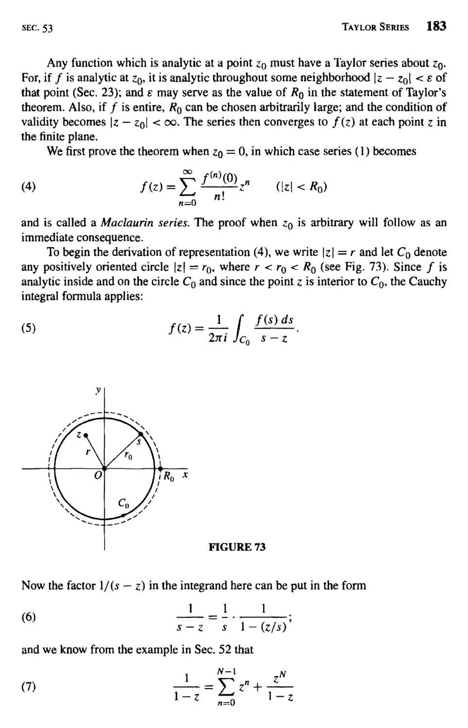
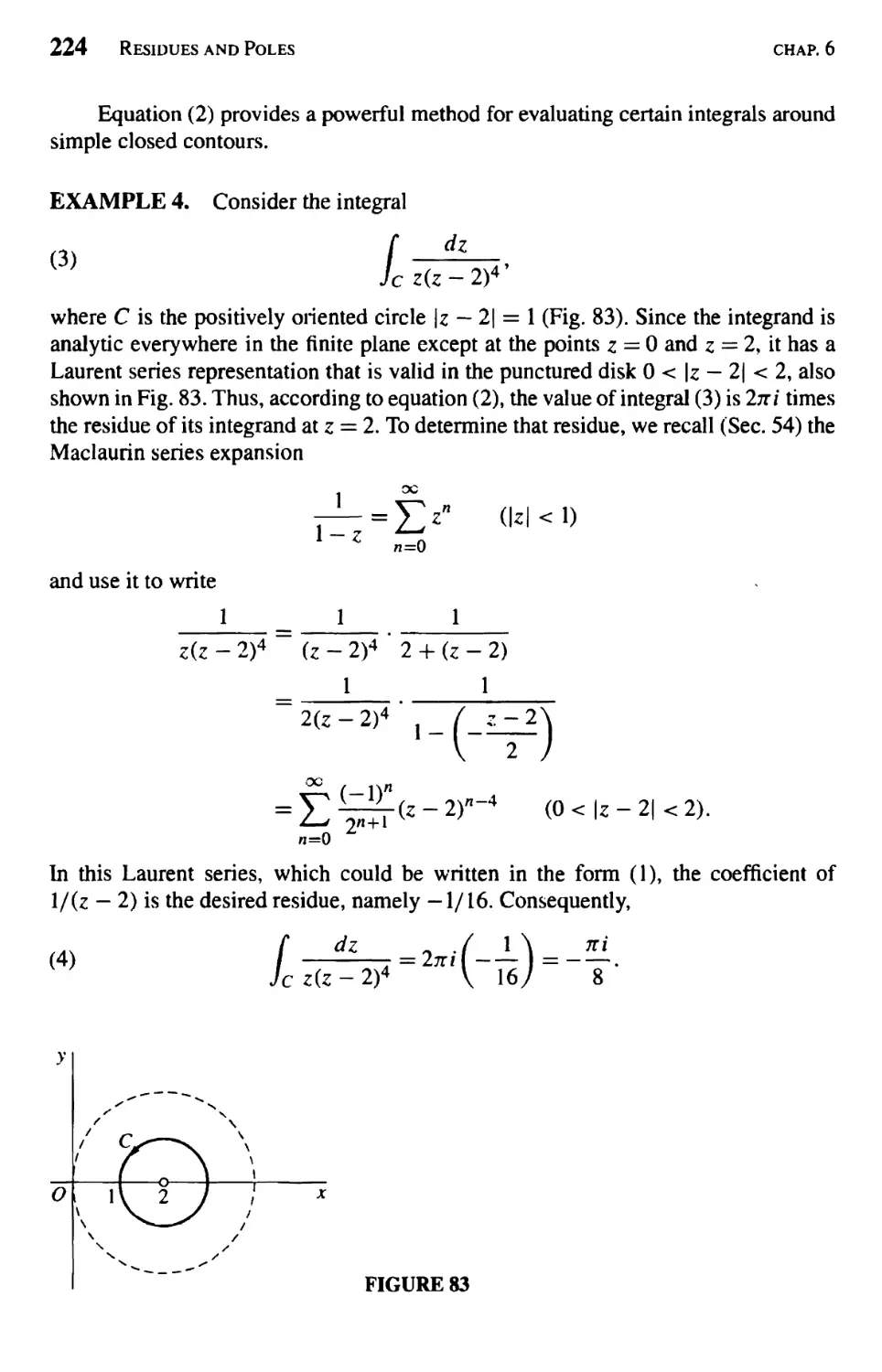
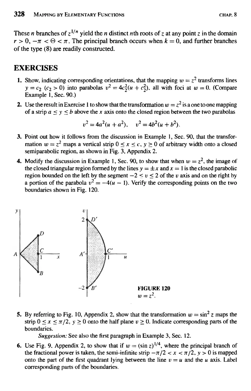
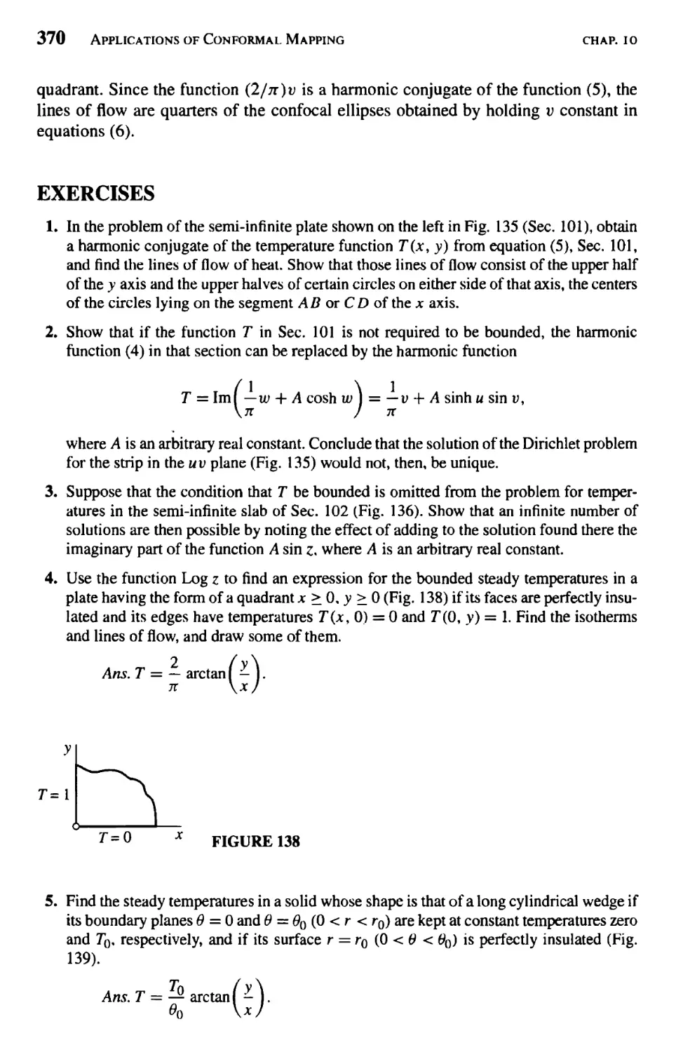
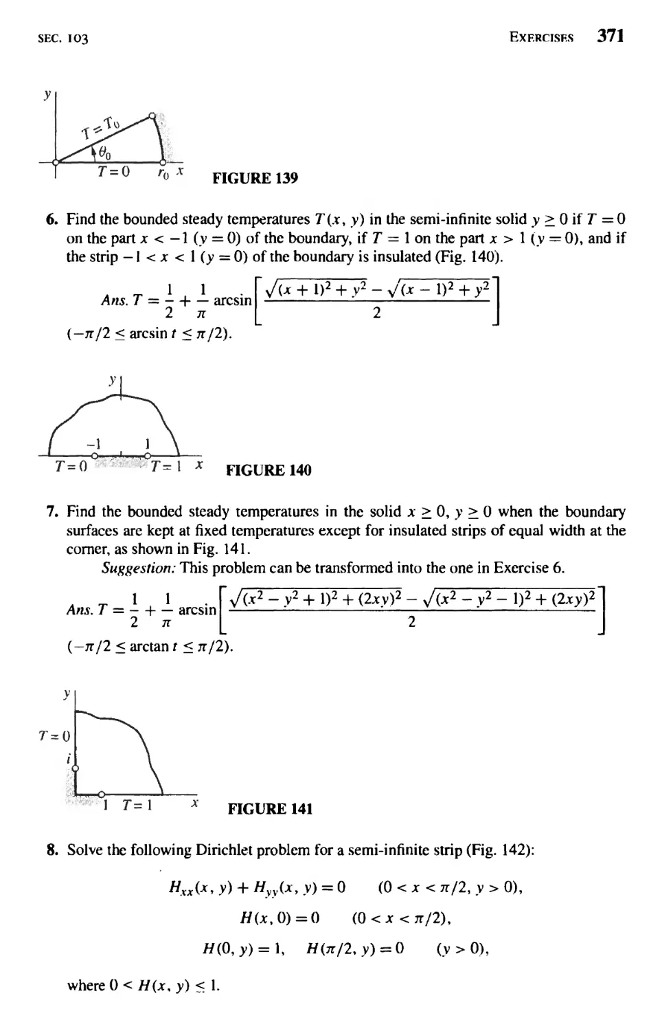
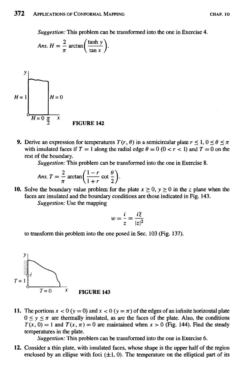
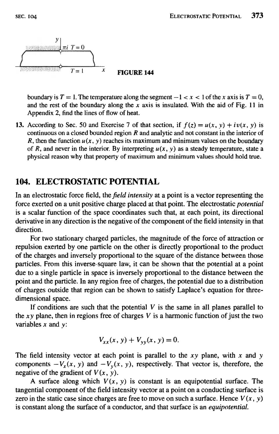
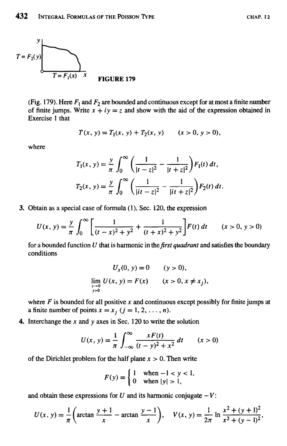
Текст
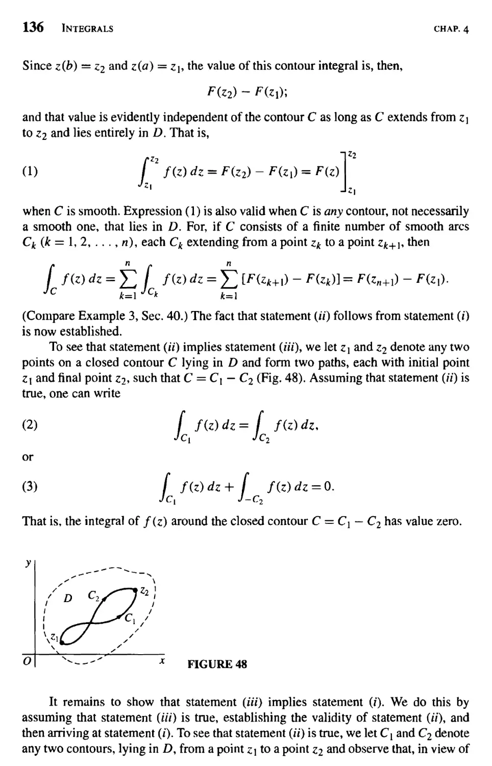
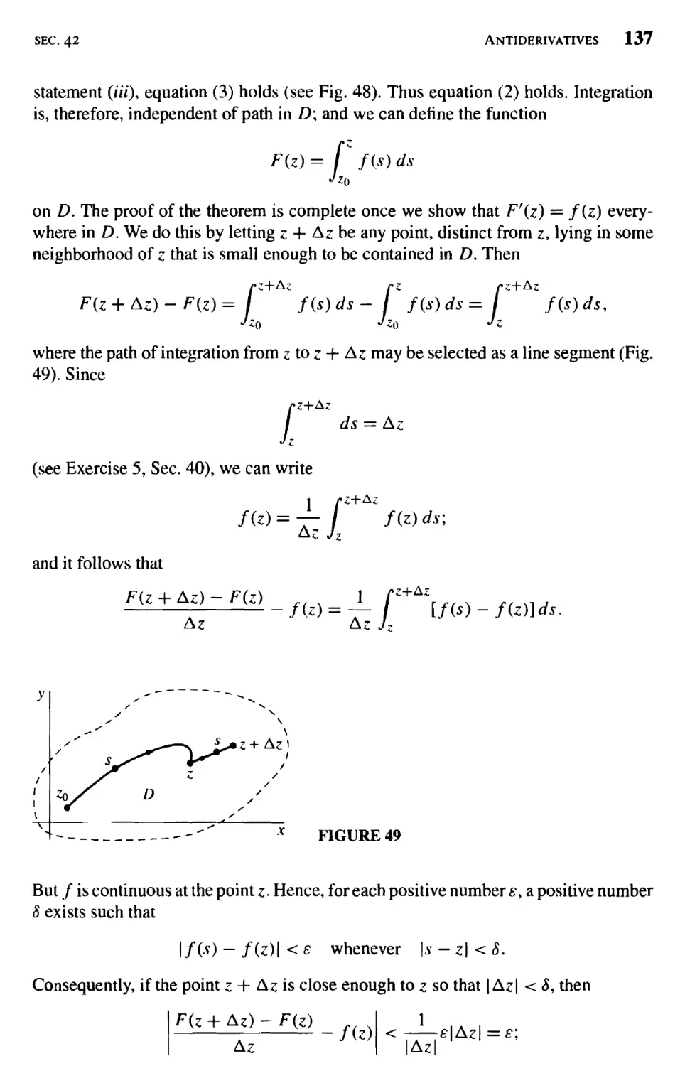
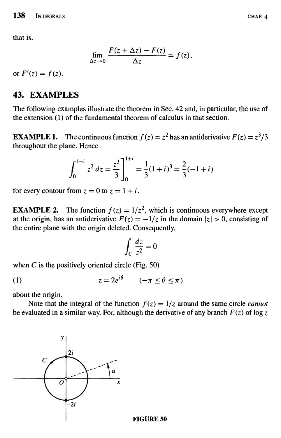
COMPLEX VARIABLES
and
APPLICATIONS
SEVENTH EDITION
JAMES WARD BROWN
RUEL V. CHURCHILL
COMPLEX VARIABLES
AND APPLICATIONS
SEVENTH EDITION
James Ward Brown
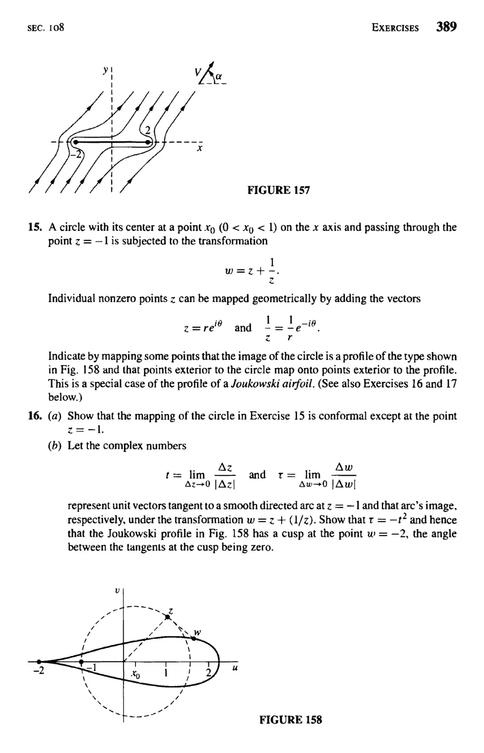
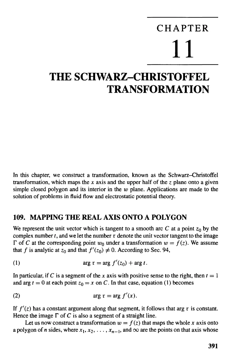
Professor of Mathematics
The University of Michigan-Dearborn
Ruel V. Churchill
Late Professor of Mathematics
The University of Michigan
|g Higher Education
Boston Burr Ridge, IL Dubuque, IA Madison, Wl New York
San Francisco St. Louis Bangkok Bogota Caracas Kuala Lumpur
Lisbon London Madrid Mexico City Milan Montreal New Delhi
Santiago Seoul Singapore Sydney Taipei Toronto
CONTENTS
Preface 15
1 Complex Numbers 1
Sums and Products 1
Basic Algebraic Properties 3
Further Properties 5
Moduli 8
Complex Conjugates 11
Exponential Form 15
Products and Quotients in Exponential Form 17
Roots of Complex Numbers 22
Examples 25
Regions in the Complex Plane 29
2 Analytic Functions 33
Functions of a Complex Variable 33
Mappings 36
Mappings by the Exponential Function 40
Limits 43
Theorems on Limits 46
Limits Involving the Point at Infinity 48
Continuity 51
Derivatives 54
Differentiation Formulas 57
Cauchy-Riemann Equations 60
XI
xii Contents
Sufficient Conditions for Differentiability 63
Polar Coordinates 65
Analytic Functions 70
Examples 72
Harmonic Functions 75
Uniquely Determined Analytic Functions 80
Reflection Principle 82
3 Elementary Functions 87
The Exponential Function 87
The Logarithmic Function 90
Branches and Derivatives of Logarithms 92
Some Identities Involving Logarithms 95
Complex Exponents 97
Trigonometric Functions 100
Hyperbolic Functions 105
Inverse Trigonometric and Hyperbolic Functions 108
4 Integrals 111
Derivatives of Functions w(t) 111
Definite Integrals of Functions w(t) 113
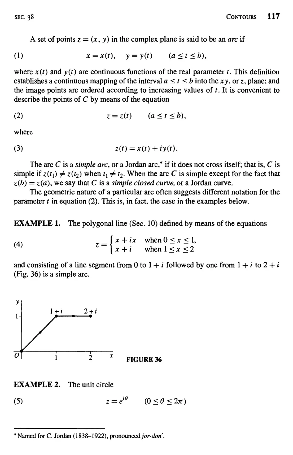
Contours 116
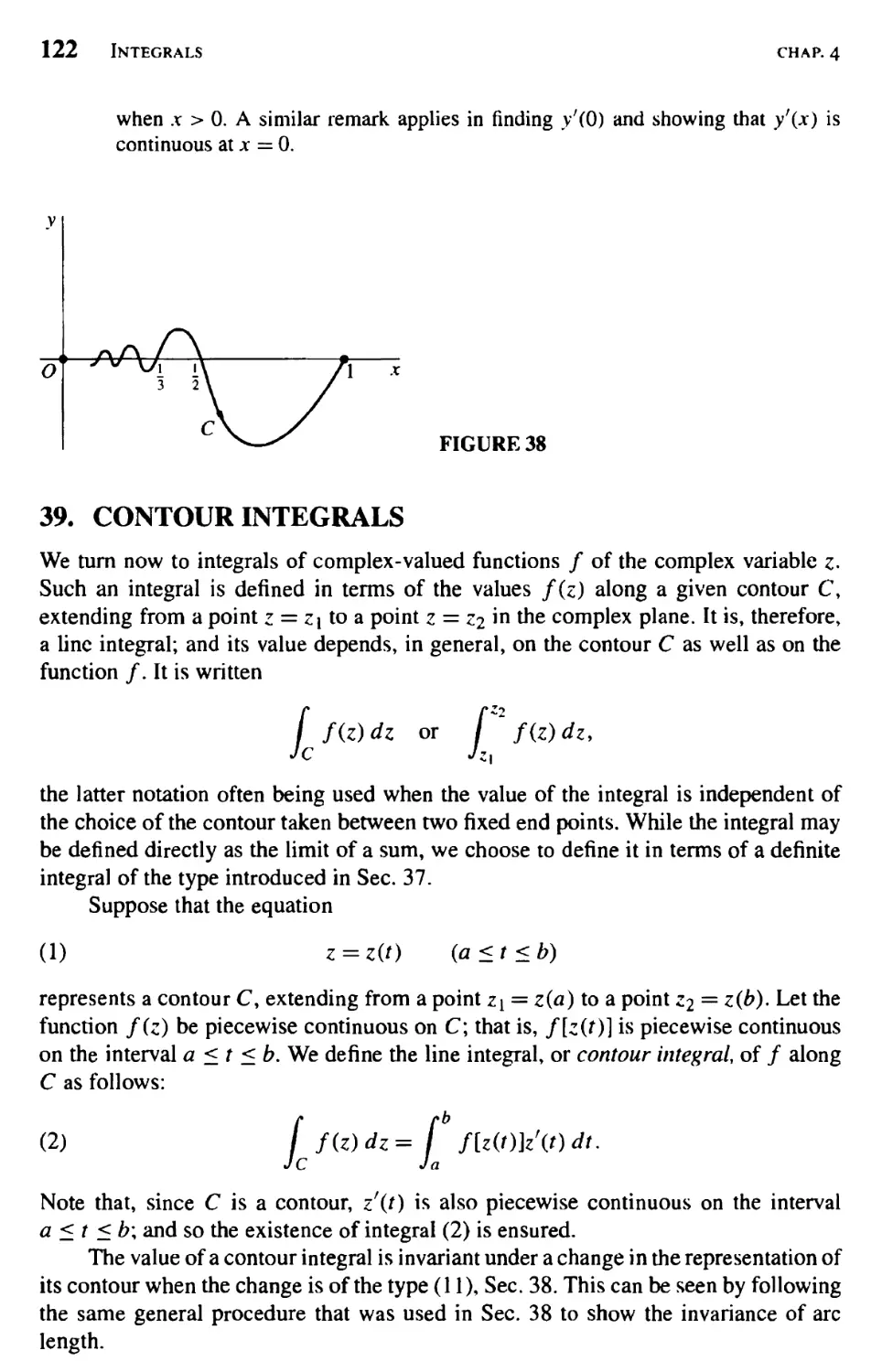
Contour Integrals 122
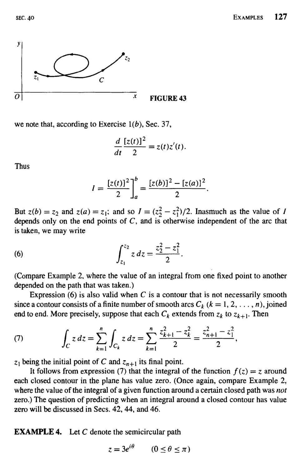
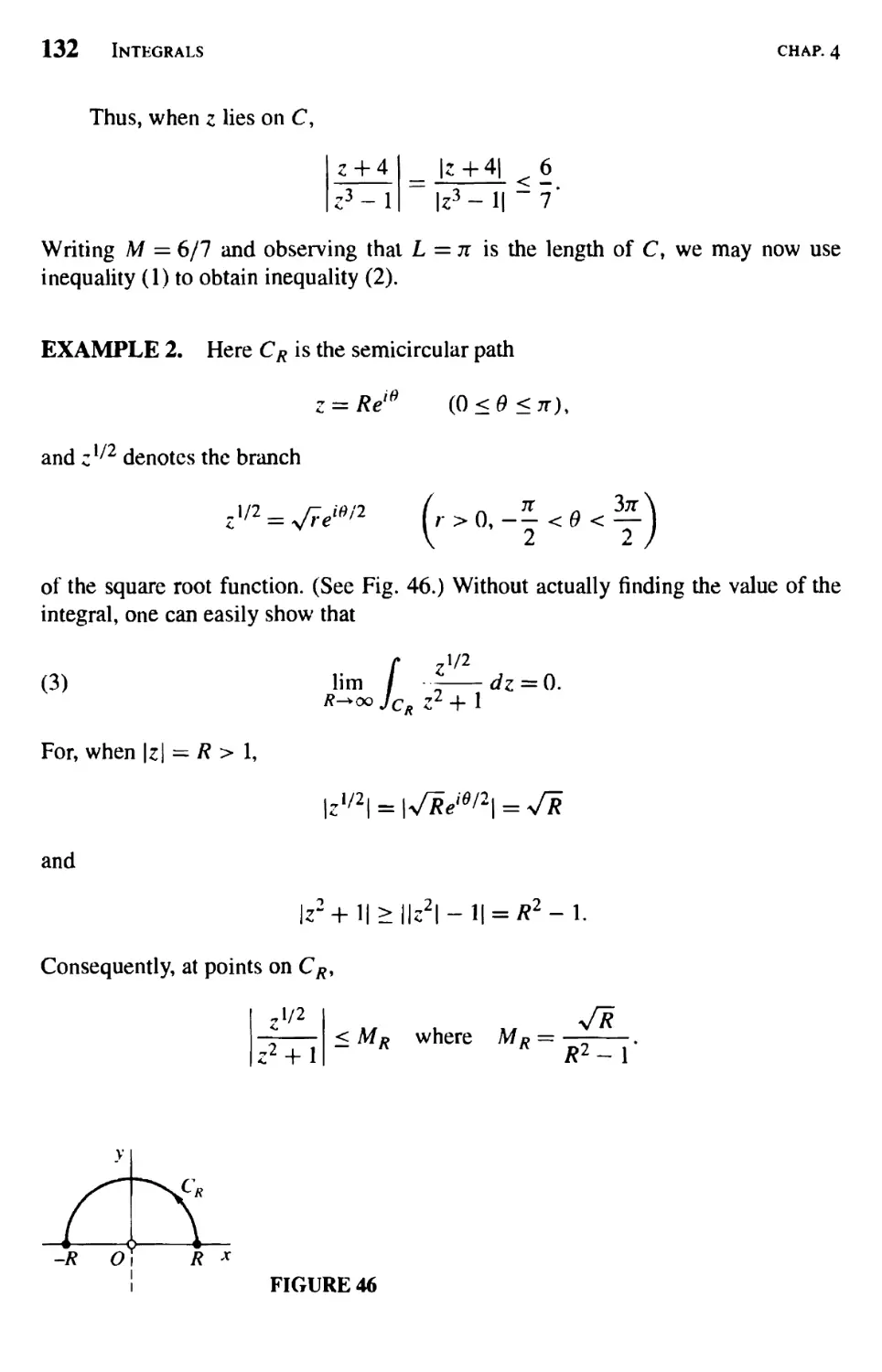
Examples 124
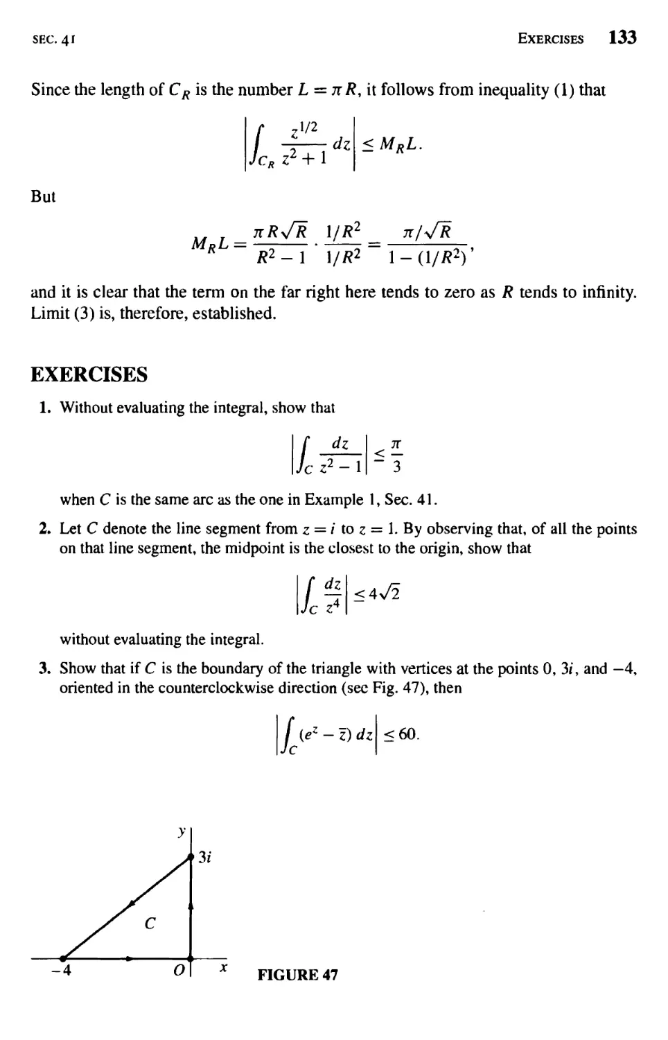
Upper Bounds for Moduli of Contour Integrals 130
Antiderivatives 135
Examples 138
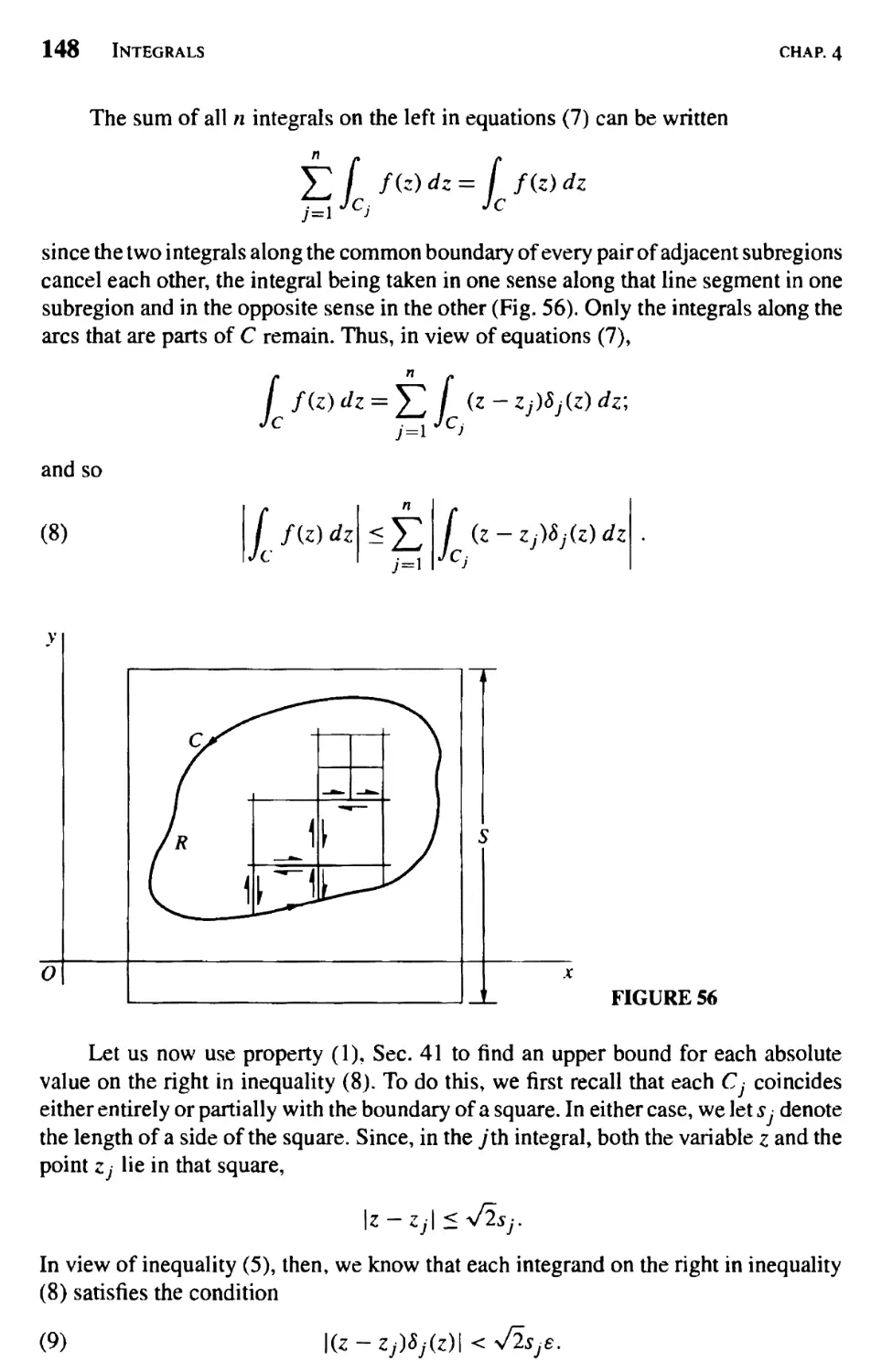
Cauchy-Goursat Theorem 142
Proof of the Theorem 144
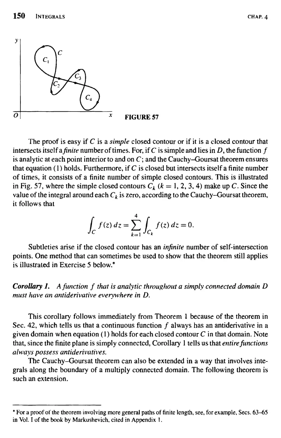
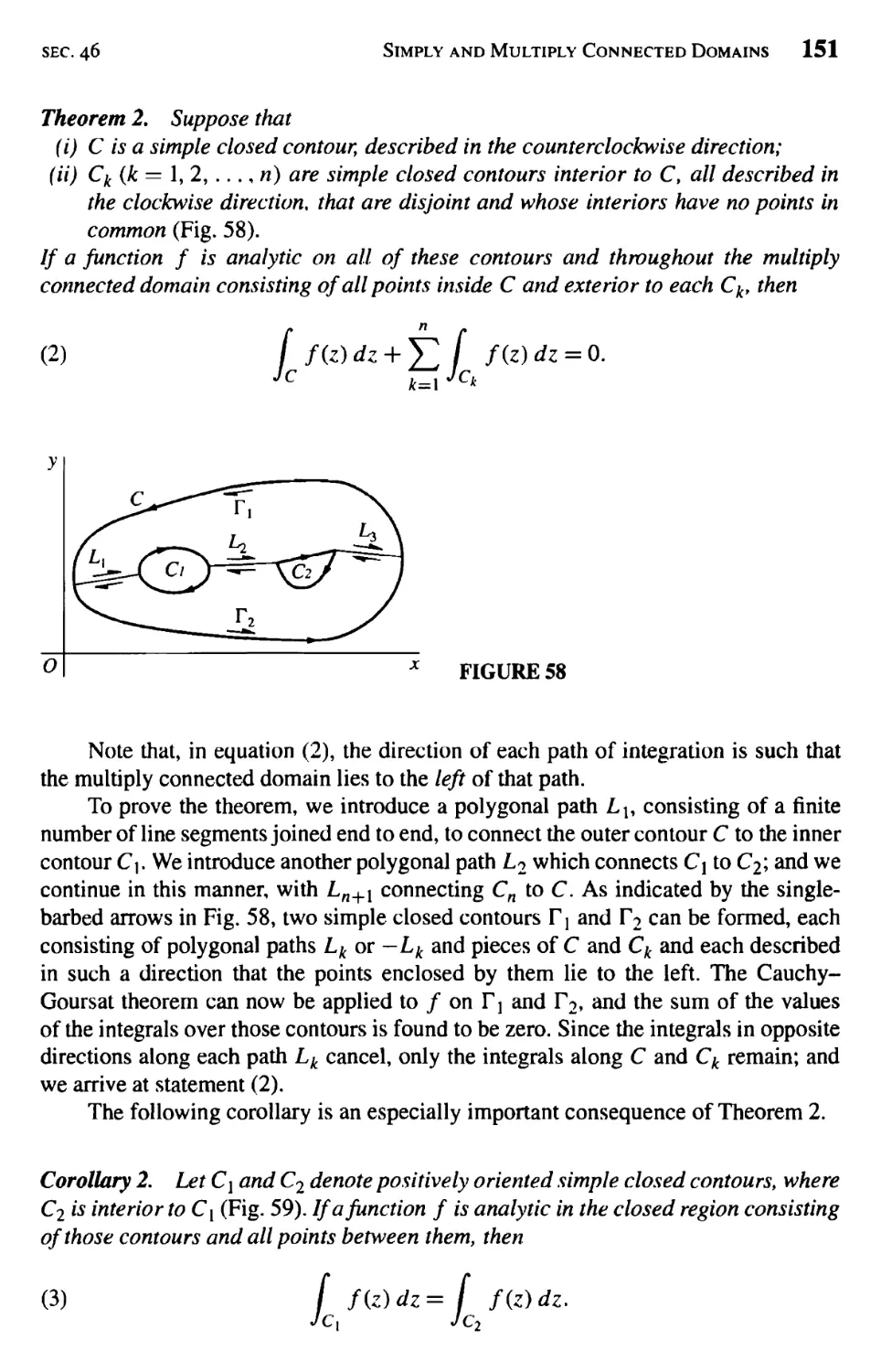
Simply and Multiply Connected Domains 149
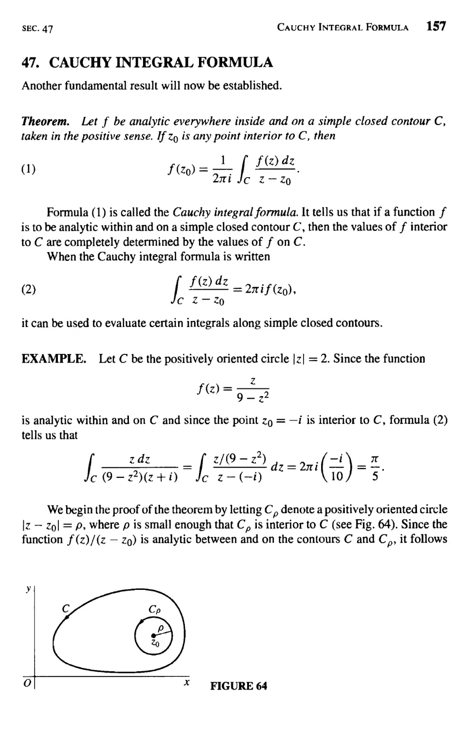
Cauchy Integral Formula 157
Derivatives of Analytic Functions 158
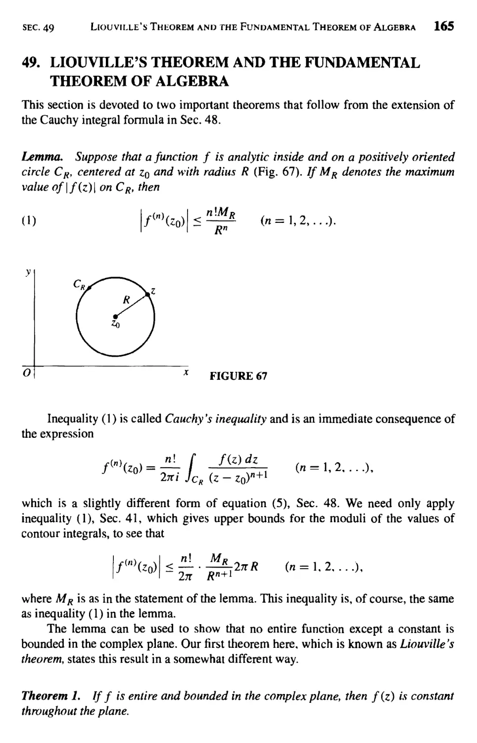
Liouville's Theorem and the Fundamental Theorem of Algebra 165
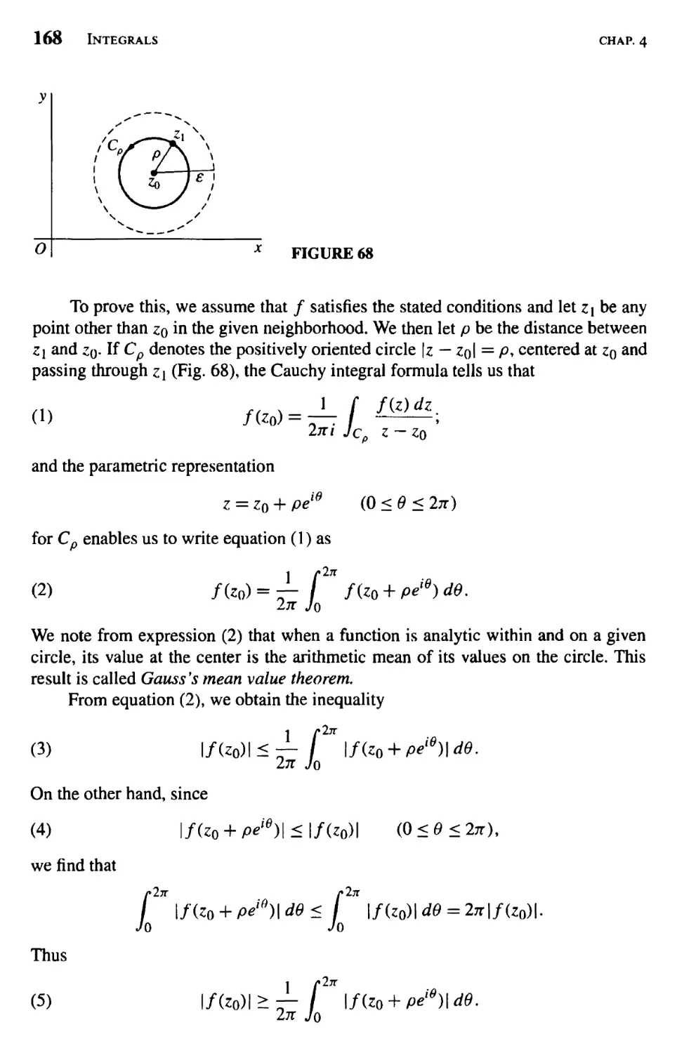
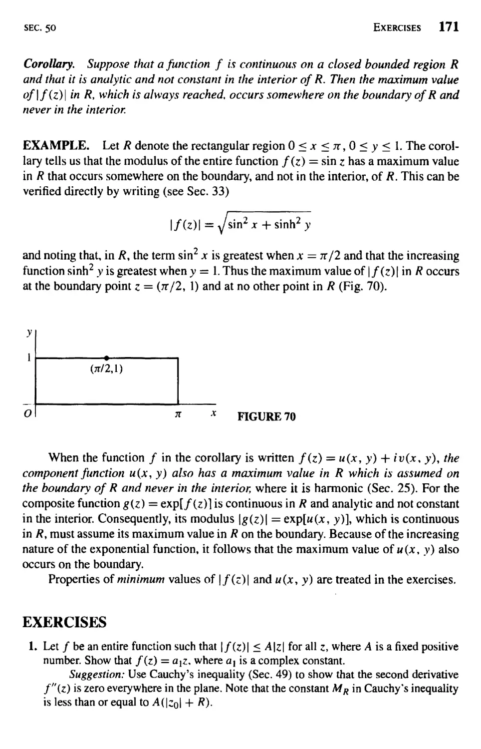
Maximum Modulus Principle 167
5 Series 175
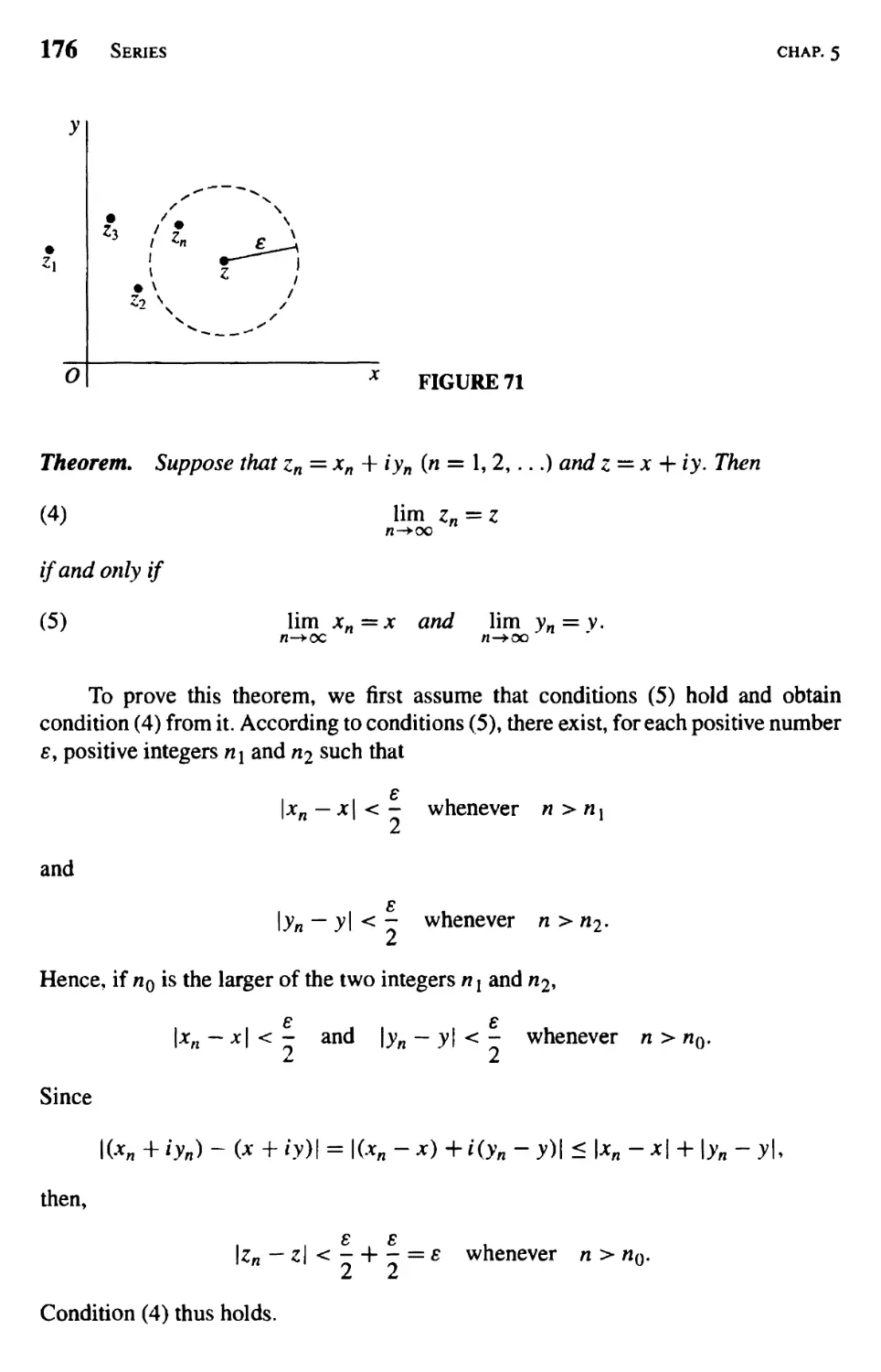
Convergence of Sequences 175
Convergence of Series 178
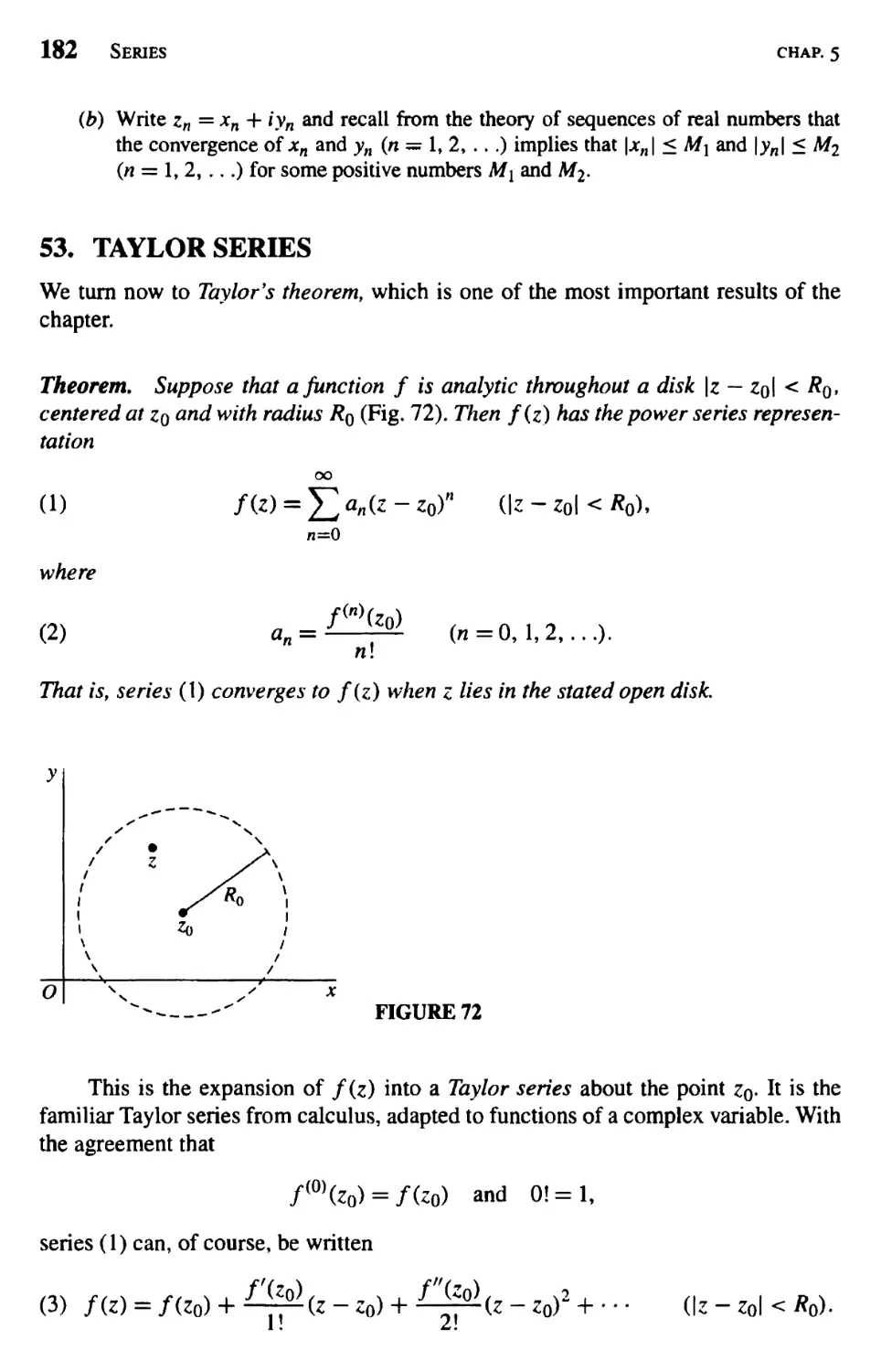
Taylor Series 182
Examples 185
Laurent Series 190
Examples 195
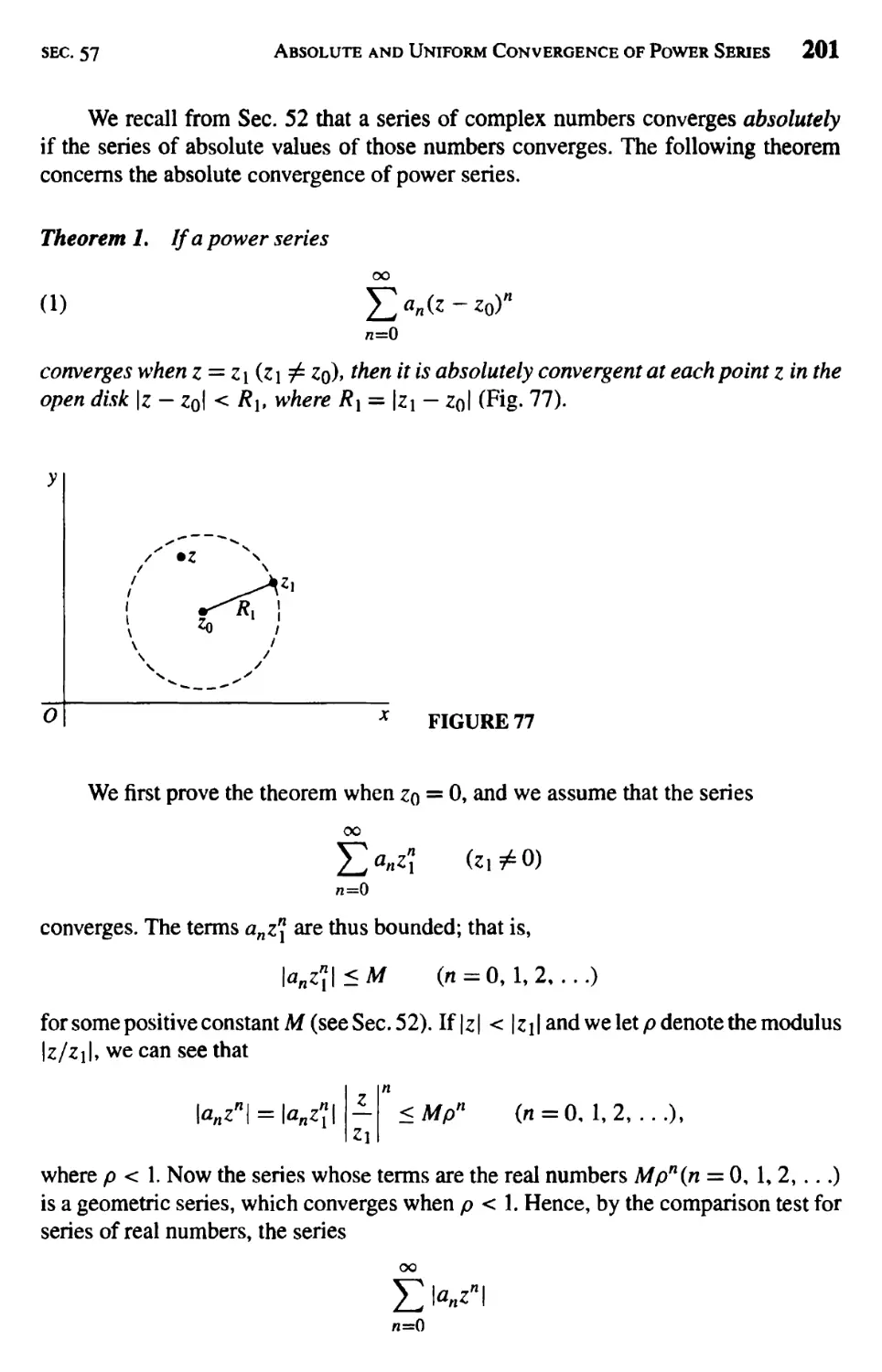
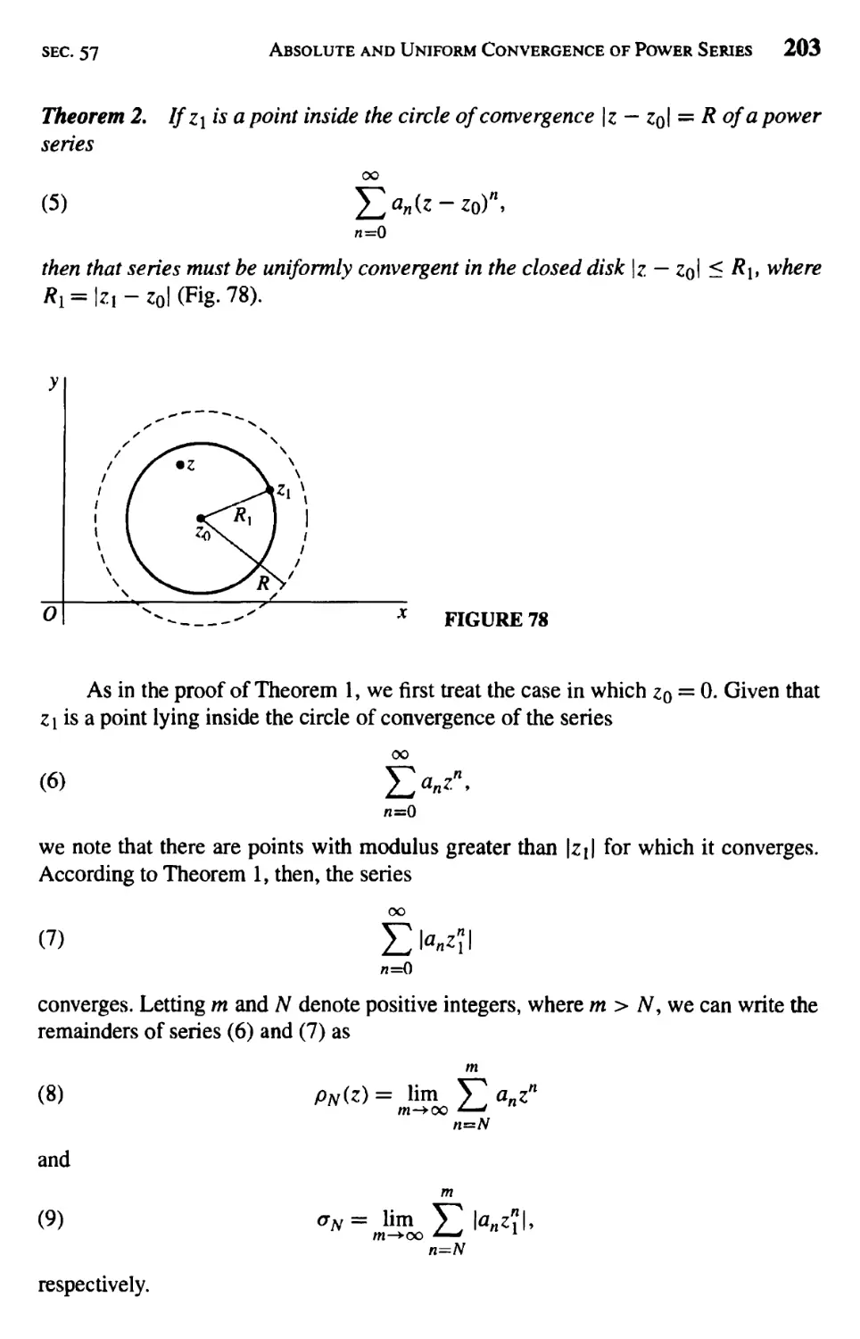
Absolute and Uniform Convergence of Power Series 200
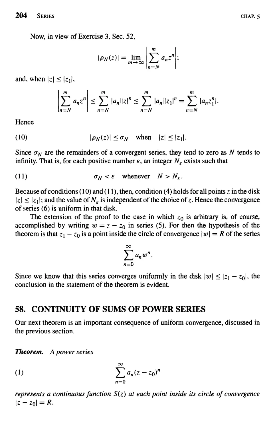
Continuity of Sums of Power Series 204
Integration and Differentiation of Power Series 206
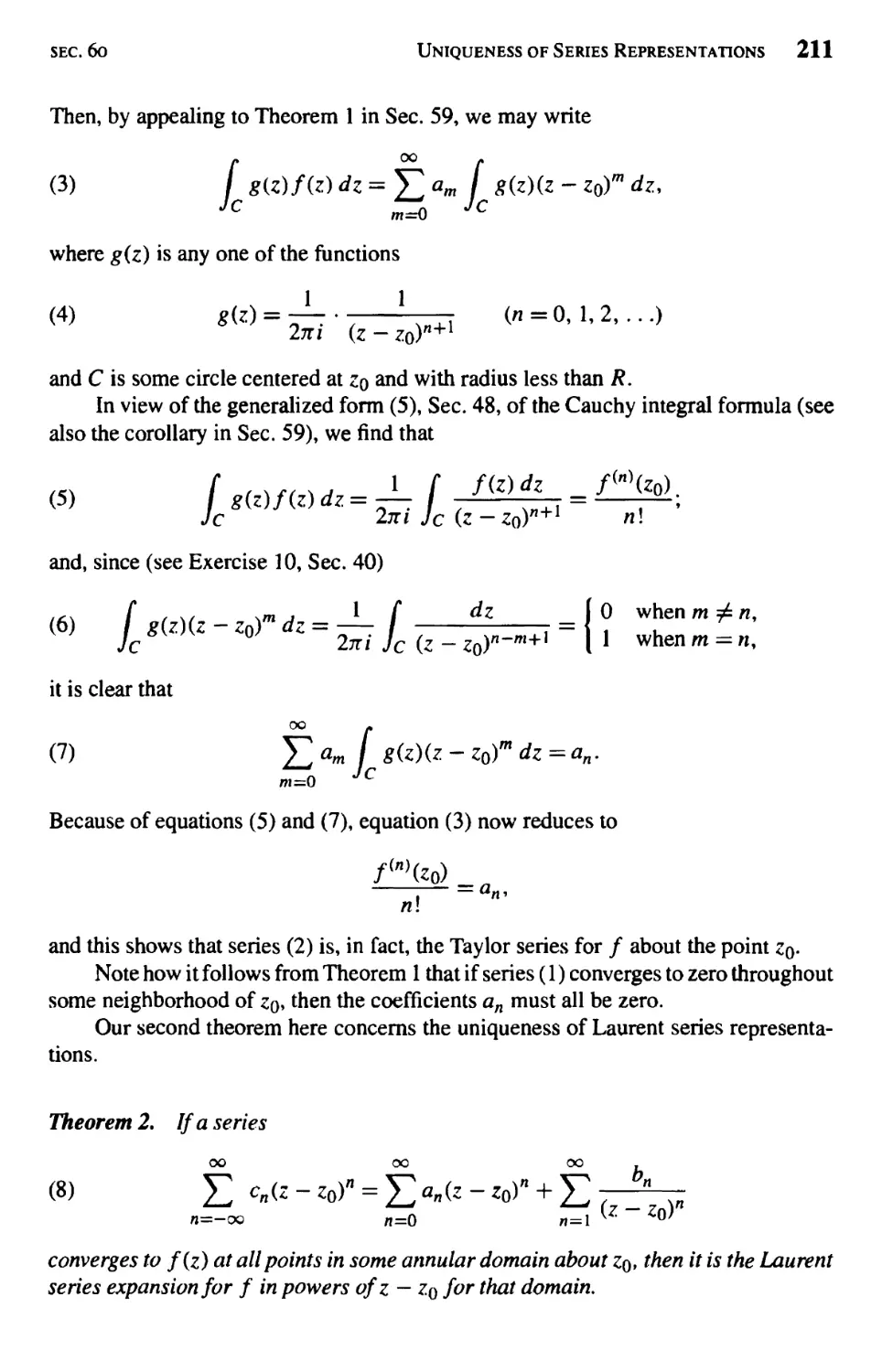
Uniqueness of Series Representations 210
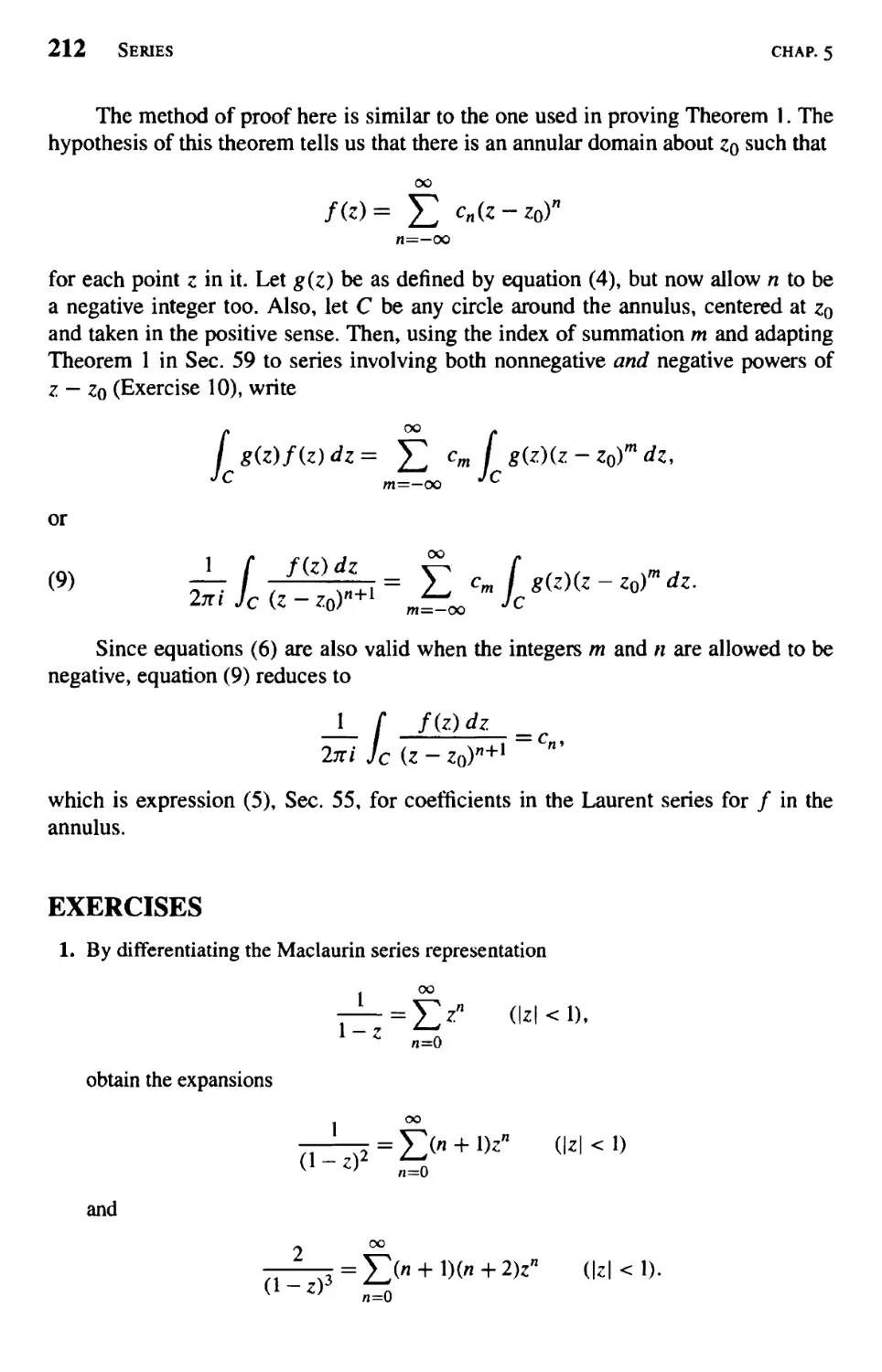
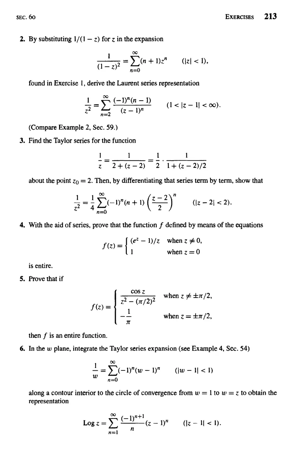
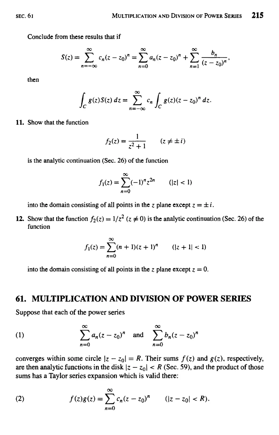
Multiplication and Division of Power Series 215
Contents xiii
6 Residues and Poles 221
Residues 221
Cauchy's Residue Theorem 225
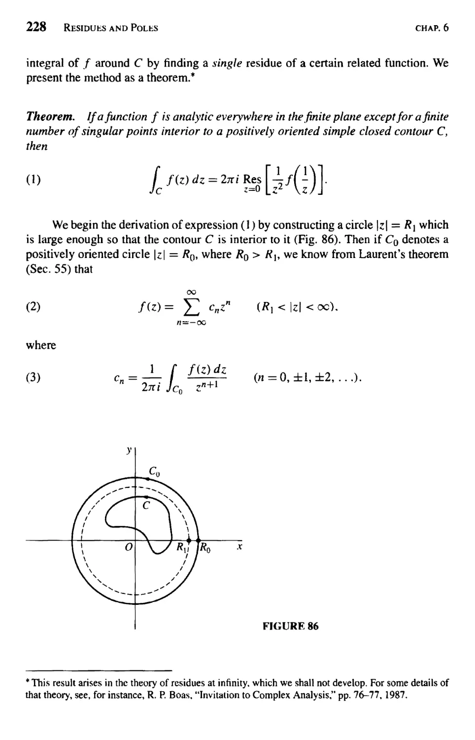
Using a Single Residue 227
The Three Types of Isolated Singular Points 231
Residues at Poles 234
Examples 236
Zeros of Analytic Functions 239
Zeros and Poles 242
Behavior of/ Near Isolated Singular Points 247
7 Applications of Residues 251
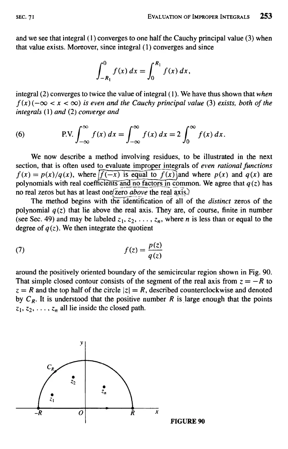
Evaluation of Improper Integrals 251
Example 254
Improper Integrals from Fourier Analysis 259
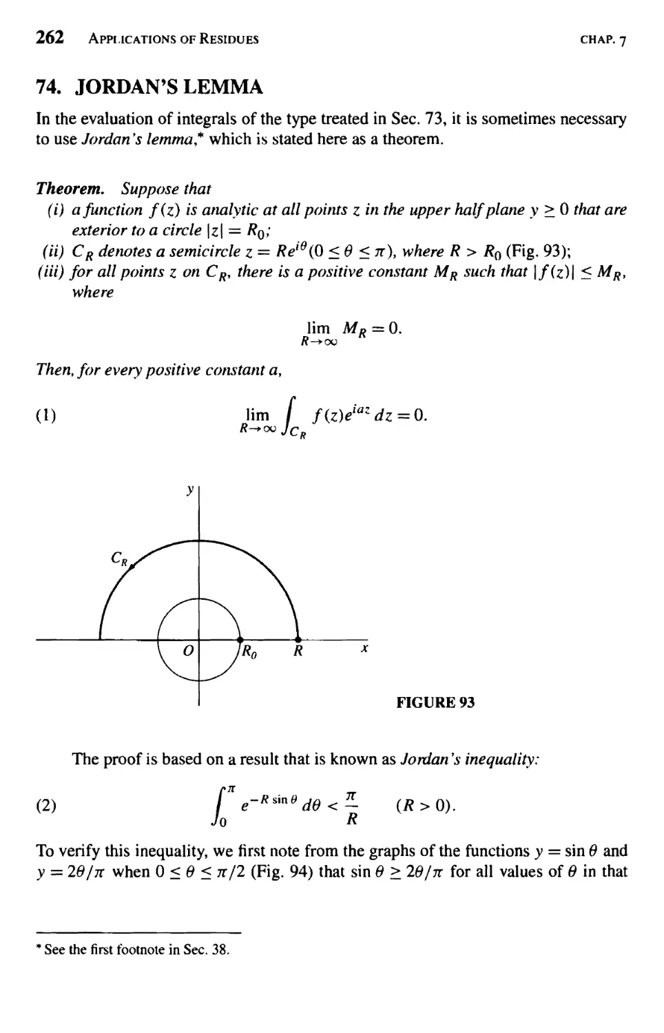
Jordan's Lemma 262
Indented Paths 267
An Indentation Around a Branch Point 270
Integration Along a Branch Cut 273
Definite Integrals involving Sines and Cosines 278
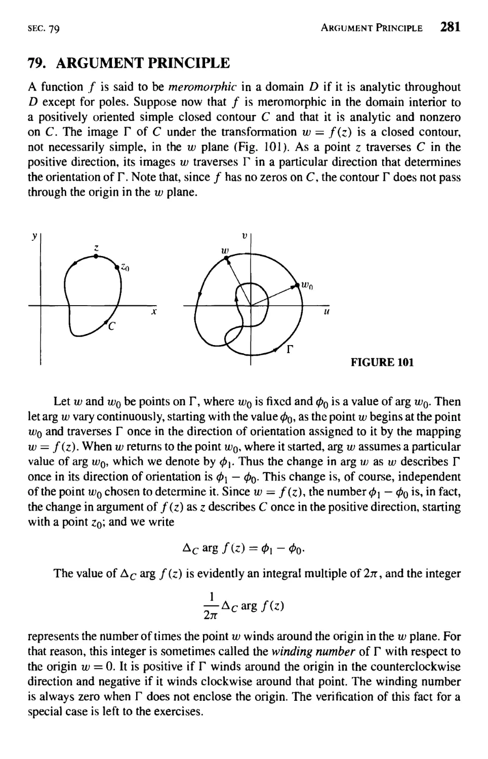
Argument Principle 281
Rouché's Theorem 284
Inverse Laplace Transforms 288
Examples 291
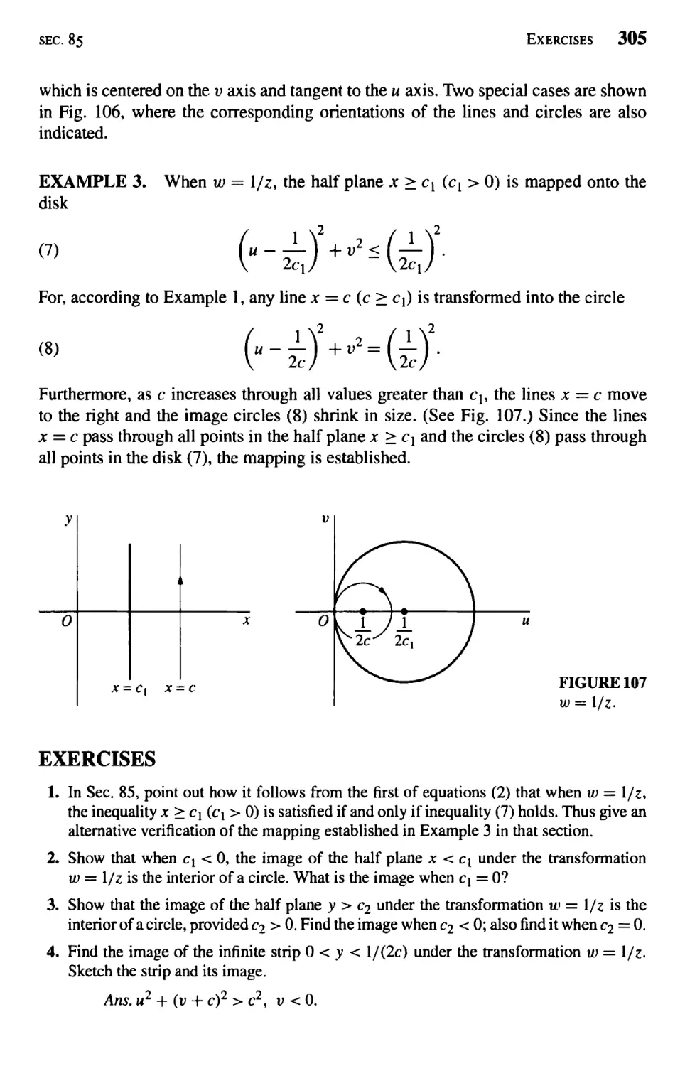
8 Mapping by Elementary Functions 299
Linear Transformations 299
The Transformation w = Vz 301
Mappings by Vz 303
Linear Fractional Transformations 307
An Implicit Form 310
Mappings of the Upper Half Plane 313
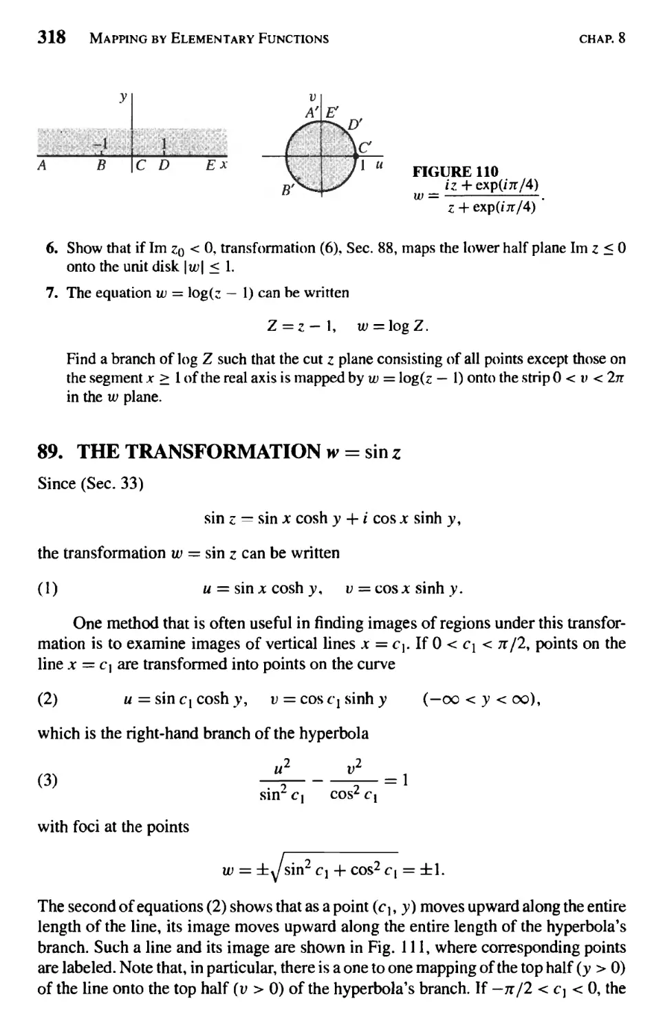
The Transformation w = sin z 318
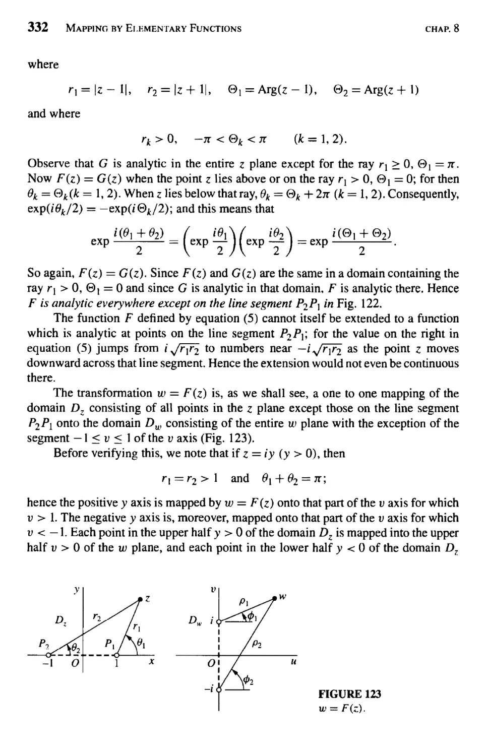
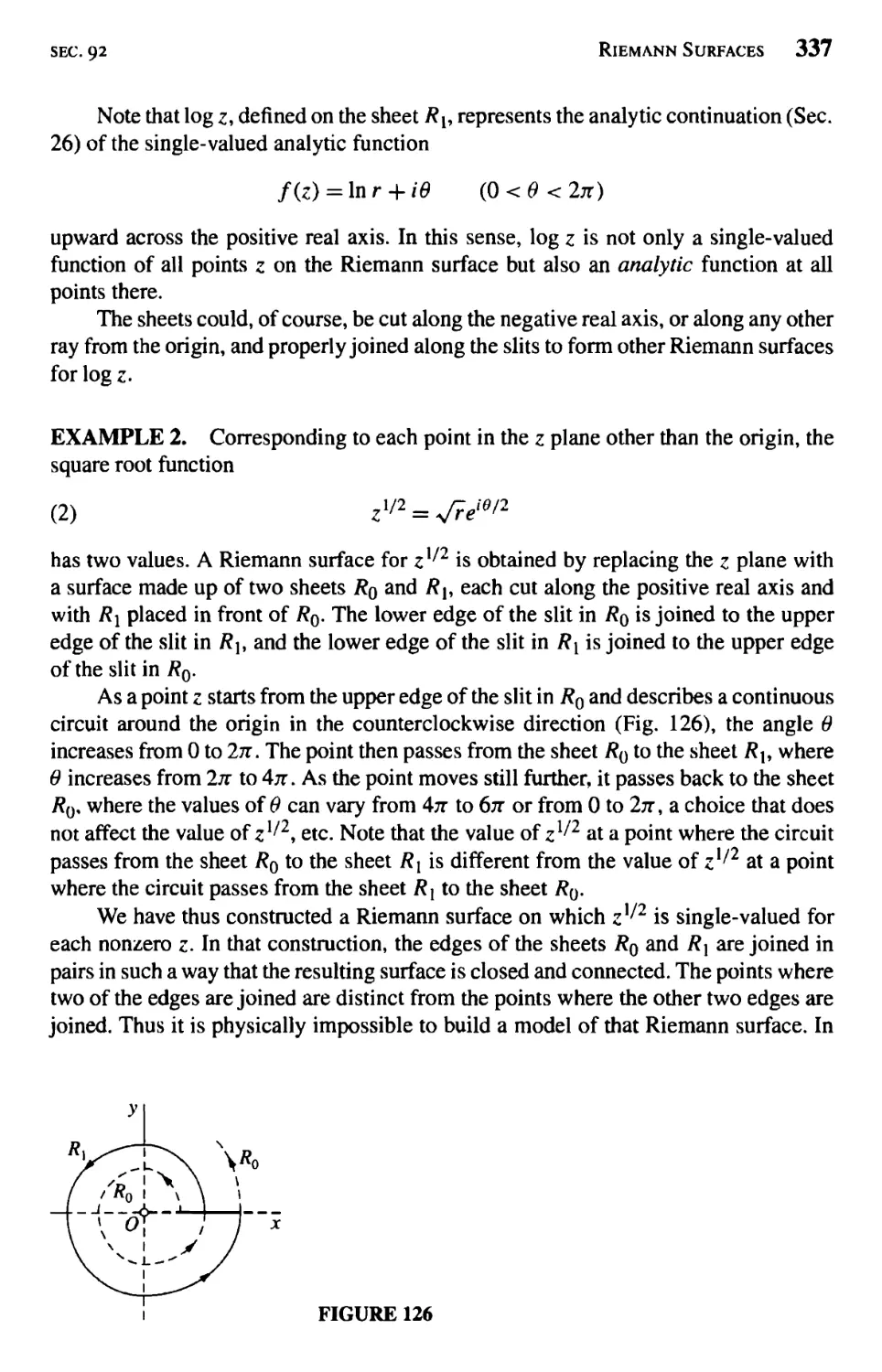
Mappings by z2 and Branches of z]''2 324
Square Roots of Polynomials 329
Riemann Surfaces 335
Surfaces for Related Functions 338
9 Conformai Mapping 343
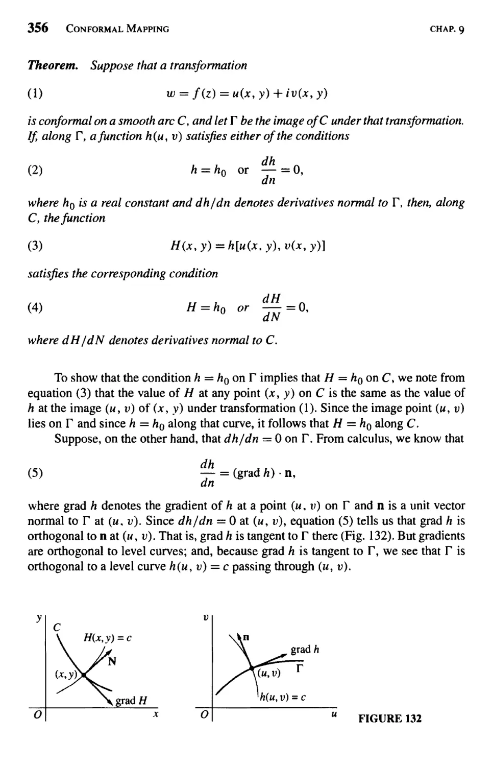
Preservation of Angles 343
Scale Factors 346
Local Inverses 348
Harmonic Conjugates 351
Transformations of Harmonic Functions 353
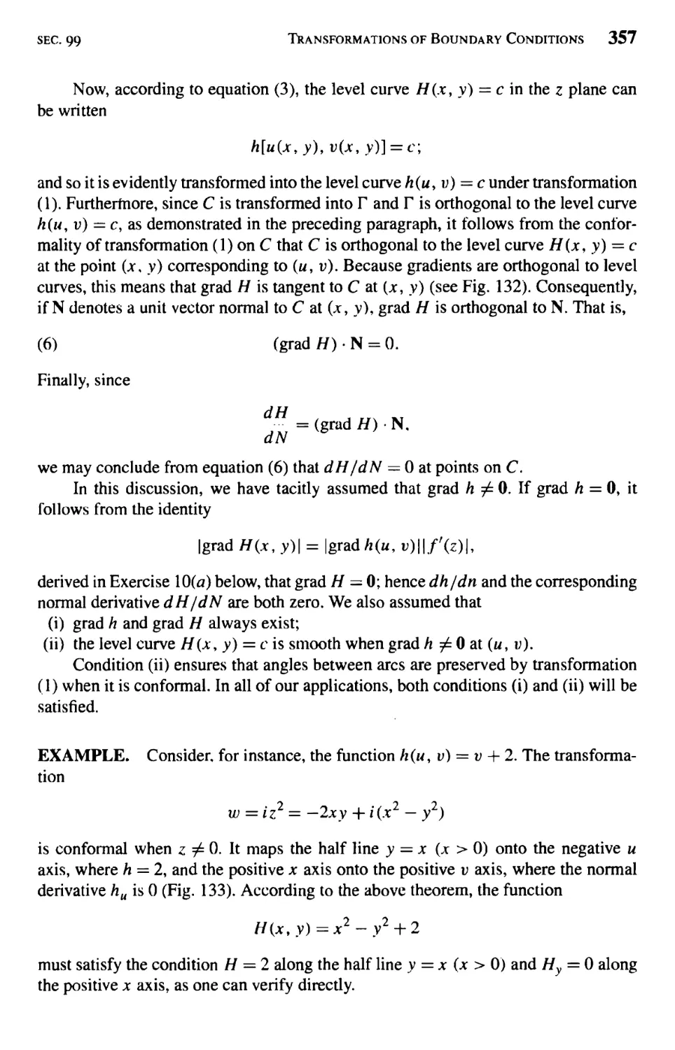
Transformations of Boundary Conditions 355
XÎV Contents
10 Applications of Conformai Mapping 361
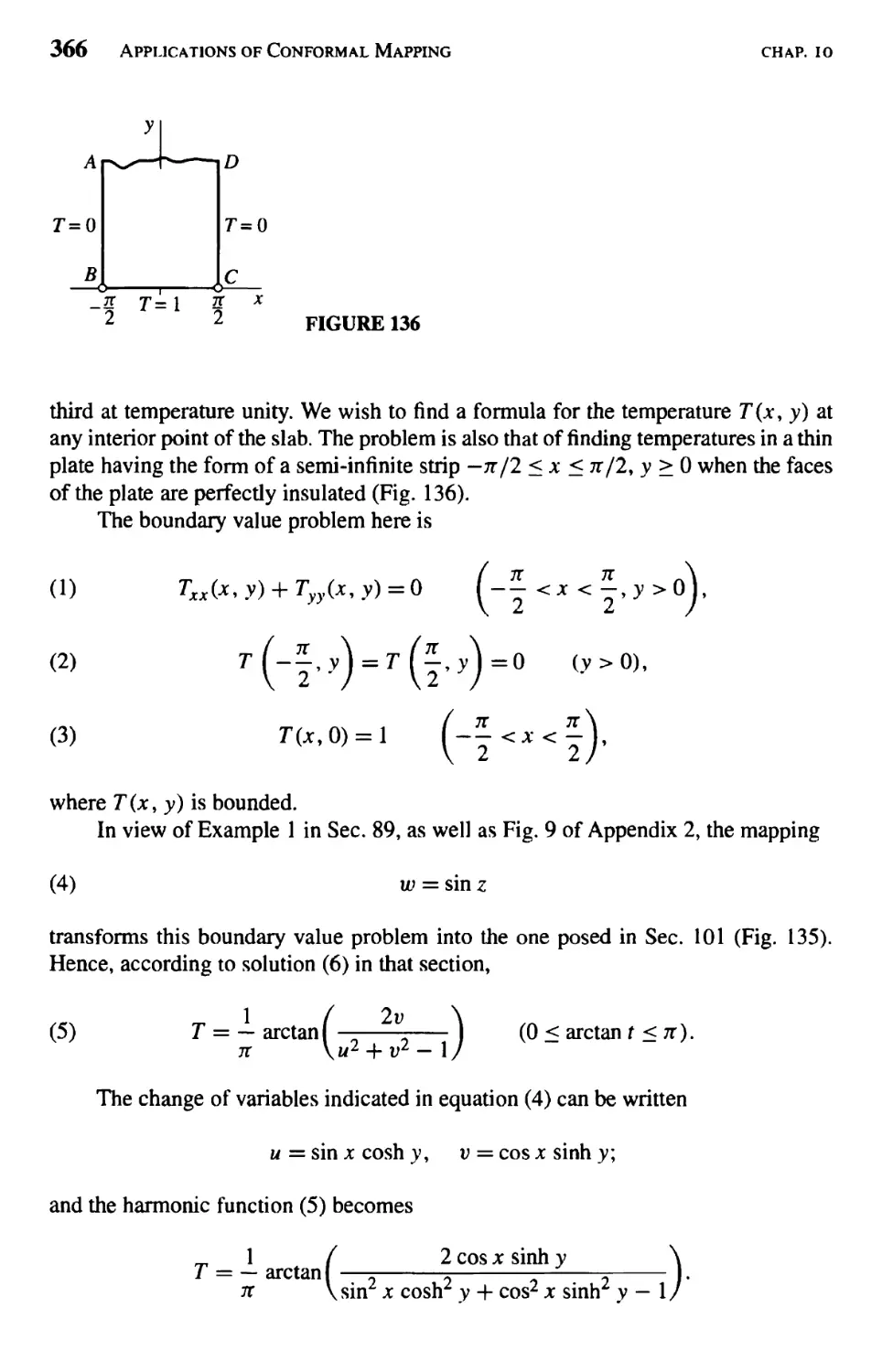
Steady Temperatures 361
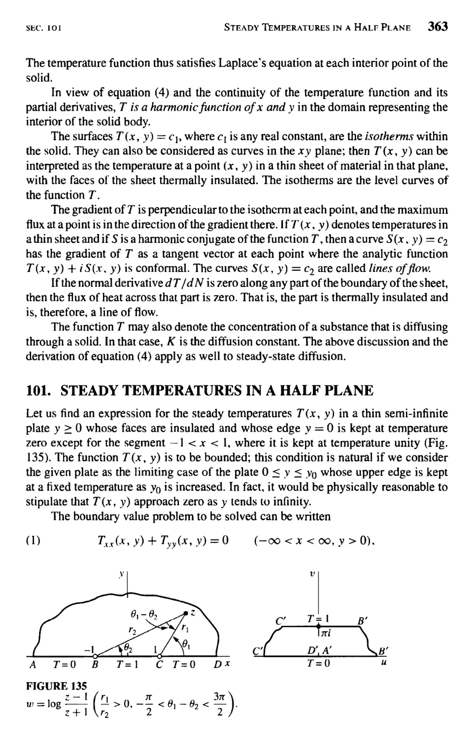
Steady Temperatures in a Half Plane 363
A Related Problem 365
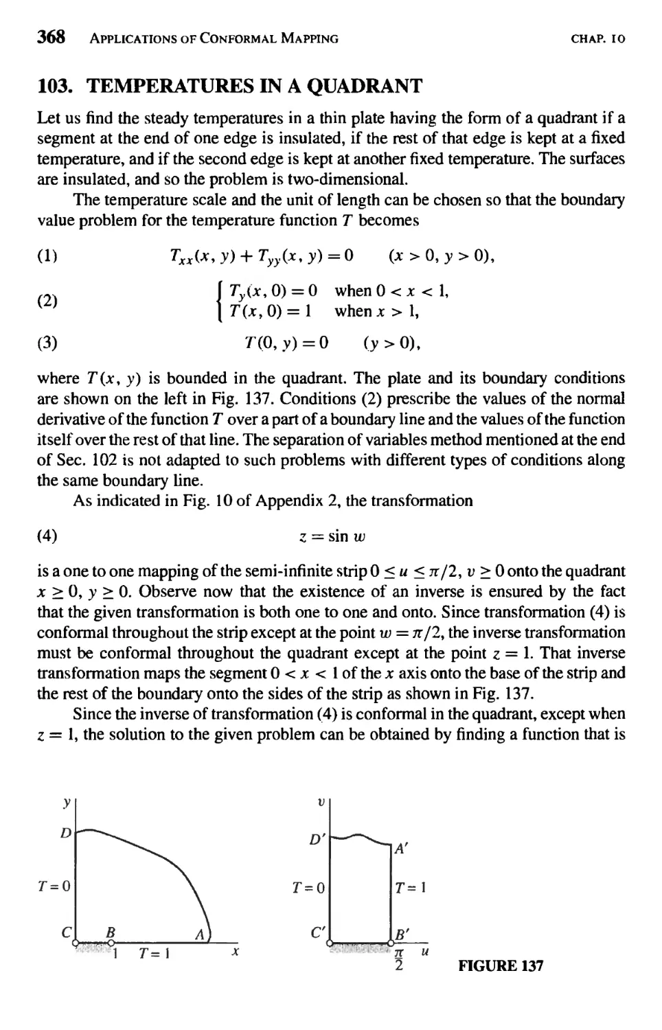
Temperatures in a Quadrant 368
Electrostatic Potential 373
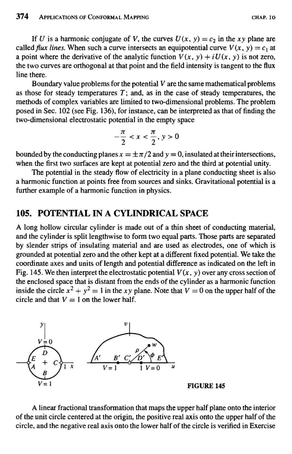
Potential in a Cylindrical Space 374
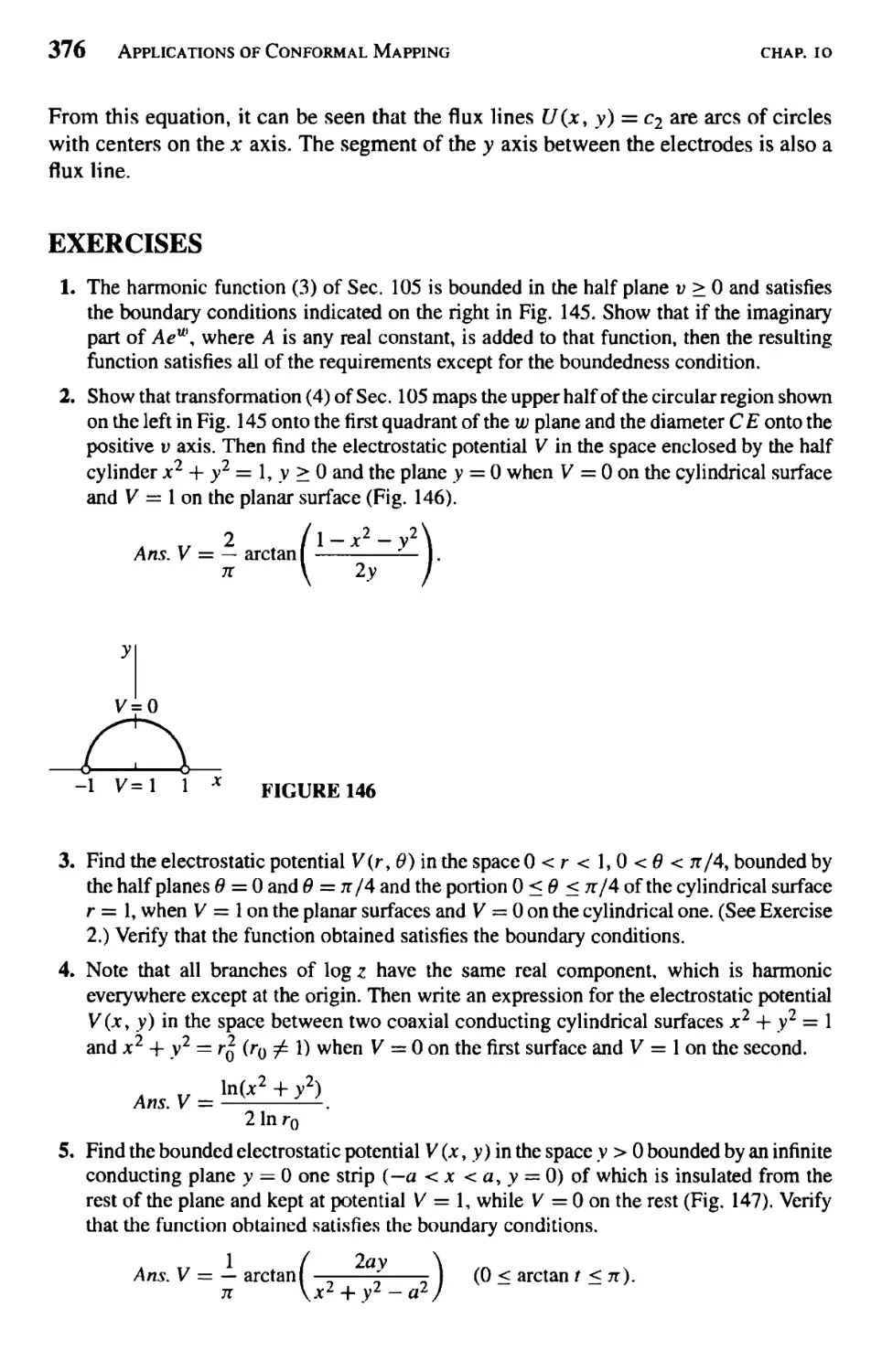
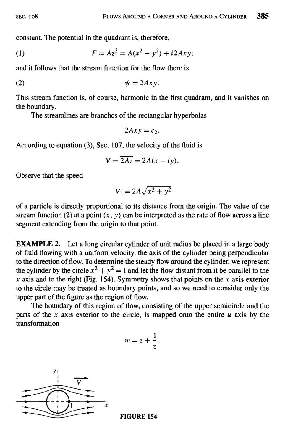
Two-Dimensional Fluid Flow 379
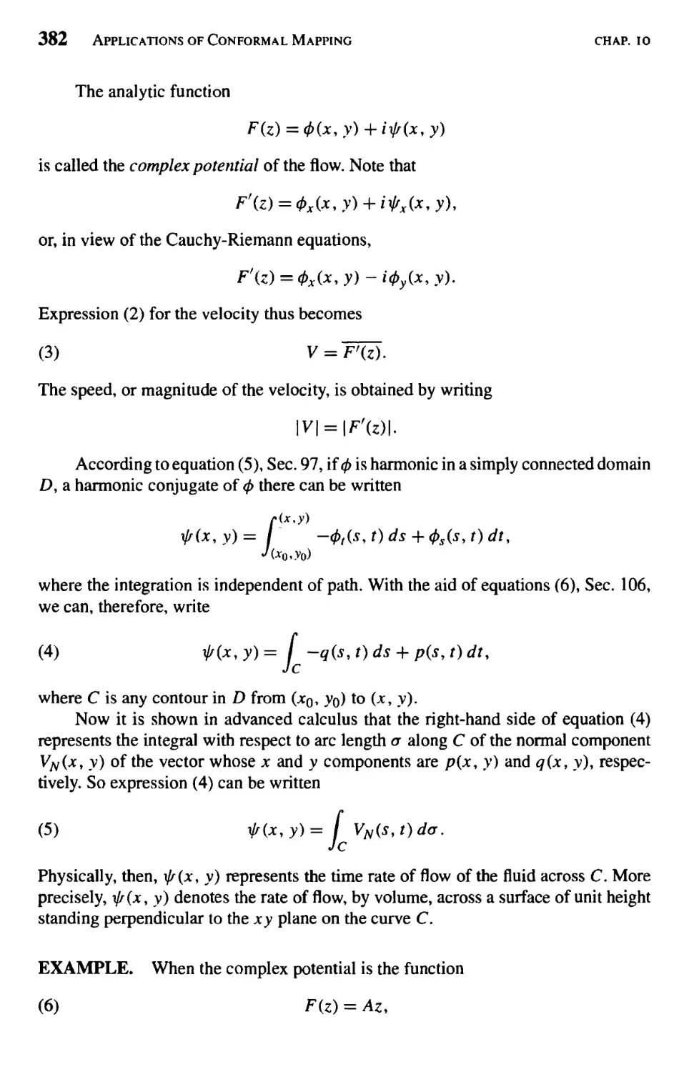
The Stream Function 381
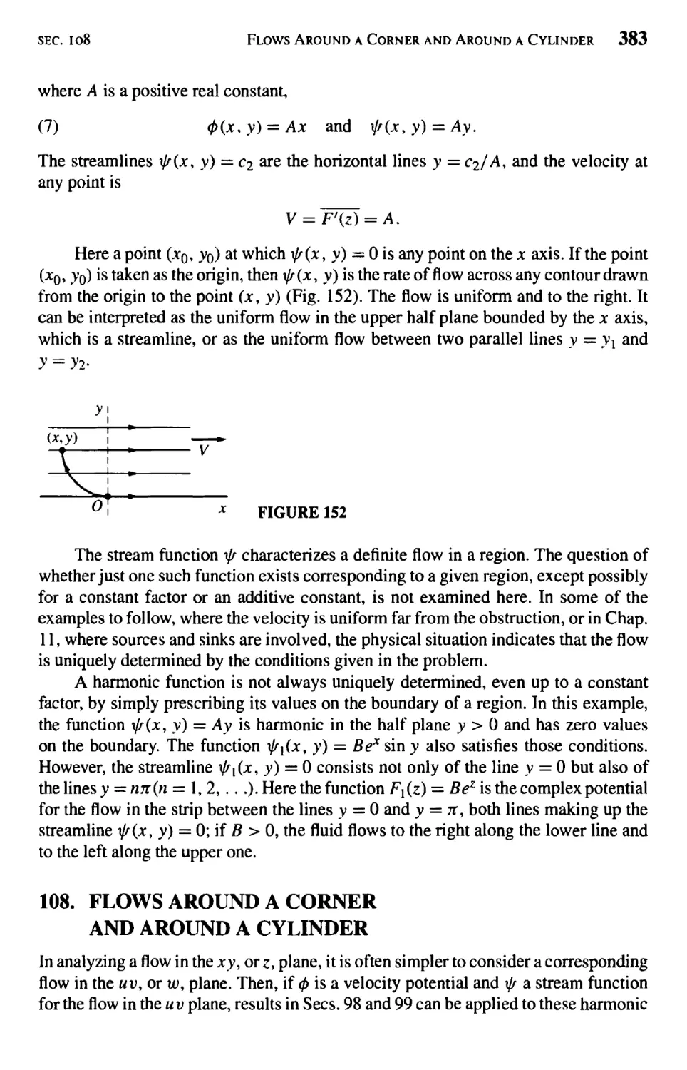
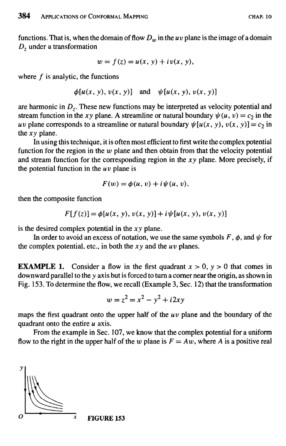
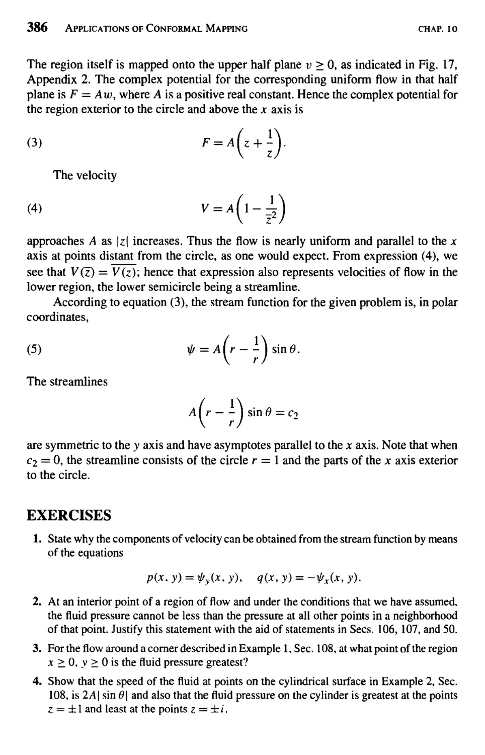
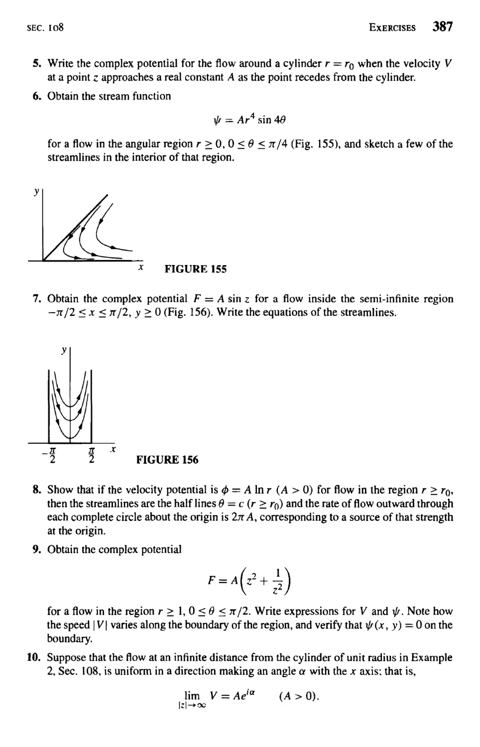
Flows Around a Corner and Around a Cylinder 383
11 The Schwarz-Christoffel Transformation 391
Mapping the Real Axis onto a Polygon 391
Schwarz-Christoffel Transformation 393
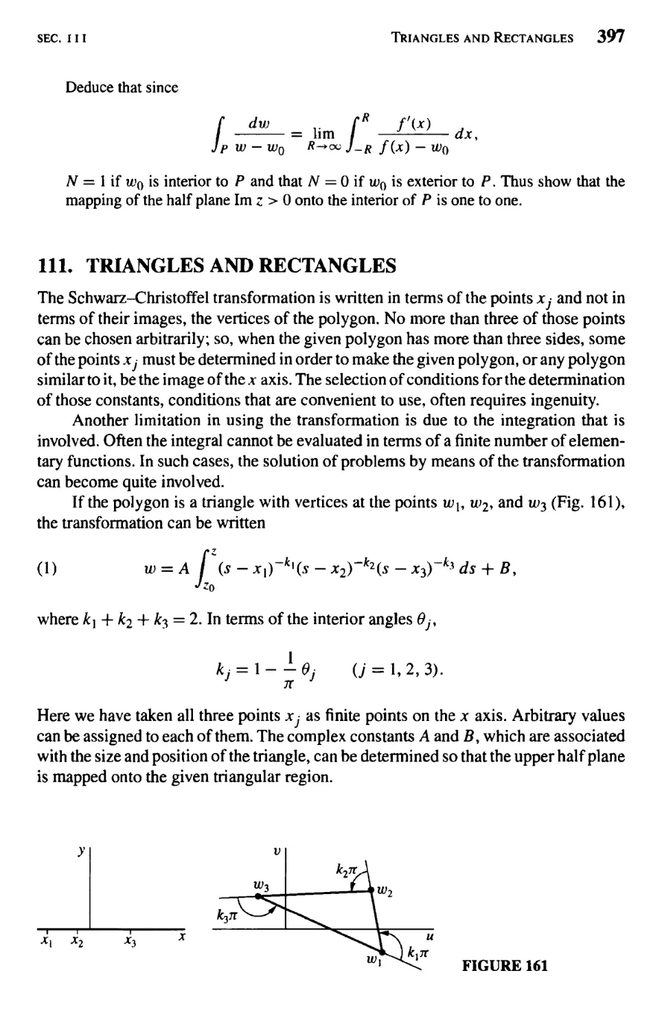
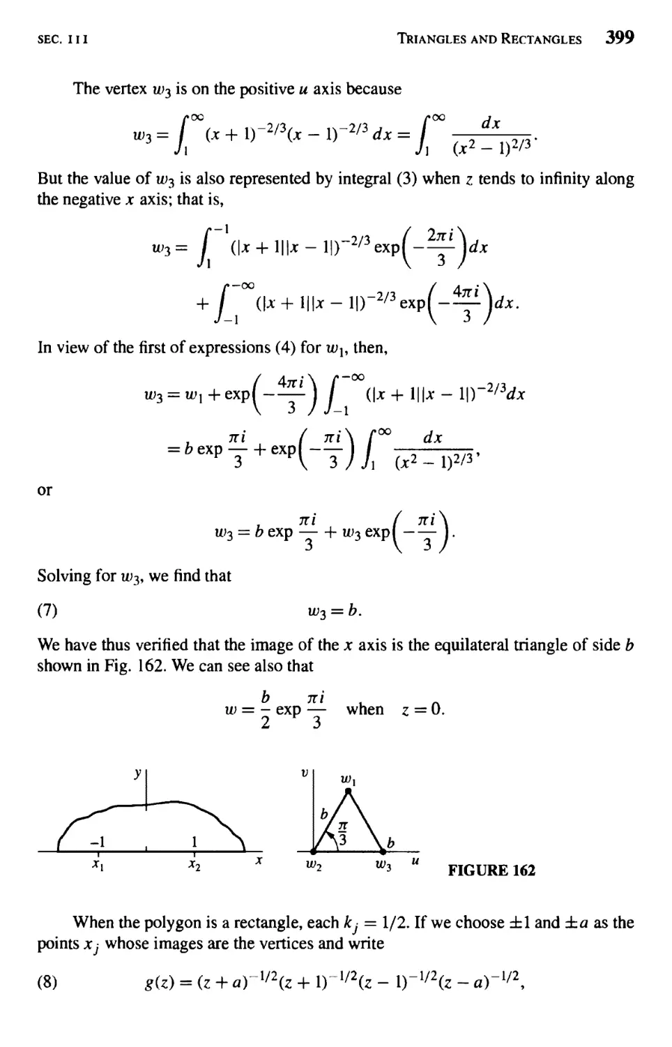
Triangles and Rectangles 397
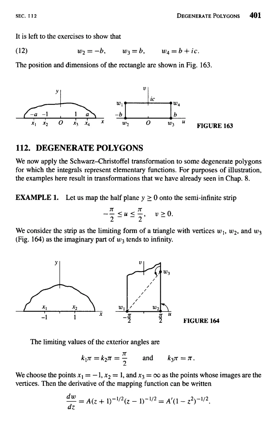
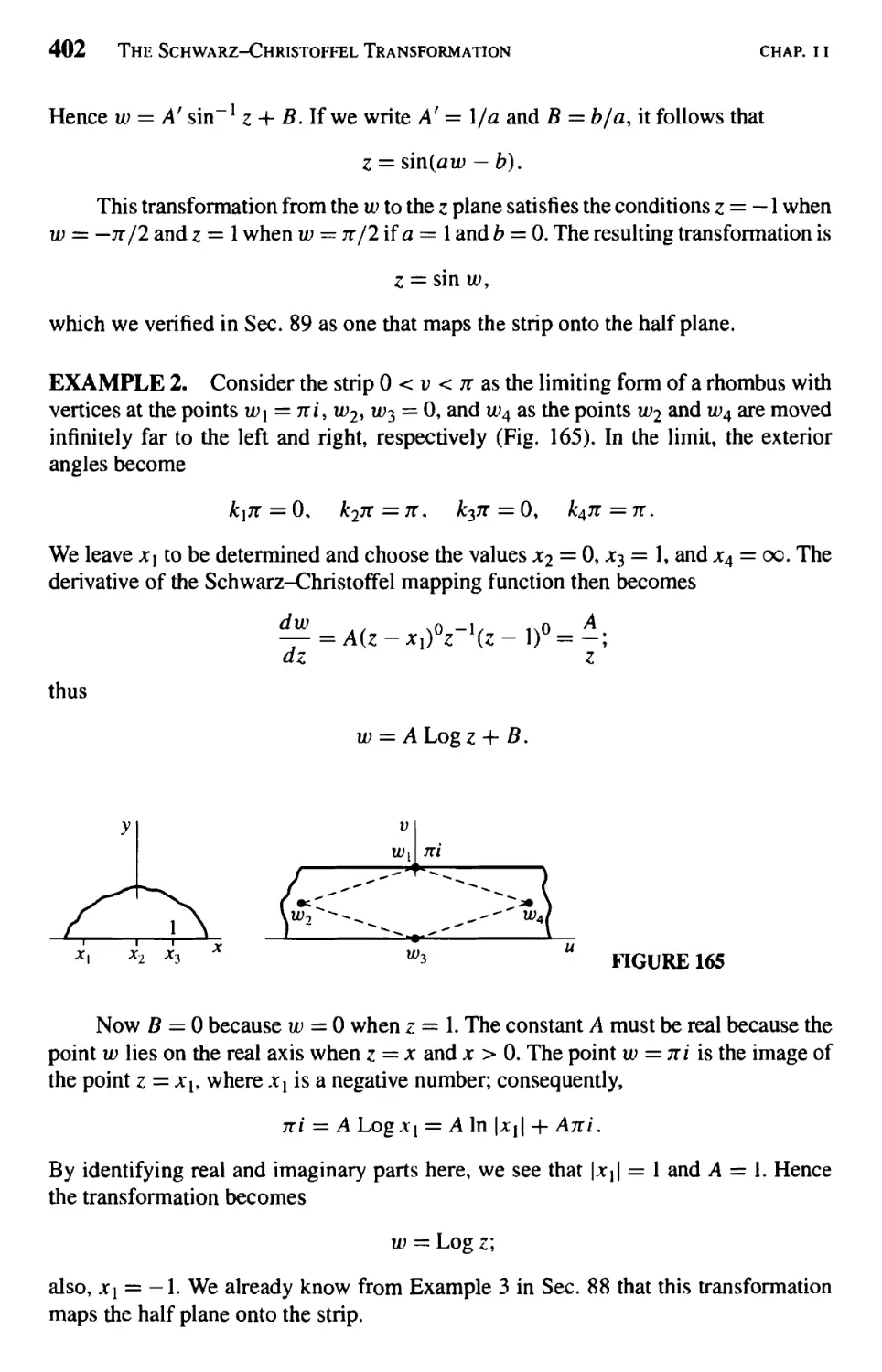
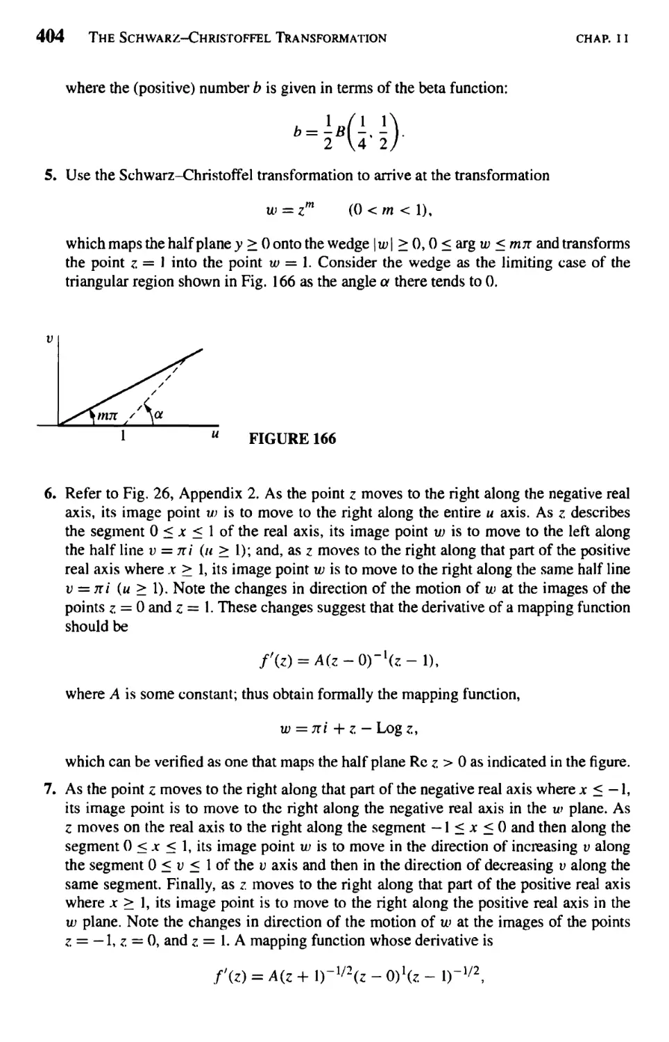
Degenerate Polygons 401
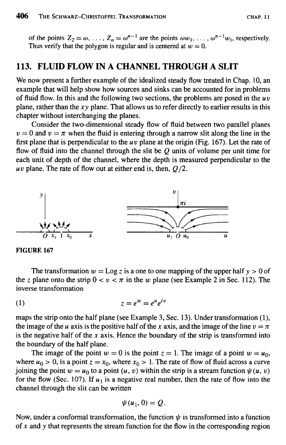
Fluid Flow in a Channel Through a Slit 406
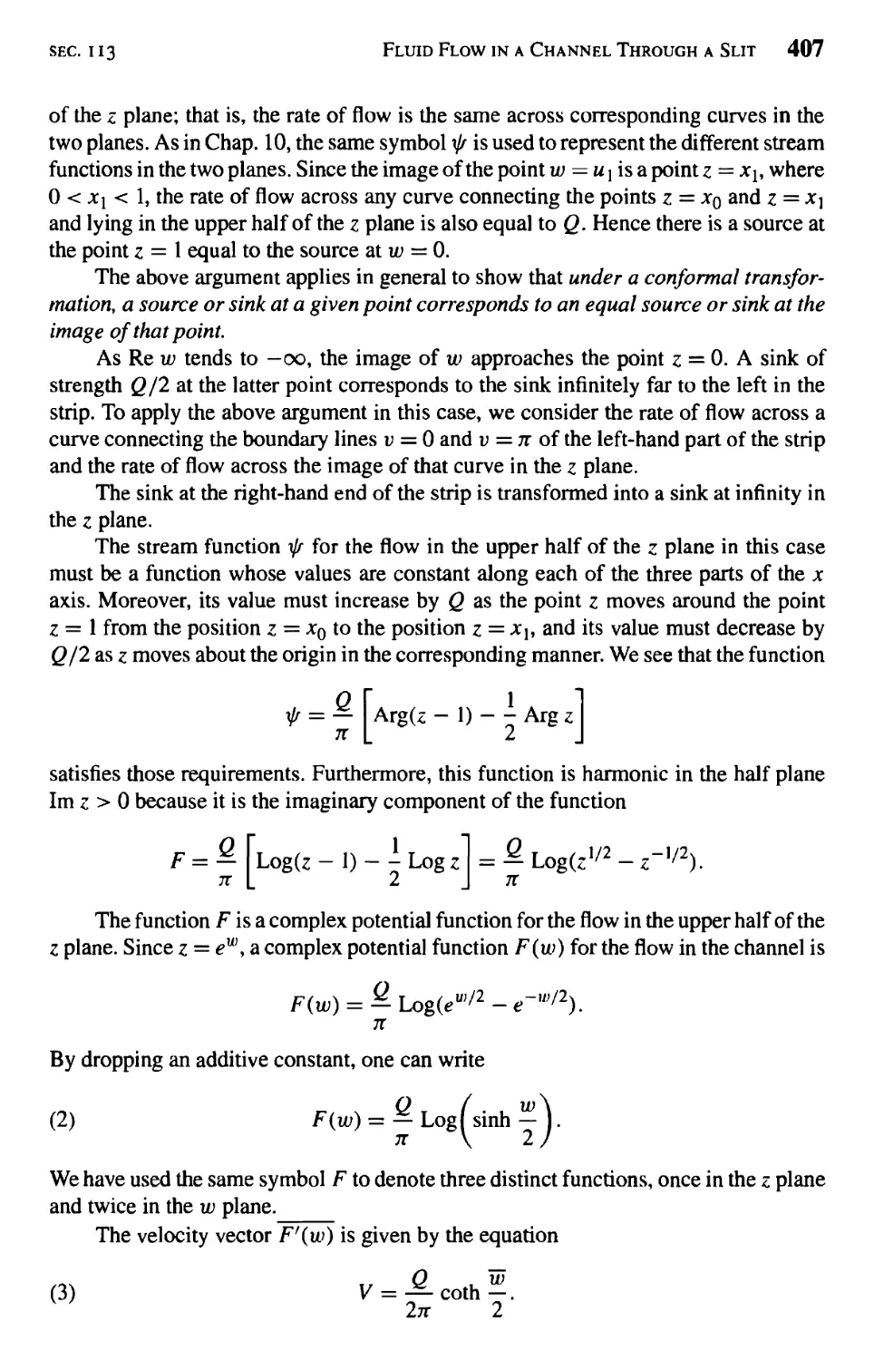
Flow in a Channel with an Offset 408
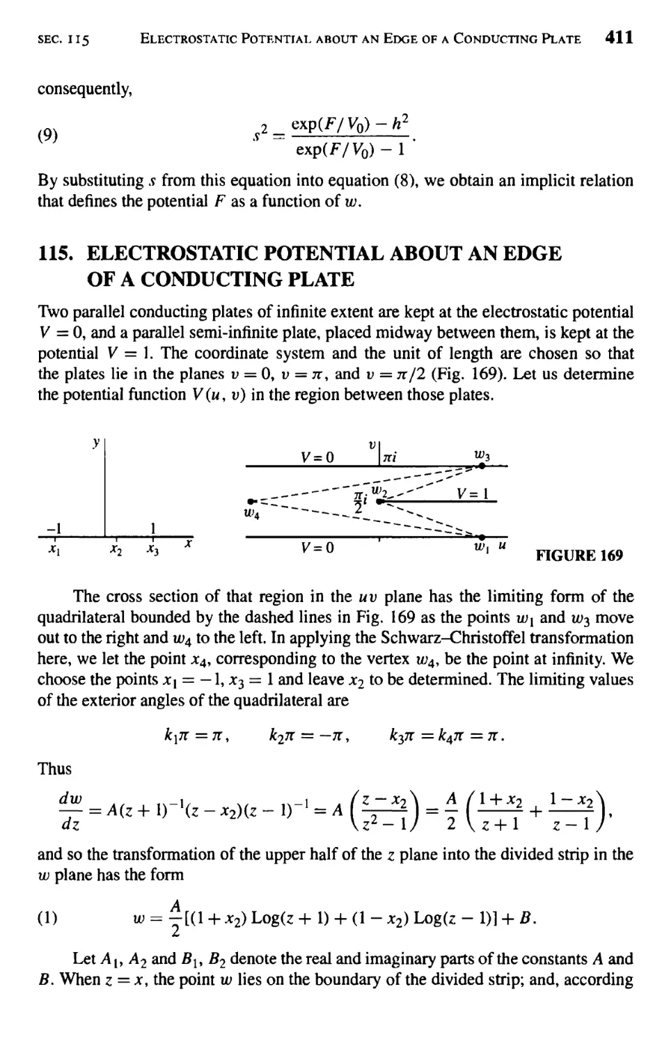
Electrostatic Potential about an Edge of a Conducting Plate 411
12 Integral Formulas of the Poisson Type 417
Poisson Integral Formula 417
Dirichlet Problem for a Disk 419
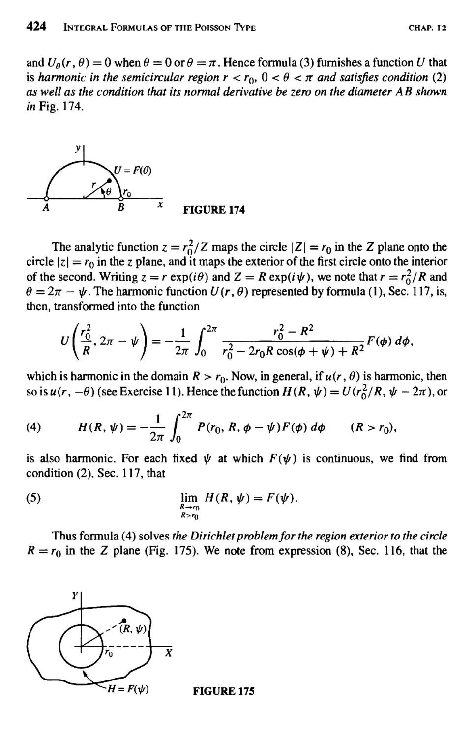
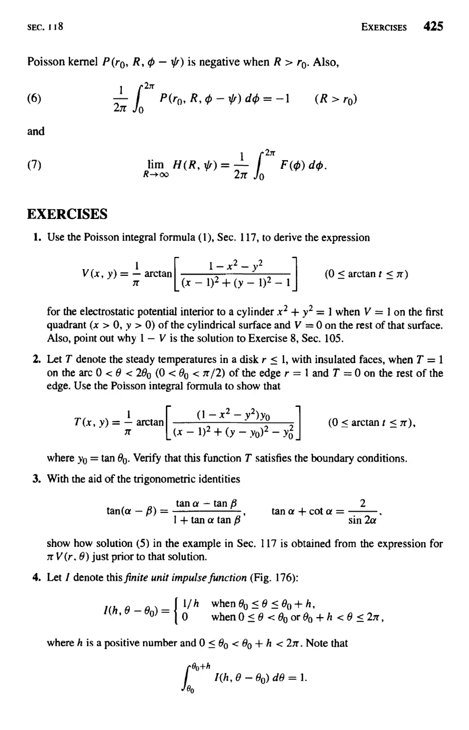
Related Boundary Value Problems 423
Schwarz Integral Formula 427
Dirichlet Problem for a Half Plane 429
Neumann Problems 433
Appendixes 437
Bibliography 437
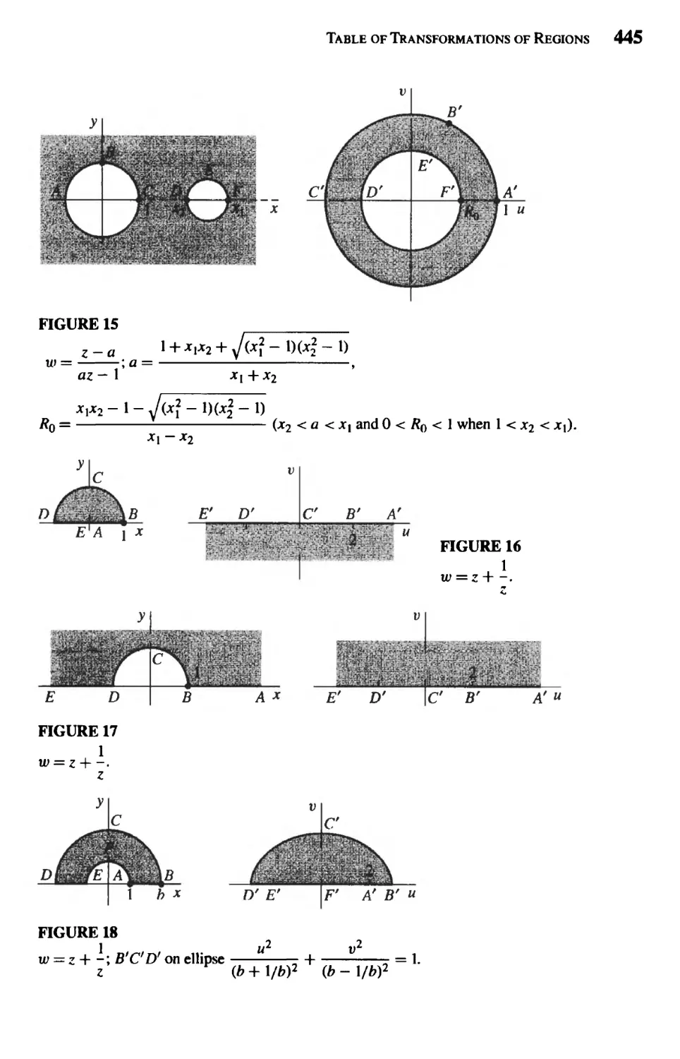
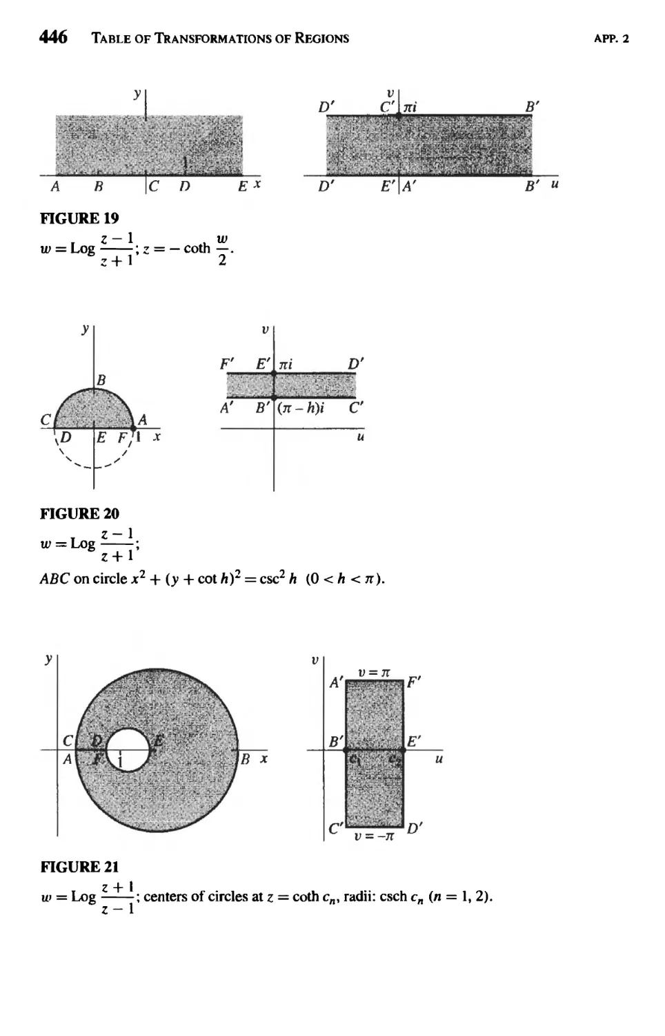
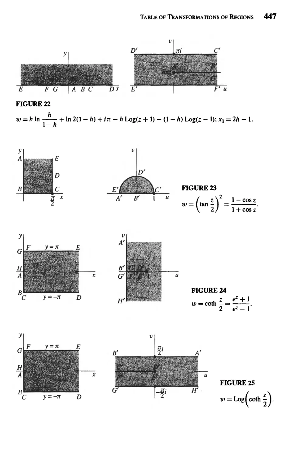
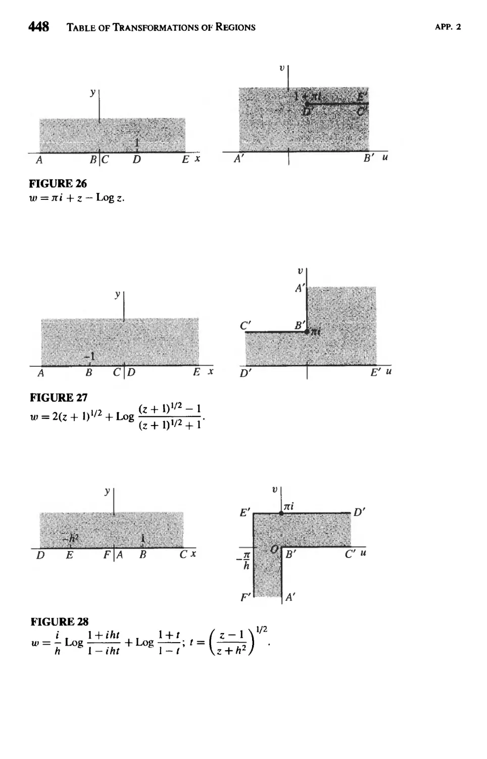
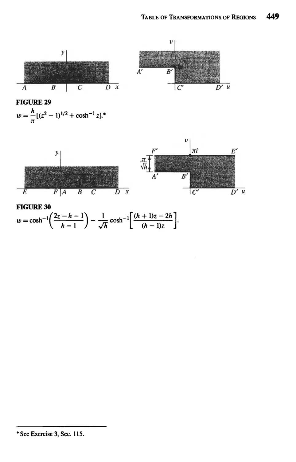
Table of Transformations of Regions 441
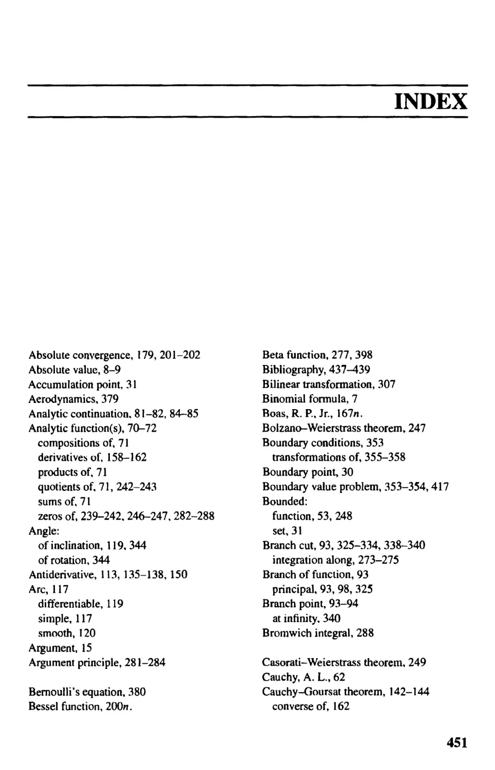
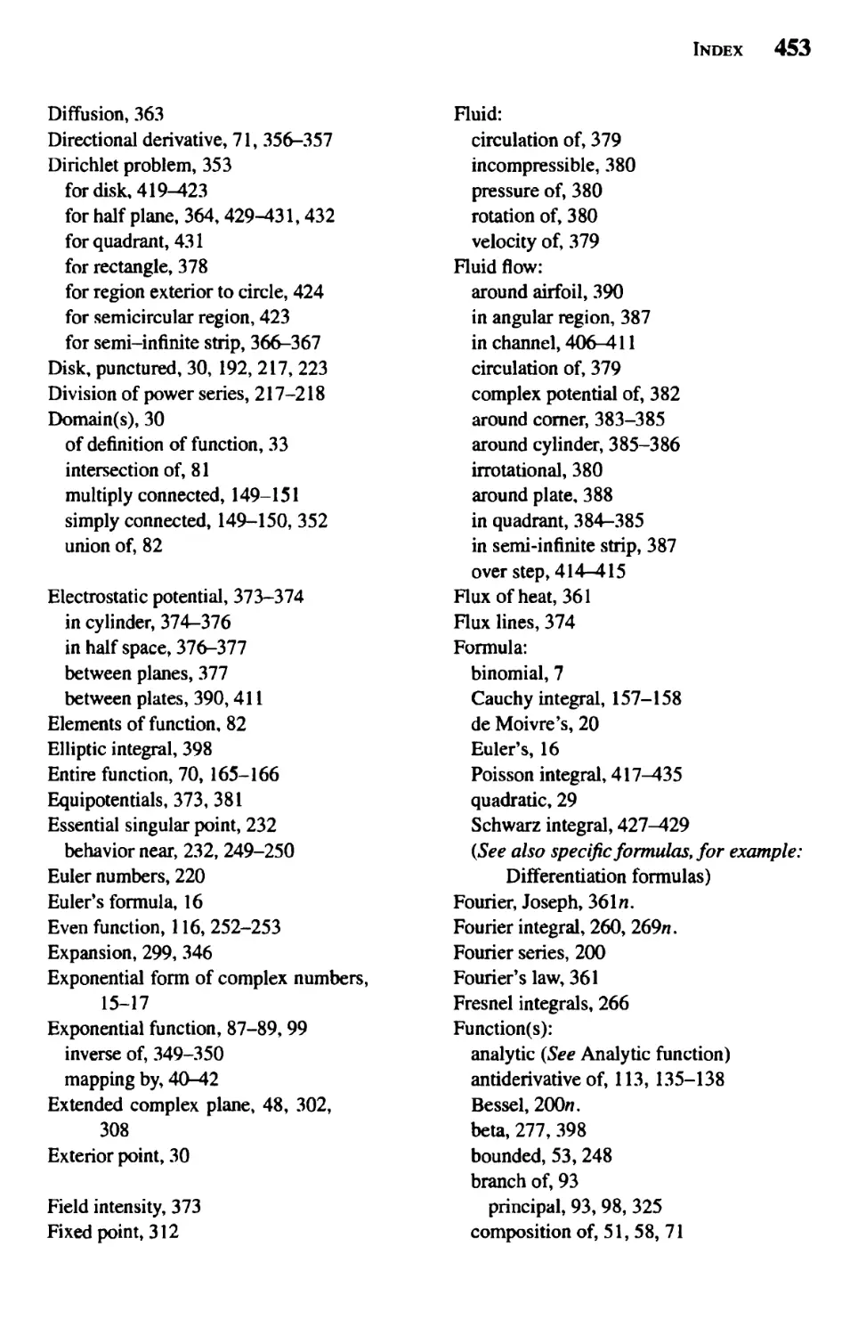
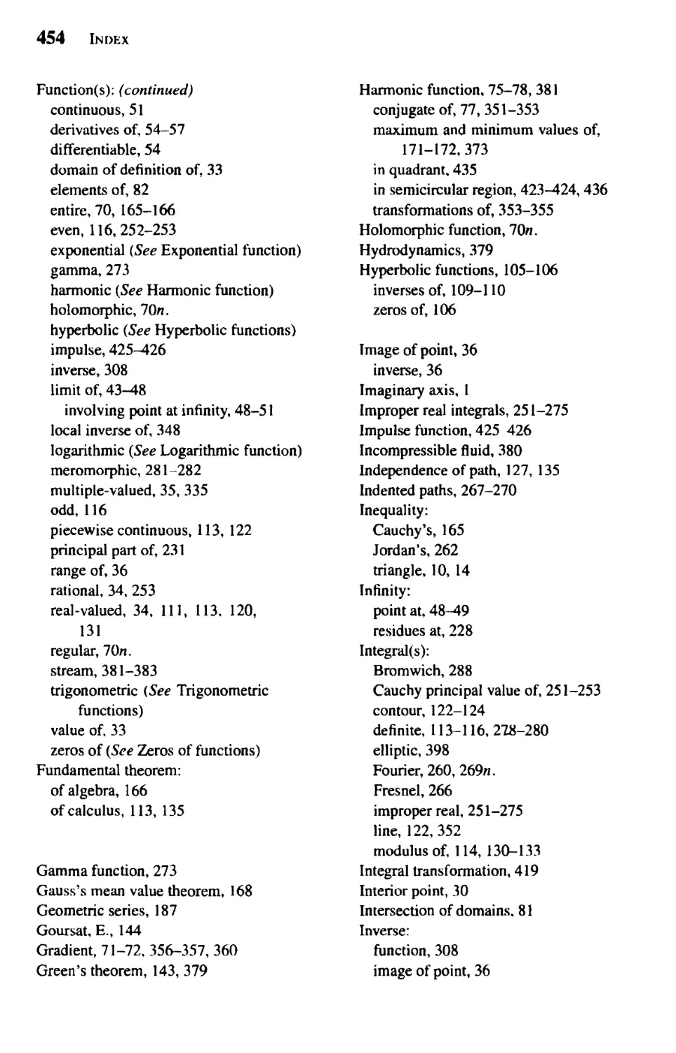
Index 451
PREFACE
This book is a revision of the sixth edition, published in 1996. That edition has served,
just as the earlier ones did, as a textbook for a one-term introductory course in the
theory and application of functions of a complex variable. This edition preserves the
basic content and style of the earlier editions, the first two of which were written by
the late Ruel V. Churchill alone.
In this edition, the main changes appear in the first nine chapters, which make up
the core of a one-term course. The remaining three chapters are devoted to physical
applications, from which a selection can be made, and are intended mainly for self-
study or reference.
Among major improvements, there are thirty new figures; and many of the old
ones have been redrawn. Certain sections have been divided up in order to emphasize
specific topics, and a number of new sections have been devoted exclusively to
examples. Sections that can be skipped or postponed without disruption are more clearly
identified in order to make more time for material that is absolutely essential in a first
course, or for selected applications later on. Throughout the book, exercise sets occur
more often than in earlier editions. As a result, the number of exercises in any given
set is generally smaller, thus making it more convenient for an instructor in assigning
homework.
As for other improvements in this edition, we mention that the introductory
material on mappings in Chap. 2 has been simplified and now includes mapping
properties of the exponential function. There has been some rearrangement of material
in Chap. 3 on elementary functions, in order to make the flow of topics more natural.
Specifically, the sections on logarithms now directly follow the one on the exponential
xv
xvi Preface
function; and the sections on trigonometric and hyberbolic functions are now closer
to the ones on their inverses. Encouraged by comments from users of the book in the
past several years, we have brought some important material out of the exercises and
into the text. Examples of this are the treatment of isolated zeros of analytic functions
in Chap. 6 and the discussion of integration along indented paths in Chap. 7.
The first objective of the book is to develop those parts of the theory which
are prominent in applications of the subject. The second objective is to furnish an
introduction to applications of residues and conformai mapping. Special emphasis
is given to the use of conformai mapping in solving boundary value problems that
arise in studies of heat conduction, electrostatic potential, and fluid flow. Hence the
book may be considered as a companion volume to the authors' "Fourier Series and
Boundary Value Problems" and Ruel V. Churchill's "Operational Mathematics," where
other classical methods for solving boundary value problems in partial differential
equations are developed. The latter book also contains further applications of residues
in connection with Laplace transforms.
This book has been used for many years in a three-hour course given each term at
The University of Michigan. The classes have consisted mainly of seniors and graduate
students majoring in mathematics, engineering, or one of the physical sciences. Before
taking the course, the students have completed at least a three-term calculus sequence,
a first course in ordinary differential equations, and sometimes a term of advanced
calculus. In order to accommodate as wide a range of readers as possible, there are
footnotes referring to texts that give proofs and discussions of the more delicate results
from calculus that are occasionally needed. Some of the material in the book need not
be covered in lectures and can be left for students to read on their own. If mapping
by elementary functions and applications of conformai mapping are desired earlier
in the course, one can skip to Chapters 8, 9, and 10 immediately after Chapter 3 on
elementary functions.
Most of the basic results are stated as theorems or corollaries, followed by
examples and exercises illustrating those results. A bibliography of other books,
many of which are more advanced, is provided in Appendix 1. A table of conformai
transformations useful in applications appears in Appendix 2.
In the preparation of this edition, continual interest and support has been provided
by a number of people, many of whom are family, colleagues, and students. They
include Jacqueline R. Brown, Ronald P. Morash, Margret H. Höft, Sandra M. Weber,
Joyce A. Moss, as well as Robert E. Ross and Michelle D. Munn of the editorial staff
at McGraw-Hill Higher Education.
James Ward Brown
COMPLEX VARIABLES AND APPLICATIONS
CHAPTER
î
COMPLEX NUMBERS
In this chapter, we survey the algebraic and geometric structure of the complex number
system. We assume various corresponding properties of real numbers to be known.
1. SUMS AND PRODUCTS
Complex numbers can be defined as ordered pairs (jc, y) of real numbers that are to
be interpreted as points in the complex plane, with rectangular coordinates x and y,
just as real numbers x are thought of as points on the real line. When real numbers
x are displayed as points (x, 0) on the real axis, it is clear that the set of complex
numbers includes the real numbers as a subset. Complex numbers of the form (0, >•)
correspond to points on the y axis and are called pure imaginary numbers. The y axis
is, then, referred to as the imaginary axis.
It is customary to denote a complex number (x, y) by z, so that
(1) z = (x9y).
The real numbers x and y are, moreover, known as the real and imaginary parts of z,
respectively; and we write
(2) Rcz=x, Imz = >\
Two complex numbers z\ = (x{, yj) and z2 = 0*2» yi) are eclua' whenever they have
the same real parts and the same imaginary parts. Thus the statement Z\ = Zi means
that Z\ and z-i correspond to the same point in the complex, or z, plane.
1
2 Complex Numbers
chap. I
The sum z\ + z2 and the product z\Z2 of two complex numbers z\ = (jtlf y{) and
z2 = (x2, y2) Me defined as follows:
(3) (*i, yi) + (x2, y2) = (*i + x2. Vi + y2),
(4) (*i, yi)(x2, y2) = (x,x2 - y^, yxx2 + *iy2).
Note that the operations defined by equations (3) and (4) become the usual operations
of addition and multiplication when restricted to the real numbers:
(jcll0) + U2»0) = (jc1+Jc2,0)f
(jcb0)(jc2,0) = (jc1jc2,0).
The complex number system is, therefore, a natural extension of the real number
system.
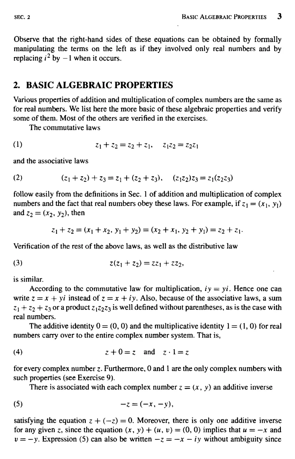
Any complex number z = (x, y) can be written z = (x, 0) + (0, y), and it is easy
to see that (0, l)(y, 0) = (0, y). Hence
z = (jc,0) + (0,l)(y,0);
and, if we think of a real number as either x or (x, 0) and let i denote the imaginary
number (0, 1) (see Fig. 1), it is clear that*
(5) Z = *+!>.
Also, with the convention z2 = zz, z3 = zz2, etc., we find that
i2 = (0,1)(0,1) = (-1,0),
or
(6) i2 = -l.
• z = (*, y)
* = (0,1)
Ol x = (*,()) x FIGURE 1
In view of expression (5), definitions (3) and (4) become
(7) (x, +1>,) + U2 + *y2) = (xi + x2) + i(yx + y2),
(8) (xi + iyi)(x2 + iy2) = (*i*2 - vi^) + '(^1^2 + *iV2)-
* In electrical engineering, the letter j is used instead of 1.
SEC. 2
Basic Algebraic Properties 3
Observe that the right-hand sides of these equations can be obtained by formally
manipulating the terms on the left as if they involved only real numbers and by
replacing i2 by -1 when it occurs.
2. BASIC ALGEBRAIC PROPERTIES
Various properties of addition and multiplication of complex numbers are the same as
for real numbers. We list here the more basic of these algebraic properties and verify
some of them. Most of the others are verified in the exercises.
The commutative laws
(1) Z] + Z2 = Z2 + Zu Z[Z2 = Z2Z\
and the associative laws
(2) (z\ + z2) + z3 = z\ + (z2 + z3), (z.\z2)z3 = -1(^2-3)
follow easily from the definitions in Sec. 1 of addition and multiplication of complex
numbers and the fact that real numbers obey these laws. For example, if z\ = (x{i yj)
and z2 = (x2,y2), then
-1 + z2 = U, + x2, y\ + y2) = (*2 + x\* >?2 + y\) = -2 + *i-
Verification of the rest of the above laws, as well as the distributive law
(3) z(z\ + z2) = zz.\ + zz2,
is similar.
According to the commutative law for multiplication, iy = yi. Hence one can
write z = x + yi instead of z = x + iy. Also, because of the associative laws, a sum
Z\ + z2 + z$ or a product z[Z2z$ is well defined without parentheses, as is the case with
real numbers.
The additive identity 0 = (0, 0) and the multiplicative identity 1 = (1, 0) for real
numbers carry over to the entire complex number system. That is,
(4) z + 0 = : and z-l = z
for every complex number z. Furthermore, 0 and 1 are the only complex numbers with
such properties (see Exercise 9).
There is associated with each complex number z = (a*, y) an additive inverse
(5) -* = (-*,->'),
satisfying the equation z + (—z) = 0. Moreover, there is only one additive inverse
for any given z, since the equation (jc, y) + (w, v) = (0, 0) implies that u = — x and
v = —y. Expression (5) can also be written — z = — x — iy without ambiguity since
4 Complex Numbers
chap. I
(Exercise 8) — (iy) = (—i)y = /(—y). Additive inverses are used to define subtraction:
(6) Z\-z2 = Zi + (-z2).
So if z\ = Oi, y\) and z2 = (*2> yi)> ^m
(7) Z\-z2 = (x\ - x2, y\ - y2) = (xx - x2) + i(yx - y2).
For any nonzero complex number z = U, y), there is a number z"1 such that
zz"x = 1. This multiplicative inverse is less obvious than the additive one. To find it,
we seek real numbers u and u, expressed in terms of x and y, such that
(*,y)(«,i;) = (l,0).
According to equation (4), Sec. 1, which defines the product of two complex numbers,
u and v must satisfy the pair
xu — yv = 1, yu + xv = 0
of linear simultaneous equations; and simple computation yields the unique solution
x -y
x2 + y2 jc2 + y2
So the multiplicative inverse of z = (x, y) is
(8) r1 = f-r^-r. -r^-r) <* * °>-
\JC2 + y2 *2 + y2/
The inverse z~~l is not defined when z = 0. In fact, z = 0 means that x2 + y2 = 0; and
this is not permitted in expression (8).
EXERCISES
1. Verify that
(a) {y/2-i) - i(l - y/2i) = -2i; (6) (2, -3)<-2, 1) = (-1, 8);
(c)(3, i)(3,-l)Qf-l)==(2, 1).
2. Show that
(a) Re(iz) = - Im z; (ft) Im(iz) = Re z.
3. Show that (1+ z)2 = 1 4- 2z 4- z2.
4. Verify that each of the two numbers z = 1 ± i satisfies the equation z2 — 2z 4- 2 = 0.
5. Prove that multiplication is commutative, as stated in the second of equations (1 ), Sec. 2.
6. Verify
(a) the associative law for addition, stated in the first of equations (2), Sec. 2;
(ft) the distributive law (3), Sec. 2.
SEC. 3
Further Properties 5
7. Use the associative law for addition and the distributive law to show that
z(Z\ + Z2 + £3) = ZZ\ + Z.Z2 + ZZ3.
8. By writing i = (0, 1) and y = (y\ 0), show that -(/>') = ( i)y = /(->')•
9. (a) Write (x, y) 4- (w, iô = (jc, >') and point out how it follows that the complex number
0 = (0, 0) is unique as an additive identity.
(b) Likewise, write (x, y)(u,v) = (x, v) and show that the number 1 = ( 1, 0) is a unique
multiplicative identity.
10. Solve the equation v + z + 1 = 0 for z = (x, y) by writing
(*, y)(x. y) + (jc, y) + (h 0) = (0, 0)
and then solving a pair of simultaneous equations in x and v.
Suggestion: Use the fact that no real number x satisfies the given equation to show
that y jL 0.
Ans.z= I --,± — I
■■(-a-?)
3. FURTHER PROPERTIES
In this section, we mention a number of other algebraic properties of addition and
multiplication of complex numbers that follow from the ones already described in
Sec. 2. Inasmuch as such properties continue to be anticipated because they also apply
to real numbers, the reader can easily pass to Sec. 4 without serious disruption.
We begin with the observation that the existence of multiplicative inverses enables
us to show that if a product z\Z% is zero, then so is at least one of the factors z\ and
Z2> For suppose that Z\Zi = 0 and z\ ^ 0. The inverse z\x exists; and, according to the
definition of multiplication, any complex number times zero is zero. Hence
That is, if Z\Zi = 0, either z\ = 0 or z? = 0; or possibly both z\ and z2 equal zero.
Another way to state this result is that if two complex numbers z\ and e2 cire nonzero,
then so is their product z\Z.2-
Division by a nonzero complex number is defined as follows:
(1) -=W iz2*0).
Uz\ = U1? y{) and z.i — (*2> V2)' equation (1) here and expression (8) in Sec. 2 tell us
that
— ^ I • /1/ I t, t> •> 2 I I 2. 2 '
yxx2 - xxy2
xl + yl ,
6 Complex Numbers
chap. I
That is,
m Zl -*i*2 + yiy2 , .yjxi-xjyi (y ,m
U) — = n 5 rl 5 5— tor^).
Z2 *£ + >'2 *2 + >2
Although expression (2) is not easy to remember, it can be obtained by writing (see
Exercise 7)
(3) £i = (xl + iyl)(x2-iy2)
Z2 {x2 + iy2){x2-iy2Y
multiplying out the products in the numerator and denominator on the right, and then
using the property
(4) £l±£2 = (Z1 + Z2)z-i = ZxZ-i + ZlZ-i = ZA + ZA (Z3 ^ o).
*3 Z3 *3
The motivation for starting with equation (3) appears in Sec. 5.
There are some expected identities, involving quotients, that follow from the
relation
(5) -=-2l (z2*0),
Zl
which is equation (1) when z\ = 1. Relation (5) enables us, for example, to write
equation (1) in the form
(6) -=*i(-) (*2*0).
z2 \z2J
Also, by observing that (see Exercise 3)
Uiz2)(*r V) = (ziz^l)(z2Z2l) = 1 izi£ 0, z2 £ 0),
and hence that (z\Z2)~l = z^lz2l< one can use relation (5) to show that
(7) -L = (Z]z2rl = zj" V = (-)(-) {zi *0,z2£0).
Another useful identity, to be derived in the exercises, is
(8) £i£ = (V)/V) ( ^ ^
Z3Z4 \Z3/\Z4/
SEC. 3
Exercises 7
EXAMPLE. Computations such as the following are now justified:
/ 1 \/ 1 \ _ 1 = _1_ 5+J_ = 5 + /
\2-3i)\l + i) " (2-3î)(l + i) ~ 5 — i " 5 + i — (5-/)(5 + /)
26 ~26 + 26~26 + 26*'
Finally, we note that the binomial formula involving real numbers remains valid
with complex numbers. That is, if z\ and z2 are any two complex numbers,
(9)
where
(n\ _ »!
\k) k\{n-k)\
A
(* = 0, 1,2, ...,*)
and where it is agreed that 0! = 1. The proof, by mathematical induction, is left as an
exercise.
EXERCISES
1. Reduce each of these quantities to a real number:
,1 + 2/2-/ /IX 5/ , x ,■ .*
(«)r—TT + -T—; <*)-—— tt:—-; c) 1-0
3-4/ 5/ (l-i)(2-i)(3-i)
Aiw. (a)-2/5; («-1/2; (c) -4.
2. Show that
1/z
3. Use the associative and commutative laws for multiplication to show that
U1Z2XZ3Z4) = (*1*3)(Z2Z4)-
4. Prove that if Z|Z2Z3 = 0, then at least one of the three factors is zero.
Suggestion: Write (z\Z2)zs = 0 and use a similar result (Sec. 3) involving two
factors.
5. Derive expression (2), Sec. 3, for the quotient Z\jz2 by the method described just after
it.
6. With the aid of relations (6) and (7) in Sec. 3, derive identity (8) there.
7. Use identity (8) in Sec. 3 to derive the cancellation law:
£i£ = £i (z27feo,z^O).
Z2Z Z2
8 Complex Numbers
chap. I
8. Use mathematical induction to verify the binomial formula (9) in Sec. 3. More precisely,
note first that the formula is true when n = 1. Then, assuming that it is valid when n = m
where m denotes any positive integer, show that it must hold when n = m + 1.
4. MODULI
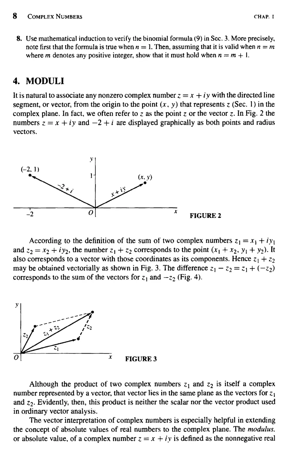
It is natural to associate any nonzero complex number z = x + iy with the directed line
segment, or vector, from the origin to the point (jc, y) that represents z (Sec. 1) in the
complex plane. In fact, we often refer to z as the point z or the vector z. In Fig. 2 the
numbers z = x + iy and —2 + / are displayed graphically as both points and radius
vectors.
(-2,1)
-2
y
1-
0
X
FIGURE 2
According to the definition of the sum of two complex numbers Z\ — X\ + iy\
and Z2 = *2 + iyi-> ^e number Zj + ^ corresponds to the point (x{ + x2, )>i 4- ^2)- ft
also corresponds to a vector with those coordinates as its components. Hence Z\ + z.i
may be obtained vectorially as shown in Fig. 3. The difference z.\ — Zi = Z\ + (-Zj)
corresponds to the sum of the vectors for Z\ and —z2 (Fig. 4).
x FIGURE 3
Although the product of two complex numbers z\ and z2 ^s itself a complex
number represented by a vector, that vector lies in the same plane as the vectors for z\
and z2- Evidently, then, this product is neither the scalar nor the vector product used
in ordinary vector analysis.
The vector interpretation of complex numbers is especially helpful in extending
the concept of absolute values of real numbers to the complex plane. The modulus,
or absolute value, of a complex number z = x + iy is defined as the nonnegative real
SEC. 4
Moduli 9
FIGURE 4
number y/x2 + y2 and is denoted by |z|; that is,
(1) \z\ = y/x* + y*.
Geometrically, the number \z\ is the distance between the point (jc, y) and the origin,
or the length of the vector representing z. It reduces to the usual absolute value in the
real number system when y = 0. Note that, while the inequality z\ < z2 is meaningless
unless bothzi and z2 ara i*Q>U the statement \z\\ < |z2| means that the point Z\ is closer
to the origin than the point z2 is.
EXAMPLE 1. Since | - 3 + 2/1 = VT3 and 11 + 4i | = VT7, the point -3 + 2/ is
closer to the origin than 1 + 4/ is.
The distance between two points z\ = xx + iy\ and z2 = *2 + ^2 *s \z1 — z2 I. "This
is clear from Fig. 4, since |zi - z2| *s the length of the vector representing z\ — z2; and,
by translating the radius vector z\ — z2, one can interpret z.\ — z2 as the directed line
segment from the point (*2, y2) to the point (xh y{). Alternatively, it follows from the
expression
Z] - z2 = Ui - x2) + i(y\ - >2)
and definition (1) that
ki - z2\ = \/(*i - *2)2 + (yi - V2)2.
The complex numbers z corresponding to the points lying on the circle with center
Zo and radius R thus satisfy the equation \z — Zol = R> and conversely. We refer to this
set of points simply as the circle \z — Zol = R
EXAMPLE 2. The equation \z - 1 + 3i | = 2 represents the circle whose center is
Zo = (1, —3) and whose radius is R = 2.
It also follows from definition (1) that the real numbers \z |, Re z = x, and Im z = y
are related by the equation
(2) |z|2 = (Rez)2 + (Imz)2.
10 Complex Numbers
chap. I
Thus
(3) Rez < |Rez\ < \z\ and Imz< |Im z\ < \z\.
We turn now to the triangle inequality, which provides an upper bound for the
modulus of the sum of two complex numbers z.\ and z2:
(4) Izi+z2l<kil + lz2l.
This important inequality is geometrically evident in Fig. 3, since it is merely a
statement that the length of one side of a triangle is less than or equal to the sum
of the lengths of the other two sides. We can also see from Fig. 3 that inequality (4)
is actually an equality when 0, z\, and z2 are collinear. Another, strictly algebraic,
derivation is given in Exercise 16, Sec. 5.
An immediate consequence of the triangle inequality is the fact that
(5) l*i+z2l>lkil-tail-
To derive inequality (5), we write
\Z\\ = |(Z 1 + Z2) + (-Z2)\ < 1*1 + Z2\ + I - Z2U
which means that
(6) l*l+Z2l>N-|*2l.
This is inequality (5) when \z\\ > \z2\- If \z\\ < \z2\, we need only interchange z.\ and
z2 in inequality (6) to get
ki + z2l>-(kil-U2l).
which is the desired result. Inequality (5) tells us, of course, that the length of one side
of a triangle is greater than or equal to the difference of the lengths of the other two
sides.
Because |— z2\ — \z2\, one can replace z2 by — z2 in inequalities (4) and (5) to
summarize these results in a particularly useful form:
(7) l*|±Z2l<N + IZ2l.
(8) ki±z2l>IN-lz2ll-
EXAMPLE 3. If a point z lies on the unit circle \z\ = 1 about the origin, then
k-2|<|*|+2 = 3
and
|z-2|>||z|-2| = l.
SEC. 5
Complex Conjugates 11
The triangle inequality (4) can be generalized by means of mathematical
induction to sums involving any finite number of terms:
(9) \z{ + z2 + • • • + zn\ < Uil + k21 + • • ' + \zn\ (n = 2, 3, ...).
To give details of the induction proof here, we note that when n = 2, inequality (9) is
just inequality (4). Furthermore, if inequality (9) is assumed to be valid when n = m,
it must also hold when n = m + 1 since, by inequality (4),
|(*i + z2 + -- + zm) + zw+il <\zi + z2 + -- + zm\ + |zw+il
Zm+\\*
EXERCISES
1. Locate the numbers z\ + z2 and Zi — z2 vectorially when
(a) zx = 2/, z2 = | - f ; (b) z, = (->/3, 1), z2 = (V§, 0);
(c) z\ = (~3, 1), z2 = (l,4); W)zi=jci + i>i, 22 = *i-'.Vi.
2. Verify inequalities (3), Sec. 4, involving Re z, Im z, and |z|.
• 3, Verify that V2!z|>|Rez|+ |Imz|.
Suggestion: Reduce this inequality to (|jc| - |y|)2 > 0.
4. In each case, sketch the set of points determined by the given condition:
(a) \z - 1 + 11 = 1; (b) \z + /1 < 3; (c) |z - 4i| > 4.
5. Using the fact that \z \ — z2 | is the distance between two points z \ and z2, give a geometric
argument that
(a) \z — 4/1 + |z + 4/1 = 10 represents an ellipse whose foci are (0, ±4);
(b) \z - 1| = \z + i\ represents the line through the origin whose slope is —1.
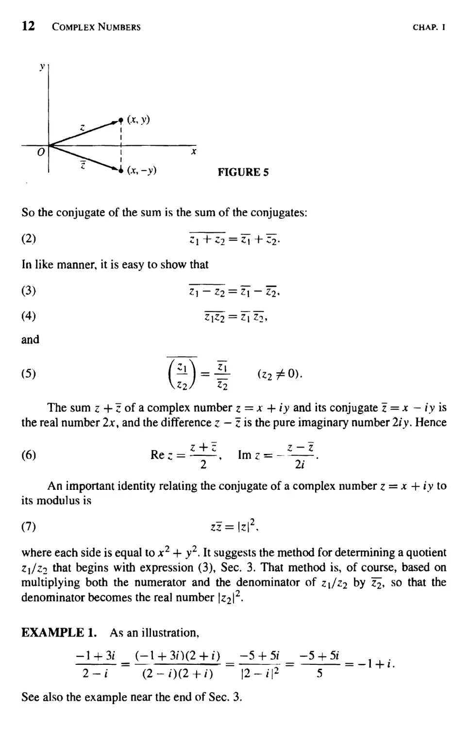
5. COMPLEX CONJUGATES
The complex conjugate, or simply the conjugate, of a complex number z = x + iy is
defined as the complex number x — iy and is denoted by z; that is,
(1) z=x-iy.
The number z is represented by the point (x, — y), which is the reflection in the real
axis of the point (x, y) representing z (Fig. 5). Note that
z = z and |z| = \z\
for all z.
If Z\=x{ + iyl and z2 = x2 + iy2, then
zTTTô = (*\ + xi) - t(y\ + yi) = (*i - ô>i) + (xi - *>2)-
12 Complex Numbers
char I
So the conjugate of the sum is the sum of the conjugates:
(2) Z\ + Zi = Z\ + ^2*
In like manner, it is easy to show that
(3) Z\ — Z2 — Z\ — Z2«
(4) z&l = z~\zl,
and
(5) (-) = = (^O).
\Z2/ *2
The sum z + z of a complex number z = a; + / j and its conjugate z = jc - /y is
the real number 2a\ and the difference z - z is the pure imaginary number 2iy. Hence
z -\~z z ~-~z
(6) Re^ = ——, Imz = -——.
2 2/
An important identity relating the conjugate of a complex number z = x + iy to
its modulus is
(7) zz = \z\\
where each side is equal to x2 + y2. It suggests the method for determining a quotient
Z\/zi that begins with expression (3), Sec. 3. That method is, of course, based on
multiplying both the numerator and the denominator of z\/z2 by Z2> so that the
denominator becomes the real number |z2l2-
EXAMPLE 1. As an illustration,
-1 + 3/ _ (-1 + 30(2 + 1) _ -5 + 5/ _ -5 + 5/
2-i ~~ (2-/)(2 + /) " |2-/|2 ~ 5
See also the example near the end of Sec. 3.
= -l + i.
sec. 5
Exercises 13
Identity (7) is especially useful in obtaining properties of moduli from properties
of conjugates noted above. We mention that
(8)
and
klZ2l = IZlliZ2l
= M <*2*0).
\Z2\
Property (8) can be established by writing
\z\Z2\2 = (z\z2)(z^) = (ziz2)(TizD = (z{z[)(z2zi) = |zil2|z2l2 = (Iziltal)2
and recalling that a modulus is never negative. Property (9) can be verified in a similar
way.
EXAMPLE 2. Property (8) tells us that |z2| = \z\z and |z3| = |z|3. Hence if z is a
point inside the circle centered at the origin with radius 2, so that \z\ < 2, it follows
from the generalized form (9) of the triangle inequality in Sec. 4 that
\z3 + 3z2 - 2z + 1| < |z|3 + 3|z|2 + 2|z| + 1 < 25.
EXERCISES
1. Use properties of conjugates and moduli established in Sec. 5 to show that
(a) z + 3i = z - 3i; (b) iz = —iv,
(c) (2 +1)2 = 3-4/; (d) |(2z + 5)(V2 - i)\ = V3 |2z + 5|.
2. Sketch the set of points determined by the condition
(a)Re(2-i) = 2; (fr)|2z-i|=4.
3. Verify properties (3) and (4) of conjugates in Sec. 5.
4. Use property (4) of conjugates in Sec. 5 to show that
(a) Tfazj = T\Z~izi; (b)z4 = z*.
5. Verify property (9) of moduli in Sec. 5.
6. Use results in Sec. 5 to show that when z2 and z3 are nonzero,
Uil
(a)
( z\ \_ Z\ .
VZ2Z3/ ZÏZÎ
(b)
<•!
Z2Z3
IZ2IM
7. Use established properties of moduli to show that when |z3| ^ |z4|,
z\ + z2
Z3 + Z4
\Zi\ + \z2\
IIZ3I-IZ4II'
14 Complex Numih:rs
chap. I
8. Show that
|Re(2 + z + ;:3)|<4 when|z|<l.
9. It is shown in Sec. 3 that if Z\Z2 = 0, then at least one of the numbers Z\ and z2 must be
zero. Give an alternative proof based on the corresponding result for real numbers and
using identity (8), Sec. 5.
10. By factoring z4 — 4z2 + 3 into two quadratic factors and then using inequality (8), Sec. 4,
show that if z lies on the circle |z| = 2, then
I 1
|z4-4z2 + 3
11. Prove that
(a) z is real if and only if z = z;
(b) z is either real or pure imaginary if and only if z2 = z2.
12. Use mathematical induction to show that when n = 2, 3, ...,
(a) Z\+Z2 + -- + Zn = T\ + T2 + • • • + Zn\ (b) Z\Z2"'Zn =T\Zi-'Z^.
13. Let ÖQ, fli, a2< . . ., an (n > 1) denote real numbers, and let z be any complex number.
With the aid of the results in Exercise 12, show that
aQ + a}z + a2Z2 H h anzn = aQ + a{z + a2z2 H h anzn.
14. Show that the equation \z — Zq\ = R of a circle, centered at zo with radius /?, can be
written
|z|2-2Refez5) + |20l2 = *2.
15. Using expressions (6), Sec. 5, for Re z and Im z, show that the hyperbola a2 - v2 = 1
can be written
Z2 + Z2 = 2.
16. Follow the steps below to give an algebraic derivation of the triangle inequality (Sec. 4)
|Zl+*2l <IZll + l*2l.
la) Show that
Ul + -2I" = (-1 + Z2)(z[ +Z0)= Z\Z\ + (Z\Z2 + Zi?2> + Z2Z2-
(b) Point out why
z\zi + Z)ii = 2 Re(zi^) < 2|z,||z2|.
(c) Use the results in parts (a) and (b) to obtain the inequality
Ui + z2l2<(kil + k2l)2>
and note hçw the triangle inequality follows.
1
< -
~ 3
SEC. 6
Exponential Form 15
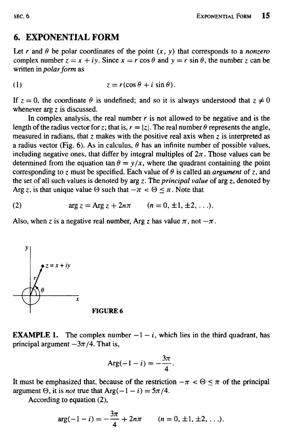
6. EXPONENTIAL FORM
Let r and 9 be polar coordinates of the point (jc, y) that corresponds to a nonzero
complex number z = x + iy. Since x = r cos 9 and v = r sin 9, the number z can be
written in polar form as
(1) z = r(cos8 + i sin#).
If z = 0, the coordinate 0 is undefined; and so it is always understood that z / 0
whenever arg z is discussed.
In complex analysis, the real number r is not allowed to be negative and is the
length of the radius vector for z; that is, r = \z\. The real number 9 represents the angle,
measured in radians, that z makes with the positive real axis when z is interpreted as
a radius vector (Fig. 6). As in calculus, 9 has an infinite number of possible values,
including negative ones, that differ by integral multiples of 2n. Those values can be
determined from the equation tan 9 — y/xy where the quadrant containing the point
corresponding to z must be specified. Each value of 9 is called an argument of z, and
the set of all such values is denoted by arg z. The principal value of arg z, denoted by
Arg z* is that unique value 0 such that — n < 0 < 7r. Note that
(2) arg z = Arg z + 2nix (n = 0, ± 1, ±2,...).
Also, when z is a negative real number, Arg z has value 7r, not — tt.
EXAMPLE L The complex number — 1 - i, which lies in the third quadrant, has
principal argument — in/4. That is,
Arg(-l-/) = -^.
4
It must be emphasized that, because of the restriction -n < 0 < it of the principal
argument 0, it is not true that Arg(— 1 — i) = 5tt/4.
According to equation (2),
arg(-l - i) = -^ + 2njt (n = 0, ±1, ±2, .. .).
4
16 Complex Numbers
chap. I
Note that the term Arg z on the right-hand side of equation (2) can be replaced by any
particular value of arg z and that one can write, for instance,
5n
arg(-l - i) = — + 2/iTT (n = 0, ±1, ±2,...).
4
(3)
The symbol ew, or exp(*0), is defined by means of Eider's formula as
el7* = cos0 + /sin0,
where 6 is to be measured in radians. It enables us to write the polar form (1) more
compactly in exponential form as
(4)
z = re
io
The choice of the symbol el9 will be fully motivated later on in Sec. 28. Its use in Sec.
7 will, however, suggest that it is a natural choice.
EXAMPLE 2. The number — 1 — /in Example 1 has exponential form
(5) -l-« = ^«p[»(-^)].
With the agreement that e~~lB = e^~e\ this can also be written — 1 — / = y/2e~,3n/4.
Expression (5) is, of course, only one of an infinite number of possibilities for the
exponential form of — 1 — i:
(6)
-1-/ = a/2
exp
['(-T—)]
(n = 0,±1,±2....)-
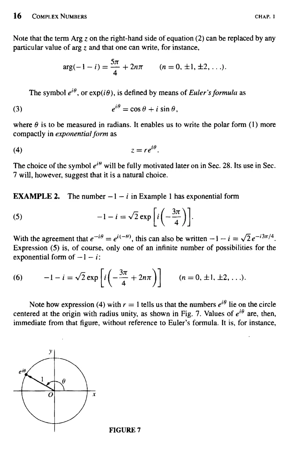
Note how expression (4) with r = 1 tells us that the numbers e'9 lie on the circle
centered at the origin with radius unity, as shown in Fig. 7. Values of e'e are, then,
immediate from that figure, without reference to Euler's formula. It is, for instance,
0\
FIGURE 7
SEC. 7
Products and Quotients in Exponential Form 17
geometrically obvious that
^ = -1, e-in'2 = -i9 and e~i4n = 1.
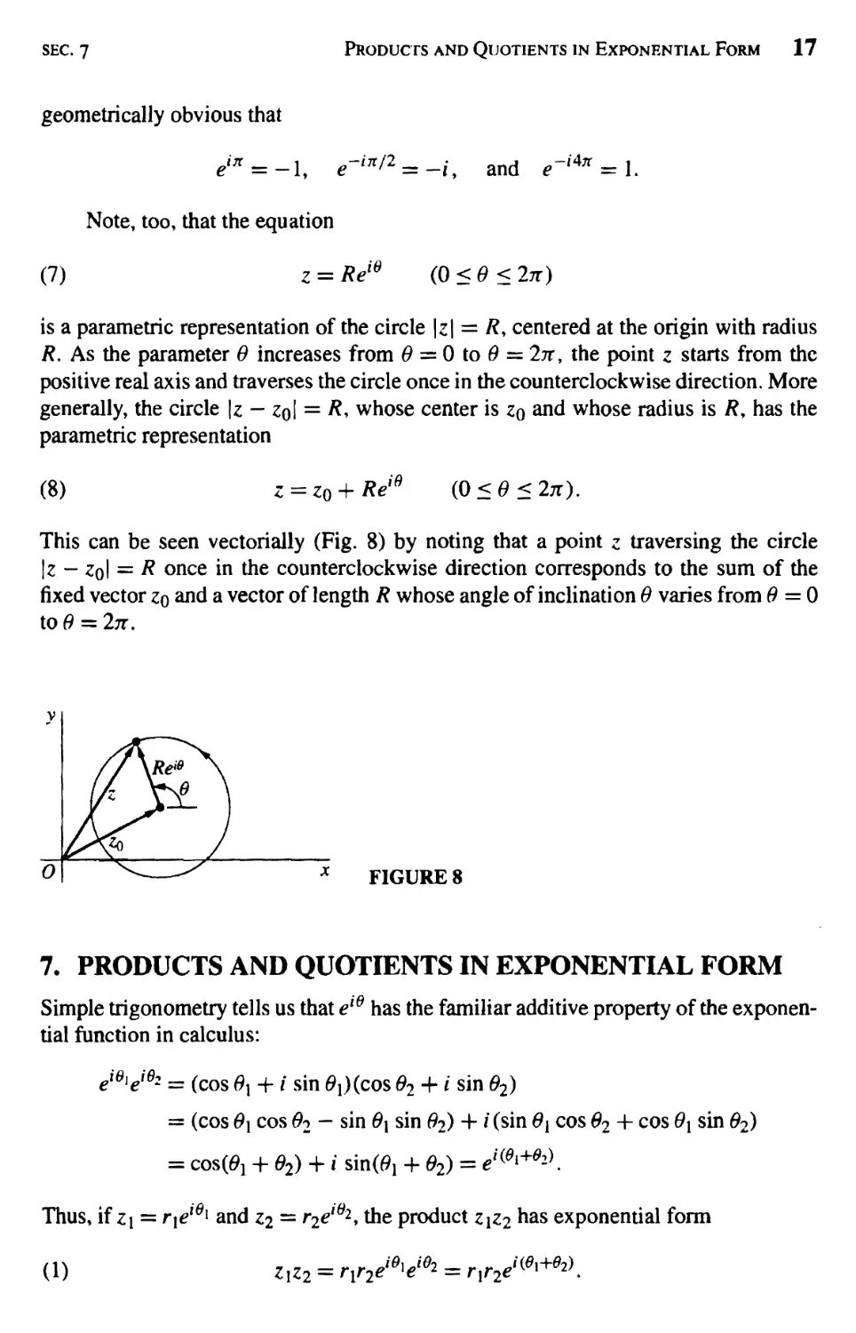
Note, too, that the equation
(7) z = Reie (O<0< 2;r)
is a parametric representation of the circle |z| = Ry centered at the origin with radius
/?, As the parameter 9 increases from 9 = 0 to 9 = 27r, the point z starts from the
positive real axis and traverses the circle once in the counterclockwise direction. More
generally, the circle \z — zq\ — R, whose center is zq and whose radius is /?, has the
parametric representation
(8) z = z0 + Rei9 (0<e<2n).
This can be seen vectorially (Fig. 8) by noting that a point z traversing the circle
\z — Zq\ = R once in the counterclockwise direction corresponds to the sum of the
fixed vector zq and a vector of length R whose angle of inclination 9 varies from 0=0
to0 = 2;r.
FIGURE 8
7. PRODUCTS AND QUOTIENTS IN EXPONENTIAL FORM
Simple trigonometry tells us that el6 has the familiar additive property of the
exponential function in calculus:
e1'V% = (cosGx + / sin <9L)(cos d2 + i sin 92)
= (cos 9\ cos 62 - sin 9\ sin 92) + i (sin 6\ cos 92 + cos 9X sin 92)
= cos(Ö! + 92) + i sin(9l + 92) = ei{e^^\
Thus, if z\ = r\el6x and z2 = r2el81, the product zjz2 has exponential form
(1) z,z2 = rxr2eie^ = r,r2e/tf'+^).
18 Complex Numbers
chap. I
Moreover,
J. — H . e e " — H . e - ÜJ&x-fo)
(2) - = -1 • ——-r = -1 ^r- = -v
z2 r2 elH2e~!^ r2 el[) r2
Because 1 = lel0< it follows from expression (2) that the inverse of any nonzero
complex number z = relS is
(3) z-' = l = ir".
z r
Expressions (1), (2), and (3) are, of course, easily remembered by applying the usual
algebraic rules for real numbers and e*.
Expression (1) yields an important identity involving arguments:
(4) arg(z1z2) = arg zx + arg z2.
It is to be interpreted as saying that if values of two of these three (multiple-valued)
arguments are specified, then there is a value of the third such that the equation holds.
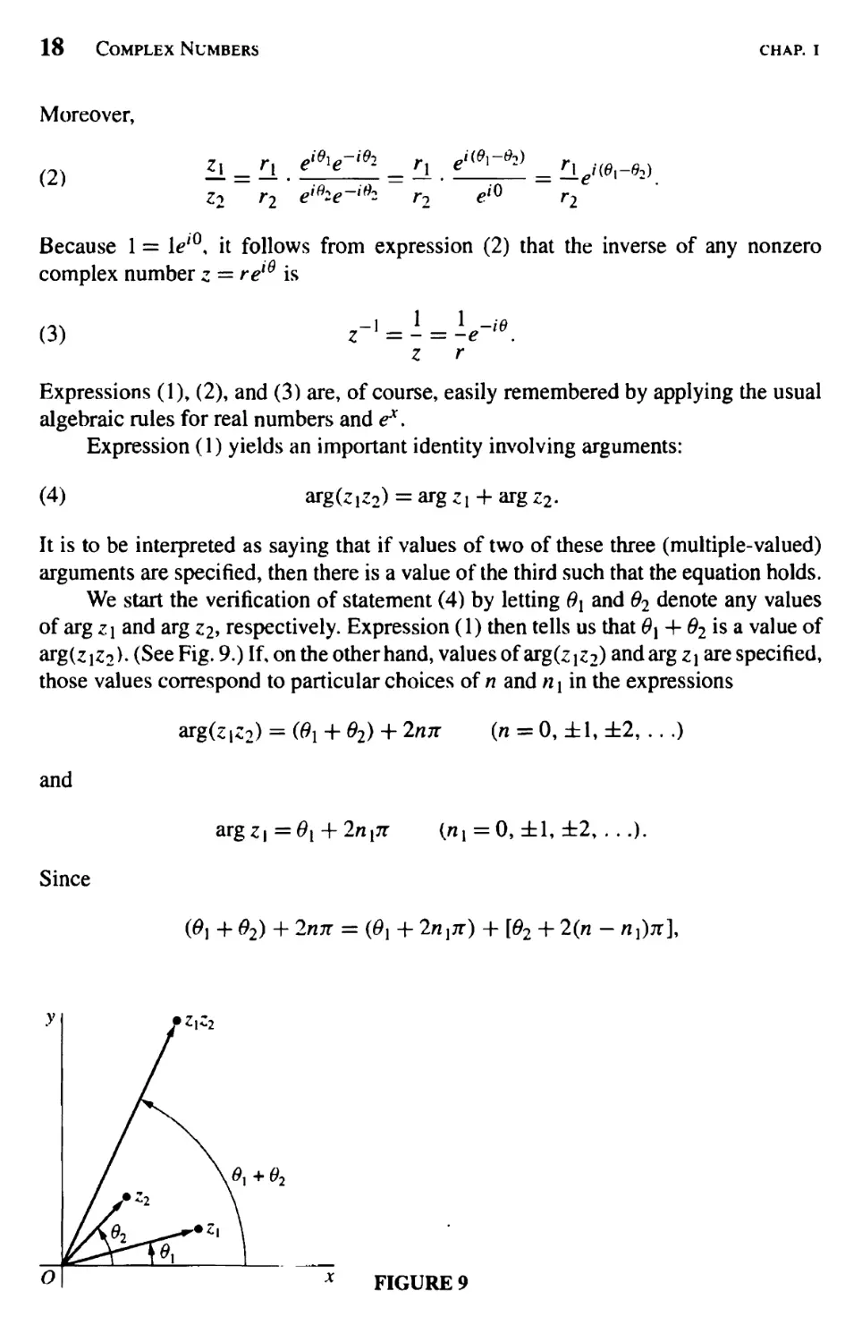
We start the verification of statement (4) by letting 9\ and 62 denote any values
of arg z\ and arg z2, respectively. Expression (1) then tells us that 0X + 62 is a value of
argCz^). (See Fig. 9.) If, on the other hand, values of arg(zj<:2) and arg z\ are specified,
those values correspond to particular choices of n and n i in the expressions
and
Since
O
KB(Z\Z2) = (0i + ©2) + 2n* (" = °> i1' ±2> • • ')
argz\ = 0{ + 2n{n (n{=0, ±1, ±2, . ..).
(01 + 02) + 2nn = (0, + 2n^n) + [02 + 2(n - n{)nl
>Z\Z2
A+0,
^Zx
FIGURE 9
SEC. 7
Products and Quotients in Exponential Form 19
equation (4) is evidently satisfied when the value
argz2 = 02 + 2(" -nu*
is chosen. Verification when values of arg(z1z2) and arg z2 are specified follows by
symmetry.
Statement (4) is sometimes valid when arg is replaced everywhere by Arg (see
Exercise 7). But, as the following example illustrates, that is not always the case.
EXAMPLE 1. When z i = -1 and z2 = i,
Arg(zjz2) = Arg(-i) = —r but Arg *i + Arg z2 = * + — = —■
If, however, we take the values of arg Z\ and arg z2 just used and select the value
Arg(2!Z2) + 2tt = -- + 2;r = y
of arg(zlz2), we find that equation (4) is satisfied.
Statement (4) tells us that
argf — J = argUiz^"1) = arg z\ + arg(^1),
and we can see from expression (3) that
(5) arg(zj1) = -argz2.
Hence
(6) ^(r) =argZi-argZ2-
Statement (5) is, of course, to be interpreted as saying that the set of all values on the
left-hand side is the same as the set of all values on the right-hand side. Statement (6)
is, then, to be interpreted in the same way that statement (4) is.
EXAMPLE 2. In order to find the principal argument Arg z when
-2
* = 7="'
l + v/3/
observe that
arg z = arg(-2) - arg(l + V3i).
20 Complex Numbers
chap. I
Since
Arg(-2) = n and Arg(l + Vli) = -,
one value of arg z is 2nß\ and, because 27r/3 is between —n and 7T, we find that
Arg z = 2tt/3.
Another important result that can be obtained formally by applying rules for real
numbers to z = re'* is
(7) zn = rVflö (n = 0, ±1, ±2, . ..).
It is easily verified for positive values of n by mathematical induction. Tobe specific,
we first note that it becomes z = rel° when n = 1. Next, we assume that it is valid
when n = m, where m is any positive integer. In view of expression ( 1 ) for the product
of two nonzero complex numbers in exponential form, it is then valid for n = m + 1:
m-fl m rJ&rmJmQ rwi + l j(/h+1)0
Expression (7) is thus verified when « is a positive integer. It also holds when n = 0,
with the convention that z° = 1. If n = — 1, —2, .. . , on the other hand, we define z"
in terms of the multiplicative inverse of z by writing
zn = (z~l)m where m = -n = 1, 2, ... .
Then, since expression (7) is valid for positive integral powers, it follows from the
exponential form (3) of z~x that
Zn = ["!e'<-*)"r = (i\m eim{-9) = (]_\ n ei(-n)(-0) = ^^nO
(W = -l,-2, ...).
Expression (7) is now established for all integral powers.
Observe that if r = 1, expression (7) becomes
(8) (eid)n = einG (n = 0, ±1, ±2, . ..).
When written in the form
(9) (cos e + i sin 6)n = cos n9 + i sin no (n = 0, ±1, ±2, ...),
this is known as de Moivre's formula.
Expression (7) can be useful in finding powers of complex numbers even when
they are given in rectangular form and the result is desired in that form.
SEC. 7
Exercises 21
EXAMPLE 3. In order to put (V3 + 07 in rectangular form, one need only write
(v/3 + i)1 = {2ei7T/6)J = 2V77r/6 = (2V^(2e'*/6£= -64(^3 + /).
EXERCISES
1. Find the principal argument Arg z when
{a)z = Z^ZYi; (b)z = (VÏ-i)6.
Ans. (a) —3tt/4; (b) n.
2. Show that (a) \ei9\ = 1; (b) e^ = e'ie.
3. Use mathematical induction to show that
JW°* • • « J0" = «Wi+*i+-+4.> (n = 2, 3, ...).
4. Using the fact that the modulus \el° — 1| is the distance between the points et0 and 1 (see
Sec. 4), give a geometric argument to find a value of 0 in the interval 0 < 0 < 2n that
satisfies the equation \e'6 — 1| = 2.
Ans. jr.
5. Use de Moivre's formula (Sec. 7) to derive the following trigonometric identities:
(a) cos 30 = cos3 0 - 3 cos 0 sin2 0; (b) sin 30 = 3 cos2 0 sin 0 - sin3 0.
6. By writing the individual factors on the left in exponential form, performing the needed
operations, and finally changing back to rectangular coordinates, show that
(a) i(l - V3/)(V3 + /) = 2(1 + V3/); (b) 5//(2 + 0 = 1 + 2Î;
(c) (-I + i)7 = -8(1 + i); (d) (1 + V30"10 = 2~n(-l + V5i).
7. Show that if Re z\ > 0 and Re zi > 0, then
ArgUiz2) = Arg z\ + Arg z2,
where Arg(^1z2) denotes the principal value of arg(ziz2), etc.
8. Let z be a nonzero complex number and n a negative integer (n = -1, -2, ...). Also,
write z = f£iö and m = -h — 1, 2 Using the expressions
zm=rm^me and z-l = / l\ ^(-^
verify that (zT1 = (z"1)m and hence that the definition zn = (z~{)m in Sec. 7 could
have been written alternatively as zn = (z™)"1.
9. Prove that two nonzero complex numbers z\ and z2 have the same moduli if and only if
there are complex numbers c\ and c2 such that z\ = cjc2 and z2 = c{cî.
Suggestion: Note that
exK'^)exp('^)=exp(/ö,)
22 Complex Numbers
chap. I
and [see Exercise 2(b)\
expl / — 1 expl / — 1 = exp(j02)-
10. Establish the identity
i _ -1+1
i + z + r + • • • + zn = —±— (z £ l)
1 - z
and then use it to derive Lagrange's trigonometric identity:
1 + cos 6 + cos 20 + ■ ■ - + cos n6 = I + Si"[(2" + ')g/2J (O<0<2tt).
2 2sin(0/2)
Suggestion: As for the first identity, write S=l + z + z2-f--' + z" and consider
the difference S — zi\ To derive the second identity, write z = el$ in the first one.
11. (a) Use the binomial formula (Sec. 3) and de Moivre's formula (Sec. 7) to write
-£CH
cos n0 + i sin w0 = 2^ ( f J cos""* 0(/ sin 0)* (w = 1,2,...).
Then define the integer m by means of the equations
{n/2 if n is even,
(n- l)/2 if nis odd
and use the above sum to obtain the expression [compare Exercise 5(a)]
cos/z<9 = J^(n )(-l)* cos"""2* 0 sin2* 0 (n = I, 2, ...).
(ft) Write x — cos 0 and suppose that 0 < 0 < ,t, in which case — 1 < x < 1. Point out
how it follows from the final result in part (a) that each of the functions
Tn(x) = cos(n cos"1 x) (/? = 0, 1, 2 )
is a polynomial of degree n in the variable jc*
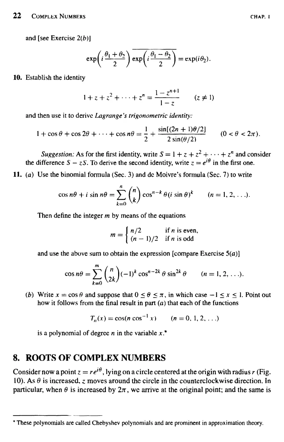
8. ROOTS OF COMPLEX NUMBERS
Consider now a point z = rel0y lying on a circle centered at the origin with radius r (Fig.
10). As 0 is increased, z moves around the circle in the counterclockwise direction. In
particular, when 0 is increased by 27T, we arrive at the original point; and the same is
* These polynomials are called Chebyshev polynomials and are prominent in approximation theory.
SEC. 8
Roots of Complex Numbers 23
: = re*
FIGURE 10
true when 9 is decreased by 2n. It is, therefore, evident from Fig. 10 that two nonzero
complex numbers
-*.J*\
m
are equal if and only if
Z\ = rxe x and z2 = r2el
rx = r2 and 6\ = 82 + 2kiz,
wAire /: w some integer (k = 0, ±1, ±2, .. .).
This observation, together with the expression zn = rnein$ in Sec. 7 for integral
powers of complex numbers z = re'6\ is useful in finding the nth roots of any nonzero
complex number z0 = rçe100, where n has one of the values n = 2, 3, ... . The method
starts with the fact that an nth root of z0 is a nonzero number z = rel6 such that zn = Zq,
or
According to the statement in italics just above, then,
rn = r0 and nO-O^ + lkir,
where k is any integer (k = 0, ±1, ±2, ...). So r = tfr^, where this radical denotes
the unique positive nth root of the positive real number r0, and
<90 + 2Jbr 0O 2for
0 = = 1
n n n
Consequently, the complex numbers
-«*4(?+v)]
(* = 0,±1,±2,...).
(* = 0,±1,±2, ...)
are the nth roots of z0- We are able to see immediately from this exponential form of
the roots that they all lie on the circle \z \ = f/r^ about the origin and are equally spaced
every 27r/rc radians, starting with argument 6q/h. Evidently, then, all of the distinct
24 Complex Numbers
chap. I
roots are obtained when k = 0, 1, 2, ..., n - 1, and no further roots arise with other
values of k. We let ck (k = 0, 1, 2, . . ., n — 1) denote these distinct roots and write
(See Fig. 11.)
(Jt = 0, 1, 2 n- 1).
FIGURE 11
The number %/ï\) is the length of each of the radius vectors representing the n
roots. The first root cq has argument 0Q/n] and the two roots when n = 2 lie at the
opposite ends of a diameter of the circle |z| = ^/r^, the second root being -c0. When
n > 3, the roots lie at the vertices of a regular polygon of n sides inscribed in that circle.
We shall let z0 denote the set of nth roots of z0- If, in particular, z0 is a positive
real number r0, the symbol r0'w denotes the entire set of roots; and the symbol j^/r^ in
expression ( 1 ) is reserved for the one positive root. When the value of d0 that is used in
expression (1 ) is the principal value of arg z0 (—n < % < n), the number c0 is referred
to as the principal root. Thus when zq is a positive real number r0, its principal root is
Finally, a convenient way to remember expression (1) is to write Zo in its most
general exponential form (compare Example 2 in Sec. 6)
(2)
Zo
= rQei{e°+2kn) (k = 0, ±1, ±2, . ..)
and to formally apply laws of fractional exponents involving real numbers, keeping in
mind that there are precisely n roots:
= j^exp[i('^ + ^')l (* =0.1,2,...,»-«.
The examples in the next section serve to illustrate this method for finding roots of
complex numbers.
SEC. 9
Examples 25
9. EXAMPLES
In each of the examples here, we start with expression (2), Sec. 8, and proceed in the
manner described at the end of that section.
EXAMPLE 1. In order to determine the nth roots of unity, we write
1 = 1 exp[/(0 + 2kn)] (k = 0, ±1, ±2 ...)
and find that
(1) li/« = yîexp[/^ + ^]=exp(/^) (* = 0,l,2,...,n-l).
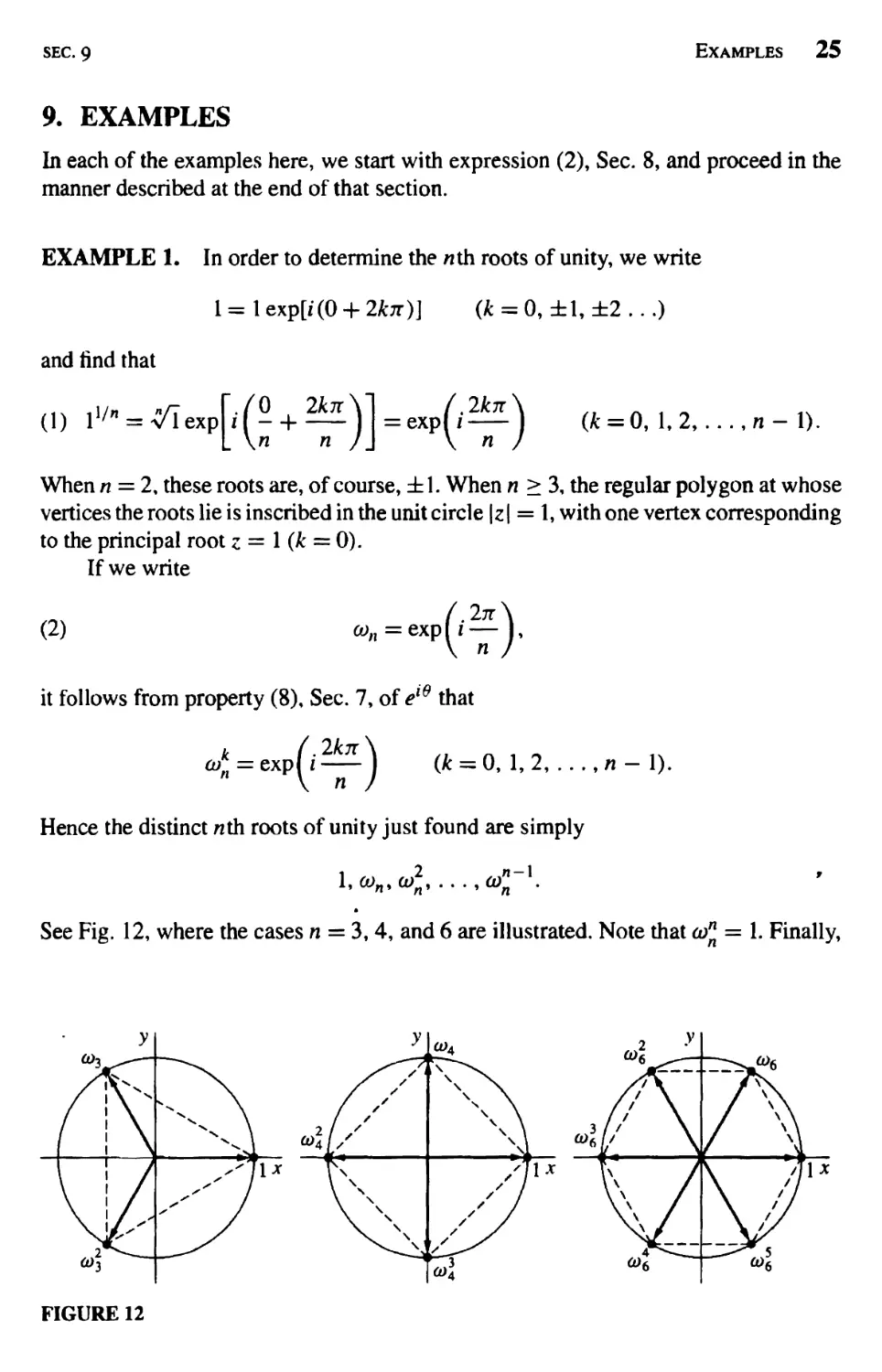
When n — 2, these roots are, of course, ±1. When n > 3, the regular polygon at whose
vertices the roots lie is inscribed in the unit circle \z | = 1, with one vertex corresponding
to the principal root z = l(k = 0).
If we write
(2) a>„=exph —
it follows from property (8), Sec. 7, of el$ that
(Jfc = 0,l,2,...,*-1).
Hence the distinct nth roots of unity just found are simply
2 n i
1, &>„, (O , . . . , CO . *
See Fig. 12, where the cases n = 3, 4, and 6 are illustrated. Note that œ" = 1. Finally,
•
FIGURE 12
26 Complex Numbers
chap. I
it is worthwhile observing that if c is any particular nth root of a nonzero complex
number z0> the set of nth roots can be put in the form
c, C(x)n,C(x?tV .. . ,cù)nn K
This is because multiplication of any nonzero complex number by con increases the
argument of that number by 2n/n, while leaving its modulus unchanged.
EXAMPLE 2. Let us find all values of (-80l/3, or the three cube roots of -8/. One
need only write
—8/ = 8 exp
to see that the desired roots are
(3) ck = 2 exp
,(-§+**)]
'(-6+-)J
(Jfc = 0, ±1,±2, ...)
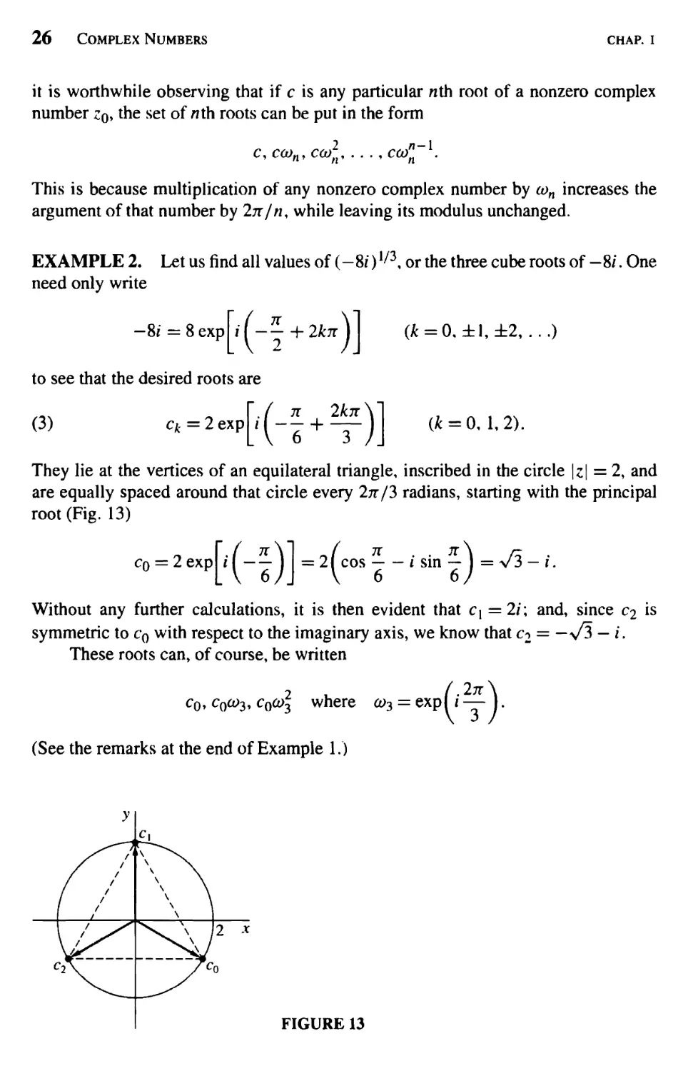
(* = 0,1.2).
They lie at the vertices of an equilateral triangle, inscribed in the circle \z\ = 2, and
are equally spaced around that circle every 27r/3 radians, starting with the principal
root (Fig. 13)
c0 = 2exp il J =2|cos i sin — J = V3 - i.
Without any further calculations, it is then evident that C\ = 2/; and, since c^ is
symmetric to c0 with respect to the imaginary axis, we know that c2 = — \/3 - i.
These roots can, of course, be written
c0, c0co3, c0o>3 where co3 = exp I / — j.
(See the remarks at the end of Example 1.)
y
/ /
/ /
/ /
/ /
/ /
/ /
\ f ^
C2 X
\ X
V, \
\ \
\ \
\ \
N \
\ 1
\\ 2 x
y%
FIGURE 13
sec. 9
Examples 27
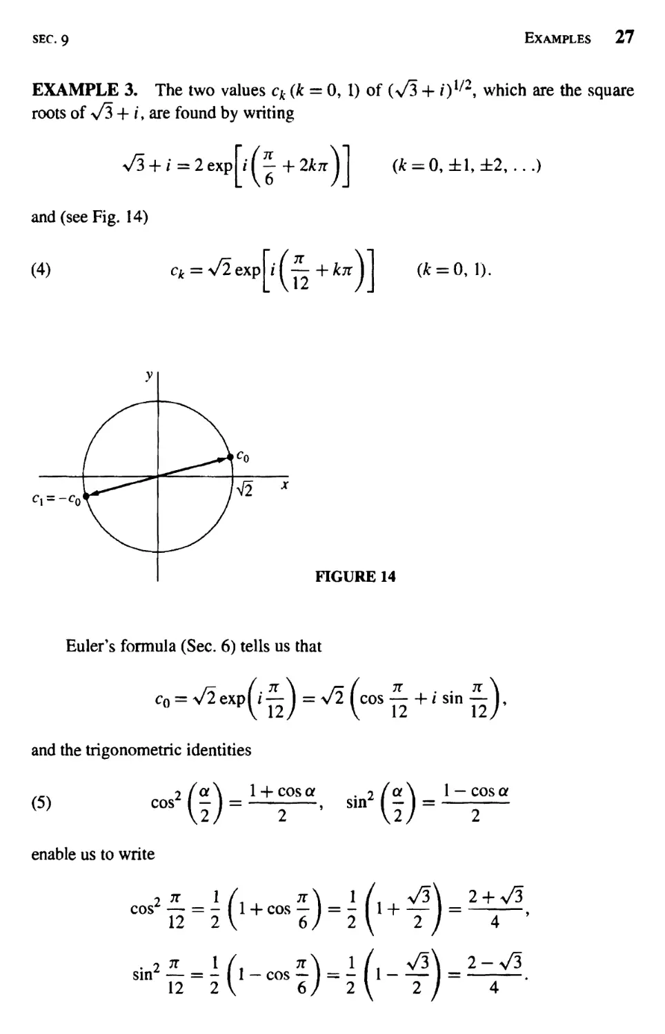
EXAMPLE 3. The two values ck (k = 0, 1) of (>/3 + i)l/2, which are the square
roots of a/3 + i, are found by writing
N/3 + / = 2exp|/( -+2*7tJ|
and (see Fig. 14)
(4) ck = VÎ exp i ( j- + kn \\
(* = 0,±1,±2,...)
(k = 0,1).
C\ = -c0
FIGURE 14
Euler's formula (Sec. 6) tells us that
c0 = \/2 expl i — ) = Vz ( cos 1- i sin — ),
0 FV 12/ V 12 12/
and the trigonometric identities
(5) cos2
enable us to write
(|) = i±p«. ^(|).
1 — cos a
cos'
sin
TV 1 / 7t\ 1 /
iL = l(,_cos£)=>(',-^ =
12 2 V 6/2\ 2/
v5\_2_+V3
2 /" 4 '
2-n/3
28 Complex Numbers
chap. I
Consequently,
Co
Since c\ = —c0, the two square roots of \/3 +1 are, then,
±
±^2+^ + ^2-^.
EXERCISES
1. Find the square roots of (a) 2i ; (b) 1 - V3j and express them in rectangular coordinates.
Aim. (a) ±(1 + i); (fc)±^_lL.
V2
2. In each case, find all of the roots in rectangular coordinates, exhibit them as vertices of
certain squares, and point out which is the principal root:
(a)(-16),/4; (fc)(-8-8V30l/4.
Ans. (a) ±V2(1 + i), ±>/2(l - i); (&) ±(V3 - i), ±(1 + >/3i).
3. In each case, find all of the roots in rectangular coordinates, exhibit them as vertices of
certain regular polygons, and identify the principal root:
(a)(-l)'/3; (b)&6.
Ans. {b) ±V2, ± ■=—, ± =—.
s/2 VÏ
4. According to Example 1 in Sec. 9, the three cube roots of a nonzero complex number z0
can be written cq, cqco^, cqco*, where c0 is the principal cube root of Zo and
.2*^ -1 + V3i
= exp(^) =
Show that if z0 = —4\/2 + 4\/2/, then c0 = \/2(l + i) and the other two cube roots are,
in rectangular form, the numbers
-(73+l) + (v/3-l)/ 2 (V3-1)-(V3+D«
c°"3 = 71 • Co"3 = H ~-
5. (ö) Let a denote any fixed real number and show that the two square roots of a + i are
±v^exph|j,
where A = \Ja1 + 1 and a = Arg(a + 0.
SEC. 10
Regions in the Complex Plane 29
(b) With the aid of the trigonometric identities (5) in Example 3 of Sec. 9, show that the
square roots obtained in part (a) can be written
1
±-^(VA + tf + iy/A-a).
V2
[Note that this becomes the final result in Example 3, Sec. 9, when a = y/3.]
6. Find the four roots of the equation zA + 4 = 0 and use them to factor z* + 4 into quadratic
factors with real coefficients.
Ans. {z2 + 2z + 2)(z2 -2z + 2).
7. Show that if c is any nth root of unity other than unity itself, then
l + c + c2 + -+c'|-1 = 0.
Suggestion: Use the first identity in Exercise 10, Sec. 7.
8. (a) Prove that the usual formula solves the quadratic equation
azr + bz + c = 0 {a £ 0)
when the coefficients a, b, and c are complex numbers. Specifically, by completing
the square on the left-hand side, derive the quadratic formula
_ -b + (b2 - 4ac){/2
Z~ la
where both square roots are to be considered when b2 - 4ac £ 0,
(b) Use the result in part (a) to find the roots of the equation z2 + 2z + (1 - i) = 0.
9. Let z = rel° be any nonzero complex number and n 2l negative integer (n = -1, -2,...).
Then define z{/n by means of the equation z{^n = (z"~l)1/m, where m = -n. By showing
that the m values of (zl/m)~l and (z_1)1/m are the same, verify that z]/n = (zl/m)~K
(Compare Exercise 8, Sec. 7.)
10. REGIONS IN THE COMPLEX PLANE
In this section, we are concerned with sets of complex numbers, or points in the z plane,
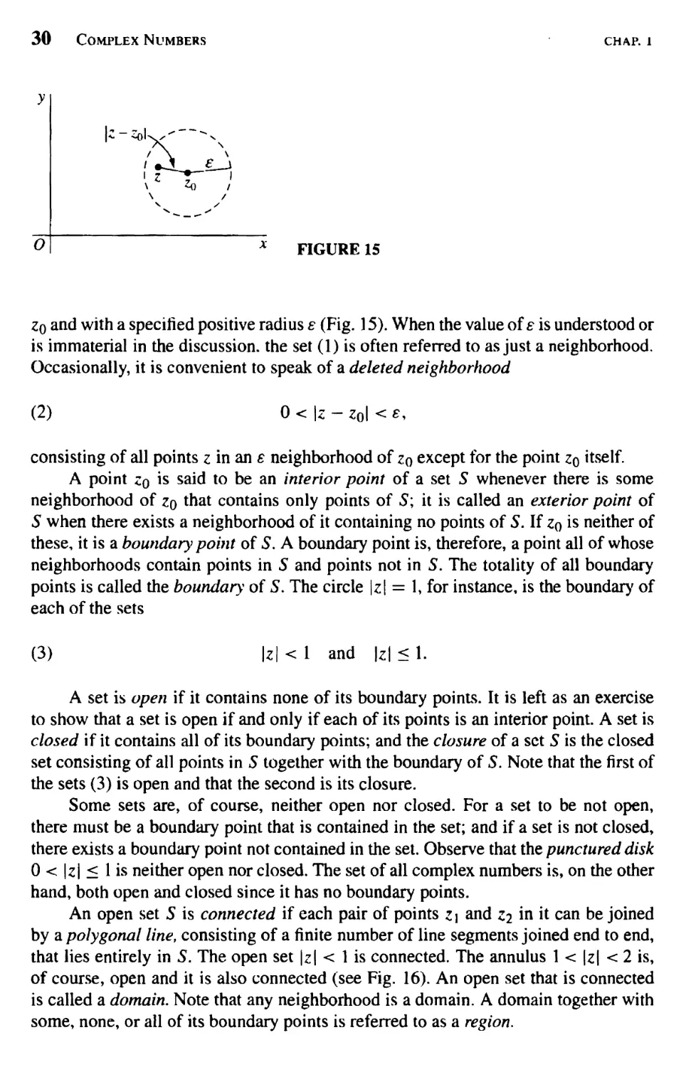
and their closeness to one another. Our basic tool is the concept of an e neighborhood
(1) \z-z0\<e
of a given point z0- It consists of all points z lying inside but not on a circle centered at
30 Complex Numbers
chap. 1
O
FIGURE 15
Zo and with a specified positive radius e (Fig. 15). When the value oîe is understood or
is immaterial in the discussion, the set (1) is often referred to as just a neighborhood.
Occasionally, it is convenient to speak of a deleted neighborhood
(2) 0 < \z - z0l < *.
consisting of all points z in an s neighborhood of z0 except for the point z0 itself.
A point zo is said to be an interior point of a set S whenever there is some
neighborhood of z0 that contains only points of 5; it is called an exterior point of
5 when there exists a neighborhood of it containing no points of S. If z0 is neither of
these, it is a boundary point of S. A boundary point is, therefore, a point all of whose
neighborhoods contain points in 5 and points not in 5. The totality of all boundary
points is called the boundary of S. The circle |z| = 1, for instance, is the boundary of
each of the sets
(3) |z|<l and \z\ < 1.
A set is open if it contains none of its boundary points. It is left as an exercise
to show that a set is open if and only if each of its points is an interior point. A set is
closed if it contains all of its boundary points; and the closure of a set 5 is the closed
set consisting of all points in S together with the boundary of 5. Note that the first of
the sets (3) is open and that the second is its closure.
Some sets are, of course, neither open nor closed. For a set to be not open,
there must be a boundary point that is contained in the set; and if a set is not closed,
there exists a boundary point not contained in the set. Observe that the punctured disk
0 < \z\ < 1 is neither open nor closed. The set of all complex numbers is, on the other
hand, both open and closed since it has no boundary points.
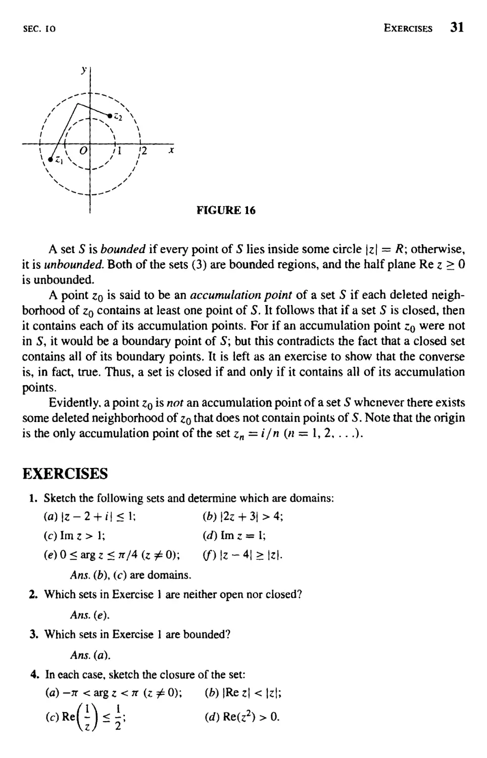
An open set S is connected if each pair of points Z\ and Zi in it can be joined
by a polygonal line, consisting of a finite number of line segments joined end to end,
that lies entirely in 5. The open set \z\ < 1 is connected. The annulus 1 < \z\ < 2 is,
of course, open and it is also connected (see Fig. 16). An open set that is connected
is called a domain. Note that any neighborhood is a domain. A domain together with
some, none, or all of its boundary points is referred to as a region.
SEC. 10
Exercises 31
y
' /
/ 1
' A
i /(
^
il \2 x
y t
/
/
/
A set S is bounded if every point of S lies inside some circle |z| = /?; otherwise,
it is unbounded. Both of the sets (3) are bounded regions, and the half plane Re z > 0
is unbounded.
A point zq is said to be an accumulation point of a set S if each deleted
neighborhood of zq contains at least one point of 5. It follows that if a set S is closed, then
it contains each of its accumulation points. For if an accumulation point z0 were not
in 5, it would be a boundary point of S; but this contradicts the fact that a closed set
contains all of its boundary points. It is left as an exercise to show that the converse
is, in fact, true. Thus, a set is closed if and only if it contains all of its accumulation
points.
Evidently, a point Zq is not an accumulation point of a set S whenever there exists
some deleted neighborhood of zq that does not contain points of S. Note that the origin
is the only accumulation point of the set zn = i/n (n = 1, 2, ...).
EXERCISES
1. Sketch the following sets and determine which are domains:
(fl)|z-2 + i|<l; (b) \2z + 3| >4;
(c) Im z > 1; (d) Im z = I;
(e) 0 < arg z < n/A (z Ï 0); (/*) |z - 4| > \z\.
Ans. (b), (c) are domains.
2. Which sets in Exercise 1 are neither open nor closed?
A/15, (e).
3. Which sets in Exercise 1 are bounded?
Ans. (a).
4. In each case, sketch the closure of the set:
(a) -n < arg z < n {z £ 0); (b) |Re z\ < \z\;
(c)Re(-)<i; (rf) Re(z2) > 0.
Complex Numbers
chap. I
5. Let S be the open set consisting of all points z such that \z\ < 1 or \z - 2| < 1. State why
S is not connected.
6. Show that a set S is open if and only if each point in S is an interior point.
7. Determine the accumulation points of each of the following sets:
(a) zn = in (n = 1, 2, ...); {b) zn = in/n (« = 1,2,...);
(c) 0 < arg z < 7T/2 (z Ï 0); (d) zn = (-1)"(1 + 0^—^ (n = 1, 2, ...).
n
Ans. (a) None; (b) 0; (d) ±(1 +1).
8. Prove that if a set contains each of its accumulation points, then it must be a closed set.
9. Show that any point zq of a domain is an accumulation point of that domain.
10. Prove that a finite set of points z\, Zi, .. -, zn cannot have any accumulation points.
CHAPTER
2
ANALYTIC FUNCTIONS
We now consider functions of a complex variable and develop a theory of
differentiation for them. The main goal of the chapter is to introduce analytic functions, which
play a central role in complex analysis.
IL FUNCTIONS OF A COMPLEX VARIABLE
Let 5 be a set of complex numbers. A function f defined on S is a rule that assigns to
each z in S a complex number w. The number w is called the value of / at z and is
denoted by /(z); that is, w = /(z). The set S is called the domain of definition of /.*
It must be emphasized that both a domain of definition and a rule are needed in
order for a function to be well defined. When the domain of definition is not mentioned,
we agree that the largest possible set is to be taken. Also, it is not always convenient
to use notation that distinguishes between a given function and its values.
EXAMPLE 1. If / is defined on the set z ^ 0 by means of the equation w = 1/z, it
may be referred to only as the function w = 1/z, or simply the function 1/z.
Suppose that w = u + i v is the value of a function / at z = x + iy, so that
u + iv = f(x + iy).
* Although the domain of definition is often a domain as defined in Sec. 10, it need not be.
33
34 Analytic Functions
chap. 2
Each of the real numbers u and v depends on the real variables x and y, and it follows
that f(z) can be expressed in terms of a pair of real-valued functions of the real
variables x and y:
(1) f(z) = u(x9y)+iv(x,y).
If the polar coordinates r and 0, instead of jc and y, are used, then
u+iv = f(rei$),
where w = u + iv and z = rel$. In that case, we may write
(2) f(z) = u(r,0) + iv(r90).
EXAMPLE 2. If f(Z) = z2, then
f(x + iy) = (x + iy)2 = x2 - y2 + ilxy.
Hence
u(x, y) = x2 — y2 and v(x, y) = 2xy.
When polar coordinates are used,
f(reie) = (rew)2 = r2em = r2 cos 2d + ir2 sin 20.
Consequently,
n(r, 0) = r2 cos 20 and v(r, 0) = r2 sin 20.
If, in either of equations (1) and (2), the function v always has value zero, then
the value of / is always real. That is, / is a real-valued function of a complex variable.
EXAMPLE 3. A real-valued function that is used to illustrate some important
concepts later in this chapter is
f(z) = \z\2 = x2 + y2 + i0.
If n is zero or a positive integer and if a0, ah a2, ..., an are complex constants,
where an ^ 0, the function
P(z) = a0 + a{z + a2z2 H h anzn
is a polynomial of degree n. Note that the sum here has a finite number of terms and that
the domain of definition is the entire z plane. Quotients P(z)/Q(z) of polynomials are
called rational functions and are defined at each point z where Q(z) ^ 0. Polynomials
and rational functions constitute elementary, but important, classes of functions of a
complex variable.
SEC. 11
Exercises 35
A generalization of the concept of function is a rule that assigns more than one
value to a point z in the domain of definition. These multiple-valued functions occur
in the theory of functions of a complex variable, just as they do in the case of real
variables. When multiple-valued functions are studied, usually just one of the possible
values assigned to each point is taken, in a systematic manner, and a (single-valued)
function is constructed from the multiple-valued function.
EXAMPLE 4. Let z denote any nonzero complex number. We know from Sec. 8
that z{/2 has the two values
zl'2 = ±VFexp(i-Y
where r = \z\ and 0(—tc < 0 < n) is the principal value of arg z. But, if we choose
only the positive value of ±y/r and write
= v^expfiyj
(3) f(z) = v^expfi-J (r > 0, -tt < © < tt),
the (single-valued) function (3) is well defined on the set of nonzero numbers in the z
plane. Since zero is the only square root of zero, we also write f(0) = 0. The function
/ is then well defined on the entire plane.
EXERCISES
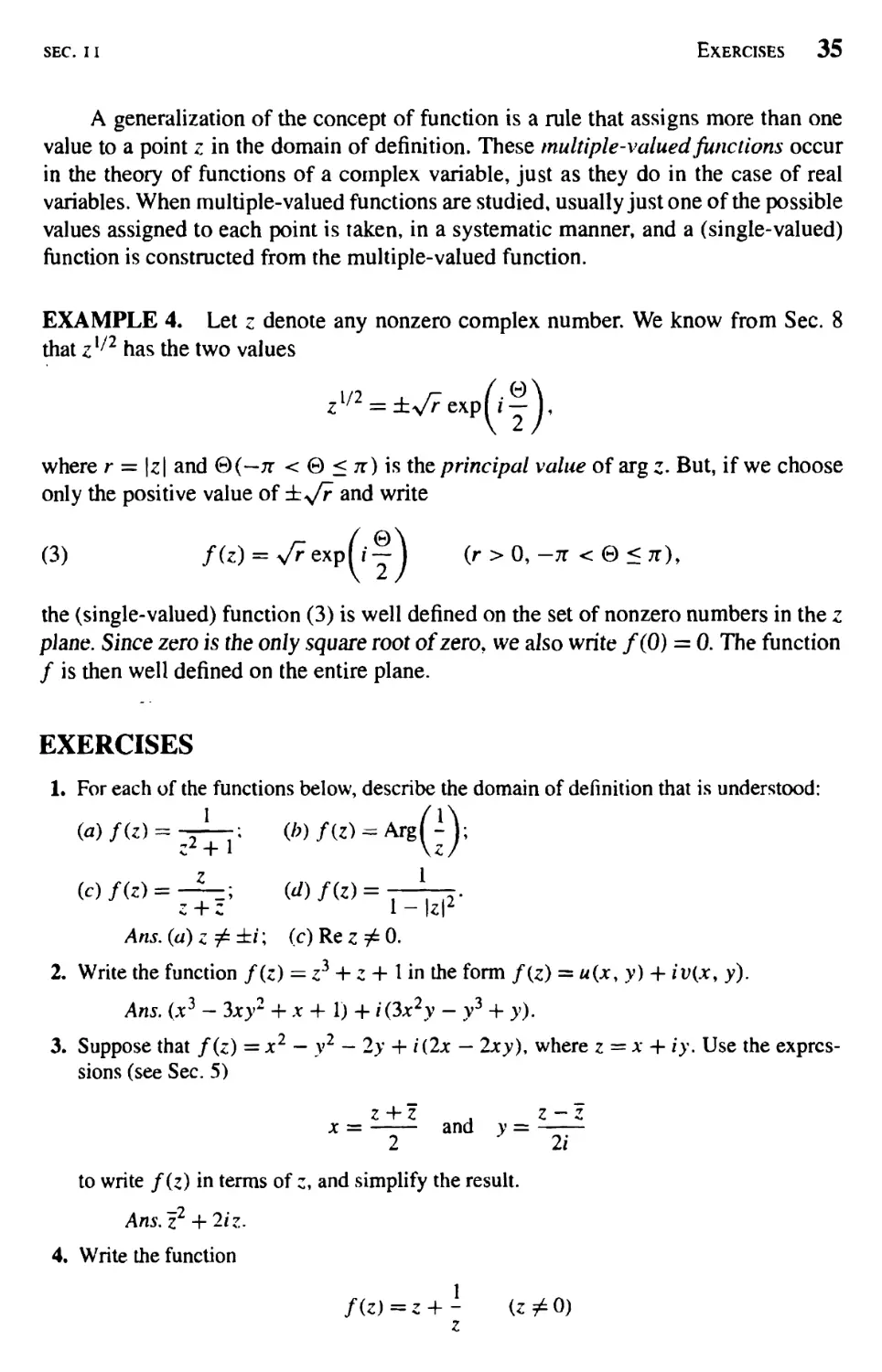
1. For each of the functions below, describe the domain of definition that is understood:
;2 + r
(a) f(z) = ^-7; (/;) f(z) - Arg^Y,
(c) f(z) = -5_; (d) f(z) = —7-j.
z + z 1 - \zr
Ans.{a)z£±i\ (c)Rez^O.
2. Write the function f(z) = z3 + z + 1 in the form f(z) = u(xy y) + iv(x> y).
Ans. (x3 - 3xy2 + x + 1) + i(3x2y - v3 + y).
3. Suppose that f(z) = x2 — v2 - 2y -f i(2x — 2xy), where z = x + iy. Use the
expressions (see Sec. 5)
Z + Z . Z-Z
x = and y =
2 2î
to write f(z) in terms of z, and simplify the result.
Ans.z2 + 2iz.
4. Write the function
f(z) = z + - {z^O)
z
36 Analytic Functions
char 2
in the form f(z) = w(r, 0) + iv(r, 6).
Ans. f r + - ) cos 6 + ii r ) sin 0.
12. MAPPINGS
Properties of a real-valued function of a real variable are often exhibited by the graph
of the function. But when w = /(z), where z and w are complex, no such convenient
graphical representation of the function / is available because each of the numbers
z and w is located in a plane rather than on a line. One can, however, display some
information about the function by indicating pairs of corresponding points z = (x> y)
and w = (u, v). To do this, it is generally simpler to draw the z and w planes separately.
When a function / is thought of in this way, it is often referred to as a mapping,
or transformation. The image of a point z in the domain of definition 5 is the point
w = /(z), and the set of images of all points in a set T that is contained in 5 is called
the image of T. The image of the entire domain of definition 5 is called the range of
/. The inverse image of a point w is the set of all points z in the domain of definition
of / that have w as their image. The inverse image of a point may contain just one
point, many points, or none at all. The last case occurs, of course, when w is not in the
range of /.
Terms such as translation, rotation, and reflection are used to convey dominant
geometric characteristics of certain mappings. In such cases, it is sometimes convenient
to consider the z and w planes to be the same. For example, the mapping
w = z + l = (x + l) + iy,
where z = x + iy, can be thought of as a translation of each point z one unit to the
right. Since / = e111^, the mapping
w = iz = r exp i\u-{—
where z = relB, rotates the radius vector for each nonzero point z through a right angle
about the origin in the counterclockwise direction; and the mapping
w = z = x - i y
transforms each point z = x + iy into its reflection in the real axis.
More information is usually exhibited by sketching images of curves and regions
than by simply indicating images of individual points. In the following examples, we
illustrate this with the transformation w = z2.
We begin by finding the images of some curves in the z plane.
SEC.12
Mappings 37
EXAMPLE 1. According to Example 2 in Sec. 11, the mapping w = z2 can be
thought of as the transformation
(1)
2 2
« = X — V ,
v = 2xy
from the jc v plane to the uv plane. This form of the mapping is especially useful in
finding the images of certain hyperbolas.
It is easy to show, for instance, that each branch of a hyperbola
(2)
X2 — V2 = C]
(q > 0)
is mapped in a one to one manner onto the vertical line u = cx. We start by noting
from the first of equations (1) that u = cx when (jc, y) is a point lying on either branch.
When, in particular, it lies on the right-hand branch, the second of equations (1) tells
us that v = 2yy/y2 + c\. Thus the image of the right-hand branch can be expressed
parametrically as
u=C), v = 2>V>'2 + ^i (-oo < >• < oo);
and it is evident that the image of a point (x, y) on that branch moves upward along the
entire line as (jc, v) traces out the branch in the upward direction (Fig. 17). Likewise,
since the pair of equations
u=C\, v = -lyy/y2 + c\ (—oo<y<oo)
furnishes a parametric representation for the image of the left-hand branch of the
hyperbola, the image of a point going downward along the entire left-hand branch
is seen to move up the entire line u = C\,
On the other hand, each branch of a hyperbola
(3)
2xy = C2 (c'2 > 0)
is transformed into the line v = c2, as indicated in Fig. 17. To verify this, we note from
the second of equations (1) that v = c2 when (jc, y) is a point on either branch. Suppose
w = cj >0
O
FIGURE 17
w
= ?2
38 Analytic Functions
chap. 2
that it lies on the branch lying in the first quadrant. Then, since y = c2/(2x), the first
of equations (1) reveals that the branch's image has parametric representation
9 1
U=X ^r, V = C2 (0<*<OO).
Observe that
lim u = -oo and lim u = oo.
jc>0
Since u depends continuously on x, then, it is clear that as (x, y ) travels down the entire
upper branch of hyperbola (3), its image moves to the right along the entire horizontal
line v = c2. Inasmuch as the image of the lower branch has parametric representation
u = -4r - y2, v = c2 (-oo < >' < 0)
4y2
and since
hm u = —oo and lim u = oo,
><0
it follows that the image of a point moving upward along the entire lower branch also
travels to the right along the entire line v = c2 (see Fig. 17).
We shall now use Example 1 to find the image of a certain region.
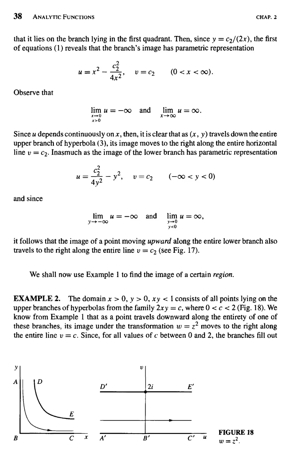
EXAMPLE 2. The domain x > 0, y > 0, xy < 1 consists of all points lying on the
upper branches of hyperbolas from the family 2xy = c, where 0 < c < 2 (Fig. 18). We
know from Example 1 that as a point travels downward along the entirety of one of
these branches, its image under the transformation w = z2 moves to the right along
the entire line v = c. Since, for all values of c between 0 and 2, the branches fill out
B
V
D'
2/ E'
A'
B'
C «
FIGURE 18
2
W — Z.
SEC. 12
Mappings 39
the domain x > 0, y > 0, xy < 1, that domain is mapped onto the horizontal strip
0 < v < 2.
In view of equations (1), the image of a point (0, y) in the z plane is (—y2, 0).
Hence as (0, y) travels downward to the origin along the y axis, its image moves to the
right along the negative u axis and reaches the origin in the w plane. Then, since the
image of a point (jc, 0) is (jc2, 0), that image moves to the right from the origin along
the u axis as (jc, 0) moves to the right from the origin along the x axis. The image
of the upper branch of the hyperbola xy = 1 is, of course, the horizontal line v = 2,
Evidently, then, the closed region x > 0, y > 0, xy < 1 is mapped onto the closed strip
0 < v < 2, as indicated in Fig. 18.
Our last example here illustrates how polar coordinates can be useful in analyzing
certain mappings.
EXAMPLE 3. The mapping w = z2 becomes
w = r2ene
when z = retB. Hence if w = peIff>, we have pel(f> = r2elle\ and the statement in italics
near the beginning of Sec. 8 tells us that
p = r2 and 0 = 20 + 2Jbr,
where k has one of the values k = 0, ± 1, ±2, ... . Evidently, then, the image of any
nonzero point z is found by squaring the modulus of z and doubling a value of arg z.
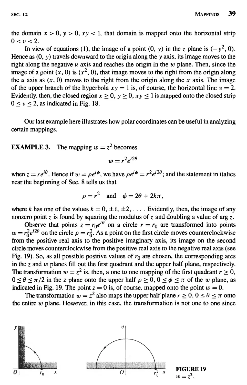
Observe that points z = r0el9 on a circle r = r0 are transformed into points
w = r^el2e on the circle p = /q. As a point on the first circle moves counterclockwise
from the positive real axis to the positive imaginary axis, its image on the second
circle moves counterclockwise from the positive real axis to the negative real axis (see
Fig. 19). So, as all possible positive values of r0 are chosen, the corresponding arcs
in the z and w planes fill out the first quadrant and the upper half plane, respectively.
The transformation id = z2 is, then, a one to one mapping of the first quadrant r > 0,
0 < 9 < jt/2 in the z plane onto the upper half p > 0, 0 < <j> < n of the w plane, as
indicated in Fig. 19. The point z = 0 is, of course, mapped onto the point w = 0.
The transformation w = z2 also maps the upper half plane r>0, O<0<7r onto
the entire w plane. However, in this case, the transformation is not one to one since
FIGURE 19
w = ;r.
40 Analytic Functions
chap. 2
both the positive and negative real axes in the z plane are mapped onto the positive
real axis in the w plane.
When n is a positive integer greater than 2, various mapping properties of the
transformation w = z", or pel<t> = rneinG, are similar to those of w = z2. Such a
transformation maps the entire z plane onto the entire w plane, where each nonzero
point in the w plane is the image of n distinct points in the z plane. The circle r = r0
is mapped onto the circle p = r^\ and the sector r < r0, 0 < 8 < 2ix/n is mapped onto
the disk p < r£, but not in a one to one manner.
13. MAPPINGS BY THE EXPONENTIAL FUNCTION
In Chap. 3 we shall introduce and develop properties of a number of elementary
functions which do not involve polynomials. That chapter will start with the exponential
function
(1) ez = exeiy (z = x + iy)y
the two factors e* and eiy being well defined at this time (see Sec. 6). Note that
definition (1), which can also be written
is suggested by the familiar property
of the exponential function in calculus.
The object of this section is to use the function ez to provide the reader with
additional examples of mappings that continue to be reasonably simple. We begin by
examining the images of vertical and horizontal lines.
EXAMPLE 1. The transformation
(2) w = ez
can be written pe1^ = exely, where z = x + iy and w = pe1^. Thus p = ex and
<f> = y + 2nn, where n is some integer (see Sec. 8); and transformation (2) can be
expressed in the form
(3) p = e\ <t> = y.
The image of a typical point z = (c{j y) on a vertical line x = c{ has polar
coordinates p = exp q and </> = y in the w plane. That image moves counterclockwise
around the circle shown in Fig. 20 as z moves up the line. The image of the line is
evidently the entire circle; and each point on the circle is the image of an infinite
number of points, spaced 27r units apart, along the line.
SEC.13
Mappings by the Exponential Function 41
O
v = c,
y = c2
FIGURE 20
w = expz.
A horizontal line y = c2 is mapped in a one to one manner onto the ray (p = c2. To
see that this is so, we note that the image of a point z = U, c2) has polar coordinates
p = ex and <j> = c2. Evidently, then, as that point z moves along the entire line from
left to right, its image moves outward along the entire ray <f> = c2, as indicated in
Fig. 20.
Vertical and horizontal line segments are mapped onto portions of circles and rays,
respectively, and images of various regions are readily obtained from observations
made in Example 1. This is illustrated in the following example.
EXAMPLE 2. Let us show that the transformation w = ez maps the rectangular
region a < x < b, c < y < d onto the region ea < p <eb, c <<p <d. The two regions
and corresponding parts of their boundaries are indicated in Fig. 21. The vertical line
segment AD is mapped onto the arc p = ea, c < <p < d, which is labeled A'D\ The
images of vertical line segments to the right of AD and joining the horizontal parts
of the boundary are larger arcs; eventually, the image of the line segment BC is the
arc p = eb, c < 0 < dy labeled B'C'. The mapping is one to one if d — c < lit. In
particular, if c = 0 and d = 7r, then 0 < <f> < n\ and the rectangular region is mapped
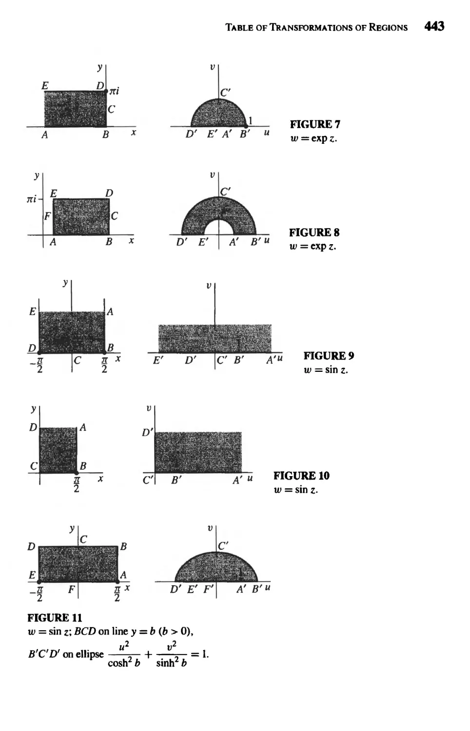
onto half of a circular ring, as shown in Fig. 8, Appendix 2.
y
d-
C
0
D
C
1
♦
1
1
A
c
I
B
1
X
v\ C,
FIGURE 21
w = exp z.
42 Analytic Functions
chap. 2
Our final example here uses the images of horizontal lines to find the image of a
horizontal strip.
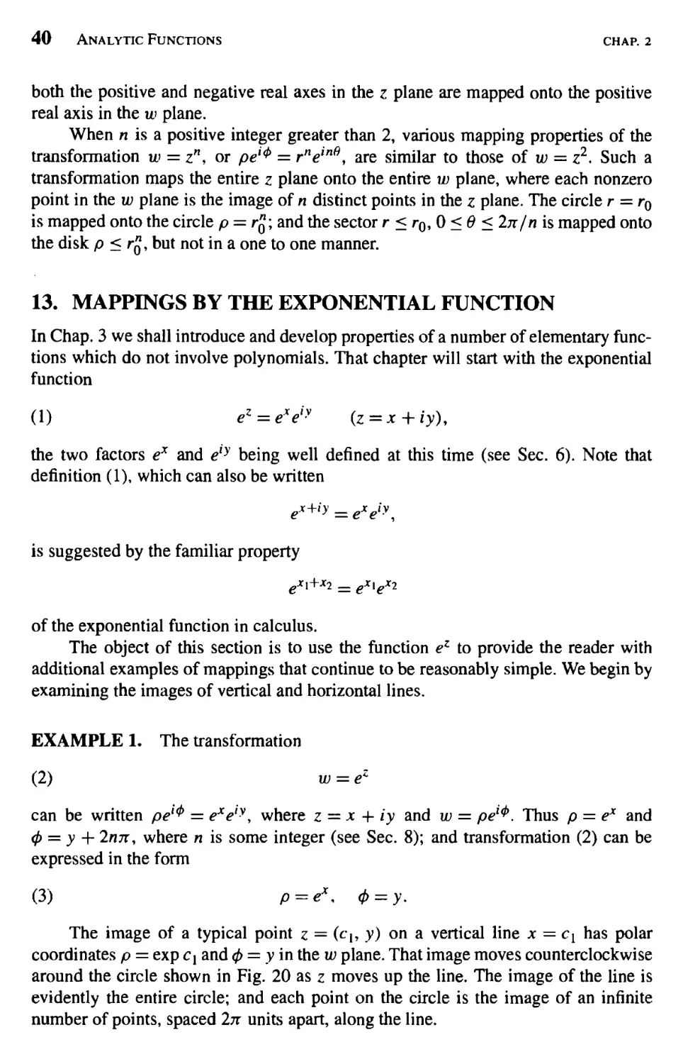
EXAMPLE 3. When w = ez, the image of the infinite strip 0 < y < n is the upper
half v > 0 of the w plane (Fig. 22). This is seen by recalling from Example 1 how
a horizontal line y = c is transformed into a ray <f> = c from the origin. As the real
number c increases from c = 0 to c = n9 the y intercepts of the lines increase from
0 to it and the angles of inclination of the rays increase from <f> = 0 to <j> = it. This
mapping is also shown in Fig. 6 of Appendix 2, where corresponding points on the
boundaries of the two regions are indicated.
.V
0
ni
ci
X
V
0
/
/
/
/
/
/
/
/
A-
u
FIGURE 22
w) = expz.
EXERCISES
1. By referring to Example 1 in Sec. 12, find a domain in the z plane whose image under
the transformation w = z2 is the square domain in the w plane bounded by the lines
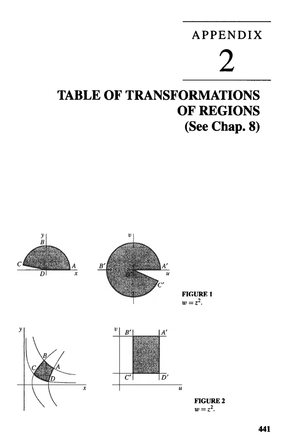
u = 1, u = 2, v = 1, and v = 2. (See Fig. 2, Appendix 2.)
2. Find and sketch, showing corresponding orientations, the images of the hyperbolas
x1 - y2 = cx (c} < 0) and 2xy = c2 (c2 < 0)
under the transformation w = z2.
3. Sketch the region onto which the sector r < 1, 0 < d < n/4 is mapped by the
transformation (a) w = z2; (b) w = z3; (c) w — z4.
4. Show that the lines ay = x (a ^ 0) are mapped onto the spirals p = exp(a<p) under the
transformation w = exp z, where w = p exp(/$).
5. By considering the images of horizontal line segments, verify that the image of the
rectangular region a <x <b,c <y <d under the transformation w = exp z is the region
ea < p < eb, c < <f> < d, as shown in Fig. 21 (Sec. 13).
6. Verify the mapping of the region and boundary shown in Fig. 7 of Appendix 2, where
the transformation is w = exp z.
7. Find the image of the semi-infinite strip x > 0, 0 < v < n under the transformation
w = exp z, and label corresponding portions of the boundaries.
SEC. 14
Limits 43
8. One interpretation of a function w = f(z) = u(x, v) + iv(x, v) is that of a vector field in
the domain of definition of /. The function assigns a vector it», with components u(x, y)
and v(x, y), to each point z at which it is defined. Indicate graphically the vector fields
represented by (a) w = iz\ (b) w = z/\z\.
14. LIMITS
Let a function / be defined at all points z in some deleted neighborhood (Sec. 10) of
zq. The statement that the limit of f(z) as z approaches z0 is a number u>0, or that
(1) Hm f(z) = w0,
means that the point w = f(z) can be made arbitrarily close to w0 if we choose the
point z close enough to z0 but distinct from it. We now express the definition of limit
in a precise and usable form.
Statement (1) means that, for each positive number £, there is a positive number
Ô such that
(2) \f(z) — w0\ < e whenever 0 < \z — Zq\ < S.
Geometrically, this definition says that, for each s neighborhood \w — w0\ < s of tu0,
there is a deleted S neighborhood 0 < \z — Zq\ < S of c<> such that every point z in it
has an image w lying in the & neighborhood (Fig. 23). Note that even though all points
in the deleted neighborhood 0 < |z — zq\ < S are to be considered, their images need
not fill up the entire neighborhood \w - iü0| < e. If / has the constant value u>0, for
instance, the image of z is always the center ofthat neighborhood. Note, too, that once
a S has been found, it can be replaced by any smaller positive number, such as 8/2.
O
i'.w ^
1 *' *,
•*Z T-
O
FIGURE 23
It is easy to show that when a limit of a function f(z) exists at a point z0, it is
unique. To do this, we suppose that
lim /(z) = w0 and lim f(z) = w{.
Z^Zq Z-*Zq
Then, for any positive number £, there are positive numbers SQ and <5] such that
|/(^) -wQ\<£ whenever 0 < \z - z0l < so
44 Analytic Functions
chap. 2
and
\f(z) — w{\ < e whenever 0 < \z — Zq\ < S\.
So if 0 < \z — Zq\ < 5, where 8 denotes the smaller of the two numbers Sq and Sh we
find that
\™i - u>ol = l[/(z) " u>ol - [/(z) ^ wJI < l/(z) - ^ol + l/fc) - ">il < * + * = 2*-
But | Wi — wo | is a nonnegative constant, and £ can be chosen arbitrarily small. Hence
W\ — Wq = 0, or u>] = wq.
Definition (2) requires that / be defined at all points in some deleted
neighborhood of z0. Such a deleted neighborhood, of course, always exists when zq is an interior
point of a region on which / is defined. We can extend the definition of limit to the case
in which z0 is a boundary point of the region by agreeing that the first of inequalities
(2) need be satisfied by only those points z that lie in both the region and the deleted
neighborhood.
EXAMPLE 1. Let us show that if f(z) = iz/2 in the open disk \z\ < 1, then
(3)
lim /(*) = -,
z-*\ 2
the point 1 being on the boundary of the domain of definition of /. Observe that when
z is in the region \z\ < 1,
zw-j
i£ _ 1
2 2
\z-l\
Hence, for any such z and any positive number e (see Fig. 24),
f(z) < e whenever 0 < \z — 1| < 2e.
/1
\2
ijn
ol
FIGURE 24
sec. 14
Limits 45
Thus condition (2) is satisfied by points in the region \z\ < 1 when S is equal to 2e or
any smaller positive number.
If zo is an interior point of the domain of definition of /, and limit (1) is to
exist, the first of inequalities (2) must hold for all points in the deleted neighborhood
0 < \z — Zo\ < 5. Thus the symbol z —► Zq implies that z is allowed to approach z0
in an arbitrary manner, not just from some particular direction. The next example
emphasizes this.
EXAMPLE 2.
(4)
the limit
(5)
If
f(z) = 4r,
Z
lim f(z)
z-*0
does not exist. For, if it did exist, it could be found by letting the point z = (x, y)
approach the origin in any manner. But when z = (jc, 0) is a nonzero point on the real
axis (Fig. 25),
/fe)-i±£-l;
and when z = (0, y) is a nonzero point on the imaginary axis,
0 - ly
Thus, by letting z approach the origin along the real axis, we would find that the desired
limit is I. An approach along the imaginary axis would, on the other hand, yield the
limit —1. Since a limit is unique, we must conclude that limit (5) does not exist.
>•
z = (0,y)<
(0,0)
z = (*,0)
X
FIGURE 25
46 Analytic Functions
chap. 2
While definition (2) provides a means of testing whether a given point wq is a
limit, it does not directly provide a method for determining that limit. Theorems on
limits, presented in the next section, will enable us to actually find many limits.
15. THEOREMS ON LIMITS
We can expedite our treatment of limits by establishing a connection between limits
of functions of a complex variable and limits of real-valued functions of two real
variables. Since limits of the latter type are studied in calculus, we use their definition
and properties freely.
Theorem L Suppose that
f(z) = u(x,y) + iv(x,y), z0 = x0 + iy0, and ^0 = uo + ivo-
Then
(1) lim /(*) = wQ
if and only if
(2) lim u(x, y) = Uq and lim v(x, y) = u0.
(x, y) -* Uo » vo) (x. v) -► Uo. >'o)
To prove the theorem, we first assume that limits (2) hold and obtain limit (1).
Limits (2) tell us that, for each positive number £, there exist positive numbers 5] and
<52 such that
(3) \u - «ol < - whenever 0 < y/(x - x0)2 + (y - y0)2 < 8\
and
(4) \v — v0\ < - whenever 0 < y/(x — x0)2 + (y — y0)2 < 82-
Let S denote the smaller of the two numbers Sx and <$2. Since
|(u + iv) - (u0 + iv0)\ = |(ii - u0) + i(v - v0)\ < \u - u0\ + \v - v0\
and
y/(x - x0)2 + (y- y0)2 = \(x- xq) + i(y- y0)\ = \{x + iy) - (x0 + /y0)|,
it follows from statements (3) and (4) that
\(u + iv) - (u0 + iv0)\ <- + -=£
SEC. 15
Theorems on Limits 47
whenever
0 < \(x + iy) - (x0 + iy0)\ < <5.
That is, limit (1) holds.
Let us now start with the assumption that limit (1) holds. With that assumption,
we know that, for each positive number e, there is a positive number S such that
(5) \(u + iv) -(u0 + iv0)\ <£
whenever
(6) 0<|U + i»-(jc0 + «yo)l<*-
But
I" - "öl ^ l(" ~ uo) + i(v ~ vo)\ = \(u + iv) - ("0 + '"»o)|,
\v-v0\ < \(u-u0) + i(v- v0)\ = \(u + iv) -(u0 + iv0)\,
and
\(x + iy) - U0 + iy0)\ = \(x-x0)+ i(y - y0)\ = y/(x - x0)2 + (y - y0)2.
Hence it follows from inequalities (5) and (6) that
\u — u0\ < s and \v — v0\ < e
whenever
0 < y/(x - jc0)2 + (y - y0)2 < 8.
This establishes limits (2), and the proof of the theorem is complete.
Theorem 2. Suppose that
(7) lim f(z) = w0 and lim F(z) = W0.
Z—*Zq Z—>Zq
Then
(8) ]im[f(z) + F(z)] = w0+W0,
Z^>Zo
(9) \im[f(z)F(z)] = w0W0;
Z-*-Zo
and,ifW0£0,
(10) lim/^=^.
Z-+Z0 F(z) W0
48 Analytic Functions
chap. 2
This important theorem can be proved directly by using the definition of the limit
of a function of a complex variable. But, with the aid of Theorem 1, it follows almost
immediately from theorems on limits of real-valued functions of two real variables.
To verify property (9), for example, we write
f(z) = w(x, y) + ii/(*, y), F(z) = U(x, y) + i V(x, y),
zo = x0 + iy0, w;0 = u0 + iv0. W0 = U0 + i VQ.
Then, according to hypotheses (7) and Theorem 1, the limits as (x, y) approaches
(jc0, v0) of the functions u%v,U, and V exist and have the values m0, vq, U0, and V0,
respectively. So the real and imaginary components of the product
f(z)F(z) = (uU - vV) + i(vU + uV)
have the limits u0U0 — v0V0 and v0U0 + u0VQ, respectively, as (jc, y) approaches
t*o> yo)- Hence, by Theorem 1 again, f(z)F(z) has the limit
(wo^o - »o^o) + i(v0U0 + U0V0)
as z approaches z0; a°d this is equal to w0W0. Property (9) is thus established.
Corresponding verifications of properties (8) and (10) can be given.
It is easy to see from definition (2), Sec. 14, of limit that
lim c = c and lim z = Zo>
where z0 and c are any complex numbers; and, by property (9) and mathematical
induction, it follows that
lim z"=4 (« = 1,2,...).
So, in view of properties (8) and (9), the limit of a polynomial
P(z) = a0 + a}z + a2z2 + • • • + anz"
as z approaches a point zo is the value of the polynomial at that point:
(11) lim P(z) = P(z0).
z-+z0
16. LIMITS INVOLVING THE POINT AT INFINITY
It is sometimes convenient to include with the complex plane the point at infinity,
denoted by oo, and to use limits involving it. The complex plane together with this
point is called the extended complex plane. To visualize the point at infinity, one can
think of the complex plane as passing through the equator of a unit sphere centered at
the point z = 0 (Fig. 26). To each point z in the plane there corresponds exactly one
point P on the surface of the sphere. The point P is determined by the intersection of
the line through the point z and the north pole N of the sphere with that surface. In
SEC. 16
Limits Involving the Point at Infinity 49
/- -~ ' FIGURE 26
like manner, to each point P on the surface of the sphere, other than the north pole N,
there corresponds exactly one point z in the plane. By letting the point N of the sphere
correspond to the point at infinity, we obtain a one to one correspondence between the
points of the sphere and the points of the extended complex plane. The sphere is known
as the Riemann sphere, and the correspondence is called a stereographic projection.
Observe that the exterior of the unit circle centered at the origin in the complex
plane corresponds to the upper hemisphere with the equator and the point N deleted.
Moreover, for each small positive number £, those points in the complex plane exterior
to the circle \z\ = \/e correspond to points on the sphere close to N. We thus call the
set \z\ > \/e an s neighborhood, or neighborhood, of oo.
Let us agree that, in referring to a point z, we mean a point in the finite plane.
Hereafter, when the point at infinity is to be considered, it will be specifically
mentioned.
A meaning is now readily given to the statement
lim f(z) = wQ
when either z0 or w0, or possibly each of these numbers, is replaced by the point
at infinity. In the definition of limit in Sec. 14, we simply replace the appropriate
neighborhoods of z0 and w0 by neighborhoods of oo. The proof of the following
theorem illustrates how this is done.
Theorem. I/zq and Wq are points in the z and w planes, respectively, then
(1) lim f{z) = oo if and only if lim =0
z->Zo z-*zo f(z)
and
(2) lim f(z) = w0 if and only if lim /( - I = w0.
Moreover,
(3) lim f(z) = oo if and only if lim = 0.
50 Analytic Functions
chap. 2
We start the proof by noting that the first of limits ( 1 ) means that, for each positive
number £, there is a positive number S such that
(4) \f(z)\ > - whenever 0 < \z - Zq\ < 5.
s
That is, the point w = f(z) lies in the e neighborhood \w\ > \/e of oo whenever z lies
in the deleted neighborhood 0 < \z — Zq\ < S of z0- Since statement (4) can be written
' -0
f(z)
< e whenever 0 < \z — Zq\ < <5>
the second of limits (1) follows.
The first of limits (2) means that, for each positive number £, a positive number
S exists such that
(5) \f(z) -w0\<e whenever |z| > -.
S
Replacing z by \/z in statement (5) and then writing the result as
'0)
/ - - u*>
<£ whenever 0 < |z — 0| < 5,
we arrive at the second of limits (2).
Finally, the first of limits (3) is to be interpreted as saying that, for each positive
number £, there is a positive number S such that
(6) \f(z)\ > - whenever |z| > -.
s 8
When z is replaced by 1/z, this statement can be put in the form
1
-0
lf(\/z)
and this gives us the second of limits (3).
EXAMPLES. Observe that
< e whenever 0 < \z — 0| < 5;
r iz + 3 . z+1
lim = oo since hm = 0
*->-i z+ 1 Z-—1 iz + 3
and
Z-+OQ z + l ^0(l/z) + l z-^0 l + z
y 2z + i 0 . r (2/z) + i y 2 + iz 0
hm = 2 since hm —■ = hm = 2.
SEC. 17
Continuity 51
Furthermore,
lin. . ^ ..... . .
z^oo z2 + 1 2_>0 (2/z3) - 1 *-►<> 2 - ^
y 2z3-l . (l/z2) + l r z + z* n
Jim — = 00 since hm —-— = hm = 0.
c
17. CONTINUITY
A function / is continuous at a point z0 if all three of the following conditions are
satisfied:
(1) lim f(z) exists,
(2) /(z0) exists,
(3) lim /(z) = /(z0).
Observe that statement (3) actually contains statements (1) and (2), since the existence
of the quantity on each side of the equation there is implicit. Statement (3) says that,
for each positive number £, there is a positive number S such that
(4) \f(z) - f(z0)\ < e whenever \z - z0\ < 8.
A function of a complex variable is said to be continuous in a region R if it is
continuous at each point in /?.
If two functions are continuous at a point, their sum and product are also
continuous at that point; their quotient is continuous at any such point where the denominator
is not zero. These observations are direct consequences of Theorem 2, Sec. 15. Note,
too, that a polynomial is continuous in the entire plane because of limit (11), Sec. 15.
We turn now to two expected properties of continuous functions whose
verifications are not so immediate. Our proofs depend on definition (4), and we present the
results as theorems.
Theorem L A composition of continuous functions is itself continuous.
A precise statement of this theorem is contained in the proof to follow. We let
w = f(z) be a function that is defined for all z in a neighborhood \z — zol < 5 of a
point zo » and we let W = g(w) be a function whose domain of definition contains the
image (Sec. 12) ofthat neighborhood under /. The composition W = g[f(z)] is, then,
defined for all z in the neighborhood \z — Zq\ <&• Suppose now that / is continuous at
z0 and that g is continuous at the point /(zo) in the w plane. In view of the continuity
of g at /(zo)> there is, for each positive number £, a positive number y such that
\g[f(z)] - *[/(z0)]l < s whenever \f(z) - f(z0)\ < Y-
52 Analytic Functions
chap. 2
Is
• Z
to
O
FIGURE 27
(See Fig. 27.) But the continuity of / at z.q ensures that the neighborhood \z - Zol < 8
can be made small enough that the second of these inequalities holds. The continuity
of the composition g[f(z)] is, therefore, established.
Theorem!. Ifafunction f(z) is continuous and nonzero at a point z.q, then f(z) ^ 0
throughout some neighborhood of that point
Assuming that f(z) is, in fact, continuous and nonzero at z0, we can prove
Theorem 2 by assigning the positive value \f(z.o)\/2 to the number e in statement
(4). This tells us that there is a positive number S such that
l/U)-/(^o)l<^^ whenever \z-z0\<S-
So if there is a point z in the neighborhood \z — Zq\ < S at which f(z) = 0, we have
the contradiction
l/(zo)l <
l/(*o)l.
and the theorem is proved.
The continuity of a function
(5)
f(z) = u(x,y) + iv{x,y)
is closely related to the continuity of its component functions u{x, y) and v(x, >).
We note, for instance, how it follows from Theorem 1 in Sec. 15 that the function
(5) is continuous at a point zq = (jcq, >q) if and only if its component functions are
SEC. 17
Exercises 53
continuous there. To illustrate the use of this statement, suppose that the function (5) is
continuous in a region R that is both closed and bounded (see Sec. 10). The function
s/\u{x9y)]2 + [v(x9y)]2
is then continuous in R and thus reaches a maximum value somewhere in that region.*
That is, / is bounded on R and \f(z)\ reaches a maximum value somewhere in R.
More precisely, there exists a nonnegative real number M such that
(6) l/(z)|<Af for all z in/?,
where equality holds for at least one such z.
EXERCISES
1. Use definition (2), Sec. 14, of limit to prove that
—2
(a) lim Re z = Re z0; (b) lim z = Zr>; (c) hm — = 0.
z-+zü Z^Zq z->0 z
2. Let a, b, and c denote complex constants. Then use definition (2), Sec. 14, of limit to
show that
(a) lim (az + b) = az0 + b\ (b) lim (z2 + c) = zl + c\
z~+zo Z^Zq
(c) lim [x + i(2x + y)] = 1 + i (z = x + iy).
3. Let nbea positive integer and let P (z) and Q(z) be polynomials, where Q(Zq) ^ 0. Use
Theorem 2 in Sec. 15 and limits appearing in that section to find
1 /'z3- 1 P(z)
(a) lim — (z0 £ 0); (b) Km- ; (c) lim —^-.
z-+zqZ" z-m z + i z~^zoQ(z)
Ans.(a)\/z%\ (ft)0; (c) P(z0)/G(zo)-
4. Use mathematical induction and property (9), Sec. 15, of limits to show that
hm z" = zn0
when n is a positive integer (n — 1, 2, . . .).
5. Show that the limit of the function
f(z)
-(})'
as z tends to 0 does not exist. Do this by letting nonzero points z — (x, 0) and z — (x, x)
approach the origin. [Note that it is not sufficient to simply consider points z = (*, 0)
and z = (0, y), as it was in Example 2, Sec. 14.1
* See, for instance, A. E. Taylor and W. R. Mann, "Advanced Calculus " 3d ed., pp. 125-126 and p. 529,
1983.
54 Analytic Functions
chap. 2
6. Prove statement (8) in Theorem 2 of Sec. 15 using
(a) Theorem 1 in Sec. 15 and properties of limits of real-valued functions of two real
variables;
(b) definition (2), Sec. 14, of limit.
7. Use definition (2), Sec. 14, of limit to prove that
if lim /(z) = u;0, then lim |/(z)| = |u>0|.
z-*z-o z~*zo
Suggestion: Observe how inequality (8), Sec. 4, enables one to write
\\f(z)\-\w0U<\f(z)-v>ol
8. Write Àz = z — Zç> and show that
lim f(z) = w0 if and only if lim /(zo + Az) = w0.
Z-*Zo Az->0
9. Show that
lim f{z)g(z) = 0 if Hm /(z) = 0
Z-+ZQ Z-+ZQ
and if there exists a positive number M such that \g(z)\ < Af for all z in some
neighborhood of Zo-
10. Use the theorem in Sec. 16 to show that
4z2 1 z2 + 1
(a) lim — 4; (b) lim = oo; (c) lim = oo.
z^od(z- 1)2 « z-+\(z- l)3 z-+ooz- 1
11. With the aid of the theorem in Sec. 16, show that when
az 4- b
T(z) = -^— (ad-bc£0),
cz + d
{a) lim7(z) = oo ifc = 0;
£-►00
(b) lim T(z) = - and lim T(z) = oo if c ^ 0.
Z-+OC c z-^-d/c
12. State why limits involving the point at infinity are unique.
13. Show that a set 5 is unbounded (Sec. 10) if and only if every neighborhood of the point
at infinity contains at least one point in 5.
18. DERIVATIVES
I-et / be a function whose domain of definition contains a neighborhood of a point z0.
The derivative of / at z0> written /'(Zn)» is defined by the equation
(1) /W=lim fM-fM,
*-2o Z-Zq
provided this limit exists. The function / is said to be differentiable at zo when its
derivative at zq exists.
SEC. 18
Derivatives 55
By expressing the variable z in definition (1 ) in terms of the new complex variable
Az = z - Zq,
we can write that definition as
(2) /'U-o)= Hm /fr6 + A*>-/fro>.
Az-*ü Az
Note that, because / is defined throughout a neighborhood of z0, the number
f(z0 + Az)
is always defined for | Az| sufficiently small (Fig. 28).
y
0
/ \
/ \
/ \
X
FIGURE 28
When taking form (2) of the definition of derivative, we often drop the subscript
on zo and introduce the number
Aw = f(z + Az)~f(z).
which denotes the change in the value of / corresponding to a change Az in the point
at which / is evaluated. Then, if we write dw/dz for /'(z), equation (2) becomes
dw Aw
(3) — = hm .
dz Az->0 Az
EXAMPLE 1. Suppose that f(z) = z2. At any point z,
r Au> y & + Az)2 ~~ Z2 y /o , a ^ n
hm = hm = hm (2z + Az) = 2z,
Az-+0 Az Az-^O Az Az-»0
since 2z + Az is a polynomial in Az. Hence dw/dz = 2z> or /'(z) = 2z.
EXAMPLE 2. Consider now the function f(z) = |z|2. Here
Aw \z + Az|2 - |z|2 (z +Az)(z+ ~Kz)-zz _ - , -t- . Az
—- = = — Z + AZ + Z-—.
Az Az Az Az
56 Analytic Functions
char 2
(0, Ay).
1
(0,0)
>
( A*, 0)
Ajc
FIGURE 29
If the limit of Aw/Az exists, it may be found by letting the point Az = (Ax, Ay)
approach the origin in the Az plane in any manner. In particular, when Az approaches
the origin horizontally through the points (Ajc, 0) on the real axis (Fig. 29),
In that case,
Az = Aa + «0 = Aa - /0 = Ax + /O = A<
Aw _ -T—
= z + Az + z.
Az
Hence, if the limit of Aw/Az exists, its value must be z + z. However, when Az
approaches the origin vertically through the points (0, Ay) on the imaginary axis, so
that
Az = 0 + iAy = -(0 + iAy) = -Az,
we find that
Au; _ —-
—- = z + Az -z.
Az
Hence the limit must be z — z if it exists. Since limits are unique (Sec. 14), it follows
that
z + z = z — z,
or z = 0, if dwjdz is to exist.
To show that dwjdz does, in fact, exist at z = 0, we need only observe that our
expression for Aw/Az reduces to Az when z = 0. We conclude, therefore, that dw/dz
exists only at z = 0, its value there being 0.
Example 2 shows that a function can be differentiable at a certain point but
nowhere else in any neighborhood of that point. Since the real and imaginary parts
of/(z) = |z|2are
(4)
u(x, y) =A*fc + y" and u(jt,y) = 0,
SEC.19
Differentiation Formulas 57
respectively, it also shows that the real and imaginary components of a function of a
complex variable can have continuous partial derivatives of all orders at a point and
yet the function may not be differentiable there.
The function f(z) = \z\2 is continuous at each point in the plane since its
components (4) are continuous at each point. So the continuity of a function at a point
does not imply the existence of a derivative there. It is, however, true that the existence
of the derivative of a function at a point implies the continuity of the function at that
point To see this, we assume that /'(zo) exists and write
lim [f(z) - f(zo)] = lim fU) ~ fUo) lim (z - z0) = /'(z0) ■ 0 = 0,
*-*'o z->Co Z — Zo *-**>
from which it follows that
lim /(z) = /(z0).
Z-*Zq
This is the statement of continuity of / at zq (Sec. 17).
Geometric interpretations of derivatives of functions of a complex variable are
not as immediate as they are for derivatives of functions of a real variable. We defer
the development of such interpretations until Chap. 9.
19. DIFFERENTIATION FORMULAS
The definition of derivative in Sec. 18 is identical in form to that of the derivative of a
real-valued function of a real variable. In fact, the basic differentiation formulas given
below can be derived from that definition by essentially the same steps as the ones used
in calculus. In these formulas, the derivative of a function / at a point z is denoted by
either
-f f(z) or /'(z),
dz
depending on which notation is more convenient.
Let c be a complex constant, and let f be a function whose derivative exists at a
point z. It is easy to show that
(1) ^c = 0, ^z = 1, ^[cf(z)] = cf'iz).
dz dz dz
Also, if n is a positive integer,
(2) ^-z"=nzn-1.
dz
This formula remains valid when n is a negative integer, provided that z^O.
58 Analytic Functions
chap. 2
If the derivatives of two functions / and F exist at a point z, then
(3) ^[f(z) + F(z)]=f(z) + F'(z),
dz
(4) ^-[f(z)F(z)]= f(z)F\z) + f'(z)F(z)\
dz
and, when F(z) ^ 0,
/(z)1 F(z)f'(z)-f(z)F'(z)
F(z)\ [F(z)l2
Let us derive formula (4). To do this, we write the following expression for the
change in the product w = f(z)F(z):
Aw = f(z + Az)F(z + Az) - f{z)F(z)
= f(z)[F(z + Az) - F(z)] + [f(z + Az) - f(z)]F(z + Az).
Thus
ÈHL = /wf"^)-fM + /fa + Az)-/(t) +
Az Az Az
and, letting Az tend to zero, we arrive at the desired formula for the derivative of
/(z)F(z). Here we have used the fact that F is continuous at the point z, since F'(z)
exists; thus F(z + Az) tends to F(z) as Az tends to zero (see Exercise 8, Sec. 17).
There is also a chain rule for differentiating composite functions. Suppose that /
has a derivative at zq and that g has a derivative at the point f(Zo). Then the function
F(z) = g[f(z)] has a derivative at Zo, and
(6) /r/(z0) = *V(2o)]/'Uo).
If we write w = /(z) and W = g(w), so that W = F(z), the chain rule becomes
dW _ dWdw
dz dw dz
EXAMPLE. To find the derivative of (2z2 + i)5, write w = 2z2 + i and W = u;5.
Then
— (2z2 + i)5 = 5u;44z = 20z(2z2 + i)4.
dz
To start the proof of formula (6), choose a specific point zo at which /\zq)
exists. Write u;0 = /(zq) and also assume that g'(w0) exists. There is, then, some
e neighborhood \w — w0\ < e of u;0 such that, for all points w in that neighborhood,
(5)
dz
SEC. 19
Exercises 59
we can define a function <J> which has the values <t>(w0) = 0 and
(7) <t>(w) = 8{W) "" g{Wo) - g'(wQ) when w£w0.
W — Wq
Note that, in view of the definition of derivative,
(8) lim <D(uO = 0.
Hence 4> is continuous at u;0.
Now expression (7) can be put in the form
(9) g(w) - g(w0) = [g'(w0) + ®(w)](w - wQ) (\w - w0\ < s),
which is valid even when w = u;0; and, since /'(Zq) exists and / is, therefore,
continuous at zo> we can choose a positive number 5 such that the point f(z) lies in
the s neighborhood \w — w0\ < e of w0 if z lies in the 5 neighborhood \z — Zq\ < S of
Zq. Thus it is legitimate to replace the variable w in equation (9) by f(z) when z is any
point in the neighborhood \z — Zq\ < <5. With that substitution, and with n>0 = /(Zn)«
equation (9) becomes
do) *[/<*>]-«[/(*>>!={g>[f(Zo)]+*[nmm^iM
Z — Zq Z — Zq
(0<|2-Z0I <<$)>
where we must stipulate that z ^ Zq so that we are not dividing by zero. As already
noted, / is continuous at Zq and <I> is continuous at the point wq = /(zo). Thus the
composition 0[/(z)J is continuous at zq\ and, since 4>(u,»0) = 0,
lim 4>r/(z)J = 0.
So equation (10) becomes equation (6) in the limit as z approaches z0.
EXERCISES
1. Use results in Sec. 19 to find f'(z) when
(a) /U) = 3r - 2Z + 4; (b) /(z) = (1 - 4z2)3;
(c) f(z) = -1—\ (z £ -1/2); (d) f(z) = °+2Z } (z 9* 0).
2z + 1 zz
2. Using results in Sec. 19, show that
(a) a polynomial
P(Z) = a0 + a]Z + a2z2 + • • • + a«*" (an £ 0)
of degree rc (n > 1) is differentiable everywhere, with derivative
P'(z) = a 1 + 2a2z + • • • + "^z"'1 ;
60 Analytic Functions
chap. 2
(b) the coefficients in the polynomial P(z) in part (a) can be written
P'(0) P"(0) P(n>(0)
3. Apply definition (3), Sec. 18, of derivative to give a direct proof that
/'(Z) = —L when /(z) = - (z^O).
z2 z
4. Suppose that /(z0) = g(z0) = ° and *at /'ten) and tf'teo) exisl» where g'(zo) 7* 0. Use
definition (1), Sec. 18, of derivative to show that
5. Derive formula (3), Sec. 19, for the derivative of the sum of two functions.
6. Derive expression (2), Sec. 19, for the derivative of zn when n is a positive integer by
using
(a) mathematical induction and formula (4), Sec. 19, for the derivative of the product of
two functions;
(b) definition (3), Sec. 18, of derivative and the binomial formula (Sec .3).
7. Prove that expression (2), Sec. 19, for the derivative of z" remains valid when n is a
negative integer (n = — 1, —2, ...), provided that zj^O.
Suggestion: Write m = —n and use the formula for the derivative of a quotient of
two functions.
8. Use the method in Example 2, Sec. 18, to show that /'(z) does not exist at any point z
when
(a) f(z) = z; {b) f(z) = Re z; (c) /(z) = Im z.
9. Let / denote the function whose values are
/(z) =
^2
— when z 7^ 0,
z
0 when z = 0.
Show that if z = 0, then Aw/Az = 1 at each nonzero point on the real and imaginary
axes in the Az, or Ax Ay, plane. Then show that Aw/ Az = -1 at each nonzero point
(A.r, Ax) on the line Ay = Ajc in that plane. Conclude from these observations that
/'(()) does not exist. (Note that, to obtain this result, it is not sufficient to consider only
horizontal and vertical approaches to the origin in the Az plane.)
20. CAUCHY-RIEMANN EQUATIONS
In this section, we obtain a pair of equations that the first-order partial derivatives of
the component functions u and v of a function
(1) f(z) = u(x.y) + iv(x,y)
SEC. 20
CAUCH Y-RlEMANN EQUATIONS 61
must satisfy at a point Zq = (xq, yo) when the derivative of / exists there. We also
show how to express /'(Zo) in terms of those partial derivatives.
We start by writing zo = *o + Oto» Az = Ajc 4- /Ay, and
Aw = f(Zo + Az) - f(zo)
= [u(x0 + Ax, y0 + Ay) - u(x0, y0)] + i[v(x0 + Ax, y0 + Ay) - v(x0, y0)].
Assuming that the derivative
(2) f'(zo> = Hm ^
Az-*0 Az
exists, we know from Theorem 1 in Sec. 15 that
(3) /'(z0) = lim Re —+i lim Im—.
(A^,Ay)-^(0,0) AZ (Ajr,Ay)-»<0,0) Az
Now it is important to keep in mind that expression (3) is valid as (Ax, Ay)
tends to (0, 0) in any manner that we may choose. In particular, we let (A.*, Ay) tend
to (0, 0) horizontally through the points (Ajc, 0), as indicated in Fig. 29 (Sec. 18).
Inasmuch as Ay = 0, the quotient Aw/Az becomes
Aw _ u(x0 + Ax, y0) - u(x0, y0) v(x0 + Ax, y0) - v(x0, y0)
Az Ax Ajc
Thus
lim Re ^ = lim "(*o + A*, y0) ~ *(*Q> ?o) =
(Ajc, Ay)-> (0,0) Az A*->0 Ax
and
lim Tm ^ = lim "<*> + A*' »>> " v{x°> yo) = vx(x0, y0)
(A*,Ay)->(0,0) Az Ax->Ü AX
where ux(x0, y0) and vx(xq, yo) denote the first-order partial derivatives with respect
to x of the functions u and v, respectively, at (jc0, y0). Substitution of these limits into
expression (3) tells us that
(4) /'(z0) = M*o. yo) + ivx(*0' yo)-
We might have let Az tend to zero vertically through the points (0, Ay). In that
case, Ajc = 0 and
Aw _ u(x0, y0 + Ay) - u(x0, y0) v(x0, y0 + Ay) - v(x0, yQ)
Az /Ay /Ay
_ *>(*q, yp + Ay) - v{x0, y0) _ ,u(x0, y0 + Ay) - u(xQ, y0)
Ay Ay
62 Analytic Functions
chap. 2
Evidently, then,
^ Aw
lim Re
(Aa,Av)-(0,0) Az
and
Am;
lim Im =
(A.x\Av)-v(0,0) &z
Hence it follows from expression (3) that
(5) f'(z0) = Vy(xQ, y0) - iuy(x0, y0),
where the partial derivatives of u and v are, this time, with respect to y. Note that
equation (5) can also be written in the form
f'(z0) = -i[uy{x0, y0) + ivy(xQ. y0)l
Equations (4) and (5) not only give /'(zq) in terms of partial derivatives of the
component functions u and t>, but they also provide necessary conditions for the
existence of /'(zo)- F°r> on equating the real and imaginary parts on the right-hand
sides of these equations, we see that the existence of /'(z0) requires that
(6) ux(x0, y0) = vy(x0, y0) and uy(xQ9 y0) = -vx(x0, y0).
Equations (6) are the Cauchy-Riemann equations, so named in honor of the French
mathematician A. L. Cauchy (1789-1857), who discovered and used them, and in
honor of the German mathematician G. F B. Riemann (1826-1866), who made them
fundamental in his development of the theory of functions of a complex variable.
We summarize the above results as follows.
Theorem. Suppose that
f(z) = u(xyy) + iv(x,y)
and that f'(z) exists at a point z0 = x0 + iy0. Then the first-order partial derivatives
ofu and v must exist at (jc0, ;y0), and they must satisfy the Cauchy-Riemann equations
(7) ux = vy9 ity = -vx
there. Also, /'(zq) can be written
(8) f'(z0) = ux + ivXi
where these partial derivatives are to be evaluated at (x0, y^).
lim ^^fcl^)=Vv(,,Vo)
Av-*o Ay
Urn tt<x°'X> + Ay)-u(x°'*>)=-u(Xo.y0).
Ay-^0 Ay
SEC. 21
Sufficient Conditions for Differentiability 63
EXAMPLE 1. In Example 1, Sec. 18, we showed that the function
f(z) = zl = x2-y2 + j2xy
is differentiable everywhere and that ff(z) = 2z. To verify that the Cauchy-Riemann
equations are satisfied everywhere, we note that
u(x, y) = x2 — y2 and v(x, y) = 2xy.
Thus
ux = 2x = Vy, uy = —2y = —vx.
Moreover, according to equation (8),
f\z) = 2x + ily = 2(x + iy) = 2z.
Since the Cauchy-Riemann equations are necessary conditions for the existence
of the derivative of a function / at a point Zo, they can often be used to locate points
at which / does not have a derivative.
EXAMPLE 2. When f{z) = |z|2, we have
u(x, y)=x2 + y2 and v(x,y) = Q.
If the Cauchy-Riemann equations are to hold at a point (x, y), it follows that 2x = 0
and 2y = 0, or that x = y = 0. Consequently, f'(z) does not exist at any nonzero point,
as we already know from Example 2 in Sec. 18. Note that the above theorem does not
ensure the existence of /'(0). The theorem in the next section will, however, do this.
21. SUFFICIENT CONDITIONS FOR DIFFERENTIABILITY
Satisfaction of the Cauchy-Riemann equations at a point zq = C*q, y$) is not sufficient
toensure the existence of the derivative of a function f(z) at that point. (See Exercise 6,
Sec. 22.) But, with certain continuity conditions, we have the following useful theorem.
Theorem. Let the function
f(z) = u(x,y) + iv(x,y)
be defined throughout some s neighborhood of a point zo = *o + ho* an^ suppose
that the first-order partial derivatives of the functions u and v with respect to x and y
exist everywhere in that neighborhood. If those partial derivatives are continuous at
C*0> yo) and satisfy the Cauchy-Riemann equations
ux = vy9 uy = -vx
at (x09 y0), then /'(z0) exists.
64 Analytic Functions chap. 2
To start the proof, we write Az = Ax + 1" Ay, where 0 < | Az| < £, and
Au; = /(zo+Az)-/(zo).
Thus
(1) Au; = Au + iAv,
where
and
Aw = u(x0 + A*, y0 + Ay) - w(x0, y0)
Au = v(x0 + Ax, y0 + Ay) - v(x0, y0).
The assumption that the first-order partial derivatives of u and v are continuous at the
point (,v0, Vo) enables us to write*
(2) Aw = ux(x0, y0)Ax + uy(x0, y0)Ay + e]y/(Ax)2 + (Ay)2
and
(3) Av = vx(x09 y0)Ax + vy(x0, y0)Ay + e2y/(Ax)2 + (Ay)2,
where £t and £2 tend to 0 as (Ax, Ay) approaches (0, 0) in the Az plane. Substitution
of expressions (2) and (3) into equation (1) now tells us that
(4) Aw = ux(x0, y0)Ax + uy(x0y y0)Ay + ely/(Ax)2 + (Ay)2
+ '[M*0> ^0^* + V'r0' }'o)&y + ^2\/(A^)2 + (Ay)2J.
Assuming that the Cauchy-Riemann equations are satisfied at (*0, y0), we can
replace uy(x0< y0) by —vx(xq, y0) and vv(xqh vq) by ux(x0, y0) in equation (4) and
then divide through by Az to get
Àw , , , x . ,VW)2 + (Ay)2
(5) —- = ux(x0, y0) + ivx(x0, y0) + (el + ie2)
Az Ar.
* See, for instance, A. E. Taylor and W. R. Mann, "Advanced Calculus" 3d ed., pp. 150-151 and 197-
198, 1983.
SEC. 22
Polar Coordinates 65
But VÏAjc)2 + (A3;)2 = IAz|, and so
U(Ax)2 + (Ay)2\_l
I Az I
Also, s 1 + i£2 tends to 0 as (Ajc, Ay) approaches (0, 0). So the last term on the right
in equation (5) tends to 0 as the variable Az = Ajc + /Ay tends to 0. This means that
the limit of the left-hand side of equation (5) exists and that
(6) f'(z0) = ux + ivxy
where the right-hand side is to be evaluated at (*0, y0).
EXAMPLE 1. Consider the exponential function
f(z) = ez = exeiy (z = x + iy)9
some of whose mapping properties were discussed in Sec. 13. In view of Euler's
formula (Sec. 6), this function can, of course, be written
f{z) = ex cos y + iex sin y,
where y is to be taken in radians when cos y and sin y are evaluated. Then
u(x, y) = ex cos y and v(x, y) = ex sin y.
Since ux = vy and uy = —vx everywhere and since these derivatives are everywhere
continuous, the conditions in the theorem are satisfied at all points in the complex
plane. Thus f'(z) exists everywhere, and
f'(z) = ux + ivx = ex cos y + iex sin y.
Note that f'(z) = f(z).
EXAMPLE 2. It also follows from the theorem in this section that the function
f(z) = |z|2, whose components are
u(x, y) = x2 + y2 and v(x, y) = 0,
has a derivative at z = 0. In fact, /'(()) = 0 + /0 = 0 (compare Example 2, Sec. 18). We
saw in Example 2, Sec. 20, that this function cannot have a derivative at any nonzero
point since the Cauchy-Riemann equations are not satisfied at such points.
22. POLAR COORDINATES
Assuming that zo ^ 0, we shall in this section use the coordinate transformation
(1) *=rcos0, y = rsin0
66 Analytic Functions
chap. 2
to restate the theorem in Sec. 21 in polar coordinates.
Depending on whether we write
z = x+iy or z = reie (z^O)
when w = f(z), the real and imaginary parts of w = u + iv are expressed in terms of
either the variables x and y or r and 0. Suppose that the first-order partial derivatives
of u and v with respect to x and y exist everywhere in some neighborhood of a given
nonzero point zo and are continuous at that point. The first-order partial derivatives
with respect to r and 6 also have these properties, and the chain rule for differentiating
real-valued functions of two real variables can be used to write them in terms of the
ones with respect to x and y. More precisely, since
du _ du dx du dy du _ du dx du dy
one can write
(2) ur = ux cos0 + uy sinö, u0 = —uxr sinö + uyr cosö.
Likewise,
(3) vr = vx cos 0 + vy sin 0, v0 = — vx r sin 9 + vyr cos 0.
If the partial derivatives with respect to x and y also satisfy the Cauchy-Riemann
equations
(4) Kjc = V uy = -vx
at z0, equations (3) become
(5) vr = —uy cos 9 + ux sin 9, ve = uy r sin 0 + ux r cos 9
at that point. It is then clear from equations (2) and (5) that
(6) rur = ve> ue = -rvr
at the point zo-
If, on the other hand, equations (6) are known to hold at zo> it is straightforward
to show (Exercise 7) that equations (4) must hold there. Equations (6) are, therefore,
an alternative form of the Cauchy-Riemann equations (4).
We can now restate the theorem in Sec. 21 using polar coordinates.
Theorem. Let the function
f(z) = u(r90) + iv(r,0)
be defined throughout some e neighborhood of a nonzero point zq = r0 exp(/0o), and
suppose that the first-order partial derivatives of the functions u and v with respect to r
SEC, 22
Polar Coordinates 67
and 9 exist everywhere in that neighborhood. If those partial derivatives are continuous
at (/g, Qq) and satisfy the polar form
rur = ve, ue = —rvr
of the Cauchy-Riemann equations at (r0, 9$), then f'(Zo) exists.
The derivative f'(zo) here can be written (see Exercise 8)
(7) f'(zo) = e-i${ur + ivr)9
where the right-hand side is to be evaluated at (r0, 0O).
EXAMPLE 1. Consider the function
(8) f(z) = - = 4- = -e~ie = -(cos0 - î sinö) (z ^0).
z rel° r r
Since
u(r,0) = and v(r,9) =
r r
the conditions in the above theorem are satisfied at every nonzero point z = re10 in the
plane. In particular, the Cauchy-Riemann equations
cos 9 . sin 9
rur = = ve and ue = = — rvr
r r
are satisfied. Hence the derivative of / exists when z^O; and, according to
expression (7),
f//,x _ „-M ( cos 0 sin 0 \ i6
*-w
r2 (re**)2 z2'
EXAMPLE 2. The theorem can be used to show that, when a is a fixed real number,
the function
(9) f(z) = ^rew/3 (r > 0, a < 9 < a + lit)
has a derivative everywhere in its domain of definition. Here
9 9
u(r, 9) = v^cos - and u(r, 9) = v^sin -.
Inasmuch as
¥r 9 , Mr . 9
rur = — cos - = Vu and u* = sin - = —rvr
3 3 3 3
68 Analytic Functions
chap. 2
and since the other conditions in the theorem are satisfied, the derivative f'(z) exists
at each point where /(z) is defined. Furthermore, expression (7) tells us that
- ,-«•»
or
f'(z) = e
f'iz) =
1
i*m
e
cos - + I
1
*m4
. 6
sin -
,-iO
*m
:eie^ =
3 (yîeWy 3 [/(z)]
2*
Note that when a specific point z is taken in the domain of definition of /, the
value f(z) is one value of z]^ (see Sec. 11 ). Hence this last expression for f\z) can
be put in the form
^/3 = —L_
3(z>/3y
when that value is taken. Derivatives of such power functions will be elaborated on in
Chap. 3 (Sec. 32).
EXERCISES
1. Use the theorem in Sec. 20 to show that f'(z) does not exist at any point if
(a)/(z) = z; (b)f(z) = z-z; (c) f(z) = 2x + ixy2; (d) f(z) = e*e~iy.
2. Use the theorem in Sec. 21 to show that /'(z) and its derivative f"{z) exist everywhere,
and find f"(z) when
(a) f(z) = iz + 2; (b) f(z) = *-**->;
(c) f(z) = z3; (d) f(z) = cos a; cosh v — / sin x sinh v.
A™, (ft) f'\z) = /(z); (J) /"(z) = -f(z).
3. From results obtained in Sees. 20 and 21, determine where f'{z) exists and find its value
when
(a) f(z) = 1/z; {b) f(z) =x2 + /v2; (c) /(z) = z Im z.
/inS.(a)/'(z) = -l/z2(z5éO); (b) f'(x + ix) = 2x; (c)/'(0) = 0.
4. Use the theorem in Sec. 22 to show that each of these functions is differentiable in the
indicated domain of definition, and then use expression (7) in that section to find /'(z):
(a) f(z) = \/zUz£0);
{b) /(z) = <J?ew'2 (r > 0, a < 6 < a + 2jr);
(c) f(z) = éTecos(ln r) + iéT9sin(ln r) (r > 0, 0 < 6 < In).
Ans. (b) /'(z) = —l— ; (c) f'(z) = i^-.
2/(z) z
SEC. 22
Exercises 69
5. Show that when f(z) = jc3 + /(l - y)3, it is legitimate to write
f'(z) = ux+ivx=3x2
only when z = i.
6. Let w and v denote the real and imaginary components of the function / defined by the
equations
Hz)=\ 7 when z*°-
[ 0 when z = 0.
Verify that the Cauchy-Riemann equations ux = vy and uy = —vx are satisfied at the
origin z = (0, 0). [Compare Exercise 9, Sec. 19, where it is shown that /'(()) nevertheless
fails to exist.]
7. Solve equations (2), Sec. 22, for w^ and uy to show that
sinö . ^ cosö
«x = wr cos0 — mö , wv = wr sin 9 + ue .
r " r
Then use these equations and similar ones for vx and vy to show that, in Sec. 22, equations
(4) are satisfied at a point zq if equations (6) are satisfied there. Thus complete the
verification that equations (6), Sec. 22, are the Cauchy-Riemann equations in polar form.
8. Let a function f(z) = u + iv be differentiate at a nonzero point z0 = ro exp(/0o). Use
the expressions for ux and vx found in Exercise 7, together with the polar form (6), Sec.
22, of the Cauchy-Riemann equations, to rewrite the expression
f'(z0) = ux + ivx
in Sec. 21 as
f'(zo) = e-i0(ur + ivr),
where ur and vr are to be evaluated at (r0, 0O).
9. (a) With the aid of the polar form (6), Sec. 22, of the Cauchy-Riemann equations, derive
the alternative form
f'(zo) = —(u0 + ive)
zo
of the expression for /'(z0) found in Exercise 8.
(b) Use the expression for /'(Zq) in part (a) to show that the derivative of the function
f(z) = 1/z (z ï 0) in Example 1, Sec. 22, is f(z) = -l/z2.
10. (a) Recall (Sec. 5) that if z = x + iy\ then
z+z A z-z
x = and y = .
2 2i
70 Analytic Functions
chap. 2
By formally applying the chain rule in calculus to a function F(x, y) of two real
variables, derive the expression
dz dx dz dy dz 2 \dx dy ) *
(b) Define the operator
dz ~ 2\dx +ldy)'
suggested by part (a), to show that if the first-order partial derivatives of the real
and imaginary parts of a function f(z) = u(x, y) + iv(x, y) satisfy the Cauchy-
Riemann equations, then
t\f 1
TZ = ~[(ux - vv) + i(Vx + uy)] = 0.
oz 2
Thus derive the complex form df/dz = 0 ö//Ae Cauchy-Riemann equations.
23. ANALYTIC FUNCTIONS
We are now ready to introduce the concept of an analytic function. A function / of the
complex variable z is analytic in an open set if it has a derivative at each point in that
set* If we should speak of a function / that is analytic in a set S which is not open,
it is to be understood that / is analytic in an open set containing 5. In particular, / is
analytic at a point zq if it is analytic throughout some neighborhood of zq.
We note, for instance, that the function f(z) = \/z is analytic at each nonzero
point in the finite plane. But the function f(z) = \z\2 is not analytic at any point since
its derivative exists only at z = 0 and not throughout any neighborhood. (See Example
2, Sec. 18.)
An entire function is a function that is analytic at each point in the entire finite
plane. Since the derivative of a polynomial exists everywhere, it follows that every
polynomial is an entire function.
If a function / fails to be analytic at a point z0 but is analytic at some point
in every neighborhood of z0> then z0 is called a singular point, or singularity, of /.
The point z = 0 is evidently a singular point of the function f(z) = \/z- The function
f(z) = \z\2, on the other hand, has no singular points since it is nowhere analytic.
A necessary, but by no means sufficient, condition for a function / to be analytic
in a domain D is clearly the continuity of / throughout D. Satisfaction of the Cauchy-
Riemann equations is also necessary, but not sufficient. Sufficient conditions for
analyticity in D are provided by the theorems in Sees. 21 and 22.
Other useful sufficient conditions are obtained from the differentiation formulas
in Sec. 19. The derivatives of the sum and product of two functions exist wherever the
* The terms regular and holomorphic are also used in the literature to denote analyticity.
SEC.23
Analytic Functions 71
functions themselves have derivatives. Thus, if two functions are analytic in a domain
D, their sum and their product are both analytic in D. Similarly, their quotient is
analytic in D provided the function in the denominator does not vanish at any point in
D. In particular, the quotient P(z)/Q(z) of two polynomials is analytic in any domain
throughout which Q(z) ^ 0.
From the chain rule for the derivative of a composite function, we find that
a composition of two analytic functions is analytic. More precisely, suppose that a
function f(z) is analytic in a domain D and that the image (Sec. 12) of D under the
transformation w = f(z) is contained in the domain of definition of a function g(w).
Then the composition g[f(z)] is analytic in £>, with derivative
^-g[f(z)] = g'[f{z)]f'{z).
dz
The following theorem is especially useful, in addition to being expected.
Theorem. If ff{z) — 0 everywhere in a domain D, then f(z) must be constant
throughout D.
We start the proof by writing f(z) = w(jc, y) + iv(x, y). Assuming that f\z) = 0
in D, we note that ux + ivx = 0; and, in view of the Cauchy-Riemann equations,
vv — iu
= 0. Consequently,
Ux — Uv = Dr = Uv =0
at each point in D.
Next, we show that u(x, y) is constant along any line segment L extending from
a point P to a point Pf and lying entirely in D. We let s denote the distance along L
from the point P and let U denote the unit vector along L in the direction of increasing
5 (see Fig. 30). We know from calculus that the directional derivative du/ds can be
written as the dot product
(1)
du
ds
= (grad u) • U,
y
t
0
y
y
/ ^*-*^
/ *
Ä v.
_^-^l X
^^ \ D \
1 P ^ ^ * '
\, _^-
X
FIGURE 30
72 Analytic Functions
chap. 2
where grad u is the gradient vector
(2) gradw = uxi + uyy
Because ux and uy are zero everywhere in D, then, grad u is the zero vector at all
points on L. Hence it follows from equation (1) that the derivative du/ds is zero along
L; and this means that u is constant on L.
Finally, since there is always a finite number of such line segments, joined end
to end, connecting any two points P and Q in D (Sec. 10), the values of u at P and
Q must be the same. We may conclude, then, that there is a real constant a such that
u(x< y) = a throughout D. Similarly, u(jc, v) = b\ and we find that f(z) = a + bi at
each point in D.
24. EXAMPLES
As pointed out in Sec. 23, it is often possible to determine where a given function is
analytic by simply recalling various differentiation formulas in Sec. 19.
EXAMPLE 1. The quotient
fU) = (z2-3)(e2+l)
is evidently analytic throughout the z plane except for the singular points z = ±>/3
and z = ± /.The analyticity is due to the existence of familiar differentiation formulas,
which need be applied only if the expression for f\z) is wanted.
When a function is given in terms of its component functions w(jc, y) and v{x, y)y
its analyticity can be demonstrated by direct application of the Cauchy-Riemann
equations.
EXAMPLE 2. When
f(z) = cosh x cos y + i sinh x sin y,
the component functions are
u{x, y) = cosh x cos y and v(x, y) = sinh x sin y.
Because
ux = sinh x cos y = vy and uy = — cosh x sin y = —vx
everywhere, it is clear from the theorem in Sec. 21 that / is entire.
SEC. 24
Exercises 73
Finally, we illustrate how the theorems in the last four sections, in particular the
one in Sec. 23, can be used to obtain some important properties of analytic functions.
EXAMPLE 3. Suppose that a function
f(z) = u(x,y) + iv(x9y)
and its conjugate
f(z) = u(x,y) - iv(x, y)
are both analytic in a given domain D. It is easy to show that f(z) must be constant
throughout D.
To do this, we write f(z) as
7Ü) = U{x,y) + iV(x,y),
where
(1) U(x, y) = u(x, y) and V(x, y) = ~v(x, y).
Because of the analyticity of /(<:), the Cauchy-Riemann equations
(2) ux = vy9 iiy = -vx
hold in D, according to the theorem in Sec. 20. Also, the analyticity of f(z) in D tells
us that
V = V U = -V
ux rv, Uy yx.
In view of relations (1), these last two equations can be written
(3) ux = -vy, uy = vx.
By adding corresponding sides of the first of equations (2) and (3), we find that
ux = 0 in D. Similarly, subtraction involving corresponding sides of the second of
equations (2) and (3) reveals that vx = 0. According to expression (8) in Sec. 20, then,
f'(z) = ux + ivx = 0 + i0 = 0\
and it follows from the theorem in Sec. 23 that f(z) is constant throughout ZX
EXERCISES
1. Apply the theorem in Sec. 21 to verify that each of these functions is entire:
(a) f(z) = 3x + y + i(3y — x)\ (b) f(z) = sin x cosh y + / cos x sinh y;
(c) f(z) = e-y sin x - ie~y cos x\ (d) f(z) = (z2 - 2)*-**-#>
74 Analytic Functions
chap. 2
2. With the aid of the theorem in Sec. 20, show that each of these functions is nowhere
analytic:
(a) f(z) = xy + iy\ (b) f(z) = 2xy + i(x2 - >>2); (c) /(z) = eV*.
3. State why a composition of two entire functions is entire. Also, state why any linear
combination c{fY(z) + 02/2(2) of two entire functions, where c\ and c2 are complex
constants, is entire.
4. In each case, determine the singular points of the function and state why the function is
analytic everywhere except at those points:
2z + 1 z3 + i z2 + 1
zfcr + 1) zz - 3z + 2 (z + 2)(zz + 2z + 2)
An*, (a) z = 0, ±1; (b) z = 1, 2; (c) z = -2, -1 ± f.
5. According to Exercise 4(b), Sec. 22, the function
g(z) = y/?eie/2 (r > 0, -n < 9 < ;r)
is analytic in its domain of definition, with derivative
1
S'(z) =
2*(z)'
Show that the composite function G(z) = g(2z — 2 + /) is analytic in the half plane
x > 1, with derivative
G'(z) = l
g(2z-2 + i)
Suggestion: Observe that Re(2z — 2 + 1) > 0 when x > 1.
6. Use results in Sec. 22 to verify that the function
g(z) = In r + i0 (r > 0, 0 < 6 < 2n)
is analytic in the indicated domain of definition, with derivative g'(z) = 1/z. Then show
that the composite function G(z) = g{z2 + 1) is analytic in the quadrant x > 0, y > 0,
with derivative
C'(z)= 2Z
z2 + \
Suggestion: Observe that lm{z2 + 1) > 0 when x > 0, >' > 0.
7. Let a function f(z) be analytic in a domain D. Prove that /(z) must be constant
throughout D if
(a) f(z) is real-valued for all z in D; (b) |/(z)l is constant throughout D.
Suggestion: Use the Cauchy-Riemann equations and the theorem in Sec. 23 to
prove part (a). To prove part (b), observe that
c2
f(z) = —~ if l/(z)|=c(c^0);
f(z)
then use the main result in Example 3, Sec. 24.
SEC. 25
Harmonic Functions 75
25. HARMONIC FUNCTIONS
A real-valued function H of two real variables x and y is said to be harmonic in a given
domain of the xy plane if, throughout that domain, it has continuous partial derivatives
of the first and second order and satisfies the partial differential equation
(1)
Hxx(x,y) + Hyy(x,y) = 0,
known as Laplace 's equation.
Harmonic functions play an important role in applied mathematics. For example,
the temperatures T(x, y) in thin plates lying in the xy plane are often harmonic. A
function V(x, y) is harmonic when it denotes an electrostatic potential that varies
only with x and y in the interior of a region of three-dimensional space that is free of
charges,
EXAMPLE 1. It is easy to verify that the function T(x, y) = e"y sin x is harmonic
in any domain of the xy plane and, in particular, in the semi-infinite vertical strip
0 < x < n, y > 0. It also assumes the values on the edges of the strip that are indicated
in Fig. 31. More precisely, it satisfies all of the conditions
Txx(x, y) + Tyy(x, y) =0,
HO, 30 = 0, T(7t9y) = 0,
r(jc,0) = sin;c, lim T(x, y) =0,
y-+oo
which describe steady temperatures T(x, y) in a thin homogeneous plate in the xy
plane that has no heat sources or sinks and is insulated except for the stated conditions
along the edges.
T = 0
O
T + T = 0
1 xx T Ä yy w
T = 0
7= sinjt n
FIGURE 31
The use of the theory of functions of a complex variable in discovering solutions,
such as the one in Example 1, of temperature and other problems is described in
76 Analytic Functions
chap. 2
considerable detail later on in Chap. 10 and in parts of chapters following it.* That
theory is based on the theorem below, which provides a source of harmonic functions.
Theorem 1. If a function f{z) = u(x, y) + iv(x, y) is analytic in a domain D, then
its component functions u and v are harmonic in D.
To show this, we need a result that is to be proved in Chap. 4 (Sec. 48). Namely,
if a function of a complex variable is analytic at a point, then its real and imaginary
components have continuous partial derivatives of all orders at that point.
Assuming that / is analytic in D, we start with the observation that the first-
order partial derivatives of its component functions must satisfy the Cauchy-Riemann
equations throughout D:
(2) ux = vy, uy = -vx.
Differentiating both sides of these equations with respect to *, we have
(J) UXX = VyX, UyX = VJCJC-
Likewise, differentiation with respect to y yields
(4) UXy = Vyy, Uyy = ~ V,y .
Now, by a theorem in advanced calculus,^ the continuity of the partial derivatives of
u and v ensures that uyx = uxy and vyx = i^. It then follows from equations (3) and
(4) that
uxx + uyy = 0 and vxx + vvy = 0.
That is, u and v are harmonic in D.
EXAMPLE 2. The function f(z) = e~y sin x — ie~y cos x is entire, as is shown
in Exercise 1 (c), Sec. 24. Hence its real part, which is the temperature function
T(x> y) = e~y sin x in Example 1, must be harmonic in every domain of the xy plane.
EXAMPLE 3. Since the function f(z) = i/z2 is analytic whenever z ^ 0 and since
i _ i z1 _ iz2 _ iz2 _ 2xy + i(x2 — y2)
i5"?'^"^"^^ (x2 + y2)2 '
* Another important method is developed in the authors' "Fourier Series and Boundary Value Problems/'
6th ed., 2001.
f See, for instance, A. E. Taylor and W. R. Mann, "Advanced Calculus," 3d ed., pp. 199-201,1983.
SEC. 25
Harmonic Functions 77
the two functions
2jc v x — v
u(x*y) = T^ 577 and v(xyy) =
(*2 + y2)2 '" (*2 + y2)2
are harmonic throughout any domain in the xy plane that does not contain the origin.
If two given functions u and v are harmonic in a domain D and their first-order
partial derivatives satisfy the Cauchy-Riemann equations (2) throughout D, v is said
to be a harmonic conjugate of u. The meaning of the word conj ugate here is, of course,
different from that in Sec. 5, where z is defined.
Theorem 2. A function f(z) = u(x, y) + iv(x, y) is analytic in a domain D if and
only ifv is a harmonic conjugate ofu.
The proof is easy. If v is a harmonic conjugate of u in D, the theorem in Sec,
21 tells us that / is analytic in D. Conversely, if / is analytic in D, we know from
Theorem 1 above that u and v are harmonic in D; and, in view of the theorem in Sec.
20, the Cauchy-Riemann equations are satisfied.
The following example shows that if v is a harmonic conjugate of u in some
domain, it is not, in general, true that m is a harmonic conjugate of v there. (See also
Exercises 3 and 4.)
EXAMPLE 4. Suppose that
u(x, y) =x2 — y2 and v(x, y) = 2xy.
Since these are the real and imaginary components, respectively, of the entire function
f(z) = z2, we know that v is a harmonic conjugate of u throughout the plane. But u
cannot be a harmonic conjugate of v since, as verified in Exercise 2(b), Sec. 24, the
function 2xy + i(x2 — y2) is not analytic anywhere.
In Chap. 9 (Sec. 97) we shall show that a function u which is harmonic in a
domain of a certain type always has a harmonic conjugate. Thus, in such domains,
every harmonic function is the real part of an analytic function. It is also true that a
harmonic conjugate, when it exists, is unique except for an additive constant.
EXAMPLE 5. We now illustrate one method of obtaining a harmonic conjugate of
a given harmonic function. The function
(5) u(x, y) = y3- 3x2y
78 Analytic Functions
chap. 2
is readily seen to be harmonic throughout the entire xy plane. Since a harmonic
conjugate v(x, y) is related to w(jc, y) by means of the Cauchy-Riemann equations
(6) ux = vyj uy — -vx,
the first of these equations tells us that
vy(xyy)--6xy.
Holding x fixed and integrating each side here with respect to y, we find that
(7) i>(jc,y) = -3xy2 + 0(x),
where <f> is, at present, an arbitrary function of x. Using the second of equations (6),
we have
3y2-3jt2 = 3y2-0'Ot),
or <f)f{x) = 3jc2. Thus 4>(x) — x3 + C, where C is an arbitrary real number. According
to equation (7), then, the function
(8) v(jc, y) = -3xy2 + x3 + C
is a harmonic conjugate of u(x, y).
The corresponding analytic function is
(9) f(z) = (.y3 - 3x2y) + * (-3xy2 + x3 + C).
The form f(z) = i {z3 + C) of this function is easily verified and is suggested by noting
that when y = 0, expression (9) becomes f(x) = i(x3 + C).
EXERCISES
1. Show that u(xyy) is harmonic in some domain and find a harmonic conjugate v(x> y)
when
(a) m(jc, y) = 2*(1 - y); (b) u(x, y) = 2x-x3 + 3xy2;
(c) u(x, y) = sinh x sin y\ (d) u(x, y) = y/(x2 + y2).
Ans. (a) v{x, y) = x2 - y2 + 2y; (b) v(x, y) = 2y - 3x2y + y3;
(c) v(x, y) = — cosh x cos y; (d) v(x, y) = x/(x2 + y2).
2. Show that if v and V are harmonic conjugates of m in a domain Z>, then v(x, y) and
V(jc, y) can differ at most by an additive constant.
3. Suppose that, in a domain D, a function i; is a harmonic conjugate of u and also that u
is a harmonic conjugate of v. Show how it follows that both u(x, y) and v(jc, y) must be
constant throughout D.
4. Use Theorem 2 in Sec. 25 to show that, in a domain D, v is a harmonic conjugate of u
if and only if — u is a harmonic conjugate of v. (Compare the result obtained in
Exercise 3.)
SEC. 25
Exercises 79
Suggestion: Observe that the function f(z) = u(x,y) + iv(x, y) is analytic in D
if and only if —if(z) is analytic there.
5. Let the function f(z) = /<(/*, 0) + iv{r, 9) be analytic in a domain D that does not
include the origin. Using the Cauchy-Riemann equations in polar coordinates (Sec. 22)
and assuming continuity of partial derivatives, show that, throughout Z), the function
w(r, 9) satisfies the partial differential equation
r\r(r, 9) + rur(r, 9) + ueo(r, 9) = 0,
which is the polar form of Laplace \s equation. Show that the same is true of the function
v(r,6).
6. Verify that the function w(r, 9) = In r is harmonic in the domain r > 0, 0 < 0 < lit by
showing that it satisfies the polar form of Laplace's equation, obtained in Exercise 5. Then
use the technique in Example 5, Sec. 25, but involving the Cauchy-Riemann equations
in polar form (Sec. 22), to derive the harmonic conjugate v{r, 9) = 0. (Compare Exercise
6, Sec. 24.)
7. Let the function f(z) = u(x, y) + iv(x, y) be analytic in a domain D, and consider the
families of level curves u(x9 y) = q and v(jt, y) = cj, where c\ and c2 are arbitrary
real constants. Prove that these families are orthogonal. More precisely, show that if
20 = (jc0, y0) is a point in D which is common to two particular curves u(xy y) = c{
and v(x, y) = C2 and if f'(zo) £ 0» then the lines tangent to those curves at (x0, vq) are
perpendicular.
Suggestion: Note how it follows from the equations u(x> y) = c\ and v(x9y) = C2
that
du du dy , 3t; 3u dy
— + = 0 and — + ^-=0.
dx dy dx dx dy dx
8. Show that when f(z) = z2, the level curves w(jc, y) = c\ and d(*, y) = c2 of the
component functions are the hyperbolas indicated in Fig. 32. Note the orthogonality of the two
FIGURE 32
80
Analytic Functions
chap. 2
families, described in Exercise 1. Observe that the curves u{xy y) = 0 and v(x, y) = 0
intersect at the origin but are not, however, orthogonal to each other. Why is this fact in
agreement with the result in Exercise 7?
9. Sketch the families of level curves of the component functions u and v when f(z) = \/z>
and note the orthogonality described in Exercise 7.
10. Do Exercise 9 using polar coordinates.
11. Sketch the families of level curves of the component functions u and v when
and note how the result in Exercise 7 is illustrated here.
26. UNIQUELY DETERMINED ANALYTIC FUNCTIONS
We conclude this chapter with two sections dealing with how the values of an analytic
function in a domain D are affected by its values in a subdomain or on a line segment
lying in D. While these sections are of considerable theoretical interest, they are not
central to our development of analytic functions in later chapters. The reader may pass
directly to Chap. 3 at this time and refer back when necessary.
Lemma. Suppose that
(i) a function f is analytic throughout a domain D;
(H) f(z) = 0at each point z of a domain or line segment contained in D.
Then f(z) = 0 in D; that is> f(z) is identically equal to zero throughout D.
To prove this lemma, we let / be as stated in its hypothesis and let zo be any
point of the subdomain or line segment at each point of which f(z) = 0. Since D is a
connected open set (Sec. 10), there is a polygonal line L, consisting of a finite number
of line segments joined end to end and lying entirely in Z), that extends from zq to any
other point P in D. We let d be the shortest distance from points on L to the boundary
of D, unless D is the entire plane; in that case, d may be any positive number. We then
form a finite sequence of points
Z0' zh Z2' • • • » 2/i-l' zn
along L, where the point zn coincides with P (Fig. 33) and where each point is
sufficiently close to the adjacent ones that
\zk -zk-\\ <d (* = 1, 2 «).
SEC. 26
Uniquely Determined Analytic Functions 81
>■ "* """ "V*- — —
Kl S
\ \ " /'
~ ^ FIGURE 33
Finally, we construct a finite sequence of neighborhoods
N09Nl9N29 ...9Nn_l9N„
where each neighborhood Nk is centered at zk and has radius d. Note that these
neighborhoods are all contained in D and that the center zk of any neighborhood Nk
(k — 1, 2, ..., n) lies in the preceding neighborhood Nk„h
At this point, we need to use a result that is proved later on in Chap. 6. Namely,
Theorem 3 in Sec. 68 tells us that since / is analytic in the domain N0 and since
f(z) = 0 in a domain or on a line segment containing z0, then f(z) = 0 in Nq. But
the point z\ lies in the domain NQ. Hence a second application of the same theorem
reveals that f(z) = 0inNl; and, by continuing in this manner, we arrive at the fact
that f(z) = 0 in Nn. Since Nn is centered at the point P and since P was arbitrarily
selected in D, we may conclude that f(z) = 0 in D. This completes the proof of the
lemma.
Suppose now that two functions / and g are analytic in the same domain D and
that f(z) = g(z) at each point z of some domain or line segment contained in D. The
difference
h(z) = f(z)-g(z)
is also analytic in D, and h (z) = 0 throughout the subdomain or along the line segment.
According to the above lemma, then, h(z) = 0 throughout D; that is, f(z) = g(z) at
each point z in D. We thus arrive at the following important theorem.
Theorem. A function that is analytic in a domain D is uniquely determined over D
by its values in a domain, or along a line segment, contained in D.
This theorem is useful in studying the question of extending the domain of
definition of an analytic function. More precisely, given two domains D\ and D2,
consider the intersection Dx n D2, consisting of all points that lie in both Dx and D2.
If D\ and D2 have points in common (see Fig. 34) and a function /] is analytic in Dj,
there may exist a function /2, which is analytic in D2, such that f2(z) = f\{z) for each
z in the intersection Dx n D2. If so, we call f2 an analytic continuation of f\ into the
second domain D2.
Whenever that analytic continuation exists, it is unique, according to the theorem
just proved. That is, not more than one function can be analytic in D2 and assume the
82 Analytic Functions chap. 2
/ 1 D,nD2 ;
/ Di ^N D2 \
/ ^--^ \ x
J
"7---
FIGURE34
value /jCz) at each point z of the domain D\D D2 interior to D2. However, if there is
an analytic continuation /3 of /2 from D2 into a domain D3 which intersects Db as
indicated in Fig. 34, it is not necessarily true that f3(z) = f\(z) for each z in Dx n D3.
Exercise 2, Sec. 27, illustrates this.
If /2 is the analytic continuation of fi from a domain Dx into a domain D2, then
the function F defined by the equations
F(z) = I f^ When Z is in Db
1 fi(z) when z is in D2
is analytic in the union Dx U D2, which is the domain consisting of all points that lie
in either D\ or D2. The function F is the analytic continuation into D\ U D2 of either
f\ °r fi\ and f\ and /2 are called elements of F.
27, REFLECTION PRINCIPLE
The theorem in this section concerns the fact that some analytic functions possess the
property that f{z) = f(z) for all points z in certain domains, while others do not. We
note, for example, that z + 1 and z2 have that property when D is the entire finite plane;
but the same is not true of z + i and iz2. The theorem, which is known as the reflection
principle, provides a way of predicting when f(z) = f(z).
Theorem. Suppose that a function f is analytic in some domain D which contains
a segment of the x axis and whose lower half is the reflection of the upper half with
respect to that axis. Then
(1) f(z) = f(z)
for each point z in the domain if and only iff(x) is real for each point x on the segment.
We start the proof by assuming that f(x) is real at each point x on the segment.
Once we show that the function
(2)
F(z) = f(z)
SEC. 27
Reflection Principle 83
is analytic in D, we shall use it to obtain equation (1). To establish the analyticity of
F(z), we write
f(z) = u(x, y) + iv(x, y), F(z) - U(x, y) + / V(x9 y)
and observe how it follows from equation (2) that, since
(3) f(z) = w(a\ -y) - iv{x9 -y),
the components of F(z) and f(z) are related by the equations
(4) U(x9 y) = u(x% t) and V(x9 y) = -u(jc, r),
where r = —v. Now, because f(x + if) is an analytic function of x + if, the first-
order partial derivatives of the functions u(x.t) and v(x, t) are continuous throughout
D and satisfy the Cauchy-Riemann equations*
(5) "x = vt' ut = -vx-
Furthermore, in view of equations (4),
dt
Ux = ux, Vv = -vt— = vt;
dy
and it follows from these and the first of equations (5) that Ux = Vy. Similarly,
11 dt v
dy
and the second of equations (5) tells us that Uy = —Vx. Inasmuch as the first-order
partial derivatives of £/(jc, y) and V(jc, y) are now shown to satisfy the Cauchy-
Riemann equations and since those derivatives are continuous, we find that the function
F(z) is analytic in D. Moreover, since f(x) is real on the segment of the real axis lying
in D, v(x, 0) — 0 on that segment; and, in view of equations (4), this means that
F(x) = U(x, 0) + iV(x9 0) = u(x9 0) - iv(x9 0) = u(x< 0).
That is,
(6) F(z) = f(z)
at each point on the segment. We now refer to the theorem in Sec. 26, which tells us
that an analytic function defined on a domain D is uniquely determined by its values
along any line segment lying in D. Thus equation (6) actually holds throughout D.
* See the paragraph immediately following Theorem 1 in Sec. 25.
84 Analytic Functions
chap. 2
Because of definition (2) of the function F(z), then,
(7) 7ë) = /(z);
and this is the same as equation (1).
To prove the converse of the theorem, we assume that equation (1) holds and note
that, in view of expression (3), the form (7) of equation (1) can be written
u(x, -v) - iv(x, -y) = u(x, y) + iv(x, y).
In particular, if (jc, 0) is a point on the segment of the real axis that lies in £>,
u(x, 0) - iv(x9 0) = u(x, 0) + iv(x, 0);
and, by equating imaginary parts here, we see that v(x, 0) = 0. Hence f(x) is real on
the segment of the real axis lying in D.
EXAMPLES, Just prior to the statement of the theorem, we noted that
z + 1 = z + 1 and z2 = z2
for all z in the finite plane. The theorem tells us, of course, that this is true, since x + 1
and x2 are real when x is real. We also noted that z + i and iz2 do not have the reflection
property throughout the plane, and we now know that this is because x + / and ix2 are
not real when x is real.
EXERCISES
1. Use the theorem in Sec. 26 to show that if f(z) is analytic and not constant throughout
a domain Z>, then it cannot be constant throughout any neighborhood lying in D.
Suggestion: Suppose that f(z) does have a constant value w0 throughout some
neighborhood in D.
2. Starting with the function
fx(z) = Vrei6/2 (r > 0, 0 < 6 < n)
and referring to Exercise 4(b), Sec. 22, point out why
/2(Z) = J?eie/2 (r > 0, - < 9 < In J
is an analytic continuation of f\ across the negative real axis into the lower half plane.
Then show that the function
Mz) = J?e^2 (V>O,;r<0<y)
is an analytic continuation of f2 across the positive real axis into the first quadrant but
that /3(z) = -/i(z) there.
SEC. 27
Exercises 85
3. State why the function
f4(z) = Jïei6/1 (r > 0, -71 < 9 < n)
is the analytic continuation of the function f\(z) in Exercise 2 across the positive real
axis into the lower half plane.
4. We know from Example 1, Sec. 21, that the function
/(z) = *V"y
has a derivative everywhere in the finite plane. Point out how it follows from the reflection
principle (Sec. 27) that
for each <:. Then verify this directly.
5. Show that if the condition that f(x) is real in the reflection principle (Sec. 27) is replaced
by the condition that /(jc) is pure imaginary, then equation (1) in the statement of the
principle is changed to
W) = -/©.
CHAPTER
3
ELEMENTARY FUNCTIONS
We consider here various elementary functions studied in calculus and define
corresponding functions of a complex variable. To be specific, we define analytic functions
of a complex variable z that reduce to the elementary functions in calculus when
z = x + iQ. We start by defining the complex exponential function and then use it
to develop the others.
28. THE EXPONENTIAL FUNCTION
As anticipated earlier (Sec. 13), we define here the exponential function ez by writing
(1) ez = exeiy (z=x + /y),
where Euler's formula (see Sec. 6)
(2) eiy = cos y + i sin y
is used and >• is to be taken in radians. We see from this definition that ez reduces to
the usual exponential function in calculus when y = 0 ; and, following the convention
used in calculus, we often write exp z for ez.
Note that since the positive nth root tfe of e is assigned to ex when x = \/n
(n = 2, 3, ...), expression (1) tells us that the complex exponential function ez is also
yfë when z = l/n (n = 2, 3, ...). This is an exception to the convention (Sec. 8) that
would ordinarily require us to interpret ex/n as the set of nth roots of e.
87
88 Elementary Functions
char 3
According to definition (1), exeiy = ex+ty\ and, as already pointed out in Sec. 13,
the definition is suggested by the additive property
ex*eX2 = ex^Xl-
of ex in calculus. That property's extension,
(3) eZ]eZ2 = ez^Z2,
to complex analysis is easy to prove. To do this, we write
Z\ = xi + Ô'i and z2=x2 + iy2.
Then
ez*eZ2 = (ex'eiy')(eX2eiy'2) = {eX]eX2)(eiy'eiy2).
But J] and x2 are both real, and we know from Sec. 7 that
eiyyeiy2 = eHy\+yi)m
Hence
ez*eZl = e{X]+x^ei{yi+yi);
and, since
(xx + *2) + « (ji + y2) = Ui + iy\) + (*2 + '>2) = z\ + Z2*
the right-hand side of this last equation becomes ez^Zl. Property (3) is now established.
Observe how property (3) enables us to write ez^ZleZl = eZ[, or
(4) —=ez^Z2.
From this and the fact that e° = 1, it follows that l/ez = e~z.
There are a number of other important properties of ez that are expected.
According to Example 1 in Sec. 21, for instance,
(5) — ez = ez
dz
everywhere in the z plane. Note that the differentiability of ez for all z tells us that
ez is entire (Sec. 23). It is also true that
(6) ez ^ 0 for any complex number z.
This is evident upon writing definition (1) in the form
ez = pel<f> where p = ex and 0 = >\
SEC. 28
Exercises 89
which tells us that
(7) |^| = ex and arg(^) = y + 2nit (n = 0, ±1, ±2, . . .)•
Statement (6) then follows from the observation that \ez\ is always positive.
Some properties of ez are, however, not expected. For example, since
ez+2ni=eze2ni and fxl = ^
we find that ez is periodic, with a pure imaginary period 2ni:
(8) ez+2jTi =ez.
The following example illustrates another property of ez that ex does not have.
Namely, while ex is never negative, there are values of ez that are.
EXAMPLE. There are values of z, for instance, such that
(9) ez = -l.
To find them, we write equation (9) as exeiy = le171. Then, in view of the statement
in italics at the beginning of Sec. 8 regarding the equality of two nonzero complex
numbers in exponential form,
ex = 1 and y = tz + 2niz (n = 0, ±1, ±2, .. .).
Thus x = 0, and we find that
(10) z = (2n + 1)tti (n = 0, ±1, ±2, . . .).
EXERCISES
1. Show that
(a) exp(2 ± 3*0 = -e\ (b) exp (^p-) = Ä 0 + 0;
(c) exp(z + xi) = - exp z.
2. State why the function 2z" — 3 — zez 4- e~z is entire.
3. Use the Cauchy-Riemann equations and the theorem in Sec. 20 to show that the function
f(z) = exp z is not analytic anywhere.
4. Show in two ways that the function exp(z2) is entire. What is its derivative?
Ans. 2z exp(z2).
5. Write |exp(2c + 01 and |exp(/z2)| in terms of x and v. Then show that
|exp(2z + 1) + exp(/^2)| < e2x + e~2xy.
6* Show that |exp(?.2)| < exp(|z|2).
90 Elementary Functions
chap. 3
7. Prove that |exp(-2^)| < 1 if and only if Re z > 0.
8. Find all values of z such that
(a) ez = -2; (b) ez = 1 + <S3i ; (c) exp(2z - 1) = 1.
Ans. (n)z=ln2 + (2n + l);rî (n =0, ±1, ±2, ...);
(b) z = In 2 + ( 2n + - W/ (n = 0, ±1, ±2, ...);
(c) z = - + nTn (n = 0, ±1, ±2, ...).
9. Show that exp(iz) = exp(iz) if and only if z = nn (n = 0, ±1, ±2, .. .)• (Compare
Exercise 4, Sec. 27.)
10. (a) Show that if ez is real, then Im z = nn (n = 0,±l, ±2, ...).
(b) If ez is pure imaginary, what restriction is placed on z?
11. Describe the behavior of ez = e*e'y as (a) jc tends to — oo; (£) y tends to oo.
12. Write Re(e1/z) in terms of x and y. Why is this function harmonic in every domain that
does not contain the origin?
13. Let the function f(z) = u(x, y) + iv(x, y) be analytic in some domain D. State why the
functions
(J(x> y) = eu{x*y) cos v(x, >■), V(x, y) = eM('v*v) sin i;(jc. y)
are harmonic in D and why V(jc, v) is, in fact, a harmonic conjugate of U(x, y).
14. Establish the identity
(ez)n = enz (n=0, ±1, ±2, ...)
in the following way.
(a) Use mathematical induction to show that it is valid when n = 0, 1, 2, ... .
(b) Verify it for negative integers n by first recalling from Sec. 7 that
zn = (z-\)m (m = _n - lf 2, . . .)
when z^0 and writing (e*)" = (l/ez)m. Then use the result in part (a), together
with the property l/ez = e~z (Sec. 28) of the exponential function.
29. THE LOGARITHMIC FUNCTION
Our motivation for the definition of the logarithmic function is based on solving the
equation
(1) e" = z
for w, where z is any nonzero complex number. To do this, we note that when z and
w are written z = rel&(—n < 0 < n) and w = u + iv, equation (1) becomes
eueiv = rgie^
SEC. 29
The Logarithmic Function 91
Then, in view of the statement in italics in Sec. 8 regarding the equality of two complex
numbers expressed in exponential form,
eu — r and v = © + 2nn
where n is any integer. Since the equation eu = r is the same as u = In r, it follows
that equation (1) is satisfied if and only if w has one of the values
w = In r + i(® + Inn) (n = 0, ±1, ±2, . ..).
Thus, if we write
(2) logz = In r + i(0 + 2/nr) (n = 0, ±1, ±2, ...),
we have the simple relation
(3) elo*z = z (z£0)9
which serves to motivate expression (2) as the definition of the (multiple-valued)
logarithmic function of a nonzero complex variable z = re10.
EXAMPLE 1. If z = -1 - V^/, then r = 2 and 0 = -2tt/3. Hence
log(-l- \/3i) = ln2 + î(-— +2/I7T j =ln2 + 2(n- - J7n
(w = 0, ±1, ±2, ...).
It should be emphasized that it is not true that the left-hand side of equation (3)
with the order of the exponential and logarithmic functions reversed reduces to just z.
More precisely, since expression (2) can be written
logz = ln \z\ +i argz
and since (Sec. 28)
\ez\ = ex and arg(^) = y + 2nix (n = 0, ±1, ±2, .. .)
when z = x + iy, we know that
log(ez) = In \ez\ + 1 arg(e?z) = ln(^) + i(y + 2nn) = (x + iy) + 2nni
(*=0,±1,±2,...).
That is,
(4) log(ir) = z + Inni (n = 0, ±1, ±2, ...).
92 Elementary Functions
chap. 3
The principal value of log z is the value obtained from equation (2) when n = 0
there and is denoted by Log z. Thus
(5) Log z = In r-H0.
Note that Log z is well defined and single-valued when z ^ 0 and that
(6) log z = Log z + 2nni (n = 0, ±1, ±2, .. .).
It reduces to the usual logarithm in calculus when z is a positive real number z = r. To
see this, one need only write z = rel09 in which case equation (5) becomes Log z = In r.
That is, Logr = lnr.
EXAMPLE 2. From expression (2), we find that
log 1 = In 1 + i (0 + 2h7t) = Inni (n = 0, ±1, ±2, ...).
As anticipated, Log 1 = 0.
Our final example here reminds us that, although we were unable to find
logarithms of negative real numbers in calculus, we can now do so.
EXAMPLE 3. Observe that
log(-l) = In 1 + i(n + Inn) = {In + l)ni (n = 0, ±1, ±2, ...)
and that Log(-l) = ni.
3<K BRANCHES AND DERIVATIVES OF LOGARITHMS
If z = rel9 is a nonzero complex number, the argument 9 has any one of the values
0 = 0 + 2nn (n = 0, ±1, ±2, ...), where 0 = Arg z. Hence the definition
log z = In r + i(0 + 2n7ï) (n = 0, ±1, ±2, . ..)
of the multiple-valued logarithmic function in Sec. 29 can be written
(1) log z = In r + i'Ö.
If we let a denote any real number and restrict the value of 8 in expression ( 1 ) so
that ot < 6 < a + 2n, the function
(2) log z = In r + id (r > 0, a < 6 < a + 27r),
with components
(3) w(r,0) = lnr and u(r,0)-0,
SEC. 30
Branches and Derivatives of Logarithms 93
/
/
/
/
/
/
/
/
XÏ
0 \ x FIGURE 35
is single-valued and continuous in the stated domain (Fig. 35). Note that if the function
(2) were to be defined on the ray 6 = a, it would not be continuous there. For, if z is
a point on that ray, there are points arbitrarily close to z at which the values of v are
near a. and also points such that the values of v are near a + 2jz .
The function (2) is not only continuous but also analytic in the domain r > 0,
a < 0 < a + In since the first-order partial derivatives of u and v are continuous
there and satisfy the polar form (Sec. 22)
rur = vG, uG = -rvr
of the Cauchy-Riemann equations. Furthermore, according to Sec. 22,
£ logz = e-'V + ivr) = e-«(l- + lu) = -L;
dz \r J relH
that is,
d 1
(4) —logz=- (|z| > 0, a < argz <a + 2n).
dz z
In particular,
d 1
(5) —Logz = - (|z| >0,-7T < Argz <7i).
dz z
A branch of a multiple-valued function / is any single-valued function F that is
analytic in some domain at each point z of which the value F(z) is one of the values
f(z). The requirement of analyticity, of course, prevents F from taking on a random
selection of the values of /. Observe that, for each fixed a, the single-valued function
(2) is a branch of the multiple-valued function (1). The function
(6) Log z — In r + i© (r > 0, — it <Q <n)
is called the principal branch.
A branch cut is a portion of a line or curve that is introduced in order to define a
branch F of a multiple-valued function /. Points on the branch cut for F are singular
points (Sec. 23) of F* and any point that is common to all branch cuts of / is called a
94 Elementary Functions
chap. 3
branch point. The origin and the ray 6 = a make up the branch cut for the branch (2)
of the logarithmic function. The branch cut for the principal branch (6) consists of the
origin and the ray 0 = n. The origin is evidently a branch point for branches of the
multiple-valued logarithmic function.
EXERCISES
1. Show that
(a) Log(-ei) = 1 - J/; (b) Log(l - i) = \ In 2 - -i.
2 2 4
2. Verify that when n = 0, ±1, ±2
(a) log e = 1 + 2n;ri; (b) log i = ( 2ai + - J */;
(c) log(-1 + sßi) = In 2 + 2 f m + - J ni.
3. Show that
(a) Log(l + i)2 = 2 Log(l + 0; 00 Log(-l +i)2 £ 2 Log(-l + i).
4. Show that
(a) log(i2) = 2 log / when log z = In r + id I r > 0, — < 6 < — ] ;
(b) log(i2) ^ 2 log i when log z = In r -f id (r > 0, — < 6 < —— Y
5. Show that
(a) the set of values of log(/l/2) is (n + \)ni (n = 0, ±1, ±2, ...) and that the same is
true of (1/2) log/;
(b) the set of values of log(«2) is not the same as the set of values of 2 log i.
6. Given that the branch log z = In r + W (r > 0, a < 6 < a + 2n) of the logarithmic
function is analytic at each point z in the stated domain, obtain its derivative by differentiating
each side of the identity exp(log z) = z (Sec. 29) and using the chain rule.
7. Find all roots of the equation log z = i7r/2.
Ans. z = i.
8. Suppose that the point z=x + iy lies in the horizontal strip a < y < a + 2n. Show that
when the branch log z = In r + id (r > 0, a < 6 < a + 2n) of the logarithmic function
is used, log(ez) = z.
9. Show that
(a) the function Log(z — 0 is analytic everywhere except on the half line v = 1 (x < 0);
(b) the function
Log(z + 4)
z2 + i
is analytic everywhere except at the points ± (1 — i)/y/2 and on the portion x < — 4
of the real axis.
SEC. 31
Some Identities Involving Logarithms 95
10. Show in two ways that the function ln(x2 4- y2) is harmonic in every domain that does
not contain the origin,
11. Show that
Re[log(z - 1)] = ^ ln[(x - l)2 + y2] (z ^ 1).
Why must this function satisfy Laplace's equation when z ^ 1?
31. SOME IDENTITIES INVOLVING LOGARITHMS
As suggested by relations (3) and (4) in Sec. 29, as well as Exercises 3, 4, and 5 with
Sec. 30, some identities involving logarithms in calculus carry over to complex analysis
and others do not. In this section, we derive a few that do carry over, sometimes with
qualifications as to how they are to be interpreted. A reader who wishes to pass to Sec.
32 can simply refer to results here when needed.
If Z\ and Z2 denote any two nonzero complex numbers, it is straightforward to
show that
(1) log(z!Z2) = log z\ + log z2.
This statement, involving a multiple-valued function, is to be interpreted in the same
way that the statement
(2) arg(z xz2) = arg z 1 + arg z2
was in Sec. 7. That is, if values of two of the three logarithms are specified, then there
is a value of the third logarithm such that equation (1) holds.
The proof of statement (1) can be based on statement (2) in the following way.
Since \z\Z2\ = \z\Wz2\ and since these moduli are all positive real numbers, we know
from experience with logarithms of such numbers in calculus that
lnkiz2l = ln|zil+ln|z2|.
So it follows from this and equation (2) that
(3) In |ziZ2| + i arg(ziz2) = (In \z]\ + i argz\) + (In |z2| + / arg z2).
Finally, because of the way in which equations (1) and (2) are to be interpreted,
equation (3) is the same as equation (1).
EXAMPLE* To illustrate statement (1), write z\ = z2 = -1 and note that ziZ2 = 1.
If the values log z\ —ni and log z2 = —ni are specified, equation (1) is evidently
satisfied when the value log(ziZ2) = 0 is chosen.
Observe that, for the same numbers z\ and z2,
Log(ziz2)=0 and Logzi + Logz2 = 2ni.
Thus statement (1) is not, in general, valid when log is replaced everywhere by Log.
96 Elementary Functions
chap. 3
Verification of the statement
(4) log( — J = log z\ - log z2,
which is to be interpreted in the same way as statement (1), is left to the exercises.
We include here two other properties of log z that will be of special interest in
Sec. 32. If z is a nonzero complex number, then
(5) z»=en\ogz („ = o±l,±2,...)
for any value of log z that is taken. When n = 1, this reduces, of course, to relation (3),
Sec. 29. Equation (5) is readily verified by writing z = rel9 and noting that each side
becomes rneinß.
It is also true that when z ^ 0,
(6) z
V^expQlogz) (n = l,2,...).
That is, the term on the right here has n distinct values, and those values are the nth
roots of z- To prove this, we write z — r exp(/0), where 0 is the principal value of
arg z. Then, in view of definition (2), Sec. 29, of log z,
expl - log z I = exp - In r H ,
where k = 0, ±1, ±2, ... . Thus
(7) expQ log z) = ^exppf® + ^\\ (k =0, ±1, ±2, ...).
Because expiUkn/n) has distinct values only when k = 0, 1, ..., n — 1, the right-
hand side of equation (7) has only n values. That right-hand side is, in fact, an
expression for the nth roots of z (Sec. 8), and so it can be written z1^. This establishes
property (6), which is actually valid when n is a negative integer too (see Exercise 5).
EXERCISES
1. Show that if Re z\ > 0 and Re z2 > 0, then
Log(z!Z2) = Log zi + Log z2>
2. Show that, for any two nonzero complex numbers Z\ and z2,
Log(ziZ2) = Log z\ 4- Log z2 4- 2Nni
where N has one of the values 0, ±1. (Compare Exercise 1.)
3. Verify expression (4), Sec. 31, for log(zj/z2) by
(a) using the fact that arg^/z^ = arg z\ — arg z2 (Sec. 7);
SEC. 32
Complex Exponents 97
(b) showing that log( 1/z) = - log z (z ^ 0), in the sense that log( \/z) and - log z have
the same set of values, and then referring to expression (1), Sec. 31, for \og(z\Z2).
4. By choosing specific nonzero values of zi and Z2, show that expression (4). Sec. 31, for
log(zi/Z2) is not always valid when log is replaced by Log.
5. Show that property (6), Sec. 31, also holds when n is a negative integer. Do this by writing
z\/n = ^i/m^-i ^m _ _w^ where n has any one of the negative values n — —1, —2, ...
(see Exercise 9, Sec. 9), and using the fact that the property is already known to be valid
for positive integers.
6. Let z denote any nonzero complex number, written z = re'® (—n < 0 < n), and let n
denote any fixed positive integer {n = 1, 2,.. .). Show that all of the values of log(z1/n)
are given by the equation
n n
where p = 0, ±1, ±2, ... and k = 0, 1, 2 n — 1. Then, after writing
- log z = - In r + / —,
n n n
where 4 =0, ±1, ±2, ..., show that the set of values of \og(zx^n) is the same as the set
of values of (1/n) log z. Thus show that logCz1/") = (\/n) log z, where, corresponding
to a value of log(z1/n) taken on the left, the appropriate value of log z is to be selected on
the right, and conversely. [The result in Exercise 5(a), Sec. 30, is a special case of this
one.]
Suggestion: Use the fact that the remainder upon dividing an integer by a positive
integer n is always an integer between 0 and n — 1, inclusive; that is, when a positive
integer n is specified, any integer q can be written q = pn + k, where p is an integer and
k has one of the values k = 0, 1, 2, ...,« — 1.
32. COMPLEX EXPONENTS
When z 7^ 0 and the exponent c is any complex number, the function zc is defined by
means of the equation
where log z denotes the multiple-valued logarithmic function. Equation (1) provides
a consistent definition of zc in the sense that it is already known to be valid (see Sec.
31) whenc = M (n = 0, ±1, ±2, . ..)andc= \/n (n = ±l, ±2, ...). Definition (1)
is, in fact, suggested by those particular choices of c.
EXAMPLE 1. Powers of z are, in general, multiple-valued, as illustrated by writing
i"2l"=cxp(-2i log/)
98 Elementary Functions
chap. 3
and then
log i = In 1 + î ( — + 2nn ) = i (In + - jn (n= 0, ±1, ±2, ...).
This shows that
(2) r2/ = exp[(4* + l);r] (n = 0, ±1, ±2, .. .).
Note that these values of i~2t are all real numbers.
Since the exponential function has the property l/ez = e~z, one can see that
— = — = exp(-c log z) = z~c
zc exp(c log z)
and, in particular, that l//2' = /~2/. According to expression (2), then,
(3) tJt = exp[(4n + 1)tt] (n = 0, ±1, ±2, ...).
If z = rel$ and a? is any real number, the branch
log z = In r +W (r > 0, a < 0 < a + 2tt)
of the logarithmic function is single-valued and analytic in the indicated domain (Sec.
30). When that branch is used, it follows that the function zc = exp(c log z) is single-
valued and analytic in the same domain. The derivative of such a branch of zc is found
by first using the chain rule to write
d r d c
—z = — exp(c log z) = - exp(c log z)
dz dz z
and then recalling (Sec. 29) the identity z = exp(log z). That yields the result
d c exp(clogz)
—r = c r ° = c exp[(c - 1) log z],
az exp(log z)
or
^ ,c__ „-c-l
(4) —zf = czc~l (\z\ >0,a<argz<<* + 2tt).
The principal value ofzc occurs when log z is replaced by Log z in definition (1):
(5) P.V.zr = ^Lo«z.
Equation (5) also serves to define the principal branch of the function zc on the domain
|z| > 0, — n < Arg z < 7t.
SEC. 32
Exercises 99
EXAMPLE 2. The principal value of (-/)' is
expl/ Log(-/)] = exp
That is,
(In 1 — 1— I I = exp —
2/J 2
(6) P.V. (-/)'= exp-.
EXAMPLE 3, The principal branch of z2/3 can be written
expf-LogzJ =exp^lnr + -/0j=V/r2exp(/^J.
Thus
20 .sn; . 20
(7) P.V. r/3 = Vr2 cos — + ZVr2 sin —.
3 3
This function is analytic in the domain r > 0, —7r < © < tt, as one can see directly
from the theorem in Sec. 22.
According to definition (1), the exponential function with base c, where c is any
nonzero complex constant, is written
(8) cz = ez,ogc.
Note that although ez is, in general, multiple-valued according to definition (8), the
usual interpretation of ez occurs when the principal value of the logarithm is taken.
For the principal value of log e is unity.
When a value of log c is specified, cz is an entire function of z. In fact,
^-cz = —ez{o*c = ezlozc[ogc;
dz dz
and this shows that
d „
(9) —c<=cclogc.
dz
EXERCISES
1. Show that when n = 0, ±1, ±2,
(a) (1 + /)' = exp(-- + 2wtt) exp(- In 2J; (ft) (-l)1/;r = ei2n+[)l.
2. Find the principal value of
(a)!"1"; (« [|(-i - V3/)]3*'; (O (l - f)4/.
Ans. (a) exp(-7r/2); (b) - exp(27r2); (c) ^[cos(2 In 2) + 1 sin(2 In 2)].
100 Elementary Functions
chap. 3
3. Use definition (1 ), Sec. 32, of zc to show that (-1 + V3/)3/2 = ± 2 VI
4. Show that the result in Exercise 3 could have been obtained by writing
(a) (-1 + \/303/2 = [(-1 + \/3/)l/2]3 and first finding the square roots of -1 + V^i';
(b) (-1 + V3i)m = [(-1 + V^/)3]1/2 and first cubing -1 + y/3i.
5. Show that the principal nth root of a nonzero complex number z0, defined in Sec. 8, is
I In
the same as the principal value of z{) , defined in Sec. 32.
6. Show that if z ^ 0 and a is a real number, then \za\ = e\p(a In \z\) = \z\a, where the
principal value of \z\a is to be taken.
7. Let c =s a + feî be a fixed complex number, where c ^ 0, ±1, ±2,..., and note that ic
is multiple-valued. What restriction must be placed on the constant c so that the values
of |ic| are all the same?
Ans. c is real.
8. Let c, d, and z denote complex numbers, where z ^ 0. Prove that if all of the powers
involved are principal values, then
(a) \/zc = z~c\ (b) (zc)n = zc" (n = 1, 2,...);
(c) zczd = zc+d; (d) zc/zd = zc~d.
9. Assuming that /'(z) exists, state the formula for the derivative of c^z\
33. TRIGONOMETRIC FUNCTIONS
Euler's formula (Sec. 6) tells us that
etx = cos x + i sin x and e~IX = cos x — / sin x
for every real number x, and it follows from these equations that
eix _ e-ix _ 2/ sin x and eix + e~ix = 2 cos x.
That is,
^''■* e~lx e*x + e~,,Jf
sin jc = and cos x = .
2/ 2
It is, therefore, natural to define the sine and cosine functions of a complex variable z
as follows:
(1) sinz = , cosz= .
2i 2
These functions are entire since they are linear combinations (Exercise 3, Sec. 24)
of the entire functions eiz and e~lz. Knowing the derivatives of those exponential
functions, we find from equations (1) that
d d
(2) —sinz = cosz, —cosz = — sin;:.
dz dz
sec. 33 Trigonometric Functions 101
It is easy to see from definitions ( 1 ) that
(3) sin(-z) = - sin z and cos(-z) = cos z\
and a variety of other identities from trigonometry are valid with complex variables.
EXAMPLE. In order to show that
(4) 2sinz,cosz2 = sin(z1 + z2) + sinU, -z2),
using definitions (1) and properties of the exponential function, wc first write
2™*,««i^—5— ){——J
Multiplication then reduces the right-hand side here to
ei(z\+z2) _ e-Uz\+Z2) eHz\-Z2) _ e-i(z\-Z2)
2/ + 2/ '
or
sinUj + z2) + sinU, - z2);
and identity (4) is established.
Identity (4) leads to the identities (see Exercises 3 and 4)
(5) sin(Z| + z2) = sin z\ cos ^2 + cos z{ sin <;2,
(6) cos(z| + z2) = cos z\ cos z2 — sin Z\ sin z2;
and from these it follows that
(7) sin2 z + cos2 z=l
(8) sin 2z = 2 sin z cos z, cos 2e = cos z — sin c,
(9) sinj z H— 1 = cos z, sin I z I = - cos z.
sin(; + |)=cosz, s«n(z-|) = -
When v is any real number, one can use definitions (1) and the hyperbolic
functions
ey — e~y ey + e~y
sinh v = and cosh v =
2 ' 2
from calculus to write
(10) sin(/y) = i sinh y and cos(/y) = cosh y.
102 Elementary Functions
char 3
The real and imaginary parts of sin z and cos z are then readily displayed by writing
Z\ = x and z2 = iy in identities (5) and (6):
(11) sin z = sin x cosh y + i cos x sinh v,
(12) cos z = cos x cosh y — i sin x sinh y,
where z = x + iy.
A number of important properties of sin z and cos z follow immediately from
expressions (11) and (12). The periodic character of these functions, for example, is
evident:
(13) sin(z + 2tv) = sin z, sin(z + n) = - sin z,
(14) cos(z + 2jt) = cos z, cos(z + n) = - cos z.
Also (see Exercise 9)
(15) |sin z\2 = sin2 x + sinh2 y,
(16) |cos z|2 = cos2 x + sinh2 y.
Inasmuch as sinh y tends to infinity as y tends to infinity, it is clear from these two
equations that sin z and cos z are not bounded on the complex plane, whereas the
absolute values of sin x and cos „r are less than or equal to unity for all values of x.
(See the definition of boundedness at the end of Sec. 17.)
A zero of a given function f(z) is a number zo such that f(zo) = 0- Since sin z
becomes the usual sine function in calculus when z is real, we know that the real
numbers z = nn (n = 0, ± 1, ±2, ...) are all zeros of sin z. To show that there are no
other zeros, we assume that sin z = 0 and note how it follows from equation (15) that
sin2 jc + sinh2 y = 0.
Thus
sin jc = 0 and sinh y = 0.
Evidently, then, jc =nn (n= 0, ±1, ±2, ...) and y — 0; that is,
(17) sinz = 0 if and only if z = «tt (n = 0, ±1, ±2, ...).
Since
according to the second of identities (9),
(18) cosz = 0 if and only if z = - + nn (n = 0, ±1, ±2, .. .)•
So, as was the case with sin z, the zeros of cos z are all real.
cos
sec. 33
Exercises 103
The other four trigonometric functions are defined in terms of the sine and cosine
functions by the usual relations:
/im sinz cosz
(19) tanz= , cotz = ,
cos z sin z
(20) sec z = , esc z —
d 2
— tanz = sec z,
dz
d
— sec z — sec z tan z,
dz
d
— cot z =
dz
d
— CSC z =
dz
- esc2 z,
- csc z cot z
cos z sin z
Observe that the quotients tan z and sec z are analytic everywhere except at the
singularities (Sec. 23)
z = -+n7t (n=0, ±1, ±2, ...).
which are the zeros of cos z. Likewise, cot z and csc z have singularities at the zeros
of sin Zn namely
z = nn (n = 0, ±1, ±2, ...).
By differentiating the right-hand sides of equations (19) and (20), we obtain the
expected differentiation formulas
(21)
(22)
The periodicity of each of the trigonometric functions defined by equations (19) and
(20) follows readily from equations (13) and (14). For example,
(23) tan(z + ;r)=tanz.
Mapping properties of the transformation w — sin z are especially important in
the applications later on. A reader who wishes at this time to learn some of those
properties is sufficiently prepared to read Sec. 89 (Chap. 8), where they are discussed.
EXERCISES
1. Give details in the derivation of expressions (2), Sec. 33, for the derivatives of sin z and
cosz.
2. Show that Euler's formula (Sec. 6) continues to hold when 9 is replaced by z:
elz = cosz + i sinz.
Suggestion: To verify this, start with the right-hand side.
3. In Sec. 33, interchange z\ and zi in equation (4) and then add corresponding sides of the
resulting equation and equation (4) to derive expression (5) for sin^ + z2)-
104 Elementary Functions
chap. 3
4. According to equation (5) in Sec. 33,
sin(z + z2) = sin z cos Z2 + cos z sin z2-
By differentiating each side here with respect to z and then setting z = Z\, derive
expression (6) for cos(zi + £2) *n that section.
5. Verify identity (7) in Sec. 33 using
(a) identity (6) and relations (3) in that section;
(b) the lemma in Sec. 26 and the fact that the entire function
f(z) = sin2 z + cos2 z - 1
has zero values along the x axis.
6. Show how each of the trigonometric identities (8) and (9) in Sec. 33 follows from one
of the identities (5) and (6) in that section.
7. Use identity (7) in Sec. 33 to show that
(a) 1 + tan2 z = sec2 z; (b) 1 4- cot2 z = esc2 z.
8. Establish differentiation formulas (21) and (22) in Sec. 33.
9. In Sec. 33, use expressions (11) and (12) to derive expressions (15) and (16) for |sinz|2
and |cos z|2.
Suggestion: Recall the identities sin2 x + cos2 x = 1 and cosh2 v — sinh2 v = 1.
10. Point out how it follows from expressions ( 15) and ( 16) in Sec. 33 for |sin e|2 and |cos z |2
that
(a) |sin z| > |sinjc|; (b) [coszl > |cosx|.
11. With the aid of expressions (15) and (16) in Sec. 33 for [sin z\2 and |cos z|2, show that
{a) |sinh v| < |sin z\ < cosh y; (ft) |sinh y\ < |cos z\ < cosh v.
12. (a) Use definitions (1), Sec. 33, of sin z and cos z to show that
2 sin(z] + z2) sin(zt — zi) = cos 2z2 - cos 2z\.
(b) With the aid of the identity obtained in part (a), show that if cos z\ = cos z2> then at
least one of the numbers z\ + Zi and z\ ~ Z2 is an integral multiple of 27T.
13. Use the Cauchy-Riemann equations and the theorem in Sec. 20 to show that neither sin I
nor cos z is an analytic function of z anywhere.
14. Use the reflection principle (Sec. 27) to show that, for all z,
(a) sin z = sin z; (b) cosz = cos z.
15. With the aid of expressions (11) and (12) in Sec. 33, give direct verifications of the
relations obtained in Exercise 14.
sec. 34
Hyperbolic Functions 105
16. Show that
(a) cos(iz) = cos(/z) for all z;
(b) sin(/z) = sin(/z) if and only if z = nizi (n = 0, ±1, ±2,...).
17. Find all roots of the equation sin z = cosh 4 by equating the real parts and the imaginary
parts of sin z and cosh 4.
Ans. I - + 2nnj ± Ai (n = 0, ±1, ±2, . . .).
18. Find all roots of the equation cos z = 2.
Ans. Inn + i cosh"1 2, or 2nn ± i ln(2 + n/3) (a = 0, ±1, ±2,...).
34. HYPERBOLIC FUNCTIONS
The hyperbolic sine and the hyperbolic cosine of a complex variable are defined as
they are with a real variable; that is,
ez _ e-z ez + e-z
(1) sinhz = , coshz = .
Since ez and e z are entire, it follows from definitions (1) that sinh z and cosh z are
entire. Furthermore,
(2) — sinh z = cosh z, — cosh z = sinh z.
dz dz
Because of the way in which the exponential function appears in definitions (1)
and in the definitions (Sec. 33)
eiz _ e-iz eiz + e-iz
sin z = , cos z =
2/ 2
of sin z and cos z, the hyperbolic sine and cosine functions are closely related to those
trigonometric functions:
(3) —/ sinh(/z) = sin z, cosh(iz) = cos z,
(4) —i sin(z'z) = sinh z* cos(/'z) = cosh ^.
Some of the most frequently used identities involving hyperbolic sine and cosine
functions are
(5) sinh(—z) = — sinh z, cosh(-z) = cosh z,
(6) cosh2 z — sinh2 z = 1,
(7) sinh(z1 + Z2) = sinh Z\ cosh Z2 + cosh zj sinh z2»
(8) cosh(zi + Z2) = cosh z\ cosh Z2 + sinh Zi sinh Z2
106 Elementary Functions
chap. 3
and
(9) sinh z = sinh x cos y + i cosh x sin y,
(10) cosh z = cosh x cos y + i sinh a* sin y,
(11) |sinh z|2 = sinh2.v + sin2y,
(12) |cosh z\2 = sinh2 x + cos2 y,
where z = x + iy. While these identities follow directly from definitions (1), they
are often more easily obtained from related trigonometric identities, with the aid of
relations (3) and (4).
EXAMPLE, To illustrate the method of proof just suggested, let us verify identity
(11). According to the first of relations (4), [sinh z\2 = |sin(/z)|2. That is,
(13) |sinhz|2 = |sin(-y + /jc)|2,
where z = x + iy. But from equation (15), Sec. 33, we know that
|sin(jc + *'y)|2 = sin2 x + sinh2 y;
and this enables us to write equation ( 13) in the desired form (11).
In view of the periodicity of sin z and cos z, it follows immediately from relations
(4) that sinh z and cosh z are periodic with period 2iri. Relations (4) also reveal that
(14) sinhz = 0 if and only if z = nni (n =0, ±1, ±2, ...)
and
(15)
coshz = 0 if and only if z = I —Ynn \i (n =0, ±1, ±2, . . .).
The hyperbolic tangent of z is defined by the equation
sinh z
(16) tanhz =
cosh
and is analytic in every domain in which cosh z^0. The functions coth z, sech z, and
csch z are the reciprocals of tanh z, cosh z> and sinh z, respectively. It is straightforward
to verify the following differentiation formulas, which are the same as those established
in calculus for the corresponding functions of a real variable:
(17) — tanh z = sech2 z, — coth z = — csch2 z,
dz dz
d d
(18) — sech z = — sech z tanh z, — csch z = — csch z coth z.
dz dz
sec. 34
Exercises 107
EXERCISES
1. Verify that the derivatives of sinh z and cosh z are as stated in equations (2), Sec. 34.
2. Prove that sinh 2z = 2 sinh z cosh z by starting with
(a) definitions (1), Sec. 34, of sinh z and cosh z;
(b) the identity sin 2z = 2 sin z cos z (Sec. 33) and using relations (3) in Sec. 34.
3. Show how identities (6) and (8) in Sec. 34 follow from identities (7) and (6), respectively,
in Sec. 33.
4. Write sinh z = sinh(x + iy) and cosh z = cosh(;t + iy), and then show how expressions
(9) and (10) in Sec. 34 follow from identities (7) and (8), respectively, in that section.
5. Verify expression (12), Sec. 34, for |cosh z|2.
6. Show that |sinh x\ < |cosh z\ < cosh x by using
(a) identity (12), Sec. 34;
(b) the inequalities |sinh y\ < |cos z\ < cosh y, obtained in Exercise 11(e), Sec. 33.
7. Show that
(a) sinh(z -I- ni) = - sinh z: (b) cosh(z + ni) — -cosh z;
(c) tanh(z 4- ni) = tanh z.
8. Give details showing that the zeros of sinh z and cosh z are as in statements ( 14) and (15)
in Sec. 34.
9. Using the results proved in Exercise 8, locate all zeros and singularities of the hyperbolic
tangent function.
10. Derive differentiation formulas (17), Sec. 34.
11. Use the reflection principle (Sec. 27) to show that, for all z,
(a) sinh z = sinh z; (b) cosh z = cosh z.
12. Use the results in Exercise 11 to show that tanh z = tanh z at points where cosh z ^ 0.
13. By accepting that the stated identity is valid when z is replaced by the real variable x and
using the lemma in Sec. 26, verify that
(a) cosh2 z — sinh2 z = 1; (b) sinh z + cosh z = ez.
[Compare Exercise 5(b), Sec. 33.]
14. Why is the function sinh(ez) entire? Write its real part as a function of x and y, and state
why that function must be harmonic everywhere.
15. By using one of the identities (9) and (10) in Sec. 34 and then proceeding as in Exercise
17, Sec. 33, find all roots of the equation
(a) sinh z = /; (b) cosh z = -.
Ans. (a) (in + - j ni (n = 0, ±1, ±2, .. .);
(b) \2n ± - ) ni (n = 0, ±1, ±2, . ..).
108 Elementary Functions
chap. 3
16, Find all roots of the equation cosh z = -2. (Compare this exercise with Exercise 18,
Sec. 33.)
Ans. ± ln(2 + V3) + (2/7 + \)ni (n = 0, ±1, ±2, . . .).
35. INVERSE TRIGONOMETRIC AND
HYPERBOLIC FUNCTIONS
Inverses of the trigonometric and hyperbolic functions can be described in terms of
logarithms.
In order to define the inverse sine function sin^1 z, we write
w = sin" z when z = sinu>.
That is, w = sin-1 z when
eiw _ e-iw
2/
If we put this equation in the form
(eiw)2- 2<W") -1 = 0,
which is quadratic in e'u\ and solve for e'w [see Exercise 8(a), Sec. 9], we find that
(1) e>w = iz + 0-z2)1'2,
where (1 - z2)m is, of course, a double-valued function of z. Taking logarithms of
each side of equation (1) and recalling that w = sin-1 z, we arrive at the expression
(2) siiT1 z = -i \og[iz + (1 - z2)l,2l
The following example illustrates the fact that sin"1 z is a multiple-valued function,
with infinitely many values at each point z.
EXAMPLE. Expression (2) tells us that
sin",(-/) = "/log(l±^).
But
log(l + y/2) = ln(l + VÏ) + 2nni (n = 0, ±1, ±2, . . .)
and
log(l - y/2) = ln(>/2 - 1) + (In + \)ni (n = 0, ±1, ±2, . . .).
sec. 35
Inverse Trigonometric and Hyperbolic Functions 109
Since
ln(>/2 - 1) = In —l— = - ln(l + V2),
1 + V2
then, the numbers
(-1)" ln(l + V2) + rnti (« = 0, ±1, ±2,...)
constitute the set of values of log(l ± V2). Thus, in rectangular form,
sin-1(-0 = nn + i(-l)"+1 ln(l + V5) (« =0, ±1, ±2, ...).
One can apply the technique used to derive expression (2) for sin-1 z to show that
I
(3) cos" lz = -i }og[z + i ( 1 - z2)1/2]
and that
-i / . i + Z
(4) tan z = - log ,
2 i - z
The functions cos-1 z and tan"1 z are also multiple-valued. When specific branches of
the square root and logarithmic functions are used, all three inverse functions become
single-valued and analytic because they are then compositions of analytic functions.
The derivatives of these three functions are readily obtained from the above
expressions. The derivatives of the first two depend on the values chosen for the square
roots:
(5) — sin"^ X
dz (1-z2)1/2'
d -i -1
(6) — cos z =
dz ^ (l-z2)1/2'
The derivative of the last one,
(7) — tan-1 z = l
dz * l + z2'
does not, however, depend on the manner in which the function is made single-valued.
Inverse hyperbolic functions can be treated in a corresponding manner. It turns
out that
(8) sintr1 z = \og[z + (z2 + 1)1/2],
(9) cosh"l z = logjz + (z2 - 1)1/2],
110 Elementary Functions
chap. 3
and
-1 1 , \ + Z
(10) tanh-'z=-log
2 l-z
Finally, we remark that common alternative notation for all of these inverse
functions is arcsin z, etc.
EXERCISES
1. Find all the values of
(a) tan",(2/): (b) tan"~l(l + i); (c) cosh"l(-1); (d) tanh-1 0.
Ans. (a) (n + - J n + - In 3 (« =0, il, ±2, . . .);
(rf)n^i (h=0. ±L±2, . ..)•
2. Solve the equation sin z = 2 for z by
(a) equating real parts and imaginary parts in that equation;
(b) using expression (2), Sec. 35, for sin~! z.
Ans. (in + - ) it ± i ln(2 + y/j) (n = 0, ±1, ±2, .. .).
3. Solve the equation cos z — y/2 for z.
4. Derive formula (5), Sec. 35, for the derivative of sin"1 z.
5. Derive expression (4), Sec. 35. for tan"1 z.
6. Derive formula (7), Sec. 35, for the derivative of tan-1 z.
7. Derive expression (9), Sec. 35, for cosh-1 z-
CHAPTER
4
INTEGRALS
Integrals are extremely important in the study of functions of a complex variable. The
theory of integration, to be developed in this chapter, is noted for its mathematical
elegance. The theorems are generally concise and powerful, and most of the proofs
are simple.
36. DERIVATIVES OF FUNCTIONS w(t)
In order to introduce integrals of f(z) in a fairly simple way, we need to first consider
derivatives of complex-valued functions w of a real variable t. We write
(1) w(t) = u(t) + iv(t),
where the functions u and v are real-valued functions of t. The derivative w\t)9 or
d[w(t)]/dty of the function (1) at a point / is defined as
(2) ii/(0 = k'(0 + «V(0,
provided each of the derivatives u! and t/ exists at t.
From definition (2), it follows that, for every complex constant z0 = x0 + iy0,
—bo^(0] = K*o + iyo)(u + *v)1l = [(xou - yov) + * (:w + -^o^)]7
at
= (xqu - y0v)' + i(y0u + xQv)' = (x0u - y0v') + i(yQu + x0v').
Ill
112 Integrals
chap. 4
But
(x0u - y0v') + i(y0u + x0v) = (x0 + iy0)(u + iv) = Zqw'(i),
and so
(3) — [z0w(t)] = zow'(t).
at
Another expected rule that we shall often use is
(4) ±ezot = Zoez0r^
dt
where z0 = jc0 + i\vo- To verify this, we write
ez0t _ ^oy v = ex0t cos y^ + iex0t sin y^t
and refer to definition (2) to see that
— ez<* = (ex°f cos yQt)' + i(ex^ sin y0t)\
dt
Familiar rules from calculus and some simple algebra then lead us to the expression
d
-ez»' = (x0 + iy0)(eXot cos y0t + iex*1 sin y00.
at
or
—eZot = (x0 + iy0)eXo'eiy^.
dt
This is, of course, the same as equation (4).
Various other rules learned in calculus, such as the ones for differentiating sums
and products, apply just as they do for real-valued functions of t. As was the case
with property (3) and formula (4), verifications may be based on corresponding rules
in calculus. It should be pointed out, however, that not every rule for derivatives in
calculus carries over to functions of type (1). The following example illustrates this.
EXAMPLE. Suppose that w(t) is continuous on an interval a <t <b\ that is, its
component functions u(t) and v(t) are continuous there. Even if u/(r) exists when
a < t < b, the mean value theorem for derivatives no longer applies. To be precise, it
is not necessarily true that there is a number c in the interval a <t <b such that
,, x w(b) - w(a)
w{c) = .
b — a
To see this, consider the function w(t) = elt on the interval 0 <t <2n. When that
function is used, |u/(f )l = \ien I = U and this means that the derivative wr(t) is never
zero, while u>(2tt) - w(0) = 0.
sec. 37
Definite Integrals of Functions w(t) 113
37. DEFINITE INTEGRALS OF FUNCTIONS w{t)
When w(t) is a complex-valued function of a real variable t and is written
(1) w(t) = u(t) + iv(t),
where « and i; are real-valued, the definite integral of w(t) over an interval a <t <b
is defined as
(2)
rb rb rb
I w(i) dt = u(t) dt + i I v(i) di
Ja Ja Ja
when the individual integrals on the right exist. Thus
rb rb rb rt
I w(t)dt= I Rc[w(t)]dt and Im/ w(t) dt = /
Ja Ja Ja Ja
EXAMPLE 1. For an illustration of definition (2),
I a + it)2dt= f (\-t2)dt + i f
Jo Jo Jo
tz)dt + i I 2tdt = - + i.
Improper integrals of w(t) over unbounded intervals are defined in a similar way.
The existence of the integrals of u and v in definition (2) is ensured if those
functions are piecewise continuous on the interval a <t <b. Such a function is
continuous everywhere in the stated interval except possibly for a finite number of
points where, although discontinuous, it has one-sided limits. Of course, only the right-
hand limit is required at a\ and only the left-hand limit is required at b. When both u
and v are piecewise continuous, the function w is said to have that property.
Anticipated rules for integrating a complex constant times a function w(t), for
integrating sums of such functions, and for interchanging limits of integration are all
valid. Those rules, as well as the property
*b re rb
rb rC rb
I w(t)dt=j w(t)dt+l w(t)dt,
Ja Ja Je
are easy to verify by recalling corresponding results in calculus.
The fundamental theorem of calculus, involving antiderivatives, can, moreover,
be extended so as to apply to integrals of the type (2). To be specific, suppose that the
functions
w(t) = u{t) + iv(t) and W(t) = U(t) + iV(t)
114 Integrals
chap. 4
are continuous on the interval a < t <b. If W\t) = w(t) when a <t < 6, then
U\t) = u(t) and V\t) = t>(0. Hence, in view of definition (2),
/»& ~\b -ifr
/ u>(0^ = ^(0 +/V(0
Ja Aa \a
That is,
(4)
= [U(b) + iV(b)} - [£/(«) + i V(a)].
A w(t) dt = W(6) - W(a) = W(0 .
Ja Ja
EXAMPLE 2. Since (<?'')' = iV* (see Sec. 36),
1^/4
= -/V*74 +1
(5)
/ <?" </r = -ie"
Jo
We finish here with an important property of moduli of integrals. Namely,
çb rb
\ w(t)dt\< / \w(t)\dt (a<b).
Ja Ja
This inequality clearly holds when the value of the integral on the left is zero, in
particular when a = b. Thus, in the verification, we may assume that its value is a
nonzero complex number. If r0 is the modulus and 0O is an argument of that constant,
then
f
Ja
<0n
wdi = r0ew°.
Solving for r0, we write
(6)
ro
-f
Ja
e'ie°wdt.
Now the left-hand side of this equation is a real number, and so the right-hand side is
too. Thus, using the fact that the real part of a real number is the number itself and
referring to the first of properties (3), we see that the right-hand side of equation (6)
can be rewritten in the following way:
rb rb rb
/ e-i0«wdt = Re e~ie°wdt= Rt(e'ie°w)dt.
Ja Ja Ja
sec. 37
Exercises 115
Equation (6) then takes the form
(7) rQ= Rt(e~ldQw)dt.
Ja
But
Rt(e~i$0w) < \e~ie°w\ = \e~ie°\\w\ = \w\\
and so, according to equation (7),
rQ< \w\dt.
Ja
Because r0 is, in fact, the left-hand side of inequality (5) when the value of the integral
there is nonzero, the verification is now complete.
With only minor modifications, the above discussion yields inequalities such as
(8) / w(t)dt\< \w(t)\dt,
\Ja I Ja
provided both improper integrals exist.
EXERCISES
1. Use the corresponding rules in calculus to establish the following rules when
w(t) = u(t) + iv(t)
is a complex-valued function of a real variable t and w'{t) exists:
(a) —w(—t) = — u/(—t)f where w'(—t) denotes the derivative of w(t) with respect to
dt
f, evaluated at — f ;
(b) ^[w(t)]2 = 2w(t)w'(t).
dt
2. Evaluate the following integrals:
/2 /1 \ 2 pn/6 /»oo
\--i) dt; (b) / ei2t dt\ (c) / e~zt dt (Re z > 0).
Ans. (a) -- - i In 4; (£>) — + -; (c) -.
2 4 A z
3. Show that if m and n are integers,
/ n eim9e~inB dO = ( ° when m ^ n>
Jo I 2tt whenm=w.
4. According to definition (2), Sec. 37, of integrals of complex-valued functions of a real
variable,
rn çix pre
I e([+l>*x dx = I ex cos x dx + i / e* sin jc </jc .
Jo Jo Jo
116 Integrals
chap. 4
Evaluate the two integrals on the right here by evaluating the single integral on the left
and then using the real and imaginary parts of the value found.
Ans.-(]+en)/2, (\ + en)/2.
5. Let w(t) be a continuous complex-valued function of / defined on an interval a < / <h.
By considering the special case w(t) = elt on the interval 0 < / < 2n, show that it is not
always true that there is a number c in the interval a <i <b such that
fb
J w(t) dt = w(c)(b -a).
Ja
Thus show that the mean value theorem for definite integrals in calculus does not apply
to such functions. (Compare the example in Sec. 36.)
6. Let it»(r) = u(t) + iv(t) denote a continuous complex-valued function defined on an
interval —a<t<a.
(a) Suppose that w(t) is even: that is, w(-t) = w(t) for each point t in the given interval.
Show that
/a pa
w(t)dt = 2 I w(t)dt.
-a JO
(b) Show that if w(r) is an odd function, one where w(—t) = — w(t) for each point t in
the interval, then
/.
a
w(t)dt=0.
a
Suggestion: In each part of this exercise, use the corresponding property of
integrals of real-valued functions of t, which is graphically evident.
7. Apply inequality (5), Sec. 37, to show that for all values of a- in the interval -1 < x < 1,
the functions*
Pn(x) = - [ (x + iyjl-x2cos9)nd0 (« = 0,1,2,...)
n Jo
satisfy the inequality |P„(jc)| < 1.
38. CONTOURS
Integrals of complex-valued functions of a complex variable are defined on curves in
the complex plane, rather than on just intervals of the real line. Classes of curves that
are adequate for the study of such integrals are introduced in this section.
* These functions are actually polynomials in x. They are known as Legendre polynomials and are
important in applied mathematics. See, for example, Chap. 4 of the book by Lebedev that is listed
in Appendix 1.
SEC.38
Contours 117
A set of points z = (x, y) in the complex plane is said to be an arc if
(1) *=*(/), y = y(t) (a<t<b),
where x(t) and y(t) are continuous functions of the real parameter t. This definition
establishes a continuous mapping of the interval a <t <b into the xy, or z, plane; and
the image points are ordered according to increasing values of /. It is convenient to
describe the points of C by means of the equation
(2) z = z(t) (a<t<b)9
where
(3) z(t)=x(î) + iy(t).
The arc C is a simple arc, or a Jordan arc,* if it does not cross itself; that is, C is
simple if z(t\) ^ z(t2) when t{ ^ r2. When the arc C is simple except for the fact that
z{b) = z(a), we say that C is a simple closed curve, or a Jordan curve.
The geometric nature of a particular arc often suggests different notation for the
parameter / in equation (2). This is, in fact, the case in the examples below.
EXAMPLE 1. The polygonal line (Sec. 10) defined by means of the equations
x + ix when 0 < x < 1,
(4) z = ,
v ' ! x + i when 1 < x < 2
and consisting of a line segment from 0 to 1 + i followed by one from 1 + i to 2 + i
(Fig. 36) is a simple arc.
EXAMPLE 2. The unit circle
(5) z = ei0 (O<0<2tt)
* Named for C. Jordan (1838-1922), pronounced jor-donf.
118 Integrals
chap. 4
about the origin is a simple closed curve, oriented in the counterclockwise direction.
So is the circle
(6) z = z0 + Reie (O<0<2tt),
centered at the point z0 and with radius R (see Sec. 6).
The same set of points can make up different arcs.
EXAMPLE 3. The arc
(7) z = e~ie (0 < 9 < lit)
is not the same as the arc described by equation (5). The set of points is the same, but
now the circle is traversed in the clockwise direction.
EXAMPLE 4. The points on the arc
(8) z = ei26 (O<0<2tt)
are the same as those making up the arcs (5) and (7). The arc here differs, however, from
each of those arcs since the circle is traversed twice in the counterclockwise direction.
The parametric representation used for any given arc C is, of course, not unique.
It is, in fact, possible to change the interval over which the parameter ranges to any
other interval. To be specific, suppose that
(9) f=0(r) (a<T<ß),
where 0 is a real-valued function mapping an interval a < z < ß onto the interval
a < t < b in representation (2). (See Fig. 37.) We assume that <p is continuous with a
continuous derivative. We also assume that 0;(r) > 0 for each r; this ensures that i
increases with r. Representation (2) is then transformed by equation (9) into
(10) z = Z(z) (a <!<£),
_ FIGURE 37
T t=<f>(z)
SEC. 38
Contours 119
where
(11) Z(r) = z[0(r)].
This is illustrated in Exercise 3, where a specific function 0(r) is found.
Suppose now that the components x'(t) and /(f) of the derivative (Sec. 36)
(12) z\t)=x\t) + iy\t)
of the function (3), used to represent C, are continuous on the entire interval a <t <b.
The arc is then called a differentiable arc, and the real-valued function
\z(t)\ = y/[xf{t)f + [yf(t)f
is integrable over the interval a < t < b. In fact, according to the definition of arc length
in calculus, the length of C is the number
(13) L= f \z\t)\dt.
Ja
The value of L is invariant under certain changes in the representation for C that
is used, as one would expect. More precisely, with the change of variable indicated in
equation (9), expression (13) takes the form [see Exercise 1(6)]
ß
[<t>(T)]\(t>'(T)dT.
Ja
So, if representation (10) is used for C, the derivative (Exercise 4)
(14) Z'(r) = /[0(r)]0'(r)
enables us to write expression (13) as
♦0
= / \Z'
Ja
(T)\dT.
Thus the same length of C would be obtained if representation (10) were to be used.
If equation (2) represents a differentiable arc and if z'(t) 7^ 0 anywhere in the
interval a <t <b> then the unit tangent vector
T= z'(0
\zV)\
is well defined for all t in that open interval, with angle of inclination arg z'(t).
Also, when T turns, it does so continuously as the parameter t varies over the entire
interval a <t < b. This expression for T is the one learned in calculus when z(t) is
120 Integrals
chap. 4
interpreted as a radius vector. Such an arc is said to be smooth. In referring to a smooth
arc z = z(t)(a <t<b), then, we agree that the derivative z'(t) is continuous on the
closed interval a <t <b and nonzero on the open interval a <t <b.
A contour, or piecewise smooth arc, is an arc consisting of a finite number of
smooth arcs joined end to end. Hence if equation (2) represents a contour, z(r) is
continuous, whereas its derivative z'(t) is piecewise continuous. The polygonal line
(4) is, for example, a contour. When only the initial and final values of z(t) are the
same, a contour C is called a simple closed contour Examples are the circles (5) and
(6), as well as the boundary of a triangle or a rectangle taken in a specific direction.
The length of a contour or a simple closed contour is the sum of the lengths of the
smooth arcs that make up the contour.
The points on any simple closed curve or simple closed contour C are boundary
points of two distinct domains, one of which is the interior of C and is bounded. The
other, which is the exterior of C, is unbounded. It will be convenient to accept this
statement, known as the Jordan curve theorem, as geometrically evident; the proof is
not easy.*
EXERCISES
1. Show that if w(t) = u(t) + iv(t) is continuous on an interval a <t < è, then
/—a pb
w(-t)dt = I w(r)dr;
-b Ja
çb rß
{b) / w(t)dt= I w[(j>(x)]4>\t) dxy where 4>(x) is the function in equation (9),
Ja Ja
Sec. 38.
Suggestion: These identities can be obtained by noting that they are valid for
real-valued functions of t.
2. Let C denote the right-hand half of the circle \z\ — 2, in the counterclockwise direction,
and note that two parametric representations for C are
z = z{9) = 2ei0
(-!*•*!)
and
z = Z(y) = y/4 - y2 + iy (-2 < y < 2).
* See pp. 115-116 of the book by Newman or Sec. 13 of the one by Thron, both of which are cited in
Appendix 1. The special case in which C is a simple closed polygon is proved on pp. 281-285 of Vol.
1 of the work by Hille, also cited in Appendix 1.
SEC. 38
Exercises 121
Verify that Z(v) = z[<f>(y)l where
1, x y ( n x\
(f)(y) = arctan —^=^ I < arctan t < — J.
v 4_ y2 \ 2 2 /
Also, show that this function 0 has a positive derivative, as required in the conditions
following equation (9), Sec. 38.
3. Derive the equation of the line through the points (a, a) and (ß, b) in the xt plane, shown
in Fig. 37. Then use it to find the linear function 0(r) which can be used in equation (9),
Sec. 38, to transform representation (2) in that section into representation (10) there.
,, , b — a aß — ba
Ans. é(z) = r + -*——.
ß-a ß-a
4. Verify expression (14), Sec. 38, for the derivative of Z(r) = z[<t>(r)].
Suggestion: Write Z(r) = x[<f>(r)] + iy[<j>(r)] and apply the chain rule for real-
valued functions of a real variable.
5. Suppose that a function /(z) is analytic at a point z0 = z(/0) lying on a smooth arc
z = z(t) (a<t < b). Show that if w(t) = f[z(t)l then
w\t) = f'[z(t)]z'(t)
when t = r0.
Suggestion: Write /(z) = w(x, >?) + iv(x, y) and z(r) = x(t) + iy(t)y so that
w(t) = u[x(t), y(t)] + iv[x(t), y(t)l
Then apply the chain rule in calculus for functions of two real variables to write
w'= (uxx' + uyy') + i(vxx' + vyy'),
and use the Cauchy-Riemann equations.
6. Let y (a:) be a real-valued function defined on the interval 0 < x < 1 by means of the
equations
y(x) = <
,3sin(|)
k 0
(a) Show that the equation
z
= x + iy(x)
when 0 < x < 1,
when jc = 0.
(0 < x < 1)
represents an arc C that intersects the real axis at the points z = \/n (n = 1, 2,...)
and z = 0, as shown in Fig. 38.
(b) Verify that the arc C in part (a) is, in fact, a smooth arc.
Suggestion: To establish the continuity of y (*) at x = 0, observe that
0<
(!)
a:3 sin ( - I < x3
122 Integrals
chap. 4
when x > 0. A similar remark applies in finding v'(0) and showing that y'(x) is
continuous at x = 0.
FIGURE 38
39. CONTOUR INTEGRALS
We turn now to integrals of complex-valued functions / of the complex variable z.
Such an integral is defined in terms of the values f(z) along a given contour C,
extending from a point z = Z\ to a point z = Z2 in the complex plane. It is, therefore,
a line integral; and its value depends, in general, on the contour C as well as on the
function /. It is written
j f(z)dz or J* f(z)dz9
the latter notation often being used when the value of the integral is independent of
the choice of the contour taken between two fixed end points. While the integral may
be defined directly as the limit of a sum, we choose to define it in terms of a definite
integral of the type introduced in Sec. 37.
Suppose that the equation
(1) z = z(t) (a<t<b)
represents a contour C, extending from a point zy = z(a) to a point z2 = z(b). Let the
function f(z) be piecewise continuous on C; that is, f[z{t)] is piecewise continuous
on the interval a <t <b. We define the line integral, or contour integral of / along
C as follows:
(2) j f(z)dz = ^ f[z(t)]z\t)dt.
Note that, since C is a contour, z'(t) is also piecewise continuous on the interval
a <t <b\ and so the existence of integral (2) is ensured.
The value of a contour integral is invariant under a change in the representation of
its contour when the change is of the type (11), Sec. 38. This can be seen by following
the same general procedure that was used in Sec. 38 to show the invariance of arc
length.
sec. 39
Contour Integrals 123
It follows immediately from definition (2) and properties of integrals of complex-
valued functions w(t) mentioned in Sec. 37 that
(3) j z0f(z)dz = z0J f(z)dz,
for any complex constant z0, and
(4) j [/(z) + g(z)] dz = J f(z) dz + j g{z) dz.
Associated with the contour C used in integral (2) is the contour — C, consisting of
the same set of points but with the order reversed so that the new contour extends from
the point z2 to the point z\ (Fig. 39). The contour — C has parametric representation
z = z(-f) (-b<t<-a);
and so, in view of Exercise 1(a), Sec. 37,
I f(z)dz= f a f[z{-t)]^-z(-t)dt = - f " f[z(-t)]z'(-t)dt9
J-C J-b dt J-b
where z\—t) denotes the derivative of z(t) with respect to t, evaluated at -f. Making
the substitution r = — t in this last integral and referring to Exercise 1(a), Sec. 38, we
obtain the expression
which is the same as
(5)
j f(z)dz = -J f[z(T)z\x)dx,
j f{z)dz = -jf(z)dz.
0
x FIGURE 39
Consider now a path C, with representation (1), that consists of a contour C\ from
Z\ to Z2 followed by a contour C2 from z2 to Z3, the initial point of C2 being the final
point of Q (Fig. 40). There is a value c of f, where a < c < b, such that z(c) = zi-
124 Integrals
chap. 4
O
FIGURE 40
c = c, + c2
Consequently, Ct is represented by
z = z(t) (a<t < c)
and C2 is represented by
z = 2(0 (c <t<b).
Also, by a rule for integrals of functions w(t) that was noted in Sec. 37,
f f[z(t)]z'(t)dt= f f[z(t))z'(t)dt+ I f[z(t)\z\t)dt.
Ja Ja Je
Evidently, then,
(6) f f(z)dz= f f(z)dz+ f f(z)dz.
Jc JC\ J Ci
Sometimes the contour C is called the sum of its legs Cj and C2 and is denoted by
C] + C2. The sum of two contours C\ and —C2 is well defined when C{ and C2 have
the same final points, and it is written C\ - C2-
Definite integrals in calculus can be interpreted as areas, and they have other
interpretations as well. Except in special cases, no corresponding helpful interpretation,
geometric or physical, is available for integrals in the complex plane.
40. EXAMPLES
The purpose of this section is to provide examples of the definition in Sec. 39 of
contour integrals and to illustrate various properties that were mentioned there. We
defer development of the concept of antiderivatives of the integrands f(z) in contour
integrals until Sec. 42.
EXAMPLE 1. Let us find the value of the integral
(1) /= / zdz
-L
SEC. 40
Examples 125
FIGURE 41
when C is the right-hand half
z = 2eie
(-1^4)
of the circle |z| = 2, from z = -2/ to z = 2i (Fig. 41). According to definition (2),
Sec. 39,
r*l2
/= / 2eiB(2el9)'dO\
J-n/2
w/2
and, since
P* = *-f' and (eiey = iei0,
this means that
I = / 2e'l02ieie d9 = 4/ / dB = 4ni.
J-n/2 J-n/2
Note that when a point z is on the circle \z\ = 2, it follows that zz = 4, or z = 4/z-
Hence the result I =4ni can also be written
(2)
f dz
Jc z
EXAMPLE 2. In this example, we first let Cx denote the contour OAB shown in Fig.
42 and evaluate the integral
(3) f f(z)dz=f f(z)dz+ [ f(z)dz,
Jc} Joa Jab
where
f(z) = y-x- /3x2 (z = x + iy).
The leg OA may be represented parametrically as z — 0 + iy (0 < y < 1); and since
x = 0 at points on that leg, the values of / there vary with the parameter y according
126 Integrals
chap. 4
FIGURE 42
to the equation f(z) — y (0 < y < 1). Consequently,
/ f(z)dz= I yidy = i I ydy=1-.
JOA JO JO 2
On the leg AB, z = x + i (0 < x < 1); and so
/ f(z)dz= I (1 -x-ilx2)- ldx= J (l-x)dx-3i j x2dx = --i.
Jab Jo Jo Jo 2
In view of equation (3), we now see that
(4) / f(z)dz = l~rL.
L
If C2 denotes the segment OB of the line y = x, with parametric representation
z = x + ix (0 < x < 1),
(5)
/ f(z)dz= j -i3x2(l + i)dx = 3(l-i) I x2dx = \-i.
Jc7 Jo Jo
Evidently, then, the integrals of f{z) along the two paths C\ and C2 have different
values even though those paths have the same initial and the same final points.
Observe how it follows that the integral of f(z) over the simple closed contour
OABO, or C{ C2< has the nonzero value
f f(z)dz- I f(z)dz = -^-
Jc, JC7 2
EXAMPLE 3. We begin here by letting C denote an arbitrary smooth arc
z = z(t) (a<t <b)
from a fixed point Z\ to a fixed point z2 (Fig- 43). In order to evaluate the integral
1= f zdz= f z(t)z'(t)dt.
SEC. 40
Examples 127
0
x FIGURE 43
we note that, according to Exercise 1(b), Sec. 37,
d [z(t)]2
dt
Thus
_fc(012f ^
2 l
= z(t)z\t).
iz(b)]2-iz(a)]2
But z(b) = zo and z(a) = Z\', and so / = (z\ — z2)/2. Inasmuch as the value of /
depends only on the end points of C, and is otherwise independent of the arc that
is taken, we may write
fly r2 _2
(6) \dz = ^J±.
Jz\ ^
(Compare Example 2, where the value of an integral from one fixed point to another
depended on the path that was taken.)
Expression (6) is also valid when C is a contour that is not necessarily smooth
since a contour consists of a finite number of smooth arcs Ck (k = 1, 2,..., n), joined
end to end. More precisely, suppose that each Ck extends from zk to z*+i- Then
- 72 _ _2 „2 _ _2
(7) i -a„ _ \ i „ ^ _ x zk±\ ZA _ S+i ZA
4/0 /r=1 JCk k=\
z\ being the initial point of C and zn+\ its final point.
It follows from expression (7) that the integral of the function /(<:) = z around
each closed contour in the plane has value zero. (Once again, compare Example 2,
where the value of the integral of a given function around a certain closed path was not
zero.) The question of predicting when an integral around a closed contour has value
zero will be discussed in Sees. 42, 44, and 46.
EXAMPLE 4. Let C denote the semicircular path
z = 3ei9 (0<e<7t)
128 Integrals
chap. 4
from the point z = 3 to the point z = -3 (Fig. 44). Although the branch (Sec. 30)
(8) f(z) = V?ei0/2 (r > 0, 0 < 9 < 2n)
of the multiple-valued function z1/2 is not defined at the initial point z = 3 of the contour
C\ the integral
(9)
•L
/= / zl/2dz
of that branch nevertheless exists. For the integrand is piecewise continuous on C. To
see that this is so, we observe that when z(0) = 3el°, the right-hand limits of the real
and imaginary components of the function
f[z(0)] = V3ei0/2 = V3cos - + iVÎ sin - (0 < d < n)
at 0 = 0 are >/3 and 0, respectively. Hence /[z(ö)] is continuous on the closed interval
0 < Ö < ii when its value at 6 = 0 is defined as >/3. Consequently,
/= r V3ew'23iei9 d6 = 3^/ f e™<2 d0;
Jo Jo
and
I* J** de =-J»*
h 3/
2
= --(1 + 0.
jo 3i
Finally, then,
/ = -2>/3(l + i).
EXERCISES
For the functions / and contours C in Exercises 1 through 6, use parametric
representations for C, or legs of C, to evaluate
L
f(z)dz.
sec. 40
Exercises 129
1. /(*) = (z + 2)/zandCis
(a) the semicircle z = 2ei$ (0 < 6 < n)\
(b) the semicircle z = 2ei0 (n < 0 < 2jr);
(c) the circle z = 2e?/ö (0 < 6 < 2tt).
Arcs, (a) -4 + 27T/; 0)4 + 2;n; (c)4jn.
2. f(z) = z — 1 and C is the arc from z = 0 to z = 2 consisting of
(a) the semicircle z = 1 + e'* (7r < (9 < 27r);
(b) the segment 0 < x < 2 of the real axis.
Ans.(a)0; (J>)0.
3. /(^) = TT exp(7rz) and C is the boundary of the square with vertices at the points 0, 1,
1 + /, and i\ the orientation of C being in the counterclockwise direction.
AnsA{en - 1).
4. f(z) is defined by the equations
f(z) =
1 when v < 0,
Ay when y > 0,
and C is the arc from z = — 1 — / to z = 1 + / along the curve v = or3.
Ans. 2 + 3/.
5. /(z) = 1 and C is an arbitrary contour from any fixed point z\ to any fixed point z2 m
the plane.
Ans. zi -z\.
6. f(z) is the branch
z~w =exp[(-l + i) log*] (|z| > 0, 0 < argz < 2tt)
of the indicated power function, and C is the positively oriented unit circle \z\ = 1.
Ans. i(l-e-2n).
7. With the aid of the result in Exercise 3, Sec. 37, evaluate the integral
/ zmzndz,
where m and n are integers and C is the unit circle \z\ = 1, taken counterclockwise.
8. Evaluate the integral / in Example 1, Sec. 40, using this representation for C.
z = y/4 - y2 + iy (-2 < y < 2).
(See Exercise 2, Sec. 38.)
9. Let C and C0 denote the circles
z = Reie (0 < 9 < 2jx) and z = z0 + Ä*/ö (0 < 0 < 2tt),
130 Integrals
chap. 4
respectively. Use these parametric representations to show that
f fiz)dz= [ f(z-z0)dz
Jc Jc0
when / is piecewise continuous on C.
10. Let C0 denote the circle \z — Zo\ = R, taken counterclockwise. Use the parametric
representation z = Zo 4- Rel6(-n < 8 < it) for C0 to derive the following integration
formulas:
(a)
f -^— = 2ttî; (h) f (z - z0)n-1 dz = 0 (n = il, ±2, .. .).
Jc0 z - Zq Jc0
11. Use the parametric representation in Exercise 10 for the oriented circle C0 there to show
that
L
1Ra
(z - Zo)a~l dz = i sin(a7T),
where a is any real number other than zero and where the principal branch of the integrand
and the principal value of Ra are taken. [Note how this generalizes Exercise 10(Z?).]
12. (a) Suppose that a function f(z) is continuous on a smooth arc C, which has a parametric
representation z = z(t) {a <t < b)\ that is, f[z(t)] is continuous on the interval
a < t < b. Show that if </>(r)(or < r < ß) is the function described in Sec. 38, then
f fiz(t)]z(t)dt= f f[Z(T)]Z'(T)dT,
Ja Ja
where Z(t) = z[0(r)].
(b) Point out how it follows that the identity obtained in part (a) remains valid when C
is any contour, not necessarily a smooth one, and f(z) is piecewise continuous on
C. Thus show that the value of the integral of f(z) along C is the same when the
representation z = Z(r) (a < x < ß) is used, instead of the original one.
Suggestion: In part (a), use the result in Exercise 1(b), Sec. 38, and then refer
to expression (14) in that section.
41. UPPER BOUNDS FOR MODULI
OF CONTOUR INTEGRALS
When C denotes a contour z = z(t)(a <t <b), we know from definition (2), Sec. 39,
and inequality (5) in Sec. 37 that
/ f(z) dz\ = \f /Lz(01z'(r) dt\ < [ \f[z(t)]\ \z'(t)\ dt.
\Jc | \Ja | Ja
So, for any nonnegative constant M such that the values of / on C satisfy the inequality
\f(z)\<M,
f f(z)dz\<M f \z'(t)\dt.
SEC. 41
Upper Bounds for Moduli of Contour Integrals 131
Since the integral on the right here represents the length L of the contour (see Sec. 38),
it follows that the modulus of the value of the integral of / along C does not exceed
ML:
(1) / f(z)dz
L
<ML.
This is, of course, a strict inequality when the values of / on C are such that
|/(z)|<Af.
Note that since all of the paths of integration to be considered here are contours
and the integrands are piecewise continuous functions defined on those contours, a
number M such as the one appearing in inequality (1) will always exist. This is
because the real-valued function | /[z(f )ll is continuous on the closed bounded interval
a <i <b when / is continuous on C; and such a function always reaches a maximum
value M on that interval.* Hence |/(z)| has a maximum value on C when / is
continuous on it. It now follows immediately that the same is true when / is piecewise
continuous on C.
EXAMPLE 1. Let C be the arc of the circle \z\ = 2 from z = 2 to z = 2/ that lies in
the first quadrant (Fig. 45). Inequality (1) can be used to show that
(2) M^*
\Jc z —
6n
< —
" 7
1
This is done by noting first that if z is a point on C, so that |z| = 2, then
|z + 4|<|z| + 4 = 6
and
|z3-l|>l|z|3-l| = 7.
FIGURE 45
* See, for instance A. E. Taylor and W. R. Mann, "Advanced Calculus" 3d ed., pp. 86-90, 1983.
132 Integrals
chap. 4
Thus, when z lies on C,
z + 4
:3-l
I*+4| <6
|z3-l| ~7*
Writing M = 6/7 and observing that L =tt is the length of C, we may now use
inequality (1) to obtain inequality (2).
EXAMPLE 2, Here CR is the semicircular path
z = Rel° (O<0<tt),
and zx/2 denotes the branch
.J/2 = V7.eiO/2 L>0t_l<9<to\
of the square root function. (See Fig. 46.) Without actually finding the value of the
integral, one can easily show that
f zx>2
(3) lim / ..î—dz = Q.
*-►<» JcR z2 + 1
For, when \z\ = R > 1,
\zi'2\ = \VReW2\ = */R
and
|Z2+1|>I|22|-1| = Ä2-1.
Consequently, at points on CR,
.1/2
Z2 + l
< MR where MR =
Vr
R2-\'
-R 0\ R x
FIGURE 46
SFX\4I
Exercises 133
Since the length of CR is the number L = nR, it follows from inequality (1) that
J,
A/2
CR Z2 + 1
dz
<MRL.
But
M»L =
7iRs/~R l/R2 tz/Jr
R2-\ \/R2 1-(1//?2)'
and it is clear that the term on the far right here tends to zero as R tends to infinity.
Limit (3) is, therefore, established.
EXERCISES
1. Without evaluating the integral, show that
dz
,c z2 - 1
IX
TX
< —
" 3
when C is the same arc as the one in Example 1, Sec. 41.
2. Let C denote the line segment from z = / to z = 1. By observing that, of all the points
on that line segment, the midpoint is the closest to the origin, show that
I / ^
l/cz4
a . < 4v/2
4 —
without evaluating the integral.
3. Show that if C is the boundary of the triangle with vertices at the points 0, 3i, and —4,
oriented in the counterclockwise direction (sec Fig. 47), then
\L
(ez - z) dz
<60.
-4
O
3/
FIGURE 47
134 Integrals
chap. 4
4. Let CR denote the upper half of the circle \z\ = R(R > 2), taken in the counterclockwise
direction. Show that
L
2z2
1
c„ z4 + 5z2 + 4
dz
jtR(2R2 + \)
(ff2-l)(/?2-4)'
Then, by dividing the numerator and denominator on the right here by R4, show that the
value of the integral tends to zero as R tends to infinity.
5. Let CR be the circle |z| = R(R > 1), described in the counterclockwise direction. Show
that
\L.
Logz
dz\ < lit
/tt + ln/?\
V R y
and then use 1'Hospital's rule to show that the value of this integral tends to zero as R
tends to infinity.
Let Cp denote the circle \z\ = p (0 < p < 1), oriented in the counterclockwise direction,
and suppose that f(z) is analytic in the disk \z\ < 1. Show that if z~l//2 represents any
particular branch of that power of z, then there is a nonnegative constant M, independent
of p, such that
1/ z-WfWdz
\Jcn
<2ttMJp.
Thus show that the value of the integral here approaches 0 as p tends to 0.
Suggestion: Note that since f{z) is analytic, and therefore continuous, throughout
the disk \z\ < 1, it is bounded there (Sec. 17).
Let CN denote the boundary of the square formed by the lines
x = ±(n + -jn and j = ±MV + ^)7r,
where N is a positive integer, and let the orientation of CN be counterclockwise.
(a) With the aid of the inequalities
|sinz| > Isinxl and |sinz| > |sinh y|,
obtained in Exercises 10(a) and 1 \(a) of Sec. 33, show that | sin z\ > 1 on the vertical
sides of the square and that |sin z\ > sinh(7r/2) on the horizontal sides. Thus show
that there is a positive constant A, independent ofN, such that |sin z\ > A for all
points z lying on the contour CN.
(b) Using the final result in part (a), show that
L
dz
sinz
16
(2N + l)nA
and hence that the value of this integral tends to zero as N tends to infinity.
SEC. 42
Antiderivatives 135
42. ANTIDERIVATIVES
Although the value of a contour integral of a function f(z) from a fixed point z\ to a
fixed point z2 depends, in general, on the path that is taken, there are certain functions
whose integrals from z\ to z2 have values that are independent of path. (Compare
Examples 2 and 3 in Sec. 40.) The examples just cited also illustrate the fact that
the values of integrals around closed paths are sometimes, but not always, zero. The
theorem below is useful in determining when integration is independent of path and,
moreover, when an integral around a closed path has value zero.
In proving the theorem, we shall discover an extension of the fundamental
theorem of calculus that simplifies the evaluation of many contour integrals. That extension
involves the concept of an antiderivative of a continuous function / in a domain D,
or a function F such that F'(z) = f(z) for all z in D. Note that an antiderivative is, of
necessity, an analytic function. Note, too, that an antiderivative of a given function /
is unique except for an additive complex constant. This is because the derivative of the
difference F(z) — G(z) of any two such antiderivatives F(z) and G(z) is zero; and,
according to the theorem in Sec. 23, an analytic function is constant in a domain D
when its derivative is zero throughout D.
Theorem. Suppose that a function f{z) is continuous on a domain D. If any one of
the following statements is true, then so are the others:
(i) f(z) has an antiderivative F{z) in D;
(ii) the integrals of f(z) along contours lying entirely in D and extending from any
fixed point z\ to any fixed point z2 cdl \\ave the same value;
(Hi) the integrals of f{z) around closed contours lying entirely in D all have value
zero.
It should be emphasized that the theorem does not claim that any of these
statements is true for a given function / and a given domain D. It says only that
all of them are true or that none of them is true. To prove the theorem, it is sufficient
to show that statement (1) implies statement (//), that statement (ii) implies statement
(///), and finally that statement (Hi) implies statement (/).
Let us assume that statement (/) is true. If a contour C from z\ to z2> lying in D, is
just a smooth arc, with parametric representation z = z(t)(a < t < fe), we know from
Exercise 5, Sec. 38, that
^-F[z(t)] = F'[z(t)]z'(t) = f[z(t)]z\t) (a<t< b).
dt
Because the fundamental theorem of calculus can be extended so as to apply to
complex-valued functions of a real variable (Sec. 37), it follows that
/ f(z) dz= j f[z(t)]z'(t) dt = F[z(t)]
lb
= F[z(b)] - F[z(a)l
-la
136 Integrals
chap. 4
Since z(b) = z2 anc* z(a) — Z\, ^e value of this contour integral is, then,
F(z2) - F(zi)\
and that value is evidently independent of the contour C as long as C extends from z\
to z2 and lies entirely in D. That is,
(1) / f(z)dz = F(z2)-F(zi) = F(z)
f.
J^l
when C is smooth. Expression (1) is also valid when C is any contour, not necessarily
a smooth one, that lies in D. For, if C consists of a finite number of smooth arcs
Ck (k = 1, 2, .. ., n), each Ck extending from a point zk to a point zk+\, then
C n C n
/ f(z) dz = ^2 f(z) dz = J2 lF(zM) - F(zk)] = F(zn+0 - F(z,).
Jc k=\Jc* Jk=i
(Compare Example 3, Sec. 40.) The fact that statement (lï) follows from statement (/)
is now established.
To see that statement (ii) implies statement (hi), we let Z\ and z2 denote any two
points on a closed contour C lying in D and form two paths, each with initial point
Z\ and final point z2, such that C = C\ — C2 (Fig. 48). Assuming that statement (ii) is
true, one can write
(2)
or
(3)
/ f(z)dz= [ f(z)dz,
Jc, Jc-,
f f(z)dz+ f f(z)dz = 0.
J ^ J-c2
That is, the integral of f(z) around the closed contour C = C] — C2 has value zero.
y
~ö
** *"*
s
S
1
I
1 /*"
\*Cs
\
v
Xv._
cy
--^'
*"" — -\
\
/
s
s
X
x FIGURE 48
It remains to show that statement (Hi) implies statement (i). We do this by
assuming that statement (in) is true, establishing the validity of statement (//), and
then arriving at statement (/). To see that statement (ii) is true, we let C\ and C2 denote
any two contours, lying in D, from a point z\ to a point z2 and observe that, in view of
SEC. 42
Antiderivatives 137
statement (m), equation (3) holds (see Fig. 48). Thus equation (2) holds. Integration
is, therefore, independent of path in D; and we can define the function
F(z)
-r
f(s)ds
on D. The proof of the theorem is complete once we show that F'(z) = f{z)
everywhere in D. We do this by letting z + Az be any point, distinct from z, lying in some
neighborhood of z that is small enough to be contained in D. Then
/»z+Az rz rz+Az
F(z + Az) - F(z) = / f(s) ds - / f(s) ds = / f(s) ds,
JzQ Jzo Jz
where the path of integration from z to z + Az may be selected as a line segment (Fig.
49). Since
r
ds = Az
(see Exercise 5, Sec. 40), we can write
1 /»Z+Az
f(z) = — / fit) ds;
Az J,
and it follows that
F(z + Az) - F(z)
Az
f(z)
1 /»z+Az
= — / [fis)-f(z)]ds.
Az Jz
£>#z +Az)
FIGURE 49
But / is continuous at the point z. Hence, for each positive number £, a positive number
5 exists such that
l/CO - f(z)\ < s whenever \s - z\ < S.
Consequently, if the point z + Az is close enough to z so that | Az| < <$, then
F(z + Az) - F(z)
Az
f(z)
|Az
■£|Az| =£\
138 Integrals
chap. 4
that is,
r F(z + Az) - F(z) ,, ,
1™ = /(z),
Az-*0 Az
or F'(z) = /(z).
43. EXAMPLES
The following examples illustrate the theorem in Sec. 42 and, in particular, the use of
the extension (1) of the fundamental theorem of calculus in that section.
EXAMPLE 1. The continuous function f(z) — z2 has an antiderivative F(z) = z3/3
throughout the plane. Hence
L
1+/
-|i+'
2 j *
z dz = —
Jo
= ^(l + 03 = ^(-l + 0
for every contour from z = 0 to z = 1 +1.
EXAMPLE 2. The function /(z) = 1/z2, which is continuous everywhere except
at the origin, has an antiderivative F(z) — —1/z in the domain |z| > 0, consisting of
the entire plane with the origin deleted. Consequently,
L
T2=°
when C is the positively oriented circle (Fig. 50)
(1)
z = 2e
id
(-7T <9 <7X)
about the origin.
Note that the integral of the function f(z) = 1/z around the same circle cannot
be evaluated in a similar way. For, although the derivative of any branch F(z) of log z
FIGURE 50
sec. 43
Examples 139
is l/z (Sec. 30), F(z) is not differentiable, or even defined, along its branch cut. In
particular, if a ray 9 = a from the origin is used to form the branch cut, F'(z) fails to
exist at the point where that ray intersects the circle C (see Fig. 50). So C does not
lie in a domain throughout which F'{z) = l/z, and we cannot make direct use of an
antiderivative. Example 3, just below, illustrates how a combination of two different
antiderivatives can be used to evaluate f{z) = l/z around C.
EXAMPLE 3. Let C, denote the right half
(2)
z = 2ë
io
(-!*•*!)
of the circle C in Example 2. The principal branch
Log z = In r + i<d (r > 0, — n < 0 < n)
of the logarithmic function serves as an antiderivative of the function l/z in the
evaluation of the integral of l/z along C\ (Fig. 51):
[ *1 = r dA = Log /I = Log(2|) - Log(_2i)
JC{ Z J-2i Z J_2i
= (l»2 + i|)-(l«2-«|)-x/.
This integral was evaluated in another way in Example 1, Sec. 40, where representation
(2) for the semicircle was used.
FIGURE 51
Next, let C2 denote the left half
(3) X-U» (§S»<f)
of the same circle C and consider the branch
log z = In r + i9 (r>0,0<9<2n)
140 Integrals
chap. 4
FIGURE 52
of the logarithmic function (Fig. 52). One can write
[—=[ l^=\ogz] =log(-20-log(2i)
= ^ln2 + iy^-(ln2 + /|)=7ri.
The value of the integral of \/z around the entire circle C = C\ + C2 is thus
obtained:
f dz f dz f dz . „ .
I — =/ — +/ — = 7T1 +7T/ =27TI.
EXAMPLE 4. Let us use an antiderivative to evaluate the integral
(4)
where the integrand is the branch
L
,1/2
dz.
(5)
z1/2 = y/rei9'2 (r > 0, 0 < S < 2n)
of the square root function and where Cx is any contour from z = — 3 to z = 3 that,
except for its end points, lies above the x axis (Fig. 53). Although the integrand is
piecewise continuous on Ch and the integral therefore exists, the branch (5) of z1/2 is
FIGURE 53
SFC. 43
Exercises 141
not defined on the ray 9 = 0, in particular at the point z = 3. But another branch,
/,(z) = v^'ö/2 (r>O,-|<0<^),
is defined and continuous everywhere on Cj. The values of f\(z) at all points on Cj
except z = 3 coincide with those of our integrand (5); so the integrand can be replaced
by /j(z). Since an antiderivative of fx(z) is the function
Fl(z) = If* = IrVïe^2 (V > 0, -| < 9 < y),
we can now write
= 2V3(6>z0 - ez3;r/2) = 2^3(1 + 0.
f zV2dz= f Mz)dz = Fl(z)
JC] J-3 j _3
(Compare Example 4 in Sec. 40.)
The integral
(6)
f zx'2dz
of the function (5) over any contour C2 that extends from z — — 3 to z — 3 below the
real axis can be evaluated in a similar way. In this case, we can replace the integrand
by the branch
/2(Z) = v^/2 (V>o,| <*<y).
whose values coincide with those of the integrand at z = — 3 and at all points on C2
below the real axis. This enables us to use an antiderivative of f2(z) to evaluate integral
(6). Details are left to the exercises.
EXERCISES
1. Use an antiderivative to show that, for every contour C extending from a point z\ to a
point z2>
[ z"dz = -^(*2+i - *ï+1> <" = 0, 1, 2, ...).
JC Al -h 1 2 l
2. By finding an antiderivative, evaluate each of these integrals, where the path is any
contour between the indicated limits of integration:
/iß Ç7t+2i / \ r3
enz dz\ {b) I cosf | j dz: (c) (z- 2)3 dz.
Ans.(a){\ + i)/n\ (b)e + (\/e); (c) 0.
142 Integrals
chap. 4
3. Use the theorem in Sec. 42 to show that
iz-z0)n~ldz = Q (* = ±1,±2, ...)
Ja
when C0 is any closed contour which does not pass through the point zo- ICompare
Exercise 10(e), Sec. 40.]
4. Find an antiderivative F2(z) of the branch f2(z) of z1/2 in Example 4, Sec. 43, to show
that integral (6) there has value 2a/3(-1 + /). Note that the value of the integral of the
function (5) around the closed contour C2 — Cx in that example is, therefore, — 4>/3.
5. Show that
where zl denotes the principal branch
zl = exp(/ Log z) {\z\ > 0, -7i < Arg z < n)
and where the path of integration is any contour from z = -1 to z = 1 that, except for its
end points, lies above the real axis.
Suggestion: Use an antiderivative of the branch
Zl = exp<7 log z) ( \z\ > 0, — < arg z < — J
of the same power function.
44. CAUCHY-GOURSAT THEOREM
In Sec. 42, we saw that when a continuous function / has an antiderivative in a domain
D, the integral of f(z) around any given closed contour C lying entirely in D has value
zero. In this section, we present a theorem giving other conditions on a function /,
which ensure that the value of the integral of f{z) around a simple closed contour
(Sec. 38) is zero. The theorem is central to the theory of functions of a complex variable;
and some extensions of it, involving certain special types of domains, will be given in
Sec. 46.
We let C denote a simple closed contour z = z(t) (a <t < b), described in the
positive sense (counterclockwise), and we assume that / is analytic at each point
interior to and on C. According to Sec. 39,
(1) / f(z)dz = j f[z(t))z'(t)dt;
and if
f(z) = u(xy y) + iv(x, y) and z(t) = x(t) + iy(t),
sec. 44
Cauchy-Goursat Theorem 143
the integrand f[z(t)]z'(t) in expression (1) is the product of the functions
u[x(t), y(t)] + iv[x(t), y(t)l x'(t) + iy\t)
of the real variable f. Thus
ç fb rb
(2) / f(z)dz= I (ux'-vy')dt + i I (vx' + uy')dt.
JC Ja Ja
Tn terms of line integrals of real-valued functions of two real variables, then,
(3) I f(z) dz= I u dx — v dy + i I v dx + u dy.
Observe that expression (3) can be obtained formally by replacing f(z) and dz on the
left with the binomials
u + iv and dx + idy,
respectively, and expanding their product. Expression (3) is, of course, also valid when
C is any contour, not necessarily a simple closed one, and f[z(t)] is only piecewise
continuous on it.
We next recall a result from calculus that enables us to express the hne integrals
on the right in equation (3) as double integrals. Suppose that two real-valued functions
P(x, y) and Q(x, v), together with their first-order partial derivatives, are continuous
throughout the closed region R consisting of all points interior to and on the simple
closed contour C. According to Green's theorem.
f Pdx+Qdy = jf(Qx-Py)dA.
Now / is continuous in /?, since it is analytic there. Hence the functions u and
v are also continuous in R, Likewise, if the derivative /' of / is continuous in /?, so
are the first-order partial derivatives of u and v. Green's theorem then enables us to
rewrite equation (3) as
(4) f f(z) dz= [ [ (-vx - uv) dA + i [ f {ux - vy) dA.
JC J J R J J R
But, in view of the Cauchy-Riemann equations
ux = vy, mv = — vx,
the integrands of these two double integrals are zero throughout R. So, when f is
analytic in R and f is continuous there,
(5) j f(z)dz = Q.
This result was obtained by Cauchy in the early part of the nineteenth century.
144 Integrals
chap. 4
Note that, once it has been established that the value of this integral is zero, the
orientation of C is immaterial. That is, statement (5) is also true if C is taken in the
clockwise direction, since then
jf(z)dz = -J f(z)dz = 0.
EXAMPLE. If C is any simple closed contour, in either direction, then
j exp(z3) dz = 0.
This is because the function f(z) = exp(z3) is analytic everywhere and its derivative
f'(z) = 3z2 exp(z3) is continuous everywhere.
Goursat* was the first to prove that the condition of continuity on f can be
omitted. Its removal is important and will allow us to show, for example, that the
derivative /' of an analytic function / is analytic without having to assume the
continuity of /', which follows as a consequence. We now state the revised form of
Cauchy's result, known as the Cauchy-Goursat theorem.
Theorem. If a function f is analytic at all points interior to and on a simple closed
contour C, then
J f(z)dz = 0.
The proof is presented in the next section, where, to be specific, we assume that
C is positively oriented. The reader who wishes to accept this theorem without proof
may pass directly to Sec. 46.
45. PROOF OF THE THEOREM
We preface the proof of the Cauchy-Goursat theorem with a lemma. We start by
forming subsets of the region R which consists of the points on a positively oriented
simple closed contour C together with the points interior to C. To do this, we draw
equally spaced lines parallel to the real and imaginary axes such that the distance
between adjacent vertical lines is the same as that between adjacent horizontal lines.
We thus form a finite number of closed square subregions, where each point of R lies
in at least one such subregion and each subregion contains points of /?. We refer to
these square subregions simply as squares, always keeping in mind that by a square we
*E. Goursat (1858-1936), pronounced gour-sah'.
sec. 45
Proof of the Theorem 145
mean a boundary together with the points interior to it. If a particular square contains
points that are not in /?, we remove those points and call what remains a partial square.
We thus cover the region R with a finite number of squares and partial squares (Fig.
54), and our proof of the following lemma starts with this covering.
y
0
«t
,■■^1
Cjt
H
«•
\
X
^v7*
**^ \
X
FIGURE 54
Lemma. Let f be analytic throughout a closed region R consisting of the points
interior to a positively oriented simple closed contour C together with the points on C
itself. For any positive number e, the region R can be covered with a finite number of
squares and partial squares, indexed by j = 1, 2, ..., n, such that in each one there
is a fixed point Zjfor which the inequality
(1)
f(z) - f(zj)
Z—Zi
- f'(Zj)
< s (Z^ Zj)
is satisfied by all other points in that square or partial square.
To start the proof, we consider the possibility that, in the covering constructed
just prior to the statement of the lemma, there is some square or partial square in
which no point Zj exists such that inequality (1) holds for all other points z in it. If
that subregion is a square, we construct four smaller squares by drawing line segments
joining the midpoints of its opposite sides (Fig. 54). If the subregion is a partial square,
we treat the whole square in the same manner and then let the portions that lie outside
R be discarded. If, in any one of these smaller subregions, no point zj exists such that
inequality (1) holds for all other points z in it, we construct still smaller squares and
partial squares, etc. When this is done to each of the original subregions that requires
it, it turns out that, after a finite number of steps, the region R can be covered with a
finite number of squares and partial squares such that the lemma is true.
146 Integrals
chap. 4
To verify this, we suppose that the needed points Zj do not exist after subdividing
one of the original subregions a finite number of times and reach a contradiction. We
let cr0 denote that subregion if it is a square; if it is a partial square, we let a0 denote
the entire square of which it is a part. After we subdivide <r0, at least one of the four
smaller squares, denoted by crh must contain points of R but no appropriate point
Zj. We then subdivide <7j and continue in this manner. It may be that after a square
ok_i (fc = 1, 2, ...) has been subdivided, more than one of the four smaller squares
constructed from \t can be chosen. To make a specific choice, we take o^ to be the one
lowest and then furthest to the left.
In view of the manner in which the nested infinite sequence
(2)
^o* ah °i>
ak-\-> °k*
of squares is constructed, it is easily shown (Exercise 9, Sec. 46) that there is a point Zq
common to each ok\ also, each of these squares contains points R other than possibly
Zq. Recall how the sizes of the squares in the sequence are decreasing, and note that
any 8 neighborhood \z — Zo\ < 8ofzo contains such squares when their diagonals have
lengths less than 5. Every 8 neighborhood \z — Zq\ < 8 therefore contains points of R
distinct from zo> and this means that z0 is an accumulation point of R. Since the region
R is a closed set, it follows that Zq is a point in /?. (See Sec. 10.)
Now the function / is analytic throughout R and, in particular, at z0-
Consequently, ff(zo) exists, According to the definition of derivative (Sec. 18), there is, for
each positive number £, a 8 neighborhood \z — zq\ < 8 such that the inequality
f(z) - f(zo)
zo
- f'(z0)
< e
is satisfied by all points distinct from zq in that neighborhood. But the neighborhood
\z — zo\ < 5 contains a square aK when the integer K is large enough that the length of
a diagonal ofthat square is less than 8 (Fig. 55). Consequently, <:0 serves as the point Zj
in inequality ( 1 ) for the subregion consisting of the square oK or a part of crK. Contrary
to the way in which the sequence (2) was formed, then, it is not necessary to subdivide
aK. We thus arrive at a contradiction, and the proof of the lemma is complete.
y
O
/
1
\
\
\
\
""" "«•»
*"\
r^
\
\
t
1
/
v /
X
FIGURE 55
sec. 45
Proof of the Theorem 147
Continuing with a function / which is analytic throughout a region R consisting
of a positively oriented simple closed contour C and points interior to it, we are now
ready to prove the Cauchy-Goursat theorem, namely that
(3) J f(z)dz=0.
Given an arbitrary positive number £, we consider the covering of R in the
statement of the lemma. Let us define on the jth square or partial square the following
function, where Zj is the fixed point in that subregion for which inequality (1) holds:
(4) Sj{z)=\
— - f(zj) when z £ Zj,
0 when z = Zj.
According to inequality (1),
(5) \&jiz)\<e
at all points z in the subregion on which Sj(z) is defined. Also, the function Sj(z) is
continuous throughout the subregion since f(z) is continuous there and
lim 8j(z) = f'(Zj)-f'(Zj) = 0.
Next, let Cj 0' = 1, 2, ... , n) denote the positively oriented boundaries of the
above squares or partial squares covering R. In view of definition (4), the value of /
at a point z on any particular Cy can be written
f(z) = f(Zj) - Zjf'iZj) + f'(Zj)Z + (2 - Zj)Sj{z)\
and this means that
(6) / f(z)dz
JCj
= lf(Zj) - Zjf'izj)] f dz + /'(zj) f zdz+ [ (z- Zj)Sj(z) dz.
But
/ dz = 0 and [ zdz = 0
JCj JCj
since the functions 1 and z possess antiderivatives everywhere in the finite plane. So
equation (6) reduces to
(7)
/ f(z) dz= I (z - Zj)Sj(z) dz (j = 1, 2, ..., n).
'Cj JCj
148 Integrals
chap. 4
The sum of all n integrals on the left in equations (7) can be written
J2J f(z)dz = jf(z)dz
,=i Jc>
since the two integrals along the common boundary of every pair of adjacent subregions
cancel each other, the integral being taken in one sense along that line segment in one
subregion and in the opposite sense in the other (Fig. 56). Only the integrals along the
arcs that are parts of C remain. Thus, in view of equations (7),
and so
(8)
f f(z)dz = Y f {z-Zj)Sj{z)dz.
Jc .._, JC,
]=!"*->
f f{z)dz \<Y \f (z-Zj)8j(z)dz
Jc I j=l \JCj
o
R
1 1
id
\
FIGURE 56
Let us now use property (1), Sec. 41 to find an upper bound for each absolute
value on the right in inequality (8). To do this, we first recall that each C} coincides
either entirely or partially with the boundary of a square. In either case, we let s ,• denote
the length of a side of the square. Since, in the yth integral, both the variable z and the
point Zj lie in that square,
\Z-Zj\<^Sj.
In view of inequality (5), then, we know that each integrand on the right in inequality
(8) satisfies the condition
(9)
\(z-Zj)8j(z)\<J2Sje.
SEC. 46
Simply and Multiply Connected Domains 149
As for the length of the path Cj, it is 4^ if Cj is the boundary of a square. In that case,
we let Aj denote the area of the square and observe that
(10)
L
(z-Zj)6j(z)dz
< s/IsjeAsj = 4y/lAj6.
If Cj is the boundary of a partial square, its length does not exceed 4s j + Lj, where
Lj is the length of that part of Cj which is also a part of C. Again letting A; denote
the area of the full square, we find that
(11)
/ (z-Zj)Sj(z)dz
V2sj£(4sj + Lj) < 4VÏAj6 + VÎSLjS,
where S is the length of a side of some square that encloses the entire contour C as
well as all of the squares originally used in covering R (Fig. 56). Note that the sum of
all the Ay's does not exceed 52.
If L denotes the length of C, it now follows from inequalities (8), (10), and (11)
that
IX
f(z)dz
{4y/2S2 + s/2SL)e.
Since the value of the positive number s is arbitrary, we can choose it so that the right-
hand side of this last inequality is as small as we please. The left-hand side, which
is independent of e9 must therefore be equal to zero; and statement (3) follows. This
completes the proof of the Cauchy-Goursat theorem.
46. SIMPLY AND MULTIPLY CONNECTED DOMAINS
A simply connected domain D is a domain such that every simple closed contour within
it encloses only points of D. The set of points interior to a simple closed contour is an
example. The annular domain between two concentric circles is, however, not simply
connected. A domain that is not simply connected is said to be multiply connected.
The Cauchy-Goursat theorem can be extended in the following way, involving a
simply connected domain.
Theorem L If a function f is analytic throughout a simply connected domain D,
then
(1) / f(z)dz = 0
for every closed contour C lying in D.
150 Integrals
chap. 4
y
0
Ve'
r*7
X
FIGURE 57
The proof is easy if C is a simple closed contour or if it is a closed contour that
intersects itself a finite number of times. For, if C is simple and lies in D, the function /
is analytic at each point interior to and on C; and the Cauchy-Goursat theorem ensures
that equation (1) holds. Furthermore, if C is closed but intersects itself a finite number
of times, it consists of a finite number of simple closed contours. This is illustrated
in Fig. 57, where the simple closed contours Ck (k = 1, 2, 3, 4) make up C. Since the
value of the integral around each Ck is zero, according to the Cauchy-Goursat theorem,
it follows that
/ f(z)dz = Y f f(z)dz = 0
Jc t\ Jck
Subtleties arise if the closed contour has an infinite number of self-intersection
points. One method that can sometimes be used to show that the theorem still applies
is illustrated in Exercise 5 below.*
Corollary L A function f that is analytic throughout a simply connected domain D
must have an antiderivative everywhere in D.
This corollary follows immediately from Theorem 1 because of the theorem in
Sec. 42, which tells us that a continuous function / always has an antiderivative in a
given domain when equation (1) holds for each closed contour C in that domain. Note
that, since the finite plane is simply connected, Corollary 1 tells us that entire functions
always possess antiderivatives.
The Cauchy-Goursat theorem can also be extended in a way that involves
integrals along the boundary of a multiply connected domain. The following theorem is
such an extension.
* For a proof of the theorem involving more general paths of finite length, see, for example, Sees. 63-65
in Vol. I of the book by Markushevich, cited in Appendix 1.
SEC. 46
Simply and Multiply Connected Domains 151
Theorem 2. Suppose that
(i) C is a simple closed contour, described in the counterclockwise direction;
(ii) Ck (k — 1, 2, ..., n) are simple closed contours interior to C, all described in
the clockwise direction, that are disjoint and whose interiors have no points in
common (Fig. 58).
If a function f is analytic on all of these contours and throughout the multiply
connected domain consisting of all points inside C and exterior to each Ck, then
(2)
/ f(z)dz + T / f(z)dz = 0
Jc k=l Jck
y
0
(LJ~
c,
Ci
r,
r2
T&
-\
rjg;
)
JC
FIGURE 58
Note that, in equation (2), the direction of each path of integration is such that
the multiply connected domain lies to the left of that path.
To prove the theorem, we introduce a polygonal path L\9 consisting of a finite
number of line segments joined end to end, to connect the outer contour C to the inner
contour Cj. We introduce another polygonal path L2 which connects C\ to C^ and we
continue in this manner, with Ln+X connecting Cn to C. As indicated by the single-
barbed arrows in Fig. 58, two simple closed contours Y\ and T2 can be formed, each
consisting of polygonal paths Lk or —Lk and pieces of C and Ck and each described
in such a direction that the points enclosed by them lie to the left. The Cauchy-
Goursat theorem can now be applied to / on Tj and T2, and the sum of the values
of the integrals over those contours is found to be zero. Since the integrals in opposite
directions along each path Lk cancel, only the integrals along C and Ck remain; and
we arrive at statement (2).
The following corollary is an especially important consequence of Theorem 2.
Corollary 2. Let Cj and C2 denote positively oriented simple closed contours, where
C2 is interior to C{ (Fig. 59). If a function f is analytic in the closed region consisting
of those contours and all points between them, then
(3) / f(z)dz= f f(z)dz.
Jc{ Jc2
152 Integrals
chap. 4
FIGURE 59
For a verification, we use Theorem 2 to write
/ f(z)dz + f f(z)dz = 0;
c2
and we note that this is just a different form of equation (3).
Corollary 2 is known as the principle of deformation of paths since it tells us that
if Cx is continuously deformed into C2, always passing through points at which / is
analytic, then the value of the integral of / over C\ never changes.
EXAMPLE. When C is any positively oriented simple closed contour surrounding
the origin, Corollary 2 can be used to show that
I
dz _ .
— = 2m.
To accomplish this, we need only construct a positively oriented circle C0 with center
at the origin and radius so small that Q lies entirely inside C (Fig. 60). Since [Exercise
10(a), Sec. 40]
FIGURE 60
SEC. 46
Exercises 153
L
— = 2ni
Cf\ z
and since l/z is analytic everywhere except at z = 0, the desired result follows.
Note that the radius of C0 could equally well have been so large that C lies entirely
inside C0.
EXERCISES
1. Apply the Cauchy-Goursat theorem to show that
I
f(z)dz = 0
when the contour C is the circle \z\ = 1, in either direction, and when
1
(a) f(z) =
(b)f(z) = ze-z; (c)/(z) = -
z-3' -" - - z2 + 2;: + 2
(rf)/(z) = sechs; (*)/(z) = tanz; (/)/(z) = Log(z + 2).
2. Let C] denote the positively oriented circle \z\ = 4 and C2 the positively oriented
boundary of the square whose sides lie along the lines x = ±1, v = ±1 (Fig. 61). With the aid
of Corollary 2 in Sec. 46, point out why
when
(a) f(z) -
1
3z2 + i;
[ f(z)dz= f f(z)dz
Jc, Jc,
(b) /(z) =
z + 2
sin(z/2) '
(c) /(z)
l-e*
HGURE 61
154 Integrals
chap. 4
3. If C0 denotes a positively oriented circle \z — Zq\ = Ä, then
Lrz°rUz=\°*>
when n = ±1, ±2, . .
when n = 0,
according to Exercise 10, Sec. 40. Use that result and Corollary 2 in Sec. 46 to show
that if C is the boundary of the rectangle 0 < x < 3, 0 < y < 2, described in the positive
sense, then
I
(z - 2 - 0n_1 d.
H
rt-i ^„ _ | 0 when n = ±1, ±2, . . . ,
27n when n = 0.
4. Use the method described below to derive the integration formula
r
e x" cos 2bx dx =
yß -b2
(b>0).
(a) Show that the sum of the integrals of exp(—z2) along the lower and upper horizontal
legs of the rectangular path in Fig. 62 can be written
2 r e~*2 dx - 2eb2 l"
Jo Jo
e xdx- 2eb / e~x cos 2bx dx
and that the sum of the integrals along the vertical legs on the right and left can be
written
ie-al [ ey2e~i2ay dy - ie'"1 [ ey2ei2ay
Jo Jo
dy.
Thus, with the aid of the Cauchy-Goursat theorem, show that
/ e~x'
Jo
cos 2bx dx = e
-b2
fa e~xl dx + e-{a2+h2) f eyl sin 2ay dy.
Jo Jo
y
-a + bi
<
r
a 0
a +
i
i
■bi
i
/ X
FIGURE 62
SEC. 46
Exercises 155
(b) By accepting the fact that*
f
Jo
e~x dx =
yfïî
and observing that
Jo
ey sin 2ay dy
L
< / ey dy,
obtain the desired integration formula by letting a tend to infinity in the equation at
the end of part (a).
5. According to Exercise 6, Sec. 38, the path C\ from the origin to the point z = 1 along
the graph of the function defined by means of the equations
y(x) =
x3gta(l)
0
when 0 < x < 1,
when x — 0
is a smooth arc that intersects the real axis an infinite number of times. Let C2 denote
the line segment along the real axis from z = 1 back to the origin, and let C3 denote
any smooth arc from the origin to z = 1 that does not intersect itself and has only its end
points in common with the arcs Cj and C2 (Fig. 63). Apply the Cauchy-Goursat theorem
to show that if a function / is entire, then
/ f(z)dz= f f(z)dz and f f(z)dz = - f f(z)dz.
FIGURE 63
* The usual way to evaluate this integral is by writing its square as
I e"x dx / e~y dy= / e^x +^ dx dy
Jo Jo Jo Jo
and then evaluating the iterated integral by changing to polar coordinates. Details are given in, for
example, A. E. Taylor and W. R. Mann, "Advanced Calculus" 3d ed., pp. 680-681, 1983.
156 Integrals
chap. 4
Conclude that, even though the closed contour C = Cj + C2 intersects itself an infinite
number of times,
j f(z)dz=0.
6. Let C denote the positively oriented boundary of the half disk 0 < r < 1, 0 < 0 < 7r, and
let f(z) be a continuous function defined on that half disk by writing /(0) = 0 and using
the branch
f{z) = Srei^ (r>O,-|<0<^)
of the multiple-valued function <:l/2. Show that
j f{z)dz = 0
by evaluating separately the integrals of f(z) over the semicircle and the two radii which
make up C. Why does the Cauchy--Goursat theorem not apply here?
7. Show that if C is a positively oriented simple closed contour, then the area of the region
enclosed by C can be written
Suggestion: Note that expression (4), Sec. 44, can be used here even though the
function f{z) = z is not analytic anywhere (see Exercise 1(a), Sec. 22).
8. Nested Intervals. An infinite sequence of closed intervals an < x < bn in = 0, 1, 2,...)
is formed in the following way. The interval ax < x < bx is either the left-hand or right-
hand half of the first interval oq < x < b0, and the interval a2 < x < £>2 is then one of the
two halves of ax < x < b{y etc. Prove that there is a point jc0 which belongs to every one
of the closed intervals an < x < bn.
Suggestion: Note that the left-hand end points an represent a bounded nondecreas-
ing sequence of numbers, since üq < an < an+1 < b0\ hence they have a limit A as n
tends to infinity. Show that the end points bn also have a limit B. Then show that A = 5,
and write x0 = A = B.
9. Nested Squares. A square a0 : a{) < x < è0, c0 < y < d$ is divided into four equal squares
by line segments parallel to the coordinate axes. One of those four smaller squares
o\ \ax < x < b\> c\<y< d{ is selected according to some rule. It, in turn, is divided
into four equal squares one of which, called a2, is selected, etc. (see Sec. 45). Prove
that there is a point (jc0, yo) which belongs to each of the closed regions of the infinite
sequence cr0, cj|, or2, ... .
Suggestion: Apply the result in Exercise 8 to each of the sequences of closed
intervals an < x < bn and cn < y <dn (n = 0, 1, 2,...).
sec. 47
Cauchy Integral Formula 157
47. CAUCHY INTEGRAL FORMULA
Another fundamental result will now be established.
Theorem. Let f be analytic everywhere inside and on a simple closed contour C,
taken in the positive sense. I/zq is any point interior to C, then
(i) /<*>.- " « mdz
= _L f £1
2ni Jc z
z0
Formula (1) is called the Cauchy integral formula. It tells us that if a function /
is to be analytic within and on a simple closed contour C, then the values of / interior
to C are completely determined by the values of / on C.
When the Cauchy integral formula is written
(2) ( MEL.wttoi.
Jc z- Zo
it can be used to evaluate certain integrals along simple closed contours.
EXAMPLE. Let C be the positively oriented circle |z| = 2. Since the function
z
/(*) =
9~z2
is analytic within and on C and since the point z0 = — i is interior to C\ formula (2)
tells us that
f Zf = f Zl{9-Z2)dz = 2ni(^) = «-.
Jc(9-z2)(z + i) Jc z-(-i) \10J 5
We begin the proof of the theorem by letting Cp denote a positively oriented circle
\z - z0| = p, where p is small enough that Cp is interior to C (see Fig. 64). Since the
function f(z)/(z — Zo) is analytic between and on the contours C and Cp, it follows
O
FIGURE 64
158 Integrals
char 4
from the principle of deformation of paths (Corollary 2, Sec. 46) that
f f(z)dz = f f(z)dz
Jc z-zo Jcp z - z0 '
This enables us to write
(3) f/w.ftQ)/A=(/(tiwfe
Jc z - Zo Jcp z - Zq Jcp z - Zq
But [see Exercise 10(tf), Sec. 40]
dz
I,
= 27T/;
fcp z - z0
and so equation (3) becomes
Jc z - z0 Jcp z - Zo
Now the fact that / is analytic, and therefore continuous, at zo ensures that,
corresponding to each positive number s, however small, there is a positive number S
such that
(5) |/(z) - f(zo)\ < £ whenever \z - z0\ < 8>
Let the radius p of the circle Cp be smaller than the number S in the second of these
inequalities. Since \z — Zq\ = p when z is on Cp, it follows that the^zm of inequalities
(5) holds when z is such a point; and inequality (1), Sec. 41, giving upper bounds for
the moduli of contour integrals, tells us that
\L
f(z) - /(Zq) a
dz
>cp z- z0
In view of equation (4), then,
< —litp = 2ne.
P
\Jc z
- 27Tlf(z0)
c z — Zo
<2ne.
Since the left-hand side of this inequality is a nonnegative constant that is less than an
arbitrarily small positive number, it must equal to zero. Hence equation (2) is valid,
and the theorem is proved.
48. DERIVATIVES OF ANALYTIC FUNCTIONS
It follows from the Cauchy integral formula (Sec. 47) that if a function is analytic at a
point, then its derivatives of all orders exist at that point and are themselves analytic
SRC. 48
Derivatives of Analytic Functions 159
there. To prove this, we start with a lemma that extends the Cauchy integral formula
so as to apply to derivatives of the first and second order.
Lemma. Suppose that a function f is analytic everywhere inside and on a simple
closed contour C, taken in the positive sense. Ifz is any point interior to C, then
a) fto-j. ( m* and fto.irm
2ni Jc (s - zr TT' Je (s -
)ds_
Note that expressions (1) can be obtained formally, or without rigorous
verification, by differentiating with respect to z under the integral sign in the Cauchy integral
formula
(2)
LTll JC S — Z
where z is interior to C and s denotes points on C.
To verify the first of expressions (1), we let d denote the smallest distance from
z to points on C and use formula (2) to write
Az
fiz + az) - /(£) = j_ r /__j i \mds
2ni Jc\s - z — Az s — z) Az
= J_f f&ds
2ni Je (s -
z - Az)0 - z)
where 0 < | Az\ < d (see Fig. 65). Evidently, then,
f(z + Az) - /(z)
(3)
Az
_ J_ f f(s) ds = 1 f Azf(s) ds
2ni Jc (s - z)2 2ni Jc (s-z- Az)(s - z
o
FIGURE 65
160 Integrals
chap. 4
Next, we let M denote the maximum value of \f(s)\ on C and observe that, since
\s — z| > rfand |Az| < d,
\s - z - Az| = \(s - z) - Az| > ||5 - z| - |Az|| > d - |Az| > 0.
Thus
\L
Az/CO ds
c (s - z - Az)(s - z)2
|Az|M
(</~|Az|)</2
L,
where L is the length of C. Upon letting Az tend to zero, we find from this inequality
that the right-hand side of equation (3) also tends to zero. Consequently,
lim
Az->0
f(z + Az) - f(z)
Az
2ni Je (s - zr
and the desired expression for /'(z) is established.
The same technique can be used to verify the expression for f"{z) in the statement
of the lemma. The details, which are outlined in Exercise 9, are left to the reader.
Theorem 1. If a function is analytic at a point, then its derivatives of all orders exist
at that point. Those derivatives are, moreover, all analytic there.
To prove this remarkable theorem, we assume that a function / is analytic at a
point zo- There must, then, be a neighborhood \z — Zol < £ of zo throughout which / is
analytic (see Sec. 23). Consequently, there is a positively oriented circle C0, centered
at zo and with radius e/2, such that / is analytic inside and on C0 (Fig. 66). According
to the above lemma.
xi Je* (s -
ds
at each point z interior to C0, and the existence of f"(z) throughout the neighborhood
|z — zq\ < s/2 means that /' is analytic at z0. One can apply the same argument to the
O
Zo
ell
FIGURE 66
SEC. 48
Derivatives of Analytic Functions 161
analytic function /' to conclude that its derivative /" is analytic, etc. Theorem 1 is
now established.
As a consequence, when a function
f(z) = u(x,y) + iv(x,y)
is analytic at a point z = (jc, v), the differentiability of /' ensures the continuity of /'
there (Sec. 18). Then, since
f\z) = ux + ivx = vy - iuy,
we may conclude that the first-order partial derivatives of u and v are continuous at
that point. Furthermore, since f" is analytic and continuous at z and since
f"(z) = uxx + ivxx = vyx - iu
yx*
etc., we arrive at a corollary that was anticipated in Sec. 25, where harmonic functions
were introduced.
Corollary. If a function f(z) = u(x, y) + iv(x, y) is defined and analytic at a point
z = (x,y) then the component functions u and v have continuous partial derivatives
of all orders at that point
One can use mathematical induction to generalize formulas (1) to
The verification is considerably more involved than for just n — 1 and n = 2, and we
refer the interested reader to other texts for it.* Note that, with the agreement that
/(°>(Z) = /(Z) and 0!=1,
expression (4) is also valid when n = 0, in which case it becomes the Cauchy integral
formula (2).
When written in the form
(5)
f/^. = 2JLlfnHzo) 0, =0.1.2....),
Jc (z -Zo) n\
expression (4) can be useful in evaluating certain integrals when / is analytic inside
and on a simple closed contour C, taken in the positive sense, and zq is any point
interior to C. It has already been illustrated in Sec. 47 when n — 0.
* See, for example, pp. 299-301 in Vol. I of the book by Markushevich, cited in Appendix 1.
162 Integrals
chap. 4
EXAMPLE 1. If C is the positively oriented unit circle |z| = 1 and
/(z)=exp(2z),
then
f exp(2z) dz f f(z) dz 2ni_ ,„ 8tt/
Jc z4 Jc (z- 0)3+1 3! J { 3 •
EXAMPLE 2. Let z0 be any point interior to a positively oriented simple closed
contour C. When /(z) = 1, expression (5) shows that
L
dz 0 .
ic z- Zo
and
dz
L
lc (z-z0)n+l
(Compare Exercise 10, Sec. 40.)
= 0 (n = l,2f...).
We conclude this section with a theorem due to E. Morera ( 1856-1909). The proof
here depends on the fact that the derivative of an analytic function is itself analytic, as
stated in Theorem 1.
Theorem 2. Let f be continuous on a domain D. If
(6) ! f(z)dz = 0
for every closed contour C lying in D, then f is analytic throughout D.
In particular, when D is simply connected, we have for the class of continuous
functions on D a converse of Theorem 1 in Sec. 46, which is the extension of the
Cauchy-Goursat theorem involving such domains.
To prove the theorem here, we observe that when its hypothesis is satisfied, the
theorem in Sec. 42 ensures that / has an antiderivative in D; that is, there exists an
analytic function F such that F\z) = f(z) at each point in D. Since / is the derivative
of F, it then follows from Theorem 1 above that / is analytic in D.
EXERCISES
1. Let C denote the positively oriented boundary of the square whose sides lie along the
lines x = ± 2 and y = ± 2. Evaluate each of these integrals:
zdz
K,Jcz-(ni/2y Jcz(z2 + S) Jc
c2z+l
SEC. 48
Exercises 163
f cosh z f tan(z/2)
(rf) / —3— rfz; (e) / dz (-2 < x0 < 2).
Je z4 Jc (z - *o)
2/
Ara. (a) 2*; {b) ttî/4; (c) -jti/2; (rf) 0; (e) /*■ sec2(x0/2).
2. Find the value of the integral of g(z) around the circle \z — i\ = 2 in the positive sense
when
(a)g(z) = -^—; (ft)«GO = , I ■
z2 + 4 (z2 + 4)2
Ans.(a)n/2; (b)jt/16.
3. Let C be the circle |z| = 3, described in the positive sense. Show that if
f 2r2 — 7-2
g(w)= / dz (\w\*3).
Je z — w
then g{2) = 8jt/. What is the value of g(w) when \w\ > 3?
4. Let C be any simple closed contour, described in the positive sense in the z plane, and
write
z3 + 2z
lc (z - u>)3
Show that g(w) = 6jriw when w is inside C and that g(w) = 0 when w is outside C.
8(w) = / * ^^ <**•
5, Show that if / is analytic within and on a simple closed contour C and Zo is not on C,
then
/ f'(z) dz = r /(z)</z
7c z - zo Jc (z - Zo)2 '
zo Jc (z - Z0)'
6. Let / denote a function that is continuous on a simple closed contour C. Following a
procedure used in Sec. 48, prove that the function
2jti Jc j - z
is analytic at each point z interior to C and that
2*i Jc (5 - z)2
at such a point.
7. Let C be the unit circle z — el0(-7t<d<n). First show that, for any real constant a,
— dz-2ni.
lc z
Then write this integral in terms of 0 to derive the integration formula
L
f eacosecos(asin0)d9 = n.
Jo
164 Integrals
chap. 4
8, (a) With the aid of the binomial formula (Sec. 3), show that, for each value of n, the
function
P»(z> = -^TT(-2 " l)H (n = 0. I. 2. .. •)
n\2n dzn
is a polynomial of degree n.*
(b) Let C denote any positively oriented simple closed contour surrounding a fixed
point z. With the aid of the integral representation (4), Sec. 48, for the nth derivative
of an analytic function, show that the polynomials in part (a) can be expressed in the
form
1 f (s2 - l)n
?n(z) = —— / f -^ ds (n = 0, 1, 2, ...).
2"+l7tl Jc (s - z)n+l
(c) Point out how the integrand in the representation for Pn(z) in part (b) can be written
(s + \)n/(s — 1) if z = 1. Then apply the Cauchy integral formula to show that
P„(l)=l (n = 0,1,2,...).
Similarly, show that
Pn(-1) = (-!)" (n =0,1,2,...).
9. Follow the steps below to verify the expression
711 Jc (S -Z)
in the lemma in Sec. 48.
(a) Use the expression for f'(z) in the lemma to show that
f\z + Az) - f'(i) 1 f f(s)ds _ 1 f 3(j - z)Az - 2(Az)
Az
J_ f f(s)ds _ 1 /• 3(j- z)Az - 2(Az)2 ^
;r* Jc (s - z)3 2wi Jc (s - z - Az)2(s - z)3
(b) Let D and d denote the largest and smallest distances, respectively, from z to points
on C. Also, let M be the maximum value of \f(s)\ on C and L the length of C. With
the aid of the triangle inequality and by referring to the derivation of the expression
for f'(z) in the lemma, show that when 0 < | Az| < d, the value of the integral on
the right-hand side in part (a) is bounded from above by
QD\Az\+2\Az\2)M L
(d-\Az\)2d*
(c) Use the results in parts (a) and (b) to obtain the desired expression for /"(z).
* These are the Legendre polynomials which appear in Exercise 7, Sec. 37, when z = x. See the footnote
to that exercise.
sec. 49 Liouville's Theorem and the Fundamental Theorem of Algebra 165
49. LIOUVILLE'S THEOREM AND THE FUNDAMENTAL
THEOREM OF ALGEBRA
This section is devoted to two important theorems that follow from the extension of
the Cauchy integral formula in Sec. 48.
Lemma. Suppose that a function f is analytic inside and on a positively oriented
circle CH, centered at z0 and with radius R (Fig. 67). If MR denotes the maximum
value of\f{z)\ on CR, then
(1)
r(»)
r\zQ)
<— («-1,2,...).
o
FIGURE 67
Inequality (1) is called Cauchy's inequality and is an immediate consequence of
the expression
/("(zo>
-—f
2Tti Jc
f(z) dz
cR (z - z0)n+1
(n = 1, 2, ...),
which is a slightly different form of equation (5), Sec. 48. We need only apply
inequality (1), Sec. 41, which gives upper bounds for the moduli of the values of
contour integrals, to see that
J ° I " 2tt ä«+i
where MR is as in the statement of the lemma. This inequality is, of course, the same
as inequality (1) in the lemma.
The lemma can be used to show that no entire function except a constant is
bounded in the complex plane. Our first theorem here, which is known as Liouville's
theorem, states this result in a somewhat different way.
Theorem 1. If f is entire and bounded in the complex plane, then f(z) is constant
throughout the plane.
166 Integrals
chap. 4
To start the proof, we assume that / is as stated in the theorem and note that,
since / is entire, Cauchy's inequality (1) with n = 1 holds for any choices of z0 and
R:
(2) |/W|<^.
Moreover, the boundedness condition in the statement of the theorem tells us that a
nonnegative constant M exists such that \f(z)\ < M for all z\ and, because the constant
MR in inequality (2) is always less than or equal to M, it follows that
(3) |/'M<f.
where z0 is any fixed point in the plane and R is arbitrarily large. Now the number M
in inequality (3) is independent of the value of R that is taken. Hence that inequality
can hold for arbitrarily large values of R only if /'(zq) = 0. Since the choice of z0 was
arbitrary, this means that f\z) = 0 everywhere in the complex plane. Consequently,
/ is a constant function, according to the theorem in Sec. 23.
The following theorem, known as the fundamental theorem of algebra, follows
readily from Liouville's theorem.
Theorem 2. Any polynomial
P(z) =a0 + axz + a2z2 + ■ • • + anzn (an ^ 0)
of degree n (n > 1) has at least one zero. That is, there exists at least one point z0 such
that P(z0) = 0.
The proof here is by contradiction. Suppose that P(z) is not zero for any value
of z. Then the reciprocal
P(z)
is clearly entire, and it is also bounded in the complex plane.
To show that it is bounded, we first write
a0 a\ a7 an-\
(4) w = -Ü + —4 + —^ + • • • + -5A
zn zn-\ zn-2 z
so that P(z) = (an + w)zn. We then observe that a sufficiently large positive number
R can be found such that the modulus of each of the quotients in expression (4) is less
than the number \an\/(2n) when |z| > /?. The generalized triangle inequality, applied
to n complex numbers, thus shows that \w\ < \an \ /2 for such values of z. Consequently,
when \z\ > /?,
l^ + w|>||flj-|u;||>^;
SEC. 50
Maximum Modulus Principle 167
and this enables us to write
(5) \P(z)\ = \an + w\\zn\>^\z\">^Rn whenever |z| > R,
Evidently, then,
1 2
\f(z)\ = < whenever \z\ > /?.
\P(z)\ \an\R"
So / is bounded in the region exterior to the disk |z| < /?. But / is continuous in that
closed disk, and this means that / is bounded there too. Hence / is bounded in the
entire plane.
It now follows from Liouville's theorem that /(z), and consequently />(z), is
constant. But P(z) is not constant, and we have reached a contradiction.*
The fundamental theorem tells us that any polynomial P(z) of degree n (n > 1)
can be expressed as a product of linear factors:
(6) P(z) = c(z - zi)(z -z2)--(z- zn),
where c and Zk (k = 1, 2, ..., n) are complex constants. More precisely, the theorem
ensures that P(z) has a zero z\- Then, according to Exercise 10, Sec. 50,
P(z) = (z-zi)Qi(z)9
where Q[(z) is a polynomial of degree n — 1. The same argument, applied to Q\(z),
reveals that there is a number zi such that
P(z) = (z-zl)(z-Z2)Q2(z),
where Q2U) is a polynomial of degree n — 2. Continuing in this way, we arrive at
expression (6). Some of the constants Zk in expression (6) may, of course, appear more
than once, and it is clear that P(z) can have no more than n distinct zeros.
50. MAXIMUM MODULUS PRINCIPLE
In this section, we derive an important result involving maximum values of the moduli
of analytic functions. We begin with a needed lemma.
Lemma. Suppose that \f(z)\ < l/(zo)l at eac^ Point z in some neighborhood
\z — Zo\ < £ in which f is analytic. Then f(z) has the constant value /(Zq) throughout
that neighborhood.
* For an interesting proof of the fundamental theorem using the Cauchy-Goursat theorem, see R. P.
Boas, Jr., Amen Math. Monthly, Vol. 71, No. 2, p. 180,1964.
168 Integrals chap. 4
y
0
(YÈS
X
FIGURE 68
To prove this, we assume that / satisfies the stated conditions and let Z\ be any
point other than z0 in the given neighborhood. We then let p be the distance between
Z\ and z0. If Cp denotes the positively oriented circle |z — zol = P» centered at zq and
passing through z\ (Fig. 68), the Cauchy integral formula tells us that
0) tW-^-.f ^^:
2ni Jcp z-zo
and the parametric representation
z = z0 + peie (0<9<2tt)
for Cp enables us to write equation (1) as
(2) /(*o) = r^- [* f{z0 + pSe)de.
2k Jo
We note from expression (2) that when a function is analytic within and on a given
circle, its value at the center is the arithmetic mean of its values on the circle. This
result is called Gauss's mean value theorem.
From equation (2), we obtain the inequality
(3) l/(zo)l<^ f71 \f^ + peie)\d6.
Lit JO
On the other hand, since
(4) |/(z0 + pei6)\ < |/(z0)l (0 < Ö < 2tt),
we find that
f * \f(z0 + pei9)\ d9<r |/U0)| d9 = 2;r|/(z0)|.
Jo Jo
Thus
(5) l/feo)l>T- [*\nzo + pe>$)\dO.
SEC. 50
Maximum Modulus Principle 169
It is now evident from inequalities (3) and (5) that
l/(-o)l = ^- I" \f{zo + peW)\d9,
2n Jo
or
fn[\f(z0)\-\f(z0 + pei0)\]d9 = 0.
Jo
The integrand in this last integral is continuous in the variable 0; and, in view of
condition (4), it is greater than or equal to zero on the entire interval 0 < 6 < In.
Because the value of the integral is zero, then, the integrand must be identically equal
to zero. That is,
(6) |/(z0 + peie)\ = |/(z0)l (0 < 9 < lit).
This shows that \f(z)\ = \f(zo)\ for all points z on the circle \z — ZqI = P-
Finally, since z\ is any point in the deleted neighborhood 0 < \z — Zo\ < £, we
see that the equation |/(z)| = |/(zo)l is' ln fact> satisfied by all points z lying on any
circle \z — zol = P> where 0 < p < e. Consequently, \f(z)\ = \f(zo)\ everywhere in
the neighborhood \z - Zo\ < £• But we know from Exercise 1(b), Sec. 24, that when the
modulus of an analytic function is constant in a domain, the function itself is constant
there. Thus f(z) = f(zo) for each point z in the neighborhood, and the proof of the
lemma is complete.
This lemma can be used to prove the following theorem, which is known as the
maximum modulus principle.
Theorem. If a function f is analytic and not constant in a given domain D, then
\f(z)\ has no maximum value in D. That is, there is no point z0 in the domain such
that \f{z)\ < \f{zo)\for all points z in iL
Given that / is analytic in D, we shall prove the theorem by assuming that |/(z)|
does have a maximum value at some point z0 in D and then showing that f(z) must
be constant throughout D.
The general approach here is similar to that taken in the proof of the lemma in
Sec. 26. We draw a polygonal line L lying in D and extending from z0 to any other
point P in D. Also, d represents the shortest distance from points on L to the boundary
of D. When D is the entire plane, d may have any positive value. Next, we observe
that there is a finite sequence of points
Z0> £l' ^2» • • • ' Z/t—1» Zn
along L such that zn coincides with the point P and
|z* -zk-\\ <d (k- 1,2, .. .,n).
170 Integrals
chap. 4
' " ~ ^— "^ >*
^ — ' FIGURE 69
On forming a finite sequence of neighborhoods (Fig. 69)
where each Nk has center zk and radius d, we see that / is analytic in each of these
neighborhoods, which are all contained in D, and that the center of each neighborhood
Nk (k = 1, 2,. .., n) lies in the neighborhood Nk_x.
Since |/(z)| was assumed to have a maximum value in D at Zo ft also has a
maximum value in N0 at that point. Hence, according to the preceding lemma, f(z)
has the constant value /(zo) throughout N0. In particular, f(z\) = /(zo). This means
that \f(z)\ < |/(zi)| for each point z in N{-, and the lemma can be applied again, this
time telling us that
f(z) = f(zx) = f(z0)
when z is in Nx. Since z2 *s *n #i> then, /(z2) = /(zo)- Hence \f(z)\ < |/(z2)| when
z is in N2; and the lemma is once again applicable, showing that
f(z) = f(Z2) = /(Z0)
when z is in N2. Continuing in this manner, we eventually reach the neighborhood Nn
and arrive at the fact that f(zn) — /(zo).
Recalling that zn coincides with the point P, which is any point other than zo in
D, we may conclude that /(z) = /(zo) for every point z in D. Inasmuch as f(z) has
now been shown to be constant throughout D, the theorem is proved.
If a function / that is analytic at each point in the interior of a closed bounded
region R is also continuous throughout /?, then the modulus |/(z)| has a maximum
value somewhere in R (Sec. 17). That is, there exists a nonnegative constant M such
that |/(z)| < M for all points z in /?, and equality holds for at least one such point.
If / is a constant function, then |/(z)| = M for all z in R. If, however, /(z) is not
constant, then, according to the maximum modulus principle, \f(z)\ ^ M for any
point z in the interior of /?. We thus arrive at an important corollary of the maximum
modulus principle.
"o\"i \ N>\
SEC. 50
Exercises 171
Corollary. Suppose that a function f is continuous on a closed bounded region R
and that it is analytic and not constant in the interior of /?. Then the maximum value
of \f(z)\ in /?, which is always reached, occurs somewhere on the boundary ofR and
never in the interior.
EXAMPLE, Let R denote the rectangular region 0<x<7r,0<y<\. The
corollary tells us that the modulus of the entire function f(z) = sin z has a maximum value
in R that occurs somewhere on the boundary, and not in the interior, of R. This can be
verified directly by writing (see Sec. 33)
1/(01 = /
sin2 x + sinh2 y
and noting that, in /?, the term sin2 x is greatest when x = n/2 and that the increasing
function sinh2 y is greatest when y = 1. Thus the maximum value of \f(z)\ in R occurs
at the boundary point z = (tt/2, 1) and at no other point in R (Fig. 70).
FIGURE 70
When the function / in the corollary is written f(z) = u(x, y) + iv(x, y), the
component function u(x, y) also has a maximum value in R which is assumed on
the boundary of R and never in the interior where it is harmonic (Sec. 25). For the
composite function g(z) = exp[/(z)] is continuous in R and analytic and not constant
in the interior. Consequently, its modulus \g(z)\ = exp[u(x, y)], which is continuous
in /?, must assume its maximum value in R on the boundary. Because of the increasing
nature of the exponential function, it follows that the maximum value of u(x, y) also
occurs on the boundary.
Properties of minimum values of \f(z)\ and u(x, y) are treated in the exercises.
EXERCISES
1. Let / be an entire function such that \f(z)\ < A\z\ for all z, where A is a fixed positive
number. Show that f(z) = ajz, where a, is a complex constant.
Suggestion: Use Cauchy's inequality (Sec. 49) to show that the second derivative
f"(z) is zero everywhere in the plane. Note that the constant MR in Cauchy's inequality
is less than or equal to A(\zq\ + R).
172 Integrals
chap. 4
2. Suppose that f{z) is entire and that the harmonic function u(x> y) = Re[/(z)] has an
upper bound u0; that is, u(x, y) < w0 for all points (x, y) in the xy plane. Show that
u(x, y) must be constant throughout the plane.
Suggestion: Apply Liouville's theorem (Sec. 49) to the function g(z) = expf f(z)].
3. Show that, for R sufficiently large, the polynomial P(z) in Theorem 2, Sec. 49, satisfies
the inequality
|P(z)|<2|flJ|zr whenever |z| > Ä.
[Compare the first of inequalities (5), Sec. 49.]
Suggestion: Observe that there is a positive number R such that the modulus of
each quotient in expression (4), Sec. 49, is less than \an\/n when \z\ > Ä.
4. Let a function / be continuous in a closed bounded region /?, and let it be analytic and
not constant throughout the interior of R. Assuming that f(z) ^ 0 anywhere in /?, prove
that \f(z)\ has a minimum value m in R which occurs on the boundary of R and never
in the interior. Do this by applying the corresponding result for maximum values (Sec.
50) to the function g(z) = l//(z).
5. Use the function f(z) = z to show that in Exercise 4 the condition f(z) ^ 0 anywhere
in R is necessary in order to obtain the result of that exercise. That is, show that |/(z)|
can reach its minimum value at an interior point when that minimum value is zero.
6. Consider the function f(z) — (z + l)2 and the closed triangular region R with vertices
at the points z = 0, z = 2, and z = /. Find points in R where |/(z)| has its maximum and
minimum values, thus illustrating results in Sec. 50 and Exercise 4.
Suggestion: Interpret |/(z)| as the square of the distance between z and — 1.
Ans. z = 2, z = 0.
7. Let f (z) = u(x, y) + iv(x, y)be a. function that is continuous on a closed bounded region
R and analytic and not constant throughout the interior of R. Prove that the component
function u (x, y) has a minimum value in R which occurs on the boundary of R and never
in the interior. (See Exercise 4.)
8. Let / be the function f{z) — ez and R the rectangular region 0 < x < 1,0 <y <n.
Illustrate results in Sec. 50 and Exercise 7 by finding points in R where the component
function u(x, y) = Re[/(z)] reaches its maximum and minimum values.
Ans. z = 1, z = 1 + ni.
9. Let the function f(z) = u(.xy y) + iv(x, y) be continuous on a closed bounded region
R, and suppose that it is analytic and not constant in the interior of R. Show that the
component function v(x, y) has maximum and minimum values in R which are reached
on the boundary of R and never in the interior, where it is harmonic.
Suggestion: Apply results in Sec. 50 and Exercise 7 to the function g(z) — —if(z).
10. Let zo be a zero of the polynomial
P(z) = a0 + axz + a2Z2 + • • • + anzn (an ^ 0)
SEC. 50
Exercises 173
of degree n (n > 1). Show in the following way that
P{z) = (z-Zq)Q(z),
where Q(z) is a polynomial of degree n — 1.
(a) Verify that
zk - 4 = (Z - z0)(zk'1 + zk~2z0 + • • • + *4"2 + 4"1) (* = 2, 3,.. .)■
(£) Use the factorization in part (a) to show that
P(z)-P(zQ) = {z-Zo)Q(z)9
where 0(z) is a polynomial of degree rc — 1, and deduce the desired result from this.
CHAPTER
5
SERIES
This chapter is devoted mainly to series representations of analytic functions. We
present theorems that guarantee the existence of such representations, and we develop
some facility in manipulating series.
51. CONVERGENCE OF SEQUENCES
An infinite sequence
(1) Z\*Zi* ..., z„,...
of complex numbers has a limit z if, for each positive number £, there exists a positive
integer n0 such that
(2) \zn — z\ < s whenever n > n0.
Geometrically, this means that, for sufficiently large values of n, the points zn lie in
any given e neighborhood of z (Fig. 71). Since we can choose e as small as we please,
it follows that the points zn become arbitrarily close to z as their subscripts increase.
Note that the value of nQ that is needed will, in general, depend on the value of s.
The sequence ( 1 ) can have at most one limit. That is, a limit z is unique if it exists
(Exercise 5, Sec. 52). When that limit exists, the sequence is said to converge to z; and
we write
(3) lim zn = z.
n—»oo
If the sequence has no limit, it diverges.
175
176 Series chap. 5
O
\
\
S
/
/
/
x FIGURE 71
Theorem. Suppose that zn=xn + iyn (n = 1, 2,...) and z = jc + iy. TTtew
(4) lim Z„ = z
//and o/i/y i/
(5) lim xn =jc a/u/ lim y„ = v.
To prove this theorem, we first assume that conditions (5) hold and obtain
condition (4) from it. According to conditions (5), there exist, for each positive number
£, positive integers n\ and w2 such that
\xn — x\ < - whenever n > nx
and
\yn — y\ < - whenever n > w2.
Hence, if n0 is the larger of the two integers nx and n2,
|x„ — *| < - and |yw — y\ < - whenever n > n0.
Since
l(*n + iyn) - (* + '»| = |(*„ - x) + i(yn - y)\ < \xn -x\ + \yn - y\9
then,
8 E
\zn — z\ < —I— = s whenever n > hq.
Condition (4) thus holds.
SEC. 51
Convergence of Sequences 177
Conversely, if we start with condition (4), we know that, for each positive number
£\ there exists a positive integer n0 such that
\(xn + iyn) - (x + iy)\ < s whenever n > m0.
But
\xn -x\< \(xn - x) + i(yn - y)\ = \(xn + iyn) - (x + iy)\
and
\yn ~y\< \(xn -x) + i(yn - y)\ = \(xn + iyn) - {x + iy)\;
and this means that
\xn — x\ < s and \yn — y\ < e whenever n > n0.
That is, conditions (5) are satisfied.
Note how the theorem enables us to write
lim (xn + iyn) = lim xn + i lim yn
whenever we know that both limits on the right exist or that the one on the left exists.
EXAMPLE. The sequence
zn = — + i (n = 1, 2, ...)
n3
converges to i since
lim [ — + i ) = lim — + i lim 1 = 0 + /• 1 = /.
By writing
one can also use definition (2) to obtain this result. More precisely, for each positive
number £,
\zn — 11 < s whenever n > —=.
178 Series
chap. 5
52. CONVERGENCE OF SERIES
An infinite series
oo
(i) YlZn=zi+zi+"'+z« + "'
of complex numbers converges to the sum S if the sequence
N
(2) SN = J2 Zn = z\ + z2 + • • • + zN (N = 1, 2,...)
of partial sums converges to 5; we then write
Note that, since a sequence can have at most one limit, a series can have at most one
sum. When a series does not converge, we say that it diverges.
Theorem. Suppose that zn=xn + iyn (n = 1, 2, ...) and S = X + iY. Then
oo
(3) X>» = 5
«=i
if and only if
OO 00
(4) X>« = * and X>» = >\
This theorem tells us, of course, that one can write
00 OO 00
whenever it is known that the two series on the right converge or that the one on the
left does.
To prove the theorem, we first write the partial sums (2) as
(5) SN = XN + iYN,
where
N N
xN=Y2x* and ^=2^
n=l n=\
SEC. 52
Con vergence of Series 179
Now statement (3) is true if and only if
(6) lim SN = S\
N-+OC
and, in view of relation (5) and the theorem on sequences in Sec. 51, limit (6) holds if
and only if
(7) lim XN = X and lim YN = Y.
N-+OQ N-KX
Limits (7) therefore imply statement (3), and conversely. Since X^ and YN are the
partial sums of the series (4), the theorem here is proved.
By recalling from calculus that the nth term of a convergent series of real numbers
approaches zero as n tends to infinity, we can see immediately from the theorems in
this and the previous section that the same is true of a convergent series of complex
numbers. That is, a necessary condition for the convergence of series (1) is that
(8) lim zn = 0.
«—►00
The terms of a convergent series of complex numbers are, therefore, bounded. To be
specific, there exists a positive constant M such that \zn\ < M for each positive integer
n. (See Exercise 9.)
For another important property of series of complex numbers, we assume that
series (1) is absolutely convergent. That is, when Zn = xn + iyn, the series
n=\ n=\
of real numbers Jx£ + y* converges. Since
l*J</*2 + .V2 and \yj<jx* + y*,
we know from the comparison test in calculus that the two series
00 00
Yl i*«i and 12 \y*\
must converge. Moreover, since the absolute convergence of a series of real numbers
implies the convergence of the series itself, it follows that there are real numbers X and
Y to which series (4) converge. According to the theorem in this section, then, series
(1) converges. Consequently, absolute convergence of a series of complex numbers
implies convergence ofthat series.
In establishing the fact that the sum of a series is a given number 5, it is often
convenient to define the remainder pN after N terms:
(9)
pN — S - SN.
180 Series
CHAP. 5
Thus S = SN + pN\ and, since \SN — S\ = \pN — 0|, we see that a series converges
to a number S if and only if the sequence of remainders tends to zero. We shall make
considerable use of this observation in our treatment of power series. They are series
of the form
00
Yl an(z - z0)n = a0 + ax(z - z0) + a2(z - z0)2 + • ■ • + an(z - z0)n + • • •,
where z0 and the coefficients an are complex constants and z may be any point in a
stated region containing z0. In such series, involving a variable z, we shall denote sums,
partial sums, and remainders by S(z), SN(z), and pN(z), respectively.
EXAMPLE. With the aid of remainders, it is easy to verify that
00
(10) Y] zn = whenever |z| < 1.
^ 1 — 7
We need only recall the identity (Exercise 10, Sec. 7)
l + z + z2 + --- + zn= \ (z £1)
' —• z
to write the partial sums
N-l
n=0
as
If
SN(z) =
\-zN
1-2
S(z) = '
then,
Thus
l-z
pN(z) = S(z) - SN(z) = j— (zï 1).
l-z
\z\N
1-21
and it is clear from this that the remainders p^iz) tend to zero when |z| < 1 but not
when |z| > 1. Summation formula (10) is, therefore, established.
SEC. 52
Exercises 181
EXERCISES
1. Show in two ways that the sequence
(-1)"
Zn = -2 + iK—J- (,1 = 1,2,...)
nl
converges to —2.
2. Let rn denote the moduli and 0„ the principal values of the arguments of the complex
numbers zn in Exercise 1. Show that the sequence rn (n = 1, 2, ...) converges but that
the sequence &n (n = 1, 2, ...) does not.
3. Show that
if lim zn = z, then lim |zJ = |z|.
rt-*oc n~-+oo
4. Write z = ré9, where 0 < r < 1, in the summation formula that was derived in the
example in Sec. 52. Then, with the aid of the theorem in Sec. 52, show that
En rcosO-r^ ^ „ . r sin 0
r cos nO = and > r sin nd =
l-2rcos# + r2 ^ l-2rcosö + r2
when 0 < r < 1. (Note that these formulas are also valid when r = 0.)
5. Show that a limit of a convergent sequence of complex numbers is unique by appealing
to the corresponding result for a sequence of real numbers.
6. Show that
00 00
if £zw = S, then £5; = 5.
/j=i *=i
7. Let c denote any complex number and show that
00 00
if YlZn = S* then YlCZfl~cS'
n=\ n=\
8. By recalling the corresponding result for series of real numbers and referring to the
theorem in Sec. 52, show that
00 00 00
if J2z"=s and X^" = r' then J2(z" + w")=s+T-
n=l n=\ n=l
9. Let a sequence zn (n = 1,2,...) converge to a number z. Show that there exists a positive
number M such that the inequality \zn\ < M holds for all n. Do this in each of the ways
indicated below.
(a) Note that there is a positive integer n0 such that
\zn\ = \z + izn-z)\<\z\ + l
whenever n > «q.
182 Series
chap. 5
(b) Write zn = xn + iyn and recall from the theory of sequences of real numbers that
the convergence of xn and yn (n ~ 1, 2, ...) implies that |jc„| < M\ and |yn| < M<i
(n = 1, 2, ...) for some positive numbers A#i and Mi.
53. TAYLOR SERIES
We turn now to Taylor's theorem, which is one of the most important results of the
chapter.
Theorem. Suppose that a function f is analytic throughout a disk \z — Zo\ < /?o>
centered at z0 and with radius Rq (Fig. 72). Then f(z) has the power series
representation
oo
(1) f(Z) = J2 «nil - to)" (\Z " Z0\ < *o),
where
(2) an = l—^ (11=0,1,2,...)-
77iar is, series (1) converges to f(z) when z lies in the stated open disk.
x
FIGURE 72
This is the expansion of f(z) into a Taylor series about the point z0- R *s the
familiar Taylor series from calculus, adapted to functions of a complex variable. With
the agreement that
/(0)feo) = /fco) and 0!=1,
series (1) can, of course, be written
(3) f(z) = /<z0) + ^~^U - zo) + ^T^ - *o)2 + • ■ • (k - zol < *o)-
sec. 53
Taylor Series 183
Any function which is analytic at a point z0 must have a Taylor series about z0-
For, if / is analytic at z0, it is analytic throughout some neighborhood |z — z0| < e of
that point (Sec. 23); and s may serve as the value of R0 in the statement of Taylor's
theorem. Also, if / is entire, R0 can be chosen arbitrarily large; and the condition of
validity becomes \z — Zq\ < oo. The series then converges to f(z) at each point z in
the finite plane.
We first prove the theorem when zq = 0, in which case series (1) becomes
(4)
/<*> = £
H=0
/tn)(0).„
(Izl < *o)
and is called a Maclaurin series. The proof when zq is arbitrary will follow as an
immediate consequence.
To begin the derivation of representation (4), we write \z\ = r and let C0 denote
any positively oriented circle |z| = r0, where r < r0 < R0 (see Fig. 73). Since / is
analytic inside and on the circle C0 and since the point z is interior to C0, the Cauchy
integral formula applies:
(5)
f(z)
2ni Jq
f(s) ds
s-z
V
f / \
/ / \
/ / \
(J 4
\\ ^
\ \
\ \
\\
\ x^
A\\
/r V
]ÏR0 x
/ /
/ /
/ /
Coy/
_>^ y
—Z*'
FIGURE 73
Now the factor l/(s — z) in the integrand here can be put in the form
(6) _L = I._L_;
S-Z S 1 - (z/s)
and we know from the example in Sec. 52 that
N-l
(7)
1 Z^ 7N
l~z to ^
184 Series
chap. 5
when z is any complex number other than unity. Replacing z by z/s in expression (7),
then, we can rewrite equation (6) as
1 "-1 1 1
s-z ~ sn+l (s - z)sN
n =u
Multiplying through this equation by f(s) and then integrating each side with respect
to s around C0, we find that
(s)ds
ico s-z j-tJcQ *»+l 7c0(s-
«=0"^ u *"~n v" Z'S
In view of expression (5) and the fact (Sec. 48) that
f(s)ds /<">(0)
■TTl JC,
(«=0,1,2,...),
2ni Jc0 s"+l n\
this reduces, after we multiply through by l/(27ri), to
(9) /(z) = F^—^zn + P„U),
where
(10) ^(Z)=2lr7ic0(^^-
Representation (4) now follows once it is shown that
(11) Jim pN(z) = 0.
To accomplish this, we recall that \z\ = r and that Q has radius r0, where r0 > r. Then,
if 5 is a point on C0, we can see that
\s-z\>\\s\-\z\\=rQ-r.
Consequently, if M denotes the maximum value of \f(s)\ on C0,
(.)i < ^ . M 2nr = -^- (-Y
~ 2n (r0-r)rg ° r0-r\r0/
Inasmuch as (r/r0) < 1, limit (11) clearly holds.
To verify the theorem when the disk of radius R0 is centered at an arbitrary point
z0, we suppose that / is analytic when \z — Zo\ < Rq and note that the composite
function f(z + zo) must be analytic when |(z + Zo) ~" *ol < ^o- Th*s ^ast inequality
is, of course, just \z\ < Rq\ and, if we write g(z) = f(z + Zq), the analyticity of g in
sec. 54
Examples 185
the disk \z\ < Ro ensures the existence of a Maclaurin series representation:
S(Z) = £*_^V (|z|<J?o).
That is,
00
n\
n=0
After replacing z by z — z0 in this equation and its condition of validity, we have the
desired Taylor series expansion (1).
54. EXAMPLES
When it is known that / is analytic everywhere inside a circle centered at z0,
convergence of its Taylor series about z0 to f(z) for each point z within that circle is ensured;
no test for the convergence of the series is required. In fact, according to Taylor's
theorem, the series converges to f(z) within the circle about z0 whose radius is the distance
from zo to the nearest point z\ where / fails to be analytic. In Sec. 59, we shall find
that this is actually the largest circle centered at z0 such that the series converges to
f(z) for all z interior to it.
Also, in Sec. 60, we shall see that if there are constants an (n = 0, 1, 2 ...) such
that
f(z) = ÎTtatt(z-Zo)n
n=0
for all points z interior to some circle centered at z0> then the power series here must
be the Taylor series for / about z0, regardless of how those constants arise. This
observation often allows us to find the coefficients an in Taylor series in more efficient
ways than by appealing directly to the formula an = f^nHzo)/nl in Taylor's theorem.
In the following examples, we use the formula in Taylor's theorem to find the
Maclaurin series expansions of some fairly simple functions, and we emphasize the
use of those expansions in finding other representations. In our examples, we shall
freely use expected properties of convergent series, such as those verified in Exercises
7 and 8, Sec. 52.
EXAMPLE 1. Since the function f(z) = ez is entire, it has a Maclaurin series
representation which is valid for all z. Here f^n\z) = ez\ and, because /(w)(0) = 1, it
follows that
n=0
186 Series
chap. 5
Note that if z = x + iO, expansion (1) becomes
oo
= y^ — (—00 < X < oo).
n=0
The entire function z2e3z also has a Maclaurin series expansion. The simplest
way to obtain it is to replace z by 3z on each side of equation (1) and then multiply
through the resulting equation by z2:
z2e>
3"
n=0
Finally, if we replace n by n - 2 here, we have
a*=Sä" (lzl<co>-
EXAMPLE 2. One can use expansion (1) and the definition (Sec. 33)
sinz =
en __ e n
2i
to find the Maclaurin series for the entire function f(z) = sin <;. To give the details,
we refer to expansion (1) and write
1
sin z = —
2î
00 (;-\n °° ( ;^\n
Ln=0
m
n=0
= èEt1-(-1)n]i
n=Q
n\
(|z|<oo).
But 1 — (— 1)" = 0 when n is even, and so we can replace n by In + 1 in this last series:
00
in z = - Y \\ - (-l)2^1] - (|z| < oo).
2î ^L J (2n+l)!
sin
n=0
Inasmuch as
this reduces to
l-(-l)2w+1 = 2 and i2n+l = {i2)ni = (-l)ni,
00
(2)
sin ; = £](-1)"
n=0
T2n+\
(2« + 1)!
(|Z| < 00).
sec. 54
Examples 187
Term by term differentiation will be justified in Sec. 59. Using that procedure
here, we differentiate each side of equation (2) and write
cos 7-^ -t»- rf-2-+i-VV n->JL» -2.
* ^(211 + 1)!^ Bt5_ (2/1 +1)!
That is,
£o (2")!
EXAMPLE 3. Because sinh z = —* sin(/<;) (Sec. 34), we need only replace z by iz
on each side of equation (2) and multiply through the result by —/ to see that
Ä "2n+l
<4) sinhî = 5^Tol (lîl<00)'
Likewise, since cosh z = cosO'z), it follows from expansion (3) that
(5) cosh- = E:^ (lzl<oo).
Observe that the Taylor series for cosh z about the point z0 = — 2ni, for example,
is obtained by replacing the variable z by z + 2ni on each side of equation (5) and
then recalling that cosh(z + 27n) = cosh z for all z:
. ^ {z + 2ni)2n
coshz=> (\z\< oo).
EXAMPLE 4. Another Maclaurin series representation is
(6) = Tzn (|z|<l).
The derivatives of the function f(z) = 1/(1 — z). which fails to be analytic at z = 1,
are
'Wfc> = öT^ C = 0.1.2....);
and, in particular, /(n)(0) = n\. Note that expansion (6) gives us the sum of an infinite
geometric series, where z is the common ratio of adjacent terms:
l + z + z2 + z3 + --- = —!- (|z|<l).
1-z
188 Series
chap. 5
This is, of course, the summation formula that was found in another way in the example
in Sec. 52.
If we substitute — z for z in equation (6) and its condition of validity, and note
that |z| < 1 when | — z\ < 1, we see that
1 «5
—- = £(_i)V (kl<l).
If, on the other hand, we replace the variable z in equation (6) by 1 — <:, we have
the Taylor series representation
1 °°
: = E("-1),I(Z",)W (u-ii<i).
n=0
This condition of validity follows from the one associated with expansion (6) since
J1 — z| < 1 is the same as \z — 1| < 1.
EXAMPLE 5, For our final example, let us expand the function
f( \ + 2z2 I 2(l+z2)~ 1 J_ / 1_\
nZ> z3 + z5 z3' \ + z2 z3V 1 + zV
into a series involving powers of z. We cannot find a Maclaurin series for f(z) since
it is not analytic at z — 0. But we do know from expansion (6) that
1 =i-z2 + z4_z6 + ^ (|z|<1).
\ + z2
Hence, when 0 < \z\ < 1,
f(z) = ±(2-\ + z2-z4 + z6-zs + -') = \ + --z + z3-z5+--.
z5 z5 z
We call such terms as l/<:3 and \/z negative powers of z since they can be written z~3
and z"1, respectively. The theory of expansions involving negative powers of z — Zo
will be discussed in the next section.
EXERCISES*
1. Obtain the Maclaurin series representation
zcoshU2)* Tj—- (1*1 < 00).
* In these and subsequent exercises on series expansions, it is recommended that the reader use, when
possible, representations (1) through (6) in Sec. 54.
sec. 54 Exercises 189
2. Obtain the Taylor series
= ^^f (Iz-lKoo)
e
for the function f(z) = ez by
(a) using /(rt)(l) (n = 0, 1, 2, ...); (b) writing ez = ez~le.
3. Find the Maclaurin series expansion of the function
/(2) » _i_ Ä £ . i .
z4 + 9 9 l + (24/9)
4. Show that if /(z) = sin z, then
/(2"\0) = ü and /(2w+1)(0) = (-1)" (» = 0, 1, 2,...).
Thus give an alternative derivation of the Maclaurin series (2) for sin z in Sec. 54.
5. Rederive the Maclaurin series (3) in Sec. 54 for the function f(z) = cos z by
(a) using the definition
eiz + e-iz
cos z =
2
in Sec. 33 and appealing to the Maclaurin series (1) for ez in Sec. 54;
(b) showing that
/<2">(0) = (-1)" and /(2,,+1)(0) =0 (n = 0, 1, 2,...).
6. Write the Maclaurin series representation of the function f(z) = sin(z2), and point out
how it follows that
/<4")(0)=0 and /(2n4l)(0)=0 (n = 0, 1, 2,...).
7. Derive the Taylor series representation
_L = fj£^)L (u-/|<V2).
1 - „=o
Suggestion: Start by writing
1 1 1 1
l-2~(l-i)-(z-0~ 1-/ ' l-(2-l)/(l-l)"
190 Series
CHAP. 5
8. With the aid of the identity (see Sec. 33)
= -sin(z-§),
COSZ :
expand cos z into a Taylor series about the point z0 = tt/2.
9* Use the identity sinh(z + ni) = — sinh z, verified in Exercise 7(a), Sec. 34, and the fact
that sinh z is periodic with period 2ixi to find the Taylor series for sinh z about the point
Ans. - > (\z -ni\ < oo).
10. What is the largest circle within which the Maclaurin series for the function tanh z
converges to tanh z? Write the first two nonzero terms of that series.
11. Show that when z ^ 0,
, ez \ \ \ z z2
<->?-? + ; + 2ï + 3ï + 4ï + -;
,.. sin(z2) 1 z1 _,_ z6 zw _,_
12. Derive the expansions
, N sinhz 1 , ^ z2n+l ,n . .
2- z « (2n + 3)!
(«z3CMh(I)=i+z3 + !_l_._i_ (0<|J|<00)
13. Show that when 0 < |z| < 4,
4z -z2 4z ~ 4"+
_ +2'
71=0
55, LAURENT SERIES
If a function / fails to be analytic at a point z0, we cannot apply Taylor's theorem
at that point. It is often possible, however, to find a series representation for f(z)
involving both positive and negative powers of z — Zo- ($ee Example 5, Sec. 54, and
also Exercises 11, 12, and 13 for that section.) We now present the theory of such
representations, and we begin with Laurent's theorem.
Theorem. Suppose that a function f is analytic throughout an annular domain
R\ < \z — Zo\ < /?2> centered at z0> ond let C denote any positively oriented simple
closed contour around zq and lying in that domain (Fig. 74). Then, at each point in
sec. 55
Laurent Series 191
the domain, f(z) has the series representation
oo oo .
and
(3)
(i) /(^Em^-^ + E
n=0 n=\
where
2ni Jc (z - zQ)n+
s— {R\<\z-Zo\<R2),
(« = 0,1,2,...)
1 f f(z) dz . n , n ,
o
c /
FIGURE 74
Expansion (1) is often written
00
(4) f(z)= Y, cn(z-z0)n (Rl<\z-z0\<R2),
n=—oo
where
(5)
n lui Jc (z-z0)n+x
(n=0,±l,±2, ...).
In either of the forms ( 1 ) or (4), it is called a Laurent series.
Observe that the integrand in expression (3) can be written f(z) (z — Zo)n~X- Thus
it is clear that when / is actually analytic throughout the disk \z - Zo\ < ^2» this
integrand is too. Hence all of the coefficients bn are zero; and, because (Sec. 48)
f{n)(z0)
_±_ f f(z)dz ^/w(
2ni Jc (z - z0)n+l n\
(n =0,1,2,...),
192 Series
chap. 5
expansion (1) reduces to a Taylor series about z0.
If, however, / fails to be analytic at z0 but is otherwise analytic in the disk
\z - Zo\ < ^2» l^e radius R\ can be chosen arbitrarily small. Representation (1) is
then valid in the punctured disk 0 < \z — z0| < /?2- Similarly, if / is analytic at each
point in the finite plane exterior to the circle \z — Zq\ = R\f the condition of validity is
R\<\z — Zo\ < oo. Observe that if / is analytic everywhere in the finite plane except
at zo> series (1) is valid at each point of analyticity, or when 0 < \z — z$\ < oo.
We shall prove Laurent's theorem first when zq = 0, in which case the annulus is
centered at the origin. The verification of the theorem when zq is arbitrary will follow
readily.
We start the proof by forming a closed annular region rx < \z\ < r2 that is
contained in the domain R\ < \z\ < #2 and whose interior contains both the point z and
the contour C (Fig. 75). We let C\ and C2 denote the circles \z\ = r\ and |z| = r2,
respectively, and we assign those two circles a positive orientation. Observe that / is
analytic on C\ and C2, as well as in the annular domain between them.
Next, we construct a positively oriented circle y with center at z and small enough
to be completely contained in the interior of the annular region rx < \z | < r2, as shown in
Fig. 75. It then follows from the extension of the Cauchy-Goursat theorem to integrals
of analytic functions around the oriented boundaries of multiply connected domains
(Theorem 2, Sec. 46) that
f f(s)ds f f(s)ds f f(s)ds ^Q
JCj S — Z Je* S — Z J y S — Z
y
s .^
' /L il /
/ / \ A//
1 1 / f^\T
1 1 / \ ' N
il LÀ' 0
\ V x. xlr*~
\\
ry\±
*J)
/ J
s /
X^ \
X X N
X \ \
x\ ^
^]\\
J \ \R2 x
J 11
/ 1l
S / /
C //
y /
FIGURE 75
sec. 55
Laurent Series 193
But, according to the Cauchy integral formula, the value of the third integral here is
27n/(z). Hence
(6) — - ■ ' ■ • • fMds
2m Jc2 s - z 2ni Jc{
z- s
Now the factor l/(s — z) in the first of these integrals is the same as in expression
(5), Sec. 53, where Taylor's theorem was proved; and we shall need here the expansion
i N~l 1 1
<7> — = E "TT*11 + ^7—^'
which was used in that earlier section. As for the factor \/{z — s) in the second integral,
an interchange of s and z in equation (7) reveals that
AT—1
1 Jyi 1 1 [ 1 SN
-s ^ s~n ' zn+l zN ' z-s
#1=0
If we replace the index of summation n here by n — 1, this expansion takes the form
1 J^ 1 1 1 Ç*
y } z-s ^s-»+i zn zN z-s'
which is to be used in what follows.
Multiplying through equations (7) and (8) by f(s)/(2ni) and then integrating
each side of the resulting equations with respect to s around C<i and Cl5 respectively,
we find from expression (6) that
Af-l N
(9) f(z) = £ anzn + pN(z) + £ -J + a"(^
n=0 n=\ Z
where the numbers an (n — 0, 1, 2,..., N — 1) and bn(n = l,29 ..., N) are given
by the equations
n 2ni Jc7 sn+l n 2iti JCx s~n+
1
and where
p {z) = ±L f f^ds a fe) = _J_ f sNf<<s
2ni Jc2 (s - z)sN * 2nizN Jcx z -
)ds
s
As N tends to 00, expression (9) evidently takes the proper form of a Laurent
series in the domain R} < \z\ < #2, provided that
(11) lim pN(z)=0 and lim crN(z) = Q.
194 Series
chap. 5
These limits are readily established by a method already used in the proof of Taylor's
theorem in Sec. 53. We write |z| = r, so that rx < r < r2, and let M denote the
maximum value of |/0)| on C\ and C2. We also note that if s is a point on C2, then
\s - z\ > r2 — r; and if s is on C{, \z — s\ > r — r\. This enables us to write
r2-r \r2/ r ~r\ \r /
Since (r/r2) < 1 and (ri/r) < 1, it is now clear that both pN{z) and crN(z) have the
desired property.
Finally, we need only recall Corollary 2 in Sec. 46 to see that the contours used in
integrals (10) may be replaced by the contour C. This completes the proof of Laurent's
theorem when z0 = 0 since, if z is used instead of s as the variable of integration,
expressions (10) for the coefficients an and bn are the same as expressions (2) and (3)
when <;0 = 0 there.
To extend the proof to the general case in which z0 is an arbitrary point in the
finite plane, we let / be a function satisfying the conditions in the theorem; and, just
as we did in the proof of Taylor's theorem, we write g(z) = f(z + Zo). Since f(z) is
analytic in the annulus R{ < \z — Zo\ < #2> the function f(z + Zq) is analytic when
R\<\(z + Zo) - Zq\ < /?2- That is, g is analytic in the annulus R\ < |z| < /?2, which is
centered at the origin. Now the simple closed contour C in the statement of the theorem
has some parametric representation z = z(t)(a <t <b), where
(12) /?, < \z(t) - z0\ < Ri
for all t in the interval a <t <b. Hence if T denotes the path
(13) z = z(0-zo (a<t<b)9
T is not only a simple closed contour but, in view of inequalities (12), it lies in the
domain Rx < \z\ < /?2. Consequently, g(z) has a Laurent series representation
(14) g(z) = J2 *«*" + E fn (R^ W < **>'
where
n=0 n=\
n 2ni Jv zn~
(15) *n = ^-: I ^r ("=0,1,2,...),
(16) bn = ^-. f ^T (* = 1>2,...).
2ni Jr z~n+x
Representation (1) is obtained if we write f(z + Zo) instead of g(z) in equation
(14) and then replace z by z — Zo in the resulting equation, as well as in the condition of
validity R\ < \z\ < /?2. Expression (15) for the coefficients an is, moreover, the same
SEC. 56
Examples 195
as expression (2) since
f g(z)dz = fb f[z(t)]z'(t) dt = f f(z)dz
Jr zn+x Ja [z(t) - z0Yl+[ Jc (z - z0)w+1 '
Similarly, the coefficients bn in expression (16) are the same as those in
expression (3).
56. EXAMPLES
The coefficients in a Laurent series are generally found by means other than by
appealing directly to their integral representations. This is illustrated in the examples
below, where it is always assumed that, when the annular domain is specified, a Laurent
series for a given function in unique. As was the case with Taylor series, we defer the
proof of such uniqueness until Sec. 60.
EXAMPLE 1. Replacing z by \/z in the Maclaurin series expansion
00 n 2 3
^=E^=1+fi + l + f;+-- (|J|<00)-
we have the Laurent series representation
V""* 1.1 1 1 ,* , .
^ = J] -— = 1 + — + rr^ + ~n + ' ' * (0 < |z| < oo>.
*—in\zn l\z 2\z2 3!z3
fl=0
Note that no positive powers of z appear here, the coefficients of the positive
powers being zero. Note, too, that the coefficient of \/z is unity; and, according to
Laurent's theorem in Sec. 55, that coefficient is the number
b{ = -L / J* dz,
2ni Jc
where C is any positively oriented simple closed contour around the origin. Since
b\ = 1, then,
L
el/zdz = 27ti.
c
This method of evaluating certain integrals around simple closed contours will be
developed in considerable detail in Chap. 6.
1% Series
CHAP. 5
EXAMPLE 2. The function f(z) = l/(z - i)2 is already in the form of a Laurent
series, where Zo = i. That is,
oo
f(z)= £ c«(^-,'),, (0<|z-/|<oo),
n=-oo
where c_2 = 1 and all of the other coefficients are zero. From formula (5), Sec. 55, for
the coefficients in a Laurent series, we know that
Cn = T~ [ , d*+* & = °> ±1. ±2* • • ■).
2m Jc (z - i)n+3
where C is, for instance, any positively oriented circle \z — i\ = R about the point
Zq = '. Thus (compare Exercise 10, Sec. 40)
L
_ j 0 when n £ -2,
c (z- j)*+3 [ 2iri when n = -2.
EXAMPLE 3. The function
(t) /(*) =
-1
1
(2-l)(2-2) z-1 z-2
which has the two singular points z = 1 and z = 2, is analytic in the domains
|z| < 1, l<|z|<2, and 2 < \z\ < oo.
In each of those domains, denoted by D\> D2> and D3, respectively, in Fig. 76, /(z) has
series representations in powers of z. They can all be found by recalling from Example
4, Sec. 54, that
1
1-*
= £V (|z|<D.
n=0
t /
1 f
■i—t
\ o
^D3
\
/
/
FIGURE 76
SEC. 56
Examples 197
The representation in D{ is a Maclaurin series. To find it, we write
11 1
/(*> = "; + x
1 - z 2 1- (z/2)
and observe that, since \z\ < 1 and \z/2\ < 1 in Dh
00 00 n 00
(2) /(z) = -£z« + £JL_ = J3(2—> - 1)z" (|,| < 1).
n=0 n=0 n=0
As for the representation in D2, we write
1111
f(z) = + .
z 1 - (1/z) 2 1 - (z/2)
Since |l/z| < 1 and |z/2| < 1 when 1 < \z\ < 2, it follows that
00 , °° -n
f^ = 'y—n + Y-Ln d<lzl<2).
If we replace the index of summation n in the first of these series by n — 1 and then
interchange the two series, we arrive at an expansion having the same form as the one
in the statement of Laurent's theorem (Sec. 55):
Since there is only one such representation for f{z) in the annulus 1 < |z| < 2,
expansion (3) is, in fact, the Laurent series for f(z) there.
The representation of f(z) in the unbounded domain D3 is also a Laurent series.
If we put expression (1) in the form
f(z) = -
z l-(l/z) z l-(2/z)
and observe that |l/z| < 1 and \2/z\ < 1 when 2 < |z| < oo, we find that
n=0 *" n=0 "" n=0 -
That is,
00 i_2"-1
(4) /(z) = Y — (2 < \z\ < oo).
*-f z"
n=\
198 Series
chap. 5
EXERCISES
1. Find the Laurent series that represents the function
f(z)
= z2sin(l)
in the domain 0 < \z\ < oo.
00
Ans. 1 + ^2
n=\
(-1)" 1
(2n + l)!* z4"'
2. Derive the Laurent series representation
ei
(z + l)2 e
(Z+Dn , 1
£*(« +
+
1
L«=0
2)! z + \ (z + 1)2
(0<|z + l|<oo).
3. Find a representation for the function
/(z) =
1 + 2 Z 1 + (1/Z)
in negative powers of z that is valid when 1 < |z| < oo.
4. Give two Laurent series expansions in powers of z for the function
f{z) = ^ Ï'
and specify the regions in which those expansions are valid.
Ans.Ytz" + - + -2 (0<lzl<D; -Y,- (I < lz| < oo).
k=0
5. Represent the function
n=3
f(z) =
Z+l
z-l
(a) by its Maclaurin series, and state where the representation is valid;
(b) by it Laurent series in the domain l < \z\ < oo.
cc
Ans.
;.(a)-l-2JTz" (|z|<lf, (b)l + 2j2^;-
n=\
6. Show that when 0 < \z — \\ < 2,
(z - l)(z - 3)
=-3E
n=0
(Z - I)" l
2"+2 2(z - l) '
SEC. 56
Exercises 199
7. Write the two Laurent series in powers of z that represent the function
/<z) = ^TÄ
in certain domains, and specify those domains.
Ans.J2(~\)n+lz2n+l + z (0<|z|<l); J2^r d<UI<oo).
8. (a) Let a denote a real number, where — 1 < a < 1, and derive the Laurent series
representation
^ n
— = £^r (ifli<ui<oo).
z-a " zl
n—\
(b) Write z = e'° in the equation obtained in part (a) and then equate real parts and
imaginary parts on each side of the result to derive the summation formulas
En acosÔ-az ^ n . asmO
a cos nu = and > a sin n9 = ,
\-2acos9 + a2 *-f l~2acos0 + a2
where — 1 < a < 1. (Compare Exercise 4, Sec. 52.)
9. Suppose that a series
00
n=—oo
converges to an analytic function X(z) in some annulus R{ < \z\ < /?2- That sum X(z)
is called the z-transform of x[n] (n = 0, ±1, ±2, ...).* Use expression (5), Sec. 55, for
the coefficients in a Laurent series to show that if the annulus contains the unit circle
\z\ = 1, then the inverse z-transform of X(z) can be written
M-ff
J$\Jn6
x[n] = — / X(ew)eln° dG (n = 0, ±1, ±2, .. .).
2tt J-„
10. (a) Let z be any complex number, and let C denote the unit circle
w = ei<f> (-7T <<t><7t)
in the w plane. Then use that contour in expression (5), Sec. 55, for the coefficients
in a Laurent series, adapted to such series about the origin in the w plane, to show
* The z-transform arises in studies of discrete-time linear systems. See, for instance, the book by
Oppenheim, Schafer, and Buck that is listed in Appendix 1.
200 Series
CHAP. 5
that
where
exp|"|(u;--Y| = JT Jn{z)wn (0<|u>|<oo),
i r
Jn(z)-— / exp[-i(n<j> -z sin<t>)]d<f> (n = 0, ±1, ±2, . . .)•
27T J-*
(£) With the aid of Exercise 6, Sec. 37, regarding certain definite integrals of even and
odd complex-valued functions of a real variable, show that the coefficients in part
(a) can be written*
/»(z) = - /
n Jo
n
cos(n^) - z sin <f>) d<\> (n = 0, ±1, ±2, .. .).
0
11. (a) Let f(z) denote a function which is analytic in some annular domain about the origin
that includes the unit circle z = el(f> (-7T < <f> < n). By taking that circle as the path
of integration in expressions (2) and (3), Sec. 55, for the coefficients an and bn in a
Laurent series in powers of z, show that
m - i £ /<•»> « + ±± £ /</♦>[(£)• + (£)■] *
when z is any point in the annular domain.
(b) Write u(6) = Re[f(el0)], and show how it follows from the expansion in part (a)
that
27T /-* TT ~ J-*
This is one form of the Fourier series expansion of the real-valued function u(9) on
the interval —n < 0 < n. The restriction on u(6) is more severe than is necessary in
order for it to be represented by a Fourier series/
57. ABSOLUTE AND UNIFORM CONVERGENCE
OF POWER SERIES
This section and the three following it are devoted mainly to various properties of
power series. A reader who wishes to simply accept the theorems and any corollaries
there can easily skip their proofs in order to reach Sec. 61 more quickly.
* These coefficients Jn(z) are called Bessel functions of the first kind. They play a prominent role in
certain areas of applied mathematics. See, for example, the authors* "Fourier Series and Boundary
Value Problems," 6th ed., Chap. 8, 2001.
* For other sufficient conditions, see Sees. 31 and 32 of the book cited in the footnote to Exercise 10.
sec. 57
Absolute and Uniform Convergence of Power Series 201
We recall from Sec. 52 that a series of complex numbers converges absolutely
if the series of absolute values of those numbers converges. The following theorem
concerns the absolute convergence of power series.
Theorem 1. If a power series
(1) X^fe-so)"
converges when z = Z\ (z\ i=- Zo), then it is absolutely convergent at each point z in the
open disk \z - z0! < Rh where R{ = \z\ - ZqI (Fig- 77)-
/
/
/
/
1
I
\
\
\
•z
Zq
\
\
^c
/
/
/
1
1
/
°\ x FIGURE 77
We first prove the theorem when z0 = 0, and we assume that the series
00
X>„z? fei#0)
n=0
converges. The terms anz" are thus bounded; that is,
\anzn{\<M (n= 0,1,2,...)
for some positive constant M (see Sec. 52). If \z | < I z \ \ and we let p denote the modulus
\z/z\\y we can see that
Kzn\ = \anz,l\
<Mpn (n = 0,1,2,...),
where p < 1. Now the series whose terms are the real numbers Mpn(n = 0, 1, 2,...)
is a geometric series, which converges when p < 1. Hence, by the comparison test for
series of real numbers, the series
E l*«*"!
n=0
202 Series
chap. 5
converges in the open disk \z\ < \z\\\ and the theorem is proved when zq = 0.
When Zo is any nonzero number, we assume that series (1) converges at z = Z\
(zj ^ Zo)m If we write w = z — zq, series (1) becomes
00
(2) X>„uA
and this series converges at w = z\ — Zo- Consequently, since the theorem is known to
be true when z0 = 0, we see that series (2) is absolutely convergent in the open disk
\w\ < \z\ — Zo\. Finally, by replacing w by z — zq in series (2) and this condition of
validity, as well as writing /?] = \z.\ — Zol, we arrive at the proof of the theorem as it
is stated.
The theorem tells us that the set of all points inside some circle centered at Zo
is a region of convergence for the power series (1), provided it converges at some
point other than zo- The greatest circle centered at zo such that series (1) converges at
each point inside is called the circle of convergence of series (1). The series cannot
converge at any point zi outside that circle, according to the theorem; for if it did, it
would converge everywhere inside the circle centered at zo and passing through z2«
The first circle could not, then, be the circle of convergence.
Our next theorem involves terminology that we must first define. Suppose that
the power series (1) has circle of convergence \z — Zol = R> and let S(z) and SN(z)
represent the sum and partial sums, respectively, of that series:
oo yv-i
S(z) - J>„(z - 20)n. SN(z) = J2 a^z - z°)n (|z ~ zo\ < *>•
Then write the remainder function
(3) pN(z) = S(z) - SN(z) (|z - z0l < R).
Since the power series converges for any fixed value of z when \z — Zol < R* we
know that the remainder p^(z) approaches zero for any such z as N tends to infinity.
According to definition (2), Sec. 51, of the limit of a sequence, this means that,
corresponding to each positive number £, there is a positive integer Ne such that
(4) \Pn(z)\ < e whenever N > Ne.
When the choice of Ne depends only on the value of e and is independent of the point
z taken in a specified region within the circle of convergence, the convergence is said
to be uniform in that region
sec. 57 Absolute and Uniform Convergence of Power Series 203
Theorem 2. Ifz\isa point inside the circle of convergence \z — Zo\ = R of a power
series
(5) J^te-zo)".
then that series must be uniformly convergent in the closed disk \z — Zç>\ < R\, where
Äi = |zi - zol (Fig- 78).
x FIGURE 78
As in the proof of Theorem 1, we first treat the case in which z0 = 0. Given that
Z[ is a point lying inside the circle of convergence of the series
00
(6) £>„A
n=0
we note that there are points with modulus greater than |zil for which it converges.
According to Theorem 1, then, the series
(7) £lVÎI
n=0
converges. Letting m and N denote positive integers, where m > Af, we can write the
remainders of series (6) and (7) as
m-*oo
n=N
(8) pN(z) = lim VVz"
and
(9) aN = lim y>„z?|
respectively.
m—»oo
n=N
204 Series
chap. 5
Now, in view of Exercise 3, Sec. 52,
\pN(z)\ = lim
m->oc
and, when \z\ < \z\\,
E««*"
n=N
< E Kiki" < Ë Kllzil" = Ë lfl^l-
n=N
n=N
n=N
Hence
(10)
\Pn(z)\ <crN when |z| < |z,|.
Since aN are the remainders of a convergent series, they tend to zero as N tends to
infinity. That is, for each positive number £, an integer Ne exists such that
(11)
crN < e whenever N > Ne.
Because of conditions ( 10) and (11), then, condition (4) holds for all points z in the disk
\z | < \z 11 ; and the value of N£ is independent of the choice of z. Hence the convergence
of series (6) is uniform in that disk.
The extension of the proof to the case in which zq is arbitrary is, of course,
accomplished by writing w = z - Zq in series (5). For then the hypothesis of the
theorem is that z\ — Zq is a point inside the circle of convergence \w\ = R of the series
oo
I>„uA
n=0
Since we know that this series converges uniformly in the disk \w\ < \z\ — ZoU the
conclusion in the statement of the theorem is evident.
58. CONTINUITY OF SUMS OF POWER SERIES
Our next theorem is an important consequence of uniform convergence, discussed in
the previous section.
Theorem. A power series
CO
(1) J>„(z-;o)n
n=0
represents a continuous function S(z) at each point inside its circle of convergence
\z - z0\ = R.
SEC. 58
Continuity of Sums of Power Series 205
Another way to state this theorem is to say that if S(z) denotes the sum of series
(1) within its circle of convergence \z — Zq\ = R and if Z\ is a point inside that circle,
then, for each positive number s, there is a positive number S such that
(2) \S(z) - S(zi)\ < € whenever \z - zx\ < 8,
the number S being small enough so that z lies in the domain of definition \z — Zq\ < R
of S(z)- [See definition (4), Sec. 17, of continuity.]
To show this, we let S#(z) denote the sum of the first N terms of series (1) and
write the remainder function
Pn(z) = S(z) - SN(z) (k-z0l<Ä).
Then, because
S(z) = SN(z) + pN(z) (\z - zQ\ < R),
one can see that
\S(z) - S(zi)\ = \SN(z) - SN(zi) + pN(z) - PN(zi)U
or
(3) \S(z) - S(zx)\ < \SN(z) - SN{zO\ + \pNiz)\ + \pN(zO\.
If z is any point lying in some closed disk \z — Zo\ < Rq whose radius Ä0 is greater
than |z! — z0l but less than the radius R of the circle of convergence of series (1) (see
Fig. 79), the uniform convergence stated in Theorem 2, Sec. 57, ensures that there is
a positive integer N£ such that
(4) IPn(z)| < - whenever N > N£.
In particular, condition (4) holds for each point z in some neighborhood \z — Z\\ <S
of Z\ that is small enough to be contained in the disk \z — ZqI ^ ^o-
JC
FIGURE 79
206 Series
chap. 5
Now the partial sum SN(z) is a polynomial and is, therefore, continuous at Z\ for
each value of N. In particular, when N = N€ + 1, we can choose our Ô so small that
(5) \SN(z) - SN(zO\ < - whenever \z - z}\ < 5.
By writing N = Ne + I'm inequality (3) and using the fact that statements (4) and (5)
are true when N = Ne + 1, we now find that
\S(z) - S(zô\ <? + ? + - whenever \z - z^\ < 8.
This is statement (2), and the corollary is now established.
By writing w = \/{z — Zo), one can modify the two theorems in the previous
section and the theorem here so as to apply to series of the type
(6) T—-*—•
If, for instance, series (6) converges at a point z\(Z\ ^ Zq), the series
E bnw"
must converge absolutely to a continuous function when
1
(7) M <
\Z\-Zo\
Thus, since inequality (7) is the same as \z — Zo\ > \z\ — Zol» series (6) must converge
absolutely to a continuous function in the domain exterior to the circle \z — z0l = R[>
where Ry = \z\ — Zo\. Also, we know that if a Laurent series representation
/(z) = E^-;o)n+ £-£*-
is valid in an annulus Rx < \z — zq\ < R2* ^en both of the series on the right converge
uniformly in any closed annulus which is concentric to and interior to that region of
validity.
59. INTEGRATION AND DIFFERENTIATION OF
POWER SERIES
We have just seen that a power series
(1) S(z) = E fl«(s " zo)"
n=0
sec. 59
Integration and Differentiation of Power Series 207
represents a continuous function at each point interior to its circle of convergence. In
this section, we prove that the sum S(z) is actually analytic within that circle. Our
proof depends on the following theorem, which is of interest in itself.
Theorem L Let C denote any contour interior to the circle of convergence of the
power series (1), and let g(z) be any function that is continuous on C. The series
formed by multiplying each term of the power series by g(z) can be integrated term
by term over C; that is,
(2) f g(z)S(z) dz = Yan I g(z)(z - z0)n dz.
To prove this theorem, we note that since both g (z) and the sum S(z) of the power
series are continuous on C, the integral over C of the product
g(z)S(z) = J2Qn S(Z)(Z - Z0)n + g(z)pN(z),
n=0
where pN(z) is the remainder of the given series after N terms, exists. The terms of
the finite sum here are also continuous on the contour C, and so their integrals over
C exist. Consequently, the integral of the quantity g(z)p#00 must exist; and we may
write
(3) f g(z)S(z) dz = Tanf g(z)(z - z0)n dz+ f g(z)pN(z) dz,
Jc ^ Jc Jc
Now let M be the maximum value of \g(z)\ on C, and let L denote the length of
C. In view of the uniform convergence of the given power series (Sec. 57), we know
that for each positive number e there exists a positive integer Ne such that, for all points
z onC,
\Pn(z)\ < £ whenever N > Ne.
Since NE is independent of <:, we find that
/ g{z)pN{z)di
\Jc
< MbL whenever N > N£\
that is,
lim / g(z)pN(z)dz = ö.
208 Series
chap. 5
It follows, therefore, from equation (3) that
r "_1 r
/ g(z)S(z) dz = lim Y\ an / g(z)(z - z0f dz.
This is the same as equation (2), and Theorem 1 is proved.
If \g(z)\ = 1 for each value of z in the open disk bounded by the circle of
convergence of power series (1), the fact that (z - Zo)n is entire when n = 0, 1, 2,...
ensures that
/ g(z)(z - z0)n dz=f(z- z0)n dz = 0 (* = 0, 1, 2, ...)
for every closed contour C lying in that domain. According to equation (2), then,
/ S(z)dz = 0
for every such contour; and, by Morera's theorem (Sec. 48), the function S(z) is
analytic throughout the domain. We state this result as a corollary.
Corollary. The sum S(z) of power series ( 1) is analytic at each point z interior to the
circle of convergence ofthat series.
This corollary is often helpful in establishing the analyticity of functions and in
evaluating limits.
EXAMPLE 1. To illustrate, let us show that the function defined by the equations
f(r\ __ | (sin z)/z when z / 0,
/U' ll whenz = 0
is entire. Since the Maclaurin series expansion
00 72w+l
sin
represents sin z for every value of z, the series
(4) yvi)»_i— = i _ L + ,
ti (2»+D! 3! 5!
obtained by dividing each term ofthat Maclaurin series by z, converges to f(z) when
z r± 0. But series (4) clearly converges to /(0) when z = 0. Hence f(z) is represented
by the convergent power series (4) for all z: and / is, therefore, an entire function.
sec. 59
Integration and Differentiation of Power Series 209
Note that, since / is continuous at z = 0 and since (sin z)/z = f(z) when z ^ 0,
(5) lim — = lim f(z) = /(0) = 1.
This is a result known beforehand because the limit here is the definition of the
derivative of sin z at z = 0.
We observed at the beginning of Sec. 54 that the Taylor series for a function /
about a point zq converges to f(z) at each point z interior to the circle centered at z0
and passing through the nearest point z.\ where / fails to be analytic. In view of the
above corollary, we now know that there is no larger circle about zo such that at each
point z interior to it the Taylor series converges to /(z). For if there were such a circle,
/ would be analytic at z\, but / is not analytic at z\.
We now present a companion to Theorem 1.
Theorem 2. The power series (1) can be differentiated term by term. That is, at each
point z interior to the circle of convergence ofthat series,
(6) S'(z) = J2nan(z-z0)n
To prove this, let z denote any point interior to the circle of convergence of series
(1); and let C be some positively oriented simple closed contour surrounding z and
interior to that circle. Also, define the function
(7) g(s) = -L *
2ni (s - z)2
at each point s on C. Since g(s) is continuous on C, Theorem 1 tells us that
(8) / g(s)S(s) ds = Tan I g(s)(s - z0)n ds.
Now S(s) is analytic inside and on C, and this enables us to write
Jc 2ni Jc (s - z)1
with the aid of the integral representation for derivatives in Sec. 48. Furthermore,
I g{s)(s - zo)n ds = -L f ('~Zo)" ds^^z- z0)n (n = 0, 1, 2,...).
Jc 2m Jc (s - zr dz
210 Series
CHAP. 5
Thus equation (8) reduces to
00 d
S'(z) = J2an-(Z-Z0)\
S dz
which is the same as equation (6). This completes the proof.
EXAMPLE 2. In Example 4, Sec. 54, we saw that
- = £(-1)',(z-l)'1 (|z-l|<l).
Differentiation of each side of this equation reveals that
1 °°
72 = 1
or
1 °°
-5 = XV1» + «te - D* dz - H < ».
60. UNIQUENESS OF SERIES REPRESENTATIONS
The uniqueness of Taylor and Laurent series representations, anticipated in Sees. 54
and 56, respectively, follows readily from Theorem 1 in Sec. 59. We consider first the
uniqueness of Taylor series representations.
Theorem 1. If a series
00
(1) ^«nÜ-Zof
converges to f(z) at all points interior to some circle \z — Zq\ = Ä, then it is the Taylor
series expansion for f in powers ofz — Zo-
To prove this, we write the series representation
00
(2) f(z) = ]T an(z - zo)'1 (\z - zo! < R)
n=0
in the hypothesis of the theorem using the index of summation m:
oo
/(z)=£ö„,(z-z0)m (\z-z0\<R).
m=0
SEC. 60
Uniqueness of Series Representations 211
Then, by appealing to Theorem 1 in Sec. 59, we may write
00
(3) f g(z)f(z) dz=Tamf g(z)(z - z0)m dz,
Jc ^ Jc
where g(z) is any one of the functions
<4) siz)=ànr^' ("=0','2-->
and C is some circle centered at zq and with radius less than Ä.
In view of the generalized form (5), Sec. 48, of the Cauchy integral formula (see
also the corollary in Sec. 59), we find that
Jc 2m Jc (z-z0)n+l n\
and, since (see Exercise 10, Sec. 40)
(6) f g(z)(z - z0r dz = ^-l —^—r = ( ? wHen m * n>
Jc 2ni Jc (z-z0)n~m+] I1 whenm = n,
00 .
... _rt J c
it is clear that
(7)
Because of equations (5) and (7), equation (3) now reduces to
fin)(zo)
:— =<*n*
n\
and this shows that series (2) is, in fact, the Taylor series for / about the point z0-
Note how it follows from Theorem 1 that if series ( 1 ) converges to zero throughout
some neighborhood of £0, then the coefficients an must all be zero.
Our second theorem here concerns the uniqueness of Laurent series
representations.
Theorem 2. If a series
oo oo OO ,
(8) £ cn(z - z0)n = £ **<* ~ zo)" + £
>?=0 *=1
-: (z - z0)n
converges to f(z) at all points in some annular domain about zq, then it is the Laurent
series expansion for f in powers ofz — ZQ for that domain.
212 Series
chap. 5
The method of proof here is similar to the one used in proving Theorem 1. The
hypothesis of this theorem tells us that there is an annular domain about z0 such that
oo
f(z)= £ cn(z-z0)n
n=-oo
for each point z in it. Let g(z) be as defined by equation (4), but now allow n to be
a negative integer too. Also, let C be any circle around the annulus, centered at z0
and taken in the positive sense. Then, using the index of summation m and adapting
Theorem 1 in Sec. 59 to series involving both nonnegative and negative powers of
z — Zo (Exercise 10), write
f g(z)f(z)dz= Y cm f g(z)(z-z0)mdz,
or
2ni Jc (z - Zf))n+i *-"„ Jc
m=-oo
Since equations (6) are also valid when the integers m and n are allowed to be
negative, equation (9) reduces to
J_ f f(z)dz
2ni Jc(z-z0)n+l Cn>
which is expression (5), Sec. 55, for coefficients in the Laurent series for / in the
annulus.
EXERCISES
1. By differentiating the Maclaurin series representation
1 °°
-— = Y2zn (|z|<l),
obtain the expansions
Z n
«=0
1 °°
- = J2(n + Dzn (|z|<l)
U~Z) n=0
and
2 =£> + l)(/i+2)z" (|z|<l).
«-& n=o
SEC. 60
Exercises 213
2. By substituting 1/(1 — z) for z in the expansion
1 °°
__=2> + i)z" (|Z|<i),
found in Exercise 1, derive the Laurent series representation
(Compare Example 2, Sec. 59.)
3. Find the Taylor series for the function
1111
z 2 + (z-2) 2 l + (z-2)/2
about the point z0 = 2. Then, by differentiating that series term by term, show that
> I £(-,)-(„+ 1)(LZ2V (U-2|<2).
4, With the aid of series, prove that the function / defined by means of the equations
(ez - \)/z when z ^ 0,
=ir
when z = 0
is entire.
5. Prove that if
/<*) = {
when z 5É ±7r/2,
Z2 - (7T/2)2
1
when z = ±7r/2,
7T
then / is an entire function.
6. In the w plane, integrate the Taylor series expansion (see Example 4, Sec. 54)
1 °°
- = T(-l)n(w~Vn (|w-l|<l)
along a contour interior to the circle of convergence from w = 1 to w = z to obtain the
representation
Log z=y; ^—<* - d" (k -11 < i).
214 Series
chap. 5
7. Use the result in Exercise 6 to show that if
f Logz
m =
when z 7^ h
z-\
1 when z = 1,
then / is analytic throughout the domain 0 < \z\ < oo, — n < Arg z < n.
$. Prove that if / is analytic at z0 and f(z0) = f\z0) = • • = f(m)(z0) = 0, then the
function g defined by the equations
g(z) =
f(z)
(z-z0)m+l
/<w+l)(zo)
I (m+1)!
when z 9^ £o>
when z = Zo
is analytic at z0.
9, Suppose that a function /(z) has a power series representation
f(z) = J^an(z-z0)n
n=0
inside some circle \z — Zq\ = R. Use Theorem 2 in Sec. 59, regarding term by term
differentiation of such a series, and mathematical induction to show that
fw(z) = f; ^4r^ wz - ^k (*=o, i. 2... o
*=()
Jt!
when |z — z0| < /?. Then, by setting z = Zo> show that the coefficients a„(« = 0,1, 2,...)
are the coefficients in the Taylor series for / about z0- Thus give an alternative proof of
Theorem 1 in Sec. 60.
10. Consider two series
Si(z) = JTan{z - z0)\ S2(z) = JT " .
n=0
3"f (z — Zq)"
n=\
which converge in some annular domain centered at z0. Let C denote any contour lying
in that annulus, and let g(z) be a function which is continuous on C. Modify the proof
of Theorem 1, Sec. 59, which tells us that
f g(z)S{(z) dz = Y,anj g(z)(z - Zo)n dz%
n=0
to prove that
I g{z)S2{z)dz = Y,bn f , 8(Z\„dZ-
Jc ~ Jc (z - Z())n
SEC. 61
Multiplication and Division of Power Series 215
Conclude from these results that if
00 h
On
then
n=-oc „=0 n=l U ~ Zo)
[ g(z)S(z) dz= T cn [ g(z)(z - z0)n dz.
Jc n^oo Jc
11. Show that the function
f2(z)=~^- (Z*±i)
Z T* 1
is the analytic continuation (Sec. 26) of the function
00
/l^^Et-1)"*2" (1*1 <»
into the domain consisting of all points in the z plane except z = ± /.
12. Show that the function /2(z) = 1/z2 (z ^ 0) is the analytic continuation (Sec. 26) of the
function
00
/lfc) = & + W* + V" fa + U < D
into the domain consisting of all points in the z plane except z = 0.
61. MULTIPLICATION AND DIVISION OF POWER SERIES
Suppose that each of the power series
OC 00
(1) I]^(z-zor and J2bn(z-z0)n
n=Q rt=0
converges within some circle \z - Zq\ = /?. Their sums /(z) and g(z), respectively,
are then analytic functions in the disk \z - Zq\ < R (Sec. 59), and the product of those
sums has a Taylor series expansion which is valid there:
00
(2) f(z)g(z) = £ Cn(z - Z0)n (IZ - Zol < *)•
n=0
216 Series
chap. 5
According to Theorem 1 in Sec. 60, the series (1) are themselves Taylor series.
Hence the first three coefficients in series (2) are given by the equations
co = f{zo)g{zo)=a0b0,
„ f(zo)g'(z0) + f'{zo)g(zo) ,
c\ = = flo&i + axb0,
and
r f(zo)g"(zQ) + 2/'(Zb)g/(z0) + f"(z0)g(z0) nh,nh,nh
c2 = — = a0b2 + axb} + a2b0.
The general expression for any coefficient cn is easily obtained by referring to Leibniz 's
rule (Exercise 6)
(3) [f(z)g(z)fn) = J2 Qf{k)(z)8^-k)(z),
where
(* = 0,1,2 n).
CD-
k) k\(n-k)\
for the nth derivative of the product of two differentiable functions. As usual,
/<°)(Z) = f{z) and 0! = 1. Evidently,
*=0 *! (»-*)! *=0
and so expansion (2) can be written
(4) f(z)g(z) = a0&o + (ao^i + ui*ö)(z ~ z0)
+ (aQb2 + axbx + a2&o)(z - ^o)2 + • ■ •
+ ( Y akbn_k\{z - z0)n + • • • (k - z0\ < /?).
\*=0
Series (4) is the same as the series obtained by formally multiplying the two series
(1) term by term and collecting the resulting terms in like powers of z — Zq\ it is called
the Cauchy product of the two given series.
EXAMPLE 1. The function ez/(l + z) has a singular point at z — — 1, and so its
Maclaurin series representation is valid in the open disk \z\ < 1. The first three nonzero
terms are easily found by writing
^=e*—!r- = (\ + z+l-z2+l-z* + -)o-z + z2-z3 + ---)
\ + z l-(-z) V 2 6 /
SEC. 61
Multiplication and Division of Power Series 217
and multiplying these two series term by term. To be precise, we may multiply each
term in the first series by 1, then each term in that series by —z, etc. The following
systematic approach is suggested, where like powers of z are assembled vertically so
that their coefficients can be readily added:
1 o 1 3
i + z + -r + 7r + ---
2 6
,2 1 3 1 4
—Z — z — -z — -z — • • •
2 6
z2+ ,3 1 4 1 5 + ...
2 6
,3 A 1 5 * 6
_ z_ z __z __, _...
The desired result is
<^
(5) -— = 1 + -*'--*' + ••• (kl<D.
1 + z 2 3
Continuing to let f(z) and g(z) denote the sums of series (1), suppose that
g(z) jk 0 when \z - Zq\ < /?. Since the quotient f(z)/g(z) is analytic throughout the
disk \z — Zo\ < R> it has a Taylor series representation
where the coefficients dn can be found by differentiating f(z)/g(z) successively and
evaluating the derivatives at z = Zo- The results are the same as those found by formally
carrying out the division of the first of series (1) by the second. Since it is usually only
the first few terms that are needed in practice, this method is not difficult.
EXAMPLE 2. As pointed out in Sec. 34, the zeros of the entire function sinh z are
the numbers z = nni (n = 0, ±1, ±2, ...). So the quotient
1 1
z2sinhz z2(z + z3/3! + z5/5!+---)'
which can be written
1
(7)
z2 sinh
z3 Vl+z2/3! + z4/5! + --7'
has a Laurent series representation in the punctured disk 0 < \z | < n. The denominator
of the fraction in parentheses on the right-hand side of equation (7) is a power series
218 Series
chap. 5
that converges to (sinh z)/z when z ^ 0 and to 1 when z = 0. Thus the sum of that
series is not zero anywhere in the disk \z\ < n\ and a power series representation of
the fraction can be found by dividing the series into unity as follows:
1 2^ 1,4
i + -r + -*4 + --- M
3! 5!
J
_ i. 2+r_L_n,4
3! L(3!)2 5!_T
1 + fr+ ^4+
-I«»- ■!«• +
3! 5!
— —Z — r<, —
3! (3!)2
L(3!)2 5!jZ
L(3!)2 5lJ
That is,
1 , 1 ,
=i-—r+
l + z2/3! + z4/5! + --- 3!
_L_il,4,
(3i)2 5!_T +
or
(8) —A = l--z2 + — z4 + ... (|z|<jt).
l + z2/3! + z4/5! + --- 6 360
Hence
(9) -"_ = _L_1.1 + _L, + ... (0<|Z|<7T).
zl sinh z z* 6 z 360
Although we have given only the first three nonzero terms of this Laurent series, any
number of terms can, of course, be found by continuing the division.
EXERCISES
1. Use multiplication of series to show that
** =- + l-^-?z2 + --- (0<|*|<1).
z(z2+\) z 2 6
SEC. 61
Exercises 219
2. By writing esc z = 1/ sin z and then using division, show that
3. Use division to obtain the Laurent series representation
1 111 1 3
ez-l z 2 12 720
4. Use the expansion
= --- + — z-—z> + ... (0<|z|<2jt).
1 1117 M , ,
= ^ --•- + —-2 +••• (fl<\z\<Jt)
z2 sinh z z3 6 z 360
in Example 2, Sec. 61, and the method illustrated in Example 1, Sec. 56, to show that
dz ni
L
z2 sinh z 3
when C is the positively oriented unit circle |z| = 1.
5. Follow the steps below, which illustrate an alternative to straightforward division of
series, to obtain representation (8) in Example 2, Sec. 61.
(a) Write
1
l+z2/3! + z4/5! +
= d0 + dxz + d2z + d3zô + d4z + • • •,
where the coefficients in the power series on the right are to be determined by
multiplying the two series in the equation
1 = (\ + iz2 + lz4 + .. \(d0 + d,z + d2z2 + d3z3 + d4z4 + •■•).
Perform this multiplication to show that
(do - 1) + dlZ + (d2 + ^o)z2 + (<*3 + ^i)z3
(d4 + hd2 + hdo}
+ \dA + -rd2 + ~-d0 \z4 + • • • = 0
when \z\ < tz.
ib) By setting the coefficients in the last series in part (a) equal to zero, find the values
of do, d\y d2t d^y and d4. With these values, the first equation in part (a) becomes
equation (8), Sec. 61.
6. Use mathematical induction to verify formula (3), Sec. 61, for the nth derivative of the
product of two differentiable functions.
220 Series
CHAR 5
7. Let f(z) be an entire function that is represented by a series of the form.
f(z) = z + a2z2 + Û3-3 + • • • (Ul < oo).
(a) By differentiating the composite function g(z) = /[/(z)] successively, find the first
three nonzero terms in the Maclaurin series for g{z) and thus show that
/[/(*)] = z + 2a2z2 + 2(a22 + *3)z3 + ■ • • (1*1 < oo).
(b) Obtain the result in part (a) in a formal manner by writing
/[/<*)] = /(z) + a2[f(z)]2 + fl3[/(z)]3 +
replacing /(z) on the right-hand side here by its series representation, and then
collecting terms in like powers of z.
(c) By applying the result in part (a) to the function f(z) = sin z, show that
sin(sin z) = z - -z3 H (|*| < oo).
8. The Euler numbers are the numbers £„ (/i = 0, 1,2,...) in the Maclaurin series
representation
1 ÄE,
cosh c ~ n\
n=0
Point out why this representation is valid in the indicated disk and why
£2rt+1=0 (n = 0,1,2,...).
Then show that
E0 — 1, E2 = — 1, £4 = 5, and £6 = —61.
CHAPTER
6
RESIDUES AND POLES
The Cauchy-Goursat theorem (Sec. 44) states that if a function is analytic at all points
interior to and on a simple closed contour C, then the value of the integral of the
function around that contour is zero. If, however, the function fails to be analytic at a
finite number of points interior to C, there is, as we shall see in this chapter, a specific
number, called a residue, which each of those points contributes to the value of the
integral. We develop here the theory of residues; and, in Chap. 7, we shall illustrate
their use in certain areas of applied mathematics.
62. RESIDUES
Recall (Sec. 23) that a point z0 is called a singular point of a function / if / fails to be
analytic at zq but is analytic at some point in every neighborhood of z0- A singular point
Zq is said to be isolated if, in addition, there is a deleted neighborhood 0 < \z — Zq\ < £
of zo throughout which / is analytic.
EXAMPLE 1. The function
z+l
zHz2 + 1)
has the three isolated singular points z = 0 and z = ±i.
221
222 Residues and Poles
chap. 6
EXAMPLE 2. The origin is a singular point of the principal branch (Sec. 30)
Log z = In r + i@ (r > 0, -n < 0 < n)
of the logarithmic function. It is not, however, an isolated singular point since every
deleted e neighborhood of it contains points on the negative real axis (see Fig. 80) and
the branch is not even defined there.
O
FIGURE 80
EXAMPLE 3. The function
1
sin(7r/z)
has the singular points z = 0 and z = l/n (n = ±1, ±2,...), all lying on the segment
of the real axis from z = — 1 to z = 1. Each singular point except z = 0 is isolated. The
singular point z = 0 is not isolated because every deleted e neighborhood of the origin
contains other singular points of the function. More precisely, when a positive number
O
\
Mm T
/
/
FIGURE 81
SEC. 62
Residues 223
£ is specified and m is any positive integer such that m > 1/e, the fact that 0 < \/m < 8
means that the point z = \/m lies in the deleted e neighborhood 0 < \z\ < e (Fig. 81).
When zq is an isolated singular point of a function /, there is a positive number
R2 such that / is analytic at each point z for which 0 < \z — Zo\ < /?2- Consequently,
f(z) is represented by a Laurent series
(i) /a) = E^-^ + ^-- + -^ + --- + 7^ + --
^ z-z0 (z-zo)2 (z-z0)n
(0<\z- z0\ < R2)*
where the coefficients an and bn have certain integral representations (Sec. 55). In
particular,
, 1 f f(z) dz , , o x
bn = — / ; —Tj (n = 1, 2, ...)
2tti Jc (z - co) n+1
where C is any positively oriented simple closed contour around z0 and lying in the
punctured disk 0 < \z - Zol < ^2 (Fig- 82). When n = i, this expression for £„ can be
written
(2) J f{z)dz = 2xibx.
The complex number bh which is the coefficient of \/{z — Zo) in expansion (1), is
called the residue of / at the isolated singular point z0- We shall often use the notation
Res f(z),
z=z0
or simply B when the point z0 and the function / are clearly indicated, to denote the
residue b{.
y
0
s
/
/
/
/
/
1 C s~
\ /
1 /
\ [
\ V
\ V
\ >\.
\ ^K
\
N
v
. — —.
Zo
- —
^
»v
V
«2
£_
S
\
\
\
\
\
\
1
/
/
/
/
/
•
X
FIGURE 82
224 Residues and Poles
chap. 6
Equation (2) provides a powerful method for evaluating certain integrals around
simple closed contours.
EXAMPLE 4. Consider the integral
<3> f -rhu-
Je z(z - 2)4
where C is the positively oriented circle \z — 2| = 1 (Fig. 83). Since the integrand is
analytic everywhere in the finite plane except at the points z = 0 and z = 2, it has a
Laurent series representation that is valid in the punctured disk 0 < |z — 2| < 2, also
shown in Fig. 83. Thus, according to equation (2), the value of integral (3) is 27n times
the residue of its integrand at z = 2. To determine that residue, we recall (Sec. 54) the
Maclaurin series expansion
1 °°
-—=yv dzi<i)
and use it to write
1 1 1
z(z-2)4 (z-2)4 2 + (*-2)
1 1
2(z - 2)4
-(-^)
= Eyr(z-2>""4 (o<k-2i<2).
In this Laurent series, which could be written in the form (1), the coefficient of
l/(z — 2) is the desired residue, namely —1/16. Consequently,
(4)
Jcz(z-2)* V 16/ 8
FIGURE 83
SEC. 63
Cauchy's Residue Theorem 225
EXAMPLE 5, Let us show that
,5) M?)*-0-
where C is the unit circle \z | = 1. Since l/z2 is analytic everywhere except at the origin,
so is the integrand. The isolated singular point z = 0 is interior to C; and, with the aid
of the Maclaurin series (Sec. 54)
eZ = l+v + v. + î. + '" (|2|<00)'
one can write the Laurent series expansion
The residue of the integrand at its isolated singular point z = 0 is, therefore, zero
(b{ = 0), and the value of integral (5) is established.
We are reminded in this example that, although the analyticity of a function within
and on a simple closed contour C is a sufficient condition for the value of the integral
around C to be zero, it is not a necessary condition.
63. CAUCHY'S RESIDUE THEOREM
If, except for a finite number of singular points, a function / is analytic inside a simple
closed contour C, those singular points must be isolated (Sec. 62). The following
theorem, which is known as Cauchy's residue theorem, is a precise statement of the
fact that if / is also analytic on C and if C is positively oriented, then the value of the
integral of / around C is Ini times the sum of the residues of / at the singular points
inside C.
Theorem. Let C be a simple closed contour, described in the positive sense. If a
function f is analytic inside and on C except for a finite number of singular points
Zk (k = 1, 2,..., n) inside C, then
(1) f f(z)dz = 27ti VRes/(z).
JC k=\
To prove the theorem, let the points Zk (it = 1, 2, ..., n) be centers of positively
oriented circles Q which are interior to C and are so small that no two of them have
points in common (Fig. 84). The circles Q, together with the simple closed contour C,
form the boundary of a closed region throughout which / is analytic and whose interior
226 Residues and Poles
chap. 6
x FIGURE 84
is a multiply connected domain. Hence, according to the extension of the Cauchy-
Goursat theorem to such regions (Theorem 2, Sec. 46),
I f(z)dz-Y [ f(z)dz = 0.
Jc £-? Jck
k=\ Jc*
This reduces to equation (1) because (Sec. 62)
L
f(z) dz = 27Ti Res f(z) (k = 1, 2,..., n),
and the proof is complete.
EXAMPLE. Let us use the theorem to evaluate the integral
5z-2
L
dz
c z(z - 1)
when C is the circle |z| = 2, described counterclockwise. The integrand has the two
isolated singularities z = 0 and z = 1, both of which are interior to C. We can find the
residues Bl at z = 0 and 52 at <■ — 1 witn toe aid of the Maclaurin series
1 =\ + z + z2 + --- (|z|<l).
1-z
We observe first that when 0 < \z\ < 1 (Fig. 85),
SEC. 64
Using a Single Residue 227
FIGURE 85
and, by identifying the coefficient of 1/z in the product on the right here, we find that
Bx = 2. Also, since
5z - 2 5(z - 1) + 3
1
z(z - 1)
z-\ 1 4- (z - 1)
+ (z - I)2 ]
when 0 < |z - 1| < 1, it is clear that B2 = 3. Thus
Jc z(z - 1)
IOjt».
In this example, it is actually simpler to write the integrand as the sum of its partial
fractions:
5z - 2 2 3
= -4-
z(z-\) z z -1
Then, since 2/z is already a Laurent series when 0 < \z\ < 1 and since 3/(z — 1) is a
Laurent series when 0 < |z — 1| < 1, it follows that
dz = 27n'(2) + 27n(3) = IOtt/.
Jc z(z
1)
64. USING A SINGLE RESIDUE
If the function / in Cauchy's residue theorem (Sec. 63) is, in addition, analytic at each
point in the finite plane exterior to C, it is sometimes more efficient to evaluate the
228 Residues and Poles
chap. 6
integral of / around C by finding a single residue of a certain related function. We
present the method as a theorem.*
Theorem. If a function f is analytic everywhere in the finite plane except for a finite
number of singular points interior to a positively oriented simple closed contour C,
then
(1)
/ f(z) dz = 2tt/ Res
Jc 2=0
X1)]
We begin the derivation of expression (1 ) by constructing a circle \z\ = R\ which
is large enough so that the contour C is interior to it (Fig. 86). Then if C0 denotes a
positively oriented circle \z\ = Rq, where Rq > Ri, we know from Laurent's theorem
(Sec. 55) that
(2)
where
(3)
f(z)= £ cnzn (i?, < |z| < oo),
1 f f(z)dz . « , , , - v
FIGURE 86
* This result arises in the theory of residues at infinity, which we shall not develop. For some details of
that theory, see, for instance, R. P. Boas, "Invitation to Complex Analysis" pp. 76-77, 1987.
SEC. 64
Using a Single Residue 229
By writing n = —1 in expression (3), we find that
(4) f f(z)dz = 2nic_].
Jc0
Observe that, since the condition of validity with representation (2) is not of the type
0 < |z| < /?2, the coefficient c_x is not the residue of / at the point z = 0, which may
not even be a singular point of /. But, if we replace z by \/z in representation (2) and
its condition of validity, we see that
c Xn,/ n=-oo ^ n=-oo c x J/
and hence that
(5) c--»[?'(!)]•
Then, in view of equations (4) and (5),
£/(«>*-*,,*. [l/(j)].
Finally, since / is analytic throughout the closed region bounded by C and C0, the
principle of deformation of paths (Corollary 2, Sec. 46) yields the desired result (1).
EXAMPLE, In the example in Sec. 63, we evaluated the integral of
5z-2
/(z) =
zU - 1)
around the circle \z\ — 2, described counterclockwise, by finding the residues of f(z)
at z = 0 and z = 1. Since
MO -
5 - 2z 5 - 2z 1
z(l-z) z 1-z
-(!-)
(l + z + z2 + --0
= - + 3 + 3z + -.. (0<|z|<l),
z
we see that the above theorem can also be used, where the desired residue is 5. More
precisely,
L
5z - 2
dz = 2ni(5) = lQni,
c z(z - 1)
230 Residues and Poles
chap. 6
where C is the circle in question. This is, of course, the result obtained in the example
in Sec. 63.
EXERCISES
1. Find the residue at z = 0 of the function
1
(a)
(ft) z cos - ); (c) ; (d) —j-; (e) — r-.
An*, (a) 1 ; (ft) -1/2; (c) 0; (d) -1/45; (e) 7/6.
2. Use Cauchy's residue theorem (Sec. 63) to evaluate the integral of each of these functions
around the circle \z\ = 3 in the positive sense:
. exp(-z) exp(-z) 0 ( 1\ z + 1
(ö) —^— ; (ft) —È1—-r- ; (c) r exp - j ; (d)
Ans. (a) -2*/; (ft) -2ni/e; (c) ni/3; (d) 2ni.
iz-\)^ ""* ~*\zr yz*-2z'
3, Use the theorem in Sec. 64, involving a single residue, to evaluate the integral of each of
these functions around the circle |z| = 2 in the positive sense:
z5 1 1
(a)-^—- (ft)- r; (c)-.
1 - z3 1 + z2 z
Ans, (a) -2ni\ (ft) 0; (c) 2ni.
4. Let C denote the circle \z\ = 1, taken counterclockwise, and follow the steps below to
show that
/ exp( z + - J dz = 2ni V — —
Jc V zj ^n!(M + l)!
(a) By using the Maclaurin series for ez and referring to Theorem 1 in Sec. 59, which
justifies the term by term integration that is to be used, write the above integral as
ÊàMî)*-
*=0
(ft) Apply the theorem in Sec. 63 to evaluate the integrals appearing in part (a) to arrive
at the desired result.
5. Let the degrees of the polynomials
P(z) =a0 + a{z + a2z2 4- • • • + anzn (an £ 0)
and
Q(z) = ft0 + b]Z + ft2r + • - • + bmzm (ftm # 0)
be such that m>n +2. Use the theorem in Sec. 64 to show that if all of the zeros of
Q(z) are interior to a simple closed contour C, then
Jc
Jc Q(z)
[Compare Exercise 3(e).]
P(Z)* = 0.
sf;c. 65
The Three Types of Isolated Singular Points 231
65. THE THREE TYPES OF ISOLATED SINGULAR POINTS
We saw in Sec. 62 that the theory of residues is based on the fact that if / has an
isolated singular point zq. then f(z) can be represented by a Laurent series
(1) f(z) = f^an(z-z0)n + -^ + -^ + ''' + -^ + -'-
~ z - e0 (z - tor (z - z0)n
in a punctured disk 0 < \z — Zq\ < Ri- The portion
b\ b-> bn
— + ^ + - ■ • + " + ■ • ■
z - zq U - z0y (z - z0)n
of the series, involving negative powers of z — Zq, is called the principal part of / al
Zq. We now use the principal part to identify the isolated singular point z0 as one of
three special types. This classification will aid us in the development of residue theory
that appears in following sections.
If the principal part of / at z0 contains at least one nonzero term but the number
of such terms is finite, then there exists a positive integer m such that
bm Ï 0 and bm+x = fcm+2 = • • - = 0.
That is, expansion (1) takes the form
~ z-zo (z-zoV (z-z0)m
(2) (0 < \z - zol < R2).
where bm £ 0. In this case, the isolated singular point z0 is called a pole of order m*
A pole of order m = 1 is usually referred to as a simple pole.
EXAMPLE 1. Observe that the function
,,_2z+3 zte-2)+3=t+3 3
z-2 z-2 z-2 z-2
(0< \z-2\ <oo)
has a simple pole (m = 1) at z0 = 2. Its residue b\ there is 3.
* Reasons for the terminology pole are suggested on p. 70 of the book by R. P. Boas mentioned in the
footnote in Sec. 64.
232 Residues and Poles
chap. 6
EXAMPLE 2. The function
sinh 2 1 / z3 z5 z1 \ 1 1 1 , z z3
— = 7{z+y. + J'. + v. + -) = ? + v.-z + T< + T< + --
(0 < \z\ < oo)
has a pole of order m = 3 at z0 = 0, with residue b\ = 1/6.
There remain two extremes, the case in which all of the coefficients in the
principal part are zero and the one in which an infinite number of them are nonzero.
When all of the b„s are zero, so that
00
(3) f(z) = £ Ante - Z0)" = flo + fllU - Zo) + fl2(z - ^0)2 + ' • •
(0 < \Z - Z0\ < Ri),
the point z0 is known as a removable singular point. Note that the residue at a
removable singular point is always zero. If we define, or possibly redefine, / at zo so that
/(z0) = a0, expansion (3) becomes valid throughout the entire disk \z — Zq\ < /?2-
Since a power series always represents an analytic function interior to its circle of
convergence (Sec. 59), it follows that / is analytic at zq when it is assigned the value
a0 there. The singularity at z0 is, therefore, removed.
EXAMPLE 3. The point s0 = 0 is a removable singular point of the function
ft . 1-cosz 1 [ / z2 ,zA z« VI
1 72 "4
= --- + ± (0<|z|<oo).
2! 4! 6!
When the value /(0) = 1/2 is assigned, / becomes entire.
When an infinite number of the coefficients bn in the principal part are nonzero,
Z0 is said to be an essential singular point of /. An important result concerning the
behavior of a function near an essential singular point is due to Picard. It states that
in each neighborhood of an essential singular point, a function assumes every finite
value, with one possible exception, an infinite number of times*
*For a proof of Picard's theorem, see Sec. 51 in Vol. Ill of the book by Markushevich, cited in
Appendix 1.
SEC. 65
Exercises 233
EXAMPLE 4. The function
has an essential singular point at z0 = 0, where the residue b{ is unity. For an illustration
of Picard's theorem, let us show that exp(l/z) assumes the value — 1 an infinite number
of times in each neighborhood of the origin. To do this, we recall from the example in
Sec. 28 that exp z = — 1 when z — (2n + \)ixi (n = 0, ±1, ±2, . . .). This means that
exp(l/z) = -1 when
1 l l (n = 0,±l,±2, ...),
(2n + \)ni i (2n + 1)tt
and an infinite number of these points clearly lie in any given neighborhood of the
origin. Since exp( \/z) ^ 0 for any value of z, zero is the exceptional value in Picard's
theorem.
In the remaining sections of this chapter, we shall develop in greater depth the
theory of the three types of isolated singular points just described. The emphasis will
be on useful and efficient methods for identifying poles and finding the corresponding
residues.
EXERCISES
1. In each case, write the principal part of the function at its isolated singular point and
determine whether that point is a pole, a removable singular point, or an essential singular
point:
{a) z exp - ; (b) —— ; (c) ; (d) ; (e) -.
\z/ \ + z z z (2-zr
2. Show that the singular point of each of the following functions is a pole. Determine the
order m of that pole and the corresponding residue B.
l-cosh, l-cxp(2z) exp^
z3 z* (z- l)2
Ans. (a) m = 1, B = -1/2; (b)m=3,B = -4/3; (c) m =2,B = 2e2.
3. Suppose that a function / is analytic at zq* and write g(z) = f{z)/{z — Zq). Show that
(a) if f(zo) 7^ 0, then zo is a simple pole of g, with residue f(zo)\
(b) if f(zo) — 0, then zo is a removable singular point of g.
Suggestion: As pointed out in Sec. 53, there is a Taylor series for f(z) about Zq
since / is analytic there. Start each part of this exercise by writing out a few terms of
that series.
234 Residues and Poles
chap. 6
4. Write the function
'(z) = 7Tt4t3 (fl>0>
(zz + a/-y
as
/(<:) = -T where </>(z) =
(z-ai)3 " (z + ai)3'
Point out why 0(z) has a Taylor series representation about z = ai, and then use it to
show that the principal part of / at that point is
4>"{fli)/2 j <t>\ai) [ <j>(ai) _ iß aß cri
z-ai (z-ai)2 (z-ai)3 z - ai (z-ai)2 (z-ai)3
66. RESIDUES AT POLES
When a function / has an isolated singularity at a point Zq, the basic method for
identifying Zo as a pole and finding the residue there is to write the appropriate Laurent
series and to note the coefficient of l/(z - Zo)- The following theorem provides an
alternative characterization of poles and another way of finding the corresponding
residues.
Theorem. An isolated singular point zq of a function f is a pole of order m if and
only if f(z) can be written in the form
(1) /(*)= *fe)
(z - z0r
where </)(z) is analytic and nonzero at z0- Moreover,
(2) Res/(z) = 0Uo) ifm = \
Z=Zq
and
(3) Res/(z) = ^—^ i/m>2.
z=zo (m — 1)!
Observe that expression (2) need not have been written separately since, with the
convention that <t>(0)(zo) = <P(zo) and 0! = 1, expression (3) reduces to it when m = 1.
sec. 66
Residues at Poles 235
To prove the theorem, we first assume that f(z) has the form (1) and recall (Sec.
53) that since (f>(z) is analytic at zq, it has a Taylor series representation
0(z) = 0Uo) H——(e ~ zo> "•—^~^ " *o) + H — —(z - z0)
1! 2! (m — 1)!
,f <fiM(z0), 7)„
in some neighborhood |z — zqI < e °f Zq\ and from expression (1 ) it follows that
(z-zo)m (z-zo)1""1 (z-z0)m~2 z-z0
when 0 < \z — Zol < £• This Laurent series representation, together with the fact that
<p(z0) ^ 0, reveals that zq is, indeed, a pole of order m of /(z). The coefficient of
l/(z ~~ Zo) te^s us> of course, that the residue of f(z) at zq is as in the statement of the
theorem.
Suppose, on the other hand, that we know only that zo is a pole of order m of /,
or that f(z) has a Laurent series representation
/(z) = ^ a„(z - zo) + + ~ ^ + • • • + —tt + ; —
~ z-z0 {z-zqY (z-z0)m ! (z-z0)m
which is valid in a punctured disk 0 < \z — zqI < ^2- The function 0(z) defined by
means of the equations
m^ _ \ (z ~ Zo)mf(z) when z ^ z0,
*Kz)-\bm whenz = z0
evidently has the power series representation
0(z) = bm + bm_{(z - zo) + • • • + b2(z - z0)m~2 + bx{z - z0)m~l
+ J^an(z-z0)n
\m+n
«=0
throughout the entire disk \z - zqI < *2- Consequently, 0(z) is analytic in that disk
(Sec. 59) and, in particular, at Zo- Inasmuch as 0(zo) = bm^0, expression (1) is
established; and the proof of the theorem is complete.
236 Residues and Poles
chap. 6
67. EXAMPLES
The following examples serve to illustrate the use of the theorem in the previous
section.
EXAMPLE 1. The function f(z) = (z + l)/(z2 + 9) has an isolated singular point
at z = 3i and can be written as
f(z) = — where 0(2) = —-—.
z — 3i z + 3i
Since (p(z) is analytic at z = 3i and 0(3/) = (3 - /)/6 ^ 0, that point is a simple pole
of the function /; and the residue there is B\ = (3 — i )/6. The point z = —3/ is also a
simple pole of /, with residue B2 = (3 + 0/6.
EXAMPLE 2. If f(z) = (z3 + 2*)/(z - i)3, then
/fe> = 7^Hï where *Ö) = ^ + 2z.
The function 0(z) is entire, and 0(/) = / ^ 0. Hence / has a pole of order 3 at z = i.
The residue there is
2!
The theorem can, of course, be used when branches of multiple-valued functions
are involved.
EXAMPLE 3. Suppose that
where the branch
log z - In r + IÔ (r > 0, 0 < 6 < 2n)
of the logarithmic function is to be used. To find the residue of / at z = i\ we write
/<*)=**> where 0fe) = ^i>!.
z -1 Z + I
The function 0(z) is clearly analytic at z = /; and, since
,r, (log/)3 (lnl + /^/2)3 TT3
0(0= — = F U,
2/ 2/ 16
the desired residue is B = 0(0 = —7T3/16.
SEC. 67
Examples 237
While the theorem in Sec. 66 can be extremely useful, the identification of an
isolated singular point as a pole of a certain order is sometimes done most efficiently
by appealing directly to a Laurent series.
EXAMPLE 4. If, for instance, the residue of the function
sinhz
/(*) =
z4
is needed at the singularity z = 0, it would be incorrect to write
f(z) = t^. where <f>(z) = sinh z
and to attempt an application of formula (3) in Sec. 66 with m = 4. For it is necessary
that 0(zq) 7^ 0 if that formula is to be used. In this case, the simplest way to find
the residue is to write out a few terms of the Laurent series for /(<:), as was done in
Example 2 of Sec. 65. There it was shown that z = 0 is a pole of the third order, with
residue B = 1/6.
In some cases, the series approach can be effectively combined with the theorem
in Sec. 66.
EXAMPLE 5. Since z{ez — 1) is entire and its zeros are
z = 2n7ti (n = 0, ±1, ±2, .. .),
the point z = 0 is clearly an isolated singular point of the function
f(z) = l
z{ez - 1)
From the Maclaurin series
^ = 1 + fi + 2!+l + '" (|z'<0o)'
we see that
*'-»-«(fj+!i+s+--)-,2(,+5j+fl+-") <'j'<°°>-
Thus
f(z) = ^- where <f>(z) = '
-C
2 ^ i + 2/2! + z2/3! + ...'
238 Residues and Poles
chap. 6
Since (f>(z) is analytic at z = 0 and 0(0) = 1 ^ 0, the point z = 0 is a pole of the second
order; and, according to formula (3) in Sec. 66, the residue is B = 0'(O). Because
-(1/2!+ 2z/3!+-.-)
0 U) =
(l + z/2! + z2/3!+--)2
in a neighborhood of the origin, then, B = —1/2.
This residue can also be found by dividing the above series representation for
z(ez — 1) into 1, or by multiplying the Laurent series for l/(ez — 1) in Exercise 3, Sec.
61,byl/z.
EXERCISES
1. In each case, show that any singular point of the function is a pole. Determine the order
m of each pole, and find the corresponding residue B.
M:2 + 2 iU.( z \3 , , exp z
(a) -; (b) ( ; (c) — -.
Ans. (a) m = 1, B = 3; (b) m = 3, B = -3/16; (c) m = 1, £ = ± 1/2*.
2. Show that
z1/4 1 +1
(a) Res -— = -^=- (|z| > 0, 0 < arg z < 2tt);
z=-iz + l V2
(i» Res ^«* *±g;
z-f (z2 + l)2 8
z1'2 1 - i
(c) Res = —— (|z| > 0, 0 < arg z < In).
z=i (zz + \y 8V2
3. Find the value of the integral
3z3 + 2
L
dz,
lc(z-l)(z2 + 9)
taken counterclockwise around the circle (a) \z — 2| = 2; (b) \z\ = 4.
Ans. (a) ni; (b)6ni.
4. Find the value of the integral
dz
L
/cz3(z + 4)'
taken counterclockwise around the circle (a) \z\ = 2; (b) \z + 2| = 3.
Ans.(a)ni/32; (b)0.
5. Evaluate the integral
/ cosh;rz ,
Jc z(z2 + 1)
sec. 68
Zeros of Analytic Functions 239
where C is the circle |z| = 2, described in the positive sense.
Ans. Ani.
6. Use the theorem in Sec. 64, involving a single residue, to evaluate the integral of f(z)
around the positively oriented circle \z\ = 3 when
r \ fi . (3z + 2)2 z\l-3z) zV/z
(a)f(z) = - — -; (b)f(z) = - ———j-\ (c)f(z) = - r.
z(z - l)(2z + 5) (1 + z)(\ + 2z4) 1 + z3
Ans.(a)9ni\ (b)-3ni; {c)2ni.
68. ZEROS OF ANALYTIC FUNCTIONS
Zeros and poles of functions are closely related. In fact, we shall see in the next section
how zeros can be a source of poles. We need, however, some preliminary results
regarding zeros of analytic functions.
Suppose that a function / is analytic at a point z0. We know from Sec. 48 that
all of the derivatives fw(z) (n = 1, 2, ...) exist at z0. If f(zo) = 0 and if there is a
positive integer m such that f^mHzo) ^ 0 and each derivative of lower order vanishes
at zo then / is said to have a zero of order m at z0- Our fifSt theorem here provides a
useful alternative characterization of zeros of order m.
Theorem L A function f that is analytic at a point zo has a zero of order m there if
and only if there is a function g, which is analytic and nonzero at Zq, such that
(1) f(z) = (z-z0)mg(z).
Both parts of the proof that follows use the fact (Sec. 53) that if a function is
analytic at a point zq, then it must have a valid Taylor series representation in powers
of z - Zo which is valid throughout a neighborhood |z — ^ol < s of that point.
We start the first part of the proof by assuming that expression (1) holds and
noting that, since g(z) is analytic at zo? it has a Taylor series representation
g(z) = g(zo) + ^jf-iz - zo) + ^~{z - zo)2 + • • •
in some neighborhood \z — Zo\ < s of z0. Expression (1) thus takes the form
f(z) = gizoKz - z0)m + ^iz- eo)m+1 + ^fe - z<>)m+2 + ■■■
when \z — Zo\ < £• Since this is actually a Taylor series expansion for f(z), according
to Theorem 1 in Sec. 60, it follows that
(2) f(z0) = f'(z0) = f"(zQ) = • ■ ■ = f{m-\zo) = 0
and that
(3) f{m)(zo) = m\g(zo)^0.
240 Residues and Poles
chap. 6
Hence Zq is a zero of order m of /.
Conversely, if we assume that / has a zero of order m at zo> its analyticity at Zo
and the fact that conditions (2) hold tell us that, in some neighborhood \z — zo\ < £>
there is a Taylor series
n=m
= (z- z0f
flmHzo) , f{m + l)(Z0), f(m+2)(Zp), 2
m\ (m + 1)! (m + 2)!
Consequently, f(z) has the form (1), where
«(2) = ;— + — ——(Z - Zo) + (Z -Z0) +••■
m ! (m + 1) ! (m + 2) !
(\z-z0\<e).
The convergence of this last series when \z — z0l < £ ensures that g is analytic in that
neighborhood and, in particular, at zq (Sec. 59). Moreover,
This completes the proof of the theorem.
EXAMPLE. The entire function f(z) = z(ez - 1) has a zero of order m = 2 at the
point z0 = 0 since
/(0) = /'(0) = 0 and /"(0) = 2/0.
The function g in expression (1) is, in this case, defined by means of the equations
pM = { (ez- l)/z whenz^O,
*u; ll whenz = 0.
It is analytic at z = 0 and, in fact, entire (see Exercise 4, Sec. 60).
Our next theorem tells us that the zeros of an analytic function are isolated
Theorem 2. Given a function f and a point Zo> suppose that
(i) f is analytic at zq ;
(H) /(-o) = 0 but f(z) is not identically equal to zero in any neighborhood ofz&
Then f(z) ^ 0 throughout some deleted neighborhood 0 < \z — Zo\ < £ ofzo-
sec. 68
Zeros of Analytic Functions 241
To prove this, let / be as stated and observe that not all of the derivatives of
/ at zo are zero. For, if they were, all of the coefficients in the Taylor series for /
about Zo would be zero; and that would mean that f(z) is identically equal to zero in
some neighborhood of z0- So it is clear from the definition of zeros of order m at the
beginning of this section that / must have a zero of some order m at z$. According to
Theorem 1, then,
(4) f(z) = (z-z0)mg(z)
where g(z) is analytic and nonzero at z0.
Now g is continuous, in addition to being nonzero, at z0 because it is analytic
there. Hence there is some neighborhood \z — Zo\ < £ in which equation (4) holds and
in which g(z) ^ 0 (see Sec. 17). Consequently, f(z)^0 in the deleted neighborhood
0 < \z — Zol < e* and the proof is complete.
Our final theorem here concerns functions with zeros that are not all isolated. It
was referred to earlier in Sec. 26 and makes an interesting contrast to Theorem 2 just
above.
Theorem 3. Given a function f and a point Zq, suppose that
(i) f is analytic throughout a neighborhood N0 ofz^l
(iï) f(Zo) = 0 and f(z) = 0 at each point z of a domain or line segment containing
z0(Fig.87).
Then f(z) = 0 in N0; that is, f(z) is identically equal to zero throughout Nq.
y
0
*" ^ 'S.
' X
' X
' \
1 / \ \
' / l N
1 ' t
! ' ^*^~ I N° !
\ - y *
\ ^. -^ /
\ /
\ /
X •
X S-
X
FIGURE 87
We begin the proof with the observation that, under the stated conditions,
f(z) = 0 in some neighborhood N of z0- For, otherwise, there would be a deleted
neighborhood of z0 throughout which f(z) ^ 0, according to Theorem 2 above; and
that would be inconsistent with the condition that f(z) = 0 everywhere in a domain
or on a line segment containing z0. Since f(z) = 0 in the neighborhood N, then, it
242 Residues and Poles
chap. 6
follows that all of the coefficients
an = -2- (n = 0, 1, 2, . ..)
n\
in the Taylor series for f(z) about zq must be zero. Thus f{z) = 0 in the neighborhood
N0, since Taylor series also represents f(z) in N0. This completes the proof.
69. ZEROS AND POLES
The following theorem shows how zeros of order m can create poles of order m.
Theorem 1. Suppose that
(i) two functions p and q are analytic at a point z$;
(ii) p(zo) t^ 0 and q has a zero of order m at Zq-
Then the quotient p(z)/q(z) has a pole of order m at Zo-
The proof is easy. Let p and q be as in the statement of the theorem. Since q has
a zero of order m at z0> we know from Theorem 2 in Sec. 68 that there is a deleted
neighborhood of z0 in which q(z) ^ 0; and so zo is an isolated singular point of the
quotient p(z)/q(z). Theorem 1 in Sec. 68 tells us, moreover, that
q(z) = (z-z0)mg{z),
where g is analytic and nonzero at £(); and this enables us to write
(1) PU) = p(z)/g(z)
q{z) (z-z0)m'
Since p(z)/g(z) is analytic and nonzero at z0, it now follows from the theorem in Sec.
66 that zo is a pole of order m of p(z)/q(z).
EXAMPLE 1. The two functions
p(z) = \ and q{z) = z(ez-\)
are entire; and we know from the example in Sec. 68 that q has a zero of order m = 2
at the point z0 = 0. Hence it follows from Theorem 1 here that the quotient
P(z) = 1
q(z) z(ez - 1)
has a pole of order 2 at that point. This was demonstrated in another way in Example 5,
Sec. 67.
SEC. 69
Zeros and Poles 243
Theorem 1 leads us to another method for identifying simple poles and finding
the corresponding residues. This method is sometimes easier to use than the one in
Sec. 66.
Theorem 2. Let two functions p and q be analytic at a point z0. If
p(z0)£09 4f(*o) = 0, and q'(z0)£0.
then z0 is a simple pole of the quotient p(z)/q(z) and
(2) RtsE^. = £M,
z=z0 q(z) qf(z0)
To show this, we assume that p and q are as stated and observe that, because of
the conditions on q, the point z0 is a zero of order m = 1 of that function. According
to Theorem 1 in Sec. 68, then,
(3) q(z) = (z-z0)g(z)
where g(z) is analytic and nonzero at z0. Furthermore, Theorem 1 in this section tells
us that z0 is a simple pole of p(z)/q(z)\ and equation (1) in its proof becomes
P(z) = p(z)/g(z)
q(z) z-zo
Now p(z)/g(z) is analytic and nonzero at z0> and it follows from the theorem in Sec.
66 that
(4) RtsE^. = EM,
z"o q(z) g(zo)
^ut H(zq) = q'iZo), as is seen by differentiating each side of equation (3) and setting
Z = Zo- Expression (4) thus takes the form (2).
EXAMPLE 2. Consider the function
f(z) = cotz = -—,
sinz
which is a quotient of the entire functions p(z) = cos z and q(z) = sin z. The
singularities of that quotient occur at the zeros of <?, or at the points
z = njt (rc=0, ±1,±2, ...).
Since
p(/wr) = (-l)V0, q(n7t)=Q, and q\nn) = (-1)" ^0,
244 Residues and Poles
chap. 6
each singular point z = nn of / is a simple pole, with residue
B = p(nn) = (-l)" =}
n q'{nn) (-1)«
EXAMPLE 3. The residue of the function
tanh z sinh z
f(z) =
z2 z2 cosh z
at the zero z = ni/2 of cosh z (see Sec. 34) is readily found by writing
p(z) = sinh z and q{z) = z2 coshz.
Since
pi — ) = sinhl — I = i sin — = i ^ 0
\2) \2) 2
and
we find that z = ni/2 is a simple pole of / and that the residue there is
P(j""/2) 4
£ =
<f'(j"72) n2'
EXAMPLE 4. One can find the residue of the function
z
f(z) =
z4 + 4
at the isolated singular point
z0 = V2e,,r/4=1 + /
by writing p(z) = z and q(z) = zA + 4. Since
P('o) = Zo^O, «f(z0)=0, and «'(z0) = 4zJ ?* 0,
/ has a simple pole at z0. The corresponding residue is the number
B _ P(zp) _ zp _ 1 _ 1 _ i
° 9'(Zo) 4^3 4Z2 8i 8'
Although this residue could also be found by the method of Sec. 66, the computation
would be somewhat more involved.
SfcC. 69
Exercises 245
There are formulas similar to formula (2) for residues at poles of higher order,
but they are lengthier and, in general, not practical.
EXERCISES
1. Show that the point z = 0 is a simple pole of the function
/(z) = cscz= -—
sinz
and that the residue there is unity by appealing to
(a) Theorem 2 in Sec. 69;
(b) the Laurent series for esc z that was found in Exercise 2, Sec. 61.
2. Show that
sinh z i
(a) Res - -,
z=ni z2 sinh z x
(b) Res^> + Res ?^ = -2cos;n.
z=m sinh z z=-m sinh z
3. Show that
(a) Res(esecz) = (-l)/I+1zrt, where zn = -+ nn (n = 0, ±1, ±2, ...);
z=z„ 2
(b) Res(tanh z) = I where zn = ( — + nn )i (n = 0, ±1, ±2 ).
zn= I- +nn\i
4. Let C denote the positively oriented circle |z| = 2 and evaluate the integral
w/,a„2„z; „,/*
Je Jc sinh 2z
Ans. (a) -4ni\ (b) -ni.
5. Let CN denote the positively oriented boundary of the square whose edges lie along the
lines
x = ±(n + -\ti and y = ±NV + -j7r,
where N is a positive integer. Show that
JcN z2smz [6 ^ n2n2 J
Then, using the fact that the value of this integral tends to zero as N tends to infinity
(Exercise 7, Sec. 41), point out how it follows that
y.(-D"+l_^2
^-T n2 12
246 Residues and Poles
chap. 6
6. Show that
f dz __ n
Jc (z2-l)2 + 3~2V2'
where C is the positively oriented boundary of the rectangle whose sides lie along the
lines x = ±2, y = 0, and y = 1.
Suggestion: By observing that the four zeros of the polynomial q (z) = (z2 - l)2 + 3
are the square roots of the numbers 1 ± \/3i, show that the reciprocal l/q(z) is analytic
inside and on C except at the points
V5 + Î . _ -V3 + /
Z« = ~7T and ~z° = ~vT"
Then apply Theorem 2 in Sec. 69.
7. Consider the function
/(z) = rr^2'
[q(z)Y
where q is analytic at z0> q (zq) = 0, and qf(Zo) ^ 0. Show that zo is a pole of order m = 2
of the function /, with residue
B g"feo)
° [<7'Uo)l3*
Suggestion: Note that zo is a zero of order m = 1 of the function <j, so that
q(z) = (z-z0)g(z)1
where g(z) is analytic and nonzero at zq. Then write
/fe) = 7^ö where ^(z) = r-TTi2-
(z-zo)2 [g(z)r
The desired form of the residue ß0 = 0'Uo) can ^ obtained by showing that
<j'(zo) = g{z0) and 4"(z0) = VUo).
8. Use the result in Exercise 7 to find the residue at z = 0 of the function
(a) f(z) = esc2 z; (b) f(z) = / l . ,.
(z + zzr
A™, (ö) 0; (b) -2.
9. Let /? and q denote functions that are analytic at a point z(> where p(zo) ^ 0 and
q(z0) = ü. Show that if the quotient p(z)/q(z) has a pole of order m at zo, then zo is
a zero of order mofq. (Compare Theorem 1 in Sec. 69.)
Suggestion: Note that the theorem in Sec. 66 enables one to write
P(z) = 4>(z)
q(z) (z-z0)m'
where 0(z) is analytic and nonzero at zo- Then solve for q(z).
SEC. 70
Behavior of/ Near Isolated Singular Points 247
10. Recall (Sec. 10) that a point z0 is an accumulation point of a set 5 if each deleted
neighborhood of z0 contains at least one point of 5. One form of the Bolzano-Weierstrass
theorem can be stated as follows: an infinite set of points lying in a closed bounded region
R has at least one accumulation point in /?.* Use that theorem and Theorem 2 in Sec.
68 to show that if a function / is analytic in the region R consisting of all points inside
and on a simple closed contour C, except possibly for poles inside C, and if all the zeros
of / in R are interior to C and are of finite order, then those zeros must be finite in
number.
11. Let R denote the region consisting of all points inside and on a simple closed contour
C. Use the Bolzano-Weierstrass theorem (see Exercise 10) and the fact that poles are
isolated singular points to show that if / is analytic in the region R except for poles
interior to C, then those poles must be finite in number.
70. BEHAVIOR OF/ NEAR ISOLATED SINGULAR POINTS
As already indicated in Sec. 65, the behavior of a function / near an isolated singular
point zo varies, depending on whether z0 is a pole, a removable singular point, or
an essential singular point. In this section, we develop the differences in behavior
somewhat further. Since the results presented here will not be used elsewhere in the
book, the reader who wishes to reach applications of residue theory more quickly may
pass directly to Chap. 7 without disruption.
Theorem 1. Ifzo is a pole of a function f, then
(1) lim f(z) = 00.
To verify limit (1), we assume that / has a pole of order m at Zq and use the
theorem in Sec. 66. It tells us that
f(z) =
(Z - 20)m
where 0(z) is analytic and nonzero at zq- Since
1 (v v \m lim (z ~ *o)w n
i->zq f(z) Z-+ZQ (f>(z) lim 4>(z) 4>(zo)
then, limit (1) holds, according to the theorem in Sec. 16 regarding limits that involve
the point at infinity.
The next theorem emphasizes how the behavior of / near a removable singular
point is fundamentally different from the behavior near a pole.
* See, for example, A. E. Taylor and W. R. Mann. "Advanced Calculus" 3d ed., pp. 517 and 521, 1983.
248 Residues and Poles
chap. 6
Theorem 2. Ifz0 is a removable singular point of a function f, then f is analytic
and bounded in some deleted neighborhood 0<\z — Zo\<£ofz&
The proof is easy and is based on the fact that the function / here is analytic
in a disk \z — Zo\ < &2 when /(z0) is properly defined; and / is then continuous in
any closed disk \z — Zq\<s where £ < /?2. Consequently, / is bounded in that disk,
according to Sec. 17; and this means that, in addition to being analytic, / must be
bounded in the deleted neighborhood 0 < \z — Zol < £>
The proof of our final theorem, regarding the behavior of a function near an
essential singular point, relies on the following lemma, which is closely related to
Theorem 2 and is known as Riemann's theorem.
Lemma. Suppose that a function f is analytic and bounded in some deleted
neighborhoods < \z — Zq\ < eofapointzo- Iff is not analytic at Zq, then it has a removable
singularity there.
To prove this, we assume that / is not analytic at z0- As a consequence, the point
z0 must be an isolated singularity of /; and f(z) is represented by a Laurent series
00 00 ,
(2) /w = £^-^ + £—^
throughout the deleted neighborhood 0 < \z — Zq\ < e. If C denotes a positively
oriented circle \z — Zq\ = p, where p < e (Fig. 88), we know from Sec. 55 that the
coefficients bn in expansion (2) can be written
y
0
\ V Zo II
X
FIGURE 88
SEC. 70
Behavior of/ Near Isolated Singular Points 249
Now the boundedness condition on / tells us that there is a positive constant M such
that |/(z)| < M whenever 0 < \z — Zq\ < £. Hence it follows from expression (3) that
\bn\<
1
M
2n p
-n+l
2np = Mpn (/i=l,2, ...).
Since the coefficients bn are constants and since p can be chosen arbitrarily small, we
may conclude that bn = 0 (n = 1, 2, ...) in the Laurent series (2). This tells us that z0
is a removable singularity of /, and the proof of the lemma is complete.
We know from Sec. 65 that the behavior of a function near an essential singular
point is quite irregular. The theorem below, regarding such behavior, is related to
Picard's theorem in that earlier section and is usually referred to as the Casorati-
Weierstrass theorem. It states that, in each deleted neighborhood of an essential singular
point, a function assumes values arbitrarily close to any given number.
Theorem 3. Suppose that Zq is an essential singularity of a function /, and let Wq be
any complex number. Then, for any positive number s, the inequality
(4)
\f(z) - w0\<e
is satisfied at some point z in each deleted neighborhood 0 < \z — Zq\ < S of z0
(Fig. 89).
.V
0
y"
/
/
/
/
\
\
">■
*0 /
/
/
y
X
o
" FIGURE 89
The proof is by contradiction. Since zq is an isolated singularity of /, there is a
deleted neighborhood 0 < \z — zo\ < S throughout which / is analytic; and we assume
that condition (4) is not satisfied for any point z there. Thus \f(z) — w0\ > e when
0 < \z — zq\ < &; and so the function
(5)
S(z) =
1
/(z) - u>o
(0<\z- z„| < 5)
250 Residues and Poles
chap. 6
is bounded and analytic in its domain of definition. Hence, according to the above
lemma, z0 is a removable singularity of g\ and we let g be defined at z$ so that it is
analytic there.
If tfteo) / 0, the function f(z), which can be written
(6) f(z) = 4t + u'o
when 0 < \z — Zo\ < <$> becomes analytic at zo if it is defined there as
f(z0) = —— + w0.
*(*o)
But this means that zq is a removable singularity of /, not an essential one, and we
have a contradiction.
If £(zo) = 0, the function g must have a zero of some finite order m (Sec. 68) at
Zo because g(z) is not identically equal to zero in the neighborhood \z ~ Zq\ < 5. In
view of equation (6), then, / has a pole of order m at e0 (see Theorem 1 in Sec. 69).
So, once again, we have a contradiction; and Theorem 3 here is proven.
CHAPTER
7
APPLICATIONS OF RESIDUES
We turn now to some important applications of the theory of residues, which was
developed in the preceding chapter. The applications include evaluation of certain types
of definite and improper integrals occurring in real analysis and applied mathematics.
Considerable attention is also given to a method, based on residues, for locating zeros
of functions and to finding inverse Laplace transforms by summing residues.
71. EVALUATION OF IMPROPER INTEGRALS
In calculus, the improper integral of a continuous function f(x) over the semi-infinite
interval x > 0 is defined by means of the equation
/»oo pR
(1) / f(x)dx = lim / f(x)dx.
Jo R^°° Jo
When the limit on the right exists, the improper integral is said to converge to that
limit. If f(x) is continuous for all x, its improper integral over the infinite interval
—oo < x < oo is defined by writing
/oo pO pR2
f(x)dx= lim / f(x)dx+ lim / " f{x)dx\
-oo R]^™J-Rl *2->co*/o
and when both of the limits here exist, integral (2) converges to their sum. Another
value that is assigned to integral (2) is often useful. Namely, the Cauchy principal
251
252 Applications of Residues
chap. 7
value (P. V.) of integral (2) is the number
/oo rR
f(x)dx= lim / fix)dx,
-oo R->°° J-R
provided this single limit exists.
If integral (2) converges, its Cauchy principal value (3) exists; and that value is
the number to which integral (2) converges. This is because
/R pO pR
f(x) dx = / f{x) dx + / f(x) dx
-R J-R JO
and the limit as R —► oo of each of the integrals on the right exists when integral (2)
converges. It is not, however, always true that integral (2) converges when its Cauchy
principal value exists, as the following example shows.
EXAMPLE. Observe that
(4) RV. / xdx= lim f x dx = lim |— 1 = lim 0 = 0.
J-oo R->™ J-R tf^oo L 2 J_/? *-*oo
On the other hand,
/OO /•O /»/?2
x dx = lim / x dx + lim / x dx
r*2!0 [x2Y2
= lim — + lim —
Recoil J* /?2-oo[2 Jo
/?, Rx
-i + lim -i
/?!—VOO 2 /?2~►OO 2
= - lim — + lim —;
and since these last two limits do not exist, we find that the improper integral (5) fails
to exist.
But suppose that fix) (—oo < x < oo) is an even function, one where
fi-x) = f{x) for all x.
The symmetry of the graph of y = fix) with respect to the y axis enables us to write
f fix)dx = \ [ f(x)dx9
JO 2 J-R
SEC. 71
Evaluation of Improper Integrals 253
and we see that integral ( 1 ) converges to one half the Cauchy principal value (3) when
that value exists. Moreover, since integral (1) converges and since
/ fix)dx= f(x)dx9
J-R, JO
integral (2) converges to twice the value of integral ( 1 ). We have thus shown that when
f(x) (—00 < x < 00) is even and the Cauchy principal value (3) exists, both of the
integrals (1) and (2) converge and
(6)
P.V.
/OO /»OO /»OO
fix) dx = / f(x) dx = 2 fix) dx.
-OO ./-OO Jo
We now describe a method involving residues, to be illustrated in the next
section, that is often used to evaluate improper integrals of even rational functions
f(x) = p(x)/q(x), where ffj—x) is eqûaTto /(JQjand where p(x) and q(x) are
polynomials with real coefficîentTân5 no factors in common. We agree that q(z) has
no real zeros but has at least one[zeroafrovg the real axis)
The method begins with the identification of all of the distinct zeros of the
polynomial q{z) that lie above the real axis. They are, of course, finite in number
(see Sec. 49) and may be labeled z\* Zi, ..., zn, where n is less than or equal to the
degree of q (z). We then integrate the quotient
(7)
f(z) =
P(z)
q(z)
around the positively oriented boundary of the semicircular region shown in Fig. 90.
That simple closed contour consists of the segment of the real axis from z = — R to
z = R and the top half of the circle \z\ = /?, described counterclockwise and denoted
by CR. It is understood that the positive number R is large enough that the points
Z\, Ziy • • • 1 zn all lie inside the closed path.
FIGURE 90
254 Applications of Residues
chap. 7
The Cauchy residue theorem in Sec. 63 and the parametric representation z = x
{—R<x<R)oi the segment of the real axis just mentioned can be used to write
/R n n
f(x)dx + f(z)dz = 2KiTRtsf(z),
R JcR t^\z^Zk
or
/R n f
fix) dx = liri T Res f(z) - / f(z) dz.
-R t^\z=z* Jc*
If
lim / f(z)dz = 0,
*-*«> JcR
/oo n
f(x)dx=2ni ^Res/(z).
it then follows that
(9)
J-°° k=\
If /(jc) is even, equations (6) tell us, moreover, that
/oo n
f(x) dx = 2ni £ R.es f(z)
*=i z~Zk
and
/•OO "
(11) / /(jc)^ = 7r/y>es/(z).
■*> jfcfz=Zk
72. EXAMPLE
We turn now to an illustration of the method in Sec. 71 for evaluating improper
integrals.
EXAMPLE. In order to evaluate the integral
L
oo x2
dx.
/o x6 + 1
we start with the observation that the function
z2
z6+l
has isolated singularities at the zeros of z6 + 1, which are the sixth roots of — 1, and is
analytic everywhere else. The method in Sec. 8 for finding roots of complex numbers
SEC. 72
Example 255
reveals that the sixth roots of — 1 are
c* = exP '(f+ -?) ^ = 0' 1*2, ...,5),
and it is clear that none of them lies on the real axis. The first three roots,
cQ = ein/6, c, = i\ and c2 = ei5n/6.
lie in the upper half plane (Fig. 91) and the other three lie in the lower one. When
R > 1, the points ck (k = 0, 1, 2) lie in the interior of the semicircular region bounded
by the segment z — x (-/? < x < R) of the real axis and the upper half CR of the
circle |z| = R from z = R to z = —/?. Integrating /(<:) counterclockwise around the
boundary of this semicircular region, we see that
(1)
f f{x)dx+ f
J-R JCR
f(z)dz = 2ni(B0 + B{ + B2),
where Bk is the residue of f(z) at ck (k = 0, 1, 2).
FIGURE 91
With the aid of Theorem 2 in Sec. 69, we find that the points ck are simple poles
of / and that
Bk = Res
-2 4 1
-~ f,—,=-T5 = Tl (A: = 0,1,2).
Thus
27ti(B0 + B\ + B2) = 2ni(± - 1 + 1 j = |;
and equation ( 1 ) can be put in the form
(2) I f(x)dx = l- I f{z)dz.
J-R 3 JcB
which is valid for all values of R greater than 1.
256 Applications or Residues
chap. 7
Next, we show that the value of the integral on the right in equation (2) tends to
0 as R tends to oo. To do this, we observe that when \z\ — /?,
and
k2l = ki2 = Ä2
|z6 + i|>lkl6-i| = /?6-i.
So, if z is any point on CR,
l/(z)l =
17*1
|Z6+1|
< MR where MR =
Rl
&-Ï
and this means that
(3)
L
/(z) dz
<MRnR,
n R being the length of the semicircle CR. (See Sec. 41.) Since the number
MRnR = —-
K R6-l
is a quotient of polynomials in R and since the degree of the numerator is less than
the degree of the denominator, that quotient must tend to zero as R tends to oo. More
precisely, if we divide both numerator and denominator by R6 and write
Mu7iR =
IT
'-F
it is evident that MRnR tends to zero. Consequently, in view of inequality (3),
lim f f(z)dz = 0.
R-+°° JcR
It now follows from equation (2) that
lim / -
R^OO J-R X
, -ax — —,
6+ 1 3
or
f°° x2
' J-oo x6 4
P.V. / -£—dx = -.
-oo *6 + 1 3
SEC. 72
Exercises 257
Since the integrand here is even, we know from equations (6) in Sec. 71 and the
statement in italics just prior to them that
00 x2 . n
(4) / -F—</* = -.
Jo x6 + 1 6
EXERCISES
Use residues to evaluate the improper integrals in Exercises 1 through 5.
h A2 + 1
Ans. 7T/2.
'Jo 0t2 + l)2'
/
Jo
Ans. n/4.
00 dx
x4+l
Ans. nftly/l).
-2.
4 r x dx
' Jo (x2 + l)(x2 + 4) '
■4)2'
Ans. tt/6.
5 f°° x2dx
' Jo (x2 + 9)(;c2 + <
Ans. tt/200.
Use residues to find the Cauchy principal values of the integrals in Exercises 6 and 7.
/oo
-oc
dx
-00 x2 + 2x + 2 '
7. r ££ .
y-00 (*2+1)C*:2 + 2jc + 2)
Ans. —n/5.
8. Use residues and the contour shown in Fig. 92, where /? > 1, to establish the integration
formula
f00 dx _ In
Jo *3+l~3V3'
258 Applications of Residues
chap. 7
/?exp(/27r/3)
R x
FIGURE 92
9. Let m and n be integers, where 0 < m < n. Follow the steps below to derive the integration
formula
f°° x2m J n /2m+ 1 \
/ — dx = — cscl Tt 1.
Jo x2»+l In \ In )
(a) Show that the zeros of the polynomial z2n + 1 lying above the real axis are
r.(2fc + l)7T
(k = 0, 1, 2, . . ., n - 1)
and that there are none on that axis.
(b) With the aid of Theorem 2 in Sec. 69, show that
Jim
Res
1
,i(2*+l)a
z=5 z2n + 1 2n
where ck are the zeros found in part (a) and
(* = 0,1,2,...,«-!),
2m + 1
a = jr.
Then use the summation formula
k=0
In
z
(z£\)
(see Exercise 10, Sec. 7) to obtain the expression
n~] Jim
Irci y^ Res -~ = .
f—i z=ck z2n + 1 n sin or
(c) Use the final result in part (b) to complete the derivation of the integration formula.
10. The integration formula
I00 r, 9 % ii7 = -T^U2"2 + 3)^/^+^ + «v/Ä^l,
Jo [(*2-a)2+l]2 8V2A3
sec. 73
Improper Integrals from Fourier Analysis 259
where a is any real number and A = y/a2 + 1, arises in the theory of case-hardening of
steel by means of radio-frequency heating.* Follow the steps below to derive it.
(a) Point out why the four zeros of the polynomial
q(z) = (z2 - a)2 + 1
are the square roots of the numbers a±i. Then, using the fact that the numbers
Zo = —F (VA +a + iy/A -a)
V2
and — Zq are the square roots of a + i (Exercise 5, Sec. 9), verify that ±zq are the
square roots of a — i and hence that z0 and — zq are the only zeros of q(z) in the
upper half plane lm z > 0.
(b) Using the method derived in Exercise 7, Sec. 69, and keeping in mind that z% = a + i
for purposes of simplification, show that the point zo in part (a) is a pole of order 2
of the function f(z) — l/[q(z)]2 and that the residue B{ at zo can be written
B g/7fa>> ^a-H2a2 + 2)
1 [q'(z0)? l6Ah0
After observing that q\—z) — -<?'(z) and <7"(-z) = <?"(z), use the same method to
show that the point —zô in part iß) is a'so a Po'e of order 2 of the function /(z), with
residue
\[q'(Z0)?\
Then obtain the expression
"" -a + i(2a2 + 3)
B^B2 = — lm
zo
for the sum of these residues.
(c) Refer to part (a) and show that \q(z) \>(R- Izol)4 if \z\ = Ä, where # > |z0|. Then,
with the aid of the final result in part (6), complete the derivation of the integration
formula.
73. IMPROPER INTEGRALS FROM FOURIER ANALYSIS
Residue theory can be useful in evaluating convergent improper integrals of the form
/OO /»OC
fix) sin ax dx or / f(x) cos ax dx,
-00 J-oo
•CM
-OO
* See pp. 359-364 of the book by Brown, Hoyler, and Bierwirth that is listed in Appendix 1.
260 Applications of Residues
chap. 7
where a denotes a positive constant. As in Sec. 71, we assume that f(x) = p(x)/q(x),
where p(x) and q(x) are polynomials with real coefficients and no factors in common.
Also, q(z) has no real zeros. Integrals of type (1) occur in the theory and application
of the Fourier integral.*
The method described in Sec. 71 and used in Sec. 72 cannot be applied directly
here since (see Sec. 33)
and
More precisely, since
|sin az\2 = sin2 ax + sinh2 ay
|cos ax|2 = cos2 ax + sinh2 ay.
sinh ay =
eay _ e-ay
the moduli |sin az\ and |cos az\ increase like eay as y tends to infinity. The modification
illustrated in the example below is suggested by the fact that
/R rR çR
f(x) cos ax dx + i I f(x) sin ax dx = I f(x)eiax dx,
■R J — R J — R
together with the fact that the modulus
\eiaz\ = \eia{x+iy)\ = \e~ayeiax\ = e~ay
is bounded in the upper half plane y > 0.
EXAMPLE. Let us show that
%oc cos3jc j 2tt
— dx = —T-
-ooU2 + l)2 g3
(2) / ^^dx = ^L.
J-C
Because the integrand is even, it is sufficient to show that the Cauchy principal value
of the integral exists and to find that value.
We introduce the function
(3) f(z) = l
(z2 + l)2
and observe that the product f(z)el3z is analytic everywhere on and above the real
axis except at the point z = /. The singularity z = i lies in the interior of the semi-
circular region whose boundary consists of the segment — R < x < R of the real axis
* See the authors* "Fourier Series and Boundary Value Problems," 6th ed., Chap. 7, 2001.
sec. 73
Improper Integrals from Fourier Analysis 261
and the upper half CR of the circle |^| = R (R > 1) from z = R to z = —/?. Integration
of f(z)el*z around that boundary yields the equation
(4)
where
/
J-R
R ei3x
{x2 + l)2
dx
= 2niBx- I f(z)ei3zdz,
Jc„
Bx = Res[f(z)ei3z].
Since
f(z)ei3z = -^-r where <f>{z) =
J3z
(z-i)2 "vw (z + 02'
the point z = i is evidently a pole of order m = 2 of f(z)e'3z; and
ßi=0'(O = -j.
f£J
By equating the real parts on each side of equation (4), then, we find that
cos 3x
(5)
£Ä-=7--/c/<^
(x2 + l)2 e- jCr
Finally, we observe that when z is a point on CR,
\f(z)\<MR where MR =
1
(*2 - l)2
and that |e'Jz| = e iy < 1 for such a point. Consequently,
(6)
Since the quantity
L
Jiz
Re / f(z)e'^ dz
Cr
L
f(z)ei3z dz
<MRnR.
MrjtR =
nR r4
re
~R3
(tf2-l)2 J_
R4
0-f)'
tends to 0 as R tends to oc and because of inequalities (6), we need only let R tend to
oc in equation (5) to arrive at the desired result (2).
262 Applications of Residues
chap. 7
74. JORDAN'S LEMMA
In the evaluation of integrals of the type treated in Sec. 73, it is sometimes necessary
to use Jordan's lemma* which is stated here as a theorem.
Theorem. Suppose that
(i) a function f{z) is analytic at all points z in the upper half plane y > 0 that are
exterior to a circle \z\ = Rq;
(ii) CR denotes a semicircle z = Rel0(0 < 6 < 7r), where R > Rq (Fig. 93);
(Hi) for all points z on CRl there is a positive constant MR such that \f(z)\ < MR,
where
lim MR = 0.
R-+OV
Then, for every positive constant a,
(i)
lim / f(z)eiazdz = 0.
FIGURE 93
(2)
The proof is based on a result that is known as Jordan's inequality:
TT
r-lt
Jo
*-R™ede <- (/?>0).
io R
To verify this inequality, we first note from the graphs of the functions y = sin 9 and
v = 20/n when 0 < 9 < n/2 (Fig. 94) that sin 9 > 29/n for all values of 9 in that
* See the first footnote in Sec. 38.
sec. 74
Jordan's Lemma 263
FIGURE 94
interval. Consequently, if R > 0,
e-Rsin9<e-2R9/n when 0 < 0 < -;
~ " 2
and so
Hence
(3)
L
7T/2 /»7T/2
e'R^ed0
çn/2
JO
"Jo 2#V
^sin^rfÖ<— (/?>0).
27?
But this is just another form of inequality (2), since the graph of y = sin 6 is symmetric
with respect to the vertical line 9 = n/2 on the interval 0 < 0 < n.
Turning now to the verification of limit (1), we accept statements (i)-(iii) in the
theorem and write
/ f(z)eiazdz=f f(Reie)exp(iaRei0)iRei0de.
JcR Jo
Since
\f(Rei0)\ < MR and \exp(iaRei$)\ < e-aRsin9
and in view of Jordan's inequality (2), it follows that
<MRR f e-aRüned9<^.
Jo a
Limit (1) is then evident, since MR -*■ 0 as R -*■ oo.
\f f(z)eiazdz
\JCr
EXAMPLE. Let us find the Cauchy principal value of the integral
*°° x sin x dx
I
00*2 +2*+ 2'
264 Applications of Residues
chap. 7
As usual, the existence of the value in question will be established by our actually
finding it.
We write
z2 + 2z + 2 (z-z\)(z-z{)
where Z\ = — 1 +1. The point Z\, which lies above the x axis, is a simple pole of the
function f(z)elz, with residue
(4)
öi =
zxe^
zi ST"
Hence, when R > >/2 and CR denotes the upper half of the positively oriented circle
\z\ = R,
f
J-R
xe'x dx
ï + lx + 2
= 27T/£,
- f f(z)eizdz;
JcR
and this means that
(5)
r
J-R
x sin x dx
c2 + 2x + 2
= 101(2^/0,)
-Im /
JcR
f(z)eizdz.
Now
(6)
Im f f(z)eizdz
JcR
JcR
f(z)eizdz
and we note that, when z is a point on CR,
\f(z)\<MR where MR =
R
(R - V2)2
and that \e'z\ = e~y < 1 for such a point. By proceeding as we did in the examples in
Sees. 72 and 73, we cannot conclude that the right-hand side of inequality (6), and
hence the left-hand side, tends to zero as R tends to infinity. For the quantity
MRnR =
it R2
n
(R - JÏ.)2
R >
does not tend to zero. Limit (1) does, however, provide the desired result.
So it does, indeed, follow from inequality (6) that the left-hand side there tends
to zero as R tends to infinity. Consequently, equation (5), together with expression (4)
SFC. 74
Exercises 265
for the residue Bh tells us that
(7) RV. / , —— = Im(27T£ß1) = -(sin 1 + cos 1).
J-c
"°° x sin x dx r ,_ . „ , ;r
-r = Im(27T(ßi) = -
-œx2 + 2x + 2 e
EXERCISES
Use residues to evaluate the improper integrals in Exercises 1 through 8.
-)(x- + b-)
f°° cos.
J-oo (x2 + a2)
Ans n ( — - —\
m a2-b2 \ b a )
h x2 +
dx (a > 0).
Ans. —e ".
f
Jo
(x2 4- *>2)2
— dx (a > 0, b > 0).
TT „ . _ _Qb
Ans. —-(1 +ab)e
4b3
Jo x2 + :
A ;°° jc sin 2x J
4 / — dx.
3
Ans. — exp(—2>/3).
2
5. I" ^P^ dx (a > 0).
J-00 *4 + 4
Ans. — e~a sin a.
2
r°° x3 sin ax
6. / , dx(a>0).
J-OQ X* + -
00 a't4
Ans. 7T£~fl cos a.
oc
A »111 A UA
00 >-3 ,
f xs'mxdx
' i-00 (*2 + l)(x2 +
f00 jc3sin*<ijc
' Jo (*2 + 1)(jc2 + 9)
266 Applications of Residues
CHAP. 7
Use residues to find the Cauchy principal values of the improper integrals in
Exercises 9 through 11.
/°° sin x dx
-cc x2 + Ax + :
Ans. sin 2.
e
J-oo X2 +
1) cos X
+ 4*+ 5
7X
dx.
Ans. —(sin 2 — cos 2).
e
J-oo (x + a)2 + b2
12. Follow the steps below to evaluate the Fresnel integrals, which are important in
diffraction theory:
f°° 7 f°° 1 i fr
/ cos(jr) dx = / sin Or ) dx = - / —.
Jo Jo 2V 2
(a) By integrating the function exp(/<:2) around the positively oriented boundary of
the sector O<r</?,O<0< n/4 (Fig. 95) and appealing to the Cauchy-Goursat
theorem, show that
/ cos(*2) dx = — / e~r^ dr - Re / é>/z dz
Jo V 2 Jo JcÄ
and
/ sin(x2)dx = ~ [ e~r2dr-lmf eiz2 dz,
Jo v 2 Jo JcR
where CR is the arc z = Reie(0 < 0 < n/4).
FIGURE 95
sec. 75
Indented Paths 267
(b) Show that the value of the integral along the arc CR in part (a) tends to zero as R
tends to infinity by obtaining the inequality
JcR 2 Jo
-Ä2sin
*d<}>
and then referring to the form (3), Sec. 74, of Jordan's inequality,
(c) Use the results in parts (a) and (è), together with the known integration formula*
f
Jo
r*dx = &.
to complete the exercise.
75. INDENTED PATHS
In this and the following section, we illustrate the use of indented paths. We begin with
an important limit that will be used in the example in this section.
Theorem. Suppose that
(i) a function f(z) has a simple pole at a point z^x^on the real axis, with a Laurent
series representation in a punctured disk 0 < \z — Xq\ < R2 (Fig. 96) and with
residue B0;
(ii) Cp denotes the upper half of a circle \z — xq\ = p, where p < R2 and the clockwise
direction is taken.
Then
(i)
lim / f(z) dz = -B0ni.
p-o Jc„
y
~~ô
y s*
f / S*
'(fCp
Il /
\\
\\.
\\
/p\\\
\ \ \
//
/ /
y/
^ y
--"
X
FIGURE 96
Assuming that the conditions in parts (/) and (ii) are satisfied, we start the proof
of the theorem by writing the Laurent series in part (/) as
f(z) = g(z) +
B,
o
Z-X0
(0 < \z - xq\ < R2),
* See the footnote with Exercise 4, Sec. 46.
268 Applications of Residues
chap. 7
where
g(z) = £ an(z - x0)n (\z - x0\ < /?2).
*=0
Thus
(2)
/ f(z)dz= f g(z)dz + B0f -^—.
Jcp Jcp Jcp z-x0
Now the function g(z) is continuous when \z — *0| < /?2> according to the
theorem in Sec. 58. Hence if we choose a number p0 such that p < p0 < R2 (see Fig. 96), it
must be bounded on the closed disk \z — x0\ < p0, according to Sec. 17. That is, there
is a nonnegative constant M such that
\g(z)\ < M whenever \z - x0\ < p0\
and, since the length L of the path Cp is L = np, it follows that
/,
g(z)dz
< ML - Mnp.
Consequently,
(3)
lim / g(z)dz = 0.
p^o JCn
Inasmuch as the semicircle — Cp has parametric representation
z = xo + pei0 (0<0<7T),
the second integral on the right in equation (2) has the value
f dz f dz r i • ie a* • r a*
I = - / = - / —-pie dd = -i I d0 = -i7t.
Jc0 z-x0 J-r z-x0 Jo pew Jo
Thus
(4)
lim
f dz
Jcp z - x0
Limit (1) now follows by letting p tend to zero on each side of equation (2) and
referring to limits (3) and (4).
sec. 75
Indented Paths 269
EXAMPLE. Modifying the method used in Sees, 73 and 74, we derive here the
integration formula*
(5)
f°° sin* , it
/ ax = —
Jo x 2
by integrating elz/z around the simple closed contour shown in Fig. 97. In that
figure, p and R denote positive real numbers, where p < R: and L\ and L2 represent
the intervals p <x < R and — R<x< —p, respectively, on the real axis. While
the semicircle CR is as in Sees. 73 and 74, the semicircle Cp is introduced here in
order to avoid integrating through the singularity z = 0 of elz/z.
FIGURE 97
The Cauchy-Goursat theorem tells us that
or
(6)
f e—dz+f — dz+f — dz+f —dz = 0,
Jl1 z Jcr z Jl2 z Jcp z
f eiz f eiz f eiz f eiz
/ —dz+ —dz = - —dz- —dz.
Jl, z Jl2 z Jc0 z J Co z
Moreover, since the legs L\ and — L2 have parametric representations
(7) z = rei0 = r (p<r < R) and z = rein = -r(p<r< Ä),
respectively, the left-hand side of equation (6) can be written
/ — dz- \ — dz = / — dr - / dr = 2i / dr
JLX Z J-L2 Z Jp r Jp r Jp r
* This formula arises in the theory of the Fourier integral. See the authors' "Fourier Series and Boundary
Value Problems " 6th ed., pp. 206-208, 2001, where it is derived in a completely different way.
270 Applications of Residues
chap. 7
Consequently,
.. fR sinr J f eiz J f eiz
(8) 2/ / dr = - —dz- —
Jp r Jcp z JcR z
Now, from the Laurent series representation
e'
z
= - + ~ + Çz + l-z2 + •. • (0 < |z| < oo),
z 1! 2! 3!
it is clear that elz/z has a simple pole at the origin, with residue unity. So, according
to the theorem at the beginning of this section,
l / —dz = —ni.
lim
p
Also, since
111--!-!
when z is a point on CR, we know from Jordan's lemma in Sec. 74 that
f elz
lim / — dz = 0.
R^OoJCß z
Thus, by letting p tend to 0 in equation (8) and then letting R tend to oc, we arrive at
the result
f°° sinr
2/ I dr = niy
JO r
which is, in fact, formula (5).
76. AN INDENTATION AROUND A BRANCH POINT
The example here involves the same indented path that was used in the example in the
previous section. The indentation is, however, due to a branch point, rather than an
isolated singularity.
EXAMPLE. The integration formula
0) r7^7^ = ^(ln2-l)
Jo (*2 +
l JC , JT
^ x dx = —,
(jc2 + 4)2 32
SEC. 76
An Indentation Around a Branch Point 271
can be derived by considering the branch
f(z) =
logz
(z2 + 4)2
( kl >0, ™ <argz< yJ
of the multiple-valued function (log z)/(z2 + 4)2. This branch, whose branch cut
consists of the origin and the negative imaginary axis, is analytic everywhere in the
indicated domain except at the point z = 2i. In order that the isolated singularity 2/
always be inside the closed path, we require that p < 2 < R. See Fig. 98, where the
isolated singularity and the branch point z = 0 are shown and where the same labels
Lj, L2, Cp, and CR as in Fig. 97 are used. According to Cauchy's residue theorem,
[ Hz)dz+ f f(z)dz+ f f(z)dz+ f f(z)dz = 2niResf(z).
JL{ JCR JL, Jco z=2i
That is,
(2)
/ f(z)dz+ f f(z)dz = 2niRtsf(z)- f f(z)dz- f f(z)dz.
JL> Jl7 *=2< JcA JCR
FIGURE 98
Since
f(z) =
In r +10
(z = rei9)%
(r2ei29 + 4)2
the parametric representations
(3) z = rei0 = r (p<r<R) and z = reilz =-r (p<r<R)
for the legs L{ and -L2 can be used to write the left-hand side of equation (2) as
Jl, J-l2 Jfi (r2 + 4)2 Jp (r2 + 4)2
272 Applications of Residues
chap. 7
Also, since
f(z) = - ^^ where </>(z) =
(z-2i)z ' ' (z + 2i)2'
the singularity z = 2/ of /(z) is a pole of order 2, with residue
,,,„., 7T .l-ln2
d>'(2i) = — +i .
^64 32
Equation (2) thus becomes
2 — -dr + in I —z - = —(ln2-l) + i —
JP (r2 + 4)2 Jfi (r2 + 4)2 16 32
(4) - / /(z)rfz- / f(z)dz;
Jcp JcR
and, by equating the real parts on each side here, we find that
<5> 2 f , 9lnr,-7</r = T2<ln2-1)-Re / f(z)dz-Ref f(z)dz.
Jp (r2 + 4)2 16 yc„ Jc«
It remains only to show that
(6)
lim
A
i Re / f(z) dz = 0 and lim Re / f(z) dz = 0.
0 Jcp Ä^oo 7Cr
For, by letting p and /? tend to 0 and oo, respectively, in equation (5), we then arrive
at
C°° In )
Jo (r2 +
r^dr = Te(]n2-l)>
which is the same as equation (1).
Limits (6) are established as follows. First, we note that if p < 1 and z — pel° is
a point on Cpy then
and
|log z\ = |ln p +10| < |ln p\ + |/0| < - In p + tt
k2 + 4|>||z|2-4|=4-p2.
As a consequence,
[ f(z)dz\<\[ f(z)dz
Jcn \Jc0
— In p + 7i up — p In p
< ^^-7tp = n-
(4-p2)2
(4-p2)
2\2 '
sec. 77
Integration Along a Branch Cut 273
and, by 1'Hospital's rule, the product p In p in the numerator on the far right here tends
to 0 as p tends to 0. So the first of limits (6) clearly holds. Likewise, by writing
L
Re / f(z)dz\<
f f(z)dz
JcR
Ti In/?
-<«2-">2 f._W
and using l'Hospital's rule to show that the quotient (In R)/R tends to 0 as R tends to
oo, we obtain the second of limits (6).
Note how another integration formula, namely
(7)
f00 dx
Jo (*2+<
TZ
+ 4)2 32
follows by equating imaginary, rather than real, parts on each side of equation (4):
(8)
jfi (^ + 4r si jtfi
Formula (7) is then obtained by letting p and R tend to 0 and oo, respectively, since
fR dr n2 f f
[ f(z)dz\<\[
Jc \Jc,
f{z)dz
f
and Im I f{z)d<
JcR
f f(z)dz
Jc„
77. INTEGRATION ALONG A BRANCH CUT
Cauchy's residue theorem can be useful in evaluating a real integral when part of the
path of integration of the function f(z) to which the theorem is applied lies along a
branch cut of that function.
EXAMPLE. Let x~", where x > 0 and 0 < o < 1, denote the principal value of the
indicated power of x; that is, x~a is the positive real number exp(—a In x). We shall
evaluate here the improper real integral
(1)
L
oo x-a
X + l
dx
(0<a< 1),
which is important in the study of the gamma function.* Note that integral (1) is
improper not only because of its upper limit of integration but also because its integrand
has an infinite discontinuity at x = 0. The integral converges when 0 < a < 1 since the
integrand behaves like x~a near x = 0 and like x~a~l as x tends to infinity. We do not,
* See, for example, p. 4 of the book by Lebedev cited in Appendix 1.
274 Applications of Residues
chap. 7
however, need to establish convergence separately; for that will be contained in our
evaluation of the integral
We begin by letting Cp and CR denote the circles \z\— p and \z\ = /?, respectively,
where p < 1 < /?; and we assign them the orientations shown in Fig. 99. We then
integrate the branch
(2)
f(z) =
z~+~\
(|z|>0,0<argz<27r)
of the multiple-valued function z~a/(z + 1), with branch cut arg z = 0, around the
simple closed contour indicated in Fig. 99. That contour is traced out by a point moving
from p to R along the top of the branch cut for /(z), next around CR and back to R,
then along the bottom of the cut to p, and finally around Cp back to p.
FIGURE 99
Now 0 = 0 and 8 = 2tt along the upper and lower "edges," respectively, of the
cut annulus that is formed. Since
/(z) =
exp(—alogz) exp[-a(lnr + /0)]
Z + l
reid + 1
where z = rel°, it follows that
,, , exp[-a(lnr + /0)] r~a
f(z)- 7T\ -TTi
on the upper edge, where z = rel°, and that
r, x exp[-a(ln r + Hit)] r-ae~i2an
J \Z) = ; = ——
r+\ r+1
on the lower edge, where z = rel27t. The residue theorem thus suggests that
CR r~a C CR r~ap~i2a7T C
(3) / :dr+ f(z)dz- — dr + / f(z)dz
Jp r + 1 JcR Jp r + 1 Jcp
= 2ni Res /(z).
sec. 77
Integration Along a Branch Cut 275
Our derivation of equation (3) is, of course, only formal since /(z) is not analytic,
or even defined, on the branch cut involved. It is, nevertheless, valid and can be fully
justified by an argument such as the one in Exercise 8.
The residue in equation (3) can be found by noting that the function
0(z) = z~a = exp(-a log z) = exp[-a(In r + W)] (r > 0, 0 < 9 < In)
is analytic at z = -1 and that
0(-1) = exp[-a(ln 1 + in)] = e~ia7T £ 0.
This shows that the point z = -1 is a simple pole of the function /(z), defined by
equation (2), and that
R^f(z) = e-ia\
(]-e-i2a*) [ — dr = 2nie'ia7t - [ f(z)dz-[ f(z)dz.
Jp r+\ JCp JcR
Equation (3) can, therefore, be written as
(4)
Referring now to definition (2) of /(z), we see that
\f f(z)d
\Jcr>
and
< — 2np=- pl a
1-P
\-p
L
f(z) dz
R~a „ „ 2nR 1
< 2ttR =
R- 1
R- 1 Ra
Since 0 < a < 1, the values of these two integrals evidently tend to 0 as p and R tend
to 0 and oo, respectively. Hence, if we let p tend to 0 and then R tend to oo in equation
(4), we arrive at the result
(1
Jo r + l
dr = lirie
or
L
oo r-a
dr = 2ni
2/
/O r + l
This is, of course, the same as
*oo v— a
j _ g—ilaiz giaTT
= TT-
oian _ p-idTT
(5)
r°° x~a
Jo x +
dx =
71
smart
(0<a < 1).
276 Applications of Residues
chap. 7
EXERCISES
In Exercises 1 through 4, take the indented contour in Fig. 97 (Sec. 75).
1. Derive the integration formula
I
00 cos(ax) - cos(for) n
—i—i— —- dx = -{b -a) (a>0,b> 0).
o *2 2
Then, with the aid of the trigonometric identity 1 - cos(2jc) = 2 sin2 jc, point out how it
follows that
/,
00 sin" x , it
—— dx = —.
o x2 2
2. Evaluate the improper integral
dx, where — 1 < a < 3 and xa = exp(tf In jc).
Jo (a2 + l)2
(\~a)7T
Ans.
4cos(ö7r/2)
3. Use the function
7l/3l0g7 ^d/3) log z
,, , Z^lOgZ ^^logz] A . n TT 3;r\
to derive this pair of integration formulas:
r^lnx  n2 [°° Iß , n
/ ^ dx = —, / -^—- dx: = —=.
Jo jc2 + 1 6 Jo x2 + \ V3
4. Use the function
to show that
*, v (logz)2 d i n n 3jT\
Jo jc2 + 1 8 Jo *2 + l
Suggestion: The integration formula obtained in Exercise 1, Sec. 72, is needed here.
5. Use the function
7l/3 .(1/3) log z
/(z)=. .. w ,LM = r -i. w ^m (UI>0,0<argz<27T)
(z + a)(z + ft) (z + a)(z + b)
and a closed contour similar to the one in Fig. 99 (Sec. 77) to show formally that
I
dx = —- - (a > b > 0).
0 (x+a)(x + b) yß a-b
sec. 77
Exercises 277
6. Show that
f
Jo
dx
n
Jo V^(x2 + 1) 72
by integrating an appropriate branch of the multiple-valued function
,-1/2 .(-1/2) log z
over (a) the indented path in Fig. 97, Sec, 75; (b) the closed contour in Fig. 99, Sec. 77.
7. The beta function is this function of two real variables:
B(p9 q) = [ tp-\\ - 0*~l dt (p>0,q> 0).
Jo
Make the substitution t = \/(x + 1) and use the result obtained in the example in Sec.
77 to show that
B(p, 1 - p) =
71
sin(p7r)
(0<p<1).
8. Consider the two simple closed contours shown in Fig. 100 and obtained by dividing
into two pieces the annulus formed by the circles Cp and CR in Fig. 99 (Sec. 77). The
legs L and — L of those contours are directed line segments along any ray arg z = 0O,
where n <90 < 3tt/2. Also, Tp and yp are the indicated portions of Cpy while rR and
yR make up CR.
FIGURE 100
{a) Show how it follows from Cauchy's residue theorem that when the branch
z+1 \
>0,--<argz<Tj
of the multiple-valued function z a/(z + 1) is integrated around the closed contour
on the left in Fig. 100,
/ —dr+ [ fx(z)dz+ I fx(z)dz+ I f{(z)dz = 2ni Res fx(z).
JP r+\ JrK Jl Jtp z=~x
278 Applications of Residues
chap. 7
(b) Apply the Cauchy-Goursat theorem to the branch
Mz)=£. (:,>0,|<argJ<|)
of z~a/(z + 1), integrated around the closed contour on the right in Fig. 100, to show
that
-/ T-^+/ fitodz- f2(z)dz+ f2(z)dz = 0.
Jp r+1 iyp Jl JyR
(c) Point out why, in the last lines in parts (a) and (b), the branches f{(z) and f2(z) of
z~a/(z + 1) can be replaced by the branch
/U) = -^—r (|z| > 0, 0 < arg z < In).
z + 1
Then, by adding corresponding sides of those two lines, derive equation (3), Sec.
77, which was obtained only formally there.
78. DEFINITE INTEGRALS INVOLVING SINES AND COSINES
The method of residues is also useful in evaluating certain definite integrals of the type
(1) / F(sin0,cos6>)</0.
The fact that 9 varies from 0 to 2n suggests that we consider 6 as an argument of a
point z on the circle C centered at the origin. Hence we write
(2)
Formally, then,
and the relations
(3)
sinö =
z = e^
dz =
(0<
: iew d0 =
cos 6 =
6<2n)
= iz d9;
dz
. .... , de = —
2/ 2 iz
enable us to transform integral (1) into the contour integral
. -i - j.,-1^
(4)
Jc V 2i ' 2 ) iz
of a function of z around the circle C in the positive direction. The original integral (1)
is, of course, simply a parametric form of integral (4), in accordance with expression
(2), Sec. 39. When the integrand of integral (4) is a rational function of z, we can
SFC 78
Definite Integrals involving Sines and Cosines 279
evaluate that integral by means of Cauchy's residue theorem once the zeros of the
polynomial in the denominator have been located and provided that none lie on C.
EXAMPLE. Let us show that
(5) / — = , (-l<a<l).
Jo 1 + a sin 6 Vl - a2
This integration formula is clearly valid when a = 0, and we exclude that case in our
derivation. With substitutions (3), the integral takes the form
(6) (t—^ *•
Jc z2 + (2i/a)z - 1
where C is the positively oriented circle \z\ — 1. The quadratic formula reveals that the
denominator of the integrand here has the pure imaginary zeros
M —
i=^y «•(=^>-
So if f(z) denotes the integrand, then
2/a
f(z) =
(z — Z\)(z — Z2)
Note that, because \a\ < 1,
\z2\ = — > 1-
M
Also, since \z\Z2\ = h it follows that \z\\ < 1. Hence there are no singular points on C,
and the only one interior to it is the point z\. The corresponding residue Bx is found
by writing
f(z) = ——- where <j>(z) =
z-Z\ z-z2
This shows that Z\ is a simple pole and that
o ,/ x 2/a 1
Bl = 4>(zl) = -J—= . n r
Consequently,
L
2/a 2tt
1 dz = 2niBx =
lcz2 + (2i/a)z-\ " vT7?'
and integration formula (5) follows.
280 Applications of Residues
chap. 7
The method just illustrated applies equally well when the arguments of the sine
and cosine are integral multiples of 0. One can use equation (2) to write, for example,
ei20 + e-m (^)2 + {ei0y2 z2 + z-2
cos w = = = .
EXERCISES
Use residues to evaluate the definite integrals in Exercises 1 through 7.
1.
2.
-»
4.
cln de
Jo 5 + 4 sin 9 '
A 2jr
Arts. —.
3
r de
J-n l + sin20'
Ans. Vîn.
t2n cos2 30 de
Jo 5-4 cos 20
A 3jr
Arts. —.
8
f2n de
Arts.
! COS0
2n
(-\<a< 1).
f* cos 20 d9
Jo 1 - 2a cos 0 + a
2 (-1<a<l).
a2n
Ans.
I-a2
f" de
Jo (a + cos 0)2
6- / — ^ (a>1)-
an
Ans.
(Va2 - l)3
7. /sin2" 0 40 (n = l, 2, ...)•
Jo
A/M. — -n.
22"(n!)2
sec. 79
Argument Principle 281
79. ARGUMENT PRINCIPLE
A function / is said to be meromorphic in a domain D if it is analytic throughout
D except for poles. Suppose now that / is meromorphic in the domain interior to
a positively oriented simple closed contour C and that it is analytic and nonzero
on C. The image T of C under the transformation w = f(z) is a closed contour,
not necessarily simple, in the w plane (Fig. 101). As a point z traverses C in the
positive direction, its images w traverses r in a particular direction that determines
the orientation of I\ Note that, since / has no zeros on C, the contour r does not pass
through the origin in the w plane.
FIGURE 101
Let w and wq be points on T, where tu0 is fixed and (p0 is a value of arg w0. Then
let arg w vary continuously, starting with the value 0O> as the point w begins at the point
Wq and traverses T once in the direction of orientation assigned to it by the mapping
w = f(z). When w returns to the point wq, where it started, arg w assumes a particular
value of arg w& which we denote by 4>\- Thus the change in arg w as w describes T
once in its direction of orientation is 0j — 0O- This change is, of course, independent
of the point w0 chosen to determine it. Since w = /(z), the number <j)X — <p0 is, in fact,
the change in argument of f{z) as z describes C once in the positive direction, starting
with a point z$\ and we write
Acarg/(z) = 0i -<p0.
The value of Ac arg f(z) is evidently an integral multiple of 2jt, and the integer
— Acarg/(z)
represents the number of times the point w winds around the origin in the w plane. For
that reason, this integer is sometimes called the winding number of T with respect to
the origin w = 0. It is positive if T winds around the origin in the counterclockwise
direction and negative if it winds clockwise around that point. The winding number
is always zero when r does not enclose the origin. The verification of this fact for a
special case is left to the exercises.
282 Applications of Residues
chap. 7
The winding number can be determined from the number of zeros and poles of
/ interior to C, The number of poles is necessarily finite, according to Exercise 11,
Sec. 69. Likewise, with the understanding that f(z) is not identically equal to zero
everywhere else inside C, it is easily shown (Exercise 4, Sec. 80) that the zeros of /
are finite in number and are all of finite order. Suppose now that / has Z zeros and P
poles in the domain interior to C. We agree that / has m0 zeros at a point z0 if it has a
zero of order m0 there; and if / has a pole of order mp at z0> that pole is to be counted
mp times. The following theorem, which is known as the argument principle, states
that the winding number is simply the difference Z — P.
Theorem. Suppose tliat
(i) a function f(z) is meromorphic in the domain interior to a positively oriented
simple closed contour C;
(ü) f(z) is analytic and nonzero on C;
(Hi) counting multiplicities, Z is the number of zeros and P is the number of poles of
f(z) inside C.
Then
(1) T^-Acaig/(z) = Z-P.
2n
To prove this, we evaluate the integral of f\z)/f(z) around C in two different
ways. First, we let z = z(t) (a < t < b) be a parametric representation for C, so that
Je f(z) Ja f[z(t)]
Since, under the transformation w = f(z), the image T of C never passes through
the origin in the w plane, the image of any point z = zU) on C can be expressed in
exponential form as w = p(t) exp[i(f>(t)]. Thus
(3) /[z(0] = P(/)*'"*(/) (a<t<b);
and, along each of the smooth arcs making up the contour T, it follows that (see
Exercise 5, Sec. 38)
(4) /Tz(0]z'(0 = ^-f[z(t)] = 4[/>('V*(°] = AOe^0 + ip(t)ei(H'W(t).
dt dt
Inasmuch as p'(t) and (p'(t) are piecewise continuous on the interval a < t < b, we
can now use expressions (3) and (4) to write integral (2) as follows:
f i^-dz= ( ^p-dt + i I 4>'{t)dt = \np(t)X + i<j>(t)]b.
JC f(z) Ja P(t) Ja J" J«
sec. 79
Argument Principle 283
But
Hence
p(b) = p(a) and (p(b) - (p(a) = Ac arg /(z).
(5) f ^-dz = iAcargf(z).
Jc f(z)
Another way to evaluate integral (5) is to use Cauchy's residue theorem. To be
specific, we observe that the integrand f'(z)/f(z) is analytic inside and on C except
at the points inside C at which the zeros and poles of / occur. If / has a zero of order
m0 at zo, then (Sec. 68)
(6) f(z) = (z-z0)m°g(z),
where g(z) is analytic and nonzero at z0- Hence
/(zo) = ™o(z - z0)m°'lg(z) + (z - Zo)m°g'(z),
or
(7) 1^1 = JHo_ + fto
f(z) z-z0 giz)'
Since g'{z)/g{z) is analytic at z0, it has a Taylor series representation about that point;
and so equation (7) tells us that f'(z)/f{z) has a simple pole at z& with residue m0.
If, on the other hand, / has a pole of order mp at z0> we know from the theorem in
Sec. 66 that
(8) /(z) = (z-z0)"m^(z),
where <p(z) is analytic and nonzero at z0. Because expression (8) has the same form
as expression (6), with the positive integer m0 in equation (6) replaced by —mp, it is
clear from equation (7) that f'(z)/f(z) has a simple pole at z0> with residue — mp.
Applying the residue theorem, then, we find that
(9) f £Qdz = 2xi(Z-P).
Jc f(z)
Expression (1) now follows by equating the right-hand sides of equations (5) and (9).
EXAMPLE. The only singularity of the function \/z2 is a pole of order 2 at the
origin, and there are no zeros in the finite plane. In particular, this function is analytic
and nonzero on the unit circle z = el0(0 < 9 < In). If we let C denote that positively
oriented circle, our theorem tells us that
±^„(1)—2.
284 Applications of Residues
chap. 7
That is, the image T of C under the transformation w = l/z2 winds around the origin
w = 0 twice in the clockwise direction. This can be verified directly by noting that T
has the parametric representation w — e~l2e{0 <0< 2n).
80. ROUCHÉ'S THEOREM
The main result in this section is known as Rouché's theorem and is a consequence of
the argument principle, just developed in Sec. 79. It can be useful in locating regions
of the complex plane in which a given analytic function has zeros.
Theorem. Suppose that
(i) two functions f(z) and g(z) are analytic inside and on a simple closed contour C;
(H) \f(z)\ > \g(z)\ at each point on C.
Then f(z) and f(z) + g(z) have the same number ofzerosy counting multiplicities,
inside C.
The orientation of C in the statement of the theorem is evidently immaterial.
Thus, in the proof here, we may assume that the orientation is positive. We begin with
the observation that neither the function f(z) nor the sum f(z) + g(z) has a zero on
C, since
l/(z)l>l*(*)l>0 and \f(z) + g(z)\>\\f(z)\-\g(z)\\>0
when z is on C.
If Zf and Zf+g denote the number of zeros, counting multiplicities, of f(z) and
f(z) + g(z)> respectively, inside C, we know from the theorem in Sec. 79 that
Zf = —Ac arg f(z) and Zf+g = — Ac arg[/(z) + g(z)l
2n 2n
Consequently, since
Acarg[/(z) + Ä(z)]=Acargj/(2)ri+^jj
= Acarg/a) + Acargri + ^l,
it is clear that
(1) Zf+g = Zf + — Ac arg F(z),
Z7T
where
F(z) = l+—.
f(z)
SEC. 80
Exercises 285
But
|F(z)-l| =
\g(z)\
l/(z)l
<i;
and this means that, under the transformation w = F(z), the image of C lies in the
open disk \w — 1| < 1. That image does not, then, enclose the origin w = 0. Hence
Ac arg F(z) = 0 and, since equation (1) reduces to 2/+^ = Z^, the theorem here is
proved.
EXAMPLE. In order to determine the number of roots of the equation
(2) z7-4z3 + z-l = 0
inside the circle \z\ = 1, write
/(z) = -4z3 and g{z) = z1 + z-\.
Then observe that \f(z)\ = 4|z|3 = 4 and \g(z)\ < |z|7 + \z\ + 1 = 3 when \z\ = 1. The
conditions in Rouché's theorem are thus satisfied. Consequently, since f(z) has three
zeros, counting multiplicities, inside the circle \z\ = 1, so does f{z) + g(z). That is,
equation (2) has three roots there.
EXERCISES
1. Let C denote the unit circle |z| = 1, described in the positive sense. Use the theorem in
Sec. 79 to determine the value of Ac arg f(z) when
(a) f(z) = z2\ (b) f(z) = (z3 + 2)/z; (c) /(z) = (2z - D7/z\
Ans. (a) An ; (b) -In ; (c) 8tt .
2. Let / be a function which is analytic inside and on a simple closed contour C, and suppose
that f(z) is never zero on C. Let the image of C under the transformation w = f(z)
be the closed contour f shown in Fig. 102. Determine the value of Ac arg f(z) from
FIGURE 102
286 Applications of Residues
chap. 7
that figure; and, with the aid of the theorem in Sec. 79, determine the number of zeros,
counting multiplicities, of / interior to C.
Ans. 67t; 3.
3. Using the notation in Sec. 79, suppose that T does not enclose the origin w = 0 and that
there is a ray from that point which does not intersect T. By observing that the absolute
value of Ac arg f(z) must be less than 2tt when a point z makes one cycle around C
and recalling that Ac arg f(z) is an integral multiple of In, point out why the winding
number of V with respect to the origin w = 0 must be zero.
4. Suppose that a function / is meromorphic in the domain D interior to a simple closed
contour C on which / is analytic and nonzero, and let D0 denote the domain consisting
of all points in D except for poles. Point out how it follows from the lemma in Sec. 26
and Exercise 10, Sec. 69, that if f(z) is not identically equal to zero in D0, then the zeros
of / in D are all of finite order and that they are finite in number.
Suggestion: Note that if a point Zq in D is a zero of / that is not of finite order, then
there must be a neighborhood of z0 throughout which f(z) is identically equal to zero.
5. Suppose that a function / is analytic inside and on a positively oriented simple closed
contour C and that it has no zeros on C. Show that if / has n zeros ^(fc = 1, 2,..., n)
inside C, where each Zk is of multiplicity mk, then
Je }{z) £î
[Compare equation (9), Sec. 79 when P = 0 there.l
6. Determine the number of zeros, counting multiplicities, of the polynomial
(a) z6 - 5z4 + z3 - 2z\ (b) 2z4 - 2z3 + 2z2-2z + 9
inside the circle |z| = 1.
Ans. (a) 4; (b) 0.
7. Determine the number of zeros, counting multiplicities, of the polynomial
(a) z4 + 3z3 + 6; (b) z4 - 2Z3 + 9z2 + z - 1; (c) z5 + 3z3 + z2 + l
inside the circle |z| = 2.
Ans. (a) 3; (b) 2; (c) 5.
8. Determine the number of roots, counting multiplicities, of the equation
2z5 - 6z2 + z + 1 = 0
in the annulus 1 < |z| < 2.
Ans. 3.
9. Show that if c is a complex number such that |c| > e, then the equation czn = ez has n
roots, counting multiplicities, inside the circle |z| = 1.
SEC. 80
Exercises 287
10. Write f(z) = zn and g(z) = a0 + a\Z + • • • -f an-\Zn x and use Rouché's theorem to
prove that any polynomial
P(Z) = a0 + a{z + • • • +an_xzn-x +anzn (an£0),
where n > 1, has precisely w zeros, counting multiplicities. Thus give an alternative proof
of the fundamental theorem of algebra (Theorem 2, Sec. 49).
Suggestion: Note that one can let an be unity. Then show that \g{z)\ < \f(z)\ on
the circle \z\ = R, where R is sufficiently large and, in particular, larger than
i + |flol + |flil + ---+K-il.
11. Inequalities (5), Sec. 49, ensure that the zeros of a polynomial
P(z) = a0 + axz + • • • + an_lZn~{ + anzn (an £ 0)
of degree n > 1 all lie inside some circle \z\ = R about the origin. Also, Exercise 4 above
tells us that they are all of finite order and that there is a finite number N of them. Use
expression (9), Sec. 79, and the theorem in Sec. 64 to show that
z=0 Z2P(1/Z)
where multiplicities of the zeros are to be counted. Then evaluate this residue to show
that N = n. (Compare Exercise 10.)
12. Let two functions / and g be as in the statement of Rouché's theorem in Sec. 80, and let
the orientation of the contour C there be positive. Then define the function
Q(r)slf^ + ^rf: (0<r<l)
2*1 Jc f(z) + rg(z)
and follow the steps below to give another proof of Rouché's theorem.
(a) Point out why the denominator in the integrand of the integral defining <t> (t) is never
zero on C. This ensures the existence of the integral.
(b) Let t and t0 be any two points in the interval 0 < t < 1 and show that
101 In \Jc if + tgHf + W)
Then, after pointing out why
fg' - fg
(7 + tg)(f + hg)
\fg' - f'g\
(\f\-\g\)2
at points on C, show that there is a positive constant A, which is independent of t
and Co, such that
|*(0-4>«o)l<*l'-'ol-
Conclude from this inequality that <t>(0 is continuous on the interval 0 < f < 1.
288 Applications of Residues
chap. 7
(c) By referring to equation (9), Sec. 79, state why the value of the function 4> is, for each
value of t in the interval 0 < t < 1, an integer representing the number of zeros of
f(z) + tg(z) inside C. Then conclude from the fact that <t> is continuous, as shown
in part (b), that f(z) and f(z) + g(z) have the same number of zeros, counting
multiplicities, inside C.
81. INVERSE LAPLACE TRANSFORMS
Suppose that a function F of the complex variable s is analytic throughout the finite s
plane except for a finite number of isolated singularities. Then let LR denote a vertical
line segment from s = y — iR to s = y + //?, where the constant y is positive and
large enough that the singularities of F all lie to the left of that segment (Fig. 103). A
new function / of the real variable t is defined for positive values of t by means of the
equation
(1) f(t) = ^~ lim I estF{s)ds (t > 0),
2tti R-kx> JLr
provided this limit exists. Expression (1) is usually written
(2)
f(t) = -L P.V.
2m
I e"
Jy—ioo
F(s) ds (t > 0)
[compare equation (3), Sec. 71], and such an integral is called a Bromwich integral.
It can be shown that, when fairly general conditions are imposed on the functions
involved, f(t) is the inverse Laplace transform of F(s). That is, if F(s) is the Laplace
transform of /(f), defined by the equation
(3)
F(s)
/»OO
e-stf(t) dt,
FIGURE 103
SEC. 81
Inverse Laplace Transforms 289
then f(t) is retrieved by means of equation (2), where the choice of the positive
number y is immaterial as long as the singularities of F all lie to the left of LR*
Laplace transforms and their inverses are important in solving both ordinary and partial
differential equations.
Residues can often be used to evaluate the limit in expression (1) when the
function F(s) is specified. To see how this is done, we let sn (n = 1, 2, ..., N) denote
the singularities of F(s). We then let R0 denote the largest of their moduli and consider
a semicircle CR with parametric representation
(4)
-,♦*" (§^f).
where R > R0 + y. Note that, for each sn,
\sn-y\<\sn\ + y<R0 + y<R.
Hence the singularities all lie in the interior of the semicircular region bounded by CR
and LR (see Fig. 103), and Cauchy's residue theorem tells us that
(5)
/ estF(s)ds = 2niJ]Res[estF(s)]- [ estF(s)ds.
Jlr n^\i=Sn Jc«
Suppose now that, for all points s on CR, there is a positive constant MR such that
\F(s)\ < MR, where MR tends to zero as R tends to infinity. We may use the parametric
representation (4) for CR to write
J9\
J0\
JO
/ estF(s) ds = / exp(y/ + Rteltf)F(y + Rew)Riew d0.
JcR Jjt/2
Then, since
| txp(yt + Rteie)\=eyteRtcos9 and \F(y + Rew)\ < MR,
we find that
37T/2
ß
(6)
f est
JCo
F(s) ds
<eYtM
rR /
€Rt cos e de
* For an extensive treatment of such details regarding Laplace transforms, see R. V. Churchill,
"Operational Mathematics," 3d ed., 1972, where transforms F(s) with an infinite number of isolated singular
points, or with branch cuts, are also discussed.
290 Applications of Residues
chap. 7
But the substitution 0 = 0- (tt/2), together with Jordan's inequality (2), Sec. 74,
reveals that
/*3jt/2 rn
/ eRtcosede= / €-Rt™<t>d(f><
Jtt/2 Jo
n
Inequality (6) thus becomes
(7)
and this shows that
(8)
/ estF(s)ds
JcR
e>"MR7z
~ t
lim / es'F(s)ds = 0.
R^oo .
Letting R tend to oo in equation (5), then, we see that the function /(f), defined by
equation (1), exists and that it can be written
(9)
f(t) = YRes[estF(s)] (t > 0).
n=\
In many applications of Laplace transforms, such as the solution of partial
differential equations arising in studies of heat conduction and mechanical vibrations, the
function F (s) is analytic for all values of s in the finite plane except for an infinite
set of isolated singular points sn(n — 1, 2,...) that lie to the left of some vertical line
Re s = y • Often the method just described for finding /(/) can then be modified in
such a way that the finite sum (9) is replaced by an infinite series of residues:
(10)
f(t) = YRes[estF(s)] (t > 0).
rt=I
The basic modification is to replace the vertical line segments LR by vertical line
segments LN (N = 1, 2, ...) from s = y — ibN to s = y + ibN. The circular arcs C^
are then replaced by contours CN (N = 1, 2,...) from y + ibN to y - ibN such that,
for each TV, the sum LN + CN is a simple closed contour enclosing the singular points
jj, s2y ..., sN. Once it is shown that
(11)
lim
N-
JcN
estF(s)ds = 0,
expression (2) for f{t) becomes expression (10).
The choice of the contours CN depends on the nature of the function F(s).
Common choices include circular or parabolic arcs and rectangular paths. Also, the
simple closed contour LN +CN need not enclose precisely N singularities. When, for
example, the region between LN + CN and LN+X + Cyv+i contains two singular points
SEC. 82
Examples 291
of F(s), the pair of corresponding residues of est F(s) are simply grouped together as
a single term in series (10). Since it is often quite tedious to establish limit (11) in any
case, we shall accept it in the examples and related exercises below that involve an
infinite number of singularities.* Thus our use of expression (10) will be only formal.
82. EXAMPLES
Calculation of the sums of the residues of est F{s) in expressions (9) and (10), Sec. 81,
is often facilitated by techniques developed in Exercises 12 and 13 of this section. We
preface our examples here with a statement of those techniques.
Suppose that F(s) has a pole of order m at a point s0 and that its Laurent series
representation in a punctured disk 0 < \s — s0\ < R2 has principal part
b\ , b2 , bm
s - s0 (s - s0y (s - s0)m
Then
(1) Res[estF(s)] = eSot
s=s0
b2 k
1! (m
'm *ro —1
-D! J*
When the pole s0 is of the form sq = a + iß (ß ^ 0) and F(s) = F(s) at points of
analyticity of F(s) (see Sec. 27), the conjugate s<) = a — iß is also a pole of order m.
Moreover,
Res[*5/F(s)l + Re_s[e'rFC01
s—so S=Sq
(2) =2e°"Re\eißt
&1 + ^ + ... + _AL_r
m —
']}
1! (m-1)!
when t is real. Note that if sq is a simple pole (m = 1), expressions (1) and (2) become
(3) Res[**'F(*)] = e*»1 Res F(s)
S=Sq S=Sq
and
(4) Res[e5'F(s)] + Res[e"F(5)] = 2eat Re\eipt Res F(s)\9
s=so s=s0 L •y==5° J
respectively.
* An extensive treatment of ways to obtain limit (11) appears in the book by R. V. Churchill that is cited
in the footnote earlier in this section. In fact, the inverse transform to be found in Example 3 in the next
section is fully verified on pp. 220-226 of that book.
292 Applications of Residues
chap. 7
EXAMPLE 1. Let us find the function /(f) that corresponds to
(5) F(s) = S (a>0).
{s1 + a1)1
The singularities of F(s) are the conjugate points
Sq = ai and Sq = —ai.
Upon writing
F(s) = ^S\ 0 where cf)(s) =
(5 — Aï) (^ + fl/)2'
we see that <j>(s) is analytic and nonzero at sq = ai. Hence s0 is a pole of order m = 2
of F(s). Furthermore, F (s) = F(s) at points where F(s) is analytic. Consequently» ^
is also a pole of order 2 of F(s); and we know from expression (2) that
(6) Res[e>5'F(*)] + Res[e"F(5)] = 2 Re[*,'flr(fr1 + b2t)l
where bx and b2 are the coefficients in the principal part
bx b2
- ni\l
s — ai (s — ai)
of F (s) at ai. These coefficients are readily found with the aid of the first two terms
in the Taylor series for <j)(s) about s0 = ai:
F (s) = —L—Ms) = , * ^ L(fli) + ^^(s - ai) +
[*(<"
(j-öi)2 (s -ai)2 L 1!
= ^L + £(aO+... (0<|s_„.|<2a).
(s — ai)1 s — ai
It is straightforward to show that <f>(ai) = —i/(Aa) and <f)f{ai) = 0, and we find that
b\ = 0 and b2 = ~*7(4a). Hence expression (6) becomes
Res[^F(5)] + Res[^rF(5)] = 2ReL'ör (- —t) 1 =
5=5o 5=^ L V 4a /J
1
—t sin at.
2a
We can, then, conclude that
(7) /(*) = —* sin af (t > 0),
2a
provided that F (5) satisfies the boundedness condition stated in italics in Sec. 81.
To verify that boundedness condition, we let s be any point on the semicircle
S = y + Rei$
(!*•*?)•
SEC. 82
Examples 293
where y > 0 and R > a + y ; and we note that
\s\ = \y + Rei0\ <y + R and \s\ = \y + Reie\ >\y - R\ = R - y > a.
Since
\s2 + a2\ > |M2 - a2\ > (R - y)2 - a2 > 0,
it follows that
\F(s)\= t '*' , <MR where MR= Y + R
\s2 + a2\2~ K " [(R-y)2-a2]2'
The desired boundedness condition is now established, since MR -► 0 as R -► 00.
EXAMPLE 2. In order to find /(*) when
tanh s sinh s
F(s) =
s2 s2 cosh s
we note that F{s) has isolated singularities at s — 0 and at the zeros (Sec. 34)
-(§+»)
i (h=0, ±1, ±2, ...)
of cosh s. We list those singularities as
(2rt - 1)7T . _ (2n - 1)7T
s0 = 0 and s„ = J, sn = j (n = 1, 2, .. .).
Then, formally,
oo ,
(8) /(/) = Res[ewF(s)] + V Resk"F(»] + Res[«*'F(j)]
Division of Maclaurin series yields the Laurent series representation
F(s) _ J_ sinh s _ 2 _ ij . .
s2 cosh 5 .y 3
(oOKf).
which tells us that s0 = 0 is a simple pole of F(s), with residue unity. Thus
(9) Res|V'F(s)\ = Res F(s) = 1,
s=s0 s=s0
according to expression (3).
The residues of F(s) at the points sn (n = 1, 2,...) are readily found by applying
the method of Theorem 2 in Sec. 69 for identifying simple poles and determining the
294 Applications of Residues
chap. 7
residues at such points. To be specific, we write
F(s) — -— where p(s) = sinhs and q(s) = s2 cosh s
q(s)
and observe that
sinh s„ = sinh il nix J = i sinl nix J = —i cos nn = (—l)""1"1 i J= 0.
Then, since
p(sn) = sinh sn ± 0, q(sn) = 0, and q'{sn) = s2 sinh sn ^ 0,
we find that
Res FW- ^4 = 4 —±-=-^3 (« = .,2,...).
*='» q'(sn) s}} ix2 {In - l)2
[Compare Example 3 in Sec. 69.] The identities
sinh s = sinh s and cosh s = cosh s
(see Exercise 11, Sec. 34) ensure that F(s) == F(s) at points of analyticity of F(s).
Hence J^ is also a simple pole of F(s), and expression (4) can be used to write
Res[estF(s)] +Rts[esi F(s)]
s~sn S=Sn
1 n* (2« - 1)2 F|_ 2 Jj
8 1 (2n- \)nt
Finally, by substituting expressions (9) and (10) into equation (8), we arrive at
the desired result:
(11) /(0=1- — L^ i^cos 5 (r>°)'
TT" , (2n — 1)*- 2
/? = !
EXAMPLE 3. We consider here the function
02) W = ^S <0<*<D,
s sinh(sI/2)
SEC. 82
Examples 295
where sx/2 denotes any branch of this double-valued function. We agree, however, to
use the same branch in the numerator and denominator, so that
(13) F(s) = xsV2 + (**1/2)3/3!+ • * • _ x +x3s/6+ • • •
s[s1'2 + (sWpßl + • • •] s + s2/6 + • • -
when s is not a singular point of F(s). One such singular point is clearly 5=0. With
the additional agreement that the branch cut of s V2 does not lie along the negative real
axis, so that sinh(s1/2) is well defined along that axis, the other singular points occur
if sl/2 = ±nni (n = 1, 2, .. .). The points
s0 = 0 and s„ = —n2TC2 (n = 1, 2, . . .)
thus constitute the set of singular points of F (s). The problem is now to evaluate the
residues in the formal series representation
00
(14) f(t) = Res[^r/<Xs)] + y^ Res[**'F(s)].
s=s0 *-^ s=sn
Division of the power series on the far right in expression (13) reveals that s0 is
a simple pole of F(s), with residue x. So expression (3) tells us that
(15) Res|>5rF(5)] = A-.
s=s0
As for the residues of F(s) at the singular points s„ = —n27t2 (n = 1, 2, ...), we
write
F(s) = ^ where p(s) = sinh(;csl/2) and q(s) = s sinh(s1/2).
Appealing to Theorem 2 in Sec. 69, as we did in Example 2, we note that
p(sn) = sinh(jts,1/2) £ 0, q(s„) = 0, and q\sn) = ^slJ2 cosh(slJ2) £ 0;
and this tells us that each sn is a simple pole of F(s), with residue
s=sn q'(sn) TT n
So, in view of expression (3),
(16) Res[^rF(j)] = e5«' Res F(s) = - • ^—^V"2*2' sin nnx.
S—Sn *—sn TX tl
Substituting expressions (15) and (16) into equation (14), we arrive at the function
(17) /(/) = x + - jp kll}le-n2n2t sin nnx (, > o).
it *—f n
296 Applications of Residues
chap. 7
EXERCISES
In Exercises 1 through 5, use the method described in Sec. 81 and illustrated in Example
1, Sec. 82, to find the function fit) corresponding to the given function Fis).
1. F(s) =
2.9J
54-4'
Ans. /(/) = cosh \/2f + cos y/2t.
2. F(s) =
2.Y-2
(s + \)(sz + 2s+5)'
Ans. fit) = e~'(sin It + cos It - 1).
3. F(s) =
12
s3 + 8'
Ans. f(t) = e~2' + e'i^ß sin sßt - cos -Jit).
4. Fis) =
2 2
s* — cr
(a > 0).
(s2 + a2)2
Ans. /(f) —t cos at.
5. F(j) =
8fl3j
3*2
(ci > 0).
(s2 + a2)3
Suggestion: Refer to Exercise 4, Sec. 65, for the principal part of F(s) at ai.
Ans. f(t) = (1 + a2t2) sin 0f — at cos a/.
In Exercises 6 through 11, use the formal method, involving an infinite series of residues
and illustrated in Examples 2 and 3 in Sec. 82, to find the function f(t) that corresponds
to the given function F(s).
, ^, N sinhf*.?)
6. F(s) = , \ (0<jc< 1).
5"* cosh 5
Am.
/«>=*+iE
8 ^ (-1)" . (2/J - 1)jtjc (2n - 1)717
sin cos .
n2^ (2n-l)2
7. F(j) =
5 coshis^2)
Ans. fit) = 1 + - J2
4^ (-1)"
71 A—' 2/Î — 1
exp
(2« - l)27r2r
SEC. 82
Exercises 297
8. F(s) = ^pB..
s2 + 1
jrr x 2 4 V^ C0S2«f .
Ans. f(t) = LtI-r-
s1 sinhÇs1'2)
Ans, f(t) = ~xix2 - 1) + xt + \Y (~l)" e-»2"2' sin nnx.
6 7t3^ n5
10. F(s) = l l
s2 s sinh $
2^ (-1)""*"1
Ans. fit) = — 7 sin htt/.
TT , «
1LFW= ,2SinT\ (0<,<1),
sÇïz + a/) cosh s
1 / (2/1 — 1)7T , . -
where co > 0 and cof^con = (« = 1,2,...).
sin oxr sin cot ^ ("" 0 Sln conx sin <*V
<W2 COS CO , û>„ CD2 - CO2
w=l " >»
12. Suppose that a function F(» has a pole of order m at s = ,y0, with a Laurent series
expansion
b\ bo bm_{ bm
^ s-s0 (s-so)2 (s-s0)">-1 (s-s0)m
in the punctured disk 0 < \s — ^0I < ^2» an(^ note mat (s ~ so)mF(s) *s represented in
that domain by the power series
bm + bm_xis - s0) + • • • + b2is - s0)m-2 + ^(s - 50)m^1 + £ a„(s - SqI
h=0
By collecting the terms that make up the coefficient of is — $o)m""l in the product (Sec. 61)
of this power series and the Taylor series expansion
est = eSQt
tm-2 tm-\
1 - \m-2 . l , xm-1
1 + -(s - s0) + • • - + —is - so)m-z + -is - s0)m-1 + •
1! im — 2)1 im - 1)!
* This is actually the rectified sine function /(f) = | sin t \. See the authors' "Fourier Series and Boundary
Value Problems;' 6th ed., p. 68, 2001.
298 Applications of Residues
chap. 7
of the entire function est = eSote(s *o)', show that
b2. , . bm-\ .m-2 , bm .m-\
Res[estF(s)] = es<>t
S=Sq
. 1! (m-2)i (m- 1)!
as stated at the beginning of Sec. 82.
13. Let the point $0 = a + iß (ß / 0) be a pole of order m of a function F(s), which has a
Laurent series representation
00 h h h
in the punctured disk 0 < \s - s0\ < R2. Also, assume that F(s) = F(s) at points ä where
F(s) is analytic.
(a) With the aid of the result in Exercise 6, Sec. 52, point out how it follows that
oo TT T~ h~
when 0 < \s — s^\ < R2. Then replace s by s here to obtain a Laurent series
representation for F(s) in the punctured disk 0 < \s — sq\ < R2, and conclude that s^ is a
pole of order m of F (s).
(b) Use results in Exercise 12 and part (a) above to show that
Res[e5'F0)] 4- Res[estF (s)] = 2eat Re\eißt\bl +*** + ...+ —^—tm~l 11
*=*o 5=5^ I L 1! (m - 1)! J J
when t is real, as stated at the beginning of Sec. 82.
14. Let F(s) be the function in Exercise 13, and write the nonzero coefficient bm there in
exponential form as bm = rm exp(/0m). Then use the main result in part (b) of Exercise
13 to show that when t is real, the sum of the residues of est F(s) at s0 = a. + iß (ß ^ 0)
and s^ contains a term of the type
2r™ :tm-]ea'cos(ßt+Om).
(m-1)!
Note that if a > 0, the product tm~^eat here tends to oo as t tends to oo. When the
inverse Laplace transform f(t) is found by summing the residues of estF(s), the term
displayed above is, therefore, an unstable component of /(/) if a > 0; and it is said to
be of resonance type. If m > 2 and a = 0, the term is also of resonance type.
CHAPTER
8
MAPPING BY ELEMENTARY
FUNCTIONS
The geometric interpretation of a function of a complex variable as a mapping, or
transformation, was introduced in Sees. 12 and 13 (Chap. 2). We saw there how the
nature of such a function can be displayed graphically, to some extent, by the manner
in which it maps certain curves and regions.
In this chapter, we shall see further examples of how various curves and regions
are mapped by elementary analytic functions. Applications of such results to physical
problems are illustrated in Chaps. 10 and 11.
83. LINEAR TRANSFORMATIONS
To study the mapping
(1) w = Az,
where A is a nonzero complex constant and z / 0, we write A and z in exponential
form:
A=aeia, z = reie.
Then
(2) w = {ar)ei{a+eK
and we see from equation (2) that transformation (1) expands or contracts the radius
vector representing z by the factor a = \A\ and rotates it through an angle a = arg A
299
300 Mapping by Elementary Functions
chap. 8
about the origin. The image of a given region is, therefore, geometrically similar to
that region.
The mapping
(3)
w = z + B,
where B is any complex constant, is a translation by means of the vector representing
B. That is, if
w = u + iv, z = x + iy, and B =b\ + ib^
then the image of any point (x, y) in the z plane is the point
(4) (u,v) = (x + bhy + b2)
in the w plane. Since each point in any given region of the z plane is mapped into the
w plane in this manner, the image region is geometrically congruent to the original
one.
The general (nonconstant) linear transformation
(5) w = Az + B M/0),
which is a composition of the transformations
Z = Az (A / 0) and w = Z + ß,
is evidently an expansion or contraction and a rotation, followed by a translation.
EXAMPLE, The mapping
iy = (l + i)z + 2
transforms the rectangular region shown in the z plane of Fig. 104 into the rectangular
y
B
0
U
/
■2i
\ x
FIGURE 104
w = 0 + i)z + 2.
-1 + 3î
SEC. 84
The Transformation w = \lz 301
region shown in the w plane there. This is seen by writing it as a composition of the
transformations
Z = (\ + i)z and w = Z + 2.
Since 1 + 1 = y/2 exp(/7r/4), the first of these transformations is an expansion by the
factor y/l and a rotation through the angle n/4. The second is a translation two units
to the right.
EXERCISES
1. State why the transformation w = iz is a rotation of the z plane through the angle rt/2.
Then find the image of the infinite strip 0 < jc < 1.
Ans. 0 < v < 1.
2. Show that the transformation w = iz + i maps the half plane x > 0 onto the half plane
v> 1.
3. Find the region onto v/hich the half plane y > 0 is mapped by the transformation
w = (l + i)z
by using (a) polar coordinates; (b) rectangular coordinates. Sketch the region.
Ans. v > u.
4. Find the image of the half plane v > 1 under the transformation w = (1 — i)z.
5. Find the image of the semi-infinite strip x > 0, 0 < >' < 2 when tu = i'z + 1. Sketch the
strip and its image.
Ans. — 1 < u < 1, u < 0.
6. Give a geometric description of the transformation w = A(z + B), where A and ß are
complex constants and A ^ 0.
84. THE TRANSFORMATION h> = Vz
The equation
0) u; = -
z
establishes a one to one correspondence between the nonzero points of the z and the
w planes. Since zz = \z\2, the mapping can be described by means of the successive
transformations
(2) Z = 7T^ W = Z>
302 Mapping by Elementary Functions
chap. 8
The first of these transformations is an inversion with respect to the unit circle
\z\ = 1. That is, the image of a nonzero point z is the point Z with the properties
|Z| = — and argZ = argz.
Izl
Thus the points exterior to the circle \z I = 1 are mapped onto the nonzero points interior
to it (Fig. 105), and conversely. Any point on the circle is mapped onto itself. The
second of transformations (2) is simply a reflection in the real axis.
FIGURE 105
If we write transformation (1) as
(3)
T(z) = - U^O),
we can define 7 at the origin and at the point at infinity so as to be continuous on the
extended complex plane. To do this, we need only refer to Sec. 16 to see that
(4)
and
(5)
lim T(z) = oo since lim = 0
z-+0 z-0 T(z)
lim T(z) = 0 since
lim 7 (-) =
In order to make 7 continuous on the extended plane, then, we write
(6)
7(0) = oo, 7(oo) = 0, and T{z) = -
z
for the remaining values of z. More precisely, equations (6), together with the first of
limits (4) and (5), show that
(7)
lim T(z) = T(z0)
Z->Zq
for every point zq in the extended plane, including z0 = 0 and zo = oo. The fact that 7
is continuous everywhere in the extended plane is now a consequence of equation (7)
SEC. 85
Mappings by Mz 303
(see Sec. 17). Because of this continuity, when the point at infinity is involved in any
discussion of the function 1/z, it is tacitly assumed that T(z) is intended.
85. MAPPINGS BY Mz
When a point w = u + iv is the image of a nonzero point z = x + iy under the
transformation w = 1/z, writing w = z/\z\2 reveals that
x —v
(1) u = -^ ,. v =
x2 + y2 x2 + y2
Also, since z = l/w = w/\w\2,
(2) x= , y= .
wz + ir kz + vz
The following argument, based on these relations between coordinates, shows that the
mapping w = \jz transforms circles and lines into circles and lines. When A, B, C,
and D are all real numbers satisfying the condition B2 + C2 > 4AD, the equation
(3) A(x2 + y2) + Bx + Cy + D = 0
represents an arbitrary circle or line, where A ^ 0 for a circle and A = 0 for a line.
The need for the condition B2 + C2 > 4AD when A 7^ 0 is evident if, by the method
of completing the squares, we rewrite equation (3) as
/ B\2 / C\2 /Vß2 + C2-4AD\2
{* + ü)+{> + 2ä)={ Ta )■
When A = 0, the condition becomes B2 + C2 > 0, which means that B and C are not
both zero. Returning to the verification of the statement in italics, we observe that if
x and y satisfy equation (3), we can use relations (2) to substitute for those variables.
After some simplifications, we find that u and t; satisfy the equation (see also Exercise
14 below)
(4) D(u2 + v2) + Bu - Cv + A = 0,
which also represents a circle or line. Conversely, if u and v satisfy equation (4), it
follows from relations (1) that x and v satisfy equation (3).
It is now clear from equations (3) and (4) that
(i) a circle (A / 0) not passing through the origin (D ^ 0) in the z plane is
transformed into a circle not passing through the origin in the w plane;
(ii) a circle (A / 0) through the origin (D — 0) in the z plane is transformed into a
line that does not pass through the origin in the w plane;
304 Mapping by Elementary Functions
chap. 8
(iii) a line (A = 0) not passing through the origin (D ^ 0) in the z plane is transformed
into a circle through the origin in the w plane;
(iv) a line (A = 0) through the origin (D = 0) in the z plane is transformed into a line
through the origin in the w plane.
EXAMPLE 1. According to equations (3) and (4), a vertical line x = cx (c\ ^ 0) is
transformed by w = \/z into the circle — q(w2 + v2) + u = 0, or
(5)
(-^-fe)'
which is centered on the u axis and tangent to the v axis. The image of a typical point
(cb y) on the line is, by equations (1),
(w, v) =
c\
-y
c\ + y2' c\ + y2 J
If c\ > 0, the circle (5) is evidently to the right of the v axis. As the point (q, v)
moves up the entire line, its image traverses the circle once in the clockwise direction,
the point at infinity in the extended z plane corresponding to the origin in the w plane.
For if y < 0, then v > 0; and, as v increases through negative values to 0, we see that
u increases from 0 to 1/q. Then, as y increases through positive values, v is negative
and u decreases to 0.
If, on the other hand, c{ < 0, the circle lies to the left of the v axis. As the point
(ch y) moves upward, its image still makes one cycle, but in the counterclockwise
direction. See Fig. 106, where the cases q = 1/3 and cx = —1/2 are illustrated.
C\=-
1
y\
l
2
i i
c -1
\ r _1
1*1 1 x
| —-c2 = -i
ci =-■a
FIGURE
106
w = \/z.
EXAMPLE 2. A horizontal line y = c2 (c2 ^ 0) is mapped by it» = \/z onto the
circle
(6)
H-ë-iàl-
SEC. 85
Exercises 305
which is centered on the v axis and tangent to the u axis. Two special cases are shown
in Fig. 106, where the corresponding orientations of the lines and circles are also
indicated.
EXAMPLE 3. When w = l/z, the half plane x > q (q > 0) is mapped onto the
disk
(7)
(-s^GU
For, according to Example 1, any line x = c (c > q) is transformed into the circle
(8)
HH-(±J
Furthermore, as c increases through all values greater than q, the lines x — c move
to the right and the image circles (8) shrink in size. (See Fig. 107.) Since the lines
x = c pass through all points in the half plane x > q and the circles (8) pass through
all points in the disk (7), the mapping is established.
V
0
x =
-
Cy JC =
I
X
= c
FIGURE 107
w = l/z.
EXERCISES
1. In Sec. 85, point out how it follows from the first of equations (2) that when w = l/z,
the inequality x > q (q > 0) is satisfied if and only if inequality (7) holds. Thus give an
alternative verification of the mapping established in Example 3 in that section.
2. Show that when q < 0, the image of the half plane x < q under the transformation
w = l/z is the interior of a circle. What is the image when q = 0?
3. Show that the image of the half plane y > C2 under the transformation w = l/z is the
interior of a circle, provided c2 > 0. Find the image when c2 < 0; also find it when c2 = 0.
4. Find the image of the infinite strip 0 < y < l/(2c) under the transformation w = l/z.
Sketch the strip and its image.
Ans. u2 + (v + c)2 > c2, v < 0.
306 Mapping by Elementary Functions
chap. 8
5. Find the image of the quadrant x > 1, y > 0 under the transformation w = l/z.
k2 /lX2
A«,(«-1)+,2<Q).v<0.
6. Verify the mapping, where w — l/z, of the regions and parts of the boundaries indicated
in (a) Fig. 4, Appendix 2; (b) Fig. 5, Appendix 2.
7. Describe geometrically the transformation w = l/(z — 1).
8. Describe geometrically the transformation w = i/z. State why it transforms circles and
lines into circles and lines.
9. Find the image of the semi-infinite strip x > 0, 0 < v < 1 when w = i/z. Sketch the strip
and its image.
.2 /1X2
Ans. (u J + t;2 > ( - | , u >0, i; > 0.
10. By writing w = p exp(/0), show that the mapping w = l/z transforms the hyperbola
x2 — y2 = 1 into the lemniscate p2 = cos 2<p. (See Exercise 15, Sec. 5.)
11. Let the circle |z| = 1 have a positive, or counterclockwise, orientation. Determine the
orientation of its image under the transformation w = l/z.
12. Show that when a circle is transformed into a circle under the transformation w = l/z,
the center of the original circle is never mapped onto the center of the image circle.
13. Using the exponential form z = rel° of z, show that the transformation
1
w = z + -,
z
which is the sum of the identity transformation and the transformation discussed in Sees.
84 and 85, maps circles r = r0 onto ellipses with parametric representations
u= (r0+ — JcosÖ, v= (r0 Jsin0 (0 < 0 < In)
and foci at the points w = ±2. Then show how it follows that this transformation maps
the entire circle |z| = 1 onto the segment — 2 < u < 2 of the u axis and the domain outside
that circle onto the rest of the w plane.
14. (a) Write equation (3), Sec. 85, in the form
2Azz + {B- Ci)z + (B + Ci)z + 2D = 0,
where z = x 4- iy.
(b) Show that when w = l/z, the result in part (a) becomes
2Dww + (B + Ci)w + (B - Ci)w + 2A = 0.
Then show that if w = u + / v, this equation is the same as equation (4), Sec. 85.
Suggestion; In part (a), use the relations (see Sec. 5)
z + z , z-z
x = and y =
2/
sec. 86
Linear Fractional Transformations 307
86. LINEAR FRACTIONAL TRANSFORMATIONS
The transformation
az + b
(1) W = J^— (ad-bc^0),
cz + d
where a, fc, c, and d are complex constants, is called a linear fractional transformation,
or Möbius transformation. Observe that equation (1) can be written in the form
(2) Azw + Bz + Cw + D^0 (AD - BC jt0);
and, conversely, any equation of type (2) can be put in the form (1). Since this
alternative form is linear in z and linear in w, or bilinear in z and w, another name
for a linear fractional transformation is bilinear transformation.
When c = 0, the condition ad -bc^O with equation (1) becomes ad ^ 0; and
we see that the transformation reduces to a nonconstant linear function. When c ^ 0,
equation (1) can be written
a be — ad 1 , f
(3) w = - + (ad-bcj^O).
c c cz + d
So, once again, the condition ad — be ^ 0 ensures that we do not have a constant
function. The transformation w = \/z is evidently a special case of transformation (1)
when c ^ 0.
Equation (3) reveals that when c ^ 0, a linear fractional transformation is a
composition of the mappings.
1 a be — ad
Z = cz+d, W = -9 w = - + W (ad-bc^0).
Z c c
It thus follows that, regardless of whether c is zero or nonzero, any linear fractional
transformation transforms circles and lines into circles and lines because these special
linear fractional transformations do. (See Sees. 83 and 85.)
Solving equation (1) for z, we find that
<a\ -dw + b
(4) z = (ad -be /0).
cad — a
When a given point w is the image of some point z under transformation (1), the point
z is retrieved by means of equation (4). If c = 0, so that a and d are both nonzero, each
point in the w plane is evidently the image of one and only one point in the z plane.
The same is true if c ^ 0, except when w — ajc since the denominator in equation
(4) vanishes if it» has that value. We can, however, enlarge the domain of definition
of transformation (1) in order to define a linear fractional transformation T on the
308 Mapping by Elementary Functions
chap. 8
extended z plane such that the point w = a/c is the image of z = oo when c / 0. We
first write
(5) T(z) = ^^; (ad-bc^0).
cz + d
We then write
and
r(oo) = oo if c = 0
r(oo)=- and r(--)=oo if c^O.
In view of Exercise 11, Sec. 17, this makes T continuous on the extended z plane.
It also agrees with the way in which we enlarged the domain of definition of the
transformation w = l/z in Sec. 84.
When its domain of definition is enlarged in this way, the linear fractional
transformation (5) is a one to one mapping of the extended z plane onto the extended
w plane. That is, T(z\) jt T(zi) whenever z\ / z^ and, for each point w in the second
plane, there is a point z in the first one such that T(z) = w. Hence, associated with
the transformation 7\ there is an inverse transformation 71-1, which is defined on the
extended w plane as follows:
T~\w) = z if and only if T(z) = w.
From equation (4), we see that
(6) T~l(w)= ~dw + b (ad-bc^0).
cw — a
Evidently, T~x is itself a linear fractional transformation, where
r_1(oo) = oo if c = 0
and
T-l[-)=oo and 7,-,(oo) = -^ if c^O.
(!)-
If T and S are two linear fractional transformations, then so is the composition S[T (z)l
This can be verified by combining expressions of the type (5). Note that, in particular,
T~l[T(z)] = z for each point z in the extended plane.
There is always a linear fractional transformation that maps three given distinct
points Z], Z2> and z3 onto three specified distinct points wbw2, and u>3, respectively.
Verification of this will appear in Sec. 87, where the image w of a point z under such
a transformation is given implicitly in terms of z. We illustrate here a more direct
approach to finding the desired transformation.
sec. 86 Linear Fractional Transformations 309
EXAMPLE 1. Let us find the special case of transformation ( 1 ) that maps the points
Z\ = -h z2 = 0, and ^3 == 1
onto the points
w{ = — i, w2 = l, and w$ = i.
Since 1 is the image of 0, expression (1) tells us that 1 = b/d, or d = b. Thus
<*z + b r,, x , M
(7) u/ = [è(a-c)^0].
cz+b
Then, since —1 and 1 are transformed into —/ and 1, respectively, it follows that
ic — ib = —a + b and ic + ib — a + b.
Adding corresponding sides of these equations, we find that c = —ib\ and subtraction
reveals that a = ib. Consequently,
ibz + b b(iz+l)
w = = .
-ibz + b b(-iz + 1)
Since b is arbitrary and nonzero here, we may assign it the value unity (or cancel it
out) and write
iz + 1 i i — z
w = • - = .
-iz + 1 1 1 + z
EXAMPLE 2. Suppose that the points
zi = 1, Z2 = 0, and z3 = — 1
are to be mapped onto
101 = /, u;2 = 00, and 103 = 1.
Since w2 = 00 corresponds to z2 = 0, we require that d = 0 in expression (1 ); and so
(8) W = ^1±È. (bc£0).
cz
Because 1 is to be mapped onto i and —1 onto 1, we have the relations
ic = a + b and — c — —a + b\
and it follows that
,1-1 i+l
b= c, a — c.
2 2
310 Mapping by Elementary Functions chap. 8
Finally, then, if we write c = 2, equation (8) becomes
(i + \)z + (i - 1)
w = .
2z
87. AN IMPLICIT FORM
The equation
(1) (W ~ U>\)(u>2 ~ w3> = fe - *l)fa ~ *3>
(w - w3)(w2 - Wi) (z - z3)(z2 - Z\)
defines (implicitly) a linear fractional transformation that maps distinct points z\9Z2*
and z3 in the finite z plane onto distinct points w\, w2, and w3, respectively, in the finite
w plane.* To verify this, we write equation (1) as
(2) (z - Z2,)(W - W{)(Z2 ~ Z\)(W2 - W3) = (Z - Z\)(W - W3)(z2 - ZJ)(W2 - W|).
If z = z\, the right-hand side of equation (2) is zero; and it follows that w = w\.
Similarly, if z = Z3, the left-hand side is zero and, consequently, w = w3. If z = z2,
we have the linear equation
(W - W{)(W2 - W3) = (w — w3)(w2 — w{),
whose unique solution is w = w2. One can see that the mapping defined by equation
(1 ) is actually a linear fractional transformation by expanding the products in equation
(2) and writing the result in the form (Sec. 86)
(3) Azw + Bz + Cw + D = 0.
The condition AD — BC ^ 0, which is needed with equation (3), is clearly satisfied
since, as just demonstrated, equation (1) does not define a constant function. It is left
to the reader (Exercise 10) to show that equation (1) defines the only linear fractional
transformation mapping the points z\* z2, and z3 onto w{> w2, and w3 respectively.
EXAMPLE 1. The transformation found in Example 1, Sec. 86, required that
Zi = — 1, z2 = Q, Z3=l and w\ = —i, w2 = 1, w3 = i.
*The two sides of equation (1) are cross ratios, which play an important role in more extensive
developments of linear fractional transformations than in this book. See, for instance, R. P. Boas,
"Invitation to Complex Analysis/* pp. 192-196, 1993 or J. B. Conway, "Functions of One Complex
Variable," 2d ed., 6th printing, pp. 48-55, 1997.
SEC. 87
An Implicit Form 311
Using equation (1) to write
(u; + i)(l - 1) = (g + 1)(0 - 1)
(u;-0(1 + 0 (z-lXO+1)
and then solving for w in terms of z, we arrive at the transformation
/ — z
w —
1 + z
found earlier.
If equation (1) is modified properly, it can also be used when the point at infinity
is one of the prescribed points in either the (extended) z ox w plane. Suppose, for
instance, that z\ = 00. Since any linear fractional transformation is continuous on the
extended plane, we need only replace z\ on the right-hand side of equation (1) by l/z\9
clear fractions, and let Z\ tend to zero:
Um (z-\/zx)(z2-z3) . £1 _ lim (z\Z - l)(z2 - z3) _ Z2-Z3
z\-+0 (z - Z3)(Z2 - Vl\) Z\ zr*0 (z - Z3)(Z\Z2 - 1) Z - Z3
The desired modification of equation (1) is, then,
(w - wx){w2 - w3) ^z2-z3
(w - w3)(w2 - w{) z- Z3
Note that this modification is obtained formally by simply deleting the factors
involving z\ in equation (1). It is easy to check that the same formal approach applies when
any of the other prescribed points is 00.
EXAMPLE 2. In Example 2, Sec. 86, the prescribed points were
Z\ = l> z2 — 0, Z3 = — 1 and wx = i, w2 = oq> w3=1.
In this case, we use the modification
w-u>\ (Z - Z\)(z2 - Z3)
w-w3 (z-z3)(z2-z\)
of equation (1), which tells us that
w-i = (z-l)(0+l)
w~l~ U + 1)(0-1)"
Solving here for w, we arrive at the desired transformation:
W=U + Dz + (' - 1)
312 Mapping by Elementary Functions
chap. 8
EXERCISES
1. Find the linear fractional transformation that maps the points Z\ = 2, z2 = *'. Z3 = _2
onto the points W] = \,w2 — /, u;3 = —1.
Ans. w = (3z + 2/)/(i'z + 6).
2. Find the linear fractional transformation that maps the points z\ = — /, z2 = 0, z3 = /
onto the points w\ = — 1, w2 = /, u>3 = 1. Into what curve is the imaginary axis x — 0
transformed?
3. Find the bilinear transformation that maps the points z\ = oc, z2 = *\ £3 = 0 onto the
points u>! = 0, u;2 = i, u>3 = 00.
Ans. w = — 1/z.
4. Find the bilinear transformation that maps distinct points z\, z2, Z3 onto the points
W\ = 0, w2 = 1, u>3 = 00.
, fa — Zi')(Z2 - Z3)
Ans. w = •— —.
(Z - Z3KZ2 - Z\)
5. Show that a composition of two linear fractional transformations is again a linear
fractional transformation, as stated in Sec. 86.
6. A fixed point of a transformation w = f(z) is a point zo such that f(zo) = 2o- Show that
every linear fractional transformation, with the exception of the identity transformation
w — z, has at most two fixed points in the extended plane.
7. Find the fixed points (see Exercise 6) of the transformation
/\ z — I ... oz — 9
(a)w = -; (b)w= .
z+l Z
A?js.(a)z = ±i; (b)z = 3.
8. Modify equation (1 ), Sec. 87, for the case in which both z2 and w2 are the point at infinity.
Then show that any linear fractional transformation must be of the form w = az (a ^ 0)
when its fixed points (Exercise 6) are 0 and 00.
9. Prove that if the origin is a fixed point (Exercise 6) of a linear fractional transformation,
then the transformation can be written in the form w = z/(cz + d), where d ^ 0.
10. Show that there is only one linear fractional transformation that maps three given distinct
points z\, z2, and Z3 in the extended z plane onto three specified distinct points w\, w2>
and IÜ3 in the extended w plane.
Suggestion: Let T and S be two such linear fractional transformations. Then, after
pointing out why S~][T(Zk)] = Zk ih = 1, 2, 3), use the results in Exercises 5 and 6 to
show that S~l[T(z)] = z for all z. Thus show that T(z) = S(z) for all z.
11. With the aid of equation ( 1 ), Sec. 87, prove that if a linear fractional transformation maps
the points of the x axis onto points of the u axis, then the coefficients in the transformation
are all real, except possibly for a common complex factor. The converse statement is
evident.
12. Let T(z) = (az + b)/(cz + d), where ad — be ^ 0, be any linear fractional
transformation other than T(z) = z. Show that T~l = T if and only if d = -a.
sec. 88
Mappings of the Upper Half Plane 313
Suggestion: Write the equation T l(z) = T(z) as
(a+d)[cz2 + (d-a)z-b] = 0.
88. MAPPINGS OF THE UPPER HALF PLANE
Let us determine all linear fractional transformations that map the upper half plane
Im z > 0 onto the open disk \w\ < 1 and the boundary Im z = 0 onto the boundary
|u;| = l(Fig. 108).
Keeping in mind that points on the line Im z = 0 are to be transformed into points
on the circle |u;| = 1, we start by selecting the points z = 0, z = 1, and z = oo on the
line and determining conditions on a linear fractional transformation
(1)
w =
az+b
cz+d
(ad -bc^Q)
which are necessary in order for the images of those points to have unit modulus.
We note from equation (1) that if \w\ = 1 when z = 0, then \b/d\ = 1; that is,
(2)
\b\ = \d\£0.
Now, according to Sec. 86, the image w of the point z = oo is a finite number, namely
w = a/cy only if c ^ 0. So the requirement that \w\ = 1 when z = oo means that
\a/c\ = 1, or
(3) \a\ = \c\^0;
and the fact that a and c are nonzero enables us to rewrite equation (1) as
(4)
Then, since \a/c\ = 1 and
a z + (b/a)
w = - • '—.
c Z + (d/c)
*0,
FIGURE 108
U; = ^£^i2(lmZo>0).
z — Zq
314 Mapping by Elementary Functions
chap. 8
according to relations (2) and (3), equation (4) can be put in the form
(5) w = ^i^io (kl| = Uo|^o),
z — Z\
where a is a real constant and zq and Z\ are (nonzero) complex constants.
Next, we impose on transformation (5) the condition that \w\ = 1 when z = 1.
This tells us that
|l-zil = |l-zol<
or
(l-2i)(l-zï) = (l-2o)(l-*b)-
But z\Z\ = ZqZÖ since \z\\ = \zo\9 and the above relation reduces to
Z\ + Z\ = Zq + Zo»
that is, Re z\ = Re zo- It follows that either
Z\ = z0 or Z\ = zö,
again since |zil = \zq\. If Z\ = z& transformation (5) becomes the constant function
w = exp(/a); hence z\ = zö.
Transformation (5), with z\ = zö, maps the point zq onto the origin w = 0;
and, since points interior to the circle |u;| = 1 are to be the images of points above
the real axis in the z plane, we may conclude that 1m zo > 0. Any linear fractional
transformation having the mapping property stated in the first paragraph of this section
must, therefore, be of the form
(6) w=eia^£ (Imzo>0),
z~z0
where a is real.
It remains to show that, conversely, any linear fractional transformation of the
form (6) has the desired mapping property. This is easily done by taking absolute
values of each side of equation (6) and interpreting the resulting equation,
w =
z- Zo
zo
geometrically. If a point z lies above the real axis, both it and the point Zo lie on the
same side ofthat axis, which is the perpendicular bisector of the line segment joining
Zo and zo. It follows that the distance \z — Zol is less than the distance \z — Zq\ (Fig-
108); that is, \w\ < 1. Likewise, if z lies below the real axis, the distance \z - Zol
is greater than the distance \z — Zq\\ and so \w\ > 1. Finally, if z is on the real axis,
\w\ = 1 because then \z — Zol = \z - zol- Since any linear fractional transformation is
a one to one mapping of the extended z plane onto the extended w plane, this shows
sec. 88
Mappings of the Upper Half Plane 315
that transformation (6) maps the half plane Im z > 0 onto the disk \w\ < 1 and the
boundary of the half plane onto the boundary of the disk.
Our first example here illustrates the use of the result in italics just above.
EXAMPLE 1. The transformation
(7) w = :
i + z
in Examples 1 in Sees. 86 and 87 can be written
w = e
z -
talics. (See also Fig. 13 in Appendix
cated.)
Hence it has the mapping property described in
2, where corresponding boundary points are indi
Images of the upper half plane Im z > 0 under other types of linear fractional
transformations are often fairly easy to determine by examining the particular
transformation in question.
EXAMPLE 2, By writing z = x + iy and w = u + i v9 we can readily show that the
transformation
(8) w = iTl
z+ 1
maps the half plane y > 0 onto the half plane v > 0 and the x axis onto the u axis. We
first note that when the number z is real, so is the number w. Consequently, since the
image of the real axis y = 0 is either a circle or a line, it must be the real axis v — 0.
Furthermore, for any point w in the finite w plane,
_ (Z-I)(z+1) 2y
v = Im w = Im =r- = —^ (z 7^ -1).
(z + i)(* + i) k + H2
The numbers y and v thus have the same sign, and this means that points above the
x axis correspond to points above the u axis and points below the x axis correspond
to points below the u axis. Finally, since points on the x axis correspond to points
on the it axis and since a linear fractional transformation is a one to one mapping of
the extended plane onto the extended plane (Sec. 86), the stated mapping property of
transformation (8) is established.
Our final example involves a composite function and uses the mapping discussed
in Example 2.
EXAMPLE 3. The transformation
(9) u; = Log^,
z + 1
316 Mapping by Elementary Functions
chap. 8
where the principal branch of the logarithmic function is used, is a composition of the
functions
z - 1
(10) Z = and w = LogZ.
z + 1
We know from Example 2 that the first of transformations (10) maps the upper
half plane y > 0 onto the upper half plane Y > 0, where z = x + iy and Z = X + iY.
Furthermore, it is easy to see from Fig. 109 that the second of transformations (10)
maps the half plane Y > 0 onto the strip 0 < v < n, where w = u + iv. More precisely,
by writing Z = R exp(/0) and
Log Z = In R + i0 (/? > 0, -7T < 0 < tt),
we see that as a point Z = R exp(/0o) (0 < 0O < n) moves outward from the origin
along the ray 0 = 0O, its image is the point whose rectangular coordinates in the w
plane are (In R, 0O). That image evidently moves to the right along the entire length
of the horizontal line v = 0O. Since these lines fill the strip 0 < v < n as the choice of
©o varies between 0O = 0 to 0O = 7r, the mapping of the half plane Y > 0 onto the
strip is, in fact, one to one.
This shows that the composition (9) of the mappings (10) transforms the plane
y > 0 onto the strip 0 < v < tt. Corresponding boundary points are shown in Fig. 19
of Appendix 2.
V
O
ni
Q0i ^
14
Y
O
t
f
/
t
/
/
/
/
/>
X
FIGURE 109
w = Log z.
EXERCISES
1. Recall from Example 1 in Sec. 88 that the transformation
maps the half plane Im z > 0 onto the disk \w\ < 1 and the boundary of the half plane
onto the boundary of the disk. Show that a point z = x is mapped onto the point
l-x2 . 2x
VJ — +1 r,
1+JC2 1 + JC2
sec. 88
Exercises 317
and then complete the verification of the mapping illustrated in Fig. 13, Appendix 2, by
showing that segments of the x axis are mapped as indicated there.
2. Verify the mapping shown in Fig. 12, Appendix 2, where
z-1
w = .
z + 1
Suggestion: Write the given transformation as a composition of the mappings
Z = iz, W = —-, w = -W.
i + Z
Then refer to the mapping whose verification was completed in Exercise 1.
3. (a) By finding the inverse of the transformation
/ -z
w =
i + z
and appealing to Fig. 13, Appendix 2, whose verification was completed in
Exercise 1, show that the transformation
1 - *
w = i
1 + z
maps the disk |z| < 1 onto the half plane Im w > 0.
(b) Show that the linear fractional transformation
z-2
w =
z
can be written
Z = z-1, W = i—-, w = iW.
1 + Z
Then, with the aid of the result in part (a), verify that it maps the disk \z - 1| < 1
onto the left half plane Re w < 0.
4. Transformation (6), Sec. 88, maps the point z = oo onto the point w = exp(/a), which
lies on the boundary of the disk \w\ < 1. Show that if 0 < a < 2n and the points z == 0
and z = 1 are to be mapped onto the points w = 1 and w = exp(/a/2), respectively, then
the transformation can be written
ia z + exp(-/a/2)
w = e ■—.
z + exp(/of/2)
5. Note that when a = n/2, the transformation in Exercise 4 becomes
iz + exp(ijr/4)
w = .
z + exp(i;r/4)
Verify that this special case maps points on the x axis as indicated in Fig. 110.
318 Mapping by Elementary Functions
chap. 8
FIGURE 110
iz + exp(/7r/4)
w — .
z + exp(/;r/4)
6. Show that if Im z0 < 0, transformation (6), Sec. 88, maps the lower half plane Im z < 0
onto the unit disk \w\ < 1.
7. The equation w = log(z — 1) can be written
Z = z — 1, u; = log Z.
Find a branch of log Z such that the cut z plane consisting of all points except those on
the segment x > 1 of the real axis is mapped by w = log(z — 1) onto the strip 0 < v < 2n
in the w plane.
89. THE TRANSFORMATION w = sin z
Since (Sec. 33)
sin z — sin x cosh y + i cos x sinh y,
the transformation w — sin z can be written
(1) u = sin.x cosh y, v = cosjc sinh y.
One method that is often useful in finding images of regions under this
transformation is to examine images of vertical lines x = q. If 0 < C\ < n/2, points on the
line x = C] are transformed into points on the curve
(2) u = sin q cosh y, v = cosej sinh y (-00 < y <oo),
which is the right-hand branch of the hyperbola
sin^q cosz<?i
with foci at the points
w
= i^sin2 cj + cos2 c{ = ±1.
The second of equations (2) shows that as a point (q, j) moves upward along the entire
length of the line, its image moves upward along the entire length of the hyperbola's
branch. Such a line and its image are shown in Fig. Ill, where corresponding points
are labeled. Note that, in particular, there is a one to one mapping of the top half (y > 0)
of the line onto the top half (i; > 0) of the hyperbola's branch. If -7r/2 < q < 0, the
SEC. 89
The Transformation h> = sin z 319
2
.v
IF
£
0
\d
c\
b\
a\
71
2
FIGURE 111
w = sin z.
line x = C[ is mapped onto the left-hand branch of the same hyperbola. As before,
corresponding points are indicated in Fig. 111.
The line x = 0, or the y axis, needs to be considered separately. According to
equations (1), the image of each point (0, y) is (0, sinh v). Hence the y axis is mapped
onto the v axis in a one to one manner, the positive y axis corresponding to the positive
v axis.
We now illustrate how these observations can be used to establish the images of
certain regions.
EXAMPLE 1. Here we show that the transformation w = sin z is a one to one
mapping of the semi-infinite strip — n/2 <x< n/2, y > 0 in the z plane onto the
upper half v > 0 of the w plane.
To do this, we first show that the boundary of the strip is mapped in a one to one
manner onto the real axis in the w plane, as indicated in Fig. 112. The image of the
line segment BA there is found by writing x = n/2 in equations (1) and restricting y
to be nonnegative. Since u = cosh y and v = 0 when x = 7T/2, a typical point (7T/2, y)
on BA is mapped onto the point (cosh yy 0) in the w plane; and that image must move
to the right from Bf along the u axis as (7r/2, y) moves upward from B. A point (jc, 0)
on the horizontal segment DB has image (sin x, 0), which moves to the right from
Df to B' as x increases from x = — n/2 to x = 7r/2, or as (jc, 0) goes from D to B.
Finally, as apoint (—7r/2, y) on the line segment DE moves upward from D, its image
(- cosh v, 0) moves to the left from D'.
Now each point in the interior — n/2 < x < 7r/2, y > 0 of the strip lies on
one of the vertical half lines x = q, y > 0 (—n/2 < c{ < n/2) that are shown in
D
i
TT
2
y
M
0
L,
c
\
n
2
B
FIGURE 112
w = sin z>
320 Mapping by Elementary Functions
chap. 8
Fig. 112. Also, it is important to notice that the images of those half lines are distinct
and constitute the entire half plane i; > 0. More precisely, if the upper half L of a line
x = c\ (0 < <?i < 7r/2) is thought of as moving to the left toward the positive y axis,
the right-hand branch of the hyperbola containing its image l! is opening up wider
and its vertex (sin clf 0) is tending toward the origin w = 0. Hence Lf tends to become
the positive v axis, which we saw just prior to this example is the image of the positive
y axis. On the other hand, as L approaches the segment BA of the boundary of the
strip, the branch of the hyperbola closes down around the segment BfAr of the u axis
and its vertex (sin cb 0) tends toward the point w = 1. Similar statements can be made
regarding the half line M and its image Mf in Fig. 112. We may conclude that the
image of each point in the interior of the strip lies in the upper half plane v > 0 and,
furthermore, that each point in the half plane is the image of exactly one point in the
interior of the strip.
This completes our demonstration that the transformation w = sin z is a one to
one mapping of the strip -7T/2 < x < 7T/2, y > 0 onto the half plane v > 0. The final
result is shown in Fig. 9, Appendix 2. The right-hand half of the strip is evidently
mapped onto the first quadrant of the w plane, as shown in Fig. 10, Appendix 2.
Another convenient way to find the images of certain regions when w = sin z
is to consider the images of horizontal line segments y = c2 (—tc <x< 7r), where
c2 > 0. According to equations (1), the image of such a line segment is the curve with
parametric representation
(4) u = sin x cosh c2, v = cos x sinh c2 (—7r<x<n).
That curve is readily seen to be the ellipse
„2
= 1,
(^\
w)
whose foci lie at the points
2 2
U V
i
cosh2 c2 sinh2 c2
w
= ± J cosh2 c2 — sinh2 c2 = ±1.
The image of a point (x, c2) moving to the right from point A to point E in Fig. 113
makes one circuit around the ellipse in the clockwise direction. Note that when smaller
values of the positive number c2 are taken, the ellipse becomes smaller but retains the
same foci (±1, 0). In the limiting case c2 = 0, equations (4) become
w = sinx, v=0 (—7T<jc<7t);
and we find that the interval — n < x < n of the x axis is mapped onto the interval
— 1 < u < 1 of the u axis. The mapping is not, however, one to one, as it is when
c2>0.
The following example relies on these remarks.
SFX. 89
The Transformation w = sin z 321
A
a__
1—
-7T
B
9
1
n
2
y
_<
~o
c
D
m
—1
2
E
—•—
1
n
-y = c2>0
X
FIGURE 113
w = sin z.
EXAMPLE 2. The rectangular region -tt/2 < x < 7r/2, 0 < y < b is mapped by
w = sin z in a one to one manner onto the semi-elliptical region shown in Fig. 114,
where corresponding boundary points are also indicated. For if L is a line segment
y = c2 (—7t/2 < x < 7t/2), where 0 < c2 < by its image V is the top half of the ellipse
(5). As c2 decreases, L moves downward toward the x axis and the semi-ellipse V
also moves downward and tends to become the line segment E'F'A' from w — — 1 to
w = 1. In fact, when c2 = 0, equations (4) become
w = sinjc, v = 0
(n n\
and this is clearly a one to one mapping of the segment EFA onto EfF'Ar. Inasmuch
as any point in the semi-elliptical region in the w plane lies on one and only one of
the semi-ellipses, or on the limiting case EfF'A\ that point is the image of exactly
one point in the rectangular region in the z plane. The desired mapping, which is also
shown in Fig. 11 of Appendix 2, is now established.
D
E,
y
bi
TT
2
0
£
L
F
7
B
,A
T X
l
cosh b u
FIGURE 114
w = sin z.
Mappings by various other functions closely related to the sine function are easily
obtained once mappings by the sine function are known.
322 Mapping by Elementary Functions
chap. 8
EXAMPLE 3. We need only recall the identity (Sec. 33)
■ I *\
cos z = sin I z H— I
to see that the transformation w = cos z can be written successively as
Z = z-\—, w = sinZ.
2
Hence the cosine transformation is the same as the sine transformation preceded by a
translation to the right through n/2 units.
EXAMPLE 4. According to Sec. 34, the transformation w = sinh z can be written
w = —/ sin(/z), or
Z = iz, W = sinZ, w = -iW.
It is, therefore, a combination of the sine transformation and rotations through right
angles. The transformation w = cosh z is, likewise, essentially a cosine transformation
since cosh z = cos(/z).
EXERCISES
1. Show that the transformation w = sin z maps the top half (y > 0) of the vertical line
x = c\ (—n/2 < c{ < 0) in a one to one manner onto the top half (v > 0) of the left-hand
branch of hyperbola (3), Sec. 89, as indicated in Fig. 112 ofthat section.
2. Show that under the transformation w = sin z, a line x = c\ (n/2 <Ci<n)is mapped
onto the right-hand branch of hyperbola (3), Sec. 89. Note that the mapping is one to
one and that the upper and lower halves of the line are mapped onto the lower and upper
halves, respectively, of the branch.
3. Vertical half lines were used in Example 1, Sec. 89, to show that the transformation
iü = sin z is a one to one mapping of the open region — 7T/2 < x < 7T/2, y > 0 onto
the half plane v > 0. Verify that result by using, instead, the horizontal line segments
y = c2 (—7T/2 < x < tt/2), where c2 > 0.
4. (a) Show that under the transformation w = sin z, the images of the line segments
forming the boundary of the rectangular region 0 < x < n/2, 0 < y < 1 are the line
segments and the arc D'E' indicated in Fig. 115. The arc D1 Ef is a quarter of the
ellipse
cosh2 1 sinh2 1
(b) Complete the mapping indicated in Fig. 115 by using images of horizontal line
segments to prove that the transformation w = sin z establishes a one to one
correspondence between the interior points of the regions ABDE and A'B* D' E\
SEC. 89
Exercises 323
V
F
E
A
:
n
c
B
T X
l
V
(
F'
E'
A'
^
B'C D' u
FIGURE 115
w = sinz.
S. Verify that the interior of a rectangular region — n <x<7t,a<y<b lying above the x
axis is mapped by w = sin z onto the interior of an elliptical ring which has a cut along
the segment —sinh b < v < — sinh a of the negative real axis, as indicated in Fig. 116.
Note that, while the mapping of the interior of the rectangular region is one to one, the
mapping of its boundary is not.
FIGURE 116
w — sin z.
6. (a) Show that the equation w = cosh z can be written
Z = iz-\—, w = sin Z.
2
(b) Use the result in part (a), together with the mapping by sin z shown in Fig. 10,
Appendix 2, to verify that the transformation w = cosh z maps the semi-infinite
strip x > 0, 0 < v < 7t/2 in the z plane onto the first quadrant u > 0, v > 0 of the w
plane. Indicate corresponding parts of the boundaries of the two regions.
7. Observe that the transformation w = cosh z can be expressed as a composition of the
mappings
Z = e\
W = Z + -t w = -W.
Z 2
Then, by referring to Figs. 7 and 16 in Appendix 2, show that when w = cosh z, the semi-
infinite strip x < 0, 0 < v < n in the z plane is mapped onto the lower half u < 0 of the
w plane. Indicate corresponding parts of the boundaries.
8. (a) Verify that the equation w = sin z can be written
-<(«+!).
W=coshZ, w = -W.
324 Mapping by Elementary Functions
chap. 8
lb) Use the result in part (a) here and the one in Exercise 7 to show that the transformation
tu = sin z maps the semi-infinite strip — n/2 < x < tt/2, y > 0 onto the half plane
v > 0, as shown in Fig. 9, Appendix 2. (This mapping was verified in a different way
in Example 1, Sec. 89.)
90. MAPPINGS BY z2 AND BRANCHES OF zl/2
In Chap 2 (Sec. 12), we considered some fairly simple mappings under the
transformation w = z2, written in the form
(1)
2 2
u=x -yL,
v = 2xy.
We turn now to a less elementary example and then examine related mappings w = z1//2,
where specific branches of the square root function are taken.
EXAMPLE 1. Let us use equations (1) to show that the image of the vertical strip
0<jc<l,y>0, shown in Fig. 117, is the closed semiparabolic region indicated there.
When 0 < x\ < 1, the point (jcj, y) moves up a vertical half line, labeled Lx in Fig.
117, as y increases from y = 0. The image traced out in the uv plane has, according
to equations (1), the parametric representation
(2)
u = x:
v = 2x]y (0<y<oo).
Using the second of these equations to substitute for y in the first one, we see that the
image points (w, v) must lie on the parabola
(3)
v2 = -4x}(u - xh,
with vertex at (jc2, 0) and focus at the origin. Since v increases with y from v = 0,
according to the second of equations (2), we also see that as the point (jcj, y) moves
up Lx from the x axis, its image moves up the top half L\ of the parabola from the
u axis. Furthermore, when a number x2 larger than x\, but less than 1, is taken, the
corresponding half line L2 has an image Lf2 that is a half parabola to the right of L'v as
Ljl*
1 i
B
FIGURE 117
7
w = z .
SEC. 90
Mappings by z2 and Branches of z{/2 325
indicated in Fig. 117. We note, in fact, that the image of the half line B A in that figure
is the top half of the parabola v2 = — 4(« - 1), labeled BfAf.
The image of the half line CD is found by observing from equations (1) that a
typical point (0, y), where y > 0, on CD is transformed into the point (—y2, 0) in the
uv plane. So, as a point moves up from the origin along CD, its image moves left from
the origin along the u axis. Evidently, then, as the vertical half lines in the xy plane
move to the left, the half parabolas that are their images in the uv plane shrink down
to become the half line C'D\
It is now clear that the images of all the half lines between and including CD and
B A fill up the closed semiparabolic region bounded by A'B'C'D'. Also, each point in
that region is the image of only one point in the closed strip bounded by ABCD. Hence
we may conclude that the semiparabolic region is the image of the strip and that there
is a one to one correspondence between points in those closed regions. (Compare Fig.
3 in Appendix 2, where the strip has arbitrary width.)
As for mappings by branches of zx/1, we recall from Sec. 8 that the values of z^2
are the two square roots of z when z ^ 0. According to that section, if polar coordinates
are used and
z = r exp(/0) (r > 0, — n < 0 < 7r),
then
(4)
the principal root occurring when k = 0. In Sec. 31, we saw that z}^2 can also be written
I/2 r i(e + 2kn)
Z1 = y/r exp {k = 0, 1),
(5) z1/2 = «pQlogz) (z^0).
The principal branch F0(z) of the double-valued function z]^2 is then obtained by
taking the principal branch of log z and writing (see Sec. 32)
F0(z) = exp(-Logzj (\z\ >0, -n < Arg z <7r).
Since
-Log<: = -(lnr+ «©) = ln Vr H
when z — r exp(/0), this becomes
r- i®
(6) F0(z) = y/r exp — (r > 0, -n < 0 < 7r).
326 Mapping by Elementary Functions
chap. 8
The right-hand side of this equation is, of course, the same as the right-hand side of
equation (4) when k = 0 and —tt < 0 < n there. The origin and the ray Ö = n form
the branch cut for F& and the origin is the branch point.
Images of curves and regions under the transformation w = F0(z) may be
obtained by writing w = p exp(/0), where p = ^/r and 0 = 0/2. Arguments are
evidently halved by this transformation, and it is understood that w = 0 when z = 0.
EXAMPLE 2. It is easy to verify that w = F0(z) is a one to one mapping of the
quarter disk 0 < r < 2, 0 <0 < n/2 onto the sector 0 < p < *Jl, 0 < <p < n/4 in the
w plane (Fig. 118). To do this, we observe that as a point z = r exp(/0i)(O <9\< n/2)
moves outward from the origin along a radius Rx of length 2 and with angle of
inclination 9h its image w = *Jy exp(/öj/2) moves outward from the origin in the
w plane along a radius R[ whose length is y/l and angle of inclination is Öj/2. See
Fig. 118, where another radius R2 and its image R'2 are also shown. It is now clear from
the figure that if the region in the z plane is thought of as being swept out by a radius,
starting with DA and ending with DC, then the region in the w plane is swept out by
the corresponding radius, starting with DfAf and ending with D'C'. This establishes a
one to one correspondence between points in the two regions.
FIGURE 118
w = F0(z).
EXAMPLE 3. The transformation w = /^(sin z) can be written
Z = sin z, w = Fq(Z) (\Z\ > 0, —n < Arg Z < it).
As noted at the end of Example 1 in Sec. 89, the first transformation maps the semi-
infinite strip 0 < x < 7T/2, y > 0 onto the first quadrant X > 0, Y > 0 in the Z plane.
The second transformation, with the understanding that F0(0) = 0, maps that quadrant
onto an octant in the w plane. These successive transformations are illustrated in Fig.
119, where corresponding boundary points are shown.
When — ix < 0 < n and the branch
logz = lnr + /(0 + 27T)
SEC. 90
Mappings by z2 and Branches of zx/1 327
FIGURE 119
w = F0(sinz).
of the logarithmic function is used, equation (5) yields the branch
(7) FAz) = V^exp *(0 + 27r) (r > 0, -n < © < n)
2
of z1/2, which corresponds to ft = 1 in equation (4). Since exp(«7r) = -1, it follows that
F\{z) = -Fq(z). The values ±F0(z) thus represent the totality of values of z1^2 at all
points in the domain r > 0, — n < © < n. If, by means of expression (6), we extend
the domain of definition of F0 to include the ray © = n and if we write F0(0) = 0,
then the values ±Fq(z) represent the totality of values of z1/2 in the entire z plane.
Other branches of z1^2 are obtained by using other branches of log z in expression
(5). A branch where the ray 9 = a is used to form the branch cut is given by the equation
(8) /a(z) = Vrexp— (r >O,a<0 <a+2;r).
Observe that when a = —7r, we have the branch F0{z) and that when a = 7r, we have
the branch Fj(z). Just as in the case of F0, the domain of definition of fa can be
extended to the entire complex plane by using expression (8) to define fa at the nonzero
points on the branch cut and by writing /a(0) = 0. Such extensions are, however, never
continuous in the entire complex plane.
Finally, suppose that n is any positive integer, where n > 2. The values of z^n are
the nth roots of z when z ^ 0; and, according to Sec. 31, the multiple-valued function
zl/n can be written
(9) z'/n = eXpQiogz\ = ^:eXpi(®±^^ (* = 0,l,2,...,n-l),
where r = \z\ and © = Arg z- The case n = 2 has just been considered. In the general
case, each of the n functions
(10) Fk(z) = ^exp *(0 + 2/:7r) (Jfc = 0, 1, 2, ..., n - 1)
n
is a branch of z1/n, defined on the domain r > 0, — n < © < 7T. When w = pe'^, the
transformation w = F^(z) is a one to one mapping of that domain onto the domain
n (2ft - 1)7T (2ft + 1)7T
328 Mapping by Elementary Functions
chap. 8
These n branches of z]/n yield the n distinct nth roots of z at any point z in the domain
r > 0, — n < 0 < 7T. The principal branch occurs when k = 0, and further branches
of the type (8) are readily constructed.
EXERCISES
1. Show, indicating corresponding orientations, that the mapping w = z2 transforms lines
y = c2 {c2 > 0) into parabolas v2 = Ac\(u + c2), all with foci at w = 0. (Compare
Example 1, Sec. 90.)
2. Use the result in Exercise 1 to show that the transformation it; = z2 is a one to one mapping
of a strip a < y < b above the x axis onto the closed region between the two parabolas
v2 = 4a2(u + a2), v2 = 4b2(u + b2).
3. Point out how it follows from the discussion in Example 1, Sec. 90, that the
transformation w = z2 maps a vertical strip 0 < x < c\ y > 0 of arbitrary width onto a closed
semiparabolic region, as shown in Fig. 3, Appendix 2.
4. Modify the discussion in Example 1, Sec. 90, to show that when w = z2, the image of
the closed triangular region formed by the lines y = ±x and jc = 1 is the closed parabolic
region bounded on the left by the segment — 2 < v < 2 of the t; axis and on the right by
a portion of the parabola v2 = — 40/ — 1). Verify the corresponding points on the two
boundaries shown in Fig. 120.
FIGURE 120
w = z~.
5. By referring to Fig. 10, Appendix 2, show that the transformation w = sin2 z maps the
strip 0 < jc < tt/2, y > 0 onto the half plane v > 0. Indicate corresponding parts of the
boundaries.
Suggestion: See also the first paragraph in Example 3, Sec. 12.
6. Use Fig. 9, Appendix 2, to show that if w = (sin z)1/4, where the principal branch of
the fractional power is taken, the semi-infinite strip — n/2 < x < tt/2, y > 0 is mapped
onto the part of the first quadrant lying between the line v — u and the u axis. Label
corresponding parts of the boundaries.
SEC. CI
Square Roots of Polynomials 329
7. According to Example 2, Sec. 88, the linear fractional transformation
z = ^
z + l
maps the x axis onto the X axis and the half planes y > 0 and y < 0 onto the half planes
Y > 0 and Y < 0, respectively. Show that, in particular, it maps the segment — 1 < x < 1
of the x axis onto the segment X < 0 of the X axis. Then show that when the principal
branch of the square root is used, the composite function
maps the z plane, except for the segment — 1 < x < 1 of the x axis, onto the half plane
u >0.
8. Determine the image of the domain r > 0, — ix < 0 < n in the z plane under each of
the transformations w = Fk(z) {k — 0, 1, 2, 3), where Fk(z) are the four branches of z1/4
given by equation (10), Sec. 90, when n = 4. Use these branches to determine the fourth
roots of 1.
91. SQUARE ROOTS OF POLYNOMIALS
We now consider some mappings that are compositions of polynomials and square
roots of z.
EXAMPLE 1. Branches of the double-valued function (z - Zq)x/1 can be obtained
by noting that it is a composition of the translation Z = z — Zo ^vith the double-valued
function Zx>2. Each branch of Z1/2 yields a branch of (z - z0)1/2- when Z = Ä*1'*.
branches of Z1/2 are
Zl/2 = v^exp — (R > 0, a < 6 < a + 2tt).
Hence if we write
/Î = k — zoU ® = Arg(£-z0), and 0 = argU-*o)>
two branches of (z - Zo)1/7 are
(1) G0(z) = V^exp— (tf >0, -;r < © < ;r)
and
(2) so(s) = V^exp — (R > 0, 0 < 6 < 2*).
The branch of Z1/2 that was used in writing Gq(z) is defined at all points in the
Z plane except for the origin and points on the ray Arg Z = n. The transformation
330 Mapping by Elementary Functions chap. 8
w = Gq(z) is, therefore, a one to one mapping of the domain
\z - Zq\ > 0, -n < Arg(z - Zo) < n
onto the right half Re w > 0 of the w plane (Fig. 121). The transformation w = g0(z)
maps the domain
\z - z0\ > 0, 0 < arg(z - z0) < 2n
in a one to one manner onto the upper half plane Im w > 0.
FIGURE 121
w = G0(z).
EXAMPLE 2. For an instructive but less elementary example, we now consider the
double-valued function (z2 — l)1^2. Using established properties of logarithms, we can
write
(z2 -1)!/2=exp ri log(,2 _ 1}i=exp n log{z _ i)+1 iog(Z+i)l
or
(3) (z2 - 1),/2 = (z - \)]/2(z + 1)1/2 (z £ ±1).
Thus, if fi(z) is a branch of (z — l)1^2 defined on a domain Dx and f2{z) is a branch
of (z + l)1^2 defined on a domain D2, the product f(z) = f\{z)f2(z) is a branch of
(z2 — 1)1//2 defined at all points lying in both D{ and D2.
In order to obtain a specific branch of (z2 — 1)1>/2, we use the branch of (z - 1)1/2
and the branch of (z + I)1/2 given by equation (2). If we write
r] = \z- 1| and 0, = arg(z - 1),
that branch of (z - 1)1/2 is
i0
/iU) = V^exp—i (r,>O,O<0,<27r).
SEC. CI
Square Roots of Polynomials 331
The branch of (z + 1) ^2 given by equation (2) is
where
fliz) = v^2 exp — (r2 > 0, 0 < 62 < 2tt),
r2 = k+l| and 02 = arg(z + 1).
The product of these two branches is, therefore, the branch / of (z2 — I)1/2 defined
by the equation
(4)
where
f(z) = y/f^t\p
i(0i + 02)
rk>0, 0<6k<2n {k=l, 2).
As illustrated in Fig. 122, the branch / is defined everywhere in the z plane except on
the ray r2 > 0, #2 = 0, which is the portion jc > — 1 of the x axis.
The branch / of (z2 — l)ly/2 given in equation (4) can be extended to a function
(5)
where
F(z) = v^exp
i{dx + d2)
rk>0, 0<0k<2n (k = 1,2)
and
rx + r2> 2.
As we shall now see, this function is analytic everywhere in its domain of definition,
which is the entire z plane except for the segment — 1 < x < 1 of the x axis.
Since F(z) = f(z) for all z in the domain of definition of F except on the ray
r{ > 0, 0j = 0, we need only show that F is analytic on that ray. To do this, we form
the product of the branches of (z — 1)1/2 and (z + l)l/2 which are given by equation
( 1 ). That is, we consider the function
G(z) = v/r^exp
/(0l + 02)
FIGURE 122
332 Mapping by Elementary Functions
chap. 8
where
rx = \z- 1|, r2 = \z +
and where
©^Aigfe-1), 02 = ArgU+l)
rk > 0, — n < ©k < n (fc = 1, 2).
Observe that G is analytic in the entire z plane except for the ray rx > 0, 0j = n.
Now F(z) = G(z) when the point z lies above or on the ray r{ > 0, &{ = 0; for then
0* = Qk(k = 1, 2). When z lies below that ray, 9k = ®k + 2n (k = 1, 2). Consequently,
expO'öfc/2) = —expO'Ojt/l); and this means that
exp
/(öl+Ö2)
= ( exp v J (exp y J=exp "
(©1 + ©2)
So again, F(z) = G(z). Since F(z) and G(z) are the same in a domain containing the
ray ^ > 0, 0] = 0 and since G is analytic in that domain, F is analytic there. Hence
F is analytic everywhere except on the line segment P2^i in Fig- 122.
The function F defined by equation (5) cannot itself be extended to a function
which is analytic at points on the line segment P2 P\, for the value on the right in
equation (5) jumps from iy/r\r2 to numbers near — i^/Ffo as the point z moves
downward across that line segment. Hence the extension would not even be continuous
there.
The transformation w = F(z) is, as we shall see, a one to one mapping of the
domain Dz consisting of all points in the z plane except those on the line segment
P2P\ onto the domain Dw consisting of the entire w plane with the exception of the
segment — 1 < v < 1 of the v axis (Fig. 123).
Before verifying this, we note that if z = iy (y > 0), then
r\~ r2 > 1 an^ 0\ + 92 = n;
hence the positive y axis is mapped by w = F(z) onto that part of the v axis for which
v > 1. The negative y axis is, moreover, mapped onto that part of the v axis for which
v < — 1. Each point in the upper half y > 0 of the domain Dz is mapped into the upper
half v > 0 of the w plane, and each point in the lower half y < 0 of the domain Dz
FIGURE 123
w = F(z).
SEC. CI
Square Roots of Polynomials 333
is mapped into the lower half v < 0 of the w plane. The ray rx > 0, 0\ = 0 is mapped
onto the positive real axis in the w plane, and the ray r2 > 0, 02 = n is mapped onto
the negative real axis there.
To show that the transformation w = F(z) is one to one, we observe that if
F(z\) = F{z2), then z\ — 1 = z\ — 1. From this, it follows that z\ = Zi or Z\ = — z2.
However, because of the manner in which F maps the upper and lower halves of the
domain D2, as well as the portions of the real axis lying in Dz, the case Z\ = —z2 is
impossible. Thus, if F(z\) = F(z2), then z\ = z2\ and F is one to one.
We can show that F maps the domain Dz onto the domain Dw by finding a
function H mapping Dw into Dz with the property that if z = H(w), then w = F(z).
This will show that, for any point w in Dw, there exists a point z in Dz such that
F(z) = w; that is, the mapping F is onto. The mapping H will be the inverse of F.
To find //, we first note that if w is a value of (z2 — l)1^2 for a specific z, then
w2 = z2 — 1; and z is, therefore, a value of (w2 + 1) ^2 for that w. The function H will
be a branch of the double-valued function
(w2 + l)l/2 = (w- i)]/2(w + /)1/2 (w Ï ±1).
Following our procedure for obtaining the function F (z), we write u; — i =p1exp(/01)
and w; + 1 = p2 exp(/02). (See Fig. 123.) With the restrictions
pk > 0, -- < <f)k < — (k = 1, 2) and p, + p2 > 2,
we then write
(6) H(W) = v^exp^±^,
the domain of definition being D^. The transformation z = H(w) maps points of Dw
lying above or below the u axis onto points above or below the x axis, respectively. It
maps the positive u axis into that part of the x axis where x > 1 and the negative u axis
into that part of the negative x axis where x < — 1. If z = H{w), then z2 = w2 + 1;
and so w2 = z2 — 1. Since z is in Dz and since F(z) and — F(z) are the two values of
(z2 — 1)1/2 for a point in Dz, we see that w — F(z) or w = —F(z). But it is evident
from the manner in which F and H map the upper and lower halves of their domains
of definition, including the portions of the real axes lying in those domains, that
w = F(z).
Mappings by branches of double-valued functions
(7) w = (z2 + Az + B)x'2 = [(z - zo)2 - z2]l/2 (zi Ï 0),
334 Mapping by Elkmentary Functions
chap. 8
where A = -2z0 and B = z^ = z\> can be treated with the aid of the results found for
the function F in Example 2 and the successive transformations
(8) z = ^^, \y = (z2-i)1/2, w = Z]w.
EXERCISES
1. The branch F of (z2 - l)1/2inExample2,Sec.91,wasdefinedintermsofthecoordinates
^i» r2y 9\, 92. Explain geometrically why the conditions r\ > 0, 0 < 9} + 92 < n describe
the quadrant x > 0, y > 0 of the z plane. Then show that the transformation w = F(z)
maps that quadrant onto the quadrant u > 0, v > 0 of the w plane.
Suggestion: To show that the quadrant x > 0, y > 0 in the z plane is described, note
that 9\ + 92 = 7T at each point on the positive y axis and that 9{ + 92 decreases as a point
z moves to the right along a ray 92 = c (0 < c < n/2).
2. For the transformation w = F(z)ofthe first quadrant ofthez plane onto the first quadrant
of the w plane in Exercise 1, show that
u = —-yjrxr2 + x1 - y2 - 1 and v = —^rxr2 - x2 + y2 + 1,
v2 V2
where
(rir2)2 = (x2 + y2 + l)2 - Ax2,
and that the image of the portion of the hyperbola x2 - y2 = 1 in the first quadrant is the
ray v = u (u > 0).
3. Show that in Exercise 2 the domain D that lies under the hyperbola and in the first
quadrant of the z plane is described by the conditions r\ > 0, 0 < 9X + 92 < n/2. Then
show that the image of D is the octant 0 < v < w. Sketch the domain D and its image.
4. Let F be the branch of (z2 — 1)1/2 defined in Example 2, Sec. 91, and let z0 = r0 e\p(i90)
be a fixed point, where r0 > 0 and 0 < 90 < 2n. Show that a branch F0 of (z2 — £j))1/2
whose branch cut is the line segment between the points z0 and —z0 can be written
Fq(z) = ZqF(Z), where Z = z/z0.
5. Write z — 1 = ^ expO*^) and z + 1 = r2 exp(/02), where
0 < 9{ < 2tt and — tt < &2 < tt ,
to define a branch of the function
M2
Wft»_1)Wi w(£y
In each case, the branch cut should consist of the two rays 9X = 0 and S2 = tt.
6. Using the notation in Sec. 91, show that the function
SEC.
92
RiEMANN Surfaces 335
is a branch with the same domain of definition Dz and the same branch cut as the function
w — F(z) in that section. Show that this transformation maps Dz onto the right half plane
p > 0% — tc/2 < <f> < tt/2, where the point w = 1 is the image of the point z = 00. Also,
show that the inverse transformation is
z=X-^ (Reu;>0).
1 — w-
(Compare Exercise 7, Sec. 90.)
7. Show that the transformation in Exercise 6 maps the region outside the unit circle \z\ — 1
in the upper half of the z plane onto the region in the first quadrant of the w plane between
the line v = u and the u axis. Sketch the two regions.
8. Write z — r exp(/0), z - 1 = r{ exp(i®{)< and z + 1 = r2 exp(/02), where the values
of all three arguments lie between — n and 71, Then define a branch of the function
[z(z2 — 1)]1//2 whose branch cut consists of the two segments x < -1 and 0 < x < 1 of
the x axis.
92. RIEMANN SURFACES
The remaining two sections of this chapter constitute a brief introduction to the concept
of a mapping defined on a Riemann surface, which is a generalization of the complex
plane consisting of more than one sheet. The theory rests on the fact that at each point
on such a surface only one value of a given multiple-valued function is assigned. The
material in these two sections will not be used in the chapters to follow, and the reader
may skip to Chap. 9 without disruption.
Once a Riemann surface is devised for a given function, the function is single-
valued on the surface and the theory of single-valued functions applies there.
Complexities arising because the function is multiple-valued are thus relieved by a geometric
device. However, the description of those surfaces and the arrangement of proper
connections between the sheets can become quite involved. We limit our attention to fairly
simple examples and begin with a surface for log z.
EXAMPLE 1. Corresponding to each nonzero number z, the multiple-valued
function
(1) logz = lnr + /0
has infinitely many values. To describe log z as a single-valued function, we replace the
z plane, with the origin deleted, by a surface on which a new point is located whenever
the argument of the number z is increased or decreased by 2ny or an integral multiple
of 2n.
We treat the z plane, with the origin deleted, as a thin sheet R0 which is cut along
the positive half of the real axis. On that sheet, let 6 range from 0 to In. Let a second
sheet R{ be cut in the same way and placed in front of the sheet R0. The lower edge of
the slit in R0 is then joined to the upper edge of the slit in /?1# On Rh the angle 0 ranges
336 Mapping by Elementary Functions
chap. 8
from 2n to 4n\ so, when z is represented by a point on R{j the imaginary component
of log z ranges from 2n to 4n.
A sheet R2 is then cut in the same way and placed in front of Rx. The lower edge
of the slit in /?i is joined to the upper edge of the slit in this new sheet, and similarly
for sheets /?3, Ä4, ... . A sheet R_x on which 9 varies from 0 to —In is cut and placed
behind Ä0, with the lower edge of its slit connected to the upper edge of the slit in /?0;
the sheets Ä_2> ^-3> —are constructed in like manner. The coordinates r and 6 of a
point on any sheet can be considered as polar coordinates of the projection of the point
onto the original z plane, the angular coordinate 6 being restricted to a definite range
of 2n radians on each sheet.
Consider any continuous curve on this connected surface of infinitely many
sheets. As a point z describes that curve, the values of log z vary continuously since 8, in
addition to r, varies continuously; and log z now assumes just one value corresponding
to each point on the curve. For example, as the point makes a complete cycle around
the origin on the sheet R0 over the path indicated in Fig. 124, the angle changes from
0 to In. As it moves across the ray 0 = 2n, the point passes to the sheet R\ of the
surface. As the point completes a cycle in Rh the angle 6 varies from 2n to An; and,
as it crosses the ray 6 =4n, the point passes to the sheet R2.
FIGURE 124
The surface described here is a Riemann surface for log z.It is a connected surface
of infinitely many sheets, arranged so that log z is a single-valued function of points
on it.
The transformation w = log z maps the whole Riemann surface in a one to one
manner onto the entire w plane. The image of the sheet R0 is the strip 0 < v < 2n (see
Example 3, Sec. 88). As a point z moves onto the sheet R\ over the arc shown in Fig.
125, its image w moves upward across the line v = 2n, as indicated in that figure.
.*,
2ni
~~0
FIGURE 125
SEC. 92
RiEMANN Surfaces 337
Note that log z9 defined on the sheet R{, represents the analytic continuation (Sec.
26) of the single-valued analytic function
/(*) = In r + /0 (O<0<2;r)
upward across the positive real axis. In this sense, log z is not only a single-valued
function of all points z on the Riemann surface but also an analytic function at all
points there.
The sheets could, of course, be cut along the negative real axis, or along any other
ray from the origin, and properly joined along the slits to form other Riemann surfaces
for log z.
EXAMPLE 2. Corresponding to each point in the z plane other than the origin, the
square root function
(2) zl'2 = VPe>"2
has two values. A Riemann surface for z^2 is obtained by replacing the z plane with
a surface made up of two sheets R0 and Rh each cut along the positive real axis and
with /?! placed in front of /?0. The lower edge of the slit in Rq is joined to the upper
edge of the slit in Rh and the lower edge of the slit in R{ is joined to the upper edge
of the slit in /?0.
As a point z starts from the upper edge of the slit in R0 and describes a continuous
circuit around the origin in the counterclockwise direction (Fig. 126), the angle 6
increases from 0 to In. The point then passes from the sheet R0 to the sheet Rh where
6 increases from In to 4n. As the point moves still further, it passes back to the sheet
R0% where the values of 0 can vary from 4n to 6n or from 0 to 27T, a choice that does
not affect the value of zl/2, etc. Note that the value of z1^2 at a point where the circuit
passes from the sheet R0 to the sheet R{ is different from the value of 7}12 at a point
where the circuit passes from the sheet R{ to the sheet /?0.
We have thus constructed a Riemann surface on which z1^2 is single-valued for
each nonzero z. In that construction, the edges of the sheets 7?0 and R} are joined in
pairs in such a way that the resulting surface is closed and connected. The points where
two of the edges are joined are distinct from the points where the other two edges are
joined. Thus it is physically impossible to build a model of that Riemann surface. In
338 Mapping by Elementary Functions
chap. 8
visualizing a Riemann surface, it is important to understand how we are to proceed
when we arrive at an edge of a slit.
The origin is a special point on this Riemann surface. It is common to both sheets,
and a curve around the origin on the surface must wind around it twice in order to be
a closed curve. A point of this kind on a Riemann surface is called a branch point
The image of the sheet R0 under the transformation w = z1/2 is the upper half
of the w plane since the argument of w is 6/2 on /?0, where 0 < 6/2 < n. Likewise,
the image of the sheet R\ is the lower half of the w plane. As defined on either sheet,
the function is the analytic continuation, across the cut, of the function defined on the
other sheet. In this respect, the single-valued function zl/2 of points on the Riemann
surface is analytic at all points except the origin.
EXERCISES
1. Describe the Riemann surface for log z obtained by cutting the z plane along the negative
real axis. Compare this Riemann surface with the one obtained in Example 1, Sec. 92.
2. Determine the image under the transformation w = log z of the sheet Rn, where n is an
arbitrary integer, of the Riemann surface for log z given in Example 1, Sec. 92.
3. Verify that, under the transformation w = z1/2, the sheet Rx of the Riemann surface for
zl//2 given in Example 2, Sec. 92, is mapped onto the lower half of the w plane.
4. Describe the curve, on a Riemann surface for z1/2, whose image is the entire circle | w | = 1
under the transformation w = z1^2.
5. Let C denote the positively oriented circle \z — 2| = 1 on the Riemann surface described
in Example 2, Sec. 92, for zly/2, where the upper half of that circle lies on the sheet R0
and the lower half on R\. Note that, for each point zonC, one can write
zy2 = ^eie/2 where 47r_* <0<47r + ^
2 2
State why it follows that
f zl/2dz = 0.
Generalize this result to fit the case of the other simple closed curves that cross from one
sheet to another without enclosing the branch points. Generalize to other functions, thus
extending the Cauchy-Goursat theorem to integrals of multiple-valued functions.
93. SURFACES FOR RELATED FUNCTIONS
We consider here Riemann surfaces for two composite functions involving simple
polynomials and the square root function.
sec. 93
Surfaces for Related Functions 339
EXAMPLE 1. Let us describe a Riemann surface for the double-valued function
(1) fiz) = e - D1/2 = V^exp 'MIE!,
where z — 1 = r} exp(/#i) and z + 1 = r2 exp(i'02). A branch of this function, with the
line segment PXP2 between the branch points z = ±1 as a branch cut (Fig. 127), was
described in Example 2, Sec. 91. That branch is as written above, with the restrictions
*k > 0» 0 < 0k < 2n (k = 1, 2) and rx + r2 > 2. The branch is not defined on the
segment P\P2^
A Riemann surface for the double-valued function ( 1 ) must consist of two sheets
of R0 and R{. Let both sheets be cut along the segment P\P2- The lower edge of the
slit in R0 is then joined to the upper edge of the slit in Rh and the lower edge in Rx is
joined to the upper edge in R0.
On the sheet Ä0, let the angles 0{ and 02 range from 0 to 27T. If a point on the
sheet R0 describes a simple closed curve that encloses the segment PXP2 once in the
counterclockwise direction, then both 0{ and 02 change by the amount 2n upon the
return of the point to its original position. The change in (0\ + 02)/2 is also 27T, and
the value of / is unchanged. If a point starting on the sheet R0 describes a path that
passes twice around just the branch point z = 1, it crosses from the sheet R0 onto the
sheet /?! and then back onto the sheet R0 before it returns to its original position. In this
case, the value of 9\ changes by the amount An, while the value of 02 does not change
at all. Similarly, for a circuit twice around the point z = — 1, the value of 02 changes
by An, while the value of 6\ remains unchanged. Again, the change in (6X + 02)/2 is
2tt\ and the value of / is unchanged. Thus, on the sheet /?0, the range of the angles öj
and 02 may be extended by changing both 0\ and 62 by the same integral multiple of
27T or by changing just one of the angles by a multiple of An. In either case, the total
change in both angles is an even integral multiple of 27r.
To obtain the range of values for 6\ and 02 on the sheet /? lt we note that if a point
starts on the sheet /?0 and describes a path around just one of the branch points once, it
crosses onto the sheet Äj and does not return to the sheet R$. In this case, the value of
one of the angles is changed by 27T, while the value of the other remains unchanged.
Hence on the sheet R{ one angle can range from 2n to An, while the other ranges from
0 to 27T. Their sum then ranges from 27r to An, and the value of (öj + 02)/2, which is
the argument of /(z), ranges from n to 2n. Again, the range of the angles is extended
340 Mapping by Elementary Functions
chap. 8
by changing the value of just one of the angles by an integral multiple of An or by
changing the value of both angles by the same integral multiple of In,
The double-valued function (1) may now be considered as a single-valued
function of the points on the Riemann surface just constructed. The transformation
w = f(z) maps each of the sheets used in the construction of that surface onto the
entire w plane.
EXAMPLE 2. Consider the double-valued function
(2)
f(z) = [z(z2-\)]l/2 = ^T2exp
i(9 + 9x + 02)
(Fig. 128). The points z = 0. ±1 are branch points of this function. We note that if the
point z describes a circuit that includes all three of those points, the argument of f(z)
changes by the angle 3n and the value of the function thus changes. Consequently, a
branch cut must run from one of those branch points to the point at infinity in order to
describe a single-valued branch of /. Hence the point at infinity is also a branch point,
as one can show by noting that the function f(\/z) has a branch point at z = 0.
Let two sheets be cut along the line segment L2 from z = -1 to z = 0 and along
the part Lx of the real axis to the right of the point z = 1. We specify that each of the
three angles 0, 0b and 92 may range from 0 to 2n on the sheet Rq and from 2n to
An on the sheet R\. We also specify that the angles corresponding to a point on either
sheet may be changed by integral multiples of 2n in such a way that the sum of the
three angles changes by an integral multiple of An. The value of the function / is,
therefore, unaltered.
A Riemann surface for the double-valued function (2) is obtained by joining the
lower edges in R0 of the slits along Lj and L2 to the upper edges in R{ of the slits
along Lj and L2, respectively. The lower edges in R{ of the slits along L\ and L2 are
then joined to the upper edges in Rq of the slits along L} and L2* respectively. It is
readily verified with the aid of Fig. 128 that one branch of the function is represented
by its values at points on R0 and the other branch at points on R\.
FIGURE 128
EXERCISES
L Describe a Riemann surface for the triple-valued function w = (z — l)1/3, and point out
which third of the w plane represents the image of each sheet of that surface.
sec. 93
Exercises 341
2. Corresponding to each point on the Riemann surface described in Example 2, Sec. 93,
for the function w = f(z) in that example, there is just one value of w. Show that,
corresponding to each value of wy there are, in general, three points on the surface.
3. Describe a Riemann surface for the multiple-valued function
4. Note that the Riemann surface described in Example 1, Sec. 93, for (z2 - 1)1/2 is also a
Riemann surface for the function
g(z)-z + (z2-D1/2.
Let /o denote the branch of (z2 — 1)1//2 defined on the sheet 7?0, and show that the branches
go and gj of g on the two sheets are given by the equations
go(z) = —— =z + fo(z).
8\(z)
5. In Exercise 4, the branch f0 of (z2 — 1)1/2 can be described by means of the equation
Mz) = sfw (exp ^J(exp ^ J,
where 0j and 62 range from 0 to lit and
z - 1 = r, exp(i0]), z + 1 = r2 exp(*<92).
Note that 2z = /*i expO'öj) 4- r2 exp(/#2), and show that the branch g0 of the function
g(z) = z + (z2 - 1)1/2 can be written in the form
*<><*) = 2 (^ ^p y + V^2 exp y J
Find go(z)go(z), and note that rj + r2 > 2 and cos[(0! — 02)/2] > 0 for all z, to prove that
\go(z)\ > 1- Then show that the transformation w = z + (z2 — 1)1/2 maps the sheet R0 of
the Riemann surface onto the region | w \ > 1, the sheet/?! onto the region | w | < 1,and the
branch cut between the points z = i: 1 onto the circle | w \ = 1. Note that the transformation
used here is an inverse of the transformation
:-î("+i>
CHAPTER
9
CONFORMAI, MAPPING
In this chapter, we introduce and develop the concept of a conformai mapping, with
emphasis on connections between such mappings and harmonic functions. Applications
to physical problems will follow in the next chapter.
94. PRESERVATION OF ANGLES
Let C be a smooth arc (Sec. 38), represented by the equation
z = z(t) (a<t <b)y
and let f(z) be a function defined at all points z on C. The equation
w = f[z(t)] (a<t<b)
is a parametric representation of the image T of C under the transformation w = /(z).
Suppose that C passes through a point z0 = z('o) (a < ro < *) at which / is
analytic and that /'(zq) ^ 0- According to the chain rule given in Exercise 5, Sec.
38,ifw(0 = /k(01,then
(0 w%) = f'[z{t0)]z'(to);
and this means that (see Sec. 7)
(2) arg w'%) = arg f[z(t0)] + arg z'(/0).
343
344 CONFORMAL MAPPING
CHAP. 9
Statement (2) is useful in relating the directions of C and T at the points z0 and
w0 = /(zoX respectively.
To be specific, let \j/0 denote a value of arg f'(zo), and let 0O be the angle of
inclination of a directed line tangent to C at zq (Pig- 129). According to Sec. 38,90 is
a value of arg z'(fo); and it follows from statement (2) that the quantity
00 = ^0 + Ö0
is a value of arg u/(f0) and is, therefore, the angle of inclination of a directed line
tangent to T at the point w0 = /(zo). Hence the angle of inclination of the directed
line at w0 differs from the angle of inclination of the directed line at z0 by the angle
of rotation
(3)
^o = arg/'(z0).
O
7i2_
V
/
0
J'Y0
'H'Ö
*T
u
FIGURE 129
0o = ^o + 0o-
Now let C\ and C2 be two smooth arcs passing through z0, and let 9X and 92 be
angles of inclination of directed lines tangent to C\ and C2, respectively, at z0. We
know from the preceding paragraph that the quantities
0i = ^o + 9\ and 02 = ^o + h
are angles of inclination of directed lines tangent to the image curves Tx and T2,
respectively, at the point w0 = f(zo)- Thus <p2 — <P\ = 92 — 9[\ that is, the angle 02 ~ 0i
from T! to T2 is the same in magnitude and sense as the angle 92 — 9\ from C\ to C2.
Those angles are denoted by a in Fig. 130.
Because of this angle-preserving property, a transformation w = f(z) is said to
be conformai at a point z0 if / is analytic there and /'(zq) 7^ 0. Such a transformation
J
0
y
^r
f
^
rC,
JC
o
u FIGURE 130
sec. 94
Preservation of Angles 345
is actually conformai at each point in a neighborhood of Zo- For / must be analytic in
a neighborhood of e0 (Sec. 23); and, since f is continuous at zq (Sec. 48), it follows
from Theorem 2 in Sec. 17 that there is also a neighborhood of that point throughout
which f'(z) £ 0.
A transformation w = /(z), defined on a domain Z), is referred to as a conformai
transformation, or conformai mapping, when it is conformai at each point in D. That
is, the mapping is conformai in D if / is analytic in D and its derivative /' has no
zeros there. Each of the elementary functions studied in Chap, 3 can be used to define
a transformation that is conformai in some domain.
EXAMPLE 1. The mapping w = ezis conformai throughout the entire z plane since
(ezY = ez 7^ 0 for each z. Consider any two lines x = c\ and y = c2 in the z plane, the
first directed upward and the second directed to the right. According to Sec. 13, their
images under the mapping w = ez are a positively oriented circle centered at the origin
and a ray from the origin, respectively. As illustrated in Fig. 20 (Sec. 13), the angle
between the lines at their point of intersection is a right angle in the negative direction,
and the same is true of the angle between the circle and the ray at the corresponding
point in the w plane. The conformality of the mapping w = ez is also illustrated in
Figs. 7 and 8 of Appendix 2.
EXAMPLE 2. Consider two smooth arcs which are level curves u(x, y) = q and
v(x, y) = c2 of the real and imaginary components, respectively, of a function
f(z) = u(xJy)+iv(x,y),
and suppose that they intersect at a point zq where / is analytic and f'{zo) ^ 0. The
transformation w = f(z) is conformai at Zq and maps these arcs into the lines u = q
and v = c2, which are orthogonal at the point wq = /(zo)- According to our theory,
then, the arcs must be orthogonal at z0. This has already been verified and illustrated
in Exercises 7 through 11 of Sec. 25.
A mapping that preserves the magnitude of the angle between two smooth arcs
but not necessarily the sense is called an isogonal mapping.
EXAMPLE 3. The transformation w = z, which is a reflection in the real axis,
is isogonal but not conformai. If it is followed by a conformai transformation, the
resulting transformation w = /(z) is also isogonal but not conformai.
Suppose that / is not a constant function and is analytic at a point z0. If, in
addition, f\zo) = 0, then zq is called a critical point of the transformation w = /(z).
EXAMPLE 4. The point z = 0 is a critical point of the transformation
w = 1 + z2,
346 CONFORMAL MAPPING
CHAP. 9
which is a composition of the mappings
Z = z2 and w = 1 + Z.
A ray 9 = a from the point z = 0 is evidently mapped onto the ray from the point
w = 1 whose angle of inclination is 2a. Moreover, the angle between any two rays
drawn from the critical point z = 0 is doubled by the transformation.
More generally, it can be shown that if zo is a critical point of a transformation
w — /(z), there is an integer m(m > 2) such that the angle between any two smooth
arcs passing through Zo is multiplied by m under that transformation. The integer m is
the smallest positive integer such that f(m\zo) #= 0. Verification of these facts is left
to the exercises.
95. SCALE FACTORS
Another property of a transformation w = f(z) that is conformai at a point z0 is
obtained by considering the modulus of /'(Zo). From the definition of derivative and a
property of limits involving moduli that was derived in Exercise 7, Sec. 17, we know
that
(1) \f(z0)\ =
lin, /W-/W
2-**o Z — Zo
= lim \fb)-f(zo)\i
Now \z — Zq\ is the length of a line segment joining z0 and z, and \f(z) — f(Zo)\ is the
length of the line segment joining the points /(zo) and f(z) in the w plane. Evidently,
then, if z is near the point zq, the ratio
l/U)-/feo)l
\z - Z0I
of the two lengths is approximately the number |/'(zo)l- Note that |/'(zo)l represents
an expansion if it is greater than unity and a contraction if it is less than unity.
Although the angle of rotation arg /'(z) (Sec. 94) and the scale factor \f'{z)\
vary, in general, from point to point, it follows from the continuity of /' that their
values are approximately arg f'(zo) and \ff(zo)\ at points z near zo- Hence the image
of a small region in a neighborhood of zo conforms to the original region in the sense
that it has approximately the same shape. A large region may, however, be transformed
into a region that bears no resemblance to the original one.
EXAMPLE. When f(z) = z2, the transformation
w = f(z) ^x2- y1 + ilxy
sec. 95
Scale Factors 347
is conformai at the point z = 1 + i\ where the half lines
y = x (x > 0) and x = \(x> 0)
intersect. We denote those half lines by C\ and C2, with positive sense upward, and
observe that the angle from C\ to C2 is n/4 at their point of intersection (Fig. 131).
Since the image of a point z = (jc, y) is a point in the w plane whose rectangular
coordinates are
u = x2 — y2 and v = 2xy\
the half line Cj is transformed into the curve 1^ with parametric representation
(2) ii = 0, v = 2x2 (0<x<oo).
Thus Tj is the upper half v > 0 of the v axis. The half line C2 is transformed into the
curve T2 represented by the equations
(3)
u = l — y~9 v = 2y (0<><oo).
Hence T2 is the upper half of the parabola v2 = — 4(w — 1). Note that, in each case,
the positive sense of the image curve is upward.
y
0
c
i
1
7\2
c,
c3
X
fiN
sflT
\4
0
T,
2/
I
r3
U
FIGURE 131
If u and u are the variables in representation (3) for the image curve T2, then
dy_ _ dv/dy _ 2 _ _2
Jw du/dy —2v v
In particular, dv/du = — 1 when i/ = 2. Consequently, the angle from the image curve
V\ to the image curve T2 at the point w = f(\ + /) = 2i is 7r/4, as required by the
conformality of the mapping at z — 1 + i. As anticipated, the angle of rotation n/4 at
the point z = 1 + i is a value of
n
arg[/'(l + i)] = arg[2(l + i)] = - + 2»*
4
(/i = 0,±l,±2,
The scale factor at that point is the number
|//(l + /)| = |2(l + /)|=2x/2.
.).
348 Conformai. Mapping
chap. 9
To illustrate how the angle of rotation and the scale factor can change from point
to point, we note that they are 0 and 2, respectively, at the point z = 1 since /'(l) = 2.
See Fig. 131, where the curves C2 and T2 are the ones just discussed and where the
nonnegative x axis C3 is transformed into the nonnegative u axis r3.
96. LOCAL INVERSES
A transformation w = f(z) that is conformai at a point z0 has a local inverse there. That
is, if w0 = /(zo)> then there exists a unique transformation z = g(w), which is defined
and analytic in a neighborhood N of it'0, such that g(w0) = Zo ^d f[g(w)] = w f°r
all points w in N. The derivative of g(w) is, moreover,
(1) g'(w)= l
f'iz)
We note from expression (1) that the transformation z = g(w) is itself conformai at
Assuming that w = f(z) is, in fact, conformai at ^ let us verify the existence
of such an inverse, which is a direct consequence of results in advanced calculus * As
noted in Sec. 94, the conformality of the transformation w = f(z) at z0 implies that
there is some neighborhood of z$ throughout which / is analytic. Hence if we write
z = x + iy\ Zo = x0 + iy0, and f(z) = u(xJy) + iv(xJy),
we know that there is a neighborhood of the point (jc0, vo) throughout which the
functions w(jc, y) and v(xy y) along with their partial derivatives of all orders, are
continuous (see Sec. 48).
Now the pair of equations
(2) u = u(x,y), v = v(x,y)
represents a transformation from the neighborhood just mentioned into the uv plane.
Moreover, the determinant
J =
Uy
= UXVy-VXUy9
which is known as the Jacobian of the transformation, is nonzero at the point (jc0, vo).
For, in view of the Cauchy-Riemann equations ux = vy and uy = -vx, one can write
J as
J = (ux)2 + (vx)2 = \f'(z)\2;
*The results from advanced calculus to be used here appear in, for instance, A. E. Taylor and W. R.
Mann, "Advanced Calculus;' 3d ed., pp. 241-247, 1983.
SEC. 96
Local Inverses 349
and f'(zo) ^ 0 since the transformation w = f{z) is conformai at z0. The above
continuity conditions on the functions u(x, y) and v(x, y) and their derivatives, together
with this condition on the Jacobian, are sufficient to ensure the existence of a local
inverse of transformation (2) at (a:0, yo)- That is, if
(3) u0 = u(x0, y0) and v0 = v(x0, y0),
then there is a unique continuous transformation
(4) x=x(u,v), y = y(w,i;),
defined on a neighborhood N of the point (u0, v0) and mapping that point onto (jcq, )>o)>
such that equations (2) hold when equations (4) hold. Also, in addition to being
continuous, the functions (4) have continuous first-order partial derivatives satisfying
the equations
,*\ 1111
throughout N.
If we write w = u + iv and wq = u0 + i vq, as well as
(6) g{w) = x{uy v) + iy(u, v),
the transformation z = g(w) is evidently the local inverse of the original transformation
w = f(z) at zo- Transformations (2) and (4) can be written
u + iv = u(x, y) + iv(x, y) and x + iy = x(u, v) + iy(u, v);
and these last two equations are the same as
w = f(z) and z = g(w),
where g has the desired properties. Equations (5) can be used to show that g is analytic
in Af. Details are left to the exercises, where expression (1) for g'(w) is also derived.
EXAMPLE. We saw in Example 1, Sec. 94, that if f(z) = ez, the transformation
w = f(z) is conformai everywhere in the z plane and, in particular, at the point
z0 = 2ixi. The image of this choice of zo is the point w0 = 1. When points in the w
plane are expressed in the form w = p exp(/0), the local inverse at z0 can be obtained
by writing g(w) = log w, where log w denotes the branch
log w — In p + z'0 (p > 0,7T < 9 < 3n)
of the logarithmic function, restricted to any neighborhood of iu0 that does not contain
the origin. Observe that
g(l)=lnl + i2n=2ni
350 Conformai. Mapping
chap. 9
and that, when w is in the neighborhood,
/te(w)l = exp(logu;) = u;.
Also,
'< ^ d i ] l
g(w) = — \ogw = — = ,
dw w exp z
in accordance with equation (1).
Note that, if the point zq = 0 is chosen, one can use the principal branch
Log w = In p + Î0 (p > 0, —71 < 0 < n)
of the logarithmic function to define g. In this case, g(l) = 0.
EXERCISES
1. Determine the angle of rotation at the point z = 2 + / when the transformation is w = z2,
and illustrate it for some particular curve. Show that the scale factor of the transformation
at that point is 2^5.
2. What angle of rotation is produced by the transformation w = \/z at the point
(a)z=\\ (b)z = n
Ans. {a) il \ {b)0.
3. Show that under the transformation w = 1/z, the images of the lines y = x — 1 and
y = 0 are the circle u2 + v2 — u — v = 0 and the line v = 0, respectively. Sketch all four
curves, determine corresponding directions along them, and verify the conformality of
the mapping at the point z=l.
4. Show that the angle of rotation at a nonzero point z0 = r0 exp(/0o) under the
transformation w = zn in = 1, 2, ...) is (n — 1)0O. Determine the scale factor of the transformation
at that point.
Ans. nr^~x.
5. Show that the transformation w = sin z is conformai at all points except
z = 7L+nn (n = 0,±l,±2, ...).
Note that this is in agreement with the mapping of directed line segments shown in Figs.
9, 10, and 11 of Appendix 2.
6. Find the local inverse of the transformation w = z2 at the point
(a)z0 = 2; (b)z0 = -2; (c)z0 = -i.
Ans. (a) wl/2 = Jpei(*>12 (p > 0, -n < <p < n)\
(c) wxf2 = Jpe1*!2 (p > 0, 2n < <f> < 4n).
7. In Sec. 96, it was pointed out that the components x(u, v) and y(u, v) of the inverse
function g(w) defined by equation (6) are continuous and have continuous first-order
sec. 97
Harmonic Conjugates 351
partial derivatives in the neighborhood N. Use equations (5), Sec. 96, to show that the
Cauchy-Riemann equations xu = yV9 xv = —yu hold in N. Then conclude that g(w) is
analytic in that neighborhood.
8. Show that if z = g(w) is the local inverse of a conformai transformation w = f(z) at a
point zq> then
g'(w) = ——
f'(z)
at points w in the neighborhood N where g is analytic (Exercise 7).
Suggestion: Start with the fact that f[g(w)] = w, and apply the chain rule for
differentiating composite functions.
9. Let C be a smooth arc lying in a domain D throughout which a transformation w = f(z)
is conformai, and let V denote the image of C under that transformation. Show that T is
also a smooth arc.
10. Suppose that a function / is analytic at zq and that
f'izo) = /"(*o> = • • ■ = fim~l)(z0) = 0, f{m)(z0) Ï 0
for some positive integer m {m > 1). Also, write w0 = /(zo)-
(a) Use the Taylor series for / about the point z0 to show that there is a neighborhood
of Zo in which the difference f(z) — w0 can be written
f(z) -w0 = (z- z0)mJ 7°'[1 + g(z)],
/w!
where g(z) is continuous at z0 and g(zçy) = 0.
(ft) Let T be the image of a smooth arc C under the transformation w = /(z), as shown
in Fig. 129 (Sec. 94), and note that the angles of inclination 0O and 0O m that figure
are limits of arg(z — z0) and arg[/(z) — w0], respectively, as z approaches z0 along
the arc C. Then use the result in part (a) to show that 0O and 0O are related by the
equation
0o = w0o + arg/(mW
(c) Let a denote the angle between two smooth arcs C\ and C2 passing through z0»
as shown on the left in Fig. 130 (Sec. 94). Show how it follows from the relation
obtained in part (b) that the corresponding angle between the image curves V^ and
T2 at the point w0 — f(zo) is ma. (Note that the transformation is conformai at z0
when m = 1 and that z0 is a critical point when m > 2.)
97. HARMONIC CONJUGATES
We saw in Sec. 25 that if a function
f(z) = u(x, y) + iv(x,y)
352 CONFORMAL MAPPING
CHAP. 9
is analytic in a domain D, then the real-valued functions u and v are harmonic in that
domain. That is, they have continuous partial derivatives of the first and second order
in D and satisfy Laplace\s equation there:
(1) Uxx + Uyy = 0, VXX + Vyy = 0.
We had seen earlier that the first-order partial derivatives of u and v satisfy the Cauchy-
Riemann equations
(2) ux = Vy, uy = —vx;
and, as pointed out in Sec. 25, v is called a harmonic conjugate of u.
Suppose now that m(jc, y) is any given harmonic function defined on a simply
connected (Sec. 46) domain ZX In this section, we show that u(x, y) always has a
harmonic conjugate v(x, y) in D by deriving an expression for v(x% y).
To accomplish this, we first recall some important facts about line integrals in
advanced calculus.* Suppose that P(x, y) and ô(jc, v) have continuous first-order
partial derivatives in a simply connected domain D of the xy plane, and let (jc0, y0)
and O, y) be any two points in D. If Py = Qx everywhere in D, then the line integral
J P(s,t)ds + Q(s,t)dt
from (xq, >>o) to (x, y) is independent of the contour C that is taken as long as the
contour lies entirely in D. Furthermore, when the point (a:0, )7o) is kept fixed and (jc, y)
is allowed to vary throughout D, the integral represents a single-valued function
f(xyy)
(3) F(jc, y) = / P(s. t) ds + Q(s, t) dt
J(xo^yo)
of x and y whose first-order partial derivatives are given by the equations
(4) Fx(x9 y) = P(x, y)9 Fy{x, y) = ß(x, v).
Note that the value of F is changed by an additive constant when a different point
(*0, y0) is taken.
Returning to the given harmonic function u(x, >>), observe how it follows from
Laplace's equation uxx + mvv = 0 that
(~Uy)y = b*x)x
everywhere in D. Also, the second-order partial derivatives of u are continuous in D;
and this means that the first-order partial derivatives of -uy and ux are continuous
* See, for example, W. Kaplan, "Advanced Mathematics for Engineers," pp. 546-550, 1992.
SKC. 98
Transformations of Harmonic Functions 353
there. Thus, if (jc0, yo) is a fixed P°int m A the function
r(*.;y)
(5) u(x, y) = / -ut(s, t) ds + us(s, t) dt
is well defined for all (jc, y) in D; and, according to equations (4),
(6) vx(x, y) = -uy(x, y), vy(*, y) = «x(x, y).
These are the Cauchy-Riemann equations. Since the first-order partial derivatives of
u are continuous, it is evident from equations (6) that those derivatives of v are also
continuous. Hence (Sec. 21) u(x, y) + iv(x, y) is an analytic function in D; and v is,
therefore, a harmonic conjugate of m.
The function v defined by equation (5) is, of course, not the only harmonic
conjugate of u. The function v(x, y) + c, where c is any real constant, is also a
harmonic conjugate of m. [Recall Exercise 2, Sec. 25.J
EXAMPLE. Consider the function u (jc , y) = xy, which is harmonic throughout the
entire xy plane. According to equation (5), the function
f(*>y)
v(x, y) = / —s ds + t dt
J(0,0)
is a harmonic conjugate of u (jc , y ). The integral here is readily evaluated by inspection.
It can also be evaluated by integrating first along the horizontal path from the point
(0, 0) to the point (jc, 0) and then along the vertical path from (jc, 0) to the point (jc, y).
The result is
1 2 1 2
v(x9y) = --x +~y >
and the corresponding analytic function is
f(z) = xy-l-(x2-y2) = -l-z2.
98. TRANSFORMATIONS OF HARMONIC FUNCTIONS
The problem of finding a function that is harmonic in a specified domain and satisfies
prescribed conditions on the boundary of the domain is prominent in applied
mathematics. If the values of the function are prescribed along the boundary, the problem
is known as a boundary value problem of the first kind, or a Dirichlet problem. If the
values of the normal derivative of the function are prescribed on the boundary, the
boundary value problem is one of the second kind, or a Neumann problem.
Modifications and combinations of those types of boundary conditions also arise.
The domains most frequently encountered in the applications are simply
connected; and, since a function that is harmonic in a simply connected domain always
354 CONFORMAL MAPPING
CHAP. 9
has a harmonic conjugate (Sec. 97), solutions of boundary value problems for such
domains are the real or imaginary parts of analytic functions.
EXAMPLE 1. In Example 1, Sec. 25, we saw that the function
T(x> y) = e~y sinjc
satisfies a certain Dirichlet problem for the strip 0 < x <n, y > 0 and noted that it
represents a solution of a temperature problem. The function T (x, y ), which is actually
harmonic throughout the xy plane, is evidently the real part of the entire function
—ielz = e~y sin x — ie~y cos x.
It is also the imaginary part of the entire function elz.
Sometimes a solution of a given boundary value problem can be discovered by
identifying it as the real or imaginary part of an analytic function. But the success of
that procedure depends on the simplicity of the problem and on one's familiarity with
the real and imaginary parts of a variety of analytic functions. The following theorem
is an important aid.
Theorem. Suppose that an analytic function
(1) w = f(z) = u(x, y) + iv(x9 y)
maps a domain Dz in the z plane onto a domain Dw in the w plane. Ifh(u,v) is a
harmonic function defined on Dw, then the function
(2) H(x,y) = h[u(x9y)9v{x,y)]
is harmonic in Dz.
We first prove the theorem for the case in which the domain Dw is simply
connected. According to Sec. 97, that property of Dw ensures that the given harmonic
function h(u, v) has a harmonic conjugate g(w, v). Hence the function
(3) 4>(u>) = h(u, v) + ig(u, v)
is analytic in Dw. Since the function f(z) is analytic in Dv the composite function
®[f(z)] is also analytic in Dv Consequently, the real part h[u(x, y), v(x, y)] of this
composition is harmonic in Dr
If Dw is not simply connected, we observe that each point wq in Dw has a
neighborhood \w — wq\ < s lying entirely in Dw. Since that neighborhood is simply
connected, a function of the type (3) is analytic in it. Furthermore, since / is continuous
at a point z0 in Dz whose image is w0l there is a neighborhood \z — Zq \ < S whose image
is contained in the neighborhood \w — w0\ < e. Hence it follows that the composition
sec. 99
Transformations of Boundary Conditions 355
^[/(z)] is analytic in the neighborhood \z - Zo\ < <5, and we may conclude that
h[u(x, y), v(x, y)] is harmonic there. Finally, since w0 was arbitrarily chosen in Dw
and since each point in Dz is mapped onto such a point under the transformation
w = f(z)y the function h[u(x, y), v(x, y)] must be harmonic throughout Dz.
The proof of the theorem for the general case in which Dw is not necessarily
simply connected can also be accomplished directly by means of the chain rule for
partial derivatives. The computations are, however, somewhat involved (see Exercise
8, Sec. 99).
EXAMPLE 2. The function h(u,v) = e~v sin u is harmonic in the domain Dw
consisting of all points in the upper half plane i; > 0 (see Example 1). If the transformation
is w = z2, then u(x, y) = x2 — y2 and v(xy y) = 2xy; moreover, the domain Dz in the
z plane consisting of the points in the first quadrant x > 0, y > 0 is mapped onto the
domain Dw, as shown in Example 3, Sec. 12. Hence the function
//(jc, y) = e~2xy sin(jc2 - y2)
is harmonic in Dz.
EXAMPLE 3. Consider the function h(u, v) = Im w = v, which is harmonic in
the horizontal strip — n/2 < v < tz/2. We know from Example 3, Sec. 88, that the
transformation w = Log z maps the right half plane x > 0 onto that strip. Hence, by
writing
Log z = In y/x2 + v2 + / arctan —,
x
where — tt/2 < arctan / < tt/2, we find that the function
y
H(x9 y) = arctan -
x
is harmonic in the half plane x > 0.
99. TRANSFORMATIONS OF BOUNDARY CONDITIONS
The conditions that a function or its normal derivative have prescribed values along
the boundary of a domain in which it is harmonic are the most common, although not
the only, important types of boundary conditions. In this section, we show that certain
of these conditions remain unaltered under the change of variables associated with a
conformai transformation. These results will be used in Chap. 10 to solve boundary
value problems. The basic technique there is to transform a given boundary value
problem in the xy plane into a simpler one in the uv plane and then to use the theorems
of this and the preceding section to write the solution of the original problem in terms
of the solution obtained for the simpler one.
356 Con formal Mapping
chap. 9
Theorem. Suppose that a transformation
(1) u) = f(z) = u(xy y) + iv(x, y)
is conformai on a smooth arc C, and let T be the image ofC under that transformation.
If along T, a function h(u,v) satisfies either of the conditions
(2)
j. j. dh n
h = h0 or — = 0,
dn
where h$ is a real constant and dh/dn denotes derivatives normal to T, then, along
Cy the function
(3) H(x,y) = h[u(x,y),v(x,y)]
satisfies the corresponding condition
(4)
u u dH n
H = hf) or = 0,
0 dN
where dH/dN denotes derivatives normal to C.
To show that the condition h = h0 on r implies that H = h$ on C\ we note from
equation (3) that the value of H at any point (jc, y) on C is the same as the value of
h at the image (u, v) of (jc, v) under transformation (1). Since the image point (w, v)
lies on T and since h = h0 along that curve, it follows that H = h0 along C.
Suppose, on the other hand, that dh/dn = 0 on T. From calculus, we know that
(5)
dh
dn
= (grad h) • n,
where grad h denotes the gradient of h at a point (w, v) on r and n is a unit vector
normal to r at (w, v). Since dh/dn — 0 at (w, u), equation (5) tells us that grad h is
orthogonal to n at (u, v). That is, grad h is tangent to T there (Fig. 132). But gradients
are orthogonal to level curves; and, because grad h is tangent to T, we see that T is
orthogonal to a level curve h{uy v) = c passing through (w, v).
O
grad/f
V
~0
\Wn
^ grad h
y^M r
'/*(W, L>) = C
M
FIGURE 132
sec. 99
Transformations of Boundary Conditions 357
Now, according to equation (3), the level curve H{x, y) = c in the z plane can
be written
h[u(xt y), v(x, y)] = e;
and so it is evidently transformed into the level curve h(u, v) — c under transformation
(1). Furthermore, since C is transformed into T and T is orthogonal to the level curve
A(w, v) = c, as demonstrated in the preceding paragraph, it follows from the confor-
mality of transformation (1) on C that C is orthogonal to the level curve H(x, y) = c
at the point (x, y) corresponding to (u, v). Because gradients are orthogonal to level
curves, this means that grad H is tangent to C at (x, y) (see Fig. 132). Consequently,
if N denotes a unit vector normal to C at (x, y), grad H is orthogonal to N. That is,
(6) (grad H) • N = 0.
Finally, since
d? = (grad H) • N,
dN
we may conclude from equation (6) that dH/dN — 0 at points on C.
In this discussion, we have tacitly assumed that grad h / 0. If grad h = 0, it
follows from the identity
|grad//Cr,y)| = |grad/z(W,i;)||//(z)|,
derived in Exercise 10(a) below, that grad H = 0; hence dh/dn and the corresponding
normal derivative dH/dN are both zero. We also assumed that
(i) grad h and grad H always exist;
(ii) the level curve //(a, y) = c is smooth when grad h / 0 at (w, u).
Condition (ii) ensures that angles between arcs are preserved by transformation
(1) when it is conformai. In all of our applications, both conditions (i) and (ii) will be
satisfied.
EXAMPLE. Consider, for instance, the function /z(w, v) = v + 2. The
transformation
w = iz2 = -2xy + i(x2 - y2)
is conformai when z ^ 0. It maps the half line y = x (x > 0) onto the negative u
axis, where h = 2, and the positive x axis onto the positive v axis, where the normal
derivative hu is 0 (Fig. 133). According to the above theorem, the function
H(x, y)=;c2-y2 + 2
must satisfy the condition H = 2 along the half line y =x (x > 0) and Hy = 0 along
the positive x axis, as one can verify directly.
358 CONFORMAL MAPPING
CHAP. 9
H=0 C X A' h = 2
C
h,=0
B' U FIGURE 133
A boundary condition that is not of one of the two types mentioned in the theorem
may be transformed into a condition that is substantially different from the original
one (see Exercise 6). New boundary conditions for the transformed problem can be
obtained for a particular transformation in any case. It is interesting to note that, under
a conformai transformation, the ratio of a directional derivative of H along a smooth
arc C in the z plane to the directional derivative of h along the image curve T at the
corresponding point in the w plane is |/'(z)|; usually, this ratio is not constant along
a given arc. (See Exercise 10.)
EXERCISES
1. Use expression (5), Sec. 97, to find a harmonic conjugate of the harmonic function
u(x> y) = x3 - 3xy2. Write the resulting analytic function in terms of the complex
variable z.
2. Let u(x, y) be harmonic in a simply connected domain D, By appealing to results in
Sees. 97 and 48, show that its partial derivatives of all orders are continuous throughout
that domain.
3. The transformation w = exp z maps the horizontal strip 0 < y < n onto the upper half
plane v > 0, as shown in Fig. 6 of Appendix 2; and the function
h(u, v) = Re(w2) = u2 — v2
is harmonic in that half plane. With the aid of the theorem in Sec. 98, show that the
function H(x, y) = e1* cos 2y is harmonic in the strip. Verify this result directly.
4. Under the transformation w = exp z, the image of the segment 0 < y < n of the y axis
is the semicircle u2 + v2 = 1, v > 0. Also, the function
/2(w, t;) = Re( 2 -u; + -)=2-w+ " 0
is harmonic everywhere in the w plane except for the origin; and it assumes the value
h = 2 on the semicircle. Write an explicit expression for the function H(x, y) defined
in the theorem of Sec. 99. Then illustrate the theorem by showing directly that H = 2
along the segment 0 < y < it of the y axis.
SRC. 99
Exercises 359
5. The transformation w = z2 maps the positive x and y axes and the origin in the z plane
onto the u axis in the w plane. Consider the harmonic function
h(u, v) = Rc(e-W) = e~u cos v,
and observe that its normal derivative hv along the u axis is zero. Then illustrate the
theorem in Sec. 99 when f(z) = z2 by showing directly that the normal derivative of the
function H(x, y) defined in that theorem is zero along both positive axes in the z plane.
(Note that the transformation w = z2 is not conformai at the origin.)
6. Replace the function h(u,v) in Exercise 5 by the harmonic function
h(u, v) = Re( 2iw f e~w) = 2v + e~u cos t>.
Then show that hv = 2 along the u axis but that Hy = Ax along the positive x axis and
Hx = 4 v along the positive y axis. This illustrates how a condition of the type
dn
is not necessarily transformed into a condition of the type dH/dN = h0.
7. Show that if a function H(x, y) is a solution of a Neumann problem (Sec. 98), then
H(x, y) + A, where A is any real constant, is also a solution ofthat problem.
8. Suppose that an analytic function w = f(z) = u(x, y) ]-iv(x, y) maps a domain Dz in
the z plane onto a domain Dw in the w plane; and let a function h(u, u), with continuous
partial derivatives of the first and second order, be defined on Dyr Use the chain rule for
partial derivatives to show that if //(*, y) = h[u(x, y), v(x, y)], then
Hxx(x, y) + Hyy(x% y) = [huu(u, v) + hvv(u, v)\\f'(z)\2.
Conclude that the function H(x, y) is harmonic in Dz when /z(m, v) is harmonic in
Dw. This is an alternative proof of the theorem in Sec.98, even when the domain Dw is
multiply connected.
Suggestion: In the simplifications, it is important to note that since / is analytic,
the Cauchy-Riemann equations ux = vy9 uy = —vx hold and that the functions u and v
both satisfy Laplace's equation. Also, the continuity conditions on the derivatives of h
ensure that hvu —huv.
9. Let p(u, v) be a function that has continuous partial derivatives of the first and second
order and satisfies Poisson s equation
Puu(u> v) 1- Pw(u> v) = *("» v)
in a domain Dw of the w plane, where * is a prescribed function. Show how it follows
from the identity obtained in Exercise 8 that if an analytic function
w = f(z) = u(x, y) + iv(x* y)
maps a domain Dz onto the domain DW9 then the function
P(x,y) = p[u(x,y), v{x,y)]
360 Conformai. Mapping
chap. 9
satisfies the Poisson equation
Pxx(x, y) + Pyy(x, y) = <*>[u(x, y), v(x, y))\f\z)\2
inDz.
10. Suppose that w = f(z) = w(jc, y) + i v(x, y) is a conformai mapping of a smooth arc C
onto a smooth arc r in the w plane. Let the function ft(w, u) be defined on I\ and write
H(x, y) = h[u(x, y), v(x% y)].
(a) From calculus, we know that the x and y components of grad H are the partial
derivatives Hx and Hy, respectively; likewise, grad h has components hu and /iv.
By applying the chain rule for partial derivatives and using the Cauchy-Riemann
equations, show that if (x, y) is a point on C and (w, v) is its image on T, then
|gradf/(^,y)| = |grad/i(W,t;)||/,(z)|.
(b) Show that the angle from the arc C to grad H at a point (jc, y) on C is equal to the
angle from T to grad h at the image (w, v) of the point (*, y).
(c) Let ^ and a denote distance along the arcs C and T, respectively; and let t and r
denote unit tangent vectors at a point (jc , y) on C and its image (u, v), in the direction
of increasing distance. With the aid of the results in parts (a) and (b) and using the
fact that
— = (grad //) • t and — = (grad h) • r,
ds da
show that the directional derivative along the arc T is transformed as follows:
ds da
CHAPTER
10
APPLICATIONS OF
CONFORMAI, MAPPING
We now use conformai mapping to solve a number of physical problems involving
Laplace's equation in two independent variables. Problems in heat conduction,
electrostatic potential, and fluid flow will be treated. Since these problems are intended to
illustrate methods, they will be kept on a fairly elementary level.
100. STEADY TEMPERATURES
In the theory of heat conduction, the fliix across a surface within a solid body at a point
on that surface is the quantity of heat flowing in a specified direction normal to the
surface per unit time per unit area at the point. Flux is, therefore, measured in such
units as calories per second per square centimeter. It is denoted here by O, and it varies
with the normal derivative of the temperature T at the point on the surface:
(1) ° = -*T77 (*>0).
dN
Relation (1) is known as Fourier's law and the constant K is called the thermal
conductivity of the material of the solid, which is assumed to be homogeneous.*
The points in the solid are assigned rectangular coordinates in three-dimensional
space, and we restrict our attention to those cases in which the temperature T varies
* The law is named for the French mathematical physicist Joseph Fourier (1768-1830). A translation of
his book, cited in Appendix 1, is a classic in the theory of heat conduction.
361
362 Applications of Conformal Mapping
chap. 10
with only the x and >? coordinates. Since T does not vary with the coordinate along
the axis perpendicular to the xy plane, the flow of heat is, then, two-dimensional and
parallel to that plane. We agree, moreover, that the flow is in a steady state; that is, T
does not vary with time.
It is assumed that no thermal energy is created or destroyed within the solid.
That is, no heat sources or sinks are present there. Also, the temperature function
T(x, y) and its partial derivatives of the first and second order are continuous at each
point interior to the solid. This statement and expression (1) for the flux of heat are
postulates in the mathematical theory of heat conduction, postulates that also apply at
points within a solid containing a continuous distribution of sources or sinks.
Consider now an element of volume that is interior to the solid and that has the
shape of a rectangular prism of unit height perpendicular to the xy plane, with base
Ax by Ay in that plane (Fig. 134). The time rate of flow of heat toward the right across
the left-hand face is — KTx(x, y)Ay: and, toward the right across the right-hand face,
it is —KTx(x + Ax, >)Ay. Subtracting the first rate from the second, we obtain the
net rate of heat loss from the element through those two faces. This resultant rate can
be written
A
Tx(x + Ax,y)-Tx(x,y)
Ax Ay,
Ax
or
(2) -KTxx(x>y)AxAy
if Ax is very small. Expression (2) is, of course, an approximation whose accuracy
increases as Ax and Av are made smaller.
FIGURE 134
In like manner, the resultant rate of heat loss through the other faces perpendicular
to the xy plane is found to be
(3) -KTyy(xy y)AxAy.
Heat enters or leaves the element only through these four faces, and the temperatures
within the element are steady. Hence the sum of expressions (2) and (3) is zero; that
is,
(4) Txx(x9y) + Tyy(x9y) = 0.
SBC. I Ol
Steady Temperatures in a Hale Plane 363
The temperature function thus satisfies Laplace's equation at each interior point of the
solid.
In view of equation (4) and the continuity of the temperature function and its
partial derivatives, T is a harmonic junction ofx and y in the domain representing the
interior of the solid body.
The surfaces T(x, y) — q, where c{ is any real constant, are the isotherms within
the solid. They can also be considered as curves in the xy plane; then T(x, y) can be
interpreted as the temperature at a point (x, y) in a thin sheet of material in that plane,
with the faces of the sheet thermally insulated. The isotherms are the level curves of
the function T.
The gradient of T is perpendicular to the isotherm at each point, and the maximum
flux at a point is in the direction of the gradient there. If T (x, y) denotes temperatures in
a thin sheet and if 5 is a harmonic conjugate of the function 7\ then a curve S(x, y) — c2
has the gradient of T as a tangent vector at each point where the analytic function
T(x, y) + i"5(jc, y) is conformai. The curves S(x, y) = c2 are called lines of flow.
If the normal derivative dT/dN is zero along any part of the boundary of the sheet,
then the flux of heat across that part is zero. That is, the part is thermally insulated and
is, therefore, a line of flow.
The function T may also denote the concentration of a substance that is diffusing
through a solid. In that case, K is the diffusion constant. The above discussion and the
derivation of equation (4) apply as well to steady-state diffusion.
101. STEADY TEMPERATURES IN A HALF PLANE
Let us find an expression for the steady temperatures T{x, y) in a thin semi-infinite
plate y > 0 whose faces are insulated and whose edge y = 0 is kept at temperature
zero except for the segment — 1 < x < 1, where it is kept at temperature unity (Fig.
135). The function T(x, y) is to be bounded; this condition is natural if we consider
the given plate as the limiting case of the plate 0 < y < y0 whose upper edge is kept
at a fixed temperature as yo is increased. In fact, it would be physically reasonable to
stipulate that T(x> y) approach zero as y tends to infinity.
The boundary value problem to be solved can be written
(1)
Txx(x> y) + Tyy(x* y) = 0 (-0° < A* < 00, V > 0),
/ ù \
7 D\ A' Kb-
D\A'
7=0
FIGURE 135
w = log
+ 1 \r2
7Ï
2
>0, -- <0]~92 <
3*
364 Applications of Conformal Mapping
chap. 10
(2) nx,o)=ji w!;en !"'"!'
[0 when |jc| > 1;
also, \T(x, y)\ < M where M is some positive constant. This is a Dirichlet problem
for the upper half of the xy plane. Our method of solution will be to obtain a new
Dirichlet problem for a region in the uv plane. That region will be the image of the
half plane under a transformation w = f(z) that is analytic in the domain y > 0 and
that is conformal along the boundary y = 0 except at the points (±1, 0), where it is
undefined. It will be a simple matter to discover a bounded harmonic function satisfying
the new problem. The two theorems in Chap. 9 will then be applied to transform the
solution of the problem in the uv plane into a solution of the original problem in the xy
plane. Specifically, a harmonic function of w and v will be transformed into a harmonic
function of x and y, and the boundary conditions in the uv plane will be preserved on
corresponding portions of the boundary in the xy plane. There should be no confusion
if we use the same symbol T to denote the different temperature functions in the two
planes.
Let us write
z — 1 = rx txp(iOi) and z + 1 = r2 exp(/02),
where 0 < 9k < it (k — 1, 2). The transformation
0) w = iog^ = inr-± + i(el-e2) (r-i>oi^<e{-e2<^-)
z + \ r2 \r2 2 2 }
is defined on the upper half plane y > 0, except for the two points z = ±1, since
0 < 0\ — 92 < it in the region. (See Fig. 135.) Now the value of the logarithm is the
principal value when 0 < Q\ — 02 < 7r, and we recall from Example 3 in Sec. 88 that
the upper half plane y > 0 is then mapped onto the horizontal strip 0 < v < it in the
w plane. As already noted in that example, the mapping is shown with corresponding
boundary points in Fig. 19 of Appendix 2. Indeed, it was that figure which suggested
transformation (3) here. The segment of the x axis between z = — 1 and z = 1, where
0X — 02 = n, is mapped onto the upper edge of the strip; and the rest of the x axis, where
9{ — 62 = 0, is mapped onto the lower edge. The required analyticity and conformality
conditions are evidently satisfied by transformation (3).
A bounded harmonic function of u and v that is zero on the edge t; = 0 of the
strip and unity on the edge v = n is clearly
(4) T = -v;
IT
it is harmonic since it is the imaginary part of the entire function (\/tv)w. Changing
to x and y coordinates by means of the equation
(5) u; = ln -—- +/arg( -—- ),
\z + \\ \z +1/
SEC. 102
A Related Problem 365
we find that
v=ar4(Z+iK?n)J=ar4 (, + »»+>» J'
or
v = arctan
" r
,( * \
The range of the arctangent function here is from 0 to it since
and 0 < öj - 02 < 7T. Expression (4) now takes the form
(6) T = - arctan( — ^ ) (0 < arctan t <n).
n \x2 + y- - 1/
Since the function (4) is harmonic in the strip 0 < v < ix and since transformation
(3) is analytic in the half plane y > 0, we may apply the theorem in Sec. 98 to conclude
that the function (6) is harmonic in that half plane. The boundary conditions for the
two harmonic functions are the same on corresponding parts of the boundaries because
they are of the type h = h0, treated in the theorem of Sec. 99. The bounded function (6)
is, therefore, the desired solution of the original problem. One can, of course, verify
directly that the function (6) satisfies Laplace's equation and has the values tending to
those indicated on the left in Fig. 135 as the point (*, y) approaches the x axis from
above.
The isotherms T(x, y) = cx (0 < cx < 1) are arcs of the circles
X2 + (y — COt 7TCi)~ = CSC TTCx,
passing through the points (±1,0) and with centers on the y axis.
Finally, we note that since the product of a harmonic function by a constant is
also harmonic, the function
T = — arctanf — ^ | (0 < arctan r < n)
n \x2 + y2-lj
represents steady temperatures in the given half plane when the temperature T = 1
along the segment -1 < x < 1 of the x axis is replaced by any constant temperature
T = T0.
102. A RELATED PROBLEM
Consider a semi-infinite slab in the three-dimensional space bounded by the planes
x = ±7r/2 and y = 0 when the first two surfaces are kept at temperature zero and the
366 Applications of Conformai, Mapping
chap. 10
B
7=0
2 2 FIGURE 136
third at temperature unity. We wish to find a formula for the temperature T(x, y) at
any interior point of the slab. The problem is also that of finding temperatures in a thin
plate having the form of a semi-infinite strip -n/2 < x < n/2, y > 0 when the faces
of the plate are perfectly insulated (Fig. 136).
The boundary value problem here is
Txx(x,y) + Tyy(x9y) = 0 l~ <x < -, y > 0j,
r (-f.,)-r (f.,)-o (, >0),
(-!<x<!)'
(i)
(2)
(3) T(x, 0) = 1
where T(x, y) is bounded.
In view of Example 1 in Sec. 89, as well as Fig. 9 of Appendix 2, the mapping
(4) w = sin z
transforms this boundary value problem into the one posed in Sec. 101 (Fig. 135).
Hence, according to solution (6) in that section,
/ 2v \
Vii2 + i;2-l/
(5) T = - arctan( ^ "\—;) (0 < arctan t < 7r).
The change of variables indicated in equation (4) can be written
u = sin x cosh >>, v = cos x sinh y;
and the harmonic function (5) becomes
„ 1 / 2 cos x sinh y \
T = — arctanl —= = = I.
TT \sin x cosïr y + cos2 x sinlr v — 1/
SEC. 102
A Related Problem 367
Since the denominator here reduces to sinh2 y - cos2 x, the quotient can be put in the
form
2 cos x sinh y 2(cos xl sinh v)
- ' = tan 2a,
sinh2 y — cos2 x 1 - (cos xj sinh v)2
where tan a = cos x/ sinh y. Hence T = (2/iz)ol\ that is
^2 / COSX \ A 7T \
(6) 7 = — arctan 0 < arctan t < — .
TT Vsinhy/ \ 2/
This arctangent function has the range 0 to n/2 since its argument is nonnegative.
Since sin z is entire and the function (5) is harmonic in the half plane v > 0, the
function (6) is harmonic in the strip -n/2 < x < n/2, y > 0. Also, the function (5)
satisfies the boundary condition T — 1 when \u \ < 1 and v = 0, as well as the condition
T = 0 when \u\ > 1 and v = 0. The function (6) thus satisfies boundary conditions (2)
and (3). Moreover, \T(x, y)\ < 1 throughout the strip. Expression (6) is, therefore, the
temperature formula that is sought.
The isotherms T(x, y) = cj (0 < q < 1) are the portions of the surfaces
-(?)
cos x = tan I —- J sinh y
within the slab, each surface passing through the points (±7r/2, 0) in the xy plane. If
K is the thermal conductivity, the flux of heat into the slab through the surface lying
in the plane y = 0 is
-KTY(X,0) = ^_ Ll<x<l\
it cos x \ 2 2 /
The flux outward through the surface lying in the plane x = tt/2 is
-KTJly) = -Z- (>>0).
V 2 / it sinh v
The boundary value problem posed in this section can also be solved by the
method of separation of variables. That method is more direct, but it gives the solution
in the form of an infinite series.*
* A similar problem is treated in the authors* "Fourier Series and Boundary Value Problems," 6th ed.,
Problem 7, p. 142, 2001. Also, a short discussion of the uniqueness of solutions to boundary value
problems can be found in Chap. 10 of that book.
368 Applications of Conformal Mapping
chap. 10
103. TEMPERATURES IN A QUADRANT
Let us find the steady temperatures in a thin plate having the form of a quadrant if a
segment at the end of one edge is insulated, if the rest of that edge is kept at a fixed
temperature, and if the second edge is kept at another fixed temperature. The surfaces
are insulated, and so the problem is two-dimensional.
The temperature scale and the unit of length can be chosen so that the boundary
value problem for the temperature function T becomes
(1) Txx{x, y) + Tyy(x9 y) =0 (x> 0, y > 0),
- J Ty(x, 0) = 0 when 0 < x < 1,
K) [T(x,0) = l whenjol,
(3) n0,v) = 0 (y>0),
where T(x, y) is bounded in the quadrant. The plate and its boundary conditions
are shown on the left in Fig. 137. Conditions (2) prescribe the values of the normal
derivative of the function T over a part of a boundary line and the values of the function
itself over the rest of that line. The separation of variables method mentioned at the end
of Sec. 102 is not adapted to such problems with different types of conditions along
the same boundary line.
As indicated in Fig. 10 of Appendix 2, the transformation
(4) z = sin w
is a one to one mapping of the semi-infinite strip 0 < u < jt/2, v > 0 onto the quadrant
x > 0, y > 0. Observe now that the existence of an inverse is ensured by the fact
that the given transformation is both one to one and onto. Since transformation (4) is
conformal throughout the strip except at the point w = 7r/2, the inverse transformation
must be conformal throughout the quadrant except at the point z = 1. That inverse
transformation maps the segment 0 < x < 1 of the x axis onto the base of the strip and
the rest of the boundary onto the sides of the strip as shown in Fig. 137.
Since the inverse of transformation (4) is conformal in the quadrant, except when
z = 1, the solution to the given problem can be obtained by finding a function that is
FIGURE 137
SEC. 103
Temperatures in a Quadrant 369
harmonic in the strip and satisfies the boundary conditions shown on the right in Fig.
137. Observe that these boundary conditions are of the types h = h0 and dh/dn = 0
in the theorem of Sec. 99.
The required temperature function T for the new boundary value problem is
clearly
(5) T = -u,
the function (2/ix)u being the real part of the entire function (2/n)w. We must now
express T in terms of jc and v.
To obtain u in terms of jc and y, we first note that, according to equation (4),
(6) x = sin u cosh v9 y = cos« sinh v.
When 0 < u < n/2, both sin u and cos u are nonzero; and, consequently,
2 2
sin u cos^ u
Now it is convenient to observe that, for each fixed w, hyperbola (7) has foci at the
points
z = ±v sin2 u + cos2 u = ± 1
and that the length of the transverse axis, which is the line segment joining the two
vertices, is 2 sin u. Thus the absolute value of the difference of the distances between
the foci and a point (jc, y) lying on the part of the hyperbola in the first quadrant is
y/(x + l)2 + v2 - y/(x - l)2 + y2 = 2 sin u.
It follows directly from equations (6) that this relation also holds when u = 0 or
u = 7T/2. In view of equation (5), then, the required temperature function is
2
(8) T = - arcsin
it
yj(x + l)2 + >>2 - y/(x - l)2 + y2
where, since 0 < u < n/2, the arcsine function has the range 0 to n/2.
If we wish to verify that this function satisfies boundary conditions (2), we must
remember that y/(x — I)2 denotes jc — 1 when jc > 1 and 1 — x when 0 < x < 1, the
square roots being positive. Note, too, that the temperature at any point along the
insulated part of the lower edge of the plate is
2
7(a, 0) = — arcsin a (0 < x < 1).
It can be seen from equation (5) that the isotherms T(x, y) —c\ (0 < q < 1)
are the parts of the confocal hyperbolas (7), where u = ttcJ2, which lie in the first
370 Applications of Conformal Mapping
chap. 10
quadrant. Since the function (2/n)v is a harmonic conjugate of the function (5), the
lines of flow are quarters of the confocal ellipses obtained by holding v constant in
equations (6).
EXERCISES
1. In the problem of the semi-infinite plate shown on the left in Fig. 135 (Sec. 101), obtain
a harmonic conjugate of the temperature function T(x, y) from equation (5), Sec. 101,
and find the lines of flow of heat. Show that those lines of flow consist of the upper half
of the y axis and the upper halves of certain circles on either side ofthat axis, the centers
of the circles lying on the segment AB or CD of the x axis.
2. Show that if the function T in Sec. 101 is not required to be bounded, the harmonic
function (4) in that section can be replaced by the harmonic function
T = Iml —w + A cosh w J = — v + A sinh u sin v,
\n / n
where A is an arbitrary real constant. Conclude that the solution of the Dirichlet problem
for the strip in the uv plane (Fig. 135) would not, then, be unique.
3. Suppose that the condition that T be bounded is omitted from the problem for
temperatures in the semi-infinite slab of Sec. 102 (Fig. 136). Show that an infinite number of
solutions are then possible by noting the effect of adding to the solution found there the
imaginary part of the function A sin z* where A is an arbitrary real constant.
4. Use the function Log z to find an expression for the bounded steady temperatures in a
plate having the form of a quadrant x > 0, y > 0 (Fig. 138) if its faces are perfectly
insulated and its edges have temperatures T(x, 0) = 0 and 7(0, y) = 1. Find the isotherms
and lines of flow, and draw some of them.
, ^ 2
Ans. T = — arctan
71
G>
7=1
T=0 x FIGURE 138
5. Find the steady temperatures in a solid whose shape is that of a long cylindrical wedge if
its boundary planes 0 = 0 and 0 = 0O (0 < r < r0) are kept at constant temperatures zero
and 70, respectively, and if its surface r = r0 (0 < 6 < 60) is perfectly insulated (Fig.
139).
Ans. r = -^arctan( - ).
0O W
SEC. 103
Exercises 371
FIGURE 139
6. Find the bounded steady temperatures T(xy y) in the semi-infinite solid y > 0 if T = 0
on the part x < -1 (v = 0) of the boundary, if T — 1 on the part x > 1 ( v = 0), and if
the strip -1 < x < 1 (y = 0) of the boundary is insulated (Fig. 140).
A T l ^ l
Ans. T = - H— arcsin
2 71
{-n/2< arcsin t <n/2).
y/(x + l)2 + v2 - VO* - I)2 + y2
FIGURE 140
7. Find the bounded steady temperatures in the solid x > 0, y > 0 when the boundary
surfaces are kept at fixed temperatures except for insulated strips of equal width at the
corner, as shown in Fig. 141.
Suggestion: This problem can be transformed into the one in Exercise 6.
A T l ^ l
Ans. T = - H— arcsin
2 n
(-tf/2 <arctanr <n/2).
\j(x2 - v2 + l)2 + (2xy)2 - y/(x2 - v2 - l)2 + (2xy)2
2
FIGURE 141
8. Solve the following Dirichlet problem for a semi-infinite strip (Fig. 142):
Hxx(xi y) + Hyy(x, v) = 0 (0 < x < tt/2, v > 0),
H(x,Q)=Q (0<x <jt/2),
//(0, y) = 1, H(n/2. y) = 0 (v > 0),
where 0< //(*, y) < 1.
372 Applications of Conformai. Mapping
chap. 10
Suggestion: This problem can be transformed into the one in Exercise 4.
2 /tanh v
Ans. H = — arctanl -
n \ tan x
H=\
H = 0
H = On x
2 FIGURE 142
9. Derive an expression for temperatures T(r, 6) in a semicircular plate r <\y 0<6 <n
with insulated faces if T = 1 along the radial edge 9 = 0 (0 < r < 1) and T = 0 on the
rest of the boundary.
Suggestion: This problem can be transformed into the one in Exercise 8.
2
Ans. T = — arctan
71
(\~r e\
cot - .
Vl + r 2)
10, Solve the boundary value problem for the plate x > 0, v > 0 in the z plane when the
faces are insulated and the boundary conditions are those indicated in Fig. 143.
Suggestion: Use the mapping
— L — lz
W~ z~\z\2
to transform this problem into the one posed in Sec. 103 (Fig. 137).
FIGURE 143
11. The portions x < 0 (v = 0) and x < 0 (v = n) of the edges of an infinite horizontal plate
0 < v < n are thermally insulated, as are the faces of the plate. Also, the conditions
7(jc, 0) = 1 and T(x, n) = 0 are maintained when x > 0 (Fig. 144). Find the steady
temperatures in the plate.
Suggestion: This problem can be transformed into the one in Exercise 6.
12. Consider a thin plate, with insulated faces, whose shape is the upper half of the region
enclosed by an ellipse with foci (±1, 0). The temperature on the elliptical part of its
SEC. I04
Electrostatic Potential 373
FIGURE 144
boundary is T = 1. The temperature along the segment — 1 < x < 1 of the x axis is T — 0,
and the rest of the boundary along the x axis is insulated. With the aid of Fig. 11 in
Appendix 2, find the lines of flow of heat.
13. According to Sec. 50 and Exercise 7 of that section, if f(z) = u(x, v) + iv(x, y) is
continuous on a closed bounded region R and analytic and not constant in the interior of
/?, then the function u(x, y) reaches its maximum and minimum values on the boundary
of /?, and never in the interior. By interpreting u(x, v) as a steady temperature, state a
physical reason why that property of maximum and minimum values should hold true.
104. ELECTROSTATIC POTENTIAL
In an electrostatic force field, the field intensity at a point is a vector representing the
force exerted on a unit positive charge placed at that point. The electrostatic potential
is a scalar function of the space coordinates such that, at each point, its directional
derivative in any direction is the negative of the component of the field intensity in that
direction.
For two stationary charged particles, the magnitude of the force of attraction or
repulsion exerted by one particle on the other is directly proportional to the product
of the charges and inversely proportional to the square of the distance between those
particles. From this inverse-square law, it can be shown that the potential at a point
due to a single particle in space is inversely proportional to the distance between the
point and the particle. In any region free of charges, the potential due to a distribution
of charges outside that region can be shown to satisfy Laplace's equation for three-
dimensional space.
If conditions are such that the potential V is the same in all planes parallel to
the xy plane, then in regions free of charges V is a harmonic function of just the two
variables* and v:
Vxx(x,y) + Vyy{x,y) = 0.
The field intensity vector at each point is parallel to the xy plane, with x and y
components — Vx(xy y) and —Vy{x, v), respectively. That vector is, therefore, the
negative of the gradient of V(x9 y).
A surface along which V(x, y) is constant is an equipotential surface. The
tangential component of the field intensity vector at a point on a conducting surface is
zero in the static case since charges are free to move on such a surface. Hence V(x, y)
is constant along the surface of a conductor, and that surface is an equipotential.
374 Applications of Conformai, Mapping
chap. 10
If U is a harmonic conjugate of V, the curves U(x, y) = c2 in the xy plane are
called flux lines. When such a curve intersects an equipotential curve V(x> y) = cY at
a point where the derivative of the analytic function V(x, y) + iU(x, y) is not zero,
the two curves are orthogonal at that point and the field intensity is tangent to the flux
line there.
Boundary value problems for the potential V are the same mathematical problems
as those for steady temperatures T\ and, as in the case of steady temperatures, the
methods of complex variables are limited to two-dimensional problems. The problem
posed in Sec. 102 (see Fig. 136), for instance, can be interpreted as that of finding the
two-dimensional electrostatic potential in the empty space
7t 71
< x < —, v > 0
2 2 '
bounded by the conducting planes x = ± n/2 and y = 0, insulated at their intersections,
when the first two surfaces are kept at potential zero and the third at potential unity.
The potential in the steady flow of electricity in a plane conducting sheet is also
a harmonic function at points free from sources and sinks. Gravitational potential is a
further example of a harmonic function in physics.
105. POTENTIAL IN A CYLINDRICAL SPACE
A long hollow circular cylinder is made out of a thin sheet of conducting material,
and the cylinder is split lengthwise to form two equal parts. Those parts are separated
by slender strips of insulating material and are used as electrodes, one of which is
grounded at potential zero and the other kept at a different fixed potential. We take the
coordinate axes and units of length and potential difference as indicated on the left in
Fig. 145. We then interpret the electrostatic potential V(x, y) over any cross section of
the enclosed space that is distant from the ends of the cylinder as a harmonic function
inside the circle x2 + y2 = 1 in the xy plane. Note that V = 0 on the upper half of the
circle and that V = 1 on the lower half.
V=l
V=l
1 V=0 u
FIGURE 145
A linear fractional transformation that maps the upper half plane onto the interior
of the unit circle centered at the origin, the positive real axis onto the upper half of the
circle, and the negative real axis onto the lower half of the circle is verified in Exercise
SEC. 105
Potential in a Cylindrical Space 375
1, Sec. 88. The result is given in Fig. 13 of Appendix 2; interchanging z and w there,
we find that the inverse of the transformation
1 — if
(1) * = :
/ + w
gives us a new problem for V in a half plane, indicated on the right in Fig. 145.
Now the imaginary part of the function
(2) - Logw = - lnp + -<p (p > 0, O<0<;r)
71 71 71
is a bounded function of u and v that assumes the required constant values on the two
parts 0 = 0 and <t> = n of the u axis. Hence the desired harmonic function for the half
plane is
(3) V = - arctan
71
(:)•
where the values of the arctangent function range from 0 to tz.
The inverse of transformation ( 1) is
(4) W = i}—1%
l + z
from which u and v can be expressed in terms of x and v. Equation (3) then becomes
(5) V = — arctan I -— — ) (0 < arctan/ < n).
1 (\-**-y*\
— arctan I
n \ 2y ;
The function (5) is the potential function for the space enclosed by the cylindrical
electrodes since it is harmonic inside the circle and assumes the required values on the
semicircles. If we wish to verify this solution, we must note that
lim arctan t = 0 and lim arctan / = n.
r>0 /<0
The equipotential curves V(*\ y) = q (0 < c{ < 1) in the circular region are arcs
of the circles
x1 + (v + tan ttcj)2 = sec2 nch
with each circle passing through the points (±1, 0). Also, the segment of the x axis
between those points is the equipotential V(.\, y) = 1/2. A harmonic conjugate U of
V is —(1/tt) In p, or the imaginary part of the function — (//;r)Log w. In view of
equation (4), U may be written
U = In
71
\-z
\ + z
376 Applications of Conformai. Mapping
chap, io
From this equation, it can be seen that the flux lines U(x, y) = c2 are arcs of circles
with centers on the x axis. The segment of the y axis between the electrodes is also a
flux line.
EXERCISES
1« The harmonic function (3) of Sec. 105 is bounded in the half plane v > 0 and satisfies
the boundary conditions indicated on the right in Fig. 145. Show that if the imaginary
part of Aeu\ where A is any real constant, is added to that function, then the resulting
function satisfies all of the requirements except for the boundedness condition.
2. Show that transformation (4) of Sec. 105 maps the upper half of the circular region shown
on the left in Fig. 145 onto the first quadrant of the w plane and the diameter CE onto the
positive v axis. Then find the electrostatic potential V in the space enclosed by the half
cylinder x2 + v2 = 1, y > 0 and the plane y = 0 when V = 0 on the cylindrical surface
and V = 1 on the planar surface (Fig. 146).
Ans. V = — arctan
n
y\
v=o
t1^)-
-L.
FIGURE 146
3. Find the electrostatic potential V(r, 9) in the space O<r<l,O<0< tt/4, bounded by
the half planes 0 = 0 and 0 = n/4 and the portion 0 < 0 < n/4 of the cylindrical surface
r = 1, when V = 1 on the planar surfaces and V = 0 on the cylindrical one. (See Exercise
2.) Verify that the function obtained satisfies the boundary conditions.
4. Note that all branches of log z have the same real component, which is harmonic
everywhere except at the origin. Then write an expression for the electrostatic potential
V(x, y) in the space between two coaxial conducting cylindrical surfaces x2 + y2 = 1
and x2 + y2 — r^ (r0 / 1) when V = 0 on the first surface and V = 1 on the second.
. _. ln(;c2+y2)
Ans. V = .
21nr0
5. Find the bounded electrostatic potential V (x, y ) in the space y > 0 bounded by an infinite
conducting plane y = 0 one strip (—a < x < a, y = 0) of which is insulated from the
rest of the plane and kept at potential V = 1, while V = 0 on the rest (Fig. 147), Verify
that the function obtained satisfies the boundary conditions.
Ans. V = — arctan! — ^ ) (0 < arctan t < n).
7i \x2 + y2 — a2 )
SEC. 105
Exercises 377
v=o v=\ v=o
FIGURE 147
Derive an expression for the electrostatic potential in the semi-infinite space indicated in
Fig. 148, bounded by two half planes and a half cylinder, when V = 1 on the cylindrical
surface and V — 0 on the planar surfaces. Draw some of the equipotential curves in the
x v plane.
Ans. V = — arctan
7Ï \X
( 2> Y
Vjc2 + v2-1/
v=o
v=o
FIGURE 148
Find the potential V in the space between the planes y = 0 and y = n when V = 0 on
the parts of those planes where x > 0 and V = 1 on the parts where x < 0 (Fig. 149).
Check the result with the boundary conditions.
Ans. V = — arctan
ix Vsinh
sin y \
sinh x )
(0 < arctan/ <n).
V=l
L
ni V=0
i
V= 1 V = 0 x FIGURE 149
8. Derive an expression for the electrostatic potential V in the space interior to a long
cylinder r = 1 when V — 0 on the first quadrant (r = 1, 0 < 0 < n/2) of the cylindrical
surface and V = 1 on the rest (r = 1, tt/2 < 0 < 2;r) of that surface. (See Exercise 5,
Sec. 88, and Fig. 110 there.) Show that V = 3/4 on the axis of the cylinder. Check the
result with the boundary conditions.
9. Using Fig. 20 of Appendix 2, find a temperature function 7(x, y) that is harmonic in the
shaded domain of the xy plane shown there and assumes the values T = 0 along the arc
378 Applications of Conformai. Mapping
chap. 10
ABC and T = 1 along the line segment DEF. Verify that the function obtained satisfies
the required boundary conditions. (See Exercise 2.)
10. The Dirichlet problem
V**(*. -V) + Vyy(*> v) = 0 (0 < x < a, 0 < v < ft),
V(x, 0) = 0, V(x, b) = l (0 < x < a),
V(0, y) = V(a9 y) =0 (0 < y < b)
for V(x, y) in a rectangle can be solved by the method of separation of variables * The
solution is
4 v—v smh(m7tv/a) . mnx
V = — > — sin
n ^—f m sinh(/?i7rft/a) a
(m = 2n- 1).
By accepting this result and adapting it to a problem in the uv plane, find the potential
V(r, 0) in the space l<r<ro,O<0<7r when V = 1 on the part of the boundary where
9 = n and V = 0 on the rest of the boundary. (See Fig. 150.)
4 ^ sinh(a„0) sin(anlnr) f (2n-l)7r1
Ans. V = — > • - an = .
n ^ smh(an7r) In - 1 L lnr0 J
V=l
V=0 *
V=0 lnr0 u
FIGURE 150
11. With the aid of the solution of the Dirichlet problem for the rectangle
0<jc<a,0<y<è
that was used in Exercise 10, find the potential V(r, 0) for the space
l<r<rQi0<0<n
when V = 1 on the part r = r0, 0 < 0 < n of its boundary and V = 0 on the rest (Fig.
151).
Ans. V = - Y^
71 „=l \r0 ~r0 / m
(m = 2n- 1).
*See the authors' "Fourier Series and Boundary Value Problems," 6th ed., pp. 135-137 and 185-187,
2001.
SEC. 106
Two-Dimensional Fluid Flow 379
y\
3 V=0 x FIGURE 151
106. TWO-DIMENSIONAL FLUID FLOW
Harmonic functions play an important role in hydrodynamics and aerodynamics.
Again, we consider only the two-dimensional steady-state type of problem. That is,
the motion of the fluid is assumed to be the same in all planes parallel to the xy plane,
the velocity being parallel to that plane and independent of time. It is, then, sufficient
to consider the motion of a sheet of fluid in the xy plane.
We let the vector representing the complex number
V = p + iq
denote the velocity of a particle of the fluid at any point {x, y)\ hence the x and y
components of the velocity vector are p(x, y) and q(xy y), respectively. At points
interior to a region of flow in which no sources or sinks of the fluid occur, the
real-valued functions p(x, y) and q{x, y) and their first-order partial derivatives are
assumed to be continuous.
The circulation of the fluid along any contour C is defined as the line integral
with respect to arc length a of the tangential component VT(x, y) of the velocity
vector along C:
(1) / VT(xyy)da.
The ratio of the circulation along C to the length of C is, therefore, a mean speed of
the fluid along that contour. It is shown in advanced calculus that such an integral can
be written*
(2) J VT(x9 y)dcr= I p(x, y) dx + q(x, y) dy.
When C is a positively oriented simple closed contour lying in a simply connected
domain of flow containing no sources or sinks, Green's theorem (see Sec. 44) enables
* Properties of line integrals in advanced calculus that are used in this and the following section are to
be found in, for instance, W. Kaplan, "Advanced Mathematics for Engineers,*' Chap. 10, 1992,
380 Applications of Conformal Mapping
chap. 10
us to write
/ p(xy y) dx + q(xy y) dy = I [qx(x, y) - py(x, y)] dA,
where R is the closed region consisting of points interior to and on C. Thus
(3) / VT(x, y) do = jJ [qx(x, y) - py{x, y)]dA
for such a contour
A physical interpretation of the integrand on the right in expression (3) for the
circulation along the simple closed contour C is readily given. We let C denote a circle
of radius r which is centered at a point (*0, y0) and taken counterclockwise. The mean
speed along C is then found by dividing the circulation by the circumference 2nr,
and the corresponding mean angular speed of the fluid about the center of the circle is
obtained by dividing that mean speed by r:
—2 // -lqAx*y)-Py(x>y)]dA.
Now this is also an expression for the mean value of the function
(4) œ(xy y) = -Aqx{x, y) - py(x, y)]
over the circular region R bounded by C. Its limit as r tends to zero is the value of
a) at the point (jc0, >>0). Hence the function &>(*, >>), called the rotation of the fluid,
represents the limiting angular speed of a circular element of the fluid as the circle
shrinks to its center (x, y), the point at which œ is evaluated.
If &>(*, y) = 0 at each point in some simply connected domain, the flow is
irrotational in that domain. We consider only irrotational flows here, and we also
assume that the fluid is incompressible and free from viscosity. Under our assumption
of steady irrotational flow of fluids with uniform density p, it can be shown that the
fluid pressure P(x, y) satisfies the following special case of Bernoulli's equation:
P 1 i
1- -|Vr = constant.
P 2
Note that the pressure is greatest where the speed | V\ is least.
Let D be a simply connected domain in which the flow is irrotational. According
to equation (4), py = qx throughout D. This relation between partial derivatives implies
that the line integral
/ p(sy t)ds + q(s, t)dt
SEC. 107
The Stream Function 381
along a contour C lying entirely in D and joining any two points (x0, y0) and (x, y)
in D is actually independent of path. Thus» if (x0, >'o) is fixed, the function
(5) 0(jc, y) = / p(s91) ds + q(s, t) dt
A*o.vo)
is well defined on D; and, by taking partial derivatives on each side of this equation,
we find that
(6) 4>x{x, y) = p(x, y), <f>y(x9 y)=q(xy y).
From equations (6), we see that the velocity vector V = p + iq is the gradient of
0; and the directional derivative of <j> in any direction represents the component of the
velocity of flow in that direction.
The function 0(x, y) is called the velocity potential. From equation (5), it is
evident that 0(jc, y) changes by an additive constant when the reference point (xQy yo)
is changed. The level curves $(*, y) = C\ are called equipotentials. Because it is the
gradient of <f>(x, y), the velocity vector V is normal to an equipotential at any point
where V is not the zero vector.
Just as in the case of the flow of heat, the condition that the incompressible fluid
enter or leave an element of volume only by flowing through the boundary of that
element requires that 0(jc, y) must satisfy Laplace's equation
4>xx(x> y) + 4>yy(x> y) = 0
in a domain where the fluid is free from sources or sinks. In view of equations (6)
and the continuity of the functions p and q and their first-order partial derivatives, it
follows that the partial derivatives of the first and second order of <f> ait continuous in
such a domain. Hence the velocity potential 0 is a harmonic function in that domain.
107. THE STREAM FUNCTION
According to Sec. 106, the velocity vector
(1) V = p(x,y) + iq(x,y)
for a simply connected domain in which the flow is irrotational can be written
(2) V = 4>x(x< y) + i4>y(x9 y) = grad </>(x9 y),
where <j> is the velocity potential. When the velocity vector is not the zero vector, it
is normal to an equipotential passing through the point (jc, y). If, moreover, \lr(x, y)
denotes a harmonic conjugate of <p(x, y) (see Sec. 97), the velocity vector is tangent to
a curve rff(x, y) = c^. The curves i/r(jt, y) = c2 are called the streamlines of the flow,
and the function ^ is the stream function. In particular, a boundary across which fluid
cannot flow is a streamline.
382 Applications of Conformal Mapping
chap. 10
The analytic function
F(z) = <f>(x9y) + ix!r(x9y)
is called the complex potential of the flow. Note that
F'(z) = <f>x(x9 y) + ix/rx(x9 y)9
or, in view of the Cauchy-Riemann equations,
F\z) = 4>x(x9 y) - i<f>y(x9 v).
Expression (2) for the velocity thus becomes
(3) V = F7Ö).
The speed, or magnitude of the velocity, is obtained by writing
\V\ = \F\z)\.
According to equation (5), Sec. 97, if $ is harmonic in a simply connected domain
D, a harmonic conjugate of <f> there can be written
f(x9 y)= I -0/fa, 0 ds + <f>s(s91) dt9
J(xQiy0)
where the integration is independent of path. With the aid of equations (6), Sec. 106,
we can, therefore, write
(4) if{x9 y)= I -q(s, t) ds + p(s, t) dt9
where C is any contour in D from (jc0, Vo) to (jc, v).
Now it is shown in advanced calculus that the right-hand side of equation (4)
represents the integral with respect to arc length a along C of the normal component
Vn(x9 v) of the vector whose x and y components are p(x9 y) and q(x, v),
respectively. So expression (4) can be written
(5) xfr(x9y) = j VN(s9t)dcr.
Physically, then, \//(x9 y) represents the time rate of flow of the fluid across C. More
precisely, \/f(x9 y) denotes the rate of flow, by volume, across a surface of unit height
standing perpendicular to the xy plane on the curve C
EXAMPLE. When the complex potential is the function
(6) F(z) = Az9
SEC. 108
Flows Around a Corner and Around a Cylinder 383
where A is a positive real constant,
(7) 0(jc, v) = Ax and ir(xy v) = Ay.
The streamlines \lr{x> y) — c2 are the horizontal lines y = c2/A, and the velocity at
any point is
V=7\z) = A.
Here a point (x0, y0) at which \// (x, y) = 0 is any point on the x axis. If the point
t*o> >'o) *s taken as the origin, then \(r{x, y) is the rate of flow across any contour drawn
from the origin to the point (x, y) (Fig. 152). The flow is uniform and to the right. It
can be interpreted as the uniform flow in the upper half plane bounded by the x axis,
which is a streamline, or as the uniform flow between two parallel lines y = >'i and
y = >'2-
>'
(*,>')
v
V
u " x FIGURE 152
The stream function xfr characterizes a definite flow in a region. The question of
whether just one such function exists corresponding to a given region, except possibly
for a constant factor or an additive constant, is not examined here. In some of the
examples to follow, where the velocity is uniform far from the obstruction, or in Chap.
11, where sources and sinks are involved, the physical situation indicates that the flow
is uniquely determined by the conditions given in the problem.
A harmonic function is not always uniquely determined, even up to a constant
factor, by simply prescribing its values on the boundary of a region. In this example,
the function \fr(xy v) = Ay is harmonic in the half plane y > 0 and has zero values
on the boundary. The function Vi(*> >') = Be* sin y also satisfies those conditions.
However, the streamline if\(x, y) = 0 consists not only of the line v = 0 but also of
the lines y = nit(n = 1, 2, .. .). Here the function Fx(z) = Bez is the complex potential
for the flow in the strip between the lines y = 0 and y = n, both lines making up the
streamline \j/(x, y) — 0; if B > 0, the fluid flows to the right along the lower line and
to the left along the upper one.
108. FLOWS AROUND A CORNER
AND AROUND A CYLINDER
In analyzing a flow in the xy, or z, plane, it is often simpler to consider a corresponding
flow in the uv, or w, plane. Then, if 0 is a velocity potential and \fs a stream function
for the flow in the uv plane, results in Sees. 98 and 99 can be applied to these harmonic
384 Applications of Conformal Mapping
chap. 10
functions. That is, when the domain of flow Dw in the uv plane is the image of a domain
Dz under a transformation
w = f(z) = u(x, v) + iv(x, v),
where / is analytic, the functions
cf>[u(x, y), v(xy y)] and \fr[u(x, y), v(x, y)]
are harmonic in Dz. These new functions may be interpreted as velocity potential and
stream function in the xy plane. A streamline or natural boundary \fr(uyv) = c2 in the
uv plane corresponds to a streamline or natural boundary \//[u(x, y), v(x, v)] = c2 in
the xy plane.
In using this technique, it is often most efficient to first write the complex potential
function for the region in the w plane and then obtain from that the velocity potential
and stream function for the corresponding region in the xy plane. More precisely, if
the potential function in the uv plane is
F(w) = <f>(u, u) + i$(u, v)%
then the composite function
F[f(z)] = 4>[u(x, y), v(x, y)} + if[u(x, y), v(x, y)]
is the desired complex potential in the xy plane.
In order to avoid an excess of notation, we use the same symbols F, <f>, and x/r for
the complex potential, etc., in both the xy and the uv planes.
EXAMPLE 1. Consider a flow in the first quadrant x > 0, y > 0 that comes in
downward parallel to the y axis but is forced to turn a corner near the origin, as shown in
Fig. 153. To determine the flow, we recall (Example 3, Sec. 12) that the transformation
9 9 9
w = z = x — y + i2xy
maps the first quadrant onto the upper half of the uv plane and the boundary of the
quadrant onto the entire u axis.
From the example in Sec. 107, we know that the complex potential for a uniform
flow to the right in the upper half of the w plane is F = Aw, where A is a positive real
y
x FIGURE 153
SEC. 108
Flows Around a Corner and Around a Cylinder 385
constant. The potential in the quadrant is, therefore,
(1) F = Az2 = A(x2 - y2) + i2Axy;
and it follows that the stream function for the flow there is
(2) \fr = 2Axy.
This stream function is, of course, harmonic in the first quadrant, and it vanishes on
the boundary.
The streamlines are branches of the rectangular hyperbolas
2 Ax y = c2-
According to equation (3), Sec. 107, the velocity of the fluid is
V = 2Az = 2A(x-iy).
Observe that the speed
|V| = 2Ay/x2 + y2
of a particle is directly proportional to its distance from the origin. The value of the
stream function (2) at a point (x, y) can be interpreted as the rate of flow across a line
segment extending from the origin to that point.
EXAMPLE 2. Let a long circular cylinder of unit radius be placed in a large body
of fluid flowing with a uniform velocity, the axis of the cylinder being perpendicular
to the direction of flow. To determine the steady flow around the cylinder, we represent
the cylinder by the circle x2 + v2 = 1 and let the flow distant from it be parallel to the
x axis and to the right (Fig. 154). Symmetry shows that points on the x axis exterior
to the circle may be treated as boundary points, and so we need to consider only the
upper part of the figure as the region of flow.
The boundary of this region of flow, consisting of the upper semicircle and the
parts of the x axis exterior to the circle, is mapped onto the entire u axis by the
transformation
1
w = z + -.
z
FIGURE 154
386 Applications of Conformai, Mapping
chap. 10
The region itself is mapped onto the upper half plane v > 0, as indicated in Fig. 17,
Appendix 2. The complex potential for the corresponding uniform flow in that half
plane is F = Aw, where A is a positive real constant. Hence the complex potential for
the region exterior to the circle and above the x axis is
The velocity
(4) V = A{l-è)
approaches A as \z\ increases. Thus the flow is nearly uniform and parallel to the x
axis at points distant from the circle, as one would expect. From expression (4), we
see that V(z) = V(z); hence that expression also represents velocities of flow in the
lower region, the lower semicircle being a streamline.
According to equation (3), the stream function for the given problem is, in polar
coordinates,
(5) \lr = A(r--)sinO.
The streamlines
/ 1\
sin 6 = Co
H)
are symmetric to the y axis and have asymptotes parallel to the x axis. Note that when
c2 = 0, the streamline consists of the circle r = 1 and the parts of the x axis exterior
to the circle.
EXERCISES
1. State why the components of velocity can be obtained from the stream function by means
of the equations
p(x< y) = iry(xy y), q(xt y) = ~irx{x, y).
2. At an interior point of a region of flow and under the conditions that we have assumed,
the fluid pressure cannot be less than the pressure at all other points in a neighborhood
of that point. Justify this statement with the aid of statements in Sees. 106, 107, and 50.
3. For the flow around a corner described in Example 1, Sec. 108, at what point of the region
x > 0, v > 0 is the fluid pressure greatest?
4. Show that the speed of the fluid at points on the cylindrical surface in Example 2, Sec.
108, is 2A| sin 0| and also that the fluid pressure on the cylinder is greatest at the points
z = ± 1 and least at the points z = ± /'.
SEC. 108
Exercises 387
5, Write the complex potential for the flow around a cylinder r = r0 when the velocity V
at a point z approaches a real constant A as the point recedes from the cylinder.
6. Obtain the stream function
\fr — Ar4 sin 40
for a flow in the angular region r > 0, 0 < 0 < n/4 (Fig. 155), and sketch a few of the
streamlines in the interior of that region.
FIGURE 155
Obtain the complex potential F — A sin z for a flow inside the semi-infinite region
-7t/2 < x < 7r/2, y > 0 (Fig. 156). Write the equations of the streamlines.
n
~2
2
FIGURE 156
Show that if the velocity potential is <f> = A In r (A > 0) for flow in the region r > tq,
then the streamlines are the half lines 0 = c(r> r0) and the rate of flow outward through
each complete circle about the origin is 27rA, corresponding to a source ofthat strength
at the origin.
9. Obtain the complex potential
■-4S)
for a flow in the region r > 1, 0 < 0 < 7r/2. Write expressions for V and xfr. Note how
the speed | V | varies along the boundary of the region, and verify that \//(x, y) = 0 on the
boundary.
10. Suppose that the flow at an infinite distance from the cylinder of unit radius in Example
2, Sec. 108, is uniform in a direction making an angle a with the x axis; that is,
lim V = Ae!a
UKoo
04 >0).
388 Applications of Conform al Mapping chap, io
Find the complex potential.
Ans.F = A(ze-ia+*eia\
11. Write
z - 2 = r, exp(/0r), z + 2 = r2 exp(/02),
and
where
O<0{<2n and O<02<2;r.
The function (z2 — 4)1/2 is then single-valued and analytic everywhere except on the
branch cut consisting of the segment of the x axis joining the points z = ±2. We know,
moreover, from Exercise 13, Sec. 85, that the transformation
1
z — w H
XV
maps the circle \w\ = 1 onto the line segment from z = — 2 to z = 2 and that it maps the
domain outside the circle onto the rest of the z plane. Use all of the observations above
to show that the inverse transformation, where \w\ > 1 for every point not on the branch
cut, can be written
w=!^ + (î2_4)^]=l(vnexpi|i + ^«p^)2.
The transformation and this inverse establish a one to one correspondence between points
in the two domains.
12. With the aid of the results found in Exercises 10 and 11, derive the expression
F = A[z cos a - i(z2 -4)1/2sina]
for the complex potential of the steady flow around a long plate whose width is 4 and
whose cross section is the line segment joining the two points z = ±2 in Fig. 157,
assuming that the velocity of the fluid at an infinite distance from the plate is A exp(ia).
The branch of {z2 — 4)1//2 that is used is the one described in Exercise 11, and A > 0.
13. Show that if sin a / 0 in Exercise 12, then the speed of the fluid along the line segment
joining the points z = ± 2 is infinite at the ends and is equal to A | cos a | at the midpoint.
14. For the sake of simplicity, suppose that 0 < a < n/2 in Exercise 12. Then show that the
velocity of the fluid along the upper side of the line segment representing the plate in
Fig. 157 is zero at the point x = 2 cos a and that the velocity along the lower side of the
segment is zero at the point x — — 2 cos a.
SEC. 108
Exercises 389
FIGURE 157
15. A circle with its center at a point x0 (0 < jcq < 1) on the x axis and passing through the
point z = — 1 is subjected to the transformation
1
w = z + -.
z
Individual nonzero points z can be mapped geometrically by adding the vectors
z = reie and - = -e~w.
Z r
Indicate by mapping some points that the image of the circle is a profile of the type shown
in Fig. 158 and that points exterior to the circle map onto points exterior to the profile.
This is a special case of the profile of a Joukowski airfoil. (See also Exercises 16 and 17
below.)
16. (a) Show that the mapping of the circle in Exercise 15 is conformai except at the point
(b) Let the complex numbers
1- &Z A 1- AU>
t = hm and r = hm
Az->o |A:
Au»-+o |Aiu[
represent unit vectors tangent to a smooth directed arc at z = — 1 and that arc's image,
respectively, under the transformation w = z + (1/z). Show that r = — t2 and hence
that the Joukowski profile in Fig. 158 has a cusp at the point w = —2, the angle
between the tangents at the cusp being zero.
FIGURE 158
390 Applications of Conformai, Mapping
chap. 10
17. Find the complex potential for the flow around the airfoil in Exercise 15 when the velocity
V of the fluid at an infinite distance from the origin is a real constant A. Recall that the
inverse of the transformation
w = z +
1
used in Exercise 15 is given, with z and w interchanged, in Exercise 11.
18. Note that under the transformation w = ez + z, both halves, where x > 0 and x < 0, of
the line y = tt are mapped onto the half line v = n(u < — 1). Similarly, the line y = — n is
mapped onto the half line v — —n{u < — 1); and the strip — n < y < n is mapped onto the
w plane. Also, note that the change of directions, arg(du;/dz), under this transformation
approaches zero as x tends to — oo. Show that the streamlines of a fluid flowing through
the open channel formed by the half lines in the w plane (Fig. 159) are the images of the
lines y = c2 in the strip. These streamlines also represent the equipotential curves of the
electrostatic field near the edge of a parallel-plate capacitor.
FIGURE 159
CHAPTER
h
THE SCHWARZ-CHRISTOFFEL
TRANSFORMATION
In this chapter, we construct a transformation, known as the Schwarz-Christoffel
transformation, which maps the x axis and the upper half of the z plane onto a given
simple closed polygon and its interior in the w plane. Applications are made to the
solution of problems in fluid flow and electrostatic potential theory.
109. MAPPING THE REAL AXIS ONTO A POLYGON
We represent the unit vector which is tangent to a smooth arc C at a point z0 by the
complex number f, and we let the number r denote the unit vector tangent to the image
r of C at the corresponding point w0 under a transformation w = /(z). We assume
that / is analytic at z0 and that /'(zq) ^ 0. According to Sec. 94,
(1) arg r = arg f\z0) + arg t.
In particular, if C is a segment of the x axis with positive sense to the right, then t = 1
and arg t = 0 at each point z0 = x on C. In that case, equation (1 ) becomes
(2) arg r = arg/'(*).
If f(z) has a constant argument along that segment, it follows that arg r is constant.
Hence the image T of C is also a segment of a straight line.
Let us now construct a transformation w — f(z) that maps the whole x axis onto
a polygon of ai sides, where jc|, x-i, ..., *n_i, and oo are the points on that axis whose
391
392 The Schwarz-Christoffel Transformation
chap. 11
images are to be the vertices of the polygon and where
x\ < *2 < ' ' * < xn-l-
The vertices are the points Wj = f(xj) (j — 1, 2, .. ., n — 1) and wn = f(oo). The
function / should be such that arg f'(z) jumps from one constant value to another at
the points z = Xj as the point z traces out the x axis (Fig. 160).
•z
A.
—r
FIGURE 160
"I r-
x2 x3
If the function / is chosen such that
(3) f'(z) = A(z - xxykKz - x2rk2 • • • (z - *„-.,)-*->,
where A is a complex constant and each k} is a real constant, then the argument of
fit) changes in the prescribed manner as z describes the real axis; for the argument
of the derivative (3) can be written
(4) arg f\z) = arg A - k{ arg(z - x})
- k2 arg(z -x2) kn_x arg(z - xn_{).
When z = x and x < xh
argû - x{) = arg(z - x2) = • • • = arg(z - xn_\) = n.
When x\ < x < x2, the argument arg(z — x{) is 0 and each of the other arguments is
it. According to equation (4), then, arg f\z) increases abruptly by the angle k\n as
z moves to the right through the point z — x\. It again jumps in value, by the amount
k2n, as z passes through the point x2, etc.
In view of equation (2), the unit vector r is constant in direction as z moves from
Xj_i to Xj; the point w thus moves in that fixed direction along a straight line. The
direction of r changes abruptly, by the angle kjTC, at the image point Wj of xy, as
shown in Fig. 160. Those angles kjir are the exterior angles of the polygon described
by the point w.
The exterior angles can be limited to angles between — n and n, in which case
— 1 < kj < 1. We assume that the sides of the polygon never cross one another and
that the polygon is given a positive, or counterclockwise, orientation. The sum of the
SEC. HO
Schwarz-Christoffel Transformation 393
exterior angles of a closed polygon is, then, 2n\ and the exterior angle at the vertex
wn, which is the image of the point z = oo, can be written
knit = 2n - (kx + k2 + • • • + kn^)n.
Thus the numbers kj must necessarily satisfy the conditions
(5) k{ + k2 + • • • + kn_x + kn=2, -l<kj<l (j = 1, 2, ..., n).
Note that kn = 0 if
(6) *1 + *2 + --- + *ll_1 = 2.
This means that the direction of r does not change at the point wn. So wn is not a
vertex, and the polygon has n - 1 sides.
The existence of a mapping function / whose derivative is given by equation (3)
will be established in the next section.
110. SCHWARZ-CHRISTOFFEL TRANSFORMATION
In our expression (Sec. 109)
(1) /'(*) = A(z - *,)-*'(* - *2)~*2 •••<*- Jn-i)"*"-1
for the derivative of a function that is to map the x axis onto a polygon, let the factors
(z — xj)~kJ represent branches
that axis. To be specific, write
(z — Xj) kJ represent branches of power functions with branch cuts extending below
(2) (z - Xj)-kJ = \z- xj\'kJ expi-ikjOj) (-| < 6j < y),
where 9j = arg(z — Xj) and j = 1, 2, ..., n — 1. Then f\z) is analytic everywhere
in the half plane y > 0 except at the n — 1 branch points jcy-.
If z0 is a point in that region of analyticity, denoted here by /?, then the function
(3) F{z) = T /'(j) rf5
is single-valued and analytic throughout the same region, where the path of integration
from z0 to z is any contour lying within /?. Moreover, F'{z) = f'(z) (see Sec. 42).
To define the function F at the point z = *i so that it is continuous there, we note
that (z - xi)~kl is the only factor in expression (1) that is not analytic at jq. Hence, if
0(z) denotes the product of the rest of the factors in that expression, <p(z) is analytic at
x\ and is represented throughout an open disk \z — xx\ < R{ by its Taylor series about
394 The Schwarz-Christoffel Transforma hon
chap. 11
X\. So we can write
f(z) = (z-xlrki<t>(.z)
= (z-xù^\(p(xl) + ^(z-xl) + ^(z^x]f +
•]•
or
(4) f'(z) = <t>(xx)(z - *!)-*' + (z - xtf-Hb)
where V* is analytic and, therefore, continuous throughout the entire open disk. Since
1 — kx > 0, the last term on the right in equation (4) thus represents a continuous
function of z throughout the upper half of the disk, where Im z > 0, if we assign it
the value zero at z = x\. It follows that the integral
/:
(s-x])i~kl\lr(s)ds
of that last term along a contour from Zj to z, where Zj and the contour lie in the half
disk, is a continuous function of z at z = x\. The integral
f\s - *!)-*■ ds = -\[(z - xx)]-kl - (Zx - x{)l'kl]
along the same path also represents a continuous function of z at x\ if we define the
value of the integral there as its limit as z approaches x\ in the half disk. The integral
of the function (4) along the stated path from Z{ to z is, then, continuous at z = jq; and
the same is true of integral (3) since it can be written as an integral along a contour in
R from zo to Z] plus the integral from Zj to z.
The above argument applies at each of the n - 1 points Xj to make F continuous
throughout the region y > 0.
From equation (1), we can show that, for a sufficiently large positive number R,
a positive constant M exists such that if Im z > 0, then
M
(5) \f'(z)\ < -rr-y whenever \z\ > /?.
\zrkn
Since 2 — kn > 1, this order property of the integrand in equation (3) ensures the
existence of the limit of the integral there as z tends to infinity; that is, a number
Wn exists such that
(6) lim F(z) = Wn (lmz>0).
Details of the argument are left to Exercises 1 and 2.
SEC. 110
Schwarz-Christoffel Transformation 395
Our mapping function, whose derivative is given by equation (1), can be written
f(z) = F(z) + B, where B is a complex constant. The resulting transformation,
(7) w = A J (s- x{yk*(s - x2)~h •••(*- JCn-i)"*"-1 ds + B<
is the Schwarz-Christoffel transformation, named in honor of the two German
mathematicians H. A. Schwarz (1843-1921) and E. B. Christoffel (1829-1900) who
discovered it independently.
Transformation (7) is continuous throughout the half plane y > 0 and is con-
formal there except for the points jc;. We have assumed that the numbers kj satisfy
conditions (5), Sec. 109. In addition, we suppose that the constants Xj and kj are such
that the sides of the polygon do not cross, so that the polygon is a simple closed
contour. Then, according to Sec. 109, as the point z describes the x axis in the positive
direction, its image w describes the polygon P in the positive sense; and there is a
one to one correspondence between points on that axis and points on P. According to
condition (6), the image wn of the point z — oo exists and ?/;„ = Wn + B.
If z is an interior point of the upper half plane y > 0 and xq is any point on the
x axis other than one of the jcy-, then the angle from the vector t at x0 up to the line
segment joining jc0 and z is positive and less than n (Fig. 160). At the image w0 of jc0,
the corresponding angle from the vector r to the image of the line segment joining Xq
and z has that same value. Thus the images of interior points in the half plane lie to the
left of the sides of the polygon, taken counterclockwise. A proof that the transformation
establishes a one to one correspondence between the interior points of the half plane
and the points within the polygon is left to the reader (Exercise 3).
Given a specific polygon P, let us examine the number of constants in the
Schwarz-Christoffel transformation that must be determined in order to map the x
axis onto P. For this purpose, we may write z0 = 0, A = 1, and 5 = 0 and simply
require that the x axis be mapped onto some polygon Pf similar to P. The size and
position of P' can then be adjusted to match those of P by introducing the appropriate
constants A and B.
The numbers kj are all determined from the exterior angles at the vertices of P.
The n — 1 constants Xj remain to be chosen. The image of the x axis is some polygon
P' that has the same angles as P. But if P' is to be similar to /\ then n — 2 connected
sides must have a common ratio to the corresponding sides of P\ this condition is
expressed by means of n — 3 equations in the n — 1 real unknowns Xj. Thus two of the
numbers x)y or two relations between them, can be chosen arbitrarily, provided those
n — 3 equations in the remaining n — 3 unknowns have real-valued solutions.
When a finite point z = xn on the x axis, instead of the point at infinity, represents
the point whose image is the vertex u;„, it follows from Sec. 109 that the Schwarz-
Christoffel transformation takes the form
(8) w = AJ(s- xxrki(s - jc2)~*2 --(s- xnyk» ds + 5,
396 The Schwarz-Christoffel Transformation
chap. 11
where k{ + k2 + • • • + kn = 2. The exponents kj are determined from the exterior
angles of the polygon. But, in this case, there are n real constants Xj that must satisfy
the n — 3 equations noted above. Thus three of the numbers Xj, or three conditions on
those n numbers, can be chosen arbitrarily in transformation (8) of the x axis onto a
given polygon.
EXERCISES
1. Obtain inequality (5), Sec. 110.
Suggestion: Let R be larger than any of the numbers \xj\(j — 1, 2, ..., n — 1).
Note that if R is sufficiently large, the inequalities \z\/2 < |z — jcy | < 2\z\ hold for each
Xj when \z\ > R. Then use equation (1), Sec. 110, along with conditions (5), Sec. 109.
2. Use condition (5), Sec. 110, and sufficient conditions for the existence of improper
integrals of real-valued functions to show that F(x) has some limit Wn as x tends to
infinity, where F(z) is defined by equation (3) in that section. Also, show that the integral
of f\z) over each arc of a semicircle \z\ = R (Im z > 0) approaches 0 as R tends to oo.
Then deduce that
lim F(z) = Wn (lmz>0),
z—*oo
as stated in equation (6) of Sec. 110.
3. According to Sec. 79, the expression
2ni Jc g(z)
can be used to determine the number (N) of zeros of a function g interior to a positively
oriented simple closed contour C when g(z) ^ 0 on C and when C lies in a simply
connected domain D throughout which g is analytic and g'{z) is never zero. In that
expression, write g(z) = f(z) — wq, where f(z) is the Schwarz-Christoffel mapping
function (7), Sec. 110, and the point Wq is either interior to or exterior to the polygon P
that is the image of the x axis; thus f(z) ^ w0. Let the contour C consist of the upper
half of a circle \z\ = R and a segment —R<x<R of \hex axis that contains all n — 1
points Xjy except that a small segment about each point Xj is replaced by the upper half
of a circle \z — x}\ = Pj with that segment as its diameter. Then the number of points z
interior to C such that f{z) = w0 is
2ni Jc f(z) - w0
Note that f(z) — w0 approaches the nonzero point Wn — wq when \z\ = R and R tends
to oo, and recall the order property (5), Sec. 110, for \f'(z)\. Let the pj tend to zero, and
prove that the number of points in the upper half of the z plane at which f(z) = wq is
„ = _L,im [' f'M „,
27TÏ K-+(X>J„R /(jc) -Wq
SEC. 111
Triangles and Rectangles 397
Deduce that since
/'(*)
f{x) - w0
dx,
N = 1 if wq is interior to P and that N = Q\f w0is exterior to P. Thus show that the
mapping of the half plane Im z > 0 onto the interior of P is one to one.
111. TRIANGLES AND RECTANGLES
The Schwarz-Christoffel transformation is written in terms of the points Xj and not in
terms of their images, the vertices of the polygon. No more than three of those points
can be chosen arbitrarily; so, when the given polygon has more than three sides, some
of the points xj must be determined in order to make the given polygon, or any polygon
similar to it, be the image of the.y axis. The selection of conditions for the determination
of those constants, conditions that are convenient to use, often requires ingenuity.
Another limitation in using the transformation is due to the integration that is
involved. Often the integral cannot be evaluated in terms of a finite number of
elementary functions. In such cases, the solution of problems by means of the transformation
can become quite involved.
If the polygon is a triangle with vertices at the points w\, w2, and w$ (Fig. 161),
the transformation can be written
0)
w
= A f\s -
*!)-*'(* - x2)~k2(s - x3yk* ds + ß,
where k} + k2 + k$ = 2. In terms of the interior angles 0j9
*, = !--*,
U = 1, 2, 3).
Here we have taken all three points x} as finite points on the x axis. Arbitrary values
can be assigned to each of them. The complex constants A and B, which are associated
with the size and position of the triangle, can be determined so that the upper half plane
is mapped onto the given triangular region.
x\ X2 xi
FIGURE 161
398 The Schwarz-Christoffel Transformation
chap. 11
If we take the vertex u;3 as the image of the point at infinity, the transformation
becomes
(2) w
= A f (s- Xlrkl(s - x2)~kl ds + B,
Jzq
where arbitrary real values can be assigned to jcj and ;c2.
The integrals in equations ( 1 ) and (2) do not represent elementary functions unless
the triangle is degenerate with one or two of its vertices at infinity. The integral in
equation (2) becomes an elliptic integral when the triangle is equilateral or when it is
a right triangle with one of its angles equal to either tt/3 or 7r/4.
EXAMPLE 1. For an equilateral triangle, kx — k2 = £3 = 2/3. It is convenient to
write X[ = — 1, *2 = 1, and jc3 = 00 and to use equation (2), where z0 = U A = 1, and
5 = 0. The transformation then becomes
(3) w
= f (s + l)-V\s-l)-2/lds.
The image of the point 7. — 1 is clearly w — 0; that is, w2 = 0. If z = — 1 in this
integral, one can write s = jc, where — 1 < jc < 1. Then
while
Hence
x + 1 > 0 and arg(jc + 1) = 0,
|jc — 1| = 1 — jc and argOc — 1) = n.
(4) w
= j'\x + 1)-2/3(] _ Jc)-2/3 exp(-^p) dx
= expvT/io (1-*
dx
With the substitution x — <ft, the last integral here reduces to a special case of the one
used in defining the beta function (Exercise 7, Sec. 77). Let b denote its value, which
is positive:
Jo (I-JC2)2/3 Jo \2 3/
The vertex w} is, therefore, the point (Fig. 162)
ni
(6) W] = ftexp —.
SEC. 111
Triangles and Rectangles 399
The vertex u;3 is on the positive u axis because
«,3 = Cix + xyv\x - ir2'3 dx = f°° —*L-
/3"
But the value of u;3 is also represented by integral (3) when z tends to infinity along
the negative x axis; that is,
u>3
-r
(|jc + l||jc-l|r2/3exp
>(-¥>*
+ /~°V + HI* -l|r2/3exp(-^)
dx.
In view of the first of expressions (4) for wh then,
*-00
u;3 = wi + exp
("x)/"i «x + l"x - l»~2ßdx
L ni ( ni\ f°°
=fcexpy+exprTJ/ ;
dx
(JC2- I)2/3'
or
7T(
u;3 = fe exp h u;3 exp
(-?)•
Solving for u;3, we find that
(7)
w3 = b.
We have thus verified that the image of the x axis is the equilateral triangle of side b
shown in Fig. 162. We can see also that
b ni U A
w = - exp — when z = 0.
2 3
i -1
I
*1
y
1
1
*2
AT
V
u
tf
h
\
w3
u
FIGURE 162
When the polygon is a rectangle, each kj = 1/2. If we choose ±1 and ± a as the
points Xj whose images are the vertices and write
(8)
g(z) = (z + ayxl\z + l)~1/2(z - l)"1/2(z - a)-1*2,
400 The Schwarz-Christoffel Transformation
chap. 11
where 0 < arg(z — xj) < n, the Schwarz-Christoffel transformation becomes
(9)
w
Jo
g(s) ds,
except for a transformation W = Aw + B to adjust the size and position of the
rectangle. Integral (9) is a constant times the elliptic integral
j\\-s2rxi\\-k2s2)-v2ds (* = £)>
but the form (8) of the integrand indicates more clearly the appropriate branches of the
power functions involved.
EXAMPLE 2. Let us locate the vertices of the rectangle when a > 1. As shown in
Fig. 163, x\ = —a, x2 = — 1, x3 = 1, and x^ = a. All four vertices can be described in
terms of two positive numbers b and c that depend on the value of a in the following
manner:
(10)
(11)
>= f \g(x)\dx= f dx =,
Jo Jo 7(1 - x2)(a2 - x2)
= ja\g(x)\dx = Ja dX
y/(x2-\)(a2-x2)'
If -1 < x < 0, then
arg(jt + a) = arg(;c + 1) = 0 and arg(jr — 1) = arg(x - a) = it;
hence
g(x)= exp/-yj
\g(x)\ = -\g(x)\.
If — a < x < — 1, then
g(x)
= [eXP("f).
\g(x)\ = i\g{x)\.
Thus
w
= - / g(x) dx = - g(x) dx - I g(x) dx
Jo Jo J-\
= j \g(x)\dx-ij \g(x)\dx = -b + ic.
SEC. 112
Degenerate Polygons 401
It is left to the exercises to show that
(12) w2 = —b, u>3 = b, w4 = b + ic.
The position and dimensions of the rectangle are shown in Fig. 163.
*1 *2
xl XA
W,
Uh
O
Wa
w3
FIGURE 163
112. DEGENERATE POLYGONS
We now apply the Schwarz-Christoffel transformation to some degenerate polygons
for which the integrals represent elementary functions. For purposes of illustration,
the examples here result in transformations that we have already seen in Chap. 8.
EXAMPLE 1. Let us map the half plane y > 0 onto the semi-infinite strip
v>0.
n it
< u < —,
2 ~ ~ 2
We consider the strip as the limiting form of a triangle with vertices wh w2, and w^
(Fig. 164) as the imaginary part of u>3 tends to infinity.
r"—^VT^3
W\
Uh
tx.
'2
E li
2
FIGURE 164
The limiting values of the exterior angles are
7Ï
k\n =k27t = —
and
*37T=7r.
We choose the points xx = — 1, x2 = 1, and x3 = oo as the points whose images are the
vertices. Then the derivative of the mapping function can be written
dw
~dz
= a(z + iyl/2(z - ir1/2 = A'a - z2t1'2.
402 The Schwarz-Christoffel Transformation
chap. 11
Hence w = A! sin-1 z + B. If we write Af = \/a and B = b/a, it follows that
z = sin(au> — b).
This transformation from the w to the z plane satisfies the conditions z — — 1 when
w = —it/2 and z = 1 when if = tt/2 ifa = l and b = 0. The resulting transformation is
z = sin u>,
which we verified in Sec. 89 as one that maps the strip onto the half plane.
EXAMPLE 2. Consider the strip 0 < v < n as the limiting form of a rhombus with
vertices at the points w\ = 7ti, w2> 1^3 = 0, and w4 as the points w2 and w4 are moved
infinitely far to the left and right, respectively (Fig. 165). In the limit, the exterior
angles become
kxn =0, k2n=n, £37T=0, kA7t=n.
We leave Xy to be determined and choose the values x2 = 0, x$ = 1, and x4 = 00. The
derivative of the Schwarz-Christoffel mapping function then becomes
dw
dz z
thus
■ 1
x\
y
1
X
1
1 1
2 *3
*
w; = A Log z + ß.
V
ni
-
/~^^^71
u
*u
FIGURE 165
Now B = 0 because w = 0 when z = 1. The constant A must be real because the
point w lies on the real axis when z = x and x > 0. The point w =7ti is the image of
the point z = jq, where *j is a negative number; consequently,
7t/ = A Logjti = A In |xj| + Ani.
By identifying real and imaginary parts here, we see that \x^\ = 1 and A = 1. Hence
the transformation becomes
w — Log z\
also, X\ — — 1. We already know from Example 3 in Sec. 88 that this transformation
maps the half plane onto the strip.
SEC. 112
Exercises 403
The procedure used in these two examples is not rigorous because limiting values
of angles and coordinates were not introduced in an orderly way. Limiting values were
used whenever it seemed expedient to do so. But, if we verify the mapping obtained,
it is not essential that we justify the steps in our derivation of the mapping function.
The formal method used here is shorter and less tedious than rigorous methods.
EXERCISES
1. In transformation (1), Sec. Ill, write B = zq = 0 and
a 3ni
A=exp , x{ = -\y x2 = 0, *3=1,
4
3 1 3
1 4 2 2 3 4
to map the x axis onto an isosceles right triangle. Show that the vertices of that triangle
are the points
w{ = bi, u>2 = 0, and u>3 = è,
where b is the positive constant
b= [\l-x2rV4x-l/2dx.
Jo
Also, show that
2b
where B is the beta function.
-GO-
2. Obtain expressions ( 12) in Sec. Ill for the rest of the vertices of the rectangle shown in
Fig. 163.
3. Show that when 0 < a < 1 in equations (8) and (9), Sec. 111, the vertices of the rectangle
are those shown in Fig. 163, where b and c now have values
b= [a\g(x)\dx, c= f \g(x)\dx.
J0 Ja
4. Show that the special case
= i [\s + l)-V2(s-irl/2s-l/2ds
Jo
w
of the Schwarz-Christoffel transformation (7), Sec. 110, maps the x axis onto the square
with vertices
wy — bi, tt>2 = 0, w^ = b, ti>4 = 4> + ib,
404 The Schwarz-Christoffel Transformation
chap. II
where the (positive) number b is given in terms of the beta function:
2 V4 2/
5. Use the Schwarz-Christoffel transformation to arrive at the transformation
w = zm (0<w<l),
which maps the half plane y > 0 onto the wedge |w|>0,0<argu;< mn and transforms
the point z = 1 into the point w = 1. Consider the wedge as the limiting case of the
triangular region shown in Fig. 166 as the angle a there tends to 0.
^^ /
mn /\<x
1 u FIGURE 166
6. Refer to Fig. 26, Appendix 2. As the point z moves to the right along the negative real
axis, its image point w is to move to the right along the entire u axis. As z describes
the segment 0 < x < 1 of the real axis, its image point w is to move to the left along
the half line v = ni (u > 1); and, as z moves to the right along that part of the positive
real axis where x > 1, its image point w is to move to the right along the same half line
v = ni (u > 1). Note the changes in direction of the motion of w at the images of the
points z = 0 and z = 1. These changes suggest that the derivative of a mapping function
should be
f'(z) = A(z-0r{(z-l),
where A is some constant; thus obtain formally the mapping function,
w =ni H- z — Logs,
which can be verified as one that maps the half plane Re z > 0 as indicated in the figure.
7. As the point z moves to the right along that part of the negative real axis where jc < -1,
its image point is to move to the right along the negative real axis in the w plane. As
z moves on the real axis to the right along the segment — 1 < jc < 0 and then along the
segment 0 < jc < 1, its image point w is to move in the direction of increasing v along
the segment 0 < v < 1 of the v axis and then in the direction of decreasing t; along the
same segment. Finally, as z moves to the right along that part of the positive real axis
where jc > 1, its image point is to move to the right along the positive real axis in the
w plane. Note the changes in direction of the motion of w at the images of the points
z = — 1, z — 0, and z = 1. A mapping function whose derivative is
f\z) = A(z + \rl/2(z - 0)\z - 1)"1/2,
SEC. 112
Exercises 405
where A is some constant, is thus indicated. Obtain formally the mapping function
w
= V?-T,
where 0 < arg y z2 — 1 < n. By considering the successive mappings
Z = z2, W = Z-l, and w = Vw,
verify that the resulting transformation maps the right half plane Re z > 0 onto the upper
half plane Im w > 0, with a cut along the segment 0 < v < 1 of the v axis.
8. The inverse of the linear fractional transformation
Z = ^
i + z
maps the unit disk |Z| < 1 conformally, except at the point Z = — 1, onto the half plane
Im z > 0. (See Fig. 13, Appendix 2.) Let Zj be points on the circle \Z\ = 1 whose
images are the points z = Xj (7 = 1,2,..., n) that are used in the Schwarz-Christoffel
transformation (8), Sec. 110. Show formally, without determining the branches of the
power functions, that
^ = a\z - zxy\z - z2yk* -. - (z - z„)"*-f
aZ
where A' is a constant. Thus show that the transformation
rZ
w = Af / (5 - Ztrkl(S - Z2rk* • • • (S - Znyk* dS + B
maps the interior of the circle |Z| = 1 onto the interior of a polygon, the vertices of the
polygon being the images of the points Zj on the circle.
9. In the integral ofExercise 8, let the numbers Z; (j = 1,2,... ,/i) be the nth roots of unity.
Write a) = exp(27n/rt) and Z{ = 1, Z2 = &>, ..., Zn = (on~l. Let each of the numbers
kj; (j = 1, 2, ..., n) have the value 2/n. The integral in Exercise 8 then becomes
W = A>[ ds +B
Jo (5" - - "
dS_
l)2/"
Show that when A' = 1 and B = 0, this transformation maps the interior of the unit circle
| Z | = 1 onto the interior of a regular polygon of n sides and that the center of the polygon
is the point w = 0.
Suggestion: The image of each of the points Zj (j = 1, 2, ..., n) is a vertex of
some polygon with an exterior angle of 2n/n at that vertex. Write
dS
w
_ f cL
~Jo (5"-
1)2/» '
where the path of the integration is along the positive real axis from Z = 0 to Z = 1 and
the principal value of the nth root of (5" — l)2 is to be taken. Then show that the images
406 The Schwarz-Christoffel Transformation
chap. 11
of the points Z2 = a>, . . ., Zn = of * are the points cùW\, . . . , of ^W], respectively.
Thus verify that the polygon is regular and is centered at w — 0.
113. FLUID FLOW IN A CHANNEL THROUGH A SLIT
We now present a further example of the idealized steady flow treated in Chap. 10, an
example that will help show how sources and sinks can be accounted for in problems
of fluid flow. In this and the following two sections, the problems are posed in the uv
plane, rather than the xy plane. That allows us to refer directly to earlier results in this
chapter without interchanging the planes.
Consider the two-dimensional steady flow of fluid between two parallel planes
v = 0 and v = n when the fluid is entering through a narrow slit along the line in the
first plane that is perpendicular to the uv plane at the origin (Fig. 167). Let the rate of
flow of fluid into the channel through the slit be Q units of volume per unit time for
each unit of depth of the channel, where the depth is measured perpendicular to the
uv plane. The rate of flow out at either end is, then, Q/2.
O *i 1 *o
"i O u()
FIGURE 167
The transformation w = Log z is a one to one mapping of the upper half y > 0 of
the z plane onto the strip 0 < v < n in the w plane (see Example 2 in Sec. 112). The
inverse transformation
(1)
z = ew = el4elv
maps the strip onto the half plane (see Example 3, Sec. 13). Under transformation (1),
the image of the u axis is the positive half of the x axis, and the image of the line v = n
is the negative half of the x axis. Hence the boundary of the strip is transformed into
the boundary of the half plane.
The image of the point w = 0 is the point z = 1. The image of a point w — w0,
where u0 > 0, is a point z = x0, where xQ > 1. The rate of flow of fluid across a curve
joining the point w = uQ to a point (u, v) within the strip is a stream function \js{u,v)
for the flow (Sec. 107). If wj is a negative real number, then the rate of flow into the
channel through the slit can be written
^(Ki,0) = ß.
Now, under a conformai transformation, the function ^r is transformed into a function
of x and y that represents the stream function for the flow in the corresponding region
SEC. 113
Fluid Flow in a Channel Through a Slit 407
of the z plane; that is, the rate of flow is the same across corresponding curves in the
two planes. As in Chap. 10, the same symbol \// is used to represent the different stream
functions in the two planes. Since the image of the point w — u j is a point z = X\, where
0 < Xi < 1, the rate of flow across any curve connecting the points z = x0 and z — X\
and lying in the upper half of the z plane is also equal to Q. Hence there is a source at
the point z = 1 equal to the source at w = 0.
The above argument applies in general to show that under a conformai
transformation, a source or sink at a given point corresponds to an equal source or sink at the
image of that point.
As Re w tends to —00, the image of w approaches the point z = 0. A sink of
strength Q/2 at the latter point corresponds to the sink infinitely far to the left in the
strip. To apply the above argument in this case, we consider the rate of flow across a
curve connecting the boundary lines v = 0 and v = n of the left-hand part of the strip
and the rate of flow across the image of that curve in the z plane.
The sink at the right-hand end of the strip is transformed into a sink at infinity in
the z plane.
The stream function \fr for the flow in the upper half of the z plane in this case
must be a function whose values are constant along each of the three parts of the x
axis. Moreover, its value must increase by Q as the point z moves around the point
z — 1 from the position z = *o t0 *e position z = xh and its value must decrease by
Q/2 as z moves about the origin in the corresponding manner. We see that the function
-?['
f = — I Arg(z - 1) - - Arg z
satisfies those requirements. Furthermore, this function is harmonic in the half plane
Im z > 0 because it is the imaginary component of the function
-*E
Log(z - 1) - - Log :
= Q Log(,>/2 _ .-1/2)
The function F is a complex potential function for the flow in the upper half of the
z plane. Since z = ew> a complex potential function F(w) for the flow in the channel is
F(w) = Ç-Log(ew'2-e~w/2).
n
By dropping an additive constant, one can write
(2) F(w) = Q Log( sinh - V
We have used the same symbol F to denote three distinct functions, once in the z plane
and twice in the w plane.
The velocity vector F'(w) is given by the equation
(3) V=Ö-coth^.
2n 2
408 The Schwarz-Christoffel Transformation
chap. II
From this, it can be seen that
lim V = —.
|w|-»oo
In
Also, the point w = ni is a stagnation point; that is, the velocity is zero there. Hence
the fluid pressure along the wall v = n of the channel is greatest at points opposite
the slit.
The stream function \//(u,v) for the channel is the imaginary component of the
function F(w) given by equation (2). The streamlines t/t(w, v) = c2 are, therefore, the
curves
— Argfsinhyj=c2.
This equation reduces to
(4)
where c is any real constant. Some of these streamlines are indicated in Fig. 167.
v , u
tan - =ctanh -,
2 2'
114. FLOW IN A CHANNEL WITH AN OFFSET
To further illustrate the use of the Schwarz-Christoffel transformation, let us find the
complex potential for the flow of a fluid in a channel with an abrupt change in its
breadth (Fig. 168). We take our unit of length such that the breadth of the wide part of
the channel is n units; then hn, where 0 < h < 1, represents the breadth of the narrow
part. Let the real constant VQ denote the velocity of the fluid far from the offset in the
wide part; that is,
lim V = V0>
«—►—ou
where the complex variable V represents the velocity vector. The rate of flow per unit
depth through the channel, or the strength of the source on the left and of the sink on
the right, is then
(1)
Q = 7TV0.
J&
x\ x2 *3
U>,
Vo
\m
wit^-
w4
tor
w2
FIGURE 168
SEC. 114
Flow in a Channel with an Offset 409
The cross section of the channel can be considered as the limiting case of the
quadrilateral with the vertices w\, w2, 1^3, and it>4 shown in Fig. 168 as the first and
last of these vertices are moved infinitely far to the left and to the right, respectively.
In the limit, the exterior angles become
&]7T=7r, k27Z = —, k-Ç( = , k47t = 7t.
As before, we proceed formally, using limiting values whenever it is convenient to do
so. If we write X\ — 0, x^ — 1, x4 — 00 and leave x2 to be determined, where 0 < x2 < 1,
the derivative of the mapping function becomes
(2) ^ = Az-l(z-x2ri/2(z-l)1'2.
dz
To simplify the determination of the constants A and x2 here, we proceed at once
to the complex potential of the flow. The source of the flow in the channel infinitely
far to the left corresponds to an equal source at z = 0 (Sec. 113). The entire boundary
of the cross section of the channel is the image of the x axis. In view of equation (1),
then, the function
(3) F=V0Logz = V0lnr + iV0e
is the potential for the flow in the upper half of the z plane, with the required source
at the origin. Here the stream function is \fr = V08. It increases in value from 0 to
Vqtt over each semicircle z = Rel6(0 < 6 < ix ), where R > 0, as 6 varies from 0 to n.
[Compare equation (5), Sec. 107, and Exercise 8, Sec. 108.]
The complex conjugate of the velocity V in the w plane can be written
dF dF dz
V(w) = — =
dw dz dw
Thus, by referring to equations (2) and (3), we can see that
1/2
(4) V(w)
-2(t3)
At the limiting position of the point w\, which corresponds to z = 0, the velocity
is the real constant V0. It therefore follows from equation (4) that
A
At the limiting position of u>4, which corresponds to z = 00, let the real number V4
denote the velocity. Now it seems plausible that as a vertical line segment spanning
the narrow part of the channel is moved infinitely far to the right, V approaches V4 at
each point on that segment. We could establish this conjecture as a fact by first finding
w as the function of z from equation (2); but, to shorten our discussion, we assume
410 The Schwarz-Christoffel Transformation
chap. 11
that this is true,
orVr4 =
Thus
(5)
and
Then,
: V0/h. Letting
since the flow is steady,
irhVA =
:nVQ =
Q,
z tend to infinity in equation (4), we
Y°
h
A = h,
v.
-Yi
A
x2-
/ T
= h2
1,2 N1/2
find that
(6) V(w)
= Yo (*-h2x
h \z-\J
From equation (6), we know that the magnitude | V\ of the velocity becomes
infinite at the corner w^ of the offset since it is the image of the point z = 1. Also,
the corner wi is a stagnation point, a point where V — 0. Along the boundary of the
channel, the fluid pressure is, therefore, greatest at wj and least at u;3.
To write the relation between the potential and the variable w, we must integrate
equation (2), which can now be written
By substituting a new variable 5, where
z-h2 ,
one can show that equation (7) reduces to
ds \\-s2 h2-s2)'
Hence
AA LT l+S T h+S
(8) w = h Log Log .
1 ~ s h — s
The constant of integration here is zero because when z = h2, the quantity s is zero
and so, therefore, is w.
In terms of s, the potential F of equation (3) becomes
h2~s2
F=V0Log~ -;
1 — sl
sec. 115 Electrostatic Potential about an Edge of a Conducting Plate 411
consequently,
(9) j2=ap(F/V0)-Ä2
cxp(F/V0)-l
By substituting s from this equation into equation (8), we obtain an implicit relation
that defines the potential F as a function of w.
115. ELECTROSTATIC POTENTIAL ABOUT AN EDGE
OF A CONDUCTING PLATE
Two parallel conducting plates of infinite extent are kept at the electrostatic potential
V = 0, and a parallel semi-infinite plate, placed midway between them, is kept at the
potential V = 1. The coordinate system and the unit of length are chosen so that
the plates lie in the planes v = 0, v = 7t, and 1; = 7t/2 (Fig. 169). Let us determine
the potential function V(u, v) in the region between those plates.
-1
1
y
11
*2
1
*3
X
WA
V=0 \m WJ
^~^?>-*
K=0 ' «£| u
FIGURE 169
The cross section of that region in the uv plane has the limiting form of the
quadrilateral bounded by the dashed lines in Fig. 169 as the points u>i and w$ move
out to the right and w4 to the left. In applying the Schwarz-Christoffel transformation
here, we let the point x4, corresponding to the vertex w4, be the point at infinity. We
choose the points xx = — 1, x3 = 1 and leave x2 to be determined. The limiting values
of the exterior angles of the quadrilateral are
fc17r=7r, kin — — Tc, k^n = k4n = n.
Thus
£-*+"-'fe-^-"-'-(ia)=i(^f+^f)'
and so the transformation of the upper half of the z plane into the divided strip in the
w plane has the form
(1) w - |[(1 + x2) Log(z + 1) + (1 - x2) Log(z - 1)1 + B.
Let A {> A2 and Bh B2 denote the real and imaginary parts of the constants A and
B. When z = x, the point w lies on the boundary of the divided strip; and, according
412 The Schwarz-Christoffel Transformation
chap. II
to equation (1),
(2) u+iv= Al^A2((l + x2)[ln \x + \\+ i arg(x + 1)]
+ (1 - *2)[ln \x - 1| + î argOc - 1)]} + Bx + iB2.
To determine the constants here, we first note that the limiting position of the
line segment joining the points w\ and u;4 is the u axis. That segment is the image of
the part of the x axis to the left of the point jci = — 1; this is because the line segment
joining u>3 and w4 is the image of the part of the x axis to the right of x3 = 1, and
the other two sides of the quadrilateral are the images of the remaining two segments
of the x axis. Hence when v = 0 and u tends to infinity through positive values, the
corresponding point x approaches the point z = — 1 from the left. Thus
arg(x + 1) = 7T, arg(x — 1) = tt,
and In |jc H-1| tends to — oo. Also, since — 1 < x2 < 1, the real part of the quantity inside
the braces in equation (2) tends to -oo. Since i; = 0, it readily follows that A2 = 0;
for, otherwise, the imaginary part on the right would become infinite. By equating
imaginary parts on the two sides, we now see that
0 = ~i[(l + x2)ir + (1 - x2)n] + ß2.
Hence
(3) -ttA1 = S2, A2 = 0.
The limiting position of the line segment joining the points wx and w2 is the half
line v = 7t/2 (u > 0). Points on that half line are images of the points z = xy where
— 1 < x < x2\ consequently,
arg(* + 1) = 0, argU - 1) = n.
Identifying the imaginary parts on the two sides of equation (2), we thus arrive at the
relation
(4) | = ^(l-*2)7T + ß2.
Finally, the limiting positions of the points on the line segment joining w3 to u;4
are the points u + izi, which are the images of the points x when x > 1. By identifying,
for those points, the imaginary parts in equation (2), we find that
n = B2.
Then, in view of equations (3) and (4),
Ax = -l, x2 = 0.
SEC. 115
Exercises 413
Thus x = 0 is the point whose image is the vertex w = ni/2\ and, upon substituting
these values into equation (2) and identifying real parts, we see that B{ = 0.
Transformation (1) now becomes
(5)
or
(6)
w = —LLog(z + 1) + Log(z - 1)] + ni,
z2=l + e~2w.
Under this transformation, the required harmonic function V(u, v) becomes a
harmonic function of x and y in the half plane y > 0; and the boundary conditions
indicated in Fig. 170 are satisfied. Note that x2 = 0 now. The harmonic function in that
half plane which assumes those values on the boundary is the imaginary component
of the analytic function
1 T z- 1
-Log——
n z+l
= -in^i + -(ö1-e2),
it r^ 71
where 6\ and 92 range from 0 to n. Writing the tangents of these angles as functions
of x and y and simplifying, we find that
(7)
tan7rV = tan (^ - 02) =
2y
x2 + y2 — 1
v = o*
FIGURE 170
Equation (6) furnishes expressions for x2 + y2 and x2 — y2 in terms of u and
v. Then, from equation (7), we find that the relation between the potential V and the
coordinates u and v can be written
(8)
where
tanjrV = -y/e~4u -s2,
j = -1 Wl + 2e~2u cos 2v + e~Au.
EXERCISES
1. Use the Schwarz-Christoffel transformation to obtain formally the mapping function
given with Fig. 22, Appendix 2.
414 The Schwarz-Christom el Transformation
chap. T I
2. Explain why the solution of the problem of flow in a channel with a semi-infinite
rectangular obstruction (Fig. 171) is included in the solution of the problem treated in
Sec. 114.
FIGURE 171
Refer to Fig. 29, Appendix 2. As the point z moves to the right along the negative part
of the real axis where x < — 1, its image point w is to move to the right along the half
line v = h (u < 0). As the point z moves to the right along the segment — 1 < x < 1 of the
x axis, its image point w is to move in the direction of decreasing v along the segment
0 < v < h of the v axis. Finally, as z moves to the right along the positive part of the real
axis where x > 1, its image point w is to move to the right along the positive real axis.
Note the changes in the direction of motion of w at the images of the points z = — 1 and
z = 1. These changes indicate that the derivative of a mapping function might be
1/2
dz \z-lj
where A is some constant. Thus obtain formally the transformation given with the figure.
Verify that the transformation, written in the form
W = -{(Z + l)1/2(. _ 1}l/2 + LogU + (z + 1}l/2(z _ 1}1/21}
TT
where 0 < arg(z ± 1) < 7r, maps the boundary in the manner indicated in the figure.
4. Let T(u% v) denote the bounded steady-state temperatures in the shaded region of the
w plane in Fig. 29, Appendix 2, with the boundary conditions T(u, h) = i when u < 0
and T = 0 on the rest (BfCrDr) of the boundary. Using the parameter a (0 < a < n/2),
show that the image of each point z = i tan a on the positive y axis is the point
w ~ — ln(tan a + sec a) + i I —h sec a J
(see Exercise 3) and that the temperature at that point w is
T{u, v) = - |0<a < - ).
7i \ 2)
5. Let F(w) denote the complex potential function for the flow of a fluid over a step in
the bed of a deep stream represented by the shaded region of the w plane in Fig. 29,
Appendix 2, where the fluid velocity V approaches a real constant V0 as \w\ tends to
infinity in that region. The transformation that maps the upper half of the z plane onto
that region is noted in Exercise 3. Use the chain rule
dw dz dw
SEC. 115
Exercises 415
to show that
V(w) = V0(z-l)l,2(Z+irl/2\
and, in terms of the points z=x whose images are the points along the bed of the stream,
show that
|V| = |V0L
x- 1
*+l
Note that the speed increases from | V0| along A'Bf until | V | = 00 at B\ then diminishes
to zero at C\ and increases toward | V0I fr°ni C to Df\ note, too, that the speed is | V0| at
the point
w
=<H>
between Br and Cf.
CHAPTER
12
INTEGRAL FORMULAS
OF THE POISSON TYPE
In this chapter, we develop a theory that enables us to obtain solutions to a variety of
boundary value problems where those solutions are expressed in terms of definite or
improper integrals. Many of the integrals occurring are then readily evaluated.
116. POISSON INTEGRAL FORMULA
Let C0 denote a positively oriented circle, centered at the origin, and suppose that a
function / is analytic inside and on C0. The Cauchy integral formula (Sec. 47)
2tci Jc0 s - z
expresses the value of / at any point z interior to C0 in terms of the values of / at points
s on C0. In this section, we shall obtain from formula (1) a corresponding formula for
the real part of the function /; and, in Sec. 117, we shall use that result to solve the
Dirichlet problem (Sec. 98) for the disk bounded by C0.
We let r0 denote the radius of C0 and write z = r exp(/0), where 0 < r < r0
(Fig. 172). The inverse of the nonzero point z with respect to the circle is the point Z\
lying on the same ray from the origin as z and satisfying the condition |zj||z| = r^\
thus, if s is a point on C0,
(2) Zl=iexpm=i = si.
r z z
417
418 Integral Formulas of the Poisson Tvpe
chap. 12
Since Z\ is exterior to the circle C0, it follows from the Cauchy-Goursat theorem that
the value of the integral in equation (1) is zero when z is replaced by z\ in the integrand.
Hence
fW = T-[ (— —)f(s)ds;
2tti Jc0 \s -z s - Z\J
and, using the parametric representation s =r0 exp(/0) (0 < <f> < In) for C0, we can
write
m = ± r (— —)m d<t>,
In Jo \s - z s - z\J
where, for convenience, we retain the s to denote r() exp(/0).
In view of the last of expressions (2) for z\> the factor inside the parentheses here
can be written
(3)
1
5 + Z
2 2
s - z 1 - Çs/z) s - z s - z \s - z\2
An alternative form of the Cauchy integral formula (1) is, therefore,
(4)
je s
ro ~ rl (ln f(ro^)
L
2n Jo \s - z\~
when 0 < r < r0. This form is also valid when r = 0; in that case, it reduces directly to
~2n
2n Jo
which is just the parametric form of equation (1) with z = 0.
The quantity \s — z\ is the distance between the points s and z, and the law of
cosines can be used to write (see Fig. 172)
(5)
|2 _ „2
|s - z\* = r£ - 2r0r cos(0 - #) + r\
<y
y
0
—*****£
/TV
/*z'
Ko x
FIGURE 172
SEC. 117
DiRiCHLET Problem for a Disk 419
Hence, if u is the real part of the analytic function /, it follows from formula (4) that
(6) u(r, 6) = — / -y— </0 (r < r0).
27T Jo a-q — 2r0A* cos(0 - 0) + rl
This is the Poisson integral formula for the harmonic function u in the open disk
bounded by the circle r = r().
Formula (6) defines a linear integral transformation of w(r0, 0) into w(r, 0). The
kernel of the transformation is, except for the factor l/(2;r), the real-valued function
2 2
(7) P(ro,r,0-0)= r°
rl - 2r0r cos(0 - 9) + a*2 *
which is known as the Poisson kernel. In view of equation (5), we can also write
r2-r2
(8) P(ro,r,0-0) = ^ -;
\s-z\2
and, since r < r0, it is clear that P is a positive function. Moreover, since z/(s — z)
and its complex conjugate z/(s — z) have the same real parts, we find from the second
of equations (3) that
(9)
P(r09 r, 0 - 0) = Re( — + -L-) = Ref î±*Y
\S -£ 5-2/ \5 - Z/
Thus P(ro» r, 0 — 0) is a harmonic function of r and 6 interior to C0 for each fixed s
on C0. From equation (7), we see that P(r0, r, 0 - 6) is an even periodic function of
0 — 0, with period 27r; and its value is 1 when r = 0.
The Poisson integral formula (6) can now be written
1 f27r
(10) u(r, 0) = — / P(r0, r, 0 - 0)i*(ro, 0) <*0 (r < r0).
2n Jo
When /(z) = u{r, 0) = 1, equation (10) shows that P has the property
(ID tW P(r0,r9 0-0)<*0 = l (r<r0).
2tt /o
We have assumed that / is analytic not only interior to C0 but also on C0 itself
and that u is, therefore, harmonic in a domain which includes all points on that circle.
In particular, u is continuous on C0. The conditions will now be relaxed.
117. DIRICHLET PROBLEM FOR A DISK
Let F be a piecewise continuous function of 0 on the interval 0 < 0 < 2n. The Poisson
integral transform of F is defined in terms of the Poisson kernel P(r0, r, 0 — 0),
420 Integral Formulas of the Poisson Type
CHAP. 12
introduced in Sec. 116, by means of the equation
1 f2n
(1) £/(r, 0) = — P(r0f r, <t> - 0)F(4>) d<f> (r < r0).
In Jo
In this section, we shall prove that the function U(r,6) is harmonic inside the
circle r = r0 and
(2) lim U(r,0) = F(6)
r->rQ
r<rQ
for each fixed 9 at which F is continuous. Thus U is a solution of the Dirichlet problem
for the disk r < tq in the sense that £/(r, 0) approaches the boundary value F(0) as
the point (r, 6) approaches (r0,6) along a radius, except at the finite number of points
(r(), 0) where discontinuities of F may occur.
EXAMPLE. Before proving the above statement, let us apply it to find the potential
V(r, 0) inside a long hollow circular cylinder of unit radius, split lengthwise into two
equal parts, when V = 1 on one of the parts and V = 0 on the other. This problem
was solved by conformai mapping in Sec. 105; and we recall how it was interpreted
there as a Dirichlet problem for the disk r < 1, where V = 0 on the upper half of the
boundary r = 1 and V = 1 on the lower half. (See Fig. 173.)
VI
v=o
r\
vj
h
\J '
y=1 FIGURE 173
In equation (1), write V for U, r0 = 1, and F((j>) = 0 when 0 < <f> < it and
F(<t>) = 1 when n < <j> < 2n to obtain
1 C7*
(3) V(r,0) = — / P(lr,<t>-9)d<f>,
2n Jn
where
1-r2
P(l, r, * - 0) = .
1 + r2 - 2r cos(0 - 0)
SEC. 117
DiRicHLET Problem for a Disk 421
An antiderivative of P(l, r, \jr) is
(4) / P(l, r, \ls)d\lr=2 arctan ( ^- tan ^ Y
the integrand here being the derivative with respect to \jr of the function on the right.
So it follows from expression (3) that
¥// ^ (\ + r 2tt-0\ (\ + r n-0\
7T V(r, 9) = arctanl tan — arctan tan ).
\\-r 2 ; \\-r 2 /
After simplifying the expression for tan|>r V(r, 0)] obtained from this last equation
(see Exercise 3, Sec. 118), we find that
1 / 1 - r2 \
(5) V(ry 0) = - arctanl J (0 < arctan t < n),
it \ 2r sin 0 )
where the stated restriction on the values of the arctangent function is physically
evident. When expressed in rectangular coordinates, the solution here is the same as
solution (5) in Sec. 105.
We turn now to the proof that the function U defined in equation (1) satisfies the
Dirichlet problem for the disk r < r0, as asserted just prior to this example. First of
all, U is harmonic inside the circle r = r0 because P is a harmonic function of r and
6 there. More precisely, since F is piecewise continuous, integral (1) can be written
as the sum of a finite number of definite integrals each of which has an integrand that
is continuous in r> 0, and 0. The partial derivatives of those integrands with respect
to r and 9 are also continuous. Since the order of integration and differentiation with
respect to r and 0 can, then, be interchanged and since P satisfies Laplace's equation
r2Prr + rPr + Pee = 0
in the polar coordinates r and 0 (Exercise 5, Sec. 25), it follows that U satisfies that
equation too.
In order to verify limit (2), we need to show that if F is continuous at 0, there
corresponds to each positive number s a positive number S such that
(6) \U(r, 0) - F(0)\ < s whenever 0 < r0 - r < 8.
We start by referring to property (11), Sec. 116, of the Poisson kernel and writing
U(r, 0) - F(9) = -i- / />(r0, r, 0 - 0)[F(<t>) - F(0)] d<f>.
2n Jo
For convenience, we let F be extended periodically, with period 2tt, so that the
integrand here is periodic in <f> with that same period. Also, we may assume that
0 < r < r0 because of the nature of the limit to be established.
422 Integral Formulas of the Poisson TVpe
CHAP. 12
Next, we observe that, since F is continuous at 0, there is a small positive number
a such that
(7)
Evidently,
(8)
where
|F(0) - F(0)| < - whenever \<f> - 0| < a.
tf(r,0)-F(0) = /,(r) + /2(r)f
7i<r> = T" / P(ro> ^ * - W^X*) - ^(ö)] dfr
2n Je-a
r6-a+27T
h(r)
2;r /fl+a
P(ro,r,0-0)[F(0)-F(0)]rf0.
The fact that F is a positive function (Sec. 116), together with the first of
inequalities (7) just above and property (11), Sec. 116, of that function, enables us
to write
|/i(r)| <
2tt
rO+a
Je-a
4n Jo
P(ro,r,0-0)|F(0)-F(0)|rf0
P(ro,r,0-0)</0 = -.
As for the integral /2(r), one can see from Fig. 172 in Sec. 116 that the denominator
\s - z\2 in expression (8) for P(r0, r, <f> — 6) in that section has a (positive) minimum
value m as the argument <f> of s varies over the closed interval
0 +ct<<t><0 -a + 2n.
So, if M denotes an upper bound of the piecewise continuous function | F(0) — F(0)\
on the interval 0 < <f> < 2n, it follows that
\h(r)\ < -1- 2n < 2 (r0 - r) < 2 S = -
2;rm m m 2
whenever r0 - r < 5, where
(9) 8 =
ms
4Mrn
Finally, the results in the two preceding paragraphs tell us that
|C/(r, 0) - F(0)\ < |/,(r)| + |/2(r)| < | + | = £
SEC. Il8
Related Boundary Value Problems 423
whenever r0 — r < S, where S is the positive number defined by equation (9). That is,
statement (6) holds when that choice of 8 is made.
According to expression (1), the value of U at r = 0 is
2n Jo
2n
F(4>) d<f>-
Thus the value of a harmonic function at the center of the circle r = r0 is the average
of the boundary values on the circle.
It is left to the exercises to prove that P and U can be represented by series
involving the elementary harmonic functions rn cos n6 and rn sin nO as follows:
(10)
and
/,(ro,r^-e)=l + 2^pj cos*(0-0) (r <r0)
(11) U(r, 8) = -a0 + V* I — ) (an cos nO + bn sin nd) (r < r0),
2 rtW
where
In i r2ir
i r l rn
(12) an = - / F((f>) cos n<t> d<f>, bn = - I F(<p) sin n<p d<f>.
71 JO 7T Jo
118. RELATED BOUNDARY VALUE PROBLEMS
Details of proofs of results given below are left to the exercises. The function F
representing boundary values on the circle r = r0 is assumed to be piecewise continuous.
Suppose that F(2tt - 8) = -F(0). The Poisson integral formula (1) of Sec. 117
then becomes
(1) i/(r, 0) = tW [P(r0, r, 0 - 6) - P(r0, r,<f> +
2tt Jo
0)]F(0) d<t>.
This function U has zero values on the horizontal radii 0=0 and 8 = n of the circle,
as one would expect when U is interpreted as a steady temperature. Formula (1) thus
solves the Dirichlet problem for the semicircular region r < r0, 0 <8 <7T, where
U = 0 on the diameter AB shown in Fig. 174 and
(2) lim U(r, 8) = F{8) (0 < 8 < n)
r-»TQ
r<rQ
for each fixed 8 at which F is continuous.
IfF(27r-0) = F(0),then
2n h
(3) U(r, Ô) = — [P(rQ, r,4>-9) + P(r0, r, 0 + 0)]F(0) d<f>;
424 Integral Formulas of the Poisson Type
CHAR 12
and Ue(ry 9) = 0 when 9 = 0 or 9 = n. Hence formula (3) furnishes a function U that
is harmonic in the semicircular region r < r0, 0 <6 <n and satisfies condition (2)
as well as the condition that its normal derivative be zero on the diameter A B shown
in Fig. 174.
U = F(6)
FIGURE 174
The analytic function z = r^/Z maps the circle \Z\ = r0 in the Z plane onto the
circle |z| = r0 in the z plane, and it maps the exterior of the first circle onto the interior
of the second. Writing z = r exp(* 0) and Z = R exp(/VO, we note that r = r^/R and
9 = lit — \/f. The harmonic function U(r,6) represented by formula (1), Sec. 117, is,
then, transformed into the function
U(rAt2n-A=-— r -,
-2
I - 2r0R cos(# + xff) + R2
F{<f>) d<t>,
which is harmonic in the domain R > r0. Now, in general, if u(r, 6) is harmonic, then
so is «(r, —9) (see Exercise It). Hence the function H(R, \jr) = U{Tq/R, \// — 2jt),ot
(4)
H(R,f)
\_ C2n
2n Jo
P(r0, R,4>- f)F(<t>) d<t> (R > r0),
is also harmonic. For each fixed rjr at which F(^) is continuous, we find from
condition (2), Sec. 117, that
(5)
lim H(R,f) = F(xfr).
R>r0
Thus formula (4) solves the Dirichlet problem for the region exterior to the circle
R = r0 in the Z plane (Fig. 175). We note from expression (8), Sec. 116, that the
~H = FW)
FIGURE 175
SEC. I l8
Exercises 425
Poisson kernel P(r0, /?, 0 — ty) is negative when R > r0. Also,
(6) -î- / P(r0, i?t 0 - ^r) rf0 = -1 (/? > r0)
27T JO
and
<-2tt
(7) lim //(*, t/t) =-L f F(0) <ty.
EXERCISES
1. Use the Poisson integral formula (1), Sec. 117, to derive the expression
1-jc2 - y2
V(x, y) = — arctan
n
(x-l)2 + (y-l)2-l
(0< arctan t <n)
for the electrostatic potential interior to a cylinder x2 + y2 = 1 when V = 1 on the first
quadrant (x > 0, v > 0) of the cylindrical surface and V = 0 on the rest of that surface.
Also, point out why 1 - V is the solution to Exercise 8, Sec. 105.
2. Let T denote the steady temperatures in a disk r < 1, with insulated faces, when T = 1
on the arc 0 < 6 < 20o (0 < Q0 < n/2) of the edge r = 1 and T = 0 on the rest of the
edge. Use the Poisson integral formula to show that
(0 < arctan/ <7r),
where y0 = tan 0O. Verify that this function T satisfies the boundary conditions.
3. With the aid of the trigonometric identities
tan a - tan ß 2
tan(a - p) = , tan a + cot a =
1 + tan a tan ß sin 2a
show how solution (5) in the example in Sec. 117 is obtained from the expression for
7T V(r* 6) just prior to that solution.
4. Let / denote this finite unit impulse function (Fig. 176):
i(h fi-fi\-l[/h whenfy<0 <*(> + /!,
n/i, v v0) - i 0 when0 < 0 < 0O or 0O + A < 6 < 2tt,
where /i is a positive number and 0 < 60 < 90 + h <2tt. Note that
/
Je<
I(h,0-00)d0 = \.
426 Integral Formulas of the Poisson Type
CHAP. 12
,0-A)
1
h
0
\ ë0
t
e0+h
In
e
FIGURE 176
With the aid of a mean value theorem for definite integrals, show that
pin r%+h
/ P(ro,r,0-Ö)/(/i,0-eo)d0 = P(ro,r,c-Ö) / /(ft,0 -%) d<f>,
Jo JBq
where 60 < c < 0{) + A, and hence that
lim / P(r0, r, </> - 6)I(h, <j> - 00) d<t> = P(r0, r, 0 - 0O) (r < r0).
Thus the Poisson kernel P(r0, r, Ö - ö0) is the limit, as h approaches 0 through positive
values, of the harmonic function inside the circle r = r0 whose boundary values are
represented by the impulse function 2nl(hf 6 — 0O).
5. Show that the expression in Exercise 8(e), Sec. 56, for the sum of a certain cosine series
can be written
l + 2V/cos nÔ = - (-l<a<l).
^ l-2acos0+02
Then show that the Poisson kernel has the series representation (10), Sec. 117.
6. Show that the series in representation (10), Sec. 117, for the Poisson kernel converges
uniformly with respect to <j>. Then obtain from formula (1) of that section the series
representation (11) for U{ry 0) there.*
7. Use expressions (11) and (12) in Sec. 117 to find the steady temperatures T(r, 0) in a
solid cylinder r < r0 of infinite length if T(r0, 0) = A cos 0. Show that no heat flows
across the plane y = 0.
A A
Ans, T = — r cos 0 = —.*.
ro
ro
* This result is obtained when r0 = 1 by the method of separation of variables in the authors* "Fourier
Series and Boundary Value Problems" 6th ed., Sec. 48, 2001.
SEC. HC
Schwarz Integral Formula 427
8, Obtain the special case
(a) //(/?, if) = -i- / [P(r0, /?, <P + if) - P(r0, Ä, 0 - if)]F(4>) <ty;
(6) //(/?, VO = --^- TtPCro, tf, <*> + V) + P(r0, /?, 0 - ^)1F(0) <ty
2n Jo
of formula (4), Sec. 118, for the harmonic function H in the unbounded region R > r0,
0 < ir < 7T, shown in Fig. 177, if that function satisfies the boundary condition
lim //(/?, if) = F (if) (0 < if < n)
K-*r0
H>r0
on the semicircle and (a) it is zero on the rays BA and DE\ (b) its normal derivative is
zero on the rays BA and DE.
-'(ä,*)\
*b I
Aß D EX FIGURE 177
9. Give the details needed in establishing formula (1) in Sec. 118 as a solution of the
Dirichlet problem stated there for the region shown in Fig. 174.
10. Give the details needed in establishing formula (3) in Sec. 118 as a solution of the
boundary value problem stated there.
11. Obtain formula (4), Sec. 118, as a solution of the Dirichlet problem for the region exterior
to a circle (Fig. 175). To show that «0, — 9) is harmonic when u(r,9) is harmonic, use
the polar form
r2w„(r, 9) + rur(ry 9) + u$$(r9 9)=0
of Laplace's equation.
12. State why equation (6), Sec. 118, is valid.
13. Establish limit (7), Sec. 118.
119. SCHWARZ INTEGRAL FORMULA
Let / be an analytic function of z throughout the half plane Im z > 0 such that, for
some positive constants a and M, / satisfies the order property
(1) \zaf(z)\<M (lmz>0).
For a fixed point z above the real axis, let CR denote the upper half of a positively
oriented circle of radius R centered at the origin, where R > \z\ (Fig. 178). Then,
428 Integral Formulas of the Poisson Type
chap. 12
FIGURE 178
according to the Cauchy integral formula,
(2)
2ni JcR s - z 2ni J-r t -
z
We find that the first of these integrals approaches 0 as R tends to oo since, in
view of condition (1),
L
f(s) ds
s -z
M
R°(R - \z\)
-7tR =
TtM
Ra(\ - \z\/R)
Thus
(3)
1 f°° f(t)dt
f(z) = -^ ^-^ (lmz>0)
2ni J-oo t - z
Condition (1) also ensures that the improper integral here converges.* The number
to which it converges is the same as its Cauchy principal value (see Sec. 71), and
representation (3) is a Cauchy integral formula for the half plane Im z > 0.
When the point z lies below the real axis, the right-hand side of equation (2) is
zero; hence integral (3) is zero for such a point. Thus, when z is above the real axis,
we have the following formula, where c is an arbitrary complex constant:
(4)
/fe) = r H (— + -^:)f(t)dt (lnu>0).
2ni J-oo \t-z t-z)
In the two cases c = — 1 and c = 1, this reduces, respectively, to
(5)
f(z)
n J-
00 y/(0
\t-z\2
dt (y > 0)
* See, for instance, A. E. Taylor and W. R. Mann, "Advanced Calculus," 3d ed., Chap. 22, 1983.
SEC. 120
DiRiCHLET Problem for a Half Plane 429
and
(6) m=±r<i^imd, iy>0).
ni J-oc \t -zr
If f(z) = u(x, y) + iv(x, y), it follows from formulas (5) and (6) that the
harmonic functions u and v are represented in the half plane y > 0 in terms of the boundary
values of u by the formulas
(7) u(xy y) = - dt = - dt (y > 0)
n J-oo \t - z\2 n J-oo (t - Jc)2 + y2
and
(8) V{x,y) = - / -z ^dt (y>0).
Formula (7) is known as the Schwarz integral formula, or the Poisson integral
formula for the half plane. In the next section, we shall relax the conditions for the
validity of formulas (7) and (8).
120. DIRICHLET PROBLEM FOR A HALF PLANE
Let F denote a real-valued function of x that is bounded for all x and continuous except
for at most a finite number of finite jumps. When y > £ and |jc| < l/e, where e is any
positive constant, the integral
J-oo (t - x)2 + y2
converges uniformly with respect to x and y, as do the integrals of the partial derivatives
of the integrand with respect to x and y. Each of these integrals is the sum of a finite
number of improper or definite integrals over intervals where F is continuous; hence
the integrand of each component integral is a continuous function of f, jc, and y when
y > e. Consequently, each partial derivative of /(jc, y) is represented by the integral
of the corresponding derivative of the integrand whenever y > 0.
We write U(x, y) = yl(x, v)/tt. Thus U is the Schwarz integral transform of F,
suggested by the second of expressions (7), Sec. 119:
(1) £/(*, v) = - f°° , yF£\ 2 <// (y > 0).
71 J-oo (t - x)1 + y1
Except for the factor 1/tt, the kernel here is y/\t — z\2. It is the imaginary component
of the function \/{t — z), which is analytic in z when y > 0. It follows that the kernel
is harmonic, and so it satisfies Laplace's equation in .r and y. Because the order of
differentiation and integration can be interchanged, the function (1) then satisfies that
equation. Consequently, U is harmonic when y > 0.
430 Integral Formulas of the Poisson Type
chap. 12
To prove that
(2) \im U(x,y) = F(x)
>>0
for each fixed x at which F is continuous, we substitute t = x + y tan r in formula (1)
and write
•*/2
(3) U(x
r/2
1 f*72
,v) = - / F(x + y\MiT)dT (y>0).
7t J-nil
Then, if
G(x, y, t) = F(x + y tan t) - F(x)
and a is some small positive constant,
rn/2
(4)
where
*[*/(*, y) ~ F(x)] = I G(x, v, r) dx = /,(y) + /2(y) + /3(y),
J-n/2
G(x, y, r) </r, /2(y) = / G(jc, y, r) dr,
-jr/2 J(-n/2)+a
*n/2
h(y)= / G(x9y,T)dr.
J(n/2)-a
Kit 12)
If Af denotes an upper bound for |F(jc)|, then \G(x> y, r)| < 2Af. For a given
positive number e, we select a so that 6A/a < e; and this means that
\I{(y)\ < 2A/<* < | and |/3(y)| < 2A/c* < |.
We next show that, corresponding to e, there is a positive number 5 such that
\h(y)\ < ~ whenever 0 < y < 5.
To do this, we observe that, since F is continuous at x> there is a positive number y
such that
\G(x, y, r)| < — whenever 0 < y|tan r| < y.
3n
Now the maximum value of | tan r | as r ranges from (—tt/2) + a to (;r/2) — a is
tan[(7r/2) — a] = cot a. Hence, if we write 5 = y tan a, it follows that
s s
\h(y)\ < —(x ~ 2or) < - whenever 0 < v < 5.
3n 3
SEC. 120
Exercises 431
We have thus shown that
I'lOOl + |/2(y)l + l^3(y)l < £ whenever 0 < y < S.
Condition (2) now follows from this result and equation (4).
Formula (1) therefore solves the Dirichlet problem for the half plane y > 0, with
the boundary condition (2). It is evident from the form (3) of expression (1) that
\U(x, y)\ < M in the half plane, where M is an upper bound of |F(jc)|; that is, U
is bounded. We note that l)(x> y) = F0 when F(x) = F0, where F0 is a constant.
According to formula (8) of Sec. 119, under certain conditions of F the function
(5) vu.„ = !f-<^i£V, (y>o,
x J-oo (t - xy + y2
is a harmonic conjugate of the function U given by formula (1). Actually, formula (5)
furnishes a harmonic conjugate of U if F is everywhere continuous, except for at most
a finite number of finite jumps, and if F satisfies an order property
\xaF(x)\ <M (a>0).
For, under those conditions, we find that U and V satisfy the Cauchy-Riemann
equations when y > 0.
Special cases of formula ( 1 ) when F is an odd or an even function are left to the
exercises.
EXERCISES
1. Obtain as a special case of formula (1), Sec. 120, the expression
U(x,y) = 2- HI- \t-—2-{ ^ \ljL_ 2]nt)dt (x>0,y>0)
for a bounded function U that is harmonic in the^rsf quadrant and satisfies the boundary
conditions
1/(0,30 = 0 (y>0),
lim U(xyy) = F(x) (x>0,x^x;),
y>0
where F is bounded for all positive x and continuous except for at most a finite number
of finite jumps at the points Xj (j = 1, 2, ..., n).
2. Let T(x, y) denote the bounded steady temperatures in a plate x > 0, y > 0, with
insulated faces, when
lim T(x<y)=F{(x) (*>0),
y->0
y>0
lim r(.r, y)= F2(y) (y > 0)
,«-►0
*>0
432 Integral Formulas of the Poisson Type
CHAP. 12
.VI
T=F2(y)\
T-F{{x) x FIGURE179
(Fig. 179). Here F\ and F2 are bounded and continuous except for at most a finite number
of finite jumps. Write x + iy = z and show with the aid of the expression obtained in
Exercise 1 that
T(x, y) = Tx(x, y) + T2(x, y) (x > 0, y > 0),
where
Ti(x, y) = L I™ (—l—, - t-^W) dî>
7t Jo \|r-z|- \t + z\zJ
72(^,.v) = Z r (x. l ,, - ,. l l7)F2{t)dt.
n Jo \\it-z\2 \it + z\2/
3. Obtain as a special case of formula (1), Sec. 120, the expression
U{x, y) = 2- f°° \- Jp—-j + l 1f(i) dt (x>0,y> 0)
7t Jo L(t-x)2 + y2 (t + x)2 + y2j
for a bounded function {/ that is harmonic in the^rsf quadrant and satisfies the boundary
conditions
Ux(0,y) = 0 <y>0),
lim I/(jc, y) = F(x) (* > 0, * ^ xj),
y>0
where F is bounded for all positive x and continuous except possibly for finite jumps at
a finite number of points x = Xj? (j = 1, 2, ..., n).
4. Interchange the x and y axes in Sec. 120 to write the solution
fr/ x I f°° xF(t)
n J-oo (t - yr + xl
of the Dirichlet problem for the half plane x > 0. Then write
F(y) = {l0
when — 1 < y < 1,
when |y| > 1,
and obtain these expressions for U and its harmonic conjugate - V:
£/(.*, >') = —( arctan arctan - 1,
n \ x x /
,<,,,, »h*2 ±0 + 8?
In x2 + (y-l)2'
SEC. 121
Neumann Problems 433
where — n/2 < arctan / < n/2. Also, show that
V(jt, .v) + iU(x, y) = -[ Log(z + i) - Logu - /)],
n
where z = .v + /y.
121. NEUMANN PROBLEMS
As in Sec. 116 and Fig. 172, we write s = r0 expO'</>) and z = r exp(iö), where r < tq.
When s is fixed, the function
(1) fi(r0, r, 0 - 0) = -2r0 In |a - z| = -r0 ln[rj - 2r0r cos(0 - 6) + r2]
is harmonic interior to the circle \z\ = /*o because it is the real component of
—2r0 log(z — 5), where the branch cut of log(z — s) is an outward ray from the point s.
If, moreover, r ^ 0,
(2) ßrCo* '><*>-0) = —
2r2 - 2r0r cos(0 - Ö)
r \r\ — 2rQr cos(0 — 9) + r2
= -1^0^,0-0)-!],
r
where P is the Poisson kernel (7) of Sec. 116.
These observations suggest that the function Q may be used to write an integral
representation for a harmonic function U whose normal derivative Ur on the circle
r = r0 assumes prescribed values G(6).
If G is piecewise continuous and UQ is an arbitrary constant, the function
(3) I/(r, 0) = ^- [ ß(r0f r, 0 - 0)G(0) d</> + UQ (r < r0)
is harmonic because the integrand is a harmonic function of r and Ö. If the mean value
of G over the circle \z\ = r0 is zero, or
(4) f G(0)</0 = O,
Jo
then, in view of equation (2),
C/r(r, 0) = ^ r ^[/>(r0, r, 0 - 0) - 1]G(0) 40
2;r Jo r
= -~ [* P(r0,r94>-0)G(4>)d4>.
r 2n Jo
434 Integral Formulas of the Poisson Type
CHAP. 12
Now, according to equations (1) and (2) of Sec. 117,
um J. r
rr7r°0 2tt Jo
P(r0,r,<f>-e)G(<f>)d4> = G(6).
Hence
(5) lim Ur(rJ9) = G(d)
r-*r0
<r0
for each value of 6 at which G is continuous.
When G is piecewise continuous and satisfies condition (4), the formula
(6) U(ry9) = --± ln[ro2-2rorcos(0-ö)+r2]G(0)^ + (/o (r<r0),
2n Jo
therefore, solves the Neumann problem for the region interior to the circle r = r0,
where G{6) is the normal derivative of the harmonic function î/(r, 0) at the boundary
in the sense of condition (5). Note how it follows from equations (4) and (6) that, since
In Tq is constant, Uq is the value of U at the center r = 0 of the circle r = r0.
The values £/(r, 0) may represent steady temperatures in a disk r < r$ with
insulated faces. In that case, condition (5) states that the flux of heat into the disk through its
edge is proportional to G(0). Condition (4) is the natural physical requirement that the
total rate of flow of heat into the disk be zero, since temperatures do not vary with time.
A corresponding formula for a harmonic function H in the region exterior to the
circle r = r0 can be written in terms of Q as
(7) «(/?, f) = ~ f Q(rQ, Ä, 0 - 1r)G(<p) d<f> + H0 (R> r0),
2tt Jo
where Hq is a constant. As before, we assume that G is piecewise continuous and that
condition (4) holds. Then
H0= Urn H{R,f)
R-+OC
and
(8) lim HR(R,ty) = Gm
R->r0
R>r0
for each \jr at which G is continuous. Verification of formula (7), as well as special
cases of formula (3) that apply to semicircular regions, is left to the exercises.
Turning now to a half plane, we let G(x) be continuous for all real jc, except
possibly for a finite number of finite jumps, and let it satisfy an order property
(9)
\xaG(x)\ <M (a>\)
SEC. 121
Exercises 435
when —oo < x < oo. For each fixed real number t9 the function Log \z — t | is harmonic
in the half plane Im z > 0. Consequently, the function
(10) U(x, y) = - [ ln|z - t\G(t) dt + U0
r»00
__L /
~ 2tt J-c
\n[(t-x)2 + y2]G(t)dt + U0 (y > 0),
where Uq is a real constant, is harmonic in that half plane.
Formula (10) was written with the Schwarz integral transform (1), Sec. 120, in
mind; for it follows from formula (10) that
(11) Uy{xs y) = - /°° vGJ° </r Cv > 0).
y n J-oo (t - x)2 + y2
In view of equations (1) and (2) of Sec. 120, then,
(12) lim UJx, y) = G{x)
at each point x where G is continuous.
Integral formula (10) evidently solves the Neumann problem for the half plane
y > 0, with boundary condition (12). But we have not presented conditions on G that
are sufficient to ensure that the harmonic function U is bounded as \z\ increases.
When G is an odd function, formula (10) can be written
(13) U(x,y) = ± PlnP~*i +yAc{t) dt (x > 0, y > 0).
2n Jo L (' + ■*) + y J
This represents a function that is harmonic in the first quadrant x > 0, y > 0 and
satisfies the boundary conditions
(14) U(09y) = 0 (v>0),
(15) lim UJx, y) = G(x) (x > 0).
y>0
EXERCISES
1. Establish formula (7), Sec. 121, as a solution of the Neumann problem for the region
exterior to a circle r = r0, using earlier results found in that section.
2. Obtain as a special case of formula (3), Sec. 121, the expression
U{r,0) = ^- I [Q(ro<r<<t>-6)-Q(r0ir,(f> + 0)]G(<p)d<t>
2n Jo
436 Integral Formulas of the Poisson Type
CHAP. 12
for a function U that is harmonic in the semicircular region r < r0,0 < 0 <tz and satisfies
the boundary conditions
£/(r,0) = t/(rf;r) = 0 (r<r0),
lim UAr, 0) = G(0) (0 < 0 < n)
r<rQ
for each 0 at which G is continuous.
3. Obtain as a special case of formula (3), Sec. 121, the expression
t/(r,0) = -L / [ß(ro,r,0-0) + ß(ro,r,0 + 0)]C((/>)rf0 + t/o
2n Jo
for a function U that is harmonic in the semicircular region r < r0,0 < 6 < n and satisfies
the boundary conditions
Ue(ry0) = Ue(r,7T) = 0 (r<rQ),
lim Ur(ry6) = G(d) (0<0<n)
r^rQ
r<r0
for each 0 at which G is continuous, provided that
n
G(<p)d<f> = 0.
4. Let 7(;t, y) denote the steady temperatures in aplate.r > 0, y > 0. The faces of the plate
are insulated, and T = 0 on the edge x = 0. The flux of heat (Sec. 100) into the plate
along the segment 0 < x < 1 of the edge y = 0 is a constant A, and the rest of that edge
is insulated. Use formula (13), Sec. 121, to show that the flux out of the plate along the
edge x = 0 is
I
APPENDIX
î
BIBLIOGRAPHY
The following list of supplementary books is far from exhaustive. Further references
can be found in many of the books listed here.
THEORY
Ahlfors, L. V: "Complex Analysis," 3d ed., McGraw-Hill Higher Education, Burr Ridge, IL, 1979.
Antimirov, M. Ya., A. A. Kolyshkin, and R. Vaillancourt: "Complex Variables," Academic Press, San
Diego, 1998.
Bak, J., and D. J. Newman: "Complex Analysis," 2d ed., Springer-Verlag, New York, 1997.
Bieberbach, L.: "Conformai Mapping," American Mathematical Society, Providence, RI, 2000.
Boas, R. P. : "Invitation to Complex Analysis " The McGraw-Hill Companies, New York, 1987.
: "Yet Another Proof of the Fundamental Theorem of Algebra," Amer. Math. Monthly, Vol. 71,
No. 2, p. 180, 1964.
Carathéodory, G: "Conformai Representation," Dover Publications, Inc., Mineola, NY, 1952.
: "Theory of Functions of a Complex Variable," American Mathematical Society, Providence,
RI, 1954.
Conway, J. B.: "Functions of One Complex Variable," 2d ed., 6th Printing, Springer-Verlag, New York,
1997.
Copson, E. T.: "Theory of Functions of a Complex Variable," Oxford University Press, London, 1962.
Evans, G. G: "The Logarithmic Potential, Discontinuous Dirichlet and Neumann Problems " American
Mathematical Society, Providence, RI, 1927.
Fisher, S. D.: "Complex Variables," 2d ed., Dover Publications, Inc., Mineola, NY, 1990.
437
438 Bibliography
app. I
Flanigan, F. J.: "Complex Variables: Harmonic and Analytic Functions" Dover Publications, Inc.,
Mineola, NY, 1983.
Hille, E.: "Analytic Function Theory" Vols. 1 and 2, 2d ed., Chelsea Publishing Co., New York, 1973.
Kaplan, W.: "Advanced Calculus," 5th ed., Addison-Wesley Higher Mathematics, Boston, MA, 2003.
: " Advanced Mathematics for Engineers ," TechBooks, Marietta, OH, 1992.
Kellogg, O. D.: "Foundations of Potential Theory," Dover Publications, Inc., New York, 1953.
Knopp, K.: "Elements of the Theory of Functions," translated by F. Bagemihl, Dover Publications, Inc.,
Mineola, NY, 1952.
: "Problem Book in the Theory of Functions," Dover Publications, Inc., Mineola, NY, 2000.
Krantz, S. G.: "Complex Analysis: The Geometric Viewpoint " Cams Mathematical Monograph Series,
The Mathematical Association of America, Washington, DC, 1990.
: "Handbook of Complex Variables," Birkhäuser Boston, Cambridge, MA, 2000.
Krzyz, J. G.: "Problems in Complex Variable Theory," Elsevier Science, New York, 1972.
Lang, S.: "Complex Analysis," 3d ed., Springer-Verlag, New York, 1993.
Levinson, N., and R. M. Redheffer: "Complex Variables," The McGraw-Hill Companies, Inc., New
York, 1988.
Markushevich, A. I.: "Theory of Functions of a Complex Variable " 3 vols, in one, 2d ed., American
Mathematical Society, Providence, RI, 1977.
Marsden, J. E., and M. J. Hoffman: "Basic Complex Analysis," 2d ed., W. H. Freeman & Company,
New York, 1987.
Mathews, J. H., and R. W. Howell: "Complex Analysis for Mathematics and Engineering," 4th ed., Jones
and Bartlett Publishers, Sudbury, MA, 2001.
Mitrinovié, D. S.: "Calculus of Residues," P. Noordhoff, Ltd., Groningen, 1966.
Nahin, P. J.: "An Imaginary Tale: The Story of V^T," Princeton University Press, Princeton, NJ, 1998.
Nehari, Z.: "Conformai Mapping," Dover Publications, Inc., Mineola, NY, 1975.
Newman, M. H. A.: "Elements of the Toplogy of Plane Sets of Points," 2d ed., Dover Publications, Inc.,
Mineola, NY, 1999.
Pennisi, L. L.: "Elements of Complex Variables," 2d ed., Holt, Rinehart & Winston, Inc., Austin, TX,
1976.
Rubenfeld, L. A.: "A First Course in Applied Complex Variables," John Wiley & Sons, Inc., New York,
1985.
Saff, E. B., and A. D. Snider: "Fundamentals of Complex Analysis," 3d ed., Prentice-Hall PTR, Paramus,
NJ.2001.
Silverman, R. A.: "Complex Analysis with Applications," Dover Publications, Inc., Mineola, NY, 1984.
Springer, G.: "Introduction to Riemann Surfaces," 2d ed., American Mathematical Society, Providence,
RI, 1981.
Taylor, A. E., and W. R. Mann: "Advanced Calculus," 3d ed., John Wiley & Sons, Inc., New York, 1983:
Thron, W. J.: "Introduction to the Theory of Functions of a Complex Variable," John Wiley & Sons,
Inc., New York, 1953.
Titchmarsh, E. C: "Theory of Functions" 2d ed., Oxford University Press, Inc., New York, 1976.
Volkovyskii, L. I., G. L. Lunts, and I. G. Aramanovich: "A Collection of Problems on Complex Analysis,"
Dover Publications, Inc., Mineola, NY, 1992.
Whittaker, E. T, and G. N. Watson: "A Course of Modern Analysis," 4th ed., Cambridge University
Press, New York, 1996.
SEC. 121
Applications 439
APPLICATIONS
Bowman, F.: "Introduction to Elliptic Functions, with Applications,*' English Universities Press,
London, 1953.
Brown, G. H., C. N. Hoyler, and R. A. Bierwirth: "Theory and Application of Radio-Frequency Heating,"
D. Van Nostrand Company, Inc., New York, 1947.
Brown, J. W., and R. V. Churchill: "Fourier Series and Boundary Value Problems," 6th ed., McGraw-Hill
Higher Education, Burr Ridge, IL, 2001.
Churchill, R. V.: "Operational Mathematics " 3d ed., McGraw-Hill Higher Education, Burr Ridge, IL,
1972.
Dettman, J. W.: "Applied Complex Variables," Dover Publications, Inc., Mineola, NY, 1984.
Fourier, J.: "The Analytical Theory of Heat," translated by A. Freeman, Dover Publications, Inc., New
York, 1955.
Hayt, W. H., Jr. and J. A. Buck: "Engineering Electromagnetics" 6th ed., McGraw-Hill Higher
Education, Burr Ridge, IL, 2000.
Henrici, P.: "Applied and Computational Complex Analysis," Vols. 1,2, and 3, John Wiley & Sons, Inc.,
1988, 1991, and 1993.
Jeffrey, A.: "Complex Analysis and Applications," CRC Press, Boca Raton, FL, 1992.
Kober, H.: "Dictionary of Conformai Representations" Dover Publications, Inc., New York, 1952.
Lebedev, N. N.: "Special Functions and Their Applications," rev. ed., translated by R. Silverman, Dover
Publications, Inc., Mineola, NY, 1972.
Love, A. E.: "Treatise on the Mathematical Theory of Elasticity," 4th ed., Dover Publications, Inc.,
Mineola, NY, 1944.
Milne-Thomson, L. M.: "Theoretical Hydrodynamics " 5th ed., Dover Publications, Inc., Mineola, NY,
1996.
Oppenheim, A. V., R. W. Schäfer, and J. R. Buck: "Discrete-Time Signal Processing," 2d ed., Prentice-
Hall PTR, Paramus, NJ, 1999.
Sokolnikoff, I. S.: "Mathematical Theory of Elasticity," 2d ed., Krieger Publishing Company,
Melbourne, FL, 1983.
Streeter, V. L., E. B. Wylie, and K. W. Bedford: "Fluid Mechanics," 9th ed., McGraw-Hill Higher
Education, Burr Ridge, IL, 1997.
Timoshenko, S. P., and J. N. Goodier: 4Theory of Elasticity," 3d ed., The McGraw-Hill Companies,
New York, 1970.
Wen, G.-C: "Conformai Mappings and Boundary Value Problems " Translations of Mathematical
Monographs, Vol. 106, American Mathematical Society, Providence, RI, 1992.
APPENDIX
2
TABLE OF TRANSFORMATIONS
OF REGIONS
(See Chap. 8)
FIGURE 1
FIGURE 2
2
w = z .
442 Table of Transformations of Regions
app. 2
FIGURE 3
w — z2\
MB' on parabola v2 = -4c2(u - c2).
FIGURE 4
Ml = \/Z.
FIGURE 5
w = 1/z.
FIGURE 6
w = exp z.
Table of Transformations of Regions 443
FIGURE 7
u» = exp z.
FIGURE 8
w = exp z.
FIGURE 9
w = sin z.
FIGURE 10
w = sin z.
FIGURE 11
w = sin z; BCD on line y = b {b > 0),
u2 v2
B'C'D' on ellipse ,- + =- = 1.
coslr b sinlr b
444 Table of Transformations of Regions
app. 2
FIGURE 12
w =
z + f
FIGURE 14
._fl i+*iX2+yo-*i)o-*2)
w= - :;a= ,
az - 1 x{ + jc2
FIGURE 13
« — 2
U> =
ï +2
1 - xtx2 + y(l-j:f)(l-jc|)
/?o = (a > 1 and R0 > 1 when — 1 < x2 < x\ < 1).
x} — x2
Table of Transformations of Regions 445
FIGURE 15
z -a
w = ; a =
az— \ x\+xi
xxx2 - 1 - J{x\ - 1)U| - 1)
Rq = (x2 < a < JC| and 0 < /?<> < 1 when 1 < x2 < x\).
xx-x2
FIGURE 16
1
w = z + -.
FIGURE 17
1
w = z + -•
FIGURE 18
1 w2 v2
w = z + -; £'C"D' on ellipse + = 1.
z (b+ \/b)2 (b - \/b)2
446 Table of Transformations of Regions
app. 2
FIGURE 19
z - 1 .10
u; = Log ; z = — coth —.
FIGURE 20
u> = Log -;
z + 1
AßC on circle jc2 + (y + cot hj1 = esc2 h (0 <h <n).
FIGURE 21
z + 1
w = Log ; centers of circles at z = coth cn, radii: csch cn (n — 1, 2).
z - 1
Table of Transformations of Regions 447
FIGURE 22
w = h In -^— + In 2(1 - h) + in - h Log(z + 1) - (1 - h) Log(z - 1); xx = 2/i - 1.
1 - h
FIGURE 23
(z \ 1 - cos z
tan - I = .
2/ 1 + cosz
FIGURE 24
u> = coth - = .
2 *z-1
FIGURE 25
w
= Logfcofh|j.
448 Table of Transformations of Regions
app. 2
FIGURE 26
w =7ii + z - Log z.
FIGURE 27
u» = 2(z + l)"/ + Log
1/2.. .„fe+»,/2-l
(z + U'^ + l
FIGURE 28
« , 1 + »*/ J.I 1 + ' /z-l\'/2
w = - Log h Log ; t = I -T J
Table of Transformations of Regions 449
FIGURE 29
u) = -[(z2-l),/2 + cosh-,z].*
n
FIGURE 30
w = cosh
V h-\ ) Vh L (h -l)z J
* See Exercise 3, Sec. 115.
INDEX
Absolute convergence , 179 , 201 - 202
Absolute value , 8 - 9
Accumulation point , 31
Aerodynamics , 379
Analytic continuation , 81 - 82 , 84 - 85
Analytic function(s) , 70 - 72
compositions of , 71
derivatives of , 158 - 162
products of , 71
quotients of , 71 , 242 - 243
sums of , 71
zeros of , 239 - 242 , 246 - 247 , 282 - 288
Angle:
of inclination , 119 , 344
of rotation , 344
Antiderivative , 113 , 135 - 138 , 150
Arc , 117
differentiable , 119
simple , 117
smooth , 120
Argument , 15
Argument principle , 281 - 284
Bernoulli's equation , 380
Bessel function , 200 w.
Beta function , 277 , 398
Bibliography , 437 - 439
Bilinear transformation , 307
Binomial formula , 7
Boas , R. P. , Jr. , 167 n.
Bolzano - Weierstrass theorem , 247
Boundary conditions , 353
transformations of , 355 - 358
Boundary point , 30
Boundary value problem , 353 - 354 , 417
Bounded:
function , 53 , 248
set , 31
Branch cut , 93 , 325 - 334 , 338 - 340
integration along , 273 - 275
Branch of function , 93
principal , 93 , 98 , 325
Branch point , 93 - 94
at infinity , 340
Bromwich integral , 288
Casorati - Weierstrass theorem , 249
Cauchy , A. L. , 62
Cauchy - Goursat theorem , 142 - 144
converse of , 162
451
452 Index
Cauchy - Goursat theorem (continued)
extensions of , 149 - 151
proof of , 144 - 149
Cauchy integral formula , 157 - 158
for half plane , 428
Cauchy principal value , 251 - 253
Cauchy product , 216
Cauchy - Riemann equations , 60 - 63
in complex form , 70
in polar form , 65 - 68
necessity of , 62
sufficiency of , 63 - 65
Cauchy's inequality , 165
Cauchy's residue theorem , 225
Chebyshev polynomials , 22 n.
Christoffel , E. B. , 395
Circle of convergence , 202
Circulation of fluid , 379
Closed contour , 135 , 149
simple , 120 , 142 , 151
Closed curve , simple , 117
Closed set , 30
Closure of set , 30
Complex conjugate , 11
Complex exponents , 97 - 99
Complex form of Cauchy - Riemann
equations , 70
Complex number(s) , 1
algebraic properties of , 3 - 7
argument of , 15
conjugate of , 11
exponential form of , 15 - 17
imaginary part of , 1
modulus of , 8 - 11
polar form of , 15
powers of , 20 , 96 - 99
real part of , 1
roots of , 22 - 24 , 96
Complex plane , 1
extended , 48 , 302 , 308
regions in , 29 - 31
Complex potential , 382
Complex variable , functions of , 33 - 35
Composition of functions , 51 , 58 , 71
Conductivity , thermal , 361
Conformai mapping , 343 - 358
applications of , 361 - 386
properties of , 343 - 350
Conformai transformation , 343 - 350
angle of rotation of , 344
local inverse of , 348
scale factor of , 346
Conjugate:
complex , 11
harmonic , 77 , 351 - 353
Connected open set , 30
Continuity , 51 - 53
Continuous function , 51
Contour , 116 - 120
closed , 135 , 149
indented , 267
simple closed , 120 , 142 , 151
Contour integral , 122 - 124
Contraction , 299 , 346
Convergence of improper integral , 251 - 253
Convergence of sequence , 175 - 177
Convergence of series , 178 - 180
absolute , 179 , 201 - 202
circle of , 202
uniform , 202
Coordinates:
polar , 15 , 34 , 39 , 65 - 68
rectangular , 1
Critical point , 345
Cross ratios , 310 n.
Curve:
Jordan , 117
level , 79 - 80
simple closed , 117
Definite integrals , 113 - 116 , 278 - 280
Deformation of paths , principle of , 152
Deleted neighborhood , 30
De Moivre's formula , 20
Derivative , 54 - 57
directional , 71 , 356 - 357
existence of , 60 - 67
Differentiable arc , 119
Differentiable function , 54
Differentiation formulas , 57 - 59
Index
Diffusion , 363
Directional derivative , 71 , 356 - 357
Dirichlet problem , 353
for disk , 419 — 423
for half plane , 364 , 429 - 431 , 432
for quadrant , 431
for rectangle , 378
for region exterior to circle , 424
for semicircular region , 423
for semi - infinite strip , 366 - 367
Disk , punctured , 30 , 192 , 217 , 223
Division of power series , 217 - 218
Domain(s) , 30
of definition of function , 33
intersection of , 81
multiply connected , 149 - 151
simply connected , 149 - 150 , 352
union of , 82
Electrostatic potential , 373 - 374
in cylinder , 374 - 376
in half space , 376 - 377
between planes , 377
between plates , 390 , 411
Elements of function , 82
Elliptic integral , 398
Entire function , 70 , 165 - 166
Equipotentials , 373 , 381
Essential singular point , 232
behavior near , 232 , 249 - 250
Euler numbers , 220
Euler's formula , 16
Even function , 116 , 252 - 253
Expansion , 299 , 346
Exponential form of complex numbers ,
15 - 17
Exponential function , 87 - 89 , 99
inverse of , 349 - 350
mapping by , 40 - 42
Extended complex plane , 48 , 302 ,
308
Exterior point , 30
Field intensity , 373
Fixed point , 312
Fluid:
circulation of , 379
incompressible , 380
pressure of , 380
rotation of , 380
velocity of , 379
Fluid flow:
around airfoil , 390
in angular region , 387
in channel , 406 - 411
circulation of , 379
complex potential of , 382
around corner , 383 - 385
around cylinder , 385 - 386
irrotational , 380
around plate , 388
in quadrant , 384 - 385
in semi - infinite strip , 387
overstep , 414 - 415
Flux of heat , 361
Flux lines , 374
Formula:
binomial , 7
Cauchy integral , 157 - 158
de Moivre's , 20
Euler's , 16
Poisson integral , 417 - 435
quadratic , 29
Schwarz integral , 427 - 429
{See also specific formulas , for example:
Differentiation formulas)
Fourier , Joseph , 361 n.
Fourier integral , 260 , 269 n.
Fourier series , 200
Fourier's law , 361
Fresnel integrals , 266
Function(s):
analytic (See Analytic function)
antiderivative of , 113 , 135 - 138
Bessel , 200 n.
beta , 277 , 398
bounded , 53 , 248
branch of , 93
principal , 93 , 98 , 325
composition of , 51 , 58 , 71
454 Index
Function(s): (continued)
continuous , 51
derivatives of , 54 - 57
differentiable , 54
domain of definition of. 33
elements of , 82
entire , 70 , 165 - 166
even , 116 , 252 - 253
exponential (See Exponential function)
gamma , 273
harmonic (See Harmonic function)
holomorphic , 70 n.
hyperbolic (See Hyperbolic functions)
impulse , 425 - 426
inverse , 308
limit of , 43 - 48
involving point at infinity , 48 - 51
local inverse of , 348
logarithmic (See Logarithmic function)
meromorphic , 281 - 282
multiple - valued , 35 , 335
odd , 116
piecewise continuous , 113 , 122
principal part of , 231
range of , 36
rational , 34 , 253
real - valued , 34 , 111 , 113 , 120 ,
131
regular , 70 n.
stream , 381 - 383
trigonometric (See Trigonometric
functions)
value of , 33
zeros of (See Zeros of functions)
Fundamental theorem:
of algebra , 166
of calculus , 113 , 135
Gamma function , 273
Gauss's mean value theorem , 168
Geometric series , 187
Goursat , E. , 144
Gradient , 71 - 72 , 356 - 357 , 360
Green's theorem , 143 , 379
Harmonic function , 75 - 78 , 381
conjugate of , 77 , 351 - 353
maximum and minimum values of ,
171 - 172 , 373
in quadrant , 435
in semicircular region , 423 - 424 , 436
transformations of , 353 - 355
Holomorphic function , 70 n.
Hydrodynamics , 379
Hyperbolic functions , 105 - 106
inverses of , 109 - 110
zeros of , 106
Image of point , 36
inverse , 36
Imaginary axis , 1
Improper real integrals , 251 - 275
Impulse function , 425 426
Incompressible fluid , 380
Independence of path , 127 , 135
Indented paths , 267 - 270
Inequality:
Cauchy's , 165
Jordan's , 262
triangle , 10 , 14
Infinity:
point at , 48 - 49
residues at , 228
Integral(s):
Bromwich , 288
Cauchy principal value of , 251 - 253
contour , 122 - 124
definite , 113 - 116 , 273 - 280
elliptic , 398
Fourier , 260 , 269 n.
Fresnel , 266
improper real , 251 - 275
line , 122 , 352
modulus of , 114 , 130 - 133
Integral transformation , 419
Interior point , 30
Intersection of domains , 81
Inverse:
function , 308
image of point , 36
Index 455
Laplace transform , 288 - 291
local , 348
point , 302 , 417
z - transform , 199
Inversion , 302
Irrotational flow , 380
Isogonal mapping , 345
Isolated singular point , 221
Isolated zeros , 240
Isotherms , 363
Jacobian , 348
Jordan , C , 117
Jordan curve , 117
Jordan curve theorem , 120
Jordan's inequality , 262
Jordan's lemma , 262 - 265
Joukowski airfoil , 389
Lagrange's trigonometric identity , 22
Laplace transform , 288
inverse , 288 - 291
Laplace's equation , 75 , 79 , 362 - 363 , 381
Laurent series , 190 - 195
Laurent's theorem , 190
Legendre polynomials , 116 m. , 164 n.
Level curves , 79 - 80
Limit(s):
of function , 43 - 46
involving point at infinity , 48 - 51
of sequence , 175
theorems on , 46 - 48
Line integral , 122 , 352
Linear combination , 74
Linear fractional transformation , 307 - 311
Linear transformation , 299 - 301
Lines of flow , 363
Liouville's theorem , 165 - 166
Local inverse , 348
Logarithmic function , 90 - 96
branch of , 93
mapping by , 316 , 318
principal branch of , 93
principal value of , 92
Riemann surface for , 335 - 337
Maclaurin series , 183
Mapping , 36
conformai (See Conformai
transformation)
by exponential function , 40 - 42
isogonal , 345
by logarithmic function , 316 , 318
one to one (See One to one mapping)
of real axis onto polygon , 391 - 393
by trigonometric functions , 318 - 322
(See also Transformation)
Maximum and minimum values , 130 ,
167 - 171 , 373
Maximum modulus principle , 169
Meromorphic function , 281 - 282
Modulus , 8 - 11
of integral , 114 , 130 - 133
Morera , E. , 162
Morera's theorem , 162
Multiple - valued function , 35 , 335
Multiplication of power series , 215 - 217
Multiply connected domain , 149 - 151
Neighborhood , 29 - 30
deleted , 30
of point at infinity , 49
Nested intervals , 156
Nested squares , 146 , 156
Neumann problem , 353
for disk , 434
for half plane , 435
for region exterior to circle , 434
for semicircular region , 436
Number:
complex , 1
winding , 281
Odd function , 116
One to one mapping , 37 - 40 , 301 , 308 , 315 ,
318 - 321 , 325 - 326 , 332 , 336
Open set , 30
Partial sum of series , 178
Picard's theorem , 232 , 249
Piecewise continuous function , 113 , 122
456 Index
Point at infinity , 48 - 49
limits involving , 48 - 51
neighborhood of , 49
Poisson integral formula , 417 - 435
for disk , 419
for half plane , 429
Poisson integral transform , 419 - 420
Poisson kernel , 419
Poisson's equation , 359
Polar coordinates , 15 , 34 , 39 , 65 - 68
Polar form:
of Cauchy - Riemann equations , 65 - 68
of complex numbers , 15
Pole(s):
number of , 247 , 282
order of , 231 , 234 , 239 , 242 , 246 , 282
residues at , 234 - 235 , 243
simple , 231 , 243 , 267
Polynomial(s):
Chebyshev , 22 n.
Legendre , 116 n. , 164 n.
zeros of , 166 , 172 , 286 - 287
Potential:
complex , 382
electrostatic (See Electrostatic potential)
velocity , 381
Power series , 180
Cauchy product of , 216
convergence of , 200 - 204
differentiation of , 209
division of , 217 - 218
integration of , 207
multiplication of , 215 - 217
uniqueness of , 210
Powers of complex numbers , 20 , 96 - 99
Pressure of fluid , 380
Principal branch of function , 93 , 98 , 325
Principal part of function , 231
Principal value:
of argument , 15
Cauchy , 251 - 253
of logarithm , 92
of powers , 98
Principle:
argument , 281 - 284
of deformation of paths , 152
maximum modulus , 167 - 171
reflection , 82 - 84
Product , Cauchy , 216
Punctured disk , 30 , 192 , 217 , 223
Pure imaginary number , 1
Quadratic formula , 29
Radio - frequency heating , 259
Range of function , 36
Rational function , 34 , 253
Real axis , 1
Real - valued function , 34 , 111 , 113 , 120 ,
131
Rectangular coordinates:
Cauchy - Riemann equations in , 62
complex number in , 8
Reflection , 11 , 36 , 82 , 302
Reflection principle , 82 - 84
Regions in complex plane , 29 - 31
Regular function , 70 n.
Remainder of series , 179 - 180
Removable singular point , 232 , 248
Residue theorems , 225 , 228
Residues , 221 - 225
applications of , 251 - 295
at infinity , 228 n.
at poles , 234 - 235 , 243
Resonance , 298
Riemann , G. F. B. , 62
Riemann sphere , 49
Riemann surfaces , 335 - 340
Riemann's theorem , 248
Roots of complex numbers , 22 - 24 , 96
Rotation , 36 , 299 - 301
angle of , 344
of fluid , 380
Rouché's theorem , 284 , 287
Scale factor , 346
Schwarz , H. A. , 395
Schwarz - Christoffel transformation ,
391 - 413
onto degenerate polygon , 401 - 403
Index 457
onto rectangle , 400 - 401
onto triangle , 397 - 399
Schwarz integral formula , 427 - 429
Schwarz integral transform , 429
Separation of variables , method of , 367 ,
378
Sequence , 175 - 177
limit of , 175
Series , 175 - 220
Fourier , 200
geometric , 187
Laurent , 190 - 195
Maclaurin , 183
partial sum of , 178
power (See Power series)
remainder of , 179 - 180
sum of , 178
Taylor , 182 - 185
(See also Convergence of series)
Simple arc , 117
Simple closed contour , 120 , 142 , 151
positively oriented , 142
Simple closed curve , 117
Simple pole , 231 , 243 , 267
Simply connected domain , 149 - 150 , 352
Singular point , 70
essential , 232 , 249 - 250
isolated , 221
removable , 232 , 248
(See also Branch point; Pole)
Sink , 407 , 408
Smooth arc , 120
Source , 407 , 408
Stagnation point , 408
Stereographic projection , 49
Stream function , 381 - 383
Streamlines , 381
Successive transformations , 300 , 307 ,
315 - 318 , 322 - 324 , 333 - 334
Sum of series , 178
Table of transformations , 441 - 449
Taylor series , 182 - 185
Taylor's theorem , 182
Temperatures , steady , 361 - 363
in cylindrical wedge , 370 - 371
in half plane , 363 - 365
in infinite strip , 364 , 372 - 373
in quadrant , 368 - 370
in semicircular plate , 372
in semi - elliptical plate , 373
in semi - infinite strip , 365 - 367
Thermal conductivity , 361
Transform:
Laplace , 288
inverse , 288 - 291
Poisson integral , 419 - 420
Schwarz integral , 429
z - transform , 199
Transformation(s):
bilinear , 307
of boundary conditions , 355 - 358
conformai , 343 - 350
critical point of , 345
of harmonic functions , 353 - 355
integral , 419
linear , 299 - 301
linear fractional , 307 - 311
Schwarz - Christoffel , 391 - 413
successive , 300 , 307 , 315 - 318 , 322 - 324 ,
333 - 334
table of , 441 - 449
(See also Mapping)
Translation , 35 , 300
Triangle inequality , 10 , 14
Trigonometric functions , 100 - 103
identities for , 101 - 102
inverses of , 108 - 109
mapping by , 318 - 322
zeros of , 102
Two - dimensional fluid flow , 379 - 381
Unbounded set , 31
Uniform convergence , 202
Union of domains , 82
Unity , roots of , 25 - 26
Unstable component , 298
458 Index
Value , absolute , 8 - 9
of function , 33
Vector field , 43
Vectors , 8 - 9
Velocity of fluid , 379
Velocity potential , 381
Viscosity , 380
Winding number , 281
Zeros of functions , 102 , 166
isolated , 240
number of , 282 , 284 - 288
order of , 239 , 242
^ - transform , 199