/


Автор: Kalnins E.G.
Теги: physics mathematical physics longman scientific & technical separation of variables riemannian spaces
Год: 1986


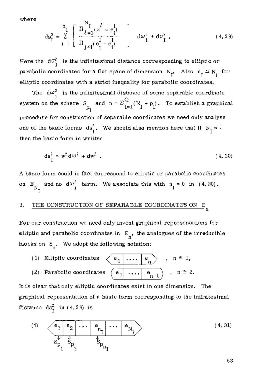
Текст
#t Pitman Monographs
and Surveys in Pure and Applied Mathematics 28
Separation of Variables
for Riemannian Spaces
of Constant Curvature
? G Kalnins
University ofWaikato, New Zealand
HUH
Longman
Scientific &
Technical
Copublished in the United States with
John WiEey &SonsH lnc.H New York
Contents
Preface
1. Introduction
Historical outline of the separation of variables
(principal results) 6
Separation of variables on the ?-sphere S 23
3.1 Mathematical preliminaries 23
3, 2 Separation of variables on S 29
3, 3 Construction of separable coordinate systems on 3 42
?
3. 4 Properties of separable systems in S 49
4. Separation of variables in Euclidean ?-space ? 56
4, I Mathematical preliminaries 56
4* 2 Separation of variables on ? 57
4? 3 Construction of separable coordinates on ? 63
5. Separation of variables on ? 70
5. 1 Mathematical preliminaries 70
5, 2 Separation of variables on ? 71
5. 3 Construction of separable coordinate systems on ? 88
5. 4 Properties of separable systems on ? 96
6. Separation of variables on conformally Euclidean spaces 107
6, 1 Mathematical preliminaries 107
6,2 Separable coordinate systems on conformally
Euclidean spaces 112
6. 3 Construction of separable coordinates for
conformally Euclidean spaces 124
7# Separation of variables for the heat equation 130
8, Other aspects of variable separation 153
Appendix: Crucial results due to Eisenhart 156
References 166
Index
171
Preface
This book arose from the desire to give a compact and, in a somewhat
restricted sense, compiete treatment of the subject of separation of
variables. The oniy book already available on the specific topic of
separation of variabies is that of Miller. This earlier work gives an
excellent treatment of the relationships between the classical special
functions of mathematical physics and Lie group theory*
The aim of the present work is to show how all the actual inequivalent
separable coordinate systems can be computed for the Hamilton-Jacobi
and Helmholtz equations on real positive definite Riemannian spaces of
constant curvature. The results necessary for the solution of this problem
are developed in the text. This allows the reader to obtain a feel· for the
subject without the necessity to read widely in the literature, It is in this
spirit that the book has been written. Proofs that are central to the
computation of all the inequivalent coordinate systems mentioned above are
given in full·; the more general results of the theory are often quoted,
suitable references being given. We also, on occasion, appeal to the
reader Ts intuition.
In Chapter 1 we give some introductory comments on the subject of
separation of variables. Included here are the basic notions of additive and
multiplicative separation of variables as well as an intuitive discussion of
the basic problems of the associated theory of separation of variables.
Chapter 2 sketches the historical developmentof the theory of separation
of variables, providing a useful summary and extracting, from the many
contributions, the most significant results. It also provides an indication
of the degrees of freedom available in the specification of a separable
coordinate system.
In Chapters 3, 4 and 5 we give a solution of the central problem of this
work, that is, we classify the separable coordinate systems on the real
?-sphere S , on the real Euclidean ?-space ? and on the upper sheet of
the double-sheeted hyperboloid ? for the Hamilton-Jacobi and Helmholtz
?
equations. The interplay between group theory and the constraints of
separation of variables theory enables an elegant solution to be obtained.
The resulting graphical calculus neatly summarizes the complete solution.
In Chapter 6 these methods are extended to the classification of all
inequivalent separable coordinate systems for Laplace's equation and the
null Hamilton-Jacobi equation on ? . In Chapter 7, these ideas are
?
further extended to the classification of all TR-separable' coordinate
systems for the heat equation on ? .
?
In Chapter 8 other aspects of the theory of separation of variables are
mentioned:
(a) the generalization of the classification of 'inequivalent' coordinate
systems to complex Eiemannian manifolds;
(b) the relationship between the special functions of mathematical physics
and Lie group theory;
( c) the intrinsic characterization of separation of variables;
(d) the development of a mathematical theory for separation of variable
techniques applied to the notiscalar valued equations of mathematical
physics (e.g. Dirac equation, Maxwell's equations).
Much of this work is a consequence of a long-standing collaboration with
my colleague Willard Miller Jr. Indeed chapters 3, 4, 5 and 6 are based on
the following research reports co-authored with W, Miller Jr:
Separation of variables on ? dimensional manifolds
1, The ? sphere 3 and Euclidean ? space R
? ?
2, The ? dimensional hyperboloid ?
?
3, ConformalLy Euclidean spaces
The first of these is to be published in the Journal of Mathematical Physics»
I would also like to acknowledge the influence and collaboration of
Charles Boyer, Greg Reid and Pavel Winternitz. Finally, I thank my wife
for her persistence in urging me to write this book.
Hamilton, New Zealand E. G. K,
July 1985
1 Introduction
The method of separation of variables has its roots in the solution of many
of the problems of classical physics [l]. In particular, we focus in this
book on the solution of the Hamilton-Jacob! equation
I n dW
Hfp., ..., ? ; x x) =E, ? =- ;, i=l,...,n, A.1)
in ? a i
ex
by means of this technique. As is known from standard texts in classical
mechanics [2|, once a complete integral has been obtained the solution of the
corresponding mechanical system can be achieved. A complete integral of
1 ?
A. 1) is any solution W = W(x t . .. , ? ; c., ..., c ) such that
? ?
? =detC2W/axLacJ v ^0,
J nXn
Most examples of the solution of the Hamilton-Jacobi equation are
obtained by looking for solutions W which are additively separable, i. e.
the solution has the form
?
W= ? W.fx1; cr .... cn). A.2)
i=l
This is the separation ansatz for an additive separation of variables. If ?
is a quadratic form in the canonical momenta pH such that
?
H= I g1JP.P +V(x) =E, gU=gJ1; l,]=l,...,n. {1.3)
U)=l J
then associated with this Hamiltonian is the Riemannian manifold having
contravariant metric g , As an example of additive separation of variables,
consider the two-dimensional harmonic oscillator. The Hamiltonian is
H = — (?? + P2) + sm(W?q? +^hh
1
where p. = raq. < i = ls 2) are the momenta conjugate to the coordinates
q « The Hamilton-Jacobi equation is
i
^[<^>2+<^2J + sm<a,^+^>=E A.5)
Now, putting W=W1(fli) + ^(9s) , the separation equations are
1 ,3W; , ? 2 2 *
7^{???> +|mw|q = ? - ?! .
The corresponding solution is
W= yBjnal-m2u}\^]) + -^- sin'^Vi^D^iq!) A.7)
+ WBm(E-0!1)-in!a>|qi) +^7^ sin^<2(E-o1))(t,2qi)-
The solution to the dynamical system is then obtained by solving
??_3?, ' t-t° "~SE A,8)
or equivalents
^ -^ ¦ta-'iVC^X-iii» -^ "ta'^VCi^^Qi) A-9)
t-t.^Bln-'tVi^f^-,)^*)
which yields the solution
qa-,T-Vt2(E"Ql)Mln(^,(t-t[))) .
For a satisfactory theory of separation of variables of A. 1) , three
impo rtant problem s are fundam en tal r
(I) Given a Hiemannian manifold ( e. g. Euclidean three space) , how many
'inequivalent' coordinate systems does it permit which give a complete
integral of A. 1) having the form A.2) ?
(II) How is it possible to characterize intrinsically (Le. in a coordinate-
free geometric way) the occurrence of additive separation of variables,
given a Riemannian manifold M?
(III) What are the 1inequivaient! types of additive separation of variables
that can occur on a Riemannian manifold of dimension n?
The main purpose of this book is to present a complete solution, for a
class of Riemannian manifolds, to problem (I). This class of manifolds
consists of the real positive definite Riemannian manifolds of constant
curvature. These manifolds are most easily thought of as the n-dimen-
sional real sphere S , real Euclidean ?-space ? and the upper
?
sheet of the double sheeted ?-dimensional hyperboloid Hn< More specifically,
these manifolds can be defined as follows:
(a) S : the set of real vectors ( s. , .,., s ) which satisfy
? J- n+1
s2 + ,,, + s2 = 1 and have infinitesimal distance ds2 = ds2 +t,. +ds2 .-
1 n+1 * n+i
(b) ? : the set of real vectors (z_, ..t> ? ) with infinitesimal
? in
distance ds2 = dz2. +,., +dz2,
1 ?
(c) ? : the set of real vectors <??, ?-., ,.., ? ) which satisfy
? ? t n
v2 - v2 - ¦.. - v2 =1* ?? > lt and have infinitesimal distance
0 1 ? ?
ds2 = dvn - dv^ ~ ¦.. - dv2,
U ? ?
In restricting ourselves to this problem we can give a complete
treatment of a well defined mathematical problem for a class of manifolds
that exhibit a lot of structure. It also serves as an introduction to the
essential ingredients required in setting up a theory of separation of
variables and, more specifically, in the solution of problem (I) in general.
In addition to the notion of additive separation, there is also the notion
of product separation. This occurs for a Riemannian manifold when one is
looking for solutions of the Helmholtz equation with a potential V:
?
i, j=lv ?&/ ?? dx
of the form ? = ?^^^?1; cp ¦ ¦* , %) ¦
As an example of product separation., consider the two-dimensional
(quantum mechanical) harmonic oscillator. The Schrodinger equation is
Putting ? - ? ? (?) ? 2 (y) j the functions ?. (i = l, 2) satisfy the
separation equations
"Li?i+('mw'x2^i)'i'i=o· A-13)
where ? : + ?^ = ?, A normalized set of solutions of these equations can be
expressed in terms of the Hermite polynomials
^=Nexp[-g-(WlX2+W2y2)lH ( V( ^ x) ? (V(~^> A.14)
? ? i\i ? ?2 ?
where
2m ? ???
2_?*
? = ^m ? wiws ?
? ?? ! ?2 I
and ? . = ?/?(?. + i) , i = 1, 2. The energy ? is thus quantized according
to
E=B[w1(n1 + ?-) + u>2(n2 +i)l A-15)
for suitable integers nt, n2, The crucial observation, of course, is that
A. 12) admits a solution via the product separation of variables ansatz
? =??{?)??(?).
The same three problems apply to product separation, i. e.
(?) Given a Riemannian manifold, how many 'inequivalent' coordinate
systems does A-11) , with V = 0, permit that provide a solution by means of
the separation of variables ansatz ? = ? t ? .(? ; c_, , c ) ?
l—l ? 1 ?
(IIT)How is it possible to characterize intrinsically the occurrence of
product separation, given a Riemannian manifold M?
(???) What are the 'inequivalent' types of product separation of variables
that can occur on a Riemannian manifold of dimension ? ?
2 Historical outline of the
separation of variables
(principal results)
The history of variable separation dates back to the work of Liouville [4]
who considered a dynamical system with kinetic energy 2? = ?[(?!J +(x2J ]
and potential V(x*, ??) and showed that if the Hamilton-Jacobi equation
admits a complete integral of the form
W-Wjix1; c1( ca) +W2(x2;cli ca) B-2)
then
*-*<"¦>¦*<"¦>. v-a;;Ii:;;g;.
Dynamical systems of this type are said to be in Liouville form. These
coordinate systems readily generalize to ?-dimensional Liouville systems
in which the kinetic energy is given by
2? = [? ?(??)}[? (xVl B.3)
and the potential is
? . ?
V= [ ? ???*)]/[ ? ?.??1) |. B.3)
j=l * i=l '
The associated Hamilton-Jacobi equation has the form
j- ? {(^J+2?.<?3) }=? B.4)
? j=l 3xJ J
where ? - ? t ?. (? ). The complete integral of this equation can be
obtained by looking for a separable solution W = ? . W.(x ); then
W^x1) = J7<2(-Mxl> +??.(?1) +G/.))dx1 B.5)
where ?? , ?, = ?. The motion can then be solved from the equations
?=1 ?
i^"i^ ^j 0 = 1. ....n-1) B.6)
J ?
*"** + ?F' 7T=pi A^L n)'
dx
Writing F.fx1) = ^B(-?.(?) + Ecr.(xL) +0/.)), i = 1, ,.., n-1, the
solution is obtained from
r dx1 ^ , dx3 ,. f dx f.
¦?7?????? +?? = J7(ii(?)) +,?? = "· = J/fF ^V-1
? (rQ_1(x ))
t-t„ = rCT'(x)dx +... + r-a
V(F,(x')) "" "V(F (/)
Consequently, if the dynamical system is in Liouville form, the
solution for the motion can be obtained by the 'method of separation of
variables1 and reduced to quadratures.
The complete solution of the separation of variables problem (III)
( Chapter 1) in two dimensions for the Hamilton-Jacobi equation has been
obtained by Stackel [s] # This is, of course, a special case of the general
problem for arbitrary n, Stackel obtained a classification which listed
three types of possible Riemannian metrics:
I (Liouville forms)
dsz = (?^?1) + ??(??))[(??1J + (dxVl
V =(?1(?1)+??C?2))/(?1(?1)+??(?2)). B-8)
? ds2 -gn^HdxV +2gl2(x1)dx1dx2 +g22(x1)(ux2J
V = V(x!).
Ill as2 = (dx1J - 2 cos^ix1) +?2(?1))?????2 + (dxV
V =0.
Some crucial observations greatly simplify this list. The reader will
probably already have realized that if the Hamilton-Jacobi equation admits
a solution via the separation of variables ansatz
?
W- ? W.(xX;c), c = (ct c) B.9)
i=l l
in some set of variables ? , then we can just as well choose a set of
coordinates y t where y = f.(x ) (i = 1, ... , n) and f.(x ) are a
suitable set of real analytic functions and all considerations are of course
local {i, e, , we are working on a coordinate patch) , Any such coordinate
systems which are related in this way will be considered to be equivalent,
in the sense of problem (III) of Chapter 1, Metrics of type BP 8) II
contain a variable x2 which corresponds to an ignorable variable. (Recall
that in classical mechanics [2 | a variable is ignorable if it does not appear
explicitly in the metric components g. .·) It is then possible to find a
solution of the Hamilton-Jacobi equation
,·?,<?5>· ¦*»<·'. ??¦.»<.¦>(?>¦-. ?
by looking for a solution of the form
W= W,(xL; QtJ c3) + c2x2 B,11)
If we now define new variables y (i = 1, 2) by
y1 = /(Vs/fenidx1. y2 -?2 + Hg^/g^idx1 <2. m
where g = g± lg21 - gn > ^hen ttie metric ? assumes the form
dsa =g(y1)[(ay{J + (dy2J]. <2. 13)
This change of variables does not affect variable separation, as the original
solution would have the form
W- W^y1; Cll C2) +c2y3 . B.14)
For this reason we can regard variables which are related in the manner
B. 12) as 'equivalent1 (in the sense of problem (III)) , in that they give
rise to variable separation for the Hamilton-Jacobi equation which gives
basically the same solutions. The metrics for type B, 8) III correspond to
locally flat spaces for which cartesian coordinates can be chosen as
? = {cos ? ? (?1) dx1 - J" cos cr2 (x2)dx? B, 15)
y = f sin ? ? (x1) dx1 + | sin ?2 (xz) dx2 .
The separable solutions cf the corresponding Hamilton-Jacobi equation are
W = cLx + c2y7 (c\ + cj? = E). These coordinates are a canonical form
for separable systems which can be obtained from cartesian coordinates
via the transformation
x = F(x*) + G(x2), y = H(x!) + J(x2) , B,16)
Again, we do not regard coordinate systems related in this way as being
essentially different and we extend our notion of Equivalence' to include
coordinate systems related via equations of type {2,16), Given this
equivalence of coordinate systems, we see that for ? = 2 any coordinate
system for which the Hamilton-Jacobi equation admits solution via
separation of variables is 'equivalent to a coordinate system in which the
Riemannian metric is in Liouville form.
The most significant development due to Stackel [? J was to give the
general solution to the separation of variables problem for the Hamilton-
Jacobi equation for an orthogonal coordinate system.
Stackers Theorem: The necessary and sufficient conditions that the
Hamilton-Jacobi equation
11 aw
? - ? ??2( :J +V(x) = ? {? * ?) B.17)
admits a complete integral via separation of variables (i. e, a solatium
W = ?? W (x\c) for which ?- det( d2 W/dx^cJ v ^0, c^(c c ))
i=l i 1 j n^n — ? ?
are:
(i) that there exist a Stackel matrix S = C..{x )) _ such that
ij nXn
?;2 ^S1 /S (i = l n) where S = detS and S1 is the (i, 1)
cofactor of S, The elements of the Stackel matrix are such that
)S../9xJ = 0 if j *ij
{ii} that there are functions v.(x ) such that
? il
?-? .,V ·
1=1
Proof: Let W = ?" W.(x\ c^, ·. - , c ) be a complete integral of B. 17)
i=l ? ? ?
and choose c = E, If we substitute this form of W into the Hamilton-
Jacobi equation and differentiate with respect to c then
? 3W.
?,?? 9TGTJ=5kr k = 1 ?· B·18)
?=1 ? k dx
, i
As W is a complete integral, ? = det( rr W/9x 9c,) ? 0; consequently,
if we write
we see that S = det(S. (x1)) = 2nn!V{ SW./??1) ??0 and the system B, 18)
i] ?=1 ? _ u
can be solved for ??2, (i = l, (tA n) to give H.z =¦ S /S with the
Stackel matrix S = (S_) w * Substituting this form for the coefficients
ij nXn
back into the original equation, we see that
? il
1=1 S l
where v, = S (x ) -(SW./SxK. To complete the proof we need only
establish sufficiency. If there exist a Stackel matrix S and functions v.
such that conditions (i) and {ii) hold then the Hamilton-Jacobi equation can
be written
? ^-[?-^+?.??1)] =?. B.20)
1=1 3?
The separation equations are
dW. . ?
(^-)? +v.(xl) = ? c.S„(xV 1 = 1 Q. B-21)
dx1 x j=i J 1J
which have the solution
? . · ? ¦
W. = [ [ ? cS,.(xL) -v.(xL)l W B.22)
The sufficiency of conditions (i) and (ii) has been proved by Stackel [?].
It was also observed by Stackel [?] that a Riemannian space which satisfies
condition {i) (i. e, is in Stackel form) admits ?-quadratic first integrals
of the geodesies
? Ji
a.= ? Vp* i = 1> ¦-·· n <2·23'
where of course Af - H, the Hamiltonian, and p. = 9\V/3xJ is the
canonical momentum. Furthermore these first integrals are independent
and in involution
[A,, Aj = 0 i» J - 1, .... n; i ? J. B.24)
(Here [ , 1 is the Poisson bracket [2].) In other articles [ s]-[s] Stackel
studies the solutions to the Hamilton-Jacobi equation when the kinetic energy
is in Stackel form. Stackel's theorem is a basic result in the study of
variable separation. Stackel matrices are a recurring phenomenon,
Stackel [??] obtained an extension of his first theorem which we now
give without proof.
StackelTs (second) theorem: Let P = (? , ? , ..., ? } be a partition
of the integers {l, ., - , ? ] into mutually exclusive non empty sets.
Further, Let S = ( STT(x )) ?? , be a Stackel matrix, i. e. ? = {? ; i ePT );
IJ ? ?? I
then if the Hamilton-Jacobi equation has the form
N s11 ?- ? ? ? s11
?=? ? V A ??,?/? Blx1) \-=E B,25)
1=1 l.i'ep S * ' ' 1=1 : fa
then there exist ? - 1 orthogonal quadratic first integrals of the motion
? LJ ? ?
?=? ? VA (*>?}?,,+ ? ??<?> V' <2·26»
J i=ii,i*€PI l ?=?
J = 2, , , , , ?, Furthermore this form of the Hamilton-Jacobi equation
permits a partial separation of variables. If we look for a solution of the
form
N ?
W= ? Wj(x iClt .... CN) B.27)
then each W satisfies the 'partial separability' equations
aw. -sw_ T n
?^,?1) -L
7 + ???1) = ? C STT . B,28)
. ., _ I ' i ^ i1 I _ t J IJ
i,i'€P dx dx J=l
The problem of central interest for Stackel (and other authors) was to try
to find all force free dynamical systems which admit first integrals of the
motion that are homogeneous quadratic forms in the canonical momenta of
a given dynamical system [??] ,
With the appearance of the class of Hamiltonians in Stackel form it was
natural to ask: what are the necessary and sufficient conditions that the
Hamilton-J acobi equation admits a complete integral W = ? , W.(x , c)
in a given set of coordinates ? (i-1, ,,., n) (not necessarily
orthogonal) ? Recall that a complete integral is a solution W(x , c_) of A, 1)
such that
det
52W
dx 3c
y
? ?.
? ? ?
Levi Civita [ll] provided the answer to this question with the following
Theorem.
12
Theorem (Levi Civita) : The necessary and sufficient condition for the
Hamilton-Jacobi equation
1 ?
?(? , ..., ?; ?! ?) =?, p.
to admit a complete integral of the form
aw
Bx1
i = l, ... , ?. <2,29)
w= ? w.(x\ c)
i=l
is that ? satisfy the |n(n - 1) equations
? ? dx dx' ? dx dx dp
J
dH 5H a2 ? dH dH 32H
- i 3pH ~ -j - i 3 j 3p.3p. ~ '
dx j op. dx dx dx ? j
B,30)
i * j* i, j = 1,
, n.
Proof r For a solution in this form it is necessary and sufficient that
dpt/dx =0, (i ? j) where each pt is considered a function of
Differentiating ? = ? with respect to ? , we obtain
_3H . ?H. ^L_n
-l ? dpb ^ ?
?? ? dx
i = l, ¦. * t ?
and consequently
a i CH/aP+ J
dx ?
The condition for separation of variables is then
i
J j *3H/3p.'
dxJ *i
(i* J)
BP31)
B.32)
B,33)
where
dxJ c?xJ
9p. ?
BxJ *j
13
These are just the conditions of the theorem. If the Hamiltonian can be
written in the form ? = Q( p. , ,,., ? ; ? , ,,.,?) + V(x , ... , ? ) ,
these conditions become
- 0
d2Q 3Q 3Q _ _3Q J?<^ d2Q
dx 3x dp. dp, dp. dx dx 3p
? 1 ? J
3Q 3Q_ d2Q 3Q 3Q 3aQ
3x 3?? 3?,3? 3x 3x 3p.3p.
3Q 3Q 3^V 3Q 32Q dV
9p, 3p. dx dx 3pt 3x 3p. 3x
3Q d2Q 3v 3aQ , _9Q _3V 3Q 3v
B.34)
. + — ( —? — + -^ ^r) - 0
3p. 3xJ3pt dx1 dp.dp ax1 3xJ 3xJ 3x*
J ? ? J
3*Q 3V 3V ? . _, . . . .
~? —?= ? ? * ], i, J = 1, .·. , n,
3?.3?. 3? 3xJ
^ J
from which we note that if the Hamilton-Jacobi equation is separable for a
Hamiltonian of the form ? = ^gljp.P. + ?Lp, + V then the same holds for the
ii
'geodesic1 Hamiltonian ? = g p.p.. The solution of the separation of
variables problem for the 'geodesic' Hamilton-Jacobi equation
? = ig^P. = E B.35)
then becomes the crucial problem.
In order to analyse separable solutions of A, 3) where (g ) is
positive definite, Levi Civita distinguishes two types of coordinates. He
does this as follows; putting
3H d2B ij 3H
? =- + gJ— B.36)
J 3p. 3p,3xJ 3xJ
J ?
then conditions B. 30) become (for i fixed)
3H , 3H 3?? 3H dzR , 3?
— ( — ——-- — ~r~) +-a =0. B.37)
3p. 9p. 3x 3xJ dx} dx 3p. 3x J
14
Here 3H/5p is a linear form in the p. and dU/dx and ??+ are
? ? ij
quadratic forms. In order that B, 37) be an identity, one of the two
latter expressions must be divisible by dH/dp.. If dK/dx is divisible
by 3H/ dp. then
—^r = 0 , ], ? ? \ . B.38)
If ?, is divisible by dH/dp, then
g1J—?? -0, B.39)
3xj
? it &rZ ij &rj
? g -gJ f* =0,
? =1 3xJ 3xJ
The two possibilities for divisibility by 3?/??, form the basis of Levi-
CivitaTs classification of types of coordinate- The coordinate ? is called
a first class coordinate if 9H/3 ? is divisible by 9?/??+, otherwise
it is said to be a second class coordinate. We adopt the convention of
denoting first class variables by Greek indices (?, ?, ?..) and second
class variables by (a, b, ,,.), Levi-Civita dealt with two cases:
(i) ? = 2, in which he showed that one obtained the list due to Stackel;
(ii) the case in which all coordinates are first class. In this case the space
can be shown to be Euclidean-
Proof: If each coordinate is of first kind then
B-40)
Ha
dx
and we have
<?>
= 0, j, ? ? :
?
= ? gSr[ij; rl
r=l
B.41)
15
which relates Christoffel symbols of the first kind [ijt r [ to symbols of
the second kind. As
[1J.
_ 1
~ 2
—&ir + —?jr - —eij
3xJ 3x ?x
B.42)
we see from B, 41) that f j } = 0 if i ? j. Using B. 31) T
s
_L9HZaA J^l {iiJp B43)
<3H/3p.) dx1 s=l s S
in addition to dp./dx - 0, If we differentiate, we deduce that
R. .. = ~{ii}+ (?)??} = 0. B.45)
isij 3?1 s j ?
Here R is the only component of the Riemannian curvature tensor
isij
which is not already zero. Consequently R. has all components zero
and the underlying space is Euclidean, Cartesian coordinates
y (?1, ,.. , ? ) can be obtained by solving the equations
y!?-1^ - ? lV)*V-=° i^M-l n. B.45)
1 J ?? dx s^l &c
These equations are clearly equivalent to
SxW
and consequently
? .
yr= 2 X;r,(xL)f B,47)
(r) i
where each of the X. functions depends on the ? coordinate only. The
corresponding infinitesimal distance is ds* = ? .(dy J·
r=l
We see from our earlier discussions that this type of coordinate
system is the natural generalization of systems of type B, S) in in
Stackers list for ? - 2. Again, if we were to extend the notion of
Equivalence' of separable systems we would not really wish to
distinguish this system from cartesian coordinates. Dall'Acqua [12]
= 0 B.46)
16
extended the application of Levi Civita's integrability conditions to three
dimensions. If we distinguish coordinate types by the indices {nj , n-n^ ,
where ni is the number of first class coordinates, then the DaU'Acqua
solution produced a list of four metric types:
3
I C,0) , ds2 = ? (aa +bb+cc )dxrdxS, B,48)
'rs rs rs
r, s=l
dB.Jdx] - 0; i ? j; i, j = 1, 2, 3,
This is the maximal (or geodesic) case treated by Levi Civita and is
accordingly 1 equivalent' to the choice of cartesian coordinates
3
yJ= ? Rdx1
i=l *
where ?-a, b, c when j = l, 2, 3 respectively, The corresponding metric is
3
ds2 = I (ay1J .
i=l
II B,1) as2 = (ag+itej+iibgXdx1J B,49)
+ A11^3 +2m2e3 +b3) (dx2 J + (dx3J
+ 2(m2a3 + Zjb3 + {l+iim3) e^)dxlax2
+ 2(c3 +m2 s3)dx2dx3 + 2(Zi c3 + s3)dx1dx3.
In this expression the subscripts on the functions denote variable dependence,
e. g, 9aj / 9xJ = 0 unless j - 1 etc.
This metric ean be put into a much more transparent form. If we
change variables according to
y1 = x1 + Jmadx2, y2 = x2 + fiidx1, y3 = x3
then
ds2 =a3(dyV + b3(dyV +2e3dy1dy2 + 2?^ +2s3dy1dy3 .
This change of variables relates to two 'equivalent' coordinate systems
as it did in the two-dimensional case for type II coordinates in StSckei's list.
17
This can be seen from the observation that solutions of the Hamilton-Jacob!
equation in the coordinates y are of the form W = c1y1 -^c2y2 +??3(?,?).
Consequently any new set of coordinates given by
y1- I XU\xJ), A = 1, 2),
y3 = FU3)
would give rise to essentially the same separable solutions of the Hamilton-
Jacobi equation. We shall therefore regard coordinate systems related in
this way as 'equivalent\ We observe here that first class coordinates relate
to the existence of an equivalent set of ignorabie variables, (Recall that a
variable x1 is ignorabie if Pi is a linear first integral of the geodesic
equations, i.e. [h, Pi 1 = 0*) In Chapter 3, this relationship is made
precise in a theorem due to Benenti, who showed that the first class
coordinates are always equivalent to a choice of equivalent ignorabie
variables.
?? A,2) ds? =^%. [(lt + 0 -di)(dxV
cj -a2
+ (mf + o, -d?)(dxV + <dxV
+ 2Z1m2dxIdx2 -f2m2dx3dx3 +2Z1dx1dx3],
B.50)
subscripts on the functions having the same significance as in type II
coordinates.
This metric is 'equivalent', via the change of variables yl = ?1
(i = 1> 2) f y3 =-x3 + Jmjdx2 + J^dx1, to the orthogonal metric
ds2 =<ai -b2)[(dyV +(dy2J + —^ (ay'J]
which is seen to be in Stackel form with Stackel matrix
S =
aj »Ci 1
-hi d2 -1
0 1 0
18
IV
@,3) ds2 =Q[
(is -q3) (Q3 -qi) (qii -<h)
B.51)
where Q = r!(q2-q3) + ^2 < <la "Qi) + MSt ~qa) · This metric is orthogonal
and already in Stackel form with Stackel matrix
*? 1 qi
S =
r2 1 Qa
r3 1 q3
For product separation of the Helmholtz equation
(? +?)? - ?
^^ w ij_^
i,j = l ox dx
Robertson [l3] obtained the first definitive result concerning the conditions
under which this equation admits a separation of variables by means of a
solution of the form ? = ? . , ? . (x f ?),
?=1 ? —
Theorem (Robertson condition). The Helmholtz equation ? ? +??=??
is separable in an orthogonal coordinate system ? if and only if the
components g and potential V satisfy the requirements of Stackers
theorem and the additional 'Robertson condition
nnlSl1 ?
-4— =? f^
sn~2 i=i 1
B.52)
Proof: To achieve separation, the quotient of the coefficients of ( d / dx }'
and d/dx should be a function of ? alone, i, e.
¦log(V(g)gU) = F (x ) f i = 1, .,,, ? +
B.53)
dx
These conditions are equivalent to the Robertson condition. The remainder
of the argument is directly analogous to that used to prove Stackers theorem,
as the equation can now be written
?
? gV {??? xS c) = E - V
i=l l l
B,54)
19
where
3 , ? , ? , __1 ?
H.(^r xSc} = ?~![< — )* + ?,{??) — )?? . B.55)
?? ??
In one of the key papers on the subject Eisenhart [14] took up the
question of orthogonal coordinates for which the Hamilton-Jacobi equation
separates and investigated the geometric significance of the Robertson
condition. We summarize and discuss his results below. The proofs are
given in detail in the appendix.
Theorem (Eisenhart), Let ? = ?. g p.p. be the fundamental
quadratic form on a Riemannian manifold M. The necessary and sufficient
conditions that there exists a local coordinate system { y ] such that ? is
? S*1
in Stackel form H= ? 1??. a**e:
i—i b i
(i) The equations of the geodesies admit ? - 1 independent {linearly)
quadratic first integrals A = Ct*J pbp., a = 1, .., , n-1, which together
a (a) i j
with ? form a complete involutive set satisfying
[Aft> Aj =0, [Aa, ?] -0, atb = l n. B,56)
(ii) The roots ? t j = lt 2 nt a = 2 n, ofthe characteristic
a
equations
<tet<3Ll -Pbglj) -0, a--2ltitln, B.57)
of these first integrals are simple and satisfy
det|p.Q -p^ | ? 0 B.58)
where i is fixed and a = 2,...Tn? j = lt itt) n, j ? 1.
(iii> The vector fields ? .. , „ h = 1, ,,. , n, determined from these first
(h) ?
integrals via
(at) -p/>\b>r° <2-59>
should be normal and be the same vector fields for the first integrals
20
A - Furthermore, the hypersurfaces defined by these vector fields may be
a
taken as parametric. The coordinate system thus defined is such that the
matrices (g ) _ t (8( J _ can aii be taken to be diagonal,
nXn (a) nX-n
What Eisenhart's theorem gives is a geometric characterization of
Stackel form. Given a suitable involutive family { ?, ??, ,¦. , A , ) ,
*¦ n-1
from purely algebraic criteria one can determine whether there are
separable coordinates. Implicit in this result is the determination of a
suitable set of separable coordinates {y ]* The condition of normality is
crucial, for this is a requirement that each of the quadratic forms
A = fl!3 ? ? ? . a = 1, ..,, n-lt can be simultaneously diagonalized in
a (a) ? j
the given coordinate system- This result and its subsequent development
provided the successful development of the solution of problem II of
Chapter 1. As a useful corollary to this theorem, Eisenhart showed:
Corollary 1 (Eisenhart) : The necessary and sufficient conditions that
? = ? . .,??^?* is in Stackel form are
?=1 ? ?
—» - log ?2 - ~ log fli ^logH? B,60)
dx dx dx dx
+ -^r-log ?? -?- log rf + -?- log U2. -^-log H2 = 0,
k* ] ^ i; i, j, k=l, lftl n.
An additional corollary enabled Eisenhart to characterize geometrically the
Robertson condition:
Corollary 2 (Eisenhart) : The necessary and sufficient conditions that the
Robertson condition B, 49) holds for a given orthogonal coordinate system
{x1} for which ? = ?, -??2?? is in Stackel form are that R.. - 0, i ? j,
i=l li ij
i, e,, the Ricci tensor R.. is diagonal.
In addition to these results, Eisenhart was able to give a complete
classification of all inequivalent orthogonal separable coordinates on E3
and S3. These coordinate systems can be found in many standard reference
works [l],
21
We note that, because of Corollary 2, any orthogonal separable system
which provides an additive separation of variables in a space of constant
curvature for the Hamilton-Jacobi equation also allows a product
separation of variables for the corresponding Helmholtz equation.
Two good reviews on the subject of separation of variables from a
historical point of view are those of Prange [l5] and Haux f 16] ,
22
3 Separation of variables on
the ?-sphere Sri
1. MATHEMATICAL PRELIMINARIES
In Chapter 1 we gave a suitable definition of the ? sphere S * As we have
?
seen in Chapter 2T coordinates that occur in the separation of variables for
Riemannian manifolds which are positive definite are of two types. Benenti
[l?] has made a complete analysis of problem III of Chapter 1 for such
manifolds and proved the following theorem.
Theorem 3.1 (Benenti) : Let ? be a positive definite Riemannian manifold
of dimension ? for which the Hamilton-Jacobi equation
V ij3W dW v
? = h g j —? —: = ? ?
i,j=l 3X1 3xJ
admits an additive separation of variables in a system of coordinates \ y ),
Then there exists a system of coordinates {x } 'equivalent7 to {y } such
that the contravariant metric tensor has the form
<- ni —> <?— ?2 ^>
<B"
nxn
in2
a
?
?
??
? J
C.1)
? ?
where the functions ? ? and g can be expressed as
?
-2 _iL «? = ? ??? b H
b
C.2)
depending only on
L e, , there exists a Stackel matrix S = (S , (x ))
a _ ab ^????
the variables {x } such that the ? 2 are in Stackel form. Here
a
nj = dim {x } is the number of second class coordinates, in the nomenclature,
of Levi Civita.
23
The variables ? are such that dg ydx = 0 for all i, j, and they
correspond to first class coordinates.
A few comments on this theorem are in order:
(i) The coordinates { y } and { ? ] are in general related by equations of
the type
? =f(y )
? =? xp (y ) +? a, (y )- C,3)
? " b ?
(ii) Clearly, the coordinates {x } are not chosen to be unique, in order
that the contravariant components of the metric tensor may have the form
( 3, 1), If { ? } is another such system then, in general,
xa1 = h(xa)
??' = ? a"/, det(aj?) ? 0, C.4)
? ? ?
Coordinate systems related in this way will of course be regarded as
1 equivalent \
(iii) The Hamilton-Jacobi equation I admits a separable solution of the form
w=2> (xa) +lc xa
a a
a o
with the separation equations
dW „
(?.,+??°????? C·5)
dx o7p
with ?? = ?.
??
(iv) The variables ? are the ignorable variables one encounters in classical
mechanics [2], [is]. In fact, [p , h] = 0, Each ? corresponds to a
linear first integral { Lie symmetry) of the geodesies. Furthermore,
[ ? , ? | = ?. This is an important observation. For the general form of
contravariant metric tensor C.1) , this implies that the underlying
Biemannian manifold ? admits an abelian algebra (under the Poisson
?
bracket) of first order Lie symmetries of dimension at least
24
ns =dimlx }s Hi + ns - n. In the case of the ?-sphere S , the algebra of
Lie symmetries has dimension -gn(n + 1) and basis
? =s ? - s ? , a >b, a,b=l n+1, C.6)
ab a 5; b s
which satisfy the commutation relations
L ab cdJ be ad ad lac bd ca ac db
The Lie algebra of the Lie symmetries described by the commutation
relations C*7) isthatof SO{n + l), the orthogonal group in ? dimensions. The
global action of these symmetries is via real orthogonal (n+1) X (n+1)
matrices 0 acting on the projective coordinates ( s .¦, , s ) via
s -*- Os.
In our discussions of the notion of equivalence thus far, we have
observed several ways in which this can occur. However, if the manifold
in question admits a group of first order Lie symmetries then an additional
concept of 'equivalence1 must be introduced, This is essentially the notion
that two coordinate systems { ? } and {y } that are related by a group
motion are not essentially different. To make this more precise, in the
case of S consider that we have a system of coordinates { ? } such that
?
the defining projective coordinates s, are well defined functions of the
{ ? }, i. e, , s = s(x ) # If we rotate the vector s via an orthogonal matrix
0 then s" = Os and
ds2 = dsT * ds' = ds ¦ ds = g dxW. ( 3, 8)
Therefore both the choices of vectors s in terms of the coordinates { ? ]
are indistinguishable when it comes to a discussion of their separability
properties.
Chosen coordinates which are related in this way are then regarded as
being'equivalent1. This is equivalence between the specification of the
projective coordinates s. (i - 1, , P, , n+1) in terms of the separable
coordinates { ? }t there being no essential distinction made between
25
coordinates specified by the vectors s(x ) and Os(x ) = s'(x ) with 0 an
orthogonal matrix.
From the form of the contra variant metric components C, 1) and the
separation equations we see that we can write
a ?,? h j,k=l J
c = 1, ..,, nls C,9)
ik ki
where 8JA = GL,., . These quadratic functions ? together with the
(i) (i) c
ignorable momenta ? form a complete involutive set of constants of the
motion. There is consequently no relation of the form
c ?, ?
? ? =0
Q
C Qtfc ?
for non-zero coefficients ? , ? \ ?
We also have the relations
[>c. Ab] = 0, [*c> pft] = 0* fpa'pii1=0' C-1T)
with ? j = ?, The quadratic forms ? are quadratic first integrals of the
C ik
geodesic equations, (The coefficients Ct, . are also referred to as
(c)
Killing tensors [is\) We note that as the metric tensor is not orthogonal
in this case, the complete integral which this coordinate system specifies
has associated with it nt quadratic first integrals A and ? - n| linear
first integrals of the geodesies (first order Lie symmetries) ? , Only when
nj = ? - 1 can all the constants of the motion be characterized by quadratic
first integrals {since then the metric tensor is necessarily orthogonal),
As we wish to deal also with product separable solutions of the
Helmholtz equation II, we can ask the question: how are the separation
constants appearing in the separation equations to be characterized? The
relevant concept here is that of symmetry operators of the Laplace
26
operator ? . First order Lie symmetry operators are defined as partiai
differential operators of the form L = ?.a(d/3x),for which
(L, ? }? =L<4 ?) - ? ??) =0
? ? ?
for all suitably differentiable functions ?; consequently { L, ? } = 0 is
an operator identity. The { , } bracket is the operator commutator
bracket-
On S the first order Lie symmetry operators form a vector space
having a basis
I.. =e. r|- "?. r^-t i, j = 1 n+1 , C,12)
J 1
Second order symmetry operators of the Helmholtz equation are
correspondingly defined as operators
m = Z a —j—r +1 b —
i, j dx dx k dx
for which
{m, ? } = 0 C,13)
?
is an operator identity. If the coordinate system {x } is also a separable
coordinate system for the Helmholtz equation, then further restrictions
must be placed on the metric coefficients.
Theorem 3. 2 : Let ? be a positive definite Riemannian manifold of
dimension n, for which the Helmholtz equation ? admits a separation of
variables in a coordinate system {y }. Then there exists a system of
coordinates {x } 'equivalent to {y } such that the contravariant
metric tensor has the form C, 1) given in BenentiTs theorem and
R L = 0 Va, b ? C,14)
ab
in the coordinate system {x J.
27
This theorem follows from BenentiTs theorem and the Robertson
condition. We make a few pertinent comments on this result
(i) The condition ? , = 0 is the analogue of the Robertson condition. It
ab
is readily proved from the conditions
—. log(V(g)gaa) -F (xa)t Va. C,15)
dx
{ii) The use of 'equivalent1 is meant in the same sense as it is for the
Hamilton^Jacobi equation. This can readily be seen as follows. In the
coordinate system {x } the coordinates ? are ignorable and the
Helmholtz equation can be written as
! gV) X^r ? BV>^=^ ,3.16)
Consequently we can always choose separable solutions of the form
? =? ? (xa)exp(? ? xa) . C,17)
a a
We thus see that if a coordinate system {x ] is separable for both the
Hamilton-Jacobi and Helmholtz equations then the same notion of
equivalence applies to both these equations,
(iii) The product separable solutions of the Helmholtz equation satisfy the
separation equations
[(?"J +?*(??1) "T^fl +< ^ ?^-^?8?>??=°· Va
, a a a a r a cv ? ? b ab a
dx dx q, ? f b
C. IS)
where ? x = ? and
dx
where ? - exp(? ? ),
From these equations we see that product separable solutions of the
Helmholtz equation are characterized by nt second order symmetry
28
operators
sab
cb
b S _ a' a' a a
a dx ox
a,p c dx ox
and ? - nj first order Lie symmetry operators
L =—?, C,21)
?? - at
dx
in that the product solutions are simultaneous eigenfunctions of these
operators with eigenvalues ? and ? f respectively.
For each theorem relating to separability of the Hamilton-Jacobi
equation there is a corresponding result concerning the separability of the
Helmholtz equation. For the Riemannian manifolds S , ? and ? t every
? ? ?
separable coordinate system will provide a separation of variables for both
the Hamilton-Jacobi equation and the corresponding Helmholtz equation.
This follows from the condition
hijk *BhkBij *hfiW K }
where ? = 1, -1 or 0 according to whether the manifold is S , ? or ? ,
? ? ?
From C,22) and C, 1) it follows that ? - 0 for a^bP
2, SEPARATION OF VARIABLES ON S
„ _ ———_ n
The complete solution of problem I for S depends in a critical way on the
underlying Lie algebra of SO(n + 1).
The following is a crucial result in the classification of separable
coordinate systems on S :
?
Theorem 3« 3: Let { ? } be a coordinate system on S for which the
?
Ham i I to ? -Jacobi equation admits a separation of variables. Then, by
passing to an'equivalent' system of coordinates if necessary, we have
29
g = 5 B721 le, t separation of variables occurs only in orthogonal
coordinates. Furthermore in terms of the standard coordinates on the
sphere s*, .. - , s , the ignorable variables can be chosen such that
??, =?12· % =I34 P(*q = I2q+l,2q+2 <3*23)
where the number of ignorable variables is q.
Proof: This is based on the general block diagonal form ( 3. 1) of the
contra variant metric tensor for a separable coordinate system. Any
Lie symmetry of S is conjugate, under the action of SO(n + 1) , to a Lie
?
symmetry element of the form [!$ |
L = I12+V34 + -"+bA„-l,2,- C-24>
If this element corresponds to the ignorable variable ? \ i. e. , L - ?
?
then by local Lie theory the standard coordinates on the ?-sphere can be
taken as
(sx Sq+1) - {?? cos(x 1+wi), Pl sin(x l + w^ ,
P2 cos(b2x 2 + w2) t P2 sin{b2x 2 +w2) p^cosfb^x 1 -f wy) ,
where p\ + «.. + p\ + s* ? + .., + s2 ? = 1. The infinitesimal distance
I 1/ 2^+1 n+1
then has the form
ds2 = dp* +.., +df^ + ?2j,(dxQl + dw )a + ... +p^(b^dxai + dw J
If there is only one ignorable variable then the coordinate system must be
orthogonal and this is only possible if bn = , ¦. = b =0, i(e(} ? = L,
^ ? Q! 1.2
Indeed, the requirement that the contravariant metric have the form C. 1)
(orthogonal in this case) is that
30
-dwt = ? ? b.dw. . C.27)
Since the differentials op,, dwH (j ^ 2) , must be independent and the only
? , ^
condition on ?? is S. ,p? +s^ _. + .. . + s2 _. = 1, the condition d2 Wi = 0
* 1 ?=? ? 2v+l ii+l
implies b. = 0, j = 2, .. t , ^, and dwj = 0, We can then take the constant
Wi = 0 by suitably redefining ??# The theorem is proved in this case.
Now suppose there are q >1 ignorable variables. The Lie
symmetries ? , i = 1, ..., q, must form an involutive set. It follows
i
from the spectral theorem [2?] for commuting skew adjoint matrices that,
for each i, ? has a representation of the form
i
i iii
for i = 2i ., . , q« in fact we can assume
P«.=Vl2 + V34 + -·· + VV-1.2*. C'28)
Pa. = 12i-lJ2i + iS Ahl-1,21- l = 1 * C'29)
i Z=q+1
for some ? ^q + 1. The projective coordinates on the sphere then have the
form
(s1, ..„, s ) = (P^osfx 1 + w1), P1sin(x l + w^ , C.30)
p cos(x q + w ) , p sinfx 4 + w ) ,
q q q q
^ i uJi
? ., cos( I b ,x + w ,
q+1 i=1 q+1 q+1
1=1
We now make the crucial requirement that the ignorable variables ? S
i = l, . ¦. , q, are part of a separable coordinate system- If we compute the
covariant metric, it should be in block diagonal form with respect to the two
classes of variables. Just as in the case q = 1, this is only possible if
31
b, = 0, i = 1, ... , q, I = q+1, *. * » ?, and dw. = G, 1 ^ i ^ q« We can
therefore assume that L1 = 112, L9 = 1^, -. - , L = I ; the ignorable
coordinates a. can then always be chosen such that w, = 0, 1 < i ^ q,
and the system is orthogonal.
This theorem enables us to bring to bear Eisenhart's results on
orthogonal systems of Stackel type. Our problem reduces to the enumeration
of ail orthogonal separable coordinate systems. We use an inductive
procedure such that, given all separable systems for S.T j < n„ we can give
the rules for construction of all systems on S ,
?
If {x } is an orthogonal coordinate system with infinitesimal distance
ds2 - ? ?? (dx )a then the conditions necessary and sufficient that the
space be S are,
?
(ii) R,_ =0, i ? h ? k.
hnk
Furthermore, the corresponding Hamiltonian ? = ?? ,?"??2 must be in
i=l i i
Stackel form as is proved in the Appendix. Eisenhart [l4] has shown that the
conditions ( 3, 31) {ii) and the requirement of Stackel form are equivalent to
the equation (A, 43), i.e.
— log H? -V log H2 - — log ?* ~ log H*
i?xJ x3xk l ^ 'Bxk J
^ logH^logfi^O,
dx dx
i, j, k pairwise distinct. The metric for a separable system can be written
in the form (A, 48)
gu = Hj=X ?(? +? ), !-!,...,„.
where ?., o\, are functions of ? at most.
There are various possibilities for the functions ?. , If all the functions
ij
32
? are such that ?" ? 0 then Eisenhart has shown that the metric
coefficients have the form (A, 57)
g., - ?* = ?. ? (?. - ?.)
where ? = ?\(? ) and ?.' ? 0. This metric will be the basic building block
iii
on which we can formulate our inductive construction. Without loss of
generality we can redefine variables {x } in such a way that ?. = ? ,
i. e. ,
?2 -?. ? {?1 -xj) , C.32)
? ? . ,.
j*l
The conditions C, 31) (i) then amount to
[? (??-?^-?^??'-?^'1 C·33)
m (xl-xV xj (x-x3) xj
??? (x'-xV i (xJ-x> i
+ ? ~—j—? j—: —~j—j~~ = -^ -
???, j X (x -x1) (x -xJ) ? {? -? )
* k*Z
These equations have the solution
, (n+1)
(—) + 4(n + 1I =0, 1 = 1, ..., n, C.34)
i
i, et,
— - -4(x ) + I a [x ) = f<x) .
The function f(x) can also be written
n+1
f(x) = -4? (x - ej . <3. 35}
j=l J
There are two requirements to determine which metrics of this type occur
on S : (i) the metric must be positive definite; < li) the variables ?
?
should vary in such a way that they correspond to a coordinate patch which
33
is compact, There is a unique solution to these requirements: the x\ e,
should satisfy
en < x1 < e0 < ,,. < e < ??< e 7. C,36)
1 2 ? n+1
These are ellipsoidal coordinates on the ?-sphere S , They can be related to
the coordinates {s. ) via a standardized choice
srn.^.(e.-e) · j =1. —.^. C.37)
These systems are the basic building blocks for separable coordinate
systems on real spheres. To complete the analysis of possible orthogonal
separable systems we need to consider the case when some of the <j..
functions are constants. If ? = a (const) there are four possibilities:
ij ij
(i) ff..=a.„, ?..-a,., ? = a , a = a
ij ij ? ji ik lk jk jk
(ii) ??+ = ab., ?., = a,#J a.. = a.. , a. . = a. .
ij ij j ? ji ik ik ki ki
(??)??, = a..t ?„ = a. ?..=3..?., ?._ =a.,a( C.38)
ij ij ik ik ji ? j jk jk j
ki ki k1 kj kj k
(??)?,, =a.,f a..=a..i a..=a..a.t ?.. = a., cr.
ij iJ kJ kj ? ? J Jk ]k j
a_a. H - a.( a, =0
where ?. is a function of ? only and i, j, k are pairwise distinct. If
we fix i and j then for k values corresponding to cases (i) -(iii) ,
o~.. = at| . To examine how the inductive process works, let us take
ik ik f*
??? = ai/ for ^ = k+1' .. · , ? and ?' ? 0 for j = 2, . ., , k. Then we
have
jZ jZ 21 ? ? ? ? ?
aZia"Z~ aZaiZ = ° for ^ = k+:' ··¦ » ?? 3 = 2 k*
Assuming that a ^0 for ? = k+1, ,. . 3 ?, j=2, tt4, k, we find the
? J
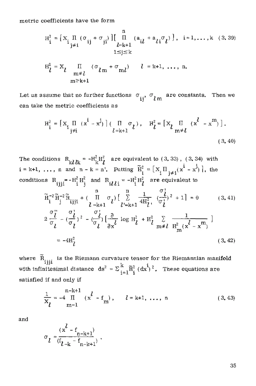
34
metric coefficients have the form
?
?2 -[?. ? (?„ + ?..)? ? (a +a ?I, i-l,...,k C.39)
1 ?]?? 1J ? Z-k+1 U ll l
B\ = X7 ? (?, + ? ) I = k+1, ... s ?,
? ? ?? lm ml
m^k+1
Let us assume that no further functions ?.., ?. are constants. Then we
ij lm
can take the metric coefficients as
H? = [x. ? (?^?])]( ? ? ), HJ=[X, ? (?* -xm)].
1 1 j=^i Z=k+1 L C m*l
C. 40)
The conditions R, , fl = -?? Ha, are equivalent to ( 3, 33) , C.34) with
kllk k L ^ . .
i = k+1, . ., , ? and ? - k = n1. Putting ?2 = [?.? (?1 - ?3) ], the
1 1 j^l
conditions R = -H2H2 and R _,. = -?2 ??, are equivalent to
ij ji ? } \ll\ ? I
? ? ??
??2????„.. +( ? ? )[ ? ~? (~)?+?1=0 C.41)
1 J ^ Z.k+l ^ i'=k+l4HZ< ??
2? -(?>' -<??[-?1???? +?? ? '? m ]
?? ?1 ?? dxl l l ???? ?? (x*-xm)
m
- -4?2 C.42)
where R is the Riemann curvature tensor for the Riemannian manifold
ijji r k i
with infinitesimal distance ds^ - ? , , ?2 (dx )?. These equations are
?=1 ?
satisfied if and only if
n-k+1
-^ = -4 ? (? -f ), Z = k+1, ..., ? C.43)
X, m
? m=l
and
tx'-fn-k+i>
35
where we take ?? < i0< ... < ? t ,. The remaining condition then is
1 ^ n—k-f-i
R.... = -H2H? so that
ijji
i J
1 k+1
1 -4? (x1 -e.)
X
j=l
The coordinates on S can be taken as
?
C. 44)
(So
Vi
) -(u1vr ..., ^\^v V *
k+1 J vn-k+l 2 -,
where ?, „ v, = 1, h-, „ u, = 1
i=l ? I =1 I
and
"?-?^-?.
a2 =
l=k+l m_
?™? ? m
The infinitesimal distance has the form
where
dsj| = dsf
ni=k+i(x
fn-k+lJ
[_ m^n-k+r m n-k+1
+ ds^
dsi
? k
4i=i
?. ..(x1 -xJ)
1*1
rrk+1, i
nj=1(x -e.)
(dxV
-Vk+i'
C, 45)
C, 46)
C, 47)
C. 48)
C. 49)
-1
dei=^ ?
nm,*(* -*J)
Z=k+i
m = k+1, P ,, , n,
[? (? « f
L m=l m
(dxS2
m
j = l, - · ' j K.
{3.50)
The choice of embedding of the sphere S in the ?-sphere S given by
C. 45) is not, of course, unique. However we will make the convention of
taking this choice of imbedding (other choices would correspond to
applying an orthogonal matrix to the vector s)«
Now suppose one of the constants a. = 0 for some fixed I and i.
IJ
36
Then from the relations
a. a.-a^.a =0 C.51)
we have a = 0 and consequently a,, = 0 for ? = 1, ,., , k. This implies
that ?, does not appear in H? i = 1, -,, , k,
? ?
Referring to the curvature equation R.„ , = -H*H; , we see that it
cannot be satisfied if ?? = a,.G. - 0 as this would imply -4H2 - 0.
Thus a ? 0 for each lt j. Recall here that we have assumed that none
of the functions ?,,(?, j - 1, .,. , k; i ? j) , ? (/,m = k+lf .,. , n; Z^m)
ij Im
is a constant Let us now push this process one step further: let
a, , = a, , for s = p-fl, ,., , ? and ?' * 0 for
k+1, s k+1, s k+1, s
s = k+1, , ,. , p« Then applying the same arguments as previously, we
see that the metric coefficients H2 I = k+1, ,.. , n, can be brought to
the form
m^Z s=p+l
k+l^Z^p
Hj =X [ ? (? + ? I- C,53)
t tL ,,' st ts
s^t
s^p+1
Here the indices run over the ranges
i, j, tA =1, ((t, k; i, m, tit = k+1, ... t p; C, 54)
s, t, n, 1(t = p-f-1, . *? t n.
We follow this convention unless otherwise stated» If none of the remaining
? , "s are constants there are two cases to consider;
ab
a. a.
Case (i), —- = for s = p+1, ... t n, i = l, .ttJ k,
a , a .
st si ? ? ?
Then the infinitesimal distance has the form
37
? ?
ds2 = { ? ?^??2 + ? Xt[ ? (? + ? ) ]{dx }2 C,55)
t=p+l t=p+l u?t
where
P k
??2 = ( ? ?. ) ? ?.[ ? (?.. + ?..) ] (dxJ {3.56)
Z=k+l ' 1=1 L j#i 1J J1
? /
+ ? ?,[ ? (? + ? )]<dx J.
Z=k+1 m^Z
The form ??2 corresponds to the choice of metric coefficients with
I ~ k+1, ... , ? < n. If we impose the conditions R , , = -?2 ?? then we
abba a b
see that for a, b = 1 k, k+1, .,. , ? the conditions are identical
with C.33), Hence
k+1 t
— =-4 ? (x^ej, i- 1, ..., k, C.57)
? ?"^1 ?
— = -4 ? (? -f ), ? = k+1, ...f p, C.58)
? m=l
and
{?? ~ Wi*
°i=a—^f i * z = k+1 ?- C·?)9>
?-k p-k+1
The remaining conditions R = -?*?2 and R = -H2H^ (a = 1, . .. , p)
runt t u taat a t
also imply
1 ?"?+1 a
— = -4 ? (? -gt), s = p+l, *.,,n} C,60)
s fc=l
and
?? = (? -? ? ' t=p+1 ?·
1 (gt-p Sn-p*V
These coordinates on S can then be constructed in a standard way:
(sv .... sn+l) hu^, .... «yWi'W ···
Vp-k+l'V "¦¦ Vp*!* C'61)
38
where
k+1 p-k+1 n-p+1
? w? = ?, ? ?|=?, ? u? = ?
i=i ! l=i i=i 1
and on each of the spheres defined by the u., ? and w, coordinates,
? j k
elliptic coordinates are chosen, i.e.,
^ (x^e)
v^ =-j^ L, j, ? - 1 k+1, C.62)
? . ,. (e. - e.)
-? (? - f3)
2 m=k+l t , . _ , ri ,w^
Wj - ^ -j——pj— } mt I = 1} ... f p-k+1, i^bd)
mil m ?
-??= (xS -g)
^ n^gB-g/ " ^1,...,?-?,1. C.64,
a, a
„ .... is , is
Casein), ?
>—u a , a .
s? si
In this case ? = a for ? = k+1, ... , ? as follows from Eisenhart's
cases C, 38) (i) -(iv). The infinitesimal distance has the form
? ?
as2 = ( ? ?)C??+( ?? (? +a))dujjj C.65)
t=p+l t=p+l
? ,
+ ? ?[ ? (crut + Jtu)] <dxJ, ?? ?
t=p+l u^t
where
u^p+l
k
da>? = ? X.[ ? ( ?,. + ?,.) ] (dx1J, C. 66)
1=1 * j*i 1J J1
j^k
dW|= ? ??[ ? (^m^mZ)]<^)^ C.67)
t =k+l m^Z
39
The conditions that this metric correspond to S require that we have the
same functions X as in the previous case and now
? a * -ft
1 <Wl-gl
t g.
* -g*
?t-p+2
Here we have adopted the convention
-?2
C.68)
8n-p*WegZ f°r k+1?i "p-
C,69)
Consequently the infinitesimal distance has the form
ds^ =
?, ,<x - gi)
"urt^u-Si)
???
dGL>^ +
t=p+l
(x -ga)
???-6»
? n
- y
t=p+l
?
u*t
fx - ? )
? ,(? -g
u=p+l &u
(dxV.
dul
<3. 70)
A standard choice of coordinates on S for this infinitesimal distance
?
can be taken as
(si> ---t s .) = <uv, .,,, ??,?. 1( u0wn,
n+1 ' 1 1
^ p+1 3 n-p-k-1
1 k+11 2 1*
C.71)
with u., v. and w coordinates as in ( 3. 61). This procedure can be
iterated without difficulty to find all separable coordinate systems on S .
?
If we do this we obtain an infinitesimal distance of the form
ds? = ? (? (HV(dxV][ ? <?, + ?_)]
1=1 i€NT L ??? l
I ""p+1
? (H^VfdxV, at * cl if r ? j<
j€N
J
r j
C. 72)
p+1
Here |n ,.,,,? /\ is a partition of the integers l(,..tn into nonempty
1 p+1
mutually exclusive sets ? u e. t ? ? ? = 0. It follows from EisenhartTs
1 I J
types C.3H) (i) -(iv) that ( d. )H. = 0 if j /N( The curvature conditions
40
can now be written down. The conditions R.,.. = -?^?? (i ? ?) are
equivalent to the equations
Rijji (Hi > <Hu > ' l' ,€Np+l·
C.73)
?,2 P+1 ?*1
1 i r
( 3, 74)
<„ * J -(
'?
(?^^) ^z+at
(^ + ai)J
_3_
ox
,???-1),
r(P+D,
1
~' * l m*l <H<P+1)J(x'-xm)
m?N .
p+1
-4(H<^V, ^Np+1,
C.75)
- ?
4 ?
°?!
?+1 Z
-1
( 3, 76)
Here we have used the notation R, ... to refer to the curvature tensor of the
hijk
Riemannian manifold with infinitesimal distance
du2 = ? <H<V(dxV *
These equations have the solutions
( 3P 77)
[ ? (??+???)] = [ ? (? -e^j/f ? (em-eI)lf C.78)
ZeN
?+1
(??1)
UN ?
p+1
?. m I.
(x " x )
p+1
(mil)
? +1 ,
? ?. (? - e
?=1 ?
????
?+1
? eN
?+1
C, 79)
41
, p+1; i, j e ?
C, 80}
where ? „ = dim ? T- The infinitesimal distance can always be written
p+1 p+1
in the form
ds^
?
1=1
? °?'.?"? ?»
nn,*I<Vl>
nj
i=l
(dx1K C.81)
where each do^ is the infinitesimal distance of a S
The coordinates
a
on each S are again separable* Clearly we must have the constraint
a
??=1?? + ?| =?*
Using this infinitesimal distance we can construct all separable
coordinate systems inductively. The basic building blocks of separable
coordinate systems are the elliptic coordinates on spheres of various
dimensions. We will prescribe a graphical procedure for obtaining
admissible coordinate systems, essentially giving the embeddings of
spheres inside spheres which are admissible so as to correspond to
separable coordinates,
3. THE CONSTRUCTION OF SEPARABLE COORDINATE SYSTEMS ON S
r
As we have seen in Section 2, the basic building blocks of separable
coordinate systems on S are the p-sphere elliptic coordinates
s2 =
?=1 ?
? J
IV V a.) ' J = l.
? = 1, ... , ?
, ?+1
{3.82)
p+1
j=l
8 =1.
? J
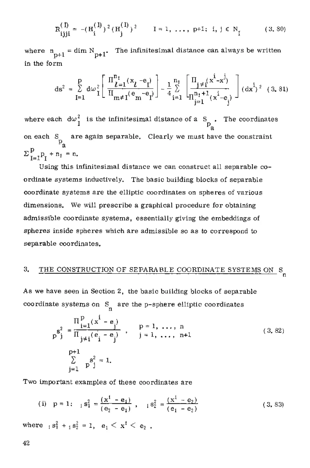
Two important examples of these coordinates are
(^ - ej) (ej - e2)
C. S3)
where l s\ + j si = 1, e{ < x1 < ea .
42
(ii) p = 2: 2s\
2 S3 =
2 _ (x - eQ (x^ - eQ
(ea
ei) (e3 - ei) '
? s2 -
e2)(x* - ea)
(et - e2){e3 - e2)
(x1 -e=i)(x2
e3)
(e3 - et) <e3 - ea)
el < x1 < e2 < x2 < e3.
We will develop a graphical calculus for calculating admissible
where 2s\ 4- 2 sj> + 2 s3 = 1
( 3. 84}
coordinate systems. We represent elliptical coordinates on S by the
?
'irreducible7 block.
el
ez
e _.
n+1
C.85)
Each separable coordinate system will be associated with a directed tree
graph. Consider for example the sphere Sa. There are two possibilities:
(i) the irreducible block 1 ej 1 e2 1 e3 [ - Most treatments of elliptic
coordinates on 3? correspond to the choice et = 0, eg = 1, e3 = a > 1,
This is just a reflection of the fact that for Jacobi elliptic coordinates the
variables ? and et can always be subjected to the transformation
1 ? ?. ?
? - ax + b, e' = ae + h;
J J
i=l,..M n, j = 1 n+1, { 3. 86)
Thus we can always choose et - 0 and e3 = 1. (Note in particular that
ei
Putting xl - cos ? we
can always be replaced by
recover lsi = cos <pt l s2 = sin ? @ < ? ^2?).)
(ii) The second system is the usual choice of spherical coordinates,
Sj = sin ? cos 0 , s2 = sin ? sin 0, s3 = cos ?.
C,87)
This system can be considered as the result of attaching a circle to a circle
and is the prototype for the construction of more complicated systems. The
graph
e1 e2
A-
k k
( 3. 88)
43
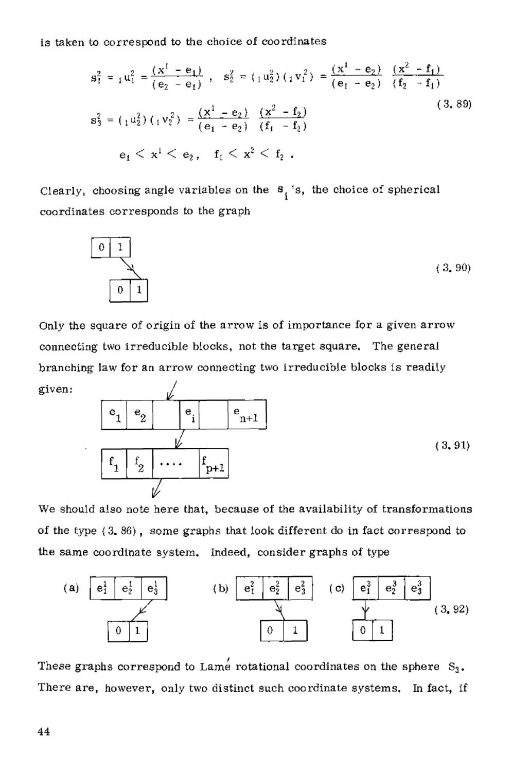
is taken to correspond to the choice of coordinates
(x1 -ea) (x* -fa)
S3 = ( 1 4 ) ( 1 V?2 ) -
C.89)
et < x1 < e2, fL < x2 < f2
Clearly, choosing angle variables on the s, Ts, the choice of spherical
coordinates corresponds to the graph
0 1
{ 3. 90)
0 1
Only the square of origin of the arrow is of importance for a given arrow
connecting two irreducible blocks, not the target square. The general
branching law for an arrow connecting two irreducible blocks is readily
given:
{3. 91)
ei
?2
fl f2
J
e.
1
i
Vi
Vil
7
We should also note here that, because of the availability of transformations
of the type {3. 86), some graphs that look different do in fact correspond to
the same coordinate system. Indeed, consider graphs of type
(a)
?]
4
4
0 1
?
(b)
4
[e|
\4
V
? ?
1
] (c)
ei
?
0
_[«? | e*
1
C,92)
These graphs correspond to Lame rotational coordinates on the sphere S3.
There are, however, only two distinct such coordinate systems. In fact, if
44
the coordinates ?1 and el (i = 1, 2, j ^ 1, 2, 3) are subjected to the
transformation
? ? ?
? = -x = y ;
el
-e! ^l
? = ?3
-?? = e;
? ?
«3 - -e3
?? ,
( 3, 93)
we see that the graphs ( 3. 92) (a) and (c) correspond to the same type of
coordinates. Graphs that are related in this way can be recognized by the
feature that, if the branch below a given irreducible block
HL
—
e
?
is obtained from that of another graph by reflection about a vertical at the
centre of the corresponding e1 .. Je1 block, then the two graphs are
equivalent, (We are of course assuming that all other features of the graphs
are identical,) Graphs that are essentially the same can be related by
several transformations of the type ( 3. 86) and the situation gets more
complicated, e. g.,
el
4
el
??
>? \ *i 1
66
i....._ V
\JL
?
13
?\
?
0 1
s\\ ?
l·
R"
]~5~
¦S
j
d\
g^
B§
"FT
0
5
^1
i.
t!
/
1
f2
1 2
f2
1 3
?
{ 3. 94)
If the two irreducible blocks of S and S occur as indicated in ( 3. 91) as
? ?
part of some larger graph, this means that the elliptic coordinates
? 1 ? ?
combinations
and v..
? 1
? „ of these blocks must occur in the
? P+1
w = u ,
1 ? 1
¦ "i^nV^V' -
w. _ = ( u.) ( ? ) , w. _ = u ,
i+p+1 ? ? ? p+1 i+p+? ? ?+?
w rt - u . ,
p+n+2 ? n+1
Arrows may emanate from different squares ( e. 's) of the same block but
45
cannot be directed at the same block. With these rules we may construct
graphs corresponding to ail separable coordinate systems on S .
?
For ? = 3 we have the following possibilities [20 J :
A)
0 [
B) (a)
1
a
b~]
|o ) ?
a
Jacobi elliptic coordinates
(b)
?
?? J 1 j aj
?
???
Lame rotational
coordinates
C)
o
¦^
0
1
/
1
a 1
<4)
0 | 1
\
1 °
Tl
j
\
0 1
Lame subgroup reduction
Spherical coordinates
E) 0 1 Cylindrical coordinates
The formation of more complicated graphs is now clear. Thus,
e2 | e3
?
f. U
X
fa U
C, 98)
C. 97)
C.98)
C.99)
C.100)
C,101)
is a coordinate system on S^ with coordinates
aa =
at = B^) . s2 = (aM (aViT, a{ = Bu2)'Cvz)'
C.102)
S4 = B^?) CV3J, 4 = (l^2J{^AJ , s| = BU3J<iW,J
s? = (zuai^dwaJ
46
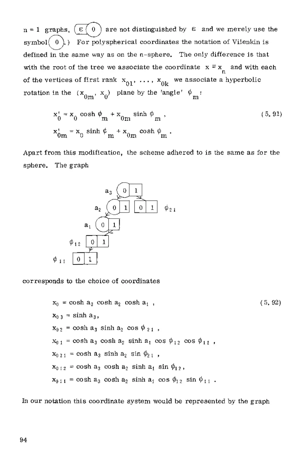
Vilenkin [2l] has studied polyspherical coordinates on S and developed
a graphical technique for constructing them. For example, he considers the
coordinates on S^. :
X0 = COS 03 COS 02 COS 0 j
xq 3 = sin ?
x0 x = cos
?" 0
0 3 sin 02 cos 0 2 i
03 cos ?^ sin 0 ? cos
cos 0^ sin 0 j cos 0 j 2 cos 0 11
3 sin ? 2 sin 02 r
3 cos 0 2 sin ? j sin ? y 2
XU 1 1 - cos 0 3 cos 0 ? sin ? 1 CoS 0 12 s*r
x021 = cos ?,
X012 ^ COS 0
sin ? 11
and represents these coordinates by the graph
C, 103)
x0 1 1
x0 12
x0 2 1
For him, spherical coordinates on S2
?? = COS ??
xo ? - sin 0i cos 0! l
x011 = sin 0 ! sin 0 j t
correspond to the graph
C,104)
«??
1 I
*D 1 1
47
Vilenkin denotes coordinates of rank r by ??. , and in the example
?? , ?
1 r
of ( 3. 103) arranges coordinates in the order
xo ? i * xo 121 xo 21 ? xn ? > xo 2 > xo 3 j xo t
C, 105)
L e, , coordinates of higher rank precede those of lower rank while
coordinates of equal rank are ordered lexicographically. Coordinates of the
form ?
0i .. .i .,, i , ?.. .i
1 s s-fl m
are called subordinate to the coordinate
? . . Further, the coordinate ? . essentially precedes the
°?'? °3l"eJm
coordinate ??. . if mi s, and jt = i, for 1 :< k < s-1 and i < i ,
0L,,,i Jk k s s
1 s
The coordinate ?
coordinates on S from this notation let ?
essentially follows xrtr , . To extract
0i-.. ¦ ? ~——* Ok. .. j
Is Jl Jm
0L.. .i
1 m
be a vertex of nonzero
rank. A rotation g( ?) by the angle ? =¦ ?, . In the (? +
h~'lm "V-'Vl'
x . ) plane is then associated with this vertex.
Ul ? ? * 1
1 m
In this way Vilenkin constructs graphs representing the various possible
polyspherical coordinates on S , In our notation his coordinate system
C. 103) is represented by the graph
02 1
o[i
? ?
r/7
0 | 1 |
03
j] 02
?
?| ??
?
[?
| ? | ? |
011
From these considerations we see that VilenkinTs polyspherical coordinates
are the special case of separable coordinates on S consisting of those
?
48
graphs which contain only the irreducible blocks of type | Q | 1 \
4. PROPERTIES OF SEPARABLE SYSTEMS IN S
Here we make more precise our graphical techniques by means of a
prescription for writing down the standard coordinates s., i = 1, ... t n+1,
on S in terms of the separable coordinates. A given standard coordinate
coming from a given graph consists of a product of r factors which we
denote
x ... = ( u.) ... ( u. ) .
Px Pr Pli1 Pr3r
This is obtained by tracing the complete length of a branch of a given tree
graph, U e.
'•?
m * -?
1
e
?
*N
e2
| 1
- * 4
...
Pi
s
e2
J
.,,
e2
P2
r
e
1
1 r
* * * I e.
J
1 r
I * >
r
e
?
r
Jl",Jr
We can then set up an ordering < for the products ? . We say
that r
*?,...? XQr..Q
1 r Is
if
p1=Q1. j1 = i1, .
•••pt = Qt' jt< V pt+i*Qt+i js*V
? ? t we
n+1
Then if we arrange the products in increasing order, say x..
can identify this ordered n-tupie with s1f ,,« , s . For th
l n+1
C* 102) given above, the choice of coordinates corresponds to this ordering.
s , For the example
49
Having settled on a prescription for writing down the coordinates
corresponding to a given coordinate system on S , we can now discuss the
separation equations for both the Hamilton-Jacobi and Helmholtz equations-
Let us first consider the coordinates corresponding to the irreducible block
The Hamilton-Jacobi equation in these coordinates
?
e2
* ¦ * *
n+1
IS
?
H= I
i-l[n..1(x,-*J)] l
?* = ?
C, 106)
where
P.Wfn (xX-ej] -^.
1 j=l J dx
The separation equations are
*+1 " dW
[? (xl-ef)| (m^[E^)n'1^ lXA*V'1}
]-l J dx j=2 ]
0 C.107)
If we set ? = >i then the quadratic first integrals associated with the
separation parameters ? i, ¦.., ? are
? ?
I-, = ? I2. (second order Casimir invariant)
C. 108)
I
LJ ?
1]
? ,>. n-H]
where S1} = ~ ? ·
I l\ i.
¦ ^ e-
. . ¦, e. and the summation extends over
1,
·!¦¦¦¦-7 - -i 7
??, ,.. , i, ? i, j and i, ? i for ? ? m. For the associated Helmholtz
it ? m
equation the eigenvalues of ? have the form ?(? +¦ ? - 1) and the
Helmholtz equation becomes
1
?
? —
V<5>.) A7i^{G>.) ~)
dx
1 a l
dx
= -cr(cr + ? - 1) ?
C,109)
50
where (P = ? _(x - e ). The separation equations are
i J=l J
1 dx1 l dx1
???·
+ ? ?.??1I1]*. = ?.
i=2 } l
The identification '?? - ?(? + ? - 1) enables us to further identify the
symmetry operators whose eigenvalues are ? , with the expressions
{ 3.108) where I., is replaced by the corresponding symmetry operator
C,110)
i]
For an irreducible block appearing in an admissible graph the
generalizations of these equations can readily be computed. Consider the
block shown as part of a given graph:
L
p+1
Then define d. (i = 1, ... , p+1) as follows:
d, = 0 if there is no arrow emanating downward from the
block
otherwise d is a constant on the sphere attached to e..
i ?
From the form of the metric we see the variables ? , ... , ? coming
from this block satisfy an equation of the form
?
?
?? + ?
1-1 [?,,.(??? [ 1=1
¦ni=i<xJ-ei>
d, = ? ,
? ?
[3.111)
Using the relation
1
where
nU(xUJ ni>3(x-xj>
1 -, 1 -, 1
]=1 J ox
1=1 <X -ek)
C.112)
51
? = ( -1> +1 ? (?1 - ?^) with ?, j ? ? ,
we see that the separation equations have the form
P+l dW. p+1 ? _ (e. - e,N
[? (^-e.,](_i,i+ ? 1*** ¦! k
j-i
J
C.113)
dx
k=i
(x - ek)
?
p' 1=2
For the corresponding Heimholtz equation the situation is somewhat more
? ? rt *¦
complicated. With each u. (j = 1, , „,, p+l) we associate an index k.
which is calculated as follows; if the irreducible block occurs as the
r step down from the trunk of the graph and if we write out the S. in
terms of our coordinates, then k is the number of coordinates for which
i \ \ J '
Jl"*3"*Jq th
x (r column) occurs. The Heimholtz equation assumes the
Pi ¦ ·. p..·?
form
? 1— I V(<P./Q.)—(V(ff.Q)—)
C.114)
where
?
+ ?
i-l
??*?'??
t.# = -?(? + ? - 1)?
P+l . p+l k.-i
<? = I (x'-ej, Q,- ? (x'-e.) ] ,
j=l
j=l
t. = Q if k. = 1 and t. = j.(j, + k. - 1) if kT ? 1. The separation equations
? ? ? li li
become
V^./Q.)—(V(<P.Q.) -?)
dx dx
C.115)
? ? (e. -e.) ?
+ ^ ? J*k k ' ?,+ [?(?+?-1)(?1)?-1+ ? yx1)^]
k=l (x-ek)
U2
?
*,=0
52
If we take the coordinates C.102) and choose
II? Ax -e.)
u2 =_Ei L
, j = 1, 2, 3, i = l, 2,
C.116)
_vi: =
, I = 1, 2, 3, 4, i = 3, 4, 5,
, (x gs>
Ir2 „ s
1 8 (gt-gB)
t, s = l, 2, t^s,
then the separation equations for the Hamilton-J acobi equation are
3 dW.
1=1
y " V
C.117)
(x - e2)
+ <e^ -^)(e, -ei) ^ +??? + ?? ^ lelf 2>
(x -e3)
4 / dWZ ? ?
(ii) [ ? (? -f }](—rJ + d2<x J +?2? + ?3 =0, ? -3, 4, 5,
m=l dx
Jttt
(iii) [n (x6 -e8)](^rV +d3 =o,
s=l
and for the Helmholtz equation the corresponding separation equations are
(i)
np- -y
d*.
«3- (Vtnf-ix'-eWx'-ejJ^x'-ea)) —- )
dx J J dx
(e, :e3)<e, - et) ji(ji + 2) +(e3 - eg) ( e3 - et) ^
(x - e2)
+ j(j +5)x + >i
(x -e3)
*. = 0, 1 = 1, 2,
?
C.118)
dx dx
+ [jiCi+2)(xV + ???* +?3]?? =0, ? -3, 4, 5,
53
(iii, V(n>=1<*« -b8)) Ipr (VO'I^ -gs) ?^>) + JJ*6 =0.
Having computed the separation equations for the Hamilton-Jacobi
equation in C. 117) , we can now compute the five quadratic first integrals for
the separation constants. We do this as follows^ in C.113) we put
?? = ? ¦ Given u.t two coordinates s,, s, are said to be connected if
d nr ? ? k
they both contain u.. The corresponding quadratic first integrals are then
calculated from the formulas C.108) with I?, replaced by 2 N I2
ij r>s rs
where the sum extends over all indices r connected to i and s connected
to j# The quadratic first integrals correspond to l{ type operators of the
next irreducible block of dimension m connected farther up the branch in
question. For example, consider the coordinates {3, 102) , The
corresponding quadratic first integrals are
U = ? t. , C.119)
U = ?1^ , k, i =2, 3, 4, 5,
k>i ??
U = <fi H- f a ) 15 ? + (fl + fS) lis + (fI + ^1*34
+ {f2 +f3)lh + {f2 +f4)I^ + (f3 +f4)ll3 ,
Le = 4 7 ·
For the Hamilton-Jacobi equation these quadratic first integrals have
the constant values
Li ~ Ej 7 L2 ~ >i, L3 - d2 f L4 ~ ?%, L5 - ?%, L$ ~ d3
54
and for the Helmholtz equation with I.. -> I1T the respiting opera
IJ ~ 1]
L (i = 11 . .. t 6) have the eigenvalues L ? ~ j (j + 5) t L2 - ? t,
^1 _ _ _
4 Separation of variables in
Euclidean ?-space En
1, MATHEMATICAL FKELIMINARIES
The same methods as used in Chapter 3 enable us to find all separable
coordinate systems for ? , The linear first integrals (Lie symmetries)
?
of ? form a |n(n+l) -dimensional Lie algebra E(n) with basis
?
I,. = ztp. - z.p. , i > j , i, j = 1 n, ( 4, 1)
ij ? J J ?
W
This basis satisfies the commutation relations
ab cd be ad ad be bd ca ac db
^b'Pc1=-5acPb+5bcV
? \? - ° ¦
Just as was observed for S , two coordinate systems \x 1
and {y } that are related by a group motion are regarded
as being essentially the same. In this case, if we are given the cartesian
coordinates z.(xJ) in terms of a separable set of coordinates {x } then
z' = Oz + a D, 3)
defines a new vector zT related to ? by means of a Euclidean group
motion specified by the orthogonal matrix 0 and constant vector a. Then,
clearly,
ds2 = dzr- dzr - dz-dz = g..dxW D,4)
56
Chosen coordinates ? and zf related in this way are then regarded as
being 'equivalent.
2. SEPARATION OF VARIABLES ON ?
_—. n
As was the case for S , all separable coordinates systems in ? can be
? ?
chosen to be orthogonal.
Theorem 4. l: Let {x } be a coordinate system on ? for which the
?
Hamilton-Jacobi equation admits separation of variables and let q be the
number of ignorable variables. Then it is always possible to choose an
equivalent coordinate system { x1 ) such that g J = 6l]B72, L e. , the
coordinates are orthogonal. Furthermore the ignorable variables
can always be taken such that
?
?? , =P2p+r "·· ?? = Pp+q'
p+1 q
Proof: We use methods similar to those used in Chapter 3. Any element
of the algebra E(n) is conjugate to one of the two forms [19]
where P= 0 if ? = 2v
L' = Pn. D.5b)
Let |x 1 be a separable system with q = 1P It follows from the block
diagonal form ( 3. 1) that this system must be orthogonal* Furthermore,
without loss of generality we can assume that ? = L or ? = LT, For
the first case we can always choose the ignorable variable Q'j such that it
is related to the cartesian coordinates (z.,, *.. , ? ) by
V n J
57
(Zlf .... ? ) = (pjCOS^ V), p,3in<X ^Wi) ,*.. D,6)
? ?
? cos<b„xQl+w„), Psm(b/'+wJ, ? +??°\
y2i*2 yn* '
The infinitesimal metric then has the form
ds2 =dp? +... +dp^+pi(dxCVl+dw1J D.7)
+ ... +p2j,(b(/cbcQl+dw!/i2 +<dp^+1 + j3dxQl)a
+ d4^2+"-+dyn·
If there is only one ignorable variable the coordinate system must be
orthogonal and consequently
rfdwj + ? bjo?dw. +0dpt, ? = 0- D.8)
j=2 ] J J ^+1
This is possible only if b = . .¦ = b^ = ? - 0 and dwt =0, (By redefining
cti we can then take w1 = 0,) Therefore, if we have only one ignorable
variable, p^ = 1?0 or ? .
Now suppose we have q Lie symmetries ? t i = 1, *. * , q. Then
they must be of the form
s ?
Li -I + ? b'L, , o; + ? ?' ? D,9)
l>p * m=2s+l
s
L*eI34 + 7? ^i-l.H* J /mPm
Z>p m=2s+l
s ?
Lp - Vl.2p + , Ifi2l-U 21 + m js+1 7mPm
11+1 m=2S+l m m
l = ? yq ?
q m=2S+i mm
58
The condition I.L., L, [ =0 implies
bL4-i=bL4 - ° D·??)
for i - 1, . <. 7 prt I = 1, .«. , q; k = p+1, ..., s. We are assuming that
there is always one b non-zero for each k and some i. Then
I I
72,_1 = ? 2k = 0 for k = p+lT ., t , s and ? =1, ,(l)qt The cartesian
coordinates are
a a a
(yis -..* y ) =(PiCos(x +wt), PiSinfx +wt),,..,? cos(x P+w )f
i- ? pp
? ?^ q z °?
pgsin(^^bsx ^, J^2s+ix +w2s+1, ....
q I °l
? y ? +w ). D.ii)
i=l n
This set of candidate ignorabie variables can take the necessary block
diagonal form only if dw. =0, b = 0 for ? = 1, - *., ? and
? ?
k = p+1, ,.,, s. Also dw, = 0 for I = 2s+l, _-,, n. We can thus assume
that w_=.i.=w =0, wn = ,. * = w =0, This implies ? = 0 for
1 ? 2s+l ? m ,
^ ?
i = 1, . -. , q» ni = 2s+q - p+1, ,., 3 ? and we can also assume y =0
ni
for i = 1 ? and m = 2s+l, ... , 2s+q - p+1. Consequently we can
take
U I12> .... L^ ^i^p1 Vl ?2?+1? "" Lq"P2s+q-p
D,12)
Of. a.
and there are no non-zero elements g J- 1 <i< j <q in the metric.
By a suitable relabelling of coordinates we can always choose s = p. All
separable coordinates in ? are orthogonal.
?
To find all possible separable coordinate systems on ? we proceed by
?
analogy with what we have done in Chapter 3. If we choose orthogonal
coordinates in which none of the o\. is a constant function then
?
59
?2 =?[ ? (?1 -?3}] , i- 1, „., ?, D.13)
where, as usual,
?
: ?
?
as2 = ? H?(dxV
i=l
The conditions R . = 0 are equivalent to C.33) in which the right-hand
side is zero. These conditions have the solution
?(?+1)=0, i=l, ...,„, D.14)
i
and 1/X. = ?, a;(x ) = g(x ) · Again we look for choices of g(x) that
1 ?— U L
are compatible with a positive definite metric. There are only two
possibilities;
?
(i) g(x) = TT {x - ej Elliptic coordinates D.15)
i=l 1
e < xl < en < *. t < ? <e < ?
1 2 ?
n-1
(ii) g(x) = ? (x - e.) Parabolic coordinates { 4, 16)
i-1 !
x1 < en < x2 < e~ < .,, < ? < e < ? +
J- ? n-l
These metrics give coordinates in ? dimensions that are the analogue of
elliptic and parabolic coordinates, familiar in Euclidean spaces of
dimension n = 2, 3, [l|, [22], To these systems we may associate cartesian
coordinates by
<1) y? =c» * J , j = l n, ? em, D.17)
} i*j<ei"T
(ii) yt = -(x1 + ... +x + e + ... + e )
? ? n-i
nn:V-. ,>
60
These two systems are fundamental for generating all separable systems on
? - As an example of the relevance of these systems we consider the
?
case when some of the ?.. functions are constants. We first treat, as we
did for S , the case in which the metric coefficients have the form {3, 39).
?
Then, as was shown in Chapter 3, these coefficients reduce to
?2=??. ???1-^)^ ? ?), ?* = ?,[? (? -? )], {4.19)
1 * j*i h=k+l h * m*l
The conditions ?^/?^ = ° imply that the quadratic form dsT2 = ?,?^ (dx J
is that of a flat space. The remaining non-zero conditions are
J JJ Z=k+1 m=k+l m m
ay ?? ?)
2— -( — J -(—)
?? ? ?
ra ra
3
0,
cx mil Hz (? -? )
m
D.21)
with R.... as in { 3. 41)« These equations are satisfied provided that
R.... = -H?H? and the function X7 and ^=(?/^1?;) are given by:
ijji ? j l ?=k+l ?
?
— = ? (xm _ez), I =k+l n, D.22)
? m=k+l
? =—= - for some m fixed, D.23)
where ? = ?, n-1. The functions l/X, are given by
k+1
— = -4 ? (?1 - e.<) , D.24)
The systems are related to cartesian coordinates on ? according to
<yr .... yn) =(wl8l wl8l?+1,w2 wn_k) D.25)
k+1 n^^xi-e.')
where ?. s? = 1 and s2. - ?? ;—; ]- ,
?=1 ? J V^"*?
61
?*"-?
w *?~? " (e -e?) - ?=1 n"k' D6)
m^i m t
???-k m
,.„ 2 m=i t 7
(ll)wi=ii ,(e -e,> ' i=1' "¦· n-k·
n-k
1, V m ?
w ( = ?( ? x + ej + „. + e ) .
n-k , n-k
There exists an additional possibility that could be discounted for S vis
? = & ¦ ? = k+1, .., , nP This corresponds to the case in which the
infinitesimal distance can be written
ds2 =ds^ +ds^ D.27)
where ds^ is the infinitesimal distance for elliptic or parabolic coordinates
in E. and ds§ is a similar infinitesimal distance on ? , . We can
k L n-k
mimic the procedure adopted for S , The only essential difference is that
the infinitesimal distance can in general be expressed as a sum of distances
that can be identified with Euclidean subspaces. This reflects the fact that
if { z. }, i = 1, ... , n{, and iw. }, j-1, tl() nSl are separable
coordinate systems in Euclidean spaces ? and ? with respective
?? ?·?
infinitesimal distances ds^, ds?. then the coordinates ? , w ,
? J
i^l, . +, , n: f j = 1, .., , n2, can be regarded as a separable coordinate
system on ? with corresponding infinitesimal distance as2 = dsj + ds?.
??+??
This is, of course, not possible for S . This property of Euclidean space
coordinates naturally extends to separable coordinate systems
^ ? ] i = l, ..., ? , ?=1, ... , Q on ? in such a way that
? ? ?
dss = ds^ + .., + dsjL .
In general the infinitesimal distance can be written as a sum of basic forms
Q
ds* - ? as2 D.2 8)
1=1
62
where
ds
e1)
1
i 1 L n-*-(e.
·:>
dw? + do7;
? I
D,29)
Here the a<J2 is the infinitesimal distance corresponding to elliptic or
parabolic coordinates for a flat space of dimension ? . Also ?
? for
elliptic coordinates with a strict inequality for parabolic coordinates.
The ??2 is the infinitesimal distance of some separable coordinate
1 ^Q
system on the sphere S and ? = ? (? + ? ), To establish a graphical
procedure for construction of separable coordinates we need only analyse
one of the basic forms ds*,
then the basic form is written
We should also mention here that if ? = 1
ds2 = wadu2 4- dw2 .
( 4. 30)
A basic form could in fact correspond to elliptic or parabolic coordinates
on ? and no d^2 term. We associate this with nT = 0 in D. 30),
N.
I
3. THE CONSTRUCTION OF SEPARABLE COORDINATES ON ?
For our construction we need only invent graphical representations for
elliptic and parabolic coordinates in ? , the analogues of the irreducible
blocks on S , We adopt the following notation:
A) Elliptic coordinates / e.
B) Parabolic coordinates ( e1
*n-l
, ? > 2,
It is clear that only elliptic coordinates exist in one dimension. The
graphical representation of a basic form corresponding to the infinitesimal
distance ds2 in D.28) is
(i)
el|e2
Sp Sp
1 2
N.
D.31)
63
(?)
?
-»??
Attached to each leg descending from the top block is the appropriate graph
of the coordinate system on the S giving rise to the form dw2. . The
?. ?
general graph corresponding to a separable system can then be constructed
as a sum of disconnected graphs of type ( 4, 31) (i) or (ii). We first
illustrate this technique for the separable systems of E3 (Table 4, 1),
As an additional non-standard example consider the graphr
which defines a coordinate system in E5, The coordinates can be chosen as
(x1 -eO(x2 -©i) 1
y2. -c2
2 2
2 2
yi = e
(e2 - et)
(©i - e3)
(x1 - e2)(x2 -_e2)
L (ej - e2)
? ? ? 1
<x -e2) {x? - e2)
B^)-( 1 = 1, 2, 3,
cos2x5 ,
¦ 2 5
sin^x ,
( 4, 32)
where
(x3 -t)(x4 -f.)
2 i (f. -f.)(f. - f.)
i, j, k distinct,
j i k i
We can set up a natural ordering for separable systems in ? , For a
?
given basic form we can impose the natural ordering of the e.'s in the
leading irreducible block on the ordering of the S branches and then
write down coordinates in a standard way.
64
Table 4, 1 Separable coordinates of ?
A)
B)
C)
D)
E)
F)
(?)
(8)
(9)
A0)
(?)
<???><?>
f<^>
? ? ? 11
<Q5><5>
? d>
0 1
| Q | 1 |
| ?[?]
?
Q
/
1
?
?
1Z
<
0
~?]
?^]
e3 I e3/
?
1 1 a|
Cartesian
Cylindrical
Elliptic cylindrical
Parabolic cylindrical
Spherical
Prolate spheroidal
Oblate spheroidal
Parabolic
Paraboloidal
Ellipsoidal
Conical
G5
The ordering of the disconnected parts of the graph is presumed aiready
given. There are equivalences relating graphs of various coordinate
systems that we have already discussed for the n-sphere and, of course,
there is an additional equivalence corresponding to the permutation of
disconnected parts of a given graph. The separation equations can also be
readily computed. For the elliptic and parabolic coordinate blocks
A) <ea | - - - | «n>
<2) (ei|---|vi)
the Hamilton-Jacob! equation has the form
where
? = ? ?-· . ¦ ?2 = ? ,
1=1 [? (?1-*', | 1
D, 33)
?,
3W
P = V[ ? (xl-e.)l-^
with Ni = ? (elliptic coordinates) and N^ = n-1 (parabolic coordinates),
The separation equations are
Nk .
[? (x'-e)]
1=1 J
dW.
Ldx
2
[E(
i n-1
+ I x.<xV_JNo.
j-2 J
D. 34)
If we identify ? = ?1 t the quadratic first integrals associated with the
rat
A)
ion parameter
iff-
i?=
«i-
P2 4
i.
1]
sij
?
s ? , *.
+ ??
? '
?
i=l
I?. + c2
1J
* ?
si
?
?
?
?2
1
s1
?-
are
j
?2
11
D. 35)
where S, = ?— ?. . , e,
? I != ?? * *. ,?, =? ?
e, and the sum is over ii, *** ,i7=^i.
66
B) ??? = ?* +.,- + F^,
? ?
I* = c ? ????? ?, ) + 0*8^ + ? C2S{P? ,
D. 36)
22 " " "Ik' ^k'+
k=2 ?]? * +
3=2
k=2 iK K i>j^2 1J J=2 J
? ,. ?
2? = ? cslli.,, p.} + ? SiJi^+cas3p^ +c2 ? sjp?
k=2 1K J i>j>2 1J j=2 J
in = Zcsk Jt ,, ? 1 + ? sij j?,+cas v\ ,
ii-l
n-2 Ik' k + .-n,.>9 n-3 ij n-1
k=2 " " *" " i>]^2
where S 1383111D.35), { , } is the anti commutator bracket and
Sj — j L e, * ,, e.
it!. . , ¦ ii i7
For the corresponding Heimholtz equation the eigenvalues of A are
? and the Helmholtz equation reads
r
where
N,
e. = ? (?1 -?.) .
1 5=1 J
The separation equations are
d*
n-1
V@.) ^-(V@J -?1) + [(-?)(?1)? + ? ????^??.-?
1 dx dx j=2 J l
D,38)
For a basic form such as ds^ the separation equations for the
Hamilton-Jacobi equation have the form
67
NIk dW ?? ?,./?,-?
[? <??-?.)|(-?-1)»+ ? *** ' '
J=i
dx
Z=l (x - e,
D. 39)
¦ V1 N'k ¦ V'
+ [e.(?1) ? + ? ?,??1) k No,
1 Z=2 ?
where k. is the constant value of the Hamiitonian on the sphere whose
infinitesimal distance is d&l . For the Helmholtz equation the
corresponding contribution of this basic form is the equation
NT
J*1
V(=r) —r(V<e.Q.)
a*.
? dx
? i -j ?
??
+ I
i=l
?5? + ?? - 1)?= "ki*·
where ^11^ (,l-V< Q. = ? JV - .fc> '
D.40)
p. + 1 if k = l,
k
* ??
if k = ? +1, ,,., ?
The separation equations are
P. d*
? dx dx
Lk=l L (x -e )
? ?
+ k <x> + ? ? (?)
1 J=2 ?
?, ?—rH'A + v1»
?. = ? ,
1
D, 41)
tn the example on E5 the separation equations for the Hamilton -
Jacobi equation are
2 dW.
[? (^-e.jJt—V+<^_lillkl + <e' -e^k,
j=l . J dx (x1 - e2) (x1 - et)
-??1 + >| = 0, t = 1, 2 .
D,42)
68
and for the Helmholtz equation they are
'nf-i"'-il
? 1 X 1 J 1 ?
dx Lj-1
2 . d*.
?1 (x -e.)(x -eiJ(x - e2) —j-
dx J
i ^ 1
For the elliptic case the only new prescription required is that P: be
replaced by ? ? where the sum extends over all indices r connected to
r r
i. Similar comments apply to expressions of the form {I , , P* L For
our example with coordinates D. 32) , the quadratic first integrals that
describe separation are
Lj - l\2 + h Z + h 3 >
L2 = fil2 3 + f^Ii 3 + f3 Ii ? >
D. 43)
i4
MS t
L4 = ? ?? ,
i=l x
3
i=l
14
+ llc ) + c2 [e2 ( ?3! + pjj + p|) + ej ( ?\ + ?^)
1<j
The operator L6 corresponds to the separation constant A1#
69
5 Separation of variables on
Hn
1, MATHEMATICAL PRELIMINARIES
Using the same methods as in Chapters 3 and 4, we can find all separable
coordinate systems for ? < The linear first integrals (Lie symmetries)
?
of ? form a §n(n+l) -dimensional Lie algebra SO(l, n) with basis
?
I.. = v,p. - v.p., ? > j, i, j = 1 n, ( 5. 1)
wrvv 3 = l ?·
This basis satisfies the commutation relations
[lab' 'J ~ Vad + e^be + 5bdIca + 6acW (^
fW'J^ab a,b,c,d = l n.
As we have discussed previously, two coordinate systems related by a group
motion are regarded as being essentially the same. In the case of ? the
group SO< 1, n) [22] consists of matrices L such that
ds2 =dv'- Jdy' = ay- Jdv E,3)
where J = diag<li -1, .-., -1) &&d
?' - Lv , E, 4)
For ? = 3 there are just the well known Lorentz transformations that
occur frequently in relativistic physics [2 j. If we are given the components
of the vector ? in terms of a separable coordinate system {x ] then a new
70
vector vT = Lv expressed in terms of these same coordinates is
regarded as specifying an equivalent coordinate system.
For ? , however, there are more cases to consider and the problem
is more complicated.
2, SEPARATION OF VARIABLES ON ?
?
The classification of separable coordinate systems on ? is greatly
?
facilitated by the fact that all such coordinate systems can be taken as
orthogonal. Indeed we haver
Theorem 5.1; Let be a coordinate svstem on ? for which the
^ n
Hamilton-Jacobi equation (I) admits a separation of variables. Then, by
passing to an equivalent system of coordinates if necessary, we have
g = ? ??2, U,, we have only orthogonal separation. In terms of the
standard coordinates on the hyperboloid Vq, v-j , , ., , ? the ignorable
a
variables ? can be chosen such that the corresponding ? - nj Lie
symmetries ? (i = l,,.. ,q) are of one of the following three types [23I;
i
(I) % =I01' ?a2 =]23 ?? =I2q-2,2q-r E'5)
<"> ?ai =I12' Ptts =I34. ¦". Pa =Vl,2q'
<ul>pttl =Io2-H2· ···· pQ "WrVi·
1 s
pa = Xs+2, s+3' '" ¦' ?? = Vi, q+2 *
Proof: This is based on the general block diagonal form C. I) of the
contra variant metric tensor for a separable coordinate system. Any
element of the symmetry algebra SO(l, n) is conjugate to an element of
one of the types
(« L = I0l + b2I23 + ··· +buJ2v,2v+l' \ E,6)
(ii) L = I12 + b2L34 + ... +\l2l;
71
(ii»L = <I02 -I12J +b2I34 + ... + ^^-1,2^
a,
If one of these elements corresponds to the ignorable variable ? l, L e. ,
L = ? t then by local Lie theory the standard coordinates on ? can be
taken in each case as
(i) (v0> v^..,, v^) - (ptcosh<x ^O, ptsinh(x Vwj), E.7)
p2cos(b2x +?2) , p2sin(b2x +?2),,„
? cos(b x +? ), ? sin(b ? W J .
y ? ? ? ? ? 7
(ii) (vQ, ??,..., ?) = (vQ, plcos{x +^1)ip1sin(x +?(),,_
?, ?,
? cos(b ? +? ) f ? sin(b ? W ),
^ ? ? ? ? ?/
??-^-- -pl-i^i-··· -< = ?.
(??)(?„, ??..., ??) = (i[p! ???'+?,?^??+?],
iEpi i(xttl+«iJ - ?) +v|,
?, (? '+CU!), p2cos(b2xai+w2),
P2sin(b2x *+?2)
p^cos(b^x V^^), p^in(b^0W^f
? ? - ?2 ^ _?2_?3 _ _?2=?
?1? ?2 ¦" *? ?2?/+2 *'* ?? "
The infinitesimal distances corresponding to these three possibilities are
Of
(i) us2 = dp? -dp \ - ... -dp * + Pt(dx ! + dw i ? E,8)
-p^(b2dx J+d^2K -_. p^(b^dx ^??^2
72
dVU2—'-dVn>
(ii) ds2 = dv% -dp\ -... -dp*-^(dx^ + d^iJ
-·" ^>,??* "dV2,+l-- "dVn
(iii) ds2 = dp i dv - ? ^ (dx *-?3? {J - dpji - .., - dp2
-p?{b2dxGl-Kiix>2J -... -p^fb^dx^+do^)*
-dv* _ -... -dv2 .
2 ?^+2 ?
If there is only one ignorable variable, ? , then the coordinate system must
be orthogonal, which is only possible if b = b2 = , ·. = b = 0, i. e. , we
have the three cases
(i) P„ =Iei E-9)
< ii) Pa = li 2
Indeed, the requirements that the contravariant metric have the form C.1)
(orthogonal in this case) imply
U) dWj = ? (-) )b,deu. , E.10)
j=2 ^ ' ^
? pi
(ii), (iii) dWi =-2 <4 jb.dw..
j=2 p' ^ J
Since the differentials dp., do>_, (j ^ 2) are independent and the only
conditions on ?\ are the requirements given in ( 5. 7) {i) -(iii) , d2 0){ = G
implies that b. = 0, j = 2f «?„ f v, and d^j = 0, Fy suitably redefining
0?i, we can put u^ = 0,. Hence the result we want to prove follows for one
ignorable variable.
Suppose now that we have ? - nt Lie symmetries ? , ? = 1, ,.M q,
i
in involution. Then they must have one of the forms:
73
?
1 Z=q+1
?
?0? = W + , ^ bZI2ZJ2Z+2 '
2 , Z=q+1
?
Po "^q-^q-l* Z ?^?^?+?
q ? ^ ?~q+l
?
(??) ??? = ?12 + ?? ^1^-1,2*'
1 ?=q+l
?
?
PG = I2q-l,2q + , ^ , V2?-1,2Z'
q H Z^q+1
?
(??)?&? =<?02 "?1^ + ,? b^2i-S+2,2Z-S+3'
1 l=q
?
% = (?03 " L13J + } bZI2Z-s+2,2^a+3*
l=q
* ?
?? = ^og+i " hs+J + 7? biV-s+2,22-8+3'
s ?=q
?
y , S+1
pcv ~ s+2,s+3 , ? 12i-s+2,2Z-s+3'
s+1 t=q
*
?
? Q
Pil· " ^q-s^q-s+l + T bZI2^-s+2i2Z-s+3 *
q * Z=q
Of these three possibilities we see that ease (ii) involves only elements of
of the SO(n) subalgebra and so is equivalent to the problem of the
corresponding case already treated on the n-sphere S * The two other
cases give rise to the coordinates
U) (votv1,<..,vii) =(p1oosh(KQfl+w1), PiBlnh^+Wi), E.12)
p2cos(x +?2)? P2sin(x +?2), ,,,,
74
q . a'.
? ^cos( ? b ? +? )
q+1 \ q+1 q+1
q . a.
1=1
V2N+2* "" V '
s O.
(ii) (v0, vlt„-, vn) = <4[pi { ? (x +?.)* + ?] +?], E,13)
i=l
s a
i[pi ? ? (? Vcu.J -?] +vl,
i=l l
Pif^+^i), ...
a o
s u s+1
••¦>ps(x + ?"B>-pa+icos* +aW'
a q t a.
q - Qr.
...,??»1?(? b^l+wN). v2N_g+4 vn).
Qi
If the ignorable variables ? correspond to part of a separable coordinate
system, the associated covariant metric should be in block diagonal form
C. 1). Just as in the case q = 1, this is only possible if bi = 0 for
I = q+1, ,. r t N, j = 1, -. - , q, We can therefore assume that the
ignorable variables can be chosen such that
(ii) P0, =I12 Pa =VlBq'
«"«?^ =I02 -]i2' — Ptt = W ~ W· p<v ? = ^-^, ?+3 ·
1 s s+1
? = I
*a 2q-s,2q-s+l
q
In each case the functions tt?i . .., , ? can be chosen to be zero by
q
suitable redefinitions of the oh 's. Thus each such coordinate system is
?
orthogonal.
75
As with the n-sphere and Euclidean ?-space, we can directly apply
EisenhartTs [l4J methods to enumerate the various possible separable
coordinate systems on ? . We proceed in analogy with the treatment in
Chapter 3.
We first consider the separable coordinate system { ? ] corresponding
to the infinitesimal distance
? ...
ds2 - ? ?.[ ? (?1 -xJ)l (dx1J , E,15)
i-1 L j*i
The curvature conditions for ? are
?
?.... =H2H* i ? j . E.16)
UJi ? J
These are equivalent to the equations
[n^.^l-J-^-^.-^L-^i E.l7)
I*} (<x - ? ) j {x -xJ) j
l*i (? 1-xJ>2 Xi {^-x1) Xi
Z*i,j Xz(x -xL)<x -?^?^?? -x^
+4
These equations have the solution
(i_}(n+l) =4(n+1), _ E18)
i
i.e. ,
— =4(x) = l a^(x) = f(x) ¦
i 1=0
We normally write
n+1
f(x) = 4 ? (? - ej - E-19)
i=l ?
To determine which metrics of this type occur on ? we must require that
?
the corresponding infinitesimal distance be that of a positive definite
76
Riemannian space* There are four classes of solution to this requirement:
Class (A). e. ? e. for i ? j, i, j = 1, 2, ?,,, n+1.
If ? = 2p + 1 there are ? 4- 1 distinct possibilities given by the
inequalities
A) eL<e2< x1 < e3< x2 < ... < e^ < ?2?*\ E.20)
B) ?1 < e2< e2< e3< ?2 < _. < ert _ < ?
2p+l
2p+2 "
i-1
(i) x1 < ex< x2 < „. < ? < e,_1< e
< e. < x* <
i-fl
< e < < e < x2p+1
"' i+2 "' 62p+2 X
(??-1) xi<e1<x2<._<xp<e <e <e <xP+l<... <ef> (><?2?+\
1 ? ?+1 p*2 2p+2
In factj with convention e., ? = 0 for j a non-positive integer, these
inequalities can be summarized in the form
<i> ¦¦•-i<V2<-i<V1<«i<Vi<xi<ei+2< E·21)
•¦¦<e2p+2<X ' 1 = ° P*
To express the coordinates for these systems in a compact way we introduce
the symbols ? defined by
EJS) =e.+i+1> 1 = 1, ..., 2p+2, j - 1, ..., pfl, E.22)
and use the definition
e = e if r = simod ? + 1) , < 5,2 IS)
r s
r, s positive integers. Then the standard coordinates on ? can always
?
be chosen to be
77
These ideas work equally well when ? - 2p + 2, i, e, , ? is even. In this
case the ? , e, satisfy the inequalities
•.•<xi<V2<xi<ei-l<ei<ei+l<xi<"-<e2p+l<x2P E·25)
where i = 0, (,,, p, If we use the EH "s as defined in ( 5, 22) then the
standard coordinates for ? are given by equations { 5. 24),
Class (B)· e ^tv+ijt, e0 = a - i^ ?, ? em, e0 =f ,..4, e =f
i ? J l n+i n-i
There is only one possible choice for the coordinates ? , i. e, t
x1<f1<x2<f < ... <xn_1<f <xn,
1 2 n-i
A suitable choice of standard coordinates on ? is
?
? J ??*-?-?>
(v0 +ivtJ = (z) —-j . E.26)
Class <C), e, = e2 - a, e. =g._2, j = 3,.. ? , n+1 with gk * g^ if
k ? ? and g, ? a for any k. This case divides into two families of
coordinate systems. With the same conventions as for type (A)
coordinates, the ranges of variation of the coordinates ? can be given as
(a) ... xi<giMl<xi<S1<a<xi+1<g1+1<...<gn_1<xI1i E.27)
(b) ,,. x1" <g._^<xL<g <xL <a<gi+1<.,.<gn_l<xn.
If ? = 2p + i {Ue4, ? is odd) , then i = 0, ..«, ? and if ? = 2p (i, e. T
? is even) then i = 0, .,, , pt so that in either case there are ? + 1
78
distinguishable cases to consider. In fact if we define symbols
where g - g if r = s (mod n-1) t r, s positive integers, then we can
? s
write down a suitable set of standard coordinates for ? as
?
(v» "VlJ =?~^?—?? ¦ E·28)
?"? (GU' -a)
(vg -v\)=ta
a rni=i<xi-a)
J=1 J
2 _ _ 1=1 ]-l
j-1 ?*j-l ? j-1
j = 2, .,. , n# Here ? - +1 if we have case <a) and ? = -1 if we have
case (b),
Class (D), e1 = e^ = e3 = b, e. = h , j = 4, ..,, n+1 with h ? h*
if k ? I and h ? a for any k. This case divides into a family of
solutions with coordinates varying in the ranges
...x <ht <x<h.<x <b<x <h. ,...<* <h 0<^x E.29)
l-l ? i+l n-Z
where, as usual, hH = 0 if i ^ 0. Just as in the previous case there are
? +¦ 1 distinct cases to consider where ? = |(n - 1) if ? is odd and
? = -|n if ? is even. Defining symbols
Hfl) =h.+r j = 1 n-2, i = 0, ..., p,
with h = h if r = s (mod n-2) , r, s positive integers, we find that a
r s
suitable set of standard coordinates for ? is
?
79
(v0 - vO1
1=1
nn-2(H(i)-b)
J=1 J
2?2(?„ - Vt) = -"g^
„2 ,,t .? _ 1 ° _
V0 - Vt - va - - a ip
n^(H(i)-b) J
¦n^x'-b)
]=1 J
¦?.!"' -Hi-2'
"^<»iB-^"-»,(i)'
( 5- 30)
j - 3, . .. , ru
Clearly the variety of separable systems for ? is much richer than that
for S and ? . There are four classes of separable coordinate systems
? ?
and in classes A, C, D the number of distinct types of coordinates increase;
with the dimension.
We now proceed to examine the possible metrics in which some of the
0\H are constant functions. The simplestsuch case occurs when the
components of the contravariant metric have the form
?
?? = [?. ? (?1 - xJ) ] ( ? ?,)( i,j = l k,
1 1??] Z=k+1
( 5, 31)
Hj = [?, ? (? - xm) 1 , !,m = k+1, ... f n.
The conditions R „ = ?^?? are the same as for E. 15) , Le( E, 17) but
with ? -*n - k = n\ With ?? = [?. ? (?1 - ?3) | , the conditions
I 1 j^l
R.... =H?H* and R,„. = H?H27 are equivalent to
ijji ? j illi ? i
~ <- ~ n n ? ai -
h:3h:3r +( ? ? >[ ? —s-{ — J-i\ = o, (?,32)
1 J 1JJ1 z-k+i ZT=k+i4Hz· ?-
?
V
0"i
2(tt) -(??)" -<7?>
^jbgllJ + Hj l—±j
Bx
m#H2 (x"-xm)
m
E.33)
80
where R is the Riemann curvature tensor for the Riemannian manifold
iJJ1 7 ? k -9 i 7
with infinitesimal distance ds? = 2. .- H: (dx ) ¦ For the functions X.
i—i, ? ?
we have
(^)(n_k+I) = 4(ii -k+ 1I E.34)
but for the metric coefficients H? there are several possibilities as
follows:
Case (A),
n-k+1 ,
^- = 4 ? (? -EU))t I = k+1 n, E.35)
X? m=l
with ? * ? if m * ? and all ? real. Then
m ? ?
?? ? ?
? ?" (? - ? )
( ? «? "? ? ? ?? ' (?·36)
where R.... =???2 if J = I
? J
i.e.,
= -?2 ?2 if J * 1,
k+1
—¦ =4 ? (?1 - ?!), i = 1, ..., k, J- 1, E.37)
? J=l
k+i .
— =„4 ? (?1 -e.)p i = 1, ,,., k, J*l. E.38)
The coordinates in these two cases can be taken as:
(a) <v0, vlt .... vn) ={u0w0, u^ uQwk, ^ Vk),
where
n-k k
Uq - ? u? = 1, w* - I w? = 1 E.39)
i-1 1 j=l J
and
81
nk (xj -e: >
^?in1= (E--E' ) ' i = °'1 k' E·40)
?11 ^ l(xm-E. ,)
ni-Sin""^E -E.J ¦ ?=0'1 n"k· E-41)
m^l m ?+1
where ?, =+1 if i = 0 arid -1 otherwise. This case corresponds to
J - 1.
(b) (v^^ vn) -(u0(Ul VlWl ??? Vk1,
( 5. 42)
where
n-k k+1
4 -? ??!=?, 1 w)= 1.
i=l L 1=1
The u* coordinates are given as in ( 5, 41) and
wi s n1 /e - e') ? i- J = ^ · · - * k+1 · < 5- 43>
J^i i 3
In this Latter case the w? are given in terms of elliptic coordinates on the
k-sphere 3, and consequently
e^ < x1 < e2 < ... < x < e . E, 44)
Case (B)«
1 I n"k_1 ?
— -4[(x -?J+??| ? (? -f ) E.45)
I m=l
with f ail real and different, ov, ? real. Then
m
The standard coordinates on ? are
?
82
(??...,??) =(u0>ull„.>uJ^wll...|liJ_1wfcfl>uJ>.(
where
n-k+1 k+1
4 - 1 n2 = ?, ? wj = ?.
1=1 l Ul
The w2 are given as in ( 5, 43). The u. coordinates are
n?:r<fz-°-tf)
?
I
„2 -
t^k+? m-1
Um L(o-f J2^2 ft (f -f ?
m-1 t?m-l i m-1
Case (C)
^ =4(x* ^aJ ? (? -GJ <
Xi m=l
There are two possibilities:
?
?
?=k+l
m
,a|(,-L<'i)-n„iT@_-G,,«il-G^
m^J m J
and R..., - -H2H2, i, J = 1, ... , k; i * j.
?? I
a ni-k+i{x ~a)
..., k; ? * j.
The coordinates in each of these cases may be taken as
and R,... = 0, i, j = 1, ..., k; ? ? j
C,47)
( 5. 48)
m = 2, .. # t n-k.
E. 49)
E.50)
E.51)
(a) (v0,vr,,vn) =(\ul VlWl Vw Vk'
E,52)
with u, , w. satisfying the same conditions as those coordinates in {5, 46),
The w2 are given as in { 5. 43). The u, coordinates are
S3
n?=k+i(x* ~a)
(??? -m)s =e + E.53)
n^^fG -a)
m=l m
, ?? , ix -a)
v ' da „n-k-l
? "-":-"{G -a)
m=i m
, ???»?<«'-0.-?>
j = 2, ,,. , n-k,
(b) (?^?^.,,,?^) = E[(u0-n1)(w^+.ii+w^+l) +(Li0+ut) E.54)
i[(u()-u1){w?1+, ie+w^-l) +(u0+Ul)]s w1(u0"U1),
The u. are given as in (a) and the w, are one of the two possible elliptic
coordinate systems on ? [l] , ir e. t
nf-i<xi-V
(i) Elliptic: w* = c2 j; — -L- , J = l, .... k. E.55)
J i*jtei"T
(ii) Parabolic: w = ic(xL + ... + ? + e^ + ... + e ) , E.56)
nk.(xl-e. )
w^=-c2-^— ^- , j=2 k.
?*]
1 I n~k I
Case(D), (—) = 4(x - bK ? (? -G ). E.57)
I m-1
There are two possibilities:
, w \ t "?-k+i"' -hj-2>
34
? ?? (x?-b)
(b) ( ? ? ) =--^2 *5·59)
Z=k+1 ?1 (?, -b)
J=1 .1
The coordinates in each of these cases may be taken as
<a> <Vvi V =<W —>V2wi ^-sVr-Vk1
E.60)
with u. , w, satisfying the same conditions as in E,42), The w2 are
given as in E. 43}. The lu coordinates are
???. ??-h)
2u2(u0 -u,) =-^(-~^
nUi-(Hrb)
2 , . ? 92 ""=^?<?? "b) ,
<b) (v0,v1,...,vn) =a[(u0-u1)(w?1+...+w^+l)+(u0+u1)]) E.62)
i[(u0-n1)(w71+...+w^-l)+(u0+u1)J, w1(uQ-u1) ,..
... wk(Uo-Ul), u2 Vk) .
The u. are given as in E. 60) and the w. correspond to the two possible
nondegenerate systems on ? : elliptic or parabolic coordinates. This
completes the treatment of the case ( 5, 31).
We recall that in general the infinitesimal distance can be written in
the form
35
dss = 1 { I <HiV<dxV J [? (?, +??I
E.63)
1=1 ieNT
i€N
?+1
??+?
I (H^V(dxJ)
? 2
jeN
?+1
where {?.., .... ? ) is a partition of the integers 1, ..., ? into
,<»
mutually exclusive sets N„; ? ?1 N„ = # (I ? J). In addition, 3 H. =0
I I J j ?
if i i NT. The curvative conditions R.... = H2H? (i ? j) are equivalent to
I iJJi ? )
the relations
Rijji -<H. ) (H. ) , i, j eNp+r
E.64)
<H<V<HiVR(I). + ? [<?.+?)][± ? <??+1)
k?N
?1?
p+1
7 ?N
p+1
(?^?^-1^0· *> j?Nl'
??
(Ci + QI> ??? + ??
I
«W
3 ,
E,65)
E.66)
H= ?
h ? *
??
ff?
m*i ?2 (?* -xm) J
p+1
= 4Hl·
p+1
= 1.
E.67)
where, as in Chapter 3, we denote R../j as the Riemannian curvature tensor
of the Riemannian manifold with infinitesimal distance
ds^= J (H1JJ(dxV
ieN
E.68)
We recall that the metric coefficients (H. ) have the form
(P+1) ,2
<H(P+iV =?.[? (x1-^)!, liH,,,
1 > ,,
p+1
E.69)
86
??+1
where A/X.) = 4(? + 1) ! There are then various possibilities
which we list in abbreviated form:
n+l
[l] (_)=4? (?1 -?), E*E. j^kiieN .. E,70)
Then
ni€N y-*i]
[ ? (? +gj] ?? ?* E.71)
p+1
where ? = +1 if 1 = 1, and ? = -l otherwise. In addition,
R(I). -eT(Ha))?(HfI)J , E,72)
iJJi ? ? J
[n| ( —) =4[(?1-?J+?2 |? (x'-fj, f.*f. if i*j, i€N ,.E.73)
?? i=i J x J P+1
Then
p+1
and
R!jji —(HiVtHJV. E.75)
? n_1 ¦
[ill] — - 4(xX-aJ ? (x^G.), G. * q. , j * k, i e ? ,. E.76)
There are then two possibilities:
? (? +0l) =e——?ti , E.77)
??
Vn y~GJ E.78)
and p
87
R(I) =0, ?^?. = ~(R<:1)J(B<:1))Z for 1*1. E.79)
ijji iJJi ? J
n-3 .
[iv| (—) =4(x1-bK ? (xl-H.), H. * ? , j * k, U ? . E.80)
?. , ? J J K p+i
There are again two possibilities:
[ ? (? +0l)]= —St , E.8l)
ifN , ??7<?. -b)
P+l 3=1 J
? (?1 - ? )
ieN K r
[ ? (ffi+ojN-B Jh HllhH)' E·82)
p+l
and Ei.0. - 0, R( 1]. = -{HiB )* (H( I})? for I * 1.
iJJi iJJi ? J
These results give us the branching laws for the construction of graphs
representing the various possible coordinate systems on ? . In each case
the infinitesimal distance has the general form
as2 = I as"
1=1
? 7 (x - e ) ? ? ? iL
7eN /A 7
F+1
I [ U.
I
1 ? ]*i . (dxV,
P+l J=l j
( 5, 83)
where ds^ is the infinitesimal distance of a Riemannian manifold of
constant (possibly zero) curvature and U is a fixed number related to the
choice of coordinates x, i ? ? ,, If ?, is a double or triple root of
n+1 ' p+l 1
? (? - ? .) then ds^ is the infinitesimal distance of a flat space. This
can of course only occur once.
3, THE CONSTRUCTION OF SEPARABLE COORDINATE SYSTEMS ON ?
— ^ .—_ . „ __ _ .—„ n
We have shown that the basic building blocks for separable coordinate
systems on ? are the four types of general coordinates (types A, Bt C,
D) and the systems we have already developed for the ?-sphere S and
real Euclidean ?-space ? - For ? = 1 the coordinates are given by
?
83
?. ?^
2 _ (?* -Et) , _ (?1 -?,)
? — ?. » V1 — — . .
Vi
(?2 - Ei) ' * (?? - Ea)
where Et < ?2 < x1.
?. (?0 +iViJ = (?) (?1 - ? - ??), ?\ ? real,
? 5. 84)
? 5. 85)
or
?§ -?\ = lt 2v0Vi = ^<xl - ?')
and x1 any real number.
C- (v0 - v{J = ? (?1 -a), vg - vf = 1
( 5. 86)
and we distinguish two cases
(i) ? = +1, ?1 >a,
(?) ? = "?,
<
In fact we need not make this distinction, since we can always define
the standard coordinates in this system as
<v0
VlJ -x!:
-I
??
1,
> 0.
( 5, 87)
It may seem somewhat superfluous to be discussing various coordinate
systems on Hj when there is only one variable. However, as we shall see
subsequently, the coordinates E, 84) and E, 86) are intimately related to
the polyspherical and horospherical coordinates for which Vilenkin [2l] has
developed graphical techniques. This relationship will be made more explicit
later in this section. There is for ? = 1 no system of type D.
The main problem remaining in developing graphical methods for
describing all such coordinate systems is to devise a suitable notation for
the 'irreducible' coordinate types A, B, C. D. We do this as follows:
{I) For type A we use the notation
?})
| E3
* ? ¦ ?
FA)
En+1
d9
to denote the coordinate system ( 5. 24).
(II) For type ? we use the notation
(^?"\ h | h
f
n-l
to denote the coordinate system E.26),
(III) For type C we use the notation
<l)
rA)
G2
¦·¦¦ | Gn-1
to denote the coordinate system E, 28),
(iv) For type D we use the notation
"N
?
u>
t(i)
?
(i)
n-2
to denote the coordinate system E. 30) # For the case when the metric
coefficients have the form E. 31) the various possible graphical
representations of coordinates are shown in Table 5, 1, In the case ? = 1,
for type A we can make the transformation
x1 T = ax1 + b, Et' = aE. -f b, i = 1, 2, E, 88)
and take E{ = 0, E2 = 1, Putting x1 = cosh2t, we get
v0 = cosht, vj = sinht,
the natural hyperbolic coordinates on the hyperbola vj> - v\ = f« This is
the analogue of VUenkin's [211 poly spherical coordinates which occur when
graphs are composed of the irreducible blocks | 0 | l|, I 0 J lj . Indeed,
consider the graph
Es
3-
I ei
90
Table 5.1
(A) (i)
<ii)
En-k+l j
F(i)
E2
....
Ek+i
1 E{1)
1 2
....
(i) 1
....
n-k+1
7
e, , e-
1
d,
ek+i
<B>
?>+?0
fl
f.
J
fn-l
sl·
^7
e2
«
1 k+1]
(C) (i)
hi"
G2
»i"
n-k-1
N^
ei
e(.
^
?
ek+i
(ii)
(D) (i)
K^
H(i>
J
\
1 ei
e~
?
Hn-k-2
/
| e
| kn
-1
91
Table 5. 1 (continued)
(?)
k>
Hn-k-2
c
ei
e2
\
Hi1*
n-k-2
vD
This graph corresponds to the choice of coordinates
??-??
??)
(E2 -Et) '
, _ _ (x1 -Ez)
E2)
?(?2 -ei) 1
L(e2 -6i) J '
¦A =
(x1 -E2) |(x2 -es)
E, 89)
(Ei - E2) L(ei -e2) J "
where E\ < E3 < xi t ej < x^ < e2«
If we now make transformations of the type E, 88) and put x1 - cosh2 a,
and x2 = cos20, Et = ex = 0, E2 = e2 = 1, we see that the graph
represents 'spherical' coordinates on H2 given by
v0 = cosh a, vt = sinh a cos 0, v2 = sinh a sin ? .
E, 90)
The rules for drawing arrows in a given graph are now evident. We adopt
an obvious shorthand to indicate this (Table 5.2), Here the notation S
pj
refers to separable coordinates on the pY sphere, ? to separable
J ?
coordinates in Euclidean ? space and ? to separable coordinates on the
Pi dimensional hyperboloid. We also here introduce the notation ? to
? i
92
Table 5.2
(A) E,
EJ
?
? S
Pi ?,
IB) ??
+ ??
?
(C) ?
GJ
_ _ .
?
ID)
HJ
denote coordinates corresponding to one of the four irreducible blocks. In
this notation, L = A, B, CorD according to whether we have type A, E,
C or D. The indices i run from 0 to n, where ? is the dimension of
the hyperboloid. One crucial observation that we can make from the rules
for drawing arrows between irreducible blocks is that irreducible blocks of
type Bf C, D can only occur once in any given graph. Vilenkin's
graphical techniques are valid for poly spherical analogues on ? , L e. ,
-—- ?
those graphs composed of
03.
irreducible blocks. He also
gives a treatment of horospherical coordinates. These coordinates are
composed of the irreducible blocks f 0 111 T | 0
and
?
(For
93
? = 1 graphs, are not distinguished by ? and we merely use the
symbol ( 0 \ ) For poly spherical coordinates the notation, of Viienkin is
defined in the same way as on the ?-sphere. The only difference is that
with the root of the tree we associate the coordinate ? = ? and with each
?
of the vertices of first rank ?
or
, ? we associate a hyperbolic
rotation in the (? , ? ) plane by the 'angle' 0 :
urn 0 m
xT = ?? cosh 0 + ? sinh 0
0 0 m 0m m
xl = x„ sinh ? + ?. cosh 0
0m 0 m 0m m
E,91)
Apart from this modification, the scheme adhered to is the same as for the
sphere. The graph
? i
?21
corresponds to the choice of coordinates
?^ = cosh a3 cosh a2 cosh &? ,
??3 = sinh a3,
x02 = cosh a 3 sinh aa cos 0 21 ,
x$ ? = cosh a 3 cosh a? sinh at cos 0 12 cos 011 *
x0 21 - cosh a3 sinh a2 sin 02 l f
x0 j ? = cosh a3 cosh a? sinh at sin 0! ? *
xoi 1 - cosh a3 cosh a2 sinh a^ cos 0} 2 sin 0t 1 .
E.92)
In our notation this coordinate system would be represented by the graph
94
??
*Q 1 1 1
?0 1?
Vilenkin goes further and discusses a graphical method for dealing
with horospherical coordinates as follows: if we consider a tree containing
a vertex x0 j { but not x0l2 as shown below
X(U
xoii
02 I
then with ail vertices except the vertex x0 M we associate the same
transformation as for polyspherical graphs. With the vertex x0 ? t we
associate a birational transformation h(t) which Vilenkin calls a horo-
spherical rotation in the subspace (xq, xflll x^j) by an angle t.
Specifically, the action of h( t) is given by the formulas
2txuU + t2
E. 93)
2tx,
Hi
*0 1
¦? 11
+ t<
2(x0 +x01) '
He then introduces a parameter 0j L by putting
95
t = ? 1 l<3 COSh 02 . . . COSh 0 ,
where k is the number of vertices of the first rank. According to this
scheme, the coordinates corresponding to the graph above can be written
x0 = cosh a^cosh^ + ^ {eVi ] t
x0 2 - sinh a^,
x0 J = cosh a3 [sinh 0! - %?\ j eVl | ,
Xoi ? = e l 0n GOS 0iii cos 0ii2 cosh a2 ,
xona = e l0n sin 0I13 cosh a2,
*o 111 = e ?? ? sin 0i ! ? cos 0i 12 cosh a2
E. 94)
In our notation this corresponds to a graph of the form
1 1 1
For ? = 2 there are nine possible graphs, shown in Table 5. 3. These
graphs simply represent all the coordinate systems which permit variable
separation on H2. The notation for these coordinates originates in [24 1,
see also [25],
PROPERTIES OF SEPARABLE SYSTEMS ON ?
-?
We can now discuss the separation equations for both the Hamilton-Jacobi
equation and the Helmholtz equation. We first consider the irreducible
blocks A, BT Ct D. In each case the Ha mil to ?-Jacobi equation has the
form
96
Table 5. 3
A)
B)
E)
<8)
IFA) ] F(l)
FA)
E3
,<2>
^3
C) (? + ??
D) +1
Gi
G) ( 0
elliptic
hyperbolic
semihyperbolic
hyperbolic parabolic
elliptic parabolic
semicircular parabolic
equidistant
spherical
(9) ( 0
ho ri cyclic
97
?
? = ? - -- ¦¦-¦: — pSe, E, 95)
1=1 [?.^?1^)! ?
where ?, = 7( ? .} ( dW/dx1) and ?. = 4(?*) ?+1 + a (?1) ? + ,, . + a0 . The
separation equations are
dW. ?
1 dx J=2 J
With the identification ? = ??, the constants of motion associated with the
separation parameters ? ... , ? are given below. Corresponding to
each of block type we give the corresponding polynomial ? (?),
, ?
I. 0 (?) = ? (x-EJJ)), e!J) ? K^j) for i*k.
i=l
E. 96)
? = .|.?38?-?' ?=1 "' <5·97)
where we define the symbol
i ? , *. - * , i ? ?
ii, . - ? , e7 = i, j, .. # , ? and i. ? i (k ? m) , k, m=l, l((! /, and it
*- .. km
is understood that S^J = 1 and S1} = 0 (we need this for the next few types)
and ? = 2? ? ^ 1,
J JO
n-1
II, 6(x) = [{x - ?I +?2 | ? (? -?.) . E.99)
1=1
p p"
Jul + ? [(<*2 + ?2)? ] ? + 2 C?S J 0 E.100)
-i 1>]>1 p-J P-*
n+1
^p-.'V^^'V'oj1
where SL'J""k = SI,i,#"sk(f , f J.
? ? ? ?-?
n-1
III. 0(x)=(x-aJ 17 (x - G.) . E.101)
3=1
98
>?>? ?
i=_Sp-llil+ ? 'a2s- ^aslo+S^Jt
i^J
p-2 p-1 i]
E.102)
+ 2t(sU + aSi-2)(Iirioj)-^"ij*W:
where S ' ,# " ' - ? v^-n
? ? 1
n-2
IV. 0(x) = (x -bK ? {? -?,),
^i—k(G11.„1Gn_1).
J=l
J
E.103)
E,104)
+ ? ( SlJ + 3b S1^ + 3b2 S*1 + b3 S*3 J I2
i>j>2 P P P P ij
+ ? (S3 _+2bSJ f>+b'SJ _)(-!?_ +?. +4,)
j>2 P-1 P-2 p-3 j() lj 2j
+ ? (s3 + bsj j {? -? , ? j
j>2 P-* p-*i Oj lj j2 +
+ ? s^ (i -1 y ,
&p ~&p (H1 n-2}·
The associated Helmholtz equation in these various coordinates becomes
?
1=1 [? (x1-^)]
dx ex
?= ?(?>?-?)?.
( 5. 105)
The separation equations are
di// . n-1
i , _ r_, _. _ , ?, ?
V(Q.) -^r(V(S.) —?1) +[?(?+?-?)(?1)?+ ? ? .<?4) ???^0,
1 dx ! dx1 j=2 J 1
< 5, 106)
The identification ?? = 0"( ? + ? - 1) enables us to further identify the
symmetry operators I whose eigenvalues are ? , with the expressions
? A r"n ^iii ^
? , where I.. ~* I., and [I, , L =0, For graphs consisting entirely of
? ij i] J k
irreducible blocks of type A the same generalizations apply directly as
were developed for S . In particular, we can set up a natural ordering of
99
coordinates as we did for S , e. g« ,
E2
E3
E4
E5
] D*
D3
«1
^2
e3
A standard choice of coordinates is
A A A A A A
(v0)vi vs) = <DVft)<2v0) ,Dv0) (aVi) , D?0) <??2) , E. 107)
A A A A A A
4Vi, 4V2, iV3( DV4)CUi)· (jVi)!,^), DV4)C^3))f
DVi'
<«V
?"?.?<''--?» 1
ri^ ?(? -?. j
?6 (?1 - E' )
i=5 ___J±1_
?. . ?(?;-?: j
k=j+ll k j+1
V'V1'
E. 108)
?8 7(x -e.)
K° *' ?
'3]
WW
We see that for graphs involving only irreducible blocks of type A for ?
c
and the single type for S , there is a natural ordering induced by the
?
ordering already adopted for the ?-sphere. Recall that this is done as
follows: a standard coordinate coming from a given graph consists of a
product of r factors
jr..jrkr..ka
= < ? ? ) ( ? ,) .
1 r 1 s 1=1 1 1 i=l 1 1
These factors come from a typical branch
100
E12
E1
?
1 ???
E2P2
Er2
? .
*
en
%
esi
?
eigi
e
sq
s
We can set up an ordering; *C for products ?
jrkr..ks
-pA-q«
> j k_... ]
r 1
1 r 1 s
p..,, ? q.. -*q
1 r I s
P\
p;qr
¦*;
if
Pi = P'i> P2 ^ P2* h = JT2.
We say that
E,109)
pt = p;· ^t<3l· pt+i^i+r WJw· %*%' ks*K-
This has an obvious extension when t > r. The coordinates given in the
example E, 107) have this ordering. This basic ordering can readily be
extended to the case in which a graph contains one irreducible block of type
B, C, D. We note from the rules for drawing graphs for ? that in any
given graph there can be at most one irreducible block of type B, C, or D.
In fact, the branch of an admissible graph containing one of these types must
look like
and
1 E12
Eln,
E32
E2n2
101
= (?+??\ , (VTaj , ? b j ,
e*g-,
E2 E3 ^4 E5
~??|
0
1
A standard choice of coordinates is
(v0 v9) - <{4vft) Dv0) , -jVoX^Vi), UvoX^),
E,110)
AD. A . . D. . . , A . , D w ^ A
DV0)Dv3), Dv0) Dv4) Bui) > i-jv0) Dv0) Bvl2) , 4Vi
AAA
DV2), DV3), DV4)),
Here the coordinates v. are given according to the standard formulas
{4V° Vl) ""?? ,(H. -b)
j=r j
, D D D , 3
"nU(*l-b)
n;=i(Hj-b'
D
D
D
(jv0)' -(*?,)' - D?2? = -*
3=
In?
?2 ?(?. - b)
uV
uvV = - I=5
(Hj-HjXb-Hj)·
E.111)
(H1-H2)(b-H2)J '
The coordinates v. are the same as in E. 24) and we may take
3u2 = cos 0» 2ui = sin 0, If we consider a graph of the form
102
??7
?3
?*
?5
Hi H3
?* ? 1 ez)
then the coordinates on ? can be written
?
v. = (^?0) Fv ) , i - 0, 1,
?· Vk=*V6
, k=7 10f
E.?2)
where
Vo = iLDv0 - 4vi) (w{ + w| + 1) + Dv0 + 4Vi) J ,
itDV0 - 4Vl) (W? + W2 - 1) + DV0 + jVi) I ,
6 v0
E,113)
/ D D,
qv2 = wlDv0 - 4Vi) ,
GV3 = W2((fV0 - 4V!) ,
GV4 = *Vi 9> ^ = 4* 5* G*
These observations enable us to set up a natural ordering for any coordinate
system on fl , In dealing with graphs that contain blocks of type B, C, D
?
we need consider only a standardized choice of coordinates for the
irreducible block components given by ( 5. 26) , ( 5, 2 8) and ( 5. 30). This
enables us to write down any coordinate system, given its graph. We can
now discuss the form of the separation equations for a given graph. Consider
a block as shown:
Qi
%
%
?
(???\
'•0
We define a symbol d( (i = 0, 1, (ll) n) as follows:
d. = 0 if there is no^ arrow emanating down and from the i
th
block or
symbol,
103
otherwise d. is a non-zero parameter. From the form of the metric we
see that the variables ?\ ,, , , ? L coming from this block satisfy an
equation of the form
\ k.
I -. ~P3 + ? l d. =E E.114)
1=1 [? (?>-?? ' 1=0 n%xJ„Q) 1 »L
] = 1 J
where ? - ?, L -A,
- n+l, L - C,
= n+2,L = D, ?
and k0 = ?? (Q. -?), k, - ? (Q, -Q,)(M -Q.) L,
?=1 ? ? j^i 3 ? ?
and the symbol ? = 1, L = A,
= 2, L = C,
= 3, L = D,
and P, = V(^. )(d\V/dx )¦ The corresponding separation equations have
the form
T dW. ? k.d. . ? -1 °L . nT -I
0L{— J+ ? —^ + E (xl) L + ? A ix1) L .0,
1 dx1 i=0 (x1 -Q.) nL· ? =2
1 E.115)
1 = 1, . -, , ? ,
For the associated Helmholtz equation the situation is more
complicated. With each block we associate an index k. which is calculated as
J
follows: kfl^l, k. (i = l ) is the number of different coordinates
1 L
v. (i = 0, ., · , n) in which the coordinate v. occurs in our choice of
? ^ ? ?
standard coordinates. The Helmholtz equation assumes the form
? 4—- W(^)^T(VieiLQ1)^)
1=1 [? <xl-XJ)I [ Qi Sx1 L ' dx1
? k.
+ ? \ ? = -?( ? + ? - 1) ? ,
104
t = 0 if kt = L and t0
i ?
\2
? i k
where Q = ? .=l(x - Q,) J ,
t = i (i + k ~ 1) if k ^ 1. The separation equations become
i i i i ?
6 ? ? d*f
Q. ' A i
? dx
1 l ? ?
dx
E, 116)
? k. ? -1 L ?? -I
+ { I —r1 1 +[?{?+? -l) + 2, ?/?1) J I
k=0 (x1 -Q.) k ^=2
?.=?.
Having given the coordinates and computed the associated separation
equations for (I) and (II) , we can also compute the quadratic first integrals
corresponding to the separation constants. Given v. , two coordinates
? and ? on ? are said to be connected if they both contain the factor
i k ?
? . The corresponding quadratic first integrals can be calculated from the
? J
corresponding expressions for the quadratic first integrals of given
irreducible blocks as follows:
(i) If the factor ? occurs in a branch of one of the forms
? J
.U)
?
nt+l
up
E(J)
n?+l
"Pi+l
where
©1
e t
a , ? a
0·
then the quadratic first integrals can be obtained by replacing the
105
expressions for the quadratic first integrals of the lowest irreducible block
by the expressions obtained by summing over connected indices,
(ii) If the corresponding branch contains a components of either of the forms
?\ ?
1 ?
?? ?
1 ?
the situation is somewhat different, The operators corresponding to these
branches can be obtained from those of the irreducible blocks
Tl
?
p-M3
? 1
Tl
?
P+Q
by placing ?
P+l
= ? = a, b, respectively, and supplementing the
p-K^
operators thus obtained by the corresponding operators of ? . indeed if
these considerations are pursued it can be shown that all Killing tensors
can be obtained in this way, We conclude with an example. The graph
is defined on H3. The quadratic first integrals that describe this graph are
??
?? 2
k 3 ?
? 3' L32
? -(?
¦0 2
In)'
106
6 Separation of variables on
conformally Euclidean
spaces
1, MATHEMATICAL PRELIMINARIES
Thus far we have addressed the problem of the solution by means of the
additive separation of variables ansatz A. 2) of the Hamiiton-Jacobi
equation ( L 3}, A natural extension of this technique can be used to find
solutions of the 'null1 Hamiiton-Jacobi equation
? ? 3W
H(p ...f ? ; ? , ... , ? ) = 0, p. = —r, i = 1, ... , ? F?)
L n L dxl
of the form
W= ? W.fx1; cv .,,, c ) F.2)
i=l
where rank [( d2 W/5x 9c.) \- ? - L We will again be interested in the case
in which ? = ?, . ng php, +V{x). One immediate observation is that if W
is a solution of F. 1) then it is also a solution of QH = H" - 0 where
Q = Q(p1T ... , ? ; ?1, .,., ??)«
1 ?
In this chapter we consider the problem of classification of all
inequivalent separable coordinate systems Ix ] for the null Hamiiton-
Jacobi equation
? 3W, 7 ? ii ^W 3w
H= ? <^")' = ? gJ— — -0 F,3)
i-1 i i, j=l dx dx'
that can be solved by the separation of variables ansatz F,2).
In addition, we are interested in product separable solutions of the
corresponding Laplace equation
107
? Vgi,]=i ex1 sxj
of the form
?
? = RH ^(x1; c^ ..., cnl) , F.5)
i=l
with R a known function. This is a variant of pure separation which is
known as R-separation. It has long been known that this type of solution
occurs for Laplace's equation in three dimensions
U I. [26 I.
The separation constants appearing in the solution of Laplace's
equation F. 4) are a generalization of the first and second order symmetry
operators defined in Chapter 3, The appropriate concept is that of a con-
formal Lie symmetry operator, A first order partial differential operator
L - ? .a ( d/dx ) + a is a conformal Lie symmetry operator for {Gt 4) if and
only if { L, ? ] ^ QA for some function Q = Q(x ). Similarly, a second
? ii
order partial differential operator
- ? ij 52 ? , k 3
m = ? a —; r- + 2 b —^ + c
i, j ?x 3x k dx
is a second order conformal symmetry for F, 4) If and only if jms ? } =
?
SA for some first order operator S = ? .r ( d / dx ) + r,
? ?
For the additive separation of variables of F,2) a theorem analogous to
that of Benenti (i, e. Theorem 3, 1) can be formulated [27 |.
Theorem ?, 1: Let ? be a positive definite Riemannian manifold of
dimension ? for which the Hamilton-Jacobi equation
i,fl 9?* 5yJ
admits an additive separation of variables in a system of coordinates {y h
Then there exists a system of coordinates {x J 'equivalent to \ y } such
that the contra variant metric tensor has the form
108
(g1J) =Q
???
o
?
? 1
<~??
(?. 6)
where the functions ? and g have the same form as in BenentiTs
theorem, i. eP
?
Sal ~?? ? ?/3 b Sbl
b
The comments (i) -< iii) that followed BenentiTs theorem remain unchanged
with the exception that ?1 = 0. The variables ? are no longer simply
ignorable variables satisfying [p , fi] = 0 as ? Q need not be zero.
However, we do have that
???, ?|= ( 3ftlnQ)H
F.7)
Linear forms in p, Ts that satisfy a relation of this type will be referred to
as conformai Lie symmetries. For Laplace's equation F, 4) the space of
first order conformai Lie symmetries has dimension i(n+l) (n+2) and a
basis
?
Pi = P i; i= l* ·" J n'
y
k
<?.?9
"]k
= -M^ -r'p k-y ? ; i^]<k^n1
D = -? A>
j y
? =((yV - I (y >2)p . W ? y ? ,t j = i n.
This algebra can be identified with the Lie algebra SO(n+l3 1) via the
equations
P] \i+l + I0,j+1
jk j+i,k+i
,1 = it . -· > ?
1 <] < k S n-I
F-9)
109
Mnl =IZ+lin+l l =1" ¦··' n_1
D =II0
where the I,, I satisfy the SO(n+l, 1) commutation relations
il1tI ?? T, - ? I . - ?. ? + ? ? F.10)
jk rs rk js sk rj jr ks js kr
V ^ WVok
Li fact this correspondence can be made explicit by passing to penta-
spherical coordinates [26]
? ?
Y0 =< ? (VJ + ??2) , ?? =( ? (i?V - rf) F.11)
j=l j=l .
Yk = 2 7jk_1J7 k = 2, ..., n+1
where the Cartesian coordinates y are given by
/'V/V Yi+1/(Y« - Yi) F.12)
i = 1, .. · , ? .
These coordinates satisfy
n+1
-Yq + 1 Y2. = 0 F,13)
i=l 1
and in terms of the Y. (i = 0t ,. ¦, n+1) variables the conformal Lie
symmetries 1*1, have the more familiar form
ij Ok
\\ " YipY "~ ???? ; j = li -"· n+li i>j F'14)
J j J i
k 0
The conformal Lie symmetry operators for F. 4) form a i(n+l) (n+2) -
dimensional Lie algebra which is isomorphic to SO (n+1, 1), A convenient
110
basis is
3
^¦^¦^llSI<kaa
a, = _?^_??^
3C. = ((yV - ? (yV) -^rW I yl -L- + (n.2)yJ
] i*j 3^ ??\ 3y
This basis can be related to the standard SO(n+l, 1) basis by taking
™„i=Vn+l i=1 ^
3) = tf„,
?, -?,??-?.^· j = 1 n*
In pentasphericai coordinates we have
*u = Yi Jy - YiW ' i,i=1 n+1;i>i F·17>
j j j i
The infinitesimal distance corresponding to the contravariant metric
tensor given as in F,6) is
ds2 =Q[2 H^dxV + ? ??^????3?] F.18)
a a ?,?
The Riemannian space with infinitesimal distance
di2 =g..dxW = ZH2(dxV + ? g ~dxQ'd/ F.19)
IJ a a a,0 °P
is such that the metric coefficients g have the form F.6) with Q = 1,
This Riemannian space is also conformally Euclidean. A necessary and
111
sufficient condition for this is that the conformai curvature tensor C7..(
vanish identically, L e. ? [ 31
tijk iijk (n~2)'0ji lk tk ij ik tk
(n-l)(n-2) (^kgij ~gZjgik'
Here R7 , , R. and R are the Riemann tensor, Ricci tensor and scalar
curvature, respectively, of the Riemannian space with infinitesimal
2?
distance ds2. The function Q = e satisfies the equations
?? - obj <2ih V - ? ~ *?"?- *??' F·21)
where ?.. — ?, + -?, ?, ? =9?/?? and ?, is the second covariant
derivative of ? with respect to g , .
2. SEPARABLE COORDINATE SYSTEMS ON CQNFORMALLY
EUCLIDEAN SPACES
As with the real ?-sphere, S , real Euclidean ?-space ? and the hyperboloid
? s a crucial step in finding all separable coordinate systems for con-
?
formally Euclidean spaces is to show that all such coordinate systems can
be taken as orthogonal.
Theorem 6.2: Let \x } be a coordinate system on ? for which the
—¦ ^— n
Hamilton-Jacobi equation F. 3) admits a separation of variables. Then,
by passing to an equivalent system of coordinates if necessary, we have
g = ? ??, L e. , there is only orthogonal separation. In terms of the
choice of "standard" pentaspherical coordinates in {6. 9) the variables
a
x ?, ? =1, ,.,, q, can be chosen such that the associated first order
Lie symmetries take one of the forms
(i) PQ,=I01' P«2=I23 PQ =I2q-2,2q~l' F'22)
(U) Pa, = I12' ??, =?34· ·*"' Pa = I2q-l,2q'
112
(iii) p = ??_ - ?_ _ , ... . ?? = ?_ ? - ?, ?
? b^a1 02 12' ' ^? Os+1 ls+1
?? ? Is+2< s+33 "' ?? Vi, q+2 *
s+1 q
Pro of: This is based on the general block diagonal form ( 6. 6) of the
contravariant metric tensor in a separable coordinate system and is closely
related to the corresponding theorem for ? . This is because in penta-
n-f-1
spherical coordinates ? the corresponding choices of coordinates are
virtually identical. What we have to show is that the conformal Lie
symmetry vectors ? can always be chosen such that the resulting separable
?
coordinate system is orthogonal* Any element L of the symmetry algebra
of SO(n+l, 1) can be chosen to be one of the types [23 I r
<» L = I01+V23+--- +V2,,2,+1' <6-23>
(ii) L = L12+h;l34 + ... +\12??2?,
<iii)L = <I02 -I12) +h2I34 + ... +V2l,_1Jl,.
?
If these elements correspond to a coordinate ? } i,e.t L = p , then by
local Lie theory the cartesian coordinates can be chosen to be
Gi
(i) (?\ ..-, yU) =e{X +Wl>{^ cos(b2xGl+w2) , F,24)
pt sinfb^x Wg) p^cosib^x ^w^,
p^sm(b^x%w^ v2iy+2, ..., ??),
with p\ + ... +P]/+v5w2 + ... + ^ = 1,
(ii) (y\ ,., , y ) - (l-ptcos(x !+Wi)) _1( ftsinfc S),...,
with Pi+--.+Pi,+vjm + 1..+van = it
(iii) {y\ .., , y ) =(x ! +wt, p2 cos(b2x !+Wj) ,
f<2 sin(b2x Wj ^cosfbx j+w ) ,
? sin(b x +w ) , ? „ ? ) .
? r ? v} ' 2f+2 ?
113
Case (in) need not be considered further as L = ? + b I + , ,. +
b L· which has already been considered in Chapter 4,
V 2^,2^+1 J l
The metrics for cases (i) and (ii) are
O i 1 \
(i) ds2=etX +Wl,((dxQl+^wjJ +dp\ +p\(b2o}lai+dw2J F.25)
+ ... +d/0ii + p2(b tfx *+dw J + dv2 n
-f- .., + dv2) ,
?
(ii) ds2 =(l-p!Cos(x l+Wi)) ~z{ dp\ +p\( ax \dw{J
+ ... + dp2 + ?2 {b ckai+dw J + dvl ? + ,,. + dv2 > .
If there is only one ignorable coordinate <X{ then it must be orthogonal,
which is only possible if b = = b = 0, Indeed, the requirements that
the contravariant metric have the form F, 6) imply
?
(i) dwt = - ? p? b,dw, , F. 26)
j=2 J" J J
? p2
(ii) dwi - -? (;4) b.dw. .
Since the differentials dphi dwT (j ^ 2) must be independent and the only
conditions on ?] are those given in B. 3) , then d2 wt =0 implies that
b. = G, j = 2, # ,., ^ and dwi = 0. By suitably redefining at we can put
wj = 0* Thus for one ignorable variable the conformal Lie symmetry ?
can be chosen as one of the three possibilities
(i) Pa =D, F,27)
(ii) ? - Pi +Kt or ??? ,
(iii)Pff = Pt .
Similarly, if we have q conformal Lie symmetries ? , i = 1, .f,} q, we
i
can repeat the arguments used in Chapter 5 with suitable modifications and
show that these q ignorable variables must correspond to one of the three
choices
114
(i) P0l=D' Pas = M12' Ptt;i = M34. ··" ?? = M2q-3,2q-2'
(it) (a) ? =Pi +Klt p0.2 =M12, .... PQ -M2q_32q2[
<b> P0l-M13 P0 " V-1.2q' F8)
<iii)p =Pr ...,pa =P , pQ
1 s s+l s+1,s+2 ?
= ?
2q-s+3,2q-s+4
0.
The choices of coordinates for F.2 8) (ii) (b) and (iii) correspond to cases
already treated for the ?-sphere S and Euclidean ?-space, respectively,
?
The other cases give rise to the coordinates
?&1
<?) G1, ..., yn) =eX (PiOosx**, ^sinx^, ..., F.29)
p cosx^L, p sinx % ? , ...f ? )
q q ??+? ?
with p; + ...+p^v;q^ + ... +v^ = i,
+ dvL^>+ · · ·+ dyi I >
2q+2 ?
(ii) (y1, .... y11) =A-PjCosx ^"'(Pisinx *, p2cosx 2, p2sinx 2
.... Pqoo8X°«. PqSinx°q, v2q+1 vn)
with p\+... +P2q + v|q+1+... + ^=i,
ds! = (l-p1cosxa,1)-i[dp!I + p^dx) U.,.+dpW<dxQV
HI 4
-?- dvl + ,,, + dva I -
2q+l ?
Thus all possible coordinate systems are orthogonal.
To solve our problem we have to find all coordinate systems 1 ? ] such
that the Riemannian space with infinitesimal distance,
?
ds2 = I -rr(dxV, n^ 4, F.30)
is conformally Euclidean, i. e, the conformal curvature tensor C*..
vanishes. Here, as in Chapter 3, S = det(St,(x )) ? and S is the il
Zijk
ij nXn
115
cofactor of the Stackel matrix (S..(x)) v . This problem has been solved
for 11 = 4 [2s| and by different methods for ? = 3 [29j . The solution to
the problem for ? - 4 was non-trivial. Central to this was the result that
it was always possible to find a function Q and Stackel matrix (S. (? )) A ^
ij 4X4
such that
ds2 ^Qds2 F, 31)
where
4 w .
dS^ = ? -g-(dxV -i^c
i=i s J
with Ricci tensor E., = 0, i =*j.
This means that any four-dimensional Riemannian space that is in
Stackel form with respect to the coordinates \x }3 and is conformally
Euclidean, is itself conformal to a Riemannian space that is in Stackel form
and also satisfies the condition of product variable separation for the
Helmholtz equation
??? = *? , F. 32)
i, e. , ?, = 0, i ? j. We show here that this result extends to ? dimensions.
ij
To establish this result we note the folio wing, due to Eisenhart [14 J.
a2 -S^tftdx^
1=1 1
for which the metric components are in Stackel form is such that the
A Riemannian space with infinitesimal distance as2 -?, ,H?(dx)
1=1 1
components of the Riemann curvature tensor R..., for i. i, k distinct can
be written
3 d2
R,.,, =tH? -—: 7- logH? . F.33)
Jllk 4 l dx*dxk
The off-diagonal part of the Ricci tensor has components
? *2
Bik= ? Hi2Ri?ik = 4 ? k 1?^??'?> U * k> F-34)
JK i=l J k 4 3xJ9x '
where the product ? ' of the H^ extends over all I * j, k. Another useful
116
result we need is Lemma 5 of reference [28j:
Lemma: Let ds2 = ?? ?2 (dxJJ be in Stackel form. Then
2(f ^ ^ i
ds2 - e ds2 is in Stickel form with respect to the coordinates ix j
if and only if for j ? kf
d2o ^ d ? da ?03, ? ? 303, *
3xJ3x dxJ 8xR SxJ 9xK J 3x* Sx} *
F, 35)
20
Any function e that satisfies these requirements is called a Stackel
multiplier. As a corollary to this result we make the observation that
20 _n
e = H. is a Stackel multiplier.
Theorem 6. 3: Let ds2 = ?. H2(dxJ be a conformally flat metric in
Stackel form. Then there exists a non-zero function q such that
ds2 = qds2 - ?. qH? (dx )? where the metric ds2 is in Stackel form and
such that R = 0 for i ? j.
Proof: We prove this by explicit construction of the various possibilities.
The conditions C . , =0 (i ? i ? k) imply
juk
juk (n-2) ? jk
for the given metric as2 = ?? ?? { dxJJ. If we take q = Hf2 then
ds2 =Etth?(dxV, where h2 = 1, h? = H?Hj, j =2, ..., n, is in
Stackel form. For this we have
v ' J oxJ3 ?
This implies that R = 0, ] *k, j, k = 2, .. „ s n, as we can always put
i - 1 in (G* 37) _ We can now apply Eisenhart's results { see Appendix) to
the metric (ds*J = h^(dx2J + ,,, + hz (dx^J for fixed ?1 , The
conditions R = 0, j ? k, j, k = 2, #., s n, imply that
h? =?..[ ? (?'. + ?! )], k = 2 ?, F.37)
3 ij ^ kj jk
117
where ?,1 = ?*(?1, ? ), ?1. = ?_.(??, xJ) . The various degenerate forms
kj kj lj lj
of this metric have been given by Eisenhart; we work through the various
possibilities. For the most general metric the coefficients tr; assume the
J
form
h? =?1.? ?<?* -?|)|, j^,tlMn, ? ?1 ??, yk. F.38)
J 13 -k*j k J k k
From Lemma 4 of reference [281,
h2 = ? ? ? (?. ?..?..) ? F-39)
] lj k^ ik ij jk
where ^ = ^(? ?, ^^/'^ "* *ki = "*ik' C°n"
sequently we can take
??-?1-*???? F·40)
The form of the functions ?* can be easily obtained- Putting x1 = y1
(fixed) in F.40) we have, in obvious notation,
? . = ?}?.{? - ?.) F.41)
where ^ = [ ? ^ (y1 , ? ) 1 H , ?* = ?^ (y1, ? ), Absorbing the ^
functions into the ? + functions, we have
This equation has only two solutions:
(a) ?? = ^& +g(xl)· z = 2'···'"'
F.43)
(b) ?^ = ?(?')?^ +g(xl), 1=2, ..., n.
For case (a) the metric coefficients h^ have the form
]
n-2.
h2 =X ? ? (? -?.) \/[{ ? (? -? ) ](? -?.) ~ ], j * ?.
Now from the Stackel conditions B, 52) for i - j, k = 1, we have
118
32
— logh2 = 0, F,44)
2 -n
i. e. X ( ?. - ff ) = X Q (x1) . From the same conditions with k = 1 we
lj 1 J J J
can deduce that q^x1) = q(x1), i.e. the functions q.fx1) are independent
of j. Multiplying the metric ds 2 by [qix1)]-1 ?, ???? ~ ?? ) > we
obtain a metric ds = ? . h. fdx ) whose coefficients have the form
j=l j
?? =?.[ ? (? - ?.) J , j = l n. F,45)
This metric satisfies E.. = 0 for all i * j, i, j - 1, ..„ , n.
For case (b) the metric coefficients can be reduced to
ha =? [ ? (? - ?.) ]. F.46)
J U W] k j
The Stackel conditions B, 52) with k = 1 imply that the metric coefficients
have the form
ha =1, h2 - X.qix1) ? (? - ?.) . F. 47)
J j k9?j k J
After multiplication by [q(x*) F1 to obtain the metric ds2 - ?. h2(dxJ) ^
the coefficients take the form
hi=X1( ??2=?. U (? -?.), j, k = 2, ,.., n, F.43)
J J k*j K }
We next consider the possibility that some of the functions o1 do not
k J
depend on ? , Proceeding as we did for the ?-sphere, we find that the
metric coefficients can assume one of the following forms;
(a) ^=1, h2 = [? ? (??-?!)|(? (?'+g)), F.49)
1 J lj k*j k J a^N, a a
h2 =?? ? (?[ - ?1) ,
a la . , b a
b^a
where if ],,,.,€ Nh a, b, ilM ?N^ and g, = g, (?1) , and the functions
?1 = ?1 (?1, xm) are such that (? ) ?] ^ 0. Ni, N2 are mutually
? m mm
exclusive subsets of {2 n].
119
(b) hj-l, hj-X ?<?^-?!), hJ-X ?(?;-^. F.50)
J Jk^j J b*a
For case (a) we can take g, = 0 by suitably redefining the functions &\ ,
I f N2. From the conditions (?.34) we see that
R_. =f — ? logh;; =0, jeN1( F.51)
lj 4 ^ ? ^ j a
Therefore the metric (ds)? = ( dx1) 2+? „ h? ( dxJ)* for fixed x*\ a e N2 ,
is in Stackel form and satisfies the conditions R.... = 0, for i, j, k € Nj
and distinct
h2 = [?, ? (or - ?.) ) { ? ?1) . F,52)
J Jk*j k J aeN, a
Using Lemma 4 as we did for F, 37) t we see that the functions C1 have the
a
forms
-** a
(b) aji = f(x1)<a1 - ?&) .
Using the Stackel conditions just as we did for the metric F. 37) , we can
readiiy see that each metric of this type is conformal to a metric
ds2= ?? h2 (dx3J where
(i) h1; = x7 ? (? - ?7), ?, m e n2 u U), F,54)
* Zm*i m Z
^ "tX< ? {\~?? ,( ? °7 > -
J Jk*j K J ZeNaullJ
(?)
h? =X,, ?? = [x. ? (? - ?.) | ( ? ? ) , F.55)
J J k*j k J ?<???
h3 = ? ? ? - ? ,
a a L . b a
b*a
These metrics both satisfy the conditions
E.. = 0, i ^ j - F.56)
For case (b) it is easy to see that Rlm = 0 for all m. This follows from
120
F, 36). Consequently this metric already satisfies the conditions F, 56)
and the metric coefficients can be taken as
<iii) hi =Xi, h2 = X„ ? (?, - ?.), h2 = ? ? (?~? ). F. 57)
J j . -, k J a a, . b a
J J k^j J b^a
We can now treat the general case. The infinitesimal distance can be written
? ? J
ds2 - (ox1J + I { ? (h J(dx)z ) 1 ? <?;+%) ? F·58>
1=1 i<EN. i?N ?
1 p+1
where ???, , ? } is a pattern of the integers 2, P, . , ? into
I
mutually exclusive sets. We also have that 3. h = 0 if j ? ? ,
D+l ^
and the coefficients (?? J have the form
{h^V =X.. n (??-ffi), jfN ,. F, 59)
p+1
From this form and the relations F, 36) we see that R.. = 0, provided that
j $ ? . As a consequence of this and the Stackel conditions B, 52) , the
metric can be written
?
ds2 = (dxV + ? q (x1) { I (h V (dxV ) (?, 60)
1=1 ifN l
x\ ? (aj+ttj]+ I X.. ? (?] -??){??}J t
p+1 J p+1
ifN ,
pfl
where { 3 ) h. = 0t a = ? (?1), Applying the results of previous
special cases, we can readily show that ?* s j ? ? , have the solutions
(b) ?} -ftx'ja., jfN F.62)
J J P+1
The Stackel conditions with i = 1. i ?N and k € ? imply that
J I p+1 ^l
121
9 log<aJ + ? ? F,63)
^ ? -. k * k II
ox ox
- ¦& logUi; ? (??+ VJ fklog< ?!<+ V
ieVi x
+ j- log( ^ + ? ) ^r log[x.k ? (?< - ?^) ! = ? .
dx ctk
I
Differentiating this expression with respect to ? , we obtain
?log< ?1+ V 777T log[^n ] = °' F·64)
9x dx1 dx I II
These conditions imply
?2 ?) " ??
dx1 dx I U
as 3 ?* ^ 0. For the first possible choice F, 61) of the functions
0" . j e ? , we choose
Ati ^ ?7
? II I1L ?? - ??
The conditions F, 65) imply ( d2 /dx1 dxl )log[A - ?^ ] = 0, hence
9j A (x1) =* 0, i.e. » A is a constant Similarly, the second choice
F,62) requires that or is a constant These conditions, when fed back
into the Stackel form conditions B, 52) , imply
qjix1) -qfx1), 1= 1, ..., ?+1 F.66)
and
(a) h* -? 1(x1)X ? (? - ?)/ U (?? - at)t j e ? F,67)
(b) ^? ??1)!, ?((?.-?)( F,68)
J T+l J 1_?. ? 3
By multiplying by suitable functions we can always reduce these metrics:
122
(i) ds2 = ? ?, [ ? (? -?)|(??J F.69)
UN ,UU) ?^?? m L
?+1
?
+ ? [ ? < ?\ + ? ) | ??2
1=1 ioi ,u{i] * * ?
?+1
(?) ds2^(dx1J+ ? ?, [ ? (? -??)](??J F,70)
?€? , l m*l m l
? ?+1
+ ? [ ? (?| + ? ) Jaw*
1=1 UN , * *
?+1
where each infinitesimal distance dw2 corresponds to a Riemannian space
1 I
which has a metric in Stackel form and satisfies the condition R.. = 0,
i» J ? * U j € ? . We note here that the form is not the most general.
In fact the general infinitesimal distance can be written
as2 = (??1J + ? h2,(dxV <6·71)
j^Q ?
p ?
+ ? \ I (h'VfdxV ?{ ? (?? + ? ) ]
1=1 1GN ll UN 1 l II
I p+1
+ ? (hp+V(dxV
J p+i
where 3 h? = 0 unless j eQO ll}. Here Q3 ?? , , . - , ? ,
? Jl ? ?+1
form a partition of {2, .,, , ? } into mutually exclusive sets. The
remainder of the metric has the same significance as in F*60) , L e. ,
S.h., » 0 unless j fN, However, we notice that for a metric of
j ll J I
this type R - 0 for i ? k for ail i, k = 1, . -. , il This is easy to see
IK
from F. 37) , as it is always possible to find an i ? j, k such that
( d2 /dx^dx ) log h2 = 0P Consequently, a metric of this type trivially
satisfies the requirements of the theorem.
123
3. CONSTRUCTION OF SEPARABLE COORDINATES FOR CON FOR MALL ?
EUCLIDEAN SPACES
To compute all the possible coordinate systems that are in Stackel form and
conformally flat we need to impose the conditions C.Jtl = 0, i ^ L Here
C.... = R,_ -T^T, [h*R.+ + H?R.,] + t * ,. H2H*R = 0.
ijji ijji <n~2) 3 11 ? jj (n-1) {n-2) ? j
F,72)
Now R =2(J ??2 R , , and if we define
ii ??? k ikki
B. . = Hr2H^R.. t F.73)
we can write F, 72) in the form
B-< ~7?~^? [? (?.? . + B.n J I + 7—* »,R = 0- F-74)
ijji (?-2) k ikki jkki (n-1) (n-2)
If i, j, kt ? are four distinct indices, then from these conditions we
observe that
ijji kit k lkki jtij iUi jkkj
It is these relations that help us to find all possible metrics that we need.
For the most general metric (?, 45) we can take <J. - ? , i = 1, . .. , n, and
the metric coefficients as
h2 =X.[ ? (?1 -xj)] i, j = 1, .,,, n, F.76)
J J i*]
In terms of these coordinates, the quantities B,... have the form
?+ + ^[?(?^??)]-?—-^— (f) -—l— (f)'J
l*i (x-xV i (xJV) Xi
Z*i,j X^(x -??)(? -?])?^(? -? )
F, 77)
124
and, if we substitute these expressions back into conditions F. 75) , the
resulting equations have the general solution 1/X, = ? ? a (x ) , If
? m=0 m
a (> ^ 0 then it is always possible to choose a0 = 0 and change
coordinates according to ? "+ (? ) ** We see that the metrics of this
type are conformal to a metric of the form
? ? (^-?1)
ds2 -- I ™J-i : (dxV . {6.78)
This form can be recognized as that of elliptic coordinates on the n-sphere
S or type A coordinates on the hyperboloid ? , In fact, if we had not
? ?
performed this transformation, the metric would have assumed the form
? ? (?3-»1)
as2 = ? -^ ; (dx1J F.79)
. ? ?+2 ? ' " !
which is the form for general cyclidic coordinates [2gJ , Bocher has given an
extensive account of such systems. We need to determine how many
coordinate systems of this type occur. Note that any set of coordinates is
conformally equivalent to one in which the coordinates and e "s have been
?
changed according to the birational transformation
tVe. + ?
e{ = ye\ 5 - i = 1, ..,, n+2, F.80)
??. + ?
i
The corresponding conformally related metric then assumes the form F. 79)
in the primed indices. Using such transformations it is not difficult to find
all inequivalent conformally flat metrics of this type. We recall that our
spaces are positive definite, i.e. , the coordinates {x ] must stay in
ranges so that the metric is positive definite. We see that the metric of the
form F, 78) corresponds to the most general cyclidic type of Bocher but
with e = °°, If we take these degrees of freedom into consideration,
?+?
there are only two elliptic types of coordinates. They are
125
(i) ?, < e2 < ?1 < e, < ?2 < ... < en+1 < ?" < eQ+2 = »,
(li) ?1 < fi < x2 < ... < f < x < f = °°> F-81)
where e{ - ? + \? , e2 = ?'-?? , e3 = fp ... , e^ = f^ As we saw in
Chapter 5, the remaining metrics of type ( 6. 78) that arise on ? occur
when there is one double or triple root in the polynomial ? , [?1 - e, ).
Upon transformation of this double or triple root to °° via a birationai
transformation of type F. 80) , the metric assumes the form
_ ? {? (??-?1) j
d*2~\l "??^ (dxV F,82)
1?1??<?1-??>
where ? = ? or n-l- This says that all such coordinate systems are
conformally equivalent to the two nondegenerate coordinate systems on ? t
i. e. , elliptic and parabolic coordinates. For the remaining conformally
flat metrics we can now make a crucial observation- Each conformally
flat metric can be written in the form
?
ds2 = ? dw2 F.83)
1=1
where ? ^ 2 and each form dw? is the metric of a Riemannian space.
We assume that the integers {l, . . - , ? } are subdivided into mutually
exclusive subsets N,I = 1 ?, ? ? ? - ? and
dw* «?. Ei?(dxV, 5 ?3 = 0 unless i, j e NT, If dim ? > 2
? ?€? ? ? i 1 I
I J
and ? > 2 then the relations { 6, 75) become
ijji kuk I J
as B.M = 0 if i 6 ? , j ? ? ; I ^ J* These conditions imply B.... = 0,
lkki ? J ijji
ia j ? ? , since if m, ? € ? then
1 ?
?.... + B - 0, ?, „. +? =0. F. 85)
ij ji mnnm kt L k mnnm
The corresponding coordinates in this case can be identified with those on
? , i- e, , B..-· = 0 for i, j € NT! I = 1, *.« t p. If we still require
? ???1
126
dim ? — 2 but ? = 2, then the only restriction we have is
Br„+BkHk = 0, i, }€Nit k,l€N2i F,86)
which implies B.... = 1, ?,n, = -1 with suitable renormalizations. The
metric dwj corresponds to that of a separable coordinate system on ?
Pi
and dsjj to a coordinate system on S where p. - dim N.f i= 1, 2,
Finally we mention the case when dim N4 = 1. If ? > 2 then we can reason
as before that B.... = 0 for all i, j, i, e, , the metric is flat If ? = 2 the
only conditions we obtain are
These conditions imply that ? =1 for all i, j. We can now summarize
these results.
Theorem 6, 4: The Hamilton-Jacobi equation ( 6. 3) admits a separation of
variables in orthogonal coordinates only. The metric associated with each
such coordinate system ] xJ } can be written as ds2 = Q ds2 =
Q( ? t_ h^ (dx }l) where as2 admits a true separation for the Helmholtz
equation ? ?- ?? on one of the manifolds
?
(i) ? ,
?
(ii) S ?? , P + q = n, pfq^lf
(iii) ? (this case includes S ).
? ?
All separable systems on these manifolds permit R-separation of the Laplace
equation F, 4),
The last statement in Theorem F, 3) has not as yet been proved. To do
this we discuss the various types of coordinate system and show that we do
obtain the correct result. For the two coordinate systems F, 81) (i) and
{ii) , a suitable choice of pentaspherical coordinates is Yq = v^f Y, = vH
(i = 1 ?), ? = ls where L = A, B and we are using the notation of
Chapter 5. The operators that describe this system are obtained from those
we already know for ? with the Casimir invariant excluded via the
127
correspondences F, 10) and F, 11), The metric has the form
-— [-M ... -dh +d^i
ds' = I -dvf ,.. -dv * + dvjj I . F, 88)
??0 + 1>*
From the general theory of confocal cyelides and their relation to orthogonal
separable coordinate systems, Bocher [2?| has shown that general cyclidic
coordinates can always be chosen such that the Laplace equation F, 4) admits
an ?-separation of variables with
B(x) =^0 + ??+1)(?)/2 - F.89)
The function 0 - R_1 ? satisfies the equation
[ 2(- — r) 0(xS ~@(xl) ~)) F.90)
1=1 ? uixl -xJ) dxl dx1
2 _ 4 ? * ? ?+2
+ (—; ?^+???? ? e.)U-0
4 . 4 . ?
i=l i=l
where 0 (?) = 2[? ?_ ix - e.) ja. In particular, if e - °° these equations
l—i i n~™
have the form
?
[? ( —. ? Q(x') -^riQix1) —)) -jn(n-2) ]? = ?
1=1 ? (x1 -xJ) Sx ax1 *
J F.91)
where
Qtx1) = 2^ (X-e)|* ? = (^0+1)(?)/2(
i=l
which can be recognized as the Helmholtz equation on ? with eigenvalue
1 n
-n(n-2) for the corresponding Laplacian, For the remaining coordinate
systems of type (ii) the metric has the form
ds2 = ( ^vi)j [dvg -dv? -,.. -dv^-du? -... -du^J F.92)
where v^ - ? ?2. - 1, 2q u3 = 1, ? + q = ? and the separation
equations have the form
12 8
(?? + AS )? " 4??? ~2)? (?<93>
? q
where ? , ? are the respective Laplace operators on ? and S and
? q ? / n^)
the R function is R = (v0 + Vi) . We see from these results that
there is no need to develop further graphical techniques for solutions of
F, 3) and F. 4) and that the last statement of the theorem readily follows
from these considerations.
129
7 Separation of variables for
the heat equation
In this chapter we use the results of Chapters 3 and 4 and extend them to
give a complete treatment of the problem of classifying all separable
coordinate systems for the heat equation in Euclidean n-space
? ? + ?? = 0 ??
? t
and the cor responding Hamilton-Jacobi equation
? ii aw aw aw n
where ? is the Laplacian operator on ? and, of course. R , ? = 0.
? ? ijkt
We note that ??? can also be thought of as a form of SchrodingerTs
equation if we write ? - ik ( k real) , This, of course, does not affect any
of the separability properties* The solution to the classification problem of
?? is due principally to Reid [30 |, [31 ].
The trick in dealing with III is to consider instead the (n+2) -dimensional
Minkowski space Hamilton-Jacobi equation
1 n-f-1 n+2 ? ??
i
If we then look for solutions of ? = ? for which W = W + ?(z + 2 rt) .
n+1 n+2
then W' satisfies the Hamilton-Jacobi equation
Hr = p'5 - «„ - ?'2 - ??' = ? G.2)
1 ? t
where p. = p! = flW/3x s p'= dWT/3t and t=z -z _. Thus solutions of
? ? t n+1 n+2
the form W =W + ?(? + ? ) are solutions of the 'heat typeT Hamilton-
n+1 n+2
Jacobi equation III. In exactly an analogous way, if we consider solutions ?
130
of the Laplace equation in {n+2) -dimensional Minkowski space
1 n+1 n+2
then we can look for solutions of the form
?(? +z )
. n+1 n+2 ,
? = e y/T
where ?' satisfies the associated heat equation
{( -K + ... + (— J + ?3^'-??'. G.4)
In dealing with these equations for which ? ? 0 we are also effectively
dealing with the case ? - 0, The relationship between solutions of ( 7, 4)
and ( 7, 3) are summarized in the following result [301 .
Theorem 7. 1 (Reid) : To every separable solution of G*3) there
corresponds an R-separable solution of G, 4) and vice versa. This
statement also holds in the case of the corresponding Hamilton-Jacobi equations.
To construct a mapping from ( 7, 4) to A, 3) t suppose that {y ] is an
R-separable coordinate system for G. 4) , ? eP
xl = *1(y1J ·.., y ) , G-5)
t -tty1, ...,y*+Y
Then there are functions ?.(*). j = 1, .... n+1, R, such that a solution
of ( 7, 4) has the form
n+1
? = e ? V/.(yJ) . G.6)
3=1 3
Consider now the coordinate system {y }:
z^x^y1 y"), j = 1 n, G.7)
131
? . + ? _ = y - R/e ,
n+1 n+2
This is a coordinate system in Minkowski space with an ignorable variable
y corresponding to the symmetry operator
L=7^^<lif7+I7V <7·8)
o n-f-1 n+2
whose eigenvalue we shall specify as e. Let
1 _ n+1
? = exp[ey |e ? ??/) .
3=1 J
As ? satisfies < 7. 4) 3 l// is easily shown to satisfy G. 3). In other words,
\ y } is a separable coordinate system for the Helmhoitz equation { 7. 3).
If Jy J is a separable coordinate system for ( 7. 4) with symmetry operator
G, 3) , then
? = xJ(y\ ..., y*14" }( G.9)
0l/-vi -*n+l.
vrV2=2t()r y >·
~n+2 _/~1 ~n+l
Vl + Vs=y +f(y y >'
which, if we let f = -R/?, is the image of G, 7) and the theorem is proved.
If we define ? = e ? then, on substituting, ? is an R-separable
solution of G, 4) with ? = 0 iff ? is an R-separable solution of ( 7, 4).
Hence we may as well consider separable coordinate systems for which
? *0,
If is found that the additive variable separation ansatz is insufficient to
deal with all the relevant solutions of { 7,2) + in fact, we need the additive
analogue of R-separation, i. e. , solutions of the form
W= R + ? W.fx1; Cj c) , G. 10)
1 ?
L
However, if we look for solutions of ( 7. I) then the usual additive ansatz
is sufficient. The classification problem that needs to be solved is then the
finding of all separable solutions of G. 1) of the form
132
n+1
i=l
U e, , in which ? + ? ? is an ignorable variable. The following result
derivable from a theorem due to Benenti [l7 J is crucial to this classification.
Theorem 7.2 ( Reid) : All Hamilton-Jacobi separable coordinate systems
? of the form W - W + ? ( ? 4- ? ) are
for ?» ? ?? -?* 9
1=1 ? ?+2
?+1 ?+2
equivalent to a coordinate system associated with the Hamilton-Jacobi
equation
where
? i] 0 n+2, n+2 2
i,j=l
? J
rn+l n+2
*n+2
?? ^
a ab
0
0
g
G.11)
with
and
?
a
??
-,al
g
??? (x)~S~'
a
n+l,n+l
g
V , a S
a
al
Here S and S are the determinant and (a, 1) -cofactor of a Stackel
matrix S = ( S (? )) _ , The cartesian coordinates z. can be expressed
ij .' mXnt ?
in terms of the ? by means of the equations
z, =z,(x1, .. *, x , t) , 1 = 1, ... , n,
? ? - ? 0 =2t = 2xn+1 ,
n+1 n+2
11+2 *, i n ^
Vl + V2=X +f<X X' t)"
G.12)
133
Using this result and the associated group theory, a complete solution can
be obtained. We first need to observe that the Lie algebra of Lie
symmetries of { 7, I) is E(n-f-l, 1), consisting of a basis
V Yk- vy u k = 1 n+1·
P. = P., i = l n+2,
The non-zero commutation relations for this basis are
[l.., It7 ] = «, .1.7 +?.7?.. +?7.?.. + ?! G,140
ij kt kj \l \l jk tj ik lk I)
^ij* Xn+2kJ = ??^?+2? " 6ikIn+25'
^n+2j' ??+2^ = V
[p, I 1=6 ? -? ? ,
? jk 13 k ki 3
[?,? n J = ? nP + ? F „ .
i' n+2jJ in+2 j ij n+2
As we are seeking solutions of the form
W=Zw(x")+2o xe+e(z +» ).
a <x
any of the ignorabie variables ? that occur in a separable coordinate
system of this type must correspond to the Lie symmetries ? such
that [p t ? + ? ] = 0, This defines a subaigebra of E(n+1, 1) for
(x ? 4-1 ?+?
which a suitable basis is
? =i(Pz +P2 ) , {7.15)
n+1 n+2
P,M = ? ? - ? ? s
u uv u zy ? zu
? = ? ? - f ( ? - ? ) ? , ??.?^?,.?,?,
?? ? ?+1 ?4? ?
u
This is the Galilean algebra whose non-zero commutation relations are
134
[? , ? ) = ? ? +5 ? + ? ? + ? ? , G. 16)
uv rs rv us us vr sv ur ur sv
[? , ? ] = ? ? - ? ?,
u rs ur s su r
[? , ? ] = ? ?,
U V UV
[? , ? J = 6 ? - ? ?.
uv w vw u wu ?
The key to the computation of all the inequivaient coordinate systems for
( 7+1) is the following result.
Theorem 7. 3 (Reid) : All Hamilton-Jacobi separable coordinate systems
for ? «= ??+, ?3 - ?3 ? = ? of the form
r=l ? *?+2
W=1IW,Cii1c1,...,On,?)+e(Vl + Zii+2)
i
are equivalent to a coordinate system associated with the Hamilton-Jacobi
equation
? ? ?? + 2??+???+2 + g ?^ = ?. G.17)
1=1
The metric tensor has only one non-diagonal term. Furthermore, there
exists a partition ]l, .,. , ? } = U »_-B, , where B. = \l 1 , . ¦, , ?n \,
B7 ? ? - 0 and ?? ^ 1, such that the metric coefficients have the form
I m i
11 1 ~ll
g =— g , I €Br G.18)
L V
n+2 n+2 v I
or
-11 -11 m mh _ , ^, ? , n+lt
— 7 = ? (
m m
where g = g {x ) s V, = V,(x ) , m e ?, , and ?_ = ?^(? ).
Proof: The proof proceeds in two parts. First we use group theory. If
the coordinate system { ? ) has q+1 ignorable coordinates ? then the
standard cartesian coordinates are obtained by means of the usual methods
of local Lie theory [32].
For each ignorable the corresponding Lie symmetry ? has the form
135
? = pU ? + m^M + ? ^ ? , ?> *?+1, ( 7. 19)
(Note; we cannot have a term tf K2, as this would imply that there are
two orthogonal vectors which are both null.) To deduce the forms that
the ? must have, we proceed as follows. Let ? =c and ? = k.
The corresponding Hamilton-Jacob! equation is then
? ?2 = ? . G.20)
u ? ;
u
Thus the choice of coordinates
zt = z.{xl t mmm, ? t c) , i = 1, .·.f nf G,21)
on this reduced Hamilton-Jacobi equation can be solved by means of
separation of variables in ? . This system of coordinates is equivalent to
a coordinate system (x } on ? for which
?
-u u ?
x =T (x ;e) G.22)
and the corresponding Lie symmetries are
P0i=ii3> ·... Ptt =?2?_?,2?' G·23)
PVl = P2p*1' "" P°r=Pp+r"
Now consider
? = ? (? ; c=0) , ? = ? , ? = ? ,
which is an equivalent separable system for G, 1) . Setting ? = ?*1 = 0,
then
— —u — —uv —
<y ? u s uv ? ¦ /
Comparing coefficients p". and mUV with G,23), we see that, with the
restriction ? = ? = 0 removed,
136
? = Ml2 + ?^? , ¦--, ?? = ?. ? „ +? UB , G.25)
*tfi w u *? ^p-lt2p ? u
?
? 2?+1 ?+1 ? * ?? p+r r u
?+1 r
for ?? =t ii-l, ?.
s
We can assume that ? = 0, s = p+1, *., , q, and ? ? 0 for some
s s
v, s = q+1, , P, , r, and we show that ? -0, s = l, ,.,, ?, Consider
s
first the Lie symmetry ? = Mj 2 + ? j^E . Using the adjoint action of
the ? Ts it is possible to choose ? \ = ? \ = 0, Now, using rotations
independent of Zj and z2» we can take ? =?12 +i^B3, Again setting
? = c and ? = k, ? -* M12 - ? ?3, which must be a Lie symmetry
for a separable system on ? , This is possible only if ? = 0. We can
now show that ? = 0, u ? s + p, q+1 ^s ^ r, Using rotations
independent of ? ,
? -+ ? + /3S+PB + ?? G.26)
? s+p s s+p ?
for some ? ? s+p where
? =[ ? <^J?*.
u^s+p
Using a further rotation about ? , ? axes, we obtain
& s+p ?
? -^i[/3S+PP - /3 ? 1 + KB G.27)
Fa KL^ s s+p ? s+p *
where
s
Applying the adjoint action of Km3,
P/v ""B . "^P <7*28)
tf s+p v
s
a _
by suitably redefining ? and taking ? = ? /?21 The corresponding
cartesian coordinates for this as a Lie symmetry are calculated from
137
?? = ?- .
dz dz dz , dz _
? _w n+1 _ n+2
77 0 iz J-z
w ? ?, s+p.
G.29)
This implies coordinates that can be written as
1 a
? ( = -? ? + A G, 30)
s+p s+p \ * t
_ of
? = -]8? ? + ? >
V V
n+2 , n+1 ?& j A ^s ^
? + ? = ? -ix (? ) * + ? ? +D,
n+1 n+2 ** ^ ' s+p
? ? + 1
z , - ? rt = 2x
n+1 n+2
? +1
where the A , #,. t A and D do not depend on ? and ? ¦ If
? 4-1
? ? 0 and ? = c then, from the arguments we used in the proof of
Theorem 7. 3, A and A are functions of ? alone. This is clearly
s+p ? J
not possible, asz , ?, ? ? ~ z 9 would then be linearly dependent.
Therefore ? = 0, Consequently, the ignorable variables can always be
chosen as
P0l=I12' Pq2=I3*·"' Po =I2p-l,2p' G-31)
p = ? = ?
°p+l 2P+1^-'»Pcyq P+q
°q+l ^ P+q+1 pQr ?+? E>fr'
Indeed, if these are the Lie symmetries that correspond to a given
separable coordinate system then the coordinates ? can be chosen as
i
^s-r^s-r'^^V' <7-32)
Z2s=A2S-lShl(X 8 + V' ^^P.
aQ
? - ? + A , p+l ^s ^q .
p+s p+s M '
-l a
? = [p - ??" jx S + A ; q+1 < s ^ r,
p+s p+s p+s ^ >
138
? = A , r+1 ^ s ^ ?,
S S
? 1+» ,=??+2+ ? <^n+^xn-1|((x°'SJ+An+/S)+D,
?+1 ?+2 _ p+s p+s
s=q+l
? ?+1
?+1 ?+2
a
where ?_, ,., , ? , D are functions of the non-ignorable variables ?
?
including ? # If we take ? to be a constant then the resulting
coordinate system is separable on ? and consequently A , 1 ^s — p+1,
A , p+1 ^ s ^ r, are not functions of the non-ignorable variables ? ,
^S n+1
a ? n+l and are consequently a function of ? only.
Using the transformations
Of a
? +A_ -*x , 1 ^s ^pt G,33)
? S
x + A -** ? p+1 ^ s ^ q,
p+s
?? . as p+s . _ ^
? -+ ? - c — , q+1 ^ s ^ r,
?/ n+1I
p+s
we can assume that
A9 =0, 1 ^s < Pl G,34)
?&
Ar,x= = 0· P+1 ~ S - ^
p+s
With this choice of ignorable variables we see that it is always possible to
take
g -g ? ?, j = 1, ,_, m G.3a)
To establish the second part of the theorem we proceed as follows.
It follows from the necessary and sufficient conditions for Stackel form
B,52) that
d ,logg = d log g 3 ,logg G.36)
vn+1 & &uu ? 6 &uu n+1 6 &uu v '
- 3 log g d , log g
? & &uu n+1 & 6w
139
We can also invoke the curvature condition
Rvuua+l = feuuSvrw.ll0gguu < 7" 37>
+ ieuu[3vIog(euu>8n+l10|C<Kuu)
- 3 log g d log g =0.
? uu n+1 w
Combining these results, we obtain that
? log g = 0 G,38)
vn+1 uu
i, e.
or = U (? )or
euu \xK '*W
where 3 , g =0, From the conditions ( 7. 36) and ( 7. 37) we deduce that
n+1 uu
V°g(Suu)en+ll0g(W =°- G9)
We can now group together coordinates whose cr functions are proportional.
Reordering the indices if necessary, we see that we can write the portion
? g p* in the form
1=1 I l€Bj
If we now substitute the particular form G, 38) of the separable solution into
the Hamilton-Jacobi equation, we obtain
L „ dW7 5W
1=1 I l€Bt 5x ??11 l
From this equation we see that g "" has the form
n+2 n+2 v ? ? t n+1
g = I -5- +h(x ) , G.41)
^~n+2
By choosing an equivalent ignorable coordinate ? by means of a
transformation of the form
140
-n+2 n+2 ? t .. n+1 n+1 -j j 1 _.
then
L V,
-n+2 n+2 v I XT m
g = 2, — with V, - V, {x ) , m € B, .
This completes the proof of the theorem.
For the completion of our classification we need to impose the curvature
conditions R , , = 0 to find the possible forms of the functions cr v, .
ijkt ^ L t
It follows from Theorem 7, 2 that the functions g , I € ? , must be in
Stackel form, i. e, , there exists a Stackel matrix
5{m)=<s; (?11)) ?
in ? ??
m m
such that g = S /S in obvious notation. The curvature conditions
R , , = 0 imply that ? ,, = 0 for i, j, k, I € ? and some m fixed,
ijkt ijkt m
Furthermore, from the requirement that the underlying Riemannian manifold
have the signature + .,, +, the corresponding quadratic form
— -II
? = ? g ? 7 must correspond to a separable coordinate system on
m
? of the type classified in Chapter 4
?
m
Further, we note from GP 40) that each V, function hag the form
Q(i)ml
m?B, S
The remaining question to answer is: given a choice of coordinate system
? , I € ?, ? what possible choice of functions V, and ?, can be made so
as to correspond to Minkowski space of dimensions ? + 2 ? A useful result
to determine the functions V, is the following.
Theorem 7. 4 (Reid) : If {x j is a separable coordinate system on E^
for which the Hamilton-Jaco
functions V\ must satisfy
Jn+2
for which the Hamilton-Jacobi equation has the form G,17) , then the
141
d d V? = 0, m * n, G. 43)
m ? ?
Proof- This result is readily proved by noting that a function V, of the
form ( 7. 42) must satisfy the conditions
dcddVl ~{dcYl){ V°g ^°C) "f 5dV ( V°g ^^ = ° G' 44)
These conditions can readily be derived from the Eisenhart conditions of
Stackel form {2, 52) applied to the Hamiitonian
UBl
11
H= ? g p^ + V -z
Further, we can compute the curvature condition R , , ? = ? and obtain
cn+ln+ld
2Scadv;+ (doYi}CdlDg^CC) + (W{Vog^dd) = °* {1-45)
The result then follows, i, e. 3 5.V, =0, Furthermore, this result is
c d ? ,
actually independent of the choice of coordinates ? s I € ? We could, in
fact, find suitable cartesian coordinates ? 3 i € B7 , such that
nl
and deduce similarly that
3.3 .V7 =0. G.46)
? J ^
For the determination of the functions ?\ we have the curvature conditions
? _ ? = 0 which are equivalent to
n+1 c c n+1 ^
^i1-^/-* ? ?-3- -° <7-47>
where ? ' = ? ? These conditions together with ( 7. 46) imply that
V™ = 2 (? ? (? J +y ? ) +6 G.48)
m UB 4 m *
m
142
and 2? ay - ?'2 = ? ?. > ?, ?, , ? reaL There are four distinct
solutions of this last equation which represent inequivalent coordinate
systems. These are summarized as follows,
„ > ?
Possible values for the functions <J{x )
Type
y.
1
II
III
IV
1
. n+1 2
(x + ? )L
q
(X + V )
q
q q
0
0
-1
±4w?, w ? 0
q q
arbitrary
arbitrary
0
0
A knowledge of how the lower-dimensional coordinate systems are
constructed provides the clue as to the general solution. If we consider the
class of Hamiltonians
*Z " ?" ( p* + Vip3} + 2p* P3' ' " Ij ?' m> IV * ' ( 7* 49)
then we can choose cartesian coordinates z,, i = 1, 2, 3, such that
zt =?1?* + ±7 /Ja-3/a,
G,50)
+ z3 -x3 -~?'( ?1)* - ^?'?^/?/2 -^-/(fc^/y,
22
z2 - z3 = 2??,
?2
where Jf(y) - J f(y)dy. If we now define
y-yo
, u n+1 u ? t rf>. ??
F_(x , ? ) =y ?' + iy JJcr-3/2
uq
q u q
G.51)
and
uq T 4 q ? q q S u ' q '
G.52)
then the cartesian coordinates for the Hamiltonian
143
??? ^( Lp-+v^p»+i>+2p-iP«+2
?=1 l ??^?,
can be obtained by means of the formulas
( 7. 53)
? = F ,
u uq
n+2
? _. + ? = ? - ? ? GJS
n+1 n+2 t ml
JLj
2 ? - ? rt = 2x
n+1 n+2
n+1
G,54)
It can readily be verified that this choice of coordinates does correspond to
a Hamiltonian of the form G. 53), The remaining problem is to find the
forms of the functions V\ compatible with a given choice of separable
coordinates ? = ? (? ), i, j e ?, ,
To find all possible coordinate systems we can generalize the graphical
calculus developed for ? separable coordinate systems. Quite generally
?
such coordinate systems can be represented by sums of two types of graphs
<A)
J
S
?
Elliptic
(B)
f
7-1
s s
? ?
nl
Parabolic
We will say that ? splits into subspaces ? . Cartesian coordinates on
? ?
? for case (A) are given by
r
N3
?
G, 55)
where n? - |?,^ p,(p. + 1), and for case (B) by
t 1—1 1 1
144
yl= w , yiq = < ,w.)(p.S) <7-56>
where 2 ? i SNfl, 1 =S q ^P.+r ^ - i2i=2 Pi<Pl + D + L
We say that the sphere S is attached to the e. in particular if p. = 0,
S is the zero-dimensional or trivial sphere and we define 0 St = 1 {i. e. s
pi
no coordinate is attached).
Each separable coordinate system on ? can be represented as a sum
of graphs of type (A) or {B). If we now permit some of the ? functions
to be equal we may assume that each set of coordinates ? , UB,, can be
chosen to correspond to a connected graph of one of these forms. From the
explicit forms of the coordinates and the criterion G, 43) we can determine
the V* for n, > 1.
Suppose that ?? ? 0, then we can take
i=l i=l ?
From the explicit form of coordinates corresponding to types (A) and (B)
we can readily verify that for case (A)
I 4 I , . ?
1=1 1=1
For case (?) it is never possible to satisfy conditions G, 43). Now
consider when ? , = 0 and suppose that at least one of the ?? is not zero.
We can in fact {by a suitable rotation) assume that only ?: ? 0, Then,
examining the explicit form of the coordinates, we can verify that type (B)
is the only compatible coordinate system. In this case
nl
V7 = irto (x1 + ... +x + et +... + e }. G. 58)
It A n7
If ? = Cv = 0 then both systems of type (A) and (B) are possible. If
q i
N; = 1 then clearly all cases of o\ and corresponding V» are possible.
It remains to develop a graphical calculus to describe all possible
separable coordinate systems. The notation chosen is to represent a given
145
coordinate system by the graphical representation
Gi
G
q
where G represents a given separable coordinate system on ? and the
q \
box indicates that there is one function, ? , associated with this graph in
the manner we have derived in equations G, 53) and G* 54). The symbol
L is a latin number (I, II, III or IV) indicating the type of cr function
associated with the graph. In general, we take each G to correspond to a
q
connected graph of a separable coordinate system on ? and allow for the
?
q
possibility that some ? functions may be identical. We note by looking at
the possibilities that in general the parameters occurring in the ? function
are needed in addition to the symbol L when specifying a given coordinate
system. This is necessary because a given coordinate system may have
several L Ts specifying the same type of ? function but with different
q q
parameters. The procedure for constructing ail coordinate systems now
emerges,
(A) Construct the graphs representing a separable system on ? as a sum
?
of disjoint components G having a typical representation
Gl G2
(B) Construct all possible separable systems associated with this graph by
considering those which have the representation
Gl
G
q
where the L correspond to those ? functions that are compatible with
q q
the corresponding graph G - The complete list of possible coordinate
146
systems for ? = 1 is given in Table 7, 1.
Table 7.1
A)
<D
zx =yJ +?(?2J/4
B)
II (vfO)
©
;2yl + ?.
IIy 4(x2 + v)
C)
III (vfO)
G>
?? = <r.
•= ?
IV±(v^0,uj2^1)
D)
?
* - -V
It is relatively straightforward to compute all the properties of a
separable system once its graph has been specified. Indeed, given a
general graph, the corresponding details of the coordinate system can
readily be deduced. As an example, consider the graph
??
R3
e
r
e >
The choice of coordinates is
?" (x'-e.)
r* ?
J = 1 *,
( 7. 59)
147
? + ? = ?
?+? ?+2
?+2 & r ? ? ?
- — ? ? (? - e.) I s
?+1 ?+2
?+1
The Hamilton-J a cobi equation assumes the form
¦i-h-i-
n+l Lc? ~ ??? i j ? ri 4
{x + v3) ??-^??? -?) ?
*n+lFn+2
????+^?< ? (^-????.??
i=l
? ' "n+2
( 7. 60)
where ?.= ?|?. .(? - ej I ¦—r .
This equation admits the separable solution of the form
n+l
W= ? W.fx1) + ?
n+2
i=l
where the separation equations are
? dW, 1
c-z[n (xl-e.)j(-f}2 +^caea(x1)
i=l J dx
? ?
G.61)
G,62)
+ (B-^<2 eJXxS11* ! ?^?^?, 1-1, ....?,
i=l
. n+1
dW ?
E + 2e_HiUK
3=2 J
dx
n+l
This separable system provides a 'separable1 solution of the corresponding
heat equation using Theorem 7. 1, The corresponding Helmholtz equation
has the form
(x +v3)
.-21
IVtffj-^TiVifl».I*·))
[n.^(xl-xJ)] ' ax1 * ax1
,2 n
+ —( ? (x-e,))
?2?
i=l
, 5 n+2 ? ?
(dx )* J
+ 2
9*?
? n+l- n+2
Cx tfx
= ? ? . G.63)
This equation admits product separable solutions of the form
148
?+2 n-1
with corresponding separation equations
c2 WC<P-)—r(V(<P.) "^) l + f^e^x1)* G,64)
1 dx l dx1
+ (?-^(!?.))(??)?-1+1 *<??-]\? =o,
4 i«l 1 j=2 J
1 = 1, ... , n.
We see from G, 59) that this particular choice of coordinate system does not
lead to R-separable solutions of the corresponding heat equation or
Hamilton-Jacobi equation.
The constants of the motion that are equal to the separation constants
are readily computed from those for the corresponding Euclidean coordinates
inside the boxes of the given representation of the coordinate system- If we
work with the corresponding heat equation the rules can be summarized as
in Table 7.2. For instance, returning to the coordinate system {7. 59) , the
Table 7. 2 : Images of Euclidean operators
L
q
*b
?2.
ab
,M.b·
pj
I
pb+ybeBb
ab
qb b +
-y b?/4
q b
II
(? ? -?.)
q b b
b b
ab
\M wv ? -
qb q b
q b
III
2 V ??
<? b *
??]+
Mab
-Bj^Does not
b+
occur
IV±
<???J
±W2P^
M3
ab
Does not
occur
corresponding operators that are in the enveloping algebra of the Galilean
algebra are obtained from those of the corresponding ? graph by replacing
149
?2 in the expressions D. 33) everywhere by ? Pj^ - i P^, Eb ?
In particular, we notice that for a general ? graph the operators
that arise from the attached spheres of a given connected component remain
unchanged and it is only those operators that arise from the block at the
base of the given graph that are modified.
The general form of a contribution corresponding to a type III ?-function
is a graphical component of the form
III
<¦·
s
Pi
1 q
°»>
s s
? ?
q ?
The same rules apply to components of this type. We should, of course,
realise that all the results that are valid for a given connected component of
a graphical representation of a coordinate system combine to give the
complete solution to any graph.
To complete the discussion, let us examine one example in detail:
II (v = 0)
G.65)
<A
5
0
1
A suitable choice of coordinates is
?
Zi = Ji*i(x! -x2) -
<7, 66)
4x*
z2 = ?4 ?<???2) cos x3 ,
z3 = x* v(x x ) sin x >
i,T4 .
ri_L„2 , 2
z4 + z5 = x5 - ix*-(xL+x")
--Mtx1-**)^*4)-'-
4xq
96
z4 - z5 = 2x4 .
150
The Hamilton-Jaeobi equation in this coordinate system is
1 r 1 3w -> 5w 5 1 3W ? ?
+ 2 -=—? -t-f + 7 (x*+x*) , jl E (a~T) = E.
The separation equations are
dW,
? ?
—) - —?? + ?^? ? ff
? ? J 4
dx3 3' ^??~?·
The operators that describe this separation are
Lt =B\ +B\ +B\ + *(P4 " Pe)Pi . G.69)
L2 =4 fan, B2 }+-Jy P^ ,
LS =I12, L4= i{P4 - P6) .
The corresponding Helmholtz equation in this coordinate system is
1 r 1 ,1 3 , |Sii/ 1 ? ??$?
1 32? 1 ? « ?2? ? ? 53? , ,
+77^+4<^«?>(??»? + 235?^·=?? <7<70)
with corresponding separation equations
(? ) a dx dx x
i = l, 2, G.71)
If, instead, we regard this as a separable coordinate system for the
151
corresponding heat equation then the corresponding solutions
separable and can be written in the form
4
? =eB ? ?.(?1)
1=1 l
where
and the ?. satisfy the above separation equations.
152
8 Other aspects of variable
separation
Evidently we have in this book followed a very deliberate path of
development. We have basically given a complete solution to Problem 1 for the
Riemannian manifolds S , ? , ? _ In addition, we have made complete
? ? ?
statements about Problem I when applied to Laplace's equation on ? and
the heat equation on ? ¦ A natural extension of these problems is to
consider the classifying of all ^equivalent" separable coordinate systems
on the corresponding complex Riemannian manifolds.
(i) S ^ , the complex n^sphere consisting of complex ? + 1 vectors
n^>
(s., (tt) s ) that satisfy s.! +tl, +s'J ? = 1. Clearly, the com-
1 n+1 I n+1
plexification of ? is identical with S m , The infinitesimal distance is
? ??
ds2 = ds\ + ,.. + ds2 t.
1 n+1
(ii) Eg, the complex Euclidean ?-space, parametrized by the complex
vectors (zn ..,, ? ) with infinitesimal distance ds2 = ??2? +i## + da^.
t ? in
These problems have not been completely solved and they involve
considerably greater complexity than in the real positive definite case. The
major reason for this is that in general there are three types of variables
involved in a separable coordinate system. In fact, Benenti [l?| has
proved:
Theorem (Benenti) : For the Hamilton-Jacobi equation
i,j=l dx 3x
to admit a complete integral obtained via an additive separation of variables
W=S w.(x;Cp -.., c ) on a complex Riemannian manifold ? the
contravariant metric can be taken to be in the form
153
\(— "? -^e
¦^r- n^
? ?
ab a
0
0
0
0
Qr
0
??
g
??
<g1J)
where H"' = ifVs, gr° = ArV) ( Srl/ S) and gQ* = ? .?°? (?*) ( SU/S),
a~ i L
Here S = (S..(x )) , v, , is a Stackei matrix with S = det S
ij ?1+??J<(?1+?2)
and S the al cofactor of S.
a r
The variables ? are second class coordinates, the variables ?
are called first order coordinates and the variables ? are first class
coordinates. We see that if n2 = 0 then we obtain the form of the contra-
variant metric given in theorem C. 1). The main difficulty in the complex
r
case is the presence of the first order variables ? ,
The complete solution of the conditions R.,i? = u from the general form
of the contravariant metric seems hopelessly difficult. Only recently the
complete solution has been obtained for the case n2 = 0 for S ~ and
? , albeit by rather indirect means [33], The complete solution of this
n6
problem is being actively pursued at present.
Other aspects of variable separation that we have not discussed are the
following.
1, The intimate relation between the special functions of mathematical
physics and Lie group theory [21 f, [32 |. The Hubert space structure that
underlies, e.g., the Helmholtz equation in ? leads to identities between
?
the various separated solutions- A good account of this is given by Miller
[341
2, The intrinsic {geometric) characterization of separation of variables.
This has been solved completely for Hamilton™ J acobi, Helmholtz and
Laplace equations. The theorems that do this characterize the symmetries
that describe a given separable coordinate system using algebraic criteria.
It is in this sense that the solution is complete, We refer the interested
reader to [35 J, [36 J for details.
154
3. The solution of the linear nonscalar equations of mathematical physics
using the techniques of separation of variables [37J. Only scattered results
are known for this type of equation [38], [39 I and a systematic approach to
these equations is currently being pursued. This has been stimulated to
some extent by studies of the separability of the wave equations for massless
fields of spin ^, 1 and 2 in non-flat Riemannian backgrounds [40 ], In
addition, the separability of the Dirac equation in a Kerr space-time
background has recently been established by Chandrasekhar [41 J. For a
systematic theory of solutions of these equations obtainable by means of a
'separation of variables' procedure, all these examples need to fit into a
suitable mathematical framework.
155
Appendix: Crucial results due
to Eisenhart
In the first part of this appendix we give the proof of EisenhartTs theorem
and its first corollary.
If A = ? Ct1Jp ? is a quadratic first integral of a Hamiltonian
11 ltJ i ]
? = ? g Jptp then
^ J ?
[A, Hj =0, (A, 1)
These conditions are equivalent to the equations
%i + \n + sak - ° (A*2>
where
?^-???^?,? -g^oa^l. (A.a)
1 i J ^
Furthermore, if ? . are the roots of the determinant equation
det(a1J~pglj)nXn = 0 (A. 4)
then the equations
?(??] -?^13)\|. = 0 (?. 5)
determine an orthogonal enuple of covariant vectors ? ?.
Ordinarily it is not possible to choose a set of local coordinates such
that ??? = ?11??? and g^-H^fi^, i.e., such that the matrices (ftlj) v
ij J n n
(g ) ? can be made simultaneously diagonal. In the case of orthogonal
separable coordinates this will turn out to be the case. If we in fact assume
that these matrices are diagonal in the given coordinate system {x j then
conditions (A,2) imply
156
rlog(CtllH2) =0, (A. 6)
: &nH* : ??2 = 0, i ? j . (A. 7)
3xJ J 3xJ 1
{This assumption is equivalent to the condition of normality in the statement
of Eisenhart's theorem in Chapter 2,}
The first of these conditions implies that
11
with 3p./9x = 0. The second set reduces to
?
d P- -P-
—r*°g( U J ) ={} - (A. 9}
dx] Hi
These equations can be written
dp d dp.
—r = (? - ? ) —r log ?*, —±- = 0. (?. 10)
5x3 L J dxJ 1 dxl
The integrability conditions for these conditions, regarded as a system of
equations for the ?., are
(P.-P.) {—: — log H2 + —r log ?2 -?- log H2) =0, (A. 11)
1 ] BxW ' dx} 1 Bk1 ]
rfi ?\ Pi
If the above system of equations admits solutions with all the p's different
then
——r log H2 - —r log ?? ~ log ?2 + -?- log H? -— log H?
3xJ3xk * 3xJ ' 3xk > 9X] 1 3xk >
+ -?-1???? -^-logH2 =0, j*k. (A. 12)
dx * 3xJ k
It follows that if equations (A. 12) are satisfied the system of equations (A. 10)
157
is completely integrable. One solution is ? . = a ( const,). We denote the
a {
other solutions by fK * a = 2, ,.,, n} {P^ = X) and assume that the
determinant of the ? solutions is not gero, L e.
|^-pa|^u (A. 13)
for i fixed and a = 2, tli, n; j = 1, ,.., n, j ? i. in this case the equations
of the geodesies admit ? - 1 quadratic first integrals
A = ? &]\ p.p,, a = 2, .,., ? (A. 14)
a . . aii
where aj\ -?^?11.
(a) li
The integrability conditions (A. 12) can now be shown to be equivalent to
Stickel form. To achieve this, denote by S,., ij=l,-.- tnt n2 functions whose
determinant 3^0 and denote by S1J the (i, j) cofactor of s.. in 8, Now
Then
put H? = S/S11, Pa = Sia/S11, where it is understood that ( 3.)p* = 0,
b.. =—=3 ^ = (A. 15)
1J Hi SSjl
where C.) b = 0. We also have that
SjISia^SUSja = SMTl. (A, 16)
jlia
where M.,. is the algebraic complement of S...S, - S S. in the
jlia Jl ia il ja
determinant S. Consequently we have that
SJV. - M_ t i, j = l n, a = 2, ..., n. (A. 17)
i] jlia
From the definition of the algebraic complement we have that
Sja = I S.-M.,. , (A· IS)
consequently
158
~-= ? S. h . (A. 19)
s]1 i*j u l]
Differentiating with respect to ? , we have
3S
0 = 1 —V ba , a = 2 , ?, ? = 1, ..., n. (A. 20)
i*j 3x] 1J
For a given j the determinant of {b ) v , (i ^ j) is not zero.
Therefore 3 is a function of ? at most. From (A. 15) we have that
Sjlba -W. . (A.21)
As a consequence of this result and (A. 17) we have that
? b.. b,.
?^ = ?7^^ = ? ^~°^> b = 3, ...,n, i#J. (?. 22)
? b.. b.. ijb 31b
As the second term is independent of ? and the third is independent of ? ,
it follows that ? does not depend on either ? or ? . Fro ?? the
?
identities
?
? S. M... - 0 (A. 23)
a^2 ka Jlia
we have, using (A.22),
?
k2 b=3 kb ijb
Differentiating with respect to ? , we have
—?+ ? —^? =0. (?.25)
??1 b=3 ??1 ljb
For fixed i and k there are ?-2 quantities S. OI .-., S, and these
k2 kn
same equations are satisfied by the derivatives of these quantities with
respect to ? . Hence we have
k& 1( ^ a t ka
, ?? S. or 5. {—^) = 0 (A.26)
2 ? lk ka 1 S,
vx kc
159
for c ? a. These equations hold for i = 1, .,. , n; i ? k. Hence we have
?.
S. = e ??, (A.27)
1a la
where ? are functions of ? at most. From (A. 17) we have
1a
biiMiiia-bilMnja' Ul-2 n (?·28)
and substituting from {A, 17) this condition becomes
v. v.
e Jba ? . =e V^N.. (A.29)
jl li ll ij
where ? is independent of x1 and x. Differentiating with respect to ?1,
we have
31 {Ui " ^ = °' *i J =2* ···« n· (A, 30)
From (A, 17) and (A.21) we have
V · v
e ^baN L + e V ? . - 0„ (A. 31)
ja ab ba aj
Differentiating with respect to ? we have
? (Vm - ? ) = 0 , (A. 32)
a j b
Combining these results, we obtain
? (? - v.) = 0, it j, k=l, .((Tn, i, j, k* . (A. 33)
K l J
Then vm - ? m ~ f.. is at most a function of ? and ? ,
? j ?
The functions F_ are also subject to the conditions
U
f+. - f., + fM = 0. (A. 34)
ij lk jk ^
Differentiating with respect to ? , we obtain
160
3f.. 3f
-A1 «—^ - (A. 35)
3x ??
Consequently f.. = o\ - 0\ where ?. is a function of ? alone. Hence we
1] X J 1
can write ? t = v+ am and
? ?
S, = e 0. , i - 1 n3 a = 2t ., , , nt (A, 36)
1a 1a
where # are functions of ? alone, But if we substitute these
ia
expressions into those for H72 and ?, T the function f disappears and
consequently we can take f = 0, and the metric tensor components ??? are
then in Stackel form. Eisenhart's theorem and the first corollary are now
proved.
In the remainder of this appendix we derive further results of Eisenhart
that are necessary in the classification proofs given in Chapters 3, 4 and 5,
From conditions (A, 12) with k = i we obtain
v . P1!"
Logfe"
?? ?? j
from which it follows that
0 <A. 37)
?* = $? t ?2 = ?2, ? (A, 38)
where 0.. is independent of ? and 0.. is independent of x, Substituting
in (A, 12) with k^i we find that
0.. = T„ + T.. (A. 39)
ij LJ J1
where T_ is independent of ? and ? is independent of x*
? ?
The Eiemann curvature tensor symbol
Ruik = iH? [2~T~k log H! + ~7log H? ~3Tlog Hi (A·40)
- ~j-log ? —r log ? - —r log ? — log hM
can in consequence of (A. 12) be written
161
r =f ?2 ^ . log ?2 . (A. 41)
If we now restrict ourselves to Riemannian manifolds that admit an
orthogonal coordinate system in Stackel form and satisfy B,**, - 0, then
(A. 40) implies
d2
log H? = 0 , (A. 42)
oxcx
a 3 ? a
— log ? — log ? - —r log ? —? log ?
3xJ l 3xk * 3xJ L 3xk 3
- — log H. —r log ? = 0, j ? k . {A, 43)
??? ? 3xJ K
An orthogonal coordinate system on a Riemannian manifold of constant
curvature satisfies these conditions, Thus coordinate systems on S , ?
? ?
and ? are included,
?
Substituting in {A, 41) from (A. 38) , we obtain
drmm
^ - (?*. + ?\.)?\,(?\ ?3) , (A. 44)
9J *J J1 J1
3x
-^ = <T- + ?..)?..(?\ xJ) .
??1 lj jl lj
Differentiating these equations with respect to ? , we obtain
af, 3i//..
L1 + ^ =0, —?*-+? ?? -0 (?. 45)
3 1 ii ij ? J1 lj
and accordingly we have
? =— log ? (A, 46)
jl 3xj
and we find that ot = a. + a; where tt, and cv. are functions of ? and
j 1 J 1 ]
? respectively. It follows that
rt + ? = (? + ? ) ? (?. 47)
162
where ? . is independent of x1 and xK Consequently
H? = x, ? (?.. + ?..) , i = 1, ..., ? (A, 48)
where ( 3, ) ?,, = ? for k ? j.
k i]
These expressions satisfy (A. 12) , i=k In order that (A,43) is
satisfied, we must have
ji ki jk kj ji kjv ki lk ki jkv ij ji v ;
Permuting the indices of this equation cyclically, we have
lk i]v ki ik kj ik' rj ji ij ki jk kj ' v }
ik jk ij Ji ik Ji Jk kj' jk ij ki ik
Equating to zero the determinant of these equations, we have
0\U\U]^<J]U\Q\ =0, (A. 52)
ij jk ki ? kj ik ' *
If none of the terms in these conditions is zero then o\ fu\ is a constant
ij ik
We can therefore put
o\. = a,.a, (A, 53)
where a., is a constant and (J, is a function of ? at most These
constants must satisfy
a..a a . + a„a .ab. = 0. (A, 54)
ij jk ki ji kj ik K '
The metric coefficients are now
?? = ?. ? (a,.tf. + a ,er ). (A. 55)
1 1.^. * ij 1 ji J
If we put ff, = a., a. ,?., ?. = a tai, then, in consequence of (A. 54)
1 jk ki 1 j kj ik j
we have that
163
a .?. + a ? = a_a a, (G - 0\) ,
ij ? Ji ] ij jk ki ? J
the constant factor being absorbed in x,. Without loss of generality we can
take a . = -a.. ) =1 and then (A, 54) becomes a , a, . - a, .a , = 0.
ij Ji _ jk la kj lk
If we now put a, tO. = -a., ?, we obtain
ki k lk k
Vk + aikVVVdk> (A'56)
so without loss of generality we may take a = -1 = -a,,. Then
and thus a = -a = 1 and consequently the metric coefficients have the
form
H? =x. ? ?. - ?,) . ?. 57
We must now consider the case when some of the ? functions are
U
constant. Suppose that ?., = a.H (const) from (A. 50). It follows that
either ? = a._ or ? = a. ., the a's being constants. If ? , = a then
ik ik kj kj * ik ik
(A, 51) is satisfied and (A. 49) is satisfied in the following cases.
(i) ? -a..} ? =a.t , (A. 58)
? ji jk jk
<ii) ?.. = a..t ? = a. .,
ji ji ki ki
(iii) ? - a. ., ? - a. . .
ki ki kj kj
The possibility (iii) follows from (i) with j and k interchanged. If Q
?
and cr are not constants we can write (A. 49) in the form
jk kj ?\ ki ik' ? . * ij ]? \ · t
ki ji J
From this condition we conclude that
Jl Kl
for some constant c, consequently
164
o\. + a.. = ?(? . - c) , o^-ha., = d(cr+c) (?. 61)
for constants b, d. Hence ?;. = bcr' ?' t = ??; so that we may put
ji jk1 ki kj p
0\. = a..a,t ? = a. or<t ?. = a ? , ? = a ?
3i Ji j jk jk j ki ki k kj k] ]
and then from (A, 59) we have (A, 54).
There are thus three distinct cases:
? ?_ - aiTi ?„ = a,., ? = a.. , ? = a , (A. 62)
ij ij ji ji ik ik jk jk'
? ?.. = a11( ?.. = a.., ? = * , ?, . = a, .,
ij ij ji ji ik lk ki ki'
III or#.=a.., ? = a.. , ?,( = a..ff.f ? = a. ?., ? = a ? ,
ij ij ik ik ji ji j jk jk j ki ki k*
? = a ? .
kj kj k
In the first two cases the aTs are arbitrary; in the last they must satisfy
{A, 54), When ? = a,
kj ?
the case (A. 58) (iii) or
{A, 54), When ? =a and ?.. - a_ we have, from (A. 49) -{A. 51) ,
kj kj ij ij
?\(?.. +a..) - ?;t(G..a„.) =0, (A. 63)
ji jk kj jk' ji ij7
If <*.. = a.., °rif = ak then we obtained {A. 62) (II) by interchanging
i, j. Otherwise we have the type
IV a..=a..f ? = a ., (T.=attf., ?. = a ?,
U ? ^ kj ji ji j jk jk j5
aT1a. , - aM atb - G.
ji kj jk ij
This completes the necessary details for the arguments in Chapter 3 to be
valid*
165
References
[l] Morse, P. ?. and Feshbach, H, Methods of Theoretical Physics,
vols 1 and II, McGraw-Hill {1953) ,
[2 J Goldstein, H, Classical Mechanics, Wiley A965),
[3I Eisenhart, L, P. Riemannian Geometry, Princeton {1964),
[4] Liouville, J. Sur quelques cas particuliers ou ies equations du
mouvement d'un point materiel peuvent a'integrer, J, de Math,
U, 345-378 A846),
[5] Stackel, P. Eine charakteristische Eigenschaft der Flachen, deren
Linienelement des durch ds2 = {X(q1) + MQa))(clqi + doJ)
gegeben wird. Math, Ann, 3^, 91-103A890),
[6] Stackel, P, Uber die Integration der Hamilton-Jacobischer
Differentialgleichung mittelst Separation der Variabeln,
Habilitationschrift, Halle A891),
[7] Stackel, P„ Sur une classe de problernes de dynamique, Coraptes
Rendug 116, 485-487 A893).
[?] Stackel, P, Sur des problernes de dynamique, qui se reduisent a
des quadratures, Comptes Bendus 116, 1284-1286A893),
[9j Stackel, P, Uber die Fewegung eines Punktes in einer n-fachen,
Mannigfaltigkeit, Math, Ann, 4^, 537-563 A893),
[10] Stackel, P. Uber quadratizche In teg rale der Differentialgleichungen
der Dynamik. Ann, Mat, Pura Appl, 2E, 55-60 A897),
LllJ Levi Civita,T, Sulla integrazione della equazione de Hamilton
Jacobi per separazion de variable. Math, Ann, 59, 383-397 A904),
[12] Dall1Acqua, F, A. Sulla integrazione delle equazione de variable.
Math. Ann, 66^, 398-415 A908),
C13J Robertson, H. P. Bermerkung uber separierbare Systeme in der
Wellenmechanik. Math. Ann, 98, 749-752 A927).
[l41 Eisenhart, L. P. Separable systems of StackeL Ann. Math, 35,
284-305 A934),
[??? Prange, G, Integration der Hamilton Jacobischen Gleichung durch
Trennung der Veranderlichen. Encyolopadie der Mathematischen,
Wissenschaft Feulner, Leipzig A935).
[??| Huaux, A. Sur la separation des variables dans 1'equation aux
derivees partielles de Hamilton-Jacobi, Ann. Mat, Fura AppL 108,
251-282 A976).
[l7] Benenti, S, Separability structures on Riemannian manifolds, in
Proceedings of Conference on Differential Geometric Methods in
Mathematical Physics, Lecture Notes in Mathematics vol. 836,
Springer-Verlag, Berlin A980),
[??] Woodhouset ?, M, J, Killing tensors and separation of the
Hamilton-Jacobi equation, Commun, Math. Phys. 44, 9-38A975),
[19] Gantmacher, F. Matrix Theory, vols I and II, Chelsea, New York
A959),
[2?| Kalnins, E. G. , Miller, W, , Jrt and Winternitz, P. The group 0D)
separation of variables and the hydrogen atom, SIAM J, Appi,Math,
3?, 630-664 A976).
[211 Vilenkin, N. Ya. Special Functions and the Theory of Group
Representations, Transl. Math. Monographs (AMS) vol, 22,
Providence, Bhode Island A968).
[22 I Boyer, C. ?, , Kalnins, E, G, and Miller, W. , Jr. Symmetry and
separation of variables for the Helmholtz and Laplace equations.
Nagoya Math, J, 60, 35-80 A976),
[23J Djokovic, D. , Patera, J., Winternitz, P« and Zassenhaus, H,
Normal forms of elements of classical real and complex Lie and
Jordan algebras, J. Math, Phys. 24, 1363-1374A983),
167
[241 Winternitz, ?,, Lukac, I. and Smorodinskii, Va. A, Quantum
numbers of the little groups of the Poincare group, Soviet J. Nucl.
Phys, 7, 139-145 { 1968).
[25] Olevski, P. The separation of variables in the equation Au + Au = ?
for spaces of constant curvature in two and three dimensions. Mat.
Sbornik, 2J7, 379-426 A950),
[26 J Bocher, M. Uber die Riehenentwickelungen der Potentialtheory,
Teubner, Leipzig A894).
[27] Kalnins, E* G. and Miller, W. , Jr. Conformai Killing tensors and
variable separation for Hamilton-J a cobi equations. SIAM J. Math,
Anal. 14, 126-137 A983).
[28J Kalnins, E. G, and Miller, W, , Jr, R-separation of variables for
the four-dimensional flat Laplace and Hamilton-Jacobi equations.
Trans. A. M.S. 244, 241-261 A978).
Eisenhart, L, P. Stackel systems in conformal Euclidean space,
Ann. Math. 36, 57-70 A935).
[30 J Reid, G. J. Variable separation for heat and Schrodinger equations.
PhD thesis, University of Waikato A984),
[ 31 j Reid, G. J, R-separation for the Heat and Schrodinger Equations.
University of Waikato Research Report No. 122 (to be published).
[32 j Miller, W. , Jr. Lie Theory and Special Functions. Academic Press
A968).
[33) Kalnins, E, G. and Miller, Wlt Jr. Separation of Variables for
Complex Riemamiian Spaces of Constant Curvature, Non-orthogonal
Coordinates. University of Waikato Research Report No. 126 (to be
published).
[34] Miller, W, , Jr. Symmetry and Separation of Variables, Addison
Wesley A977).
[35 I Kalnins, E. G, and Miller, W. , Jr. Killing tensors and variable
separation for Hamilton-Jacobi and HelmhoLta equations. SI A M J.
Math. Anal. 11, 1011-1026 A980).
[36 I Kalnins, ?. G. and Miller, W., Jr, Killing tensors and non-
orthogonal variable separation for Hamilton-Jacobi equations.
SIAMJ. Math, Anal. 12, 617-629A981).
[37 J Gelfand, L M, t Minlos, R, A. and Shapiro, Z, Ya, Representations
of the Rotation and Lorentz Groups and their Applications.
Pergamon A963).
[381 Kalnins, E. G. Subgroup reductions of the Lorentz group, PhD
thesis, University of Western Ontario A972),
[39 I Atakashiev, ?, M, and Verdiev, I. A. Invariant expansion of
solutions of relativistic Dirac type equations. Theor, Math. Fhys,
±, 833-840 A970).
[401 Dudley, A, L, and Finiey, J, D,, III, Covariant perturbed wave
equations in arbitrary type D backgrounds. J« Math. Fhys. 20,
311-328 A979),
[41J Chandrasekhar, S. The Mathematical Theory of Black Holes.
Oxford University Press A984),
169
This page intentionally left blank
Index
abelian algebra 24
adjoint action 137
algebraic complement 158
anticommutator bracket 67
Benenti, S. 23, 108, 133, 153
hi rational transformation 125
block diagonal form 31
Bocher, M, 125, 12R
Cartesian coordinates 65
Christoffel symbols 16
complete integral 1, 12
conformal curvature tensor 112
conformal Lie symmetry 109
operator 108
conformally Euclidean space 112
conical coordinates 65
coordinates, first class/second
class 15
curvature tensor 161
cyclidic coordinates 125
cyiindrical coordinates 65
DallTAcqiia, F. A. 16
? 56
?
Eisenhart, L. P. 20, 76
ellipsoidal coordinates on ? 63, 64
?
ellipsoidal coordinates on S 34, 42
?
elliptic coordinates 97
elliptic cylindrical coordinates 65
elliptic parabolic coordinates 97
Euclidean n-space 56
Euclidean operators 149
Galilean algebra 134
graph 47
? 70
?
Hamiltotiian 14
harmonic oscillator, classical 1
harmonic oscillator, quantum
mechanical 4
Haux, A. 22
heat equation 131
Helmholtz equation 3, 28, 137
horicyclic coordinates 97
hyperbolic coordinates 97
hyperbolic parabolic coordinates 97
hyperboloid, n-dimensionai 3, 70
ignorable variable 8
integrability conditions 157
Killing tensor 26
Levi Civita, T. 12
Lie algebra
of ? 56
?
of ? 70
?
of S 25
?
Lie symmetry operator 27
linear first integral 24
Liouvilie, J, 6
Liouville form 6t 7
Miller, W. Jr 34
oblate spheroidal coordinates 65
operator commutator bracker 27
parabolic coordinates in ? 63
?
parabolic cylindrical coordinates
?entaspherical coordinates 110
Poisson bracket 11
potential lt 3
Prange, G, 22
prolate spheroidal coordinates 65
Keid, G, J. 130, 135, 141
Riemannian manifold 2, 3
Robertson, H. P. 19
Robertson condition 3, 19, 28
Semicircular parabolic
coordinates 97
semihyperbolic coordinates 97
separation of variables
additive 1
important problems 2
product separation 4
172
R-separation 10S, 127
sphere S 3
?
spherical coordinates 65, 97
Shekel, P. 7, 9, 11, 12
form 9, 10, 21
matrix 10
multiplier 117
Stackers theorem 9, 10
Vilenkin, N, Ya. 47t 90