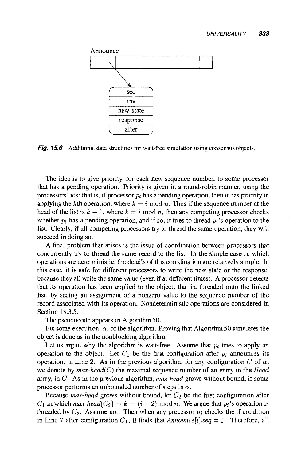
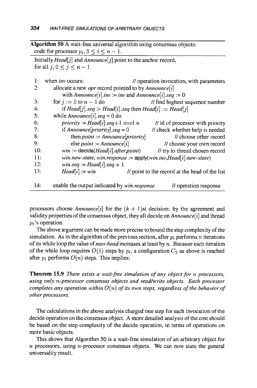
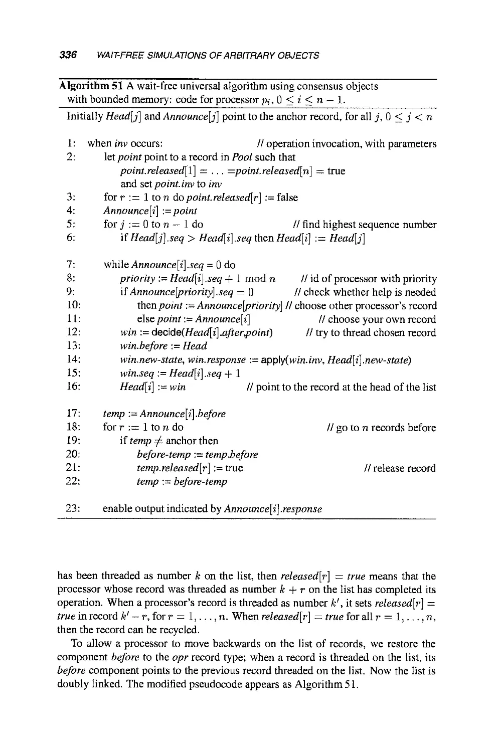
/


Теги: mathematics mathematical modeling simulations computer modeling publisher john wiley & sons
ISBN: 0-471-45324-2
Год: 2004


Текст
Distributed Computing
WILEY SERIES ON PARALLEL
AND DISTRIBUTED COMPUTING
Editor: Albert Y. Zomaya
A complete list of titles in this series appears at the end of this volume.
Distributed Computing
Fundamentals, Simulations
and Advanced Topics
Second Edition
HagitAttiya
Jennifer Welch
>WILEY~
INTERSCIENCE
A JOHN WILEY & SONS, INC., PUBLICATION
This text is printed on acid-free paper. ©
Copyright © 2004 by John Wiley & Sons, Inc. All rights reserved.
Published by John Wiley & Sons, Inc., Hoboken, New Jersey.
Published simultaneously in Canada,
No part of this publication may be reproduced, stored in a retrieval system, or transmitted in any form
or by any means, electronic, mechanical, photocopying, recording, scanning, or otherwise, except as
permitted under Section 107 or 108 of the 1976 United States Copyright Act, without either the prior
written permission of the Publisher, or authorization through payment of the appropriate per-copy fee to
the Copyright Clearance Center, Inc., 222 Rosewood Drive, Danvers, MA 01923, (978) 750-8400, fax
(978) 646-8600, or on the web at www.copyright.com. Requests to the Publisher for permission should
be addressed to the Permissions Department, John Wiley & Sons, Inc., Ill River Street, Hoboken, NJ
07030, B01) 748-6011, fax B01) 748-6008.
Limit of Liability/Disclaimer of Warranty: While the publisher and author have used their best efforts in
preparing this book, they make no representations or warranties with respect to the accuracy or
completeness of the contents of this book and specifically disclaim any implied warranties of
merchantability or fitness for a particular purpose. No warranty may be created or extended by sales
representatives or written sales materials. The advice and strategies contained herein may not be
suitable for your sitnation. You should consult with a professional where appropriate. Neither the
publisher nor author shall be liable for any loss of profit or any other commercial damages, including
but not limited to special, incidental, consequential, or other damages.
For general information on our other products and services please contact our Customer Care
Department within the U.S. at 877-762-2974, outside the U.S. at 317-572-3993 or fax 317-572-4002.
Wiley also publishes its books in a variety of electronic formats. Some content that appears in print,
however, may not be available in electronic format.
Library of Congress Cataloging-in-Publication Data is available.
ISBN 0-471-45324-2
Printed in the United States of America.
10 987654321
Preface
The explosive growth of distributed computing systems makes understanding them
imperative. Yet achieving such understanding is notoriously difficult, because of the
uncertainties introduced by asynchrony, limited local knowledge, and partial failures.
The field of distributed computing provides the theoretical underpinning for the design
and analysis of many distributed systems: from wide-area communication networks,
through local-area clusters of workstations to shared-memory multiprocessors.
This book aims to provide a coherent view of the theory of distributed computing,
highlighting common themes and basic techniques. It introduces the reader to the
fundamental issues underlying the design of distributed systems—communication,
coordination, synchronization, and uncertainty—and to the fundamental algorithmic
ideas and lower bound techniques. Mastering these techniques will help the reader
design correct distributed applications.
This book covers the main elements of the theory of distributed computing, in
a unifying approach that emphasizes the similarities between different models and
explains inherent discrepancies between them. The book presents up-to-date results
in a precise, and detailed, yet accessible manner. The emphasis is on fundamental
ideas, not optimizations. More difficult results are typically presented as a series
of increasingly complex solutions. The exposition highlights techniques and results
that are applicable in several places throughout the text. This approach exposes the
inherent similarities in solutions to seemingly diverse problems.
The text contains many accompanying figures and examples. A set of exercises,
ranging in difficulty, accompany each chapter. The notes at the end of each chapter
vi PREFACE
provide a bibliographic history of the ideas and discuss their practical applications in
existing systems.
Distributed Computing is intended as a textbook for graduate students and ad-
advanced undergraduates and as a reference for researchers and professionals. It should
be useful to anyone interested in learning fundamental principles concerning how to
make distributed systems work, and why they sometimes fail to work. The expected
prerequisite knowledge is equivalent to an undergraduate course in analysis of (se-
(sequential) algorithms. Knowledge of distributed systems is helpful for appreciating
the applications of the results, but it is not necessary.
This book presents the major models of distributed computing, varying by the
mode of communication (message passing and shared memory), by the synchrony
assumptions (synchronous, asynchronous, and clocked), and by the failure type (crash
and Byzantine). The relationships between the various models are demonstrated by
simulations showing that algorithms designed for one model can be run in another
model. The book covers a variety of problem domains within the models, including
leader election, mutual exclusion, consensus, and clock synchronization. It presents
several recent developments, including fast mutual exclusion algorithms, queue locks,
distributed shared memory, the wait-free hierarchy, and failure detectors.
Part I of the book introduces the major issues—message passing and shared
memory communication, synchronous and asynchronous timing models, failures,
proofs of correctness, and lower bounds—in the context of three canonical problems:
leader election, mutual exclusion, and consensus. It also presents the key notions of
causality of events and clock synchronization.
Part II addresses the central theme of simulation between models of distributed
computing. It consists of a series of such simulations and their applications, in-
including more powerful interprocess communication from less powerful interprocess
communication, shared memory from message passing, more synchrony from less
synchrony, and more benign kinds of faults from less benign kinds of faults.
Part III samples advanced topics that have been the focus of recent research, in-
including randomization, the wait-free hierarchy, asynchronous solvability, and failure
detectors.
An introductory course based in this book could cover Chapters 2 through 10,
omitting Section 10.3. A more theoretical course could cover Chapters 2, 3, 4, 5,
Section 14.3, and Chapters 10,15, 11 and 17. Other courses based on this book are
possible; consider the chapter dependencies on the next page. The book could also
be used as a supplemental text in a more practically oriented course, to flesh out the
treatment of logical and vector clocks (Chapter 6), clock synchronization (Chapters 6
and 13), fault tolerance (Chapters 5 and 8), distributed shared memory (Chapter 9),
and failure detectors (Chapter 17).
Changes in the second edition: We have made the following changes:
• We added a new chapter (Chapter 17) on failure detectors and their application
to solving consensus in asynchronous systems and deleted two chapters, those
on bounded timestamps (formerly Chapter 16) and sparse network covers
(formerly Chapter 18).
PREFACE
vii
Chapter 1
Introduction
I
Chapter 2
Basic Message Passing
Chapter 3
Leader Election
Chapter 4
Mutual Exclusion
Chapter 8
Broadcast
Chapter 5
Consensus
Chapter 6
Time
Chapter 9
Distributed Snared Memory
Chapter 12
Fault Tolerance
Chapter 11
Synchrony
Chapter 10
Read/Write Objects
Chapter 13
Clock
Synchronizatior
Chapter 15
Wait-Free Simulations
Chapter 14
Randomization
Chapter 17
Eventually Stable Consensus
Chapter 16
Asynchronous Solvability
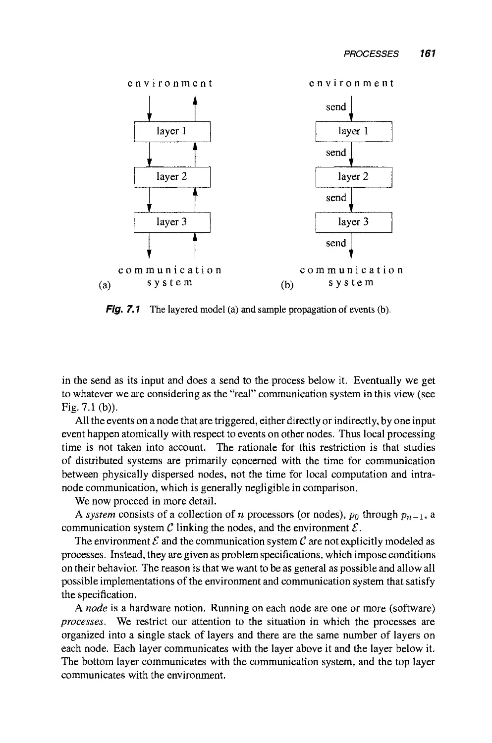
Chapter dependencies.
• We added new material to the existing chapters on fast mutual exclusion and
queue locks (Chapter 4), practical clock synchronization (Chapters 6 and 13),
and the processor lower bound for simulating shared memory with message
passing (Chapter 10).
• We corrected errors and improved the presentation throughout. Improvements
include a simpler proof of the round lower bound for consensus (Chapter 5)
and a simpler randomized consensus algorithm in Chapter 14.
Acknowledgments for the first edition: Many people contributed to our view of
distributed computing in general, and to this book in particular. Danny Dolev and
Nancy Lynch introduced us to this subject area. Fred Schneider provided moral
support in continuing the book and ideas for organization. Oded Goldreich and Marc
Snir inspired a general scientific attitude.
Our graduate students helped in the development of the book. At the Technion,
Ophir Rachman contributed to the lecture notes written in 1993-94, which were the
origin of this book. Jennifer Walter read many versions of the book very carefully
Viil PREFACE
at TAMU, as did Leonid Fouren, who was the teaching assistant for the class at the
Technion.
The students in our classes suffered through confusing versions of the material and
provided a lot of feedback; in particular, we thank Eyal Dagan, Eli Stein (Technion,
Spring 1993), Saad Biaz, Utkarsh Dhond, Ravishankar Iyer, Peter Nuernberg, Jingyu
Zhang (TAMU, Fall 1996), Alia Gorbach, Noam Rinetskey, Asaf Shatil, and Ronit
Teplixke (Technion, Fall 1997).
Technical discussions with Yehuda Afek, Brian Coan, Eli Gafni, and Maurice
Herlihy helped us a lot. Several people contributed to specific chapters (in alphabetic
order): Jim Anderson (Chapter 4), Rida Bazzi (Chapter 12), Ran Cannetti (Chap-
(Chapter 14), Soma Chaudhuri (Chapter 3),Shlomi Dolev (Chapters 2 and 3),Roy Friedman
(Chapters 8 and 9), Sibsankar Haldar (Chapters 10), Martha Kosa (Chapter 9), Eyal
Kushilevitz (Chapter 14), Dahlia Malkhi (Chapter 8), Mark Moir (Chapter 4), Gil
Neiger (Chapter 5), Boaz Patt-Shamir (Chapters 6, 7 and 11), Sergio Rajsbaum
(Chapter 6), and Krishnamurthy Vidyasankar (Chapters 10).
Acknowledgments for the second edition: We appreciate the time that many people
spent using the first edition and giving us feedback. We benefited from many of Eli
Gafni's ideas. Panagiota Fatourou provided us with a thoughtful review. Evelyn
Pierce carefully read Chapter 10. We received error reports and suggestions from Uri
Abraham, James Aspnes, Soma Chaudhuri, Jian Chen, Lucia Dale, Faith Fich, Roy
Friedman, Mark Handy, Maurice Herlihy, Ted Herman, Lisa Higham, Iyad Kanj,
Idit Keidar, Neeraj Koul, Ajay Kshemkalyani, Marios Mavronicolas, Erich Mikk,
Krzysztof Parzyszej, Antonio Romano, Eric Ruppert, Cheng Shao, T.N. Srikanta,
Jennifer Walter, and Jian Xu.
Several people affiliated with John Wiley & Sons deserve our thanks. We are
grateful to Albert Zomaya, the editor-in-chief of the Wiley Series on Parallel and
Distributed Computing for his support. Our editor Val Moliere and program coordi-
coordinator Kirsten Rohstedt answered our questions and helped keep us on track.
Writing this book was a long project, and we could not have lasted without the love
and support of our families. Hagit thanks Osnat, Rotem and Eyal, and her parents.
Jennifer thanks George, Glenn, Sam, and her parents.
The following web site contains supplementary material relating to this book,
including pointers to courses using the book and information on exercise solutions
and lecture notes for a sample course:
http://www.cs.technion.ac.il/~hagit/DC/
Dedicated to our parents:
Malka and David Attiya
Judith and Ernest Lundelius
Contents
1 Introduction 1
1.1 Distributed Systems 1
1.2 Theory of Distributed Computing 2
1.3 Overview 3
1.4 Relationship of Theory to Practice 4
Part I Fundamentals
2 Basic Algorithms in Message-Passing Systems 9
2.1 Formal Models for Message Passing Systems 9
2.1.1 Systems 9
2.1.2 Complexity Measures 13
2.1.3 Pseudocode Conventions 14
2.2 Broadcast and Convergecast on a Spanning Tree 15
2.3 Flooding and Building a Spanning Tree 19
2.4 Constructing a Depth-First Search Spanning Tree for
a Specified Root 23
2.5 Constructing a Depth-First Search Spanning Tree
without a Specified Root 25
Ix
X CONTENTS
3 Leader Election in Rings 31
3.1 The Leader Election Problem 31
3.2 Anonymous Rings 32
3.3 Asynchronous Rings 34
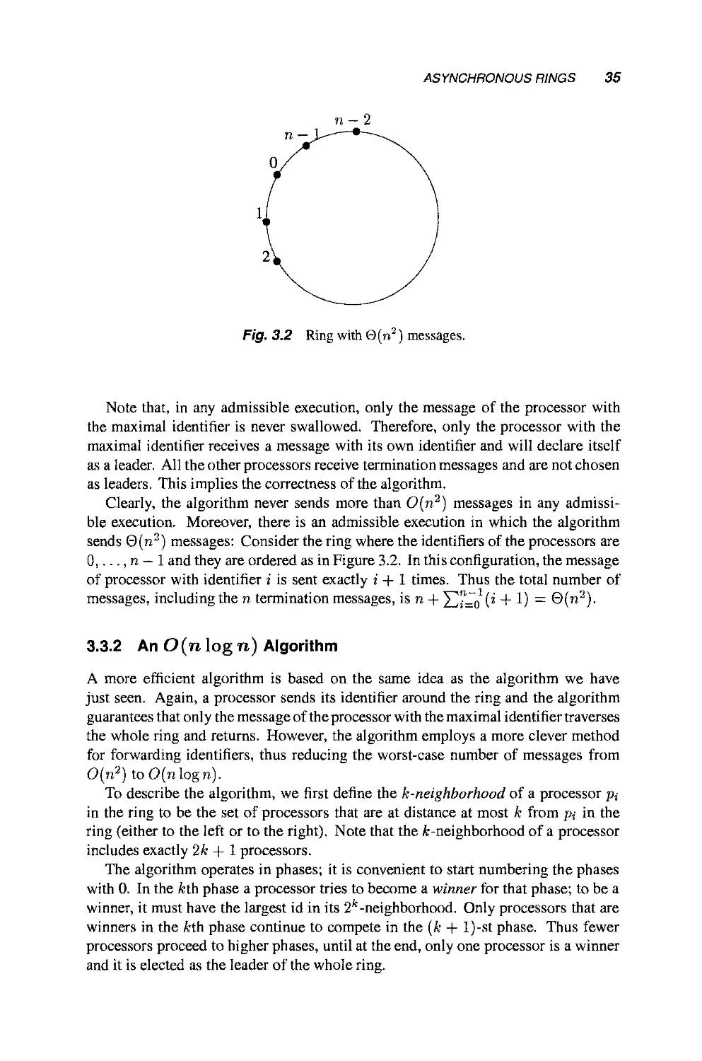
3.3.1 An 0{n2) Algorithm 34
3.3.2 An 0(n log n) Algorithm 35
3.3.3 An fi(nlogn) Lower Bound 38
3.4 Synchronous Rings 42
3.4.1 An O(n) Upper Bound 43
3.4.2 An fi(nlogn) Lower Bound for Restricted
Algorithms 48
4 Mutual Exclusion in Shared Memory 59
4.1 Formal Model for Shared Memory Systems 60
4.1.1 Systems 60
4.1.2 Complexity Measures 62
4.1.3 Pseudocode Conventions 62
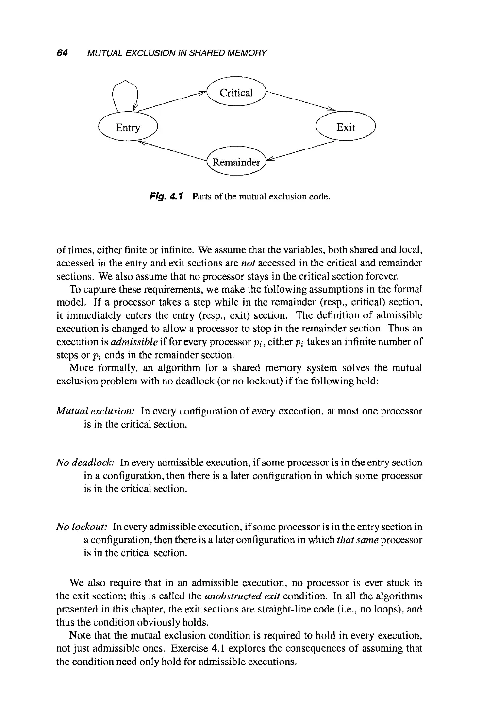
4.2 The Mutual Exclusion Problem 63
4.3 Mutual Exclusion Using Powerful Primitives 65
4.3.1 Binary Test&Set Registers 65
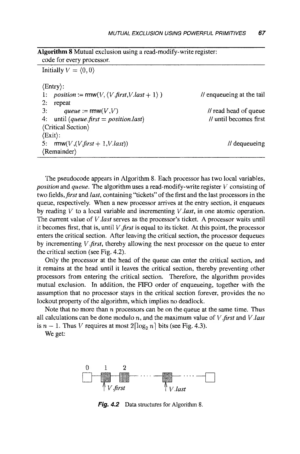
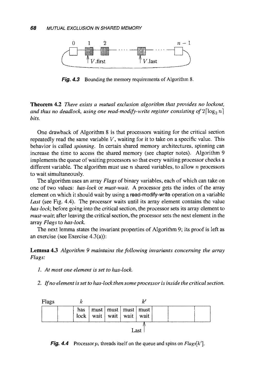
4.3.2 Read-Modify-Write Registers 66
4.3.3 Lower Bound on the Number of Memory States 69
4.4 Mutual Exclusion Using Read/Write Registers 71
4.4.1 The Bakery Algorithm 71
4.4.2 A Bounded Mutual Exclusion Algorithm for
Two Processors 73
4.4.3 A Bounded Mutual Exclusion Algorithm for n
Processors 77
4.4.4 Lower Bound on the Number of Read/Write
Registers 80
4.4.5 Fast Mutual Exclusion 84
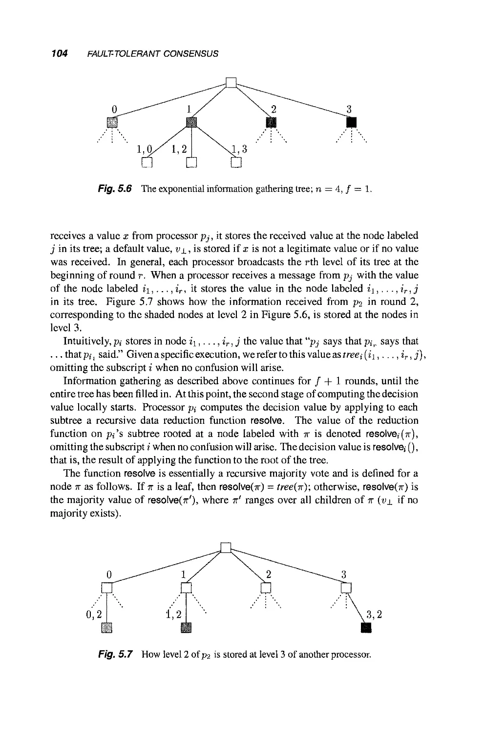
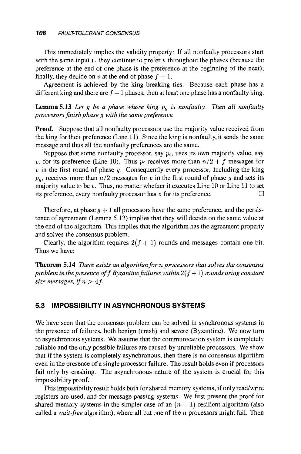
5 Fault-Tolerant Consensus 91
5.1 Synchronous Systems with Crash Failures 92
5.1.1 Formal Model 92
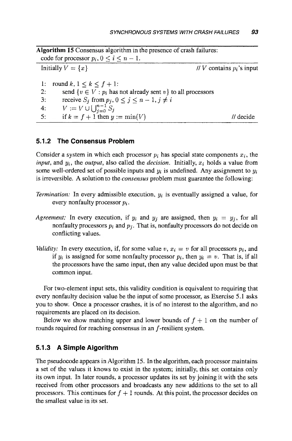
5.1.2 The Consensus Problem 93
5.1.3 A Simple Algorithm 93
5.1.4 Lower Bound on the Number of Rounds 95
5.2 Synchronous Systems with Byzantine Failures 99
CONTENTS XI
5.2.1 Formal Model 100
5.2.2 The Consensus Problem Revisited 100
5.2.3 Lower Bound on the Ratio of Faulty Processors 101
5.2.4 An Exponential Algorithm 103
5.2.5 A Polynomial Algorithm 106
5.3 Impossibility in Asynchronous Systems 108
5.3.1 Shared Memory—The Wait-Free Case 109
5.3.2 Shared Memory—The General Case 111
5.3.3 Message Passing 119
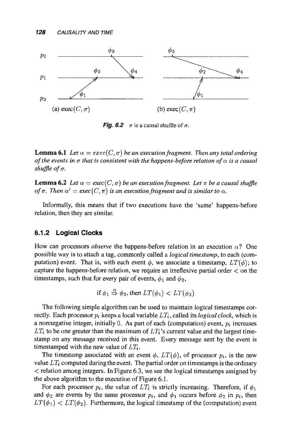
Causality and Time 125
6.1 Capturing Causality 126
6.1.1 The Happens-Before Relation 126
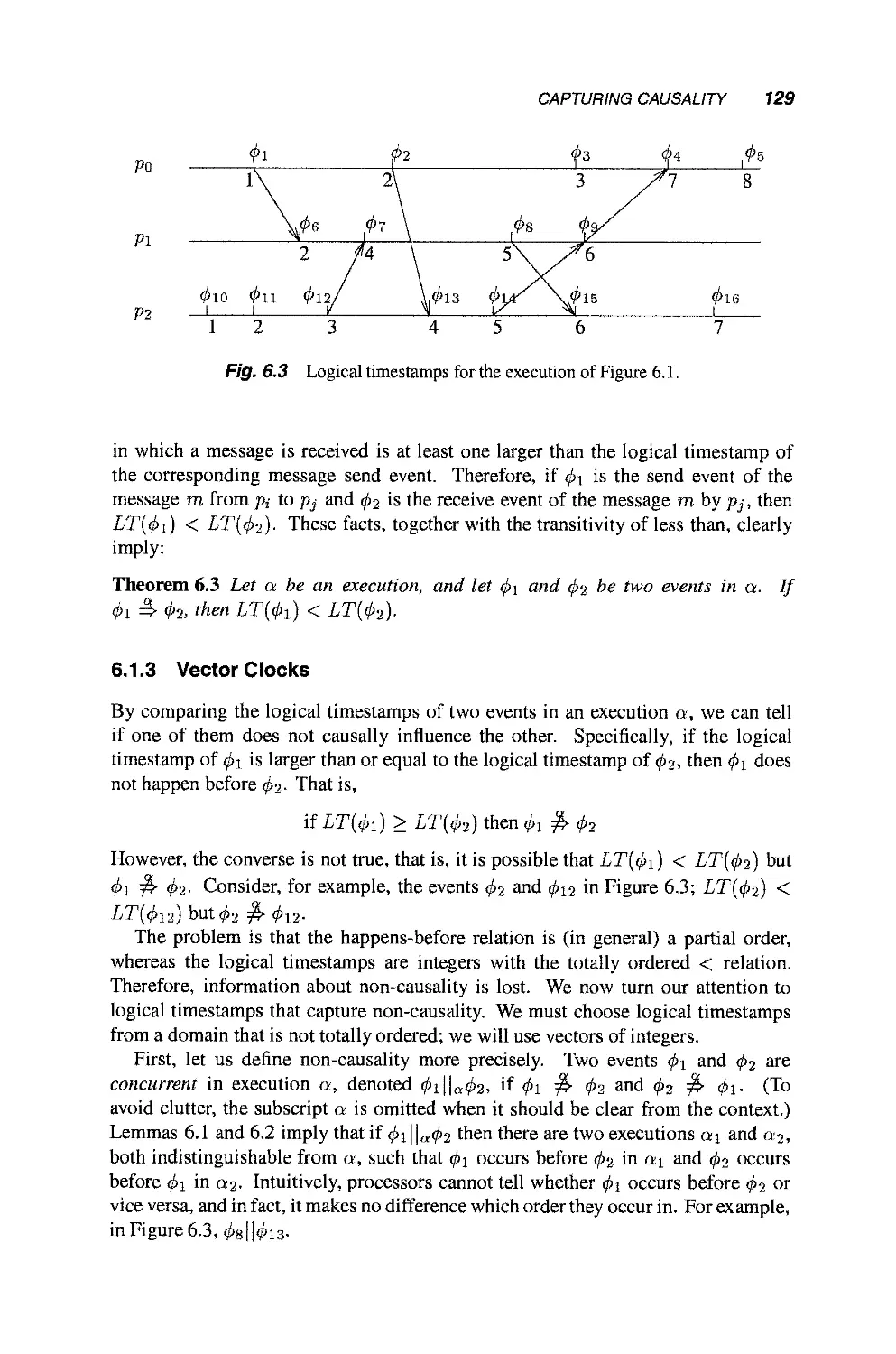
6.1.2 Logical Clocks 128
6.1.3 Vector Clocks 129
6.1.4 Shared Memory Systems 133
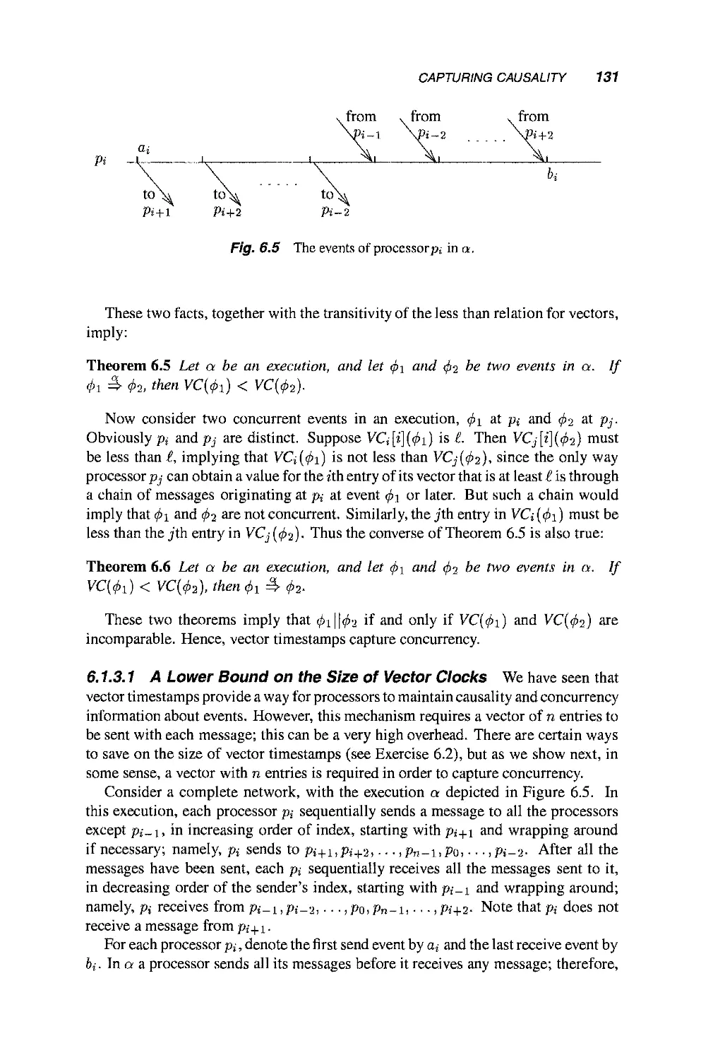
6.2 Examples of Using Causality 133
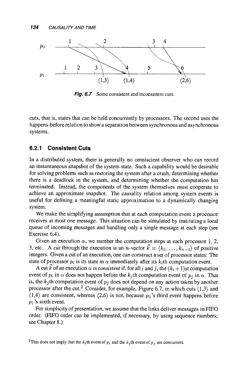
6.2.1 Consistent Cuts 134
6.2.2 A Limitation of the Happens-Before Relation:
The Session Problem 137
6.3 Clock Synchronization 140
6.3.1 Modeling Physical Clocks 140
6.3.2 The Clock Synchronization Problem 143
6.3.3 The Two Processors Case 144
6.3.4 An Upper Bound 146
6.3.5 A Lower Bound 148
6.3.6 Practical Clock Synchronization: Estimating
Clock Differences 149
Part II Simulations
7 A Formal Model for Simulations 157
7.1 Problem Specifications 157
7.2 Communication Systems 158
7.2.1 Asynchronous Point- to-Point Message Passing 159
7.2.2 Asynchronous Broadcast 159
7.3 Processes 160
7.4 Admissibility 163
xii CONTENTS
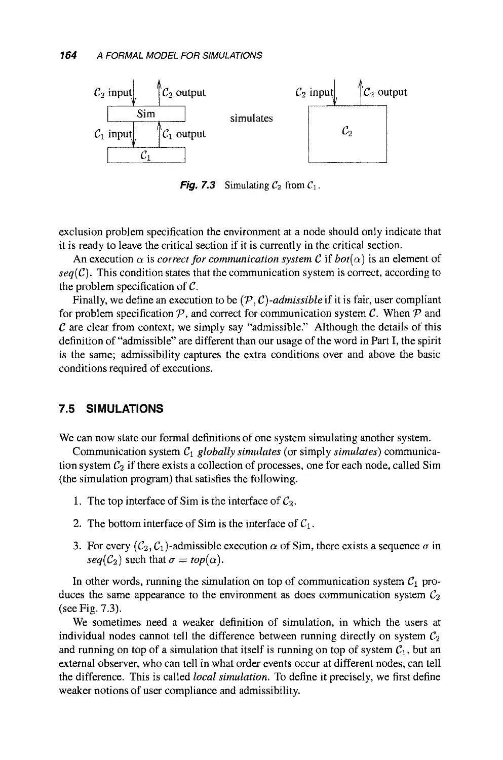
7.5 Simulations 164
7.6 Pseudocode Conventions 165
8 Broadcast and Multicast 167
8.1 Specification of Broadcast Services 168
8.1.1 The Basic Service Specification 168
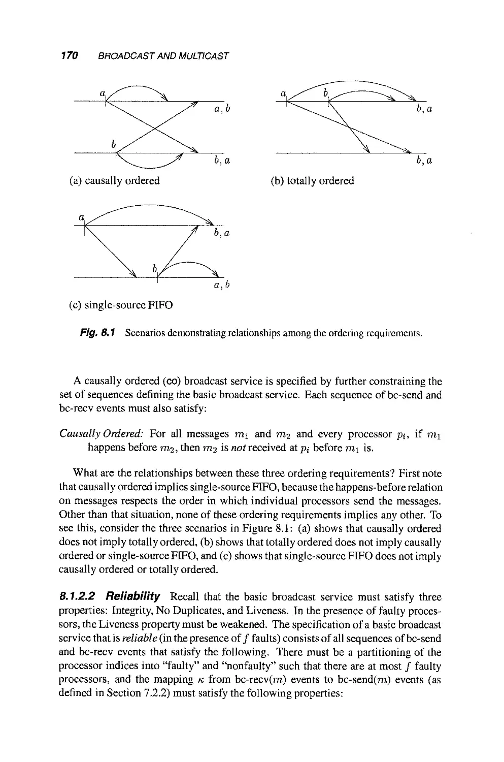
8.1.2 Broadcast Service Qualities 169
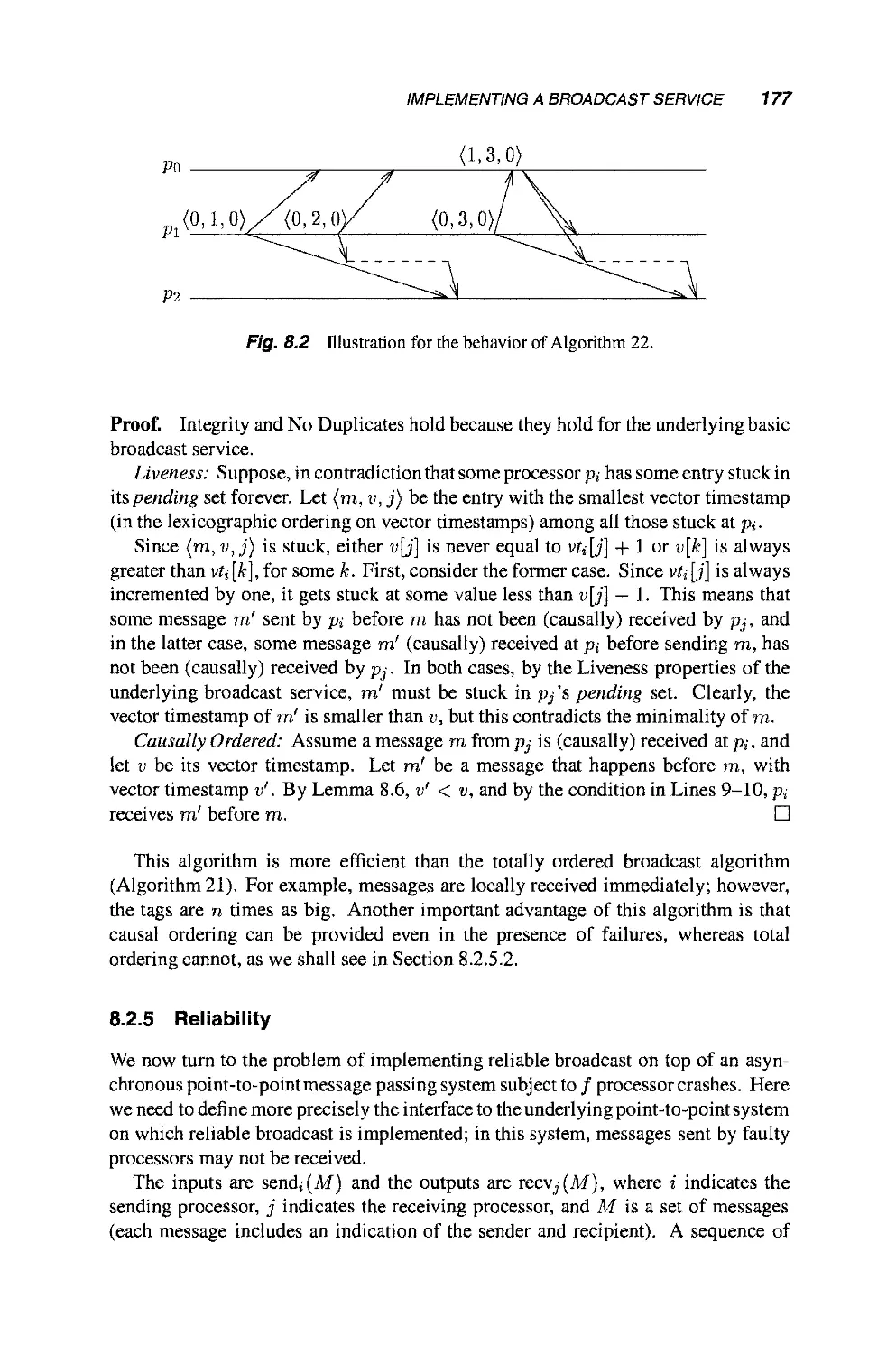
8.2 Implementing a Broadcast Service 171
8.2.1 Basic Broadcast Service 172
8.2.2 Single-Source FIFO Ordering 172
8.2.3 Totally Ordered Broadcast 172
8.2.4 Causality 175
8.2.5 Reliability 177
8.3 Multicast in Groups 179
8.3.1 Specification 180
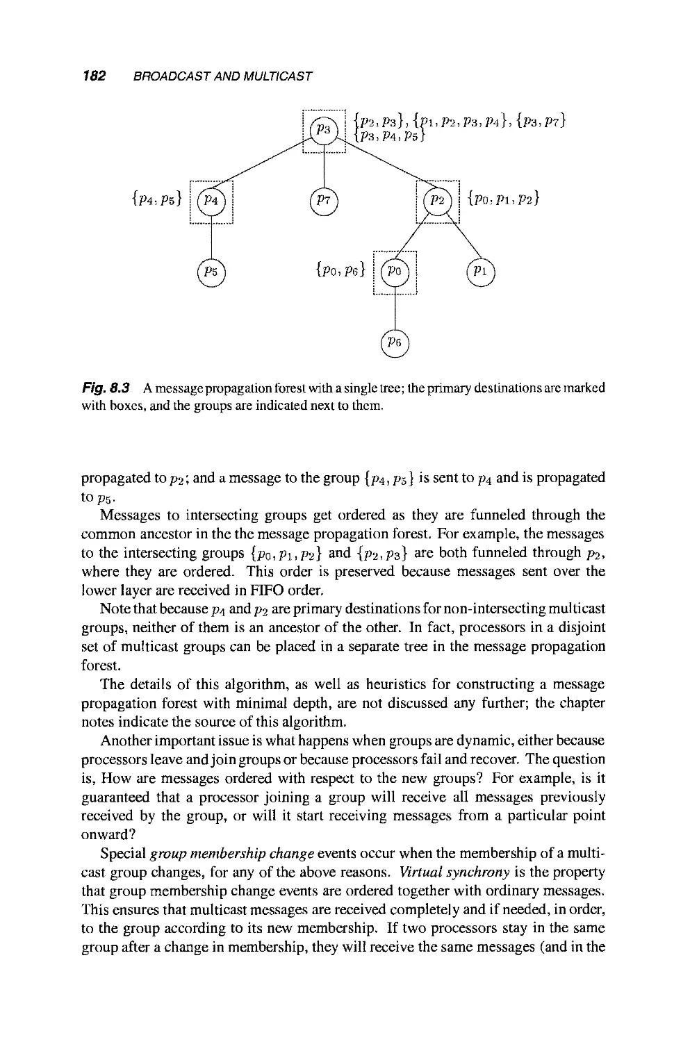
8.3.2 Implementation 181
8.4 An Application: Replication 183
8.4.1 Replicated Database 183
8.4.2 The State Machine Approach 183
9 Distributed Shared Memory 189
9.1 Linearizable Shared Memory 190
9.2 Sequentially Consistent Shared Memory 192
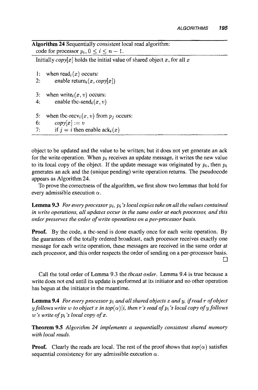
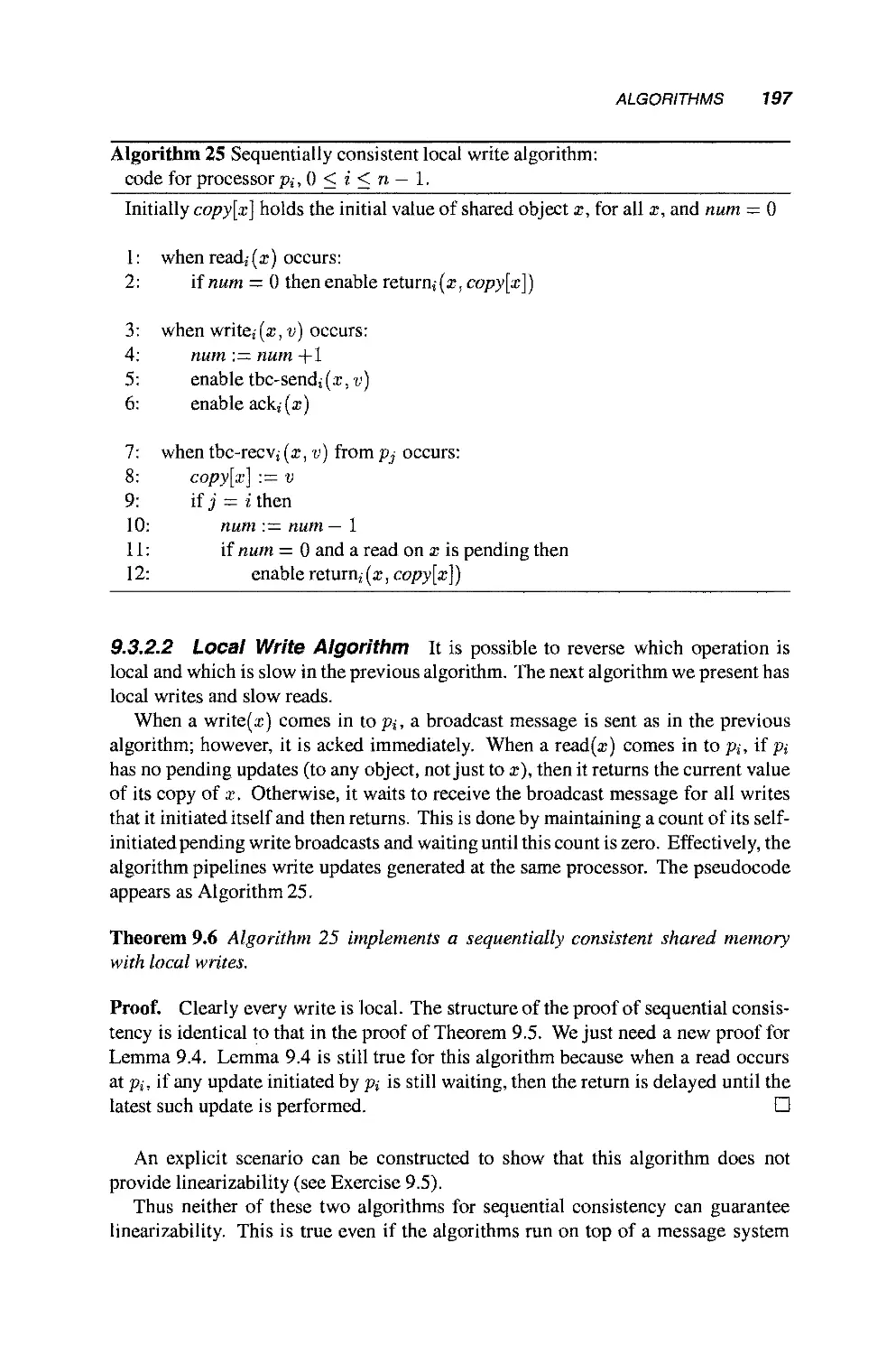
9.3 Algorithms 193
9.3.1 Linearizability 193
9.3.2 Sequential Consistency 194
9.4 Lower Bounds 198
9.4.1 Adding Time and Clocks to the Layered Model 198
9.4.2 Sequential Consistency 199
9.4.3 Linearizability 199
10 Fault-Tolerant Simulations of Read/Write Objects 207
10.1 Fault-Tolerant Shared Memory Simulations 208
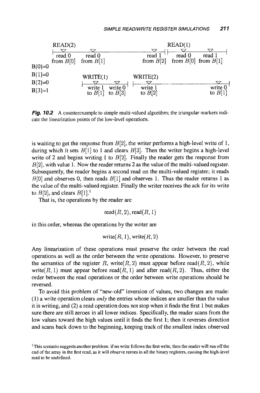
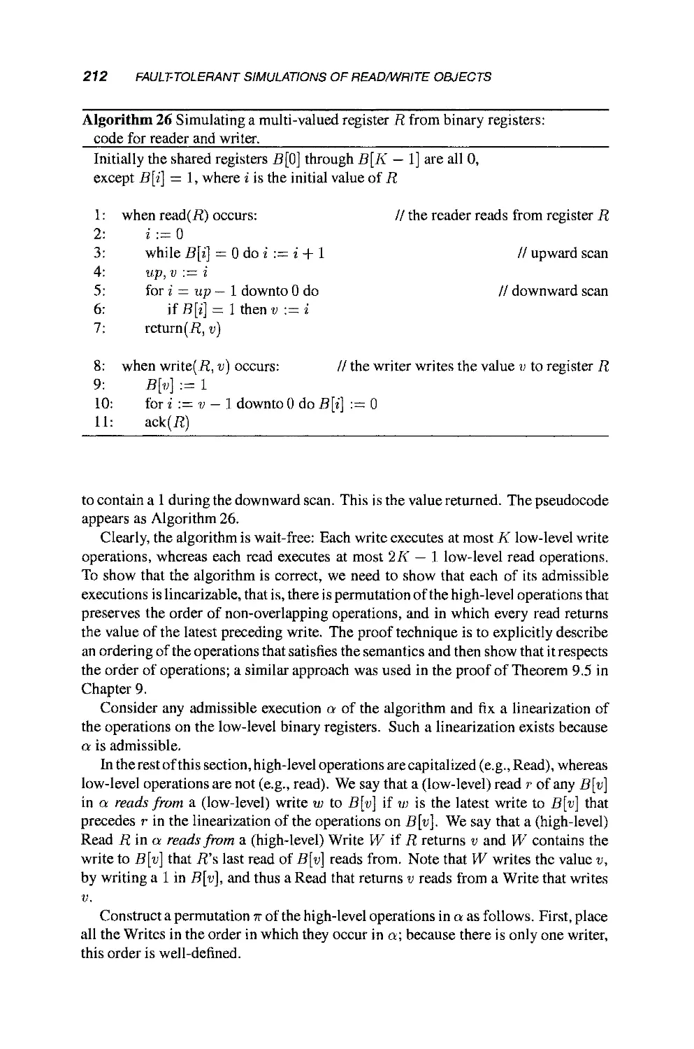
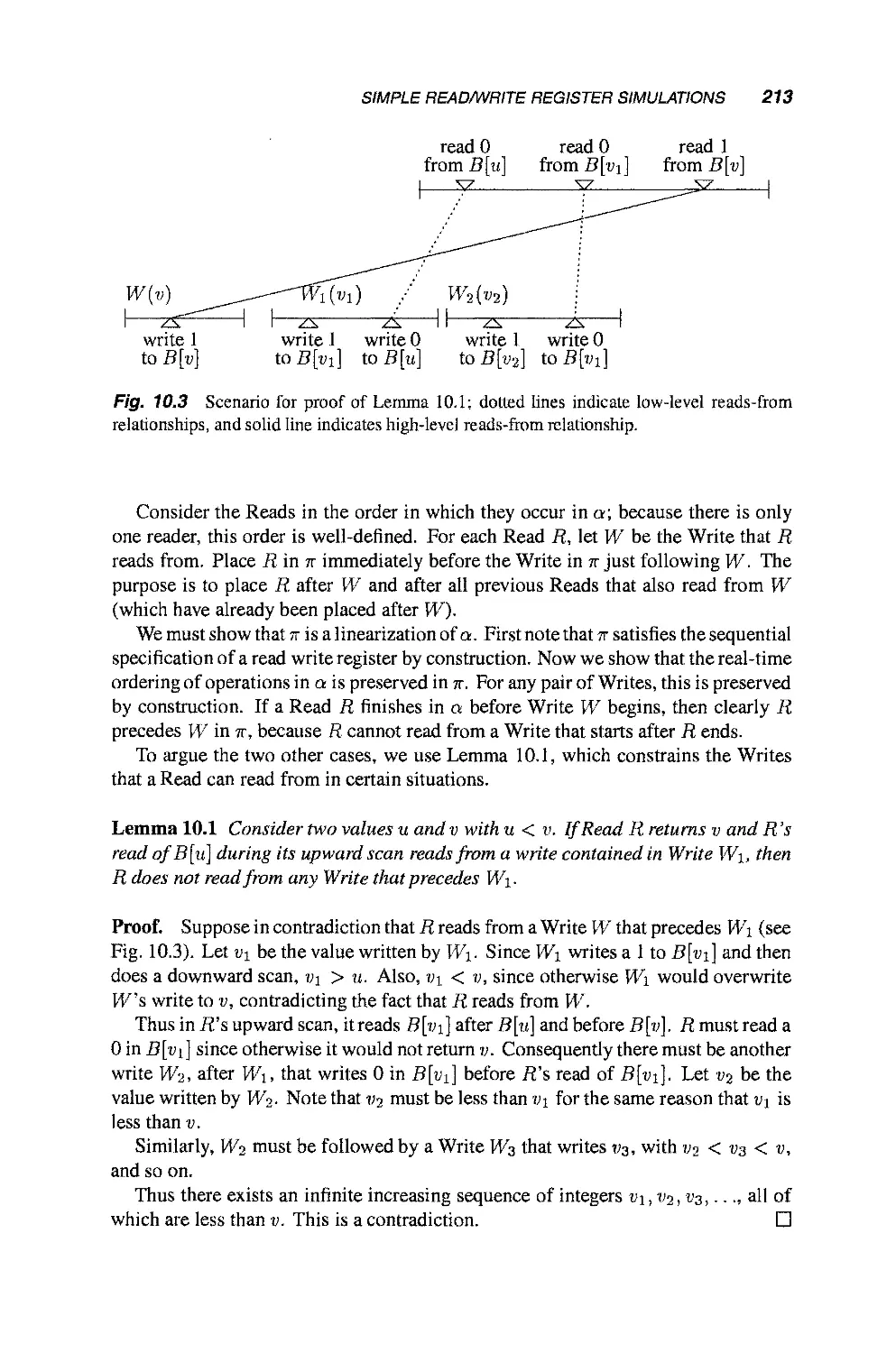
10.2 Simple Read/Write Register Simulations 209
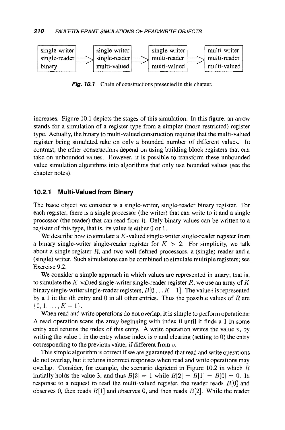
10.2.1 Multi-Valued from Binary 210
10.2.2 Multi-Reader from Single-Reader 215
10.2.3 Multi-Writer from Single-Writer 219
10.3 Atomic Snapshot Objects 222
CONTENTS xiii
10.3.1 Handshaking Procedures 223
10.3.2 A Bounded Memory Simulation 225
10.4 Simulating Shared Registers in Message-Passing
Systems 229
11 Simulating Synchrony 239
11.1 Synchronous Message-Passing Specification 240
11.2 Simulating Synchronous Processors 241
11.3 Simulating Synchronous Processors and Synchronous
Communication 243
11.3.1 A Simple Synchronizer 243
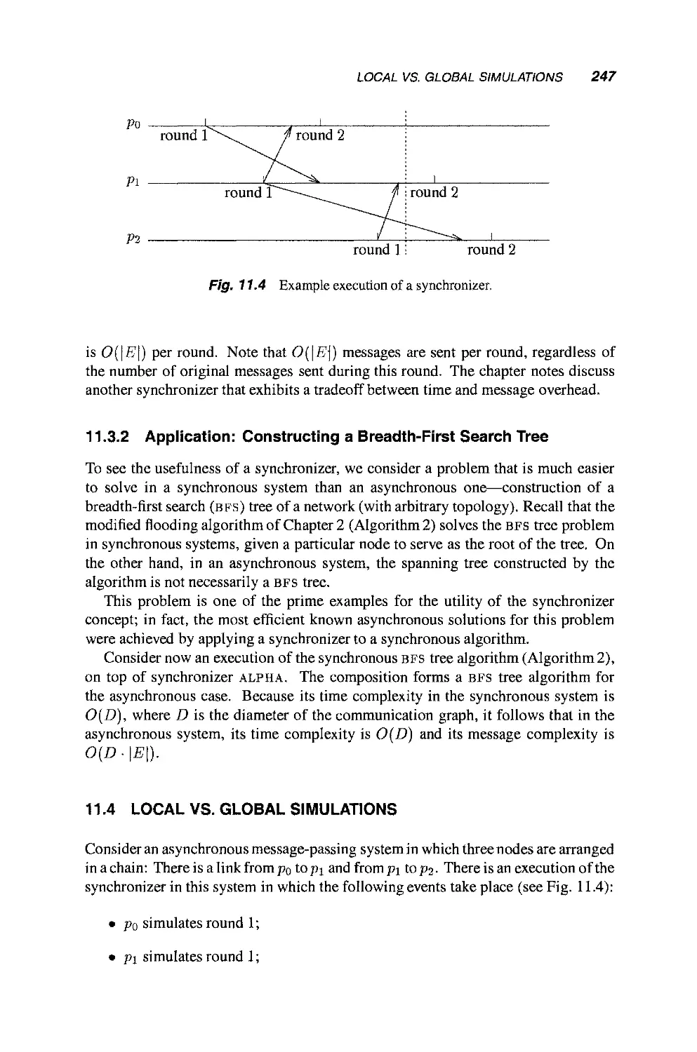
11.3.2 Application: Constructing a Breadth-First
Search Tree 247
11.4 Local vs. Global Simulations 247
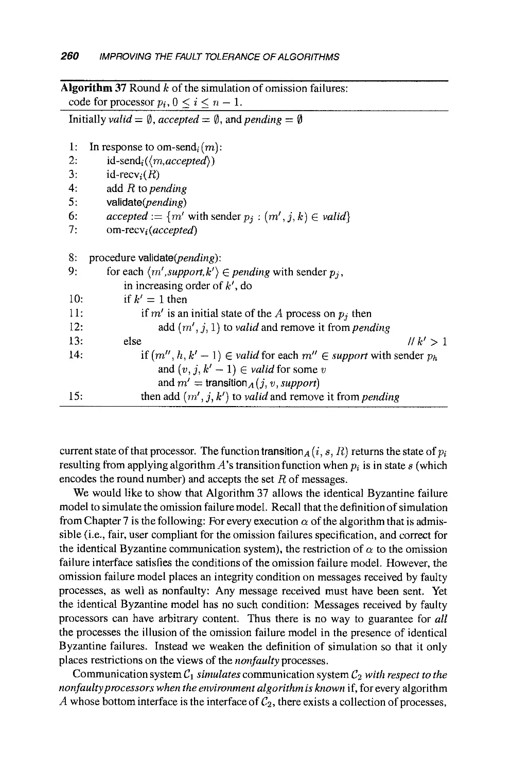
12 Improving the Fault Tolerance of Algorithms 251
12.1 Overview 251
12.2 Modeling Synchronous Processors and Byzantine
Failures 253
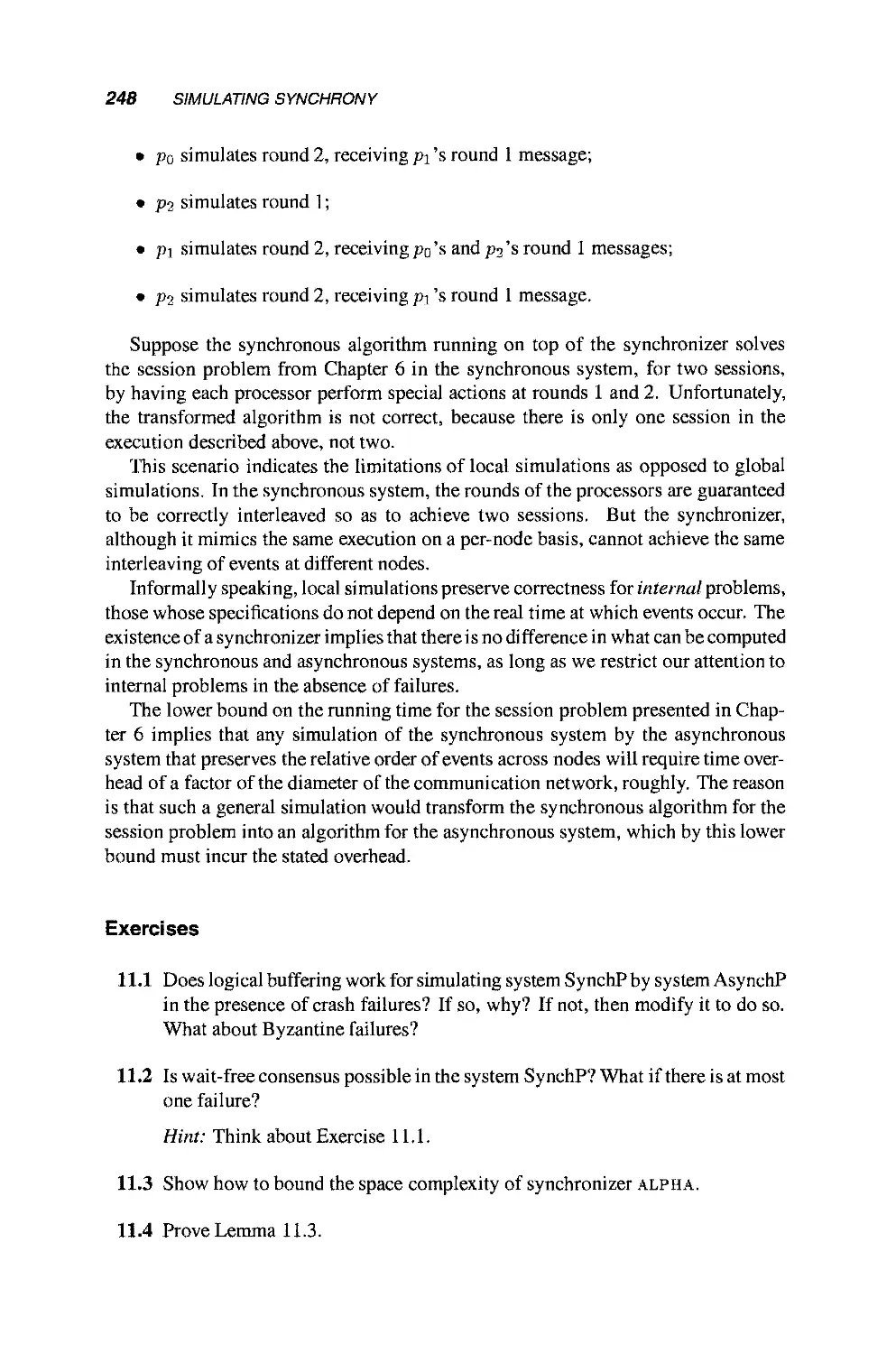
12.3 Simulating Identical Byzantine Failures on Top of
Byzantine Failures 255
12.3.1 Definition of Identical Byzantine 255
12.3.2 Simulating Identical Byzantine 256
12.4 Simulating Omission Failures on Top of Identical
Byzantine Failures 258
12.4.1 Definition of Omission 259
12.4.2 Simulating Omission 259
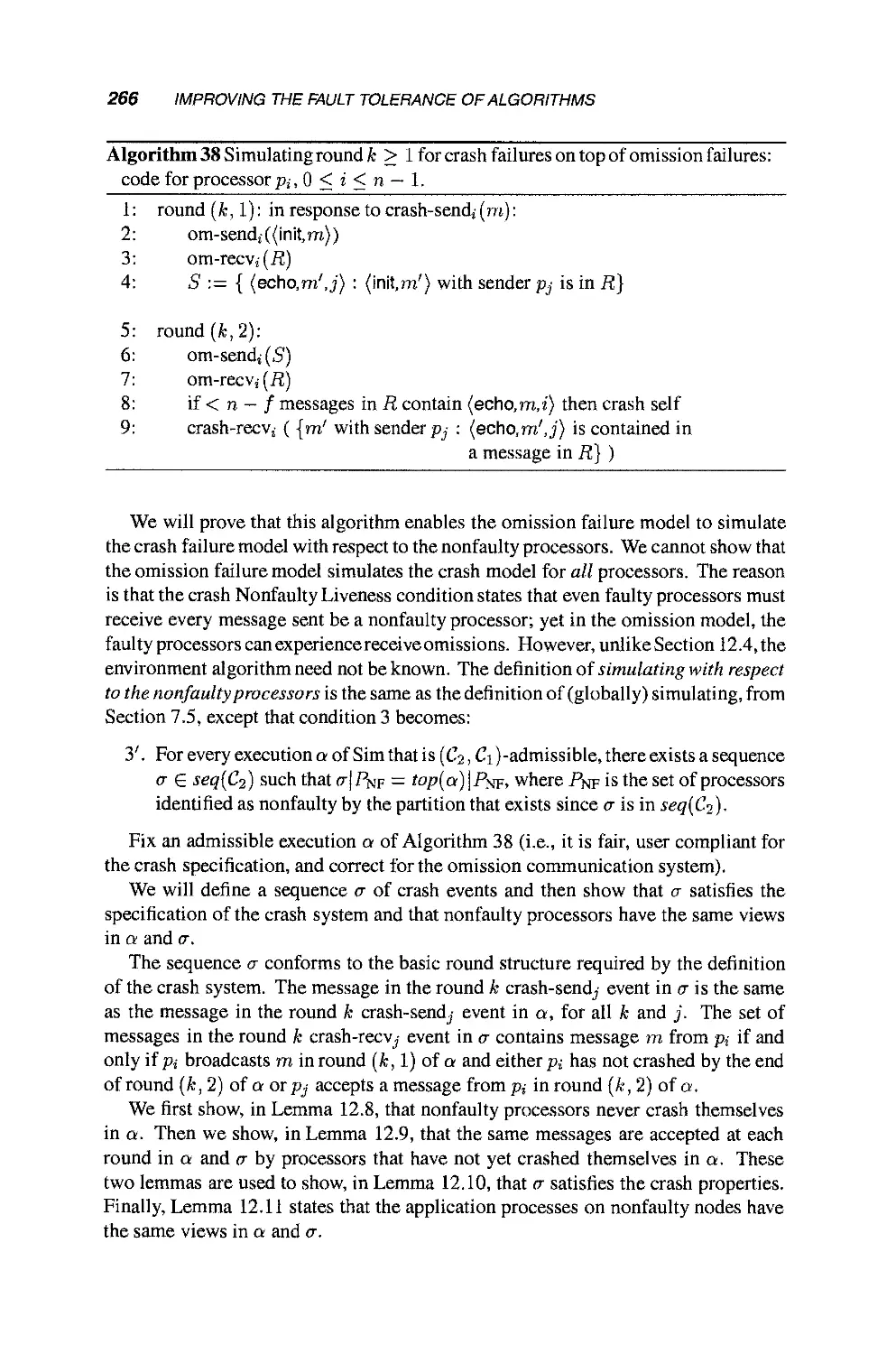
12.5 Simulating Crash Failures on Top of Omission Failures 264
12.5.1 Definition of Crash 264
12.5.2 Simulating Crash 265
12.6 Application: Consensus in the Presence of Byzantine
Failures 268
12.7 Asynchronous Identical Byzantine on Top of Byzantine
Failures 269
12.7.1 Definition of Asynchronous Identical
Byzantine 269
12.7.2 Definition of Asynchronous Byzantine 270
12.7.3 Simulating Asynchronous Identical Byzantine 2 70
13 Fault-Tolerant Clock Synchronization 277
XIV CONTENTS
13.1 Problem Definition 277
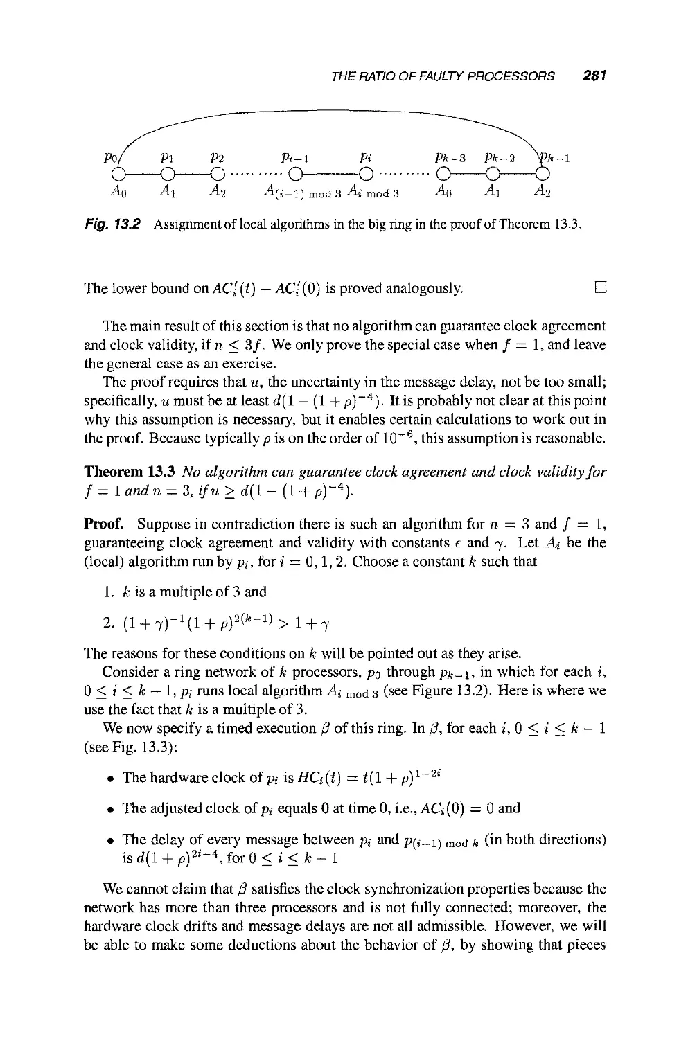
13.2 The Ratio of Faulty Processors 279
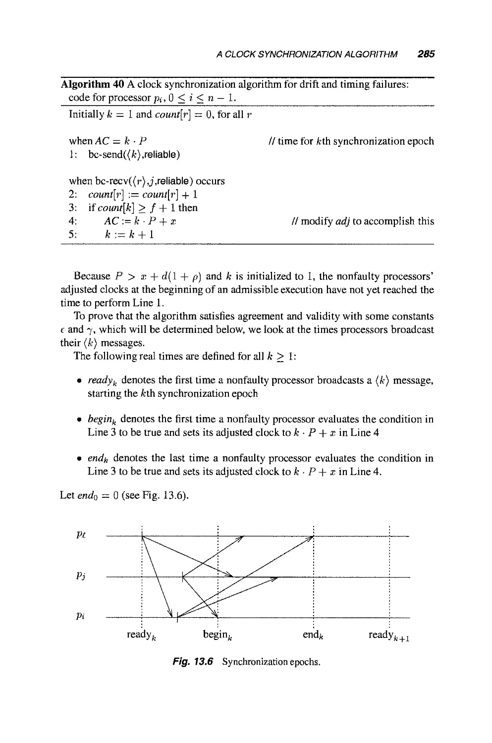
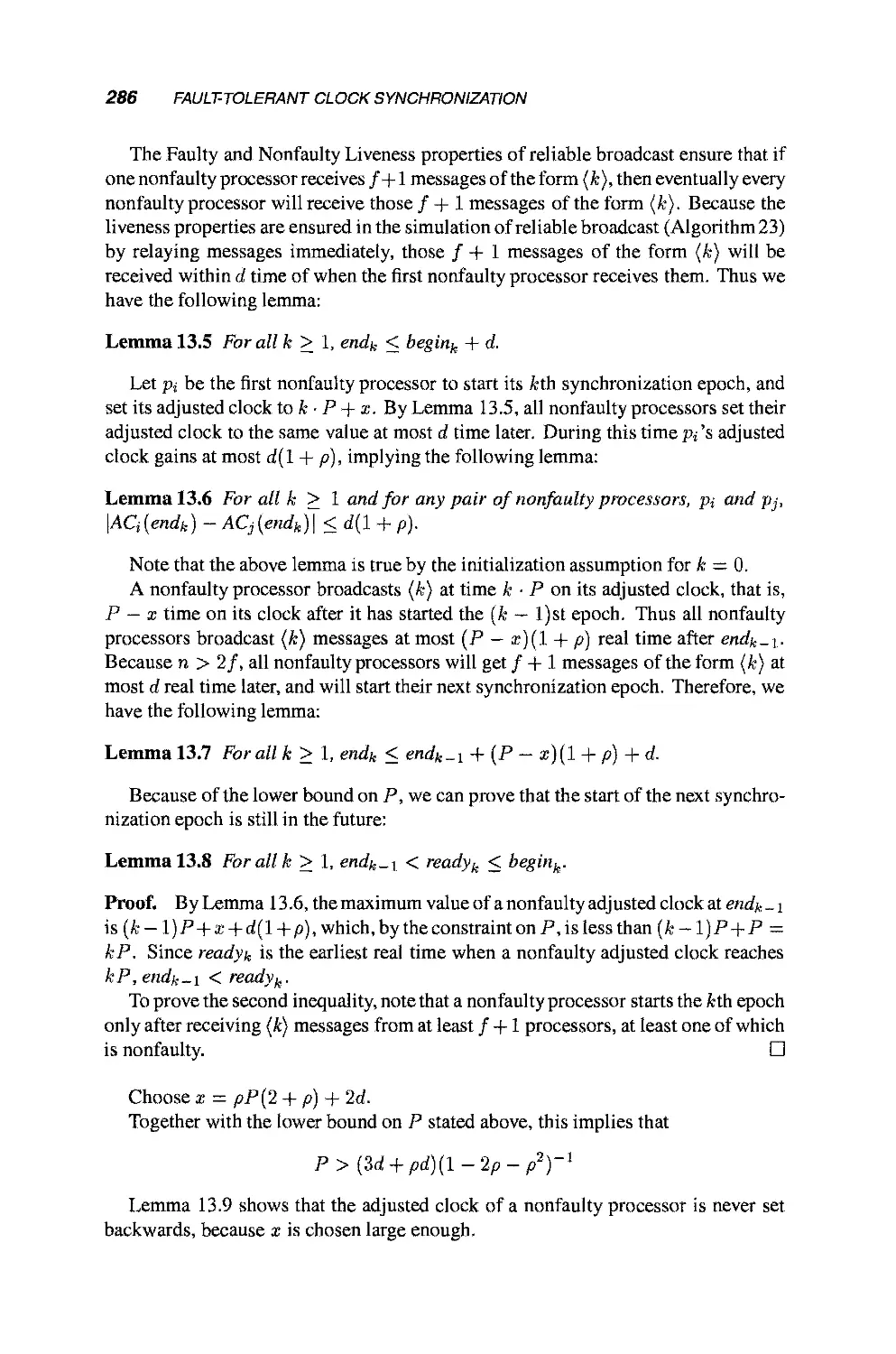
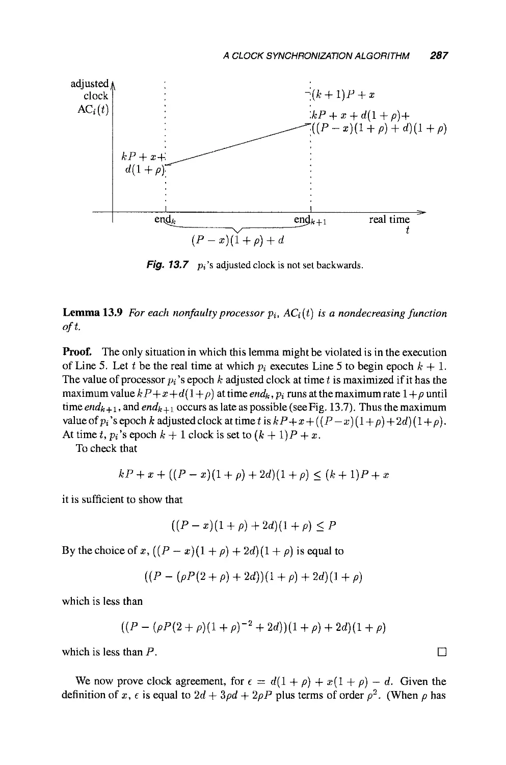
13.3 A Clock Synchronization Algorithm 284
13.3.1 Timing Failures 284
13.3.2 Byzantine Failures 290
13.4 Practical Clock Synchronization: Identifying Faulty
Clocks 291
Part III Advanced Topics
14 Randomization 297
14.1 Leader Election: A Case Study 297
14.1.1 Weakening the Problem Definition 297
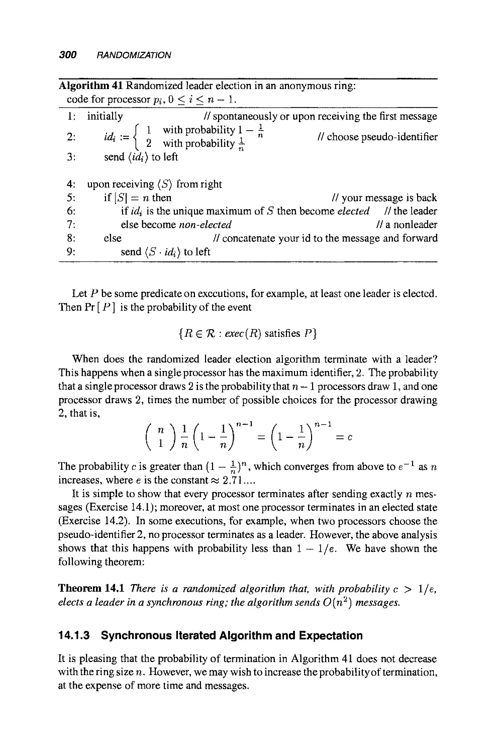
14.1.2 Synchronous One-Shot Algorithm 299
14.1.3 Synchronous Iterated Algorithm and
Expectation 300
14.1.4 Asynchronous Systems and Adversaries 302
14.1.5 Impossibility of Uniform Algorithms 303
14.1.6 Summary of Probabilistic Definitions 303
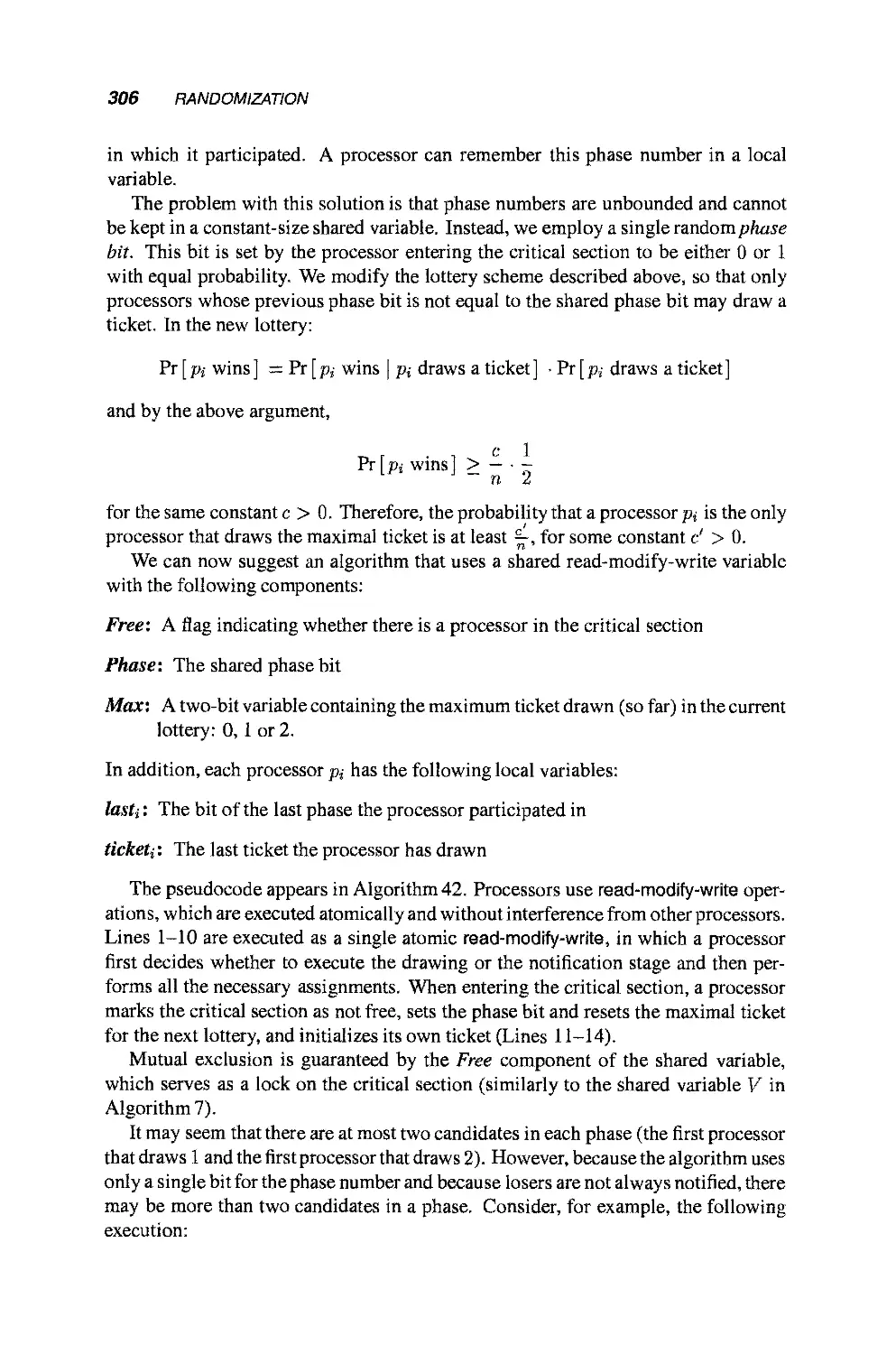
14.2 Mutual Exclusion with Small Shared Variables 305
14.3 Consensus 308
14.3.1 The General Algorithm Scheme 309
14.3.2 A Common Coin with Constant Bias 314
14.3.3 Tolerating Byzantine Failures 315
14.3.4 Shared Memory Systems 316
15 Wait-Free Simulations of Arbitrary Objects 321
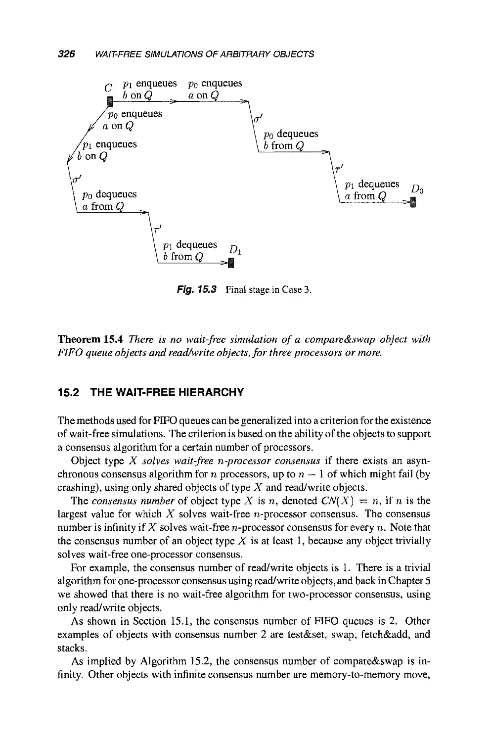
15.1 Example: A FIFO Queue 322
15.2 The Wait-Free Hierarchy 326
15.3 Universality 327
15.3.1 A Nonblocking Simulation Using
Compare&Swap 328
15.3.2 A Nonblocking Algorithm Using Consensus
Objects 329
15.3.3 A Wait-Free Algorithm Using Consensus
Objects 332
15.3.4 Bounding the Memory Requirements 335
15.3.5 HandlingNondeterminism 337
CONTENTS XV
15.3.6 Employing Randomized Consensus 338
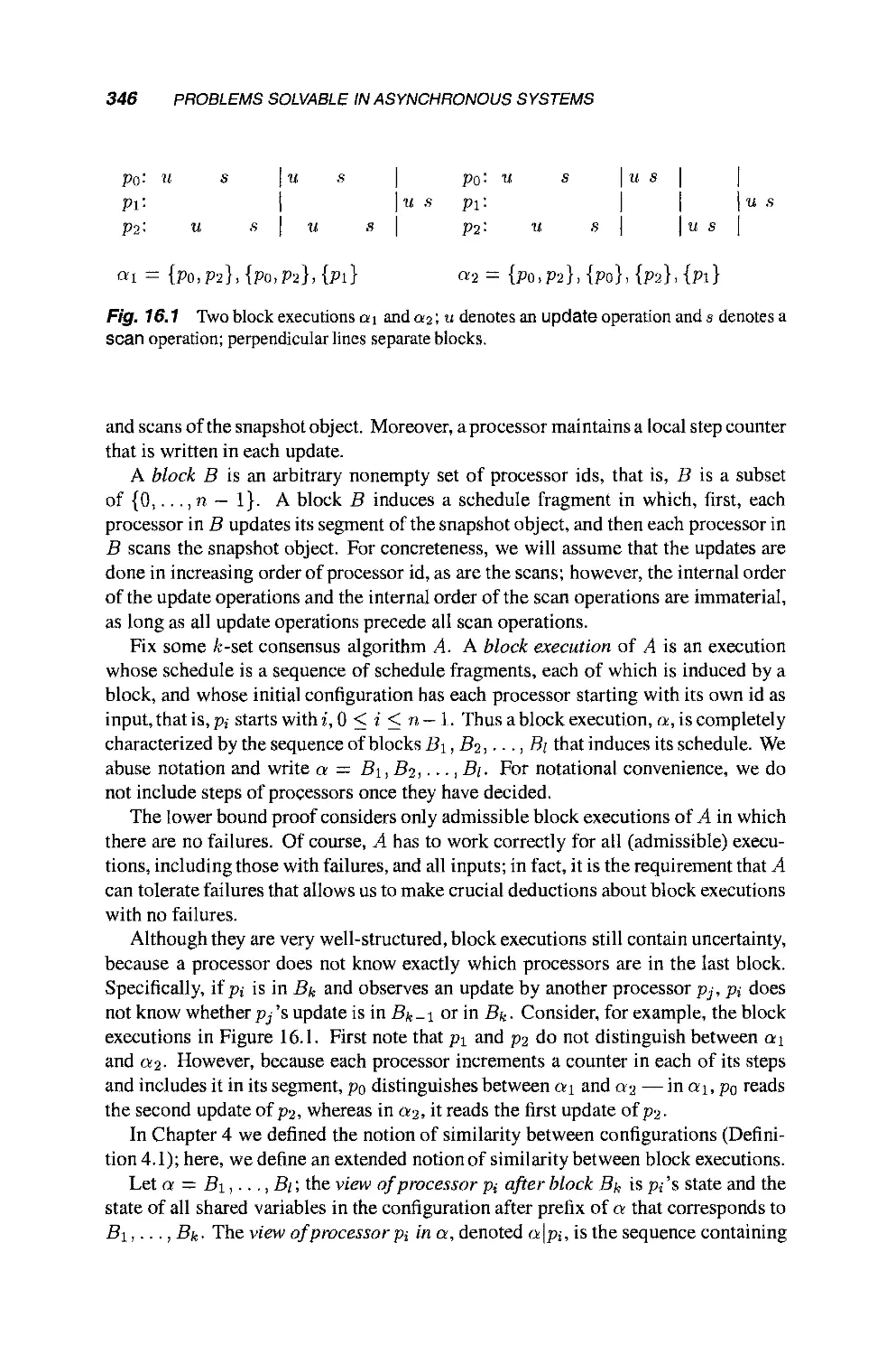
16 Problems Solvable in Asynchronous Systems 343
16.1 k-Set Consensus 344
16.2 Approximate Agreement 352
16.2.1 Known Input Range 352
16.2.2 Unknown Input Range 354
16.3 Renaming 356
16.3.1 The Wait-Free Case 357
16.3.2 The General Case 359
16.3.3 Long-Lived Renaming 360
16.4 k-Exclusion and k-Assignment 361
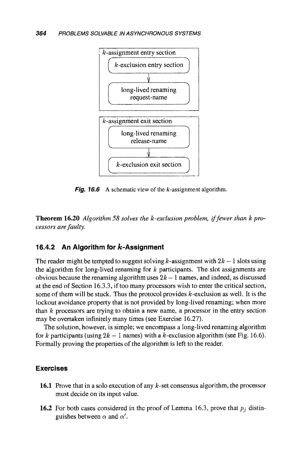
16.4.1 An Algorithm for k-Exclusion 362
16.4.2 An Algorithm for k-Assignment 364
17 Solving Consensus in Eventually Stable Systems 369
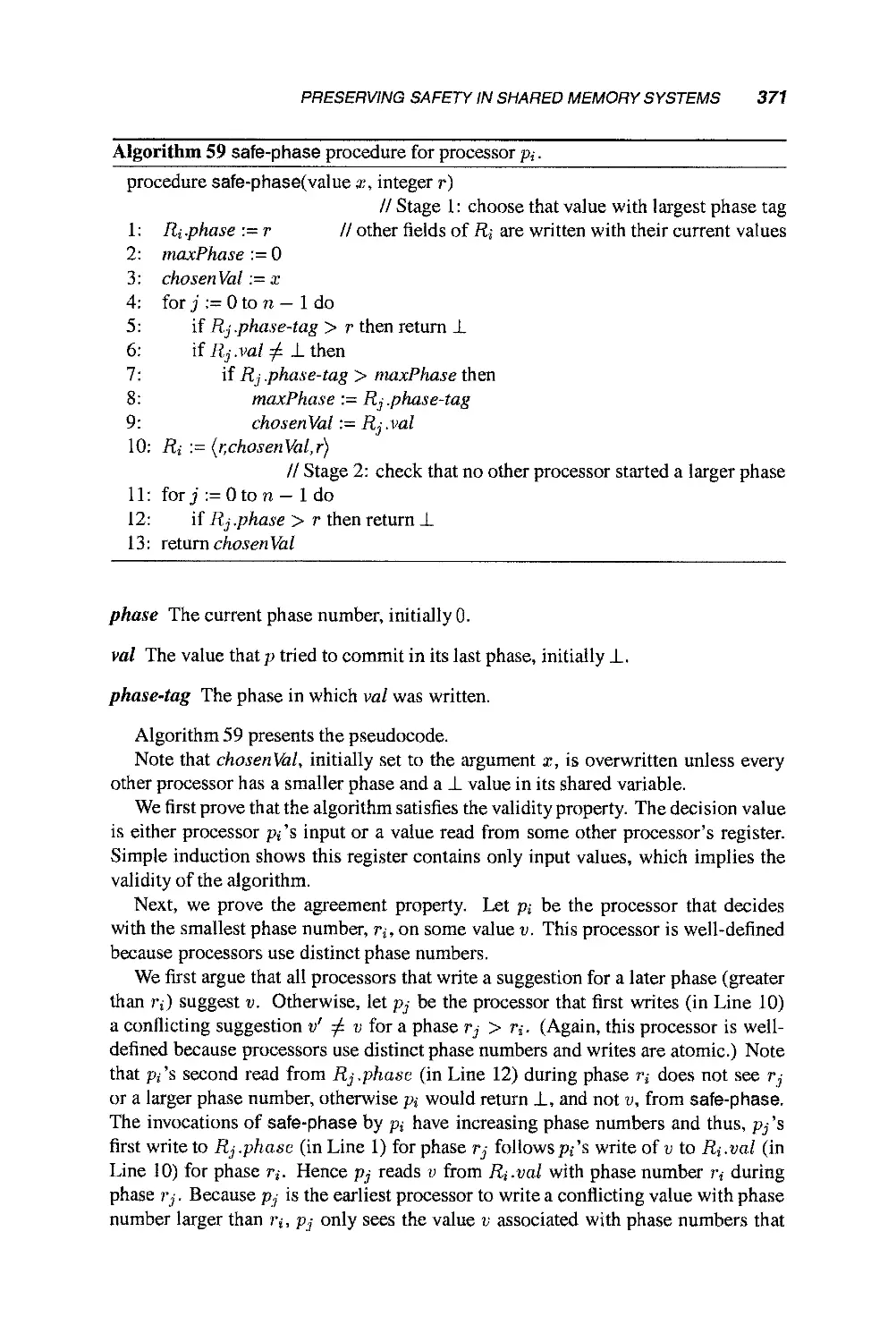
17.1 Preserving Safety in Shared Memory Systems 3 70
17.2 Failure Detectors 372
17.3 Solving Consensus using Failure Detectors 373
17.3.1 Solving Consensus with oS 373
17.3.2 Solving Consensus with S 375
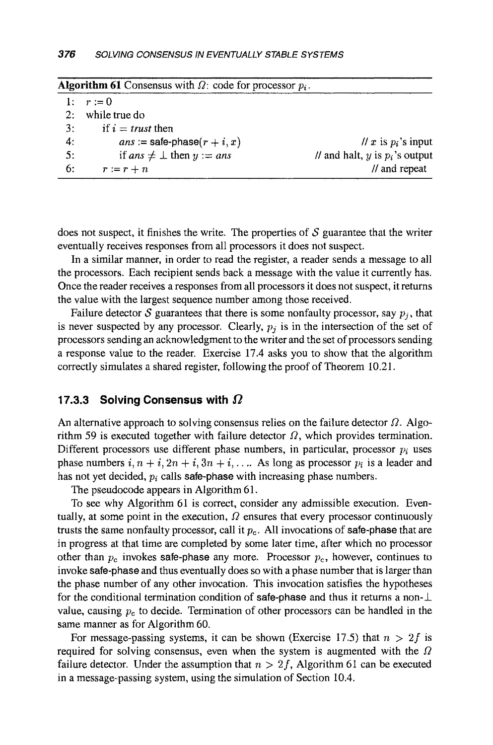
17.3.3 Solving Consensus with O 376
17.4 Implementing Failure Detectors 377
17.5 State Machine Replication with Failure Detectors 377
References 381
Index 401
1
Introduction
This chapter describes the subject area of the book, explains the approach taken, and
provides an overview of the contents.
1.1 DISTRIBUTED SYSTEMS
A distributed system is a collection of individual computing devices that can com-
communicate with each other. This very general definition encompasses a wide range
of modern-day computer systems, ranging from a VLSI chip, to a tightly-coupled
shared memory multiprocessor, to a local-area cluster of workstations, to the Internet.
This book focuses on systems at the more loosely coupled end of this spectrum. In
broad terms, the goal of parallel processing is to employ all processors to perform
one large task. In contrast, each processor in a distributed system generally has its
own semiindependent agenda, but for various reasons, including sharing of resources,
availability, and fault tolerance, processors need to coordinate their actions.
Distributed systems are ubiquitous today throughout business, academia, govern-
government, and the home. Typically they provide means to share resources, for instance,
special purpose equipment such as color printers or scanners, and to share data, cru-
crucial for our information-based economy. Peer-to-peer computing is a paradigm for
distributed systems that is becoming increasingly popular for providing computing
resources and services. More ambitious distributed systems attempt to provide im-
improved performance by attacking subproblems in parallel, and to provide improved
availability in case of failures of some components.
2 INTRODUCTION
Although distributed computer systems are highly desirable, putting together a
properly functioning system is notoriously difficult. Some of the difficulties are
pragmatic, for instance, the presence of heterogeneous hardware and software and
the lack of adherence to standards. More fundamental difficulties are introduced
by three factors: asynchrony, limited local knowledge, and failures. The term
asynchrony means that the absolute and even relative times at which events take
place cannot always be known precisely. Because each computing entity can only be
aware of information that it acquires, it has only a local view of the global situation.
Computing entities can fail independently, leaving some components operational
while others are not.
The explosive growth of distributed systems makes it imperative to understand
how to overcome these difficulties. As we discuss next, the field of distributed
computing provides the theoretical underpinning for the design and analysis of many
distributed systems.
1.2 THEORY OF DISTRIBUTED COMPUTING
The study of algorithms for sequential computers has been a highly successful en-
endeavor. It has generated a common framework for specifying algorithms and com-
comparing their performance, better algorithms for problems of practical importance, and
an understanding of inherent limitations (for instance, lower bounds on the running
time of any algorithm for a problem, and the notion of NP-completeness).
The goal of distributed computing is to accomplish the same for distributed sys-
systems. In more detail, we would like to identify fundamental problems that are
abstractions of those that arise in a variety of distributed situations, state them pre-
precisely, design and analyze efficient algorithms to solve them, and prove optimality of
the algorithms.
But there are some important differences from the sequential case. First, there is
not a single, universally accepted model of computation, and there probably never will
be, because distributed systems tend to vary much more than sequential computers
do. There are major differences between systems, depending on how computing
entities communicate, whether through messages or shared variables; what kind of
timing information and behavior are available; and what kind of failures, if any, are
to be tolerated.
In distributed systems, different complexity measures are of interest. We are still
interested in time and (local) space, but now we must consider communication costs
(number of messages, size and number of shared variables) and the number of faulty
vs. nonfaulty components.
Because of the complications faced by distributed systems, there is increased
scope for "negative" results, lower bounds, and impossibility results. It is (all too)
often possible to prove that a particular problem cannot be solved in a particular kind
of distributed system, or cannot be solved without a certain amount of some resource.
These results play a useful role for a system designer, analogous to learning that some
problem is NP-complete: they indicate where one should not put effort in trying to
OVERVIEW 3
solve the problem. But there is often more room to maneuver in a distributed system:
If it turns out that your favorite problem cannot be solved under a particular set of
assumptions, then you can change the rules! Perhaps a slightly weaker problem
statement can suffice for your needs. An alternative is to build stronger guarantees
into your system.
Since the late 1970s, there has been intensive research in applying this theoretical
paradigm to distributed systems. In this book, we have attempted to distill what
we believe is the essence of this research. To focus on the underlying concepts, we
generally care more about computability issues (i.e., whether or not some problem
can be solved) than about complexity issues (i.e., how expensive it is to solve a
problem). Section 1.3 gives a more detailed overview of the material of the book and
the rationale for the choices we made.
1.3 OVERVIEW
The book is divided into three parts, reflecting three goals. First, we introduce the
core theory, then we show relationships between the models, and finally we describe
some current issues.
Part I, Fundamentals, presents the basic communication models, shared mem-
memory and message passing; the basic timing models, synchronous, asynchronous, and
clocked; and the major themes, role of uncertainty, limitations of local knowledge,
and fault tolerance, in the context of several canonical problems. The presenta-
presentation highlights our emphasis on rigorous proofs of algorithm correctness and the
importance of lower bounds and impossibility results.
Chapter 2 defines our basic message-passing model and builds the reader's famil-
familiarity with the model and proofs of correctness using some simple distributed graph
algorithms for broadcasting and collecting information and building spanning trees.
In Chapter 3, we consider the problem of electing a leader in a ring network. The
algorithms and lower bounds here demonstrate a separation of models in terms of
complexity. Chapter 4 introduces our basic shared memory model and uses it in a
study of the mutual exclusion problem. The technical tools developed here, both
for algorithm design and for the lower bound proofs, are used throughout the rest
of the book. Fault tolerance is first addressed in Chapter 5, where the consensus
problem (the fundamental problem of agreeing on an input value in the presence of
failures) is studied. The results presented indicate a separation of models in terms
of computability. Chapter 6 concludes Part I by introducing the notion of causality
between events in a distributed system and describing the mechanism of clocks.
Part II, Simulations, shows how simulation is a powerful tool for making distributed
systems easier to design and reason about. The chapters in this part show how to
provide powerful abstractions that aid in the development of correct distributed algo-
algorithms, by providing the illusion of a better-behaved system. These abstractions are
message broadcasts, shared objects with strong semantics, synchrony, less destructive
faults, and fault-tolerant clocks.
4 INTRODUCTION
To place the simulation results on a rigorous basis, we need a more sophisticated
formal model than we had in Part I; Chapter 7 presents the essential features of this
model. In Chapter 8, we study how to provide a variety of broadcast mechanisms
using a point-to-point message-passing system. The simulation of shared objects
by message-passing systems and using weaker kinds of shared objects is covered
in Chapters 9 and 10. In Chapter 11, we describe several ways to simulate a more
synchronous system with a less synchronous system. Chapter 12 shows how to
simulate less destructive failures in the presence of more destructive failures. Finally,
in Chapter 13 we discuss the problem of synchronizing clocks in the presence of
failures.
Part III, Advanced Topics, consists of a collection of topics of recent research
interest. In these chapters, we explore some issues raised earlier in more detail,
present some results that use more difficult mathematical analyses, and give a flavor
of other areas in the field.
Chapter 14 indicates the benefits that can be gained from using randomization (and
weakening the problem specification appropriately) in terms of "beating" a lower
bound or impossibility result. In Chapter 15, we explore the relationship between
the ability of a shared object type to solve consensus and its ability to provide fault-
tolerant implementations of other object types. In Chapter 16 three problems that
can be solved in asynchronous systems subject to failures are investigated; these
problems stand in contrast to the consensus problem, which cannot be solved in this
situation. The notion of a failure detector as a way to abstract desired system behavior
is presented in Chapter 17, along with ways to use this abstraction to solve consensus
in environments where it is otherwise unsolvable.
1.4 RELATIONSHIP OF THEORY TO PRACTICE
Distributed computing comes in many flavors. In this section, we discuss the main
kinds and their relationships to the formal models employed in distributed computing
theory.
Perhaps the simplest, and certainly the oldest, example of a distributed system is an
operating system for a conventional sequential computer. In this case processes on the
same hardware communicate with the same software, either by exchanging messages
or through a common address space. To time-share a single CPU among multiple
processes, as is done in most contemporary operating systems, issues relating to the
(virtual) concurrency of the processes must be addressed. Many of the problems
faced by an operating system also arise in other distributed systems, such as mutual
exclusion and deadlock detection and prevention.
Multiple-instruction multiple-data (MIMD) machines with shared memory are
tightly coupled and are sometimes called multiprocessors. These consist of separate
hardware running common software. Multiprocessors may be connected with a bus
or, less frequently, by a switching network. Alternatively, MIMD machines can be
loosely coupled and not have shared memory. They can be either a collection of
CHAPTER NOTES 5
workstations on a local area network or a collection of processors on a switching
network.
Even more loosely coupled distributed systems are exemplified by autonomous
hosts connected by a network, either wide area such as the Internet or local area
such as Ethernet. In this case, we have separate hardware running separate software,
although the entities interact through well-defined interfaces, such as the TCP/IP
stack, CORBA, or some other groupware or middleware.
Distributed computing is notorious for its surplus of models; moreover, the models
do not translate exactly to real-life architectures. For this reason, we chose not to
organize the book around models, but rather around fundamental problems (in Part
I), indicating where the choice of model is crucial to the solvability or complexity of
a problem, and around simulations (in Part II), showing commonalities between the
models.
In this book, we consider three main models based on communication medium
and degree of synchrony. Here we describe which models match with which architec-
architectures. The asynchronous shared memory model applies to tightly-coupled machines,
in the common situation where processors do not get their clock signal from a sin-
single source. The asynchronous message-passing model applies to loosely-coupled
machines and to wide-area networks. The synchronous message-passing model is
an idealization of message-passing systems in which some timing information is
known, such as upper bounds on message delay. More realistic systems can simulate
the synchronous message-passing model, for instance, by synchronizing the clocks.
Thus the synchronous message-passing model is a convenient model in which to de-
design algorithms; the algorithms can then be automatically translated to more realistic
models.
In addition to communication medium and degree of synchrony, the other main
feature of a model is the kind of faults that are assumed to occur. Much of this
book is concerned with crash failures. A processor experiences a crash failure if it
ceases to operate at some point without any warning. In practice, this is often the
way components fail. We also study the Byzantine failure model. The behavior
of Byzantine processors is completely unconstrained. This assumption is a very
conservative, worst-case assumption for the behavior of defective hardware and
software. It also covers the possibility of intelligent, that is, human, intrusion.
Chapter Notes
Representative books on distributed systems from a systems perspective include those
by Coulouris, Dollimore, and Kindberg [85], Nutt [202], and Tanenbaum [249,250].
The book edited by Mullender [195] contains a mixture of practical and theoretical
material, as does the book by Chow and Johnson [82], Other textbooks that cover
distributed computing theory are those by Barbosa [45], Lynch [175], Peleg [208],
Raynal[226],andTel[252].
Parti
Fundamentals
2_
Basic Algorithms in
Message-Passing Systems
In this chapter we present our first model of distributed computation, for message-
passing systems with no failures. We consider the two main timing models, syn-
synchronous and asynchronous. In addition to describing formalism for the systems,
we also define the main complexity measures—number of messages and time—and
present the conventions we will use for describing algorithms in pseudocode.
We then present a few simple algorithms for message-passing systems with ar-
arbitrary topology, both synchronous and asynchronous. These algorithms broadcast
information, collect information, and construct spanning trees of the network. The
primary purpose is to build facility with the formalisms and complexity measures and
to introduce proofs of algorithm correctness. Some of the algorithms will be used
later in the book as building blocks for other, more complex, algorithms.
2.1 FORMAL MODELS FOR MESSAGE PASSING SYSTEMS
This section first presents our formal models for synchronous and asynchronous
message-passing systems with no failures. It then defines the basic complexity
measures, and finally it describes our pseudocode conventions for describing message
passing algorithms.
2.1.1 Systems
In a message-passing system, processors communicate by sending messages over
communication channels, where each channel provides a bidirectional connection
9
10 BASIC ALGORITHMS IN MESSAGE-PASSING SYSTEMS
V2
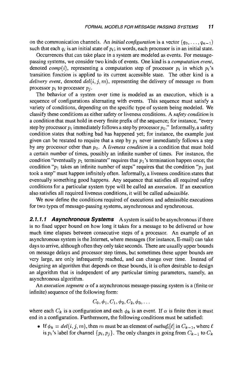
Fig. 2.1 A simple topology graph.
between two specific processors. The pattern of connections provided by the channels
describes the topology of the system. The topology is represented by an undirected
graph in which each node represents a processor and an edge is present between two
nodes if and only if there is a channel between the corresponding processors. We
will deal exclusively with connected topologies. The collection of channels is often
referred to as the network. An algorithm for a message-passing system with a specific
topology consists of a local program for each processor in the system. A processor's
local program provides the ability for the processor to perform local computation and
to send messages to and receive messages from each of its neighbors in the given
topology.
More formally, a system or algorithm consists of n processors po,,.., pn-i', i
is the index of processor pi. Each processor pi is modeled as a (possibly infinite)
state machine with state set Qi. The processor is identified with a particular node
in the topology graph. The edges incident on p, in the topology graph are labeled
arbitrarily with the integers 1 through r, where r is the degree of p, (see Fig. 2.1 for
an example). Each state of processor p,- contains 2r special components, outbufi[?]
and inbufi[?], for every ?, 1 < ? < r. These special components are sets of messages:
outbufi [?] holds messages that pi has sent to its neighbor over its Ah incident channel
but that have not yet been delivered to the neighbor, and inbufi [?] holds messages that
have been delivered to p, on its Ah incident channel but that pi has not yet processed
with an internal computation step. The state set Qi contains a distinguished subset of
initial states; in an initial state every inbuf[?] must be empty, although the outbuf[?]
components need not be.
The processor's state, excluding the outbuf [?} components, comprises the acces-
accessible state of pi. Processor pi's transition function takes as input a value for the
accessible state of pi, It produces as output a value for the accessible state of pi in
which each inbuf [?] is empty. It also produces as output at most one message for
each ? between 1 and r: This is the message to be sent to the neighbor at the other end
of pi's ?th incident channel. Thus messages previously sent by pt that are waiting to
be delivered cannot influence pt 's current step; each step processes all the messages
waiting to be delivered to pt and results in a state change and at most one message to
be sent to each neighbor.
A configuration is a vector C = (go,. • .,qn-i) where <?,- isastateofp,. The states
of the outbuf variables in a configuration represent the messages that are in transit
FORMAL MODELS FOR MESSAGE PASSING SYSTEMS 11
on the communication channels. An initial configuration is a vector (<?o,..., <?n-i)
such that each g; is an initial state of pf, in words, each processor is in an initial state.
Occurrences that can take place in a system are modeled as events. For message-
passing systems, we consider two kinds of events. One kind is a computation event,
denoted comp(i), representing a computation step of processor pi in which p,'s
transition function is applied to its current accessible state. The other kind is a
delivery event, denoted del{i, j, m), representing the delivery of message m from
processor p, to processor pj.
The behavior of a system over time is modeled as an execution, which is a
sequence of configurations alternating with events. This sequence must satisfy a
variety of conditions, depending on the specific type of system being modeled. We
classify these conditions as either safety or liveness conditions. A safety condition is
a condition that must hold in every finite prefix of the sequence; for instance, "every
step by processor pi immediately follows a step by processor po." Informally, a safety
condition states that nothing bad has happened yet; for instance, the example just
given can be restated to require that a step by p\ never immediately follows a step
by any processor other than p0. A liveness condition is a condition that must hold
a certain number of times, possibly an infinite number of times. For instance, the
condition "eventually p\ terminates" requires that p\ "s termination happen once; the
condition "pi takes an infinite number of steps" requires that the condition "p\ just
took a step" must happen infinitely often. Informally, a liveness condition states that
eventually something good happens. Any sequence that satisfies all required safety
conditions for a particular system type will be called an execution. If an execution
also satisfies all required liveness conditions, it will be called admissible.
We now define the conditions required of executions and admissible executions
for two types of message-passing systems, asynchronous and synchronous.
2.1.1.1 Asynchronous Systems A system is said to be asynchronous if there
is no fixed upper bound on how long it takes for a message to be delivered or how
much time elapses between consecutive steps of a processor. An example of an
asynchronous system is the Internet, where messages (for instance, E-mail) can take
days to arrive, although often they only take seconds. There are usually upper bounds
on message delays and processor step times, but sometimes these upper bounds are
very large, are only infrequently reached, and can change over time. Instead of
designing an algorithm that depends on these bounds, it is often desirable to design
an algorithm that is independent of any particular timing parameters, namely, an
asynchronous algorithm.
An execution segment a of a asynchronous message-passing system is a (finite or
infinite) sequence of the following form:
Co,<t>l,Ci,<l>2,C2,<l>3, ¦ ¦ ¦
where each Ck is a configuration and each (f>k is an event. If a is finite then it must
end in a configuration. Furthermore, the following conditions must be satisfied:
• If cf>k = del(i, j, m), then m must be an element of outbufi [?] in Ck -1, where ?
is pi's label for channel {pi ,pj}. The only changes in going from Ck -1 to Ck
12 BASIC ALGORITHMS IN MESSAGE-PASSING SYSTEMS
are that m is removed from outbufi [?} in Ck and m is added to inbufj [h] in Ck,
where h is p^-'s label for channel {pi,Pj}- In words, a message is delivered
only if it is in transit and the only change is to move the message from the
sender's outgoing buffer to the recipient's incoming buffer. (In the example
of Fig. 2.1, a message from p3 to p0 would be placed in outbufy[l] and then
delivered to inbufo [2].)
• If ^^ = comp(i), then the only changes in going from Ck-i to Ck are thatp,
changes state according to its transition function operating on pt 's accessible
state inCk-i and the set of messages specified by p,-'s transition function are
added to the outbufi variables in Ck ¦ These messages are said to be sent at
this event. In words, p,- changes state and sends out messages according to its
transition function (local program) based on its current state, which includes
all pending delivered messages (but not pending outgoing messages). Recall
that the processor's transition function guarantees that the inbuf variables are
emptied.
An execution is an execution segment Co, 4>\, C\, <f>2, C^, <f>3, •.., where Co is an
initial configuration.
With each execution (or execution segment) we associate a schedule (or schedule
segment) that is the sequence of events in the execution, that is, cf>i,(f>2, <j>s, ¦ ¦ •¦ Not
every sequence of events is a schedule for every initial configuration; for instance,
del( 1, 2, m) is not a schedule for an initial configuration with empty outbufi, because
there is no prior step by pi that could cause m to be sent. Note that if the local
programs are deterministic, then the execution (or execution segment) is uniquely
determined by the initial (or starting) configuration Co and the schedule (or schedule
segment) a and is denoted exec (Co, a).
In the asynchronous model, an execution is admissible if each processor has an
infinite number of computation events and every message sent is eventually delivered.
The requirement for an infinite number of computation events models the fact that
processors do not fail. It does not imply that the processor's local program must
contain an infinite loop; the informal notion of termination of an algorithm can be
accommodated by having the transition function not change the processor's state
after a certain point, once the processor has completed its task. In other words, the
processor takes "dummy steps" after that point. A schedule is admissible if it is the
schedule of an admissible execution.
2.1.1.2 Synchronous Systems In the synchronous model processors execute
in lockstep: The execution is partitioned into rounds, and in each round, every pro-
processor can send a message to each neighbor, the messages are delivered, and every
processor computes based on the messages just received. This model, although gen-
generally not achievable in practical distributed systems, is very convenient for designing
algorithms, because an algorithm need not contend with much uncertainty. Once an
algorithm has been designed for this ideal timing model, it can be automatically
simulated to work in other, more realistic, timing models, as we shall see later.
FORMAL MODELS FOR MESSAGE PASSING SYSTEMS 13
Formally, the definition of an execution for the synchronous case is further con-
constrained over the definition from the asynchronous case as follows. The sequence of
alternating configurations and events can be partitioned into disjointrounds. A round
consists of a deliver event for every message in an outbuf variable, until all outbuf
variables are empty, followed by one computation event for every processor. Thus a
round consists of delivering all pending messages and then having every processor
take an internal computation step to process all the delivered messages.
An execution is admissible for the synchronous model if it is infinite. Because
of the round structure, this implies that every processor takes an infinite number
of computation steps and every message sent is eventually delivered. As in the
asynchronous case, assuming that admissible executions are infinite is a technical
convenience; termination of an algorithm can be handled as in the asynchronous
case.
Note that in a synchronous system with no failures, once the algorithm is fixed,
the only relevant aspect of executions that can differ is the initial configuration. In an
asynchronous system, there can be many different executions of the same algorithm,
even with the same initial configuration and no failures, because the interleaving of
processor steps and the message delays are not fixed.
2.1.2 Complexity Measures
We will be interested in two complexity measures, the number of messages and the
amount of time, required by distributed algorithms. For now, we will concentrate
on worst-case performance; later in the book we will sometimes be concerned with
expected-case performance.
To define these measures, we need a notion of the algorithm terminating. We
assume that each processor's state set includes a subset of terminated states and each
processor's transition function maps terminated states only to terminated states. We
say that the system (algorithm) has terminated when all processors are in terminated
states and no messages are in transit. Note that an admissible execution must still
be infinite, but once a processor has entered a terminated state, it stays in that state,
taking "dummy" steps.
The message complexity of an algorithm for either a synchronous or an asyn-
asynchronous message-passing system is the maximum, over all admissible executions of
the algorithm, of the total number of messages sent.
The natural way to measure time in synchronous systems is simply to count the
number of rounds until termination. Thus the time complexity of an algorithm for
a synchronous message-passing system is the maximum number of rounds, in any
admissible execution of the algorithm, until the algorithm has terminated.
Measuring time in an asynchronous system is less straightforward. A common
approach, and the one we will adopt, is to assume that the maximum message delay in
any execution is one unit of time and then calculate the running time until termination.
To make this approach precise, we must introduce the notion of time into executions.
A timed execution is an execution that has a nonnegative real number associated
with each event, the time at which that event occurs. The times must start at 0, must
14 BASIC ALGORITHMS IN MESSAGE-PASSING SYSTEMS
be nondecreasing, must be strictly increasing for each individual processor1, and
must increase without bound if the execution is infinite. Thus events in the execution
are ordered according to the times at which they occur, several events can happen at
the same time as long as they do not occur at the same processor, and only a finite
number of events can occur before any finite time.
We define the delay of a message to be the time that elapses between the com-
computation event that sends the message and the computation event that processes the
message. In other words, it consists of the amount of time that the message waits in
the sender's outbuf together with the amount of time that the message waits in the
recipient's inbuf.
The time complexity of an asynchronous algorithm is the maximum time until
termination among all timed admissible executions in which every message delay is
at most one. This measure still allows arbitrary interleavings of events, because no
lower bound is imposed on how closely events occur. It can be viewed as taking
any execution of the algorithm and normalizing it so that the longest message delay
becomes one unit of time.
2.1.3 Pseudocode Conventions
In the formal model just presented, an algorithm would be described in terms of state
transitions. However, we will seldom do this, because state transitions tend to be
more difficult for people to understand; in particular, flow of control must be coded
in a rather contrived way in many cases.
Instead, we will describe algorithms at two different levels of detail. Simple
algorithms will be described in prose. Algorithms that are more involved will also
be presented in pseudocode. We now describe the pseudocode conventions we will
use for synchronous and asynchronous message-passing algorithms.
Asynchronous algorithms will be described in an interrupt-driven fashion for each
processor. In the formal model, each computation event processes all the messages
waiting in the processor's inbuf variables at once. For clarity, however, we will
generally describe the effect of each message individually. This is equivalent to the
processor handling the pending messages one by one in some arbitrary order; if more
than one message is generated for the same recipient during this process, they can be
bundled together into one big message. It is also possible for the processor to take
some action even if no message is received. Events that cause no message to be sent
and no state change will not be listed.
The local computation done within a computation event will be described in a style
consistent with typical pseudocode for sequential algorithms. We use the reserved
word "terminate" to indicate that the processor enters a terminated state.
An asynchronous algorithm will also work in a synchronous system, because a
synchronous system is a special case of an asynchronous system. However, we
will often be considering algorithms that are specifically designed for synchronous
lcomp(i) is considered to occur at p; and del(i, j, m) at both pi and p}.
BROADCAST AND CONVERGECAST ON A SPANNING TREE 15
systems. These synchronous algorithms will be described on a round-by-round basis
for each processor. For each round we will specify what messages are to be sent
by the processor and what actions it is to take based on the messages just received.
(Note that the messages to be sent in the first round are those that are initially in the
outbuf variables.) The local computation done within a round will be described in a
style consistent with typical pseudocode for sequential algorithms. Termination will
be implicitly indicated when no more rounds are specified.
In the pseudocode, the local state variables of processor pi will not be subscripted
with i; in discussion and proof, subscripts will be added when necessary to avoid
ambiguity.
Comments will begin with //.
In the next sections we will give several examples of describing algorithms in
prose, in pseudocode, and as state transitions.
2.2 BROADCAST AND CONVERGECAST ON A SPANNING TREE
We now present several examples to help the reader gain a better understanding of the
model, pseudocode, correctness arguments, and complexity measures for distributed
algorithms. These algorithms solve basic tasks of collecting and dispersing informa-
information and computing spanning trees for the underlying communication network. They
serve as important building blocks in many other algorithms.
Broadcast
We start with a simple algorithm for the (single message) broadcast problem, as-
assuming a spanning tree of the network is given. A distinguished processor, pr, has
some information, namely, a message (M), it wishes to send to all other processors.
Copies of the message are to be sent along a tree that is rooted at pr and spans
all the processors in the network. The spanning tree rooted at pr is maintained in
a distributed fashion: Each processor has a distinguished channel that leads to its
parent in the tree as well as a set of channels that lead to its children in the tree.
Here is the prose description of the algorithm. Figure 2.2 shows a sample asyn-
asynchronous execution of the algorithm; solid lines depict channels in the spanning tree,
dashed lines depict channels not in the spanning tree, and shaded nodes indicate
processors that have received (M) already. The root, pr, sends the message (M) on all
the channels leading to its children (see Fig. 2.2(a)). When a processor receives the
message {M} on the channel from its parent, it sends (M) on all the channels leading
to its children (see Fig. 2.2(b)).
The pseudocode for this algorithm is in Algorithm 1; there is no pseudocode for
a computation step in which no messages are received and no state change is made.
Finally, we describe the algorithm at the level of state transitions: The state of
each processor pi contains:
• A variable parent, which holds either a processor index or nil
16 BASIC ALGORITHMS IN MESSAGE-PASSING SYSTEMS
Fig. 2.2 Two steps in an execution of the broadcast algorithm.
• A variable childrerii, which holds a set of processor indices
• A Boolean terminatedi, which indicates whether pi is in a terminated state
Initially, the values of the parent and children variables are such that they form a
spanning tree rooted at pr of the topology graph. Initially, all terminated variables
are false. Initially, outbufr[j) holds (M) for each j in children,-;2 all other outbuf
variables are empty. The result of comp(i) is that, if (M) is in an inbufi[k] for some
k, then (M) is placed in outbufi [j], for each j in children^, and p, enters a terminated
state by setting terminatedi to true. Ifi — r and terminatedr is false, then terminated,.
is set to true. Otherwise, nothing is done.
Note that this algorithm is correct whether the system is synchronous or asyn-
asynchronous. Furthermore, as we discuss now, the message and time complexities of the
algorithm are the same in both models.
What is the message complexity of the algorithm? Clearly, the message (M) is
sent exactly once on each channel that belongs to the spanning tree (from the parent to
the child) in both the synchronous and asynchronous cases. That is, the total number
of messages sent during the algorithm is exactly the number of edges in the spanning
tree rooted at pr. Recall that a spanning tree of n nodes has exactly n — 1 edges;
therefore, exactly n — 1 messages are sent during the algorithm.
Let us now analyze the time complexity of the algorithm. It is easier to perform
this analysis when communication is synchronous and time is measured in rounds.
The following lemma shows that by the end of round t, the message (M) reaches
all processors at distance t (or less) from pr in the spanning tree. This is a simple
claim, with a simple proof, but we present it in detail to help the reader gain facility
with the model and proofs about distributed algorithms. Later in the book we will
leave such simple proofs to the reader.
2Here we are using the convention that inbuf and outbuf variables are indexed by the neighbors' indices
instead of by channellabels.
BROADCAST AND CONVERGECAST ON A SPANNING TREE 17
Algorithm 1 Spanning tree broadcast algorithm.
Initially (M) is in transit from pr to all its children in the spanning tree.
Code for pr:
1: upon receiving no message: // first computation event by pr
2: terminate
Code for pi, 0 < i:- < n — 1, i ^ r:
3: upon receiving (M) from parent:
4: send (M) to all children
5: terminate
Lemma 2.1 In every admissible execution of the broadcast algorithm in the syn-
synchronous model, every processor at distance t from pr in the spanning tree receives
the message (M) in round t.
Proof. The proof proceeds by induction on the distance t of a processor from pr.
The basis is t — 1. From the description of the algorithm, each child of pr receives
(M) from pr in the first round.
We now assume that every processor at distance t — 1 > 1 from pr in the spanning
tree receives the message (M) in round t — 1.
We must show that every processor pi at distance t from pr in the spanning tree
receives (M) in round t. Let pj be the parent of pi in the spanning tree. Since pj is at
distance t — 1 from pr, by the inductive hypothesis, pj receives (M) in round t — 1.
By the description of the algorithm, pj then sends (M) to pi in the next round. D
By Lemma 2.1, the time complexity of the algorithm is d, where d is the depth of
the spanning tree. Recall that d is at most n — 1, when the spanning tree is a chain.
Thus we have:
Theorem 2.2 There is a synchronous broadcast algorithm with message complexity
n — 1 and time complexity d, when a rooted spanning tree with depth d is known in
advance.
A similar analysis applies when communication is asynchronous. Once again,
the key is to prove that by time t, the message (M) reaches all processors at distance
t (or less) from pr in the spanning tree. This implies that the time complexity of
the algorithm is also d when communication is asynchronous. We now analyze this
situation more carefully.
Lemma 2.3 In every admissible execution of the broadcast algorithm in an asyn-
asynchronous system, every processor at distance tfrom pr in the spanning tree receives
message (M) by time t.
Proof. The proof is by induction on the distance t of a processor from pr.
18 BASIC ALGORITHMS IN MESSAGE-PASSING SYSTEMS
The basis is t = 1. From the description of the algorithm, {M) is initially in transit
to each processor pi at distance 1 from pr. By the definition of time complexity for
the asynchronous model, pt receives (M) by time 1.
We must show that every processor pi at distance t from pr in the spanning tree
receives (M) in round t. Let pj be the parent of pi in the spanning tree. Since pj is
at distance i — 1 from pr, by the inductive hypothesis, pj receives (M) by time t — 1.
By the description of the algorithm, pj sends (M) top; when it receives (M), that is,
by time i—1. By the definition of time complexity for the asynchronous model, p,-
receives (M) by time t. ?
Thus we have:
Theorem 2,4 There is an asynchronous broadcast algorithm with message complex-
complexity n — 1 and time complexity d, when a rooted spanning tree with depth d is known
in advance.
Convergecast
The broadcast problem requires one-way communication, from the root, pr, to all the
nodes of the tree. Consider now the complementary problem, called convergecast,
of collecting information from the nodes of the tree to the root. For simplicity, we
consider a specific variant of the problem in which each processor pi starts with
a value Xi and we wish to forward the maximum value among these values to the
root pr. (Exercise 2.3 concerns a general convergecast algorithm that collects all the
information in the network.)
Once again, we assume that a spanning tree is maintained in a distributed fashion,
as in the broadcast problem. Whereas the broadcast algorithm is initiated by the root,
the convergecast algorithm is initiated by the leaves. Note that a leaf of the spanning
tree can be easily distinguished, because it has no children.
Conceptually, the algorithm is recursive and requires each processor to compute
the maximum value in the subtree rooted at it. Starting at the leaves, each processor
Pi computes the maximum value in the subtree rooted at it, which we denote by v,-,
and sends Vi to its parent. The parent collects these values from all its children,
computes the maximum value in its subtree, and sends the maximum value to its
parent.
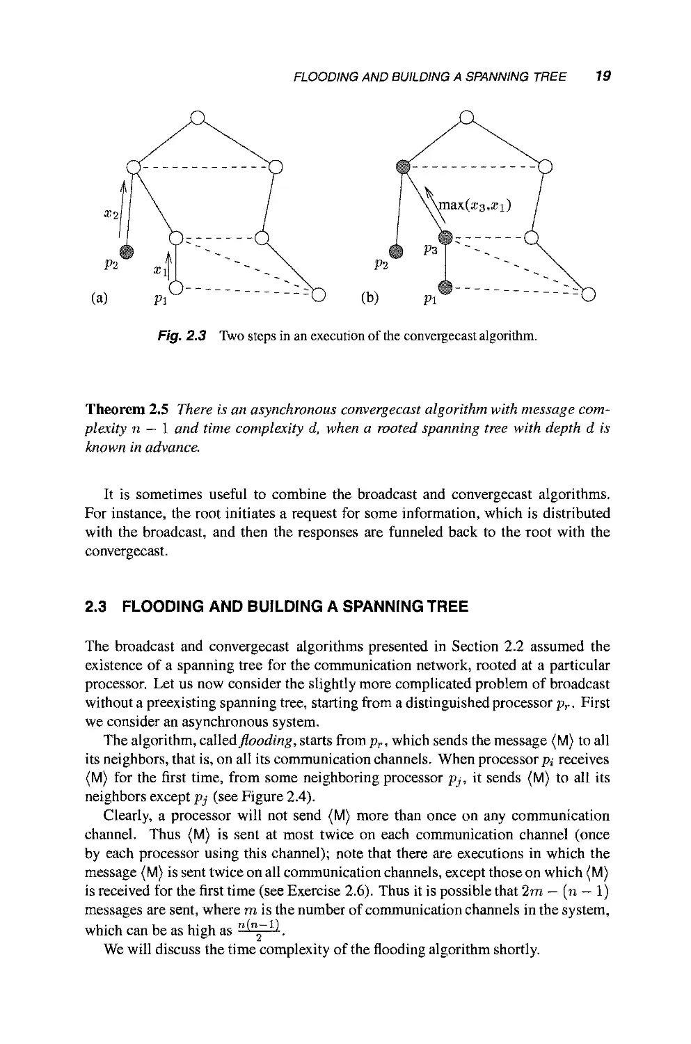
In more detail, the algorithm proceeds as follows. If a node p,- is a leaf, then it
starts the algorithm by sending its value xi to its parent (see Fig. 2.3(a)). A non-leaf
node, pj, with k children, waits to receive messages containing Vi1,..., Vik from its
children p^,..., p»t. Then it computes Vj = m&x{xj, v,-,,..., v,-t} and sends Vj to
its parent. (See Figure 2.3(b).)
The analyses of the message and time complexities of the convergecast algorithm
are very much like those of the broadcast algorithm. (Exercise 2.2 indicates how to
analyze the time complexity of the convergecast algorithm.)
FLOODING AND BUILDING A SPANNING TREE
19
(b) Pi
Fig. 2.3 Two steps in an execution of the convergeeast algorithm.
Theorem 2.5 There is an asynchronous convergecast algorithm with message com-
complexity n — 1 and time complexity d, when a rooted spanning tree with depth d is
known in advance.
It is sometimes useful to combine the broadcast and convergecast algorithms.
For instance, the root initiates a request for some information, which is distributed
with the broadcast, and then the responses are funneled back to the root with the
convergecast.
2.3 FLOODING AND BUILDING A SPANNING TREE
The broadcast and convergecast algorithms presented in Section 2.2 assumed the
existence of a spanning tree for the communication network, rooted at a particular
processor. Let us now consider the slightly more complicated problem of broadcast
without a preexisting spanning tree, starting from a distinguished processor pr. First
we consider an asynchronous system.
The algorithm, called flooding, starts from pr, which sends the message {M) to all
its neighbors, that is, on all its communication channels. When processor pi receives
{M) for the first time, from some neighboring processor pj, it sends (M) to all its
neighbors except pj (see Figure 2.4).
Clearly, a processor will not send {M) more than once on any communication
channel. Thus (M) is sent at most twice on each communication channel (once
by each processor using this channel); note that there are executions in which the
message {M) is sent twice on all communication channels, except those on which (M)
is received for the first time (see Exercise 2.6). Thus it is possible that 2ra — (n — 1)
messages are sent, where m is the number of communication channels in the system,
which can be as high as "'~ '.
We will discuss the time complexity of the flooding algorithm shortly.
20 BASIC ALGORITHMS IN MESSAGE-PASSING SYSTEMS
I S
A O=:: Q
(a) 6---- I::VO
Fig, 2.4 Two steps in an execution of the flooding algorithm; solid lines indicate channels
that are in the spanning tree at this point in the execution.
Effectively, the flooding algorithm induces a spanning tree, with the root at pr,
and the parent of a processor pi being the processor from which p, received (M) for
the first time. It is possible that pi received (M) concurrently from several processors,
because a comp event processes all messages that have been delivered since the last
comp event by that processor; in this case, pi's parent is chosen arbitrarily among
them.
The flooding algorithm can be modified to explicitly construct this spanning tree,
as follows: First, pr sends (M) to all its neighbors. As mentioned above, it is possible
that a processor pi receives (M) for the first time from several processors. When
this happens, p,- picks one of the neighboring processors that sent (M) to it, say, pj,
denotes it as its parent and sends a (parent) message to it. To all other processors,
and to any other processor from which (M) is received later on, p,- sends an (already)
message, indicating that pi is already in the tree. After sending (M) to all its other
neighbors (from which (M) was not previously received), ps- waits for a response
from each of them, either a (parent) message or an (already) message. Those who
respond with (parent) messages are denoted as p;'s children. Once all recipients of
Pi's (M) message have responded, either with (parent) or (already), p, terminates
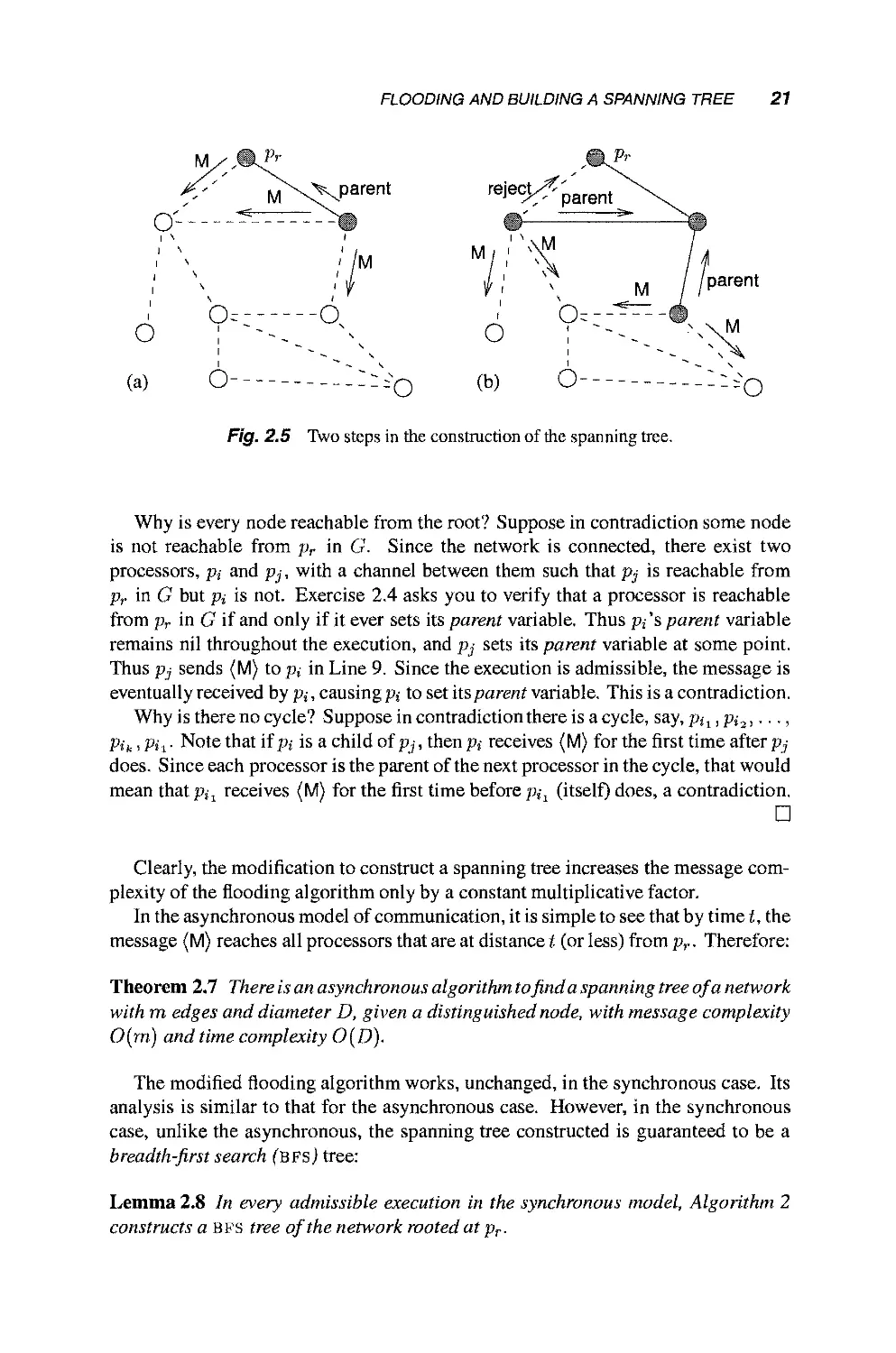
(see Figure 2.5).
The pseudocode for the modified flooding algorithm is in Algorithm 2.
Lemma 2.6 In every admissible execution in the asynchronous model, Algorithm 2
constructs a spanning tree of the network rooted at pr.
Proof. Inspecting the code reveals two important facts about the algorithm. First,
once a processor sets its parent variable, it is never changed (and it has only one
parent). Second, the set of children of a processor never decreases. Thus, eventually,
the graph structure induced by parent and children variables is static, and the parent
and children variables at different nodes are consistent, that is, if pj is a child of
Pi, then pi is pj's parent. We show that the resulting graph, call it G, is a directed
spanning tree rooted at pr.
FLOODING AND BUILDING A SPANNING TREE 21
, ^M^N^ parent
M
6 ; ~~~-, \ 6 ; ~~.
"* "*¦ ~. ^
(a) O---- -:-O (b) -:-O
Fig. 2.5 Two steps in the construction of the spanning tree.
Why is every node reachable from the root? Suppose in contradiction some node
is not reachable from pr in G. Since the network is connected, there exist two
processors, p,- and pj, with a channel between them such that pj is reachable from
pr in G but pi is not. Exercise 2.4 asks you to verify that a processor is reachable
from pr in G if and only if it ever sets its parent variable. Thus p8- 's parent variable
remains nil throughout the execution, and pj sets its parent variable at some point.
Thus pj sends (M) to p,- in Line 9. Since the execution is admissible, the message is
eventually received by p,-, causing p,- to set its parent variable. This is a contradiction.
Why is there no cycle? Suppose in contradiction there is a cycle, say, p^p,-.,,...,
Pit, i Pn • Note that if p, is a child of pj, then p,- receives (M) for the first time after pj
does. Since each processor is the parent of the next processor in the cycle, that would
mean that pSl receives (M) for the first time before pi1 (itself) does, a contradiction.
?
Clearly, the modification to construct a spanning tree increases the message com-
complexity of the flooding algorithm only by a constant multiplicative factor.
In the asynchronous model of communication, it is simple to see that by time t, the
message (M) reaches all processors that are at distance i (or less) from pr. Therefore:
Theorem 2.7 There is an asynchronous algorithm to find a spanning tree of a network
with m edges and diameter D, given a distinguished node, with message complexity
0{m) and time complexity O(D).
The modified flooding algorithm works, unchanged, in the synchronous case. Its
analysis is similar to that for the asynchronous case. However, in the synchronous
case, unlike the asynchronous, the spanning tree constructed is guaranteed to be a
breadth-first search (bfs) tree:
Lemma 2.8 In every admissible execution in the synchronous model, Algorithm 2
constructs a BFS tree of the network rooted at pr.
22 BASIC ALGORITHMS IN MESSAGE-PASSING SYSTEMS
Algorithm 2 Modified flooding algorithm to construct a spanning tree:
code for processor p,-, 0 < i < n — 1.
Initially parent = _L, children — 0, and other = 0.
1: upon receiving no message:
2: if pi = pr and parent — _L then // root has not yet sent (M)
3: send (M) to all neighbors
4: parent :— p,-
5: upon receiving (M) from neighbor pj:
6: if parent = _L then // pi has not received (M) before
7: parent '¦— Pj
8: send {parent) to pj
9: send (M) to all neighbors except pj
10: else send (already) to pj
11: upon receiving (parent) from neighbor pj:
12: add pj to children
13: if children U other contains all neighbors except parent then
14: terminate
15: upon receiving (already) from neighbor pj:
16: add pj to other
17: if children U other contains all neighbors except parent then
18: terminate
Proof. We show by induction on t that at the beginning of round t, A) the graph
constructed so far according to the parent variables is a BFS tree consisting of all
nodes at distance at most t—l from pr, and B) (M) messages are in transit only from
nodes at distance exactly t — l from pr.
The basis is t = 1. Initially, all parent variables are nil, and (M) messages are
outgoing from pr and no other node.
Suppose the claim is true for round t — l > 1. During round t — l, the (M)
messages in transit from nodes at distance t — 2 are received. Any node that receives
(M) is at distance t — 1 or less from pr. A recipient node with a non-nil parent
variable, namely, a node at distance t — 2 or less from pr, does not change its parent
variable or send out an (M) message. Every node at distance t—l from pr receives
an (M) message in round t—l and, because its parent variable is nil, it sets it to an
appropriate parent and sends out an (M) message. Nodes not at distance t — 1 do not
receive an (M) message and thus do not send any. D
Therefore:
CONSTRUCTING A DEPTH-FIRST SEARCH SPANNING TREE FORA SPECIFIED ROOT 23
M
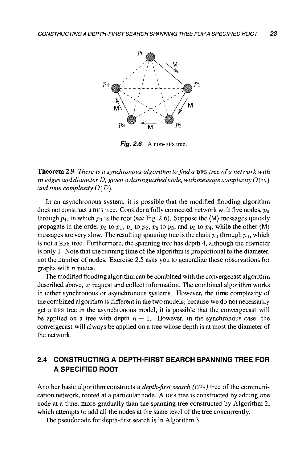
Fig. 2.6 A non-BFS tree.
Theorem 2.9 There is a synchronous algorithm to find a BFS tree of a network with
m edges and diameter D, given a distinguished node, with message complexity O(m)
and time complexity O(D).
In an asynchronous system, it is possible that the modified flooding algorithm
does not construct a bfs tree. Consider a fully connected network with five nodes, po
through f4, in which po is the root (see Fig. 2.6). Suppose the (M) messages quickly
propagate in the order po to p\, p\ to pi, pi to p^, and p% to p$, while the other (M)
messages are very slow. The resulting spanning tree is the chain po through p^, which
is not a bfs tree. Furthermore, the spanning tree has depth 4, although the diameter
is only 1. Note that the running time of the algorithm is proportional to the diameter,
not the number of nodes. Exercise 2.5 asks you to generalize these observations for
graphs with n nodes.
The modified flooding algorithm can be combined with the convergecast algorithm
described above, to request and collect information. The combined algorithm works
in either synchronous or asynchronous systems. However, the time complexity of
the combined algorithm is different in the two models; because we do not necessarily
get a bfs tree in the asynchronous model, it is possible that the convergecast will
be applied on a tree with depth n — 1. However, in the synchronous case, the
convergecast will always be applied on a tree whose depth is at most the diameter of
the network.
2.4 CONSTRUCTING A DEPTH-FIRST SEARCH SPANNING TREE FOR
A SPECIFIED ROOT
Another basic algorithm constructs a depth-first search (dfs) tree of the communi-
communication network, rooted at a particular node. A dfs tree is constructed by adding one
node at a time, more gradually than the spanning tree constructed by Algorithm 2,
which attempts to add all the nodes at the same level of the tree concurrently.
The pseudocode for depth-first search is in Algorithm 3.
1:
2:
3:
4:
5:
6:
8:
9:
10:
11:
12:
13:
14:
15:
upon receiving no message:
if pi = pr and parent = _L then
parent:— pi
exploreQ
upon receiving (M) from pf.
if parent = J_ then
parent:— pj
remove pj from unexplored
explore ()
else
send (already) to pj
remove pj from unexplored
upon receiving (already) from pj:
exploref)
24 BASIC ALGORITHMS IN MESSAGE-PASSING SYSTEMS
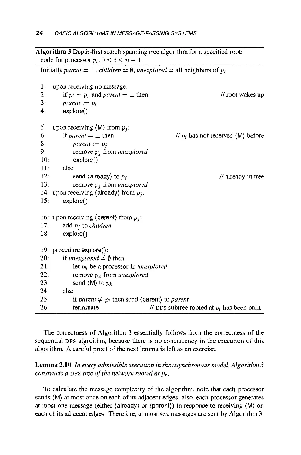
Algorithm 3 Depth-first search spanning tree algorithm for a specified root:
code for processor pi, 0 < i < n — 1.
Initially parent = _L, children — 0, unexplored — all neighbors of pi
II root wakes up
II Pi has not received (M) before
// already in tree
16: upon receiving (parent) from pj\
17: add pj to children
18: explore()
19: procedure explore():
20: if unexplored ^ 0 then
21: let pk be a processor in unexplored
22: remove pk from unexplored
23: send (M) top/;
24: else
25: if parent ^ p,- then send (parent) to parent
26: terminate // dfs subtree rooted at p,- has been built
The correctness of Algorithm 3 essentially follows from the correctness of the
sequential DFS algorithm, because there is no concurrency in the execution of this
algorithm. A careful proof of the next lemma is left as an exercise.
Lemma 2.10 In every admissible execution in the asynchronous model, Algorithm 3
constructs a DFS tree of the network rooted at pr.
To calculate the message complexity of the algorithm, note that each processor
sends (M) at most once on each of its adjacent edges; also, each processor generates
at most one message (either (already) or (parent)) in response to receiving (M) on
each of its adjacent edges. Therefore, at most 4m messages are sent by Algorithm 3.
CONSTRUCTING A DEPTH-FIRST SEARCH SPANNING TREE WITHOUT A SPECIFIED ROOT 25
Showing that the time complexity of the algorithm is O(m) is left as an exercise for
the reader. We summarize:
Theorem 2.11 There is an asynchronous algorithm to find a depth-first search span-
spanning tree of a network with m edges and n nodes, given a distinguished node, with
message complexity O(m) and time complexity O(m)-
2.5 CONSTRUCTING A DEPTH-FIRST SEARCH SPANNING TREE
WITHOUT A SPECIFIED ROOT
Algorithm 2 and Algorithm 3 build a spanning tree for the communication network,
with reasonable message and time complexities. However, both of them require the
existence of a distinguished node, from which the construction starts. In this section,
we discuss how to build a spanning tree when there is no distinguished node. We
assume, however, that the nodes have unique identifiers, which are natural numbers;
as we shall see in Section 3.2, this assumption is necessary.
To build a spanning tree, each processor that wakes up spontaneously attempts to
build a DFS tree with itself as the root, using a separate copy of Algorithm 3. If two
dfs trees try to connect to the same node (not necessarily at the same time), the node
will join the dfs tree whose root has the higher identifier.
The pseudocode appears in Algorithm 4. To implement the above idea, each node
keeps the maximal identifier it has seen so far in a variable leader, which is initialized
to a value smaller than any identifier.
When a node wakes up spontaneously, it sets its leader to its own identifier and
sends a dfs message carrying its identifier. When a node receives a dfs message
with identifier y, it compares y and leader. lfy> leader, then this might be the dfs
of the processor with maximal identifier; in this case, the node changes leader to be
y, sets its parent variable to be the node from which this message was received, and
continues the dfs with identifier y. If y = leader, then the node already belongs to
this spanning tree. If y < leader, then this dfs belongs to a node whose identifier is
smaller than the maximal identifier seen so far; in this case, no message is sent, which
stalls the dfs tree construction with identifier y. Eventually, a DFS message carrying
the identifier leader (or a larger identifier) will arrive at the node with identifier y,
and connect it to its tree.
Only the root of the spanning tree constructed explicitly terminates; other nodes
do not terminate and keep waiting for messages. It is possible to modify the algorithm
so that the root sends a termination message using Algorithm 1.
Proving correctness of the algorithm is more involved than previous algorithms in
this chapter; we only outline the arguments here. Consider the nodes that wake up
spontaneously, and let pm be the node with the maximal identifier among them; let
m be pm 's identifier.
First observe that (leader) messages with leader id m are never dropped because
of discovering a larger leader id, by definition of m.
26 BASIC ALGORITHMS IN MESSAGE-FASSING SYSTEMS
Algorithm 4 Spanning tree construction: code for processor p;, 0 < i < n - 1.
Initially parent = J_, leader = —1, children = 0, unexplored = all neighbors of p;
1: upon receiving no message:
2: if parent = X then // wake up spontaneously
3: leader := id
4: parent := pt
5: exploreQ
6: upon receiving {\eader,new-id} from pj:
7: if leader < new-id then // switch to new tree
8: leader := new-id
9: parent := p^
10: children :- 0
11: unexplored := all neighbors of p,- except pj
12: explore()
13: else if leader = new-id then
14: send (already,leader) to pj // already in same tree
// otherwise, leader > new-id and the DFS for new-id is stalled
15: upon receiving {already,new-id) from p^:
16: if new-id = leader then exploreQ
17: upon receiving (parerft,new-id) from py.
18: if new-id — leader then //otherwise ignore message
19: add pj to children
20: exploreQ
21: procedure explore():
22: if unexplored ^ 0 then
23: let pu be a processor in unexplored
24: remove pk from unexplored
25: send (leader,/ear/er) topfe
26: else
27: if parent ¦? p,- then send (parent,/earfer) to parent
28: else terminate as root of spanning tree
Second, (already) messages with leader id m are never dropped because they have
the wrong leader id. Why? Suppose p,- receives an (already) message from pj with
leader id m. The reason pj sent this message to p8- is that it received a (leader)
message from p,- with leader id m. Once p; sets its leader id to m, it never resets it,
because m is the largest leader id in the system. Thus when p, receives pj's (already)
CONSTRUCTING A DEPTH-FIRST SEARCH SPANNING TREE WITHOUT A SPECIFIED ROOT 27
message with leader id m, pi still has its leader id as m, the message is accepted, and
the exploration proceeds.
Third, {parent) messages with leader id m are never dropped because they have
the wrong leader id. The argument is the same as for (already) messages.
Finally, messages with leader id m are never dropped because the recipient has
terminated. Suppose in contradiction that some p,- has terminated before receiving
a message with leader id m. Then p; thinks it is the leader, but its id, say i, is less
than m, The copy of Algorithm 3 with leader id i must have reached every node in
the graph, including pm. But pm would not have responded to the leader message,
so this copy of Algorithm 3 could not have completed, a contradiction.
Thus the copy of Algorithm 3 for leader id m completes, and correctness of
Algorithm 3 implies correctness of Algorithm 4.
A simple analysis of the algorithm uses the fact that, in the worst case, each proces-
processor tries to construct a DFS tree. Therefore, the message complexity of Algorithm 4
is at most n times the message complexity of Algorithm 3, that is, O(nm). The time
complexity is similar to the time complexity of Algorithm 3, that is, O (m).
Theorem 2.12 Algorithm 4 finds a spanning tree of a network with m edges and n
nodes, with message complexity O(n ¦ m) and time complexity O(m).
Exercises
2.1 Code one of the simple algorithms in state transitions.
2.2 Analyze the time complexity of the convergecast algorithm of Section 2.2
when communication is synchronous and when communication is asyn-
asynchronous.
Hint: For the synchronous case, prove that during round t + 1, a processor at
height t sends a message to its parent. For the asynchronous case, prove that
by time t, a processor at height t has sent a message to its parent.
2.3 Generalize the convergecast algorithm of Section 2.2 to collect all the infor-
information. That is, when the algorithm terminates, the root should have the input
values of all the processors. Analyze the bit complexity, that is, the total
number of bits that are sent over the communication channels.
2.4 Prove the claim used in the proof of Lemma 2.6 that a processor is reachable
from pr in G if and only if it ever sets its parent variable.
2.5 Describe an execution of the modified flooding algorithm (Algorithm 2) in an
asynchronous system with n nodes that does not construct a bfs tree.
2.6 Describe an execution of Algorithm 2 in some asynchronous system, where
the message is sent twice on communication channels that do not connect a
parent and its children in the spanning tree.
28 BASIC ALGORITHMS IN MESSAGE-PASSING SYSTEMS
2.7 Perform a precise analysis of the time complexity of the modified flooding
algorithm (Algorithm 2), for the synchronous and the asynchronous models.
2.8 Explain how to eliminate the (already) messages from the modified flooding
algorithm (Algorithm 2) in the synchronous case and still have a correct
algorithm. What is the message complexity of the resulting algorithm?
2.9 Do the broadcast and convergecast algorithms rely on knowledge of the num-
number of nodes in the system?
2.10 Modify Algorithm 3 so that it handles correctly the case where the distin-
distinguished node has no neighbors.
2.11 Modify Algorithm 3 so that all nodes terminate.
2.12 Prove that Algorithm 3 constructs a dfs tree of the network rooted at pr.
2.13 Prove that the time complexity of Algorithm 3 is O (ra).
2.14 Modify Algorithm 3 so it constructs a dfs numbering of the nodes, indicating
the order in which the message (M) arrives at the nodes.
2.15 Modify Algorithm 3 to obtain an algorithm that constructs a dfs tree with
O(n) time complexity.
Hint: When a node receives the message (M) for the first time, it notifies all
its neighbors but passes the message only to one of them.
2.16 Prove Theorem 2.12.
2.17 Show that in Algorithm 4 if the leader variable is not included in the (parent)
message and the test in Line 18 is not performed, then the algorithm is
incorrect.
Chapter Notes
The first part of this chapter introduced our formal model of a distributed message-
passing system; this model is closely based on that used by Attiya, Dwork, Lynch,
and Stockmeyer [27], although many papers in the literature on distributed algorithms
have used similar models.
Modeling each processor in a distributed algorithm as a state machine is an idea
that goes back at least to Lynch and Fischer [176], Two early papers that explicitly
represent an execution of a distributed system as a sequence of state transitions are
by Owicki and Lamport [204] and by Lynch and Fischer [176]. The same idea is,
more implicitly, present in the paper by Owicki and Gries [203].
A number of researchers (e.g., Fischer, Lynch, and Paterson [110]) have used the
term "admissible" to distinguish those executions that satisfy additional constraints
from all executions: That is, the term "execution" refers to sequences that satisfy
CHAPTER NOTES 29
some relatively basic syntactic constraints, and "admissible" indicates that additional
properties are satisfied. But the details vary from paper to paper. Emerson's chap-
chapter [103] contains an informative discussion of safety and liveness properties and
many references.
The asynchronous time complexity measure was first proposed by Peterson and
Fischer [214] for the shared memory case and is naturally extended to the message
passing case, as in Awerbuch's paper [36].
The formal model introduced in this chapter, and used throughout Part I of this
book does not address composition or interactions with users; Part II takes up these
issues.
The second part of the chapter presented a few algorithms for message-passing
systems, to demonstrate how to use the formalisms and complexity measures pre-
presented earlier. The algorithms solve the problems of broadcast, convergecast, dfs,
bfs, and leader election; Gafni [115] includes these problems in a set of useful
"building blocks" for constructing algorithms for message-passing systems.
The algorithms presented in the chapter appear to be folklore. The broadcast
and convergecast algorithms of Section 2.2 are described by Segall [240], who also
describes an asynchronous algorithm for finding a bfs tree rooted at a distinguished
node. A bfs tree is useful for broadcasting information in a network within minimum
time, as it allows information to be routed between processors along shortest paths.
The algorithm for constructing a dfs tree from a specified root (Algorithm 3) first
appeared in Cheung [78]. An algorithm to construct a dfs tree with linear time
complexity (Exercise 2.15) was presented by Awerbuch [37].
Algorithm 4 for constructing a spanning tree works by extinction of the dfs trees
of processors with low identifiers. This algorithm is folklore, and our presentation
of it is inspired by the algorithm of Gallager [117]. The message complexity of
Gallager's algorithm is O(m + nlogn); it carefully balances the expansion of the
trees constructed by different processors by guaranteeing that only small trees are
extinguished and not much work is being lost.
Exercise 2.17 was suggested by Uri Abraham.
Algorithm 4 and Gallager's algorithm produce spanning trees of the networks
without taking into account the cost of sending messages on different communication
links. If weights are assigned to edges representing communication links according
to their costs, then a minimum-weight spanning tree of the network minimizes the
communication cost of broadcast and convergecast.
An algorithm for constructing a minimum-weight spanning tree was given by
Gallager, Humblet, and Spira [118]; the message complexity of this algorithm is
O(m + n log n). The next chapter includes lower bounds indicating that fi(n log n)
messages are needed to elect a leader. The time complexity of the algorithm for
finding a minimum-weight spanning tree is O(n logn); Awerbuch [39] presented an
algorithm for finding a minimum-weight spanning tree with O(n) time complexity
and O(n log n) message complexity.
Because only one node terminates as the root in any spanning tree algorithm, it
can be called a leader, leaders are very useful, and Chapter 3 is dedicated to the
problem of electing them with as few messages as possible in a ring topology.
3
Leader Election in Rings
In this chapter, we consider systems in which the topology of the message passing
system is a ring. Rings are a convenient structure for message-passing systems
and correspond to physical communication systems, for example, token rings. We
investigate the leader election problem, in which a group of processors must choose
one among them to be the leader. The existence of a leader can simplify coordination
among processors and is helpful in achieving fault tolerance and saving resources—
recall how the existence of the special processor pr made possible a simple solution
to the broadcast problem in Chapter 2. Furthermore, the leader election problem
represents a general class of symmetry-breaking problems. For example, when a
deadlock is created, because of processors waiting in a cycle for each other, the
deadlock can be broken by electing one of the processors as a leader and removing it
from the cycle.
3.1 THE LEADER ELECTION PROBLEM
The leader election problem has several variants, and we define the most general
one below. Informally, the problem is for each processor eventually to decide that
either it is the leader or it is not the leader, subject to the constraint that exactly one
processor decides that it is the leader. In terms of our formal model, an algorithm is
said to solve the leader election problem if it satisfies the following conditions:
• The terminated states are partitioned into elected and not-elected states. Once
a processor enters an elected (respectively, not-elected) state, its transition
31
32 LEADER ELECTION IN RINGS
Fig. 3.1 A simple oriented ring.
function will only move it to another (or the same) elected (respectively, not-
elected) state.
• In every admissible execution, exactly one processor (the leader) enters an
elected state and all the remaining processors enter a not-elected state.
We restrict our attention to the situation in which the topology of the system is a
ring. In particular, we assume that the edges in the topology graph go between p,
and Pi+i, for all i, 0 < i < n, where addition is mod n. Furthermore, we assume
that processors have a consistent notion of left and right, resulting in an oriented
ring. Formally, this assumption is modeled by requiring that, for every i, 0 < i < n,
Pi's channel to pJ+i is labeled 1, also known as left or clockwise, and ps's channel
to pi-i is labeled 2, also known as right or counterclockwise (as usual, addition and
subtraction are mod n). Figure 3.1 contains a simple example of a three-node ring.
(See the chapter notes for more on orientation.)
3.2 ANONYMOUS RINGS
A leader election algorithm for a ring system is anonymous if processors do not have
unique identifiers that can be used by the algorithm. More formally, every processor
in the system has the same state machine. In describing anonymous algorithms,
recipients of messages can be specified only in terms of channel labels, for example,
left and right neighbors.
A potentially useful piece of information for an algorithm is n, the number of
processors. If n is not known to the algorithm, that is, n is not hardcoded in advance,
the algorithm is said to be "uniform," because the algorithm looks the same for every
value of n. Formally, in an anonymous uniform algorithm, there is only one state
machine for all processors, no matter what the ring size. In an anonymous nonuniform
algorithm, for each value of n, the ring size, there is a single state machine, but there
can be different state machines for different ring sizes, that is, n can be explicitly
present in the code.
We show that there is no anonymous leader election algorithm for ring systems.
ANONYMOUS RINGS 33
For generality and simplicity, we prove the result for nonuniform algorithms and
synchronous rings. Impossibility for synchronous rings immediately implies the
same result for asynchronous rings (see Exercise 3.1). Similarly, impossibility for
nonuniform algorithms, that is, algorithms in which n, the number of processors, is
known, implies impossibility for algorithms when n is unknown (see Exercise 3.2).
Recall that in a synchronous system, an algorithm proceeds in rounds, where in
each round all pending messages are delivered, following which every processor takes
one computation step. The initial state of a processor includes in the outbuf variables
any messages that are to be delivered to the processor's right and left neighbors in
the first round.
The idea behind the impossibility result is that in an anonymous ring, the symmetry
between the processors can always be maintained; that is, without some initial
asymmetry, such as provided by unique identifiers, symmetry cannot be broken.
Specifically, all processors in the anonymous ring algorithm start in the same state.
Because they are identical and execute the same program (i.e., they have the same state
machine), in every round each of them sends exactly the same messages; thus they all
receive the same messages in each round and change state identically. Consequently,
if one of the processors is elected, then so are all the processors. Hence, it is
impossible to have an algorithm that elects a single leader in the ring.
To formalize this intuition, consider a ring R of size n > 1 and assume, by way of
contradiction, that there exists an anonymous algorithm, A, for electing a leader in
this ring. Because the ring is synchronous and there is only one initial configuration,
there is a unique admissible execution of A on R.
Lemma 3.1 For every round k of the admissible execution of A in R, the states of
all the processors at the end of round k are the same.
Proof. The proof is by induction on k. The base case, k — 0 (before the first round),
is straightforward because the processors begin in the same initial state.
For the inductive step, assume the lemma holds for round k — 1. Because the
processors are in the same state in round k - 1, they all send the same message mr to
the right and the same message mi to the left. In round k, every processor receives
the message nn on its right edge and the message mr on its left edge. Thus all
processors receive exactly the same messages in round k; because they execute the
same program, they are in the same state at the end of round k. ?
The above lemma implies that if at the end of some round some processor an-
announces itself as a leader, by entering an elected state, so do all other processors.
This contradicts the assumption that A is a leader election algorithm and proves:
Theorem 3.2 There is no nonuniform anonymous algorithm for leader election in
synchronous rings.
34 LEADER ELECTION IN RINGS
3.3 ASYNCHRONOUS RINGS
This section presents upper and lower bounds on the message complexity for the
leader election problem in asynchronous rings. Because Theorem 3.2 just showed
that there is no anonymous leader election algorithm for rings, we assume in the
remainder of this chapter that processors have unique identifiers.
We assume that each processor in a ring has a unique identifier. Every natural
number is a possible identifier. When a state machine (local program) is associated
with each processor p,-, there is a distinguished state component id{ that is initialized
to the value of that identifier.
We will specify a ring by listing the processors' identifiers in clockwise order,
beginning with the smallest identifier. Thus each processor pt, 0 < i < n, is
assigned an identifier id,. Note that two identifier assignments, one of which is a
cyclic shift of the other, result in the same ring by this definition, because the indices
of the underlying processors (e.g., the 97 of processor pgj) are not available.
The notions of uniform and nonuniform algorithms are slightly different when
unique identifiers are available.
A (non-anonymous) algorithm is said to be uniform if, for every identifier, there is
a state machine and, regardless of the size of the ring, the algorithm is correct when
processors are assigned the unique state machine for their identifier. That is, there is
only one local program for a processor with a given identifier, no matter what size
ring the processor is a part of.
A (non-anonymous) algorithm is said to be nonuniform if, for every n and every
identifier, there is a state machine. For every n, given any ring of size n, the algorithm
in which every processor has the state machine for its identifier and for ring size n
must be correct.
We start with a very simple leader election algorithm for asynchronous rings that
requires O(n2) messages. This algorithm motivates a more efficient algorithm that
requires O(n log n) messages. We show that this algorithm has optimal message
complexity by proving a lower bound of Q(nlogn) on the number of messages
required for electing a leader.
3.3.1 An O(n2) Algorithm
In this algorithm, each processor sends a message with its identifier to its left neighbor
and then waits for messages from its right neighbor. When it receives such a message,
it checks the identifier in this message. If the identifier is greater than its own identifier,
it forwards the message to the left; otherwise, it "swallows" the message and does
not forward it. If a processor receives a message with its own identifier, it declares
itself a leader by sending a termination message to its left neighbor and terminating
as a leader. A processor that receives a termination message forwards it to the left
and terminates as a non-leader. Note that the algorithm does not depend on the size
of the ring, that is, it is uniform.
ASYNCHRONOUS RINGS 35
Fig. 3.2 Ring with©(n2) messages.
Note that, in any admissible execution, only the message of the processor with
the maximal identifier is never swallowed. Therefore, only the processor with the
maximal identifier receives a message with its own identifier and will declare itself
as a leader. All the other processors receive termination messages and are not chosen
as leaders. This implies the correctness of the algorithm.
Clearly, the algorithm never sends more than O(n2) messages in any admissi-
admissible execution. Moreover, there is an admissible execution in which the algorithm
sends @(n2) messages: Consider the ring where the identifiers of the processors are
0,..., n — 1 and they are ordered as in Figure 3.2. In this configuration, the message
of processor with identifier i is sent exactly i + 1 times. Thus the total number of
messages, including the n termination messages, is n + JZ^To {i + 1) = ©(n2).
3.3.2 An O(n log n) Algorithm
A more efficient algorithm is based on the same idea as the algorithm we have
just seen. Again, a processor sends its identifier around the ring and the algorithm
guarantees that only the message of the processor with the maximal identifier traverses
the whole ring and returns. However, the algorithm employs a more clever method
for forwarding identifiers, thus reducing the worst-case number of messages from
O(n2) to O(n log n).
To describe the algorithm, we first define the k-neighborhood of a processor p,
in the ring to be the set of processors that are at distance at most k from pi in the
ring (either to the left or to the right). Note that the ^-neighborhood of a processor
includes exactly 2k + 1 processors.
The algorithm operates in phases; it is convenient to start numbering the phases
with 0. In the kth phase a processor tries to become a winner for that phase; to be a
winner, it must have the largest id in its 2k -neighborhood. Only processors that are
winners in the kth phase continue to compete in the (k + l)-st phase. Thus fewer
processors proceed to higher phases, until at the end, only one processor is a winner
and it is elected as the leader of the whole ring.
36 LEADER ELECTION IN RINGS
In more detail, in phase 0, each processor attempts to become a phase 0 winner
and sends a (probe) message containing its identifier to its 1-neighborhood, that is,
to each of its two neighbors. If the identifier of the neighbor receiving the probe is
greater than the identifier in the probe, it swallows the probe; otherwise, it sends back
a (reply) message. If a processor receives a reply from both its neighbors, then the
processor becomes a phase 0 winner and continues to phase 1.
In general, in phase k, a processor pi that is a phase k — 1 winner sends (probe)
messages with its identifier to its 2fc-neighborhood (one in each direction). Each such
message traverses 2k processors one by one. A probe is swallowed by a processor if it
contains an identifier that is smaller than its own identifier. If the probe arrives at the
last processor in the neighborhood without being swallowed, then that last processor
sends back a (reply) message to />;. If p8 receives replies from both directions,
it becomes a phase k winner, and it continues to phase k + 1. A processor that
receives its own (probe) message terminates the algorithm as the leader and sends a
termination message around the ring.
Note that in order to implement the algorithm, the last processor in a 2k -neighborhood
must return a reply rather than forward a (probe) message. Thus we have three fields
in each (probe) message: the identifier, the phase number, and a hop counter. The
hop counter is initialized to 0, and is incremented by 1 whenever a processor forwards
the message. If a processor receives a phase k message with a hop counter 2k, then
it is the last processor in the 2k -neighborhood.
The pseudocode appears in Algorithm 5. Phase k for a processor corresponds
to the period between its sending of a (probe) message in line 4 or 15 with third
parameter k and its sending of a (probe) message in line 4 or 15 with third parameter
k +1, The details of sending the termination message around the ring have been left
out in the code, and only the leader terminates.
The correctness of the algorithm follows in the same manner as in the simple
algorithm, because they have the same swallowing rules. It is clear that the probes
of the processor with the maximal identifier are never swallowed; therefore, this
processor will terminate the algorithm as a leader. On the other hand, it is also
clear that no other (probe) can traverse the whole ring without being swallowed.
Therefore, the processor with the maximal identifier is the only leader elected by the
algorithm.
To analyze the worst-case number of messages that is sent during any admissible
execution of the algorithm, we first note that the probe distance in phase k is 2k, and
thus the number of messages sent on behalf of a particular competing processor in
phase k is 4 • 2k. How many processors compete in phase k, in the worst case? For
k — 0, the number is n, because all processors could begin the algorithm. For k > 1,
every processor that is a phase k — 1 winner competes in phase k. The next lemma
gives an upper bound on the number of winners in each phase.
Lemma 3.3 For every k > 1, the number of processors that are phase k winners is
at most r.".,.
Proof. If a processor p,- is a phase k winner, then every processor in p,'s 2k-
neighborhood must have an id smaller than p,'s id. The closest together that two
ASYNCHRONOUS RINGS 37
Algorithm 5 Asynchronous leader election: code for processor pi,Q < i < n.
Initially, asleep = true
1: upon receiving no message:
2: if asleep then
3: asleep :— false
4: send (probe./^O, 1) to left and right
5: upon receiving (probe, j,fc,d) from left (resp., right):
6: if j — id then terminate as the leader
7: if j > id and d < 2fc then // forward the message
8: send (probe, j,k,d + 1} to right (resp., left) //increment hop counter
9: if j > id and d > 2k then // reply to the message
10: send (reply, j,&) to left (resp., right)
// if j < id, message is swallowed
11: upon receiving (reply, j,k) from left (resp., right):
12: if j ^ id then send (reply, j,fc) to right (resp., left) // forward the reply
13: else // reply is for own probe
14: if already received (reply, j,&) from right (resp., left) then
15: send (probe.id.k +1,1) // phase k winner
phase k winners, p,- and pj, can be is if the left side of p,- 's 2&-neighborhood is exactly
the right side of pj's 2k-neighborhood. That is, there are 2k processors in between
Pi and pj. The maximum number of phase k winners is achieved when this dense
packing continues around the ring. The number of winners in this case is 2fc" 1- ?
By the previous lemma, there is only one winner once the phase number is at least
log(n — 1). In the next phase, the winner elects itself as leader. The total number of
messages then, including the An phase 0 messages and n termination messages, is at
most:
5n+ Yl 4-2fc-2fc_"+1 <8n(logn + 2) + 5n
To conclude, we have the following theorem:
Theorem 3.4 There is an asynchronous leader election algorithm whose message
complexity is O(n log n).
Note that, in contrast to the simple algorithm of Section 3.3.1, this algorithm uses
bidirectional communication on the ring. The message complexity of this algorithm
is not optimal with regard to the constant factor, 8; the chapter notes discuss papers
that achieve smaller constant factors.
38 LEADER ELECTION IN RINGS
3.3.3 An O(n log n) Lower Bound
In this section, we show that the leader election algorithm of Section 3.3.2 is asymp-
asymptotically optimal. That is, we show that any algorithm for electing a leader in an
asynchronous ring sends at least Q(n log n) messages. The lower bound we prove is
for uniform algorithms, namely, algorithms that do not know the size of the ring.
We prove the lower bound for a special variant of the leader election problem,
where the elected leader must be the processor with the maximum identifier in the
ring; in addition, all the processors must know the identifier of the elected leader.
That is, before terminating each processor writes to a special variable the identity of
the elected leader. The proof of the lower bound for the more general definition of
the leader election problem follows by reduction and is left as Exercise 3.5.
Assume we are given a uniform algorithm A that solves the above variant of the
leader election problem. We will show that there exists an admissible execution of
A in which Q(nlogn) messages are sent. Intuitively, this is done by building a
"wasteful" execution of the algorithm for rings of size n/2, in which many messages
are sent. Then we "paste together" two different rings of size n/2 to form a ring of
size n, in such a way that we can combine the wasteful executions of the smaller
rings and force 0(n) additional messages to be received.
Although the preceding discussion referred to pasting together executions, we will
actually work with schedules. The reason is that executions include configurations,
which pin down the number of processors in the ring. We will want to apply the same
sequence of events to different rings, with different numbers of processors. Before
presenting the details of the lower bound proof, we first define schedules that can be
"pasted together."
Definition 3.1 A schedule it of A for a particular ring is open if there exists an edge
e of the ring such that in it no message is delivered over the edge e in either direction;
e is an open edge of a.
Note that an open schedule need not be admissible; in particular, it can be finite,
and processors may not have terminated yet.
Intuitively, because the processors do not know the size of the ring, we can paste
together two open schedules of two small rings to form an open schedule of a larger
ring. Note that this argument relies on the fact that the algorithm is uniform and
works in the same manner for every ring size.
We now give the details. For clarity of presentation, we assume that n is an integral
power of 2 for the rest of the proof. (Exercise 3.6 asks you to prove the lower bound
for other values of n.)
Theorem 3.5 For every n and every set ofn identifiers, there is a ring using those
identifiers that has an open schedule of A in which at least M{n) messages are
received, where AfB) = 1 andM{n) = 2M(f) + i(f - l)forn > 2.
Since M(n) = 0(nlogn), this theorem implies the desired lower bound. The
proof of the theorem is by induction. Lemma 3.6 is the base case (n = 21) and
ASYNCHRONOUS RINGS 39
. JPoT TP\,
with x \ I with y
Fig. 3.3 Illustration for Lemma 3,6.
Lemma 3.7 is the inductive step (n = T, i > 1). For the base case ring consisting of
two processors, we assume that there are actually two distinct links connecting the
processors.
Lemma 3.6 For every set consisting of two identifiers, there is a ring R using those
two identifiers that has an open schedule of A in which at least one message is
received.
Proof. Assume R contains processors po and p\ and the identifier of pa (say, a;) is
larger than the identifier of p\ (say, y) (see Fig. 3.3).
Let a be an admissible execution of A on the ring. Since A is correct, eventually
Pi must write po's identifier a; in a. Note that at least one message must be received
in a; otherwise, if p\ does not get a message from po it cannot discover that the
identifier of po is x. Let <r be the shortest prefix of the schedule of a that includes the
first event in which a message is received. Note that the edge other than the one over
which the first message is received is open. Since exactly one message is received in
<r and one edge is open, <r is clearly an open schedule that satisfies the requirements
of the lemma. ?
The next lemma provides the inductive step of the pasting procedure. As men-
mentioned above, the general approach is to take two open schedules on smaller rings
in which many messages are received and to paste them together at the open edges
into an open schedule on the bigger ring in which the same messages plus extra
messages are received. Intuitively, one can see that two open schedules can be pasted
together and still behave the same (this will be proved formally below). The key step,
however, is forcing the additional messages to be received. After the two smaller
rings are pasted together, the processors in the half that does not contain the eventual
leader must somehow learn the id of the eventual leader, and this can only occur
through message exchanges. We unblock the messages delayed on the connecting
open edges and continue the schedule, arguing that many messages must be received.
Our main problem is how to do this in a way that will yield an open schedule on
the bigger ring so that the lemma can be applied inductively. The difficulty is that
if we pick in advance which of the two edges connecting the two parts to unblock,
then the algorithm can choose to wait for information on the other edge. To avoid
this problem, we first create a 'test' schedule, learning which of the two edges, when
40 LEADER ELECTION IN RINGS
^+-^
Pi P.
U Y
V
Fig. 3.4 RiandR2.
Fig. 3.5 Pasting together Ri and R% into R.
unblocked, causes the larger number of messages to be received. We then go back to
our original pasted schedule and only unblock that edge.
Lemma 3.7 Choose n > 2. Assume that for every set of ^ identifiers, there is a
ring using those identifiers that has an open schedule of A in which at least M[j)
messages are received. Then for every set ofn identifiers, there is a ring using those
identifiers that has an open schedule of A in which at least 2M(j) + |(j — 1)
messages are received.
Proof. Let S be a set of n identifiers. Partition S into two sets Si and S2, each
of size |. By assumption, there exists a ring Rx using the identifiers in Si that has
an open schedule ax of A in which at least M(f) messages are received. Similarly,
there exists ring i?2 using the identifiers in S2 that has an open schedule cr2 of A
in which at least M(§•) messages are received. Let ei and e2 be the open edges of
<rx and cr2, respectively. Denote the processors adjacent to e\ by p\ and q\ and the
processors adjacent to e2 by p2 and g2- Paste Rx and R2 together by deleting edges
ej and e2 and connecting pt to p2 with edge ev and qx to g2 with edge eq; denote the
resulting ring by R. (This is illustrated in Figs. 3.4 and 3.5.)
We now show how to construct an open schedule <r of A on R in which 2M( j) +
|( j — 1) messages are received. The idea is to first let each of the smaller rings
execute its wasteful open schedule separately.
We now explain why ux followed by ui constitutes a schedule for A in the ring R.
Consider the occurrence of the event sequence <yx starting in the initial configuration
for ring R. Since the processors in Rx cannot distinguish during these events whether
Rx is an independent ring or a sub-ring of R, they execute <rx exactly as though Rx
AS YNCHRONOUS RINGS 41
was independent. Consider the subsequent occurrence of the event sequence <x2 in
the ring R. Again, since no messages are delivered on the edges that connect Ri
and R2, processors in R2 cannot distinguish during these events whether R2 is an
independent ring or a sub-ring of R. Note the crucial dependence on the uniformity
assumption.
Thus Ci0 is a schedule for R in which at least 2M(?|) messages are received.
We now show how to force the algorithm into receiving |B. — 1) additional
messages by unblocking either ep or eq, but not both.
Consider every finite schedule of the form <t\ <t2 C3 in which ep and eq both remain
open. If there is a schedule in which at least |(-| — 1) messages are received in (T3,
then the lemma is proved.
Suppose there is no such schedule. Then there exists some schedule <7i<72<73 that
results in a "quiescent" configuration in the corresponding execution. A processor
state is said to be quiescent if there is no sequence of computation events from that
state in which a message is sent. That is, the processor will not send another message
until it receives a message, A configuration is said to be quiescent (with respect to
ep and eq) if no messages are in transit except on the open edges ep and eq and every
processor is in a quiescent state.
Assume now, without loss of generality, that the processor with the maximal
identifier in R is in the sub-ring Rx. Since no message is delivered from Rx to R2,
processors in R2 do not know the identifier of the leader, and therefore no processor
in R2 can terminate at the end of Gi <7a 0-3 (as in the proof of Lemma 3.6).
We claim that in every admissible schedule extending cr1o-2o'3, every processor in
the sub-ring R2 must receive at least one additional message before terminating. This
holds because a processor in R2 can learn the identifier of the leader only through
messages that arrive from R\, Since in gxGiGz no message is delivered between Rx
and R2, such a processor will have to receive another message before it can terminate.
This argument depends on the assumption that all processors must learn the id of the
leader.
The above argument clearly implies that an additional O(|) messages must be
received on R. However, we cannot conclude our proof here because the above
claim assumes that both ep and eq are unblocked (becasue the schedule must be
admissible), and thus the resulting schedule is not open. We cannot a priori claim
that many messages will be received if ep alone is unblocked, because the algorithm
might decide to wait for messages on eq. However, we can prove that it suffices to
unblock only one of ep or eq and still force the algorithm to receive 0(|) messages.
This is done in the next claim.
Claim 3.8 There exists a finite schedule segment 04 in which - (^ — 1) messages are
received, such that gxg2g^g4 is an open schedule in which either ep or eq is open.
Proof. Let <r'l be such that gxg2gsg'1 is an admissible schedule. Thus all messages
are delivered on ep and eq and all processors terminate. As we argued above, since
each of the processors in R2 must receive a message before termination, at least ^
messages are received in <r4' before A terminates. Let 04 be the shortest prefix of <r'l
in which § — 1 messages are received. Consider all the processors in R that received
42 LEADER ELECTION IN RINGS
Q
Fig. 3.6 Illustration for Claim 3.8.
messages in <r'4. Since a'4 starts in a quiescent configuration in which messages are
in transit only on ep and eq, these processors form two consecutive sets of processors
P and Q. P contains the processors that are awakened because of the unblocking of
ep and thus contains at least one of pi and p2- Similarly, Q contains the processors
that are awakened because of the unblocking of eq and thus contains at least one of
qx and q2 (see Fig. 3.6).
Since at most | - 1 processors are included in these sets and the sets are consec-
consecutive, it follows that the two sets are disjoint. Furthermore, the number of messages
received by processors in one of the sets is at least |(§ — 1). Without loss of
generality, assume this set is P, that is, the one containing p\ or p2. Let cr4 be the
subsequence of <t\ that contains only the events on processors in P. Since in <t'a there
is no communication between processors in P and processors in Q, cr^o^cs0^ is a
schedule. By assumption, at least |(|- — 1) messages are received in cr4. Further-
Furthermore, by construction, no message is delivered on tq. Thus o-1o-2°'3o'4 is the desired
open schedule. ?
To summarize, we started with two separate schedules on Rx and R2, in which
2M(f) messages were received. We then forced the ring into a quiescent con-
configuration. Finally, we forced |(^ — 1) additional messages to be received from
the quiescent configuration, while keeping either ep or eq open. Thus we have con-
constructed an open schedule in which at least 2M(|)+|(| — 1) messages are received.
?
3.4 SYNCHRONOUS RINGS
We now turn to the problem of electing a leader in a synchronous ring. Again, we
present both upper and lower bounds. For the upper bound, two leader election algo-
SYNCHRONOUS RINGS 43
rithms that require 0(n) messages are presented. Obviously, the message complexity
of these algorithms is optimal. However, the running time is not bounded by any
function (solely) of the ring size, and the algorithms use processor identifiers in an
unusual way. For the lower bound, we show that any algorithm that is restricted to
use only comparisons of identifiers, or is restricted to be time bounded (that is, to
terminate in a number of rounds that depends only on the ring size), requires at least
Q(nlogn) messages.
3.4.1 An O(n) Upper Bound
The proof of the O(nlogn) lower bound for leader election in an asynchronous
ring presented in Section 3.3.3, heavily relied on delaying messages for arbitrarily
long periods. It is natural to wonder whether better results can be achieved in
the synchronous model, where message delay is fixed. As we shall see, in the
synchronous model information can be obtained not only by receiving a message but
also by not receiving a message in a certain round.
In this section, two algorithms for electing a leader in a synchronous ring are
presented. Both algorithms require O(n) messages. The algorithms are presented
for a unidirectional ring, where communication is in the clockwise direction. Of
course, the same algorithms can be used for bidirectional rings. The first algorithm
is nonuniform, and requires all processors in the ring to start at the same round, as
is provided for in the synchronous model. The second algorithm is uniform, and
processors may start in different rounds, that is, the algorithm works in a model that
is slightly weaker than the standard synchronous model.
3.4.1.1 The Nonuniform Algorithm The nonuniform algorithm elects the
processor with the minimal identifier to be the leader. It works in phases, each
consisting of n rounds. In phase i (i > 0), if there is a processor with identifier i, it
is elected as the leader, and the algorithm terminates. Therefore, the processor with
the minimal identifier is elected.
In more detail, phase i includes rounds n-i + l,n-i + 2,...,n-i + n. At the
beginning of phase i, if a processor's identifier is i, and it has not terminated yet,
the processor sends a message around the ring and terminates as a leader. If the
processor's identifier is not i and it receives a message in phase i, it forwards the
message and terminates the algorithm as a non-leader.
Because identifiers are distinct, it is clear that the unique processor with the
minimal identifier terminates as a leader. Moreover, exactly n messages are sent in
the algorithm; these messages are sent in the phase in which the winner is found.
The number of rounds, however, depends on the minimal identifier in the ring. More
precisely, if m is the minimal identifier, then the algorithm takes n ¦ (m + 1) rounds.
Note that the algorithm depends on the requirements mentioned—knowledge of
n and synchronized start. The next algorithm overcomes these restrictions.
3.4.1.2 The Uniform Algorithm The next leader election algorithm does not
require knowledge of the ring size. In addition, the algorithm works in a slightly
44 LEADER ELECTION IN RINGS
weakened version of the standard synchronous model, in which the processors do
not necessarily start the algorithm simultaneously. More precisely, a processor either
wakes up spontaneously in an arbitrary round or wakes up upon receiving a message
from another processor (see Exercise 3.7).
The uniform algorithm uses two new ideas. First, messages that originate at
different processors are forwarded at different rates. More precisely, a message that
originates at a processor with identifier i is delayed 2* — 1 rounds at each processor
that receives it, before it is forwarded clockwise to the next processor. Second,
to overcome the unsynchronized starts, a preliminary wake-up phase is added. In
this phase, each processor that wakes up spontaneously sends a "wake-up" message
around the ring; this message is forwarded without delay. A processor that receives a
wake-up message before starting the algorithm does not participate in the algorithm
and will only act as a relay, forwarding or swallowing messages. After the preliminary
phase the leader is elected among the set of participating processors.
The wake-up message sent by a processor contains the processor's identifier.
This message travels at a regular rate of one edge per round and eliminates all the
processors that are not awake when they receive the message. When a message from
a processor with identifier i reaches a participating processor, the message starts to
travel at a rate of 28; to accomplish this slowdown, each processor that receives such
a message delays it for T - 1 rounds before forwarding it. Note that after a message
reaches an awake processor, all processors it will reach are awake. A message is
in the first phase until it is received by a participating processor; after reaching a
participating processor, a message is in the second phase, and it is forwarded at a rate
of2\
Throughout the algorithm, processors forward messages. However, as in previous
leader election algorithms we have seen, processors sometimes swallow messages
without forwarding them. In this algorithm, messages are swallowed according to
the following rules:
1. A participating processor swallows a message if the identifier in the message is
larger than the minimal identifier it has seen so far, including its own identifier.
2. A relay processor swallows a message if the identifier in the message is larger
than the minimal identifier it has seen so far, not including its own id.
The pseudocode appears in Algorithm 6.
As we prove below, n rounds after the first processor wakes up, only second-phase
messages are left, and the leader is elected among the participating processors. The
swallowing rules guarantee that only the participating processor with the smallest
identifier receives its message back and terminates as a leader. This is proved in
Lemma 3.9.
For each i, 0 < i < n, let id, be the identifier of processor ps- and (id,) be the
message originated by p,-.
Lemma 3.9 Only the processor with the smallest identifier among the participating
processors receives its own message back.
SYNCHRONOUS RINGS 45
Algorithm 6 Synchronous leader election: code for processor pi, 0 < i < n.
Initially waiting is empty and status is asleep
1: let R be the set of messages received in this computation event
2: S := 0 // the messages to be sent
3: if status = asleep then
4: if R is empty then // woke up spontaneously
5: status := participating
6: min := id
7: add (W,/) to 5 // first phase message
8: else
9: status := relay
10: min := oo
9: for each (m,h) in R do
10: if m < min then
11: become not elected
12: mm := rn
13: if {status = relay) and (h = 1) then // m stays first phase
14: add (m,h) to 5
15: else // m is/becomes second phase
16: add (m,2) to waiting tagged with current round number
17: elseif m = id then become elected
// if m > min then message is swallowed
18: for each {m,2) in waiting do
19: if (m,2) was received 2m — 1 rounds ago then
20: remove (m) from waiting and add to 5
21: send S to left
Proof. Let p8 be the participating processor with the smallest identifier. (Note that
at least one processor must participate in the algorithm.) Clearly, no processor,
participating or not, can swallow (idi).
Furthermore, since (idi) is delayed at most 2ldi rounds at each processor, p;
eventually receives its message back.
Assume, by way of contradiction, that some other processor pj, j ^ j, also
receives back its message (idj). Thus, (idj) must pass through all the processors in
the ring, including p*. But idi < idj, and since p% is a participating processor, it does
not forward (idj), a contradiction. ?
The above lemma implies that exactly one processor receives its message back.
Thus this processor will be the only one to declare itself a leader, implying the
46 LEADER ELECTION IN RINGS
correctness of the algorithm. We now analyze the number of messages sent during
an admissible execution of the algorithm.
To calculate the number of messages sent during an admissible execution of the
algorithm we divide them into three categories:
1. First-phase messages
2. Second-phase messages sent before the message of the eventual leader enters
its second phase
3. Second-phase messages sent after the message of the eventual leader enters its
second phase
Lemma 3,10 The total number of messages in the first category is at most n.
Proof. We show that at most one first-phase message is forwarded by each processor,
which implies the lemma.
Assume, by way of contradiction, that some processor pi forwards two messages in
their first phase, (idj) from pj and (idk) from p^. Assume, without loss of generality,
that pj is closer to p,- than pi, is to pi, in terms of clockwise distance. Thus, (idk)
must pass through pj before it arrives at pt. If (id/,) arrives at pj after pj woke up and
sent (idj), (idk) continues as a second-phase message, at a rate of 2lrf*; otherwise, pj
does not participate and (idj) is not sent. Thus either (idk) arrives at pt as a second
phase message or (idj) is not sent, a contradiction. ?
Let r be the first round in which some processor starts executing the algorithm,
and let p,- be one of these processors. To bound the number of messages in the second
category, we first show that n rounds after the first processor starts executing the
algorithm, all messages are in their second phase.
Lemma 3,11 Ifpj is at (clockwise) distance kfrom pt, then a first-phase message is
received by pj no later than round r + k.
Proof. The proof is by induction on k. The base case, k = 1, is obvious because
Pi's neighbor receives pi's message in round r + 1. For the inductive step, assume
that the processor at (clockwise) distance fe -1 from p,- receives a first-phase message
no later than round r + k — 1. If this processor is already awake when it receives
the first-phase message, it has already sent a first-phase message to its neighbor py,
otherwise, it forwards the first-phase message to pj in round r + k. ?
Lemma 3.12 The total number of messages in the second category is at most n.
Proof. As shown in the proof of Lemma 3.10, at most one first-phase message is sent
on each edge. Since by round r + n one first-phase message was sent on every edge,
it follows that after round r + n no first-phase messages are sent. By Lemma 3.11,
the message of the eventual leader enters its second phase at most n rounds after the
first message of the algorithm is sent. Thus messages from the second category are
sent only in the n rounds following the round in which the first processor woke up.
SYNCHRONOUS RINGS 47
Message (i) in its second phase is delayed 2* — 1 rounds before being forwarded.
Thus {/) is sent at most ^ times in this category. Since messages containing smaller
identifiers are forwarded more often, the maximum number of messages is obtained
when all the processors participate, and when the identifiers are as small as possible,
that is, 0,1,..., n — 1. Note that second-phase messages of the eventual leader (in
our case, 0) are not counted in this category. Thus the number of messages in the
second category is at most Ym=i % < "• ^
Let pi be the processor with the minimal identifier; no processor forwards a
message after it forwards (idi). Once (idi) returns to pj, all the processors in the ring
have already forwarded it, and therefore we have the following lemma:
Lemma 3.13 No message is forwarded after (idi) returns to p,%
Lemma 3.14 The total number of messages in the third category is at most 2n.
Proof. Let p,- be the eventual leader, and let pj be some other participating processor.
By Lemma 3.9, idi < idj. By Lemma 3.13, there are no messages in the ring after
Pi receives its message back. Since (idi) is delayed at most 2ldi rounds at each
processor, at most n • 2id' rounds are needed for (idi) to return to p,-. Therefore,
messages in the third category are sent only during n ¦ 2'di rounds. During these
rounds, (idj) is forwarded at most
1 .n-2idi =n-2id'-id'
2idi
times. Hence, the total number of messages transmitted in this category is at most
n-l
By the same argument as in the proof of Lemma 3.12, this is less than or equal to
n-l
?
Lemmas 3.10, 3.12, and 3.14 imply:
Theorem 3.15 There is a synchronous leader election algorithm whose message
complexity is at most An.
Now consider the time complexity of the algorithm. By Lemma 3.13, the compu-
computation ends when the elected leader receives its message back. This happens within
O(n2') rounds since the first processor starts executing the algorithm, where i is the
identifier of the elected leader.
48 LEADER ELECTION IN RINGS
3.4.2 An fl(n log n) Lower Bound for Restricted Algorithms
In Section 3.4.1, we presented two algorithms for electing a leader in synchronous
rings whose worst-case message complexity is 0[n). Both algorithms have two
undesirable properties. First, they use the identifiers in a nonstandard manner (to
decide how long a message should be delayed). Second, and more importantly,
the number of rounds in each admissible execution depends on the identifiers of
processors. The reason this is undesirable is that the identifiers of the processors can
be huge relative to n.
In this section, we show that both of these properties are inherent for any message
efficient algorithm. Specifically, we show that if an algorithm uses the identifiers
only for comparisons it requires Q(n log n) messages. Then we show, by reduction,
that if an algorithm is restricted to use a bounded number of rounds, independent of
the identifiers, then it also requires Q(n log n) messages.
The synchronous lower bounds cannot be derived from the asynchronous lower
bound (of Theorem 3.5), because the algorithms presented in Section 3.4.1 indicate
that additional assumptions are necessary for the synchronous lower bound to hold.
The synchronous lower bound holds even for nonuniform algorithms, whereas the
asynchronous lower bound holds only for uniform algorithms. Interestingly, the
converse derivation, of the asynchronous result from the synchronous, is correct
and provides an asynchronous lower bound for nonuniform algorithms, as explored
in Exercise 3.11.
3.4.2.1 Comparison-Based Algorithms In this section, we formally define
the concept of comparison-based algorithms.
For the purpose of the lower bound, we assume that all processors begin executing
at the same round.
Recall that a ring is specified by listing the processors' identifiers in clockwise
order, beginning with the smallest identifier. Note that in the synchronous model an
admissible execution of the algorithm is completely defined by the initial configura-
configuration, because there is no choice of message delay or relative order of processor steps.
The initial configuration of the system, in turn, is completely defined by the ring,
that is, by the listing of processors' identifiers according to the above rule. When the
choice of algorithm is clear from context, we will denote the admissible execution
determined by ring R as exec(R).
Two processors, p, in ring Rx and pj in ring R2, are matching if they both have the
same position in the respective ring specification. Note that matching processors are
at the same distance from the processor with the smallest identifier in the respective
rings.
Intuitively, an algorithm is comparison based if it behaves the same on rings that
have the same order pattern of the identifiers. Formally, two rings, x0,..., xn_\ and
j/o,..., j/n _ i, are order equivalent if for every i and j, x\< x j if and only if yt < yj.
Recall that the k-neighborhood of a processor p, in a ring is the sequence of 2k + 1
identifiers of processors pi-k, ¦ ¦ ¦, pi- i,Pi, Pi+i, ¦ ¦ ¦, pt+k (all indices are calculated
SYNCHRONOUS RINGS 49
modulo n). We extend the notion of order equivalence to fc-neighborhoods in the
obvious manner.
We now define what it means to "behave the same." Intuitively, we would like to
claim that in the admissible executions on order equivalent rings Rx and i?2. the same
messages are sent and the same decisions are made. In general, however, messages
sent by the algorithm contain identifiers of processors; thus messages sent on Ri will
be different from messages sent on R%. For our purpose, however, we concentrate
on the message pattern, that is, when and where messages are sent, rather than their
content, and on the decisions. Specifically, consider two executions ax and 02 and
two processors pi and pj. We say that the behavior of p,- in «i is similar in round k
to the behavior of pj in a2 if the following conditions are satisfied:
1. pi sends a message to its left (right) neighbor in round k in a\ if and only if pj
sends a message to its left (right) neighbor in round k in a2
2. pi terminates as a leader in round k of «i if and only if pj terminates as a
leader in round k of a 2
We say that that the behaviors ofpt in ai and pj in 02 are similar if they are similar
in all rounds k > 0. We can now formally define comparison-based algorithms.
Definition 3.2 An algorithm is comparison based if for every pair of order-equivalent
rings Ri and R2, every pair of matching processors have similar behaviors in
exec(Ri) andexec{R-x).
3.4.2.2 Lower Bound for Comparison-Based Algorithms Let A be a
comparison-based leader election algorithm. The proof considers a ring that is highly
symmetric in its order patterns, that is, a ring in which there are many order-equivalent
neighborhoods. Intuitively, as long as two processors have order-equivalent neigh-
neighborhoods they behave the same under A. We derive the lower bound by executing
A on a highly symmetric ring and arguing that if a processor sends a message in a
certain round, then all processors with order-equivalent neighborhoods also send a
message in that round.
A crucial point in the proof is to distinguish rounds in which information is
obtained by processors from rounds in which no information is obtained. Recall that
in a synchronous ring it is possible for a processor to obtain information even without
receiving a message. For example, in the nonuniform algorithm of Section 3.4.1, the
fact that no message is received in rounds 1 through n implies that no processor in
the ring has the identifier 0. The key to the proof that follows is the observation that
the nonexistence of a message in a certain round r is useful to processor pi only if a
message could have been received in this round in a different, but order-equivalent,
ring. For example, in the nonuniform algorithm, if some processor in the ring had the
identifier 0, a message would have been received in rounds 1,..., n. Thus a round
in which no message is sent in any order-equivalent ring is not useful. Such useful
rounds are called active, as defined below:
50 LEADER ELECTION IN RINGS
Definition 3.3 A round r is active in an execution on a ring R if some processor
sends a message in round r of the execution. When R is under stood from context, we
denote by ru the index of the kth active round.1
Recall that, by definition, a comparison-based algorithm generates similar behav-
behaviors on order-equivalent rings. This implies that, for order equivalent rings Rx and
R2, a round is active in exec{Rx) if and only if it is active in exec(i?2)-
Because information in messages can travel only k processors around the ring in
k rounds, the state of a processor after round k depends only on its fe-neighborhood.
We have, however, a stronger property that the state of a processor after the kth active
round depends only on its fe-neighborhood. This captures the above intuition that
information is obtained only in active rounds and is formally proved in Lemma 3.16.
Note that the lemma does not require that the processors be matching (otherwise the
claim follows immediately from the definition) but does require that their neighbor-
neighborhoods be identical. This lemma requires the hypothesis that the two rings be order
equivalent. The reason is to ensure that the two executions under consideration have
the same set of active rounds; thus ru is well-defined.
Lemma 3.16 Let R\ andRi be order-equivalent rings, and let pi inR\ andpj inRi
be two processors with identical k-neighborhoods. Then the sequence of transitions
that pi experiences in rounds 1 through r/j ofexec[Rx) is the same as the sequence
of transitions that pj experiences in rounds 1 through r^ of
Proof. Informally, the proof shows that after k active rounds, a processor may learn
only about processors that are at most k away from itself.
The formal proof follows by induction on k. For the base case k — 0, note that
two processors with identical 0-neighborhoods have the same identifiers, and thus
they are in the same state.
For the inductive step, assume that every two processors with identical [k — 1)-
neighborhoods are in the same state after the (k — l)-st active round. Since pt and
Pj have identical fe-neighborhoods, they also have identical {k — 1)-neighborhoods;
therefore, by the inductive hypothesis, p,- and pj are in the same state after the
(k — l)-st active round. Furthermore, their respective neighbors have identical
(k — l)-neighborhoods. Therefore, by the inductive hypothesis, their respective
neighbors are in the same state after the {k — l)-st active round.
In the rounds between the (k — 1) -st active round and the feth active round (if there
are any), no processor receives any message and thus p,- and pj remain in the same
state as each other, and so do their respective neighbors. (Note that p,- might change
its state during the nonactive rounds, but since pj has the same transition function,
it makes the same state transition.) In the feth active round, if both pt and pj do not
receive messages they are in the same states at the end of the round. If p, receives
a message from its right neighbor, pj also receives an identical message from its
1 Recall that once the ring is fixed, the whole admissible execution is determined because the system is
synchronous.
SYNCHRONOUS RINGS 51
100
40
94
60 92
Fig. 3.7 Example for the proof of Lemma 3.17; k = 1 and n = 8.
right neighbor, because the neighbors are in the same state, and similarly for the left
neighbor. Hence, p; and pj are in the same state at the end of the feth active round, as
needed. ?
Lemma 3.17 extends the above claim from processors with identical fe-neighborhoods
to processors with order-equivalent fc-neighborhoods. It relies on the fact that A is
comparison based. Furthermore, it requires the ring R to be spaced, which intuitively
means that for every two identifiers in R, there are n unused identifiers between
them, where n is the size of the ring. Formally, a ring of size n is spaced if for every
identifier x in the ring, the identifiers x — 1 through x — n are not in the ring.
Lemma 3.17 Let Rbea spaced ring and let pt and pj be two processors with order-
equivalent k-neighborhoods in R. Then pi and pj have similar behaviors in rounds
1 through r/s ofexec(R).
Proof. We construct another ring R that satisfies the following:
• pj's ^-neighborhoodis the same as p,'s fc-neighborhoodfrom R
• the identifiers in R' are unique
• R' is order equivalent to R with pj in R1 matching pj in R
R' can be constructed because R is spaced (see an example in Fig. 3.7).
By Lemma 3.16, the sequence of transitions that p, experiences in rounds 1 through
r/s of exec(R) is the same as the sequence of transitions that pj experiences in rounds
1 through Tk of exec(R'). Thus p,-'s behavior in rounds 1 through ru of exec(R) is
similar to pj's behavior in rounds 1 through r^ of exec(R'). Since the algorithm is
comparison based and pj in R is matching to pj in R, pj 's behavior in rounds 1
through r/s of exec(R) is similar to pj's behavior in rounds 1 through r^ of exec(R).
52 LEADER ELECTION IN RINGS
0102 = 2
1012 = 5\^P4__^/H02 = 6
0012 = 1
Fig. 3.8 The ring Rfv.
Thus pi's behavior and p/s behavior in rounds 1 through r* of ecec(i?) are similar.
?
We can now prove the main theorem:
Theorem 3.18 For every n > 8 that is a power of 2, there exists a ring Sn of size
n such that for every synchronous comparison-based leader election algorithm A,
0(n log n) messages are sent in the admissible execution of A on Sn.
Proof. Fix any such algorithm A. The key to this proof is the construction of
Sn, a highly symmetric ring, in which many processors have many order equivalent
neighborhoods. Sn is constructed in two steps.
First, define the n-processor ring R™ as follows. For each i, 0 < i < n, letpj's
identifier be rev(i), where rev(i) is the integer whose binary representation using
log n bits is the reverse of the binary representation of i. (See the special case n = 8
in Fig. 3.8.) Consider any partitioning of i?Jfv into consecutive segments of length j,
where j is a power of 2. It can be shown that all these segments are order equivalent
(see Exercise 3.9).
Sn is a spaced version of R™y, obtained by multiplying each identifier in RT?y by
n + 1 and then adding n to it. These changes do not alter the order equivalence of
segments.
Lemma 3.19 quantifies how many order-equivalent neighborhoods of a given size
there are in Sn. This result is then used to show, in Lemma 3.20, a lower bound on
the number of active rounds of the algorithms and to show, in Lemma 3.21, a lower
bound on the number of messages sent in each active round. The desired bound of
O(n log n) is obtained by combining the latter two bounds.
Lemma 3.19 For all k < n/8,andforallk-neighborhoodsNofSn, there are more
than 2Bk+i) k-neighborhoods of Sn that are order equivalent to N (including N
itself).
SYNCHRONOUS RINGS 53
Proof. N consists of a sequence of Ik +1 identifiers. Let j be the smallest power of
2 that is bigger than 2k + 1. Partition Sn into " consecutive segments such that one
segment totally encompasses N. By the construction of Sn, all of these segments are
order equivalent. Thus there are at least " neighborhoods that are order equivalent
to N. Since j < 2Bk + 1), the number of neighborhoods order equivalent to N is
more than
Lemma 3.20 The number of active rounds in exec(Sn) is at least n/8.
Proof. Let T be the number of active rounds. Suppose in contradiction T < n/8.
Let pi be the processor that is elected the leader in exec{Sn). By Lemma 3.19,
there are more than 2BT+i) T-neighborhoods that are order equivalent to p, 's T-
neighborhood. By assumption on T,
n n 2n
2BT+1) 2Bn/8+l) n + 4
and, since n > 8, ^jpj > 1. Thus there exists some processor p3- other than pi whose
T-neighborhood is order equivalent to pi's T-neighborhood, By Lemma 3.17, pj is
also elected, contradicting the assumed correctness of A. D
Lemma 3.21 At least 2<2%+1\ messages are sent in the kth active round ofexec(Sn),
for each k,i<k < n/8.
Proof. Consider the feth active round. Since it is active, at least one processor sends
a message, say p,-. By Lemma 3.19, there are more than 2Bk+i) processors whose
fe-neighborhoods are order equivalent to p,-'s fe-neighborhood. By Lemma 3.17, each
of them also sends a message in the &th active round. ?
We now finish the proof of the main theorem. By Lemma 3.20 and Lemma 3.21,
the total number of messages sent in exec(Sn) is at least
n/8 n/8 ,
n v-^ 1 n , n
which is O(n log n). ?
Note that in order for this theorem to hold, the algorithm need not be comparison
based for every set of identifiers drawn from the natural numbers, but only for
identifiers drawn from the set {0,1,.. .,n2 + 2n— 1}. The reason is that the largest
identifier in Sn is n2 + n — 1 = (n + 1) ¦ rev(n — 1) + n (recall that n is a power
of 2 and thus the binary representation of n — 1 is a sequence of Is). We require the
algorithm to be comparison based on all identifiers between 0 and n2 + 2n — 1, and
not just on identifiers that occur in Sn, because the proof of Lemma 3.17 uses the
fact that the algorithm is comparison based on all identifiers that range from n less
than the smallest in Sn to n greater than the largest in Sn.
54 LEADER ELECTION IN RINGS
3.4.2.3 Lower Bound for Time-Bounded Algorithms The next definition
disallows the running time of an algorithm from depending on the identifiers: It
requires the running time for each ring size to be bounded, even though the possible
identifiers are not bounded, because they come from the set of natural numbers.
Definition 3.4 A synchronous algorithm A is time-bounded if, for each n, the worst-
case running time of A over all rings of size n, with identifiers drawn from the natural
numbers, is bounded.
We now prove the lower bound for time-bounded algorithms, by reduction to
comparison-based algorithms. We first show how to map from time-bounded algo-
algorithms to comparison-based algorithms. Then we use the lower bound of Q,{n log n)
messages for comparison-based algorithms to obtain a lower bound on the number
of messages sent by time-bounded algorithms. Because the comparison-based lower
bound as stated is only for values of n that are powers of 2, the same is true here,
although the lower bound holds for all values of n (see chapter notes).
To map from time-bounded to comparison-based algorithms, we require defini-
definitions describing the behavior of an algorithm during a bounded amount of time.
Definition 3.5 A synchronous algorithm A is t-comparison based over identifier set
S for ring size n if, for every two order equivalent rings, Ri and R%, of size n, every
pair of matching processors have similar behaviors in rounds 1 through t ofexec'(Ri)
and exec (Rz).
Intuitively, an r-comparison based algorithm over S is an algorithm that behaves
as a comparison-based algorithm in the first r rounds, as long as identifiers are chosen
from S. If the algorithm terminates within r rounds, then this is the same as being
comparison based over S for all rounds.
The first step is to show that every time-bounded algorithm behaves as a comparison-
based algorithm over a subset of its inputs, provided that the input set is sufficiently
large. To do this we use the finite version of Ramsey's theorem. Informally, the
theorem states that if we take a large set of elements and we color each subset of
size k with one of t colors, then we can find some subset of size I such that all its
subsets of size k have the same color. If we think of the coloring as partitioning into
equivalence classes (two subsets of size k belong to the same equivalence class if
they have the same color), the theorem says that there is a set of size ? such that all its
subsets of size k axe in the same equivalence class. Later, we shall color rings with
the same color if the behavior of matching processors is similar in them.
For completeness, we repeat Ramsey's theorem:
Ramsey's Theorem (finite version) For all integers k, ?, and t, there exists an
integer f(k,?,t) such that for every set S of size at least f(k,?,t), and every t-
coloring of the k-subsets ofS, some l-subset ofS has all its k-subsets with the same
color.
In Lemma 3.22, we use Ramsey's theorem to map any time-bounded algorithm to
a comparison-based algorithm.
SYNCHRONOUS RINGS 55
Lemma 3.22 Let A be a synchronous time-bounded algorithm with running time
r(n). Then, for every n, there exists a set Cn ofn2 + In identifiers such that A is
r{n)-comparison based over Cn for ring size n.
Proof. Fix n. Let Y and Z be any two n-subsets of N (the natural numbers). We
say that Y and Z are equivalent subsets if, for every pair of order equivalent rings,
R\ with identifiers from Y and R2 with identifiers from Z, matching processors have
similar behaviors in rounds 1 throughi(n) oiexec{Ri) and exec (i?2)- This definition
partitions the n-subsets of N into finitely many equivalence classes, since the term
'similar behavior' only refers to the presence or absence of messages and terminated
states. We color the n-subsets of N such that two n-subsets have the same color if
and only if they are in the same equivalence class.
By Ramsey's theorem, if we take t to be the number of equivalence classes (colors),
? to be n2 + In, and k to be n, then, since N is infinite, there exists a subset Cn of N
of cardinality n2 + 2n such that all n-subsets of Cn belong to the same equivalence
class.
We claim that A is an r(n)-comparison based algorithm over Cn for ring size n.
Consider two order-equivalent rings, R\ and R%, of size n with identifiers from Cn.
Let Y be the set of identifiers in Rx and Z be the set of identifiers in Ri- Y and
Z are n-subsets of Cn; therefore, they belong to the same equivalence class. Thus
matching processors have similar behaviors in rounds 1 through r[n) of exec(Ri)
and exec{R'i)- Therefore, A is an r(n)-comparison based algorithm over Cn for ring
size n. ?
Theorem 3.18 implies that every comparison-based algorithm has worst-case mes-
message complexity fi(n log n). Wecannot immediately apply this theorem now,because
we have only shown that a time-bounded algorithm A is comparison based on a spe-
specific set of ids, not on all ids. However, we will use A to design another algorithm
A', with the same message complexity as A, that is comparison based on rings of
size n with ids from the set {0,1,..., n2 -f 2n — 1}. As was discussed just after the
proof of Theorem 3.18, this will be sufficient to show that the message complexity
of A' is O(n log n). Thus the message complexity of A is O(n log n).
Theorem 3.23 For every synchronous time-bounded leader election algorithm A
and every n > 8 that is a power of 2, there exists a ring R of size n such that
Q(n log n) messages are sent in the admissible execution of A on R.
Proof. Fix an algorithm A satisfying the hypotheses of the theorem with running
time r(n). Fix n; let Cn be the set of identifiers guaranteed by Lemma 3.22, and let
Co, ci,..., cn2+2n_i be the elements of Cn in increasing order.
We define an algorithm A' that is comparison based on rings of size n with
identifiers from the set {0,1,.. ,,n2 + 2n-l} and that has the same time and message
complexity as A. In algorithm A', a processor with identifier i executes algorithm A
as if though had the identifier c,-. Since A is r(n)-comparison based over Cn for ring
size n and since A terminates within r(n) rounds, it follows that A' is comparison
based on rings of size n with identifiers from the set {0,1,..., n2 + 2n — 1}.
56 LEADER ELECTION IN RINGS
By Theorem 3.18, there is a ring of size n with identifiers from {0,1,..., n2 +
2n - 1} in which A' sends O(nlogn) messages. By the way A' was constructed,
there is an execution of A in a ring of size n with identifiers from Cn in which the
same messages are sent, which proves the theorem. ?
Exercises
3.1 Prove that there is no anonymous leader election algorithm for asynchronous
ring systems.
3.2 Prove that there is no anonymous leader election algorithm for synchronous
ring systems that is uniform.
3.3 Is leader election possible in a synchronous ring in which all but one processor
have the same identifier? Either give an algorithm or prove an impossibility
result.
3.4 Consider the following algorithm for leader election in an asynchronous ring:
Each processor sends its identifier to its right neighbor; every processor for-
forwards a message (to its right neighbor) only if it includes an identifier larger
than its own.
Prove that the average number of messages sent by this algorithm is O (n log n),
assuming that identifiers are uniformly distributed integers.
3.5 In Section 3.3.3, we have seen a lower bound of O(n log n) on the number of
messages required for electing a leader in an asynchronous ring. The proof of
the lower bound relies on two additional properties: (a) the processor with the
maximal identifier is elected, and (b) all processors must know the identifier
of the elected leader.
Prove that the lower bound holds also when these two requirements are omit-
omitted.
3.6 Extend Theorem 3.5 to the case in which n is not an integral power of 2.
Hint: Consider the largest n' < n that is an integral power of 2, and prove the
theorem for n'.
3.7 Modify the formal model of synchronous message passing systems to describe
the non-synchronized start model of Section 3.4.1. That is, state the conditions
that executions and admissible executions must satisfy.
3.8 Prove that the order-equivalent ring R' in proof of Lemma 3.17 can always be
constructed.
3.9 Recall the ring R™ from the proof of Theorem 3.18. For every partition of
R™ into " consecutive segments, where j is a power of 2, prove that all of
these segments are order equivalent.
CHAPTER NOTES 57
3.10 Consider an anonymous ring where processors start with binary inputs.
1. Prove there is no uniform synchronous algorithm for computing the
AND of the input bits.
Hint: Assume by way of contradiction that such an algorithm exists, and
consider the execution of the algorithm on the all-ones ring; then embed
this ring in a much larger ring with a single 0.
2. Present an asynchronous (nonuniform) algorithm for computing the
AND; the algorithm should send O(n2) messages in the worst case.
3. Prove that O(n2) is a lower bound on the message complexity of any
asynchronous algorithm that computes the AND.
4. Present a synchronous algorithm for computing the AND; the algorithm
should send O(n) messages in the worst case.
3.11 Derive an O(n log n) lower bound on the number of messages required for
leader election in the asynchronous model of communication from the lower
bound for the synchronous model. In the asynchronous model, the proof
should not rely on the algorithm being comparison based or time-bounded.
Chapter Notes
This chapter consists of an in-depth study of the leader election problem in message-
passing systems with a ring topology. Ring networks have attracted so much study
because their behavior is easy to describe and because lower bounds derived for them
apply to algorithms designed for networks with arbitrary topology. Moreover, rings
correspond to token ring networks [18].
We first showed that it is impossible to choose a leader in an anonymous ring
(Theorem 3.2); this result was proved by Angluin [17]. In Chapter 14, we describe
how to use randomization to overcome this impossibility result.
We then presented algorithms for leader election in asynchronous rings. The
O(n2) algorithm for leader election in asynchronous rings (presented in Section 3.3.1)
is based on an algorithm of LeLann [ 165], who was the first to study the leader election
problem, with optimizations of Chang and Roberts [70]. It can be viewed as a special
case of Algorithm 4. Chang and Roberts also prove that, averaged over all possible
inputs, the message complexity of this algorithm is O(n log n) (Exercise 3.4).
An O(n log n) algorithm for leader election in asynchronous rings was first sug-
suggested by Hirschberg and Sinclair [139]; this is the algorithm presented in Section
3.3.2. Subsequently, leader election in rings was studied in numerous papers, and we
shall not list all of them here. The best algorithm currently known is due to Higham
andPrzytycka [137] and has message complexity 1.271n logn + O(n).
The Hirschberg and Sinclair algorithm assumes that the ring is bidirectional;
O(n logn) algorithms for the unidirectional case were presented by Dolev, Klawe,
and Rodeh [95] and by Peterson [212].
58 LEADER ELECTION IN RINGS
The issue of orientation is discussed at length by Attiya, Snir, and Warmuth [33];
their paper contains the answer to Exercise 3.10.
A major part of this chapter was dedicated to lower bounds on the number of
messages needed for electing a leader in a ring. The lower bound for the asynchronous
case is due to Burns [61]. This lower bound applies only to uniform algorithms. A
lower bound of O(n log n) on the average message complexity of leader election in
asynchronous rings was presented by Pachl, Korach, and Rotem [205]. In this lower
bound, the average is taken over all possible rings of a particular size, and, therefore,
the lower bound applies to nonuniform algorithms.
The linear algorithms as well as the lower bound for the synchronous case, pre-
presented in Section 3.4, are taken from the paper by Frederickson and Lynch [111]; our
formal treatment of comparison-based algorithms is somewhat different from theirs.
Constructions of symmetric rings of size n, where n is not an integral power of 2,
appear in [33, 111], Exercise 3.11 follows an observation of Eli Gafni.
4
Mutual Exclusion in Shared
Memory
Having introduced the message-passing paradigm already, we now turn to the other
major communication model for distributed systems, shared memory. In a shared
memory system, processors communicate via a common memory area that contains
a set of shared variables. We only consider asynchronous shared memory systems.1
Several types of variables can be employed. The type of a shared variable specifies
the operations that can be performed on it and the values returned by the operations.
The most common type is a read/write register, in which the operations are the familiar
reads and writes such that each read returns the value of the latest preceding write.
Other types of shared variables support more powerful operations, such as read-
modify-write, test&set, or compare&swap. Registers can be further characterized
according to their access patterns, that is, how many processors can access a specific
variable with a specific operation. Not surprisingly, the type of shared variables used
for communication determines the possibility and the complexity of solving a given
problem.
In this chapter, we concentrate on the mutual exclusion problem. We present
several algorithms and lower bounds. Our presentation highlights the connection
between the type of shared memory accesses used and the cost of achieving mutual
exclusion in terms of the amount of shared memory required.
We first give the formal definitions for shared memory systems. We then study
the memory requirement for solving mutual exclusion when powerful variables are
used. The main result here is that G(logn) bits are necessary and sufficient for
providing strong fairness properties for n processors. Finally, we consider systems
1 Synchronous shared memory systems are studied in the PRAM model of parallel computation.
59
60 MUTUAL EXCLUSION IN SHARED MEMORY
in which processors can only share read/write variables. We present two algorithms
that provide mutual exclusion for n processors using O(n) registers, one that relies
on unbounded values and another that avoids them. We then show that any algorithm
that provides mutual exclusion using only read/write registers must employ Q(n)
registers.
4.1 FORMAL MODEL FOR SHARED MEMORY SYSTEMS
Here we describe our formal model of shared memory systems. As in the case
of message-passing systems, we model processors as state machines and model
executions as alternating sequences of configurations and events. The difference is
the nature of the configurations and events. In this section, we discuss in detail the new
features of the model and only briefly mention those that are similar to the message-
passing model. We also discuss the relevant complexity measures and pseudocode
conventions for presenting shared memory algorithms. Later, in Chapters 9 and 10,
we study alternative ways to model shared memory systems.
4.1.1 Systems
We assume the system contains n processors, po, ¦ • -,pn-i, and m registers, ROl,..,
Rrn-1'
As in the message-passing case, each processor is modeled as a state machine, but
there are no special inbuf 'or outbuf 'state components.
Each register has a type, which specifies:
1. The values that can be taken on by the register
2. The operations that can be performed on the register
3. The value to be returned by each operation (if any)
4. The new value of the register resulting from each operation
An initial value can be specified for each register.
For instance, an integer-valued read/write register R can take on all integer values
and has operations read(i?, v) and write(i?, v). The read(i?, v) operation returns
the value v, leaving R unchanged. The wrlte(i?, v) operation takes an integer input
parameter v, returns no value, and changes i?'s value to v.
A configuration in the shared memory model is a vector
C = (qo,---,qn-i,ro,...,rm-i)
where qi is a state of p, and tj is a value of register Rj. Denote by mem(C) the
state of the memory in C, namely (ro,..., rm-\)- In an initial configuration, all
processors are in their initial states and all registers contain initial values.
FORMAL MODEL FOR SHARED MEMORY SYSTEMS 61
The events in a shared memory system are computation steps by the processors
and are denoted by the index of the processor. At each computation step by processor
Pi, the following happen atomically:
1. p,- chooses a shared variable to access with a specific operation, based on p,- 's
current state
2. The specified operation is performed on the shared variable
3. p,'s state changes according to pi's transition function, based on p,'s current
state and the value returned by the shared memory operation performed
We define an execution segment of the algorithm to be a (finite or infinite) sequence
with the following form:
Co,<j>i>Ci,<f>2,C2,4>a ¦ ¦ ¦
where each Ck is a configuration and each $>k is an event. Furthermore, the application
of cj)k to Cfe_i results in Ck, as follows. Suppose <f>k = i and p,-'s state in Ck-i
indicates that shared variable Rj is to be accessed. Then Ck is the result of changing
Ck~i in accordance with p,-'s computation step acting onpi's state in Ck-i and the
value of the register Rj in Ck -1', thus the only changes are to p,- 's state and the value
of the register Rj.
As in the message-passing model, an execution is an execution segment that
begins in an initial configuration. As for message-passing systems, we need to
define the admissible executions. In asynchronous shared memory systems the only
requirement is that in an infinite execution, each processor has an infinite number of
computation steps.
A schedule in the shared memory model is simply a sequence of processor indices,
indicating the sequence of events in an execution (segment).
A schedule is P-only, where P is a set of processors, if the schedule consists
solely of indices for processors in P. If P contains only a single processor, say p,-,
then we write p,--only.
As in the message-passing case, we assume that each processor's state set has a set
of terminated states and each processor's transition function maps terminated states
only to terminated states. Furthermore, when a processor is in a terminated state, it
makes no further changes to any shared variables. We say that the system (algorithm)
has terminated when all processors are in terminated states.
A configuration C and a schedule <x = i\ ii... uniquely determine an execution
segment resulting from applying the events in a one after the other, starting from C;
the execution is denoted exec(C, a). This execution segment is well-defined because
processors are deterministic. If a is finite, then cr{C) is the final configuration
in the execution segment exec(C, a). We say that configuration C" is reachable
from configuration C if there exists a finite schedule a such that C" = <r(C). A
configuration is simply reachable if it is reachable from the initial configuration.
The following notion plays a crucial role in lower bounds in this chapter and in
several other chapters.
62 MUTUAL EXCLUSION IN SHARED MEMORY
Definition 4.1 Configuration C is similar to configuration C with respect to a set
p
of processors P, denoted C ~ C, if each processor in P has the same state in C as
in C andmem(C) — mem(C).
If C and C are similar with respect to P, then the processors in P do not observe
any difference between C and C".
4.1.2 Complexity Measures
Obviously in shared memory systems there are no messages to measure. Instead, we
focus on the space complexity, the amount of shared memory needed to solve prob-
problems. The amount is measured in two ways, the number of distinct shared variables
required, and the amount of shared space (e.g., number of bits or, equivalently, how
many distinct values) required.
Although one could extend the definition of time complexity for message-passing
systems (cf. Exercise 4.4) it is not clear whether this definition correctly captures
the total time for executing an algorithm in a shared memory system. For example,
the delay of an access to a shared register may depend on the contention—the
number of processors concurrently competing for this register. Meaningful and
precise definitions of time complexity for shared memory algorithms are the subject
of current research; the chapter notes indicate some pointers. Instead, we sometimes
count the number of steps taken by processors to solve a problem in the worst case;
generally, we are only interested in whether the number is infinite, finite, or bounded.
4.1.3 Pseudocode Conventions
Shared memory algorithms will be described, for each processor, in a pseudocode
similar to that used generally for sequential algorithms. The pseudocode will involve
accesses both to local variables, which are part of the processor's state, and to shared
variables. The names of shared variables are capitalized (e.g., Want), whereas the
names of local variables are in lower case (e.g., last). The operations on shared
variables will be in sans-serif (e.g., read). In terms of the formal model, a transition
of a processor starts with an operation on a shared variable and continues according
to the flow of control until just before the next operation on a shared variable.
In the special case of read/write variables, we employ an even more familiar style
of code. Instead of explicitly saying read and write in the pseudocode, we use the
familiar imperative style: a reference to a shared variable on the left-hand side of
an assignment statement means write, whereas a reference on the right-hand side
means read, A single statement of pseudocode may represent several steps in the
formal model. In this case, the reads of the shared variables on the right-hand side
of the assignment statement are performed in left-to-right order, the return values
are saved in local variables, the specified computation is performed on the local
variables, and finally the result is written to the variable on the left-hand side of
the assignment statement. For instance, if X, Y, and Z are shared variables, the
pseudocode statement X :— Y + Z means first, read Y and save result in a local
THE MUTUAL EXCLUSION PROBLEM 63
variable, second, read Z and save result in a local variable, and third, write the sum
of those local variables to X.
We also use the construct "wait until P", where P is some predicate involving
shared variables. In terms of the formal model, this is equivalent to a loop in which
the relevant shared variable is repeatedly read until P is true.
4.2 THE MUTUAL EXCLUSION PROBLEM
The mutual exclusion problem concerns a group of processors that occasionally need
access to some resource that cannot be used simultaneously by more than a single
processor, for example, some output device. Each processor may need to execute a
code segment called a critical section, such that, informally speaking, at any time, at
most one processor is in the critical section (mutual exclusion), and if one or more
processors try to enter the critical section, then one of them eventually succeeds as
long as no processor stays in the critical section forever (no deadlock).
The above properties do not provide any guarantee on an individual basis because
a processor may try to enter the critical section and yet fail because it is always
bypassed by other processors. A stronger property, which implies no deadlock, is
no lockout: If a processor wishes to enter the critical section, then it will eventually
succeed as long as no processor stays in the critical section forever. (This property
is sometimes called no starvation.) Later we will see an even stronger property that
limits the number of times a processor might be bypassed while trying to enter the
critical section.
Original solutions to the mutual exclusion problem relied on special synchro-
synchronization support such as semaphores and monitors. Here, we focus on distributed
software solutions, using ordinary shared variables.
Each processor executes some additional code before and after the critical section
to ensure the above properties; we assume the program of a processor is partitioned
into the following sections:
Entry (trying): the code executed in preparation for entering the critical section
Critical: the code to be protected from concurrent execution
Exit: the code executed on leaving the critical section
Remainder: the rest of the code
Each processor cycles through these sections in the order: remainder, entry,
critical, and exit (see Fig. 4.1). If a processor wants to enter the critical section it first
executes the entry section; after that, the processor enters the critical section; then,
the processor releases the critical section by executing the exit section and returning
to the remainder section.
A mutual exclusion algorithm consists of code for the entry and exit sections and
should work no matter what goes in the critical and remainder sections. In particular,
a processor may transition from the remainder section to the entry section any number
64 MUTUAL EXCLUSION IN SHARED MEMORY
Fig. 4.1 Parts of the mutual exclusion code.
of times, either finite or infinite. We assume that the variables, both shared and local,
accessed in the entry and exit sections are not accessed in the critical and remainder
sections. We also assume that no processor stays in the critical section forever.
To capture these requirements, we make the following assumptions in the formal
model. If a processor takes a step while in the remainder (resp., critical) section,
it immediately enters the entry (resp., exit) section. The definition of admissible
execution is changed to allow a processor to stop in the remainder section. Thus an
execution is admissible if for every processor p,, either pi takes an infinite number of
steps or pi ends in the remainder section.
More formally, an algorithm for a shared memory system solves the mutual
exclusion problem with no deadlock (or no lockout) if the following hold:
Mutual exclusion: In every configuration of every execution, at most one processor
is in the critical section.
No deadlock: In every admissible execution, if some processor is in the entry section
in a configuration, then there is a later configuration in which some processor
is in the critical section.
No lockout: In every admissible execution, if some processor is in the entry section in
a configuration, then there is a later configuration in which that same processor
is in the critical section.
We also require that in an admissible execution, no processor is ever stuck in
the exit section; this is called the unobstructed exit condition. In all the algorithms
presented in this chapter, the exit sections are straight-line code (i.e., no loops), and
thus the condition obviously holds.
Note that the mutual exclusion condition is required to hold in every execution,
not just admissible ones. Exercise 4.1 explores the consequences of assuming that
the condition need only hold for admissible executions.
MUTUAL EXCLUSION USING POWERFUL PRIMITIVES 65
Algorithm 7 Mutual exclusion using a test&set register: code for every processor.
Initially V equals 0
(Entry):
1: wait until test&set( V) = 0
(Critical Section)
(Exit):
2; reset(V)
(Remainder)
4.3 MUTUAL EXCLUSION USING POWERFUL PRIMITIVES
In this section, we study the memory requirements for solving mutual exclusion
when powerful shared memory primitives are used. We show that one bit suffices
for guaranteeing mutual exclusion with no deadlock. However, Q(logn) bits are
necessary (and sufficient) for providing stronger fairness properties.
4.3.1 Binary Test&Set Registers
We start with a simple type of variable, called test&set. A test&set variable V is a
binary variable that supports two atomic operations, test&set and reset, defined as
follows:
test&se^V : memory address) returns binary value :
temp := V
V:=l
return (temp)
reset(V : memory address):
V:=0
The test&set operation atomically reads and updates the variable. (The variable
is "tested" to see whether it equals 0, and if so it is "set" to 1.) The reset operation
is merely a write.
There is a simple mutual exclusion algorithm with no deadlock that uses one
test&set register. The pseudocode appears in Algorithm 7.
Assume the initial value of a test&set variable V is 0. In the entry section,
processor pi repeatedly tests V until it returns 0; the last test by p» assigns 1 to
V, causing any following test to return 1 and prohibiting any other processor from
entering the critical section. In the exit section, p,- resets V to 0, so one of the
processors waiting at the entry section can enter the critical section.
To see that the algorithm provides mutual exclusion, assume, by way of contra-
contradiction, that two processors, pi and pj, axe in the critical section together at some
point in an execution. Consider the earliest such point in the execution. Without
loss of generality, assume that this point occurs when pj enters the critical section,
that is, pi is already in the critical section. According to the code, when pt enters
66 MUTUAL EXCLUSION IN SHARED MEMORY
the critical section most recently prior to this point, it tests V, sees that V = 0, and
sets V to 1. Also according to the code, V remains equal to 1 until some processor
leaves the critical section. By assumption that the point under consideration is the
first violation of mutual exclusion, no processor other than pi is in the critical section
until pj enters the critical section. Thus no processor leaves the critical section in
the interval since pi sets V to 1 just before entering the critical section and until pj
enters the critical section, implying that V remains 1. Finally, we see that whenpj
enters the critical section, its test of V must return 1, and not 0, and thus pj cannot
enter the critical section after all, a contradiction.
To show that the algorithm provides no deadlock, assume in contradiction there
is an admissible execution in which, after some point, at least one processor is in the
entry section but no processor ever enters the critical section. Since no processor
stays in the critical section forever in an admissible execution, there is a point after
which at least one processor is in the entry section but no processor is in the critical
section. The key is to note that V = 0 if and only if no processor is in the critical
section. This fact can be shown by induction, because mutual exclusion holds. Thus
any processor that executes Line 1 after the specified point discovers V — 0 and
enters the critical section, a contradiction. Therefore, we have:
Theorem 4.1 Algorithm 7 provides mutual exclusion and no deadlock with one
test&set register.
4.3.2 Read-Modify-Write Registers
In this section, we consider an even stronger type of register, one that supports
read-modify-write operations.
A read-modify-write register V is a variable that allows the processor to read
the current value of the variable, compute a new value as a function of the current
value, and write the new value to the variable, all in one atomic operation. The
operation returns the previous value of the variable. Formally, a read-modify-write
(rmw) operation on register V is defined as follows:
rmw(y : memory address, / : function) returns value:
temp := V
V:=f(V)
return (temp)
The rmw operation takes as a parameter a function / that specifies how the new
value is related to the old value. In this definition, the size and type of V are not
constrained; in practice, of course, they typically are.
Clearly, the test&set operation is a special case of rmw, where f(V) = 1 for any
value of V.
We now present a mutual exclusion algorithm that guarantees no lockout (and thus
no deadlock), using only one, read-modify-write register. The algorithm organizes
processors into a FIFO queue, allowing the processor at the head of the queue to enter
the critical section.
MUTUAL EXCLUSION USING POWERFUL PRIMITIVES 67
Algorithm 8 Mutual exclusion using a read-modify-write register:
code for every processor.
Initially V = @,0)
(Entry):
1: position := rmwCV, {V.first,V.last + 1)) // enqueueing at the tail
2: repeat
3: queue := rmw(K, V) // read head of queue
4: until (queue.first — position.last) II until becomes first
(Critical Section)
(Exit):
5: rmw(V ,(V.first + ly.last)) //dequeueing
(Remainder)
The pseudocode appears in Algorithm 8. Each processor has two local variables,
position and queue. The algorithm uses a read-modify-write register V consisting of
two fields,,/?™* and last, containing "tickets" of the first and the last processors in the
queue, respectively. When a new processor arrives at the entry section, it enqueues
by reading V to a local variable and incrementing V.last, in one atomic operation.
The current value of V last serves as the processor's ticket. A processor waits until
it becomes first, that is, until V .first is equal to its ticket. At this point, the processor
enters the critical section. After leaving the critical section, the processor dequeues
by incrementing V -first, thereby allowing the next processor on the queue to enter
the critical section (see Fig. 4.2).
Only the processor at the head of the queue can enter the critical section, and
it remains at the head until it leaves the critical section, thereby preventing other
processors from entering the critical section. Therefore, the algorithm provides
mutual exclusion. In addition, the FIFO order of enqueueing, together with the
assumption that no processor stays in the critical section forever, provides the no
lockout property of the algorithm, which implies no deadlock.
Note that no more than n processors can be on the queue at the same time. Thus
all calculations can be done modulo n, and the maximum value of V.first and V.last
is n — 1. Thus V requires at most 2[log2 n] bits (see Fig. 4.3).
We get:
f V.first f v.
last
Fig. 4.2 Data structures for Algorithm 8.
68 MUTUAL EXCLUSION IN SHARED MEMORY
0 1
n- 1
Tv.
first
Tv.
last
Fig. 4.3 Bounding the memory requirements of Algorithm 8.
Theorem 4.2 There exists a mutual exclusion algorithm that provides no lockout,
and thus no deadlock, using one read-modify-write register consisting of 2 [log2 n]
bits.
One drawback of Algorithm 8 is that processors waiting for the critical section
repeatedly read the same variable V, waiting for it to take on a specific value. This
behavior is called spinning. In certain shared memory architectures, spinning can
increase the time to access the shared memory (see chapter notes). Algorithm 9
implements the queue of waiting processors so that every waiting processor checks a
different variable. The algorithm must use n shared variables, to allow n processors
to wait simultaneously.
The algorithm uses an array Flags of binary variables, each of which can take on
one of two values: has-lock or must-wait. A processor gets the index of the array
element on which it should wait by using a read-modify-write operation on a variable
Last (see Fig. 4.4). The processor waits until its array element contains the value
has-lock; before going into the critical section, the processor sets its array element to
must-wait, after leaving the critical section, the processor sets the next element in the
array Flags to has-lock.
The next lemma states the invariant properties of Algorithm 9; its proof is left as
an exercise (see Exercise 4.3(a)):
Lemma 4.3 Algorithm 9 maintains the following invariants concerning the array
Flags:
1. At most one element is set to has-lock.
2. If no element is set to has-lock then some processor is inside the critical section.
Flags
k
has
lock
must
wait
must
wait
must
wait
k1
must
wait
Last
Fig. 4.4 Processorp, threads itself on the queue and spins on Flags[k'}
MUTUAL EXCLUSION USING POWERFUL PRIMITIVES 69
Algorithm 9 Mutual exclusion using local spinning: code for every processor.
Initially Last = 0; Flags[0] = has-lock; Flags[i] = must-wait, 0 < i < n.
(Entry):
1: my-place := rm\N(Last,Last + 1 mod n) II thread yourself on queue
2: wait until ( Flags[my-place] — has-lock) // spin
3: Flags[my-place] := must-wait //clean
(Critical Section)
(Exit):
4: Flags[my-place+l mod n] := has-lock II tap next in line
(Remainder)
3. lfFlags[k] is set to has-lock then exactly (k — Last — 1) mod n processors are
in the entry section, each of them spinning on a different entry of Flags.
These invariants imply that the algorithm provides mutual exclusion and no lock-
lockout (in fact, FIFO entry); the proof is similar to the proof of Algorithm 8 (see
Exercise 4.3(b)).
4.3.3 Lower Bound on the Number of Memory States
Previously, we have seen that one binary test&set register suffices to provide deadlock-
free solutions to the mutual exclusion problem. However, in this algorithm, a pro-
processor can be indefinitely starved in the entry section. Then we have seen a mutual
exclusion algorithm that provides no lockout by using one read-modify-write register
of 2[log2 n\ bits. In fact, to avoid lockout at least y/n distinct memory states are
required. In the rest of this section we show a weaker result, that if the algorithm
does not allow a processor to be overtaken an unbounded number of times then it
requires at least n distinct memory states.
Definition 4.2 A mutual exclusion algorithm provides fc-bounded waiting if, in every
execution, no processor enters the critical section more than k times while another
processor is waiting in the entry section.
Note that the k -bounded waiting property, together with the no deadlock property,
implies the no lockout property. The main result of this section is:
Theorem 4.4 If an algorithm solves mutual exclusion with no deadlock and k-
bounded waiting (for some k), then the algorithm uses at least n distinct shared
memory states.
Proof. The proof uses the following definition:
Definition 4.3 A configuration of a mutual exclusion algorithm is quiescent if all
processors are in the remainder section.
70 MUTUAL EXCLUSION IN SHARED MEMORY
g
JPp Pi JPl,---,_
critical in entry in entry
Fig. 4.5 Proof of Theorem 4.4.
Let C be the initial configuration of the algorithm. Note that it is quiescent. Let t'q
be an infinitepo-only schedule. Since exec(C, Tp) is admissible (po takes an infinite
number of steps and the rest of the processors stay in the remainder section), the no
deadlock property implies that there exists a finite prefix tq of tq such that po is m
the critical section in Co = tq(C). Inductively, construct for every i, 1 < i < n — 1,
a pi -only schedule t, such that jo, is in the entry section in C% — r,- (C,-_ i) (p8- takes a
step to go from the remainder section to the entry section). Thus, po is in the critical
section and p\,.. -,pn-i are in the entry section at Cn_i = rori.. . rn_i(C).
Assume, by way of contradiction, that there are strictly less than n distinct shared
memory states. This implies that there are two configurations, d and Cj, 0 < i <
j < n - 1, with identical shared memory states, that is, mem(C\) = mem(Cj).
Note that po, • • ¦ ,Pi do not take any steps in r,-+i., ,tj and therefore, Ci povc'p* Cj.
Furthermore, in d and thus in Cj, po is in the critical section, and pi,..., p,- are in
the entry section (see Fig. 4,5).
Apply an infinite schedule p' to Ci in which processors po through pi take an
infinite number of steps and the rest take no steps. Since exec(C, Ton ¦ ¦ ¦ Tip')
is admissible (p0 through jo,- take an infinite number of steps, and the remaining
processors stay in their remainder section), the no deadlock property implies that
some processor pt, 0 < I < i, enters the critical section an infinite number of times
in exec(C'i,p').
Let p be some finite prefix of p' in which pt enters the critical section k + 1 times.
Since C% P° ~'P> Cj and p is {p0,..., p,}-only, it follows that pt enters the critical
section k + 1 times in exec(Cj, p). Note that pj is in the entry section at Cj. Thus
while pj is in the entry section, pt enters the critical section k +1 times in exec(Cj, p).
Let <r be an infinite schedule in which j»o through pj take an infinite number of steps
and the rest take no steps. The execution exec(C, tqti ... Tjpcr) is admissible, since
po through pj take an infinite number of steps and the remaining processors stay in
their remainder section. However, in the segment of this execution corresponding to
p, pj is bypassed more than k times by pt, violating the fc-bounded waiting property.
?
It is worth understanding why this proof does not work if the algorithm only needs
to satisfy no lockout instead of bounded waiting. We cannot prove that the admissible
execution constructed at the end of the last paragraph fails to satisfy no-lockout; for
MUTUAL EXCLUSION USING READ/WRITE REGISTERS 71
instance, after pj is bypassed k + 1 times by pi, pj might enter the critical section.
This problem cannot be fixed by replacing pa with p', because the resulting execution
is not admissible: jo,+i through pj are stuck in their trying section because they take
no steps in p', and non-admissible executions are not required to satisfy no lockout.
4.4 MUTUAL EXCLUSION USING READ/WRITE REGISTERS
In this section, we concentrate on systems in which processors access the shared
registers only by read and write operations. We present two algorithms that provide
mutual exclusion and no lockout for n processors, one that uses unbounded values
and another that avoids them. Both algorithms use O(n) separate registers. We then
show that any algorithm that provides mutual exclusion, even with the weak property
of no deadlock, must use n separate read/write registers, regardless of the size of
each register. These results contrast with the situation where stronger primitives are
used, in which a single register is sufficient.
4.4.1 The Bakery Algorithm
In this section, we describe the bakery algorithm for mutual exclusion among n
processors; the algorithm provides mutual exclusion and no lockout.
The main idea is to consider processors wishing to enter the critical section as
customers in a bakery.2 Each customer arriving at the bakery gets a number, and the
one with the smallest number is the next to be served. The number of a customer
who is not standing in line is 0 (which does not count as the smallest ticket).
To make the bakery metaphor more concrete, we employ the following shared
data structures: Number is an array of n integers, which holds in its ith entry the
number of pi; Choosing is an array of n Boolean values such that Choosing[i] is true
while jo,- is in the process of obtaining its number.
Each processor p, wishing to enter the critical section tries to choose a number that
is greater than all the numbers of the other processors and writes it to Number[i]. This
is done by reading Number[G],..., Number[n — 1] and taking the maximum among
them plus one. However, because several processors can read Number concurrently it
is possible for several processors to obtain the same number. To break symmetry, we
define jo, 's ticket to be the pair [Number[i], i). Clearly, the tickets held by processors
wishing to enter the critical section are unique. We use the lexicographic order on
pairs to define an ordering between tickets.
After choosing its number, pi waits until its ticket is minimal: For each other
processor pj, p,- waits until pj is not in the middle of choosing its number and then
compares their tickets. If pj's ticket is smaller, jo,- waits until pj executes the critical
section and leaves it. The pseudocode appears in Algorithm 10.
2 Actually, in Israel, there are no numbers in the bakeries and the metaphor of a health care clinic is more
appropriate.
72 MUTUAL EXCLUSION IN SHARED MEMORY
Algorithm 10 The bakery algorithm: code for processor p,, 0 < i < n — 1.
Initially Number[i\ — 0 and
Choosing[i] = false, for i, 0 < ii < n — 1
(Entry):
1: Choosing[i] :— true
2: Number[i] := max(iVMmfcer[O],..., Number[n — 1]) + 1
3: Choosing[i] :— false
4: for j := 0 to n — 1(^ i) do
5: wait until Choosing\j] = false
6: wait until Number[j] — 0 or (Number[j], j) > (/VMmfcerf?], i)
(Critical Section)
(Exit):
7: Number[i\ := 0
(Remainder)
We now prove the correctness of the bakery algorithm. That is, we prove that
the algorithm provides the three properties discussed above, mutual exclusion, no
deadlock and no lockout.
Fix an execution a of the algorithm. To show mutual exclusion, we first prove a
property concerning the relation between tickets of processors.
Lemma 4.5 In every configuration C of a, if processor pi is in the critical section,
and for some k ^ i, Number[k] ^ 0, then [Number[k], k) > (Number[i], i).
Proof, Since pi is in the critical section in configuration C, it finished the for loop,
in particular, the second wait statement (Line 6), for j — k. There are two cases,
according to the two conditions in Line 6:
Case 1: jo,- read that Number[k] — 0. In this case, when p,- finished Line 6 (the
second wait statement) with j = k, pi, either was in the remainder or was not finished
choosing its number (since Number[k] — 0). But pi already finished Line 5 (the first
wait statement) with j — k and observed Choosing[k] = false. Thus pu was not in
the middle of choosing its number. Therefore, pt, started reading the Number array
after p,- wrote to Number[i}. Thus, in configuration C, Number[i] < Number[k],
which implies (Number[i), i) < (Number[k], k).
Case 2: pi read that [Number[k], k) > (Number[i],i). In this case, the condition will
clearly remain valid until p,- exits the critical section or as long as pk does not choose
another number. If pk chooses a new number, the condition will still be satisfied
since the new number will be greater than Number[i] (as in Case 1). ?
The above lemma implies that a processor that is in the critical section has the
smallest ticket among the processors trying to enter the critical section. To apply
this lemma, we need to prove that whenever a processor is in the critical section its
number is nonzero.
MUTUAL EXCLUSION USING READ/WRITE REGISTERS 73
Lemma 4.6 Ifpi is in the critical section, then Number[i] > 0.
Proof. First, note that for any processor jo,-, Number[i] is always nonnegative. This
can be easily proved by induction on the number of assignments to Number in the
execution. The base case is obvious by the initialization. For the inductive step, each
number is assigned either 0 (when exiting the critical section) or a number greater
than the maximum current value, which is nonnegative by assumption.
Each processor chooses a number before entering the critical section. This number
is strictly greater than the maximum current number, which is nonnegative. Therefore,
the value chosen is positive. ?
To prove mutual exclusion, note that if two processors, p, and pj, are simul-
simultaneously in the critical section, then Number[i\ ^ 0 and Number[j] ^ 0, by
Lemma 4.6. Lemma 4.5 can then be applied (twice), to derive that (Number[i], i) <
[Number[j], j) and [Number[i], i) > [Number[j], j), which is a contradiction. This
implies:
Theorem 4.7 Algorithm 10 provides mutual exclusion.
Finally, we show that each processor wishing to enter the critical section eventually
succeeds (no lockout). This also implies the no deadlock property.
Theorem 4.8 Algorithm 10 provides no lockout.
Proof. Consider any admissible execution. Thus no processor stays in the critical
section forever. Assume, by way of contradiction, that there is a starved processor
that wishes to enter the critical section but does not succeed. Clearly, all processors
wishing to enter the critical section eventually finish choosing a number, because
there is no way to be blocked while choosing a number. Let p, be the processor with
the smallest (Number[i], i) that is starved.
All processors entering the entry section after pi has chosen its number will
choose greater numbers and therefore will not enter the critical section before jo,-. All
processors with smaller numbers will eventually enter the critical section (since by
assumption they are not starved) and exit it (since no processor stays in the critical
section forever). At this point, p, will pass all the tests in the for loop and enter the
critical section, a contradiction. ?
The numbers can grow without bound, unless there is a situation in which all
processors are in the remainder section. Therefore, there is a problem in implementing
the algorithm on real systems, where variables have finite size. We next discuss how
to avoid this behavior.
4.4.2 A Bounded Mutual Exclusion Algorithm for Two Processors
In this section, we develop a two-processor mutual exclusion algorithm that uses
bounded variables, as a preliminary step toward an algorithm for n processors.
74 MUTUAL EXCLUSION IN SHARED MEMORY
Algorithm 11 A bounded
allows lockout.
Initially Wan?[0] and We
code for po
(Entry):
3: Want[0] := 1
6: wait until (Wfon?[l]
(Critical Section)
(Exit):
8: Want[0] := 0
(Remainder)
mutual exclusion algorithm for two processors:
int[l] are 0
code for pi
(Entry):
1: Want[l] := 0
2: wait until (Wknf[0] = 0)
3: Want[l] :- 1
5: if{Want[0]= 1) then
goto Line 1
-0)
(Critical Section)
(Exit):
8: Want[l] := 0
(Remainder)
We start with a very simple algorithm that provides mutual exclusion and no
deadlock for two processors pa and p\; however, the algorithm gives priority to one
of the processors and the other processor can starve. We then convert this algorithm
to one that provides no lockout as well.
In the first algorithm, each processor p, has a Boolean shared variable lVanf[i]
whose value is 1 if p,- is interested in entering the critical section and 0 otherwise.
The algorithm is asymmetric: p0 enters the critical section whenever it is empty,
without considering pi's attempts to do so; pi enters the critical section only if po
is not interested in it at all. The code appears in Algorithm 11; line numbers are
nonconsecutive for compatibility with the next algorithm.
Lemma 4.9 follows immediately from the code.
Lemma 4.9 In any configuration of any execution, ifpi is after Line 3 and before
Line 8 (including the critical section) then Want\i\ = 1.
This algorithm uses a flag mechanism to coordinate between processors competing
for the critical section: pi raises a flag (by setting Wfonffi]) and then inspects the other
processor's flag (by reading Wfanffl — (|). As proved Theorem 4.10, at least one of
the processors observes the other processor's flag as raised and avoids entering the
critical section.
Theorem 4.10 Algorithm 11 provides mutual exclusion.
Proof. Consider any execution. Assume, by way of contradiction, that both pro-
processors are in the critical section at some point. By Lemma 4.9, it follows that
Wfan?[0] = Wan?[l] = 1 at this point. Assume, without loss of generality, thatpo's
last write to Wanf[0] before entering the critical section follows pi's last write to
before entering the critical section. Note that p0 reads Wfonfjl] = 0 before
MUTUAL EXCLUSION USING READ/WRITE REGISTERS 75
Po —i—. . . 1 .
write 1 to read 0 from
Want[0] Want[l]
Pi
write 1 to
Want[l]
Fig. 4.6 Illustration for the proofs ofTheorem 4.10 and Theorem 4.11.
entering the critical section (in Line 6), after its write to WfanifO], which by assump-
assumption, follows pi's write to Wanf[l]. (see Fig. 4.6). But in this case, po's read of
should return 1. A contradiction. ?
We leave it to the reader to verify that this algorithm provides no deadlock (Exer-
(Exercise 4.7).
Note that if po is continuously interested in entering the critical section, it is
possible that pi will never enter the critical section because it gives up whenever po
is interested.
To achieve no lockout, we modify the algorithm so that instead of always giving
priority to po, each processor gives priority to the other processor on leaving the
critical section. A shared variable Priority contains the id of the processor that has
priority at the moment, and is initialized to 0. This variable is read and written by
both processors. The processor with the priority plays the role of jo0 in the previous
algorithm, so it will enter the critical section. When exiting, it will give the priority
to the other processor and will play the role of pi from the previous algorithm, and
so on. We will show that this ensures no lockout.
The modified algorithm provides mutual exclusion in the same manner as Algo-
Algorithm 11: A processor raises a flag and then inspects the other processor's flag; at
least one of the processors observes the other processor's flag as raised and avoids
entering the critical section.
The pseudocode for the algorithm appears in Algorithm 12; note that the algorithm
is symmetric.
Lemma 4.9 is still valid for Algorithm 12, and can be used to prove:
Theorem 4.11 Algorithm 12 provides mutual exclusion.
Proof. Consider any execution. Assume, by way of contradiction, that both pro-
processors are in the critical section at some point. By Lemma 4.9, it follows that
Wfonr[0] = Wfanf[l] = 1 at this point. Assume, without loss of generality, that po's
last write to W4znf[0] before entering the critical section follows pi's last write to
Wanf[l] before entering the critical section. Note that po can enter the critical sec-
section either through Line 5 or through Line 6; in both cases, p0 reads Wfanf[l] = 0.
However, po's read of Wfon?[l] follows po's write to Wfon?[0], which by assumption,
follows pi's write to Wfanffl] (see Fig. 4.6). But in this case, po's read of Wfonf[l]
should return 1, a contradiction. ?
76 MUTUAL EXCLUSION IN SHARED MEMORY
Algorithm 12 A bounded mutual exclusion algorithm for two processors:
with no lockout.
Initially Wimf[0] and Wfonffl] and Priority are all 0
code for po
(Entry):
1: Want[0] := 0
2: wait until (Wfcnr[l] = 0
or Priority — 0)
3: Want[0] := 1
4: if (Priority = 1) then
5: if (Want[l]= 1) then
goto Line 1
6: else wait until (Wimf[l] = 0)
(Critical Section)
(Exit):
7: Priority := 1
8: Want[0] := 0
(Remainder)
code for p\
(Entry):
1: Want[l}:=0
2: wait until Want[0] = 0
or Priority = 1
3: Want[l] := 1
4: if (Priority = 0) then
5: if [Want[0] = 1) then
goto Line 1
6: else wait until (Wimr[0] = 0)
(Critical Section)
(Exit):
7: Priority := 0
8: Want[l] := 0
(Remainder)
We now show the no deadlock condition.
Theorem 4.12 Algorithm 12 provides no deadlock.
Proof. Consider any admissible execution. Suppose in contradiction there is a point
after which at least one processor is forever in the entry section and no processor
enters the critical section.
First consider the case when both processors are forever in the entry section.
Since both processors are in the entry section, the value of Priority does not change.
Assume, without loss of generality, that Priority — 0. Thus p0 passes the test in Line
2 and loops forever in Line 6 with Wfonf[0] = 1. Since Priority = 0, p\ does not
reach Line 6. Thus p\ waits in Line 2, with Wfonf[l] = 0. In this case, p0 passes the
test in Line 6 and enters the critical section, a contradiction.
Thus, it must be that only one processor is forever in the entry section, say po.
Since pi does not stay in the critical section or exit section forever, after some point
pi is forever in the remainder section. So after some point Wfanf[l] equals 0 forever.
Then p0 does not loop forever in the entry section (see Lines 2, 5, and 6) and enters
the critical section, a contradiction. ?
Theorem 4.13 Algorithm 12 provides no lockout.
Proof. Consider any admissible execution. Assume, by way of contradiction, that
some processor, say po, is starved. Thus from some point on, po is forever in the
entry section.
MUTUAL EXCLUSION USING READ/WRITE REGISTERS 77
Case 1: Suppose jox executes Line 7 (setting Priority to 0) at some later point.
Then Priority equals 0 forever after. Thus po passes the test in Line 2 and skips Line
5. So po must be stuck in Line 6, waiting for Wtwtffl] to be 0, which never occurs.
Thus pi is always executing between Lines 3 and 8, But since pi does not stay in the
critical section forever, this would mean that pi is stuck in the entry section forever,
violating no deadlock (Theorem 4.12).
Case 2: Suppose pi never executes Line 7 at some later point. Since there is no
deadlock, it must be that pi is forever in the remainder section. Thus W4znr[l] equals
0 henceforth. Then joq can never be stuck at Line 2, 5, or 6 and it enters the critical
section, a contradiction. ?
4.4.3 A Bounded Mutual Exclusion Algorithm for n Processors
To construct a solution for the general case of n processors we employ the algorithm
for two processors. Processors compete pairwise, using the two-processor algorithm
described in Section 4.4.2, in a tournament tree arrangement. The pairwise competi-
competitions are arranged in a complete binary tree. Each processor begins at a specific leaf
of the tree. At each level, the winner gets to proceed to the next higher level, where
it competes with the winner of the competition on the other side of the tree. The
processor on the left side plays the role of p0, and the processor on the right plays the
role of pi. The processor that wins at the root enters the critical section.
Let k — [log n~\ — 1. Consider a complete binary tree with 2k leaves (and a total
of 2fe+1 — 1 nodes). The nodes of the tree are numbered inductively as follows.
The root is numbered 1; the left child of a node numbered v is numbered 2v and
the right child is numbered 2v + 1. Note that the leaves of the tree are numbered
2k, 2k + 1,..., 2k+1 - 1 (see Fig. 4.7).
With each node we associate three binary shared variables whose roles are anal-
analogous to the variables used by the two-processor algorithm (Algorithm 12). Specif-
Specifically, with node number v we associate shared variables Want [0], Wfanf"[l], and
Priority", whose initial values are all 0.
The algorithm is recursive and instructs a processor what to do when reaching some
node in the tree. The code for the algorithm consists of a procedure Node(v,side)
that is executed when a processor accesses node number v while playing the role
of processor side; the procedure appears in Algorithm 13. We associate a critical
section with each node. A node's critical section (Lines 7 through 9) includes the
entry code (Lines 1 through 6) executed at all the nodes on the path from that node's
parent to the root, the original critical section, and the exit code (Lines 10 through
11) executed at all the nodes on the path from the root to that node's parent. To begin
the competition for the (real) critical section, processor pi executes NodeBfe + [j'/2J ,
i mod 2); that is, this starts the recursion.
We now present the correctness proof of the algorithm.
We want to consider the "projection" of an execution of the tree algorithm onto
node v, that is, we only consider steps that are taken while executing the code in
Node(-u, 0) and Node(t), 1). We will show that this is an execution of the 2-processor
78 MUTUAL EXCLUSION IN SHARED MEMORY
1
2
Po Pi P2 P3 Pa Pa Pg Pi
Fig. 4.7 The tournament tree for n = 8.
algorithm, if we view every processor that executes Node(-u, 0) as p0 and every
processor that executes Node(t), 1) as p±. Thus different processors play the roles of
pa (for node v) throughout the execution, and the same for px. We now proceed more
formally.
Fix any execution
a = G'o<piG\<p2C2 ...
of the tournament tree algorithm. Let av be the sequence of alternating configurations
and events
defined inductively as follows. Do is the initial configuration of the 2-processor
algorithm. Suppose av has been defined up to A-i- Let (pj be the ith event of a
that is a step in Node(v, 0) or Node(t), 1). Let ipj = k, meaning pk takes this step.
Suppose without loss of generality that ipj is a step in Node(t), 0). Then let ny = 0
(i.e., let j»o take this step), and let ?>,• be the configuration in which the variables'
states are those of the node v variables in Cj, the state of pi is the same as in U,_i,
and the state of pa is the same as the state of pu in Cj except for the id being replaced
with 0. (Note that all processors have the same code in the tournament tree algorithm
except for their ids, and the id is only used in the start of the recursion to determine
which leaf is the starting place.)
Lemma 4.14 For every v, av is an execution of the 2-processor algorithm.
Proof. Comparing the code of Node(t), i) with the 2-processor algorithm for p,,
i=0,l, shows that they are the same. The only thing we have to check is that
only one processor performs instructions of Node(w, i) at a time. We show this by
induction on the level of v, starting at the leaves.
Basis: v is a leaf. By construction only one processor ever performs the instruc-
instructions of Node(t), i), i = 0,1.
Induction: v is not a leaf. By the code, if a processor executes instructions
of Node(t), 0), then it is in the critical section for t)'s left child. By the inductive
hypothesis and the fact that the 2-processor algorithm guarantees mutual exclusion
(Theorem 4.11), only one processor at a time is in the critical section for v's left child.
MUTUAL EXCLUSION USING READ/WRITE REGISTERS 79
Algorithm 13 The tournament tree algorithm:
A bounded mutual exclusion algorithm for n processors.
procedure Node(i;: integer; side: 0..1)
1: Wan?[side]:=Q
2: wait until (Wan? [I - side] = 0 or Priority" = side)
3: Wan?[side] :- 1
4: if (Priority" = 1 - side) then
5: if (Wan? [1 - side] = 1) then goto Line 1
6: else wait until (Wan?[I — side] — 0)
7: if (v = 1) then // at the root
8: (Critical Section)
9: elseNode([v/2\,v mod 2)
10: Priority" ~ 1 - side
11: Wan?[side] := 0
end procedure
Thus only one processor at a time executes instructions of Node(i;, 0). Similarly,
only one processor at a time executes instructions of Node(i;, 1). ?
Lemma 4.15 For all v, if a is admissible, then av is admissible.
Proof. Pick a node v. The proof is by induction on the level of v, starting at the
root.
Basis: Suppose v is the root. Since exit sections have no loops, it is sufficient
to show that in av, no processor stays in the critical section forever. Since a is
admissible, no processor stays in the real critical section forever. Since the critical
section for av is the real critical section, the same is true of av.
Induction: Suppose v is not the root. Again, it is sufficient to show that in
av, no processor stays in the critical section forever. Let u be v's parent. By the
inductive hypothesis, au is admissible, and therefore, since there is no lockout in
au (Theorem 4.13), the processor eventually enters the critical section for u. By
the inductive hypothesis, the processor eventually exits the critical section for u,
completes the exit section for u, and exits the critical section for v. ?
Theorem 4.16 Algorithm 13 provides mutual exclusion and no lockout.
Proof. To show mutual exclusion, assume in contradiction there is an admissible
execution in which two processors are in the critical section simultaneously. Lemma
4.14 implies that the restriction to the root of the tree is an admissible execution of the
2-processor algorithm. Since the 2-processor algorithm guarantees mutual exclusion
by Theorem 4.11, two processors cannot be in the critical section simultaneously, a
contradiction.
To show no lockout, assume in contradiction there is an admissible execution in
which no processor stays in the critical section forever, and some processor, say p,-, is
80 MUTUAL EXCLUSION IN SHARED MEMORY
stuck in the entry section forever after some point. Let v be the leaf node associated
with pi in the tournament tree. Lemmas 4.14 and 4.15 imply that the restriction to v
is an admissible execution of the 2-processor algorithm in which no processor stays
in the critical section forever. Since the 2-processor algorithm has no lockout by
Theorem 4.13, p,- cannot be locked out, a contradiction. ?
4.4.4 Lower Bound on the Number of Read/Write Registers
In this section, we show that any deadlock-free mutual exclusion algorithm using
only shared read/write registers must use at least n shared variables, regardless of
their size.
The proof allows the shared variables to be multi-writer, that is, every processor
can write to every variable. Note that if variables are single-writer, then the lower
bound is obvious, because every processor must write something (to a separate
variable) before entering the critical section. Otherwise, a processor could enter the
critical section without other processors knowing, and some other processor may
enter concurrently, thereby violating mutual exclusion.
Fix a no deadlock mutual exclusion algorithm A. We will show that A uses at
least n shared variables by showing that there is some reachable configuration of A
in which each of the n processors is about to write to a distinct shared variable. The
notion of being about to write to a variable is captured in the definition of a processor
"covering" a variable:
Definition 4.4 A processor covers a variable in a configuration if it is about to write
it (according to its state in the configuration).
We will use induction on the number of covered variables to show the existence
of the desired configuration. For the induction to go through, we will need the
configuration to satisfy an additional property, that of appearing to be quiescent to a
certain set of processors. This notion is captured in the definition of P-quiescent:
Definition 4.5 Configuration C is P-quiescent, where P is a set of processors, if
there exists a reachable quiescent configuration D such that C ~ D.
A useful fact about covered variables is that, under certain circumstances, a
processor must write to at least one variable that is not covered before it can enter
the critical section. The intuition is that the processor must inform the others that it
is in the critical section, in order to avoid a violation of mutual exclusion, and this
information must not be overwritten before it is observed by some other processor.
The following lemma formalizes this fact.
Lemma 4.17 Let C be a reachable configuration that is pi-quiescent for some pro-
processor pi. Then there exists a pi -only schedule a such that pi is in the critical section
in a(C), and during exec(C, a), pi writes to some variable that is not covered by any
other processor in C.
MUTUAL EXCLUSION USING READ/WRITE REGISTERS 81
Q
pronly
critical
Pi critical Pj-only p,-and py critical
Fig. 4.8 Proof of Lemma 4.17.
Proof. First we show that <r exists. Since C is p;-quiescent, there is a quiescent
configuration D such that C ~ D. By the no deadlock condition, if p,- alone takes
steps from D, it eventually enters the critical section. Thus if p,- alone takes steps
from C, the same will happen.
Now we show that during exec(C, <x), pi writes to some variable that is not covered
by any other processor in C. Suppose in contradiction during exec(C, <r), pt never
writes to a variable that is not covered by any other processor in C. Let W be the set
of variables that are covered in C by at least one processor other than p,- and let P
be a set of processors, not including p,-, such that each variable in W is covered by
exactly one processor in P (see Fig. 4.8).
Starting at C, let each processor in P take one step (in any order). The result is
that all the variables that were covered in W have now been overwritten. Then invoke
the no deadlock condition and the unobstructed exit condition successively to cause
every processor that is not in the remainder section in C to go into the critical section
(if necessary), complete the exit section, and enter the remainder section, where it
stays. Let r be this schedule and call the resulting configuration Q. Note that Q is
quiescent.
Pick any processor pj other than pt. By the no deadlock condition, there is a pj-
only schedule from Q that causes pj to enter the critical section. Call this schedule
w. So at the end of exec(C, rw), pj is in the critical section.
Finally, observe that during r and tt, the other processors cannot tell whether pi
has performed the steps in u or not, because the first part of r overwrites anything
that pi may have written (since we are assuming p,- only writes to covered variables).
Thus, at the end of exec(C, <ttw) , pj is in the critical section, just as it was at the end
of exec(C, tw). Butp,- is also in the critical section at the end of exec(C, am) since
it took no steps during ttt, violating mutual exclusion. ?
The next lemma is the heart of the proof, showing inductively the existence of a
number of covered variables.
Lemma 4.18 For all k, 1 < k < n, and for all reachablequiescent configurations C,
there exists a configuration D reachable from C by a {po,..., pk~i}-only schedule
such that po,.. .,pk-i cover k distinct variables in D and D is {p^,...,pn_i}-
quiescent.
82 MUTUAL EXCLUSION IN SHARED MEMORY
po,...,Ph~i
cover W; \
{pk,...,Pn~\)
quiescent
quiescent
po,...,pk-i
cover W;
{pk,...,Pn-
quiescent
covers X
pu in entry,
rest in remainder
Po, • • ¦, Pfc
cover W U {X};
{Pk + 1, ¦ ¦ .,pn-l}-
quiescent
Fig. 4.9 Simple case in proof of Lemma 4.18.
Proof. By induction on k.
Basis: k — 1. For the basis, note that before entering the critical section, a
processor must write to some shared variable. The desired configuration is obtained
by considering the execution in which only p0 takes steps and truncating it just before
the first write by po-
In more detail: Fix a reachable quiescent configuration C. By Lemma 4.17, there
exists a pQ-only schedule a such that p0 performs at least one write during exec(G\ a).
Let a' be the prefix of a ending just before po performs its first write, say to
variable x. Let D = <r'{C). Clearly, p0 covers x in D. Since mem(D) = mem(C)
and only p0 takes steps in a1, D is {pi,,.., pn.jj-quiescent.
Induction: Assume the lemma is true for k > 1 and show it for k + 1.
For purposes of explanation, assume for now that every application of the inductive
hypothesis causes the same set W of k variables to be covered by p0 through pk-x-
Refer to Figure 4.9 for this simpler situation.
By the inductive hypothesis, we can get to a configuration C\ that appears quiescent
to pk through pn-i in which po through pk-i cover W. We must show how to cover
one more variable, for a total of k + 1 covered variables.
Lemma 4.17 implies that we can get pk to cover an additional variable, say X,
by starting at C\ and just having pk take steps. Call this schedule tt1 . However, the
resulting configuration does not necessarily appear quiescent top^+i through pn-u
because pk may have written to some (covered) variables.
From 7r'(Ci), we can get to a {pn+i, • • ¦ ,pn_i}-quiescent configuration while
still keeping X covered by pk as follows. First, we overwrite all traces of pk by
having po through Pk-\ each take a step. Second, we successively invoke the no
deadlock condition and the unobstructed exit condition to cause po through pk-\ (in
some order) to cycle through the critical section and into the remainder section. Call
this schedule r and let D'x = t(tt'{Ci)).
Finally, we would like to invoke the inductive hypothesis on D[ to get to another
configuration in which W is covered again and which appears quiescent to
MUTUAL EXCLUSION USING READ/WRITE REGISTERS 83
Di
!
quiescent quiescent po,- ¦ -,Pk-i FF; is quiescent
cover Wj overwritten
{Pk,--.,Pn-l}- P0,.--,Pk-l
quiescent go to remainder
Fig. 4.10 General structure of the execution constructed in Lemma 4.18,
through pn-i- This would be the desired configuration, because X is still covered,
giving a total of k + 1 covered variables.
But the inductive hypothesis requires that we start with a (totally) quiescent
configuration, and D[ is not quiescent because pk is in the entry section. However,
this problem can be solved by noting that applying r to C\ produces a configuration
D\ that is quiescent. Thus by the inductive hypothesis, there is a {po, ¦ ¦ .,pfe_i}-only
schedule <r such that C? = <t{D\) is {pk,..., pn_i}-quiescent and W is covered by
Po throughpk-i-
Since Dx looks like D[ to po through pk-i, po through pk-i do the same thing
in exec(D[, <r) as in exec(D\, a). Thus in C2 = cr(Dj), ft -f 1 variables are covered
(W plus X) and C2 appears quiescent to pk+i through pn_i.
However, it may not be the case that every application of the inductive hy-
hypothesis causes the same set of k variables to be covered. But because only a
finite number of shared variables is used by the algorithm, there is only a finite
number of different possibilities for which k variables are covered. Thus we re-
repeatedly apply the inductive hypothesis, cycling between quiescent configurations
(D\, D2,...) and {pk,..., pn_i}-quiescent configurations in which k variables are
covered {C\,C2, ¦ ¦ ¦)• Eventually we will find two configurations C» and Cj in
which the same set of k variables are covered. We can then use essentially the same
argument as we did above with C\ and C2-
We now proceed with the details. Let C be a reachable quiescent configuration.
We now inductively define an infinite execution fragment starting with C = Do and
passing through configurations C\, Di,.. .,C», A> • • • (see Fig. 4.10).
Given quiescent configuration D»_i- i > 0, define configuration C» as follows.
By the inductive hypothesis, there exists a schedule <r,- such that C» = <r,-(I?i_i) is
{pk, ¦. ¦ ,pn_i}-quiescent and in C,-, po through pn-i cover a set Wi of k distinct
variables.
Given configuration C,-, * > 0, define D,' as follows. First, apply the schedule
0,..., k — 1 to C». This schedule causes every variable in Wi to be written. Now
successively invoke the no deadlock condition and the unobstructed exit condition k
times in order to cause each of p0 through pk-i, in some order, to enter the critical
section, exit the critical section, go to the remainder section, and stay there. Call this
schedule r,-. Let Di be the resulting configuration, Ti(d). Clearly D, is quiescent.
84
MUTUAL EXCLUSION IN SHARED MEMORY
Ct.
\pV,- quiescent wi+1
\ covered covered
i-
quiescent quiescent pv,- = Wi
covered
W-only
Pk first
covers
C'
PVS- and X
covered
Fig. 4.11 Perturbation of the execution constructed in Lemma 4,18.
Since the set of variables is finite, there exist i and j, 1 < i < j, such that
Wi = PV,-.
Recall that C\ is {pk,... ,pn_i}-quiescent. By Lemma 4.17, there is a p^-only
schedule tt such that pk is in the critical section in 7r(Ct-), and during exec(Ci, n),pk
writes to some variable not in Wi.
Let it1 be the schedule of the prefix of exec(Ci, tt) just before pu 's first write to
some variable, say X, not in PV,-. Apply to C,- the schedule tt'(ii.. ./?j_i, where
^ = r?G?+i, j < ^ < j — 1. Let Cj be the resulting configuration (see Figure 4.11).
We finish by showing that Cj is the desired configuration D. Since tt' is p^-only,
the beginning of r,- writes to all variables in PV*, and /?,-.. .^,-_i involves only p0
P
through ph-i, it follows that Cj ~ C7j, where P is the set of all processors except
Pk- Thus Cj is {pfe+i,... ,pn_i}-quiescent and, in Cj, p0 through pu-\ cover PV,-
and pk covers X. Since X is not in PV,- and PV,- = PVj, it follows that X is not in PV,-,
and thus k + 1 distinct variables are covered in Cj. D
This lemma, instantiated with k = n and C equal to the initial configuration,
implies the existence of at least n distinct variables, namely the covered variables.
Thus we have proved:
Theorem 4,19 Any no deadlock mutual exclusion algorithm using only read/write
registers must use at least n shared variables.
4.4.5 Fast Mutual Exclusion
Previously, we have seen two general mutual exclusion algorithms, the bakery al-
algorithm (Algorithm 10) and the tournament tree algorithm (Algorithm 13). In both
algorithms, the number of steps a processor executes when trying to enter the critical
section depends on n, even in the absence of contention, that is, when it is the only
processor in the entry section. In most systems, it is expected that the typical con-
contention is significantly smaller than n, that is, only a small number of processors are
concurrently trying to enter the critical section.
MUTUAL EXCLUSION USING READ/WRITE REGISTERS 85
Algorithm 14 Contention detector.
Initially, door := open, race := —1
1: race := id II write identifier
2: if door = closed then return lose // doorway closed
3: else // doorway open
4: door := closed II close doorway
5: if race = id then return win
6: else return lose
A mutual exclusion algorithm is fast if a processor enters the critical section within
a constant number of steps when it is the only processor trying to enter the critical
section.
A fast algorithm clearly requires the use of multi-writer shared variables; if each
variable is written only by a single processor, then a processor wishing to enter the
critical section has to check at least n variables for possible competition.
The key for the algorithm is the correct combination of two mechanisms, one for
providing fast entry when only a single processor wants the critical section, and the
other for providing deadlock freedom when there is contention. We first describe a
contention detector that allows a processor to detect whether there is contention for
the critical section or not, by using only read and write operations.
The contention detector combines two mechanisms. First, a doorway mechanism
catches a nonempty set of concurrent processors accessing the detector. A two-
valued door flag is used: When it is open, the contention detector is free (and not yet
accessed); door is set to closed after the first processor enters the contention detector.
Because door is not accessed atomically, two or more processors might be able
to pass through the doorway concurrently. A simple race is used to pick one winner
among this set of processors. This is done by having each processor write its identifier
to a shared variable race, and then reading it to see whether some processor has written
to race after it. A processor returns "win", and is said to win the contention detector,
if it passes through the doorway and does not observe another processor in race;,
otherwise, it returns "lose". The pseudocode is presented in Algorithm 14.
Theorem 4.20 In every admissible execution of Algorithm 14:
A) At most one processor wins the contention detector.
B) If processor p,- executes the contention detector alone, that is, no other processor
starts the procedure before p» completes it, thenpt wins the contention detector.
Proof. Let C be the set of processors that read open from door, note that this set is
not empty, because the value of door is initially open. Processors in C are candidates
for winning the contention detector, while other processors lose in Line 2.
Let pj be the processor whose write to race is the last before door is set to closed
for the first time. All processors that write to race after the write of processor pj to
race are not in C because they read closed from door. Every processor in C checks
race after door is set to closed; thus it reads idj or an identifier written afterwards.
86 MUTUAL EXCLUSION IN SHARED MEMORY
contention detector
wim
fail
n-processor mutual exclusion
ileft right
2-processor mutual exclusion
critical
section
Fig. 4.12 Design of fast mutual exclusion algorithm.
Thus only if pj ? C and there is no later write to race does
detector. This implies A).
Property B) is simple to verify.
win the contention
?
A processor may win the contention detector even if there is contention, but it is
guaranteed that in this case, all other processors lose.
With the contention detector, it is simple to devise a fast mutual exclusion al-
algorithm. Processors enter the contention detector and processors that lose in the
contention detector use an ordinary mutual exclusion algorithm, for example, the
bakery algorithm (Algorithm 10), so that a single processor is selected to enter the
critical section. The winner of the n-processor mutual exclusion and the (possible)
winner of the contention detector are arbitrated with a 2-processor mutual exclusion
algorithm (Algorithm 12) to select the next processor to enter the critical section (see
Fig. 4.12).
Figure 4.12 does not show the exit section of the fast mutual exclusion algorithm.
In principle, the processor performs the exit sections of the modules it accessed on
the entry to the critical section: first for the 2-processor mutual exclusion algorithm
and then either for the contention detector or for the n-processor mutual exclusion
algorithm.
However, the contention detector should be reset even if a processor reached the
critical section along the so-called slow path (after losing the contention detector),
so it can detect later intervals without contention. To do that in a correct manner, the
contention detector is reset immediately after the processor leaves the critical section,
while it is still in exclusion. The details of how this is done are rather sophisticated;
see the chapter notes.
MUTUAL EXCLUSION USING READ/WRITE REGISTERS 87
Note that when there is contention, however small, a processor may have to enter
the critical section along the slow path, after reading n variables. The chapter notes
discuss other algorithms that guarantee fast access to the critical section even when
there is small contention.
Exercises
4.1 Suppose an algorithm satisfies the condition that in every admissible execution,
at most one processor is in the critical section in any configuration. Show that
this algorithm also satisfies the mutual exclusion condition.
4.2 An algorithm solves the 2-mutual exclusion problem if at any time at most
two processors are in the critical section. Present an algorithm for solving the
2-mutual exclusion problem by using read-modify-write registers.
4.3 (a) Prove, by induction on the length of the execution, the invariant properties
of Algorithm 9, as stated in Lemma 4.3.
(b) Based on the invariants, prove that Algorithm 9 provides mutual exclusion
and FIFO entry to the critical section.
4.4 Propose a method for measuring worst-case time complexity in the asyn-
asynchronous shared memory model analogous to that in the asynchronous message-
passing model.
4.5 Calculate the waiting time for the algorithm presented in Section 4.4.3 using
the method from Exercise 4.4. That is, calculate how long a processor waits,
in the worst case, since entering the entry section until entering the critical
section. Assume that each execution of the critical section takes at most one
time unit.
Hint: Use recursion inequalities.
4.6 Present an algorithm that solves the 2-mutual exclusion problem (defined in
Exercise 4.2) and efficiently exploits the resources, that is, a processor does
not wait when only one processor is in the critical section. The algorithm
should use only read/write registers, but they can be unbounded.
4.7 Prove that Algorithm 11 provides no deadlock.
4.8 Modify the tournament tree mutual exclusion algorithm for n processors
so that it can use an arbitrary two-processor mutual exclusion algorithm as
"subroutines" at the nodes of the tree. Prove that your algorithm is correct.
Try to minimize any assumptions you need to make about the two-processor
algorithm.
4.9 Show why the variable Choosing[i] is needed in the bakery algorithm (Al-
(Algorithm 10). Specifically, consider a version of Algorithm 10 in which this
88 MUTUAL EXCLUSION IN SHARED MEMORY
variable is omitted, and construct an execution in which mutual exclusion is
violated.
4.10 Formalize the discussion at the beginning of Section 4.4.4 showing that n
variables are required for no deadlock mutual exclusion if they are single-
writer.
4.11 Show a simplified version of the lower bound presented in Section 4.4.4 for
the case n = 2. That is, prove that any mutual exclusion algorithm for two
processors requires at least two shared variables.
4.12 Write the pseudocode for the algorithm described in Figure 4.12, and prove
that it satisfies the mutual exclusion and the no deadlock properties.
Which properties should the embedded components satisfy in order to provide
the no lockout property?
4.13 Construct an execution of the algorithm from Exercise 4.12 in which there
are two processors in the entry section and both read at least fi(n) variables
before entering the critical section.
4.14 Design a fast mutual exclusion algorithm using test&set operations.
Chapter Notes
We started this chapter by adapting the model of Chapter 2 to shared memory sys-
systems. This book considers only asynchronous shared memory systems; several
books address the PRAM model of synchronous shared memory systems, for exam-
example, [142,164].
Guaranteeing mutual exclusion is a fundamental problem in distributed computing,
and many algorithms have been designed to solve it. We have only touched on a
few of them in this chapter. Good coverage of this topic appears in the book by
Raynal [225].
We first showed simple algorithms for achieving mutual exclusion using strong
hardware primitives; these algorithms, presented in Section 4.3, are folklore. The
lower bound of n on shared space for bounded waiting (Section 4.3.3) was proved by
Burns, Jackson, Lynch, Fischer, and Peterson [62]. In the same paper they showed
a lower bound of Q(\/[n)) on the number of states of the shared memory for no
lockout and a lower bound of nj'l if processors cannot remember anything about
previous invocations of the mutual exclusion protocol. Chapter 14 discusses how to
use randomization to guarantee no lockout with small shared variables, despite the
lower bound.
In shared memory multiprocessors, copies of shared locations are cached locally
at the processors; this means that if a processor is spinning on a particular location,
then waiting will be done on the cached copy. Algorithm 9 is based on the queue lock
algorithm of Anderson [16], who also discusses its architectural justification. The
CHAPTER NOTES 89
algorithm actually uses fetch&inc, a special instance of rmw that allows a processor
to read a shared location and increment it by 1, in a single atomic operation. Graunke
and Thakkar [125] present a variant using fetch&store (swapping a value between a
local register and a shared memory location),
In Algorithm 9, different processors spin on the same location (an entry in the
Flags array) at different times. This is quite harmful in distributed shared memory
systems (described in Chapter 9), where it causes migration of shared memory
between processors. An algorithm by Mellor-Crummey and Scott [184] avoids this
problem by not assigning memory locations to different processors at different points
during the execution.
The first mutual exclusion algorithm using only read/write operations was given
by Dijkstra [90], who extended a two-processor algorithm of Dekker to an arbitrary
number of processors.
This chapter presents three other algorithms for mutual exclusion using only
read/write operations: The bakery algorithm (Algorithm 10) is due to Lamport [153];
the bounded algorithm for two processors (Algorithm 12) is due to Peterson [211].
The use of a tournament tree for generalizing to n processors (Algorithm 13) is
adapted from a paper by Peterson and Fischer [214]. This paper, however, uses a
different algorithm as the embedded two-processor algorithm. Their algorithms are
more sophisticated and use only single-writer registers, whereas our algorithms use
multi-writer registers. This presentation was chosen for simplicity and clarity.
Section 4.4.4 presents a lower bound on the number of read/write registers needed
for achieving mutual exclusion without deadlock. This lower bound was proved by
Burns and Lynch [63]; our proof organizes their ideas in a slightly different form.
Finally, we discussed the notion of fast mutual exclusion algorithms, guaranteeing
that a processor enters the critical section within a constant number of steps when
there is no contention. This notion was suggested by Lamport [160]. Our presen-
presentation follows Moir and Anderson [188] in abstracting the contention detector; the
implementation of the contention detector is extracted from Lamport's original fast
mutual exclusion algorithm. Rather than using the bakery algorithm when there is
contention, Lamport uses a simpler n-processor algorithm that guarantees only no
deadlock. Furthermore, "smashing" the 2-processor mutual exclusion procedure onto
the other modules leads to a very compact algorithm, in which a processor performs
only seven steps in order to enter the critical section in the absence of contention.
As Exercise 4.13 demonstrates, being fast provides no guarantee about the behavior
of the algorithm in the presence of any contention, even a very low level. In an
adaptive mutual exclusion algorithm, the number of steps a processor executes when
trying to enter the critical section depends on fc, a bound on the number of processors
concurrently competing for the critical section, that is, the maximum contention. A
recent survey of this topic is given by Anderson, Kim and Herman [15].
5
Fault-Tolerant Consensus
Coordination problems require processors to agree on a common course of action.
Such problems are typically very easy to solve in reliable systems of the kind we have
considered so far. In real systems, however, the various components do not operate
correctly all the time. In this chapter, we start our investigation of the problems
arising when a distributed system is unreliable. Specifically, we consider systems in
which processors' functionality is incorrect.
In Section 5.1, we consider benign types of failures in synchronous message
passing systems. In this case, a faulty processor crashes, that is, stops operating,
but does not perform wrong operations (e.g., deliver messages that were not sent).
We study the consensus problem, a fundamental coordination problem that requires
processors to agree on a common output, based on their (possibly conflicting) inputs.
Matching upper and lower bounds on the number of rounds required for solving
consensus are shown.
In Section 5.2, we consider more severe types of (mis)behavior of the faulty
processors, still in synchronous message-passing systems. We assume failures are
Byzantine, that is, a failed processor may behave arbitrarily. We show that if we
want to solve consensus, less than a third of the processors can be faulty. Under
this assumption, we present two algorithms for reaching consensus in the presence
of Byzantine failures. One algorithm uses the optimal number of rounds but has
exponential message complexity; the second algorithm has polynomial message
complexity, but it doubles the number of rounds.
Finally, we turn to asynchronous systems. We show that consensus cannot be
achieved by a deterministic algorithm in asynchronous systems, even if only one
processor fails in a benign manner by simply crashing. This result holds whether
91
92 FAULT-TOLERANT CONSENSUS
communication is via messages or through shared read/write variables. Chapter 15
considers the ability of other types of shared variables to solve consensus. Chap-
Chapter 16 studies weaker coordination problems that can be solved in such asynchronous
systems.
In this chapter, we study both synchronous and asynchronous message-passing
systems and asynchronous shared memory systems. In each section, we discuss how
to modify the model of the respective reliable system to include the specific type of
faulty behavior.
5.1 SYNCHRONOUS SYSTEMS WITH CRASH FAILURES
In this section, we discuss a simple scenario for fault-tolerant distributed computing:
a synchronous system in which processors fail by simply ceasing to operate. For all
message-passing systems in this section, we assume that the communication graph
is complete, that is, processors are located at the nodes of a clique. We further
assume that the communication links are completely reliable and all messages sent
are delivered.
5.1.1 Formal Model
We need to modify the formal definitions from Chapter 2 for a synchronous message-
passing system to handle processor crashes.
A vital parameter of the system definition is /, the maximum number of processors
that can fail. We call the system f-resilient.
Recall that in the reliable case, an execution of the synchronous system consists
of a series of rounds. Each round consists of the delivery of all messages pending in
outbuf variables, followed by one computation event for every processor.
For an /-resilient system, the definition of an execution is modified as follows.
There exists a subset F of at most / processors, the faulty processors; the set of faulty
processors can be different in different executions, so that it is not known in advance
which processors are faulty. Each round contains exactly one computation event for
every processor not in F and at most one computation event for every processor in
F. Furthermore, if a processor in F does not have a computation event in some
round, then it has no computation event in any subsequent round. Finally, in the last
round in which a faulty processor has a computation event, an arbitrary subset of its
outgoing messages are delivered.
This last property is quite important and causes the difficulties associated with
this failure model. If every crash is a clean crash, in which either all or none of the
crashed processor's outgoing messages from its last step are delivered, consensus can
be solved very efficiently (see Exercise 5.2). But the uncertainty in the effect of the
crash means that processors must do more work (e.g., exchange more messages) in
order to solve consensus.
SYNCHRONOUS SYSTEMS WITH CRASH FAILURES 93
Algorithm 15 Consensus algorithm in the presence of crash failures:
code for processor p,-, 0 < i < n — 1.
Initially V = {x} IIV contains pt's input
1: round fc, 1 < k <f+ 1:
2: send {v ? V : p* has not already sent v) to all processors
3: receive Sj frompj, Q<j<n— l,j^i
4: V:=V\J\J}ZoSj
5: if & = / + 1 then y := min( V) // decide
5.1.2 The Consensus Problem
Consider a system in which each processor pi has special state components a:,-, the
input, and y,-, the output, also called the decision. Initially, a:,- holds a value from
some well-ordered set of possible inputs and y,- is undefined. Any assignment to y,-
is irreversible. A solution to the consensus problem must guarantee the following:
Termination: In every admissible execution, y,- is eventually assigned a value, for
every nonfaulty processor p<.
Agreement: In every execution, if y,- and yj are assigned, then y,- = yj, for all
nonfaulty processors p; and pj. That is, nonfaulty processors do not decide on
conflicting values.
Validity: In every execution, if, for some value v, a:,- = v for all processors p,-, and
if y, is assigned for some nonfaulty processor p,-, then y,- = d. That is, if all
the processors have the same input, then any value decided upon must be that
common input.
For two-element input sets, this validity condition is equivalent to requiring that
every nonfaulty decision value be the input of some processor, as Exercise 5.1 asks
you to show. Once a processor crashes, it is of no interest to the algorithm, and no
requirements are placed on its decision.
Below we show matching upper and lower bounds of / + 1 on the number of
rounds required for reaching consensus in an /-resilient system.
5.1.3 A Simple Algorithm
The pseudocode appears in Algorithm 15. In the algorithm, each processor maintains
a set of the values it knows to exist in the system; initially, this set contains only
its own input. In later rounds, a processor updates its set by joining it with the sets
received from other processors and broadcasts any new additions to the set to all
processors. This continues for / + 1 rounds. At this point, the processor decides on
the smallest value in its set.
94 FAULT-TOLERANT CONSENSUS
\x
Fig. 5.1 Illustration for the proof of Lemma 5.1, / = 3.
Clearly, the algorithm requires exactly / + 1 rounds, which implies termination.
Furthermore, it is obvious that the validity condition is maintained, because the
decision value is an input of some processor. The next lemma is the key to proving
that the agreement condition is satisfied.
Lemma 5.1 In every execution, at the end of round f + 1, Vi — Vj, for every two
nonfaultyprocessors pi andpj.
Proof. It suffices to show that if x ? Vi at the end of round / + 1, then x 6 Vj at
the end of round / + 1, for all nonfaulty processors p,- and pj.
Let r be the first round in which x is added to Vi (in Line 4), for any nonfaulty
processor p,-. If x is initially in Vi, let r be 0. If r < / then, in round r + 1 < / + 1,
Pi sends x to each pj, which causes pj to add x to Vj, if it is not already present.
Otherwise, suppose r — f + 1 and let pj be a nonfaulty processor that receives
x for the first time in round / + 1. Then there must be a chain of / + 1 processors
P%x, ¦ - ¦> Pi}+i that transfers the value a: to pj. That is, pi1 sends a: to p,-2 in round 1,
pi2 sends x to p,-3 in round 2, etc., and finally p,-; sends x to p1/+1 in round /, and
Pi1+i sends x to pj in round / + 1. (Fig. 5.1 illustrates this situation for / = 3.)
Since each processor sends a particular value only once, the processors p8l,..., pJ/+1
form a set of /+ 1 distinct processors. Thus there must be at least one nonfaulty
processor among ptl,..., p!/+1. However, this processor adds a: to its set at a round
< f < r, contradicting the assumption that r is minimal. ?
Therefore, nonfaulty processors have the same set in Line 5 and decide on the
same value. This implies that the agreement condition is satisfied. Thus we have:
Theorem 5.2 Algorithm 15 solves the consensus problem in the presence off crash
failures within / + 1 rounds.
SYNCHRONOUS SYSTEMS WITH CRASH FAILURES 95
5.1.4 Lower Bound on the Number of Rounds
We now present a lower bound of / +1 on the number of rounds required for reaching
consensus in the presence of crash failures. This implies that the algorithm presented
in Section 5.1.3 is optimal. We assume that / < n — 2.1
The intuition behind the lower bound is that if processors decide too early, they
cannot distinguish between admissible executions in which they should make different
decisions. The notion of indistinguishability is crucial to this proof and is central
in our understanding of distributed systems. To capture this notion formally, we
introduce the following definition of a processor's view of the execution.
Definition 5.1 Let a be an execution and let pi be a processor. The view of p,- in a,
denoted by a|p,-, is the subsequence of computation and message delivery events that
occur in a at pi together with the state of pi in the initial configuration of a.
Chapter 4 included a definition of two (shared memory) configurations being
similar for a processor (Definition^ 1). Using the notion of view that was just defined,
we can extend the definition of similarity to entire (message passing) executions.
However, here we are only concerned if a nonfaulty processor cannot distinguish
between the executions.
Definition 5.2 Let ct\ and a^be two executions and let pi be a processor that is
nonfaulty in a\ and a.2- Execution a\ is similar to execution ai with respect to p,-,
denoted a\ ~ a?, if a\\pi — a-i\pi-
Some technical details in the lower bound proof are made easier if we restrict
attention to consensus algorithms in which every processor is supposed to send a
message to every other processor at each round. This does not impair the generality
of the result, because any consensus algorithm can be modified trivially to conform
to this rule by adding dummy messages where necessary. We also assume that every
processor keeps a history of all the messages it has received in all the previous rounds,
so that a configuration contains the information concerning which processors have
failed and how many rounds (or parts of rounds) have elapsed.
An execution is said to be failure sparse if there is at most one crash per round.
Such executions are very useful in proving the lower bound — even a single failure
can cause some information to be lost, and stretching out the failures over more
rounds increases the amount of time in which there is uncertainty about the decision.
In the remainder of this section, we only consider executions that are prefixes of
admissible failure-sparse executions and configurations appearing in such executions.
In particular, all definitions in this section are with respect to failure-sparse executions,
and we will only explicitly mention "failure sparse" when the argument crucially
depends on this property.
1 If / = n — 1 then consensus can be achieved within / rounds, by a small modification to Algorithm 15;
see Exercise 5.3.
96 FAULT-TOLERANT CONSENSUS
Fig. 5.2 Schematic of the set S of all admissible failure-sparse executions that include
configuration C. Solid lines (a, fi, 7) represent single executions. Shaded triangle with
endpoint C, D or E represents all executions in S that include that configuration. If all
decisions in the white triangle are 1, then D is 1-valent; if all decisions in the black triangle
are 0, then E is 0-valent; in this case C is bivalent.
A key notion in this proof (and in others) is the set of decisions that can be reached
from a particular configuration. The next few definitions formalize this notion.
The valence of configuration C is the set of all values that are decided upon by a
nonfaulty processor in some configuration that is reachable from C in an (admissible
failure sparse) execution that includes C. By the termination condition, the set cannot
be empty. C is univalent if this set contains one value; it is 0-valent if this value is
0, and 1-valent if this value is 1. If the set contains two values then C is bivalent.
Figure 5.2 shows an example of 0-valent, 1-valent, and bivalent configurations.
If some processor has decided in a configuration, the agreement condition implies
that the configuration is univalent.
Theorem 5.3 Any consensus algorithm for n processors that is resilient to f crash
failures requires at least f +1 rounds in some admissible execution, for all n > f + 2.
Proof. Consider any consensus algorithm A for n processors and / crash failures,
with n > f + 2.
The proof strategy is, first, to show that there exists an (/ - 1)-round execution
of A in which the configuration at the end is undecided. The next step is to show
that with just one more round it is not possible for the processors to decide explicitly.
Thus at least / + 1 rounds are required for decision.
The (/ - 1)-round execution in the first stage is constructed by induction. Lemma
5.4 shows that there is an "undecided" initial configuration. Lemma 5.5 shows how
to construct an undecided fe-round execution out of an undecided (k — l)-round
execution, up to the limit of / — 1. The executions manipulated by the proof are
failure-sparse ones, and thus "undecided" here means bivalent with respect to failure-
sparse executions.
Lemma 5.4 Algorithm A has a bivalent initial configuration.
SYNCHRONOUS SYSTEMS WITH CRASH FAILURES 97
Proof. Suppose in contradiction that all initial configurations are univalent. Since
the initial configuration in which all inputs are 0 is 0-valent and the initial configu-
configuration in which all inputs are 1 is 1-valent, there must exist two configurations that
differ in the input of only one processor yet have different valences.
In particular, let /q be a 0-valent initial configuration and I\ be a 1-valent initial
configuration such that Jo and I\ differ only in the input of processor pi.
Consider the schedule a in which p,- fails initially and no other processors fail.
Assume that a is long enough to ensure that all the nonfaulty processors decide when
starting from Jo- Note that the resulting execution is failure sparse. Since Jo is
0-valent, applying a to Jo results in a decision of 0.
What happens if a is applied to I\ ? The processors other than pi are nonfaulty and
cannot tell the difference between these two executions (formally, the executions are
similar with respect to every processor other than p,). Thus the nonfaulty processors
decide 0 in I\, contradicting the 1-valence of Ix.
Thus there is at least one bivalent initial configuration. ?
Lemma 5.5 For each k, 0 < k < / — 1, there is a k-round execution of A that ends
in a bivalent configuration.
Proof. The proof is by induction on k. The base case, k = 0, follows from
Lemma 5.4.
Assume that the lemma is true for k — 1 > 0 and show it is true for k < / — 1.
Let ajf-i be the [k — l)-round execution ending in a bivalent configuration whose
existence is guaranteed by the inductive hypothesis.
Assume in contradiction that all one-round extensions of a^-i with at most one
additional crash end in a univalent configuration.
Without loss of generality, assume that the one-round failure-free extension of
ak-u denoted /?*, leads to a 1-valent configuration. Since au-i ends in a bivalent
configuration, there is another one-round extension of a^-i that ends in a 0-valent
configuration. Call this execution 7*. Since we are working exclusively with failure-
sparse execution, exactly one failure occurs in round k of 7/.. In the execution jk, let
Pi be the processor that crashes and q\,..., qm be the processors to whom pi fails to
send (see Fig. 5.3); rn is some value between 1 and n inclusive.
For each j, 0 < j < m, define execution aj. to be the one-round extension of
af*-i in which p, fails to send to gj,...,qj. Note that a\ = /fe and is 1-valent,
whereas a™ = fk and is 0-valent.
What are the valences of the intermediate a3k executions? Somewhere in the
sequence aQk, a\,..., akn~x, a™ there is a switch from 1-valent to 0-valent. Let j be
such that a3k is 1-valent and a3k+1 is 0-valent. Note that the only difference between
aJk and ay is that p,- sends to qj+i in aJk but not in a3k+ .
The number of faulty processors in aj, (and also in a{+1) is less than /, since
at most k — 1 < / — 1 processors crash in a.k-\ and p,- crashes in round k. Thus
there is still one more processor that can crash without violating the bound / on the
number of failures. Consider the admissible extensions S3k andj|+1 ofa? and cr?+1,
respectively, in which qj+i crashes at the beginning of round k + 1, without ever
98 FAULT-TOLERANT CONSENSUS
pi fails to send to 0
Oik-l
•
0/1
fails to send to
fails to send to {qx,...,
Pi fails to send to {qi,... ,qm}
-• 0
rounds
1 to k - 1 *~ — — round k
Fig. 5.3 Illustration for the proof that there is a fc-round execution ending in a bivalent
configuration (Lemma 5.5). Valences of configurations are indicated by values in boxes. Edge
labels indicate to whomp, fails to send.
getting a chance to reveal whether or not it received a message from pt in round k + 1,
and no further processors crash. The two executions S3k and S3k+1 are similar with
respect to every nonfaulty processor, since the only difference between them is thatp,'
sends to qj+\ in Sk but not in Sk+ , yet qj+i crashes before revealing this information.
Thus a?k and a3k+ must have the same valence, which is a contradiction.
Thus there must exist a one-round extension of a?A;_i with at most one additional
crash that ends in a bivalent configuration. ?
From the previous lemma, we have an (/ — 1)-round execution that ends in a
bivalent configuration. The next lemma concerns round / — this round may not
preserve bivalence, but we show that nonfaulty processors cannot determine yet what
decision to make, and thus an additional round is necessary.
Lemma 5.6 Ifaj-i isan(f — l)-round execution of A that ends in a bivalent con-
configuration, then there exists a one-round extension ofaj-i in which some nonfaulty
processor has not decided.
Proof. Let /?/ be the one-round extension of ce/-i in which no failure occurs in
round /. If /fy ends in a bivalent configuration, we are done. Suppose /?/ ends in a
univalent configuration, say 1-valent. Since the configuration at the end of o.j-\ is
bivalent, some other one-round extension of a results in a configuration that is either
bivalent (in which case we are done) or 0-valent; call this execution jj. It must be
that exactly one processor fails in round / of 7/, that is, some processor p,- is faulty
and fails to send a message to some nonfaulty processor pj. The reason why pj exists
is that pj cannot fail in round /, since p, is the processor that fails in this round, and
SYNCHRONOUS SYSTEMS WITH BYZANTINE FAILURES
99
Of— i
0/1
rounds
- 1 to / - 1 -
—
Pi sends to pj
/""~p, sends to pk
Pi fails to send to pj
Pi sends to pu
v^__P« fails to send to pj
pi might send to pk
-*— — round/ *-
Fig. 5.4 Illustration for the proof that some processor is still undecided in round /
(Lemma 5.6). Valences of configurations are indicated by values in boxes. Edge labels
indicate to whom pi fails or does not fail to send.
Pj cannot already have failed since otherwise there would be no observable difference
between the executions. Consider a third one-round extension Sf ofa^_i that is the
same as fj except that p,- succeeds in sending to some nonfaulty processor pk other
than pj; pk must exist since n > f + 2. (It is possible for Sf to be the same as 7/.)
See Fig. 5.4.
The executions /3j and Sf are similar with respect to pk ¦ Thus at the end of round
/ in Sf, ph is either undecided or has decided 1, since f3j is 1-valent. Similarly, the
executions 7/ and Sf are similar with respect to pj. Thus at the end of round / in
Sf, pj is either undecided or has decided 0, since 7/ is 0-valent. Since the algorithm
satisfies the agreement property, it cannot be the case in Sf that both pj and pk have
decided. ?
We now conclude the proof of Theorem 5.3. Lemmas 5.5 and 5.6 together imply
the existence of an /-round execution in which some nonfaulty processor has not
decided. In every admissible extension of this execution (for instance, the extension in
which there are no further crashes), at least / +1 rounds are required for termination.
?
5.2 SYNCHRONOUS SYSTEMS WITH BYZANTINE FAILURES
We now turn to study more severe, malicious failures, still in the context of syn-
synchronous systems. This model is often called the Byzantine model, because of the
following metaphoric description of the consensus problem:
WO FAULT-TOLERANT CONSENSUS
Several divisions of the Byzantine army are camped outside an enemy city. Each
division is commanded by a general. The generals can communicate with each other
only by reliable messengers. The generals should decide on a common plan of action,
that is, they should decide whether to attack the city or not (cf. agreement), and if
the generals are unanimous in their initial opinion, then that opinion should be the
decision (cf. validity). The new wrinkle is that some of the generals may be traitors
(that is why they are in the Byzantine army) and may try to prevent the loyal generals
from agreeing. To do so, the traitors send conflicting messages to different generals,
falsely report on what they heard from other generals, and even conspire and form a
coalition.
5.2.1 Formal Model
We need to modify the definition of execution from Chapter 2 (for reliable syn-
synchronous message passing) to handle Byzantine processor failures. In an execution
of an /-resilient Byzantine system, there exists a subset of at most / processors, the
faulty processors.2 In a computation step of a faulty processor, the new state of the
processor and the contents of the messages sent are completely unconstrained. As in
the reliable case, every processor takes a computation step in every round and every
message sent is delivered in that round.
Thus a faulty processor can behave arbitrarily and even maliciously, for example,
it can send different messages to different processors (or not send messages at all)
when it is supposed to send the same message. The faulty processors can appear to
coordinate with each other. In some situations, the recipient of a message from a
faulty processor can detect that the sender is faulty, for instance, if the message is
improperly formatted. Difficulties arise when the message received is plausible to
the recipient, yet not correct. A faulty processor can also mimic the behavior of a
crashed processor by failing to send any messages from some point onward.
5.2.2 The Consensus Problem Revisited
The definition of the consensus problem in the presence of Byzantine failures is the
same as for crash failures and is repeated here. Each processor pi has input and output
state components, xi and yt; initially, Xi holds a value from some well-ordered set
and yi is undefined. Any assignment to yt is irreversible. A solution to the consensus
problem must guarantee the following:
Termination: In every admissible execution, y,- is eventually assigned a value, for
every nonfaulty processor pi.
Agreement: In every execution, if yi and yj are assigned, then yi = yj, for all
nonfaulty processors pi and pj. That is, nonfaulty processors do not decide on
conflicting values.
2 In some of the literature, the upper bound on the number of Byzantine processors is denoted t, for traitors.
SYNCHRONOUS SYSTEMS WITH BYZANTINE FAILURES 101
Validity: In every execution, if, for some value v, x, = v for all processors pi, and if
yi is assigned for some nonfaulty processor p,-, then yi — v. That is, if all the
processors have the same input, then any value decided upon by a nonfaulty
processor must be that common input.
For input sets whose size is larger than two, this validity condition is not equivalent
to requiring that every nonfaulty decision value be the input of some processor, as
Exercise 5.7 asks you to show. As in the crash case, no requirements are placed on
the decisions of faulty processors.
We first show a lower bound on the ratio between faulty and nonfaulty processors.
We then present two algorithms for reaching consensus in the presence of Byzantine
failures. The first is relatively simple but uses exponential-size messages. The
round complexity of this algorithm is / + 1 and matches the lower bound proved in
Section 5.1.4. Recall that the / + 1 round lower bound was shown assuming crash
failures. The same lower bound also holds in any system that is worse-behaved,
including one with Byzantine failures; a Byzantine-faulty processor can act like a
crash-faulty processor. The second algorithm is more complicated and doubles the
number of rounds; however, it uses constant-size messages.
5.2.3 Lower Bound on the Ratio of Faulty Processors
In this section, we prove that if a third or more of the processors can be Byzantine,
then consensus cannot be reached. We first show this result for the special case of a
system with three processors, one of which might be Byzantine; the general result is
derived by reduction to this special case.
Theorem 5.7 In a system with three processors and one Byzantine processor, there
is no algorithm that solves the consensus problem.
Proof. Assume, by way of contradiction, that there is an algorithm for reaching
consensus in a system with three processors, po,pi, and p2, connected by a complete
communication graph. Let A be the local algorithm (state machine) for po, B the
local algorithm for p\, and C the local algorithm for pi.
Consider a synchronous ring system with six processors in which po ar>d pz have
A for their local algorithm, p\ and p$ have B for their local algorithm, and p% and
Ps have G for their local algorithm, as depicted in Figure 5.5(a). We cannot assume
that such a system solves consensus, since the combination of A, B, and C only
has to work correctly in a triangle. However, this system does have some particular,
well-defined behavior, when each processor begins with an input value and there are
no faulty processors.
The particular execution of the ring of interest is when the input values are 1 for
po, pi, and pi and 0 for ps, p$, and ps (see Fig. 5.5(a)). Call this execution /?. This
execution will be used to specify the behavior of faulty processors in some triangles.
Consider an execution ot\ of the algorithm in a triangle in which all processors
start with input 1 and processor pi is faulty (see Fig. 5.5(b)). Furthermore, assume
that processor pi is sending to po the messages sent in /? by ps (bottom left) to po
102 FAULT-TOLERANT CONSENSUS
(a) Reference system Ps ¦ A@) p2 : C(l)
(faulty) P2-:"C(O)
(c)a2
(faulty)
p2;C@)
(b)ai
(d)a3 Pi (faulty)
Fig. 5.5 Proof of Theorem 5.7.
and to p\ the messages sent in C by p2 (upper right) to p\. By the validity condition,
both po and p\ must decide 1 in ct\.
Now consider an execution a2 of the algorithm in a triangle in which all processors
start with input 0, and processor p0 is faulty (Fig. 5.5(c)). Furthermore, assume that
processor po is sending to p\ the messages sent in j3 by ps (top left) to p^ and to p2
the messages sent in C by po (bottom right) to p5. By the validity condition, both pi
and p2 must decide 0 in a2-
Finally, consider an execution Q3 of the algorithm in a triangle where processor
po starts with input 1, processor p2 starts with input 0, and processor p\ is faulty
(Fig. 5.5(d)). Furthermore, assume that processor pi is sending to p2 the messages
sent in /? by p^ (middle left) to ps and to po the messages sent in C by p\ (middle
right) to po-
We now argue that oc\ ~ 0:3. Since the messages sent by faulty processor p2 are
defined with reference to j3, a simple induction on the round number verifies that po
has the same view in Qi as it does in f3 and that p\ has the same view in Qj as it does
in /?. Similarly, induction on the round number verifies that po has the same view in
Po
a3,
C as it does in a^ and ps has the same view in C as p2 does in Q3. Thus a\
and consequently, p0 decides 1 in a3.
But since Q2 ~ Q3 (cf. Exercise 5.10), p2 decides 0in«3, violating the agreement
condition, a contradiction. D
SYNCHRONOUS SYSTEMS WITH BYZANTINE FAILURES 103
We prove the general case by reduction to the previous theorem.
Theorem 5.8 In a system with n processors and f Byzantine processors, there is no
algorithm that solves the consensus problem ifn < 3/.
Proof. Assume, by way of contradiction, that there exists an algorithm that reaches
consensus in a system with n processors, / of which might be Byzantine. Partition
the processors into three sets, Pq,P\, and P-^, each containing at most n/3 processors.
Consider now a system with three processors, pa, pi, and p2- We now describe a
consensus algorithm for this system, which can tolerate one Byzantine failure.
In the algorithm, po simulates all the processors in Po, p\ simulates all the pro-
processors in Pi, and pi simulates all the processors in P^. We leave the details of the
simulation to the reader. If one processor is faulty in the three-processor system,
then since n/3 < /, at most / processors are faulty in the simulated system with
n processors. Therefore, the simulated algorithm must preserve the validity and
agreement conditions in the simulated system, and hence also in the three-processor
system.
Thus we have a consensus algorithm for a system with three processors that
tolerates the failure of one processor. This contradicts Theorem 5.7. D
5.2.4 An Exponential Algorithm
In this section, we describe an algorithm for reaching consensus in the presence of
Byzantine failures. The algorithm takes exactly / + 1 rounds, where / is the upper
bound on the number of failures, and requires that n > 3/ + 1. Thus the algorithm
meets two of the lower bounds for consensus in the presence of Byzantine failure, on
the number of rounds and resilience. However, it uses messages of exponential size.
The algorithm contains two stages. In the first stage, information is gathered by
communication among the processors. In the second stage, each processor locally
computes its decision value using the information collected in the previous stage.
It is convenient to describe the information maintained by each processor during
the algorithm as a tree in which each path from the root to a leaf contains / + 2 nodes;
thus the height of the tree is / + 1. We label nodes with sequences of processors'
names in the following manner. The root is labeled with the empty sequence. Let
v be an internal node in the tree labeled with the sequence h,h,..., ir; for every i
between 0 and n — 1 that is not in this sequence, v has one child labeled 11, i'a, ¦ ¦ ¦ ,ir, i-
(Fig. 5.6 contains an example for a system with n = 4 and / = 1; the shadings in
the nodes at level 2 will be used in Fig. 5.7.) Note that no processor appears twice in
the label of a node. A node labeled with the sequence n corresponds to processor p,-
if 7T ends with i.
In the first stage of the algorithm, information is gathered and stored in the nodes
of the tree. In the first round of the information gathering stage, each processor sends
its initial value to all processors, including itself.3 When a nonfaulty processor p;
3 Although processors do not actually have channels to themselves, they can "pretend" that they do.
104
FAULT-TOLERANT CONSENSUS
Fig. 5.6 The exponential information gathering tree; n = 4, / = 1.
receives a value x from processor pj, it stores the received value at the node labeled
j in its tree; a default value, Vi_ > is stored if x is not a legitimate value or if no value
was received. In general, each processor broadcasts the rth level of its tree at the
beginning of round r. When a processor receives a message from pj with the value
of the node labeled i\,..., ir, it stores the value in the node labeled i\,.,., ir, j
in its tree. Figure 5.7 shows how the information received from p^ in round 2,
corresponding to the shaded nodes at level 2 in Figure 5.6, is stored at the nodes in
level 3.
Intuitively, p, stores in node i\,... ,ir,j the value that "pj says that pir says that
... that pi l said." Given a specific execution, we refer to this value as free,- (ii,..., ir, j),
omitting the subscript i when no confusion will arise.
Information gathering as described above continues for / + 1 rounds, until the
entire tree has been filled in. At this point, the second stage of computing the decision
value locally starts. Processor p,- computes the decision value by applying to each
subtree a recursive data reduction function resolve. The value of the reduction
function on p,-'s subtree rooted at a node labeled with ir is denoted resolve, (tt),
omitting the subscript i when no confusion will arise. The decision value is resolve,- (),
that is, the result of applying the function to the root of the tree.
The function resolve is essentially a recursive majority vote and is defined for a
node 7T as follows. If n is a leaf, then resolve(Tr) = tree{ir); otherwise, resolve(Tr) is
the majority value of resolve(Tr'). where it' ranges over all children of n (vjl if no
majority exists).
Fig. 5.7 How level 2 of pi is stored at level 3 of another processor.
SYNCHRONOUS SYSTEMS WITH BYZANTINE FAILURES 105
tree,-
Fig. 5.8 Illustration for the proof of Lemma 5.9.
In summary, processor p, gathers information for / + 1 rounds, computes the
reduced value using resolve, and decides on resolve* ()•
We now prove that the algorithm is correct. Fix an admissible execution of the
algorithm. We first prove Lemma 5.9, which is useful in establishing the validity
condition. It states that nonfaulty processor p;'s resolved value for what another
nonfaulty process pj reports for node it1 equals the value that pj has stored in its tree
in node tt' .
A key aspect of the proof is that, if a node n in pi's tree corresponds to pj, then
the value stored in treei (tt) was received by p, in a message from pj.
Lemma 5.9 For every tree node label ir of the form ir'j, where pj is nonfaulty,
resolve;(tt) = treej(ir'), for every nonfaultyprocessor p*.
Proof. The proof is by induction on the height of the node tt in the tree, starting
from the leaves.
The basis of the induction is when tt is a leaf. By definition, resolve* (tt) equals
treei (tt). Note that treet (tt) stores the value for tt' that pj sent to p,- in the last round.
Since pj is nonfaulty, this value is treej(ir').
For the inductive step, let tt be an internal node. Note that tt has depth at most
/. Since the tree has / + 2 levels, the root has degree n, and in every level of the
tree the degree of nodes decreases by one, it follows that the degree of tt is at least
n — f. Since n > 3/ + 1, the degree of tt is at least 2/ + 1. Thus the majority of the
children of tt correspond to nonfaulty processors.
Let irk be some child of it that corresponds to a nonfaulty processor pk (see
Fig. 5.8). By the inductive hypothesis, resolve,-(irk) equals treek(ir). Since pj is
nonfaulty, treek(ir) equals treej(Tr'), that is, pj correctly reports to pk the value that
Pj has stored for tt' .
Thus pi resolves each child of tt corresponding to a nonfaulty processor to
treej (tt'), and thus resolve*(tt) equals the majority value, treej(tt'). ?
We can now show the validity condition. Suppose all nonfaulty processors start
with the same input value, v. The decision ofeach nonfaulty processor p,- is resolve,-(),
106 FAULT-TOLERANT CONSENSUS
which is the majority of the resolved values for all children of the root. For each
child j of the root where pj is nonfaulty, Lemma 5.9 implies that resolve, (j) equals
treej (), which is pj's input v. Since a majority of the children of the root correspond
to nonfaulty processors, p,- decides v.
The next lemma is used to show the agreement condition, A node tt is common in
an execution if all nonfaulty processors compute the same reduced value for it, that
is, resolve^Tr) = resolve^Tr), for every pair of nonfaulty processors p, and pj. A
subtree has a common frontier if there is a common node on every path from the root
of the subtree to its leaves.
Lemma 5.10 Let it be a node. If there is a common frontier in the subtree rooted at
tt, then tt is common.
Proof. The lemma is proved by induction on the height of tt. The base case is when
tt is a leaf and it follows immediately.
For the inductive step, assume that tt is the root of a subtree with height k + 1
and that the lemma holds for every node with height k. Assume in contradiction
that tt is not common. Since by hypothesis the subtree rooted at it has a common
frontier, every subtree rooted at a child of n must have a common frontier. Since
the children of tt have height k, the inductive hypothesis implies that they are all
common. Therefore, all processors resolve the same value for all the children of it
and the lemma follows since the resolved value for tt is the majority of the resolved
values of its children. ?
Note that the nodes on each path from a child of the root of the tree to a leaf
correspond to different processors. Because the nodes on each such path correspond
to / +1 different processors, at least one of them corresponds to a nonfaulty processor
and hence is common, by Lemma 5.9. Therefore, the whole tree has a common
frontier, which implies, by Lemma 5.10, that the root is common. The agreement
condition now follows. Thus we have:
Theorem 5.11 There exists an algorithmfor n processors that solves the consensus
problem in the presence off Byzantine failures within / +1 rounds using exponential
size messages, ifn > 3/.
In each round, every processor sends a message to every processor. Therefore, the
total message complexity of the algorithm is n2 (/ +1). Unfortunately, in each round,
every processor broadcasts a whole level of its tree (the one that was filled in most
recently) and thus the longest message contains n(n — 1) (n — 2) ¦ ¦ • (n — (/ + 1)) =
Q(n,l+2) values.
5.2.5 A Polynomial Algorithm
The following simple algorithm uses messages of constant size, takes 2 (/+1) rounds,
and assumes that n > 4/. It shows that it is possible to solve the consensus problem
SYNCHRONOUS SYSTEMS WITH BYZANTINE FAIL URES 107
Algorithm 16 A polynomial consensus algorithm in the presence of
Byzantine failures: code for pi? 0 < i < n — 1.
Initially pref[i] — x If initial preference for self is for own input
and pref[j] — vj_, for any j ^ i II default for others
1: round 2k — 1,1 < k < f + 1: II first round of phase k
2: send (pref[i\) to all processors
3: receive {vj) from pj and assign to prej\j], for all 0 < j < n — 1, j ^ i
4: let maj be the majority value of preJ[0],.. .,prej\n — 1] (vj_ if none)
5: let mult be the multiplicity of maj
6: round 2k, 1 < k < f + 1: // second round of phase k
7: if i~ k then send {maj) to all processors //king of this phase
8: receive (king-maj) frompfc (v±. if none)
9: ifwtt/r>f + /
10: then pref[i] := maj
11: else prej\i] := king-maj
12: if k - f + 1 then y := pref[i] II decide
with constant-size messages, although with an increase in the number of rounds and
a decrease in the resilience.
The algorithm contains / +1 phases, each taking two rounds. Each processor has
a preferred decision (in short, preference) for each phase, initially its input value. At
the first round of each phase, all processors send their preferences to each other. Let
vf be the majority value in the set of values received by processor pi at the end of
the first round of phase k. If there is no majority, then a default value, vj_, is used.
In the second round of the phase, processor pk, called the king of the phase, sends
its majority value v% to all processors. If p,- receives more than n/2 + / copies of
v* (in the first round of the phase) then it sets its preference for the next phase to be
vf; otherwise, it sets its preference to be the phase king's preference, v^, received
in the second round of the phase. After / + 1 phases, the processor decides on its
preference.
Each processor maintains a local array pref with n entries. The pseudocode
appears in Algorithm 16.
The following lemmas are with respect to an arbitrary admissible execution of the
algorithm. The first property to note is persistence of agreement:
Lemma 5.12 If all nonfaulty processors prefer v at the beginning of phase k, then
they all prefer v at the end of phase k, for all k, 1 < k < f + 1.
Proof. Since all nonfaulty processors prefer v at the beginning of phase k, each
processor receives at least n — f copies of v (including its own) in the first round of
phase k. Since n > 4/, n — f > n/2 + f, which implies that all nonfaulty processors
will prefer v at the end of phase k. ?
108 FAULT-TOLERANT CONSENSUS
This immediately implies the validity property: If all nonfaulty processors start
with the same input v, they continue to prefer v throughout the phases (because the
preference at the end of one phase is the preference at the beginning of the next);
finally, they decide on v at the end of phase / + 1.
Agreement is achieved by the king breaking ties. Because each phase has a
different king and there are / +1 phases, then at least one phase has a nonfaulty king.
Lemma 5.13 Let g be a phase whose king pg is nonfaulty. Then all nonfaulty
processors finish phase g with the same preference.
Proof. Suppose that all nonfaulty processors use the majority value received from
the king for their preference (Line 11). Since the king is nonfaulty, it sends the same
message and thus all the nonfaulty preferences are the same.
Suppose that some nonfaulty processor, say p,-, uses its own majority value, say
v, for its preference (Line 10). Thus pi receives more than nj'l + f messages for
v in the first round of phase g. Consequently every processor, including the king
pg, receives more than n/2 messages for v in the first round of phase g and sets its
majority value to be v. Thus, no matter whether it executes Line 10 or Line 11 to set
its preference, every nonfaulty processor has v for its preference. ?
Therefore, at phase g + 1 all processors have the same preference, and the persis-
persistence of agreement (Lemma 5.12) implies that they will decide on the same value at
the end of the algorithm. This implies that the algorithm has the agreement property
and solves the consensus problem.
Clearly, the algorithm requires 2(/ + 1) rounds and messages contain one bit.
Thus we have:
Theorem 5.14 There exists an algorithm for n processors that solves the consensus
problem in the presence off Byzantine failures within2(f +1) rounds using constant
size messages, ifn> 4/.
5.3 IMPOSSIBILITY IN ASYNCHRONOUS SYSTEMS
We have seen that the consensus problem can be solved in synchronous systems in
the presence of failures, both benign (crash) and severe (Byzantine). We now turn
to asynchronous systems. We assume that the communication system is completely
reliable and the only possible failures are caused by unreliable processors. We show
that if the system is completely asynchronous, then there is no consensus algorithm
even in the presence of a single processor failure. The result holds even if processors
fail only by crashing. The asynchronous nature of the system is crucial for this
impossibility proof.
This impossibility result holds both for shared memory systems, if only read/write
registers are used, and for message-passing systems. We first present the proof for
shared memory systems in the simpler case of an (n — l)-resilient algorithm (also
called a wait-free algorithm), where all but one of the n processors might fail. Then
IMPOSSIBILITY IN ASYNCHRONOUS SYSTEMS 109
we use a simulation to deduce the same impossibility result for the harder case of
shared memory systems with n processors only one of which might crash. Another
simulation, of shared memory in message-passing systems, allows us to obtain the
impossibility result for message-passing systems as well.
The only change to the formal model needed is to allow the possibility of processors
crashing, in both shared memory and message-passing asynchronous systems. This is
done for shared memory simply by changing the definition of admissible executions
to require that all but / of the processors must take an infinite number of steps, where
/ is the resiliency of the system (number of failures to be tolerated). In addition, for
message passing, the definition of admissible execution requires that all messages
sent must be eventually delivered, except for messages sent by a faulty processor in
its last step, which may or may not be delivered.
The precise problem statement is the same as for the synchronous model in
Section 5.1.2; we emphasize that ?,• and j/,- are private state components of processor
Pi, not shared variables. We concentrate on the case of trying to decide when the
input set is simply {0,1}.
5.3.1 Shared Memory—The Wait-Free Case
We first consider the relatively simple situation of n > 1 processors all but one of
which might crash. That is, we show that there is no wait-free algorithm for consensus
in the asynchronous case. We assume that the shared registers are single-writer but
multi-reader. (Chapter 10 shows that multi-writer registers can be simulated with
single-writer registers, and thus this impossibility result also holds for multi-writer
registers.)
The proof proceeds by contradiction. We assume there is a wait-free algorithm
and then create an admissible execution in which no processor decides. This proof
relies on the notion of bivalence, which was first introduced in Section 5.1.4 for
a specific class of executions (failure-sparse ones) in the synchronous model. We
adapt the definition to the asynchronous model and generalize it for all admissible
executions, as follows.
Throughout this section, we consider only configurations that are reachable from
an initial configuration by a prefix of an admissible execution. The valence of
configuration C is the set of all values that are decided upon, by any processor, in
some configuration reachable from C. Here, the term "reachable" is with respect to
any execution, and not just failure-sparse executions as it was in Section 5.1.4. In an
asynchronous system, a faulty processor cannot be distinguished from a nonfaulty
processor in a finite execution, and therefore, the definition of valence refers to the
decision of any processor, not just the nonfaulty processors. Bivalence, univalence,
1-valence, and 0-valence are defined analogously to the definitions in Section 5.1.4,
but again with regard to any execution, not just failure-sparse ones, and any processor,
not just nonfaulty ones.
The proof constructs an infinite execution in which every configuration is bivalent
and thus no processor can decide.
110 FAULT-TOLERANT CONSENSUS
In this section, we are concerned with the similarity of configurations in a shared
memory model, as opposed to the message-passing synchronous lower bound in Sec-
Section 5.1.4, where we worked with similar executions. Here we review Definition 4.1,
originally used to study mutual exclusion algorithms: Two configurations C\ and
Ci are similar to processor p*, denoted C\ ~ C'2, if the values of all the shared
variables and the state of p, are the same in C\ and Cg- Lemma 5.15 shows that if
two univalent configurations are similar for a single processor, then they cannot have
different valences.
Lemma 5.15 LetCi andCi be two univalent configurations. IfC\ ~ C2, for some
processor pi, then C\ is v-valent if and only ifCi is v-valent, for v — 0,1.
Proof. Suppose C\ is v-valent. Consider an infinite execution from C\ in which
only pi takes steps. Since the algorithm is supposed to be wait-free, this execution is
admissible and eventually pi must decide. Since C\ is v-valent, pi must eventually
decide v. Apply the same schedule to Ci- Since C\ ~ C'2 and only p, takes steps, it
follows that pi decides v also in the execution from CV Thus C2 is also «-valent. ?
Lemma 5.16 states that some initial configuration is bivalent. Exercise 5.15 asks
you to prove this fact, which is just a simpler version of Lemma 5.4.
Lemma 5.16 There exists a bivalent initial configuration.
Note that given a configuration C, there are n possible configurations that can
immediately follow C: one for every possible processor to take the next step. If C is
bivalent and the configuration resulting by letting p,- take a step from C is univalent,
then pi is said to be critical in C. We next prove that not all the processors can be
critical in a bivalent configuration:
Lemma 5.17 If C is a bivalent configuration, then at least one processor is not
critical in C.
Proof. Assume, by way of contradiction, that all processors are critical in C. Since
C is bivalent, it follows that there exist two processors, p,- and pj, such that i(C) is
0-valent and j(C) is l-valent. The rest of the proof depends on the type of accesses
performed by the processors in these steps.
If pi and pj access different registers or if both read the same register, then
i(j(C)) is the same as j(i(C)), which implies that z'(C) and j(C) cannot have
different valences.
Since registers are single-writer, the only remaining case is when one processor
writes to a shared register and the other processor reads from the same register.
Without loss of generality, assume thatp* writes to R and pj reads from R. Consider
the configurations i{C) and i(j(C)), that is, the configurations resulting when pi
takes a step from C and when pj and then p,- take a step from C (see Fig. 5.9).
Note that i{j{C)) is l-valent and i(C) is 0-valent. However, i[j(C)) ~ i(C), which
contradicts Lemma 5.15. ?
Pi writes
IMPOSSIBILITY IN ASYNCHRONOUS SYSTEMS 111
Pi reads
from R
Fig. 5.9 Illustration for the proof of Lemma 5.17.
We now inductively create an admissible execution Coi%Cii2 ... in which the
configurations remain bivalent forever. Let Co be the initial bivalent configuration
provided by Lemma 5.16. Suppose the execution has been created up to bivalent
configuration Ck- By Lemma 5.17, some processor is not critical in Ck\ denote
this processor by p,t. Then pik can take a step without resulting in a univalent
configuration. We apply the event 4 to Ck to obtain Ck+i, which is bivalent, and
repeat the process again.
The execution constructed in this manner is admissible for the wait-free case,
because at least one processor takes an infinite number of steps. It is possible that
after some point, all the pik 's are the same, meaning that n — 1 processors have
failed. The strong assumption of wait freedom made our life easier in constructing
this counterexample execution (cf. the complications in modifying this proof for the
1-resilient case in Exercise 5.18).
To summarize, we have constructed an admissible execution in which all the
configurations are bivalent. Therefore, no processor ever decides, contradicting the
termination property of the algorithm and implying:
Theorem 5.18 There is no wait-free algorithm/or solving the consensus problem in
an asynchronous shared memory system with n processors.
5.3.2 Shared Memory—The General Case
The impossibi lity proof of Section 5.3.1 assumed that the consensus algorithm is wait-
free, that is, each processor must be able to decide even when all other processors fail.
However, a stronger claim holds: There is no consensus algorithm even if only one
processor may fail. This section proves this impossibility result. There exists a direct
proof of this claim (see the chapter notes and Exercise 5.18); here we prove the more
general result by reduction to the impossibility result of Section 5.3.1. Specifically,
we assume, by way of contradiction, that there is a consensus algorithm for a system
of n > 2 processors that tolerates the failure of one processor and show that there is
a wait-free consensus algorithm for a system of two processors, that is, an algorithm
that tolerates the failure of one processor. (Note that in the case of two processors, an
algorithm that tolerates the failure of one processor is wait-free, and vice versa.) As
112 FAULT- TOLERANT CONSENSUS
we just proved that there can be no wait-free algorithm for any value of n, including
n = 2, the assumed 1-resilient algorithm cannot exist.
5.3.2.1 Overview of Simulation The reduction works by having two proces-
processors simulate the code of the local algorithms (state machines) of the n processors.
To explain the idea in more detail, let us denote the n simulated processors by
go, • • •»9n-i and, as usual, denote the two simulating processors by po and pi.
A simple approach to the simulation would be to let p0 simulate half of the
processors and let pi simulate the other half of the processors. Under this approach,
however, a failure of a single simulating processor may lead to the failure of a majority
of the simulated processors. Thus we would only be able to derive the impossibility
of solving consensus when a majority of the processors may fail, and not when just
a single processor may fail.
Instead, each of p0 and pi goes through the codes of q0,..., qn-i, in round-robin
order, and tries to simulate their computation, one step at a time. Each simulating
processor uses its input as the input for each simulated code. Once a decision is
made by some simulated code, this decision is taken as the output by the simulating
processor, which then stops the simulation.
It is possible that both po and p\ may try to simulate the same step, say, the kth,
of the same simulated processor, qj. To guarantee the consistency of the simulation,
we require that po and pi agree on each step of each simulated processor. Roughly
and glossing over some details, this is done as follows: When a simulating processor
simulates the kth step of qj, it writes its suggestion for this step, then it checks to
see whether the other processor has written a suggestion for the kth step of qj. If
the other processor has not yet written a suggestion, the first processor declares itself
as the winner (by setting a flag to be 1), and its suggestion is used henceforth as the
kth step for the simulated processor qj. Otherwise, if the other processor has already
written a suggestion, the first processor sets its flag to be 0. If both processors set their
flags to 0, processors subsequently break the tie by using the suggestion of p0 as the
feth simulated step. (This is very similar to the asymmetric code for two-processor
mutual exclusion, Algorithm 11.)
There are situations when it is not clear which processor wins, for example, if the
flag of po is 0 and the flag of pi is not yet set for the last simulated step of some
processor qj. In this case, we cannot know the result of this step until pi sets its flag.
Thus the simulation of the code of qj might be blocked if pi fails before writing its
flag. Superficially, this seems to imply that the simulation algorithm is not wait-free.
Yet, note that the reason we are blocked is that some simulating processor (in the
above example, pi) is in the middle of simulating a step of qj. Clearly, this means
it is not in the middle of simulating any step of any other simulated processor <?j>.
As we shall show below, this means that the other processor (in the above example,
po) can continue to simulate the other processors' codes on its own until it is able to
decide. Thus the simulation of at most one processor can be stuck.
We now discuss the main details that were glossed over in the above description,
namely, what a step is and what the suggestions made by simulating processors are.
We make the following assumptions about the algorithm being simulated:
IMPOSSIBILITY IN ASYNCHRONOUS SYSTEMS 113
1. Each processor qj can write to a single shared register, whose initial value is
arbitrary
2. The code of each processor qj consists of strictly alternating read steps and
write steps, beginning with a read step
3. Each write step of each processor qj writes qj's current state into qj's shared
register
There is no loss of generality in making these assumptions, because any algorithm
in which processors communicate by reading and writing single-writer multi-reader
registers can be expressed in this form. (See Exercise 5.23.)
Thus qj's computation is a sequence of pairs of read steps and write steps. Each
pair can be viewed as a kind of "super-step" in which qj reads the state of some other
processor qji, changes its local state, based on its previous state and the value read,
and writes its new state. Of course, the read and write are not done atomically—
other steps of other processors can be interposed between them. The suggestions
made by the simulating processors can be different and must be reconciled in the
simulation. The state of the simulated processor can be read only after the suggestions
are reconciled. Thus the suggestions are for the states of simulated processors (which
equal the values of shared registers) at the end of the pairs, that is, after the write
steps.
5.3.2.2 The Simulation The algorithm employs the following shared data
structures. For each simulating processor pi, i = 0,1, for each simulated pro-
processor qj, j = 0,..., n — 1, and for each integer k > 0, there are two registers, both
written by p,- and read by pi_»:
Suggest[j, k, i]: The state of simulated processor qj at the end of the kth pair, as
suggested by simulating processor p*. The initial value is _L.
Flag[j, k, i]: The competition flag of simulating processor pt, for the feth pair of
simulated processor qj. The initial value is J_.
In addition, each simulating processor maintains some local variables for book-
bookkeeping during the simulation. The main local variable is an array lastpair, where
lastpair{j] is the number of pairs of steps by qj that it has simulated. The meanings
of the other local variables should be obvious from their usage in the code.
The pseudocode for the simulation appears in Algorithm 17. The function
transition, given a simulated processor, the current state, and the value read, pro-
produces the next state of the simulated processor, according to its code.
5.3.2.3 Correctness Proof All the lemmas are with respect to an arbitrary
admissible execution of the simulation algorithm. We start with some basic properties
of the synchronization structure of the algorithm. The following simple lemma holds
because, for each pair, a simulating processor first sets its own suggestion and then
114 FAULT- TOLERANT CONSENSUS
Algorithm 17 Simulating n processors and one failure:
code for pj, i — 0,1.
Initially lastpair{j) = 0, 0 < j < n - 1
1: jf :=0 //start with q0
2: while true do
3: if computed^',lastpair[j]) then // previous pair for <y is computed
4: k, lastpair[j] := lastpair[j] + 1
5: if Flag[j, k, 1 — i] ^ 1 then // other processor has not won
6: s := get-state(j, fc - 1)
7: if s is a decision state of qj then
8: decide same and terminate
9: r := simulated processor whose variable is
to be read next according to s
10: v :— get-read(r)
11: Suggest[j, k, i] := transition(j, s, v) II new state for qj
12: if Suggest[j, k, 1 — i] = J_ then // p; has won
13: Flag[j,k,i];=l
14: else Flag[j, k, i) := 0
15: j := (j + 1) mod n // go to next simulated processor
16: function computed( j, k) II has fcth pair of qj been computed?
17: if k = 0 then return true
18: if Flag[j, k, 0] = 1 or FZagfj, fe, 1] = 1 then return true
19: if Flag[j, k, 0] = 0 and Flag[j, k, 1] = 0 then return true // need not reread
20: return false
21: function get-state( j, ?) II return state of qj after Ah pair
22: if ? = 0 then return initial state of qj with input equal to p,- 's input
23: to := winner( j, ?) II who won competition on ?th pair of gj?
24: return Suggest[j, ?, w]
25: function get-read(r) // return current value of qr 's variable
26: m := 1
27: while computed(r, m) do m := m + 1
// m — 1 is largest numbered pair that is computed for qr
28: if m — 1 = 0 then return initial value of qr 's variable
29: return get-state(r, m — 1)
30: function winner(j, k) II who won competition on kth pair of qjl
31: if FZa#[j, Ar, 1] = 1 then return 1 else return 0
IMPOSSIBILITY IN ASYNCHRONOUS SYSTEMS 115
checks the other processor's suggestion. Therefore, at least one of them sees the
other processor's suggestion and sets its flag to be 0.
Lemma 5.19 For every simulated processor qj and every k > 1, at most one of
Flag[j, k, 0] and Flag[j, k, 1] equals 1 in every configuration.
This implies that if one processor's flag is set to 1, then the other processor's flag
will be set to 0, if it is set at all. Note, however, that it is possible that both processors
will set their flags to 0, if they write their suggestions "together" and then read each
other's. We say that k is a computed pair of qj either if Flag[j, k, 0] and Flag[j, k, 1]
are both set or one of them is not set and the other one equals 1. We define the winner
of the kth computed pair of qj to be the simulating processor p,% i — 0,1, that sets
Flag[j,k,i] to 1, if there is such a processor, and to be p0 otherwise. By Lemma 5.19,
the winner is well-defined. Note that the function winner is only called for computed
pairs and it returns the id of the winner, according to this definition. Furthermore,
the procedures get-state and get-read return the winner's suggestion.
There is a slight asymmetry between get-state and get-read for pair 0: get-state
returns the initial state of the processor, which includes the input value, whereas
get-read returns the initial value of the register, which does not include the input
value.
Each processor p,- executes Lines 4 through 14 of the main code with particular
values of j and k at most once; we will refer to the execution of these lines as p,- 's
simulation of qj's kth pair.
Lemma 5.20 states that if one processor simulates a pair on its own (in the sense
made precise by the lemma), then its flag will be set to 1. As a result, its suggestion
for this pair will be taken subsequently.
Lemma 5.20 For every simulated processor qj, and every k > 1, if simulating
processor pi executes Line 12 of its simulation of qj's kth pair before p\-i executes
Line 11 of its simulation of qj's kth pair, then pi sets Flag[j, k, i] to 1.
Thus, if one processor simulates on its own, it is able to decide on the simulated pair
without waiting for the other simulating processor. We can already argue progress:
Lemma 5.21 Suppose simulating processor pi never fails or decides. Then the
values of its lastpair[j] variable grow without bound, for all j, 0 < j < n— 1, except
possibly one.
Proof. Suppose there exists a simulated processor gj0 such that simulating processor
p,'s lastpair[j0] variable does not grow without bound. Since the variable never
decreases, it reaches some value ko and never changes. Since p, is stuck on pair
k0 for qj0, pi writes 0 to Flag[j0, k0, i] and never finds Flag[j0, ko, 1 — i] set. This
behavior is caused by the other simulating processor, pi_j, crashing after writing
Suggest\j0, k0,1 — i] in Line 11 and before writing Flag[j0, ko, 1 — i) in Line 13
or 14.
Suppose, in contradiction, that pi also fails to make progress on qit for some
h 7^ jo- Let k\ be the highest value reached by p,-'s lastpair[ji] variable. It is not
hard to see that k\ is at least 1.
116 FAULT-TOLERANT CONSENSUS
By the assumption that p,- is stuck on the ki-th pair for qj1, computed(j1, ki) is
never true. Thus neither Flag[ji, ki, i] nor Flag[ji,ki, 1 — i] is ever set to 1. As
a result, p,- executes Lines 6 through 14 of its simulation of qj^s fci-th pair. By
Lemma 5.20, it must be that p,- executes Line 12 of its simulation of gjj 's ki-th pair
after pj_; executes Line 11 of its simulation of qj1 's fei-th pair, or else p; would set
its flag to 1. Thus p,- finds the other processor's suggestion already set and sets its
flag to 0. Since computed(ji, fei) is never true, it must be that pi_j never sets its flag,
that is, it fails after Line 11 but before Line 13 or 14 of its simulation of qjl 's ki-th
pair. But this contradicts the fact that pi _ j fails during the simulation of qj0, not qj1.
D
The above lemma guarantees that if one simulating processor does not halt, then
it makes progress through the simulated codes of at least n — 1 processors. Yet
this does not necessarily mean that the processor will eventually decide correctly, or
even decide at all. This will follow only if we show that the codes are simulated
correctly. To prove this, we explicitly construct, for each admissible execution a of
the simulation, a corresponding admissible execution /? of go,..., qn _ i, in which the
same state transitions are made and at most one (simulated) processor fails. Because
the algorithm of q0,..,, gn_i is assumed to solve the consensus problem in the
presence of one fault, it follows that the nonfaulty simulated processors eventually
decide correctly in /? and, therefore, the nonfaulty simulating processors eventually
decide correctly in a.
For every simulated processor qj, and every k < 1, we first identify two points in
a: one for the read done in the kth pair from the register of some other processor and
another for the write to qj's register in the feth pair. Note that because the simulated
algorithm is for the read/write model, these points can be separate. The read point is
when the winner of the kth pair of qj returns from the last call to computed in Line 27
of get-read. This is the call that returns false, based on the values of the two flags
that are read. The write point is when the winner of the feth pair of qj sets its flag to
1, or, if neither flag is ever set to 1, when the second simulating processor writes 0 to
its flag.
Strictly speaking, the read point specified above is not well-defined, because the
execution of computed does two reads and thus does not correspond to a single event
in a. Note, however, that one of these flags is the winner's own flag and, therefore,
this read need not be from the shared memory, but can instead be done from a copy
in the local memory. Therefore, the execution of computed translates into a single
shared memory operation, and the read point is well-defined.4
The next lemma shows that the values returned by get-read in a are consistent
with the read and write points defined.
Lemma 5.22 Let v be the value suggested by the winner of qj's kth pair, that is, v
is the value written to Suggest\j, k, i], where i = winner^', k). Then, in a, any read
4 Another solution is to use atomic snapshots, which will be defined in Chapter 10.
IMPOSSIBILITY IN ASYNCHRONOUS SYSTEMS 117
Ah write feth write {k + l)th write
point of qj point of qj point of qj
l J i L
k'th read
point of qji
Fig. 5.10 Illustration for the proof of Lemma 5.22,1 < k.
kth write (k + l)th write {? - l)th write
point of qj point of q3- point of qj
' r L '
k'th read
point of qji
Fig. 5.11 Illustration for the proof of Lemma 5.22, ? > k + 1.
from the register ofqj whose read point is between the kth write point of qj and the
(k + l)st write point of qj (if it exists) returns v.
Proof. Consider some pair, say the k'-th, of qji that reads from the register of qj,
such that its read point is between the kth write point of qj and the next write point
of qj. Without loss of generality, assume p0 is the winner for this pair of qji and let
? be the value of m when po finishes Line 27 of procedure get-read. We argue that
? = k + 1, which proves the lemma.
If ? < k then, since the write point of the kth pair of qj is before the read point of
the k'th pair of qji, the write point of the Ah pair of qj is also before the read point
of the fe'th pair of qji (see Fig. 5.10). Therefore, either the winner of the Ah pair of
qj has set its flag to 1 or both simulating processors wrote 0 to their flags, before the
read point of the fe'th pair of qji. Thus when po checks computed^', ?) in the while
loop of get-read, it continues the loop beyond ?, a contradiction.
On the other hand, if ? > k + 1, then the write point for the {? — l)th pair of qj is
after the read point of the fc'thpairof qji (see Fig. 5.11). Therefore, at the read point
of the k'th pair of qji, the winner of the Ah pair of qj has not written 1 to its flag,
and one of the processors has not written at all to its flag. Therefore, in Line 27 of
get-read, p0 finds computed(j, k + 1) false and exits the while loop at k + 1, which
is less than ?, a contradiction. ?
We now construct an execution /? of go, • ¦ • > qn-i based on execution a; we will
show a precise correspondence between the two executions that will allow us to
deduce the desired impossibility.
Consider the sequence of read and write points, for all simulated processors, in
a. (The occurrence of the points forms a sequence because each point is an atomic
occurrence in a.) Let a be the sequence of simulated processor indices corresponding
to the read and write points. Define an initial configuration Co, in which the input
118 FAULT-TOLERANT CONSENSUS
value of each qt is the input value of the simulating processor that is the winner for
the first pair of q^. If there is no winner for the first pair of </», then use po's input
as the input value of m in Co. Let E be the execution of go, ¦ • ¦, ?n-i obtained by
starting with Co and applying computation events in the order specified by a. In
other words, we let the simulated processors take steps in the order of their read and
write points in a.
Lemma 5.23 shows that the values suggested by the winners for the pairs in a are
consistent with the states and register values in /?.
Lemma 5.23 Let qj be any processor and k be such that qj executes at least k > 0
pairs in C. Then in a,
(a) eventually computed(j, k) is true, and, after that point,
(b) the value ofSugges^j, k, w], where w is winner(j, k), is equal to the value ofqj 's
state (and shared register) after its kthpair in fS.
Proof, (a) By the construction of j3 from a, if qj executes at least k pairs in f3, it
must be that computed(j, k) is set to true.
(b) We will prove this by induction on the prefixes of a.
For the basis, we consider the initial configuration of a. Since every processor
has completed 0 pairs at this point, the lemma is vacuously true.
Suppose the lemma is true for prefix a' of a. Let -k be the next event in a following
a'. If n does not cause any additional pair to be computed, then the lemma remains
true.
Suppose w causes computed^', k) to become true. Let i be winner(j, k).
First, we show thatp/s execution of get-state (j, k — 1) returns the correct value.
If k = 1 (this is the first pair by qj), then get-state(j, k — 1) returns the initial state
of qj, with input equal to p,-'s input. If k > 1, then get-state(j, k — 1) returns
Suggest[j,k — l,w], where w is winner(j, k — 1). By the inductive hypothesis,
Suggest[j,k — l,w] equals the value of g/s state (and shared register) after its
(k - l)-st pair in /?. Let s be the value returned by get-state(j, k - 1).
Suppose the read step of qj's kth pair involves reading the register of qr and at the
time of this read, qr has performed h pairs (and thus h writes).
We now show that p,'s execution of get-read(r) returns the correct value. If h — 0,
then get-read(r) returns the initial value of qv's variable. If h > 0, then get-read(r)
returns Suggest[r, h,«/], where w' is winner(r, h). By the inductive hypothesis,
Suggest[r, h, w'], equals the value of qr 's state (and shared register) after its hth pair
in j3. By construction of j3, the read point of this execution of get-read is between
the hth and (h + l)st write points of qr. By Lemma 5.22, the value read is correct.
Let v be the value returned by get-read(r).
Thus the winning suggestion for g/s feth pair is transition(j, s, v), which is the
value of qj's state after its kth pair in /?. ?
Exercise 5.24 asks you to put together the pieces shown by Lemma 5.21 and
Lemma 5.23 in order to prove that Algorithm 17 correctly simulates an n-processor
consensus algorithm with two processors. Consequently, if there is a 1-resilient
consensus algorithm for n processors, then there is a 1-resilient consensus algorithm
IMPOSSIBILITY IN ASYNCHRONOUS SYSTEMS 119
for two processors. But a 1-resilient consensus algorithm for two processors is
wait-free, and Theorem 5.18 states that no such algorithm can exist. Thus we have
proved:
Theorem 5.24 There is no consensus algorithm for a read/write asynchronous
shared memory system that can tolerate even a single crash failure.
5.3.3 Message Passing
Finally, we extend the result of Section 5.3.2 to message-passing systems. Again, this
is done by simulation; that is, we show how to simulate a message-passing algorithm
by a shared memory algorithm. Therefore, if there is a message-passing algorithm
for consensus there would be a shared memory algorithm for consensus, which is
impossible (Theorem 5.24).
The simulation is simple: For each ordered pair of processors we have a separate
single-writer single-reader register. The "sender" writes every new message it wishes
to send in this register by appending the new message to the prior contents, and the
"receiver" polls this register at every step to see whether the sender has sent anything
new. This can be very easily done, if we assume that registers can hold an infinite
number of values.
Because the receiver needs to check whether a message was sent by a number
of senders, it has to poll a number of registers (one for each sender). However,
in each computation step, the receiver can read only one register. Therefore, the
reader should read the registers in a round-robin manner, checking each register only
once every number of steps. This scheme introduces some delay, because a message
is not necessarily read by the reader immediately after it is written by the sender.
However, this delay causes no problems, because the message-passing algorithm is
asynchronous and can withstand arbitrary message delays. As a result:
Theorem 5.25 There is no algorithm for solving the consensus problem in an asyn-
asynchronous message-passing system with n processors, one of which may fail by crash-
crashing.
Exercises
5.1 Show that for two-element input sets, the validity condition given in Sec-
Section 5.1.2 is equivalent to requiring that every nonfaulty decision be the input
of some processor.
5.2 Consider a synchronous system in which processors fail by clean crashes, that
is, in a round, a processor either sends all its messages or none. Design an
algorithm that solves the consensus problem in one round.
5.3 (a) Modify Algorithm 15 to achieve consensus within / rounds, in the case
/ = n- 1.
120 FAULT-TOLERANT CONSENSUS
Algorithm 18 fe-set consensus algorithm in the presence of crash failures:
code for processor p,-, 0 < i < n — 1.
Initially V = {x}
1: round r, 1 < r < ? + 1: // assume that k divides /
2: send V to all processors
3: receive Sj frompj,Q < j < n — l,j ^ i
4: V-VUU^oSj
5: if r = //A; + 1 then y := min(y) // decide
(b) Show that / is a lower bound on the number of rounds required in this
case.
5.4 Design a consensus algorithm for crash failures with the following early
stopping property: If /' processors fail in an execution, then the algorithm
terminates within O(f) rounds.
Hint: Processors need not decide in the same round.
5.5 Define the k-set consensus problem as follows. Each processor starts with
some arbitrary integer value Xi and should output an integer value y, such
that:
Validity: & ? {x0,..., xn_\), and
k-Agreement: the number of different output values is at most k.
Show that Algorithm 18 solves the fe-set consensus problem in the presence
of / crash failures, for any f < n. The algorithm is similar to Algorithm 15
(for consensus in the presence of crash failures) and is based on collecting
information.
What is the message complexity of the algorithm?
5.6 Present a synchronous algorithm for solving the k-sst consensus problem in
the presence of / = n — 1 crash failures using an algorithm for consensus
as a black box. Using Algorithm 15 as the black box, the round complexity
of the algorithm should be (^ + 1), and its message complexity should be
O(^-|y|), where \V\ is the number of possible input values. For simplicity
assume that k divides n.
5.7 Show that, if the input set has more than two elements, the validity condition
given in Section 5.2.2 is not equivalent to requiring that every nonfaulty
decision be the input of some processor. In particular, design an algorithm
that satisfies the validity condition of Section 5.2.2 but does not guarantee that
every nonfaulty decision is the input of some processor.
Hint: Consider the exponential message and phase king algorithms when the
size of the input set is larger than 2.
IMPOSSIBILITY IN ASYNCHRONOUS SYSTEMS 121
5.8 Consider the exponential message consensus algorithm described in Sec-
Section 5.2.4. By the result of Section 5.2.3, the algorithm does not work cor-
correctly if n = 6 and f — 2. Construct an execution for this system in which
the algorithm violates the conditions of the consensus problem.
5.9 Repeat Exercise 5.8 for the polynomial message algorithm of Section 5.2.5.
5.10 Prove that a2 ~ «3 in the proof of Theorem 5.7.
5.11 Modify the exponential information gathering algorithm in Section 5.2.4 to
reduce the number of messages to be O(/3 + fn).
5.12 Show that to satisfy the stronger validity condition (every nonfaulty deci-
decision is some nonfaulty input) for Byzantine failures, n must be greater than
maxC, rn) ¦ f, where m is the size of the input set.
5.13 Assuming n is sufficiently large, modify the exponential message algorithm
of Section 5.2.4 to satisfy the stronger validity condition of Exercise 5.12.
5.14 Assuming n is sufficiently large, modify the polynomial message algorithm
of Section 5.2.5 to satisfy the stronger validity condition of Exercise 5.12.
5.15 Prove Lemma 5.16. That is, assume there is a wait-free consensus algorithm
for the asynchronous shared memory system and prove that it has a bivalent
initial configuration.
5.16 Consider a variation of the consensus problem in which the validity condition
is the following: There must be at least one admissible execution with decision
value 0, and there must be at least one admissible execution with decision
value 1. Prove that there is no wait-free algorithm for this problem in an
asynchronous system.
Hint: Modify the the proof of the existence of a bivalent initial configuration
(Lemma 5.16).
5.17 In the transaction commit problem for di stributed databases, each of n proces-
processors forms an independent opinion whether to commit or abort a distributed
transaction. The processors must come to a consistent decision such that if
even one processor's opinion is to abort, then the transaction is aborted, and
if all processors' opinions are to commit, then the transaction is committed.
Is this problem solvable in an asynchronous system subject to crash failures?
Why or why not?
5.18 This exercise guides you through a direct proof of the impossibility of 1-
resilient consensus for shared memory. Assume A is a 1-resilient consensus
algorithm for n processors in shared memory.
(a) Prove that there is a bivalent initial configuration of A.
122 FAULT-TOLERANT CONSENSUS
(b) Let D be a bivalent configuration of A and p, be any processor. Using the
outline given below, prove that there exists a schedule <r ending with the event
i such that <r{D) is bivalent.
Outline: Suppose, in contradiction, that there is no such schedule. Then every
schedule that ends in i, when started at D, leads to a univalent configuration.
Without loss of generality, assume that i(D) is 0-valent.
(b.l) Show that there exists a finite schedule a, in which p,- does not take
a step, and a processor pj other than p,, such that i{a(D)) is 0-valent and
i(j(a(D))) is 1-valent.
(b.2) Let Dq — a(D) and D\ — j(a(D)). Consider the possible actions
being performed by p,- and pj in taking a step from Do (e.g., reading or
writing) and show that a contradiction is obtained in each case.
(c) Combine (a) and (b) above to show there exists an admissible execution
of A that does not satisfy the termination condition.
5.19 Consider an asynchronous shared memory system in which there are only
test&set registers (as defined in Chapter 4) and two processors. Show that it
is possible to solve consensus in this system even if one processor can crash.
5.20 Show that the consensus problem cannot be solved in an asynchronous system
with only test&set registers and three processors, if two processors may fail
by crashing. The proof may follow Section 5.3.1:
1. Define C ~ J C to mean that C is similar to C for all processors
but pi and pj.
2. Argue why Lemma 5.16 holds in this case as well.
3. Prove Lemma 5.17 for this model. (This is where most of the work is.)
5.21 Show that consensus cannot be solved in an asynchronous shared memory
system with only test&set registers, with n > 2 processors, two of which may
fail by crashing.
5.22 Can consensus be solved in an asynchronous shared memory system with
n > 2 processors, two of which may fail by crashing, if we allow read/write
operations, in addition to test&set operations?
5.23 Argue why the restricted form of the algorithms assumed in Section 5.3.2 does
not lose any generality.
5.24 Prove that Algorithm 17 correctly simulates an n-processor consensus algo-
algorithm with two processors.
5.25 Modify Algorithm 17 (and its correctness proof) so that get-read skips steps
that are known to be computed (based on lastpair).
CHAPTER NOTES 123
5.26 An alternative version of the consensus problem requires that the input value of
one distinguished processor (called the general) be distributed to all the other
processors (called the lieutenants); this problem is known as single-source
consensus. In more detail, the conditions to be satisfied are:
Termination: Every nonfaulty lieutenant must eventually decide
Agreement: All the nonfaulty lieutenants must have the same decision
Validity: If the general is nonfaulty, then the common decision value is the
general's input.
The difference is in the validity condition: note that if the general is faulty,
then the nonfaulty processors need not decide on the general's input but they
must still agree with each other. Consider the synchronous message-passing
model subject to Byzantine faults. Show how to transform a solution to the
consensus problem into a solution to the general's problem and vice versa.
What are the message and round overheads of your transformations?
Chapter Notes
The consensus problem was introduced by Lamport, Pease, and Shostak in two
papers [163, 207]. The problem was originally defined for Byzantine failures, The
simple algorithm for solving consensus in the presence of crash failures presented in
Section 5.1.3 is based on an algorithm of Dolev and Strong that uses authentication
to handle more severe failures [99]. The lower bound on the number of rounds
needed for solving consensus was originally proved by Fischer and Lynch [107] for
Byzantine failures and was later extended to crash failures by Dolev and Strong [99],
Subsequent work simplified and strengthened the lower bound [101,185, 193]. Our
presentation is based on that by Aguilera and Toueg [7].
After considering crash failures, we turned to the Byzantine failure model; this
is a good model for human malfeasance. It is a worst-case assumption and is also
applicable to machine errors—it covers the situation when a seemingly less malicious
fault happens at just the wrong time for the software, causing the most damage. If
a system designer is not sure exactly how errors will be manifested, a conservative
assumption is that they will be Byzantine.
The 3/ + 1 lower bound on the number of faulty processors as well as the simple
exponential algorithm were first proved in [207]. Our presentation follows later
formulations of these results by Fischer, Lynch, and Merritt [109] for the 3/ + 1
lower bound, and by Bar-Noy, Dolev, Dwork, and Strong [44] for the exponential
algorithm of Section 5.2.4. We also presented a consensus algorithm with constant
message size (Algorithm 16); this algorithm is due to Berman and Garay [50]. Garay
and Moses present a consensus algorithm tolerating Byzantine failures; the algorithm
sends messages with polynomial size, works in / + 1 rounds, and requires only that
124 FAULT-TOLERANT CONSENSUS
There is an efficient reduction from the consensus problem with a general to
ordinary consensus by Turpin and Coan [255].
The consensus algorithms we have presented assume that all processors can di-
directly exchange messages with each other; this means that the topology of the com-
communication graph is a clique. For other topologies, Dolev [91] has shown that a
necessary and sufficient condition for the existence of a consensus algorithm tol-
tolerating Byzantine failures is that the connectivity of the graph is at least 2/ + 1.
Fischer, Lynch, and Merritt present an alternative proof for the necessity of this con-
condition, using an argument similar to the 3/ + 1 lower bound on the number of faulty
processors [109].
Exercises 5.12 through 5.14 were suggested by Neiger [196].
The impossibility of achieving consensus in an asynchronous system was first
proved in a breakthrough paper by Fischer, Lynch, and Paterson [110]. Their proof
dealt only with message-passing systems. Exercise 5.18 walks through their proof,
adapted for shared memory. Later, the impossibility result was extended to the shared
memory model by Loui and Abu-Amara [173] and (implicitly) by Dolev, Dwork, and
Stockmeyer [92]. Loui and Abu-Amara [173] provide a complete direct proof of the
general impossibility result for shared memory systems. Special cases of this result
were also proved by Chor, Israeli, and Li [81]. Loui and Abu-Amara also studied
the possibility of solving consensus by using test&set operations (see Exercises 5.19
through 5.22).
We have chosen to prove the impossibility result by first concentrating on the
shared memory wait-free case and then extending it to the other cases, a single failure
and message-passing systems, by reduction. Not only is the shared memory wait-free
case simpler, but this also fits better with our aim of unifying models of distributed
computation by showing simulations (explored in more depth in Part II of the book).
The impossibility proof for the shared memory wait-free case follows Her-
lihy [134], who uses the consensus problem to study the "power" of various object
types, as shall be seen in Chapter 15. The simulation result for 1-resiliency is based
on the algorithm of Borowsky and Gafni [58].
The simulation depends on the ability to map the inputs of the simulating proces-
processors into inputs of the simulated algorithm and then to map back the outputs of the
simulated algorithm to outputs of the simulating processors. This mapping is trivial
for the consensus problem but is not necessarily so for other problems; for more
discussion of this issue and another description of the simulation, see the work of
Borowsky, Gafni, Lynch, and Rajsbaum [59].
6
Causality and Time
Notions of causality and time play an important role in the design of distributed
algorithms. It is often helpful to know the relative order in which events take place
in the system. This knowledge can be achieved even in totally asynchronous systems
that have no way of measuring the passage of real time, by observing the causality
relations between events. In the first part of this chapter, we precisely define the
causality relationships in a distributed system and study mechanisms for observing
them.
In many systems, processors have access to real-time measuring devices, either in
the form of hardware clocks, by tuning in to a satellite clock, or by reading the time
across a communication network. Solutions to many problems in distributed systems
are much simpler or more efficient if clocks are available and provide good readings
of real time. Therefore, this chapter also considers the problem of getting clocks to
provide good approximations of real time.
The message-passing systems considered in this chapter can have arbitrary topolo-
topologies.
This is the first of three chapters that address issues of causality and time in
distributed systems. Chapter 11 presents methods for running algorithms designed
for one set of timing assumptions in systems that provide another set of assumptions.
Chapter 13 considers the problem of maintaining synchronized clocks in the presence
of drift and faults.
125
126 CAUSALITY AND TIME
6.1 CAPTURING CAUSALITY
Let us now take a more careful look at the structure of executions and the relationships
between events in a distributed system. We mostly address asynchronous message-
passing systems, but at the end of this section, we describe how to extend the same
notions to shared memory systems.
Because executions are sequences of events, they induce a total order on all the
events. Because a sequence orders all events with respect to each other, this way
of describing executions loses information. For example, it is possible that two
computation events by different processors do not influence each other, yet they are
(arbitrarily) ordered by the execution. The structure of causality between events is
lost.
We start by carefully defining the notion of one computation event influencing
another computation event. Then we define logical clocks, which are a way for
assigning timestamps to computation events in a manner that captures the causality
structure on them. We also present a variant of logical clocks, called vector clocks,
which indicate whether one event does not influence another as well as indicating
whether one event does influence another.
6.1.1 The Happens-Before Relation
We now take a more careful look at the information about the causality relations
between computation events that is contained in an execution. Let us fix some
execution a.
First, consider two events1 fa and fa> by the same processor pi. One event fa
of pi can causally influence another event <j>2 of pt only if fa occurs before fay at
Pi, because we assume that each processor is a sequential process. The execution
respects this ordering.
Next, consider two events by different processors. The only way for one processor
to influence another processor is by sending a message to the other processor. That
is, an event fa of processor p, causally influences an event fax of processor pj if fa is
the event that sends message m from p,- to pj and fat is the event in which the message
m is received by pj. Recall that in our formal model, a processor can receive several
messages and send several messages at the same (computation) event.
Finally, note that events can causally influence each other indirectly through other
events. See Figure 6.1. (The figures in this chapter represent an execution as a set of
sequences, one per processor, with arrows between sequences representing messages,
in order to highlightthe causality, or lack of causality, between events. For simplicity,
we depict only one message being sent or received at each event.) In this figure, fa
influences <f>2 because it is an earlier event of the same processor po\ <f>2 influences
fa3 because the message sent by po at <f>2 is received by p? in $i3'> by transitivity, fa
influences fa$.
1 For the rest of this section only, "event" means "computation event," when this should not cause confusion.
CAPTURING CAUSALITY 127
fao $11 $12
I |
F/g. 6.7 Causal influence in an example execution.
To summarize the above discussion, the happens-before relation for execution a
is formally defined as follows. Given two events fa and fa< in a, fa happens before
fa, denoted fa =5- fa, if one of the following conditions holds:
1. fa and fa are events by the same processor pi, and fa- occurs before fa in a.
2. <j> i is the send event of the message m from p,- to pj, and fa is the receive event
of the message m by pj.
3. There exists an event <j> such that fa ^ <f> and 0 => <^.
The first condition captures the causality relation between events of the same
processor, the second condition captures the causality relation between events of
different processors, and the third condition induces transitivity. Obviously, => is an
irreflexive partial order.
The important property of the happens-before relation is that it completely charac-
characterizes the causality relations in an execution. In particular, if the events of an execu-
execution are reordered with respect to each other but without altering the happens-before
relation, the result is still an execution and it is indistinguishable to the processors.
The reorderings that can occur without affecting the happens-before relation do
not change the order in which events occur at individual processors and do not cause
a message to be delivered before it is sent. Other than these constraints, events at
different processors can be reshuffled.
We make the following more precise definition.
Definition 6.1 Given an execution segment a = exec(G, cr), a permutation n of a
schedule cr is a causal shuffle ofcr if
1. for alii, 0 < i < n — 1, a\i — n\i, and
2. if a message m is sent during processor pi's (computation) event <f> in a, then
in 7r, (j> precedes the delivery ofm.
See an example in Figure 6.2.
The next two lemmas follow directly from the definitions of the happens-before
relation, causal shuffle, and similarity.
128 CAUSALITY AND TIME
fa
fa
Pi
P'2
(a)exec(C, er) (b) exec(C, ?r)
Fig. 6.2 ir is a causal shuffle of a.
Lemma 6.1 Let a — exec[C, cr) be an execution fragment. Then any total ordering
of the events in cr that is consistent with the happens-before relation of a is a causal
shuffle of a.
Lemma 6.2 Let a — exec(C, cr) be an execution fragment. Let n be a causal shuffle
ofcr. Then a' = exec(C, ?r) is an execution fragment and is similar to a.
Informally, this means that if two executions have the 'same' happens-before
relation, then they are similar.
6.1.2 Logical Clocks
How can processors observe the happens-before relation in an execution a? One
possible way is to attach a tag, commonly called a logical timestamp, to each (com-
(computation) event. That is, with each event <f>, we associate a timestamp, LT(<f>); to
capture the happens-before relation, we require an irreflexive partial order < on the
timestamps, such that for every pair of events, fa and <j>2,
if fa
2, then LT{fa) < LT{fa)
The following simple algorithm can be used to maintain logical timestamps cor-
correctly. Each processor p,- keeps a local variable ?2}, called its logical clock, which is
a nonnegative integer, initially 0. As part of each (computation) event, p, increases
LTi to be one greater than the maximum of LTi 's current value and the largest time-
stamp on any message received in this event. Every message sent by the event is
timestamped with the new value of LTi.
The timestamp associated with an event <j>, LT(<j>), of processor ps, is the new
value LTi computed during the event. The partial order on timestamps is the ordinary
< relation among integers. In Figure 6.3, we see the logical timestamps assigned by
the above algorithm to the execution of Figure 6.1.
For each processor pi, the value of LTi is strictly increasing. Therefore, if fa
and fa are events by the same processor p,-, and fa occurs before fa\ in p,-, then
LT(fa) < LT(fa). Furthermore, the logical timestamp of the (computation) event
PO
Pi
CAPTURING CAUSALITY 129
1 2 3 4 5 6 7
Fig. 6.3 Logical timestamps for the execution of Figure 6.1.
in which a message is received is at least one larger than the logical timestamp of
the corresponding message send event. Therefore, if fa is the send event of the
message m from p,- to pj and <ft2 is the receive event of the message m by pj, then
LT(<j>i) < LT(fa). These facts, together with the transitivity of less than, clearly
imply:
Theorem 6.3 Let a be an execution, and let fa and fa> be two events in a. If
fa 4- <f>2, then LT(fa) < LT{<f>2).
6.1.3 Vector Clocks
By comparing the logical timestamps of two events in an execution a, we can tell
if one of them does not causally influence the other. Specifically, if the logical
timestamp of fa is larger than or equal to the logical timestamp of <f>2, then 4>\ does
not happen before <f>2- That is,
if LT{4>i) > LT(<j>2) then fa $ <p2
However, the converse is not true, that is, it is possible that LT(fa) < LT(<f>2) but
fa $¦ fa. Consider, for example, the events fa and fa2 in Figure 6.3;
LT{fa2) butcf>2 $<f>i2-
The problem is that the happens-before relation is (in general) a partial order,
whereas the logical timestamps are integers with the totally ordered < relation.
Therefore, information about non-causality is lost. We now turn our attention to
logical timestamps that capture non-causality. We must choose logical timestamps
from a domain that is not totally ordered; we will use vectors of integers.
First, let us define non-causality more precisely. Two events fa and fa are
concurrent in execution a, denoted fa\\afa, if fa $¦ fa and fa> $• fa. (To
avoid clutter, the subscript a is omitted when it should be clear from the context.)
Lemmas 6.1 and 6.2 imply that if fa\\a<p2 then there are two executions a% and a2*
both indistinguishable from a, such that fa occurs before fa> in ux and fa occurs
before fa in a2. Intuitively, processors cannot tell whether fa occurs before fa or
vice versa, and in fact, it makes no difference which order they occur in. For example,
in Figure 6.3, ^s||^i3-
130 CAUSALITY AND TIME
Po
A,0,0)
C!0,0)//{4,4,5)EL,5)
0Wf \,015
1/ ^l
@,0,l)@,0,2) @,0,3) B,0,412,0,5) B,3,6) B,3,7)
Fig. 6.4 Vector timestamps for the execution of Figure 6.1.
Vector timestamps provide a way to capture causality and non-causality, as follows.
Each processor p,- keeps a local n-element array Vd, called its vector clock, each
element of which is a nonnegative integer, initially 0. As part of each (computation)
event, p, updates VC, as follows. Vd [i] is incremented by one. For each j ^ i,
Vd [j] is set equal to the maximum of its current value and the largest value for entry
j among the timestamps of messages received in this event. Every message sent by
the event is timestamped with the new value of VCi.
The vector timestatnp of an event is the value of VC at the end of the event. Fig-
Figure 6.4 shows the vector timestamps assigned by the above algorithm to the execution
of Figure 6.1; the reader is encouraged to compare this figure with Figure 6.3.
In a sense, for any pair of processors p,- and pj, the value of VCj [i] is an "estimate,"
maintained by pj, of VCi[i] (the number of steps taken by p,- so far). Only p; can
increase the value of the ?th coordinate, and therefore:
Proposition 6.4 For every processor pj, in every reachable configuration, VCj [i] <
VCi\i},foralli,0<i<n-l.
For logical timestamps, which are integers, we had the natural total ordering of
the integers. For vector timestamps, which are vectors of integers, we now define a
partial ordering. Let vi and v? be two vectors of n integers. Then v\ < V2 if and
only if for every i, 0 < i < n - 1, Hi [i] < v2 [i}\ and %>i < v2 if and only if vi < v2
and vi ^ V2 ¦ Vectors v\ and v2 are incomparable if neither v\ < v2 nor v2 < #i ¦
Vector timestamps are said to capture concurrency if for any pair of events 0i and
02 in any execution, 0i||02 if and only if VC{<f>i) and VCD>2) are incomparable.
Suppose event 0j occurs at processor p,- in an execution and subsequently event
02 occurs at p,. Each entry in VCi is nondecreasing and furthermore, because 0i
occurs before 02 at p,-, VCi[i\{<f>\) < VCi[i}(<f>2), for every i. This implies that
VCifa) < VC(fo).
Now consider two events in an execution, 0i, the sending of a message with vector
timestamp T by p,-, and 02, the receipt of the message by pj. During 02, Pj updates
each entry of its vector to be at least as large as the corresponding entry in T and
then pj increments its own entry by one. Therefore, Proposition 6.4 implies that
< VC{<fo).
CAPTURING CAUSALITY 131
from vfrom . from
\ \Pi-2
\
Pi
,a' ¦ \ \, \.
Pi+l Pi+2 Pi-2
Fig. 6.5 The events of processor pi in a.
These two facts, together with the transitivity of the less than relation for vectors,
imply:
Theorem 6.5 Let a be an execution, and let fa and fa be two events in a. If
fa ^ fa, then VC(fa) < VC(fa).
Now consider two concurrent events in an execution, fa at pi and fa at pj.
Obviously p, and pj are distinct. Suppose Vd[i](fa) is t. Then VCj[i](fa) must
be less than ?, implying that VCi{<j>\) is not less than VCj(fa), since the only way
processor pj can obtain a value for the ith entry of its vector that is at least ? is through
a chain of messages originating at p,- at event fa or later. But such a chain would
imply that fa and fa are not concurrent. Similarly, the jth entry in Vd (fa) must be
less than the jth entry in VCj (fa). Thus the converse of Theorem 6.5 is also true:
Theorem 6.6 Let a be an execution, and let fa and fa, be two events in a. If
VC{fa) < VC(fa), then fa ?¦ fa.
These two theorems imply that 0i||02 if and onty if VC(fa) and VC(fa) are
incomparable. Hence, vector timestamps capture concurrency.
6.1.3.1 A Lower Bound on the Size of Vector Clocks We have seen that
vector timestamps provide a way for processors to maintain causality and concurrency
information about events. However, this mechanism requires a vector of n entries to
be sent with each message; this can be a very high overhead. There are certain ways
to save on the size of vector timestamps (see Exercise 6.2), but as we show next, in
some sense, a vector with n entries is required in order to capture concurrency.
Consider a complete network, with the execution a depicted in Figure 6.5. In
this execution, each processor p,- sequentially sends a message to all the processors
except P(_i, in increasing order of index, starting with pj+i and wrapping around
if necessary; namely, pi sends to Pi+i,Pi+2, • ¦ ->Pn-i,Po, ¦ • -,Pi-2- After all the
messages have been sent, each p,- sequentially receives all the messages sent to it,
in decreasing order of the sender's index, starting with p,_! and wrapping around;
namely, pi receives from pi_i,p,_2, •.. ,Po,Pn-i, ¦ ¦ ¦ ,P«+2- Note that p,- does not
receive a message from pj+1.
For each processor p;, denote the first send event by a, and the last receive event by
bi. In a a processor sends all its messages before it receives any message; therefore,
732 CAUSALITY AND TIME
Pi + l
Fig. 6.6 pi+i andpj in a.
the causality relation is simple and does not include any transitively derived relations.
Because no message is sent from pi+1 to p,-, the lack of transitivity in the message
pattern of a implies:
Lemma 6.7 For every i, 0 < i < n — 1, a,-+i||6,-.
On the other hand, for every processor pj other than p,-, the first send event of pt-+i
causally influences some receive event of pj. That is:
Lemma 6.8 For every i and j, 0 < i ^ j < n — 1, ai+1 ^ by
Proof. If j = i + 1, then a,+i and bj — fe,+i occur at the same processor p,-+i, and
therefore a,+i =$¦ bj.
Otherwise, suppose j ^ i+1. By the assumption that j ^ i,pi+i sends a message
to pj in the execution. Since a;+i is the first send by p»+i, a,-+i is either equal to,
or happens before, p,+i sends to pj. By definition, p,+i 's send to pj happens before
Pj's receipt from Pi+i. Since bj is the last receive by pj, pfs receipt from p,+i is
either equal to, or happens before, bj (see Fig. 6.6). ?
The main theorem here claims that if we map events in a to vectors in a manner
that captures concurrency, then the vectors must have n entries.
Theorem 6.9 If VC is a function that maps each event in a to a vector in 5ffe in a
manner that captures concurrency, then k > n.
Proof. Fix some i, 0 < i < n — 1. By Lemma 6.7, aj+i ||6,-. Since VC captures
concurrency, this implies that VC(a,i+i) and VC(bi) are incomparable. If for all
coordinates r, VC[r](&,-) > VC[r](a,-+i), then VC(bi) > VC(a,+1). Therefore, there
exists some coordinate r such that VC[r]F,-) < VC[r](a,-+i); denote one of these
indices by ?(i).
In this manner, we have defined a function
We prove that fe > n by showing that this function is one-to-one.
EXAMPLES OF USING CAUSALITY 133
Assume, by way of contradiction, that ? is not one-to-one, that is, there exist two
indices i and j, i ^ j, such that ?{i) — ?(j) = r. By the definition of the function ?,
VC[r}(bi) < VC[r](o,-+i) and VC[r}{bj) < VC[r](aj+1).
By Lemma 6.8, a,-+i =$¦ bj. Since VC captures concurrency, it follows that
VC(ai+1) < VC(bj). Thus
VC[r}(bi) < VC[r](ai+1) < VC[r](bj) < VC[r]{aj+1)
which contradicts Lemma 6.8. D
This theorem implies that if timestamps are represented as vectors of real numbers
that capture concurrency, then they must have n coordinates. The proof does not rely
on the fact that vector entries are reals, just that they are all comparable. Thus, the
same proof holds for vectors in Sk, where S is any (infinite) totally ordered set, and
vectors are ordered lexicographically according to the ordering relation on S. This
shows the optimality of the vector timestamps algorithm we described. However,
at least theoretically, timestamps may be represented as other mathematical objects,
potentially requiring less space and yet still capturing causality.
6.1.4 Shared Memory Systems
The happens-before relation was defined for message-passing systems in which pro-
processors influence each other by sending messages. Here we describe how to extend
it to shared memory systems in which shared variables are accessed only with read
and write operations.
In a shared memory system, one processor p,- influences another processor pj
by writing a value to a shared variable, which is later read by pj. Earlier events
of a processor still influence later events, just as in message-passing systems. This
discussion motivates the following definition.
Given two events fa and fa in an execution a, fa happens before fa, denoted
fa Q fa,, if one of the following conditions holds:
1. fa and <f>2 are events by the same processor p,-, and fa occurs before <f>2 in a.
2. fa and <j>2 are conflicting events, that is, both access the same shared variable
and one of them is a write, and fa occurs before fa in a.
3. There exists an event <j> such that fa ^ <f> and <f> ^ fa.
The notion of a causal shuffle can be adapted to the shared memory model, so that
lemmas similar to Lemmas 6.1 and 6.2 can be proved (see Exercise 6.3).
6.2 EXAMPLES OF USING CAUSALITY
In this section, we present examples of using the happens-before relation to under-
understand the behavior of a distributed system. The first example is to find consistent
134 CAUSALITY AND TIME
1 2 3 4
Pi
A,3) A,4)
Fig. 6.7 Some consistent and inconsistent cuts.
cuts, that is, states that can be held concurrently by processors. The second uses the
happens-before relation to show a separation between synchronous and asynchronous
systems.
6.2.1 Consistent Cuts
In a distributed system, there is generally no omniscient observer who can record
an instantaneous snapshot of the system state. Such a capability would be desirable
for solving problems such as restoring the system after a crash, determining whether
there is a deadlock in the system, and determining whether the computation has
terminated. Instead, the components of the system themselves must cooperate to
achieve an approximate snapshot. The causality relation among system events is
useful for defining a meaningful static approximation to a dynamically changing
system.
We make the simplifying assumption that at each computation event a processor
receives at most one message. This situation can be simulated by instituting a local
queue of incoming messages and handling only a single message at each step (see
Exercise 6.4).
Given an execution a, we number the computation steps at each processor 1, 2,
3, etc.. A cut through the execution is an n-vector k = {ko,..., fcn-i) of positive
integers. Given a cut of an execution, one can construct a set of processor states: The
state of processor p,- is its state in a immediately after its fe,th computation event.
A cut k of an execution a is consistent if, for all i and j, the (&,• + l)st computation
event of p,- in a does not happen before the kjth computation event of pj in a. That
is, the kjth computation event of pj does not depend on any action taken by another
processor after the cut.2 Consider, for example, Figure 6.7, in which cuts A,3) and
A,4) are consistent, whereas B,6) is not, because po's third event happens before
pi's sixth event.
For simplicity of presentation, we assume that the links deliver messages in FIFO
order. (FIFO order can be implemented, if necessary, by using sequence numbers;
see Chapter 8.)
2This does not imply that the ki th event of pi and the kjth event of p} are concurrent.
EXAMPLES OF USING CAUSALITY 135
6.2.1.1 Finding the Maximal Consistent Cut Given a cut k of an execution,
we would like to find a consistent cut that precedes (or at least, does not follow) k.
In fact, we usually would like to find the most recent such consistent cut k\, where
"most recent" means that there is no other consistent cut &2 where ki < &2 (using the
relation on vectors defined in Section 6.1.3). It can be shown that there is a unique
such maximal consistent cut preceding k (see Exercise 6.5).
We now define in more detail the problem of finding the maximal consistent cut
preceding a given cut.
We assume that there is an algorithm A running in a reliable asynchronous
message-passing system. At some instant, every processor is given a cut k (that
is not in the future) and each processor is to compute its own entry in the maximal
consistent cut preceding k. The means by which the input is given to the processors
is intentionally not pinned down (see the chapter notes). To achieve this task, pro-
processors are allowed to store extra information, tag algorithm A messages with extra
information, and send additional messages.
We describe a method for solving this problem that requires O(n) overhead on
each algorithm A message but no additional messages. Algorithm A messages are
tagged with vector timestamps. The vector timestamp of each computation event of
a processor is stored at that processor; that is, each p,- has an (unbounded lengthK
array storei such that storey [m] holds the vector timestamp at the end of ps 's mth
computation event. When p,- gets the input k, it begins with store,-[m], where m
is pi's entry in k, and scans down storei, until finding the largest m! that does not
exceed m such that storei[m'\ < k. The answer computed by p,- is m'.
It should be straightforward to see that the algorithm is correct (see Exercise 6.6).
6.2.1.2 Taking a Distributed Snapshot A different approach to the problem
of finding a recent consistent cut is, instead of being given the upper bounding
cut, processors are told when to start finding a consistent cut. While processors
are executing algorithm A, each processor in some set S of processors receives an
indication that the processors are to start computing a consistent cut that includes the
state of at least one processor in S at the time it received the start indication. Such a
cut is a distributed snapshot.
There is an algorithm for this problem that sends additional messages (called
markers) instead of adding overhead to algorithm A messages. Processing of a
marker message should not affect the computation of algorithm A. Because the
problem is to obtain a snapshot of the execution of algorithm A, the receipt of marker
messages must not disrupt the computation of the cut. To avoid this problem, each
processor keeps track of the number of algorithm A messages that it has received so
far (thus excluding marker messages).
The marker messages are disseminated by using flooding, interspersed with the
algorithm A messages. In more detail, each processor pi has a local variable ansi that
is initially undefined and that at the end holds the answer (p,- 's entry in the desired
3The space needed for the array can be garbage collected by using checkpoints; see the chapter notes.
136 CAUSALITY AND TIME
Algorithm 19 Distributed snapshot algorithm:
code for processor p,-, 0 < i < n — 1.
Initially am= _L and num.— 0
1: upon receiving an algorithm A message:
2: num.:— num-\-l
3: perform algorithm A action
4: upon receiving a marker message or indication to take snapshot:
5: if ans— JL then
6: ans:— num
7: send marker to all neighbors
consistent cut). On receiving a marker message from a neighbor or an indication
to begin the algorithm, p, does the following. If anst has already been set, then
Pi does nothing. Otherwise, p,- sets ans{ to the number of algorithm A messages
received so far and sends a marker message to all its neighbors. The code appears in
Algorithm 19.
Theorem 6.10 Algorithm 19 computes a distributed snapshot using O(m) additional
messages.
Proof. Let k be the answer computed by the algorithm. Let p; be the first processor
to receive a start indication. Since no marker messages have yet been sent, its state
when the indication was received is included in k. Suppose in contradiction there
exist processors p, and pj such that the fcjth (algorithm A) computation event of pj
depends on the (&* + l)st (algorithm A) computation event of p,-. Then there is a
chain of (algorithm A) messages from p,- to pj, mi, mi,..., mj, such that m\ is sent
by pi to some p;3 after the cut at pt, m? is sent by p,-2 to some p,-3 after the receipt
of mi, etc., and mi is sent by p,-, to pj after the receipt of m;_i and received by pj
before the cut.
Thus there exists some message mj that is sent by p,-h after the cut and received
by Pih+l before the cut. But since m/, is sent after the cut, p!h has already sent the
marker message to Pih+1 before sending m/j. Since the links are FIFO, the marker
message is received at p»h+1 before mj is, and thus m/, is not received before the cut.
?
6.2.1.3 What About the Channel States? The algorithms just discussed for
finding the maximal consistent cut and a distributed snapshot ignored the contents of
the message channels. One solution to this problem is to assume that the processors'
local states encode which messages have been sent and received. Then the information
can be inferred from the collection of processor states.
EXAMPLES OF USING CAUSALITY 137
However, this is often not a practical or efficient solution. For one thing, this
approach means that the size of the processor states must grow without bound. More
generally, it does not allow convenient optimizations.
Luckily, the channel states can be captured in both cases without making such a
strong assumption on the nature of the processor states.
The maximal consistent cut algorithm is modified as follows. Each entry in a
store array contains the number of messages received (directly) from each neighbor
so far, in addition to the vector timestamp. When the maximal consistent cut is to
be computed, each processor p8- scans its storei array upward starting at the earliest
entry, instead of downward starting at the most recent entry. As it scans upward, it
"replays" the earlier computation and keeps track of the sequence of messages it is
supposed to send. The procedure stops with the latest entry in storei, say the m'th,
such that the vector timestamp stored in storei [m'] is less than or equal to k, the given
cut. Consider any neighbor pj ofpj. The information recorded in storei [mf] includes
the number of messages received by p, from p,- through p,'s m'th computation event.
Let x be this number. When p* has finished its replay, it sends x to pj. When pj
receives the message from p,-, it waits until it has finished its own replay. Then pj
computes the state of the channel from pj to p* for the consistent cut to be the suffix,
beginning at the (x + l)st, of the sequence of messages that it generated during the
replay destined for p,-.
The distributed snapshot algorithm can be modified so that each processor pt
records the sequence of messages it receives from each neighbor pj between the time
that pj recorded its own answer and the time that p,- received the marker message
from pj. Exercise 6.7 asks you to work out the details of this modification and verify
that the sequence of messages recorded by p; for neighbor pj is the sequence of
messages in transit in the configuration corresponding to the computed snapshot.
6.2,2 A Limitation of the Happens-Before Relation: The Session
Problem
In this subsection, we explore an aspect of executions that cannot be captured by the
happens-before relation, yet one that is important for some applications. Informally,
the happens-before relation only captures dependencies inside the system, but does
not take into account relationships observed from outside the system, in its interaction
with the environment. We consider a problem, called the session problem, that can
be solved quickly in the synchronous model, but requires significant time overhead
in the asynchronous model, because of the necessity of explicit communication.
Intuitively, a session is a minimal length of time during which each processor
performs a special action at least once. The problem has a numeric parameter, s,
representing the number of sessions to be achieved.
More precisely, each processor p,- has an integer variable SAi. During the course
of execution, p, increments SAi every now and then. The incrementing of this
variable represents the "special action" mentioned above. An execution is divided
138 CAUSALITY AND TIME
into disjoint sessions, where a session is a minimal length fragment of the execution
in which every processor increments its SA variable at least once.
An algorithm for the s-session problem must guarantee the following conditions,
in every admissible execution:
• There are at least s sessions
• No processor increments its SA variable infinitely many times (i.e., the proces-
processors eventually stop performing special actions).
The running time of an execution is the time of the last increment of an SA variable,
using the standard asynchronous time measure from Chapter 2.
In the synchronous model, there is a simple algorithm for generating s sessions:
Just let each processor perform s special actions and then cease. At each round there
is a session, because each processor performs a special action. Clearly, the time is at
most s.
In contrast, in the asynchronous model it can be shown that the time to solve the
problem depends on D, the diameter of the communication network, as well as s. In
particular, a lower bound on the time is (s — 1) ¦ D.
Theorem 6.11 Let A be any s-session algorithm for an asynchronous message-
passing system whose diameter is D. Then the (asynchronous) time complexity of A
is greater than (s — 1) • D.
Proof. Suppose in contradiction there is an s-session algorithm A for the system
with time complexity at most (s - 1) ¦ D.
Let a be an admissible execution of A that happens to be synchronous. That is,
a consists of a series of rounds, where each round contains a deliver event for every
message in transit, followed by a computation step by each processor. (Of course A
must also work correctly in asynchronous executions as well as in such well-behaved
ones as a.)
Let f38 be the schedule of a, where f3 ends at the end of the round containing the
final special action. Thus 6 contains no special actions. By the assumption on the
time complexity of A and the construction of a, /? consists of at most (s — 1) • D
rounds.
We will show how to shuffle the events in /? so that fewer than s sessions are
achieved, yet processors cannot distinguish this situation from the original, and thus
they will stop performing special actions prematurely. The intuition is that there
is not enough time for information concerning the achievement of sessions to flow
through the communication network. Yet explicit communication is the only way in
an asynchronous system that processors can know whether a session has occurred.
Lemma 6.12 proves a general fact about shufflings of events. Lemma 6.13 uses the
general lemma to show that a specific shuffling has the desired effect.
Lemma 6.12 Let 7 be any contiguous subsequence of E consisting of at most x
complete rounds, for any positive integer x. Let C be the configuration immediately
preceding the first event ofj in execution a. Choose any two processors p, and pj.
EXAMPLES OF USING CAUSALITY 139
If dist(pi, pj) > x, then there exists a sequence of events 7' = 7172, also denoted
splitG, j, i), such that
• 71 is pi-free,
• 72 is pj-free, and
• exec(C, 7') is an execution fragment that is similar to exec(C, 7).
Proof. Let <fn be the first event by p,- in 7 and let <f>j be the last event by pj in 7. (If
Pi takes no steps in 7, then let 71 equal 7 and 72 be empty. Similarly, if pj takes no
steps in 7, let 72 equal 7 and 71 be empty.)
We first prove that 4>i & $3 • That is, no event of pj during 7 depends on any
event of pi during 7. If there were such a dependency, then there would be a chain
of messages from <f>i to <f>j in 7. The number of rounds required for this chain is at
least dist(pi,pj) + l,by the construction of a. (Remember that a computation event
cannot causally influence another computation event within the same round.) But
this number of rounds is at least x + 1, contradicting the assumption on the number
of rounds in 7.
Let R be the relation consisting of the happens-before relation of a restricted to
events in 7, plus the additional ordering constraint (<f>j,<f>i), namely, <f>j should appear
before </>,-. By the previous lemma, fc $¦ </>j, and thus R is a partial order on the
events of 7.
Let 7' be any total order of the events in 7 that is consistent with R. Since 7' is
consistent with the constraint that fc (the first event of pi) appear after <f>j (the last
event of Pj), it follows that 7' = 7172, where 71 is p,-free and 72 is pj-free.
Since 7' is a causal shuffle of 7 (see Exercise 6.8), Lemma 6.2 implies that
exec(C, 7') is an execution fragment and is similar to exec(C, 7). ?
Partition C into /?i .../?,_ 1, where each /?,¦ consists of at most D complete rounds.
(If this were not possible, then the number of rounds in /? would be more than
(s — 1) • D, violating the assumption on the running time of A.)
Pick p0 and pi such that dist(po,pi) = D.
Define $ to be split{Ci, 1,0) if i is odd and to be splits, 0,1) if i is even,
1< i < s- 1.
Lemma 6.13 Let Co be the initial configuration of a. Then exec (Co, /3[ ¦ ¦ ¦ /?s-i) 's
an execution of A that is similar to exec(Co, /?).
Proof. The lemma is proved by showing that execifio ,/3[... /?,') is an execution of
A that is similar to exec(CQ,f3i.. ./?,•), 1 < i < s - 1. This is proved by induction
on i.
Basis: i = 0. True since Co = Co.
Induction: i > 0. By the inductive hypothesis, exec(Co,f3[ •..$_].) is an
execution of A that is similar to exec (Co, f3\.. .$_i). Thus the two executions
end in the same configuration, call it C,-_i. By Lemma 6.12, exec(C'i-i, /?J) is an
140 CAUSALITY AND TIME
Pa- Pi- Pi- po- Pi- Po- no special
free free free free free free actions
Fig. 6.8 The sessions in the shuffled execution a', assuming s — 1 is even.
execution fragment that is similar to exec(d-i ,/?,¦), implying that the inductive step
is true. ?
As a corollary to Lemma 6.13, a' = exec{C§,fl'x.. ./?J_i<J) is an admissible
execution of A
We finish the proof by showing that there are too few sessions in a', contradicting
the assumed correctness of A Session 1 cannot end before the second part of j3[,
since po takes no steps in the first part of f3[. Session 2 cannot end before the second
part of j3'2, since pi takes no steps after the end of session 1 until the second part of
j3'2- Continuing this argument, we see that session s — 1 cannot end until the second
part of Ft-x- But the remaining part of ^'s_1 does not comprise a complete session,
since either po orpi takes no steps (depending on whether s — 1 is even or odd). See
Figure 6.8.
Since no special actions are performed in S, all sessions must be included in
exec (Co, fix ¦ ¦ -/?i_i)> and therefore, a' contains at most s — 1 sessions. ?
6.3 CLOCK SYNCHRONIZATION
The next part of this chapter is concerned with issues that arise when processors have
access to physical clocks that provide (approximations to) the real time. First, we
explain how to model such clocks. Then we define the problem of getting these clocks
close together and give tight bounds on how closely such clocks can be synchronized
in one simple situation, when clocks do not drift. Chapter 13 will consider in more
detail the problem of maintaining synchronized clocks in the presence of drift, in
addition to handling faults.
6.3.1 Modeling Physical Clocks
Recall the definition of a timed execution for asynchronous systems from Chapter 2.
In the asynchronous model, the times at which events occur (called real time) are
not available to the processors. We now consider stronger models in which the real
times, or at least some approximation of them, are available to the processors. The
mechanism by which such time information is made available to a processor is a
hardware clock.
We now define the formal model for a system with hardware clocks. In each
timed execution, associated with each processor p,, there is an increasing function
CLOCK SYNCHRONIZATION 141
HC, from nonnegative real numbers to nonnegative real numbers. When pi performs
a computation step at real time t, the value of HQ (t) is available as part of the input
to pi's transition function. However, pi's transition function cannot change HCi.
At the least informative extreme, HCt simply counts how many steps p» has taken
so far in the execution; that is, for each t such that p,- has a computation event with
occurrence time t, HCt{t) equals the number of computation events by p,- so far.
(Such a mechanism can be achieved with a simple counter and does not require any
additional model assumptions.) At the most informative extreme, HQ tells p,- the
current real time, that is, HQ (t) — t.
In this section, we will consider an intermediate situation, when Hd reliably
measures how much real time has elapsed, although its actual value is not equal to
real time; that is, HC{{t) = t + c», where c,- is some constant offset. In Chapter 13,
we will consider the possibility that the rate at which Hd increases drifts away from
real time, either gaining or losing time.
Although events may happen simultaneously in a distributed system, for math-
mathematical convenience, we have considered executions as sequences of events by
imposing an arbitrary ordering on concurrent events. However, it is sometimes use-
useful to break apart an execution into n sequences, where each sequence represents the
"view" of a processor. Because processors have access to hardware clocks, we must
modify the definition of view from Chapter 5:
Definition 6.2 A view with clock values of a processor p,- (in a model with hardware
clocks) consists of an initial state of pi, a sequence of events (computation and
deliver) that occur at p,, and a hardware clock value assigned to each event. The
hardware clock values must be increasing, and if the sequence of events is infinite
they must increase without bound.
Definition 6.3 A timed view with clock values of a processor pi (in a model with
hardware clocks) is a view with clock values together with a real time assigned to
each event. The assignment must be consistent with the hardware clock having the
form HC, (t) = t + e; for some constant c,-.
Obviously, given a timed execution a, timed views with clock values can be
extracted, denoted a\i for pj's timed view with clock values. For the rest of this
chapter, we refer to (timed and untimed) views with clock values simply as views.
A set of n timed views rji, one for each p,, 0 < i < n — 1, can be merged as
follows. Begin with the initial configuration obtained by combining the initial states
of all the timed views. Then obtain a sequence of events by interleaving the events in
the timed views consistently with the real times, breaking ties by ordering all deliver
events at time t before any computation events at time t, and breaking any remaining
ties with processor indices. Finally, apply this sequence of events in order, beginning
with the initial configuration constructed, to obtain a timed execution. Denote the
result merge (?jo, ¦ ¦ -,r)n-i)- Let the hardware clock function for p,-be any increasing
function that is consistent with the real and clock times associated with each event in
pi's timed view.
142 CAUSALITY AND TIME
realtime t-Xi
Pi
Pi shifted
Xi >0
Pi shifted
=T
Bj) =T
Fig. 6.9 Shifting a processor later and earlier.
Whether the resulting sequence is an execution depends on whether the timed
views are "consistent." For instance, if a message is delivered to p, from pj at time
t in rji, but pj does not send m to p, before time i in tjj, then the merge of the timed
views is not a timed execution. For the merge of a set of n timed views to make a
timed execution, each message received must have been previously sent.
The notion of timed views is useful in proving lower bounds, when we want to
start with one timed execution, modify the processors' timed views in certain ways,
and then recombine the timed views to obtain another timed execution. We next give
an example of such modifications. We define a notion of shifting a processor's timed
view by some additive amount in an execution; the real times at which the events of
the processor occur are made later (or earlier) by some fixed amount. The net result is
that the processors cannot tell any difference because events still happen at the same
hardware clock times, although the hardware clocks have changed. This observation
is formalized in the lemma following the definition.
Definition 6.4 Let a be a timed execution with hardware clocks and let xbea vector
of n real numbers. Define shift(a, x) to be merge(?70,..., ijn_i), where »?»¦ is the
timed view obtained by adding a:,- to the real time associated with each event in a | i.
See Figure 6.9 for an example of shifting a processor later and earlier. Real time
is indicated at the top, increasing to the right. The first horizontal line represents p,- 's
timed view in which its hardware clock reads T at real time t. The second horizontal
line is the result of shifting p,'s timed view by a positive amount x^, after which
Pi's hardware clock reads T at a later real time, t + a?j. The third horizontal line
is the result of shifting p; 's timed view by a negative amount —a;,-, after which p;'s
hardware clock reads T at an earlier real time, t — *,•.
The result of shifting an execution is not necessarily an execution. The potential
violation of the definition of execution is that a message may not be in the appro-
appropriate processor's outbuf variable when a deliver event occurs. This would occur if
processors have been shifted relative to each other in such a way that a message is
now delivered before it is sent. However, we can still make some claims about the
message delays and hardware clocks concerning the result of shifting an execution.
CLOCK SYNCHRONIZATION 143
Lemma 6.14 Let a be a timed execution with hardware clocks HCi, 0 < i < n — 1,
and x be a vector ofn real numbers. In shift(a, x):
(a) the hardware clock ofpi, HC\, is equal to HCi — Xi, 0 < i < n — 1, and
(b) every message from p, to pj has delay S — *,¦ + Xj, where 6 is the delay of the
message in a, 0 < i, j < n — 1.
Proof. Let a' = shift(a, x).
(a) Suppose p,-'s hardware clock reads T at real time t in a, that is, HQ(t) =
T. By definition, in a', pi's hardware clock reads T at real time t + *», that is,
HCfit + Xi) = T. Thus HC'i{t+Xi) = #?(*). Since hardware clocks have no drift,
#C(-(t + ar,-) equals HC^t) + Xi, and part (a) of the lemma follows.
(b) Consider message m sent by pi at real time t, and received by pj at real time
ir in a. The delay of m in a is S — tr — ts. In a', the computation event of p,- that
sends m occurs at ts + Xj and the computation event of Pj that receives m occurs at
tr + Xj. Thus the delay of rn in a' is tr + Xj - (ts + xt) = 6 — *,¦ + Xj, and part
(b) of the lemma follows. ?
6.3.2 The Clock Synchronization Problem
The clock synchronization problem requires processors to bring their clocks close
together, by using communication among them. Because the hardware clocks are
not under the control of the processors, we assume that each processor has a special
state component adj{ that it can manipulate. The adjusted clock of p; is a function
of pi's hardware clock and state variable adj\. During the process of synchronizing
the clocks, p; can change the value stored in adj( and thus change the value of the
adjusted clock.
Here we assume that hardware clocks do not drift, and hence the only compensation
needed for each hardware clock is an (additive) offset. Thus the adjusted clock is
defined to be the sum of the hardware clock and the current value of adj^.
Given a timed execution, the adjusted clock of p,- can be represented as a function
ACi(t) = Hd(i) + adj^t), where adj^t) is the value of adjt in the configuration
immediately before the earliest event whose occurrence time is greater than t.
In the case hardware clocks have no drift, once synchronization is achieved,
no further action is required. Thus the clock synchronization problem under the
assumption of no drift is defined as follows:
Definition 6.5 Achieving e-Synchronized Clocks: In every admissible4 timed exe-
execution, there exists real time tf such that the algorithm has terminated by real time
tf, and, for all processors pi andpj, and all t > tf, \AQ(t) — ACj(t)\ < e.
This condition states that at any given real time t, the adjusted clock values are
within some e, called the skew. Another way of looking at this is to measure how
far apart in real time the clocks reach the same clock time T, called the precision.
4 A timed execution is admissible if clocks do not drift.
144
CAUSALITY AND TIME
clock time'
T
precision: reaItime
Fig. 6.10 Relationship between skew and precision for clocks with no drift.
"When clocks have no drift, these are equal. (See Fig. 6.10; the skew and precision
are equal because both clock functions have slope 1.) Sometimes one viewpoint is
more convenient than another.
The requirement that the algorithm terminates at some point, implying that no
further changes are made to the adj variables, is important (see Exercise 6.9).
Throughout this section, we will assume that there exist nonnegative constants
d and u, d > u, such that in every admissible timed execution, every message has
delay within the interval [d — u,d]. The value u is the uncertainty in the message
delay. Since the delay of a message is the time between the computation event
that sends the message and the computation event when the recipient processes the
message, this condition has implications for the frequency of deliver and computation
events—namely, if p, sends a message m to pj at real time t, then a deliver event for
m followed by a computation step for pj must occur no later than time t + d and no
sooner than time t + d - u.
It is possible to achieve clock synchronization when upper bounds on message
delay are not known or do not exist, given an appropriately modified definition of
clock synchronization. However, such algorithms are more complicated to analyze
and cannot guarantee an upper bound on skew that holds for all executions (see
Exercise 6.10).
6.3.3 The Two Processors Case
To obtain some intuition about the clock synchronization problem, let us consider the
simple case of two processors, p0 and p\. The first idea is the following algorithm:
Processor p0 sets adj0 to 0 and sends its current hardware clock value to processor
pi. On receiving the message with value T, processor pi sets its adjusted clock to
be T + (d - u) by setting adjx equal to T + (d - u) - HC\. (In this formula, HC\
indicates the current value of pi's hardware clock.)
The best-case performance of the algorithm is when po's message actually has
delay d - u, in which case the skew between the two processors' adjusted clocks is
0 (see Fig. 6.11 (a)). On the other hand, the worst case of the algorithm is when the
CLOCK SYNCHRONIZATION 145
T+d-u
Po
Pi
T+d-u
(a) Best case of simple algorithm: skew is 0
T T + d
Po
Pi
T+d-u
(b) Worst case of simple algorithm: skew is u
T T + S
Po
Pi
T + d-u/2
(c) Improved algorithm: skew is at most u/2
Fig. 6.11 Clock synchronization for two processors.
message has delay d, because the adjustment is calculated assuming that the message
was delayed only d — u time units. In this case, the skew is u (see Fig. 6.1 l(b)).
One might be tempted to calculate the adjustment assuming that the message was
delayed d time units. However, in this case, the worst case of the algorithm happens
when the message is delayed d — u time units, again giving a skew of u.
As indicated by these two examples, the difficulty of clock synchronization is the
difference between the estimated delay used for calculating the adjustment and the
actual delay. As we show below, it is best to estimate the delay as d — u/2. That is,
on receiving the message with value T, px sets adjl to be T + (d — u/2) — HC\. The
skew achieved by this algorithm is at most u/2, because if we consider an arbitrary
execution of the algorithm, and let 8 be the delay of the message from po to p\, then
d —u < S < d. Therefore, \S — (d — u/2)\ < u/2, which implies the bound (see
The last algorithm assumes that d and u are known to the algorithm. The same
skew (u/2) can be achieved even if d and u are unknown; see Exercise 6.12.
We now argue that u/2 is the best skew that can be achieved in the worst case by
a clock synchronization algorithm A for two processors po and pi •
146 CAUSALITY AND TIME
real time T
Po
AC0
d-\ /d
Pi
Ad
(a) Execution a
Po
Pi
(b) Execution a'
Fig. 6.12 Executions used in the proof of the lower bound for two processors.
Let a be an admissible timed execution of A in which the delay of messages from
po to pi is d — u and the delay of messages from pi to po is d (see Fig. 6.12(a)).
Because we assume that hardware clocks do not drift, neither do adjusted clocks
after termination, and thus the skew between adjusted clocks does not change. Let
ACq and AC\ be the adjusted clocks at some time T after termination. Because the
algorithm has skew e,
AC0 >ACi-c
Now consider a' = shift(a, (-u, 0)), the result of shifting p0 earlier by it and not
shifting pi (see Fig. 6.12(b)). Note that a' is an admissible timed execution, because
all message delays are between d — u and d, by Lemma 6.14. By the same lemma,
at time T in a', the adjusted clock of po is AC0 + u whereas the adjusted clock of pi
remains AC\. Because the algorithm has skew e,
ACi > {ACo + u)-e
Putting these inequalities together, we get;
ACo > ACo + u - 2e
which after simple algebraic manipulation implies that e > u/2.
In Sections 6.3.4 and 6.3.5, we extend the above algorithm and lower bound to the
general case of n processors, to show that the smallest skew that can be achieved is
exactly u(l — ^).
6.3.4 An Upper Bound
Recall that we assume that processors are located at the nodes of a complete com-
communication network. A very simple algorithm is to choose one of the processors as
CLOCK SYNCHRONIZATION 147
Algorithm 20 A clock synchronization algorithm for n processors:
code for processor pi, 0 < i < n — 1.
initially dijfii] - 0
1: at first computation step:
2: send HC (current hardware clock value) to all other processors
3: upon receiving message T from some pj:
4: dijftj] := T + d - u/2 - HC
5: if a message has been received from every other processor then
a center, and to apply the two-processor algorithm between any processor and the
center. Because each processor is at most u/2 away from the clock of the center, it
follows that the skew of this algorithm is u.
We next see that we can do slightly better: There is a clock synchronization
algorithm with skew u A — 1), The pseudocode appears in Algorithm 20. Essentially,
each processor computes an estimate of the average hardware clock value and adjusts
its clock to that value.
Theorem 6.15 Algorithm 20 achieves u(l — ^-synchronization for n processors.
Proof. Consider any admissible timed execution of the algorithm. After p; receives
the message from pj, difft [j] holds pi's approximation of the difference between HCj
and HCi. Because of the way diff^j] is calculated, the error in the approximation is
plus or minus u/2. More formally:
Lemma 6.16 For every time t after pi sets difft[j], j ^ i, diffUj^t) — HCj(t) —
HCi{i) + errji, where errji is a constant with —u/2 < errji < u/2.
We now bound the difference between p, 's and pj's adjusted clocks at any time t
after the algorithm terminates. By the definition of the adjusted clocks,
Hd(t) + -
n k=o
After some algebraic manipulation, we obtain:
-. n —1 ^ n —1
HQ(t) - HCj(t) + diffM ~ diffj[i\ + HQ(t) - HCj(t) + difft[j] - diff
{HQ (t) - HCj (t) + diffi[k] - diffj[*]) I
n-l
By laws of absolute value and the fact that dijf^i] = diffj[j] — 0, this expression is
at most
- ( \HCAt) - Hd(t) + dijfM\ + \HCi(t) - HCj(t) ¦
148 CAUSALITY AND TIME
n-1
+ Yl \HCi (*) - HCiM + diffi M - diffj[k] |)
The first term corresponds to the difference between pj's knowledge of its own
clock and pfs estimate of p^s clock. The second term corresponds to the difference
between pj 's knowledge of its own clock and pt 's estimate of pj 's clock. Each of the
remaining n — 2 terms corresponds to the difference between p, 's estimate of pk 's
clock and pj's estimate of p^'s clock.
By Lemma 6.16, the first term is equal to |mvj|, which is at most u/2, and the
second term is equal to |err,j|, which is also at most u/2. Each of the remaining
n-2 terms, \HQ(t) - HCj(t) + diff^k] - diff^k]], is equal to
\HQ{t) - HCj{i) + HCk(i) - HQ{t) + errki - HCk{t) + HCj(t) - errkj\
All the terms other than errki and errkj cancel, leaving a quantity that is at most
u/2 + u/2-u.
Thus the overall expression is at most ±-(| + f + (n - 2)u) = u(l - i). ?
6.3.5 A Lower Bound
We now show that w(l — —) is the best skew that can be achieved by a clock
synchronization algorithm for n processors connected by a complete communication
network, where u is the uncertainty in the message delay.
Theorem 6.17 For every algorithm that achieves e-synchronized clocks, e is at least
Proof. Consider any clock synchronization algorithm A. Let a be an admissible
timed execution of A with hardware clocks HCi, 0 < i < n — 1, and the following
(fixed) message delays. For two processors p, and pj, i < j:
• The delay of every message from p,- to pj is exactly d — u.
• The delay of every message from pj to p,- is exactly d.
(See Fig. 6.13.)
Let ACi, 0 < i < n — 1, be the adjusted clocks in a after termination. Pick any
time t after termination.
Lemma 6.18 For each k, 1 < k < n - 1, ACk-i{t) < ACk{t) - u + e.
Proof. Pick any k, 1 < k < n — 1. Define a' = shift(a, x), where Xi — —u if
0 < i < k - 1 and a;,- = 0 if k < i < n - 1 (see Figure 6.13).
By Lemma 6.14, the message delays in a' are as follows. Consider two processors
Pi and pj with i < j. Jfj<k--lovk< i, then the delays from p,- to pj are d — u
and the delays from pj to p,- are d. Otherwise, when i < k — I < j, the delays from
Pi to pj are d and the delays from pj to p< are d — u.
CLOCK SYNCHRONIZATION 149
Pk-1
Pi
d-
\
\
- u
\ /
V
/
T
d-u
Fig. 6.13 Illustration for Theorem 6.17: executions a (left) and a' (right).
Thus a' is admissible and the algorithm must work correctly in it; in particular, it
must achieve e-synchronized clocks. Since processors are shifted earlier in real time,
t is also after termination in a'. Thus AC'k_1(t) < AC'k(t) + e.
By Lemma 6.14,/4Crffe_1(t) = ACk-i(t) + u and ACfk(t) = ACk[t).
Putting all the pieces together gives ACk-i(t) < ACk (t) — u + e. ?
Since A is presumed to achieve e-synchronized clocks, ACn-i(t) < ACo(t) + e.
We apply the lemma repeatedly to finish the proof, as follows.
ACn-i{t) < AC0(t) + e
< ACi(t)-u + 2e
< AC2(t)-2u+3e
< ...
< ACn-i(t)-(n-l)u + ne
Thuse> u(l- 1). D
6.3.6 Practical Clock Synchronization: Estimating Clock Differences
Measurements of actual message delays in networks indicate that they are not uni-
uniformly distributed between a minimum and a maximum value. Instead, the distri-
distribution typically has a spike close to the minimum and then a long tail going toward
infinity. One consequence is that there is not a well-defined maximum delay — delays
can be arbitrarily large if we are sufficiently unlucky. However, as the probability of
very large delays is very small, often this problem is dealt with by assuming some
upper bound on delay that captures a large enough fraction of the messages, and any
message that arrives later than that is treated as a lost message.
"When mapping this reality to the abstract model presented earlier in this section,
d — u represents the minimum delay and d the assumed upper bound. Thus d is used
as a "timeout parameter" and can trigger some action to be taken when a message is
viewed as lost.
However, when d is chosen to be very large, most messages take significantly less
time than d to reach their destination. Algorithms such as Algorithm 20 that assume
that message delays are d — u/2 are thus massively overestimating the delay, which
150 CAUSALITY AND TIME
causes the resulting skew to be quite large. In other words, it is inappropriate to use
the timeout interval to approximate delays of messages in the clock synchronization
algorithm.
A more clever approach is to take advantage of the smaller delays that occur
most of the time in practice to get improved performance for clock synchronization.
To expand on this idea, let's consider a primitive that is popular in many clock
synchronization algorithms: having one processor estimate the difference between
its clock and that of another processor.
In Algorithm 20, processor pj sends its current clock value to processor p,- and
then pi calculates the difference assuming that this message was in transit for d — w/2
time. Note that pj just sends the message on its own initiative, not in response to
something that p,- does. The resulting error in the estimate is at most w/2, and when
d, the maximum delay, is much larger than the minimum delay d — u, this error is
approximately d/2, which is still large.
An alternative is to have p; send a query message to pj, which pj answers imme-
immediately with its current clock value. When pj receives the response, it calculates the
round-trip time of this pair of messages and assumes that each message took half the
time. If the round-trip time is significantly less than 2d, we have a much better clock
estimate, as we now explain. Suppose the round-trip time is 2d', where d' -C d. The
error is at most half of d' — (d - «), or w/2 — (d — d')/2, which is less than d'/2 and
much less than d/2.
Note, though, that double the number of messages are required for the latter
method.
What if you want to guarantee, at least with high probability, that you get a good
estimate? A processor can repeatedly initiate the query-response until one occurs with
a sufficiently small round-trip delay. The expected number of times that a processor
will need to do so depends on the desired probability of success, the desired bound
on the error, and the distribution on the message delay.
Now consider what processors can do with the improved clock difference es-
estimates. Assume that the response to a query requires no local processing time
(Exercise 6.12 addresses how to relax this assumption). The two-processor algo-
algorithm from Section 6.3.3 can be modified so that pj sends a query to p0 when its
hardware clock reads Ts. In response, po sets adj0 to 0 and sends the current value
T of its hardware clock back to p\. When pi gets the response T, at hardware
clock time Tr, it sets its adjustment variable to T + \{Tr - Ts) - HC\. When the
round-trip delay of the query-response pair is d', the resulting worst-case skew is
w/2 — (d — d')/2, which contrasts with the worst-case skew of w/2 for the original
algorithm. The difference is significant if d' -C d.
Exercises
6.1 Consider the execution in Figure 6.14.
(a) Assign logical timestamps to the events.
CLOCK SYNCHRONIZATION 151
Po
Pi
P2
Fig. 6.14 Execution for Exercise 6.1.
(b) Assign vector timestamps to the events.
6.2 Suggest improvements in the message complexity of vector clocks.
6.3 Extend the notion of a causal shuffle and prove Lemmas 6.1 and 6.2 for the
shared memory model.
6.4 Prove that there is no loss of generality in assuming that at each computation
event a processor receives exactly one message.
6.5 Prove that there is a unique maximal consistent cut preceding any given cut.
6.6 Prove that the algorithm for finding a maximal consistent cut is correct.
6.7 Modify the snapshot algorithm to record the channel states as well as the
processor states. Prove that your algorithm is correct.
6.8 In the proof of Theorem 6.11, verify that 7' is a causal shuffle of 7.
6.9 Show that if the requirement of termination is dropped from the definition of
achieving clock synchronization, a skew of 0 is obtainable.
Hint: The adjusted clocks in this scheme are not very useful.
6.10 Devise an algorithm to synchronize clocks when there is no upper bound on
message delays.
6.11 Suppose we have a distributed system whose topology is a tree instead of a
clique. Assume the message delay on every link is in the range [d — u, d].
What is the tight bound on the skew obtainable in this case?
6.12 Explain how a processor can calculate the round-trip delay of a query-response
message pair when an arbitrary amount of time can elapse between the receipt
of the query and the sending of the response.
6.13 Modify Algorithm 20 for synchronizing the clocks of n processors to use the
improved clock difference estimation technique in Section 6.3.6.
Analyze the worst-case skew achieved by your algorithm when the maximum
message delay is some d' <C d.
152 CAUSALITY AND TIME
6.14 Suppose that p0 has access to some external source of time, so that its adjusted
clock can be considered correct and should not be altered. How can the two-
processor algorithm from Section 6.3.3 be modified so that px can synchronize
its clock as closely as possible to that of pa ?
Chapter Notes
The first part of this chapter concentrated on the notion of causal influence between
events. The happens-before relation was defined by Lamport [155], as was the
algorithm for logical timestamps. Vector timestamps were defined independently
by Mattem [181] and by Fidge [106]. The first applications of vectors to capture
causality were for distributed database management, for example, by Strom and
Yemini [247]. The lower bound on the size of vector timestamps is due to Charron-
Bost [72]. Schwarz and Mattern describe several implementations and uses of logical
and vector clocks in their exposition of causality and non-causality [239].
The happens-before relation is used widely in the theory and practice of distributed
systems; we presented only two of its applications. Johnson and Zwaenepoel [145]
proved that there is a unique maximal consistent cut below another cut (Exercise 6.5).
The algorithm for finding a maximal consistent cut is from Sistla and Welch [244],
who used it for crash recovery with independent logging; here, the input k contains
log information provided by the processors.
The algorithm for taking a consistent snapshot (Algorithm 19) is due to Chandy
and Lamport [69]. Distributed snapshots can be used to solve several problems
including termination detection, scheduling, and detection of stable properties. For
more information about distributed snapshots, see the papers of Chandy [68] and Lai
and Yang [152], as well as the chapter by Babaoglu and Marzullo [42]. Distributed
snapshots are related to the problem of taking an atomic snapshot of shared memory,
which will be studied in Chapter 10.
Another important application of logical time is for debugging (using nonstable
predicates), see, for example, the work of Garg and Waldecker [121]; additional
applications are discussed by Mattern [181] and Morgan [191].
The results for the session problem (Section 6.2.2) are based on results of Arjo-
mandi, Fischer, and Lynch [19] and Attiya and Mavronicolas [30].
The second part of the chapter was dedicated to clock synchronization in the
no drift case (Section 6.3); our exposition is based on the results of Lundelius and
Lynch [ 174]. Their results concern only a complete network with the same uncertainty
bounds for all communication links; arbitrary topologies and arbitrary uncertainties
(as well as the situation in Exercise 6.11) were investigated by Halpern, Megiddo, and
Munshi [130], The case when uncertainties are unknown or unbounded was consid-
considered by Attiya, Herzberg, and Rajsbaum [29] and Patt-Shamir and Rajsbaum [206].
Lamport [155] describes and analyzes an algorithm that tolerates drift.
Chapter 13 discusses the problem of synchronizing clocks in the presence of
failures and drift.
CHAPTER NOTES 153
Our definition of the clock synchronization problem only requires the adjusted
clocks to be close to each other, this is known as internal clock synchronization.
External clock synchronization requires that the adjusted clocks to be close to real
time; external clock synchronization can be achieved only if there are sources for
measuring the real time.
Practical network protocols for clock synchronization, especially Mills' Network
Time Protocol (NTP) [186] rely on having access to a reliable and accurate time
source, such as a Global Positioning System satellite; these protocols achieve external
clock synchronization. Mills' paper [186] contains the solution to Exercise 6.14. The
time sampling algorithm described in Section 6.3.6 was suggested by Cristian [87].
His paper expands on this idea, handling the case when clocks drift, and describes a
time service that tolerates failures of processes, clocks, and communication.
Yang and Marsland edited a collection of papers on global states and time in
distributed systems [263]; some of the papers mentioned above appear in this collec-
collection.
Part II
Simulations
7
A Formal Model for
Simulations
In the remainder of the book, we will be studying tools and abstractions for simplifying
the design of distributed algorithms. To put this work on a formal footing, we need
to modify our model to handle specifications and implementations in a more general
manner.
7.1 PROBLEM SPECIFICATIONS
There are various approaches to specifying a problem to be solved. So far in this
book, we have taken a relatively ad hoc approach, which has served us adequately,
because we have been discussing particular problems, for example, leader election,
mutual exclusion, and consensus. In this ad hoc approach, we have put conditions
on the states of the processors as they relate to each other and to the initial states.
Now we wish to specify problems more generally, so that we can talk about
system simulations and algorithms for arbitrary problems. Instead of looking inside
an algorithm, we will focus on the interface between an algorithm (equivalently, the
processors) and the external world.
Formally, a problem specification V is a set of inputs in(V), a set of outputs
out{V), and a set of allowable sequences seq(V) of inputs and outputs; in(V) and
out(V) form the interface for V. Each input or output has a name and may have some
data associated with it as a parameter. These are how the processors communicate
with the external world, that is, with the users of the algorithm. Inputs come in
to the processor from the external world, and outputs go out from the processor to
the external world. The sequences specify the allowed interleavings of inputs and
157
158 A FORMAL MODEL FOR SIMULATIONS
outputs. Thus a problem is specified at the interface between the algorithm and the
external world. A problem specification might impose certain constraints on the
inputs, meaning that the users must use the system "properly."
For example, the mutual exclusion problem for n processors can be specified as
follows. The inputs are Tj and E,, 0 < i < n — 1, where T» indicates that the fth
user wishes to try to enter the critical section and E, indicates that the ith user wishes
to exit the critical section. The outputs are C, and /?,-, 0 < i < n — 1, where C,-
indicates that the ith user may now enter the critical section and Hi indicates that
the ith user may now enter the remainder section. A sequence a of these inputs and
outputs is in the set of allowable sequences if and only if, for each i,
1. a\i cycles through 7}, C{, E%, R, in that order, and
2. Whenever C,- occurs, the most recent preceding input or output for any other j
is not Cj
Condition 1 states that the user and the algorithm interact properly with each other.
Note that condition 1 imposes some constraints on the user to behave "properly."
Condition 2 states that no two users are simultaneously in the critical section. Spec-
Specifying the no-lockout and no-deadlock versions of the mutual exclusion problem is
left as an exercise (Exercise 7.1).
7.2 COMMUNICATION SYSTEMS
The formal model used in Part I of this book explicitly modeled the communication
systems—with inbuf and outbuf state components and deliver events for message
passing and with explicit shared variables as part of the configurations for shared
memory.
In this part of the book, our focus is on how to provide such communication
mechanisms in software, via simulations. Thus we no longer explicitly model mes-
message channels or shared variables. Instead we have a communication system that
is interposed between the processors. Processors communicate with each other via
the communication system. The communication system will be different in different
situations; for instance, it has a different interface for message passing (sends and re-
receives) than it does for shared memory (invocations and responses on shared objects),
and it provides different ordering guarantees under different synchrony assumptions.
It even provides different guarantees on the contents of messages, depending on the
failure assumptions being made.
We will be studying how to simulate certain kinds of communication systems
out of weaker ones; in particular, how to implement broadcasts in message passing
(Chapter 8), how to implement shared objects either out of message passing (Chap-
(Chapters 9 and 10) or out of other shared objects (Chapters 10 and 15), how to implement
stronger synchrony guarantees (Chapter 11), and how to implement more benign
failures (Chapter 12).
COMMUNICATION SYSTEMS 159
Next we describe two kinds of (failure-free) asynchronous message-passing sys-
systems, one with point-to-point communication and the other with broadcast communi-
communication, by giving a problem specification for each one. At relevant points later in the
book, as needed, we will provide problem specifications for shared memory, other
synchrony requirements, and various failure modes.
7.2.1 Asynchronous Point-to-Point Message Passing
The interface to an asynchronous point-to-point message-passing system is with two
types of events:
send,(M): an input event of the message-passing system, on behalf of processor p,,
that sends a (possibly empty) set M of messages. Each message includes an
indication of the sender and recipient, there is at most one message for each
recipient, and the sender-recipient pairs must be compatible with the assumed
topology of the underlying system.
recv,- (M): an output event of the message-passing system, on behalf of processor p,-,
in which the (possibly empty) set M of messages is received. Each message
in M must have pt as its recipient.
The set of allowable sequences of inputs and outputs consists of every sequence
satisfying the following. There exists a mapping k from the set of messages appearing
in all the recv,- (M) events, for all i, to the set of messages appearing in send,-(M)
events, for all i, such that each message m in a recv event is mapped to a message
with the same content appearing in an earlier send event, and
Integrity: k is well-defined. That is, every message received was previously sent-—
no message is received "out of thin air." This implies there is no corruption of
messages.
No Duplicates: k is one-to-one. That is, no message is received more than once.
Liveness: k is onto. That is, every message that is sent is received. This means there
is no omission of messages.
These properties will be modified later when failures are considered.
7.2.2 Asynchronous Broadcast
Here we describe a system supporting generic broadcast communication. In Chapter 8
we define broadcasts with different service qualities.
The interface to a basic asynchronous broadcast service is with two types of events:
bc-sendj (ro): An input event of the broadcast service, on behalf of processor pt, that
sends a message m to all processors.
160 A FORMAL MODEL FOR SIMULATIONS
be-reevi(ro, j): An output event of the broadcast service, on behalf of processor p,-,
that receives the message m previously broadcast by pj.
The set of allowable sequences of inputs and outputs consists of every sequence
satisfying the following. There exists a mapping k from each bc-recv,(m,j) event to
an earlier be-sendj(ro) event, with the following properties:
Integrity: «is well-defined. That is, every message received was previously sent—no
message is received "out of thin air."
No Duplicates: For each processor p,-, 0 < i < n — 1, the restriction of «to bc-recv,-
events is one-to-one. That is, no message is received more than once at any
single processor.
Liveness: For each processor p,-, 0 < i < n -1, the restriction of «to bc-recv,- events
is onto. That is, every message that is sent is received at every processor.
As in the point-to-point case, these properties will be modified later when failures
are considered.
7.3 PROCESSES
To simulate one kind of system out of another, there will be a piece of code running
on each processor that implements the desired communication system. Thus it is no
longer accurate to identify "the algorithm" with the processor, because there will be
multiple processes running on each processor. For instance, there could be a process
corresponding to an algorithm that uses the asynchronous broadcast system and a
process corresponding to an algorithm that simulates the asynchronous broadcast
system on top of the asynchronous point-to-point message-passing system.
We present a relatively restricted form of algorithm composition, which is suf-
sufficient for our needs in this book. We assume an ordering of processes, forming a
"stack of protocols", as shown in Figure7.1 (a). The environment, or external world,
is the user (either human or software) of the system we are explicitly modeling. The
communication system is the black-box entity through which the nodes ultimately
communicate; its implementation is currently not of interest. Each layer in the stack
communicates with the layer above through what it views as inputs and outputs to
the external world. Likewise, each process uses communication primitives to interact
with the layer beneath it, as if it were communicating directly with some underlying
communication system. Only the top process actually communicates with the ex-
external world, and only the bottom process actually interacts with the communication
system.
An input coming in either from the external world or from the communication
system triggers the processes on a node to take a series of steps. For example,
suppose we have a stack of processes, all of which use a message-passing paradigm
for communication, and an input occurs at the top layer process. That process takes
in the input and in response does a send. The next process down in the stack takes
PROCESSES 161
environment
I t
environment
send
layer 1
i
layer 1
send
i
layer 2
i
layer 2
send
layer 3
layer 3
communication
(a) system
(b)
send I
communication
system
Fig. 7.1 The layered model (a) and sample propagation of events (b).
in the send as its input and does a send to the process below it. Eventually we get
to whatever we are considering as the "real" communication system in this view (see
Fig. 7.1 (b)).
All the events on a node that are triggered, either directly or indirectly, by one input
event happen atomieally with respect to events on other nodes. Thus local processing
time is not taken into account. The rationale for this restriction is that studies
of distributed systems are primarily concerned with the time for communication
between physically dispersed nodes, not the time for local computation and intra-
node communication, which is generally negligible in comparison.
We now proceed in more detail.
A system consists of a collection of n processors (or nodes), po through pn-i, a
communication system C linking the nodes, and the environment ?.
The environment ? and the communication system C are not explicitly modeled as
processes. Instead, they are given as problem specifications, which impose conditions
on their behavior. The reason is that we want to be as general as possible and allow all
possible implementations of the environment and communication system that satisfy
the specification.
A node is a hardware notion. Running on each node are one or more (software)
processes. We restrict our attention to the situation in which the processes are
organized into a single stack of layers and there are the same number of layers on
each node. Each layer communicates with the layer above it and the layer below it.
The bottom layer communicates with the communication system, and the top layer
communicates with the environment.
162 A FORMAL MODEL FOR SIMULATIONS
layer i — 1
1
layer i
layer i + 1
top interface
of layer i
bottom interface
of layer i
Fig. 7.2 Events at a process.
Each process is modeled as an automaton. It has a (possibly infinite) set of states,
including a subset of initial states. Transitions between the states are triggered by
the occurrence of events of the process. The process has four kinds of events (see
Fig. 7.2):
1. Inputs coming in from the layer above (or the environment, if this is the top
layer)
2. Outputs going out to the layer above
3. Inputs coming in from the layer below (or the communication system, if this
is the bottom layer)
4. Outputs going out to the layer below
Events of type 1 and 2 form the top interface of the process, and events of type 3
and 4 form the bottom interface of the process.
An event is said to be enabled in a state of a process if there is a transition from that
state labeled with that event. An event that is an input for a process is one over which
the process has no control; formally, an input must be enabled in every state of the
process. A process has control over the occurrence of an output event; the transition
function encodes when the output can occur. Events are shared by processes; an
output from one layer is an input to an adjacent layer.
Inputs from the environment and from the communication system are called node
inputs. In asynchronous systems, we require that the processes on a single node
interact in such a way that only a finite number of events (other than node inputs) are
directly or indirectly enabled in response to any single node input. Each node input
can cause some (finite number of) events to be enabled on that node; when each of
those occurs it can cause some other events to be enabled; etc. Eventually, though,
all this activity must die down. No constraints are put on the order in which enabled
events must occur in the node.
A configuration of the system specifies a state for every process on every node.
Note that, unlike the definition of configuration in the model of Part I, now a configura-
configuration does not include the state of the communication system. An initial configuration
contains all initial states.
ADMISSIBIUTY 163
An execution of the system is a sequence C^iCifoCz ... of alternating config-
configurations d and events <f>i, beginning with a configuration and, if it is finite, ending
with a configuration, that satisfies the following conditions.
1. Configuration Co is an initial configuration.
2. For each i > 1, event <f>i is enabled in configuration Cj_ i and configuration C,-
is the result of <j>i acting on C* _ i. In more detail, every state component is the
same in C, as it is in C;_i, except for the (at most two) processes for which </>,¦
is an event. The state components for those processes change according to the
transition functions of those processes.
3. For each i > 1, if event <f>i is not a node input, then i > 1 and it is on the same
node as event ^,-_ i. Thus the first event must be a node input, and every event
that is not a node input must immediately follow some other event on the same
node.
4. For each i > 1, if event 4>i is a node input, then no event (other than a node
input) is enabled in Q_i. Thus a node input does not occur until all the other
events have "played out" and no more are enabled.
The last two conditions specify atomicity with respect to the events on different
nodes. A node is triggered into action by the occurrence of an input, either from the
environment or from the communication system. The trigger causes a chain reaction
of events at the same node, and this chain reaction occurs atomically until no more
events are enabled, other than node inputs.
The schedule of an execution is the sequence of events in the execution, without
the configurations.
Given execution a, we denote by top(a) (respectively, bot(a)) the restriction of
the schedule of a to the events of the top (respectively, bottom) interface of the top
(respectively, bottom) layer.
7.4 ADMISSIBILITY
We will only require proper behavior of the system when the communication system
and the environment behave "properly." These situations are captured as "admissi-
bility" conditions on executions. Only admissible executions will be required to be
correct.
An execution is fair if every event, other than a node input, that is continuously
enabled eventually occurs. Fairness makes sure that the execution does not halt
prematurely, while there is still a step to be taken.
An execution a is user compliant for problem specification V if, informally
speaking, the environment satisfies the input constraints of V (if any). More formally,
for every prefix a'<f> of a, where (j> is an input from the environment, if a' is a prefix
of some element of seq(P), then so is a'<j). The details of the input constraints
will naturally vary depending on the particular problem. For instance, in the mutual
164 A FORMAL MODEL FOR SIMULATIONS
C2 input IC2 output C2 input] | C2 output
C\ input
Sim. I simulates
i
C\ output
Fig. 7.3 Simulating C2 from Ci.
exclusion problem specification the environment at a node should only indicate that
it is ready to leave the critical section if it is currently in the critical section.
An execution a is correct for communication system C if bot(a) is an element of
seq(C). This condition states that the communication system is correct, according to
the problem specification of C.
Finally, we define an execution to be (V, C)-admissible if it is fair, user compliant
for problem specification V, and correct for communication system C. When V and
C are clear from context, we simply say "admissible." Although the details of this
definition of "admissible" are different than our usage of the word in Part I, the spirit
is the same; admissibility captures the extra conditions over and above the basic
conditions required of executions.
7.5 SIMULATIONS
We can now state our formal definitions of one system simulating another system.
Communication system C\ globally simulates (or simply simulates) communica-
communication system C2 if there exists a collection of processes, one for each node, called Sim
(the simulation program) that satisfies the following.
1. The top interface of Sim is the interface of Ci-
2. The bottom interface of Sim is the interface of C\.
3. For every (C2, Ci)-admissible execution a of Sim, there exists a sequence a in
seq(C'j) such that cr — top(a).
In other words, running the simulation on top of communication system C\ pro-
produces the same appearance to the environment as does communication system C2
(see Fig. 7.3).
We sometimes need a weaker definition of simulation, in which the users at
individual nodes cannot tell the difference between running directly on system C2
and running on top of a simulation that itself is running on top of system C\, but an
external observer, who can tell in what order events occur at different nodes, can tell
the difference. This is called local simulation. To define it precisely, we first define
weaker notions of user compliance and admissibility.
PSEUDOCODE CONVENTIONS 165
An execution a is locally user compliant for problem specification "P if, informally
speaking, the environment satisfies the input constraints of V on a per node basis,
but not necessarily globally. More formally, for every prefix a'<j> of a, where <j> is an
input from the environment, if there exists cr' in seq(P) such that if a' \ i is a prefix of
a'\i, for all i, then there exists a in seq(V) such that a'<f>\i is a prefix of <r\i, for all i.
An execution is (V, C) -locally-admissible if it is fair, locally user compliant for
V, and correct for the communication system C.
The definition of local simulation is the same as global simulation except that
condition 3 becomes:
3'. For every {C-2,Ci)-locally-admissible execution a of Sim, there exists a se-
sequence a in seq(Ci) such that a\i = top(a)\i for all i, 0 < i < n — 1.
7.6 PSEUDOCODE CONVENTIONS
The pseudocode description of an asynchronous message-passing algorithm will
consist of a list of input and output events. Each list element will begin with the name
of the event and include the changes to the local state that result from the occurrence
of the event; the changes will be described in typical sequential pseudocode.
Besides local state changes, the occurrence of an event causes zero or more outputs
to become enabled. Most of the time, this will be indicated by simply stating "enable
output X." Occasionally it is more convenient to list the conditions under which an
output is enabled together with the local state changes caused by its occurrence; this
is usually the case when the enabling conditions are somewhat involved.
If the result of an occurrence of an output event is simply to disable it, that is,
no (additional) local state changes are made, then we will not include a separate list
element for that output.
Recall that in the asynchronous systems, the order in which the enabled outputs
occur in an execution is immaterial, as long as the proper atomicity for events on the
same node is maintained.
Exercises
7.1 Using the model presented in this chapter, specify the no deadlock and no
lockout versions of the mutual exclusion problem.
7.2 Prove that global simulation implies local simulation.
7.3 Prove that global simulation is transitive, that is, if A globally simulates B,
and B globally simulates C, then A globally simulates C.
Is the same true of local simulation?
166 A FORMAL MODEL FOR SIMULATIONS
Chapter Notes
The formal model presented in this chapter is a special case of the input-output
automaton (IOA) model of Lynch and Tuttle [177]. The IOA model is a very
general model for describing entities that interact asynchronously through inputs and
outputs. We have used IOA as an "assembly language" to describe layered systems.
The first two conditions on the definition of execution are the conditions for being an
execution in the IOA model. However, we have restricted our attention to a subset of
executions that also satisfy the node atomicity property, with the last two conditions.
Our motivation for doing so was to have a (relatively) unified treatment of both
asynchronous and synchronous models; our definitions for the synchronous model
appear in Chapters 11 and 12. The IOA model treats composition and fairness more
generally and provides support for a number of verification methods, in particular,
hierarchical proofs of correctness. Chapter 8 of the book by Lynch [175] contains
additional references concerning the IOA model.
Layering is the technique that allows system designers to control the complexity
of building large-scale systems. In particular, layering in communication systems is
exemplified by the International Standards Organization's Open Systems Intercon-
Interconnection Reference Model for computer networks (cf. [251]).
Although the specification of broadcast presented here results in a message being
received by all the processors, the actual topology of the system need not be a clique.
Typically the broadcast will be running on top of a network layer protocol, which
takes care of routing messages over paths of point-to-point channels for any topology
(again, cf. [251]).
8
Broadcast and Multicast
In this chapter, we discuss one of the most important abstractions for designing
distributed programs: communication primitives that provide broadcast and multicast
with powerful semantics.
Previously, when addressing the message passing model, we assumed that pro-
processors communicate over point-to-point links, which provides one-to-one commu-
communication, that is, one processor sends a message on an incident link to a single other
processor. However, in many cases, it is useful to send a message to several processors
at the same time. Such a facility provides one-to-all or one-to-many communication,
by having a broadcast or a multicast step, in which a processor sends a message
either to all or to a number of processors.
Broadcast and multicast can easily be simulated by sending a number of point-
to-point messages; furthermore, in certain systems, based on local area networks,
the low-level communication layer provides broadcast or multicast primitives of this
kind. Yet, in both cases, there is no guarantee regarding ordering, because messages
are not necessarily received in the same order. Similarly, there is no guarantee
regarding reliability, because failures might cause processors to receive different sets
of messages.
This chapter formalizes several ordering and reliability requirements, and shows
how to provide them. The first part of the chapter addresses broadcast services,
which support one-to-all communication with guarantees about ordering and relia-
reliability of messages. Then we address multicast services, which provide one-to-many
communication.
167
168 BROADCAST AND MULTICAST
8.1 SPECIFICATION OF BROADCAST SERVICES
In this section, we define various broadcast services. We begin with the basic
definitions. We then describe three different ordering properties that can be provided,
and we finish with a definition of fault tolerance.
8.1.1 The Basic Service Specification
A broadcast service can support various properties specified, for example, by the
type of ordering and by the degree of fault tolerance they provide. These properties
together form the quality of service provided by the broadcast; several such properties
are specified in Section 8.1.2. To specify the quality of service, the interface to the
basic broadcast service from Chapter 7 is modified:
bc-send; (ra, qos)i An input event of processor p,, which sends a message m to all
processors, containing an indication of the sender; qos is a parameter describing
the quality of service required.
bc-recvj(ra, j, qos): An output event in which processor p, receives the message
m previously broadcast by pj; qos, as above, describes the quality of service
provided.
A broadcast message is also received at the sender itself. Note that the bc-send and
bc-recv operations do not block, that is, the bc-send operation does not wait for the
message to be received at all processors, and the bc-recv operation works in interrupt
mode.
These procedures for a particular quality of service (say, X) are transparently
implemented on top of some low-level communication system that provides another,
usually weaker, quality of service (say, Y). The type of the low-level communication
system is unimportant in the specification of the broadcast, although it can influence
the design of the implementation. For each processor,1 there is a piece of code
that, by communicating with its counterparts on other nodes using the low-level
communication system, provides the desired quality of service.
As defined in Section 7.2.2, the basic broadcast service specification for n proces-
processors consists of sequences of bc-sendj and bc-recvj events, 0 < i < n — 1. In these
sequences, each bc-recv;(m,j,basic) event is mapped to an earlier bc-sendj(m.basic)
event, every message received was previously sent (Integrity), and every message that
is sent is received once (Liveness) and only once (No Duplicates) at every processor.
The Liveness property is a strong one. When we consider the possibility of failures
later, we will weaken the Liveness property.
1 There can be several user processes on the same processor requiring broadcast communication; typically,
a single daemon process interacts on behalf of all user processes with the low-level communication system.
Keeping with the terminology used earlier in this book, we refer to this daemon as a processor.
SPECIFICATION OF BROADCAST SERVICES 169
8.1.2 Broadcast Service Qualities
Broadcast properties can be organized along two axes:
Ordering: Do processors see all messages in the same order or just see the
messages from a single processor in the order they were sent? Does the order in
which messages are received by the broadcast service preserve the happens-before
relation?
Reliability: Do all processors see the same set of messages even if failures occur
in the underlying system? Do all processors see all the messages broadcast by a
nonfaulty processor?
We next explore these two axes separately.
8.1.2.1 Ordering We consider three popular ordering requirements. The first
one requires the ordering of all messages sent by the same processor. The second one
requires the ordering of all messages, irrespective of sender. The final one requires
the ordering of messages that are causally related.
A single-source FIFO (ssf) broadcast service is specified by further constraining
the set of sequences defining the basic broadcast service. Using the mapping k to
disambiguate messages with the same content, we require that sequences of bc-send
and bc-recv events also satisfy:2
Single-Source FIFO: For all messages mi and m2 and all processors pi and pj, if
Pi sends mi before it sends m2, then m2 is not received at pj before mi is.
A totally ordered (to) broadcast service is specified by further constraining the
set of sequences defining the basic broadcast service. Each sequence of bc-send and
bc-recv events must also satisfy:
Totally Ordered: For all messages mi and m2 and all processors pt and pj, if mi is
received at pi before m^ is, then m,2 is not received at pj before mi is.
Before defining the next ordering property, we extend the notion of one event
happening before another to define what is meant by one message happening before
another. We assume that all communication of the high-level application is performed
by using only bc-send and bc-recv. That is, there are no "behind the scenes" messages.
Given a sequence of bc-send and bc-recv events, message mi is said to happen before
message m2 if either:
• The bc-recv event for mi happens before (in the sense from Chapter 6) the
bc-send event for rri2, or
• mi and m2 are sent by the same processor and mi is sent before m^
2 "Send" and "recv" here refer to "bc-send" and "bc-recv" with quality of service SSf. Analogous
shortenings are used subsequently.
170 BROADCAST AND MULTICAST
(a) causally ordered
6, a
(b) totally ordered
(c) single-source FIFO
Fig. 8.1 Scenarios demonstrating relationships among the ordering requirements.
A causally ordered (co) broadcast service is specified by further constraining the
set of sequences defining the basic broadcast service. Each sequence of bc-send and
bc-recv events must also satisfy:
Causally Ordered: For all messages rai and rri2 and every processor p,-, if mi
happens before mi, then m,2 is not received at p, before mi is.
What are the relationships between these three ordering requirements? First note
that causally ordered implies single-source FIFO, because the happens-before relation
on messages respects the order in which individual processors send the messages.
Other than that situation, none of these ordering requirements implies any other. To
see this, consider the three scenarios in Figure 8.1: (a) shows that causally ordered
does not imply totally ordered, (b) shows that totally ordered does not imply causally
ordered or single-source FIFO, and (c) shows that single-source FIFO does not imply
causally ordered or totally ordered.
8.1.2.2 Reliability Recall that the basic broadcast service must satisfy three
properties: Integrity, No Duplicates, and Liveness. In the presence of faulty proces-
processors, the Liveness property must be weakened. The specification of a basic broadcast
service that is reliable (in the presence of/ faults) consists of all sequences of bc-send
and bc-recv events that satisfy the following. There must be a partitioning of the
processor indices into "faulty" and "nonfaulty" such that there are at most / faulty
processors, and the mapping k from bc-recv(ro) events to bc-send(m) events (as
defined in Section 7.2.2) must satisfy the following properties:
IMPLEMENTING A BROADCAST SERVICE 171
Integrity: For each processor pi, 0 < i < n — 1, the restriction of k to bc-recv,-
events is well-defined. That is, every message received was previously sent—
no message is received "out of thin air."
No Duplicates: For each processor p,-, 0 < i < n — 1, the restriction of k to bc-recVj
events is one-to-one. That is, no message is received more than once at any
single processor.
Nonfaulty Liveness: When restricted to bc-send and bc-recv events at nonfaulty pro-
processors, k is onto. That is, all messages broadcast by a nonfaulty processor are
eventually received by all nonfaulty processors.
Faulty Liveness: If one nonfaulty processor has a bc-recv event that maps to a par-
particular bc-send event of a faulty processor, then every nonfaulty processor has
a bc-recv event that maps to the same bc-send event. That is, every message
sent by a faulty processor is either received by all nonfaulty processors or by
none of them.
This specification is independent of the particular type of failures to be toler-
tolerated. However, we will restrict our attention in this chapter to crash failures of the
processors.
These conditions give no guarantee on the messages received by faulty processors.
The notes at the end of the chapter discuss why we may want to make such provisions,
and how to extend the definitions accordingly.
8.1.2.3 Discussion of Broadcast Properties Recall that a bc-send, (m)
event does not force an immediate bc-reevj(ra) at pt. That is, it is possible that
the message m is received at p% with some delay (similar to the delay it incurs before
being received at other processors).
If a broadcast service provides total ordering as well as single-source FIFO order-
ordering, then it is causally ordered. (See Exercise 8.1.)
Several combinations of broadcast service properties have proven to be useful and
have been assigned their own names. Atomic broadcast is a reliable broadcast with
total ordering; atomic broadcast is also called total broadcast. FIFO atomic broadcast
is an atomic broadcast with single-source FIFO ordering. Causal atomic broadcast
is an atomic broadcast that preserves causality (and is therefore also FIFO atomic
broadcast). This implies that FIFO atomic broadcast and causal atomic broadcast are
equivalent.
8.2 IMPLEMENTING A BROADCAST SERVICE
In this section, we present several implementations of broadcast services, with various
qualities of service. By "implementation" we mean global simulation, as defined in
Chapter 7.
172 BROADCAST AND MULTICAST
We first present algorithms for providing basic broadcast and the ordering prop-
properties when there are no failures. In Section 8.2.5, we discuss implementations of
reliable broadcast.
Throughout this chapter we assume that the underlying message system is asyn-
asynchronous and point-to-point.
8.2.1 Basic Broadcast Service
The basic broadcast service is simple to implement on top of an asynchronous point-
to-point message system with no failures. When a bc-send occurs for message m at
processor p,-, p,- uses the underlying point-to-point message system to send a copy
of m to all the processors. Once a processor receives the message from p,- over the
underlying message system, it performs the bc-recv event for m and i. The proof
that this implementation is correct is left to the reader.
8.2.2 Single-Source FIFO Ordering
Single-source FIFO ordering is probably the simplest property to implement on top of
basic broadcast. Each processor assigns a sequence number to each of the messages
it broadcasts; the sequence number is incremented by one whenever a new message
is broadcast. The recipient of a message from p; with sequence number T waits to
perform the single-source FIFO receipt of that message until it has done so for all
messages from p,- with sequence numbers less than T. More detailed pseudocode
and the proof that this algorithm indeed provides single-source FIFO ordering are
left to the reader (Exercise 8.3).
8.2.3 Totally Ordered Broadcast
A more difficult property to provide is total ordering. Here we describe two possible
ways to do so, on top of basic broadcast. First, we outline an asymmetric algorithm
that relies on a central coordinator that orders all messages; second, we describe in
detail a symmetric algorithm in which processors decide together on an order for all
broadcast messages. The second algorithm works on top of a single-source FIFO
broadcast service.
8.2.3.1 An Asymmetric Algorithm In response to a request to send a message
m in the totally ordered broadcast service, processor p,- sends m using the basic
broadcast service to a unique central site at processor pc. Processor pc assigns
a sequence number to each message and then sends it to all processors using the
basic broadcast service. Processors perform the receives for the totally ordered
broadcast service in the order specified by the sequence numbers on the messages,
waiting if necessary to receive all messages with sequence number less than T before
performing the receive for the message with sequence number T. Clearly, because
all messages are assigned a number in a central site, the receives of the totally ordered
IMPLEMENTING A BROADCAST SERVICE 173
broadcast service happen in the same order at all processors. A more detailed proof
that this algorithm indeed provides a total ordering is left to the reader.
To spread the communication overhead, the role of the central site can rotate
among processors; the central site is identified with a token, and this token circulates
among the processors. Here, we do not discuss the details of this idea any further
(see the notes at the end of this chapter).
8.2.3.2 A Symmetric Algorithm The broadcast algorithm we present is based
on assigning timestamps to messages. It also assumes that the underlying commu-
communication system provides single-source FIFO broadcast, for example, by using the
algorithm of Section 8.2.2.
In the algorithm, each processor maintains an increasing counter, or timestamp.
When the processor is supposed to broadcast a message, it tags the message with
the current value of its counter before sending it out. Each processor also maintains
a vector with estimates of the timestamps of all other processes. The meaning of
processor p,- 's entry for processor pj in the vector is that p,- will never again receive
a message from pj with timestamp smaller than or equal to that value. Processor p,-
updates its entry for pj by using the tags on messages received from pj and using
special "timestamp update" messages sent by pj.
Each processor maintains its own timestamp to be greater than or equal to its
estimates of the timestamps of all the other processors, based on the tags of messages
it receives. When a processor jumps its own timestamp up in order to ensure this
condition, it sends out a timestamp update message.
Each processor maintains a set of messages that are waiting to be received (for
the totally ordered broadcast). A message with timestamp T is (total order) received
only when the processor is certain that all other messages with timestamp < T have
arrived at it. This is done by waiting until every entry in its vector is at least T- Then
the processor handles all pending messages with timestamps less than or equal to T,
in order, breaking ties using processor ids.
The pseudocode appears in Algorithm 21.
To show that this algorithm implements totally ordered broadcast, we must show
that messages are received in the same order at all processors. The ordering of
messages is done by timestamps, breaking ties with processor ids. The resulting
sequence respects the order at each processor by construction and because of the way
timestamps are assigned.
More formally, fix some fair execution a of the algorithm that is correct for the
single-source FIFO communication system. (Because there are no input constraints
that must be satisfied by the environment, the requirement to be user compliant can
be dropped from the definition of admissible.)
The next lemma follows immediately from the code.
Lemma 8.1 Let p,- be any processor. Then every message contained in a bc-
sendi(m,to) event in a is given a unique timestamp, and timestamps are assigned by
Pi in increasing order,
This immediately implies:
174 BROADCAST AND MULTICAST
Algorithm 21 Totally ordered broadcast algorithm: code for p,-, 0 < i < n — 1.
Initially ts[j] — 0,0 < j < n — 1, and pending is empty
1: when bc-send,(m,to) occurs: // quality of service to means totally ordered
2: ts[i] := ts[i] + 1
3: add (m,ts[i],i) to pending
4: enable bc-sendi({m,w[j]),ssf)
// quality of service ssf means single-source FIFO
5: when bc-recv; ((m,T) J,ssf), j ^ i, occurs:
// j indicates sender; ignore messages from self
6: ts[j] := T
7: add (ro, T,j) to pending
8: if T > ts[«] then
9: ts[i\ := T
10: enable bc-send,({f.y-Mp,T},ssf) // beast timestamp update message
11: when bc-recvj({?s-M/?,T),j,ssf), j ^ i, occurs: // ignore messages from self
12: ts[j] := T
13: enable bc-recv,-(mj,to) when
14: (m,T,j) is the entry in pending with the smallest (T, j)
15: T < ts[k] for all k
16: result: remove {m,T,j) from pending
Lemma 8.2 The timestamps assigned to messages in a, together with processor ids,
form a total order.
This total order is called timestamp order.
Theorem 8,3 Algorithm 21 is a totally ordered broadcast algorithm.
Proof. In order to show that the algorithm is correct, we must show the Integrity,
No Duplicates, Liveness, and Total Ordering properties.
Integrity and No Duplicates hold because they hold for the underlying single-
source FIFO broadcast service.
Liveness: Suppose in contradiction that some processor p2- has some entry stuck
in its pending set forever. Let (m,T,j) be the entry with the smallest (T, j) among
all those stuck atp,-.
Since processors assign timestamps in increasing order, eventually (m,T,j) is the
smallest entry overall in pi's pending set. Since (m,T,j) is stuck, there exists some
k such that T > ts[k] at p,- forever. So at some point p,- stops increasing ts[k]. Let T"
be the largest value attained by ts[k] at p,-.
Note that k cannot equal i, since p,- 's timestamp never decreases. Then p,- receives
no more messages from p& (over the single-source FIFO broadcast service) after
IMPLEMENTING A BROADCAST SERVICE 175
some point. Since messages from pk are received at p; in the order sent and since
they have increasing timestamps, pu never sends a message with timestamp larger
than T'. But that means pk never gets the message (m,T,j) from pj, contradicting
the correctness of the single-source FIFO broadcast service.
Total Ordering: Suppose p, performs bc-recv,-(mi,ji,to) and later performs bc-
recv,-(m2,J2,to). We must show that (Ti.j'i) < (T2, j2), where (li, ji) is mi's
timestamp and (T2, j2) is m2's timestamp.
Case 1: Suppose (ni2,T2,J2} is in p,'s pending set when bc-recv,-(mi, ji,to)
occurs. Then(Ti,ji) < (T2, j2), since otherwisem2 would be accepted before mi.
Case 2: Suppose {m2,T2,J2) is not yet in p,'s pending set when bc-recv,(mi, j\,
to) occurs. However, T\ < ts\J2\. Therefore p,- received some message m from pj2
(over the single-source FIFO broadcast service) before this point whose timestamp
T is greater than or equal to T\. By the single-source FIFO property, pj2 sends m2
after it sends m, and thus m2 's timestamp T2 is greater than T. Thus T2 > T\. ?
8.2.4 Causality
Both totally ordered broadcast algorithms presented in Section 8.2.3 already preserve
causality. The proof that the asymmetric algorithm of Section 8.2.3 provides causal
receipt of messages is left to the reader; see Exercise 8.6. Here we show that the
timestamp order, defined for the symmetric algorithm, Algorithm 21, extends the
happens-before relation on the high-level broadcast messages.
Lemma 8.4 The timestamp order extends the happens-before relation.
Proof. Let pi be any processor. Clearly, the timestamps assigned to messages
broadcast by p,- are increasing. So, we only need to prove that the timestamp
assigned to a message broadcast by p,- is strictly larger than the timestamp of any
message previously received at pi.
Let (Ti, j) be the timestamp of a message mi received at p,- and let (T2, i) be the
timestamp of a message m2 broadcast by p,- after the receipt of mi. Clearly, by the
code of the algorithm, Ti < T2, which proves the lemma. ?
Therefore, we have:
Theorem 8.5 Algorithm 21 is a causally ordered broadcast algorithm.
However, causality can be implemented without total ordering. Logical time
can be used to add causality to a broadcast algorithm, with any quality of service.
We now describe an algorithm that provides causality but not total ordering. The
pseudocode appears as Algorithm 22. The algorithm uses vector timestamps, as
defined in Chapter 6. Each processor maintains a vector clock and each message is
tagged with a vector timestamp that is the current value of the vector clock. Before a
message can be (causally) received, it has to pass through a "logical ordering" filter,
which guarantees that messages are received according to the causal ordering.
176 BROADCAST AND MULTICAST
Algorithm 22 Causally ordered broadcast algorithm: code forpj, 0 < i < n — 1.
Initially vt[j] = 0,0 < j < n — 1, and pending is empty
1: when bc-sendf(m,co) occurs:
// quality of service co means causally ordered
2: vt[i] :- vt[i] + 1
3: enable bc-recv,({m),co) //receive the message locally
4: enable bc-send,((m,v?),basic)
// quality of service basic means ordinary broadcast
5: when bc-recVj({m,i>) J.basic),,;' =^ i, occurs:
// j indicates sender; ignore messages from self
6: add {m,v,j) to pending
1: enable bc-recv; (m, j, co) when:
8: (m, v, j) is in pending
9: v[j] = vt[j] + 1
10: v[k] < vt[k] for all k ^ i
11: result: remove (m, v,j) from pending
12: vt[j] := vt\j] + 1
Recall that the value of the &th coordinate of the vector clock at processor pj
indicates how many messages from pk were (causally) received by pj. Assume that
a message m tagged with vector timestamp v arrives at pj from p,- (using the basic
broadcast service); when can pj (causally) receive m? Clearly, pj must first (causally)
receive all previous messages from p,; their number is indicated by v[i] — 1. For all
other processors pk, Pj must first (causally) receive all messages (causally) received
by pi before sending m; their number is indicated by v[k]. As we argue below, when
these conditions are satisfied, pj has already (causally) received all messages that
happen before m. Therefore, pj can (causally) receive m.
Figure 8.2 presents an example execution of Algorithm 22. In this execution,
two messages are delayed: First, the message @,2,0) is delayed until the previous
message from pi, @,1,0), arrives; later, the message A,3,0) from p0 is delayed
until the message @,3,0) from p\ (which happens before it) arrives.
The precondition in Line 9 for performing the causal receive guarantees that, in
Line 12, p, assigns the maximum of vti[k] and v to vti[k], for every k. This implies
the following lemma, whose proof is left to the reader (Exercise 8.6):
Lemma 8.6 vti is a vector clock.
Intuitively, this lemma implies that messages are received in causal order and
justifies the immediate (causal) receipt of messages to self, as shown in the proof of
Theorem 8.7.
Theorem 8.7 Algorithm 22 is a causally ordered broadcast algorithm.
IMPLEMENTING A BROADCAST SERVICE 177
A,3,0)
Fig. 8.2 Illustration for the behavior of Algorithm 22.
Proof. Integrity and No Duplicates hold because they hold for the underlying basic
broadcast service.
Liveness: Suppose, in contradiction that some processor pi has some entry stuck in
it'&pending set forever. Let (m, v, j) be the entry with the smallest vector timestamp
(in the lexicographic ordering on vector timestamps) among all those stuck at p*.
Since (m, v, j) is stuck, either v[j] is never equal to vtt[j] + 1 or v[k] is always
greater than vU [k], for some k. First, consider the former case. Since v/8 [j] is always
incremented by one, it gets stuck at some value less than v[j] — 1. This means that
some message m' sent by pi before m has not been (causally) received by pj, and
in the latter case, some message m' (causally) received at p,- before sending m, has
not been (causally) received by pj. In both cases, by the Liveness properties of the
underlying broadcast service, m' must be stuck in p/s pending set. Clearly, the
vector timestamp of m' is smaller than v, but this contradicts the minimality of m.
Causally Ordered: Assume a message m from pj is (causally) received at p,-, and
let v be its vector timestamp. Let m' be a message that happens before m, with
vector timestamp v'. By Lemma 8.6, v' < v, and by the condition in Lines 9-10, p8
receives m' before m. ?
This algorithm is more efficient than the totally ordered broadcast algorithm
(Algorithm 21). For example, messages are locally received immediately; however,
the tags are n times as big. Another important advantage of this algorithm is that
causal ordering can be provided even in the presence of failures, whereas total
ordering cannot, as we shall see in Section 8.2.5.2.
8.2.5 Reliability
We now turn to the problem of implementing reliable broadcast on top of an asyn-
asynchronous point-to-point message passing system subject to / processor crashes. Here
we need to define more precisely the interface to the underlying point-to-point system
on which reliable broadcast is implemented; in this system, messages sent by faulty
processors may not be received.
The inputs are sendj(M) and the outputs are recvj(M), where i indicates the
sending processor, j indicates the receiving processor, and M is a set of messages
(each message includes an indication of the sender and recipient). A sequence of
178 BROADCAST AND MULTICAST
Algorithm 23 Reliable broadcast algorithm: code for p,-, 0 < i < n — 1.
1: when bc-send,(m,reliable) occurs:
2: enable bc-send,({m,i).basic) // message includes id of original sender
// quality of service basic means ordinary broadcast
3: when bc-recv8-({m,fc),j,basic) occurs:
4: if m was not already received then
5: enable bc-send,({m,fc), basic)
// quality of service basic means ordinary broadcast
6: enable bc-recvs(m,fc, reliable)
inputs and outputs is in the allowable set if it satisfies the following: There exists
a partitioning of processor indices into faulty and nonfaulty, with at most / being
faulty, satisfying the following properties.
Integrity: Every message received by any processor p,- was previously sent to ps by
some processor.
No Duplicates: No message sent is received more than once.
Nonfaulty Liveness: Every message sent by a nonfaulty processor to any nonfaulty
processor is eventually received.
In the above definition, no restrictions are placed on the messages received by
faulty processors; see the chapter notes for further discussion of the problems this
might cause.
8.2.5.1 Reliable Basic Broadcast The following simple "message diffusion"
algorithm provides reliable broadcast in the presence of crash failures. The algorithm
is simple: When a processor is supposed to perform the reliable broadcast send for
a message, it sends the message to all the processors. When a processor receives
a message for the first time (from the underlying message system), it sends this
message to all its neighbors and then performs the reliable broadcast receive for it.
The pseudocode appears in Algorithm 23.
Theorem 8.8 Algorithm 23 is a reliable broadcast algorithm.
Proof. We need to prove that the algorithm satisfies the four properties for reliable
broadcast.
Integrity and No Duplicates: They follow immediately from the analogous prop-
properties of the underlying point-to-point communication system.
Nonfaulty Liveness: Clearly, if a nonfaulty processor broadcasts a message then
it sends it to all processors (including itself). By the Nonfaulty Liveness property of
the underlying communication system, all nonfaulty processors receive this message
and, by the code, perform the reliable bc-recv for it.
MULTICAST IN GROUPS 179
Faulty Liveness: Assume that some nonfaulty processor performs the reliable
bc-recv for a message m. Before doing so, the processor forwards the message to all
processors. By the Nonfaulty Liveness property of the underlying communication
system, all processors receive this message and perform the reliable bc-recv for it, if
they have not done so already. ?
8.2.5.2 Reliable Broadcast with Ordering Properties Adding single-source
FIFO to reliable broadcast can be achieved exactly as in the failure-free case discussed
above.
Totally ordered reliable broadcast cannot be achieved in the presence of crash
failures when the underlying communication system is asynchronous. This is true
because totally ordered reliable broadcast can be used to solve consensus (Exer-
(Exercise 8.10), and as we saw in Chapter 5, consensus cannot be solved in an asyn-
asynchronous system subject to crash failures. In Section 8.4, we discuss strengthenings
of the model that permit totally ordered reliable broadcast to be implemented.
In contrast, causally ordered broadcast can be achieved in the presence of crash
failures. In particular, using Algorithm 22 with a reliable broadcast service instead of
a basic broadcast service provides a reliable causally ordered broadcast service. The
proof of correctness is similar to the proof of Theorem 8.7 and is left to the reader.
Messages sent by nonfaulty processors are delivered rather quickly, because of the
underlying message diffusion algorithm used to achieve reliability.
8.3 MULTICAST IN GROUPS
So far in this chapter, we have assumed that messages are broadcast to all the
processors. However, in many realistic situations, a message need only get to a
subset of the processors. For example, in the replicated database application we
present in Section 8.4, it is expected that only a (small) number of processors will
be servers. It is not desirable to replicate the data in all processors, for reasons
of efficiency, security, maintenance, and so on. In this case, we need only send a
message to a subset of the processors, that is, we desire one-to-many communication.
A group is a collection of processors that act together, as specified by the system
or by an application. A processor can belong to several groups, depending on its
functionality. We would like to enable processors to view groups of processors as
a single entity and to provide the illusion that information can be sent to the whole
group as one. We formalize this by extending the notions developed for broadcast
services.
At this point, we sidestep the issues of managing the groups by assuming that
groups are static and well-defined. That is, the groups are specified in advance, and
no new groups are formed during the execution of the system. Furthermore, groups
are identified by a group id, and it is known which processors belong to which group.
The chapter notes discuss how groups are managed.
180 BROADCAST AND MULTICAST
8.3.1 Specification
A multicast service, like the broadcast services discussed in Section 8.1.2, will satisfy
various reliability and ordering properties, modified to be with respect to the relevant
group. An additional property we require is that messages should be ordered across
groups.
In more detail, the interface to a basic multicast system is with two events:
mc-sendi(m,G, qos): An input event of processor pt, which sends a message m to
all processors in group G, where qos is a parameter describing the quality of
service required.
mc-recv;(mj, qos): An output event in which processor p,- receives a message m
previously multicast by pj, where qos, as above, describes the quality of service
provided.
A sequence of inputs and outputs is in the set of allowable sequences for a basic
multicast systems if there exists a mapping, k, from each mc-recv; (m, j) event in the
sequence to an earlier mc-sendj (m, G) event such that pj G G. That is, no message
is received by a processor that is not in the group to which the message was multicast.
The mapping k must also satisfy the same Integrity and No Duplicates properties
as for broadcast (Section 7.2.2), and a slightly modified Liveness condition; the
modification is that every message sent is received at every processor in the group to
which it was directed.
The definition of a reliable multicast extends the notion of reliable broadcast in
the obvious manner. A multicast service is reliable if the mapping k satisfies the
following properties:
Integrity: Every message received by a processor was previously sent to the group
containing that processor.
No Duplicates: No message is received more than once at the same processor.
Nonfaulty Liveness: If a mc-recv(m) event at a nonfaulty processor is mapped by
k to some mc-send(ra,G) event, then every nonfaulty processor in G has an
mc-recv(m) event that is mapped by k to the same mc-send event. That is,
every message sent by a nonfaulty processor is received by every nonfaulty
processor in the target group.
Faulty Liveness: Every message sent by a faulty processor is either received by all
nonfaulty processors in the target group or by none of them.
The definition of an ordered multicast also extends the definition for ordered
broadcast. Once again, we distinguish between total ordering and single-source
FIFO ordering; here, in addition, we require the same order of receipt only for two
messages that were multicast to the same group by arbitrary senders (in the totally
ordered case) or by the same sender (in the single-source FIFO case).
We also have a stronger condition, defined as follows:
MULTICAST IN GROUPS 181
Multiple-Group Ordering: Let mj and ra-i be messages. For any pair of processors
Pi and pj, if the events mc-recvi(mi) and mc-recv,(m2) occur at p; and pj,
then they occur in the same order.
This condition implies that mi and rri2 were either sent to the same group or to
groups whose intersection contains p, and pj.
Finally, we modify the causality property along the same lines. A multicast
service is causally ordered if for any pair of messages mi and m.2, if mi happens
before ra-i. then for any processor pt, if the event mc-recv(m2) occurs at p,, the event
mc-recv(mi) occurs at p,- earlier.
8.3.2 Implementation
A simple technique to implement multicast is to impose it on top of a broadcast
service. To each message, we attach the id of the group to which it is addressed. The
multicast algorithm filters the messages received by the broadcast service and delivers
only the messages addressed to groups to which the processor belongs. Different
service qualities are achieved by employing an underlying broadcast service with
the corresponding qualities. This correspondence is obvious for all qualities, except
for Multiple-Group Ordering. Yet, if the underlying broadcast algorithm supports
Total Ordering, then we also have Multiple-Group Ordering (see Exercise 8.11).
This method is not very efficient—it employs a heavy broadcast mechanism, even if
groups are small, and enforces global ordering, even if groups are disjoint.
An alternative approach extends the asymmetric algorithm for total ordering (of
Section 8.2.3.1). Instead of a single central site, we have a number of coordinator
sites; in particular, a single processor in each multicast group is designated as the
primary destination. We assume that each processor can communicate with each
other processor and that messages between them are received in FIFO order.
We pick a primary destination for each multicast group and organize all processors
into a message propagation forest, so that the following properties are guaranteed:
• The primary destination of a group G is an ancestor of all processors in G.
• If two multicast groups intersect, then the primary destination of one group is
an ancestor of the primary destination of the other group.
The second property implies that the primary destinations of intersecting multicast
groups are in the same tree in the message propagation forest.
For example, Figure 8.3 presents a possible message propagation forest (in this
case, a tree) for a system with eight processors and seven multicast groups. In this
example, p3 is the primary destination for {p2, P3 }, {pi, P2, P3, Pa }, {?3, Pa , P5 }»and
{P3,P7}-
To send a message to group G, a processor sends it to the primary destination of
G; the message is then propagated down the tree until it reaches all the processors in
group G. In the example of Figure 8.3, a message to the group {po,Pi,P2} is sent to
P2 and is propagated to po and pi; a message to the group {p2, P3} is sent to P3 and is
182 BROADCAST AND MULTICAST
P2,P3}){Pl,P2,P3,P4},
,Pa},{p
,P4,P5i
{P0,Pl,P2}
Fig. 8.3 Amessagepropagationforestwithasingletree; the primary destinations are marked
with boxes, and the groups are indicated next to them.
propagated to p2; and a message to the group {p4, ps } is sent to p4 and is propagated
top5.
Messages to intersecting groups get ordered as they are funneled through the
common ancestor in the the message propagation forest. For example, the messages
to the intersecting groups {po,Pi,P2} and {Pi,Ps} are both funneled through p2>
where they are ordered. This order is preserved because messages sent over the
lower layer are received in FIFO order.
Note that because -pA and P2 are primary destinations for non-intersecting multicast
groups, neither of them is an ancestor of the other. In fact, processors in a disjoint
set of multicast groups can be placed in a separate tree in the message propagation
forest.
The details of this algorithm, as well as heuristics for constructing a message
propagation forest with minimal depth, are not discussed any further; the chapter
notes indicate the source of this algorithm.
Another important issue is what happens when groups are dynamic, either because
processors leave and join groups or because processors fail and recover. The question
is, How are messages ordered with respect to the new groups? For example, is it
guaranteed that a processor joining a group will receive all messages previously
received by the group, or will it start receiving messages from a particular point
onward?
Special group membership change events occur when the membership of a multi-
multicast group changes, for any of the above reasons. Virtual synchrony is the property
that group membership change events are ordered together with ordinary messages.
This ensures that multicast messages are received completely and if needed, in order,
to the group according to its new membership. If two processors stay in the same
group after a change in membership, they will receive the same messages (and in the
AN APPLICATION: REPLICATION 183
same order, according to the ordering constraint required). Virtual synchrony places
no restriction on the behavior of faulty processors or on processors that become
detached from the majority of processors because of communication failures.
8.4 AN APPLICATION: REPLICATION
8.4.1 Replicated Database
Here we describe a highly simplified example of the utility of a broadcast facility,
with different qualities of service. The example is the implementation of a replicated
database.
In this application, a database is replicated in a number of sites. Replication
increases availability of the data because the data is available even when some of
the replicas fail and improves performance by allowing data to be retrieved from the
least loaded or "nearest" replica.
For simplicity, we assume the database is replicated in all processors. To guarantee
the consistency of the database, it is required that the same set of updates is applied
to all copies of the database that are situated at nonfaulty processors and that the
updates are applied in the same order.
Assume that updates are sent with an atomic broadcast, which is reliable and
supports total ordering. Then applying the updates in the order in which the corre-
corresponding messages are received immediately ensures the consistency of the database.
FIFO atomic broadcast (or multicast) is useful when updates may depend on each
other. Consider, for example, a database that contains data on bank accounts, and a
customer that first deposits money to an account and then withdraws money from the
same account (counting on the money just deposited). Assume that the order of these
transactions is reversed. Then it is possible that the account will show a negative
balance, or even that the withdrawal will not be approved.
8.4.2 The State Machine Approach
The database example is generalized by the state machine approach, a general
methodology for handling replicated data as part of an implementation of a fault-
tolerant service, which is used by a number of client processors. The service is
conceptually provided by a state machine.
A state machine consists of some internal variables and responds to various re-
requests from clients. A request may cause changes to the internal variables and may
cause some outputs. An output may be directed to the client that invoked the request
or may be directed to other entities in the system. Two important assumptions made
in the state machine approach are A) requests are processed by a state machine in
causal order and B) outputs are completely determined by the sequence of requests
processed and by nothing else.
To make the service that is being provided fault tolerant, the state machine is
replicated at a number of processors. Client interactions with the state machine
184 BROADCAST AND MULTICAST
replicas must be carefully coordinated. In particular, we must ensure that every
replica receives the same sequence of requests.3 This condition can be achieved by a
totally ordered broadcast mechanism. As we discussed above, such a broadcast cannot
be achieved in an asynchronous system subject to (unannounced) crash failures.
We now discuss three ways to achieve a totally ordered broadcast in two stronger
models.
We first consider a type of processor failure that is even more benign than crash
failures, called failstop. In the failstop model, processors have some method for
correctly detecting whether another processor has failed. (See the chapter notes for
a discussion of some such methods.)
Second, we consider a stronger model in which there are known upper bounds on
message delay and processor step time. In this model, we can tolerate unannounced
crash failures.
Each of the three methods is based on the idea of assigning timestamps to requests
and processing the requests in timestamp order. The trick is to figure out when a
request can be processed; we have to be sure that no request with higher priority
(lower timestamp) will be received later, that is, we have to be sure that the first
request is stable.
Method 1: In the asynchronous system with failstop processors, FIFO channels
are implemented. Logical clocks are used as the timestamps by the clients, and every
client is required to invoke a request infinitely often (a request can be null). The client
sends the request (and its timestamp) using reliable broadcast. A request is stable at
a state machine replica if the replica has received a request with a larger timestamp
from every nonfaulty client. The failstop assumption is crucial for determining which
clients are faulty.
Method 2: In the system with bounded message delay d and crash failures, we
implement synchronized clocks. (Chapter 13 discusses fault-tolerant clock synchro-
synchronization algorithms for such systems.) Each client assigns its request a timestamp
consisting of the current value of its synchronized clocks and its id (to break ties).
The synchronized clocks must ensure that every request from the same client has a
different clock time, and that the clock skew, e, is less than the minimum message
delay, d — u. These conditions are needed to make sure that the timestamps are
consistent with causality. A client sends a request (and its timestamp) using reliable
broadcast. The request is stable at a state machine replica once the replica's clock
time is at least 2d+ e larger than the timestamp on the request. At this time, every
request with a smaller timestamp will have been received already. The reason is that
any other request reaches a nonfaulty processor within d time, and that processor
relays the request, as part of the reliable broadcast, so that all nonfaulty processors
receive the request within another d time. The e term takes care of the clock skew.
Method 3: We assume the same kind of system as for Method 2; however, the
clocks need not be synchronized. In this method, the timestamps are assigned by the
3This requirement can be weakened in special cases. For instance, a read-only request need not go to all
replicas, and two requests that commute can be processed in either order.
AN APPLICATION: REPLICATION 185
replicas, not the clients. Clients send requests (without timestamps) using reliable
broadcast. The replicas determine the timestamps as follows. There are two kinds of
timestamps, candidate and final. When the replica at processor pt receives a request,
it assigns a candidate timestamp to it whose value is ii -f 1 more than the maximum
of the largest timestamp, either candidate or final, assigned by pi so far. After pi
has waited 2d time, it has received the candidate timestamp for that request from
all nonfaulty replicas. Then p,- assigns the maximum candidate timestamp received
as the final timestamp. A request r is stable at replica p,- if it has been assigned a
final timestamp by pi and there is no other request r' for which pi has proposed a
candidate timestamp smaller than r's final timestamp. Thus there is no possibility
that the final timestamp for r' will be earlier than that of r.
Exercises
8.1 Prove that if a broadcast service provides both single-source FIFO ordering
and total ordering, then it is also causal.
8.2 Write pseudocode for thebasic broadcast algorithm described in Section 8.2.1;
prove its correctness,
8.3 Write pseudocode for the single-source FIFO broadcast algorithm described
in Section 8.2.2; prove its correctness.
8.4 Extend the asymmetric algorithm of Section 8.2.3 to provide FIFO ordering.
Hint: Force a FIFO order on the messages from each processor to the central
site.
8.5 Show that the symmetric algorithm of Section 8.2.3.2 (Algorithm 21) provides
FIFO ordering.
8.6 Show that Algorithm 21 provides the causal ordering property, if each point-
to-point link delivers messages in FIFO order.
8.7 Prove Lemma 8.6.
8.8 Can the vector timestamps used in Algorithm 22 be replaced with ordinary
(scalar) timestamps?
8.9 Show that Algorithm 22 does not provide total ordering, by explicitly con-
constructing an execution in which (concurrent) messages are not received in the
same order by all processors.
8.10 Prove that totally ordered reliable broadcast cannot be implemented on top of
an asynchronous point-to-point message system.
Hint: Use reduction to the consensus problem,
8.11 Show that broadcast with total ordering implies multiple-group ordering.
186 BROADCAST AND MULTICAST
Chapter Notes
Broadcast and multicast are the cornerstones of many distributed systems. A few
of them provide only reliability, for example, SIFT [261], whereas others provide
ordering and/or causality, in addition to reliability, for example, Amoeba [146],
Delta-4 [218], Isis [55], Psync [215], Transis [11], Totem [183], and Horus [256].
Besides supporting different service qualities, different systems rely on different
implementations. There has been work comparing the performance of different
implementations of atomic broadcast (cf. [86]).
Atomic broadcast implementations were first suggested by Chang and Maxem-
chuk [71], by Schneider, Gries, and Schlichting [236], and by Cristian, Aghili, Dolev,
and Strong [88]. Cheriton and Zwaenepoel suggested process groups as an abstraction
in the V system [77]. Birman and Joseph were the first to connect the ordering and
reliability concepts suggested for broadcast with the notion of process groups [53].
This chapter started with definitions of several qualities of service that could be
provided by a broadcast simulation; our definitions build on the work of Garcia-
Molina and Spauster [120] as well as Hadzilacos and Toueg [129].
Next, several simulations of broadcast with various qualities of service were de-
described. The algorithm for FIFO ordering is folklore. The asymmetric algorithm of
Section 8.2.3.1 is due to Chang and Maxemchuk [71], who also describe mechanisms
for rotating the coordinator's job. In this algorithm, a message is sent to the coordi-
coordinator via point-to-point transmission, and then it is broadcast to all processors. An
alternative algorithm is to broadcast the message to all processors and then have the
coordinator send ordering information; this alternative is beneficial when the mes-
message body is large. The symmetric algorithm (Algorithm 21) is based on the ideas of
Lamport [154] and Schneider [238]. Our treatment follows Attiya and Welch [34],
as corrected by Higham and Warpechowska-Gruca [138]. Other algorithms can be
found in [9,10,53,54, 120, 129, 146, 183].
The causal broadcast algorithm (Algorithm 22) is based on algorithms of Schiper,
Eggli, and Sandoz [235] and of Raynal, Schiper, and Toueg [227]; Schwarz and
Mattern describe this algorithm in the general context of causality [239].
Algorithm 23, the implementation of reliable broadcast by message diffusion, is
from Cristian, Aghili, Dolev, and Strong [88]; this paper also contains implementa-
implementations that can withstand Byzantine failures.
The propagation forest algorithm for providing multi-group ordering (described
in Section 8.3) is by Garcia-Molina and Spauster [120].
There is a wide body of algorithms that build broadcast or multicast over hard-
hardware that provides unreliable broadcast, for example, Amoeba [146], Psync [215],
Transis [11], and Totem [183].
Handling dynamic groups is typically studied in the context of group communica-
communication systems. The April 1996 issue of the Communications of the ACM is dedicated
to this topic, and among others, it includes papers describing the Totem, the Transis,
and the Horus systems. Virtual synchrony was originally defined for Isis (see Birman
and van Renesse [55]). Extended virtual synchrony specifies how group membership
events are reported to processors that recover and to processors that are detached
CHAPTER NOTES 187
from the majority of processors. It was defined for Totem by Moser, Amir, Melliar-
Smith, and Agrawal [192]. An alternative specification extending virtual synchrony
to apply when the network partitions was implemented in Transis (see Dolev, Malki,
and Strong [97]).
The Rampart toolkit built by Reiter [228] supports secure group membership
changes and reliable atomic group multicasts, in the presence of Byzantine failure.
The state machine approach (described in Section 8.4.2) was suggested by Lam-
Lamport [155] for failure-free systems; it was extended to failstop processors by Schnei-
Schneider [237] and to Byzantine failures by Lamport [157]. Schneider [238] gives a survey
of the state machine approach. A different way to realize the state-machine approach
is described in Chapter 17.
The failstop algorithm for totally ordered broadcast (Method 1 in Section 8.4.2) is
from Schneider [237]. The totally ordered broadcast algorithm using synchronized
clocks (Method 2 in Section 8.4.2) is due to Cristian, Aghili, Strong and Dolev [88];
they also discuss algorithms for more severe fault models. The other totally ordered
broadcast algorithm (Method 3 in Section 8.4.2) is essentially the abcast algorithm
in ISIS [53].
The ordering and reliability properties we have specified for broadcasts put no
restrictions on messages received by faulty processors. For example, it is possible
that a faulty processor receives a certain message and nonfaulty processors do not
receive this message. Alternatively, it is possible that messages are received by a
faulty processor in an order that does not obey the requirements placed on nonfaulty
processors. Even worse, nonfaulty processors may receive the first message broadcast
by a faulty processor, then fail to receive the second one, then receive the third one,
etc.
We may require the properties to hold uniformly, for both nonfaulty and faulty
processors. For example, uniform integrity requires that every processor (nonfaulty
or faulty) receives a message only if it was previously sent. The notion of uniformity
was introduced by Neiger and Toueg [199]; it is discussed at length in Hadzilacos
andToueg[129].
Even when broadcast properties are uniform, it is not trivial to avoid contamination
of the information in the system. For example, assume that atomic broadcast is used to
keep consistent multiple copies of some data. It is possible that a faulty processor will
skip the receipt of one atomic broadcast message, including some update to the data;
this processor later operates correctly and replies to queries based on the incorrect
data it has. To avoid contamination, a processor can refuse to receive any message
that reflects the receipt of a series of messages not compatible with the messages
received so far by the processor. Gopal and Toueg [124] discuss contamination and
how to avoid it.
Group communication systems have been a lively research topic in recent years,
with numerous implementations and almost as many specifications. One reason
for this proliferation is that fault-tolerant group communication systems inherently
require agreement among failure-prone processors: on a sequence of message deliv-
deliveries, on the membership of a multicast group, or on the order of processor crashes
and recoveries. The natural specification of these mechanisms cannot be satisfied
188 BROADCAST AND MULTICAST
when the system is asynchronous, because agreement is not possible in such systems
(as was shown in Chapter 5).
An abundance of specifications have tried to cope with this impossibility either
by weakening the problem specification or by making stronger environment assump-
assumptions. Chockler, Keidar and Vitenberg [79] present a comprehensive description of
these specifications and discuss related implementations.
9
Distributed Shared Memory
Distributed shared memory (dsm) is a model for interprocess communication that
provides the illusion of a shared memory on top of a message passing system. In
this model, processes running on separate nodes can access a shared memory address
space, provided by the underlying dsm system, through familiar read and write
operations. Thus, by avoiding the programming complexities of message passing, it
has become a convenient model for programmers. Such systems are becoming quite
common in practical distributed systems (see the notes at the end of this chapter).
In terms of our model in Chapter 7, a dsm is a (global) simulation of an asyn-
asynchronous shared memory model by the asynchronous message passing model. We
call the simulation program, which runs on top of the message system providing the
illusion of shared memory, the memory consistency system (mcs). The mcs consists
of local mcs processes at each processor p;, which use local memory (e.g., caches)
and communicate with each other using a message-passing communication system
(see Fig. 9.1). We are not considering faults (see the notes for Chapter 10 for pointers
to papers concerning fault-tolerant dsms).
This chapter focuses on shared memory systems in which all the shared objects
are read/write registers. The exercises and chapter notes mention implementations
of other data types.
We start this chapter with specifications of the two asynchronous shared memory
communication systems to be simulated, introducing the notions of linearizability
and sequential consistency. Next, we present implementations of distributed shared
memory, both for linearizability and for sequential consistency. It turns out that
sequential consistency has implementations with local operations. In contrast, we
show that no such implementations exist for linearizability. By "local" we mean that
189
190 DISTRIBUTED SHARED MEMORY
invocation
\i
response
invocation
response
invocation
\i
response
mcs
atp0
mcs
at pi
mcs
atpn_i
send
A
receive
send
receive
send
receive
network
distributed shared memory
Fig. 9.1 A memory consistency system.
the mcs can decide on the response to an invocation using local computation and
need not wait for the result of any communication.
9.1 LINEARIZABLE SHARED MEMORY
Every shared object is assumed to have a sequential specification, which indicates
the desired behavior of the object in the absence of concurrency. The object supports
operations, which are pairs of invocations and matching responses. A sequential
specification consists of a set of operations and a set of sequences of operations. The
latter set comprises the legal operation sequences.
For example, a read/write object X supports read and write operations. The
invocation for a read is read, (X) and responses are return,- [X, v), where i indicates the
node and v the return value. The invocations for a write have the form write,- (X, v),
where v is the value to be written, and the response is ackj-(X). A sequence of
operations is legal if each read returns the value of the most recent preceding write,
if there is one, and otherwise returns the initial value.
We can now specify a linearizable shared memory communication system. Its
inputs are invocations on the shared objects, and its outputs are responses from the
shared objects.
For a sequence cr to be in the allowable set, the following properties must be
satisfied:
LINEARIZABLE SHARED MEMORY 191
writeo(a;,l) acko(s) reado(y) retumo(y, 1)
writei(j/, 1) aeki(y) readi(x) retumi(a;,l)
Pi | . 1 | 1
Fig. 9.2 A linearizable execution a\.
Correct interaction: For each p,-, <r \ i consists of alternating invocations and matching
responses, beginning with an invocation.1 This condition imposes constraints
on the inputs.
The correct interaction property applies to all objects simultaneously, implying
that a processor has to wait for a response from one object before submitting an
invocation on another object; this prohibits processors from pipelining operations on
shared objects.
Liveness: Every invocation has a matching response.
Linearizability: There exists a permutation -k of all the operations in a such that
1. For each object O, it\O is legal2 (i.e., is in the sequential specification of
O); and
2. If the response of operation o\ occurs in a before the invocation of
operation 02, then o\ appears before 02 in tt.
In other words, a sequence is linearizable if there is a way to reorder the operations
in the sequence that A) respects the semantics of the objects, as expressed in their
sequential specifications, and B) respects the real-time ordering of events among all
the nodes.
For instance, suppose we have two shared registers x and y, both initially 0. The
sequence
(?i — writeo(a;, 1) writei(j/, 1) acko(s) acki(y)
reado(?/) readi(a;) returno(?/, 1) returni(a;, 1)
(see Fig. 9.2) is linearizable, because tti = w^w\ror\ is the desired permutation,
where W{ indicates the (complete) write operation by p,- and rj the (complete) read
operation by p8-.
Suppose that r$ returns 0 instead of 1. The resulting sequence
'The notation <x\i indicates the subsequence of a consisting of all invocations and responses that are
performed by y>j.
2 The notation tt|O indicates the subsequence of it consisting of all invocations and responses that are
performed on object O.
192 DISTRIBUTED SHARED MEMORY
(T2 = writeo(a:, 1) writei(y, 1) acko(a;) ackj(y)
reado(y) readi(a;) returno(y, 0) return^a:, 1)
is not linearizable. To respect the semantics of y, tq (which returns 0 from y) must
precede w\ (which writes 1 to y). But this would violate the real-time ordering,
because w\ precedes ro in o^ ¦
9.2 SEQUENTIALLY CONSISTENT SHARED MEMORY
However, as we have seen before in this book, in many situations the relative order
of events at different nodes is irrelevant. The consistency condition called sequential
consistency exploits this idea. Formally, a sequence a of invocations and responses
(satisfying the same correct interaction and liveness properties as for linearizable
shared memory) is sequentially consistent if there exists a permutation -k of the
operations in a such that
1. For every object O, tt\O is legal, according to the sequential specification of
O; and
2. If the response for operation oy at node pi occurs in a before the invocation
for operation o2 at node pi, then oy appears before 02 in n.
The first condition, requiring the permutation to be legal, is the same as for lineariz-
ability. The second condition has been weakened; instead of having to preserve the
order of all non overlapping operations at all nodes, it is only required for operations
at the same node. The second condition is equivalently written a\i = n\i, for all i.
The sequence a^ is sequentially consistent; w^raWiri is the desired permutation.
The read by po has been moved before the write by p\.
Linearizability is a strictly stronger condition than sequential consistency, that is,
every sequence that is linearizable is also sequentially consistent, but the reverse is
not true (for example, (T2). As we shall see below, this difference between sequential
consistency and linearizability imposes a difference in the cost of implementing them.
There exist sequences that are not sequentially consistent. For example, suppose
r\ also returns 0 instead of 1, resulting in the sequence
<t3 = writeo(a:) 1) write^r/, 1) acko(a;) ack^r/)
reado(y) readi(a;) returnQ(y, 0) return! (x, 0)
This sequence is not sequentially consistent. To respect the semantics of x and y, tq
must precede wy and n must precede wq. To respect the order of events at p\, w\
must precede r\. Yet, by transitivity, these constraints would require ro to precede
wq, which violates the order of events at pQ.
Both linearizability and sequential consistency are considered strong consistency
conditions. In a strong consistency condition, it is required that all processes agree
on the same view of the order in which operations occur.
ALGORITHMS 193
9.3 ALGORITHMS
In this section we present one algorithm for a dsm that provides linearizability and
two algorithms that provide sequential consistency.
The design and correctness proofs of the algorithms are greatly simplified by as-
assuming that the underlying message-passing communication system supports totally
ordered broadcast, as discussed in Chapter 8. In fact, some form of reliable broadcast
is probably embedded in most implementations of distributed shared memory. There-
Therefore, it is helpful to decouple the broadcast component when designing and verifying
the implementation; later, it is possible to optimize the broadcast implementation for
this specific usage. This also provides an interesting application, demonstrating the
usefulness of ordered broadcast.
In this chapter, we use the shorthand notation tbc-send,(m) to mean bc-send,- (m,to)
and tbc-recv;(m) to mean bc-recv,(m,to); that is, a broadcast send and receive with
the quality of service required to be totally ordered.
All of our algorithms use complete replication; there is a local copy of every
shared object in the state of the mcs process at every node. See the chapter notes for
references to algorithms that are more space efficient.
9.3.1 Linearizability
When a request to read or write a shared object is received by the mcs process at a
node, it sends a broadcast message containing the request and waits to receive its own
message back. When the message arrives, it performs the response for the pending
operation, returning the value of its copy of the object for a read and performing an
ack for a write. Furthermore, whenever an mcs process receives a broadcast message
for a write, it updates its copy of the object accordingly.
Theorem 9.1 The linearizable shared memory system is simulated by the totally
ordered broadcast system.
Proof. Let a be an admissible execution of the algorithm (i.e., it is fair, user
compliant for the shared memory system, and correct for the totally ordered broadcast
communication system). We must show that top(a) is linearizable.
Let a = top(a). Order the operations in <r according to the total order provided
in a for their broadcasts, to create the desired permutation jr.
We now check that ir respects the semantics of the objects. Let a; be a read/write
object. ir\x is the sequence of operations that access x. Since the broadcasts are
totally ordered, every mcs process receives the messages for the operations on x in
the same order, which is the order of n, and manages its copy of x correctly.
We now check that n respects the real time ordering of operations in a. Suppose
operation o\ finishes in a before operation 02 begins. Then 01 's broadcast has been
received at its initiator before 02's broadcast is sent by its initiator. Obviously, 02's
broadcast is ordered after 01 's. Thus 01 appears in ir before 02. til
194 DISTRIBUTED SHARED MEMORY
read(a;,
,write(a;' X) tbc-send/
Pi
read(a;,
F/g. 9.3 A nonlinearizable execution.
Since the totally ordered broadcast system is simulated by the (point-to-point)
message passing system (cf. Chapter 8), we have as a corollary:
Theorem 9.2 The linearizable shared memory system is simulated by the (point-to-
point) message passing system.
The linearizability algorithm requires every operation, whether a read or a write,
to wait until the initiator receives its own broadcast message back. Measured in
terras of broadcast operations, the linearizability algorithm is quite efficient—each
operation completes within a constant number of broadcast operations. However,
a more accurate way to measure the algorithm is in terms of basic point-to-point
communication; such analysis depends on the complexities of the underlying totally
ordered broadcast algorithm, which are quite high.
Let's try to optimize this algorithm. Note that no copies are changed as a result of
receiving the broadcast message for a read. One might think, Why bother to send it?
Why not just return the value of your own copy right away?
The problem is that the resulting algorithm does not guarantee linearizability.
Consider an execution in which the initial value of x is 0. Processor p* experiences
an invocation to write 1 to a; and performs the tbc-send for the write. The broadcast
message arrives at processor pj, which updates its local copy of x to be 1, subsequently
does a read on x, and returns the new value 1. Consider a third processor pk, which
has not yet received pi's broadcast message and still has its local copy of x equal to
0. Suppose that after pj's read but before receiving p,'s broadcast message, pk does
a read on x, returning the old value 0 (see Fig. 9.3).
No permutation of these three operations can both conform to the read/write
specification and preserve the relative real-time orderings of all non overlapping
operations.
However, as we show next, this algorithm does provide sequential consistency.
9.3.2 Sequential Consistency
9.3.2.1 Local Read Algorithm In the algorithm, each processor keeps a local
copy of every object. A read returns the value of the local copy immediately. When a
write comes in to pi, p, sends a totally ordered broadcast containing the name of the
ALGORITHMS 195
Algorithm 24 Sequentially consistent local read algorithm:
code for processor p,-, 0 < / < n — 1.
Initially co/ry[a;] holds the initial value of shared object x, for all x
1: when readj-(a;) occurs:
2: enable return, (x, copy[x])
3: when write,-(a;, v) occurs:
4: enable tbc-send, (x,v)
5: when tbc-recv,- (a;, v) from pj occurs:
6: copy[x] := v
7: if j = i then enable ack, (x)
object to be updated and the value to be written; but it does not yet generate an ack
for the write operation. When p, receives an update message, it writes the new value
to its local copy of the object. If the update message was originated by p,-, then p,
generates an ack and the (unique pending) write operation returns. The pseudocode
appears as Algorithm 24.
To prove the correctness of the algorithm, we first show two lemmas that hold for
every admissible execution a.
Lemma 9.3 For every processor pi, p,- 's local copies take on all the values contained
in write operations, all updates occur in the same order at each processor, and this
order preserves the order of write operations on a per-processor basis.
Proof. By the code, a tbc-send is done exactly once for each write operation. By
the guarantees of the totally ordered broadcast, each processor receives exactly one
message for each write operation, these messages are received in the same order at
each processor, and this order respects the order of sending on a per-processor basis.
?
Call the total order of Lemma 9.3 the tbcast order. Lemma 9.4 is true because a
write does not end until its update is performed at its initiator and no other operation
has begun at the initiator in the meantime.
Lemma 9.4 For every processor pi and all shared objects x and y, if read r of object
y follows write w to object x in top(a) | i, then r 's read ofpi 's local copy of y follows
w 's write ofpt 's local copy ofx.
Theorem 9.5 Algorithm 24 implements a sequentially consistent shared memory
with local reads.
Proof. Clearly the reads are local. The rest of the proof shows that top(a) satisfies
sequential consistency for any admissible execution a.
196 DISTRIBUTED SHARED MEMORY
Define the permutation tt of operations in top(a) as follows. Order the writes in
7r in tbcast order. Now we explain where to insert the reads. We consider each read
in order starting at the beginning of a. Read r by p,- on x is placed immediately after
the later (in ir) of A) the previous (in a) operation for p,- (either read or write, on any
object) and B) the write that caused the latest update of p,- 's local copy of x preceding
the point when r's return was enabled. Break ties using processor ids (e.g., if every
processor reads some object before any processor writes any object, then n begins
with po 's read, followed by p\ 's read, etc.).
We must show top{a)\i — ir\i for all processors p,. Fix some processor p,-. The
relative ordering of two reads in top{a)\i is the same as in ir\i, by the definition of
n. The relative ordering of two writes in top(a) \i is the same in ?r|i, by Lemma 9.3.
Suppose in top(a) \i that read r follows write w. By the definition of n, r comes after
w in 7r.
Suppose in top(a) \i that read r precedes write w. Suppose in contradiction that
r comes after w in ir. Then in n there is some read r' by pi that reads v from x and
some write w' by some pj that writes v to x such that A) r' equals r or occurs before
r in a, B) w' equals w or follows w in the tbcast order, and C) w' causes the latest
update to p,- 's copy of x that precedes the enabling of the return event for r'.
But in a, r' finishes before w starts. Since updates are performed in a in tbcast
order (Lemma 9.3), r' cannot see the update of w', a contradiction.
We must show ir is legal. Consider read r by p, that reads v from x in ir. Let w
be the write in a that causes the latest update to p,- 's copy of x preceding r's read of
Pi's copy of a;. Suppose w is performed by pj. (If there is no such w, then consider
an imaginary "initializing" write at the beginning of a.) By the definition of tt, r
follows w in 7r. We must show that no other write to x falls in between w and r in
?r. Suppose in contradiction that w' does, where w' is a write of v' to x by some pu-
Then by Lemma 9.3, the update for w' follows the update for w at every processor in
a.
Case 1: k = i. Since -k preserves the order of operations at p(, w' precedes r in
a. Since the update for w' follows the update for w in a, r sees the update belonging
to w', not w, contradicting the choice of w.
Case 2: k ^ i. By Condition 1 of the definition of ir, there is some operation in
top[a) \i that, in n, precedes r and follows w' (otherwise r would not follow w'). Let
o be the first such operation.
Suppose o is a write to some object y. By Lemma 9.4, o's update to p,- 's copy of y
precedes r's read of p, 's copy of x. Since updates are done in tbcast order, the update
for w' occurs at p,- before the update for o, and thus before r's read, contradicting the
choice of w.
Suppose o is a read. By the definition of ix, o is a read of x, and the update of p,- 's
copy of x due to u>' is the latest one preceding o's read (otherwise o would not follow
w'). Since updates are done in tbcast order, the value from w' supersedes the value
from w, contradicting the choice of w. ?
ALGORITHMS 197
Algorithm 25 Sequentially consistent local write algorithm:
code for processor p,-, 0 < i < n — 1.
Initially copy[x\ holds the initial value of shared object x, for all x, and num — 0
1: when read,-(a;) occurs:
2: if num = 0 then enable return,(a;, copy[x])
3: when write,-(a;, v) occurs:
4: num := num +1
5: enable tbc-sendi(a;,w)
6: enable ack,- (x)
7: when tbc-recv^ (x, v) from pj occurs:
8: copy[x] := v
9: ifj^ithen
10: num := niim — 1
11: if num = 0 and a read on a; is pending then
12: enable return8 (a;, copy[x\)
9.3.2.2 Local Write Algorithm It is possible to reverse which operation is
local and which is slow in the previous algorithm. The next algorithm we present has
local writes and slow reads.
When a write(s) comes in to p,-, a broadcast message is sent as in the previous
algorithm; however, it is acked immediately. When a read(a;) comes in to p,-, if p;
has no pending updates (to any object, not just to a;), then it returns the current value
of its copy of x. Otherwise, it waits to receive the broadcast message for all writes
that it initiated itself and then returns. This is done by maintaining a count of its self-
initiated pending write broadcasts and waiting until this count is zero. Effectively, the
algorithm pipelines write updates generated at the same processor. The pseudocode
appears as Algorithm 25.
Theorem 9.6 Algorithm 25 implements a sequentially consistent shared memory
with local writes.
Proof. Clearly every write is local. The structure of the proof of sequential consis-
consistency is identical to that in the proof of Theorem 9.5. We just need a new proof for
Lemma 9.4. Lemma 9.4 is still true for this algorithm because when a read occurs
at pi, if any update initiated by p$ is still waiting, then the return is delayed until the
latest such update is performed. ?
An explicit scenario can be constructed to show that this algorithm does not
provide linearizability (see Exercise 9.5).
Thus neither of these two algorithms for sequential consistency can guarantee
linearizability. This is true even if the algorithms run on top of a message system
198 DISTRIBUTED SHARED MEMORY
that provides more stringent timing guarantees than in the asynchronous case. As we
will show below, reads and writes for linearizability cannot be local as long as there
is any uncertainty in the message delay.
9.4 LOWER BOUNDS
In this section we show some lower bounds on the time to perform operations in dsm
implementations. The lower bounds assume that the underlying communication
system is the (asynchronous) point-to-point message passing system, and not the
totally ordered broadcast system.
First, we show that the trade-off hinted at by the existence of the local read and
local write algorithms for sequential consistency is inherent. We show that the sum
of the worst-case times for read and write must be at least the maximum message
delay, in any sequentially consistent implementation.
Then we show that the worst-case times of both reads and writes for linearizability
are at least a constant fraction of the uncertainty in the message delay.
To make these claims precise, we must add provisions for time and clocks to our
new layered model of computation.
9.4.1 Adding Time and Clocks to the Layered Model
We adapt the definitions from Part I, in particular, the notion of a timed execution
from Chapter 2 and the notions of hardware clocks and shifting from Chapter 6.
The only change needed to the definition of a timed execution is that only node
input events are assigned times. The time of an event that is not a node input is
"inherited" from the node input event that (directly or indirectly) triggered it.
Hardware clocks are modeled as in Chapter 6. The lower bounds shown in this
chapter assume that the hardware clocks run at the same rate as real time but are not
initially synchronized.
The notions of a processor's view and timed view (with clock values) and the
merge operation on timed views are the same.
The definition of shifting executions is the same, and Lemma 6.14 is still valid.
In this section, the definition of an admissible timed execution will include the
following additional constraint:
• Every message delay is in the range [d — u, d], for some nonnegative constants
d and u, with u < d.
Given a particular mcs, we will let fop be the worst-case time, over all admissible
executions, for an operation of type "op. (The time for an operation is the difference
3Technically, an operation consists of a specific invocation and its matching specific response. However,
it is often convenient to group together a number of "similar" operations into a single operation type; for
instance, operation type "write" includes [write(i-, v), ack], for all x and v.
LOWER BOUNDS 199
between the real time when the response occurs and the real time when the invocation
occurs.)
9.4.2 Sequential Consistency
Theorem 9.7 For any sequentially consistent memory consistency system that pro-
provides two read/write objects, <reacj + twtm > d.
Proof. Fix a sequentially consistent mcs that provides two shared objects x and y,
both initially 0.
Assume by way of contradiction that iread + twrjte < d.
There exists an admissible execution a^ of the mcs such that
top(a0) = writeo(a;, 1) acko(a;) reado(y) returno(y, 0)
and the write begins at time 0 and the read returns before time d. Assume further that
every message sent in ao has delay d. Thus no messages have been received by any
node at the time when the read returns.
Similarly, there exists an admissible execution ot\ of the mcs such that
top(ai) = writei(y, 1) ack^y) readi(a;) return^, 0)
and the write begins at time 0 and the read returns before time d. Assume further that
every message sent in a\ has delay d. Thus no messages have been received by any
node at the time when the read returns.
Informally, the final step of the proof is to create a new execution a that combines
the behavior of p0 in ao> in which pQ writes x and reads y, with the behavior of p1
in «i, in which p\ writes y and reads x. Because both operations of each processor
complete before time d, po does not know about p\ 's operations and vice versa. Thus
the processors return the same values in a as they do in a0 (or aj). After time d in
a, we allow any pending messages to be delivered, but it is too late for them to affect
the values returned earlier. And the values that were returned are inconsistent with
sequential consistency.
We proceed more formally. Recall from Chapter 6 that, for i¦ = 0,1, a, \i denotes
the timed history of pi in a,-. (Recall that the timed history consists of the initial state
and the sequence of events that occur at ps together with the real times and the clock
times.) Let 7?,- be the prefix of a8|i ending just before time d. Let a' be merge(r?o, Vi)-
The result is a prefix of an admissible execution a. Because a is admissible, it is
supposed to satisfy sequential consistency. But top(a) is the sequence (T3, which we
showed in Section 9.2 is not sequentially consistent. ?
9.4.3 Linearizability
The lower bound of d just shown for sequential consistency on the sum of the worst-
case times for a read and a write also holds for linearizability, because linearizability
is a stronger condition.
200 DISTRIBUTED SHARED MEMORY
For linearizability, we can show additional lower bounds on the worst-case times
for reads and writes. In particular, under reasonable assumptions about the pattern
of sharing, in any linearizable implementation of an object, the worst-case time for
a write is «/2 and the worst-case time for a read is «/4. Thus it is not possible to
have local read or local write algorithms for linearizability, as it was for sequential
consistency.
Note that if u = 0, then the lower bounds for linearizability become 0. In fact,
this bound is tight in that case; if u — 0, then local read and local write algorithms
are possible for linearizability (see Exercise 9.7).
Theorem 9.8 For any linearizable memory consistency system that provides a read/write
object written by two processors and read by a third, iwrjte > |.
Proof. Fix a linearizable mcs that provides a shared object x, initially 0, that is read
by pa and written by pi and p2.
Assume by way of contradiction that twr;te < |.
We construct an execution of the mcs that, because of the shortness of the writes,
can be shifted without violating the message delay constraints so as to violate lin-
linearizability. In the original execution p\ writes 1 to a;, then p2 writes 2 to x, and then
po reads x, returning 2. After shifting p\ and p2 so that their writes have exchanged
places, the result is no longer linearizable, since po should return 1 instead of 2. The
details follow.
There exists an admissible execution a of the mcs such that (see Fig. 9.4(a)):
• top(a) is writers;, 1) ack^a;) writers, 2) ack2(a;) reado(a;) returno(a;, 2);
• The writei(a;) 1) occurs at time 0, the write2(?, 2) occurs at time ^, and the
reado(a;) occurs at time u; and
• The message delays in a are d from p\ \a p2, d — u from p2 to pi, and d - |
for all other ordered pairs of processors.
Let /? = shift(a, @, |, -|)); that is, we shift px later by | and p2 earlier by |
(see Fig. 9.4(b)). The result is still admissible, since by Lemma 6.14 the delay of a
message either from pj or to p2 becomes d — u, the delay of a message from p2 or to
px becomes d, and all other delays are unchanged.
But top(p) is
write2(a;, 2) ack2(a;) writers;, 1) acki(a;) reado(a;) returno(a;, 2)
which violates linearizability, because po's read should return 1, not 2. ?
Now we show the lower bound for reads.
Theorem 9.9 For any linearizable memory consistency system that provides a read/write
object x read by two processors and written by a third, tread > f •
Proof. Fix a linearizable mcs that provides a shared object x, initially 0, that is
written by po and read by p\ and p2.
LOWER BOUNDS 201
w(a;,2)
Po
Pi
P2
(a) a.
Po
Pi
P2
(b)/?.
F/jg. 9.4 Illustration for the proof of Theorem 9.8; important time points are marked at the
top.
Assume by way of contradiction that fread < |.
As in the previous proof, we construct an execution of the mcs that, because of the
shortness of the reads, can be shifted without violating the message delay constraints
so as to violate linearizability. In the original execution, p\ reads 0 from x, then p\
and p2 alternate reading x while po concurrently writes 1 to x, and then p2 reads 1
from x. Thus there exists a read r\, say by pi, that returns 0 and is immediately
followed by a read r2 by p2 that returns 1. After shifting p2 so that adjacent reads
by pi and p2 have exchanged places, and in particular r2 precedes r\, the result is no
longer linearizable, since r2 returns the new value 1 and r\ returns the old value 0.
The details follow.
Let k = [2write/«l ¦ There exists an admissible execution a of the mcs in which
all message delays are d — |, containing the following events (see Fig. 9.5(a)).
• At time j, po does a writeo(a;, 1).
• At some time between ^ and Dfe + 1) • ^, pg does an acko(a;). (By definition
of k, Dk + 1) • f > \ + iwrite* and thus po's write operation is guaranteed to
finish in this interval.)
• At time 2i ¦ ~, pi does a readi (x), 0 < i < 2k.
• At some time between 2i ¦ ^ and B? + 1) • j, pi does a returni(a;, V2i),
0 < i < 2k.
At time Bf + 1) • |, p2 does a read2(a;), 0 < i < 2k.
202 DISTRIBUTED SHARED MEMORY
Po
Pi
(a) a.
Po
Pi
P2
| D*
r(x,v4k
r(x,v2)
r(x,v4k)
F/g. 9.5 Illustration for the proof of Theorem 9.9; important time points are marked at the
top.
• At some time between Bi +1) • f and B« + 2) ¦ \,P2 does a return2(a;, t>2«+i).
0 < i < 2*.
Thus in top(a), pi's read of v0 precedes po's write, p2's read of V4k+i follows
Po's write, no two read operations overlap, and the order of the values read from x is
fo» fl. V2. • • •) V4k+\. By linearizability, vq = 0 and «4fe+i = 1. Thus there exists
some j, 0 < j < 4A;, such that ty = 0 and t)j+i = 1. Without loss of generality,
assume that j is even, so that vj is the result of a read by p\.
Define 0 = shift(a, @,0, - §)); that is, we shift p2 earlier by | (see Fig. 9.5(b)).
The result is admissible, since by Lemma 6.14 the message delays to p% become
d — u, the message delays from P2 become d, and the remaining message delays are
unchanged.
As a result of the shifting, we have reordered read operations with respect to each
other at p\ and P2- Specifically, in top{C), the order of the values read from x is vi,
vQ,v3,v2, ¦. -,Vj+i,vj, Thus in top(P) wenowhavet>j+i = 1 being read before
= 0, which violates linearizability.
?
Exercises
9.1 Prove that an algorithm that locally simulates a linearizable shared memory
provides sequential consistency.
LOWER BOUNDS 203
9.2 Prove that linearizability is local, that is, if we compose separate implemen-
implementations of linearizable shared variables x and y, the result is also linearizable.
9.3 Prove that sequential consistency is not composable. That is, present a sched-
schedule that is not sequentially consistent but whose projection on each object is
sequentially consistent.
9-4 Prove that the response time of the totally ordered broadcast algorithm of
Section 8.2.3.2 (Algorithm 21) is 2d.
9.5 Present a schedule of the local writes algorithm (Algorithm 25) that is sequen-
sequentially consistent but is not linearizable.
9.6 For each e between 0 and u, describe an algorithm for sequential consistency
in which reads take time d — e and writes take time e.
9.7 Show that if u = 0, then local read and local write algorithms are possible for
linearizability.
9.8 What happens to Theorem 9.8 if the assumption about the number of distinct
readers and writers is removed?
9.9 Develop a linearizable algorithm for implementing shared objects of other
data types besides read/write registers, for instance, stacks and queues. Try
to get the best time complexity for operations that you can.
9.10 This exercise asks you to generalize the proof of Theorem 9.8 that tmits > j.
(a) Consider a shared object (data type) specification with the following prop-
property. There exists a sequence p of operations and two operations op1 and op2
that are both of type op such that A) pop1 op2 and p op2 op1 are both legal and
B) there exists a sequence 7 of operations such that p op1 op2 7 is legal but p
op7 op1 7 is not. Suppose at least two processors can perform operations of
type op and there is a third processor that can perform the operations in p and
7. Prove that in any linearizable implementation of this data type, top > ^.
(b) What does this result imply about the worst-case time for linearizable
implementations of stacks and queues?
9.11 (a) An operation of a data type is called an accessor if, informally speaking, it
does not change the "state" of the object. Make a formal definition of accessor
using the notion of legal sequences of operations.
(b) Consider a shared object (data type) specification that satisfies the follow-
following property. There exists a sequence p of operations, two operations aop1
and aop2 that are both of type aop, an accessor, and there exists an operation
op such that A) p aop1 and p op aop3 are legal, but B) p aop2 and p op aop1
are not legal. Suppose at least two processors can perform operations of type
aop and a third can perform op. Prove that in any linearizable implementation
of this data type, taop > |.
204 DISTRIBUTED SHARED MEMORY
(c) What does this result imply about the worst-case time for linearizable
implementations of read/write registers and of augmented stacks and queues?
(An augmented stack or queue provides an additional peek operation that
returns the value at the top of the stack or head of the queue but does not
change the data structure.)
Chapter Notes
In the shared memory model presented in this chapter, there is no obvious way to
determine the state of a shared object in a configuration, if an operation on that object
is pending. An alternative characterization of linearizability is that each operation,
which actually takes some amount of time to complete (between the invocation and
response) can be condensed to occur at a single point, so that no other events appear
to occur in between. This point is called the linearization point of the operation.
Because these two definitions are equivalent, the type of model used in Part I, in
which the current values of the shared objects are explicitly part of configurations,
is valid. For proving properties of shared memory algorithms, it is usually more
convenient to use the approach from Part I. The new style of definition is more useful
for showing how to implement shared objects, either out of other kinds of shared
objects or on top of message passing.
The defining characteristic of a dsm is providing the illusion of physically shared
memory in a system in which each node has its own local memory. Both hardware and
software systems have been built that implement various consistency conditions. The
types of systems have ranged from tightly coupled multiprocessors to collections of
homogeneous machines on an Ethernet, and even include heterogeneous distributed
systems. Although many of the specification questions are the same in these different
types of systems, implementation issues are different. Survey papers on dsm systems
include those by Nitzberg and Lo [201] and by Protic et al. [221].
Representative software systems include, in rough chronological order, Ivy by Li
and Hudak [166, 167], Munin by Bennett et al. [49], Orca by Bal et al. [43], and
TreadMarks by Amza et al. [12]. On the hardware side, several multiprocessors
supporting dsm have been described, including Dash by Gharachorloo et al. [122]
and Plus by Bisiani and Ravishankar [56].
As mentioned in the survey paper by Nitzberg and Lo [201], many of the issues
involved in building a dsm have arisen in other contexts, such as multiprocessor
caches, networked file systems, and distributed database management systems. These
issues include the consistency condition to be provided, the structure of the shared data
(i.e., whether associative addressing is used, whether the data is object oriented), the
size of the unit of sharing, the handling of heterogeneous hardware, and interactions
with the system's synchronization primitives and memory management schemes. In
this chapter we have focused on the consistency condition to be provided.
Sequential consistency and linearizability are "strong" consistency conditions,
both requiring the existence of a single view held by all the processors of the order
in which operations occur. The term sequential consistency was first proposed by
CHAPTER NOTES 205
Lamport in [156]. Lamport also formalized the notion of linearizability [159] for
read/write registers, although he called it "atomicity"; the term "linearizability" was
coined by Herlihy and Wing [135], who extended atomicity to arbitrary data types
and explored the issue of composition (cf. Exercise 9.3).
The style of specification for consistency conditions in this chaper is taken from
Attiya and Welch [34] and follows that of Herlihy and Wing [135]. Afek, Brown and
Merritt [4] specify sequential consistency differently, by describing an explicit state
machine and requiring a particular relationship between the executions of the state
machine and those of any algorithm that is to provide sequential consistency.
We described some simple algorithms for linearizability and sequential consis-
consistency that rely on full replication and a broadcast primitive. The local-read and
local-write algorithms for sequential consistency are taken from [34]; the Orca dis-
distributed programming language [43] is implemented with a similar style algorithm
for sequential consistency. A similar algorithm for linearizability, but with improved
response time, is described by Mavronicolas and Roth [182] and by Chaudhuri et
al. [74],
In many situations, full replication of each shared data item is not desirable. So-
Solutions more along the lines of caching algorithms, where the locations of copies
can change dynamically, have been proposed. Afek et al. [4] have described an
algorithm for sequential consistency that does not rely on full replication. A lineariz-
able algorithm that incorporates replica management is described by Poulakidas and
Singh [217].
The lower bounds presented in this chapter were taken from [34]. The lower bound
for sequential consistency was originally proved by Lipton and Sandberg [170]. An
improved lower bound on the time for linearizable reads appears in the paper by
Mavronicolas and Roth [182] (as does the solution to Exercise 9.6 for read/write
objects).
Separation results between sequential consistency and linearizability for other data
types besides read/write registers have been shown for stacks and queues by Attiya
and Welch [34] and for several classes of arbitrary data types by Kosa [149]. The
latter paper contains the solutions to Exercises 9.10 and 9.11.
We have seen in this chapter that implementing sequential consistency or lineariz-
linearizability requires significant time overhead. "Weak" consistency conditions overcome
this drawback. In weak conditions, there is no common (global) view of the order in
which all the operations occur; rather, each processor has its own view of the order
of operations. Different weak conditions are distinguished from each other by the
subset of operations on which views should agree. The research on weak conditions
was spearheaded in the computer architecture community. Early papers include those
by Dubois and Scheurich [100], Adve and Hill [2], and Gharachorloo et al. [122].
A formal treatment of weak conditions within a framework similar to the one in this
chapter can be found in [28, 112, 113], These papers include a good description of
related definitions, as well as examples and comparisons with other frameworks for
specifying consistency conditions.
Protic, Tomasevic, and Milutinovic edited a collection of papers on distributed
shared memory [222]; some of the papers mentioned above appear in this collection.
10
Fault-Tolerant Simulations
of Read/Write Objects
In preceding chapters, we have seen several types of shared objects, differing both in
their sharing patterns (i.e., how many processors can access an object) and in their
semantics (i.e., what type of operations can be applied to the object). A natural
question concerns the relative power of these objects, that is, do different types of
shared objects admit solutions to different problems?
One way to compare the power of shared object types is to simulate a shared
object of one type, the high-level type, using shared objects of another type, the
low-level type. Such a simulation implies that any algorithm that uses objects of the
high-level type will also work using objects of the low-level type, allowing one to
design algorithms assuming the more convenient high-level objects, but to run it in
a system that provides only the low-level objects, which might be a more realistic
assumption. The existence of such a simulation indicates that, at least theoretically,
the low-level type allows solutions to the same problems that the high-level type does.
A traditional method of simulating shared objects using low-level objects is to use
critical sections (cf. Chapter 4). In this method, access to the low-level objects in
the simulation of the high-level object is guarded by a critical section and the objects
are updated in mutual exclusion. Although simple, this solution is very sensitive
to processor failures and slowdowns. A failed or slow processor that is inside the
critical section can block or delay the progress of all processors and prohibit them from
accessing the simulated shared object. Therefore, we are interested in simulations
that are wait-free, that is, such that each processor can complete an access to the
high-level object using a finite number of accesses to the low-level objects, without
depending on other processors. (A more precise definition appears below.)
207
208 FAULT-TOLERANT SIMULATIONS OF READ/WRITE OBJECTS
This chapter is the first of two chapters that discuss the relationships between
various types of shared objects. In this chapter, we restrict our attention to a few
kinds of objects that can be wait-free simulated from read/write registers. Chapter 15
addresses arbitrary data types.
Throughout this chapter we are concerned solely with linearizable objects.
10.1 FAULT-TOLERANT SHARED MEMORY SIMULATIONS
In this chapter, we study how to simulate shared memory systems both on top of other
kinds of shared memory and on top of an asynchronous message-passing system, in
the presence of crash failures. We consider two ways to formalize such simulations.
In the first, we define a failure-prone version of linearizable shared memory and
require the existence of a global simulation as defined in Chapter 7. In the second,
we place an additional constraint on the definition of the simulation but keep the
original (failure free) definition of linearizable shared memory.
The definition of an (asynchronous) shared memory system that is subject to crash
failures differs from the failure-free definition in Chapter 9 (Section 9.1) in two ways.
First, the liveness condition is weakened to require responses only for invocations
by nonfaulty processors. Second, the linearizability condition must be modified.
Consider the situation in which a processor has done all the work to implement a
high-level operation but fails just before it completes the operation. Subsequent
reads will observe the result of the operation, even though it is not complete. Thus
the definition of linearizability must require that there is a permutation of all the
completed operations and some subset of the pending operations satisfying the same
properties.
Here is the definition of an f-resilient shared memory system. Inputs are invoca-
invocations on the shared object, and outputs are responses from the shared object. For a
sequence of events a to be in the allowable set, there must be a partitioning of the
processor indices into "faulty" and "nonfaulty" such that there are at most / faulty
processors and the following properties are satisfied:
Correct Interaction: For each processor pi, a\i consists of alternating invocations
and matching responses, beginning with an invocation. This condition imposes
constraints on the inputs.
Nonfaulty Liveness: Every invocation by a nonfaulty processor has a matching re-
response.
Extended Linearizability: There exists a permutation n of all the completed opera-
operations in a and some subset of the pending operations such that
1. For each object O, n\ O is legal, that is, it is in the sequential specification
of O; and
2. If the response of operation o\ occurs in a before the invocation of
operation o2, then oi appears before 02 in n
SIMPLE READ/WRITE REGISTER SIMULATIONS 209
We will be studying whether communication system C\ can simulate communi-
communication system C2, where C2 is a shared memory system consisting of certain types of
objects and subject to / processor crashes and C\ is a communication system (either
shared memory or message passing) that is also subject to / processor crashes.
Throughout most of this chapter, we will be studying the wait-free case, that is,
when / = n - 1. For this case, there is an alternative definition of a simulation of
an /-resilient shared memory system. (Exercise 10.2 asks you to show that the two
definitions are equivalent.)
Intuitively, we want the simulation not to delay faster processors on account of
slower ones. Thus we define a wait-free simulation to be a (global) simulation of one
(failure free) shared memory system by another (failure free) shared memory system
with the following additional property:
• Let a be any admissible execution of the simulation program. Let a' be any
finite prefix of a in which some processor p,- has a pending high-level operation,
that is, there is an invocation from the environment at p,- without a matching
response. Then there must exist an extension of a' consisting solely of events
by pi in which the pending operation is completed.
Another way of stating the wait-free property is that every operation is able to
complete on its own, from any point, without assistance from other processors.
Usually we will use the wait-free simulation definition when / = n — 1.
By the definition of linearizability, there exists a single point, called the lineariza-
linearization point, somewhere between the invocation and response of the operation at which
the operation appears to take effect. One strategy for showing that an execution is
linearizable is to explicitly assign a candidate for the linearization point of every
simulated operation, somewhere between its invocation and response. Clearly, the
order implied by the sequence of linearization points preserves the order of non-
overlapping operations. If we show, in addition, that every read operation returns
the value of the write operation with the latest linearization point that precedes the
linearization point of the read operation, then we have shown the desired linearization
of the execution. Linearization points correspond to our intuition that each operation
"appears" to execute atomically at some point during its execution interval.
10.2 SIMPLE READ/WRITE REGISTER SIMULATIONS
In Chapter 4, we mentioned different types of read/write registers, depending on the
manner in which processors access them: single-reader or multi-reader, single-writer
or multi-writer. Registers can be further classified depending on the number of values
that can be written to them; they may be binary, with only two possible values, or
multi-valued, with any finite number of possible values.
In this section, we show that registers that may seem more complicated, namely,
multi-writer multi-reader multi-valued registers, have a wait-free simulation using
simpler registers, that is, single-writer single-reader binary registers. This simulation
is incremental, going through several stages in which the versatility of accesses
210
FAULT-TOLERANT SIMULATIONS OF READ/WRITE OBJECTS
single-writer
single-reader
binary
single-writer
single-reader
multi-valued
single-writer
multi-reader
multi-valued
multi-writer
multi-reader
multi-valued
Fig. 10.1 Chain of constructions presented in this chapter.
increases. Figure 10.1 depicts the stages of this simulation. In this figure, an arrow
stands for a simulation of a register type from a simpler (more restricted) register
type. Actually, the binary to multi-valued construction requires that the multi-valued
register being simulated take on only a bounded number of different values. In
contrast, the other constructions depend on using building block registers that can
take on unbounded values. However, it is possible to transform these unbounded
value simulation algorithms into algorithms that only use bounded values (see the
chapter notes).
10.2.1 Multi-Valued from Binary
The basic object we consider is a single-writer, single-reader binary register. For
each register, there is a single processor (the writer) that can write to it and a single
processor (the reader) that can read from it. Only binary values can be written to a
register of this type, that is, its value is either 0 or 1.
We describe how to simulate a A'-valued single-writer single-reader register from
a binary single-writer single-reader register for K > 2. For simplicity, we talk
about a single register R, and two well-defined processors, a (single) reader and a
(single) writer. Such simulations can be combined to simulate multiple registers; see
Exercise 9.2.
We consider a simple approach in which values are represented in unary; that is,
to simulate the A'-valued single-writer single-reader register R, we use an array of K
binary single- writer single-reader registers, B[0 .. .K—l]. The value i is represented
by a 1 in the j'th entry and 0 in all other entries. Thus the possible values of R are
{O,1,...,A'-1}.
When read and write operations do not overlap, it is simple to perform operations:
A read operation scans the array beginning with index 0 until it finds a 1 in some
entry and returns the index of this entry. A write operation writes the value v, by
writing the value 1 in the entry whose index is v and clearing (setting to 0) the entry
corresponding to the previous value, if different from v.
This simple algorithm is correct if we are guaranteed that read and write operations
do not overlap, but it returns incorrect responses when read and write operations may
overlap. Consider, for example, the scenario depicted in Figure 10.2 in which R
initially holds the value 3, and thus B[S\ = 1 while B[2] = B[l] - B[0] = 0. In
response to a request to read the multi-valued register, the reader reads B[0] and
observes 0, then reads B[l] and observes 0, and then reads 5[2], While the reader
SIMPLE READ/WRITE REGISTER SIMULATIONS 211
READB)
B[0]=0
B[1]=O
B[2]=0
B[3]=l
read 0 read 0
from B[0] from B[l]
WRITE(l)
READ(l)
write 1 write 0
toS[l] toS[3]
read 1 ' read 0 read 1
from ?[2] from B[0] from B[1]
WRITEB)
write 1
to B[2]
write 0
to B[l]
Fig. 10.2 A counterexample to simple multi-valued algorithm; the triangular markers indi-
indicate the linearization points of the low-level operations.
is waiting to get the response from 5[2], the writer performs a high-level write of 1,
during which it sets B[l] to 1 and clears B[S\. Then the writer begins a high-level
write of 2 and begins writing 1 to B [2]. Finally the reader gets the response from
B [2], with value 1. Now the reader returns 2 as the value of the multi-valued register.
Subsequently, the reader begins a second read on the multi-valued register; it reads
B[Q] and observes 0, then reads B[l] and observes 1. Thus the reader returns 1 as
the value of the multi-valued register. Finally the writer receives the ack for its write
to 5[2], and clears B[I].1
That is, the operations by the reader are
read(i?,2),read(i?, 1)
in this order, whereas the operations by the writer are
write(i?, l),write(_R,2)
Any linearization of these operations must preserve the order between the read
operations as well as the order between the write operations. However, to preserve
the semantics of the register R, write(i?, 2) must appear before read(i?, 2), while
write(i?, 1) must appear before read(_R, 1) and after read(_R, 2). Thus, either the
order between the read operations or the order between write operations should be
reversed.
To avoid this problem of "new-old" inversion of values, two changes are made:
A) a write operation clears only the entries whose indices are smaller than the value
it is writing, and B) a read operation does not stop when it finds the first 1 but makes
sure there are still zeroes in all lower indices. Specifically, the reader scans from the
low values toward the high values until it finds the first 1; then it reverses direction
and scans back down to the beginning, keeping track of the smallest index observed
1 This scenario suggests another problem: if no write follows the first write, then the reader will run off the
end of the array in the first read, as it will observe zeroes in all the binary registers, causing the high-level
read to be undefined.
212 FAULT-TOLERANT SIMULATIONS OF READ/WRITE OBJECTS
Algorithm 26 Simulating a multi-valued register R from binary registers:
code for reader and writer.
Initially the shared registers B[0] through B[K — 1] are all 0,
except B[i] = 1, where i is the initial value of R
1: when read(ii) occurs: // the reader reads from register R
2: i := 0
3: while B[i] — 0 do i :— i + 1 II upward scan
4: up, v := i
5: for i = up — 1 down to 0 do // downward scan
6: if5[/]= lthen-u := i
7; return(-R, v)
8: when write(-R, v) occurs: // the writer writes the value v to register R
9: B[v] := 1
10: for i :-v -1 downto 0 do B[i] := 0
11: ack(i?)
to contain a 1 during the downward scan. This is the value returned. The pseudocode
appears as Algorithm 26.
Clearly, the algorithm is wait-free: Each write executes at most K low-level write
operations, whereas each read executes at most 2K — 1 low-level read operations.
To show that the algorithm is correct, we need to show that each of its admissible
executions is linearizable, that is, there is permutation of the high-level operations that
preserves the order of non-overlapping operations, and in which every read returns
the value of the latest preceding write. The proof technique is to explicitly describe
an ordering of the operations that satisfies the semantics and then show that it respects
the order of operations; a similar approach was used in the proof of Theorem 9.5 in
Chapter 9.
Consider any admissible execution a of the algorithm and fix a linearization of
the operations on the low-level binary registers. Such a linearization exists because
a is admissible.
In therestof this section, high-level operations are capitalized (e.g., Read), whereas
low-level operations are not (e.g., read). We say that a (low-level) read r of any B[v]
in a reads from a (low-level) write w to B[v] if w is the latest write to B[v] that
precedes r in the linearization of the operations on B[v]. We say that a (high-level)
Read R in a reads from a (high-level) Write W if R returns v and W contains the
write to B[v] that R'& last read of B[v] reads from. Note that W writes the value v,
by writing a 1 in B[v], and thus a Read that returns v reads from a Write that writes
v.
Construct a permutation n of the high-level operations in a as follows. First, place
all the Writes in the order in which they occur in a; because there is only one writer,
this order is well-defined.
SIMPLE READ/WRITE REGISTER SIMULATIONS 213
readO
from B[u]
V7
readO
from B[vi]
SZ-
W(v)
write 1
toB[v2]
write 0
toB[vi]
read 1
from B[v]
Fig. 10.3 Scenario for proof of Lemma 10.1; dotted lines indicate low-level reads-from
relationships, and solid line indicates high-level reads-from relationship.
Consider the Reads in the order in which they occur in a; because there is only
one reader, this order is well-defined. For each Read R, let W be the Write that R
reads from. Place R in tt immediately before the Write in tt just following W. The
purpose is to place R after W and after all previous Reads that also read from W
(which have already been placed after W).
We must show that n is a linearization of a. First note that w satisfies the sequential
specification of a read write register by construction. Now we show that the real-time
ordering of operations in a is preserved in ir. For any pair of Writes, this is preserved
by construction. If a Read R finishes in a before Write W begins, then clearly R
precedes W in ?r, because R cannot read from a Write that starts after R ends.
To argue the two other cases, we use Lemma 10.1, which constrains the Writes
that a Read can read from in certain situations.
Lemma 10.1 Consider two values u andv with u < v. If Read R returns v and R's
read ofB [u] during its upward scan reads from a write contained in Write W\, then
R does not read from, any Write that precedes W\.
Proof. Suppose in contradiction that R reads from a Write W that precedes W\ (see
Fig. 10.3). Let v\ be the value written by W\. Since W\ writes a 1 to B[v\] and then
does a downward scan, v\ > u. Also, v\ < v, since otherwise W\ would overwrite
W's write to v, contradicting the fact that R reads from W.
Thus in _R's upward scan, it reads B [v i ] after B[u] and before B[v]. R must read a
0 in B[v\] since otherwise it would not return v. Consequently there must be another
write 14^2. after W\, that writes 0 in B[v{\ before R's read of B[v\}. Let i>2 be the
value written by W^. Note that v% must be less than vi for the same reason that v\ is
less than v.
Similarly, W2 must be followed by a Write W3 that writes v3, with i>2 < V3 < v,
and so on.
Thus there exists an infinite increasing sequence of integers v\, vi, V3, ¦ ¦ -, all of
which are less than v. This is a contradiction. ?
214
FAULT-TOLERANT SIMULATIONS OF READ/WRITE OBJECTS
W(v'
write 1
to B[v'}
write 1
to B[v]
readO
from B[v]
write 0
to B[v]
read 1
from B[v'}
Fig. 10.4 Scenario for the Write-before-Read case.
We now return to verifying that tt, the permutation defined above, respects the
ordering of non-overlapping high-level operations in the execution a.
Case 1: Write before Read: Suppose in contradiction that Write W finishes in
a before Read R begins but in n, R is placed before W. Then R reads from some
Write W' that precedes W. Let W write v and W' write v'. Thus the value of R is
v'.
First, assume v' < v. Then W overwrites the write to B[v'\ by W before R
begins, and R cannot read from W.
Now consider the case v' > v (see Fig. 10.4). W writes a 1 in B[v]. Since R does
not see this 1 and stop at B[v] during its upward scan, there must be a Write after W
containing a write of 0 to B[v] that R's read of B[v] reads from. Then, by Lemma
10.1, R cannot read from W.
Case 2: Read before Read: Suppose in contradiction that Read R\ precedes Read
R2 in a but follows R2 in tt. This inversion implies that Ri reads from a Write
W\ (vi) that follows the Write W^ (u2) that i?2 reads from.
First, consider the case where v\ — v2- Then when W\ writes 1 to B[v\], it
overwrites the 1 that W2 wrote to B[n2] earlier. To be consistent with real time, the
operations on B[v{\ must be linearized in the order: WVs write, WVs write, R\S
last read, i?j's ^ast read. This contradicts the assumption that R2 reads from W2 ¦
Since vi and V2 must therefore be distinct, we next consider the case where
hi > v2 (see Fig. 10.5). Since i?2 reads from W2, no write to B[v%] is linearized
between WVs write of 1 to B[u2] and R2's last read of B[v2]. Since Ri reads from
Wi, WVs write of 1 to B[v\] precedes Ri's last read of B[vi]. So B[vj\ has the
value 1 starting before R\ does its last read of B[v{\ and ending after R2 does its last
read of B[i>2]- But then Ri's read of B[i;2] during its downward scan would return
1, not 0, a contradiction since Ri returns vi, which is larger than v2.
Finally, we consider the case where v\ < V2 (see Figure 10.6). Since Ri reads
from Wi, W\ 's write of 1 to B[vi\ precedes R\ 's last read of B[vi]. Since i?2 returns
v2 > vi, i?2's first read of B[v\] must return 0. So there must be another Write after
W\ containing a write of 0 to B[vi] that i?2's read of B[v{\ reads from. Then, by
Lemma 10.1, R cannot read from W.
SIMPLE READ/WRITE REGISTER SIMULATIONS 215
read 1
from B[v\
read?
from B[vz]
read 1
from B[v-i\
write 1
to B[v2]
write 1
to B[vi]
write 0
to B[vi]
Fig. 10.5 Scenario for the Read-before-Read case when fi > V2-
read 1
from B\y{\
readO
from B[v{\
read 1
from B[v2J
write 1
to B[v2]
write 1
toB[vi
write 0
to B[Vl]
Fig. 10.6 Scenario for the Read-before-Read case when v% < v2.
Thus it is a linearization of a and we have:
Theorem 10.2 There exists a wait-free simulation of a K-valued register using
K binary registers in which each high-level operation performs O(K) low-level
operations.
10.2.2 Multi-Reader from Single-Reader
The next step we take in the simulation of general read/write registers is to allow
several processors to read from the same register; we still allow only one processor
to write the register. That is, we use single-writer single-reader registers to build a
wait-free simulation of a single-writer mwW-reader register.
Let n be the number of reading processors to be supported by the multi-reader
register. A simple idea for this simulation is to use a collection of n shared single-
writer single-reader registers, Val[i], i = 1,..., n, one for each reader. In a write
operation, the writer stores the new value in the registers, one after the other. In a
read operation, the read returns the value in its register. The simulation is clearly
wait-free. However, it is incorrect, that is, it has executions that are not linearizable.
216 FAULT-TOLERANT SIMULATIONS OF READMRITE OBJECTS
WRITE(l)
write 1 write 1
to Valfll to Val[2]
read 1
from Valfl]
read™
readO
from Val[2]
Fig. 10.7 A counterexample to the multi-reader algorithm.
Consider for example the following execution in which a new-old inversion of values
happens, that is, a later read operation returns the value of an earlier write.
Assume that the initial value of the register is 0 and that the writer, pw, wishes to
writel to the register. Consider the following sequence of operations (see Fig. 10.7):
• pw starts the write operation and begins writing 1 to
• pi reads the value 1 from Val[l] and returns 1.
• p2 reads the value 0 from Val[2] and returns 0.
• pw finally receives the ack for its write to Val[l], writes 1 to Val[2], and returns.
This execution cannot be linearized because the read of p\ should be ordered after
the write of pw and the read of p2 should be ordered before the write of pw; therefore,
the read of pi should be ordered after the read of p2\ however, the read of pi occurs
strictly before the read of p2-
One might be tempted to require the readers to read again and again, to use more
registers, or to require the writer to write more values. None of these fixes is correct
(see Exercise 10.3 for an example), as shown by Theorem 10.3.
Theorem 10.3 In any wait-free simulation of a single-writer multi-reader register
from any number of single-writer single-reader registers, at least one reader must
write.
Proof. Suppose in contradiction there exists such a simulation for a register R in
which the readers do not write. Let pw be the writer and p\ and pi the readers of R.
Suppose the initial value of R is 0.
Since the readers do not write, the execution of the writer is unaffected by con-
concurrent reading.
Since the registers used by the simulation are single-reader, they can be partitioned
into two sets, S\ and S^, such that only the reader pi reads the registers in S\ and
only the reader pi reads the registers in Si-
SIMPLE READ/WRITE REGISTER SIMULATIONS 217
WRITE(l)
write write write write
tO W\ tO Wj tO Wj+i to Wk
i READD)
Fig. 10.8 Illustration of a) in the proof of Theorem 10.3.
Consider the execution a of a high-level write of 1 to R, starting in the initial
configuration. The writer pw performs a series of low-level writes, u>i,..,, Wk, on
the single-reader registers. Each wi involves a register in either Si or S2 ¦
For each i = 1,2, and each j = 0,..., k, define an alternative execution a*-
obtained from a by interposing a high-level read operation by pt after the linearization
point of Wj (if this write exists) and before the linearization point of Wj+i (if this
write exists). Let v'j be the value returned by this high-level read (see Fig. 10.8). That
is, we check to see what value would be returned by each reader after each low-level
write.
Since the simulation guarantees linearizability, for each i = 1,2, there exists j,
between 1 and k such that v'j = 0 for all j < ji and vj = 1 for all j > j,-. That
is, there is a single low-level write operation that causes pi to observe the simulated
register as having changed its value from 0 to 1.
It is crucial to realize that ji cannot equal jV The reason is that Wj1 writes some
register in Si, the set of registers that pi can read. (See Exercise 10.4.) Similarly,
Wj2 writes some register in S?, the set of registers that p2 can read. Since Si and S%
are disjoint, j\ cannot equal ji.
Without loss of generality, assume j\ < ji- Let a' be an execution obtained from
a by inserting a read by p\ followed by a read by pi after Wj1 and before Wj1+i ¦
By definition of ji and j2 and the assumption that j\ < j'2, pi's read returns 1
and p2's read returns 0 in a'. But this contradicts the assumption that the simulation
guarantees linearizability, since pi's read precedes pa's, yet sees the newer value. ?
To avoid the ordering problem described above, the readers write to each other
(through additional registers), creating an ordering among them. Before a reader
returns from a read operation, it announces the value it has decided to return. A
reader reads not only the value written for it by the writer, but also the values
announced by the other readers. It then chooses the most recent value among the
values it has read.
Crucial to this algorithm is the ability to compare different values and choose the
most recent one among them. We assume that registers can take on an unbounded
number of values. Therefore, the writer chooses a nonnegative integer to associate as
a sequence number, or timestamp, with each value it writes. The writer increments
the sequence number each time it wishes to write a new value. Clearly, the value
associated with the largest sequence number among a set of values is the one written
by the most recent write.
218 FAULT-TOLERANT SIMULATIONS OF READ/WRITE OBJECTS
Algorithm 27 Simulating a multi-reader register R from single-reader registers:
code for readers and writer.
Initially Report[i, j] = Val[i] = (vQ,0), 1 < i,j < n,
where vq is the initial value of R
1: when readr (R) occurs: // reader pr reads from register R
2: MO], s[0]) :— Val[r] II most recent value reported to pr by writer
3: fort := 1 to n do
(v[i\, s[i\) := Report[i, r] II most recent value reported to pr by reader p,-
4: let j be such that s[j] = max{s[0], s[l],,.., s[n]}
5: for i := 1 to n do Report[r, i] :— (v[j], s[j]) II pr reports to each reader p,
6: return,, (i?, v[j])
7: when write(i?, v) occurs: // the writer writes v to register R
8: seq := seq +1 // local variable seq = 0 initially
9: for j := 1 to n do V&/[i] := (v,seq)
10: ack(i?)
In the rest of this section, we refer to a value as a pair containing a value of the
high-level register and a sequence number.
The pseudocode for a register supporting one writer pw and n readers pt,.. .,pn
appears in Algorithm 27; it uses the following shared arrays of single-writer single-
reader read/write registers:
TM[i]: The value written by pw for each reader p,-, 1 < i < n.
Report[i, j]: The value returned by the most recent read operation performed by p,¦:,
written by pi and read by pj, 1 < i,j < n.
Each processor has two local arrays, v and s, each of which is an (n + l)-element
array, that hold the values and corresponding sequence numbers respectively reported
most recently by the writer and n readers.
The algorithm is clearly wait-free: Each simulated operation performs a fixed
number of low-level operations—n for a write operation and In + 1 for a read
operation. To prove that the simulation is correct it remains to show that every
admissible execution is linearizable.
Consider any admissible execution a. To show that a is linearizable, we have to
show that there is a permutation ?r of the high-level operations in a that preserves the
order of non-overlapping operations, and in which every read operation returns the
value of the latest preceding write.
For this algorithm, we prove linearizability by explicitly constructing n, as was
done in Section 10.2.1. We construct tt in two steps.
First, we put in tt all the write operations according to the order in which they
occur in a; because write operations are executed sequentially by the unique writer,
SIMPLE READ/WRITE REGISTER SIMULATIONS 219
this sequence is well-defined. Note that this order is consistent with that of the
timestamps associated with the values written.
Next, we add the read operations to tt. We consider the reads one by one, in the
order of their responses in a. A read operation that returns a value with timestamp
T is placed immediately before the write that follows (in tt) the write operation that
generated timestamp T. (If there is no such write, then it goes at the end.)
By the defined placement of each read, every read returns the value of the latest
preceding write and therefore w is legal.
Lemma 10.4 shows that n preserves the real-time order of non-overlapping oper-
operations.
Lemma 10.4 Let op\ and opi be two high-level operations in a such that opi ends
before op^ begins. Then op\ precedes opi in ir.
Proof. By construction, the real-time order of write operations is preserved.
Consider some read operation r by pi that returns a value associated with time-
stamp T.
Consider a write w that follows r in a. Suppose in contradiction that read r is
placed after write w in tt. Then the write w' that generates timestamp T must be
either tvora later write, implying that w' occurs after r in a, which is a contradiction.
Consider a write w that precedes r in a. Since r occurs after w, r reads from
Val[i] the value written by w or a later write, by the linearizability of M?/[i]. By the
semantics of max on integers and because timestamps are increasing, r returns a
value whose associated timestamp is generated by w or a later write. Thus r is not
placed before w in n.
Consider a read r' by pj that follows r in a. By linearizability, pj obtains
a timestamp from Report[i] during r' that is written during r or later. Since the
timestamps are increasing integers, no timestamp written to Report[i] after r was
generated before T was generated. Thus the max in r' returns a timestamp that was
generated at least as recently as T, and thus r' will not be placed before r. ?
Note that the simulation of a single register requires n low-level (single-reader)
registers for communication from the writer to the readers and n(n — 1) low-level
registers for communication among the n readers.
Thus we have:
Theorem 10.5 There exists a wait-free simulation of an n-reader register using
O(n2) single-reader registers in which each high-level operation performs O(n)
low-level operations.
10.2.3 Multi-Writer from Single-Writer
The final step we make in this section is to construct a multi-writer multi-reader
read/write register from single-writer multi-reader registers. As for the previous
simulation, we assume here that the registers can hold an unbounded number of
values.
220 FAULT-TOLERANT SIMULATIONS OF READ/WRITE OBJECTS
The idea of the algorithm is to have each writer announce each value it desires to
write to all the readers, by writing it in its own (single-writer multi-reader) register;
each reader reads all the values written by the writers and picks the most recent one
among them.
Once again, the crucial issue is to find a way to compare the values written by
the writes and find the most recent one among them. To achieve this, we assign
a timestamp to each value written. Unlike the previous algorithm, in this one the
timestamps are not generated by a single processor (the single writer), but by several
processors (all possible writers). The most important requirement of the timestamps
is that they be totally ordered. Furthermore, the timestamps should reflect the order of
non-overlapping operations; that is, if a write operation completely precedes another
write operation then the first operation should get a lower timestamp.
Interestingly, we have already seen a method for creating such timestamps, in the
context of vector clocks (Chapter 6). Recall that these timestamps are vectors of
length m, where m is the number of writers, and that the algorithm for picking a
timestamp is as follows: The new timestamp of a processor is the vector consisting of
the local timestamps read from all other processors, with its local timestamp increased
by 1.
We apply lexicographic order to the vectors of timestamps; that is, two vectors are
ordered according to the relative order of the values in the first coordinate in which
the vectors differ. This is a total order extending the partial order defined for vector
timestamps in Chapter 6 (Section 6.1.3).
The m writers are pa,..., pm~ l * and all of the processors, po, • • •, Pn - i . afe the
readers. The pseudocode appears in Algorithm 28. It uses the following shared
arrays of single-writer multi-reader read/write registers:
TS[i]; The vector timestamp of writer pt, 0 < i < m — 1. It is written by p% and
read by all writers.
Val[i]: The latest value written by writer p,-, 0 < i < m — 1, together with the vector
timestamp associated with that value. It is written by ps- and read by all readers.
Clearly, the algorithm is wait-free because any simulated operation requires a
linear number of low-level operations.
To prove that the simulation is correct we have to show that every admissible
execution is linearizable. The proof is very similar to the linearizability proof of the
previous simulation.
Consider any admissible execution a. To show a is linearizable, we have to show
that there is a permutation n of the high-level operations in a that preserves the order
of non-overlapping operations, and in which every read operation returns the value
of the latest preceding write.
The key to the proof is the lexicographic order on timestamps. The proof of
Lemma 10.6 is left as an exercise to the reader (Exercise 10.6).
Lemma 10.6 The lexicographic order of the timestamps is a total order consistent
with the partial order in which they are generated.
SIMPLE READ/WRITE REGISTER SIMULATIONS 221
Algorithm 28 Simulating a multi-writer register R from single-writer registers:
code for readers and writers.
Initially TS[i\ = @,.. .,0) and
Val[i] equals the desired initial value of R, 0 < i < m — 1
1: when readr (R) occurs: // reader pr reads from register R, 0 < r < n
2: for i := 0 to m — 1 do («[«],<[*']) := Val[i] II v and t are local
3: let j be such that t[j] = max{<[0],..., t[m — 1]} // lexicographic max
4: return,, (i?, u[j])
5: when write^i?, u) occurs: // writer pw writes v to register R, 0 < w < m — 1
6: ?s := NewCTSQ //»is local
7: V&Z[u>] := (v,/s) //write to shared register
8: ackuj(i?)
9: procedure NewCTS^C): // writer pw obtains a new vector timestamp
10: for i — 0 to m - 1 do
11: lts[i] : = TS[i]. [i] II extract the ith entry from TS of ith writer
12: lts[w] :— lts[w] + 1 // increment own entry
13: TS[w] := to //write to shared register
14: return Its
Inspection of the pseudocode reveals that the values written to each TS variable are
written in nondecreasing lexicographic order, and therefore we have the following
lemma:
Lemma 10.7 For each i, if vector timestamp VT\ is written to Val[i] and later vector
timestamp VT2 is written to Val[i], then VTj <
The candidate linearization order tt is defined in two steps, in a manner similar to
that in Section 10.2.2.
First, we put into n all the write operations according to the lexicographic ordering
on the timestamps associated with the values they write. Second, we consider each
read operation in turn, in the order in which its response occurs in a. A read operation
that returns a value associated with timestamp VT is placed immediately before the
write operation that follows (in tt) the write operation that generated VT.
By the defined placement of each read, -k is legal, since each read returns the value
of the latest preceding write.
Lemma 10.8 shows that tt preserves the real-time order of non-overlapping oper-
operations.
Lemma 10.8 Let op\ and opi be two high-level operations in a such that opi ends
before op2 begins. Then opi precedes op% in it.
Proof. By construction and Lemma 10.6, the real-time order of write operations is
preserved.
222 FAULT-TOLERANT SIMULATIONS OF READ/WRITE OBJECTS
Consider a read operation, r, by pi that returns a value associated with timestamp
VT,
Consider a write w that follows r in a. Suppose in contradiction that read r is
placed after write w in n. Then the write tv' that generates timestamp VT must be
either w or a later write, implying that w' occurs in a after r, a contradiction.
Consider a write w by pj that precedes r in a. Since r occurs after w, r reads
from Val[j] the value written by to or a later write, by the linearizability of Val[j].
By the semantics of max on vectors of integers and Lemma 10.6, r returns a value
whose associated timestamp is generated by w or a later write. Thus r is not placed
before w in n.
Consider a read r' by pj that follows r in a. During r, p% reads all Val variables and
returns the value whose associated timestamp is the lexicographic maximum. Later,
during r', pj does the same thing. By Lemma 10.7, the timestamps appearing in
each Val variable are in non-decreasing lexicographic order, and thus by Lemma 10.6
the timestamps are in non-decreasing order of when they were generated. Thus r'
obtains timestamps from the Val variables that are at least as recent as those obtained
by r. By the semantics of max on vectors of integers, the timestamp associated with
the value returned by r' is at least as recent as the timestamp associated with the value
returned by r. Thus r' is not placed before r in tt. ?
Note that the construction of a single register requires O(m) low-level (single-
writer) registers, where m is the number of writers.
Thus we have:
Theorem 10.9 There exists a wait-free simulation of an m-writer register using
O(m) single-writer registers in which each high-level operation performs O(m)
low-level operations.
10.3 ATOMIC SNAPSHOT OBJECTS
The shared objects we have seen so far in this chapter allow only a single data item to
be accessed in a memory operation, although they allow several processors to access
it (for reading, writing, or both). We now turn to atomic snapshot objects—shared
objects partitioned into segments. Each segment belongs to a different processor
and is written separately, but all segments can be read at once by any processor. In
this section, we present a wait-free simulation of an atomic snapshot object from
bounded-size read/write registers.
As we shall see (e.g., in Chapter 16), the ability to read all segments atomically
can simplify the design and verification of shared memory algorithms. Because they
can be simulated from read/write registers, there is no loss of generality in assuming
the existence of atomic snapshot objects.
The sequential specification of an atomic snapshot object provides two kinds of
operations for each user i, 0 < i < n — 1:
ATOMIC SNAPSHOT OBJECTS 223
• A scan,- invocation whose response is return;(F), where V is an n-element
vector called a view (with a value for each segment), and
• An update; (d) invocation whose response is ack,-, where d is the data to be
written to p,- 's segment
A sequence of scan and update operations is in the allowable set if and only if, for
each V returned by a scan operation, V[i] equals the parameter of the latest preceding
update; operation, for all i. If there is no preceding update,- operation, then V[i] equals
the initial value of p;'s segment of the object.
We describe a simulation of an atomic snapshot object from single-reader, single-
writer read/write registers of bounded size.
The main idea of the scan is to collect (i.e., read) all the segments twice; this is
called a double collect. If no segment is updated during the double collect, then the
result of each collect is clearly a snapshot, as no updates occur in between the two
collects. When a successful double collect occurs, the scan can return; this is the crux
of the algorithm. There are two difficulties in implementing this idea: how to tell if
the segments have been updated and what to do if the segments have been updated.
A simple way to sol ve the first problem is to include an (unbounded) sequence num-
number with the data item in each segment (see the chapter notes). A more space-efficient
solution is to employ a handshaking mechanism. The handshaking mechanism is not
powerful enough to indicate precisely how many changes have been made; instead,
it can indicate whether at least one change has been made to a segment or whether at
most one change has been made.
To solve the problem of what to do if a change to a segment is observed, we show
that if a scanner observes several changes in the segment of a specific updater then
the updater has performed a complete update during the scan. We embed a scan
operation at the beginning of the update; the view obtained in this scan is written
with the data. The scanner returns the view obtained in the last collect. As we prove
below, this view is an allowed response for this scan.
10.3.1 Handshaking Procedures
We now describe the general method of handshaking that provides two properties
that are crucial to the correct operation of the atomic snapshot algorithm.
Consider a fixed ordered pair of distinct processors (p;, pj). Four procedures are
denned for this ordered pair2: tryHS;, tryHSj, checkHSj, and checkHSj. The proce-
procedures interact via two shared single-reader, single-writer binary read/write registers,
called the handshaking bits: hi, which is written by p,- and read by pj, and hj, which
is written by pj and read by p;. Processor p; tries to handshake by modifying its
own bit to make the two bits equal, whereas pj tries to make the bits unequal. Then
Pi checks whether a handshake occurred (informally, whether pj tries to handshake
2The atomic snapshot algorithm only uses three of the procedures; for generality we include the fourth
224 FAULT-TOLERANT SIMULATIONS OF READ/WRITE OBJECTS
Algorithm 29 Handshaking procedures for the ordered pair of processors (p,- ,pj).
1: procedure tryHSj (): // p,- tries to handshake
2: hi := hj II by trying to make the bits equal
3: return
4: procedure tryHSj (): // Pj tries to handshake
5: hj := ->hi II by trying to make the bits unequal
6: return
7: procedure checkHS* (): // p,- checks whether a handshake occurred
8: return (hi ^ hj)
9: procedure checkHSj (): // pj checks whether a handshake occurred
10: return (hj = hi)
between the time of p, 's last handshake try and the check) by testing whether the
bits are unequal. To check whether a handshake occurs, pj tests whether the bits are
equal.
The pseudocode for the handshaking procedures appears in Algorithm 29. To
make the code more readable, it appears as if both processors read each bit, but
because each bit is single-writer, the writer can simply remember in a local variable
what it last wrote to the bit.
Consider an admissible execution containing multiple calls to the handshaking
procedures and a fixed linearization of the read and write operations embedded in the
procedures. In the sequel we refer to these operations as occurring before, after, or
between other operations with respect to this linearization. The properties we wish
to have are (cf. Fig. 10.9):
Handshaking Property 1: If acheckHSj returns true, then there exists a tryHSj whose
write occurs between the read of the previous tryHS,- and the read of the
checkHSj. The same is also true with i and j reversed.
Handshaking Property 2: If a checkHS, returns false, then there is no tryHSj whose
read and write occur between the write of the previous tryHS,- and the read of
the checkHSi. The same is also true with i and j reversed.
Note that Handshaking Property 2 is not quite the negation of Handshaking Property 1;
this uncertainty is the weakness mentioned earlier in our discussion of the mechanism.
The following theorem proves that the handshaking properties above are ensured
by the procedures of Algorithm 29.
Theorem 10.10 Consider any execution of the handshaking procedures that is cor-
correct for the read/write registers communication system, in which only the handshaking
procedures alter the handshaking bits. Then the procedures satisfy the handshaking
properties.
ATOMIC SNAPSHOT OBJECTS 225
write read write read
read same opposite read same same
X7
(a)
tryHSj checkHSi ' ' tryHS*
a tryHSj writes here
(b)
checkHS,
no tryHSj reads
and writes here
Fig. 10.9 Demonstrations for Handshaking Properties 1 (a) and 2 (b): Triangles indicate
linearization points of low-level operations.
Proof. We prove the handshaking properties as stated; the proofs when i and j are
reversed are left as an exercise (cf. Exercise 10.7).
Handshaking Property 1: Suppose a call to checkHS, returns true. Then p,-
observes the bits to be unequal, that is, its read of hj returns the opposite of what was
written to hi in the preceding tryHSj. Without loss of generality, suppose p, reads hj
to be 1 in the checkHS*, while hi is 0. Then in the preceding tryHSj, p8- wrote a 0 to
hi because it observed hj to be 0. Thus there must be a call to tryHSj whose write to
hj (changing it from 0 to 1) is linearized between the specified points.
Handshaking Property 2: Suppose a call to checkHSj returns false. Then p,-
observes the bits to be equal, that is, its read of hj returns the same value that was
written to ft,- in the preceding tryHSj. Without loss of generality, suppose this value
is 0, Suppose in contradiction there is a call to tryHSj whose read and write occur
between the specified points. In particular, the read of hi in tryHSj follows the prior
tryHSj, and will return 0; hence, 1 will be written to hj in tryHSj. Any subsequent
calls to tryHSj in that interval will do the same. But then the read of hj in checkHSj
returns 1, not 0, a contradiction. ?
10.3.2 A Bounded Memory Simulation
For each processor p; acting as a scanner and each (distinct) processor pj acting
as an updater, we have a separate handshaking mechanism in the atomic snapshot
simulation, denoted by the ordered pair (pi,pj). The first entry in the pair indicates
the scanner, and the second indicates the updater. Thus we need a way to distinguish
the procedure names and the variable names so that, for instance, the variables for the
pair (pi,pj) will be distinct from those for (pj,pi) and so that the procedure names
will not be confused. We will use the superscript (i, j) on the procedure and variable
names for the ordered pair (pt ,pj), for example, ft,-' and checkHS8- .
A scanner tries to handshake with all the other processors, then does the double
collect, and then checks the handshakes with all the other processors. Because
handshaking and collecting, on the scanner's side, and writing and handshaking, on
the updater's side, are done in separate operations, an update to some segment may
not be observed (see Fig. 10.10). To differentiate two consecutive updates to the
226 FAULT-TOLERANT SIMULATIONS OF READ/WRITE OBJECTS
. .v:.
write
to segment tryHS"
V. S7. S7.
read read checkHSs'
pw 's segment pw 's segment
Fig. 10.10 Why toggle bits are needed.
same segment, we include a bit with the data of each segment, which the updater
toggles in each update.
The scanner, pi, repeatedly tries to handshake, double collects, and checks for
handshakes until it observes three changes in the segment of some processor pj. The
implication of observing three changes in pj's segment is that pj has performed a
complete update during pi's scan. We alter the update code to first perform a scan
and then include the view returned by the scan with the data and toggle bit. The
scanner p,- returns the view obtained from pj in the last collect.
The pseudocode appears as Algorithm 30. Each processor p* has a local array
shook[0 ,.. n — 1], which counts, for each updater pj, the number of times pj was
observed by p8- to have tried to handshake with p%.
The following lemmas are with respect to an admissible execution a of Algo-
Algorithm 30. When we refer to a scan execution, we mean the execution of the procedure
scan inside either a scan or an update operation.
Lemma 10.11 explains how the condition in Line 15 "catches" an intervening
update operation.
Lemma 10.11 If, during some execution by p,- of Line 15 in the scan procedure, the
condition returns true for some j, then pj executes either Line 6 or the write of the
handshake with pi in Line 7 between the previous execution in Line 12 of the read of
f-" and this execution of Line 15.
Proof. The condition in Line 15 is true for j either because a[j].toggle ^ b[j] toggle
or because checkHSflJ^ returns true. In the first case, pj writes to Segment[j] (Line 6)
during pj's double collect (Lines 13-14). In the second case, Handshaking Property 1
implies that there has been a write of tryHSJ* '¦" (Line 7) since the read of the previous
tryHSf>j) (Line 12). ?
Note that a scan execution can either return a view in Line 18, in which case it
is called a direct scan, or borrow a view, in Line 16, in which case it is called an
indirect scan. Lemma 10.12 indicates why it is reasonable for an indirect scan to
borrow the view returned by another scan.
Lemma 10.12 An indirect scan returns the view of a direct scan whose execution is
enclosed within the execution of the indirect scan.
ATOMIC SNAPSHOT OBJECTS 227
Algorithm 30 Wait-free atomic snapshot object simulation from read/write
registers: code for processor p,-, 0 < i < n — 1.
Initially Segment[i}.data = V{, Segment[i].viewequals (v0,..,, vn-i).
where Vj is the initial value of pj 's segment,
and (local) shook[j] — 0, for all j
1: when scan,- {) occurs: // scan; is an input event
2: view :— scan() // scan is a procedure; view is local
3: return, (view) II return; is an output event
4: when update, (d) occurs: // processor p; updates its segment to hold d
5: view := scan()
6: Segment[i] := (d,view,-iSegment[i].toggle) //flip the toggle bit
7: for all j ^ i do tryHS,- ' () // handshake with all scanners
8: acks-
9: procedure scan() :
10: for all j ^ i do shook[j] :— 0 // shook is local
11: while true do
12: for all j ^ i do tryHSf J') () // handshake with all updaters
13: for all j ^ i do a[j] := Segment[j] II first collect
14: for all j ^ i do b[j] := Segment[j] II second collect
15: if, for some j ? i, checkHsf'j) ()
or (a[j].toggle ^ b[j].toggle) then // update progress observed
16: if shook[j] = 2 then returnF[j].v/ew) // indirect scan
17: else shook[j] := shook[j] + 1
18: else retiiTn((b[O].data,.. .,b[n— l].datd)) II direct scan
Proof. Let p,- be the processor that executes the indirect scan. Assume that the
indirect scan borrows a view to return from processor pj. Thus p,'s indirect scan
evaluates the condition in Line 15 to be true for j three times. By Lemma 10.11, pj
performs Line 6 or Line 7 in three distinct intervals; hence, pj performs Line 6 or
Line 7 three different times. It follows that the third execution by pj of Line 6 or 7
is part of an updatej operation that starts after p,- 's scan starts. The reason is that a
single update operation can cause the condition in Line 15 to be true twice, first in
Line 6 and then in Line 7. Thus the scan embedded in that updatej operation, which
provides the borrowed view, is enclosed within the execution of the indirect scan of
Pi-
If that embedded scan is direct, we are done. If not, then this argument can be
applied inductively, noting that there can be at most n concurrent operations in the
system. Hence, eventually the embedded scan is direct, and the result follows by the
transitivity of containment of the embedded scan intervals. ?
228 FAULT-TOLERANT SIMULATIONS OF READ/WRITE OBJECTS
Because the execution a is correct for the read/write registers communication
system, the reads and writes on the Segment[i] shared registers are linearizable. For
each configuration Ck in a, define the actual value of the snapshot object to be the
vector (do,..., dn_i), where di is the first parameter of the latest write by processor
Pi to Segment[i\ (in Line 6) that is linearized before Ck ¦ If there is no such write,
then di is the initial value of Segment[i] .data,
A direct scan has a successful double collect when the test in Line 15 is false for
all j. That is, no processor is observed to make progress in between the two collects
in Lines 13 and 14. Lemma 10.13 proves that the values returned by a direct scan
constitute a "snapshot" after the first collect of the successful double collect.
Lemma 10.13 A direct scan in a returns the actual value of the atomic snapshot
object in the configuration immediately following the last read in the first collect of
the successful double collect.
Proof. Suppose pi performs a direct scan. Let pj be any other processor.
Consider the behavior of p; during the final execution of the while loop (Lines 11-
18). Let s{ bethetryHSj- '^ execution in Line 12. Let ri be the linearization point of
the last read in the first collect (Line 13). Let r-z be the linearization point of the read
of Segment[j] in the second collect (Line 14). Let cs- be the checkHSJ8'¦" execution
in Line 15.
Since the direct scan returns the value read at r2, we must show that no write to
Segment[j] is linearized in between n and r%.
Since c; returns false, Handshaking Property 2 implies that there is no complete
tryHSj execution between the point of s,- and the point of c,-. Thus at most one write
to Segment[j] can take place in that interval. If there were one such write, and it took
place between r\ and r^, then it would cause the toggle bit to change between the
reads of Segment[j] in the two collects. This contradicts the fact that the if condition
in Line 15 was false. D
To prove linearizability, we identify a linearization point for each operation, inside
its interval, in a way that preserves the semantics of the snapshot object. The proposed
linearization for the scan and update operations in a is the result of ordering the
operations according to these linearization points.
A scan operation whose embedded call to procedure scan is direct is linearized
immediately after the last read of the first collect in the successful double collect.
A scan operation whose embedded call to procedure scan is indirect is linearized at
the same point as the direct scan whose view is borrowed. Lemma 10.12 guarantees
that such a direct scan exists and is entirely contained in the interval of the scan
operation. Thus all scan operations are linearized inside their intervals. Furthermore,
Lemma 10.13 implies:
Lemma 10.14 Every scan operation returns a view that is the actual value of the
atomic snapshot object at the linearization point of the scan.
An update operation by ps- is linearized at the same point in the execution as its
embedded write to Segment[i]. By Lemma 10.14, data values returned by a scan
SIMULATING SHARED REGISTERS IN MESSAGE-PASSING SYSTEMS 229
operation are simultaneously held in all the registers at the linearization point of
the operation. Therefore, each scan operation returns the value for the ith segment
written by the latest update operation by p, that precedes it in the linearization.
This completes the proof of linearizability, and leaves only the wait-free require-
requirement. Each unsuccessful double collect by p, can be attributed to some j, for which
the condition in Line 15 holds. By the pigeonhole principle, in In -f 1 unsuccessful
double collects three are attributed to the same j. Two of these double collects will
increment shoolq, [j] to 1 and then 2 (in Line 17), and the third will borrow an indirect
view from pj (in Line 16).
Hence scan operations are wait-free, because the tryHS and checkHS procedures
are wait-free. This, in turn, implies that update operations are wait-free. The same
argument shows that each high-level operation performs O(n2) low-level operations.
Theorem 10.15 There exists a wait-free simulation of an atomic snapshot object
using read/write registers.
10.4 SIMULATING SHARED REGISTERS IN MESSAGE-PASSING
SYSTEMS
The last simulation we present in this chapter shows how to take algorithms designed
for shared memory systems and run them in asynchronous message-passing systems.
If we are not concerned with failures or slowdowns of processors, then the methods
of Chapter 9 can be used to simulate read/write registers (e.g., the algorithm of
Section 9.3.1). However, these methods are based on waiting for acknowledgments
(in the underlying total broadcast algorithm) and hence are not resilient to failures.
We describe a simulation of a single-reader single-writer read/write register by n
processors, in the presence of / failures, where / < n/2. The simulated register
satisfies the definition of /-resilient shared memory. The simulation can be replicated
to provide multiple shared registers.
When there are failures in a message-passing system, a processor cannot be sure
that another processor will receive a message sent to it. Moreover, it cannot wait
for an acknowledgment from the receiver, because the receiver may fail. To provide
tolerance to / < n/2 failures, we use all the processors, not just the designated reader
and writer of the register, as extra storage to help with the simulation of each shared
register. In order to be able to pick the latest value among those stored at various
processors, the values are accompanied by a sequence number.
Consider a particular simulated register. When the writer wants to write a value to
this register, it increments a local counter to produce a sequence number and sends
a (newval) message containing the new value and the sequence number to all the
processors. Each recipient updates its local copy of the register with the information,
if the sequence number is larger than what it currently has; in any event, the recipient
sends back an (ack) message. Once the writer receives an {ack) from at least [f J -f 1
processors, it finishes the write. Because n > 2/, it follows that [f J + l < n — f, and
thus, the writer is guaranteed to receive responses from at least that many processors.
230 FAULT-TOLERANT SIMULATIONS OF READ/WRITE OBJECTS
When the reader wants to read the register, it sends a (request) message to all the
processors. Each recipient sends back a {value) message containing the information
it currently has. Once the reader receives a {value) message from at least [f J +
1 processors, it returns the value with the largest sequence number among those
received.
Each read and write operation communicates with a set of at least [§¦] + 1
processors, which is a majority of the processors. Thus there is at least one processor
in the intersection of the subsets for each read and write operation. This intersection
property guarantees that the latest value written will be obtained by each read.
To overcome potential problems caused by the asynchrony of the underlying
message system, both the reader and writer maintain a local array status[0..n — 1], to
manage the communication; status[j] contains one of the following values:
notjent: The message for the most recent operation has not yet been sent to pj
(because pj has not acknowledged a previous message).
notjicked: The message for the most recent operation has been sent to pj but not
yet acknowledged by pj.
ached: The message for the most recent operation has been acknowledged by pj.
In addition, an integer counter, nunuacks, counts the number of responses received
so far during the current operation.
The pseudocode for the writer and reader appear as Algorithms 31 and 32, re-
respectively; the code common to all processors appears as Algorithm 33. To avoid
cluttering the code, the register name is not explicitly included; however, we do need
a separate copy of all the local variables for each simulated register, and the register
name should be a parameter to the high-level event names.
To prove the correctness of the algorithm, consider an arbitrary admissible exe-
execution of the algorithm. The next two lemmas show that the status variables ensure
that the responses received were indeed sent in reply to the message sent during the
current read or write operation.
Lemma 10.16 When a write operation completes, at least [ f J + 1 processors store
a value in their copy of the variable last whose sequence number equals the sequence
number of the write.
Proof. Choose any processor pj. The following facts about the writer pw 's stat us[j]
variable can be verified by induction.
• If status[j] equals acked, then no message is in transit from pw to pj or vice
versa.
• If status[j] equals not jacked, then exactly one message is in transit from pw to
Pj or vice versa, either {newval) or {ack). Furthermore, if it is (newval), then
the data in the message is for pw 's most recent write.
SIMULATING SHARED REGISTERS IN MESSAGE-PASSING SYSTEMS 231
Algorithm 31 Read/write register simulation by message passing:
code for processor pw, the (unique) writer of the simulated register.
Initially status[j] equals acked for all j, seq equals 0, and pending equals false
1: when writettl(w) occurs: // processor pw writes v to the register
2: pending ;— true
3: seq :— seq -f 1
4: nuni-acks := 0
5: for all j do
6: if status[j] = acked then // got response for previous operation
7: enable sendu, (newval, (v,seq)) to pj
8: status[j] :— notMcked
9: else status[j] :— notsent
10: when (ack) is received from py.
11: if not pending then status[j] := acked II no operation in progress
12: else if stafttsf,/] = notsent then // response to a previous message
13: enable sendm {newval, (v,seq)} to pj
14: status[j] := notMcked
15: else //response for the current operation
16: s?afw,s[j] := acked
17: num.ja.cks :— numjicks -f 1
18: if num.jacks > [f J + 1 then // acks received from majority
19: pending .—false
20: enable ack,,,
• If status[j] equals notjsent, then exactly one message is in transit from pw to
Pj or vice versa, either (newval) or (ack). Furthermore, if it is {newval), then
the data in the message is for a write prior to the most recent one.
Then numjacks correctly counts the number of acks received for the current write,
and each one indicates that the sending processor has set its variable last to the data
for the current write. ?
Lemma 10.17 can be proved in a very similar way (see Exercise 10.8).
Lemma 10.17 When a read operation completes, the reader has received a (value)
message from at least [ f J +1 processors containing the value of the sender's variable
last at some point since the read began.
Lemma 10.18 deals with the ordering of the value returned by a read operation
and the value written by a write operation that completely precedes it.
Lemma 10.18 If write operation w completes before read operation r starts, then
the sequence number assigned to w (in Line 3) is less than or equal to the sequence
number associated with the value returned by r (cf Line 15).
232 FAULT-TOLERANT SIMULATIONS OF READ/WRITE OBJECTS
Algorithm 32 Read/write register simulation by message passing:
code for processor pr, the (unique) reader of the simulated register.
Initially status[j] equals acked for all j, seq equals 0, and pending equals/a/se
1:
2:
3:
4:
5:
6:
7:
8:
9:
10:
11:
12:
13:
14:
15:
16:
17:
18:
19:
20:
when readr() occurs: //
pending := true
num jacks := 0
for all j do
if status[j] — acked then //
enable sendr {request) to pj
status[j] := not jacked
else status[j] := notjsent
when {value,(v, s)) is received from pf
if not pending then status[j] :— acked
else if status[j] = notjsent then
enable sendr {request) to pj
status\j] :— notjacked
else
if s > set/ then { val := v; seq :=
stafw.s[j] := acked
numjicks :— numjicks -f 1
if numjacks > [| J -f 1 then
pending :~ false
enable return,, (val)
processor pr reads from the register
got response for previous operation
// no operation in progress
// response to a previous message
// response for the current operation
s } II more recent value
// acks received from majority
Proof. Let a; be the sequence number of w. By Lemma 10.16, when w ends, at
least [ f J + 1 processors store data in their copies of the variable last with sequence
number x. Call this set of processors Sw. By Lemma 10.17, when r ends, it has
received at least [f J + 1 messages from processors containing the values of their
copies of the variable last at some point since r began. Call this set of processors Sr.
Since n is the total number of processors, Sw and Sr have a nonempty intersection.
SeeFigurelO.il.
Let pj be some processor in their intersection. Since the sequence number in pj's
variable lastj never decreases, the sequence number reported by pj to the read r is at
least x, and the lemma follows. ?
Obviously, each read returns a value written by some write that began before the
read ended. Since the sequence numbers of writes are strictly increasing, we have:
Lemma 10.19 If write operation w starts after the completion of read operation
r, then the sequence number assigned to w is greater than the sequence number
associated with the value returned by r.
Finally, we can prove (see Exercise 10.9):
SIMULATING SHARED REGISTERS IN MESSAGE-FASSING SYSTEMS 233
Algorithm 33 Read/write register simulation by message passing:
code for every processor pi, 0 < i < n — 1, includingpw and pr.
Initially last equals [vo, 0), where vo is the initial value of the simulated register
1: when {newval, [v, s)) is received from pw:
// v is more recent than current value
2: last:= (v,s)
3: enable send, (ack) to pw
4: when (request) is received from pr:
5: enable send, (value.last) topr
Lemma 10.20 If read operation r\ occurs before read operation r-i, then the se-
sequence number associated with the value returned by r\ is less than or equal to the
sequence number associated with the value returned by r^.
These three lemmas prove that the algorithm is correct (see Exercise 10.10). Each
invocation of a read or write operation requires sending one message to a majority of
the processors and receiving their responses. Clearly, at most 2n messages are sent
as the result of each invocation of an operation. Moreover, if each message takes at
most one time unit, then the existence of a nonfaulty majority implies that the time
complexity is 0A).
Theorem 10,21 If f < n/2, then there exists a simulation of a single-reader single-
writer read/write register for n processors using asynchronous message passing, in
the presence of f crash failures. Each register operation requires O(n) messages
and 0A) time.
What happens if we have multiple readers? It can be shown that new-old in-
inversions, similar to those described in Section 10.2.2, can occur when there are
concurrent read operations (Exercise 10.11). One solution is to employ Algorithm 27
(see Exercise 10.12). However, this requires another layer of sequence numbers and
increases the time and message complexity.
-'Pw
n-
pj\ ,
Fig. 10.11 Illustration for the proof of Lemma 10.18.
234 FAULT-TOLERANT SIMULATIONS OF READ/WRITE OBJECTS
An alternative, more optimized, approach is to piggyback on the sequence numbers
already used in our algorithm. The only modification we need to make is to have
a reader communicate the value it is about to return to a majority of the processors
(in a manner similar to the algorithm performed by the writer). This way, any read
operation that starts later will observe a larger timestamp and return a later value.
Once we have multi-reader registers, we can then use Algorithm 28 to build multi-
writer registers in the message passing model. We can also simulate atomic snapshot
objects in message passing.
We conclude this section by proving that the requirement that / < n/2 is neces-
necessary, that is, if more than half the processors may fail then read/write registers cannot
be simulated in message passing.
Theorem 10.22 In any simulation of a single-reader single-writer read/write register
for n processors using asynchronous message passing, the number of failures f must
be less than n/2.
Proof. Suppose in contradiction there is such a simulation A with n <2f. Partition
the set of processors into two sets So and Si, with |Sq | = fn/2] and \S\ | = [«/2J •
Note that both sets have size at most /.
Consider an admissible execution oq of A in which the initial value of the simulated
register is 0, all processors in Sq are nonfaulty, and all processors in Si crash initially.
Suppose processor po in So invokes a write operation with value 1 at time 0 and no
other operations are invoked. Since the algorithm must tolerate up to / failures, po's
write operation will eventually finish at some time to.
Consider a second admissible execution a\ of A in which the initial value of the
simulated register is 0, all processors in So crash initially, and all processors in Si
are nonfaulty. Suppose processor p^ in Si invokes a read operation at time to + 1 and
no other operations are invoked. Since the algorithm must tolerate up to / failures,
Pi's read operation will eventually finish at some time t\ and, by linearizability, will
return the value 0.
Finally, consider an admissible execution /? of A that is a "merger" of ao and a\.
In more detail, processors in So experience the same sequence of events up through
time t\ as they do in a0, while processors in Si experience the same sequence of
events up through time <i as they do in a.\. There are no failures in /?, but messages
that are sent between the two groups have their delivery delayed until after time t\.
Since pi cannot distinguish between a\ and /?, it still returns 0 for its read. However,
this violates linearizability, since the latest preceding write (the write by p0) has the
value 1. ?
Exercises
10.1 Expand on the critical section idea for simulating shared memory (in a non-
fault-tolerant way).
CHAPTER NOTES 235
10.2 Show that the two definitions of wait-free simulation discussed in Section 10.1
are equivalent.
10.3 Suppose we attempt to fix the straw man multi-reader algorithm of Sec-
Section 10.2.2 without having the readers write, by having each reader read the
array B twice. Show a counterexample to this algorithm.
10.4 In the proof of Theorem 10.3, show that Wjt must be a write to a register in
S,-,forj= 1,2.
10.5 Does there exist a wait-free simulation of an n-reader register from single-
reader registers in which only one reader writes, when n > 2?
Does there exist such a simulation for n > 2 readers in which only n — 1
readers write?
10.6 Prove Lemma 10.6.
10.7 Prove the properties in Theorem 10.10 when i and j are reversed.
10.8 Prove Lemma 10.17.
10.9 Prove Lemma 10.20.
10.10 Prove Theorem 10.21.
10.11 Construct an execution in which multiple readers run the simulation of a single-
writer single-reader register in the message-passing model (Section 10.4) and
experience a new-old inversion.
10.12 Show how to combine Algorithm 27 and the simulation of a single-writer
single-reader register from message passing (Section 10.4) to obtain a simu-
simulation of a single-writer multi-reader read/write register in a message-passing
system with / failures, / < In. What are the message and time complexities
of the resulting algorithm?
10.13 Show a direct simulation of a single-writer multi-reader register from message
passing extending the algorithm of Section 10.4, without using an extra layer
of sequence numbers. Prove the correctness of this algorithm.
Chapter Notes
This chapter concentrated on the simulation of read/write objects from other, lower-
level, read/write objects and from asynchronous message passing.
The original definitions of different types of registers based on their sharing
patterns were proposed by Lamport [158, 159]. Lamport also defined weaker types
of registers, called safe and regular. Loosely speaking, safe registers are guaranteed
to return correct values only for read operations that do not overlap write operations;
236 FAULT-TOLERANT SIMULATIONS OF READ/WRITE OBJECTS
regular registers guarantee that a read operation returns a "current" value but do not
prohibit new-old inversions between reads.
The general notion of linearizability was extended to wait-free algorithms by
Herlihy [ 134]. Algorithm 26, the simulation of the multi-valued register from binary
registers, is due to Vidyasankar [257]. Algorithm 27, the unbounded multi-reader
algorithm, is due to Israeli and Li [140]. Algorithm 28, the unbounded multi-writer
algorithm, is due to Vitanyi and Awerbuch [258].
The unbounded timestamps used in the algorithms for simulating multi-reader
registers and multi-writer registers can be replaced with bounded timestamps using
ideas of Dolev and Shavit [98] and Dwork and Waarts [102]; see Chapter 16 of [35]
for details.
Other simulations of multi-valued registers from binary ones appear in Chaudhuri,
Kosa, and Welch [76]. Bounded simulations of multi-reader registers were given by
Singh, Anderson, and Gouda [243], Li, Tromp, and Vitanyi [168] presented a
bounded simulation of multi-writer multi-reader registers from single-writer single-
reader registers.
The atomic snapshot problem was defined using three different specification meth-
methods by Afek et al. [3], by Anderson [13], and by Aspnes and Herlihy [22]; these papers
also presented simulations of atomic snapshots from registers.
The simulation we presented is based on the algorithm of Afek et al. [3]. This algo-
algorithm uses O(n2) read and write operations for each snapshot operations; the best al-
algorithm to date, using 0{n log n) operations, was given by Attiya and Rachman [31].
The handshaking bits were first used by Peterson [213] and by Lamport [159].
We have specified single-writer atomic snapshot objects, which allow only one
processor to write to each segment; multi-writer snapshot objects were defined by
Anderson [14], who also showed how they can be simulated using single-writer
snapshot objects and multi-writer read/write registers.
Atomic snapshots resemble distributed snapshots, studied in Chapter 6, in requir-
requiring an instantaneous view of many system components. An atomic snapshot gives
the effect of reading several memory segments at once; a distributed snapshot records
the local states of several processors. One difference is in the specification: atomic
snapshots order the views obtained by scanners, whereas distributed snapshots do
not provide any guarantee about the consistent cuts obtained in different invocations.
Another difference is in the simulations: the atomic snapshot algorithm is wait-free
and can tolerate processor failures, whereas the distributed snapshot algorithm does
not tolerate failures.
The simulation of read/write registers from message passing is due to Attiya,
Bar-Noy, and Dolev [25]. It requires integer sequence numbers, and thus the size
of messages is unbounded. To bound the message size, Attiya, Bar-Noy, and Dolev
used bounded timestamps. An alternative simulation with bounded messages was
given by Attiya [24]. The shared memory simulation uses a particular kind of quorum
system, the majority quorum system, to ensure that each read obtains the value of the
most recent write. This idea has been generalized to other quorum systems, including
those that can tolerate Byzantine failures [179].
CHAPTER NOTES 237
The simulation in Section 10.4 provides a distributed shared memory that is fault
tolerant, in contrast to the distributed shared memory algorithms of Chapter 9, which
were not fault tolerant. The fault tolerance provided here ensures that the data in the
shared objects remains available to correct processors, despite the failures of some
processors. Processors that fail are no longer of interest, and no guarantees are made
about them. One-resilient algorithms for the same notion of fault-tolerant distributed
shared memory were presented by Stumm and Zhou [248].
dsms that can tolerate processor failures and recoveries have been a subject
of recent interest. Many sequentially consistent dsm systems that are tolerant of
processors that crash and recover have been described in the literature (e.g., [248,
262, 229, 147]). There has also been work on recoverable dsms that support weaker
consistency conditions (e.g., [143, 148,200]), In these papers, techniques including
checkpoints of consistent cuts and logging information to stable storage are employed
to reintegrate recovered processors.
11
Simulating Synchrony
As we have seen in previous chapters, the possible behaviors of a synchronous system
are more restricted than the possible behaviors of an asynchronous system. Thus it is
easier to design and understand algorithms for synchronous systems. However, most
real systems are at least somewhat asynchronous. In Chapter 6, we have seen ways
to observe the causality structure of events in executions. In this chapter, we show
how they can be employed to run algorithms designed under strict synchronization
assumptions, in systems that provide weaker synchronization guarantees.
Throughout this chapter, we only consider message-passing systems in which
there are no failures. The topology of the communication system can be arbitrary
and, as always, the only (direct) communication is between nodes that are neighbors
in the topology.
We begin the chapter by specifying synchronous message-passing systems in our
layered model of computation.
Then we show how a small modification to the logical clocks from Chapter 6,
called logical buffering, can be used to provide the illusion that the processors take
steps in lockstep, when in reality they are totally asynchronous. Thus logical buffering
is a way to simulate a system in which processors are synchronous and messages
are asynchronous with a (totally) asynchronous system. Another way to view this
simulation is that asynchronous processors can simulate processors with the most
powerful kind of hardware clocks, those that always equal real time, as long as
message delay remains asynchronous.
The second synchrony simulation we study in this chapter is one to simulate the
synchronous system with the asynchronous system. Logical buffering can be used
to simulate synchronous processors, but it does not ensure any bounds on message
239
240 SIMULATING SYNCHRONY
delay. To create the illusion of synchronous message delay, more effort is required.
A simulation from the synchronous system to the asynchronous system is called a
synchronizer. We present a simple synchronizer in this chapter.
Both simulations are local, not global. We conclude the chapter by discussing
some implications of this fact.
11.1 SYNCHRONOUS MESSAGE-PASSING SPECIFICATION
In this section, we give a problem specification of the communication system we
wish to simulate, a synchronous message-passing system. The key difference from
the asynchronous case is that send and recv events at different processors must be
interleaved in a regular way to achieve the lockstep rounds that characterize the
synchronous model.
Formally, the inputs and outputs are the same as for asynchronous message passing,
defined in Chapter 7, that is, the inputs are of the form send,-(M) and the outputs
are of the form recv,-(M), where i indicates a processor and M is a set of messages
(including possibly the empty set).
As in the model used in Part I, a round for a processor consists of sending messages,
receiving messages sent in that round, and performing local computation, which will
determine what messages to send in the next round. Conceptually, each round occurs
concurrently at all the processors. Because our notion of execution is a sequence of
events, we must choose some (arbitrary) total order of events that is consistent with
the partial order. There are a number of total orders that will work. We choose a
particular total order here that is consistent with our requirement, from Chapter 7,
that all enabled events take place on a node before any event on another node can take
place. This total order is embodied in the Round-Robin property below that is placed
on allowable sequences of the synchronous message passing model. According to
the Round-Robin property, all the round 1 send events take place. Then the receipts
of the round 1 messages occur. Because of the node atomicity requirement, when a
processor receives a message, the very next event must be the send that is triggered by
that receipt, which in this case is the send for round 2. Because the receive for round
1 cannot be separated from the send for round 2, we have a series of recv-send pairs,
one for each processor, in which messages for round 1 are received and messages for
round 2 are sent. Then we have another series of recv-send pairs, in which messages
for round 2 are received and messages for round 3 are sent.
Formally, every sequence in the allowable set must conform to the following
"round" structure:
Round-Robin: The sequence is infinite and consists of a series of subsequences,
where the first subsequence has the form sendo, ..., sendn_i, and each later
subsequence has the form recvo, sendo, recvi, sendi, ..., recvn_i, sendn_i.
The kth send,' and the &th recv,- events form round k for processor pi.
SIMULATING SYNCHRONOUS PROCESSORS 241
round 1 for po round 2 for po round 3 for po
recvoF2) sendo(a3)
Po
round 1 for p%
Fig. 11.1 How rounds overlap.
send1F2) recvi(a2) sendiF3)
round 2 for p\
The Round-Robin property imposes constraints on the inputs (the send events)
from the environment; they must occur in Round-Robin order and be properly inter-
interleaved with the outputs (the recv events).
As an example, consider three rounds of a system consisting of two processors p0
and pi, which are directly connected:
, sendo(a2), recvi(ai), send1F2),
recvoF2))sendo(a3),recv1(a2),send1F3),recvoF3),...
(See Fig. 11.1.)
The sets of messages sent and received must satisfy the following conditions:
Integrity: Every message received by processor p; from processor pj in round k was
sent in round k by pj.
No Duplicates: No message is received more than once. Thus each recv event
contains at most one message from each neighbor.
Liveness: Every message sent in round k is received in round k.
The environment (that is, the algorithm using the synchronous message-passing
system) decides unilaterally what should be sent in the first round for each processor.
In later rounds, the environment can decide based on what it has previously received.
11.2 SIMULATING SYNCHRONOUS PROCESSORS
In this section, we consider two systems with asynchronous communication (i.e.,
unbounded message delays), one with synchronous (lockstep) processors, called
SynchP, and one with asynchronous processors, called Asynch. We will show that
Asynch can locally simulate SynchP.
Asynch is the standard asynchronous message-passing communication system.
SynchP is a weakening of the standard synchronous message-passing communication
242 SIMULATING SYNCHRONY
Algorithm 34 Logical buffering to simulate synchronous processors:
code for p,-, 0 < i < n — 1.
Initially round = 0 and buffer = 0
1: when SynchP-send,-E) occurs:
2: round := round -f 1
3: enable Asynch-send,({(m,round) : m g SJ)
4: when Asynch-recvj(M) occurs:
5: add M to buffer
6: rearfy := {m : (m, fag) G buffer and tag < n?Mn<i}
7: remove from buffer every element that contributed to ready
8: enable SynchP-recv* (ready)
system; an allowable sequence is still an infinite series of rounds, but there is no longer
the requirement that every message sent in round k be received in round k. Instead,
every message sent in round & must be received in round k or later. Messages need
not be delivered in FIFO order, but no message is delivered more than once.
The only situation observable to the processors that can happen in Asynch but not
in SynchP is for a message that was sent at the sender's &th send step to be received
at the recipient's jth recv step, where j < k. If this situation were to occur when
processors take steps in lockstep, it would mean that the message is received before
it is sent. To avoid this situation, the simulation employs logical buffering; each
processor keeps a round counter that counts how many send steps it has taken, each
message is tagged with the sender's round count, and the recipient delays processing
of a message until its round count equals or exceeds that on the message.
Logical buffering provides properties similar to those of logical clocks; however,
with logical clocks some logical times may be skipped, but not with logical buffering.
Skipping some logical times may have drawbacks, for instance, if certain actions are
scheduled to occur at certain logical times. With logical buffering, the round counts
themselves are consistent with the happens-before relation.
The pseudocode is presented in Algorithm 34. SynchP-send indicates the send
for system SynchP and is an input to the logical buffering algorithm. SynchP-recv
indicates the receive for system SynchP and is an output of the logical buffering
algorithm. Asynch-send and Asynch-recv are the communication primitives used by
the logical buffering processes to communicate with each other over the asynchronous
communication system. The result of the occurrence of Asynch-send,- and SynchP-
recvj is simply to disable that event, as explained in Section 7.6. There must be
an infinite number of SynchP-send; events, for each i; however, the empty set of
messages is an allowable parameter for SynchP-send;.
Theorem 11.1 System Asynch locally simulates system SynchP.
Proof. Consider the logical buffering algorithm, Algorithm 34. Obviously, it has
the correct top and bottom interfaces.
SIMULATING SYNCHRONOUS PROCESSORS AND SYNCHRONOUS COMMUNICATION 243
Let a be an execution of the logical buffering algorithm that is locally admissible
for (SynchP,Asynch). Locally user compliant for SynchP means that each node
alternates sends and receives, but the sends and receives at different nodes are not
necessarily interleaved regularly as they would be in the actual SynchP system. We
must show that there exists a sequence o- in ^(SynchP) such that <r\i = top{a)\i,
for all*, 0< i < n - 1.
Define tr to be the result of taking the n sequences top(a)\i, 0 < i < n — 1, and
interleaving them so as to conform to the Round-Robin property of the synchronous
system.
To verify that o- is in ieg(SynchP), we only need to check that every message sent
in some round is eventually received in the same or a later round and is not received
twice. No message is delivered too early, since messages are tagged and held in
buffer variables in execution a. Every message is eventually delivered, since the
round counter increments without bound because of the infinite number of SynchP-
send,- events, and the tags do not change in a. No message is received twice since
messages are removed from buffer once they become ready. ?
Thus logical buffering can provide the illusion that processors possess more syn-
synchrony than they already do, going from totally asynchronous to lockstep. However,
the level of synchrony of the communication is not improved.
11.3 SIMULATING SYNCHRONOUS PROCESSORS AND
SYNCHRONOUS COMMUNICATION
Previously in this chapter, we have seen how to (locally) simulate synchronous proces-
processors with asynchronous processors. In this section we show how to (locally) simulate
the fully synchronous message-passing communication system, denoted Synch, with
Asynch, the fully asynchronous message-passing communication system. Such a
simulation is called a synchronizer.
In addition to having synchronous processors, the synchronous system guarantees
that in the kth round of each processor it receives all the messages that were sent
to it by its neighbors in their kth round. In this section, we show how to achieve
this property, by using a synchronizer and thus locally simulating the synchronous
system by the asynchronous system.
The main difficulty in ensuring the above property is that a node does not usually
know which of its neighbors have sent a message to it in the current round. Because
there is no bound on the delay a message can incur in the asynchronous system,
simply waiting long enough before generating the (synchronous) receive event does
not suffice; additional messages have to be sent in order to achieve synchronization.
11.3.1 A Simple Synchronizer
In this section, we present a simple synchronizer called alpha. Synchronizer alpha
is efficient in terms of time but inefficient in terms of messages; the chapter notes
244 SIMULATING SYNCHRONY
Po
(acKk)f \(acKk)
6 O
Pl P2
Fig. 11.2 Processor po sends round k messages to its neighbors (left) and then receives
(ack) messages (right).
discuss another synchronizer that provides a trade-off between time complexity and
message complexity.
Before generating the receive for round k, the synchronizer at a node pt must know
that it has received all the round k messages that were sent to this node. The idea
is to have the neighbors of p,- check whether all their messages were received and
have them notify p;. It is simple for a node to know whether all its messages were
received, if we require each node to send an acknowledgment for every message (of
the original synchronous algorithm) received. If all round k messages sent by a node
have been acknowledged, then the node is said to be safe for round k. Observe that the
acknowledgments only double the number of messages sent by the original algorithm.
Also observe that each node detects that it is safe for round k a constant time after
it generates the synchronous send for round k (using the method of measuring time
complexity for asynchronous algorithms from Chapter 2).
Figure 11.2 presents a simple execution in which p0 sends messages to its neighbors
and receives acknowledgments; at this point, p0 is safe. In this figure and Figure 11.3,
a black node represents a processor just starting a round and a gray node represents
a safe processor; otherwise, the node is white.
A node can generate its next synchronous receive once all its neighbors are safe.
Most synchronizers use the same mechanism of acknowledgments to detect that nodes
are safe; they differ in the mechanism by which nodes notify their neighbors that they
are safe. In synchronizer alpha, a safe node directly informs all its neighbors by
sending them messages. When node p,- has been informed that all its neighbors are
safe for round k, pi knows that all round k messages sent to it have arrived, and it
generates the synchronous receive for round k.
Figure 11.3 presents the extension of the execution in Figure 11.2: po and P2
indicate they are safe, allowing pi to do its round k receive and the move on to send
its round k + 1 messages.
The pseudocode appears in Algorithm 35. Synch-send and Synch-recv indicate
the events of the synchronous system, whereas Asynch-send and Asynch-recv indi-
indicate those of the asynchronous system. This version of the code uses unbounded
space for simplicity. An exercise is to reduce the space usage (Exercise 11.3). As
we did in Chapter 2, we describe the algorithm as if each message of the under-
underlying asynchronous system is received separately. Similar arguments justify this
simplification.
SIMULATING SYNCHRONOUS PROCESSORS AND SYNCHRONOUS COMMUNICATION 245
Fig. 11.3 Processors po and p2 send (safe) messages for round k (left) and then pi sends
round k + 1 message (right).
Theorem 11.2 Asynch locally simulates Synch.
Proof. Consider synchronizer alp HA of Algorithm 35. Obviously, it has the correct
top and bottom interfaces.
Let a be any execution of synchronizer alpha that is (Synch,Asyneh)-loeally-
admissible. We must show that there exists a sequence <x in je<7(Synch) such that
<r\i — top(a)\i, for all i, 0 < i < n — 1.
Define <x to be the result of taking the n sequences top(a) \i, 0 < i < n — 1, and
interleaving them so as to conform to the Round-Robin property of the synchronous
system.
To verify that a is in je<7(Syneh), we prove three lemmas. Lemma 11.3 states that
the Synch-recv events at pj are done in the correct order, that is, that if pj performs
Synch-recv for round r, then the previous Synch-recv performed by pj was for round
r — 1. Lemma 11.4 states that if processor pj performs Synch-recv for round r, then
buffer[r] consists exactly of all round r messages sent to pj. Lemma 11.5 states that
Pj performs an infinite number of Synch-recv events.
The proof of Lemma 11.3 is left as an exercise (Exercise 11.4).
Lemma 11.3 If pj performs Synch-recv for round r in a, then the previous Synch-
recv performed by pj is for round r — 1.
Lemma 11.4 If pj performs Synch-recv for round r, then buffer[r] consists of all
round r messages sent to pj in a.
Proof. The use of the round tag and the separate variables for each round ensure
that no extraneous messages are in bujfer[r\.
Let m be a message Synch-sent by pi to pj in round r. After the Synch-send, p,-
Asynch-sends m to pj. On its arrival, pj puts it in buffer[r}. Suppose in contradiction
Pj has already done Synch-recv for round r. Then safej [r] must have included i at
the time when pj performed the Synch-recv. So pj received a (safe,r) message from
Pi, But then pi would have already received an {ack,r} message from pj for this
message, which it has not sent yet, a contradiction. ?
Lemma 11.5 Each processor performs a Synch-recv event for round r, for every
r > 1.
246 SIMULATING SYNCHRONY
Algorithm 35 Simple synchronizer alpha with unbounded space:
code for p,-, 0 < i < n — 1.
Initially round = 0 and
buffer[r], safe[r], and ack-missing[r] are empty, for all r > 1
1: when Synch-send; (S) occurs:
2: round := round + 1
3: ack-missing[round] := {j : pj is a recipient of a message in S}
4: enable Asyneh-send,({ra,roM«d)) to pj, for each mgS with recipient p^
5: when Asyneh-reevj ((ra,r)) from pj occurs:
6: add (m, j) to buffer[r]
7: enable Asyneh-send,((ack,r)) to pj // acknowledge
8: when Asynch-recvi({ack,r)) from pj occurs:
9: remove j from ack-missing\r]
10: if ack-missing[r] — 0 then // all neighbors have acknowledged
11: enable Asyneh-send;({safe,r)) to all neighbors // p; is safe
12: when Asynch-recvi((safe,r)) from pj occurs:
13: add j to ,ra/e[r]
14: if safe[r] includes all neighbors then // all neighbors are safe
15: enable Synch-recvj [buffer[r]) II for round r
Proof. Suppose in contradiction that the lemma is false. Let r be the smallest round
number such that some processor pi never performs Synch-recv for round r.
First we argue that Synch-send for round r occurs at every node. If r — 1, then
the Synch-sends occur because a is locally user compliant for Synch. If r > 1,
then every processor performs Synch-recv for round r — 1 by choice of r, and so
Synch-send for round r occurs at every node because a is locally user compliant for
Synch.
Thus every neighbor pj of pi experiences Synch-send for round r. Then pj does
Asynch-send to the appropriate neighbors, gets back the (ack) messages, becomes
safe, and sends (safe) messages to all neighbors, including p,-.
Thus pi receives (safe) messages from all neighbors and performs Synch-recv for
round r, a contradiction. ?
These three lemmas show that Asynch locally simulates Synch using alpha. D
The total complexity of the resulting algorithm depends on the overhead introduced
by the synchronizer and, of course, on the time and message complexity of the
synchronous algorithm.
Clearly, the time overhead of alpha is 0A) per round. Because two additional
messages per edge are sent (one in each direction), the message overhead of alpha
LOCAL VS. GLOBAL SIMULATIONS 247
1 1
round f^\^^ $ round 2
round l"""""---^^^ f
round 1
i
round 2
round 2
Pa
Pi
P2
Fig. 11.4 Example execution of a synchronizer.
is O(|U|) per round. Note that O([I?|) messages are sent per round, regardless of
the number of original messages sent during this round. The chapter notes discuss
another synchronizer that exhibits a tradeoff between time and message overhead.
11.3.2 Application: Constructing a Breadth-First Search Tree
To see the usefulness of a synchronizer, we consider a problem that is much easier
to solve in a synchronous system than an asynchronous one—construction of a
breadth-first search (bfs) tree of a network (with arbitrary topology). Recall that the
modified flooding algorithm of Chapter 2 (Algorithm 2) solves the bfs tree problem
in synchronous systems, given a particular node to serve as the root of the tree. On
the other hand, in an asynchronous system, the spanning tree constructed by the
algorithm is not necessarily a bfs tree.
This problem is one of the prime examples for the utility of the synchronizer
concept; in fact, the most efficient known asynchronous solutions for this problem
were achieved by applying a synchronizer to a synchronous algorithm.
Consider now an execution of the synchronous bfs tree algorithm (Algorithm 2),
on top of synchronizer alpha. The composition forms a bfs tree algorithm for
the asynchronous case. Because its time complexity in the synchronous system is
O(D), where D is the diameter of the communication graph, it follows that in the
asynchronous system, its time complexity is O(D) and its message complexity is
0{D-\E\).
11.4 LOCAL VS. GLOBAL SIMULATIONS
Consider an asynchronous message-passing system in which three nodes are arranged
inachain: There is a link from po to p% and from p\ top2- There is an execution of the
synchronizer in this system in which the following events take place (see Fig. 11.4):
• po simulates round 1;
• pi simulates round 1;
248 SIMULATING SYNCHRONY
• p0 simulates round 2, receiving pi's round 1 message;
• p2 simulates round 1;
• pi simulates round 2, receiving po 's and p^ 's round 1 messages;
• P2 simulates round 2, receiving p% 's round 1 message.
Suppose the synchronous algorithm running on top of the synchronizer solves
the session problem from Chapter 6 in the synchronous system, for two sessions,
by having each processor perform special actions at rounds 1 and 2. Unfortunately,
the transformed algorithm is not correct, because there is only one session in the
execution described above, not two.
This scenario indicates the limitations of local simulations as opposed to global
simulations. In the synchronous system, the rounds of the processors are guaranteed
to be correctly interleaved so as to achieve two sessions. But the synchronizer,
although it mimics the same execution on a per-node basis, cannot achieve the same
interleaving of events at different nodes.
Informally speaking, local simulations preserve correctness for internal problems,
those whose specifications do not depend on the real time at which events occur. The
existence of a synchronizer implies that there is no difference in what can be computed
in the synchronous and asynchronous systems, as long as we restrict our attention to
internal problems in the absence of failures.
The lower bound on the running time for the session problem presented in Chap-
Chapter 6 implies that any simulation of the synchronous system by the asynchronous
system that preserves the relative order of events across nodes will require time over-
overhead of a factor of the diameter of the communication network, roughly. The reason
is that such a general simulation would transform the synchronous algorithm for the
session problem into an algorithm for the asynchronous system, which by this lower
bound must incur the stated overhead.
Exercises
11.1 Does logical buffering work for simulating system SynchP by system AsynchP
in the presence of crash failures? If so, why? If not, then modify it to do so.
What about Byzantine failures?
11.2 Is wait-free consensus possible in the system SynchP? What if there is at most
one failure?
Hint: Think about Exercise 11.1.
11.3 Show how to bound the space complexity of synchronizer alpha.
11.4 Prove Lemma 11.3.
CHAPTER NOTES 249
11.5 What are the worst-case time and message complexities of the asynchronous
bfs tree algorithm that results from applying synchronizer alpha? What
network topology exhibits this worst-case behavior?
11.6 Apply synchronizer alpha to both of the synchronous leader election algo-
algorithms in Chapter 3. What are the resulting time and message complexities?
How do they compare to the lower bounds for asynchronous leader election?
11.7 Is mutual exclusion an internal problem?
11.8 If a specification is not internal, does that mean it cannot be implemented in
an asynchronous system?
Chapter Notes
This chapter described two methods for simulating synchrony: logical buffering and
synchronizers.
Logical buffering was independently developed by Neiger and Toueg [199] and
by Welch [259], Neiger and Toueg's paper defined the class of internal problems
for which the translation is valid and applied it to systems with synchronized clocks,
as well as other situations. Welch's paper gave fault-tolerant implementations of
logical buffering in the asynchronous case. The latter paper contains the answer to
Exercise 11.1, as well as to Exercise 11.2. An alternative answer to Exercise 11.2
can be found in Dolev, Dwork, and Stockmeyer [92].
Synchronizers were introduced by Awerbuch [36], who also suggested alpha
(Algorithm 35) and the application to bfs tree construction; additional applications
appear in [38]. Awerbuch [36] also describes two other synchronizers, beta, with
low message overhead, and gamma, which provides a trade-off between message
and time overhead. Chapter 18 of [35] describes synchronizer ZETA, having the same
trade-off as gamma.
Awerbuch [36] proved that the trade-off given by gamma is essentially opti-
optimal, if the synchronizer must simulate one round after the other. Some improved
synchronizers have been suggested under various restrictions, for example on the
network topology (Peleg and Ullman [209]). Awerbuch and Peleg [40] showed that
if a synchronizer is not required to work in a round-by-round manner then the above
trade-off is not inherent. Peleg's book [208] includes a thorough discussion of these
topics.
12
Improving the Fault
Tolerance of Algorithms
In Chapter 11, we saw examples of simulating a more well-behaved situation (namely,
a synchronous system) with a less well-behaved situation (namely, an asynchronous
system). The advantage of such simulations is that often algorithms can be developed
for the more well-behaved case with less effort and complexity and then automatically
translated to work in the less well-behaved case.
The same idea can be applied in the realm of fault tolerance. As we have seen in
Chapter 5, more benign types of faults, such as crash failures, are easier to handle
than more severe types of faults, such as Byzantine failures. In particular, more
benign types of faults can often be tolerated with simpler algorithms. In this chapter,
we explore methods that automatically translate algorithms designed to tolerate more
benign faults into algorithms that can tolerate more severe faults. This chapter
deals only with message-passing systems, because usually only crash failures are
considered in the context of shared memory systems. We also extend the layered
model of computation to handle synchronous processors.
12.1 OVERVIEW
The bulk of this chapter presents a simulation that makes Byzantine failures appear
to be crash failures in the synchronous case. Although it is possible to achieve this
in one step (see the notes at the end of the chapter), it is conceptually easier to break
this task down into subtasks, each one focusing on masking a particular aspect of
Byzantine failures.
251
252 IMPROVING THE FAULT TOLERANCE OF ALGORITHMS
There are three problematic aspects of Byzantine behavior. The first is that a faulty
processor can send messages with different contents to different processors in the
same round. The second is that a faulty processor can send messages with arbitrary
content (even if it sends the same message to all processors). The third is that this
type of bad behavior can persist over many rounds.
Our approach to designing the overall simulation is to tackle each problem in
isolation, designing three fault model simulations. The first simulation is from
Byzantine to "identical Byzantine" (like Byzantine, but where faulty processors are
restricted so that each one sends either nothing or the same message to all processors
at each round). The second simulation is from identical Byzantine to "omission"
(faulty processors send messages with correct contents but may fail to receive or
send some messages). The third simulation is from omission to crash. More precise
definitions of the communication system in the presence of these types of faults are
given below.
In going from Byzantine to identical Byzantine, we must prevent faulty processors
from sending conflicting messages. This can be done by having processors echo to
each other the messages received over the lower level and then receiving at the higher
level only those messages for which sufficiently many echoes were received. By
setting this threshold high enough and assuming enough processors are nonfaulty,
this scheme will ensure that no conflicting messages are received.
In going from identical Byzantine to omission, the contents of the messages
received must be validated as being consistent with the high level algorithm A being
run on top of the omission system. This is achieved by sending along with each
message of the algorithm A the set of messages received by the algorithm at the
previous simulated round, as justification for the sending of this message.
In going from omission to crash, once a processor exhibits a failure, we must
ensure that it takes no more steps. This is accomplished by having processors echo
to each other the messages received over the lower level. If a processor does not
receive enough echoes of its own message, then it halts (crashes itself).
However, there is a problem with this approach. In order to validate messages in
going from identical Byzantine to omission, a processor must have more information
about messages sent by faulty processors than that described above. It is possible
that a faulty processor pk 's message at some round will be received at one processor,
Pi, but not at another, pj. However, for pj to correctly validate later messages from
Pi, it needs to know that pt received pk's message.
As a result, the interface of the identical Byzantine model is slightly different than
the other interfaces. Each message includes a round tag, meaning that the message
was originally sent in the round indicated by the tag. The identical Byzantine
model guarantees that if one nonfaulty processor receives a message from a faulty
processor, then eventually every nonfaulty processor receives that message, although
not necessarily in the same round.
After describing the modifications to the formal model in Section 12.2, we start
in Section 12.3 with a simulation of the identical Byzantine model on top of Byzan-
Byzantine failures (Fig. 12.1 (a)). This simulation masks inconsistent messages of faulty
processors, but doubles the number of rounds.
MODELING SYNCHRONOUS PROCESSORS AND BYZANTINE FAILURES 253
Byzantine
identical
Byzantine
omission
crash
Fig. 12.1 Summary of simulations for the synchronous case.
Next, in Section 12.4 we show a simulation of omission failures on top of the
identical Byzantine model (Fig. 12.1(b)). This simulation is based on validating the
messages of faulty processors to make sure they are consistent with the application
program; it has no overhead in rounds.
Finally, in Section 12.5 we show a simulation of crash failures on top of omission
failures (Fig. 12.1(c)). This simulation is based on having processors crash themselves
if they perform an omission failure; it doubles the number of rounds.
Throughout this chapter, / is the upper bound on the number of faulty processors.
The faulty behavior in all cases is pushed into the communication system. Thus
in the formal model, the processes always change state correctly (according to what
information they receive from the communication system). The communication sys-
system decides to stop delivering some processor's message, or to corrupt the contents,
etc. (Exercise 12.2 asks you to prove that this model is equivalent to the previous
definition.)
We assume that the topology of the message-passing system is fully connected,
and that each processor sends the same message to all the processors at each round,
that is, the processor is actually doing a broadcast.
When we consider a particular simulation from one model to another, we some-
sometimes call the high level send event broadcast and the high-level receive event accept,
to distinguish them from the low-level send and receive events.
12.2 MODELING SYNCHRONOUS PROCESSORS AND BYZANTINE
FAILURES
In Chapter 11, we gave a specification of a synchronous message-passing communi-
communication system and showed how to locally simulate it with asynchronous systems. We
now consider the other side of the coin: how to use a synchronous message-passing
communication system to solve some other problem. In this section, we describe
restrictions on the behavior of synchronous processors in our layered model.
In the synchronous message-passing system, we impose a more structured require-
requirement on the interaction of processes at a node. The transition function of each process
must satisfy the following: When an input from the layer below occurs at a process,
at most one output is enabled, either to the layer above or the layer below. When an
input from the layer above occurs at a process, at most one output is enabled and it
must be to the layer below. The resulting behavior of all the processes on a node is
that activity propagates down the process stack, or propagates up the process stack,
or propagates up the stack and turns around and propagates down. The reason for the
254
IMPROVING THE FAULT TOLERANCE OF ALGORITHMS
send
recv
send
send
crash
simulation
recv
send
recv
omission
recv
identical Byzantine
simulation
send
recv
simulation
send
recv
send
recv
send
recv
send
recv
Byzantine communication system
Fig. 12.2 Sample execution of all layers at one node; a single round of the environment
with Byzantine failures is two rounds of the crash failure simulation and the omission failure
simulation and is four rounds of the identical Byzantine failures simulation.
asymmetry is that we want to model the response to receiving a set of messages as
happening atomically with the receipt, but the response to an environment input will
have to wait (generally, for some communication).
In the synchronous message-passing model, in addition to the four conditions
specified at the end of Section 7.3, an execution must satisfy the following:
5. The first event at each node is an input from the environment. Each output to
the environment at a node, except for the last one for that node, is immediately
followed by an input from the environment at the same node.
This condition places restrictions on the behavior of the environment and ensures that
environment events and communication system events are interleaved properly.
Figure 12.2 shows node steps and rounds in the fault tolerance simulations; in the
figure, dotted lines link together events that happen atomically at the node.
In pseudocode descriptions of algorithms for synchronous message-passing sys-
systems, the order in which all the events triggered by a node input occur must be
specified carefully. In this case, the triggered events must conform to a specific
pattern (e.g., going up from the bottom layer, then turning around and coming back
down). Instead of stating that output X has become enabled (and being rather loose
about when it should occur), we will have a line of code with the name of the output,
meaning that the output must actually occur before proceeding.
Next, we define the synchronous message-passing model subject to Byzantine
processor failures.
The inputs are of the form Byz-send,(ra) and the outputs are of the form Byz-
recv,(M), where i indicates a processor, m is a message (to be sent to all the
processors), and M is a set of messages, at most one coming from each processor.
SIMULATING IDENTICAL BYZANTINE FAILURES ON TOP OF BYZANTINE FAILURES 255
A sequence is in the allowable set if it conforms to the standard synchronous round
structure described in Chapter 7.
Furthermore, there must be a partitioning of the processor ids into faulty and
nonfaulty, with at most / faulty, satisfying the following conditions (here and in the
rest of the chapter, we assume that variables range over the appropriate values):
Nonfaulty Integrity: If nonfaulty processor p,- receives message m from nonfaulty
processor pj in round k, then pj sends m in round k.
Nonfaulty Liveness: If nonfaulty processor p, sends m in round k, then nonfaulty
processor pj receives m from p, in round k.
Note that there are no requirements on the messages received from or by faulty
processors.
When there is the potential for confusion, "send" is replaced with "Byz-send" and
"recv" with "Byz-recv."
12.3 SIMULATING IDENTICAL BYZANTINE FAILURES ON TOP OF
BYZANTINE FAILURES
In this section we specify a communication system model called identical Byzantine
that restricts the power of Byzantine processors. The basic idea is that faulty proces-
processors can still send arbitrary messages, but all processors that receive a message from
a faulty processor receive the same message. We start with a precise definition of the
identical Byzantine fault model and then describe how to simulate it in the presence
of (unrestricted) Byzantine failures.
12.3.1 Definition of Identical Byzantine
The formal definition of a synchronous message-passing communication system
subject to identical Byzantine failures is the same as for (unrestricted) Byzantine
failures with these changes. Each message received has the format (m, k), where
m is the content of the message and k is a positive integer (the round tag); and the
conditions to be satisfied are the following:
Nonfaulty Integrity: If nonfaulty processor p, receives {rn, k) from nonfaulty pro-
processor pj, then pj sends rn in round k.
Faulty Integrity (Identical Contents): If nonfaulty processor p, receives (m, k) from
Ph and nonfaulty processor pj receives {m', k) fromp/,, then m = rn'.
No Duplicates: Nonfaulty processor pi receives only one message with tag k from
Nonfaulty Liveness: If nonfaulty processor p,- sends m in round k, then nonfaulty
processor pj receives (m, k) in round k.
256 IMPROVING THE FAULT TOLERANCE OF ALGORITHMS
Faulty Liveness (Relay): If nonfaulty processor p8- receives (m, k) from (faulty) pro-
processor ph in round r, then nonfaulty processor pj receives (m, k) from p/, by
round r + 1.
When there is the potential for confusion, "send" is replaced with "id-send" and
"recv" with "id-recv."
12.3.2 Simulating Identical Byzantine
We now present a simulation of the identical Byzantine failure model in the Byzantine
failure model. Intuitively, to successfully broadcast a message, a processor has to
obtain a set of "witnesses" for this message. A nonfaulty processor accepts a message
only when it knows that there are enough witnesses for this broadcast. The simulation
uses two rounds of the underlying Byzantine system to simulate each round of the
identical Byzantine system and requires that n > 4/.
Round k of the identical Byzantine system is simulated by rounds Ik — 1 and Ik
of the underlying Byzantine system, which are also denoted {k, 1) and (k,2).
To broadcast m in simulated round k, the sender, p,-, sends a message (init,m,&) to
all1 processors in round (k,l). When a processor receives the first init message of p,
for round k, it acts as witness for this broadcast and sends a message (echo,m,k,i) to
all processors in round (fe, 2). When a processor receives n — 2/ echo messages in a
single round, it becomes a witness to the broadcast and sends its own echo message to
all processors; at this point, it knows that at least one nonfaulty processor is already a
witness to this message. When a processor receives n — / echo messages in a single
round, it accepts that message, if it has not already accepted a message from p,- for
simulated round k.
The pseudocode appears in Algorithm 36. The function first-accept(&', j) returns
true if and only if the processor has not already accepted a message from pj for round
k'.
We now prove that this algorithm simulates identical Byzantine failures on top of
Byzantine failures, according to the definition of (global) simulation in Chapter 7.
Theorem 12.1 In any execution of Algorithm 36 that is admissible (i.e., fair, user
compliant for the identical Byzantine specification, and correct for the Byzantine
communication system), the five conditions defining identical Byzantine are satisfied.
Proof. Since a is correct for the Byzantine communication system, bot(a) is in the
allowable set of sequences for that specification. In particular, there is a partitioning
of the processor ids into faulty and nonfaulty, with at most / faulty. Throughout this
proof, this partitioning is what defines which processors are faulty and which are
nonfaulty.
Nonfaulty Integrity: Suppose nonfaulty processor pi accepts (m, k) from non-
faulty processor pj. Then (m, k) with sender pj is in p,-'s accepted set in round
1 Throughout this chapter, this means including itself.
SIMULATING IDENTICAL BYZANTINE FAILURES ON TOP OF BYZANTINE FAILURES 257
Algorithm 36 Simulating round k > 1 of the identical Byzantine fault model:
code for processor p,-, 0 < i < n — 1.
Initially 5=0 and accepted = 0
1: round (k, 1): in response to id-send,-(m):
2: Byz-send;(SU{<init,m,A;)})
3: Byz-recv,(i?)
4: 5 := { {echo.m1 ,k,j) : there is a single (init,m',&) in R with sender pj }
5: 5 := 5 U { (scho,m'.k'.j) : k' < k and
m' is the only message for which at least n — If
(ecbo,m',k',j) messages have been received in this round }
6: accepted :— {(m',kr) with sender pj : at least n — / (echo,m',k',j)
messages have been received in this round and first-accept(fe', j)}
7: round (k, 2):
8: Byz-send,(S)
9: Byz-recv,(i?)
10: S :={ (echo,m',k',j) :k'<k and
m! is the only message for which at least n — 2/
(echo,m',k',j) messages have been received in this round }
11: accepted := accepted U{{m!, k') with sender pj : at least n — /
(echo,m',k',j} messages have been received in this round
and first-accept(&', j)}
12: id-recv,- (accepted)
(r, 2), for some r. Thus p,- receives at least n — / (echo,m,k,j) messages in round
(r, 2). Consequently, at least n — 2/ nonfaulty processors sent {echo,m, k, j) in round
(r, 2). Let pu be among the first nonfaulty processors to send (echa,m,k,j) (in any
round). Since the threshold for sending an echo due to the receipt of many echoes
is n — 2/ > /, and since only faulty processors have sent {echo,m,&,j) in earlier
rounds, p/j sends (echo,m,&,j) due to the receipt of (init,m,&) frompj in round (k, 1)
(see Line 4 of the code). Since pj is nonfaulty, p, broadcasts m in simulated round k.
Note that this proof only requires that n > 3/; however, a later property, Faulty
Liveness, requires that n > 4/.
No Duplicates: This condition holds because of the first-accept check performed
in Lines 6 and 11.
Nonfaulty Liveness: This condition follows in a straightforward way from the
code.
Faulty Liveness (Relay): Suppose nonfaulty processor pt accepts (m,k) from
processor ph in simulated round r. Then there are at least n — 2f nonfaulty processors
that send (echa,m,k,h) for some h, say, in round (r, 2).
Thus every nonfaulty processor pj receives at least n — 2/ {echa,m,k,h) messages
in round (r, 2). The number of additional (echo, *,k, h) messages received by pj in
258 IMPROVING THE FAULT TOLERANCE OF ALGORITHMS
round (r, 2) is at most 2/; since n > 4/, this number is smaller than n - 2/, and
thus pj cannot send a different (echo,*,k,h) message. So pj sends {echa,m,k,h) in
round (r + 1,1). Consequently, every nonfaulty processor receives at least n — /
(echo,m,k,h) messages in round (r + 1,1) and accepts (m, k) from ph by simulated
round r + 1.
Faulty Integrity: Suppose nonfaulty processor p,- accepts (m, k) from processor
Ph in round r and and nonfaulty processor pj accepts (m', k) from ph in round r'.
Toward a contradiction, assume m ^ m'. If r < r', then by Faulty Liveness, pj
accepts (m,k) from p^, and by No Duplicates, it cannot accept (m',k) later; the
same argument holds if r' < r. Thus it suffices to consider the case in which pi
accepts (m, k) from p^ and pj accepts (m', k) from ph in the same round.
As argued above for Nonfaulty Integrity, there are at least n — 2/ nonfaulty
processors that send (echo,m,k,h) in this round, and at least n — 2/ nonfaulty
processors that send (echo, m',k, h) in this round. Since each nonfaulty processor
only sends one (echo, *,k,h) message in each round, these sets of nonfaulty processors
are disjoint. Thus the total number of nonfaulty processors, n—/, is at least 2(n—2/).
This implies that n < 3/, a contradiction. ?
What are the costs of this simulation? Clearly, the simulation doubles the number
of rounds.
As specified, the algorithm requires processors to echo messages in all rounds
after they are originally sent. Yet, once a processor accepts a message, Faulty and
Nonfaulty Integrity guarantee that all processors accept this message within at most
a single round. Thus we can modify the simulation so that a processor stops echoing
a message one round after it accepts it.
We now calculate the maximum number of bits sent in messages by nonfaulty
processors. Consider message m broadcast in round k by a nonfaulty processor p,-.
As a result, p; sends {init,m,&) to all processors, and then all nonfaulty processors
exchange {echo,m,&,i) messages. The total number of bits sent due to m is O(n2(s+
log n + log k)), where s is the size of m in bits.
Theorem 12.2 Using Algorithm 36, the Byzantine model simulates the identical
Byzantine model, ifn> 4/. Every simulated round requires two rounds, and the
number of message bits sent by all nonfaulty processors for each simulated round k
message rnfrom a nonfaulty processor is O(n2(s + logn + log&)), where s is the
size ofm in bits.
12.4 SIMULATING OMISSION FAILURES ON TOP OF IDENTICAL
BYZANTINE FAILURES
The omission model of failure is intermediate between the more benign model of
crash failures and the more malicious model of Byzantine failures. In this model, a
faulty processor does not fabricate messages that are not according to the algorithm;
SIMULATING OMISSION FAILURES ON TOP OF IDENTICAL BYZANTINE FAILURES 259
however, it may omit to send or receive some messages, send a message to some
processors and not to others, etc.
After defining the model more precisely, we describe a simulation of omission
failures on top of identical Byzantine failures.
12.4.1 Definition of Omission
The formal definition of a synchronous message-passing communication system
subject to omission failures is the same as for the Byzantine case, except that the
conditions to be satisfied are the following:
Integrity: Every message received by processor pt from processor pj in round k was
sent in round k by pj.
Nonfaulty Liveness: The message sent in round k by nonfaulty processor pi is re-
received by nonfaulty processor pj in round k.
Note that a faulty processor may fail to receive messages sent by some nonfaulty
processors, and messages sent by a faulty processor may fail to be received at some
processors.
When there is the potential for confusion, "send" is replaced with "om-send" and
"recv" with "om-recv."
The omission failure model is a special case of the Byzantine failure model.
However, the omission failure model does not allow the full range of faulty behavior
that Byzantine failures can exhibit; for instance, the contents of messages cannot be
arbitrary. Thus omission failures are strictly weaker than Byzantine failures.
12.4.2 Simulating Omission
The identical Byzantine fault model gives us some of the properties of omission
failures. That is, if two nonfaulty processors receive a message in some round
from another processor, faulty or nonfaulty, then it must be the same message. Yet,
the identical Byzantine model still allows a nonfaulty processor to send incorrect
messages, not according to the protocol, for example, claiming it received a message
that was never sent to it.
To circumvent this problem, we apply a validation procedure, exploiting the fact
that the same messages should be received by all processors in the identical Byzantine
model, although possibly with a one round lag. Thus, whenever a processor p, sends
a message m, it also sends its support set, i.e., the messages that cause p,- to generate
m. If pi generated this message correctly, then the receiver of m has also received
the support messages, and the receiver can check the validity of generating m.
Unlike the other simulations we have seen, this one requires knowledge of the
application program A, i.e., the environment that is using the communication system
being simulated.
The pseudocode for the simulation appears in Algorithm 37. We assume, without
loss of generality, that the message to be sent in round k of A by a processor is the
260 IMPROVING THE FAULT TOLERANCE OF ALGORITHMS
Algorithm 37 Round k of the simulation of omission failures:
code for processor p,-, 0 < i < n — 1.
Initially valid = 0, accepted = 0, and pending = 0
1: In response to om-sendj (m):
2: id-sendi({m,accepted))
3: id-recvj(fl)
4: add R to pending
5; validate(pendm,g)
6: accepted := {m! with sender pj : (m',j, k) ? valid}
7: om-recv, (accepted)
8: procedure validate(penc?m,g):
9: for each (m',support, k') 6 pending with sender pj,
in increasing order of fe', do
10: if A;'= 1 then
11: if m' is an initial state of the A process on pj then
12: add (m', j, 1) to va/icf and remove it fmmpending
13: else II k'> I
14: if (m", h,k' — 1) € valid for each m" € support with sender p/j
and (w, j, A' — 1) 6 valid for some t;
and m' = transition^ (j, v, support)
15: then add (m', j, A:') to valid and remove it from pending
current state of that processor. The function transition^ (j, s, R) returns the state of pi
resulting from applying algorithm ^4's transition function when pt is in state s (which
encodes the round number) and accepts the set R of messages.
We would like to show that Algorithm 37 allows the identical Byzantine failure
model to simulate the omission failure model. Recall that the definition of simulation
from Chapter 7 is the following: For every execution a of the algorithm that is admis-
admissible (i.e., fair, user compliant for the omission failures specification, and correct for
the identical Byzantine communication system), the restriction of a to the omission
failure interface satisfies the conditions of the omission failure model. However, the
omission failure model places an integrity condition on messages received by faulty
processes, as well as nonfaulty: Any message received must have been sent. Yet
the identical Byzantine model has no such condition: Messages received by faulty
processors can have arbitrary content. Thus there is no way to guarantee for all
the processes the illusion of the omission failure model in the presence of identical
Byzantine failures. Instead we weaken the definition of simulation so that it only
places restrictions on the views of the nonfaulty processes.
Communication system C% simulates communication system C^ with respect to the
nonfaulty processors when the environment algorithm is known if, for every algorithm
A whose bottom interface is the interface of C2, there exists a collection of processes,
SIMULATING OMISSION FAILURES ON TOP OF IDENTICAL BYZANTINE FAILURES 261
A
bot{/3) '
F
A
I
c2
omission
botA(a)
Sim^
{
Ci
identical Byzantine
Fig. 12.3 Illustration for the definition of simulating with respect to the nonfaulty processors;
identical Byzantine simulates omission failures with respect to the nonfaulty processors.
one for each node, called Sirru (the simulation program) that satisfies the following
(see Fig. 12.3):
1. The top interface of Sim is the interface of Ci.
2. The bottom interface of Sim is the interface of C\.
3. Let a be any execution of the system in which A is layered on top of Sim^ that
is correct for communication system Ci. There must exist an execution /? of
A that is correct for communication system C2 such that, informally speaking,
the nonfaulty algorithm A processes have the same views in C as they do in a.
More formally, bot@) | P^p = botA(a)\P^Fi where Pnf is the set of processors
that are nonfaulty in a and botA{<%) is the restriction of a to the events of the
bottom interface of A.
We define execution /? of A as follows. We have the same nonfaulty processors
in C as in a. The execution /? has the standard synchronous rounds structure.
The initial state of processor pj in /? is the content of any round 1 message from
Pj that is validated by a nonfaulty processor in a. If no nonfaulty processor ever does
so, then pj's initial state is arbitrary. By the definition of identical Byzantine, the
initial state of pj is well-defined—no two nonfaulty processors will validate different
round 1 messages frompj.
In round k of /?, processor pj broadcasts its current state and changes state
according to A depending on its current state and the messages accepted.
In round k of f3, processor pj accepts message m from processor pi if and only if,
in a, some nonfaulty processor validates pj's round k + 1 message claiming that pj
accepted m from p,- in round k. Although it may seem counter-intuitive, a message
from pj is defined to be received in C only if some nonfaulty processor validates it in
the next round of a; later, we prove that messages sent by nonfaulty processors are
always received.
262 IMPROVING THE FAULT TOLERANCE OF ALGORITHMS
First, we show that if a nonfaulty processor validates another processor's round r
message in a, then by the next round every nonfaulty processor has done so, and the
contents of the message are consistent with the algorithm A state in j3.
Lemma 12.3 If nonfaulty processor pi validates processor pj 's round r message m
in round k of a, then
1. Every nonfaulty processor validates pj's round r message m by round k + 1
of a, and
2. m is the state of the algorithm A process at pj at the beginning of round r in
p.
Proof. First we prove Part 1.
Suppose nonfaulty processor p,- validates processor p/s round r message m in
round k of a. Then p, validates all messages in the support set of pj's round r
message by round k. Furthermore, p,- validates pj's round r — 1 message v by round
k. Finally, m = transitions^', v, support).
Processor pi is able to validate all these messages because it has received some set
5 of messages. By the identical Byzantine Nonfaulty and Faulty Liveness conditions,
every nonfaulty processor receives all the messages in S by round k +1, and validates
Pj's round r message.
We prove Part 2 by induction on k.
Basis: k = 1. Suppose nonfaulty processor pi validates processor pj's round r
message m in round 1 of a. Then r = 1, m is an initial state of pj in A, and pi
receives m as p/s round 1 message in round 1. By definition, m is the state of pj at
the beginning of round 1 in j3.
Induction: k > 1. Suppose nonfaulty processor ps- validates processor pj's round
r message m in round k of a. Then pi validates all messages in the support set of
Pj's round r message by round k. Furthermore, pi validates pj's round r — 1 message
v by round k. Finally, m = transition^j, v, support).
By the inductive hypothesis for Part 2, v is the state of pj at the beginning of round
r — 1 in j3. By the construction of j3, support is the set of messages received by pj in
round r — 1 of /?. Therefore, m is the state of Pj at the beginning of round r of /?. ?
Lemma 12.4 states that if a nonfaulty processor broadcasts a message in a, then
all the nonfaulty processors validate that message in the same round and the message
content is consistent with the algorithm A state in a. The proof relies on Lemma
12.3.
Lemma 12.4 If nonfaulty processor pj sends m as its round k message in a, then
1. Every nonfaulty processor validates pj's round k message in round k of a, and
2. m is the state of the algorithm A process at pj at the beginning of round k in
a.
Proof. We prove this lemma by induction on k.
SIMULATING OMISSION FAILURES ON TOP OF IDENTICAL BYZANTINE FAILURES 263
Basis: k — 1. Suppose nonfaulty processor pj sends m as its round 1 message in
a. Part 2: Since A is running on top of the simulation, the round 1 message for pj
is an initial state of pj in A. Part 1: By the identical Byzantine Nonfaulty Liveness
condition, p,- receives pj's round 1 message in round 1 and validates it.
Induction: k > 1. Suppose the lemma is true for k — 1. Suppose nonfaulty
processor pj sends m as its round k message in a.
Part 1: By the inductive hypothesis for Part 1, nonfaulty processor pi validates
Pj's round k — 1 message i> in round k — 1, By Lemma 12.3, Part 1, p,- validates all
the messages in the support set for pj *s round k message by round k (since they are
validated by pj by round k — 1).
Finally, m — transition^ (j, v, support) and pi validates pfs round k message.
The reason is that v is the state of the algorithm A process at pj at the beginning of
round k — 1 in a, by the inductive hypothesis for Part 2, and support is the set of
messages accepted by pj in round k — 1.
Part 2 follows from the previous paragraph. ?
Lemma 12.5 uses the last two lemmas to show that f3 satisfies the omission
conditions.
Lemma 12.5 The execution C satisfies the definition of the omission model.
Proof. Integrity: Suppose p, accepts m from pj in round k of C. Then in a, some
nonfaulty processor p/j validates p; 's round k + 1 message claiming p,- accepted m
from pj in round k. We must show that Pj broadcast m in round k of /?.
Since p/j validates p,- 's round k + 1 message, it validates all the messages in the
support set for p8- 's round k + 1 message, including pj's round k message containing
m. Since ph validates pj's round k message, by Lemma 12.3, Part 2, m is the state
of pj at the beginning of round k in /?. Thus pj broadcasts m in round k of C.
Nonfaulty Liveness: Suppose nonfaulty processor ps- broadcasts message m in
round k of /?. Let pj be any nonfaulty processor. We must show that, in a, some
nonfaulty processor p/, validates Pj's round k + 1 message claiming that pj accepted
m from p,- in round &,
By Lemma 12.4, Part 2, the algorithm A process at pi in a is in state m at the
beginning of round k. Thus p,- broadcasts m in round & of a. Thus p,- sends m and
its support set to all processors in round k of a.
By Lemma 12.4, Part 1, pj validates p,'s round k message in round k of a. Thus
Pj's round k + 1 message m' includes p,'s round k message m in its support set.
By Lemma 12.3, Part 1, p/, validates all the supporting messages for p/s round
k + 1 message by round k + 1 of a. By Lemma 12.4, Part 1, ph validates p/s round
k message v in round k. Finally, p/, validates pj*$ round k + 1 message m', since
m' = transition^(j, v, support). The reason is that the following three facts are true:
v is the state of the algorithm A process at pj at the beginning of round k in a (by
Lemma 12.4, Part 2); support is the set of messages accepted by pj in round k\ and
m' is the message broadcast by pj in round k of a. ?
We finish by showing that the application A processes on nonfaulty nodes have
the same views in a and C.
264 IMPROVING THE FAULT TOLERANCE OF ALGORITHMS
Lemma 12.6 bot(/3)\PNF — botA(a)\PNF.
Proof. Let pj be a nonfaulty processor. We must show that in each round, the
messages it receives from the underlying omission communication system in /? are
the same as the messages it accepts in a. Suppose pj receives message m from
processor pi in round k of /?. By the definition of /?, some nonfaulty processor pi,
validates pj's round k + 1 message in a, claiming that pj accepted m from p,- in
round k. By the identical Byzantine Nonfaulty Integrity condition, pj really did send
this message to pj,, and thus pj did accept m from p,- in round k. ?
The simulation has no overhead in rounds over the identical Byzantine—it just
requires some additional tests at the end of each round. However, the messages
sent by the simulation are significantly longer than messages sent by the identical
Byzantine simulation, because each message is accompanied by its support set. In
the worst case, the support set includes n messages, one from each processor, and
thus each message requires O(n-s) bits, where s is the maximum size of an algorithm
A message in bits.
We summarize this section with the following theorem:
Theorem 12.7 Using Algorithm 37, the identical Byzantine failure model simulates
the omission failure model with respect to the nonfaulty processors, when the environ-
environment algorithm of the omission system is known. The simulation adds no additional
rounds and multiplies the number of message bits (sent by a nonfaulty processor) by
n.
12.5 SIMULATING CRASH FAILURES ON TOP OF OMISSION
FAILURES
In this section, we make an additional step and show how to simulate crash failures in a
system with omission failures with respect to nonfaulty processors. The environment
algorithm need not be known. By combining this simulation with the simulations
described in the Sections 12.3 and 12.4, we can simulate crash failures with respect to
the nonfaulty processors in a system with Byzantine failures, when the environment
algorithm is known. (See Exercise 12.13.)
12.5.1 Definition of Crash
The formal definition of a synchronous message-passing communication system
subject to crash failures is the same as for the omission case, except that the conditions
to be satisfied are the following:
Integrity: Every message received by processor p,- from processor pj in round k was
sent in round k by pj.
SIMULATING CRASH FAILURES ON TOP OF OMISSION FAILURES 265
Nonfaulty Liveness: The message sent in round k by nonfaulty processor p, is re-
received by (faulty or nonfaulty) processor pj in round k.
Faulty Liveness: If processor p,- fails to receive (faulty) processor pj's round k mes-
message, then no processor receives any message from pj in round k + 1.
The Faulty Liveness condition implies that a faulty processor works correctly, sending
and receiving the correct messages, up to some round. The faulty processor might
succeed in delivering only some of its messages for that round. Subsequently, no
processor ever hears from it again.
When there is the potential for confusion, "send" is replaced with "crash-send"
and "recv" with "crash-recv."
12.5.2 Simulating Crash
In both crash and omission failure models, processors fail by not sending (or receiv-
receiving) some of the messages. However, in the crash failure model, once a processor
omits to send a message it does not send any further messages, whereas in the omis-
omission failure model, a processor may omit to send a message in one round, and then
resume sending messages in later rounds.
Our approach for simulating crash failures is by having a processor p,- "crash"
itself if it omits a message. A processor crashes itself by sending a special (crashed)
message, with empty content, in every subsequent round, which is ignored by the
recipients.
How can processor p,- detect that it has omitted to send a message? We require
processors to echo messages they receive; then, if some processor, say, pj, does not
echo Pi's message, then either p,- omitted to send this message, or pj omitted to
receive this message. If pi receives less than n — / echoes of its message, then it
blames itself for not sending the message and crashes itself; otherwise, it blames pj
(and the other processors who did not echo the message) and continues.
Unfortunately, it is possible that p,- is faulty and omits to send a message only to a
single nonfaulty processor, py, it is also possible that pj will not even know this has
happened. (See Exercise 12.5.) To get around this problem, we require that n > 2/.
In this case, if p,- decides not to crash itself, that is, if it sees at least n — / echoes of
its own message, then, because n — / > /, at least one nonfaulty processor echoes
Pi's message. Processors accept any echoed message they receive, even if they did
not receive it directly. (See Exercise 12.6.)
Thus each round k of the crash failure model translates into two rounds of the
omission failure model, 2k — 1 and 2k, also denoted (k, 1) and (k, 2).
In the first round, a processor sends to all processors the message it is supposed
to broadcast. In the second round, processors echo the messages they have received.
If a processor receives an echo of its own message from less than n — / processors,
then it crashes itself (i.e., sends special crash messages in subsequent rounds). If a
processor receives an echo of a message it did not receive directly, it accepts it. The
pseudocode for the simulation appears in Algorithm 38.
266 IMPROVING THE FAULT TOLERANCE OF ALGORITHMS
Algorithm 38 Simulating round k > 1 for crash failures on top of omission failures:
code for processor pi, 0 < i < n — 1.
1: round (k, 1): in response to crash-send,- (m):
2: om-send,({init,m))
3: om-recv,(ii)
4: S := { (echo.m'j) : (init.ra') with sender pj is in R}
5: round (A;, 2):
6: om-send8E)
7: om-recv,- (R)
8: if < n — f messages in R contain (echo.m, i) then crash self
9: crash-recv, ( {m1 with sender pj : (echo.m'j) is contained in
a message in R] )
We will prove that this algorithm enables the omission failure model to simulate
the crash failure model with respect to the nonfaulty processors. We cannot show that
the omission failure model simulates the crash model for all processors. The reason
is that the crash Nonfaulty Liveness condition states that even faulty processors must
receive every message sent be a nonfaulty processor; yet in the omission model, the
faulty processors can experience receive omissions. However, unlike Section 12.4, the
environment algorithm need not be known. The definition of simulating with respect
to the nonfaulty processors is the same as the definition of (globally) simulating, from
Section 7.5, except that condition 3 becomes:
3'. For every execution a of Sim that is (Ca, C\ )-admissible, there exists a sequence
<r ? seq{C2) such that <t|Pnf = top{a)\Pw> where Pnf is the set of processors
identified as nonfaulty by the partition that exists since <r is in seq{C-2).
Fix an admissible execution a of Algorithm 38 (i.e., it is fair, user compliant for
the crash specification, and correct for the omission communication system).
We will define a sequence <r of crash events and then show that a satisfies the
specification of the crash system and that nonfaulty processors have the same views
in a and <r.
The sequence a conforms to the basic round structure required by the definition
of the crash system. The message in the round k crash-sendj event in cr is the same
as the message in the round k crash-sendj event in a, for all k and j. The set of
messages in the round k crash-recvy event in <r contains message m from p, if and
only if pi broadcasts m in round (A;, 1) of a and either pt has not crashed by the end
of round (k, 2) of a or pj accepts a message fromp,- in round (k,2) of a.
We first show, in Lemma 12.8, that nonfaulty processors never crash themselves
in a. Then we show, in Lemma 12.9, that the same messages are accepted at each
round in a and a by processors that have not yet crashed themselves in a. These
two lemmas are used to show, in Lemma 12.10, that <r satisfies the crash properties.
Finally, Lemma 12.11 states that the application processes on nonfaulty nodes have
the same views in a and <r.
SIMULATING CRASH FAILURES ON TOP OF OMISSION FAILURES 267
Lemma 12.8 If processor pi is nonfaulty, then p, never crashes itself in a.
Proof. We prove by induction on k that p,- has not crashed by the beginning of round
(M).
The basis, k ~ 1, follows because processes are initialized to be not yet crashed.
Suppose k > 1. By the inductive hypothesis, p,- has not crashed by the beginning
of round (k — 1,1). Thus it sends an {init) message to all processors in round
(k — 1,1). All nonfaulty processors receive p,-'s {init) message, because of the
omission Nonfaulty Liveness condition, and echo it. Thus p,- receives at least n — /
echoes for its own round k — 1 message and does not crash itself by the beginning of
round (k,l). ?
Lemma 12.9 For all k > 1, and every processor pi that has not crashed by the
beginning of round (k, 1) in a, the messages that pi accepts in round (k — 1,2) of a
are the same as the messages received by pi in round k — 1 of <r.
Proof. Suppose p, has not crashed itself by the beginning of round (k, 1). We will
show that the messages accepted by p,- in round (k — 1,2) of a are the same as those
accepted in round k — 1 of a. Consider processor pj. It broadcasts m' in round
(k — 1,2), and thus, by construction of <r, it broadcasts ml in round k — 1 of <r. By
the definition of <r, pi receives m' from pj in round k - 1 of <r if and only if pj has
not crashed by the end of round (k, 2) or p,- accepted a message from pj in round
(Ar,2)ofa.
The only potential discrepancy between a and <r is if p, does not accept the
message from pj in round (k — 1, 2) of a, yet pj does not crash by the end of round
(k — 1, 2). Since Pj does not crash, it receives at least n — / echoes for its own round
k — 1 message. Since, by assumption, pi does not yet crash either, it gets at least
n — f echoes for its own round k — 1 message. Since p8- does not accept pj's round
k - 1 message, these echoes are from processors distinct from the processors that
echoed pj's round k — 1 message.
Thus n, the total number of processors, must be at least 2(n - /), implying that
n < 2/, a contradiction. ?
Lemma 12.10 The sequence a satisfies the definition of the crash model.
Proof. Integrity. Suppose pj accepts m from p,- in round k of a. By the definition
of <r, pi broadcasts m in round (k, 1) of a. By construction, p,- broadcasts m in round
k of a.
Nonfaulty Liveness. Suppose nonfaulty processor p,- broadcasts m in round k of
<r. By construction of <r, p,- broadcasts m in round (k, 1) of a. Since p« is nonfaulty,
by Lemma 12.8 p,- has not yet crashed itself, and thus it sends (init.m) in round (k, 1)
of a. By the definition of <r, pj accepts m from p, in round k of <r.
Fa«/fy Liveness. Suppose pj fails to accept p,- 's round A; message in <r. Then by
the definition of <r,p,- has crashed itselfby the end of round (&, 2) of a. Thusp; sends
only special crashed messages in round (k + 1,1) of a, and no processor accepts a
message from p,- in round k + 1 of <r. ?
268 IMPROVING THE FAULT TOLERANCE OF ALGORITHMS
Finally, we must show that the nonfaulty processors have the same views in a as
in a. We must show that the messages a nonfaulty processor receives in each round
of <t are the same as the messages it accepts in the corresponding simulated round of
a. This is true because of Lemmas 12.8 and 12.9.
Lemma 12.11 <t|Pnf = top(a)\Pw
Similarly to Algorithm 36, the number of message bits sent by a nonfaulty pro-
processor is O(n2(s + log n)), where s is the maximum size of an environment message
in bits. This implies the following simulation result.
Theorem 12.12 Using Algorithm 38, the omission failure model simulates the crash
failure model with respect to the nonfaulty processors, ifn> 2/. Every simulated
round requires two rounds, and the number of message bits sent by a nonfaulty
processor is 0{v?(s + logn)), where s is the maximum size of an environment
message in bits.
By combining Theorem 12.12 with Theorems 12.2 and 12.7, we obtain the fol-
following important simulation result.
Theorem 12.13 Ifn> 4/, the Byzantine failure model simulates the crash model
with respect to the nonfaulty processors when the environment algorithm is known.
Every simulated round requires four rounds, and the number of message bits sent by
a nonfaulty processor for simulated round k is O(ns(s + logn + logA;)(s + logn)),
where s is the maximum size of an environment message in bits.
12.6 APPLICATION: CONSENSUS IN THE PRESENCE OF BYZANTINE
FAILURES
As a simple example, we apply the simulations developed in this chapter to derive
an algorithm for solving consensus in the presence of Byzantine failures. Recall
the very simple consensus algorithm that tolerates crash failures from Chapter 5
(Algorithm 15). This algorithm requires /+1 rounds and messages of size n log |V|
bits, where | V | is the number of input values. We can run this algorithm together with
the simulation of crash failures in a system with Byzantine failures. By appealing to
Theorem 12.13, we have:
Theorem 12.14 If n > 4/, then there exists an algorithm that solves the consensus
problem in the presence of f Byzantine failures. The algorithm requires 4(/ + 1)
rounds and messages of size O(n5 (n\V\ + logn + log/)(nlog \V\ +logn)).
Note that this algorithm is inferior to Algorithm 16, which requires 2 (/+1) rounds
and one-bit messages. (This algorithm also requires that n > 4/.) A simple way
to reduce the number of rounds required is to note that Algorithm 15 also tolerates
omission failures (see Exercise 12.7). Therefore, we can employ the simulation of
omission failures, which has smaller overhead (Theorems 12.2 and 12.7), to get:
ASYNCHRONOUS IDENTICAL BYZANTINE ON TOP OF BYZANTINE FAILURES 269
Theorem 12.15 Ifn> if, then there exists an algorithm that solves the consensus
problem in the presence of f Byzantine failures. The algorithm requires 2(/ + 1)
rounds and messages of size O(n3(n log | V\ + log n + log /)).
There is a simulation of identical Byzantine failures that requires only that n > 3/
(Exercise 12.11); this implies a simulation of crash failures in a system with Byzantine
failures that only requires that n > 3/. This, in turn, implies:
Theorem 12.16 If n > 3/, then there exists an algorithm that solves the consensus
problem in the presence of f Byzantine failures. The algorithm requires 3(/ + 1)
rounds and messages of size O(n3(n log \V\ + logn + log/)).
12.7 ASYNCHRONOUS IDENTICAL BYZANTINE ON TOP OF
BYZANTINE FAILURES
We have seen simulations of crash failures in a system with more severe failures—
omissions or even Byzantine failures. These simulations applied to the synchronous
model; similar simulations exist also for the asynchronous model, but they are fairly
restricted and can only be applied to deterministic algorithms. Because many inter-
interesting problems, for example, consensus, have only non-deterministic fault-tolerant
solutions in asynchronous systems, even in the presence of the most benign failures,
the benefit of such simulations is rather limited. More useful is the asynchronous
version of Algorithm 36, which simulates identical Byzantine failures in the presence
of Byzantine failures. This simulation works for any algorithm and is not restricted
to deterministic algorithms; as we shall see later (in Chapters 13 and 14), this makes
it particularly helpful in designing clock synchronization algorithms for Byzantine
failures and randomized asynchronous algorithms for consensus in the presence of
Byzantine failures.
12.7.1 Definition of Asynchronous Identical Byzantine
The definition of the identical Byzantine fault model for the synchronous case in
Section 12.3.1 refers explicitly to round numbers, and therefore, it has to be altered
in order to fit the asynchronous model. We replace the reference to specific rounds
with the requirement for eventual delivery.
In the synchronous model, processors could broadcast different messages at dif-
different rounds. It was guaranteed that, for each round, at most one message is accepted
from each processor. In the asynchronous model, there is no similar notion of round.
Instead, we assume that each processor assigns distinguishing tags to the messages
it broadcasts.
The definition of asynchronous identical Byzantine is the same as for the asyn-
asynchronous crash point-to-point system in Chapter 8, except that the event names are
id-send and id-recv; each message sent and received has the format (m, k), where
270 IMPROVING THE FAULT TOLERANCE OF ALGORITHMS
m is the message content and k is the tag, and the conditions to be satisfied are the
following:
Uniqueness: There is at most one id-send*(*, k) event, for each i and k. This is a
restriction on the inputs from the environment.
Nonfaulty Integrity: If nonfaulty processor p; receives (m, k) from nonfaulty pro-
processor pj, then pj sent (m, k).
Faulty Integrity (Identical Contents): If nonfaulty processor pi receives (m, k) from
processor ph and nonfaulty processor pj receives (m1 ,k) from ph, then m —
m1.
No Duplicates: Nonfaulty processor pi receives only one message with tag k from
Pi.
Nonfaulty Liveness: If nonfaulty processor pi sends (m, A;),thennonfaultyprocessor
Pj receives (m, k) from p,-.
Fawfry Liveness (Relay): If nonfaulty processor ps- receives (m, A;) from (faulty) pro-
processor ph, then nonfaulty processor pj receives (m, &) from pu ¦
These latter five conditions are analogous to those in the synchronous case (cf.
Section 12.3), but with no reference to rounds.
12.7.2 Definition of Asynchronous Byzantine
We want to simulate the asynchronous identical Byzantine fault model specified in
Section 12.7.1 in an asynchronous point-to-point system subject to (unrestricted)
Byzantine failures. In this subsection we define the implementation system.
The definition of the asynchronous Byzantine model is the same as for the
asynchronous crash point-to-point system in Chapter 8, except that the conditions to
be satisfied are the following:
Nonfaulty Integrity: If nonfaulty processor pi receives m from nonfaulty processor
Pj, then pj sent m to pi.
No Duplicates: No message sent is received more than once.
Nonfaulty Liveness: If nonfaulty processor p,- sends m to nonfaulty processor pj,
then pj receives m from pi.
When there is the potential for confusion, "send" is replaced with "Byz-send" and
"recv" with "Byz-recv."
12.7.3 Simulating Asynchronous Identical Byzantine
The synchronous algorithm for simulating identical Byzantine failures (Algorithm 36)
can be modified to work in the asynchronous case; this simulation also assumes that
ASYNCHRONOUS IDENTICAL BYZANTINE ON TOP OF BYZANTINE FAILURES 271
Algorithm 39 The asynchronous identical Byzantine simulation:
code for processor pt, 0 < i < n — 1.
1: when id-send,-(m, k) occurs:
2: enable Byz-sendj((init,m,A:)) to all processors
3: when Byz-recv,((init,m,A:)) from pj occurs:
4: if first-echo(Ar, j) then enable Byz-sendi((echo,m,A:,j)) to all processors
5: when Byz-recv8({echo,m,A;,-/}) occurs:
6: num := number of copies of (echo,m,k,j) received so far
from distinct processors
7: if num >n — f and first-ready(A:, j) then
8: enable Byz-send,({ready,m,A;,i/)) to all processors
9: when Byz-recv,((ready,m,A:,j)) occurs:
10: num := number of copies of {ready,m,k,j) received so far
from distinct processors
11: if num > n - 2/ and first-ready (A;, j) then
12: enable Byz-sendj((ready,m,A;,j)) to all processors
13: if num > n — f and first-accept(&, j) then
14: enable id-recv8(m, k) from pj
n > if. We do not present this simulation here, and leave it as an exercise to the
reader (Exercise 12.10). Instead, we present another simulation that only requires
that n > 3/, but uses three types of messages. Interestingly, this implementation can
be modified to work in the synchronous model (Exercise 12.11).
To broadcast a high-level message (m,k), the sender, p», sends a message
(init,m,A;) to all processors (including itself). Processors receiving this init mes-
message act as witnesses for this broadcast and send a message {echo,m,A:,j) to all
processors. Once a processor receives n — f echo messages, it notifies the other
processors it is about to accept (m, k) from pi, by sending a (ready.m.A;,i) message.
Once a processor receives n — f (ready,m,A;,i) messages, it accepts (m, k) from p,-.
In addition, if a processor receives n — 2/ ready messages, it also sends a ready
message.
The pseudocode appears in Algorithm 39. The function first-echo (A;, j) returns
true if and only if the processor has not already sent an echo message with tag A;
for pj; first-ready (A:, j) returns true if and only if the processor has not already sent
a ready message with tag A: for pf, first-accept(Ar, j) returns true if and only if the
processor has not yet accepted a message from pj with tag A;.
We now show that the latter five properties of asynchronous identical Byzantine
faults are satisfied by this algorithm. The following lemma and theorem are with
respect to an arbitrary admissible execution a (i.e., it is fair, user compliant for the
272 IMPROVING THE FAULT TOLERANCE OF ALGORITHMS
asynchronous identical Byzantine specification, and correct for the asynchronous
Byzantine communication system).
Lemma 12.17 If one nonfaulty processor sends (ready,m,k,h) and another non-
faulty processor sends (ready,m',k,h'), then m must equal m'.
Proof. Suppose in contradiction m ^ m'. Let pf be the first nonfaulty processor
to send (ready,ra,A:,/i). Since p; can only receive ready messages from the / faulty
processors up till this point and / is less than n — 2/, pi received at least n — f
(echo,m,k,h) messages. At least n — 2/ of these are from nonfaulty processors.
Similarly, pj, the first nonfaulty processor to send (ready,m',&,/i), received at
least n — 2/ (echo.m',k,h) messages from nonfaulty processors.
Since each nonfaulty processor sends only one echo message for k and h, the total
number of nonfaulty processors, n — /, must be at least 2 (n — 2/), implying n < 3/,
a contradiction. D
Theorem 12.18 The latter five conditions for asynchronous identical Byzantine are
satisfied.
Proof. Nonfaulty Integrity: Suppose nonfaulty processor ps- accepts (m, k) from
nonfaulty processor pj. Thuspj receives at least n — f (ready,m,A:,j) messages, at
least n — 2/ of which are from nonfaulty processors. Let ph be the first nonfaulty
processor to send (ready,m,A;,j). Then ph cannot have received n — 2/ ready
messages already, since n — 2/ > / (recall that n > 3/) and up till now only faulty
processors have sent (ready, m, &,_?'). Thus ph receives at least n — / (echo,m,A;,j)
messages, at least n — 2/ of which are from nonfaulty processors. A nonfaulty
processor only sends (echo.m.A:,,;) if it receives (init,m,&) from pj. Since pj is
nonfaulty, pj did broadcast (m, k).
Faulty Integrity (Identical Contents): Suppose nonfaulty processor p,- accepts
(m, k) from processor p^ and nonfaulty processor pj accepts (m', k) from p^. As-
Assume for contradiction that m ^ m'. Thus pi receives at least n - / (ready,m,k,h)
messages, at least n — 2/ of which are from nonfaulty processors. Similarly, pj
receives at least n — / {ready,m',k,h) messages, at least n — 2/ of which are from
nonfaulty processors. But this violates Lemma 12.17.
No Duplicates: This condition is ensured by the first-accept check in the code.
Nonfaulty Liveness: Suppose nonfaulty processor pi broadcasts (m,k). Thenp,-
sends (init,m,A;) to all processors and every nonfaulty processor pj receives (init,m,&).
This is the first (init,*,A:) message that pj has received from p,- by the uniqueness
condition. Thus pj sends (ecbo,m,k,i) to all processors.
Every nonfaulty processor pj receives at least n — / (echo,m,&,i) messages. So
Pj receives at most / (echo,m',A;,i) messages for any ml ^ m. Since f < n — f
(recall n > 3/), pj sends (ready,m,A:,i).
Every nonfaulty processor pj receives at least n — f (ready,m.k.i) messages, so
Pj receives at most / (ready,m',A;,?) messages for any m' ^ m. Since / < n — /,
Pj accepts (m, k) fromp,-.
ASYNCHRONOUS IDENTICAL BYZANTINE ON TOP OF BYZANTINE FAILURES 273
Faulty Liveness (Relay): Suppose nonfaulty processor p{ accepts (m, k) from
Ph- Then pi receives at least n — f (ready, m,&,/i) messages, meaning that at least
n — 2/ nonfaulty processors send (ready,m,A:,/i). Thus every nonfaulty processor
Pj receives at least n — 2/ (ready,m,k,h) messages. By Lemma 12.17, pj does not
send {ready,m',k,h), with m' ^ m, and therefore, pj sends {ready,m,k,h). Thus
every nonfaulty processor receives at least n — f (ready,m,k,h) messages and accepts
(m, k) from ph. ?
It is easy to calculate the number of messages sent by nonfaulty processors. When
a nonfaulty processor pi broadcasts m, each nonfaulty processor sends one echo
message to every processor, and then each nonfaulty processor sends one ready
message to every processor. Hence, the simulation requires nonfaulty processors to
send a total of O(n2) point-to-point messages per original broadcast message. The
total number of bits is calculated as for Algorithm 36. We leave the time complexity
analysis as an exercise to the reader (Exercise 12.12). To summarize:
Theorem 12.19 The asynchronous Byzantine failures model simulates the asyn-
asynchronous identical Byzantine failures model, ifn> 3/. The number of messages
sent by nonfaulty processors for each broadcast is O(n2) and the total number of bits
is O(n2(s + log n + log k)), where s is the size ofm in bits. A message broadcast
by a nonfaulty processor is accepted within 0A) time.
Exercises
12.1 Show that there is no loss of generality in assuming that at each round a
processor sends the same message to all processors.
12.2 Show that assuming processors are nonfaulty and the network corrupts mes-
messages is equivalent to assuming processors are faulty and the network does
not corrupt messages.
12.3 Explain why the following synchronous algorithm does not solve the con-
consensus problem: Each processor broadcasts its input using Algorithm 36.
Each processor waits for two rounds and then decides on the minimum value
received.
12.4 Show how to reduce the size of messages in the synchronous simulation of
identical Byzantine failures (Algorithm 36).
12.5 What happens in the simulation of crash failures on omission failures (Sec-
(Section 12.5) if n < 2/?
12.6 In the simulation of crash failures on omission failures (Section 12.5), why
do we need processors to accept messages echoed by other processors?
12.7 Prove that the algorithm for consensus in the presence of crash failures (Al-
(Algorithm 15) is correct even in the presence of omission failures.
274 IMPROVING THE FAULT TOLERANCE OF ALGORITHMS
12.8 Show a simulation of crash failures on top of send omission failures that
assumes only that n > /. (Informally speaking, in the send omission failure
model, a faulty processor can either crash permanently at some round or at
intermittent rounds, the message it sends can fail to be delivered to some of
the other processors.)
12.9 Show how to avoid validation of messages and use the simulation of identical
Byzantine on top of Byzantine to get a simulation of Algorithm 15 with smaller
messages.
Hint; Note that in this algorithm, messages include a sequence of processor
identifiers and the support are messages with prefixes of this sequence.
12.10 Modify the algorithm of Section 12.3.2 to simulate asynchronous identical
Byzantine faults using only two types of messages. Assume n > 4/. What
is the asynchronous time complexity of this algorithm?
12.11 Modify the algorithm of Section 12.7.3 to simulate synchronous identical
Byzantine faults assuming n > 3/ and using three rounds for each simulated
round.
12.12 Show that the time complexity of Algorithm 39 is 0A). That is, a message
broadcast by a nonfaulty processor is received by all nonfaulty processors
within 0A) time.
12.13 (a) Show that if A can simulate B, then A can simulate B with respect to the
nonfaulty processors.
(b) Show that if A can simulate B with respect to the nonfaulty processors,
then A can simulate B with respect to the nonfaulty processors when the
environment algorithm is known.
(c) Show that if A can simulate B according to one definition and B can
simulate C according to another definition, then A can simulate C according
to the weaker of the two definitions.
Chapter Notes
The identical Byzantine model is a variant on authenticated broadcast of Srikanth
and Toueg [246]. Our simulation of the identical Byzantine model, which assumes
n > 4/, as well as the validated broadcast and the simulation of omission failures
on top of crash failures, are all based on the work of Neiger and Toueg [198]. The
asynchronous simulation of identical Byzantine was first introduced by Bracha [60],
which is also the source of the simulation presented here.
For the synchronous model, the first simulation of the type considered in this
chapter, of crash failures on top of send omission failures, was given by Hadzilacos
[128]. However, this simulation is not completely general and relies on certain
assumptions on the behavior of faulty processors. The best (in terms of message and
CHAPTER NOTES 275
time complexity) simulations of crash failures on top of Byzantine failures are due to
Bazzi and Neiger [47,46]. Their work contains a thorough study of the cost of such
simulations, including lower bounds and trade-offs, in terms of the rounds overhead
and the ratio of faulty processors tolerated.
Omission failures of the type considered here are sometimes called general omis-
omission failures, defined by Perry and Toueg [210]. Two specific types of omission
failures—send omission, in which faulty processors only fail to send messages, and
receive omission, in which faulty processors only fail to receive messages-—have
been suggested by Hadzilacos [128].
For the asynchronous model, a general simulation of crash failures on top of
Byzantine failures was given by Coan [84]. It applies only to deterministic algorithms
in a restricted form. One of Coan's contributions is an asynchronous simulation of
identical Byzantine failures, assuming n > 4/; this is the origin of Neiger and
Toueg's synchronous simulation we presented here (Algorithm 36); the paper [84]
contains the solution to Exercise 12.10.
13
Fault-Tolerant Clock
Synchronization
We now consider the problem of keeping real-time clocks synchronized in a dis-
distributed system when processors may fail. This problem is tantalizingly similar to
the consensus problem, but no straightforward reductions are known between the
problems.
In this chapter, we assume that hardware clocks are subject to drift. Therefore, the
software clocks may drift apart as time elapses and subsequent periodic resynchro-
nization is necessary. Now the clock synchronization problem has two parts: getting
the clocks close together initially and keeping them close together.
In this chapter we focus on the problem of keeping the clocks close together,
assuming that they are initially close. First, we show that, as for consensus, to solve
the problem, the total number of processors, n, must be more than 3/, where / is the
maximum number of faulty processors. Then we present an algorithm for solving the
problem in the presence of Byzantine failures. The algorithm is first described for a
simpler fault model, and then fault-tolerant simulations from Chapter 12 are applied.
13.1 PROBLEM DEFINITION
As in Chapter 5, we have n processors in a fully connected network, in which the
message delays are always in the range [d — u, d], for some constants d and u. Each
processor j»s has hardware clock HC% (t), adjustment variable adji, and adjusted clock
AQ{t) = HQ(t) + adj^t).
However, we now allow the possibility that up to / of the processors may exhibit
Byzantine failures.
277
278 FAULT-TOLERANT CLOCK SYNCHRONIZATION
hardware
clock
HQ@) _
max slope _
+py
/
_?——-
/
V--
\
min slope
HQ(<)
'''A +
t (real
time)
F/gf. 13.1 Drift of a hardware clock.
We also consider the complications introduced when the hardware clocks can drift
from real time. We assume that hardware clocks stay within a linear envelope of the
real time; that is, there exists a positive constant p (the drift) such that each hardware
clock HCi satisfies the following property (see Fig. 13.1):
Bounded Drift: For all times t\ and t2. <2 > ^i.
A + p)-l{h - h) < HQ(t2) - HCi{h) <
- h).
The difference between hardware clocks of nonfaulty processors grows at a rate
which is bounded by pB + p)(l + p)~l (see Exercise 13.1).
Because hardware clocks can drift away from real time, either by gaining or
losing time (or both), processors must continually resynchronize their clocks in order
to keep them close. In this chapter we focus on the problem of keeping the clocks
close together, assuming they begin close together. (Contrast this with the problem
studied in Chapter 6, which was to get the clocks close together in the first place.)
We wish to guarantee that processors' clocks stay close to each other, assuming
that they begin close to each other. To formalize the initialization assumption, we put
an additional restriction on the definition of admissible execution, stating that at real
time 0, the adjusted clocks of nonfaulty processors are within some bound B of each
other. The amount B can be considered a parameter to the definition of admissible;
the closeness of synchronization achievable may depend on B, the initial closeness.
We require the following:
Clock Agreement: There exists a constant e such that in every admissible timed
execution, for all times t and all nonfaulty processors pi and pj,
\AQ(t) - ACj(t)\ < e
A trivial solution would be to set all adjusted clocks to 0; to rule this out, we require
that clocks stay within a linear envelope of their hardware clocks; formally this is
stated as:
THE RATIO OF FAULTY PROCESSORS 279
Clock Validity: There exists a positive constant 7 such that in every admissible timed
execution, for all times t and every nonfaulty processor pi,
(l + 7)-1(//Ci(<)-ffC,-@)) < ACi(t)-ACi@) < (l + i)(HCi{t)-HCi{Q))
The clock validity condition states that the change in the adjusted clock since the
beginning of the execution must be within a linear envelope of the change in the
hardware clock since the beginning of the execution. Notice the difference from the
hardware clock drift condition, which was a constraint on the instantaneous rate: The
adjusted clock can change discontinuously, and therefore we can bound the change
only over a long period. The clock validity condition is stated with respect to the
hardware clocks, not real time. However, as Exercise 13.2 asks you to show, if the
adjusted clock is within a linear envelope of the hardware clock and the hardware
clock is within a linear envelope of real time, then the adjusted clock is within a linear
envelope of real time, albeit a larger envelope.
The goal is to achieve clock agreement and validity with e and 7 that are as small
as possible. Intuitively, the validity parameter, 7, cannot be smaller than the validity
of the hardware clocks captured by p.
An algorithm for maintaining synchronized clocks will instruct processors to take
actions periodically. A mechanism is needed for a processor to program itself to take
a step when its hardware clock reaches a certain value. This ability is modeled by
assuming that each processor pi has a special state component timeri that it can set.
For an execution to be admissible, each processor must take a step once its hardware
clock reaches the current value of its timer.
13.2 THE RATIO OF FAULTY PROCESSORS
In this section, we show that there can be no algorithm to satisfy clock agreement
and clock validity if n < 3/; this result holds for any constants e and 7, regardless
of their specific values.
We will prove this result using ideas similar to two we have already seen, namely,
shifting of executions (used to prove the lower bound on closeness of synchronization
in Chapter 6) and specifying faulty behavior with a big ring (used to prove the n > 3/
lower bound for consensus in Chapter 5).
Before proving the lower bound, we need a result similar to one we used to show
the lower bound on the closeness of synchronization; if both hardware clocks and
message delays are altered appropriately, processors cannot tell the difference. In
Chapter 6, the alteration was to add certain quantities to the real times of occurrences,
resulting in a shifted execution. Here we will multiply the real times by a certain
quantity, resulting in a scaled execution.
Definition 13.1 Let a be a timed execution with hardware clocks and let a be a real
number. Define scale(a, s) to be the execution obtained by multiplying by s the real
time associated with each event in a.
280 FAULT-TOLERANT CLOCK SYNCHRONIZATION
Lemma 13.1 states the relationships between the clocks and between the message
delays in a timed execution and its scaled version.
Lemma 13.1 If a is a timed execution then in a1 = scale(a, s),
(a) HC[ (t) = HQ (t/s) for all times t, where HQ is pi's hardware clock in a and
[ is pi's hardware clock in a', and
(b) AC!(t) = ACi{t/s) for all times t, where AC, is pi's adjusted clock in a and
AC/ is pi's adjusted clock in a', and
(c) If a message has delay S in a, then it has delay s ¦ 5 in a'
Proof. The first two properties follow directly from the definition of scaling. For
the last property, consider message m sent at real time ts and received at real time tr
in a. Then in a' it is sent at real time s ¦ ts and received at real time s ¦ tr. Thus its
delay in a' is s ¦ [tT - ts). ?
If HQ is a linear function, then the factor of 1/s can be brought out of the argument
to the function, and we have HC{(t) - Hd(t)/s.
If s is larger than 1, then the hardware clocks slow down and message delays
increase. If s is smaller than 1, then the hardware clocks speed up and message
delays decrease. The scaled execution may or may not be admissible, because
message delays and drifts may be too large or too small; however, we still have the
following result:
Lemma 13.2 If a timed execution a satisfies the clock agreement condition with
parameter e or the clock validity condition with parameter 7 for a set of processors,
then the same is true in a' = scale(a, s), for any s > 0.
Proof. Suppose a satisfies the clock agreement condition for processors pi and pj.
Denote p8's adjusted clock in a by AC, and ja,'s adjusted clock in a' by AC[. By
Lemma 13.1 (b), for any time t:
|AC/(i) -AC;(t)\ = \ACi{t/s) -ACjit/s)]
Since the adjusted clocks of pi and pj satisfy the clock agreement condition in a,
AQ and ACj are within e for every argument, including t/s, and the result follows.
Next, suppose a satisfies the clock validity condition for processor p*. By
Lemma 13.1 (b), for all times t:
AC'i(t) - AC/@) =Ad(t/s) -AQ{0/s)
Since the adjusted clock of pi satisfies the clock validity condition in a,
AQ(t/s) -AQ@/8) < A + t){HQ{t/s) - ffC,-@/«))
which by Lemma 13.1 (a) is equal to
(l + 1)(HC!(t)-HC!@))
THE RATIO OF FAULTY PROCESSORS 281
Pi-l
o
A[i—l) mod 3 Ai mod 3
Fig. 13.2 Assignment of local algorithms in the big ring in the proof of Theorem 13.3.
The lower bound on AC- (t) — AC/@) is proved analogously. ?
The main result of this section is that no algorithm can guarantee clock agreement
and clock validity, if n < 3/. We only prove the special case when / = 1, and leave
the general case as an exercise.
The proof requires that u, the uncertainty in the message delay, not be too small;
specifically, u must be at least d(l - A + p)~4). It is probably not clear at this point
why this assumption is necessary, but it enables certain calculations to work out in
the proof. Because typically p is on the order of 10~6, this assumption is reasonable.
Theorem 13.3 No algorithm can guarantee clock agreement and clock validity for
f = landn-3, ifu > d{\ - A + p)~A).
Proof. Suppose in contradiction there is such an algorithm for n = 3 and / — 1,
guaranteeing clock agreement and validity with constants e and 7. Let Ai be the
(local) algorithm run by pi, for i — 0,1,2. Choose a constant k such that
1. k is a multiple of 3 and
2. (i + 7)-i(i
The reasons for these conditions on k will be pointed out as they arise.
Consider a ring network of k processors, pa through pk-i, in which for each i,
0 < i < k — 1, pi runs local algorithm At mocj 3 (see Figure 13.2). Here is where we
use the fact that k is a multiple of 3.
We now specify a timed execution /? of this ring. In /?, for each i, 0 < i < k — 1
(see Fig. 13.3):
• The hardware clock of p, is HQ(t) =t(l + pI~2i
• The adjusted clock of pi equals 0 at time 0, i.e., Ad @) = 0 and
• The delay of every message between p,- and p(j_i) mod k (in both directions)
is d(l + pJi~4, for 0 < i < k - 1
We cannot claim that /? satisfies the clock synchronization properties because the
network has more than three processors and is not fully connected; moreover, the
hardware clock drifts and message delays are not all admissible. However, we will
be able to make some deductions about the behavior of /?, by showing that pieces
282 FAULT-TOLERANT CLOCK SYNCHRONIZATION
hardware clock hardware clock hardware clock hardware clock
F/g. 73.3 Timed execution /3 of the big ring in the proof of Theorem 13.3.
of the ring "look like" certain systems in which the algorithm is supposed to behave
properly.
Lemma 13.4 states that the adjusted clocks of two adjacent processors in the timed
execution /? of the ring satisfy the clock agreement condition and each adjusted clock
in /? satisfies the clock validity condition. The statement of the clock validity condition
is simplified because the hardware clocks and adjusted clocks are all initially 0.
Lemma 13.4 For all times i:
(a) \AQ{t) - ACi+l(t)\ < e, for all i, 0 < i < k - 2 and
(b) A + f)-lHQ(t) < ACi(i) < A + ^HCi^Jorall i, 0 < i < k - 1
Proof. Fix i, 0 < i < k — 2. Take processors p,- and p,+i from the big ring and put
them in a three-processor ring (which is also fully connected) with a third processor
that is faulty in such a way that it acts like pi_x from the big ring toward pt and acts
like pi+2 from the big ring toward pJ+i (see Fig. 13.4). The hardware clock times
of pi and p!+i and the message delays for messages to and from p,- and p,-_|_i are the
same as in the big ring's timed execution /?. Call the resulting timed execution a.
As was done in the proof of Theorem 5.7, a simple induction can be used to show
that pi and pi+\ have the same views in a as they do in the timed execution of the
big ring and thus they have the same adjusted clocks.
Let a' = scale(a, A + p)~2i) (see Fig. 13.5).
We will now verify that a' is admissible. By Lemma 13.1 (a), ps's hardware clock
in a' is
HC>(i)=HCi(t(l + pfi)=t(l + p)
By Lemma 13.1 (a), pJ+i's hardware clock in a' is
HC>+1(t)=HCi+1(t(l+pf) = t(l+p)-1
By Lemma 13.1 (c), the message delays between the faulty processor and p,+1
are d{\ + p)~2l(l + pJ('+2)~4, which equals d. Similarly, the message delays
between pi+\ and pi are d(l + p)~2, and the message delays between pi and the
faulty processor are d{\ + p)~4- The assumption that u > d(l — A + p)~4) ensures
that all message delays are between d - u and d.
Since a' is admissible, the clock agreement and clock validity conditions hold for
the adjusted clocks of pi and p;+i in a'. Lemma 13.2 implies that these conditions
THE RATIO OF FAULTY PROCESSORS 283
behaving likepi-i jmk behaving likep,+2
with hardware clock /\ with hardware clock
/ \
hardware clock
hardware clock
Fig. 13.4 A triangle based on the ring, for the proof of Lemma 13.4; gray node is faulty.
behaving like pj _! behaving like p,-+2
with hardware clock /\ with hardware clock
/ V
hardware clock
hardware clock
3f. 73.5 Scaling the triangle by A + p)
also hold in a. Since pi and p^+1 have the same adjusted clocks in a as in /?, the
lemma follows. D
We can now complete the main proof. Repeated application of Lemma 13.4 (a),
implies the following inequalities:
AC0(t) < ACi(t)+e
< AC2(t) + 2e
Rearranging the terms produces:
Lemma 13.4 (b) implies that AC0{t) > A + ry)~1HC0(t), and the definition of j3
implies that HC0{t) = A + p^-^HC^^t). Thus
> A +
+
- (ft - l)e
284 FAULT-TOLERANT CLOCK SYNCHRONIZATION
Lemma 13.4 (b) implies that
The last two inequalities are combined to show:
A + 7) A + pfC-VHC-tQ) - (ft - l)e <
Rearranging produces:
(A + 7)-1 A +
HCk-i increases without bound as t grows, and by choice of k, A + 7)" A +
pJ(fc-i) _ ^ _|_ ^ js p0Sitive. (This is where we need the second condition in the
definition of k.) Thus the left-hand side of the inequality increases without bound.
Yet the right-hand side, (k - l)e, is a constant, which is a contradiction. ?
The case when / > 1 is proved by reduction to this theorem, as was done in
Theorem 5.8; the details are left to an exercise.
13.3 A CLOCK SYNCHRONIZATION ALGORITHM
We start with an algorithm tolerating / timing failures, in which nonfaulty processors
fail either by crashing or by having hardware clocks whose drift exceeds the bounds
given in the Bounded Drift condition and thus run faster or slower; the algorithm
requires n > 2/. Later, we discuss how to modify the algorithm to handle identical
Byzantine failures. Finally, the simulation of identical Byzantine failures in a totally
asynchronous system, from Chapter 12, is used. The latter simulation requires
n > 3/, matching the bound proved in Section 13.2.
13.3.1 Timing Failures
The algorithm proceeds in synchronization epochs. A processor starts the Arth syn-
synchronization epoch by broadcasting a message of the form (k), when the value of
its adjusted clock is k ¦ P, for some constant P that will be specified below. P will
be chosen to ensure that the start of the (k + l)st synchronization epoch is still in
the future, according to the newly adjusted clock. When a processor receives / + 1
messages of the form (k), it sets its adjusted clock to be k ¦ P + x. The value of x
will be specified and explained shortly; its value will ensure that the adjusted clocks
are never set backwards.
We assume that the adjusted clocks are initialized so that at time 0, the adjusted
clock of every nonfaulty processor is between x and x + d(l + p). Thus the initial
closeness of synchronization must be at most d(l+p) in every admissible execution.
Assume we have picked P > x + d(l + p).
The pseudocode appears in Algorithm 40; it uses the basic reliable broadcast
algorithm of Chapter 8 (Algorithm 23).
A CLOCK SYNCHRONIZATION ALGORITHM 285
Algorithm 40 A clock synchronization algorithm for drift and timing failures:
code for processor pi, 0 < i < n — 1.
Initially k = 1 and count[r] = 0, for all r
when AC = Ar • P
1: bc-send((Ar),reliable)
when bc-recv((r),j,reliable) occurs
2: coMrtf[r] := coM«?[r] + 1
3: if count[k] > f+ 1 then
4: AC := k ¦ P + x
5: k:=k + l
II time for fcth synchronization epoch
// modify adj to accomplish this
Because P > x + d(l + p) and Ar is initialized to 1, the nonfaulty processors'
adjusted clocks at the beginning of an admissible execution have not yet reached the
time to perform Line 1.
To prove that the algorithm satisfies agreement and validity with some constants
e and 7, which will be determined below, we look at the times processors broadcast
their (k) messages.
The following real times are defined for all At > 1:
• readyk denotes the first time a nonfaulty processor broadcasts a (k) message,
starting the Arth synchronization epoch
• begink denotes the first time a nonfaulty processor evaluates the condition in
Line 3 to be true and sets its adjusted clock to Ar • P + x in Line 4
• end), denotes the last time a nonfaulty processor evaluates the condition in
Line 3 to be true and sets its adjusted clock to Ar • P + x in Line 4.
Let end0 = 0 (see Fig. 13.6).
Pi
Pi
ready
ready
fc+i
Fig. 13.6 Synchronization epochs.
286 FAULT-TOLERANT CLOCK SYNCHRONIZATION
The Faulty and Nonfaulty Liveness properties of reliable broadcast ensure that if
one nonfaulty processor receives /+1 messages of the form {?), then eventually every
nonfaulty processor will receive those / + 1 messages of the form (k). Because the
liveness properties are ensured in the simulation of reliable broadcast (Algorithm 23)
by relaying messages immediately, those / + 1 messages of the form (k) will be
received within d time of when the first nonfaulty processor receives them. Thus we
have the following lemma:
Lemma 13.5 For all k > 1, ends, < begink + d.
Let pi be the first nonfaulty processor to start its kxh synchronization epoch, and
set its adjusted clock to k ¦ P + x. By Lemma 13.5, all nonfaulty processors set their
adjusted clock to the same value at most d time later. During this time Pi 's adjusted
clock gains at most dA + p), implying the following lemma:
Lemma 13.6 For all k > 1 and for any pair of nonfaulty processors, p, and pj,
\ACi(endk) - ACj{endk)\ < d{l + p).
Note that the above lemma is true by the initialization assumption for k — 0.
A nonfaulty processor broadcasts (k) at time k ¦ P on its adjusted clock, that is,
P — x time on its clock after it has started the (k — l)st epoch. Thus all nonfaulty
processors broadcast (k) messages at most (P — x)(l + p) real time after endk-i-
Because n > 2/, all nonfaulty processors will get / + 1 messages of the form (k) at
most d real time later, and will start their next synchronization epoch. Therefore, we
have the following lemma:
Lemma 13.7 For all k > 1, endk < endk_i + (P - x)(l + p) + d.
Because of the lower bound on P, we can prove that the start of the next synchro-
synchronization epoch is still in the future:
Lemma 13.8 For all k > 1, endk_x < readyk < begink.
Proof. By Lemma 13.6, themaximumvalueof a nonfaulty adjusted clock at eno^i
is (k — l)P+x + d(l+p), which, by the constraint on P, is less than (k - l)P+P —
kP. Since readyk is the earliest real time when a nonfaulty adjusted clock reaches
kP, endft-i < readyk.
To prove the second inequality, note that a nonfaulty processor starts the feth epoch
only after receiving (k) messages from at least / +1 processors, at least one of which
is nonfaulty. ?
Choose x = pPB + p) + 2d.
Together with the lower bound on P stated above, this implies that
P>Cd + pd)(l-2p-p2)-1
Lemma 13.9 shows that the adjusted clock of a nonfaulty processor is never set
backwards, because x is chosen large enough.
A CLOCK SYNCHRONIZATION ALGORITHM 287
adjusted,
clock
kP + x-f.
kP + x
real time
t
Fig. 13.7 pi's adjusted clock is not set backwards.
Lemma 13.9 For each nonfaulty processor pi, ACi(t) is a nondecreasing function
oft.
Proof. The only situation in which this lemma might be violated is in the execution
of Line 5. Let t be the real time at which p, executes Line 5 to begin epoch k + 1.
The value of processor p^s epoch k adjusted clock at time t is maximized if it has the
maximum value kP+x+d(l+p) attimecn<4,Pj runs at the maximum rate 1+p until
time endk+i, and endk+i occurs as late as possible (see Fig. 13.7). Thus the maximum
value of pi's epoch A; adjusted clock at time t is kP+x+((P—x) A+p)+2d)(l+p).
At time t, pi's epoch k+1 clock is set to (k + 1)P + x.
To check that
kP + x + {{P -
it is sufficient to show that
2d)(l + p) <
By the choice of a;, ((P-x){l+p) +2d)(l + p) is equal to
((P - (pPB + p) + 2d))(l + p) + 2d)(l + p)
which is less than
((P - (PPB + p)(l + p)-2 + 2d))(l + P) + 2d)(l + P)
which is less than P.
?
We now prove clock agreement, for e = rf(l + p) + x{l + p) — d. Given the
definition of x, c is equal to 2d + ipd + 2pP plus terms of order p2. (When p has
288 FAULT-TOLERANT CLOCK SYNCHRONIZATION
adjusted'
clocks
real time
t
Fig. 13.8 Proof of Lemma 13.10: Epoch k clock and epoch k + l clock.
a typical value of 10 6, terms of order p2 are negligible.) To minimize e, P must
be chosen to be as small as possible; in this case, e is slightly more than 2d + 9pd
plus terms of order p1, when p is small. However, there are some disadvantages
associated with making P very small—in particular, more resources are taken up by
the clock synchronization procedure, because resynchronization messages are sent
more often.
Lemma 13.10 (clock agreement) For any time t > 0 and any two nonfaulty pro-
processors pi andpj, \AQ(t) —ACj(t)\ < e.
Proof. We partition time into intervals between end points and prove the lemma for
any time t, 0 < t < end),, by induction on k.
Since clocks are initially synchronized, the lemma holds for the base case, k = 0,
that is, for time 0. So, assume the lemma holds for k, that is, for any time t,
0 < t < endk-
First, we consider the case when both processors, p» and pj, have already done
the (k + l)st synchronization; that is, ACi and ACj are both epoch k+l clocks. By
Lemma 13.6, their difference is at most dA + p), which is less than e.
Next we consider the case when one processor, say, pj, has already done the
(k + l)st synchronization, but the other, p,-, has not; that is, AC,- is an epoch k
clock and ACj is an epoch k + l clock. Since clocks are never set backward by
Lemma 13.9, the difference between them is maximized at real time en<4+i if ACj
is set to (k + l)P + x at begirik+i and has the maximum rate, AQ is set to kP + x at
endk and has the minimum rate, and endk+i occurs as late as possible (see Fig. 13.8).
Exercise 13.6 asks you to verify that the difference between the clocks is at most e.
Last we consider the case when both processors, p,- and pj, have yet not done the
(k + l)st synchronization; that is, AC,- and ACj are both epoch k clocks. They are
A CLOCK SYNCHRONIZATION ALGORITHM 289
adjusted
clocks
real time
t
Fig. 13,9 Proof of Lemma 13.10: Epoch k clocks.
maximally far apart at real time endk+i if ACi has the minimum value kP + x at
real time endk and has the minimum rate A + p)~l, ACj has the maximum value
kP -f x + d{\ + p) at endk and has the maximum rate A + p), and endk+i occurs as
late as possible (see Figure 13.9). Exercise 13.7 asks you to verify that the difference
between the clocks is at most e. ?
We now show the clock validity condition, namely, that the adjusted clocks do
not deviate too much from the hardware clocks. Let 7 = P(l + pJ(P — as) — 1.
Simple algebraic manipulations show that
7 = - - 1 + 2p + p2
c
where c = 1 — pB + p) — 2d/P. In the common case when p is small and P is large
relative to d, c is slightly less than 1, and thus ^ — 1 is close to 0. Because p2 is also
extremely small, 7 is approximately 2p. The rate of the adjusted clocks with respect
to real time is approximately A + 2p)(l + p), which is roughly 1 + 3/?, ignoring
terms of order p2. Thus the drift of the adjusted clocks is roughly three times that of
the hardware clocks.
Lemma 13.11 (clock validity) For all times i and every nonfaulty processor p%,
A + 7)-1 (HQ(t) - HQ(Q)) < ACi(i) - AQ@) < A + y)(HCi{t) - Hd{Q))
Proof. ACi runs at the same rate as HC{ except for when Line 5 is executed.
By Lemma 13.9, AC, is never set backwards. Thus the change in AQ during the
real time interval [0, t] is always at least equal to the change in the corresponding
hardware clock HQ, and clearly
- Hd(Q)) < AQ(t) - Ad(Q)
290 FAULT-TOLERANT CLOCK SYNCHRONIZATION
(This condition holds for any 7 > —1.)
We now have to consider how much faster AQ can go than HCt. Consider the
real time i when AQ is set to kP + x, for any k. The change in AQ during the real
time interval [0, t] is at most kP + x — x = kP. That is,
AQ{t)-AQ{Q) < kP
The change in HQ during the same real time interval is minimized if we assume
that each of the k resynchronization epochs takes the minimum amount of real time,
(P - x)(l + p)~l, and HQ has the slowest rate, (l + p)'1. Thus the change in HC;
is at least k(P - x)(l + p)~2. That is,
k(P - x)(l + p)~2 < HQ{t) - HQ(Q)
Therefore, to show that
AQ(t) -ACt(Q) < A + f)(HQ(t) - HQ@))
it suffices to show that,
kP<(l + f)k(P-x){l+p)-2
which follows by simple algebraic manipulations (see Exercise 13.8). ?
To summarize, we have:
Theorem 13.12 Algorithm 40 satisfies the clock agreement and clock validity con-
conditions with
e = d{l + p) + (pPB + p)+ 2d)(l + p)~d
and
7 = P(l + pf{P - (PPB + p)+ 2c/))-1 - 1
aslongasP > Cd + pd)(l — 2p — p2)~1, in the presence of f < n/2 timing failures.
13.3.2 Byzantine Failures
In the algorithm just presented, all communication between processors is via the reli-
reliable broadcast primitive. The particular simulation that we assumed in Section 13.3.1,
Algorithm 23, works for asynchronous crash failures, and thus it works for timing
failures. However, it does not work for Byzantine failures.
To get a clock synchronization algorithm that tolerates Byzantine failures, we can
develop a simulation of reliable broadcast that tolerates Byzantine failures and use it
in Algorithm 40. We will develop this simulation in two steps (a similar development
appears in Chapter 14, for the randomized consensus algorithm in the presence of
Byzantine failures).
First, to go from identical Byzantine failures to the timing failure model, we can
employ a validation procedure as in Chapter 12. The validation makes the messages
PRACTICAL CLOCK SYNCHRONIZATION: IDENTIFYING FAULTY CLOCKS 291
longer and causes some additional local computation, but these changes do not affect
the performance analysis of the clock synchronization algorithm.
Second, to go from Byzantine failures to identical Byzantine failures we use the
asynchronous simulation (Algorithm 39) from Chapter 12. This simulation affects
the performance of the clock synchronization algorithm in two ways. One impact
is that the number of processors, n, must now be greater than 3/, instead of only
greater than 2/. The other impact is that in the definitions of e and 7 for the clock
agreement and validity conditions, every occurrence of d must be replaced by 3d.
The reason is that three "rounds" of communication are required in Algorithm 39 for
each simulated "round."
13.4 PRACTICAL CLOCK SYNCHRONIZATION: IDENTIFYING FAULTY
CLOCKS
The Internet standard Network Time Protocol (NTP) provides synchronized clocks.
Certain nodes in the system are identified as time servers. Time servers are classified
as primary or secondary — primaries get their time from a reference source, such as
a satellite, whereas secondaries get their clock times from either a primary or other
secondaries. Time servers are organized conceptually into a hierarchy based on how
many hops they are away from a primary server; this distance is called the stratum of
the server. When a path goes down between two time servers, the strata, or shortest
path distances from a primary, are recalculated.
Time servers exchange timestamped messages periodically in order to estimate
round trip delays, clock offsets, and error (cf. Section 6.3.6); filtering is applied to
reduce timing noise. When a node wants to update its local clock, it selects an
appropriate subset of its neighboring time servers; the choice of subset is made by
an algorithm that has been carefully optimized on the basis of experimental data
and depends on the strata of the neighbors, among other things. Finally, the offsets
estimated for this subset are combined to calculate a new value for the local clock.
The algorithms in NTP have been carefully tailored to work well with the statistical
behavior of links in the Internet.
One of the interesting algorithms in NTP is that for choosing which set of clock
values will be combined to compute a clock update. Like the algorithm presented
in this chapter, the possibility of Byzantine failures (i.e., processors with arbitrarily
faulty clocks) is considered. When a processor p,- obtains an estimate of the difference
between its clock and that of another processor pj, it actually gets an interval in which
the difference lies. Given a set of m such time intervals, up to / of which might
represent values of faulty clocks, the processor must choose a subset of time intervals
to use in the combining step. The time intervals that are discarded when the subset
is chosen should be those that have (relatively) bad data, that is, that came from
processors with faulty clocks. The assumption is that nonfaulty clocks are close to
real time, and thus their time intervals will be relatively close to each other. As a
result, one way to identify bad time intervals is to see which ones are not sufficiently
292 FAULT-TOLERANT CLOCK SYNCHRONIZATION
close to enough other time intervals. In particular, the NTP algorithm finds the
smallest interval / that contains the midpoint of at least m - / time intervals. The
time intervals that intersect the interval I are then used in the combining stage.
Exercises
13.1 Prove that the rate at which two hardware clocks of nonfaulty processors drift
from each other is pB + p) A + p)~l; that is, prove:
13.2 Show that if the hardware clock is within a linear envelope of real time and
the adjusted clock is within a linear envelope of the hardware clock, then the
adjusted clock is within a linear envelope of real time.
Calculate the validity parameter of the adjusted clocks with respect to real
time, as a function of p and 7.
13.3 What happens to Theorem 13.3 if there is no drift?
What happens to the result? That is, if there is no drift but there are Byzantine
failures, do we need n > 3/ to keep the adjusted clocks synchronized?
13.4 Prove that if a' = scale(o, s), then a — scale(a', j).
13.5 In the text it was shown that clock synchronization is impossible for three
processors, one of which can be Byzantine. Extend this result to show that n
must be larger than 3/, for any value of/ (not just / = 1).
Hint: Do not try to modify the previous proof. Instead use a reduction, as in
the proof of Theorem 5.8.
13.6 Complete the second case in the proof of Lemma 13.10 by showing that the
difference between a nonfaulty epoch k clock and a nonfaulty epoch k + 1
clock is never more than e.
13.7 Complete the third case in the proof of Lemma 13.10 by showing that the
difference between two nonfaulty epoch k ¦+ 1 clocks is never more than e.
13.8 Complete the algebra in the proof of Lemma 13.11 by showing that
kP < A + j)k{P - x)(l + p)-2
13.9 Show that the reliable broadcast simulation of Algorithm 23 does not work in
the presence of Byzantine failures.
13.10 Work out the details sketched at the end of Section 13.3.2 for handling Byzan-
Byzantine failures in the clock synchronization algorithm and the effect on the
performance.
Try to find ways to reduce the cost of validating the messages of this algorithm.
CHAPTER NOTES 293
Chapter Notes
The problem of synchronizing clocks in the presence of Byzantine faults was first
posed by Lamport and Melliar-Smith [162]. The lower bound on the number of
processors, shown in Section 13.2, was first proved by Dolev, Halpern and Strong [94].
The proof presented here was developed by Fischer, Lynch and Merritt [109], who
also proved that the connectivity of the topology graph must be at least 2/ + 1.
The clock synchronization algorithm presented in Section 13.3 is based on an
algorithm of Srikanth and Toueg [245], which uses authenticated broadcast. It is
similar in flavor to the algorithm of Dolev et al. [93]. Srikanth and Toueg also prove
that that the clock validity parameter, 7, must be larger than or equal to hardware
clocks' drift bound, p; they show how to modify the algorithm to get f — p. The
clock agreement parameter, e, obtained in the algorithm of Dolev et al. is smaller
than the parameter obtained in the algorithm of Srikanth and Toueg, presented here.
Welch and Lynch [260] and Mahaney and Schneider [178] designed algorithms
based on approximate agreement, a problem defined in Chapter 16. In their sem-
seminal paper, Lamport and Melliar-Smith [162] presented algorithms based on using
algorithms for consensus.
For some applications, discontinuities in the adjusted clock are undesirable; for
instance, jobs that are supposed to begin automatically at certain times might be
skipped when the clock is set forward. If adjusted clocks can be set backwards, as
is the case in some algorithms, then some activities might be done twice, or a later
event might be timestamped before an earlier one. These problems can be eliminated
by amortizing the necessary adjustment over an interval of time, as suggested by
Lamport and Melliar-Smith [162].
Solutions to the problem of achieving synchronization initially in the presence of
faults are presented in [93,245,260]. Some of the literature on clock synchronization
is described in the survey of Simons, Welch, and Lynch [242]. Other papers appear
in the collection edited by Yang and Marsland [263].
The Network Time Protocol, described in Section 13.4, was developed by Mills [ 186,
187]. Marzullo and Owicki [ 180] proposed the idea of intersecting time intervals to
discard faulty clock values.
Part III
Advanced Topics
14
Randomization
Previous chapters concentrated on specific problems (Part I) or on simulations be-
between specific models of computation (Part II); this chapter concentrates on a specific
type of distributed algorithms, which employ randomization. Randomization has
proved to be a very powerful tool for designing distributed algorithms (as for many
other areas). Randomization often simplifies algorithms and, more importantly, al-
allows us to solve problems in situations where they cannot be solved by deterministic
algorithms, or with fewer resources than the best deterministic algorithm.
This chapter extends the formal model to include randomization and describes
randomized algorithms for three basic problems: leader election, mutual exclusion,
and consensus.
For all three problems, randomization allows us to overcome impossibility results
and lower bounds, by relaxing the termination conditions or the individual liveness
properties (in the case of mutual exclusion).
14.1 LEADER ELECTION: A CASE STUDY
This section has the dual purpose of demonstrating a simple but powerful application
of randomization and developing the formal definitions relating to randomization.
14.1.1 Weakening the Problem Definition
A randomized algorithm is an algorithm that has access to some source of random
information, such as that provided by flipping a coin or rolling dice. More formally,
297
298 RANDOMIZATION
we extend the transition function of a processor to take as an additional input a
random number, drawn from a bounded range under some fixed distribution. The
assumption of a fixed distribution suffices for all algorithms we present in this chapter.
Many other probability distributions can be implemented using this type of coin (by
appropriate mappings).
The addition of random information alone typically will not affect the existence
of impossibility results or worst-case bounds. For instance, even if processors have
access to random numbers, they will not be able to elect a leader in an anonymous
ring or solve consensus in fewer than / + 1 rounds in all (admissible) executions.
However, randomization in conjunction with a judicious weakening of the problem
statement is a powerful tool for overcoming limitations. Usually the weakening
involves the termination condition (for instance, a leader must be elected with a
certain probability) while the other conditions are not changed (for instance, it should
never be the case that two leaders are elected).
Randomization differs from average case analysis of a deterministic algorithm. In
average case analysis, there are several choices as to what is being averaged over.
One natural choice is the inputs. (Other possibilities in systems that have some degree
of uncertainty are the interleavings of processor steps, the message delays, and the
occurrences of failures.) There are two difficulties with this approach. One is that
determining an accurate probability distribution on the inputs (not to mention the
processor scheduling, the message delays, or the failure events) is often not practical.
Another drawback is that, even if such distributions can be chosen with some degree
of confidence, very little is guaranteed about the behavior of the algorithm on a
particular input. For instance, even if the average running time over all inputs is
determined to be small, there still could be some inputs for which the running time
is enormous.
In the randomized approach, more stringent guarantees can be made. Because the
random numbers introduce another dimension of variability even for the same inputs,
there are many different executions for the same input. A good randomized algorithm
will guarantee good performance with some probability for each individual input.
Typically the performance of a randomized algorithm is defined to be the worst-case
probability over all inputs.
The simplest use of randomization is to create initial asymmetry in situations
that are inherently symmetric. One such situation is anonymous rings (studied in
Chapter 3). Recall that in anonymous rings, where processors do not have distinct
identifiers, it is impossible to elect a unique leader (Theorem 3.2). This impossibility
result holds even for randomized algorithms. However, a randomized algorithm can
ensure that a leader is elected with some probability. Thus we can solve a variant of
the leader election problem that relaxes the condition that eventually a leader must
be elected in every admissible execution.
The relaxed version of the leader election problem requires:
Safety; In every configuration of every admissible execution, at most one processor
is in an elected state.
Liveness: At least one processor is elected with some nonzero probability.
LEADER ELECTION: A CASE STUDY 299
The safety property has to hold with certainty; that is, the algorithm should never elect
two leaders. The liveness condition is relaxed, and the algorithm need not always
terminate with a leader, rather, it is required to do so with nonzero probability. (We
will spend some time exploring exactly how to define this probabilistic condition.)
An algorithm that satisfies this weakened liveness condition can fail to elect a leader
either by not terminating at all or by terminating without a leader. As demonstrated
below, these two ways to express liveness are typically related, and one can be traded
off against the other.
14.1.2 Synchronous One-Shot Algorithm
First, let us consider synchronous rings. There is only one admissible execution
on an anonymous synchronous ring for a deterministic algorithm. For a randomized
algorithm, however, there can be many different executions, depending on the random
choices.
The approach we will use to devising a randomized leader election algorithm
is to use randomization to create asymmetry by having processors choose random
/Mew^o-identifiers, drawn from some range, and then execute a deterministic leader
election algorithm.
Not every deterministic leader election algorithm can be employed. Regardless
of the method used for generating the pseudo-identifiers, there is always a chance
that they are not distinct. The deterministic leader election algorithm must guarantee
that at most a single processor terminates as a leader even in this case. Also, it is
important that the algorithm does not freeze when all processors choose the same
pseudo-identifier. Finally, it is helpful if the deterministic leader election algorithm
detects that no leader was elected.
A simple deterministic leader election algorithm with these properties is the follow-
following. Each processor sends a message around the ring to collect all pseudo-identifiers.
When the message returns (after collecting n pseudo-identifiers), a processor knows
whether it is a unique maximum or not.
The pseudocode appears in Algorithm 41.
In this algorithm, the pseudo-identifier is chosen to be 2 with probability 1/ra and
1 with probability A — 1/n), where n is the number of processors on the ring. Thus
each processor makes use of its source of randomness exactly once, and the random
numbers are drawn from the range [1..2].
The set of all possible admissible executions of this algorithm for fixed ring size
n contains exactly one execution for each element of the set K = {1,2}n. That is,
by specifying which random number, 1 or 2, is obtained by each of the n processors
in its first step, we have completely determined the execution. Given an element R
of %, we will denote the corresponding execution by exec(R).
We would like to make some claims about the probabilistic behavior of this
algorithm. These claims reduce to claims about the random choices.
300 RANDOMIZATION
Algorithm 41 Randomized leader election in an anonymous ring:
code for processor pi, 0 < i < n — 1.
1: initially // spontaneously or upon receiving the first message
„ .. f 1 with probability 1 — - ,, , , ., ._
2: idi := < n •,.,¦,• i n //choose pseudo-identifier
[ 2 with probability ^
3: send (idi) to left
4: upon receiving (S) from right
5: if [5| = n then // your message is back
6: if idi is the unique maximum of S then become elected II the leader
7: else become non-elected II a nonleader
8: else // concatenate your id to the message and forward
9: send (S ¦ idi) to left
Let P be some predicate on executions, for example, at least one leader is elected.
Then Pr [ P ] is the probability of the event
{R ? 71: exec(R) satisfies P]
When does the randomized leader election algorithm terminate with a leader?
This happens when a single processor has the maximum identifier, 2. The probability
that a single processor draws 2 is the probability that n — 1 processors draw 1, and one
processor draws 2, times the number of possible choices for the processor drawing
2, that is,
The probability c is greater than A — —)n, which converges from above to e~x as n
increases, where e is the constant ss 2.71
It is simple to show that every processor terminates after sending exactly n mes-
messages (Exercise 14.1); moreover, at most one processor terminates in an elected state
(Exercise 14.2). In some executions, for example, when two processors choose the
pseudo-identifier 2, no processor terminates as a leader. However, the above analysis
shows that this happens with probability less than 1 — 1/e. We have shown the
following theorem:
Theorem 14.1 There is a randomized algorithm that, with probability c > 1/e,
elects a leader in a synchronous ring; the algorithm sends O(n2) messages.
14.1.3 Synchronous Iterated Algorithm and Expectation
It is pleasing that the probability of termination in Algorithm 41 does not decrease
with the ring size n. However, we may wish to increase the probability of termination,
at the expense of more time and messages.
LEADER ELECTION: A CASE STUDY 301
The algorithm can be modified so that each processor receiving a message with n
pseudo-identifiers checks whether a unique leader exists (in Lines 5-7). If not, the
processor chooses a new pseudo-identifier and iterates the algorithm. We will show
that this approach amplifies the probability of success.
We can either have the algorithm terminate after some number of iterations and
experience a nonzero probability of not electing a leader or iterate until a leader is
found and risk that the algorithm does not terminate.
Let us consider the second option in more detail. In order to repeat Algorithm 41,
each processor will need to access the random number source multiple times, in fact,
potentially infinitely often. To completely specify an execution of the algorithm,
we will need to specify, for each processor, the sequence of random numbers that it
obtains. Thus 1Z now becomes the set of all n-tuples, each element of which is a
possibly infinite sequence over {1,2}.
For the iterated algorithm, the probability that the algorithm terminates at the end
of the kth iteration is equal to the probability that the algorithm fails to terminate in
the first k — 1 iterations and succeeds in terminating in the kth iteration. The analysis
in Section 14.1.2 shows that the probability of success in a single iteration is c > 1/e.
Because the probability of success or failure in each iteration is independent, the
desired probability is
(l-c)*"^
This probability tends to 0 as k tends to oo; thus the probability that the algorithm
terminates with an elected leader is 1.
We would now like to measure the time complexity of the iterated algorithm.
Clearly, a worst-case analysis is not informative, since in the worst case the required
number of iterations is infinite. Instead, we will measure the expected number of
iterations. The number of iterations until termination is a geometric random variable
whose expected value is c~ * < e. Thus the expected number of iterations is less than
three.
In general, the expected value of any complexity measure is defined as follows.
Let T be a random variable that, for a given execution, is the value of the com-
complexity measure of interest for that run (for instance, the number of iterations until
termination). Let E [ T] be the expected value of T, taken over all R ? 71. That is,
E[T] = ? x-?r[T=x]
x is a value of T
Note that by the definition of Pr [ P ] above, this is ultimately taking probabilities
over %,
With this definition, we have the following theorem:
Theorem 14,2 There is a randomized algorithm that elects a leader in a synchronous
ring with probability 1 in A/e) ¦ n < e ¦ n expected rounds; the algorithm sends
O(p?) expected messages.
302 RANDOMIZATION
14.1.4 Asynchronous Systems and Adversaries
Now suppose we would like to find a randomized leader election algorithm for
asynchronous anonymous rings. Even without the random choices, there are many
executions of the algorithm, depending on when processors take steps and when
messages arrive. To be able to calculate probabilities, we need a way to factor out
the variations due to causes other than the random choices. That is, we need a way to
group the executions of interest so that each group differs only in the random choices;
then we can perform probabilistic calculations separately for each group and then
combine those results in some fashion.
The concept used to account for all the variability other than the random choices is
an adversary. An adversary is a function that takes an execution segment and returns
the next event that is to occur, namely, which processor receives which pending
messages in the next step. The adversary must satisfy the admissibility conditions for
the asynchronous message-passing communication system: Every processor must
take an infinite number of steps and every message must eventually be received. The
adversary can also control the occurrence of failures in the execution, subject to the
relevant admissibility conditions.
An execution of a specific anonymous leader election algorithm is uniquely deter-
determined by an adversary A and an element R ? 7Z; it is denoted exec{A, R).
We need to generalize the definitions of Pr [ P ] and E [ T ] from the previous
subsections. Given a particular adversary A, Pr^ [ P ] is the probability of the event
{R E 11 : exec(A, R) satisfies P}. Similarly,
x is a value of T
The performance of the algorithm overall is taken to be the worst over all possible
adversaries. Thus the liveness condition for leader election is that there is a nonzero
probability of termination, for every adversary:
Liveness: There exists c > 0 such that Pr^ [ a leader is elected ] > c, for every
(admissible) adversary A-
Similarly, the expected number of iterations until termination taken by the algorithm
over all possible adversaries is defined to be
E[T] =ma.xEA[T]
A
where T is the number of iterations. E [T] is a "worst-case average."
Exercise 14.4 asks you to verify that both the one-shot and the iterated synchronous
leader election algorithms have the same performance in the asynchronous case as
they do in the synchronous case. The reason is that the adversaries actually cannot
affect the termination of these algorithms. Once the pseudo-identifiers are chosen,
the ability of the algorithm to terminate in that iteration is completely unaffected by
the message delays or processor step times.
LEADER ELECTION: A CASE STUDY 303
However, in most situations the adversary can have a great deal of impact on the
workings of a randomized algorithm. As we shall see below, the interaction among
the adversary, the algorithm, and the random choices can be extremely delicate.
Sometimes it is necessary to restrict the power of the adversary in order to be able
to solve the problem. Formally, this is done by defining the input to the function
modeling the adversary to be something less than the entire execution so far.
For example, in message-passing systems, a weak adversary cannot look at the
contents of messages; it is defined as a function that takes as input the message pattern
(indicating who sent messages to whom so far and when they were received, but not
including the contents of the messages).
In shared memory systems, where the output of the adversary is just which proces-
processor takes the next step, a weak adversary cannot observe the local states of processors
or the contents of the shared memory. (Such an adversary is sometimes called
oblivious.)
14.1.5 Impossibility of Uniform Algorithms
The randomized leader election algorithms considered so far have all been nonuni-
form, that is, they depend on n, the number of processors in the ring. Theorem 14.3
states that knowing n is necessary for electing a leader in an anonymous ring, even for
a randomized algorithm. In fact, this impossibility result holds even if the algorithm
only needs to guarantee termination in a single situation.
Theorem 14.3 There is no uniform randomized algorithm for leader election in a
synchronous anonymous ring that terminates in even a single execution for a single
ring size.
We only sketch the proof of this theorem. Assume there exists such a uniform
randomized leader election algorithm A. Consider some execution, a, of A on an
anonymous ring with n processors, qo,. ¦ ¦, qn-u m which processor qi is elected as
leader. Such an execution exists by assumption. Note that (the description of) the
execution includes the outcomes of the random choices of the processors.
Now consider another execution, /?, of A on an anonymous ring with In processors,
Po, ¦ ¦ ¦,P2n-i, which is a "doubling" of a. That is, for any i = 0,..., n — 1, the
events of pi and pn+i in /? are the events of qi in a, including the random choices,
with the same interleaving (see Fig. 14.1, for n = 4). The execution /? is possible
because processors are anonymous, so we can have pi and pn+% take the same steps.
However, in /?, both pi and pn+i are elected as leaders. This violates the requirement
that only a single leader is elected.
14.1.6 Summary of Probabilistic Definitions
In this subsection, we finish generalizing our definitions and summarize them all.
Our running example so far has been leader election in anonymous rings. Because
any anonymous ring algorithm has a single initial configuration, we have seen no
304 RANDOMIZATION
P7
P6\ I P2
elected\ /elected
elected
P5 V, - ^/ P3
Pi
Fig. 14.1 Illustration for the proof of Theorem 14.3; n = 4.
impact of the initial configuration on the behavior of randomized algorithm. In the
general case, though, an algorithm can have multiple initial configurations. The
initial configuration is a third source of variability in the behavior of a randomized
algorithm, in addition to the random choices and the adversary.
An execution of a specific algorithm is uniquely determined by an adversary A,
an initial configuration Co, and an element R ? 11; it is denoted exec (A,CQ,R). (R
is determined by the domain from which the random choices of the algorithm are
drawn.)
Let P be some predicate on executions. For fixed adversary A and initial configura-
configuration Co.Pr^c [P] is the probability of the event {R ? K : exec(A, Co, R) satisfies P}.
A and Co may be omitted when they are clear from the context.
The expected value of any complexity measure is defined as follows. Let T be a
random variable that, for a given execution, is the value of the complexity measure
of interest for that run. For a fixed admissible adversary A and initial configuration
Co, let EAtcB[T] be the expected value of T, taken over all Ren. That is,
x is a value of T
Sometimes, we are interested in the probability that a complexity measure (especially
the time complexity) is smaller than some quantity, that is, in Pr^cD [T < x]. In
many cases (depending on the distribution of T), this quantity and the expected value
of T are related.
Define the expected value of a complexity measure for an algorithm, E [ T], to
be the maximum, over all admissible adversaries A and initial configurations Co, of
E^Cq [T]. Because the maximum is taken over all initial configurations, we get to
pick the worst inputs for the algorithm for each adversary.
MUTUAL EXCLUSION WITH SMALL SHARED VARIABLES 305
14.2 MUTUAL EXCLUSION WITH SMALL SHARED VARIABLES
In Chapter 4, we have seen that any deterministic mutual exclusion algorithm for n
processors with fe-bounded waiting requires a shared variable with at least f2(log n)
bits (Theorem 4.4). A randomized algorithm can reduce the number of shared bits
required for mutual exclusion while still being fair to all processors, by guaranteeing
that a processor has probability 6(l/n) of succeeding in each attempt to enter the
critical section; the algorithm uses only a constant-size shared variable. The number
of attempts is measured in terms of the number of steps a processor takes after moving
into the entry section and until entering the critical section. This section outlines this
algorithm and points out its intricacies, demonstrating the delicate interplay between
the adversary and the algorithm's random choices.
The adversary does not have access to the contents of the shared variable or to the
local states of the processors, but it can observe the interaction of the algorithm with
the environment. That is, the adversary can tell which of the four sections, entry,
critical, exit, or remainder, each processor is currently in.
The algorithm consists of phases, each happening between successive entries to
the critical section. Each phase is partitioned into two stages, which determine which
processor will enter the critical section next. While the critical section is not free,
there is a drawing stage, during which each processor wishing to enter the critical
section draws a ticket. The winner of the lottery in the drawing stage is the processor
that draws the highest ticket; if more than one processor draws the highest lottery
ticket, then the first one to draw this ticket (by the actual time of the drawing) is
the winner. When the critical section becomes free, the winner of the lottery is
discovered in a notification stage. The winning processor enters the critical section,
and the drawing stage of the next phase begins.
Assume that each contending processor draws a ticket according to the lottery
used in the previous section (for leader election): 1 with probability 1 — i and 2 with
probability K A calculation similar to the one in the previous section shows that the
probability that a specific processor pt is the only one that draws the maximal ticket
is at least ^, for the same constant c > 0. This fact can be used to bound the number
of attempts a processor needs to execute until entering the critical section. Clearly,
the range of lottery tickets is constant (independent of n), and the maximal ticket
drawn so far can be kept in a shared variable of constant size.
It is possible that several processors see themselves as candidates; in particular, if
1 is drawn before 2 is drawn, then the first processor to draw 1 and the first processor
to draw 2 are both candidates. The notification stage is used to pick the winner among
candidates.
The argument bounding the chances of a specific processor to enter the critical
section depends on having each processor draw a ticket at most once in each phase.
One way to guarantee this property is to keep the phase number in the shared
variable and have the winner of the phase (the processor entering the critical section)
increment it. Then, a processor can limit itself to draw at most one ticket in each
phase by drawing a ticket only if the current phase is larger than the previous phase
306 RANDOMIZATION
in which it participated. A processor can remember this phase number in a local
variable.
The problem with this solution is that phase numbers are unbounded and cannot
be kept in a constant-size shared variable. Instead, we employ a single mndamphase
bit. This bit is set by the processor entering the critical section to be either 0 or 1
with equal probability. We modify the lottery scheme described above, so that only
processors whose previous phase bit is not equal to the shared phase bit may draw a
ticket. In the new lottery:
Pr [pi wins] = Pr [pt wins | p,- draws a ticket] • Pr [p,- draws a ticket]
and by the above argument,
c 1
Pr[p,-wins] > - • -
for the same constant c > 0. Therefore, the probability that a processor pi is the only
processor that draws the maximal ticket is at least ^-, for some constant c' > 0.
We can now suggest an algorithm that uses a shared read-modify-write variable
with the following components:
Free: A flag indicating whether there is a processor in the critical section
Phase: The shared phase bit
Max: A two-bit variable containing the maximum ticket drawn (so far) in the current
lottery: 0,1 or 2.
In addition, each processor p, has the following local variables:
lasti: The bit of the last phase the processor participated in
ticketi: The last ticket the processor has drawn
The pseudocode appears in Algorithm 42. Processors use read-modify-write oper-
operations, which are executed atomically and without interference from other processors.
Lines 1-10 are executed as a single atomic read-modify-write, in which a processor
first decides whether to execute the drawing or the notification stage and then per-
performs all the necessary assignments. When entering the critical section, a processor
marks the critical section as not free, sets the phase bit and resets the maximal ticket
for the next lottery, and initializes its own ticket (Lines 11-14).
Mutual exclusion is guaranteed by the Free component of the shared variable,
which serves as a lock on the critical section (similarly to the shared variable V in
Algorithm 7).
It may seem that there are at most two candidates in each phase (the first processor
that draws 1 and the first processor that draws 2). However, because the algorithm uses
only a single bit for the phase number and because losers are not always notified, there
may be more than two candidates in a phase. Consider, for example, the following
execution:
MUTUAL EXCLUSION WITH SMALL SHARED VARIABLES 307
Algorithm 42 Mutual exclusion algorithm with small shared variables:
code for processor p,;, 0 < i < n — 1.
(Entry): //drawing stage
1: if last ^ Phase then // didn't participate in this phase
„ . , f 1 with probability 1 — - ,, , A. , x
2: ticket :=< n . ,* , .... i " //draw a ticket
[ 2 with probability ^
3: /as? := Phase II remember this phase number
4: if {ticket > Max) then // p,- is a candidate in this phase
5: Max := ticket
6: else ticket := 0 // p,- lost
// notification stage
7: wait until Free = true
8: if ticket ^ Max then // p,- lost the lottery
9: ft'eferf := 0
10: goto Line 1 // try again
// have the critical section, but clean up first
11: Free := false
. o D, f 0 with probability i
12: Phase := i . • . , .-,. ?
(_ 1 with probability |
13: Max := 0
14: ticket := 0
(Critical Section)
(Exit):
15: Free :=true
In some phase with bit 0, pi is the first to draw a 1 ticket and pj is the first to
draw a 2 ticket. In the notification stage, pj is scheduled first, initializes a new phase,
and enters the critical section. When pj is scheduled next, the phase bit is again 0,
and the critical section is free. If no processor drew a 2 ticket so far in this phase,
then pi will execute its notification stage and observes that its ticket is equal to max;
therefore, pi enters the critical section.
Although this kind of behavior is unpredictable, it does not violate the expected
bounded waiting property. Scenarios of the type described before affect only phases
in which the highest ticket drawn is 1; however, the analysis of the lottery considered
only the case where the winner draws 2. Thus the behavior of a winner with a 1 ticket
does not influence the above analysis.
There is, however, a possibility that the adversary can make the algorithm violate
the bounded waiting property. If the adversary wishes to bias against some processor
pit, it can let pk take steps only in phases in which there are processors with high
lottery values. This decreases pu 's probability of winning the lottery and violates
the bounded waiting property. The adversary could easily have done this if it had
full knowledge of the execution so far, including the local states of processors and
the contents of the shared register. Surprisingly, even without this knowledge, the
308 RANDOMIZATION
adversary can make deductions about information "hidden" from it; the adversary
can "learn" whether a processor p, has a high lottery value by observing the external
behavior of other processors that participate with this processor in the lottery. The
adversary can learn about the lottery value of a processor by a small "experiment":
The adversary waits for the critical section to be free. Then it schedules one step
of processor pi, then two steps of some other processor pj, j ^ i, and then observes
whether pj enters the critical section or not. If pj does not enter the critical section
after these two steps, then pj's lottery value must be 1 and pi's lottery value is 2.
Note that if pj enters the critical section, the adversary waits for it to exit the critical
section.
If the phase bit of pj happens to be equal to the phase bit of p/., then when pi, is
scheduled to take its steps together with pj, it has no chance of entering the critical
section. Similar tricks can be used by the adversary to learn the exact phase bits,
but this is slightly more complicated. Instead, note that the adversary can repeat
the experiment, with other processors, and accumulate a set of processors, P, with
lottery value 2, namely, the processors that play the role of p,- when pj does not enter
the critical section after two steps, in the scenario just described.
Note that the phase bits are random, so, with high probability, these processors
have the same phase bit as pk- Once we have this set of processors at our disposal,
we can let pk take steps always with processors with lottery value 2. Thus, pk's
probability of entering the critical section can be made very small.
This counterexample shows that arguing about the ability of an adversary is a
delicate task. In this case, the adversary can deduce the values of the local variables
and the shared variable, by scheduling processors and observing their interface with
the environment.
This problem can be avoided by hiding the results of the lottery: The winner of the
current lottery does not enter the critical section immediately, but waits for the next
phase. The winner of the lottery in the previous phase enters the critical section in the
current phase. In each phase, the algorithm executes the drawing stage of the current
lottery, together with the notification stage of the previous lottery. Thus the behavior
of the processors (as observed in the interface) does not indicate the results of the
drawing stage in the current phase. The details of the implementation of this idea,
as well as its correctness proof, are left out; the chapter notes discuss the relevant
literature.
14.3 CONSENSUS
Our last, and perhaps most important, example of the utility of randomization in
distributed computing is the consensus problem. For this problem, randomization
allows us to circumvent inherent limitations—it allows us to solve consensus in
asynchronous systems, and it allows us to achieve consensus in synchronous systems
in fewer than / + 1 rounds, in the presence of / failures.
The randomized consensus problem is to achieve the following conditions:
CONSENSUS 309
Agreement: Nonfaulty processors do not decide on conflicting values.
Validity; If all the processors have the same input, then any value decided upon must
be that common input.
Termination: All nonfaulty processors decide with some nonzero probability.
Agreement and Validity are the usual safety conditions (cf. the definition of the
consensus problem for crash failures in Chapter 5). The Termination condition has
been weakened; ideally, we would like to have termination with probability 1.
We present a randomized asynchronous algorithm for reaching randomized con-
consensus that tolerates / crash failures, under the assumption n > 2/ + 1. The
algorithm has constant expected time complexity. This result does not contradict the
impossibility result proved in Chapter 5 (Theorem 5.25), because the randomized
algorithm has executions in which processors do not terminate; however, these exe-
executions occur with zero probability. In addition, if it is used in a synchronous system,
the randomized algorithm is faster, on average, than the lower bound on the number
of rounds proved in Chapter 5 (Theorem 5.3), for every set of inputs and pattern of
failures.
The proof for Theorem 10.22 can be modified to show that n > 2/ + 1 is a
necessary condition for solving randomized consensus in an asynchronous systems,
in the presence of / crash failures (Exercise 14.9). Thus the algorithm we present is
optimal in the number of processors.
The algorithm has two parts: the first is a general phase-based voting scheme
using individual processors' preferences to reach agreement (when possible), and the
second is a common coin procedure used to break ties among these preferences. As
described later, the general scheme can be adapted to tolerate Byzantine failures by
using the asynchronous simulation of identical Byzantine failures (Algorithm 39). We
also describe a simple common coin procedure that can tolerate Byzantine failures,
which gives exponential expected time complexity.
Randomized consensus algorithms have been the subject of extensive research;
some of the wide literature in this area is mentioned in the chapter notes.
14.3.1 The General Algorithm Scheme
The core of the algorithm is a phase-based voting scheme: In each phase, a processor
votes on its (binary) preference for this phase by sending a message containing its
preference. It calculates the outcome of the vote as the majority of all the preferences
received; different processors may see different outcomes. If a processor sees a
unanimous vote for some preference, it decides on this preference. In case some
processors were not able to reach a decision by this point in the phase, processors
exchange their outcomes from the vote. If all outcomes reported to a particular
processor are the same, the processor sets its preference for the next phase to be this
value; otherwise, it obtains its preference for the next phase by "flipping" a common
coin.
310 RANDOMIZATION
Intuitively, a common coin procedure imitates the public tossing of a biased coin
such that all processors see the coin landing on side v with probability at least p,
for every v\ there is a possibility that processors will not see the coin landing on
the same value. Formally, an f-resilient common coin with bias p is a procedure
(with no input) that returns a binary output. For every admissible adversary and
initial configuration, all nonfaulty processors executing the procedure output v with
probability at least p, for any value v ? {0,1}.
A simple /-resilient common coin procedure for any / < n is to have each
processor output a random bit with uniform distribution; the bias of this common
coin is small, 2~n. Later, we present a common coin procedure with constant bias.
As we shall see below, a larger bias decreases the expected number of rounds until
processors decide.
The voting mechanism and the common coin procedure employ a simple infor-
information exchange procedure called get-core. This procedure guarantees the existence
of a core set of n - f processors whose values are observed by all (nonfaulty) pro-
processors; the procedure relies on the assumption that n > 2/ and that all processors
execute it.
Algorithm 43 presents procedure get-core, which has three asynchronous phases;
in every phase, a processor broadcasts to all processors and then collects information
from n — f processors. The algorithm relies on basic broadcast, which involves only
sending a message to all processors and can be implemented in O(l) time.
We first prove the properties of procedure get-core. The next lemma, whose proof
is left to Exercise 14.10, shows that each nonfaulty processor eventually terminates
its invocation of get-core. Recall that we assume that all n > 2/ processes execute
get-core.
Lemma 14.4 If processor pi is nonfaulty, then pi eventually returns from get-core.
Next, we prove the existence of a large core group of processors whose values are
seen by all nonfaulty processors.
Lemma 14.5 There exists a set of processors, C, such that \C\ > j and, for every
processor pi ? C and every processor pj that returns Vj from get-core, Vj contains
pi's argument to get-core.
Proof. Define a table T with n rows and n columns. For each i and j between 0 and
n — 1, entry T[i, j] contains a one if processor pt receives a (second) message from
Pj before sending its (third) message and a zero otherwise. If pi never sends a (third)
message, then T[i, j] contains a one if and only if pj sends its (second) message.
Each row contains at least n — / ones, since a processor that sends a (third)
message waits for n — f (second) messages before doing so, and a processor that
does not send a (third) message is the recipient of a (second) message from each of
the n — f (or more) nonfaulty processors. Thus the total number of ones in the table
is at least n(n — f). Since there are n columns it follows that some column ? contains
at least n — f ones. This means that the set P' of processors not receiving a (second)
message from pi before sending their (third) message, contains at most / processors.
CONSENSUS 311
Algorithm 43 Procedure get-core: code for processor pi, 0 < i < n — 1.
Initially first-set, second-set, third-set = 0; values{j] = ±.,0 < j <n - I
1: when get-core(vaZ) is invoked:
2: va/«e,s[i] := val
3: be- send((first,va/), basic)
4: when (first, v) is received from ¦py.
5: va/Me.s[j] := v
6: add j to first-set //track the senders of (first) messages
7: if l/ira/-je?| — n — f then
bc-send((second, values) ,basic)
8: when (second,V) is received from pj:
9: if values[k] - 1 then vafoeif/fc] := V[k], 0 < k < n - I
II merge with pj's values
10: add j to second-set II track the senders of (second) messages
11: if |second-set\ — n — f then
bc-send((third, values) ,basic)
12: when (third,V) is received from pj\
13: if values[k] = ± then va/Mei[fc] := V'[k],0 < k < n - I
II merge with pj '& values
14: add j to third-set II track the senders of (third) messages
15: if \third-set\ —n — f then return values
Let W be the set of values sent by pt in its (second) message. By the algorithm,
\W\ > n — f > n/2, that is, W contains the values of at least n — f processors (the
"core" processors).
Since n — f > /, every processor receives at least one (third) message from
a processor not in P' before completing procedure get-core. This (third) message
clearly includes W, the values of the core processors. This implies the lemma. ?
The voting mechanism appears in Algorithm 44. It is deterministic—all the
randomization is embedded in the common coin procedure.
Fix some admissible execution a of the algorithm. We say that processor pt
prefers v in phase r if preferi equals v in Lines 1-5 of phase r. For phase 1 the
preference is the input. For any phase r > 1, the preference for phase r is assigned
either in Line 6 or in Line 7 of the previous phase; if the assignment is in Line 6 then
pi detertninistically prefers v in phase r.
If all processors prefer v in some phase r, then they all vote for v in phase r.
Therefore, all processors that reach Line 4 of phase r obtain n — f votes for v and
decide on v. This implies:
312 RANDOMIZATION
Algorithm 44 The consensus algorithm: code for processor pit 0 < i < n - 1.
Initially r = 1 and prefer = p,'s input Xi
1: while true do // phase r
2: votes := get-core((vote, prefer, r))
3: let v be the majority of phase r votes // default if no majority
4: if all phase r votes are v then y :— v II decide v
II do not terminate, continue with the algorithm
5: outcomes := get-core({outcome, v, r))
6: if all phase r outcome values received are w then prefer := w
7: else prefer := common-coin()
8: r:=r+l
Lemma 14.6 For any r > 1, if all processors reaching phase r prefer v in phase r,
then all nonfaulty processors decide on v no later than phase r.
This lemma already shows that the algorithm has the validity property; if all
processors start with the same input v, then they all prefer v in the first phase and,
therefore, decide on v in the first phase. To prove agreement, we show that if a
processor decides on some value in some phase, then all other processors prefer this
value in later phases. In particular, this implies that once a processor decides on v, it
continues to prefer v in later phases.
For any binary value v, let v denote 1 — v.
Lemma 14.7 For any r > 1, if some processor decides on v in phase r, then all
nonfaulty processors either decide on v in phase r or deterministically prefer v in
phase r + 1.
Proof. Assume that some processor p,- decides on v in phase r. This implies that pi
obtains only votes for v in phase r. By Lemma 14.5, every other processor obtains
at least n — f votes for v and at most / votes for v, in phase r. Since n > If + 1,
n — f has majority over /, and thus all processors see a majority vote for v in phase r.
Thus a processor either decides v or has outcome v in phase r. Since all (outcome)
messages in round r have value v, every processor sets its prefer variable to v at the
end of round r. D
The next lemma shows that if processors' preferences were picked deterministi-
deterministically then they agree.
Lemma 14.8 For any r > 1, if some processor deterministically prefers v in phase
r + 1, then no processor decides on v in phase r or deterministically prefers v in
phase r + 1.
Proof. Assume that some processor pi deterministically prefers v in phase r + 1.
By Lemma 14.7, no processor decides on v in phase r.
CONSENSUS 313
Assume, by way of contradiction, that some processor pj deterministically prefers
v in phase r + 1. But then pi sees n — f processors with outcome value v, and
Pj sees n — f processors with outcome value v. However, 2(n — /) > n, since
n > 2/ + 1; thus, some processor sent (outcome) messages for both v and v, which
is a contradiction. ?
Assume that ro is the earliest phase in which some processor, say p,, decides on
some value, say v. By Lemma 14.8, no nonfaulty processor decides on v in phase
tq ; by the minimality of ro, no nonfaulty processor decides on v in any earlier phase.
Lemma 14.7 implies that all nonfaulty processors prefer v in round ro +1, and finally,
Lemma 14.6 implies that all nonfaulty processors decide on v no later than round
»"o + 1. Thus the algorithm satisfies the agreement condition:
Lemma 14.9 If some processor decides on v then all nonfaulty processors eventually
decide on v.
In fact, all nonfaulty processors decide on v no later than one phase later. The
algorithm, as presented so far, requires processors to continue even after they decide;
however, the last observation implies that a processor need only participate in the
algorithm for one more phase after deciding. (See Exercise 14.12.)
To bound the expected time complexity of the algorithm, we prove that the prob-
probability of deciding in a certain phase is at least p, the bias of the common coin.
Lemma 14.10 For any r > 1, the probability that all nonfaulty processors decide
by phase r is at least p.
Proof. We consider two cases.
Case 1: All nonfaulty processors set their preference for phase r to the return
value of the common coin. The probability that all nonfaulty processors obtain the
same value from the common coin is at least 2p—with probability p they all obtain
0 and with probability p they all obtain 1, and these two events are disjoint. In this
case, all processors prefer v in phase r, so they decide at the end of phase r, by
Lemma 14.6.
Case 2; Some processor deterministically prefers v in phase r. Then no processor
deterministically prefers v in phase r, by Lemma 14.8. Thus each processor that
reaches phase r either decides on v in phase r — 1, or deterministically prefers v in
phase r, or uses the common coin to set its preference for phase r. In the latter case,
with probability at least p, the return value of the common coin of phase r is v for all
processors. Thus, with probability at least p, all processors that reach phase r prefer
v in phase r, and, by Lemma 14.6, all nonfaulty processors decide on v in phase r.
?
Theorem 14.11 If Algorithm 44 uses a common coin procedure with bias p, whose
expected time complexity is T, then the expected time complexity of Algorithm 44 is
O(p-lT).
314 RANDOMIZATION
Algorithm 45 Procedure common-coin: code for processor p;,0<i<n — 1.
1: when common-coinQ is invoked:
._ f 0 with probability ^
\ 1 with probability 1 — —
3: coins := get-core({flip,e))
4: if there exists j such that coins[j] = 0 then return 0
5: else return 1
Proof. First note that when n > 2/ + 1, procedure get-core takes 0A) time.
By Lemma 14.10, the probability of terminating after one phase is at least p.
Therefore, the probability of terminating after i phases is at least A — p)'~1p. There-
Therefore, the number of phases until termination is a geometric random variable whose
expected value is p~x.
Clearly, the time complexity of the common coin procedure dominates the time
complexity of a phase. Thus each phase requires 0(T) expected time and therefore,
the expected time complexity of the algorithm is O [p~1T). ?
14.3.2 A Common Coin with Constant Bias
As mentioned before, there is a simple /-resilient common coin algorithm with bias
2~™ and constant running time, for every f < n; each processor outputs a random
bit with uniform distribution. Clearly, with probability 2~n the value of the common
coin for all processors is v, for any v = 0,1. The expected time complexity of
Algorithm 44 when using this coin is OBn), by Theorem 14.11.
To get constant expected time complexity, we present an implementation for the
procedure common-coin with constant bias. The different invocations of common-coin
in the different phases of Algorithm 44 need to be distinguished from each other; this
can be achieved by adding the phase number to the messages.
We present a common coin algorithm with bias \; the algorithm tolerates [ ^ ] — 1
crash failures. The key idea of the common coin algorithm is to base the value of the
common coin on the local (independent) coin flips of a set of processors. Procedure
get-core (from the previous section) is used to ensure that there is a large core set of
processors whose local coin flips are used by all nonfaulty processors; this increases
the probability that nonfaulty processors obtain the same return value for the common
coin.
Processors begin the algorithm by randomly choosing 0 or 1 (with carefully se-
selected asymmetric probabilities) and exchange their flips by using get-core. Processor
Pi returns 0 for the common coin procedure if it received at least one 0 flip; otherwise,
it returns 1. The pseudocode appears in Algorithm 45.
The correctness of the algorithm depends on all processors executing it; we can
modify Algorithm 44 so that the procedure is executed in every phase, regardless of
whether the processor needs the coin in that phase.
CONSENSUS 315
The common coin procedure assumes that the channels are secure and cannot
be read by the adversary—only the recipient of a message can learn its contents.
This assumption corresponds to a weak adversary, that is, one that takes as input the
pattern of messages, but not their contents; because the message pattern is the same
regardless of the random choices, the adversary can obtain no information at runtime
about the random choices.
Lemma 14.12 Algorithm45 implements a ([^] — l)-resilient coin with bias |.
Proof, Fix any admissible adversary and initial configuration. All probabilities are
calculated with respect to them.
First we show that the probability that all nonfaulty processors see the coin as 1 is
at least |. This probability is at least the probability that every processor that executes
Line 1 obtains 1. (Of course, there are other cases in which all nonfaulty processors
terminate with 1, but it is sufficient to consider only this case.) The probability that
an arbitrary processor obtains 1 in Line 1 is 1 — ^, and thus the probability that every
processor that executes Line 1 obtains 1 is at least A — ^)", because the different
processors' random choices are independent. For n > 2, the function A — ?¦)" is
increasing up to its limit of e~J. When n = 2, this function is ^ and we are done.
To show the probability that all nonfaulty processors see the coin as 0 is at least \,
consider the set C of core processors, whose existence is guaranteed by Lemma 14.5.
Since every processor that returns from Algorithm 45 observes the random choices
of all processors in C, all nonfaulty processors see the coin as 0 if some processor in
C obtains 0 in Line 1.
The probability that some processor in C gets a 0 in Line 1 is 1 — A — ^-)'c?',
which is more than 1 — A — ^)n/<2- To verify that this last expression is at least ^,
it suffices to verify that A — —)" < (fJ. Since A — ~)n is increasing up to its
limit, we must verify that the limiting value e~l is at most (|J. This holds since
e-1 « 0.46 and (fJ » 0.56. ?
Note that the time complexity of the common coin algorithm is O(l). Because
Algorithm45 provides a ([ ^-] — 1)-resilientcommon coin with bias i, Theorem 14.11
implies:
Theorem 14,13 If n > 2f+l, then there is a randomized consensus algorithm with
O(l) expected time complexity that can tolerate f crash failures in an asynchronous
system.
14.3.3 Tolerating Byzantine Failures
In this section, we describe modifications to the previous algorithm to tolerate Byzan-
Byzantine failures.
The first modification is to the broadcast primitive employed. Instead of using the
basic broadcast from Chapter 8, we will use failure model simulations from Chap-
Chapter 12, The first step is to mask the potential two-faced behavior of the Byzantine
316 RANDOMIZATION
processors with the asynchronous identical Byzantine failures simulation (Algo-
(Algorithm 39). On top of that, we will need a validation procedure to eliminate inap-
inappropriate messages and simulate asynchronous omission failures; the synchronous
validate procedure (from Algorithm 37) can be modified to work in the asynchronous
case.
The second modification is to use a common coin procedure that tolerates /
Byzantine failures with bias p. The simple common coin algorithm, in which each
processor flips a local coin, tolerates any number of Byzantine failures with an ex-
exponential bias. However, the exponentially small bias leads to exponentially large
expected time complexity for the resulting algorithm. The running time is dramati-
dramatically improved if a common coin with constant bias is used. Implementing a common
coin with constant bias that tolerates Byzantine failures requires sophisticated tech-
techniques; for more details, see the chapter notes.
We leave it to the reader as an exercise to prove that the modified Algorithm 44
solves randomized consensus in the presence of / Byzantine failures. Moreover, if the
expected time complexity of the common coin algorithm is T, then the expected time
complexity of the randomized consensus algorithm is p~lT. (See Exercise 14.13.)
The proof of the lower bound of Chapter 5 (Theorem 5.8) can be extended to
prove that randomized consensus is possible only if n > 3/ + 1. Thus the algorithm
sketched in this section is optimal in the number of processors.
14.3.4 Shared Memory Systems
We now discuss how randomized consensus can be achieved in shared memory
systems.
One possible way is to run the algorithms for message-passing systems by using
some simple simulation, for example, the one described in Section 5.3.3, in a shared
memory system. This approach suffers from two major shortcomings: First, the
resulting algorithms are not wait-free, that is, they tolerate only n/2 failures at best;
in message-passing systems we cannot hope to tolerate more failures, but this is not the
case in shared memory systems. Second, because we only care about tolerating crash
failures in shared memory systems, the algorithm can cope with stronger adversaries,
such as those that have access to the local states and the contents of shared memory.
Interestingly, randomized consensus algorithms for shared memory systems have
a general structure very similar to that of the message-passing algorithms.
Again, we have a deterministic algorithm that operates in (asynchronous) phases:
A processor has a preference for decision at each phase; the processor announces its
preference and it checks to see whether there is support for some decision value; if
there is strong support for some value, the processor decides on it; if there is weak
support for some value, the processor takes this value as preference to the next phase;
if no single value has support, then the processor flips a coin (typically using some
common coin procedure) to get a preference for the next phase.
Unlike the message-passing algorithms, because the algorithm has to be wait-free,
we cannot count on the existence of a certain number of nonfaulty processors in each
phase. Therefore, support level is not determined by the number of votes for a value,
CONSENSUS 317
but rather according to the largest phase in which some processor prefers this value.
We do not discuss further details of this scheme here, and refer the reader to the
chapter notes.
A simple common coin with exponential bias can be implemented by independent
coin flips, as described for message-passing systems. More sophisticated techniques
are required to obtain constant bias; they are also discussed in the chapter notes.
Exercises
14.1 Prove that every processor terminates Algorithm 41 after sending n messages.
14.2 Prove that at most one processor terminates Algorithm 41 as a leader.
14.3 Modify Algorithm 41 so that each message contains a single pseudo-identifier:
The termination condition for the algorithm (Lines 6 and 7) needs to be
modified.
14.4 Prove that both the one-shot and the iterated synchronous leader election
algorithms (Algorithm 41 and its extension) have the same performance in the
asynchronous case as they do in the synchronous.
14.5 Show that for synchronous anonymous ring algorithms, there is only a single
adversary.
14.6 Complete the details of the proof of Theorem 14.3.
Try to prove a stronger result showing that there is no randomized leader
election algorithm that knows n within a factor larger than 2. Formally, prove
that there is no randomized leader election algorithm that works both for rings
of size n and for rings of size 2n.
14.7 Calculate the average message complexity of the randomized consensus al-
algorithm (Algorithm 44), given a common coin with bias p > 0.
14.8 Calculate the average message complexity of the common coin procedure of
Algorithm 45.
14.9 Prove that n > 2/ + 1 is a necessary condition for solving randomized
consensus in an asynchronous systems, in the presence of / crash failures.
Hint: Modify the proof for Theorem 10.22.
14.10 Prove Lemma 14.4.
14.11 Suppose we have a more restricted model, in which processors can choose
random values only with uniform probability distributions (on a bounded
range). Show how to pick 0 with probability 1/n and 1 with probability
1 — 1/n, as needed for Algorithm45.
318 RANDOMIZATION
14.12 Modify the pseudocode of Algorithm 44 so that processors terminate one
phase after deciding. Prove that the modified algorithm solves randomized
consensus.
14.13 Extend Algorithm 44 to tolerate / > n/3 Byzantine failures, using asyn-
asynchronous identical Byzantine failures and a modified version of validate from
Chapter 12. Assume the existence of a common coin procedure that tolerates
/ Byzantine failures, with bias p.
14.14 Prove that randomized consensus with probability 1 is possible only if n >
3/ + 1, when there are Byzantine failures.
Hint: Extend the proof of Theorem 5.8, noting that every finite execution has
at least one extension that terminates.
Chapter Notes
The book on randomized algorithms by Motwani and Raghavan [194] includes a
chapter on distributed algorithms. The survey by Gupta, Smolka, and Bhaskar [127]
covers randomized algorithms for dining philosophers, leader election, message
routing, and consensus.
Itai and Rodeh [141] were the first to study randomized algorithms for leader
election; the proof showing nonexistence of a uniform leader election algorithm in
an anonymous ring is taken from their paper. In fact, they show that a necessary and
sufficient condition for the existence of a randomized leader election algorithm for
anonymous rings is knowing the number of processors on the ring within a factor of
two (Exercise 14.6). Higham's thesis [136] describes improved algorithms and lower
bounds for leader election and computation of other functions on rings.
Randomized leader election algorithms for systems with general topology were
presented by Schieber and Snir [234] and by Afek and Matias [6].
An algorithm for mutual exclusion with small shared variables was suggested by
Rabin [223]; this algorithm has average waiting time depending on m, the number of
processors actually contending for the critical section, and requires a O(log log n)-bit
shared variable. The algorithm we presented has average waiting time depending
on n, the number of processors, and uses a constant-size shared variable; this algo-
algorithm appears in [223] and is credited to Ben-Or. Saias [232] has shown that the
adversary can increase the expected waiting time of a processor, showing that the
original algorithm of Rabin did not have the claimed properties. Kushilevitz and Ra-
Rabin [151] have shown how to overcome this problem; Kushilevitz, Mansour, Rabin,
and Zuckerman [150] proved lower bounds on the size of shared variables required
for providing low expected bounded waiting.
The first randomized algorithm for consensus in an asynchronous message-passing
system was suggested by Ben-Or [48]; this algorithm tolerated Byzantine failures
and required n > 5/; its expected running time was exponential. A long sequence of
randomized algorithms for consensus followed, solving the problem under different
CHAPTER NOTES 319
assumptions about the adversary, the failure type, the ratio of faulty processors, and
more. A survey by Chor and Dwork [80] describes this research prior to 1988.
Aspnes [21] surveys later advances in this area.
In 1988, Feldman and Micali [104] presented the first algorithm that tolerates a
linear fraction of Byzantine failures with constant expected time; they presented a
synchronous algorithm requiring n > 3/ and an asynchronous algorithm requiring
n > 4/. The best asynchronous algorithm known to date, due to Canetti and
Rabin [65], tolerates Byzantine failures with constant expected time and only requires
n> 3/.
Our presentation follows Canetti and Rabin's algorithm, simplified to handle only
crash failures; the procedure for obtaining a core set of values was suggested by Eli
Gafni. The deterministic voting scheme of Canetti and Rabin's algorithm is inspired
by Bracha [60]. Bracha's algorithm uses a simulation of identical Byzantine failures
together with a validation (as in Chapter 12); Bracha's paper includes the answer to
Exercise 14.13. Canetti and Rabin, on the other hand, embed explicit validation in
their algorithm.
There is no upper bound on the running time of the consensus algorithm presented
here that holds for all executions. Goldreich and Petrank [123] showed how to
obtain a synchronous consensus algorithm (for Byzantine failures) that has constant
expected time complexity and is guaranteed to terminate within / + 2 rounds.
There are also many randomized consensus algorithms for shared memory sys-
systems. Although there are many similarities in the overall structure, the common coin
is typically implemented using different techniques than those in message-passing
systems. These algorithms are wait-free but do not have to tolerate Byzantine fail-
failures. Therefore, they can withstand a strong adversary, which can observe the local
states and the shared memory. Against such an adversary, cryptographic techniques
are not helpful.
The first randomized consensus algorithm for shared memory systems was given
by Chor, Israeli, and Li [81]; this algorithm assumed an adversary that cannot read
the local states of processors. Later, Abrahamson [1] presented the first algorithm
that can withstand a strong adversary. This was followed by a number of algorithms;
to date, the best algorithm that tolerates a strong adversary is due to Aspnes and
Waarts [23]. Aspnes [20] proved a lower bound on the number of coin flips needed
for solving consensus.
The algorithms presented here demonstrate a general methodology for using ran-
randomization safely. A deterministic mechanism guarantees the safety properties re-
regardless of the adversary (mostly as a separate module), for example, having only a
single leader or having agreement and validity; randomization enters the algorithm
only to guarantee liveness properties, for example, termination or bounded waiting.
15
Wait-Free Simulations of
Arbitrary Objects
The results of Chapter 5 indicate that read/write registers memory do not suffice for
wait-free coordination among processors; for example, consensus cannot be solved
by using only reads and writes. Indeed, most modern and proposed multiproces-
multiprocessors provide some set of "stronger" hardware primitives for coordination. But are
these primitives sufficient? Can they be used to provide a wait-free (fault tolerant)
simulation of any desired high-level object in software?
In Chapter 10, we saw how stronger shared objects can be simulated with simpler
shared objects, in a manner that is wait-free. A closer look at the objects studied
in that chapter reveals that the operations they support involve either reading or
writing portions of the shared memory. They differ in their size (whether the values
read are binary or can take arbitrary values), in their access pattern (whether a
single processor or several processors can read or write a location), and in their read
granularity (whether a single location or several locations are read in a single step).
However, none of them allows a processor to read and write in an atomic step, as
happens in a read-modify-write or test&set operation.
In this chapter, we show that this is inherent, that is, that some shared objects
cannot be simulated with other shared objects, in a wait-free manner. We investigate
the following question: Given two types of (linearizable) shared objects, X and Y,
is there a wait-free simulation of object type Y using only objects of type X and
read/write objects? It turns out that the answer depends on whether X and Y can be
used to solve the consensus problem.
Slightly weaker than wait-free simulations are nonblocking simulations. The idea
of a nonblocking simulation is that, starting at any point in an admissible execution in
which some high-level operations are pending, there is a finite sequence of steps by a
327
322 WAIT-FREE SIMULATIONS OF ARBITRARY OBJECTS
single processor that will complete one of the pending operations. It is not necessarily
the processor taking the steps whose operation is completed—it is possible that this
processor will make progress on behalf of another processor while being unable
to finish its own operation. However, this definition is not quite correct. For an
operation to complete, technically speaking, the invoking processor has to do at
least one step, the response. That is, another processor cannot totally complete an
operation for another. To avoid this problem, we specify that an operation {spending
if its response is not enabled.
The nonblocking condition is a global progress property that applies to the whole
system, not to individual processors. The distinction between wait-free and non-
blocking algorithms is similar to the distinction between no-lockout and no-deadlock
algorithms for mutual exclusion.
We start this chapter by considering a specific object, the FIFO queue, and then
extend the results to arbitrary objects. For convenience, we often identify an object
type with the operations that can be applied to its instances.
15.1 EXAMPLE: A FIFO QUEUE
The approach we take is to compare the objects by their ability to support a wait-free
consensus algorithm among a certain number of processors. To gain intuition, let
us consider, first, a specific object, namely a FIFO queue, and see which objects
cannot simulate it and which objects cannot be simulated with it. This example
illustrates many of the general ideas we discuss later; furthermore, the FIFO queue
is an important data structure widely used in operating systems software.
By the methodology of Chapter 7, the specification of a FIFO queue Q is as
follows. The operations are [enq(Q, x),ack(Q)] and [deq(Q),return(E, x)], where
x can be any value that can be stored in the queue (x can be ± for the return). The
set of allowable operation sequences consists of all sequences of operations that are
consistent with the usual semantics of a sequential FIFO queue, namely, values are
dequeued in the order in which they were enqueued. The events on FIFO queues are
enq, deq, ack, and return.
Recall, from Chapter 5, that there is no wait-free consensus algorithm for any
number of processors greater than one if we only have read/write objects. We now
show that there is a wait-free consensus algorithm for two processors po and p\, using
a FIFO queue and read/write objects.
The algorithm uses two read/write objects and one shared FIFO queue Q that
initially holds 0. Processor pi writes its input to a shared read/write object Prefer[i]
and then dequeues the queue. If the dequeued value is 0, then pi accessed the queue
before the other processor did and is the "winner," and it decides on its own input.
Otherwise pt "lost" to the other processor and it reads Prefer[l — i] and decides on
that value (see pseudocode in Algorithm 46). The correctness of the algorithm is left
as an exercise.
Lemma 15.1 Algorithm 46 solves consensus for two processors.
EXAMPLE: A FIFO QUEUE 323
Algorithm 46 Consensus algorithm for two processors, using a FIFO queue:
code for processor pi, i = 0,1.
Initially Q = {0} and Prefer[i] = 1, i = 0,1
1: Prefer[i] := x II write your input
2: val := deq(Q)
3: if val = 0 then y := k // dequeued the first element, decide on your input
4: else j/ := Prefer[l — i] II decide on other's input
If there was a wait-free simulation of FIFO queues with read/write objects, then
there would be a wait-free consensus algorithm, for two processors, using only
read/write objects. Because there is no such algorithm, an immediate implication is:
Theorem 15.2 There is no wait-free simulation of a FIFO queue with read/write
objects for any number of processors.
This is a special case of a general theorem we present below (Theorem 15.5).
There are objects that admit wait-free consensus algorithms for any number of
processors, for example, compare&swap. It is simplest to present the sequential
specification of a compare&swap object by the following procedure:
compare&swap(X : memory address; old, new : value) returns value
previous : = X
if previous = old then X := new
return previous
Algorithm 47 solves consensus for any number of processors, using a single
compare&swap object. The object, called First, is initially ±. Processor pi performs
compare&swap on First, trying to store its own input, Xi in it, if First is still initialized.
If the operation is successful, that is, if it returns _L, the processor decides on its own
input; otherwise, the compare&swap operation returns the input value, v, of some
processor, and processor pi decides on v.
On the other hand, FIFO queue objects (and read/write objects) cannot support a
wait-free consensus algorithm for three processors or more.
Theorem 15.3 There is no n-processor wait-free consensus algorithm using only
FIFO queues and read/write objects, ifn > 3.
Proof. We must show that there is no three-processor consensus algorithm using
queues and read/write objects in an asynchronous system in which up to two pro-
processors can fail. The proof of this theorem has the same structure as the proof of
Theorem 5.18.
Assume, in contradiction, that there is such an algorithm for three processors,
po, pi, and p2. Because shared objects are linearizable, we shall simplify our notation
by combining invocations and matching responses on a shared object into a single
step by the processor.
324
WAIT-FREE SIMULATIONS OF ARBITRARY OBJECTS
Algorithm 47 Consensus algorithm for any number of processors, using
compare&swap: code for processor p,, 0 < i < n — 1.
Initially First = J_
1: v := compare&swap(First,L,x)
2: if v = _L then
3: y := x
4: else y := v
II this is the first compare&swap
// decide on your own input
// decide on someone else's input
By Lemma 5.16, the algorithm has an initial bivalent configuration, B.
As in the proof of Theorem 5.18, we let po,pi, and p2 take steps until we reach a
critical configuration, C, such thatpo{C),pi(C), andp2(C) are all univalent. Note
that they cannot all have the same value, or C would not be bivalent. Without loss of
generality, assume thatpo(C) is 0-valent andpi(C) is l-valent (see Fig. 15.1).
What are po and p\ doing in their steps from C? If po and pi access different
variables or access the same read/write object, then we can employ arguments similar
to those used in the proof of Theorem 5.18 to derive a contradiction. So, the interesting
case is when p0 and pi access the same FIFO queue object, Q. We consider three
cases.
Case 1: po and p\ both dequeue from Q. In this case, po{C) ~ pi(C). Since
Po(C) is 0-valent, Lemma 5.15 implies that Pi{C) is also 0-valent, which is a
contradiction.
Case 2: pq enqueues on Q, and p\ dequeues from Q (or vice versa). If Q is not
empty in C, then in p\ (po (C1)) and po(p\ (C)) all objects and all processors are in the
same state, which is a contradiction since p\ (po (C)) is 0-valent whereas po (pi (C))
is l-valent.
If Q is empty, then p\ 's dequeue in C returns an empty indication, whereas p\ 's
dequeue in po (C) does not return an empty indication; so the previous argument does
not apply. However, po(C) ~ Po(pi{C))- Since p\{C) is l-valent, po{p\{C)) is
also l-valent, and by Lemma 5.15, po(C) is l-valent, which is a contradiction.
Case 3: po and p\ both enqueue on Q. Suppose po enqueues a and p\ enqueues 6
(see Fig. 15.2). Let k — 1 be the number of values in Q in C. Thus in po[C) the kth
value is a, and in p\ (C) the Atth value is 6.
bivalent
Pi\
0-valent l-valent univalent
Fig. 15.1 The critical configuration, C.
EXAMPLE: A FIFO QUEUE 325
px enqueues
1-valent
1 pa enqueues
a on Q
0-valent
Fig. 15.2 Case 3 in the proof of Theorem 15.3.
We will show that we can run p0 alone until it dequeues the a and then run px
alone until it dequeues the 6. This means that even if a and 6 are enqueued in the
opposite order, we can run p0 alone until it dequeues the b and then run p\ alone until
it dequeues the a. Now P2 cannot tell the difference between the two possible orders
in which a and b are enqueued, which is a contradiction. The details follow.
Starting from p\ (po(C))> there is a finite po-only schedule, <r, that ends with po
deciding 0, since po(C) is 0-valent and the algorithm is wait-free. We first argue that
in a, p0 must dequeue the kth element. Suppose otherwise, that in a, po does fewer
than k dequeues on Q, so that it never dequeues the a. Then, when we apply the
schedule pQa to p\{C), p0 also decides 0, which contradicts the fact that pi(C) is
1-valent.
Thus po must perform at least k dequeues on Q in a. Let a' be the longest prefix
of cr that does not include po's kth dequeue on Q.
Starting from <r'(px(po(C))), there is a finite px-only schedule r that ends withpi
deciding 0. We now argue that px must dequeue from Q at some point in r. Assume
otherwise that px never dequeues from Q in r; namely, pi never dequeues b from the
head of Q. Then when we apply the scheduler to cr'(po(pi(C))),pi also decides 0,
which contradicts the fact thatp! (C) is 1-valent.
Thus it must be that p\ dequeues from Q in r. Let t' be the longest prefix of r
that does not include px 's dequeue on Q.
Consider two extensions from C (see Fig. 15.3):
First, consider the execution in which po enqueues a on Q; px enqueues 6 on Q;
Po only takes steps in <r'; p0 dequeues the a; px only takes steps in r'; p\ dequeues
the b. Let Do be the resulting configuration.
Second, consider the execution in which p\ enqueues b on Q\ p0 enqueues a on
Q; po only takes steps in a'; po dequeues the b; px only takes steps in r'; px dequeues
the a. Let Dx be the resulting configuration.
However, Do ~ Dx, and therefore, by Lemma 5.15, they must have the same
valence. This is a contradiction since Do is reachable from px(po(C)), which is
0-valent, whereas DX is reachable fromp0(pi(C)), which is 1-valent. D
This implies:
326 WAIT-FREE SIMULATIONS OF ARBITRARY OBJECTS
pi enqueues po enqueues
6 on Q __ aonQ
po enqueues
a on Q
\ po dequeues
enqueues \ 6 from Q
'bonQ "\
V
\ pi dequeues
po dequeues \ a from Q
a from Q
pi dequeues jj
b from Q ml
^-i
Fig. 15.3 Final stage in Case 3.
Theorem 15.4 There is no wait-free simulation of a compare&swap object with
FIFO queue objects and read/write objects, for three processors or more.
15.2 THE WAIT-FREE HIERARCHY
The methods used for FIFO queues can be generalized into a criterion for the existence
of wait-free simulations. The criterion is based on the ability of the objects to support
a consensus algorithm for a certain number of processors.
Object type X solves wait-free n-processor consensus if there exists an asyn-
asynchronous consensus algorithm for n processors, up to n — 1 of which might fail (by
crashing), using only shared objects of type X and read/write objects.
The consensus number of object type X is n, denoted CN(X) = n, if n is the
largest value for which X solves wait-free n-processor consensus. The consensus
number is infinity if X solves wait-free n-processor consensus for every n. Note that
the consensus number of an object type X is at least 1, because any object trivially
solves wait-free one-processor consensus.
For example, the consensus number of read/write objects is 1. There is a trivial
algorithm for one-processor consensus using read/write objects, and back in Chapter 5
we showed that there is no wait-free algorithm for two-processor consensus, using
only read/write objects.
As shown in Section 15.1, the consensus number of FIFO queues is 2. Other
examples of objects with consensus number 2 are test&set, swap, fetch&add, and
stacks.
As implied by Algorithm 15.2, the consensus number of compare&swap is in-
infinity. Other objects with infinite consensus number are memory-to-memory move,
UNIVERSALITY 327
memory-to-memory swap, augmented queues, and fetch&cons (see Exercise 15.7).
In fact, there is a hierarchy of object types, according to their consensus numbers; in
particular, there are objects with consensus number m, for any m (see Exercise 15.8).
The consensus number of objects is interesting because of Theorem 15.5, which
is the key result of this section.
Theorem 15.5 If CN{X) — m and CN(Y) = n > m, then there is no wait-free
simulation of Y with X and read/write registers in a system with more than m
processors.
Proof. Suppose, in contradiction, that there is a wait-free simulation of Y with X
and read/write registers in a system with k > m processors. Denote / = min{&, n},
and note that I > m. We argue that there exists a wait-free /-processor consensus
algorithm using objects of type X and read/write objects.
Note that even if I < k, then there is also a wait-free simulation of Y with X in
a system with I processors. Such a simulation can be achieved by employing k - I
"fictitious" processors, that never access the object Y.
Since I < n, there exists a wait-free /-processor consensus algorithm, A, which
uses only objects of type Y and read/write objects. We can obtain another algorithm
A' by replacing each type Y object with a wait-free simulation of it using objects of
type X and read/write objects. Such a wait-free simulation of type Y objects exists,
by assumption.
Then A' is a wait-free /-processor consensus algorithm using objects of type X
and read/write objects. Therefore, X has consensus number at least / > m, which is
a contradiction. ?
Corollary 15.6 There is no wait-free simulation of any object with consensus number
greater than 1 using read/write objects.
Corollary 15.7 There is no wait-free simulationof any objectwith consensus number
greater than 2 using FIFO queues and read/write objects.
15.3 UNIVERSALITY
In Section 15.2, we have used the consensus number of objects to prove that certain
objects cannot be wait-free simulated by other objects, that is, to show impossibility
results. It turns out the consensus number can also be used to derive positive results,
that is, wait-free simulations of objects, as shown in this section.
An object is universal if it, together with read/write registers, wait-free simulates
any other object. In this section we show that any object X whose consensus number
is n is universal in a system of at most n processors. Somewhat counter-intuitively,
this does not imply, say, that X is universal in any system with m > n processors;
this and other anomalies of the notion of universality are discussed in the chapter
notes.
328
WAIT-FREE SIMULATIONS OF ARBITRARY OBJECTS
anchor
Fig. 15.4 Data structures for nonblocking simulation using compare&swap.
We prove this result by presenting a universal algorithm for wait-free simulating
any object using only objects of type X and read/write registers. First, we present a
universal algorithm for any object in a system of n processors using only n-processor
consensus objects and read/write registers. Informally speaking, n-processor con-
consensus objects are data structures that allow n processors to solve consensus; a
more precise specification appears below. We then use X to simulate n-processor
consensus objects.
15.3.1 A Nonblocking Simulation Using Compare&Swap
We start with a simple universal algorithm that is nonblocking but not wait-free.
Furthermore, this algorithm uses a specific universal object, that is, compare&swap.
This will introduce the basic ideas of the universal algorithm; later, we show how to
use a generic consensus object and how to make the algorithm wait-free.
The idea is to represent an object as a shared linked list, which contains the ordered
sequence of operations applied to the object. To apply an operation to the object, a
processor has to thread it at the head of the linked list. A compare&swap object is
used to manage the head of the list. Specifically, an operation is represented by a
shared record of type opr with the following components:
inv: The operation invocation, including its parameters
new-state: The new state of the object, after applying the operation
response: The response of the operation, including its return value
before: A pointer to the record of the previous operation on the object
In addition, a compare&swap variable, called Head, points to the opr record of
the last operation applied to the object. The initial value of the object is represented
by a special anchor record, of type opr, with new-state set to the initial state of the
object. Initially, Head points to the anchor record.
The Head pointer, the opr records, and their before pointers comprise the object's
representation (see Fig. 15.4).
To perform an operation, a processor allocates an opr record, initializing it to the
appropriate values, using the state information in the record at the Head of the list.
UNIVERSALITY 329
Algorithm 48 A nonblocking universal algorithm using compare&swap:
code for processor p,-, 0 < i < n — 1.
Initially Head points to the anchor record
1: when inv occurs: // operation invocation, including parameters
2: allocate a new opr record pointed to by point with point.inv := inv
3: repeat
4: h := Head
5: point.new-state,point.response := apply(inv,h.new-state)
6: point.before := h
7: until compare&swap(//ead, h, point) = h
8: enable the output indicated by point, response II operation response
Then it tries to thread this record onto the linked list by applying compare&swap to
Head.
In more detail, the compare&swap compares the current Head with the value of
Head obtained by the processor when it updated the new opr record. If the compare
finds that they are the same, implying that no new operation record has been threaded
in the meantime, then the swap causes Head to point to the processor's opr record.
Otherwise, the processor again reads Head, updates its new record, and tries the
compare&swap.
The pseudocode appears in Algorithm 48. It uses the function apply, which
calculates the result of applying an operation to the current state of the object. The
notation X.v, where X is a pointer to a record, refers to the v field of the record
pointed to by X.
Proving that Algorithm 48 simulates the object is straightforward. The desired
linearization is derived from the ordering of operations in the linked list.
The algorithm is nonblocking—if a processor does not succeed in threading its
operation on the linked list, it must be that some other processor's compare&swap
operation succeeded, that is, another processor has threaded its operation on the list.
Note that the algorithm is not wait-free because the same processor might succeed in
applying its operation again and again, locking all other processors out of access to
the shared object.
15.3.2 A Nonblocking Algorithm Using Consensus Objects
Algorithm 48 has three shortcomings: first, it uses compare&swap objects, rather
than arbitrary consensus objects; second, it is nonblocking, rather than wait-free;
and third, it uses an unbounded amount of memory. We now address each of these
problems, incrementally presenting the algorithm.
First, we show how to replace the compare&swap operations with an arbitrary con-
consensus object. A consensus object Obj provides a single operation [decide@Zy, in),
retum@bj, out)], where in and out are taken from some domain of values. The set
330 WAIT-FREE SIMULATIONS OF ARBITRARY OBJECTS
of operation sequences consists of all sequences of operations in which all out values
are equal to some in value. Consensus objects provide a data structure version of the
consensus problem.
A first attempt might be to replace the Head pointer (which is a compare&swap
object) with a consensus object. The consensus object will be used to decide which
processor will thread its new operation on the list, that is, which operation will be
applied next to the shared object being simulated. Note, however, that a consensus
object can be used only once; after the first processor wins the consensus and threads
its operation, the consensus object will always return the same value. Therefore, the
consensus object cannot be used to thread additional records on the list.
The solution is to perform the competition (to decide which processor gets to
thread its next operation) on a consensus object associated with the record at the head
of the list. That is, we replace the before component of the record with a component
called after, which is a consensus object pointing to the next operation applied to the
object. To perform an operation, as in the previous algorithm, a processor creates
an opr record and tries to thread it to the list. The attempt to thread is done by
accessing the consensus object at the head of the list with the pointer to its opr record
as preference. If it wins the consensus, then its operation has been threaded as the
next operation on the simulated object, after the current head of the list. Note that the
linked list is directed from the first to the latest entry now, instead of from the latest
to the first.
There is one problem with the above idea, namely, how to locate the record at the
head of the list. Note that we cannot hold a pointer in a simple read/write object
(otherwise, we could wait-free simulate a queue), and a consensus object cannot
change with time. This was not a problem in the previous algorithm, because we
kept a pointer to the head of the list in a compare&swap object.
The way around this problem is to have each processor maintain a pointer to the
last record it has seen at the head of the list. These pointers are kept in a shared array
called Head. This information might be stale, that is, a processor might thread an
operation to the list, save a pointer to the threaded operation in its entry in the Head
array, and then be suspended for a long time. A processor following this pointer later
might end up in the middle of the list because other processors may thread many
operations in the meanwhile. So how can a processor know which of these records
is the latest? It is not possible to check whether the consensus object after is already
set, because the consensus object cannot be read without altering its value. Instead,
we add sequence numbers to the records on the list. Sequence numbers are assigned
so that later operations get higher sequence numbers. The record with the highest
sequence number, to which an entry in the Head array is pointing, is the latest on the
list.
The above ideas lead to the following algorithm, which is a nonblocking simulation
of an arbitrary object (for n processors) using n-processor consensus objects. The
algorithm augments the record type opr so it contains the following components (see
Fig. 15.5):
seq: Sequence number (read/write)
UNIVERSALITY 331
Head
\
/
/
anchor
inv
new-state
response
after
mv
new-state
response
after
inv=J_
new-state=initial
response=J_
after
Fig. 15.5 Data structures for nonblocking simulation using consensus objects.
inv. Operation type and parameters (read/write)
new-state; The new state of the object (read/write)
response: The value to be returned by the operation (read/write)
after. Pointer to next record (consensus object)
In addition to the linked list of the operations applied to the object, the algorithm
uses a shared array Head[0..n - 1]; the ith entry, Head[i], is a pointer to the last
cell in the list that p, has observed. Initially, all entries in Head point to the anchor
record, which has sequence number 1.
The pseudocode appears in Algorithm 49.
Showing that Algorithm 49 simulates the object is rather straightforward. Given an
admissible execution a of the algorithm, the desired linearization is derived from the
sequence numbers of the records representing operations in the linked list. Clearly,
this linearization preserves the semantics of the simulated object, and the relative
order of non-overlapping operations.
We now study the progress properties of the algorithm.
For each configuration, C, in a, denote:
max-head(C) = vaax{Head\i].seq | 0 < i < n — 1}
This is the maximal sequence number of an entry in the Head array in the configuration
C. We abuse terminology and refer to Head[i].seq as the sequence number of the ith
entry of the Head array.
Inspecting the pseudocode reveals that the sequence number of each entry of
the Head array is monotonically nondecreasing during the execution. Furthermore,
we have the following lemma, whose proof is left as an exercise to the reader
(Exercise 15.12):
Lemma 15.8 If a processor performs ? iterations of its repeat loop, then max-head
increases at least by ?.
332 WAIT-FREE SIMULATIONS OF ARBITRARY OBJECTS
Algorithm 49 A nonblocking universal algorithm using consensus objects:
code for processor pt, 0 < i < n — 1.
Initially Head[j] points to anchor, for all j, 0 < j < n — 1
1: when inv occurs: // operation invocation, including parameters
2: allocate a new opr record pointed to by point with point.inv := inv
3: for j := 0 to n — 1 do // find record with highest sequence number
4: if Head[j].seq > Head[i] .seq then Head[i] — //ead[j]
5: repeat
6: win := dec\de(Head[i].after,point) II try to thread your record
7: win.seq := Head[i].seq+1
8: vwn.neK'-.sfate, win-response := app\y(win.inv,Head[i].new-state)
9: Head[i] := win II point to the record at the head of the list
10: until win = point
11: enable the output indicated by point, response II operation response
Therefore, if processor p,- performs an unbounded number of steps, then max-head
is not bounded. This implies that max-head is nondecreasing during the execution;
furthermore, if a is infinite, then max-head is not bounded.
The above observation can be used to show that the algorithm is nonblocking.
Assume that some processor, pi, performs an unbounded number of steps, without
threading its operation to the list. Then max-head increases without bound, and
therefore, the sequence numbers are increasing. It follows that other processors
succeed in threading their operations to the list.
The algorithm is still not wait-free because the same processor might succeed in
applying its operation again and again, locking all other processors out of access to
the shared object.
15.3.3 A Wait-Free Algorithm Using Consensus Objects
As mentioned, the algorithm of the previous section is nonblocking, and it is possible
that a processor will never get to thread its opr record to the linked list. To make the
algorithm wait-free, we use the method of helping. This method means performing
the operations of other processors, not letting them be locked out of access to the
shared object.
The key to this idea is to know which processors are trying to apply an operation to
the object. This is done by keeping an additional shared array Announce[0.,n — 1]; the
ith entry of this array, Announce[i], is a pointer to the opr record that p, is currently
trying to thread onto the list (see Fig. 15.6). Initially, all entries in Announce point to
the anchor record, because no processor is trying to thread an operation.
Given that it is known which processors are trying to apply an operation, the first
question is how to choose the processor to help, in a way that guarantees that this
processor will succeed in applying its operation.
UNIVERSALITY
333
Announce
\
seq
inv
new-state
response
after
Fig. 15.6 Additional data structures for wait-free simulation using consensus objects.
The idea is to give priority, for each new sequence number, to some processor
that has a pending operation. Priority is given in a round-robin manner, using the
processors' ids; that is, if processor pi has a pending operation, then it has priority in
applying the kth operation, where k — i mod n. Thus if the sequence number at the
head of the list is k — 1, where k — i mod n, then any competing processor checks
whether pt has a pending operation, and if so, it tries to thread pj's operation to the
list. Clearly, if all competing processors try to thread the same operation, they will
succeed in doing so.
A final problem that arises is the issue of coordination between processors that
concurrently try to thread the same record to the list. In the simple case in which
operations are deterministic, the details of this coordination are relatively simple. In
this case, it is safe for different processors to write the new state or the response,
because they all write the same value (even if at different times). A processor detects
that its operation has been applied to the object, that is, threaded onto the linked
list, by seeing an assignment of a nonzero value to the sequence number of the
record associated with its operation. Nondeterministic operations are considered in
Section 15.3.5.
The pseudocode appears in Algorithm 50.
Fix some execution, a, of the algorithm. Proving that Algorithm 50 simulates the
object is done as in the nonblocking algorithm.
Let us argue why the algorithm is wait-free. Assume that p» tries to apply an
operation to the object. Let C\ be the first configuration after pt announces its
operation, in Line 2. As in the previous algorithm, for any configuration C of a,
we denote by max-head{C) the maximal sequence number of an entry in the Head
array, in C. As in the previous algorithm, max-head grows without bound, if some
processor performs an unbounded number of steps in a.
Because max-head grows without bound, let Ci be the first configuration after
C\ in which max-headiC^) — k = (i + 2) mod n. We argue that p^s operation is
threaded by Ci. Assume not. Then when any processor pj checks the if condition
in Line 7 after configuration C\, it finds that Announce[i].seq - 0. Therefore, all
334 WAIT-FREE SIMULATIONS OF ARBITRARY OBJECTS
Algorithm 50 A wait-free universal algorithm using consensus objects:
code for processor ps-, 0 < i < n — 1.
Initially Head[j] and Announce[j] point to the anchor record,
for all j, 0 < j < n - 1
1: when inv occurs: // operation invocation, with parameters
2: allocate a new opr record pointed to by Announce[i]
with Announce[i].inv := inv and Announce[i].seq := 0
3: for j := 0 to n — 1 do // find highest sequence number
4: if Head[j].seq > Head[i],seq then Head[i\ := Head[j]
5: while Announce\i\.seq = 0 do
6: priority := Head[i\.seq-\-\ mod n II id of processor with priority
7: if Announce\priority\.seq = 0 //check whether help is needed
8: then/Jom* := Announce\priority] II choose other record
9: else point:- Announce[i] II choose your own record
10: win := decide(Head[i].after,poinf) II try to thread chosen record
11: win.new-state, win.response :— app\y(win.inv,Head[i].new-state)
12: win.seq := Head[i].seq + 1
13: Head[i] := win II point to the record at the head of the list
14: enable the output indicated by win. response II operation response
processors choose Announce[i] for the (k + l)st decision; by the agreement and
validity properties of the consensus object, they all decide on Announce[i] and thread
pi's operation.
The above argument can be made more precise to bound the step complexity of the
simulation. As in the algorithm of the previous section, after p, performs n iterations
of its while loop the value of max-head increases at least by n. Because each iteration
of the while loop requires 0A) steps by p,-, a configuration Ci as above is reached
after p, performs O(n) steps. This implies:
Theorem 15.9 There exists a wait-free simulation of any object for n processors,
using only n-processor consensus objects and read/write objects. Each processor
completes any operation within 0{n) of its own steps, regardless of the behavior of
other processors.
The calculations in the above analysis charged one step for each invocation of the
decide operation on the consensus object. A more detailed analysis of the cost should
be based on the step complexity of the decide operation, in terms of operations on
more basic objects.
This shows that Algorithm 50 is a wait-free simulation of an arbitrary object for
n processors, using n-processor consensus objects. We can now state the general
universality result.
UNIVERSALITY 335
Theorem 15.10 Any object X with consensus number n is universal in a system with
at most n processors.
Proof. Algorithm 50 uses an arbitrary n-processor consensus object to wait-free
simulate any object Y in a wait-free manner. We use objects of type X to wait-free
simulate the n-processor consensus object. ?
15.3.4 Bounding the Memory Requirements
We have presented a wait-free simulation of an arbitrary n-processor object using n-
processor consensus objects and read/write objects. In this section, we show how to
bound the memory requirements of the construction. Note that there are two types of
memory unboundedness in this algorithm: The number of records used to represent
an object as well as the values of the sequence numbers grow linearly, without bound,
with the number of operations applied to the simulated object. Here, we describe
how to control the first type of unboundedness—the number of records; handling the
other type of unboundedness—the values of sequence numbers, is not treated here.
The basic idea is to recycle the records used for the representation of the object.
That is, each processor maintains a pool of records belonging to it; for each operation,
the processor takes some free record from its pool and uses it in the previous algorithm;
eventually, a record can be reclaimed and reused for another operation. A record can
be reclaimed if no processor is going to access it. The main difficulty is knowing
which of the records already threaded on the list will not be accessed anymore and
can be recycled.
To understand how this is done, we first inspect how records are accessed in
Algorithm 50. Note that each of the records already threaded on the list belongs
to some processor whose operation it represents. Such a record has an assigned
sequence number, which remains fixed for the rest of the execution. Consider some
record threaded on the list, belonging to processor p,-, with sequence number k; we
refer to it as record number k.
Let pj be a processor that may access record number k. It follows that Head[j]
after Line 4 is less than or equal to k, and therefore, p/s record is threaded with
sequence number k + n or less. Note that pj's record could be threaded by other
processors helping it, yet pj will not detect it (being inside the while loop) and will
try to access record k on the list although its record is already threaded. However,
once pj detects that its record has been threaded, it will never access record k on the
list anymore.
The above argument implies that the processors that may access record number k
on the list are the processors whose records are threaded as numbers k + 1,..., k + n
on the list. These records do not necessarily belong to n different processors but
may represent several operations by the same processor. Considered backwards, this
means that if pj's record is threaded as number k', pj should release records number
IV ~~ J. j ¦ , . j IV ~~ li.
We add to the opr record type an array, released]).,.., n], of binary variables.
Before a record is used, all entries of the released array are set to false. If a record
336 WAIT-FREE SIMULATIONS OF ARBITRARY OBJECTS
Algorithm 51 A wait-free universal algorithm using consensus objects
with bounded memory: code for processor p,-, 0 < i < n — 1.
Initially Head[j] and Announce[j] point to the anchor record, for all j, 0 < j < n
1: when inv occurs: //operation invocation, with parameters
2: let point point to a record in Pool such that
point.released[l] — ... =point.released[n] — true
and set point.inv to inv
3: for r := 1 to n do point.released[r] := false
4: Announce[i] := point
5: for j :— 0 to n — 1 do // find highest sequence number
6: if Head[j].seq > Head[i].seq then Head[i] :— Head[j]
7: while Announce[i].seq = 0 do
8: priority := Head[i].seq + 1 mod n II id of processor with priority
9: if Announce\priority].$eq =0 // check whether help is needed
10: then point := Announce[priority] II choose other processor's record
11: else point := Announce[i] II choose your own record
12: win : = dec\de(Head[i] .after,point) II try to thread chosen record
13: win.before : = Head
14: win.new-state, win.response := apply(win.inv, Head[i].new-state)
15: win.seq := Head[i\ .seq + 1
16: Head[i] := win II point to the record at the head of the list
17: temp := Announce[i].before
18: for r := 1 to n do // go to n records before
19: if temp ^ anchor then
20: before-temp := temp.before
21: temp.released[r] := true //release record
22: temp := before-temp
23: enable output indicated by Announce[i].response
has been threaded as number k on the list, then released[r] = fr«e means that the
processor whose record was threaded as number Hron the list has completed its
operation. When a processor's record is threaded as number k', it sets released[r] —
true in record k' — r, for r — 1,..., n. When released[r] — true for all r = 1,..., n,
then the record can be recycled.
To allow a processor to move backwards on the list of records, we restore the
component before to the opr record type; when a record is threaded on the list, its
before component points to the previous record threaded on the list. Now the list is
doubly linked. The modified pseudocode appears as Algorithm 51.
UNIVERSALITY 337
We leave the correctness proof (linearizability and wait-freedom) to the reader as
an exercise.
To calculate how many records a processor's pool should contain, we need to
know how many unreleased records there may be, that is, records with false in some
entry of their released array. Note that if released\r] = false for record number k on
the list, then the record number k + r on the list belongs to an incomplete operation.
Because each processor has at most one operation pending at a time, there are at most
n records belonging to incomplete operations. Each of these records is responsible
for at most n unreleased records. Thus, there are at most n2 unreleased records. It is
possible that all n2 records belong to the same processor; therefore, each processor
needs a pool of n2 + 1 records, yielding a total of O(n3) records.
15.3.5 Handling Nondeterminism
The universal algorithms described so far assumed that operations on the simulated
object are deterministic. That is, given the current state of the object and the invo-
invocation (the operation to be applied and its parameters), the next state of the object,
as well as the return value of the operation, are unique. Many objects have this
property, for example, queues, stacks, and read/write objects; however, there are
object types with nondeterministic operations, for example, an object representing
an unordered set with a choose operation returning an arbitrary element of the set.
In this section, we outline how to modify the universal algorithm to simulate objects
with nondeterministic operations.
For simplicity, we refer to the version of the algorithm that uses unbounded
memory (Algorithm 50). Line 11 of this algorithm is where the new state and the
response are calculated, based on the current state and the invocation. Because we
assumed operations were deterministic, it is guaranteed that any processor applying
the invocation to the current state will obtain the same new state and response. Thus
it suffices to use read/write objects for the new-state and response fields of the opr
record; even if processors write these fields at different times, they will write the
same value.
When operations are nondeterministic, it is possible that different processors
applying the invocation to the current state will obtain a different new state or response
value. If we leave the new-state and response fields of the opr record as read/write
objects, it is possible to get inconsistencies as different processors overwrite new
(and different) values for the new-state or the response fields.
The solution is to reach consensus on the new state and the response. We modify
the opr record type so that the new state and response value are stored jointly in a
single consensus object. We replace the simple writing of the new-state and response
fields (in Line 11) with a decide operation of the consensus object, using as input
the local computation of a new state and response (using apply). The rest of the
algorithm remains the same.
We leave the details of this algorithm, as well as its proof, to the reader as an
exercise.
338 WAIT-FREE SIMULATIONS OF ARBITRARY OBJECTS
15.3.6 Employing Randomized Consensus
We can relax the Liveness condition in the definition of a linearizable shared memory
(Section 9.1) to be probabilistic, that is, require operations to terminate only with
high probability; this way we can define randomized wait-free simulations of a shared
objects. Because randomized wait-free consensus algorithms can be implemented
from read/write objects (see Chapter 14), they can replace the consensus objects
in Algorithm 50. Thus there are randomized wait-free simulations of any object
from read/write objects, and there is no hierarchy of objects if termination has to be
guaranteed only with high probability.
Exercises
15.1 Prove that Algorithm46 is a wait-free consensus algorithm for two processors.
What happens if three processors (or more) use this algorithm?
15.2 Prove that Algorithm 47 is a wait-free consensus algorithm for any number of
processors.
15.3 Prove that Ci?(test&set)= 2.
15.4 Prove that Ci?(stack)= 2.
15.5 Prove that Ci?(fetch&inc)= 2.
15.6 The wait-free consensus algorithm for two processors using a FIFO queue
relies on the fact that the queue was nonempty initially. Present a two-
processor wait-free consensus algorithm that uses two queues that are initially
empty and read/write objects.
15.7 Show that the consensus number of an augmented queue, which allows peek
operations, that is, reading the head of the queue without removing it, is
infinite.
15.8 Show that for every integer m > 1, there exists an object with consensus
number m.
Hint: Consider a variation of an augmented queue that can hold up to m
values; once a processor attempts to enqueue the (m + l)st value, the queue
"breaks" and returns a special JL response to every subsequent operation.
15.9 Show that consensus numbers also determine the existence of nonblocking
simulations. That is, prove that if CN{X) — m and CN(Y) = n > m, then
there is no nonblocking simulation of Y by X in a system with more than m
processors.
15.10 Prove the linearizability property of Algorithm 48.
15.11 Prove the linearizability property of Algorithm 49.
CHAPTER NOTES 339
15.12 Prove Lemma 15.8.
15.13 Consider the following modification to Algorithm 50: First try to thread your
own operation and only then try to help other processors. Show that the
modified algorithm is not wait-free.
15.14 Consider the following modification to Algorithm 50: Add an iteration of
the for loop (of Lines 3-4) inside the while loop (of Lines 5-13). What is
the step complexity of the new algorithm? Are there situations in which this
modification has improved step complexity?
15.15 Present a universal wait-free algorithm for simulating an n-processor object
type with nondeterministic operations, using n-processor consensus objects;
follow the outline in Section 15.3.5. Present the correctness proof for this
algorithm.
15.16 Consider the same modification as in Exercise 15.14 to Algorithm 51: Add an
iteration of the for loop (of Lines 5-6) inside the while loop (of Lines 7-16).
What is the step complexity of the new algorithm? Are there situations in
which this modification has improved step complexity?
15.17 Complete the correctness proof for Algorithm 51.
15.18 Show an execution of Algorithm 51, where n2 records belonging to the same
processor are not released.
15.19 A way to slightly reduce the memory requirements of Algorithm 51 is to
have all processors use the same pool of records. Develop the details of this
algorithm, which requires O(n2) records.
Chapter Notes
The results in this chapter indicate that there is a rich hierarchy of object types, and
that some objects can be used to solve more problems than others. As mentioned
in the introduction to this chapter, modern and proposed multiprocessors typically
provide hardware primitives more powerful than just reading and writing. One would
like to program at a higher level of abstraction than register operations, using shared
objects of arbitrary types. As we have shown, if an object has a low consensus
number, then it cannot be used, either alone or with additional read/write registers, to
wait-free simulate an object with a high consensus number. Many common objects
are universal and can be used to solve consensus among any number of processors,
for example, compare&swap, or load-linked and store-conditional. Universal objects
are desirable in hardware as they promise solutions for many other problems.
It is tempting to classify object types according to their consensus number. One
way to do that, mentioned in passing before, is to organize object types into a hierar-
hierarchy, where level n of the hierarchy contains exactly those objects whose consensus
340 WAIT-FREE SIMULATIONS OF ARBITRARY OBJECTS
number is n. This classification into levels of a hierarchy is meaningful only if object
types at a higher level are somehow "stronger" than object types at lower levels.
The term "robust" has been applied to the notion of a meaningful hierarchy. A
reasonable definition of robustness is that objects at a lower level cannot be used to
simulate objects at a higher level. In more detail, a hierarchy is defined to be robust
if any collection of object types T, all at level k (or lower) of the hierarchy, cannot
wait-free simulate an object type T that is at level k + 1 (or higher) of the hierarchy.
Jayanti [144] asked whether the wait-free hierarchy is robust and showed that if the
consensus number is defined without allowing the use of read/write registers, or by
allowing only a single object of the lower type, then the hierarchy is not robust. Our
definition of the consensus number is consistent with this result, because it allows
read/write registers and multiple objects of the lower type.
It turns out that the answer to the robustness question depends on additional aspects
of the model. One aspect is whether operations of the object are deterministic or
not; that is, whether the result of applying an operation to the object is unique, given
the sequence of operations applied so far. Lo and Hadzilacos [172] showed that
if objects are not deterministic, then the hierarchy is not robust. If the objects are
deterministic, then the issue of robustness depends on some delicate assumptions
concerning the relationships between the processors and the "ports" of the objects.
Think of a port as a conduit through which operations can be applied to an object. An
object may or may not be able to return different values, depending on which port is
in use, and various rules concerning the binding of processors to ports are possible.
The complete story has not yet been discovered; see a recent survey [105] for more
information and references.
Another reasonable definition of robustness is that objects at a higher level can
solve more problems than objects at a lower level. Specifically, consider two object
types T and T", such that CN(T) = m < CN(T') = n. Under this interpretation,
a robust hierarchy would mean that by using T' we can solve a strictly larger set of
problems than by using T. However, such a hierarchy does not exist: It was shown by
Rachman [224] that for any N, there exists an object type T, which can be accessed
by 2iV + 1 processors, whose consensus number is 1; furthermore, T can be used to
solve 2-set consensus (defined in Section 16.1) among 2N + 1 processors. However,
any number of N-consensus objects and read/write registers cannot be used to solve
2-set consensus among 2N + 1 processors. Thus T, an object type at level 1, can be
used to solve the 2-set consensus problem, but an object at level N (N-consensus)
cannot be used to solve the same problem. This anomalous behavior is possible
because the number of processors is larger than the number for which //-consensus
is universal.
Most of this chapter is based on Herlihy's work on impossibility and universality
of shared objects [134]. Universality results for a specific consensus object (sticky
bits) were presented by Plotkin [216]. Universality results using load-linked and
store-conditional were presented by Herlihy [131]. Other general simulations were
given by Prakash, Lee, and Johnson [219], by Shavit and Touitou [241], and by Turek,
Shasha, and Prakash [254].
CHAPTER NOTES 341
There have also been suggestions to modify the operating system in order to
support more efficient nonblocking simulations of objects; interesting research in
this direction was presented by Alemany and Felten [8] and by Bershad [51].
16
Problems Solvable in
Asynchronous Systems
The impossibility result proved in Chapter 5 shows that consensus cannot be solved
deterministically in failure-prone asynchronous systems. As shown in Chapter 15,
the impossibility of solving consensus implies that many other important problems
cannot be solved deterministically in failure-prone asynchronous systems. However,
there are some interesting problems that can be solved in such systems.
In this chapter we survey several such problems. The first problem is set consensus,
a weakening of the original consensus problem in which a fixed number of different
decisions are allowed. We present a lower bound that relates the number of different
decisions to the number of processor failures. The second problem is an alternative
weakening of consensus, called approximate agreement, in which the decisions must
lie in a sufficiently small range of each other. The third problem is renaming, in which
processors must choose new identifiers for themselves. We also discuss k-exclusion,
a fault-tolerant variant of mutual exclusion in which multiple processes can be in the
critical section at a time. Solutions to the renaming problem can be used to solve a
variant of fc-exclusion, in which processes must each occupy a specific "place" in the
critical section.
Throughout this chapter we assume the asynchronous shared memory model with
crash failures. The maximum number of crash failures allowed in an admissible
execution is denoted /. The simulation presented in Chapter 10 (Section 10.4)
allows us to translate these results to the message-passing model, with / < n/2
crash failures.
343
344 PROBLEMS SOLVABLE IN ASYNCHRONOUS SYSTEMS
16.1 K-SEJ CONSENSUS
The consensus problem for crash failures (studied in Chapter 5) required that all
nonfaulty processors eventually decide on a single value, where that value is one of
the original input values. We can loosen this problem statement to require only that
the number of different values decided upon by nonfaulty processors be at most some
quantity, say k, while still requiring that every decision value be some processor's
original input. Obviously, this problem is only challenging to solve if the number of
values, k, is less than the number of processors, n; otherwise, the trivial algorithm,
in which every processor decides on its input value, is a solution to this problem that
tolerates any number of failures. The original consensus problem can be viewed as
a special case of this problem, where k = 1.
We now give a more formal definition of the k-set consensus problem. Each
processor p,- has special state components X{, the input, and j/,-, the output, also called
the decision. Initially Xj holds a value from some set of possible inputs and j/8 is
undefined. Any assignment to j/,- is irreversible. A solution to the consensus problem
must guarantee the following, in every admissible execution:
Termination: For every nonfaulty processor p,-, j/,- is eventually assigned a value.
k-Agreement: |{y,- •. p,- is nonfaulty, 0 < i < n — 1}| < k. That is, the set of deci-
decisions made by nonfaulty processors contains at most k values.
Validity: If y, is assigned, then j/,- € {x0,..., zn-i}» for every nonfaulty processor
Pi. That is, the output of a nonfaulty processor is one of the inputs.
In this section, we show that the k-set consensus problem is solvable in an asyn-
asynchronous system subject to crash failures as long as /, the number of failures to be
tolerated, is at most k — 1, Afterwards, we show that this bound is tight. In the
wait-free case, where the number of failures to be tolerated is n — 1, it follows that
k-mt consensus is possible only if k = n; in this case, the trivial algorithm, in which
each processor decides on its own input, solves the problem.
We now describe a simple algorithm for k-set consensus. This algorithm, like most
algorithms in this chapter, is presented for the shared memory model, and employs
an atomic snapshot object, as defined in Chapter 10.
The snapshot object initially holds an empty indication in each segment. Each
processor p, writes its input x, to its segment in the snapshot object; then, it repeatedly
scans the snapshot object until it sees at least n — f nonempty segments. Processor
Pi decides on the minimum value contained in its last scan of the snapshot object.
The pseudocode appears as Algorithm 52. The name of the atomic snapshot object
is not explicitly included in the calls to the update and scan procedures.
Theorem 16.1 Algorithm 52 solves k-set consensus in the presence of f crash fail-
failures, where f < k — 1.
Proof. We show that the above algorithm solves fc-set consensus. Fix an admissible
execution of the algorithm.
K-SET CONSENSUS 345
Algorithm 52 fc-set consensus algorithm for f < k failures:
code for processor pi, 0 < i < n — 1.
1: update8 (x) II write input value to snapshot segment
2: repeat
3: values :=scan,()
4: until values contains at least n — f nonempty segments
5: y :— min(va/Mei) // decide on smallest element of values
Consider any nonfaulty processor p,. Termination follows since there are at most
/ crash failures. Because processors fail only by crashing, every value that is ever
put into a processor's local variable values is the input value of some processor.
Therefore, pi decides on the input value of some processor, and the validity condition
is satisfied.
Let S be the set of all values v such that v is the minimum value contained in
the final scan of the snapshot object by some nonfaulty processor. We now prove
that the set S contains at most / + 1 distinct values. Suppose, in contradiction, that
S contains at least / + 2 distinct values, and let v be the largest among them. It
follows that there are / + 1 distinct input values that are strictly smaller than v, say
Xi0,..., Xij (the input values of pi0,,.., pif). Let p,- be a nonfaulty processor such
that v is the minimum value contained in its final scan. Thus p,'s final scan does not
include the input values of pi0,..., pif, but then p,'s last scan missed at least / + 1
input values, which contradicts the code.
Since the set S is exactly the set of decision values of nonfaulty processors, we
have just shown that the number of nonfaulty decisions is at most / + 1, which is at
most k, which implies the ^-agreement condition. ?
The obvious next question is, what happens when the number of failures exceeds
kl Is fc-set consensus still solvable? As we shall see next, the answer is negative.
Lower Bound
We now show that there is no algorithm for solving &-set consensus in the presence of
/ > & failures. For& = 1, this amounts to the impossibility of solving the consensus
problem, proved in Chapter 5. We first prove the lower bound for k = 2 and n = 3
and later discuss how to extend the result for other values of k and n.
For the purpose of the lower bound, we assume that all communication is via
an atomic snapshot object1 with a single segment for each processor and that an
algorithm consists of an alternating sequence of updates to the processor's segment
1 Almost the same proof works if processors communicate by ordinary read and write operations; we assume
a snapshot object because it slightly simplifies matters, and to be consistent with the other algorithms in
this chapter.
346 PROBLEMS SOLVABLE IN ASYNCHRONOUS SYSTEMS
p0: u s
Pi-
p2; u s
u s
u s
po'- u s
us pi'.
P2~- U S
u s
\ u s
u s |
«1 = {P0,P2},{P0,P2},{Pl} «2 = {PO,P2},{Po},{P2},{Pl}
Fig. 16.1 Two block executions a\ and 02; « denotes an update operation and s denotes a
scan operation; perpendicular lines separate blocks.
and scans of the snapshot object. Moreover, aprocessor maintains a local step counter
that is written in each update.
A block B is an arbitrary nonempty set of processor ids, that is, B is a subset
of {0,..., n — 1}. A block B induces a schedule fragment in which, first, each
processor in B updates its segment of the snapshot object, and then each processor in
B scans the snapshot object. For concreteness, we will assume that the updates are
done in increasing order of processor id, as are the scans; however, the internal order
of the update operations and the internal order of the scan operations are immaterial,
as long as all update operations precede all scan operations.
Fix some k-set consensus algorithm A. A block execution of A is an execution
whose schedule is a sequence of schedule fragments, each of which is induced by a
block, and whose initial configuration has each processor starting with its own id as
input, that is, p,- starts with i, 0 < i < n — 1. Thus ablock execution, a, is completely
characterized by the sequence of blocks B\, B2, ¦ ¦ ¦, B\ that induces its schedule. We
abuse notation and write a. — B\^Bi,.. ¦ ,Bi. For notational convenience, we do
not include steps of processors once they have decided.
The lower bound proof considers only admissible block executions of A in which
there are no failures. Of course, A has to work correctly for all (admissible) execu-
executions, including those with failures, and all inputs; in fact, it is the requirement that A
can tolerate failures that allows us to make crucial deductions about block executions
with no failures.
Although they are very well-structured, block executions still contain uncertainty,
because a processor does not know exactly which processors are in the last block.
Specifically, if p,- is in Bk and observes an update by another processor pj, pi does
not know whether pj's update is in Bk _ 1 or in Bk ¦ Consider, for example, the block
executions in Figure 16.1. First note that pi and p2 do not distinguish between ct\
and a<2- However, because each processor increments a counter in each of its steps
and includes it in its segment, po distinguishes between a.\ and a^ — in a\, pa reads
the second update of pi, whereas in a<i, it reads the first update of pi-
In Chapter 4 we defined the notion of similarity between configurations (Defini-
(Definition 4.1); here, we define an extended notion of similarity between block executions.
Let a = B\,..., Bi; the view of processor pi after block Bk is pi's state and the
state of all shared variables in the configuration after prefix of a that corresponds to
B\,..., Bk- The view of processor pi in a, denoted a\pt, is the sequence containing
K -SET CONSENSUS 347
jD,'s view after each block in which p,- appears; a\pi is empty if p; does not appear in
any block.
Two block executions, a and a', are similar to some set of processors P, denoted
p
a ~ a', if for any processor ps- e P, a|ps- = a'\pi. When P = {p0, ¦ ¦. ,pn-i} —
{Pj}> we use a ~J a> as a shorthand; for the nontrivial case a ^ a', this means that
Pj is the only processor distinguishing between a and a'.
We say that pj is unseen in a block execution a if there exists k > 1, such that
Pj ^ 5r for every r < k and 5r = {p^} for every r > k. Intuitively, this means
that pj's steps are taken after all other processors decide and none of them ever sees
a step by pj. Note that at most one processor is unseen in a block execution. For
example, p\ is unseen in executions a\ and a2 of Figure 16.1.
It is crucial to this proof to understand that it impossible to have an unseen processor
Pi in an admissible execution of the algorithm A. The reason is that A is supposed to
be able to tolerate the failure of (at least) one processor: If p; takes no steps initially,
the other processors must be prepared for the possibility that p,- has failed and thus
they must decide without communicating with p,-. After the remaining processors
have decided, it is possible for p* to start taking steps.
Lemma 16.2 If"a processor pj is unseen in a block execution a then there is no block
execution a' 7^ a such that a ~J a'.
Proof. Let a = Bi, B2, ¦ ¦ ¦¦ If jo, is unseen in a, then there exists some k such
that pj ^ Br for every r < k and Br = {pj} for every r > k. Assume, by way
of contradiction, that there is a block execution a' — B[,B'2l... ^ a, such that
a ~ a!. Let I be the minimum index such that Bi ^ B[, that is, the first block in
which a and a' differ.
If I > k then Bi = {pj} in a, whereas in a', B\ must include some other
processor, p,-; however, pi distinguishes between a and a', a contradiction. If I < k
then pj g B[. Since no processor in 5; distinguishes between a and a', then the
same processors must be in B\, again contradicting the assumption that 5; ^ B[. ?
If Pj is not unseen in a, then it is seen. Formally, a processor pj is seen in k, if
Pj € 5fc, and some processor p,- ^ pj is in Br, for some r > k. If pj is seen, then
Pj is last seen in k, if k is the largest index in which pj is seen. For example, po and
Pi are seen in both a.\ and cti (Fig, 16.1); in a\, pa is last seen in Bi-
Lemma 16.3 If pj is seen in a block execution a, then there is a unique block
execution a1 ^ a such that a1 ~J a.
Proof. Assume that in a = B\,B<i,..., Pj is last seen in k. It is possible
that pj appears in blocks later than Bk, but in this case a can be written as
a = B\,..., Bt, {pj}, ¦ ¦ ¦, {pj}- Define a block execution a' as follows:
1. If5fe ^ {Pj}-, then take pj into an earlier block by itself, that is,
a' = B1,...,Bk-i,{pj},Bk - {pj},Bk+i,--.,Btl{pj},...,{pj}
348 PROBLEMS SOLVABLE IN ASYNCHRONOUS SYSTEMS
Pj: .. . | u s ... pj: .. . | u s |
Pi: ... | u s ... p,: ... ] | u s
Bu.,., Bk-i, Bk, flfc+i. a> = BX,...) Bk-x, {Pj},Bk - {pj}, Bk+1.
Fig. 16.2 Dlustration for first case in proof of Lemma 16.3, Bk = {pi,Pj}-
where the number of final blocks consisting only of pj is sufficient for pj to
decide (see Fig. 16.2).
2. If Bk — {pj}, then merge pj with the next block, that is,
a' = BU.. .,Bk-u {pj} U Bfc+i, Bfc+a, ...,Btt {
where the number of final blocks consisting only of pj is sufficient for pj to
decide.
Clearly, a' ~J a. Since pj distinguishes between a and a' (Exercise 16.2), we have
that a ¦? a'. We now show that a1 is unique.
If Bk ¦? {pj} (Case A)), then clearly, there is another processor p, ? Bk- If
Bk = {pj} (Case B)), then there is another processor p,- ? Bk+\: Bk+\ is not
empty and does not include pj. Moreover, if pj ? Br, for some r > k, then
Bri — {pj} for every r' > r (otherwise, pj would be last seen in k — 1 of a).
In both cases, for any block execution a" that is neither a nor a', ps distinguishes
between a and a", which proves the uniqueness of a'. ?
Now construct a graph Bn. The nodes of Bn correspond to block executions
with n processors; since the algorithm is wait-free, there is a finite number of block
executions and, therefore, the graph has a finite number of nodes (Exercise 16.5).
There is an edge between two nodes corresponding to block executions a and a' if
andonlyifa ~"~J a', for some processor py, theedge is labeled with pj. Forexample,
the part of Ba for the two executions of Figure 16.1 has two nodes, one for a.\ and
one for a-i, and an edge between them labeled with po (Fig. 16.3).
By Lemma 16.2, a node with degree n - 1 corresponds to a block execution in
which some processor p, is unseen.
By Lemma 16.3, the degree of a node in Bn that corresponds to a block execution
without an unseen processor must be n.
Fig. 16.3 Part of B3 for the executions of Figure 16.1.
K-SET CONSENSUS 349
PO
unseen
Fig. 16.4 The graph for block executions of two processors, &2, with the imaginary node,
A.
We now color the edges of Bn • If there is an edge between executions a and a'
labeled with pj then, by definition, a ~J a'. Therefore, all processors other than
Pj, namely, p0,..., pj^t,pj+l,..., pn-x, decide on the same values in a and in a'.
The edge is colored with this set of decisions. Consider, for example, the executions
of Figure 16.1; if pi decides on 1 and p2 decides on 2 then the edge in Figure 16.3 is
colored {1,2}.
The discussion so far has applied to any number of processors; consider now the
very simple case of a system with two processors. In this case, we can list all block
executions; for example, if each processor (always) takes exactly two steps before
deciding, then some of the block executions are:
A = {po},{po},{pi}Api}
"^ $2 = {Pa}, {Po,Pi}, {Pi}
1& lh = {po},{Pih{Po}APi}
~"~° /?4 = {p0}, {pi}, {pQipi}
^ fk = {po},{pi},{Pih{Po}
"~° #_i = {px}, {pi,pa}, {po}
"~l A = {p\}, {pi}, {po}, {po}
Note that there are two nodes with degree 1—one for the single execution in
which po is unseen and one for the single execution in which px is unseen. We add
an imaginary node, A, with edges to these nodes, labeled with the unseen processor.
Let $2 be $2 with the imaginary node. Figure 16.4 shows 82-
In B'i, the color of an edge is a single value—the decision of a processor not
distinguishing between the two incident executions. The coloring of edges extends
naturally to the edges adjacent to A; an edge labeled with ps- is colored with the
decision of px-i, the other processor. We concentrate on edges in Bi colored with
{0} and define the restricted degree of a node v to be the number of edges colored
with {0} that are incident to v.
350 PROBLEMS SOLVABLE IN ASYNCHRONOUS SYSTEMS
Consider a non-imaginary node v with one incident edge colored with 0 and
another incident edge colored with 1 (that is, the restricted degree of v is exactly 1).
Node v corresponds to an execution in which one processor decides 0 and the other
processor decides 1. That is:
Lemma 16.4 If the restricted degree of a (non-imaginary) node is 1, then the node
corresponds to an execution in which {0,1} are decided.
Clearly, the edge incident to the imaginary node, A, labeled with p\, is colored
with {0}; the other incident edge, labeled with po, is colored with {1}. Thus the
restricted degree of A is exactly 1. The sum of the restricted degrees of all nodes
must be even, because each edge is counted twice in the summation. Thus there is
an odd number of non-imaginary nodes with odd restricted degree, that is, there is an
odd number of non-imaginary nodes with restricted degree 1. That is:
Lemma 16.5 There is an odd number of executions in which {0,1} are decided.
Therefore, there is at least one execution in which {0,1} are decided. This
provides an alternative proof for the impossibility of consensus; moreover, this can
be used to prove the impossibility of wait-free three-processor algorithms for 2-set
consensus, as shown next.
Let us now consider the case of three processors, po, p\ and p2. Recall that
in block executions pi starts with input i, namely, 0, 1, or 2, and by the problem
definition, processors must decide on at most two different values and the decisions
must be a subset of the inputs.
We consider the graph S3, defined as above, and add an imaginary node A, with
an edge to each node with degree 2, corresponding to a block execution with an
unseen processor; the edge is labeled with the unseen processor. The extended graph
is denoted B3. After A is added, the degree of each non-imaginary node is exactly 3;
each of its adjacent edges is labeled with a different processor. In the same manner,
the additional edges are colored with the set containing the decisions of all processors
but the unseen processor.
For three processors, we concentrate on edges colored with the pair {0,1}; this
means that the pair of processors that do not distinguish between the two adjacent
executions decide on 0 and on 1 (in both executions). Similarly to the two-processor
case, the restricted degree of a node v is the number of edges colored with {0,1}
that are incident to v. Exercise 16.6 asks you to show that a (non-imaginary) node
cannot have restricted degree 3, that is, it cannot have three incident edges colored
with {0,1}.
Therefore, the restricted degree of a node is at most 2. As in the case of two
processors, the restricted degree is interesting because we can prove:
Lemma 16.6 If the restricted degree of a (non-imaginary) node is 1, then the node
corresponds to an execution in which {0,1,2} are decided.
Proof. Let a be the block execution corresponding to a node v. Without loss of
generality, assume that the single incident edge colored with {0,1} is labeled by
K -SET CONSENSUS 351
processor po and that p\ decides 0 and P2 decides 1 in a. We argue that po decides 2
in a.
If po decides 0 in a, then consider the edge incident to v labeled with p\. This
edge must exist since each node has n an adjacent edges, each labeled with a different
processor. It must be colored with {0,1} (the decisions of po and P2). Similarly, if
po decides 1 in a, then consider the edge incident to v and labeled with p2\ it must be
colored with {0,1} (the decisions of p0 and p{). In both cases, the restricted degree
of v must be 2. D
What is the restricted degree of the imaginary node? This is the number of
block executions with an unseen processor in which {0,1} are decided by the seen
processors. By the validity condition, these can only be executions in which p2 is
unseen. Thus these are block executions in which p$ and p\ run on their own, not
seeing p^ at all, and p2 runs after they decide. It can be shown (Exercise 16.8)
that these executions have a one-to-one correspondence with all two-processor block
executions, as captured by B%- By Lemma 16.5, there is an odd number of two-
processor block executions in which {0,1} are decided. Therefore, the restricted
degree of A is odd.
Because the sum of restricted degrees of nodes in the extended graph B3 (including
A) is even, there must be an odd number of non-imaginary nodes with odd restricted
degree. Because the restricted degree of a node is at most two, it follows that an odd
number of nodes have restricted degree 1. Therefore, at least one node has restricted
degree 1. By Lemma 16.6, this node corresponds to an execution in which {0,1,2}
are decided, which proves:
Theorem 16.7 There is no wait-free algorithm/or solving the 2-set consensus prob-
problem in an asynchronous shared memory system with three processors.
For wait-free algorithms, the lower bound for any value of k is proved by consid-
considering Bk, colored as before. Define the restricted degree of a node to be the number
of edges colored with {0,..., k — 2} that are incident on the node. The above com-
combinatorial argument can be extended, by induction, to show that an odd number of
nodes has restricted degree 1 (Exercise 16.10). The lower bound then follows from
the natural extension of Lemma 16.6 for Bk (Exercise 16.11).
The lower bound can be extended to any number of failures / > k, in the same
manner that the impossibility of consensus is extended from wait-free algorithms
to any number of failures (Chapter 5). The simulation of Section 5.3.2 needs to
be extended to work for any number of simulating processors (not just two); more
details appear in Exercise 16.12 and the chapter notes.
Finally, the simulation of atomic snapshot objects from read/write registers (Al-
(Algorithm 30), together with the simulation of read/write registers in message-passing
systems (described in Section 5.3.3), imply that the same lower bounds hold for asyn-
asynchronous message-passing systems, as long as / > n/2. If / < n/2, this problem,
as well as all the other problems in this chapter, cannot be solved in asynchronous
message-passing systems; the proof is similar to proof of Theorem 10.22.
352 PROBLEMS SOLVABLE IN ASYNCHRONOUS SYSTEMS
16.2 APPROXIMATE AGREEMENT
The approximate agreement problem is another weakening of the standard consensus
problem, which, like k-set consensus, admits fault-tolerant solutions in asynchronous
systems. Instead of allowing limited disagreement in terms of the number of different
values decided, a range is specified in which decision values must fall.
Processor pi's input value is denoted xt and its output value is denoted y,, 0 < i <
n—1. Input and output values are real numbers. The following conditions should be
satisfied in every admissible execution by a solution to the ^-approximate agreement
problem, for some positive real number e:
Termination: For every nonfaulty processor pi, y, is eventually assigned a value.
e-Agreement: For all nonfaulty processors p,- and pj, |j/, — yj\ < e. That is, all
nonfaulty decisions are within e of each other.
Validity: For every nonfaulty processor p^, there exist processors pj and pu such that
xj 5- V% < xk- That is, every nonfaulty decision is within the range of the
input values.
Below, we present two wait-free algorithms for approximate agreement: a simple
algorithm that depends on knowing the range of possible input values and an adaptive
algorithm that does not require this knowledge.
16.2.1 Known Input Range
We now present an algorithm that solves the approximate agreement problem for up
to n — 1 failures. The algorithm proceeds in a series of asynchronous rounds. In each
round, processors exchange values and apply an averaging function (specifically,
computing the midpoint) to the values exchanged in order to compute new values,
which are used in the next round. Values are exchanged by having each processor first
update its segment of an atomic snapshot object and then scan the snapshot object.
The exchange of values is asymmetric in that a fast process might see many fewer
values in the snapshot object than a slow one; however, it is guaranteed to see at least
one (its own).
As will be shown, each round reduces the spread of the values held by processors
by a factor of 2. The number of rounds required until the spread is within the
specified e is the log of the range of the inputs divided by e. The intuition behind this
calculation is that the number of factor-of-2 reductions required to shrink the spread
from its original range to e is the log (base 2) of the ratio of the old and new ranges.
Later, we discuss how to modify the algorithm to work with an unknown input range.
For simplicity of presentation, the algorithm uses a separate snapshot object for
each round r, ASOr. Initially each segment in ASOr holds an empty indication.
The pseudocode appears as Algorithm 53. Given a nonempty set X, the function
range(X) returns the interval [min(X), max(X)], and the function spread(X) returns
the length of this interval, that is, max(X) - min(X); the function midpoint(X)
returns the middle of range(X), that is, |(min(X) + max(X)).
APPROXIMATE AGREEMENT 353
Algorithm 53 Asynchronous round r > 1 of wait-free e-approximate agreement
algorithm for known input range: code for processor pi, 0 < i < n — 1.
Initially v = x and maxRound — [log2 y ] + 1,
where D is the maximal spread of inputs
1: updatej(ASOr,u)
2: values[r) := scan,(ASOr)
3: v :=midpoint(va/Mei[r])
4: if r = maxRound then y := v and terminate // decide
The algorithm uses a separate snapshot object for each round, but they can be re-
replaced with a single snapshot object, in which each processor writes the concatenation
of its values for all rounds so far (see Exercise 16.13).
The following lemmas are with respect to an arbitrary admissible execution of the
algorithm.
For each r > 1 and each processor pi, denote by V[ the value of pt 's local variable
values[r] after Line 2 of asynchronous round r. For each r > 1, denote by Ur the set
of all values ever written to ASOr; this can be by either faulty or nonfaulty processors.
Denote by U° the set of input values of all processes.
Let M be the value of maxRound. Note that Ur is not empty, for every r,
0 < r < M. The key for the correctness of the algorithm is the next lemma.
Lemma 16.8 For every asynchronous round r, 0 < r < M, there exists a value
u G range(Ur), such that min(f7r+1) > (min(Ur) + w)/2 and max(Ur+1) <
(max(l/r) + «)/2 (see Fig. 16.5).
Proof. Let u be the first value written (in Line 1) with round number r, by some
processor pj. We argue that u satisfies the claim of the lemma.
By the properties of the atomic snapshot object, each processor that participates
in round r + 1 reads u when calculating its value for round r + 1. This holds since if
Pj overwrites u, it is with a round number larger than r, so scans that are linearized
after pj overwrites u will be used for a round strictly bigger than r+l. Thus u ? V[,
for any processor pi calculating a value Vf+1 for round r+l. The lemma follows by
proving that (min(Ur) + u)/2 < v\+l < (max(f/r) + w)/2, which we leave as an
exercise to the reader (see Exercise 16.16). D
As Figure 16.5 makes obvious, the above lemma implies:
mm{Ur) minG)+" « max(^r)+" max(f/r)
/r+1) max(C/r+1)
Fig. 16.5 Illustration for Lemma 16.8.
354 PROBLEMS SOLVABLE IN ASYNCHRONOUS SYSTEMS
Lemma 16.9 For every r, 0 < r < M, range(?/r+1) C range(?/r).
Moreover, the spread of values is reduced by a factor of 2 at each asynchronous
round.
Lemma 16.10 For every r, 0 < r < M, spread (Ur+l) < |spread(!7r).
Theorem 16.11 Algorithm 53 solves wait-free (.-approximate agreement when the
input range is known.
Proof. Fix an admissible execution of the algorithm.
Termination follows since each processor performs at most maxRound asyn-
asynchronous rounds and each asynchronous round completes within a finite number
of steps.
To prove validity, consider some nonfaulty processor p,-. By repeated application
of Lemma 16.9, its decision ?/,- is in the range of all the input values.
We now consider e-agreement. Consider any two nonfaulty processors pi and pj.
By definition, maxRound= [log2(D/e)"|; clearly, maxRound > Iog2(spread({7°)/e).
By repeated application of Lemma 16.10,
d) < spread(?/°) • 2-maxR"und
Substituting the above lower bound on maxRound shows that
spread(?/™JcRounrf) < e
By the code, pi's decision, y,-, and pj's decision, j/j, are in jjmnxRour"l_ Hence,
\yi-Vj\<e. ?
We can state an explicit bound on the number of steps taken by a nonfaulty
processor.
Theorem 16.12 A nonfaulty processor performs O([log2(D/f)]) scan and update
operations on a snapshot object before deciding, in any admissible execution of
Algorithm 53,
16.2.2 Unknown Input Range
Algorithm 53 depends on knowing D, an upper bound on the spread of input values.
Such a bound is not always available, and even when it is available, the bound can be
very large compared with the actual spread of input values in the execution. We now
describe an algorithm that does not rely on knowing D.
A close look at the algorithm reveals that what we really need is a bound on
the spread of inputs in the execution. A first idea would be to modify the current
algorithm so it calculates the number of rounds dynamically at each round, based on
the spread of the inputs of processors that have started the execution so far. However,
consider the case where some processor, say po, takes a solo execution in which it
APPROXIMATE AGREEMENT 355
Algorithm 54 Wait-free e-approximate agreement algorithm for unknown input
range: code for processor pi, 0 < i < n — 1.
1: updatei((a:,l,a;))
2: repeat
3: (xo,ro,vo),.. .,(xn-i,rn-i,vn^i) := scan^)
4: maxRound := Iog2(spread(a;o,.. •, xn-i)/t) II assume that log2 0 = —oo
5: rMS:=max{ro,...,rn-i}
6: values := {vj | rj = rmax, 0 < i < n - 1}
7: updatej((a;,rmax+ l,midpoint(va/z«w)})
8: until rmax > maxRound
9: y := midpoint values); II decide
writes its input, executes some number of rounds, K, and then decides, without p\
taking any steps. It can be shown that, in this case, pa must decide on its input, xo
(see Exercise 16.15). Suppose after p0 decides, processor p\ starts a solo execution
with an input x\, such that \x§ — x\ \ > i ¦ 2K+2; po writes its input, reads xq, x\ and
calculates a number of rounds to execute, K' > K + 2. Note that by asynchronous
round K +1, p\ 's preference is still more than e away from xq . Later, when executing
asynchronous round K + 2, p\ reads only its own preference for round K + 1, so
Pi's preference remains the same until it decides. Thus p\ decides on a value that is
more than e away from xq, contradicting the e-agreement property.
To avoid this problem, a processor does not go from one round to the next round,
but rather skips to one more than the maximal round r that it observes in a scan, taking
the midpoint of the values already written for this round r (and possibly ignoring its
own input value).
The pseudocode appears as Algorithm 54.
The correctness proof assumes an arbitrary admissible execution of the algorithm.
We use the same notation of Ur and V[ as in the proof of the previous approximate
agreement algorithm, but with slightly modified definitions because space is reused.
For r > 1, Ur is the set of all values ever written (in Line 1 or Line 7) to the atomic
snapshot object with round number r (middle element of the triple). U° is defined to
be the set of input values of all processors. For r > 1, V{ is the value of pi's variable
values after executing Line 6 with rmax = r. (If pi never has its rmax variable equal
to r, then Vf is undefined.)
Let M be the largest r such that Ur is not empty. Convince yourself that Ur is not
empty, for every r, 1 < r < M. The proof of Lemma 16.8 remains almost exactly
the same (except that u can be written either in Line 1 or in Line 7 of the algorithm).
Therefore, we can derive Lemma 16.9 and Lemma 16.10.
Theorem 16.13 Algorithm 54 solves wait-free e-approximate agreement when the
input range is unknown.
Proof. Fix an admissible execution of the algorithm.
To show that termination holds, we must show that no processor can keep in-
increasing maxRound forever. maxRound only can increase if another processor starts
356 PROBLEMS SOLVABLE IN ASYNCHRONOUS SYSTEMS
executing the algorithm, thus increasing the spread of observable inputs. Since there
is a finite number of processes, maxRound can only be increased finitely many times.
Validity follows in a manner similar to the proof for Theorem 16.11.
We consider e-agreement. Let R be the smallest round in which some nonfaulty
processor pt decides. We claim that spread({7K) < e. By Lemma 16.9, for any
round R! such that R < R! < M, range(f/ii) C range(!7ii), which, together with
the claim, implies e-agreement.
We now verify the claim that spread(f/ii) < t. Consider some value vr- € UR
written for round R by pj. If pj writes its input value (i.e., performs its first update)
before p, computes maxRound for the last time, then the claim follows as in the proof
of Theorem 16.11. If, on the other hand, pj writes its input value after p,- computes
maxRound for the last time, then the maximal round number seen by pj in its first
scan is at least R. (In this case, pj ignores its input.) Thus, the value written by pj
for any round greater than or equal to R is in the range of the values written so far
for round R, which proves the claim. ?
16.3 RENAMING
The coordination problems considered so far in this chapter—ft-set consensus and
approximate agreement—require processors to decide on values that are close to-
together. We now present a problem in which processors should decide on distinct
values, but in a small range.
The renaming problem considers a situation in which processors start with unique
names from a large domain (the original names) and, for some reason, they need to
shrink it. Thus each processor should pick a new name from some small name space
[1..M], Denote by y, the new name chosen by processor p,-; the main requirements
of the renaming problem are:
Termination; For every nonfaulty processor p,-, yi is eventually assigned a value.
Uniqueness: For all distinct nonfaulty processors p» and pj, ?/,¦ ^ yj.
The goal is to minimize M, the size of the new name space. A superficial solution
is to let processors choose their index, that is, processor p,- takes i as its new name;
the new name space is of size n. Yet this solution is not good if the indices are
larger than the actual number of processors. To rule out this solution, we make the
following additional requirement:
Anonymity: The code executed by processor pi with original name x is exactly the
same as the code executed by processor pj with original name x.
The uniqueness condition implies that M must be at least n. Here we show
renaming algorithms with M = n + /, where / is the number of crash failures to be
tolerated.
RENAMING 357
Algorithm 55 Wait-free renaming algorithm: code for processor p,-,0 < i < n — 1.
_____ . . _____ __ .
2: while true do
3: update, ((_,«))
4: ((xo,so),...,{xn-i,Sn-i)) :=scani()
5: if s _ Sj for some j ^ i, then
6: let r be the rank of x in {xj ^-L|0<ji<n— 1}
7: let s be the rth integer not in {sj ^_|0<j^i<n—1}
8: else
9: y := s II decide on 5 as new name
10: terminate
16.3.1 The Wait-Free Case
We start with the wait-free case, namely, / = n—1. For this case, there is a
renaming algorithm whose output domain contains n + f — In — 1 names, namely,
M — In — 1. This algorithm is simpler than the algorithm for arbitrary /, because
it uses a larger name space.
The idea of the algorithm is quite simple; processors communicate using some
atomic snapshot object containing for each processor its original name and a new
name it suggests for itself. Each processor, p,, starts the algorithm by writing its
original name to its segment in the snapshot object. Then pi scans the snapshot object
and picks some new name that has not been suggested yet by another processor (the
exact rule will be defined later). Processor p,- suggests this name by writing it to
its segment in the snapshot object and scans the snapshot object again. If no other
processor suggests this name, p,- decides on it; otherwise, it picks another new name
and suggests it again.
The pseudocode appears in Algorithm 55. In this algorithm, the rule for picking a
new name is to choose the rth ranked integer from the free (not suggested) numbers
in the range [1..2n— 1], where r is the rank of the processor's original name among
all the original names of participating processors. The algorithm uses a single atomic
snapshot object, whose name is left implicit in the calls to the update and scan
procedures. The ith segment of the snapshot object contains a pair of values: pj's
original name _,¦ and p,-'s current suggestion s,- for its new name.
The following lemmas are with respect to an arbitrary admissible execution a of
the algorithm. Obviously, anonymity is obeyed.
Lemma 16.14 (Uniqueness) No two processors decide on the same name.
Proof. Assume by way of contradiction that two processors, pi and pj, decide on
the same name, say y. Let ((_0, so), • ¦ ¦, {xn-i,sn-i)) be the view returned the last
time pi executes Line 4 before deciding. By the code, s, _ y, since p, writes its
suggested name before its last scan. Similarly, let ((_'o, s'o),..., {x'n_1,s'n_i}) be
the view returned the last time pj executes Line 4 before deciding, and again, s'- = y.
358 PROBLEMS SOLVABLE IN ASYNCHRONOUS SYSTEMS
Without loss of generality, we may assume that pi's scan precedes pj 's scan, by
the linearizability property of the atomic snapshot object. Also, pi does not change its
suggestion after it decides, and thus s(- = y. This violates the condition for deciding,
and yields a contradiction. D
Note that the lemma does not depend on the specific rule used for picking the
suggested name, as it does not consider Lines 6-7, where thenew name is picked. This
rule is important only for bounding the size of the new names and for guaranteeing
termination of nonfaulty processors, as done in the next two lemmas.
The rank of a processor is at most n, and at most n — 1 integers are already
suggested by other processors, so the highest integer a processor may suggest is
2n — 1. Because a processor decides only on a name it has previously suggested:
Lemma 16.15 The new names are in the range [1 ..In — 1].
The delicate part of the correctness proof is arguing termination; that is, proving
that a processor cannot take an infinite number of steps without deciding, regardless
of the behavior of other processors.
Lemma 16.16 (Termination) Any processor either takes a finite number of steps or
decides.
Proof. Assume, by way of contradiction, that some processor takes an infinite
number of steps in the execution a without deciding; we say that such a processor
is trying. Consider a finite prefix of a such that all trying processors have already
executed Line 3 at least once and all other processors have either decided or taken all
their steps. Denote by a1 the remaining suffix of a; note that only trying processors
take steps in a'. Let pi be the trying processor with smallest original name; we argue
that pi decides in a', which is a contradiction.
Let NF (for "not free") be the set of suggested names appearing in the atomic
snapshot object at the beginning of a1 in the segments of processors that are not
trying; note that this set remains fixed in a'. Let F (for "free") be all the remaining
names, that is, F = [1..2n — 1] — NF; assume that F = {z\,z^,.. ¦}, where
Zl < Z2 < ....
Consider a point in a1 where all trying processors have written a suggestion (for a
new name) based on a view returned by a scan that started in a'. Since no processor
performs Line 3 for the first time in a', it follows that all views contain the same set
of original names; therefore, each processor gets a distinct rank.
Let r be the rank of p,'s original name Xi in this view. By choice of p,-, r is the
smallest rank among all the trying processors.
We first argue that no trying processor other than p,- ever suggests a name in
{z\,..., zr } once every trying processor has done an update based on a scan that
started in a'. Consider another trying processor pj. When pj performs a scan in a1,
it sees every name in NF in use and possibly some other names as well. Thus the free
names from p^-'s perspective form a set F' C F. Since pj's original name has rank
greater than r, pj suggests a name greater than zr.
RENAMING 359
Algorithm 56 A renaming algorithm resilient to / failures:
code for processor p,, 0 < i < n — 1.
_____
2: repeat
3: update^ ((x,s, false))
4: ((xo,sa,do),., .,{xn-i,sn_i,dn_i)) :=scan,()
5: if (s = J_) or (s = sj for some j ^ i) then
6: let r be the rank of x in {xj ^ ± | dj = false, 0 < j < n - 1}
7: ifr</+lthen
let 8 be the rth integer not in {sj ^ i_ | 0 < j ^ i < n — 1}
8: else
9: update;((a:, s, true)) //indicate decided
10: y '¦— s II decide on s as new name
11: terminate
12: until false
We now argue that pi will eventually suggest zr in a'. If not, then pi always sees
?r as someone else's suggestion. By definition, zr is not a member of NF. Thus
it is continually suggested by other trying processors. But by the previous claim,
every other trying processor will eventually reach a point in time after which it only
suggests higher names. Thus eventually pi will stop seeing zr as someone else's
suggestion.
Thus eventually p,- will suggest zr, see no conflicting suggestion of zr, and decide
zr. D
16.3.2 The General Case
Let us now consider the general case of an arbitrary / < n; for this case, we present
a renaming algorithm with n + f new names. Although the wait-free algorithm will
obviously work in this case as well, we pay a price in terms of an unnecessarily large
name space when / is smaller than n — 1. Thus we are interested in more efficient
algorithms for smaller numbers of failures.
The algorithm extends the idea of the previous algorithm by restricting the number
of processors that are proposing names at the same time. A processor suggests a
name only if its original name is among the / + 1 lowest names of processors that
have not decided yet.
The only addition to the data in the snapshot object is a bit, where the processor
announces that it has decided. The pseudocode is very similar and appears as
Algorithm 56.
The uniqueness property follows by the same arguments as in Lemma 16.14.
Clearly, at most n — 1 integers are suggested or chosen by processors other than pi
itself, in any view returned in Line 4. A processor suggests a name only if its rank is at
most /+l;thus the name suggested by a processor is at most (n—!)+(/+!) = n+f.
360 PROBLEMS SOLVABLE IN ASYNCHRONOUS SYSTEMS
Since a processor decides only on a name it has previously suggested, its new name
must be in the range [l..n + /].
The next lemma cl aims termination and is proved along the same lines as Lemma 16.16;
the proof is left as an exercise for the reader (Exercise 16.21).
Lemma 16.17 A processor either takes a finite number of steps or decides.
16.3.3 Long-Lived Renaming
An interesting aspect of the renaming problem is in a long-lived setting, where
processors request and release new names dynamically. For example, assume that we
have a large potential set of processors po,... , pn_i, with original names 0,..., n — 1;
however, at each point in the execution at most A: of them are interested in participating
in the algorithm. There are reasons to reassign names to the participating processors,
for example, to use small data structures, whose size depends on the number of
participating processors, k, rather than on the total number of processors, n.
To specify the long-lived renaming problem with k participants, we need to use
the tools from the layered model of Chapter 7; there are inputs and outputs to deal
with and later in this chapter we describe an algorithm that layers two algorithms, one
of which is an algorithm for long-lived renaming. The inputs for the specification
are request-namei and release-namet, 0 < i < n— 1; the outputs are new-namei{y),
0 < i < n - 1, where y is a potential name. The allowable sequences of inputs and
outputs are those satisfying the following properties:
Correct Interaction: The subsequence of inputs and outputs for each i is a prefix of
request-namei, new-name,, release-namet, repeated forever.
To define the next properties, we need a notion of a participating process: pi is
participating after a prefix of a sequence of inputs and outputs if the most recent input
for i that has occurred is request-name. We also define a participating processor p,-
to be named y if new-namei(y) has occurred since the most recent request-namei.
k-Participants: After every prefix of the sequence, the number of processors that are
participating is at most k.
The uniqueness and termination properties need to be slightly reworded:
Uniqueness: If participating processor pt is named yi and participating processor pj
(j ^ i) is named yj after any prefix of the sequence, then j/,- ^ yj.
Termination: The subsequence of inputs and outputs for each i does not end with
request-name.
The anonymity requirement from before is modified to require that the range of the
new names will only depend on k, the maximum number of concurrent participants,
rather than on n, the total number of potential participants.
K -EXCLUSION AND K-ASSIGNMENT 361
Algorithm 57 A long-lived renaming algorithm for k participating processors:
code for processor p,-.
1: upon request-name event:
2: s:=L
3: repeat
4: update8({a:,s, false))
5: {(xQ,sa,do),...1{xn-i,8n-i,dn-i)) :=scan,-()
6: if (s = 1) or (s = Sj for some j ^ i) then
7: let r be the rank of x in {xj jL _L\ dj = false, 0 < j < n — 1}
8: ifr<fcthen
let s be the rth integer not in {sj ^-L|0<j"^i<n—1}
9: else
10: update,-((:c, s, true)) // indicate decided
11: new-name(s) and exit
12: until false
13: upon release-name event:
14: update^!, J_, _L»
Bounded Name Space: For each new-namei(y) output, y is in {1,..., M(k)}, for
some function M.
Simple modifications to Algorithm 56 give an algorithm that solves long-lived
renaming for k participants with new name space 2fc — 1. See Algorithm 57.
The properties of the algorithm, uniqueness, Bk — 1) name space, and termination
are proved along the lines of the general renaming algorithm. Only the last property,
termination, depends on assuming that at most k processors participate concurrently:
If more than k processors participate, we are still guaranteed that new names taken
concurrently by participating processors are unique and in the range [1..2k — 1],
but it is possible that some processor(s) will not terminate (see Exercise 16.24 to
Exercise 16.26).
After translating the scan and update procedures into their constituent reads and
writes, the number of steps performed by a processor between a request-name event
and new-name event depends on n, the total number of processors; the chapter notes
discuss algorithms whose step complexity depends on k, the number of participating
processors.
16.4 K-EXCLUSION AND K-ASSIGNMENT
The section presents two problems that extend the mutual exclusion problem (studied
in Chapter 4). In the first problem, k-exclusion, some number of processors (specified
by the parameter k) are allowed to be inside the critical section concurrently. The
362 PROBLEMS SOLVABLE IN ASYNCHRONOUS SYSTEMS
fc-exclusion problem is a natural way to incorporate fault tolerance into the mutual
exclusion problem, as will be discussed shortly.
The second problem, k-assignment with m slots, extends ^-exclusion even further
and requires each processor inside the critical section to have a unique number
between 1 and m (a slot). The ^-assignment problem is an abstraction of the situation
when there is a pool of identical resources, each of which must be used by only one
processor at a time; for instance, suppose a user needs to print a file but does not care
which of the several available printers is used, as long as it gets exclusive access to
the printer. The parameter k indicates the number of processors that can be using
resources in the pool simultaneously, whereas m is the number of resources in the
pool. In the absence of failures, k and m would be the same, but, as we shall see, the
potential for failures indicates that m should be larger than k.
After defining the problems more precisely, we present an algorithm that solves
^-exclusion in the presence of less than k failures. Then we show that ^-assignment
with m slots can be solved by combining a ^-exclusion algorithm with a long-lived
renaming algorithm for k participants whose new name space has size m.
The properties we require for ^-exclusion are extensions of the properties required
in the mutual exclusion problem.
k-Exclusion: No more than k processors are concurrently in the critical section.
k-Lockout avoidance: If at most f < k processors are faulty, then any nonfaulty
processor wishing to enter the critical section eventually does so.
Note that ^-lockout avoidance (or even the weaker property of fe-deadlock avoidance)
cannot be attained if processors may get stuck inside the critical section. Thus, we
assume that nonfaulty processors take only a finite number of steps in the critical
section and eventually transfer to the exit and the remainder section. Faulty processors
may fail inside the critical section, but because fewer than k processors can fail, this
allows an additional nonfaulty processor to make progress and enter the critical
section.
For the ^-assignment problem with m slots we also require that processors in the
critical section have a slot, denoted s, for p,-, where s,- is an integer between 1 and m.
Uniqueness: If p, and pj are concurrently in the critical section then s,- ^ sj .
As in the renaming problem, we would like to reduce the range of values held in
S{ variables, that is, make m as small as possible.
16.4.1 An Algorithm for ^-Exclusion
The algorithm is similar to the bakery algorithm for mutual exclusion (Algorithm 10)
from Chapter 4 in that it uses tickets to order the requests by processes. (The chapter
notes discuss how the tickets can be bounded.) When starting the entry section, a
processor obtains a ticket, ordering itself among the processors competing for the
critical section. Then it checks the tickets of the competing processors; if fewer than
K -EXCLUSION AND K -ASSIGNMENT 363
Algorithm 58 A ^-exclusion algorithm: code for processor p,, 0 < i < n — 1.
(Entry):
1: ticketo,..., ticketn-\ :— scan,-()
2: update;(ma,x(ticketj ^ oo | j = 0,..., n - 1) + 1)
3: repeat
4: ticket®,..., ticketn^\ := scan,-()
5: until |{{ricte,-, j) : {ticketj,j) < (ficifcef,-,i)}| < k IIlexicographic order
{Critical Section)
(Exit):
6: update, (oo)
(Remainder)
k of them have "older" tickets, it enters the critical section. In the exit section, a
processor sets its ticket to oo.
The algorithm uses a single atomic snapshot object, whose name is left implicit in
the calls to the update and scan procedures. The ith segment of the snapshot object
contains the current ticket of processor p,. If pt is not interested in the critical section,
then its ticket is set to oo, which is also the initial value. The pseudocode appears as
Algorithm 58.
We now discuss why the algorithm provides ^-exclusion and ^-lockout avoidance.
Fix an execution of the algorithm.
Lemma 16.18 Algorithm 58 provides k-exclusion.
Proof. Assume in contradiction there is a configuration in which more than k
processors are in the critical section. Before entering the critical section, each of
these processors executed a scan, stored a new ticket, and scanned again (at least
once).
Let pi be the processor who stored its ticket latest in the execution. The lineariz-
ability property of snapshots implies that the scan of pi contains the tickets of all
other processors. That is, p,- must see at least k smaller tickets, which contradicts the
condition on Line 5. ?
The proof of ^-lockout avoidance considers some processor p, that gets stuck in
the entry section. Eventually, all nonfaulty processors that enter the critical section
before p,- exit; in addition, all nonfaulty processors that scanned before the update of
pi (in the linearizability order of the snapshot) enter the critical section as well and
exit. In both cases, if these processors ever move to the entry section, they will get a
ticket larger than p,- 's ticket. Thus eventually the only processors with tickets smaller
than pi's are the faulty ones; because fewer than k processors are faulty, the condition
in Line 5 will be satisfied and pi will enter the critical section. This proves:
Lemma 16.19 Algorithm 58 provides k-lockout avoidance.
Together, the last two lemmas prove:
364
PROBLEMS SOLVABLE IN ASYNCHRONOUS SYSTEMS
^-assignment entry section
^-exclusion entry section
, *
long-lived renaming
request-name
fe-assignment exit section
long-lived renaming
release-name
^-exclusion exit section
Fig. 16.6 A schematic view of the &-assignment algorithm.
Theorem 16.20 Algorithm 58 solves the k-exclusion problem, if fewer than k pro-
processors are faulty.
16.4.2 An Algorithm for ^-Assignment
The reader might be tempted to suggest solving ^-assignment with 2Ar — 1 slots using
the algorithm for long-lived renaming for k participants. The slot assignments are
obvious because the renaming algorithm uses 2k — 1 names, and indeed, as discussed
at the end of Section 16.3.3, if too many processors wish to enter the critical section,
some of them will be stuck. Thus the protocol provides ^-exclusion as well. It is the
lockout avoidance property that is not provided by long-lived renaming; when more
than k processors are trying to obtain a new name, a processor in the entry section
may be overtaken infinitely many times (see Exercise 16.27).
The solution, however, is simple; we encompass a long-lived renaming algorithm
for k participants (using 2k — 1 names) with a ^-exclusion algorithm (see Fig. 16.6).
Formally proving the properties of the algorithm is left to the reader.
Exercises
16.1 Prove that in a solo execution of any k-set consensus algorithm, the processor
must decide on its input value.
16.2 For both cases considered in the proof of Lemma 16.3, prove that
guishes between a and a'.
distin-
distinK -EXCLUSION AND K -ASSIGNMENT 365
g PO ° P2 g
Fig. 16.7 Illustration for Exercise 16.6.
16.3 Consider the following block execution for four processors:
a = {PO,P2,P3},{P2,P3},{Po},{Pi}APi}
1. Which processor is unseen in a?
2. Is p0 seen in block 1 of a?
3. Is p3 last seen in block 3 of a?
4. Construct the unique execution a' ~^' a, for every i — 0,1,2,3.
16.4 Find a formula for the number of block executions with two processors,
assuming that each processor always takes exactly s steps before deciding.
16.5 Prove that for a system with n processors there is a finite number of block
executions.
16.6 Prove that the restricted degree of a non-imaginary node in B3 cannot be 3.
Hint: Consider a non-imaginary node and its adjacent nodes, as described in
Figure 16.7, and try to determine the decisions of all three processors in the
four block executions corresponding to these nodes.
16.7 Extend the proof of Exercise 16.6 to show that in Bk there is no non-imaginary
node whose restricted degree is 3.
16.8 Let A be a Asset consensus algorithm for three processors. Show a one-to-one
correspondence between the block executions of A in which p2 is unseen and
the block executions of a Asset consensus algorithm A' for two processors.
Hint: A' behaves like A behaves in block executions that do not contain any
steps of p2.
16.9 Explain how the definition of block executions should be modified so that the
proof of Theorem 16.7 holds also when processors communicate by ordinary
read and write operations, rather than update and scan operations.
16.10 Prove, by induction on k > 2, that an odd number of nodes in Bk have
restricted degree 1.
366 PROBLEMS SOLVABLE IN ASYNCHRONOUS SYSTEMS
Hint: Add an imaginary node connected to all nodes corresponding to block
executions with an unseen processor; use the inductive hypothesis on k to
prove that the restricted degree of the imaginary node is odd; complete the
proof as was done for A: = 3.
16.11 Extend Lemma 16.6 to any k > 2. That is, prove that if the restricted degree
of a non-imaginary node in Bk is 1, then it corresponds to an execution in
which {0,..., k — 1} are decided.
16.12 Extend the simulation of Section 5.3.2 to prove: If there is a fe-set consensus
algorithm for a system of n > k processors that tolerates the failure of k
processors, then there is a wait-free k-set consensus algorithm for a system of
k processors.
16.13 Modify the code of the approximate agreement algorithm to use only a single
snapshot object, with possibly unbounded number of values in each segment.
16.14 Prove Theorem 16.12.
16.15 Prove that in a solo execution of any approximate agreement algorithm, the
processor must decide on its input value.
16.16 Complete the proof of Lemma 16.8.
16.17 Use Lemma 16.8 to prove Lemma 16.9 and Lemma 16.10.
16.18 Prove that Algorithm 53 is correct even if processors use only an array of
atomic single-writer multi-reader registers.
16.19 Modify the approximate agreement algorithm (Algorithm 54) and its cor-
correctness proof so that maxRound is calculated only in the first asynchronous
round.
16.20 Present an execution of the renaming algorithm (Algorithm 55) in which some
process takes an exponential number of steps before deciding.
16.21 Prove Lemma 16.17.
16.22 Describe an execution of Algorithm 56 that uses name n + f.
16.23 Prove that there is no wait-free renaming algorithm with new name space of
size n.
Hint: Follow the ideas used to prove that there is no wait-free algorithm for
solving consensus (Theorem 5.18).
16.24 Prove the uniqueness property of Algorithm 57, even when more than k
processors participate concurrently.
16.25 Prove that [1..2k +1] is the new name space used by Algorithm 57, even when
more than k processors participate concurrently.
CHAPTER NOTES 367
16.26 Prove the termination property of Algorithm 57, when k processors or less
participate concurrently.
16.27 Show an execution of Algorithm 57 with more than A: participating processors
(concurrently), in which some processor does not terminate.
16.28 Show an execution of Algorithm 57 with 2k participating processors (concur-
(concurrently), in which all processors terminate.
16.29 Explain why Algorithm 58 needs a flag.
Hint: Assume that many processors (more than k) exit the critical section and
are now in the remainder; now consider what happens when some processor
wishes to enter the critical section.
16.30 Specify the ^-exclusion and ^-assignment problems using the model of Chap-
Chapter 7. Then describe and prove correct the ^-assignment algorithm mentioned
in Section 16.4.2 using the layered model.
Chapter Notes
The study of solvable problems has been a prolific research area in the last five years,
and our presentation has only touched it; here, we try to describe some of the key
developments.
The ?-set consensus problem was first presented by Chaudhuri [73], who also
presented an /-resilient algorithm for k-set consensus, for any / < k. The lower
bound showing that &-set consensus cannot be solved in the presence of / > k failures
was proved concurrently by Borowsky and Gafni [58], by Herlihy and Shavit [132],
and by Saks and Zaharoglou [233].
Our proof of the lower bound for k-set consensus combines an operational argu-
argument about block executions and their similarity (and non-similarity) structure with
a combinatorial argument about a coloring of a graph representing this structure.
Block executions were defined by Saks and Zaharoglou [233] and by Borowsky and
Gafni [58], who called them immediate snapshot executions because they correspond
to executions in which restricted snapshot objects are employed. Lemma 16.2 and
Lemma 16.3 were stated and proved by Attiya and Rajsbaum [32]. The graph repre-
representation of the similarity structure of block executions (Bn) is new; it is inspired, in
part, by the lower bound on the number of rounds for solving k-set consensus in the
synchronous model, presented by Chaudhuri, Herlihy, Lynch, and Tuttle [75]. The
combinatorial argument follows a graph-theoretic proof of Sperner's lemma given by
Tompkins [253]; see also Bondy and Murty's standard text [57, pp. 21-23].
Approximate agreement was first presented by Dolev, Lynch, Pinter, Stark, and
Weihl [96]; they considered message-passing models with crash and Byzantine fail-
failures. The algorithms we presented are based on an algorithm of Moran [190].
The renaming problem was first presented by Attiya, Bar-Noy, Dolev, Peleg,
and Reischuk [26] for message-passing systems. The algorithms we presented here
368 PROBLEMS SOLVABLE IN ASYNCHRONOUS SYSTEMS
(Algorithm 55 for the wait-free case and Algorithm 56 for the general case) are
adaptations of the algorithm of Attiya et al. to shared memory systems.
Moir and Anderson [188] presented algorithms for long-lived renaming that are
fast in the sense discussed for mutual exclusion, that is, in the absence of contention,
a processor will pick a new name in a constant number of steps. Better algorithms
for long-lived renaming were presented by Moir and Garay [189].
The ^-exclusion problem was introduced by Fischer, Lynch, Burns, and Borodin [108];
we have presented an algorithm of Afek, Dolev, Gafni, Merritt, and Shavit [5], who
also showed that the number of times a processor is overtaken is bounded in this
algorithm. As for the algorithms of Chapter 10, a bounded timestamp system can be
used instead of explicit tickets, to bound the memory requirements of this algorithm.
The ^-assignment problem was introduced in message-passing systems under the
name slotted k-exclusion by Attiya, Bar-Noy, Dolev, Peleg, and Reischuk [26]; the
term k-assignment was coined by Burns and Peterson [64], who were the first to
study this problem in shared memory systems. Burns and Peterson also showed that
at least 2k + 1 "slots" are required to solve this problem, by a proof that extends the
methods of Fischer, Lynch, andPaterson [110].
All algorithms for variants of the renaming problem require the number of new
names to be at least n + /, where / is the number of failures to be tolerated. An
obvious question is whether the number of new names can be reduced. Attiya, Bar-
Noy, Dolev, Peleg, and Reischuk [26] showed that at least n + 1 new names are
needed (Exercise 16.23). Much later, Herlihy and Shavit proved that the number of
new names must be at least n + f [132].
Herlihy and Shavit derive the lower bounds for fe-set consensus and renaming
from a more general theorem characterizing the problems that can be solved by an
/-resilient algorithm with only read and write operations [133]. This theorem uses
techniques of algebraic topology. A simpler characterization theorem, relying only
on graph-theoretic concepts, was proved by Biran, Moran, and Zaks [52] when only
a single processor may fail. Their theorem is stated for message-passing systems,
but simulations such as those presented in Chapter 5 and Chapter 10 can be used to
translate it to shared memory systems.
17
Solving Consensus in
Eventually Stable Systems
We have seen that fault-tolerant consensus is impossible to solve in an asynchronous
system in which processors communicate via message passing or shared read-write
registers. The key difficulty in trying to tolerate failures in an asynchronous system
is distinguishing between a crashed processor and a slow processor. However, the
assumption of complete asynchrony is often an overly pessimistic view of practical
systems. If there are upper bounds on processor step time and message delays, syn-
synchrony can be used to detect failed processors, for instance, by having the processors
exchange 'I'm alive' messages periodically.
A more abstract approach to detecting failures is to assume a service that does
so but whose inner workings are not known to the users. This failure detector
service could then be used in any kind of system, including an asynchronous one.
The motivation for this approach is that there could be some other, and better, way
to detect failures rather than imposing more stringent timing assumptions on the
systems. This approach ignores the operational features of a failure detector and
concentrates on the properties needed to solve consensus.
Strengthening the system assumptions, for instance, with failure detectors or
stronger synchrony, is one strategy for circumventing the impossibility of consensus
presented in Chapter 5. Recall from Chapter 5 that guaranteeing both safety (agree-
(agreement and validity) and termination is impossible when the system is asynchronous.
A system may be poorly behaved for arbitrarily long periods, yet safety should
nonetheless be preserved during these periods; that is, processors should never decide
on conflicting or invalid values. We describe a simple mechanism to guarantee safety
requirements, whereas termination is achieved only when the environment is well-
behaved. Later, we describe how failure detectors encapsulate the treatment of the
369
370 SOLVING CONSENSUS IN EVENTUALLY STABLE SYSTEMS
environment's behavior. A similar approach is taken in Chapter 14, where termination
relied on lucky rolling of a dice.
The chapter starts with the mechanism for guaranteeing safety, which may termi-
terminate under fortunate circumstances. We present a formal model for failure detectors
and define three types of failure detectors and show how they can be combined
with the safety preserving algorithm to solve consensus, in both shared memory
and message-passing systems. Possible implementations of failure detectors are
discussed, as well as an application of these algorithms to state-machine replication.
17.1 PRESERVING SAFETY IN SHARED MEMORY SYSTEMS
This section presents a basic algorithm for guaranteeing safety; the algorithm is
presented for asynchronous shared memory systems.
The algorithm consists of many invocations of a procedure called safe-phase.
Each invocation has an associated phase number as a parameter. A processor may
have several (non-overlapping) invocations of safe-phase; the numbers passed as
parameters to the invocations of a particular processor are strictly increasing over
the duration of the execution. Different processors may execute phases concurrently,
but it is assumed that a separate set of phase numbers is used by each processor, for
example, by appending the processor id as the "lower" bits of the phase number.
Calls to safe-phase also take a value parameter and return a value subject to the
following conditions:
Validity: If an invocation of safe-phase returns v ^ JL, then v is the value parameter
in some invocation of safe-phase that begins before the return of v
Agreement: If an invocation returns v ^ _L, then no invocation returns a value other
than uorl.
Conditional termination: If there is an invocation of safe-phase with phase number
r such that every other invocation that begins before this one ends has a smaller
phase number, then the invocation returns a value v ^ _L.
Each processor maintains its current suggestion regarding a return value in a shared
register. Each phase consists of two stages: In the first stage, the processor chooses a
value v, and in the second stage it tries to decide on v as its return value. Specifically,
in the first stage, a processor writes its new phase number, and reads all the registers.
If some other processor is observed to have reached a larger phase, the processor ends
the phase without choosing. Otherwise, the processor chooses the observed value
with the largest phase number and writes this value, tagged with its own current phase
number, as its suggestion to its register. If no value has yet been suggested, then
the processor suggests the value that was its input parameter. In the second stage,
the processor reads all the registers; if all processors are still in a smaller phase, the
processor decides on its chosen value.
In more detail, processor p,- has a single-writer multi-reader register /?,• with the
following fields:
PRESERVING SAFETY IN SHARED MEMORY SYSTEMS 371
Algorithm 59 safe-phase procedure for processor p,-.
procedure safe-phase(value x, integer r)
// Stage 1: choose that value with largest phase tag
1: R{ .phase :=r II other fields of /?«• are written with their current values
2: maxPhase := 0
3: chosenVal := x
4: for j := 0 to n — 1 do
5: if Rj .phase-tag > r then return J_
6: if Rj.val ^ ± then
7: if Rj .phase-tag > maxPhase then
8: maxPhase := Rj .phase-tag
9: chosenVal := Rj.val
10: /?; := (r,chosenVal,r)
II Stage 2: check that no other processor started a larger phase
11: for j := 0 to n — 1 do
12: if Rj.phase > r then return _L
13: return chosenVal
phase The current phase number, initially 0.
val The value that p tried to commit in its last phase, initially ±.
phase-tag The phase in which val was written.
Algorithm 59 presents the pseudocode.
Note that chosenVal, initially set to the argument x, is overwritten unless every
other processor has a smaller phase and a ± value in its shared variable.
We first prove that the algorithm satisfies the validity property. The decision value
is either processor pi's input or a value read from some other processor's register.
Simple induction shows this register contains only input values, which implies the
validity of the algorithm.
Next, we prove the agreement property. Let p,- be the processor that decides
with the smallest phase number, rj, on some value v. This processor is well-defined
because processors use distinct phase numbers.
We first argue that all processors that write a suggestion for a later phase (greater
than r») suggest v. Otherwise, let pj be the processor that first writes (in Line 10)
a conflicting suggestion v' ^ v for a phase rj > r,-. (Again, this processor is well-
defined because processors use distinct phase numbers and writes are atomic.) Note
that pi's second read from Rj .phase (in Line 12) during phase r,- does not see rj
or a larger phase number, otherwise p,- would return _L, and not v, from safe-phase.
The invocations of safe-phase by p; have increasing phase numbers and thus, pj's
first write to Rj .phase (in Line 1) for phase rj follows p,- 's write of v to R,.val (in
Line 10) for phase r,-. Hence pj reads v from Ri.val with phase number n during
phase rj. Because pj is the earliest processor to write a conflicting value with phase
number larger than rj, pj only sees the value v associated with phase numbers that
372 SOLVING CONSENSUS IN EVENTUALLY STABLE SYSTEMS
are at least n during the for loop in Lines 11-12. Thus pj suggests v, not v', for
phase rj.
Because processors decide only on values they suggest, no processor decides on
a value different than v.
Finally, we verify conditional termination. Inspecting the code reveals that if a
nonfaulty processor p,- executes an entire phase with the largest phase number, then
Pi decides.
17.2 FAILURE DETECTORS
A way to capture stability properties of an asynchronous system is with the concept
of a failure detector. When combined with the safety-preserving mechanism in
Algorithm 59, failure detectors allow termination to be achieved. This section
augments the formal model of computation given in Chapters 2 and 5 to model
failure detectors.
Every processor p,- has a failure detector component called suspect, that contains
a set of processor ids. The state transition function of a processor uses the current
value of suspect, as one of its arguments (in addition to the current accessible state
of pi).
The state transition function does not change suspecti. Instead, suspect, is updated
by a failure detector algorithm, which we are not explicitly modeling. In each
configuration of the system, the value of each suspecti component contains a set
of processor ids. If pj is in suspecti, then we say that p,- suspects pj (of being
faulty). Below we put constraints on the values of the suspect variables in admissible
executions to reflect the workings of a specific kind of failure detector.
What do we want a failure detector to do? First, it should tell us that a failed
processor has failed. Such a condition is called "completeness." In particular, we
shall insist that eventually every processor that crashes is permanently suspected by
every nonfaulty processor. To rule out unhelpful failure detectors that would simply
suspect everyone, we also would like a failure detector not to tell us that an operational
processor has failed. Such a condition is called "accuracy." We first consider a
fairly weak form of accuracy, in which eventually some nonfaulty processor is never
suspected by any nonfaulty processor. Note that the failure detector is allowed to
make some mistakes for a while before settling down to good behavior. Incorporating
the above discussion into the formal model, we get the following definition.
Definition 17.1 A failure detector is eventually strong, denoted oS, if every admis-
admissible execution satisfies the following two properties:
• For every nonfaulty processor p, and faulty processor pj, there is a suffix of
the execution in which j is in suspecti in every configuration of the suffix.
• There exists a nonfaulty processor pi and a suffix of the execution such that for
every nonfaulty processor pj, i is not in suspect j in any configuration of the
suffix.
SOLVING CONSENSUS USING FAILURE DETECTORS 373
The accuracy property can be strengthened so that there is some nonfaulty pro-
processor that is never suspected.
Definition 17.2 A failure detector is strong, denoted S, if every admissible execution
satisfies the following two properties:
• For every nonfaulty processor p,- and faulty processor pj, there is a suffix of
the execution in which j is in suspect, in every configuration of the suffix.
• There exists a nonfaulty processor p, such that for every nonfaulty processor
Pj, i is not in suspect j in any configuration of the execution.
A complementary approach equips every processor pi with a component called
trusti that contains a single processor id, instead of suspectj. The indicated processor
can be considered a leader. In a similar manner, the state transition function of a
processor uses the current value of trust, as one of its arguments; trusti is updated by
Si failure detection algorithm, which we are not explicitly modeling; this algorithm
can also be viewed as a leader election algorithm. If trusti is Pj, then we say that p*
trusts pj (as being nonfaulty).
Analogously to the o5 failure detector, we allow this failure detector, called Q, to
be initially unreliable; it can fail either by electing a faulty processor or by causing
different processors to trust different leaders. More formally:
Definition 17.3 A failure detector is a leader elector, denoted Q, if every admissible
execution satisfies the following property:
• Eventually trusti at every nonfaulty processor Pi holds the id of the same
nonfaulty processor.
17.3 SOLVING CONSENSUS USING FAILURE DETECTORS
17.3.1 Solving Consensus with OS
A "rotating coordinator" paradigm is employed to solve consensus with oS. The
cooreKnatar of phase r is the processor pc,wherec = r mod n, and it calls safe-phase
with phase number r. A processor that is not the coordinator of phase r simply waits
until either the coordinator completes phase r, or it suspects the coordinator. Then
the processor increases its phase number and repeats.
The pseudocode appears in Algorithm 60.
We now show that, in any admissible execution of Algorithm 60, the hypothesis
for conditional termination of safe-phase holds, that is, eventually there will be a
processor that executes an entire invocation of safe-phase with the largest phase
number. Consider a point in the execution when all the faulty processors have
crashed and henceforth some nonfaulty processor pc is never suspected. Let rmax be
the maximum phase (according to Rj .phase) of any nonfaulty processor at that point.
Let r be the smallest multiple of c that is larger than rmax. Clearly, no nonfaulty
374 SOLVING CONSENSUS IN EVENTUALLY STABLE SYSTEMS
Algorithm 60 Consensus with oS: code for processor p*.
1:
2:
3:
4:
5:
6:
7:
8:
r :=0
while true
c :=r mod n
if i = e then
ans := safe-phase(r,a;)
if ans -? J_ then y := ans
else wait until c ? suspect or Rc.phase > r
r := r + 1
//a; is p,'s input
// and halt, y is p, 's output
// not a coordinator
// and repeat
processor gets stuck at any phase number unless it decides. Thus eventually pc
executes safe-phase with phase number r and is the coordinator of that phase.
Suppose, in contradiction, that there is another processor pj that executes safe-phase
with a phase number r' > r concurrently with pc 's execution of safe-phase with phase
number r. Because different processors use different phase numbers, r' -? r, and
thus r' > r. Because processors do not skip phases, p, executed phase r at some
earlier time. How did p,- finish phase r? Obviously pc had not finished phase r yet,
so pi must have suspected pc. But p,- executes phase r after the time when pc is no
longer suspected, because r > rmax, which is a contradiction.
As stated, the conditional termination property ensures only that processor pc
terminates. It is possible to make all processors terminate in this case, by having
a processor write its decision to a shared register once it has decided. A processor
begins each iteration of the while loop by checking the decision registers of the
other processors; if anyone else has decided, the processor decides the same value.
This modification ensures that after pc decides, eventually every nonfaulty processor
decides as well.
Theorem 17.1 Consensus can be solved in shared memory systems using oS, for
any number of crash failures.
In contrast to the wait-freedom possible in shared memory, n > 2/ is necessary
for solving consensus with oS when processors communicate by message passing.
This result is shown using a familiar partitioning argument (cf. Theorem 10.22 in
Chapter 10).
Theorem 17.2 Consensus cannot be solved using the oS failure detector in an
asynchronous system ifn < n/2.
Proof. Suppose in contradiction that there is an algorithm A that solves consensus
using the oS failure detector in an asynchronous system with n < 2/. Partition the
set of processors into two sets So and5i with |5o| — \n/2] and |5i| = [«/2j.
Consider an admissible execution ag of A in which all inputs are 0, all processors
in So are nonfaulty, and all processors in Si crash initially. Furthermore, suppose
the failure detector behavior is such that every processor in So permanently suspects
SOLVING CONSENSUS USING FAILURE DETECTORS 375
every processor in Si and never suspects any processor in Sq. By the termination
and validity conditions of A, some processor pi in Sq decides 0 at some time to-
Consider an analogous admissible execution a% of A in which all inputs are 1, all
processors in Si are nonfaulty, and all processors in So crash initially. Suppose the
failure detector behavior is such that every processor in S\ permanently suspects every
processor in So and never suspects any processor in Si. Again, by the termination
and validity conditions of A, some processor pj in Si decides 1 at some time t\.
Finally, consider an admissible execution a-} of A that is a "merger" of ao and cti.
In more detail, all processors in So have input 0, all processors in Si have input 1,
and there are no faulty processors, but messages between So and Si are delayed until
time i-i — max{io, ii}. Suppose the oS failure detector behaves as follows: Every
processor in So suspects every processor in Si until time ?2, and then it suspects no
one. Every processor in Si suspects every processor in Sq until time ti, and then it
suspects no one.
Executions cto and a2 are indistinguishable to p, until time i2* so p,- decides 0
at time t0 in a2. But executions a\ and a2 are indistinguishable to pj until time
t2, so pj decides 1 at time ti in a2. Thus a2 violates the agreement condition for
consensus. D
The simulation of shared memory in a message-passing system (Section 10.4) can
be applied to the algorithm of Theorem 17.1 to obtain Theorem 17.3.
Theorem 17,3 Consensus can be solved in message-passing systems using oS, as-
assuming that n > 2/.
17.3.2 Solving Consensus with S
In shared memory systems, the same algorithm used with oS (Algorithm 60) can be
used to solve consensus with S. Because S guarantees that some nonfaulty processor
Pj is never suspected by nonfaulty processors, the algorithm terminates when pj takes
on the role of coordinator. That is, the algorithm terminates within n phases.
When message-passing systems are considered, Theorem 17.2 cannot be extended
to show that n > 2/ is required for solving consensus with S. In fact, consensus can
be solved for any value of n and / when S can be employed.
One way to derive this algorithm (Exercise 17.3 explores another way) is to use
S in order to simulate shared memory on top of message passing, without requiring
that n > 2/.
Specifically, we modify the simulation of shared memory in a message-passing
system (Section 10.4) so that processor p, waits for responses from all processors not
in suspectf.
In more detail, when the writer wants to write a value to a register, it sends a
message containing the new value and an incremented sequence number to all the
processors. Each recipient updates a local variable with the value, if the sequence
number is larger than what it currently has; in any event, the recipient sends back an
acknowledgment. Once the writer receives acknowledgments from all processors it
376 SOLVING CONSENSUS IN EVENTUALLY STABLE SYSTEMS
Algorithm 61 Consensus with O: code for processor p,-.
1: r:=0
2: while true do
3: if i — trust then
4: ans:- safe-phase(r + i, x) II x is p,'s input
5: if ans -? _L then y :— ans II and halt, y is p,'s output
6: r :=r + n II and repeat
does not suspect, it finishes the write. The properties of S guarantee that the writer
eventually receives responses from all processors it does not suspect.
In a similar manner, in order to read the register, a reader sends a message to all
the processors. Each recipient sends back a message with the value it currently has.
Once the reader receives a responses from all processors it does not suspect, it returns
the value with the largest sequence number among those received.
Failure detector S guarantees that there is some nonfaulty processor, say pj, that
is never suspected by any processor. Clearly, pj is in the intersection of the set of
processors sending an acknowledgment to the writer and the set of processors sending
a response value to the reader. Exercise 17.4 asks you to show that the algorithm
correctly simulates a shared register, following the proof of Theorem 10.21.
17.3.3 Solving Consensus with tt
An alternative approach to solving consensus relies on the failure detector Q. Algo-
Algorithm 59 is executed together with failure detector Q, which provides termination.
Different processors use different phase numbers, in particular, processor p; uses
phase numbers i, n + i, 2n + i, Zn + i,.... As long as processor p,- is a leader and
has not yet decided, pi calls safe-phase with increasing phase numbers.
The pseudocode appears in Algorithm 61.
To see why Algorithm 61 is correct, consider any admissible execution. Even-
Eventually, at some point in the execution, Q ensures that every processor continuously
trusts the same nonfaulty processor, call it pc. All invocations of safe-phase that are
in progress at that time are completed by some later time, after which no processor
other than pc invokes safe-phase any more. Processor pc, however, continues to
invoke safe-phase and thus eventually does so with a phase number that is larger than
the phase number of any other invocation. This invocation satisfies the hypotheses
for the conditional termination condition of safe-phase and thus it returns a non-i_
value, causing pc to decide. Termination of other processors can be handled in the
same manner as for Algorithm 60.
For message-passing systems, it can be shown (Exercise 17.5) that n > 2/ is
required for solving consensus, even when the system is augmented with the J?
failure detector. Under the assumption that n > 2/, Algorithm 61 can be executed
in a message-passing system, using the simulation of Section 10.4.
IMPLEMENTING FAILURE DETECTORS 377
17.4 IMPLEMENTING FAILURE DETECTORS
Because o<5 can be used to solve consensus, it is not possible to implement oS in an
asynchronous system subject to crash failures. If it were, then consensus could be
solved, contradicting the impossibility of doing so shown in Chapter 5. Obviously, the
same observation holds for any failure detector that can be used to solve consensus,
for example, S and Q.
However, this observation is a theoretical one, which shows that for any proposed
algorithm, there is a particularly adversarial execution in which it will fail. More
practically speaking, there is a simple implementation of oS based on timeouts. Each
processor periodically sends an 'I'm alive' message to all the other processors. If a
processor p,- does not hear from another processor pj for some length of time (called
the timeout interval for pj), then p,- puts pj in its suspect list. If p, hears from pj
while pi suspects pj, then p,- removes pj from its suspect list and increases the timeout
interval for pj.
Clearly this scheme satisfies the completeness property of o5: Because a proces-
processor that has failed never sends any more 'I'm alive' messages, this processor will
eventually be put in every nonfaulty processor's suspect list and never removed. What
about the accuracy property of oS? It is possible that a nonfaulty processor pj will
continually be added to and removed from the suspect list of another nonfaulty pro-
processor. This behavior, which violates the accuracy property, occurs if the messages
from pj to pi always have delay longer than the current timeout interval for pj being
maintained by p,. However, such a pattern of message delays is highly unlikely to
occur.
A similar scheme implements S if some nonfaulty process never violates the
timing assumptions.
Q can be built on top of another failure detector, in particular, oS, or implemented
directly using timing assumptions.
17.5 STATE MACHINE REPLICATION WITH FAILURE DETECTORS
Recall the state machine approach for implementing distributed systems, described
in Section 8.4.2. In this approach, a system is described as a state machine, whose
transitions are initiated by client requests and return responses. If the state machine
is deterministic, then the key issue is ordering (or sequencing) the clients' requests.
A simple way to order the requests uses a single coordinator (server), who receives
requests from clients, applies them to the state machine, computes responses, and
sends them back to the clients. Obviously, in this scheme, the server is a single point
of failure. Fault tolerance can be improved by replacing the single server with a
collection of servers.
One approach to state machine replication has one of the servers act as the coor-
coordinator in normal execution mode; when the coordinator fails, one of the remaining
servers is elected to replace it as the new coordinator. When the system is asyn-
asynchronous, leader election must rely on timing assumptions or other mechanisms for
378 SOLVING CONSENSUS IN EVENTUALLY STABLE SYSTEMS
detecting failures; the leader election mechanism may fail to converge, when the
system does not obey the timing assumptions. This behavior can be encapsulated
within failure detector Q.
Q may produce erroneous results for a while, causing several servers to consider
themselves coordinators until J? stabilizes and elects a single leader. If each (self-
proclaimed) coordinator orders clients' request on its own, different processors'
views of the state machine transitions will diverge and become inconsistent. Instead,
agreement among coordinators must be used to order clients' requests. Servers
that consider themselves coordinators invoke a copy of Algorithm 61 for each state
machine transition; their input is the next client request they wish to commit. The
coordinators invoke the algorithm for transition ? + 1 only after transitions 1 ,...,?
are decided, and the state of the machine after the first ? transitions is fixed.
Note that even when the system is stable, with a unique nonfaulty coordinating
server, the coordinator still calls Algorithm 61 for every transition of the state machine.
The reason is that other processors may erroneously suspect the coordinator is faulty
and try to replace it.
Exercises
17.1 Modify the proof of Theorem 17.2 to show that nonfaulty processors must
continue to send messages in order to solve consensus with oS.
17.2 Show optimizations to the message and time complexity of the simulation of
shared memory by message passing in the context of Theorem 17.3.
17.3 Directly derive a consensus algorithm for message-passing systems, with any
number of faulty processors, using S.
Hint: Follow Algorithm 15.
17.4 Expand the ideas presented in Section 17.3.2 to show a simulation of a shared
register in a message-passing system, with any number of failures, assuming
failure detector S.
Hint: Follow Theorem 10.21.
17.5 Modify the proof of Theorem 17.2, to show that consensus cannot be solved
using the Q failure detector in an asynchronous system if n < 2/.
17.6 Suppose that the completeness property of the oS failure detector is weak-
weakened to require that eventually every crashed processor is suspected by some
nonfaulty processor (instead of every one). Either show how to convert this
weaker failure detector into oS in an asynchronous system with n > 2/, or
prove that it is impossible.
Can this weaker failuredetector be used to solve consensus in an asynchronous
system?
CHAPTER NOTES 379
17.7 Suppose that the accuracy property of the oS failure detector is strength-
strengthened to require that eventually no nonfaulty processor is suspected by any
nonfaulty processor. Either show that consensus cannot be solved in an asyn-
asynchronous system with this stronger failure detector when n < 2/ or describe
an algorithm using this failure detector that works when n < 2/.
17.8 oV is a failure detector that guarantees that eventually each processor's sus-
suspected list contains exactly the faulty processors. Can you use oV to simulate
m
Can you use Q to simulate o"P?
Either give algorithms or give impossibility proofs. Assume a message pass-
passing system with crash failures.
Chapter Notes
The original paper introducing failure detectors was by Chandra and Toueg [67], who
proposed a variety of completeness and accuracy conditions. They also presented
consensus algorithms for message-passing systems, using various failure detectors.
Lo and Hadzilacos [171] studied failure detectors in shared-memory systems, and
presented consensus algorithms using o5 and S.
Our presentation is inspired by the work of Delporte-Gallet, Fauconnier, and
Guerraoui [89], who studied shared memory simulations using failure detectors.
(The solution to Exercise 17.4 can be found in this paper.) Algorithm 59 is based on
algorithms presented by Lo, and Hadzilacos [171] and by Gafni and Lamport [116].
The failure detector in Exercise 17.6 is oW; Chandra, Hadzilacos, and Toueg [66]
showed that no weaker failure detector can solve consensus.
In the crash failure model, a failed processor is indistinguishable from a slow
processor. In contrast, in the failstop model, described in Chapter 8, it is possible
to tell whether a processor has failed. Sabel and Marzullo [230] use failure detector
oW to simulate failstop processors in the presence of crash failures.
Failure detectors have been applied to several other problems, including various
kinds of broadcasts [67], atomic commitment [126], leader election [231], and group
membership [41, 79, 114, 169]. Additional work has addressed the relationships
between different failure detector specifications [67, 83], and failure detectors in
shared memory [171, 197].
Algorithm 61 is the shared memory version of the Paxos algorithm for message-
passing systems, presented by Lamport [161], originally in 1989. Our description
is inspired by the so-called Disk Paxos algorithm of Gafni and Lamport [116]. De
Prisco, Lampson, and Lynch [220] describe an alternative way to derive Algorithm 61,
by embedding the leader election into the algorithm. Their algorithm uses processor
ids to break ties when there are several conflicting proposals for the same phase and
terminates when certain timing assumptions hold.
In the state machine replication scheme described in Section 17.5, Algorithm 61
is invoked for each transition of the state machine, because it is not clear whether
380 SOLVING CONSENSUS IN EVENTUALLY STABLE SYSTEMS
the system is stable or a new coordinator is being elected. Lamport [161] optimizes
the normal case, where the system is stable and there is a single coordinator. The
coordinator performs the first stage of safe-phase for several transitions at once. Thus,
ideally, a leader will be able to commit several waiting transitions fairly quickly.
It is worth comparing the Paxos approach to state machine replication, discussed
in this chapter, with state machine replication using totally order broadcast, described
in Chapter 8. The latter approach is more flexible because applications can trade off
weaker semantics of the broadcast service for better performance; this allows the
development of applications in an incremental manner, first prototyping using strong
semantics, then gradually weakening the semantics provided by the broadcast service
in order to improve performance, while preserving correctness. On the other hand,
the safety mechanism embedded in the Paxos approach, when translated to message
passing, requires a processor to communicate only with a majority of the processors,
whereas broadcast-based replication requires all group members to acknowledge each
operation.
References
1. Karl Abrahamson. On achieving consensus using a shared memory. In Proceed-
Proceedings of the 7th Annual ACM Symposium on Principles of Distributed Computing,
pages 291-302. ACM, 1988.
2. Sarita Adve and Mark Hill. Weak ordering—A new definition. In Proceedings
of the 17th Annual International Symposium on Computer Architecture, pages
2-14, 1990.
3. Yehuda Afek, Hagit Attiya, Danny Dolev, Eli Gafni, Michael Merritt, and Nir
Shavit. Atomic snapshots of shared memory. Journal of the ACM, 40D):873-
890, September 1993.
4. Yehuda Afek, Geoffrey Brown, and Michael Merritt. Lazy caching. ACM
Transactions on Programming Languages and Systems, 15A):182—205, Jan-
January 1993.
5. Yehuda Afek, Danny Dolev, Eli Gafni, Michael Merritt, and Nir Shavit. A
bounded flrst-in, first-enabled solution to the /-exclusion problem. ACM Trans-
Transactions on Programming Languages and Systems, 16C):939-953,May 1994.
6. Yehuda Afek and Yossi Matias. Elections in anonymous networks. Information
and Computation, 113B):312-330, September 1994.
7. Marcos Kawazoe Aguilera and Sam Toueg. A simple bivalency proof that
^-resilient consensus requires t + 1 rounds. Information Processing Letters,
71C-4): 155-158,1999.
381
382 REFERENCES
8. J. Alemany and E. W. Felten. Performance issues in non-blocking synchroniza-
synchronization on shared-memory multiprocessors. In Proceedings of the 11th Annual
ACM Symposium on Principles of Distributed Computing, pages 125-134,
1992.
9. Y. Amir, D. Dolev, S. Kramer, and D. Malki. Total Ordering of Messages in
Broadcast Domains. Technical Report CS92-9, Dept. of Computer Science,
The Hebrew University of Jerusalem, 1992.
10. Y. Amir, L. E. Moser, P. M. Melliar-Smith, D. A. Agarwal, and P. Ciarfella. The
totem single-ring ordering and membership protocol. ACM Transactions on
Computer Systems, 13D):311-342,1995.
11. Yair Amir, Danny Dolev, Shlomo Kramer, and Dalia Malki. Transis: A com-
communication sub-system for high availability. In Proceedings of the 22nd Annual
International Symposium on Fault-Tolerant Computing, pages 76-84, 1992.
12. Cristiana Amza, Alan L. Cox, Sandhya Dwarkadas, Pete Keleher, Honghui Lu,
Ramakrishnan Rajamony, Weimin Yu, and Willy Zwaenepoel. TreadMarks:
Shared memory computing on networks of workstations. IEEE Computer,
29B): 18-28, February 1996.
13. James Anderson. Composite registers. Distributed Computing, 6C): 141-154,
April 1993.
14. James Anderson. Multi-writer composite registers. Distributed Computing,
7D): 175-196, May 1994.
15. James H. Anderson, Yong-Jik Kim, and Ted Herman. Shared-memory mutual
exclusion: major research trends since 1986. Distributed Computing, 16B-
3):75-110,2003.
16. Thomas E. Anderson. The performance of spin lock alternatives for shared-
memory multiprocessors. IEEE Transactions on Parallel and Distributed Sys-
Systems, 1A):6—16, January 1990.
17. Dana Angluin. Local and global properties in networks of processors. In
Proceedings of the 12th ACM Symposium on Theory of Computing, pages 82-
93, 1980.
18. ANSI/IEEE. Local Area Networks: Token Ring Access Method and physical
Layer Specifications, Std 802.5. Technical report, 1989.
19. Eshrat Arjomandi, Michael J. Fischer, and Nancy A. Lynch. Efficiency of
synchronous versus asynchronous distributed systems. Journal of the ACM,
30C):449-456, July 1983.
20. James Aspnes. Lower bounds for distributed coin-flipping and randomized
consensus. Journal of the ACM, 45C):415-450,1998.
REFERENCES 383
21. James Aspnes. Randomized protocols for asynchronous consensus. Distributed
Computing, 16B-3): 165-175,2003.
22. James Aspnes and Maurice Herlihy. Wait-free data structures in the asyn-
asynchronous PRAM model. In Proceedings of the 2nd Annual ACM Symposium
on Parallel Algorithms and Architectures, pages 340-349, 1990.
23. James Aspnes and Orli Waarts. Randomized consensus in expected
O(N \og2 N) operations per processor, SIAM Journal on Computing,
25E): 1024-1044, October 1996.
24. Hagit Attiya. Efficient and robust sharing of memory in message-passing
systems. Journal of Algorithms, 34A): 109-127,2000.
25. Hagit Attiya, Amotz Bar-Noy, and Danny Dolev. Sharing memory robustly in
message-passing systems. Journal of the ACM, 42A): 121-132, January 1995.
26. Hagit Attiya, Amotz Bar-Noy, Danny Dolev, David Peleg, and Rudiger Reis-
chuk. Renaming in an asynchronous environment. Journal of the ACM,
37C):524-548, July 1990.
27. Hagit Attiya, Cynthia Dwork, Nancy Lynch, and Larry Stockmeyer. Bounds
on the time to reach agreement in the presence of timing uncertainty. Journal
of the ACM, 41A): 122-152, January 1994.
28. Hagit Attiya and Roy Friedman. A correctness condition for high-performance
multiprocessors. SIAM Journal on Computing, 27'F): 1637'-1670,1998.
29. Hagit Attiya, Amir Herzberg, and Sergio Rajsbaum. Clock synchronization
under different delay assumptions. SIAM Journal on Computing, 25B):369-
389, April 1996.
30. Hagit Attiya and Marios Mavronicolas. Efficiency of semi synchronous ver-
versus asynchronous networks. Mathematical Systems Theory, 27F):547-571,
Nov./Dec. 1994.
31. Hagit Attiya and Ophir Rachman. Atomic snapshots in O(n log n) operations.
SIAM Journal on Computing, 27'B):319-340, March 1998.
32. Hagit Attiya and Sergio Rajsbaum. The combinatorial structure of wait-free
solvable tasks. SIAM Journal on Computing, 31D):1286-1313,2002.
33. Hagit Attiya, Marc Snir, and Manfred Warmuth. Computing on an anonymous
ring. Journal of the ACM, 35D): 845-876, October 1988.
34. Hagit Attiya and Jennifer L. Welch. Sequential consistency versus linearizabil-
ity. ACM Transactions on Computer Systems, 12B):91-122, May 1994.
35. Hagit Attiya and Jennifer L. Welch. Distributed Computing: Fundamentals,
Simulations and Advanced Topics. McGraw-Hill Publishing Company, May
1998.
384 REFERENCES
36. Baruch Awerbuch. Complexity of network synchronization. Journal of the
ACM, 32D):804-823, October 1985.
37. Baruch Awerbuch. New distributed depth-first-search algorithm. Information
Processing Letters, 20C); 147-150, April 1985.
38. Baruch Awerbuch. Reducing complexities of distributed maximum flow and
breadth-first-search algorithms by means of network synchronization. Net-
Networks, 15D):425^137, Winter 1985.
39. Baruch Awerbuch. Optimal distributed algorithms for minmum weight span-
spanning tree, counting, leader election and related problems. In Proceedings of the
19th ACM Symposium on Theory of Computing, pages 230-240. ACM, 1987.
40. Baruch Awerbuch and David Peleg. Network synchronization with polyloga-
rithmic overhead. In Proceedings of the 31th IEEE Symposium on Foundations
of Computer Science, volume II, pages 514-522,1990.
41. Ozalp Babaoglu, Renzo Davoli, and Alberto Montresor. Group communication
in partitionable systems: Specification and algorithms. IEEE Transactions on
Software Engineering, 27D):308-336,2001.
42. Ozalp Babaoglu and Keith Marzullo. Consistent global states of distributed
systems: Fundamental concepts and mechanisms. In Sape Mullender, editor,
Distributed Systems, chapter 4. Addison-Wesley Publishing Company, Wok-
ingham, 2nd edition, 1993.
43. Henri E. Bal, M. Frans Kaashoek, and Andrew S. Tanenbaum. Orca: A
language for parallel programming of distributed systems. IEEE Transactions
on Software Engineering, 18C): 180-205, March 1992.
44. Amotz Bar-Noy, Danny Dolev, Cynthia Dwork, and H. Raymond Strong. Shift-
Shifting gears: Changing algorithms on the fly to expedite Byzantine agreement.
Information and Computational B):205-233, April 1992.
45. Valmir Barbosa. An Introduction to Distributed Algorithms. MIT Press, 1996.
46. Rida A. Bazzi and Gil Neiger. The complexity of almost-optimal coordination.
Algorithmica, 17C):308-321, March 1997.
47. Rida Adnan Bazzi. Automatically Improving the Fault-Tolerance in Distributed
Systems. PhD thesis, College of Computing, Georgia Institute of Technology,
1994. Technical Report GIT-CC-94-62.
48. Michael Ben-Or. Another advantage of free choice: Completely asynchronous
agreement protocols. In Proceedings of the 2nd Annual ACM Symposium on
Principles of Distributed Computing, pages 27-30, 1983.
49. J. K. Bennett, J. B. Carter, and W Zwaenepoel. Munin: Distributed shared
memory based on type-specific memory coherence. In Proceedings of the 2nd
REFERENCES 385
Annual ACM Symposium on Principles and Practice of Parallel Processing,
pages 168-176,1990.
50. Pioter Berman and Juan Garay. Cloture votes: n/4-resilient distributed con-
consensus in t + 1 rounds. Mathematical Systems Theory, 26A):3-19,1993.
51. B. N. Bershad. Practical considerations for non-blocking concurrent objects.
In Proceedings of the 13th International Conference on Distributed Computing
Systems, pages 264-274, 1993.
52. Ofer Biran, Shlomo Moran, and Shmuel Zaks. A combinatorial characterization
of the distributed 1-solvable tasks. Journal of Algorithms, llC):420-440,
September 1990.
53. Ken Birman and Tommy Joseph. Reliable communication in the presence of
failures. ACM Transactions on Computer Systems, 5(l):47-76, February 1987.
54. Ken Birman, Andre Schiper, and Pat Stephenson. Lightweight causal and
atomic group multicast. ACM Transactions on Computer Systems, 9C): 272-
314, August 1991.
55. Ken Birman and Robert van Renesse (eds.). Reliable Distributed Programming
with the Isis Toolkit. IEEE Computer Society Press, 1993.
56. R. Bisiani and M. Ravishankar. PLUS: A distributed shared-memory system.
In Proceedings of the 17th Annual International Symposium on Computer Ar-
Architecture, pages 115-124,1990.
57. J. A. Bondy and U. S. R. Murty. Graph Theory with Applications. MacMillan,
London and Basingstoke, 1976.
58. Elizabeth Borowsky and Eli Gafni. Generalized FLP impossibility result for
^-resilient asynchronous computations. In Proceedings of the 25th ACM Sym-
Symposium on Theory of Computing, pages 91-100, New-York, 1993.
59. Elizabeth Borowsky, Eli Gafni, Nancy Lynch, and Sergio Rajsbaum. The BG
distributed simulation algorithm. Distributed Computing, 14C): 127-146,2001.
60. Gabriel Bracha. Asynchronous Byzantine agreement protocols. Information
and Computation, 75B): 130-143, November 1987.
61. James E. Burns. A Formal Model for Message Passing Systems. Technical
Report 91, Indiana University, September 1980.
62. James E. Burns, Paul Jackson, Nancy A. Lynch, Michael J. Fischer, and Gary L.
Peterson. Data requirements for implementation of n-process mutual exclusion
using a single shared variable. Journal of the ACM, 29A): 183-205, January
1982.
386 REFERENCES
63. James E. Burns and Nancy A. Lynch. Bounds on shared memory for mutual
exclusion. Information and Computation, 107B): 171-184, December 1993.
64. James E. Burns and Gary L. Peterson. The ambiguity of choosing. In Proceed-
Proceedings of the 8th Annual ACM Symposium on Principles of Distributed Computing,
pages 145-158,1989.
65. R. Canetti and T. Rabin. Fast asynchronous Byzantine agreement with optimal
resilience. In Proceedings of the 25th ACM Symposium on Theory of Computing,
pages 42-51,1993.
66. Tushar Deepak Chandra, Vassos Hadzilacos, and Sam Toueg. The weakest
failure detector for solving consensus. Journal of the ACM, 43D):685-722,
1996.
67. Tushar Deepak Chandra and Sam Toueg. Unreliable failure detectors for reliable
distributed systems. Journal of the ACM, 43B): 225-267, March 1996.
68. K. Mani Chandy. Essence of Distributed Snapshots. Technical Report CS-TR-
89-05, California Institute of Technology, 1989.
69. K. Mani Chandy and Leslie Lamport. Distributed snapshots: Determining
global states of distributed systems. ACM Transactions on Computer Systems,
3(l):63-75, February 1985.
70. Ernest Chang and Rosemary Roberts. An improved algorithm for decentralized
extrema-finding in circular configurations of processes. Communications of the
ACM, 22E):281-283,May 1979.
71. Jo-Mei Chang and N. F. Maxemchuk. Reliable broadcast protocols. ACM
Transactions on Computer Systems, 2C):251-273, August 1984.
72. Bernadette Charron-Bost. Concerning the size of logical clocks in distributed
systems. Information Processing Letters, 39:11-16, July 1991.
73. Soma Chaudhuri. More choices allow more faults: Set consensus problems in
totally asynchronous systems. Information and Computation, 103A): 132-158,
July 1993.
74. Soma Chaudhuri, Rainer Gawlick, and Nancy Lynch. Designing algorithms for
distributed systems with partially synchronized clocks. In Proceedings of the
12th Annual ACM Symposium on Principles of Distributed Computing, pages
121-132,1993.
75. Soma Chaudhuri, Maurice Herlihy, Nancy A. Lynch, and Mark R. Tuttle. Tight
bounds for k-set agreement. Journal of the ACM, 47E):912-943,2000.
76. Soma Chaudhuri, Martha J. Kosa, and Jennifer L. Welch. One-write algorithms
for multivalued regular and atomic registers. Ada Informatica, 37C): 161-192,
2000.
REFERENCES 387
77. D. R. Cheriton and W. Zwaenepoel. Distributed process groups in the V kernel.
ACM Transactions on Computer Systems, 2C):77-107, May 1985.
78. Tb-Yat Cheung. Graph traversal techniques and the maximum flow prob-
problem in distributed computation. IEEE Transactions on Software Engineering,
9D):504-512, July 1983.
79. Gregory Chockler, Idit Keidar, and Roman Vitenberg. Group communication
specifications: A comprehensive study. ACM Computing Surveys, 33D):427-
469, December 2001.
80. B. Chor and C. Dwork. Randomization in Byzantine agreement. In Advances
in Computing Research 5: Randomness and Computation, pages 443-497. JAI
Press, 1989.
81. Benny Chor, Amos Israeli, and Ming Li. Wait-free consensus using asyn-
asynchronous hardware. SIAM Journal on Computing, 23D):701-712, August
1994.
82. Randy Chow and Theodore Johnson. Distributed Operating Systems and Algo-
Algorithms. Addison-Wesley Publishing Company, 1997.
83. Francis Chu. Reducing Q to oW. Information Processing Letters, 67:289-293,
1998.
84. Brian A. Coan. A compiler that increases the fault-tolerance of asynchronous
protocols. IEEE Transactions on Computers, 37A2):1541—1553, December
1988.
85. G. Coulouris, J. Dollimore, and T. Kindberg. Distributed Systems, Concepts
and Designs. Addison-Wesley Publishing Company, 2nd edition, 1994.
86. F. Cristian, R. Beijer, and S. Mishra. A performance comparison of asyn-
asynchronous atomic broadcast protocols. Distributed Systems Engineering Journal,
1D): 177-201,1994.
87. Flaviu Cristian. Probabilistic clock synchronization. Distributed Computing,
3C): 146-158, July 1989.
88. Flaviu Cristian, H. Aghili, Ray Strong, and Danny Dolev. Atomic broadcast:
From simple message diffusion to Byzantine agreement. Information and
Computation, 118A): 158-179, April 1995.
89. Carole Delporte-Gallet, Hugues Fauconnier, and Rachid Guerraoui. Failure
detection lower bounds on registers and consensus. In Proceedings of the 16th
International Conference on Distributed Computing, pages 237-251,2002.
90. E. W. Dijkstra. Solution of a problem in concurrent programming control.
Communications of the ACM, 8(9):569,1965.
388 REFERENCES
91. Danny Dolev. The Byzantine generals strike again. Journal of Algorithms,
3A): 14-30, March 1982.
92. Danny Dolev, Cynthia Dwork, and Larry Stockmeyer. On the minimal syn-
synchronism needed for distributed consensus. Journal of the ACM, 34(l):77-97,
January 1987.
93. Danny Dolev, Joseph Y. Halpern, Barbara Simons, and H. Raymond Strong.
Dynamic fault-tolerant clock synchronization. Journal of the ACM, 42A): 143—
185, January 1995.
94. Danny Dolev, Joseph Y. Halpern, and H. Raymond Strong. On the possibility
and impossibility of achieving clock synchronization. Journal of Computer and
System Sciences, 32B):23O-25O, April 1986.
95. Danny Dolev, Maria Klawe, and Michael Rodeh. An O(n log n) unidirectional
distributed algorithm for extrema finding in a circle. Journal of Algorithms,
3C):245-260, September 1982.
96. Danny Dolev, Nancy A. Lynch, Shlomit S. Pinter, Eugene W. Stark, and
William E. Weihl. Reaching approximate agreement in the presence of faults.
Journal of the ACM, 33C):499-516, July 1986.
97. Danny Dolev, Dalia Malki, and H. Raymond Strong. An asynchronous mem-
membership protocol that tolerates partitions. Technical Report CS94-6, Institute
of Computer Science, The Hebrew University, 1994.
98. Danny Dolev andNirShavit. Bounded concuirenttime-stamping.SMA/JoMraaJ
on Computing, 26B)-A18-455, April 1997.
99. Danny Dolev and H. Raymond Strong. Authenticated algorithms for Byzantine
agreement. SI AM Journal on Computing, 12D):656-666, November 1983.
100. M. Dubois and C. Scheurich. Memory access dependencies in shared-memory
multiprocessors. IEEE Transactions on Software Engineering, 16F):660-673,
June 1990.
101. Cynthia Dwork and Yoram Moses. Knowledge and common knowledge in
a Byzantine environment: Crash failures. Information and Computation,
88B): 156-186, October 1990.
102. Cynthia Dwork and Orli Waarts. Simple and efficient bounded concurrent
timestamping and the traceable use abstraction. Journal of the ACM, 46E):633-
666, September 1999.
103. E. Allen Emerson. Temporal and modal logic. In J. van Leeuwen, editor,
Handbook of Theoretical Computer Science, volume B, chapter 16, pages 996-
1072. Elsevier Science Publisher B. V., Amsterdam, 1990.
REFERENCES 389
104. P. Feldman and S. Micali. Optimal algorithms for Byzantine agreement. In
Proceedings of the 20th ACM Symposium on Theory ofComputing, pages 162-
172, 1988.
105. Faith E. Fich and Eric Ruppert. Hundreds of impossibility results for distributed
computing. Distributed Computing, 16B-3): 121-163,2003.
106. C. Fidge. Logical time in distributed computing systems. IEEE Computer,
24(8):28, August 1991.
107. Michael J. Fischer and Nancy A. Lynch. A lower bound for the time to assure
interactive consistency. Information Processing Letters, 14D):183—186, June
1982.
108. Michael J. Fischer, Nancy A. Lynch, James E. Burns, and Allan Borodin.
Distributed FIFO allocation of identical resources using small shared space.
ACM Transactions on Programming Languages and Systems, 1 l(l):90—114,
January 1989.
109. Michael J. Fischer, Nancy A. Lynch, and Michael Merritt. Easy impossibility
proofs for distributed consensus problems. Distributed Computing, 1A):26—39,
January 1986.
110. Michael J. Fischer, Nancy A. Lynch, and Michael S. Paterson. Impossibility of
distributed consensus with one faulty processor. Journal of the ACM, 32B):374-
382, April 1985.
111. Greg N. Frederickson and Nancy Lynch. Electing a leader in a synchronous
ring. Journal of the ACM, 34A):98-115, January 1987.
112. Roy Friedman. Consistency Conditions for Distributed Shared Memories. PhD
thesis, Department of Computer Science, The Technion, 1994.
113. Roy Friedman. Implementing hybrid consistency with high-level synchroniza-
synchronization operations. Distributed Computing, 9C): 119-129, December 1995.
114. Roy Friedman and Robbert van Renesse. Strong and weak synchrony in horus.
In Proceedings of the 16th IEEE Symposium On Reliable Distributed Systems,
1996.
115. Eli Gafni. Perspectives on distributed network protocols: A case for building
blocks. In Proceedings IEEEMILCOM '86, 1986.
116. Eli Gafni and Leslie Lamport. Diskpaxos. Distributed Computing, 16A):1—20,
2003.
117. Robert Gallager. Finding a leader in a network with o(e) + o(n log n) messages.
MIT Internal Memorandum, 1977.
390 REFERENCES
118. Robert Gallager, Pierre Humblet, and Philip Spira. A distributed algorithm
for minimum-weight spanning trees. ACM Transactions on Programming Lan-
Languages and Systems, 5(l):66-77, January 1983.
119. Juan Garay and Yoram Moses. Fully polynomial Byzantine agreement for
n > it processors in t + 1 rounds. SIAM Journal on Computing, 27A):247-
290, February 1998.
120. Hector Garcia-Molina and Annemarie Spauster. Ordered and reliable multicast
communication. ACM Transactions on Programming Languages and Systems,
9:242-271, August 1991.
121. Vijay K. Garg and Brian Waldecker. Detection of weak unstable predicates in
distributed programs. IEEE Transactions on Parallel and Distributed Systems,
5C):299-307, March 1994.
122. K. Gharachorloo, D. Lenoski, J. Laudon, P. Gibbons, A. Gupta, and J. Hen-
nessy. Memory consistency and event ordering in scalable shared-memory
multiprocessors. In Proceedings of the 17th Annual International Symposium
on Computer Architecture, pages 15-26,1990.
123. Oded Goldreich and Erez Petrank. The best of both worlds: Guaranteeing
termination in fast randomized Byzantine agreement protocols. Information
Processing Letters, 36(l):45-49, October 1990.
124. Ajei Gopal and Sam Toueg. Inconsistency and contamination. In Proceedings
of the 10th Annual ACM Symposium on Principles of Distributed Computing,
pages 257-272,1991.
125. Gary Graunke and Shreekant Thakkar. Synchronization algorithms for shared-
memory multiprocessors. IEEE Computer, 23F):60-69, June 1990.
126. Rachid Guerraoui. Non-blocking atomic commit in asynchronous distributed
systems with failure detectors. Distributed Computing, 15A): 17-25,2002.
127. Rajiv Gupta, Scott A. Smolka, and Shaji Bhaskar. On randomization in sequen-
sequential and distributed algorithms. ACM Computing Surveys, 26(l):7-86, March
1994.
128. Vassos Hadzilacos. Issues of Fault Tolerance in Concurrent Computations.
PhD thesis, Aiken Computation Laboratory, Harvard University, June 1984.
129. Vassos Hadzilacos and Sam Toueg. A modular approach to fault-tolerant broad-
broadcasts and related problems. Technical Report TR 94-1425, Cornell University,
Dept. of Computer Science, Cornell University, Ithaca, NY 14853, May 1994.
130. Joseph Y. Halpern, Nimrod Megiddo, and A. A. Munshi. Optimal precision in
the presence of uncertainty. Journal of Complexity, 1B): 170-196, December
1985.
REFERENCES 391
131. Maurice Herlihy. A methodology for implementing highly concurrent data ob-
objects. ACM Transactions on Programming Languages and Systems, 15E):745-
770, November 1993.
132. Maurice Herlihy and Nir Shavit. The asynchronous computability theorem for
^-resilient tasks. In Proceedings of the 25th ACM Symposium on Theory of
Computing, pages 111-120,1993.
133. Maurice Herlihy and Nir Shavit. The topological structure of asynchronous
computability. JournaloftheACM, 46F):858-923,1999.
134. Maurice P. Herlihy. Wait-free synchronization. ACM Transactions on Pro-
Programming Languages and Systems, 13A): 124—149, January 1991.
135. Maurice P. Herlihy and JeannetteM. Wing. Linearizability: A correctness con-
condition for concurrent objects. ACM Transactions on Programming Languages
and Systems, 12C):463-492, July 1990.
136. Lisa Higham. Randomized Distributed Computing on Rings. PhD thesis, De-
Department of Computer Science, University of British Columbia, 1989. Technical
Report 89-05.
137. Lisa Higham and Teresa Przytycka. A simple, efficient algorithm for maximum
finding on rings. Information Processing Letters, 58F):319-324,1996.
138. Lisa Higham and Jolanta Warpechowska-Gruea. Notes on Atomic Broadcast.
Technical Report 95/562/14, University of Calgary, Department of Computer
Science, 1995.
139. D. S. Hirschberg and J. B. Sinclair. Decentralized extrema-finding in circular
configurations of processors. Communications of the ACM, 23A1):627-628,
November 1980.
140. Amos Israeli and Ming Li. Bounded time-stamps. Distributed Computing,
6D):205-209, July 1993.
141. Alon Itai and Michael Rodeh. Symmetry breaking in distributed networks.
Information and Computation, 88(l):60-87, September 1990.
142. Joseph JaJa. An Introduction to Parallel Algorithms. Addison-Wesley Publish-
Publishing Company, Reading, Massachusetts, 1992.
143. B. Janssens and W K. Fuchs. Relaxing consistency in recoverable distributed
shared memory. In Proceedings of the 23rd Annual International Symposium
on Fault-Tolerant Computing, pages 155-165,1993.
144. Prasad Jayanti. Robust wait-free hierarchies. Journal of the ACM, 44D):592-
614, July 1997.
392 REFERENCES
145. David B. Johnson and Willy Zwaenepoel. Recovery in distributed systems
using optimistic message logging and checkpointing. Journal of Algorithms,
UC):462-491, September 1990.
146. Frans Kaashoek, Andy Tanenbaum, S. Hummel, and Henri Bal. An efficient
reliable broadcast protocol. Operating Systems Review, 23D):5-19, October
1989.
147. Sundar Kanthadai and Jennifer L. Welch. Implementation of recoverable dis-
distributed shared memory by logging writes. In Proceedings of the 16th Interna-
International Conference on Distributed Computing Systems, pages 116-124, 1996.
148. J-H. Kim and N. H. Vaidya. Recoverable distributed shared memory using the
competitive update protocol. In Proceedings of the 1995 Pacific Rim Interna-
International Conference on Fault-Tolerant Systems, pages 152-157,1995.
149. Martha J. Kosa. Making operations of concurrent data types fast. In Proceedings
of the 13th Annual ACM Symposium on Principles of Distributed Computing,
pages 32-41,1994.
150. Eyal Kushilevitz, Yishay Mansour, Michael O. Rabin, and David Zuckerman.
Lower bounds for randomized mutual exclusion. SIAM Journal on Computing,
27F): 1550-1563,1998.
151. Eyal Kushilevitz and Michael O. Rabin. Randomized mutual exclusion al-
algorithms revisited. In Proceedings of the 11th Annual ACM Symposium on
Principles of Distributed Computing, pages 275-284,1992.
152. T. H. Lai and T. H. Yang. On distributed snapshots. In Zhonghua Yang and
T. Anthony Marsland, editors, Global States and Time in Distributed Systems.
IEEE Computer Society Press, 1994.
153. Leslie Lamport. A new solution of Dijkstra's concurrent programming problem.
Communications of the ACM, 18(8) :453-455, August 1974.
154. Leslie Lamport. The implementation of reliable distributed multiprocess sys-
systems. Computer Networks, 2:95-114,1978.
155. Leslie Lamport. Time, clocks, and the ordering of events in a distributed system.
Communications of the ACM, 21G):558-564, July 1978.
156. Leslie Lamport. How to make a multiprocessor that correctly executes multipro-
multiprocess programs. IEEE Transactions on Computers, C-28(9):690-691, September
1979.
157. Leslie Lamport. Using time instead of timeout for fault-tolerant distributed sys-
systems. ACM Transactions on Programming Languages and Systems, 6B):254—
280, April 1984.
REFERENCES 393
158. Leslie Lamport. On interprocess communication, Part I: Basic formalism.
Distributed Computing, lB):77-85,1986.
159. Leslie Lamport. On interprocess communication, Part II: Algorithms. Dis-
Distributed Computing, lB):86-101,1986.
160. Leslie Lamport. A fast mutual exclusion algorithm. ACM Transactions on
Computer Systems, 5( 1): 1-11, February 1987.
161. Leslie Lamport. The part-time parliament. ACM Transactions on Computer
Systems, 16B): 133-169,1998.
162. Leslie Lamport and P. M. Melliar-Smith. Synchronizing clocks in the presence
of faults. Journal of the ACM, 32(l):52-78, January 1985.
163. Leslie Lamport, Robert Shostak, and Marshall Pease. The Byzantine gener-
generals problem. ACM Transactions on Programming Languages and Systems,
4C):382-401,July 1982.
164. F. Thomson Leighton. Introduction to Parallel Algorithms and Architectures:
Arrays, Trees, Hypercubes. Morgan Kaufmann, 1992.
165. Gerard LeLann. Distributed systems, towards a formal approach. In IFIP
Congress Proceedings, pages 155-160,1977.
166. Kai Li. Shared Virtual Memory on Loosely-Coupled Processors. PhD the-
thesis, Yale University, New Haven, Connecticut, September 1986. Number:
YALEU/DCS/RR-492.
167. Kai Li and Paul Hudak. Memory coherence in shared virtual memory systems.
ACM Transactions on Programming Languages and Systems, 7D):321-359,
November 1989.
168. Ming Li, John Tromp, and Paul M. B. Vitanyi. How to share concurrent
wait-free variables. Journal of the ACM, 43D) :723-746, July 1996.
169. Kai Lin and Vassos Hadzilacos. Asynchronous group membership with oracles.
In Proceedings of the 13th International Conference on Distributed Computing,
pages 79-93,1999.
170. Richard Lipton and John Sandberg. PRAM: A Scalable Shared Memory, Tech-
Technical Report CS-TR-180-88, Computer Science Department, Princeton Univer-
University, September 1988.
171. Wai-Kau Lo and Vassos Hadzilacos. Using failure detectors to solve consensus
in asynchronous sharde-memory systems. In Proceedings of the 8th Interna-
International Workshop on Distributed Algorithms, pages 280-295,1994.
172. Wai-Kau Lo and Vassos Hadzilacos. All of us are smarter than any of us: Non-
deterministic wait-free hierarchies are not robust. SIAM Journal on Computing,
30C):689-728,2000.
394 REFERENCES
173. Michael C. Loui and Hosame H. Abu-Amara. Memory requirements for agree-
agreement among unreliable asynchronous processes. In Advances in Computing
Research, Vol. 4, pages 163-183. JAI Press, Inc., 1987.
174. Jennifer Lundelius and Nancy Lynch. An upper and lower bound for clock
synchronization. Information and Control, 62B/3): 190-204, Aug./Sept. 1984.
175. Nancy Lynch. Distributed Algorithms. Morgan Kaufmann, 1996.
176. Nancy Lynch and Michael Fischer. On describing the behavior and imple-
implementation of distributed systems. Theoretical Computer Science, 13A): 17-43,
January 1981.
177. Nancy A. Lynch and Mark R. Turtle. Hierarchical correctness proofs for dis-
distributed algorithms. In Proceedings of the 6th Annual ACM Symposium on
Principles of Distributed Computing, pages 137-151. ACM, 1987. A full
version is available as MIT Technical Report MIT/LCS/TR-387.
178. Stephen R. Mahaney and Fred B. Schneider. Inexact agreement: Accuracy,
precision, and graceful degradation. In Proceedings of the 4th Annual ACM
Symposium on Principles of Distributed Computing, pages 237-249,1985.
179. Dahlia Malkhi and Michael K. Reiter. Byzantine quorum systems. Distributed
Computing, llD):203-213,1998.
180. Keith Marzullo and Susan S. Owicki. Maintaining the time in a distributed
system. Operating Systems Review, 19C):44-54,1985.
181. Friedemann Mattern. Virtual time and global states of distributed systems. In
M. Cosnard et. al, editor, Parallel and Distributed Algorithms: Proceedings
of the International Workshop on Parallel and Distributed Algorithms, pages
215-226. Elsevier Science Publishers B. V., 1989.
182. Marios Mavronicolas and Dan Roth. Linearizable read/write objects. Theoret-
Theoretical Computer Science, 220(l):267-319,1999.
183. P. M. Melliar-Smith, LouiseE. Moser, and Vivek Agrawala. Broadcast protocols
for distributedsystems. IEEE Transactions on Parallel and Distributed Systems,
1A): 17-25, January 1990.
184. John M. Mellor-Crummey and Michael L. Scott. Algorithms for scalable
synchronization on shared-memory multiprocessors. ACM Transactions on
Computer Systems, 9(l):21-65,1991.
185. Michael Merritt. Notes on the Dolev-Strong lower bound for Byzantine agree-
agreement. Unpublished manuscript, 1985.
186. David L. Mills. Internet time synchronization: The Network Time Protocol.
IEEE Transactions on Communications, 39A0): 1482-1493, October 1991.
REFERENCES 395
187. David L. Mills. Improved algorithms for synchronizing computer network
clocks. IEEE/ACM Transactions on Networking, 3C):245-254, June 1995.
188. Mark Moir and James H. Anderson. Wait-free algorithms for fast, long-lived
renaming. Science of Computer Programming, 25A):1—39, October 1995.
189. Mark Moir and Juan A. Garay. Fast long-lived renaming improved and sim-
simplified. In Proceedings of the 10th International Workshop on Distributed Al-
Algorithms, volume 1151 of Lecture Notes in Computer Science, pages 287-303.
Springer- Verlag, 1996.
190. Shlomo Moran. Using approximate agreement to obtain complete disagree-
disagreement: The output structure of input free asynchronous computations. In Pro-
Proceedings of the 3rd Israel Symposium on Theory of Computing and Systems,
pages 251-257,1995.
191. Carol Morgan. Global and logical time in distributed systems. Information
Processing Letters, 20D): 189-194, May 1985.
192. L. E. Moser, Y. Amir, P. M. Melliar-Smith, and D. A. Agarwal. Extended virtual
synchrony. In Proceedings of the 14th International Conference on Distributed
Computing Systems, pages 56-65,1994.
193. Yoram Moses and Mark R. Tuttle. Programming simultaneous actions using
common knowledge. Algorithmica, 3A): 121-169,1988.
194. Rajeev Motwani and Prabhakar Raghavan. Randomized Algorithms. Cambridge
University Press, 1995.
195. Sape Mullender, editor. Distributed Systems. Addison-Wesley Publishing Com-
Company, 2nd edition, 1993.
196. Gil Neiger. Distributed consensus revisited. Information Processing Letters,
49D): 195-201, February 1994.
197. Gil Neiger. Failure detectors and the wait-free hierarchy. In Proceedings of the
14th Annual ACM Symposium on Principles of Distributed Computing, pages
100-109,1995.
198. Gil Neiger and Sam Toueg. Automatically increasing the fault-tolerance of
distributed algorithms. Journal of Algorithms, llC):374-419,September 1990.
199. Gil Neiger and Sam Toueg. Simulating synchronized clocks and common
knowledge in distributed systems. Journal of the ACM, 40B):334-367, April
1993.
200. Nuno Neves, Miguel Castro, and Paulo Guedes. A checkpoint protocol for an
entry consistent shared memory system. In Proceedings of the 13th Annual ACM
Symposium on Principles of Distributed Computing, pages 121-129, 1994.
396 REFERENCES
201. Bill Nitzberg and VirginiaLo. Distributed shared memory: A survey of issues
and algorithms. IEEE Computer, 24(8):52-60, August 1991.
202. GaryNutt. Centralized and Distributed Operating Systems. Prentice-Hall, Inc.,
1992.
203. Susan Owicki and David Gries. An axiomatic proof technique for parallel
programs I. Acta Informatica, 6D):319-340,1976.
204. Susan Owicki and Leslie Lamport. Proving liveness properties of concur-
concurrent programs. ACM Transactions on Programming Languages and Systems,
4C):455-495, July 1982.
205. J. Pachl, E. Korach, and D. Rotem, Lower bounds for distributed maximum-
finding algorithms. Journal of the ACM, 31D):905-918, October 1984.
206. Boaz Patt-Shamir and Sergio Rajsbaum. A theory of clock synchronization.
In Proceedings of the 26th ACM Symposium on Theory of Computing, pages
810-819,1994.
207. Marshall Pease, Robert Shostak, and Leslie Lamport. Reaching agreement in
the presence of faults. Journal of the ACM, 27B):228-234, April 1980.
208. David Peleg. Distributed Computing: A Locality-Sensitive Approach. SIAM
Mongraphs on Discrete Mathematics and Applications. Philadelphia, PA, 2000.
209. David Peleg and Jeffrey D. Ullman. An optimal synchronizer for the hypercube.
In Proceedings of the 6th Annual ACM Symposium on Principles of Distributed
Computing, pages 77-85,1987.
210. Kenneth J. Perry and Sam Toueg. Distributed agreement in the presence of pro-
processor and communication faults. IEEE Transactions on Software Engineering,
12C) ;477-482, March 1986.
211. Gary L. Peterson. Myths about the mutual exclusion problem. Information
Processing Letters, 12:115-116, June 1981.
212. Gary L. Peterson. An O(n log n) unidirectional algorithm for the circular
extrema problem. ACM Transactions on Programming Languages and Systems,
4D):758-762, October 1982.
213. Gary L. Peterson. Concurrent reading while writing. ACM Transactions on
Programming Languages and Systems, 5(l):46-55, January 1983.
214. Gary L. Peterson and Michael J. Fischer. Economical solutions for the criti-
critical section problem in a distributed system. In Proceedings of the 9th ACM
Symposium on Theory of Computing, pages 91-97,1977.
215. Larry L. Peterson, Nick C. Buchholz, and Richard D. Schlichting. Preserving
and using context information in interprocess communication. ACM Transac-
Transactions on Computer Systems, 7C):217-246, August 1989.
REFERENCES 397
216. S. A. Plotkin. Sticky bits and universality of consensus. In Proceedings of the
8th Annual ACM Symposium on Principles of Distributed Computing, pages
159-175, 1989.
217. Athanassios S. Poulakidas and Ambuj K. Singh. Online replication of shared
variables. In Proceedings of the 17th International Conference on on Distributed
Computing Systems, pages 500-507,1997.
218. David Powell, Peter Barrett, Gottfried Bonn, Marc Chereque, Douglas Seaton,
and Paulo Verfssimo. The Delta-4 distributed fault-tolerant architecture. In
Thomas L. Casavant and Mukesh Singhal, editors, Readings in Distributed
Systems. IEEE Computer Society Press, 1994.
219. S. Prakash, Y. Lee, and T. Johnson. A nonblocking algorithm for shared queues
using compare-and-swap. IEEE Transactions on Computers, 43:548-559, May
1994.
220. Roberto De Prisco, Butler W. Lampson, and Nancy A. Lynch. Revisiting the
PAXOS algorithm. Theoretical Computer Science, 243(l-2);35-91,2002.
221. J. Protic, M. Tomasevic, and V. Milutinovic. A survey of distributed shared
memory systems. In Proceedings of the 28th Hawaii Conference on System
Sciences, volume I, pages 74-84,1995.
222. Jelica Protic, Milo Tomasevic, and Veljko Milutinovic, editors. Distributed
Shared Memory: Concepts and Systems. IEEE Computer Society Press, August
1997.
223. Michael O. Rabin. N-process mutual exclusion with bounded waiting by
4 • log n-valued shared variable. Journal of Computer and System Sciences,
25(l):66-75, August 1982.
224. Ophir Rachman. Anomalies in the wait-free hierarchy. In Proceedings of the
8th International Workshop on Distributed Algorithms, volume 857 of Lecture
Notes in Computer Science, pages 156-163. Springer-Verlag, 1994.
225. M. Raynal. Algorithms for Mutual Exclusion. MIT Press, 1986.
226. Michel Raynal. Networks and Distributed Computation: Concepts, Tools, and
Algorithms. MIT Press, 1988.
227. Michel Raynal, Andre Schiper, and Sam Toueg. The causal ordering abstraction
and a simple way to implement it. Information Processing Letters, 39F):343-
350, September 1991.
228. Michael K. Reiter. Distributing trust with the Rampart toolkit. Communications
of the ACM, 39D):71-74, April 1996.
398 REFERENCES
229. G. G. Richard III and M. Singhal. Using logging and asynchronous checkpoint-
checkpointing to implement recoverable distributed shared memory. In Proceedings of the
12th IEEE Symposium on Reliable Distributed Systems, pages 58-67,1993.
230. Laura Sabel and Keith Marzullo. Simulating fail-stop in asynchronous dis-
distributed systems (brief announcement). In Proceedings of the 13th Annual ACM
Symposium on Principles of Distributed Computing, pages 399-399,1994.
231. Laura Sabel and Keith Marzullo. Election vs. Consensus in Asynchronous
Systems. Technical Report TR95-411,UC San-Diego, 1995.
232. Isaac Saias. Proving probabilistic correctness statements: The case of Rabin's
algorithm for mutual exclusion. In Proceedings of the 11th Annual ACM
Symposium on Principles of Distributed Computing, pages 263-274, 1992.
233. Michael Saks and Fotios Zaharoglou. Wait-free A;-set agreement is impossible:
The topology of public knowledge. In Proceedings of the 25th ACM Symposium
on Theory of Computing, pages 101-110,1993.
234. Baruch Schieber and Marc Snir. Calling names on nameless networks. Infor-
Information and Computation, 113(l):8O—101, August 1994.
235. Andre Schiper, Jorge Eggli, and Alain Sandoz. A new algorithm to implement
causal ordering. In Proceedings of the 3rd International Workshop on Dis-
Distributed Algorithms, number 392 in Lecture Notes in Computer Science, pages
219-232. Springer-Verlag, 1989.
236. F. B. Schneider, D. Gries, and R. D. Schlichting. Fault-tolerant broadcasts.
Science of Computer Programming, 4A): 1-15, April 1984.
237. Fred B.Schneider. Synchronization in distributed programs. ACM Transactions
on Programming Languages and Systems, 4B): 125-148, April 1982.
238. FredB. Schneider. Implementing fault-tolerant services using the state machine
approach: A tutorial. ACM Computing Surveys, 22D):299-319, December
1990.
239. Reinhard Schwarz and Friedemann Mattern. Detecting causal relationships in
distributed computations: In search of the holy grail. Distributed Computing,
7C): 149-174,1994.
240. Adrian Segall. Distributed network protocols. IEEE Transactions on Informa-
Information Theory, IT-29(l):23-35, January 1983.
241. Nir Shavit and Dan Touitou. Software transactional memory. Distributed
Computing, 10B):99-l 16, February 1997.
242. Barbara Simons, Jennifer Welch, and Nancy Lynch. An overview of clock
synchronization. In Fault-Tolerant Distributed Computing, number 448 in
REFERENCES 399
Lecture Notes in Computer Science, pages 84-96. Springer-Verlag, 1984. Also
IBM Technical Report RJ 6505, October 1988.
243. Ambuj K. Singh, James H. Anderson, and Mohamed G. Gouda. The elusive
atomic register. Journal of the ACM, 41B): 311-339, March 1994.
244. A. Prasad Sistla and Jennifer L. Welch. Efficient distributed recovery using mes-
message logging. In Proceedings of the 8th Annual ACM Symposium on Principles
of Distributed Computing, pages 223-238,1989.
245. T. K. Srikanth and Sam Toueg. Optimal clock synchronization. Journal of the
ACM, 34C):626-645, July 1987.
246. T. K. Srikanth and Sam Toueg. Simulating authenticated broadcasts to derive
simple fault-tolerant algorithms. Distributed Computing, 2B):80-94, August
1987.
247. Robert E. Strom and Shaula A. Yemini. Optimistic recovery in distributed
systems. ACM Transactions on Computer Systems, 3C):204-226, August 1985.
248. Michael Stumm and Songnian Zhou. Fault-tolerant distributed shared mem-
memory algorithms. In Proceedings of the 2nd IEEE Symposium on Parallel and
Distributed Processing, pages 719-724,1990.
249. Andrew Tanenbaum. Modern Operating Systems. Prentice-Hall, Inc., 1992.
250. Andrew Tanenbaum. Distributed Operating Systems. Prentice-Hall, Inc., 1995.
251. Andrew Tanenbaum. Computer Networks. Prentice-Hall, Inc., 5th edition,
1996.
252. Gerard Tel. Introduction to Distributed Algorithms. Cambridge University
Press, 1994.
253. C. B. Tompkins. Sperner's lemma and some extensions. In E. F. Beckenbach,
editor, Applied Combinatorial Mathematics, chapter 15, pages 416—455. John
Wiley and Sons, Inc., New York, 1964.
254. John Turek, Dennis Shasha, and Sundeep Prakash. Locking without block-
blocking: Making lock based concurrent data structure algorithms nonblocking. In
Proceedings of the 11th Annual ACM Symposium on Principles of Database
Systems, pages 212-222,1992.
255. Russel Turpin and Brian Coan. Extending binary Byzantine agreement to
multivalued Byzantine agreement. Information Processing Letters, 18B):73-
76, February 1984.
256. Robbert van Renesse, Kenneth P. Birman, and Silvano Maffeis. Horus: A
flexible group communication system. Communications of the ACM, 39D):76-
83, April 1996.
400 REFERENCES
257. K. Vidyasankar. Converting Lamport's regular register to atomic register. In-
Information Processing Letters, 28:287-290, August 1988.
258. Paul M. B. Vitanyi and Baruch Awerbuch. Atomic shared register access
by asynchronous hardware. In Proceedings of the 27th IEEE Symposium on
Foundations of Computer Science, pages 233-243. IEEE, 1986.
259. Jennifer Lundelius Welch. Simulating synchronous processors. Information
and Computation, 74B): 159-171, August 1987.
260. Jennifer Lundelius Welch and Nancy A. Lynch. A new fault-tolerant algorithm
for clock synchronization. Information and Computation, 77A): 1-36, April
1988.
261. J. H. Wensley et al. SIFT: The design and analysis of a fault-tolerant computer
for aircraft control. Proceedings of the IEEE, 66A0):1240-1255,October 1978.
262. K.-L. Wu and W. K. Fuchs. Recoverable distributed shared virtual memory.
IEEE Transactions on Computers, 39D):460-469, April 1990.
263. Zhonghua Yang and T. Anthony Marsland, editors. Global States and Time in
Distributed Systems. IEEE Computer Society Press, 1994.
Index
O-valent configuration, 96,109
1-valent configuration, 96, 109
Abrahamson, K., 319
Abu-Amara, H., 124
active round, 50
actual value
of snapshot object, 228
adaptive mutual exclusion, 89
adjusted clock, 277
adjustment variable, 277
admissible execution, 164
for mutual exclusion, 64
in asynchronous message pass-
passing, 12
in shared memory, 61
in synchronous message passing,
13
in unreliable asynchronous, 109
locally, 165
admissible schedule, 12
admissible timed execution, 143,198
with clock drift, 278
Adve, S., 205
adversary, 302, 307, 318
oblivious, 303
strong, 319
weak, 303, 315
Afek, Y., 205,236, 318,368
Agarwal, D. A., 187
Aghili,H., 186, 187
agreement property
clock, 278,287
for approximate agreement, 352
for consensus, 93
for fc-set consensus, 344
for randomized consensus, 308
Aguilera, M. K., 123
Alemany, J., 341
algorithm, 10
comparison based, 49
nonuniform, 303
nonuniform and anonymous, 32
nonuniform and non-anonymous,
34
uniform and anonymous, 32
uniform and non-anonymous, 34
allowable sequence, 157
Amir, Y., 187
401
402 INDEX
Amoeba, 186
Amza, C, 204
Anderson, J., 89,236, 368
Anderson, T., 88
Angluin, D., 57
anonymity property, for renaming, 356
apply, 329
approximate agreement, 343, 352
Arjomandi, E., 152
Aspnes, J., 236, 319
Asynch, 241
asynchronous Byzantine failure, 316
asynchronous identical Byzantine fail-
failure, 316
asynchronous message passing, 11
failure-prone, 177
asynchronous shared memory, 60,343
asynchrony, 2
atomic broadcast, 183
atomic snapshot, 116, 152, 222, 234,
344, 345, 352, 357
multi-writer, 236
Attiya, H., 28,58,152,186,205,236,
367, 368
augmented queue, 204, 327, 338
augmented stack, 204
authenticated broadcast, 274,293
average case analysis, 298
average message complexity, 57, 58
averaging function, 352
Awerbuch, B., 29,236,249
Babaoglu, O., 152
bakery algorithm, 71
Bal, H., 204
Barbosa, V., 5
Bar-Noy, A., 123,236, 367, 368
Bazzi, R., 275
Bennett, J., 204
Ben-Or,M., 318
Berman, P., 123
Bershad, B., 341
Bhaskar, S., 318
bias of common coin, 310, 314, 316,
317
binary register, 209
Biran, O., 368
Birman, K., 186
Bisiani, R., 204
bit complexity, 27
bivalent configuration, 96,109
block, 346
block execution, 346
blocking, of broadcast operations, 168
Bondy, J. A., 367
Borodin, A., 368
Borowsky, E., 124, 367
bot, 163
bounded drift property, 278,284
bounded name space property
for long-lived renaming, 360
bounded timestamp system, 236,368
bounded timestamps, 236
bounded values, 210
bounded waiting, 69, 318
Bracha, G., 274, 319
breadth-first search, 21,247
broadcast, 167,253
asynchronous basic, 159,168,172
atomic, 171,183
authenticated, 274, 293
causal atomic, 171
causally ordered, 170,175,179
FIFO atomic, 171
reliable, 170, 177,178,284,292
single message, 15
single-source FIFO, 169,172
total, 171
totally ordered, 169,193,380
asymmetric algorithm, 172
symmetric algorithm, 173
uniform, 187
Brown, G., 205
building blocks, 29
Burns, J., 58, 88, 89, 368
Byzantine failure, 91, 99, 187, 248,
254,277,291
asynchronous, 270
caching, 88
INDEX
403
Canetti,R., 319
capturing concurrency, 130
causal shuffle, 127
causality, 126
non-, 129
causally ordered property
for broadcast, 170,175
for multicast, 181
for reliable broadcast, 179
center, 147
Chandra, T., 379
Chandy, K., 152
Chang, E., 57
Chang, J.-M., 186
Charron-Bost.B., 152
Chaudhuri, S., 205,236, 367
Cheriton,D., 186
Cheung, T.-Y., 29
child, in spanning tree, 15
Chockler.G., 188
Chor,B., 124,319
Chow, R., 5
clean crash, 92, 119
clock
adjusted, 143,277
drift of, 277,278
hardware, 140,198,277
logical, 128,239,242
vector, 130,176
clock adjustment
amortized, 293
discontinuous, 293
clock agreement property, 278,287
clock synchronization, 143, 184,249,
269
external, 153
internal, 153
clock validity property, 279,289
Coan, B., 124,275
common
frontier, 106
node, 106
common coin, 309
bias of, 310, 314, 316, 317
/-resilient, 310
communication system, 158,161
and faulty behavior, 253
compare&swap, 59, 323, 328, 339
comparison based, 49, 54
t-,54
complexity measures
for message passing, 13
for shared memory, 62
composition of algorithms, 160
computed pair, 115
winner of, 115
concurrent events, 129
configuration
for layered model, 162
initial, 304
for layered model, 162
message passing, 11
shared memory, 60
message passing, 10
quiescent
for leader election, 41
for mutual exclusion, 69
reachable, 61
shared memory, 60
similar, 62, 110
conflicting events, 133
connectivity
for clock synchronization with Byzan-
Byzantine failures, 293
for consensus with Byzantine fail-
failures, 124
consensus, 91,93,100,179,185,248,
268,277,279,321,343,369
randomized, 308,318
single-source, 123
wait-free, 323
consensus number, 326
consensus object, 328, 329
consistent cut, 134,237
maximal, 135
contamination, 187
contention, 84, 368
convergecast, 18
correct for communication system, 164
correct interaction property
404
INDEX
for /-resilient shared memory, 208
for long-lived renaming, 360
for shared memory, 190,192
Coulouris, G., 5
covering a variable, 80
crash failure, 91, 171, 177, 208, 248,
264, 309, 343
clean, 92, 119
crash recovery, 152
Cristian,R, 153,186,187
critical section, 63,207, 343, 362
cut, 134
consistent, 134,237
maximal, 135
Dash, 204
database
distributed, 121
replicated, 183
De Prisco, R., 379
deadlock, 31
debugging, 152
decision, 93
Dekker, T., 89
delay, of a message, 14,277
Delporte-Gallet, C, 379
Delta-4,186
depth-first search, 23
detection of stable properties, 152
diameter, 21, 23,138,248
Dijkstra, E., 89
direct scan, 226
Disk Paxos, 379
distributed shared memory, 189
fault tolerant, 237
recoverable, 237
distributed snapshot, 135,152,236
distributed system, 1
Dolev,D., 57,123,124,186,187,236,
249,293, 367, 368
Dollimore, J., 5
double collect, 223, 225, 226, 228,
229
drift
adjusted clock, 289
hardware clock, 278
DSM, 189
fault-tolerant, 237
recoverable, 237
Dubois, M., 205
Dwork, C, 28, 123, 124, 236, 249,
319
early stopping, 120
Eggli,!, 186
Emerson, E,, 29
enabled, 162
entry section, 63
environment, 161
epoch
synchronization, 284
equivalent, 55
event
computation, for message pass-
passing, 11
computation, for shared memory,
61
delivery, 11
enabled, 162
input, 162
output, 162
events
concurrent, 129
conflicting, 133
exec, 12,48,61,299,302,304
execution, 11
admissible, 11, 164
asynchronous, for layered model,
163
block, 346
correct for communication sys-
system, 164
fair, 163
in asynchronous message pass-
passing, 12
in shared memory, 61
in synchronous message passing,
13
scaled, 279
similar, 128, 139
INDEX
405
synchronous, for layered model,
254
timed, 13, 198
user compliant, 163
execution segment
in asynchronous message pass-
passing, 11
in shared memory, 61
exit section, 63
expected value, 301
given an adversary, 302
given an adversary and initial con-
configuration, 304
extended linearizability property
for /-resilient shared memory, 208
extended virtual synchrony, 186
external clock synchronization, 153
extinction, 29
/-resilient
common coin, 310
message passing, 92
renaming, 359
shared memory, 208
failstop failure, 184,187, 379
failure detector, 369
accuracy, 372
completeness, 372
definition, 372
eventually strong, 372
omega, 373
strong, 373
weakest for consensus, 379
failure type
asynchronous Byzantine, 270,316
asynchronous identical Byzantine,
269,316
Byzantine, 91,99,187,248,254,
277,291
crash, 91, 171, 177, 208, 248,
264, 309, 343
failstop, 184, 187,379
general omission, 275
identical Byzantine, 252,255,290
omission, 252,258
receive omission, 275
send omission, 274,275
timing, 284,290
fair execution, 163
fast mutual exclusion, 85
fast renaming, 368
Fauconnier, H., 379
faulty integrity property
for asynchronous identical Byzan-
Byzantine, 270
for synchronous identical Byzan-
Byzantine, 255
faulty liveness property
for asynchronous identical Byzan-
Byzantine, 270
for crash, 265
for reliable broadcast, 171
for reliable multicast, 180
for synchronous identical Byzan-
Byzantine, 256
faulty processor, 92,100
Feldman, P., 319
Felten,E. W., 341
fetch&add, 326
fetch&cons, 327
fetch&inc, 338
Fidge,C, 152
FIFO message delivery, 134
Fischer, M., 28, 29, 88, 89, 123, 124,
152,293,368
flooding, 19,135
Frederickson, G., 58
Gafni, E., 29, 58,124, 319, 367, 368,
379
Gallager, R., 29
Garay, I, 123, 368
Garcia-Molina, H., 186
Garg, V. K., 152
general omission failures, 275
Gharachorloo, K., 204,205
global simulation, 164,171,189,208,
256
Goldreich, O., 319
Gopal, A., 187
406 INDEX
Gouda, M., 236
Graunke, G., 89
Gries,D.,28,186
group, 179
group identifier, 179
Guerraoui, R., 379
Gupta, R., 318
Hadzilacos, V., 186, 187, 274, 275,
340, 379
Halpern,J., 152,293
handshake, 223,225,226
handshaking
bits, 223,236
procedures, 223
properties, 224
happens before, 127
for broadcast messages, 169,175
for message passing, 127, 169,
170,242
for shared memory, 133
hardware clock, 140, 198,277
helping, 332
Herlihy, M., 124, 205, 340, 367, 368
Herman, T., 89
Herzberg, A., 152
hierarchy
robust, 340
wait-free, 327,338, 339
Higham,L., 57,186,318
Hill, M., 205
Hirschberg, D., 57
Horus, 186
Hudak, P., 204
Humblet, P., 29
identical Byzantine failure, 252, 255,
290
asynchronous, 269
identical contents property
for asynchronous identical Byzan-
Byzantine, 270
for synchronous identical Byzan-
Byzantine, 255
identifier
pseudo-, 299
unique, 25, 34
immediate snapshot, 367
implementation, 171
inbuf, 10
incomparable vectors, 130
index, 10
indirect scan, 226
indistinguishable, 95
initial configuration, 304
message passing, 11
shared memory, 60
input, 93,157
event, 162
integrity property
for asynchronous basic broadcast,
160
for asynchronous point-to-point
message passing, 159
for crash, 264
for failure-prone asynchronous mes-
message passing, 178
for omission, 259
for reliable broadcast, 171
for reliable multicast, 180
for synchronous message pass-
passing, 241
integrity, uniform, 187
interface, 157
bottom, 162
top, 162
internal clock synchronization, 153
internal problem, 248,249
Isis, 186,187
Israeli, A., 124,236,319
Itai, A., 318
Ivy, 204
Jackson, P., 88
Jayanti, P., 340
Johnson, D., 152
Johnson, T., 5, 340
Joseph, T., 186
fc-assignment, 362, 364
INDEX
407
fc-exclusion, 343, 361, 362
slotted, 368
fe-lockout avoidance property, 362
fc-participants property
for long-lived renaming, 360
fe-set consensus, 120, 344
Keidar, I., 188
Kim, J.-Y., 89
Kindberg, T., 5
king, of phase, 107
Klawe, M., 57
Korach,E., 58
Kosa, M., 205,236
Kushilevitz, E., 318
Lai, T. H., 152
Lamport, L., 28, 89, 123, 152, 186,
187,205,235,236,293,379,
380
Lampson, B., 379
layer, 160, 161
leader election, 25, 29, 31, 249, 298,
373
randomized, 298,318
leader elector, 373
leaf, in spanning tree, 18
Lee, Y., 340
legal operation sequence, 190
legal permutation, 192
LeLann, G., 57
lexicographic order, 71,133,177,220
Li, K., 204
Li, M., 124,236,319
linear envelope, 278
linearizability, 190,208,236
linearizability property
for shared memory, 191,200,208
linearization point, 204,209,228
Lipton, R., 205
liveness, 11, 319
liveness property
for asynchronous basic broadcast,
160
for asynchronous point-to-point
message passing, 159
for randomized leader election,
298
for shared memory, 191,192,208
for synchronous message pass-
passing, 241
Lo, V., 204
Lo, W.-K., 340, 379
load-linked, 339, 340
local knowledge, 2
local operation, 189
local simulation, 165, 202, 240, 241,
248
locally admissible, 165
locally user compliant, 165,243
logical buffering, 239,242
logical clock, 128,184,239,242
logical timestamp, 128
long-lived renaming, 360
Loui, M., 124
Lundelius (Welch), J., 152
Lynch, L., 379
Lynch, N., 5,28, 58, 88, 89,123,124,
152,166,293, 367, 368
Mahaney, S., 293
Malki, D., 187
Mansour, Y, 318
marker, 135
Marsland, T. A, 153,293
Marzullo, K., 152,293, 379
matching processors, 48
Matias, Y, 318
Mattern,R, 152,186
Mavronicolas, M., 152,205
Maxemchuk, N. R, 186
maximal consistent cut, 135
Megiddo.N., 152
Melliar-Smith,P.M., 187
Mellor-Crummey, J., 89
mem, 60
memory consistency system, 189
memory-to-memory move, 327
memory-to-memory swap, 327
merge, 141,198
Merritt.M., 123,124,205, 293, 368
408
INDEX
message
first phase, 44
second phase, 44
message complexity, 13
message delay, 277
message diffusion, 178,179,186
message passing
asynchronous, 11, 159
synchronous, 12,240
message pattern, 49
message propagation forest, 181
Micali, S., 319
midpoint, 352
Mills, D., 153,293
Milutinovic,V., 205
Moir, M., 89, 368
monitor, 63
Moran, S., 367, 368
Morgan, C, 152
Moser, L., 187
Moses, Y., 123
Motwani,R., 318
Mullender, S., 5
multicast, 167
basic, 180
causally ordered, 181
reliable, 180
multiple-group ordering property, 180
multi-reader register
unbounded simulation of, 215
multi-valued register, 209
multi-writer register
unbounded simulation of, 219
Munin, 204
Munshi, A., 152
Murty, U. S. R., 367
mutual exclusion, 112
adaptive, 89
fast, 85
mutual exclusion problem, 63, 158,
164,249, 343, 362
randomized, 305, 318
mutual exclusion property, 64
Neiger, G., 124,187,249,274,275
neighborhood, 35
network, 10
network partition, 187
Network Time Protocol, 153,291,293
new-old inversion, 211,216,233,235,
236
Nitzberg, B., 204
no deadlock, 64, 322
no duplicates property
for asynchronous basic broadcast,
160
for asynchronous Byzantine, 270
for asynchronous identical Byzan-
Byzantine, 270
for asynchronous point-to-point
message passing, 159
for failure-prone asynchronous mes-
message passing, 178
for reliable broadcast, 171
for reliable multicast, 180
for synchronous identical Byzan-
Byzantine, 255
for synchronous message pass-
passing, 241
no lockout, 64, 322
no starvation, 63
node, 161
node input, 162
non-causality, 129
nonblocking simulation, 321,328,338,
341
nondeterministic operations, 337,339,
340
nonfaulty integrity property
for asynchronous Byzantine, 270
for asynchronous identical Byzan-
Byzantine, 270
for synchronous Byzantine, 255
for synchronous identical Byzan-
Byzantine, 255
nonfaulty liveness property
for /-resilient shared memory, 208
for asynchronous Byzantine, 270
for asynchronous identical Byzan-
Byzantine, 270
INDEX 409
for crash, 264
for failure-prone asynchronous mes-
message passing, 178
for omission, 259
for reliable broadcast, 171
for reliable multicast, 180
for synchronous Byzantine, 255
for synchronous identical Byzan-
Byzantine, 255
nonuniform, 303
NTP, 153,291,293
Nutt, G., 5
object, universal, 327, 335
oblivious adversary, 303
omission failure, 252,258
one-to-all communication, 167
one-to-many communication, 167,179
one-to-one communication, 167
open
edge, 38
schedule, 38
operating system, 4, 322, 341
operation
local, 189
pending, 322
time of, 198
Orca, 204,205
order-equivalent neighborhoods, 49
order-equivalent ring, 48
ordering
of broadcast, 167, 169
of multicast, 167
orientation, 32,58
outbuf, 10,15
output, 93,157
event, 162
Owicki, S., 28,293
P-quiescent, 80
Pachl, I, 58
pair, 113
computed, 115
parent, in spanning tree, 15
participating process, 360
participating processor, 44
partition, of a network, 187
Paterson, M, 28,124, 368
Patt-Shamir, B., 152
Paxos, 379
Disk, 379
Pease, M., 123
peek, 204
Peleg, D., 5,249, 367, 368
pending operation, 322
permutation, legal, 192
Perry, K., 275
Peterson, G, 29, 57, 88, 89,236, 368
Petrank,E., 319
phase bit, 306
phase king, 107
Pinter, S., 367
Plotkin, S., 340
Plus, 204
point
linearization, 209,228
read, 116
write, 116
port, 340
Poulakidas, A., 205
Prakash, S., 340
precision of clock, 144
preference, 107
primary destination, 181
probability, 300
given an adversary, 302
given an adversary and initial con-
configuration, 304
problem specification, 157
process, 161,162
processor, 10,161
critical, 110
faulty, 92
projection, 77
Protic, J., 204,205
Przytycka, T., 57
pseudo-identifier, 299
pseudocode conventions, 14
for asynchronous message-passing
algorithms, 14
410 INDEX
for layered model, 165,254
for shared memory algorithms,
62
for synchronous message-passing
algorithms, 15
Psync, 186
quality of service, 168
queue, 203, 322,338
augmented, 204, 338
FIFO, 66
queue lock, 88
quiescent
configuration
for leader election, 41
for mutual exclusion, 69
P-,80
state, 41
quorum system, 236
Rabin, M., 318
Rabin, T., 319
Rachman, O., 236, 340
Raghavan.R, 318
Rajsbaum, S., 124,152, 367
Rampart, 187
Ramsey's theorem, 54,55
randomization, 57, 88,269,290
randomized
algorithm, 297,318
consensus, 308, 318
leader election, 298, 318
mutual exclusion problem, 305,
318
wait-free simulation, 338
range, 352
Ravishankar, M., 204
Raynal, M., 5, 88,186
reachable, 61
read point, 116
read-modify-write, 59,66, 306, 321
read/write, 59, 321
read/write register, 60
real time, 140
receive omission failure, 275
register
binary, 209
compare&swap, 59
multi-valued, 209
read-modify-write, 59, 66, 306
read/write, 59, 60, 321
regular, 235
safe, 235
test&set, 59, 65
type of, 60
Reischuk,R.,367, 368
Reiter, M., 187
relay, 44
relay property
for asynchronous identical Byzan-
Byzantine, 270
for synchronous identical Byzan-
Byzantine, 256
reliability
of broadcast, 167,169
of multicast, 167
remainder section, 63
renaming, 343, 356
/-resilient, 359
long-lived, 360
wait-free, 357
reset operation, 65
resolve, 104
restricted degree, 349-351
ring, 31
anonymous, 32,298
oriented, 32
spaced, 51
Roberts, R., 57
robust, 340
Rodeh, M., 57, 318
rotating coordinator, 373
Rotem, D., 58
Roth, D., 205
round, 13
active, 50
in layered model, 240
round tag, 255
round-robin property, 240
INDEX
411
Sabel, L., 379
safe, 244
safety, 11,319
safety property
for randomized leader election,
298
Saias,L, 318
Saks, M., 367
Sandberg, J., 205
Sandoz, A., 186
scaled execution, 279
scan operation, 223
direct, 226
indirect, 226
schedule
P-only, 61
for layered model, 163
in message passing, 12
in shared memory, 61
open, 38
scheduling, 152
Scheurich, C, 205
Schieber, B., 318
Schiper, A., 186
Schlichting,R., 186
Schneider, R, 186,187,293
Schwarz, R., 152, 186
Scott, M., 89
seen in a block execution, 347
Segall, A., 29
semaphore, 63
send omission failure, 274,275
sequence number, 217,223
sequential consistency, 192
sequential consistency property
for shared memory, 192,199
sequential specification, 208
session, 138
session problem, 138
set consensus, 120, 343
shared
variables, 59
shared memory, 59,208
distributed, 189
linearizable, 190
operations, 190
shared variable, type of, 59
Shasha, D., 340
Shavit, N., 236, 340,367, 368
shifting of clock, 142, 146, 148, 198,
200,201,279
Shostak, R., 123
SIFT, 186
similar
behaviors, 49
block executions, 346, 347
configurations, 62, 80, 110, 324
executions, 95,128, 139
Simons, B., 293
simulation, 112,119,207
global, 164,171,189,208,256
local, 165,202,240, 241,248
nonblocking, 321, 328, 338, 341
wait-free, 209,222
randomized, 338
when environment algorithm is
known, 260,264
with respect to nonfaulty, 260,
264,266
simulation of shared memory using
message passing, 189, 229,
343
Sinclair, J., 57
Singh, A., 205,236
single-source consensus, 123
single-source FIFO property
for broadcast, 169,172, 173
for reliable broadcast, 179
Sistla, A., 152
skew of clock, 143
slot, 362
Smolka, S., 318
snapshot
atomic, 116, 152, 222, 234, 344,
345, 352, 357
distributed, 135, 152,236
Snir,M.,58, 318
solves wait-free n-processor consen-
consensus, 326
space complexity, 62
412
INDEX
spanning tree, 15
minimum-weight, 29
Spauster, A., 186
Sperner's lemma, 367
spinning, 68
Spira, P., 29
spread, 352
Srikanth, T., 274,293
stable properties
detection of, 152
stable request, 184,185
stack, 203, 326, 338
augmented, 204
Stark, E., 367
state
accessible, 10
initial, 10
quiescent, 41
terminated, in message passing,
13
terminated, in shared memory, 61
state machine approach, 183
sticky bits, 340
Stockmeyer, L., 28, 124,249
store-conditional, 339, 340
Strom, R., 152
strong adversary, 319
strong consistency, 192,204
Strong, H.R., 123,186,187,293
Stumm, M., 237
super-step, 113
support, 259
swallowing, 34, 36,44
swap, 326
symmetry, 33, 298
SynchP, 241
synchronization epoch, 284
synchronizer, 240,243
synchronous message passing, 12,240
in layered model, 240,254
synchronous processor
in layered model, 253
system, 10
in layered model, 161
topology of, 10
Tanenbaum, A., 5, 166
tbcast order, 195
Tel, G., 5
terminated algorithm, 13, 61
termination detection, 152
termination property
for approximate agreement, 352
for consensus, 93
for k-set consensus, 344
for long-lived renaming, 360
for randomized consensus, 309
for renaming, 356
test&set, 59, 65, 122, 124, 321, 326,
338
Thakkar, S., 89
ticket
for bakery mutual exclusion al-
algorithm, 71
for read-modify-write mutual ex-
clusion algorithm, 67
time, 13
for an operation, 198
time complexity, 13,14
in shared memory, 62, 87
time-bounded, 54
timed execution, 13,140,198
timed view
with clock values, 141,198
timestamp, 173,217,220
bounded, 236
candidate, 185
final, 185
logical, 128
vector, 130,135
timestamp order
for broadcast messages, 174,175
timestamp system
bounded, 236, 368
timing failure, 284,290
toggle bit, 226,228
token, 173
token ring, 57
Tomasevic, M., 205
Tompkins, C. B., 367
top, 163
INDEX 413
topology, of a system, 10, 159, 166,
239,253,318
totally ordered property
for broadcast, 169,193
for reliable broadcast, 179
Totem, 186,187
Toueg, S., 123, 186, 187, 249, 274,
275,293, 379
Touitou, D., 340
tournament tree, 77
transaction commit, 121
Transis, 186,187
transition function, 10-13,32,50,61-
63,113,141,260,298
TreadMarks, 204
tree, for information gathering, 103
Tromp, J,, 236
trying section, 63
Turek, J., 340
Turpin, R., 124
Tuttle,M., 166,367
Ullman, J., 249
unbounded values, 71,73
uncertainty of message delay, 144,281
uniform broadcast, 187
unique identifier, 25, 34
uniqueness property
for asynchronous identical Byzan-
Byzantine, 270
for ft-assignment, 362
for long-lived renaming, 360
for renaming, 356
univalent configuration, 96,109
universal object, 327, 335
unobstructed exit, 64, 81—83
unseen in a block execution, 347
update operation, 223
user compliant, 163,173
locally, 165,243
valence, 96, 109
validation, 252,259, 290, 316, 319
validity property
clock, 279, 289
for approximate agreement, 352
for consensus, 93
for fe-set consensus, 344
for randomized consensus, 309
vanRenesse, R., 186
vector clock, 130, 176,220
vector timestamp, 130,135,175
vectors
incomparable, 130
Vidyasankar, K., 236
view, 95,223,266,282
after a block, 346
in a block execution, 346
timed, with clock values, 141,
198
with clock values, 141, 198
virtual synchrony, 182,186
Vitanyi.R, 236
Vitenberg, R., 188
Vitanyi,R, 236
voting, 309,319
Waarts, O.,236, 319
wait-free, 108,209,248, 316, 319
consensus, 323
renaming, 357
wait-free hierarchy, 326,327,338,339
wait-free simulation, 207,209,222
randomized, 338
wait until, 63
Waldecker, B., 152
Warmuth, M., 58
Warpechowska-Gruca, J., 186
weak adversary, 303, 315
weakening a problem statement, 298
Weihl, W., 367
Welch, J., 152,186,236,249,293
Wing, J., 205
winner of computed pair, 115
winner of lottery, 305
winner, phase, 35
write point, 116
Yang, Z., 152,153,293
Yemini, S., 152
414 INDEX
Zaharoglou, R, 367
Zaks, S., 368
Zhou, S., 237
Zuckerman, D., 318
Zwaenepoel, W., 152,186
WILEY SERIES ON PARALLEL AND DISTRIBUTED COMPUTING
Series Editor: Albert Y. Zomaya
Parallel and Distributed Simulation Systems / Richard Fujimoto
Surviving the Design of Microprocessor and Multimicroprocessor Systems:
Lessons Learned / Veljko Milutinovic
Mobile Processing in Distributed and Open Environments / Peter Sapaty
Introduction to Parallel Algorithms / C. Xavier and S. S. lyengar
Solutions to Parallel and Distributed Computing Problems: Lessons from
Biological Sciences / Albert Y. Zomaya, Fikret Ercal, and Stephan Olariu (Editors)
New Parallel Algorithms for Direct Solution of Linear Equations / C. Siva Ram
Murthy, K. N. Balasubramanya Murthy, and Srinivas Aluru
Practical PRAM Programming / Joerg Keller, Chrlstoph Kessler, and
Jesper Larsson Traeff
Computational Collective Intelligence / Tadeusz M. Szuba
Parallel and Distributed Computing: A Survey of Models, Paradigms, and
Approaches / Claudia Leopold
Fundamentals of Distributed Object Systems: A CORBA Perspective /
Zahir Tari and Omran Bukhres
Pipelined Processor Farms: Structured Design for Embedded Parallel
Systems / Martin Fleury and Andrew Downton
Handbook of Wireless Networks and Mobile Computing /
Ivan Stojmenoviic (Editor)
Internet-Based Workflow Management: Toward a Semantic Web /
Dan C. Marinescu
Parallel Computing on Heterogeneous Networks / Alexey L. Lastovetsky
Tools and Environments for Parallel and Distributed Computing /
S. Hariri and M. Parashar {Editors)
Distributed Computing: Fundamentals, Simulations and Advanced Topics,
Second Edition I Hagit Attiya and Jennifer Welch