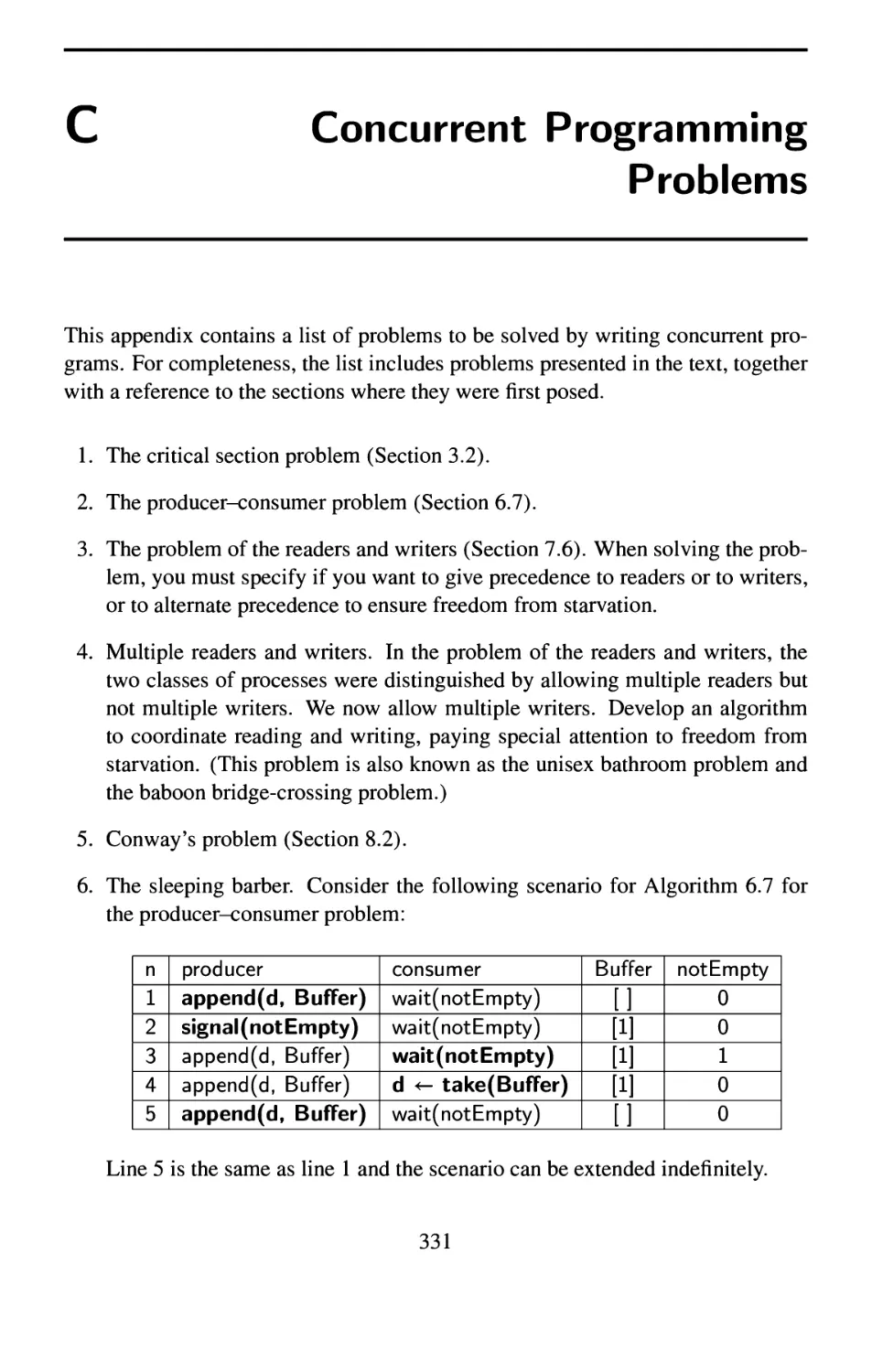
\
\
second edition
PRINCIPL
CONCUR'
1 DISTRIBU
PROGRA
•
•ENT
Eb
Ml G
I
I
. BEN'AR ( ^ ADDISON-WESLEY

Principles of Concurrent and
Distributed Programming
Visit the Principles of Concurrent and Distributed Programming, Second
Edition Companion Website at www.pearsoned.co.uk/ben-ari to find
valuable student learning material including:
• Source code for all the algorithms in the book
• Links to sites where software for studying concurrency may be downloaded.

PEARSON
Education
We work with leading authors to develop the
strongest educational materials in computing,
bringing cutting-edge thinking and best learning
practice to a global market.
Under a range of well-known imprints, including
Addison-Wesley, we craft high quality print and
electronic publications which help readers to
understand and apply their content, whether
studying or at work.
To find out more about the complete range of our
publishing, please visit us on the World Wide Web at:
www.pearsoned.co.uk

Principles of Concurrent and
Distributed Programming
Second Edition
M. Ben-Ari
ADDISON-WESLEY
Harlow, England • London • New York • Boston • San Francisco • Toronto • Sydney • Singapore • Hong Kong
Tokyo • Seoul • Taipei • New Delhi • Cape Town • Madrid • Mexico City • Amsterdam • Munich • Paris • Milan

Pearson Education Limited
Edinburgh Gate
Harlow
Essex CM20 2JE
England
and Associated Companies throughout the world
Visit us on the World Wide Web at:
www.pearsoned.co.uk
First published 1990
Second edition 2006
© Prentice Hall Europe, 1990
© Mordechai Ben-Ari, 2006
The right of Mordechai Ben-Ari to be identified as author of this work has
been asserted by him in accordance with the Copyright, Designs and Patents Act 1988.
All rights reserved. No part of this publication may be reproduced, stored in a retrieval
system, or transmitted in any form or by any means, electronic, mechanical,
photocopying, recording or otherwise, without either the prior written permission of the
publisher or a licence permitting restricted copying in the united Kingdom issued by the
Copyright Licensing Agency Ltd, 90 Tottenham Court Road, London WIT 4LP.
All trademarks used herein are the property of their respective owners. The use of any
trademark in this text does not vest in the author or publisher any trademark ownership
rights in such trademarks, nor does the use of such trademarks imply any affiliation with
or endorsement of this book by such owners.
ISBN-13: 978-0-321-31283-9
ISBN-10:0-321-31283-X
British Library Cataloguing-in-Publication Data
A catalogue record for this book is available from the British Library
Library of Congress Cataloging-in-Publication Data
A catalog record for this book is available from the Library of Congress
10 987654321
10 09 08 07 06
Printed and bound by Henry Ling Ltd, at the Dorset Press, Dorchester, Dorset
The publisher's policy is to use paper manufactured from sustainable forests.

Contents
Preface xi
1 What is Concurrent Programming? 1
1.1 Introduction 1
1.2 Concurrency as abstract parallelism 2
1.3 Multitasking 4
1.4 The terminology of concurrency 4
1.5 Multiple computers 5
1.6 The challenge of concurrent programming 5
2 The Concurrent Programming Abstraction 7
2.1 The role of abstraction 7
2.2 Concurrent execution as interleaving of atomic statements .... 8
2.3 Justification of the abstraction 13
2.4 Arbitrary interleaving 17
2.5 Atomic statements 19
2.6 Correctness 21
2.7 Fairness 23
2.8 Machine-code instructions 24
2.9 Volatile and non-atomic variables 28
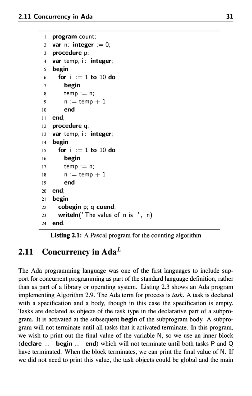
2.10 The BACI concurrency simulator 29
2.11 Concurrency in Ada 31
v

vi Contents
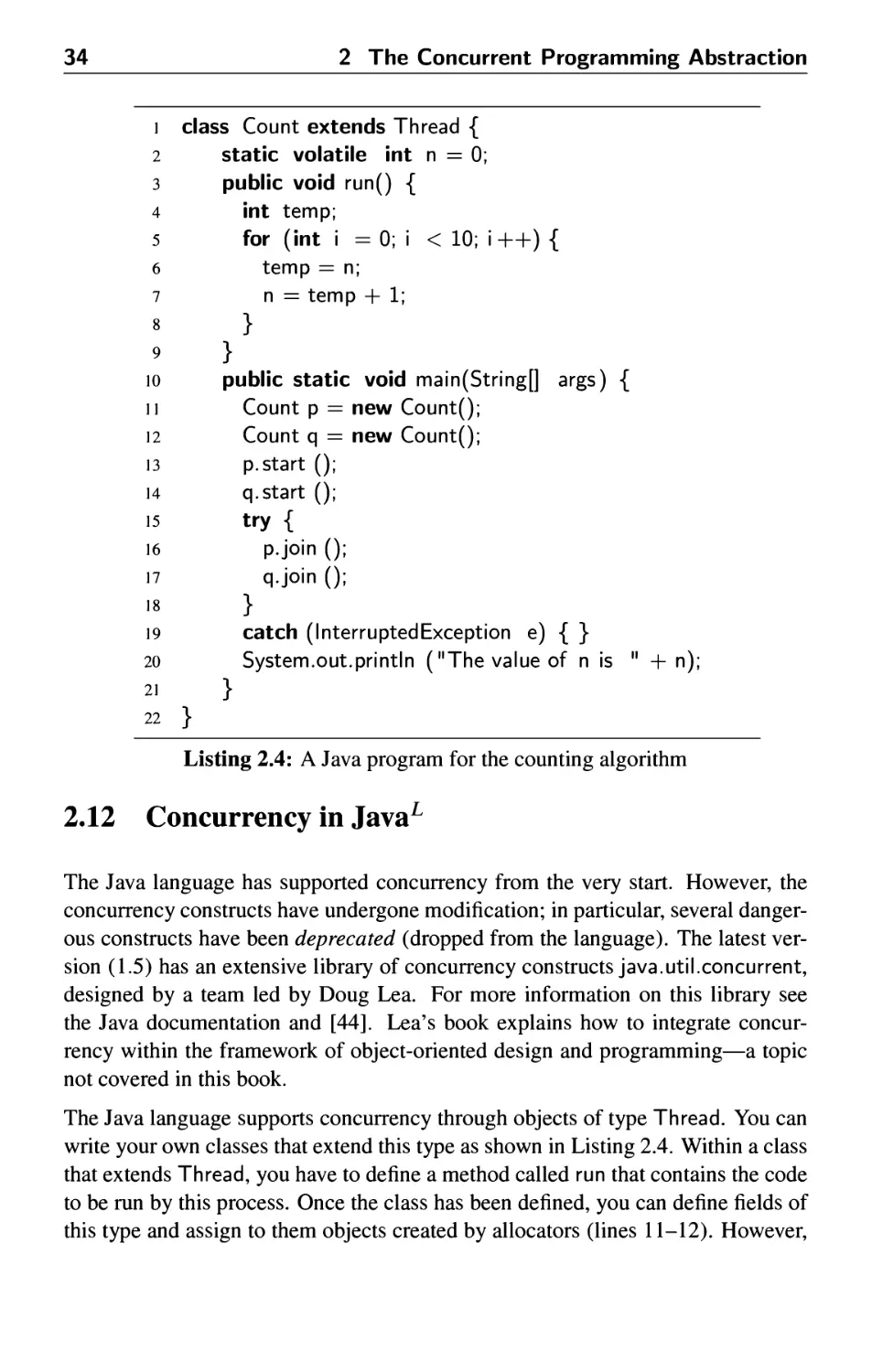
2.12 Concurrency in Java 34
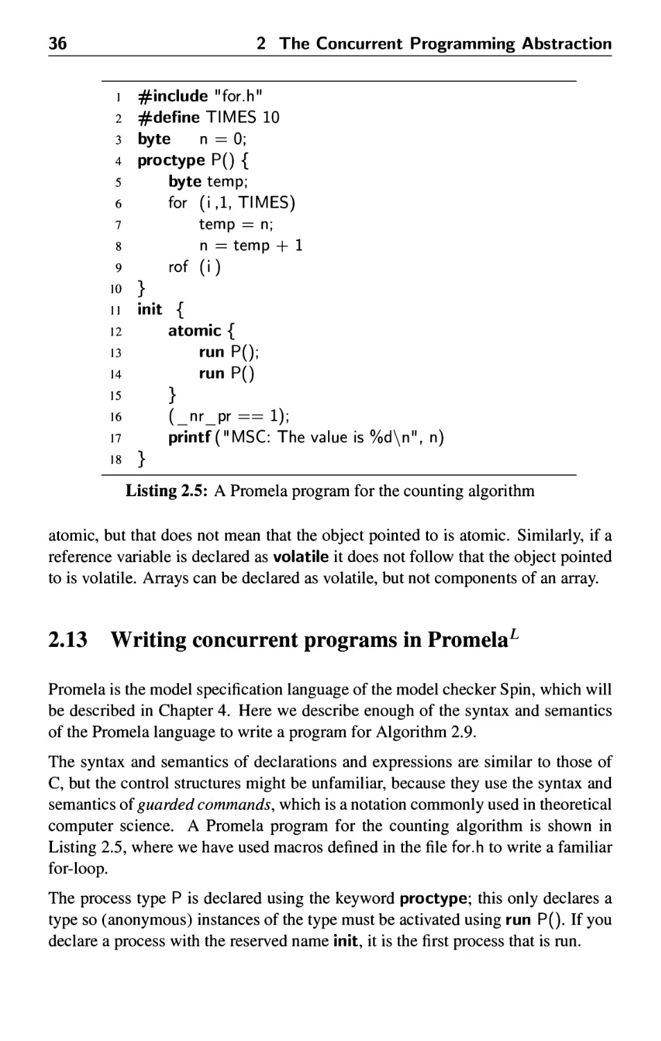
2.13 Writing concurrent programs in Promela 36
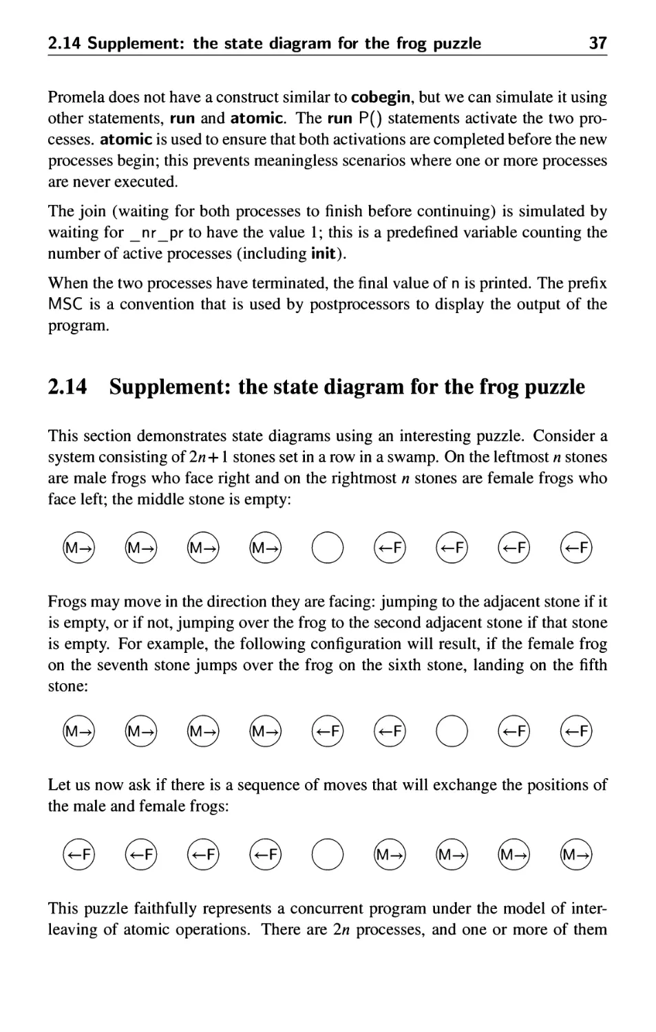
2.14 Supplement: the state diagram for the frog puzzle 37
3 The Critical Section Problem 45
3.1 Introduction 45
3.2 The definition of the problem 45
3.3 First attempt 48
3.4 Proving correctness with state diagrams 49
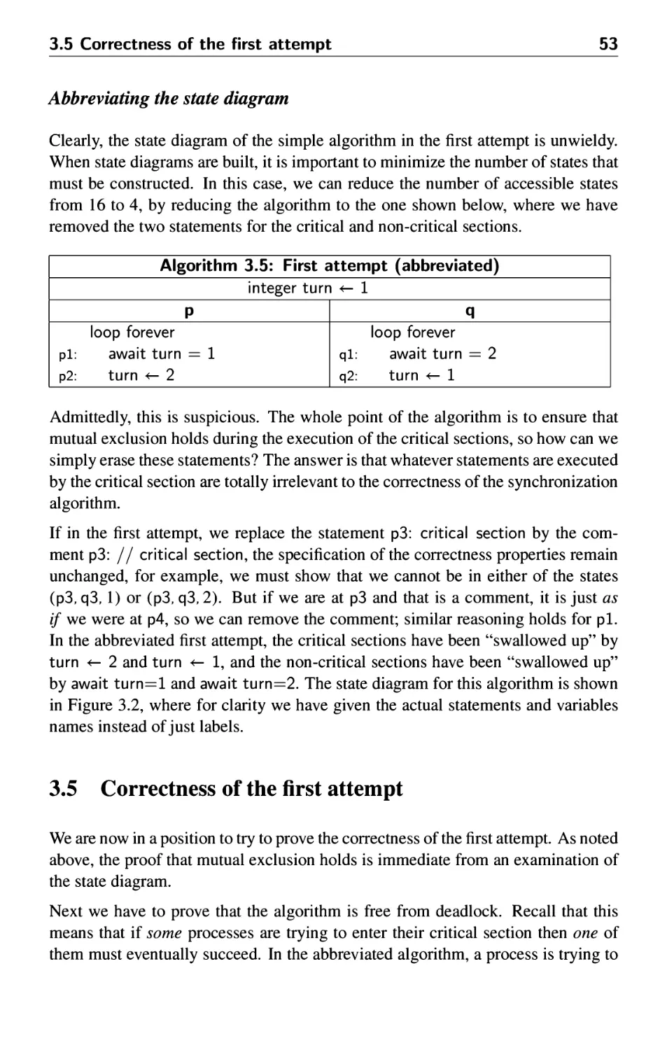
3.5 Correctness of the first attempt 53
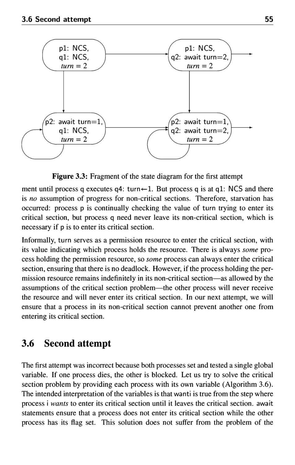
3.6 Second attempt 55
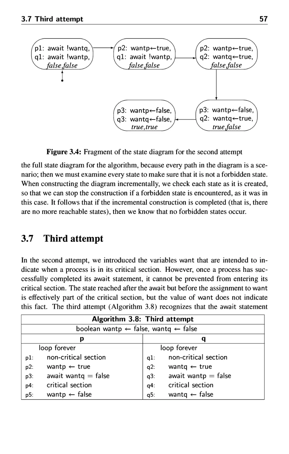
3.7 Third attempt 57
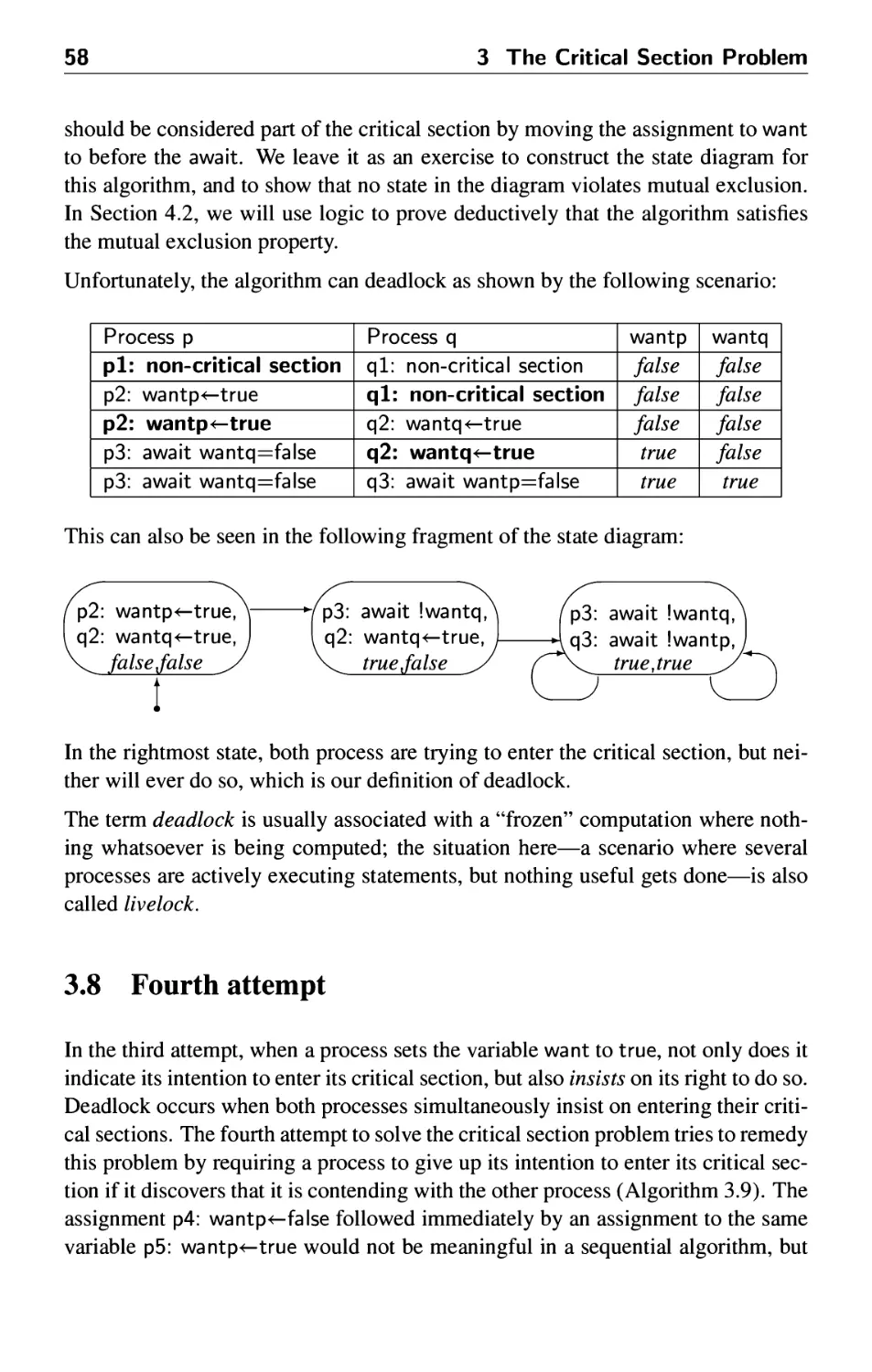
3.8 Fourth attempt 58
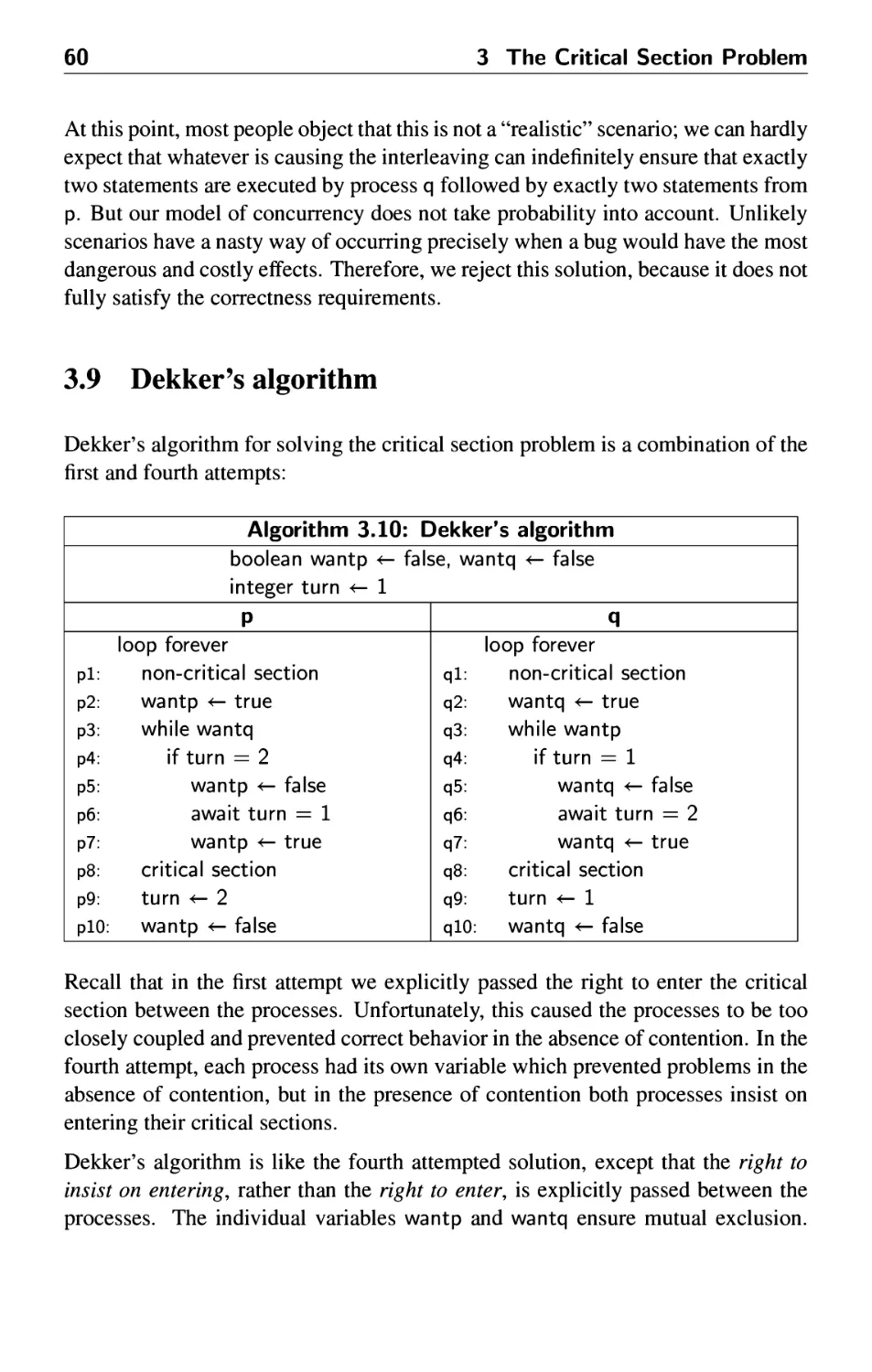
3.9 Dekker's algorithm 60
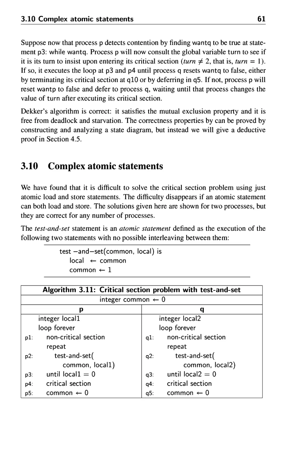
3.10 Complex atomic statements 61
4 Verification of Concurrent Programs 67
4.1 Logical specification of correctness properties 68
4.2 Inductive proofs of invariants 69
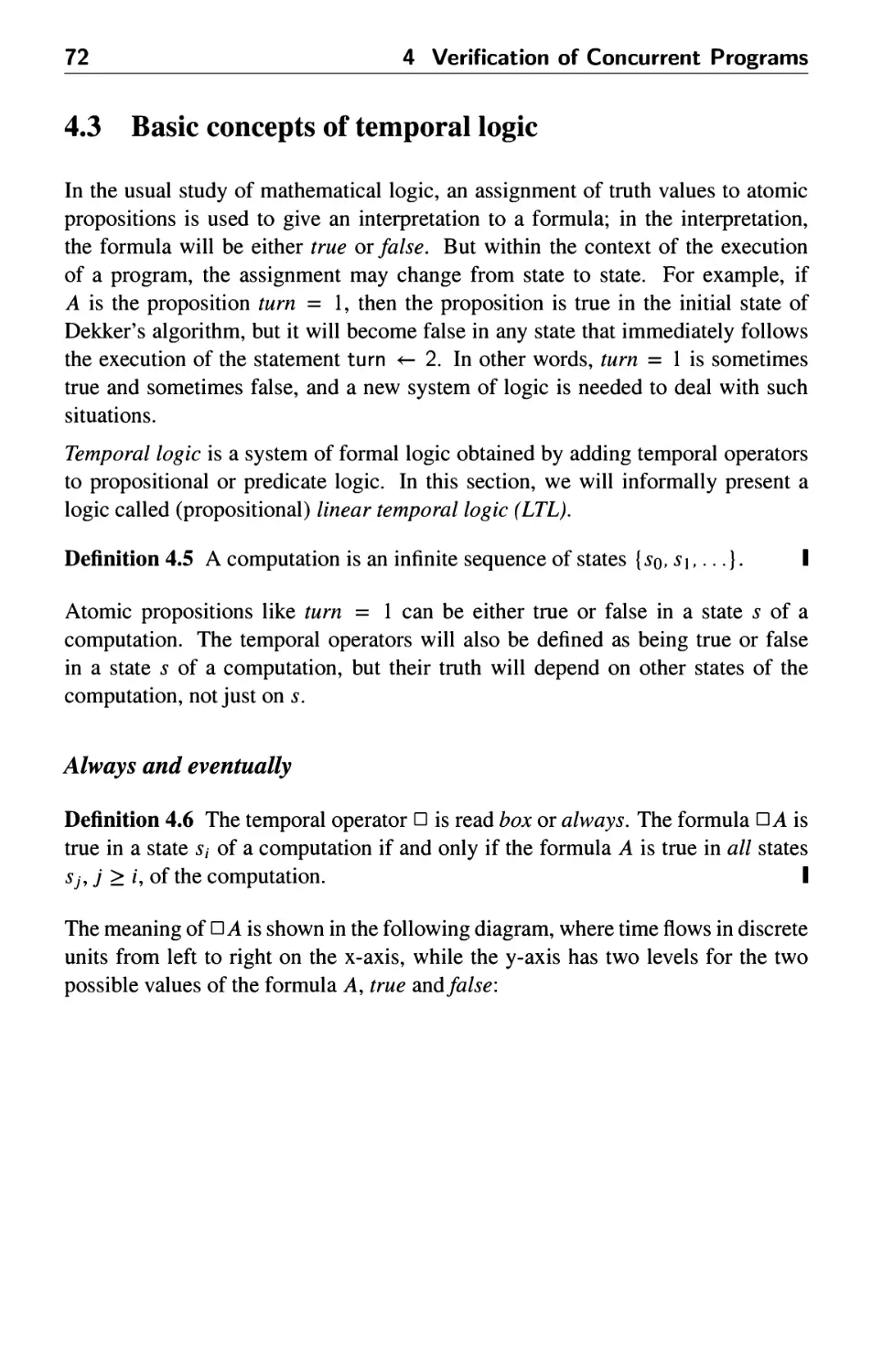
4.3 Basic concepts of temporal logic 72
4.4 Advanced concepts of temporal logic 75
4.5 A deductive proof of Dekker's algorithm 79
4.6 Model checking 83
4.7 Spin and the Promela modeling language 83
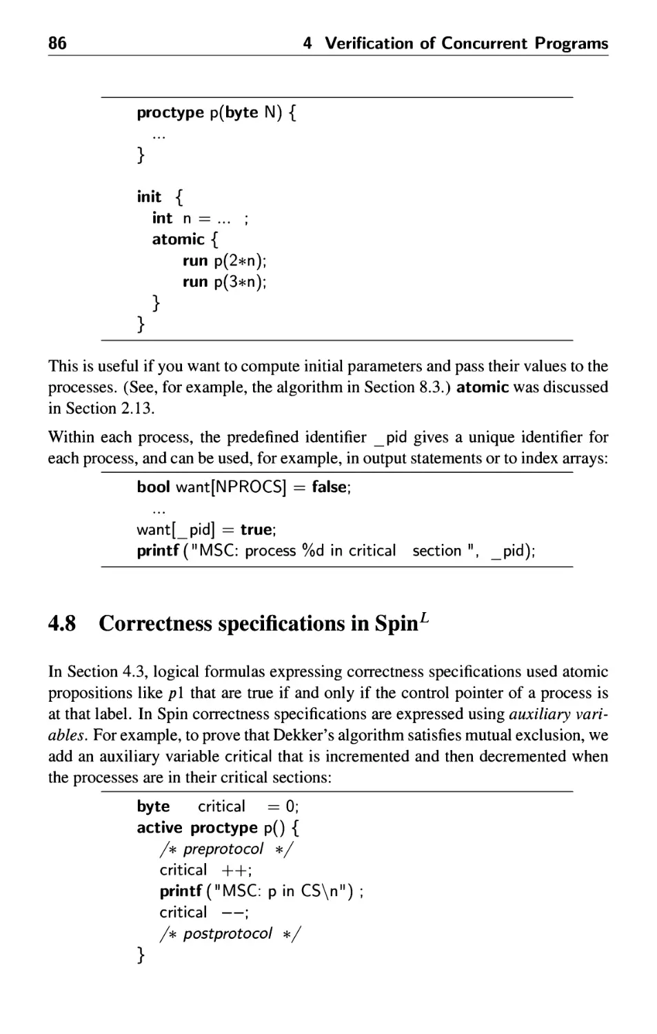
4.8 Correctness specifications in Spin 86
4.9 Choosing a verification technique 88
5 Advanced Algorithms for the Critical Section Problem 93
5.1 The bakery algorithm 93
5.2 The bakery algorithm for AT processes 95
5.3 Less restrictive models of concurrency 96

Contents vii
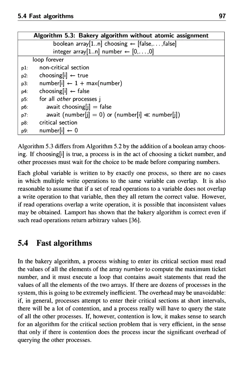
5.4 Fast algorithms 97
5.5 Implementations in Promela 104
6 Semaphores 107
6.1 Process states 107
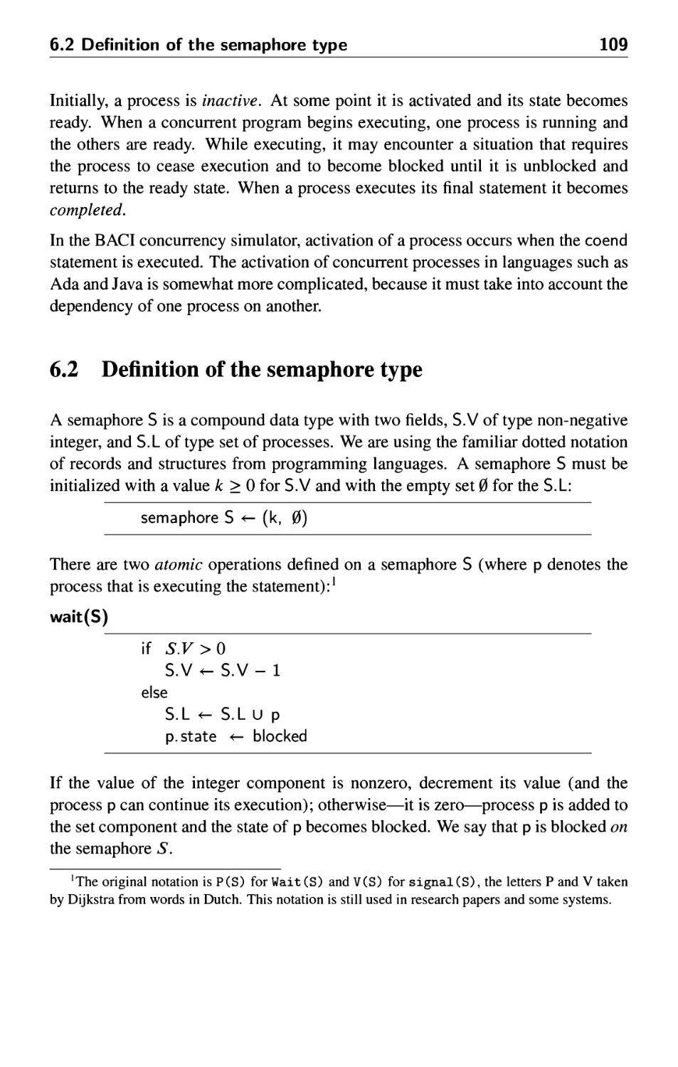
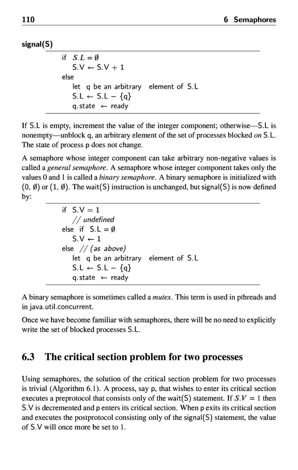
6.2 Definition of the semaphore type 109
6.3 The critical section problem for two processes 110
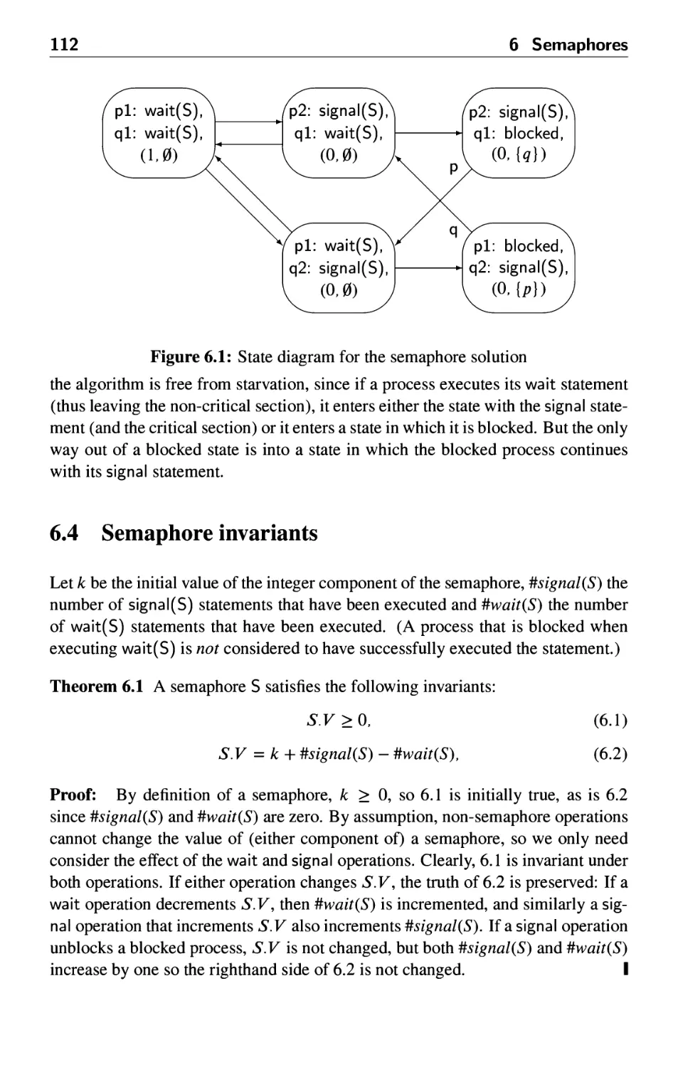
6.4 Semaphore invariants 112
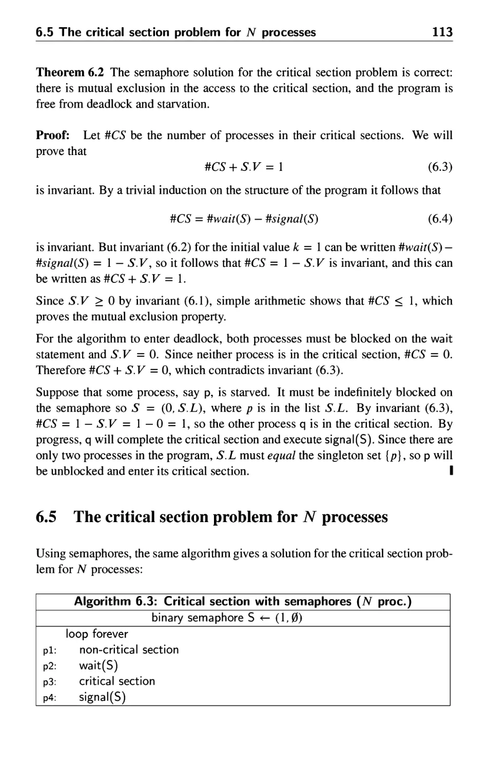
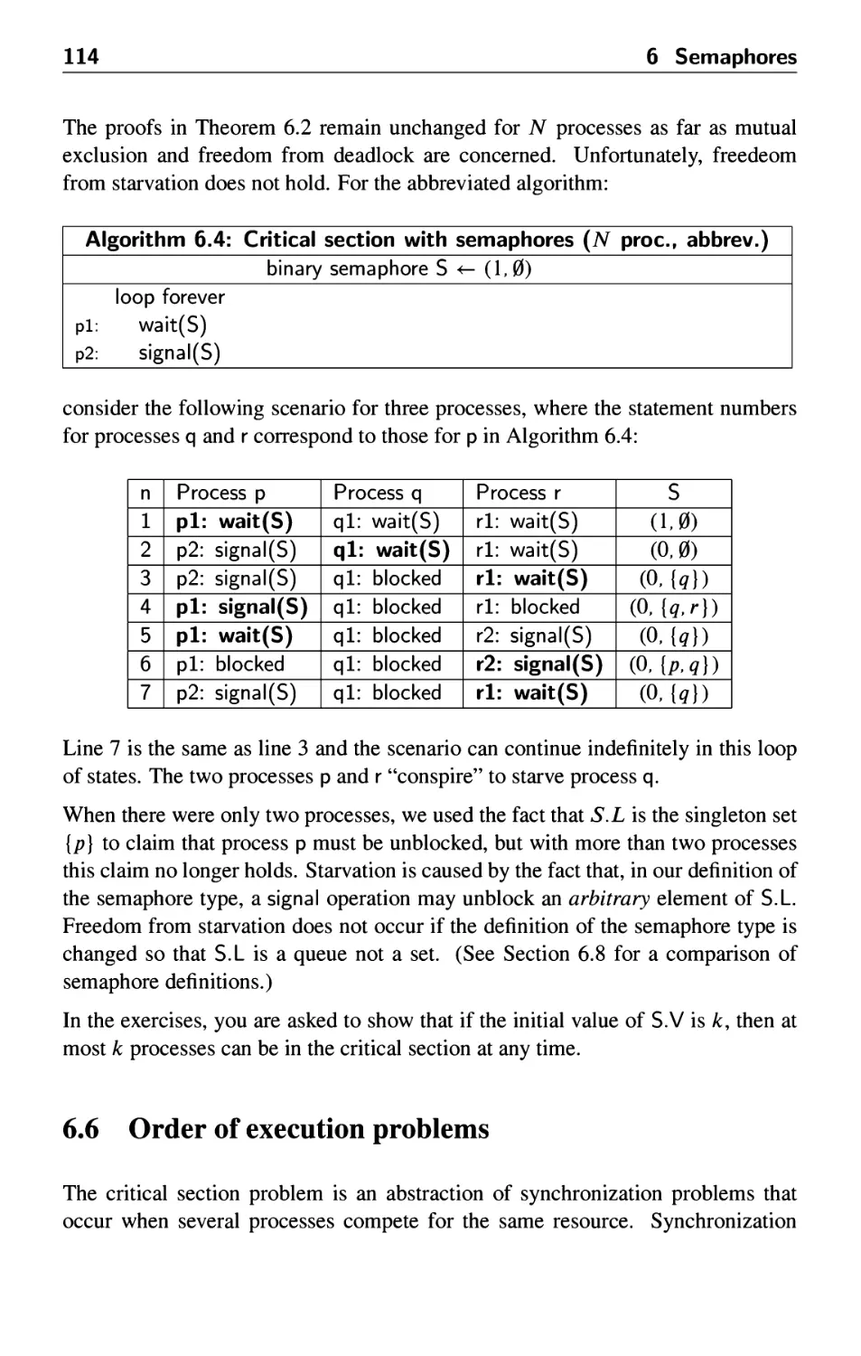
6.5 The critical section problem for AT processes 113
6.6 Order of execution problems 114
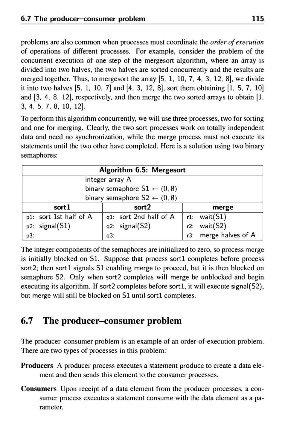
6.7 The producer-consumer problem 115
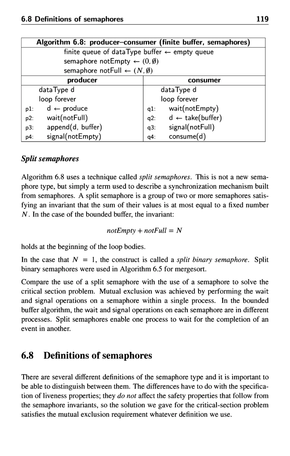
6.8 Definitions of semaphores 119
6.9 The problem of the dining philosophers 122
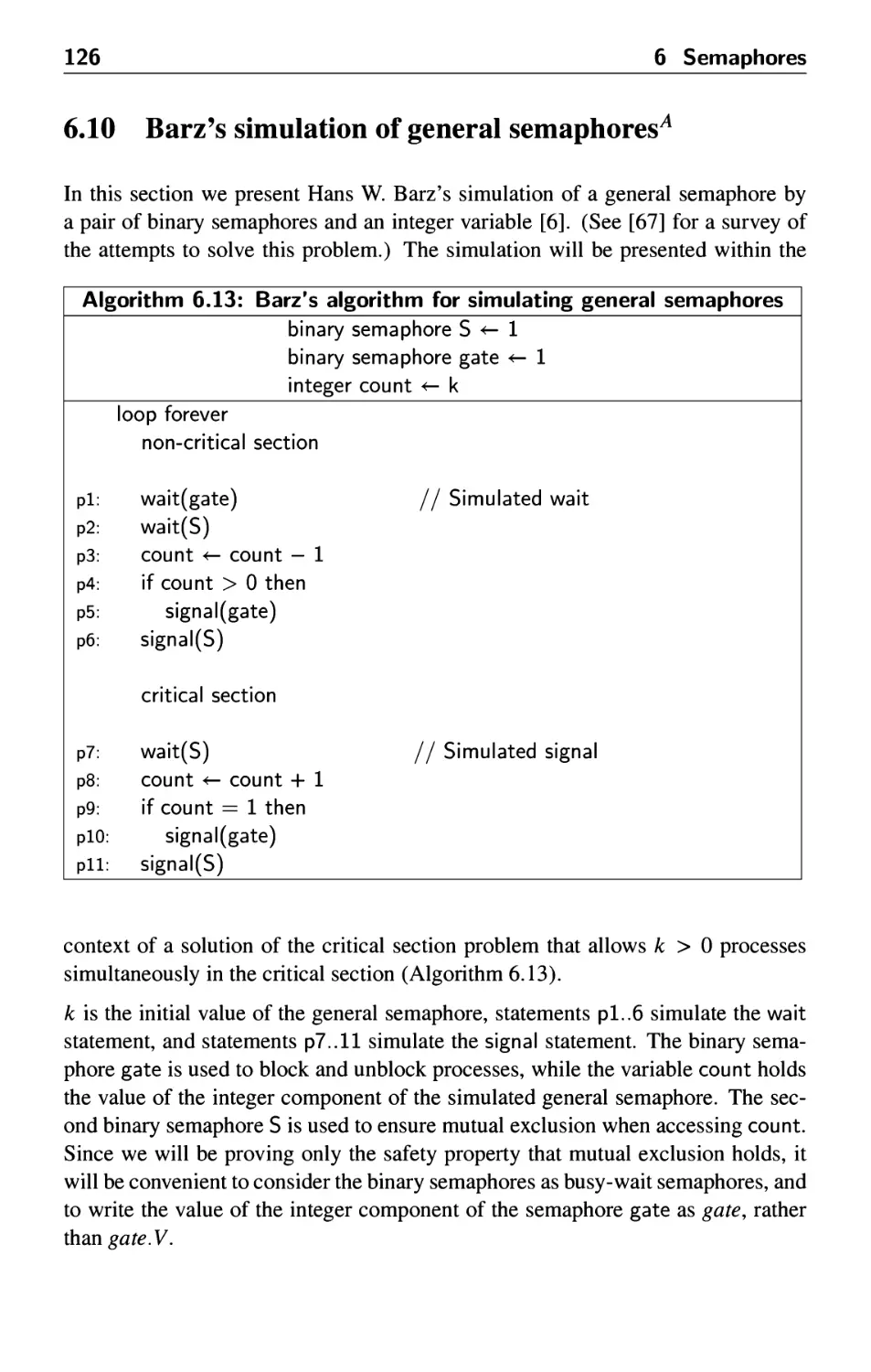
6.10 Barz's simulation of general semaphores 126
6.11 Udding's starvation-free algorithm 129
6.12 Semaphores in BACI 131
6.13 Semaphores in Ada 132
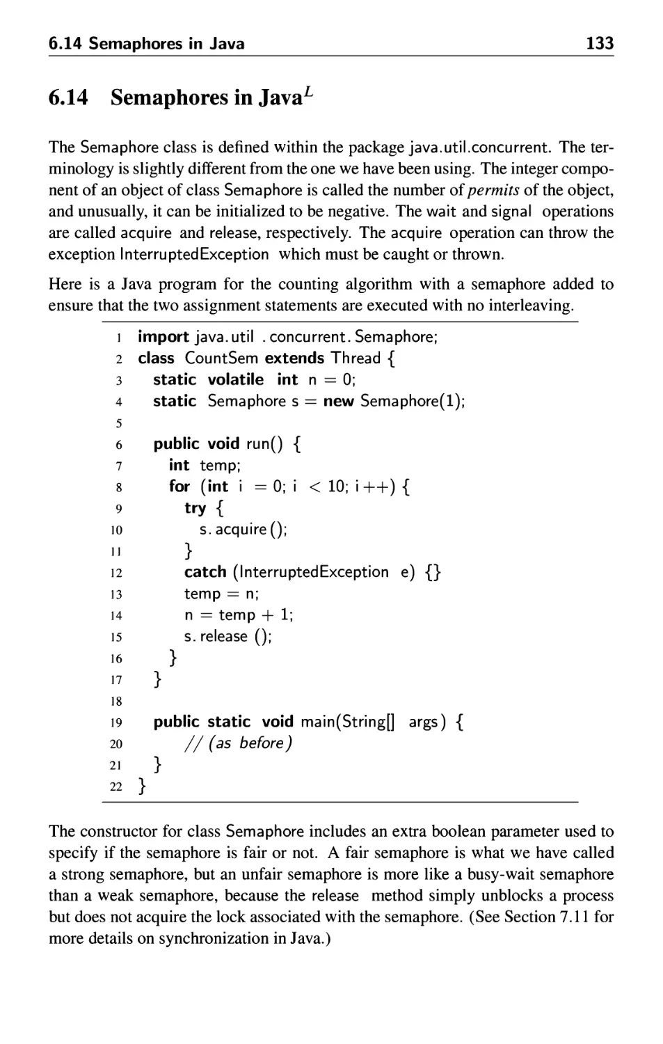
6.14 Semaphores in Java 133
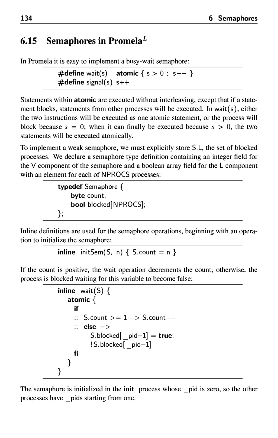
6.15 Semaphores in Promela 134
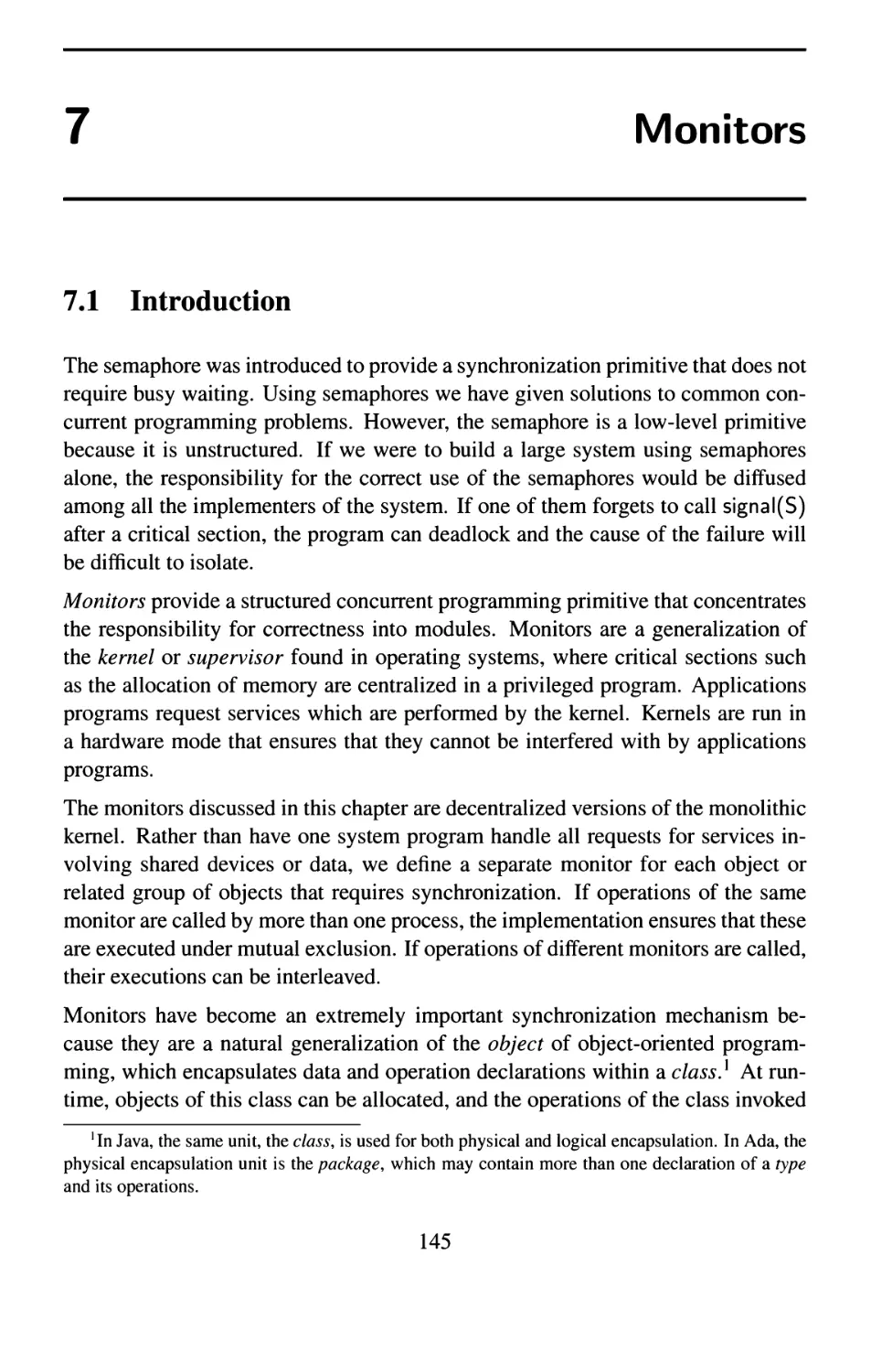
7 Monitors 145
7.1 Introduction 145
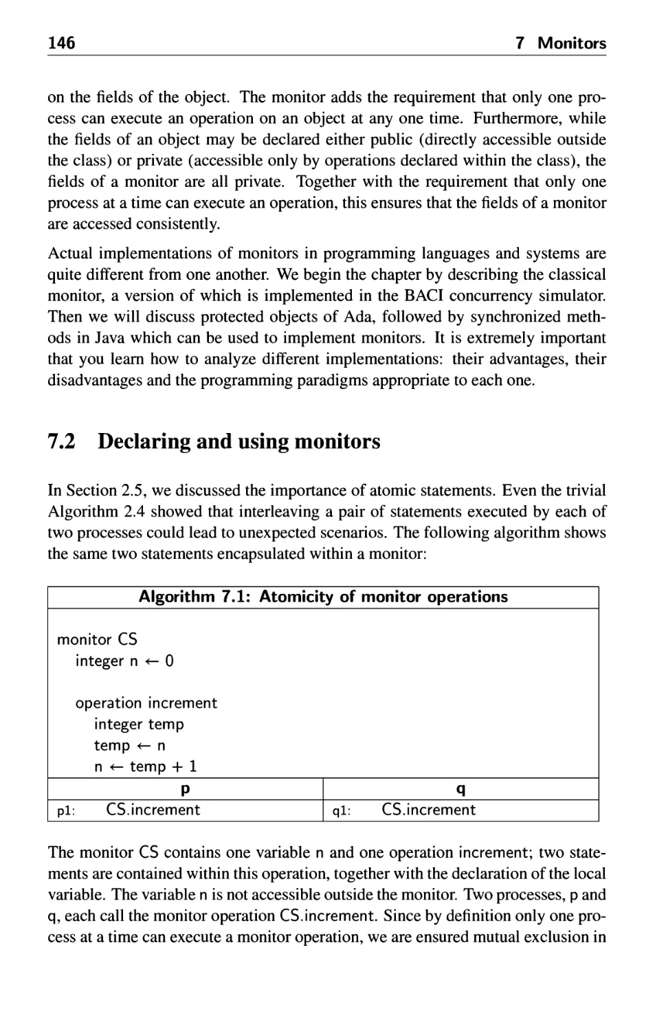
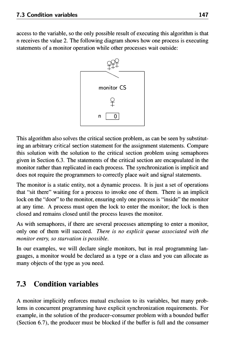
7.2 Declaring and using monitors 146
7.3 Condition variables 147
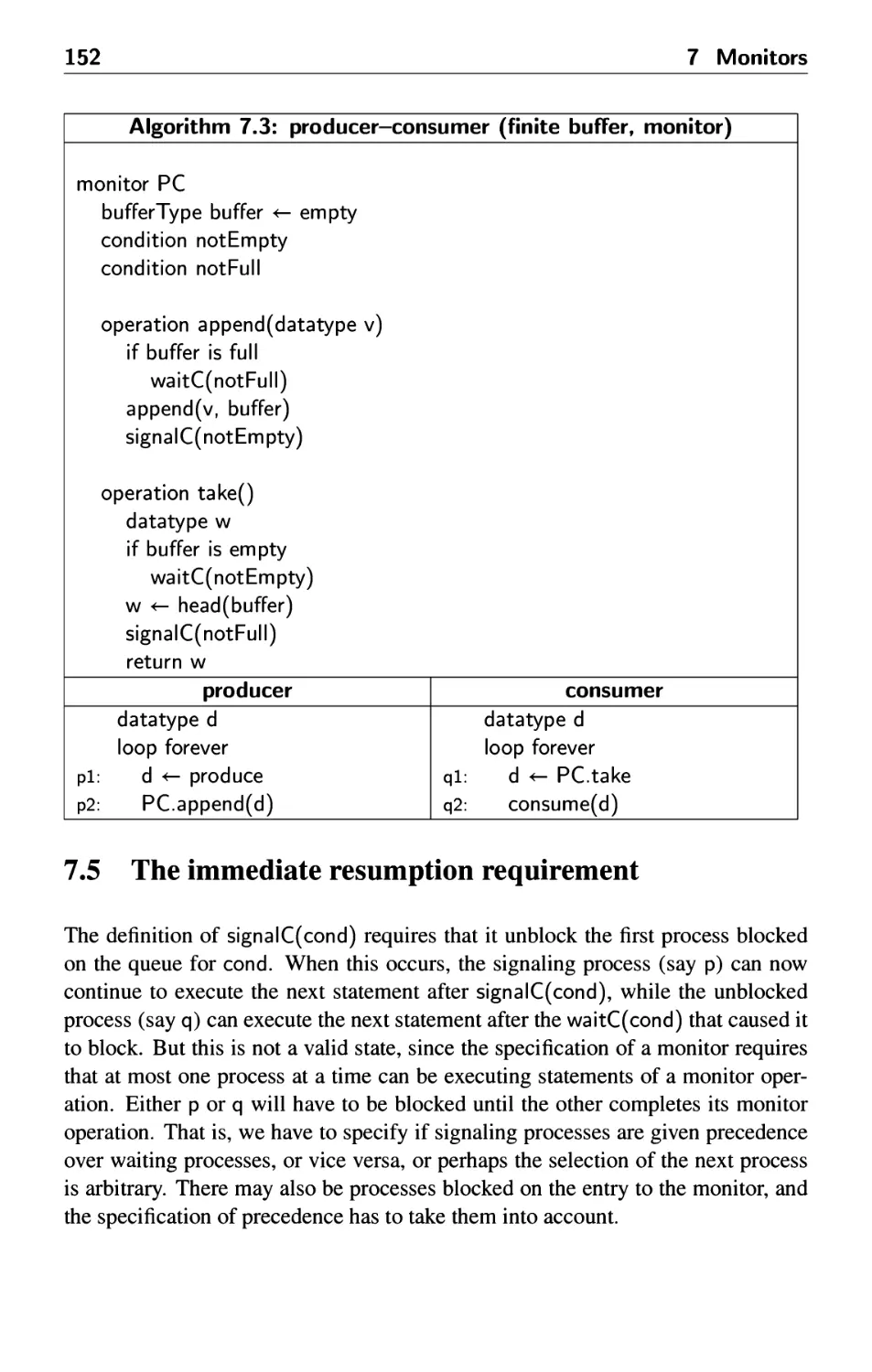
7.4 The producer-consumer problem 151
7.5 The immediate resumption requirement 152
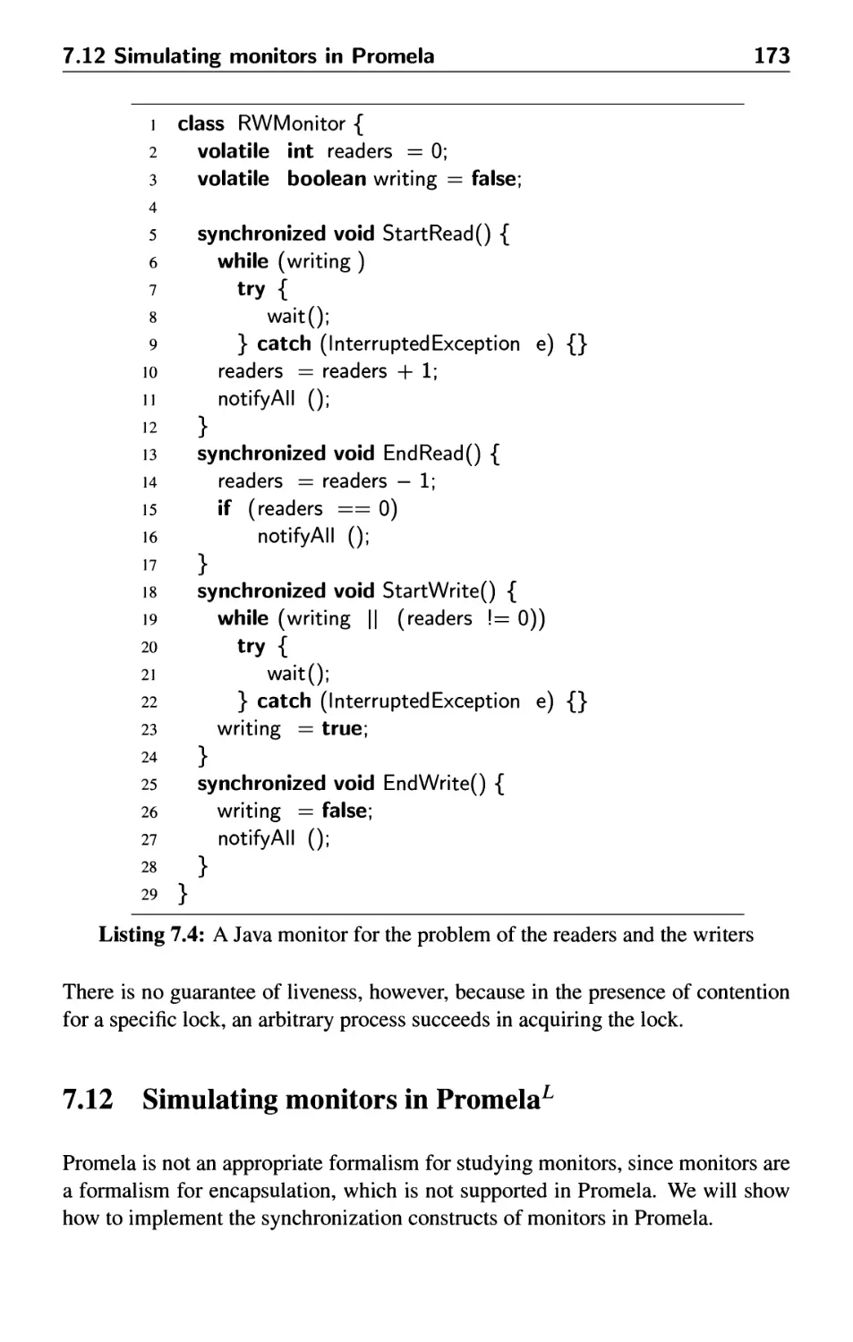
7.6 The problem of the readers and writers 154
7.7 Correctness of the readers and writers algorithm 157
7.8 A monitor solution for the dining philosophers 160
7.9 Monitors in BACI 162

viii Contents
7.10 Protected objects 162
7.11 Monitors in Java 167
7.12 Simulating monitors in Promela 173
8 Channels 179
8.1 Models for communications 179
8.2 Channels 181
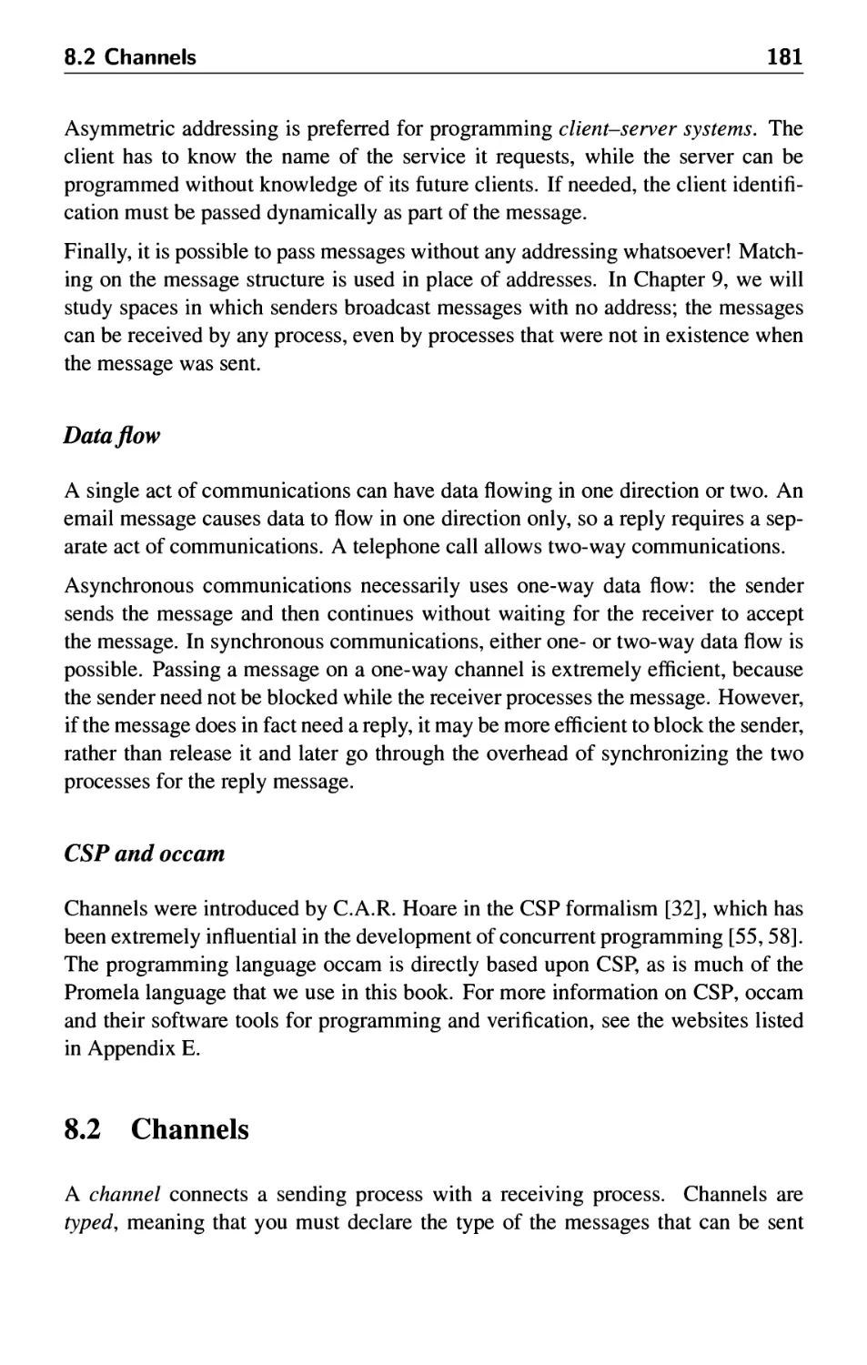
8.3 Parallel matrix multiplication 183
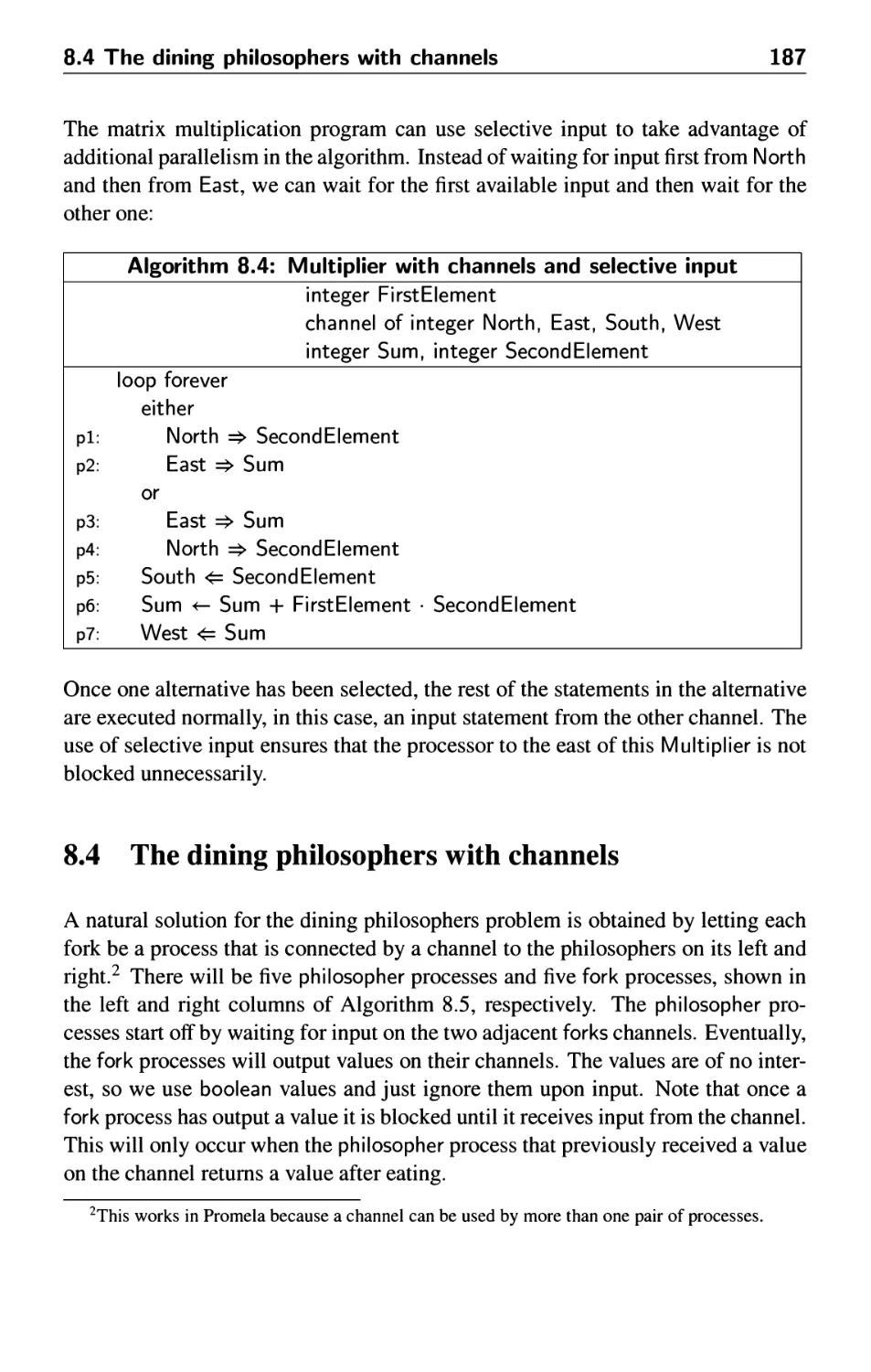
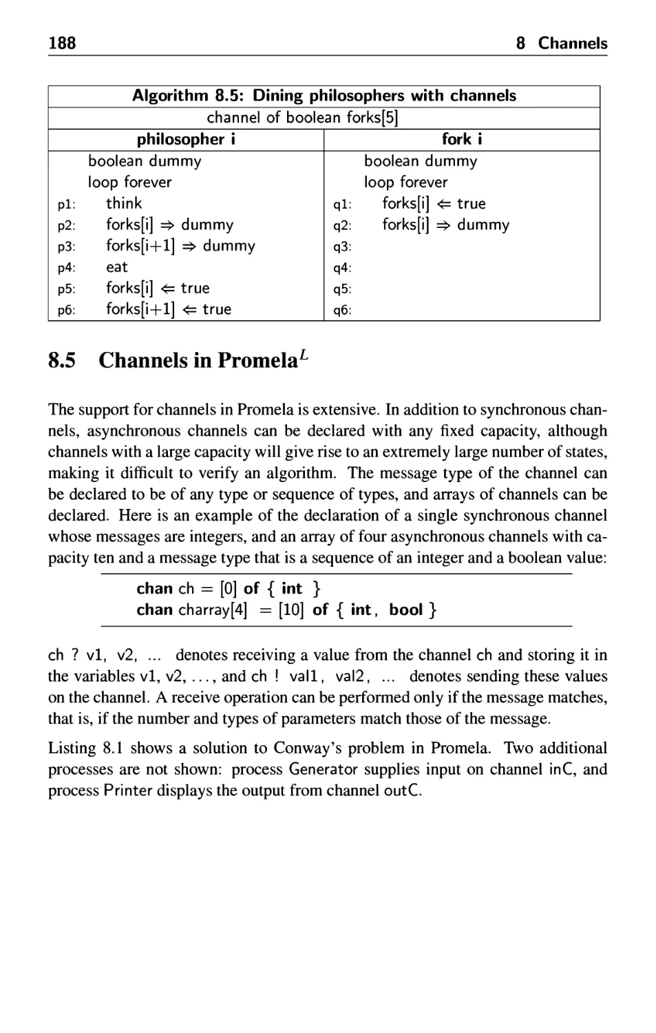
8.4 The dining philosophers with channels 187
8.5 Channels in Promela 188
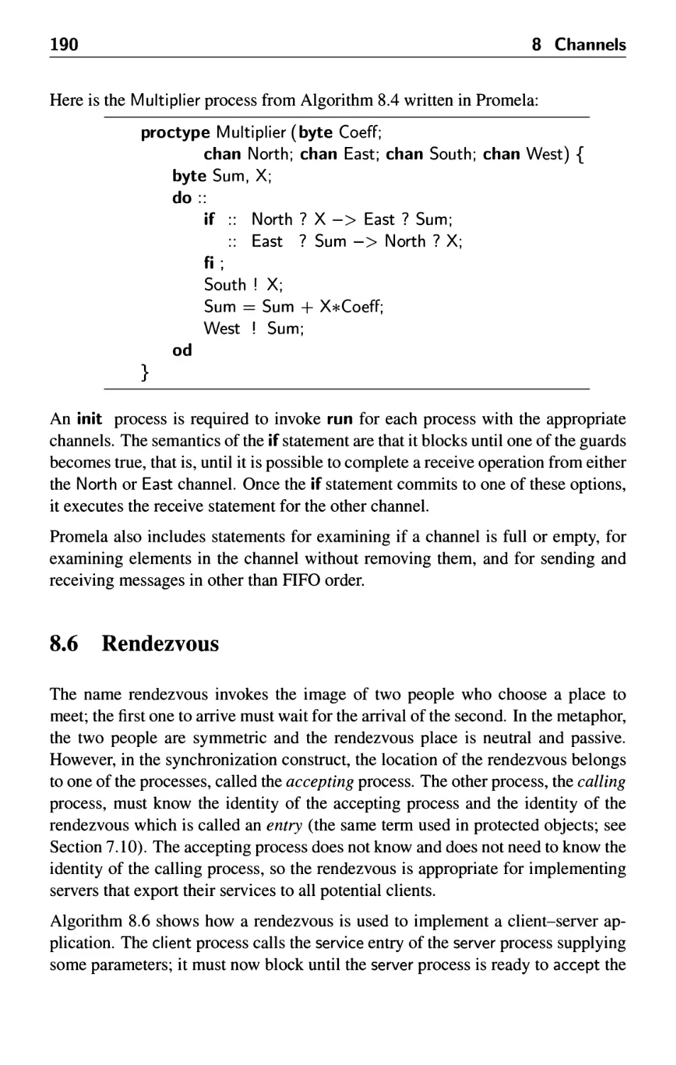
8.6 Rendezvous 190
8.7 Remote procedure calls 193
9 Spaces 197
9.1 The Linda model 197
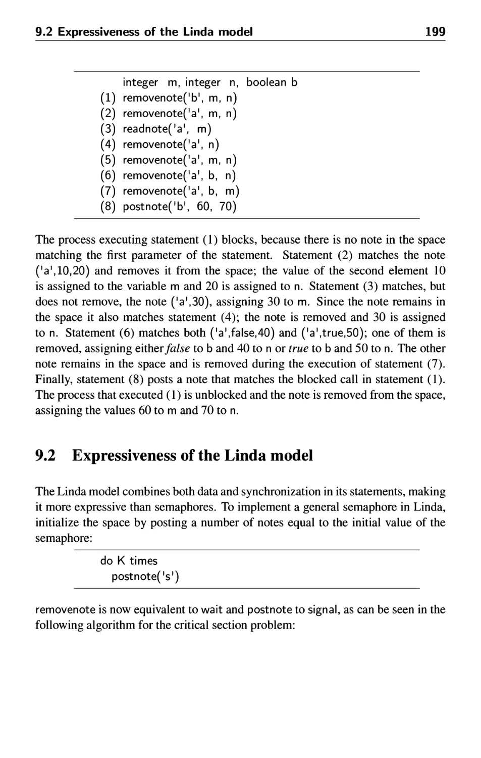
9.2 Expressiveness of the Linda model 199
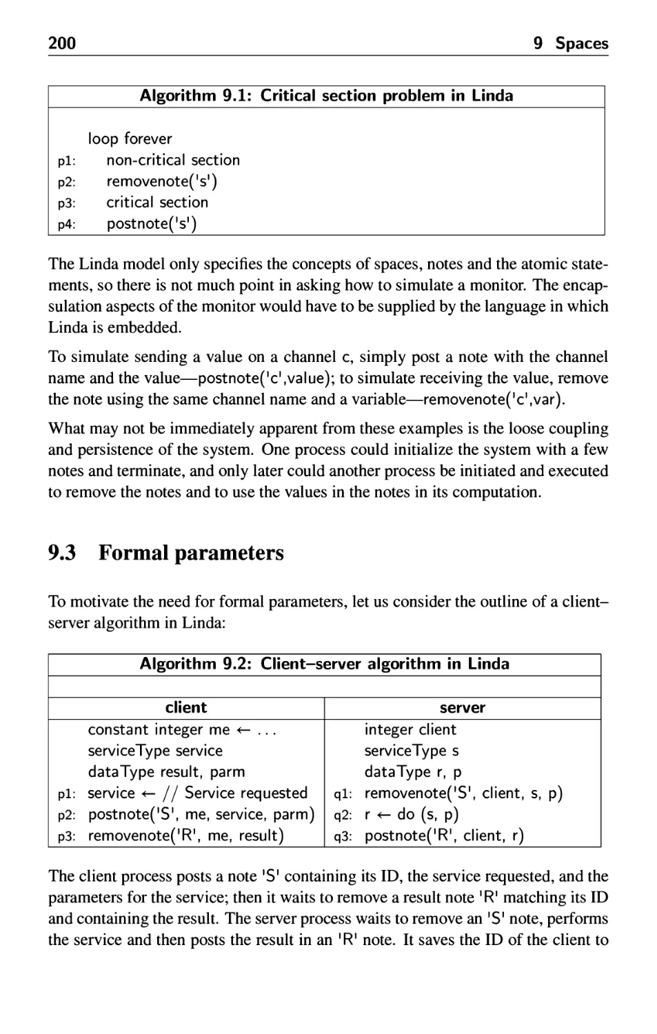
9.3 Formal parameters 200
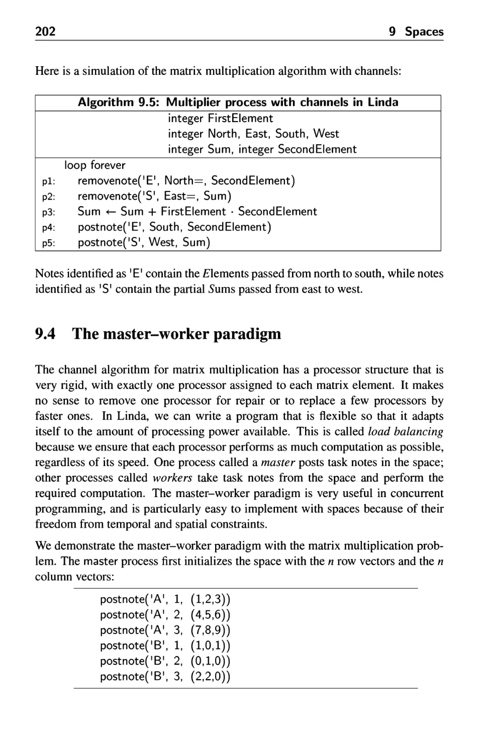
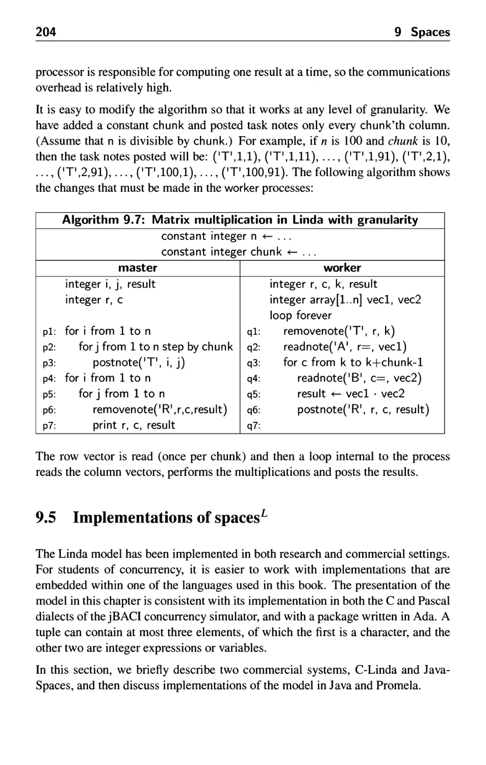
9.4 The master-worker paradigm 202
9.5 Implementations of spaces 204
10 Distributed Algorithms 211
10.1 The distributed systems model 211
10.2 Implementations 215
10.3 Distributed mutual exclusion 216
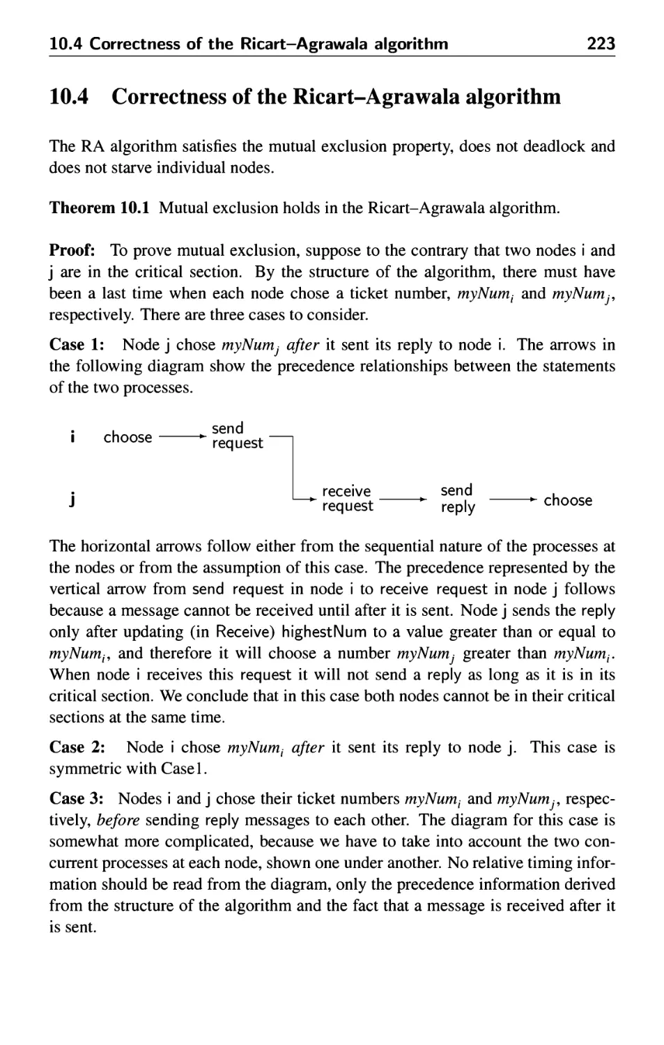
10.4 Correctness of the Ricart-Agrawala algorithm 223
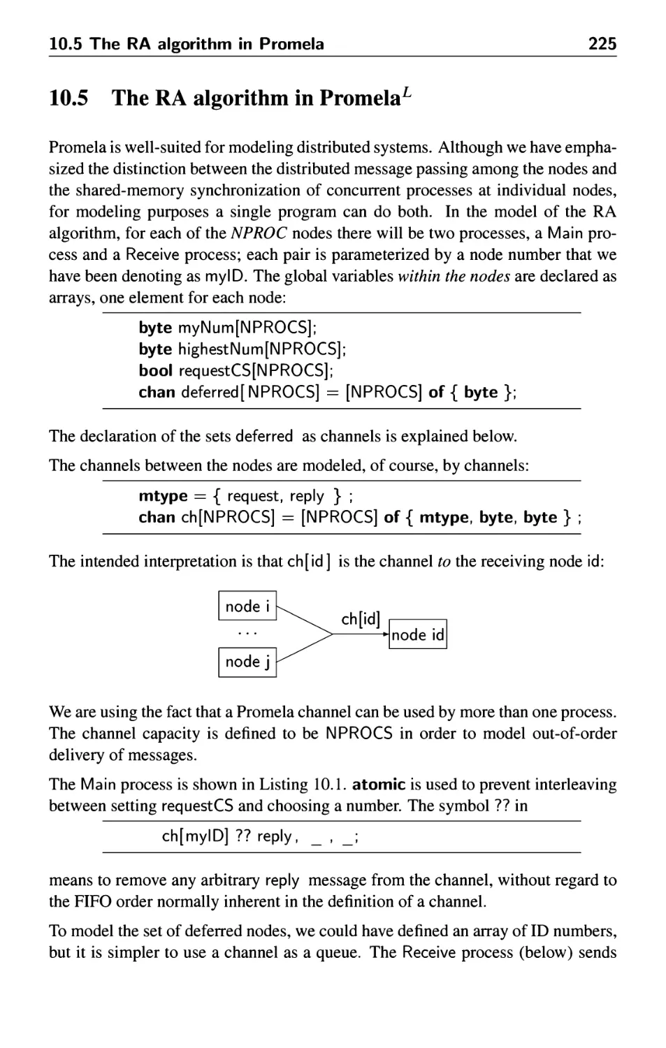
10.5 The RA algorithm in Promela 225
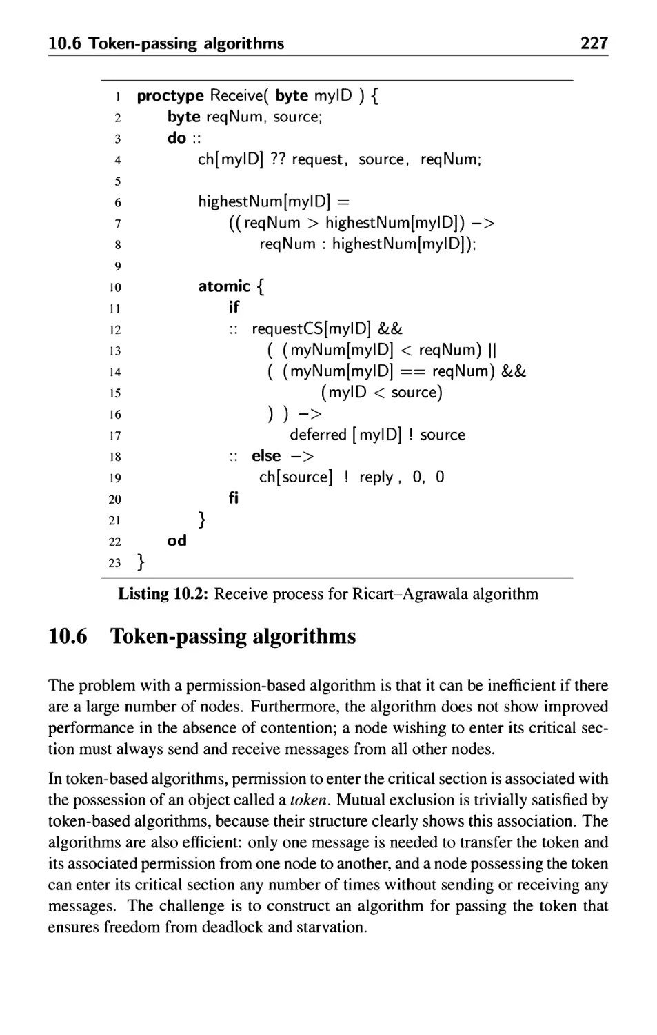
10.6 Token-passing algorithms 227
10.7 Tokens in virtual trees 230
11 Global Properties 237
11.1 Distributed termination 237

Contents
ix
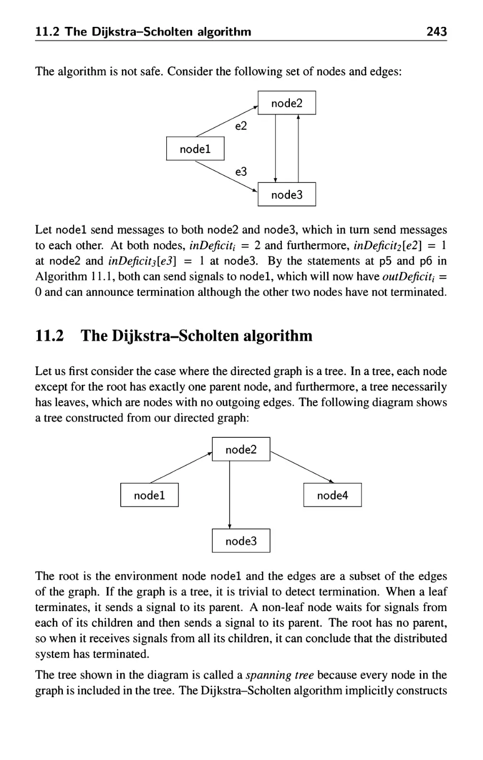
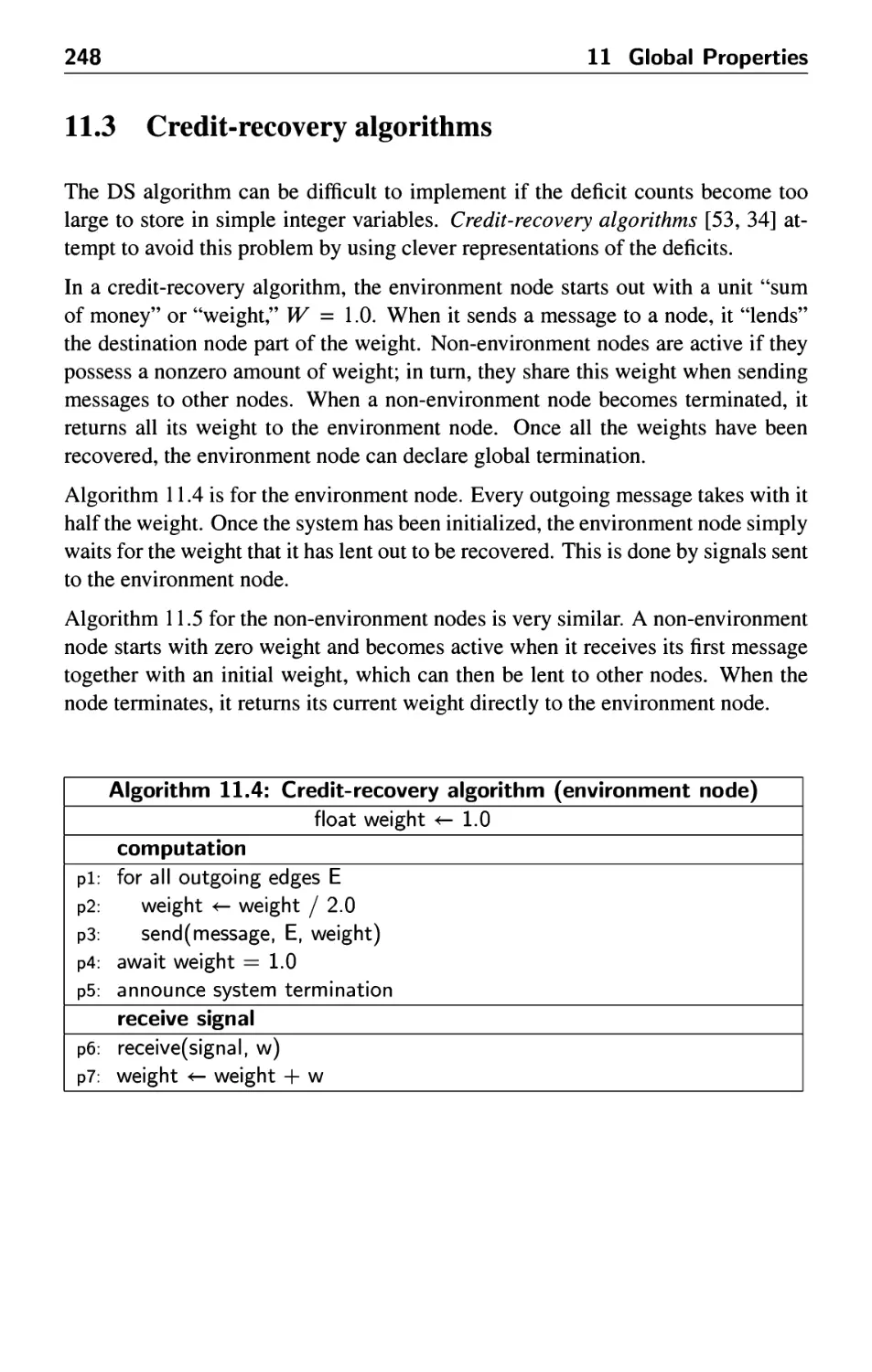
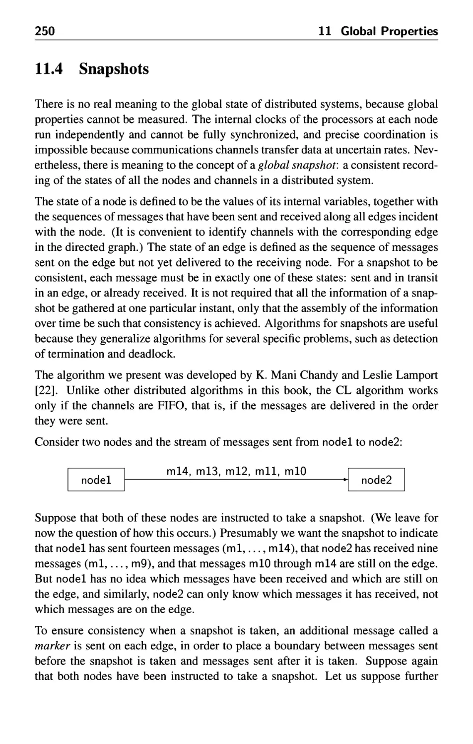
11.2 The Dijkstra-Scholten algorithm 243
11.3 Credit-recovery algorithms 248
11.4 Snapshots 250
12 Consensus 257
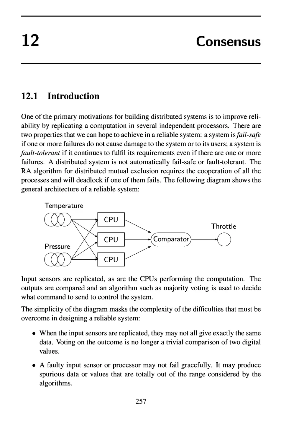
12.1 Introduction 257
12.2 The problem statement 258
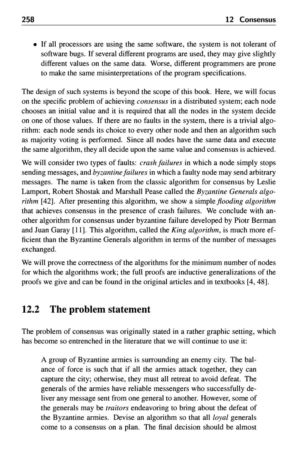
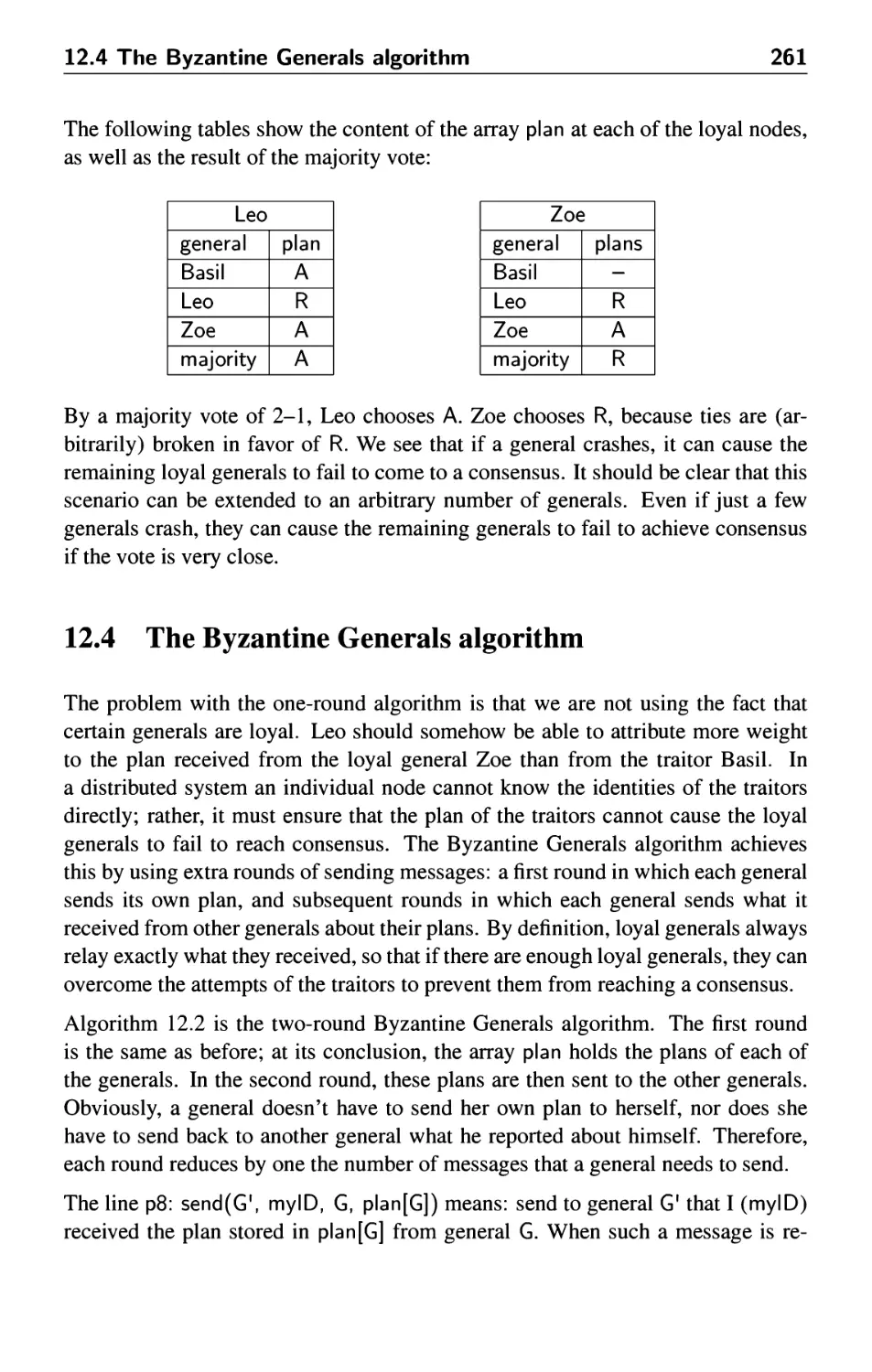
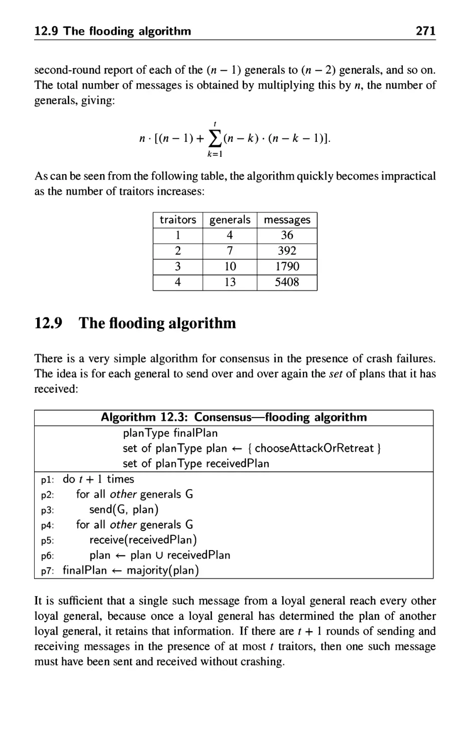
12.3 A one-round algorithm 260
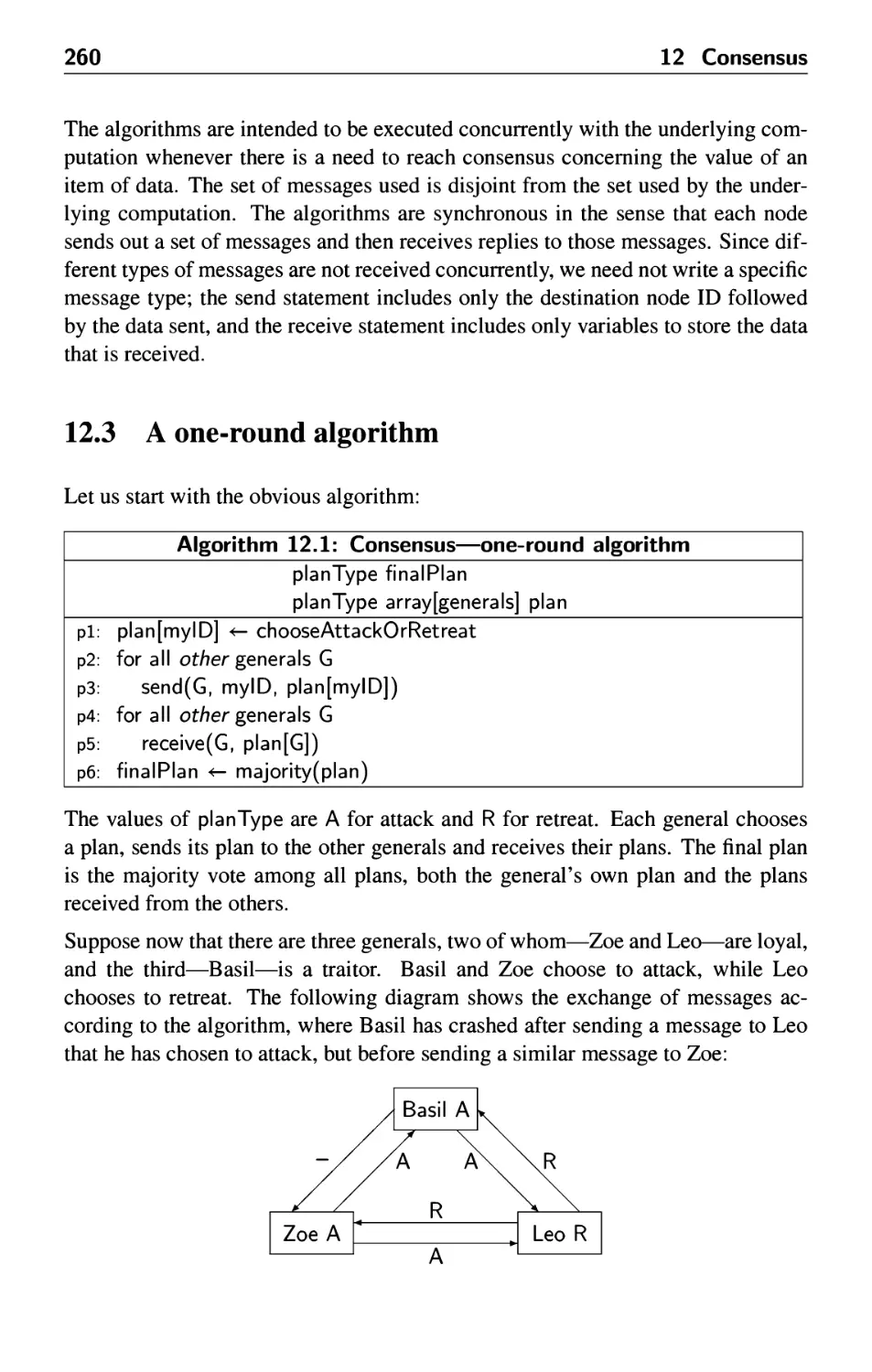
12.4 The Byzantine Generals algorithm 261
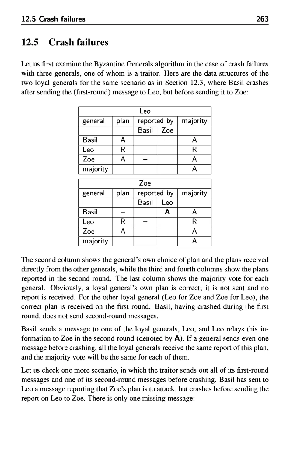
12.5 Crash failures 263
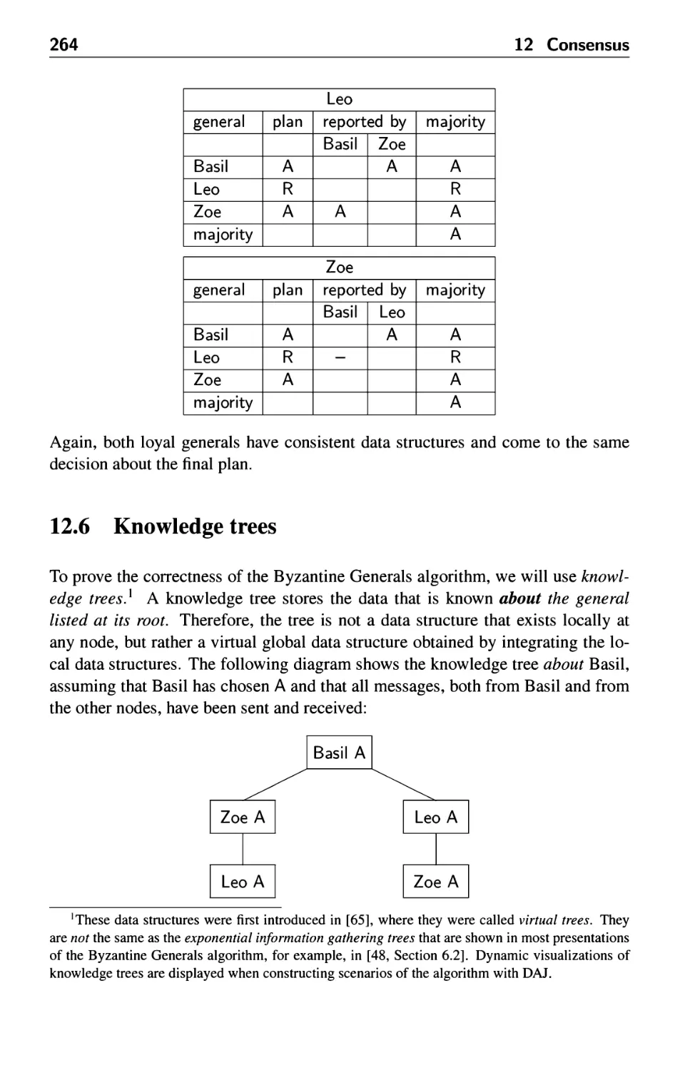
12.6 Knowledge trees 264
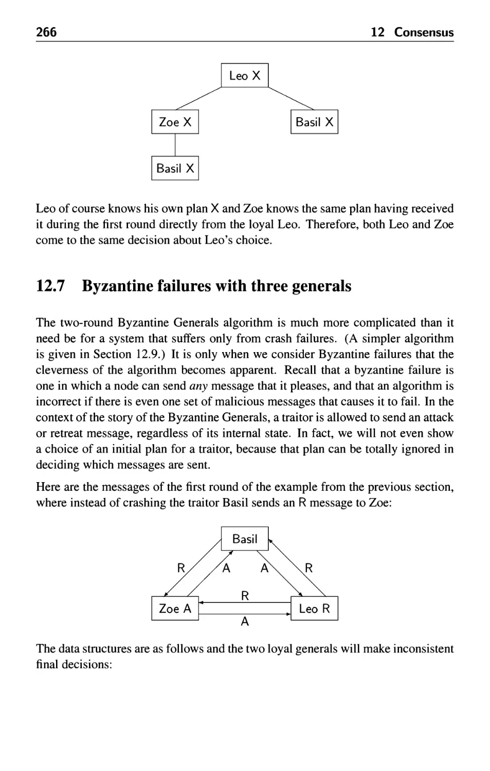
12.7 Byzantine failures with three generals 266
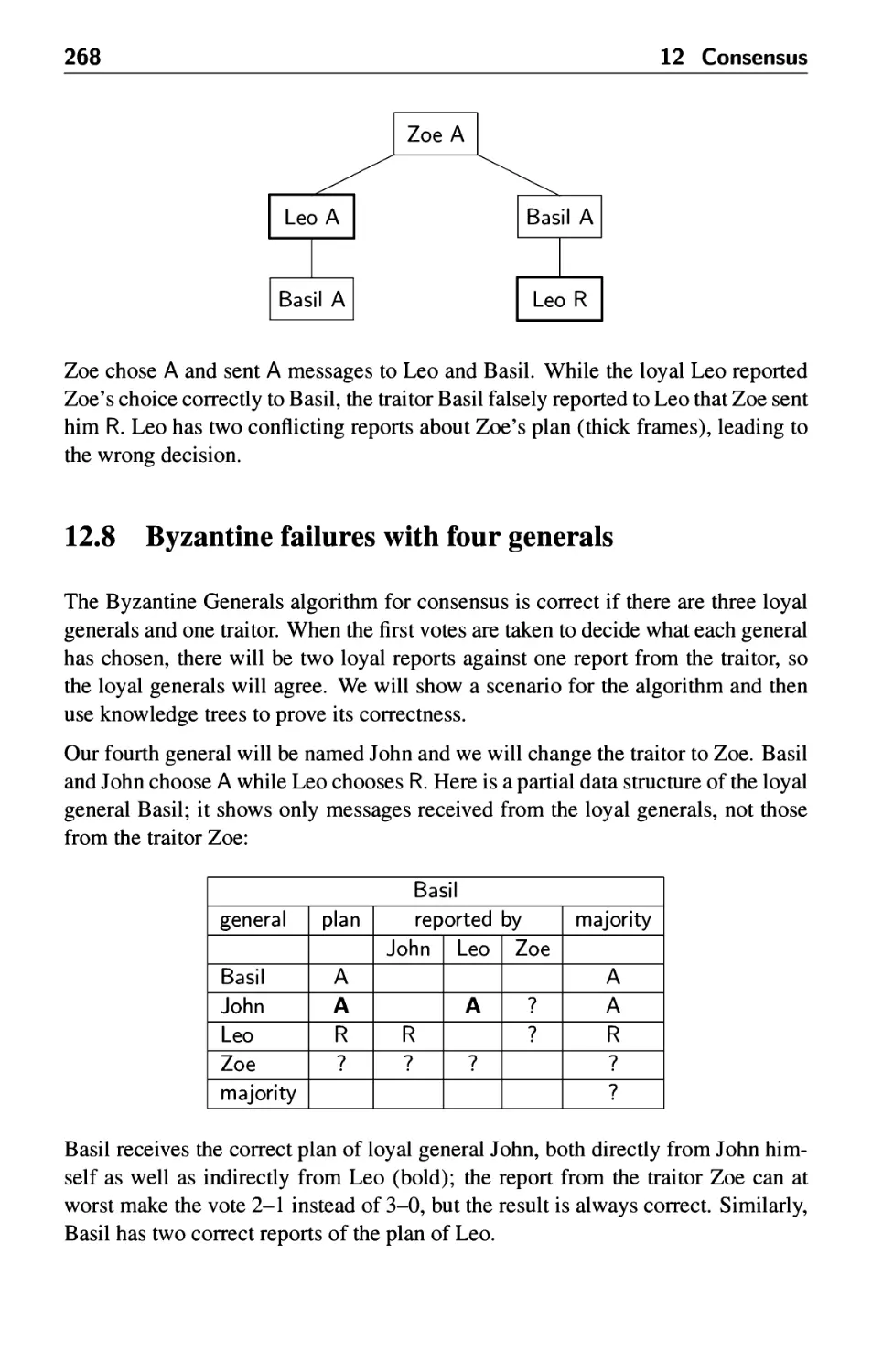
12.8 Byzantine failures with four generals 268
12.9 The flooding algorithm 271
12.10 The King algorithm 274
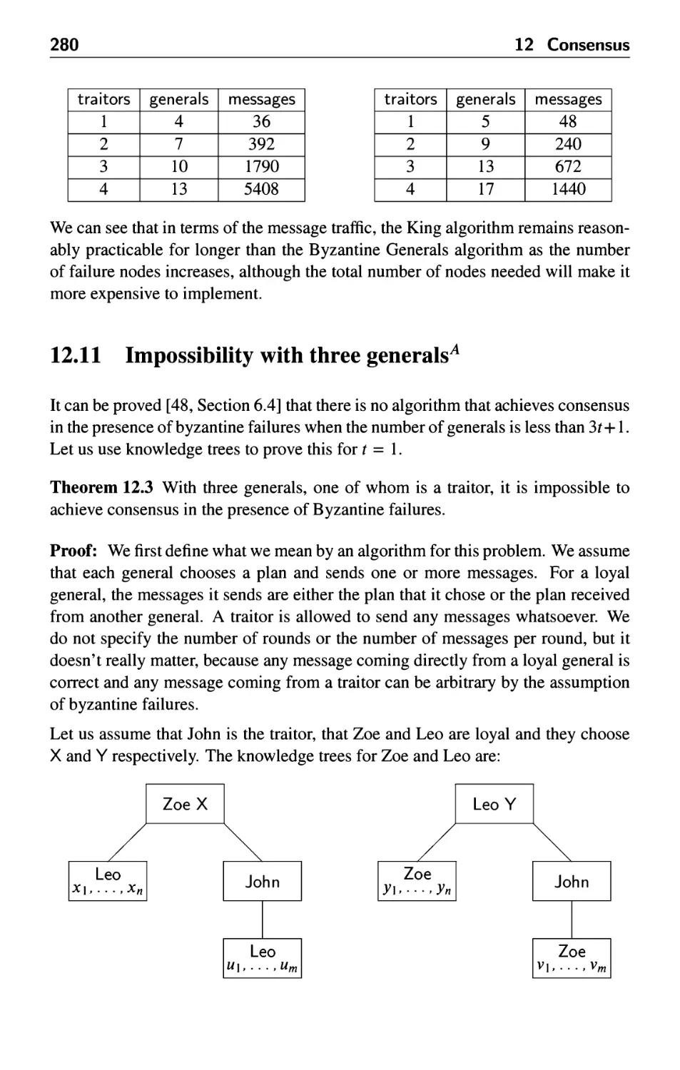
12.11 Impossibility with three generals 280
13 Real-Time Systems 285
13.1 Introduction 285
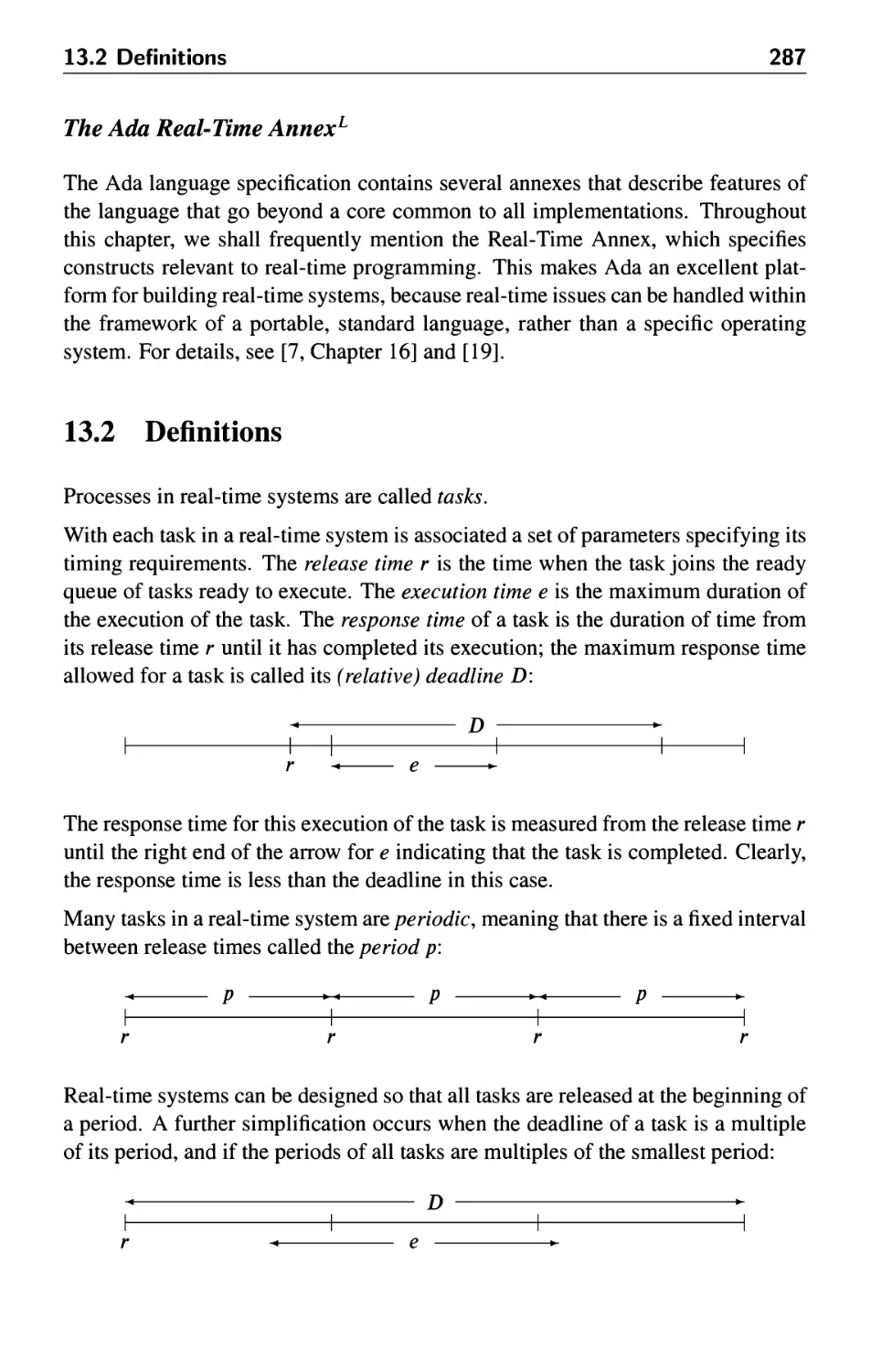
13.2 Definitions 287
13.3 Reliability and repeatability 288
13.4 Synchronous systems 290
13.5 Asynchronous systems 293
13.6 Interrupt-driven systems 297
13.7 Priority inversion and priority inheritance 299
13.8 The Mars Pathfinder in Spin 303
13.9 Simpson's four-slot algorithm 306
13.10 The Ravenscar profile 309
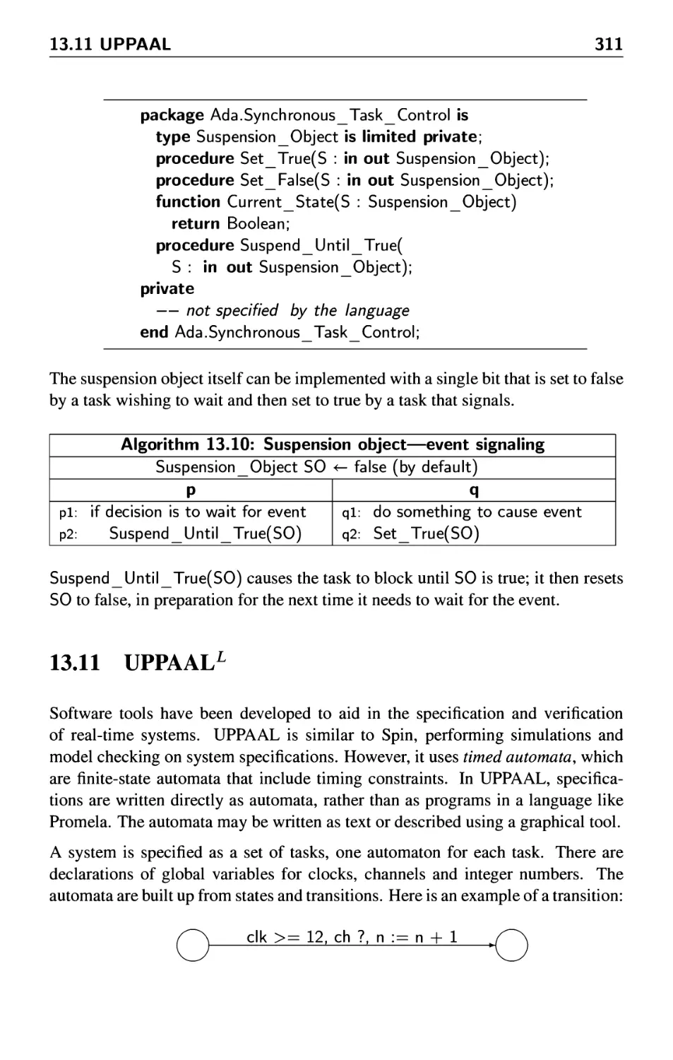
13.11 UPPAAL 311
13.12 Scheduling algorithms for real-time systems 312

x Contents
A The Pseudocode Notation 317
B Review of Mathematical Logic 321
B.l The propositional calculus 321
B.2 Induction 323
B.3 Proofmethods 324
B.4 Correctness of sequential programs 326
C Concurrent Programming Problems 331
D Software Tools 339
D.l BACIandjBACI 339
D.2 Spin and jSpin 341
D.3 DAJ 345
E Further Reading 349
Bibliography 351
Index 355
Supporting Resources
Visit www.pearsoned.co.uk/ben-ari to find valuable online resources
Companion Website for students
• Source code for all the algorithms in the book
• Links to sites where software for studying concurrency may be downloaded.
For instructors
• PDF slides of all diagrams, algorithms and scenarios (with ETfnX source)
• Answers to exercises
For more information please contact your local Pearson Education sales
representative or visit www.pearsoned.co.uk/ben-ari

Preface
Concurrent and distributed programming are no longer the esoteric subjects for
graduate students that they were years ago. Programs today are inherently
concurrent or distributed, from event-based implementations of graphical user interfaces
to operating and real-time systems to Internet applications like multiuser games,
chats and ecommerce. Modern programming languages and systems (including
Java, the system most widely used in education) support concurrent and distributed
programming within their standard libraries. These subjects certainly deserve a
central place in computer science education.
What has not changed over time is that concurrent and distributed programs cannot
be "hacked." Formal methods must be used in their specification and
verification, making the subject an ideal vehicle to introduce students to formal methods.
Precisely for this reason I find concurrency still intriguing even after forty years'
experience writing programs; I hope you will too.
I have been very gratified by the favorable response to my previous books
Principles of Concurrent Programming and the first edition of Principles of Concurrent
and Distributed Programming. Several developments have made it advisable to
write a new edition. Surprisingly, the main reason is not any revolution in the
principles of this subject. While the superficial technology may change, basic concepts
like interleaving, mutual exclusion, safety and liveness remain with us, as have
the basic constructs used to write concurrent programs like semaphores, monitors,
channels and messages. The central problems we try to solve have also remained
with us: critical section, producer-consumer, readers and writers and consensus.
What has changed is that concurrent programming has become ubiquitous, and this
has affected the choice of language and software technology.
Language: I see no point in presenting the details of any particular language or
system, details that in any case are likely to obscure the principles. For that reason,
I have decided not to translate the Ada programs from the first edition into Java
programs, but instead to present the algorithms in pseudocode. I believe that the
high-level pseudocode makes it easier to study the algorithms. For example, in the
xi

xii
Preface
Byzantine Generals algorithm, the pseudocode line:
for all other nodes
is much easier to understand than the Java lines:
for (int i = 0; i < numberOfNodes; i++)
if (i != mylD)
and yet no precision is lost.
In addition, I am returning to the concept of Principles of Concurrent
Programming, where concurrency simulators, not concurrent programming languages, are
the preferred tool for teaching and learning. There is simply no way that extreme
scenarios—like the one you are asked to construct in Exercise 2.3—can be
demonstrated without using a simulator.
Along with the language-independent development of models and algorithms,
explanations have been provided on concurrency in five languages: the Pascal and
C dialects supported by the BACI concurrency simulator, Ada1 and Java, and
Promela, the language of the model checker Spin. Language-dependent sections
are marked by L. Implementations of algorithms in these languages are supplied in
the accompanying software archive.
A word on the Ada language that was used in the first edition of this book. I
believe that—despite being overwhelmed by languages like C++ and Java—Ada is
still the best language for developing complex systems. Its support for concurrent
and real-time programming is excellent, in particular when compared with the trials
and tribulations associated with the concurrency constructs in Java. Certainly, the
protected object and rendezvous are elegant constructs for concurrency, and I have
explained them in the language-independent pseudocode.
Model checking: A truly new development in concurrency that justifies writing
a revised edition is the widespread use of model checkers for verifying concurrent
and distributed programs. The concept of a state diagram and its use in checking
correctness claims is explained from the very start. Deductive proofs continue to
be used, but receive less emphasis than in the first edition. A central place has
been given to the Spin model checker, and I warmly recommend that you use it in
your study of concurrency. Nevertheless, I have refrained from using Spin and its
language Promela exclusively because I realize that many instructors may prefer to
use a mainstream programming language.
1 All references to Ada in this book are to Ada 95.

Preface
xiii
I have chosen to present the Spin model checker because, on the one hand, it is
a widely-used industrial-strength tool that students are likely to encounter as
software engineers, but on the other hand, it is very "friendly." The installation is
trivial and programs are written in a simple programming language that can be easily
learned. I have made a point of using Spin to verify all the algorithms in the book,
and I have found this to be extremely effective in increasing my understanding of
the algorithms.
An outline of the book: After an introductory chapter, Chapter 2 describes the
abstraction that is used: the interleaved execution of atomic statements, where the
simplest atomic statement is a single access to a memory location. Short
introductions are given to the various possibilities for studying concurrent programming:
using a concurrency simulator, writing programs in languages that directly support
concurrency, and working with a model checker. Chapter 3 is the core of an
introduction to concurrent programming. The critical-section problem is the central
problem in concurrent programming, and algorithms designed to solve the problem
demonstrate in detail the wide range of pathological behaviors that a concurrent
program can exhibit. The chapter also presents elementary verification techniques
that are used to prove correctness.
More advanced material on verification and on algorithms for the critical-section
problem can be found in Chapters 4 and 5, respectively. For Dekker's algorithm,
we give a proof of freedom from starvation as an example of deductive reasoning
with temporal logic (Section 4.5). Assertional proofs of Lamport's fast mutual
exclusion algorithm (Section 5.4), and Barz's simulation of general semaphores by
binary semaphores (Section 6.10) are given in full detail; Lamport gave a proof that
is partially operational and Barz's is fully operational and difficult to follow.
Studying assertional proofs is a good way for students to appreciate the care required to
develop concurrent algorithms.
Chapter 6 on semaphores and Chapter 7 on monitors discuss these classical
concurrent programming primitives. The chapter on monitors carefully compares the
original construct with similar constructs that are implemented in the programming
languages Ada and Java.
Chapter 8 presents synchronous communication by channels, and generalizations
to rendezvous and remote procedure calls. An entirely different approach discussed
in Chapter 9 uses logically-global data structures called spaces; this was pioneered
in the Linda model, and implemented within Java by JavaSpaces.
The chapters on distributed systems focus on algorithms: the critical-section
problem (Chapter 10), determining the global properties of termination and snapshots
(Chapter 11), and achieving consensus (Chapter 12). The final Chapter 13 gives
an overview of concurrency in real-time systems. Integrated within this chapter

xiv
Preface
are descriptions of software defects in spacecraft caused by problems with
concurrency. They are particularly instructive because they emphasize that some software
really does demand precise specification and formal verification.
A summary of the pseudocode notation is given in Appendix A. Appendix B
reviews the elementary mathematical logic needed for verification of concurrent
programs. Appendix C gives a list of well-known problems for concurrent
programming. Appendix D describes tools that can be used for studying concurrency: the
BACI concurrency simulator; Spin, a model checker for simulating and verifying
concurrent programs; and DAJ, a tool for constructing scenarios of distributed
algorithms. Appendix E contains pointers to more advanced textbooks, as well as
references to books and articles on specialized topics and systems; it also contains
a list of websites for locating the languages and systems discussed in the book.
Audience: The intended audience includes advanced undergraduate and
beginning graduate students, as well as practicing software engineers interested in
obtaining a scientific background in this field. We have taught concurrency
successfully to high-school students, and the subject is particularly suited to non-
specialists because the basic principles can be explained by adding a very few
constructs to a simple language and running programs on a concurrency simulator.
While there are no specific prerequisites and the book is reasonably self-contained,
a student should be fluent in one or more programming languages and have a basic
knowledge of data structures and computer architecture or operating systems.
Advanced topics are marked by A. This includes material that requires a degree of
mathematical maturity.
Chapters 1 through 3 and the non-A parts of Chapter 4 form the introductory core
that should be part of any course. I would also expect a course in concurrency
to present semaphores and monitors (Chapters 6 and 7); monitors are particularly
important because concurrency constructs in modern programming languages are
based upon the monitor concept. The other chapters can be studied more or less
independently of each other.
Exercises: The exercises following each chapter are technical exercises intended
to clarify and expand on the models, the algorithms and their proofs. Classical
problems with names like the sleeping barber and the cigarette smoker appear in
Appendix C because they need not be associated with any particular construct for
synchronization.
Supporting material: The companion website contains an archive with the
source code in various languages for the algorithms appearing in the book. Its
address is:
http://www.pearsoned.co.uk/ben-ari.

Preface
xv
Lecturers will find slides of the algorithms, diagrams and scenarios, both in ready-
to-display PDF files and in LTjnX source for modification. The site includes
instructions for obtaining the answers to the exercises.
Acknowledgements: I would like to thank:
• Yifat Ben-David Kolikant for six years of collaboration during which we
learned together how to really teach concurrency;
• Pieter Hartel for translating the examples of the first edition into Promela,
eventually tempting me into learning Spin and emphasizing it in the new
edition;
• Pieter Hartel again and Hans Henrik L0vengreen for their comprehensive
reviews of the manuscript;
• Gerard Holzmann for patiently answering innumerable queries on Spin
during my development of j Spin and the writing of the book;
• Bill Bynum, Tracy Camp and David Strite for their help during my work on
jBACI;
• Shmuel Schwarz for showing me how the frog puzzle can be used to teach
state diagrams;
• The Helsinki University of Technology for inviting me for a sabbatical
during which this book was completed.
M. Ben-Ari
Rehovot and Espoo, 2005

1 What is Concurrent
Programming?
1.1 Introduction
An "ordinary" program consists of data declarations and assignment and control-
flow statements in a programming language. Modern languages include structures
such as procedures and modules for organizing large software systems through
abstraction and encapsulation, but the statements that are actually executed are still
the elementary statements that compute expressions, move data and change the
flow of control. In fact, these are precisely the instructions that appear in the
machine code that results from compilation. These machine instructions are executed
sequentially on a computer and access data stored in the main or secondary
memories.
A concurrent program is a set of sequential programs that can be executed in
parallel. We use the word process for the sequential programs that comprise a concurrent
program and save the term program for this set of processes.
Traditionally, the word parallel is used for systems in which the executions of
several programs overlap in time by running them on separate processors. The
word concurrent is reserved for potential parallelism, in which the executions may,
but need not, overlap; instead, the parallelism may only be apparent since it may
be implemented by sharing the resources of a small number of processors, often
only one. Concurrency is an extremely useful abstraction because we can better
understand such a program by pretending that all processes are being executed in
parallel. Conversely, even if the processes of a concurrent program are actually
executed in parallel on several processors, understanding its behavior is greatly
facilitated if we impose an order on the instructions that is compatible with shared
execution on a single processor. Like any abstraction, concurrent programming is
important because the behavior of a wide range of real systems can be modeled
and studied without unnecessary detail.
In this book we will define formal models of concurrent programs and study
algorithms written in these formalisms. Because the processes that comprise a concur-

2
1 What is Concurrent Programming?
rent program may interact, it is exceedingly difficult to write a correct program for
even the simplest problem. New tools are needed to specify, program and verify
these programs. Unless these are understood, a programmer used to writing and
testing sequential programs will be totally mystified by the bizarre behavior that a
concurrent program can exhibit.
Concurrent programming arose from problems encountered in creating real
systems. To motivate the concurrency abstraction, we present a series of examples of
real-world concurrency.
1.2 Concurrency as abstract parallelism
It is difficult to intuitively grasp the speed of electronic devices. The fingers of
a fast typist seem to fly across the keyboard, to say nothing of the impression of
speed given by a printer that is capable of producing a page with thousands of
characters every few seconds. Yet these rates are extremely slow compared to the
time required by a computer to process each character.
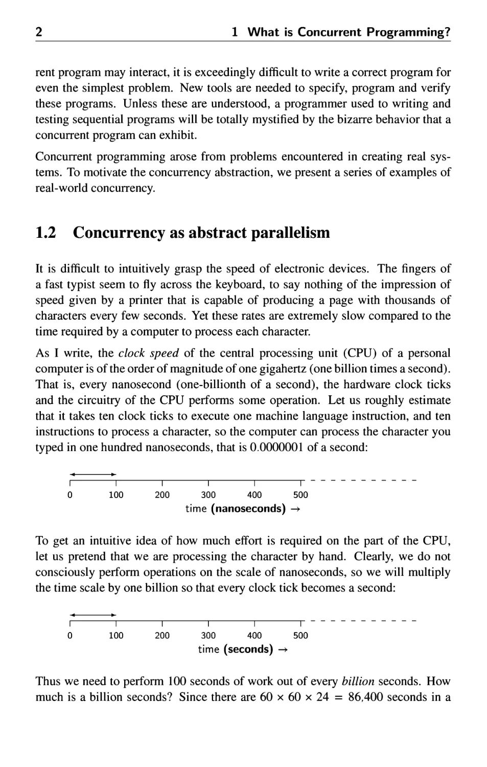
As I write, the clock speed of the central processing unit (CPU) of a personal
computer is of the order of magnitude of one gigahertz (one billion times a second).
That is, every nanosecond (one-billionth of a second), the hardware clock ticks
and the circuitry of the CPU performs some operation. Let us roughly estimate
that it takes ten clock ticks to execute one machine language instruction, and ten
instructions to process a character, so the computer can process the character you
typed in one hundred nanoseconds, that is 0.0000001 of a second:
0 100 200 300 400 500
time (nanoseconds) -►
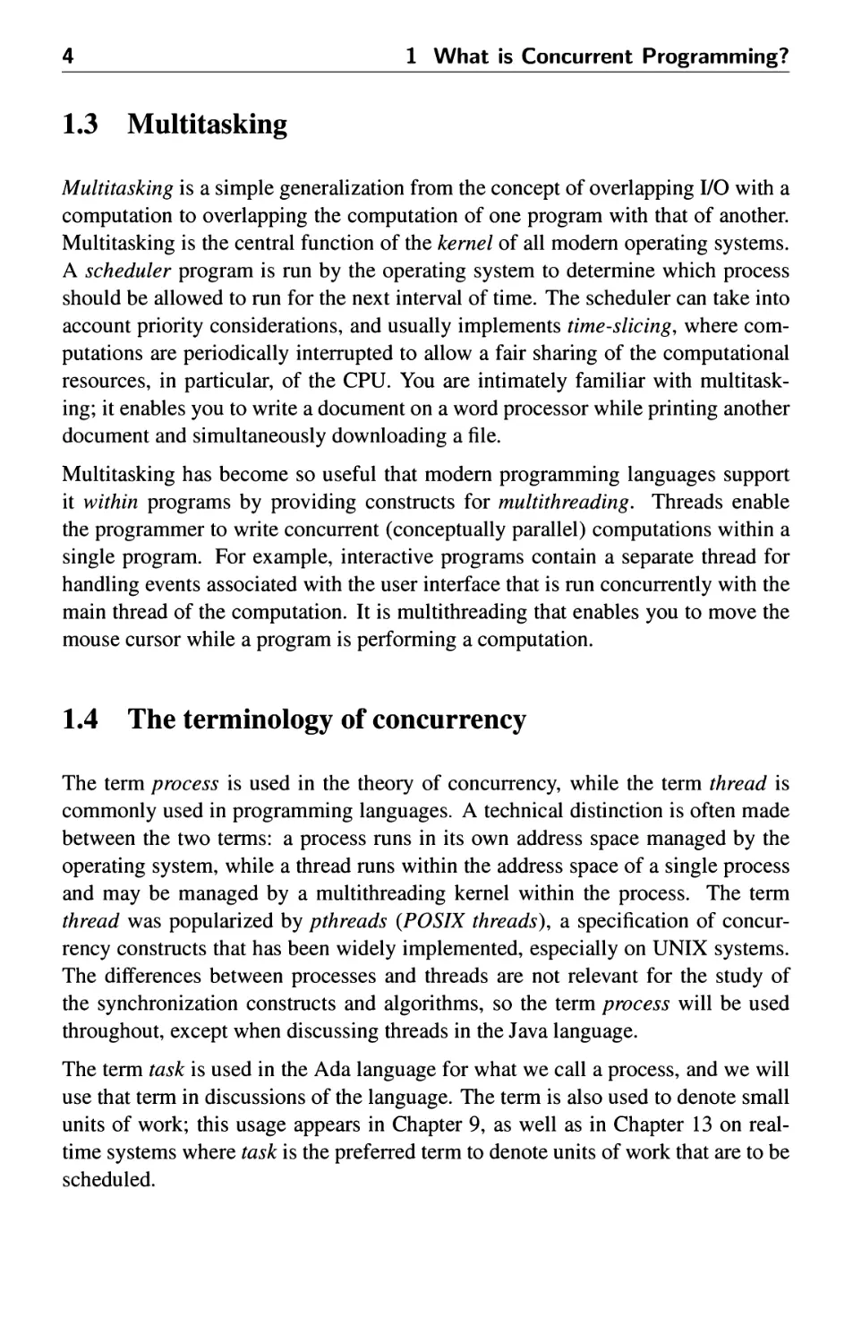
To get an intuitive idea of how much effort is required on the part of the CPU,
let us pretend that we are processing the character by hand. Clearly, we do not
consciously perform operations on the scale of nanoseconds, so we will multiply
the time scale by one billion so that every clock tick becomes a second:
-4 ►-
I 1 1 1 1 1
0 100 200 300 400 500
time (seconds) -►
Thus we need to perform 100 seconds of work out of every billion seconds. How
much is a billion seconds? Since there are 60 x 60 x 24 = 86,400 seconds in a

1.2 Concurrency as abstract parallelism
3
day, a billion seconds is 1,000,000,000/86,400 = 11,574 days or about 32 years.
You would have to invest 100 seconds every 32 years to process a character, and a
3,000-character page would require only (3,000 x 100)/(60 x 60) « 83 hours over
half a lifetime. This is hardly a strenuous job!
The tremendous gap between the speeds of human and mechanical processing on
the one hand and the speed of electronic devices on the other led to the
development of operating systems which allow I/O operations to proceed "in parallel" with
computation. On a single CPU, like the one in a personal computer, the processing
required for each character typed on a keyboard cannot really be done in parallel
with another computation, but it is possible to "steal" from the other computation
the fraction of a microsecond needed to process the character. As can be seen from
the numbers in the previous paragraph, the degradation in performance will not be
noticeable, even when the overhead of switching between the two computations is
included.
What is the connection between concurrency and operating systems that overlap
I/O with other computations? It would theoretically be possible for every program
to include code that would periodically sample the keyboard and the printer to see
if they need to be serviced, but this would be an intolerable burden on programmers
by forcing them to be fully conversant with the details of the operating system.
Instead, I/O devices are designed to interrupt the CPU, causing it to jump to the code
to process a character. Although the processing is sequential, it is conceptually
simpler to work with an abstraction in which the I/O processing performed as the
result of the interrupt is a separate process, executed concurrently with a process
doing another computation. The following diagram shows the assignment of the
CPU to the two processes for computation and I/O.
I/O
Computation
i t
start I/O end I/O
time ->

4
1 What is Concurrent Programming?
1.3 Multitasking
Multitasking is a simple generalization from the concept of overlapping I/O with a
computation to overlapping the computation of one program with that of another.
Multitasking is the central function of the kernel of all modern operating systems.
A scheduler program is run by the operating system to determine which process
should be allowed to run for the next interval of time. The scheduler can take into
account priority considerations, and usually implements time-slicing, where
computations are periodically interrupted to allow a fair sharing of the computational
resources, in particular, of the CPU. You are intimately familiar with
multitasking; it enables you to write a document on a word processor while printing another
document and simultaneously downloading a file.
Multitasking has become so useful that modern programming languages support
it within programs by providing constructs for multithreading. Threads enable
the programmer to write concurrent (conceptually parallel) computations within a
single program. For example, interactive programs contain a separate thread for
handling events associated with the user interface that is run concurrently with the
main thread of the computation. It is multithreading that enables you to move the
mouse cursor while a program is performing a computation.
1.4 The terminology of concurrency
The term process is used in the theory of concurrency, while the term thread is
commonly used in programming languages. A technical distinction is often made
between the two terms: a process runs in its own address space managed by the
operating system, while a thread runs within the address space of a single process
and may be managed by a multithreading kernel within the process. The term
thread was popularized by pthreads (POSIX threads), a specification of
concurrency constructs that has been widely implemented, especially on UNIX systems.
The differences between processes and threads are not relevant for the study of
the synchronization constructs and algorithms, so the term process will be used
throughout, except when discussing threads in the Java language.
The term task is used in the Ada language for what we call a process, and we will
use that term in discussions of the language. The term is also used to denote small
units of work; this usage appears in Chapter 9, as well as in Chapter 13 on
realtime systems where task is the preferred term to denote units of work that are to be
scheduled.

1.5 Multiple computers
5
1.5 Multiple computers
The days of one large computer serving an entire organization are long gone.
Today, computers hide in unforeseen places like automobiles and cameras. In fact,
your personal "computer" (in the singular) contains more than one processor: the
graphics processor is a computer specialized for the task of taking information from
the computer's memory and rendering it on the display screen. I/O and
communications interfaces are also likely to have their own specialized processors. Thus,
in addition to the multitasking performed by the operating systems kernel, parallel
processing is being carried out by these specialized processors.
The use of multiple computers is also essential when the computational task
requires more processing than is possible on one computer. Perhaps you have seen
pictures of the "server farms" containing tens or hundreds of computers that are
used by Internet companies to provide service to millions of customers. In fact, the
entire Internet can be considered to be one distributed system working to
disseminate information in the form of email and web pages.
Somewhat less familiar than distributed systems are multiprocessors, which are
systems designed to bring the computing power of several processors to work in
concert on a single computationally-intensive problem. Multiprocessors are
extensively used in scientific and engineering simulation, for example, in simulating the
atmosphere for weather forecasting and studying climate.
1.6 The challenge of concurrent programming
The challenge in concurrent programming comes from the need to synchronize
the execution of different processes and to enable them to communicate. If the
processes were totally independent, the implementation of concurrency would only
require a simple scheduler to allocate resources among them. But if an I/O process
accepts a character typed on a keyboard, it must somehow communicate it to the
process running the word processor, and if there are multiple windows on a display,
processes must somehow synchronize access to the display so that images are sent
to the window with the current focus.
It turns out to be extremely difficult to implement safe and efficient synchronization
and communication. When your personal computer "freezes up" or when using one
application causes another application to "crash," the cause is generally an error in
synchronization or communication. Since such problems are time- and situation-
dependent, they are difficult to reproduce, diagnose and correct.

6
1 What is Concurrent Programming?
The aim of this book is to introduce you to the constructs, algorithms and systems
that are used to obtain correct behavior of concurrent and distributed programs.
The choice of construct, algorithm or system depends critically on assumptions
concerning the requirements of the software being developed and the architecture
of the system that will be used to execute it. This book presents a survey of the
main ideas that have been proposed over the years; we hope that it will enable you
to analyze, evaluate and employ specific tools that you will encounter in the future.
Transition
We have defined concurrent programming informally, based upon your experience
with computer systems. Our goal is to study concurrency abstractly, rather than
a particular implementation in a specific programming language or operating
system. We have to carefully specify the abstraction that describe the allowable data
structures and operations. In the next chapter, we will define the concurrent
programming abstraction and justify its relevance. We will also survey languages and
systems that can be used to write concurrent programs.

2 The Concurrent Programming
Abstraction
2.1 The role of abstraction
Scientific descriptions of the world are based on abstractions. A living animal is
a system constructed of organs, bones and so on. These organs are composed of
cells, which in turn are composed of molecules, which in turn are composed of
atoms, which in turn are composed of elementary particles. Scientists find it
convenient (and in fact necessary) to limit their investigations to one level, or maybe
two levels, and to "abstract away" from lower levels. Thus your physician will
listen to your heart or look into your eyes, but he will not generally think about the
molecules from which they are composed. There are other specialists,
pharmacologists and biochemists, who study that level of abstraction, in turn abstracting away
from the quantum theory that describes the structure and behavior of the molecules.
In computer science, abstractions are just as important. Software engineers
generally deal with at most three levels of abstraction:
Systems and libraries Operating systems and libraries—often called Application
Program Interfaces (API)—define computational resources that are available
to the programmer. You can open a file or send a message by invoking the
proper procedure or function call, without knowing how the resource is
implemented.
Programming languages A programming language enables you to employ the
computational power of a computer, while abstracting away from the details
of specific architectures.
Instruction sets Most computer manufacturers design and build families of CPUs
which execute the same instruction set as seen by the assembly language
programmer or compiler writer. The members of a family may be
implemented in totally different ways—emulating some instructions in software
or using memory for registers—but a programmer can write a compiler for
that instruction set without knowing the details of the implementation.
7

8
2 The Concurrent Programming Abstraction
Of course, the list of abstractions can be continued to include logic gates and their
implementation by semiconductors, but software engineers rarely, if ever, need to
work at those levels. Certainly, you would never describe the semantics of an
assignment statement like x<-y+z in terms of the behavior of the electrons within
the chip implementing the instruction set into which the statement was compiled.
Two of the most important tools for software abstraction are encapsulation and
concurrency.
Encapsulation achieves abstraction by dividing a software module into a public
specification and a hidden implementation. The specification describes the
available operations on a data structure or real-world model. The detailed
implementation of the structure or model is written within a separate module that is not
accessible from the outside. Thus changes in the internal data representation and
algorithm can be made without affecting the programming of the rest of the system.
Modern programming languages directly support encapsulation.
Concurrency is an abstraction that is designed to make it possible to reason about
the dynamic behavior of programs. This abstraction will be carefully explained
in the rest of this chapter. First we will define the abstraction and then show
how to relate it to various computer architectures. For readers who are
familiar with machine-language programming, Sections 2.8-2.9 relate the abstraction
to machine instructions; the conclusion is that there are no important concepts of
concurrency that cannot be explained at the higher level of abstraction, so these
sections can be skipped if desired. The chapter concludes with an introduction
to concurrent programming in various languages and a supplemental section on a
puzzle that may help you understand the concept of state and state diagram.
2.2 Concurrent execution as interleaving of atomic
statements
We now define the concurrent programming abstraction that we will study in this
textbook. The abstraction is based upon the concept of a (sequential) process,
which we will not formally define. Consider it as a "normal" program fragment
written in a programming language. You will not be misled if you think of a process
as a fancy name for a procedure or method in an ordinary programming language.
Definition 2.1 A concurrent program consists of a finite set of (sequential)
processes. The processes are written using a finite set of atomic statements. The
execution of a concurrent program proceeds by executing a sequence of the atomic

2.2 Concurrent execution as interleaving of atomic statements 9
statements obtained by arbitrarily interleaving the atomic statements from the
processes. A computation is an execution sequence that can occur as a result of the
interleaving. Computations are also called scenarios. I
Definition 2.2 During a computation the control pointer of a process indicates the
next statement that can be executed by that process.1 Each process has its own
control pointer. I
Computations are created by interleaving, which merges several statement streams.
At each step during the execution of the current program, the next statement to be
executed will be "chosen" from the statements pointed to by the control pointers
cp of the processes.
/ p3, ...
pl.rl.p2, ql q2, ...
y ^cPq
\ r2, ...
\cpr
Suppose that we have two processes, p composed of statements pi followed by p2
and q composed of statements ql followed by q2, and that the execution is started
with the control pointers of the two processes pointing to pi and ql. Assuming that
the statements are assignment statements that do not transfer control, the possible
scenarios are:
pl^ql^p2^q2,
pl^ql^q2^p2,
pl^p2^ql^q2,
ql^pl^q2^p2,
ql^pl^p2^q2,
ql^q2^pl^p2.
Note that p2-»pl->-ql-»q2 is not a scenario, because we respect the sequential
execution of each individual process, so that p2 cannot be executed before pi.
'Alternate terms for this concept are instruction pointer and location counter.

10
2 The Concurrent Programming Abstraction
We will present concurrent programs in a language-independent form, because the
concepts are universal, whether they are implemented as operating systems calls,
directly in programming languages like Ada or Java,2 or in a model specification
language like Promela. The notation is demonstrated by the following trivial two-
process concurrent algorithm:
Algorithm 2.1: Trivial concurrent program
integer n <- 0
P
integer kl <- 1
pi: n <- kl
q
integer k2 <- 2
ql: n <- k2
The program is given a title, followed by declarations of global variables, followed
by two columns, one for each of the two processes, which by convention are named
process p and process q. Each process may have declarations of local variables,
followed by the statements of the process. We use the following convention:
Each labeled line represents an atomic statement.
A description of the pseudocode is given in Appendix A.
States
The execution of a concurrent program is defined by states and transitions between
states. Let us first look at these concepts in a sequential version of the above
algorithm:
Algorithm
2.2:
Trivial sequential
program
integer n <- 0
Pi:
p2:
integer kl
integer k2
n <- kl
n <- k2
<- 1
^2
At any time during the execution of this program, it must be in a state defined by
the value of the control pointer and the values of the three variables. Executing a
statement corresponds to making a transition from one state to another. It is clear
that this program can be in one of three states: an initial state and two other states
2The word Java will be used as an abbreviation for the Java programming language.

2.2 Concurrent execution as interleaving of atomic statements 11
obtained by executing the two statements. This is shown in the following diagram,
where a node represents a state, arrows represent the transitions, and the initial
state is pointed to by the short arrow on the left:
pi: n *- kl
kl = l,it2 = 2
n = 0
p2: n <- k2^_
kl = 1,62 = 2 f
(end)
kl = l,k2 = 2
« = 2
Consider now the trivial concurrent program Algorithm 2.1. There are two
processes, so the state must include the control pointers of both processes.
Furthermore, in the initial state there is a choice as to which statement to execute, so there
are two transitions from the initial state.
(end)
ql: n <- k2
kl = l,k2 = 2
n= 1
(end)
(end)
kl = l,k2 = 2
n = 2
pi: n <- kl
ql: n <- k2
kl = l,k2 = 2
n = 0
pi: n <- kl
(end)
kl = l,k2 = 2
n = 2
(end)
(end)
kl = 1,62 = 2
« = 1
The lefthand states correspond to executing pi followed by ql, while the righthand
states correspond to executing ql followed by pi. Note that the computation can
terminate in two different states (with different values of n), depending on the
interleaving of the statements.
Definition 2.3 The state of a (concurrent) algorithm is a tuple3 consisting of one
element for each process that is a label from that process, and one element for each
global or local variable that is a value whose type is the same as the type of the
variable. I
3The word tuple is a generalization of the sequence pair, triple, quadruple, etc. It means an
ordered sequence of values of any fixed length.

12
2 The Concurrent Programming Abstraction
The number of possible states—the number of tuples—is quite large, but in an
execution of a program, not all possible states can occur. For example, since no
values are assigned to the variables kl and k2 in Algorithm 2.1, no state can occur
in which these variables have values that are different from their initial values.
Definition 2.4 Let s\ and 52 be states. There is a transition between s\ and 52 if
executing a statement in state s\ changes the state to 52. The statement executed
must be one of those pointed to by a control pointer in s\. I
Definition 2.5 A state diagram is a graph defined inductively. The initial state
diagram contains a single node labeled with the initial state. If state s\ labels a
node in the state diagram, and if there is a transition from s\ to 52, then there is a
node labeled 52 in the state diagram and a directed edge from s\ to 52.
For each state, there is only one node labeled with that state.
The set of reachable states is the set of states in a state diagram. I
It follows from the definitions that a computation (scenario) of a concurrent
program is represented by a directed path through the state diagram starting from the
initial state, and that all computations can be so represented. Cycles in the state
diagram represent the possibility of infinite computations in a finite graph.
The state diagram for Algorithm 2.1 shows that there are two different scenarios,
each of which contains three of the five reachable states.
Before proceeding, you may wish to read the supplementary Section 2.14, which
describes the state diagram for an interesting puzzle.
Scenarios
A scenario is defined by a sequence of states. Since diagrams can be hard to draw,
especially for large programs, it is convenient to use a tabular representation of
scenarios. This is done simply by listing the sequence of states in a table; the
columns for the control pointers are labeled with the processes and the columns for
the variable values with the variable names. The following table shows the scenario
of Algorithm 2.1 corresponding to the lefthand path:
Process p
pi: n-«-kl
(end)
(end)
Process q
ql: n^k2
ql: n<-k2
(end)
n
0
1
2
kl
1
1
1
k2
2
2
2

2.3 Justification of the abstraction
13
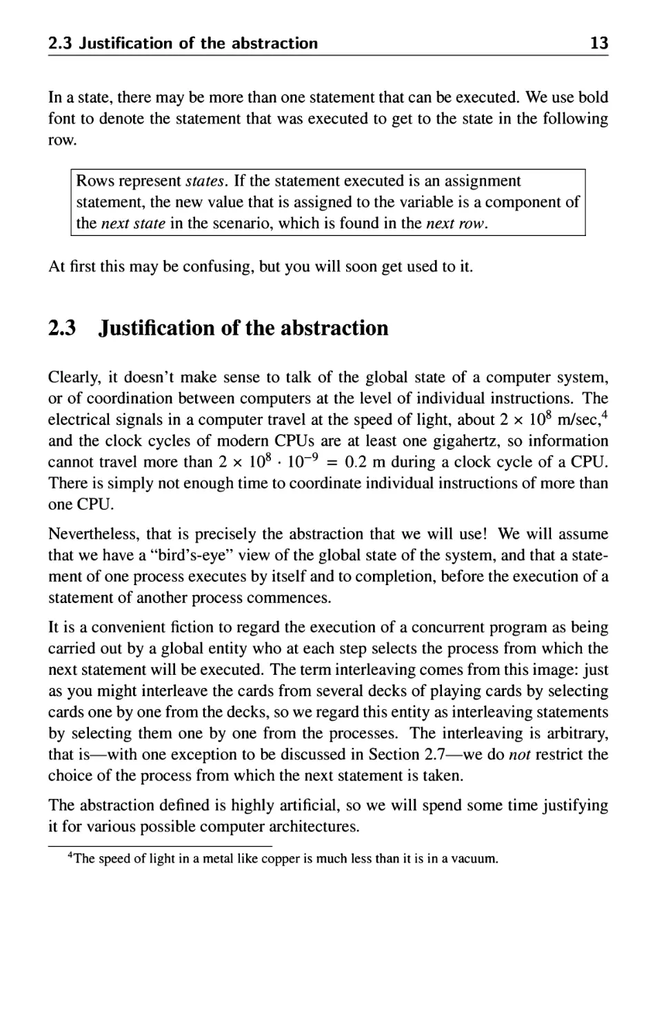
In a state, there may be more than one statement that can be executed. We use bold
font to denote the statement that was executed to get to the state in the following
row.
Rows represent states. If the statement executed is an assignment
statement, the new value that is assigned to the variable is a component of
the next state in the scenario, which is found in the next row.
At first this may be confusing, but you will soon get used to it.
2.3 Justification of the abstraction
Clearly, it doesn't make sense to talk of the global state of a computer system,
or of coordination between computers at the level of individual instructions. The
electrical signals in a computer travel at the speed of light, about 2 x 108 m/sec,4
and the clock cycles of modern CPUs are at least one gigahertz, so information
cannot travel more than 2 x 108 • 10"9 = 0.2 m during a clock cycle of a CPU.
There is simply not enough time to coordinate individual instructions of more than
one CPU.
Nevertheless, that is precisely the abstraction that we will use! We will assume
that we have a "bird's-eye" view of the global state of the system, and that a
statement of one process executes by itself and to completion, before the execution of a
statement of another process commences.
It is a convenient fiction to regard the execution of a concurrent program as being
carried out by a global entity who at each step selects the process from which the
next statement will be executed. The term interleaving comes from this image: just
as you might interleave the cards from several decks of playing cards by selecting
cards one by one from the decks, so we regard this entity as interleaving statements
by selecting them one by one from the processes. The interleaving is arbitrary,
that is—with one exception to be discussed in Section 2.7—we do not restrict the
choice of the process from which the next statement is taken.
The abstraction defined is highly artificial, so we will spend some time justifying
it for various possible computer architectures.
4The speed of light in a metal like copper is much less than it is in a vacuum.

14
2 The Concurrent Programming Abstraction
Multitasking systems
Consider the case of a concurrent program that is being executed by multitasking,
that is, by sharing the resources of one computer. Obviously, with a single CPU
there is no question of the simultaneous execution of several instructions. The
selection of the next instruction to execute is carried out by the CPU and the operating
system. Normally, the next instruction is taken from the same process from which
the current instruction was executed; occasionally, interrupts from I/O devices or
internal timers will cause the execution to be interrupted. A new process called an
interrupt handler will be executed, and upon its completion, an operating system
function called the scheduler may be invoked to select a new process to execute.
This mechanism is called a context switch. The diagram below shows the memory
divided into five segments, one for the operating system code and data, and four
for the code and data of the programs that are running concurrently:
R- Operating
g; System
—i
r:
e ■ Program 1
g:
R'
e ■ Program 2
g:
g:
r:
e ■ Program 4
g:
When the execution is interrupted, the registers in the CPU (not only the registers
used for computation, but also the control pointer and other registers that point to
the memory segment used by the program) are saved into a prespecified area in
the program's memory. Then the register contents required to execute the interrupt
handler are loaded into the CPU. At the conclusion of the interrupt processing,
the symmetric context switch is performed, storing the interrupt handler registers
and loading the registers for the program. The end of interrupt processing is a
convenient time to invoke the operating system scheduler, which may decide to
perform the context switch with another program, not the one that was interrupted.
In a multitasking system, the non-intuitive aspect of the abstraction is not the
interleaving of atomic statements (that actually occurs), but the requirement that any
arbitrary interleaving is acceptable. After all, the operating system scheduler may
only be called every few milliseconds, so many thousands of instructions will be
executed from each process before any instructions are interleaved from another.
We defer a discussion of this important point to Section 2.4.

2.3 Justification of the abstraction
15
Multiprocessor computers
A multiprocessor computer is a computer with more than one CPU. The memory
is physically divided into banks of local memory, each of which can be accessed
only by one CPU, and global memory, which can be accessed by all CPUs:
Global
Memory
CPU
Local
Memory
CPU
Local
Memory
CPU
Local
Memory
If we have a sufficient number of CPUs, we can assign each process to its own
CPU. The interleaving assumption no longer corresponds to reality, since each
CPU is executing its instructions independently. Nevertheless, the abstraction is
useful here.
As long as there is no contention, that is, as long as two CPUs do not attempt
to access the same resource (in this case, the global memory), the computations
defined by interleaving will be indistinguishable from those of truly parallel
execution. With contention, however, there is a potential problem. The memory of
a computer is divided into a large number of cells that store data which is read
and written by the CPU. Eight-bit cells are called bytes and larger cells are called
words, but the size of a cell is not important for our purposes. We want to ask what
might happen if two processors try to read or write a cell simultaneously so that
the operations overlap. The following diagram indicates the problem:
Global memory
loooo oooo oooo oonl
0000 0000 0000 0001
0000 0000 0000 0010

16
2 The Concurrent Programming Abstraction
It shows 16-bit cells of local memory associated with two processors; one cell
contains the value 0 • • • 01 and one contains 0 • • • 10 = 2. If both processors write
to the cell of global memory at the same time, the value might be undefined; for
example, it might be the value 0- • • 11 = 3 obtained by or'ing together the bit
representations of 1 and 2.
In practice, this problem does not occur because memory hardware is designed
so that (for some size memory cell) one access completes before the other
commences. Therefore, we can assume that if two CPUs attempt to read or write the
same cell in global memory, the result is the same as if the two instructions were
executed in either order. In effect, atomicity and interleaving are performed by the
hardware.
Other less restrictive abstractions have been studied; we will give one example of
an algorithm that works under the assumption that if a read of a memory cell
overlaps a write of the same cell, the read may return an arbitrary value (Section 5.3).
The requirement to allow arbitrary interleaving makes a lot of sense in the case of
a multiprocessor; because there is no central scheduler, any computation resulting
from interleaving may certainly occur.
Distributed systems
A distributed system is composed of several computers that have no global
resources; instead, they are connected by communications channels enabling them
to send messages to each other. The language of graph theory is used in discussing
distributed systems; each computer is a node and the nodes are connected by
(directed) edges. The following diagram shows two possible schemes for
interconnecting nodes: on the left, the nodes are fully connected while on the right they are
connected in a ring:
Node
Node
Node
Node

2.4 Arbitrary interleaving
17
In a distributed system, the abstraction of interleaving is, of course, totally false,
since it is impossible to coordinate each node in a geographically distributed
system. Nevertheless, interleaving is a very useful fiction, because as far as each node
is concerned, it only sees discrete events: it is either executing one of its own
statements, sending a message or receiving a message. Any interleaving of all the
events of all the nodes can be used for reasoning about the system, as long as the
interleaving is consistent with the statement sequences of each individual node and
with the requirement that a message be sent before it is received.
Distributed systems are considered to be distinct from concurrent systems. In a
concurrent system implemented by multitasking or multiprocessing, the global
memory is accessible to all processes and each one can access the memory
efficiently. In a distributed system, the nodes may be geographically distant from each
other, so we cannot assume that each node can send a message directly to all other
nodes. In other words, we have to consider the topology or connectedness of the
system, and the quality of an algorithm (its simplicity or efficiency) may be
dependent on a specific topology. A fully connected topology is extremely efficient
in that any node can send a message directly to any other node, but it is extremely
expensive, because for n nodes, we need n • (n - 1) « n2 communications channels.
The ring topology has minimal cost in that any node has only one communications
line associated with it, but it is inefficient, because to send a message from one
arbitrary node to another we may need to have it relayed through up to n - 2 other
nodes.
A further difference between concurrent and distributed systems is that the behavior
of systems in the presence of faults is usually studied within distributed systems.
In a multitasking system, hardware failure is usually catastrophic since it affects
all processes, while a software failure may be relatively innocuous (if the process
simply stops working), though it can be catastrophic (if it gets stuck in an infinite
loop at high priority). In a distributed system, while failures can be catastrophic
for single nodes, it is usually possible to diagnose and work around a faulty node,
because messages may be relayed through alternate communication paths. In fact,
the success of the Internet can be attributed to the robustness of its protocols when
individual nodes or communications channels fail.
2.4 Arbitrary interleaving
We have to justify the use of arbitrary interleavings in the abstraction. What this
means, in effect, is that we ignore time in our analysis of concurrent programs.
For example, the hardware of our system may be such that an interrupt can occur
only once every millisecond. Therefore, we are tempted to assume that several

18
2 The Concurrent Programming Abstraction
thousand statements are executed from a single process before any statements are
executed from another. Instead, we are going to assume that after the execution
of any statement, the next statement may come from any process. What is the
justification for this abstraction?
The abstraction of arbitrary interleaving makes concurrent programs amenable to
formal analysis, and as we shall see, formal analysis is necessary to ensure the
correctness of concurrent programs. Arbitrary interleaving ensures that we only
have to deal with finite or countable sequences of statements a\,a2,a^,..., and
need not analyze the actual time intervals between the statements. The only relation
between the statements is that at precedes or follows (or immediately precedes or
follows) cij. Remember that we did not specify what the atomic statements are,
so you can choose the atomic statements to be as coarse-grained or as fine-grained
as you wish. You can initially write an algorithm and prove its correctness under
the assumption that each function call is atomic, and then refine the algorithm to
assume only that each statement is atomic.
The second reason for using the arbitrary interleaving abstraction is that it enables
us to build systems that are robust to modification of their hardware and software.
Systems are always being upgraded with faster components and faster algorithms.
If the correctness of a concurrent program depended on assumptions about time
of execution, every modification to the hardware or software would require that
the system be rechecked for correctness (see [62] for an example). For example,
suppose that an operating system had been proved correct under the assumption
that characters are being typed in at no more than 10 characters per terminal per
second. That is a conservative assumption for a human typist, but it would become
invalidated if the input were changed to come from a communications channel.
The third reason is that it is difficult, if not impossible, to precisely repeat the
execution of a concurrent program. This is certainly true in the case of systems that
accept input from humans, but even in a fully automated system, there will
always be some jitter, that is some unevenness in the timing of events. A concurrent
program cannot be "debugged" in the familiar sense of diagnosing a problem,
correcting the source code, recompiling and rerunning the program to check if the bug
still exists. Rerunning the program may just cause it to execute a different scenario
than the one where the bug occurred. The solution is to develop programming and
verification techniques that ensure that a program is correct under all interleavings.

2.5 Atomic statements
19
2.5 Atomic statements
The concurrent programming abstraction has been defined in terms of the
interleaving of atomic statements. What this means is that an atomic statement is
executed to completion without the possibility of interleaving statements from another
process. An important property of atomic statements is that if two are executed
"simultaneously," the result is the same as if they had been executed sequentially
(in either order). The inconsistent memory store shown on page 15 will not occur.
It is important to specify the atomic statements precisely, because the correctness
of an algorithm depends on this specification. We start with a demonstration of the
effect of atomicity on correctness, and then present the specification used in this
book.
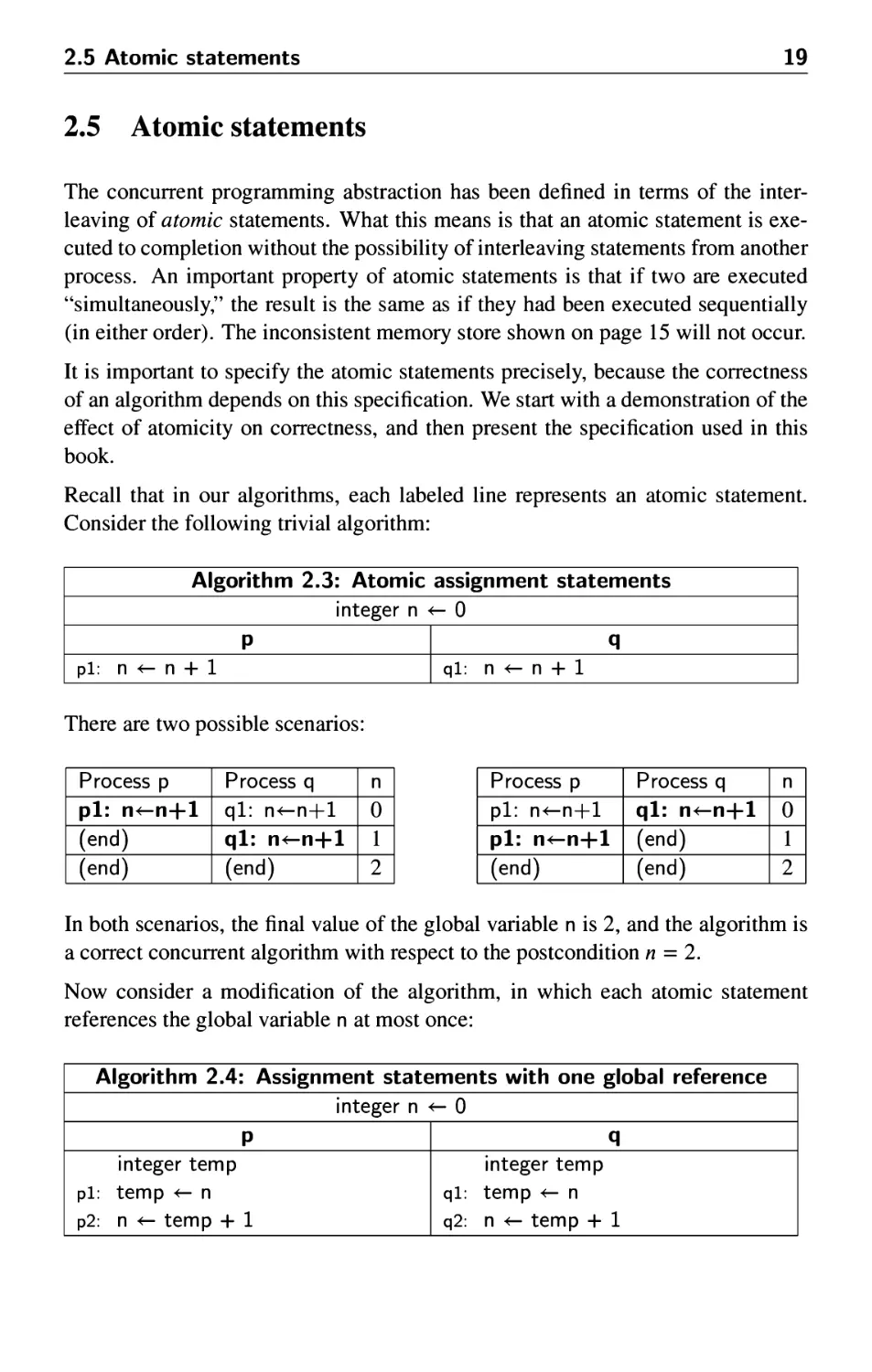
Recall that in our algorithms, each labeled line represents an atomic statement.
Consider the following trivial algorithm:
Algorithm 2.3: Atomic assignment statements
integer n <- 0
P
pi: n <- n + 1
q
ql: n <- n + 1
There are two possible scenarios:
Process p
pi: n<-n+l
pi: n-«-n+l
(end)
Process q
ql: n<-n+l
(end)
(end)
n
0
1
2
Process p
pi: n-«-n+l
(end)
(end)
Process q
ql: n<-n+l
ql: n<-n+l
(end)
n
0
1
2
In both scenarios, the final value of the global variable n is 2, and the algorithm is
a correct concurrent algorithm with respect to the postcondition n = 2.
Now consider a modification of the algorithm, in which each atomic statement
references the global variable n at most once:
Algorithm 2.4: Assignment statements with one global reference
integer n <- 0
P
integer temp
pi: temp <- n
p2: n <- temp + 1
q
integer temp
ql: temp <- n
q2: n <- temp + 1

20
2 The Concurrent Programming Abstraction
There are scenarios of the algorithm that are also correct with respect to the
postcondition n = 2:
Process p
pi: temp<-n
p2: n<-temp+l
(end)
(end)
(end)
Process q
ql: temp<-n
ql: temp<-n
ql: temp<-n
q2: n<-temp+l
(end)
n
0
0
1
1
2
p.temp
?
0
q.temp
?
?
?
1
As long as pi and p2 are executed immediately one after the other, and similarly
for ql and q2, the result will be the same as before, because we are simulating the
execution of n<-n+l with two statements. However, other scenarios are possible
in which the statements from the two processes are interleaved:
Process p
pi: temp<-n
p2: n<-temp+l
p2: n<-temp+l
(end)
(end)
Process q
ql: temp<-n
ql: temp<-n
q2: n<-temp+l
q2: n<-temp+l
(end)
n
0
0
0
1
1
p.temp
?
0
0
q.temp
?
?
0
0
Clearly, Algorithm 2.4 is not correct with respect to the postcondition n = 2.5
We learn from this simple example that the correctness of a concurrent program is
relative to the specification of the atomic statements. The convention in the book
is that:
Assignment statements are atomic statements, as are evaluations of
boolean conditions in control statements.
This assumption is not at all realistic, because computers do not execute source
code assignment and control statements; rather, they execute machine-code
instructions that are defined at a much lower level. Nevertheless, by the simple expedient
of defining local variables as we did above, we can use this simple model to
demonstrate the same behaviors of concurrent programs that occur when machine-code
instructions are interleaved. The source code programs might look artificial, but the
convention spares us the necessity of using machine code during the study of
concurrency. For completeness, Section 2.8 provides more detail on the interleaving
of machine-code instructions.
5Unexpected results that are caused by interleaving are sometimes called race conditions.

2.6 Correctness
21
2.6 Correctness
In sequential programs, rerunning a program with the same input will always give
the same result, so it makes sense to "debug" a program: run and rerun the program
with breakpoints until a problem is diagnosed; fix the source code; rerun to check
if the output is not correct. In a concurrent program, some scenarios may give the
correct output while others do not. You cannot debug a concurrent program in the
normal way, because each time you run the program, you will likely get a different
scenario. The fact that you obtain the correct answer may just be a fluke of the
particular scenario and not the result of fixing a bug.
In concurrent programming, we are interested in problems—like the problem with
Algorithm 2.4—that occur as a result of interleaving. Of course, concurrent
programs can have ordinary bugs like incorrect bounds of loops or indices of arrays,
but these present no difficulties that were not already present in sequential
programming. The computations in examples are typically trivial such as incrementing a
single variable, and in many cases, we will not even specify the actual
computations that are done and simply abstract away their details, leaving just the name of a
procedure, such as "critical section." Do not let this fool you into thinking that
concurrent programs are toy programs; we will use these simple programs to develop
algorithms and techniques that can be added to otherwise correct programs (of any
complexity) to ensure that correctness properties are fulfilled in the presence of
interleaving.
For sequential programs, the concept of correctness is so familiar that the formal
definition is often neglected. (For reference, the definition is given in Appendix B.)
Correctness of (non-terminating) concurrent programs is defined in terms of
properties of computations, rather than in terms of computing a functional result. There
are two types of correctness properties:
Safety properties The property must always be true.
Liveness properties The property must eventually become true.
More precisely, for a safety property P to hold, it must be true that in every state of
every computation, P is true. For example, we might require as a safety property of
the user interface of an operating system: Always, a mouse cursor is displayed. If
we can prove this property, we can be assured that no customer will ever complain
that the mouse cursor disappears, no matter what programs are running on the
system.
For a liveness property P to hold, it must be true that in every computation there
is some state in which P is true. For example, a liveness property of an operating

22
2 The Concurrent Programming Abstraction
system might be: If you click on a mouse button, eventually the mouse cursor will
change shape. This specification allows the system not to respond immediately to
the click, but it does ensure that the click will not be ignored indefinitely.
It is very easy to write a program that will satisfy a safety property. For example,
the following program for an operating system satisfies the safety property AIways,
a mouse cursor is displayed:
while true
display the mouse cursor
I seriously doubt if you would find users for an operating system whose only feature
is to display a mouse cursor. Furthermore, safety properties often take the form
of Always, something "bad" is not true, and this property is trivially satisfied by
an empty program that does nothing at all. The challenge is to write concurrent
programs that do useful things—thus satisfying the liveness properties—without
violating the safety properties.
Safety and liveness properties are duals of each other. This means that the negation
of a safety property is a liveness property and vice versa. Suppose that we want
to prove the safety property Always, a mouse cursor is displayed. The negation
of this property is a liveness property: Eventually, no mouse cursor will be
displayed. The safety property will be true if and only if the liveness property is false.
Similarly, the negation of the liveness property If you click on a mouse button,
eventually the cursor will change shape, can be expressed as Once a button has
been clicked, always, the cursor will not change its shape. The liveness property is
true if this safety property is false. One of the forms will be more natural to use in
a specification, though the dual form may be easier to prove.
Because correctness of concurrent programs is defined on all scenarios, it is
impossible to demonstrate the correctness of a program by testing it. Formal methods
have been developed to verify concurrent programs, and these are extensively used
in critical systems.
Linear and branching temporal logicsA
The formalism we use in this book for expressing correctness properties and
verifying programs is called linear temporal logic (LTL). LTL expresses properties that
must be true at a state in a single (but arbitrary) scenario. Branching temporal logic
is an alternate formalism; in these logics, you can express that for a property to be
true at state, it must be true in some or all scenarios starting from the state. CTL
[24] is a branching temporal logic that is widely used especially in the verification

2.7 Fairness
23
of computer hardware. Model checkers for CTL are SMV and NuSMV. LTL is
used in this book both because it is simpler and because it is more appropriate for
reasoning about software algorithms.
2.7 Fairness
There is one exception to the requirement that any arbitrary interleaving is a valid
execution of a concurrent program. Recall that the concurrent programming
abstraction is intended to represent a collection of independent computers whose
instructions are interleaved. While we clearly stated that we did not wish to assume
anything about the absolute speeds at which the various processors are executing, it
does not make sense to assume that statements from any specific process are never
selected in the interleaving.
Definition 2.6 A scenario is (weakly) fair if at any state in the scenario, a statement
that is continually enabled eventually appears in the scenario. I
If after constructing a scenario up to the ith state so, s i,..., sf-, the control pointer of
a process p points to a statement pj that is continually enabled, then pj will appear
in the scenario as s^ for k > i. Assignment and control statements are continually
enabled. Later we will encounter statements that may be disabled, as well as other
(stronger) forms of fairness.
Consider the following algorithm:
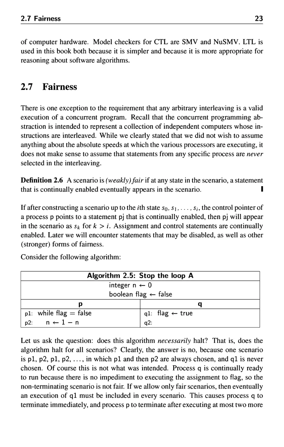
Algorithm 2.5: Stop the loop A
integer n <- 0
boolean flag <- false
P
pi: while flag = false
p2: n <- 1 — n
q
ql: flag <- true
q2:
Let us ask the question: does this algorithm necessarily halt? That is, does the
algorithm halt for all scenarios? Clearly, the answer is no, because one scenario
is pi, p2, pi, p2, ..., in which pi and then p2 are always chosen, and ql is never
chosen. Of course this is not what was intended. Process q is continually ready
to run because there is no impediment to executing the assignment to flag, so the
non-terminating scenario is not fair. If we allow only fair scenarios, then eventually
an execution of ql must be included in every scenario. This causes process q to
terminate immediately, and process p to terminate after executing at most two more

24
2 The Concurrent Programming Abstraction
statements. We will say that under the assumption of weak fairness, the algorithm
is correct with respect to the claim that it always terminates.
2.8 Machine-code instructions^1
Algorithm 2.4 may seem artificial, but it a faithful representation of the actual
implementation of computer programs. Programs written in a programming language
like Ada or Java are compiled into machine code. In some cases, the code is for a
specific processor, while in other cases, the code is for a virtual machine like the
Java Virtual Machine (JVM). Code for a virtual machine is then interpreted or a
further compilation step is used to obtain code for a specific processor. While there
are many different computer architectures—both real and virtual—they have much
in common and typically fall into one of two categories.
Register machines
A register machine performs all its computations in a small amount of high-speed
memory called registers that are an integral part of the CPU. The source code of
the program and the data used by the program are stored in large banks of memory,
so that much of the machine code of a program consists of load instructions, which
move data from memory to a register, and store instructions, which move data from
a register to memory, load and store of a memory cell (byte or word) is atomic.
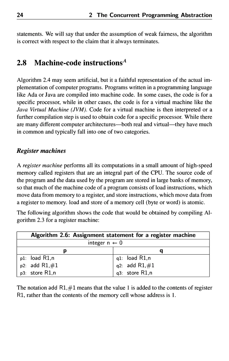
The following algorithm shows the code that would be obtained by compiling
Algorithm 2.3 for a register machine:
Algorithm 2.6: Assignment statement for a register machine
integer n <- 0
p I q
pi: load Rl,n I ql: load Rl,n
P2: add Rl,#l q2: add Rl,#l
p3: store Rl,n q3: store Rl,n
The notation add Rl,#l means that the value 1 is added to the contents of register
Rl, rather than the contents of the memory cell whose address is 1.

2.8 Machine-code instructions
25
The following diagram shows the execution of the three instructions:
Memory
Memory
Memory
0
0
1
load
store
0
1
1
Registers
Registers
Registers
First, the value stored in the memory cell for n is loaded into one of the registers;
second, the value is incremented within the register; and third, the value is stored
back into the memory cell.
Ostensibly, both processes are using the same register Rl, but in fact, each
process keeps its own copy of the registers. This is true not only on a multiprocessor
or distributed system where each CPU has its own set of registers, but even on a
multitasking single-CPU system, as described in Section 2.3. The context switch
mechanism enables each process to run within its own context consisting of the
current data in the computational registers and other registers such as the control
pointer. Thus we can look upon the registers as analogous to the local variables
temp in Algorithm 2.4 and a bad scenario exists that is analogous to the bad
scenario for that algorithm:
Process p
pi: load Rl,n
p2: add Rl,#l
p2: add Rl,#l
p3: store Rl,n
p3: store Rl,n
(end)
(end)
Process q
ql: load Rl,n
ql: load Rl.n
q2: add Rl,#l
q2: add Rl,#l
q3: store Rl,n
q3: store Rl,n
(end)
n
0
0
0
0
0
1
1
p.Rl
?
0
0
1
1
q.Rl
?
?
0
0
1
1
Stack machines
The other type of machine architecture is the stack machine. In this architecture,
data is held not in registers but on a stack, and computations are implicitly
performed on the top elements of a stack. The atomic instructions include push and

26
2 The Concurrent Programming Abstraction
pop, as well as instructions that perform arithmetical, logical and control
operations on elements of the stack. In the register machine, the instruction add Rl,#l
explicitly mentions its operands, while in a stack machine the instruction would
simply be written add, and it would add the values in the top two positions in the
stack, leaving the result on the top in place of the two operands:
Algorithm 2.7: Assignment statement for a stack machine
integer n «- 0
P
pi: push n
p2: push #1
p3: add
p4: pop n
q
ql
q2
q3
q4
push n
push #1
add
pop n
The following diagram shows the execution of these instructions on a stack
machine:
Memory
Memory
Memory
0
push \
c
Stc
0
act
<
1
0
<
Stc
1
ad
<
1
<
Stc
\ pop
1
)ck
Initially, the value of the memory cell for n is pushed onto the stack, along with the
constant 1. Then the two top elements of the stack are added and replaced by one
element with the result. Finally (on the right), the result is popped off the stack and
stored in the memory cell. Each process has its own stack, so the top of the stack,
where the computation takes place, is analogous to a local variable.
It is easier to write code for a stack machine, because all computation takes place in
one place, whereas in a register machine with more than one computational register
you have to deal with the allocation of registers to the various operands. This is a
non-trivial task that is discussed in textbooks on compilation. Furthermore, since
different machines have different numbers and types of registers, code for register
machines is not portable. On the other hand, operations with registers are extremely
fast, whereas if a stack is implemented in main memory access to operands will be
much slower.

2.8 Machine-code instructions
27
For these reasons, stack architectures are common in virtual machines where
simplicity and portability are most important. When efficiency is needed, code for the
virtual machine can be compiled and optimized for a specific real machine. For
our purposes the difference is not great, as long as we have the concept of memory
that may be either global to all processes or local to a single process. Since global
and local variables exist in high-level programming languages, we do not need to
discuss machine code at all, as long as we understand that some local variables are
being used as surrogates for their machine-language equivalents.
Source statements and machine instructions
We have specified that source statements like
n <- n + 1
are atomic. As shown in Algorithm 2.6 and Algorithm 2.7, such source statements
must be compiled into a sequence of machine language instructions. (On some
computers n<-n+l can be compiled into an atomic increment instruction, but this
is not true for a general assignment statement.) This increases the number of inter-
leavings and leads to incorrect results that would not occur if the source statement
were really executed atomically.
However, we can study concurrency at the level of source statements by
decomposing atomic statements into a sequence of simpler source statements. This is what
we did in Algorithm 2.4, where the above atomic statement was decomposed into
the pair of statements:
temp <- n + 1
n <- temp + 1
The concept of a "simple" source statement can be formally defined:
Definition 2.7 An occurrence of a variable v is defined to be critical reference: (a)
if it is assigned to in one process and has an occurrence in another process, or (b) if
it has an occurrence in an expression in one process and is assigned to in another.
A program satisfies the limited-critical-reference (LCR) restriction if each
statement contains at most one critical reference. I
Consider the first occurrence of n in n<-n+l. It is assigned to in process p and
has (two) occurrences in process q, so it is critical by (a). The second occurrence
of n in n<-n+l is critical by (b) because it appears in the expression n+1 in p

28 2 The Concurrent Programming Abstraction
and is also assigned to in q. Consider now the version of the statements that uses
local variables. Again, the occurrences of n are critical, but the occurrences of
temp are not. Therefore, the program satisfies the LCR restriction. Concurrent
programs that satisfy the LCR restriction yield the same set of behaviors whether
the statements are considered atomic or are compiled to a machine architecture
with atomic load and store. See [50, Section 2.2] for more details.
The more advanced algorithms in this book do not satisfy the LCR restriction,
but can easily be transformed into programs that do satisfy it. The transformed
programs may require additional synchronization to prevent incorrect scenarios,
but the additions are simple and do not contribute to understanding the concepts of
the advanced algorithms.
2.9 Volatile and non-atomic variables^1
There are further complications that arise from the compilation of high-level
languages into machine code. Consider for example, the following algorithm:
Algorithm 2.8: Volatile variables
integer n •
P
integer locall, local2
Pi
p2
p3
P4
p5
n «- some expression
computation not using n
locall <- (n + 5) * 7
local2 <- n + 5
n «- locall * local2
^0
q
integer local
ql
q2
q3
q4
q5
local <- n + 6
The single statement in process q can be interleaved at any place during the
execution of the statements of p. Because of optimization during compilation, the
computation in q may not use the most recent value of n. The value of n may be
maintained in a register from the assignment in pi through the computations in p2,
p3 and p4, and only actually stored back into n at statement p5. Furthermore, the
compiler may re-order p3 and 4 to take advantage of the fact that the value of n+5
needed in p3 is computed in p4.
These optimizations have no semantic effect on sequential programs, but they do
in concurrent programs that use global variables, so they can cause programs to be
incorrect. Specifying a variable as volatile instructs the compiler to load and store
the value of the variable at each use, rather than attempt to optimize away these
loads and stores.

2.10 The BACI concurrency simulator
29
Concurrency may also affect computations with multiword variables. A load or
store of a full-word variable (32 bits on most computers) is accomplished atomi-
cally, but if you need to load or store longer variables (like higher precision
numbers), the operation might be carried out non-atomically. A load from another
process might be interleaved between storing the lower half and the upper half
of a 64-bit variable. If the processor is not able to ensure atomicity for
multiword variables, it can be implemented using a synchronization mechanism such as
those to be discussed throughout the book. However, these mechanisms can block
processes, which may not be acceptable in a real-time system; a non-blocking
algorithm for consistent access to multiword variables is presented in Section 13.9.
2.10 The BACI concurrency simulatorL
In Section 2.3, we argued that the proper abstraction for concurrent programs is
the arbitrary interleaving of the atomic statements of sequential processes. The
main reason why this abstraction is appropriate is that we have no control over the
relative rate at which processes execute or over the occurrence of external stimuli
that drive reactive programs. For this reason, the normal execution of a program
on a computer is not the best way to study concurrency. Later in this section,
we discuss the implementation of concurrency in two programming languages,
because eventually you will wish to write concurrent programs using the constructs
available in real languages, but for studying concurrency there is a better way.
A concurrency simulator is a software tool that interprets a concurrent program
under the fine-grained control of the user. Rather than executing or interpreting
the program as fast as possible, a concurrency simulator allows the user to control
the interleaving at the level of atomic statements. The simulator maintains the data
structures required to emulate concurrent execution: separate stacks and registers
for each process. After interpreting a single statement of the program, the simulator
updates the display of the state of the program, and then optionally halts to enable
the user to choose the process from which the next statement will be taken. This
fine-grained control is essential if you want to create potentially incorrect
scenarios, such as the one shown in Sections 2.5 and 2.8. For this reason, we recommend
that you use a concurrency simulator in your initial study of the topic.
This textbook is intended to be used with one of two concurrency simulators: Spin
or BACI. The Spin system is described later in Section 4.6 and Appendix D.2. Spin
is primarily a professional verification tool called a model checker, but it can also
be used as a concurrency simulator. BACI is a concurrency simulator designed as
an educational tool and is easier to use than Spin; you may wish to begin your
studies using BACI and then move on to Spin as your studies progress. In this

30
2 The Concurrent Programming Abstraction
section, we will explain how to translate concurrent algorithms into programs for
the BACI system.
BACI (Ben-Ari Concurrency Interpreter) consists of a compiler and an interpreter
that simulates concurrency. BACI and the user interface jBACI are described in
Appendix D.l. We now describe how to write the following algorithm in the
dialects of Pascal and C supported by the BACI concurrency simulator:
Algorithm 2.9: Concurrent counting algorithm
integer n <- 0
P
integer temp
pi: do 10 times
p2: temp <- n
p3: n <- temp + 1
q
integer temp
ql: do 10 times
q2: temp <- n
q3: n <- temp + 1
The algorithm simply increments a global variable twenty times, ten times in each
of two processes.
The Pascal version of the counting algorithm is shown in Listing 2.1.6 The main
difference between this program and a normal Pascal program is the cobegin
... coend compound statement in line 22. Syntactically, the only statements that
may appear within this compound statement are procedure calls. Semantically,
upon executing this statement, the procedures named in the calls are initialized as
concurrent processes (in addition to the main program which is also considered to
be a process). When the coend statement is reached, the processes are allowed to
execute concurrently, and the main process is blocked until all of the new processes
have terminated. Of course, if one or more processes do not terminate, the main
process will be permanently blocked.
The C version of the counting algorithm is shown in Listing 2.2. The compound
statement cobegin { } in line 17 is used to create concurrent processes as
described above for Pascal. One major difference between the BACI dialect of C and
standard C is the use of I/O statements taken from C++.
The BACI dialects support other constructs for implementing concurrent programs,
and these will be described in due course. In addition, there are a few minor
differences between the standard languages and these dialects that are described in the
BACI documentation.
6By convention, to execute a loop n times, indices in Pascal and Ada range from 1 to n, while
indices in C and Java range from 0 to n - 1.

2.11 Concurrency in Ada
31
1
2
3
4
5
6
7
8
9
10
11
12
13
14
15
16
17
18
19
20
21
22
23
24
program count;
var n: integer := 0;
procedure p;
var temp, i: integer;
begin
for i := 1 to 10 do
begin
temp := n;
n := temp + 1
end
end;
procedure q;
var temp, i: integer;
begin
for i := 1 to 10 do
begin
temp := n;
n := temp + 1
end
end;
begin
cobegin p; q coend;
writeln('The value c
end.
Listing 2.1: A Pascal program for the counting algorithm
2.11 Concurrency in AdaL
The Ada programming language was one of the first languages to include
support for concurrent programming as part of the standard language definition, rather
than as part of a library or operating system. Listing 2.3 shows an Ada program
implementing Algorithm 2.9. The Ada term for process is task. A task is declared
with a specification and a body, though in this case the specification is empty.
Tasks are declared as objects of the task type in the declarative part of a
subprogram. It is activated at the subsequent begin of the subprogram body. A
subprogram will not terminate until all tasks that it activated terminate. In this program,
we wish to print out the final value of the variable N, so we use an inner block
(declare ... begin ... end) which will not terminate until both tasks P and Q
have terminated. When the block terminates, we can print the final value of N. If
we did not need to print this value, the task objects could be global and the main

32
2 The Concurrent Programming Abstraction
1
2
3
4
5
6
7
8
9
10
11
12
13
14
15
16
17
18
19
int n = 0;
void p() {
int temp, i;
for (i = 0; i < 10;
temp = n;
n = temp + 1;
}
}
void q() {
int temp, i;
for (i = 0; i < 10;
temp = n;
n = temp + 1;
}
}
void main() {
cobegin { p(); q();
cout << "The value
}
i++){
i++){
}
of n is " « n « "\n";
Listing 2.2: AC program for the counting algorithm
program would simply be null; after executing the null statement, the program
waits for the task to terminate:
procedure Count is
task type Count_Task;
task body Count_Task is ...end Count_Task;
P, Q: Count_Task;
begin
null;
end Count;
Of course, if you run this program, you will almost certainly get the answer 20,
because it is highly unlikely that there will be a context switch from one task to
another during the loop. We can artificially introduce context switches by writing
the statement delay 0.0 between the two statements in the loop. When I ran this
version of the program, it consistently printed 10.

2.11 Concurrency in Ada
33
1
2
3
4
5
6
7
8
9
10
11
12
13
14
15
16
17
18
19
20
21
with Ada.Text_IO; use Ada.Text_IO;
procedure Count is
N: Integer := 0;
pragma Volatile(N);
task type Count_Task;
task body CountTask is
Temp: Integer;
begin
for 1 in 1..10 loop
Temp := N;
N := Temp + 1;
end loop;
end Count_Task;
begin
declare
P, Q: Count_Task;
begin
null;
end;
Put_Line("The value of N is " & Integer' Image(N));
end Count;
Listing 2.3: An Ada program for the counting algorithm
Volatile and atomic
A type or variable can be declared as volatile or atomic (Section 2.9) using pragma
Volatile or pragma Atomic:7
N: Integer := 0;
pragma Volatile(N);
pragma Volatile_Components and pragma Atomic_Components are used for
arrays to ensure that the components of an array are volatile or atomic. An atomic
type or variable is also volatile. It is implementation-dependent which types can
be atomic.
7These constructs are described in the Systems Programming Annex (C.6) of the Ada Language
Reference Manual.

34
2 The Concurrent Programming Abstraction
1
2
3
4
5
6
7
8
9
10
11
12
13
14
15
16
17
18
19
20
21
22
class Count extends Thread {
}
static volatile int n = 0;
public void run() {
int temp;
for (int i = 0; i < 10; i++) {
temp = n;
n = temp + 1;
}
}
public static void main(String[] args) {
Count p = new CountQ;
Count q = new Count();
p. start ();
q. start ();
try {
p.join ();
q.join ();
}
catch (InterruptedException e) { }
System.out.println ("The value of n is " + n);
}
Listing 2.4: A Java program for the counting algorithm
2.12 Concurrency in JavaL
The Java language has supported concurrency from the very start. However, the
concurrency constructs have undergone modification; in particular, several
dangerous constructs have been deprecated (dropped from the language). The latest
version (1.5) has an extensive library of concurrency constructs Java.util.concurrent,
designed by a team led by Doug Lea. For more information on this library see
the Java documentation and [44]. Lea's book explains how to integrate
concurrency within the framework of object-oriented design and programming—a topic
not covered in this book.
The Java language supports concurrency through objects of type Thread. You can
write your own classes that extend this type as shown in Listing 2.4. Within a class
that extends Thread, you have to define a method called run that contains the code
to be run by this process. Once the class has been defined, you can define fields of
this type and assign to them objects created by allocators (lines 11-12). However,

2.12 Concurrency in Java
35
allocation and construction of a Thread object do not cause the thread to run. You
must explicitly call the start method on the object (lines 13-14), which in turn will
call the run method.
The global variable n is declared to be static so that we will have one copy that
is shared by all of the objects declared to be of this class. The main method
of the class is used to allocate and initiate the two processes; we then use the
join method to wait for termination of the processes so that we can print out the
value of n. Invocations of most thread methods require that you catch (or throw)
Interrupted Exception .
If you run this program, you will almost certainly get the answer 20, because it is
highly unlikely that there will be a context switch from one task to another during
the loop. You can artificially introduce context switches between between the two
assignment statements of the loop: static method Thread.yield () causes the
currently executing thread to temporarily cease execution, thus allowing other threads
to execute.
Since Java does not have multiple inheritance, it is usually not a good idea to extend
the class Thread as this will prevent extending any other class. Instead, any class
can contain a thread by implementing the interface Runnable:
class Count extends JFrame implements Runnable {
public void run() { ... }
}
Threads are created from Runnable objects as follows:
Count count = new Count();
Thread tl = new Thread(count);
or simply:
Thread tl = new Thread(new CountQ);
Volatile
A variable can be declared as volatile (Section 2.9):
volatile int n = 0;
Variables of primitive types except long and double are atomic, and long and
double are also atomic if they are declared to be volatile. A reference variable is

36
2 The Concurrent Programming Abstraction
i #include "for.h"
2 #define TIMES 10
3 byte n = 0;
4 proctype P() {
5 byte temp;
6 for (i,l, TIMES)
7 temp = n;
8 n = temp + 1
9 rof (i )
10 }
ii init {
12 atomic {
13 run P();
14 run P()
'5 }
16 (_r"'_pr == 1);
n printf ("MSC: The value is %d\n", n)
■8 }
Listing 2.5: A Promela program for the counting algorithm
atomic, but that does not mean that the object pointed to is atomic. Similarly, if a
reference variable is declared as volatile it does not follow that the object pointed
to is volatile. Arrays can be declared as volatile, but not components of an array.
2.13 Writing concurrent programs in PromelaL
Promela is the model specification language of the model checker Spin, which will
be described in Chapter 4. Here we describe enough of the syntax and semantics
of the Promela language to write a program for Algorithm 2.9.
The syntax and semantics of declarations and expressions are similar to those of
C, but the control structures might be unfamiliar, because they use the syntax and
semantics of guarded commands, which is a notation commonly used in theoretical
computer science. A Promela program for the counting algorithm is shown in
Listing 2.5, where we have used macros defined in the file for.h to write a familiar
for-loop.
The process type P is declared using the keyword proctype; this only declares a
type so (anonymous) instances of the type must be activated using run P(). If you
declare a process with the reserved name init, it is the first process that is run.

2.14 Supplement: the state diagram for the frog puzzle 37
Promela does not have a construct similar to cobegin, but we can simulate it using
other statements, run and atomic. The run P() statements activate the two
processes, atomic is used to ensure that both activations are completed before the new
processes begin; this prevents meaningless scenarios where one or more processes
are never executed.
The join (waiting for both processes to finish before continuing) is simulated by
waiting for _nr_pr to have the value 1; this is a predefined variable counting the
number of active processes (including init).
When the two processes have terminated, the final value of n is printed. The prefix
MSC is a convention that is used by postprocessors to display the output of the
program.
2.14 Supplement: the state diagram for the frog puzzle
This section demonstrates state diagrams using an interesting puzzle. Consider a
system consisting of 2n+1 stones set in a row in a swamp. On the leftmost n stones
are male frogs who face right and on the rightmost n stones are female frogs who
face left; the middle stone is empty:
©@©©oeeee
Frogs may move in the direction they are facing: jumping to the adjacent stone if it
is empty, or if not, jumping over the frog to the second adjacent stone if that stone
is empty. For example, the following configuration will result, if the female frog
on the seventh stone jumps over the frog on the sixth stone, landing on the fifth
stone:
Let us now ask if there is a sequence of moves that will exchange the positions of
the male and female frogs:
This puzzle faithfully represents a concurrent program under the model of
interleaving of atomic operations. There are 2n processes, and one or more of them

38 2 The Concurrent Programming Abstraction
(MFuMF) (MFMFu)
(MFFuM) (uFMFM)
x I
(FuMFJvQ
j
(FFMuM)
»
(FFuMM)
x
Figure 2.1: State diagram for the frog puzzle
may be able to make a move at any time, although only one of the possible moves
is selected. The configuration of the frogs on the stones represents a state, and the
transitions are the allowable moves.
It is easy to put an upper bound on the number of possible states: there are In frogs
and one empty place that can be placed one after another giving (In + 1 )\/(n\ • n\)
possible states. The divisor n\ • n\ comes from the fact that all the male frogs and
all the female frogs are identical, so permutations among frogs of the same gender
result in identical states. For n = 2, there are 30 states, and for n = 3, there are 140
states. However, not all states will be reachable in an actual computation.
To build a state diagram, start with the initial state and for each possible move draw
the new state; if the new state already exists, draw an arrow to the existing state.
For n = 2, Figure 2.1 shows all possible states that can occur if the computation
starts with a move by a male frog. Note that the state U MMFF can be reached in
either one or two moves, and that from this state no further moves are possible as
indicated by the symbol x.
(uFMMF)
(FuMMF)

Transition
39
From the diagram we can read off interesting correctness assertions. For example,
there is a computation leading to the target state FFu MM; no computation from
state M F U M F leads to the target state; all computations terminate (trivial, but still
nice to know).
Transition
This chapter has presented and justified the concurrent program abstraction as the
interleaved execution of atomic statements. The specification of atomic statements
is a basic task in the definition of a concurrent system; they can be machine
instructions or higher-order statements that are executed atomically. We have also
shown how concurrent programs can be written and executed using a concurrency
simulator (Pascal and C in BACI), a programming language (Ada and Java) or
simulated with a model checker (Promela in Spin). But we have not actually solved
any problems in concurrent programming. The next three chapters will focus on
the critical section problem, which is the most basic and important problem to be
solved in concurrent programming.
Exercises
1. How many computations are there for Algorithm 2.7.
2. Construct a scenario for Algorithm 2.9 in which the final value of n is 10.
3. (Ben-Ari and Burns [10]) Construct a scenario for Algorithm 2.9 in which the
final value of n is 2.
4. For positive values of K, what are the possible final values of n in the following
algorithm?
Algorithm 2.10: Incrementing and decrementing
integer n <- 0
P
integer temp
pi: do K times
p2: temp <- n
p3: n <- temp + 1
q
integer temp
ql: do K times
q2: temp <- n
q3: n <- temp - 1

40
2 The Concurrent Programming Abstraction
5. (Apt and Olderog [3]) Assume that for the function /, there is some integer
value / for which /(/) = 0. Here are five concurrent algorithms that search for
i. An algorithm is correct if for all scenarios, both processes terminate after
one of them has found the zero. For each algorithm, show that it is correct or
find a scenario that is a counterexample.
Algorithm 2.11: Zero A
boolean found
P
integer i 4- 0
Pi
p2
p3
P4
found *- false
while not found
i <- i + 1
found *- f(i) =
= 0
q
integer j 4- 1
ql
q2
q3
q4
found 4- false
while not found
j<-j-l
found 4- f(j) = 0
Algorithm 2.12: Zero B
boolean found <- false
P
integer i <- 0
pi: while not found
p2: i <- i + 1
p3: found <- f(i) =
= 0
q
integer j <- 1
ql: while not found
q2: j <- j - 1
q3: found <- f(j) =
= 0
Algorithm 2.13: Zero C
boolean found <- false
P
integer i <- 0
pi: while not found
p2: i <- i + 1
P3: if f(i) = 0
p4: found <- true
q
integer j <- 1
ql
q2
q3
q4
while not found
j<_j_i
if f(j) = 0
found <- true
In process p of the following two algorithms, await turn = 1 and turn <- 2
are executed as a one atomic statement when the value of turn is 1; similarly,
await turn = 2 and turn <- 1 are executed atomically in process q.

Exercises
41
Algorithm 2.14:
Zero D
boolean found «- false
integer turn <- 1
p
pi:
p2:
p3:
p4:
p5:
integer i «- 0
while not found
await turn = 1
turn *- 2
i <- i + 1
if f(i) = 0
found *- true
q
ql:
q2:
q3:
q4:
q5:
integer j «- 1
while not found
await turn = 2
turn *- 1
j<-j-l
if f(j) = 0
found <- true
Algorithm 2.15
boolean found <-
integer turn <- 1
P
pl
p2
p3
p4
p5
p6
integer i <- 0
while not found
await turn = 1
turn <- 2
i <- i + 1
if f(i) = 0
found <- true
turn <- 2
: Zero E
false
q
ql
q2
q3
q4
q5
q6
integer j <- 1
while not found
await turn = 2
turn <- 1
j^j-i
iff(j) = 0
found <- true
turn <- 1
6. Consider the following algorithm where each of ten processes executes the
statements with i set to a different number in 1,..., 10:
Algorithm 2.16: Concurrent algorithm A
integer array[1..10] C
integer array[1..10] D
ten distinct initial values
integer myNumber, count
myNumber <- C[i]
count <- number of elements of C less than myNumber
D[count + 1] <- myNumber
(a) What does the algorithm do?
(b) What would happen if C in line p3 were replaced by D?
(c) What would happen if the array C were initialized with values that are
not all distinct? Correct the algorithm to take care of this case.

42
2 The Concurrent Programming Abstraction
7. Consider the following algorithm:
Algorithm 2.17: Concurrent algorithm B
integer n <- 0
P
pi: while n < 2
p2: write(n)
q
ql: n <- n + 1
q2: n <- n + 1
(a) Construct scenarios that give the output sequences: 012, 002, 02.
(b) Must the value 2 appear in the output?
(c) How many times can the value 2 appear in the output?
(d) How many times can the value 1 appear in the output?
8. Consider the following algorithm:
Algorithm 2.18: Concurrent algorithm C
integer n <- 1
P
pi: while n < 1
p2: n <- n + 1
q
ql: while n > 0
q2: n <- n — 1
(a) Construct a scenario in which the loop in p executes exactly once.
(b) Construct a scenario in which the loop in p executes exactly three times.
(c) Construct a scenario in which both loops execute infinitely often.
9. Consider the following algorithm:
Algorithm 2.19: Stop the loop B
integer n <- 0
boolean flag <- false
P
pi: while flag = false
p2: n <- 1 — n
P3:
q
ql: while flag = false
q2: if n = 0
q3: flag <- true
(a) Construct a scenario for which the program terminates.
(b) What are the possible values of n when the program terminates?
(c) Does the program terminate for all scenarios?
(d) Does the program terminate for all fair scenarios?

Exercises
43
10. Consider the following algorithm:
Algorithm 2.20: Stop the loop C
integer n <- 0
boolean flag <- false
P
pi: while flag = false
p2: n <- 1 — n
q
ql: while n = 0
// Do nothing
q2: flag <- true
(a) Construct a scenario for which the program terminates.
(b) What are the possible values of n when the program terminates?
(c) Does the program terminate for all scenarios?
(d) Does the program terminate for all fair scenarios?
11. Complete Figure 2.1 with all possible states that can occur if the computation
starts with a move by a female frog. Make sure not to create duplicate states.
12. (The welfare crook problem, Feijen [3, Section 7.5]) Let a, b, c be three
ordered arrays of integer elements; it is known that some element appears in
each of the three arrays. Here is an outline of a sequential algorithm to find
the smallest indices i, j, k, for which a[i] = b[j] = c[k]:
Algorithm 2.21: Welfare crook problem
pl
p2
p3
p4
p5
p6
integer array[0..N] a, b, c <- ... (as required)
integer i <- 0, j <- 0, k <- 0
loop
if condition-1
i <- i + 1
else if condition-2
j<-j + 1
else if condition-3
k <- k + 1
else exit loop
(a) Write conditional expressions that make the algorithm correct.
(b) Develop a concurrent algorithm for this problem.

3 The Critical Section Problem
3.1 Introduction
This chapter presents a sequence of attempts to solve the critical section problem
for two processes, culminating in Dekker's algorithm. The synchronization
mechanisms will be built without the use of atomic statements other than atomic load
and store. Following this sequence of algorithms, we will briefly present solutions
to the critical section problem that use more complex atomic statements. In the
next chapter, we will present algorithms for solving the critical section problem for
N processes.
Algorithms like Dekker's algorithm are rarely used in practice, primarily because
real systems support higher synchronization primitives like those to be discussed in
subsequent chapters (though see the discussion of "fast" algorithms in Section 5.4).
Nevertheless, this chapter is the heart of the book, because each incorrect algorithm
demonstrates some pathological behavior that is typical of concurrent algorithms.
Studying these behaviors within the framework of these elementary algorithms will
prepare you to identify and correct them in real systems.
The proofs of the correctness of the algorithms will be based upon the explicit
construction of state diagrams in which all scenarios are represented. Some of the
proofs are left to the next chapter, because they require more complex tools, in
particular the use of temporal logic to specify and verify correctness properties.
3.2 The definition of the problem
We start with a specification of the structure of the critical section problem and the
assumptions under which it must be solved:
• Each of N processes is executing in a infinite loop a sequence of statements
that can be divided into two subsequences: the critical section and the non-
critical section.
• The correctness specifications required of any solution are:
45

46
3 The Critical Section Problem
Mutual exclusion Statements from the critical sections of two or more
processes must not be interleaved.
Freedom from deadlock If some processes are trying to enter their critical
sections, then one of them must eventually succeed.
Freedom from (individual) starvation If any process tries to enter its
critical section, then that process must eventually succeed.
• A synchronization mechanism must be provided to ensure that the
correctness requirements are met. The synchronization mechanism consists of
additional statements that are placed before and after the critical section. The
statements placed before the critical section are called the preprotocol and
those after it are called the postprotocol. Thus, the structure of a solution for
two processes is as follows:
Algorithm 3.1: Critical section problem
global variables
P
local variables
loop forever
non-critical section
preprotocol
critical section
postprotocol
q
local variables
loop forever
non-critical section
preprotocol
critical section
postprotocol
• The protocols may require local or global variables, but we assume that no
variables used in the critical and non-critical sections are used in the
protocols, and vice versa.
• The critical section must progress, that is, once a process starts to execute
the statements of its critical section, it must eventually finish executing those
statements.
• The non-critical section need not progress, that is, if the control pointer of a
process is at or in its non-critical section, the process may terminate or enter
an infinite loop and not leave the non-critical section.

3.2 The definition of the problem
47
The following diagram will help visualize the critical section problem:
The stick figures represent processes and the box is a critical region in which at
most one process at a time may be executing the statements that form its critical
section. The solution to the problem is given by the protocols for opening and
closing the door to the critical region in such a manner that the correctness properties
are satisfied.
The critical section problem is intended to model a system that performs complex
computation, but occasionally needs to access data or hardware that is shared by
several processes. It is unreasonable to expect that individual processes will never
terminate, or that nothing bad will ever occur in the programs of the system. For
example, a check-in kiosk at an airport waits for a passenger to swipe his credit card
or touch the screen. When that occurs, the program in the kiosk will access a central
database of passengers, and it is important that only one of these programs update
the database at a time. The critical section is intended to model this operation only,
while the non-critical section models all the computation of the program except for
the actual update of the database.
It would not make sense to require that the program actually participate in the
update of the database by programs in other kiosks, so we allow it to wait indefinitely
for input, and we take into account that the program could malfunction. In other
words, we do not require that the non-critical section progress. On the other hand,
we do require that the critical section progress so that it eventually terminates. The
reason is that the process executing a critical section typically holds a "lock" or
"permission resource," and the lock or resource must eventually be released so that
other processes can enter their critical sections. The requirement for progress is
reasonable, because critical sections are usually very short and their progress can
be formally verified.
Obviously, deadlock ("my computer froze up") must be avoided, because systems
are intended to provide a service. Even if there is local progress within the
protocols as the processes set and check the protocol variables, if no process ever

48
3 The Critical Section Problem
succeeds in making the transition from the preprotocol to the critical section, the
program is deadlocked.
Freedom from starvation is a strong requirement in that it must be shown that no
possible execution sequence of the program, no matter how improbable, can cause
starvation of any process. This requirement can be weakened; we will see one
example in the algorithm of Section 5.4.
A good solution to the critical section problem will also be efficient, in the sense
that the pre- and postprotocols will use as little time and memory as possible. In
particular, if only a single process wishes to enter its critical section it will succeed
in doing so almost immediately.
3.3 First attempt
Here is a first attempt at solving the critical section problem for two processes:
Algorithm 3.2: First attempt
integer turn <- 1
P
Pi:
p2:
P3:
p4:
loop forever
non-critical section
await turn = 1
critical section
turn <- 2
q
loop forever
ql
q2
q3
q4
non-critical section
await turn = 2
critical section
turn <- 1
The statement await turn=l is an implementation-independent notation for a
statement that waits until the condition turn=l becomes true. This can be implemented
(albeit inefficiently) by a busy-wait loop that does nothing until the condition is
true.
The global variable turn can take the two values 1 and 2, and is initially set to the
arbitrary value 1. The intended meaning of the variable is that it indicates whose
"turn" it is to enter the critical section. A process wishing to enter the critical
section will execute a preprotocol consisting of a statement that waits until the
value of turn indicates that its turn has arrived. Upon exiting the critical section,
the process sets the value of turn to the number of the other process.
We want to prove that this algorithm satisfies the three properties required of a
solution to the critical section problem. To that end we first explain the
construction of state diagrams for concurrent programs, a concept that was introduced in
Section 2.2.

3.4 Proving correctness with state diagrams
49
3.4 Proving correctness with state diagrams
States
You do not need to know the history of the execution of an algorithm in order to
predict the result of the next step to be executed. Let us first examine this claim for
sequential algorithms and then consider how it has to be modified for concurrent
algorithms. Consider the following algorithm:
Algorithm 3.3: History in a sequential algorithm
integer a ■«- 1, b «- 2
pi:
p2:
P3:
Millions of statements
a <- (a+b)*5
Suppose now that the computation has reached statement p2, and the values of a
and b are 10 and 20, respectively. You can now predict with absolute certainty that
as a result of the execution of statement p2, the value of a will become 150, while
the value of b will remain 20; furthermore, the control pointer of the computer will
now contain p3. The history of the computation—how exactly it got to statement
p2 with those values of the variables—is irrelevant.
For a concurrent algorithm, the situation is similar:
Algorithm 3.4: History in a concurrent algorithm
integer a <- 1, b *- 2
P
pi: Millions of statements
P2: a <- (a+b)*5
P3: ...
q
ql: Millions of statements
q2: b <- (a+b)*5
q3: ...
Suppose that the execution has reached the point where the first process has reached
statement p2 and the second has reached q2, and the values of a and b are again 10
and 20, respectively. Because of the interleaving, we cannot predict whether the
next statement to be executed will come from process p or from process q; but we
can predict that it will be from either one or the other, and we can specify what the
outcome will be in either case.
In the sequential Algorithm 3.3, states are triples such as 57 = (p2, 10,20). From
the semantics of assignment statements, we can predict that executing the
statement p2 in state 57 will cause the state of the computation to change to si+\ =
(p3, 150, 20). Thus, given the initial state of the computation sq = (pi, 1, 2), we

50
3 The Critical Section Problem
can predict the result of the computation. (If there are input statements, the values
placed into the input variables are also part of the state.) It is precisely this
property that makes debugging practical: if you find an error, you can set a breakpoint
and restart a computation in the same initial state, confident that the state of the
computation at the breakpoint is the same as it was in the erroneous computation.
In the concurrent Algorithm 3.4, states are quadruples such as 57 = (p2, q2, 10, 20).
We cannot predict what the next state will be, but we can be sure that it is either
■sf+i = (P3, q2, 150,20) or sqi+] = (p2, q3, 10, 150) depending on whether the next
state taken is from process p or process q, respectively. While we cannot predict
which states will appear in any particular execution of a concurrent algorithm,
the set of reachable states (Definition 2.5) are the only states that can appear in
any computation. In the example, starting from state 57, the next state will be an
element of the set {sf+1, sf+1}. From each of these states, there are possibly two
new states that can be reached, and so on. To check correctness properties, it is
only necessary to examine the set of reachable states and the transitions among
them; these are represented in the state diagram.
For the first attempt, Algorithm 3.2, states are triples of the form (p,, qy, rwra),
where turn denotes the value of the variable turn. Remember that we are assuming
that any variables used in the critical and non-critical sections are distinct from the
variables used in the protocols and so cannot affect the correctness of the solution.
Therefore, we leave them out of the description of the state. The mutual exclusion
correctness property holds if the set of all accessible states does not contain a state
of the form (p3, q3, turn) for some value of turn, because p3 and q3 are the labels
of the critical sections.
State diagrams
How many states can there be in a state diagram? Suppose that the algorithm has
N processes with nt statements in process /, and M variables where variable j
has nij possible values. The number of possible states is the number of tuples that
can be formed from these values, and we can choose each element of the tuple
independently, so the total number of states is n\ x • • • x n^ x m\ • • • x rriM- For
the first attempt, the number of states is /tj x n^ x m\ = 4 x 4 x 2 = 32, since it is
clear from the text of the algorithm that the variable turn can only have two values,
1 and 2. In general, variables may have as many values as their representation can
hold, for example, 232 for a 32-bit integer variable.
However, it is possible that not all states can actually occur, that is, it is possible
that some states do not appear in any scenario starting from the initial state so =
(pi, ql, 1). In fact, we hope so! We hope that the states (p3, q3, 1) and (p3, q3,2),

3.4 Proving correctness with state diagrams
51
which violate the correctness requirement of mutual exclusion, are not accessible
from the initial state.
To prove a property of a concurrent algorithm, we construct a state diagram and
then analyze if the property holds in the diagram. The diagram is constructed
incrementally, starting with the initial state and considering what the potential next
states are. If a potential next state has already been constructed, then we can
connect to it, thus obtaining a finite presentation of an unbounded execution of the
algorithm. By the nature of the incremental construction, turn will only have the
values 1 and 2, because these are the only values that are ever assigned by the
algorithm.
The following diagram shows the first four steps of the incremental construction of
the state diagram for Algorithm 3.2:
pl.ql.l
p2,ql,l
Pl.q2,l
P2,q2,l
The initial state is (pi, ql, 1). If we execute pi from process p, the next state is
(p2, ql, 1): the first element of the tuple changes because we executed a
statement of the first process, the second element does not change because we did not
execute a statement of that process, and the third element does not change since—
by assumption—the non-critical section does not change the value of the variable
turn. If, however, we execute ql from process q, the next state is (pi, q2, 1). From
this state, if we try to execute another statement, q2, from process q, we remain
in the same state. The statement is await turn=2, but turn = 1. We do not draw
another instance of (pi, q2, 1); instead, the arrow representing the transition points
to the existing state.
The incremental construction terminates after 16 of the 32 possible states have been
constructed, as shown in Figure 3.1. You may (or may not!) want to check if the
construction has been carried out correctly.
A quick check shows that neither of the states (p3, q3, 1) nor (p3, q3, 2) occurs;
thus we have proved that the mutual exclusion property holds for the first attempt.

52
3 The Critical Section Problem
Figure 3.1: State diagram for the first attempt

3.5 Correctness of the first attempt
53
Abbreviating the state diagram
Clearly, the state diagram of the simple algorithm in the first attempt is unwieldy.
When state diagrams are built, it is important to minimize the number of states that
must be constructed. In this case, we can reduce the number of accessible states
from 16 to 4, by reducing the algorithm to the one shown below, where we have
removed the two statements for the critical and non-critical sections.
Algorithm 3.5: First attempt (abbreviated)
integer turn <- 1
P
loop forever
pi: await turn = 1
p2: turn <- 2
q
loop forever
ql: await turn = 2
q2: turn <- 1
Admittedly, this is suspicious. The whole point of the algorithm is to ensure that
mutual exclusion holds during the execution of the critical sections, so how can we
simply erase these statements? The answer is that whatever statements are executed
by the critical section are totally irrelevant to the correctness of the synchronization
algorithm.
If in the first attempt, we replace the statement p3: critical section by the
comment p3: // critical section, the specification of the correctness properties remain
unchanged, for example, we must show that we cannot be in either of the states
(p3, q3, 1) or (p3, q3,2). But if we are at p3 and that is a comment, it is just as
if we were at p4, so we can remove the comment; similar reasoning holds for pi.
In the abbreviated first attempt, the critical sections have been "swallowed up" by
turn <- 2 and turn <- 1, and the non-critical sections have been "swallowed up"
by await turn=l and await turn=2. The state diagram for this algorithm is shown
in Figure 3.2, where for clarity we have given the actual statements and variables
names instead of just labels.
3.5 Correctness of the first attempt
We are now in a position to try to prove the correctness of the first attempt. As noted
above, the proof that mutual exclusion holds is immediate from an examination of
the state diagram.
Next we have to prove that the algorithm is free from deadlock. Recall that this
means that if some processes are trying to enter their critical section then one of
them must eventually succeed. In the abbreviated algorithm, a process is trying to

54
3 The Critical Section Problem
pi: await turn=l/\
ql: await turn=2,;
turn = 2
pi: await turn=l/\
q2: turn<-l,
turn = 2
/pi: await turn=l,
^ ql: await turn=2,
turn = 1
( p2: turn^2,
I ql: await turn=2,
\^ turn = 1
Figure 3.2: State diagram for the abbreviated first attempt
enter its critical section if it is trying to execute its await statement. We have to
check this for the four states; since the two left states are symmetrical with the two
right states, it suffices to check one of the pairs.
Consider the upper left state (await turn=l, await turn=2, turn = 2). Both
processes are trying to execute their critical sections; if process q tries to execute await
turn=2, it will succeed and enter its critical section.
Consider now the lower left state (await turn=l, turn <- 1, turn = 2). Process p
may try to execute await turn=l, but since turn = 2, it does not change the state.
By the assumption of progress on the critical section and the assignment statement,
process q will eventually execute turn <- 1, leading to the upper right state. Now,
process p can enter its critical section. Therefore, the property of freedom from
deadlock is satisfied.
Finally, we have to check that the algorithm is free from starvation, meaning that
if any process is about to execute its preprotocol (thereby indicating its intention
to enter its critical section), then eventually it will succeed in entering its critical
section. The problem will be easier to understand if we consider the state diagram
for the unabbreviated algorithm; the appropriate fragment of the diagram is shown
in Figure 3.3, where NCS denotes the non-critical section. Consider the state at the
lower left. Process p is trying to enter its critical section by executing p2: await
turn=l, but since turn = 2, the process will loop indefinitely in its await state-

3.6 Second attempt
55
pi: NCS,
ql: NCS,
turn = 2
pi: NCS,
~*(q2: await turn=2,;
turn = 2
p2: await turn=l,
ql: NCS,
turn = 2
p2: await turn=l,
q2: await turn=2,;
turn = 2
Figure 3.3: Fragment of the state diagram for the first attempt
ment until process q executes q4: turn<-l. But process q is at ql: NCS and there
is no assumption of progress for non-critical sections. Therefore, starvation has
occurred: process p is continually checking the value of turn trying to enter its
critical section, but process q need never leave its non-critical section, which is
necessary if p is to enter its critical section.
Informally, turn serves as a permission resource to enter the critical section, with
its value indicating which process holds the resource. There is always some
process holding the permission resource, so some process can always enter the critical
section, ensuring that there is no deadlock. However, if the process holding the
permission resource remains indefinitely in its non-critical section—as allowed by the
assumptions of the critical section problem—the other process will never receive
the resource and will never enter its critical section. In our next attempt, we will
ensure that a process in its non-critical section cannot prevent another one from
entering its critical section.
3.6 Second attempt
The first attempt was incorrect because both processes set and tested a single global
variable. If one process dies, the other is blocked. Let us try to solve the critical
section problem by providing each process with its own variable (Algorithm 3.6).
The intended interpretation of the variables is that wanti is true from the step where
process i wants to enter its critical section until it leaves the critical section, await
statements ensure that a process does not enter its critical section while the other
process has its flag set. This solution does not suffer from the problem of the

56
3 The Critical Section Problem
Algorithm 3.6:
Second attempt
boolean wantp <- false, wantq <- false
P
pl
p2
p3
p4
p5
loop forever
non-critical section
await wantq = false
wantp <- true
critical section
wantp <- false
q
loop forever
ql
q2
q3
q4
q5
non-critical section
await wantp = false
wantq <- true
critical section
wantq <- false
previous one: if a process halts in its non-critical section, the value of its variable
want will remain false and the other process will always succeed in immediately
entering its critical section.
Let us construct a state diagram for the abbreviated algorithm:
Algorithm 3.7: Second attempt (abbreviated)
boolean wantp <- false, wantq <- false
P
loop forever
pl: await wantq = false
p2: wantp <- true
p3: wantp <- false
q
loop forever
ql: await wantp = false
q2: wantq <- true
q3: wantq <- false
Unfortunately, when we start to incrementally construct the state diagram
(Figure 3.4), we quickly find the state (p3: wantp<-false, q3: wantq<-false, true, true),
showing that the mutual exclusion property is not satisfied, (await !want is used
instead of await want=false because of space constraints in the node.)
Paths in the state diagram correspond to scenarios; this portion of the scenario can
also be displayed in tabular form:
Process p
pl: await wantq=false
p2: wantp<-true
p2: wantp<-true
p3: wantp<-false
p3: wantp<-false
Process q
ql: await wantp=false
ql: await wantp=false
q2: wantq<-true
q2: wantq<-true
q3: wantq<-false
wantp
false
false
false
true
true
wantq
false
false
false
false
true
To prove that mutual exclusion holds, we must check that no forbidden state
appears in any scenario. So if mutual exclusion does in fact hold, we need to construct

3.7 Third attempt
57
pi: await Iwantq,
ql: await Iwantp,
falsefalse
p2: wantp<-true,
ql: await Iwantp,
falsefalse
p3: wantp<-false,
^q3: wantq<-false, }<-
true,true
p2: wantp<-true,
q2: wantq<-true,
falsefalse
p3: wantp<-false,
q2: wantq<-true,
truefalse
Figure 3.4: Fragment of the state diagram for the second attempt
the full state diagram for the algorithm, because every path in the diagram is a
scenario; then we must examine every state to make sure that it is not a forbidden state.
When constructing the diagram incrementally, we check each state as it is created,
so that we can stop the construction if a forbidden state is encountered, as it was in
this case. It follows that if the incremental construction is completed (that is, there
are no more reachable states), then we know that no forbidden states occur.
3.7 Third attempt
In the second attempt, we introduced the variables want that are intended to
indicate when a process is in its critical section. However, once a process has
successfully completed its await statement, it cannot be prevented from entering its
critical section. The state reached after the await but before the assignment to want
is effectively part of the critical section, but the value of want does not indicate
this fact. The third attempt (Algorithm 3.8) recognizes that the await statement
Algorithm 3.8: Third attempt
boolean wantp <- false, wantq <- false
P
pl
p2
p3
p4
p5
loop forever
non-critical section
wantp <- true
await wantq = false
critical section
wantp <- false
q
loop forever
ql
q2
q3
q4
q5
non-critical section
wantq <- true
await wantp = false
critical section
wantq <- false

58
3 The Critical Section Problem
should be considered part of the critical section by moving the assignment to want
to before the await. We leave it as an exercise to construct the state diagram for
this algorithm, and to show that no state in the diagram violates mutual exclusion.
In Section 4.2, we will use logic to prove deductively that the algorithm satisfies
the mutual exclusion property.
Unfortunately, the algorithm can deadlock as shown by the following scenario:
Process p
pi: non-critical section
p2: wantp<-true
p2: wantp<-true
p3: await wantq=false
p3: await wantq=false
Process q
ql: non-critical section
ql: non-critical section
q2: wantq<-true
q2: wantq<-true
q3: await wantp=false
wantp
false
false
false
true
true
wantq
false
false
false
false
true
This can also be seen in the following fragment of the state diagram:
/p2: wantp<-true,
I q2: wantq<-true,
V^ false false
p3: await !wantq,
q2: wantq<-true,
truefalse
p3: await Iwantq,
q3: await Iwantp,
true,true
In the rightmost state, both process are trying to enter the critical section, but
neither will ever do so, which is our definition of deadlock.
The term deadlock is usually associated with a "frozen" computation where
nothing whatsoever is being computed; the situation here—a scenario where several
processes are actively executing statements, but nothing useful gets done—is also
called livelock.
3.8 Fourth attempt
In the third attempt, when a process sets the variable want to true, not only does it
indicate its intention to enter its critical section, but also insists on its right to do so.
Deadlock occurs when both processes simultaneously insist on entering their
critical sections. The fourth attempt to solve the critical section problem tries to remedy
this problem by requiring a process to give up its intention to enter its critical
section if it discovers that it is contending with the other process (Algorithm 3.9). The
assignment p4: wantp<-false followed immediately by an assignment to the same
variable p5: wantp<-true would not be meaningful in a sequential algorithm, but

3.8 Fourth attempt
59
Algorithm 3.9:
Fourth attempt
boolean wantp <- false, wantq <- false
P
pl
p2
p3
p4
p5
p6
p7
loop forever
non-critical section
wantp <- true
while wantq
wantp <- false
wantp <- true
critical section
wantp <- false
q
loop forever
ql
q2
q3
q4
q5
q6
q7
non-critical section
wantq <- true
while wantp
wantq <- false
wantq <- true
critical section
wantq <- false
it can be useful in a concurrent algorithm. Since we allow arbitrary interleaving
of statements from the two processes, the second process may execute an arbitrary
number of statements between the two assignments to wantp. When process p
relinquishes the attempt to enter the critical section by resetting wantp to false,
process q may now execute the await statement and succeed in entering its critical
section.
A state diagram or deductive proof will show that the mutual exclusion property
is satisfied and that there is no deadlock. However, a scenario for starvation exists
as shown by the cycle in Figure 3.5. The interleaving is "perfect" in the sense that
the execution of a statement by process q is always followed immediately by the
execution of the equivalently-numbered statement in process p. In this scenario,
both processes are starved.
/p3: while wantq,
q3: while wantp,
true,true
/p5: wantp<-true^
q3: while wantp,
false,true
'p3: while wantq,
\q4: wantq<-false,)
true,true
/p5: wantp<-true,
(q5: wantq<-true,
falsefalse
/p4: wantp<-false\
(q4: wantq<-false,)
true,true ^/
d4: wantp<-false\
[q5: wantq<-true,J
truefalse ^/
Figure 3.5: Cycle in a state diagram for the fourth attempt

60
3 The Critical Section Problem
At this point, most people object that this is not a "realistic" scenario; we can hardly
expect that whatever is causing the interleaving can indefinitely ensure that exactly
two statements are executed by process q followed by exactly two statements from
p. But our model of concurrency does not take probability into account. Unlikely
scenarios have a nasty way of occurring precisely when a bug would have the most
dangerous and costly effects. Therefore, we reject this solution, because it does not
fully satisfy the correctness requirements.
3.9 Dekker's algorithm
Dekker's algorithm for solving the critical section problem is a combination of the
first and fourth attempts:
Algorithm 3.10: Dekker's algorithm
boolean wantp <- false, wantq <- false
integer turn <- 1
P
pl
p2
p3
p4
p5
p6
p7
p8
p9
pl(
loop forever
non-critical section
wantp <- true
while wantq
if turn = 2
wantp <- false
await turn = 1
wantp <- true
critical section
turn <- 2
3: wantp <- false
q
ql
q2
q3
q4
q5
q6
q7
q8
q9
ql
loop forever
non-critical section
wantq <- true
while wantp
if turn = 1
wantq <- false
await turn = 2
wantq <- true
critical section
turn <- 1
3: wantq <- false
Recall that in the first attempt we explicitly passed the right to enter the critical
section between the processes. Unfortunately, this caused the processes to be too
closely coupled and prevented correct behavior in the absence of contention. In the
fourth attempt, each process had its own variable which prevented problems in the
absence of contention, but in the presence of contention both processes insist on
entering their critical sections.
Dekker's algorithm is like the fourth attempted solution, except that the right to
insist on entering, rather than the right to enter, is explicitly passed between the
processes. The individual variables wantp and wantq ensure mutual exclusion.

3.10 Complex atomic statements
61
Suppose now that process p detects contention by finding wantq to be true at
statement p3: while wantq. Process p will now consult the global variable turn to see if
it is its turn to insist upon entering its critical section (turn ^ 2, that is, turn = 1).
If so, it executes the loop at p3 and p4 until process q resets wantq to false, either
by terminating its critical section at qlO or by deferring in q5. If not, process p will
reset wantp to false and defer to process q, waiting until that process changes the
value of turn after executing its critical section.
Dekker's algorithm is correct: it satisfies the mutual exclusion property and it is
free from deadlock and starvation. The correctness properties by can be proved by
constructing and analyzing a state diagram, but instead we will give a deductive
proof in Section 4.5.
3.10 Complex atomic statements
We have found that it is difficult to solve the critical section problem using just
atomic load and store statements. The difficulty disappears if an atomic statement
can both load and store. The solutions given here are shown for two processes, but
they are correct for any number of processes.
The test-and-set statement is an atomic statement defined as the execution of the
following two statements with no possible interleaving between them:
test -and-set(common, local) is
local <- common
common <- 1
Algorithm 3.11: Critical section problem with test-and-set
integer common <- 0
P
integer locall
loop forever
pi: non-critical section
repeat
p2: test-and-set (
common, locall)
p3: until locall = 0
p4: critical section
p5: common <- 0
q
integer local2
loop forever
ql: non-critical section
repeat
q2: test-and-set(
common, local2)
q3: until local2 = 0
q4: critical section
q5: common <- 0

62
3 The Critical Section Problem
Algorithm 3.12: Critical section problem with exchange
integer common <- 1
P
integer locall <- 0
loop forever
pi: non-critical section
repeat
p2: exchange(common, locall)
p3: until locall = 1
p4: critical section
p5: exchange(common, locall)
q
integer local2 <- 0
loop forever
ql: non-critical section
repeat
q2
q3
q4
q5
exchange(common, local2)
until local2 = 1
critical section
exchange(common, local2)
Algorithm 3.11 is the simple solution to the critical section problem using test-
and-set. We leave it as an exercise to prove that this solution satisfies the mutual
exclusion property.
Note: A commonly used notation for specifying atomicity is to put angled brackets
around the group of statements: (local <- common; common <- 1). In Promela,
the keyword atomic is used.
The exchange statement is an atomic statement defined as the atomic swap of the
values of two variables:
exchange(a, b) is
integer temp
temp <- a
a <- b
b <- temp
The solution to the critical section problem with exchange is also very simple
(Algorithm 3.12). Here too, the proof of correctness is left as an exercise.
We conclude with two other atomic statements that have been implemented in
computers; in the exercises you are asked to solve the critical section problem using
these statements.
The fetch-and-add statement is defined as the atomic execution of the following
statements:
fetch—and—add(common, local, x) is
local <- common
common <- common + x

Transition
63
The compare-and-swap statement is defined as the atomic execution of the
following statements:
compare—and—swap(common, old, new) is
integer temp
temp <- common
if common = old
common <- new
return temp
These solutions use busy-wait loops, but this is not a disadvantage in a
multiprocessor, especially if the contention is low.
Transition
This chapter introduced the basic concepts of writing a concurrent program to solve
a problem. Even in the simplest model of atomic load and store of shared memory,
Dekker's algorithm can solve the critical section problem, although it leaves much
to be desired in terms of simplicity and efficiency. Along the journey to Dekker's
algorithm, we have encountered numerous ways in which concurrent programs
can be faulty. Since it is impossible to check every possible scenario for faults,
state diagrams are an invaluable tool for verifying the correctness of concurrent
algorithms.
The next chapter will explore verification of concurrent programming in depth, first
using invariant assertions which are relatively easy to understand and use, and then
using deductive proofs in temporal logic which are more sophisticated. Finally, we
show how programs can be verified using the Spin model checker.
Exercises
1. Complete the state diagram for the abbreviated version of the second attempt
(Figure 3.4).
2. Construct the state diagram for (an abbreviated version of) the third attempt
(Algorithm 3.8). Use it to show that mutual exclusion holds for the algorithm.

64
3 The Critical Section Problem
3. For the fourth attempt (Algorithm 3.9):
(a) Construct the tabular form of the scenario for starvation shown in
Figure 3.5.
(b) Explain why this scenario is considered to be starvation and not livelock
as in the third attempt.
(c) Construct a scenario in which one process is starved while the other
enters its critical section infinitely often.
4. Peterson's algorithm for the critical section problem is based upon Dekker's
algorithm but is more concise because it collapses two await statements into
one with a compound condition. Prove the correctness of Peterson's algorithm
by constructing a state diagram for an abbreviated version of the algorithm.
Algorithm 3.13: Peterson's algorithm
boolean wantp <- false, wantq <- false
integer last ^— 1
P
Pi
p2
p3
p4
p5
p6
loop forever
non-critical section
wantp <- true
last <- 1
await wantq = false or
last = 2
critical section
wantp <- false
q
loop forever
ql
q2
q3
q4
non-critical section
wantq <- true
last <- 2
await wantp = false or
last = 1
q5: critical section
q6: wantq <- false
(In our presentation, the compound condition is atomic because it is in one
labeled line; the algorithm also works if the two conditions are evaluated non-
atomically.)
5. (Buhr and Haridi [16]) Compare the use of the variable turn in Dekker's
algorithm with the use of the variable last in Peterson's algorithm. What advantage
does Dekker's algorithm have? Does it matter if the order of the assignments
in the postprotocol is switched?

Exercises
65
6. (Manna and Pnueli [51, p. 156]) Prove that mutual exclusion is satisfied by
the following algorithm for the critical section problem:
Algorithm 3.14: Manna-
integer wantp <-
p
Pi:
p2:
p3:
p4:
p5:
loop forever
non-critical section
if wantq = —1
wantp < 1
else wantp <- 1
await wantq ^ wantp
critical section
wantp <- 0
-Pnueli algorithm
0, wantq <- 0
q
ql:
q2:
q3:
q4:
q5:
loop forever
non-critical section
if wantp = —1
wantq <- 1
else wantq < 1
await wantp ^ — wa
critical section
wantq <- 0
intq
Note that the if statement is atomic. Find a scenario showing that the algorithm
is not correct if the if statement is not atomic.
7. (Doran and Thomas [26]) Prove the correctness of the following variant of
Dekker's algorithm:
Algorithm 3.15: Doran-Thomas algorithm
boolean wantp <- false, wantq <- false
integer turn <- 1
P
Pi
p2
p3
p4
p5
p6
p7
p8
p9
pl<
pl
loop forever
non-critical section
wantp <- true
if wantq
if turn = 2
wantp <- false
await turn = 1
wantp <- true
await wantq = false
critical section
3: wantp <- false
1: turn <- 2
q
loop forever
ql
q2
q3
q4
q5
q6
q7
q8
q9
non-critical section
wantq <- true
if wantp
if turn = 1
wantq <- false
await turn = 2
wantq <- true
await wantp = false
critical section
qlO: wantq <- false
qll: turn <- 1

66
3 The Critical Section Problem
8. (Lamport [38]) Consider possible solutions of the critical section problem
with one bit per process. (Assume that the initial value of all bits is 0.) Show
that there are no solutions of the following forms:
(a) Bit / is set to 1 only by process / and returns spontaneously to 0.
(b) Bit / is set to 1 only by process / and reset to 0 only by processes other
than /.
9. Prove the correctness of Algorithm 3.11 for the critical section problem using
test-and-set.
10. Prove the correctness of Algorithm 3.12 for the critical section problem using
exchange.
11. Solve the critical section problem using fetch-and-add.
12. Solve the critical section problem using compare-and-swap.

4 Verification of Concurrent
Programs
The previous chapters have shown that concurrent programs can have subtle errors,
that the errors cannot be discovered by debugging and that corrections cannot be
checked by testing. For this reason, formal specification and verification of
correctness properties are far more important for concurrent programs than they are
for sequential programs. In this chapter we will explore several such methods.
We begin with a short section on the specification of correctness properties and then
present the most important technique for proving properties, inductive proofs of
invariants. This technique is used to prove that mutual exclusion holds for the third
attempt. Inductive proofs are easy to carry out once you know what the invariants
are, but they can be quite difficult to discover.
We have already discussed the construction of state diagrams and their use for
proving correctness properties. Unfortunately, the full state diagram of even the
simplest concurrent program is quite large, so it is not practical to manually
construct such diagrams. In fact, for algorithms after the first attempt, we did not
bother to construct full diagrams, and limited ourselves to displaying interesting
fragments. Even if we could display a large diagram, there remains the task of
reasoning with the diagram, that is, of finding forbidden states, cycles that lead to
starvation of a process, and so on.
However, we can use a computer program not only to construct the diagram, but
also to simultaneously check a correctness property. Such a program is called a
model checker, because it checks if the state diagram of the concurrent program is
a model (satisfying interpretation) of a formula specifying a correctness property of
the program. Model checkers have become practical tools for verifying concurrent
programs, capable of checking properties of programs that have billions of states.
They use advanced algorithms and data structures to deal efficiently with large
numbers of states.
Before discussing model checking in general and the Spin tool in particular, we
present a system of temporal logic. Temporal logics have proved to be the most
effective formalism for specifying and verifying concurrent programs. They can
67

68
4 Verification of Concurrent Programs
be used deductively to verify programs as will be shown in Section 4.5; temporal
logics are also used to specify correctness properties for model checkers, and as
such must be mastered by every student of concurrency. We have (more or less
arbitrarily) divided the presentation of temporal logic into two sections: Section 4.3
should suffice for readers interested in using temporal logic to specify elementary
correctness properties in Spin, while Section 4.4 covers more advanced aspects of
the logic.
For further study of temporal logics, consult [9, 50, 51]. You may want to examine
the STeP system, [12] which provides computer support for the construction of
deductive proofs, and the Temporal Logic of Actions (TLA) [41], developed by
Leslie Lamport for specifying concurrent programs.
4.1 Logical specification of correctness properties
We assume that you understand the basic concepts of the propositional calculus, as
summarized in Appendix B.
The atomic propositions will be propositions about the values of the variables and
the control pointers during an execution of a concurrent program. Given a variable
of boolean type such as wantp, the atomic proposition wantp is true in a state if
and only if the value of the variable wantp is true in that state. These two fonts
will be used to denote the program variables and the associated symbols in logic.
Similarly, boolean-valued relations on arithmetic variables are atomic propositions:
turn ^ 2 is true in a state if and only if the value of the variable turn in that state is
not 2.
Each label of a statement of a process will be used as an atomic proposition whose
intended interpretation is "the control pointer of that process is currently at that
label." We again use fonts to distinguish between the label pi and the proposition
pi that may be true or false, depending on the state of the computation. Of course,
since the control pointer of a single process can only point to one statement at a
time, if pi is true, then pj is false for all y # /; we will use this fact implicitly in our
proofs.
To give a concrete example, let use write some formulas related to Algorithm 3.8,
the third attempt. The formula
pi A q\ A -• wantp A -• wantq
is true in exactly one state, (pi, ql false false), where the control pointers of both
processes are at the initial statements and the values of both variables axe false. The

4.2 Inductive proofs of invariants
69
formula is certainly true in the initial state of any computation (by construction of
the program), and just as certainly is false in the second state of any computation
(because either pi or ql will become false), unless, of course, both processes halt
in their non-critical sections, in which case the computation remains in this state
indefinitely.
A more interesting formula is
pA A qA,
which is true if the control pointers of both processes point to critical section; in
other words, if this formula is true, the mutual exclusion property is not satisfied.
Therefore, the program satisfies the mutual exclusion property in states in which
-■(/?4 A qA),
the negation of pA A qA, is true.
pi Aql A -• wantp A -• wantp is an example of a formula that is true in some states
(the initial state of the computation), but false in (most) other states, in particular,
in any state in which the control pointers of the processes are at statements other
than pi and ql. For the program to satisfy the mutual exclusion property, the
formula -«(/?4 A qA) must be true in all possible states of all possible computations.
The next section shows how to prove such claims.
4.2 Inductive proofs of invariants
The formula -«(/?4 A qA) is called an invariant because it must invariably be true at
any point of any computation. Invariants are proved using induction, not over the
natural numbers, but over the states of all computations. (You may want to review
Appendix B.2 on arithmetical induction before reading on.)
(a) Prove that A holds in the initial state. This is called the base case.
(b) Assume that A is true in all states up to the current one, and prove that A
is true in the next state. This is called the inductive step, and the
assumption that A is true in the current and previous states is called the inductive
hypothesis. In a concurrent program, there may be more than one possible
successor to the current state, so the inductive step must be proved for each
one of them.
If (a) and (b) can be proved, we can conclude that A is true for all states of all
computations.

70
4 Verification of Concurrent Programs
Given an invariant, a proof by induction over all states is easier than it sounds. First,
it is only necessary to take into account the effect of statements that can potentially
change the truth of the atomic propositions in the formula. For example, it is trivial
to prove the invariance of (turn = 1) V (turn = 2) in the first attempt or in Dekker's
algorithm. The initial value of the variable turn is 1. The only two statements that
can affect the truth of the formula are the two assignments to that variable; but one
assigns the value 1 and the other assigns the value 2, so the inductive step is trivial
to prove.
Second, many correctness claims are implications of the form pA -> wantp, that is,
if a control pointer is at a certain statement, then a formula on the values of the
variables is true. By the properties of material implication, if the formula is assumed
true by the inductive hypothesis, it can be falsified in only two very limited ways;
see Appendix B.3 for a review of this property of material implication. We now
show how to prove that the third attempt satisfies the mutual exclusion property.
Proof of mutual exclusion for the third attempt
Algorithm 3.8, the third attempt at solving the critical section problem, is repeated
here for convenience:
Algorithm 4.1: Third attempt
boolean wantp <- false, wantq <- false
P
Pi
p2
P3
p4
p5
loop forever
non-critical section
wantp <- true
await wantq = false
critical section
wantp <- false
q
loop forever
ql
q2
q3
q4
q5
non-critical section
wantq <- true
await wantp = false
critical section
wantq <- false
Lemma 4.1 The formula A = p3..5 -> wantp is invariant.
A disjunction of consecutive locations pi V • • • V pj is abbreviated pi. J.
Proof: The base case is trivial because pi is true initially so p3..5 is false.
Let us prove the inductive step, assuming the truth of A. Trivially, the execution of
any statement by process q cannot change the truth of A, because A is expressed in
terms of locations in process p that process q cannot change, and a variable wantp
whose value is changed only by statements of p. Trivially, executing pi: non-
critical section cannot change the truth of A. Only slightly less trivially, executing

4.2 Inductive proofs of invariants
71
p3 or p4 does not change the truth of A: these statements do not assign to wantp
and executing p3 (respectively, p4) moves the control pointer to p4 (respectively
p5), maintaining the truth of p3..5.
So, the only two statements that can possibly falsify A are p2 and p5. Normally, of
course, we wouldn't go through such a long list of trivialities; we would just begin
the proof by saying: the only statements that need to be checked are p2 and p5.
Executing p2 makes p3..5 true, but it also makes wantp true, so A remains true.
Executing p5 makes p3..5 false, so by the properties of material implication A
remains true, regardless of what happens to wantp. Therefore, we have proved by
induction that A = p3..5 -> wantp is true in all states of all computations. I
The converse of formula A is also easily proved:
Lemma 4.2 The formula B = wantp -> p3..5 is invariant.
Proof: The base case is trivial because wantp is false initially. Again, the only
statements that can falsify B are p2 and p5. p2 makes wantp "suddenly" become
true, but it also makes p3..5 true, preserving the truth of B. p5 makes p3..5 false,
but it also falsifies wantp. I
Combining the two lemmas and symmetrical proofs for process q, we have:
Lemma 4.3 p3..5 <-► wantp and q3..5 <-► wantq are invariant.
We are now ready to prove that the third attempt satisfies mutual exclusion.
Theorem 4.4 The formula -«(/?4 A qA) is invariant.
Proof: The proof will be easier to understand if, rather than show that -«(/?4 A q4)
is an invariant, we show that pA A qA is false in every state. Clearly, pA A qA is false
in the initial state. So assume that pA A qA is false; what statements might make it
"suddenly" become true? There are only two: (successfully) executing p3: await
wantq=false when qA is true, and (successfully) executing q3: await wantp=false
when pA is true. Since the program is symmetrical, it is sufficient to consider one
of them.
p3: await wantq=false can be successfully executed only if wantq is false; but by
Lemma 4.3, if process q is at q4 then wantq is true. We conclude that the await
statement in p3 cannot be successfully executed when qA is true, so pA A qA cannot
become true. I

72
4 Verification of Concurrent Programs
4.3 Basic concepts of temporal logic
In the usual study of mathematical logic, an assignment of truth values to atomic
propositions is used to give an interpretation to a formula; in the interpretation,
the formula will be either true ox false. But within the context of the execution
of a program, the assignment may change from state to state. For example, if
A is the proposition turn = 1, then the proposition is true in the initial state of
Dekker's algorithm, but it will become false in any state that immediately follows
the execution of the statement turn <- 2. In other words, turn = 1 is sometimes
true and sometimes false, and a new system of logic is needed to deal with such
situations.
Temporal logic is a system of formal logic obtained by adding temporal operators
to propositional or predicate logic. In this section, we will informally present a
logic called (propositional) linear temporal logic (LTL).
Definition 4.5 A computation is an infinite sequence of states {so, si,...}. '
Atomic propositions like turn = 1 can be either true or false in a state 5 of a
computation. The temporal operators will also be defined as being true or false
in a state 5 of a computation, but their truth will depend on other states of the
computation, not just on s.
Always and eventually
Definition 4.6 The temporal operator □ is read box or always. The formula DA is
true in a state Si of a computation if and only if the formula A is true in all states
Sj, j > i, of the computation. I
The meaning of DA is shown in the following diagram, where time flows in discrete
units from left to right on the x-axis, while the y-axis has two levels for the two
possible values of the formula A, true and false:

4.3 Basic concepts of temporal logic
73
The origin of the x-axis is the index / of the state s,- at which the truth of the formula
is being evaluated; this is not necessarily the beginning of the computation.
In Section 2.6, correctness properties were divided into safety and liveness
properties. DA is a safety property because it specifies what must always be true. For
example, the specification of the mutual exclusion property discussed previously
can be expressed as □ ->(/?4 A qA). Read this as always ->(/?4 A q4), or in every state
-«(/?4 A qA) is true.
Definition 4.7 The temporal logic operator O is read diamond or eventually. The
formula OA is true in a state s, of a computation if and only if the formula A is
true in some state Sj, j > /, of the computation. I
The meaning of O A is shown in the following diagram:
A I
true I 1
false 1 I
i i i i i i i i i
i time -►
Note that if OA is true in si because A is true in Sj (j > /), then A may subsequently
become false in a later state s^, k > j. In the example, OA is true in state s-t because
A is true in state si+3 (and in state S/+4), although it subsequently becomes false in
state Si+5 and remains false in subsequent states.
The eventually operator is used to specify liveness properties, for example, the
freedom from starvation for the third attempt. Since the algorithm is symmetric, it
is sufficient to specify for one process, say p, that it must enter its critical section.
The formula pi -> Op4 means that if the computation is at a state in which the
control pointer of process p is at statement p2 (indicating that it wishes to enter the
critical section), then eventually the control pointer will be at p4. More precisely,
freedom from starvation should be specified as d(p2 -> Op4), so that we require
that any state in which pi is true is followed by a state in which p\ is true.
The meaning of the operator O is consistent with our model of concurrency, in that
it only specifies that eventually some proposition must be true, without specifying
if that will happen immediately, soon, or after many millions of execution steps.

74 4 Verification of Concurrent Programs
Both DA and OA are interpreted reflexively: if DA is true in a state s,
then A must be true in s, and if A is true in s, then OA is true. In words,
"always" and "eventually" include "now."
Duality
There is a duality to temporal operators, similar to the duality of deMorgan's laws:
-«(A AB)n(nA V-«fl)f
-«(A VB)«(nA A-«fl).
-• □ A (it is false that A is always true) is equivalent to O -• A (eventually A is false):
A I
true 1 I
false I 1
i i i i i i i i i
i time -►
-• OA (it is false that A is eventually true) is equivalent to □ -• A (A is always false):
A I
true
false
i i i i i i i i i
i time -►
Sequences of operators
The meaning of the formula OB A with a compound temporal operator is shown in
the following diagram:

4.4 Advanced concepts of temporal logic
75
A I
true I
false 1
i i i i i i i i i
i time -►
Eventually A will be come true and remain true; in the diagram, A is false for the
first three units of time, but then it becomes and remains true.
The meaning of DO A is different:
A I
true I 1 I 1 I—I
false —I I—I I 1 I—
i i i i i i i i i
i time -►
At every point in time, there is a time in the future when A becomes true; later, it
may return to have the value false, but if so, it must become true again.
4.4 Advanced concepts of temporal logicA
Until
The always and eventually operators have limited expressive power, because they
are applied to only one formula. Many specifications of correctness properties
involve two or more propositions. For example, we may want to specify that
process pi enters its critical section at most once before process p2 enters its critical
section.
The until operator If is a binary temporal operator. A IfB means that eventually
B becomes true and that A is true until that happens:
Definition 4.8 A IfB is true is a state s, if and only if B is true in some state Sj,
j > i, and A is true in all states s^, i < k < j. I

76
4 Verification of Concurrent Programs
This is shown in the diagram below, where the truth value of A is represented by
the thin line and the truth value of B by the thick line:
A, Bl
true j| i=j—I
false 11 ' I—!=
i time -►
At the fifth state from the origin, B becomes true, and until then, A is true. What
happens afterwards is not relevant to the truth of A1SB. Note that A is not required
to remain true when B becomes true. By reflexivity, A MB is true if B is true at
the initial state; in this case the requirement on A is vacuous.
There is also an operator called weak until, denoted W. For the weak operator, the
formula B is not required to become true eventually, though if it does not, A must
remain true indefinitely.
Next
The semantics of linear temporal logic are defined over the sequence of states of a
computation over time. Thus, in any state, it makes sense to talk of the next state.
The corresponding unary temporal operator is denoted X or O-
Definition 4.9 CM is true is a state 57 if and only if A is true in state 57+1. I
The next operator is rarely used in specifications because the interleaving semantics
of concurrent computation are not sensitive to the precise sequence of states, only
to their relative order. For example, given the following statements in a process:
integer x <- 0
x <- 1
x <- 2
it makes sense to claim that (x = 1) -> 0(x = 2) (assuming that the computation is
fair), but not to claim (x = 1) -> 0(x = 2). We don't know how many states may
occur between the execution of the first assignment statement and the second, nor
do we usually care.

4.4 Advanced concepts of temporal logic 77
If the precise behavior of the system in the interval between the execution of the
statements is important, we would use an until formula because we want to specify
something about all intervening states and not just the next one. For example,
(x = 1)1/(x = 2) claims that x = 1 remains true in all states between the execution
of these two statements.
Deduction with temporal operators
Temporal logic is a formal system of deductive logic with its own axioms and
rules of inference [9]. Similarly, the semantics of concurrent programs can be
formalized within temporal logic, and then the logic can be used to rigorously prove
correctness properties of programs. Here we will show how semi-formal reasoning
can be used to prove formulas of temporal logic. This type of reasoning will be
used in the next section to prove freedom from starvation in Dekker's algorithm.
Here is a formula that is a theorem of temporal logic:
(ODA1AODA2) -+ OD(AlAA2).
To prove an implication, we have to prove that if the antecedent is true, then so
is the consequent. The antecedent is a conjunction, so we assume that both its
subformulas are true. Let us now use the definitions of the temporal operators.
ODAl is true if there is some state s^ such that DAI is true in s^; this holds if
A\ is true for all states Sj such that j > k\. For OUA2 to be true, there must be
some Sk2 with a similar property. The following diagram shows what it means for
the antecedent to be true.
A1.A2
true
false
i time -►
Let k be the larger of k\ and /c2. Clearly, A\ A A2 is true in all states Sj such that
j > k. By definition of □, D(A1 A A2) is true in s^, and then by definition of O,
OD(Al A AT) is true in the initial state s\.
Let us now consider the similar formula
(DOA1ADOA2) -► DO(AlAA2).
Sfc2
i
i

78
4 Verification of Concurrent Programs
Suppose that A1 is true at S3, s^, sg,
as shown in the following diagram:
A1.A2
and that A2 is true at s\, S2, S4, s$, sq, s%,
true
false
time
Clearly, the antecedent is true and the consequent is false, so we have falsified the
formula, showing that it is not a theorem of temporal logic.
In the exercises, you are asked to prove or disprove other important formulas of
temporal logic.
Specifying overtaking
Consider the following scenario:
tryP> tryq> csq,
1
., try csq, csp.
v
1000 times
Process p tries to enter its critical section, but does so only after process q tries and
successfully enters its critical section one thousand times. The scenario is not an
example of starvation, because it remains true that eventually p enters its critical
section. This scenario shows that freedom from starvation is a very weak property.
To ensure that a process enters its critical section within a reasonable amount of
time, we can specify that an algorithm satisfy the property of k-bounded
overtaking, meaning that from the time a process p attempts to enter its critical section,
another process can enter at most k times before p does:
tfyP> tryq> csq, tryq, csq, tryq, csq, csp.
v
3-overtaking
The bakery algorithm for the critical section problem to be discussed in Chapter 5
satisfies the property of 1-bounded overtaking: if process p tries to enter its critical

4.5 A deductive proof of Dekker's algorithm
79
section, any other process can enter its critical section at most once before p does.
This property can be expressed using the weak until operator W:
tryp -+ (-.«,) W (csq) W (^csq) W (csp). (4.1)
Let us interpret this formula on the following diagram, where the execution of p is
represented by thin lines and that of q by thick lines:
p. q
cs I 1 I 1 |—
try I j=l ' I—I
ncs k^ 1 I !=l
0 1 2 3 4 5 6 7 8 9 10 11 12 13
time -►
We want the formula to be true at time 1 when tryp is true. Between 1 and 4, i csq
is true, so we have to check the truth of (csq) W (-*csq) W (csp) at time 4. Now
csq is true from time 4 to time 6, so it remains to check if (-• csq) W (csp) is true at
time 6. And, in fact, -• csq remains true until csp becomes true at time 8.
Note that the formula does not specify freedom from starvation, because the W
operator does not require that its right operand ever becomes true. Therefore, the
formula is true in an execution in which both csp and csq are always false. In the
exercises, we ask you to modify the formula so that it also specifies freedom from
starvation.
4.5 A deductive proof of Dekker's algorithmA
In this section we give a full deductive proof of the correctness of Algorithm 3.10,
Dekker's algorithm, repeated as Algorithm 4.2 for convenience. The following
lemma is a direct result of the structure of the program and its proof is very similar
to that of Lemma 4.3.
Lemma 4.10 The following formulas are invariant:
turn = 1 V turn = 2, (4.2)
p3..5 V p8.. 10 ++ wantp, (4.3)
q3..5 V #8.. 10 ++ wantq. (4.4)

80
4 Verification of Concurrent Programs
Algorithm 4.2: Dekker's algorithm
boolean wantp <- false, wantq <- false
integer turn <- 1
P
Pi:
p2:
P3:
p4:
p5:
P6:
P7:
P8:
p9:
plO:
loop forever
non-critical section
wantp <- true
while wantq
if turn = 2
wantp <- false
await turn = 1
wantp <- true
critical section
turn <- 2
wantp <- false
q
loop forever
ql
q2
q3
q4
q5
q6
q7
q8
q9
non-critical section
wantq <- true
while wantp
if turn = 1
wantq <- false
await turn = 2
wantq <- true
critical section
turn <- 1
qlO: wantq <- false
The statement and proof that mutual exclusion holds for Dekker's algorithm is
similar to that of Theorem 4.4 and is left as an exercise.
Reasoning about progress
Invariants can be used to specify and verify safety properties like mutual exclusion,
but they cannot be used for proving liveness properties like freedom from
starvation. To prove a liveness property, we must reason about progress, that is, if the
computation is in a state satisfying A, it must progress to another state in which
B is true. We will now explain how to reason about progress and then use the
techniques to prove the freedom from starvation of Dekker's algorithm.
We will assume that all computations are weakly fair (Section 2.7). In terms of
progress, this means that if a statement of a process can be executed, then
eventually it will be executed. Weak fairness is needed to rule out trivial counterexamples;
if a process is never allowed to execute, then of course it may be starved. We are
only interested in scenarios for counterexamples that are the result of a lack of
synchronization among processes.
Assignment statements: Clearly, if the control pointer of a process p points to
an assignment statement var<-expression and if (by weak fairness) p is eventually
allowed to execute, then the execution eventually completes. Therefore, progress
holds for assignment statements, meaning that in any such computation, there are
states si and 57+1, such that 57+1 is obtained from 57 by changing the control pointer
of p—it is incremented to the next statement—and changing the value of var to be
the value of expression as evaluated in 57.

4.5 A deductive proof of Dekker's algorithm
81
Critical and non-critical sections: By assumption (Section 3.2), critical sections
progress while non-critical sections need not. In Dekker's algorithm, progress for
the critical section means that p& -> Op9 must always be true, or equivalently,
□ (p8 -> Op9) must be true. For the non-critical section, we cannot claim p 1 -> Op2,
because it is possible that ODpl, if, from some point in time, process p remains at
pi indefinitely.
Control statements: The situation is more complicated in the case of control
statements with conditions like if, while and await statements. Consider for example,
statement p4: if turn = 2. Neither of the following formulas is true:
pA A {turn = 2) -► Op5,
pA A ^{turn = 2) -► Op3.
Suppose that the control pointer of process p is actually at p4 and that the value
of the variable turn is actually 2. It does not follow that the process p eventually
reaches p5. This does happen in interleavings in which the next step is taken from
process p, but there are interleavings in which process q executes an arbitrary
number of statements, among which might be q9: turn<-l. When p is next allowed to
execute, it will continue to statement p3, not to p5.
To prove that a specific branch of a conditional statement is taken, we must first
prove that the condition is held at a certain value indefinitely:
p4AB(turn = 2)^Op5.
This may seem to be too strong a requirement, because turn = 2 may not be true
forever, but it is important that it be true indefinitely, until process p is allowed to
execute the if statement and continue to statement p5.
A proof rule for progress: Frequently, we will have a pair of lemmas of the form:
(a) DA -> OB, meaning that if (from now) A remains true then B is eventually
true, and (b) OD A, meaning that eventually A remains true indefinitely. We would
like to conclude OB. If (b) had been DA, this would follow immediately from (a)
by modus ponens. Nevertheless, the inference is sound, as we ask you to show in
an exercise.
We now turn to the proof of freedom from starvation of Dekker's algorithm. Semi-
formal reasoning will be used about progress. When we say that a formula OB
becomes true "by progress," we mean that the statements of the program and
formulas of the form BA that have already been proved constrain the program to
execute statements making B eventually true.

82
4 Verification of Concurrent Programs
Aproof of freedom from starvation
We will prove freedom from starvation under the assumption that q always
progresses out of its critical section: DO -• q 1; this will be called the progress
assumption on q. The full proof follows from additional invariants that you are asked to
prove in the exercises.
The intended interpretation of the following lemma is that if p insists on entering its
critical section then eventually q will defer to it. Read it as: if wantp and turn = 1
are always true, then eventually wantq will be indefinitely false.
Lemma 4.11 Uwantp A Uturn = 1 -> OD -< wantq.
Proof: If the antecedent Uwantp A Uturn = 1 is true, by the progress
assumption on q and the progress of the other statements of q, process q will eventually
reach q6: await turn=2, and it will remain there because Uturn = 1. Invariant
(4.4) implies that wantq eventually becomes false and remains false, making the
consequent true. I
Theorem 4.12 p2 -+ OpS.
Proof: To prove the theorem, we assume its negation p2 A i OpS and derive a
contradiction.
If Uturn = 2, then p2 A 10pS implies by progress that OUp6 (eventually process
p remains p6: await turn=l). By invariant (4.3), this implies OU-t wantp. By
the progress assumption for q and progress of the other statements in process q,
Uturn = 2 and <>□ ->wantp imply that eventually q9: turn <- 1 is executed, so
Oturn = 1. This contradicts the assumption Uturn = 2, establishing the truth of
-« Uturn = 2, which is equivalent to Oturn = 1 by invariant (4.2).
By assumption, p2A-« OpS, so process p will never execute p9: turn <- 2; therefore,
Oturn = 1 implies OUturn = 1. By progress, it follows that process p is
eventually looping at the two statements p3: while wantq and p4: if turn=2. Invariant
(4.3) then implies Uwantp, and from Lemma 4.11 it follows that OU-» wantq,
contradicting the claim that p repeatedly executes p3 without entering the critical
section. I

4.6 Model checking
83
4.6 Model checking
If the number of reachable states in a program is not too large, it is possible to
construct a diagram of the states and transitions, and to check correctness properties by
examining the diagram. Clearly, if we use variables of types like integer or floating
point, the number of possible states is astronomical. Nevertheless, constructing
state diagrams is a practical tool for verification for several reasons.
First, algorithms for concurrency typically use variables which take on only a few
values or which can be modeled by just a few values. If we want to verify a
communications protocol, for example, we need not include the rich structure of the
messages themselves, as it is sufficient to represent any message by a small
number representing its type.
Second, the construction of the state diagram can be incremental, starting with the
initial state. The structure of the program often limits the number of states that can
actually be accessible in an execution. Furthermore, we can perform model
checking: checking the truth of a correctness specification as the incremental diagram
is constructed, so that if a falsifying state is found, the construction need not be
carried further.
Third, we do not actually have to display the state diagram. The diagram is just a
data structure which can be constructed and stored by a computer program. It is
a directed graph whose nodes contain tuples of values, and the size of a tuple (the
number of bits needed to store it) is fixed for any particular program.
In this book we will explain how to perform model checking using Spin
(Appendix D.2). Spin is a model checker that has become very popular in both
academic research and in industrial software development, because it is extremely
efficient and yet easy to use. There are many other model checkers intended for use
with different languages, models and logics. We draw your attention in particular
to Java PathFinder (JPF) [69] and to the tools developed by the SAnToS research
group. They are intended to be used for the verification of programs written in
Java, in contrast with Spin which is intended for use in the modeling and design of
concurrent and distributed systems.
4.7 Spin and the Promela modeling language^
In this section we present the Promela language that is used in Spin to write
concurrent programs. Promela is a programming language with syntax and semantics
like any other language, but it is called a modeling language, because it contains a

84
4 Verification of Concurrent Programs
1
2
3
4
5
6
7
8
9
10
11
12
13
14
15
16
17
18
19
20
21
bool wantp = talse, wantq = talse;
byte turn = 1;
active proctype p() {
do :: wantp = true;
do :: ! wantq -> break;
:: else ->
if :: (turn == 1)
:: (turn == 2) ->
wantp = false;
(turn == 1);
wantp = true
fi
od;
printf(nMSC: pin CS\n") ;
turn = 2;
wantp = false
od
}
active proctype q() { /* similar */}
Listing 4.1: Dekker's algorithm in Promela
limited number of constructs that are intended to be used to build models of
concurrent systems. Designing such a language is a delicate balancing act: a larger
language is more expressive and easier to use for writing algorithms and programs,
but a smaller language facilitates efficient model checking. We will not give the
details of the syntax and semantics of Promela, as these are readily available in
the Spin online documentation and in the reference manual [33]. Instead, we will
describe how it can be used to model and verify the algorithms that are used in this
textbook.
The description of the language will refer to Listing 4.1 which shows Dekker's
algorithm in Promela. The syntax and semantics of declarations and expressions are
similar to those of C. The control structures might be unfamiliar, as they use the
syntax and semantics of guarded commands, frequently used in theoretical
computer science. To execute an if statement, the guards are evaluated; these are the
first expressions following the :: in each alternative. If some of them evaluate to
true, one of them is (nondeterministically) selected for execution; if none evaluate
to true, the statement blocks. In the algorithm, the guards of the if statement:

4.7 Spin and the Promela modeling language
85
if
:: (turn == 1)
:: (turn == 2) -> ...
fi
are exhaustive and mutually exclusive (because the value of turn is either 1 or 2),
so there is no blocking and no nondeterminism. A do statement is executed like
an if statement, except that after executing the statements of one alternative, the
execution loops back to its beginning. A break statement is needed to exit a loop.
An else guard is used to obtain the semantics of a non-blocking if or do statement
as shown in line 7. The meaning of this guard is that if all other guards evaluate to
false, then this alternative is selected.
Of course, the concept of blocking the execution of statement makes sense only
within the context of a concurrent program. So writing:
if :: (turn == 1) -> /* Do nothing */
fi
makes sense. There is only one guard turn ==1 and if it is false, the statement will
block until some other process assigns 1 to turn, making the statement executable.
In fact, in Promela, any boolean expression will simply block until it evaluates to
true, so the above if statement can be expressed simply as:
(turn == 1)
as shown in line 9.
A process is declared as a proctype, that is, a process declaration is a type and you
can instantiate several processes from the process type. We have used active as a
shortcut to both declare the types, and instantiate and activate a procedure of each
type.
An array-like syntax can be used to activate several procedures of the same type:
#define NPROCS 3
active [NPROCS] proctype p() { ... }
Note the use of the C-language preprocessor to parameterize the program.
Alternatively, processes can be declared without active and then explicitly activated
within a special initialization process:

86
4 Verification of Concurrent Programs
proctype p(byte N) {
init {
int n = ... ;
atomic {
run p(2*n);
run p(3*n);
}
}
This is useful if you want to compute initial parameters and pass their values to the
processes. (See, for example, the algorithm in Section 8.3.) atomic was discussed
in Section 2.13.
Within each process, the predefined identifier pid gives a unique identifier for
each process, and can be used, for example, in output statements or to index arrays:
bool want[NPROCS] = false;
want[_pid] = true;
printf ("MSC: process %d in critical section ", pid);
4.8 Correctness specifications in SpinL
In Section 4.3, logical formulas expressing correctness specifications used atomic
propositions like pi that are true if and only if the control pointer of a process is
at that label. In Spin correctness specifications are expressed using auxiliary
variables. For example, to prove that Dekker's algorithm satisfies mutual exclusion, we
add an auxiliary variable critical that is incremented and then decremented when
the processes are in their critical sections:
byte critical = 0;
active proctype p() {
/* preprotocol */
critical ++;
printf ("MSC: pin CS\n") ;
critical —;
/* postprotocol */
}

4.8 Correctness specifications in Spin
87
The values of these variables are not otherwise used in the computation (and you
will receive a warning message to that effect when you compile the program), so
they cannot affect the correctness of the algorithm. However, it is clear that the
boolean-valued expression critical < 1 is true if and only if at most one process
is in its critical section. A state in which critical > 1 is a state in which mutual
exclusion is violated.
The printf statements are not used in the proof of correctness; they serve only to
display information during simulation.
We are now ready to ask Spin to verify that Dekker's algorithm satisfies mutual
exclusion. The simplest way to do this is to attach an assertion to each critical
section claiming that at most one process is there in any state:
critical ++;
assert(critical <= 1);
critical —;
Clearly, if mutual exclusion is violated then it is violated when the two processes
are in their critical sections, so it is sufficient to check within the critical sections
that the property is always true. Running a Spin verification in Safety mode will
return the answer that there are no errors. (Verification of Promela models in Spin
is described in greater detail in Appendix D.2.)
An alternative way of proving that the algorithm satisfies mutual exclusion is to
use a formula in temporal logic. Atomic propositions in Spin must be identifiers,
so we start by defining an identifier that is true when mutual exclusion holds:
#define mutex (critical <= 1)
We can now execute a verification run of Spin in Acceptance mode with the
temporal logic formula [] mutex. The two-character symbol [] is used for the temporal
operator always □, and the two-character symbol <> is used for the temporal
operator eventually O. Spin will report that there are no errors.
Let us introduce an error into the program; for example, suppose that we forget to
write the not symbol! in the guard in line 6. Running a verification will cause Spin
to report an error: claim violated. To assist the user in diagnosing the error, Spin
writes a trail, which is a representation of a scenario that leads to the claim being
violated. You can now run Spin in simulation mode on the trail to examine this
scenario, and you will in fact discover that the execution reaches a state in which
critical = 2, falsifying the proposition mutex.
We can use Spin to verify that Dekker's algorithm is free from starvation. Since
the algorithm is symmetric, it is sufficient to prove this for one of the processes,

88
4 Verification of Concurrent Programs
say process p. First we define a proposition that is true if p is in its critical section:
bool PinCS = false;
#define nostarve PinCS
active proctype p() {
/* preprotocol */
critical ++;
PinCS = true;
PinCS = false;
critical —;
/* postprotocol */
y
The property we want to verify is given by the following temporal logic formula:
[]<> nostarve
and a verification run shows that this holds. By default, Spin will check all
scenarios, even those that are not weakly fair (Section 2.7). To prove freedom from
starvation of Dekker's algorithm, you must specify that only weakly fair scenarios
are to be checked.
4.9 Choosing a verification technique^
Verification of concurrent and distributed programs is a dynamic field. A central
goal of this introductory book is to prepare you for further study of verification by
introducing a variety of techniques and tools, instead of choosing and presenting a
unified approach. A few words are in order to compare the various approaches, and
you may wish to return to this discussion again as you progress in your studies.
The basic concept in defining the semantics of any program is that of the state,
consisting of the control pointers and the contents of the memory. Executing a
statement of a program simply transforms one state into another. The correctness
specification of a sequential program is straightforward: it relates the final state at
termination to the initial state. (See Appendix B.4 for an example.) Concurrent
programs are much more difficult to verify, both because of the nondeterministic
nature of the computation, and also because of the complexity of the correctness
specifications. There are basically two classes of specifications: safety properties
and liveness properties.

Transition
89
A safety property must be true at all states, so—needless to say—you have to check
that it is true at all states. There are two ways of doing this: generate all possible
states and check that each one satisfies the property, or show that any state that may
be generated satisfies the property. The former technique is used by model checkers
and the latter by deductive systems. Model checking is basically a "mindless"
mechanical enumeration of all the possible states of the computation. Practical model
checkers like Spin are thus characterized by the clever and sophisticated techniques
they employ for incrementally and efficiently constructing and checking the set of
states, not by any insight they provide into the structure of a concurrent algorithm.
They are primarily used for debugging high-level system specifications, because
if a verification run fails, the model check will provide the detailed scenario of a
counterexample to the property. Receiving the message errors: 0 is a cause for
rejoicing, but it doesn't help you understand why an algorithm is correct.
Deductive systems are similar to those used in mathematics. A safety property in
the form of an invariant is proved by induction over the structure of the algorithm:
if it is true initially and if its truth is preserved by all statements in the program, then
it will be true in any possible state. This we know without actually creating any
states. The first advantage a deductive proof has over model checking is that it can
handle state spaces of indefinite size that might overwhelm a model checker; since
no states are actually created, there is no problem of computational resources. The
second advantage is the insight that you get from working through the steps of the
induction. The are two disadvantages of deductive proofs relative to model
checking. First, it can require some ingenuity to develop the proof, so your failure to
prove an algorithm may just be the result of failing to find the right invariant.
Second, although mechanical systems are available to help develop deductive proofs
[12], most proofs are done by hand and thus are prone to human error, unlike a
well-debugged model checker which does not make mistakes.
Deductive proofs and model checking complement each other, which is why they
are both included in this book. For example, while it is easy and important to
verify Barz's algorithm by model checking in Spin, the complex deductive proof
in Section 6.10 gives insight into how the algorithm works.
A liveness property claims that a state satisfying a property will inevitably occur.
It is not sufficient to check states one by one; rather, all possible scenarios must be
checked. This requires more complex theory and software techniques. More
resources are required for checking liveness properties and this limits the complexity
of models that can be checked. In deductive proofs, it is not sufficient to check
the inductive steps of individual statements; the proof rules needed are much more
sophisticated, as shown by the proof of the freedom from starvation of Dekker's
algorithm.

90
4 Verification of Concurrent Programs
Transition
The proof of safety properties of concurrent programs like mutual exclusion is
usually straightforward. The difficulty is to discover the right invariants, but once
the invariants are specified, checking them is relatively easy. Deductive proofs of
liveness properties require complex reasoning in temporal logic. A practical
alternative is to use computer programs called model checkers to conduct a systematic
search for counterexamples to the correctness assertions. The Spin model checker
and its language Promela were described.
By now you must be totally bored solving the critical section problem within the
model of atomic load and store to global memory. If so, skip to Chapter 6 to
continue your study with new models and new problems. Eventually, you will
want to return to Chapter 5 to study more advanced algorithms for the critical
section problem.
Exercises
1. Give invariants for the first attempt (Algorithm 3.2) and show that mutual
exclusion holds.
2. Prove Lemma 4.10 and use it to prove that Dekker's algorithm satisfies the
mutual exclusion property.
3. What is the difficulty in proving freedeom from starvation in Dekker's
algorithm for the case where process q may terminate in its critical section? Prove
the following invariants and use them to prove freedom from starvation:
p6 A (turn = 2) -+ q2..9, (4.5)
q6A(turn=l) -+ p2..9, (4.6)
410 -+ turn = 1, (4.7)
plO -+ turn = 2. (4.8)
4. Prove the proof rule for progress: DA -> OB and OB A imply OB.
5. Express □ and O in terms of V.
6. Prove that □ distributes over conjunction (DA A DB) ++ D(A A B) and that
O distributes over disjunction (OA V OB) ++ 0(A V B). Prove or disprove
the corresponding formulas for distributing □ over disjunction and O over
conjunction.

Exercises
91
aaA
OOA
oooa
noaA
-«-»
<-►
-«-»
<-►
□A,
OA.
aoA
OOA
7. Prove:
(4.9)
(4.10)
(4.11)
(4.12)
It follows that strings of unary temporal operators "collapse" to a single
operator or to a pair of distinct operators.
8. Using the operator V, modify Equation 4.1 (page 79) so that it also specifies
freedom from starvation for process p.
9. The temporal operator leads to, denoted ^, is defined as: A ^ B is true in a
state Si if and only if for all states Sj, j > i, if A is true Sj, then B is true in
some state s^, k > j. Express ^ in terms of the other temporal operators.
10. Prove the correctness of Peterson's algorithm, repeated here for convenience:
Algorithm 4.3:
boolean wantp <-
integer last <- 1
Peterson's algorithm
false, wantq <- false
p
pi
p2
p3
p4
p5
p6
loop forever
non-critical section
wantp <- true
last <r- 1
await wantq = false or
last = 2
critical section
wantp <- false
q
loop forever
ql
q2
q3
q4
non-critical section
wantq <- true
last <r- 2
await wantp = false or
last = 1
q5: critical section
q6: wantq <- false
First show that
(p4 A q5)
(p5Aq4)
(wantq A last = 1),
(wantp A last = 2)
(4.13)
(4.14)
are invariant, and then use them to prove that mutual exclusion holds. To prove
liveness for process p, prove the following formulas:
p4AB^p5 -+ DO (wantq A (last #2)), (4.15)
OD(-* wantq) V 0(last = 2), (4.16)
p4AB^p5AO(last = 2) -+ OB(last = 2), (4.17)
and deduce a contradiction.

92
4 Verification of Concurrent Programs
11. Show that Peterson's algorithm does not satisfy the LCR restriction (page 27).
Write a Promela program for the algorithm that does satisfy the restriction.
12. Write a Promela program for the frog puzzle of Section 2.14 with six frogs
and use Spin to find a solution. Hint: use atomic to ensure that each move of
a frog is an atomic operation.
13. In the Promela program for Dekker's algorithm, is it sufficient to add the
assertion to just one of the processes p and q, or should they be added to both?
14. Modify the Promela program for Dekker's algorithm to prove that DOp8.
15. (Ruys [56]) To check a safety property P of a Promela program, we use the
LTL formula [] P. Alternatively, we could add an additional process that is
always enabled and checks the property as an assertion:
active proctype monitor() {
assert(P)
}
Discuss the advantages and disadvantages of the two approaches. Similarly,
discuss the following alternatives for the monitor process:
active proctype monitor() {
! P -> assert(P)
}
active proctype monitor() {
do :: assert(P) od
}

5 Advanced Algorithms for the
Critical Section ProblemA
In this chapter we present two advanced algorithms for the critical section problem.
These algorithms are important for two reasons: first, they work for an arbitrary
number of processes, and second, they raise additional issues concerning the
concurrency abstraction and the specification of the critical section problem. Both
algorithms were developed by Leslie Lamport.
5.1 The bakery algorithm
In the bakery algorithm, a process wishing to enter its critical section is required
to take a numbered ticket, whose value is greater than the values of all outstanding
tickets. The process waits until its ticket has the lowest value of all outstanding
tickets and then enters its critical section. The name of the algorithm is taken from
ticket dispensers used at the entrance of bakeries and similar institutions that wish
to serve customers on a first-come, first-served basis. Before looking at the full
bakery algorithm, let us examine a simplified version for two processes:
Algorithm 5.1: Bakery algorithm (two processes)
integer np <- 0, nq <- 0
P
Pi
p2
p3
p4
p5
loop forever
non-critical section
np <- nq + 1
await nq = 0 or np < nq
critical section
np <r- 0
q
loop forever
ql
q2
q3
q4
q5
non-critical section
nq <- np + 1
await np = 0 or nq < np
critical section
nq <- 0
np and nq hold the ticket numbers of the two processes. A value of 0 indicates
that the process does not want to enter its critical section, while a positive value
represents an implicit queue of the processes that do want to enter, with lower
ticket numbers denoting closeness to the head of the queue. If the ticket numbers
are equal, we arbitrarily assign precedence to process p.
93

94
5 Advanced Algorithms for the Critical Section Problem
Lemma 5.1 The following formulas are invariant:
np = 0 <r+ pi v pi,
nq = 0 <r± q\ V ql,
pA -> (nq = 0) V (np < nq),
qA -> (np = 0) V (nq < np).
Proof: The first two invariants follow trivially from the structure of the program,
since np is only assigned to in process p and nq is only assigned to in process q.
Let us prove the third invariant as the proof of the fourth is symmetric. Clearly,
pA -> (nq = 0) V (np < nq) is true initially. Suppose that it is true because both
the antecedent and consequent are false; can it be falsified by the antecedent
"suddenly" becoming true? This will occur if process p executes p3, successfully
passing the await statement. But, by the condition, nq = 0 V (np < nq) must be true, so
the consequent cannot have been false.
Suppose now that the formula is true because both the antecedent and consequent
are true; can it be falsified by the consequent "suddenly" becoming false? For
the antecedent to remain true, process p must remain at p4, so the values of the
variables can be changed only by process q. The only possibility is to change the
value of nq, either in statement q2 or in statement q5. But q2 makes np < nq true
and q5 makes nq = 0 true, so the consequent remains true. I
Theorem 5.2 The bakery algorithm for two processes satisfies the mutual
exclusion property.
Proof: Combining the third and fourth invariants from Lemma 5.1, we get:
(pA A qA) -► ((nq = 0) V (np < nq)) A ((np = 0) V (nq < np)).
By the first two invariants of the lemma, if pA A qA is true, then neither np = 0 nor
nq = 0 is true, so the formula simplifies to:
(pA A qA) -> (np < nq) A (nq < np).
The consequent is clearly false by the properties of arithmetic, so we can deduce
that pA A qA is always false, and therefore ->(pA A qA) is invariant, proving that the
mutual exclusion property holds. I
Theorem 5.3 The two-process bakery algorithm is free from starvation.
Proof: Let us prove that process p is not starved: p2 -> OpA. Suppose to the
contrary that p2 and -• OpA are true. By progress of the assignment statement p2,

5.2 The bakery algorithm for N processes
95
p3 becomes true; together with -• Op4, this implies ODp3. By the first invariant
of Lemma 5.1, OD/?3 implies OD(np = k) for some k > 0. Furthermore, OD/?3
is true only if eventually the await statement at p3 is never executed successfully.
By weak fairness, p must attempt to execute p3 infinitely often only to find the
condition false. Therefore,
□ Oi(/i0 = 0V np<nq)
must be true. From deMorgan's laws and the distributive laws of temporal logic,
specifically:
B(AAB)^(BAABB) and 0(A A B) -+ (OA A OB),
this formula implies
DO(nq # 0) A DO(nq < rip).
BO(nq ± 0) means that process q leaves the critical section infinitely often, so by
progress, q executes q2: nq<-np+l infinitely often. By OD(np = k), OB(nq =
k + 1), for k > 0, contradicting DO(nq < np). I
We have assumed that the assignments at statements p2 and q2 are atomic. This
can be unrealistic, because each involves computing an expression with the value
of one variable and assigning the result to another. In the exercises you are asked
to find a scenario that violates mutual exclusion when the normal load and store
model is used, and to prove the correctness of another version of the algorithm.
5.2 The bakery algorithm for N processes
Here is the bakery algorithm for N processes:
Algorithm 5.2: Bakery algorithm (N processes)
integer array[l..n] number <- [0 0]
loop forever
non-critical section
number[i] <- 1 + max(number)
for all other processes j
await (numberp] = 0) or (number[i] <c numberp])
critical section
number[i] <- 0
Each of the N processes executes the same algorithm, except that i is set to a
different constant in the range 1 to AT, called the ID number of the process.

96
5 Advanced Algorithms for the Critical Section Problem
The statement for all other processes j is an abbreviation for
for j from 1 to N
if j # i
The notation (number[i] <c numberp]) is an abbreviation for:
(number[i] < numberp]) or
((number[i] = numberp]) and (i < j))
that is, either the first ticket number is lower than the second, or they are equal and
the first process ID number is lower than the second.
Each process chooses a number that is greater than the maximum of all outstanding
ticket numbers. A process is allowed to enter its critical section when it has a lower
ticket number than all other processes who want to enter their critical sections. In
case of a tie in comparing ticket numbers, the lower numbered process is arbitrarily
given precedence. Again we are making an unrealistic assumption, namely, that
computing the maximum of the values of an array is atomic. As shown in the
next section, these assumptions can be removed at the cost of complicating the
algorithm.
The bakery algorithm is elegant because it has the property that no variable is both
read and written by more than one process (unlike the variable turn in Dekker's
algorithm). Despite this elegance, the bakery algorithm is impractical for two
reasons. First, the ticket numbers will be unbounded if some process is always in the
critical section. Second, each process must query every other process for the value
of its ticket number, and the entire loop must be executed even if no other process
wants to enter its critical section.
See [48, Section 10.7] for a proof of the correctness of the bakery algorithm. The
ideas used in the algorithm are also used in the Ricart-Agrawala algorithm for
distributed mutual exclusion (Section 10.3).
5.3 Less restrictive models of concurrency
The model of concurrency that we use throughout this book is that of interleaved
execution of atomic statements, where each access to a variable in memory (load
or store) is atomic. In a sense, we are "passing the buck," because we are
depending on a hardware-level synchronization mechanism to ensure mutual exclusion of
memory accesses. Here is the original bakery algorithm for N processes, which
is correct under weaker assumptions than the atomicity of load and store to global
variables:

5.4 Fast algorithms
97
Algorithm 5.3: Bakery algorithm without atomic assignment
pl
p2
p3
p4
p5
p6
p7
p8
p9
boolean array[l..n] choosing <- [false false]
integer array[l..n] number <- [0 0]
loop forever
non-critical section
choosing[i] <- true
number[i] <- 1 + max(number)
choosing[i] <- false
for all other processes j
await choosing[j] = false
await (number[j] = 0) or (number[i] <c number[j])
critical section
number[i] <- 0
Algorithm 5.3 differs from Algorithm 5.2 by the addition of a boolean array
choosing. If choosing[i] is true, a process is in the act of choosing a ticket number, and
other processes must wait for the choice to be made before comparing numbers.
Each global variable is written to by exactly one process, so there are no cases
in which multiple write operations to the same variable can overlap. It is also
reasonable to assume that if a set of read operations to a variable does not overlap
a write operation to that variable, then they all return the correct value. However,
if read operations overlap a write operation, it is possible that inconsistent values
may be obtained. Lamport has shown that the bakery algorithm is correct even if
such read operations return arbitrary values [36].
5.4 Fast algorithms
In the bakery algorithm, a process wishing to enter its critical section must read
the values of all the elements of the array number to compute the maximum ticket
number, and it must execute a loop that contains await statements that read the
values of all the elements of the two arrays. If there are dozens of processes in the
system, this is going to be extremely inefficient. The overhead may be unavoidable:
if, in general, processes attempt to enter their critical sections at short intervals,
there will be a lot of contention, and a process really will have to query the state
of all the other processes. If, however, contention is low, it makes sense to search
for an algorithm for the critical section problem that is very efficient, in the sense
that only if there is contention does the process incur the significant overhead of
querying the other processes.

98
5 Advanced Algorithms for the Critical Section Problem
An algorithm for the critical section problem is fast, if in the absence of contention
a process can access its critical section by executing pre- and postprotocols
consisting of a fixed (and small) number of statements, none of which are await
statements. The first fast algorithm for mutual exclusion was given by Lamport in [40],
and this paper initiated extensive research into algorithms that are efficient under
various assumptions about the characteristics of a system, such as the amount of
contention and the behavior of the system under errors. Here we will describe and
prove Lamport's algorithm restricted to two processes and then note the changes
needed for an arbitrary number of processes.
Outline of the fast algorithm
Here is the outline of the algorithm, where we assume that the process identifiers p
and q are encoded as nonzero integer constants so that their values can be assigned
to variables and compared with the values of these variables:
Algorithm 5.4: Fast algorithm for two processes (outline)
integer gatel <-
P
Pi
p2
p3
p4
p5
p6
loop forever
non-critical section
gatel <- p
if gate2 ^ 0 goto pi
gate2 <- p
if gatel # p
if gate2 ^ p goto pi
critical section
gate2 <- 0
0, gate2 <- 0
q
loop forever
non-critical section
ql
q2
q3
q4
q5
gatel <- q
if gate2 ^ 0 goto ql
gate2 <- q
if gatel ^ q
if gate2 ^ q goto ql
critical section
q6: gate2 <- 0
(To simplify the proof of correctness, we have given an abbreviated algorithm as
was done in the previous chapters.)
The concept of the algorithm is displayed graphically in Figures 5.1-5.3. A
process is represented by a stick figure. The non-critical section is at the left of each
diagram; a process must pass through two gates to reach the critical section on the
right side of the diagram. Figure 5.1 shows what happens in the absence of
contention. The process enters the first gate, writing its ID number on the gate [pi,
(a)]. (The notation correlates the line number pi in the algorithm with diagram
(a) in the figure.) It then looks at the second gate [p2, (b)]; in the absence of
contention, this gate will not have an ID written upon it, so the process writes its ID
on that gate also [p3, (c)]. It then looks back over its shoulder at the first gate to

5.4 Fast algorithms
99
(P)
A
n A
(a)
(b)
I~p~I «
/
1 1 /
\
\ 1 1
p|^ Pp
(c)
(d)
P | | P | (P) (P) | P
A A
n i i A A r~
(e)
(f)
Figure 5.1: Fast algorithm—no contention
check if its ID is still written there [p4, (d)]. If so, it enters the critical section [p6,
(e)]. Upon leaving the critical section and returning to the non-critical section, it
erases its ID from the second gate [p6, (f)].
In the absence of contention, the algorithm is very efficient, because a process can
access its critical section at the cost of three statements that assign a constant to a
global variable (pi, p3, p6), and two if statements that check that the value of a
global variable is not equal to a constant (p2, p4).
The case of contention at the second gate is shown in Figure 5.2. The process
enters the first gate [pi, (a)], but when it checks the second gate [p2, (b)], it sees
that the other process q has already written its ID, preparing to enter the critical
section. Since q has gotten through both gates sooner, process p returns to before
the first gate [p2, (c)] to try again [pi, (d)].
In the case of contention at the first gate, the algorithm is a bit more complex
(Figure 5.3). Initially, the algorithm proceeds as before [pi, (a)], [p2, (b)], [p3,
(c)], until looking back over its shoulder, process p perceives that process q has
entered the first gate and written its ID [p4, (d)]. There are now two possibilities:

100 5 Advanced Algorithms for the Critical Section Problem
® r~q~1 I I
\ 1 1 1 1
P_J ®^l_q
n A r~
(a)
(b)
• /
P [jl]
® fp
(c)
(d)
Figure 5.2: Fast algorithm—contention at gate 2
® Q^ 1 1
4^
^\ 1 1 1 1
(a)
P_J ®-
A
~\ A
(b)
/
P Cl]
(c)
r~q~H
/
i i /
\ i i
(d)
®-
i i /
\ i i
(e)
(f)
Figure 5.3: Fast algorithm—contention at gate 1

5.4 Fast algorithms
101
the ID of process p is still written on the second gate; if so, it continues into the
critical section [p5, (e)]. Or, process q has passed process p and written its ID on
the second gate; if so, the new process defers and returns to the first gate [p5, (f)L
The outline of the algorithm is not correct; in the exercises you are asked to find
a scenario in which mutual exclusion is not satisfied. We will now partially prove
the outline of the algorithm and then modify the algorithm to ensure correctness.
Partial proof of the algorithm
To save turning pages, here is the algorithm again:
Algorithm 5.5: Fast algorithm for two processes (outline)
integer gatel <-
P
Pi
p2
p3
p4
p5
p6
loop forever
non-critical section
gatel <- p
if gate2 ^ 0 goto pi
gate2 <- p
if gatel ^ p
if gate2 ^ p goto pi
critical section
gate2 <- 0
0, gate2 <- 0
q
loop forever
non-critical section
ql
q2
q3
q4
q5
gatel <- q
if gate2 ^ 0 goto ql
gate2 <- q
if gatel ^ q
if gate2 ^ q goto ql
critical section
q6: gate2 <- 0
Lemma 5.4 The following formulas are invariant:
p5 A gate2 = p
q5 A gate2 = q
-*(q3 V qA V q6)
-■(/?3 V/?4V/?6)
(5.1)
(5.2)
We assume the truth of this lemma and use it to prove the following lemma:
Lemma 5.5 The following formulas are invariant:
pA A gatel = p -+ gate2 ^ 0 (5.3)
p6 -> gate2 ^ 0 A i q6 A (q3 V qA -+ gatel ^ q) (5.4)
qA A gatel = q -> gate2 ^ 0 (5.5)
q6 -> gate2 ^ 0 A i p6 A (p3 V pA -+ gatel ^ p) (5.6)
Mutual exclusion follows immediately from invariants (5.4) and (5.6).

102 5 Advanced Algorithms for the Critical Section Problem
Proof: By symmetry of the algorithm, it is sufficient to prove that (5.3) and (5.4)
are invariant. Trivially, both formulas are true initially.
Proof of 5.3: Executing p3 makes p4, the first conjunct of the antecedent, true, but
it also makes gate2 = p, so the consequent is true. Executing statement pi makes
the second conjunct of the antecedent gatel = p true, but p4, the first conjunct,
remains false. Executing q6 while process p is at p4 can make the consequent
false, but by the inductive hypothesis, (5.6) is true, so pi V pA -> gatel ^ p, and
therefore the antecedent remains false.
Proof of 5.4: There are two transitions that can make the antecedent p6 true—
executing p4 or p5 when the conditions are false:
p4 to p6: By the if statement, gatel ^ p is false, so gatel = p is true; therefore, by
the inductive hypothesis for (5.3), gate2 ± 0, proving the truth of the first conjunct
of the consequent. Since gatel = p is true, gatel ^ q, so the third conjunct is true.
It remains to show -• q6. Suppose to the contrary that q6 is true. By the inductive
hypothesis for (5.6), if both q6 and p4 are true, then so is gatel ^ p, contradicting
gatel = p.
p5 to p6: By the if statement, gate2 = p, so gate2 ^ 0, proving the truth of the
first conjunct. By the assumed invariance of (5.1), -*(q3 V qA V q6), so -«q6, which
is the second conjunct, is true, as is the third conjunct since its antecedent is false.
Assume now that the antecedent is true; there are five transitions of process q that
can possibly make the consequent false:
q6: This statement cannot be executed since -• q6 by the inductive hypothesis.
q4 to q6: This statement cannot be executed because qi V q\ -> gatel ± q by the
inductive hypothesis.
q5 to q6: This statement cannot be executed. It can only be executed if gate2 ± q
is false, that is, if gate2 - q. By the assumed invariance of (5.2) this can be true
only if -i(p3 V pA V p6), but -«p6 contradicts the truth of the antecedent p6.
ql: This can falsify gatel ± q, but trivially, qi V q\ will also be false.
q2 to q3: This can falsify the third conjunct if gatel ^ q is false. But the statement
will be executed only if gate2 = 0, contradicting the inductive hypothesis of the
first conjunct. I
Lemma 5.4 is not true for Algorithm 5.5. The algorithm must be modified so
that (5.1) and (5.2) are invariant without invalidating the invariants we have already
proved. This is done by adding local variables wantp and wantq with the usual
meaning of wanting to enter the critical section (Algorithm 5.6). Clearly, these
additions do not invalidate the proof of Lemma 5.5 because the additional variables

5.4 Fast algorithms
103
Algorithm 5.6: Fast algorithm for two processes
integer gatel <-
boolean wantp <-
P
Pi:
p2:
p3:
p4:
p5:
p6:
loop forever
non-critical section
gatel <- p
wantp <- true
if gate2 ^ 0
wantp <- false
goto pi
gate2 <- p
if gatel ^ p
wantp <- false
await wantq = false
if gate2 ^ p goto pi
else wantp <- true
critical section
gate2 <- 0
wantp <- false
0, gate2 <r- 0
-false
wantq <- false
q
ql:
q2:
q3:
q4:
q5:
q6:
loop forever
non-critical section
gatel <- q
wantq <- true
if gate2 ^ 0
wantq <- false
goto ql
gate2 <- q
if gatel ^ q
wantq <- false
await wantp = false
if gate2 ^ q goto ql
else wantq <- true
critical section
gate2 <r- 0
wantq <- false
are not referenced in the proof, and because await statements can affect the liveness
of the algorithm, but not the truth of the invariants.
Let use now prove that 5.1 is invariant in Algorithm 5.6.
Lemma 5.6 p5 A gate2 = p -> -*(q3 V q\ V q6) is invariant.
Proof: Suppose that the antecedent is true; then gate2 = p prevents the execution
of both q2 to q3 and q5 to q6, so the consequent cannot be falsified.
Suppose now that the consequent is false; can the antecedent become true? The
conjunct gate2 = p in the antecedent cannot become true, because gate2 is not
assigned the value p when executing p4 (making p5 true) nor by any statement in
process q.
Consider now executing p4 to p5 to make p5 true. By assumption, the consequent
-*(q3 V qA V q6) is false, so the control pointer of process q is at q3 or q4 or q6. It
follows trivially from the structure of the program that wantq <-► (q2 V q3 V q\ V q6)
is invariant. Therefore, await wantq = false will not allow the control pointer of
process p to reach p5. I

104 5 Advanced Algorithms for the Critical Section Problem
Generalization to N processes
To generalize Algorithm 5.6 to an arbitrary number of processes, use an array of
boolean variables want so that each process writes to its own variable. Replace the
statement await wantq = false by a loop that waits in turn for each want variable
to become false, meaning that that process has left its critical section:
for all other processes j
await wantp] = false
The AT-process algorithm is still a fast algorithm, because in the absence of
contention it executes a fixed number of statements, none of which is an a
wait-statement. Only if there is contention will the loop of await statements be executed.
This algorithm does not prevent starvation of an individual process (though there
are other algorithms that do satisfy this requirement). However, since starvation
scenarios typically involve a high rate of contention, if (as assumed) little
contention occurs, a process will not be indefinitely starved.
5.5 Implementations in PromelaL
A complete verification of the bakery algorithm cannot be done in Spin because
the ticket numbers are unbounded, so either variables will overflow or the number
of states will overflow the memory allocated to Spin. The depth of search can be
increased to some large value (say, pan -mlOOO); then, you can claim that if mutual
exclusion is satisfied to that depth, there is unlikely to be a counterexample.
Transition
This chapter has presented advanced algorithms for the critical section problem that
improve on earlier algorithms in two areas. First, algorithms have been developed
for models that are weaker than atomic load and store to global memory. While
this model is adequate to describe multitasking on a single CPU, the required level
of atomicity cannot be guaranteed for multiprocessor architectures. Second, early
algorithms for solving the critical section problem required that a process wishing
to enter its critical section interrogate every other process. This can be highly
inefficient if the number of processes is large, and newer algorithms can reduce
this inefficiency under certain assumptions.

Exercises
105
In most systems, higher-level synchronization constructs are used to simplify the
development of concurrent programs. The next chapter introduces the semaphore,
the first such construct.
Exercises
1. The correctness proof of the two-process bakery algorithm (Algorithm 5.1)
assumed that the assignment statements np<-nq+l and nq<-np+l are atomic.
Find a scenario in which mutual exclusion does not hold when np<-nq+l
is replaced by temp <- nq followed by np <- temp + 1, and similarly for
nq<-np+l.
2. Show that Algorithm 5.1 as modified in the previous exercise is correct if the
statement np<-l is added before np<-nq+l in process p and similarly for q.
3. Construct a scenario for the bakery algorithm showing that the ticket numbers
can be unbounded.
4. (Fisher, cited in [40]) Show that the following algorithm solves the critical
section problem for n processes provided that delay is sufficiently long:
Algorithm 5.7: Fisher's algorithm
integer gate <- 0
Pi
p2
p3
P4
P5
loop forever
non-critical section
loop
await gate = 0
gate <- i
delay
until gate = i
critical section
gate <- 0
5. Show that mutual exclusion does not hold for Algorithm 5.4.
6. Show that Algorithm 5.6 is free from deadlock.
7. Construct a scenario that leads to starvation in Algorithm 5.6.

106 5 Advanced Algorithms for the Critical Section Problem
8. (Lamport [39]) Show that mutual exclusion and freedom from deadlock hold
for the following algorithm:
Algorithm 5.8: Lamport's one-bit algorithm
boolean array[l..n] want <- [false false]
Pi
p2
P3
P4
P5
P6
P7
P8
loop forever
non-critical section
want[i] <- true
for all processes j < i
if wantp]
want[i] <- false
await not wantp]
goto pi
for all processes j > i
await not wantp]
critical section
want[i] <- false
Show that starvation is possible. Prove that mutual exclusion is satisfied even
if a process i terminates arbitrarily, provided that it resets want[i] to false.
9. (Manna and Pnueli [51, p. 232]) Show that mutual exclusion and freedom
from deadlock (but not starvation) hold for the following algorithm with a
server process and n client processes:
Algorithm 5.9: M;
anna-Pnueli central server algorithm
integer request <- 0, respond <- 0
client process i
pl
p2
p3
loop forever
non-critical section
while respond ^ i
request <- i
critical section
respond <- 0
server process
P4
p5
p6
p7
loop forever
await request ^ 0
respond <- request
await respond = 0
request <- 0

6 Semaphores
The algorithms for the critical section problem described in the previous chapters
can be run on a bare machine, that is, they use only the machine language
instructions that the computer provides. However, these instructions are too low-level to
be used efficiently and reliably. In this chapter, we will study the semaphore, which
provides a concurrent programming construct on a higher level than machine
instructions. Semaphores are usually implemented by an underlying operating
system, but we will investigate them by defining the required behavior and assuming
that this behavior can be efficiently implemented.
Semaphores are a simple, but successful and widely used, construct, and thus worth
exploring in great detail. We start with a section on the concept of process state.
Then we define the semaphore construct and show how it trivially solves the
critical section problem that we worked so hard to solve in the previous chapters.
Section 6.4 defines invariants on semaphores that can be used to prove correctness
properties. The next two sections present new problems, where the requirement is
not to achieve mutual exclusion but rather cooperation between processes.
Semaphores can be defined in various ways, as discussed in Section 6.8.
Section 6.9 introduces Dijkstra's famous problem of the dining philosophers; the
problem is of little practical importance, but it is an excellent framework in which to
study concurrent programming techniques. The next two sections present advanced
algorithms by Barz and Udding that explore the relative strength of different
definitions of semaphores. The chapter ends with a discussion of semaphores in various
programming languages.
6.1 Process states
A multiprocessor system may have more processors than there are processes in a
program. In that case, every process is always running on some processor. In a
multitasking system (and similarly in a multiprocessor system in which there are
more processes than processors), several processes will have to share the
computing resources of a single CPU. A process that "wants to" run, that is, a process that
107

108
6 Semaphores
can execute its next statement, is called a ready process. At any one time, there
will be one running process and any number of ready processes. (If no processes
are ready to run, an idle process will be run.)
A system program called a scheduler is responsible for deciding which of the ready
processes should be run, and performing the context switch, replacing a running
process with a ready process and changing the state of the running process to ready.
Our model of concurrency by interleaving of atomic statements makes no
assumptions about the behavior of a scheduler; arbitrary interleaving simply means that
the scheduler may perform a context switch at any time, even after executing a
single statement of a running process. The reader is referred to textbooks on operating
systems [60, 63] for a discussion of the design of schedulers.
Within our model, we do not explicitly mention the concept of a scheduler.
However, it is convenient to assume that every process p has associated with it an
attribute called its state, denoted p.state. Assignment to this attribute will be used to
indicate a change in the state of a process. For example, if p.state = running and
q.state = ready, then a context switch between them can be denoted by:
p. state <- ready
q. state <- running
The synchronization constructs that we will define assume that there exists another
process state called blocked. When a process is blocked, it is not ready so it is not a
candidate for becoming the running process. A blocked process can be unblocked
or awakened or released only if an external action changes the process state from
blocked to ready. At this point the unblocked process becomes a candidate for
execution along with all the current ready processes; with one exception (Section 7.5),
an unblocked process will not receive any special treatment that would make it the
new running process. Again, within our model we do not describe the
implementation of the actions of blocking and unblocking, and simply assume that they happen
as defined by the synchronization primitives. Note that the await statement does
not block a process; it is merely a shorthand for a process that is always ready, and
may be running and checking the truth of a boolean expression.
The following diagram summarizes the possible state changes of a process:
inactive
ready
running
completed
blocked

6.2 Definition of the semaphore type
109
Initially, a process is inactive. At some point it is activated and its state becomes
ready. When a concurrent program begins executing, one process is running and
the others are ready. While executing, it may encounter a situation that requires
the process to cease execution and to become blocked until it is unblocked and
returns to the ready state. When a process executes its final statement it becomes
completed.
In the BACI concurrency simulator, activation of a process occurs when the coend
statement is executed. The activation of concurrent processes in languages such as
Ada and Java is somewhat more complicated, because it must take into account the
dependency of one process on another.
6.2 Definition of the semaphore type
A semaphore S is a compound data type with two fields, S. V of type non-negative
integer, and S.L of type set of processes. We are using the familiar dotted notation
of records and structures from programming languages. A semaphore S must be
initialized with a value k > 0 for S.V and with the empty set 0 for the S.L:
semaphore S <- (k, 0)
There are two atomic operations defined on a semaphore S (where p denotes the
process that is executing the statement):1
wait(S)
if S.V>0
S.V <- S.V- 1
else
S.L <- S.L u p
p. state <- blocked
If the value of the integer component is nonzero, decrement its value (and the
process p can continue its execution); otherwise—it is zero—process p is added to
the set component and the state of p becomes blocked. We say that p is blocked on
the semaphore S.
'The original notation is P(S) for Wait (S) and V(S) for signal(S), the letters P and V taken
by Dijkstra from words in Dutch. This notation is still used in research papers and some systems.

110
6 Semaphores
signal(S)
if S.L = 0
S.V^ S.V + 1
else
let q be an arbitrary element of S.L
S.L <- S.L- {q}
q. state <- ready
If S.L is empty, increment the value of the integer component; otherwise—S.L is
nonempty—unblock q, an arbitrary element of the set of processes blocked on S.L.
The state of process p does not change.
A semaphore whose integer component can take arbitrary non-negative values is
called a general semaphore. A semaphore whose integer component takes only the
values 0 and 1 is called a binary semaphore. A binary semaphore is initialized with
(0, 0) or (1, 0). The wait(S) instruction is unchanged, but signal(S) is now defined
by:
if S.V = 1
// undefined
else if S.L =0
S.V^ 1
else // (as above)
let q be an arbitrary element of S.L
S.L <- S.L- {q}
q. state <- ready
A binary semaphore is sometimes called a mutex. This term is used in pthreads and
in Java.util.concurrent.
Once we have become familiar with semaphores, there will be no need to explicitly
write the set of blocked processes S.L.
6.3 The critical section problem for two processes
Using semaphores, the solution of the critical section problem for two processes
is trivial (Algorithm 6.1). A process, say p, that wishes to enter its critical section
executes a preprotocol that consists only of the wait(S) statement. If S.V = 1 then
S.V is decremented and p enters its critical section. When p exits its critical section
and executes the postprotocol consisting only of the signal(S) statement, the value
of S.V will once more be set to 1.

6.3 The critical section problem for two processes
111
Algorithm 6.1: Critical section with semaphores (two processes)
binary semaphore S <- (1,0)
P
loop forever
Pi
p2
P3
P4
non-critical section
wait(S)
critical section
signal(S)
q
loop forever
ql: non-critical section
q2: wait(S)
q3: critical section
q4: signal(S)
If q attempts to enter its critical section by executing wait(S) before p has left,
S.V = 0 and q will become blocked on S. 5, the value of the semaphore S, will
become (0, {q}). When p leaves the critical section and executes signal(S), the
"arbitrary" process in the set S.L = [q] will be q, so that process will be unblocked
and can continue into its critical section.
The solution is similar to Algorithm 3.6, the second attempt, except that the
definition of the semaphore operations as atomic statements prevents interleaving
between the test of S.V and the assignment to S.V.
To prove the correctness of the solution, consider the abbreviated algorithm where
the non-critical section and critical section statements have been absorbed into the
following wait(S) and signal(S) statements, respectively.
Algorithm 6.2: Critical section with semaphores (two proc, abbrev.)
binary semaphore S <- (1, 0)
P
loop forever
pi: wait(S)
p2: signal(S)
q
loop forever
ql: wait(S)
q2: signal(S)
The state diagram for this algorithm is shown in Figure 6.1. Look at the state in the
top center, which is reached if initially process p executes its wait statement,
successfully entering the critical section. If process q now executes its wait statement,
it finds S.V = 0, so the process is added to S.L as shown in the top right state.
Since q is blocked, there is no outgoing arrow for q, and we have labeled the only
arrow by p to emphasize that fact. Similarly, in the bottom right state, p is blocked
and only process q has an outgoing arrow.
A violation of the mutual exclusion requirement would be a state of the form
(p2: signal(S), q2: signal(S), ...). We immediately see that no such state
exists, so we conclude that the solution satisfies this requirement. Similarly, there is
no deadlock, since there are no states in which both processes are blocked. Finally,

112
6 Semaphores
pi: wait(S),
ql: wait(S),
(1.0)
p2: signal(S),
ql: wait(S),
, (0.0) ,
pi: wait(S),
q2: signal(S),
, (0,0) ,
p2: signal(S),
ql: blocked,
(0.{«})
pi: blocked,
q2: signal(S),
(0.{P})
Figure 6.1: State diagram for the semaphore solution
the algorithm is free from starvation, since if a process executes its wait statement
(thus leaving the non-critical section), it enters either the state with the signal
statement (and the critical section) or it enters a state in which it is blocked. But the only
way out of a blocked state is into a state in which the blocked process continues
with its signal statement.
6.4 Semaphore invariants
Let k be the initial value of the integer component of the semaphore, #signal(S) the
number of signal(S) statements that have been executed and #wait(S) the number
of wait(S) statements that have been executed. (A process that is blocked when
executing wait(S) is not considered to have successfully executed the statement.)
Theorem 6.1 A semaphore S satisfies the following invariants:
S.V>0,
S.V = k+ #signal(S) - #wait(S),
(6.1)
(6.2)
Proof: By definition of a semaphore, k > 0, so 6.1 is initially true, as is 6.2
since #signal(S) and #wait(S) are zero. By assumption, non-semaphore operations
cannot change the value of (either component of) a semaphore, so we only need
consider the effect of the wait and signal operations. Clearly, 6.1 is invariant under
both operations. If either operation changes S.V, the truth of 6.2 is preserved: If a
wait operation decrements S.V, then #wait(S) is incremented, and similarly a
signal operation that increments S.V also increments #signal(S). If a signal operation
unblocks a blocked process, S.V is not changed, but both #signal(S) and #wait(S)
increase by one so the righthand side of 6.2 is not changed. I

6.5 The critical section problem for N processes
113
Theorem 6.2 The semaphore solution for the critical section problem is correct:
there is mutual exclusion in the access to the critical section, and the program is
free from deadlock and starvation.
Proof: Let #CS be the number of processes in their critical sections. We will
prove that
#CS + SV = 1 (6.3)
is invariant. By a trivial induction on the structure of the program it follows that
#CS = #wait(S) - #signal(S) (6.4)
is invariant. But invariant (6.2) for the initial value k = 1 can be written #wait(S) -
#signal(S) = 1 - S. V, so it follows that #CS = 1 - S. V is invariant, and this can
be written as #CS + S.V = 1.
Since S.V > 0 by invariant (6.1), simple arithmetic shows that #CS < 1, which
proves the mutual exclusion property.
For the algorithm to enter deadlock, both processes must be blocked on the wait
statement and S.V = 0. Since neither process is in the critical section, #CS = 0.
Therefore #CS + S.V = 0, which contradicts invariant (6.3).
Suppose that some process, say p, is starved. It must be indefinitely blocked on
the semaphore so S = (0, S.L), where p is in the list S.L. By invariant (6.3),
#CS = 1 — S.V = 1 — 0 = 1, so the other process q is in the critical section. By
progress, q will complete the critical section and execute signal(S). Since there are
only two processes in the program, S.L must equal the singleton set {/?}, so p will
be unblocked and enter its critical section. I
6.5 The critical section problem for N processes
Using semaphores, the same algorithm gives a solution for the critical section
problem for N processes:
Algorithm 6.3: Critical section with semaphores (N proc.)
binary semaphore S <- (1,0)
loop forever
pi: non-critical section
p2: wait(S)
p3: critical section
p4: signal(S)

114
6 Semaphores
The proofs in Theorem 6.2 remain unchanged for N processes as far as mutual
exclusion and freedom from deadlock are concerned. Unfortunately, freedeom
from starvation does not hold. For the abbreviated algorithm:
Algorithm 6.4: Critical section with semaphores (N proc, abbrev.)
binary semaphore S <- (1,0)
loop forever
pi: wait(S)
p2: signal(S)
consider the following scenario for three processes, where the statement numbers
for processes q and r correspond to those for p in Algorithm 6.4:
n
1
2
3
4
5
6
7
Process p
pi: wait(S)
p2: signal(S)
p2: signal(S)
pi: signal(S)
pi: wait(S)
pi: blocked
p2: signal(S)
Process q
ql: wait(S)
ql: wait(S)
ql: blocked
ql: blocked
ql: blocked
ql: blocked
ql: blocked
Process r
rl: wait(S)
rl: wait(S)
rl: wait(S)
rl: blocked
r2: signal(S)
r2: signal(S)
rl: wait(S)
S
(1,0)
(0,0)
(0.{«})
(0.[q.r})
(0.{«})
(0, {/>,<?})
(0.{«})
Line 7 is the same as line 3 and the scenario can continue indefinitely in this loop
of states. The two processes p and r "conspire" to starve process q.
When there were only two processes, we used the fact that S.L is the singleton set
{p} to claim that process p must be unblocked, but with more than two processes
this claim no longer holds. Starvation is caused by the fact that, in our definition of
the semaphore type, a signal operation may unblock an arbitrary element of S.L.
Freedom from starvation does not occur if the definition of the semaphore type is
changed so that S.L is a queue not a set. (See Section 6.8 for a comparison of
semaphore definitions.)
In the exercises, you are asked to show that if the initial value of S.V is /c, then at
most k processes can be in the critical section at any time.
6.6 Order of execution problems
The critical section problem is an abstraction of synchronization problems that
occur when several processes compete for the same resource. Synchronization

6.7 The producer-consumer problem
115
problems are also common when processes must coordinate the order of execution
of operations of different processes. For example, consider the problem of the
concurrent execution of one step of the mergesort algorithm, where an array is
divided into two halves, the two halves are sorted concurrently and the results are
merged together. Thus, to mergesort the array [5, 1, 10, 7, 4, 3, 12, 8], we divide
it into two halves [5, 1, 10, 7] and [4, 3, 12, 8], sort them obtaining [1, 5, 7, 10]
and [3, 4, 8, 12], respectively, and then merge the two sorted arrays to obtain [1,
3, 4, 5, 7, 8, 10, 12].
To perform this algorithm concurrently, we will use three processes, two for sorting
and one for merging. Clearly, the two sort processes work on totally independent
data and need no synchronization, while the merge process must not execute its
statements until the two other have completed. Here is a solution using two binary
semaphores:
Algorithm 6.5: Mergesort
integer array A
binary semaphore SI <- (0,0)
binary semaphore S2 <- (0,0)
sortl
pi: sort 1st half of A
p2: signal(Sl)
P3:
sort2
ql: sort 2nd half of A
q2: signal(S2)
q3:
merge
rl: wait(Sl)
r2: wait(S2)
r3: merge halves of A
The integer components of the semaphores are initialized to zero, so process merge
is initially blocked on SI. Suppose that process sortl completes before process
sort2; then sortl signals SI enabling merge to proceed, but it is then blocked on
semaphore S2. Only when sort2 completes will merge be unblocked and begin
executing its algorithm. If sort2 completes before sortl, it will execute signal(S2),
but merge will still be blocked on SI until sortl completes.
6.7 The producer-consumer problem
The producer-consumer problem is an example of an order-of-execution problem.
There are two types of processes in this problem:
Producers A producer process executes a statement produce to create a data
element and then sends this element to the consumer processes.
Consumers Upon receipt of a data element from the producer processes, a
consumer process executes a statement consume with the data element as a
parameter.

116
6 Semaphores
As with the critical section and non-critical section statements, the produce and
consume statements are assumed not to affect the additional variables used for
synchronization and they can be omitted in abbreviated versions of the algorithms.
Producers and consumers are ubiquitous in computing systems:
Producer
Communications line
Web browser
Keyboard
Word processor
Joystick
Game program
Pilot controls
Control program
Consumer
Web browser
Communications line
Operating system
Printer
Game program
Display screen
Control program
Aircraft control surfaces
When a data element must be sent from one process to another, the
communications can be synchronous, that is, communications cannot take place until both the
producer and the consumer are ready to do so. Synchronous communication is
discussed in detail in Chapter 8.
More common, however, is asynchronous communications in which the
communications channel itself has some capacity for storing data elements. This store,
which is a queue of data elements, is called a buffer. The producer executes an
append operation to place a data element on the tail of the queue, and the consumer
executes a take operation to remove a data element from the head of the queue.
The use of a buffer allows processes of similar average speeds to proceed smoothly
in spite of differences in transient performance. It is important to understand that
a buffer is of no use if the average speeds of the two processes are very different.
For example, if your web browser continually produces and sends more data than
your communications line can carry, the buffer will always be full and there is no
advantage to using one. A buffer can also be used to resolve a clash in the structure
of data. For example, when you download a compressed archive (a zip file), the
files inside cannot be accessed until the entire archive has been read.
There are two synchronization issues that arise in the producer-consumer problem:
first, a consumer cannot take a data element from an empty buffer, and second,
since the size of any buffer is finite, a producer cannot append a data element to a
full buffer. Obviously, there is no such thing as an infinite buffer, but if the buffer is
very large compared to the rate at which data is produced, you might want to avoid
the extra overhead required by a finite buffer algorithm and risk an occasional loss
of data. Loss of data will occur when the producer tries to append a data element to

6.7 The producer-consumer problem
117
a full buffer; either the operation will not succeed, in which case that element is lost,
or it will overwrite one of the existing elements in the buffer (see Section 13.6).
Infinite buffers
If there is an infinite buffer, there is only one interaction that must be synchronized:
the consumer must not attempt a take operation from an empty buffer. This is an
order-of-execution problem like the mergesort algorithm; the difference is that it
happens repeatedly within a loop.
Algorithm 6.6: producer-consumer (infinite buffer)
infinite queue of dataType buffer <- empty queue
semaphore notEmpty <- (0, 0)
producer
dataType d
loop forever
pi: d <- produce
p2: append(d, buffer)
p3: signal(notEmpty)
consumer
dataType d
loop forever
ql: wait(notEmpty)
q2: d <- take(buffer)
q3: consume(d)
Since the buffer is infinite, it is impossible to construct a finite state diagram for the
algorithm. A partial state diagram for the abbreviated algorithm:
Algorithm 6.7: producer-consumer (infinite buffer, abbreviated)
infinite queue of dataType buffer <- empty queue
semaphore notEmpty <- (0,0)
producer
dataType d
loop forever
pi: append(d, buffer)
p2: signal(notEmpty)
consumer
dataType d
loop forever
ql: wait(notEmpty)
q2: d <- take(buffer)
is shown in Figure 6.2. In the diagram, the value of the buffer is written with square
brackets and a buffer element is denoted by x; the consumer process is denoted by
con. The horizontal arrows indicate execution of operations by the producer, while
the vertical arrows are for the consumer. Note that the left two states in the lower
row have no arrows for the consumer because it is blocked.
Assume now that the two statements of each process form one atomic statement
each. (You are asked to remove this restriction in an exercise.) The following
invariant holds:
notEmpty.V = ftbuffer,

118
6 Semaphores
pi: append,
ql: wait(S),
(O,0),[]
pi: append,
ql: blocked,
(0, [con}),[]
p2: signal(S),
ql: wait(S),
, (0,0), [x]
p2: signal(S),
ql: blocked,
(0,{con}),[x\
pi: append,
ql: wait(S),
(1.0). M
pi: append,
q2: take,
(0,0), [x]
Figure 6.2: Partial state diagram for producer-consumer with infinite buffer
where #buffer is the number of elements in buffer. The formula is true initially
since there are no elements in the buffer and the value of the integer component of
the semaphore is zero. Each execution of the statements of the producer appends
an element to the buffer and also increments the value of notEmpty.V. Each
execution of the statements of the consumer takes an element from the buffer and also
decrements the value of notEmpty.V. From the invariant, it easily follows that the
consumer does not remove an element from an empty buffer.
The algorithm is free from deadlock because as long as the producer continues to
produce data elements, it will execute signal(notEmpty) operations and unblock
the consumer. Since there is only one possible blocked process, the algorithm is
also free from starvation.
Bounded buffers
The algorithm for the producer-consumer problem with an infinite buffer can be
easily extended to one with a finite buffer by noticing that the producer "takes"
empty places from the buffer, just as the consumer takes data elements from the
buffer (Algorithm 6.8). We can use a similar synchronization mechanism with a
semaphore notFull that is initialized to AT, the number of (initially empty) places
in the finite buffer. We leave the proof of the correctness of this algorithm as an
exercise.

6.8 Definitions of semaphores
119
Algorithm 6.8: producer-consumer (finite buffer, semaphores)
finite queue of dataType buffer <- empty queue
semaphore notEmpty <- (0,0)
semaphore notFull <- (AT, 0)
producer
dataType d
loop forever
Pi
p2
p3
P4
d <- produce
wait(notFull)
append(d, buffer)
signal(notEmpty)
consumer
dataType d
loop forever
ql: wait(notEmpty)
q2: d <- take(buffer)
q3: signal(notFull)
q4: consume(d)
Split semaphores
Algorithm 6.8 uses a technique called split semaphores. This is not a new
semaphore type, but simply a term used to describe a synchronization mechanism built
from semaphores. A split semaphore is a group of two or more semaphores
satisfying an invariant that the sum of their values is at most equal to a fixed number
N. In the case of the bounded buffer, the invariant:
notEmpty + notFull = N
holds at the beginning of the loop bodies.
In the case that N = 1, the construct is called a split binary semaphore. Split
binary semaphores were used in Algorithm 6.5 for mergesort.
Compare the use of a split semaphore with the use of a semaphore to solve the
critical section problem. Mutual exclusion was achieved by performing the wait
and signal operations on a semaphore within a single process. In the bounded
buffer algorithm, the wait and signal operations on each semaphore are in different
processes. Split semaphores enable one process to wait for the completion of an
event in another.
6.8 Definitions of semaphores
There are several different definitions of the semaphore type and it is important to
be able to distinguish between them. The differences have to do with the
specification of liveness properties; they do not affect the safety properties that follow from
the semaphore invariants, so the solution we gave for the critical-section problem
satisfies the mutual exclusion requirement whatever definition we use.

120
6 Semaphores
Strong semaphores
The semaphore we defined is called a weak semaphore and can be compared with
a strong semaphore. The difference is that S.L, the set of processes blocked on the
semaphore S, is replaced by a queue:
wait(S)
if S.V>0
S.V <- S.V- 1
else
S.L <- append(S.L, p)
p. state <- blocked
signal(S)
if S.L = 0
S.V <- S.V + 1
else
q <- head(S.L)
S.L <- tail (S.L)
q. state <- ready
Recall (page 114) that we gave a scenario showing that starvation is possible in the
solution for the critical section problem with more than two processes. For a strong
semaphore, starvation is impossible for any number N of processes. Suppose p is
blocked on S, that is, p appears in the queue S.L. There are at most N — 1 processes
in S.L, so there are at most N - 2 processes ahead of p on the queue. After at
most N - 2 signal(S) operations, p will be at the head of the queue S.L so it will
unblocked by the next signal(S) operation.
Busy-wait semaphores
A busy-wait semaphore does not have a component S.L, so we will identify S with
S.V. The operations are defined as follows:

6.8 Definitions of semaphores
121
wait(S)
await S > 0
S <- S- 1
signal(S)
S <- S + 1
Semaphore operations are atomic so there is no interleaving between the two
statements implementing the wait(S) operation.
With busy-wait semaphores you cannot ensure that a process enters its critical
section even in the two-process solution, as shown by the following scenario:
n
1
2
3
4
Process p
pi: wait(S)
p2: signal(S)
p2: signal(S)
pi: wait(S)
Process q
ql: wait(S)
ql: wait(S)
ql: wait(S)
ql: wait(S)
S
1
0
0
1
Line 4 is identical to line 1 so these states can repeat indefinitely. The scenario is
fair, in the technical sense of Section 2.7, because process q is selected infinitely
often in the interleaving, but because it is always selected when S = 0, it never
gets a chance to successfully complete the wait(S) operation.
Busy-wait semaphores are appropriate in a multiprocessor system where the
waiting process has its own processor and is not wasting CPU time that could be used
for other computation. They would also be appropriate in a system with little
contention so that the waiting process would not waste too much CPU time.
Abstract definitions of semaphores*
The definitions given above are intended to be behavioral and not to specify data
structures for implementation. The set of the weak semaphore is a mathematical
entity and is only intended to mean that the unblocked process is chosen
arbitrarily. The queue of the strong semaphore is intended to mean that processes are
unblocked in the order they were blocked (although it can be difficult to specify
what order means in a concurrent system [37]). A busy-wait semaphore simply
allows interleaving of other processes between the signal and the unblocking of a
blocked process. How these three behaviors are implemented is unimportant.

122
6 Semaphores
It is possible to give abstract definitions of strongly fair and weakly fair
semaphores, similar to the definitions of scheduling fairness given in Section 2.7 (see
[58, Section 10.1]). However, these definitions are not very useful, and any real
implementation will almost certainly provide one of the behaviors we have given.
6.9 The problem of the dining philosophers
The problem of the dining philosophers is a classical problem in the field of
concurrent programming. It offers an entertaining vehicle for comparing various
formalisms for writing and proving concurrent programs, because it is sufficiently
simple to be tractable yet subtle enough to be challenging.
The problem is set in a secluded community of five philosophers who engage in
only two activities—thinking and eating:
Algorithm 6.9: Dining philosophers (outline)
Pi
p2
p3
p4
loop forever
think
preprotocol
eat
postprotocol
Meals are taken communally at a table set with five plates and five forks
(Figure 6.3). In the center of the table is a bowl of spaghetti that is endlessly
replenished. Unfortunately, the spaghetti is hopelessly tangled and a philosopher needs
two forks in order to eat.2 Each philosopher may pick up the forks on his left
and right, but only one at a time. The problem is to design pre- and postprotocols
to ensure that a philosopher only eats if she has two forks. The solution should
also satisfy the correctness properties that we described in the chapter on mutual
exclusion.
The correctness properties are:
• A philosopher eats only if she has two forks.
• Mutual exclusion: no two philosophers may hold the same fork
simultaneously.
2It is part of the folklore of computer science to point out that the story would be more believable
if the bowl contained rice and the utensils were chopsticks.

6.9 The problem of the dining philosophers 123
Figure 6.3: The dining philosophers
• Freedom from deadlock.
• Freedom from starvation (pun!).
• Efficient behavior in the absence of contention.
Here is a first attempt at a solution, where we assume that each philosopher is
initialized with its index i, and that addition is implicitly modulo 5.
Algorithm 6.10: Dining philosophers (first attempt)
semaphore array[0..4] fork <- [1,1,1,1,1]
Pi
p2
p3
P4
P5
P6
loop forever
think
wait(fork[i])
wait(fork[i+l])
eat
signal(fork[i])
signal(fork[i+l])
Each fork is modeled as a semaphore: wait corresponds to taking a fork and signal
corresponds to putting down a fork. Clearly, a philosopher holds both forks before
eating.

124
6 Semaphores
Theorem 6.3 No fork is ever held by two philosophers.
Proof: Let #P/ be the number of philosophers holding fork i, so that #P/ =
#wait(fork[i]) - #signal(fork[i]). By the semaphore invariant (6.2), fork[i] = 1 +
(-#P,), or #Pi = 1 —fork[i\. Since the value of a semaphore is non-negative (6.1),
we conclude that #P; < 1. I
Unfortunately, this solution deadlocks under an interleaving that has all
philosophers pick up their left forks—execute wait(fork[i])—before any of them tries to
pick up a right fork. Now they are all waiting on their right forks, but no process
will ever execute a signal operation.
One way of ensuring liveness in a solution to the dining philosophers problem is to
limit the number of philosophers entering the dining room to four:
Algorithm 6.11: Dining philosophers (second attempt)
pl
p2
p3
p4
p5
p6
p7
p8
semaphore array[0..4] fork <- [1,1,1,1,1]
semaphore room <- 4
loop forever
think
wait(room)
wait(fork[i])
wait(fork[i+l])
eat
signal(fork[i])
signal(fork[i+l])
signal(room)
The addition of the semaphore room obviously does not affect the correctness of
the safety properties we have proved.
Theorem 6.4 The algorithm is free from starvation.
Proof: We must assume that the semaphore room is a blocked-queue semaphore
so that any philosopher waiting to enter the room will eventually do so. The fork
semaphores need only be blocked-set semaphores since only two philosophers use
each one. If philosopher / is starved, she is blocked forever on a semaphore. There
are three cases depending on whether she is blocked on fork[i], fork[i+l] or room.
Case 1: Philosopher i is blocked on her left fork. Then philosopher / - 1 holds
fork[i] as her right fork, that is, philosopher / — 1 has successfully executed both
her wait statements and is either eating, or about to signal her left or right fork

6.9 The problem of the dining philosophers
125
semaphores. By progress and the fact that there are only two processes executing
operations on a fork semaphore, eventually she will release philosopher /.
Case 2: Philosopher i is blocked on her right fork. This means that philosopher
i + 1 has successfully taken her left fork (fork[i+l]) and will never release it. By
progress of eating and signaling, philosopher / + 1 must be blocked forever on her
right fork. By induction, it follows that if i is blocked on her right fork, then so
must all the other philosophers: / + j, 1 < j < 4. However, by the semaphore
invariant on room, for some j, philosopher / + j is not in the room, thus obviously
not blocked on a fork semaphore.
Case 3: We assume that the room semaphore is a blocked-queue semaphore, so
philosopher / can be blocked on room only if its value is zero indefinitely. By
the semaphore invariant, there are at most four philosophers executing the
statements between wait(room) and signal(room). The previous cases showed that
these philosophers are never blocked indefinitely, so one of them will eventually
execute signal (room). I
Another solution that is free from starvation is an asymmetric algorithm, which has
the first four philosophers execute the original solution, but the fifth philosopher
waits first for the right fork and then for the left fork:
Algorithm 6.12: Dining philosophers (third attempt)
semaphore array[0..4] fork <- [1,1,1,1,1]
philosopher 4
pl
p2
p3
p4
p5
p6
loop forever
think
wait(fork[0])
wait (fork [4])
eat
signal(fork[0])
signal(fork[4])
Again it is obvious that the correctness properties on eating are satisfied. Proofs
of freedom from deadlock and freedom from starvation are similar to those of the
previous algorithm and are left as an exercise.
A solution to the dining philosophers problem by Lehmann and Rabin uses random
numbers. Each philosopher "flips a coin" to decide whether to take her left or right
fork first. It can be shown that with probability one no philosopher starves [48,
Section 11.4].

126
6 Semaphores
6.10 Barz's simulation of general semaphores^1
In this section we present Hans W. Barz's simulation of a general semaphore by
a pair of binary semaphores and an integer variable [6]. (See [67] for a survey of
the attempts to solve this problem.) The simulation will be presented within the
Algorithm 6.13: Barz's algorithm for simulating general semaphores
Pi
p2
p3
p4
p5
p6
p7
p8
p9
Pi
Pi
binary
binary
integer
loop forever
non-critical section
wait(gate)
wait(S)
count <- count - 1
if count > 0 then
signal(gate)
signal(S)
critical section
wait(S)
count <- count + 1
if count = 1 then
3: signal(gate)
1: signal(S)
semaphore S <- 1
semaphore gate <- 1
count <- k
// Simulated wait
// Simulated signal
context of a solution of the critical section problem that allows k > 0 processes
simultaneously in the critical section (Algorithm 6.13).
k is the initial value of the general semaphore, statements pi..6 simulate the wait
statement, and statements p7..11 simulate the signal statement. The binary
semaphore gate is used to block and unblock processes, while the variable count holds
the value of the integer component of the simulated general semaphore. The
second binary semaphore S is used to ensure mutual exclusion when accessing count.
Since we will be proving only the safety property that mutual exclusion holds, it
will be convenient to consider the binary semaphores as busy-wait semaphores, and
to write the value of the integer component of the semaphore gate as gate, rather
than gate. V.

6.10 Barz's simulation of general semaphores
127
It is clear from the structure of the algorithm that S is a binary semaphore; it is less
clear that gate is one. Therefore, we will not assume anything about the value of
gate other than that it is an integer and prove (Lemma 6.5(6), below) that it only
takes on the values 0 and 1.
Let us start with an informal description of the algorithm. Since gate is
initialized to 1, the first process attempting to execute a simulated wait statement will
succeed in passing pi: wait(gate), but additional processes will block. The first
process and each subsequent process, up to a total of k — 1, will execute p5: sig-
nal(gate), releasing additional processes to successfully complete pi: wait(gate).
The if statement at p4 prevents the kth process from executing p5: signal(gate), so
further processes will be blocked at pi: wait(gate).
When count = 0, a single simulated signal operation will increment count and
execute pll: signal(gate), unblocking one of the processes blocked at pi: wait(gate);
this process will promptly decrement count back to zero. A sequence of simulated
signal operations, however, will cause count to have a positive value, although the
value of gate remains 1 since it is only signaled once. Once count has a positive
value, one or more processes can now successfully execute the simulated wait.
An inductive proof of the algorithm is quite complex, but it is worth studying
because so many incorrect algorithms have been proposed for this problem.
In the proof, we will reduce the number of steps in the induction to three. The
binary semaphore S prevents the statements p2..6 from interleaving with the
statements p7..11. pi can interleave with statements p2..6 or p7..11, but cannot affect
their execution, so the effect is the same as if all the statements p2..6 or p7..11
were executed before pi.3
We will use the notation entering for p2..6 and inCS for pi. We also denote by
Centering, respectively #inCS, the number of processes for which entering,
respectively inCS, is true.
Lemma 6.5 The conjunction of the following formulas is invariant:
(1)
(2)
(3)
(4)
(5)
(6)
entering -*■ (gate = 0),
entering -*■ (count > 0),
Centering < 1,
((gate = 0) A -> entering) -*■ (count ■
(count < 0) -*■ (gate = 0),
(gate = 0) V (gate = 1).
= 0),
3 Formally, wait statements are right movers [46].

128
6 Semaphores
Proof: The phrase "by (n), A holds" will mean: by the inductive hypothesis
on formula (n), A must be true before executing this statement. The presentation
is somewhat terse, so before reading further, make sure that you understand how
material implications can be falsified (Appendix B.3).
Initially:
(1) All processes start at pi, so the antecedent is false.
(2) As for (1).
(3) Centering — 0.
(4) gate — 1 so the antecedent is false.
(5) count = k > 0 so the antecedent is false.
(6) gate = 1 so the formula is true.
Executing pi:
(1) By (6), gate < 1, so pi: wait(gate) can successfully execute only if gate = 1,
making the consequent gate = 0 true.
(2) entering becomes true, so the formula can be falsified only if the consequent
is false because count < 0. But pi does not change the value of count, so we
must assume count < 0 before executing the statement. By (5), gate = 0, so the
pi: wait(gate) cannot be executed.
(3) This can be falsified only if entering is true before executing pi. By (1), if
entering is true, then gate = 0, so the pi: wait (gate) cannot be executed.
(4) entering becomes true, so the antecedent -• entering becomes false.
(5) As for (1).
(6) As for (1).
Executing p2..6:
(1) Some process must be at p2 to execute this statement, so entering is true, and
by (3), Centering — 1. Therefore, the antecedent entering becomes false.
(2) As for (1).
(3) As for (1).
(4) By (1), gate — 0, and by (2), count > 0. If count = 1, the consequent count = 0
becomes true. If count > 1, p3, p4 and p5 will be executed, so that gate becomes
1, falsifying the antecedent.
(5) By (1), gate = 0, and by (2), count > 0. If count > 1, after decrementing its
value in p3, count > 0 will become true, falsifying the antecedent. If count = 1,
the antecedent becomes true, but p5 will not be executed, so gate = 0 remains true.
(6) By (1), gate = 0 and it can be incremented only once, by p5.
Executing p7..11:
(1) The value of entering does not change. If it was true, by (2) count > 0, so
that count becomes greater than 1 by p8, ensuring by the if statement at p9 that the
value of gate does not change in plO.

6.11 Udding's starvation-free algorithm
129
(2) The value of entering does not change, and the value of count can only increase.
(3) Trivially, the value ofCentering is not changed.
(4) Suppose that the consequent count = 0 were true before executing the
statements and that it becomes false. By the if statement at p9, statement plO: sig-
nal(gate) is executed, so the antecedent gate = 0 is also falsified. Suppose now
that both the antecedent and the consequent were false; then the antecedent cannot
become true, because the value of entering does not change, and if gate = 0 is
false, it certainly cannot become true by executing plO: signal(gate).
(5) The consequent can be falsified only if gate = 0 were true before executing
the statements and plO was executed. By the if statement at p9, that can happen
only if count = 0. Then count = 1 after executing the statements, falsifying the
antecedent. If the antecedent were false so that count > 0, it certainly remains false
after incrementing count in p8.
(6) The formula can be falsified only if gate = 1 before executing the statements
and plO: signal(gate) is executed. But that happens only if count = 0, which
implies gate = 0 by (5). I
Lemma 6.6 The formula count = k — #inCS is invariant.
Proof: The formula is initially true by the initialization of count and the fact
that all processes are initially at their non-critical sections. Executing pi does not
change any term in the formula. Executing p2..6 increments #inCS and decrements
count, preserving the invariant, as does executing p7..11, which decrements #inCS
and increments count. I
Theorem 6.7 Mutual exclusion holds for Algorithm 6.13, that is, #inCS < k is
invariant.
Proof: Initially, #inCS < k is true since k > 0. The only step that can falsify
the formula is p2..6 executed in a state in which #inCS = k. By Lemma 6.6, in
this state count = 0, but entering is also true in that state, contradicting (2) of
Lemma 6.5. I
The implementation of Barz's algorithm in Promela is discussed in Section 6.15.
6.11 Udding's starvation-free algorithm^
There are solutions to the critical-section problem using weak semaphores that are
free of starvation. We give without proof a solution developed by Jan T Udding
[68]. Algorithm 6.14 is similar to the fast algorithms described in Section 5.4, with
two gates that must be passed in order to enter the critical section.

130
6 Semaphores
Pi:
p2:
p3:
p4:
p5:
P6:
p7:
p8:
p9:
pK
pU
Pi:
pi:
Algorithm 6.14: lidding'
s starvation-free algorithm
semaphore gatel <- 1, gate2 <- 0
integer numGatel
loop forever
non-critical section
wait(gatel)
numGatel <- numGatel + 1
signal(gatel)
wait(gatel)
numGate2 <- numGate2 + 1
if numGatel > 0
signal(gatel)
else signal(gate2)
wait(gate2)
): numGate2 <- numGate2 - 1
critical section
L: if numGate2 > 0
>: signal(gate2)
J: else signal(gatel)
<- 0, numGate2 <- 0
// First gate
// Second gate
The two semaphores constitute a split binary semaphore satisfying 0 < gatel +
gate2 < 1, and the integer variables count the number of processes about to enter
or trying to enter each gate.
numGatel
gatel numGate2 gate2
CS
OD
a
A
J>
V 1 1
k
kl 1
The semaphore gatel is reused to provided mutual exclusion during the initial
increment of numGatel. In our model, where each line is an atomic operation,
this protection is not needed, but freedom from starvation depends on it so we have
included it.

6.12 Semaphores in BACI
131
The idea behind the algorithm is that processes successfully pass through a gate
(complete the wait operation) as a group, without interleaving wait operations from
the other processes. Thus a process p passing through gate2 into the critical section
may quickly rejoin the group of processes in front of gatel, but all of the colleagues
from its group will enter the critical section before p passes the first gate again. This
ensures that the algorithm is free from starvation.
The attempted solution still suffers from the possibility of starvation, as shown by
the following outline of a scenario:
n
1
2
3
4
5
6
7
8
9
Process p
p4: wait(gl)
p9: wait(g2)
CS
pl2: signal(g2)
pi: wait(gl)
pi: wait(gl)
pi: blocked
p4: wait(gl)
p4: wait(gl)
Process q
q4
q9
q9
q9
wait(gl)
wait(g2)
wait(g2)
wait(g2)
CS
ql3: signal(gl)
ql3: signal(gl)
ql: wait(gl)
q4: wait(gl)
gatel
1
0
0
0
0
0
0
1
1
gate2
0
1
0
0
0
0
0
0
0
nGatel
2
0
0
0
0
0
0
1
2
nGate2
0
2
1
1
0
0
0
0
0
Two processes are denoted p and q with appropriate line numbers; the third process
r is omitted because it remains blocked at rl: wait(gl) throughout the scenario.
Variable names have been shortened: gate to g and numGate to nGate.
The scenario starts with processes p and q at gates p4 and q4, respectively, while
the third process r has yet to pass the initial wait operation at rl. The key line in the
scenario is line 7, where q unblocks his old colleague p waiting again at pi instead
of r who has been waiting at rl for quite a long time.
By adding an additional semaphore, we can ensure that at most one process is at
the second gate at any one time. The semaphore onlyOne is initialized to 1, a
wait(onlyOne) operation is added before p4 and a signal(onlyOne) operation is
added before p9. This ensures that at most one process will be blocked at gatel.
6.12 Semaphores in BACIL
Types semaphore and binarysem with the operations wait and signal are defined
in both the C and Pascal dialects of BACI. The implementation is of weak
semaphores: when a signal statement is executed, the list of processes blocked on this
semaphore is searched starting from a random position in the list.

132
6 Semaphores
6.13 Semaphores in AdaL
The Ada language does not include a semaphore type, but it is easily implemented
using protected types:4
i protected type Semaphore(Initial: Natural) is
2 entry Wait;
3 procedure Signal;
4 private
5 Count: Natural := Initial ;
6 end Semaphore;
7
8 protected body Semaphore is
9 entry Wait when Count > 0 is
10 begin
n Count := Count - 1 ;
12 end Wait;
13
14 procedure Signal is
15 begin
16 Count := Count + 1 ;
n end Signal;
18 end Semaphore;
The private variable Count is used to store the integer component of the
semaphore. The queue of the entry Wait is the queue of the processes blocked on the
semaphore, and its barrier when Count > 0 ensures that the wait operation can
be executed only if the value of Count is positive. Since entry queues in Ada are
defined to be FIFO queues, this code implements a strong semaphore.
To use this semaphore, declare a variable with a value for the discriminant Initial
and then invoke the protected operations:
S: Semaphore(l);
S.wait ;
— critical section
S.signal ;
4Protected types and objects are explained in Sections 7.10-7.10.

6.14 Semaphores in Java
133
6.14 Semaphores in JavaL
The Semaphore class is defined within the package Java.util.concurrent. The
terminology is slightly different from the one we have been using. The integer
component of an object of class Semaphore is called the number of permits of the object,
and unusually, it can be initialized to be negative. The wait and signal operations
are called acquire and release, respectively. The acquire operation can throw the
exception Interrupted Exception which must be caught or thrown.
Here is a Java program for the counting algorithm with a semaphore added to
ensure that the two assignment statements are executed with no interleaving.
i import Java, util . concurrent. Semaphore;
2 class CountSem extends Thread {
3 static volatile int n = 0;
4 static Semaphore s = new Semaphore(l);
5
6 public void run() {
7 int temp;
8 for (int i = 0; i < 10; i++) {
9 try {
10 s. acquire ();
" }
12 catch (InterruptedException e) {}
13 temp = n;
14 n = temp + 1;
15 s. release ();
■6 }
.7 }
18
19 public static void main(String[] args) {
20 // (as before)
2. }
22 }
The constructor for class Semaphore includes an extra boolean parameter used to
specify if the semaphore is fair or not. A fair semaphore is what we have called
a strong semaphore, but an unfair semaphore is more like a busy-wait semaphore
than a weak semaphore, because the release method simply unblocks a process
but does not acquire the lock associated with the semaphore. (See Section 7.11 for
more details on synchronization in Java.)

134
6 Semaphores
6.15 Semaphores in PromelaL
In Promela it is easy to implement a busy-wait semaphore:
#define wait(s) atomic { s > 0 ; s— }
#define signal(s) s++
Statements within atomic are executed without interleaving, except that if a
statement blocks, statements from other processes will be executed. In wait(s), either
the two instructions will be executed as one atomic statement, or the process will
block because 5 = 0; when it can finally be executed because s > 0, the two
statements will be executed atomically.
To implement a weak semaphore, we must explicitly store S.L, the set of blocked
processes. We declare a semaphore type definition containing an integer field for
the V component of the semaphore and a boolean array field for the L component
with an element for each of NPROCS processes:
typedef Semaphore {
byte count;
bool blocked[NPROCS];
};
Inline definitions are used for the semaphore operations, beginning with an
operation to initialize the semaphore:
inline initSem(S, n) { S.count = n }
If the count is positive, the wait operation decrements the count; otherwise, the
process is blocked waiting for this variable to become false:
inline wait(S) {
atomic {
if
:: S.count >= 1 -> S.count—
:: else ->
S.blocked[_pid-l] = true;
!S.blocked[_pid-l]
fi
}
}
The semaphore is initialized in the init process whose pid is zero, so the other
processes have _pids starting from one.

6.15 Semaphores in Promela
135
The signal operation nondeterministically sets one of the blocked processes to be
unblocked. If there are no blocked processes, the count is incremented. The
following code assumes that there are three processes:
inline signal (S) {
atomic {
if
:: S. blocked[0] -> S.blocked[0] = false
:: S. blocked[1] -> S.blocked[1] = false
:: S. blocked[2] -> S.blocked[2] = false
:: else -> S.count++
fi
}
}
The code for an arbitrary number of processes is more complicated:
inline signal (S) {
atomic {
S.i =0;
S. choice = 255;
do
:: (S.i == NPROCS) -> break
:: (S.i < NPROCS) && !S.blocked[S.i] -> S.i++
:: else ->
if
:: (S.choice == 255) -> S.choice = S.i
:: (S.choice != 255) -> S.choice = S.i
:: (S.choice != 255) ->
fi;
S.i++
od;
if
:: S.choice == 255 -> S.count++
:: else -> S. blocked [S.choice] = false
fi
}
}
Two additional variables are added to the typedef: i to loop through the array of
blocked processes, and choice to record the choice of a process to unblock, where

136
6 Semaphores
255 indicates that a process has yet to be chosen. If some process is blocked—
indicated by S. blocked[ S. i ] being true—we nondeterministically choose either to
select it by assigning its index to S.choice or to ignore it.
The implementation of strong semaphores using channels is left as an exercise.
We also present an implementation of weak semaphores using channels, that is not
restricted to a fixed number of processes.
Proving Barz's algorithm in SpinA
A Promela program for Algorithm 6.13, Barz's algorithm, is shown in Listing 6.1.
The semaphore gate is implemented as a general semaphore; then we prove that it
is a binary semaphore by defining a symbol bingate as (gate <= 1) and proving
the temporal logic formula [] bingate. Mutual exclusion is proved by incrementing
and decrementing the variable critical and checking assert (critical<=K).
It is more difficult to check the invariants of Lemma 6.5. The reason is that some
of them are not true at every statement, for example, between p8: count<-count+l
and plO: signalB(gate). Promela enables us to do what we did in the proof:
consider all the statements p2..6 and p7..11 as single statements. d_step, short for
deterministic step, specifies that the included statements are to be executed as a
single statement. d_step differs from atomic in that it cannot contain any statement
that blocks; this is true in Listing 6.1 because within the scope of the d_steps there
are no blocking expressions like gate>0, and because the if statements include an
else alternative to ensure that they don't block.
Transition
Semaphores are an elegant and efficient construct for solving problems in
concurrent programming. Semaphores are a popular construct, implemented in many
systems and easily simulated in others. However, before using semaphores you must
find out the precise definition that has been implemented, because the liveness of a
program can depend on the specific semaphore semantics.
Despite their popularity, semaphores are usually relegated to low-level
programming because they are not structured. Variants of the monitor construct described
in the next chapter are widely used because they enable encapsulation of
synchronization.

Transition
137
i #define NPROCS 3
2 #define K 2
3 byte gate = 1;
4 int count = K;
5 byte critical = 0;
6 active [NPROCS] proctype P () {
7 do ::
8 atomic { gate > 0; gate—; }
9 d_step {
10 count—;
n if
12 :: count > 0 -> gate++
13 :: else
14 fi
>5 }
16 critical ++;
17 assert (critical <= 1);
18 critical —;
19 d_step {
20 count++;
21 if
22 :: count == 1 -> gate++
23 :: else
24 fi
25 }
26 Od
27 }
Listing 6.1: Barz's algorithm in Promela

138
6 Semaphores
Exercises
1. Consider the following algorithm:
Algorithm 6.15: Semaphore algorithm A
semaphore S <- 1, T <- 0
P
pi: wait(S)
P2: write("p")
p3: signal(T)
q
ql: wait(T)
q2: write("q")
q3: signal(S)
(a) What are the possible outputs of this algorithm?
(b) What are the possible outputs if we erase the statement wait(S)?
(c) What are the possible outputs if we erase the statement wait(T)?
2. What are the possible outputs of the following algorithm?
Algorithm 6.16: Semaphore algorithm B
semaphore SI <- 0, S2 <- 0
P
pi: write("p")
p2: signal(Sl)
P3: signal(S2)
q
ql: wait(Sl)
q2: write("q")
q3:
r
rl: wait(S2)
r2: write("r")
r3:
3. What are the possible outputs of the following algorithm?
Algorithm 6.17: Semaphore algorithm with a loop
semaphore S <- 1
boolean B •*- false
P
Pi
p2
p3
p4
wait(S)
B *- true
signal(S)
q
ql
q2
q3
q4
wait(S)
while not B
write("*")
signal(S)
4. Show that if the initial value of S.V in Algorithm 6.3 is k, at most k processes
can be in the critical section at any time.

Exercises
139
5. The following algorithm attempts to use binary semaphores to solve the
critical section problem with at most k out of N processes in the critical section:
Algorithm 6.18: Critical section problem (k out of N processes)
binary semaphore S <- 1, delay <- 0
integer count <- k
Pi
p2
P3
P4
P5
P6
P7
P8
P9
plO:
pll:
pl2:
pl3:
integer m
loop forever
non-critical section
wait(S)
count <- count - 1
m <- count
signal(S)
if m < -1
wait(delay)
critical section
wait(S)
count <- count + 1
if count < 0
signal(delay)
signal(S)
For N = 4 and k = 2, construct a scenario in which delay = 2, contrary to the
definition of a binary semaphore. Show this also for N = 3 and k = 2.
6. Modify Algorithm 6.5 to use a single general semaphore.
7. Prove the correctness of Algorithm 6.7 without the assumption of atomicity.
8. Develop an abbreviated version of Algorithm 6.8. Assumimg atomicity of the
statements of each process, show that notFull.V = N - #Buffer is invariant.
What correctness property can you conclude from this invariant?
9. A bounded buffer is frequently implemented using a circular buffer, which is
an array that is indexed modulo its length:

140
6 Semaphores
^^^
t
^\
out
in
T
in
^^
t
out
One variable, in, contains the index of the first empty space and another, out,
the index of the first full space. If in > out, there is data in buffer[out..in-l];
if in < out, there is data in buffer[out..N] and buffer[0..in-l]; if in = out,
the buffer is empty. Prove the correctness of the following algorithm for the
producer-consumer problem with a circular buffer:
Algorithm 6.19: producer-consumer (circular buffer)
dataType array[0..N] buffer
integer in, out <- 0
semaphore notEmpty <- (0,0)
semaphore notFull <- (AT, 0)
producer
dataType d
loop forever
pi: d <- produce
p2: wait(notFull)
p3: buffer[in] <- d
p4: in <- (in+1) modulo N
p5: signal(notEmpty)
consumer
dataType d
loop forever
ql: wait(notEmpty)
q2: d <- buffer[out]
q3: out <- (out+1) modulo N
q4: signal(notFull)
q5: consume(d)
10. Prove the correctness of the asymmetric solution to the dining philosophers
problem (Algorithm 6.12).
11. A partial scenario for starvation in Udding's algorithm was given on page 131;
complete the scenario.
12. Prove or disprove the correctness of Algorithm 6.20 for implementing a
general semaphore by binary semaphores.
13. Implement a strong semaphore in Promela.

Exercises
141
Algorithm 6.20: Simulating general semaphores
binary semaphore S <- 1, gate <- 0
integer count <- 0
wait
Pi
p2
p3
p4
p5
p6
wait(S)
count <- count - 1
if count < 0
signal(S)
wait(gate)
else signal(S)
signal
p7
p8
p9
wait(S)
count <- count + 1
if count < 0
plO: signal(gate)
pll: signal(S)
14. Here is a version of the implementation of the signal operation of a weak
semaphore in Promela that does not use the variable choice. Is the program
correct?
inline signal (S) {
atomic {
S.i = 0;
do
S.i == NPROCS -> break
(S.i < NPROCS) && S.blocked[S.i] -> break
(S.i < NPROCS) && S.blocked[S.i] -> S.i++
(S.i < NPROCS) && !S.blocked[S.i] -> S.i++
od;
if
:: S.i == NPROCS -> S.count++
:: else -> S.blocked[S.i] = false
fi

142
6 Semaphores
15. Weak semaphores can be implemented in Promela by storing the blocked
processes in a channel:
chan ch = [NPROCS] of { pid };
Explain the following implementations of the wait and signal operations:
inline wait(S) {
atomic {
if :: S.count >= 1 -> S.count—;
:: else ->
S.ch ! pid;
!(S.ch ?? [eval(_pid)])
fi
}
}
inline signal (S) {
atomic {
S.i = len(S.ch);
if :: S.i == 0 -> S.count++
:: else ->
do :: S.i == 1 -> S.ch ? _; break
:: else ->
S.i—;
S.ch ? S.temp;
if
:: break
:: S.ch ! S.temp
fi
od
fi
}
}
5My thanks to Gerard Holzmann for his assistance in developing this implementation.

Exercises
143
16. [2, Section 4.4]6 Algorithm 6.21 is a solution of the problem of the readers
and writers using semaphores. SignalProcess is a subprogram that is executed
following each of the start and end operations.
(a) Prove that entry, readerSem and writerSem form a split binary
semaphore, that is, prove that
0 < entry + readerSem + writerSem < 1.
Prove the correctness of the algorithm by showing the invariance of:
(writers > 0) -> (writers = 1) A (readers = 0).
(b) The subprogram SignalProcess is uniform for all the operations.
Simplify the algorithm by writing separate code for each of the operations.
(c) Show that readers are given precedence over writers.
(d) Modify the algorithm to give writers precedence over readers.
(e) Modify the algorithm to give alternate precedence to readers and writers.
6This exercise should be attempted only after studying the description of the problem and monitor
solution in Section 7.6.

144
6 Semaphores
Algorithm 6.21: Readers and writers with semaphores
semaphore readerSem <- 0, writerSem <- 0
integer delayedReaders <- 0, delayedWriters <- 0
semaphore entry <- 1
integer readers <- 0, writers <- 0
SignalProcess
if writers = 0 or delayedReaders > 0
delayedReaders <- delayedReaders - 1
signal(readerSem)
else if readers = 0 and writers = 0 and delayedWriters > 0
delayedWriters <- delayedWriters - 1
signal(writerSem)
else signal(entry)
StartRead
Pi
P2
p3
p4
p5
p6
p7
wait(entry)
if writers > 0
delayedReaders <- delayedReaders + 1
signal(entry)
wait(readerSem)
readers <- readers + 1
SignalProcess
EndRead
p8: wait(entry)
p9: readers <- readers - 1
plO: SignalProcess
StartWrite
pll: wait(entry)
pl2: if writers > 0 or readers > 0
pl3: delayedWriters «- delayedWriters + 1
pl4: signal(entry)
pl5: wait(writerSem)
pl6: writers <- writers + 1
pl7: SignalProcess
EndWrite
pl8: wait(entry)
pl9: writers <- writers — 1
p20: SignalProcess

7 Monitors
7.1 Introduction
The semaphore was introduced to provide a synchronization primitive that does not
require busy waiting. Using semaphores we have given solutions to common
concurrent programming problems. However, the semaphore is a low-level primitive
because it is unstructured. If we were to build a large system using semaphores
alone, the responsibility for the correct use of the semaphores would be diffused
among all the implementers of the system. If one of them forgets to call signal(S)
after a critical section, the program can deadlock and the cause of the failure will
be difficult to isolate.
Monitors provide a structured concurrent programming primitive that concentrates
the responsibility for correctness into modules. Monitors are a generalization of
the kernel or supervisor found in operating systems, where critical sections such
as the allocation of memory are centralized in a privileged program. Applications
programs request services which are performed by the kernel. Kernels are run in
a hardware mode that ensures that they cannot be interfered with by applications
programs.
The monitors discussed in this chapter are decentralized versions of the monolithic
kernel. Rather than have one system program handle all requests for services
involving shared devices or data, we define a separate monitor for each object or
related group of objects that requires synchronization. If operations of the same
monitor are called by more than one process, the implementation ensures that these
are executed under mutual exclusion. If operations of different monitors are called,
their executions can be interleaved.
Monitors have become an extremely important synchronization mechanism
because they are a natural generalization of the object of object-oriented
programming, which encapsulates data and operation declarations within a class.1 At
runtime, objects of this class can be allocated, and the operations of the class invoked
'In Java, the same unit, the class, is used for both physical and logical encapsulation. In Ada, the
physical encapsulation unit is the package, which may contain more than one declaration of a type
and its operations.
145

146
7 Monitors
on the fields of the object. The monitor adds the requirement that only one
process can execute an operation on an object at any one time. Furthermore, while
the fields of an object may be declared either public (directly accessible outside
the class) or private (accessible only by operations declared within the class), the
fields of a monitor are all private. Together with the requirement that only one
process at a time can execute an operation, this ensures that the fields of a monitor
are accessed consistently.
Actual implementations of monitors in programming languages and systems are
quite different from one another. We begin the chapter by describing the classical
monitor, a version of which is implemented in the BACI concurrency simulator.
Then we will discuss protected objects of Ada, followed by synchronized
methods in Java which can be used to implement monitors. It is extremely important
that you learn how to analyze different implementations: their advantages, their
disadvantages and the programming paradigms appropriate to each one.
7.2 Declaring and using monitors
In Section 2.5, we discussed the importance of atomic statements. Even the trivial
Algorithm 2.4 showed that interleaving a pair of statements executed by each of
two processes could lead to unexpected scenarios. The following algorithm shows
the same two statements encapsulated within a monitor:
Algorithm 7.1: Atomicity of monitor operations
monitor CS
integer n <- 0
operation increment
integer temp
temp <- n
n <- temp + 1
P
pi: CS.increment
q
ql: CS.increment
The monitor CS contains one variable n and one operation increment; two
statements are contained within this operation, together with the declaration of the local
variable. The variable n is not accessible outside the monitor. Two processes, p and
q, each call the monitor operation CS.increment. Since by definition only one
process at a time can execute a monitor operation, we are ensured mutual exclusion in

7.3 Condition variables
147
access to the variable, so the only possible result of executing this algorithm is that
n receives the value 2. The following diagram shows how one process is executing
statements of a monitor operation while other processes wait outside:
monitor CS
This algorithm also solves the critical section problem, as can be seen by
substituting an arbitrary critical section statement for the assignment statements. Compare
this solution with the solution to the critical section problem using semaphores
given in Section 6.3. The statements of the critical section are encapsulated in the
monitor rather than replicated in each process. The synchronization is implicit and
does not require the programmers to correctly place wait and signal statements.
The monitor is a static entity, not a dynamic process. It is just a set of operations
that "sit there" waiting for a process to invoke one of them. There is an implicit
lock on the "door" to the monitor, ensuring only one process is "inside" the monitor
at any time. A process must open the lock to enter the monitor; the lock is then
closed and remains closed until the process leaves the monitor.
As with semaphores, if there are several processes attempting to enter a monitor,
only one of them will succeed. There is no explicit queue associated with the
monitor entry, so starvation is possible.
In our examples, we will declare single monitors, but in real programming
languages, a monitor would be declared as a type or a class and you can allocate as
many objects of the type as you need.
7.3 Condition variables
A monitor implicitly enforces mutual exclusion to its variables, but many
problems in concurrent programming have explicit synchronization requirements. For
example, in the solution of the producer-consumer problem with a bounded buffer
(Section 6.7), the producer must be blocked if the buffer is full and the consumer

148
7 Monitors
must be blocked if the buffer is empty. There are two approaches to providing
synchronization in monitors. In one approach, the required condition is named by an
explicit condition variable (sometimes called an event). Ordinary boolean
expressions are used to test the condition, blocking on the condition variable if necessary;
a separate statement is used to unblock a process when the condition becomes true.
The alternate approach is to block directly on the expression and let the
implementation implicitly unblock a process when the expression is true. The classical
monitor uses the first approach, while the second approach is used by protected
objects (Section 7.10). Condition variables are one of the synchronization constructs
in pthreads, although they are not part of an encapsulating structure like monitors.
Simulating semaphores
Let us see how condition variables work by simulating a solution to the critical
section problem using semaphores:
Algorithm 7.2:
monitor Sem
integer s <- k
condition notZero
operation wait
if s = 0
waitC(notZero)
s <- s — 1
operation signal
s «- s + 1
signalC(notZero)
Semaphore
P
loop forever
non-critical section
pi: Sem.wait
critical section
p2: Sem.signal
\ simulated with a monitor
q
loop forever
non-critical section
ql: Sem.wait
critical section
q2: Sem.signal
We refrain from giving line numbers for the statements in the monitor because each
operation is executed as a single atomic operation.

7.3 Condition variables
149
The monitor implementation follows directly from the definition of semaphores.
The integer component of the semaphore is stored in the variable s and the
condition variable cond implements the queue of blocked processes. By convention,
condition variables are named with the condition you want to be true. waitC(notZero)
is read as "wait for notZero to be true," and signalC(notZero) is read as "signal
that notZero is true." The names waitC and signalC are intended to reduce the
possibility of confusion with the similarly-named semaphore statements.
If the value of s is zero, the process executing Sem.wait—the simulated semaphore
operation—executes the monitor statement waitC(notZero). The process is said to
be blocked on the condition:
monitor Sem
s /
s 1 0|
notZero
A process executing waitC blocks unconditionally, because we assume that the
condition has been tested for in a preceding if statement; since the entire monitor
operation is atomic, the value of the condition cannot change between testing its
value and executing waitC. When a process executes a Sem.signal operation, it
unblocks the first process (if any) blocked on that condition.
Operations on condition variables
With each condition variable is associated a FIFO queue of blocked processes.
Here is the definition of the execution of the atomic operations on condition
variables by an arbitrary process p:
waitC(cond)
append p to cond
p. state <- blocked
monitor, lock <- release
Process p is blocked on the queue cond. Process p leaves the monitor, releasing the
lock that ensures mutual exclusion in accessing the monitor.

150
7 Monitors
signalC(cond)
if cond ^ empty
remove head of cond and assign to q
q. state <- ready
If the queue cond is nonempty, the process at the head of the queue is unblocked.
There is also an operation that checks if the queue is empty:
empty(cond)
return cond = empty
Since the state of the process executing the monitor operation waitC becomes
blocked, it is clear that it must release the lock to enable another process to
enter the monitor (and eventually signal the condition).2 In the case of the signalC
operation, the unblocked process becomes ready and there is no obvious
requirement for the signaling operation to leave the monitor (see Section 7.5).
The following table summarizes the differences between the monitor operations
and the similarly-named semaphore operations:
Semaphore
wait may or may not block
signal always has an effect
signal unblocks an arbitrary
blocked process
a process unblocked by signal
can resume execution immediately
Monitor
waitC always blocks
signalC has no effect
if queue is empty
signalC unblocks the process
at the head of the queue
a process unblocked by signalC
must wait for the signaling process
to leave monitor
Correctness of the semaphore simulation
When constructing a state diagram for a program with monitors, all the statements
of a monitor operation can be considered to be a single step because they are
executed under mutual exclusion and no interleaving is possible between the
statements. In Algorithm 7.2, each state has four components: the control pointers of
the two processes p and q, the value of the monitor variable s and the queue
associated with the condition variable notZero. Here is the state diagram assuming that
the value of s has been initialized to 1:
2In pthreads, there is no implicit lock as there is for a monitor, so a mutex must be explicitly
supplied to the operation pthread_cond_wait.

7.4 The producer-consumer problem
151
pi: Sem.wait
ql: Sem.wait,
1, <>
Sem. signal,
blocked,
0, <q>
Consider, first, the transition from the state (p2: Sem.signal, ql: Sem.wait, 0, <>)
at the top center of the diagram to the state (p2: Sem.signal, blocked, 0, < q >)
at the upper right. Process q executes the Sem.wait operation, finds that the value
of s is 0 and executes the waitC operation; it is then blocked on the queue for the
condition variable notZero.
Consider, now, the transition from (p2: Sem.signal, blocked, 0, < q >) to the state
(pi: Sem.wait, q2: Sem.signal, 0, <>) at the lower left of the diagram. Process p
executes the Sem.signal operation, incrementing s, and then signalC will unblock
process q. As we shall discuss in Section 7.5, process q immediately resumes the
execution of its Sem.wait operation, so this can be considered as part of the same
atomic statement, q will decrement s back to zero and exit the monitor. Since
signalC(nonZero) is the last statement of the Sem.signal operation executed by
process p, we may also consider that that process exits the monitor as part of the
atomic statement. We end up in a state where process q is in its critical section,
denoted in the abbreviated algorithm by the control pointer indicating the next
invocation of Sem.signal, while process p is outside its critical section, with its
control pointer indicating the next invocation of Sem.wait.
There is no state of the form (p2: Sem.signal, q2: Sem.signal, • • •, • • •) in the
diagram, so the mutual exclusion requirement is satisfied.
The state diagram for a monitor can be relatively simple, because the internal
transitions of the monitor statements can be grouped into a single transition.
7.4 The producer-consumer problem
Algorithm 7.3 is a solution for the producer-consumer problem with a finite buffer
using a monitor. Two condition variables are used and the conditions are explicitly
checked to see if a process needs to be suspended. The entire processing of the
buffer is encapsulated within the monitor and the buffer data structure is not visible
to the producer and consumer processes.

152
7 Monitors
Algorithm 7.3: producer-consumer (finite buffer, monitor)
monitor PC
bufferType buffer <- empty
condition notEmpty
condition notFull
operation append(datatype v)
if buffer is full
waitC(notFull)
append(v, buffer)
signalC(notEmpty)
operation take()
datatype w
if buffer is empty
waitC(notEmpty)
w <- head(buffer)
signalC(notFull)
return w
producer
datatype d
loop forever
pi: d <- produce
p2: PC.append(d)
consumer
datatype d
loop forever
ql: d «- PC.take
q2: consume(d)
7.5 The immediate resumption requirement
The definition of signalC(cond) requires that it unblock the first process blocked
on the queue for cond. When this occurs, the signaling process (say p) can now
continue to execute the next statement after signalC(cond), while the unblocked
process (say q) can execute the next statement after the waitC(cond) that caused it
to block. But this is not a valid state, since the specification of a monitor requires
that at most one process at a time can be executing statements of a monitor
operation. Either p or q will have to be blocked until the other completes its monitor
operation. That is, we have to specify if signaling processes are given precedence
over waiting processes, or vice versa, or perhaps the selection of the next process
is arbitrary. There may also be processes blocked on the entry to the monitor, and
the specification of precedence has to take them into account.

7.5 The immediate resumption requirement
153
Note that the terminology is rather confusing, because the waiting processes are
processes that have just been released from being blocked, rather than processes
that are waiting because they are blocked.
The following diagram shows the states that processes can be in: waiting to enter
the monitor, executing within the monitor (but only one), blocked on condition
queues, on a queue of processes just released from waiting on a condition, and on
a queue of processes that have just completed a signal operation:
condition 1
waiting
monitor
condition 2
signaling
Let us denote the precedence of the signaling processes by S, that of the waiting
processes by W and that of the processes blocked on the entry by E. There are
thirteen different ways of assigning precedence, but many of them make no sense.
For example, it does not make sense to have E greater than either W or S, because
that would quickly cause starvation as new processes enter the monitor before
earlier ones have left. The classical monitor specifies that E < S <W and later we
will discuss the specification E = W < S that is implemented in Java. See [15]
for an analysis of monitor definitions.
The specification E < S < W is called the immediate resumption requirement
(IRR), or signal and urgent wait. It means that when a process blocked on a
condition variable is signaled, it immediately begins executing ahead of the
signaling process. It is easy to see the rationale behind IRR. Presumably, the signaling
process has changed the state of the monitor (modified its variables) so that the
condition now holds; if the waiting process resumes immediately, it can assume
the condition does hold and continue with the statements in its operation. For
example, look again at the monitor that simulates a semaphore (Algorithm 7.2).
The Sem.signal operation increments s just before executing the signalC(notZero)
statement; if the Sem.wait operation resumes immediately, it will find s to be
nonzero, the condition it was waiting for.

154
7 Monitors
Similarly, in Algorithm 7.3, the monitor solution for the producer-consumer
problem, append(v, Buffer) immediately precedes signalC(notEmpty), ensuring that
the buffer is not empty when a consumer process is unblocked, and the statement
w <- head(Buffer) immediately precedes signalC(notFull), ensuring that the buffer
is not full when a producer process is unblocked. With immediate resumption there
is no need to recheck the status of the buffer.
Without the IRR, it would be possible for the signaling process to continue its
execution, causing the condition to again become false. Waiting processes would
have to recheck the boolean expression for the condition in a while loop:
while s = 0
waitC(notZero)
s <- s - 1
The disadvantage of the IRR is that the signaling process might be unnecessarily
delayed, resulting in less concurrency than would otherwise be possible. However,
if—as in our examples—signalC(cond) is the last statement in a monitor operation,
there is no need to block the execution of the process that invoked the operation.
7.6 The problem of the readers and writers
The problem of the readers and writers is similar to the mutual exclusion problem
in that several processes are competing for access to a critical section. In this
problem, however, we divide the processes into two classes:
Readers Processes which are required to exclude writers but not other readers.
Writers Processes which are required to exclude both readers and other writers.
The problem is an abstraction of access to databases, where there is no danger
in having several processes read data concurrently, but writing or modifying data
must be done under mutual exclusion to ensure consistency of the data. The
concept database must be understood in the widest possible sense; even a couple of
memory words in a real-time system can be considered a database that needs
mutual exclusion when being written to, while several processes can read it
simultaneously.
Algorithm 7.4 is a solution to the problem using monitors. We will use the term
"reader" for any process executing the statements of reader and "writer" for any
process executing the statements of writer.

7.6 The problem of the readers and writers
155
Algorithm 7.4: Readers and writers with a monitor
monitor RW
integer readers <- 0
integer writers <- 0
condition OKtoRead, OKtoWrite
operation StartRead
if writers ^ 0 or not empty(OKtoWrite)
waitC(OKtoRead)
readers <- readers + 1
signalC(OKtoRead)
operation EndRead
readers <- readers - 1
if readers = 0
signalC(OKtoWrite)
operation StartWrite
if writers ^ 0 or readers ^ 0
waitC(OKtoWrite)
writers <- writers + 1
operation EndWrite
writers <- writers — 1
if empty(OKtoRead)
then signalC(OKtoWrite)
else signalC(OKtoRead)
reader
pi: RW.StartRead
p2: read the database
P3: RW.EndRead
writer
ql: RW.StartWrite
q2: write to the database
q3: RW. EndWrite

156
7 Monitors
The monitor uses four variables:
readers The number of readers currently reading the database after successfully
executing StartRead but before executing End Read.
writers The number of writers currently writing to the database after successfully
executing StartWrite but before executing EndWrite.
OKtoRead A condition variable for blocking readers until it is "OK to read."
OKtoWrite A condition variable for blocking writers until it is "OK to write."
The general form of the monitor code is not difficult to follow. The variables
readers and writers are incremented in the Start operations and decremented in the End
operations to reflect the natural invariants expressed in the definitions above. At
the beginning of the Start operations, a boolean expression is checked to see if the
process should be blocked, and at the end of the End operations, another boolean
expression is checked to see if some condition should be signaled to unblock a
process.
A reader is suspended if some process is currently writing (writers ^ 0) or if some
process is waiting to write (->empty(OKto Write)). The first condition is obviously
required by the specification of the problem. The second condition is a decision to
give the first blocked writer precedence over waiting readers. A writer is blocked
only if there are processes currently reading (readers ^ 0) or writing (writers ^ 0).
StartWrite does not check the condition queues.
EndRead executes signalC(OKtoWrite) if there are no more readers. If there are
blocked writers, one will be unblocked and allowed to complete StartWrite. End-
Write gives precedence to the first blocked reader, if any; otherwise it unblocks a
blocked writer, if any.
Finally, what is the function of signalC(OKtoRead) in the operation StartRead?
This statement performs a cascaded unblocking of the blocked readers. Upon
termination of a writer, the algorithm gives precedence to unblocking a blocked reader
over a blocked writer. However, if one reader is allowed to commence reading, we
might as well unblock them all. When the first reader completes StartRead, it
will signal the next reader and so on, until this cascade of signals unblocks all the
blocked readers.
What about readers that attempt to start reading during the cascaded unblocking?
Will they have precedence over blocked writers? By the immediate resumption
requirement, the cascaded unblocking will run to completion before any new reader
is allowed to commence execution of a monitor operation. When the last sig-
nalC(OKtoRead) is executed (and does nothing because the condition queue is
empty), the monitor will be released and a new reader may enter. However, it is

7.7 Correctness of the readers and writers algorithm
157
subject to the check in StartRead that will cause it to block if there are waiting
writers.
These rules ensure that there is no starvation of either readers or writers. If there are
blocked writers, a new reader is required to wait until the termination of (at least)
the first write. If there are blocked readers, they will (all) be unblocked before the
next write.
7.7 Correctness of the readers and writers algorithm^4
Proving monitors can be relatively succinct, because monitor invariants are only
required to hold outside the monitor procedures themselves. Furthermore, the
immediate resumption requirement allows us to infer that what was true before executing
a signal is true when a process blocked on that condition becomes unblocked.
Let R be the number of readers currently reading and W the number of writers
currently writing. The proof of the following lemma is immediate from the structure
of the program.
Lemma 7.1 The following formulas are invariant:
R > 0,
W > 0,
R = readers,
W = writers.
We implicitly use these invariants to identify changes in the values of the program
variables readers and writers with changes in the variables R and W that count
processes. The safety of the algorithm is expressed using the variables R and W\
Theorem 7.2 The following formula is invariant:
(R>0^W=0) A (W<\) A (W = l^R = 0).
In words, if a reader is reading then no writer is writing; at most one writer is
writing; and if a writer is writing then no reader is reading.
Proof: Clearly, the formula is initially true. Because of the properties of the
monitor, there are eight atomic statements: execution of the four monitor operations
from start to completion, and execution of the four monitor operations that include
signalC statements unblocking a waiting process.

158
7 Monitors
Consider first executing a monitor operation from start to completion:
• StartRead: This operation increments R and could falsify R > 0 -> W = 0,
but the if statement ensures that the operation completes only if W = 0 is
true. The operation could falsify R = 0 and hence W = I -> R = 0, but
again the if statement ensures that the operation completes only if W = 1 is
false.
• EndRead: This operation decrements R, possibly making R > 0 false and
R = 0 true, but these changes cannot falsify the invariant.
• StartWrite: This operation increments W and could falsify W < 1, but
the if statement ensures that the operation completes only if W = 0 is true.
The operation could falsify W = 0 and hence R > 0 -> W = 0, but the if
statement ensures that R > 0 is false.
• End Write: This operation decrements W, so W = 0 and W < 1 could both
become true while W = 1 becomes false; these changes cannot falsify the
invariant.
Consider now the monitor operations that result in unblocking a process from the
queue of a condition variable.
• signal(OKtoRead) in StartRead: The execution of StartRead including sig-
nal(OKtoRead) can cause a reader r to become unblocked. But the if
statement ensures that this happens only if W = 0, and the IRR ensures that r
continues its execution immediately so that W = 0 remains true.
• signal(OKtoRead) in EndWrite: By the inductive hypothesis, W < 1, so
W = 0 when the reader resumes, preserving the truth of the invariant.
• signal(OKtoWrite) in EndRead: The signal is executed only if R = 1 upon
starting the operation; upon completion R = 0 becomes true, preserving the
truth of the first and third subformulas. In addition, if R = 1, by the inductive
hypothesis we also have that W = 0 was true. By the IRR for StartWrite
of the unblocked writer, W = 1 becomes true, preserving the truth of the
second subformula.
• signal(OKtoWrite) in EndWrite: By the inductive hypothesis W < 1, the
writer executing EndWrite must be the only writer that is writing so that
W = 1. By the IRR, the unblocked writer will complete StartWrite,
preserving the truth of W = 1 and hence W < 1. The value of R is, of course,
not affected, so the truth of the other subformulas is preserved. I

7.7 Correctness of the readers and writers algorithm 159
The expressions not empty(OKtoWrite) in StartRead and empty(OKtoRead) in
EndWrite were not used in the proof because they are not relevant to the safety of
the algorithm.
We now prove that readers are not starved and leave the proof that writers are not
starved as an exercise. It is important to note that freedom from starvation holds
only for processes that start executing StartRead or StartWrite, because starvation
is possible at the entrance to a monitor. Furthermore, both reading and writing are
assumed to progress like critical sections, so starvation can occur only if a process
is blocked indefinitely on a condition variable.
Let us start with a lemma relating the condition variables to the number of
processes reading and writing:
Lemma 7.3 The following formulas are invariant:
-■ empty(OKtoRead) -+ (W ^ 0) V i empty (OKtoWrite),
- empty(OKtoWrite) -+ (R # 0) V (W # 0).
Proof: Clearly, both formulas are true initially since condition variables are
initialized as empty queues.
The antecedent of the first formula can only become true by executing StartRead,
but the if statement ensures that the consequent is also true. Can the consequent
of the formula become false while the antecedent is true? One way this can
happen is by executing EndWrite for the last writer. By the assumption of the
truth of the antecedent -> empty(OKtoRead), signalC(OKtoRead) is executed. By
the IRR, this leads to a cascade of signals that form part of the atomic monitor
operation, and the final signal falsifies -> empty (OKtoRead). Alternatively, End-
Read could be executed for the last reader, causing signalC(OKtoWrite) to falsify
-> empty(OKtoWrite). But this causes W ^ 0 to become true, so the consequent
remains true.
The truth of the second formula is preserved when executing StartWrite by the
condition of the if statement. Can the consequent of the formula become false
while the antecedent is true? Executing End Read for the last reader falsifies R ^ 0,
but since -> empty (OKtoWrite) by assumption, signalC(OKtoWrite) makes W ^ 0
true. Executing EndWrite for the last (only) writer could falsify W ^ 0, but one
of the signalC statements will make either R ^ 0 or W ^ 0 true. I
Theorem 7.4 Algorithm 7.4 is free from starvation of readers.
Proof: If a reader is starved is must be blocked indefinitely on OKtoRead. We will
show that a signal(OKtoRead) statement must eventually be executed, unblocking

160
7 Monitors
the first reader on the queue. Since the condition queues are assumed to be FIFO,
it follows by (numerical) induction on the position of a reader in the queue that it
will eventually be unblocked and allowed to read.
To show
-> empty(OKtoRead) -> OsignalC(OKtoRead),
assume to the contrary that
-> empty(OKtoRead) A □ -> signalC(OKtoRead).
By the first invariant of Lemma 7.3, (W ^ 0) V i empty (OKtoWrite). If W ^ 0, by
progress of the writer, eventually EndWrite is executed; signalC(OKtoRead) will
be executed since by assumption -> empty (OKtoRead) is true (and it remains true
until some signalC(OKtoRead) statement is executed), a contradiction.
If -i empty(OKtoWrite) is true, by the second invariant of Lemma 7.3, (R ^ 0) V
(W ^ 0). We have just shown that W ^ 0 leads to a contradiction, so
consider the case that R ^ 0. By progress of readers, if no new readers execute
StartRead, all readers eventually execute End Reader, and the last one will execute
signalC(OKtoWrite); since we assumed that -> empty(OKtoWrite) is true, a writer
will be unblocked making W ^ 0 true, and reducing this case to the previous one.
The assumption that no new readers successfully execute StartRead holds because
-> empty(OKtoWrite) will cause a new reader to be blocked on OKtoRead. I
7.8 A monitor solution for the dining philosophers
Algorithm 6.10, an attempt at solving the problem of the dining philosophers with
semaphores, suffered from deadlock because there is no way to test the value of
two fork semaphores simultaneously. With monitors, the test can be encapsulated,
so that a philosopher waits until both forks are free before taking them.
Algorithm 7.5 is a solution using a monitor. The monitor maintains an array fork
which counts the number of free forks available to each philosopher. The take-
Forks operation waits on a condition variable until two forks are available. Before
leaving the monitor with these two forks, it decrements the number of forks
available to its neighbors. After eating, a philosopher calls releaseForks, which, in
addition to updating the array fork, checks if freeing these forks makes it possible
to signal a neighbor.
Let eating[i] be true if philosopher / is eating, that is, if she has successfully
executed takeForks(i) and has not yet executed releaseForks(i). We leave it as an
exercise to show that eating[i]<r+(forks[i] = 2) is invariant. This formula expresses
the requirement that a philosopher eats only if she has two forks.

7.8 A monitor solution for the dining philosophers
161
Algorithm 7.5: Dining philosophers with a monitor
monitor ForkMonitor
integer array[0..4] fork <- [2 2]
condition array[0..4] OKtoEat
operation takeForks(integer i)
if fork[i] j4 2
waitC(OKtoEat[i])
fork[i+l] <- fork[i+l] - 1
forkji 1] <- forkji 1] 1
operation releaseForks(integer i)
fork[i+l] <- fork[i+l] + 1
fork[i-l] <- fork[i-l] + 1
if fork[i+l] = 2
signalC(OKtoEat[i+l])
if fork[i-l] = 2
signalC(OKtoEat[i-l])
philosopher i
loop forever
Pi
p2
p3
P4
think
takeForks(i)
eat
releaseForks(i)
Theorem 7.5 Algorithm 7.5 is free from deadlock.
Proof: Let E be the number of philosophers who are eating, In the exercises, we
ask you to show that the following formulas are invariant:
-* empty(OKtoEat[i]) -+ (fork[i]<2), (7.1)
4
J^fork[i] = 10 - 2 * E. (7.2)
/=o
Deadlock implies E = 0 and all philosophers are enqueued on OKtoEat. If no
philosophers are eating, from (7.2) we conclude ^fork[i] = 10. If they are all
enqueued waiting to eat, from (7.1) we conclude ^fork[i] < 5 which contradicts
the previous formula. I
Starvation is possible in Algorithm 7.5. Two philosophers can conspire to starve
their mutual neighbor as shown in the following scenario (with the obvious
abbreviations):

162
7 Monitors
n
1
?
3
4
5
6
7
phill
take(l)
release(l)
release(l)
release(l)
take(l)
release(l)
release(l)
phil2
take(2)
take(2)
take(2) to
waitC(OK[2])
(blocked)
(blocked)
(blocked)
(blocked)
phil3
take(3)
take(3)
release(3)
release(3)
release(3)
release(3)
take(3)
/o
2
2
/I
2
2
2
2
2
2
2
/2
2
1
0
0
1
0
1
/3
2
2
2
2
2
2
2
/4
2
2
1
1
1
1
2
Philosophers 1 and 3 both need a fork shared with philosopher 2. In lines 1 and 2,
they each take a pair of forks, so philosopher 2 is blocked when trying to take forks
in line 3. In lines 4 and 5 philosopher 1 releases her forks and then immediately
takes them again; since forks[2] does not receive the value 2, philosopher 2 is not
signaled. Similarly, in lines 6 and 7, philosopher 3 releases her forks and then
immediately takes them again. Lines 4 through 7 of the scenario can be continued
indefinitely, demonstrating starvation of philosopher 2.
7.9 Monitors in BACIL
The monitor of the C implementation of Algorithm 7.4 is shown in Listing 7.1. The
program is written in the dialect supported by BACI. The syntax and the semantics
are very similar to those of Algorithm 7.4, except that the condition queues are not
FIFO, and boolean variables are not supported. A Pascal program is also available
in the archive.
7.10 Protected objects
In the classical monitor, tests, assignment statements and the associated statements
waitC, signalC and emptyC must be explicitly programmed. The protected
object simplifies the programming of monitors by encapsulating the manipulation of
the queues together with the evaluation of the expressions. This also enables
significant optimization of the implementation. Protected objects were defined and
implemented in the language Ada, though the basic concepts have been around
since the beginning of research on monitors. The construct is so elegant that it is
worthwhile studying it in our language-independent notation, even if you don't use
Ada in your programming.

7.10 Protected objects
163
i monitor RW {
2 int readers = 0, writing = 1;
3 condition OKtoRead, OKtoWrite;
4
5 void StartRead() {
6 if (writing || !empty(OKtoWrite))
7 waitc(OKtoRead);
8 readers = readers + 1;
9 signalc( OKtoRead);
.0 }
11
12 void EndRead() {
13 readers = readers - 1;
14 if (readers == 0)
15 signalc (OKtoWrite);
.6 }
17
18 void StartWrite() {
19 if (writing || (readers != 0))
20 waitc(OKtoWrite);
21 writing = 1;
22 }
23
24 void EndWrite() {
25 writing = 0;
26 if (empty(OKtoRead))
27 signalc (OKtoWrite);
28 else
29 signalc (OKtoRead);
30 }
31 }
Listing 7.1: AC solution for the problem of the readers and writers

164
7 Monitors
Algorithm 7.6: Readers and writers with a protected object
protected object RW
integer readers <- 0
boolean writing <- false
operation StartRead when not writing
readers <- readers + 1
operation EndRead
readers <- readers - 1
operation StartWrite when not writing and readers = 0
writing <- true
operation EndWrite
writing <- false
reader
loop forever
pi: RW.StartRead
p2: read the database
P3: RW. End Read
writer
loop forever
ql: RW.StartWrite
q2: write to the database
q3: RW.EndWrite
Algorithm 7.6 is a solution to the problem of the readers and writers that uses
a protected object. As with monitors, execution of the operations of a protected
object is done under mutual exclusion. Within the operations, however, the code
consists only of the trivial statements that modify the variables.
Synchronization is performed upon entry to and exit from an operation. An
operation may have a suffix when expression, called a barrier. The operation may start
executing only when the expression of the barrier is true. If the barrier is false,
the process is blocked on a FIFO queue; there is a separate queue associated with
each entry. (By a slight abuse of language, we will say that the barrier is evaluated
and its value is true or false.) In Algorithm 7.6, StartRead can be executed only if
no process is writing and StartWrite can be executed only if no process is either
reading or writing.
When can a process become unblocked? Assuming that the barrier refers only to
variables of the protected object, their values can be changed only by executing an
operation of the protected object. So, when the execution of an operation has been
completed, all barriers are re-evaluated; if one of them is now true, the process at

7.10 Protected objects
165
the head of the FIFO queue associated with that barrier is unblocked. Since the
process evaluating the barrier is terminating its operation, there is no failure of
mutual exclusion when a process is unblocked.
In the terminology of Section 7.5, the precedence specification of protected objects
is E < W. Signaling is done implicitly upon the completion of a protected action
so there are no signaling processes. Servicing entry queues is given precedence
over new processes trying to enter the protected objects.
Starvation is possible in Algorithm 7.6; we leave it as an exercise to develop
algorithms that are free from starvation.
Protected objects are simpler than monitors because the barriers are used
implicitly to carry out what was done explicitly with condition variables. In addition,
protected objects enable a more efficient implementation. Consider the following
outline of a scenario of Algorithm 7.4, the monitor solution to the readers and
writers problem:
Process reader
waitC(OKtoRead)
(blocked)
(blocked)
readers <- readers + 1
signalC(OKtoRead)
read the data
read the data
Process writer
operation EndWrite
writing <- false
signalC(OKtoRead)
return from EndWrite
return from EndWrite
return from EndWrite
When the writer executes signalC(OKtoRead), by the IRR it must be blocked to
let a reader process be unblocked. But as soon as the process exits its monitor
operation, the blocked signaling process is unblocked, only to exit its monitor
operation. These context switches are denoted by the breaks in the table. Even with
the optimization of combining signalC with the monitor exit, there will still be a
context switch from the signaling process to the waiting process.
Consider now a similar scenario for Algorithm 7.6, the solution that uses a
protected object:
Process reader
when not writing
(blocked)
(blocked)
(blocked)
read the data
Process writer
operation EndWrite
writing <- false
when not writing
readers <- readers + 1

166
7 Monitors
The variables of the protected object are accessible only from within the object
itself. When the writer resets the variable writing, it is executing under mutual
exclusion, so it might as well evaluate the barrier for reader and even execute the
statements of reader's entry! When it is finished, both processes can continue
executing other statements. Thus a. protected action can include not just the execution
of the body of an operation, but also the evaluation of the barriers and the
execution of the bodies of other operations. This reduces the number of context switches
that must be done; as a context switch is usually much more time-consuming than
simple statements, protected objects can be more efficient than monitors.
To enable this optimization, it is forbidden for barriers to depend on parameters
of the entries. That way there need be only one queue per entry, not one queue
per entry call, and the data needed to evaluate the barrier are globally accessible to
all operations, not just locally in the entry itself. In order to block a process on a
queue that depends on data in the call, the entry call first uses a barrier that does
not depend on this data; then, within the protected operation, the data are checked
and the call is requeued on another entry. A discussion of this topic is beyond the
scope of this book.
Protected objects in Ada1
If you only want to protect a small amount of data (and freedom from starvation is
not required), the problem of the readers and writers can be solved simply by using
procedures and functions of protected objects:
i protected RW is
2 procedure Write( I: Integer);
3 function Read return Integer;
4 private
5 N: Integer := 0;
6 end RW;
7
8 protected body RW is
9 procedure Write(l: Integer) is
10 begin
n N := I;
12 end Write;
13 function Read return Integer is
14 begin
15 return N;
16 end Read;
17 end RW;

7.11 Monitors in Java
167
The operations are declared in the public part of the specification, while variables
that are global to the operations are declared in the private part. These "monitor
variables" are only accessible in the bodies of the operations declared in the body
of the protected object and not by its clients, procedures are operations that are
never blocked except for the ordinary mutual exclusion of access to a protected
object, functions are limited to read-only access of the variables and more than
one task may call a function concurrently. As discussed in the previous section, an
entry is guarded by a barrier.
Listing 7.2 shows the implementation of Algorithm 7.6 in Ada. Full explanations
of protected objects in Ada can be found in [7, 18].
7.11 Monitors in JavaL
In Java, there is no special construct for a monitor; instead, every object has a lock
that can be used for synchronizing access to fields of the object. Listing 7.3 shows
a class for the producer-consumer problem. Once the class is defined, we can
declare objects of this class:
PCMonitor monitor = new PCMonitorQ;
and then invoke its methods:
monitor. Append(5);
int n = monitor.TakeQ;
The addition of the synchronized specifier to the declaration of a method means
that a process must acquire the lock for that object before executing the method.
From within a synchronized method, another synchronized method of the same
object can be invoked while the process retains the lock. Upon return from the last
synchronized method invoked on an object, the lock is released.
There are no fairness specifications in Java, so if there is contention to call
synchronized methods of an object an arbitrary process will obtain the lock.
A class all of whose methods are declared synchronized can be called a Java
monitor. This is just a convention because—unlike the case with protected objects in
Ada—there is no syntactical requirement that all of the methods of an object be
declared as synchronized. It is up to the programmer to ensure that no
synchronization errors occur when calling an unsynchronized method.

168
7 Monitors
i protected RW is
2 entry StartRead;
3 procedure End Read;
4 entry StartWrite;
5 procedure EndWrite;
6 private
7 Readers: Natural :=0;
8 Writing: Boolean := false ;
9 end RW;
10
11 protected body RW is
12 entry StartRead
13 when not Writing is
14 begin
15 Readers := Readers + 1;
16 end StartRead;
17
18 procedure End Read is
19 begin
20 Readers := Readers - 1;
21 end EndRead;
22
23 entry StartWrite
24 when not Writing and Readers = 0 is
25 begin
26 Writing := true;
27 end StartWrite;
28
29 procedure EndWrite is
30 begin
31 Writing := false ;
32 end EndWrite;
33 end RW;
Listing 7.2: Solution for the problem of the readers and writers in Ada

7.11 Monitors in Java
169
1
2
3
4
5
6
7
8
9
10
11
12
13
14
15
16
17
18
19
20
21
22
23
24
25
26
27
28
29
30
class PCMonitor {
final int N = 5;
int Oldest = 0, Newest = 0;
volatile int Count = 0;
int Buffer[] = new int[N];
synchronized void Appendant V) {
while (Count == N)
try {
wait();
} catch (InterruptedException e) {}
Buffer [Newest] = V;
Newest = (Newest + 1) % N;
Count = Count + 1;
notifyAII ();
}
synchronized int Take() {
int temp;
while (Count == 0)
try {
wait();
} catch (InterruptedException e) {}
temp = Buffer[Oldest];
Oldest = (Oldest + 1) % N;
Count = Count — 1;
notifyAII ();
return temp;
}
}
Listing 7.3: A Java monitor for the producer-consumer problem
If a process needs to block itself—for example, to avoid appending to a full buffer
or taking from an empty buffer—it can invoke the method wait. (This method
throws InterruptedException which must be thrown or caught.) The method notify
is similar to the monitor statement signalC and will unblock one process, while
notifyAII will unblock all processes blocked on this object.

170
7 Monitors
The following diagram shows the structure of a Java monitor:
There is a lock which controls the door to the monitor and only one process at a
time is allowed to hold the lock and to execute a synchronized method. A process
executing wait blocks on this object; the process joins the wait set associated with
the object shown on the righthand side of the diagram. When a process joins the
wait set, it also releases the lock so that another process can enter the monitor,
notify will release one process from the wait set, while notifyAII will release all of
them, as symbolized by the circle and arrow.
A process must hold the synchronization lock in order to execute either notify or
notifyAII, and it continues to hold the lock until it exits the method or blocks on a
wait. The unblocked process or processes must reacquire the lock (only one at a
time, of course) in order to execute, whereas with the IRR in the classical monitor,
the lock is passed from the signaling process to the unblocked process.
Furthermore, the unblocked processes receive no precedence over other processes trying
to acquire the lock. In the terminology of Section 7.5, the precedence specification
of Java monitors is E = W < S.
An unblocked process cannot assume that the condition it is waiting for is true, so
it must recheck it in a while loop before continuing:3
synchronized methodl() {
while (! boolean Expression)
wait();
// Assume boolean Expression is true
}
synchronized method2() {
// Make boolean Expression true
notifyAII ()
}
lWe have left out the exception block for clarity.

7.11 Monitors in Java
171
If the expression in the loop is false, the process joins the wait set until it is
unblocked. When it acquires the lock again it will recheck the expression; if it is true,
it remains true because the process holds the lock of the monitor and no other
process can falsify it. On the other hand, if the expression is again false, the process
will rejoin the wait set.
When notify is invoked an arbitrary process may be unblocked so starvation is
possible in a Java monitor. Starvation-free algorithms may be written using the
concurrency constructs defined in the library Java.util.concurrent.
A Java monitor has no condition variables or entries, so that it is impossible to
wait on a specific condition.4 Suppose that there are two processes waiting for
conditions to become true, and suppose that process p has called method 1 and
process q has called method2, and that both have invoked wait after testing for a
condition. We want to be able to unblock the process whose condition is now true:
synchronized methodl() {
if (x == 0)
wait();
}
synchronized method2() {
if (y == 0)
wait();
}
synchronized method3( ... ) {
if (... ) {
x = 10;
notify (someProcessBlockedlnMethodl); // Not legal!!
}
else {
y = 20;
notify (someProcessBlockedlnMethod2); // Not legal!!
y
}
Since an arbitrary process will be unblocked, this use of notify is not correct,
because it could unblock the wrong process. Instead, we have to use notifyAII which
unblocks all processes; these processes now compete to enter the monitor again. A
process must wait within a loop to check if its condition is now true:
4Condition variables can be defined using the interface Java.util.concurrent.locks.Condition.

172
7 Monitors
synchronized methodl() {
while (x == 0)
wait();
}
synchronized method2() {
while (y == 0)
wait();
}
synchronized method3( ... ) {
if ( ... )
x = 10;
else
y = 20;
notifyAII ();
}
If the wrong process is unblocked it will return itself to the wait set.
However, if only one process is waiting for a lock, or if all the processes waiting
are waiting for the same condition, then notify can be used, at a significant saving
in context switching.
A Java solution for the problem of the readers and writers is shown in Listing 7.4.
The program contains no provision for preventing starvation.
Synchronized blocks
We have shown a programming style using synchronized methods to build monitors
in Java. But synchronized is more versatile because it can be applied to any
object and to any sequence of statements, not just to a method. For example, we
can obtain the equivalent of a critical section protected by a binary semaphore
simply by declaring an empty object and then synchronizing on its lock. Given the
declaration:
Object obj = new ObjectQ;
the statements within any synchronized block on this object in any process are
executed under mutual exclusion:
synchronized (obj) {
// critical section
}

7.12 Simulating monitors in Promela 173
i class RWMonitor {
2 volatile int readers = 0;
3 volatile boolean writing = false;
4
5 synchronized void StartRead() {
6 while (writing )
7 try {
8 wait();
9 } catch (InterruptedException e) {}
10 readers = readers + 1;
n notifyAII ();
12 }
13 synchronized void EndRead() {
14 readers = readers - 1;
15 if (readers == 0)
16 notifyAII ();
17 }
18 synchronized void StartWrite() {
19 while (writing || (readers != 0))
20 try {
21 wait();
22 } catch (InterruptedException e) {}
23 writing = true;
24 }
25 synchronized void EndWrite() {
26 writing = false;
27 notifyAII ();
28 }
29 }
Listing 7.4: A Java monitor for the problem of the readers and the writers
There is no guarantee of liveness, however, because in the presence of contention
for a specific lock, an arbitrary process succeeds in acquiring the lock.
7.12 Simulating monitors in PromelaL
Promela is not an appropriate formalism for studying monitors, since monitors are
a formalism for encapsulation, which is not supported in Promela. We will show
how to implement the synchronization constructs of monitors in Promela.

174
7 Monitors
A monitor has a lock associated with it; the code of each procedure of the monitor
must be enclosed within enterMon and leaveMon:
bool lock = false;
inline enterMon() {
atomic {
Mock;
lock = true;
}
}
inline leaveMon() {
lock = false;
}
The variable lock is true when the lock is held by a process, so enterMon simply
blocks until the lock is false.
Each simulated condition variable contains a field gate for blocking the process
and a count of processing waiting on the condition:
typedef Condition {
bool gate;
byte waiting;
}
The field waiting is used only to implement emptyC:
#define emptyC(C) (C.waiting == 0)
The name has been changed since empty is a reserved word in Promela.
The operation waitC sets lock to false to release the monitor and then waits for
C.gate to become true:
inline waitC(C) {
atomic {
C. waiting ++;
lock = false;
C.gate;
C.gate = false;
C.waiting—;
}
}
/* Exit monitor */
/* Wait for gate */
/* Reset gate */

Transition
175
signalC sets C.gate to true so that the blocked process may continue:
inline signalC(C) {
atomic {
if
:: (C.waiting > 0) -> /* Signal only if waiting */
C.gate = true; /* Signal the gate */
! lock; /* IRR, wait for lock */
lock = true; /* Take lock again */
:: else
fi;
}
}
The signalC operation does not release the lock, so the waitC operation will be able
to execute under the IRR. When the waiting process finally leaves the monitor, it
will reset the lock, allowing the signaling process to continue.5
We leave the implementation of FIFO condition queues as an exercise.
Transition
Monitor-like constructs are the most popular form of synchronization found in
programming languages. These constructs are structured and integrate well with the
techniques of object-oriented programming. The original formulation by Hoare
and Brinch Hansen has served as inspiration for similar constructs, in
particular the synchronized methods of Java, and the very elegant protected objects of
Ada. As with semaphores, it is important to understand the precise semantics of
the construct that you are using, because the style of programming as well as the
correctness and efficiency of the resulting programs depend on the details of the
implementation.
Both the semaphore and the monitor are highly centralized constructs, blocking
and unblocking processes, maintaining queues of blocked processes and
encapsulating data. As multiprocessing and distributed architectures become more popular,
there is a need for synchronization constructs that are less centralized. These
constructs are based upon communications rather than upon sharing. The next chapter
presents several models that achieve synchronization by using communications
between sending processes and receiving processes.
5The implementation does not give precendence to signaling processes over entering processes.

176
7 Monitors
Exercises
1. Develop a simulation of monitors by semaphores.
2. Show that in Algorithm 7.4, the integer variable writers can be replaced by a
boolean variable writing that is equivalent to writers > 0.
3. Prove that there is no starvation of writers in Algorithm 7.4.
4. Modify the solution to the problem of the readers and the writers so as to
implement each of the following rules:
(a) If there are reading processes, a new reader may commence reading even
if there are waiting writers.
(b) If there are waiting writers, they receive precedence over all waiting
readers.
(c) If there are waiting readers, no more than two writers will write before a
process is allowed to read.
5. Prove the invariant eating[i] ++ (forks[i] = 2) from Section 7.8 on the
problem of the dining philosophers. Prove also that formulas (7.1) and (7.2) are
invariant.
6. Here is the declaration of a protected object in Ada for a starvation-free
solution of the problem of the readers and writers. The solution uses an extra
pair of private entries to distinguish between groups of processes that have
been waiting to read or write, and new processes that we want to block until
the previous group has succeeded. Write the body of the protected object and
prove the correctness of the program.
protected RW is
entry StartRead;
procedure End Read;
entry StartWrite;
procedure EndWrite;
private
entry ReadGate;
entry WriteGate;
Readers: Natural := 0;
Writing: Boolean := false ;
end RW;

Exercises
177
7. Here is the declaration of a protected object in Ada for a starvation-free
solution of the problem of the readers and writers. The solution uses an extra
variable WaitingToRead to record the group of waiting readers. Write the
body of the protected object and prove the correctness of the program.6
protected RW is
entry StartRead;
procedure End Read;
entry StartWrite;
procedure EndWrite;
private
WaitingToRead: Integer := 0;
Readers: Natural := 0;
Writing: Boolean := false ;
end RW;
8. In Java, what does synchronized (this) mean? What is the difference, if any,
between:
void p() {
synchronized (this) {
// statements
y
}
and
synchronized void p() {
// statements
}
9. Suppose that we are performing computations with variables of type int in
Java, and that these variables are likely to be accessed by other processes.
Should you declare the variables to be volatile or should you use a
synchronized block around each access to the variables?
10. Implement FIFO condition queues in Promela.
6My thanks to Andy Wellings and Alan Burns for providing this solution.

178
7 Monitors
11. In his original paper on monitors, Hoare allowed the waitC statement to have
an additional integer parameter called a priority:
waitC(cond, priority )
Processes are stored on the queue associated with the condition variable in
ascending order of the priority given in the waitC statement. Show how this
can be used to implement a discrete event simulation, where each process
executes a computation and then determines the next time at which it is to be
executed.

8 Channels
The concurrent programming constructs that we have studied use shared memory,
whether directly or through a shared service of an operating system. Now we turn
to constructs that are based upon communications, in which processes send and
receive messages to and from each other. We will study synchronization in
progressively looser modes of communications: in this chapter, we discuss
synchronization mechanisms appropriate for tightly coupled systems (channels, rendezvous
and remote procedure call); then we discuss spaces which provide
communications with persistence; and finally we will study algorithms that were developed
for fully distributed systems. As always, we will be dealing with an abstraction
and not with the underlying implementation. The interleaving model will continue
to be used; absolute time will not be considered, only the relative order in which
messages are sent and received by a process.
The chapter begins with an analysis of alternatives in the design of constructs for
synchronization by communications. Sections 8.2-8.4 present algorithms using
channels, the main topic of the chapter. The implementation of channels in Promela
is discussed in Section 8.5. The rendezvous construct and its implementation in
Ada is presented in Section 8.6. The final section gives a brief survey of remote
procedure calls.
8.1 Models for communications
Synchronous vs. asynchronous communications
Communications by its nature requires two processes—one to send a message and
one to receive it—so we must specify the degree of cooperation required between
the two processes. In synchronous communications, the exchange of a message
is an atomic action requiring the participation of both the sending process, called
the sender, and the receiving process, called the receiver. If the sender is ready to
send but the receiver is not ready to receive, the sender is blocked, and similarly,
if the receiver is ready to receive before the sender is ready to send, the receiver
is blocked. The act of communications synchronizes the execution sequences of
179

180
8 Channels
the two processes. Alternatively, the sender can be allowed to send a message and
continue without blocking. Communications are then asynchronous because there
is no temporal dependence between the execution sequences of the two processes.
The receiver could be executing any statement when a message is sent, and only
later check the communications channel for messages.
Deciding on a scheme is based upon the capacity of the communications channel
to buffer messages, and on the need for synchronization. In asynchronous
communications, the sender may send many messages without the receiver removing
them from the channel, so the channel must be able to buffer a potentially
unlimited number of messages. Since any buffer is finite, eventually the sender will be
blocked or messages will be discarded. Synchronous and asynchronous
communications are familiar from telephone calls and email messages. A telephone call
synchronizes the activities of the caller and the person who answers. If the persons
cannot synchronize, busy signals and unanswered calls result. On the other hand,
any number of messages may be sent by email, and the receiver may choose to
check the incoming mail at any time. Of course, the capacity of an electronic
mailbox is limited, and email is useless if you need immediate synchronization between
the sender and the receiver.
The choice between synchronous and asynchronous communications also depends
on the level of the implementation. Asynchronous communications requires a
buffer for messages sent but not received, and this memory must be allocated
somewhere, as must the code for managing the buffers. Therefore, asynchronous
communications is usually implemented in software, rather than in hardware.
Synchronous communications requires no support other than send and receive
instructions that can be implemented in hardware (see Section 8.3).
Addressing
In order to originate a telephone call, the caller must know the telephone number,
the address, of the receiver of the call. Addressing is asymmetric, because the
receiver does not know the telephone number of the caller. (Caller identification is
possible, though the caller may choose to block this option.) Email messages use
symmetric addressing, because every message contains the address of the sender.
Symmetric addressing is preferred when the processes are cooperating on the
solution of a problem, because the addresses can be fixed at compile time or during
a configuration stage, leading to easier programming and more efficient execution.
This type of addressing can also be implemented by the use of channels: rather
than naming the processes, named channels are declared for use by a pair or a
group of processes.

8.2 Channels
181
Asymmetric addressing is preferred for programming client-server systems. The
client has to know the name of the service it requests, while the server can be
programmed without knowledge of its future clients. If needed, the client
identification must be passed dynamically as part of the message.
Finally, it is possible to pass messages without any addressing whatsoever!
Matching on the message structure is used in place of addresses. In Chapter 9, we will
study spaces in which senders broadcast messages with no address; the messages
can be received by any process, even by processes that were not in existence when
the message was sent.
Dataflow
A single act of communications can have data flowing in one direction or two. An
email message causes data to flow in one direction only, so a reply requires a
separate act of communications. A telephone call allows two-way communications.
Asynchronous communications necessarily uses one-way data flow: the sender
sends the message and then continues without waiting for the receiver to accept
the message. In synchronous communications, either one- or two-way data flow is
possible. Passing a message on a one-way channel is extremely efficient, because
the sender need not be blocked while the receiver processes the message. However,
if the message does in fact need a reply, it may be more efficient to block the sender,
rather than release it and later go through the overhead of synchronizing the two
processes for the reply message.
CSP and occam
Channels were introduced by C.A.R. Hoare in the CSP formalism [32], which has
been extremely influential in the development of concurrent programming [55,58].
The programming language occam is directly based upon CSP, as is much of the
Promela language that we use in this book. For more information on CSP, occam
and their software tools for programming and verification, see the websites listed
in Appendix E.
8.2 Channels
A channel connects a sending process with a receiving process. Channels are
typed, meaning that you must declare the type of the messages that can be sent

182
8 Channels
on the channel. In this section, we discuss synchronous channels. The
following algorithm shows how a producer and a consumer can be synchronized using a
channel:
Algorithm 8.1: Producer-consumer (channels)
channel of integer ch
producer
integer x
loop forever
pi: x <- produce
p2: ch <= X
consumer
integer y
loop forever
ql: ch => y
q2: consume(y)
The notation ch<=x means that the value of x is sent on the channel ch, and
similarly, ch=>y means that the value of the message received from the channel is
assigned to the variable y. The producer will attempt to send a message at p2,
while the consumer will attempt to receive a message at ql. The data transfer will
take place only after the control pointers of the two processes reach those points.
Synchronous execution of the send and receive operations is considered to be a
single change in state. So if x = v in process p, then executing ch<=x in p and
ch=>y in process q leads to a state in which y = v. Channels in operating systems
are called pipes', they enable programs to be constructed by connecting an existing
set of programs.
Pipelined computation using channels can be demonstrated using a variant of
Conway's problem (Algorithm 8.2). The input to the algorithm is a sequence of
characters sent by an environment process to an input channel; the output is the same
sequence sent to an environment process on another channel after performing two
transformations: (a) runs of 2 < n < 9 occurrences of the same character are
replaced by the digit corresponding to n and the character; (b) a newline character is
appended following every ^th character of the transformed sequence.
The algorithm is quite easy to follow because the two transformations are
implemented in separate processes: the compress process replaces runs as required and
sends the characters one by one on the pipe channel, while the output process takes
care of inserting the newline characters:
inC
compress
pipe
output
outC
Channels are efficient and easy to use but they lack flexibility. In particular, it is
difficult to program a server using channels, because it is not possible for a server
simply to export the interface of the services that it is offering; it must also export

8.3 Parallel matrix multiplication
183
Algorithm 8.2: Conway's problem
constant integer MAX «- 9
constant integer K <- 4
channel of integer inC, pipe, outC
compress
Pi
p2
P3
p4
p5
p6
p7
p8
char c, previous <- 0
integer n <- 0
inC => previous
loop forever
inC => c
if (c = previous) and
(n < MAX-1)
n «- n + 1
else
if n > 0
pipe <= intToChar(n-hl)
n «- 0
pipe <= previous
previous <- c
output
char c
integer m <- 0
loop forever
ql: pipe => c
q2: OUtC <= C
q3: m <- m + 1
q4
q5
q6
q7
q8
if m >= K
outC <= newline
m «- 0
a specific set of channels. In other words, programs that use channels must be
configured, either at compile time or when the program is initiated. In Section 8.6, we
describe the rendezvous which is more flexible and appropriate for writing servers.
8.3 Parallel matrix multiplication
One-way channels are extremely efficient, and can be implemented in hardware.
There used to be a computing element called a transputer, which contained a CPU,
memory and four pairs of one-way channels on a single chip. Synchronous
communications was implemented through channel statements which could be directly
compiled to machine-language instructions of the transputer. This facilitated the
construction of arrays of processors that could be programmed to execute truly
parallel programs. While the transputer no longer exists, its architecture has
influenced that of modern chips, especially digital signal processors. Here we will
demonstrate an algorithm that can be efficiently implemented on such systems.

184
8 Channels
Consider the problem of matrix multiplication:
1 2 3
4 5 6
7 8 9
X
1 0 2
0 1 2
1 0 0
=
4 2 6
10 5 18
16 8 30
Each element of the resulting matrix can be computed independently of the other
elements. For example, the element 30 in the bottom right corner of the matrix is
obtained by the following computation, which can be performed before, after or
simultaneously with the computation of other elements:
[7, 8,9] x
2
2
0
= 7-2 + 8-2 + 9-0=14+16 + 0 = 30.
We will implement matrix multiplication for 3 x 3 matrices using small numbers,
although this algorithm is practical only for large matrices of large values, because
of the overhead involved in the communications.
Figure 8.1 shows 21 processors connected so as to compute the matrix
multiplication.1 Each processor will execute a single process. The one-way channels
are denoted by arrows. We will use geographical directions to denote the various
neighbors of each processor.
The central array of 3 x 3 processes multiplies pairs of elements and computes
the partial sums. One process is assigned to each element of the first matrix and
initialized with the value of that element. The Source processes are initialized
with the row vectors of the second matrix and the elements are sent one by one
to the Multiplier processes to the south; they in turn pass on the elements until
they are finally caught in the Sink processes. (The Sink processes exist so that the
programming of all the Multiplier processes can be uniform without a special case
for the bottom row of the array.) A Multiplier process receives a partial sum from
the east, and adds to it the result of multiplying its element and the value received
from the north. The partial sums are initialized by the Zero processes and they are
finally sent to the Result processes on the west.
Let us study the computation of one element of the result:
Result
30
'
2
7
(
16
2
p
c
3
0
■
0
o
7
0
Zero
'In the general case, n2 + An processors are needed for multiplication of matrices of size n x n.

8.3 Parallel matrix multiplication
185
Result
Result
Result
, 4,2,6
,10,5,18
,16,8,30
Source
2
0
1
i
2
0
1
4
2
0
1
7
•
2
0
1
Sink
, 3,2,4
,6,5,10
,9,8,16
Source
2
1
0
2
2
1
0
5
2
1
0
8
2
1
0
Sink
, 3,0,0
, 6,0,0
, 9,0,0
Source
0
0
1
3
0
0
1
6
0
0
1
9
•
0
0
1
Sink
, 0,0,0
, 0,0,0
, 0,0,0
Zero
Zero
Zero
Figure 8.1: Process array for matrix multiplication
This is the computation of the corner element that we showed above as a
mathematical equation. Since each process waits for its two input values before computing
an output, we can read the diagram from right to left: first, 9-0 + 0 = 0, where the
partial sum of 0 comes from the Zero process; then, 8 • 2 + 0 = 16, but now the
the partial sum of 0 comes from the Multiplier process labeled 9; finally, using this
partial sum of 16, we get 7 • 2 + 16 = 30 which is passed to the Result process.
Except for the Multiplier processes, the algorithms for the other processes are
trivial. A Zero process executes West<=0 three times to initialize the Sum
variables of a Multiplier process; a Source process executes South<=Vector[i] for each
of the three elements of the rows of the second matrix; a Sink process executes

186
8 Channels
North=>dummy three times and ignores the values received; a Result process
executes East=>result three times and prints or otherwise uses the values received.
A Result process knows which row and column the result belongs to: the row is
determined by its position in the structure and the column by the order in which
the values are received.
Here is the algorithm for a Multiplier process:
| Algorithm 8.3: Multiplier process with channels |
integer FirstElement
channel of integer North, East, South, West
integer Sum, integer SecondElement
loop forever
pi: North => SecondElement
p2: East => Sum
p3: Sum <- Sum + FirstElement • SecondElement
p4: South <= SecondElement
| p5: West <= Sum
Each process must be initialized with five parameters: the element FirstElement
and channels that are appropriate for its position in the structure. This configuration
can be quite language-specific and we do not consider it further here.
Selective input
In all our examples so far, an input statement ch=>var is for a single channel, and the
statement blocks until a process executes an output statement on the corresponding
channel. Languages with synchronous communication like CSP, Promela and Ada
allow selective input, in which a process can attempt to communicate with more
than one channel at the same time:
either
chl => varl
or
ch2 => var2
or
ch3 => var3
Exactly one alternative of a selective input statement can succeed. When the
statement is executed, if communications can take place on one or more channels, one
of them is selected nondeterministically. Otherwise, the process blocks until the
communications can succeed on one of the alternatives.

8.4 The dining philosophers with channels
187
The matrix multiplication program can use selective input to take advantage of
additional parallelism in the algorithm. Instead of waiting for input first from North
and then from East, we can wait for the first available input and then wait for the
other one:
Algorithm 8.4: Multiplier with channels and selective input
integer FirstElement
channel of integer North, East, South, West
integer Sum, integer SecondElement
loop forever
either
pi: North => SecondElement
p2: East => Sum
or
p3: East => Sum
p4: North => SecondElement
p5: South <= SecondElement
p6: Sum <- Sum + FirstElement • SecondElement
p7: West 4= Sum
Once one alternative has been selected, the rest of the statements in the alternative
are executed normally, in this case, an input statement from the other channel. The
use of selective input ensures that the processor to the east of this Multiplier is not
blocked unnecessarily.
8.4 The dining philosophers with channels
A natural solution for the dining philosophers problem is obtained by letting each
fork be a process that is connected by a channel to the philosophers on its left and
right.2 There will be five philosopher processes and five fork processes, shown in
the left and right columns of Algorithm 8.5, respectively. The philosopher
processes start off by waiting for input on the two adjacent forks channels. Eventually,
the fork processes will output values on their channels. The values are of no
interest, so we use boolean values and just ignore them upon input. Note that once a
fork process has output a value it is blocked until it receives input from the channel.
This will only occur when the philosopher process that previously received a value
on the channel returns a value after eating.
2This works in Promela because a channel can be used by more than one pair of processes.

188
8 Channels
Algorithm 8.5: Dining philosophers with channels
channel of boolean forks[5]
philosopher i
boolean dummy
loop forever
Pi
p2
P3
P4
P5
p6
think
forks[i] => dummy
forks[i+l] => dummy
eat
forks[i] <= true
forks[i+l] 4= true
forki
boolean dummy
loop forever
ql
q2
q3
q4
q5
q6
forks[i] <= true
forks[i] => dummy
8.5 Channels in Promela
The support for channels in Promela is extensive. In addition to synchronous
channels, asynchronous channels can be declared with any fixed capacity, although
channels with a large capacity will give rise to an extremely large number of states,
making it difficult to verify an algorithm. The message type of the channel can
be declared to be of any type or sequence of types, and arrays of channels can be
declared. Here is an example of the declaration of a single synchronous channel
whose messages are integers, and an array of four asynchronous channels with
capacity ten and a message type that is a sequence of an integer and a boolean value:
chan ch = [0] of { int }
chan charray[4] = [10] of { int, bool }
ch ? vl, v2, ... denotes receiving a value from the channel ch and storing it in
the variables vl, v2, ..., and ch ! vail, val2, ... denotes sending these values
on the channel. A receive operation can be performed only if the message matches,
that is, if the number and types of parameters match those of the message.
Listing 8.1 shows a solution to Conway's problem in Promela. Two additional
processes are not shown: process Generator supplies input on channel inC, and
process Printer displays the output from channel outC.

8.5 Channels in Promela
189
1
2
3
4
5
6
7
8
9
10
11
12
13
14
15
16
17
18
19
20
21
22
23
24
25
26
27
28
29
30
31
32
33
34
35
36
#define N 9
#define K 4
chan inC, pipe, outC = [0] of { byte };
active proctype Compress() {
byte previous, c, count = 0;
inC ? previous;
do
:: inC ? c ->
if
:: (c == previous) && (count < N-1) -> count++
:: else ->
if
:: count > 0 ->
pipe ! count+1;
count = 0
:: else
fi;
pipe ! previous;
previous = c;
fi
od
}
active proctype Output() {
byte c, count = 0;
do
:: pipe ? c;
outC ! c;
count++;
if
:: count >= K ->
outC ! '\n';
count = 0
:: else
fi
od
}
Listing 8.1: A solution to Conway's problem in Promela

190
8 Channels
Here is the Multiplier process from Algorithm 8.4 written in Promela:
proctype Multiplier (byte Coeff;
chan North; chan East; chan South; chan West) {
byte Sum, X;
do::
if :: North ? X -> East ? Sum;
:: East ? Sum -> North ? X;
fi;
South ! X;
Sum = Sum + X* Coeff;
West ! Sum;
od
}
An init process is required to invoke run for each process with the appropriate
channels. The semantics of the if statement are that it blocks until one of the guards
becomes true, that is, until it is possible to complete a receive operation from either
the North or East channel. Once the if statement commits to one of these options,
it executes the receive statement for the other channel.
Promela also includes statements for examining if a channel is full or empty, for
examining elements in the channel without removing them, and for sending and
receiving messages in other than FIFO order.
8.6 Rendezvous
The name rendezvous invokes the image of two people who choose a place to
meet; the first one to arrive must wait for the arrival of the second. In the metaphor,
the two people are symmetric and the rendezvous place is neutral and passive.
However, in the synchronization construct, the location of the rendezvous belongs
to one of the processes, called the accepting process. The other process, the calling
process, must know the identity of the accepting process and the identity of the
rendezvous which is called an entry (the same term used in protected objects; see
Section 7.10). The accepting process does not know and does not need to know the
identity of the calling process, so the rendezvous is appropriate for implementing
servers that export their services to all potential clients.
Algorithm 8.6 shows how a rendezvous is used to implement a client-server
application. The client process calls the service entry of the server process supplying
some parameters; it must now block until the server process is ready to accept the

8.6 Rendezvous
191
Algorithm 8.6: Rendezvous
client
integer parm, result
loop forever
pi: parm <- ...
p2: server.service(parm, result)
p3: use(result)
server
integer p, r
loop forever
ql:
q2: accept service(p, r)
q3: r <- do the service(p)
call. Then the rendezvous is performed using the parameters and possibly
producing a result. Upon completion of the rendezvous, the result is returned to the client
process. At the completion of the rendezvous, the client process is unblocked and
the server process remains, of course, unblocked.
The semantics of a rendezvous are illustrated in the following diagram:
calling
accepting
t\ t2 t3
parameters
•
,
results
time
At time t\, the calling process is blocked pending acceptance of the call which
occurs at ^. At this time the parameters are transferred to the accepting process.
The execution of the statements of the accept block by the accepting process (the
interval t^-h) is called the execution of the rendezvous. At time t3, the rendezvous
is complete, the results are returned to the calling process and both processes may
continue executing. We leave it as an exercise to draw the timing diagram for
the case where the accepting task tries to execute the accept statement before the
calling task has called its entry.
The rendezvous in Ada1
The rendezvous is one of the main synchronization constructs in the Ada language.
Here we describe the construct using the standard example, the bounded buffer:

192
8 Channels
1
2
3
4
5
6
7
8
9
10
11
12
13
14
15
16
17
18
19
20
21
22
task body Buffer is
B: Buffer Array;
InPtr, Out_Ptr, Count: Index := 0;
begin
loop
select
when Count < Index'Last =>
accept Append(l: in Integer) do
B(ln Ptr) := 1;
end Append;
Count := Count + 1; ln_Ptr := ln_Ptr + 1;
or
when Count > 0 =>
accept Take(l: out Integer) do
1 := B(Out_Ptr);
end Take;
Count := Count - 1; Out_Ptr := Out_Ptr + 1;
or
terminate;
end select;
end loop;
end Buffer;
The select statement enables the buffer to choose nondeterministically between two
guarded alternatives. The guards are boolean expressions prefixed the accept
statements. If the expression evaluates to true, the alternative an open alternative and a
rendezvous with the accept statement is permitted. If the expression evaluates to
false, the alternative is closed and rendezvous is not permitted.
In the example, if the buffer is empty {Count = 0), the only open alternative is the
Append entry, while if the buffer is full (Count = N), the only open alternative is
Take. It is required that there always be at least one open alternative; in the example
this requirement holds because for a buffer of positive length it is impossible that
Count = 0 and Count = N simultaneously.
If 0 < Count < N, both alternatives are open. If there are calling tasks waiting
on both entries, the accepting task will choose arbitrarily between the entries and
commence a rendezvous with the first task on the queue associated with the chosen
entry. If only one entry queue is nonempty, the rendezvous will be with the first
calling task on that queue. If both queues are empty, the accepting task will wait
for the first task that calls an entry.

8.7 Remote procedure calls
193
An Ada programmer would normally prefer to use a protected object rather than a
task with rendezvous to implement a bounded buffer, because protected objects are
passive and their statements are executed by the producer and consumer tasks that
exist anyway. Here, there is an extra task and thus the extra overhead of context
switches. This design would be appropriate if, for example, the task had complex
processing to perform on the buffer such as writing parts of it to a disk.
What happens to the buffer task if all producer and consumer tasks that could
potentially call it terminate? The answer is that the program would deadlock with
the select statement indefinitely waiting for an entry call. The terminate
alternative (line 19) enables graceful shutdown of systems containing server tasks of this
form. See [7] or [18] for details of this feature, as well as of other features that
enable conditional rendezvous and timeouts.
8.7 Remote procedure callsA
Remote procedure call (RPC) is a construct that enables a client to request a service
from a server that may be located on a different processor. The client calls a server
in a manner no different from an ordinary procedure call; then, a process is created
to handle the invocation. The process may be created on the same processor or on
another one, but this is transparent to the client which invokes the procedure and
waits for it to return. RPC is different from a rendezvous because the latter involves
the active participation of two processes in synchronous communications.
RPC is supported in Ada by the constructs in the Distributed Systems Annex and in
Java by the Remote Method Invocation (RMI) library. Alternatively, a system can
implement a language-independent specification called Common Object Request
Broker Architecture (CORBA). Writing software for distributed systems using RPC
is not too difficult, but it is language-specific and quite delicate. We will just give
the underlying concepts here and refer you to language textbooks for the details.
To implement RPC, both the client and the server processes must be compiled
with a remote interface containing common type and procedure declarations; the
client process will invoke the procedures that are implemented in the server
process. In Java, a remote interface is created by extending the library interface
java. rmi. Remote. In Ada, packages are declared with pragma Remote_Types
and pragma Remote_Call_lnterface. The following diagram shows what
happens when the client calls a procedure that is implemented in the server:

194
8 Channels
Remote
interface
Client program
Sending stub
Commur
liLduurib
Server program
Receiving stub
Communications
Remote
interface
Since the procedure does not actually exist in the client process, the call is
processed by a stub. The stub marshals the parameters, that is, it transforms the
parameters from their internal format into a sequence of data elements that can be
sent through the communications channel. When the remote call is received by the
server, it is sent to another stub which unmarshals the parameters, transforming
them back into the internal format expected by the language. Then it performs the
call to the server program on behalf of the client. If there are return values,
similar processing is performed: the values are marshaled, sent back to the client and
unmarshaled.
To execute a program using RPC, processes must be assigned to processors, and
the clients must be able to locate the services offered by the servers. In Java this
is performed by a system called a registry, servers call the registry to bind the
services they offer and the clients call the registry to lookup the services they need.
In Ada, a configuration tool is used to allocate programs to partitions on the
available processors. Again, the details are somewhat complex and we refer you to the
language documentation.
Transition
Channels enable us to construct decentralized concurrent programs that do not
necessarily share the same address space. Synchronous communication, where the
sender and receiver wait for each other, is the basic form of synchronization, as it
does not require design decisions about buffering. More complex forms of
communication, the rendezvous in Ada and the remote procedure call implemented in

Exercises
195
many systems, are used for higher-level synchronization, and are especially suited
to client-server architectures.
What is common to all the synchronization constructs studied so far is that they
envision a set of processes executing more or less simultaneously, so it makes sense
to talk about one process blocking while waiting for the execution of a statement
in another process. The Linda model for concurrency discussed in the next chapter
enables highly flexible programs to be written by replacing process-based
synchronization with data-based synchronization.
Exercises
1. Develop an algorithm for pipeline sort. There are n processes and n numbers
are fed into the input channel of the first process. When the program
terminates, the numbers are stored in ascending order in the processes:
12
18
2. Develop a solution for the dining philosophers problem under the restriction
that a channel must be connected to exactly one sender and one receiver.
3. Develop an algorithm to merge two sequences of data. A process receives data
on two input channels and interleaves the data on one output channel. Try to
implement a fair merge that is free from starvation of both input channels.
4. Develop an algorithm to simulate a digital logic circuit. Each gate in the
circuit will be represented by a process and wires between the gates will be
represented by channels. You need to decide how to handle fan-out, when a single
wire leading from one gate is connected to several other gates.
5. (Hamming's problem) Develop an algorithm whose output is the sequence
of all multiples of 2, 3 and 5 in ascending order. The first elements of the
sequence are: 0, 2, 3,4,5,6, 8,9, 10, 12, 15. There will be four processes: one
to multiply by each of the three factors and a fourth process to merge the
results.
6. (Hoare [32]) Let x\, X2,.. • and y\, yi,... be two sequences of numbers.
Develop an algorithm to compute the sequence 2x\ + 3y\,2x2 + 3>>2,.... The
multiplications must be performed in parallel. Modify the program to
compute 2x\ + 3xi, 2x2 + 3x2,... by splitting the input sequence x\, X2,... into
two identical sequences.

196
8 Channels
7. (Hoare [32]) Develop an algorithm to simulate the following game. A counter
is placed on the lower lefthand square of a rectangular board, some of whose
squares are blocked. The counter is required to move to the upper righthand
square of the board by a sequence of moves either upward or to the right:
8. Draw a timing diagram similar to the one in Section 8.6 for the case where the
accepting task in a rendezvous tries to execute the accept statement before the
calling task has called its entry.
9. Suppose that an exception (runtime error) occurs during the execution of the
server (accepting) process in a rendezvous. What is a reasonable action to take
and why?
10. Compare the monitor solution of the producer-consumer problem in Java
given in Section 7.11, with the rendezvous solution in Ada given in
Section 8.6. In which solution is there a greater potential for parallel execution?

9 Spaces
Synchronization primitives that are based upon shared memory or synchronous
communications have the disadvantage of tight coupling, both in time and in space.
To communicate using synchronous channels, both the sending and the receiving
processes must exist simultaneously, and the identity of the channel must be
accessible to both. The Linda model decouples the processes involved in
synchronization. It also enables shared data to be persistent, that is, data can exist after
the termination of the process that created them and used by processes that are
activated only later. The properties of loose coupling and persistence exist in the
file systems of operating systems, but Linda provides an abstract model that can be
implemented in various ways.
Sections 9.1-9.4 present the Linda model. The model is particularly appropriate
for the master-worker paradigm, described in Section 9.5. The chapter concludes
with a discussion of implementations of the Linda model.
9.1 The Linda model
The model defines a global data structure, for which will we use the metaphor
of a giant bulletin board called a space on which notes can be posted.] A note
is a sequence of typed elements; for example, ('a'^T.false) is a note whose three
elements are of types character, integer and boolean, respectively. The first element
of a note is a character literal that conveys the intended meaning of a note.
The atomic statements of Linda are:
postnote(vl, v2, ...) This statement creates a note from the values of the
parameters and posts it in the space. If there are processes blocked waiting
for a note matching this parameter signature, an arbitrary one of them is
unblocked.
'This text will use terminology consistent with that used in the jBACI concurrency simulator.
The original terminology of Linda is described in Section 9.5.
197

198
9 Spaces
removenote(xl, x2, ...) The parameters must be variables. The statement
removes a note that matches the parameter signature from the space and
assigns its values to the parameters. If no matching note exists, the process
is blocked. If there is more than one matching note, an arbitrary one is
removed.
readnote(xl, x2, ...) Like removenote, but it leaves the note in the space.
Suppose that the following statements are executed:
postnoteCa', 10, 20);
postnoteCa', 30);
postnoteCa', false , 40);
postnoteCa1, true, 50);
The content of the space is shown in the following diagram:
('a',30)
('a',true,50)
('a1,10,20)
('a',false,40)
We must define what it means for the parameter signature of an operation and a
node to match. The two are defined to match if the following two conditions hold:
(a) The sequence of types of the parameters equals the sequence of types of the
note elements. (This implies, of course, that the number of parameters is the same
as the number of elements of a note.) (b) If a parameter is not a variable, its
value must equal the value of the element of the note in the same position. For the
space shown in the diagram above, let us trace the result of executing the following
statements:

9.2 Expressiveness of the Linda model
199
(1)
(2)
(3)
(4)
(5)
(6)
(7)
(8)
integer m, integer n,
removenoteCb1, m, n)
removenoteCa1, m, n)
readnoteCa1, m)
removenoteCa1, n)
removenoteCa1, m, n)
removenoteCa1, b, n)
removenoteCa1, b, m)
postnoteCb', 60, 70)
boolean b
The process executing statement (1) blocks, because there is no note in the space
matching the first parameter of the statement. Statement (2) matches the note
('a',10,20) and removes it from the space; the value of the second element 10
is assigned to the variable m and 20 is assigned to n. Statement (3) matches, but
does not remove, the note ('a',30), assigning 30 to m. Since the note remains in
the space it also matches statement (4); the note is removed and 30 is assigned
to n. Statement (6) matches both Ca\falsef40) and ('a'.true.SO); one of them is
removed, assigning either false to b and 40 to n or true to b and 50 to n. The other
note remains in the space and is removed during the execution of statement (7).
Finally, statement (8) posts a note that matches the blocked call in statement (1).
The process that executed (1) is unblocked and the note is removed from the space,
assigning the values 60 to m and 70 to n.
9.2 Expressiveness of the Linda model
The Linda model combines both data and synchronization in its statements, making
it more expressive than semaphores. To implement a general semaphore in Linda,
initialize the space by posting a number of notes equal to the initial value of the
semaphore:
do K times
postnoteCs1)
removenote is now equivalent to wait and postnote to signal, as can be seen in the
following algorithm for the critical section problem:

200
9 Spaces
Algorithm 9.1: Critical section problem in Linda
loop forever
non-critical section
removenoteCs1)
critical section
postnoteCs1)
The Linda model only specifies the concepts of spaces, notes and the atomic
statements, so there is not much point in asking how to simulate a monitor. The
encapsulation aspects of the monitor would have to be supplied by the language in which
Linda is embedded.
To simulate sending a value on a channel c, simply post a note with the channel
name and the value—postnoteCc1,value); to simulate receiving the value, remove
the note using the same channel name and a variable—removenoteCc'.var).
What may not be immediately apparent from these examples is the loose coupling
and persistence of the system. One process could initialize the system with a few
notes and terminate, and only later could another process be initiated and executed
to remove the notes and to use the values in the notes in its computation.
9.3 Formal parameters
To motivate the need for formal parameters, let us consider the outline of a client-
server algorithm in Linda:
Algorithm 9.2: Client-server algorithm in Linda
client
constant integer me <- ...
serviceType service
dataType result, parm
pi: service <- // Service requested
p2: postnoteCS1, me, service, parm)
p3: removenoteCR1, me, result)
server
integer client
serviceType s
dataType r, p
ql: removenoteCS1, client, s,
q2: r <- do (s, p)
q3: postnoteCR', client, r)
p)
The client process posts a note 'S1 containing its ID, the service requested, and the
parameters for the service; then it waits to remove a result note 'R1 matching its ID
and containing the result. The server process waits to remove an 'S1 note, performs
the service and then posts the result in an 'R1 note. It saves the ID of the client to

9.3 Formal parameters
201
ensure that the result returns to the client that requested the service. This algorithm
works well as long as all servers are able to perform all the services that will be
requested. More often, however, different servers provide different services.
The Linda statements described so far are somewhat limited in the way they match
parameter signatures with notes; a parameter whose value is a constant expression
like a literal matches only that value, while a variable parameter matches any value
of the same type. More flexibility is obtained with & formal parameter, which is
a variable parameter that only matches notes containing the current value of the
variable. We will denote this by appending the symbol = to the variable name.
Suppose that a server can provide one service only; Algorithm 9.2 can be changed
so that a server removes only notes requesting that service:
Algorithm 9.3: Specific service
client
constant integer me <- ...
serviceType service
dataType result, parm
pi: service <- // Service requested
p2: postnoteCS1, me, service, parm)
P3:
p4: removenoteCR1, me, result)
server
integer client
serviceType s
dataType r, p
ql: s <- // Service provided
q2: removenoteCS1, client, s=
q3: r «- do (s, p)
q4: postnoteCR1, client, r)
p)
In the server process, the variable s is specified as a formal parameter so re-
movenote will only match notes whose third element is equal to the current value
of the variable.
Formal parameters can be used to implement an infinite buffer:
Algorithm 9.4: Buffering in a space
producer
integer count <- 0
dataType d
loop forever
pi: d <- produce
p2: postnoteCB1, count, d)
p3: count <- count + 1
consumer
integer count <- 0
dataType d
loop forever
ql: removenoteCB1, count=
q2: consume(d)
q3: count <- count + 1
• d)
The formal parameter in the consumer ensures that it consumes the values in the
order they are produced. We leave it as an exercise to implement a bounded buffer
in Linda.

202
9 Spaces
Here is a simulation of the matrix multiplication algorithm with channels:
Algorithm 9.5: Multiplier process with channels in Linda
Pi
p2
P3
p4
p5
integer FirstElement
integer North, East, South, West
integer Sum, integer SecondElement
loop forever
removenoteCE1, North=, SecondElement)
removenoteCS1, East=, Sum)
Sum <- Sum + FirstElement • SecondElement
postnoteCE1, South, SecondElement)
postnoteCS', West, Sum)
Notes identified as 'E1 contain the Elements passed from north to south, while notes
identified as 'S1 contain the partial Sums passed from east to west.
9.4 The master-worker paradigm
The channel algorithm for matrix multiplication has a processor structure that is
very rigid, with exactly one processor assigned to each matrix element. It makes
no sense to remove one processor for repair or to replace a few processors by
faster ones. In Linda, we can write a program that is flexible so that it adapts
itself to the amount of processing power available. This is called load balancing
because we ensure that each processor performs as much computation as possible,
regardless of its speed. One process called a master posts task notes in the space;
other processes called workers take task notes from the space and perform the
required computation. The master-worker paradigm is very useful in concurrent
programming, and is particularly easy to implement with spaces because of their
freedom from temporal and spatial constraints.
We demonstrate the master-worker paradigm with the matrix multiplication
problem. The master process first initializes the space with the n row vectors and the n
column vectors:
postnoteCA1, 1, (1,2,3))
postnotef'A1, 2, (4,5,6))
postnoteCA', 3, (7,8,9))
postnote^B', 1, (1,0,1))
postnotei'B', 2, (0,1,0))
postnotef'B', 3, (2,2,0))

9.4 The master-worker paradigm
203
Then it posts n2 notes of the form (T1, i, j), one for each task. Finally, it waits for
the n2 result notes of the form ('R1, i, j, result). A worker process removes a task
note, performs the (vector) multiplication and posts a note with the result:
Algorithm 9.6: Matrix multiplication in Linda
constant integer n
master
integer i, j, result
integer r, c
Pi
p2
p3
P4
P5
P6
p7
for i from 1 to n
for j from 1 to n
postnote('T', i, j)
for i from 1 to n
for j from 1 to n
removenote('R',r,c, result)
print r, c, result
<— . . .
worker
ql
q2
q3
q4
q5
q6
q7
integer r, c, result
integer array[l..n] vecl, vec2
loop forever
rem oven oteCT1, r, c)
readnoteCA', r=, vecl)
readnoteCB1, c=, vec2)
result <- vecl • vec2
postnoteCR1, r, c, result)
Note the use of variable parameters x— and c= in the worker processes to ensure
that the correct vectors are read. In the master process, statement p6 uses variables
r and c so that the loop indices i and j are not overwritten; the notes with the results
are removed in an arbitrary order as they are posted.
The code of the algorithm is totally independent of the number of worker
processes. As long as a process successfully removes a task note, it contributes to
the ongoing computation. Nor is the algorithm sensitive to the relative speeds at
which the worker processes are executed. A worker executed by a fast processor
will simply complete more tasks during a time period than a worker executed by
a slow processor. Furthermore, computation can be dynamically speeded up if the
computer architecture enables the addition of processors during the execution of
the program; the new processors can begin executing the algorithm for the worker
process on tasks that are still posted in the space. Conversely, if a specific
processor needs to be removed from the system, the worker process it is executing can be
stopped at any time after completing the body of the loop.
Granularity
The master-worker paradigm is quite flexible because we can specify the
granularity of the task to suit the relative performances of the processors and the
communications system. The above algorithm uses a very small granularity where one

204
9 Spaces
processor is responsible for computing one result at a time, so the communications
overhead is relatively high.
It is easy to modify the algorithm so that it works at any level of granularity. We
have added a constant chunk and posted task notes only every chunk'th column.
(Assume that n is divisible by chunk.) For example, if n is 100 and chunk is 10,
then the task notes posted will be: (T',1,1), (T'.l.ll), • • •, (T',1,91), ('T',2,1),
..., ('T',2,91),..., ('T',100,1),..., ('T',100,91). The following algorithm shows
the changes that must be made in the worker processes:
Algorithm 9.7: Matrix multiplication in Linda with granularity
constant integer n
<— . . .
constant integer chunk <- ...
master
integer i, j, result
integer r, c
Pi
p2
p3
P4
P5
P6
P7
for i from 1 to n
for j from 1 to n step by chunk
postnote('T\ i, j)
for i from 1 to n
for j from 1 to n
removenote('R',r,c, result)
print r, c, result
worker
ql
q2
q3
q4
q5
q6
q7
integer r, c, k, result
integer array[l..n] vecl, vec2
loop forever
removenoteCT1, r, k)
readnoteCA', r=f vecl)
for c from k to k+chunk-1
readnoteCB1, c=, vec2)
result <r- vecl • vec2
postnoteCR1, r, c, result)
The row vector is read (once per chunk) and then a loop internal to the process
reads the column vectors, performs the multiplications and posts the results.
9.5 Implementations of spacesL
The Linda model has been implemented in both research and commercial settings.
For students of concurrency, it is easier to work with implementations that are
embedded within one of the languages used in this book. The presentation of the
model in this chapter is consistent with its implementation in both the C and Pascal
dialects of the jBACI concurrency simulator, and with a package written in Ada. A
tuple can contain at most three elements, of which the first is a character, and the
other two are integer expressions or variables.
In this section, we briefly describe two commercial systems, C-Linda and Java-
Spaces, and then discuss implementations of the model in Java and Promela.

9.5 Implementations of spaces
205
C-Linda
The first implementation of Linda embedded the model in the C language. The
resulting system, which has evolved into a commercial product, is called C-Linda.
We will briefly review the original presentation of Linda so that you will be able to
read the literature on this topic.
A note is called a tuple and a space is called a tuple space. The names of the
statements are out for postnote, in for removenote and rd for readnote. There is
an additional statement, eval, that is used primarily for activating processes. There
are also non-blocking versions of in and rd, which allow a process to remove or
read a tuple and to continue executing if a matching tuple does not exist in the tuple
space.
There is no limit on the number or types of parameters; by convention, the first
parameter is a string giving the type of the tuple. The notation for formal parameters
is ?var.
JavaSpaces
In JavaSpaces, notes are called entries. Each type of note is declared in a
separate class that implements the Entry interface. For the task notes of the matrix
multiplication example, this would be:
public class Task implements Entry {
public Integer row;
public Integer col;
public Task() {
}
public Task(int r, int c) {
row = new Integer(r);
col = new Integer(c);
}
}
For technical reasons, an entry must have a public constructor with no arguments,
even if it has other constructors. All fields must be public so that the JavaSpaces
system can access them when comparing entries.
JavaSpaces implements write, take and read operations on the space (or spaces—
there may be more than one space in a system). An operation is given a template
entry that must match an entry in the space, null fields can match any value.

206 9 Spaces
Since an entry is an object of a class, the class may have methods declared within
it. A remote processor reading or taking an entry from a space can invoke these
methods on the object.
JavaSpaces is integrated into Sun's Jini Network Technology, and it provides
features that were not part of the original Linda model. Leases enable you to specify
a period of time that an entry is to remain in the space; when the time expires,
the entry is removed by the space itself. Distributed events enable you to specify
listener methods that are called when certain events occur in a space. Transactions
are used to make a system more fault tolerant by grouping space operations so that
they either all execute to completion or they leave the space unchanged.
Java
The software archive contains an implementation of the Linda primitives in Java
that demonstrates how Linda can be embedded into object-oriented programming.
Here is the outline of the definition of a note:
i public class Note {
2 public String id ;
3 public Object[] p;
4
5 // Constructor for an array of objects
6 public Note (String id, Object[] p) {
7 this, id = id;
8 if (p != null) this.p = p.clone();
9 }
io // Constructor for a single integer
n public Note (String id, int pi) {
12 this (id , new Object[]{new Integer(pl)});
.3 }
14
15 // Accessor for a single integer value
16 public int get (int i) {
17 return ((Integer )p[i]). intValue();
.8 }
.9 }
A note consists of a String value for its type, together with an array of elements
of type Object. To make it easy to use in simple examples, constructors taking
parameters of type int are included; these must be placed within objects of the

9.5 Implementations of spaces
207
wrapper class Integer in order to store them as elements of type Object. For
convenience, the method get retrieves a value of type int from the wrapper.
The class Space is not shown here. It is implemented as a Java Vector into which
notes may be added and removed. The method that searches for a matching note
for removenote or readnote checks that the id fields are equal. A match is then
declared if either of the arrays of elements of the two notes is null. Otherwise,
after ensuring that the arrays are of the same length, the elements are matched one
by one with a null element matching any value. If a matching note is not found,
the thread executes wait; any call to post note executes notifyAII and the blocked
threads perform the search again in case the new note matches.
For the matrix multiplication example, the class Worker is declared as a private
inner class derived from Thread:
i private class Worker extends Thread {
2 public void run() {
3 Note task = new NoteC'task");
4 while (true) {
5 Note t = space.removenote(task);
6 int row = t.get(O);
7 int col = t.get(l);
8 Note r = space.readnote(match("a,,f row));
9 Note c = space.readnote(match(,,b,,f col));
10 int sum = 0;
n for (int i = 1; i <= SIZE; i++)
12 sum = sum + r.get(i)*c.get(i);
13 space. postnote(new Note(,,result"frowfcol, sum));
}
'5 }
.6 }
The code is straightforward except for the calls to the method match. The call
match(,,a"frow) creates a note
{ "a", new Integer(row), null, null, null }
that will match precisely the "a" note whose first element is the value of row. The
entire note is then returned by the method readnote.

208
9 Spaces
i chan space = [25] of {byte, short, short, short, short};
2
3 active[WORKERS] proctype Worker() {
4 short row, col, sum, rl, r2, r3, cl, c2, c3;
5 do
6 :: space ?? 't', row, col, _, _;
7 space ?? <'a', eval(row), rl, r2, r3>;
8 space?? <'b', eval(col), cl, c2, c3>;
9 sum = rl*cl + r2*c2 + r3*c3;
10 space ! V, row, col, sum, 0;
n od;
■2 }
Listing 9.1: A Promela program for matrix multiplication
Promela
It is interesting to look at a Linda-like program for matrix multiplication
(Listing 9.1), if only because it shows some of the features of programming with
channels in Promela. The notes are stored in a space implemented as a channel.
Normally, the send operation ch ! values and receive operation ch ? variables treat a
channel as a FIFO data structure; the send operation places the data on the tail of
the queue, while the receive operation removes the data from the head of the queue.
This is reasonable since most communications channels are in fact FIFO structures.
Here we use the receive operation ch ?? message which removes a message from
the channel only if it matches the template given in the operation. Therefore, if the
message template contains some constants, only a message with those values will
be removed by the receive operation.
In the program, each message in the channel consists of five fields, a byte field and
four short integers. The first receive statement is:
space ?? V, row, col, _, _
Since the first element is the constant't1, the operation will remove from the
channel only those messages whose first element is 't1; these are the notes containing
the tasks to be performed. The other fields are variables so they will be filled in
with the values that are in the message. In this case, only the first two fields are
of interest; the other two are thrown away by reading them into the anonymous
variable _.
The next two operations read the row and column vectors, where notes with 'a1 are
the row vectors and notes with 'b1 are the column vectors:

Transition
209
space ?? <'a,f eval(row), rl, r2, r3>;
The word eval is used to indicate that we don't want row to be considered as a
variable, but rather as a constant whose value is the current value of the variable.
This ensures that the correct row is read. The angled brackets < > are used to
indicate that the values of the messages should be read, while the message itself
remains on the channel. Of course, this is exactly the functionality needed for
read note. After computing the inner product of the vectors, the result note is posted
to the space by sending it to the channel.
The obstacles to implementing Linda programs in Promela include the lack of true
data structuring and even more so the restriction that a channel can hold only one
data type.
Transition
The constructs of the Linda model are simple, yet they enable the construction of
elegant and flexible programs. Even so, implementations of the model are
efficient and are used in distributed systems, especially in those attempting to achieve
shorter execution times by dividing large computations into many smaller tasks.
With this chapter we leave the presentation of different models of concurrency
and focus on algorithms appropriate for distributed systems that communicate by
sending and receiving messages.
Exercises
1. Implement a general semaphore in Linda using just one note.
2. Implement an array in Linda.
3. Suppose that the space contains a large number of notes of the form (V.rc).
Develop an algorithm in Linda that prints out the maximum value of n in the
space.
4. Implement a bounded buffer in Linda.
5. Modify Algorithm 9.6 so that the worker processes terminate.

210
9 Spaces
6. Compare the following algorithm for matrix multiplication with Algorithm 9.6:
Algorithm 9.8: Matrix multiplication in Linda (exercise)
constant integer n
master
integer i, j, result
integer r, c
pi: postnote(T\ 0)
p2:
P3:
p4:
p5
p6
P7
p8
p9
for i from 1 to n
for j from 1 to n
removenote(' R1, r, c, result)
print r, c, result
<- ...
worker
ql
q2
q3
q4
q5
q6
q7
q8
q9
integer i, r, c, result
integer array[l..n] vecl, vec2
loop forever
removenoteCT1 i)
if i < (n • n) - 1
postnoteCT', i+1)
r <- (i / n) + 1
c <- (i modulo n) + 1
readnoteCA1, r=, vecl)
readnoteCB1, c=, vec2)
result <- vecl • vec2
postnoteCR1, r, c, result)
7. Suppose that one of the worker processes in Algorithm 9.6 or Algorithm 9.8
terminates prematurely. How does that affect the computation?
8. Introduce additional parallelism into the Linda algorithm for matrix
multiplication by dividing the computation of the inner products result <- vecl • vec2
into several tasks.
9. An/ix/i sparse matrix is one in which the number of nonzero elements is
significantly smaller than n2. Develop an algorithm in Linda for multiplication
of sparse matrices.
10. Write the initializing postnote statements so that Algorithm 9.5 will compute
the matrix multiplication on the example in Figure 8.1.

10 Distributed Algorithms
In this chapter and the next two, we present algorithms designed for loosely-
connected distributed systems that communicate by sending and receiving
messages over a communications network.
The algorithms in this chapter are for the critical section problem.
(Traditionally, the problem is called distributed mutual exclusion, although mutual exclusion
is just one of the correctness requirements.) The first algorithm is the Ricart-
Agrawala algorithm, which is based upon the concept of permissions', a node
wishing to enter its critical section must obtain permission from each of the other nodes.
Algorithms based upon token-passing can be more efficient, because permission to
enter the critical section resides in a token can that easily be passed from one node
to another. We present a second algorithm by Ricart and Agrawala that uses token-
passing, followed by a more efficient algorithm by Neilsen and Mizuno.
The variety of models studied in distributed systems is large, because you can
independently vary assumptions concerning the topology of the network, and the
reliability of the channels and the nodes. Therefore, we start with a section defining
our model for distributed systems.
10.1 The distributed systems model
We distinguish between nodes and processes: A node is intended to represent a
physically identifiable object like a computer, while the individual computers may
be running multiple processes, either by sharing a single processor or on multiple
processors. We assume that the internal synchronization among processes in a
node is accomplished using shared-memory primitives, while processes in different
nodes can communicate only by sending and receiving messages.
In Chapters 10 and 11, we assume that the nodes do not fail. Actually, a somewhat
weaker assumption will suffice: A node may fail in the sense of not performing its
"own" computation, as long as it continues to execute the processes that send and
receive messages as required by the algorithms in these chapters. In Chapter 12 we
will present algorithms that are robust under failure of individual nodes.
211

212
10 Distributed Algorithms
Communications channels
There are additional assumptions on the communications channels between the
nodes:
• Each node has a two-way channel connecting it with each other node.
• The channels deliver the messages without error, although (except for the
CL algorithm in Section 11.4) not necessarily in the order they were sent.
• The transit times of messages are finite but arbitrary.
The design of an algorithm must take into account the topology of the network.
The algorithms presented here assume a fully-connected topology. In one sense
this is arbitrary because algorithms for other topologies could also be presented,
but in another sense it is a reasonable choice, because one node can usually send a
message to any other node, although it may have to be relayed through intermediate
nodes before reaching its destination.
The assumption that communications are error-free is an abstraction, but again, a
reasonable abstraction. There is a large body of knowledge on techniques for
ensuring reliable communications in the presence of errors, and we assume that the
underlying network implements these techniques. The algorithms studied here are
intended for higher-level software built upon the network. Finally, the
assumption of finite but arbitrary transit times for messages is consistent with the type of
models that we have used before: we do not want our algorithms to be sensitive to
changes in the relative speeds of the channels and the processors at the nodes, so
correctness will never depend on absolute times.
The algorithm for each node will be parameterized by a unique identification
number for the node:
constant integer mylD <- ...
To save space in the algorithms, this declaration will not be explicitly written.
Sending and receiving messages
There are two statements for communications:
send(MessageType, Destination^ Parameters]) MessageType identifies the
type of the message which is sent from this node to a Destination node with
optional arbitrary Parameters.

10.1 The distributed systems model
213
receive(MessageType[, Parameters]) A message of type MessageType with
optional arbitrary Parameters is received by this node.
Here is an example, where node 5 sends a message of type request to node 3,
together with two integer parameters whose values are 20 and 30:
node 5 node 3
integer k <- 20
send(request, 3, k, 30)
integer m, n
receive(request, m, n)
When the message is received at node 3, these values are transferred to the variables
m and n declared at that node.
There is an asymmetry between the two statements. In our algorithms, the data
(message type and parameters) sent to each destination node will usually depend
on the destination node. Therefore, the algorithm of the sending node must pass
the destination ID to the underlying communications protocol so that the protocol
can send the message to the correct node. Neither the ID of the source node nor the
ID of the destination node need be sent within the message; the latter because the
destination (receiving) node knows its own ID and does not have to be told what it
is by the protocol, and the former because this information is not needed in most
algorithms.
If the source node does wish to make its ID known to the destination node, for
example to receive a reply, it must include my ID as an explicit parameter:
node 5 node 3
send(request, 3, mylD)
integer source
receive(request, source)
The mechanics of formatting parameters into a form suitable for a communications
protocol are abstracted away. A process that executes a receive statement:
receive (message, parameters)
blocks until a message of the proper type is received; values are copied into the
variable parameters and the process is awakened. We have thus abstracted away
the processes executing the communications protocol, in particular, the process
responsible for identifying the message type and unblocking processes waiting for
such messages.

214
10 Distributed Algorithms
Concurrency within the nodes
The model of distributed computation is intended to represent a network of nodes
that are independent computers, synchronizing and communicating by sending and
receiving messages. Clearly, the programs running at each node can be composed
of concurrent processes that are synchronized using constructs such as semaphores
and monitors. In the following chapters, the algorithms given for a node may be
divided up into several concurrent processes.
We assume atomicity of the algorithms at each process within a node.
This does not apply to the critical and non-critical sections in a solution of
the critical section problem, only to the pre- and postprotocols.
In particular, when a message is received, the handling of the message is considered
part of the same atomic statement, and interleaving with other processes of the
same node is prevented. The reason for this assumption is that we are interested
in analyzing synchronization by message passing between nodes, and therefore
ignore the synchronization within a node. The latter can be easily solved using
constructs such as semaphores that will be familiar by now.
The algorithms in Chapters 11-12 are intended to perform a function for an
underlying computation that is the real work being done at the node. The algorithms are
grafted onto the underlying computations as explained in each case.
Studying distributed algorithms
There are several possibilities available for studying the execution of distributed
algorithms. Many modern languages like Ada and Java include libraries for
implementing distributed systems; in fact, you can even write distributed programs on
a single personal computer by using a technique called loopback, where messages
sent by the computer are received by the same computer without actually traversing
a network. However, these libraries are complex and it takes some effort to learn
how to use them, but more importantly, mastering the mechanics of distributed
programming will tend to obscure the concepts of the distributed algorithms. You
are likely to encounter many languages and systems over time, but the algorithmic
principles will not change.
The real difficulty in understanding distributing algorithms comes from the
"bookkeeping": at each step, you must remember the state of each node in the network,
its local data and which messages have been sent to and received from the other
nodes. To facilitate learning distributed algorithms, I have developed a software

10.2 Implementations
215
tool called DAJ for constructing scenarios step-by-step (see Appendix D.3 and
[8]). At each step the tool displays the data structures at the nodes and
optionally prompts for algorithm-specific messages that remain to be sent.
Visualizations of virtual global data structures are also provided for some algorithms: the
global queue of the Ricart-Agrawala algorithm, the spanning tree of the Dijkstra-
Scholten algorithm and the knowledge trees of the Byzantine Generals algorithm.
10.2 Implementations
The model that we have described is appropriate for a network of computers
connected by a protocol that enables reliable point-to-point communications. The
Transmission Control Protocol (TCP) is the most commonly used protocol for
these purposes, especially in local area networks and on the Internet. TCP is built
upon a lower-level protocol called the Internet Protocol (IP) which is used to send
packets of data. The assembling of packets into messages, together with recovery
from lost or damaged packets, is the responsibility of TCP.
Implementing a distributed system, however, involves more than just sending and
receiving messages. The nodes have to learn the network topology which may
change dynamically as new nodes are added and as others are removed, perhaps
as a result of faults. Processes have to be assigned to nodes, and the location of
data must be specified. If the nodes are heterogeneous, that is, if they use different
computers, operating systems and languages, there will be problems adapting the
data in the messages to the nodes. On a heterogeneous network, some nodes may
be more appropriate for executing a certain process than others, and the assignment
of processes to nodes must take this into account.
The subject of the implementation of distributed systems is beyond the scope of
this book. We have already discussed two types of systems. Remote procedure
calls, as implemented by the Java Remote Method Invocation and Ada, integrate
extremely well with the object-oriented constructs of those languages.
Implementations of Linda and JavaSpaces distribute the data—the space—over the nodes
of the network, so that programming an application is relatively simple because
transferring data from one node to another is automatic.
There are two important and very popular implementations of distributed systems
that present the programmer with an abstract view of the underlying network: the
Parallel Virtual Machine (PVM) [27] and the Message Passing Interface (MPI)
[29].
PVM is a software system that presents the programmer with a virtual distributed
machine. This means that, regardless of the actual network configuration, the pro-

216
10 Distributed Algorithms
grammer sees a set of nodes and can freely assign processes to nodes. The
architecture of the virtual machine can be dynamically changed by any of the nodes in
the system, so that PVM can be used to implement fault-tolerant systems. PVM
is portable over a wide range of architectures, and furthermore, it is designed for
interoperability, that is, the same program can run on a node of any type and it can
send messages to and receive message from a node of any type.
While PVM is a specific software system that you can download and use, MPI
is a specification that has been implemented for many computers and systems. It
was originally designed to provide a common interface to multiprocessors so that
applications programs written to execute on one computer could be easily ported
to execute on another.
MPI was designed to emphasize performance by letting each implementation use
the most efficient constructs on the target computer, while the designers of PVM
emphasized interoperability at the expense of performance (an approach more
suited to a network of computers than to a multiprocessor). While there has been
some convergence between the two systems, there are significant differences that
have to be taken into account when choosing a platform for implementing a
distributed system. Detailed comparisons of PVM and MPI can be found in articles
posted on the websites of the two systems listed in Appendix E.
10.3 Distributed mutual exclusion
Recall that a process in the critical section problem is structured as an infinite loop
consisting of the non-critical section, the preprotocol, the critical section and the
postprotocol. As before, we are not concerned with the computation within the
non-critical or critical sections; the critical section might consist of the
modification of a database accessible from any node within the network.
The algorithm we describe was proposed by Glenn Ricart and Ashok K. Agrawala,
and it is based upon ticket numbers as in the bakery algorithm (Section 5.2). Nodes
choose ticket numbers and compare them; the lowest number is allowed to enter the
critical section, while other numbers must wait until that node has left the critical
section. In a distributed system, the numbers cannot be directly compared, so they
must be sent in messages.
Initial development of the algorithm
We will develop the algorithm in stages. Algorithm 10.1 is an initial outline. The
algorithm is structured as two concurrent processes: a Main process that contains

10.3 Distributed mutual exclusion 217
Algorithm 10.1: Ricart-Agrawala algorithm (outline)
integer myNum <- 0
set of node IDs deferred <- empty set
Main
loop forever
non-critical section
myNum <- chooseNumber
for all other nodes N
send(request, N, mylD, myNum)
await reply's from all other nodes
critical section
for all nodes N in deferred
remove N from deferred
send(reply, N, mylD)
Receive
integer source, requestedNum
loop forever
plO: receive(request, source, requestedNum)
pll: if requestedNum < myNum
pl2: send(reply, source, mylD)
pl3: else add source to deferred
the familiar elements of the critical section problem, while the second process
Receive executes a portion of the algorithm upon receipt of a request message.
The preprotocol begins with the selection of an arbitrary ticket number, which is
then sent in a request message to all other processes. The process then waits until
it has received reply messages from all these processes, at which point it may enter
its critical section.
Before discussing the postprotocol, let us consider what happens in the Receive
process. That process receives the request message and compares the
requestedNum with the number myNum chosen by the node. (For now we assume that the
numbers chosen are distinct.) If requestedNum is less than myNum, this means
that the sending node has taken a lower ticket number, so the receiving node agrees
to let it enter the critical section by sending a reply message to the node that was
the source of the request message. The node that has the lowest ticket number will
receive replies from all other nodes and enter its critical section.
If, however, requestedNum is greater than myNum, the receiving node has the
lower ticket number, so it notifies the sending node not to enter the critical section.
Cleverly, it does this by simply not sending a reply message! Since a node must

218
10 Distributed Algorithms
receive replies from all other nodes in order to enter its critical section, the absence
of a reply is sufficient to prevent it from prematurely entering its critical section.
A set of processes called deferred is maintained. This set contains the IDs of nodes
that sent request messages with higher ticket numbers than the number chosen
by the node. In the postprotocol that is executed upon completion of the critical
section, these nodes are finally sent their reply messages.
The scenario of an example
We now demonstrate a scenario using diagrams to show the states that occur in the
scenario. Rather than use numbers, we personify the nodes by giving them names
for IDs. Nodes are shown as rectangles containing the data structures: my ID, the
identity of the node, in the upper left corner; myNurn, the number chosen by the
node, in the upper right corner; and deferred, the set of deferred nodes, in the lower
part of the rectangle. Arrows show the messages sent from one node to another.
Here is the state of the system after all nodes have chosen ticket numbers and sent
request messages (abbreviated req) to all other nodes:
The following diagram shows the result of the execution of the loop body for
Receive at each node:

10.3 Distributed mutual exclusion
219
Chloe sends reply messages to both Aaron and Becky, because both have lower
numbers than she does. Becky does not send any reply messages, instead adding
Aaron and Chloe to her set of deferred nodes, because both processes have higher
numbers than she does. Aaron's number is in between the other two, so he sends a
reply to Becky while appending Chloe to his deferred set.
At this point, the three nodes have constructed a virtual queue:
Becky
Aaron
Chloe
The queue is virtual because it does not actually exist as a data structure in any
node, but the effect of the messages is to order the nodes as if in a queue.
Becky can now execute her critical section, denoted by the symbol • next to her
name. When she completes her critical section, Becky sends the two deferred reply
messages to Aaron and Chloe:
| Aaron • |
~W\
Chloe
reply
Becky |~5~|
1 1
reply
Chloe |~15~|
1 1
Aaron has now received both replies and can enter his critical section. Upon
completion, he sends a reply message to Chloe who can now enter her critical section:
Aaron 10
reply
Becky | |~5~1
Chloe • | |~J5]

220
10 Distributed Algorithms
There are many more possible scenarios even with this choice of ticket numbers.
In our scenario, all request messages were sent before any reply messages, but it is
also possible that a node immediately replies to a received request message.
Equal ticket numbers
Since the system is distributed it is impossible to coordinate the choice of ticket
numbers, so several processes can choose the same number. In a truly symmetric
algorithm where all nodes execute exactly the same program, there is no way to
break ties, but here we can use the symmetry-violating assumption that each
process has a distinct ID. The comparison of numbers will use the IDs to break ties,
by replacing line pll in the Receive process by:
if (requestedNum < myNum) or
( (requestedNum = myNum) and (source < mylD) )
As with the bakery algorithm (Section 5.2), it is convenient to introduce a new
notation for this comparison:
if requestedNum <c myNum
Choosing ticket numbers
We have not specified the manner in which ticket numbers are chosen, but have left
it as an arbitrary function chooseNumber. If the choice is in fact arbitrary, it is not
hard to find a scenario even with just two nodes that leads to a violation of mutual
exclusion.
Let Aaron and Becky choose the same ticket numbers as before and send requests
to each other:
Becky 5
1 1
req
req
Aaron 10
1 1
Aaron sends a reply enabling Becky to enter her critical section:
Becky • 5
| Aaron |
reply
Aaron | 10

10.3 Distributed mutual exclusion
221
Eventually, Becky completes her critical section and sends a reply to the deferred
node Aaron:
Becky |~5~|
1 1
►
reply
Aaron • | 10 |
1 1
Suppose now that Becky quickly re-executes her loop body, choosing a new ticket
number 8 and sending the request to Aaron:
Becky 8
req
Aaron • 10 |
Aaron will compare ticket numbers and send a reply to Becky, enabling her to enter
her critical section before Aaron leaves his:
Becky • | | 8 |
reply
Aaron • | 10 |
To prevent this violation of mutual exclusion, we must ensure (as in a real bakery
with physical tickets) that the numbers chosen are monotonic, in the sense that a
node will choose a number that is higher than all other ticket numbers it knows
about. To each node we add a variable highestNum, which stores the highest
number received in any request message so far. p2: myNum <- chooseNumber is
implemented to assign a new ticket number that is larger than highestNum:
myNum <- highestNum + 1
In process Receive the following statement is inserted after plO: receive(...):
highestNum <- max(highestNum, requestedNum)
Quiescent nodes
There is a problem associated with the possibility that a node is not required by the
specification of the critical section problem to actually attempt to enter its critical
section. In our model of a distributed system, all that we require is that the Receive

222
10 Distributed Algorithms
Algorithm 10.2: Ricart-Agrawala algorithm
integer myNum <- 0
set of node IDs deferred <- empty set
integer highestNum <- 0
boolean requestCS <- false
Main
Pi:
p2:
P3:
p4:
p5:
P6:
p7:
p8:
P9:
plO
pll
loop forever
non-critical section
requestCS <- true
myNum <- highestNum + 1
for all other nodes N
send(request, N, mylD, myNum)
await reply's from all other nodes
critical section
requestCS <- false
for all nodes N in deferred
remove N from deferred
send(reply, N, mylD)
Receive
Pl2
pl3
pl4
pl5
pl6
integer source, requestedNum
loop forever
receive(request, source, requestedNum)
highestNum <- max(highestNum, requestedNum)
if not requestCS or requestedNum <c myNum
send(reply, source, mylD)
else add source to deferred
process continues to receive requests and send replies even if the Main process has
terminated in its non-critical section.
However, Receive will only send a reply if myNum is greater than requestedNum.
Initially, myNum is zero so the node will not send a reply. Similarly, if the node
remains inactive for a long period while other nodes attempt to enter their critical
sections, the selection of ever-increasing ticket numbers will cause them to become
larger than the current value of myNum at the quiescent node.
To solve this problem, we add an additional flag requestCS which the Main process
sets before choosing a ticket number and resets upon exit from its critical section.
If this flag is not set, the Receive process will immediately send a reply; otherwise,
it will compare ticket numbers to decide if a reply should be sent or deferred.
The complete RA algorithm is shown as Algorithm 10.2.

10.4 Correctness of the Ricart-Agrawala algorithm
223
10.4 Correctness of the Ricart-Agrawala algorithm
The RA algorithm satisfies the mutual exclusion property, does not deadlock and
does not starve individual nodes.
Theorem 10.1 Mutual exclusion holds in the Ricart-Agrawala algorithm.
Proof: To prove mutual exclusion, suppose to the contrary that two nodes i and
j are in the critical section. By the structure of the algorithm, there must have
been a last time when each node chose a ticket number, myNumi and myNumj,
respectively. There are three cases to consider.
Case 1: Node j chose myNurrij after it sent its reply to node i. The arrows in
the following diagram show the precedence relationships between the statements
of the two processes.
i choose
choose
^ send
*" request
^ receive
request
% send
~~*" reply
►-
The horizontal arrows follow either from the sequential nature of the processes at
the nodes or from the assumption of this case. The precedence represented by the
vertical arrow from send request in node i to receive request in node j follows
because a message cannot be received until after it is sent. Node j sends the reply
only after updating (in Receive) highestNum to a value greater than or equal to
myNumh and therefore it will choose a number myNurrij greater than myNumr
When node i receives this request it will not send a reply as long as it is in its
critical section. We conclude that in this case both nodes cannot be in their critical
sections at the same time.
Case 2: Node i chose myNurn^ after it sent its reply to node j. This case is
symmetric with Casel.
Case 3: Nodes i and j chose their ticket numbers myNumi and myNurrij,
respectively, before sending reply messages to each other. The diagram for this case is
somewhat more complicated, because we have to take into account the two
concurrent processes at each node, shown one under another. No relative timing
information should be read from the diagram, only the precedence information derived
from the structure of the algorithm and the fact that a message is received after it
is sent.

224
10 Distributed Algorithms
i Main choose
i Receive
j Main choose
j Receive
^ send
*" request
^ send
*" request
receive
"*" request
_^ receive
~~*" request
t send
reply
^ send
reply
Consider now what happens when the nodes i and j decide to reply. For the entire
period between choosing ticket numbers and making this decision, they both want
to enter the critical section so that requestCS = true, and the ticket numbers that are
being compared are the same ticket numbers that they have chosen. So i will reply if
and only if myNurrij <c myNuml and j will reply if and only if myNumi <c myNurrij.
By the definition of <3C both expressions cannot be true, so one of these expressions
will evaluate to false, causing that node to defer its reply. We conclude that in this
case too both nodes cannot be in their critical sections at the same time. I
Theorem 10.2 The Ricart-Agrawala algorithm is free from starvation and
therefore free from deadlock.
Proof: Suppose that node i requests entry to the critical section by setting
requestCS, choosing a ticket number myNumi and sending request messages to all
other nodes. Can node i be blocked forever waiting for reply messages at p6?
At some point in time t, these request messages will have arrived at all the other
nodes, and their variables highestNum will be set to values greater than or equal
to myNunij. So from t onwards, any process attempting to enter its critical section
will choose a ticket number higher than myNumr
Let aheadOf(i) be the set of nodes that at time t are requesting to enter the critical
section and have chosen a ticket numbers lower than myNumr We have shown that
processes can only leave aheadOf(i), never join it. If we can show that eventually
some node will leave aheadOf(i), it follows by (numerical) induction that the set
is eventually empty, enabling node i to enter its critical section.
Since the ticket numbers form a monotonic sequence under <c, there must be a
node k in aheadOf(i) with a minimal number. By the assumptions on sending and
receiving messages, the request messages from node k must eventually be sent and
received; since k has the minimal ticket number, all other nodes will send reply
messages that are eventually received. Therefore, node k will eventually enter and
exit its critical section, and leave the set aheadOf(i). I

10.5 The RA algorithm in Promela
225
10.5 The RA algorithm in PromelaL
Promela is well-suited for modeling distributed systems. Although we have
emphasized the distinction between the distributed message passing among the nodes and
the shared-memory synchronization of concurrent processes at individual nodes,
for modeling purposes a single program can do both. In the model of the RA
algorithm, for each of the NPROC nodes there will be two processes, a Main
process and a Receive process; each pair is parameterized by a node number that we
have been denoting as my ID. The global variables within the nodes are declared as
arrays, one element for each node:
byte myNum[NPROCS];
byte highestNum[NPROCS];
bool requestCS[NPROCS];
chan deferred [NPROCS] = [NPROCS] of { byte };
The declaration of the sets deferred as channels is explained below.
The channels between the nodes are modeled, of course, by channels:
mtype = { request, reply } ;
chan ch[NPROCS] = [NPROCS] of { mtype, byte, byte } ;
The intended interpretation is that ch[id ] is the channel to the receiving node id:
ch[id]
node i
node id
We are using the fact that a Promela channel can be used by more than one process.
The channel capacity is defined to be NPROCS in order to model out-of-order
delivery of messages.
The Main process is shown in Listing 10.1. atomic is used to prevent interleaving
between setting requestCS and choosing a number. The symbol ?? in
ch[mylD] ?? reply, _ , _;
means to remove any arbitrary reply message from the channel, without regard to
the FIFO order normally inherent in the definition of a channel.
To model the set of deferred nodes, we could have defined an array of ID numbers,
but it is simpler to use a channel as a queue. The Receive process (below) sends

226
10 Distributed Algorithms
1
2
3
4
5
6
7
8
9
10
11
12
13
14
15
16
17
18
19
20
21
22
23
24
25
26
27
28
29
proctype Main( byte mylD ) {
}
do ::
atomic {
requestCS[mylD] = true ;
myNum[mylD] = highestN urn [mylD] + 1 ;
}
for (J, 0, NPROCS-1)
if
:: J != mylD ->
ch[J] ! request, mylD, myNum[mylD];
:: else
fi
rof (J);
for (K, 0, NPROCS-2)
ch[mylD] ?? reply, , ;
rof (K);
critical_section ();
requestCS[mylD] = false;
byte N;
do
:: empty (deferred [my ID]) -> break;
:: deferred [mylD] ? N -> ch[N] ! reply, 0, 0
od
od
Listing 10.1: Main process for Ricart-Agrawala algorithm
deferred processes to the channel and the Main process receives node IDs until the
channel is empty. These IDs are then used as indices to send reply messages.
The Receive process is shown in Listing 10.2. atomic is used to prevent
interleaving with the Main process, and ?? is used to receive an arbitrary request message.

10.6 Token-passing algorithms
227
1
2
3
4
c
6
7
8
Q
7
10
11
12
13
14
15
16
17
18
19
20
21
22
23
proctype Receive( byte my ID ) {
}
byte reqNum, source;
do ::
ch[mylD] ?? request, source, reqNum;
highestNum[mylD] =
((reqNum > highestNum[mylD]) ->
reqNum : highestNum[mylD]);
atomic {
if
:: requestCS[mylD] &&
( (myNum[mylD] < reqNum) ||
( (myNum[mylD] == reqNum) &&
(mylD < source)
)) ->
deferred [mylD] ! source
:: else ->
ch[source] ! reply, 0, 0
fi
}
od
Listing 10.2: Receive process for Ricart-Agrawala algorithm
10.6 Token-passing algorithms
The problem with a permission-based algorithm is that it can be inefficient if there
are a large number of nodes. Furthermore, the algorithm does not show improved
performance in the absence of contention; a node wishing to enter its critical
section must always send and receive messages from all other nodes.
In token-based algorithms, permission to enter the critical section is associated with
the possession of an object called a token. Mutual exclusion is trivially satisfied by
token-based algorithms, because their structure clearly shows this association. The
algorithms are also efficient: only one message is needed to transfer the token and
its associated permission from one node to another, and a node possessing the token
can enter its critical section any number of times without sending or receiving any
messages. The challenge is to construct an algorithm for passing the token that
ensures freedom from deadlock and starvation.

228
10 Distributed Algorithms
Algorithm 10.3: Ricart-Agrawala token-passing algorithm
boolean haveToken <- true in node 0, false in others
integer array[NODES] requested <- [0 0]
integer array[NODES] granted <- [0 0]
integer myNum <- 0
boolean inCS <- false
sendToken
if exists N such that requested[N] > granted[N]
for some such N
send (token, N, granted)
haveToken <- false
Main
loop forever
pi: non-critical section
p2: if not haveToken
p3: myNum <- myNum + 1
p4: for all other nodes N
p5: send(request, N, mylD, myNum)
p6: receive(token, granted)
p7: haveToken <- true
p8: inCS <- true
p9: critical section
plO: granted[mylD] <- myNum
pll: inCS <- false
pl2: sendToken
Receive
integer source, reqNum
loop forever
pl3: receive(request, source, reqNum)
pl4: requested [source] <- max( requested [source], reqNum)
pl5: if haveToken and not inCS
pl6: sendToken

10.6 Token-passing algorithms
229
Algorithm 10.3 was developed by Ricart and Agrawala as a token-passing version
of their original algorithm.'
Look first at the algorithm without considering the content of the token message
sent in sendToken (called from pl2 and pl6), and received in p6. Unlike the
permissions in the RA algorithm, the passing of the permission by a token is
contingent; a token will not be passed unless it is needed. As long as it is not needed,
a node may hold the token as indicated by the boolean variable haveToken; the if
statement at p2 enables the node to repeatedly enter its critical section.
Two data structures are used by the algorithm to decide if there are outstanding
requests that require a node to give up the token it holds. The token message
includes an array granted whose elements are the ticket numbers held by each
node the last time it was granted permission to enter its critical section. In addition,
each node stores in the array requested the ticket numbers accompanying the last
request messages from the other nodes. While each node may have different data
in requested depending on when request messages are received, only the copy
of granted maintained by the node with the token is meaningful, and it is passed
from one node to another as part of the token. It enables the algorithm to decide
unambiguously what outstanding request messages have not been satisfied.
Here is an example of these two data structures maintained by the node Chloe in a
five-node system:
requested
granted
4 3 0 5 1
4 I 2 I 2 I 4 I 1
Aaron Becky Chloe Danielle Evan
request messages have been received at node Chloe from Becky and Danielle that
were sent after the last time they were granted permission to enter their critical
sections. Therefore, if Chloe holds the token and is not in her critical section, she
must send it to one of them. If she is in the critical section, Chloe sends the token
upon leaving, thereby preventing starvation that would occur if she immediately
reentered her critical section. However, if Chloe has not received a request message
from another process, she can retain the token and re-enter her critical section.
The rest of the algorithm simply maintains these data structures. The current ticket
number of a node is incremented in p3 and then sent in request messages to enable
'The algorithm appears in the Authors' Response to a Technical Correspondence by Carvalho and
Roucairol [21]. A similar algorithm was discovered independently by Suzuki and Kasami [64].

230
10 Distributed Algorithms
the array requested to be updated in the other nodes, granted is updated when a
node completes its critical section.
It is easy to show (exercise) that there is only a single token and that this ensures
that mutual exclusion is satisfied.
Theorem 10.3 The algorithm does not deadlock.
Proof: If some nodes wish to enter their critical sections and cannot, they must
be blocked indefinitely waiting at receive(token, granted). For all such nodes i,
requested[i] is eventually greater than granted[i] in the node holding the token, so
at pl6 a token message will be sent to some node when its request is received,
unless the node with the token is in its critical section. By the assumed progress of
critical sections, the token will eventually be sent in pl2. I
Starvation is possible because of the arbitrary selection of a requesting process for
some such N in the algorithm for sendToken. In the exercises, you are asked to
modify the algorithm to prevent starvation.
The original RA algorithm required that a node entering its critical section send
N - 1 request messages and receive N - 1 reply messages. These messages are
short, containing only a few values of fixed size. In the token-passing algorithm, a
node need not send messages if it possesses the token; otherwise, it needs to send
N - 1 request messages as before, but it only need receive one token message.
However, the token message is long, containing N ticket numbers for the other
processes. If N is large, this can be inefficient, but in practice, the token-passing
algorithm should be more efficient than the RA algorithm because there is a large
overhead to sending a message, regardless of its size.
10.7 Tokens in virtual treesA
The problem with the RA token-passing algorithm is that the queue of waiting
processes is carried along with the token message. In this section we describe
the Neilsen-Mizuno algorithm for distributed mutual exclusion [54] that is based
upon passing a small token in a set of virtual trees that is implicitly constructed by
the algorithm. It is recommended that you first study the concept of virtual data
structures in the context of the Dijkstra-Scholten algorithm (Section 11.1) before
studying this algorithm.
Before presenting the algorithm, let us work out an example on a five-node
distributed system, where we assume that the nodes are fully connected, that is, that
any node can send a message directly to any other node:

10.7 Tokens in virtual trees
231
Danielle
i
f /
Aaron
■
Chloe
.
Evan
*
f
Becky
Let us now suppose that the system is initialized so that a set of edges is selected
that define an arbitrary spanning tree with the directed edges pointing to the root,
for example:
Danielle
Evan
Chloe
Aaron
\
Becky
It will be convenient to draw the nodes in a horizontal line:
Aaron
Becky
| Chloe |
Danielle
Evan
The node at the root of the tree possesses the token and is possibly in its critical
section. The node possessing the token, in this case Chloe, is drawn with double
lines. As in the RA token-passing algorithm, Chloe can enter her critical section
repeatedly as long as she does not receive any request messages.
Suppose now that Aaron wishes to enter his critical section. He sends to his parent
node, Becky, a message (request, Aaron, Aaron); the first parameter is the ID of
the sender of the message, while the second parameter is the ID of the originator of
the request. In the first message sent by a node wishing to enter its critical section,
the two parameters are, of course, the same. After sending the message, Aaron
zeroes out his parent field, indicating that he is the root of a new tree:
Aaron
Becky
Chloe
Danielle
Evan

232
10 Distributed Algorithms
The intent is that Aaron will eventually become the root with the token, and enter
his critical section; he receives requests from other nodes so that he can pass the
token to another node when he leaves his critical section.
Becky will now relay the request to the root by sending the message (request,
Becky, Aaron). Becky is sending a message on behalf of Aaron who wishes to
enter his critical section. Becky also changes her parent field, but this time to
Aaron, the sender of the message she is relaying:
Aaron
Becky
| Chloe |
Danielle
Evan
The node receiving this message, Chloe, possesses the token; however, by the
assumption in this scenario, she is in her critical section and must therefore defer
sending the token. Chloe sets a field deferred to the value of the originator
parameter in the message. This is indicated by the dashed arrow in the following
diagram:
r
Aaron
Becky
""1
Chloe
Danielle
Evan
Chloe also sets her parent field to the sender of the message so that she can relay
other messages.
Suppose now that Evan concurrently originates a request to enter his critical
section, and suppose that his request is received by Chloe after the request from Aaron.
Chloe is no longer a root node, so she will simply relay the message as an ordinary
node, setting her parent to be Danielle. The chain of relays will continue until the
message (request, Becky, Evan) arrives at the root, Aaron:
£
Aaron
Becky
""1
Chloe
Danielle
Evan
Aaron is a wot node without the token, so he knows that he must appear in the
deferred field of some other node. (In fact, he is in the deferred field of Chloe who
holds the token.) Therefore, Aaron places the originator he has just received in his
deferred field and as usual sets his parent field to the sender:
r
Aaron
Becky
1
| Chloe |
Danielle
Evan

Transition
233
The deferred fields implicitly define a queue of processes waiting to enter their
critical sections.
When Chloe finally leaves her critical section, she sends a token message to the
node Aaron listed in her deferred field, enabling Aaron to enter his critical section:
Aaron
L__
Becky
Chloe
Danielle
Evan
__ t
When Aaron leaves his critical section, and then sends the token to Evan who enters
his critical section:
Aaron
Becky
Chloe
Danielle
Evan
The state of the computation returns to a quiescent state with one node possessing
the token.
Algorithm 10.4, the Neilsen-Mizuno algorithm, is very memory-efficient. Only
three variables are needed at each node: the boolean flag holding, which is used
to indicate that a root node holds the token but is not in its critical section, and
the node numbers for parent and deferred. The messages are also very small: the
request message has two integer-valued parameters and the token message has no
parameters. We leave it as an exercise to write the statements that initialize the
parent fields.
The time that elapses between sending a request and receiving the token will vary,
depending on the topology of the virtual trees. In Algorithm 10.3, a request
message was sent to every node, so the token, if available, could be directly sent to the
next requesting process; here the request message might have to be relayed through
many nodes, although the token itself will be sent directly to the node whose ID is
passed along in the originator field.
A proof of the correctness of the algorithm can be found in [54].
Transition
We have shown several algorithms for solving the critical section problem, which
is the basic problem of concurrent programming. In a certain sense, the critical
section problem is not typical of distributed algorithms, because it assumes that
there is a centralized resource that needs to be protected from being accessed by
several nodes. The next chapter poses problems that go to the heart of distributed
programming: implementing cooperation among a set of independent nodes.

234
10 Distributed Algorithms
Algorithm 10.4: Neilsen-Mizuno token-passing algorithm
integer parent <- (initialized to form a tree)
integer deferred <- 0
boolean holding <- true in the root, false in others
Main
Pi:
p2:
p3:
p4:
p5:
p6:
p7:
p8:
p9:
plC
P"
loop forever
non-critical section
if not holding
send(request, parent, mylD, mylD)
parent <- 0
receive(token)
holding <- false
critical section
if deferred ^ 0
send(token, deferred)
deferred <- 0
else holding <- true
Receive
Pl2
pl3
pl4
pl5
pie
pl7
pia
pig
integer source, originator
loop forever
receive(request, source, originator)
if parent = 0
if holding
send(token, originator)
holding <- false
else deferred <- originator
else send(request, parent, mylD, originator)
parent <- source
Exercises
Ricart-Agrawala
1. What is the total number of messages sent in a scenario in which all nodes
enter their critical sections once?
2. (a) Construct a scenario in which the ticket numbers are unbounded,
(b) What is the maximum difference between two ticket numbers?
3. What would happen if several nodes had the same value for my ID?

Exercises
235
4. (a) Can the deferred lists of all the nodes be nonempty?
(b) What is the maximum number of entries in a single deferred list?
(c) What is the maximum number of entries in all the deferred lists together?
The following four questions refer to Algorithm 10.2 and do not assume that
the processes in each node are executed atomically.
5. Suppose that we exchanged the lines p8 and p9-pll. Would the algorithm still
be correct?
6. Why don't we have to add highestNum <- max(highestNumf myNum) after
statement p3: myNum <- highestNum + 1?
7. Can the statement pl3: highestNum <- max(highestNum, requestNum) be
replaced by pi3: highestNum <- requestNum?
8. Construct a faulty scenario in which there is interleaving between the choosing
statements p2-p3 and the statements that make the decision to defer pl3-16.
9. Modify the Promela program for the RA algorithm to implement the deferred
list using an array instead of a channel.
Ricart-Agrawala token-passing algorithm
10. Prove that mutual exclusion holds.
11. In node i, can requested^] be less than grantedp] for j ^ /?
12. Show that the algorithm is not correct if the pre- and postprotocols and the
processing of a request message in Receive are not executed under mutual
exclusion.
13. Construct a scenario leading to starvation. Modify the algorithm so that it is
free from starvation. You can either modify the statement for some such N in
SendToken (Ricart-Agrawala) or modify the data structure granted (Suzuki-
Kasami).
Neilsen-Mizuno algorithm
14. Develop a distributed algorithm to initialize the virtual tree in Algorithm 10.4.

11 Global Properties
Almost by definition, there is no meaning to a global property of a distributed
system. There is a parallel with Albert Einstein's theory of relativity: since
information takes a finite amount of time to travel from one node to another, by the
time you collect information on the global state of a system in a single node, it
is "out of date." As with relativity, even the concept of time is problematic, and
a central problem in the field of distributed systems is that of defining time and
synchronizing clocks ([37], [48, Chapter 18]).
In this chapter, we present algorithms for two problems that can be characterized
as detecting and recording global properties of distributed systems. The central
concept is not simultaneity, but consistency: an unambiguous accounting of the
state of the system. The first problem is to determine if the computations at each
node in the system have terminated. This problem has no counterpart in concurrent
systems that have shared resources, because each process can simply set a flag
in shared memory to indicate that it has terminated. The second problem is to
construct a snapshot of a distributed system. We would like to know where every
message actually is at a "certain time," but since each node has its own clock and
there are transmission delays, it is not feasible to talk about a "certain time." It does
make sense, however, to compute a consistent snapshot, in the sense that every
message is unambiguously attributed to a specific node or to a specific channel.
11.1 Distributed termination
A concurrent program terminates when all of its processes have terminated, and
similarly a distributed system terminates when the processes at all of its nodes have
terminated. The problem posed in this section is to detect a state in which all nodes
have terminated. A survey of algorithms for distributed termination can be found
in [52]. In this section, we describe an algorithm by Edsger W. Dijkstra and Carel
S. Scholten for detecting termination in a distributed system. The presentation
follows that in [25], where a preliminary algorithm is developed that is live but not
safe, and is then extended to the full Dijkstra-Scholten (DS) algorithm which is
also safe.
237

238
11 Global Properties
The algorithm collects information from a set of nodes over a period of time in
order to decide whether termination has occurred or not. We make one change from
the model of distributed computation described in Section 10.1: we do not assume
that each node is connected to each other node, only that the set of nodes form a
connected directed graph. We do assume the existence of a unique environment
node which has no incoming edges and from which every node is accessible by a
path through the directed graph. The environment node is responsible for reporting
termination. The following diagram shows such a directed graph with four nodes,
where nodel is the environment node with no incoming edges:
The DS algorithm to detect termination is to be run concurrently with the
computation being carried out at each node. The computation sends messages over the
edges from one node to another; the DS algorithm specifies additional statements
that must be executed as part of the processing of messages by the sender and the
receiver. The algorithm assumes that for each edge in the graph from node i to
node j, there is a back edge that carries a special type of message called a signal
from j to i. The back edges are shown by thick arrows in the following diagram:
node2
nodel
node4
node3
A further assumption is that all the nodes except for the environment node are
initially inactive, meaning that they are not performing any computation but are
merely waiting to receive messages. The computation of the distributed system is
initiated when the environment node sends messages on its outgoing edges. When
a node that is not an environmental node receives its first message on any incoming

11.1 Distributed termination
239
edge, it can begin its computation. Eventually the computation in each node
terminates and it will no longer send messages, although if it receives more messages it
may be restarted. At all times, a node is able to receive, process and send signals,
as required by the termination algorithm.
Under this set of assumptions, we want to develop an algorithm in which the
environment node announces termination of the system if and only if the computation
has terminated in all the nodes.
Preliminary algorithm
For each message received by a destination node, it is required to eventually send a
signal on the corresponding back edge to the source node. The difference between
the number of messages received on an incoming edge E of node / and the
number of signals sent on the corresponding back edge is denoted inDeficiti[E]. The
difference between the number of messages sent on outgoing edges of node / and
the number of signals received on back edges is denoted outDeficiti. inDeficiti[E]
must be known for each incoming edge separately, while for outgoing edges it is
sufficient to maintain the sum of the deficits over all the edges. When a node
terminates it will no longer send messages; the sending of signals will continue as long
as inDeficiti[E] is nonzero for any incoming edge. When outDeficitenv = 0 for the
environment node, the algorithm announces termination.
Let us start with a preliminary algorithm (Algorithm 11.1). There are three
variables for keeping track of deficits. outDeficit and the array inDeficit[E] were
described above. In addition to the array of incoming deficits, the algorithm needs
the sum of all these deficits:
2j inDeficiti[E].
Eeincoming
No confusion will result if we use in Deficit without an index to represent this sum.
(Alternatively, the sum could be generated as needed in send signal.)
There are four parts to this algorithm that must be integrated into the underlying
computation of each node:
send message When the underlying computation sends a message (whatever it
is), an additional statement is executed to increment the outgoing deficit.
receive message When the underlying computation receives a message
(whatever it is), additional statements are executed to increment the incoming
deficit on that edge, as well as the total incoming deficit.

240
11 Global Properties
Algorithm 11.1: Dijkstra-Scholten algorithm (preliminary)
integer array [incoming] in Deficit <- [0 0]
integer inDeficit <- 0
integer outDeficit <- 0
send message
pi: send(message, destination, mylD)
p2: increment outDeficit
receive message
p3: receive(message, source)
p4: increment in Deficit [source] and inDeficit
send signal
p5: when inDeficit > 1 or
(inDeficit = 1 and isTerminated and outDeficit = 0)
p6: E <- some edge E with inDeficit[E] ^ 0
p7: send(signal, E, mylD)
p8: decrement inDeficit[E] and inDeficit
receive signal
p9: receive(signal, _)
plO: decrement outDeficit
send signal This is an additional process added to the program at each node. The
statements of this process may be executed if the condition in the when
clause is true; otherwise, the process is blocked. Whenever the incoming
deficit is nonzero, the node may send a signal on the back edge, but it does
not send the final signal until the underlying computation has terminated and
the outgoing deficit is zero. It is assumed that a node can decide if its local
computation has terminated; this is denoted by calling the boolean-valued
function isTerminated.
receive signal This is also an additional process that is executed whenever a
signal is received; it decrements the outgoing deficit.
For the environment node, the only field needed is the counter for the outgoing
deficit (Algorithm 11.2).
Correctness of the preliminary algorithm
We now prove that if the computation terminates at all nodes, eventually the
environment node announces termination. For the purpose of simplifying the invariants

11.1 Distributed termination
241
Algorithm 11.2: Dijkstra-Scholten algorithm (env.f preliminary)
integer outDeficit <- 0
computation
for all outgoing edges E
send(message, E, mylD)
increment outDeficit
await outDeficit = 0
announce system termination
receive signal
p6: receive(signal, source)
p7: decrement outDeficit
and their proofs, it will be convenient to assume that communications are
synchronous, so that every message and signal sent is immediately received; by doing
this, we do not have to account for messages that are in transit. Since we are
proving a liveness formula with "eventually," this does not affect correctness, because
we have assumed that each individual message and signal is eventually received.
Notation: inDeficiti is the value of in Deficit at node / and similarly for outDeficit7.
Lemma 11.1 At each node i, inDeficiti > 0 and outDeficit7 > 0 are invariant, as is
the equality of the sums of the two deficits over all nodes:
V inDeficiti = V outDeficit,. (11.1)
iGnodes iGnodes
Proof: Let i and j be arbitrary nodes such that e is the edge from node i to j, and
e' is the matching back edge for sending signals from j to i:
i
e
"
j
Let n be the number of messages received by j on e and n' the number of signals sent
by j on e'; then inDeficitj[e] = n-n'. But n is also the number of messages sent by
node i on e and n' is also the number of signals received by i on e' so outDeficiti\e\ -
n-n\ where the notation outDeficit\e\ means that we are counting the contribution
of edge e to the total outDeficit7. We have shown that for an arbitrary edge e,
inDeficitj[e] = outDeficiti\e\. Since each edge is an outgoing edge for exactly one
node and an incoming edge for exactly one node, summing over all the edges in
the graph gives
2j 2^ inDeficitj[e] = ^ ^ outDeficit \e\. (11.2)
jenodes eeincomingj ienodes eGoutgoingi

242
11 Global Properties
By definition,
inDeficit^ = V inDeficit\e\ (11-3)
eeincomingi
outDeficiti = V outDeficiti[e], (11-4)
e£outgoingi
Substituting (11.3) and (11.4) into (11.2) proves the invariance of (11.1).
For any edge e, inDeficitj[e] > 0 is invariant, because inDeficitj[e] is decremented
only in send signal and only after explicitly checking that its value is positive. Since
outDeficit[\e\ = inDeficitj[e] for the node j at the other end of e, outDeficit[\e\ > 0
is also invariant. The invariance of inDeficiti > 0 and outDeficiti > 0 follows by
summing the individual deficits of the edges. I
Theorem 11.2 If the system terminates, the source node eventually announces
termination.
Proof: The system terminates when the underlying computation terminates at
each node; therefore, no more messages will be sent so neither inDeficiti nor
outDeficiti increase after termination. By the condition in send signal, each non-
environment node will continue sending signals until
inDeficiti > 1 V (inDeficiti = 1 A outDeficiti = 0)
becomes false. Using the invariants inDeficiti > 0 and outDeficiti > 0 of Lemma
11.1, it can be shown (exercise) that the negation of this formula is equivalent to:
inDeficiti = 0 V (inDeficiti < 1 A outDeficiti > 0). (11.5)
If inDeficiti = 0, the formula is true regardless of the truth of outDeficiti > 0), so
this formula is in turn equivalent to:
inDeficiti = 0 V (inDeficiti = 1 A outDeficiti > 0).
From this we deduce inDeficiti < outDeficiti as follows: if inDeficiti = 0 the
formula follows from outDeficiti > 0, while if inDeficiti = 1, from the second
disjunct we have outDeficiti > 0 which is the same as outDeficiti > 1.
We have shown that at termination, inDeficiti < outDeficiti holds for all non-
environment nodes. For the environment node, inDeficiti = 0 (since there are
no incoming edges) and the invariant outDeficiti > 0 also imply that inDeficiti <
outDeficiti. Since this holds for all /, it follows from (11.2) that inDeficiti must
be equal to outDeficiti at all nodes, in particular for the environment node where
inDeficiti = 0. Therefore, outDeficiti = 0 and the node announces termination. I

11.2 The Dijkstra-Scholten algorithm
243
The algorithm is not safe. Consider the following set of nodes and edges:
Let nodel send messages to both node2 and node3, which in turn send messages
to each other. At both nodes, inDeficiti = 2 and furthermore, inDeficit2[e2] = 1
at node2 and inDeficit3[e3] = 1 at node3. By the statements at p5 and p6 in
Algorithm 11.1, both can send signals to nodel, which will now have outDeficiti =
0 and can announce termination although the other two nodes have not terminated.
11.2 The Dijkstra-Scholten algorithm
Let us first consider the case where the directed graph is a tree. In a tree, each node
except for the root has exactly one parent node, and furthermore, a tree necessarily
has leaves, which are nodes with no outgoing edges. The following diagram shows
a tree constructed from our directed graph:
The root is the environment node nodel and the edges are a subset of the edges
of the graph. If the graph is a tree, it is trivial to detect termination. When a leaf
terminates, it sends a signal to its parent. A non-leaf node waits for signals from
each of its children and then sends a signal to its parent. The root has no parent,
so when it receives signals from all its children, it can conclude that the distributed
system has terminated.
The tree shown in the diagram is called a spanning tree because every node in the
graph is included in the tree. The Dijkstra-Scholten algorithm implicitly constructs

244
11 Global Properties
Algorithm 11.3: Dijkstra-Scholten algorithm
integer array[incoming] inDeficit
integer inDeficit <- 0
integer outDeficit <- 0
integer parent < 1
<-[0...
.0]
send message
Pi:
p2:
p3:
when parent ^ -1 // Only active nodes send messages
send(message, destination, mylD)
increment outDeficit
receive message
P4:
p5:
p6:
p7:
receive(message,source)
if parent = -1
parent <- source
increment inDeficit[source] and inDeficit
send signal
P8:
P9:
plO
Pll
Pl2
pl3
pl4
pl5
pie
when inDeficit > 1
E <- some edge E for which
(inDeficit[E] > 1) or (inDeficit[E] =
send(signal, E, mylD)
decrement inDeficit[E] and inDeficit
1 and E
^ parent)
: or when inDeficit = 1 and isTerminated and outDeficit = 0
send(signal, parent, mylD)
in Deficit [parent] <- 0
inDeficit <- 0
parent < 1
receive signal
P17
pl8
: receive(signal, _)
: decrement outDeficit
a spanning tree from the directed graph. By "implicitly," we mean that the tree is
not held in any actual data structure, but it can be deduced from the internal states
of the nodes. The trivial algorithm for termination in a tree can then be executed
on the spanning tree.
The source field of the first message to arrive at a node defines the parent of that
node. We will call that incoming edge the parent edge of the node. The preliminary
algorithm is modified so that the last signal from a node is sent on its parent edge;
the parent then knows that no more signals will ever be received from the node. A
node sends its last signal only when outDeficiti has become zero, so it becomes a
leaf node in the spanning tree of non-terminated nodes.

11.2 The Dijkstra-Scholten algorithm
245
The modifications are shown in Algorithm 11.3. The new variable parent stores
the identity of the parent edge. The value -1 is used as a flag to indicate that the
parent edge is not yet known, send message is modified to restrict the sending of
messages to nodes that have already received a message and thus have an edge to
their parent nodes, received message is modified to save the parent edge when the
first message is received, send signal is modified to make sure that the last signal
is sent on the parent edge; signals can be sent along any edge with an outstanding
deficit (including the parent), as long as the final signal is saved for the parent
node. When terminating, a node resets its parent variable because it may receive
new messages causing it to be restarted.
Here a partial scenario:
Action
1 =>2
2=>4
2=>3
2=>4
1 =>3
3=>2
4=^3
nodel
(-U1.0)
(-U1.1)
(-U1.1)
(-U1.1)
(-U1.1)
(-U1.2)
(-1.M.2)
(-U1.2)
node2
(-1,[0,0],0)
(1,[1,0],0)
(i.[i.o].i)
(1.[1.0].2)
(1,[1,0],3)
(1,[1,0],3)
(1,[1.1],3)
(1.[1.1].3)
node3
(-1,[0,0,0],0)
(-1,[0,0,0],0)
(-1,[0,0,0],0)
(2,[0,1,0],0)
(2,[0,1,0],0)
(2,[1,1,0],0)
(2,[1,1,0],1)
(2,[1,1,1],1)
node4
(-1.M.0)
(-1.M.0)
(2.W.0)
(2.W.0)
(2.[2],0)
(2.[2],0)
(2,[2],0)
(2,[2],1)
The first column show the actions: n => m means that node n sends a message to
node m. The other columns show the local data structures at each node: (parent,
in Deficit [E], out Deficit). The values of the array in Deficit [E] are shown in
increasing numerical order of the nodes. (The variable containing the sum of the values in
the array can be easily computed as needed.) The data structures upon completion
of this part of the scenario are graphically shown in the following diagram:
nodel (2)
1^
node2 (3)
1^
1
r
1
node3 (1)
\2
node4 (1)
*1
The outgoing deficits are shown in parentheses next to the node labels, while the
incoming deficits are shown next to the edges.

246
11 Global Properties
We leave it as an exercise to expand the scenario to include decisions to terminate,
and sending and receiving signals.
Correctness of the Dijkstra-Scholten algorithm
The proof of the liveness of the algorithm is almost the same as it is for the
preliminary algorithm. We have delayed the sending of the last signal on the parent edge,
but eventually it is sent, maintaining the liveness property.
Let us now prove the safety of the the algorithm. Define a non-environment node
as active if and only if parent ^ -1.
Lemma 11.3 inDeficiti = 0 -> outDeficiti = 0 is invariant at non-environment
nodes.
Proof: send message can make outDeficiti = 0 false by sending a message, but
it never does so unless the node is active. A node is not active initially and
becomes active in receive message when inDeficit[source] is incremented; therefore,
the antecedent must be false. inDeficiti = 0 becomes true only after waiting for
outDeficiti to become zero, so the truth of the formula is again maintained. I
Lemma 11.4 The edges defined by the parent variables in each node form a
spanning tree of the active nodes with the environment node as its root. Furthermore,
for each active node, inDeficiti ^ 0.
Proof: A non-environment node can become active only by receiving a message,
and this causes parent to be set to the parent edge. Therefore the the parent edges
span the active nodes. Do these edges form a tree? Yes, because parent is set to a
non-negative value when the first message is received and is never changed again
as long as as the node is active.
A node can become inactive only by resetting in Deficit to zero. By Lemma 11.3,
this implies that outDeficiti = 0, so the children of this node must not be active.
Therefore, this node must have been a leaf of the spanning tree of active nodes, and
its removal maintains the property that all active nodes are in the tree. I
Theorem 11.5 If the environment node announces termination, then the system
has terminated.
Proof: If the environment node announces termination, outDeficitenv = 0. By
Lemma 11.4, if there were active nodes, they would form a spanning tree and at
least one child of the environment node would have inDeficiti ^ 0, which
contradicts outDeficitenv = 0. I

11.2 The Dijkstra-Scholten algorithm
247
Performance
A problem with the DS algorithm is that the number of signals equals the number
of messages that are sent during the entire execution of the system. But consider a
distributed system that is shutting down after it has been executing for several days
sending billions of messages; a similarly large number of signals will have to be
sent. In such a computation, it should be possible to reduce the number of signals.
A first idea is to reduce the deficit as much as possible in a signal. The algorithm
for send signal becomes:
when inDeficit > 1
(E, N) <- selectEdgeAndNum
send(signal , E, mylD, N)
inDeficit [E] <- inDeficit [E] - N
inDeficit <- inDeficit - N
where selectEdgeAndNum is:
if E ^ parent and inDeficit [E] > 1
return (E, inDeficit [E])
else if inDeficit [parent] > 1
return (parent, inDeficit [parent]-l)
The algorithm for receive signal is changed to:
receive (signal , source, N)
outDeficit <- outDeficit - N
A further improvement in the algorithm can be obtained by initializing all the
parent edges to point to the environment node with ID zero, forming a "spanning
bush" rather than creating a spanning tree on-the-fly. The initialization for non-
environment nodes now becomes:
integer parent <- 0
integer array [incoming] inDeficit <- [1, 0 0]
integer inDeficit <- 1
integer outDeficit <- 0
In the exercises, you are asked to show the correctness of these modifications and
to discuss the conditions under which performance is improved.

248
11 Global Properties
11.3 Credit-recovery algorithms
The DS algorithm can be difficult to implement if the deficit counts become too
large to store in simple integer variables. Credit-recovery algorithms [53, 34]
attempt to avoid this problem by using clever representations of the deficits.
In a credit-recovery algorithm, the environment node starts out with a unit "sum
of money" or "weight," W = 1.0. When it sends a message to a node, it "lends"
the destination node part of the weight. Non-environment nodes are active if they
possess a nonzero amount of weight; in turn, they share this weight when sending
messages to other nodes. When a non-environment node becomes terminated, it
returns all its weight to the environment node. Once all the weights have been
recovered, the environment node can declare global termination.
Algorithm 11.4 is for the environment node. Every outgoing message takes with it
half the weight. Once the system has been initialized, the environment node simply
waits for the weight that it has lent out to be recovered. This is done by signals sent
to the environment node.
Algorithm 11.5 for the non-environment nodes is very similar. A non-environment
node starts with zero weight and becomes active when it receives its first message
together with an initial weight, which can then be lent to other nodes. When the
node terminates, it returns its current weight directly to the environment node.
Algorithm 11.4: Credit-recovery algorithm (environment node)
float weight <- 1.0
computation
for all outgoing edges E
weight <- weight / 2.0
send(message, E, weight)
await weight =1.0
announce system termination
receive signal
p6: receive(signal, w)
p7: weight <- weight + w

11.3 Credit-recovery algorithms
249
Algorithm 11.5: Credit-recovery algorithm (non-environment node)
constant integer parent <- 0 // Environment node
boolean active <- false
float weight <- 0.0
send message
if active // Only active nodes send messages
weight <- weight / 2.0
send(message, destination, mylD, weight)
receive message
receive(message, source, w)
active <- true
weight <- weight + w
send signal
when terminated
send(signal, parent, weight)
weight <- 0.0
plO: active <- false
While we have shown non-environment nodes waiting until they terminate to return
their weight, the algorithm could have enabled or required them to return excess
weight earlier. For example, in Mattern's algorithm, weight received while a node
is active is immediately returned to the environment node:
receive (message, source, w)
if active then
send(signal , parent, w)
else
active <- true
weight <- w
Just as the deficit counters in the DS algorithm can grow to be very large, the
values of weight can grow to be very small. The first node to receive a message from
the environment node receives a value of 2"1. If it now sends out one million
messages, the values of weight will become 2~2, 2~3,..., 2"1000001. By storing just the
negative exponent, this is no more difficult than storing the value 1000000 in out-
Deficit. The problem arises when arbitrary weights are added in the environment
node, leading to values such as: 2"1 + 2"15 + 2"272 + • • • + 2"204592 + • • • + 2"822850.
In the exercises you are asked to explore various data structures for improving the
space efficiency of the algorithm.

250
11 Global Properties
11.4 Snapshots
There is no real meaning to the global state of distributed systems, because global
properties cannot be measured. The internal clocks of the processors at each node
run independently and cannot be fully synchronized, and precise coordination is
impossible because communications channels transfer data at uncertain rates.
Nevertheless, there is meaning to the concept of a global snapshot: a consistent
recording of the states of all the nodes and channels in a distributed system.
The state of a node is defined to be the values of its internal variables, together with
the sequences of messages that have been sent and received along all edges incident
with the node. (It is convenient to identify channels with the corresponding edge
in the directed graph.) The state of an edge is defined as the sequence of messages
sent on the edge but not yet delivered to the receiving node. For a snapshot to be
consistent, each message must be in exactly one of these states: sent and in transit
in an edge, or already received. It is not required that all the information of a
snapshot be gathered at one particular instant, only that the assembly of the information
over time be such that consistency is achieved. Algorithms for snapshots are useful
because they generalize algorithms for several specific problems, such as detection
of termination and deadlock.
The algorithm we present was developed by K. Mani Chandy and Leslie Lamport
[22]. Unlike other distributed algorithms in this book, the CL algorithm works
only if the channels are FIFO, that is, if the messages are delivered in the order
they were sent.
Consider two nodes and the stream of messages sent from nodel to node2:
nodel
ml4f ml3, ml2f mil, mlO
node2
Suppose that both of these nodes are instructed to take a snapshot. (We leave for
now the question of how this occurs.) Presumably we want the snapshot to indicate
that nodel has sent fourteen messages (ml,..., ml4), that node2 has received nine
messages (ml,..., m9), and that messages mlO through ml4 are still on the edge.
But nodel has no idea which messages have been received and which are still on
the edge, and similarly, node2 can only know which messages it has received, not
which messages are on the edge.
To ensure consistency when a snapshot is taken, an additional message called a
marker is sent on each edge, in order to place a boundary between messages sent
before the snapshot is taken and messages sent after it is taken. Suppose again
that both nodes have been instructed to take a snapshot. Let us suppose further

11.4 Snapshots
251
that nodel received this command after sending message mil, but before sending
message ml2. It will send the marker to node2 immediately upon reception of the
snapshot command, so the messages on the edge will be as follows:
nodel
ml4, ml3, ml2, marker, mil, mlO
node2
nodel records its state immediately when the snapshot command is given; its state,
therefore, includes messages ml through mil. node2 also records its state, so
the messages received by then—messages ml through m9—are part of its state.
This leaves messages mlO and mil, which have been sent but not received, to be
assigned to the state of the edge. Receiving nodes are responsible for recording
the state of an edge, which is defined as the set of messages received after it has
recorded its state but before it has received the marker.
There is an additional possibility: a node may receive a marker before it is
instructed to take a snapshot. In that case, the edge will be considered empty, as all
messages received before the marker are considered to be part of the state of the
receiving node.
As with the DS algorithm, it is convenient to assume that an environment node
is responsible for initiating the algorithm, although the algorithm is very flexible
and only requires that every node be reachable from some node that spontaneously
decides to record the state. In fact, several nodes could concurrently decide to
record the state and the algorithm would still succeed. The environment node will
initiate the snapshot by sending a marker on each of its outgoing edges.
for all outgoing edges E
send(marker, E, mylD)
Algorithm 11.6 is the Chandy-Lamport (CL) algorithm for global snapshots. It
consists of modifications to the sending and receiving of messages by the
underlying algorithm, as well as a process that receives the markers. There is also a
process that waits until all markers have been received and then records the state
as described below.
To simplify the presentation, we do not store the contents of the messages, only
their number within the sequence. Since FIFO channels are assumed these
numbers suffice to specify which messages are sent and received. The internal state
consists of simply the (number of the) last message sent on each outgoing edge—
stored in the variable lastSent during send message, and the (number of the) last
message received on each incoming edge—stored in the variable lastReceived
during receive message. When the first marker is received, the state of the outgoing

252
11 Global Properties
Algorithm 11.6: Chandy-Lamport algorithm for global snapshots
integer array[outgoing] lastSent <- [0 0]
integer array[incoming] lastReceived <- [0 0]
integer array [outgoing] stateAtRecord <- [-1, ..., -1]
integer array[incoming] messageAtRecord <- [-1 -1]
integer array[incoming] messageAtMarker <- [-1 -1]
send message
pi: send(message, destination, mylD)
p2: lastSent[destination] <- message
receive message
p3: receive(message,source)
p4: lastReceived[source] <- message
receive marker
p5: receive(marker, source)
p6: messageAtMarker[source] <- lastReceived [source]
P7: if stateAtRecord = [-1 -1] // Not yet recorded
p8: stateAtRecord <- lastSent
p9: messageAtRecord <- lastReceived
plO: for all outgoing edges E
pll: send(marker, E, mylD)
record state
pl2: await markers received on all incoming edges
pl3: recordState
edges is recorded in stateAtRecord. All elements of the array are initialized to -1
and this is also used as a flag to indicate that the marker has not been received. (The
assignments at p8 and p9 are array assignments; similarly, the test at p7 compares
two arrays, although an additional boolean flag would suffice.)
For incoming edges, two array variables are needed: messageAtRecord stores the
(number of the) last message received on each edge before the state was recorded,
and messageAtMarker stores the (number of the) last message received on each
edge before the first marker was received.
When the first marker is received, it initiates the recording of the state. For
outgoing edges this is easy: the state is simply the last message sent on each edge.
Similarly, for the incoming edge upon which the first marker was received, all
messages received before the marker are part of the state of the node. For other
incoming edges, it is possible that additional messages will be received after the
state is recorded, but before the marker is received. The state of the edge is defined
as the difference between the last message received before the node recorded its

11.4 Snapshots
253
state (in messageAt Record) and the last message received before the marker was
received on this edge (in messageAtMarker).
When marker messages have been received from each incoming edge, the node can
record its state, which consists of the following data:
• stateAtRecord[E]: the last message sent on each outgoing edge E.
• messageAtRecord[E]: the last message received on each incoming edge E.
• For each incoming edge E, if messageAtRecord[E] is not equal to mess-
geAtMarker[E], then the messages from messageAtRecord[E]+l to mess-
geAtMarker[E] form the state of edge E.
The recorded global state is composed of the state recorded at the individual nodes.
An algorithm similar to the DS algorithm can be used to send all the state
information back to an environment node.
Let us construct a scenario for an example on the following graph:
Each of the nodes sends three messages 1, 2 and 3 in that order and then a marker
M. In the display of the scenario, we have abbreviated the variables: Is for last-
Sent; Ir for lastReceived; sr for stateAt Record; mr for messageAt Record; mm for
messageAtMarker. Variables that have not changed from their initial values are
indicated by a blank cell. The scenario starts by sending all three messages from
nodel to node2, where they are received. Then three messages are sent from nodel
to node3 and from node2 to node3, but they are not yet received. We display the
scenario starting from the first state in this table:
Action
1M=>2
1M=>3
2<=1M
2M=>3
nodel
Is
[3,3]
[3,3]
[3,3]
[3,3]
[3,3]
Ir
sr
[3,3]
[3,3]
[3,3]
[3,3]
mr
mm
node2
Is
[3]
[3]
[3]
[3]
[3]
Ir
[3]
[3]
[3]
[3]
[3]
sr
[3]
mr
[3]
mm
[3]

254
11 Global Properties
(To save space, the data structures of node3, which are empty, are omitted.) nodel,
the source node, decides to initiate a snapshot. It sends markers to node2 and
node3 (denoted 1M=>2 and 1M=>3), and records its own state as having sent three
messages on each of its outgoing edges. node2 receives the marker (2<=1M) and
records its state: it has sent three messages and received three messages. We can
see that there are no messages on the edge from nodel to node2. Finally, node2
sends a marker to node3 (2M=>3).
The scenario continues as follows:
Action
3<rf
3<rf
3<rf
3<rfM
3<=1
3<=1
3<=1
3<=1M
node3
Is
Ir
[0,1]
[0,2]
[0,3]
[0,3]
[1,3]
[2,3]
[3,3]
[3,3]
sr
mr
[0,3]
[0,3]
[0,3]
[0,3]
[0,3]
mm
[0,3]
[0,3]
[0,3]
[0,3]
[3,3]
(The data structures for nodel and node2, which do not change, are omitted.)
node3 receives the three messages from node2 and updates its lastReceived
variable. Then it reads the marker sent by node2 and records its state; again the state
shows that the edge from node2 is empty. Finally, node3 receives the three
messages from nodel (updating lastReceived as usual), and then receives the marker,
recording its state. Since a marker has already been received by this node, mes-
sageAtRecord is not updated (p9), but messageAtMarker is updated to reflect the
messages received on this edge (p6). The difference between the first components
of these two variables indicates that the three messages sent from nodel to node3
are considered to have been on that edge when the snapshot was taken.
Correctness of the Chandy-Lamport algorithm
Theorem 11.6 If the environment node initiates a snapshot, eventually the
algorithm displays a consistent snapshot.
Proof: The termination of the algorithm follows by the connectedness of the
graph. The environment node sends a marker to each child node; when the marker

Transition
255
is received by any node, it immediately sends a marker to each of its children.
By induction a marker is sent on each outgoing edge and hence received on each
incoming edge, eventually causing display state to be executed at each node.
Since we assume that messages (and markers) are never lost, the only way that a
snapshot could be inconsistent is if some message m appears in the state of i, but
does not appear in exactly one of the states of the destination node or the edge.
There are four cases, depending on whether m was sent before or after the marker
from node i to node j, and whether it was received before or after node j recorded
its state.
The first two cases are those where the message m was sent before i sent the marker.
Case 1: If m was received before j recorded its state, it will be stored in lastRe-
ceived by receive message and appear in the state of node j only.
Case 2: If m was received after j recorded its state, it will be stored in lastRe-
ceived by receive message but not in messageAtRecorded. Eventually the marker
from node i will be received, so m will have a value greater than the value mes-
sageAtRecorded and less than or equal to the value of messageAtMarker; it will
appear only in the state of the edge from i to j.
The other two cases are those where the message m was sent after i sent the marker
to j. In these cases, the message is not part of the state of i, so we have to ensure
that it does not appear in the state of j or in the state of the edge from i to j.
Case 3: m was received before j recorded its state. But this is impossible because
j already recorded its state when it received the marker sent before m.
Case 4: m was received after j recorded its state. Clearly, m will not be recorded
in the state of j or in the state of the edge. I
In the exercises you are asked to show that the state displayed by the snapshot need
not be an actual state that occurred during the computation.
Transition
This chapter and the preceding one have presented algorithms for the solution of
three classical problems in distributed programming: mutual exclusion,
termination detection and snapshots. The algorithms have been given under certain
assumptions about the topology of the network; furthermore, we have assumed that
nodes do not fail and that messages are reliably received. In the next chapter, we
show how reliable algorithms can be built even if some nodes or channels are not
reliable.

256
11 Global Properties
Exercises
Dijkstra-Scholten
1. How many spanning trees are there for the example with four nodes?
Construct scenarios that create each of the trees. (Assume that nodel remains the
environment node.)
2. Given the details of the derivation of Equation 11.5 in Theorem 11.2.
3. Complete the scenario on page 245 assuming that no more messages are sent.
4. Prove the correctness of the modifications to the DS algorithm discussed on
page 247.
5. Under what conditions does the modified DS algorithm lead to an
improvement in performance?
6. Develop an algorithm that enables the environment node to collect a full
description of the topology of the distributed system.
Credit-recovery
7. When an active node receives a message with a weight, it can be added to the
current node's weight or it can be returned immediately to the environment
node. Discuss the advantages and disadvantages of each possibility.
8. Develop efficient data structures for storing arbitrary sums of weights.
(a) (Huang) Store fixed ranges of nonzero values, thus {2~4,2"5,2"7,2"8}
would be stored as (4, 1101).
(b) (Mattern) Store the values as a set and perform implicit addition as new
values are received; for example, if 2"8 is received and added to the
above set, we get the smaller set {2~4,2"5,2"6}.
Chandy-Lamport
9. Construct a scenario such that the state displayed by the snapshot is not a state
that occurred during the computation.
10. Where in the proof of correctness have we implicitly used the fact that the
channels must be FIFO?

12 Consensus
12.1 Introduction
One of the primary motivations for building distributed systems is to improve
reliability by replicating a computation in several independent processors. There are
two properties that we can hope to achieve in a reliable system: a system is fail-safe
if one or more failures do not cause damage to the system or to its users; a system is
fault-tolerant if it continues to fulfil its requirements even if there are one or more
failures. A distributed system is not automatically fail-safe or fault-tolerant. The
RA algorithm for distributed mutual exclusion requires the cooperation of all the
processes and will deadlock if one of them fails. The following diagram shows the
general architecture of a reliable system:
Temperature
Input sensors are replicated, as are the CPUs performing the computation. The
outputs are compared and an algorithm such as majority voting is used to decide
what command to send to control the system.
The simplicity of the diagram masks the complexity of the difficulties that must be
overcome in designing a reliable system:
• When the input sensors are replicated, they may not all give exactly the same
data. Voting on the outcome is no longer a trivial comparison of two digital
values.
• A faulty input sensor or processor may not fail gracefully. It may produce
spurious data or values that are totally out of the range considered by the
algorithms.
257

258
12 Consensus
• If all processors are using the same software, the system is not tolerant of
software bugs. If several different programs are used, they may give slightly
different values on the same data. Worse, different programmers are prone
to make the same misinterpretations of the program specifications.
The design of such systems is beyond the scope of this book. Here, we will focus
on the specific problem of achieving consensus in a distributed system; each node
chooses an initial value and it is required that all the nodes in the system decide
on one of those values. If there are no faults in the system, there is a trivial
algorithm: each node sends its choice to every other node and then an algorithm such
as majority voting is performed. Since all nodes have the same data and execute
the same algorithm, they all decide upon the same value and consensus is achieved.
We will consider two types of faults: crash failures in which a node simply stops
sending messages, and byzantine failures in which a faulty node may send arbitrary
messages. The name is taken from the classic algorithm for consensus by Leslie
Lamport, Robert Shostak and Marshall Pease called the Byzantine Generals
algorithm [42]. After presenting this algorithm, we show a simple flooding algorithm
that achieves consensus in the presence of crash failures. We conclude with
another algorithm for consensus under byzantine failure developed by Piotr Berman
and Juan Garay [11]. This algorithm, called the King algorithm, is much more
efficient than the Byzantine Generals algorithm in terms of the number of messages
exchanged.
We will prove the correctness of the algorithms for the minimum number of nodes
for which the algorithms work; the full proofs are inductive generalizations of the
proofs we give and can be found in the original articles and in textbooks [4, 48].
12.2 The problem statement
The problem of consensus was originally stated in a rather graphic setting, which
has become so entrenched in the literature that we will continue to use it:
A group of Byzantine armies is surrounding an enemy city. The
balance of force is such that if all the armies attack together, they can
capture the city; otherwise, they must all retreat to avoid defeat. The
generals of the armies have reliable messengers who successfully
deliver any message sent from one general to another. However, some of
the generals may be traitors endeavoring to bring about the defeat of
the Byzantine armies. Devise an algorithm so that all loyal generals
come to a consensus on a plan. The final decision should be almost

12.2 The problem statement
259
the same as a majority vote of their initial choices; if the vote is tied,
the final decision is to retreat.
Historical note: The Byzantine Empire existed from the year 323 until it was
finally destroyed by the Ottoman Turks in 1453. Its capital city Constantinople (now
Istanbul) was named after Constantine, the founder of the empire. Its history has
given rise to the word byzantine meaning devious and treacherous political
maneuvering, though they were probably no worse than any comparable political entity.
To maintain the verisimilitude of the story, I will call the nodes of the system by
real names of Byzantine emperors.
In terms of distributed systems, the generals model nodes and the messengers
model communications channels. While the generals may fail, we assume that
the messengers are perfectly reliable. We will model two types of node failures:
Crash failures A traitor (failure node) simply stops sending messages at any
arbitrary point during the execution of the algorithm.
Byzantine failures A traitor can send arbitrary messages, not just the messages
required by the algorithm.
In the case of crash failures, we assume that we know that the node has crashed; for
example, there might be a timeout value such that the receiving node knows that
any message will arrive within that amount of time. If we have no way to decide if
a node has crashed or if a message is merely delayed, the consensus problem is not
solvable [48, Chapter 17]. Byzantine failures are more difficult to handle; since it
is sufficient that there exist one scenario for the algorithm to be incorrect, we must
take into account a "malicious" traitor who designs exactly the set of messages that
will break the algorithm.
The requirement that the consensus be "almost" the same as the majority vote
ensures that the algorithm will be applicable and that a trivial solution is not given.
A trivial solution, for example, is an algorithm stating that all loyal generals decide
to attack, but this does not model a system that actually computes a value. Suppose
that we have 10 generals of whom 2 are traitors. If the initial choices of the loyal
generals are 6 to attack and 2 to retreat, the traitors could cause some generals to
think that the choices were split 8-2 and others to think 6-4, but the majority vote
is to attack in any case and the algorithm must also ensure that this decision is
reached. If, on the other hand, the initial choices were A-A or 5-3, it is possible
for the traitors to affect the final outcome, as long as there is consensus. This is
meaningful, for if four non-faulty computers say to open the throttle and four say
to close the throttle, then it probably doesn't make a difference, as long as they all
choose the same command.

260
12 Consensus
The algorithms are intended to be executed concurrently with the underlying
computation whenever there is a need to reach consensus concerning the value of an
item of data. The set of messages used is disjoint from the set used by the
underlying computation. The algorithms are synchronous in the sense that each node
sends out a set of messages and then receives replies to those messages. Since
different types of messages are not received concurrently, we need not write a specific
message type; the send statement includes only the destination node ID followed
by the data sent, and the receive statement includes only variables to store the data
that is received.
12.3 A one-round algorithm
Let us start with the obvious algorithm:
Algorithm 12.1: Consensus—one-round algorithm
planType finalPlan
planType array[generals] plan
plan [my ID] <- chooseAttackOrRetreat
for all other generals G
send(G, mylD, plan[mylD])
for all other generals G
receive(G, plan[G])
finalPlan <- majority(plan)
The values of planType are A for attack and R for retreat. Each general chooses
a plan, sends its plan to the other generals and receives their plans. The final plan
is the majority vote among all plans, both the general's own plan and the plans
received from the others.
Suppose now that there are three generals, two of whom—Zoe and Leo—are loyal,
and the third—Basil—is a traitor. Basil and Zoe choose to attack, while Leo
chooses to retreat. The following diagram shows the exchange of messages
according to the algorithm, where Basil has crashed after sending a message to Leo
that he has chosen to attack, but before sending a similar message to Zoe:

12.4 The Byzantine Generals algorithm
261
The following tables show the content of the array plan at each of the loyal nodes,
as well as the result of the majority vote:
Zoe
general
Basil
Leo
Zoe
majority
plans
-
R
A
R
Leo
general
Basil
Leo
Zoe
majority
plan
A
R
A
A
By a majority vote of 2-1, Leo chooses A. Zoe chooses R, because ties are
(arbitrarily) broken in favor of R. We see that if a general crashes, it can cause the
remaining loyal generals to fail to come to a consensus. It should be clear that this
scenario can be extended to an arbitrary number of generals. Even if just a few
generals crash, they can cause the remaining generals to fail to achieve consensus
if the vote is very close.
12.4 The Byzantine Generals algorithm
The problem with the one-round algorithm is that we are not using the fact that
certain generals are loyal. Leo should somehow be able to attribute more weight
to the plan received from the loyal general Zoe than from the traitor Basil. In
a distributed system an individual node cannot know the identities of the traitors
directly; rather, it must ensure that the plan of the traitors cannot cause the loyal
generals to fail to reach consensus. The Byzantine Generals algorithm achieves
this by using extra rounds of sending messages: a first round in which each general
sends its own plan, and subsequent rounds in which each general sends what it
received from other generals about their plans. By definition, loyal generals always
relay exactly what they received, so that if there are enough loyal generals, they can
overcome the attempts of the traitors to prevent them from reaching a consensus.
Algorithm 12.2 is the two-round Byzantine Generals algorithm. The first round
is the same as before; at its conclusion, the array plan holds the plans of each of
the generals. In the second round, these plans are then sent to the other generals.
Obviously, a general doesn't have to send her own plan to herself, nor does she
have to send back to another general what he reported about himself. Therefore,
each round reduces by one the number of messages that a general needs to send.
The line p8: send(G\ mylD, G, plan[G]) means: send to general G' that I (mylD)
received the plan stored in plan[G] from general G. When such a message is re-

262
12 Consensus
Algorithm 12.2: Consensus—Byzantine Generals algorithm
planType finalPlan
planType array[generals] plan
planType array[generals, generals] reportedPlan
planType array[generals] majorityPlan
pi: plan [my ID] <- chooseAttackOrRetreat
for all other generals G // First round
send(G, mylD, plan[mylD])
for all other generals G
receive(G, plan[G])
p6: for all other generals G // Second round
p7: for all other generals G' except G
p8: send(G'f mylD, G, plan[G])
p9: for all other generals G
plO: for all other generals G' except G
pll: receive(Gf G'f reportedPlan[Gf G'])
pl2: for all other generals G // First vote
pl3: majorityPlan[G] <- majority(plan[G] U reportedPlan[*f G])
pl4: majorityPlan[mylD] <- plan[mylD] // Second vote
pl5: finalPlan <- majority(majorityPlan)
ceived, it is stored in reported Plans, where the value of the array element
reported plan [G, G'] is the plan that G reported receiving from G'.
Voting is done in a two-stage procedure. For each other general G, a majority
vote is taken of the plan received directly from G—the value of plan[G]—together
with the reported plans for G received from the other generals—denoted in the
algorithm by reportedPlan[*,G]. This is taken as the "real" intention of G and is
stored in majorityplan[G]. The final decision is obtained from a second majority
vote of the values stored in majorityPlan, which also contains plan[mylD].
Don't worry if the algorithm seems confusing at this point! The concept will
become clearer as we work through some examples.

12.5 Crash failures
263
12.5 Crash failures
Let us first examine the Byzantine Generals algorithm in the case of crash failures
with three generals, one of whom is a traitor. Here are the data structures of the
two loyal generals for the same scenario as in Section 12.3, where Basil crashes
after sending the (first-round) message to Leo, but before sending it to Zoe:
Leo
general
Basil
Leo
Zoe
majority
plan
A
R
A
reported by
Basil
-
Zoe
-
majority
A
R
A
A
Zoe
general
Basil
Leo
Zoe
majority
plan
-
R
A
reported by
Basil
-
Leo
A
majority
A
R
A
A
The second column shows the general's own choice of plan and the plans received
directly from the other generals, while the third and fourth columns show the plans
reported in the second round. The last column shows the majority vote for each
general. Obviously, a loyal general's own plan is correct; it is not sent and no
report is received. For the other loyal general (Leo for Zoe and Zoe for Leo), the
correct plan is received on the first round. Basil, having crashed during the first
round, does not send second-round messages.
Basil sends a message to one of the loyal generals, Leo, and Leo relays this
information to Zoe in the second round (denoted by A). If a general sends even one
message before crashing, all the loyal generals receive the same report of this plan,
and the majority vote will be the same for each of them.
Let us check one more scenario, in which the traitor sends out all of its first-round
messages and one of its second-round messages before crashing. Basil has sent to
Leo a message reporting that Zoe's plan is to attack, but crashes before sending the
report on Leo to Zoe. There is only one missing message:

264
12 Consensus
Leo
general
Basil
Leo
Zoe
majority
plan
A
R
A
reported by
Basil
A
Zoe
A
majority
A
R
A
A
Zoe
general
Basil
Leo
Zoe
majority
plan
A
R
A
reported by
Basil
-
Leo
A
majority
A
R
A
A
Again, both loyal generals have consistent data structures and come to the same
decision about the final plan.
12.6 Knowledge trees
To prove the correctness of the Byzantine Generals algorithm, we will use
knowledge trees.1 A knowledge tree stores the data that is known about the general
listed at its root. Therefore, the tree is not a data structure that exists locally at
any node, but rather a virtual global data structure obtained by integrating the
local data structures. The following diagram shows the knowledge tree about Basil,
assuming that Basil has chosen A and that all messages, both from Basil and from
the other nodes, have been sent and received:
Zoe A
Leo A
Basil A
Leo A
Zoe A
'These data structures were first introduced in [65], where they were called virtual trees. They
are not the same as the exponential information gathering trees that are shown in most presentations
of the Byzantine Generals algorithm, for example, in [48, Section 6.2]. Dynamic visualizations of
knowledge trees are displayed when constructing scenarios of the algorithm with DAJ.

12.6 Knowledge trees
265
The root of the tree shows that Basil has chosen to attack. The first level below
the root shows the results of the first round of messages: Basil sends his plan to
both Leo and Zoe. The second level below the root shows the results of the second
round of messages: Zoe sends to Leo that Basil's plan is to attack and Leo sends
to Zoe that Basil's plan is to attack. Both Zoe and Leo receive two messages about
Basil, and both messages are the same.
We can use knowledge trees to prove the correctness of Algorithm 12.2 under crash
failures when there are three generals, one of whom is a traitor. We show that in
any scenario, both Leo and Zoe come to the same conclusion about Basil's plan.
If Basil sends no messages, both Zoe and Leo know nothing about Basil's plan, but
they correctly send their own plans to each other. Together with their own plans,
the two generals have the same set of plans and reach the same decision.
If Basil sends exactly one first-round message before crashing, then since both Zoe
and Leo are loyal, the one who receives it (say, Leo) will report the message to the
other. Exactly one branch of the tree will be constructed, as shown in the following
diagram where we have represented an arbitrary plan chosen by Basil as X:
Basil X
LeoX
ZoeX
Both Zoe and Leo have exactly one message each about Basil's plan and will vote
the same way.
If Basil sends two first-round messages, the result is the first tree in this section
with A replaced by the arbitrary X. Both Zoe and Leo have received the same two
messages about Basil's plan and come to the same decision.
We also have to consider the possibility that a crash of Basil before a second-round
message can cause Leo to make an inconsistent decision about Zoe, or vice versa.
Here is the knowledge tree about Leo that results if Basil crashes before sending
the second-round message to Zoe:

266
12 Consensus
Leo of course knows his own plan X and Zoe knows the same plan having received
it during the first round directly from the loyal Leo. Therefore, both Leo and Zoe
come to the same decision about Leo's choice.
12.7 Byzantine failures with three generals
The two-round Byzantine Generals algorithm is much more complicated than it
need be for a system that suffers only from crash failures. (A simpler algorithm
is given in Section 12.9.) It is only when we consider Byzantine failures that the
cleverness of the algorithm becomes apparent. Recall that a byzantine failure is
one in which a node can send any message that it pleases, and that an algorithm is
incorrect if there is even one set of malicious messages that causes it to fail. In the
context of the story of the Byzantine Generals, a traitor is allowed to send an attack
or retreat message, regardless of its internal state. In fact, we will not even show
a choice of an initial plan for a traitor, because that plan can be totally ignored in
deciding which messages are sent.
Here are the messages of the first round of the example from the previous section,
where instead of crashing the traitor Basil sends an R message to Zoe:
The data structures are as follows and the two loyal generals will make inconsistent
final decisions:

12.7 Byzantine failures with three generals
267
Leo
general
Basil
Leo
Zoe
majority
plans
A
R
A
A
Zoe
general
Basil
Leo
Zoe
majority
plans
R
R
A
R
We are not surprised, because the one-round algorithm was not correct even in the
presence of crash failures.
Consider now the two-round algorithm. In the first round, Basil sends an A
message to both Zoe and Leo; in the second round, he correctly reports to Zoe that
Leo's plan is R, but erroneously reports to Leo that Zoe's plan is R. The following
data structure results:
Leo
general
Basil
Leo
Zoe
majority
plans
A
R
A
reported by
Basil
R
Zoe
A
majority
A
R
R
R
Zoe
general
Basil
Leo
Zoe
majority
plans
A
R
A
reported by
Basil
R
Leo
A
majority
A
R
A
A
Basil's byzantine failure has caused Leo to make an erroneous decision about Zoe's
plan (the one-one tie is broken in favor of retreat). The two loyal generals reach
inconsistent final decisions, so we conclude that the algorithm is incorrect for three
generals of whom one is a traitor.
Let us look at the failure using the knowledge tree about Zoe:

268
12 Consensus
Leo A
Basil A
Zoe A
Basil A
Leo R
Zoe chose A and sent A messages to Leo and Basil. While the loyal Leo reported
Zoe's choice correctly to Basil, the traitor Basil falsely reported to Leo that Zoe sent
him R. Leo has two conflicting reports about Zoe's plan (thick frames), leading to
the wrong decision.
12.8 Byzantine failures with four generals
The Byzantine Generals algorithm for consensus is correct if there are three loyal
generals and one traitor. When the first votes are taken to decide what each general
has chosen, there will be two loyal reports against one report from the traitor, so
the loyal generals will agree. We will show a scenario for the algorithm and then
use knowledge trees to prove its correctness.
Our fourth general will be named John and we will change the traitor to Zoe. Basil
and John choose A while Leo chooses R. Here is a partial data structure of the loyal
general Basil; it shows only messages received from the loyal generals, not those
from the traitor Zoe:
Basil
general
Basil
John
Leo
Zoe
majority
plan
A
A
R
?
reported by
John
R
?
Leo
A
?
Zoe
?
?
majority
A
A
R
?
?
Basil receives the correct plan of loyal general John, both directly from John
himself as well as indirectly from Leo (bold); the report from the traitor Zoe can at
worst make the vote 2-1 instead of 3-0, but the result is always correct. Similarly,
Basil has two correct reports of the plan of Leo.

12.8 Byzantine failures with four generals
269
Basil now has three correct votes—his own and the ones from John and Leo—as
do the other two loyal generals. But it is premature to conclude that they come to
a consensus in the final vote, because Zoe could send messages convincing some
of them that her plan is A and others that it is R. It remains to show that the three
loyal generals come to a consensus about the plan of Zoe.
Let us continue our example and suppose that Zoe sends first-round messages of R
to Basil and Leo and A to John; these are relayed correctly in the second round by
the loyal generals. Basil's data structure now becomes:
Basil
general
Basil
John
Leo
Zoe
plans
A
A
R
R
reported by
John
R
A
Leo
A
R
Zoe
?
?
majority
A
A
R
R
R
Clearly, Zoe can send arbitrary messages to the loyal generals, but during the
second round these messages are accurately reported by all the loyal generals (bold),
leading them to the same majority vote about Zoe's plan. In the example, the final
decision taken by all the loyal generals will be a 2-1 vote in favor of R for Zoe's
plan.
Thus the traitor cannot cause the loyal generals to fail to come to a consensus;
at worst, their decision may be slightly influenced. For example, if Zoe had sent
attack instead of retreat to Basil, it can be shown that the final decision would have
been to attack (exercise). If the loyal generals initially choose the same plan, the
final decision would be this plan, regardless of the actions of the traitor.
Correctness
We can use knowledge trees to show the correctness of the Byzantine Generals
algorithm. Consider an arbitrary loyal general, say, Leo. Whatever plan X that
Leo chooses, he correctly relays it to the other generals. The other loyal generals
correctly report it to each other as X, though the traitor Zoe can report it as arbitrary
plans Y and Z. Here is the knowledge tree about Leo that results:

270
12 Consensus
From the tree it is easy to see that both John (thick frames) and Basil (dashed
frames) each received two reports that Leo chose X. Therefore, the messages Y
and Z cannot influence their votes.
Let us now examine the knowledge tree about the traitor Zoe, who can choose
to send first-round messages with arbitrary plans X, Y and Z to the other three
generals:
The contents of these messages are accurately relayed by the loyal generals during
the second round. As you can see in the diagram, all three generals received exactly
one each of the plans X, Y and Z; therefore, they all come to the same conclusion
about the plan of Zoe.
Complexity
The Byzantine Generals algorithm can be generalized to any number of generals.
For every additional traitor, an additional round of messages must be sent. The
total number of generals must be at least 3t + 1, where t is the number of traitors.
The total number of messages sent by each general is (n - 1) + (n - 1) • (n - 2) +
{n - 2) • {n - 3) + • • •, because it sends its plan to every other general {n - 1), a

12.9 The flooding algorithm
271
second-round report of each of the (n - 1) generals to (n - 2) generals, and so on.
The total number of messages is obtained by multiplying this by n, the number of
generals, giving:
n-[(n-l)+ J^(n -k)-(n-k- 1)].
k=\
As can be seen from the following table, the algorithm quickly becomes impractical
as the number of traitors increases:
traitors
1
2
3
4
generals
4
7
10
13
messages
36
392
1790
5408
12.9 The flooding algorithm
There is a very simple algorithm for consensus in the presence of crash failures.
The idea is for each general to send over and over again the set of plans that it has
received:
Algorithm 12.3: Consensus—flooding algorithm
planType finalPlan
set of planType plan <- { chooseAttackOrRetreat
set of planType receivedPlan
Pi
p2
p3
P4
P5
p6
p7
do t + 1 times
for all other generals G
send(G, plan)
for all other generals G
receive(receivedPlan)
plan <- plan U receivedPlan
finalPlan <- majority (plan)
It is sufficient that a single such message from a loyal general reach every other
loyal general, because once a loyal general has determined the plan of another
loyal general, it retains that information. If there are t + 1 rounds of sending and
receiving messages in the presence of at most t traitors, then one such message
must have been sent and received without crashing.

272
12 Consensus
Let us examine how the algorithm works with four nodes—two of whom traitors—
and three rounds. The following diagram shows a portion of the knowledge tree
about Leo, assuming that no processes crash. There is not enough room to display
the entire tree, so we display only those nodes that affect the decision of an arbitrary
loyal general Zoe about Leo:
Leo X
Zoe X
Zoe X
Zoe X
Basil X
John X
Zoe X
ZoeX
John X
Zoe X
ZoeX
Zoe X
Basil X
Zoe X
Leo chooses X. Each row below the box for Leo shows the messages sent and
received during a round. In the first round, Leo sends his plan to the other three
generals. Basil and John receive Leo's plan and send it to Zoe. In the third round,
Leo's plan is still stored in the sets plan for Basil and John, so they both send it
again to Zoe. On the left, we see the messages that Zoe receives directly from Leo
on the three rounds.
Is there a scenario in which at most two out of the three generals Leo, Basil and
John crash, and Zoe cannot determine the plan of Leo? If not, then since Zoe and
Leo were chosen arbitrarily, this implies that all loyal generals receive the same set
of plans and can come to a consensus by majority vote.
We will make the assumption that no general crashes immediately after activation
or after receiving a message without sending at least one message. The algorithm
still works and we leave it as an exercise to extend the proof of correctness for these
cases.
Leo sends at least one message; if he sends a message to Zoe before crashing,
then Zoe knows his plan and correctness follows. If not, suppose that one of these
messages went to Basil. The knowledge tree about Leo is a subtree of the tree
shown in the following diagram:

12.9 The flooding algorithm
273
LeoX
Basil X
Zoe X
i
ZoeX
John X
ZoeX
In the second round, if Basil sends a message to Zoe, all is well, and we don't
care if he crashes immediately afterwards, or if he never crashes and it is John who
is the second traitor. However, Basil may send a message to John and then crash
before sending a message to Zoe. The following diagram results:
LeoX
Basil X
John X
ZoeX
But we have already "used up" the two traitors allowed in the statement of the
problem, so John must be loyal and he sends Leo's plan to Zoe.
It can be proved [48, Section 6.2] that for any number of nodes of which t are
subject to crash failure, the algorithm reaches consensus in t + 1 rounds. The idea
of the proof is similar to the argument for four generals and two traitors: since there
are more rounds than traitors, a loyal general must eventually send the set of plans
it knows to all other generals, and from then on, the loyal generals exchange this
information in order to reach consensus.

274
12 Consensus
12.10 The King algorithm
The Byzantine Generals algorithm requires a large number of messages, especially
as the number of traitors (and thus generals) increases. In this section, we describe
another algorithm for consensus, the King algorithm, which uses many fewer
messages. However, the algorithm requires an extra general per traitor, that is, the
number of generals n must be at least At + 1, where t is the number of traitors,
instead of the 3t + 1 required by the Byzantine Generals algorithm. We will present
the algorithm for the simplest case of one traitor and 4-1 + 1=5 generals.
The algorithm is based upon the fact that a small number of traitors cannot
influence the final vote if there is an overwhelming majority for one plan. If there are
four loyal generals and the vote is 4-0 or 3-1, then the single traitor cannot
influence the outcome. Only if the vote is tied at 2-2 can the traitor cause consensus to
fail by sending A to some generals and R to others.
The algorithm is called the King algorithm because in each round one of the
generals is given a special status as a king whose vote is more important than the vote
of the other generals. To preserve the distributed nature of the algorithm, we will
not assume that the identity of the king is known to all other nodes. All we need
is that each node knows whether it is or is not a king on any particular round.
Furthermore, to preserve the property that the system be fault-tolerant under arbitrary
failure, we will not assume that the king node does not fail. That is, whatever
method is used to designate the king, it is possible that the king will be a traitor.
However, if two generals take the role of king one after the other, then we are
assured that at least one of them will be loyal. When a loyal general is king, he will
cause the other generals to come to a consensus. If he is the second king, the final
vote will be according to that consensus. If he is the first king, the loyal generals
will have an overwhelming majority in favor of the consensus, so that even if the
second king is the traitor, he cannot cause the loyal generals to change their plans.
Algorithm 12.4 is the King algorithm. As before, each general chooses a plan and
sends it to each other general. After receiving all these messages, each general has
five plans and stores the result of a majority vote in myMajority. In addition, the
number of votes for the majority (3, 4 or 5) is stored in the variable votesMajority.
The second round starts with the king (only) sending his plan to the other generals.
The choice of a king is decided according to some arbitrary, but fixed, algorithm
executed by all the generals; for example, the generals can be ordered in
alphabetical order and the king chosen according to this order. When a node receives the
king's plan, it checks votesMajority, the number of votes in favor of myMajority;
if the majority was overwhelming (greater than ln/2\ + f, here greater than 3), it
ignores the king's plan, otherwise, it changes its own plan to the king's plan.

12.10 The King algorithm
275
Algorithm 12.4: Consensus—King algorithm
planType finalPlan, myMajority, kingPlan
planType array[generals] plan
integer votesMajority, kingID
pi: plan[mylD] <- chooseAttackOrRetreat
do two times
for all other generals G // First and third rounds
send(G, mylD, plan[mylD])
for all other generals G
receive(G, plan[G])
myMajority <- majority(plan)
votesMajority <- number of votes for myMajority
p9: if my turn to be king // Second and fourth rounds
plO: for all other generals G
pll: send(G, mylD, myMajority)
pl2: plan[mylD] <- myMajority
else
pl3: receive(kinglD, kingPlan)
pl4: if votesMajority > 3
pl5: plan[mylD] <- myMajority
else
pl6: plan[mylD] <- kingPlan
pl7: finalPlan <- plan[mylD] // Final decision
Finally, the entire algorithm is executed a second time during which the king will
be a different general.
Let us work through an example. We need five generals, so Mike will join as the
fifth general, and we will assume that he is the traitor, so that we are only interested
in the data structures of the other four generals. Let us suppose that the initial plans
are evenly divided, with Basil and John choosing attack and Leo and Zoe choosing
retreat. Let us further suppose that the traitor Mike sends attack to two of the
generals and retreat to the other two in an attempt to foil the consensus. Upon
completion of the first round, the data structures will be as follows:

276
12 Consensus
Basil
Basil
A
John
A
Leo
R
Mike
R
Zoe
R
myMajority
R
votesMajority
3
kingPlan
John
Basil
A
John
A
Leo
R
Mike
A
Zoe
R
myMajority
A
votesMajority
3
kingPlan
Leo
Basil
A
John
A
Leo
R
Mike
A
Zoe
R
myMajority
A
votesMajority
3
kingPlan
Zoe
Basil
A
John
A
Leo
R
Mike
R
Zoe
R
myMajority
R
votesMajority
3
kingPlan
Consider the case where the first king is a loyal general, say Zoe. Zoe sends R, her
myMajority; since no general had computed its myMajority with an overwhelming
majority (votesMajority>3), they all change their own plans to be the same as the
king's:
Basil
Basil
R
John
Leo
Mike
Zoe
myMajority
votesMajority
kingPlan
R
John
Basil
John
R
Leo
Mike
Zoe
myMajority
votesMajority
kingPlan
R
Leo
Basil
John
Leo
R
Mike
Zoe
myMajority
votesMajority
kingPlan
R
Zoe
Basil
John
Leo
Mike
Zoe
R
myMajority
votesMajority
kingPlan
In the third round, the plans are sent again and the variables myMajority and votes-
Majority recomputed:

12.10 The King algorithm
277
Basil
Basil
R
John
R
Leo
R
Mike
?
Zoe
R
my Majority
R
votes Majority
4-5
kingPlan
John
Basil
R
John
R
Leo
R
Mike
?
Zoe
R
my Majority
R
votes Majority
4-5
kingPlan
Leo
Basil
R
John
R
Leo
R
Mike
?
Zoe
R
my Majority
R
votes Majority
4-5
kingPlan
Zoe
Basil
R
John
R
Leo
R
Mike
?
Zoe
R
1 my Majority
R
votesMajority
4-5
kingPlan
We have not shown the messages sent by the traitor Mike; regardless of what he
sends, all the loyal generals agree that all of them have chosen R, so they all set
myMajority to R and votesMajority to four (or five if the traitor happened to send
R). Both four and five votes are considered an overwhelming majority, so it doesn't
matter if the king in the fourth round is a traitor or not, because his plan will be
ignored, and all the loyal generals will come to a consensus on R.
Consider now the case where the first king is the traitor Mike. In his role as king,
the traitor Mike can, of course, send any messages he wants:
Basil
Basil
R
John
Leo
Mike
Zoe
myMajority
votesMajority
kingPlan
R
John
Basil
John
A
Leo
Mike
Zoe
myMajority
votesMajority
kingPlan
A
Leo
Basil
John
Leo
A
Mike
Zoe
myMajority
votesMajority
kingPlan
A
Zoe
Basil
John
Leo
Mike
Zoe
R
1 myMajority
votesMajority
kingPlan
R

278
12 Consensus
During the third round, the plans are again exchanged and the votes recomputed,
resulting in the following data structures:
Basil
Basil
R
John
A
Leo
A
Mike
?
Zoe
R
my Majority
?
votesMajority
3
kingPlan
John
Basil
R
John
A
Leo
A
Mike
?
Zoe
R
myMajority
?
votesMajority
3
kingPlan
Leo
Basil
R
John
A
Leo
A
Mike
?
Zoe
R
myMajority
?
votesMajority
3
kingPlan
Zoe
Basil
R
John
A
Leo
A
Mike
?
Zoe
R
myMajority
?
votesMajority
3
kingPlan
All loyal generals have the same set of plans tied at two so, clearly, whatever
messages the traitor sends will affect the value of myMajority at each node. But
regardless of whether myMajority is for A or R, for each loyal general votesMajority
will be three, that is, the choice is not overwhelming. Now the general chosen to be
king in the fourth round will be a loyal general, say Zoe, so whatever Zoe sends as
the king's plan, say A, will be adopted by all the other loyal generals in statement
pl6: plan[mylD]<-kingPlan:
Basil
Basil
A
John
Leo
Mike
Zoe
myMajority
votesMajority
kingPlan
A
John
Basil
John
A
Leo
Mike
Zoe
myMajority
votesMajority
kingPlan
A
Leo
Basil
John
Leo
A
Mike
Zoe
myMajority
votesMajority
kingPlan
A
Zoe
Basil
John
Leo
Mike
Zoe
A
myMajority
votesMajority
kingPlan
These plans become the final plans, so they come to a consensus on A.

12.10 The King algorithm
279
Correctness
Lemma 12.1 If a king is loyal, then the values of plan[myID] are equal for all
loyal generals after an even (second or fourth) round.
Proof: The proof is by cases on the set of values of plan[myID] held by the loyal
generals at the beginning of the associated odd (first or third) round.
Case 1: If the values of plan[myID] were equal for all loyal generals, then so were
those of myMajority and the majorities were overwhelming; therefore, the plan
sent by the king will not change them.
Case 2: If the values of plan[myID] were split 3-1, the values of myMajority were
the same for all generals, although some majorities may have been overwhelming
and some not. The plan sent by the loyal king is the common value of myMajority,
so it doesn't matter if the value is accepted or rejected by each loyal general.
Case 3: If the values of plan[myID] were split 2-2, the values of myMajority may
have been different for different generals, but no majority was overwhelming, so
the plan sent by the loyal king is accepted by all the loyal generals. I
Theorem 12.2 The King algorithm achieves consensus with four loyal generals
and one traitor.
Proof: If the second king is loyal, the result follows from Lemma 12.1. If the
first king is loyal, Lemma 12.1 shows that the values of plan[myID] will be equal
for the loyal generals at end of the second round and thus the beginning of third
round. Therefore, all loyal generals will compute the same myMajority; since it
is an overwhelming majority, the plan sent by the traitor king will not change the
common value in plan[myID]. I
Complexity
While the King algorithm requires an extra general per traitor, the message traffic
is much reduced. In the first round, each general sends a message to each other
general, a total of n • (n - 1) messages. But in the second round, only the king
sends messages, so the additional number of messages is n - 1. The total number
of pairs of rounds is t + 1, giving a total message count of (t + 1) • (n + 1) • (n - 1).
The following tables compare the number of generals and messages, on the left for
the Byzantine Generals algorithm and on the right for the King algorithm:

280
12 Consensus
traitors
1
2
3
4
generals
4
7
10
13
messages
36
392
1790
5408
traitors
1
2
3
4
generals
5
9
13
17
messages
48
240
672
1440
We can see that in terms of the message traffic, the King algorithm remains
reasonably practicable for longer than the Byzantine Generals algorithm as the number
of failure nodes increases, although the total number of nodes needed will make it
more expensive to implement.
12.11 Impossibility with three generals^
It can be proved [48, Section 6.4] that there is no algorithm that achieves consensus
in the presence of byzantine failures when the number of generals is less than 3f +1.
Let us use knowledge trees to prove this for t = 1.
Theorem 12.3 With three generals, one of whom is a traitor, it is impossible to
achieve consensus in the presence of Byzantine failures.
Proof: We first define what we mean by an algorithm for this problem. We assume
that each general chooses a plan and sends one or more messages. For a loyal
general, the messages it sends are either the plan that it chose or the plan received
from another general. A traitor is allowed to send any messages whatsoever. We
do not specify the number of rounds or the number of messages per round, but it
doesn't really matter, because any message coming directly from a loyal general is
correct and any message coming from a traitor can be arbitrary by the assumption
of byzantine failures.
Let us assume that John is the traitor, that Zoe and Leo are loyal and they choose
X and Y respectively. The knowledge trees for Zoe and Leo are:
ZoeX
LeoY
Leo
X\,...,Xn
John
Leo
U\,...,Un
Zoe
John
Zoe
vj,...,v„

Transition
281
The decision by a loyal general is made applying a function / to the set of plans
stored in local data or received as messages. For any algorithm to work, a loyal
general must correctly infer the plans of the other loyal generals, so it must be true
that:
/({*i x„)U{ui um)) = X,
f({y\ y«}u{v, vm}) = Y,
(12.1)
(12.2)
whatever the values of the sets [u\
and [v\
Zoe and Leo must also come to a consensus on a plan for John. John sends a set
of messages to Zoe and another set to Leo; both loyal generals relay the messages
to the other. By "maliciously" choosing messages to send, the traitor can cause its
knowledge tree to be:
John
/
Leo
X\,...,Xn
Zoe
X\,...,Xn
\
Zoe
y\,---,yn
Leo
y\.---.yn
Substituting [y\,... ,yn] for [u\,..., um) in (12.1) shows that Leo decides
f({x],...,xn}V{yl,...,yn}) = X,
and substituting [x\,..., xn] for {v\,..., vm) in (12.2) shows that Zoe decides
/({yi,...,y«}u{x,,...,xw}) = y.
Consensus is not achieved.
Transition
There are many algorithms for consensus differing in their assumptions about the
possible faults and in the importance assigned to various parameters of efficiency.
We have described three algorithms: the original Byzantine Generals algorithm
which is quite efficient in the presence of crash failures but much less so in the

282
12 Consensus
presence of Byzantine failures; the King algorithm which showed that efficiency
tradeoffs exist (better message efficiency in return for more processors per faulty
processor); and the flooding algorithm which showed that crash failures are much
easier to overcome than Byzantine failures.
The Byzantine Generals algorithm was originally developed during a project to
build a reliable computing system for spacecraft. The reliability demands of
realtime embedded systems have driven the development of constructs and algorithms
in concurrent and distributed programming. Our final chapter will investigate the
principles of real-time systems, especially as they pertain to issues of concurrent
programming.
Exercises
1. On page 269, we claimed that if Zoe had sent attack instead of retreat to Basil,
the decision would have been to attack. Work out the scenario for this case
and draw the data structures.
2. We have been using the statement for all other generals. What would happen
if a node sent its plan to itself?
3. (Ben-David Kolikant) In the Byzantine Generals algorithm, suppose that there
is exactly one traitor and that Zoe's data structures are:
Zoe
general
Basil
John
Leo
Zoe
plan
R
A
R
A
reported by
Basil
R
R
John
A
R
Leo
R
A
majority
?
?
?
A
?
(a) What can you know about the identity of the traitor?
(b) Fill in the values marked ?.
(c) Construct a minimal scenario leading to this data structure.
(d) For this scenario, describe the data structures of the other generals.
4. Draw diagrams of data structures that are consistent with the knowledge trees
on 270.

Exercises
283
5. The Byzantine Generals algorithm can be generalized to achieve consensus in
the presence of t traitors, if the total number of generals is at least 3f + 1. For
each additional traitor, an additional round of messages is exchanged.
Implement the algorithm for seven generals, of whom two are traitors. Construct a
faulty scenario for the case where there are only six generals.
6. Derive a formula for the maximum number of messages sent in the flooding
algorithm for n nodes.
7. Prove that consensus is reached in the flooding algorithm even if a process
crashes upon activation or after receiving a message, but before sending any
messages of its own.
8. Give a scenario showing that the flooding algorithm is not correct if it is run
for only t rounds instead of t + 1 rounds.
9. Construct a scenario for the King algorithm in which the initial decisions of
the loyal generals are three for attack and one for retreat.
10. Suppose that two of five generals are traitors. Construct a scenario for the
King algorithm in which consensus is not achieved. Draw diagrams of the
data structures.
11. Construct scenarios that show the three cases discussed in Lemma 12.1 of the
proof of correctness of the King algorithm.

13 Real-Time Systems
13.1 Introduction
A reactive system is one that runs continuously, receiving inputs from and sending
outputs to hardware components. If a reactive system must operate according to
strict constraints on its response time, it is called a real-time system. Modern
computer systems are more likely than not to be reactive systems: a word processor
can be considered to be a reactive system because it waits for input from hardware
components (the keyboard and the mouse) and produces output on other hardware
components (the screen and the hard disk). Nevertheless, the study of reactive
systems in general, and real-time systems in particular, primarily concerns embedded
computer systems, which have a computer as only one of a set of components that
together comprise a system. Examples are: aircraft and spacecraft flight control
systems, industrial plant controllers, medical imaging systems and monitors, and
communications networks. Most of these systems are real-time systems, because
given an input they must produce an output within a precisely-defined period of
time, ranging from a few milliseconds for aerospace systems, to perhaps a few
seconds for the controller of an industrial plant.
The difficulty in designing real-time systems lies in satisfying the strict requirement
to meet processing deadlines. Here are two examples of challenging, complex
computer systems which are not real-time:
• Simulation of the weather to develop a forecast. This requires the use of
powerful supercomputers, but it is not a critical failure if the answers are
received ten seconds or even ten minutes late.
• An airline reservation system. A large network of computers, databases and
communications channels is needed to implement the system. The response
time requirement for such a system is usually expressed statistically, rather
than in terms of strict deadlines; for example, it may be required that 95% of
the transactions are completed within 5 seconds and 99% within 15 seconds.
We don't want to imply that these systems shouldn't be designed to meet their
deadlines all the time; however, there can be some flexibility in satisfying response-time
285

286
13 Real-Time Systems
requirements if it would be prohibitively expensive to guarantee that all responses
are produced within the target deadlines. A real-time system, on the other hand,
need not be complex or high-performance. Checking the radioactivity levels in a
nuclear power plant or monitoring the vital signs of a patient may require only the
simplest processing, but a delay in decreasing the power level of the plant or in
raising an alarm if the patient's vital signs deteriorate can literally be fatal.
This chapter surveys a range of topics concerning real-time systems, with
emphasis on those related to synchronization issues. Detailed treatments of real-time
systems can be found in the textbooks by Liu [47] and Burns and Wellings [19].
We start with a section that defines the temporal characteristics of real-time
systems, followed by a description of two famous examples of problems that arose in
real-time systems. Sections 13.4-13.6 present three different approaches to writing
software for real-time systems: synchronous, asynchronous and interrupt driven.
Almost invariably, some tasks performed by a real-time system are more important
or more urgent than others. Priority assignments enable the designer to specify
these constraints, but the interaction between priority and synchronization leads
to a difficult problem called priority inversion. Section 13.7 discusses priority
inversion, together with techniques to overcome it, priority inheritance and priority
ceiling locking; Section 13.8 shows how priority inversion and inheritance can be
modeled in Spin.
Real-time systems have requirements for moving data from processes reading
sensors to processes computing algorithms and from there to processes controlling
actuators. These are classical producer-consumer problems, but with the added
requirement that blocking synchronization constructs like semaphores cannot be
used. Section 13.9 presents Simpson's four-slot algorithm for ensuring wait-free
atomic communication of data from a producer to a consumer.
The topic of languages and tools for specifying and implementing real-time
systems is a current topic of research. Section 13.10 presents an overview of the
Ravenscar profile, which is the specification of a subset of the Ada language
designed for the performance requirements of real-time systems. Section 13.11
briefly introduces UPPAAL, a tool for verifying real-time algorithms specified as timed
automata. The final section is a short introduction to scheduling algorithms.
Software problems occurring in spacecraft have a particularly high profile and are
widely reported, and the danger and expense of exploring space ensure that such
problems are carefully analyzed. We bring several examples of "bugs in space"
that we hope will motivate the study of concurrency.

13.2 Definitions
287
The Ada Real-Time Annex1
The Ada language specification contains several annexes that describe features of
the language that go beyond a core common to all implementations. Throughout
this chapter, we shall frequently mention the Real-Time Annex, which specifies
constructs relevant to real-time programming. This makes Ada an excellent
platform for building real-time systems, because real-time issues can be handled within
the framework of a portable, standard language, rather than a specific operating
system. For details, see [7, Chapter 16] and [19].
13.2 Definitions
Processes in real-time systems are called tasks.
With each task in a real-time system is associated a set of parameters specifying its
timing requirements. The release time r is the time when the task joins the ready
queue of tasks ready to execute. The execution time e is the maximum duration of
the execution of the task. The response time of a task is the duration of time from
its release time r until it has completed its execution; the maximum response time
allowed for a task is called its (relative) deadline D:
- D
I 1 1 1 1 1
r -* e ►■
The response time for this execution of the task is measured from the release time r
until the right end of the arrow for e indicating that the task is completed. Clearly,
the response time is less than the deadline in this case.
Many tasks in a real-time system are periodic, meaning that there is a fixed interval
between release times called the period p:
-* P *~4 P *~4 P ►
I 1 1 1
r r r r
Real-time systems can be designed so that all tasks are released at the beginning of
a period. A further simplification occurs when the deadline of a task is a multiple
of its period, and if the periods of all tasks are multiples of the smallest period:

288
13 Real-Time Systems
In addition to periodic tasks, a real-time system may have sporadic and aperiodic
tasks which are released at arbitrary times. The difference between the two is that
sporadic tasks have hard deadlines while aperiodic tasks have soft deadlines.
A task in a real-time system is categorized as having a hard or soft deadline,
depending on the importance attached by the designer to meeting the deadline. (The
terminology is extended so that a real-time system is hard if it contains tasks with
hard deadlines.) The classification of a task is not simply a binary decision
between hard and soft. Some tasks like those for flight control of an aircraft must
meet their deadlines every time or almost every time. Of course it makes no sense
to have a task that never need meet its deadline, but there are tasks like the self-test
of a computer that can be significantly delayed without affecting the usefulness of
a system. In the middle are tasks that can fail to meet their deadlines occasionally,
or fail to meet them with a specified probability, for example, the task may fail to
meet its deadline at most 5% of the time. An example would be the telemetry task
of a spacecraft: an occasional delay in the transmission of telemetry data would
not endanger the mission.
The designer of a real-time system has to decide what happens if a deadline is not
met. Should the task continue executing, thereby delaying other tasks? Or should
the task be terminated if it has not completed by its deadline (thereby freeing up
CPU time for other tasks) because a late result is of no use?
13.3 Reliability and repeatability
We have become tolerant of unreliable desktop software that crashes frequently.
This attitude is simply unacceptable for embedded systems that control critical
tasks, especially for systems that cannot be debugged. I call a computer system for
a rocket launcher a "disposable computer" because you run the software once and
then "throw away" the computer! There is no analog to pressing ctrl-alt-del. Two
famous examples highlight the problems involved. The first launch of the Ariane 5
rocket failed because of a chain of mistakes related to issues of testing, verification
and reliability. The first launch of the space shuttle was delayed because of a minor
problem that had never occurred in countless hours of testing.
The Ariane 5 rocket
The first launch of the Ariane 5 rocket was carried out by the European Space
Agency in 1996 from Kourou in Guyana. Thirty-seven seconds after launch, the
rocket veered on its side and began to break up; it was then destroyed as a safety

13.3 Reliability and repeatability
289
measure. Investigation revealed that the failure was due to problems with the
software that controlled the rocket.
The Ariane rocket uses an inertial navigation system (INS) to sense the position of
the rocket. Data from motion sensors are processed by the INS and relayed to the
main computer which issues commands to actuators that control the nozzles of the
engines:
Sensors
INS
Main
Computer
Actuators
The sequence of events that led to the destruction of the Ariane 5 was as follows.
A runtime error occurred during a data conversion operation in the INS, causing it
to terminate execution. The error also occurred on the backup computer since both
were executing the same program. The error was reported to the main computer
which erroneously interpreted it as legal data; the main computer then gave an
extreme command to the actuators, causing the rocket to go off course and break
up.
The root of the software problem was traced to a decision to reuse the INS of
the earlier Ariane 4 rocket. The new, larger rocket had a different trajectory than
the Ariane 4, and one sensor value could no longer fit into 16-bits. To save CPU
time, the value to be converted from 64- to 16-bits was not checked prior to the
conversion, nor was there any provision for exception handling more sophisticated
than reporting the error, nor had the omission of the check been justified on physical
grounds. Finally, the INS software was not revalidated for the Ariane 5 under the
assumption that it was unchanged from the software that had been validated for the
Ariane 4 and had worked for many years.
The decision not to revalidate the software was not a simple oversight. Embedded
systems cannot be tested as such: you can't launch thousands of rockets costing
hundreds of millions of dollars each just to debug the software. Something has to
be simulated somehow in a lab, and the better the fidelity of the simulation, the
more it costs and the harder it is to perform. The difficult of testing software for
embedded systems emphasizes the importance of both formal approaches to
verification and the practices of software engineering. The full report of the
investigating committee of the Ariane 5 failure has been published [45]; it is recommended
reading for aspiring software engineers.

290
13 Real-Time Systems
The space shuttle
Just before the first launch of the space shuttle, a fault occurred in the backup
computer indicating that it could not receive data from the main computers. While
the problem did not seem to be serious, the decision was made not to launch the
new spacecraft as long as a fault was known to exist. The flight was delayed for
two days until the problem was diagnosed [62].
The fault was eventually traced back to the scheduling algorithms used in the main
computer. Two algorithms were used, one for periodic tasks related to flight
control, and one for other, less critical, tasks. The algorithms should have been
consistent, but investigation showed that in one case they were not, and this eventually
caused the timing errors that were observed. The ultimate cause of the error was
what can be called degradation of assumptions, where an initially valid assumption
used by the programmers became incorrect as the software was modified.
Strangely enough, the fault could only occur if one of the computers was turned
on during a single 15 millisecond window of each second. The following diagram
will give you an indication of how short that interval is:
i n ■ i
0 225 240 1000
The workaround to the fault was simply to turn the computer off and then back
on again; there was only a 15 in 1000 (1 in 67) chance of falling into the window
again. This also explains why the fault was not discovered in countless hours of
testing; normally, you turn on a system and run hours of tests, rather than turning
it on and off for each new test.
13.4 Synchronous systems
In a synchronous system, a hardware clock is used to divide the available processor
time into intervals called frames. The program must then be divided into tasks
so that every task can be completed in the worst case during a single frame. A
scheduling table is constructed which assigns the tasks to frames, so that all the
tasks in a frame are completed by the end of the frame. When the clock signals the
beginning of the frame, the scheduler invokes the tasks as described in the table. If
a task is too long to fit in one frame, it must be artificially split into smaller subtasks
that can be individually scheduled.
The following diagram shows a typical, but extremely simple, assignment of tasks
from an aircraft system to frames:

13.4 Synchronous systems
291
Sample
Compute
Telemetry
Self-test
I 1 1 1 1 1 1 1 1 1 1 1 1 1 1 1
0 1 2 3 4 5 6 7 8 9 10 11 12 13 14 15
There are three critical flight-control tasks: Sample, Compute and Control; these
tasks can each be executed within a single frame and they must be executed every
five frames. We show two other tasks that are less critical: a Telemetry task that
takes two frames and must be executed twice every fifteen frames, and a Self-
test task that takes one frame and must be executed once every ten frames. We
have managed to assign tasks to frames, breaking up the Telemetry task into two
subtasks Telemetry 1 and Telemetry 2 that are scheduled separately. This of course
requires the programmer to save the state at the end of the first subtask and restore
it at the beginning of the second subtask.
Here is a scheduling table assigning tasks to frames:
0
Sample
1
Compute
2
Control
3
Telemetry 1
4
Self-test
5
Sample
6
Compute
7
Control
8
Telemetry 2
9
Telemetry 1
10
Sample
11
Compute
12
Control
13
Telemetry 2
14
Self-test
Algorithm 13.1 for scheduling the tasks is very simple. The assumption underlying
this algorithm is that every task can be executed within a single frame. In fact, it
has to take a bit less time than that to account for the overhead of the scheduler
algorithm. Since the programming of a task may involve if and loop statements,
it may not be possible to precisely calculate the length of time it takes to execute;
therefore, it is prudent to ensure that there is time left over in a frame after a task

292
13 Real-Time Systems
Algorithm 13.1: Synchronous scheduler
taskAddressType array[0..numberFrames-l] tasks
[task address,... .task address]
integer currentFrame <- 0
Pi
P2:
P3
P4:
loop
await beginning of frame
invoke tasks[currentFrame]
increment currentFrame modulo numberFrames
executes. The statement await beginning of frame is intended to ensure that each
task starts when a frame begins, so that time-dependent algorithms can work as
designed. It would normally be implemented as waiting for an interrupt from a
hardware clock.
The simplicity of the synchronous scheduler is deceiving. All the hard work is
hidden in dividing up the computation into tasks and constructing the scheduling
table. These systems are very fragile in the sense that it is quite likely that as the
system is modified, a task may become too long, and dividing it up may cause
difficulties in re-assigning tasks to frames. A further disadvantage is that quite a
lot of processor time may be wasted. The worst-case estimate of task duration must
be used to ensure that it can be run within a single frame; if the average duration
is much smaller, the processor will spend a lot of time waiting for the clock to
tick. The frame duration is a basic parameter of the system. If it is made long
to accommodate tasks of long duration, the system will not use processor time
efficiently. If it is made short, it will become difficult to fit tasks into frames, and
they must be divided into subtasks with the accompanying overhead and loss of
reliability and maintainability.
On the surface, it may seem that synchronization is not a problem in synchronous
systems, because at any time at most one task is executing and the order of
execution of the tasks is known. For example, here is a system with a pair of producer-
consumer algorithms:
Algorithm 13.2: Producer-consumer (synchronous system)
queue of dataType bufferl, buffer2
sample
compute
control
dataType d
d <- sample
append(d,bufferl)
ql
q2
q3
dataType dl, d2
dl <- take(bufferl)
d2 <- compute(dl)
append(d2,buffer2)
dataType d
rl: d <- take(buffer2)
r2: control(d)
r3:

13.5 Asynchronous systems
293
We assume that each task executes to completion during a frame, so there is no
danger that one task might increment the count of elements in the buffer while another
is decrementing it. Digging deeper, we find that this is far from true. First, tasks—
like the Telemetry task in the example—may have to be split between frames. The
programmer of the task cannot assume that a global variable retains its value from
one subtask to another, because arbitrary tasks may be scheduled between the two.
Second, the system is certain to undergo modification as time passes. We might
initially assume that there is no need to synchronize the buffer used for passing
data between the Sample task and the Compute task, and between the Compute
task and the Control task, since they always occur one after another. This
assumption may become invalid, or, more probably, it may be retained (because you don't
want to modify code that has worked reliably for a long time), thus constraining
future modifications to the program.
Synchronous systems are primarily used in control systems, where the algorithms
require strict adherence to a timing specification. Feedback loops typically involve
computations of the form xt = f(xt-\), where the value of a variable at time t
depends on its value at time t - 1; the computation of the function / may not be
very complex, but it is essential that it be carried out at precise intervals.
13.5 Asynchronous systems
In an asynchronous system tasks are not required to complete execution within
fixed time frames. Instead, each task executes to completion and then the scheduler
is called to find the next task, if any, ready to execute:
Algorithm 13.3: Asynchronous scheduler
queue of taskAddressType readyQueue <- ...
taskAddressType currentTask
loop forever
pi: await readyQueue not empty
p2: currentTask <- take head of readyQueue
p3: invoke currentTask
In the following example, the dashed line starting at time 2 indicates that the
Communications task is ready to execute, but it must wait until the completion of the
Data management task in order to begin execution. The Telemetry task is released
at time 10 and can be executed immediately:

294
13 Real-Time Systems
Data management
Communications
Telemetry
I 1 1 1 1 1 1 1 1 1 1 1 1 1 1 1
0 1 2 3 4 5 6 7 8 9 10 11 12 13 14 15
What we haven't shown is how tasks join the queue. One possibility is for one task
to request that another be executed by adding it to the queue. This may occur, for
example, as the result of receiving input data. Alternatively, a task may request that
it be periodically executed, by adding itself to the queue together with an indication
of the earliest next time at which it can be run. The scheduler, rather than simply
removing and invoking the head of the queue, searches for a task whose time of
next execution has passed.
Asynchronous systems are highly efficient, because no processor time is wasted: if
a task is ready to run and the processor is free, it will be started immediately. On the
other hand, it can be difficult to ensure that deadlines are met in an asynchronous
system. For example, if the Communications task rescheduled itself to execute at
time 11, it would have to wait until time 15 when the execution of the Telemetry
task is completed.
Priorities and preemptive scheduling
Asynchronous systems of the type described are not practical for real-time systems,
because a predefined limit would have to be set of the length of a task to ensure
that important tasks can be executed when needed. There must be a way to ensure
that more important tasks can be executed at the expense of less important tasks.
This can done by defining priorities and using preemptive scheduling.
A priority is a natural number assigned to a task; higher-priority tasks are assumed
to be more important or more urgent than lower-priority tasks. In preemptive
scheduling, a task will not be executed if there is a higher-priority task on the
ready queue. This is implemented by defining scheduling events that cause the

13.5 Asynchronous systems
295
scheduler to be invoked. Whenever a task becomes ready by being appended to the
queue, a scheduling event occurs. A scheduling event can also be forced to occur
at other times—for example, as the result of a clock interrupt—to ensure a more
fair assignment of processor time.
The preemptive scheduler checks the queue of ready tasks; if there is a task on
the queue whose priority is higher than the currently running task, it is allowed to
run:
Algorithm 13.4: Preemptive scheduler
queue of taskAddressType readyQueue
taskAddressType currentTask
loop forever
await a scheduling event
if currentTask.priority < highest priority of a task on readyQueue
save partial computation of currentTask and place on readyQueue
currentTask <- take task of highest priority from readyQueue
invoke currentTask
else if currentTask's timeslice is past and
currentTask.priority = priority of some task on readyQueue
save partial computation of currentTask and place on readyQueue
currentTask <- take a task of the same priority from readyQueue
invoke currentTask
plO: else resume currentTask
Here is a timing diagram of the execution of tasks with preemptive scheduling:
H I 1
Watchdog
Data management
+ - -h
Communications
Telemetry
~i 1 1 1 1 1 1 1 1 1 1 1 1 1 1
1 2 3 4 5 6 7 8 9 10 11 12 13 14 15

296
13 Real-Time Systems
In the diagram, higher priority is denoted by a higher position on the y-axis. The
diagram shows the Telemetry task starting its execution at time 1, and then being
preempted at time 3 by the Data management task. The dashed line starting at
time 4 indicates that the Communications task is ready to execute, but it will not
preempt the higher-priority Data management task. Only when it completes at
time 7 will the Communications task begin executing, and only when it completes
at time 12 will the low-priority Telemetry task finally be resumed.
The Watchdog is a task that is executed periodically with the highest priority in
order to check that certain other tasks run sufficiently often. Suppose we wish to
ensure that the important Data management task runs at least once every nine
units of time. We define a global boolean variable ran which is set to true as the
last statement of the Data management task:
Algorithm 13.5: Watchdog supervision of response time
boolean ran <— false
data management
Pi
P2
p3
p4
P5
loop forever
do data management
ran <- true
rejoin readyQueue
watchdog
loop forever
ql
q2
q3
q4
q5
await ninth frame
if ran is false
response-time overflow
ran <- false
rejoin readyQueue
If the watchdog task executes twice without an intervening execution of the Data
management task, the variable ran will remain false, indicating that the task has
either failed to execute or failed to be completed within the required time span.
Algorithm 13.4 also shows how processor time can be shared among tasks of equal
priority by time-slicing. Each task is granted a period of time called a timeslice;
when a task has been computing at least for the duration of its timeslice, another
ready task of equal priority (if any) is allowed to execute. As a rule, tasks of equal
priority are executed in FIFO order of their joining the ready queue; this is called
round-robin scheduling and it ensures that no task is ever starved for CPU time
(provided, of course, that higher-priority tasks do not monopolize the CPU).
With proper assignment of priorities, preemptive schedulers do a good job of
ensuring adequate response time as well as highly efficient use of processor time.
Asynchronous systems have to contend with difficult problems of synchronization.
By definition, a preemptive scheduler can interrupt the execution of a task at any
point, so the task cannot even assume that two adjacent statements will be executed
one after another. In fact, this is an important justification for the definition of

13.6 Interrupt-driven systems
297
the concurrency model in terms of arbitrary interleaving. Since we do not know
precisely when an interrupt occurs, it is best to simply assume that it can occur at
any time.
13.6 Interrupt-driven systems
An interrupt is the invocation of a software task by the hardware. The software
task itself is called an interrupt handler. Since many real-time systems are
embedded systems, they may be wholly or partially built around interrupts. In fact,
it is convenient to consider an interrupt handler to be a normal task whose priority
happens to be higher than that of any normal software task. This ensures that
interrupt handlers can execute as critical sections with no danger of being interrupted
by other tasks. If there are several interrupts, the hardware can be programmed
to mask interrupts during the execution of an interrupt handler, thus ensuring
mutual exclusion. Alternatively, interrupts themselves may have their own priorities
that can be utilized in the design of the system: a higher-priority interrupt can be
assured that it will not be preempted by a lower-priority one.
However, the problem remains of how the interrupt handlers synchronize and
communicate with the software tasks. For example, suppose that an interrupt signals
that data may be read from a temperature sensor; the interrupt handler will read
the data and store it in a global buffer for use by another task. This is a producer-
consumer problem and we must ensure synchronization between the two tasks. Of
course, we could use a synchronization construct like a semaphore to ensure that
the consumer does not read from an empty buffer and that the producer does not
write to a full buffer. However, there is a lot of overhead in the use of semaphores,
and, furthermore, semaphores are a relatively high-level construct that may not be
appropriate to use in low-level interrupt handlers.
For these reasons, non-blocking producer-consumer algorithms are preferred for
interrupt handling in real-time systems. One possibility is for the producer to throw
away the new data if the buffer is full:
Algorithm 13.6: Real-time buffering—throw away new data
queue of dataType buffer <- empty queue
sample
dataType d
loop forever
pi: d <- sample
p2: if buffer is full do nothing
p3: else append(d, buffer)
compute
dataType d
loop forever
ql: await buffer not empty
q2: d <- take(buffer)
q3: compute(d)

298
13 Real-Time Systems
The compute task waits for data, either in a busy-wait loop or by being blocked.
The sample task is invoked by an interrupt whenever data arrives, so there is the
possibility that the buffer will be full. If so, it simply throws away the new data.
You should be quite familiar with throwing away new data: if you type on your
keyboard so fast that the keyboard buffer fills up, the interrupt handler for the keyboard
simply throws the data away (with an annoying beep). This alternative is used in
communications systems that depend on acknowledgement of received messages,
and retrying in the presence of errors. The system would be able to report that
it has successfully received messages l..n, but that, sorry, it threw away the later
messages that now have to be resent.
Rather than throw away new data, real-time control systems overwrite old data:
Algorithm 13.7: Real-time buffering—overwrite old data
queue of dataType buffer <- empty queue
sample
dataType d
loop forever
pi: d <- sample
p2: append(d, buffer)
P3:
compute
dataType d
loop forever
ql: await buffer not empty
q2: d <- take(buffer)
q3: compute(d)
Interrupt overflow in the Apollo 11 lunar module
The absolutely higher priority given to interrupts over software tasks can cause
problems, especially when they are invoked by hardware components over which
the designer has little control. This was vividly demonstrated during the first
landing on the moon. The radar of the lunar module was programmed to raise
interrupts during the descent, but as the module neared the moon's surface, the number
of interrupts increased so fast that that they tied up 15% of the resources of the
computer system. Figure 13.1 shows what happened. The counter interrupts are
unpredictable. The design presumed that they would not occur too often, but in this
case, too many interrupts caused a Main task to be delayed and not to complete its
execution before the check by the Watchdog.
In the case of the Apollo 11 landing module, the computer reinitialized itself three
times during a 40-second period, causing a warning light to appear. Fortunately,
NASA engineers recognized the source of the problem, and knew that it would not
affect the success of the landing.
For more information about the Apollo computer system, see [66].

13.7 Priority inversion and priority inheritance
299
—I I 1
Watchdog
I h - -h
Counter increments
I h
Main task
~i 1 1 1 1 1 1 1 1 1 1 1 1 1 1
1 2 3 4 5 6 7 8 9 10 11 12 13 14 15
Figure 13.1: Interrupt overflow
13.7 Priority inversion and priority inheritance
Preemptive scheduling based upon priorities can interact with synchronization
constructs in unforeseen ways; in particular, priority inversion [59] can arise. Consider
the following timing diagram:
CS
I 1 1 1 1
Data management
CS
H h - H 1 1 1
Telemetry
~i 1 1 1 1 1 1 1 1 1 1 1 1 1 1
1 2 3 4 5 6 7 8 9 10 11 12 13 14 15
The low-priority Telemetry task begins executing and at time 1 enters its critical
section. At time 2, it is preempted by the high-priority Data management task.

300
13 Real-Time Systems
This poses no problem until time 3, when the Data management task attempts
to enter a critical section that is to be executed under mutual exclusion with the
critical section of the Telemetry task. The Data management task will block at
the entry to its critical section, releasing the processor. The Telemetry task now
resumes its critical section which completes at time 5. The Data management
task can now preempt it and execute to completion, at which time the Telemetry
task can be resumed.
At first glance, this seems to be a design defect, because a low-priority task is being
executed in preference to a high-priority task, but there is really no other option.
By definition, if a task starts a critical section, it must complete it before another
task can start its critical section. Real-time systems designers must take to heart the
suggestion that critical sections should be as short as possible. If critical sections
are short, perhaps only taking a value from a buffer, then their maximum durations
are easy to compute and take into account when analyzing if the response time
requirements of the system are satisfied.
Priority inversion results if there is a third task whose priority is between those of
the other two tasks, and which does not attempt to enter the critical section:
-4
1 1
1 1
Data management
i
i
Communications
-4
1 1 1 1
CS
CS
1
1
►
1 1 1
1 1 1
—►
1 1 1 1 II II
Telemetry
1 1 1 1 1 1 1 1 1 1 1 1 1 1 1
0 1 2 3 4 5 6 7 8 9 10 11 12 13 14 15
When the Communications task becomes ready at time 4, it preempts the
Telemetry task and executes to completion at time 10; then the Telemetry task can resume
its critical section. Only at time 11 when the critical section is exited can the high-
priority Data management task continue. Its completion at time 14 will be way
past its deadline and this will be detected by a Watchdog task (not shown in the
diagram).
Since the medium-priority task may execute for an arbitrarily long amount of time,
the high-priority task is delayed for this amount of time, defeating the concept of

13.7 Priority inversion and priority inheritance
301
preemptive scheduling. Priority inversion must be prevented so that the analysis of
the performance of a real-time system can be done independently for each priority
level, considering only tasks with higher priorities and the time spent executing
critical sections.
Priority inheritance
Priority inversion can be solved by a mechanism called priority inheritance.
Whenever a task p is about to be blocked waiting to enter a critical section, a check is
made if a lower-priority task q is in its critical section; if so, q's priority is
temporarily raised to be greater than or equal to the priority of p. Task q is said to
inherit the priority of task p, enabling q to complete its critical section at a high
priority, so that p will not be unnecessarily delayed.
In the following diagram, when the Data management task tries to enter its critical
section at time 3, the Telemetry task will have its priority raised to be equal to the
priority of the Data management task:
-— cs -
1 1 1
1 1 1
Data management
i i
i i
Telemetry
—►
i i
i i
i i
Communications
-— cs —-
ii ii
ii ii
Telemetry
1 1 1 1 1 1 1 1 1 1 1 1 1 1 1
0 1 2 3 4 5 6 7 8 9 10 11 12 13 14 15
(For clarity in the diagram, this part of the time line of the Telemetry task is shown
slightly below that of the Data management task.)
During the period from time 3 to time 5, the Telemetry task executes its critical
section at the higher priority, and therefore is not preempted by the Communications
task. Upon completion of the critical section at time 5, it relinquishes the higher
priority and settles down to wait until time 14 when the other two tasks have been
completed.

302
13 Real-Time Systems
Priority inversion from queues
Priority inversion can also be caused by tasks waiting on queues of monitors or
protected objects (Section 7.10). Normally these queues are implemented as FIFO
queues. This means that a low-priority task could be blocked on a queue ahead
of a high-priority task. The Real-Time Annex of Ada enables you to specify
pragma Priority_Queuing; queues associated with entries of protected objects are
then maintained in order of priority. However, if the queues are long, the overhead
associated with maintaining these ordered queues may be significant.
Priority ceiling locking
For real-time systems with a single CPU, priority inversion can be avoided using an
implementation technique called priority ceiling locking. This technique is
appropriate when synchronization is performed by monitors or protected objects, where
the statements that must be executed under mutual exclusion are clearly identified
as belonging to a specific software component.
In priority ceiling locking, such component is assigned a ceiling priority which is
greater than or equal to the highest priority of any task that can call its operations.
When a task does call one of these operations, it inherits the ceiling priority. By
definition, no other task that can invoke an operation of the component has the same
or a higher priority, so by the normal rules of preemptive scheduling, no other task
will ever preempt the task during its execution of the operation. This is sufficient
to prevent priority inversion.
Not only will there be no priority inversion, but ceiling priority locking implements
mutual exclusion without any need for additional statements! This follows from
the same consideration as before: no task can ever preempt a task executing at the
ceiling priority.
The Real-Time Annex of the Ada programming language specifies that ceiling
priorities must be implemented for protected objects.
The Mars Pathfinder
The description of priority inversion in this section was adapted from a problem
that occurred on the Mars Pathfinder mission. This small spacecraft landed on
Mars in 1997 and—although designed to last only one month—continued to work
for three months, sending back almost ten thousand pictures and large numbers of
measurements of scientific data. The computer on the spacecraft used a real-time

13.8 The Mars Pathfinder in Spin
303
operating system with preemptive scheduling, and global data areas were protected
by semaphores.
The Pathfinder and its computer system were extremely successful, but there was
an incident of priority inversion. The symptom of the problem was excessive resets
of the software, causing a loss of valuable data. Using a duplicate system on the
ground, the problem was finally diagnosed as priority inversion. Fortunately, the
operating system implemented priority inheritance and the software was designed
to allow remote modification. Once priority inheritance was specified, there were
no more resets causing loss of data. For further details, see [35].
13.8 The Mars Pathfinder in SpinL
While Spin cannot model the timing aspects of real-time systems, it can
nevertheless be used to model qualitative aspects of such systems. Conceptually, the
problem that occurred in the Mars Pathfinder is that a "long" computation in a task
of medium priority was able to block the completion of a "short" computation in
the critical section of a lower-priority task; it is not necessary to define precisely
what is meant by "long" and "short."
Listing 13.1 shows a Promela model of the Pathfinder software. There are three
processes: Data and Telem which alternate between executing critical and non-
critical sections, and Comm which executes a long computation. The state of each
process is stored in the corresponding variables data, telem and comm. The
values of these variables are taken from the mtype definition and include idle and
blocked which model the scheduler, and three states to model the various
computational states: nonCS, CS and long.
The implementation of entering and exiting the critical section is shown in
Listing 13.2. The two operations are defined as atomic so that no interleaving can
occur between the operations on the binary semaphore and the change in the state
of the process.
In order to model priority scheduling, we use the provided clause of Promela.
When a process declaration is suffixed with a provided clause, the expression in
the clause is implicitly added as a constraint on the execution of any statement in
the process. We have defined the symbol ready(p) for the expression that checks
that the state of process p is neither idle nor blocked. The provided clause for the
medium-priority process Comm ensures that a statement of the process can only
execute if the Data process is not ready, and similarly, the provided clause for the
low-priority process Telem ensures that a statement of the process can only execute
if both other processes are not ready.

304
13 Real-Time Systems
1
2
3
A
4
5
6
7
8
9
10
11
12
13
14
15
16
17
18
19
20
21
22
23
24
25
26
27
28
29
mtype = { idle, blocked, nonCS, CS, long };
mtype data = idle, comm = idle, telem = idle;
#define ready(p) (p != idle && p != blocked)
active proctype Data() {
}
do
data = nonCS;
enterCS(data);
exitCS(data);
data = idle;
od
active proctype Comm() provided (Iready(data)) {
}
do
comm = long;
comm = idle;
od
active proctype Telem ()
_3_
provided (Iready(data) && Iready(comm)) {
do
telem = nonCS;
enterCS(telem);
exitCS(telem);
telem = idle;
od
Listing 13.1: A Promela program for the Mars Pathfinder
What can this model show about the correctness of the program? Suppose we add
the assertion:
assert( ! (telem == CS) );
between lines 7 and 8 of the program. This claims that when the high-priority
process wants to enter its critical section, the low-priority process cannot be in its
critical section. Clearly, this assertion is false, but that is not considered to be a
problem, because critical sections are designed to be short.

13.8 The Mars Pathfinder in Spin
305
1
2
3
4
5
6
7
8
9
10
11
12
13
14
15
16
17
18
19
20
bit
sem = 1;
inline
}
enterCS(state) {
atomic {
}
inline
}
if
:: sem == 0 ->
state = blocked;
sem != 0;
:: else ->
fi;
sem = 0;
state = CS;
exitCS( state) {
atomic {
}
sem = 1;
state = idle
Listing 13.2: Entering and exiting the critical section
Unfortunately, however, the following assertion is also false:
assert( ! (telem == CS && comm == long) );
Not only is the low-priority process Telem in its critical section, but it will not
be allowed to execute because the medium-priority process Comm is executing a
"long" computation. You can check this by running Spin in its interactive
simulation mode. Execute a few steps of Telem until it completes execution of enterCS
and then execute one step of Comm. A few steps of Data lead now to the following
system state:
data = blocked, comm = long, telem = CS, sem = 0
The interactive simulation offers the following two choices (using the format of the
jSpin display):
choice 1: 1 (Comm) [comm = idle]
choice 2: 0 (Data) [((! sem=0))]

306
13 Real-Time Systems
Choice 1 represents the medium-priority process Comm completing its long
computation and returning to the idle state, while Choice 2 represents the high-priority
process Data evaluating the semaphore and continuing execution if it is non-zero.
We have priority inversion: process Telem, which is the only process that can set
the semaphore to a nonzero value, is not among the processes that can be selected
to run because the medium-priority Comm is executing a long computation.
The problem can be solved by priority inheritance. This can be modeled by
defining the symbol:
#define inherit(p) (p == CS)
and changing the provided clauses to:
active proctype Comm()
provided (Iready(data) && Mnherit(telem))
active proctype Telem()
provided (Iready(data) &&
(! ready(comm) || inherit (telem)))
This will ensure that the low-priority process Telem has the highest priority when
it is in its critical section. Executing a safety verification run in Spin proves that
the assertion
assert( ! (telem == CS && comm == long) );
is never violated.
13.9 Simpson's four-slot algorithm^
In Section 2.9 we discussed atomic variables, which are variables that can be read
from and written to in a single CPU instruction. On most computer systems, the
hardware provides for atomicity at the level of bits or words, so that if we want
atomic access to multiword variables (like records) a software mechanism must be
provided. For communicating values from interrupts, or more generally in
realtime systems, the use of synchronization mechanisms like semaphores and
monitors is not appropriate, because they can block the tasks. Here we present
Simpson's algorithm [61 J,1 which enables consistent access to memory by a reading
task and a writing task without blocking either one.
'More precisely, this is called Simpson's asynchronous communication mechanism.

13.9 Simpson's four-slot algorithm
307
The data structures of the algorithm are illustrated in the following diagram:
lastWrittenPair
0 1
lastReadPair
0 1
currentSlot
At the center are shown four slots, variables of the type that must be passed from
the writer to the reader. The slots are arranged in two pairs of two slots each. The
array currentSlot contains the indices of the current slot within each pair; in the
diagram, the current slot of pair 0 is 0 and the current slot of pair 1 is 1.
In Algorithm 13.8, the two-dimensional array data stores the four slots; the first
index is the pair number and second is the slot number within the pair. Note that
the indices are bit values and the complement of b is computed as 1 — b.
pi, p4 and pll, pl2 are the normal statements of a solution to the producer-
consumer problem. The rest of the algorithm is devoted to computing indices of
the pairs and slots.
If a writer task is not active, clearly, the reader tasks will continue to read the
freshest data available. If a reader task is not active, the writer task uses the slots
of one of the pairs alternately, as shown by the assignment to writeSlot in p3. The
pair index is computed in p2 as the complement of lastReadPair and after the write
is stored in lastWrittenPair.
Consider now what happens if a write operation commences during the execution
of a read operation. lastReadPair contains the index of the pair being read from
and the writer writes to its complement; therefore, it will not interfere with the read
operation and the reader will obtain a consistent value. This holds true even if there
is a sequence of write operations during the read operation, because the values will
be written to the two slots of 1-lastReadPair. Although the reader may not read
the latest value, it will obtain a consistent value.
What happens if a read operation commences during the execution of a write
operation? "During the execution of a write operation" means after executing p2

308
13 Real-Time Systems
Algorithm 13.8: Simpson's four-slot algorithm
dataType array[0..1,0..1] data <- default initial values
bit array[0..1] currentSlot <- { 0, 0 }
bit lastWrittenPair <- 1, lastReadPair <- 1
writer
Pi
P2:
P3
p4:
p5:
P6:
bit writePair, writeSlot
dataType item
loop forever
item <- produce
writePair <- 1- lastReadPair
writeSlot <- 1— currentSlot[writePair]
data[writePair, writeSlot] <- item
currentSlot[writePair] <- writeSlot
lastWrittenPair <- writePair
reader
bit readPair, readSlot
dataType item
loop forever
p7: readPair <- lastWrittenPair
p8: lastReadPair <- readPair
p9: readSlot <- currentSlot[readPair]
plO: item <- data[readPair, readSlot]
pll: consume(item)
but before executing p6. It is possible that lastReadPair and lastWrittenPair have
different values, so that after the writer executes p2 and the reader executes p7,
both writePair and readPair contain the same value (exercise). But p3 and p9
ensure that the reader and writer access separate slots within the pair so there is no
interference.
All the values in the algorithm, except for the data type being read and written, are
single bits, which can be read and written atomically. Furthermore, only one task
writes to each global variable: lastReadPair by the reader and the others by the
writer. The overhead of the algorithm is fixed and small: the memory overhead is
just four bits and the three extra slots, and the time overhead is four assignments
of bit values in the writer and three in the reader. At no time is either the reader or
the writer blocked.
A Promela program for verifying Simpson's algorithm is included in the software
archive.

13.10 The Ravenscar profile
309
13.10 The Ravenscar profile1
There is an obvious tradeoff between powerful and flexible constructs for
concurrency, and the efficiency and predictability required for building real-time systems.
Ada—a language designed for developing high-reliability real-time systems—has
a very rich set of constructs for concurrency, some of which are not deterministic
and are difficult to implement efficiently. The designer of a hard real-time
system must use only constructs known to be efficiently implemented and to have a
predictable execution time.
The Ravenscar profile [17] is a specification of a set of concurrency constructs
in Ada to be used in developing hard real-time systems. The intention is that
the profile be accepted as a standard so that programs will be portable across
implementations. Note that the portability refers not to the language constructs
themselves, which are already standardized, but to the assurance that this set of
constructs will be efficiently implemented and that their execution times will be
fixed and predictable for any particular selection of hardware and runtime system.
This predictability ensures that programs developed according to the profile can
be scheduled using real-time scheduling algorithms such as those described in the
next section.
Another aim of the Ravenscar profile is to enable verification of programs by static
analysis. Static analysis refers to techniques like model checking and SPARK
(Appendix B.4) that are designed to verify the correctness of a program without
execution and testing. There are also tools that can statically analyze a scheduling
algorithm and the timing constraints for a set of tasks (periods, durations and
priorities), in order to determine if hard deadlines can be met. The examples of space
system given in this chapter show that testing by itself is not sufficient to verify
real-time systems.
To make a system amenable to real-time scheduling algorithms, the Ravenscar
profile ensures that the number of tasks is fixed and known when the software is
written, and further that tasks are non-terminating. Tasks must be statically
declared and after initiation must consist of a non-terminating loop. The scheduler of
the runtime system is specified to use pragma FIFO_Within_Priorities, meaning
that the running task is always one with the highest priority and that it runs until it
is blocked, at which point other tasks with the same priority are run in FIFO order.
The rendezvous construct (Section 8.6) is incompatible with the requirements for
predictability, so all synchronization must be carried out using low-level constructs:
variables defined with pragma Atomic (Section 2.9), suspension objects (see
below) or a very restricted form of protected objects (Section 7.10).

310
13 Real-Time Systems
The requirement for predictability imposes the following restrictions on protected
objects: only one entry per protected object, only one task can be blocked upon an
entry and a barrier must contain only boolean variables or constants. Interrupt
handlers can be written as procedures in protected objects. The runtime system must
implement pragma Ceiling_Locking to ensure that mutual exclusion in access to
a protected object is implemented efficiently by priority ceiling locking rather than
by blocking. Static analysis can then ensure that deadlines are met because the
delay in entering a protected object depends only on the fixed characteristics of tasks
with higher priority.
Clearly, these restrictions severely limit the possible ways of writing concurrent
programs in Ada (see [17] for examples of programming style according to the
Ravenscar profile). But it is precisely these restrictions that make it possible to
verify the correct performance of hard real-time systems.
A recent development is the integration of the Ravenscar profile into the SPARK
language and toolset [5].
Suspension objects
Suppose that we just want a task to signal the occurrence of one event in order
to unblock another task waiting for this event. Of course we could use a binary
semaphore or a protected object:
Algorithm 13.9: Event signaling
binary semaphore s <- 0
P
pi: if decision is to wait for event
p2: wait(s)
q
ql: do something to cause event
q2: signal(s)
The problem is that a semaphore is associated with a set or queue of blocked tasks,
and a protected entry can also have parameters and statements. The overhead of
executing a semaphore wait statement or the barrier and body of an entry call is
inappropriate when the requirement is for a simple signal. Furthermore, the barrier
of a protected entry is limited in the kinds of conditions it can check.
The Real-Time Annex of Ada defines a new type called a suspension object by the
following package declaration:

13.11 UPPAAL
311
package Ada.Synchronous_Task_Control is
type SuspensionObject is limited private;
procedure Set_True(S : in out Suspension_Object);
procedure Set_False(S : in out Suspension_Object);
function Current_State(S : Suspension_Object)
return Boolean;
procedure Suspend_Until_True(
S : in out Suspension_Object);
private
— not specified by the language
end Ada.Synchronous_Task_Control;
The suspension object itself can be implemented with a single bit that is set to false
by a task wishing to wait and then set to true by a task that signals.
Algorithm 13.10: Suspension object—event signaling
Suspension_Object SO <- false (by default)
P
pi: if decision is to wait for event
p2: Suspend _ Until _True(SO)
q
ql: do something to cause event
q2: Set_True(SO)
Suspend_Until_True(SO) causes the task to block until SO is true; it then resets
SO to false, in preparation for the next time it needs to wait for the event.
13.11 UPPAAI/
Software tools have been developed to aid in the specification and verification
of real-time systems. UPPAAL is similar to Spin, performing simulations and
model checking on system specifications. However, it uses timed automata, which
are finite-state automata that include timing constraints. In UPPAAL,
specifications are written directly as automata, rather than as programs in a language like
Promela. The automata may be written as text or described using a graphical tool.
A system is specified as a set of tasks, one automaton for each task. There are
declarations of global variables for clocks, channels and integer numbers. The
automata are built up from states and transitions. Here is an example of a transition:
elk >= 12, ch ?, n := n + 1

312
13 Real-Time Systems
The first expression is a guard on the transition, which will only be taken when
the guard evaluates to true. The guard also includes an input operation on a
channel; communication between tasks is synchronous as with rendezvous in Promela.
When the transition is taken, the assignment statement (called a reset) is executed.
Correctness specifications are expressed in branching temporal logic.
For more details see [43] and the UPPAAL website.
13.12 Scheduling algorithms for real-time systems
Asynchronous systems have the advantage of flexibility and high utilization of the
CPU. In such systems, priorities must be assigned to tasks, and a preemptive
scheduler ensures that the processor is assigned to a task with the highest priority. The
system designer must be able to assign priorities and to prove that all tasks will
meet their deadlines; if so, the assignment is called feasible. There are various
scheduling algorithms and a large body of theory describing the necessary and
sufficient conditions for feasible assignments to exist. In this section, we present
two of these algorithms, one for a fixed assignment of priorities and the other for
dynamic assignment of priorities.
Let us start with an example. Suppose that there are two tasks PI and P2, such that
(p, =DX =2,ex = 1), (pz = D2 = 5,e2 = 2).
PI needs to be executed every two units of time and it requires one unit during that
period, while P2 requires two units in every five-unit period.
There are two possibilities for assigning priorities: PI can have a higher priority
than P2 or vice versa. The first priority assignment is feasible. PI completes its
execution during the first unit of the first two-unit interval, leaving an an additional
unit for P2. At the end of two units, the higher-priority task PI preempts P2 for its
next interval, after which P2 continues with its second unit.
PI
P2
I 1 1 1 1 1
0 12 3 4 5
However, the second priority assignment is not feasible. If the priority of P2 is
higher than that of PI, it will execute for a two-unit period during which PI cannot

Transition
313
preempt it. Therefore, PI has not received its one-unit period during this two-unit
interval as required.
P2
PI
I 1 1 1 1 1
0 12 3 4 5
The rate monotonic algorithm
The rate monotonic (RM) algorithm assigns fixed priorities to tasks in inverse
order of the periods pi9 that is, the smaller the period (the faster a task needs to be
executed), the higher its priority, regardless of the duration of the task. In our
example, p\ < P2, so task PI receives the higher priority. Under certain assumptions,
the RM algorithm is an optimal fixed-priority algorithm, meaning that if there
exists a feasible fixed-priority assignment for a set of tasks, then the assignment given
by the RM algorithm is also feasible [47, Section 6.4].
The earliest deadline first algorithm
The earliest deadline first (EDF) algorithm is an example of an algorithm based
upon dynamic modification of task priorities. When a scheduling decision must be
made, the EDF assigns the highest priority to the task with the closest deadline.
The EDF algorithm is optimal: if it is feasible to schedule a set of tasks, then EDF
also gives a feasible schedule. It can be proved that the algorithm is feasible if and
only if the processor utilization of the set of tasks, defined as 2/(ei/Pi)»ls less than
or equal to one [47, Section 6.3].
EDF is not always applicable because hardware tasks like interrupt routines may
have fixed priorities. In addition, the algorithm may impose a serious overhead
on the real-time scheduler, because the deadlines have to be recomputed at each
scheduling event.
Transition
Concurrency has been a basic property of computer systems since the first
multitasking operating systems. As the examples in this chapter have shown, even well-
engineered and well-tested systems can fall victim to synchronization problems

314
13 Real-Time Systems
that appear in unexpected scenarios. As computer systems become increasingly
integrated into critical aspects of daily life, it becomes more and more important to
ensure the safety and reliability of the systems.
Virtually every language or system you are likely to encounter will contain some
variant of the constructs you have studied in this book, such as monitors or message
passing. I hope that the principles you have studied will enable you to analyze any
such construct and use it effectively.
The most important lesson that has been learned from the theory and practice of
concurrency is that formal methods are essential for specifying, designing and
verifying programs. Until relatively recently, the techniques and tools of formal
methods were difficult to use, but the advent of model checking has changed that. I
believe that a major challenge for the future of computer science is to facilitate the
employment of formal methods in ever larger and more complex concurrent and
distributed programs.
Exercises
1. Does the following algorithm ensure that the task compute executes once
every period units of time?
Algorithm 13.11
Periodic
task
constant integer period <- ...
Pi:
p2:
P3:
integer next <-
loop forever
currentTime
delay for (next — currentTime) ;
compute
next <- next + period
seconds
The function currentTime returns the current time and you can ignore
overflow of the integer variables.
2. In Algorithm 13.4 for preemptive scheduling, a single ready queue is used;
the algorithm searches for tasks of certain priorities on the queue. Modify the
algorithm to use separate ready queues for each level of priority.
3. When a task is preempted, it is returned to the ready queue. Should it be
placed at the head or tail of the queue (for its priority)? What about a task
that is released from being blocked on a semaphore or other synchronization
construct?

Exercises
315
4. In Ada, you can specify that tasks are stored on the queues associated with
entries of tasks and protected objects in order of ascending priority, rather
than in FIFO order:
pragma Queuing_Policy(Priority_Queuing)
Explain the connection between this and priority inversion.
5. Prove that protected objects can be implemented using priorities and ceiling
priority locking with no additional locking.
6. Upon completion of a critical section, a low-priority task will lose its inherited
priority and will likely be preempted by the high-priority task whose priority
it inherited. Should the low-priority task be placed at the head or tail of the
ready queue (for its priority)?
7. Construct a full scenario of Simpson's algorithm showing how read Pair and
writePair can get the same value without there being interference between the
reader and the writer.
8. Solve the critical section problem using a suspension object.
The following three exercises are taken from Liu [47]. In every case, D/ = p,
and /•/ = 0 unless otherwise indicated.
9. Let PI, P2 and P3 be three nonpreemptable tasks whose timing constraints
are:
(Pi = 10fe, =3fr, =0),
(P2 = 14, e2 = 6,r2 = 2),
(p3 = 12,e3=4,r3 = 4).
Show that the schedule produced by the EDF algorithm is not feasible, but
that there is a feasible schedule. Can this schedule be generated by a priority-
driven scheduling algorithm?
10. Let PI, P2 and P3 be three tasks whose timing constraints are:
(pi = 4, ei = 1), (p2 = 5, e2 = 2), (p3 = 20, e3 = 5).
Find the RM schedule for these tasks. At what times is the processor idle?
11. Let PI, P2 and P3 be three tasks. For which of the three following timing
constraints is the RM algorithm feasible? For which is the EDF algorithm
feasible?
(a) (p, = 8, ex = 3), (p2 = 9, e2 = 3), (p3 = 15, e3 = 3),
(b) (p, = 8, ex = 4), (p2 = 12, e2 = 4), (p3 = 20, e3 = 4),
(c) (p,=8,e,=4), (p2=10,e2 = 2), (p3 = 12, e3 = 3).

A The Pseudocode Notation
The algorithms are written in a pseudocode notation that is intended to be easy to
translate into a programming language. It not only allows a language-independent
presentation of the models and algorithms, but also enables us to abbreviate
computations that are trivial for a programmer to supply. Examples are:
number[i] <- 1 + max(number)
in the bakery algorithm (Algorithm 5.2), and
for all other nodes
in the Byzantine Generals algorithm (Algorithm 12.2).
Structure
The title area gives the name and reference number of the algorithm. The following
area is used for the declaration of global variables. Then come the statements of the
processes. For two processes, which are named p and q, the statements are written
in two columns. Algorithms for N processes are written in a single column. The
code for each process is identical except for the ID of each process, written i in the
concurrent algorithms and my ID in the distributed algorithms.
In the distributed algorithms, the algorithm is given for each node. The node
itself may contain several processes which are denoted by giving them titles; see
Algorithm 11.3 for an example.
Monitors and other global subprograms that can be executed by any process appear
between the global data declarations and the statements of the processes.
Syntax
Text from the symbol // until the end of a line is a comment.
317

318
A The Pseudocode Notation
Data declarations are of the form:
type-name variable-name <- initial value
The most common type is integer, which represents any integer type;
implementations can use other types such as byte or short. In some algorithms, like producer-
consumer algorithms, a data type for arbitrary elements is needed, but its precise
specification is not important. In these cases, a name ending in Type is used,
usually dataType.
Arrays are declared by giving the element type, the index range and the initial
values:
integer array [1.. n] number <- [0,... ,0]
Elementary abstract data types like queues and sets are used as needed.
The arrow <- is used in assignments, so that we don't have to choose between
languages that use = and those that use :=. In expressions, mathematical symbols
like =, ^ and < are used.
Indentation indicates the substatements of compound statements.
if statements are conventional. We are quite flexible in the syntax of loop
statements, from conventional while statements to abbreviations like do two times,
loop forever is used in most concurrent algorithms to denote the indefinite looping
of a process.
Semantics
Numbered statements represent atomic operations as in Promela; if a continuation
line is needed, it is not numbered.
Assignment statements and expression evaluations are atomic statements. The
atomicity of evaluating the expression in a condition includes the decision to take
one branch or another; for example, in the statement if a<b then si else s2, if the
value of a is in fact less than the value of b, evaluating a<b will cause the control
pointer of the process to point to si.
Note that loop forever, else and goto are not numbered; they serve only to specify
the control flow and do not denote executable statements.

319
Synchronization constructs
The statement await boolean-valued-expression is an implementation-independent
notation for a statement that waits until the expression becomes true. This can be
implemented (albeit inefficiently) by a busy-wait loop that does nothing until the
condition is true. Note that in Promela, an await statement can be implemented by
simply writing an expression:
turn == 1
The notation ch<=x indicates that the value of x is sent on the channel ch, and
similarly, the notation ch=>y means that the value of the message received from the
channel ch is assigned to the variable y. In CSP and Promela these are denoted
ch!x and ch?y, but the use of arrows clarifies the data flow.

B Review of Mathematical Logic
Mathematical logic is used to state correctness properties and to prove that a
program or algorithm has these properties. Fortunately, the logic needed in this book
is not very complex, and consists of the propositional calculus (which is reviewed
in this appendix) and its extension to temporal logic (Chapter 4). Variables in
concurrent algorithms typically take on a small number of values, so that the number
of different states in a computation is finite and relatively small. If a complicated
calculation is required, it is abstracted away. For example, a concurrent algorithm
may calculate heat flow over a surface by dividing up the surface into many cells,
computing the heat flow in each and then composing the results. The concurrent
algorithm will not concern itself with the calculations using real numbers, but only
with the division of the calculation into tasks, and the synchronization and
communications among the tasks.
For more on mathematical logic in the context of computer science, see my
textbook [9].
B.l The propositional calculus
Syntax
We assume the existence of an unbounded set of atomic propositions {p,q,r,...}9
one unary operator -■ (not), and four binary operators, V (disjunction, or), A
(conjunction, and), -> (implication) and <-► (equivalence). A formula of the
propositional calculus is constructed inductively as the smallest set such that an atomic
proposition is a formula, and if / and g are formulas, then so are (-■ /), (/ V g),
(f A g), (f -+ g) and (/ ++ g).
In an implication (p -> q), p is called the antecedent and q is called the
consequent.
As with expressions in programming languages, parentheses can be omitted by
assigning a precedence to each operator: -■ has the highest precedence, followed
321

322
B Review of Mathematical Logic
in descending order by A, V, -> and <-►. We can further omit parentheses since it
follows from the definition of the semantics of formulas that all the binary operators
are associative except for -k Therefore, the meaning of the formula (p V q) V r is
the same as that of p V (q V r), and it can be written pV^Vr. However, p -► q -> r
must be written as (p -> q) -> r or p -> (q -> r), because the meanings of the two
formulas are different.
Here are some examples of formulas of the propositional calculus:
P> P^il^P), (^P^^q)+*(q^P)> (pV q)^(pAq), p^^p.
Semantics
The semantics of a formula is obtained by defining a function v, called an
assignment, that maps the set of atomic propositions into {T, F} (or {true, false}). Given
an assignment, it can be inductively extended to an interpretation of a formula
(which we will also denote by v) using the following rules:
A
-A,
-A,
A\ V A2
A\ V A2
A\ A A2
A\ A A2
M^A2
M^A2
A\ <r+ A2
A] <r+ A2
v(A,)
T
F
F
othei
v(A2)
F
rwise
T T
otherwise
T F
otherwise
v(Aj) = v(A2)
v(A,)^v(A2)
v(A)
F
T
F
T
T
F
F
T
T
F
A formula / is said to be true in an interpretation v if v(/) = T and false if
v(/) = F. Under the assignment v(p) = T, v(q) = F, the formula p -> (q -> p)
is true, as can be seen by inductively checking the interpretation using the above
table: v(q -> p) = T since v(g) = F and v(p) = T, from which it follows that
V(P -> (<I -> P)) — T. On the other hand, the formula (p V q) -> (p A q) is false in
the same interpretation, since v(p V q) = T and v(p A q) = F, which is precisely
the one case in which the implication is false.
A formula / is satisfiable if it is true in some interpretation, and it is valid if it is
true in all interpretations. Similar definitions can be given in terms of falsehood: A
formula / is unsatisfiable if it is false in all interpretations, and it is falsifiable if it

B.2 Induction
323
is false in some interpretation. The two sets of definitions are dual: f is satisfiable
if and only if -■ / is falsifiable, and / is valid if and only if -■ / is unsatisfiable. It is
easy to show that a formula is satisfiable or falsifiable since you only have to come
up with one interpretation in which the formula is true or false, respectively; it is
difficult to show that a formula is valid or unsatisfiable since you have to check all
interpretations.
We have already shown that (p V q) -> (p A q) is not valid (falsifiable) by finding an
assignment in which it is false. We leave it to the reader to check that p -> (q -> p)
is valid, while (p V q) -> (p A q), though not valid, is satisfiable.
Logical equivalence
Two formulas are logically equivalent to each other if their values are the same
under all interpretations. Logical equivalence is important, because logically
equivalent formulas can be substituted for one another. This is often done implicitly,
just as we replace the arithmetic expression 1 + 3 by the expression 2 + 2 without
explicit justification.
The two formulas p -> q and -• p V q are logically equivalent because they are both
false in any interpretation in which v(p) = T, v(q) = F, and are both true under all
other interpretations. Other important equivalences are deMorgan's laws: ->(p A q)
is logically equivalent to -• p V -• q and ->(p V q) is logically equivalent to -• p A -■ q.
For a more complete list, see [9, Section 2.4].
B.2 Induction
The concept of proof by numerical induction should be familiar from mathematics.
Suppose that we want to prove that a formula F(n) containing a variable n is true
for all possible values of n in the non-negative integers. There are two steps to the
proof:
(a) Prove F(0). This is called the base case.
(b) Assume that F(m) is true for all m < n and prove F(n + 1). This is called
the inductive step and the assumption F{m) form<n is called the inductive
hypothesis.
If these are proved, we can conclude that F(n) is true for all values of n. This
form of induction is called generalized induction, because we assume F{m) for all
numbers m less than n + 1 and not just for n.

324
B Review of Mathematical Logic
Let us use generalized induction to prove the formula F(n): if n is a positive even
number, then it is the sum of two odd numbers:
(a) We need to prove two base cases: F(l) is trivially true because 1 is not even,
and F(2) is true because 2 = 1 + 1.
(b) Let us assume the inductive hypothesis F{m) form<n and prove F(n + 1).
The proof is divided into two cases:
(1) n + 1 is odd. In this case, the proof is trivial because the antecedent is
false.
(2) n + 1 is even and n + 1 > 2. But /i — 1 is also even and n—\ > 2, so by
the inductive hypothesis, there are two odd numbers 2/ + 1 and 2j + 1
such that n - 1 = (2/ + 1) + (2j + 1). A bit of arithmetic gives us:
/i+l =(fl-l) + 2 = (2/ + l) + (2y + l) + 2 = (2/+l) + (20 + l) + l),
showing that n + 1 is also the sum of two odd numbers.
Computational induction is used to prove programs; the induction is on the states
of a computation rather than on natural numbers, but the concept is similar because
the states are also arranged in an increasing sequence.
Frequently, we will want to prove invariants, which are formulas that are valid in
every state of a computation. These will be proved using induction on the
computation: the base case is to show that the formula is true in the initial step; the
inductive step is to show that if the formula is assumed to be true in a state, it
remains true in any successor state.
B.3 Proof methods
Model checking
f is valid if and only if -■ / is unsatisfiable, so in order to show that / is valid,
search for an interpretation that satisfies -• /. If you find one, / is falsifiable, that
is, it is not valid; if not, -• / is unsatisfiable, so / is valid. In mathematical logic,
this dual approach is used in important techniques for proving validity: semantic
tableaux, analytic tableaux and resolution.
The advantage of this method is that the search can be systematic and efficient, so
that it can be mechanized by a computer program. Software systems called model

B.3 Proof methods
325
checkers combine a (concurrent) program together with the negation of a logical
formula expressing a correctness property, and then search for a satisfying scenario.
If one is found, the correctness property does not hold, and the scenario produced
by the model checker is a falsifying interpretation. If an exhaustive search turns up
no such scenario, the program is correct.
Deductive proof
The more classical approach to showing that a formula is valid is to prove it. We
assume that certain formulas, called axioms, are valid, and that certain rules can
be used to infer new true formulas from existing ones. A proof is a sequence of
formulas, each one of which is either an axiom, or a formula that can be inferred
from previous formulas using a rule. A formula has been proved if it is the last
formula in a proof sequence. For a proof system to be useful it must be sound and
preferably complete: a proof system is sound if every formula it proves is valid and
it is complete if every valid formula can be proved. There is an axiom system for
propositional LTL that is sound and complete (see [9, Section 12.2]).
Material implication
Many correctness properties can be expressed as implications p -> q. An
examination of the table on page 322 shows that the only way that p -> q can be false is if
v(p) = T and v{q) = F. This is somewhat counterintuitive, because it means, for
example, that the formula
(1 + 1=3) -+ (1 + 1=2)
is true. This definition, called material implication, is the one that is used in
mathematics.
Suppose that p -> q is true in a state and that we want to prove that it remains true
in any successor state. We need only concern ourselves with: (a) states in which
v(p) = v(q) = T, but "suddenly" in the next state v(q) becomes false while v(p)
remains true, and (b) states in which v(p) = v(q) = F, but "suddenly" in the next
state v(p) becomes true while v{q) remains false. If we can show that neither of
these situations can occur, the inductive step has been proved.1
If the correctness claim is an implication of the form "the computation is at
statement p3 implies thai flag = 1," the entire verification is reduced to two claims:
'It is also possible that v(p) = F and v(q) = T, but " suddenly" v(p) becomes true and v(q)
becomes false.

326
B Review of Mathematical Logic
(a) any statement of process p leading to the control pointer pointing to p3 cannot
be taken if flag = 1 is false or if the statement leads to a state in which flag = 1
becomes or remains true, and (b) if the control pointer of process p is at statement
p3, then no other process can falsify flag = 1.
Psychologists have investigated the difficulties of reasoning with material
implication using Wason selection tasks. Suppose that the following four cards are placed
before you:
p3
P5
flag = 1
flag = 0
On one side of each card is written the current location of the computation (denoted
p3 if the control pointer is at statement p3 and similarly for p5), and on the other
side the value of flag. What is the smallest set of cards that you need to turn over
to check that they all describe true instances of the claim "if the computation is at
statement p3, then flag = 1"? The answer is that you need to turn over the first card
(to ensure that the true antecedent is associated with a true consequent on the other
side of the card) and the fourth card (to ensure that the false consequent is
associated with a false antecedent on the other side of the card). If the antecedent is false
(the second card), it doesn't matter what the consequent is, and if the consequent
is true (the third card), it doesn't matter what the antecedent is.
B.4 Correctness of sequential programs
Let us assume that a program P contains only one read statement as its first
statement, and one write statement as its last statement:
read(xl,x2f... ,xM), ..., write(ylfy2f... ,yl\l).
There are two definitions of correctness of P. Informally, they are:
Partial correctness If P halts, the answer is "correct."
Total correctness P does halt and with the answer is "correct."
These concepts can be formalized mathematically. We use the notation x and y to
denote sequences of (mathematical) variables that contain the values of the
(program) variables (xl,x2f... ,xM) and (yl,y2f... ,yl\l), and similarly for sequences
of values a and b. Let A(x) be a logical formula with free variables x called the
precondition, and B(x, y) be a logical formula with free variables x, y called the
postcondition.

B.4 Correctness of sequential programs
327
Partial correctness
Program P is partially correct with respect to A(x) and B(x, y) if and only
if for all values of a:
if A(a) is true,
and a are the input values read into (xl,x2f... ,xM),
and P terminates writing out the values b of (yl,y2f... ,yl\l),
then B{a, b) is true.
Total correctness
Program P is totally correct with respect to A(x) and B{x, y) if and only if
for all values of a:
if A(x) is true,
and a are the input values read into (xl,x2f... ,xM),
then P terminates writing out the values b of (yl,y2f... ,yl\l),
and B(a, b) is true.
Consider the following program, and take a few minutes to try to understand what
the program does before reading on:
Algorithm B.l: Verification example
Pi
p2
p3
p4
p5
p6
P7
p8
P9
Pi
integer xl, integer x2
integer yl <- 0, integer y2 <- 0, integer y3
read(xl,x2)
y3 ^xl
while y3 ^ 0
if y2+l = x2
yl <- yl + 1
y2^0
else
y2 <- y2 + 1
y3 ^ y3 - 1
D: write(yl,y2)

328
B Review of Mathematical Logic
The program is partially correct with respect to A(xl,x2) defined as true and
B{x\, x2, yl, yl) defined as
(xl = x2 • y\ + yl) A (0 < yl < x2).
The program computes the result and the remainder of dividing the integer xl by
the integer xl. It does this by counting down from xl in the variable y3, adding one
to the remainder y2 on each execution of the loop body. When the remainder would
become equal to the divisor x2, it is zeroed out and the result yl is incremented.
It is true that if zero or a negative number is read into x2, then the program will
not terminate, but termination is not required for partial correctness; the only
requirement is that if the program terminates, then the postcondition holds. On the
other hand, the program is totally correct with respect to the precondition A{x 1, x2)
defined as (xl > 0) A (x2 > 0) and the same postcondition.
This emphasizes that it is always wrong to speak of a program as being correct.
A program can only be correct with respect to its specification, here its pre- and
postconditions.
The problem with the concepts of partial and total correctness is that they are
appropriate only for programs that terminate. While there are concurrent programs
that terminate (such as scientific simulations that use parallelism to compute the
behavior of complex systems), most concurrent programs (such as operating systems
and real-time controllers) are designed to be non-terminating. The term reactive is
often used to emphasize that the program is designed to repeatedly react to
external stimuli (such clicking a button on a mouse) or to repeatedly sample an external
sensor. If one of these systems ever does terminate, we say that the computer has
"crashed" and consider it a bug! A new definition of correctness is needed for
concurrent programs.
Verification in SPARK1
Most of the proof of the algorithm for integer division can be mechanically
carried out by SPARK [5]. Listing B.l shows the algorithm written in the SPARK
language, which is a subset of Ada augmented with annotations. (Some of the
variable names have been changed for clarity.) The annotation derives, together
with the mode declarations in and out of the parameters, is used for checking
information flow, derives states that the values of Q and R that are returned from the
procedure are obtained from the values of XI and X2 that enter the procedure.
The proof annotations are the precondition pre that states that the dividend XI
is non-negative and that the divisor X2 is positive, and the postcondition post

B.4 Correctness of sequential programs
329
1
2
3
4
5
6
7
8
9
10
11
12
13
14
15
16
17
18
19
20
—# main program;
procedure Divide(Xl, X2: in Integer; Q, R : out Integer)
—# derives Q, R from XI, X2;
—# pre (X1>=0) and (X2>0);
—# post (X1=Q*X2+R) and (X2>R) and (R>=0);
is
N: Integer;
begin
Q := 0; R := 0; N := XI;
while N /= 0
—# assert (X1=Q*X2+R+N) and (X2>R) and (R>=0);
loop
if R+l = X2 then
Q := Q + 1; R := 0;
else
R:=R + 1;
end if;
N := N - 1;
end loop;
end Divide;
Listing B.l: A SPARK program for integer division
that states the relation among the variables required for the correctness of integer
division. The assert annotation specifies what must be true upon entering the
while loop, namely that the division relation hold as long as the value of N is
added to Q*X2+R. Clearly, when leaving the loop, the value of N will be zero and
the relation will hold among the variables that are the parameters of the procedure.
When SPARK is run, it verifies the information flow and then generates four
verification conditions that must be proved in order to prove the partial correctness of
the procedure. A verification condition is a formula that describes the execution of
a program along a path in the program. The four conditions are:
• From the precondition at the beginning of the procedure until the assertion:
(XI >0)A(X2>0)^
(XI = Q • X2 + R + N) A (X2 > R) A (R > 0).
• From the assertion until the postcondition at the end of the procedure (using
the knowledge that the while loop terminates, so N = 0):
(XI = Q • X2 + R + N) A (X2 > R) A (R > 0) A (N = 0) -►
(XI = Q • X2 + R) A (X2 > R) A (R > 0).

330
B Review of Mathematical Logic
• From the assertion, around the loop via the then branch, and back to the
assertion (using the knowledge that the condition of the if statement is true):
(XI = Q • X2 + R + N) A (X2 > R) A (R > 0) A (R + 1 = X2) -+
(XI = Q! • X2 + R' + N') A (X2 > R') A (Rf > 0).
The primed variables indicate denote the new values of the variables after
executing the assignments in the loop body.
• From the assertion, around the loop via the else branch, and back to the
assertion (using the knowledge that the condition of the if statement is false):
(XI = Q • X2 + R + N) A (X2 > R) A (R > 0) A (R + 1 ^ X2) -+
(XI = Q' • X2 + R' + N') A (X2 > R') A (R' > 0).
The simplifier tool of SPARK can reduce the first three formulas to true. It does
this by substituting the expressions for the variables in the assignment statements,
and then simplifying the formulas using elementary knowledge of arithmetic. For
example, substituting the initial values into the first formula gives:
(XI >0)A(X2>0)^
(XI = 0 • X2 + XI) A (X2 > 0) A (0 > 0).
It does not take much knowledge of arithmetic to conclude that the formula is true.
The condition that goes through the else branch cannot be proved by the simplifier.
Substituting Q for Q\ R+1 for R' and AT-1 for N, the formula that must be proved
is:
(XI = Q • X2 + R + N) A (X2 > R) A (R > 0) A (R + 1 ^ X2) -►
(XI = Q • X2 + R + 1 + N - 1) A (X2 > R + 1) A (R + 1 > 0).
The first subformulas on either side of the implication are equivalent, so this
reduces to:
(X2 > R) A (R > 0) A (R + 1 ^ X2) -► (X2 > R + 1) A (R + 1 > 0).
But this is easy for us to prove. By the properties of arithmetic, if X2 > R then
X2 = R + k for k > 1. From the antecedent we know that R + 1 ^ X2, so k > 1,
proving that X2 > R + 1. Finally, from R > 0, it is trivial that R + 1 > 0.
Another component of SPARK, the proof checker, can be used to partially
automate the proof of verification conditions such as this one that the simplifier cannot
perform.

C Concurrent Programming
Problems
This appendix contains a list of problems to be solved by writing concurrent
programs. For completeness, the list includes problems presented in the text, together
with a reference to the sections where they were first posed.
1. The critical section problem (Section 3.2).
2. The producer-consumer problem (Section 6.7).
3. The problem of the readers and writers (Section 7.6). When solving the
problem, you must specify if you want to give precedence to readers or to writers,
or to alternate precedence to ensure freedom from starvation.
4. Multiple readers and writers. In the problem of the readers and writers, the
two classes of processes were distinguished by allowing multiple readers but
not multiple writers. We now allow multiple writers. Develop an algorithm
to coordinate reading and writing, paying special attention to freedom from
starvation. (This problem is also known as the unisex bathroom problem and
the baboon bridge-crossing problem.)
5. Conway's problem (Section 8.2).
6. The sleeping barber. Consider the following scenario for Algorithm 6.7 for
the producer-consumer problem:
n
1
2
3
4
5
producer
append(d, Buffer)
signal(notEmpty)
append(d, Buffer)
append(d, Buffer)
append(d, Buffer)
consumer
wait(notEmpty)
wait(notEmpty)
wait(notEmpty)
d <- take(Buffer)
wait(notEmpty)
Buffer
[]
[1]
[1]
[1]
[]
notEmpty
0
0
1
0
0
Line 5 is the same as line 1 and the scenario can be extended indefinitely.
331

332
C Concurrent Programming Problems
Every time that the consumer process executes wait, the value of the
semaphore is nonzero so it never blocks. Nevertheless, both processes must
execute semaphore operations, which are less efficient than ordinary statements.
Develop an algorithm to solve the producer-consumer problem so that the
consumer executes wait only if it actually has to wait for the buffer to be
nonempty.
7. (Patil, Parnas) The cigarette smokers problem. The problem concerns three
resources, three servers and three clients. Server S12 can supply resources r\
and r2, server S13 can supply resources r\ and n, and server S23 can supply
resources r2 and r^. Similarly, client C12 needs resources r\ and r2, client
C13 needs resources r\ and r?>, and client C23 needs resources r2 and r^}
The servers supply resources one at a time and notify accordingly, so clients
cannot simply wait for pairs of resources to become available. For example,
server S23 may execute signal(r2) to indicate that resource r2 is available, but
this may unblock client C12 waiting for its second semaphore or client C23
waiting for its first semaphore. The original statement of the problem asks for
a solution using only semaphore operations without conditional statements.
8. (Manna and Pnueli) Computation of the binomial coefficient:
( n\ n\ _/i-(/i-1) (/i-fc+1)
\ k ) ~ (n-k)\'k\~ 1-2 k
Let one process compute the numerator and the other the denominator. Prove
that /! divides j • (jf + 1) (7 + / — 1). Therefore, the numerator process
can receive partial results from the denominator process and do the division
immediately, keeping the intermediate results from becoming too big. For
example, 1 • 2 divides 10 • 9, 1 • 2 • 3 divides 10-9-8 and so on.
9. The dining philosophers (Section 6.9).
10. The roller-coaster problem. There are n people at an amusement park who can
decide they want to ride the roller-coaster, or they can be engaged in other
activities and may never try to ride the roller-coaster. A single-car roller-coaster
ride begins its run only when exactly r passengers are ready. Develop an
algorithm to synchronize the actions of the roller-coaster and the passengers.
Generalize the program to multiple roller-coaster cars; however, the cars
cannot pass each other.
'The problem was originally described in terms of smokers needing tobacco, paper and matches;
in the interests of public health, it is presented in terms of abstract resources.

333
11. (Trono) The Santa Claus problem. Develop an algorithm to simulate the
following system: Santa Claus sleeps at the North Pole until awakened by either
all of the nine reindeer, or by a group of three out of ten elves. He then
performs one of two indivisible actions: If awakened by the group of reindeer,
Santa harnesses them to a sleigh, delivers toys, and finally unharnesses the
reindeer who then go on vacation. If awakened by a group of elves, Santa
shows them into his office, consults with them on toy R&D, and finally shows
them out so they can return to work constructing toys. A waiting group of
reindeer must be served by Santa before a waiting group of elves. Since Santa's
time is extremely valuable, marshaling the reindeer or elves into a group must
not be done by Santa.
12. Consider an arbitrary directed graph with no cycles and at least one source
node, for example:
The graph is intended to represent precedence requirements: the computation
at a node cannot begin until the computations at previous nodes have been
completed. Develop an algorithm that takes a representation of a precedence
graph as an input and generates a synchronization skeleton that ensures that
the precedence requirements are respected.
13. Barriers.2 In Section 6.6 we showed how to use semaphores to solve order-of-
execution problems and the previous problem asked you to generalize this to
arbitrary precedence relations. The barrier problem is another generalization,
in which a group of processes have to repeatedly synchronize phases of their
computation (Algorithm C. 1). Barrier synchronization is important in parallel
scientific computation on multiprocessors. Solve the problem efficiently using
the constructs in Section 3.10.
14. Sorting algorithms. Section 6.6 briefly mentioned mergesort, but many other
sorting algorithms can be written to run concurrently, in particular those like
quicksort that work by divide and conquer.
2There is no connection between this problem and the concept of barriers of protected objects
(Section 7.10).

334
C Concurrent Programming Problems
Algorithm C.l: Barrier synchronization
global variables for synchronization
loop forever
pi: wait to be released
p2: computation
p3: wait for all process to finish their computation
15. (Hoare) Develop an algorithm for a server that minimizes the amount of seek
time done by the arm of a disk drive. A simple server could satisfy requests
for data in decreasing order of distance from the current position of the arm.
Unfortunately, this could starve a request for data if requests for close tracks
arrive too fast. Instead, maintain two queues of requests: one for requests for
data from track numbers less than the current position and one for requests
with higher track numbers. Satisfy all requests from one queue before
considering requests from the other queue. Make sure that a stream of requests for
data from the current track cannot cause starvation.
16. Matrix multiplication (Sections 8.3 and 9.4).
17. (Roussel) Given two binary trees with labeled leaves, check if the sequence
of labels is the same in each tree. For example, the two trees defined by the
expressions {a, (b, c)) and {{a, b), c) have the same sequence of leaves. Two
processes will traverse the trees concurrently, sending the leaf labels in the
order encountered to a third process for comparison.
18. (Dijkstra) Let S and T be two disjoint sets of numbers. Develop an algorithm
that modifies the two sets so that S contains the |5| smallest members of Sl)T
and T contains the \T\ largest members of S U T. One process will find the
largest element in S and send it to a second process that returns the smallest
element in T.
19. (Conway) The Game of Life. A set of cells is arranged in a (potentially
infinite) rectangular array so that each cell has eight neighbors (horizontally,
vertically and diagonally). Each cell is alive or dead. Given an initial finite
set of alive cells, compute the configuration obtained after a sequence of
generations, using a separate process for each cell or group of cells. The rules for
passing from one generation to the next are:
•If a cell is alive and has fewer than two live neighbors, it dies.
•If it has two or three live neighbors, it continues to live.
•If it has four or more live neighbors, it dies.

335
•A dead cell with exactly three live neighbors becomes alive.
20. Given a binary tree with nodes labeled by numbers, compute the sum of the
labels in the tree.
21. Given a binary tree representing the parse tree of an arithmetical or logical
expression, evaluate the expression.
22. Computation of all prime numbers from 2 to n. First prove that if k is not
a prime, it is divisible by a prime p(k) < [Vk\. The algorithm called the
Sieve of Eratosthenes can be written as a concurrent program using dynamic
creation of processes. Allocate a process to delete all multiples of 2. Whenever
a number is discovered to be prime by all existing processes, allocate a new
process to delete all multiples of this prime.
23. Image processing is a natural application area for concurrent programming.
Typically, discrete integral and differential operators are applied independently
at each pixel in the image. For example, to smooth an image, replace the pixel
at Xij with the weighted average of the pixel and its four neighbors:
(4 • xij + xi+\j + Xij+\ + Xi-\j + Xtj-\)/S.
To sharpen an image, replace the pixel with:
(4 • xLj - xi+\j - Xij+\ - Xi-\j - Xij-\)/&.
24. Solutions to the critical section problem enable processes to obtain exclusion
access to a single resource. In the resource allocation problem, there is a set of
n (identical) resources that m processes can request, use and then return. (Of
course the problem is meaningful only if m > n\ otherwise, a resource could be
allocated permanently to each process.) A server allocates available resources
and blocks clients when no more resources are available. Solve the resource
allocation problem, first for the case where each process requests only a single
resource at a time, and then for the case where a process can request k < n
resources at a time. The latter problem is difficult to solve because of the
need to ensure atomicity of execution from the request to the allocation of the
resources, and furthermore, if the process is blocked due to lack of resources,
the request must be retried or resubmitted when resources become available.
25. The stable marriage problem concerns matching two sets of items, in a manner
that is consistent with the preferences of each item [30]. A real-world
application is matching between hospitals offering residencies and medical students
applying to the hospitals. The problem itself is conventionally expressed in
terms of matching men and women:

336 C Concurrent Programming Problems
Given a set of n men and n women, each man lists the women
in order of preference and each woman lists the men in order of
preference. A matching is a list of n pairs (m, w), where the first
element is from the set of men and second from the set of women.
A matching is unstable if there exists a pair of matches (nt\, w\)
and (m2, W2) such that m\ prefers W2 to w\ and also W2 prefers m\
to fti2. A matching is stable if it is not unstable. Find an algorithm
to construct a stable matching.
Here is an example of preference lists, where decreasing preference is from
left to right in each line:
Man
1
2
3
4
List of women
2 4 13
3 14 2
2 3 14
4 13 2
Woman
1
2
3
4
List of men
2 14 3
4 3 1 2
14 3 2
2 14 3
Any matching containing the pairs (1,1) and (4,4) is unstable, because man 1
prefers woman 4 to woman 1 and woman 4 prefers man 1 to man 4. There are
two stable matchings for this instance of the problem:
{(1.4). (2.3). (3.2). (4.1)}. {(1,4),(2,1),(3,2),(4,3)}.
Algorithm C.2: Gale-Shapley algorithm for a stable marriage
integer list freeMen <- {1,... ,n}
integer list freeWomen <- {1,... ,n}
integer pair-list matched <- 0
integer array[l..n, l..n] menPrefs <- ...
integer array[l..n, l..n] womenPrefs <- ...
integer array[l..n] next <- 1
while freeMen ^ 0, choose some m from freeMen
w <- menPrefs[m, next[m]]
next[m] <- next[m] + 1
if w in freeWomen
add (m,w) to matched, and remove w from freeWomen
else if w prefers m to m1 // where (m\w) in matched
replace (m'.w) in matched by (m.w), and remove m1 from freeMen
else // w rejects m, and nothing is changed

337
Algorithm C.2 is the Gale-Shapley algorithm for constructing a stable
matching. (The implementation of w prefers m to m1 is not given; it is easy to
program using the preference matrices or by constructing auxiliary arrays that
directly return the answer to this question.) The algorithm has the remarkable
property that for any instance of the problem, it will find a stable matching,
and the same matching will be found regardless of the order in which the men
are chosen.
Develop a concurrent algorithm to solve the stable marriage problem. Is your
algorithm significantly more efficient than a sequential one?
26. The n-Queens problem is to place n queens on an n x n board so that no queen
can take another according to the rules of chess. Here is an example of a
solution of the 8-queens problem:
Q
Q
Q
Q
Q
Q
Q
Q
12 3 4 5 6 7 8
Develop a concurrent algorithm to find one solution (or all solutions) to the
rt-queens problem. There are several different ways of utilizing the inherent
concurrency in the problem. A separate process can search for a solution
starting from each of the n possible assignments of a queen to the first column.
Or, each time a queen is successfully placed on the board, a new process can
be allocated to continue expanding this potential solution.
27. Develop a distributed algorithm for leader election in a ring of n nodes. In a
ring, each process can communicate only with its successor and predecessor
nodes (or, in another version of the problem, only with its successor node).
Eventually, exactly one node outputs a notification that it is the leader.

D
Software Tools
In this appendix we give a brief overview of software tools that can facilitate
studying concurrent and distributed programming. For further information, see the
documentation associated with each tool.
D.l BACIandjBACI
BACI, the Ben-An Concurrency Interpreter, was developed by Tracy Camp and
Bill Bynum [20]. The following diagram shows the architecture of BACI.
Editor
/-
Pascal ^
source
C __
source
Pascal
compiler
C
compiler
N
P-code —+■
x
Interpreter
The compilers compile the source program into P-Code, an intermediate code for
a virtual stack machine. The P-Code is then interpreted by the interpreter. The
compilers for Pascal and C and the interpreter are written in C; the compilers are
built using the generators lex and yacc (flex and bison can also be used). The
software has been carefully designed so as to minimize system-dependent aspects,
and prebuilt versions for many systems are available on the BACI website. The
compilers and the interpreter are run as command-line tools; you can interactively
run a concurrent program step-by-step or set breakpoints to examine the values
of the variables at any step. There is also a graphical user interface, but this is
available for UNIX systems only.
David Strite has developed a new interpreter for P-Code and a GUI that is written
in Java and thus portable over all platforms. I used this software as the basis of
jBACI, which is an integrated development environment (IDE) for concurrent
programming. The graphical user interface of jBACI includes menus, mnemonics and
accelerator keys. Many aspects of the software, especially of the user interface, are
configurable at either compile time or upon initialization.
339

340
D Software Tools
jBACI Concurrency Simulator V1.4.5
EHe Editor Program Options Window
Open Save Copy Cut Paste Find Find ajjam
Previous | Metf
\tm\ Compile Fjun | [gp| Pause | | Step Source || Step Pcode |
If Code f Console \ Details |
0 Process 0
Missilel; Hi
shoot 1
shoot2
exploded
Q Process 31
If Code fconsofe [ Detaps |
proqrai AlienGaie;
{ Shoot down a red alien sp,
{ Uses graphics and non-bloq
.^
_L±L
? Vanables
£
n
If Code f Console \ Detaps |
proqrai AlienGaie;
{ Shoot down a red alien sp,
{ Uses graphics
0 Process 2 missie2
If Code \ Console f Detaps |
proqrai AlienGaie;
{ Shoot down a red alien s
pn-b'
jBACI Drawing Canvas
? Variables
missilex
missiley
B Process 4 aMen \>,,>,,<,,^,^,^ p" a" 13
1 Code fconsofe \ Detaps |
wait(S);
HoveBv(Ali'enHead,
HoveBy(Ali enBody,
AlienX :- AlienX n
m
Most recent instructions
Missile 1, Missile2, La
lAJienX - AJienStartX,
CreateCAJienBody, R
CreateCAJienHead, C
signal(S),
|49 |while true do
HitAJien = false.
[52 [while (AlienX < MaxX
After you open a source file, it can be edited in a large panel that appears below
the toolbar. (This mode is not shown in the above screenshot.) Then you can select
Compile and the appropriate BACI compiler is invoked as a subprocess. When the
program has been compiled successfully, select Run to invoke the interpreter. The
program can be interpreted by selecting Go. Pause will halt the execution, which
can be restarted by Go or restarted from the beginning by selecting Run.
The atomic statements of BACI are the individual P-Code instructions, but in
Strite's interpreter and in jBACI you can interleave source code statements as if
they were atomic statements. Step Source considers a source code line as an atomic
statement, while Step PCode considers a P-Code instruction to be an atomic
statement.
To run the programs in this textbook in the intended manner, make sure
that each assignment statement and each condition in a control statement
are written on a single line.
The process table on the left side of the screen enables you to select the process
from which to execute the next statement.
There is a process window for each process, displaying the source code and the
P-Code for the process, as well as console output from the process and the values

D.2 Spin and jSpin
341
of its variables. Breakpoints can be set by clicking on a source code or P-Code line
in a process window and then selecting the Add button above the display of the
code. A red dot will appear in front of the line. To remove a breakpoint, click on
the line and select Remove.
Other optional windows can be displayed which show the global variables, the
Linda tuple space, a history of the last statements executed, and a console
containing the output from all processes.
As part of the jBACI package, I have modified the compilers and interpreters to
support a simplified version of the Linda model of synchronization. In addition,
some graphics commands from the Java Swing library are made available at the
source code level, so that you can study synchronization issues within the
framework of simple game-like displays.
D.2 Spin and jSpin
The Spin Model Checker was developed by Gerard J. Holzmann [33]. It is written
in C and the source code is available together with prebuilt executable files for
many computers and systems. Spin has a command-line interface using options to
configure the software. Two GUIs exist: XSpin written by Holzmann in Tcl/Tk,
and jSpin written by this author in Java.
Spin can be used as a concurrency simulator. In random simulation mode the
interleaving as well as the resolution of nondeterminism in if and do statements is
performed randomly, while in interactive simulation mode the user is prompted to
guide the selection of the next statement to execute.
Verification is performed as shown in the following diagram:
Editor
/
\
Promela
source
t
LTL
translator
I
LTL
formula
Parser/
Generator
i
Verifier
C source
i
c
Compiler
Trail
t
Computer
t
Verifier
Executable
First, Spin is executed to analyze the Promela source code and to generate source
code in C for a verifier that is optimized for the specific program and the options

342
D Software Tools
that you have chosen. The Promela source code may be augmented with a never
claim produced by translating a formula in linear temporal logic; Spin includes
such a translator, although other translators can be used.
When the verifier program has been generated, it is compiled with a C compiler and
linked as usual to produce an executable verifier. Running the verifier will result in
a notice that no errors were found or an indication of the error. In the latter case,
the verifier writes a coded file called the trail, which can be used to guide Spin to
reproduce the computation that led to the error.
There are three modes of verification in Spin (safety, acceptance and non-progress),
and one of these must be selected. Safety mode is used to verify safety properties
like freedom from deadlock, assertions and invariants, such as those expressed by
□-formulas. Acceptance mode is used to verify liveness properties such as freedom
from starvation which can be expressed with O-formulas. Non-progress mode is
an alternate method of verifying liveness properties without explicitly writing LTL
formulas.
You can select if (weak) fairness is to be assumed during verification.
ThejSpin user interface
The user interface of j Spin consists of a single window with menus, a toolbar and
three adjustable text areas. The left area is an editor for Promela source code; the
right area is used for the output of the Spin simulation (random, guided or obtained
from a trail file); the bottom area displays messages from Spin. Spin option strings
are automatically supplied.
When running a random simulation, the output appears in the right text area; the
degree of detail can be set through menu selections. For guided simulation, the
alternatives for the next statement to execute are displayed in the lower text area
and a popup window enables selection of one of the alternatives. The Spin output
is filtered so as not to overwhelm the user; the filtering algorithm works on output
lines of Java type String and can be easily changed by modifying the class Filter
of j Spin. A special feature enables the user to interactively select which variables
will be displayed.
The menu bar contains a text field for entering LTL formulas. Invoking Translate
negates the formula and translates it to a never claim. When Verify is selected, the
claim together with the Promela program is passed to Spin.

D.2 Spin and jSpin
343
jSpin Version 2.2 |_ |fnj|j
lote Edit Spin Convert Options Settings yelp LTL formula onostarve
1 Qpen | Check Bandom Interactive IraH Weak fairness 0 [safety
■ 1 /* Dekker's algorithm */
12
|3 #define NOSTARVE
I4 ^include "critical.h"
15
|6 bool wantp - false, wantq - false;
■7 byte turn - 1;
18
|9 active proctype p() {
[10 do
111 wantp - true;
112 do
113 :: '.wantq -> break;
114 : else ->
Il5 if
Il6 :: (turn — 1)
Il7 :: (turn — 2) ->
118 wantp - false;
119 (turn -= 1);
■20 wantp - true
|21 fi
|22 od;
■23 critical_section('p');
|24 wantp - false;
|25 turn - 2
126 od
I27 }
I28
|c:\spin\spin -g -1 -p -r -s -X -u250 dekker.pml
=
4
►
s
▼J Verify Stoo. Translate Clear J Load nostarvejwp Mm 1
1 (q) wantq - 0
1 (q) turn = 1
0 (p) ((turn-=l))
1 (q) wantq - 1
1 (q) ('.(wantp))
0 (p) wantp - 1
q in CS
1 (q) printf('MSC: %c
1 (q) critical - (cri
0 (p) ((turn-1))
Proces Statement F
1 (q) assert((critica
0 (p) ((turn-1))
1 (q) ((_pid-l))
1 (q) PlinCS = 1
0 (p) ((turn==l))
1 (q) critical - (cri
1 (q) wantq - 0
0 (p) ('.(wantq))
1 (q) turn = 1
p in CS
0 (p) printf('MSC: %c
0 (p) critical - (en
0 (p) assert((critica
1 (q) wantq = 1
0 (p) critical - (en
1 (q)
0 (p)
... donel
L 0 2 0
L 0 2 0
0
L 0
L 0
L 0
L 0
L 0
L 1
linCS critica
L 0
L 0
L 0
L 0
L 0
L 1
L 1
L 1
L 0
L 0
L 0
L 0
L 0
L 0
turn wantp
1
0
0
0
wantq
0
0
0
0
0
0
1
1
1
1
= 1
jSpin is written in Java for portability and is distributed under the GNU General
Public License. All aspects of j Spin are configurable: some at compile time, some
at initialization through a configuration file and some at runtime.
How Spin verifies properties
The description of verification by model checking in Section 4.6 is over-simplified,
because Spin does not check a property Di7 by constructing all states and checking
F on each state. Instead, states are constructed incrementally and the property is
checked as each state is constructed. If -• F is true in a state, then the formula BF
is falsified and there is no reason to construct the rest of the states.
A correctness property expressed as a formula in temporal logic is negated and
added to the Promela program in a form that enables it to be executed in parallel
with the program. So, to prove Di7, we add -• Di7 to the program. This formula
can be written as O -• F, which can be considered as a "program":
loop forever
if ->F is true in this state then break

344
D Software Tools
One step of this "program" is run after every step of the Promela program; if the
condition is ever true, the "program" terminates and Spin has found a
counterexample to the correctness claim BF.
It may help to understand this process if we repeat the explanation on a specific
example, Dekker's algorithm described in Section 4.7. Consider the correctness
claim given by the formula F = criticalp+criticalq < 1. Di7 means that something
good (at most one process in its critical section) is always true; that is, true in every
state. What does ->BF mean? It means that it is not true that in every state F is
true, so, eventually, there must be a state in which F is false, that is, a state in
which criticalp + criticalq > 1 is true, meaning that more than one process is in its
critical section, violating mutual exclusion. The corresponding "program" is:
loop forever
if criticalp + criticalq > 1 in this state then break
If Spin successfully finds a state in which criticalp + criticalq > 1 is true, then we
have failed to prove U(criticalp + criticalq < 1); conversely, if Spin fails to find a
state in which criticalp + criticalq > 1 is true, then we have successfully proved
U(criticalp + criticalq < 1).
For liveness properties, the situation is somewhat more complex. Consider the
correctness claim of freedom from starvation O(criticalp > 0). Negating this gives
U(criticalp < 0). Now it is not necessary for criticalp < 0 to be true in all states for
a counterexample to exist. All that is necessary is that there exist some (potentially
infinite) computation in which criticalp < 0 is true in all states of that computation.
A potentially infinite computation in a finite program is one that contains a cycle
of states that can be repeated indefinitely. So Spin looks for acceptance cycles:
loop forever
if criticalp > 0 then abandon this computation
else if this state has been encountered then break
A computation in which starvation does not occur is uninteresting as we are trying
to see if there exists some computation that can starve process p. However, we find
a counterexample if a state is reached that has been previously encountered and
criticalp < 0 has remained true throughout. This is demonstrated in the following
diagram; the values of the variables criticalp and criticalq are explicitly given,
while the ellipses represent all other elements of the state.

D.3 DAJ
345
criticalp = 0 \ J criticalp = 0 \ J criticalp = 0
criticalq = 0 J V criticalq = 1 J V criticalq = 0
criticalp = 0 V / criticalp = 0 V / criticalp = 0
criticalq = 0 y V criticalq = 1 / V criticalq = 0
This computation goes through three states followed by a cycle representing a
potentially infinite repetition of three other states. While the critical section of process
q is repeatedly entered, the critical section of process p is never entered. Such a
cycle is called an acceptance cycle and proves that there exists a computation that
starves process p.
The "programs" constructed from correctness claims are actually nondeterministic
finite automata which can be executed in parallel with the Promela programs, a
process called model checking. For a brief introduction to model checking see [9,
Section 12.5]; more advanced treatments are given in [51, Chapter 5] and [24].
The details of the construction of the automata in Spin and an explanation of the
concept of acceptance cycles (and the related non-progress cycles) can be found in
the Spin reference manual [33].
D.3 DAJ
DAJ is an interactive, visual study aid for learning distributed algorithms [8].
Interactive, because you must explicitly specify every step of the interleaved execution
sequence. Visual, because the state of the nodes is continuously displayed. Study
aid, because DAJ solves one of the most difficult problems encountered by students
of these algorithms by automatically doing the necessary "book-keeping."
The program is an interactive state machine that displays the state of execution of
an algorithm as you construct a scenario. The structure of the display for each
algorithm is identical. Most of the screen is devoted to a grid of two to six panels,
each one displaying the local state of a node in the system. The data for each node
is color-coded, with a separate color for each node. Each panel contains a pair of
lines for data relating to the node itself, followed by a pair of lines for data relating
to each of the other nodes. The first line of a pair contains the data, followed by a
second line which lists the outstanding messages that must be sent.

346
D Software Tools
DAJV3.1 Byzantine generals
1 General John. Plan Is to A. Decision is to ? 1
1 Relay plan to Basil Leo 1
1 Relay plan to Zoe Leo 1
Izoe sentR, Basil relayed A, Leo relayed?. Vote? 1
1 Relay plan to Basil 1
Leo sent?, Basil relayed ?, Zoe relayed?. Vote? 1
1 Send to | Basil 11 Zoe \ | Leo 11 AU
1 General Zoe . Plan is to A. Decision is to ? 1
1 Relay plan to Leo 1
Ijohn sent A, Basil relayed ?, Leo relayed?. Vote? 1
1 Relay plan to Basil Leo 1
1 Basil sent A, John relayed ?, Leo relayed ?. Vote ? 1
1 Relay plan to Leo 1
Leo sent?, John relayed?, Basirelayed?. Vote?
1 Send to | John 11 Basil 11 Leo 11 AJI
Beset [J FieX
| Mew || Step
O Log on O Auto o
* Lofl off '■•:■ Auto o
l-Jinjixj
1 General Basil. Plan is to R. Decision is to ? 1
Relay plan to Leo 1
John sent?, Zoe relayed?, Leo relayed?.
Zoe sent A, John relayed?, Leo relayed?.
Vote? 1
Vote? 1
Relay plan to Leo 1
Leo sent?, John relayed?, Zoe relayed?.
1 Send to | John 11 Zoe Leo
1 General Leo . Plan is to ?. Decision is to ?
John sent ?, Basil relayed ?, Zoe relayed ?.
Basil sent ?, John relayed ?, Zoe relayed ?.
Zoe sent ?, John relayed R, Basil relayed ?.
Vote? 1
nm 1
Vote? 1
Vote? 1
Vote? 1
1 Choose plan Attack Rjetreat 1
n (•) Prompt on & Irace on
ff O Prompt off O Trage off
'•'' Graphics on 1
O Graphics off 1
At the bottom of the screen is a line of buttons that globally affect all the nodes,
while at the bottom of each node panel is a line of buttons for choosing a step of
the algorithm. The contents of these buttons change according to the state of the
node. To perform a step of an algorithm, select a button in one of the nodes. A
sequence of such steps results in sending a message to another node, and the data
structures of both the sending and receiving nodes are updated. Some buttons may
not be active, although this is not denoted by any visual change in the buttons. It
is a test of your understanding of the algorithm that you not click on a non-active
node, though if you do so, the data structure is not changed.
For example, in the Byzantine Generals algorithm, a possible panel for General
John is structured as follows:

D.3 DAJ
347
General John. Plan is to A. Decision is to ?.
Relay plan to Basil Leo
Basil send R. Zoe relayed R. Leo relayed ?. Vote R.
Relay plan to Zoe Leo
Zoe send R. Basil relayed A. Leo relayed ?. Vote ?.
Relay plan to Basil
Leo send ?. Basil relayed ?. Zoe relayed ?. Vote ?.
Plan of Basil Zoe Leo Me
The first line displays John's plan A and eventually his decision; the second line
shows that he has yet to relay his initial choice to Basil and Leo. Since he has
already relayed it to Zoe, the button for sending to Zoe will be inactive. The second
pair of lines shows that Basil has sent his plan R to John, and that Zoe has relayed
that she thinks that Basil's plan is R. This information is sufficient to enable John
to carry out the vote concerning Basil's plan, as shown by the notation Vote R.
The second line of prompts shows that John still has to relay the plan he received
from Basil to Zoe and Leo. The line of buttons would be the second in a sequence
for relaying message: Send to, Plan of, Which is to.
The Reset button returns all the nodes to their initial state. The New button will
terminate the execution of the algorithm and return to the algorithm selection menu.
The buttons FileX, Step, Log on/off and Auto on/off are used for reading and
writing the log file, so that you can save a scenario and automatically rerun it.
Prompt on/off selects whether to display the prompt lines, and Trace on/off
selects whether to display the action trace window. Normally, prompts and traces will
be turned on, but they can be turned off for assessment. Graphics on/off selects
whether to display the graphics window. Currently, the visualizations that have
been implemented are: the global queue of the Ricart-Agrawala algorithm
(Section 10.3), the knowledge trees of the Byzantine Generals algorithm (Section 12.6)
and the spanning tree of the Dijkstra-Scholten algorithm (Section 11.1).
A trace of all actions is displayed so that you and your instructor can discuss the
sequence of actions leading to a particular state. The log file can also be used to
analyze scenarios offline.
Ten distributed algorithms are currently implemented, including the following
algorithms described in this book: the Ricart-Agrawala algorithm, the Dijkstra-
Scholten algorithm, the Chandy-Lamport algorithm, the Byzantine Generals
algorithm, the Berman-Garay King algorithm and the Huang-Mattern algorithm. The
source code is structured so that you can implement other algorithms with only
an elementary knowledge of Java: you need to implement a state machine for the

348
D Software Tools
algorithm and to construct the strings to display in the panels. Knowledge of the
Swing libraries for constructing a user interface is not needed, because the uniform
interface is constructed in an abstract superclass common to all the algorithms.

E Further Reading
Undergraduate textbooks on concurrency are [2, 31, 49]. [2] is strong on systems
and languages, but has much less material on verification. [31] shows how to
implement concurrent algorithms in Java, while [49] combines CSP-based theory
with Java programming. Advanced textbooks on concurrency are [3, 23, 50, 51,
57]; they emphasize the formal verification of programs.
The discussion of distributed algorithms in Chapters 10-12 just begins to scratch
the surface of this fascinating topic. Extensive presentations can be found in [4,48].
A summary of Leslie Lamport's work on mutual exclusion and an extensive list of
references is given in [1].
My textbook on mathematical logic [9] provides the background needed to study
advanced books on concurrency.
The monitor construct is widely used, but there are so many options for defining
its semantics that it can be difficult to understand. These issues are fully analyzed
in [15]. Much material on monitors can be found in the historical collection of Per
Brinch Hansen [13].
A good analysis of the confusing terminology of concurrency is given in [16].
References to specific languages and systems have been given throughout the book.
Here we summarize the main ones: Ada [7, 18]; Java [31,44]; Linda [28]; Promela
and Spin [33]. Advanced programming techniques in Promela are described in
[56].
Operating systems are a major application of concurrency. Two popular textbooks
are [60, 63]. You will also find the historical collection [14] interesting. Textbooks
on real-time systems are [19, 47].
Reports of concurrency problems in spacecraft [35, 62, 66] are extremely
interesting and make for motivational reading!
349

350
E Further Reading
Websites
This is a list of websites for the languages, tools and systems mentioned in the
book. This list also includes the archive of Edsger W. Dijkstra's technical notes and
letters on verification and concurrency, Leslie Lamport's list of his works (many
of which can be downloaded), and the Oxford University Computing Laboratory's
website of links on concurrency and formal methods.
The URLs here and in the bibliography were checked on 15 September 2005.
Ada
BACI
CSP
DAJ
Dijkstra
GNAT
Java
JPF
JavaSpaces
jBACI
jSpin
Lamport
MPI
occam
Oxford
pthreads
PVM
SAnToS
SMV
NuSMV
SPARK
Spin
STeP
TLA
UPPAAL
http
http
http
http
http
http
http
http
http
http
http
http
http
http
http
http
http
http
http
http
http
http
http
http
//www.sigada.org/
//www.mines.edu/fs_home/tcamp/baci/
//archive.comlab.ox.ac.uk/csp.html
//stwww.weizmann.ac.il/g-cs/benari/daj/
//www.cs.utexas.edu/users/EWD/
//libre.adacore.com/
//java.sun.com
//j avapathfinder.sourceforge.net/
//j ava.sun.com/developer/products/j ini/
//stwww.weizmann.ac.il/g-cs/benari/jbaci/
//stwww.weizmann.ac.il/g-cs/benari/j spin/
//research.microsoft.com/users/lamport/
//www-unix.mcs.anl.gov/mpi/
//www.wotug.org/
//archive.comlab.ox.ac.uk/
//www.opengroup.org/
//www.csm.ornl.gov/pvm/
//www.cis.ksu.edu/santos/
//www-2.cs.emu.edu/~modelcheck/smv.html
//nusmv.irst.itc.it/
//www.sparkada.com
//www.spinroot.com
//www-step.stanford.edu/
//research.microsoft.com/users/
lamport/tla/tla.html
http://www.uppaal.com/

Bibliography
James H. Anderson. Lamport on mutual exclusion: 27 years of planting seeds. In Twentieth
Annual ACM Symposium on Principles of Distributed Computing, pages 3-12, 2001.
Gregory R. Andrews. Foundations of Multithreaded, Parallel, and Distributed Programming.
Addison-Wesley, Reading, MA, 2000.
Krzysztof R. Apt and Ernst-Riidiger Olderog. Verification of Sequential and Concurrent
Programs. Springer-Verlag, Berlin, 1991.
Hagit Attiya and Jennifer Welch. Distributed Computing. McGraw-Hill, London, 1998.
John Barnes. High Integrity Software: The SPARK Approach to Safety and Security. Addison-
Wesley, Harlow, 2003.
Hans W. Barz. Implemementing semaphores by binary semaphores. ACM SIGPLAN Notices,
18(2):39^5, 1983.
Mordechai Ben-Ari. Ada for Software Engineers. John Wiley, Chichester, 1998. Out of
print. The book can be freely downloaded for use in education and research from my website
http://stwww.weizmann.ac.il/g-cs/benari/books/.
Mordechai Ben-Ari. Interactive execution of distributed algorithms. ACM Journal on
Educational Resources in Computing, 1(2), 2001.
Mordechai Ben-Ari. Mathematical Logic for Computer Science (Second Revised Edition).
Springer-Verlag, London, 2001.
Mordechi Ben-Ari and Alan Burns. Extreme interleavings. IEEE Concurrency, 6(3):90, 1998.
Piotr Berman and Juan A. Garay. Cloture votes: Ai/4-resilient distributed consensus in t + 1
rounds. Mathematical Systems Theory, 26(1):3—19, 1993.
Nikolaj S. Bj0rner, Anca Browne, Michael A. Colon, Bernd Finkbeiner, Zohar Manna,
Henny B. Sipma, and Tomas E. Uriber. Verifying temporal properties of reactive systems:
A STeP tutorial. Formal Methods in System Design, 16(3):227-270, 2000.
Per Brinch Hansen. The Search for Simplicity: Essays in Parallel Programming. IEEE
Computer Society Press, Los Alamitos, CA, 1996.
Per Brinch Hansen, editor. Classic Operating Systems: From Batch Processing to Distributed
Systems. Springer-Verlag, New York, 2001.
Peter A. Buhr, Michel Fortier, and Michael H. Coffin. Monitor classification. ACM Computing
Surveys,21(\)\6?>-\01, 1995.
Peter A. Buhr and Ashif S. Harji. Concurrent urban legends. Concurrency and Computation:
Practice and Experience, 17:1133-1172, 2005.
351

352 Bibliography
Alan Burns, Brian Dobbing, and Tullio Vardanega. Guide for the use of the Ada Ravenscar
Profile in high integrity systems. Technical Report YCS-2003-348, University of York, 2003.
http://www.cs.york.ac.uk/ftpdir/reports/YCS-2003-348.pdf.
Alan Burns and Andy Wellings. Concurrency in Ada (Second Edition). Cambridge University
Press, Cambridge, 1998.
Alan Burns and Andy Wellings. Real Time Systems and Programming Languages: Ada 95,
Real-Time Java and Real-Time C/POSIX (3rd Edition). Addison-Wesley, Reading, MA, 2001.
Bill Bynum and Tracy Camp. After you, Alfonse: A mutual exclusion toolkit. ACM SIGCSE
Bulletin, 28(1): 170-174, 1996.
O.S.F. Carvalho and G. Roucairol. On mutual exclusion in computer networks.
Communications of the ACM, 26(2): 146-148, 1983.
K. Mani Chandy and Leslie Lamport. Distributed snapshots: Determining global states of
distributed systems. ACM Transactions on Computer Systems, 3(l):63-75, 1985.
K. Mani Chandy and Jayadev Misra. Parallel Program Design: A Foundation. Addison-
Wesley, Reading, MA, 1988.
Edmund M. Clarke, Jr., Orna Grumberg, and Doron A. Peled. Model Checking. MIT Press,
Cambridge, MA, 1999.
Edsger W Dijkstra and Carel S. Scholten. Termination detection for diffusing computations.
Information Processing Letters, 11(1): 1-4, 1980.
R.W. Doran and L.K. Thomas. Variants of the software solution to mutual exclusion.
Information Processing Letters, 10(4/5):206-208, 1980.
Al Geist, Adam Beguelin, Jack Dongarra, Weicheng Jiang, Robert Manchek, and Vaidy Sun-
deram. PVM: Parallel Virtual Machine: A User's Guide and Tutorial for Networked Parallel
Computing. MIT Press, Cambridge, MA, 1994. http://www.netlib.org/pvm3/index.
html.
David Gelernter and Nicholas Carriero. How to Write Parallel Programs—A First Course. MIT
Press, Cambridge, MA, 1990.
William Gropp, Ewing Lusk, and Anthony Skjellum. Using MPI: Portable Parallel
Programming with the Message-Passing Interface (Second Edition). MIT Press, Cambridge, MA, 1999.
Dan Gusfield and Robert W. Irving. The Stable Marriage Problem: Structure and Algorithms.
MIT Press, Cambridge, MA, 1989.
Stephen J. Hartley. Concurrent Programming: The Java Programming Language. Oxford
University Press, Oxford, 1998.
C. A. R. Hoare. Communicating Sequential Processes. Prentice Hall International, Hemel
Hempstead, UK, 1985-2004. http://www.usingcsp.com/cspbook.pdf.
Gerard J. Holzmann. The Spin Model Checker: Primer and Reference Manual. Addison-
Wesley, Reading, MA, 2004.
Shing-Tsaan Huang. Detecting termination of distributed computations by external agents. In
IEEE 9th International Conference on Distributed Computer Systems, pages 79-84, 1989.
Mike Jones. What really happened on Mars Rover Pathfinder. The Risks Digest, 19(49), 1997.
http://catless.ncl.ac.uk/Risks/19.49.html.
Leslie Lamport. A new solution of Dijkstra's concurrent programming problem.
Communications of the ACM, 17(8):453^55, 1974.

Bibliography
353
Leslie Lamport. Time, clocks, and the ordering of events in a distributed system.
Communications of the ACM, 21(7):558-565, 1978.
Leslie Lamport. The mutual exclusion problem: Part I—a theory of interprocess
communication. Journal of the ACM, 33(2):313-326, 1986.
Leslie Lamport. The mutual exclusion problem: Part II—statement and solutions. Journal of
the ACM, 33(2):327-348, 1986.
Leslie Lamport. A fast mutual exclusion algorithm. ACM Transactions on Computer Systems,
5(1):1-11,1987.
Leslie Lamport. Specifying Systems: The TLA+ Language and Tools for Hardware and
Software Engineers. Addison-Wesley, Reading, MA, 2002. http://research.microsof t.
com/users/lamport/tla/tla.html.
Leslie Lamport, Robert Shostak, and Marshall Pease. The Byzantine Generals problem. ACM
Transactions on Programming Languages and Systems, 4(3):382^t01, 1982.
Kim G. Larsen, Paul Pettersson, and Wang Yi. UPPAAL in a nutshell. International Journal on
Software Tools for Technology Transfer, 1(1-2):134-152, 1998. http://www.uppaal.com/
documentation.shtml.
Doug Lea. Concurrent Programming in Java. Addison-Wesley, Reading, MA, 1997.
J. L. Lions. Ariane 5 flight 501 failure: Report by the inquiry board, http: //ravel. esrin.
esa.it/docs/esa-x-1819eng.pdf, 1996.
Richard J. Lipton. Reduction: A method of proving properties of parallel programs.
Communications of the ACM, 18(12):717-721, 1975.
Jane W. S. Liu. Real-Time Systems. Prentice Hall, Upper Saddle River, NJ, 2000.
Nancy A. Lynch. Distributed Algorithms. Morgan Kaufman, San Francisco, CA, 1996.
Jeff Magee and Jeff Kramer. Concurrency: State Models & Java Programs. John Wiley,
Chichester, 1999.
Zohar Manna and Amir Pnueli. The Temporal Logic of Reactive and Concurrent Systems.
Volume I: Specification. Springer-Verlag, New York, 1992.
Zohar Manna and Amir Pnueli. The Temporal Verification of Reactive Systems. Volume II:
Safety. Springer-Verlag, New York, 1995.
Jeff Matocha and Tracy Camp. A taxonomy of distributed termination algorithms. The Journal
of Systems and Software, 43:207-221, 1998.
Friedemann Mattern. Global quiescence detection based on credit distribution and recovery.
Information Processing Letters, 30(4): 195-200, 1989.
Mitchell L. Neil sen and Masaaki Mizuno. A dag-based algorithm for distributed mutual
exclusion. In IEEE 11th International Conference on Distributed Computing Systems, pages
354-360, 1991.
A. W. Roscoe. Theory and Practice of Concurrency. Prentice Hall, Hemel Hempstead, UK,
1998.
Theo C. Ruys. Towards Effective Model Checking. PhD thesis, University of Twente, 2001.
http://wwwhome.cs.utwente.nl/~ruys/.
Fred B. Schneider. On Concurrent Programming. Springer-Verlag, New York, 1997.
Steve Schneider. Concurrent and Real-time Systems: The CSP Approach. John Wiley,
Chichester, 2000.

354
Bibliography
[59] Liu Sha, Ragunathan Rajkumar, and John P. Lehoczky. Priority inheritance protocols: An
approach to real-time synchronization. IEEE Transactions on Computers, 39:1175-1185, 1990.
[60] Abraham Silberschatz, Greg Gagne, and Peter Baer Galvin. Operating Systems Concepts. John
Wiley, Hoboken, NJ, 2002.
[61] H. R. Simpson. Four-slot fully asynchronous communication mechanism. IEE Proceedings,
137 Part E(l): 17-30, 1990.
[62] Alfred Spector and David Gifford. The Space Shuttle primary computer system.
Communications of the ACM, 27(9):874-900, 1984.
[63] William Stallings. Operating Systems: Internals and Design Principles. Prentice Hall, Upper
Saddle River, NJ, 2000.
[64] Ichiro Suzuki and Tadao Kasami. A distributed mutual exclusion algorithm. ACM Transactions
on Computer Systems, 3(4):344-349, 1985.
[65] Ahuva Tikvati, Mordechai Ben-Ari, and Yifat Ben-David Kolikant. Virtual trees for the
Byzantine Generals algorithm. ACM SIGCSE Bulletin, 36(l):392-396, 2004.
[66] James E. Tomayko. Computers in spaceflight: The NASA experience, http://www.hq.
nasa.gov/office/pao/History/computers/Compspace.html, 1988.
[67] John A. Trono and William E. Taylor. Further comments on "a correct and unrestrictive
implementation of general semaphores". ACM SIGOPS Operating Systems Review, 34(3):5-10,
2000.
[68] Jan Tijmen Udding. Absence of individual starvation using weak semaphores. Information
Processing Letters, 23:159-162, 1986.
[69] Willem Visser, Klaus Havelund, Guillaume Brat, Seungjoon Park, and Flavio Lerda. Model
checking programs. Automated Software Engineering, 10(2):203-232, 2003.

Ada, 30, 132, 166, 176, 177, 191, 196, 204,
215, 287, 302, 309, 310, 315, 350
addressing, 180
Agrawala, Ashok K., 216, 229
algorithm,
Assignment statement for a register
machine, 24
Assignment statement for a stack
machine, 26
Assignment statements with one global
reference, 19
Asynchronous scheduler, 293
Atomic assignment statements, 19
Atomicity of monitor operations, 146
Bakery algorithm (N processes), 95
Bakery algorithm (two processes), 93
Bakery algorithm without atomic
assignment, 97
Barrier synchronization, 334
Barz's algorithm for simulating general
semaphores, 126
Buffering in a space, 201
Chandy-Lamport algorithm for global
snapshots, 252
Client-server algorithm in Linda, 200
Concurrent algorithm A, 41
Concurrent algorithm B, 42
Concurrent algorithm C, 42
Concurrent counting algorithm, 30
Consensus—Byzantine Generals
algorithm, 262
Consensus—flooding algorithm, 271
Consensus—King algorithm, 275
Consensus—one-round algorithm, 260
Conway's problem, 183
Credit-recovery algorithm (environment
node), 248
Credit-recovery algorithm (non-
environment node), 248
Critical section problem, 46
Critical section problem (k out of N
processes), 139
Critical section problem in Linda, 198
Critical section problem with exchange,
62
Critical section problem with test-and-
set, 61
Critical section with semaphores (N
proa), 113
Critical section with semaphores (N
proa, abbrev.), 114
Critical section with semaphores (two
proa, abbrev.), 111
Critical section with semaphores (two
processes), 111
Dekker's algorithm, 60, 80
Dijkstra-Scholten algorithm, 244
Dijkstra-Scholten algorithm (env.,
preliminary), 241

Dijkstra-Scholten algorithm
(preliminary), 239
Dining philosophers (first attempt), 123
Dining philosophers (outline), 122
Dining philosophers (second attempt),
124
Dining philosophers (third attempt), 125
Dining philosophers with a monitor, 161
Dining philosophers with channels, 188
Doran-Thomas algorithm, 65
Event signaling, 310
Fast algorithm for two processes, 103
Fast algorithm for two processes
(outline), 98, 101
First attempt, 48
First attempt (abbreviated), 53
Fisher's algorithm, 105
Fourth attempt, 59
Gale-Shapley algorithm for a stable
marriage, 336
History in a concurrent algorithm, 49
History in a sequential algorithm, 49
Incrementing and decrementing, 39
Lamport's one-bit algorithm, 106
Manna-Pnueli algorithm, 65
Manna-Pnueli central server algorithm,
106
Matrix multiplication in Linda, 203
Matrix multiplication in Linda (exercise),
210
Matrix multiplication in Linda with
granularity, 204
Mergesort, 115
Multiplier process with channels, 186
Multiplier process with channels in Linda,
202
Multiplier with channels and selective
input, 187
Neilsen-Mizuno token-passing
algorithm, 233
Periodic task, 314
Peterson's algorithm, 64, 91
Preemptive scheduler, 295
Producer-consumer (channels), 182
producer-consumer (circular buffer), 140
producer-consumer (finite buffer,
monitor), 152
producer-consumer (finite buffer,
semaphores), 119
producer-consumer (infinite buffer), 117
producer-consumer (infinite buffer,
abbreviated), 117
Producer-consumer (synchronous
system), 292
Readers and writers with a monitor, 155
Readers and writers with a protected
object, 164
Readers and writers with semaphores,
143
Real-time buffering—overwrite old data,
298
Real-time buffering—throw away new
data, 297
Rendezvous, 191
Ricart-Agrawala algorithm, 222
Ricart-Agrawala algorithm (outline), 217
Ricart-Agrawala token-passing
algorithm, 227
Second attempt, 56
Second attempt (abbreviated), 56
Semaphore algorithm A, 138
Semaphore algorithm B, 138

Dijkstra-Scholten algorithm
(preliminary), 239
Dining philosophers (first attempt), 123
Dining philosophers (outline), 122
Dining philosophers (second attempt),
124
Dining philosophers (third attempt), 125
Dining philosophers with a monitor, 161
Dining philosophers with channels, 188
Doran-Thomas algorithm, 65
Event signaling, 310
Fast algorithm for two processes, 103
Fast algorithm for two processes
(outline), 98, 101
First attempt, 48
First attempt (abbreviated), 53
Fisher's algorithm, 105
Fourth attempt, 59
Gale-Shapley algorithm for a stable
marriage, 336
History in a concurrent algorithm, 49
History in a sequential algorithm, 49
Incrementing and decrementing, 39
Lamport's one-bit algorithm, 106
Manna-Pnueli algorithm, 65
Manna-Pnueli central server algorithm,
106
Matrix multiplication in Linda, 203
Matrix multiplication in Linda (exercise),
210
Matrix multiplication in Linda with
granularity, 204
Mergesort, 115
Multiplier process with channels, 186
Multiplier process with channels in Linda,
202
Multiplier with channels and selective
input, 187
Neilsen-Mizuno token-passing
algorithm, 233
Periodic task, 314
Peterson's algorithm, 64, 91
Preemptive scheduler, 295
Producer-consumer (channels), 182
producer-consumer (circular buffer), 140
producer-consumer (finite buffer,
monitor), 152
producer-consumer (finite buffer,
semaphores), 119
producer-consumer (infinite buffer), 117
producer-consumer (infinite buffer,
abbreviated), 117
Producer-consumer (synchronous
system), 292
Readers and writers with a monitor, 155
Readers and writers with a protected
object, 164
Readers and writers with semaphores,
143
Real-time buffering—overwrite old data,
298
Real-time buffering—throw away new
data, 297
Rendezvous, 191
Ricart-Agrawala algorithm, 222
Ricart-Agrawala algorithm (outline), 217
Ricart-Agrawala token-passing
algorithm, 227
Second attempt, 56
Second attempt (abbreviated), 56
Semaphore algorithm A, 138
Semaphore algorithm B, 138

consensus,
impossibility result, 261, 280
consensus problem, 257
definition, 258
consistency, 237
contention, 15,97, 104, 123
context switch, 14, 108, 165, 172
control pointer, 9, 73, 80, 81
Conway, John, 334
Conway, Melvin E., 182, 331
correctness,
of concurrent programs, 21
partial, 327
of sequential programs, 326
specification in Spin, 85
specification of, 68, 73
total, 327
crash failure, 259, 263
credit-recovery algorithm, 248, 256
critical section, 45, 81
critical section problem, 45, 55, 58, 60, 62,
64,70, 105, 126, 139, 147
in Linda, 198
with load and store, 48, 55, 93
with monitors, 147
with semaphores, 110
CSP, 181, 186,350
CTL, 22
D
DAJ, 215, 345, 350
deadline, 287
deadlock, 46, 58
deductive proof, 89, 325
Dekker's algorithm, 60, 64, 65, 79, 84, 85,
90,92
deMorgan's laws, 74, 323
digital logic, 195
Dijkstra, EdsgerW., 237
Dijkstra, EdsgerW., , 334, 350
Dijkstra-Scholten algorithm, 237, 256
dining philosophers problem, 122, 140, 195
with channels, 187
with monitors, 160, 176
with semaphores, 123
distributed algorithm,
mutual exclusion, 216
distributed system, 5, 16
Distributed Systems Annex, 193, 215
distributed termination, 237
E
Einstein, Albert, 237
embedded computer system, 285
exchange, 62, 66
execution time, 287
F
fail-safe, 257
fairness, 23, 80, 88, 167
falsifiable, 322
fast algorithm for mutual exclusion, 97
fault-tolerant, 257
Feijen, W.H.J., 43
fetch-and-add, 62, 66
finite buffer, 118
Fisher, Michael, 105
flooding algorithm, 258, 271, 283
frame, 290

frog puzzle, 37, 43, 92
jSpin, 342, 350
G
GNAT, 350
granularity, 203
guarded commands, 84
H
Hamming, Richard W., 195
Hartel, Pieter, xv
Hoare, CAR., 178, 181, 195, 196, 334
Holzmann, Gerard J., xv, 341
Huang, Shing-Tsaan, 256
I
induction,
computational, 324
numerical, 323
over states, 69
infinite buffer, 117, 139,201
interleaving, 9, 17,81, 96
Internet Protocol (IP), 215
interrupt, 14, 297
invariant, 69
J
Java, 34, 133, 167, 193, 196, 206, 215,
Java PathFinder (JPF), 83, 350
Java Virtual Machine (JVM), 24
JavaSpaces, 205, 215, 350
jBACI, 197, 204, 339, 350
K
kernel, 4, 145
King algorithm, 258, 274, 283
message complexity, 279
knowledge tree, 264, 282
L
Lvengreen, Hans Henrik, xv
Lamport, Leslie, 68, 93, 97, 98, 106, 250,
258, 349, 350
Lea, Doug, 34
limited-critical-reference (LCR), 27, 92
Linda, 197,215
in Ada, 204
in C, 204
formal parameters, 200
implementation of, 204
in Promela, 208
in Java, 206
in Pascal, 204
Liu, Jane W.S., 286, 315
livelock, 58
liveness property, 21, 73, 89
load balancing, 202
logically equivalent, 323
M
machine code, 24
Manna, Zohar, 65, 106, 332
Mars Pathfinder, 302

master-worker paradigm, 202
material implication, 325
mathematical logic, 321
matrix multiplication problem, 183
with channels, 183
in Linda, 207, 208, 210, 202
with channels, 202
Mattern, Friedemann, 256
Message Passing Interface (MPI), 216, 350
model checking, 23, 67, 83, 89, 325, 341,
345
monitor, 145
in Ada, See protected object
in BACI, 162
inC, 162
compared with semaphore, 150
condition variable, 148, 165, 171
entry, 147
immediate resumption requirement
(IRR), 152, 158, 170
in Java, 167
in Pascal, 162
priority, 178
simulation of semaphores, 148
multiprocessor, 5, 15
multitasking, 4, 14
multithreading, 4
mutex, 110
mutual exclusion, 46
specifying in Spin, 85, 87
specifying in temporal logic, 73
in state diagrams, 51, 111
Neilsen-Mizuno algorithm, 230, 235
network topology, 212
never claim, 342
node, 211
non-critical section, 45, 81
NuSMV, 23, 350
O
occam, 181, 350
Olderog, Ernst-Rudiger, 40
overtaking, 78
Oxford University Computing Laboratory,
350
P
Parallel Virtual Machine (PVM), 215, 350
Parnas, David, 332
Pascal, 30, 131, 162,204,339
Patil, Suhas S., 332
Pease, Marshall, 258
period, 287
periodic task, 287, 314
Peterson's algorithm, 64, 91, 92
pipe, 182, 195
Pnueli, Amir, 65, 106, 332
postcondition, 326
postprotocol, 46
precondition, 326
preprotocol, 46
priority, 294, 314
in queues, 302, 315
priority ceiling locking, 302
priority inheritance, 301, 303, 306, 315
priority inversion, 299, 315
problem,

n-Queens, 337
barrier synchronization, 333
on binary trees, 334, 335
binomial coefficient, 332
cigarette smokers, 332
Conway's, 182,331
critical section, See critical section
problem
dining philosophers, See dining
philosophers problem
disjoint sets, 334
disk server, 334
game of life, 334
Hamming, 195
image processing, 335
leader election, 337
matrix multiplication, See matrix
multiplication problem
order of execution, 114
prime numbers, 335
producer-consumer, See
producer-consumer problem
readers and writers, See readers and
writers problem
resource allocation, 335
roller-coaster, 332
Santa Claus, 333
sleeping barber, 331
stable marriage, 335
welfare crook, 43
process, 1, 4, 8
state, 107
producer-consumer problem, 115, 167,
196
with channels, 182
with monitors, 151
non-blocking algorithm, 297, 306
with semaphores, 117, 140
program,
Ada, 191
bounded buffer, 191
count, 30
implementation of semaphores, 132
readers and writers, 167
C, 30
count, 30
readers and writers, 162
Java, 34
count, 34
count with semaphore, 133
definition of a note, 206
matrix multiplication, 207
monitor for producer-consumer, 167
monitor for readers and writers, 172
Pascal, 30
count, 30
Promela, 136
Barz's algorithm, 136
Conway's problem, 188
count, 36
Dekker, 84
matrix multiplication in Linda, 208
priority inversion, 303
priority inversion - critical section, 303
Ricart-Agrawala main process, 225
Ricart-Agrawala receive process, 226
SPARK, 328
integer division, 328
progress, 46, 80, 90
Promela, 36, 83, 92, 104, 134, 140, 181,
188,225,303
proposition calculus, 321

protected object, 132, 162, 176, 177, 309,
315
pseudocode, 317
pthreads, 4, 350
R
Ravenscar profile, 309
reactive system, 285
readers and writers problem, 154, 165
in Java, 172
with monitors, 155, 176
with protected objects, 164, 176, 177
with semaphores, 143
real-time system, 285
asynchronous, 293
hard or soft, 288
scheduling algorithm, 312
synchronous, 290
register machine, 24
release time, 287
Remote Method Invocation (RMI), 193, 215
remove procedure call (RPC), 193
rendezvous, 190, 196, 309
Ricart, Glenn, 216, 229
Ricart-Agrawala algorithm, 216, 233
in Promela, 225
Ricart-Agrawala token-passing algorithm,
227, 235
Roussel, Philippe, 334
Ruys, Theo, 92
S
safety property, 21, 73, 92
SAnToS, 83, 350
satisfiable, 322
scenario, 9, 12
scheduler, 4, 14, 108, 292, 303, 309
asynchronous, 293
preemptive, 294, 295, 312, 314
synchronous, 291
scheduling algorithm,
earliest deadline first (EDF), 313, 315
rate monotonic (RM), 313, 315
round robin, 296
Scholten, Carel S., 237
Schwarz, Shmuel, xv
semaphore, 107
in Ada, 132
inBACI, 131
Barz's algorithm, 126
binary, 110, 126, 139, 140
busy-wait, 120, 134
definition, 109, 114, 119
general, 110, 126, 140
invariant, 112
in Java, 133
in Promela, 134
simulated in Linda, 198, 208
simulation of monitor, 176
split, 119
strong, 120, 132, 140
strongly fair, 122
Udding's algorithm, 129, 140
weak, 120, 131, 134, 142
weakly fair, 122
Shostak, Robert, 258
Sieve of Eratosthenes, 335
Simpson's algorithm, 306
SMV, 23, 350
snapshot, 250

sorting, 115, 139, 195,333
space shuttle, 290
spaces, See Linda
spanning tree, 243, 256
SPARK, 310, 350
Spin, 83, 85, 87, 92, 104, 303, 341, 350
sporadic task, 288
stack machine, 25
starvation, 46
compared with overtaking, 78
freedom from with weak semaphores,
129
at monitor entry, 147
specifying in Spin, 87, 88
state, 11, 49
diagram, 12,38,50,83
reachable, 12
STeP, 68, 350
Strite, David, xv, 339
suspension object, 310, 315
synchronized block, 172, 177
synchronized method, 167
synchronous communications, 179, 181
T
task, 4
temporal logic, 67, 72, 87
branching, 22, 312
linear, 22, 72
temporal operator,
always, 72, 87
deduction with, 77, 91
duality, 74
eventually, 73, 87
leads to, 91
next, 76
sequences of, 74
until, 75, 90, 91
weak until, 76, 79
test-and-set, 61,66
thread, 4, 34
time-slicing, 4, 296
TLA, 68, 350
token-passing algorithms, 211, 227
transition, 12
Transmission Control Protocol (TCP), 215
Trono, John A., 333
U
Udding, Jan T., 129
UNIX, 4, 339
unsatisfiable, 322
UPPAAL, 310, 350
V
valid, 322
verification,
in Spin, 343
of Dekker's algorithm, 79
of integer division, 328
of Peterson's algorithm, 91
with state diagram, 53, 111, 150
of third attempt, 70
volatile, 28, 33, 35, 177
W
wait set, 170

Wason selection task, 326
watchdog, 296
Wellings, Andy, 286
X
XSpin, 341